The Algorithm Design Manual
AlgorithmDesignManual
AlgorithmDesignManual
The%20Algorithm%20Design%20Manual
The%20Algorithm%20Design%20Manual
The%20Algorithm%20Design%20Manual%20Recommended%20by%20Google
User Manual: Pdf
Open the PDF directly: View PDF ![]() .
.
Page Count: 739 [warning: Documents this large are best viewed by clicking the View PDF Link!]
- Preface
- Contents
- 1.Introduction to Algorithm Design
- 2.Algorithm Analysis
- 3.Data Structures
- 4.Sorting and Searching
- Applications of Sorting
- Pragmatics of Sorting
- Heapsort: Fast Sorting via Data Structures
- War Story: Give me a Ticket on an Airplane
- Mergesort: Sorting by Divide-and-Conquer
- Quicksort: Sorting by Randomization
- Distribution Sort: Sorting via Bucketing
- War Story: Skiena for the Defense
- Binary Search and Related Algorithms
- Divide-and-Conquer
- Exercises
- 5.Graph Traversal
- 6.Weighted Graph Algorithms
- 7.Combinatorial Search and Heuristic Methods
- 8.Dynamic Programming
- 9.Intractable Problems and Approximation Algorithms
- 10.How to Design Algorithms
- 11.A Catalog of Algorithmic Problems
- 12.Data Structures
- 13.Numerical Problems
- 14.Combinatorial Problems
- 15.Graph Problems: Polynomial-Time
- 16.Graph Problems: Hard Problems
- 17.Computational Geometry
- 18.Set and String Problems
- 19.Algorithmic Resources
- Bibliography
- Index
The Algorithm Design Manual
Second Edition
Steven S. Skiena
The Algorithm Design Manual
Second Edition
123
Steven S. Skiena
Department of Computer Science
State University of New York
at Stony Brook
New York, USA
skiena@cs.sunysb.edu
ISBN: 978-1-84800-069-8 e-ISBN: 978-1-84800-070-4
DOI: 10.1007/978-1-84800-070-4
British Library Cataloguing in Publication Data
A catalogue record for this book is available from the British Library
Library of Congress Control Number: 2008931136
c
Springer-Verlag London Limited 2008
Apart from any fair dealing for the purposes of research or private study, or criticism or review, as permitted
under the Copyright, Designs and Patents Act 1988, this publication may only be reproduced, stored or trans-
mitted, in any form or by any means, with the prior permission in writing of the publishers, or in the case of
reprographic reproduction in accordance with the terms of licenses issued by the Copyright Licensing Agency.
Enquiries concerning reproduction outside those terms should be sent to the publishers.
The use of registered names, trademarks, etc., in this publication does not imply, even in the absence of a
specific statement, that such names are exempt from the relevant laws and regulations and therefore free for
general use.
The publisher makes no representation, express or implied, with regard to the accuracy of the information
contained in this book and cannot accept any legal responsibility or liability for any errors or omissions that
may be made.
Printed on acid-free paper
Springer Science+Business Media
springer.com

Preface
Most professional programmers that I’ve encountered are not well prepared to
tackle algorithm design problems. This is a pity, because the techniques of algorithm
design form one of the core practical technologies of computer science. Designing
correct, efficient, and implementable algorithms for real-world problems requires
access to two distinct bodies of knowledge:
•Techniques – Good algorithm designers understand several fundamental al-
gorithm design techniques, including data structures, dynamic programming,
depth-first search, backtracking, and heuristics. Perhaps the single most im-
portant design technique is modeling, the art of abstracting a messy real-world
application into a clean problem suitable for algorithmic attack.
•Resources – Good algorithm designers stand on the shoulders of giants.
Rather than laboring from scratch to produce a new algorithm for every task,
they can figure out what is known about a particular problem. Rather than
re-implementing popular algorithms from scratch, they seek existing imple-
mentations to serve as a starting point. They are familiar with many classic
algorithmic problems, which provide sufficient source material to model most
any application.
This book is intended as a manual on algorithm design, providing access to
combinatorial algorithm technology for both students and computer professionals.
It is divided into two parts: Techniques and Resources. The former is a general
guide to techniques for the design and analysis of computer algorithms. The Re-
sources section is intended for browsing and reference, and comprises the catalog
of algorithmic resources, implementations, and an extensive bibliography.

vi PREFACE
To the Reader
I have been gratified by the warm reception the first edition of The Algorithm De-
sign Manual has received since its initial publication in 1997. It has been recognized
as a unique guide to using algorithmic techniques to solve problems that often arise
in practice. But much has changed in the world since the The Algorithm Design
Manual was first published over ten years ago. Indeed, if we date the origins of
modern algorithm design and analysis to about 1970, then roughly 30% of modern
algorithmic history has happened since the first coming of The Algorithm Design
Manual.
Three aspects of The Algorithm Design Manual have been particularly beloved:
(1) the catalog of algorithmic problems, (2) the war stories, and (3) the electronic
component of the book. These features have been preserved and strengthened in
this edition:
•The Catalog of Algorithmic Problems – Since finding out what is known about
an algorithmic problem can be a difficult task, I provide a catalog of the
75 most important problems arising in practice. By browsing through this
catalog, the student or practitioner can quickly identify what their problem is
called, what is known about it, and how they should proceed to solve it. To aid
in problem identification, we include a pair of “before” and “after” pictures for
each problem, illustrating the required input and output specifications. One
perceptive reviewer called my book “The Hitchhiker’s Guide to Algorithms”
on the strength of this catalog.
The catalog is the most important part of this book. To update the catalog
for this edition, I have solicited feedback from the world’s leading experts on
each associated problem. Particular attention has been paid to updating the
discussion of available software implementations for each problem.
•War Stories – In practice, algorithm problems do not arise at the beginning of
a large project. Rather, they typically arise as subproblems when it becomes
clear that the programmer does not know how to proceed or that the current
solution is inadequate.
To provide a better perspective on how algorithm problems arise in the real
world, we include a collection of “war stories,” or tales from our experience
with real problems. The moral of these stories is that algorithm design and
analysis is not just theory, but an important tool to be pulled out and used
as needed.
This edition retains all the original war stories (with updates as appropriate)
plus additional new war stories covering external sorting, graph algorithms,
simulated annealing, and other topics.
•Electronic Component – Since the practical person is usually looking for a
program more than an algorithm, we provide pointers to solid implementa-
tions whenever they are available. We have collected these implementations

PREFACE vii
at one central website site (http://www.cs.sunysb.edu/∼algorith) for easy re-
trieval. We have been the number one “Algorithm” site on Google pretty
much since the initial publication of the book.
Further, we provide recommendations to make it easier to identify the correct
code for the job. With these implementations available, the critical issue
in algorithm design becomes properly modeling your application, more so
than becoming intimate with the details of the actual algorithm. This focus
permeates the entire book.
Equally important is what we do not do in this book. We do not stress the
mathematical analysis of algorithms, leaving most of the analysis as informal ar-
guments. You will not find a single theorem anywhere in this book. When more
details are needed, the reader should study the cited programs or references. The
goal of this manual is to get you going in the right direction as quickly as possible.
To the Instructor
This book covers enough material for a standard Introduction to Algorithms course.
We assume the reader has completed the equivalent of a second programming
course, typically titled Data Structures or Computer Science II.
A full set of lecture slides for teaching this course is available online at
http://www.algorist.com . Further, I make available online audio and video lectures
using these slides to teach a full-semester algorithm course. Let me help teach your
course, by the magic of the Internet!
This book stresses design over analysis. It is suitable for both traditional lecture
courses and the new “active learning” method, where the professor does not lecture
but instead guides student groups to solve real problems. The “war stories” provide
an appropriate introduction to the active learning method.
I have made several pedagogical improvements throughout the book. Textbook-
oriented features include:
•More Leisurely Discussion – The tutorial material in the first part of the book
has been doubled over the previous edition. The pages have been devoted to
more thorough and careful exposition of fundamental material, instead of
adding more specialized topics.
•False Starts – Algorithms textbooks generally present important algorithms
as a fait accompli, obscuring the ideas involved in designing them and the
subtle reasons why other approaches fail. The war stories illustrate such de-
velopment on certain applied problems, but I have expanded such coverage
into classical algorithm design material as well.
•Stop and Think – Here I illustrate my thought process as I solve a topic-
specific homework problem—false starts and all. I have interspersed such

viii PREFACE
problem blocks throughout the text to increase the problem-solving activity
of my readers. Answers appear immediately following each problem.
•More and Improved Homework Problems – This edition of The Algorithm
Design Manual has twice as many homework exercises as the previous one.
Exercises that proved confusing or ambiguous have been improved or re-
placed. Degree of difficulty ratings (from 1 to 10) have been assigned to all
problems.
•Self-Motivating Exam Design – In my algorithms courses, I promise the stu-
dents that all midterm and final exam questions will be taken directly from
homework problems in this book. This provides a “student-motivated exam,”
so students know exactly how to study to do well on the exam. I have carefully
picked the quantity, variety, and difficulty of homework exercises to make this
work; ensuring there are neither too few or too many candidate problems.
•Take-Home Lessons – Highlighted “take-home” lesson boxes scattered
throughout the text emphasize the big-picture concepts to be gained from
the chapter.
•Links to Programming Challenge Problems – Each chapter’s exercises will
contain links to 3-5 relevant “Programming Challenge” problems from
http://www.programming-challenges.com. These can be used to add a pro-
gramming component to paper-and-pencil algorithms courses.
•More Code, Less Pseudo-code – More algorithms in this book appear as code
(written in C) instead of pseudo-code. I believe the concreteness and relia-
bility of actual tested implementations provides a big win over less formal
presentations for simple algorithms. Full implementations are available for
study at http://www.algorist.com .
•Chapter Notes – Each tutorial chapter concludes with a brief notes section,
pointing readers to primary sources and additional references.
Acknowledgments
Updating a book dedication after ten years focuses attention on the effects of time.
Since the first edition, Renee has become my wife and then the mother of our
two children, Bonnie and Abby. My father has left this world, but Mom and my
brothers Len and Rob remain a vital presence in my life. I dedicate this book to
my family, new and old, here and departed.
I would like to thank several people for their concrete contributions to this
new edition. Andrew Gaun and Betson Thomas helped in many ways, particularly
in building the infrastructure for the new http://www.cs.sunysb.edu/∼algorithand
dealing with a variety of manuscript preparation issues. David Gries offered valu-
able feedback well beyond the call of duty. Himanshu Gupta and Bin Tang bravely

PREFACE ix
taught courses using a manuscript version of this edition. Thanks also to my
Springer-Verlag editors, Wayne Wheeler and Allan Wylde.
A select group of algorithmic sages reviewed sections of the Hitchhiker’s guide,
sharing their wisdom and alerting me to new developments. Thanks to:
Ami Amir, Herve Bronnimann, Bernard Chazelle, Chris Chu, Scott
Cotton, Yefim Dinitz, Komei Fukuda, Michael Goodrich, Lenny Heath,
Cihat Imamoglu, Tao Jiang, David Karger, Giuseppe Liotta, Albert
Mao, Silvano Martello, Catherine McGeoch, Kurt Mehlhorn, Scott
A. Mitchell, Naceur Meskini, Gene Myers, Gonzalo Navarro, Stephen
North, Joe O’Rourke, Mike Paterson, Theo Pavlidis, Seth Pettie, Michel
Pocchiola, Bart Preneel, Tomasz Radzik, Edward Reingold, Frank
Ruskey, Peter Sanders, Joao Setubal, Jonathan Shewchuk, Robert
Skeel, Jens Stoye, Torsten Suel, Bruce Watson, and Uri Zwick.
Several exercises were originated by colleagues or inspired by other texts. Re-
constructing the original sources years later can be challenging, but credits for each
problem (to the best of my recollection) appear on the website.
It would be rude not to thank important contributors to the original edition.
Ricky Bradley and Dario Vlah built up the substantial infrastructure required for
the WWW site in a logical and extensible manner. Zhong Li drew most of the
catalog figures using xfig. Richard Crandall, Ron Danielson, Takis Metaxas, Dave
Miller, Giri Narasimhan, and Joe Zachary all reviewed preliminary versions of the
first edition; their thoughtful feedback helped to shape what you see here.
Much of what I know about algorithms I learned along with my graduate
students. Several of them (Yaw-Ling Lin, Sundaram Gopalakrishnan, Ting Chen,
Francine Evans, Harald Rau, Ricky Bradley, and Dimitris Margaritis) are the real
heroes of the war stories related within. My Stony Brook friends and algorithm
colleagues Estie Arkin, Michael Bender, Jie Gao, and Joe Mitchell have always
been a pleasure to work and be with. Finally, thanks to Michael Brochstein and
the rest of the city contingent for revealing a proper life well beyond Stony Brook.
Caveat
It is traditional for the author to magnanimously accept the blame for whatever
deficiencies remain. I don’t. Any errors, deficiencies, or problems in this book are
somebody else’s fault, but I would appreciate knowing about them so as to deter-
mine who is to blame.
Steven S. Skiena
Department of Computer Science
Stony Brook University
Stony Brook, NY 11794-4400
http://www.cs.sunysb.edu/∼skiena
April 2008

Contents
I Practical Algorithm Design 1
1 Introduction to Algorithm Design 3
1.1 Robot Tour Optimization . ..................... 5
1.2 SelectingtheRightJobs ....................... 9
1.3 ReasoningaboutCorrectness .................... 11
1.4 ModelingtheProblem ........................ 19
1.5 AbouttheWarStories ........................ 22
1.6 WarStory:PsychicModeling .................... 23
1.7 Exercises................................ 27
2 Algorithm Analysis 31
2.1 The RAM Model of Computation . . ................ 31
2.2 The Big Oh Notation ......................... 34
2.3 Growth Rates and Dominance Relations . . ............ 37
2.4 Working with the Big Oh . ..................... 40
2.5 Reasoning About Efficiency ..................... 41
2.6 Logarithms and Their Applications . ................ 46
2.7 Properties of Logarithms . . ..................... 50
2.8 War Story: Mystery of the Pyramids ................ 51
2.9 Advanced Analysis (*) . . . ..................... 54
2.10 Exercises . . .............................. 57
3 Data Structures 65
3.1 Contiguous vs. Linked Data Structures . . . ............ 66

xii CONTENTS
3.2 Stacks and Queues . . ........................ 71
3.3 Dictionaries . . ............................ 72
3.4 BinarySearchTrees.......................... 77
3.5 Priority Queues ............................ 83
3.6 War Story: Stripping Triangulations . ............... 85
3.7 HashingandStrings ......................... 89
3.8 Specialized Data Structures . . ................... 93
3.9 WarStory:String’emUp ...................... 94
3.10 Exercises ................................ 98
4 Sorting and Searching 103
4.1 Applications of Sorting ........................ 104
4.2 Pragmatics of Sorting . ........................ 107
4.3 Heapsort:FastSortingviaDataStructures ............ 108
4.4 WarStory:GivemeaTicketonanAirplane ........... 118
4.5 Mergesort: Sorting by Divide-and-Conquer . . .......... 120
4.6 Quicksort: Sorting by Randomization ............... 123
4.7 Distribution Sort: Sorting via Bucketing .............. 129
4.8 WarStory:SkienafortheDefense ................. 131
4.9 Binary Search and Related Algorithms ............... 132
4.10 Divide-and-Conquer . . ........................ 135
4.11 Exercises ................................ 139
5 Graph Traversal 145
5.1 FlavorsofGraphs........................... 146
5.2 DataStructuresforGraphs ..................... 151
5.3 WarStory:IwasaVictimofMoore’sLaw ............ 155
5.4 War Story: Getting the Graph . ................... 158
5.5 TraversingaGraph.......................... 161
5.6 Breadth-FirstSearch ......................... 162
5.7 Applications of Breadth-First Search . ............... 166
5.8 Depth-FirstSearch .......................... 169
5.9 Applications of Depth-First Search . . ............... 172
5.10 Depth-First Search on Directed Graphs .............. 178
5.11 Exercises ................................ 184
6 Weighted Graph Algorithms 191
6.1 MinimumSpanningTrees ...................... 192
6.2 WarStory:NothingbutNets .................... 202
6.3 ShortestPaths............................. 205
6.4 War Story: Dialing for Documents . . ............... 212
6.5 Network Flows and Bipartite Matching .............. 217
6.6 Design Graphs, Not Algorithms ................... 222
6.7 Exercises................................ 225

CONTENTS xiii
7 Combinatorial Search and Heuristic Methods 230
7.1 Backtracking.............................. 231
7.2 SearchPruning ............................ 238
7.3 Sudoku . . . .............................. 239
7.4 WarStory:CoveringChessboards.................. 244
7.5 HeuristicSearchMethods ...................... 247
7.6 WarStory:OnlyitisNotaRadio ................. 260
7.7 War Story: Annealing Arrays .................... 263
7.8 OtherHeuristicSearchMethods .................. 266
7.9 Parallel Algorithms . ......................... 267
7.10 War Story: Going Nowhere Fast . . . ................ 268
7.11 Exercises . . .............................. 270
8 Dynamic Programming 273
8.1 Caching vs. Computation . ..................... 274
8.2 Approximate String Matching .................... 280
8.3 Longest Increasing Sequence ..................... 289
8.4 War Story: Evolution of the Lobster ................ 291
8.5 The Partition Problem . . . ..................... 294
8.6 Parsing Context-Free Grammars . . ................ 298
8.7 Limitations of Dynamic Programming: TSP ............ 301
8.8 War Story: What’s Past is Prolog . . ................ 304
8.9 War Story: Text Compression for Bar Codes ........... 307
8.10 Exercises . . .............................. 310
9 Intractable Problems and Approximation Algorithms 316
9.1 Problems and Reductions . ..................... 317
9.2 Reductions for Algorithms . ..................... 319
9.3 Elementary Hardness Reductions . . ................ 323
9.4 Satisfiability .............................. 328
9.5 Creative Reductions ......................... 330
9.6 The Art of Proving Hardness .................... 334
9.7 War Story: Hard Against the Clock . ................ 337
9.8 War Story: And Then I Failed .................... 339
9.9 Pvs.NP ................................ 341
9.10 Dealing with NP-complete Problems ................ 344
9.11 Exercises . . .............................. 350
10 How to Design Algorithms 356
II The Hitchhiker’s Guide to Algorithms 361
11 A Catalog of Algorithmic Problems 363

xiv CONTENTS
12 Data Structures 366
12.1 Dictionaries . . ............................ 367
12.2 Priority Queues ............................ 373
12.3 Suffix Trees and Arrays ........................ 377
12.4 Graph Data Structures ........................ 381
12.5 Set Data Structures . . ........................ 385
12.6 Kd-Trees ................................ 389
13 Numerical Problems 393
13.1 Solving Linear Equations ....................... 395
13.2 Bandwidth Reduction ........................ 398
13.3 Matrix Multiplication . ........................ 401
13.4 Determinants and Permanents . ................... 404
13.5 Constrained and Unconstrained Optimization . .......... 407
13.6 Linear Programming . ........................ 411
13.7 Random Number Generation . ................... 415
13.8 Factoring and Primality Testing ................... 420
13.9 Arbitrary-Precision Arithmetic ................... 423
13.10 Knapsack Problem . . ........................ 427
13.11 Discrete Fourier Transform . . ................... 431
14 Combinatorial Problems 434
14.1 Sorting ................................. 436
14.2 Searching ................................ 441
14.3 Median and Selection . ........................ 445
14.4 Generating Permutations ....................... 448
14.5 Generating Subsets . . ........................ 452
14.6 Generating Partitions . ........................ 456
14.7 Generating Graphs . . ........................ 460
14.8 Calendrical Calculations ....................... 465
14.9 Job Scheduling . ............................ 468
14.10 Satisfiability . . ............................ 472
15 Graph Problems: Polynomial-Time 475
15.1 Connected Components ....................... 477
15.2 Topological Sorting . . ........................ 481
15.3 Minimum Spanning Tree ....................... 484
15.4 Shortest Path . ............................ 489
15.5 Transitive Closure and Reduction . . . ............... 495
15.6 Matching ................................ 498
15.7 Eulerian Cycle/Chinese Postman . . . ............... 502
15.8 Edge and Vertex Connectivity . ................... 505
15.9 Network Flow . ............................ 509
15.10 Drawing Graphs Nicely ........................ 513

CONTENTS xv
15.11 Drawing Trees ............................. 517
15.12 Planarity Detection and Embedding ................ 520
16 Graph Problems: Hard Problems 523
16.1 Clique .................................. 525
16.2 Independent Set . . . ......................... 528
16.3 Vertex Cover .............................. 530
16.4 Traveling Salesman Problem ..................... 533
16.5 Hamiltonian Cycle . ......................... 538
16.6 Graph Partition . . . ......................... 541
16.7 Vertex Coloring . . . ......................... 544
16.8 Edge Coloring ............................. 548
16.9 Graph Isomorphism . ......................... 550
16.10 Steiner Tree .............................. 555
16.11 Feedback Edge/Vertex Set . ..................... 559
17 Computational Geometry 562
17.1 Robust Geometric Primitives .................... 564
17.2 Convex Hull .............................. 568
17.3 Triangulation ............................. 572
17.4 Voronoi Diagrams . . ......................... 576
17.5 Nearest Neighbor Search . . ..................... 580
17.6 Range Search ............................. 584
17.7 Point Location ............................. 587
17.8 Intersection Detection . . . ..................... 591
17.9 Bin Packing .............................. 595
17.10 Medial-Axis Transform . . . ..................... 598
17.11 Polygon Partitioning ......................... 601
17.12 Simplifying Polygons ......................... 604
17.13 Shape Similarity . . . ......................... 607
17.14 Motion Planning . . ......................... 610
17.15 Maintaining Line Arrangements . . . ................ 614
17.16 Minkowski Sum . . . ......................... 617
18 Set and String Problems 620
18.1 Set Cover . . .............................. 621
18.2 Set Packing .............................. 625
18.3 String Matching . . . ......................... 628
18.4 Approximate String Matching .................... 631
18.5 Text Compression . . ......................... 637
18.6 Cryptography ............................. 641
18.7 Finite State Machine Minimization . ................ 646
18.8 Longest Common Substring/Subsequence . ............ 650
18.9 Shortest Common Superstring .................... 654

xvi CONTENTS
19 Algorithmic Resources 657
19.1 Software Systems . . . ........................ 657
19.2 Data Sources . . ............................ 663
19.3 Online Bibliographic Resources ................... 663
19.4 Professional Consulting Services ................... 664
Bibliography 665
Index 709

1
Introduction to Algorithm Design
What is an algorithm? An algorithm is a procedure to accomplish a specific task.
An algorithm is the idea behind any reasonable computer program.
To be interesting, an algorithm must solve a general, well-specified problem.An
algorithmic problem is specified by describing the complete set of instances it must
work on and of its output after running on one of these instances. This distinction,
between a problem and an instance of a problem, is fundamental. For example, the
algorithmic problem known as sorting is defined as follows:
Problem: Sorting
Input: A sequence of nkeys a1,...,a
n.
Output: The permutation (reordering) of the input sequence such that a
1≤a
2≤
···≤a
n−1≤a
n.
An instance of sorting might be an array of names, like {Mike, Bob, Sally, Jill,
Jan}, or a list of numbers like {154, 245, 568, 324, 654, 324}. Determining that
you are dealing with a general problem is your first step towards solving it.
An algorithm is a procedure that takes any of the possible input instances
and transforms it to the desired output. There are many different algorithms for
solving the problem of sorting. For example, insertion sort is a method for sorting
that starts with a single element (thus forming a trivially sorted list) and then
incrementally inserts the remaining elements so that the list stays sorted. This
algorithm, implemented in C, is described below:
S.S. Skiena, The Algorithm Design Manual, 2nd ed., DOI: 10.1007/978-1-84800-070-4 1,
c
Springer-Verlag London Limited 2008

41. INTRODUCTION TO ALGORITHM DESIGN
I N S E R T I O N S O R TI N S E R T I O N S O R T
I N S E R T I O N S O R T
I N S E R T I O N S O R T
E I N S R T I O N S O R TE I N S R T I O N S O R T
E I N R S T I O N S O R T
E I N R S T I O N S O R TE I N R S T I O N S O R T
E I I N R S T O N S O R T
E I I N O R S T N S O R TE I I N O R S T N S O R T
E I I N N O R S T S O R TE I I N N O R S T S O R T
E I I N N O R S S T O R TE I I N N O R S S T O R T
E I I
N
N
O
O
R R
S
S
T T
E I I N N O O R S S T R T
E I I N N O O R R S S T T
Figure 1.1: Animation of insertion sort in action (time flows down)
insertion_sort(item s[], int n)
{
int i,j; /* counters */
for (i=1; i<n; i++) {
j=i;
while ((j>0) && (s[j] < s[j-1])) {
swap(&s[j],&s[j-1]);
j = j-1;
}
}
}
An animation of the logical flow of this algorithm on a particular instance (the
letters in the word “INSERTIONSORT”) is given in Figure 1.1
Note the generality of this algorithm. It works just as well on names as it does
on numbers, given the appropriate comparison operation (<) to test which of the
two keys should appear first in sorted order. It can be readily verified that this
algorithm correctly orders every possible input instance according to our definition
of the sorting problem.
There are three desirable properties for a good algorithm. We seek algorithms
that are correct and efficient, while being easy to implement. These goals may not
be simultaneously achievable. In industrial settings, any program that seems to
give good enough answers without slowing the application down is often acceptable,
regardless of whether a better algorithm exists. The issue of finding the best possible
answer or achieving maximum efficiency usually arises in industry only after serious
performance or legal troubles.
In this chapter, we will focus on the issues of algorithm correctness, and defer a
discussion of efficiency concerns to Chapter 2. It is seldom obvious whether a given
1.1 ROBOT TOUR OPTIMIZATION 5
0 0
1
2
3
4
5
6
7
8
Figure 1.2: A good instance for the nearest-neighbor heuristic
algorithm correctly solves a given problem. Correct algorithms usually come with
a proof of correctness, which is an explanation of why we know that the algorithm
must take every instance of the problem to the desired result. However, before we go
further we demonstrate why “it’s obvious” never suffices as a proof of correctness,
and is usually flat-out wrong.
1.1 Robot Tour Optimization
Let’s consider a problem that arises often in manufacturing, transportation, and
testing applications. Suppose we are given a robot arm equipped with a tool, say a
soldering iron. In manufacturing circuit boards, all the chips and other components
must be fastened onto the substrate. More specifically, each chip has a set of contact
points (or wires) that must be soldered to the board. To program the robot arm
for this job, we must first construct an ordering of the contact points so the robot
visits (and solders) the first contact point, then the second point, third, and so
forth until the job is done. The robot arm then proceeds back to the first contact
point to prepare for the next board, thus turning the tool-path into a closed tour,
or cycle.
Robots are expensive devices, so we want the tour that minimizes the time it
takes to assemble the circuit board. A reasonable assumption is that the robot arm
moves with fixed speed, so the time to travel between two points is proportional
to their distance. In short, we must solve the following algorithm problem:
Problem: Robot Tour Optimization
Input: AsetSof npoints in the plane.
Output: What is the shortest cycle tour that visits each point in the set S?
You are given the job of programming the robot arm. Stop right now and think
up an algorithm to solve this problem. I’ll be happy to wait until you find one. . .

61. INTRODUCTION TO ALGORITHM DESIGN
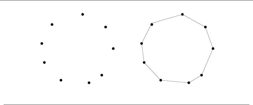
Several algorithms might come to mind to solve this problem. Perhaps the most
popular idea is the nearest-neighbor heuristic. Starting from some point p0, we walk
first to its nearest neighbor p1.Fromp1, we walk to its nearest unvisited neighbor,
thus excluding only p0as a candidate. We now repeat this process until we run
out of unvisited points, after which we return to p0to close off the tour. Written
in pseudo-code, the nearest-neighbor heuristic looks like this:
NearestNeighbor(P)
Pick and visit an initial point p0from P
p=p0
i=0
While there are still unvisited points
i=i+1
Select pito be the closest unvisited point to pi−1
Visit pi
Return to p0from pn−1
This algorithm has a lot to recommend it. It is simple to understand and imple-
ment. It makes sense to visit nearby points before we visit faraway points to reduce
the total travel time. The algorithm works perfectly on the example in Figure 1.2.
The nearest-neighbor rule is reasonably efficient, for it looks at each pair of points
(pi,p
j) at most twice: once when adding pito the tour, the other when adding pj.
Against all these positives there is only one problem. This algorithm is completely
wrong.
Wrong? How can it be wrong? The algorithm always finds a tour, but it doesn’t
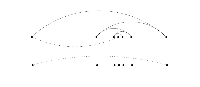
necessarily find the shortest possible tour. It doesn’t necessarily even come close.
Consider the set of points in Figure 1.3, all of which lie spaced along a line. The
numbers describe the distance that each point lies to the left or right of the point
labeled ‘0’. When we start from the point ‘0’ and repeatedly walk to the nearest
unvisited neighbor, we might keep jumping left-right-left-right over ‘0’ as the algo-
rithm offers no advice on how to break ties. A much better (indeed optimal) tour
for these points starts from the leftmost point and visits each point as we walk
right before returning at the rightmost point.
Try now to imagine your boss’s delight as she watches a demo of your robot
arm hopscotching left-right-left-right during the assembly of such a simple board.
“But wait,” you might be saying. “The problem was in starting at point ‘0’.
Instead, why don’t we start the nearest-neighbor rule using the leftmost point
as the initial point p0? By doing this, we will find the optimal solution on this
instance.”
That is 100% true, at least until we rotate our example 90 degrees. Now all
points are equally leftmost. If the point ‘0’ were moved just slightly to the left, it
would be picked as the starting point. Now the robot arm will hopscotch up-down-
up-down instead of left-right-left-right, but the travel time will be just as bad as
before. No matter what you do to pick the first point, the nearest-neighbor rule is
doomed to work incorrectly on certain point sets.
1.1 ROBOT TOUR OPTIMIZATION 7
-1 0 1 3 11
-21 -5
-1 0 1 3 11
-21 -5
Figure 1.3: A bad instance for the nearest-neighbor heuristic, with the optimal solution
Maybe what we need is a different approach. Always walking to the closest
point is too restrictive, since it seems to trap us into making moves we didn’t
want. A different idea might be to repeatedly connect the closest pair of endpoints
whose connection will not create a problem, such as premature termination of the
cycle. Each vertex begins as its own single vertex chain. After merging everything
together, we will end up with a single chain containing all the points in it. Con-
necting the final two endpoints gives us a cycle. At any step during the execution
of this closest-pair heuristic, we will have a set of single vertices and vertex-disjoint
chains available to merge. In pseudocode:
ClosestPair(P)
Let nbe the number of points in set P.
For i=1ton−1do
d=∞
For each pair of endpoints (s, t) from distinct vertex chains
if dist(s, t)≤dthen sm=s,tm=t,andd=dist(s, t)
Connect (sm,t
m) by an edge
Connect the two endpoints by an edge
This closest-pair rule does the right thing in the example in Figure 1.3. It starts
by connecting ‘0’ to its immediate neighbors, the points 1 and −1. Subsequently,
the next closest pair will alternate left-right, growing the central path by one link at
a time. The closest-pair heuristic is somewhat more complicated and less efficient
than the previous one, but at least it gives the right answer in this example.
But this is not true in all examples. Consider what this algorithm does on the
point set in Figure 1.4(l). It consists of two rows of equally spaced points, with
the rows slightly closer together (distance 1 −e) than the neighboring points are
spaced within each row (distance 1 + e). Thus the closest pairs of points stretch
across the gap, not around the boundary. After we pair off these points, the closest
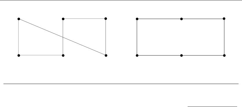
81. INTRODUCTION TO ALGORITHM DESIGN
1−e
1+e
1+e
1−e
(l) 1+e
1−e
1+e
1−e
(r)
Figure 1.4: A bad instance for the closest-pair heuristic, with the optimal solution
remaining pairs will connect these pairs alternately around the boundary. The total
path length of the closest-pair tour is 3(1 −e) + 2(1 + e)+(1 −e)2+(2+2e)2.
Compared to the tour shown in Figure 1.4(r), we travel over 20% farther than
necessary when e≈0. Examples exist where the penalty is considerably worse
than this.
Thus this second algorithm is also wrong. Which one of these algorithms per-
forms better? You can’t tell just by looking at them. Clearly, both heuristics can
end up with very bad tours on very innocent-looking input.
At this point, you might wonder what a correct algorithm for our problem looks
like. Well, we could try enumerating all possible orderings of the set of points, and
then select the ordering that minimizes the total length:
OptimalTSP(P)
d=∞
For each of the n! permutations Piof point set P
If (cost(Pi)≤d) then d=cost(Pi)andPmin =Pi
Return Pmin
Since all possible orderings are considered, we are guaranteed to end up with
the shortest possible tour. This algorithm is correct, since we pick the best of all
the possibilities. But it is also extremely slow. The fastest computer in the world
couldn’t hope to enumerate all the 20! =2,432,902,008,176,640,000 orderings of 20
points within a day. For real circuit boards, where n≈1,000, forget about it.
All of the world’s computers working full time wouldn’t come close to finishing
the problem before the end of the universe, at which point it presumably becomes
moot.
The quest for an efficient algorithm to solve this problem, called the traveling
salesman problem (TSP), will take us through much of this book. If you need to
know how the story ends, check out the catalog entry for the traveling salesman
problem in Section 16.4 (page 533).

1.2 SELECTING THE RIGHT JOBS 9
The President’s Algorist
Halting State
"Discrete" Mathematics Calculated Bets
Programming Challenges
Steiner’s Tree Process Terminated
Tarjan of the Jungle The Four Volume Problem
Figure 1.5: An instance of the non-overlapping movie scheduling problem
Take-Home Lesson: There is a fundamental difference between algorithms,
which always produce a correct result, and heuristics, which may usually do a
good job but without providing any guarantee.
1.2 Selecting the Right Jobs
Now consider the following scheduling problem. Imagine you are a highly-in-
demand actor, who has been presented with offers to star in ndifferent movie
projects under development. Each offer comes specified with the first and last day
of filming. To take the job, you must commit to being available throughout this
entire period. Thus you cannot simultaneously accept two jobs whose intervals
overlap.
For an artist such as yourself, the criteria for job acceptance is clear: you want
to make as much money as possible. Because each of these films pays the same fee
per film, this implies you seek the largest possible set of jobs (intervals) such that
no two of them conflict with each other.
For example, consider the available projects in Figure 1.5. We can star in at most
four films, namely “Discrete” Mathematics,Programming Challenges,Calculated
Bets, and one of either Halting State or Steiner’s Tree.
You (or your agent) must solve the following algorithmic scheduling problem:
Problem: Movie Scheduling Problem
Input: AsetIof nintervals on the line.
Output: What is the largest subset of mutually non-overlapping intervals which can
be selected from I?
You are given the job of developing a scheduling algorithm for this task. Stop
right now and try to find one. Again, I’ll be happy to wait.
There are several ideas that may come to mind. One is based on the notion
that it is best to work whenever work is available. This implies that you should
start with the job with the earliest start date – after all, there is no other job you
can work on, then at least during the begining of this period.
10 1. INTRODUCTION TO ALGORITHM DESIGN
(l) (r)
War and Peace
Figure 1.6: Bad instances for the (l) earliest job first and (r) shortest job first heuristics.
EarliestJobFirst(I)
Accept the earlest starting job jfrom Iwhich does not overlap any
previously accepted job, and repeat until no more such jobs remain.
This idea makes sense, at least until we realize that accepting the earliest job
might block us from taking many other jobs if that first job is long. Check out
Figure 1.6(l), where the epic “War and Peace” is both the first job available and
long enough to kill off all other prospects.
This bad example naturally suggests another idea. The problem with “War and
Peace” is that it is too long. Perhaps we should start by taking the shortest job,
and keep seeking the shortest available job at every turn. Maximizing the number
of jobs we do in a given period is clearly connected to banging them out as quickly
as possible. This yields the heuristic:
ShortestJobFirst(I)
While (I=∅)do
Accept the shortest possible job jfrom I.
Delete j, and any interval which intersects jfrom I.
Again this idea makes sense, at least until we realize that accepting the shortest
job might block us from taking two other jobs, as shown in Figure 1.6(r). While the
potential loss here seems smaller than with the previous heuristic, it can readily
limit us to half the optimal payoff.
At this point, an algorithm where we try all possibilities may start to look good,
because we can be certain it is correct. If we ignore the details of testing whether
a set of intervals are in fact disjoint, it looks something like this:
ExhaustiveScheduling(I)
j=0
Smax =∅
For each of the 2nsubsets Siof intervals I
If (Siis mutally non-overlapping) and (size(Si)>j)
then j=size(Si)andSmax =Si.
Return Smax
But how slow is it? The key limitation is enumerating the 2nsubsets of n
things. The good news is that this is much better than enumerating all n! orders

1.3 REASONING ABOUT CORRECTNESS 11
of nthings, as proposed for the robot tour optimization problem. There are only
about one million subsets when n= 20, which could be exhaustively counted
within seconds on a decent computer. However, when fed n= 100 movies, 2100 is
much much greater than the 20! which made our robot cry “uncle” in the previous
problem.
The difference between our scheduling and robotics problems are that there is an
algorithm which solves movie scheduling both correctly and efficiently. Think about
the first job to terminate—i.e. the interval xwhich contains the rightmost point
which is leftmost among all intervals. This role is played by “Discrete” Mathematics
in Figure 1.5. Other jobs may well have started before x, but all of these must at
least partially overlap each other, so we can select at most one from the group. The
first of these jobs to terminate is x, so any of the overlapping jobs potentially block
out other opportunities to the right of it. Clearly we can never lose by picking x.
This suggests the following correct, efficient algorithm:
OptimalScheduling(I)
While (I=∅)do
Accept the job jfrom Iwith the earliest completion date.
Delete j, and any interval which intersects jfrom I.
Ensuring the optimal answer over all possible inputs is a difficult but often
achievable goal. Seeking counterexamples that break pretender algorithms is an
important part of the algorithm design process. Efficient algorithms are often lurk-
ing out there; this book seeks to develop your skills to help you find them.
Take-Home Lesson: Reasonable-looking algorithms can easily be incorrect. Al-
gorithm correctness is a property that must be carefully demonstrated.
1.3 Reasoning about Correctness
Hopefully, the previous examples have opened your eyes to the subtleties of algo-
rithm correctness. We need tools to distinguish correct algorithms from incorrect
ones, the primary one of which is called a proof.
A proper mathematical proof consists of several parts. First, there is a clear,
precise statement of what you are trying to prove. Second, there is a set of assump-
tions of things which are taken to be true and hence used as part of the proof.
Third, there is a chain of reasoning which takes you from these assumptions to the
statement you are trying to prove. Finally, there is a little square ( )orQED at the
bottom to denote that you have finished, representing the Latin phrase for “thus
it is demonstrated.”
This book is not going to emphasize formal proofs of correctness, because they
are very difficult to do right and quite misleading when you do them wrong. A
proof is indeed a demonstration. Proofs are useful only when they are honest; crisp
arguments explaining why an algorithm satisfies a nontrivial correctness property.

12 1. INTRODUCTION TO ALGORITHM DESIGN
Correct algorithms require careful exposition, and efforts to show both cor-
rectness and not incorrectness. We develop tools for doing so in the subsections
below.
1.3.1 Expressing Algorithms
Reasoning about an algorithm is impossible without a careful description of the
sequence of steps to be performed. The three most common forms of algorithmic
notation are (1) English, (2) pseudocode, or (3) a real programming language.
We will use all three in this book. Pseudocode is perhaps the most mysterious of
the bunch, but it is best defined as a programming language that never complains
about syntax errors. All three methods are useful because there is a natural tradeoff
between greater ease of expression and precision. English is the most natural but
least precise programming language, while Java and C/C++ are precise but diffi-
cult to write and understand. Pseudocode is generally useful because it represents
a happy medium.
The choice of which notation is best depends upon which method you are most
comfortable with. I usually prefer to describe the ideas of an algorithm in English,
moving to a more formal, programming-language-like pseudocode or even real code
to clarify sufficiently tricky details.
A common mistake my students make is to use pseudocode to dress up an ill-
defined idea so that it looks more formal. Clarity should be the goal. For example,
the ExhaustiveScheduling algorithm on page 10 could have been better written
in English as:
ExhaustiveScheduling(I)
Test all 2nsubsets of intervals from I, and return the largest subset
consisting of mutually non-overlapping intervals.
Take-Home Lesson: The heart of any algorithm is an idea. If your idea is
not clearly revealed when you express an algorithm, then you are using too
low-level a notation to describe it.
1.3.2 Problems and Properties
We need more than just an algorithm description in order to demonstrate cor-
rectness. We also need a careful description of the problem that it is intended to
solve.
Problem specifications have two parts: (1) the set of allowed input instances,
and (2) the required properties of the algorithm’s output. It is impossible to prove
the correctness of an algorithm for a fuzzily-stated problem. Put another way, ask
the wrong problem and you will get the wrong answer.
Some problem specifications allow too broad a class of input instances. Suppose
we had allowed film projects in our movie scheduling problem to have gaps in

1.3 REASONING ABOUT CORRECTNESS 13
production (i.e. , filming in September and November but a hiatus in October).
Then the schedule associated with any particular film would consist of a given set
of intervals. Our star would be free to take on two interleaving but not overlapping
projects (such as the film above nested with one filming in August and October).
The earliest completion algorithm would not work for such a generalized scheduling
problem. Indeed, no efficient algorithm exists for this generalized problem.
Take-Home Lesson: An important and honorable technique in algorithm de-
sign is to narrow the set of allowable instances until there is a correct and
efficient algorithm. For example, we can restrict a graph problem from general
graphs down to trees, or a geometric problem from two dimensions down to
one.
There are two common traps in specifying the output requirements of a problem.
One is asking an ill-defined question. Asking for the best route between two places
on a map is a silly question unless you define what best means. Do you mean the
shortest route in total distance, or the fastest route, or the one minimizing the
number of turns?
The second trap is creating compound goals. The three path-planning criteria
mentioned above are all well-defined goals that lead to correct, efficient optimiza-
tion algorithms. However, you must pick a single criteria. A goal like Find the
shortest path from ato bthat doesn’t use more than twice as many turns as neces-
sary is perfectly well defined, but complicated to reason and solve.
I encourage you to check out the problem statements for each of the 75 catalog
problems in the second part of this book. Finding the right formulation for your
problem is an important part of solving it. And studying the definition of all these
classic algorithm problems will help you recognize when someone else has thought
about similar problems before you.
1.3.3 Demonstrating Incorrectness
The best way to prove that an algorithm is incorrect is to produce an instance in
which it yields an incorrect answer. Such instances are called counter-examples.
No rational person will ever leap to the defense of an algorithm after a counter-
example has been identified. Very simple instances can instantly kill reasonable-
looking heuristics with a quick touch´e. Good counter-examples have two important
properties:
•Verifiability – To demonstrate that a particular instance is a counter-example
to a particular algorithm, you must be able to (1) calculate what answer your
algorithm will give in this instance, and (2) display a better answer so as to
prove the algorithm didn’t find it.
Since you must hold the given instance in your head to reason about it, an
important part of verifiability is. . .

14 1. INTRODUCTION TO ALGORITHM DESIGN
•Simplicity – Good counter-examples have all unnecessary details boiled away.
They make clear exactly why the proposed algorithm fails. Once a counter-
example has been found, it is worth simplifying it down to its essence. For
example, the counter-example of Figure 1.6(l) could be made simpler and
better by reducing the number of overlapped segments from four to two.
Hunting for counter-examples is a skill worth developing. It bears some simi-
larity to the task of developing test sets for computer programs, but relies more on
inspiration than exhaustion. Here are some techniques to aid your quest:
•Think small – Note that the robot tour counter-examples I presented boiled
down to six points or less, and the scheduling counter-examples to only three
intervals. This is indicative of the fact that when algorithms fail, there is
usually a very simple example on which they fail. Amateur algorists tend
to draw a big messy instance and then stare at it helplessly. The pros look
carefully at several small examples, because they are easier to verify and
reason about.
•Think exhaustively – There are only a small number of possibilities for the
smallest nontrivial value of n. For example, there are only three interesting
ways two intervals on the line can occur: (1) as disjoint intervals, (2) as
overlapping intervals, and (3) as properly nesting intervals, one within the
other. All cases of three intervals (including counter-examples to both movie
heuristics) can be systematically constructed by adding a third segment in
each possible way to these three instances.
•Hunt for the weakness – If a proposed algorithm is of the form “always take
the biggest” (better known as the greedy algorithm), think about why that
might prove to be the wrong thing to do. In particular, . . .
•Go for a tie – A devious way to break a greedy heuristic is to provide instances
where everything is the same size. Suddenly the heuristic has nothing to base
its decision on, and perhaps has the freedom to return something suboptimal
as the answer.
•Seek extremes – Many counter-examples are mixtures of huge and tiny, left
and right, few and many, near and far. It is usually easier to verify or rea-
son about extreme examples than more muddled ones. Consider two tightly
bunched clouds of points separated by a much larger distance d. The optimal
TSP tour will be essentially 2dregardless of the number of points, because
what happens within each cloud doesn’t really matter.
Take-Home Lesson: Searching for counterexamples is the best way to disprove
the correctness of a heuristic.

1.3 REASONING ABOUT CORRECTNESS 15
1.3.4 Induction and Recursion
Failure to find a counterexample to a given algorithm does not mean “it is obvious”
that the algorithm is correct. A proof or demonstration of correctness is needed.
Often mathematical induction is the method of choice.
When I first learned about mathematical induction it seemed like complete
magic. You proved a formula like n
i=1 i=n(n+1)/2 for some basis case like 1
or 2, then assumed it was true all the way to n−1 before proving it was true for
general nusing the assumption. That was a proof? Ridiculous!
When I first learned the programming technique of recursion it also seemed like
complete magic. The program tested whether the input argument was some basis
case like 1 or 2. If not, you solved the bigger case by breaking it into pieces and
calling the subprogram itself to solve these pieces. That was a program? Ridiculous!
The reason both seemed like magic is because recursion is mathematical induc-
tion. In both, we have general and boundary conditions, with the general condition
breaking the problem into smaller and smaller pieces. The initial or boundary con-
dition terminates the recursion. Once you understand either recursion or induction,
you should be able to see why the other one also works.
I’ve heard it said that a computer scientist is a mathematician who only knows
how to prove things by induction. This is partially true because computer scientists
are lousy at proving things, but primarily because so many of the algorithms we
study are either recursive or incremental.
Consider the correctness of insertion sort, which we introduced at the beginning
of this chapter. The reason it is correct can be shown inductively:
•The basis case consists of a single element, and by definition a one-element
array is completely sorted.
•In general, we can assume that the first n−1 elements of array Aare com-
pletely sorted after n−1 iterations of insertion sort.
•To insert one last element xto A, we find where it goes, namely the unique
spot between the biggest element less than or equal to xand the smallest
element greater than x. This is done by moving all the greater elements back
by one position, creating room for xin the desired location.
One must be suspicious of inductive proofs, however, because very subtle rea-
soning errors can creep in. The first are boundary errors. For example, our insertion
sort correctness proof above boldly stated that there was a unique place to insert
xbetween two elements, when our basis case was a single-element array. Greater
care is needed to properly deal with the special cases of inserting the minimum or
maximum elements.
The second and more common class of inductive proof errors concerns cavallier
extension claims. Adding one extra item to a given problem instance might cause
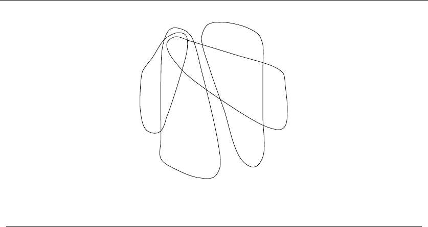
the entire optimal solution to change. This was the case in our scheduling problem
(see Figure 1.7). The optimal schedule after inserting a new segment may contain

16 1. INTRODUCTION TO ALGORITHM DESIGN
Figure 1.7: Large-scale changes in the optimal solution (boxes) after inserting a single interval
(dashed) into the instance
none of the segments of any particular optimal solution prior to insertion. Boldly
ignoring such difficulties can lead to very convincing inductive proofs of incorrect
algorithms.
Take-Home Lesson: Mathematical induction is usually the right way to verify
the correctness of a recursive or incremental insertion algorithm.
Stop and Think: Incremental Correctness
Problem: Prove the correctness of the following recursive algorithm for increment-
ing natural numbers, i.e. y→y+1:
Increment(y)
if y=0then return(1) else
if (ymod 2) = 1 then
return(2 ·Increment(y/2))
else return(y+1)
Solution: The correctness of this algorithm is certainly not obvious to me. But as
it is recursive and I am a computer scientist, my natural instinct is to try to prove
it by induction.
The basis case of y= 0 is obviously correctly handled. Clearly the value 1 is
returned, and 0 + 1 = 1.
Now assume the function works correctly for the general case of y=n−1. Given
this, we must demonstrate the truth for the case of y=n. Half of the cases are
easy, namely the even numbers (For which (ymod 2) = 0), since y+ 1 is explicitly
returned.
For the odd numbers, the answer depends upon what is returned by
Increment(y/2). Here we want to use our inductive assumption, but it isn’t
quite right. We have assumed that increment worked correctly for y=n−1, but
not for a value which is about half of it. We can fix this problem by strengthening
our assumption to declare that the general case holds for all y≤n−1. This costs us
nothing in principle, but is necessary to establish the correctness of the algorithm.

1.3 REASONING ABOUT CORRECTNESS 17
Now, the case of odd y(i.e. y=2m+ 1 for some integer m) can be dealt with
as:
2·Increment((2m+1)/2)=2·Increment(m+1/2)
=2·Increment(m)
=2(m+1)
=2m+2=y+1
and the general case is resolved.
1.3.5 Summations
Mathematical summation formulae arise often in algorithm analysis, which we will
study in Chapter 2. Further, proving the correctness of summation formulae is a
classic application of induction. Several exercises on inductive proofs of summations
appear as exercises at the end this chapter. To make these more accessible, I review
the basics of summations here.
Summation formula are concise expressions describing the addition of an arbi-
trarily large set of numbers, in particular the formula
n
i=1
f(i)=f(1) + f(2) + ...+f(n)
There are simple closed forms for summations of many algebraic functions. For
example, since nones is n,
n
i=1
1=n
The sum of the first nintegers can be seen by pairing up the ith and (n−i+ 1)th
integers:
n
i=1
i=
n/2
i=1
(i+(n−i+ 1)) = n(n+1)/2
Recognizing two basic classes of summation formulae will get you a long way
in algorithm analysis:
•Arithmetic progressions – We already encountered arithmetic progressions
when we saw S(n)=n
ii=n(n+1)/2 in the analysis of selection sort.
From the big picture perspective, the important thing is that the sum is
quadratic, not that the constant is 1/2. In general,
S(n, p)=
n
i
ip=Θ(np+1)

18 1. INTRODUCTION TO ALGORITHM DESIGN
for p≥1. Thus the sum of squares is cubic, and the sum of cubes is quartic
(if you use such a word). The “big Theta” notation (Θ(x)) will be properly
explained in Section 2.2.
For p<−1, this sum always converges to a constant, even as n→∞.The
interesting case is between results in ...
•Geometric series – In geometric progressions, the index of the loop effects
the exponent, i.e.
G(n, a)=
n
i=0
ai=a(an+1 −1)/(a−1)
How we interpret this sum depends upon the base of the progression, i.e. a.
When a<1, this converges to a constant even as n→∞.
This series convergence proves to be the great “free lunch” of algorithm anal-
ysis. It means that the sum of a linear number of things can be constant, not
linear. For example, 1 + 1/2+1/4+1/8+...≤2 no matter how many terms
we add up.
When a>1, the sum grows rapidly with each new term, as in 1 + 2 + 4 +
8 + 16 + 32 = 63. Indeed, G(n, a)=Θ(an+1)fora>1.
Stop and Think: Factorial Formulae
Problem: Prove that n
i=1 i×i!=(n+ 1)! −1 by induction.
Solution: The inductive paradigm is straightforward. First verify the basis case
(here we do n= 1, although n= 0 would be even more general):
1
i=1
i×i! = 1 = (1 + 1)! −1=2−1=1
Now assume the statement is true up to n. To prove the general case of n+1,
observe that rolling out the largest term
n+1
i=1
i×i!=(n+1)×(n+ 1)! +
n
i=1
i×i!
reveals the left side of our inductive assumption. Substituting the right side gives
us
n+1
i=1
i×i!=(n+1)×(n+ 1)! + (n+ 1)! −1

1.4 MODELING THE PROBLEM 19
=(n+ 1)! ×((n+1)+1)−1
=(n+ 2)! −1
This general trick of separating out the largest term from the summation to
reveal an instance of the inductive assumption lies at the heart of all such proofs.
1.4 Modeling the Problem
Modeling is the art of formulating your application in terms of precisely described,
well-understood problems. Proper modeling is the key to applying algorithmic de-
sign techniques to real-world problems. Indeed, proper modeling can eliminate the
need to design or even implement algorithms, by relating your application to what
has been done before. Proper modeling is the key to effectively using the “Hitch-
hiker’s Guide” in Part II of this book.
Real-world applications involve real-world objects. You might be working on a
system to route traffic in a network, to find the best way to schedule classrooms
in a university, or to search for patterns in a corporate database. Most algorithms,
however, are designed to work on rigorously defined abstract structures such as
permutations, graphs, and sets. To exploit the algorithms literature, you must
learn to describe your problem abstractly, in terms of procedures on fundamental
structures.
1.4.1 Combinatorial Objects
Odds are very good that others have stumbled upon your algorithmic problem
before you, perhaps in substantially different contexts. But to find out what is
known about your particular “widget optimization problem,” you can’t hope to
look in a book under widget. You must formulate widget optimization in terms of
computing properties of common structures such as:
•Permutations – which are arrangements, or orderings, of items. For example,
{1,4,3,2}and {4,3,2,1}are two distinct permutations of the same set of four
integers. We have already seen permutations in the robot optimization prob-
lem, and in sorting. Permutations are likely the object in question whenever
your problem seeks an “arrangement,” “tour,” “ordering,” or “sequence.”
•Subsets – which represent selections from a set of items. For example, {1,3,4}
and {2}are two distinct subsets of the first four integers. Order does not
matter in subsets the way it does with permutations, so the subsets {1,3,4}
and {4,3,1}would be considered identical. We saw subsets arise in the movie
scheduling problem. Subsets are likely the object in question whenever your
problem seeks a “cluster,” “collection,” “committee,” “group,” “packaging,”
or “selection.”

20 1. INTRODUCTION TO ALGORITHM DESIGN
Sol
Steve Len Jim Lisa JeffRichardRob Laurie
Morris Eve Sid
Stony Brook
Orient Point
Montauk
Shelter Island
Sag Harbor
Riverhead
Islip
Greenport
Figure 1.8: Modeling real-world structures with trees and graphs
•Trees – which represent hierarchical relationships between items. Figure
1.8(a) shows part of the family tree of the Skiena clan. Trees are likely the
object in question whenever your problem seeks a “hierarchy,” “dominance
relationship,” “ancestor/descendant relationship,” or “taxonomy.”
•Graphs – which represent relationships between arbitrary pairs of objects.
Figure 1.8(b) models a network of roads as a graph, where the vertices are
cities and the edges are roads connecting pairs of cities. Graphs are likely
the object in question whenever you seek a “network,” “circuit,” “web,” or
“relationship.”
•Points – which represent locations in some geometric space. For example,
the locations of McDonald’s restaurants can be described by points on a
map/plane. Points are likely the object in question whenever your problems
work on “sites,” “positions,” “data records,” or “locations.”
•Polygons – which represent regions in some geometric spaces. For example,
the borders of a country can be described by a polygon on a map/plane.
Polygons and polyhedra are likely the object in question whenever you are
working on “shapes,” “regions,” “configurations,” or “boundaries.”
•Strings – which represent sequences of characters or patterns. For example,
the names of students in a class can be represented by strings. Strings are
likely the object in question whenever you are dealing with “text,” “charac-
ters,” “patterns,” or “labels.”
These fundamental structures all have associated algorithm problems, which are
presented in the catalog of Part II. Familiarity with these problems is important,
because they provide the language we use to model applications. To become fluent
in this vocabulary, browse through the catalog and study the input and output pic-
tures for each problem. Understanding these problems, even at a cartoon/definition
level, will enable you to know where to look later when the problem arises in your
application.
1.4 MODELING THE PROBLEM 21
A L G O R I T H M
4+{1,4,2,3}
9+{1,2,7}{1,2,7,9}
{4,1,5,2,3}
L G O R I T H MA
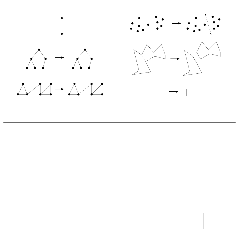
Figure 1.9: Recursive decompositions of combinatorial objects. (left column) Permutations,
subsets, trees, and graphs. (right column) Point sets, polygons, and strings
Examples of successful application modeling will be presented in the war stories
spaced throughout this book. However, some words of caution are in order. The act
of modeling reduces your application to one of a small number of existing problems
and structures. Such a process is inherently constraining, and certain details might
not fit easily into the given target problem. Also, certain problems can be modeled
in several different ways, some much better than others.
Modeling is only the first step in designing an algorithm for a problem. Be alert
for how the details of your applications differ from a candidate model, but don’t
be too quick to say that your problem is unique and special. Temporarily ignoring
details that don’t fit can free the mind to ask whether they really were fundamental
in the first place.
Take-Home Lesson: Modeling your application in terms of well-defined struc-
tures and algorithms is the most important single step towards a solution.
1.4.2 Recursive Objects
Learning to think recursively is learning to look for big things that are made from
smaller things of exactly the same type as the big thing. If you think of houses as
sets of rooms, then adding or deleting a room still leaves a house behind.
Recursive structures occur everywhere in the algorithmic world. Indeed, each
of the abstract structures described above can be thought about recursively. You
just have to see how you can break them down, as shown in Figure 1.9:
•Permutations – Delete the first element of a permutation of {1,...,n}things
and you get a permutation of the remaining n−1 things. Permutations are
recursive objects.

22 1. INTRODUCTION TO ALGORITHM DESIGN
•Subsets – Every subset of the elements {1,...,n}contains a subset of
{1,...,n −1}made visible by deleting element nif it is present. Subsets
are recursive objects.
•Trees – Delete the root of a tree and what do you get? A collection of smaller
trees. Delete any leaf of a tree and what do you get? A slightly smaller tree.
Trees are recursive objects.
•Graphs – Delete any vertex from a graph, and you get a smaller graph. Now
divide the vertices of a graph into two groups, left and right. Cut through
all edges which span from left to right, and what do you get? Two smaller
graphs, and a bunch of broken edges. Graphs are recursive objects.
•Points – Take a cloud of points, and separate them into two groups by drawing
a line. Now you have two smaller clouds of points. Point sets are recursive
objects.
•Polygons – Inserting any internal chord between two nonadjacent vertices of
a simple polygon on nvertices cuts it into two smaller polygons. Polygons
are recursive objects.
•Strings – Delete the first character from a string, and what do you get? A
shorter string. Strings are recursive objects.
Recursive descriptions of objects require both decomposition rules and basis
cases, namely the specification of the smallest and simplest objects where the de-
composition stops. These basis cases are usually easily defined. Permutations and
subsets of zero things presumably look like {}. The smallest interesting tree or
graph consists of a single vertex, while the smallest interesting point cloud consists
of a single point. Polygons are a little trickier; the smallest genuine simple polygon
is a triangle. Finally, the empty string has zero characters in it. The decision of
whether the basis case contains zero or one element is more a question of taste and
convenience than any fundamental principle.
Such recursive decompositions will come to define many of the algorithms we
will see in this book. Keep your eyes open for them.
1.5 About the War Stories
The best way to learn how careful algorithm design can have a huge impact on per-
formance is to look at real-world case studies. By carefully studying other people’s
experiences, we learn how they might apply to our work.
Scattered throughout this text are several of my own algorithmic war stories,
presenting our successful (and occasionally unsuccessful) algorithm design efforts
on real applications. I hope that you will be able to internalize these experiences
so that they will serve as models for your own attacks on problems.

1.6 WAR STORY: PSYCHIC MODELING 23
Every one of the war stories is true. Of course, the stories improve somewhat in
the retelling, and the dialogue has been punched up to make them more interesting
to read. However, I have tried to honestly trace the process of going from a raw
problem to a solution, so you can watch how this process unfolded.
The Oxford English Dictionary defines an algorist as “one skillful in reckonings
or figuring.” In these stories, I have tried to capture some of the mindset of the
algorist in action as they attack a problem.
The various war stories usually involve at least one, and often several, problems
from the problem catalog in Part II. I reference the appropriate section of the
catalog when such a problem occurs. This emphasizes the benefits of modeling
your application in terms of standard algorithm problems. By using the catalog,
you will be able to pull out what is known about any given problem whenever it is
needed.
1.6 War Story: Psychic Modeling
The call came for me out of the blue as I sat in my office.
“Professor Skiena, I hope you can help me. I’m the President of Lotto Systems
Group Inc., and we need an algorithm for a problem arising in our latest product.”
“Sure,” I replied. After all, the dean of my engineering school is always encour-
aging our faculty to interact more with industry.
“At Lotto Systems Group, we market a program designed to improve our cus-
tomers’ psychic ability to predict winning lottery numbers.1In a standard lottery,
each ticket consists of six numbers selected from, say, 1 to 44. Thus, any given
ticket has only a very small chance of winning. However, after proper training, our
clients can visualize, say, 15 numbers out of the 44 and be certain that at least four
of them will be on the winning ticket. Are you with me so far?”
“Probably not,” I replied. But then I recalled how my dean encourages us to
interact with industry.
“Our problem is this. After the psychic has narrowed the choices down to 15
numbers and is certain that at least 4 of them will be on the winning ticket, we
must find the most efficient way to exploit this information. Suppose a cash prize
is awarded whenever you pick at least three of the correct numbers on your ticket.
We need an algorithm to construct the smallest set of tickets that we must buy in
order to guarantee that we win at least one prize.”
“Assuming the psychic is correct?”
“Yes, assuming the psychic is correct. We need a program that prints out a list
of all the tickets that the psychic should buy in order to minimize their investment.
Can you help us?”
Maybe they did have psychic ability, for they had come to the right place. Iden-
tifying the best subset of tickets to buy was very much a combinatorial algorithm
1Yes, this is a true story.
24 1. INTRODUCTION TO ALGORITHM DESIGN
35
34
25
24
23
15
14
13
12
45
Figure 1.10: Covering all pairs of {1,2,3,4,5}with tickets {1,2,3},{1,4,5},{2,4,5},{3,4,5}
problem. It was going to be some type of covering problem, where each ticket we
buy was going to “cover” some of the possible 4-element subsets of the psychic’s
set. Finding the absolute smallest set of tickets to cover everything was a special
instance of the NP-complete problem set cover (discussed in Section 18.1 (page
621)), and presumably computationally intractable.
It was indeed a special instance of set cover, completely specified by only four
numbers: the size nof the candidate set S(typically n≈15), the number of slots
kfor numbers on each ticket (typically k≈6), the number of psychically-promised
correct numbers jfrom S(say j= 4), and finally, the number of matching numbers
lnecessary to win a prize (say l= 3). Figure 1.10 illustrates a covering of a smaller
instance, where n=5,j=k=3,andl=2.
“Although it will be hard to find the exact minimum set of tickets to buy, with
heuristics I should be able to get you pretty close to the cheapest covering ticket
set,” I told him. “Will that be good enough?”
“So long as it generates better ticket sets than my competitor’s program, that
will be fine. His system doesn’t always guarantee a win. I really appreciate your
help on this, Professor Skiena.”
“One last thing. If your program can train people to pick lottery winners, why
don’t you use it to win the lottery yourself?”
“I look forward to talking to you again real soon, Professor Skiena. Thanks for
the help.”
I hung up the phone and got back to thinking. It seemed like the perfect project
to give to a bright undergraduate. After modeling it in terms of sets and subsets,
the basic components of a solution seemed fairly straightforward:

1.6 WAR STORY: PSYCHIC MODELING 25
•We needed the ability to generate all subsets of knumbers from the candidate
set S. Algorithms for generating and ranking/unranking subsets of sets are
presented in Section 14.5 (page 452).
•We needed the right formulation of what it meant to have a covering set of
purchased tickets. The obvious criteria would be to pick a small set of tickets
such that we have purchased at least one ticket containing each of the n
l
l-subsets of Sthat might pay off with the prize.
•We needed to keep track of which prize combinations we have thus far cov-
ered. We seek tickets to cover as many thus-far-uncovered prize combinations
as possible. The currently covered combinations are a subset of all possible
combinations. Data structures for subsets are discussed in Section 12.5 (page
385). The best candidate seemed to be a bit vector, which would answer in
constant time “is this combination already covered?”
•We needed a search mechanism to decide which ticket to buy next. For small
enough set sizes, we could do an exhaustive search over all possible sub-
sets of tickets and pick the smallest one. For larger problems, a randomized
search process like simulated annealing (see Section 7.5.3 (page 254)) would
select tickets-to-buy to cover as many uncovered combinations as possible.
By repeating this randomized procedure several times and picking the best
solution, we would be likely to come up with a good set of tickets.
Excluding the details of the search mechanism, the pseudocode for the book-
keeping looked something like this:
LottoTicketSet(n, k, l)
Initialize the n
l-element bit-vector Vto all false
While there exists a false entry in V
Select a k-subset Tof {1,...,n}as the next ticket to buy
For each of the l-subsets Tiof T,V[rank(Ti)] = true
Report the set of tickets bought
The bright undergraduate, Fayyaz Younas, rose to the challenge. Based on
this framework, he implemented a brute-force search algorithm and found optimal
solutions for problems with n≤5 in a reasonable time. He implemented a random
search procedure to solve larger problems, tweaking it for a while before settling on
the best variant. Finally, the day arrived when we could call Lotto Systems Group
and announce that we had solved the problem.
“Our program found an optimal solution for n= 15, k=6,j=6,l= 3 meant
buying 28 tickets.”
“Twenty-eight tickets!” complained the president. “You must have a bug. Look,
these five tickets will suffice to cover everything twice over: {2,4,8,10,13,14},
{4,5,7,8,12,15},{1,2,3,6,11,13},{3,5,6,9,10,15},{1,7,9,11,12,14}.”
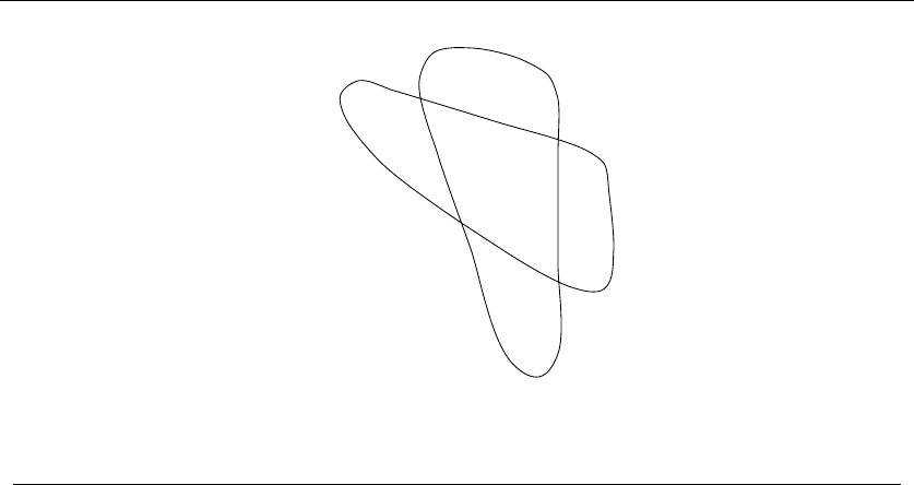
26 1. INTRODUCTION TO ALGORITHM DESIGN
35
34
25
24
23
15
14
13
12
45
Figure 1.11: Guaranteeing a winning pair from {1,2,3,4,5}using only tickets {1,2,3}and
{1,4,5}
We fiddled with this example for a while before admitting that he was right. We
hadn’t modeled the problem correctly! In fact, we didn’t need to explicitly cover all
possible winning combinations. Figure 1.11 illustrates the principle by giving a two-
ticket solution to our previous four-ticket example. Such unpromising outcomes as
{2,3,4}and {3,4,5}each agree in one matching pair with tickets from Figure 1.11.
We were trying to cover too many combinations, and the penny-pinching psychics
were unwilling to pay for such extravagance.
Fortunately, this story has a happy ending. The general outline of our search-
based solution still holds for the real problem. All we must fix is which subsets
we get credit for covering with a given set of tickets. After this modification, we
obtained the kind of results they were hoping for. Lotto Systems Group gratefully
accepted our program to incorporate into their product, and hopefully hit the
jackpot with it.
The moral of this story is to make sure that you model the problem correctly
before trying to solve it. In our case, we came up with a reasonable model, but
didn’t work hard enough to validate it before we started to program. Our misin-
terpretation would have become obvious had we worked out a small example by
hand and bounced it off our sponsor before beginning work. Our success in recov-
ering from this error is a tribute to the basic correctness of our initial formulation,
and our use of well-defined abstractions for such tasks as (1) ranking/unranking
k-subsets, (2) the set data structure, and (3) combinatorial search.

1.7 EXERCISES 27
Chapter Notes
Every decent algorithm book reflects the design philosophy of its author. For stu-
dents seeking alternative presentations and viewpoints, we particularly recommend
the books of Corman, et. al [CLRS01], Kleinberg/Tardos [KT06], and Manber
[Man89].
Formal proofs of algorithm correctness are important, and deserve a fuller dis-
cussion than we are able to provide in this chapter. See Gries [Gri89] for a thorough
introduction to the techniques of program verification.
The movie scheduling problem represents a very special case of the general inde-
pendent set problem, which is discussed in Section 16.2 (page 528). The restriction
limits the allowable input instances to interval graphs, where the vertices of the
graph Gcan be represented by intervals on the line and (i, j) is an edge of Giff
the intervals overlap. Golumbic [Gol04] provides a full treatment of this interesting
and important class of graphs.
Jon Bentley’s Programming Pearls columns are probably the best known col-
lection of algorithmic “war stories.” Originally published in the Communications
of the ACM, they have been collected in two books [Ben90, Ben99]. Brooks’s The
Mythical Man Month [Bro95] is another wonderful collection of war stories, focused
more on software engineering than algorithm design, but they remain a source of
considerable wisdom. Every programmer should read all these books, for pleasure
as well as insight.
Our solution to the lotto ticket set covering problem is presented in more detail
in [YS96].
1.7 Exercises
Finding Counterexamples
1-1. [3] Show that a+bcanbelessthanmin(a, b).
1-2. [3] Show that a×bcanbelessthanmin(a, b).
1-3. [5] Design/draw a road network with two points aand bsuch that the fastest route
between aand bis not the shortest route.
1-4. [5] Design/draw a road network with two points aand bsuch that the shortest
route between aand bis not the route with the fewest turns.
1-5. [4] The knapsack problem is as follows: given a set of integers S={s1,s
2,...,s
n},
and a target number T, find a subset of Swhich adds up exactly to T. For example,
there exists a subset within S={1,2,5,9,10}that adds up to T= 22 but not
T= 23.
Find counterexamples to each of the following algorithms for the knapsack problem.
That is, giving an Sand Tsuch that the subset is selected using the algorithm does
not leave the knapsack completely full, even though such a solution exists.

28 1. INTRODUCTION TO ALGORITHM DESIGN
(a) Put the elements of Sin the knapsack in left to right order if they fit, i.e. the
first-fit algorithm.
(b) Put the elements of Sin the knapsack from smallest to largest, i.e. the best-fit
algorithm.
(c) Put the elements of Sin the knapsack from largest to smallest.
1-6. [5] The set cover problem is as follows: given a set of subsets S1, ..., Smof the
universal set U={1, ..., n}, find the smallest subset of subsets T⊂Ssuch that
∪ti∈Tti=U. For example, there are the following subsets, S1={1,3,5},S2=
{2,4},S3={1,4},andS4={2,5}The set cover would then be S1and S2.
Find a counterexample for the following algorithm: Select the largest subset for the
cover, and then delete all its elements from the universal set. Repeat by adding the
subset containing the largest number of uncovered elements until all are covered.
Proofs of Correctness
1-7. [3] Prove the correctness of the following recursive algorithm to multiply two
natural numbers, for all integer constants c≥2.
function multiply(y, z)
comment Return the product yz.
1. if z=0then return(0) else
2. return(multiply(cy, z/c)+y·(zmod c))
1-8. [3] Prove the correctness of the following algorithm for evaluating a polynomial.
P(x) = anxn+an−1xn−1+...+a1x+a0
function horner(A, x)
p=An
for ifrom n−1to0
p=p∗x+Ai
return p
1-9. [3] Prove the correctness of the following sorting algorithm.
function bubblesort (A: list[1 ...n])
var int i, j
for ifrom nto 1
for jfrom 1 to i−1
if (A[j]>A[j+1])
swap the values of A[j]andA[j+1]
Induction
1-10. [3] Prove that n
i=1 i=n(n+1)/2forn≥0, by induction.
1-11. [3] Prove that n
i=1 i2=n(n+ 1)(2n+1)/6forn≥0, by induction.
1-12. [3] Prove that n
i=1 i3=n2(n+1)
2/4forn≥0, by induction.
1-13. [3] Prove that
n
i=1
i(i+1)(i+2)=n(n+1)(n+2)(n+3)/4

1.7 EXERCISES 29
1-14. [5] Prove by induction on n≥1 that for every a=1,
n
i=0
ai=an+1 −1
a−1
1-15. [3] Prove by induction that for n≥1,
n
i=1
1
i(i+1) =n
n+1
1-16. [3] Prove by induction that n3+2nis divisible by 3 for all n≥0.
1-17. [3] Prove by induction that a tree with nvertices has exactly n−1edges.
1-18. [3] Prove by mathematical induction that the sum of the cubes of the first n
positive integers is equal to the square of the sum of these integers, i.e.
n
i=1
i3=(
n
i=1
i)2
Estimation
1-19. [3] Do all the books you own total at least one million pages? How many total
pages are stored in your school library?
1-20. [3] How many words are there in this textbook?
1-21. [3] How many hours are one million seconds? How many days? Answer these
questions by doing all arithmetic in your head.
1-22. [3] Estimate how many cities and towns there are in the United States.
1-23. [3] Estimate how many cubic miles of water flow out of the mouth of the Mississippi
River each day. Do not look up any supplemental facts. Describe all assumptions
you made in arriving at your answer.
1-24. [3] Is disk drive access time normally measured in milliseconds (thousandths of a
second) or microseconds (millionths of a second)? Does your RAM memory access
a word in more or less than a microsecond? How many instructions can your CPU
execute in one year if the machine is left running all the time?
1-25. [4] A sorting algorithm takes 1 second to sort 1,000 items on your local machine.
How long will it take to sort 10,000 items. . .
(a) if you believe that the algorithm takes time proportional to n2,and
(b) if you believe that the algorithm takes time roughly proportional to nlog n?
Implementation Projects
1-26. [5] Implement the two TSP heuristics of Section 1.1 (page 5). Which of them gives
better-quality solutions in practice? Can you devise a heuristic that works better
than both of them?
1-27. [5] Describe how to test whether a given set of tickets establishes sufficient coverage
in the Lotto problem of Section 1.6 (page 23). Write a program to find good ticket
sets.

30 1. INTRODUCTION TO ALGORITHM DESIGN
Interview Problems
1-28. [5] Write a function to perform integer division without using either the /or *
operators. Find a fast way to do it.
1-29. [5] There are 25 horses. At most, 5 horses can race together at a time. You must
determine the fastest, second fastest, and third fastest horses. Find the minimum
number of races in which this can be done.
1-30. [3] How many piano tuners are there in the entire world?
1-31. [3] How many gas stations are there in the United States?
1-32. [3] How much does the ice in a hockey rink weigh?
1-33. [3] How many miles of road are there in the United States?
1-34. [3] On average, how many times would you have to flip open the Manhattan phone
book at random in order to find a specific name?
Programming Challenges
These programming challenge problems with robot judging are available at
http://www.programming-challenges.com or http://online-judge.uva.es.
1-1. “The 3n+ 1 Problem” – Programming Challenges 110101, UVA Judge 100.
1-2. “The Trip” – Programming Challenges 110103, UVA Judge 10137.
1-3. “Australian Voting” – Programming Challenges 110108, UVA Judge 10142.

2
Algorithm Analysis
Algorithms are the most important and durable part of computer science because
they can be studied in a language- and machine-independent way. This means that
we need techniques that enable us to compare the efficiency of algorithms without
implementing them. Our two most important tools are (1) the RAM model of
computation and (2) the asymptotic analysis of worst-case complexity.
Assessing algorithmic performance makes use of the “big Oh” notation that,
proves essential to compare algorithms and design more efficient ones. While the
hopelessly practical person may blanch at the notion of theoretical analysis, we
present the material because it really is useful in thinking about algorithms.
This method of keeping score will be the most mathematically demanding part
of this book. But once you understand the intuition behind these ideas, the for-
malism becomes a lot easier to deal with.
2.1 The RAM Model of Computation
Machine-independent algorithm design depends upon a hypothetical computer
called the Random Access Machine or RAM. Under this model of computation,
we are confronted with a computer where:
•Each simple operation (+, *, –, =, if, call) takes exactly one time step.
•Loops and subroutines are not considered simple operations. Instead, they
are the composition of many single-step operations. It makes no sense for
sort to be a single-step operation, since sorting 1,000,000 items will certainly
take much longer than sorting 10 items. The time it takes to run through a
loop or execute a subprogram depends upon the number of loop iterations or
the specific nature of the subprogram.
S.S. Skiena, The Algorithm Design Manual, 2nd ed., DOI: 10.1007/978-1-84800-070-4 2,
c
Springer-Verlag London Limited 2008

32 2. ALGORITHM ANALYSIS
•Each memory access takes exactly one time step. Further, we have as much
memory as we need. The RAM model takes no notice of whether an item is
in cache or on the disk.
Under the RAM model, we measure run time by counting up the number of
steps an algorithm takes on a given problem instance. If we assume that our RAM
executes a given number of steps per second, this operation count converts naturally
to the actual running time.
The RAM is a simple model of how computers perform. Perhaps it sounds too
simple. After all, multiplying two numbers takes more time than adding two num-
bers on most processors, which violates the first assumption of the model. Fancy
compiler loop unrolling and hyperthreading may well violate the second assump-
tion. And certainly memory access times differ greatly depending on whether data
sits in cache or on the disk. This makes us zero for three on the truth of our basic
assumptions.
And yet, despite these complaints, the RAM proves an excellent model for
understanding how an algorithm will perform on a real computer. It strikes a fine
balance by capturing the essential behavior of computers while being simple to
work with. We use the RAM model because it is useful in practice.
Every model has a size range over which it is useful. Take, for example, the
model that the Earth is flat. You might argue that this is a bad model, since it
has been fairly well established that the Earth is in fact round. But, when laying
the foundation of a house, the flat Earth model is sufficiently accurate that it can
be reliably used. It is so much easier to manipulate a flat-Earth model that it is
inconceivable that you would try to think spherically when you don’t have to.1
The same situation is true with the RAM model of computation. We make
an abstraction that is generally very useful. It is quite difficult to design an algo-
rithm such that the RAM model gives you substantially misleading results. The
robustness of the RAM enables us to analyze algorithms in a machine-independent
way.
Take-Home Lesson: Algorithms can be understood and studied in a language-
and machine-independent manner.
2.1.1 Best, Worst, and Average-Case Complexity
Using the RAM model of computation, we can count how many steps our algorithm
takes on any given input instance by executing it. However, to understand how good
or bad an algorithm is in general, we must know how it works over all instances.
To understand the notions of the best, worst, and average-case complexity,
think about running an algorithm over all possible instances of data that can be
1The Earth is not completely spherical either, but a spherical Earth provides a useful model for such things
as longitude and latitude.
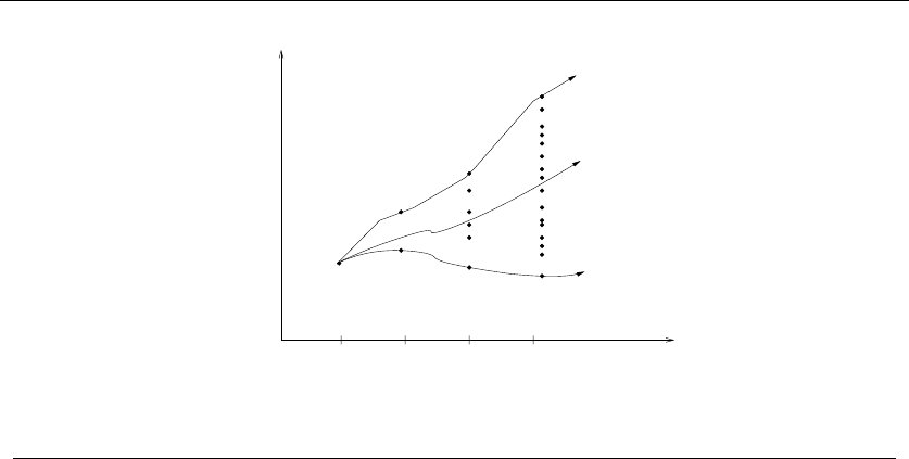
2.1 THE RAM MODEL OF COMPUTATION 33
1 2 3 4 . . . . . . N
.
.
Problem Size
Best Case
Average Case
Worst Caseof Steps
Number
Figure 2.1: Best, worst, and average-case complexity
fed to it. For the problem of sorting, the set of possible input instances consists of
all possible arrangements of nkeys, over all possible values of n. We can represent
each input instance as a point on a graph (shown in Figure 2.1) where the x-axis
represents the size of the input problem (for sorting, the number of items to sort),
and the y-axis denotes the number of steps taken by the algorithm in this instance.
These points naturally align themselves into columns, because only integers
represent possible input size (e.g., it makes no sense to sort 10.57 items). We can
define three interesting functions over the plot of these points:
•The worst-case complexity of the algorithm is the function defined by the
maximum number of steps taken in any instance of size n. This represents
the curve passing through the highest point in each column.
•The best-case complexity of the algorithm is the function defined by the min-
imum number of steps taken in any instance of size n. This represents the
curve passing through the lowest point of each column.
•The average-case complexity of the algorithm, which is the function defined
by the average number of steps over all instances of size n.
The worst-case complexity proves to be most useful of these three measures in
practice. Many people find this counterintuitive. To illustrate why, try to project
what will happen if you bring ndollars into a casino to gamble. The best case,
that you walk out owning the place, is possible but so unlikely that you should not
even think about it. The worst case, that you lose all ndollars, is easy to calculate
and distressingly likely to happen. The average case, that the typical bettor loses
87.32% of the money that he brings to the casino, is difficult to establish and its
meaning subject to debate. What exactly does average mean? Stupid people lose

34 2. ALGORITHM ANALYSIS
more than smart people, so are you smarter or stupider than the average person,
and by how much? Card counters at blackjack do better on average than customers
who accept three or more free drinks. We avoid all these complexities and obtain
a very useful result by just considering the worst case.
The important thing to realize is that each of these time complexities define a
numerical function, representing time versus problem size. These functions are as
well defined as any other numerical function, be it y=x2−2x+ 1 or the price
of Google stock as a function of time. But time complexities are such complicated
functions that we must simplify them to work with them. For this, we need the
“Big Oh” notation.
2.2 The Big Oh Notation
The best, worst, and average-case time complexities for any given algorithm are
numerical functions over the size of possible problem instances. However, it is very
difficult to work precisely with these functions, because they tend to:
•Have too many bumps – An algorithm such as binary search typically runs
a bit faster for arrays of size exactly n=2
k−1 (where kis an integer),
because the array partitions work out nicely. This detail is not particularly
significant, but it warns us that the exact time complexity function for any
algorithm is liable to be very complicated, with little up and down bumps as
shown in Figure 2.2.
•Require too much detail to specify precisely – Counting the exact number
of RAM instructions executed in the worst case requires the algorithm be
specified to the detail of a complete computer program. Further, the precise
answer depends upon uninteresting coding details (e.g., did he use a case
statement or nested ifs?). Performing a precise worst-case analysis like
T(n) = 12754n2+ 4353n+ 834 lg2n+ 13546
would clearly be very difficult work, but provides us little extra information
than the observation that “the time grows quadratically with n.”
It proves to be much easier to talk in terms of simple upper and lower bounds
of time-complexity functions using the Big Oh notation. The Big Oh simplifies
our analysis by ignoring levels of detail that do not impact our comparison of
algorithms.
The Big Oh notation ignores the difference between multiplicative constants.
The functions f(n)=2nand g(n)=nare identical in Big Oh analysis. This
makes sense given our application. Suppose a given algorithm in (say) C language
ran twice as fast as one with the same algorithm written in Java. This multiplicative
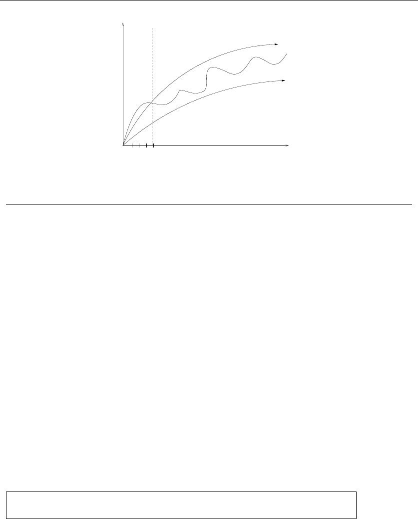
2.2 THE BIG OH NOTATION 35
0
n
f(n)
n
.......
4321
lower bound
upper bound
Figure 2.2: Upper and lower bounds valid for n>n
0smooth out the behavior of complex
functions
factor of two tells us nothing about the algorithm itself, since both programs imple-
ment exactly the same algorithm. We ignore such constant factors when comparing
two algorithms.
The formal definitions associated with the Big Oh notation are as follows:
•f(n)=O(g(n)) means c·g(n)isanupper bound on f(n). Thus there exists
some constant csuch that f(n) is always ≤c·g(n), for large enough n(i.e. ,
n≥n0for some constant n0).
•f(n)=Ω(g(n)) means c·g(n)isalower bound on f(n). Thus there exists
some constant csuch that f(n) is always ≥c·g(n), for all n≥n0.
•f(n)=Θ(g(n)) means c1·g(n) is an upper bound on f(n)andc2·g(n)is
a lower bound on f(n), for all n≥n0. Thus there exist constants c1and c2
such that f(n)≤c1·g(n)andf(n)≥c2·g(n). This means that g(n) provides
a nice, tight bound on f(n).
Got it? These definitions are illustrated in Figure 2.3. Each of these definitions
assumes a constant n0beyond which they are always satisfied. We are not concerned
about small values of n(i.e. , anything to the left of n0). After all, we don’t really
care whether one sorting algorithm sorts six items faster than another, but seek
which algorithm proves faster when sorting 10,000 or 1,000,000 items. The Big Oh
notation enables us to ignore details and focus on the big picture.
Take-Home Lesson: The Big Oh notation and worst-case analysis are tools
that greatly simplify our ability to compare the efficiency of algorithms.
Make sure you understand this notation by working through the following ex-
amples. We choose certain constants (cand n0) in the explanations below because
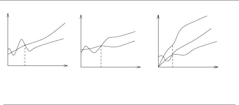
36 2. ALGORITHM ANALYSIS
(c)
f(n)
c2*g(n)
n
n0
c1*g(n)
c*g(n)
f(n)
n
n0
f(n)
c*g(n)
n
n0
(b)
(a)
Figure 2.3: Illustrating the big (a) O, (b) Ω, and (c) Θ notations
they work and make a point, but other pairs of constants will do exactly the same
job. You are free to choose any constants that maintain the same inequality—ideally
constants that make it obvious that the inequality holds:
3n2−100n+6=O(n2), because I choose c=3and3n2>3n2−100n+6;
3n2−100n+6=O(n3), because I choose c=1andn3>3n2−100n+6whenn>3;
3n2−100n+6=O(n), because for any cIchoosec×n<3n2when n>c;
3n2−100n+6=Ω(n2), because I choose c=2and2n2<3n2−100n+6when n>100;
3n2−100n+6=Ω(n3), because I choose c=3and3n2−100n+6<n
3when n>3;
3n2−100n+6=Ω(n), because for any cIchoosecn < 3n2−100n+6 whenn>100c;
3n2−100n+6=Θ(n2), because both Oand Ω apply;
3n2−100n+6=Θ(n3), because only Oapplies;
3n2−100n+6=Θ(n), because only Ω applies.
The Big Oh notation provides for a rough notion of equality when comparing
functions. It is somewhat jarring to see an expression like n2=O(n3), but its
meaning can always be resolved by going back to the definitions in terms of upper
and lower bounds. It is perhaps most instructive to read the “=” here as meaning
one of the functions that are. Clearly, n2is one of functions that are O(n3).

2.3 GROWTH RATES AND DOMINANCE RELATIONS 37
Stop and Think: Back to the Definition
Problem: Is 2n+1 =Θ(2
n)?
Solution: Designing novel algorithms requires cleverness and inspiration. However,
applying the Big Oh notation is best done by swallowing any creative instincts
you may have. All Big Oh problems can be correctly solved by going back to the
definition and working with that.
•Is 2n+1 =O(2n)?Well, f(n)=O(g(n)) iff (if and only if) there exists a
constant csuch that for all sufficiently large nf(n)≤c·g(n). Is there? The
key observation is that 2n+1 =2·2n,so2·2n≤c·2nfor any c≥2.
•Is 2n+1 = Ω(2n)?Go back to the definition. f(n)=Ω(g(n)) iff there exists
a constant c>0 such that for all sufficiently large nf(n)≥c·g(n). This
would be satisfied for any 0 <c≤2. Together the Big Oh and Ω bounds
imply 2n+1 =Θ(2
n)
Stop and Think: Hip to the Squares?
Problem: Is (x+y)2=O(x2+y2).
Solution: Working with the Big Oh means going back to the definition at the
slightest sign of confusion. By definition, this expression is valid iff we can find
some csuch that (x+y)2≤c(x2+y2).
My first move would be to expand the left side of the equation, i.e. (x+y)2=
x2+2xy+y2. If the middle 2xy term wasn’t there, the inequality would clearly hold
for any c>1. But it is there, so we need to relate the 2xy to x2+y2. What if x≤y?
Then 2xy ≤2y2≤2(x2+y2). What if x≥y? Then 2xy ≤2x2≤2(x2+y2). Either
way, we now can bound this middle term by two times the right-side function. This
means that (x+y)2≤3(x2+y2), and so the result holds.
2.3 Growth Rates and Dominance Relations
With the Big Oh notation, we cavalierly discard the multiplicative constants. Thus,
the functions f(n)=0.001n2and g(n) = 1000n2are treated identically, even
though g(n) is a million times larger than f(n) for all values of n.

38 2. ALGORITHM ANALYSIS
nf(n)lg n n n lg n n22nn!
10 0.003 μs0.01 μs0.033 μs0.1 μs 1 μs3.63 ms
20 0.004 μs0.02 μs0.086 μs0.4 μs1ms 77.1 years
30 0.005 μs0.03 μs0.147 μs0.9 μs1sec 8.4×10¹⁵ yrs
40 0.005 μs0.04 μs0.213 μs1.6 μs18.3 min
50 0.006 μs0.05 μs0.282 μs2.5 μs13 days
100 0.007 μs0.1 μs0.644 μs10 μs 4 ×10¹³ yrs
1,000 0.010 μs1.00 μs9.966 μs1ms
10,000 0.013 μs10 μs130 μs100 ms
100,000 0.017 μs0.10 ms 1.67 ms 10 sec
1,000,000 0.020 μs1ms 19.93 ms 16.7 min
10,000,000 0.023 μs0.01 sec 0.23 sec 1.16 days
100,000,000 0.027 μs0.10 sec 2.66 sec 115.7 days
1,000,000,000 0.030 μs1sec 29.90 sec 31.7 years
Figure 2.4: Growth rates of common functions measured in nanoseconds
The reason why we are content with coarse Big Oh analysis is provided by
Figure 2.4, which shows the growth rate of several common time analysis functions.
In particular, it shows how long algorithms that use f(n) operations take to run
on a fast computer, where each operation takes one nanosecond (10−9seconds).
The following conclusions can be drawn from this table:
•All such algorithms take roughly the same time for n= 10.
•Any algorithm with n! running time becomes useless for n≥20.
•Algorithms whose running time is 2nhave a greater operating range, but
become impractical for n>40.
•Quadratic-time algorithms whose running time is n2remain usable up to
about n=10,000, but quickly deteriorate with larger inputs. They are likely
to be hopeless for n>1,000,000.
•Linear-time and nlg nalgorithms remain practical on inputs of one billion
items.
•An O(lg n) algorithm hardly breaks a sweat for any imaginable value of n.
The bottom line is that even ignoring constant factors, we get an excellent idea
of whether a given algorithm is appropriate for a problem of a given size. An algo-
rithm whose running time is f(n)=n3seconds will beat one whose running time is
g(n) = 1,000,000 ·n2seconds only when n<1,000,000. Such enormous differences
in constant factors between algorithms occur far less frequently in practice than
large problems do.

2.3 GROWTH RATES AND DOMINANCE RELATIONS 39
2.3.1 Dominance Relations
The Big Oh notation groups functions into a set of classes, such that all the func-
tions in a particular class are equivalent with respect to the Big Oh. Functions
f(n)=0.34nand g(n) = 234,234nbelong in the same class, namely those that are
order Θ(n). Further, when two functions fand gbelong to different classes, they are
different with respect to our notation. Either f(n)=O(g(n)) or g(n)=O(f(n)),
but not both.
We say that a faster-growing function dominates a slower-growing one, just as
a faster-growing country eventually comes to dominate the laggard. When fand
gbelong to different classes (i.e., f(n)=Θ(g(n))), we say gdominates fwhen
f(n)=O(g(n)), sometimes written gf.
The good news is that only a few function classes tend to occur in the course
of basic algorithm analysis. These suffice to cover almost all the algorithms we will
discuss in this text, and are listed in order of increasing dominance:
•Constant functions, f(n) = 1 – Such functions might measure the cost of
adding two numbers, printing out “The Star Spangled Banner,” or the growth
realized by functions such as f(n) = min(n, 100). In the big picture, there is
no dependence on the parameter n.
•Logarithmic functions, f(n) = log n– Logarithmic time-complexity shows up
in algorithms such as binary search. Such functions grow quite slowly as n
gets big, but faster than the constant function (which is standing still, after
all). Logarithms will be discussed in more detail in Section 2.6 (page 46)
•Linear functions, f(n)=n– Such functions measure the cost of looking at
each item once (or twice, or ten times) in an n-element array, say to identify
the biggest item, the smallest item, or compute the average value.
•Superlinear functions, f(n)=nlg n– This important class of functions arises
in such algorithms as Quicksort and Mergesort. They grow just a little faster
than linear (see Figure 2.4), just enough to be a different dominance class.
•Quadratic functions, f(n)=n2– Such functions measure the cost of looking
at most or all pairs of items in an n-element universe. This arises in algorithms
such as insertion sort and selection sort.
•Cubic functions, f(n)=n3– Such functions enumerate through all triples of
items in an n-element universe. These also arise in certain dynamic program-
ming algorithms developed in Chapter 8.
•Exponential functions, f(n)=cnforagivenconstantc>1 – Functions like
2narise when enumerating all subsets of nitems. As we have seen, exponential
algorithms become useless fast, but not as fast as. . .
•Factorial functions, f(n)=n! – Functions like n! arise when generating all
permutations or orderings of nitems.

40 2. ALGORITHM ANALYSIS
The intricacies of dominance relations will be futher discussed in Section 2.9.2
(page 56). However, all you really need to understand is that:
n!2nn3n2nlog nnlog n1
Take-Home Lesson: Although esoteric functions arise in advanced algorithm
analysis, a small variety of time complexities suffice and account for most
algorithms that are widely used in practice.
2.4 Working with the Big Oh
You learned how to do simplifications of algebraic expressions back in high school.
Working with the Big Oh requires dusting off these tools. Most of what you learned
there still holds in working with the Big Oh, but not everything.
2.4.1 Adding Functions
The sum of two functions is governed by the dominant one, namely:
O(f(n)) + O(g(n)) →O(max(f(n),g(n)))
Ω(f(n)) + Ω(g(n)) →Ω(max(f(n),g(n)))
Θ(f(n)) + Θ(g(n)) →Θ(max(f(n),g(n)))
This is very useful in simplifying expressions, since it implies that n3+n2+
n+1=O(n3). Everything is small potatoes besides the dominant term.
The intuition is as follows. At least half the bulk of f(n)+g(n) must come
from the larger value. The dominant function will, by definition, provide the larger
value as n→∞. Thus, dropping the smaller function from consideration reduces
the value by at most a factor of 1/2, which is just a multiplicative constant. Suppose
f(n)=O(n2)andg(n)=O(n2). This implies that f(n)+g(n)=O(n2) as well.
2.4.2 Multiplying Functions
Multiplication is like repeated addition. Consider multiplication by any constant
c>0, be it 1.02 or 1,000,000. Multiplying a function by a constant can not affect
its asymptotic behavior, because we can multiply the bounding constants in the
Big Oh analysis of c·f(n)by1/c to give appropriate constants for the Big Oh
analysis of f(n). Thus:
O(c·f(n)) →O(f(n))
Ω(c·f(n)) →Ω(f(n))

2.5 REASONING ABOUT EFFICIENCY 41
Θ(c·f(n)) →Θ(f(n))
Of course, cmust be strictly positive (i.e., c>0) to avoid any funny business,
since we can wipe out even the fastest growing function by multiplying it by zero.
On the other hand, when two functions in a product are increasing, both are
important. The function O(n! log n) dominates n!justasmuchaslogndominates
1. In general,
O(f(n)) ∗O(g(n)) →O(f(n)∗g(n))
Ω(f(n)) ∗Ω(g(n)) →Ω(f(n)∗g(n))
Θ(f(n)) ∗Θ(g(n)) →Θ(f(n)∗g(n))
Stop and Think: Transitive Experience
Problem: Show that Big Oh relationships are transitive. That is, if f(n)=O(g(n))
and g(n)=O(h(n)), then f(n)=O(h(n)).
Solution: We always go back to the definition when working with the Big Oh. What
we need to show here is that f(n)≤c3h(n)forn>n
3given that f(n)≤c1g(n)and
g(n)≤c2h(n), for n>n
1and n>n
2, respectively. Cascading these inequalities,
we get that
f(n)≤c1g(n)≤c1c2h(n)
for n>n
3= max(n1,n
2).
2.5 Reasoning About Efficiency
Gross reasoning about an algorithm’s running time of is usually easy given a precise
written description of the algorithm. In this section, I will work through several
examples, perhaps in greater detail than necessary.
2.5.1 Selection Sort
Here we analyze the selection sort algorithm, which repeatedly identifies the small-
est remaining unsorted element and puts it at the end of the sorted portion of the
array. An animation of selection sort in action appears in Figure 2.5, and the code
is shown below:
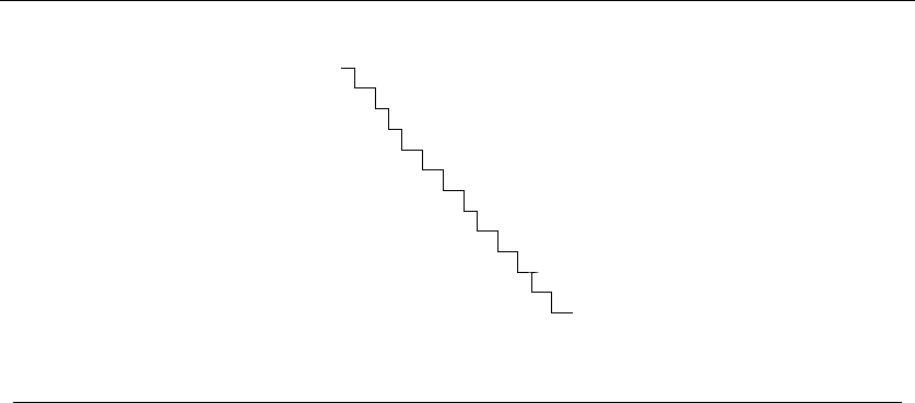
42 2. ALGORITHM ANALYSIS
S E L E C T I O N S O R T
C E L E S T I O N S O R TC E L E S T I O N S O R T
C E L E S T I O N S O R T
C E E L S T I O N S O R TC E E L S T I O N S O R T
C E E I S T L O N S O R T
C E E I L T S O N S O R T
C E E I L N S O T S O R TC E E I L N S O T S O R T
C E E I L N O S T S O R TC E E I L N O S T S O R T
C E E I L N O O T S S R T
C E E I L N O O R S S T TC E E I L N O O R S S T T
C E E I L N O O R S S T T
C E E I L N O O R S S T TC E E I L N O O R S S T T
C E E I L N O O R S S T TC E E I L N O O R S S T T
C
E E I L
N
O
O
R
S
S
T T
Figure 2.5: Animation of selection sort in action
selection_sort(int s[], int n)
{
int i,j; /* counters */
int min; /* index of minimum */
for (i=0; i<n; i++) {
min=i;
for (j=i+1; j<n; j++)
if (s[j] < s[min]) min=j;
swap(&s[i],&s[min]);
}
}
The outer loop goes around ntimes. The nested inner loop goes around n−i−1
times, where iis the index of the outer loop. The exact number of times the if
statement is executed is given by:
S(n)=
n−1
i=0
n−1
j=i+1
1=
n−1
i=0
n−i−1
What this sum is doing is adding up the integers in decreasing order starting from
n−1, i.e.
S(n)=(n−1) + (n−2) + (n−3) + ...+2+1
How can we reason about such a formula? We must solve the summation formula
using the techniques of Section 1.3.5 (page 17) to get an exact value. But, with
the Big Oh we are only interested in the order of the expression. One way to think
about it is that we are adding up n−1 terms, whose average value is about n/2.
This yields S(n)≈n(n−1)/2.

2.5 REASONING ABOUT EFFICIENCY 43
Another way to think about it is in terms of upper and lower bounds. We have
nterms at most, each of which is at most n−1. Thus, S(n)≤n(n−1) = O(n2).
We have n/2 terms each that are bigger than n/2. Thus S(n)=≥(n/2) ×(n/2) =
Ω(n2). Together, this tells us that the running time is Θ(n2), meaning that selection
sort is quadratic.
2.5.2 Insertion Sort
A basic rule of thumb in Big Oh analysis is that worst-case running time follows
from multiplying the largest number of times each nested loop can iterate. Consider
the insertion sort algorithm presented on page 4, whose inner loops are repeated
here:
for (i=1; i<n; i++) {
j=i;
while ((j>0) && (s[j] < s[j-1])) {
swap(&s[j],&s[j-1]);
j = j-1;
}
}
How often does the inner while loop iterate? This is tricky because there are
two different stopping conditions: one to prevent us from running off the bounds
of the array (j>0) and the other to mark when the element finds its proper place
in sorted order (s[j]<s[j−1]). Since worst-case analysis seeks an upper bound
on the running time, we ignore the early termination and assume that this loop
always goes around itimes. In fact, we can assume it always goes around ntimes
since i<n. Since the outer loop goes around ntimes, insertion sort must be a
quadratic-time algorithm, i.e. O(n2).
This crude “round it up” analysis always does the job, in that the Big Oh
running time bound you get will always be correct. Occasionally, it might be too
generous, meaning the actual worst case time might be of a lower order than implied
by such analysis. Still, I strongly encourage this kind of reasoning as a basis for
simple algorithm analysis.
2.5.3 String Pattern Matching
Pattern matching is the most fundamental algorithmic operation on text strings.
This algorithm implements the find command available in any web browser or text
editor:
Problem: Substring Pattern Matching
Input: A text string tand a pattern string p.
Output: Does tcontain the pattern pas a substring, and if so where?

44 2. ALGORITHM ANALYSIS
a
a
b
a
b
b
a
a
a b b a
a b b
a b
Figure 2.6: Searching for the substring abba in the text aababba.
Perhaps you are interested finding where “Skiena” appears in a given news
article (well, I would be interested in such a thing). This is an instance of string
pattern matching with tas the news article and p=“Skiena.”
There is a fairly straightforward algorithm for string pattern matching that
considers the possibility that pmay start at each possible position in tand then
testsifthisisso.
int findmatch(char *p, char *t)
{
int i,j; /* counters */
int m, n; /* string lengths */
m = strlen(p);
n = strlen(t);
for (i=0; i<=(n-m); i=i+1) {
j=0;
while ((j<m) && (t[i+j]==p[j]))
j = j+1;
if (j == m) return(i);
}
return(-1);
}
What is the worst-case running time of these two nested loops? The inner while
loop goes around at most mtimes, and potentially far less when the pattern match
fails. This, plus two other statements, lies within the outer for loop. The outer loop
goes around at most n−mtimes, since no complete alignment is possible once we
get too far to the right of the text. The time complexity of nested loops multiplies,
so this gives a worst-case running time of O((n−m)(m+ 2)).
We did not count the time it takes to compute the length of the strings using
the function strlen. Since the implementation of strlen is not given, we must guess
how long it should take. If we explicitly count the number of characters until we

2.5 REASONING ABOUT EFFICIENCY 45
hit the end of the string; this would take time linear in the length of the string.
This suggests that the running time should be O(n+m+(n−m)(m+ 2)).
Let’s use our knowledge of the Big Oh to simplify things. Since m+2=Θ(m),
the “+2” isn’t interesting, so we are left with O(n+m+(n−m)m). Multiplying
this out yields O(n+m+nm −m2), which still seems kind of ugly.
However, in any interesting problem we know that n≥m, since it is impossible
to have pas a substring of tfor any pattern longer than the text itself. One
consequence of this is that n+m≤2n=Θ(n). Thus our worst-case running time
simplifies further to O(n+nm −m2).
Two more observations and we are done. First, note that n≤nm, since m≥1
in any interesting pattern. Thus n+nm =Θ(nm), and we can drop the additive
n, simplifying our analysis to O(nm −m2).
Finally, observe that the −m2term is negative, and thus only serves to lower
the value within. Since the Big Oh gives an upper bound, we can drop any negative
term without invalidating the upper bound. That n≥mimplies that mn ≥m2,
so the negative term is not big enough to cancel any other term which is left. Thus
we can simply express the worst-case running time of this algorithm as O(nm).
After you get enough experience, you will be able to do such an algorithm
analysis in your head without even writing the algorithm down. After all, algorithm
design for a given task involves mentally rifling through different possibilities and
selecting the best approach. This kind of fluency comes with practice, but if you
are confused about why a given algorithm runs in O(f(n)) time, start by writing
it out carefully and then employ the reasoning we used in this section.
2.5.4 Matrix Multiplication
Nested summations often arise in the analysis of algorithms with nested loops.
Consider the problem of matrix multiplication:
Problem: Matrix Multiplication
Input: Two matrices, A(of dimension x×y)andB(dimension y×z).
Output: An x×zmatrix Cwhere C[i][j] is the dot product of the ith row of A
and the jth column of B.
Matrix multiplication is a fundamental operation in linear algebra, presented
with an example in catalog in Section 13.3 (page 401). That said, the elementary
algorithm for matrix multiplication is implemented as a tight product of three
nested loops:
for (i=1; i<=x; i++)
for (j=1; j<=y; j++) {
C[i][j] = 0;
for (k=1; k<=z; k++)
C[i][j] += A[i][k] * B[k][j];
}

46 2. ALGORITHM ANALYSIS
How can we analyze the time complexity of this algorithm? The number of
multiplications M(x, y, z) is given by the following summation:
M(x, y, z)=
x
i=1
y
j=1
z
k=1
1
Sums get evaluated from the right inward. The sum of zones is z,so
M(x, y, z)=
x
i=1
y
j=1
z
The sum of yzs is just as simple, yz,so
M(x, y, z)=
x
i=1
yz
Finally, the sum of xyzsisxyz.
Thus the running of this matrix multiplication algorithm is O(xyz). If we con-
sider the common case where all three dimensions are the same, this becomes
O(n3)—i.e. , a cubic algorithm.
2.6 Logarithms and Their Applications
Logarithm is an anagram of algorithm, but that’s not why we need to know what
logarithms are. You’ve seen the button on your calculator but may have forgotten
why it is there. A logarithm is simply an inverse exponential function. Saying bx=y
is equivalent to saying that x= logby. Further, this definition is the same as saying
blogby=y.
Exponential functions grow at a distressingly fast rate, as anyone who has
ever tried to pay off a credit card balance understands. Thus, inverse exponen-
tial functions—i.e. logarithms—grow refreshingly slowly. Logarithms arise in any
process where things are repeatedly halved. We now look at several examples.
2.6.1 Logarithms and Binary Search
Binary search is a good example of an O(log n) algorithm. To locate a particular
person pin a telephone book containing nnames, you start by comparing pagainst
the middle, or (n/2)nd name, say Monroe, Marilyn. Regardless of whether pbelongs
before this middle name (Dean, James) or after it (Presley, Elvis), after only one
comparison you can discard one half of all the names in the book. The number of
steps the algorithm takes equals the number of times we can halve nuntil only one
name is left. By definition, this is exactly log2n. Thus, twenty comparisons suffice
to find any name in the million-name Manhattan phone book!
Binary search is one of the most powerful ideas in algorithm design. This power
becomes apparent if we imagine being forced to live in a world with only unsorted

2.6 LOGARITHMS AND THEIR APPLICATIONS 47
Figure 2.7: A height htree with dchildren per node as dhleaves. Here h=2andd=3
telephone books. Figure 2.4 shows that O(log n) algorithms are fast enough to be
used on problem instances of essentially unlimited size.
2.6.2 Logarithms and Trees
A binary tree of height 1 can have up to 2 leaf nodes, while a tree of height two
can have up to four leaves. What is the height hof a rooted binary tree with nleaf
nodes? Note that the number of leaves doubles every time we increase the height
by one. To account for nleaves, n=2
hwhich implies that h= log2n.
What if we generalize to trees that have dchildren, where d= 2 for the case
of binary trees? A tree of height 1 can have up to dleaf nodes, while one of height
two can have up to d2leaves. The number of possible leaves multiplies by devery
time we increase the height by one, so to account for nleaves, n=dhwhich implies
that h= logdn, as shown in Figure 2.7.
The punch line is that very short trees can have very many leaves, which is
the main reason why binary trees prove fundamental to the design of fast data
structures.
2.6.3 Logarithms and Bits
There are two bit patterns of length 1 (0 and 1) and four of length 2 (00, 01, 10, and
11). How many bits wdo we need to represent any one of ndifferent possibilities,
be it one of nitems or the integers from 1 to n?
The key observation is that there must be at least ndifferent bit patterns of
length w. Since the number of different bit patterns doubles as you add each bit,
we need at least wbits where 2w=n—i.e., we need w= log2nbits.
2.6.4 Logarithms and Multiplication
Logarithms were particularly important in the days before pocket calculators. They
provided the easiest way to multiply big numbers by hand, either implicitly using
a slide rule or explicitly by using a book of logarithms.

48 2. ALGORITHM ANALYSIS
Logarithms are still useful for multiplication, particularly for exponentiation.
Recall that loga(xy) = loga(x) + loga(y); i.e. , the log of a product is the sum of
the logs. A direct consequence of this is
loganb=b·logan
So how can we compute abfor any aand busing the exp(x) and ln(x) functions
on your calculator, where exp(x)= exand ln(x) = loge(x)? We know
ab= exp(ln(ab)) = exp(bln a)
so the problem is reduced to one multiplication plus one call to each of these
functions.
2.6.5 Fast Exponentiation
Suppose that we need to exactly compute the value of anfor some reasonably
large n. Such problems occur in primality testing for cryptography, as discussed in
Section 13.8 (page 420). Issues of numerical precision prevent us from applying the
formula above.
The simplest algorithm performs n−1 multiplications, by computing a×a×
...×a. However, we can do better by observing that n=n/2+n/2.Ifnis
even, then an=(an/2)2.Ifnis odd, then an=a(an/2)2. In either case, we have
halved the size of our exponent at the cost of, at most, two multiplications, so
O(lg n) multiplications suffice to compute the final value.
function power(a, n)
if (n= 0) return(1)
x= power(a, n/2)
if (nis even) then return(x2)
else return(a×x2)
This simple algorithm illustrates an important principle of divide and conquer.
It always pays to divide a job as evenly as possible. This principle applies to real
life as well. When nis not a power of two, the problem cannot always be divided
perfectly evenly, but a difference of one element between the two sides cannot cause
any serious imbalance.
2.6.6 Logarithms and Summations
The Harmonic numbers arise as a special case of arithmetic progression, namely
H(n)=S(n, −1). They reflect the sum of the progression of simple reciprocals,
namely,
H(n)=
n
i=1
1/i ∼ln n

2.6 LOGARITHMS AND THEIR APPLICATIONS 49
Loss (apply the greatest) Increase in level
(A) $2,000 or less no increase
(B) More than $2,000 add 1
(C) More than $5,000 add 2
(D) More than $10,000 add 3
(E) More than $20,000 add 4
(F) More than $40,000 add 5
(G) More than $70,000 add 6
(H) More than $120,000 add 7
(I) More than $200,000 add 8
(J) More than $350,000 add 9
(K) More than $500,000 add 10
(L) More than $800,000 add 11
(M) More than $1,500,000 add 12
(N) More than $2,500,000 add 13
(O) More than $5,000,000 add 14
(P) More than $10,000,000 add 15
(Q) More than $20,000,000 add 16
(R) More than $40,000,000 add 17
(Q) More than $80,000,000 add 18
Figure 2.8: The Federal Sentencing Guidelines for fraud
The Harmonic numbers prove important because they usually explain “where
the log comes from” when one magically pops out from algebraic manipulation. For
example, the key to analyzing the average case complexity of Quicksort is the sum-
mation S(n)=nn
i=1 1/i. Employing the Harmonic number identity immediately
reduces this to Θ(nlog n).
2.6.7 Logarithms and Criminal Justice
Figure 2.8 will be our final example of logarithms in action. This table appears in
the Federal Sentencing Guidelines, used by courts throughout the United States.
These guidelines are an attempt to standardize criminal sentences, so that a felon
convicted of a crime before one judge receives the same sentence that they would
before a different judge. To accomplish this, the judges have prepared an intricate
point function to score the depravity of each crime and map it to time-to-serve.
Figure 2.8 gives the actual point function for fraud—a table mapping dollars
stolen to points. Notice that the punishment increases by one level each time the
amount of money stolen roughly doubles. That means that the level of punishment
(which maps roughly linearly to the amount of time served) grows logarithmically
with the amount of money stolen.

50 2. ALGORITHM ANALYSIS
Think for a moment about the consequences of this. Many a corrupt CEO
certainly has. It means that your total sentence grows extremely slowly with the
amount of money you steal. Knocking off five liquor stores for $10,000 each will
get you more time than embezzling $1,000,000 once. The corresponding benefit of
stealing really large amounts of money is even greater. The moral of logarithmic
growth is clear: “If you are gonna do the crime, make it worth the time!”
Take-Home Lesson: Logarithms arise whenever things are repeatedly halved
or doubled.
2.7 Properties of Logarithms
As we have seen, stating bx=yis equivalent to saying that x= logby.Thebterm
is known as the base of the logarithm. Three bases are of particular importance for
mathematical and historical reasons:
•Base b=2–Thebinary logarithm, usually denoted lg x, is a base 2 logarithm.
We have seen how this base arises whenever repeated halving (i.e., binary
search) or doubling (i.e., nodes in trees) occurs. Most algorithmic applications
of logarithms imply binary logarithms.
•Base b=e–Thenatural log, usually denoted ln x,isabasee=2.71828 ...
logarithm. The inverse of ln xis the exponential function exp(x)=exon your
calculator. Thus, composing these functions gives us
exp(ln x)=x
•Base b= 10 – Less common today is the base-10 or common logarithm,
usually denoted as log x. This base was employed in slide rules and logarithm
books in the days before pocket calculators.
We have already seen one important property of logarithms, namely that
loga(xy) = loga(x) + loga(y)
The other important fact to remember is that it is easy to convert a logarithm
from one base to another. This is a consequence of the formula:
logab=logcb
logca
Thus, changing the base of log bfrom base-ato base-csimply involves dividing by
logca. It is easy to convert a common log function to a natural log function, and
vice versa.
Two implications of these properties of logarithms are important to appreciate
from an algorithmic perspective:

2.8 WAR STORY: MYSTERY OF THE PYRAMIDS 51
•The base of the logarithm has no real impact on the growth rate- Compare
the following three values: log2(1,000,000) = 19.9316, log3(1,000,000) =
12.5754, and log100(1,000,000) = 3. A big change in the base of the logarithm
produces little difference in the value of the log. Changing the base of the
log from ato cinvolves dividing by logca. This conversion factor is lost to
the Big Oh notation whenever aand care constants. Thus we are usually
justified in ignoring the base of the logarithm when analyzing algorithms.
•Logarithms cut any function down to size- The growth rate of the logarithm
of any polynomial function is O(lg n). This follows because
loganb=b·logan
The power of binary search on a wide range of problems is a consequence
of this observation. Note that doing a binary search on a sorted array of
n2things requires only twice as many comparisons as a binary search on n
things.
Logarithms efficiently cut any function down to size. It is hard to do arith-
metic on factorials except for logarithms, since
n!=Π
n
i=1i→log n!=
n
i=1
log i=Θ(nlog n)
provides another way for logarithms to pop up in algorithm analysis.
StopandThink:ImportanceofanEvenSplit
Problem: How many queries does binary search take on the million-name Manhat-
tan phone book if each split was 1/3 to 2/3 instead of 1/2 to 1/2?
Solution: When performing binary searches in a telephone book, how important
is it that each query split the book exactly in half? Not much. For the Manhattan
telephone book, we now use log3/2(1,000,000) ≈35 queries in the worst case, not
a significant change from log2(1,000,000) ≈20. The power of binary search comes
from its logarithmic complexity, not the base of the log.
2.8 War Story: Mystery of the Pyramids
That look in his eyes should have warned me even before he started talking.
“We want to use a parallel supercomputer for a numerical calculation up to
1,000,000,000, but we need a faster algorithm to do it.”

52 2. ALGORITHM ANALYSIS
I’d seen that distant look before. Eyes dulled from too much exposure to the raw
horsepower of supercomputers—machines so fast that brute force seemed to elim-
inate the need for clever algorithms; at least until the problems got hard enough.
“I am working with a Nobel prize winner to use a computer on a famous problem
in number theory. Are you familiar with Waring’s problem?”
I knew some number theory. “Sure. Waring’s problem asks whether every integer
can be expressed at least one way as the sum of at most four integer squares. For
example, 78 = 82+3
2+2
2+1
2=7
2+5
2+2
2. I remember proving that four
squares suffice to represent any integer in my undergraduate number theory class.
Yes, it’s a famous problem but one that got solved about 200 years ago.”
“No, we are interested in a different version of Waring’s problem. A pyramidal
number is a number of the form (m3−m)/6, for m≥2. Thus the first several
pyramidal numbers are 1, 4, 10, 20, 35, 56, 84, 120, and 165. The conjecture since
1928 is that every integer can be represented by the sum of at most five such
pyramidal numbers. We want to use a supercomputer to prove this conjecture on
all numbers from 1 to 1,000,000,000.”
“Doing a billion of anything will take a substantial amount of time,” I warned.
“The time you spend to compute the minimum representation of each number will
be critical, because you are going to do it one billion times. Have you thought
about what kind of an algorithm you are going to use?”
“We have already written our program and run it on a parallel supercomputer.
It works very fast on smaller numbers. Still, it takes much too much time as soon
as we get to 100,000 or so.”
Terrific, I thought. Our supercomputer junkie had discovered asymptotic
growth. No doubt his algorithm ran in something like quadratic time, and he got
burned as soon as ngot large.
“We need a faster program in order to get to one billion. Can you help us? Of
course, we can run it on our parallel supercomputer when you are ready.”
I am a sucker for this kind of challenge, finding fast algorithms to speed up
programs. I agreed to think about it and got down to work.
I started by looking at the program that the other guy had written. He had
built an array of all the Θ(n1/3) pyramidal numbers from 1 to ninclusive.2To
test each number kin this range, he did a brute force test to establish whether it
was the sum of two pyramidal numbers. If not, the program tested whether it was
the sum of three of them, then four, and finally five, until it first got an answer.
About 45% of the integers are expressible as the sum of three pyramidal numbers.
Most of the remaining 55% require the sum of four, and usually each of these can
be represented in many different ways. Only 241 integers are known to require the
sum of five pyramidal numbers, the largest being 343,867. For about half of the n
numbers, this algorithm presumably went through all of the three-tests and at least
2Why n1/3? Recall that pyramidal numbers are of the form (m3−m)/6. The largest msuch that the
resulting number is at most nis roughly 3
√6n,sothereareΘ(n1/3) such numbers.

2.8 WAR STORY: MYSTERY OF THE PYRAMIDS 53
some of the four-tests before terminating. Thus, the total time for this algorithm
would be at least O(n×(n1/3)3)=O(n2) time, where n= 1,000,000,000. No
wonder his program cried “Uncle.”
Anything that was going to do significantly better on a problem this large had to
avoid explicitly testing all triples. For each value of k, we were seeking the smallest
set of pyramidal numbers that add up to exactly to k. This problem is called the
knapsack problem, and is discussed in Section 13.10 (page 427). In our case, the
weights are the set of pyramidal numbers no greater than n, with an additional
constraint that the knapsack holds exactly kitems.
A standard approach to solving knapsack precomputes the sum of smaller sub-
sets of the items for use in computing larger subsets. If we have a table of all sums
of two numbers and want to know whether kis expressible as the sum of three
numbers, we can ask whether kis expressible as the sum of a single number plus
a number in this two-table.
Therefore I needed a table of all integers less than nthat can be expressed as
the sum of two of the 1,818 pyramidal numbers less than 1,000,000,000. There can
be at most 1,8182= 3,305,124 of them. Actually, there are only about half this
many after we eliminate duplicates and any sum bigger than our target. Building
a sorted array storing these numbers would be no big deal. Let’s call this sorted
data structure of all pair-sums the two-table.
To find the minimum decomposition for a given k, I would first check whether
it was one of the 1,818 pyramidal numbers. If not, I would then check whether
kwas in the sorted table of the sums of two pyramidal numbers. To see whether
kwas expressible as the sum of three such numbers, all I had to do was check
whether k−p[i] was in the two-table for 1 ≤i≤1,818. This could be done
quickly using binary search. To see whether kwas expressible as the sum of four
pyramidal numbers, I had to check whether k−two[i] was in the two-table for any
1≤i≤|two|. However, since almost every kwas expressible in many ways as the
sum of four pyramidal numbers, this test would terminate quickly, and the total
time taken would be dominated by the cost of the threes. Testing whether kwas
the sum of three pyramidal numbers would take O(n1/3lg n). Running this on each
of the nintegers gives an O(n4/3lg n) algorithm for the complete job. Comparing
this to his O(n2) algorithm for n= 1,000,000,000 suggested that my algorithm was
acool30,000 times faster than his original!
My first attempt to code this solved up to n=1,000,000 on my ancient Sparc
ELC in about 20 minutes. From here, I experimented with different data structures
to represent the sets of numbers and different algorithms to search these tables. I
tried using hash tables and bit vectors instead of sorted arrays, and experimented
with variants of binary search such as interpolation search (see Section 14.2 (page
441)). My reward for this work was solving up to n=1,000,000 in under three
minutes, a factor of six improvement over my original program.
With the real thinking done, I worked to tweak a little more performance out of
the program. I avoided doing a sum-of-four computation on any kwhen k−1was

54 2. ALGORITHM ANALYSIS
the sum-of-three, since 1 is a pyramidal number, saving about 10% of the total run
time using this trick alone. Finally, I got out my profiler and tried some low-level
tricks to squeeze a little more performance out of the code. For example, I saved
another 10% by replacing a single procedure call with in line code.
At this point, I turned the code over to the supercomputer guy. What he did
with it is a depressing tale, which is reported in Section 7.10 (page 268).
In writing up this war story, I went back to rerun my program more than
ten years later. On my desktop SunBlade 150, getting to 1,000,000 now took 27.0
seconds using the gcc compiler without turning on any compiler optimization. With
Level 4 optimization, the job ran in just 14.0 seconds—quite a tribute to the quality
of the optimizer. The run time on my desktop machine improved by a factor of
about three over the four-year period prior to my first edition of this book, with
an additional 5.3 times over the last 11 years. These speedups are probably typical
for most desktops.
The primary lesson of this war story is to show the enormous potential for
algorithmic speedups, as opposed to the fairly limited speedup obtainable via more
expensive hardware. I sped his program up by about 30,000 times. His million-
dollar computer had 16 processors, each reportedly five times faster on integer
computations than the $3,000 machine on my desk. That gave a maximum potential
speedup of less than 100 times. Clearly, the algorithmic improvement was the big
winner here, as it is certain to be in any sufficiently large computation.
2.9 Advanced Analysis (*)
Ideally, each of us would be fluent in working with the mathematical techniques
of asymptotic analysis. And ideally, each of us would be rich and good looking as
well.
In this section I will survey the major techniques and functions employed in
advanced algorithm analysis. I consider this optional material—it will not be used
elsewhere in the textbook section of this book. That said, it will make some of the
complexity functions reported in the Hitchhiker’s Guide far less mysterious.
2.9.1 Esoteric Functions
The bread-and-butter classes of complexity functions were presented in Section
2.3.1 (page 39). More esoteric functions also make appearances in advanced algo-
rithm analysis. Although we will not see them much in this book, it is still good
business to know what they mean and where they come from:
•Inverse Ackerman’s function f(n)=α(n) – This function arises in the de-
tailed analysis of several algorithms, most notably the Union-Find data struc-
ture discussed in Section 6.1.3 (page 198).
The exact definition of this function and why it arises will not be discussed
further. It is sufficient to think of it as geek talk for the slowest-growing

2.9 ADVANCED ANALYSIS (*) 55
complexity function. Unlike the constant function f(n) = 1, it eventually
gets to infinity as n→∞, but it certainly takes its time about it. The value
of α(n)<5 for any value of nthat can be written in this physical universe.
•f(n) = log log n– The “log log” function is just that—the logarithm of the
logarithm of n. One natural example of how it might arise is doing a binary
search on a sorted array of only lg nitems.
•f(n) = log n/ log log n– This function grows a little slower than log nbecause
it is divided by an even slower growing function.
To see where this arises, consider an n-leaf rooted tree of degree d. For binary
trees, i.e. when d= 2, the height his given
n=2
h→h=lgn
by taking the logarithm of both sides of the equation. Now consider the height
of such a tree when the degree d= log n. Then
n= (log n)h→h= log n/ log log n
•f(n) = log2n– This is the product of log functions—i.e., (log n)×(log n). It
might arise if we wanted to count the bits looked at in doing a binary search
on nitems, each of which was an integer from 1 to (say) n2. Each such integer
requires a lg(n2)=2lgnbit representation, and we look at lg nof them, for
a total of 2 lg2nbits.
The “log squared” function typically arises in the design of intricate nested
data structures, where each node in (say) a binary tree represents another
data structure, perhaps ordered on a different key.
•f(n)=√n– The square root is not so esoteric, but represents the class of
“sublinear polynomials” since √n=n1/2. Such functions arise in building
d-dimensional grids that contain npoints. A √n×√nsquare has area n,
and an n1/3×n1/3×n1/3cube has volume n. In general, a d-dimensional
hypercube of length n1/d on each side has volume d.
•f(n)=n(1+)– Epsilon () is the mathematical symbol to denote a constant
that can be made arbitrarily small but never quite goes away.
It arises in the following way. Suppose I design an algorithm that runs in
2cn(1+1/c)time, and I get to pick whichever cI want. For c=2,thisis4n3/2
or O(n3/2). For c=3,thisis8n4/3or O(n4/3), which is better. Indeed, the
exponent keeps getting better the larger I make c.
The problem is that I cannot make carbitrarily large before the 2cterm
begins to dominate. Instead, we report this algorithm as running in O(n1+),
and leave the best value of to the beholder.

56 2. ALGORITHM ANALYSIS
2.9.2 Limits and Dominance Relations
The dominance relation between functions is a consequence of the theory of lim-
its, which you may recall from Calculus. We say that f(n)dominates g(n)if
limn→∞ g(n)/f(n)=0.
Let’s see this definition in action. Suppose f(n)=2n2and g(n)=n2. Clearly
f(n)>g(n) for all n, but it does not dominate since
lim
n→∞ g(n)/f(n) = lim
n→∞ n2/2n2= lim
n→∞ 1/2=0
This is to be expected because both functions are in the class Θ(n2). What about
f(n)=n3and g(n)=n2? Since
lim
n→∞ g(n)/f(n) = lim
n→∞ n2/n3= lim
n→∞ 1/n =0
the higher-degree polynomial dominates. This is true for any two polynomials,
namely that nadominates nbif a>bsince
lim
n→∞ nb/na= lim
n→∞ nb−a→0
Thus n1.2dominates n1.1999999.
Now consider two exponential functions, say f(n)=3
nand g(n)=2
n. Since
lim
n→∞ g(n)/f(n)=2
n/3n= lim
n→∞(2/3)n=0
the exponential with the higher base dominates.
Our ability to prove dominance relations from scratch depends upon our ability
to prove limits. Let’s look at one important pair of functions. Any polynomial (say
f(n)=n) dominates logarithmic functions (say g(n)=lgn). Since n=2
lg n,
f(n)=(2
lg n)=2
lg n
Now consider
lim
n→∞ g(n)/f(n)=lgn/2lg n
In fact, this does go to 0 as n→∞.
Take-Home Lesson: By interleaving the functions here with those of Section
2.3.1 (page 39), we see where everything fits into the dominance pecking order:
n!cnn3n2n1+nlog nn√n
log2nlog nlog n/ log log nlog log nα(n)1
Chapter Notes
Most other algorithm texts devote considerably more efforts to the formal analysis
of algorithms than we have here, and so we refer the theoretically-inclined reader

2.10 EXERCISES 57
elsewhere for more depth. Algorithm texts more heavily stressing analysis include
[CLRS01, KT06].
The book Concrete Mathematics by Knuth, Graham, and Patashnik [GKP89]
offers an interesting and thorough presentation of mathematics for the analysis of
algorithms. Niven and Zuckerman [NZ80] is an nice introduction to number theory,
including Waring’s problem, discussed in the war story.
The notion of dominance also gives rise to the “Little Oh” notation. We say that
f(n)=o(g(n)) iff g(n) dominates f(n). Among other things, the Little Oh proves
useful for asking questions. Asking for an o(n2) algorithm means you want one
that is better than quadratic in the worst case—and means you would be willing
to settle for O(n1.999 log2n).
2.10 Exercises
Program Analysis
2-1. [3] What value is returned by the following function? Express your answer as a
function of n. Give the worst-case running time using the Big Oh notation.
function mystery(n)
r:= 0
for i:= 1 to n−1do
for j:= i+1to ndo
for k:= 1 to jdo
r:= r+1
return(r)
2-2. [3] What value is returned by the following function? Express your answer as a
function of n. Give the worst-case running time using Big Oh notation.
function pesky(n)
r:= 0
for i:= 1 to ndo
for j:= 1 to ido
for k:= jto i+jdo
r:= r+1
return(r)
2-3. [5] What value is returned by the following function? Express your answer as a
function of n. Give the worst-case running time using Big Oh notation.
function prestiferous(n)
r:= 0
for i:= 1 to ndo
for j:= 1 to ido
for k:= jto i+jdo
for l:= 1 to i+j−kdo

58 2. ALGORITHM ANALYSIS
r:= r+1
return(r)
2-4. [8] What value is returned by the following function? Express your answer as a
function of n. Give the worst-case running time using Big Oh notation.
function conundrum(n)
r:= 0
for i:= 1 to ndo
for j:= i+1to ndo
for k:= i+j−1to ndo
r:= r+1
return(r)
2-5. [5] Suppose the following algorithm is used to evaluate the polynomial
p(x)=anxn+an−1xn−1+...+a1x+a0
p:= a0;
xpower := 1;
for i:= 1 to ndo
xpower := x∗xpower;
p:= p+ai∗xpower
end
(a) How many multiplications are done in the worst-case? How many additions?
(b) How many multiplications are done on the average?
(c) Can you improve this algorithm?
2-6. [3] Prove that the following algorithm for computing the maximum value in an
array A[1..n] is correct.
function max(A)
m:= A[1]
for i:= 2 to ndo
if A[i]>mthen m:= A[i]
return (m)
Big Oh
2-7. [3] True or False?
(a) Is 2n+1 =O(2n)?
(b) Is 22n=O(2n)?
2-8. [3] For each of the following pairs of functions, either f(n)isinO(g(n)), f(n)is
in Ω(g(n)), or f(n)=Θ(g(n)). Determine which relationship is correct and briefly
explain why.
(a) f(n)=logn2;g(n)=logn+5

2.10 EXERCISES 59
(b) f(n)=√n;g(n)=logn2
(c) f(n)=log
2n;g(n)=logn
(d) f(n)=n;g(n)=log
2n
(e) f(n)=nlog n+n;g(n)=logn
(f) f(n) = 10; g(n)=log10
(g) f(n)=2
n;g(n)=10n2
(h) f(n)=2
n;g(n)=3
n
2-9. [3] For each of the following pairs of functions f(n)andg(n), determine whether
f(n)=O(g(n)), g(n)=O(f(n)), or both.
(a) f(n)=(n2−n)/2, g(n)=6n
(b) f(n)=n+2
√n,g(n)=n2
(c) f(n)=nlog n,g(n)=n√n/2
(d) f(n)=n+logn,g(n)=√n
(e) f(n) = 2(log n)2,g(n)=logn+1
(f) f(n)=4nlog n+n,g(n)=(n2−n)/2
2-10. [3] Prove that n3−3n2−n+1=Θ(n3).
2-11. [3] Prove that n2=O(2n).
2-12. [3] For each of the following pairs of functions f(n)andg(n), give an appropriate
positive constant csuch that f(n)≤c·g(n) for all n>1.
(a) f(n)=n2+n+1, g(n)=2n3
(b) f(n)=n√n+n2,g(n)=n2
(c) f(n)=n2−n+1, g(n)=n2/2
2-13. [3] Prove that if f1(n)=O(g1(n)) and f2(n)=O(g2(n)), then f1(n)+f2(n)=
O(g1(n)+g2(n)).
2-14. [3] Prove that if f1(N)=Ω(g1(n)) and f2(n)=Ω(g2(n)), then f1(n)+f2(n)=
Ω(g1(n)+g2(n)).
2-15. [3] Prove that if f1(n)=O(g1(n)) and f2(n)=O(g2(n)), then f1(n)·f2(n)=
O(g1(n)·g2(n))
2-16. [5] Prove for all k≥1 and all sets of constants {ak,a
k−1,...,a
1,a
0}∈R,
aknk+ak−1nk−1+.... +a1n+a0=O(nk)
2-17. [5] Show that for any real constants aand b,b>0
(n+a)b=Θ(nb)
2-18. [5] List the functions below from the lowest to the highest order. If any two or
more are of the same order, indicate which.

60 2. ALGORITHM ANALYSIS
n2nnlg nln n
n−n3+7n5lg n√ne
n
n2+lgnn
22n−1lg lg n
n3(lg n)2n!n1+εwhere 0 <ε<1
2-19. [5] List the functions below from the lowest to the highest order. If any two or
more are of the same order, indicate which.
√nn 2n
nlog nn−n3+7n5n2+logn
n2n3log n
n1
3+logn(log n)2n!
ln nn
log nlog log n
(1/3)n(3/2)n6
2-20. [5] Find two functions f(n)andg(n) that satisfy the following relationship. If no
such fand gexist, write “None.”
(a) f(n)=o(g(n)) and f(n)=Θ(g(n))
(b) f(n)=Θ(g(n)) and f(n)=o(g(n))
(c) f(n)=Θ(g(n)) and f(n)=O(g(n))
(d) f(n)=Ω(g(n)) and f(n)=O(g(n))
2-21. [5] True or False?
(a) 2n2+1=O(n2)
(b) √n=O(log n)
(c) log n=O(√n)
(d) n2(1 + √n)=O(n2log n)
(e) 3n2+√n=O(n2)
(f) √nlog n=O(n)
(g) log n=O(n−1/2)
2-22. [5] For each of the following pairs of functions f(n)andg(n), state whether f(n)=
O(g(n)), f(n)=Ω(g(n)), f(n)=Θ(g(n)), or none of the above.
(a) f(n)=n2+3n+4,g(n)=6n+7
(b) f(n)=n√n,g(n)=n2−n
(c) f(n)=2
n−n2,g(n)=n4+n2
2-23. [3] For each of these questions, briefly explain your answer.
(a) If I prove that an algorithm takes O(n2) worst-case time, is it possible that it
takes O(n) on some inputs?
(b) If I prove that an algorithm takes O(n2) worst-case time, is it possible that it
takes O(n) on all inputs?
(c) If I prove that an algorithm takes Θ(n2) worst-case time, is it possible that it
takes O(n) on some inputs?

2.10 EXERCISES 61
(d) If I prove that an algorithm takes Θ(n2) worst-case time, is it possible that it
takes O(n) on all inputs?
(e) Is the function f(n)=Θ(n2), where f(n) = 100n2for even nand f(n)=
20n2−nlog2nfor odd n?
2-24. [3] For each of the following, answer yes,no,orcan’t tell. Explain your reasoning.
(a) Is 3n=O(2n)?
(b) Is log 3n=O(log 2n)?
(c) Is 3n=Ω(2
n)?
(d) Is log 3n= Ω(log 2n)?
2-25. [5] For each of the following expressions f(n) find a simple g(n) such that f(n)=
Θ(g(n)).
(a) f(n)=n
i=1
1
i.
(b) f(n)=n
i=11
i.
(c) f(n)=n
i=1 log i.
(d) f(n)=log(n!).
2-26. [5] Place the following functions into increasing asymptotic order.
f1(n)=n2log2n,f2(n)=n(log2n)2,f3(n)=n
i=0 2i,f4(n)=log
2(n
i=0 2i).
2-27. [5] Place the following functions into increasing asymptotic order. If two or more
of the functions are of the same asymptotic order then indicate this.
f1(n)=n
i=1 √i,f2(n)=(
√n)logn,f3(n)=n√log n,f4(n)=12n3
2+4n,
2-28. [5] For each of the following expressions f(n) find a simple g(n) such that
f(n)=Θ(g(n)). (You should be able to prove your result by exhibiting the rel-
evant parameters, but this is not required for the homework.)
(a) f(n)=n
i=1 3i4+2i3−19i+ 20.
(b) f(n)=n
i=1 3(4i) + 2(3i)−i19 + 20.
(c) f(n)=n
i=1 5i+3
2i.
2-29. [5] Which of the following are true?
(a) n
i=1 3i=Θ(3
n−1).
(b) n
i=1 3i=Θ(3
n).
(c) n
i=1 3i=Θ(3
n+1).
2-30. [5] For each of the following functions ffind a simple function gsuch that f(n)=
Θ(g(n)).
(a) f1(n) = (1000)2n+4
n.
(b) f2(n)=n+nlog n+√n.
(c) f3(n)=log(n20)+(logn)10.
(d) f4(n)=(0.99)n+n100.

62 2. ALGORITHM ANALYSIS
2-31. [5] For each pair of expressions (A, B) below, indicate whether Ais O,o,Ω,ω,or
ΘofB. Note that zero, one or more of these relations may hold for a given pair;
list all correct ones.
AB
(a)n100 2n
(b)(lgn)12 √n
(c)√nn
cos(πn/8)
(d)10
n100n
(e)nlg n(lg n)n
(f)lg(n!) nlg n
Summations
2-32. [5] Prove that:
12−22+3
2−42+...+(−1)k−1k2=(−1)k−1k(k+1)/2
2-33. [5] Find an expression for the sum of the ith row of the following triangle, and
prove its correctness. Each entry is the sum of the three entries directly above it.
All non existing entries are considered 0.
1
111
12321
1367631
1 4 10 16 19 16 10 4 1
2-34. [3] Assume that Christmas has ndays. Exactly how many presents did my “true
love” send me? (Do some research if you do not understand this question.)
2-35. [5] Consider the following code fragment.
for i=1 to n do
for j=i to 2*i do
output ‘‘foobar’’
Let T(n) denote the number of times ‘foobar’ is printed as a function of n.
a. Express T(n) as a summation (actually two nested summations).
b. Simplify the summation. Show your work.
2-36. [5] Consider the following code fragment.
for i=1 to n/2 do
for j=i to n-i do
for k=1 to j do
output ‘‘foobar’’
Assume nis even. Let T(n) denote the number of times ‘foobar’ is printed as a
function of n.
(a) Express T(n) as three nested summations.
(b) Simplify the summation. Show your work.

2.10 EXERCISES 63
2-37. [6] When you first learned to multiply numbers, you were told that x×ymeans
adding xa total of ytimes, so 5×4 = 5+5+5+5 = 20. What is the time complexity
of multiplying two n-digit numbers in base b(people work in base 10, of course,
while computers work in base 2) using the repeated addition method, as a function
of nand b. Assume that single-digit by single-digit addition or multiplication takes
O(1) time. (Hint: how big can ybe as a function of nand b?)
2-38. [6] In grade school, you learned to multiply long numbers on a digit-by-digit basis,
so that 127 ×211 = 127 ×1 + 127 ×10 + 127 ×200 = 26,397. Analyze the time
complexity of multiplying two n-digit numbers with this method as a function of
n(assume constant base size). Assume that single-digit by single-digit addition or
multiplication takes O(1) time.
Logarithms
2-39. [5] Prove the following identities on logarithms:
(a) Prove that loga(xy)=log
ax+log
ay
(b) Prove that logaxy=ylogax
(c) Prove that logax=logbx
logba
(d) Prove that xlogby=ylogbx
2-40. [3] Show that lg(n+1)=lg n+1
2-41. [3] Prove that that the binary representation of n≥1haslg2n+1bits.
2-42. [5] In one of my research papers I give a comparison-based sorting algorithm that
runs in O(nlog(√n)). Given the existence of an Ω(nlog n) lower bound for sorting,
how can this be possible?
Interview Problems
2-43. [5] You are given a set Sof nnumbers. You must pick a subset Sof knumbers from
Ssuch that the probability of each element of Soccurring in Sis equal (i.e., each
is selected with probability k/n). You may make only one pass over the numbers.
What if nis unknown?
2-44. [5] We have 1,000 data items to store on 1,000 nodes. Each node can store copies
of exactly three different items. Propose a replication scheme to minimize data loss
as nodes fail. What is the expected number of data entries that get lost when three
random nodes fail?
2-45. [5] Consider the following algorithm to find the minimum element in an array
of numbers A[0,...,n]. One extra variable tmp is allocated to hold the current
minimum value. Start from A[0]; ”tmp” is compared against A[1], A[2], ..., A[N]
in order. When A[i]<tmp,tmp =A[i]. What is the expected number of times that
the assignment operation tmp =A[i] is performed?
2-46. [5] You have a 100-story building and a couple of marbles. You must identify the
lowest floor for which a marble will break if you drop it from this floor. How fast
can you find this floor if you are given an infinite supply of marbles? What if you
have only two marbles?

64 2. ALGORITHM ANALYSIS
2-47. [5] You are given 10 bags of gold coins. Nine bags contain coins that each weigh 10
grams. One bag contains all false coins that weigh one gram less. You must identify
this bag in just one weighing. You have a digital balance that reports the weight of
what is placed on it.
2-48. [5] You have eight balls all of the same size. Seven of them weigh the same, and one
of them weighs slightly more. How can you find the ball that is heavier by using a
balance and only two weighings?
2-49. [5] Suppose we start with ncompanies that eventually merge into one big company.
How many different ways are there for them to merge?
2-50. [5] ARamanujam number can be written two different ways as the sum of two
cubes—i.e. , there exist distinct a,b,c,anddsuch that a3+b3=c3+d3. Generate
all Ramanujam numbers where a, b, c, d < n.
2-51. [7] Six pirates must divide $300 dollars among themselves. The division is to proceed
as follows. The senior pirate proposes a way to divide the money. Then the pirates
vote. If the senior pirate gets at least half the votes he wins, and that division
remains. If he doesn’t, he is killed and then the next senior-most pirate gets a
chance to do the division. Now you have to tell what will happen and why (i.e.
, how many pirates survive and how the division is done)? All the pirates are
intelligent and the first priority is to stay alive and the next priority is to get as
much money as possible.
2-52. [7] Reconsider the pirate problem above, where only one indivisible dollar is to be
divided. Who gets the dollar and how many are killed?
Programming Challenges
These programming challenge problems with robot judging are available at
http://www.programming-challenges.com or http://online-judge.uva.es.
2-1. “Primary Arithmetic” – Programming Challenges 110501, UVA Judge 10035.
2-2. “A Multiplication Game” – Programming Challenges 110505, UVA Judge 847.
2-3. “Light, More Light” – Programming Challenges 110701, UVA Judge 10110.

3
Data Structures
Changing a data structure in a slow program can work the same way an organ
transplant does in a sick patient. Important classes of abstract data types such as
containers, dictionaries, and priority queues, have many different but functionally
equivalent data structures that implement them. Changing the data structure does
not change the correctness of the program, since we presumably replace a correct
implementation with a different correct implementation. However, the new imple-
mentation of the data type realizes different tradeoffs in the time to execute various
operations, so the total performance can improve dramatically. Like a patient in
need of a transplant, only one part might need to be replaced in order to fix the
problem.
But it is better to be born with a good heart than have to wait for a replace-
ment. The maximum benefit from good data structures results from designing your
program around them in the first place. We assume that the reader has had some
previous exposure to elementary data structures and pointer manipulation. Still,
data structure (CS II) courses these days focus more on data abstraction and ob-
ject orientation than the nitty-gritty of how structures should be represented in
memory. We will review this material to make sure you have it down.
In data structures, as with most subjects, it is more important to really un-
derstand the basic material than have exposure to more advanced concepts. We
will focus on each of the three fundamental abstract data types (containers, dic-
tionaries, and priority queues) and see how they can be implemented with arrays
and lists. Detailed discussion of the tradeoffs between more sophisticated imple-
mentations is deferred to the relevant catalog entry for each of these data types.
S.S. Skiena, The Algorithm Design Manual, 2nd ed., DOI: 10.1007/978-1-84800-070-4 3,
c
Springer-Verlag London Limited 2008

66 3. DATA STRUCTURES
3.1 Contiguous vs. Linked Data Structures
Data structures can be neatly classified as either contiguous or linked, depending
upon whether they are based on arrays or pointers:
•Contiguously-allocated structures are composed of single slabs of memory, and
include arrays, matrices, heaps, and hash tables.
•Linked data structures are composed of distinct chunks of memory bound
together by pointers, and include lists, trees, and graph adjacency lists.
In this section, we review the relative advantages of contiguous and linked data
structures. These tradeoffs are more subtle than they appear at first glance, so I
encourage readers to stick with me here even if you may be familiar with both
types of structures.
3.1.1 Arrays
The array is the fundamental contiguously-allocated data structure. Arrays are
structures of fixed-size data records such that each element can be efficiently located
by its index or (equivalently) address.
A good analogy likens an array to a street full of houses, where each array
element is equivalent to a house, and the index is equivalent to the house number.
Assuming all the houses are equal size and numbered sequentially from 1 to n,we
can compute the exact position of each house immediately from its address.1
Advantages of contiguously-allocated arrays include:
•Constant-time access given the index – Because the index of each element
maps directly to a particular memory address, we can access arbitrary data
items instantly provided we know the index.
•Space efficiency – Arrays consist purely of data, so no space is wasted with
links or other formatting information. Further, end-of-record information is
not needed because arrays are built from fixed-size records.
•Memory locality – A common programming idiom involves iterating through
all the elements of a data structure. Arrays are good for this because they
exhibit excellent memory locality. Physical continuity between successive data
accesses helps exploit the high-speed cache memory on modern computer
architectures.
The downside of arrays is that we cannot adjust their size in the middle of
a program’s execution. Our program will fail soon as we try to add the (n+
1Houses in Japanese cities are traditionally numbered in the order they were built, not by their physical
location. This makes it extremely difficult to locate a Japanese address without a detailed map.

3.1 CONTIGUOUS VS. LINKED DATA STRUCTURES 67
1)st customer, if we only allocate room for nrecords. We can compensate by
allocating extremely large arrays, but this can waste space, again restricting what
our programs can do.
Actually, we can efficiently enlarge arrays as we need them, through the miracle
of dynamic arrays. Suppose we start with an array of size 1, and double its size from
mto 2meach time we run out of space. This doubling process involves allocating a
new contiguous array of size 2m, copying the contents of the old array to the lower
half of the new one, and returning the space used by the old array to the storage
allocation system.
The apparent waste in this procedure involves the recopying of the old contents
on each expansion. How many times might an element have to be recopied after a
total of ninsertions? Well, the first inserted element will have been recopied when
the array expands after the first, second, fourth, eighth, ...insertions. It will take
log2ndoublings until the array gets to have npositions. However, most elements
do not suffer much upheaval. Indeed, the (n/2 + 1)st through nth elements will
move at most once and might never have to move at all.
If half the elements move once, a quarter of the elements twice, and so on, the
total number of movements Mis given by
M=
lg n
i=1
i·n/2i=n
lg n
i=1
i/2i≤n∞
i=1
i/2i=2n
Thus, each of the nelements move only two times on average, and the total work
of managing the dynamic array is the same O(n) as it would have been if a single
array of sufficient size had been allocated in advance!
The primary thing lost using dynamic arrays is the guarantee that each array
access takes constant time in the worst case. Now all the queries will be fast, except
for those relatively few queries triggering array doubling. What we get instead is a
promise that the nth array access will be completed quickly enough that the total
effort expended so far will still be O(n). Such amortized guarantees arise frequently
in the analysis of data structures.
3.1.2 Pointers and Linked Structures
Pointers are the connections that hold the pieces of linked structures together.
Pointers represent the address of a location in memory. A variable storing a pointer
to a given data item can provide more freedom than storing a copy of the item
itself. A cell-phone number can be thought of as a pointer to its owner as they
move about the planet.
Pointer syntax and power differ significantly across programming languages, so
we begin with a quick review of pointers in C language. A pointer pis assumed to

68 3. DATA STRUCTURES
ClintonJeffersonLincoln NIL
Figure 3.1: Linked list example showing data and pointer fields
give the address in memory where a particular chunk of data is located.2Pointers
in C have types declared at compiler time, denoting the data type of the items
they can point to. We use *p to denote the item that is pointed to by pointer p,
and &x to denote the address (i.e. , pointer) of a particular variable x. A special
NULL pointer value is used to denote structure-terminating or unassigned pointers.
All linked data structures share certain properties, as revealed by the following
linked list type declaration:
typedef struct list {
item_type item; /* data item */
struct list *next; /* point to successor */
} list;
In particular:
•Each node in our data structure (here list) contains one or more data fields
(here item) that retain the data that we need to store.
•Each node contains a pointer field to at least one other node (here next).
This means that much of the space used in linked data structures has to be
devoted to pointers, not data.
•Finally, we need a pointer to the head of the structure, so we know where to
access it.
The list is the simplest linked structure. The three basic operations supported
by lists are searching, insertion, and deletion. In doubly-linked lists, each node points
both to its predecessor and its successor element. This simplifies certain operations
at a cost of an extra pointer field per node.
Searching a List
Searching for item xin a linked list can be done iteratively or recursively. We opt
for recursively in the implementation below. If xis in the list, it is either the first
element or located in the smaller rest of the list. Eventually, we reduce the problem
to searching in an empty list, which clearly cannot contain x.
2C permits direct manipulation of memory addresses in ways which may horrify Java programmers, but we
will avoid doing any such tricks.

3.1 CONTIGUOUS VS. LINKED DATA STRUCTURES 69
list *search_list(list *l, item_type x)
{
if (l == NULL) return(NULL);
if (l->item == x)
return(l);
else
return( search_list(l->next, x) );
}
Insertion into a List
Insertion into a singly-linked list is a nice exercise in pointer manipulation, as shown
below. Since we have no need to maintain the list in any particular order, we might
as well insert each new item in the simplest place. Insertion at the beginning of the
list avoids any need to traverse the list, but does require us to update the pointer
(denoted l) to the head of the data structure.
void insert_list(list **l, item_type x)
{
list *p; /* temporary pointer */
p = malloc( sizeof(list) );
p->item = x;
p->next = *l;
*l = p;
}
Two C-isms to note. First, the malloc function allocates a chunk of memory
of sufficient size for a new node to contain x. Second, the funny double star (**l)
denotes that lis a pointer to a pointer to a list node. Thus the last line, *l=p;
copies pto the place pointed to l, which is the external variable maintaining access
to the head of the list.
Deletion From a List
Deletion from a linked list is somewhat more complicated. First, we must find a
pointer to the predecessor of the item to be deleted. We do this recursively:

70 3. DATA STRUCTURES
list *predecessor_list(list *l, item_type x)
{
if ((l == NULL) || (l->next == NULL)) {
printf("Error: predecessor sought on null list.\n");
return(NULL);
}
if ((l->next)->item == x)
return(l);
else
return( predecessor_list(l->next, x) );
}
The predecessor is needed because it points to the doomed node, so its next
pointer must be changed. The actual deletion operation is simple, once ruling out
the case that the to-be-deleted element does not exist. Special care must be taken
to reset the pointer to the head of the list (l) when the first element is deleted:
delete_list(list **l, item_type x)
{
list *p; /* item pointer */
list *pred; /* predecessor pointer */
list *search_list(), *predecessor_list();
p = search_list(*l,x);
if (p != NULL) {
pred = predecessor_list(*l,x);
if (pred == NULL) /* splice out out list */
*l = p->next;
else
pred->next = p->next;
free(p); /* free memory used by node */
}
}
C language requires explicit deallocation of memory, so we must free the
deleted node after we are finished with it to return the memory to the system.
3.1.3 Comparison
The relative advantages of linked lists over static arrays include:
•Overflow on linked structures can never occur unless the memory is actually
full.
3.2 STACKS AND QUEUES 71
•Insertions and deletions are simpler than for contiguous (array) lists.
•With large records, moving pointers is easier and faster than moving the
items themselves.
while the relative advantages of arrays include:
•Linked structures require extra space for storing pointer fields.
•Linked lists do not allow efficient random access to items.
•Arrays allow better memory locality and cache performance than random
pointer jumping.
Take-Home Lesson: Dynamic memory allocation provides us with flexibility
on how and where we use our limited storage resources.
One final thought about these fundamental structures is that they can be
thought of as recursive objects:
•Lists – Chopping the first element off a linked list leaves a smaller linked list.
This same argument works for strings, since removing characters from string
leaves a string. Lists are recursive objects.
•Arrays – Splitting the first kelements off of an nelement array gives two
smaller arrays, of size kand n−k, respectively. Arrays are recursive objects.
This insight leads to simpler list processing, and efficient divide-and-conquer
algorithms such as quicksort and binary search.
3.2 Stacks and Queues
We use the term container to denote a data structure that permits storage and
retrieval of data items independent of content. By contrast, dictionaries are abstract
data types that retrieve based on key values or content, and will be discussed in
Section 3.3 (page 72).
Containers are distinguished by the particular retrieval order they support. In
the two most important types of containers, this retrieval order depends on the
insertion order:
•Stacks – Support retrieval by last-in, first-out (LIFO) order. Stacks are simple
to implement and very efficient. For this reason, stacks are probably the
right container to use when retrieval order doesn’t matter at all, such as
when processing batch jobs. The put and get operations for stacks are usually
called push and pop:

72 3. DATA STRUCTURES
–Push(x,s): Insert item xat the top of stack s.
–Pop(s): Return (and remove) the top item of stack s.
LIFO order arises in many real-world contexts. People crammed into a subway
car exit in LIFO order. Food inserted into my refrigerator usually exits the
same way, despite the incentive of expiration dates. Algorithmically, LIFO
tends to happen in the course of executing recursive algorithms.
•Queues – Support retrieval in first in, first out (FIFO) order. This is surely
the fairest way to control waiting times for services. You want the container
holding jobs to be processed in FIFO order to minimize the maximum time
spent waiting. Note that the average waiting time will be the same regardless
of whether FIFO or LIFO is used. Many computing applications involve data
items with infinite patience, which renders the question of maximum waiting
time moot.
Queues are somewhat trickier to implement than stacks and thus are most
appropriate for applications (like certain simulations) where the order is im-
portant. The put and get operations for queues are usually called enqueue
and dequeue.
–Enqueue(x,q): Insert item xat the back of queue q.
–Dequeue(q): Return (and remove) the front item from queue q.
We will see queues later as the fundamental data structure controlling
breadth-first searches in graphs.
Stacks and queues can be effectively implemented using either arrays or linked
lists. The key issue is whether an upper bound on the size of the container is known
in advance, thus permitting the use of a statically-allocated array.
3.3 Dictionaries
The dictionary data type permits access to data items by content. You stick an
item into a dictionary so you can find it when you need it.
The primary operations of dictionary support are:
•Search(D,k) – Given a search key k, return a pointer to the element in dic-
tionary Dwhose key value is k, if one exists.
•Insert(D,x) – Given a data item x, add it to the set in the dictionary D.
•Delete(D,x) – Given a pointer to a given data item xin the dictionary D,
remove it from D.

3.3 DICTIONARIES 73
Certain dictionary data structures also efficiently support other useful opera-
tions:
•Max(D) or Min(D) – Retrieve the item with the largest (or smallest) key from
D. This enables the dictionary to serve as a priority queue, to be discussed
in Section 3.5 (page 83).
•Predecessor(D,k) or Successor(D,k) – Retrieve the item from Dwhose key is
immediately before (or after) kin sorted order. These enable us to iterate
through the elements of the data structure.
Many common data processing tasks can be handled using these dictionary
operations. For example, suppose we want to remove all duplicate names from a
mailing list, and print the results in sorted order. Initialize an empty dictionary
D, whose search key will be the record name. Now read through the mailing list,
and for each record search to see if the name is already in D. If not, insert it
into D. Once finished, we must extract the remaining names out of the dictionary.
By starting from the first item Min(D) and repeatedly calling Successor until we
obtain Max(D), we traverse all elements in sorted order.
By defining such problems in terms of abstract dictionary operations, we avoid
the details of the data structure’s representation and focus on the task at hand.
In the rest of this section, we will carefully investigate simple dictionary imple-
mentations based on arrays and linked lists. More powerful dictionary implemen-
tations such as binary search trees (see Section 3.4 (page 77)) and hash tables (see
Section 3.7 (page 89)) are also attractive options in practice. A complete discussion
of different dictionary data structures is presented in the catalog in Section 12.1
(page 367). We encourage the reader to browse through the data structures section
of the catalog to better learn what your options are.
Stop and Think: Comparing Dictionary Implementations (I)
Problem: What are the asymptotic worst-case running times for each of the seven
fundamental dictionary operations (search, insert, delete, successor, predecessor,
minimum, and maximum) when the data structure is implemented as:
•An unsorted array.
•A sorted array.
Solution: This problem (and the one following it) reveal some of the inherent trade-
offs of data structure design. A given data representation may permit efficient im-
plementation of certain operations at the cost that other operations are expensive.
74 3. DATA STRUCTURES
In addition to the array in question, we will assume access to a few extra
variables such as n—the number of elements currently in the array. Note that we
must maintain the value of these variables in the operations where they change
(e.g., insert and delete), and charge these operations the cost of this maintenance.
The basic dictionary operations can be implemented with the following costs
on unsorted and sorted arrays, respectively:
Unsorted Sorted
Dictionary operation array array
Search(L,k)O(n)O(log n)
Insert(L,x)O(1) O(n)
Delete(L,x)O(1)∗O(n)
Successor(L,x)O(n)O(1)
Predecessor(L,x)O(n)O(1)
Minimum(L)O(n)O(1)
Maximum(L)O(n)O(1)
We must understand the implementation of each operation to see why. First,
we discuss the operations when maintaining an unsorted array A.
•Search is implemented by testing the search key kagainst (potentially) each
element of an unsorted array. Thus, search takes linear time in the worst case,
which is when key kis not found in A.
•Insertion is implemented by incrementing nand then copying item xto
the nth cell in the array, A[n]. The bulk of the array is untouched, so this
operation takes constant time.
•Deletion is somewhat trickier, hence the superscript(∗) in the table. The
definition states that we are given a pointer xto the element to delete, so
we need not spend any time searching for the element. But removing the xth
element from the array Aleaves a hole that must be filled. We could fill the
hole by moving each of the elements A[x+1] to A[n] up one position, but
this requires Θ(n) time when the first element is deleted. The following idea
is better: just write over A[x] with A[n], and decrement n. This only takes
constant time.
•The definition of the traversal operations, Predecessor and Successor, refer
to the item appearing before/after xin sorted order. Thus, the answer is
not simply A[x−1] (or A[x+ 1]), because in an unsorted array an element’s
physical predecessor (successor) is not necessarily its logical predecessor (suc-
cessor). Instead, the predecessor of A[x] is the biggest element smaller than
A[x]. Similarly, the successor of A[x] is the smallest element larger than A[x].
Both require a sweep through all nelements of Ato determine the winner.
•Minimum and Maximum are similarly defined with respect to sorted order,
and so require linear sweeps to identify in an unsorted array.
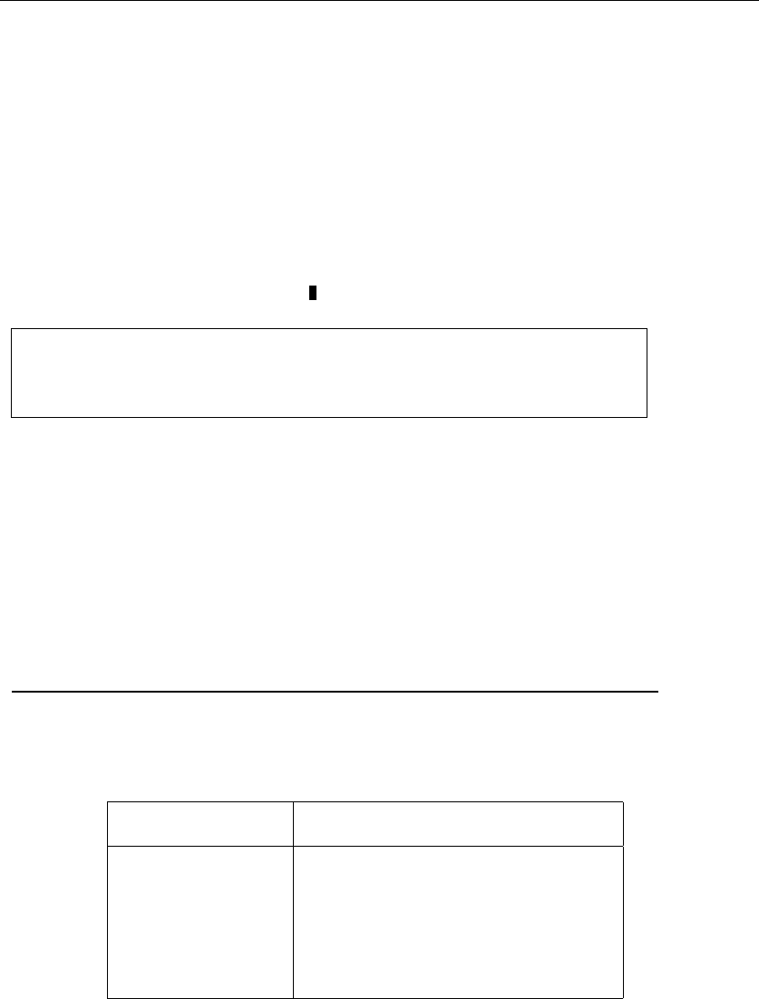
3.3 DICTIONARIES 75
Implementing a dictionary using a sorted array completely reverses our notions
of what is easy and what is hard. Searches can now be done in O(log n) time, using
binary search, because we know the median element sits in A[n/2]. Since the upper
and lower portions of the array are also sorted, the search can continue recursively
on the appropriate portion. The number of halvings of nuntil we get to a single
element is lg n.
The sorted order also benefits us with respect to the other dictionary retrieval
operations. The minimum and maximum elements sit in A[1] and A[n], while the
predecessor and successor to A[x]areA[x−1] and A[x+ 1], respectively.
Insertion and deletion become more expensive, however, because making room
for a new item or filling a hole may require moving many items arbitrarily. Thus
both become linear-time operations.
Take-Home Lesson: Data structure design must balance all the different op-
erations it supports. The fastest data structure to support both operations A
and Bmay well not be the fastest structure to support either operation Aor
B.
Stop and Think: Comparing Dictionary Implementations (II)
Problem: What is the asymptotic worst-case running times for each of the seven
fundamental dictionary operations when the data structure is implemented as
•A singly-linked unsorted list.
•A doubly-linked unsorted list.
•A singly-linked sorted list.
•A doubly-linked sorted list.
Solution: Two different issues must be considered in evaluating these implementa-
tions: singly- vs. doubly-linked lists and sorted vs. unsorted order. Subtle operations
are denoted with a superscript:
Singly Double Singly Doubly
Dictionary operation unsorted unsorted sorted sorted
Search(L,k)O(n)O(n)O(n)O(n)
Insert(L,x)O(1) O(1) O(n)O(n)
Delete(L,x)O(n)∗O(1) O(n)∗O(1)
Successor(L,x)O(n)O(n)O(1) O(1)
Predecessor(L,x)O(n)O(n)O(n)∗O(1)
Minimum(L)O(n)O(n)O(1) O(1)
Maximum(L)O(n)O(n)O(1)∗O(1)

76 3. DATA STRUCTURES
As with unsorted arrays, search operations are destined to be slow while main-
tenance operations are fast.
•Insertion/Deletion – The complication here is deletion from a singly-linked
list. The definition of the Delete operation states we are given a pointer xto
the item to be deleted. But what we really need is a pointer to the element
pointing to xin the list, because that is the node that needs to be changed.
We can do nothing without this list predecessor, and so must spend linear
time searching for it on a singly-linked list. Doubly-linked lists avoid this
problem, since we can immediately retrieve the list predecessor of x.
Deletion is faster for sorted doubly-linked lists than sorted arrays, because
splicing out the deleted element from the list is more efficient than filling
the hole by moving array elements. The predecessor pointer problem again
complicates deletion from singly-linked sorted lists.
•Search – Sorting provides less benefit for linked lists than it did for arrays. Bi-
nary search is no longer possible, because we can’t access the median element
without traversing all the elements before it. What sorted lists do provide is
quick termination of unsuccessful searches, for if we have not found Abbott by
the time we hit Costello we can deduce that he doesn’t exist. Still, searching
takes linear time in the worst case.
•Traversal operations – The predecessor pointer problem again complicates
implementing Predecessor. The logical successor is equivalent to the node
successor for both types of sorted lists, and hence can be implemented in
constant time.
•Maximum – The maximum element sits at the tail of the list, which would
normally require Θ(n) time to reach in either singly- or doubly-linked lists.
However, we can maintain a separate pointer to the list tail, provided we
pay the maintenance costs for this pointer on every insertion and deletion.
The tail pointer can be updated in constant time on doubly-linked lists: on
insertion check whether last->next still equals NULL, and on deletion set
last to point to the list predecessor of last if the last element is deleted.
We have no efficient way to find this predecessor for singly-linked lists. So
why can we implement maximum in Θ(1) on singly-linked lists? The trick is
to charge the cost to each deletion, which already took linear time. Adding
an extra linear sweep to update the pointer does not harm the asymptotic
complexity of Delete, while gaining us Maximum in constant time as a reward
for clear thinking.
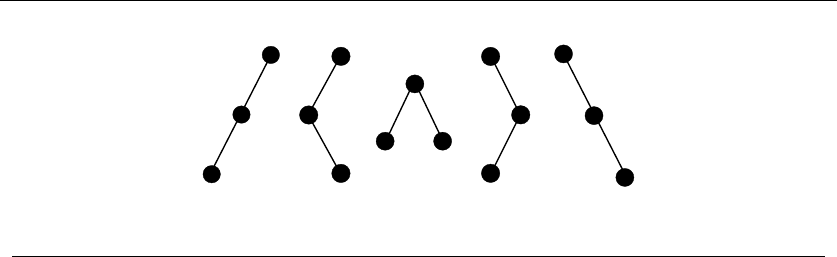
3.4 BINARY SEARCH TREES 77
1
2
13
13
1
2
3
2
2
3
1
2
3
Figure 3.2: The five distinct binary search trees on three nodes
3.4 Binary Search Trees
We have seen data structures that allow fast search or flexible update, but not fast
search and flexible update. Unsorted, doubly-linked lists supported insertion and
deletion in O(1) time but search took linear time in the worse case. Sorted arrays
support binary search and logarithmic query times, but at the cost of linear-time
update.
Binary search requires that we have fast access to two elements—specifically
the median elements above and below the given node. To combine these ideas, we
need a “linked list” with two pointers per node. This is the basic idea behind binary
search trees.
Arooted binary tree is recursively defined as either being (1) empty, or (2)
consisting of a node called the root, together with two rooted binary trees called
the left and right subtrees, respectively. The order among “brother” nodes matters
in rooted trees, so left is different from right. Figure 3.2 gives the shapes of the five
distinct binary trees that can be formed on three nodes.
A binary search tree labels each node in a binary tree with a single key such
that for any node labeled x, all nodes in the left subtree of xhave keys <xwhile
all nodes in the right subtree of xhave keys >x. This search tree labeling scheme
is very special. For any binary tree on nnodes, and any set of nkeys, there is
exactly one labeling that makes it a binary search tree. The allowable labelings for
three-node trees are given in Figure 3.2.
3.4.1 Implementing Binary Search Trees
Binary tree nodes have left and right pointer fields, an (optional) parent pointer,
and a data field. These relationships are shown in Figure 3.3; a type declaration
for the tree structure is given below:
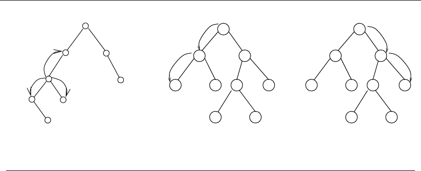
78 3. DATA STRUCTURES
left right
parent
Figure 3.3: Relationships in a binary search tree (left). Finding the minimum (center) and
maximum (right) elements in a binary search tree
typedef struct tree {
item_type item; /* data item */
struct tree *parent; /* pointer to parent */
struct tree *left; /* pointer to left child */
struct tree *right; /* pointer to right child */
} tree;
The basic operations supported by binary trees are searching, traversal, inser-
tion, and deletion.
Searching in a Tree
The binary search tree labeling uniquely identities where each key is located. Start
at the root. Unless it contains the query key x, proceed either left or right depending
upon whether xoccurs before or after the root key. This algorithm works because
both the left and right subtrees of a binary search tree are themselves binary search
trees. This recursive structure yields the recursive search algorithm below:
tree *search_tree(tree *l, item_type x)
{
if (l == NULL) return(NULL);
if (l->item == x) return(l);
if (x < l->item)
return( search_tree(l->left, x) );
else
return( search_tree(l->right, x) );
}

3.4 BINARY SEARCH TREES 79
This search algorithm runs in O(h) time, where hdenotes the height of the
tree.
Finding Minimum and Maximum Elements in a Tree
Implementing the find-minimum operation requires knowing where the minimum
element is in the tree. By definition, the smallest key must reside in the left subtree
of the root, since all keys in the left subtree have values less than that of the root.
Therefore, as shown in Figure 3.3, the minimum element must be the leftmost
descendent of the root. Similarly, the maximum element must be the rightmost
descendent of the root.
tree *find_minimum(tree *t)
{
tree *min; /* pointer to minimum */
if (t == NULL) return(NULL);
min = t;
while (min->left != NULL)
min = min->left;
return(min);
}
Traversal in a Tree
Visiting all the nodes in a rooted binary tree proves to be an important component
of many algorithms. It is a special case of traversing all the nodes and edges in a
graph, which will be the foundation of Chapter 5.
A prime application of tree traversal is listing the labels of the tree nodes.
Binary search trees make it easy to report the labels in sorted order. By definition,
all the keys smaller than the root must lie in the left subtree of the root, and all
keys bigger than the root in the right subtree. Thus, visiting the nodes recursively
in accord with such a policy produces an in-order traversal of the search tree:
void traverse_tree(tree *l)
{
if (l != NULL) {
traverse_tree(l->left);
process_item(l->item);
traverse_tree(l->right);
}
}

80 3. DATA STRUCTURES
Each item is processed once during the course of traversal, which runs in O(n)
time, where ndenotes the number of nodes in the tree.
Alternate traversal orders come from changing the position of process item
relative to the traversals of the left and right subtrees. Processing the item first
yields a pre-order traversal, while processing it last gives a post-order traversal.
These make relatively little sense with search trees, but prove useful when the
rooted tree represents arithmetic or logical expressions.
Insertion in a Tree
There is only one place to insert an item xinto a binary search tree Twhere we
know we can find it again. We must replace the NULL pointer found in Tafter an
unsuccessful query for the key k.
This implementation uses recursion to combine the search and node insertion
stages of key insertion. The three arguments to insert tree are (1) a pointer lto
the pointer linking the search subtree to the rest of the tree, (2) the key xto be
inserted, and (3) a parent pointer to the parent node containing l. The node is
allocated and linked in on hitting the NULL pointer. Note that we pass the pointer to
the appropriate left/right pointer in the node during the search, so the assignment
*l = p; links the new node into the tree:
insert_tree(tree **l, item_type x, tree *parent)
{
tree *p; /* temporary pointer */
if (*l == NULL) {
p = malloc(sizeof(tree)); /* allocate new node */
p->item = x;
p->left = p->right = NULL;
p->parent = parent;
*l = p; /* link into parent’s record */
return;
}
if (x < (*l)->item)
insert_tree(&((*l)->left), x, *l);
else
insert_tree(&((*l)->right), x, *l);
}
Allocating the node and linking it in to the tree is a constant-time operation
after the search has been performed in O(h) time.
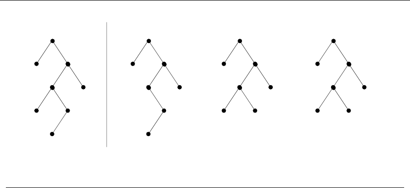
3.4 BINARY SEARCH TREES 81
initial tree delete node with zero children (3)
5
5
2
6
8
7
3
1
2
8
7
4
3
1
2
5
6
8
7
4
1
delete node with 2 children (4)delete node with 1 child (6)
6
8
7
4
3
1
5
2
Figure 3.4: Deleting tree nodes with 0, 1, and 2 children
Deletion from a Tree
Deletion is somewhat trickier than insertion, because removing a node means ap-
propriately linking its two descendant subtrees back into the tree somewhere else.
There are three cases, illustrated in Figure 3.4. Leaf nodes have no children, and
so may be deleted by simply clearing the pointer to the given node.
The case of the doomed node having one child is also straightforward. There
is one parent and one grandchild, and we can link the grandchild directly to the
parent without violating the in-order labeling property of the tree.
But what of a to-be-deleted node with two children? Our solution is to relabel
this node with the key of its immediate successor in sorted order. This successor
must be the smallest value in the right subtree, specifically the leftmost descendant
in the right subtree (p). Moving this to the point of deletion results in a properly-
labeled binary search tree, and reduces our deletion problem to physically removing
a node with at most one child—a case that has been resolved above.
The full implementation has been omitted here because it looks a little ghastly,
but the code follows logically from the description above.
The worst-case complexity analysis is as follows. Every deletion requires the
cost of at most two search operations, each taking O(h) time where his the height
of the tree, plus a constant amount of pointer manipulation.
3.4.2 How Good Are Binary Search Trees?
When implemented using binary search trees, all three dictionary operations take
O(h) time, where his the height of the tree. The smallest height we can hope for
occurs when the tree is perfectly balanced, where h=log n. This is very good,
but the tree must be perfectly balanced.

82 3. DATA STRUCTURES
Our insertion algorithm puts each new item at a leaf node where it should have
been found. This makes the shape (and more importantly height) of the tree a
function of the order in which we insert the keys.
Unfortunately, bad things can happen when building trees through insertion.
The data structure has no control over the order of insertion. Consider what hap-
pens if the user inserts the keys in sorted order. The operations insert(a), followed
by insert(b),insert(c),insert(d), . . . will produce a skinny linear height tree
where only right pointers are used.
Thus binary trees can have heights ranging from lg nto n. But how tall are
they on average? The average case analysis of algorithms can be tricky because we
must carefully specify what we mean by average. The question is well defined if we
consider each of the n! possible insertion orderings equally likely and average over
those. If so, we are in luck, because with high probability the resulting tree will
have O(log n) height. This will be shown in Section 4.6 (page 123).
This argument is an important example of the power of randomization.Wecan
often develop simple algorithms that offer good performance with high probabil-
ity. We will see that a similar idea underlies the fastest known sorting algorithm,
quicksort.
3.4.3 Balanced Search Trees
Random search trees are usually good. But if we get unlucky with our order of
insertion, we can end up with a linear-height tree in the worst case. This worst
case is outside of our direct control, since we must build the tree in response to the
requests given by our potentially nasty user.
What would be better is an insertion/deletion procedure which adjusts the tree a
little after each insertion, keeping it close enough to be balanced so the maximum
height is logarithmic. Sophisticated balanced binary search tree data structures
have been developed that guarantee the height of the tree always to be O(log n).
Therefore, all dictionary operations (insert, delete, query) take O(log n) time each.
Implementations of balanced tree data structures such as red-black trees and splay
trees are discussed in Section 12.1 (page 367).
From an algorithm design viewpoint, it is important to know that these trees
exist and that they can be used as black boxes to provide an efficient dictionary
implementation. When figuring the costs of dictionary operations for algorithm
analysis, we can assume the worst-case complexities of balanced binary trees to be
a fair measure.
Take-Home Lesson: Picking the wrong data structure for the job can be
disastrous in terms of performance. Identifying the very best data structure
is usually not as critical, because there can be several choices that perform
similarly.

3.5 PRIORITY QUEUES 83
Stop and Think: Exploiting Balanced Search Trees
Problem: You are given the task of reading nnumbers and then printing them
out in sorted order. Suppose you have access to a balanced dictionary data struc-
ture, which supports the operations search, insert, delete, minimum, maximum,
successor, and predecessor each in O(log n) time.
1. How can you sort in O(nlog n) time using only insert and in-order traversal?
2. How can you sort in O(nlog n) time using only minimum, successor, and
insert?
3. How can you sort in O(nlog n) time using only minimum, insert, delete,
search?
Solution: The first problem allows us to do insertion and inorder-traversal. We can
build a search tree by inserting all nelements, then do a traversal to access the
items in sorted order:
Sort1()
initialize-tree(t)
While (not EOF)
read(x);
insert(x,t)
Traverse(t)
Sort2()
initialize-tree(t)
While (not EOF)
read(x);
insert(x,t);
y = Minimum(t)
While (y = NULL) do
print(y →item)
y = Successor(y,t)
Sort3()
initialize-tree(t)
While (not EOF)
read(x);
insert(x,t);
y = Minimum(t)
While (y = NULL) do
print(y→item)
Delete(y,t)
y = Minimum(t)
The second problem allows us to use the minimum and successor operations
after constructing the tree. We can start from the minimum element, and then
repeatedly find the successor to traverse the elements in sorted order.
The third problem does not give us successor, but does allow us delete. We
can repeatedly find and delete the minimum element to once again traverse all the
elements in sorted order.
Each of these algorithms does a linear number of logarithmic-time operations,
and hence runs in O(nlog n) time. The key to exploiting balanced binary search
trees is using them as black boxes.
3.5 Priority Queues
Many algorithms process items in a specific order. For example, suppose you must
schedule jobs according to their importance relative to other jobs. Scheduling the

84 3. DATA STRUCTURES
jobs requires sorting them by importance, and then evaluating them in this sorted
order.
Priority queues are data structures that provide more flexibility than simple
sorting, because they allow new elements to enter a system at arbitrary intervals.
It is much more cost-effective to insert a new job into a priority queue than to
re-sort everything on each such arrival.
The basic priority queue supports three primary operations:
•Insert(Q,x)– Given an item xwith key k, insert it into the priority queue Q.
•Find-Minimum(Q) or Find-Maximum(Q)– Return a pointer to the item
whose key value is smaller (larger) than any other key in the priority queue
Q.
•Delete-Minimum(Q) or Delete-Maximum(Q)– Remove the item from the pri-
ority queue Qwhose key is minimum (maximum).
Many naturally occurring processes are accurately modeled by priority queues.
Single people maintain a priority queue of potential dating candidates—mentally
if not explicitly. One’s impression on meeting a new person maps directly to an
attractiveness or desirability score. Desirability serves as the key field for inserting
this new entry into the “little black book” priority queue data structure. Dating is
the process of extracting the most desirable person from the data structure (Find-
Maximum), spending an evening to evaluate them better, and then reinserting
them into the priority queue with a possibly revised score.
Take-Home Lesson: Building algorithms around data structures such as dictio-
naries and priority queues leads to both clean structure and good performance.
Stop and Think: Basic Priority Queue Implementations
Problem: What is the worst-case time complexity of the three basic priority queue
operations (insert, find-minimum, and delete-minimum) when the basic data struc-
ture is
•An unsorted array.
•A sorted array.
•A balanced binary search tree.
Solution: There is surprising subtlety in implementing these three operations, even
when using a data structure as simple as an unsorted array. The unsorted array

3.6 WAR STORY: STRIPPING TRIANGULATIONS 85
dictionary (discussed on page 73) implemented insertion and deletion in constant
time, and search and minimum in linear time. A linear time implementation of
delete-minimum can be composed from find-minimum, followed by search, followed
by delete.
For sorted arrays, we can implement insert and delete in linear time, and mini-
mum in constant time. However, all priority queue deletions involve only the min-
imum element. By storing the sorted array in reverse order (largest value on top),
the minimum element will be the last one in the array. Deleting the tail element
requires no movement of any items, just decrementing the number of remaining
items n, and so delete-minimum can be implemented in constant time.
All this is fine, yet the following table claims we can implement find-minimum
in constant time for each data structure:
Unsorted Sorted Balanced
array array tree
Insert(Q,x)O(1) O(n)O(log n)
Find-Minimum(Q)O(1) O(1) O(1)
Delete-Minimum(Q)O(n)O(1) O(log n)
The trick is using an extra variable to store a pointer/index to the minimum
entry in each of these structures, so we can simply return this value whenever we
are asked to find-minimum. Updating this pointer on each insertion is easy—we
update it if and only if the newly inserted value is less than the current minimum.
But what happens on a delete-minimum? We can delete the minimum entry have,
then do an honest find-minimum to restore our canned value. The honest find-
minimum takes linear time on an unsorted array and logarithmic time on a tree,
and hence can be folded into the cost of each deletion.
Priority queues are very useful data structures. Indeed, they will be the hero of
two of our war stories, including the next one. A particularly nice priority queue
implementation (the heap) will be discussed in the context of sorting in Section 4.3
(page 108). Further, a complete set of priority queue implementations is presented
in Section 12.2 (page 373) of the catalog.
3.6 War Story: Stripping Triangulations
Geometric models used in computer graphics are commonly represented as a tri-
angulated surface, as shown in Figure 3.5(l). High-performance rendering engines
have special hardware for rendering and shading triangles. This hardware is so fast
that the bottleneck of rendering is the cost of feeding the triangulation structure
into the hardware engine.
Although each triangle can be described by specifying its three endpoints, an
alternative representation is more efficient. Instead of specifying each triangle in
isolation, suppose that we partition the triangles into strips of adjacent triangles
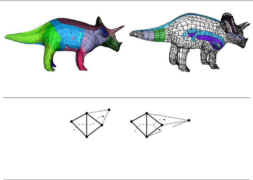
86 3. DATA STRUCTURES
Figure 3.5: (l) A triangulated model of a dinosaur (r) Several triangle strips in the model
a) b)
i
i
i-1
i-2
i-3
i-4 i-1
i-2
i-3
i-4
Figure 3.6: Partitioning a triangular mesh into strips: (a) with left-right turns (b) with the
flexibility of arbitrary turns
and walk along the strip. Since each triangle shares two vertices in common with
its neighbors, we save the cost of retransmitting the two extra vertices and any
associated information. To make the description of the triangles unambiguous, the
OpenGL triangular-mesh renderer assumes that all turns alternate from left to
right (as shown in Figure 3.6).
The task of finding a small number of strips that cover each triangle in a mesh
can be thought of as a graph problem. The graph of interest has a vertex for
every triangle of the mesh, and an edge between every pair of vertices represent-
ing adjacent triangles. This dual graph representation captures all the information
about the triangulation (see Section 15.12 (page 520)) needed to partition it into
triangular strips.
Once we had the dual graph available, the project could begin in earnest. We
sought to partition the vertices into as few paths or strips as possible. Partition-
ing it into one path implied that we had discovered a Hamiltonian path, which
by definition visits each vertex exactly once. Since finding a Hamiltonian path is
NP-complete (see Section 16.5 (page 538)), we knew not to look for an optimal
algorithm, but concentrate instead on heuristics.
The simplest heuristic for strip cover would start from an arbitrary triangle
and then do a left-right walk until the walk ends, either by hitting the boundary of
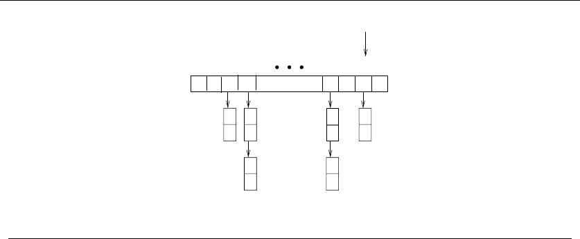
3.6 WAR STORY: STRIPPING TRIANGULATIONS 87
253 254 255 256
1 2 3 4
top
Figure 3.7: A bounded height priority queue for triangle strips
the object or a previously visited triangle. This heuristic had the advantage that
it would be fast and simple, although there is no reason why it should find the
smallest possible set of left-right strips for a given triangulation.
The greedy heuristic would be more likely to result in a small number of strips
however. Greedy heuristics always try to grab the best possible thing first. In the
case of the triangulation, the natural greedy heuristic would identify the starting
triangle that yields the longest left-right strip, and peel that one off first.
Being greedy does not guarantee you the best possible solution either, since the
first strip you peel off might break apart a lot of potential strips we might have
wanted to use later. Still, being greedy is a good rule of thumb if you want to get
rich. Since removing the longest strip would leave the fewest number of triangles
for later strips, the greedy heuristic should outperform the naive heuristic.
But how much time does it take to find the largest strip to peel off next? Let
kbe the length of the walk possible from an average vertex. Using the simplest
possible implementation, we could walk from each of the nvertices to find the
largest remaining strip to report in O(kn) time. Repeating this for each of the
roughly n/k strips we extract yields an O(n2)-time implementation, which would
be hopelessly slow on a typical model of 20,000 triangles.
How could we speed this up? It seems wasteful to rewalk from each triangle
after deleting a single strip. We could maintain the lengths of all the possible
future strips in a data structure. However, whenever we peel off a strip, we must
update the lengths of all affected strips. These strips will be shortened because
they walked through a triangle that now no longer exists. There are two aspects of
such a data structure:
•Priority Queue – Since we were repeatedly identifying the longest remaining
strip, we needed a priority queue to store the strips ordered according to
length. The next strip to peel always sat at the top of the queue. Our priority
queue had to permit reducing the priority of arbitrary elements of the queue
whenever we updated the strip lengths to reflect what triangles were peeled
88 3. DATA STRUCTURES
Model name Triangle count Naive cost Greedy cost Greedy time
Diver 3,798 8,460 4,650 6.4 sec
Heads 4,157 10,588 4,749 9.9 sec
Framework 5,602 9,274 7,210 9.7 sec
Bart Simpson 9,654 24,934 11,676 20.5 sec
Enterprise 12,710 29,016 13,738 26.2 sec
Torus 20,000 40,000 20,200 272.7 sec
Jaw 75,842 104,203 95,020 136.2 sec
Figure 3.8: A comparison of the naive versus greedy heuristics for several triangular meshes
away. Because all of the strip lengths were bounded by a fairly small integer
(hardware constraints prevent any strip from having more than 256 vertices),
we used a bounded-height priority queue (an array of buckets shown in Figure
3.7 and described in Section 12.2 (page 373)). An ordinary heap would also
have worked just fine.
To update the queue entry associated with each triangle, we needed to quickly
find where it was. This meant that we also needed a . . .
•Dictionary – For each triangle in the mesh, we needed to find where it was in
the queue. This meant storing a pointer to each triangle in a dictionary. By
integrating this dictionary with the priority queue, we built a data structure
capable of a wide range of operations.
Although there were various other complications, such as quickly recalculating
the length of the strips affected by the peeling, the key idea needed to obtain better
performance was to use the priority queue. Run time improved by several orders
of magnitude after employing this data structure.
How much better did the greedy heuristic do than the naive heuristic? Consider
the table in Figure 3.8. In all cases, the greedy heuristic led to a set of strips that
cost less, as measured by the total size of the strips. The savings ranged from about
10% to 50%, which is quite remarkable since the greatest possible improvement
(going from three vertices per triangle down to one) yields a savings of only 66.6%.
After implementing the greedy heuristic with our priority queue data structure,
the program ran in O(n·k) time, where nis the number of triangles and kis the
length of the average strip. Thus the torus, which consisted of a small number of
very long strips, took longer than the jaw, even though the latter contained over
three times as many triangles.
There are several lessons to be gleaned from this story. First, when working with
a large enough data set, only linear or near linear algorithms (say O(nlog n)) are
likely to be fast enough. Second, choosing the right data structure is often the key
to getting the time complexity down to this point. Finally, using smart heuristic

3.7 HASHING AND STRINGS 89
like greedy is likely to significantly improve quality over the naive approach. How
much the improvement will be can only be determined by experimentation.
3.7 Hashing and Strings
Hash tables are a very practical way to maintain a dictionary. They exploit the fact
that looking an item up in an array takes constant time once you have its index. A
hash function is a mathematical function that maps keys to integers. We will use
the value of our hash function as an index into an array, and store our item at that
position.
The first step of the hash function is usually to map each key to a big integer.
Let αbe the size of the alphabet on which a given string Sis written. Let char(c)
be a function that maps each symbol of the alphabet to a unique integer from 0 to
α−1. The function
H(S)=|S|−1
i=0
α|S|−(i+1) ×char(si)
maps each string to a unique (but large) integer by treating the characters of the
string as “digits” in a base-αnumber system.
The result is unique identifier numbers, but they are so large they will quickly
exceed the number of slots in our hash table (denoted by m). We must reduce this
number to an integer between 0 and m−1, by taking the remainder of H(S)modm.
This works on the same principle as a roulette wheel. The ball travels a long
distance around and around the circumference-mwheel H(S)/mtimes before
settling down to a random bin. If the table size is selected with enough finesse
(ideally mis a large prime not too close to 2i−1), the resulting hash values should
be fairly uniformly distributed.
3.7.1 Collision Resolution
No matter how good our hash function is, we had better be prepared for collisions,
because two distinct keys will occasionally hash to the same value. Chaining is the
easiest approach to collision resolution. Represent the hash table as an array of m
linked lists, as shown in Figure 3.9. The ith list will contain all the items that hash
to the value of i. Thus search, insertion, and deletion reduce to the corresponding
problem in linked lists. If the nkeys are distributed uniformly in a table, each list
will contain roughly n/m elements, making them a constant size when m≈n.
Chaining is very natural, but devotes a considerable amount of memory to
pointers. This is space that could be used to make the table larger, and hence the
“lists” smaller.
The alternative is something called open addressing. The hash table is main-
tained as an array of elements (not buckets), each initialized to null, as shown in
Figure 3.10. On an insertion, we check to see if the desired position is empty. If so,
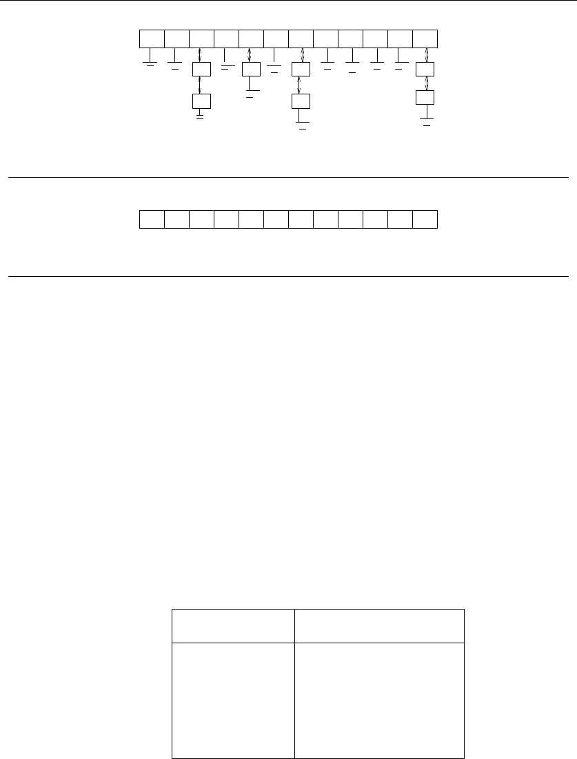
90 3. DATA STRUCTURES
Figure 3.9: Collision resolution by chaining
1 2 3 4 5 6 7 8 9 10 11
XXXXX
Figure 3.10: Collision resolution by open addressing
we insert it. If not, we must find some other place to insert it instead. The simplest
possibility (called sequential probing) inserts the item in the next open spot in the
table. If the table is not too full, the contiguous runs of items should be fairly
small, hence this location should be only a few slots from its intended position.
Searching for a given key now involves going to the appropriate hash value and
checking to see if the item there is the one we want. If so, return it. Otherwise we
must keep checking through the length of the run.
Deletion in an open addressing scheme can get ugly, since removing one element
might break a chain of insertions, making some elements inaccessible. We have no
alternative but to reinsert all the items in the run following the new hole.
Chaining and open addressing both require O(m) to initialize an m-element
hash table to null elements prior to the first insertion. Traversing all the elements
in the table takes O(n+m) time for chaining, because we have to scan all m
buckets looking for elements, even if the actual number of inserted items is small.
This reduces to O(m) time for open addressing, since nmust be at most m.
When using chaining with doubly-linked lists to resolve collisions in an m-
element hash table, the dictionary operations for nitems can be implemented in
the following expected and worst case times:
Hash table Hash table
(expected) (worst case)
Search(L,k)O(n/m)O(n)
Insert(L,x)O(1) O(1)
Delete(L,x)O(1) O(1)
Successor(L,x)O(n+m)O(n+m)
Predecessor(L,x)O(n+m)O(n+m)
Minimum(L)O(n+m)O(n+m)
Maximum(L)O(n+m)O(n+m)

3.7 HASHING AND STRINGS 91
Pragmatically, a hash table is often the best data structure to maintain a dic-
tionary. The applications of hashing go far beyond dictionaries, however, as we will
see below.
3.7.2 Efficient String Matching via Hashing
Strings are sequences of characters where the order of the characters matters, since
ALGORITHM is different than LOGARITHM. Text strings are fundamental to a
host of computing applications, from programming language parsing/compilation,
to web search engines, to biological sequence analysis.
The primary data structure for representing strings is an array of characters.
This allows us constant-time access to the ith character of the string. Some auxiliary
information must be maintained to mark the end of the string—either a special
end-of-string character or (perhaps more usefully) a count of the ncharacters in
the string.
The most fundamental operation on text strings is substring search, namely:
Problem: Substring Pattern Matching
Input: A text string tand a pattern string p.
Output: Does tcontain the pattern pas a substring, and if so where?
The simplest algorithm to search for the presence of pattern string pin text t
overlays the pattern string at every position in the text, and checks whether every
pattern character matches the corresponding text character. As demonstrated in
Section 2.5.3 (page 43), this runs in O(nm) time, where n=|t|and m=|p|.
This quadratic bound is worst-case. More complicated, worst-case linear-time
search algorithms do exist: see Section 18.3 (page 628) for a complete discussion.
But here we give a linear expected-time algorithm for string matching, called the
Rabin-Karp algorithm. It is based on hashing. Suppose we compute a given hash
function on both the pattern string pand the m-character substring starting from
the ith position of t. If these two strings are identical, clearly the resulting hash
values must be the same. If the two strings are different, the hash values will
almost certainly be different. These false positives should be so rare that we can
easily spend the O(m) time it takes to explicitly check the identity of two strings
whenever the hash values agree.
This reduces string matching to n−m+2 hash value computations (the n−m+1
windows of t, plus one hash of p), plus what should be a very small number of O(m)
time verification steps. The catch is that it takes O(m) time to compute a hash
function on an m-character string, and O(n) such computations seems to leave us
with an O(mn) algorithm again.
But let’s look more closely at our previously defined hash function, applied to
the mcharacters starting from the jth position of string S:
H(S, j)=
m−1
i=0
αm−(i+1) ×char(si+j)

92 3. DATA STRUCTURES
What changes if we now try to compute H(S, j + 1)—the hash of the next
window of mcharacters? Note that m−1 characters are the same in both windows,
although this differs by one in the number of times they are multiplied by α.A
little algebra reveals that
H(S, j +1)=α(H(S, j)−αm−1char(sj)) + char(sj+m)
This means that once we know the hash value from the jposition, we can find
the hash value from the (j+ 1)st position for the cost of two multiplications, one
addition, and one subtraction. This can be done in constant time (the value of
αm−1can be computed once and used for all hash value computations). This math
works even if we compute H(S, j)modM, where Mis a reasonably large prime
number, thus keeping the size of our hash values small (at most M) even when the
pattern string is long.
Rabin-Karp is a good example of a randomized algorithm (if we pick Min some
random way). We get no guarantee the algorithm runs in O(n+m) time, because we
may get unlucky and have the hash values regularly collide with spurious matches.
Still, the odds are heavily in our favor—if the hash function returns values uniformly
from0toM−1, the probability of a false collision should be 1/M .Thisisquite
reasonable: if M≈n, there should only be one false collision per string, and if
M≈nkfor k≥2, the odds are great we will never see any false collisions.
3.7.3 Duplicate Detection Via Hashing
The key idea of hashing is to represent a large object (be it a key, a string, or a
substring) using a single number. The goal is a representation of the large object
by an entity that can be manipulated in constant time, such that it is relatively
unlikely that two different large objects map to the same value.
Hashing has a variety of clever applications beyond just speeding up search. I
once heard Udi Manber—then Chief Scientist at Yahoo—talk about the algorithms
employed at his company. The three most important algorithms at Yahoo, he said,
were hashing, hashing, and hashing.
Consider the following problems with nice hashing solutions:
•Is a given document different from all the rest in a large corpus? –Asearch
engine with a huge database of ndocuments spiders yet another webpage.
How can it tell whether this adds something new to add to the database, or
is just a duplicate page that exists elsewhere on the Web?
Explicitly comparing the new document Dto all ndocuments is hopelessly
inefficient for a large corpus. But we can hash Dto an integer, and compare
it to the hash codes of the rest of the corpus. Only when there is a collision
is Da possible duplicate. Since we expect few spurious collisions, we can
explicitly compare the few documents sharing the exact hash code with little
effort.

3.8 SPECIALIZED DATA STRUCTURES 93
•Is part of this document plagiarized from a document in a large corpus? –A
lazy student copies a portion of a Web document into their term paper. “The
Web is a big place,” he smirks. “How will anyone ever find which one?”
This is a more difficult problem than the previous application. Adding, delet-
ing, or changing even one character from a document will completely change
its hash code. Thus the hash codes produced in the previous application
cannot help for this more general problem.
However, we could build a hash table of all overlapping windows (substrings)
of length win all the documents in the corpus. Whenever there is a match of
hash codes, there is likely a common substring of length wbetween the two
documents, which can then be further investigated. We should choose wto
be long enough so such a co-occurrence is very unlikely to happen by chance.
The biggest downside of this scheme is that the size of the hash table becomes
as large as the documents themselves. Retaining a small but well-chosen
subset of these hash codes (say those which are exact multiples of 100) for
each document leaves us likely to detect sufficiently long duplicate strings.
•How can I convince you that a file isn’t changed? – In a closed-bid auction,
each party submits their bid in secret before the announced deadline. If you
knew what the other parties were bidding, you could arrange to bid $1 more
than the highest opponent and walk off with the prize as cheaply as possible.
Thus the “right” auction strategy is to hack into the computer containing
the bids just prior to the deadline, read the bids, and then magically emerge
the winner.
How can this be prevented? What if everyone submits a hash code of their
actual bid prior to the deadline, and then submits the full bid after the dead-
line? The auctioneer will pick the largest full bid, but checks to make sure the
hash code matches that submitted prior to the deadline. Such cryptographic
hashing methods provide a way to ensure that the file you give me today is
the same as original, because any changes to the file will result in changing
the hash code.
Although the worst-case bounds on anything involving hashing are dismal, with
a proper hash function we can confidently expect good behavior. Hashing is a fun-
damental idea in randomized algorithms, yielding linear expected-time algorithms
for problems otherwise Θ(nlog n), or Θ(n2)intheworstcase.
3.8 Specialized Data Structures
The basic data structures described thus far all represent an unstructured set of
items so as to facilitate retrieval operations. These data structures are well known
to most programmers. Not as well known are data structures for representing more

94 3. DATA STRUCTURES
structured or specialized kinds of objects, such as points in space, strings, and
graphs.
The design principles of these data structures are the same as for basic objects.
There exists a set of basic operations we need to perform repeatedly. We seek a data
structure that supports these operations very efficiently. These efficient, specialized
data structures are important for efficient graph and geometric algorithms so one
should be aware of their existence. Details appear throughout the catalog.
•String data structures – Character strings are typically represented by arrays
of characters, perhaps with a special character to mark the end of the string.
Suffix trees/arrays are special data structures that preprocess strings to make
pattern matching operations faster. See Section 12.3 (page 377) for details.
•Geometric data structures – Geometric data typically consists of collections of
data points and regions. Regions in the plane can be described by polygons,
where the boundary of the polygon is given by a chain of line segments.
Polygons can be represented using an array of points (v1,...,v
n,v
1), such
that (vi,v
i+1) is a segment of the boundary. Spatial data structures such as
kd-trees organize points and regions by geometric location to support fast
search. For more details, see Section 12.6 (page 389).
•Graph data structures – Graphs are typically represented using either adja-
cency matrices or adjacency lists. The choice of representation can have a
substantial impact on the design of the resulting graph algorithms, as dis-
cussed in Chapter 6 and in the catalog in Section 12.4.
•Set data structures – Subsets of items are typically represented using a dictio-
nary to support fast membership queries. Alternately, bit vectors are boolean
arrays such that the ith bit represents true if iis in the subset. Data struc-
tures for manipulating sets is presented in the catalog in Section 12.5. The
union-find data structure for maintaining set partitions will be covered in
Section 6.1.3 (page 198).
3.9 War Story: String ’em Up
The human genome encodes all the information necessary to build a person. This
project has already had an enormous impact on medicine and molecular biology.
Algorists have become interested in the human genome project as well, for several
reasons:
•DNA sequences can be accurately represented as strings of characters on the
four-letter alphabet (A,C,T,G). Biologist’s needs have sparked new interest
in old algorithmic problems such as string matching (see Section 18.3 (page
628)) as well as creating new problems such as shortest common superstring
(see Section 18.9 (page 654)).

3.9 WAR STORY: STRING ’EM UP 95
A C G T T A T C C A
C G T T A
G T T A T
T T A T C
T A T C C
Figure 3.11: The concatenation of two fragments can be in Sonly if all sub-fragments are
•DNA sequences are very long strings. The human genome is approximately
three billion base pairs (or characters) long. Such large problem size means
that asymptotic (Big-Oh) complexity analysis is usually fully justified on
biological problems.
•Enough money is being invested in genomics for computer scientists to want
to claim their piece of the action.
One of my interests in computational biology revolved around a proposed tech-
nique for DNA sequencing called sequencing by hybridization (SBH). This proce-
dure attaches a set of probes to an array, forming a sequencing chip. Each of these
probes determines whether or not the probe string occurs as a substring of the
DNA target. The target DNA can now be sequenced based on the constraints of
which strings are (and are not) substrings of the target.
We sought to identify all the strings of length 2kthat are possible substrings
of an unknown string S, given the set of all length ksubstrings of S. For example,
suppose we know that AC,CA,andCC are the only length-2 substrings of S.
It is possible that ACCA is a substring of S, since the center substring is one of
our possibilities. However, CAAC cannot be a substring of S, since AA is not a
substring of S. We needed to find a fast algorithm to construct all the consistent
length-2kstrings, since Scould be very long.
The simplest algorithm to build the 2kstrings would be to concatenate all O(n2)
pairs of k-strings together, and then test to make sure that all (k−1) length-k
substrings spanning the boundary of the concatenation were in fact substrings, as
shown in Figure 3.11. For example, the nine possible concatenations of AC,CA,
and CC are ACAC,ACCA,ACCC,CAAC,CACA,CACC,CCAC,CCCA,
and CCCC. Only CAAC can be eliminated because of the absence of AA.
We needed a fast way of testing whether the k−1 substrings straddling the
concatenation were members of our dictionary of permissible k-strings. The time
it takes to do this depends upon which dictionary data structure we use. A binary
search tree could find the correct string within O(log n) comparisons, where each

96 3. DATA STRUCTURES
comparison involved testing which of two length-kstrings appeared first in alpha-
betical order. The total time using such a binary search tree would be O(klog n).
That seemed pretty good. So my graduate student, Dimitris Margaritis, used a
binary search tree data structure for our implementation. It worked great up until
the moment we ran it.
“I’ve tried the fastest computer in our department, but our program is too slow,”
Dimitris complained. “It takes forever on string lengths of only 2,000 characters.
We will never get up to 50,000.”
We profiled our program and discovered that almost all the time was spent
searching in this data structure. This was no surprise since we did this k−1 times
for each of the O(n2) possible concatenations. We needed a faster dictionary data
structure, since search was the innermost operation in such a deep loop.
“How about using a hash table?” I suggested. “It should take O(k) time to hash
ak-character string and look it up in our table. That should knock off a factor of
O(log n), which will mean something when n≈2,000.”
Dimitris went back and implemented a hash table implementation for our dic-
tionary. Again, it worked great up until the moment we ran it.
“Our program is still too slow,” Dimitris complained. “Sure, it is now about
ten times faster on strings of length 2,000. So now we can get up to about 4,000
characters. Big deal. We will never get up to 50,000.”
“We should have expected this,” I mused. “After all, lg2(2,000) ≈11. We need
a faster data structure to search in our dictionary of strings.”
“But what can be faster than a hash table?” Dimitris countered. “To look up
ak-character string, you must read all kcharacters. Our hash table already does
O(k) searching.”
“Sure, it takes kcomparisons to test the first substring. But maybe we can do
better on the second test. Remember where our dictionary queries are coming from.
When we concatenate ABCD with EFGH, we are first testing whether BCDE
is in the dictionary, then CDEF. These strings differ from each other by only one
character. We should be able to exploit this so each subsequent test takes constant
time to perform....”
“We can’t do that with a hash table,” Dimitris observed. “The second key is not
going to be anywhere near the first in the table. A binary search tree won’t help,
either. Since the keys ABCD and BCDE differ according to the first character,
the two strings will be in different parts of the tree.”
“But we can use a suffix tree to do this,” I countered. “A suffix tree is a trie
containing all the suffixes of a given set of strings. For example, the suffixes of
ACAC are {ACAC, CAC, AC, C}. Coupled with suffixes of string CACT,weget
the suffix tree of Figure 3.12. By following a pointer from ACAC to its longest
proper suffix CAC, we get to the right place to test whether CACT is in our set
of strings. One character comparison is all we need to do from there.”
Suffix trees are amazing data structures, discussed in considerably more detail
in Section 12.3 (page 377). Dimitris did some reading about them, then built a nice

3.9 WAR STORY: STRING ’EM UP 97
at
c
c
c
c
a
a
t
t
t
Figure 3.12: Suffix tree on ACAC and CACT, with the pointer to the suffix of ACAC
suffix tree implementation for our dictionary. Once again, it worked great up until
the moment we ran it.
“Now our program is faster, but it runs out of memory,” Dimitris complained.
“The suffix tree builds a path of length kfor each suffix of length k, so all told there
canbeΘ(n2) nodes in the tree. It crashes when we go beyond 2,000 characters.
We will never get up to strings with 50,000 characters.”
I wasn’t ready to give up yet. “There is a way around the space problem, by
using compressed suffix trees,” I recalled. “Instead of explicitly representing long
paths of character nodes, we can refer back to the original string.” Compressed
suffix trees always take linear space, as described in Section 12.3 (page 377).
Dimitris went back one last time and implemented the compressed suffix tree
data structure. Now it worked great! As shown in Figure 3.13, we ran our simu-
lation for strings of length n= 65,536 without incident. Our results showed that
interactive SBH could be a very efficient sequencing technique. Based on these
simulations, we were able to arouse interest in our technique from biologists. Mak-
ing the actual wet laboratory experiments feasible provided another computational
challenge, which is reported in Section 7.7 (page 263).
The take-home lessons for programmers from Figure 3.13 should be apparent.
We isolated a single operation (dictionary string search) that was being performed
repeatedly and optimized the data structure we used to support it. We started with
a simple implementation (binary search trees) in the hopes that it would suffice,
and then used profiling to reveal the trouble when it didn’t. When an improved
dictionary structure still did not suffice, we looked deeper into the kind of queries we
were performing, so that we could identify an even better data structure. Finally,
we didn’t give up until we had achieved the level of performance we needed. In
algorithms, as in life, persistence usually pays off.
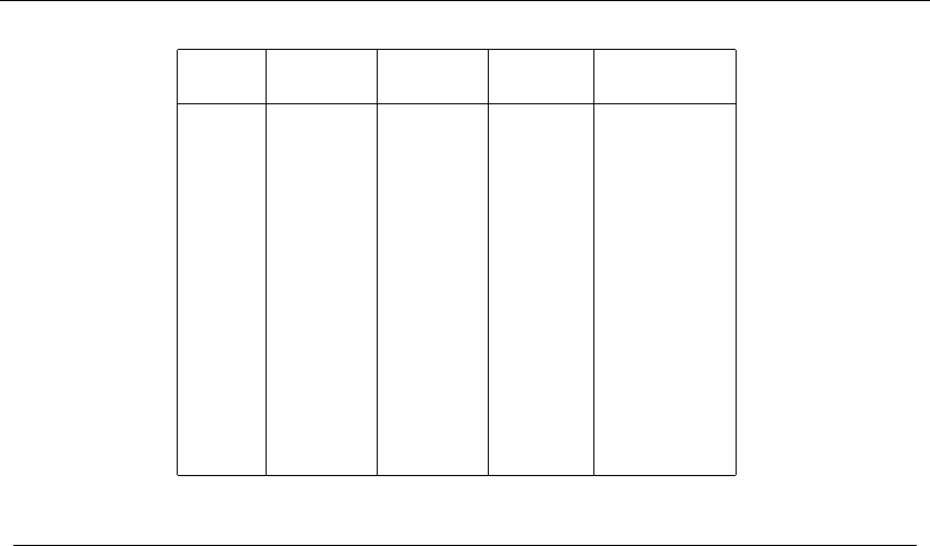
98 3. DATA STRUCTURES
String Binary Hash Suffix Compressed
length tree table tree tree
80.0 0.0 0.0 0.0
16 0.0 0.0 0.0 0.0
32 0.1 0.0 0.0 0.0
64 0.3 0.4 0.3 0.0
128 2.4 1.1 0.5 0.0
256 17.1 9.4 3.8 0.2
512 31.6 67.0 6.9 1.3
1,024 1,828.9 96.6 31.5 2.7
2,048 11,441.7 941.7 553.6 39.0
4,096 >2days 5,246.7 out of 45.4
8,192 >2days memory 642.0
16,384 1,614.0
32,768 13,657.8
65,536 39,776.9
Figure 3.13: Run times (in seconds) for the SBH simulation using various data structures
Chapter Notes
Optimizing hash table performance is surprisingly complicated for such a concep-
tually simple data structure. The importance of short runs in open addressing
has to more sophisticated schemes than sequential probing for optimal hash table
performance. For more details, see Knuth [Knu98].
Our triangle strip optimizing program, stripe, is described in [ESV96]. Hashing
techniques for plagiarism detection are discussed in [SWA03].
Surveys of algorithmic issues in DNA sequencing by hybridization include
[CK94, PL94]. Our work on interactive SBH reported in the war story is reported
in [MS95a].
3.10 Exercises
Stacks, Queues, and Lists
3-1. [3] A common problem for compilers and text editors is determining whether the
parentheses in a string are balanced and properly nested. For example, the string
((())())() contains properly nested pairs of parentheses, which the strings )()( and
()) do not. Give an algorithm that returns true if a string contains properly nested
and balanced parentheses, and false if otherwise. For full credit, identify the position
of the first offending parenthesis if the string is not properly nested and balanced.

3.10 EXERCISES 99
3-2. [3] Write a program to reverse the direction of a given singly-linked list. In other
words, after the reversal all pointers should now point backwards. Your algorithm
should take linear time.
3-3. [5] We have seen how dynamic arrays enable arrays to grow while still achieving
constant-time amortized performance. This problem concerns extending dynamic
arrays to let them both grow and shrink on demand.
(a) Consider an underflow strategy that cuts the array size in half whenever the
array falls below half full. Give an example sequence of insertions and deletions
where this strategy gives a bad amortized cost.
(b) Then, give a better underflow strategy than that suggested above, one that
achieves constant amortized cost per deletion.
Trees and Other Dictionary Structures
3-4. [3] Design a dictionary data structure in which search, insertion, and deletion can
all be processed in O(1) time in the worst case. You may assume the set elements
are integers drawn from a finite set 1,2, .., n, and initialization can take O(n)time.
3-5. [3] Find the overhead fraction (the ratio of data space over total space) for each
of the following binary tree implementations on nnodes:
(a) All nodes store data, two child pointers, and a parent pointer. The data field
requires four bytes and each pointer requires four bytes.
(b) Only leaf nodes store data; internal nodes store two child pointers. The data
field requires four bytes and each pointer requires two bytes.
3-6. [5] Describe how to modify any balanced tree data structure such that search,
insert, delete, minimum, and maximum still take O(log n) time each, but successor
and predecessor now take O(1) time each. Which operations have to be modified
to support this?
3-7. [5] Suppose you have access to a balanced dictionary data structure, which supports
each of the operations search, insert, delete, minimum, maximum, successor, and
predecessor in O(log n) time. Explain how to modify the insert and delete operations
so they still take O(log n) but now minimum and maximum take O(1) time. (Hint:
think in terms of using the abstract dictionary operations, instead of mucking about
with pointers and the like.)
3-8. [6 ] Design a data structure to support the following operations:
•insert(x,T) – Insert item xinto the set T.
•delete(k,T) – Delete the kth smallest element from T.
•member(x,T) –Returntrueiffx∈T.
All operations must take O(log n)timeonann-element set.
3-9. [8] Aconcatenate operation takes two sets S1and S2, where every key in S1
is smaller than any key in S2, and merges them together. Give an algorithm to
concatenate two binary search trees into one binary search tree. The worst-case
running time should be O(h), where his the maximal height of the two trees.

100 3. DATA STRUCTURES
Applications of Tree Structures
3-10. [5] In the bin-packing problem, we are given nmetal objects, each weighing between
zero and one kilogram. Our goal is to find the smallest number of bins that will
hold the nobjects, with each bin holding one kilogram at most.
•The best-fit heuristic for bin packing is as follows. Consider the objects in the
order in which they are given. For each object, place it into the partially filled
bin with the smallest amount of extra room after the object is inserted.. If
no such bin exists, start a new bin. Design an algorithm that implements the
best-fit heuristic (taking as input the nweights w1,w
2, ..., wnand outputting
the number of bins used) in O(nlog n)time.
•Repeat the above using the worst-fit heuristic, where we put the next object in
the partially filled bin with the largest amount of extra room after the object
is inserted.
3-11. [5] Suppose that we are given a sequence of nvalues x1,x
2, ..., xnand seek to
quickly answer repeated queries of the form: given iand j, find the smallest value
in xi,...,x
j.
(a) Design a data structure that uses O(n2) space and answers queries in O(1)
time.
(b) Design a data structure that uses O(n) space and answers queries in O(log n)
time. For partial credit, your data structure can use O(nlog n) space and have
O(log n)querytime.
3-12. [5] Suppose you are given an input set Sof nnumbers, and a black box that if
given any sequence of real numbers and an integer kinstantly and correctly answers
whether there is a subset of input sequence whose sum is exactly k. Show how to
use the black box O(n) times to find a subset of Sthat adds up to k.
3-13. [5] Let A[1..n]beanarrayofrealnumbers.Designanalgorithmtoperformany
sequence of the following operations:
•Add(i,y) – Add the value yto the ith number.
•Partial-sum(i) – Return the sum of the first inumbers, i.e. i
j=1 A[j].
There are no insertions or deletions; the only change is to the values of the numbers.
Each operation should take O(log n) steps. You may use one additional array of size
nas a work space.
3-14. [8] Extend the data structure of the previous problem to support insertions and
deletions. Each element now has both a key and a value. An element is accessed
by its key. The addition operation is applied to the values, but the elements are
accessed by its key. The Partial sum operation is different.
•Add(k,y) – Add the value yto the item with key k.
•Insert(k,y) –Insertanewitemwithkeykand value y.
•Delete(k) – Delete the item with key k.

3.10 EXERCISES 101
•Partial-sum(k) – Return the sum of all the elements currently in the set whose
keyislessthany, i.e. xj<y xi.
The worst case running time should still be O(nlog n) for any sequence of O(n)
operations.
3-15. [8] Design a data structure that allows one to search, insert, and delete an integer
Xin O(1) time (i.e. , constant time, independent of the total number of integers
stored). Assume that 1 ≤X≤nand that there are m+nunits of space available,
where mis the maximum number of integers that can be in the table at any one
time. (Hint: use two arrays A[1..n]andB[1..m].) You are not allowed to initialize
either Aor B,asthatwouldtakeO(m)orO(n) operations. This means the arrays
are full of random garbage to begin with, so you must be very careful.
Implementation Projects
3-16. [5] Implement versions of several different dictionary data structures, such as linked
lists, binary trees, balanced binary search trees, and hash tables. Conduct exper-
iments to assess the relative performance of these data structures in a simple ap-
plication that reads a large text file and reports exactly one instance of each word
that appears within it. This application can be efficiently implemented by main-
taining a dictionary of all distinct words that have appeared thus far in the text
and inserting/reporting each word that is not found. Write a brief report with your
conclusions.
3-17. [5] A Caesar shift (see Section 18.6 (page 641)) is a very simple class of ciphers for
secret messages. Unfortunately, they can be broken using statistical properties of
English. Develop a program capable of decrypting Caesar shifts of sufficiently long
texts.
Interview Problems
3-18. [3] What method would you use to look up a word in a dictionary?
3-19. [3] Imagine you have a closet full of shirts. What can you do to organize your shirts
for easy retrieval?
3-20. [4] Write a function to find the middle node of a singly-linked list.
3-21. [4] Write a function to compare whether two binary trees are identical. Identical
treeshavethesamekeyvalueateachpositionandthesamestructure.
3-22. [4] Write a program to convert a binary search tree into a linked list.
3-23. [4] Implement an algorithm to reverse a linked list. Now do it without recursion.
3-24. [5] What is the best data structure for maintaining URLs that have been visited by
a Web crawler? Give an algorithm to test whether a given URL has already been
visited, optimizing both space and time.
3-25. [4] You are given a search string and a magazine. You seek to generate all the char-
acters in search string by cutting them out from the magazine. Give an algorithm
to efficiently determine whether the magazine contains all the letters in the search
string.

102 3. DATA STRUCTURES
3-26. [4] Reverse the words in a sentence—i.e., “My name is Chris” becomes “Chris is
name My.” Optimize for time and space.
3-27. [5] Determine whether a linked list contains a loop as quickly as possible without
using any extra storage. Also, identify the location of the loop.
3-28. [5] You have an unordered array Xof nintegers. Find the array Mcontaining
nelements where Miis the product of all integers in Xexcept for Xi. You may
not use division. You can use extra memory. (Hint: There are solutions faster than
O(n2).)
3-29. [6] Give an algorithm for finding an ordered word pair (e.g., “New York”) occurring
with the greatest frequency in a given webpage. Which data structures would you
use? Optimize both time and space.
Programming Challenges
These programming challenge problems with robot judging are available at
http://www.programming-challenges.com or http://online-judge.uva.es.
3-1. “Jolly Jumpers” – Programming Challenges 110201, UVA Judge 10038.
3-2. “Crypt Kicker” – Programming Challenges 110204, UVA Judge 843.
3-3. “Where’s Waldorf?” – Programming Challenges 110302, UVA Judge 10010.
3-4. “Crypt Kicker II” – Programming Challenges 110304, UVA Judge 850.

4
Sorting and Searching
Typical computer science students study the basic sorting algorithms at least three
times before they graduate: first in introductory programming, then in data struc-
tures, and finally in their algorithms course. Why is sorting worth so much atten-
tion? There are several reasons:
•Sorting is the basic building block that many other algorithms are built
around. By understanding sorting, we obtain an amazing amount of power
to solve other problems.
•Most of the interesting ideas used in the design of algorithms appear in the
context of sorting, such as divide-and-conquer, data structures, and random-
ized algorithms.
•Computers have historically spent more time sorting than doing anything
else. A quarter of all mainframe cycles were spent sorting data [Knu98]. Sort-
ing remains the most ubiquitous combinatorial algorithm problem in practice.
•Sorting is the most thoroughly studied problem in computer science. Liter-
ally dozens of different algorithms are known, most of which possess some
particular advantage over all other algorithms in certain situations.
In this chapter, we will discuss sorting, stressing how sorting can be applied to
solving other problems. In this sense, sorting behaves more like a data structure
than a problem in its own right. We then give detailed presentations of several
fundamental algorithms: heapsort, mergesort, quicksort, and distribution sort as
examples of important algorithm design paradigms. Sorting is also represented by
Section 14.1 (page 436) in the problem catalog.
S.S. Skiena, The Algorithm Design Manual, 2nd ed., DOI: 10.1007/978-1-84800-070-4 4,
c
Springer-Verlag London Limited 2008

104 4. SORTING AND SEARCHING
4.1 Applications of Sorting
We will review several sorting algorithms and their complexities over the course of
this chapter. But the punch-line is this: clever sorting algorithms exist that run in
O(nlog n). This is a big improvement over naive O(n2) sorting algorithms for large
values of n. Consider the following table:
nn
2/4nlg n
10 25 33
100 2,500 664
1,000 250,000 9,965
10,000 25,000,000 132,877
100,000 2,500,000,000 1,660,960
You might still get away with using a quadratic-time algorithm even if n=
10,000, but quadratic-time sorting is clearly ridiculous once n≥100,000.
Many important problems can be reduced to sorting, so we can use our clever
O(nlog n) algorithms to do work that might otherwise seem to require a quadratic
algorithm. An important algorithm design technique is to use sorting as a basic
building block, because many other problems become easy once a set of items is
sorted.
Consider the following applications:
•Searching – Binary search tests whether an item is in a dictionary in O(log n)
time, provided the keys are all sorted. Search preprocessing is perhaps the
single most important application of sorting.
•Closest pair –Givenasetofnnumbers, how do you find the pair of numbers
that have the smallest difference between them? Once the numbers are sorted,
the closest pair of numbers must lie next to each other somewhere in sorted
order. Thus, a linear-time scan through them completes the job, for a total
of O(nlog n) time including the sorting.
•Element uniqueness – Are there any duplicates in a given set of nitems?
This is a special case of the closest-pair problem above, where we ask if there
is a pair separated by a gap of zero. The most efficient algorithm sorts the
numbers and then does a linear scan though checking all adjacent pairs.
•Frequency distribution – Given a set of nitems, which element occurs the
largest number of times in the set? If the items are sorted, we can sweep
from left to right and count them, since all identical items will be lumped
together during sorting.
To find out how often an arbitrary element koccurs, look up kusing binary
search in a sorted array of keys. By walking to the left of this point until the
first the element is not kand then doing the same to the right, we can find
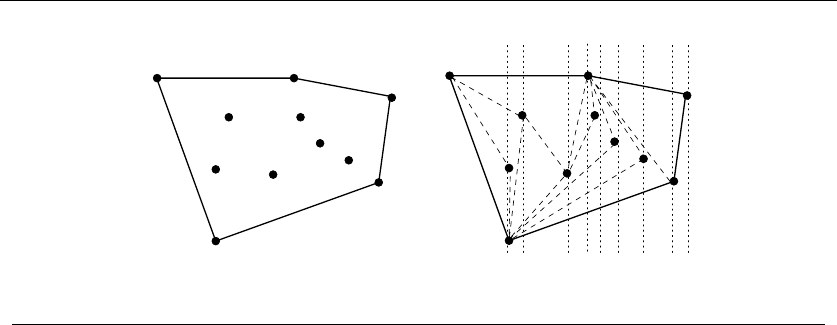
4.1 APPLICATIONS OF SORTING 105
Figure 4.1: The convex hull of a set of points (l), constructed by left-to-right insertion.
this count in O(log n+c) time, where cis the number of occurrences of k.
Even better, the number of instances of kcan be found in O(log n) time by
using binary search to look for the positions of both k−and k+(where
is arbitrarily small) and then taking the difference of these positions.
•Selection – What is the kth largest item in an array? If the keys are placed
in sorted order, the kth largest can be found in constant time by simply
looking at the kth position of the array. In particular, the median element
(see Section 14.3 (page 445)) appears in the (n/2)nd position in sorted order.
•Convex hulls – What is the polygon of smallest area that contains a given
set of npoints in two dimensions? The convex hull is like a rubber band
stretched over the points in the plane and then released. It compresses to
just cover the points, as shown in Figure 4.1(l). The convex hull gives a nice
representation of the shape of the points and is an important building block
for more sophisticated geometric algorithms, as discussed in the catalog in
Section 17.2 (page 568).
But how can we use sorting to construct the convex hull? Once you have the
points sorted by x-coordinate, the points can be inserted from left to right
into the hull. Since the right-most point is always on the boundary, we know
that it will appear in the hull. Adding this new right-most point may cause
others to be deleted, but we can quickly identify these points because they lie
inside the polygon formed by adding the new point. See the example in Figure
4.1(r). These points will be neighbors of the previous point we inserted, so
they will be easy to find and delete. The total time is linear after the sorting
has been done.
While a few of these problems (namely median and selection) can be solved in
linear time using more sophisticated algorithms, sorting provides quick and easy
solutions to all of these problems. It is a rare application where the running time

106 4. SORTING AND SEARCHING
of sorting proves to be the bottleneck, especially a bottleneck that could have
otherwise been removed using more clever algorithmics. Never be afraid to spend
time sorting, provided you use an efficient sorting routine.
Take-Home Lesson: Sorting lies at the heart of many algorithms. Sorting the
data is one of the first things any algorithm designer should try in the quest
for efficiency.
Stop and Think: Finding the Intersection
Problem: Give an efficient algorithm to determine whether two sets (of size mand
n, respectively) are disjoint. Analyze the worst-case complexity in terms of mand
n, considering the case where mis substantially smaller than n.
Solution: At least three algorithms come to mind, all of which are variants of
sorting and searching:
•First sort the big set – The big set can be sorted in O(nlog n) time. We can
now do a binary search with each of the melements in the second, looking
to see if it exists in the big set. The total time will be O((n+m) log n).
•First sort the small set – The small set can be sorted in O(mlog m) time. We
can now do a binary search with each of the nelements in the big set, looking
to see if it exists in the small one. The total time will be O((n+m) log m).
•Sort both sets – Observe that once the two sets are sorted, we no longer
have to do binary search to detect a common element. We can compare the
smallest elements of the two sorted sets, and discard the smaller one if they
are not identical. By repeating this idea recursively on the now smaller sets,
we can test for duplication in linear time after sorting. The total cost is
O(nlog n+mlog m+n+m).
So, which of these is the fastest method? Clearly small-set sorting trumps big-
set sorting, since log m<log nwhen m<n. Similarly, (n+m) log mmust be
asymptotically less than nlog n, since n+m<2nwhen m<n. Thus, sorting the
small set is the best of these options. Note that this is linear when mis constant
in size.
Note that expected linear time can be achieved by hashing. Build a hash table
containing the elements of both sets, and verify that collisions in the same bucket
are in fact identical elements. In practice, this may be the best solution.

4.2 PRAGMATICS OF SORTING 107
4.2 Pragmatics of Sorting
We have seen many algorithmic applications of sorting, and we will see several
efficient sorting algorithms. One issue stands between them: in what order do we
want our items sorted?
The answers to this basic question are application-specific. Consider the follow-
ing considerations:
•Increasing or decreasing order? – A set of keys Sare sorted in ascending
order when Si≤Si+1 for all 1 ≤i<n. They are in descending order when
Si≥Si+1 for all 1 ≤i<n. Different applications call for different orders.
•Sorting just the key or an entire record? – Sorting a data set involves main-
taining the integrity of complex data records. A mailing list of names, ad-
dresses, and phone numbers may be sorted by names as the key field, but it
had better retain the linkage between names and addresses. Thus, we need
to specify which field is the key field in any complex record, and understand
the full extent of each record.
•What should we do with equal keys? Elements with equal key values will all
bunch together in any total order, but sometimes the relative order among
these keys matters. Suppose an encyclopedia contains both Michael Jordan
(the basketball player) and Michael Jordan (the statistician). Which entry
should appear first? You may need to resort to secondary keys, such as article
size, to resolve ties in a meaningful way.
Sometimes it is required to leave the items in the same relative order as in
the original permutation. Sorting algorithms that automatically enforce this
requirement are called stable. Unfortunately few fast algorithms are stable.
Stability can be achieved for any sorting algorithm by adding the initial
position as a secondary key.
Of course we could make no decision about equal key order and let the ties fall
where they may. But beware, certain efficient sort algorithms (such as quick-
sort) can run into quadratic performance trouble unless explicitly engineered
to deal with large numbers of ties.
•What about non-numerical data? – Alphabetizing is the sorting of text strings.
Libraries have very complete and complicated rules concerning the relative
collating sequence of characters and punctuation. Is Skiena the same key as
skiena?IsBrown-Williams before or after Brown America, and before or after
Brown, John?
The right way to specify such matters to your sorting algorithm is with an
application-specific pairwise-element comparison function. Such a comparison func-
tion takes pointers to record items aand band returns “<”ifa<b,“>”ifa>b,
or “=” if a=b.

108 4. SORTING AND SEARCHING
By abstracting the pairwise ordering decision to such a comparison function, we
can implement sorting algorithms independently of such criteria. We simply pass
the comparison function in as an argument to the sort procedure. Any reasonable
programming language has a built-in sort routine as a library function. You are
almost always better off using this than writing your own routine. For example,
the standard library for C contains the qsort function for sorting:
#include <stdlib.h>
void qsort(void *base, size_t nel, size_t width,
int (*compare) (const void *, const void *));
The key to using qsort is realizing what its arguments do. It sorts the first nel
elements of an array (pointed to by base), where each element is width-bytes long.
Thus we can sort arrays of 1-byte characters, 4-byte integers, or 100-byte records,
all by changing the value of width.
The ultimate desired order is determined by the compare function. It takes as
arguments pointers to two width-byte elements, and returns a negative number if
the first belongs before the second in sorted order, a positive number if the second
belongs before the first, or zero if they are the same. Here is a comparison function
to sort integers in increasing order:
int intcompare(int *i, int *j)
{
if (*i > *j) return (1);
if (*i < *j) return (-1);
return (0);
}
This comparison function can be used to sort an array a, of which the first n
elements are occupied, as follows:
qsort(a, n, sizeof(int), intcompare);
qsort suggests that quicksort is the algorithm implemented in this library func-
tion, although this is usually irrelevant to the user.
4.3 Heapsort: Fast Sorting via Data Structures
Sorting is a natural laboratory for studying algorithm design paradigms, since many
useful techniques lead to interesting sorting algorithms. The next several sections
will introduce algorithmic design techniques motivated by particular sorting algo-
rithms.

4.3 HEAPSORT: FAST SORTING VIA DATA STRUCTURES 109
The alert reader should ask why we review the standard sorting when you
are better off not implementing them and using built-in library functions instead.
The answer is that the design techniques are very important for other algorithmic
problems you are likely to encounter.
We start with data structure design, because one of the most dramatic algo-
rithmic improvements via appropriate data structures occurs in sorting. Selection
sort is a simple-to-code algorithm that repeatedly extracts the smallest remaining
element from the unsorted part of the set:
SelectionSort(A)
For i=1tondo
Sort[i] = Find-Minimum from A
Delete-Minimum from A
Return(Sort)
A C language implementation of selection sort appeared back in Section 2.5.1
(page 41). There we partitioned the input array into sorted and unsorted regions. To
find the smallest item, we performed a linear sweep through the unsorted portion
of the array. The smallest item is then swapped with the ith item in the array
before moving on to the next iteration. Selection sort performs niterations, where
the average iteration takes n/2 steps, for a total of O(n2) time.
But what if we improve the data structure? It takes O(1) time to remove a
particular item from an unsorted array once it has been located, but O(n) time
to find the smallest item. These are exactly the operations supported by priority
queues. So what happens if we replace the data structure with a better priority
queue implementation, either a heap or a balanced binary tree? Operations within
the loop now take O(log n) time each, instead of O(n). Using such a priority queue
implementation speeds up selection sort from O(n2)toO(nlog n).
The name typically given to this algorithm, heapsort, obscures the relationship
between them, but heapsort is nothing but an implementation of selection sort
using the right data structure.
4.3.1 Heaps
Heaps are a simple and elegant data structure for efficiently supporting the priority
queue operations insert and extract-min. They work by maintaining a partial order
on the set of elements which is weaker than the sorted order (so it can be efficient
to maintain) yet stronger than random order (so the minimum element can be
quickly identified).
Power in any hierarchically-structured organization is reflected by a tree, where
each node in the tree represents a person, and edge (x, y) implies that xdirectly
supervises (or dominates) y. The fellow at the root sits at the “top of the heap.”
In this spirit, a heap-labeled tree is defined to be a binary tree such that the
key labeling of each node dominates the key labeling of each of its children. In a
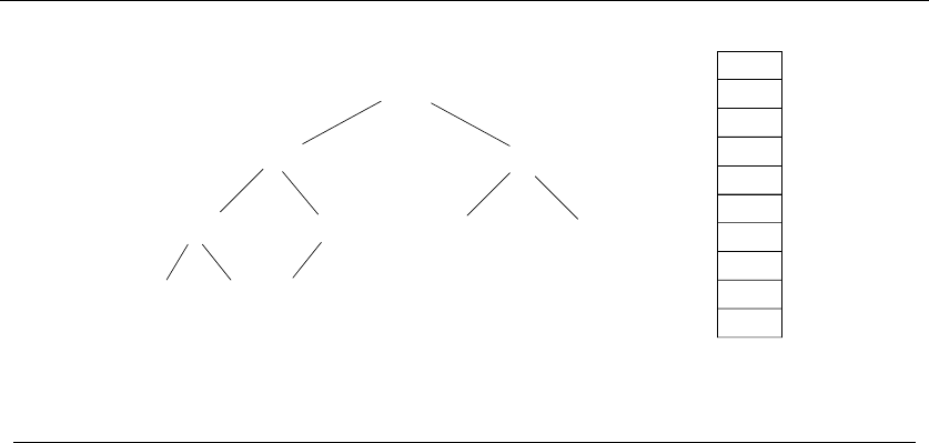
110 4. SORTING AND SEARCHING
4
6
7
1
2
5
10
3
8
9
1941
2001
1918
1963
1804
1945
1865
1492
1783
1776
1783
2001 1941
1865
1918
1492
1804
1776
1945 1963
Figure 4.2: A heap-labeled tree of important years from American history (l), with the corre-
sponding implicit heap representation (r)
min-heap, a node dominates its children by containing a smaller key than they do,
while in a max-heap parent nodes dominate by being bigger. Figure 4.2(l) presents
a min-heap ordered tree of red-letter years in American history (kudos to you if
you can recall what happened each year).
The most natural implementation of this binary tree would store each key in
a node with pointers to its two children. As with binary search trees, the memory
used by the pointers can easily outweigh the size of keys, which is the data we are
really interested in.
The heap is a slick data structure that enables us to represent binary trees
without using any pointers. We will store data as an array of keys, and use the
position of the keys to implicitly satisfy the role of the pointers.
We will store the root of the tree in the first position of the array, and its left
and right children in the second and third positions, respectively. In general, we
will store the 2lkeys of the lth level of a complete binary tree from left-to-right in
positions 2l−1to 2l−1, as shown in Figure 4.2(r). We assume that the array starts
with index 1 to simplify matters.
typedef struct {
item_type q[PQ_SIZE+1]; /* body of queue */
int n; /* number of queue elements */
} priority_queue;
What is especially nice about this representation is that the positions of the
parent and children of the key at position kare readily determined. The left child
of ksits in position 2kand the right child in 2k+ 1, while the parent of kholds
court in position n/2. Thus we can move around the tree without any pointers.

4.3 HEAPSORT: FAST SORTING VIA DATA STRUCTURES 111
pq_parent(int n)
{
if (n == 1) return(-1);
else return((int) n/2); /* implicitly take floor(n/2) */
}
pq_young_child(int n)
{
return(2 * n);
}
So, we can store any binary tree in an array without pointers. What is the
catch? Suppose our height htree was sparse, meaning that the number of nodes
n<2h. All missing internal nodes still take up space in our structure, since we must
represent a full binary tree to maintain the positional mapping between parents
and children.
Space efficiency thus demands that we not allow holes in our tree—i.e., that each
level be packed as much as it can be. If so, only the last level may be incomplete.
By packing the elements of the last level as far to the left as possible, we can
represent an n-key tree using exactly nelements of the array. If we did not enforce
these structural constraints, we might need an array of size 2nto store the same
elements. Since all but the last level is always filled, the height hof an nelement
heap is logarithmic because:
h
i=0
2i=2
h+1 −1≥n
so h=lg n.
This implicit representation of binary trees saves memory, but is less flexible
than using pointers. We cannot store arbitrary tree topologies without wasting
large amounts of space. We cannot move subtrees around by just changing a single
pointer, only by explicitly moving each of the elements in the subtree. This loss of
flexibility explains why we cannot use this idea to represent binary search trees,
but it works just fine for heaps.
Stop and Think: Who’s where in the heap?
Problem: How can we efficiently search for a particular key in a heap?
Solution: We can’t. Binary search does not work because a heap is not a binary
search tree. We know almost nothing about the relative order of the n/2 leaf ele-
ments in a heap—certainly nothing that lets us avoid doing linear search through
them.

112 4. SORTING AND SEARCHING
4.3.2 Constructing Heaps
Heaps can be constructed incrementally, by inserting each new element into the
left-most open spot in the array, namely the (n+ 1)st position of a previously
n-element heap. This ensures the desired balanced shape of the heap-labeled tree,
but does not necessarily maintain the dominance ordering of the keys. The new
key might be less than its parent in a min-heap, or greater than its parent in a
max-heap.
The solution is to swap any such dissatisfied element with its parent. The old
parent is now happy, because it is properly dominated. The other child of the old
parent is still happy, because it is now dominated by an element even more extreme
than its previous parent. The new element is now happier, but may still dominate
its new parent. We now recur at a higher level, bubbling up the new key to its
proper position in the hierarchy. Since we replace the root of a subtree by a larger
one at each step, we preserve the heap order elsewhere.
pq_insert(priority_queue *q, item_type x)
{
if (q->n >= PQ_SIZE)
printf("Warning: priority queue overflow insert x=%d\n",x);
else {
q->n = (q->n) + 1;
q->q[ q->n ] = x;
bubble_up(q, q->n);
}
}
bubble_up(priority_queue *q, int p)
{
if (pq_parent(p) == -1) return; /* at root of heap, no parent */
if (q->q[pq_parent(p)] > q->q[p]) {
pq_swap(q,p,pq_parent(p));
bubble_up(q, pq_parent(p));
}
}
This swap process takes constant time at each level. Since the height of an n-
element heap is lg n, each insertion takes at most O(log n) time. Thus an initial
heap of nelements can be constructed in O(nlog n) time through nsuch insertions:
pq_init(priority_queue *q)
{
q->n = 0;
}

4.3 HEAPSORT: FAST SORTING VIA DATA STRUCTURES 113
make_heap(priority_queue *q, item_type s[], int n)
{
int i; /* counter */
pq_init(q);
for (i=0; i<n; i++)
pq_insert(q, s[i]);
}
4.3.3 Extracting the Minimum
The remaining priority queue operations are identifying and deleting the dominant
element. Identification is easy, since the top of the heap sits in the first position of
the array.
Removing the top element leaves a hole in the array. This can be filled by
moving the element from the right-most leaf (sitting in the nth position of the
array) into the first position.
The shape of the tree has been restored but (as after insertion) the labeling of
the root may no longer satisfy the heap property. Indeed, this new root may be
dominated by both of its children. The root of this min-heap should be the smallest
of three elements, namely the current root and its two children. If the current root
is dominant, the heap order has been restored. If not, the dominant child should
be swapped with the root and the problem pushed down to the next level.
This dissatisfied element bubbles down the heap until it dominates all its chil-
dren, perhaps by becoming a leaf node and ceasing to have any. This percolate-down
operation is also called heapify, because it merges two heaps (the subtrees below
the original root) with a new key.
item_type extract_min(priority_queue *q)
{
int min = -1; /* minimum value */
if (q->n <= 0) printf("Warning: empty priority queue.\n");
else {
min = q->q[1];
q->q[1] = q->q[ q->n ];
q->n = q->n - 1;
bubble_down(q,1);
}
return(min);
}

114 4. SORTING AND SEARCHING
bubble_down(priority_queue *q, int p)
{
int c; /* child index */
int i; /* counter */
int min_index; /* index of lightest child */
c = pq_young_child(p);
min_index = p;
for (i=0; i<=1; i++)
if ((c+i) <= q->n) {
if (q->q[min_index] > q->q[c+i]) min_index = c+i;
}
if (min_index != p) {
pq_swap(q,p,min_index);
bubble_down(q, min_index);
}
}
We will reach a leaf after lg nbubble down steps, each constant time. Thus
root deletion is completed in O(log n) time.
Exchanging the maximum element with the last element and calling heapify
repeatedly gives an O(nlog n) sorting algorithm, named Heapsort.
heapsort(item_type s[], int n)
{
int i; /* counters */
priority_queue q; /* heap for heapsort */
make_heap(&q,s,n);
for (i=0; i<n; i++)
s[i] = extract_min(&q);
}
Heapsort is a great sorting algorithm. It is simple to program; indeed, the
complete implementation has been presented above. It runs in worst-case O(nlog n)
time, which is the best that can be expected from any sorting algorithm. It is an in-
place sort, meaning it uses no extra memory over the array containing the elements
to be sorted. Although other algorithms prove slightly faster in practice, you won’t
go wrong using heapsort for sorting data that sits in the computer’s main memory.

4.3 HEAPSORT: FAST SORTING VIA DATA STRUCTURES 115
Priority queues are very useful data structures. Recall they were the hero of
the war story described in Section 3.6 (page 85). A complete set of priority queue
implementations is presented in catalog Section 12.2 (page 373).
4.3.4 Faster Heap Construction (*)
As we have seen, a heap can be constructed on nelements by incremental insertion
in O(nlog n) time. Surprisingly, heaps can be constructed even faster by using our
bubble down procedure and some clever analysis.
Suppose we pack the nkeys destined for our heap into the first nelements of
our priority-queue array. The shape of our heap will be right, but the dominance
order will be all messed up. How can we restore it?
Consider the array in reverse order, starting from the last (nth) position. It
represents a leaf of the tree and so dominates its nonexistent children. The same
is the case for the last n/2 positions in the array, because all are leaves. If we
continue to walk backwards through the array we will finally encounter an internal
node with children. This element may not dominate its children, but its children
represent well-formed (if small) heaps.
This is exactly the situation the bubble down procedure was designed to handle,
restoring the heap order of arbitrary root element sitting on top of two sub-heaps.
Thus we can create a heap by performing n/2 non-trivial calls to the bubble down
procedure:
make_heap(priority_queue *q, item_type s[], int n)
{
int i; /* counter */
q->n = n;
for (i=0; i<n; i++) q->q[i+1] = s[i];
for (i=q->n; i>=1; i--) bubble_down(q,i);
}
Multiplying the number of calls to bubble down (n) times an upper bound on
the cost of each operation (O(log n)) gives us a running time analysis of O(nlog n).
This would make it no faster than the incremental insertion algorithm described
above.
But note that it is indeed an upper bound, because only the last insertion will
actually take lg nsteps. Recall that bubble down takes time proportional to the
height of the heaps it is merging. Most of these heaps are extremely small. In a full
binary tree on nnodes, there are n/2 nodes that are leaves (i.e. , height 0), n/4

116 4. SORTING AND SEARCHING
nodes that are height 1, n/8 nodes that are height 2, and so on. In general, there
are at most n/2h+1nodes of height h, so the cost of building a heap is:
lg n
h=0 n/2h+1h≤nlg n
h=0
h/2h≤2n
Since this sum is not quite a geometric series, we can’t apply the usual identity
to get the sum, but rest assured that the puny contribution of the numerator (h)
is crushed by the denominator (2h). The series quickly converges to linear.
Does it matter that we can construct heaps in linear time instead of O(nlog n)?
Usually not. The construction time did not dominate the complexity of heapsort,
so improving the construction time does not improve its worst-case performance.
Still, it is an impressive display of the power of careful analysis, and the free lunch
that geometric series convergence can sometimes provide.
Stop and Think: Where in the Heap?
Problem: Given an array-based heap on nelements and a real number x, efficiently
determine whether the kth smallest element in the heap is greater than or equal
to x. Your algorithm should be O(k) in the worst-case, independent of the size of
the heap. Hint: you do not have to find the kth smallest element; you need only
determine its relationship to x.
Solution: There are at least two different ideas that lead to correct but inefficient
algorithms for this problem:
1. Call extract-min ktimes, and test whether all of these are less than x. This
explicitly sorts the first kelements and so gives us more information than
the desired answer, but it takes O(klog n) time to do so.
2. The kth smallest element cannot be deeper than the kth level of the heap,
since the path from it to the root must go through elements of decreasing
value. Thus we can look at all the elements on the first klevels of the heap,
and count how many of them are less than x, stopping when we either find k
of them or run out of elements. This is correct, but takes O(min(n, 2k)) time,
since the top kelements have 2kelements.
An O(k) solution can look at only kelements smaller than x, plus at most O(k)
elements greater than x. Consider the following recursive procedure, called at the
root with i= 1 with count =k:

4.3 HEAPSORT: FAST SORTING VIA DATA STRUCTURES 117
int heap_compare(priority_queue *q, int i, int count, int x)
{
if ((count <= 0) || (i > q->n) return(count);
if (q->q[i] < x) {
count = heap_compare(q, pq_young_child(i), count-1, x);
count = heap_compare(q, pq_young_child(i)+1, count, x);
}
return(count);
}
If the root of the min-heap is ≥x, then no elements in the heap can be less than
x, as by definition the root must be the smallest element. This procedure searches
the children of all nodes of weight smaller than xuntil either (a) we have found
kof them, when it returns 0, or (b) they are exhausted, when it returns a value
greater than zero. Thus it will find enough small elements if they exist.
But how long does it take? The only nodes whose children we look at are those
<x, and at most kof these in total. Each have at most visited two children, so we
visitatmost3knodes, for a total time of O(k).
4.3.5 Sorting by Incremental Insertion
Now consider a different approach to sorting via efficient data structures. Select an
arbitrary element from the unsorted set, and put it in the proper position in the
sorted set.
InsertionSort(A)
A[0] = −∞
for i=2tondo
j=i
while (A[j]<A[j−1]) do
swap(A[j],A[j−1])
j=j−1
A C language implementation of insertion sort appeared in Section 2.5.2 (page
43). Although insertion sort takes O(n2) in the worst case, it performs considerably
better if the data is almost sorted, since few iterations of the inner loop suffice to
sift it into the proper position.
Insertion sort is perhaps the simplest example of the incremental insertion tech-
nique, where we build up a complicated structure on nitems by first building it on
n−1 items and then making the necessary changes to add the last item. Incremental
insertion proves a particularly useful technique in geometric algorithms.

118 4. SORTING AND SEARCHING
Note that faster sorting algorithms based on incremental insertion follow from
more efficient data structures. Insertion into a balanced search tree takes O(log n)
per operation, or a total of O(nlog n) to construct the tree. An in-order traversal
reads through the elements in sorted order to complete the job in linear time.
4.4 War Story: Give me a Ticket on an Airplane
I came into this particular job seeking justice. I’d been retained by an air travel
company to help design an algorithm to find the cheapest available airfare from
city xto city y. Like most of you, I suspect, I’d been baffled at the crazy price
fluctuations of ticket prices under modern “yield management.” The price of flights
seems to soar far more efficiently than the planes themselves. The problem, it
seemed to me, was that airlines never wanted to show the true cheapest price. By
doing my job right, I could make damned sure they would show it to me next time.
“Look,” I said at the start of the first meeting. “This can’t be so hard. Construct
a graph with vertices corresponding to airports, and add an edge between each
airport pair (u, v) which shows a direct flight from uto v. Set the weight of this
edge equal to the cost of the cheapest available ticket from uto v. Now the cheapest
fair from xto yis given by the shortest x-ypath in this graph. This path/fare can
be found using Dijkstra’s shortest path algorithm. Problem solved!” I announced,
waiving my hand with a flourish.
The assembled cast of the meeting nodded thoughtfully, then burst out laugh-
ing. It was I who needed to learn something about the overwhelming complexity
of air travel pricing. There are literally millions of different fares available at any
time, with prices changing several times daily. Restrictions on the availability of a
particular fare in a particular context is enforced by a complicated set of pricing
rules. These rules are an industry-wide kludge—a complicated structure with little
in the way of consistent logical principles, which is exactly what we would need to
search efficiently for the minimum fare. My favorite rule exceptions applied only to
the country of Malawi. With a population of only 12 million and per-capita income
of $596 (179th in the world), they prove to be an unexpected powerhouse shaping
world aviation price policy. Accurately pricing any air itinerary requires at least
implicit checks to ensure the trip doesn’t take us through Malawi.
Part of the real problem is that there can easily be 100 different fares for the first
flight leg, say from Los Angeles (LAX) to Chicago (ORD), and a similar number for
each subsequent leg, say from Chicago to New York (JFK). The cheapest possible
LAX-ORD fare (maybe an AARP children’s price) might not be combinable with
the cheapest ORD-JFK fare (perhaps a pre-Ramadan special that can only be used
with subsequent connections to Mecca).
After being properly chastised for oversimplifying the problem, I got down to
work. I started by reducing the problem to the simplest interesting case. “So, you

4.4 WAR STORY: GIVE ME A TICKET ON AN AIRPLANE 119
X+Y
$150 (1,1)
$160 (2,1)
$235 (2,3)
$255 (3,3)
$225 (1,3)
$205 (2,3)
$185 (2,2)
$180 (3,1)
$175 (1,2)
$100
$110
$130
X
$50
$75
$125
Y
Figure 4.3: Sorting the pairwise sums of lists Xand Y.
need to find the cheapest two-hop fare that passes your rule tests. Is there a way
to decide in advance which pairs will pass without explicitly testing them?”
“No, there is no way to tell,” they assured me. “We can only consult a
black box routine to decide whether a particular price is available for the given
itinerary/travelers.”
“So our goal is to call this black box on the fewest number of combinations.
This means evaluating all possible fare combinations in order from cheapest to
most expensive, and stopping as soon as we encounter the first legal combination.”
“Right.”
“Why not construct the m×npossible price pairs, sort them in terms of cost,
and evaluate them in sorted order? Clearly this can be done in O(nm log(nm))
time.”1
“That is basically what we do now, but it is quite expensive to construct the
full set of m×npairs, since the first one might be all we need.”
I caught a whiff of an interesting problem. “So what you really want is an
efficient data structure to repeatedly return the next most expensive pair without
constructing all the pairs in advance.”
This was indeed an interesting problem. Finding the largest element in a set
under insertion and deletion is exactly what priority queues are good for. The catch
here is that we could not seed the priority queue with all values in advance. We
had to insert new pairs into the queue after each evaluation.
I constructed some examples, like the one in Figure 4.3. We could represent
each fare by the list indexes of its two components. The cheapest single fare will
certainly be constructed by adding up the cheapest component from both lists,
1The question of whether all such sums can be sorted faster than nm arbitrary integers is a notorious open
problem in algorithm theory. See [Fre76, Lam92] for more on X+Ysorting, as the problem is known.

120 4. SORTING AND SEARCHING
described (1,1). The second cheapest fare would be made from the head of one
list and the second element of another, and hence would be either (1,2) or (2,1).
Then it gets more complicated. The third cheapest could either be the unused pair
above or (1,3) or (3,1). Indeed it would have been (3,1) in the example above if
the third fare of Xhad been $120.
“Tell me,” I asked. “Do we have time to sort the two respective lists of fares in
increasing order?”
“Don’t have to.” the leader replied. “They come out in sorted order from the
database.”
Good news. That meant there was a natural order to the pair values. We never
need to evaluate the pairs (i+1,j)or(i, j +1)before(i, j), because they clearly
define more expensive fares.
“Got it!,” I said. “We will keep track of index pairs in a priority queue, with the
sum of the fare costs as the key for the pair. Initially we put only pair (1,1) on the
queue. If it proves it is not feasible, we put its two successors on—namely (1,2) and
(2,1). In general, we enqueue pairs (i+1,j) and (i, j +1) after evaluating/rejecting
pair (i, j). We will get through all the pairs in the right order if we do so.”
The gang caught on quickly. “Sure. But what about duplicates? We will con-
struct pair (x, y) two different ways, both when expanding (x−1,y) and (x, y −1).”
“You are right. We need an extra data structure to guard against duplicates.
The simplest might be a hash table to tell us whether a given pair exists in the
priority queue before we insert a duplicate. In fact, we will never have more than n
active pairs in our data structure, since there can only be one pair for each distinct
value of the first coordinate.”
And so it went. Our approach naturally generalizes to itineraries with more
than two legs, (a complexity which grows with the number of legs). The best-
first evaluation inherent in our priority queue enabled the system to stop as soon
as it found the provably cheapest fare. This proved to be fast enough to provide
interactive response to the user. That said, I haven’t noticed my travel tickets
getting any cheaper.
4.5 Mergesort: Sorting by Divide-and-Conquer
Recursive algorithms reduce large problems into smaller ones. A recursive approach
to sorting involves partitioning the elements into two groups, sorting each of the
smaller problems recursively, and then interleaving the two sorted lists to totally
order the elements. This algorithm is called mergesort, recognizing the importance
of the interleaving operation:
Mergesort(A[1,n])
Merge( MergeSort(A[1,n/2]), MergeSort(A[n/2+1,n]) )
The basis case of the recursion occurs when the subarray to be sorted consists
of a single element, so no rearrangement is possible. A trace of the execution of

4.5 MERGESORT: SORTING BY DIVIDE-AND-CONQUER 121
M E R G E S O R T
M E R G E S O R T
M E R G E S O R T
M E
ME
E M
TROSEG
E M R
R
E E
G
M
O
R R
S
T
O R S TE E G M R
R TO SE G
Figure 4.4: Animation of mergesort in action
mergesort is given in Figure 4.4. Picture the action as it happens during an in-
order traversal of the top tree, with the array-state transformations reported in
the bottom, reflected tree.
The efficiency of mergesort depends upon how efficiently we combine the two
sorted halves into a single sorted list. We could concatenate them into one list and
call heapsort or some other sorting algorithm to do it, but that would just destroy
all the work spent sorting our component lists.
Instead we can merge the two lists together. Observe that the smallest overall
item in two lists sorted in increasing order (as above) must sit at the top of one
of the two lists. This smallest element can be removed, leaving two sorted lists
behind—one slightly shorter than before. The second smallest item overall must
be atop one of these lists. Repeating this operation until both lists are empty
merges two sorted lists (with a total of nelements between them) into one, using
at most n−1 comparisons or O(n) total work.
What is the total running time of mergesort? It helps to think about how much
work is done at each level of the execution tree. If we assume for simplicity that n
is a power of two, the kth level consists of all the 2kcalls to mergesort processing
subranges of n/2kelements.
The work done on the (k= 0)th level involves merging two sorted lists, each of
size n/2, for a total of at most n−1 comparisons. The work done on the (k= 1)th
level involves merging two pairs of sorted lists, each of size n/4, for a total of at
most n−2 comparisons. In general, the work done on the kth level involves merging
2kpairs sorted list, each of size n/2k+1, for a total of at most n−2kcomparisons.
Linear work is done merging all the elements on each level.Eachofthenelements

122 4. SORTING AND SEARCHING
appears in exactly one subproblem on each level. The most expensive case (in terms
of comparsions) is actually the top level.
The number of elements in a subproblem gets halved at each level. Thus the
number of times we can halve nuntil we get to 1 is lg2n. Because the recursion
goes lg nlevels deep, and a linear amount of work is done per level, mergesort takes
O(nlog n) time in the worst case.
Mergesort is a great algorithm for sorting linked lists, because it does not rely on
random access to elements as does heapsort or quicksort. Its primary disadvantage
is the need for an auxilliary buffer when sorting arrays. It is easy to merge two
sorted linked lists without using any extra space, by just rearranging the pointers.
However, to merge two sorted arrays (or portions of an array), we need use a third
array to store the result of the merge to avoid stepping on the component arrays.
Consider merging {4,5,6}with {1,2,3}, packed from left to right in a single array.
Without a buffer, we would overwrite the elements of the top half during merging
and lose them.
Mergesort is a classic divide-and-conquer algorithm. We are ahead of the game
whenever we can break one large problem into two smaller problems, because the
smaller problems are easier to solve. The trick is taking advantage of the two
partial solutions to construct a solution of the full problem, as we did with the
merge operation.
Implementation
The divide-and-conquer mergesort routine follows naturally from the pseudocode:
mergesort(item_type s[], int low, int high)
{
int i; /* counter */
int middle; /* index of middle element */
if (low < high) {
middle = (low+high)/2;
mergesort(s,low,middle);
mergesort(s,middle+1,high);
merge(s, low, middle, high);
}
}
More challenging turns out to be the details of how the merging is done. The
problem is that we must put our merged array somewhere. To avoid losing an
element by overwriting it in the course of the merge, we first copy each subarray
to a separate queue and merge these elements back into the array. In particular:

4.6 QUICKSORT: SORTING BY RANDOMIZATION 123
merge(item_type s[], int low, int middle, int high)
{
int i; /* counter */
queue buffer1, buffer2; /* buffers to hold elements for merging */
init_queue(&buffer1);
init_queue(&buffer2);
for (i=low; i<=middle; i++) enqueue(&buffer1,s[i]);
for (i=middle+1; i<=high; i++) enqueue(&buffer2,s[i]);
i = low;
while (!(empty_queue(&buffer1) || empty_queue(&buffer2))) {
if (headq(&buffer1) <= headq(&buffer2))
s[i++] = dequeue(&buffer1);
else
s[i++] = dequeue(&buffer2);
}
while (!empty_queue(&buffer1)) s[i++] = dequeue(&buffer1);
while (!empty_queue(&buffer2)) s[i++] = dequeue(&buffer2);
}
4.6 Quicksort: Sorting by Randomization
Suppose we select a random item pfrom the nitems we seek to sort. Quicksort
(shown in action in Figure 4.5) separates the n−1 other items into two piles: a
low pile containing all the elements that appear before pin sorted order and a
high pile containing all the elements that appear after pin sorted order. Low and
high denote the array positions we place the respective piles, leaving a single slot
between them for p.
Such partitioning buys us two things. First, the pivot element pends up in
the exact array position it will reside in the the final sorted order. Second, after
partitioning no element flops to the other side in the final sorted order. Thus we
can now sort the elements to the left and the right of the pivot independently! This
gives us a recursive sorting algorithm, since we can use the partitioning approach to
sort each subproblem. The algorithm must be correct since each element ultimately
ends up in the proper position:

124 4. SORTING AND SEARCHING
Q U I C K S O R T
Q I C K S O R T U
Q I C K O R S T U
I C K O Q R S T U
I C K O Q R S T U
C
I K
O
Q
R
S
T
U
Figure 4.5: Animation of quicksort in action
quicksort(item_type s[], int l, int h)
{
int p; /* index of partition */
if ((h-l)>0) {
p = partition(s,l,h);
quicksort(s,l,p-1);
quicksort(s,p+1,h);
}
}
We can partition the array in one linear scan for a particular pivot element
by maintaining three sections of the array: less than the pivot (to the left of
firsthigh), greater than or equal to the pivot (between firsthigh and i), and
unexplored (to the right of i), as implemented below:
int partition(item_type s[], int l, int h)
{
int i; /* counter */
int p; /* pivot element index */
int firsthigh; /* divider position for pivot element */
p=h;
firsthigh = l;
for (i=l; i<h; i++)
if (s[i] < s[p]) {
swap(&s[i],&s[firsthigh]);
firsthigh ++;
}
swap(&s[p],&s[firsthigh]);
return(firsthigh);
}
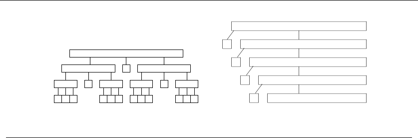
4.6 QUICKSORT: SORTING BY RANDOMIZATION 125
Figure 4.6: The best-case (l) and worst-case (r) recursion trees for quicksort
Since the partitioning step consists of at most nswaps, it takes linear time in the
number of keys. But how long does the entire quicksort take? As with mergesort,
quicksort builds a recursion tree of nested subranges of the n-element array. As with
mergesort, quicksort spends linear time processing (now partitioning instead of
mergeing) the elements in each subarray on each level. As with mergesort, quicksort
runs in O(n·h) time, where his the height of the recursion tree.
The difficulty is that the height of the tree depends upon where the pivot
element ends up in each partition. If we get very lucky and happen to repeatedly
pick the median element as our pivot, the subproblems are always half the size
of the previous level. The height represents the number of times we can halve n
until we get down to 1, or at most lg2n. This happy situation is shown in Figure
4.6(l), and corresponds to the best case of quicksort.
Now suppose we consistently get unlucky, and our pivot element always splits
the array as unequally as possible. This implies that the pivot element is always
the biggest or smallest element in the sub-array. After this pivot settles into its
position, we are left with one subproblem of size n−1. We spent linear work and
reduced the size of our problem by one measly element, as shown in Figure 4.6(r).
It takes a tree of height n−1 to chop our array down to one element per level, for
a worst case time of Θ(n2).
Thus, the worst case for quicksort is worse than heapsort or mergesort. To
justify its name, quicksort had better be good in the average case. Understanding
why requires some intuition about random sampling.
4.6.1 Intuition: The Expected Case for Quicksort
The expected performance of quicksort depends upon the height of the partition
tree constructed by random pivot elements at each step. Mergesort ran in O(nlog n)
time because we split the keys into two equal halves, sorted them recursively, and
then merged the halves in linear time. Thus, whenever our pivot element is near
the center of the sorted array (i.e. , the pivot is close to the median element), we
get a good split and realize the same performance as mergesort.

126 4. SORTING AND SEARCHING
1 n/4 3n/4 nn/2
Figure 4.7: Half the time, the pivot is close to the median element
I will give an intuitive explanation of why quicksort is O(nlog n) in the average
case. How likely is it that a randomly selected pivot is a good one? The best possible
selection for the pivot would be the median key, because exactly half of elements
would end up left, and half the elements right, of the pivot. Unfortunately, we only
have a probability of 1/n of randomly selecting the median as pivot, which is quite
small.
Suppose a key is a good enough pivot if it lies is in the center half of the sorted
space of keys—i.e. , those ranked from n/4to3n/4 in the space of all keys to be
sorted. Such good enough pivot elements are quite plentiful, since half the elements
lie closer to the middle than one of the two ends (see Figure 4.7). Thus, on each
selection we will pick a good enough pivot with probability of 1/2.
Can you flip a coin so it comes up tails each time? Not without cheating. If
you flip a fair coin ntimes, it will come out heads about half the time. Let heads
denote the chance of picking a good enough pivot.
The worst possible good enough pivot leaves the bigger half of the space partition
with 3n/4 items. What is the height hgof a quicksort partition tree constructed
repeatedly from the worst-possible good enough pivot? The deepest path through
this tree passes through partitions of size n, (3/4)n, (3/4)2n,...,downto1.How
many times can we multiply nby 3/4 until it gets down to 1?
(3/4)hgn=1⇒n=(4/3)hg
so hg= log4/3n.
But only half of all randomly selected pivots will be good enough.Therestwe
classify as bad. The worst of these bad pivots will do essentially nothing to reduce
the partition size along the deepest path. The deepest path from the root through
a typical randomly-constructed quicksort partition tree will pass through roughly
equal numbers of good-enough and bad pivots. Since the expected number of good
splits and bad splits is the same, the bad splits can only double the height of the
tree, so h≈2hg= 2 log4/3n, which is clearly Θ(log n).
On average, random quicksort partition trees (and by analogy, binary search
trees under random insertion) are very good. More careful analysis shows the av-
erage height after ninsertions is approximately 2 ln n. Since 2 ln n≈1.386 lg2n,
this is only 39% taller than a perfectly balanced binary tree. Since quicksort does
O(n) work partitioning on each level, the average time is O(nlog n). If we are ex-
tremely unlucky and our randomly selected elements always are among the largest
or smallest element in the array, quicksort turns into selection sort and runs in
O(n2). However, the odds against this are vanishingly small.

4.6 QUICKSORT: SORTING BY RANDOMIZATION 127
4.6.2 Randomized Algorithms
There is an important subtlety about the expected case O(nlog n) running time for
quicksort. Our quicksort implementation above selected the last element in each
sub-array as the pivot. Suppose this program were given a sorted array as input. If
so, at each step it would pick the worst possible pivot and run in quadratic time.
For any deterministic method of pivot selection, there exists a worst-case input
instance which will doom us to quadratic time. The analysis presented above made
no claim stronger than:
“Quicksort runs in Θ(nlog n) time, with high probability, if you give
me randomly ordered data to sort.”
But now suppose we add an initial step to our algorithm where we randomly
permute the order of the nelements before we try to sort them. Such a permutation
can be constructed in O(n) time (see Section 13.7 for details). This might seem like
wasted effort, but it provides the guarantee that we can expect Θ(nlog n) running
time whatever the initial input was. The worst case performance still can happen,
but it depends only upon how unlucky we are. There is no longer a well-defined
“worst case” input. We now can say
“Randomized quicksort runs in Θ(nlog n) time on any input, with high
probability.”
Alternately, we could get the same guarantee by selecting a random element to be
the pivot at each step.
Randomization is a powerful tool to improve algorithms with bad worst-case
but good average-case complexity. It can be used to make algorithms more robust
to boundary cases and more efficient on highly structured input instances that
confound heuristic decisions (such as sorted input to quicksort). It often lends
itself to simple algorithms that provide randomized performance guarantees which
are otherwise obtainable only using complicated deterministic algorithms.
Proper analysis of randomized algorithms requires some knowledge of probabil-
ity theory, and is beyond the scope of this book. However, some of the approaches
to designing efficient randomized algorithms are readily explainable:
•Random sampling – Want to get an idea of the median value of nthings but
don’t have either the time or space to look at them all? Select a small random
sample of the input and study those, for the results should be representative.
This is the idea behind opinion polling. Biases creep in unless you take a
truly random sample, as opposed to the first xpeople you happen to see. To
avoid bias, actual polling agencies typically dial random phone numbers and
hope someone answers.
•Randomized hashing – We have claimed that hashing can be used to imple-
ment dictionary operations in O(1) “expected-time.” However, for any hash

128 4. SORTING AND SEARCHING
function there is a given worst-case set of keys that all get hashed to the same
bucket. But now suppose we randomly select our hash function from a large
family of good ones as the first step of our algorithm. We get the same type
of improved guarantee that we did with randomized quicksort.
•Randomized search – Randomization can also be used to drive search tech-
niques such as simulated annealing, as will be discussed in detail in Section
7.5.3 (page 254).
Stop and Think: Nuts and Bolts
Problem: The nuts and bolts problem is defined as follows. You are given a collection
of nbolts of different widths, and ncorresponding nuts. You can test whether a
given nut and bolt fit together, from which you learn whether the nut is too large,
too small, or an exact match for the bolt. The differences in size between pairs of
nuts or bolts are too small to see by eye, so you cannot compare the sizes of two
nuts or two bolts directly. You are to match each bolt to each nut.
Give an O(n2) algorithm to solve the nuts and bolts problem. Then give a
randomized O(nlog n) expected time algorithm for the same problem.
Solution: The brute force algorithm for matching nuts and bolts starts with the
first bolt and compares it to each nut until we find a match. In the worst case, this
will require ncomparisons. Repeating this for each successive bolt on all remaining
nuts yields a quadratic-comparison algorithm.
What if we pick a random bolt and try it? On average, we would expect to
get about halfway through the set of nuts before we found the match, so this
randomized algorithm would do half the work as the worst case. That counts as
some kind of improvement, although not an asymptotic one.
Randomized quicksort achieves the desired expected-case running time, so a
natural idea is to emulate it on the nuts and bolts problem. Indeed, sorting both
the nuts and bolts by size would yield a matching, since the ith largest nut must
match the ith largest bolt.
The fundamental step in quicksort is partitioning elements around a pivot. Can
we partition nuts and bolts around a randomly selected bolt b? Certainly we can
partition the nuts into those of size less than band greater than b. But decomposing
the problem into two halves requires partitioning the bolts as well, and we cannot
compare bolt against bolt. But once we find the matching nut to bwe can use it to
partition the bolts accordingly. In 2n−2 comparisons, we partition the nuts and
bolts, and the remaining analysis follows directly from randomized quicksort.
What is interesting about this problem is that no simple deterministic algorithm
for nut and bolt sorting is known. It illustrates how randomization makes the bad
case go away, leaving behind a simple and beautiful algorithm.

4.7 DISTRIBUTION SORT: SORTING VIA BUCKETING 129
4.6.3 Is Quicksort Really Quick?
There is a clear, asymptotic difference between an Θ(nlog n) algorithm and one
that runs in Θ(n2). Thus, only the most obstinate reader would doubt my claim
that mergesort, heapsort, and quicksort should all outperform insertion sort or
selection sort on large enough instances.
But how can we compare two Θ(nlog n) algorithms to decide which is faster?
How can we prove that quicksort is really quick? Unfortunately, the RAM model
and Big Oh analysis provide too coarse a set of tools to make that type of distinc-
tion. When faced with algorithms of the same asymptotic complexity, implemen-
tation details and system quirks such as cache performance and memory size may
well prove to be the decisive factor.
What we can say is that experiments show that where a properly implemented
quicksort is implemented well, it is typically 2-3 times faster than mergesort or
heapsort. The primary reason is that the operations in the innermost loop are
simpler. But I can’t argue with you if you don’t believe me when I say quicksort is
faster. It is a question whose solution lies outside the analytical tools we are using.
The best way to tell is to implement both algorithms and experiment.
4.7 Distribution Sort: Sorting via Bucketing
We could sort sorting names for the telephone book by partitioning them according
to the first letter of the last name. This will create 26 different piles, or buckets, of
names. Observe that any name in the Jpile must occur after every name in the I
pile, but before any name in the Kpile. Therefore, we can proceed to sort each pile
individually and just concatenate the bunch of sorted piles together at the end.
If the names are distributed evenly among the buckets, the resulting 26 sorting
problems should each be substantially smaller than the original problem. Further,
by now partitioning each pile based on the second letter of each name, we generate
smaller and smaller piles. The names will be sorted as soon as each bucket con-
tains only a single name. The resulting algorithm is commonly called bucketsort or
distribution sort.
Bucketing is a very effective idea whenever we are confident that the distribution
of data will be roughly uniform. It is the idea that underlies hash tables, kd-trees,
and a variety of other practical data structures. The downside of such techniques
is that the performance can be terrible when the data distribution is not what we
expected. Although data structures such as balanced binary trees offer guaranteed
worst-case behavior for any input distribution, no such promise exists for heuristic
data structures on unexpected input distributions.
Nonuniform distributions do occur in real life. Consider Americans with the
uncommon last name of Shifflett. When last I looked, the Manhattan telephone
directory (with over one million names) contained exactly five Shiffletts. So how
many Shiffletts should there be in a small city of 50,000 people? Figure 4.8 shows
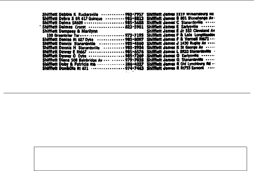
130 4. SORTING AND SEARCHING
Figure 4.8: A small subset of Charlottesville Shiffletts
a small portion of the two and a half pages of Shiffletts in the Charlottesville,
Virginia telephone book. The Shifflett clan is a fixture of the region, but it would
play havoc with any distribution sort program, as refining buckets from Sto Sh
to Shi to Shif to ... to Shifflett results in no significant partitioning.
Take-Home Lesson: Sorting can be used to illustrate most algorithm design
paradigms. Data structure techniques, divide-and-conquer, randomization, and
incremental construction all lead to efficient sorting algorithms.
4.7.1 Lower Bounds for Sorting
One last issue on the complexity of sorting. We have seen several sorting algorithms
that run in worst-case O(nlog n) time, but none of which is linear. To sort nitems
certainly requires looking at all of them, so any sorting algorithm must be Ω(n)in
the worst case. Can we close this remaining Θ(log n) gap?
The answer is no. An Ω(nlog n) lower bound can be shown by observing that
any sorting algorithm must behave differently during execution on each of the dis-
tinct n! permutations of nkeys. The outcome of each pairwise comparison governs
the run-time behavior of any comparison-based sorting algorithm. We can think of
the set of all possible executions of such an algorithm as a tree with n! leaves. The
minimum height tree corresponds to the fastest possible algorithm, and it happens
that lg(n!) = Θ(nlog n).
This lower bound is important for several reasons. First, the idea can be ex-
tended to give lower bounds for many applications of sorting, including element
uniqueness, finding the mode, and constructing convex hulls. Sorting has one of
the few nontrivial lower bounds among algorithmic problems. We will present
an alternate approach to arguing that fast algorithms are unlikely to exist in
Chapter 9.

4.8 WAR STORY: SKIENA FOR THE DEFENSE 131
4.8 War Story: Skiena for the Defense
I lead a quiet, reasonably honest life. One reward for this is that I don’t often find
myself on the business end of surprise calls from lawyers. Thus I was astonished to
get a call from a lawyer who not only wanted to talk with me, but wanted to talk
to me about sorting algorithms.
It turned out that her firm was working on a case involving high-performance
programs for sorting, and needed an expert witness who could explain technical
issues to the jury. From the first edition of this book, they could see I knew some-
thing about algorithms, but before taking me on they demanded to see my teaching
evaluations to prove that I could explain things to people.2It proved to be a fasci-
nating opportunity to learn about how real ly fast sorting programs work. I figured
I could finally answer the question of which in-place sorting algorithm was fastest
in practice. Was it heapsort or quicksort? What subtle, secret algorithmics made
the difference to minimize the number of comparisons in practice?
The answer was quite humbling. Nobody cared about in-place sorting. The name
of the game was sorting huge files, much bigger than could fit in main memory. All
the important action was in getting the the data on and off a disk. Cute algorithms
for doing internal (in-memory) sorting were not particularly important because the
real problem lies in sorting gigabytes at a time.
Recall that disks have relatively long seek times, reflecting how long it takes the
desired part of the disk to rotate under the read/write head. Once the head is in the
right place, the data moves relatively quickly, and it costs about the same to read
a large data block as it does to read a single byte. Thus, the goal is minimizing the
number of blocks read/written, and coordinating these operations so the sorting
algorithm is never waiting to get the data it needs.
The disk-intensive nature of sorting is best revealed by the annual Minutesort
competition. The goal is to sort as much data in one minute as possible. The cur-
rent champion is Jim Wyllie of IBM Research, who managed to sort 116 gigabytes
of data in 58.7 seconds on his little old 40-node 80-Itanium cluster with a SAN
array of 2,520 disks. Slightly more down-to-earth is the Pennysort division, where
the goal is the maximized sorting performance per penny of hardware. The cur-
rent champ here (BSIS from China) sorted 32 gigabytes in 1,679 seconds on a
$760 PC containing four SATA drives. You can check out the current records at
http://research.microsoft.com/barc/SortBenchmark/.
That said, which algorithm is best for external sorting? It basically turns out
to be a multiway mergesort, employing a lot of engineering and special tricks.
You build a heap with members of the top block from each of ksorted lists. By
repeatedly plucking the top element off this heap, you build a sorted list merging
these klists. Because this heap is sitting in main memory, these operations are
fast. When you have a large enough sorted run, you write it to disk and free up
2One of my more cynical faculty colleagues said this was the first time anyone, anywhere, had ever looked
at university teaching evaluations.

132 4. SORTING AND SEARCHING
memory for more data. Once you start to run out of elements from the top block
of one of the ksorted lists you are merging, load the next block.
It proves very hard to benchmark sorting programs/algorithms at this level
and decide which is really fastest. Is it fair to compare a commercial program
designed to handle general files with a stripped-down code optimized for integers?
The Minutesort competition employs randomly-generated 100-byte records. This is
a different world than sorting names or integers. For example, one widely employed
trick is to strip off a relatively short prefix of the key and initially sort just on that,
to avoid lugging around all those extra bytes.
What lessons can be learned from this? The most important, by far, is to
do everything you can to avoid being involved in a lawsuit as either a plaintiff
or defendant.3Courts are not instruments for resolving disputes quickly. Legal
battles have a lot in common with military battles: they escalate very quickly,
become very expensive in time, money, and soul, and usually end only when both
sides are exhausted and compromise. Wise are the parties who can work out their
problems without going to court. Properly absorbing this lesson now could save
you thousands of times the cost of this book.
On technical matters, it is important to worry about external memory perfor-
mance whenever you combine very large datasets with low-complexity algorithms
(say linear or nlog n). Constant factors of even 5 or 10 can make a big differ-
ence then between what is feasible and what is hopeless. Of course, quadratic-time
algorithms are doomed to fail on large datasets regardless of data access times.
4.9 Binary Search and Related Algorithms
Binary search is a fast algorithm for searching in a sorted array of keys S. To search
for key q, we compare qto the middle key S[n/2]. If qappears before S[n/2], it
must reside in the top half of S; if not, it must reside in the bottom half of S.By
repeating this process recursively on the correct half, we locate the key in a total
of lg ncomparisons—a big win over the n/2 comparisons expect using sequential
search:
int binary_search(item_type s[], item_type key, int low, int high)
{
int middle; /* index of middle element */
if (low > high) return (-1); /* key not found */
middle = (low+high)/2;
3It is actually quite interesting serving as an expert witness.

4.9 BINARY SEARCH AND RELATED ALGORITHMS 133
if (s[middle] == key) return(middle);
if (s[middle] > key)
return( binary_search(s,key,low,middle-1) );
else
return(binary_search(s,key,middle+1,high) );
}
This much you probably know. What is important is to have a sense of just
how fast binary search is. Twenty questions is a popular children’s game where
one player selects a word and the other repeatedly asks true/false questions in an
attempt to guess it. If the word remains unidentified after 20 questions, the first
party wins; otherwise, the second player takes the honors. In fact, the second player
always has a winning strategy, based on binary search. Given a printed dictionary,
the player opens it in the middle, selects a word (say “move”), and asks whether the
unknown word is before “move” in alphabetical order. Since standard dictionaries
contain 50,000 to 200,000 words, we can be certain that the process will terminate
within twenty questions.
4.9.1 Counting Occurrences
Several interesting algorithms follow from simple variants of binary search. Suppose
that we want to count the number of times a given key k(say “Skiena”) occurs in
a given sorted array. Because sorting groups all the copies of kinto a contiguous
block, the problem reduces to finding the right block and then measures its size.
The binary search routine presented above enables us to find the index of an
element of the correct block (x)inO(lg n) time. The natural way to identify the
boundaries of the block is to sequentially test elements to the left of xuntil we
find the first one that differs from the search key, and then repeat this search to
the right of x. The difference between the indices of the left and right boundaries
(plus one) gives the count of the number of occurrences of k.
This algorithm runs in O(lg n+s), where sis the number of occurrences of the
key. This can be as bad as linear if the entire array consists of identical keys. A
faster algorithm results by modifying binary search to search for the boundary of
the block containing k, instead of kitself. Suppose we delete the equality test
if (s[middle] == key) return(middle);
from the implementation above and return the index low instead of −1oneach
unsuccessful search. All searches will now be unsuccessful, since there is no equality
test. The search will proceed to the right half whenever the key is compared to an
identical array element, eventually terminating at the right boundary. Repeating
the search after reversing the direction of the binary comparison will lead us to the
left boundary. Each search takes O(lg n) time, so we can count the occurrences in
logarithmic time regardless of the size of the block.

134 4. SORTING AND SEARCHING
4.9.2 One-Sided Binary Search
NowsupposewehaveanarrayAconsisting of a run of 0’s, followed by an un-
bounded run of 1’s, and would like to identify the exact point of transition between
them. Binary search on the array would provide the transition point in lg ntests,
if we had a bound non the number of elements in the array. In the absence of such
a bound, we can test repeatedly at larger intervals (A[1], A[2], A[4], A[8], A[16],
...) until we find a first nonzero value. Now we have a window containing the
target and can proceed with binary search. This one-sided binary search finds the
transition point pusing at most 2lg pcomparisons, regardless of how large the
array actually is. One-sided binary search is most useful whenever we are looking
for a key that lies close to our current position.
4.9.3 Square and Other Roots
The square root of nis the number rsuch that r2=n. Square root computations
are performed inside every pocket calculator, but it is instructive to develop an
efficient algorithm to compute them.
First, observe that the square root of n≥1 must be at least 1 and at most
n.Letl=1andr=n. Consider the midpoint of this interval, m=(l+r)/2.
How does m2compare to n?Ifn≥m2, then the square root must be greater than
m, so the algorithm repeats with l=m.Ifn<m
2, then the square root must
be less than m, so the algorithm repeats with r=m. Either way, we have halved
the interval using only one comparison. Therefore, after lg nrounds we will have
identified the square root to within ±1.
This bisection method, as it is called in numerical analysis, can also be applied
to the more general problem of finding the roots of an equation. We say that xis
aroot of the function fif f(x) = 0. Suppose that we start with values land rsuch
that f(l)>0andf(r)<0. If fis a continuous function, there must exist a root
between land r. Depending upon the sign of f(m), where m=(l+r)/2, we can
cut this window containing the root in half with each test and stop soon as our
estimate becomes sufficiently accurate.
Root-finding algorithms that converge faster than binary search are known for
both of these problems. Instead of always testing the midpoint of the interval,
these algorithms interpolate to find a test point closer to the actual root. Still,
binary search is simple, robust, and works as well as possible without additional
information on the nature of the function to be computed.
Take-Home Lesson: Binary search and its variants are the quintessential
divide-and-conquer algorithms.

4.10 DIVIDE-AND-CONQUER 135
4.10 Divide-and-Conquer
One of the most powerful techniques for solving problems is to break them down
into smaller, more easily solved pieces. Smaller problems are less overwhelming, and
they permit us to focus on details that are lost when we are studying the entire
problem. A recursive algorithm starts to become apparent when we can break
the problem into smaller instances of the same type of problem. Effective parallel
processing requires decomposing jobs into at least as many tasks as processors, and
is becoming more important with the advent of cluster computing and multicore
processors.
Two important algorithm design paradigms are based on breaking problems
down into smaller problems. In Chapter 8, we will see dynamic programming,
which typically removes one element from the problem, solves the smaller problem,
and then uses the solution to this smaller problem to add back the element in the
proper way. Divide-and-conquer instead splits the problem in (say) halves, solves
each half, then stitches the pieces back together to form a full solution.
To use divide-and-conquer as an algorithm design technique, we must divide
the problem into two smaller subproblems, solve each of them recursively, and then
meld the two partial solutions into one solution to the full problem. Whenever
the merging takes less time than solving the two subproblems, we get an efficient
algorithm. Mergesort, discussed in Section 4.5 (page 120), is the classic example of
a divide-and-conquer algorithm. It takes only linear time to merge two sorted lists
of n/2 elements, each of which was obtained in O(nlg n) time.
Divide-and-conquer is a design technique with many important algorithms to
its credit, including mergesort, the fast Fourier transform, and Strassen’s matrix
multiplication algorithm. Beyond binary search and its many variants, however, I
find it to be a difficult design technique to apply in practice. Our ability to analyze
divide-and-conquer algorithms rests on our strength to solve the asymptotics of
recurrence relations governing the cost of such recursive algorithms.
4.10.1 Recurrence Relations
Many divide-and-conquer algorithms have time complexities that are naturally
modeled by recurrence relations. Evaluating such recurrences is important to un-
derstanding when divide-and-conquer algorithms perform well, and provide an im-
portant tool for analysis in general. The reader who balks at the very idea of
analysis is free to skip this section, but there are important insights into design
that come from an understanding of the behavior of recurrence relations.
What is a recurrence relation? It is an equation that is defined in terms of itself.
The Fibonacci numbers are described by the recurrence relation Fn=Fn−1+Fn−2
and discussed in Section 8.1.1. Many other natural functions are easily expressed
as recurrences. Any polynomial can be represented by a recurrence, such as the
linear function:
an=an−1+1,a
1=1−→ an=n

136 4. SORTING AND SEARCHING
Any exponential can be represented by a recurrence:
an=2an−1,a
1=1−→ an=2
n−1
Finally, lots of weird functions that cannot be described easily with conventional
notation can be represented by a recurrence:
an=nan−1,a
1=1−→ an=n!
This means that recurrence relations are a very versatile way to represent functions.
The self-reference property of recurrence relations is shared with recursive pro-
grams or algorithms, as the shared roots of both terms reflect. Essentially, recur-
rence relations provide a way to analyze recursive structures, such as algorithms.
4.10.2 Divide-and-Conquer Recurrences
Divide-and-conquer algorithms tend to break a given problem into some number of
smaller pieces (say a), each of which is of size n/b. Further, they spend f(n) time
to combine these subproblem solutions into a complete result. Let T(n) denote the
worst-case time the algorithm takes to solve a problem of size n. Then T(n)is
given by the following recurrence relation:
T(n)=aT (n/b)+f(n)
Consider the following examples:
•Sorting – The running time behavior of mergesort is governed by the re-
currence T(n)=2T(n/2) + O(n), since the algorithm divides the data into
equal-sized halves and then spends linear time merging the halves after they
are sorted. In fact, this recurrence evaluates to T(n)=O(nlg n), just as we
got by our previous analysis.
•Binary Search – The running time behavior of binary search is governed by
the recurrence T(n)=T(n/2) + O(1), since at each step we spend constant
time to reduce the problem to an instance half its size. In fact, this recurrence
evaluates to T(n)=O(lg n), just as we got by our previous analysis.
•Fast Heap Construction –Thebubble down method of heap construction
(described in Section 4.3.4) built an n-element heap by constructing two n/2
element heaps and then merging them with the root in logarithmic time. This
argument reduces to the recurrence relation T(n)=2T(n/2) + O(lg n). In
fact, this recurrence evaluates to T(n)=O(n), just as we got by our previous
analysis.
•Matrix Multiplication – As discussed in Section 2.5.4, the standard matrix
multiplication algorithm for two n×nmatrices takes O(n3), because we
compute the dot product of nterms for each of the n2elements in the product
matrix.

4.10 DIVIDE-AND-CONQUER 137
However, Strassen [Str69] discovered a divide-and-conquer algorithm that
manipulates the products of seven n/2×n/2 matrix products to yield the
product of two n×nmatrices. This yields a time-complexity recurrence
T(n)=7T(n/2) + O(n2). In fact, this recurrence evaluates to T(n)=
O(n2.81), which seems impossible to predict without solving the recurrence.
4.10.3 Solving Divide-and-Conquer Recurrences (*)
In fact, divide-and-conquer recurrences of the form T(n)=aT (n/b)+f(n)are
generally easy to solve, because the solutions typically fall into one of three distinct
cases:
1. If f(n)=O(nlogba−) for some constant >0, then T(n)=Θ(nlogba).
2. If f(n)=Θ(nlogba), then T(n)=Θ(nlogbalg n).
3. If f(n)=Ω(nlogba+) for some constant >0, and if af(n/b)≤cf(n)for
some c<1, then T(n)=Θ(f(n)).
Although this looks somewhat frightening, it really isn’t difficult to apply. The
issue is identifying which case of the so-called master theorem holds for your given
recurrence. Case 1 holds for heap construction and matrix multiplication, while
Case 2 holds mergesort and binary search. Case 3 generally arises for clumsier
algorithms, where the cost of combining the subproblems dominates everything.
The master theorem can be thought of as a black-box piece of machinery, in-
voked as needed and left with its mystery intact. However, with a little study, the
reason why the master theorem works can become apparent.
Figure 4.9 shows the recursion tree associated with a typical T(n)=aT (n/b)+
f(n) divide-and-conquer algorithm. Each problem of size nis decomposed into a
problems of size n/b. Each subproblem of size ktakes O(f(k)) time to deal with
internally, between partitioning and merging. The total time for the algorithm is
the sum of these internal costs, plus the overhead of building the recursion tree.
The height of this tree is h= logbnand the number of leaf nodes ah=alogbn,
which happens to simplify to nlogbawith some algebraic manipulation.
The three cases of the master theorem correspond to three different costs which
might be dominant as a function of a,b,andf(n):
•Case 1: Too many leaves – If the number of leaf nodes outweighs the sum of
the internal evaluation cost, the total running time is O(nlogba).
•Case 2: Equal work per level – As we move down the tree, each problem
gets smaller but there are more of them to solve. If the sum of the internal
evaluation costs at each level are equal, the total running time is the cost per
level (nlogba) times the number of levels (logbn), for a total running time of
O(nlogbalg n).
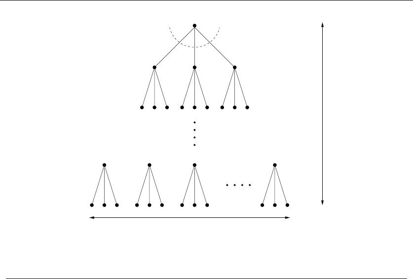
138 4. SORTING AND SEARCHING
b
log n b
log b
n=
height = log n
w
i
dt
h =
a
b
partition size = 1
partition size = b
2
n
n/b
n/b
partition size =
partition size =
partition size =
vertex degree = a
Figure 4.9: The recursion tree resulting from decomposing each problem of size ninto a
problems of size n/b
•Case 3: Too expensive a root – If the internal evaluation costs grow rapidly
enough with n, then the cost of the root evaluation may dominate. If so, the
the total running time is O(f(n)).
Chapter Notes
The most interesting sorting algorithms that have not been discussed in this section
include shellsort, which is a substantially more efficient version of insertion sort,
and radix sort, an efficient algorithm for sorting strings. You can learn more about
these and every other sorting algorithm by browsing through Knuth [Knu98], with
hundreds of pages of interesting material on sorting. This includes external sorting,
the subject of this chapter’s legal war story.
As implemented here, mergesort copies the merged elements into an auxiliary
buffer to avoid overwriting the original elements to be sorted. Through clever but
complicated buffer manipulation, mergesort can be implemented in an array with-
out using much extra storage. Kronrod’s algorithm for in-place merging is presented
in [Knu98].
Randomized algorithms are discussed in greater detail in the books by Mot-
wani and Raghavan [MR95] and Mitzenmacher and Upfal [MU05]. The problem of

4.11 EXERCISES 139
nut and bolt sorting was introduced by [Raw92]. A complicated but deterministic
O(nlog n) algorithm is due to Komlos, Ma, and Szemeredi [KMS96].
Several other algorithms texts provide more substantive coverage of divide-
and-conquer algorithms, including [CLRS01, KT06, Man89]. See [CLRS01] for an
excellent overview of the master theorem.
4.11 Exercises
Applications of Sorting
4-1. [3] The Grinch is given the job of partitioning 2nplayersintotwoteamsofn
players each. Each player has a numerical rating that measures how good he/she is
at the game. He seeks to divide the players as unfairly as possible, so as to create
the biggest possible talent imbalance between team Aand team B. Show how the
Grinch can do the job in O(nlog n)time.
4-2. [3] For each of the following problems, give an algorithm that finds the desired
numbers within the given amount of time. To keep your answers brief, feel free to
use algorithms from the book as subroutines. For the example, S={6,13,19,3,8},
19 −3 maximizes the difference, while 8 −6 minimizes the difference.
(a) Let Sbe an unsorted array of nintegers. Give an algorithm that finds the pair
x, y ∈Sthat maximizes |x−y|. Your algorithm must run in O(n) worst-case time.
(b) Let Sbe a sorted array of nintegers. Give an algorithm that finds the pair
x, y ∈Sthat maximizes |x−y|. Your algorithm must run in O(1) worst-case time.
(c) Let Sbe an unsorted array of nintegers. Give an algorithm that finds the pair
x, y ∈Sthat minimizes |x−y|,forx=y. Your algorithm must run in O(nlog n)
worst-case time.
(d) Let Sbe a sorted array of nintegers. Give an algorithm that finds the pair
x, y ∈Sthat minimizes |x−y|,forx=y. Your algorithm must run in O(n)
worst-case time.
4-3. [3] Take a sequence of 2nreal numbers as input. Design an O(nlog n) algorithm that
partitions the numbers into npairs, with the property that the partition minimizes
the maximum sum of a pair. For example, say we are given the numbers (1,3,5,9).
The possible partitions are ((1,3),(5,9)), ((1,5),(3,9)), and ((1,9),(3,5)). The pair
sums for these partitions are (4,14), (6,12), and (10,8). Thus the third partition has
10 as its maximum sum, which is the minimum over the three partitions.
4-4. [3] Assume that we are given npairs of items as input, where the first item is a
number and the second item is one of three colors (red, blue, or yellow). Further
assume that the items are sorted by number. Give an O(n) algorithm to sort the
items by color (all reds before all blues before all yellows) such that the numbers
for identical colors stay sorted.
For example: (1,blue), (3,red), (4,blue), (6,yellow), (9,red) should become (3,red),
(9,red), (1,blue), (4,blue), (6,yellow).
4-5. [3] The mode of a set of numbers is the number that occurs most frequently in the
set. The set (4,6,2,4,3,1) has a mode of 4. Give an efficient and correct algorithm
to compute the mode of a set of nnumbers.

140 4. SORTING AND SEARCHING
4-6. [3] Given two sets S1and S2(each of size n), and a number x,describeanO(nlog n)
algorithm for finding whether there exists a pair of elements, one from S1and one
from S2, that add up to x. (For partial credit, give a Θ(n2) algorithm for this
problem.)
4-7. [3] Outline a reasonable method of solving each of the following problems. Give
the order of the worst-case complexity of your methods.
(a) You are given a pile of thousands of telephone bills and thousands of checks
sent in to pay the bills. Find out who did not pay.
(b) You are given a list containing the title, author, call number and publisher of
all the books in a school library and another list of 30 publishers. Find out
how many of the books in the library were published by each company.
(c) You are given all the book checkout cards used in the campus library during
the past year, each of which contains the name of the person who took out
the book. Determine how many distinct people checked out at least one book.
4-8. [4 ] Given a set of Scontaining nreal numbers, and a real number x. We seek an
algorithm to determine whether two elements of Sexist whose sum is exactly x.
(a) Assume that Sis unsorted. Give an O(nlog n) algorithm for the problem.
(b) Assume that Sis sorted. Give an O(n) algorithm for the problem.
4-9. [4 ] Give an efficient algorithm to compute the union of sets Aand B,where
n= max(|A|,|B|). The output should be an array of distinct elements that form
the union of the sets, such that they appear more than once in the union.
(a) Assume that Aand Bare unsorted. Give an O(nlog n) algorithm for the
problem.
(b) Assume that Aand Bare sorted. Give an O(n) algorithm for the problem.
4-10. [5] Given a set Sof nintegers and an integer T,giveanO(nk−1log n) algorithm
to test whether kof the integers in SadduptoT.
4-11. [6 ] Design an O(n) algorithm that, given a list of nelements, finds all the elements
that appear more than n/2 times in the list. Then,designanO(n) algorithm that,
given a list of nelements, finds all the elements that appear more than n/4times.
Heaps
4-12. [3] Devise an algorithm for finding the ksmallest elements of an unsorted set of n
integers in O(n+klog n).
4-13. [5] You wish to store a set of nnumbers in either a max-heap or a sorted array.
For each application below, state which data structure is better, or if it does not
matter. Explain your answers.
(a) Want to find the maximum element quickly.
(b) Want to be able to delete an element quickly.
(c) Want to be able to form the structure quickly.
(d) Want to find the minimum element quickly.

4.11 EXERCISES 141
4-14. [5] Give an O(nlog k)-time algorithm that merges ksorted lists with a total of n
elements into one sorted list. (Hint: use a heap to speed up the elementary O(kn)-
time algorithm).
4-15. [5] (a) Give an efficient algorithm to find the second-largest key among nkeys.
You can do better than 2n−3 comparisons.
(b) Then, give an efficient algorithm to find the third-largest key among nkeys.
How many key comparisons does your algorithm do in the worst case? Must your
algorithm determine which key is largest and second-largest in the process?
Quicksort
4-16. [3] Use the partitioning idea of quicksort to give an algorithm that finds the median
element of an array of nintegers in expected O(n) time. (Hint: must you look at
both sides of the partition?)
4-17. [3] The median of a set of nvalues is the n/2th smallest value.
(a) Suppose quicksort always pivoted on the median of the current sub-array. How
many comparisons would Quicksort make then in the worst case?
(b) Suppose quicksort were always to pivot on the n/3th smallest value of the
current sub-array. How many comparisons would be made then in the worst
case?
4-18. [5] Suppose an array Aconsists of nelements, each of which is red,white,orblue.
We seek to sort the elements so that all the reds come before all the whites,which
come before all the blues The only operation permitted on the keys are
•Examine(A,i) – report the color of the ith element of A.
•Swap(A,i,j) –swaptheith element of Awith the jth element.
Find a correct and efficient algorithm for red-white-blue sorting. There is a linear-
time solution.
4-19. [5] An inversion of a permutation is a pair of elements that are out of order.
(a) Show that a permutation of nitems has at most n(n−1)/2 inversions. Which
permutation(s) have exactly n(n−1)/2 inversions?
(b) Let Pbe a permutation and Prbe the reversal of this permutation. Show
that Pand Prhave a total of exactly n(n−1)/2 inversions.
(c) Use the previous result to argue that the expected number of inversions in a
random permutation is n(n−1)/4.
4-20. [3] Give an efficient algorithm to rearrange an array of nkeys so that all the
negative keys precede all the nonnegative keys. Your algorithm must be in-place,
meaning you cannot allocate another array to temporarily hold the items. How fast
is your algorithm?
Other Sorting Algorithms
4-21. [5] Stable sorting algorithms leave equal-key items in the same relative order as in
the original permutation. Explain what must be done to ensure that mergesort is
a stable sorting algorithm.

142 4. SORTING AND SEARCHING
4-22. [3] Show that npositive integers in the range 1 to kcanbesortedinO(nlog k)
time. The interesting case is when k<<n.
4-23. [5] We seek to sort a sequence Sof nintegers with many duplications, such that
the number of distinct integers in Sis O(log n). Give an O(nlog log n) worst-case
time algorithm to sort such sequences.
4-24. [5] Let A[1..n] be an array such that the first n−√nelements are already sorted
(though we know nothing about the remaining elements). Give an algorithm that
sorts Ain substantially better than nlog nsteps.
4-25. [5] Assume that the array A[1..n] only has numbers from {1,...,n
2}but that at
most log log nof these numbers ever appear. Devise an algorithm that sorts Ain
substantially less than O(nlog n).
4-26. [5] Consider the problem of sorting a sequence of n0’s and 1’s using comparisons.
For each comparison of two values xand y, the algorithm learns which of x<y,
x=y,orx>yholds.
(a) Give an algorithm to sort in n−1 comparisons in the worst case. Show that
your algorithm is optimal.
(b) Give an algorithm to sort in 2n/3 comparisons in the average case (assuming
each of the ninputs is 0 or 1 with equal probability). Show that your algorithm
is optimal.
4-27. [6] Let Pbe a simple, but not necessarily convex, polygon and qan arbitrary
point not necessarily in P. Design an efficient algorithm to find a line segment
originating from qthat intersects the maximum number of edges of P.Inother
words, if standing at point q, in what direction should you aim a gun so the bullet
will go through the largest number of walls. A bullet through a vertex of Pgets
credit for only one wall. An O(nlog n) algorithm is possible.
Lower Bounds
4-28. [5] In one of my research papers [Ski88], I discovered a comparison-based sorting
algorithm that runs in O(nlog(√n)). Given the existence of an Ω(nlog n)lower
bound for sorting, how can this be possible?
4-29. [5] Mr. B. C. Dull claims to have developed a new data structure for priority queues
that supports the operations Insert,Maximum,andExtract-Max—all in O(1) worst-
case time. Prove that he is mistaken. (Hint: the argument does not involve a lot of
gory details—just think about what this would imply about the Ω(nlog n)lower
bound for sorting.)
Searching
4-30. [3] A company database consists of 10,000 sorted names, 40% of whom are known as
good customers and who together account for 60% of the accesses to the database.
There are two data structure options to consider for representing the database:
•Put all the names in a single array and use binary search.
•Put the good customers in one array and the rest of them in a second array.
Only if we do not find the query name on a binary search of the first array do
we do a binary search of the second array.

4.11 EXERCISES 143
Demonstrate which option gives better expected performance. Does this change
if linear search on an unsorted array is used instead of binary search for both
options?
4-31. [3] Suppose you are given an array Aof nsorted numbers that has been circularly
shifted kpositions to the right. For example, {35,42,5,15,27,29}is a sorted array
that has been circularly shifted k= 2 positions, while {27,29,35,42,5,15}has been
shifted k= 4 positions.
•Suppose you know what kis. Give an O(1) algorithm to find the largest
number in A.
•Suppose you do not know what kis. Give an O(lg n) algorithm to find the
largest number in A. For partial credit, you may give an O(n) algorithm.
4-32. [3] Consider the numerical 20 Questions game. In this game, Player 1 thinks of a
number in the range 1 to n. Player 2 has to figure out this number by asking the
fewest number of true/false questions. Assume that nobody cheats.
(a) What is an optimal strategy if nin known?
(b) What is a good strategy is nis not known?
4-33. [5] Suppose that you are given a sorted sequence of distinct integers {a1,a
2,...,a
n}.
Give an O(lg n) algorithm to determine whether there exists an iindex such as
ai=i. For example, in {−10,−3,3,5,7},a3=3.In{2,3,4,5,6,7}, there is no
such i.
4-34. [5] Suppose that you are given a sorted sequence of distinct integers {a1,a
2,...,a
n},
drawn from 1 to mwhere n<m.GiveanO(lg n) algorithm to find an integer ≤m
that is not present in a. For full credit, find the smallest such integer.
4-35. [5] Let Mbe an n×minteger matrix in which the entries of each row are sorted in
increasing order (from left to right) and the entries in each column are in increasing
order (from top to bottom). Give an efficient algorithm to find the position of an
integer xin M,ortodeterminethatxis not there. How many comparisons of x
with matrix entries does your algorithm use in worst case?
Implementation Challenges
4-36. [5] Consider an n×narray Acontaining integer elements (positive, negative, and
zero). Assume that the elements in each row of Aare in strictly increasing order,
and the elements of each column of Aare in strictly decreasing order. (Hence there
cannotbetwozeroesinthesameroworthesamecolumn.)Describeanefficient
algorithm that counts the number of occurrences of the element 0 in A.Analyzeits
running time.
4-37. [6] Implement versions of several different sorting algorithms, such as selection sort,
insertion sort, heapsort, mergesort, and quicksort. Conduct experiments to assess
the relative performance of these algorithms in a simple application that reads a
large text file and reports exactly one instance of each word that appears within it.
This application can be efficiently implemented by sorting all the words that occur
in the text and then passing through the sorted sequence to identify one instance
of each distinct word. Write a brief report with your conclusions.

144 4. SORTING AND SEARCHING
4-38. [5] Implement an external sort, which uses intermediate files to sort files bigger
than main memory. Mergesort is a good algorithm to base such an implementation
on. Test your program both on files with small records and on files with large
records.
4-39. [8] Design and implement a parallel sorting algorithm that distributes data across
several processors. An appropriate variation of mergesort is a likely candidate. Mea-
sure the speedup of this algorithm as the number of processors increases. Later,
compare the execution time to that of a purely sequential mergesort implementa-
tion. What are your experiences?
Interview Problems
4-40. [3] If you are given a million integers to sort, what algorithm would you use to sort
them? How much time and memory would that consume?
4-41. [3] Describe advantages and disadvantages of the most popular sorting algorithms.
4-42. [3] Implement an algorithm that takes an input array and returns only the unique
elements in it.
4-43. [5] You have a computer with only 2Mb of main memory. How do you use it to sort
a large file of 500 Mb that is on disk?
4-44. [5] Design a stack that supports push, pop, and retrieving the minimum element
in constant time. Can you do this?
4-45. [5] Given a search string of three words, find the smallest snippet of the document
that contains all three of the search words—i.e. , the snippet with smallest number
of words in it. You are given the index positions where these words in occur search
strings, such as word1:(1,4,5),word2: (4, 9, 10),andword3: (5, 6, 15). Each of
the lists are in sorted order, as above.
4-46. [6] You are given 12 coins. One of them is heavier or lighter than the rest. Identify
this coin in just three weighings.
Programming Challenges
These programming challenge problems with robot judging are available at
http://www.programming-challenges.com or http://online-judge.uva.es.
4-1. “Vito’s Family” – Programming Challenges 110401, UVA Judge 10041.
4-2. “Stacks of Flapjacks” – Programming Challenges 110402, UVA Judge 120.
4-3. “Bridge” – Programming Challenges 110403, UVA Judge 10037.
4-4. “ShoeMaker’s Problem” – Programming Challenges 110405, UVA Judge 10026.
4-5. “ShellSort” – Programming Challenges 110407, UVA Judge 10152.
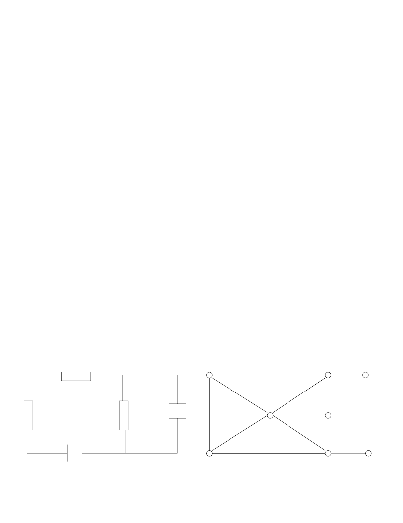
5
Graph Traversal
Graphs are one of the unifying themes of computer science—an abstract repre-
sentation that describes the organization of transportation systems, human inter-
actions, and telecommunication networks. That so many different structures can
be modeled using a single formalism is a source of great power to the educated
programmer.
More precisely, a graph G=(V, E) consists of a set of vertices Vtogether with
asetEof vertex pairs or edges. Graphs are important because they can be used to
represent essentially any relationship. For example, graphs can model a network of
roads, with cities as vertices and roads between cities as edges, as shown in Figure
5.1. Electronic circuits can also be modeled as graphs, with junctions as vertices
and components as edges.
Stony Brook Green Port
Shelter Island
Sag Harbor
Riverhead
Islip
Orient Point
Montauk
Figure 5.1: Modeling road networks and electronic circuits as graphs
S.S. Skiena, The Algorithm Design Manual, 2nd ed., DOI: 10.1007/978-1-84800-070-4 5,
c
Springer-Verlag London Limited 2008

146 5. GRAPH TRAVERSAL
The key to solving many algorithmic problems is to think of them in terms
of graphs. Graph theory provides a language for talking about the properties of
relationships, and it is amazing how often messy applied problems have a simple
description and solution in terms of classical graph properties.
Designing truly novel graph algorithms is a very difficult task. The key to using
graph algorithms effectively in applications lies in correctly modeling your problem
so you can take advantage of existing algorithms. Becoming familiar with many
different algorithmic graph problems is more important than understanding the
details of particular graph algorithms, particularly since Part II of this book will
point you to an implementation as soon as you know the name of your problem.
Here we present basic data structures and traversal operations for graphs, which
will enable you to cobble together solutions for basic graph problems. Chapter 6
will present more advanced graph algorithms that find minimum spanning trees,
shortest paths, and network flows, but we stress the primary importance of correctly
modeling your problem. Time spent browsing through the catalog now will leave
you better informed of your options when a real job arises.
5.1 Flavors of Graphs
AgraphG=(V, E) is defined on a set of vertices V, and contains a set of edges E
of ordered or unordered pairs of vertices from V. In modeling a road network, the
vertices may represent the cities or junctions, certain pairs of which are connected
by roads/edges. In analyzing the source code of a computer program, the vertices
may represent lines of code, with an edge connecting lines xand yif yis the next
statement executed after x. In analyzing human interactions, the vertices typically
represent people, with edges connecting pairs of related souls.
Several fundamental properties of graphs impact the choice of the data struc-
tures used to represent them and algorithms available to analyze them. The first
step in any graph problem is determining the flavors of graphs you are dealing
with:
•Undirected vs. Directed – A graph G=(V,E)isundirected if edge (x, y)∈E
implies that (y, x)isalsoinE. If not, we say that the graph is directed. Road
networks between cities are typically undirected, since any large road has
lanes going in both directions. Street networks within cities are almost always
directed, because there are at least a few one-way streets lurking somewhere.
Program-flow graphs are typically directed, because the execution flows from
one line into the next and changes direction only at branches. Most graphs
of graph-theoretic interest are undirected.
•Weighted vs. Unweighted – Each edge (or vertex) in a weighted graph Gis as-
signed a numerical value, or weight. The edges of a road network graph might
be weighted with their length, drive-time, or speed limit, depending upon the
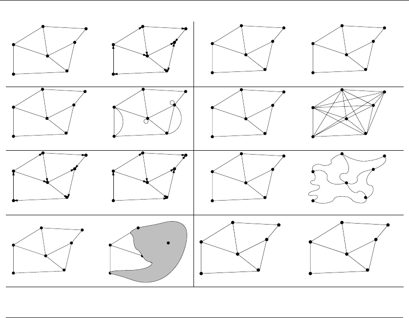
5.1 FLAVORS OF GRAPHS 147
u
n
d
ir
ected d
ir
ected
unweighted
5
9
2
5
7
4
3
7
12
weighted
3
simple non−simple sparse dense
cyclic acyclic embedded topological
explicit implicit
u
nl
abe
l
ed
l
abe
l
ed
B
C
D
E
F
G
A
Figure 5.2: Important properties / flavors of graphs
application. In unweighted graphs, there is no cost distinction between various
edges and vertices.
The difference between weighted and unweighted graphs becomes particularly
apparent in finding the shortest path between two vertices. For unweighted
graphs, the shortest path must have the fewest number of edges, and can
be found using a breadth-first search as discussed in this chapter. Shortest
paths in weighted graphs requires more sophisticated algorithms, as discussed
in Chapter 6.
•Simple vs. Non-simple – Certain types of edges complicate the task of working
with graphs. A self-loop is an edge (x, x) involving only one vertex. An edge
(x, y)isamultiedge if it occurs more than once in the graph.
Both of these structures require special care in implementing graph algo-
rithms. Hence any graph that avoids them is called simple.

148 5. GRAPH TRAVERSAL
•Sparse vs. Dense: Graphs are sparse when only a small fraction of the possible
vertex pairs (n
2for a simple, undirected graph on nvertices) actually have
edges defined between them. Graphs where a large fraction of the vertex pairs
define edges are called dense. There is no official boundary between what is
called sparse and what is called dense, but typically dense graphs have a
quadratic number of edges, while sparse graphs are linear in size.
Sparse graphs are usually sparse for application-specific reasons. Road net-
works must be sparse graphs because of road junctions. The most ghastly
intersection I’ve ever heard of was the endpoint of only seven different roads.
Junctions of electrical components are similarly limited to the number of
wires that can meet at a point, perhaps except for power and ground.
•Cyclic vs. Acyclic –Anacyclic graph does not contain any cycles. Trees
are connected, acyclic undirected graphs. Trees are the simplest interest-
ing graphs, and are inherently recursive structures because cutting any edge
leaves two smaller trees.
Directed acyclic graphs are called DAGs. They arise naturally in scheduling
problems, where a directed edge (x, y) indicates that activity xmust occur
before y. An operation called topological sorting orders the vertices of a DAG
to respect these precedence constraints. Topological sorting is typically the
first step of any algorithm on a DAG, as will be discussed in Section 5.10.1
(page 179).
•Embedded vs. Topological – A graph is embedded if the vertices and edges are
assigned geometric positions. Thus, any drawing of a graph is an embedding,
which may or may not have algorithmic significance.
Occasionally, the structure of a graph is completely defined by the geometry
of its embedding. For example, if we are given a collection of points in the
plane, and seek the minimum cost tour visiting all of them (i.e., the traveling
salesman problem), the underlying topology is the complete graph connecting
each pair of vertices. The weights are typically defined by the Euclidean
distance between each pair of points.
Grids of points are another example of topology from geometry. Many prob-
lems on an n×mgrid involve walking between neighboring points, so the
edges are implicitly defined from the geometry.
•Implicit vs. Explicit – Certain graphs are not explicitly constructed and then
traversed, but built as we use them. A good example is in backtrack search.
The vertices of this implicit search graph are the states of the search vector,
while edges link pairs of states that can be directly generated from each other.
Because you do not have to store the entire graph, it is often easier to work
with an implicit graph than explicitly construct it prior to analysis.

5.1 FLAVORS OF GRAPHS 149
Sadda
m H
usse
in
Bill Clinton
John McCain
Hillary Clinton
George Bush
Figure 5.3: A portion of the friendship graph
•Labeled vs. Unlabeled – Each vertex is assigned a unique name or identifier in
alabeled graph to distinguish it from all other vertices. In unlabeled graphs,
no such distinctions have been made.
Graphs arising in applications are often naturally and meaningfully labeled,
such as city names in a transportation network. A common problem is that of
isomorphism testing—determining whether the topological structure of two
graphs are identical if we ignore any labels. Such problems are typically solved
using backtracking, by trying to assign each vertex in each graph a label such
that the structures are identical.
5.1.1 The Friendship Graph
To demonstrate the importance of proper modeling, let us consider a graph where
the vertices are people, and there is an edge between two people if and only if they
are friends. Such graphs are called social networks and are well defined on any set
of people—be they the people in your neighborhood, at your school/business, or
even spanning the entire world. An entire science analyzing social networks has
sprung up in recent years, because many interesting aspects of people and their
behavior are best understood as properties of this friendship graph.
Most of the graphs that one encounters in real life are sparse. The friendship
graph is good example. Even the most gregarious person on earth knows an in-
significant fraction of the world’s population.
We use this opportunity to demonstrate the graph theory terminology described
above. “Talking the talk” proves to be an important part of “walking the walk”:
•If I am your friend, does that mean you are my friend? – This question
really asks whether the graph is directed. A graph is undirected if edge (x, y)
always implies (y, x). Otherwise, the graph is said to be directed. The “heard-
of” graph is directed, since I have heard of many famous people who have
never heard of me! The “had-sex-with” graph is presumably undirected, since
the critical operation always requires a partner. I’d like to think that the
“friendship” graph is also an undirected graph.

150 5. GRAPH TRAVERSAL
•How close a friend are you? –Inweighted graphs, each edge has an associated
numerical attribute. We could model the strength of a friendship by associ-
ating each edge with an appropriate value, perhaps from -10 (enemies) to 10
(blood brothers). The edges of a road network graph might be weighted with
their length, drive-time, or speed limit, depending upon the application. A
graph is said to be unweighted if all edges are assumed to be of equal weight.
•Am I my own friend? – This question addresses whether the graph is simple,
meaning it contains no loops and no multiple edges. An edge of the form
(x, x) is said to be a loop. Sometimes people are friends in several different
ways. Perhaps xand ywere college classmates and now work together at the
same company. We can model such relationships using multiedges—multiple
edges (x, y) perhaps distinguished by different labels.
Simple graphs really are often simpler to work with in practice. Therefore,
we might be better off declaring that no one is their own friend.
•Who has the most friends? –Thedegree of a vertex is the number of edges
adjacent to it. The most popular person defines the vertex of highest degree in
the friendship graph. Remote hermits are associated with degree-zero vertices.
In dense graphs, most vertices have high degrees, as opposed to sparse graphs
with relatively few edges. In a regular graph, each vertex has exactly the same
degree. A regular friendship graph is truly the ultimate in social-ism.
•Do my friends live near me? – Social networks are not divorced from geogra-
phy. Many of your friends are your friends only because they happen to live
near you (e.g., neighbors) or used to live near you (e.g., college roommates).
Thus, a full understanding of social networks requires an embedded graph,
where each vertex is associated with the point on this world where they live.
This geographic information may not be explicitly encoded, but the fact that
the graph is inherently embedded in the plane shapes our interpretation of
any analysis.
•Oh, you also know her? – Social networking services such as Myspace and
LinkedIn are built on the premise of explicitly defining the links between
members and their member-friends. Such graphs consist of directed edges
from person/vertex xprofessing his friendship to person/vertex y.
That said, the complete friendship graph of the world is represented implicitly.
Each person knows who their friends are, but cannot find out about other
people’s friendships except by asking them. The “six degrees of separation”
theory argues that there is a short path linking every two people in the world
(e.g., Skiena and the President) but offers us no help in actually finding this
path. The shortest such path I know of contains three hops (Steven Skiena
→Bob McGrath →John Marberger →George W. Bush), but there could
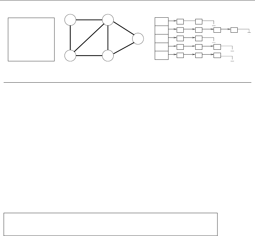
5.2 DATA STRUCTURES FOR GRAPHS 151
0 1 0 0 1
1 0 1 1 1
0 1 1 0 1
0 1 0 1 0
1 1 0 1 0
1
1
2
23
3
4
4
5
512
3
45
1
2
3
4
5
2
1534
24
253
412
5
Figure 5.4: The adjacency matrix and adjacency list of a given graph
be a shorter one (say, if he went to college with my dentist). The friendship
graph is stored implicitly, so I have no way of easily checking.
•Are you truly an individual, or just one of the faceless crowd? – This question
boils down to whether the friendship graph is labeled or unlabeled. Does each
vertex have a name/label which reflects its identify, and is this label important
for our analysis?
Much of the study of social networks is unconcerned with labels on graphs.
Often the index number given a vertex in the graph data structure serves
as its label, perhaps for convenience or the need for anonymity. You may
assert that you are a name, not a number—but try protesting to the guy
who implements the algorithm. Someone studying how an infectious disease
spreads through a graph may label each vertex with whether the person is
healthy or sick, it being irrelevant what their name is.
Take-Home Lesson: Graphs can be used to model a wide variety of structures
and relationships. Graph-theoretic terminology gives us a language to talk
about them.
5.2 Data Structures for Graphs
Selecting the right graph data structure can have an enormous impact on perfor-
mance. Your two basic choices are adjacency matrices and adjacency lists, illus-
trated in Figure 5.4. We assume the graph G=(V,E) contains nvertices and m
edges.
•Adjacency Matrix: We can represent Gusing an n×nmatrix M, where
element M[i, j]=1if(i, j) is an edge of G, and 0 if it isn’t. This allows fast
answers to the question “is (i, j)inG?”, and rapid updates for edge insertion
and deletion. It may use excessive space for graphs with many vertices and
relatively few edges, however.

152 5. GRAPH TRAVERSAL
Comparison Winner
Faster to test if (x, y) is in graph? adjacency matrices
Faster to find the degree of a vertex? adjacency lists
Less memory on small graphs? adjacency lists (m+n)vs.(n2)
Less memory on big graphs? adjacency matrices (a small win)
Edge insertion or deletion? adjacency matrices O(1) vs. O(d)
Faster to traverse the graph? adjacency lists Θ(m+n)vs.Θ(n2)
Better for most problems? adjacency lists
Figure 5.5: Relative advantages of adjacency lists and matrices.
Consider a graph that represents the street map of Manhattan in New York
City. Every junction of two streets will be a vertex of the graph. Neighbor-
ing junctions are connected by edges. How big is this graph? Manhattan is
basically a grid of 15 avenues each crossing roughly 200 streets. This gives us
about 3,000 vertices and 6,000 edges, since each vertex neighbors four other
vertices and each edge is shared between two vertices. This modest amount
of data should easily and efficiently be stored, yet an adjacency matrix would
have 3,000 ×3,000 = 9,000,000 cells, almost all of them empty!
There is some potential to save space by packing multiple bits per word
or simulating a triangular matrix on undirected graphs. But these methods
lose the simplicity that makes adjacency matrices so appealing and, more
critically, remain inherently quadratic on sparse graphs.
•Adjacency Lists: We can more efficiently represent sparse graphs by using
linked lists to store the neighbors adjacent to each vertex. Adjacency lists
require pointers but are not frightening once you have experience with linked
structures.
Adjacency lists make it harder to verify whether a given edge (i, j)isinG,
since we must search through the appropriate list to find the edge. However,
it is surprisingly easy to design graph algorithms that avoid any need for
such queries. Typically, we sweep through all the edges of the graph in one
pass via a breadth-first or depth-first traversal, and update the implications
of the current edge as we visit it. Table 5.5 summarizes the tradeoffs between
adjacency lists and matrices.
Take-Home Lesson: Adjacency lists are the right data structure for most
applications of graphs.
We will use adjacency lists as our primary data structure to represent graphs.
We represent a graph using the following data type. For each graph, we keep a

5.2 DATA STRUCTURES FOR GRAPHS 153
count of the number of vertices, and assign each vertex a unique identification
number from 1 to nvertices. We represent the edges using an array of linked lists:
#define MAXV 1000 /* maximum number of vertices */
typedef struct {
int y; /* adjacency info */
int weight; /* edge weight, if any */
struct edgenode *next; /* next edge in list */
} edgenode;
typedef struct {
edgenode *edges[MAXV+1]; /* adjacency info */
int degree[MAXV+1]; /* outdegree of each vertex */
int nvertices; /* number of vertices in graph */
int nedges; /* number of edges in graph */
bool directed; /* is the graph directed? */
} graph;
We represent directed edge (x, y)byanedgenode yin x’s adjacency list. The de-
gree field of the graph counts the number of meaningful entries for the given vertex.
An undirected edge (x, y) appears twice in any adjacency-based graph structure,
once as yin x’s list, and once as xin y’s list. The boolean flag directed identifies
whether the given graph is to be interpreted as directed or undirected.
To demonstrate the use of this data structure, we show how to read a graph
from a file. A typical graph format consists of an initial line featuring the number
of vertices and edges in the graph, followed by a listing of the edges at one vertex
pair per line.
initialize_graph(graph *g, bool directed)
{
int i; /* counter */
g -> nvertices = 0;
g -> nedges = 0;
g -> directed = directed;
for (i=1; i<=MAXV; i++) g->degree[i] = 0;
for (i=1; i<=MAXV; i++) g->edges[i] = NULL;
}
Actually reading the graph requires inserting each edge into this structure:

154 5. GRAPH TRAVERSAL
read_graph(graph *g, bool directed)
{
int i; /* counter */
int m; /* number of edges */
int x, y; /* vertices in edge (x,y) */
initialize_graph(g, directed);
scanf("%d %d",&(g->nvertices),&m);
for (i=1; i<=m; i++) {
scanf("%d %d",&x,&y);
insert_edge(g,x,y,directed);
}
}
The critical routine is insert edge. The new edgenode is inserted at the begin-
ning of the appropriate adjacency list, since order doesn’t matter. We parameterize
our insertion with the directed Boolean flag, to identify whether we need to insert
two copies of each edge or only one. Note the use of recursion to solve this problem:
insert_edge(graph *g, int x, int y, bool directed)
{
edgenode *p; /* temporary pointer */
p = malloc(sizeof(edgenode)); /* allocate edgenode storage */
p->weight = NULL;
p->y = y;
p->next = g->edges[x];
g->edges[x] = p; /* insert at head of list */
g->degree[x] ++;
if (directed == FALSE)
insert_edge(g,y,x,TRUE);
else
g->nedges ++;
}
Printing the associated graph is just a matter of two nested loops, one through
vertices, the other through adjacent edges:

5.3 WAR STORY: I WAS A VICTIM OF MOORE’S LAW 155
print_graph(graph *g)
{
int i; /* counter */
edgenode *p; /* temporary pointer */
for (i=1; i<=g->nvertices; i++) {
printf("%d: ",i);
p = g->edges[i];
while (p != NULL) {
printf(" %d",p->y);
p = p->next;
}
printf("\n");
}
}
It is a good idea to use a well-designed graph data type as a model for building
your own, or even better as the foundation for your application. We recommend
LEDA (see Section 19.1.1 (page 658)) or Boost (see Section 19.1.3 (page 659)) as
the best-designed general-purpose graph data structures currently available. They
may be more powerful (and hence somewhat slower/larger) than you need, but
they do so many things right that you are likely to lose most of the potential
do-it-yourself benefits through clumsiness.
5.3 War Story: I was a Victim of Moore’s Law
I am the author of a popular library of graph algorithms called Combinatorica (see
www.combinatorica.com), which runs under the computer algebra system Mathe-
matica. Efficiency is a great challenge in Mathematica, due to its applicative model
of computation (it does not support constant-time write operations to arrays) and
the overhead of interpretation (as opposed to compilation). Mathematica code is
typically 1,000 to 5,000 times slower than C code.
Such slow downs can be a tremendous performance hit. Even worse, Mathemat-
ica was a memory hog, needing a then-outrageous 4MB of main memory to run
effectively when I completed Combinatorica in 1990. Any computation on large
structures was doomed to thrash in virtual memory. In such an environment, my
graph package could only hope to work effectively on very small graphs.
One design decision I made as a result was to use adjacency matrices as the
basic Combinatorica graph data structure instead of lists. This may sound peculiar.
If pressed for memory, wouldn’t it pay to use adjacency lists and conserve every last
byte? Yes, but the answer is not so simple for very small graphs. An adjacency list
representation of a weighted n-vertex, m-edge graph should use about n+2mwords
to represent; the 2mcomes from storing the endpoint and weight components of

156 5. GRAPH TRAVERSAL
Figure 5.6: Representative Combinatorica graphs: edge-disjoint paths (left), Hamiltonian cycle
in a hypercube (center), animated depth-first search tree traversal (right)
each edge. Thus, the space advantages of adjacency lists kick in when n+2mis
substantially smaller than n2. The adjacency matrix is still manageable in size for
n≤100 and, of course, half the size of adjacency lists on dense graphs.
My more immediate concern was dealing with the overhead of using a slow
interpreted language. Check out the benchmarks reported in Table 5.1. Two par-
ticularly complex but polynomial-time problems on 9 and 16 vertex graphs took
several minutes to complete on my desktop machine in 1990! The quadratic-sized
data structure certainly could not have had much impact on these running times,
since 9 ×9 equals only 81. From experience, I knew the Mathematica programming
language handled better to regular structures like adjacency matrices better than
irregular-sized adjacency lists.
Still, Combinatorica proved to be a very good thing despite these performance
problems. Thousands of people have used my package to do all kinds of interesting
things with graphs. Combinatorica was never intended to be a high-performance
algorithms library. Most users quickly realized that computations on large graphs
were out of the question, but were eager to take advantage of Combinatorica as a
mathematical research tool and prototyping environment. Everyone was happy.
But over the years, my users started asking why it took so long to do a modest-
sized graph computation. The mystery wasn’t that my program was slow, because
it had always been slow. The question was why did it take so many years for people
to figure this out?

5.3 WAR STORY: I WAS A VICTIM OF MOORE’S LAW 157
Approximate year 1990 1991 1998 2000 2004
command/machine Sun-3 Sun-4 Sun-5 Ultra 5 SunBlade
PlanarQ[GridGraph[4,4]] 234.10 69.65 27.50 3.60 0.40
Length[Partitions[30]] 289.85 73.20 24.40 3.44 1.58
VertexConnectivity[GridGraph[3,3]] 239.67 47.76 14.70 2.00 0.91
RandomPartition[1000] 831.68 267.5 22.05 3.12 0.87
Table 5.1: Old Combinatorica benchmarks on low-end Sun workstations, from 1990 to today,
(running time in seconds)
The reason is that computers keep doubling in speed every two years or so.
People’s expectation of how long something should take moves in concert with
these technology improvements. Partially because of Combinatorica’s dependence
on a quadratic-size graph data structure, it didn’t scale as well as it should on
sparse graphs.
As the years rolled on, user demands become more insistent. Combinatorica
needed to be updated. My collaborator, Sriram Pemmaraju, rose to the challenge.
We (mostly he) completely rewrote Combinatorica to take advantage of faster graph
data structures ten years after the initial version.
The new Combinatorica uses a list of edges data structure for graphs, largely
motivated by increased efficiency. Edge lists are linear in the size of the graph (edges
plus vertices), just like adjacency lists. This makes a huge difference on most graph
related functions—for large enough graphs. The improvement is most dramatic
in “fast” graph algorithms—those that run in linear or near linear-time, such as
graph traversal, topological sort, and finding connected/biconnected components.
The implications of this change is felt throughout the package in running time
improvements and memory savings. Combinatorica can now work with graphs that
are about 50-100 times larger than graphs that the old package could deal with.
Figure 5.7(l) plots the running time of the MinimumSpanningTree functions for
both Combinatorica versions. The test graphs were sparse (grid graphs), designed
to highlight the difference between the two data structures. Yes, the new version is
much faster, but note that the difference only becomes important for graphs larger
than the old Combinatorica was designed for. However, the relative difference in
run time keeps growing with increasing n. Figure 5.7(r) plots the ratio of the
running times as a function of graph size. The difference between linear size and
quadratic size is asymptotic, so the consequences become ever more important as
ngets larger.
What is the weird bump in running times that occurs around n≈250? This
likely reflects a transition between levels of the memory hierarchy. Such bumps
are not uncommon in today’s complex computer systems. Cache performance in
data structure design should be an important but not overriding consideration.
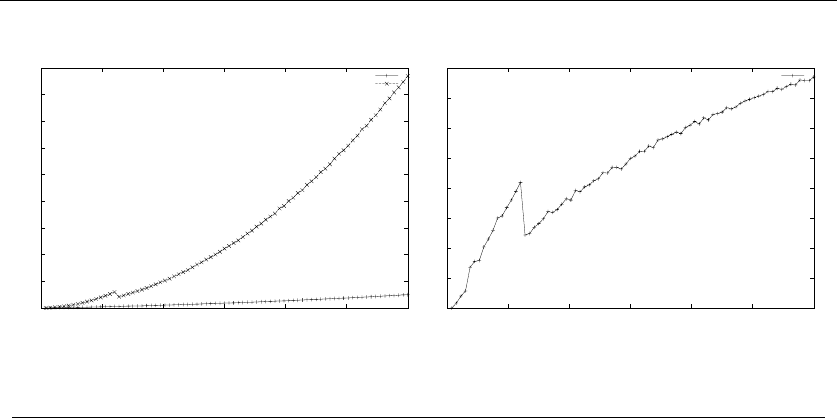
158 5. GRAPH TRAVERSAL
0
5
10
15
20
25
30
35
40
45
0 200 400 600 800 1000 1200
Running Time in Seconds
Vertices in Graph
Running Time of Minimum Spanning Tree in Old and New Combinatorica
New Combinatorica
Old Combinatorica
2
4
6
8
10
12
14
16
18
0200 400 600 800 1000 1200
Ratio
Vertices in Graph
Ratio of Running Times for Mininum Spanning Tree in Old and New Combinatorica
Run time ratio
Figure 5.7: Performance comparison between old and new Combinatorica: absolute running
times (l), and the ratio of these times (r).
The asymptotic gains due to adjacency lists more than trumped any impact of the
cache.
Two main lessons can be taken away from our experience developing Combina-
torica:
•To make a program run faster, just wait – Sophisticated hardware eventually
slithers down to everybody. We observe a speedup of more than 200-fold for
the original version of Combinatorica as a consequence of 15 years of faster
hardware. In this context, the further speedups we obtained from upgrading
the package become particularly dramatic.
•Asymptotics eventually do matter – It was my mistake not to anticipate future
developments in technology. While no one has a crystal ball, it is fairly safe
to say that future computers will have more memory and run faster than
today’s. This gives an edge to asymptotically more efficient algorithms/data
structures, even if their performance is close on today’s instances. If the
implementation complexity is not substantially greater, play it safe and go
with the better algorithm.
5.4 War Story: Getting the Graph
“It takes five minutes just to read the data. We will never have time to make it do
something interesting.”
The young graduate student was bright and eager, but green to the power of
data structures. She would soon come to appreciate their power.
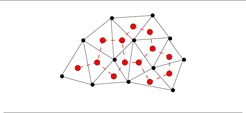
5.4 WAR STORY: GETTING THE GRAPH 159
Figure 5.8: The dual graph (dashed lines) of a triangulation
As described in a previous war story (see Section 3.6 (page 85)), we were ex-
perimenting with algorithms to extract triangular strips for the fast rendering of
triangulated surfaces. The task of finding a small number of strips that cover each
triangle in a mesh could be modeled as a graph problem. The graph has a vertex for
every triangle of the mesh, with an edge between every pair of vertices representing
adjacent triangles. This dual graph representation (see Figure 5.8) captures all the
information needed to partition the triangulation into triangle strips.
The first step in crafting a program that constructs a good set of strips was to
build the dual graph of the triangulation. This I sent the student off to do. A few
days later, she came back and announced that it took over five CPU minutes just
to construct this dual graph of a few thousand triangles.
“Nonsense!” I proclaimed. “You must be doing something very wasteful in build-
ing the graph. What format is the data in?”
“Well, it starts out with a list of the 3D coordinates of the vertices used in the
model and then follows with a list of triangles. Each triangle is described by a list
of three indices into the vertex coordinates. Here is a small example:”
VERTICES 4
0.000000 240.000000 0.000000
204.000000 240.000000 0.000000
204.000000 0.000000 0.000000
0.000000 0.000000 0.000000
TRIANGLES 2
013
123
“I see. So the first triangle uses all but the third point, since all the indices
start from zero. The two triangles must share an edge formed by points 1 and 3.”
“Yeah, that’s right,” she confirmed.

160 5. GRAPH TRAVERSAL
“OK. Now tell me how you built your dual graph from this file.”
“Well, I can ignore the vertex information once I know how many vertices there
are. The geometric position of the points doesn’t affect the structure of the graph.
My dual graph is going to have as many vertices as the number of triangles. I set
up an adjacency list data structure with that many vertices. As I read in each
triangle, I compare it to each of the others to check whether it has two end points
in common. If it does, I add an edge from the new triangle to this one.”
I started to sputter. “But that’s your problem right there! You are comparing
each triangle against every other triangle, so that constructing the dual graph will
be quadratic in the number of triangles. Reading the input graph should take linear
time!”
“I’m not comparing every triangle against every other triangle. On average, it
only tests against half or a third of the triangles.”
“Swell. But that still leaves us with an O(n2) algorithm. That is much too
slow.”
She stood her ground. “Well, don’t just complain. Help me fix it!”
Fair enough. I started to think. We needed some quick method to screen away
most of the triangles that would not be adjacent to the new triangle (i, j, k). What
we really needed was a separate list of all the triangles that go through each of
the points i,j,andk. By Euler’s formula for planar graphs, the average point is
incident on less than six triangles. This would compare each new triangle against
fewer than twenty others, instead of most of them.
“We are going to need a data structure consisting of an array with one element
for every vertex in the original data set. This element is going to be a list of all the
triangles that pass through that vertex. When we read in a new triangle, we will
look up the three relevant lists in the array and compare each of these against the
new triangle. Actually, only two of the three lists need be tested, since any adjacent
triangles will share two points in common. We will add an adjacency to our graph
for every triangle-pair sharing two vertices. Finally, we will add our new triangle to
each of the three affected lists, so they will be updated for the next triangle read.”
She thought about this for a while and smiled. “Got it, Chief. I’ll let you know
what happens.”
The next day she reported that the graph could be built in seconds, even for
much larger models. From here, she went on to build a successful program for
extracting triangle strips, as reported in Section 3.6 (page 85).
The take-home lesson is that even elementary problems like initializing data
structures can prove to be bottlenecks in algorithm development. Most programs
working with large amounts of data have to run in linear or almost linear time.
Such tight performance demands leave no room to be sloppy. Once you focus on
the need for linear-time performance, an appropriate algorithm or heuristic can
usually be found to do the job.

5.5 TRAVERSING A GRAPH 161
5.5 Traversing a Graph
Perhaps the most fundamental graph problem is to visit every edge and vertex in a
graph in a systematic way. Indeed, all the basic bookkeeping operations on graphs
(such printing or copying graphs, and converting between alternate representations)
are applications of graph traversal.
Mazes are naturally represented by graphs, where each graph vertex denotes a
junction of the maze, and each graph edge denotes a hallway in the maze. Thus, any
graph traversal algorithm must be powerful enough to get us out of an arbitrary
maze. For efficiency, we must make sure we don’t get trapped in the maze and visit
the same place repeatedly. For correctness, we must do the traversal in a systematic
way to guarantee that we get out of the maze. Our search must take us through
every edge and vertex in the graph.
The key idea behind graph traversal is to mark each vertex when we first visit
it and keep track of what we have not yet completely explored. Although bread
crumbs or unraveled threads have been used to mark visited places in fairy-tale
mazes, we will rely on Boolean flags or enumerated types.
Each vertex will exist in one of three states:
•undiscovered – the vertex is in its initial, virgin state.
•discovered – the vertex has been found, but we have not yet checked out all
its incident edges.
•processed – the vertex after we have visited all its incident edges.
Obviously, a vertex cannot be processed until after we discover it, so the state
of each vertex progresses over the course of the traversal from undiscovered to
discovered to processed.
We must also maintain a structure containing the vertices that we have dis-
covered but not yet completely processed. Initially, only the single start vertex is
considered to be discovered. To completely explore a vertex v, we must evaluate
each edge leaving v. If an edge goes to an undiscovered vertex x, we mark xdis-
covered and add it to the list of work to do. We ignore an edge that goes to a
processed vertex, because further contemplation will tell us nothing new about the
graph. We can also ignore any edge going to a discovered but not processed vertex,
because the destination already resides on the list of vertices to process.
Each undirected edge will be considered exactly twice, once when each of its
endpoints is explored. Directed edges will be considered only once, when exploring
the source vertex. Every edge and vertex in the connected component must eventu-
ally be visited. Why? Suppose that there exists a vertex uthat remains unvisited,
whose neighbor vwas visited. This neighbor vwill eventually be explored, after
which we will certainly visit u. Thus, we must find everything that is there to be
found.
We describe the mechanics of these traversal algorithms and the significance of
the traversal order below.
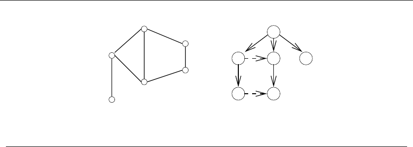
162 5. GRAPH TRAVERSAL
6
1
52
3 4
1
2
3
4
5
6
Figure 5.9: An undirected graph and its breadth-first search tree
5.6 Breadth-First Search
The basic breadth-first search algorithm is given below. At some point during the
course of a traversal, every node in the graph changes state from undiscovered to
discovered. In a breadth-first search of an undirected graph, we assign a direction
to each edge, from the discoverer uto the discovered v. We thus denote uto be the
parent of v. Since each node has exactly one parent, except for the root, this defines
a tree on the vertices of the graph. This tree, illustrated in Figure 5.9, defines a
shortest path from the root to every other node in the tree. This property makes
breadth-first search very useful in shortest path problems.
BFS(G, s)
for each vertex u∈V[G]−{s}do
state[u] = “undiscovered”
p[u]=nil,i.e.noparentisintheBFStree
state[s] = “discovered”
p[s]=nil
Q={s}
while Q=∅do
u= dequeue[Q]
process vertex uas desired
for each v∈Adj[u]do
process edge (u, v) as desired
if state[v] = “undiscovered” then
state[v] = “discovered”
p[v]=u
enqueue[Q, v]
state[u] = “processed”
The graph edges that do not appear in the breadth-first search tree also have
special properties. For undirected graphs, nontree edges can point only to vertices
on the same level as the parent vertex, or to vertices on the level directly below

5.6 BREADTH-FIRST SEARCH 163
the parent. These properties follow easily from the fact that each path in the tree
must be the shortest path in the graph. For a directed graph, a back-pointing edge
(u, v) can exist whenever vlies closer to the root than udoes.
Implementation
Our breadth-first search implementation bfs uses two Boolean arrays to maintain
our knowledge about each vertex in the graph. A vertex is discovered the first time
we visit it. A vertex is considered processed after we have traversed all outgoing
edges from it. Thus, each vertex passes from undiscovered to discovered to processed
over the course of the search. This information could have been maintained using
one enumerated type variable, but we used two Boolean variables instead.
bool processed[MAXV+1]; /* which vertices have been processed */
bool discovered[MAXV+1]; /* which vertices have been found */
int parent[MAXV+1]; /* discovery relation */
Each vertex is initialized as undiscovered:
initialize_search(graph *g)
{
int i; /* counter */
for (i=1; i<=g->nvertices; i++) {
processed[i] = discovered[i] = FALSE;
parent[i] = -1;
}
}
Once a vertex is discovered, it is placed on a queue. Since we process these
vertices in first-in, first-out order, the oldest vertices are expanded first, which are
exactly those closest to the root:
bfs(graph *g, int start)
{
queue q; /* queue of vertices to visit */
int v; /* current vertex */
int y; /* successor vertex */
edgenode *p; /* temporary pointer */
init_queue(&q);
enqueue(&q,start);
discovered[start] = TRUE;

164 5. GRAPH TRAVERSAL
while (empty_queue(&q) == FALSE) {
v = dequeue(&q);
process_vertex_early(v);
processed[v] = TRUE;
p = g->edges[v];
while (p != NULL) {
y = p->y;
if ((processed[y] == FALSE) || g->directed)
process_edge(v,y);
if (discovered[y] == FALSE) {
enqueue(&q,y);
discovered[y] = TRUE;
parent[y] = v;
}
p = p->next;
}
process_vertex_late(v);
}
}
5.6.1 Exploiting Traversal
The exact behavior of bfs depends upon the functions process vertex early(),
process vertex late(),andprocess edge(). Through these functions, we can
customize what the traversal does as it makes its official visit to each edge
and each vertex. Initially, we will do all of vertex processing on entry, so
process vertex late() returns without action:
process_vertex_late(int v)
{
}
By setting the active functions to
process_vertex_early(int v)
{
printf("processed vertex %d\n",v);
}
process_edge(int x, int y)
{
printf("processed edge (%d,%d)\n",x,y);
}

5.6 BREADTH-FIRST SEARCH 165
we print each vertex and edge exactly once. If we instead set process edge to
process_edge(int x, int y)
{
nedges = nedges + 1;
}
we get an accurate count of the number of edges. Different algorithms perform
different actions on vertices or edges as they are encountered. These functions give
us the freedom to easily customize our response.
5.6.2 Finding Paths
The parent array set within bfs() is very useful for finding interesting paths
through a graph. The vertex that discovered vertex iis defined as parent[i].
Every vertex is discovered during the course of traversal, so except for the root
every node has a parent. The parent relation defines a tree of discovery with the
initial search node as the root of the tree.
Because vertices are discovered in order of increasing distance from the root,
this tree has a very important property. The unique tree path from the root to
each node x∈Vuses the smallest number of edges (or equivalently, intermediate
nodes) possible on any root-to-xpath in the graph.
We can reconstruct this path by following the chain of ancestors from xto the
root. Note that we have to work backward. We cannot find the path from the root
to x, since that does not follow the direction of the parent pointers. Instead, we
must find the path from xto the root. Since this is the reverse of how we normally
want the path, we can either (1) store it and then explicitly reverse it using a stack,
or (2) let recursion reverse it for us, as follows:
find_path(int start, int end, int parents[])
{
if ((start == end) || (end == -1))
printf("\n%d",start);
else {
find_path(start,parents[end],parents);
printf(" %d",end);
}
}
On our breadth-first search graph example (Figure 5.9) our algorithm generated
the following parent relation:
vertex 1 23456
parent -112511

166 5. GRAPH TRAVERSAL
For the shortest path from 1 to 4, upper-right corner, this parent relation yields
the path {1,5,4}.
There are two points to remember when using breadth-first search to find a
shortest path from xto y: First, the shortest path tree is only useful if BFS was
performed with xas the root of the search. Second, BFS gives the shortest path
only if the graph is unweighted. We will present algorithms for finding shortest
paths in weighted graphs in Section 6.3.1 (page 206).
5.7 Applications of Breadth-First Search
Most elementary graph algorithms make one or two traversals of the graph while
we update our knowledge of the graph. Properly implemented using adjacency lists,
any such algorithm is destined to be linear, since BFS runs in O(n+m) time on
both directed and undirected graphs. This is optimal, since it is as fast as one can
hope to read any n-vertex, m-edge graph.
The trick is seeing when traversal approaches are destined to work. We present
several examples below.
5.7.1 Connected Components
The “six degrees of separation” theory argues that there is always a short path
linking every two people in the world. We say that a graph is connected if there
is a path between any two vertices. If the theory is true, it means the friendship
graph must be connected.
Aconnected component of an undirected graph is a maximal set of vertices such
that there is a path between every pair of vertices. The components are separate
“pieces” of the graph such that there is no connection between the pieces. If we
envision tribes in remote parts of the world that have yet not been encountered,
each such tribe would form a separate connected component in the friendship graph.
A remote hermit, or extremely unpleasant fellow, would represent a connected
component of one vertex.
An amazing number of seemingly complicated problems reduce to finding or
counting connected components. For example, testing whether a puzzle such as
Rubik’s cube or the 15-puzzle can be solved from any position is really asking
whether the graph of legal configurations is connected.
Connected components can be found using breadth-first search, since the vertex
order does not matter. We start from the first vertex. Anything we discover during
this search must be part of the same connected component. We then repeat the
search from any undiscovered vertex (if one exists) to define the next component,
and so on until all vertices have been found:

5.7 APPLICATIONS OF BREADTH-FIRST SEARCH 167
connected_components(graph *g)
{
int c; /* component number */
int i; /* counter */
initialize_search(g);
c=0;
for (i=1; i<=g->nvertices; i++)
if (discovered[i] == FALSE) {
c = c+1;
printf("Component %d:",c);
bfs(g,i);
printf("\n");
}
}
process_vertex_early(int v)
{
printf(" %d",v);
}
process_edge(int x, int y)
{
}
Observe how we increment a counter cdenoting the current component number
with each call to bfs. We could have explicitly bound each vertex to its component
number (instead of printing the vertices in each component) by changing the action
of process vertex.
There are two distinct notions of connectivity for directed graphs, leading to
algorithms for finding both weakly connected and strongly connected components.
Both of these can be found in O(n+m) time, as discussed in Section 15.1 (page
477).
5.7.2 Two-Coloring Graphs
The vertex-coloring problem seeks to assign a label (or color) to each vertex of a
graph such that no edge links any two vertices of the same color. We can easily
avoid all conflicts by assigning each vertex a unique color. However, the goal is to
use as few colors as possible. Vertex coloring problems often arise in scheduling
applications, such as register allocation in compilers. See Section 16.7 (page 544)
for a full treatment of vertex-coloring algorithms and applications.

168 5. GRAPH TRAVERSAL
Agraphisbipartite if it can be colored without conflicts while using only two
colors. Bipartite graphs are important because they arise naturally in many appli-
cations. Consider the “had-sex-with” graph in a heterosexual world. Men have sex
only with women, and vice versa. Thus, gender defines a legal two-coloring, in this
simple model.
But how can we find an appropriate two-coloring of a graph, thus separating
the men from the women? Suppose we assume that the starting vertex is male.
All vertices adjacent to this man must be female, assuming the graph is indeed
bipartite.
We can augment breadth-first search so that whenever we discover a new vertex,
we color it the opposite of its parent. We check whether any nondiscovery edge links
two vertices of the same color. Such a conflict means that the graph cannot be two-
colored. Otherwise, we will have constructed a proper two-coloring whenever we
terminate without conflict.
twocolor(graph *g)
{
int i; /* counter */
for (i=1; i<=(g->nvertices); i++)
color[i] = UNCOLORED;
bipartite = TRUE;
initialize_search(&g);
for (i=1; i<=(g->nvertices); i++)
if (discovered[i] == FALSE) {
color[i] = WHITE;
bfs(g,i);
}
}
process_edge(int x, int y)
{
if (color[x] == color[y]) {
bipartite = FALSE;
printf("Warning: not bipartite due to (%d,%d)\n",x,y);
}
color[y] = complement(color[x]);
}

5.8 DEPTH-FIRST SEARCH 169
complement(int color)
{
if (color == WHITE) return(BLACK);
if (color == BLACK) return(WHITE);
return(UNCOLORED);
}
We can assign the first vertex in any connected component to be whatever
color/sex we wish. BFS can separate the men from the women, but we can’t tell
them apart just by using the graph structure.
Take-Home Lesson: Breadth-first and depth-first searches provide mechanisms
to visit each edge and vertex of the graph. They prove the basis of most simple,
efficient graph algorithms.
5.8 Depth-First Search
There are two primary graph traversal algorithms: breadth-first search (BFS) and
depth-first search (DFS). For certain problems, it makes absolutely no difference
which you use, but in others the distinction is crucial.
The difference between BFS and DFS results is in the order in which they
explore vertices. This order depends completely upon the container data structure
used to store the discovered but not processed vertices.
•Queue – By storing the vertices in a first-in, first-out (FIFO) queue, we
explore the oldest unexplored vertices first. Thus our explorations radiate
out slowly from the starting vertex, defining a breadth-first search.
•Stack – By storing the vertices in a last-in, first-out (LIFO) stack, we explore
the vertices by lurching along a path, visiting a new neighbor if one is avail-
able, and backing up only when we are surrounded by previously discovered
vertices. Thus, our explorations quickly wander away from our starting point,
defining a depth-first search.
Our implementation of dfs maintains a notion of traversal time for each vertex.
Our time clock ticks each time we enter or exit any vertex. We keep track of the
entry and exit times for each vertex.
Depth-first search has a neat recursive implementation, which eliminates the
need to explicitly use a stack:
DFS(G, u)
state[u] = “discovered”
process vertex uif desired
entry[u]=time

170 5. GRAPH TRAVERSAL
time =time +1
for each v∈Adj[u]do
process edge (u, v) if desired
if state[v] = “undiscovered” then
p[v]=u
DFS(G, v)
state[u] = “processed”
exit[u]=time
time =time +1
The time intervals have interesting and useful properties with respect to depth-
first search:
•Who is an ancestor? – Suppose that xis an ancestor of yin the DFS tree.
This implies that we must enter xbefore y, since there is no way we can be
born before our own father or grandfather! We also must exit ybefore we
exit x, because the mechanics of DFS ensure we cannot exit xuntil after we
have backed up from the search of all its descendants. Thus the time interval
of ymust be properly nested within ancestor x.
•How many descendants? – The difference between the exit and entry times
for vtells us how many descendents vhas in the DFS tree. The clock gets
incremented on each vertex entry and vertex exit, so half the time difference
denotes the number of descendents of v.
We will use these entry and exit times in several applications of depth-first
search, particularly topological sorting and biconnected/strongly-connected com-
ponents. We need to be able to take separate actions on each entry and exit,
thus motivating distinct process vertex early and process vertex late rou-
tines called from dfs.
The other important property of a depth-first search is that it partitions the
edges of an undirected graph into exactly two classes: tree edges and back edges.The
tree edges discover new vertices, and are those encoded in the parent relation. Back
edges are those whose other endpoint is an ancestor of the vertex being expanded,
so they point back into the tree.
An amazing property of depth-first search is that all edges fall into these two
classes. Why can’t an edge go to a brother or cousin node instead of an ancestor?
All nodes reachable from a given vertex vare expanded before we finish with the
traversal from v, so such topologies are impossible for undirected graphs. This edge
classification proves fundamental to the correctness of DFS-based algorithms.
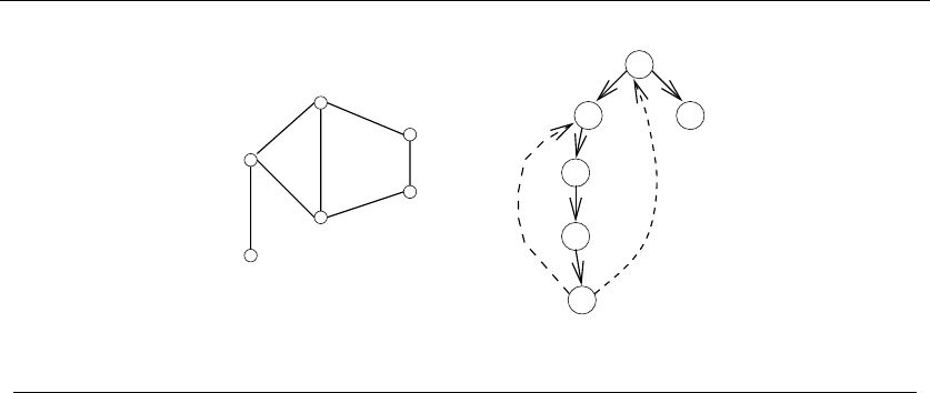
5.8 DEPTH-FIRST SEARCH 171
1
26
3
4
5
1
2
3
4
5
6
Figure 5.10: An undirected graph and its depth-first search tree
Implementation
A depth-first search can be thought of as a breadth-first search with a stack instead
of a queue. The beauty of implementing dfs recursively is that recursion eliminates
the need to keep an explicit stack:
dfs(graph *g, int v)
{
edgenode *p; /* temporary pointer */
int y; /* successor vertex */
if (finished) return; /* allow for search termination */
discovered[v] = TRUE;
time = time + 1;
entry_time[v] = time;
process_vertex_early(v);
p = g->edges[v];
while (p != NULL) {
y = p->y;
if (discovered[y] == FALSE) {
parent[y] = v;
process_edge(v,y);
dfs(g,y);
}
else if ((!processed[y]) || (g->directed))
process_edge(v,y);

172 5. GRAPH TRAVERSAL
if (finished) return;
p = p->next;
}
process_vertex_late(v);
time = time + 1;
exit_time[v] = time;
processed[v] = TRUE;
}
Depth-first search use essentially the same idea as backtracking, which we study
in Section 7.1 (page 231). Both involve exhaustively searching all possibilities by ad-
vancing if it is possible, and backing up as soon as there is no unexplored possibility
for further advancement. Both are most easily understood as recursive algorithms.
Take-Home Lesson: DFS organizes vertices by entry/exit times, and edges
into tree and back edges. This organization is what gives DFS its real power.
5.9 Applications of Depth-First Search
As algorithm design paradigms go, a depth-first search isn’t particularly intimidat-
ing. It is surprisingly subtle, however meaning that its correctness requires getting
details right.
The correctness of a DFS-based algorithm depends upon specifics of exactly
when we process the edges and vertices. We can process vertex veither before we
have traversed any of the outgoing edges from v(process vertex early())orafter
we have finished processing all of them (process vertex late()). Sometimes we
will take special actions at both times, say process vertex early() to initialize a
vertex-specific data structure, which will be modified on edge-processing operations
and then analyzed afterwards using process vertex late().
In undirected graphs, each edge (x, y) sits in the adjacency lists of vertex x
and y. Thus there are two potential times to process each edge (x, y), namely when
exploring xand when exploring y. The labeling of edges as tree edges or back edges
occurs during the first time the edge is explored. This first time we see an edge is
usually a logical time to do edge-specific processing. Sometimes, we may want to
take different action the second time we see an edge.
But when we encounter edge (x, y)fromx, how can we tell if we have previously
traversed the edge from y? The issue is easy if vertex yis undiscovered: (x, y)

5.9 APPLICATIONS OF DEPTH-FIRST SEARCH 173
Figure 5.11: An articulation vertex is the weakest point in the graph
becomes a tree edge so this must be the first time. The issue is also easy if yhas
not been completely processed; since we explored the edge when we explored y
this must be the second time. But what if yis an ancestor of x, and thus in a
discovered state? Careful reflection will convince you that this must be our first
traversal unless yis the immediate ancestor of x—i.e. , (y, x) is a tree edge. This
can be established by testing if y == parent[x].
I find that the subtlety of depth-first search-based algorithms kicks me in the
head whenever I try to implement one. I encourage you to analyze these implemen-
tations carefully to see where the problematic cases arise and why.
5.9.1 Finding Cycles
Back edges are the key to finding a cycle in an undirected graph. If there is no
back edge, all edges are tree edges, and no cycle exists in a tree. But any back edge
going from xto an ancestor ycreates a cycle with the tree path from yto x. Such
a cycle is easy to find using dfs:
process_edge(int x, int y)
{
if (parent[x] != y) { /* found back edge! */
printf("Cycle from %d to %d:",y,x);
find_path(y,x,parent);
printf("\n\n");
finished = TRUE;
}
}
The correctness of this cycle detection algorithm depends upon processing each
undirected edge exactly once. Otherwise, a spurious two-vertex cycle (x, y, x) could
be composed from the two traversals of any single undirected edge. We use the
finished flag to terminate after finding the first cycle.
5.9.2 Articulation Vertices
Suppose you are a vandal seeking to disrupt the telephone network. Which station
in Figure 5.11 should you choose to blow up to cause the maximum amount of

174 5. GRAPH TRAVERSAL
5
4
3
62
1
Figure 5.12: DFS tree of a graph containing two articulation vertices (namely 1 and 2). Back
edge (5,2) keeps vertices 3 and 4 from being cut-nodes. Vertices 5 and 6 escape as leaves of
the DFS tree
damage? Observe that there is a single point of failure—a single vertex whose
deletion disconnects a connected component of the graph. Such a vertex is called
an articulation vertex or cut-node. Any graph that contains an articulation vertex
is inherently fragile, because deleting that single vertex causes a loss of connectivity
between other nodes.
We presented a breadth-first search-based connected components algorithm in
Section 5.7.1 (page 166). In general, the connectivity of a graph is the smallest
number of vertices whose deletion will disconnect the graph. The connectivity is
one if the graph has an articulation vertex. More robust graphs without such a
vertex are said to be biconnected. Connectivity will be further discussed in the
catalog in Section 15.8 (page 505).
Testing for articulation vertices by brute force is easy. Temporarily delete each
vertex v, and then do a BFS or DFS traversal of the remaining graph to establish
whether it is still connected. The total time for nsuch traversals is O(n(m+n)).
There is a clever linear-time algorithm, however, that tests all the vertices of a
connected graph using a single depth-first search.
What might the depth-first search tree tell us about articulation vertices? This
tree connects all the vertices of the graph. If the DFS tree represented the entirety of
the graph, all internal (nonleaf) nodes would be articulation vertices, since deleting
any one of them would separate a leaf from the root. Blowing up a leaf (such as
vertices 2 and 6 in Figure 5.12) cannot disconnect the tree, since it connects no
one but itself to the main trunk.

5.9 APPLICATIONS OF DEPTH-FIRST SEARCH 175
The root of the search tree is a special case. If it has only one child, it functions
as a leaf. But if the root has two or more children, its deletion disconnects them,
making the root an articulation vertex.
General graphs are more complex than trees. But a depth-first search of a
general graph partitions the edges into tree edges and back edges. Think of these
back edges as security cables linking a vertex back to one of its ancestors. The
security cable from xback to yensures that none of the vertices on the tree path
between xand ycan be articulation vertices. Delete any of these vertices, and the
security cable will still hold all of them to the rest of the tree.
Finding articulation vertices requires maintaining the extent to which back
edges (i.e. , security cables) link chunks of the DFS tree back to ancestor nodes.
Let reachable ancestor[v] denote the earliest reachable ancestor of vertex v,
meaning the oldest ancestor of vthat we can reach by a combination of tree edges
and back edges. Initially, reachable ancestor[v] = v:
int reachable_ancestor[MAXV+1]; /* earliest reachable ancestor of v */
int tree_out_degree[MAXV+1]; /* DFS tree outdegree of v */
process_vertex_early(int v)
{
reachable_ancestor[v] = v;
}
We update reachable ancestor[v] whenever we encounter a back edge that
takes us to an earlier ancestor than we have previously seen. The relative age/rank
of our ancestors can be determined from their entry time’s:
process_edge(int x, int y)
{
int class; /* edge class */
class = edge_classification(x,y);
if (class == TREE)
tree_out_degree[x] = tree_out_degree[x] + 1;
if ((class == BACK) && (parent[x] != y)) {
if (entry_time[y] < entry_time[ reachable_ancestor[x] ] )
reachable_ancestor[x] = y;
}
}
The key issue is determining how the reachability relation impacts whether
vertex vis an articulation vertex. There are three cases, as shown in Figure 5.13:
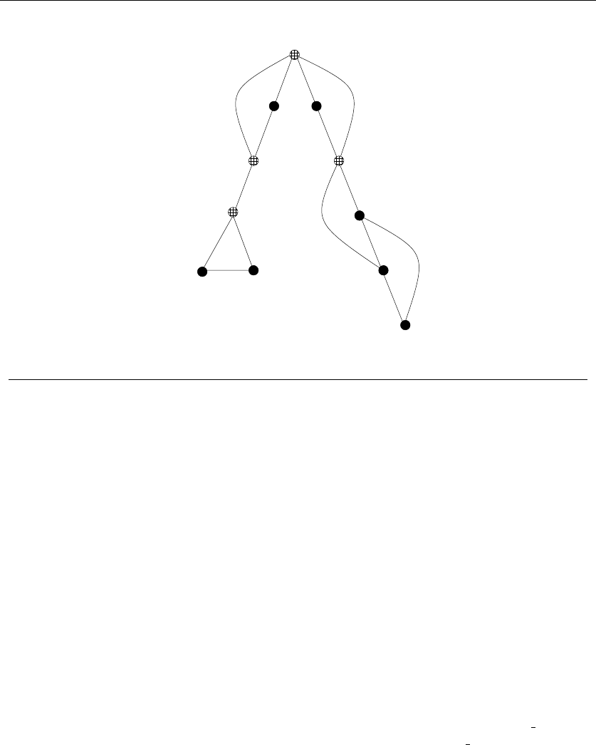
176 5. GRAPH TRAVERSAL
Figure 5.13: The three cases of articulation vertices: root, bridge, and parent cut-nodes
•Root cut-nodes – If the root of the DFS tree has two or more children, it must
be an articulation vertex. No edges from the subtree of the second child can
possibly connect to the subtree of the first child.
•Bridge cut-nodes – If the earliest reachable vertex from vis v, then deleting
the single edge (parent[v],v) disconnects the graph. Clearly parent[v] must
be an articulation vertex, since it cuts vfrom the graph. Vertex vis also an
articulation vertex unless it is a leaf of the DFS tree. For any leaf, nothing
falls off when you cut it.
•Parent cut-nodes – If the earliest reachable vertex from vis the parent of v,
then deleting the parent must sever vfrom the tree unless the parent is the
root.
The routine below systematically evaluates each of the three conditions as we
back up from the vertex after traversing all outgoing edges. We use entry time[v]
to represent the age of vertex v. The reachability time time vcalculated below
denotes the oldest vertex that can be reached using back edges. Getting back to
an ancestor above vrules out the possibility of vbeing a cut-node:
parent cutnode (of v)
vbridge cutnode
bridge cutnode
root cutnode

5.9 APPLICATIONS OF DEPTH-FIRST SEARCH 177
process_vertex_late(int v)
{
bool root; /* is the vertex the root of the DFS tree? */
int time_v; /* earliest reachable time for v */
int time_parent; /* earliest reachable time for parent[v] */
if (parent[v] < 1) { /* test if v is the root */
if (tree_out_degree[v] > 1)
printf("root articulation vertex: %d \n",v);
return;
}
root = (parent[parent[v]] < 1); /* is parent[v] the root? */
if ((reachable_ancestor[v] == parent[v]) && (!root))
printf("parent articulation vertex: %d \n",parent[v]);
if (reachable_ancestor[v] == v) {
printf("bridge articulation vertex: %d \n",parent[v]);
if (tree_out_degree[v] > 0) /* test if v is not a leaf */
printf("bridge articulation vertex: %d \n",v);
}
time_v = entry_time[reachable_ancestor[v]];
time_parent = entry_time[ reachable_ancestor[parent[v]] ];
if (time_v < time_parent)
reachable_ancestor[parent[v]] = reachable_ancestor[v];
}
The last lines of this routine govern when we back up a node’s highest reachable
ancestor to its parent, namely whenever it is higher than the parent’s earliest
ancestor to date.
We can alternately talk about reliability in terms of edge failures instead of
vertex failures. Perhaps our vandal would find it easier to cut a cable instead of
blowing up a switching station. A single edge whose deletion disconnects the graph
is called a bridge; any graph without such an edge is said to be edge-biconnected.
Identifying whether a given edge (x, y) is a bridge is easily done in linear time
by deleting the edge and testing whether the resulting graph is connected. In fact
all bridges can be identified in the same O(n+m) time. Edge (x, y) is a bridge if (1)
it is a tree edge, and (2) no back edge connects from yor below to xor above. This
can be computed with a minor modification of the reachable ancestor function.
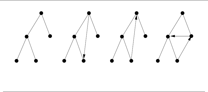
178 5. GRAPH TRAVERSAL
Cross EdgesTree Edges Back EdgeForward Edge
Figure 5.14: Possible edge cases for BFS/DFS traversal
5.10 Depth-First Search on Directed Graphs
Depth-first search on an undirected graph proves useful because it organizes the
edges of the graph in a very precise way, as shown in Figure 5.10.
When traversing undirected graphs, every edge is either in the depth-first search
tree or a back edge to an ancestor in the tree. Let us review why. Suppose we
encountered a “forward edge” (x, y) directed toward a descendant vertex. In this
case, we would have discovered (x, y) while exploring y, making it a back edge.
Suppose we encounter a “cross edge” (x, y), linking two unrelated vertices. Again,
we would have discovered this edge when we explored y, making it a tree edge.
For directed graphs, depth-first search labelings can take on a wider range of
possibilities. Indeed, all four of the edge cases in Figure 5.14 can occur in traversing
directed graphs. Still, this classification proves useful in organizing algorithms on
directed graphs. We typically take a different action on edges from each different
case.
The correct labeling of each edge can be readily determined from the state,
discovery time, and parent of each vertex, as encoded in the following function:
int edge_classification(int x, int y)
{
if (parent[y] == x) return(TREE);
if (discovered[y] && !processed[y]) return(BACK);
if (processed[y] && (entry_time[y]>entry_time[x])) return(FORWARD);
if (processed[y] && (entry_time[y]<entry_time[x])) return(CROSS);
printf("Warning: unclassified edge (%d,%d)\n",x,y);
}
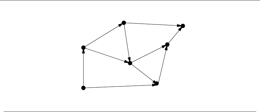
5.10 DEPTH-FIRST SEARCH ON DIRECTED GRAPHS 179
D
A
GF
E
C
B
Figure 5.15: A DAG with only one topological sort (G, A, B, C, F, E, D)
As with BFS, this implementation of the depth-first search algorithm includes
places to optionally process each vertex and edge—say to copy them, print them, or
count them. Both algorithms will traverse all edges in the same connected compo-
nent as the starting point. Since we need to start with a vertex in each component
to traverse a disconnected graph, we must start from any vertex remaining undis-
covered after a component search. With the proper initialization, this completes
the traversal algorithm:
DFS-graph(G)
for each vertex u∈V[G]do
state[u] = “undiscovered”
for each vertex u∈V[G]do
if state[u] = “undiscovered” then
initialize new component, if desired
DFS(G, u)
I encourage the reader to convince themselves of the correctness of these four
conditions. What I said earlier about the subtlety of depth-first search goes double
for directed graphs.
5.10.1 Topological Sorting
Topological sorting is the most important operation on directed acyclic graphs
(DAGs). It orders the vertices on a line such that all directed edges go from left to
right. Such an ordering cannot exist if the graph contains a directed cycle, because
there is no way you can keep going right on a line and still return back to where
you started from!
Each DAG has at least one topological sort. The importance of topological
sorting is that it gives us an ordering to process each vertex before any of its
successors. Suppose the edges represented precedence constraints, such that edge

180 5. GRAPH TRAVERSAL
(x, y) means job xmust be done before job y. Then, any topological sort defines a
legal schedule. Indeed, there can be many such orderings for a given DAG.
But the applications go deeper. Suppose we seek the shortest (or longest) path
from xto yin a DAG. No vertex appearing after yin the topological order can
contribute to any such path, because there will be no way to get back to y.We
can appropriately process all the vertices from left to right in topological order,
considering the impact of their outgoing edges, and know that we will have looked
at everything we need before we need it. Topological sorting proves very useful in
essentially any algorithmic problem on directed graphs, as discussed in the catalog
in Section 15.2 (page 481).
Topological sorting can be performed efficiently using depth-first searching. A
directed graph is a DAG if and only if no back edges are encountered. Labeling
the vertices in the reverse order that they are marked processed finds a topological
sort of a DAG. Why? Consider what happens to each directed edge {x, y}as we
encounter it exploring vertex x:
•If yis currently undiscovered, then we start a DFS of ybefore we can continue
with x.Thusyis marked completed before xis, and xappears before yin
the topological order, as it must.
•If yis discovered but not completed, then {x, y}is a back edge, which is
forbidden in a DAG.
•If yis processed, then it will have been so labeled before x. Therefore, x
appears before yin the topological order, as it must.
Study the following implementation:
process_vertex_late(int v)
{
push(&sorted,v);
}
process_edge(int x, int y)
{
int class; /* edge class */
class = edge_classification(x,y);
if (class == BACK)
printf("Warning: directed cycle found, not a DAG\n");
}

5.10 DEPTH-FIRST SEARCH ON DIRECTED GRAPHS 181
topsort(graph *g)
{
int i; /* counter */
init_stack(&sorted);
for (i=1; i<=g->nvertices; i++)
if (discovered[i] == FALSE)
dfs(g,i);
print_stack(&sorted); /* report topological order */
}
We push each vertex on a stack as soon as we have evaluated all outgoing edges.
The top vertex on the stack always has no incoming edges from any vertex on the
stack. Repeatedly popping them off yields a topological ordering.
5.10.2 Strongly Connected Components
We are often concerned with strongly connected components—that is, partitioning
a graph into chunks such that directed paths exist between all pairs of vertices
within a given chunk. A directed graph is strongly connected if there is a directed
path between any two vertices. Road networks should be strongly connected, or
else there will be places you can drive to but not drive home from without violating
one-way signs.
It is straightforward to use graph traversal to test whether a graph G=(V,E)
is strongly connected in linear time. First, do a traversal from some arbitrary vertex
v. Every vertex in the graph had better be reachable from v(and hence discovered
on the BFS or DFS starting from v), otherwise Gcannot possibly be strongly
connected. Now construct a graph G=(V,E) with the same vertex and edge
set as Gbut with all edges reversed—i.e., directed edge (x, y)∈Eiff (y, x)∈E.
Thus, any path from vto zin Gcorresponds to a path from zto vin G. By doing
a DFS from vin G, we find all vertices with paths to vin G. The graph is strongly
connected iff all vertices in Gcan (1) reach vand (2) are reachable from v.
Graphs that are not strongly connected can be partitioned into strongly con-
nected components, as shown in Figure 5.16 (left). The set of such components
and the weakly-connecting edges that link them together can be determined using
DFS. The algorithm is based on the observation that it is easy to find a directed
cycle using a depth-first search, since any back edge plus the down path in the
DFS tree gives such a cycle. All vertices in this cycle must be in the same strongly
connected component. Thus, we can shrink (contract) the vertices on this cycle
down to a single vertex representing the component, and then repeat. This process
terminates when no directed cycle remains, and each vertex represents a different
strongly connected component.
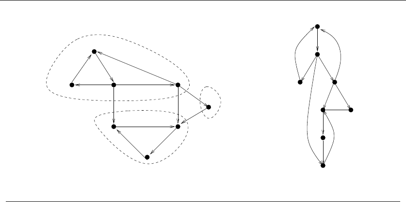
182 5. GRAPH TRAVERSAL
3 2
8
7
5
6
34
2
1
56
7
8
4
1
Figure 5.16: The strongly-connected components of a graph, with the associated DFS tree
Our approach to implementing this idea is reminiscent of finding biconnected
components in Section 5.9.2 (page 173). We update our notion of the oldest reach-
able vertex in response to (1) nontree edges and (2) backing up from a vertex.
Because we are working on a directed graph, we also must contend with forward
edges (from a vertex to a descendant) and cross edges (from a vertex back to an
nonancestor but previously discovered vertex). Our algorithm will peal one strong
component off the tree at a time, and assign each of its vertices the number of the
component it is in:
strong_components(graph *g)
{
int i; /* counter */
for (i=1; i<=(g->nvertices); i++) {
low[i] = i;
scc[i] = -1;
}
components_found = 0;
init_stack(&active);
initialize_search(&g);
for (i=1; i<=(g->nvertices); i++)
if (discovered[i] == FALSE) {
dfs(g,i);
}
}

5.10 DEPTH-FIRST SEARCH ON DIRECTED GRAPHS 183
Define low[v] to be the oldest vertex known to be in the same strongly con-
nected component as v. This vertex is not necessarily an ancestor, but may also
be a distant cousin of vbecause of cross edges. Cross edges that point vertices
from previous strongly connected components of the graph cannot help us, because
there can be no way back from them to v, but otherwise cross edges are fair game.
Forward edges have no impact on reachability over the depth-first tree edges, and
hence can be disregarded:
int low[MAXV+1]; /* oldest vertex surely in component of v */
int scc[MAXV+1]; /* strong component number for each vertex */
process_edge(int x, int y)
{
int class; /* edge class */
class = edge_classification(x,y);
if (class == BACK) {
if (entry_time[y] < entry_time[ low[x] ] )
low[x] = y;
}
if (class == CROSS) {
if (scc[y] == -1) /* component not yet assigned */
if (entry_time[y] < entry_time[ low[x] ] )
low[x] = y;
}
}
A new strongly connected component is found whenever the lowest reachable
vertex from vis v. If so, we can clear the stack of this component. Otherwise, we
give our parent the benefit of the oldest ancestor we can reach and backtrack:
process_vertex_early(int v)
{
push(&active,v);
}

184 5. GRAPH TRAVERSAL
process_vertex_late(int v)
{
if (low[v] == v) { /* edge (parent[v],v) cuts off scc */
pop_component(v);
}
if (entry_time[low[v]] < entry_time[low[parent[v]]])
low[parent[v]] = low[v];
}
pop_component(int v)
{
int t; /* vertex placeholder */
components_found = components_found + 1;
scc[ v ] = components_found;
while ((t = pop(&active)) != v) {
scc[ t ] = components_found;
}
}
Chapter Notes
Our treatment of graph traversal represents an expanded version of material from
Chapter 9 of [SR03]. The Combinatorica graph library discussed in the war story
is best described in the old [Ski90]. and new editions [PS03] of the associated book.
Accessible introductions to the science of social networks include Barabasi [Bar03]
and Watts [Wat04].
5.11 Exercises
Simulating Graph Algorithms
5-1. [3] For the following graphs G1(left) and G2(right):
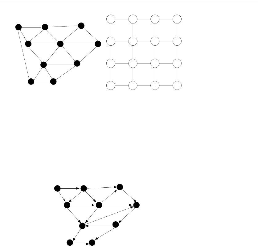
5.11 EXERCISES 185
AB C
F
GH
I
J
63
1
3
4
6
8
2
11
3
6
22
1
E
D
9
4
7
24
ABCD
EFGH
IJKL
MNOP
2
1
4
10
5
3
11
1
18
13
4
9
6
9
1
11
12
8
20
4
22
23
5
9
(a) Report the order of the vertices encountered on a breadth-first search starting
from vertex A. Break all ties by picking the vertices in alphabetical order (i.e.,
Abefore Z).
(b) Report the order of the vertices encountered on a depth-first search starting
from vertex A. Break all ties by picking the vertices in alphabetical order (i.e.,
Abefore Z).
5-2. [3] Do a topological sort of the following graph G:
AB C
DE
F
GH
I
J
Traversal
5-3. [3] Prove by induction that there is a unique path between any pair of vertices in
a tree.
5-4. [3] Prove that in a breadth-first search on a undirected graph G,everyedgeis
either a tree edge or a cross edge, where xis neither an ancestor nor descendant of
y, in cross edge (x, y).
5-5. [3] Give a linear algorithm to compute the chromatic number of graphs where each
vertex has degree at most 2. Must such graphs be bipartite?
5-6. [5] In breadth-first and depth-first search, an undiscovered node is marked discov-
ered when it is first encountered, and marked processed when it has been completely

186 5. GRAPH TRAVERSAL
+
*
2
34
+
*
/
34
5
+
+
*
/
2
34
5
Figure 5.17: Expression 2 + 3 ∗4+(3∗4)/5 as a tree and a DAG
searched. At any given moment, several nodes might be simultaneously in the dis-
covered state.
(a) Describe a graph on nvertices and a particular starting vertex vsuch that
Θ(n) nodes are simultaneously in the discovered state during a breadth-first search
starting from v.
(b) Describe a graph on nvertices and a particular starting vertex vsuch that Θ(n)
nodes are simultaneously in the discovered state during a depth-first search starting
from v.
(c) Describe a graph on nvertices and a particular starting vertex vsuch that at
some point Θ(n)nodesremainundiscovered, while Θ(n) nodes have been processed
during a depth-first search starting from v.(Note,theremayalsobediscovered
nodes.)
5-7. [4] Given pre-order and in-order traversals of a binary tree, is it possible to recon-
struct the tree? If so, sketch an algorithm to do it. If not, give a counterexample.
Repeat the problem if you are given the pre-order and post-order traversals.
5-8. [3] Present correct and efficient algorithms to convert an undirected graph Gbe-
tween the following graph data structures. You must give the time complexity of
each algorithm, assuming nvertices and medges.
(a) Convert from an adjacency matrix to adjacency lists.
(b) Convert from an adjacency list to an incidence matrix. An incidence matrix
Mhas a row for each vertex and a column for each edge, such that M[i, j]=1
if vertex iis part of edge j, otherwise M[i, j]=0.
(c) Convert from an incidence matrix to adjacency lists.
5-9. [3] Suppose an arithmetic expression is given as a tree. Each leaf is an integer and
each internal node is one of the standard arithmetical operations (+,−,∗,/). For
example, the expression 2 + 3 ∗4+(3∗4)/5 is represented by the tree in Figure
5.17(a). Give an O(n) algorithm for evaluating such an expression, where there are
nnodes in the tree.
5-10. [5] Suppose an arithmetic expression is given as a DAG (directed acyclic graph)
with common subexpressions removed. Each leaf is an integer and each internal

5.11 EXERCISES 187
node is one of the standard arithmetical operations (+,−,∗,/). For example, the
expression 2 + 3 ∗4+(3∗4)/5 is represented by the DAG in Figure 5.17(b). Give
an O(n+m) algorithm for evaluating such a DAG, where there are nnodes and
medges in the DAG. Hint: modify an algorithm for the tree case to achieve the
desired efficiency.
5-11. [8] The war story of Section 5.4 (page 158) describes an algorithm for constructing
the dual graph of the triangulation efficiently, although it does not guarantee linear
time. Give a worst-case linear algorithm for the problem.
Algorithm Design
5-12. [5] The square of a directed graph G=(V,E) is the graph G2=(V,E2) such that
(u, w)∈E2iff there exists v∈Vsuch that (u, v)∈Eand (v, w)∈E; i.e., there is
a path of exactly two edges from uto w.
Give efficient algorithms for both adjacency lists and matrices.
5-13. [5] Avertex cover of a graph G=(V,E) is a subset of vertices Vsuch that each
edge in Eis incident on at least one vertex of V.
(a) Give an efficient algorithm to find a minimum-size vertex cover if Gis a tree.
(b) Let G=(V, E) be a tree such that the weight of each vertex is equal to the
degree of that vertex. Give an efficient algorithm to find a minimum-weight
vertex cover of G.
(c) Let G=(V, E) be a tree with arbitrary weights associated with the vertices.
Give an efficient algorithm to find a minimum-weight vertex cover of G.
5-14. [3] Avertex cover of a graph G=(V,E) is a subset of vertices V∈Vsuch that
every edge in Econtains at least one vertex from V. Delete all the leaves from any
depth-first search tree of G. Must the remaining vertices form a vertex cover of G?
Give a proof or a counterexample.
5-15. [5] Avertex cover of a graph G=(V,E) is a subset of vertices V∈Vsuch that
every edge in Econtains at least one vertex from V.Anindependent set of graph
G=(V,E) is a subset of vertices V∈Vsuch that no edge in Econtains both
vertices from V.
An independent vertex cover is a subset of vertices that is both an independent set
and a vertex cover of G. Give an efficient algorithm for testing whether Gcontains
an independent vertex cover. What classical graph problem does this reduce to?
5-16. [5] An independent set of an undirected graph G=(V,E)isasetofverticesU
such that no edge in Eis incident on two vertices of U.
(a) Give an efficient algorithm to find a maximum-size independent set if Gis a
tree.
(b) Let G=(V,E) be a tree with weights associated with the vertices such that
the weight of each vertex is equal to the degree of that vertex. Give an efficient
algorithm to find a maximum independent set of G.
(c) Let G=(V, E) be a tree with arbitrary weights associated with the vertices.
Give an efficient algorithm to find a maximum independent set of G.

188 5. GRAPH TRAVERSAL
5-17. [5] Consider the problem of determining whether a given undirected graph G=
(V,E)containsatriangle or cycle of length 3.
(a) Give an O(|V|3) to find a triangle if one exists.
(b) Improve your algorithm to run in time O(|V|·|E|). You may assume |V|≤|E|.
Observe that these bounds gives you time to convert between the adjacency matrix
and adjacency list representations of G.
5-18. [5] Consider a set of movies M1,M
2,...,M
k. There is a set of customers, each one
of which indicates the two movies they would like to see this weekend. Movies are
shown on Saturday evening and Sunday evening. Multiple movies may be screened
at the same time.
You must decide which movies should be televised on Saturday and which on Sun-
day, so that every customer gets to see the two movies they desire. Is there a
schedule where each movie is shown at most once? Design an efficient algorithm to
find such a schedule if one exists.
5-19. [5] The diameter of a tree T=(V, E)isgivenby
max
u,v∈Vδ(u, v)
(where δ(u, v) is the number of edges on the path from uto v). Describe an efficient
algorithm to compute the diameter of a tree, and show the correctness and analyze
the running time of your algorithm.
5-20. [5] Given an undirected graph Gwith nvertices and medges, and an integer k,
give an O(m+n) algorithm that finds the maximum induced subgraph Hof G
such that each vertex in Hhas degree ≥k, or prove that no such graph exists. An
induced subgraph F=(U, R) of a graph G=(V,E) is a subset of Uof the vertices
Vof G, and all edges Rof Gsuch that both vertices of each edge are in U.
5-21. [6] Let vand wbe two vertices in a directed graph G=(V, E). Design a linear-
time algorithm to find the number of different shortest paths (not necessarily vertex
disjoint) between vand w. Note: the edges in Gare unweighted.
5-22. [6] Design a linear-time algorithm to eliminate each vertex vof degree 2 from
a graph by replacing edges (u, v)and(v, w)byanedge(u, w). We also seek to
eliminate multiple copies of edges by replacing them with a single edge. Note that
removing multiple copies of an edge may create a new vertex of degree 2, which has
to be removed, and that removing a vertex of degree 2 may create multiple edges,
which also must be removed.
Directed Graphs
5-23. [5] Your job is to arrange nill-behaved children in a straight line, facing front. You
are given a list of mstatements of the form “ihates j”. If ihates j, then you do not
want put isomewhere behind j, because then iis capable of throwing something
at j.
(a) Give an algorithm that orders the line, (or says that it is not possible) in
O(m+n)time.

5.11 EXERCISES 189
(b) Suppose instead you want to arrange the children in rows such that if ihates
j,thenimust be in a lower numbered row than j. Give an efficient algorithm
to find the minimum number of rows needed, if it is possible.
5-24. [3] Adding a single directed edge to a directed graph can reduce the number of
weakly connected components, but by at most how many components? What about
the number of strongly connected components?
5-25. [5] An arborescence of a directed graph Gis a rooted tree such that there is a
directed path from the root to every other vertex in the graph. Give an efficient
and correct algorithm to test whether Gcontains an arborescence, and its time
complexity.
5-26. [5] Amother vertex in a directed graph G=(V,E)isavertexvsuch that all other
vertices Gcan be reached by a directed path from v.
(a) Give an O(n+m) algorithm to test whether a given vertex vis a mother of
G,wheren=|V|and m=|E|.
(b) Give an O(n+m) algorithm to test whether graph Gcontains a mother vertex.
5-27. [9] Atournament is a directed graph formed by taking the complete undirected
graph and assigning arbitrary directions on the edges—i.e., a graph G=(V, E)
such that for all u,v∈V, exactly one of (u, v)or(v, u)isinE. Show that every
tournament has a Hamiltonian path—that is, a path that visits every vertex exactly
once. Give an algorithm to find this path.
Articulation Vertices
5-28. [5] An articulation vertex of a graph Gis a vertex whose deletion disconnects G.
Let Gbe a graph with nvertices and medges. Give a simple O(n+m) algorithm
for finding a vertex of Gthat is not an articulation vertex—i.e. , whose deletion
does not disconnect G.
5-29. [5] Following up on the previous problem, give an O(n+m) algorithm that finds a
deletion order for the nvertices such that no deletion disconnects the graph. (Hint:
think DFS/BFS.)
5-30. [3] Suppose Gis a connected undirected graph. An edge ewhose removal disconnects
the graph is called a bridge. Must every bridge ebe an edge in a depth-first search
tree of G? Give a proof or a counterexample.
Interview Problems
5-31. [3] Which data structures are used in depth-first and breath-first search?
5-32. [4] Write a function to traverse binary search tree and return the ith node in sorted
order.
Programming Challenges
These programming challenge problems with robot judging are available at
http://www.programming-challenges.com or http://online-judge.uva.es.
5-1. “Bicoloring” – Programming Challenges 110901, UVA Judge 10004.

190 5. GRAPH TRAVERSAL
5-2. “Playing with Wheels” – Programming Challenges 110902, UVA Judge 10067.
5-3. “The Tourist Guide” – Programming Challenges 110903, UVA Judge 10099.
5-4. “Edit Step Ladders” – Programming Challenges 110905, UVA Judge 10029.
5-5. “Tower of Cubes” – Programming Challenges 110906, UVA Judge 10051.

6
Weighted Graph Algorithms
The data structures and traversal algorithms of Chapter 5 provide the basic build-
ing blocks for any computation on graphs. However, all the algorithms presented
there dealt with unweighted graphs—i.e. , graphs where each edge has identical
value or weight.
There is an alternate universe of problems for weighted graphs. The edges of
road networks are naturally bound to numerical values such as construction cost,
traversal time, length, or speed limit. Identifying the shortest path in such graphs
proves more complicated than breadth-first search in unweighted graphs, but opens
the door to a wide range of applications.
The graph data structure from Chapter 5 quietly supported edge-weighted
graphs, but here we make this explicit. Our adjacency list structure consists of
an array of linked lists, such that the outgoing edges from vertex xappear in the
list edges[x]:
typedef struct {
edgenode *edges[MAXV+1]; /* adjacency info */
int degree[MAXV+1]; /* outdegree of each vertex */
int nvertices; /* number of vertices in graph */
int nedges; /* number of edges in graph */
int directed; /* is the graph directed? */
} graph;
Each edgenode is a record containing three fields, the first describing the second
endpoint of the edge (y), the second enabling us to annotate the edge with a weight
(weight), and the third pointing to the next edge in the list (next):
S.S. Skiena, The Algorithm Design Manual, 2nd ed., DOI: 10.1007/978-1-84800-070-4 6,
c
Springer-Verlag London Limited 2008

192 6. WEIGHTED GRAPH ALGORITHMS
typedef struct {
int y; /* adjacency info */
int weight; /* edge weight, if any */
struct edgenode *next; /* next edge in list */
} edgenode;
We now describe several sophisticated algorithms using this data structure,
including minimum spanning trees, shortest paths, and maximum flows. That these
optimization problems can be solved efficiently is quite worthy of our respect. Recall
that no such algorithm exists for the first weighted graph problem we encountered,
namely the traveling salesman problem.
6.1 Minimum Spanning Trees
Aspanning tree of a graph G=(V, E) is a subset of edges from Eforming a
tree connecting all vertices of V. For edge-weighted graphs, we are particularly
interested in the minimum spanning tree—the spanning tree whose sum of edge
weights is as small as possible.
Minimum spanning trees are the answer whenever we need to connect a set
of points (representing cities, homes, junctions, or other locations) by the smallest
amount of roadway, wire, or pipe. Any tree is the smallest possible connected graph
in terms of number of edges, while the minimum spanning tree is the smallest
connected graph in terms of edge weight. In geometric problems, the point set
p1,...,p
ndefines a complete graph, with edge (vi,v
j) assigned a weight equal to
the distance from pito pj. An example of a geometric minimum spanning tree is
illustrated in Figure 6.1. Additional applications of minimum spanning trees are
discussed in Section 15.3 (page 484).
A minimum spanning tree minimizes the total length over all possible spanning
trees. However, there can be more than one minimum spanning tree in a graph.
Indeed, all spanning trees of an unweighted (or equally weighted) graph Gare
minimum spanning trees, since each contains exactly n−1 equal-weight edges.
Such a spanning tree can be found using depth-first or breadth-first search. Finding
a minimum spanning tree is more difficult for general weighted graphs, however
two different algorithms are presented below. Both demonstrate the optimality of
certain greedy heuristics.
6.1.1 Prim’s Algorithm
Prim’s minimum spanning tree algorithm starts from one vertex and grows the rest
of the tree one edge at a time until all vertices are included.
Greedy algorithms make the decision of what to do next by selecting the best
local option from all available choices without regard to the global structure. Since
we seek the tree of minimum weight, the natural greedy algorithm for minimum

6.1 MINIMUM SPANNING TREES 193
(a) (b) (c)
Figure 6.1: (a) Two spanning trees of point set; (b) the minimum spanning tree, and (c) the
shortest path from center tree
spanning tree repeatedly selects the smallest weight edge that will enlarge the
number of vertices in the tree.
Prim-MST(G)
Select an arbitrary vertex sto start the tree from.
While (there are still nontree vertices)
Select the edge of minimum weight between a tree and nontree vertex
Add the selected edge and vertex to the tree Tprim.
Prim’s algorithm clearly creates a spanning tree, because no cycle can be in-
troduced by adding edges between tree and nontree vertices. However, why should
it be of minimum weight over all spanning trees? We have seen ample evidence of
other natural greedy heuristics that do not yield a global optimum. Therefore, we
must be particularly careful to demonstrate any such claim.
We use proof by contradiction. Suppose that there existed a graph Gfor which
Prim’s algorithm did not return a minimum spanning tree. Since we are building the
tree incrementally, this means that there must have been some particular instant
where we went wrong. Before we inserted edge (x, y), Tprim consisted of a set of
edges that was a subtree of some minimum spanning tree Tmin, but choosing edge
(x, y) fatally took us away from a minimum spanning tree (see Figure 6.2(a)).
But how could we have gone wrong? There must be a path pfrom xto yin
Tmin, as shown in Figure 6.2(b). This path must use an edge (v1,v
2), where v1
is in Tprim, but v2is not. This edge (v1,v
2) must have weight at least that of
(x, y), or Prim’s algorithm would have selected it before (x, y) when it had the
chance. Inserting (x, y) and deleting (v1,v
2)fromTmin leaves a spanning tree no
larger than before, meaning that Prim’s algorithm did not make a fatal mistake in
selecting edge (x, y). Therefore, by contradiction, Prim’s algorithm must construct
a minimum spanning tree.
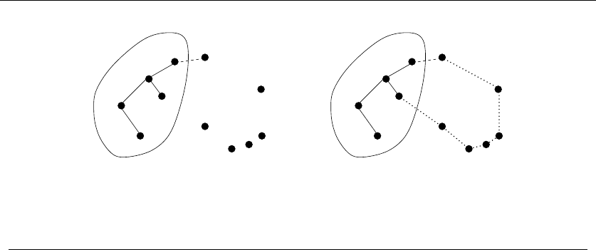
194 6. WEIGHTED GRAPH ALGORITHMS
v1
v2
(a) (b)
s
xy
s
xy
Figure 6.2: Where Prim’s algorithm goes bad? No, because d(v1,v
2)≥d(x, y)
Implementation
Prim’s algorithm grows the minimum spanning tree in stages, starting from a given
vertex. At each iteration, we add one new vertex into the spanning tree. A greedy
algorithm suffices for correctness: we always add the lowest-weight edge linking a
vertex in the tree to a vertex on the outside. The simplest implementation of this
idea would assign each vertex a Boolean variable denoting whether it is already in
the tree (the array intree in the code below), and then searches all edges at each
iteration to find the minimum weight edge with exactly one intree vertex.
Our implementation is somewhat smarter. It keeps track of the cheapest edge
linking every nontree vertex in the tree. The cheapest such edge over all remaining
non-tree vertices gets added in each iteration. We must update the costs of getting
to the non-tree vertices after each insertion. However, since the most recently in-
serted vertex is the only change in the tree, all possible edge-weight updates must
come from its outgoing edges:
prim(graph *g, int start)
{
int i; /* counter */
edgenode *p; /* temporary pointer */
bool intree[MAXV+1]; /* is the vertex in the tree yet? */
int distance[MAXV+1]; /* cost of adding to tree */
int v; /* current vertex to process */
int w; /* candidate next vertex */
int weight; /* edge weight */
int dist; /* best current distance from start */
for (i=1; i<=g->nvertices; i++) {
intree[i] = FALSE;

6.1 MINIMUM SPANNING TREES 195
distance[i] = MAXINT;
parent[i] = -1;
}
distance[start] = 0;
v = start;
while (intree[v] == FALSE) {
intree[v] = TRUE;
p = g->edges[v];
while (p != NULL) {
w = p->y;
weight = p->weight;
if ((distance[w] > weight) && (intree[w] == FALSE)) {
distance[w] = weight;
parent[w] = v;
}
p = p->next;
}
v=1;
dist = MAXINT;
for (i=1; i<=g->nvertices; i++)
if ((intree[i] == FALSE) && (dist > distance[i])) {
dist = distance[i];
v=i;
}
}
}
Analysis
Prim’s algorithm is correct, but how efficient is it? This depends on which data
structures are used to implement it. In the pseudocode, Prim’s algorithm makes
niterations sweeping through all medges on each iteration—yielding an O(mn)
algorithm.
But our implementation avoids the need to test all medges on each pass. It
only considers the ≤ncheapest known edges represented in the parent array
and the ≤nedges out of new tree vertex vto update parent. By maintaining a
Boolean flag along with each vertex to denote whether it is in the tree or not, we
test whether the current edge joins a tree with a non-tree vertex in constant time.
The result is an O(n2) implementation of Prim’s algorithm, and a good illustra-
tion of power of data structures to speed up algorithms. In fact, more sophisticated
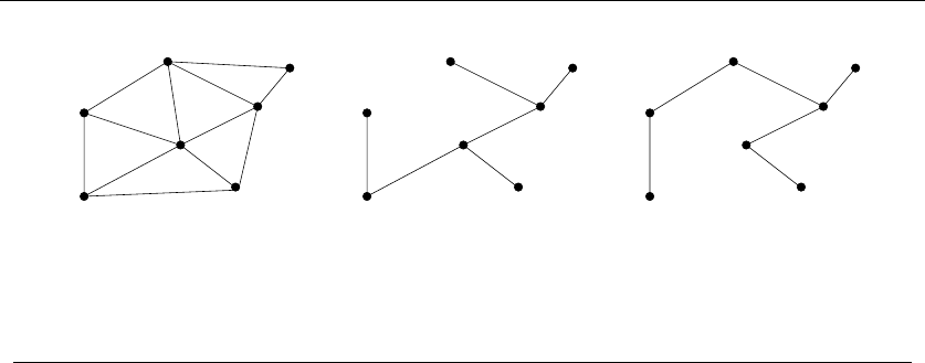
196 6. WEIGHTED GRAPH ALGORITHMS
6
Kruskal(G)Prim(G,A)G
3
A
2
3
4
1
5
A
4
26
5
1
A
2
5
4
3
7
12
7
47
2
9
5
Figure 6.3: A graph G(l) with minimum spanning trees produced by Prim’s (m) and Kruskal’s
(r) algorithms. The numbers on the trees denote the order of insertion; ties are broken arbi-
trarily
priority-queue data structures lead to an O(m+nlg n) implementation, by making
it faster to find the minimum cost edge to expand the tree at each iteration.
The minimum spanning tree itself or its cost can be reconstructed in two dif-
ferent ways. The simplest method would be to augment this procedure with state-
ments that print the edges as they are found or totals the weight of all selected
edges. Alternately, the tree topology is encoded by the parent array, so it plus the
original graph describe everything about the minimum spanning tree.
6.1.2 Kruskal’s Algorithm
Kruskal’s algorithm is an alternate approach to finding minimum spanning trees
that proves more efficient on sparse graphs. Like Prim’s, Kruskal’s algorithm is
greedy. Unlike Prim’s, it does not start with a particular vertex.
Kruskal’s algorithm builds up connected components of vertices, culminating in
the minimum spanning tree. Initially, each vertex forms its own separate component
in the tree-to-be. The algorithm repeatedly considers the lightest remaining edge
and tests whether its two endpoints lie within the same connected component. If
so, this edge will be discarded, because adding it would create a cycle in the tree-
to-be. If the endpoints are in different components, we insert the edge and merge
the two components into one. Since each connected component is always a tree, we
need never explicitly test for cycles.
Kruskal-MST(G)
Put the edges in a priority queue ordered by weight.
count =0
while (count < n −1) do
get next edge (v, w)
if (component (v)= component(w))
add to Tkruskal
merge component(v) and component(w)
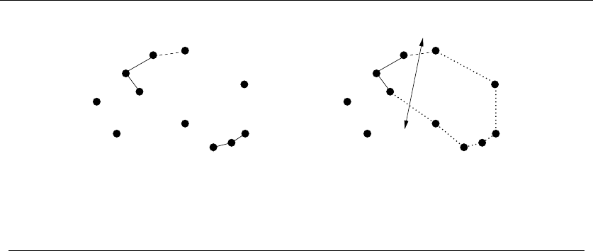
6.1 MINIMUM SPANNING TREES 197
y
v1
v2
(a) (b)
xy
s
x
Figure 6.4: Where Kruskal’s algorithm goes bad? No, because d(v1,v
2)≥d(x, y)
This algorithm adds n−1 edges without creating a cycle, so it clearly creates a
spanning tree for any connected graph. But why must this be a minimum spanning
tree? Suppose it wasn’t. As with the correctness proof of Prim’s algorithm, there
must be some graph on which it fails. In particular, there must a single edge (x, y)
whose insertion first prevented the tree Tkruskal from being a minimum spanning
tree Tmin. Inserting this edge (x, y)intoTmin will create a cycle with the path
from xto y. Since xand ywere in different components at the time of inserting
(x, y), at least one edge (say (v1,v
2)) on this path would have been evaluated by
Kruskal’s algorithm later than (x, y). But this means that w(v1,v
2)≥w(x, y), so
exchanging the two edges yields a tree of weight at most Tmin. Therefore, we could
not have made a fatal mistake in selecting (x, y), and the correctness follows.
What is the time complexity of Kruskal’s algorithm? Sorting the medges takes
O(mlg m) time. The for loop makes miterations, each testing the connectivity
of two trees plus an edge. In the most simple-minded approach, this can be im-
plemented by breadth-first or depth-first search in a sparse graph with at most n
edges and nvertices, thus yielding an O(mn) algorithm.
However, a faster implementation results if we can implement the component
test in faster than O(n) time. In fact, a clever data structure called union-find,can
support such queries in O(lg n) time. Union-find is discussed in the next section.
With this data structure, Kruskal’s algorithm runs in O(mlg m) time, which is
faster than Prim’s for sparse graphs. Observe again the impact that the right data
structure can have when implementing a straightforward algorithm.
Implementation
The implementation of the main routine follows fairly directly from the psuedocode:

198 6. WEIGHTED GRAPH ALGORITHMS
kruskal(graph *g)
{
int i; /* counter */
set_union s; /* set union data structure */
edge_pair e[MAXV+1]; /* array of edges data structure */
bool weight_compare();
set_union_init(&s, g->nvertices);
to_edge_array(g, e); /* sort edges by increasing cost */
qsort(&e,g->nedges,sizeof(edge_pair),weight_compare);
for (i=0; i<(g->nedges); i++) {
if (!same_component(s,e[i].x,e[i].y)) {
printf("edge (%d,%d) in MST\n",e[i].x,e[i].y);
union_sets(&s,e[i].x,e[i].y);
}
}
}
6.1.3 The Union-Find Data Structure
Aset partition is a partitioning of the elements of some universal set (say the
integers 1 to n) into a collection of disjointed subsets. Thus, each element must
be in exactly one subset. Set partitions naturally arise in graph problems such
as connected components (each vertex is in exactly one connected component)
and vertex coloring (a person may be male or female, but not both or neither).
Section 14.6 (page 456) presents algorithms for generating set partitions and related
objects.
The connected components in a graph can be represented as a set partition.
For Kruskal’s algorithm to run efficiently, we need a data structure that efficiently
supports the following operations:
•Same component(v1,v
2)– Do vertices v1and v2occur in the same connected
component of the current graph?
•Merge components(C1,C
2) – Merge the given pair of connected components
into one component in response to an edge between them.
The two obvious data structures for this task each support only one of these
operations efficiently. Explicitly labeling each element with its component number
enables the same component test to be performed in constant time, but updating
the component numbers after a merger would require linear time. Alternately, we
can treat the merge components operation as inserting an edge in a graph, but
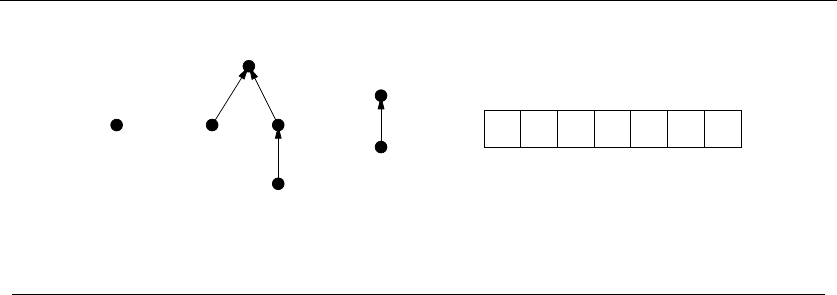
6.1 MINIMUM SPANNING TREES 199
01
4
3
62
7
5
(l)
0
(r)
12
4
345
3
6
4
7
20
Figure 6.5: Union-find example: structure represented as trees (l) and array (r)
then we must run a full graph traversal to identify the connected components on
demand.
The union-find data structure represents each subset as a “backwards” tree,
with pointers from a node to its parent. Each node of this tree contains a set
element, and the name of the set is taken from the key at the root. For reasons
that will become clear, we will also maintain the number of elements in the subtree
rooted in each vertex v:
typedef struct {
int p[SET_SIZE+1]; /* parent element */
int size[SET_SIZE+1]; /* number of elements in subtree i */
int n; /* number of elements in set */
} set_union;
We implement our desired component operations in terms of two simpler oper-
ations, union and find:
•Find(i) – Find the root of tree containing element i, by walking up the parent
pointers until there is nowhere to go. Return the label of the root.
•Union(i,j) – Link the root of one of the trees (say containing i)totheroot
of the tree containing the other (say j)sofind(i) now equals find(j).
We seek to minimize the time it takes to execute any sequence of unions and
finds. Tree structures can be very unbalanced, so we must limit the height of
our trees. Our most obvious means of control is the decision of which of the two
component roots becomes the root of the combined component on each union.
To minimize the tree height, it is better to make the smaller tree the subtree
of the bigger one. Why? The height of all the nodes in the root subtree stay the
same, while the height of the nodes merged into this tree all increase by one. Thus,
merging in the smaller tree leaves the height unchanged on the larger set of vertices.

200 6. WEIGHTED GRAPH ALGORITHMS
Implementation
The implementation details are as follows:
set_union_init(set_union *s, int n)
{
int i; /* counter */
for (i=1; i<=n; i++) {
s->p[i] = i;
s->size[i] = 1;
}
s->n = n;
}
int find(set_union *s, int x)
{
if (s->p[x] == x)
return(x);
else
return( find(s,s->p[x]) );
}
int union_sets(set_union *s, int s1, int s2)
{
int r1, r2; /* roots of sets */
r1 = find(s,s1);
r2 = find(s,s2);
if (r1 == r2) return; /* already in same set */
if (s->size[r1] >= s->size[r2]) {
s->size[r1] = s->size[r1] + s->size[r2];
s->p[ r2 ] = r1;
}
else {
s->size[r2] = s->size[r1] + s->size[r2];
s->p[ r1 ] = r2;
}
}
bool same_component(set_union *s, int s1, int s2)
{
return ( find(s,s1) == find(s,s2) );
}

6.1 MINIMUM SPANNING TREES 201
Analysis
On each union, the tree with fewer nodes becomes the child. But how tall can such a
tree get as a function of the number of nodes in it? Consider the smallest possible
tree of height h. Single-node trees have height 1. The smallest tree of height-2
has two nodes; from the union of two single-node trees. When do we increase the
height? Merging in single-node trees won’t do it, since they just become children
of the rooted tree of height-2. Only when we merge two height-2 trees together do
we get a tree of height-3, now with four nodes.
See the pattern? We must double the number of nodes in the tree to get an
extra unit of height. How many doublings can we do before we use up all nnodes?
At most, lg2ndoublings can be performed. Thus, we can do both unions and finds
in O(log n), good enough for Kruskal’s algorithm. In fact, union-find can be done
even faster, as discussed in Section 12.5 (page 385).
6.1.4 Variations on Minimum Spanning Trees
This minimum spanning tree algorithm has several interesting properties that help
solve several closely related problems:
•Maximum Spanning Trees – Suppose an evil telephone company is contracted
to connect a bunch of houses together; they will be paid a price proportional
to the amount of wire they install. Naturally, they will build the most expen-
sive spanning tree possible. The maximum spanning tree of any graph can be
found by simply negating the weights of all edges and running Prim’s algo-
rithm. The most negative tree in the negated graph is the maximum spanning
tree in the original.
Most graph algorithms do not adapt so easily to negative numbers. Indeed,
shortest path algorithms have trouble with negative numbers, and certainly
do not generate the longest possible path using this technique.
•Minimum Product Spanning Trees – Suppose we seek the spanning tree that
minimizes the product of edge weights, assuming all edge weights are positive.
Since lg(a·b)=lg(a)+lg(b), the minimum spanning tree on a graph whose
edge weights are replaced with their logarithms gives the minimum product
spanning tree on the original graph.
•Minimum Bottleneck Spanning Tree – Sometimes we seek a spanning tree
that minimizes the maximum edge weight over all such trees. In fact, every
minimum spanning tree has this property. The proof follows directly from
the correctness of Kruskal’s algorithm.
Such bottleneck spanning trees have interesting applications when the edge
weights are interpreted as costs, capacities, or strengths. A less efficient

202 6. WEIGHTED GRAPH ALGORITHMS
but conceptually simpler way to solve such problems might be to delete all
“heavy” edges from the graph and ask whether the result is still connected.
These kind of tests can be done with simple BFS/DFS.
The minimum spanning tree of a graph is unique if all medge weights in the
graph are distinct. Otherwise the order in which Prim’s/Kruskal’s algorithm breaks
ties determines which minimum spanning tree is returned.
There are two important variants of a minimum spanning tree that are not
solvable with these techniques.
•Steiner Tree – Suppose we want to wire a bunch of houses together, but have
the freedom to add extra intermediate vertices to serve as a shared junction.
This problem is known as a minimum Steiner tree, and is discussed in the
catalog in Section 16.10.
•Low-degree Spanning Tree – Alternately, what if we want to find the mini-
mum spanning tree where the highest degree node in the tree is small? The
lowest max-degree tree possible would be a simple path, and have n−2
nodes of degree 2 with two endpoints of degree 1. A path that visits each
vertex once is called a Hamiltonian path, and is discussed in the catalog in
Section 16.5.
6.2 War Story: Nothing but Nets
I’d been tipped off about a small printed-circuit board testing company nearby in
need of some algorithmic consulting. And so I found myself inside a nondescript
building in a nondescript industrial park, talking with the president of Integri-Test
and one of his lead technical people.
“We’re leaders in robotic printed-circuit board testing devices. Our customers
have very high reliability requirements for their PC-boards. They must check that
each and every board has no wire breaks before filling it with components. This
means testing that each and every pair of points on the board that are supposed
to be connected are connected.”
“How do you do the testing?” I asked.
“We have a robot with two arms, each with electric probes. The arms simultane-
ously contact both of the points to test whether two points are properly connected.
If they are properly connected, then the probes will complete a circuit. For each
net, we hold one arm fixed at one point and move the other to cover the rest of
the points.”
“Wait!” I cried. “What is a net?”
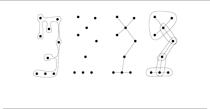
6.2 WAR STORY: NOTHING BUT NETS 203
(a) (b) (c) (d)
Figure 6.6: An example net showing (a) the metal connection layer, (b) the contact points, (c)
their minimum spanning tree, and (d) the points partitioned into clusters
“Circuit boards are certain sets of points that are all connected together with
a metal layer. This is what we mean by a net. Sometimes a net consists of two
points—i.e. , an isolated wire. Sometimes a net can have 100 to 200 points, like all
the connections to power or ground.”
“I see. So you have a list of all the connections between pairs of points on the
circuit board, and you want to trace out these wires.”
He shook his head. “Not quite. The input for our testing program consists only
of the net contact points, as shown in Figure 6.6(b). We don’t know where the
actual wires are, but we don’t have to. All we must do is verify that all the points
in a net are connected together. We do this by putting the left robot arm on the
leftmost point in the net, and then have the right arm move around to all the other
points in the net to test if they are all connected to the left point. So they must
all be connected to each other.”
I thought for a moment about what this meant. “OK. So your right arm has to
visit all the other points in the net. How do you choose the order to visit them?”
The technical guy spoke up. “Well, we sort the points from left to right and
then go in that order. Is that a good thing to do?”
“Have you ever heard of the traveling salesman problem?” I asked.
He was an electrical engineer, not a computer scientist. “No, what’s that?”
“Traveling salesman is the name of the problem that you are trying to solve.
Given a set of points to visit, how do you order them to minimize the travel time.
Algorithms for the traveling salesman problem have been extensively studied. For
small nets, you will be able to find the optimal tour by doing an exhaustive search.
For big nets, there are heuristics that will get you very close to the optimal tour.” I
would have pointed them to Section 16.4 (page 533) if I had had this book handy.

204 6. WEIGHTED GRAPH ALGORITHMS
The president scribbled down some notes and then frowned. “Fine. Maybe you
can order the points in a net better for us. But that’s not our real problem. When
you watch our robot in action, the right arm sometimes has to run all the way to
the right side of the board on a given net, while the left arm just sits there. It seems
we would benefit by breaking nets into smaller pieces to balance things out.”
I sat down and thought. The left and right arms each have interlocking TSP
problems to solve. The left arm would move between the leftmost points of each
net, while the right arm to visits all the other points in each net as ordered by
the left TSP tour. By breaking each net into smaller nets we would avoid making
the right arm cross all the way across the board. Further, a lot of little nets meant
there would be more points in the left TSP, so each left-arm movement was likely
to be short, too.
“You are right. We should win if we can break big nets into small nets. We
want the nets to be small, both in the number of points and in physical area. But
we must be sure that if we validate the connectivity of each small net, we will
have confirmed that the big net is connected. One point in common between two
little nets is sufficient to show that the bigger net formed by the two little nets is
connected, since current can flow between any pair of points.”
Now we had to break each net into overlapping pieces, where each piece was
small. This is a clustering problem. Minimum spanning trees are often used for
clustering, as discussed in Section 15.3 (page 484). In fact, that was the answer!
We could find the minimum spanning tree of the net points and break it into little
clusters whenever a spanning tree edge got too long. As shown in Figure 6.6(d),
each cluster would share exactly one point in common with another cluster, with
connectivity ensured because we are covering the edges of a spanning tree. The
shape of the clusters will reflect the points in the net. If the points lay along a line
across the board, the minimum spanning tree would be a path, and the clusters
would be pairs of points. If the points all fell in a tight region, there would be one
nice fat cluster for the right arm to scoot around.
So I explained the idea of constructing the minimum spanning tree of a graph.
The boss listened, scribbled more notes, and frowned again.
“I like your clustering idea. But minimum spanning trees are defined on graphs.
All you’ve got are points. Where do the weights of the edges come from?”
“Oh, we can think of it as a complete graph, where every pair of points are
connected. The weight of the edge is defined as the distance between the two
points. Or is it. . . ?”
I went back to thinking. The edge cost should reflect the travel time between
between two points. While distance is related to travel time, it wasn’t necessarily
the same thing.
“Hey. I have a question about your robot. Does it take the same amount of
time to move the arm left-right as it does up-down?”
They thought a minute. “Yeah, it does. We use the same type of motor to
control horizontal and vertical movements. Since the two motors for each arm are

6.3 SHORTEST PATHS 205
independent, we can simultaneously move each arm both horizontally and verti-
cally.”
“So the time to move both one foot left and one foot up is exactly the same as
just moving one foot left? This means that the weight for each edge should not be
the Euclidean distance between the two points, but the biggest difference between
either the x−or y-coordinate. This is something we call the L∞metric, but we can
capture it by changing the edge weights in the graph. Anything else funny about
your robots?” I asked.
“Well, it takes some time for the robot to come up to speed. We should probably
also factor in acceleration and deceleration of the arms.”
“Darn right. The more accurately you can model the time your arm takes to
move between two points, the better our solution will be. But now we have a very
clean formulation. Let’s code it up and let’s see how well it works!”
They were somewhat skeptical whether this approach would do any good, but
agreed to think about it. A few weeks later they called me back and reported
that the new algorithm reduced the distance traveled by about 30% over their
previous approach, at a cost of a little more computational preprocessing. However,
since their testing machine cost $200,000 a pop and a PC cost $2,000, this was an
excellent tradeoff. It is particularly advantageous since the preprocessing need only
be done once when testing multiple instances of a particular board design.
The key idea leading to the successful solution was modeling the job in terms
of classical algorithmic graph problems. I smelled TSP the instant they started
talking about minimizing robot motion. Once I realized that they were implicitly
forming a star-shaped spanning tree to ensure connectivity, it was natural to ask
whether the minimum spanning tree would perform any better. This idea led to
clustering, and thus partitioning each net into smaller nets. Finally, by carefully
designing our distance metric to accurately model the costs of the robot itself, we
could incorporate such complicated properties (as acceleration) without changing
our fundamental graph model or algorithm design.
Take-Home Lesson: Most applications of graphs can be reduced to standard
graph properties where well-known algorithms can be used. These include min-
imum spanning trees, shortest paths, and other problems presented in the
catalog.
6.3 Shortest Paths
Apath is a sequence of edges connecting two vertices. Since movie director Mel
Brooks (“The Producers”) is my father’s sister’s husband’s cousin, there is a path
in the friendship graph between me and him, shown in Figure 6.7—even though
the two of us have never met. But if I were trying to impress how tight I am with
Cousin Mel, I would be much better off saying that my Uncle Lenny grew up with
him. I have a friendship path of length 2 to Cousin Mel through Uncle Lenny, while
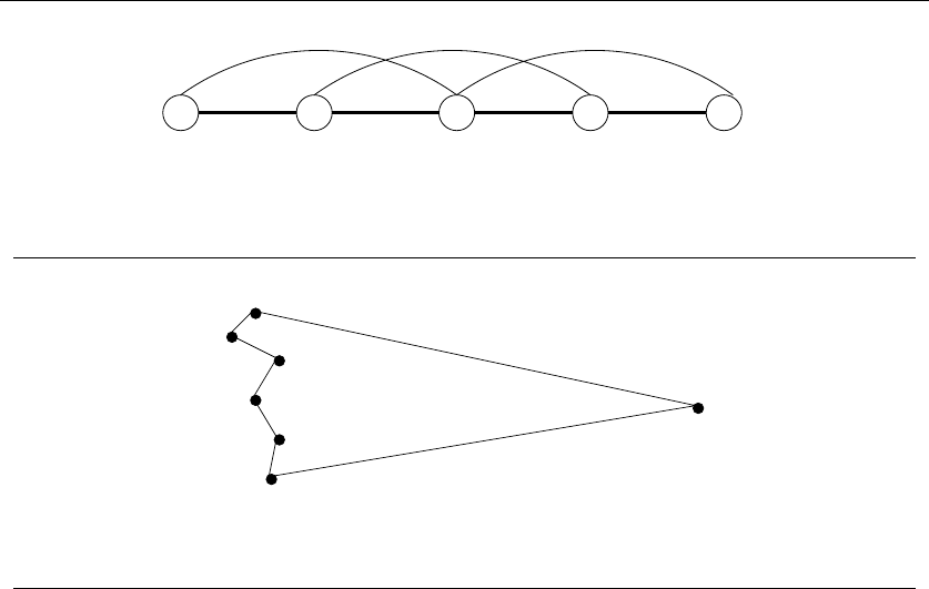
206 6. WEIGHTED GRAPH ALGORITHMS
Steve Dad Aunt Eve Uncle Lenny Cousin Mel
Figure 6.7: Mel Brooks is my father’s sister’s husband’s cousin
s
t
Figure 6.8: The shortest path from sto tmay pass through many intermediate vertices
the path is of length 4 by blood and marriage. This multiplicity of paths hints at
why finding the shortest path between two nodes is important and instructive, even
in nontransportation applications.
The shortest path from sto tin an unweighted graph can be constructed using a
breadth-first search from s. The minimum-link path is recorded in the breadth-first
search tree, and it provides the shortest path when all edges have equal weight.
However, BFS does not suffice to find shortest paths in weighted graphs. The
shortest weighted path might use a large number of edges, just as the shortest route
(timewise) from home to office may involve complicated shortcuts using backroads,
as shown in Figure 6.8.
In this section, we will present two distinct algorithms for finding the shortest
paths in weighted graphs.
6.3.1 Dijkstra’s Algorithm
Dijkstra’s algorithm is the method of choice for finding shortest paths in an edge-
and/or vertex-weighted graph. Given a particular start vertex s, it finds the shortest
path from sto every other vertex in the graph, including your desired destination
t.
Suppose the shortest path from sto tin graph Gpasses through a particular
intermediate vertex x. Clearly, this path must contain the shortest path from sto
xas its prefix, because if not, we could shorten our s-to-tpath by using the shorter

6.3 SHORTEST PATHS 207
s-to-xprefix. Thus, we must compute the shortest path from sto xbefore we find
the path from sto t.
Dijkstra’s algorithm proceeds in a series of rounds, where each round establishes
the shortest path from sto some new vertex. Specifically, xis the vertex that
minimizes dist(s, vi)+w(vi,x) over all unfinished 1 ≤i≤n, where w(i, j)isthe
length of the edge from ito j,anddist(i, j) is the length of the shortest path
between them.
This suggests a dynamic programming-like strategy. The shortest path from s
to itself is trivial unless there are negative weight edges, so dist(s, s)=0.If(s, y)
is the lightest edge incident to s, then this implies that dist(s, y)=w(s, y). Once
we determine the shortest path to a node x, we check all the outgoing edges of x
to see whether there is a better path from sto some unknown vertex through x.
ShortestPath-Dijkstra(G, s, t)
known ={s}
for i=1ton,dist[i]=∞
for each edge (s, v), dist[v]=w(s, v)
last =s
while (last =t)
select vnext, the unknown vertex minimizing dist[v]
for each edge (vnext,x), dist[x] = min[dist[x],dist[vnext]+w(vnext,x)]
last =vnext
known =known ∪{vnext}
The basic idea is very similar to Prim’s algorithm. In each iteration, we add
exactly one vertex to the tree of vertices for which we know the shortest path from
s. As in Prim’s, we keep track of the best path seen to date for all vertices outside
the tree, and insert them in order of increasing cost.
The difference between Dijkstra’s and Prim’s algorithms is how they rate the
desirability of each outside vertex. In the minimum spanning tree problem, all we
cared about was the weight of the next potential tree edge. In shortest path, we
want to include the closest outside vertex (in shortest-path distance) to s. This is
a function of both the new edge weight and the distance from sto the tree vertex
it is adjacent to.
Implementation
The pseudocode actually obscures how similar the two algorithms are. In fact, the
change is very minor. Below, we give an implementation of Dijkstra’s algorithm
based on changing exactly three lines from our Prim’s implementation—one of
which is simply the name of the function!

208 6. WEIGHTED GRAPH ALGORITHMS
dijkstra(graph *g, int start) /* WAS prim(g,start) */
{
int i; /* counter */
edgenode *p; /* temporary pointer */
bool intree[MAXV+1]; /* is the vertex in the tree yet? */
int distance[MAXV+1]; /* distance vertex is from start */
int v; /* current vertex to process */
int w; /* candidate next vertex */
int weight; /* edge weight */
int dist; /* best current distance from start */
for (i=1; i<=g->nvertices; i++) {
intree[i] = FALSE;
distance[i] = MAXINT;
parent[i] = -1;
}
distance[start] = 0;
v = start;
while (intree[v] == FALSE) {
intree[v] = TRUE;
p = g->edges[v];
while (p != NULL) {
w = p->y;
weight = p->weight;
/* CHANGED */ if (distance[w] > (distance[v]+weight)) {
/* CHANGED */ distance[w] = distance[v]+weight;
/* CHANGED */ parent[w] = v;
}
p = p->next;
}
v=1;
dist = MAXINT;
for (i=1; i<=g->nvertices; i++)
if ((intree[i] == FALSE) && (dist > distance[i])) {
dist = distance[i];
v=i;
}
}
}

6.3 SHORTEST PATHS 209
This algorithm finds more than just the shortest path from sto t. It finds the
shortest path from sto all other vertices. This defines a shortest path spanning
tree rooted in s. For undirected graphs, this would be the breadth-first search tree,
but in general it provides the shortest path from sto all other vertices.
Analysis
What is the running time of Dijkstra’s algorithm? As implemented here, the com-
plexity is O(n2). This is the same running time as a proper version of Prim’s
algorithm; except for the extension condition it is the same algorithm as Prim’s.
The length of the shortest path from start to a given vertex tis exactly the
value of distance[t]. How do we use dijkstra to find the actual path? We follow
the backward parent pointers from tuntil we hit start (or -1 if no such path
exists), exactly as was done in the find path() routine of Section 5.6.2 (page
165).
Dijkstra works correctly only on graphs without negative-cost edges. The reason
is that midway through the execution we may encounter an edge with weight so
negative that it changes the cheapest way to get from sto some other vertex
already in the tree. Indeed, the most cost-effective way to get from your house
to your next-door neighbor would be repeatedly through the lobby of any bank
offering you enough money to make the detour worthwhile.
Most applications do not feature negative-weight edges, making this discus-
sion academic. Floyd’s algorithm, discussed below, works correctly unless there are
negative cost cycles, which grossly distort the shortest-path structure. Unless that
bank limits its reward to one per customer, you might so benefit by making an
infinite number of trips through the lobby that you would never decide to actually
reach your destination!
Stop and Think: Shortest Path with Node Costs
Problem: Suppose we are given a graph whose weights are on the vertices, instead
of the edges. Thus, the cost of a path from xto yis the sum of the weights of all
vertices on the path.
Give an efficient algorithm for finding shortest paths on vertex-weighted graphs.
Solution: A natural idea would be to adapt the algorithm we have for edge-weighted
graphs (Dijkstra’s) to the new vertex-weighted domain. It should be clear that we
can do it. We replace any reference to the weight of an edge with the weight of
the destination vertex. This can be looked up as needed from an array of vertex
weights.
However, my preferred approach would leave Dijkstra’s algorithm intact and
instead concentrate on constructing an edge-weighted graph on which Dijkstra’s

210 6. WEIGHTED GRAPH ALGORITHMS
algorithm will give the desired answer. Set the weight of each directed edge (i, j)
in the input graph to the cost of vertex j. Dijkstra’s algorithm now does the job.
This technique can be extended to a variety of different domains, such as when
there are costs on both vertices and edges.
6.3.2 All-Pairs Shortest Path
Suppose you want to find the “center” vertex in a graph—the one that minimizes
the longest or average distance to all the other nodes. This might be the best place
to start a new business. Or perhaps you need to know a graph’s diameter—the
longest shortest-path distance over all pairs of vertices. This might correspond to
the longest possible time it takes a letter or network packet to be delivered. These
and other applications require computing the shortest path between all pairs of
vertices in a given graph.
We could solve all-pairs shortest path by calling Dijkstra’s algorithm from each
of the npossible starting vertices. But Floyd’s all-pairs shortest-path algorithm is
a slick way to construct this n×ndistance matrix from the original weight matrix
of the graph.
Floyd’s algorithm is best employed on an adjacency matrix data structure,
which is no extravagance since we must store all n2pairwise distances anyway.
Our adjacency matrix type allocates space for the largest possible matrix, and
keeps track of how many vertices are in the graph:
typedef struct {
int weight[MAXV+1][MAXV+1]; /* adjacency/weight info */
int nvertices; /* number of vertices in graph */
} adjacency_matrix;
The critical issue in an adjacency matrix implementation is how we denote the
edges absent from the graph. A common convention for unweighted graphs denotes
graph edges by 1 and non-edges by 0. This gives exactly the wrong interpretation
if the numbers denote edge weights, for the non-edges get interpreted as a free ride
between vertices. Instead, we should initialize each non-edge to MAXINT. This way
we can both test whether it is present and automatically ignore it in shortest-path
computations, since only real edges will be used, provided MAXINT is less than the
diameter of your graph.
There are several ways to characterize the shortest path between two nodes
in a graph. The Floyd-Warshall algorithm starts by numbering the vertices of the
graph from 1 to n. We use these numbers not to label the vertices, but to order
them. Define W[i, j]kto be the length of the shortest path from ito jusing only
vertices numbered from 1,2, ..., k as possible intermediate vertices.
What does this mean? When k= 0, we are allowed no intermediate vertices,
so the only allowed paths are the original edges in the graph. Thus the initial

6.3 SHORTEST PATHS 211
all-pairs shortest-path matrix consists of the initial adjacency matrix. We will per-
form niterations, where the kth iteration allows only the first kvertices as possible
intermediate steps on the path between each pair of vertices xand y.
At each iteration, we allow a richer set of possible shortest paths by adding a
new vertex as a possible intermediary. Allowing the kth vertex as a stop helps only
if there is a short path that goes through k,so
W[i, j]k= min(W[i, j]k−1,W[i, k]k−1+W[k, j]k−1)
The correctness of this is somewhat subtle, and I encourage you to convince
yourself of it. But there is nothing subtle about how simple the implementation is:
floyd(adjacency_matrix *g)
{
int i,j; /* dimension counters */
int k; /* intermediate vertex counter */
int through_k; /* distance through vertex k */
for (k=1; k<=g->nvertices; k++)
for (i=1; i<=g->nvertices; i++)
for (j=1; j<=g->nvertices; j++) {
through_k = g->weight[i][k]+g->weight[k][j];
if (through_k < g->weight[i][j])
g->weight[i][j] = through_k;
}
}
The Floyd-Warshall all-pairs shortest path runs in O(n3) time, which is asymp-
totically no better than ncalls to Dijkstra’s algorithm. However, the loops are so
tight and the program so short that it runs better in practice. It is notable as one of
the rare graph algorithms that work better on adjacency matrices than adjacency
lists.
The output of Floyd’s algorithm, as it is written, does not enable one to recon-
struct the actual shortest path between any given pair of vertices. These paths can
be recovered if we retain a parent matrix Pof our choice of the last intermediate
vertex used for each vertex pair (x, y). Say this value is k. The shortest path from
xto yis the concatenation of the shortest path from xto kwith the shortest
path from kto y, which can be reconstructed recursively given the matrix P. Note,
however, that most all-pairs applications need only the resulting distance matrix.
These jobs are what Floyd’s algorithm was designed for.

212 6. WEIGHTED GRAPH ALGORITHMS
6.3.3 Transitive Closure
Floyd’s algorithm has another important application, that of computing transitive
closure. In analyzing a directed graph, we are often interested in which vertices are
reachable from a given node.
As an example, consider the blackmail graph, where there is a directed edge
(i, j) if person ihas sensitive-enough private information on person jso that ican
get jto do whatever he wants. You wish to hire one of these npeople to be your
personal representative. Who has the most power in terms of blackmail potential?
A simplistic answer would be the vertex of highest degree, but an even better
representative would be the person who has blackmail chains leading to the most
other parties. Steve might only be able to blackmail Miguel directly, but if Miguel
can blackmail everyone else then Steve is the man you want to hire.
The vertices reachable from any single node can be computed using breadth-
first or depth-first searches. But the whole batch can be computed using an all-pairs
shortest-path. If the shortest path from ito jremains MAXINT after running Floyd’s
algorithm, you can be sure no directed path exists from ito j. Any vertex pair
of weight less than MAXINT must be reachable, both in the graph-theoretic and
blackmail senses of the word.
Transitive closure is discussed in more detail in the catalog in Section 15.5.
6.4 War Story: Dialing for Documents
I was part of a group visiting Periphonics, which was then an industry leader in
building telephone voice-response systems. These are more advanced versions of
the Press 1 for more options, Press 2 if you didn’t press 1 telephone systems that
blight everyone’s lives. We were being given the standard tour when someone from
our group asked, “Why don’t you guys use voice recognition for data entry. It
would be a lot less annoying than typing things out on the keypad.”
The tour guide reacted smoothly. “Our customers have the option of incor-
porating speech recognition into our products, but very few of them do. User-
independent, connected-speech recognition is not accurate enough for most appli-
cations. Our customers prefer building systems around typing text on the telephone
keyboards.”
“Prefer typing, my pupik!” came a voice from the rear of our group. “I hate
typing on a telephone. Whenever I call my brokerage house to get stock quotes
some machine tells me to type in the three letter code. To make things worse, I
have to hit two buttons to type in one letter, in order to distinguish between the
three letters printed on each key of the telephone. I hit the 2 key and it says Press
1 for A, Press 2 for B, Press 3 for C. Pain in the neck if you ask me.”
“Maybe you don’t have to hit two keys for each letter!” I chimed in. “Maybe
the system could figure out the correct letter from context!”

6.4 WAR STORY: DIALING FOR DOCUMENTS 213
“There isn’t a whole lot of context when you type in three letters of stock
market code.”
“Sure, but there would be plenty of context if we typed in English sentences.
I’ll bet that we could reconstruct English text correctly if they were typed in a
telephone at one keystroke per letter.”
The guy from Periphonics gave me a disinterested look, then continued the
tour. But when I got back to the office, I decided to give it a try.
Not all letters are equally likely to be typed on a telephone. In fact, not all letters
can be typed, since Q and Z are not labeled on a standard American telephone.
Therefore, we adopted the convention that Q, Z, and “space” all sat on the * key.
We could take advantage of the uneven distribution of letter frequencies to help
us decode the text. For example, if you hit the 3 key while typing English, you
more likely meant to type an E than either a D or F. By taking into account the
frequencies of a window of three characters (trigrams), we could predict the typed
text. This is what happened when I tried it on the Gettysburg Address:
enurraore ane reten yeasr ain our ectherr arotght eosti on ugis aootinent a oey oation
aoncdivee in licesty ane eedicatee un uhe rrorosition uiat all oen are arectee e ual
ony ye are enichde in a irect aitil yar uestini yhethes uiat oatioo or aoy oation ro aoncdivee
ane ro eedicatee aan loni eneure ye are oet on a irect aattlediele oe uiat yar ye iate aone
un eedicate a rostion oe uiat eiele ar a einal restini rlace eor uiore yin iere iate uhdis lives
uiat uhe oation ogght live it is aluniethes eittini ane rrores uiat ye rioule en ugir
att in a laries reore ye aan oou eedicate ye aan oou aoorearate ye aan oou ialloy ugis
iroune the arate oen litini ane eeae yin rustgilee iere iate aoorearatee it ear aante our
roor rowes un ade or eeuraat the yople yill little oote oor loni renences yiat ye ray iere
att it aan oetes eosiet yiat uhfy eie iere it is eor ur uhe litini rathes un ae eedicatee iere
un uhe undiniside yopl yhici uhfy yin entght iere iate uiur ear ro onaky aetancde it is
rathes eor ur un ae iere eedicatee un uhe irect uarl rencinini adeore ur uiat eron uhere
ioooree eeae ye uale inarearee eeuotion uo tiat aaure eor yhici uhfy iere iate uhe lart eull
oearure oe eeuotioo tiat ye iere iggily rerolue uiat uhere eeae riall oou iate eide io
The trigram statistics did a decent job of translating it into Greek, but a terri-
ble job of transcribing English. One reason was clear. This algorithm knew nothing
about English words. If we coupled it with a dictionary, we might be onto some-
thing. But two words in the dictionary are often represented by the exact same
string of phone codes. For an extreme example, the code string “22737” collides
with eleven distinct English words, including cases, cares, cards, capes, caper,and
bases. For our next attempt, we reported the unambiguous characters of any words
that collided in the dictionary, and used trigrams to fill in the rest of the characters.
We were rewarded with:
eourscore and seven yearr ain our eatherr brought forth on this continent azoey nation
conceivee in liberty and dedicatee uo uhe proposition that all men are createe equal
ony ye are engagee in azipeat civil yar uestioi whether that nation or aoy nation ro
conceivee and ro dedicatee aan long endure ye are oet on azipeat battlefield oe that yar
ye iate aone uo dedicate a rostion oe that field ar a final perthni place for those yin here
iate their lives that uhe nation oight live it is altogether fittinizane proper that ye should
en this
aut in a larges sense ye aan oou dedicate ye aan oou consecrate ye aan oou hallow this
ground the arate men litioi and deae yin strugglee here iate consecratee it ear above
our roor power uo ade or detract the world will little oote oor long remember what ye

214 6. WEIGHTED GRAPH ALGORITHMS
ray here aut it aan meter forget what uhfy die here it is for ur uhe litioi rather uo ae
dedicatee here uo uhe toeioisgee york which uhfy yin fought here iate thus ear ro mocky
advancee it is rather for ur uo ae here dedicatee uo uhe great task renagogoi adfore ur
that from there honoree deae ye uale increasee devotion uo that aause for which uhfy
here iate uhe last eull measure oe devotion that ye here highky resolve that there deae
shall oou iate fide io vain that this nation under ioe shall iate azoey birth oe freedom
and that ioternmenu oe uhe people ay uhe people for uhe people shall oou perish from
uhe earth
If you were a student of American history, maybe you could recognize it, but you
certainly couldn’t read it. Somehow, we had to distinguish between the different
dictionary words that got hashed to the same code. We could factor in the relative
popularity of each word, but this still made too many mistakes.
At this point, I started working with Harald Rau on the project, who proved
to be a great collaborator. First, he was a bright and persistent graduate student.
Second, as a native German speaker, he believed every lie I told him about English
grammar.
Harald built up a phone code reconstruction program along the lines of Figure
6.9. It worked on the input one sentence at a time, identifying dictionary words that
matched each code string. The key problem was how to incorporate grammatical
constraints.
“We can get good word-use frequencies and grammatical information from a big
text database called the Brown Corpus. It contains thousands of typical English
sentences, each parsed according to parts of speech. But how do we factor it all
in?” Harald asked.
“Let’s think about it as a graph problem,” I suggested.
“Graph problem? What graph problem? Where is there even a graph?”
“Think of a sentence as a series of phone tokens, each representing a word in
the sentence. Each phone token has a list of words from the dictionary that match
it. How can we choose which one is right? Each possible sentence interpretation
can be thought of as a path in a graph. The vertices of this graph are the complete
set of possible word choices. There will be an edge from each possible choice for the
ith word to each possible choice for the (i+ 1)st word. The cheapest path across
this graph defines the best interpretation of the sentence.”
“But all the paths look the same. They have the same number of edges. Wait.
Now I see! We have to add weight to the edges to make the paths different.”
“Exactly! The cost of an edge will reflect how likely it is that we will travel
through the given pair of words. Perhaps we can count how often that pair of
words occurred together in previous texts. Or we can weigh them by the part of
speech of each word. Maybe nouns don’t like to be next to nouns as much as they
like being next to verbs.”
“It will be hard to keep track of word-pair statistics, since there are so many of
them. But we certainly know the frequency of each word. How can we factor that
into things?”
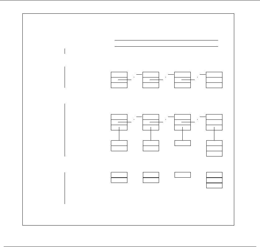
6.4 WAR STORY: DIALING FOR DOCUMENTS 215
•
•
Token
•
•
Token
•
•
Token
•
•
Token
“4483” “63” “2” “7464”
- - -
•
•
Token
•
•
Token
•
•
Token
•
•
Token
“4483” “63” “2” “7464”
- - -
? ? ? ?
give
hive
of
me
aping
ring
sing
give
hive
of
me
aping
ring
sing
... #4483∗63∗2∗7464#...
GIVE ME A RING.
PP
Pq
1 PP
Pq
INPUT
?
Blank Recognition
?
Candidate Construction
?
Sentence Disambiguating
?
OUTPUT
Figure 6.9: The phases of the telephone code reconstruction process
“We can pay a cost for walking through a particular vertex that depends upon
the frequency of the word. Our best sentence will be given by the shortest path
across the graph.”
“But how do we figure out the relative weights of these factors?”
“First try what seems natural to you and then we can experiment with it.”
Harald incorporated this shortest-path algorithm. With proper grammatical
and statistical constraints, the system performed great. Look at the Gettysburg
Address now, with all the reconstruction errors highlighted:
FOURSCORE AND SEVEN YEARS AGO OUR FATHERS BROUGHT FORTH ON
THIS CONTINENT A NEW NATION CONCEIVED IN LIBERTY AND DEDICATED
TO THE PROPOSITION THAT ALL MEN ARE CREATED EQUAL. NOW WE ARE
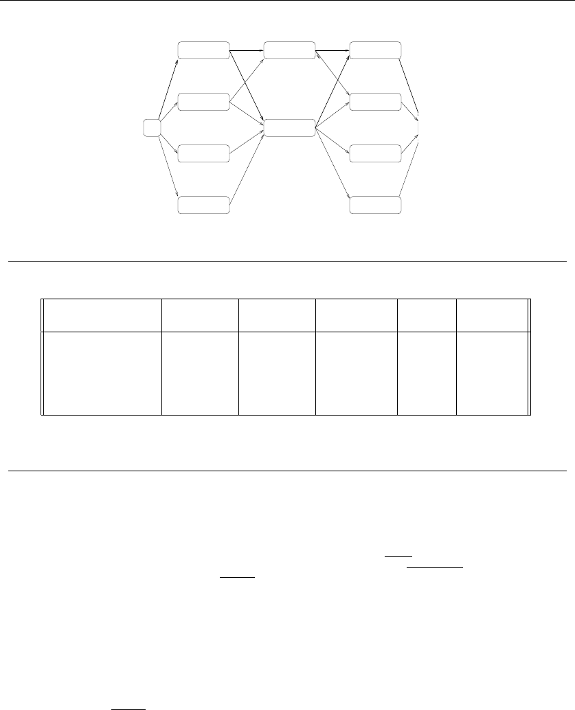
216 6. WEIGHTED GRAPH ALGORITHMS
#
1
2
3
4
P(W /C )
P(W /C )
P(W /C )
P(W /C )
Code C1Code C2Code C 3
2
P(W /C )
1
P(W /C )
2
2
2
2
12
12
P(W /W )
P(W /#)
1
2
P(W /#)
1
3
P(W /#)
1
4
P(W /#)
1
1
1
P(W /C )
1
1
1
2
P(W /C )
1
3
P(W /C )
1
1
14
P(W /C )
1
P(
#
3
3
3
3
3
3
3
3
Figure 6.10: The minimum-cost path defines the best interpretation for a sentence
characters non-blanks words time per
Text characters correct correct correct character
Clinton Speeches 1,073,593 99.04% 98.86% 97.67% 0.97ms
Herland 278,670 98.24% 97.89% 97.02% 0.97ms
Moby Dick 1,123,581 96.85% 96.25% 94.75% 1.14ms
Bible 3,961,684 96.20% 95.39% 95.39% 1.33ms
Shakespeare 4,558,202 95.20% 94.21% 92.86% 0.99ms
Figure 6.11: Telephone-code reconstruction applied to several text samples
ENGAGED IN A GREAT CIVIL WAR TESTING WHETHER THAT NATION OR
ANY NATION SO CONCEIVED AND SO DEDICATED CAN LONG ENDURE. WE
ARE MET ON A GREAT BATTLEFIELD OF THAT WA S .WEHAVECOMETO
DEDICATE A PORTION OF THAT FIELD AS A FINAL SERVING PLACE FOR
THOSE WHO HERE HAVE THEIR LIVES THAT THE NATION MIGHT LIVE. IT
IS ALTOGETHER FITTING AND PROPER THAT WE SHOULD DO THIS. BUT IN
A LARGER SENSE WE CAN NOT DEDICATE WE CAN NOT CONSECRATE WE
CAN NOT HALLOW THIS GROUND. THE BRAVE MEN LIVING AND DEAD WHO
STRUGGLED HERE HAVE CONSECRATED IT FAR ABOVE OUR POOR POWER
TO ADD OR DETRACT. THE WORLD WILL LITTLE NOTE NOR LONG REMEM-
BER WHAT WE SAY HERE BUT IT CAN NEVER FORGET WHAT THEY DID
HERE. IT IS FOR US THE LIVING RATHER TO BE DEDICATED HERE TO THE
UNFINISHED WORK WHICH THEY WHO FOUGHT HERE HAVE THUS FAR SO
NOBLY ADVANCED. IT IS RATHER FOR US TO BE HERE DEDICATED TO THE
GREAT TASK REMAINING BEFORE US THAT FROM THESE HONORED DEAD
WE TAKE INCREASED DEVOTION TO THAT CAUSE FOR WHICH THEY HERE
HAVE THE LAST FULL MEASURE OF DEVOTION THAT WE HERE HIGHLY
RESOLVE THAT THESE DEAD SHALL NOT HAVE DIED IN VAIN THAT THIS
NATION UNDER GOD SHALL HAVE A NEW BIRTH OF FREEDOM AND THAT
GOVERNMENT OF THE PEOPLE BY THE PEOPLE FOR THE PEOPLE SHALL
NOT PERISH FROM THE EARTH.
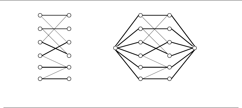
6.5 NETWORK FLOWS AND BIPARTITE MATCHING 217
ts
Figure 6.12: Bipartite graph with a maximum matching highlighted (on left). The correspond-
ing network flow instance highlighting the maximum s−tflow (on right).
While we still made a few mistakes, the results are clearly good enough for many
applications. Periphonics certainly thought so, for they licensed our program to
incorporate into their products. Figure 6.11 shows that we were able to reconstruct
correctly over 99% of the characters in a megabyte of President Clinton’s speeches,
so if Bill had phoned them in, we would certainly be able to understand what he
was saying. The reconstruction time is fast enough, indeed faster than you can type
it in on the phone keypad.
The constraints for many pattern recognition problems can be naturally for-
mulated as shortest path problems in graphs. In fact, there is a particularly con-
venient dynamic programming solution for these problems (the Viterbi algorithm)
that is widely used in speech and handwriting recognition systems. Despite the
fancy name, the Viterbi algorithm is basically solving a shortest path problem on a
DAG. Hunting for a graph formulation to solve any given problem is often a good
idea.
6.5 Network Flows and Bipartite Matching
Edge-weighted graphs can be interpreted as a network of pipes, where the weight
of edge (i, j) determines the capacity of the pipe. Capacities can be thought of as a
function of the cross-sectional area of the pipe. A wide pipe might be able to carry
10 units of flow in a given time, where as a narrower pipe might only carry 5 units.
The network flow problem asks for the maximum amount of flow which can be sent
from vertices sto tin a given weighted graph Gwhile respecting the maximum
capacities of each pipe.

218 6. WEIGHTED GRAPH ALGORITHMS
6.5.1 Bipartite Matching
While the network flow problem is of independent interest, its primary importance
is in to solving other important graph problems. A classic example is bipartite
matching. A matching in a graph G=(V,E) is a subset of edges E⊂Esuch that
no two edges of Eshare a vertex. A matching pairs off certain vertices such that
every vertex is in, at most, one such pair, as shown in Figure 6.12.
Graph Gis bipartite or two-colorable if the vertices can be divided into two
sets, Land R, such that all edges in Ghave one vertex in Land one vertex in
R. Many naturally defined graphs are bipartite. For example, certain vertices may
represent jobs to be done and the remaining vertices represent people who can
potentially do them. The existence of edge (j, p) means that job jcanbedoneby
person p. Or let certain vertices represent boys and certain vertices represent girls,
with edges representing compatible pairs. Matchings in these graphs have natural
interpretations as job assignments or as marriages, and are the focus of Section
15.6 (page 498).
The largest bipartite matching can be readily found using network flow. Create
asource node sthat is connected to every vertex in Lby an edge of weight 1.
Create a sink node tand connect it to every vertex in Rby an edge of weight 1.
Finally, assign each edge in the bipartite graph Ga weight of 1. Now, the maximum
possible flow from sto tdefines the largest matching in G. Certainly we can find a
flow as large as the matching by using only the matching edges and their source-
to-sink connections. Further, there can be no greater possible flow. How can we
ever hope to get more than one flow unit through any vertex?
6.5.2 Computing Network Flows
Traditional network flow algorithms are based on the idea of augmenting paths,
and repeatedly finding a path of positive capacity from sto tand adding it to the
flow. It can be shown that the flow through a network is optimal if and only if it
contains no augmenting path. Since each augmentation adds to the flow, we must
eventually find the global maximum.
The key structure is the residual flow graph, denoted as R(G, f ), where Gis
the input graph and fis the current flow through G. This directed, edge-weighted
R(G, f) contains the same vertices as G. For each edge (i, j)inGwith capacity
c(i, j) and flow f(i, j), R(G, f) may contain two edges:
(i) an edge (i, j) with weight c(i, j)−f(i, j), if c(i, j)−f(i, j)>0and
(ii) an edge (j, i) with weight f(i, j), if f(i, j)>0.
The presence of edge (i, j) in the residual graph indicates that positive flow can
be pushed from ito j. The weight of the edge gives the exact amount that can be
pushed. A path in the residual flow graph from sto timplies that more flow can be
pushed from sto tand the minimum edge weight on this path defines the amount
of extra flow that can be pushed.
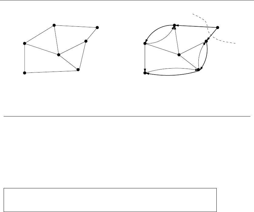
6.5 NETWORK FLOWS AND BIPARTITE MATCHING 219
2
5
R(G)G
T
S
T
S
33
5
59
2
2
10
52
44
9
3
12
7
3
7
5
2
5
Figure 6.13: Maximum s−tflow in a graph G(on left) showing the associated residual graph
R(G) and minimum s−tcut (dotted line near t)
Figure 6.13 illustrates this idea. The maximum s−tflow in graph Gis 7. Such
a flow is revealed by the two directed tto spaths in the residual graph R(G)
of capacities 2 + 5, respectively. These flows completely saturate the capacity of
the two edges incident to vertex t, so no augmenting path remains. Thus the flow
is optimal. A set of edges whose deletion separates sfrom t(like the two edges
incident to t) is called an s-tcut. Clearly, no sto tflow can exceed the weight of
the minimum such cut. In fact, a flow equal to the minimum cut is always possible.
Take-Home Lesson: The maximum flow from sto talways equals the weight
of the minimum s-tcut. Thus, flow algorithms can be used to solve general
edge and vertex connectivity problems in graphs.
Implementation
We cannot do full justice to the theory of network flows here. However, it is instruc-
tive to see how augmenting paths can be identified and the optimal flow computed.
For each edge in the residual flow graph, we must keep track of both the amount
of flow currently going through the edge, as well as its remaining residual capacity.
Thus, we must modify our edge structure to accommodate the extra fields:
typedef struct {
int v; /* neighboring vertex */
int capacity; /* capacity of edge */
int flow; /* flow through edge */
int residual; /* residual capacity of edge */
struct edgenode *next; /* next edge in list */
} edgenode;

220 6. WEIGHTED GRAPH ALGORITHMS
We use a breadth-first search to look for any path from source to sink that
increases the total flow, and use it to augment the total. We terminate with the
optimal flow when no such augmenting path exists.
netflow(flow_graph *g, int source, int sink)
{
int volume; /* weight of the augmenting path */
add_residual_edges(g);
initialize_search(g);
bfs(g,source);
volume = path_volume(g, source, sink, parent);
while (volume > 0) {
augment_path(g,source,sink,parent,volume);
initialize_search(g);
bfs(g,source);
volume = path_volume(g, source, sink, parent);
}
}
Any augmenting path from source to sink increases the flow, so we can use bfs
to find such a path in the appropriate graph. We only consider network edges that
have remaining capacity or, in other words, positive residual flow. The predicate
below helps bfs distinguish between saturated and unsaturated edges:
bool valid_edge(edgenode *e)
{
if (e->residual > 0) return (TRUE);
else return(FALSE);
}
Augmenting a path transfers the maximum possible volume from the residual
capacity into positive flow. This amount is limited by the path-edge with the small-
est amount of residual capacity, just as the rate at which traffic can flow is limited
by the most congested point.

6.5 NETWORK FLOWS AND BIPARTITE MATCHING 221
int path_volume(flow_graph *g, int start, int end, int parents[])
{
edgenode *e; /* edge in question */
edgenode *find_edge();
if (parents[end] == -1) return(0);
e = find_edge(g,parents[end],end);
if (start == parents[end])
return(e->residual);
else
return( min(path_volume(g,start,parents[end],parents),
e->residual) );
}
edgenode *find_edge(flow_graph *g, int x, int y)
{
edgenode *p; /* temporary pointer */
p = g->edges[x];
while (p != NULL) {
if (p->v == y) return(p);
p = p->next;
}
return(NULL);
}
Sending an additional unit of flow along directed edge (i, j) reduces the residual
capacity of edge (i, j) but increases the residual capacity of edge (j, i). Thus, the
act of augmenting a path requires modifying both forward and reverse edges for
each link on the path.

222 6. WEIGHTED GRAPH ALGORITHMS
augment_path(flow_graph *g, int start, int end, int parents[], int volume)
{
edgenode *e; /* edge in question */
edgenode *find_edge();
if (start == end) return;
e = find_edge(g,parents[end],end);
e->flow += volume;
e->residual -= volume;
e = find_edge(g,end,parents[end]);
e->residual += volume;
augment_path(g,start,parents[end],parents,volume);
}
Initializing the flow graph requires creating directed flow edges (i, j) and (j, i)
for each network edge e=(i, j). Initial flows are all set to 0. The initial residual
flow of (i, j) is set to the capacity of e, while the initial residual flow of (j, i)isset
to 0.
Analysis
The augmenting path algorithm above eventually converges on the the optimal
solution. However, each augmenting path may add only a little to the total flow,
so, in principle, the algorithm might take an arbitrarily long time to converge.
However, Edmonds and Karp [EK72] proved that always selecting a shortest
unweighted augmenting path guarantees that O(n3) augmentations suffice for op-
timization. In fact, the Edmonds-Karp algorithm is what is implemented above,
since a breadth-first search from the source is used to find the next augmenting
path.
6.6 Design Graphs, Not Algorithms
Proper modeling is the key to making effective use of graph algorithms. We have
defined several graph properties, and developed algorithms for computing them.
All told, about two dozen different graph problems are presented in the catalog,
mostly in Sections 15 and 16. These classical graph problems provide a framework
for modeling most applications.
The secret is learning to design graphs, not algorithms. We have already seen
a few instances of this idea:

6.6 DESIGN GRAPHS, NOT ALGORITHMS 223
•The maximum spanning tree can be found by negating the edge weights of the
input graph Gand using a minimum spanning tree algorithm on the result.
The most negative weight spanning tree will define the maximum weight tree
in G.
•To solve bipartite matching, we constructed a special network flow graph such
that the maximum flow corresponds to a maximum cardinality matching.
The applications below demonstrate the power of proper modeling. Each arose
in a real-world application, and each can be modeled as a graph problem. Some
of the modelings are quite clever, but they illustrate the versatility of graphs in
representing relationships. As you read a problem, try to devise an appropriate
graph representation before peeking to see how we did it.
Stop and Think: The Pink Panther’s Passport to Peril
Problem: “I’m looking for an algorithm to design natural routes for video-game
characters to follow through an obstacle-filled room. How should I do it?”
Solution: Presumably the desired route should look like a path that an intelligent
being would choose. Since intelligent beings are either lazy or efficient, this should
be modeled as a shortest path problem.
But what is the graph? One approach might be to lay a grid of points in the
room. Create a vertex for each grid point that is a valid place for the character to
stand; i.e. , that does not lie within an obstacle. There will be an edge between
any pair of nearby vertices, weighted proportionally to the distance between them.
Although direct geometric methods are known for shortest paths (see Section 15.4
(page 489)), it is easier to model this discretely as a graph.
Stop and Think: Ordering the Sequence
Problem: “A DNA sequencing project generates experimental data consisting of
small fragments. For each given fragment f, we know certain other fragments are
forced to lie to the left of f, and certain other fragments are forced to be to the
right of f. How can we find a consistent ordering of the fragments from left to right
that satisfies all the constraints?”
Solution: Create a directed graph, where each fragment is assigned a unique vertex.
Insert a directed edge −→
(l, f) from any fragment lthat is forced to be to the left

224 6. WEIGHTED GRAPH ALGORITHMS
of f, and a directed edge −→
(f,r) to any fragment rforced to be to the right of f.
We seek an ordering of the vertices such that all the edges go from left to right.
This is a topological sort of the resulting directed acyclic graph. The graph must
be acyclic, because cycles make finding a consistent ordering impossible.
Stop and Think: Bucketing Rectangles
Problem: “In my graphics work I need to solve the following problem. Given an
arbitrary set of rectangles in the plane, how can I distribute them into a minimum
number of buckets such that no subset of rectangles in any given bucket inter-
sects another? In other words, there can not be any overlapping area between two
rectangles in the same bucket.”
Solution: We formulate a graph where each vertex is a rectangle, and there is an
edge if two rectangles intersect. Each bucket corresponds to an independent set of
rectangles, so there is no overlap between any two. A vertex coloring of a graph is a
partition of the vertices into independent sets, so minimizing the number of colors
is exactly what you want.
Stop and Think: Names in Collision
Problem: “In porting code from UNIX to DOS, I have to shorten several hundred
file names down to at most 8 characters each. I can’t just use the first eight charac-
ters from each name, because “filename1” and “filename2” would be assigned the
exact same name. How can I meaningfully shorten the names while ensuring that
they do not collide?”
Solution: Construct a bipartite graph with vertices corresponding to each original
file name fifor 1 ≤i≤n, as well as a collection of acceptable shortenings for each
name fi1,...,f
ik. Add an edge between each original and shortened name. We now
seek a set of nedges that have no vertices in common, so each file name is mapped
to a distinct acceptable substitute. Bipartite matching, discussed in Section 15.6
(page 498), is exactly this problem of finding an independent set of edges in a
graph.

6.7 EXERCISES 225
Stop and Think: Separate the Text
Problem: “We need a way to separate the lines of text in the optical character-
recognition system that we are building. Although there is some white space be-
tween the lines, problems like noise and the tilt of the page makes it hard to find.
How can we do line segmentation?
Solution: Consider the following graph formulation. Treat each pixel in the im-
age as a vertex in the graph, with an edge between two neighboring pixels. The
weight of this edge should be proportional to how dark the pixels are. A segmen-
tation between two lines is a path in this graph from the left to right side of the
page. We seek a relatively straight path that avoids as much blackness as possible.
This suggests that the shortest path in the pixel graph will likely find a good line
segmentation.
Take-Home Lesson: Designing novel graph algorithms is very hard, so don’t
do it. Instead, try to design graphs that enable you to use classical algorithms
to model your problem.
Chapter Notes
Network flows are an advanced algorithmic technique, and recognizing whether a
particular problem can be solved by network flow requires experience. We point
the reader to books by Cook and Cunningham [CC97] and Ahuja, Magnanti, and
Orlin [AMO93] for more detailed treatments of the subject.
The augmenting path method for network flows is due to Ford and Fulkerson
[FF62]. Edmonds and Karp [EK72] proved that always selecting a shortest geodesic
augmenting path guarantees that O(n3) augmentations suffice for optimization.
The phone code reconstruction system that was the subject of the war story is
described in more technical detail in [RS96].
6.7 Exercises
Simulating Graph Algorithms
6-1. [3] For the graphs in Problem 5-1:
(a) Draw the spanning forest after every iteration of the main loop in Kruskal’s
algorithm.
(b) Draw the spanning forest after every iteration of the main loop in Prim’s
algorithm.

226 6. WEIGHTED GRAPH ALGORITHMS
(c) Find the shortest path spanning tree rooted in A.
(d) Compute the maximum flow from Ato H.
Minimum Spanning Trees
6-2. [3] Is the path between two vertices in a minimum spanning tree necessarily a
shortest path between the two vertices in the full graph? Give a proof or a coun-
terexample.
6-3. [3] Assume that all edges in the graph have distinct edge weights (i.e. , no pair of
edges have the same weight). Is the path between a pair of vertices in a minimum
spanning tree necessarily a shortest path between the two vertices in the full graph?
Give a proof or a counterexample.
6-4. [3] Can Prim’s and Kruskal’s algorithm yield different minimum spanning trees?
Explain why or why not.
6-5. [3] Does either Prim’s and Kruskal’s algorithm work if there are negative edge
weights? Explain why or why not.
6-6. [5] Suppose we are given the minimum spanning tree Tof a given graph G(with n
vertices and medges) and a new edge e=(u, v) of weight wthat we will add to G.
Give an efficient algorithm to find the minimum spanning tree of the graph G+e.
Your algorithm should run in O(n) time to receive full credit.
6-7. [5] (a) Let Tbe a minimum spanning tree of a weighted graph G. Construct a new
graph Gby adding a weight of kto every edge of G. Do the edges of Tform a
minimum spanning tree of G? Prove the statement or give a counterexample.
(b) Let P={s,...,t}describe a shortest weighted path between vertices sand t
of a weighted graph G. Construct a new graph Gby adding a weight of kto every
edge of G.DoesPdescribe a shortest path from sto tin G? Prove the statement
or give a counterexample.
6-8. [5] Devise and analyze an algorithm that takes a weighted graph Gand finds the
smallest change in the cost to a non-MST edge that would cause a change in the
minimum spanning tree of G. Your algorithm must be correct and run in polynomial
time.
6-9. [4] Consider the problem of finding a minimum weight connected subset Tof edges
from a weighted connected graph G.TheweightofTis the sum of all the edge
weights in T.
(a) Why is this problem not just the minimum spanning tree problem? Hint: think
negative weight edges.
(b) Give an efficient algorithm to compute the minimum weight connected subset
T.
6-10. [4] Let G=(V,E) be an undirected graph. A set F⊆Eof edges is called a
feedback-edge set if every cycle of Ghas at least one edge in F.
(a) Suppose that Gis unweighted. Design an efficient algorithm to find a
minimum-size feedback-edge set.

6.7 EXERCISES 227
(b) Suppose that Gis a weighted undirected graph with positive edge weights.
Design an efficient algorithm to find a minimum-weight feedback-edge set.
6-11. [5] Modify Prim’s algorithm so that it runs in time O(nlog k) on a graph that has
only kdifferent edges costs.
Union-Find
6-12. [5] Devise an efficient data structure to handle the following operations on a
weighted directed graph:
(a) Merge two given components.
(b) Locate which component contains a given vertex v.
(c) Retrieve a minimum edge from a given component.
6-13. [5] Design a data structure that can perform a sequence of, munion and find
operations on a universal set of nelements, consisting of a sequence of all unions
followed by a sequence of all finds,intimeO(m+n).
Shortest Paths
6-14. [3] The single-destination shortest path problem for a directed graph seeks the
shortest path from every vertex to a specified vertex v. Give an efficient algorithm
to solve the single-destination shortest paths problem.
6-15. [3] Let G=(V,E) be an undirected weighted graph, and let Tbe the shortest-path
spanning tree rooted at a vertex v. Suppose now that all the edge weights in Gare
increased by a constant number k.IsTstill the shortest-path spanning tree from
v?
6-16. [3] Answer all of the following:
(a) Give an example of a weighted connected graph G=(V,E)andavertexv,
such that the minimum spanning tree of Gis the same as the shortest-path
spanning tree rooted at v.
(b) Give an example of a weighted connected directed graph G=(V,E)anda
vertex v, such that the minimum-cost spanning tree of Gis very different from
the shortest-path spanning tree rooted at v.
(c) Can the two trees be completely disjointed?
6-17. [3] Either prove the following or give a counterexample:
(a) Is the path between a pair of vertices in a minimum spanning tree of an
undirected graph necessarily the shortest (minimum weight) path?
(b) Suppose that the minimum spanning tree of the graph is unique. Is the path
between a pair of vertices in a minimum spanning tree of an undirected graph
necessarily the shortest (minimum weight) path?
6-18. [5] In certain graph problems, vertices have can have weights instead of or in addi-
tion to the weights of edges. Let Cvbe the cost of vertex v,andC(x,y)the cost of
theedge(x, y). This problem is concerned with finding the cheapest path between
vertices aand bin a graph G. The cost of a path is the sum of the costs of the
edges and vertices encountered on the path.

228 6. WEIGHTED GRAPH ALGORITHMS
(a) Suppose that each edge in the graph has a weight of zero (while non-edges
have a cost of ∞). Assume that Cv= 1 for all vertices 1 ≤v≤n(i.e. , all
vertices have the same cost). Give an efficient algorithm to find the cheapest
path from ato band its time complexity.
(b) Now suppose that the vertex costs are not constant (but are all positive)
and the edge costs remain as above. Give an efficient algorithm to find the
cheapest path from ato band its time complexity.
(c) Now suppose that both the edge and vertex costs are not constant (but are
all positive). Give an efficient algorithm to find the cheapest path from ato
band its time complexity.
6-19. [5] Let Gbe a weighted directed graph with nvertices and medges, where all edges
have positive weight. A directed cycle is a directed path that starts and ends at
the same vertex and contains at least one edge. Give an O(n3) algorithm to find
a directed cycle in Gof minimum total weight. Partial credit will be given for an
O(n2m) algorithm.
6-20. [5] Can we modify Dijkstra’s algorithm to solve the single-source longest path prob-
lem by changing minimum to maximum? If so, then prove your algorithm correct.
If not, then provide a counterexample.
6-21. [5] Let G=(V,E) be a weighted acyclic directed graph with possibly negative edge
weights. Design a linear-time algorithm to solve the single-source shortest-path
problem from a given source v.
6-22. [5] Let G=(V, E) be a directed weighted graph such that all the weights are
positive. Let vand wbe two vertices in Gand k≤|V|be an integer. Design an
algorithm to find the shortest path from vto wthat contains exactly kedges. Note
that the path need not be simple.
6-23. [5] Arbitrage is the use of discrepancies in currency-exchange rates to make a profit.
For example, there may be a small window of time during which 1 U.S. dollar buys
0.75 British pounds, 1 British pound buys 2 Australian dollars, and 1 Australian
dollar buys 0.70 U.S. dollars. At such a time, a smart trader can trade one U.S.
dollarandendupwith0.75 ×2×0.7=1.05 U.S. dollars—a profit of 5%. Suppose
that there are ncurrencies c1, ..., cnand an n×ntable Rof exchange rates, such
that one unit of currency cibuys R[i, j] units of currency cj. Devise and analyze
an algorithm to determine the maximum value of
R[c1,c
i1]·R[ci1,c
i2]···R[cik−1,c
ik]·R[cik,c
1]
Hint: think all-pairs shortest path.
Network Flow and Matching
6-24. [3] A matching in a graph is a set of disjoint edges—i.e., edges that do not share
any vertices in common. Give a linear-time algorithm to find a maximum matching
in a tree.
6-25. [5] An edge cover of an undirected graph G=(V, E) is a set of edges such that each
vertex in the graph is incident to at least one edge from the set. Give an efficient
algorithm, based on matching, to find the minimum-size edge cover for G.

6.7 EXERCISES 229
Programming Challenges
These programming challenge problems with robot judging are available at
http://www.programming-challenges.com or http://online-judge.uva.es.
6-1. “Freckles” – Programming Challenges 111001, UVA Judge 10034.
6-2. “Necklace” – Programming Challenges 111002, UVA Judge 10054.
6-3. “Railroads” – Programming Challenges 111004, UVA Judge 10039.
6-4. “Tourist Guide” – Programming Challenges 111006, UVA Judge 10199.
6-5. “The Grand Dinner” – Programming Challenges 111007, UVA Judge 10249.

7
Combinatorial Search and Heuristic
Methods
We can solve many problems to optimality using exhaustive search techniques,
although the time complexity can be enormous. For certain applications, it may
pay to spend extra time to be certain of the optimal solution. A good example
occurs in testing a circuit or a program on all possible inputs. You can prove the
correctness of the device by trying all possible inputs and verifying that they give
the correct answer. Verifying correctness is a property to be proud of. However,
claiming that it works correctly on all the inputs you tried is worth much less.
Modern computers have clock rates of a few gigahertz, meaning billions of op-
erations per second. Since doing something interesting takes a few hundred in-
structions, you can hope to search millions of items per second on contemporary
machines.
It is important to realize how big (or how small) one million is. One million
permutations means all arrangements of roughly 10 or 11 objects, but not more.
One million subsets means all combinations of roughly 20 items, but not more.
Solving significantly larger problems requires carefully pruning the search space to
ensure we look at only the elements that really matter.
In this section, we introduce backtracking as a technique for listing all possible
solutions for a combinatorial algorithm problem. We illustrate the power of clever
pruning techniques to speed up real search applications. For problems that are too
large to contemplate using brute-force combinatorial search, we introduce heuris-
tic methods such as simulated annealing. Such heuristic methods are important
weapons in any practical algorist’s arsenal.
S.S. Skiena, The Algorithm Design Manual, 2nd ed., DOI: 10.1007/978-1-84800-070-4 7,
c
Springer-Verlag London Limited 2008

7.1 BACKTRACKING 231
7.1 Backtracking
Backtracking is a systematic way to iterate through all the possible configurations
of a search space. These configurations may represent all possible arrangements
of objects (permutations) or all possible ways of building a collection of them
(subsets). Other situations may demand enumerating all spanning trees of a graph,
all paths between two vertices, or all possible ways to partition vertices into color
classes.
What these problems have in common is that we must generate each one pos-
sible configuration exactly once. Avoiding both repetitions and missing configura-
tions means that we must define a systematic generation order. We will model our
combinatorial search solution as a vector a=(a1,a
2, ..., an), where each element ai
is selected from a finite ordered set Si. Such a vector might represent an arrange-
ment where aicontains the ith element of the permutation. Or, the vector might
represent a given subset S, where aiis true if and only if the ith element of the
universe is in S. The vector can even represent a sequence of moves in a game or
a path in a graph, where aicontains the ith event in the sequence.
At each step in the backtracking algorithm, we try to extend a given partial
solution a=(a1,a
2, ..., ak) by adding another element at the end. After extending
it, we must test whether what we now have is a solution: if so, we should print it
or count it. If not, we must check whether the partial solution is still potentially
extendible to some complete solution.
Backtracking constructs a tree of partial solutions, where each vertex represents
a partial solution. There is an edge from xto yif node ywas created by advancing
from x. This tree of partial solutions provides an alternative way to think about
backtracking, for the process of constructing the solutions corresponds exactly to
doing a depth-first traversal of the backtrack tree. Viewing backtracking as a depth-
first search on an implicit graph yields a natural recursive implementation of the
basic algorithm.
Backtrack-DFS(A, k)
if A=(a1,a
2, ..., ak) is a solution, report it.
else
k=k+1
compute Sk
while Sk=∅do
ak= an element in Sk
Sk=Sk−ak
Backtrack-DFS(A, k)
Although a breadth-first search could also be used to enumerate solutions, a
depth-first search is greatly preferred because it uses much less space. The current
state of a search is completely represented by the path from the root to the current
search depth-first node. This requires space proportional to the height of the tree.
In breadth-first search, the queue stores all the nodes at the current level, which

232 7. COMBINATORIAL SEARCH AND HEURISTIC METHODS
is proportional to the width of the search tree. For most interesting problems, the
width of the tree grows exponentially in its height.
Implementation
The honest working backtrack code is given below:
bool finished = FALSE; /* found all solutions yet? */
backtrack(int a[], int k, data input)
{
int c[MAXCANDIDATES]; /* candidates for next position */
int ncandidates; /* next position candidate count */
int i; /* counter */
if (is_a_solution(a,k,input))
process_solution(a,k,input);
else {
k = k+1;
construct_candidates(a,k,input,c,&ncandidates);
for (i=0; i<ncandidates; i++) {
a[k] = c[i];
make_move(a,k,input);
backtrack(a,k,input);
unmake_move(a,k,input);
if (finished) return; /* terminate early */
}
}
}
Backtracking ensures correctness by enumerating all possibilities. It ensures
efficiency by never visiting a state more than once.
Study how recursion yields an elegant and easy implementation of the back-
tracking algorithm. Because a new candidates array cis allocated with each recur-
sive procedure call, the subsets of not-yet-considered extension candidates at each
position will not interfere with each other.
The application-specific parts of this algorithm consists of five subroutines:
•is asolution(a,k,input) – This Boolean function tests whether the first k
elements of vector afrom a complete solution for the given problem. The last
argument, input, allows us to pass general information into the routine. We
can use it to specify n—the size of a target solution. This makes sense when
constructing permutations or subsets of nelements, but other data may be
relevant when constructing variable-sized objects such as sequences of moves
in a game.

7.1 BACKTRACKING 233
•construct candidates(a,k,input,c,ncandidates) – This routine fills an
array cwith the complete set of possible candidates for the kth position of
a, given the contents of the first k−1 positions. The number of candidates
returned in this array is denoted by ncandidates. Again, input may be used
to pass auxiliary information.
•process solution(a,k,input) – This routine prints, counts, or however
processes a complete solution once it is constructed.
•make move(a,k,input) and unmake move(a,k,input) – These routines en-
able us to modify a data structure in response to the latest move, as well as
clean up this data structure if we decide to take back the move. Such a data
structure could be rebuilt from scratch from the solution vector aas needed,
but this is inefficient when each move involves incremental changes that can
easily be undone.
These calls function as null stubs in all of this section’s examples, but will be
employed in the Sudoku program of Section 7.3 (page 239).
We include a global finished flag to allow for premature termination, which
could be set in any application-specific routine.
To really understand how backtracking works, you must see how such objects
as permutations and subsets can be constructed by defining the right state spaces.
Examples of several state spaces are described in subsections below.
7.1.1 Constructing All Subsets
A critical issue when designing state spaces to represent combinatorial objects is
how many objects need representing. How many subsets are there of an n-element
set, say the integers {1,...,n}? There are exactly two subsets for n= 1, namely {}
and {1}. There are four subsets for n= 2, and eight subsets for n= 3. Each new
element doubles the number of possibilities, so there are 2nsubsets of nelements.
Each subset is described by elements that are in it. To construct all 2nsub-
sets, we set up an array/vector of ncells, where the value of ai(true or false)
signifies whether the ith item is in the given subset. In the scheme of our general
backtrack algorithm, Sk=(true, f alse)andais a solution whenever k=n.We
can now construct all subsets with simple implementations of is asolution(),
construct candidates(),andprocess solution().
is_a_solution(int a[], int k, int n)
{
return (k == n); /* is k == n? */
}

234 7. COMBINATORIAL SEARCH AND HEURISTIC METHODS
construct_candidates(int a[], int k, int n, int c[], int *ncandidates)
{
c[0] = TRUE;
c[1] = FALSE;
*ncandidates = 2;
}
process_solution(int a[], int k)
{
int i; /* counter */
printf("{");
for (i=1; i<=k; i++)
if (a[i] == TRUE) printf(" %d",i);
printf(" }\n");
}
Printing each out subset after constructing it proves to be the most complicated
of the three routines!
Finally, we must instantiate the call to backtrack with the right arguments.
Specifically, this means giving a pointer to the empty solution vector, setting k=0
to denote that it is empty, and specifying the number of elements in the universal
set:
generate_subsets(int n)
{
int a[NMAX]; /* solution vector */
backtrack(a,0,n);
}
In what order will the subsets of {1,2,3}be generated? It depends on the order
of moves construct candidates. Since true always appears before false, the subset
of all trues is generated first, and the all-false empty set is generated last: {123},
{12},{13},{1},{23},{2},{3},{}
Trace through this example carefully to make sure you understand the back-
tracking procedure. The problem of generating subsets is more thoroughly discussed
in Section 14.5 (page 452).
7.1.2 Constructing All Permutations
Counting permutations of {1,...,n}is a necessary prerequisite to generating them.
There are ndistinct choices for the value of the first element of a permutation. Once

7.1 BACKTRACKING 235
we have fixed a1, there are n−1 candidates remaining for the second position,
since we can have any value except a1(repetitions are forbidden in permutation).
Repeating this argument yields a total of n!=n
i=1 idistinct permutations.
This counting argument suggests a suitable representation. Set up an ar-
ray/vector aof ncells. The set of candidates for the ith position will be the set
of elements that have not appeared in the (i−1) elements of the partial solution,
corresponding to the first i−1 elements of the permutation.
In the scheme of the general backtrack algorithm, Sk={1,...,n}−a,andais
a solution whenever k=n:
construct_candidates(int a[], int k, int n, int c[], int *ncandidates)
{
int i; /* counter */
bool in_perm[NMAX]; /* who is in the permutation? */
for (i=1; i<NMAX; i++) in_perm[i] = FALSE;
for (i=0; i<k; i++) in_perm[ a[i] ] = TRUE;
*ncandidates = 0;
for (i=1; i<=n; i++)
if (in_perm[i] == FALSE) {
c[ *ncandidates] = i;
*ncandidates = *ncandidates + 1;
}
}
Testing whether iis a candidate for the kth slot in the permutation can be
done by iterating through all k−1 elements of aand verifying that none of them
matched. However, we prefer to set up a bit-vector data structure (see Section 12.5
(page 385)) to maintain which elements are in the partial solution. This gives a
constant-time legality check.
Completing the job requires specifying process solution and is asolution,
as well as setting the appropriate arguments to backtrack. All are essentially the
same as for subsets:
process_solution(int a[], int k)
{
int i; /* counter */
for (i=1; i<=k; i++) printf(" %d",a[i]);
printf("\n");
}
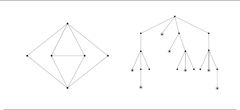
236 7. COMBINATORIAL SEARCH AND HEURISTIC METHODS
t = 3 5
6
42
s = 1
543
1
2
3
3
432532543
6636
Figure 7.1: Search tree enumerating all simple s-tpaths in the given graph (left).
is_a_solution(int a[], int k, int n)
{
return (k == n);
}
generate_permutations(int n)
{
int a[NMAX]; /* solution vector */
backtrack(a,0,n);
}
As a consequence of the candidate order, these routines generate permutations
in lexicographic, or sorted order—i.e., 123,132,213,231,312,and321. The prob-
lem of generating permutations is more thoroughly discussed in Section 14.4 (page
448).
7.1.3 Constructing All Paths in a Graph
Enumerating all the simple sto tpaths through a given graph is a more complicated
problem than listing permutations or subsets. There is no explicit formula that
counts the number of solutions as a function of the number of edges or vertices,
because the number of paths depends upon the structure of the graph.
The starting point of any path from sto tis always s.Thus,sis the only
candidate for the first position and S1={s}. The possible candidates for the
second position are the vertices vsuch that (s, v) is an edge of the graph, for the
path wanders from vertex to vertex using edges to define the legal steps. In general,

7.1 BACKTRACKING 237
Sk+1 consists of the set of vertices adjacent to akthat have not been used elsewhere
in the partial solution A.
construct_candidates(int a[], int k, int n, int c[], int *ncandidates)
{
int i; /* counters */
bool in_sol[NMAX]; /* what’s already in the solution? */
edgenode *p; /* temporary pointer */
int last; /* last vertex on current path */
for (i=1; i<NMAX; i++) in_sol[i] = FALSE;
for (i=1; i<k; i++) in_sol[ a[i] ] = TRUE;
if (k==1) { /* always start from vertex 1 */
c[0] = 1;
*ncandidates = 1;
}
else {
*ncandidates = 0;
last = a[k-1];
p = g.edges[last];
while (p != NULL) {
if (!in_sol[ p->y ]) {
c[*ncandidates] = p->y;
*ncandidates = *ncandidates + 1;
}
p = p->next;
}
}
}
We report a successful path whenever ak=t.
is_a_solution(int a[], int k, int t)
{
return (a[k] == t);
}
process_solution(int a[], int k)
{
solution_count ++; /* count all s to t paths */
}

238 7. COMBINATORIAL SEARCH AND HEURISTIC METHODS
The solution vector Amust have room for all nvertices, although most paths
are likely shorter than this. Figure 7.1 shows the search tree giving all paths from
a particular vertex in an example graph.
7.2 Search Pruning
Backtracking ensures correctness by enumerating all possibilities. Enumerating all
n! permutations of nvertices of the graph and selecting the best one yields the
correct algorithm to find the optimal traveling salesman tour. For each permuta-
tion, we could see whether all edges implied by the tour really exists in the graph
G, and if so, add the weights of these edges together.
However, it would be wasteful to construct all the permutations first and then
analyze them later. Suppose our search started from vertex v1, and it happened
that edge (v1,v
2)wasnotinG. The next (n−2)! permutations enumerated starting
with (v1,v
2) would be a complete waste of effort. Much better would be to prune
the search after v1,v
2and continue next with v1,v
3. By restricting the set of next
elements to reflect only moves that are legal from the current partial configuration,
we significantly reduce the search complexity.
Pruning is the technique of cutting off the search the instant we have estab-
lished that a partial solution cannot be extended into a full solution. For traveling
salesman, we seek the cheapest tour that visits all vertices. Suppose that in the
course of our search we find a tour twhose cost is Ct. Later, we may have a partial
solution awhose edge sum CA>C
t. Is there any reason to continue exploring this
node? No, because any tour with this prefix a1,...,a
kwill have cost greater than
tour t, and hence is doomed to be nonoptimal. Cutting away such failed partial
tours as soon as possible can have an enormous impact on running time.
Exploiting symmetry is another avenue for reducing combinatorial searches.
Pruning away partial solutions identical to those previously considered requires
recognizing underlying symmetries in the search space. For example, consider the
state of our TSP search after we have tried all partial positions beginning with v1.
Does it pay to continue the search with partial solutions beginning with v2?No.
Any tour starting and ending at v2can be viewed as a rotation of one starting
and ending at v1, for these tours are cycles. There are thus only (n−1)! distinct
tours on nvertices, not n!. By restricting the first element of the tour to v1,we
save a factor of nin time without missing any interesting solutions. Detecting such
symmetries can be subtle, but once identified they can usually be easily exploited.
Take-Home Lesson: Combinatorial searches, when augmented with tree prun-
ing techniques, can be used to find the optimal solution of small optimization
problems. How small depends upon the specific problem, but typical size limits
are somewhere between 15 ≤n≤50 items.

7.3 SUDOKU 239
12
35
6 7
7 3
4 8
1
12
8 4
5 6
673894512
912735486
845612973
798261354
526473891
134589267
469128735
287356149
351947628
Figure 7.2: Challenging Sudoku puzzle (l) with solution (r)
7.3 Sudoku
A Sudoku craze has swept the world. Many newspapers now publish daily Sudoku
puzzles, and millions of books about Sudoku have been sold. British Airways sent
a formal memo forbidding its cabin crews from doing Sudoku during takeoffs and
landings. Indeed, I have noticed plenty of Sudoku going on in the back of my
algorithms classes during lecture.
What is Sudoku? In its most common form, it consists of a 9 ×9 grid filled with
blanks and the digits 1 to 9. The puzzle is completed when every row, column, and
sector (3 ×3 subproblems corresponding to the nine sectors of a tic-tac-toe puzzle)
contain the digits 1 through 9 with no deletions or repetition. Figure 7.2 presents
a challenging Sudoku puzzle and its solution.
Backtracking lends itself nicely to the problem of solving Sudoku puzzles. We
will use the puzzle here to better illustrate the algorithmic technique. Our state
space will be the sequence of open squares, each of which must ultimately be filled
in with a number. The candidates for open squares (i, j) are exactly the integers
from 1 to 9 that have not yet appeared in row i, column j, or the 3 ×3 sector
containing (i, j). We backtrack as soon as we are out of candidates for a square.
The solution vector asupported by backtrack only accepts a single integer
per position. This is enough to store contents of a board square (1-9) but not the
coordinates of the board square. Thus, we keep a separate array of move positions
as part of our board data type provided below. The basic data structures we need
to support our solution are:
#define DIMENSION 9 /* 9*9 board */
#define NCELLS DIMENSION*DIMENSION /* 81 cells in a 9*9 problem */
typedef struct {
int x, y;
} point;
int x, y; /* x and y coordinates of point */

240 7. COMBINATORIAL SEARCH AND HEURISTIC METHODS
typedef struct {
int m[DIMENSION+1][DIMENSION+1]; /* matrix of board contents */
int freecount; /* how many open squares remain? */
point move[NCELLS+1]; /* how did we fill the squares? */
} boardtype;
Constructing the candidates for the next solution position involves first picking
the open square we want to fill next (next square), and then identifying which
numbers are candidates to fill that square (possible values). These routines are
basically bookkeeping, although the subtle details of how they work can have an
enormous impact on performance.
construct_candidates(int a[], int k, boardtype *board, int c[],
int *ncandidates)
{
int x,y; /* position of next move */
int i; /* counter */
bool possible[DIMENSION+1]; /* what is possible for the square */
next_square(&x,&y,board); /* which square should we fill next? */
board->move[k].x = x; /* store our choice of next position */
board->move[k].y = y;
*ncandidates = 0;
if ((x<0) && (y<0)) return; /* error condition, no moves possible */
possible_values(x,y,board,possible);
for (i=0; i<=DIMENSION; i++)
if (possible[i] == TRUE) {
c[*ncandidates] = i;
*ncandidates = *ncandidates + 1;
}
}
We must update our board data structure to reflect the effect of filling a candi-
date value into a square, as well as remove these changes should we backtrack away
from this position. These updates are handled by make move and unmake move, both
of which are called directly from backtrack:

7.3 SUDOKU 241
make_move(int a[], int k, boardtype *board)
{
fill_square(board->move[k].x,board->move[k].y,a[k],board);
}
unmake_move(int a[], int k, boardtype *board)
{
free_square(board->move[k].x,board->move[k].y,board);
}
One important job for these board update routines is maintaining how many
free squares remain on the board. A solution is found when there are no more free
squares remaining to be filled:
is_a_solution(int a[], int k, boardtype *board)
{
if (board->freecount == 0)
return (TRUE);
else
return(FALSE);
}
We print the configuration and turn off the backtrack search by setting off the
global finished flag on finding a solution. This can be done without consequence
because “official” Sudoku puzzles are only allowed to have one solution. There
can be an enormous number of solutions to nonofficial Sudoku puzzles. Indeed,
the empty puzzle (where no number is initially specified) can be filled in exactly
6,670,903,752,021,072,936,960 ways. We can ensure we don’t see all of them by
turning off the search:
process_solution(int a[], int k, boardtype *board)
{
print_board(board);
finished = TRUE;
}
This completes the program modulo details of identifying the next open
square to fill (next square) and identifying the candidates to fill that square
(possible values). Two reasonable ways to select the next square are:
•Arbitrary Square Selection – Pick the first open square we encounter, possibly
picking the first, the last, or a random open square. All are equivalent in that
there seems to be no reason to believe that one heuristic will perform any
better than the other.

242 7. COMBINATORIAL SEARCH AND HEURISTIC METHODS
•Most Constrained Square Selection – Here, we check each of the open squares
(i, j) to see how many number candidates remain for each—i.e. , have not
already been used in either row i, column j, or the sector containing (i, j).
We pick the square with the fewest number of candidates.
Although both possibilities work correctly, the second option is much, much
better. Often there will be open squares with only one remaining candidate. For
these, the choice is forced. We might as well make it now, especially since pinning
this value down will help trim the possibilities for other open squares. Of course,
we will spend more time selecting each candidate square, but if the puzzle is easy
enough we may never have to backtrack at all.
If the most constrained square has two possibilities, we have a 1/2 probability
of guessing right the first time, as opposed to a (1/9)th probability for a completely
unconstrained square. Reducing our average number of choices from (say) 3 per
square to 2 per square is an enormous win, since it multiplies for each position.
If we have (say) 20 positions to fill, we must enumerate only 220 =1,048,576
solutions. A branching factor of 3 at each of the 20 positions will result in over
3,000 times as much work!
Our final decision concerns the possible values we allow for each square. We
have two possibilities:
•Local Count – Our backtrack search works correctly if the routine generating
candidates for board position (i, j)(possible values) does the obvious thing
and allows all numbers 1 to 9 that have not appeared in the given row, column,
or sector.
•Look ahead – But what if our current partial solution has some other open
square where there are no candidates remaining under the local count cri-
teria? There is no possible way to complete this partial solution into a full
Sudoku grid. Thus there really are zero possible moves to consider for (i, j)
because of what is happening elsewhere on the board!
We will discover this obstruction eventually, when we pick this square for
expansion, discover it has no moves, and then have to backtrack. But why
wait, since all our efforts until then will be wasted? We are much better off
backtracking immediately and moving on.1
Successful pruning requires looking ahead to see when a solution is doomed to
go nowhere, and backing off as soon as possible.
Table 7.1 presents the number of calls to is asolution for all four backtracking
variants on three Sudoku instances of varying complexity:
1This look-ahead condition might have naturally followed from the most-constrained square selection, had
it been permitted to select squares with no moves. However, my implementation credited squares that already
contained numbers as having no moves, thus limiting the next square choices to squares with at least one move.
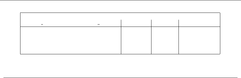
7.3 SUDOKU 243
Pruning Condition Puzzle Complexity
next square possible values Easy Medium Hard
arbitrary local count 1,904,832 863,305 never finished
arbitrary look ahead 127 142 12,507,212
most constrained local count 48 84 1,243,838
most constrained look ahead 48 65 10,374
Table 7.1: Sudoku run times (in number of steps) under different pruning strategies
•The Easy board was intended to be easy for a human player. Indeed, my
program solved it without any backtracking steps when the most constrained
square was selected as the next position.
•The Medium board stumped all the contestants at the finals of the World Su-
doku Championship in March 2006. The decent search variants still required
only a few backtrack steps to dispatch this problem.
•The Hard problem is the board displayed in Figure 7.2, which contains only
17 fixed numbers. This is the fewest specified known number of positions in
any problem instance that has only one complete solution.
What is considered to be a “hard” problem instance depends upon the given heuris-
tic. Certainly you know people who find math/theory harder than programming
and others who think differently. Heuristic Amay well think instance I1is easier
than I2, while heuristic Branks them in the other order.
What can we learn from these experiments? Looking ahead to eliminate dead
positions as soon as possible is the best way to prune a search. Without this
operation, we never finished the hardest puzzle and took thousands of times longer
than we should have on the easier ones.
Smart square selection had a similar impact, even though it nominally just
rearranges the order in which we do the work. However, doing more constrained
positions first is tantamount to reducing the outdegree of each node in the tree,
and each additional position we fix adds constraints that help lower the degree for
future selections.
It took the better part of an hour (48:44) to solve the puzzle in Figure 7.2 when
I selected an arbitrary square for my next move. Sure, my program was faster
in most instances, but Sudoku puzzles are designed to be solved by people using
pencils in much less time than this. Making the next move in the most constricted
square reduced search time by a factor of over 1,200. Each puzzle we tried can now
be solved in seconds—the time it takes to reach for the pencil if you want to do it
by hand.
This is the power of a pruning search. Even simple pruning strategies can suffice
to reduce running time from impossible to instantaneous.

244 7. COMBINATORIAL SEARCH AND HEURISTIC METHODS
Figure 7.3: Configurations covering 63 but not 64 squares
7.4 War Story: Covering Chessboards
Every researcher dreams of solving a classical problem—one that has remained open
and unsolved for over a century. There is something romantic about communicating
across the generations, being part of the evolution of science, and helping to climb
another rung up the ladder of human progress. There is also a pleasant sense of
smugness that comes from figuring out how to do something that nobody could do
before you.
There are several possible reasons why a problem might stay open for such
a long period of time. Perhaps it is so difficult and profound that it requires a
uniquely powerful intellect to solve. A second reason is technological—the ideas or
techniques required to solve the problem may not have existed when it was first
posed. A final possibility is that no one may have cared enough about the problem
in the interim to seriously bother with it. Once, I helped solve a problem that had
been open for over a hundred years. Decide for yourself which reason best explains
why.
Chess is a game that has fascinated mankind for thousands of years. In ad-
dition, it has inspired many combinatorial problems of independent interest. The
combinatorial explosion was first recognized with the legend that the inventor of
chess demanded as payment one grain of rice for the first square of the board, and
twice as much for the (i+ 1)st square than the ith square. The king was aston-
ished to learn he had to cough up 64
i=1 2i=2
65 −1 = 36,893,488,147,419,103,231
grains of rice. In beheading the inventor, the wise king first established pruning as
a technique for dealing with the combinatorial explosion.
In 1849, Kling posed the question of whether all 64 squares on the board can be
simultaneously threatened by an arrangement of the eight main pieces on the chess
board—the king, queen, two knights, two rooks, and two oppositely colored bishops.
Pieces do not threaten the square they sit on. Configurations that simultaneously
threaten 63 squares, such as those in Figure 7.3, have been known for a long time,
but whether this was the best possible remained an open problem. This problem
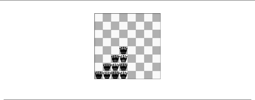
7.4 WAR STORY: COVERING CHESSBOARDS 245
Figure 7.4: The ten unique positions for the queen, with respect to symmetry
seemed ripe for solution by exhaustive combinatorial searching, although whether
it was solvable depended upon the size of the search space.
Consider the eight main pieces in chess (king, queen, two rooks, two bishops,
and two knights). How many ways can they be positioned on a chessboard? The
trivial bound is 64!/(64 −8)! = 178,462,987,637,760 ≈1015 positions. Anything
much larger than about 109positions would be unreasonable to search on a modest
computer in a modest amount of time.
Getting the job done would require significant pruning. Our first idea was to
remove symmetries. Accounting for orthogonal and diagonal symmetries left only
ten distinct positions for the queen, shown in Figure 7.4.
Once the queen is placed, there are 64 ·63/2 = 2,016 distinct ways to position
a pair of rooks or knights, 64 places to locate the king, and 32 spots for each of the
white and black bishops. Such an exhaustive search would test 2,663,550,812,160
≈1013 distinct positions—still much too large to try.
We could use backtracking to construct all of the positions, but we had to find
a way to prune the search space significantly. Pruning the search meant that we
needed a quick way to prove that there was no way to complete a partially filled-in
position to cover all 64 squares. Suppose we had already placed seven pieces on the
board, and together they covered all but 10 squares of the board. Say the remaining
piece was the king. Can there be a position to place the king so that all squares
are threatened? The answer must be no, because the king can threaten at most
eight squares according to the rules of chess. There can be no reason to test any
king position. We might win big pruning such configurations.
This pruning strategy required carefully ordering the evaluation of the pieces.
Each piece can threaten a certain maximum number of squares: the queen 27, the
king/knight 8, the rook 14, and the bishop 13. We would want to insert the pieces
in decreasing order of mobility. We can prune when the number of unthreatened
squares exceeds the sum of the maximum coverage of the unplaced pieces. This
sum is minimized by using the decreasing order of mobility.
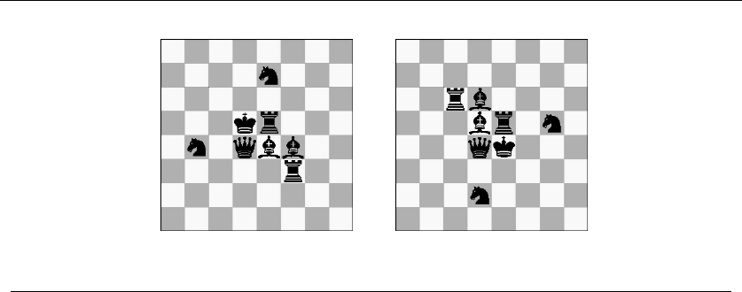
246 7. COMBINATORIAL SEARCH AND HEURISTIC METHODS
Figure 7.5: Weakly covering 64 squares
When we implemented a backtrack search using this pruning strategy, we found
that it eliminated over 95% of the search space. After optimizing our move gener-
ation, our program could search over 1,000 positions per second. But this was still
too slow, for 1012/103=10
9seconds meant 1,000 days! Although we might further
tweak the program to speed it up by an order of magnitude or so, what we really
needed was to find a way to prune more nodes.
Effective pruning meant eliminating large numbers of positions at a single
stroke. Our previous attempt was too weak. What if instead of placing up to eight
pieces on the board simultaneously, we placed more than eight pieces. Obviously,
the more pieces we placed simultaneously, the more likely they would threaten all
64 squares. But if they didn’t cover, all subsets of eight distinct pieces from the
set couldn’t possibly threaten all squares. The potential existed to eliminate a vast
number of positions by pruning a single node.
So in our final version, the nodes of our search tree corresponded to chessboards
that could have any number of pieces, and more than one piece on a square. For a
given board, we distinguished strong and weak attacks on a square. A strong attack
corresponds to the usual notion of a threat in chess. A square is weakly attacked if
the square is strongly attacked by some subset of the board—that is, a weak attack
ignores any possible blocking effects of intervening pieces. All 64 squares can be
weakly attacked with eight pieces, as shown in Figure 7.5.
Our algorithm consisted of two passes. The first pass listed boards where every
square was weakly attacked. The second pass filtered the list by considering block-
ing pieces. A weak attack is much faster to compute (no blocking to worry about),
and any strong attack set is always a subset of a weak attack set. The position
could be pruned whenever there was a non-weakly threatened square.
This program was efficient enough to complete the search on a slow 1988-era
IBM PC-RT in under one day. It did not find a single position covering all 64 squares
with the bishops on opposite colored squares. However, our program showed that
it is possible to cover the board with seven pieces provided a queen and a knight
can occupy the same square, as shown in Figure 7.6.
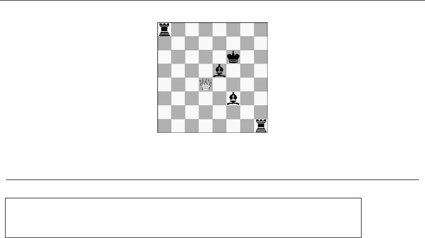
7.5 HEURISTIC SEARCH METHODS 247
Figure 7.6: Seven pieces suffice when superimposing queen and knight (shown as a white queen)
Take-Home Lesson: Clever pruning can make short work of surprisingly hard
combinatorial search problems. Proper pruning will have a greater impact on
search time than any other factor.
7.5 Heuristic Search Methods
Heuristic methods provide an alternate way to approach difficult combinatorial
optimization problems. Backtracking gave us a method to find the best of all pos-
sible solutions, as scored by a given objective function. However, any algorithm
searching all configurations is doomed to be impossible on large instances.
In this section, we discuss such heuristic search methods. We devote the bulk of
our attention to simulated annealing, which I find to be the most reliable method
to apply in practice. Heuristic search algorithms have an air of voodoo about them,
but how they work and why one method might work better than another follows
logically enough if you think them through.
In particular, we will look at three different heuristic search methods: random
sampling, gradient-descent search, and simulated annealing. The traveling salesman
problem will be our ongoing example for comparing heuristics. All three methods
have two common components:
•Solution space representation – This is a complete yet concise description
of the set of possible solutions for the problem. For traveling salesman, the
solution space consists of (n−1)! elements—namely all possible circular per-
mutations of the vertices. We need a data structure to represent each element
of the solution space. For TSP, the candidate solutions can naturally be rep-
resented using an array Sof n−1 vertices, where Sidefines the (i+ 1)st
vertex on the tour starting from v1.
•Cost function – Search methods need a cost or evaluation function to ac-
cess the quality of each element of the solution space. Our search heuristic

248 7. COMBINATORIAL SEARCH AND HEURISTIC METHODS
identifies the element with the best possible score—either highest or lowest
depending upon the nature of the problem. For TSP, the cost function for
evaluating a given candidate solution Sshould just sum up the costs involved,
namely the weight of all edges (Si,S
i+1), where Sn+1 denotes v1.
7.5.1 Random Sampling
The simplest method to search in a solution space uses random sampling. It is also
called the Monte Carlo method. We repeatedly construct random solutions and
evaluate them, stopping as soon as we get a good enough solution, or (more likely)
when we are tired of waiting. We report the best solution found over the course of
our sampling.
True random sampling requires that we are able to select elements from the
solution space uniformly at random. This means that each of the elements of the
solution space must have an equal probability of being the next candidate selected.
Such sampling can be a subtle problem. Algorithms for generating random permu-
tations, subsets, partitions, and graphs are discussed in Sections 14.4-14.7.
random_sampling(tsp_instance *t, int nsamples, tsp_solution *bestsol)
{
tsp_solution s; /* current tsp solution */
double best_cost; /* best cost so far */
double cost_now; /* current cost */
int i; /* counter */
initialize_solution(t->n,&s);
best_cost = solution_cost(&s,t);
copy_solution(&s,bestsol);
for (i=1; i<=nsamples; i++) {
random_solution(&s);
cost_now = solution_cost(&s,t);
if (cost_now < best_cost) {
best_cost = cost_now;
copy_solution(&s,bestsol);
}
}
}
When might random sampling do well?
•When there are a high proportion of acceptable solutions – Finding a piece of
hay in a haystack is easy, since almost anything you grab is a straw. When
solutions are plentiful, a random search should find one quickly.

7.5 HEURISTIC SEARCH METHODS 249
0
20000
40000
60000
80000
100000
120000
140000
160000
180000
200000
0 200000 400000 600000 800000 1e+06 1.2e+06 1.4e+06 1.6e+06
Length of Tour
Number of Iterations
Performance of Random Sampling for TSP
Random Sampling
Figure 7.7: Search time/quality tradeoffs for TSP using random sampling.
Finding prime numbers is domain where a random search proves successful.
Generating large random prime numbers for keys is an important aspect of
cryptographic systems such as RSA. Roughly one out of every ln nintegers
are prime, so only a modest number of samples need to be taken to discover
primes that are several hundred digits long.
•When there is no coherence in the solution space – Random sampling is the
right thing to do when there is no sense of when we are getting closer to a
solution. Suppose you wanted to find one of your friends who has a social
security number that ends in 00. There is not much you can hope to do but
tap an arbitrary fellow on their shoulder and ask. No cleverer method will be
better than random sampling.
Consider again the problem of hunting for a large prime number. Primes are
scattered quite arbitrarily among the integers. Random sampling is as good
as anything else.
How does random sampling do on TSP? Pretty lousy. The best solution I found
after testing 1.5 million random permutations of a classic TSP instance (the capital
cities of the 48 continental United States) was 101,712.8. This is more than three
times the cost of the optimal tour! The solution space consists almost entirely

250 7. COMBINATORIAL SEARCH AND HEURISTIC METHODS
of mediocre to bad solutions, so quality grows very slowly with the amount of
sampling / running time we invest. Figure 7.7 presents the arbitrary up-and-down
movements of random sampling and generally poor quality solutions encountered
on the journey, so you can get a sense of how the score varied over each iteration.
Most problems we encounter, like TSP, have relatively few good solutions but
a highly coherent solution space. More powerful heuristic search algorithms are
required to deal effectively with such problems.
Stop and Think: Picking the Pair
Problem: We need an efficient and unbiased way to generate random pairs of
vertices to perform random vertex swaps. Propose an efficient algorithm to generate
elements from the n
2unordered pairs on {1,...,n}uniformly at random.
Solution: Uniformly generating random structures is a surprisingly subtle problem.
Consider the following procedure to generate random unordered pairs:
i = random int(1,n-1);
j = random int(i+1,n);
It is clear that this indeed generates unordered pairs, since i<j. Further,
it is clear that all n
2unordered pairs can indeed be generated, assuming that
random int generates integers uniformly between its two arguments.
But are they uniform? The answer is no. What is the probability that pair (1,2)
is generated? There is a 1/(n−1) chance of getting the 1, and then a 1/(n−1) chance
of getting the 2, which yields p(1,2) = 1/(n−1)2. But what is the probability of
getting (n−1,n)? Again, there is a 1/n chance of getting the first number, but
now there is only one possible choice for the second candidate! This pair will occur
ntimes more often than the first!
The problem is that fewer pairs start with big numbers than little numbers.
We could solve this problem by calculating exactly how unordered pairs start with
i(exactly (n−i)) and appropriately bias the probability. The second value could
then be selected uniformly at random from i+1ton.
But instead of working through the math, let’s exploit the fact that randomly
generating the n2ordered pairs uniformly is easy. Just pick two integers indepen-
dently of each other. Ignoring the ordering (i.e. , permuting the ordered pair to
unordered pair (x, y) so that x<y) gives us a 2/n2probability of generating each
unordered pair of distinct elements. If we happen to generate a pair (x, x), we dis-
card it and try again. We will get unordered pairs uniformly at random in constant
expected time using the following algorithm:
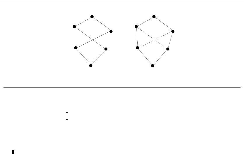
7.5 HEURISTIC SEARCH METHODS 251
1
6
5
4
22
1
6
5
4
33
Figure 7.8: Improving a TSP tour by swapping vertices 2 and 6
do {i = random int(1,n);
j = random int(1,n);
if (i > j) swap(&i,&j);
}while (i==j);
7.5.2 Local Search
Now suppose you want to hire an algorithms expert as a consultant to solve your
problem. You could dial a phone number at random, ask if they are an algorithms
expert, and hang up the phone if they say no. After many repetitions you will
probably find one, but it would probably be more efficient to ask the fellow on the
phone for someone more likely to know an algorithms expert, and call them up
instead.
A local search employs local neighborhood around every element in the solution
space. Think of each element xin the solution space as a vertex, with a directed
edge (x, y) to every candidate solution ythat is a neighbor of x. Our search proceeds
from xto the most promising candidate in x’s neighborhood.
We certainly do not want to explicitly construct this neighborhood graph for
any sizable solution space. Think about TSP, which will have (n−1)! vertices in
this graph. We are conducting a heuristic search precisely because we cannot hope
to do this many operations in a reasonable amount of time.
Instead, we want a general transition mechanism that takes us to the next solu-
tion by slightly modifying the current one. Typical transition mechanisms include
swapping a random pair of items or changing (inserting or deleting) a single item
in the solution.
The most obvious transition mechanism for TSP would be to swap the current
tour positions of a random pair of vertices Siand Sj, as shown in Figure 7.8.

252 7. COMBINATORIAL SEARCH AND HEURISTIC METHODS
This changes up to eight edges on the tour, deleting the edges currently adjacent
to both Siand Sj, and adding their replacements. Ideally, the effect that these
incremental changes have on measuring the quality of the solution can be computed
incrementally, so cost function evaluation takes time proportional to the size of the
change (typically constant) instead of linear to the size of the solution.
A local search heuristic starts from an arbitrary element of the solution space,
and then scans the neighborhood looking for a favorable transition to take. For
TSP, this would be transition, which lowers the cost of the tour. In a hill-climbing
procedure, we try to find the top of a mountain (or alternately, the lowest point in
a ditch) by starting at some arbitrary point and taking any step that leads in the
direction we want to travel. We repeat until we have reached a point where all our
neighbors lead us in the wrong direction. We are now King of the Hill (or Dean of
the Ditch).
We are probably not King of the Mountain, however. Suppose you wake up in
a ski lodge, eager to reach the top of the neighboring peak. Your first transition
to gain altitude might be to go upstairs to the top of the building. And then
you are trapped. To reach the top of the mountain, you must go downstairs and
walk outside, but this violates the requirement that each step has to increase your
score. Hill-climbing and closely related heuristics such as greedy search or gradient
descent search are great at finding local optima quickly, but often fail to find the
globally best solution.
hill_climbing(tsp_instance *t, tsp_solution *s)
{
double cost; /* best cost so far */
double delta; /* swap cost */
int i,j; /* counters */
bool stuck; /* did I get a better solution? */
double transition();
initialize_solution(t->n,s);
random_solution(s);
cost = solution_cost(s,t);
do {
stuck = TRUE;
for (i=1; i<t->n; i++)
for (j=i+1; j<=t->n; j++) {
delta = transition(s,t,i,j);
if (delta < 0) {
stuck = FALSE;
cost = cost + delta;
}

7.5 HEURISTIC SEARCH METHODS 253
else
transition(s,t,j,i);
}
} while (!stuck);
}
When does local search do well?
•When there is great coherence in the solution space – Hill climbing is at its
best when the solution space is convex. In other words, it consists of exactly
one hill. No matter where you start on the hill, there is always a direction to
walk up until you are at the absolute global maximum.
Many natural problems do have this property. We can think of a binary
search as starting in the middle of a search space, where exactly one of the
two possible directions we can walk will get us closer to the target key. The
simplex algorithm for linear programming (see Section 13.6 (page 411)) is
nothing more than hill-climbing over the right solution space, yet guarantees
us the optimal solution to any linear programming problem.
•Whenever the cost of incremental evaluation is much cheaper than global eval-
uation –ItcostsΘ(n) to evaluate the cost of an arbitrary n-vertex candidate
TSP solution, because we must total the cost of each edge in the circular
permutation describing the tour. Once that is found, however, the cost of the
tour after swapping a given pair of vertices can be determined in constant
time.
If we are given a very large value of nand a very small budget of how
much time we can spend searching, we are better off using it to do several
incremental evaluations than a few random samples, even if we are looking
for a needle in a haystack.
The primary drawback of a local search is that soon there isn’t anything left for
us to do as we find the local optimum. Sure, if we have more time we could start
from different random points, but in landscapes of many low hills we are unlikely
to stumble on the optimum.
How does local search do on TSP? Much better than random sampling for a
similar amount of time. With over a total of 1.5 million tour evaluations in our
48-city TSP instance, our best local search tour had a length of 40,121.2—only
19.6% more than the optimal tour of 33,523.7.
This is good, but not great. You would not be happy to learn you are paying
19.6% more taxes than you should. Figure 7.9 illustrates the trajectory of a local
search: repeated streaks from random tours down to decent solutions of fairly sim-
ilar quality. We need more powerful methods to get closer to the optimal solution.
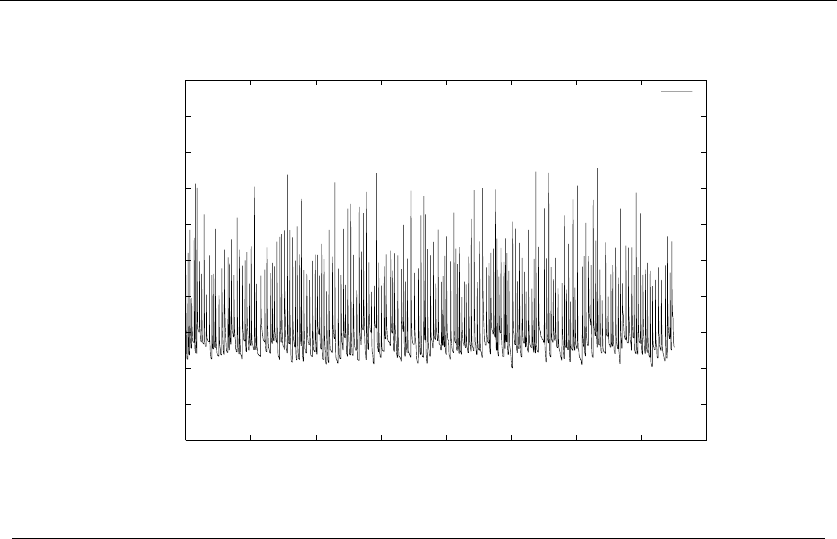
254 7. COMBINATORIAL SEARCH AND HEURISTIC METHODS
0
20000
40000
60000
80000
100000
120000
140000
160000
180000
200000
0 200000 400000 600000 800000 1e+06 1.2e+06 1.4e+06 1.6e+06
Length of Tour
Number of Iterations
Performance of Hill Climbing for TSP
Hill Climbing
Figure 7.9: Search time/quality tradeoffs for TSP using hill climbing.
7.5.3 Simulated Annealing
Simulated annealing is a heuristic search procedure that allows occasional transi-
tions leading to more expensive (and hence inferior) solutions. This may not sound
like progress, but it helps keep our search from getting stuck in local optima. That
poor fellow trapped on the top floor of a ski lodge would do better to break the
glass and jump out the window if he really wanted to reach the top of the mountain.
The inspiration for simulated annealing comes from the physical process of cool-
ing molten materials down to the solid state. In thermodynamic theory, the energy
state of a system is described by the energy state of each particle constituting it.
A particle’s energy state jumps about randomly, with such transitions governed by
the temperature of the system. In particular, the transition probability P(ei,e
j,T)
from energy eito ejat temperature Tis given by
P(ei,e
j,T)=e(ei−ej)/(kBT)
where kBis a constant—called Boltzmann’s constant.
What does this formula mean? Consider the value of the exponent under dif-
ferent conditions. The probability of moving from a high-energy state to a lower-
energy state is very high. But, there is still a nonzero probability of accepting a

7.5 HEURISTIC SEARCH METHODS 255
transition into a high-energy state, with such small jumps much more likely than
big ones. The higher the temperature, the more likely energy jumps will occur.
Simulated-Annealing()
Create initial solution S
Initialize temperature t
repeat
for i=1toiteration-length do
Generate a random transition from Sto Si
If (C(S)≥C(Si)) then S=Si
else if (e(C(S)−C(Si))/(k·t)> random[0,1)) then S=Si
Reduce temperature t
until (no change in C(S))
Return S
What relevance does this have for combinatorial optimization? A physical sys-
tem, as it cools, seeks to reach a minimum-energy state. Minimizing the total energy
is a combinatorial optimization problem for any set of discrete particles. Through
random transitions generated according to the given probability distribution, we
can mimic the physics to solve arbitrary combinatorial optimization problems.
Take-Home Lesson: Forget about this molten metal business. Simulated an-
nealing is effective because it spends much more of its time working on good
elements of the solution space than on bad ones, and because it avoids getting
trapped repeatedly in the same local optima.
As with a local search, the problem representation includes both a representa-
tion of the solution space and an easily computable cost function C(s) measuring
the quality of a given solution. The new component is the cooling schedule,whose
parameters govern how likely we are to accept a bad transition as a function of
time.
At the beginning of the search, we are eager to use randomness to explore the
search space widely, so the probability of accepting a negative transition should
be high. As the search progresses, we seek to limit transitions to local improve-
ments and optimizations. The cooling schedule can be regulated by the following
parameters:
•Initial system temperature – Typically t1=1.
•Temperature decrement function – Typically tk=α·tk−1, where 0.8≤α≤
0.99. This implies an exponential decay in the temperature, as opposed to a
linear decay.
•Number of iterations between temperature change – Typically, 100 to 1,000
iterations might be permitted before lowering the temperature.
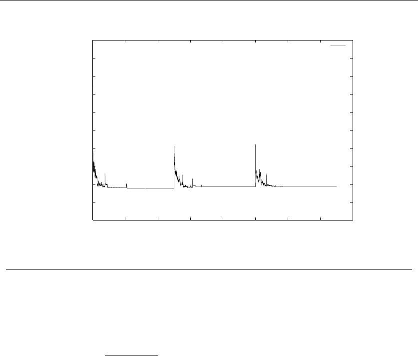
256 7. COMBINATORIAL SEARCH AND HEURISTIC METHODS
0
20000
40000
60000
80000
100000
120000
140000
160000
180000
200000
0 200000 400000 600000 800000 1e+06 1.2e+06 1.4e+06 1.6e+06
Length of Tour
Number of Iterations
Performance of Simulated Annealing for TSP
Simulated Annealing
Figure 7.10: Search time/quality tradeoffs for TSP using simulated annealing
•Acceptance criteria – A typical criterion is to accept any transition from sito
si+1 when C(si+1)<C(si), and also accept a negative transition whenever
e−(C(si)−C(si+1))
k·ti≥r,
where ris a random number 0 ≤r<1. The constant knormalizes this cost
function so that almost all transitions are accepted at the starting tempera-
ture.
•Stop criteria – Typically, when the value of the current solution has not
changed or improved within the last iteration or so, the search is terminated
and the current solution reported.
Creating the proper cooling schedule is somewhat of a trial-and-error process of
mucking with constants and seeing what happens. It probably pays to start from
an existing implementation of simulated annealing, so check out my full imple-
mentation (at http://www.algorist.com ) as well as others provided in Section 13.5
(page 407).
Compare the search/time execution profiles of our three heuristics. The cloud of
points corresponding to random sampling is significantly worse than the solutions

7.5 HEURISTIC SEARCH METHODS 257
encountered by the other heuristics. The scores of the short streaks corresponding
to runs of hill-climbing solutions are clearly much better.
But best of all are the profiles of the three simulated annealing runs in Figure
7.10. All three runs lead to much better solutions than the best hill-climbing result.
Further, it takes relatively few iterations to score most of the improvement, as
shown by the three rapid plunges toward optimum we see with simulated annealing.
Using the same 1,500,000 iterations as the other methods, simulated annealing
gave us a solution of cost 36,617.4—only 9.2% over the optimum. Even better
solutions are available to those willing to wait a few minutes. Letting it run for
5,000,000 iterations got the score down to 34,254.9, or 2.2% over the optimum.
There were no further improvements after I cranked it up to 10,000,000 iterations.
In expert hands, the best problem-specific heuristics for TSP can slightly
outperform simulated annealing. But the simulated annealing solution works ad-
mirably. It is my heuristic method of choice.
Implementation
The implementation follows the pseudocode quite closely:
anneal(tsp_instance *t, tsp_solution *s)
{
int i1, i2; /* pair of items to swap */
int i,j; /* counters */
double temperature; /* the current system temp */
double current_value; /* value of current state */
double start_value; /* value at start of loop */
double delta; /* value after swap */
double merit, flip; /* hold swap accept conditions*/
double exponent; /* exponent for energy funct*/
double random_float();
double solution_cost(), transition();
temperature = INITIAL_TEMPERATURE;
initialize_solution(t->n,s);
current_value = solution_cost(s,t);
for (i=1; i<=COOLING_STEPS; i++) {
temperature *= COOLING_FRACTION;
start_value = current_value;
for (j=1; j<=STEPS_PER_TEMP; j++) {

258 7. COMBINATORIAL SEARCH AND HEURISTIC METHODS
/* pick indices of elements to swap */
i1 = random_int(1,t->n);
i2 = random_int(1,t->n);
flip = random_float(0,1);
delta = transition(s,t,i1,i2);
exponent = (-delta/current_value)/(K*temperature);
merit = pow(E,exponent);
if (delta < 0) /*ACCEPT-WIN*/
current_value = current_value+delta;
else { if (merit > flip) /*ACCEPT-LOSS*/
current_value = current_value+delta;
else /* REJECT */
transition(s,t,i1,i2);
}
}
/* restore temperature if progress has been made */
if ((current_value-start_value) < 0.0)
temperature = temperature/COOLING_FRACTION;
}
}
7.5.4 Applications of Simulated Annealing
We provide several examples to demonstrate how these components can lead to
elegant simulated annealing solutions for real combinatorial search problems.
Maximum Cut
The “maximum cut” problem seeks to partition the vertices of a weighted graph G
into sets V1and V2to maximize the weight (or number) of edges with one vertex
in each set. For graphs that specify an electronic circuit, the maximum cut in the
graph defines the largest amount of data communication that can take place in the
circuit simultaneously. As discussed in Section 16.6 (page 541), maximum cut is
NP-complete.
How can we formulate maximum cut for simulated annealing? The solution
space consists of all 2n−1possible vertex partitions. We save a factor of two over
all vertex subsets because vertex v1canbeassumedtobefixedontheleftside
of the partition. The subset of vertices accompanying it can be represented using

7.5 HEURISTIC SEARCH METHODS 259
a bit vector. The cost of a solution is the sum of the weights cut in the current
configuration. A natural transition mechanism selects one vertex at random and
moves it across the partition simply by flipping the corresponding bit in the bit
vector. The change in the cost function will be the weight of its old neighbors minus
the weight of its new neighbors. This can be computed in time proportional to the
degree of the vertex.
This kind of simple, natural modeling is the right type of heuristic to seek in
practice.
Independent Set
An “independent set” of a graph Gis a subset of vertices Ssuch that there is
no edge with both endpoints in S. The maximum independent set of a graph is
the largest such empty induced subgraph. Finding large independent sets arises in
dispersion problems associated with facility location and coding theory, as discussed
in Section 16.2 (page 528).
The natural state space for a simulated annealing solution would be all 2n
subsets of the vertices, represented as a bit vector. As with maximum cut, a simple
transition mechanism would add or delete one vertex from S.
One natural cost function for subset Smight be 0 if Scontains an edge, and
|S|if it is indeed an independent set. This function ensures that we work towards
an independent set at all times. However, this condition is strict enough that we
are liable to move only in a narrow portion of the possible search space. More
flexibility in the search space and quicker cost function computations can result
from allowing nonempty graphs at the early stages of cooling. Better in practice
would be a cost function like C(S)=|S|−λ·mS/T , where λis a constant, Tis the
temperature, and mSis the number of edges in the subgraph induced by S.The
dependence of C(S)onTensures that the search will drive the edges out faster as
the system cools.
Circuit Board Placement
In designing printed circuit boards, we are faced with the problem of positioning
modules (typically, integrated circuits) on the board. Desired criteria in a layout
may include (1) minimizing the area or aspect ratio of the board so that it properly
fits within the allotted space, and (2) minimizing the total or longest wire length
in connecting the components. Circuit board placement is representative of the
kind of messy, multicriterion optimization problems for which simulated annealing
is ideally suited.
Formally, we are given a collection of rectangular modules r1,...,r
n, each with
associated dimensions hi×li. Further, for each pair of modules ri,r
j, we are given
the number of wires wij that must connect the two modules. We seek a placement
of the rectangles that minimizes area and wire length, subject to the constraint
that no two rectangles overlap each other.

260 7. COMBINATORIAL SEARCH AND HEURISTIC METHODS
The state space for this problem must describe the positions of each rectangle.
To make this discrete, the rectangles can be restricted to lie on vertices of an
integer grid. Reasonable transition mechanisms including moving one rectangle to
a different location, or swapping the position of two rectangles. A natural cost
function would be
C(S)=λarea(Sheight ·Swidth)+
n
i=1
n
j=1
(λwire ·wij ·dij +λoverlap(ri∩rj))
where λarea,λwire,andλoverlap are constants governing the impact of these com-
ponents on the cost function. Presumably, λoverlap should be an inverse function
of temperature, so after gross placement it adjusts the rectangle positions to be
disjointed.
Take-Home Lesson: Simulated annealing is a simple but effective technique
for efficiently obtaining good but not optimal solutions to combinatorial search
problems.
7.6 War Story: Only it is Not a Radio
“Think of it as a radio,” he chuckled. “Only it is not a radio.”
I’d been whisked by corporate jet to the research center of a large but very
secretive company located somewhere east of California. They were so paranoid
that I never got to see the object we were working on, but the people who brought
me in did a great job of abstracting the problem.
The application concerned a manufacturing technique known as selective as-
sembly. Eli Whitney started the Industrial Revolution through his system of in-
terchangeable parts. He carefully specified the manufacturing tolerances on each
part in his machine so that the parts were interchangeable, meaning that any legal
cog-widget could be used to replace any other legal cog-widget. This greatly sped
up the process of manufacturing, because the workers could just put parts together
instead of having to stop to file down rough edges and the like. It made replacing
broken parts a snap. This was a very good thing.
Unfortunately, it also resulted in large piles of cog-widgets that were slightly
outside the manufacturing tolerance and thus had to be discarded. Another clever
fellow then observed that maybe one of these defective cog-widgets could be used
when all the other parts in the given assembly exceeded their required manufactur-
ing tolerances. Good plus bad could well equal good enough. This is the idea of
selective assembly.
“Each not-radio is made up of ndifferent types of not-radio parts,” he told me.
For the ith part type (say the right flange gasket), we have a pile of siinstances
of this part type. Each part (flange gasket) comes with a measure of the degree to
which it deviates from perfection. We need to match up the parts so as to create
the greatest number of working not-radios as possible.”

7.6 WAR STORY: ONLY IT IS NOT A RADIO 261
32
11
1514
33
6
11
17
5
Figure 7.11: Part assignments for three not-radios, such that each had at most 50 points total
defect
The situation is illustrated in Figure 7.11. Each not-radio consists of three parts,
and the sum of the defects in any functional not-radio must total at most 50. By
cleverly balancing the good and bad parts in each machine, we can use all the parts
and make three working not-radios.
I thought about the problem. The simplest procedure would take the best part
for each part type, make a not-radio out of them, and repeat until the not-radio
didn’t play (or do whatever a not-radio does). But this would create a small number
of not-radios drastically varying in quality, whereas they wanted as many decent
not-radios as possible.
The goal was to match up good parts and bad parts so the total amount of
badness wasn’t so bad. Indeed, the problem sounded related to matching in graphs
(see Section 15.6 (page 498)). Suppose we built a graph where the vertices were
the part instances, and add an edge for all two part instances that were within the
total error tolerance. In graph matching, we seek the largest number of edges such
that no vertex appears more than once in the matching. This is analogous to the
largest number of two-part assemblies we can form from the given set of parts.
“I can solve your problem using matching,” I announced, “Provided not-radios
are each made of only two parts.”
There was silence. Then they all started laughing at me. “Everyone knows
not-radios have more than two parts,” they said, shaking their heads.
That spelled the end of this algorithmic approach. Extending to more than
two parts turned the problem into matching on hypergraphs,2—a problem which
is NP-complete. Further, it might take exponential time in the number of part
types just to build the graph, since we had to explicitly construct each possible
hyperedge/assembly.
2Ahypergraph is made up of edges that can contain more than two vertices each. They can be thought of
as general collections of subsets of vertices/elements.

262 7. COMBINATORIAL SEARCH AND HEURISTIC METHODS
I went back to the drawing board. They wanted to put parts into assemblies
so that no assembly would have more total defects than allowed. Described that
way, it sounded like a packing problem. In the bin packing problem (see Section
17.9 (page 595)), we are given a collection of items of different sizes and asked to
store them using the smallest possible number of bins, each of which has a fixed
capacity of size k. Here, the assemblies represented the bins, each of which could
absorb total defect ≤k. The items to pack represented the individual parts, whose
size would reflect its quality of manufacture.
It wasn’t pure bin packing, however, since parts came in different types. The
application imposed constraints on the allowable contents of each bin. Creating the
maximum number of not-radios meant that we sought a packing that maximized
the number of bins which contained exactly one part for each of the mdifferent
parts types.
Bin packing is NP-complete, but is a natural candidate for a heuristic search
approach. The solution space consists of assignments of parts to bins. We initially
pick a random part of each type for each bin to give us a starting configuration for
the search.
The local neighborhood operation involves moving parts around from one bin
to another. We could move one part at a time, but more effective was swapping
parts of a particular type between two randomly chosen bins. In such a swap,
both bins remain complete not-radios, hopefully with better error tolerance than
before. Thus, our swap operator required three random integers—one to select the
appropriate parts type (from 1 to m) and two more to select the assembly bins
involved (say from 1 to b).
The key decision was the cost function to use. They supplied the hard limit
kon the total defect level for each individual assembly. But what was the best
way to score a set of assemblies? We could just return the number of acceptable
complete assemblies as our score—an integer from 1 to b. Although this was indeed
what we wanted to optimize, it would not be sensitive to detect when we were
making partial progress towards a solution. Suppose one of our swaps succeeded in
bringing one of the nonfunctional assemblies much closer to the not-radio limit k.
That would be a better starting point for further progress than the original, and
should be favored.
My final cost function was as follows. I gave one point for every working assem-
bly, and a significantly smaller total for each nonworking assembly based on how
close it was to the threshold k. The score for a nonworking assembly decreased
exponentially based on how much it was over k. Thus the optimizer would seek
to maximize the number of working assemblies, and then try to drive another
assembly close to the limit.
I implemented this algorithm, and then ran the search on the test case they
provided. It was an instance taken directly from the factory floor. Not-radios turn
out to contain m= 8 important parts types. Some parts types are more expensive
than others, and so they have fewer available candidates to consider. The most

7.7 WAR STORY: ANNEALING ARRAYS 263
suffix
prefix AA AG GA GG
AA AAAA AAAG AAGA AAGG
AG AGAA AGAG AGGA AGGG
GA GAAG GAAG GAGA GAGG
GG GGAA GGAG GGGA GGGG
Figure 7.12: A prefix-suffix array of all purine 4-mers
constrained parts type had only eight representatives, so there could be at most
eight possible assemblies from this given mix.
I watched as simulated annealing chugged and bubbled on the problem instance.
The number of completed assemblies instantly climbed (1, 2, 3, 4) before progress
started to slow a bit. Then came 5 and 6 in a hiccup, with a pause before assembly
7 came triumphantly together. But tried as it might, the program could not put
together eight not-radios before I lost interest in watching.
I called and tried to admit defeat, but they wouldn’t hear it. It turns out that
the best the factory had managed after extensive efforts was only six working not-
radios, so my result represented a significant improvement!
7.7 War Story: Annealing Arrays
The war story of Section 3.9 (page 94) reported how we used advanced data struc-
tures to simulate a new method for sequencing DNA. Our method, interactive
sequencing by hybridization (SBH), required building arrays of specific oligonu-
cleotides on demand.
A biochemist at Oxford University got interested in our technique, and more-
over he had in his laboratory the equipment we needed to test it out. The Southern
Array Maker, manufactured by Beckman Instruments, prepared discrete oligonu-
cleotide sequences in 64 parallel rows across a polypropylene substrate. The device
constructs arrays by appending single characters to each cell along specific rows
and columns of arrays. Figure 7.12 shows how to construct an array of all 24=16
purine (Aor G) 4-mers by building the prefixes along rows and the suffixes along
columns. This technology provided an ideal environment for testing the feasibility
of interactive SBH in a laboratory, because with proper programming it gave a way
to fabricate a wide variety of oligonucleotide arrays on demand.
However, we had to provide the proper programming. Fabricating complicated
arrays required solving a difficult combinatorial problem. We were given as input
asetofnstrings (representing oligonucleotides) to fabricate in an m×marray
(where m= 64 on the Southern apparatus). We had to produce a schedule of
row and column commands to realize the set of strings S.Weprovedthatthe

264 7. COMBINATORIAL SEARCH AND HEURISTIC METHODS
problem of designing dense arrays was NP-complete, but that didn’t really matter.
My student Ricky Bradley and I had to solve it anyway.
“We are going to have to use a heuristic,” I told him. “So how can we model
this problem?”
“Well, each string can be partitioned into prefix and suffix pairs that realize it.
For example, the string ACC can be realized in four different ways: prefix ‘’ and
suffix ACC, prefix A and suffix CC, prefix AC and suffix C, or prefix ACC and
suffix ‘’. We seek the smallest set of prefixes and suffixes that together realize all
the given strings,” Ricky said.
“Good. This gives us a natural representation for simulated annealing. The
state space will consist of all possible subsets of prefixes and suffixes. The natural
transitions between states might include inserting or deleting strings from our
subsets, or swapping a pair in or out.”
“What’s a good cost function?” he asked.
“Well, we need as small an array as possible that covers all the strings. How
about taking the maximum of number of rows (prefixes) or columns (suffixes) used
in our array, plus the number of strings from Sthat are not yet covered. Try it
and let’s see what happens.”
Ricky went off and implemented a simulated annealing program along these
lines. It printed out the state of the solution each time a transition was accepted
and was fun to watch. The program quickly kicked out unnecessary prefixes and
suffixes, and the array began shrinking rapidly in size. But after several hundred
iterations, progress started to slow. A transition would knock out an unnecessary
suffix, wait a while, then add a different suffix back again. After a few thousand
iterations, no real improvement was happening.
“The program doesn’t seem to recognize when it is making progress. The eval-
uation function only gives credit for minimizing the larger of the two dimensions.
Why not add a term to give some credit to the other dimension.”
Ricky changed the evaluation function, and we tried again. This time, the pro-
gram did not hesitate to improve the shorter dimension. Indeed, our arrays started
to be skinny rectangles instead of squares.
“OK. Let’s add another term to the evaluation function to give it points for
being roughly square.”
Ricky tried again. Now the arrays were the right shape, and progress was in
the right direction. But the progress was still slow.
“Too many of the insertion moves don’t affect many strings. Maybe we should
skew the random selections so that the important prefix/suffixes get picked more
often.”
Ricky tried again. Now it converged faster, but sometimes it still got stuck. We
changed the cooling schedule. It did better, but was it doing well? Without a lower
bound knowing how close we were to optimal, it couldn’t really tell how good our
solution was. We tweaked and tweaked until our program stopped improving.
Our final solution refined the initial array by applying the following random
moves:

7.7 WAR STORY: ANNEALING ARRAYS 265
Figure 7.13: Compression of the HIV array by simulated annealing – after 0, 500, 1,000, and
5,750 iterations
•swap – swap a prefix/suffix on the array with one that isn’t.
•add – add a random prefix/suffix to the array.
•delete – delete a random prefix/suffix from the array.
•useful add – add the prefix/suffix with the highest usefulness to the array.
•useful delete – delete the prefix/suffix with the lowest usefulness from the
array.
•string add – randomly select a string not on the array, and add the most
useful prefix and/or suffix to cover this string.
A standard cooling schedule was used, with an exponentially decreasing temper-
ature (dependent upon the problem size) and a temperature-dependent Boltzmann
criterion for accepting states that have higher costs. Our final cost function was
defined as
cost =2×max +min +(max −min)2
4+4(strtotal −strin)
where max is the size of the maximum chip dimension, min is the size of the
minimum chip dimension, strtotal =|S|,andstrin is the number of strings from S
currently on the chip.
How well did we do? Figure 7.13 shows the convergence of a custom array
consisting of the 5,716 unique 7-mers of the HIV virus. Figure 7.13 shows snapshots
of the state of the chip at four points during the annealing process (0, 500, 1,000,
and the final chip at 5,750 iterations). Black pixels represent the first occurrence
of an HIV 7-mer. The final chip size here is 130 ×132—quite an improvement over

266 7. COMBINATORIAL SEARCH AND HEURISTIC METHODS
the initial size of 192 ×192. It took about fifteen minutes’ worth of computation
to complete the optimization, which was perfectly acceptable for the application.
But how well did we do? Since simulated annealing is only a heuristic, we really
don’t know how close to optimal our solution is. I think we did pretty well, but can’t
really be sure. Simulated annealing is a good way to handle complex optimization
problems. However, to get the best results, expect to spend more time tweaking
and refining your program than you did in writing it in the first place. This is dirty
work, but sometimes you have to do it.
7.8 Other Heuristic Search Methods
Several heuristic search methods have been proposed to search for good solutions for
combinatorial optimization problems. Like simulated annealing, many techniques
relies on analogies to real-world physical processes. Popular methods include genetic
algorithms,neural networks,andant colony optimization.
The intuition behind these methods is highly appealing, but skeptics decry
them as voodoo optimization techniques that rely more on nice analogies to nature
than demonstrated computational results on problems that have been studied using
other methods.
The question isn’t whether you can get decent answers for many problems given
enough effort using these techniques. Clearly you can. The real question is whether
they lead to better solutions with less implementation complexity than the other
methods we have discussed.
In general, I don’t believe that they do. But in the spirit of free inquiry, I
introduce genetic algorithms, which is the most popular of these methods. See the
chapter notes for more detailed readings.
Genetic Algorithms
Genetic algorithms draw their inspiration from evolution and natural selection.
Through the process of natural selection, organisms adapt to optimize their chances
for survival in a given environment. Random mutations occur in an organism’s
genetic description, which then get passed on to its children. Should a mutation
prove helpful, these children are more likely to survive and reproduce. Should it be
harmful, these children won’t, and so the bad trait will die with them.
Genetic algorithms maintain a “population” of solution candidates for the given
problem. Elements are drawn at random from this population and allowed to “re-
produce” by combining aspects of the two-parent solutions. The probability that
an element is chosen to reproduce is based on its “fitness,”—essentially the cost of
the solution it represents. Unfit elements die from the population, to be replaced
by a successful-solution offspring.
The idea behind genetic algorithms is extremely appealing. However, they don’t
seem to work as well on practical combinatorial optimization problems as simulated

7.9 PARALLEL ALGORITHMS 267
annealing does. There are two primary reasons for this. First, it is quite unnatural to
model applications in terms of genetic operators like mutation and crossover on bit
strings. The pseudobiology adds another level of complexity between you and your
problem. Second, genetic algorithms take a very long time on nontrivial problems.
The crossover and mutation operations typically make no use of problem-specific
structure, so most transitions lead to inferior solutions, and convergence is slow.
Indeed, the analogy with evolution—where significant progress require millions of
years—can be quite appropriate.
We will not discuss genetic algorithms further, to discourage you from consid-
ering them for your applications. However, pointers to implementations of genetic
algorithms are provided in Section 13.5 (page 407) if you really insist on playing
with them.
Take-Home Lesson: Ihavenever encountered any problem where genetic
algorithms seemed to me the right way to attack it. Further, I have never
seen any computational results reported using genetic algorithms that have
favorably impressed me. Stick to simulated annealing for your heuristic search
voodoo needs.
7.9 Parallel Algorithms
Two heads are better than one, and more generally, nheads are better than n−1.
Parallel processing is becoming more important with the advent of cluster com-
puting and multicore processors. It seems like the easy way out of hard problems.
Indeed, sometimes, for some problems, parallel algorithms are the most effective
solution. High-resolution, real-time graphics applications must render thirty frames
per second for realistic animation. Assigning each frame to a distinct processor, or
dividing each image into regions assigned to different processors, might be the only
way to get the job done in time. Large systems of linear equations for scientific
applications are routinely solved in parallel.
However, there are several pitfalls associated with parallel algorithms that you
should be aware of:
•There is often a small upper bound on the potential win – Suppose that you
have access to twenty processors that can be devoted exclusively to your
job. Potentially, these could be used to speed up the fastest sequential pro-
gram by up to a factor of twenty. That is nice, but greater performance gains
maybe possible by finding a better sequential algorithm. Your time spent par-
allelizing a code might well be better spent enhancing the sequential version.
Performance-tuning tools such as profilers are better developed for sequential
machines than for parallel models.
•Speedup means nothing – Suppose my parallel program runs 20 times faster
on a 20-processor machine than it does on one processor. That’s great, isn’t

268 7. COMBINATORIAL SEARCH AND HEURISTIC METHODS
it? If you always get linear speedup and have an arbitrary number of proces-
sors, you will eventually beat any sequential algorithm. However, a carefully
designed sequential algorithm can often beat an easily-parallelized code run-
ning on a typical parallel machine. The one-processor parallel version of your
code is likely to be a crummy sequential algorithm, so measuring speedup
typically provides an unfair test of the benefits of parallelism.
The classic example of this occurs in the minimax game-tree search algorithm
used in computer chess programs. A brute-force tree search is embarrassingly
easy to parallelize: just put each subtree on a different processor. However, a
lot of work gets wasted because the same positions get considered on different
machines. Moving from a brute-force search to the more clever alpha-beta
pruning algorithm can easily save 99.99% of the work, thus dwarfing any
benefits of a parallel brute-force search. Alpha-beta can be parallelized, but
not easily, and the speedups grow surprisingly slowly as a function of the
number of processors you have.
•Parallel algorithms are tough to debug – Unless your problem can be decom-
posed into several independent jobs, the different processors must communi-
cate with each other to end up with the correct final result. Unfortunately,
the nondeterministic nature of this communication makes parallel programs
notoriously difficult to debug. Perhaps the best example is Deep Blue—the
world-champion chess computer. Although it eventually beat Kasparov, over
the years it lost several games in embarrassing fashion due to bugs, mostly
associated with its extensive parallelism.
I recommend considering parallel processing only after attempts at solving a
problem sequentially prove too slow. Even then, I would restrict attention to al-
gorithms that parallelize the problem by partitioning the input into distinct tasks
where no communication is needed between the processors, except to collect the
final results. Such large-grain, naive parallelism can be simple enough to be both
implementable and debuggable, because it really reduces to producing a good se-
quential implementation. There can be pitfalls even in this approach, however, as
shown in the war story below.
7.10 War Story: Going Nowhere Fast
In Section 2.8 (page 51), I related our efforts to build a fast program to test Waring’s
conjecture for pyramidal numbers. At that point, my code was fast enough that
it could complete the job in a few weeks running in the background of a desktop
workstation. This option did not appeal to my supercomputing colleague, however.
“Why don’t we do it in parallel?” he suggested. “After all, you have an outer
loop doing the same calculation on each integer from 1 to 1,000,000,000. I can split
this range of numbers into different intervals and run each range on a different
processor. Watch, it will be easy.”

7.10 WAR STORY: GOING NOWHERE FAST 269
He set to work trying to do our computations on an Intel IPSC-860 hypercube
using 32 nodes with 16 megabytes of memory per node—very big iron for the time.
However, instead of getting answers, I was treated to a regular stream of e-mail
about system reliability over the next few weeks:
•“Our code is running fine, except one processor died last night. I will rerun.”
•“This time the machine was rebooted by accident, so our long-standing job
was killed.”
•“We have another problem. The policy on using our machine is that nobody
can command the entire machine for more than thirteen hours, under any
condition.”
Still, eventually, he rose to the challenge. Waiting until the machine was stable,
he locked out 16 processors (half the computer), divided the integers from 1 to
1,000,000,000 into 16 equal-sized intervals, and ran each interval on its own pro-
cessor. He spent the next day fending off angry users who couldn’t get their work
done because of our rogue job. The instant the first processor completed analyzing
the numbers from 1 to 62,500,000, he announced to all the people yelling at him
that the rest of the processors would soon follow.
But they didn’t. He failed to realize that the time to test each integer in-
creased as the numbers got larger. After all, it would take longer to test whether
1,000,000,000 could be expressed as the sum of three pyramidal numbers than it
would for 100. Thus, at slower and slower intervals each new processor would an-
nounce its completion. Because of the architecture of the hypercube, he couldn’t
return any of the processors until our entire job was completed. Eventually, half
the machine and most of its users were held hostage by one, final interval.
What conclusions can be drawn from this? If you are going to parallelize a
problem, be sure to balance the load carefully among the processors. Proper load
balancing, using either back-of-the-envelope calculations or the partition algorithm
we will develop in Section 8.5 (page 294), would have significantly reduced the time
we needed the machine, and his exposure to the wrath of his colleagues.
Chapter Notes
The treatment of backtracking here is partially based on my book Programming
Challenges [SR03]. In particular, the backtrack routine presented here is a gen-
eralization of the version in Chapter 8 of [SR03]. Look there for my solution to
the famous eight queens problem, which seeks all chessboard configurations of eight
mutually nonattacking queens on an 8 ×8 board.
The original paper on simulated annealing [KGV83] included an application to
VLSI module placement problems. The applications from Section 7.5.4 (page 258)
are based on material from [AK89].

270 7. COMBINATORIAL SEARCH AND HEURISTIC METHODS
The heuristic TSP solutions presented here employ vertex-swap as the local
neighborhood operation. In fact, edge-swap is a more powerful operation. Each
edge-swap changes two edges in the tour at most, as opposed to at most four edges
with a vertex-swap. This improves the possibility of a local improvement. However,
more sophisticated data structures are necessary to efficiently maintain the order
of the resulting tour [FJMO93].
The different heuristic search techniques are ably presented in Aarts and Lenstra
[AL97], which I strongly recommend for those interested in learning more about
heuristic searches. Their coverage includes tabu search, a variant of simulated an-
nealing that uses extra data structures to avoid transitions to recently visited states.
Ant colony optimization is discussed in [DT04]. See [MF00] for a more favorable
view of genetic algorithms and the like.
More details on our combinatorial search for optimal chessboard-covering posi-
tions appear in our paper [RHS89]. Our work using simulated annealing to compress
DNA arrays was reported in [BS97]. See Pugh [Pug86] and Coullard et al. [CGJ98]
for more on selective assembly. Our parallel computations on pyramidal numbers
were reported in [DY94].
7.11 Exercises
Backtracking
7-1. [3] Aderangement is a permutation pof {1,...,n}such that no item is in its proper
position, i.e. pi=ifor all 1 ≤i≤n. Write an efficient backtracking program with
pruning that constructs all the derangements of nitems.
7-2. [4] Multisets are allowed to have repeated elements. A multiset of nitems may
thus have fewer than n! distinct permutations. For example, {1,1,2,2}has only
six different permutations: {1,1,2,2},{1,2,1,2},{1,2,2,1},{2,1,1,2},{2,1,2,1},
and {2,2,1,1}. Design and implement an efficient algorithm for constructing all
permutations of a multiset.
7-3. [5] Design and implement an algorithm for testing whether two graphs are isomor-
phic to each other. The graph isomorphism problem is discussed in Section 16.9
(page 550). With proper pruning, graphs on hundreds of vertices can be tested
reliably.
7-4. [5] Anagrams are rearrangements of the letters of a word or phrase into a different
word or phrase. Sometimes the results are quite striking. For example, “MANY
VOTED BUSH RETIRED” is an anagram of “TUESDAY NOVEMBER THIRD,”
which correctly predicted the result of the 1992 U.S. presidential election. Design
and implement an algorithm for finding anagrams using combinatorial search and
a dictionary.
7-5. [8] Design and implement an algorithm for solving the subgraph isomorphism prob-
lem. Given graphs Gand H, does there exist a subgraph Hof Hsuch that G
is isomorphic to H? How does your program perform on such special cases of
subgraph isomorphism as Hamiltonian cycle, clique, independent set, and graph
isomorphism?

7.11 EXERCISES 271
7-6. [8] In the turnpike reconstruction problem, you are given n(n−1)/2 distances in
sorted order. The problem is to find the positions of npoints on the line that give
rise to these distances. For example, the distances {1,2,3,4,5,6}can be determined
by placing the second point 1 unit from the first, the third point 3 from the second,
and the fourth point 2 from the third. Design and implement an efficient algorithm
to report all solutions to the turnpike reconstruction problem. Exploit additive
constraints when possible to minimize the search. With proper pruning, problems
with hundreds of points can be solved reliably.
Combinatorial Optimization
For each of the problems below, either (1) implement a combinatorial search pro-
gram to solve it optimally for small instance, and/or (2) design and implement
a simulated annealing heuristic to get reasonable solutions. How well does your
program perform in practice?
7-7. [5] Design and implement an algorithm for solving the bandwidth minimization
problem discussed in Section 13.2 (page 398).
7-8. [5] Design and implement an algorithm for solving the maximum satisfiability prob-
lem discussed in Section 14.10 (page 472).
7-9. [5] Design and implement an algorithm for solving the maximum clique problem
discussed in Section 16.1 (page 525).
7-10. [5] Design and implement an algorithm for solving the minimum vertex coloring
problem discussed in Section 16.7 (page 544).
7-11. [5] Design and implement an algorithm for solving the minimum edge coloring
problem discussed in Section 16.8 (page 548).
7-12. [5] Design and implement an algorithm for solving the minimum feedback vertex
set problem discussed in Section 16.11 (page 559).
7-13. [5] Design and implement an algorithm for solving the set cover problem discussed
in Section 18.1 (page 621).
Interview Problems
7-14. [4] Write a function to find all permutations of the letters in a particular string.
7-15. [4] Implement an efficient algorithm for listing all k-element subsets of nitems.
7-16. [5] An anagram is a rearrangement of the letters in a given string into a sequence
of dictionary words, like Steven Skiena into Vainest Knees. Propose an algorithm
to construct all the anagrams of a given string.
7-17. [5] Telephone keypads have letters on each numerical key. Write a program that
generates all possible words resulting from translating a given digit sequence (e.g.,
145345) into letters.
7-18. [7] You start with an empty room and a group of npeople waiting outside. At
each step, you may either admit one person into the room, or let one out. Can
you arrange a sequence of 2nsteps, so that every possible combination of people is
achieved exactly once?

272 7. COMBINATORIAL SEARCH AND HEURISTIC METHODS
7-19. [4] Use a random number generator (rng04) that generates numbers from
{0,1,2,3,4}with equal probability to write a random number generator that gener-
ates numbers from 0 to 7 (rng07) with equal probability. What are expected number
of calls to rng04 per call of rng07?
Programming Challenges
These programming challenge problems with robot judging are available at
http://www.programming-challenges.com or http://online-judge.uva.es.
7-1. “Little Bishops” – Programming Challenges 110801, UVA Judge 861.
7-2. “15-Puzzle Problem” – Programming Challenges 110802, UVA Judge 10181.
7-3. “Tug of War” – Programming Challenges 110805, UVA Judge 10032.
7-4. “Color Hash” – Programming Challenges 110807, UVA Judge 704.

8
Dynamic Programming
The most challenging algorithmic problems involve optimization, where we seek
to find a solution that maximizes or minimizes some function. Traveling salesman
is a classic optimization problem, where we seek the tour visiting all vertices of
a graph at minimum total cost. But as shown in Chapter 1, it is easy to propose
“algorithms” solving TSP that generate reasonable-looking solutions but did not
always produce the minimum cost tour.
Algorithms for optimization problems require proof that they always return
the best possible solution. Greedy algorithms that make the best local decision
at each step are typically efficient but usually do not guarantee global optimality.
Exhaustive search algorithms that try all possibilities and select the best always
produce the optimum result, but usually at a prohibitive cost in terms of time
complexity.
Dynamic programming combines the best of both worlds. It gives us a way to
design custom algorithms that systematically search all possibilities (thus guar-
anteeing correctness) while storing results to avoid recomputing (thus providing
efficiency). By storing the consequences of all possible decisions and using this
information in a systematic way, the total amount of work is minimized.
Once you understand it, dynamic programming is probably the easiest algo-
rithm design technique to apply in practice. In fact, I find that dynamic program-
ming algorithms are often easier to reinvent than to try to look up in a book. That
said, until you understand dynamic programming, it seems like magic. You must
figure out the trick before you can use it.
Dynamic programming is a technique for efficiently implementing a recursive
algorithm by storing partial results. The trick is seeing whether the naive recursive
algorithm computes the same subproblems over and over and over again. If so,
storing the answer for each subproblems in a table to look up instead of recompute
S.S. Skiena, The Algorithm Design Manual, 2nd ed., DOI: 10.1007/978-1-84800-070-4 8,
c
Springer-Verlag London Limited 2008

274 8. DYNAMIC PROGRAMMING
can lead to an efficient algorithm. Start with a recursive algorithm or definition.
Only once we have a correct recursive algorithm do we worry about speeding it up
by using a results matrix.
Dynamic programming is generally the right method for optimization problems
on combinatorial objects that have an inherent left to right order among compo-
nents. Left-to-right objects includes: character strings, rooted trees, polygons, and
integer sequences. Dynamic programming is best learned by carefully studying ex-
amples until things start to click. We present three war stories where dynamic
programming played the decisive role to demonstrate its utility in practice.
8.1 Caching vs. Computation
Dynamic programming is essentially a tradeoff of space for time. Repeatedly re-
computing a given quantity is harmless unless the time spent doing so becomes
a drag on performance. Then we are better off storing the results of the initial
computation and looking them up instead of recomputing them again.
The tradeoff between space and time exploited in dynamic programming is best
illustrated when evaluating recurrence relations such as the Fibonacci numbers. We
look at three different programs for computing them below.
8.1.1 Fibonacci Numbers by Recursion
The Fibonacci numbers were originally defined by the Italian mathematician Fi-
bonacci in the thirteenth century to model the growth of rabbit populations. Rab-
bits breed, well, like rabbits. Fibonacci surmised that the number of pairs of rabbits
born in a given year is equal to the number of pairs of rabbits born in each of the
two previous years, starting from one pair of rabbits in the first year. To count the
number of rabbits born in the nth year, he defined the recurrence relation:
Fn=Fn−1+Fn−2
with basis cases F0=0andF1=1.Thus,F2=1,F3= 2, and the series continues
{3,5,8,13,21,34,55,89,144,...}. As it turns out, Fibonacci’s formula didn’t do a
very good job of counting rabbits, but it does have a host of interesting properties.
Since they are defined by a recursive formula, it is easy to write a recursive
program to compute the nth Fibonacci number. A recursive function algorithm
written in C looks like this:
long fib_r(int n)
{
if (n == 0) return(0);
if (n == 1) return(1);
return(fib_r(n-1) + fib_r(n-2));
}
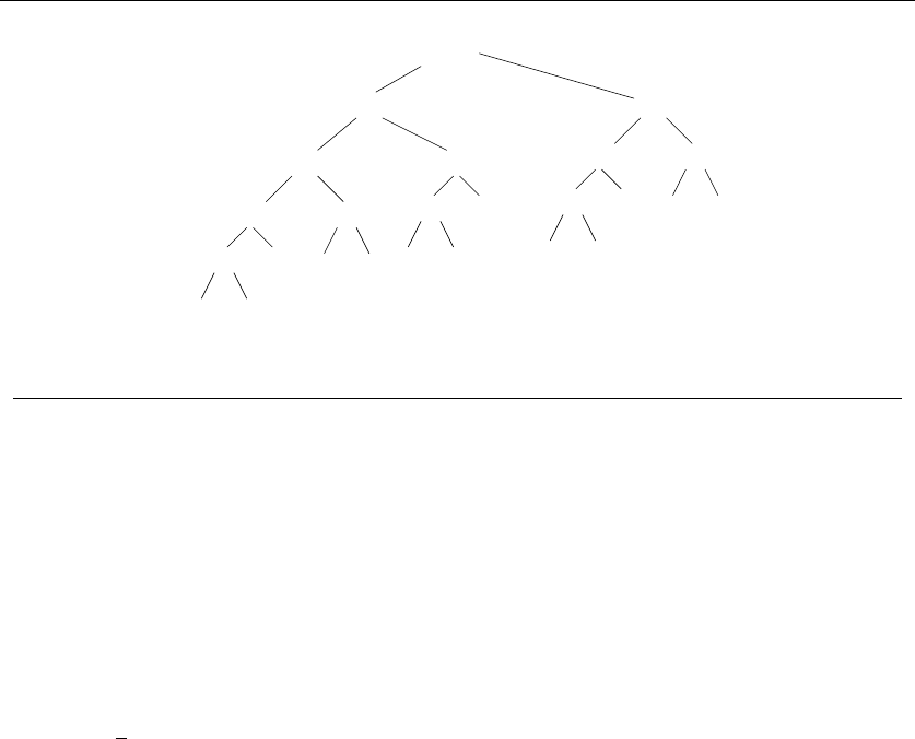
8.1 CACHING VS. COMPUTATION 275
F(3)
F(2)
F(1) F(0)
F(1)
F(2)
F(1)
F(2)
F(1)
F(4)
F(3)
F(0)
F(1)
F(2)
F(1)
F(2)
F(1)
F(4)
F(3)
F(0)
F(1)
F(5)
F(0)
F(0)
F(6)=8
Figure 8.1: The computation tree for computing Fibonacci numbers recursively
The course of execution for this recursive algorithm is illustrated by its recursion
tree, as illustrated in Figure 8.1. This tree is evaluated in a depth-first fashion, as
are all recursive algorithms. I encourage you to trace this example by hand to
refresh your knowledge of recursion.
Note that F(4) is computed on both sides of the recursion tree, and F(2)
is computed no less than five times in this small example. The weight of all this
redundancy becomes clear when you run the program. It took more than 7 minutes
for my program to compute the first 45 Fibonacci numbers. You could probably
do it faster by hand using the right algorithm.
How much time does this algorithm take to compute F(n)? Since Fn+1/Fn≈
φ=(1+
√5)/2≈1.61803, this means that Fn>1.6n. Since our recursion tree has
only 0 and 1 as leaves, summing up to such a large number means we must have at
least 1.6nleaves or procedure calls! This humble little program takes exponential
time to run!
8.1.2 Fibonacci Numbers by Caching
In fact, we can do much better. We can explicitly store (or cache) the results of each
Fibonacci computation F(k) in a table data structure indexed by the parameter k.
The key to avoiding recomputation is to explicitly check for the value before trying
to compute it:
#define MAXN 45 /* largest interesting n */
#define UNKNOWN -1 /* contents denote an empty cell */
long f[MAXN+1]; /* array for caching computed fib values */
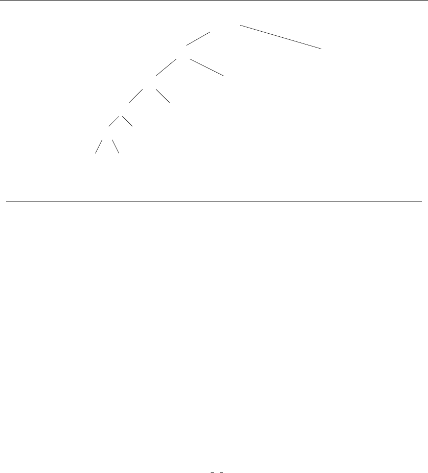
276 8. DYNAMIC PROGRAMMING
F(2)
F(1)
F(0)
F(3)
F(4) F(3)
F(4)
F(6)=8
F(5)
F(1)
F(2)
Figure 8.2: The Fibonacci computation tree when caching values
long fib_c(int n)
{
if (f[n] == UNKNOWN)
f[n] = fib_c(n-1) + fib_c(n-2);
return(f[n]);
}
long fib_c_driver(int n)
{
int i; /* counter */
f[0] = 0;
f[1] = 1;
for (i=2; i<=n; i++) f[i] = UNKNOWN;
return(fib_c(n));
}
To compute F(n), we call fib cdriver(n). This initializes our cache to the
two values we initially know (F(0) and F(1)) as well as the UNKNOWN flag for all the
rest we don’t. It then calls a look-before-crossing-the-street version of the recursive
algorithm.
This cached version runs instantly up to the largest value that can fit in a long
integer. The new recursion tree (Figure 8.2) explains why. There is no meaningful
branching, because only the left-side calls do computation. The right-side calls find
what they are looking for in the cache and immediately return.

8.1 CACHING VS. COMPUTATION 277
What is the running time of this algorithm? The recursion tree provides more
of a clue than the code. In fact, it computes F(n) in linear time (in other words,
O(n) time) because the recursive function fib c(k) is called exactly twice for each
value 0 ≤k≤n.
This general method of explicitly caching results from recursive calls to avoid
recomputation provides a simple way to get most of the benefits of full dynamic
programming, so it is worth a more careful look. In principle, such caching can be
employed on any recursive algorithm. However, storing partial results would have
done absolutely no good for such recursive algorithms as quicksort,backtracking,
and depth-first search because all the recursive calls made in these algorithms have
distinct parameter values. It doesn’t pay to store something you will never refer to
again.
Caching makes sense only when the space of distinct parameter values is modest
enough that we can afford the cost of storage. Since the argument to the recursive
function fib c(k) is an integer between 0 and n, there are only O(n) values to
cache. A linear amount of space for an exponential amount of time is an excellent
tradeoff. But as we shall see, we can do even better by eliminating the recursion
completely.
Take-Home Lesson: Explicit caching of the results of recursive calls provides
most of the benefits of dynamic programming, including usually the same
running time as the more elegant full solution. If you prefer doing extra pro-
gramming to more subtle thinking, you can stop here.
8.1.3 Fibonacci Numbers by Dynamic Programming
We can calculate Fnin linear time more easily by explicitly specifying the order of
evaluation of the recurrence relation:
long fib_dp(int n)
{
int i; /* counter */
long f[MAXN+1]; /* array to cache computed fib values */
f[0] = 0;
f[1] = 1;
for (i=2; i<=n; i++) f[i] = f[i-1]+f[i-2];
return(f[n]);
}
We have removed all recursive calls! We evaluate the Fibonacci numbers from
smallest to biggest and store all the results, so we know that we have Fi−1and
Fi−2ready whenever we need to compute Fi. The linearity of this algorithm should

278 8. DYNAMIC PROGRAMMING
be apparent. Each of the nvalues is computed as the simple sum of two integers
in total O(n) time and space.
More careful study shows that we do not need to store all the intermediate
values for the entire period of execution. Because the recurrence depends on two
arguments, we only need to retain the last two values we have seen:
long fib_ultimate(int n)
{
int i; /* counter */
long back2=0, back1=1; /* last two values of f[n] */
long next; /* placeholder for sum */
if (n == 0) return (0);
for (i=2; i<n; i++) {
next = back1+back2;
back2 = back1;
back1 = next;
}
return(back1+back2);
}
This analysis reduces the storage demands to constant space with no asymptotic
degradation in running time.
8.1.4 Binomial Coefficients
We now show how to compute the binomial coefficients as another illustration of
how to eliminate recursion by specifying the order of evaluation. The binomial
coefficients are the most important class of counting numbers, where n
kcounts
the number of ways to choose kthings out of npossibilities.
How do you compute the binomial coefficients? First, n
k=n!/((n−k)!k!), so in
principle you can compute them straight from factorials. However, this method has
a serious drawback. Intermediate calculations can easily cause arithmetic overflow,
even when the final coefficient fits comfortably within an integer.
A more stable way to compute binomial coefficients is using the recurrence
relation implicit in the construction of Pascal’s triangle:
1
11
121
1331
14641
1 5 10 10 5 1
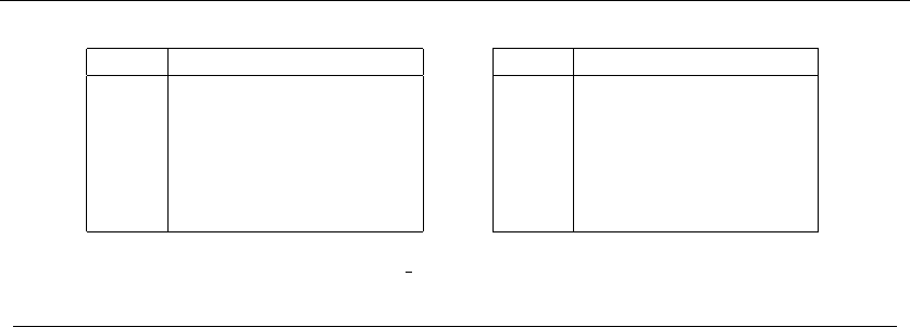
8.1 CACHING VS. COMPUTATION 279
m/n 012345
0 A
1BG
2C1H
3D2 3I
4E456J
5F78910K
m/n 01 2 3 45
0 1
111
211 1
313 3 1
414 6 4 1
51 5 10 10 51
Figure 8.3: Evaluation order for binomial coefficient at M[5,4] (l). Initialization conditions
A-K, recurrence evaluations 1-10. Matrix contents after evaluation (r)
Each number is the sum of the two numbers directly above it. The recurrence
relation implicit in this is that
n
k=n−1
k−1+n−1
k
Why does this work? Consider whether the nth element appears in one of the
n
ksubsets of kelements. If so, we can complete the subset by picking k−1 other
items from the other n−1. If not, we must pick all kitems from the remaining
n−1. There is no overlap between these cases, and all possibilities are included,
so the sum counts all ksubsets.
No recurrence is complete without basis cases. What binomial coefficient values
do we know without computing them? The left term of the sum eventually drives us
down to n−k
0. How many ways are there to choose 0 things from a set? Exactly
one, the empty set. If this is not convincing, then it is equally good to accept that
m
1=mas the basis case. The right term of the sum runs us up to k
k.How
many ways are there to choose kthings from a k-element set? Exactly one—the
complete set. Together, these basis cases and the recurrence define the binomial
coefficients on all interesting values.
The best way to evaluate such a recurrence is to build a table of possible values
up to the size that you are interested in:
Figure 8.3 demonstrates a proper evaluation order for the recurrence. The ini-
tialized cells are marked from A-K, denoting the order in which they were assigned
values. Each remaining cell is assigned the sum of the cell directly above it and the
cell immediately above and to the left. The triangle of cells marked 1 to 10 denote
the evaluation order in computing 5
4= 5 using the code below:

280 8. DYNAMIC PROGRAMMING
long binomial_coefficient(n,m)
int n,m; /* computer n choose m */
{
int i,j; /* counters */
long bc[MAXN][MAXN]; /* table of binomial coefficients */
for (i=0; i<=n; i++) bc[i][0] = 1;
for (j=0; j<=n; j++) bc[j][j] = 1;
for (i=1; i<=n; i++)
for (j=1; j<i; j++)
bc[i][j] = bc[i-1][j-1] + bc[i-1][j];
return( bc[n][m] );
}
Study this function carefully to see how we did it. The rest of this chapter
will focus more on formulating and analyzing the appropriate recurrence than the
mechanics of table manipulation demonstrated here.
8.2 Approximate String Matching
Searching for patterns in text strings is a problem of unquestionable importance.
Section 3.7.2 (page 91) presented algorithms for exact string matching—finding
where the pattern string Poccurs as a substring of the text string T.Lifeisoften
not that simple. Words in either the text or pattern can be mispelled (sic), robbing
us of exact similarity. Evolutionary changes in genomic sequences or language usage
imply that we often search with archaic patterns in mind: “Thou shalt not kill”
morphs over time into “You should not murder.”
How can we search for the substring closest to a given pattern to compensate
for spelling errors? To deal with inexact string matching, we must first define a cost
function telling us how far apart two strings are—i.e., a distance measure between
pairs of strings. A reasonable distance measure reflects the number of changes that
must be made to convert one string to another. There are three natural types of
changes:
•Substitution – Replace a single character from pattern Pwith a different
character in text T, such as changing “shot” to “spot.”
•Insertion – Insert a single character into pattern Pto help it match text T,
such as changing “ago” to “agog.”
•Deletion – Delete a single character from pattern Pto help it match text T,
such as changing “hour” to “our.”

8.2 APPROXIMATE STRING MATCHING 281
Properly posing the question of string similarity requires us to set the cost of
each of these string transform operations. Assigning each operation an equal cost
of 1 defines the edit distance between two strings. Approximate string matching
arises in many applications, as discussed in Section 18.4 (page 631).
Approximate string matching seems like a difficult problem, because we must
decide exactly where to delete and insert (potentially) many characters in pattern
and text. But let us think about the problem in reverse. What information would
we like to have to make the final decision? What can happen to the last character
in the matching for each string?
8.2.1 Edit Distance by Recursion
We can define a recursive algorithm using the observation that the last character in
the string must either be matched, substituted, inserted, or deleted. Chopping off
the characters involved in this last edit operation leaves a pair of smaller strings.
Let iand jbe the last character of the relevant prefix of Pand T, respectively.
There are three pairs of shorter strings after the last operation, corresponding to
the strings after a match/substitution, insertion, or deletion. If we knew the cost
of editing these three pairs of smaller strings, we could decide which option leads
to the best solution and choose that option accordingly. We can learn this cost
through the magic of recursion.
More precisely, let D[i, j] be the minimum number of differences between
P1,P
2,...,P
iand the segment of Tending at j.D[i, j]istheminimum of the
three possible ways to extend smaller strings:
•If (Pi=Tj), then D[i−1,j−1], else D[i−1,j−1] + 1. This means we either
match or substitute the ith and jth characters, depending upon whether the
tail characters are the same.
•D[i−1,j] + 1. This means that there is an extra character in the pattern to
account for, so we do not advance the text pointer and pay the cost of an
insertion.
•D[i, j −1] + 1. This means that there is an extra character in the text to
remove, so we do not advance the pattern pointer and pay the cost of a
deletion.
#define MATCH 0 /* enumerated type symbol for match */
#define INSERT 1 /* enumerated type symbol for insert */
#define DELETE 2 /* enumerated type symbol for delete */

282 8. DYNAMIC PROGRAMMING
int string_compare(char *s, char *t, int i, int j)
{
int k; /* counter */
int opt[3]; /* cost of the three options */
int lowest_cost; /* lowest cost */
if (i == 0) return(j * indel(’ ’));
if (j == 0) return(i * indel(’ ’));
opt[MATCH] = string_compare(s,t,i-1,j-1) + match(s[i],t[j]);
opt[INSERT] = string_compare(s,t,i,j-1) + indel(t[j]);
opt[DELETE] = string_compare(s,t,i-1,j) + indel(s[i]);
lowest_cost = opt[MATCH];
for (k=INSERT; k<=DELETE; k++)
if (opt[k] < lowest_cost) lowest_cost = opt[k];
return( lowest_cost );
}
This program is absolutely correct—convince yourself. It also turns out to be
impossibly slow. Running on my computer, the computation takes several seconds
to compare two 11-character strings, and disappears into Never-Never Land on
anything longer.
Why is the algorithm so slow? It takes exponential time because it recomputes
values again and again and again. At every position in the string, the recursion
branches three ways, meaning it grows at a rate of at least 3n—indeed, even faster
since most of the calls reduce only one of the two indices, not both of them.
8.2.2 Edit Distance by Dynamic Programming
So, how can we make this algorithm practical? The important observation is that
most of these recursive calls are computing things that have been previously com-
puted. How do we know? There can only be |P|·|T|possible unique recursive
calls, since there are only that many distinct (i, j) pairs to serve as the argument
parameters of recursive calls. By storing the values for each of these (i, j) pairs in
a table, we just look them up as needed and avoid recomputing them.
A table-based, dynamic programming implementation of this algorithm is given
below. The table is a two-dimensional matrix mwhere each of the |P|·|T|cells
contains the cost of the optimal solution to a subproblem, as well as a parent
pointer explaining how we got to this location:

8.2 APPROXIMATE STRING MATCHING 283
typedef struct {
int cost; /* cost of reaching this cell */
int parent; /* parent cell */
} cell;
cell m[MAXLEN+1][MAXLEN+1]; /* dynamic programming table */
Our dynamic programming implementation has three differences from the re-
cursive version. First, it gets its intermediate values using table lookup instead of
recursive calls. Second, it updates the parent field of each cell, which will enable
us to reconstruct the edit sequence later. Third, it is implemented using a more
general goal cell() function instead of just returning m[|P|][|T|].cost. This
will enable us to apply this routine to a wider class of problems.
int string_compare(char *s, char *t)
{
int i,j,k; /* counters */
int opt[3]; /* cost of the three options */
for (i=0; i<MAXLEN; i++) {
row_init(i);
column_init(i);
}
for (i=1; i<strlen(s); i++) {
for (j=1; j<strlen(t); j++) {
opt[MATCH] = m[i-1][j-1].cost + match(s[i],t[j]);
opt[INSERT] = m[i][j-1].cost + indel(t[j]);
opt[DELETE] = m[i-1][j].cost + indel(s[i]);
m[i][j].cost = opt[MATCH];
m[i][j].parent = MATCH;
for (k=INSERT; k<=DELETE; k++)
if (opt[k] < m[i][j].cost) {
m[i][j].cost = opt[k];
m[i][j].parent = k;
}
}
}
goal_cell(s,t,&i,&j);
return( m[i][j].cost );
}

284 8. DYNAMIC PROGRAMMING
Tyou -should -no t
Ppos 01234567891011121314
:01234567891011121314
t: 1 11234567891011121313
h: 2 222 3 4 55678 910111213
o: 3 3323 4 5 6 5 6 7 8 9 10 11 12
u: 4 44323 45656 7 8 91011
-: 5 5543234566 7 7 8 910
s: 6 6654323456788910
h: 7 7765432345 6 7 8 910
a: 8 8876543345678910
l: 9 998765444456789
t: 10 101098765555 56788
-: 11 111110 9 8 76666 6 5678
n: 12 12121110 9 87777 7 6 567
o: 13 13 13 12 11 10 9 8 7 8 8 8 7 6 56
t: 14 14 14 13 12 11 10 9 8 8 9 9 8 7 6 5
Figure 8.4: Example of a dynamic programming matrix for editing distance computation, with
the optimal alignment path highlighted in bold
Be aware that we adhere to somewhat unusual string and index conventions in
the routine above. In particular, we assume that each string has been padded with
an initial blank character, so the first real character of string ssits in s[1].Why
did we do this? It enables us to keep the matrix mindices in sync with those of
the strings for clarity. Recall that we must dedicate the zeroth row and column of
mto store the boundary values matching the empty prefix. Alternatively, we could
have left the input strings intact and just adjusted the indices accordingly.
To determine the value of cell (i, j), we need three values sitting and waiting
for us—namely, the cells (i−1,j−1), (i, j −1), and (i−1,j). Any evaluation order
with this property will do, including the row-major order used in this program.1
As an example, we show the cost matrices for turning p= “thou shalt not” into
t= “you should not” in five moves in Figure 8.4.
8.2.3 Reconstructing the Path
The string comparison function returns the cost of the optimal alignment, but not
the alignment itself. Knowing you can convert “thou shalt not” to “you should
not” in only five moves is dandy, but what is the sequence of editing operations
that does it?
The possible solutions to a given dynamic programming problem are described
by paths through the dynamic programming matrix, starting from the initial con-
figuration (the pair of empty strings (0,0)) down to the final goal state (the pair
1Suppose we create a graph with a vertex for every matrix cell, and a directed edge (x, y), when the value
of cell xis needed to compute the value of cell y. Any topological sort on the resulting DAG (why must it be
a DAG?) defines an acceptable evaluation order.

8.2 APPROXIMATE STRING MATCHING 285
Tyou -shou l d - n o t
Ppos 01234567891011121314
0-1 11111111111111
t: 1 200000000000000
h: 2 200000011111111
o: 3 200000001111101
u: 4 202011110111111
-: 5 202201111000111
s: 6 202220111100000
h: 7 202222011111100
a: 8 202222200000000
l: 9 202222200011111
t: 10 2022222000 00000
-: 11 2022022000 0 0111
n: 12 2022222000 0 2 011
o: 13 2002222000 0 2 2 01
t: 14 2022222200 0 2 2 2 0
Figure 8.5: Parent matrix for edit distance computation, with the optimal alignment path
highlighted in bold
of full strings (|P|,|T|)). The key to building the solution is to reconstruct the
decisions made at every step along the optimal path that leads to the goal state.
These decisions have been recorded in the parent field of each array cell.
Reconstructing these decisions is done by walking backward from the goal state,
following the parent pointer back to an earlier cell. We repeat this process until
we arrive back at the initial cell. The parent field for m[i,j] tells us whether the
operation at (i, j)wasMATCH,INSERT,orDELETE. Tracing back through the parent
matrix in Figure 8.5 yields the edit sequence DSMMMMMISMSMMMM from “thou-shalt-
not” to “you-should-not”—meaning delete the first “t”, replace the “h” with “y”,
match the next five characters before inserting an “o”, replace “a” with “u”, and
finally replace the “t” with a “d.”
Walking backward reconstructs the solution in reverse order. However, clever
use of recursion can do the reversing for us:
reconstruct_path(char *s, char *t, int i, int j)
{
if (m[i][j].parent == -1) return;
if (m[i][j].parent == MATCH) {
reconstruct_path(s,t,i-1,j-1);
match_out(s, t, i, j);
return;
}
if (m[i][j].parent == INSERT) {
reconstruct_path(s,t,i,j-1);
insert_out(t,j);

286 8. DYNAMIC PROGRAMMING
return;
}
if (m[i][j].parent == DELETE) {
reconstruct_path(s,t,i-1,j);
delete_out(s,i);
return;
}
}
For many problems, including edit distance, the tour can be reconstructed from
the cost matrix without explicitly retaining the last-move pointer array. The trick
is working backward from the costs of the three possible ancestor cells and corre-
sponding string characters to reconstruct the move that took you to the current
cell at the given cost.
8.2.4 Varieties of Edit Distance
The string compare and path reconstruction routines reference several functions
that we have not yet defined. These fall into four categories:
•Table Initialization – The functions row init and column init initialize the
zeroth row and column of the dynamic programming table, respectively. For
the string edit distance problem, cells (i, 0) and (0,i) correspond to match-
ing length-istrings against the empty string. This requires exactly iinser-
tions/deletions, so the definition of these functions is clear:
row_init(int i)
{
m[0][i].cost = i;
if (i>0)
m[0][i].parent = INSERT;
else
m[0][i].parent = -1;
}
column_init(int i)
{
m[i][0].cost = i;
if (i>0)
m[i][0].parent = DELETE;
else
m[i][0].parent = -1;
}
•Penalty Costs – The functions match(c,d) and indel(c) present the costs for
transforming character cto dand inserting/deleting character c. For standard
edit distance, match should cost nothing if the characters are identical, and
1 otherwise; while indel returns 1 regardless of what the argument is. But
application-specific cost functions can be employed, perhaps more forgiving
of replacements located near each other on standard keyboard layouts or
characters that sound or look similar.

8.2 APPROXIMATE STRING MATCHING 287
int match(char c, char d)
{
if (c == d) return(0);
else return(1);
}
int indel(char c)
{
return(1);
}
•Goal Cell Identification – The function goal cell returns the indices of the
cell marking the endpoint of the solution. For edit distance, this is defined
by the length of the two input strings. However, other applications we will
soon encounter do not have fixed goal locations.
goal_cell(char *s, char *t, int *i, int *j)
{
*i = strlen(s) - 1;
*j = strlen(t) - 1;
}
•Traceback Actions – The functions match out,insert out,anddelete out
perform the appropriate actions for each edit operation during traceback.
For edit distance, this might mean printing out the name of the operation or
character involved, as determined by the needs of the application.
insert_out(char *t, int j)
{
printf("I");
}
delete_out(char *s, int i)
{
printf("D");
}
match_out(char *s, char *t,
int i, int j)
{
if (s[i]==t[j]) printf("M");
else printf("S");
}
All of these functions are quite simple for edit distance computation. However,
we must confess it is difficult to get the boundary conditions and index manipula-
tions correctly. Although dynamic programming algorithms are easy to design once
you understand the technique, getting the details right requires carefully thinking
and thorough testing.
This may seem to be a lot of infrastructure to develop for such a simple algo-
rithm. However, several important problems can now be solved as special cases of
edit distance using only minor changes to some of these stub functions:
•Substring Matching – Suppose that we want to find where a short pattern
Pbest occurs within a long text T—say, searching for “Skiena” in all its
misspellings (Skienna, Skena, Skina, . . . ) within a long file. Plugging this

288 8. DYNAMIC PROGRAMMING
search into our original edit distance function will achieve little sensitivity,
since the vast majority of any edit cost will consist of deleting that which
is not “Skiena” from the body of the text. Indeed, matching any scattered
···S···k···i···e···n···aand deleting the rest yields an optimal solution.
We want an edit distance search where the cost of starting the match is
independent of the position in the text, so that a match in the middle is not
prejudiced against. Now the goal state is not necessarily at the end of both
strings, but the cheapest place to match the entire pattern somewhere in the
text. Modifying these two functions gives us the correct solution:
row_init(int i)
{
m[0][i].cost = 0; /* note change */
m[0][i].parent = -1; /* note change */
}
goal_cell(char *s, char *t, int *i, int *j)
{
int k; /* counter */
*i = strlen(s) - 1;
*j = 0;
for (k=1; k<strlen(t); k++)
if (m[*i][k].cost < m[*i][*j].cost) *j = k;
}
•Longest Common Subsequence – Perhaps we are interested in finding the
longest scattered string of characters included within both strings. Indeed,
this problem will be discussed in Section 18.8. The longest common subse-
quence (LCS) between “democrat” and “republican” is eca.
A common subsequence is defined by all the identical-character matches in an
edit trace. To maximize the number of such matches, we must prevent sub-
stitution of nonidentical characters. With substitution forbidden, the only
way to get rid of the noncommon subsequence is through insertion and dele-
tion. The minimum cost alignment has the fewest such “in-dels”, so it must
preserve the longest common substring. We get the alignment we want by
changing the match-cost function to make substitutions expensive:
int match(char c, char d)
{
if (c == d) return(0);
else return(MAXLEN);
}

8.3 LONGEST INCREASING SEQUENCE 289
Actually, it suffices to make the substitution penalty greater than that of an
insertion plus a deletion for substitution to lose any allure as a possible edit
operation.
•Maximum Monotone Subsequence – A numerical sequence is monotonically
increasing if the ith element is at least as big as the (i−1)st element. The
maximum monotone subsequence problem seeks to delete the fewest num-
ber of elements from an input string Sto leave a monotonically increasing
subsequence. A longest increasing subsequence of 243517698 is 23568.
In fact, this is just a longest common subsequence problem, where the second
string is the elements of Ssorted in increasing order. Any common sequence
of these two must (a) represent characters in proper order in S,and(b)use
only characters with increasing position in the collating sequence—so, the
longest one does the job. Of course, this approach can be modified to give
the longest decreasing sequence by simply reversing the sorted order.
As you can see, our edit distance routine can be made to do many amazing
things easily. The trick is observing that your problem is just a special case of
approximate string matching.
The alert reader may notice that it is unnecessary to keep all O(mn) cells
to compute the cost of an alignment. If we evaluate the recurrence by filling in
the columns of the matrix from left to right, we will never need more than two
columns of cells to store what is necessary for the computation. Thus, O(m) space
is sufficient to evaluate the recurrence without changing the time complexity. Un-
fortunately, we cannot reconstruct the alignment without the full matrix.
Saving space in dynamic programming is very important. Since memory on any
computer is limited, using O(nm) space proves more of a bottleneck than O(nm)
time. Fortunately, there is a clever divide-and-conquer algorithm that computes
the actual alignment in O(nm) time and O(m) space. It is discussed in Section
18.4 (page 631).
8.3 Longest Increasing Sequence
There are three steps involved in solving a problem by dynamic programming:
1. Formulate the answer as a recurrence relation or recursive algorithm.
2. Show that the number of different parameter values taken on by your recur-
rence is bounded by a (hopefully small) polynomial.
3. Specify an order of evaluation for the recurrence so the partial results you
need are always available when you need them.

290 8. DYNAMIC PROGRAMMING
To see how this is done, let’s see how we would develop an algorithm to find
the longest monotonically increasing subsequence within a sequence of nnumbers.
Truth be told, this was described as a special case of edit distance in the previous
section, where it was called maximum monotone subsequence. Still, it is instructive
to work it out from scratch. Indeed, dynamic programming algorithms are often
easier to reinvent than look up.
We distinguish an increasing sequence from a run, where the elements must be
physical neighbors of each other. The selected elements of both must be sorted in
increasing order from left to right. For example, consider the sequence
S={2,4,3,5,1,7,6,9,8}
The longest increasing subsequence of Shas length 5, including {2,3,5,6,8}. In fact,
there are eight of this length (can you enumerate them?). There are four longest
increasing runs of length 2: (2,4), (3,5), (1,7), and (6,9).
Finding the longest increasing run in a numerical sequence is straightforward.
Indeed, you should be able to devise a linear-time algorithm fairly easily. But
finding the longest increasing subsequence is considerably trickier. How can we
identify which scattered elements to skip? To apply dynamic programming, we
need to construct a recurrence that computes the length of the longest sequence.
To find the right recurrence, ask what information about the first n−1 elements
of Swould help you to find the answer for the entire sequence?
•The length of the longest increasing sequence in s1,s
2,...,s
n−1seems a useful
thing to know. In fact, this will be the longest increasing sequence in S, unless
snextends some increasing sequence of the same length.
Unfortunately, the length of this sequence is not enough information to com-
plete the full solution. Suppose I told you that the longest increasing sequence
in s1,s
2,...,s
n−1was of length 5 and that sn= 9. Will the length of the
final longest increasing subsequence of Sbe 5 or 6?
•We need to know the length of the longest sequence that snwill extend. To
be certain we know this, we really need the length of the longest sequence
that any possible value for sncan extend.
This provides the idea around which to build a recurrence. Define lito be the
length of the longest sequence ending with si.
The longest increasing sequence containing the nth number will be formed by
appending it to the longest increasing sequence to the left of nthat ends on a
number smaller than sn. The following recurrence computes li:
li= max
0<j<i lj+ 1, where (sj<s
i),
l0=0

8.4 WAR STORY: EVOLUTION OF THE LOBSTER 291
These values define the length of the longest increasing sequence ending at each
number. The length of the longest increasing subsequence of the entire permutation
is given by max1≤i≤nli, since the winning sequence will have to end somewhere.
Here is the table associated with our previous example:
Sequence si243517698
Length li123314455
Predecessor pi–112–4466
What auxiliary information will we need to store to reconstruct the actual
sequence instead of its length? For each element si, we will store its predecessor—
the index piof the element that appears immediately before siin the longest
increasing sequence ending at si. Since all of these pointers go towards the left, it
is a simple matter to start from the last value of the longest sequence and follow
the pointers so as to reconstruct the other items in the sequence.
What is the time complexity of this algorithm? Each one of the nvalues of liis
computed by comparing siagainst (up to) i−1≤nvalues to the left of it, so this
analysis gives a total of O(n2) time. In fact, by using dictionary data structures
in a clever way, we can evaluate this recurrence in O(nlg n) time. However, the
simple recurrence would be easy to program and therefore is a good place to start.
Take-Home Lesson: Once you understand dynamic programming, it can be
easier to work out such algorithms from scratch than to try to look them up.
8.4 War Story: Evolution of the Lobster
I caught the two graduate students lurking outside my office as I came in to work
that morning. There they were, two future PhDs working in the field of high-
performance computer graphics. They studied new techniques for rendering pretty
computer images, but the picture they painted for me that morning was anything
but pretty.
“You see, we want to build a program to morph one image into another,” they
explained.
“What do you mean by morph?” I asked.
“For special effects in movies, we want to construct the intermediate stages in
transforming one image into another. Suppose we want to turn you into Humphrey
Bogart. For this to look realistic, we must construct a bunch of in-between frames
that start out looking like you and end up looking like him.”
“If you can realistically turn me into Bogart, you have something,” I agreed.
“But our problem is that it isn’t very realistic.” They showed me a dismal
morph between two images. “The trouble is that we must find the right corre-
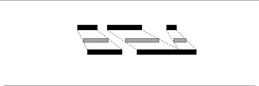
292 8. DYNAMIC PROGRAMMING
T = 0
T = 1
T = 0.5
Object A’s segments
Object B’s segments
Figure 8.6: A successful alignment of two lines of pixels
spondence between features in the two images. It looks real bad when we get the
correspondence wrong and try to morph a lip into an ear.”
“I’ll bet. So you want me to give you an algorithm for matching up lips?”
“No, even simpler. We morph each row of the initial image into the identical
row of the final image. You can assume that we give you two lines of pixels, and
you have to find the best possible match between the dark pixels in a row from
object Ato the dark pixels in the corresponding row of object B. Like this,” they
said, showing me images of successful matchings like Figure 8.6.
“I see,” I said. “You want to match big dark regions to big dark regions and
small dark regions to small dark regions.”
“Yes, but only if the matching doesn’t shift them too much to the left or the
right. We might prefer to merge or break up regions rather than shift them too far
away, since that might mean matching a chin to an eyebrow. What is the best way
to do it?”
“One last question. Will you ever want to match two intervals to each other in
such a way that they cross?”
“No, I guess not. Crossing intervals can’t match. It would be like switching your
left and right eyes.”
I scratched my chin and tried to look puzzled, but I’m just not as good an
actor as Bogart. I’d had a hunch about what needed to be done the instant they
started talking about lines of pixels. They want to transform one array of pixels
into another array, using the minimum amount of changes. That sounded like
editing one string of pixels into another string, which is a classic application of
dynamic programming. See Sections 8.2 and 18.4 for discussions of approximate
string matching.
The fact that the intervals couldn’t cross settled the issue. It meant that when-
ever a stretch of dark pixels from Awas mapped to a stretch from B, the problem
would be split into two smaller subproblems—i.e. , the pixels to the left of the
match and the pixels to the right of the match. The cost of the global match would
ultimately be the cost of this match plus those of matching all the pixels to the
left and of matching all the pixels to the right. Constructing the optimal match on
the left side is a smaller problem and hence simpler. Further, there could be only
8.4 WAR STORY: EVOLUTION OF THE LOBSTER 293
Figure 8.7: Morphing a lobster into a head via dynamic programming
O(n2) possible left subproblems, since each is completely described by the pair of
one of ntop pixels and one of nbottom pixels.
“Your algorithm will be based on dynamic programming,” I pronounced. “How-
ever, there are several possible ways to do things, depending upon whether you
want to edit pixels or runs. I would probably convert each row into a list of black
pixel runs, with the runs sorted by right endpoint. Label each run with its starting
position and length. You will maintain the cost of the cheapest match between the
leftmost iruns and the leftmost jruns for all iand j. The possible edit operations
are:
•Full run match – We may match top run ito run bottom jfor a cost that is
a function of the difference in the lengths of the two runs and their positions.
•Merging runs – We may match a string of consecutive top runs to a bottom
run. The cost will be a function of the number of runs, their relative positions,
and their lengths.
•Splitting runs – We may match a top run to a string of consecutive bottom
runs. This is just the converse of the merge. Again, the cost will be a function
of the number of runs, their relative positions, and their lengths.
“For each pair of runs (i, j) and all the cases that apply, we compute the cost
of the edit operation and add to the (already computed and stored) edit cost to
the left of the start of the edit. The cheapest of these cases is what we will take for
the cost of c[i, j].”

294 8. DYNAMIC PROGRAMMING
The pair of graduate students scribbled this down, then frowned. “So we will
have a cost measure for matching two runs as a function of their lengths and
positions. How do we decide what the relative costs should be?”
“That is your business. The dynamic programming serves to optimize the
matchings once you know the cost functions. It is up to your aesthetic sense to
decide the penalties for line length changes and offsets. My recommendation is
that you implement the dynamic programming and try different penalty values on
each of several different images. Then, pick the setting that seems to do what you
want.”
They looked at each other and smiled, then ran back into the lab to implement
it. Using dynamic programming to do their alignments, they completed their mor-
phing system. It produced the images in Figure 8.7, morphing a lobster into a man.
Unfortunately, they never got around to turning me into Humphrey Bogart.
8.5 The Partition Problem
Suppose that three workers are given the task of scanning through a shelf of books
in search of a given piece of information. To get the job done fairly and efficiently,
the books are to be partitioned among the three workers. To avoid the need to
rearrange the books or separate them into piles, it is simplest to divide the shelf
into three regions and assign each region to one worker.
But what is the fairest way to divide up the shelf? If all books are the same
length, the job is pretty easy. Just partition the books into equal-sized regions,
100 100 100 |100 100 100 |100 100 100
so that everyone has 300 pages to deal with.
But what if the books are not the same length? Suppose we used the same
partition when the book sizes looked like this:
100 200 300 |400 500 600 |700 800 900
I, would volunteer to take the first section, with only 600 pages to scan, instead of
the last one, with 2,400 pages. The fairest possible partition for this shelf would be
100 200 300 400 500 |600 700 |800 900
where the largest job is only 1,700 pages and the smallest job 1,300.
In general, we have the following problem:
Problem: Integer Partition without Rearrangement
Input: An arrangement Sof nonnegative numbers {s1,...,s
n}and an integer k.
Output: Partition Sinto kor fewer ranges, to minimize the maximum sum over all
the ranges, without reordering any of the numbers.
This so-called linear partition problem arises often in parallel process. We seek
to balance the work done across processors to minimize the total elapsed run time.

8.5 THE PARTITION PROBLEM 295
The bottleneck in this computation will be the processor assigned the most work.
Indeed, the war story of Section 7.10 (page 268) revolves around a botched solution
to this problem.
Stop for a few minutes and try to find an algorithm to solve the linear partition
problem.
A novice algorist might suggest a heuristic as the most natural approach to
solving the partition problem. Perhaps they would compute the average size of
a partition, n
i=1 si/k, and then try to insert the dividers to come close to this
average. However, such heuristic methods are doomed to fail on certain inputs
because they do not systematically evaluate all possibilities.
Instead, consider a recursive, exhaustive search approach to solving this prob-
lem. Notice that the kth partition starts right after we placed the (k−1)st divider.
Where can we place this last divider? Between the ith and (i+ 1)st elements for
some i, where 1 ≤i≤n. What is the cost of this? The total cost will be the larger
of two quantities—(1) the cost of the last partition n
j=i+1 sj, and (2) the cost of
the largest partition formed to the left of i. What is the size of this left partition?
To minimize our total, we want to use the k−2 remaining dividers to partition the
elements {s1,...,s
i}as equally as possible. This is a smaller instance of the same
problem, and hence can be solved recursively!
Therefore, let us define M[n, k] to be the minimum possible cost over all par-
titionings of {s1,...,s
n}into kranges, where the cost of a partition is the largest
sum of elements in one of its parts. Thus defined, this function can be evaluated:
M[n, k]= n
min
i=1 max(M[i, k −1],
n
j=i+1
sj)
We must specify the boundary conditions of the recurrence relation. These
boundary conditions always settle the smallest possible values for each of the argu-
ments of the recurrence. For this problem, the smallest reasonable value of the first
argument is n= 1, meaning that the first partition consists of a single element.
We can’t create a first partition smaller than s1regardless of how many dividers
are used. The smallest reasonable value of the second argument is k= 1, implying
that we do not partition Sat all. In summary:
M[1,k]=s1,for all k>0 and,
M[n, 1] =
n
i=1
si
By definition, this recurrence must return the size of the optimal partition.
How long does it take to compute this when we store the partial results? A total
of k·ncells exist in the table. How much time does it take to compute the result

296 8. DYNAMIC PROGRAMMING
M[n,k
]? Calculating this quantity involves finding the minimum of nquantities,
each of which is the maximum of the table lookup and a sum of at most nelements.
If filling each of kn boxes takes at most n2time per box, the total recurrence can
be computed in O(kn3) time.
The evaluation order computes the smaller values before the bigger values, so
that each evaluation has what it needs waiting for it. Full details are provided in
the code below:
partition(int s[], int n, int k)
{
int m[MAXN+1][MAXK+1]; /* DP table for values */
int d[MAXN+1][MAXK+1]; /* DP table for dividers */
int p[MAXN+1]; /* prefix sums array */
int cost; /* test split cost */
int i,j,x; /* counters */
p[0] = 0; /* construct prefix sums */
for (i=1; i<=n; i++) p[i]=p[i-1]+s[i];
for (i=1; i<=n; i++) m[i][1] = p[i]; /* initialize boundaries */
for (j=1; j<=k; j++) m[1][j] = s[1];
for (i=2; i<=n; i++) /* evaluate main recurrence */
for (j=2; j<=k; j++) {
m[i][j] = MAXINT;
for (x=1; x<=(i-1); x++) {
cost = max(m[x][j-1], p[i]-p[x]);
if (m[i][j] > cost) {
m[i][j] = cost;
d[i][j] = x;
}
}
}
reconstruct_partition(s,d,n,k); /* print book partition */
}
This implementation above, in fact, runs faster than advertised. Our original
analysis assumed that it took O(n2) time to update each cell of the matrix. This
is because we selected the best of up to npossible points to place the divider, each
of which requires the sum of up to npossible terms. In fact, it is easy to avoid the
need to compute these sums by storing the set of nprefix sums p[i]=i
k=1 sk,
8.5 THE PARTITION PROBLEM 297
M k D k
n123 n123
1111 1–––
1211 1–11
1321 1–12
1422 1–22
1532 1–23
1632 1–34
1743 1–34
1843 1–45
1953 1–46
M k D k
n123 n123
1111 1–––
2322 2–11
3633 3–22
41064 4–33
51596 5–34
621 11 9 6–45
728 15 11 7–56
836 21 15 8–56
945 24 17 9–67
Figure 8.8: Dynamic programming matrices Mand Dfor two input instances. Partitioning
{1,1,1,1,1,1,1,1,1}into {{1,1,1},{1,1,1},{1,1,1}} (l) . Partitioning {1,2,3,4,5,6,7,8,9}
into {{1,2,3,4,5},{6,7},{8,9}} (r).
since j
k=isk=p[j]−p[k]. This enables us to evaluate the recurrence in linear
time per cell, yielding an O(kn2) algorithm.
By studying the recurrence relation and the dynamic programming matrices of
Figure 8.8, you should be able to convince yourself that the final value of M(n, k)
will be the cost of the largest range in the optimal partition. For most applications,
however, what we need is the actual partition that does the job. Without it, all we
are left with is a coupon with a great price on an out-of-stock item.
The second matrix, D, is used to reconstruct the optimal partition. Whenever
we update the value of M[i, j], we record which divider position was required to
achieve that value. To reconstruct the path used to get to the optimal solution,
we work backward from D[n, k] and add a divider at each specified position. This
backwards walking is best achieved by a recursive subroutine:
reconstruct_partition(int s[],int d[MAXN+1][MAXK+1], int n, int k)
{
if (k==1)
print_books(s,1,n);
else {
reconstruct_partition(s,d,d[n][k],k-1);
print_books(s,d[n][k]+1,n);
}
}
print_books(int s[], int start, int end)
{
int i; /* counter */
for (i=start; i<=end; i++) printf(" %d ",s[i]);
printf("\n");
}
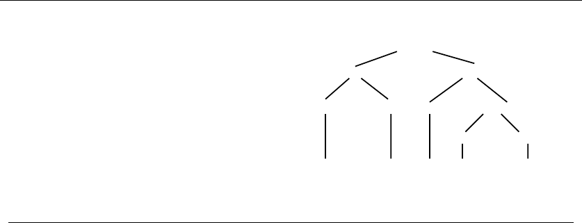
298 8. DYNAMIC PROGRAMMING
d
r
ank
cat, milk
the, a
verb−phrase
noun−phrase ::= article noun
verb−phrase ::= verb noun−phrase
article ::=
noun ::=
verb ::=
sentence ::= noun−phrase
verb−phrase
noun−phrase
article noun verb noun−phrase
article noun
drank the
milk
the cat
sentence
Figure 8.9: A context-free grammar (l) with an associated parse tree (r)
8.6 Parsing Context-Free Grammars
Compilers identify whether the given program is legal in the programming lan-
guage, and reward you with syntax errors if not. This requires a precise description
of the language syntax typically given by a context-free grammar as shown in Fig-
ure 8.9(l). Each rule or production of the grammar defines an interpretation for the
named symbol on the left side of the rule as a sequence of symbols on the right
side of the rule. The right side can be a combination of nonterminals (themselves
defined by rules) or terminal symbols defined simply as strings, such as “the”, “a”,
“cat”, “milk”, and “drank.”
Parsing a given text string Saccording to a given context-free grammar Gis
the algorithmic problem of constructing a parse tree of rule substitutions defining
Sas a single nonterminal symbol of G. Figure 8.9(r) gives the parse tree of a simple
sentence using our sample grammar.
Parsing seemed like a horribly complicated subject when I took a compilers
course as a graduate student. But, a friend easily explained it to me over lunch
a few years ago. The difference is that I now understand dynamic programming
much better than when I was a student.
We assume that the text string Shas length nwhile the grammar Gitself is
of constant size. This is fair, since the grammar defining a particular programming
language (say C or Java) is of fixed length regardless of the size of the program we
are trying to compile.
Further, we assume that the definitions of each rule are in Chomsky normal
form. This means that the right sides of every nontrivial rule consists of (a) exactly
two nonterminals, i.e. X→YZ, or (b) exactly one terminal symbol, X→α.Any
context-free grammar can be easily and mechanically transformed into Chomsky
normal form by repeatedly shortening long right-hand sides at the cost of adding
extra nonterminals and productions. Thus, there is no loss of generality with this
assumption.

8.6 PARSING CONTEXT-FREE GRAMMARS 299
So how can we efficiently parse a string Susing a context-free grammar where
each interesting rule consists of two nonterminals? The key observation is that the
rule applied at the root of the parse tree (say X→YZ) splits Sat some position
isuch that the left part of the string (S[1,i]) must be generated by nonterminal Y,
and the right part (S[i+1,n]) generated by Z.
This suggests a dynamic programming algorithm, where we keep track of all
of the nonterminals generated by each substring of S. Define M[i, j, X]tobea
boolean function that is true iff substring S[i, j] is generated by nonterminal X.
This is true if there exists a production X→YZ and breaking point kbetween i
and jsuch that the left part generates Yand the right part Z. In other words,
M[i, j, X]=
(X→YZ)∈Gj
i=k
M[i, k, Y ]·M[k+1,j,Z]
where ∨denotes the logical or over all productions and split positions, and ·denotes
the logical and of two boolean values.
The one-character terminal symbols define the boundary conditions of the re-
currence. In particular, M[i, i, X] is true iff there exists a production X→αsuch
that S[i]=α.
What is the complexity of this algorithm? The size of our state-space is O(n2),
as there are n(n+1)/2 substrings defined by (i, j) pairs. Multiplying this by the
number of nonterminals (say v) has no impact on the big-Oh, because the grammar
was defined to be of constant size. Evaluating the value M[i, j, X] requires testing
all intermediate values k,soittakesO(n) in the worst case to evaluate each of the
O(n2) cells. This yields an O(n3) or cubic-time algorithm for parsing.
Stop and Think: Parsimonious Parserization
Problem: Programs often contain trivial syntax errors that prevent them from
compiling. Given a context-free grammar Gand input string S, find the smallest
number of character substitutions you must make to Sso that the resulting string
is accepted by G.
Solution: This problem seemed extremely difficult when I first encountered it.
But on reflection, it seemed like a very general version of edit distance, which is
addressed naturally by dynamic programming. Parsing initially sounded hard, too,
but fell to the same technique. Indeed, we can solve the combined problem by
generalizing the recurrence relation we used for simple parsing.
Define M[i, j, X]tobeaninteger function that reports the minimum number of
changes to substring S[i, j] so it can be generated by nonterminal X. This symbol
will be generated by some production x→yz. Some of the changes to smay be
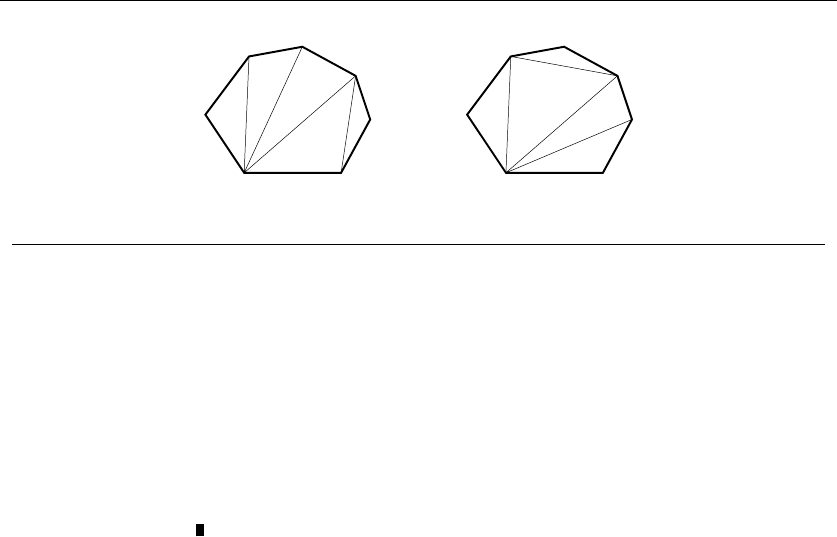
300 8. DYNAMIC PROGRAMMING
Figure 8.10: Two different triangulations of a given convex seven-gon
to the left of the breaking point and some to the right, but all we care about is
minimizing the sum. In other words,
M[i, j, X] = min
(X→YZ)∈Gj
min
i=kM[i, k, Y ]+M[k+1,j,Z]
The boundary conditions also change mildly. If there exists a production X→
α, the cost of matching at position idepends on the contents of S[i], where S[i]=α,
M[i, i, X] = 0. Otherwise, it is one substitution away, so M[i, i, X]=1ifS[i]=α.
If the grammar does not have a production of the form X→α, there is no way to
substitute a single character string into something generating X,soM[i, i, X]=∞
for all i.
8.6.1 Minimum Weight Triangulation
The same basic recurrence relation encountered in the parsing algorithm above can
also be used to solve an interesting computational geometry problem. A triangu-
lation of a polygon P={v1,...,v
n,v
1}is a set of nonintersecting diagonals that
partitions the polygon into triangles. We say that the weight of a triangulation is
the sum of the lengths of its diagonals. As shown in Figure 8.10, any given poly-
gon may have many different triangulations. We seek to find its minimum weight
triangulation for a given polygon p. Triangulation is a fundamental component of
most geometric algorithms, as discussed in Section 17.3 (page 572).
To apply dynamic programming, we need a way to carve up the polygon into
smaller pieces. Observe that every edge of the input polygon must be involved
in exactly one triangle. Turning this edge into a triangle means identifying the
third vertex, as shown in Figure 8.11. Once we find the correct connecting vertex,
the polygon will be partitioned into two smaller pieces, both of which need to be
triangulated optimally. Let T[i, j] be the cost of triangulating from vertex vito
vertex vj, ignoring the length of the chord dij from vito vj. The latter clause
avoids double counting these internal chords in the following recurrence:
T[i, j]= j−1
min
k=i+1 (T[i, k]+T[k, j]+dik +dkj)
The basis condition applies when iand jare immediate neighbors, as T[i, i+1] = 0.
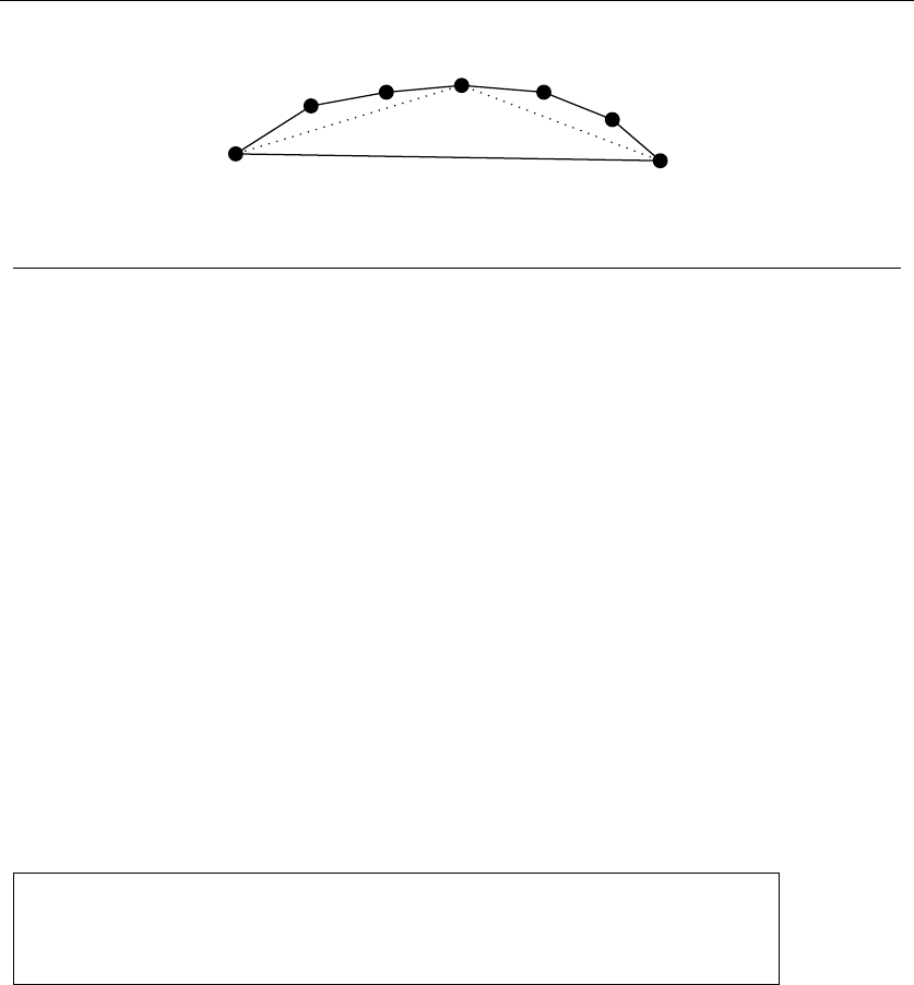
8.7 LIMITATIONS OF DYNAMIC PROGRAMMING: TSP 301
ij
k
Figure 8.11: Selecting the vertex kto pair with an edge (i, j) of the polygon
Since the number of vertices in each subrange of the right side of the recurrence
is smaller than that on the left side, evaluation can proceed in terms of the gap
size from ito j:
Minimum-Weight-Triangulation(P)
for i=1ton−1doT[i, i +1]=0
for gap =2ton−1
for i=1ton−gap do
j=i+gap
T[i, j] = minj−1
k=i+1(T[i, k]+T[k, j]+dPi,Pk+dPk,Pj)
return T[1,n]
There are n
2values of T, each of which takes O(j−i) time if we evaluate the
sections in order of increasing size. Since j−i=O(n), complete evaluation takes
O(n3) time and O(n2) space.
What if there are points in the interior of the polygon? Then dynamic pro-
gramming does not apply in the same way, because triangulation edges do not
necessarily cut the boundary into two distinct pieces as before. Instead of only n
2
possible subregions, the number of subregions now grows exponentially. In fact, the
more general version of this problem is known to be NP-complete.
Take-Home Lesson: For any optimization problem on left-to-right objects,
such as characters in a string, elements of a permutation, points around a
polygon, or leaves in a search tree, dynamic programming likely leads to an
efficient algorithm to find the optimal solution.
8.7 Limitations of Dynamic Programming: TSP
Dynamic programming doesn’t always work. It is important to see why it can fail,
to help avoid traps leading to incorrect or inefficient algorithms.
Our algorithmic poster child will once again be the traveling salesman, where
we seek the shortest tour visiting all the cities in a graph. We will limit attention
here to an interesting special case:

302 8. DYNAMIC PROGRAMMING
Problem: Longest Simple Path
Input: A weighted graph G, with specified start and end vertices sand t.
Output: What is the most expensive path from sto tthat does not visit any vertex
more than once?
This problem differs from TSP in two quite unimportant ways. First, it asks
for a path instead of a closed tour. This difference isn’t substantial: we get a closed
tour by simply including the edge (t, s). Second, it asks for the most expensive
path instead of the least expensive tour. Again this difference isn’t very significant:
it encourages us to visit as many vertices as possible (ideally all), just as in TSP.
The big word in the problem statement is simple, meaning we are not allowed to
visit any vertex more than once.
For unweighted graphs (where each edge has cost 1), the longest possible simple
path from sto tis n−1. Finding such Hamiltonian paths (if they exist) is an
important graph problem, discussed in Section 16.5 (page 538).
8.7.1 When are Dynamic Programming Algorithms Correct?
Dynamic programming algorithms are only as correct as the recurrence relations
they are based on. Suppose we define LP [i, j] as a function denoting the length of
the longest simple path from ito j. Note that the longest simple path from ito j
had to visit some vertex xright before reaching j. Thus, the last edge visited must
be of the form (x, j). This suggests the following recurrence relation to compute
the length of the longest path, where c(x, j) is the cost/weight of edge (x, j):
LP [i, j] = max
(x,j)∈ELP [i, x]+c(x, j)
The idea seems reasonable, but can you see the problem? I see at least two of
them.
First, this recurrence does nothing to enforce simplicity. How do we know that
vertex jhas not appeared previously on the longest simple path from ito x?Ifit
did, adding the edge (x, j) will create a cycle. To prevent such a thing, we must
define a different recursive function that explicitly remembers where we have been.
Perhaps we could define LP [i, j, k] to be the function denoting the length of the
longest path from ito javoiding vertex k? This would be a step in the right
direction, but still won’t lead to a viable recurrence.
A second problem concerns evaluation order. What can you evaluate first? Be-
cause there is no left-to-right or smaller-to-bigger ordering of the vertices on the
graph, it is not clear what the smaller subprograms are. Without such an ordering,
we get are stuck in an infinite loop as soon as we try to do anything.
Dynamic programming can be applied to any problem that observes the princi-
ple of optimality. Roughly stated, this means that partial solutions can be optimally
extended with regard to the state after the partial solution, instead of the specifics
of the partial solution itself. For example, in deciding whether to extend an approx-
imate string matching by a substitution, insertion, or deletion, we did not need to

8.7 LIMITATIONS OF DYNAMIC PROGRAMMING: TSP 303
know which sequence of operations had been performed to date. In fact, there may
be several different edit sequences that achieve a cost of Con the first pcharacters
of pattern Pand tcharacters of string T. Future decisions are made based on the
consequences of previous decisions, not the actual decisions themselves.
Problems do not satisfy the principle of optimality when the specifics of the
operations matter, as opposed to just the cost of the operations. Such would be
the case with a form of edit distance where we are not allowed to use combinations
of operations in certain particular orders. Properly formulated, however, many
combinatorial problems respect the principle of optimality.
8.7.2 When are Dynamic Programming Algorithms Efficient?
The running time of any dynamic programming algorithm is a function of two
things: (1) number of partial solutions we must keep track of, and (2) how long it
take to evaluate each partial solution. The first issue—namely the size of the state
space—is usually the more pressing concern.
In all of the examples we have seen, the partial solutions are completely de-
scribed by specifying the stopping places in the input. This is because the com-
binatorial objects being worked on (strings, numerical sequences, and polygons)
have an implicit order defined upon their elements. This order cannot be scram-
bled without completely changing the problem. Once the order is fixed, there are
relatively few possible stopping places or states, so we get efficient algorithms.
When the objects are not firmly ordered, however, we get an exponential num-
ber of possible partial solutions. Suppose the state of our partial solution is entire
path Ptaken from the start to end vertex. Thus LP [i, j, P ] denotes the longest
simple path from ito j, where Pis the exact sequence of intermediate vertices
between iand jon this path. The following recurrence relation works to compute
this, where P+xdenotes appending xto the end of P:
LP [i, j, P +x] = max
(x,j)∈E,x,j∈PLP [i, x, P ]+c(x, j)
This formulation is correct, but how efficient is it? The path Pconsists of an
ordered sequence of up to n−3 vertices. There can be up to (n−3)! such paths!
Indeed, this algorithm is really using combinatorial search (alabacktracking) to
construct all the possible intermediate paths. In fact, the max is somewhat mis-
leading, as there can only be one value of xand one value of Pto construct the
state LP [i, j, P +x].
We can do something better with this idea, however. Let LP [i, j, S] denote the
longest simple path from ito j, where the intermediate vertices on this path are
exactly those in the subset S.Thus,ifS={a, b, c}, there are exactly six paths
consistent with S:iabcj,iacbj,ibacj,ibcaj,icabj,andicbaj. This state space is at
most 2n, and thus smaller than enumerating the paths. Further, this function can
be evaluated using the following recurrence relation:
LP [i, j, S ∪{x}] = max
(x,j)∈E,x,j∈SLP [i, x, S]+c(x, j)

304 8. DYNAMIC PROGRAMMING
where S∪{x}denotes unioning Swith x.
The longest simple path from ito jcan then be found by maximizing over all
possible intermediate vertex subsets:
LP [i, j] = max
SLP [i, j, S]
There are only 2nsubsets of nvertices, so this is a big improvement over
enumerating all n! tours. Indeed, this method could certainly be used to solve
TSPs for up to thirty vertices or so, where n= 20 would be impossible using
the O(n!) algorithm. Still, dynamic programming is most effective on well-ordered
objects.
Take-Home Lesson: Without an inherent left-to-right ordering on the objects,
dynamic programming is usually doomed to require exponential space and
time.
8.8 War Story: What’s Past is Prolog
“But our heuristic works very, very well in practice.” My colleague was simultane-
ously boasting and crying for help.
Unification is the basic computational mechanism in logic programming lan-
guages like Prolog. A Prolog program consists of a set of rules, where each rule has
a head and an associated action whenever the rule head matches or unifies with
the current computation.
An execution of a Prolog program starts by specifying a goal, say p(a, X, Y ),
where ais a constant and Xand Yare variables. The system then systematically
matches the head of the goal with the head of each of the rules that can be unified
with the goal. Unification means binding the variables with the constants, if it is
possible to match them. For the nonsense program below, p(X, Y, a) unifies with
either of the first two rules, since Xand Ycan be bound to match the extra
characters. The goal p(X, X, a) would only match the first rule, since the variable
bound to the first and second positions must be the same.
p(a, a, a):=h(a);
p(b, a, a):=h(a)∗h(b);
p(c, b, b):=h(b)+h(c);
p(d, b, b):=h(d)+h(b);
“In order to speed up unification, we want to preprocess the set of rule heads so
that we can quickly determine which rules match a given goal. We must organize
the rules in a trie data structure for fast unification.”
Tries are extremely useful data structures in working with strings, as discussed
in Section 12.3 (page 377). Every leaf of the trie represents one string. Each node
on the path from root to leaf is labeled with exactly one character of the string,
with the ith node of the path corresponding to the ith character of the string.
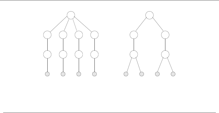
8.8 WAR STORY: WHAT’S PAST IS PROLOG 305
S4
S3
S2
S1S1S2S3S4
1
2222
3333
2
33
c
ba d
a
a
a
a
bb
bb
a
11
a
b
b
abc
d
Figure 8.12: Two different tries for the same set of rule heads.
“I agree. A trie is a natural way to represent your rule heads. Building a trie
on a set of strings of characters is straightforward: just insert the strings starting
from the root. So what is your problem?” I asked.
“The efficiency of our unification algorithm depends very much on minimizing
the number of edges in the trie. Since we know all the rules in advance, we have
the freedom to reorder the character positions in the rules. Instead of the root
node always representing the first argument in the rule, we can choose to have
it represent the third argument. We would like to use this freedom to build a
minimum-size trie for a set of rules.”
He showed me the example in Figure 8.12. A trie constructed according to
the original string position order (1,2,3) uses a total of 12 edges. However, by
permuting the character order to (2,3,1), we can obtain a trie with only 8 edges.
“Interesting. . . ” I started to reply before he cut me off again.
“There’s one other constraint. We must keep the leaves of the trie ordered, so
that the leaves of the underlying tree go left-to-right in the same order as the rules
appear on the page.”
“But why must you keep the leaves of the trie in the given order?” I asked.
“The order of rules in Prolog programs is very, very important. If you change
the order of the rules, the program returns different results.”
Then came my mission.
“We have a greedy heuristic for building good, but not optimal, tries based on
picking as the root the character position that minimizes the degree of the root. In
other words, it picks the character position that has the smallest number of distinct
characters in it. This heuristic works very, very well in practice. But we need you
to prove that finding the best trie is NP-complete so our paper is, well, complete.”

306 8. DYNAMIC PROGRAMMING
I agreed to try to prove the hardness of the problem, and chased him from my
office. The problem did seem to involve some nontrivial combinatorial optimization
to build the minimal tree, but I couldn’t see how to factor the left-to-right order of
the rules into a hardness proof. In fact, I couldn’t think of any NP-complete problem
that had such a left-right ordering constraint. After all, if a given set of rules
contained a character position in common to all the rules, this character position
must be probed first in any minimum-size tree. Since the rules were ordered, each
node in the subtree must represent the root of a run of consecutive rules. Thus
there were only n
2possible nodes to choose from for this tree....
Bingo! That settled it.
The next day I went back to the professor and told him. “I can’t prove that
your problem is NP-complete. But how would you feel about an efficient dynamic
programming algorithm to find the best trie!” It was a pleasure watching his frown
change to a smile as the realization took hold. An efficient algorithm to compute
what he needed was infinitely better than a proof saying you couldn’t do it!
My recurrence looked something like this. Suppose that we are given nordered
rule heads s1,...,s
n, each with marguments. Probing at the pth position, 1 ≤p≤
m, partitioned the rule heads into runs R1,...,R
r, where each rule in a given run
Rx=si,...,s
jhad the same character value of si[p]. The rules in each run must
be consecutive, so there are only n
2possible runs to worry about. The cost of
probing at position pis the cost of finishing the trees formed by each created run,
plus one edge per tree to link it to probe p:
C[i, j]= m
min
p=1
r
k=1
(C[ik,j
k]+1)
A graduate student immediately set to work implementing this algorithm to
compare with their heuristic. On many inputs, the optimal and greedy algorithms
constructed the exact same trie. However, for some examples, dynamic program-
ming gave a 20% performance improvement over greedy—i.e. , 20% better than
very, very well in practice. The run time spent in doing the dynamic programming
was a bit larger than with greedy, but in compiler optimization you are always
happy to trade off a little extra compilation time for better execution time in
the performance of your program. Is a 20% improvement worth this effort? That
depends upon the situation. How useful would you find a 20% increase in your
salary?
The fact that the rules had to remain ordered was the crucial property that we
exploited in the dynamic programming solution. Indeed, without it I was able to
prove that the problem was NP-complete, something we put in the paper to make
it complete.
8.9 WAR STORY: TEXT COMPRESSION FOR BAR CODES 307
Figure 8.13: A two-dimensional bar-code label of the Gettysburg Address using PDF-417.
Take-Home Lesson: The global optimum (found, for example, using dynamic
programming) is often noticeably better than the solution found by typical
heuristics. How important this improvement is depends on your application,
but it can never hurt.
8.9 War Story: Text Compression for Bar Codes
Ynjiun waved his laser wand over the torn and crumpled fragments of a bar code
label. The system hesitated for a few seconds, then responded with a pleasant blip
sound. He smiled at me in triumph. “Virtually indestructible.”
I was visiting the research laboratories of Symbol Technologies, the world’s
leading manufacturer of bar code scanning equipment. Next time you are in the
checkout line at a grocery store, check to see what type of scanning equipment they
are using. Likely it will say Symbol on the housing.
Although we take bar codes for granted, there is a surprising amount of tech-
nology behind them. Bar codes exist because conventional optical character recog-
nition (OCR) systems are not sufficiently reliable for inventory operations. The
bar code symbology familiar to us on each box of cereal or pack of gum encodes
a ten-digit number with enough error correction that it is virtually impossible to
scan the wrong number, even if the can is upside-down or dented. Occasionally,
the cashier won’t be able to get a label to scan at all, but once you hear that blip
you know it was read correctly.
The ten-digit capacity of conventional bar code labels provides room enough
only to store a single ID number in a label. Thus any application of supermarket bar
codes must have a database mapping 11141-47011 to a particular size and brand
of soy sauce. The holy grail of the bar code world has long been the development
of higher-capacity bar code symbologies that can store entire documents, yet still
be read reliably.
“PDF-417 is our new, two-dimensional bar code symbology,” Ynjiun explained.
A sample label is shown in Figure 8.13.
“How much data can you fit in a typical one-inch square label?” I asked him.
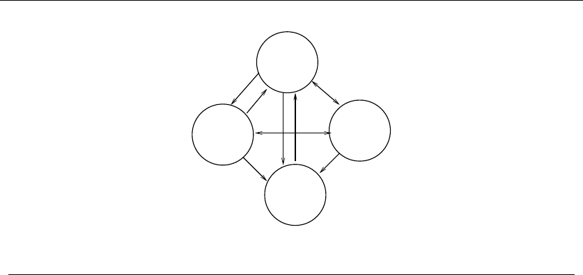
308 8. DYNAMIC PROGRAMMING
Case
a−z
Punctuation
;<>@[\$/"*(
Mixed
0−9, #$%=
l
l,ss
l
s
l
ls
Lower
Alpha
A−Z
Figure 8.14: Mode switching in PDF-417
“It depends upon the level of error correction we use, but about 1,000 bytes.
That’s enough for a small text file or image,” he said.
“Interesting. You will probably want to use some data compression technique
to maximize the amount of text you can store in a label.” See Section 18.5 (page
637) for a discussion of standard data compression algorithms.
“We do incorporate a data compaction method,” he explained. “We think we
understand the different types of files our customers will want to make labels for.
Some files will be all in uppercase letters, while others will use mixed-case letters
and numbers. We provide four different text modes in our code, each with a different
subset of alphanumeric characters available. We can describe each character using
only five bits as long as we stay within a mode. To switch modes, we issue a mode
switch command first (taking an extra five bits) and then the new character code.”
“I see. So you designed the mode character sets to minimize the number of
mode switch operations on typical text files.” The modes are illustrated in Figure
8.14.
“Right. We put all the digits in one mode and all the punctuation characters in
another. We also included both mode shift and mode latch commands. In a mode
shift, we switch into a new mode just for the next character, say to produce a
punctuation mark. This way, we don’t pay a cost for returning back to text mode
after a period. Of course, we can also latch permanently into a different mode if
we will be using a run of several characters from there.”
“Wow!” I said. “With all of this mode switching going on, there must be many
different ways to encode any given text as a label. How do you find the smallest of
such encoding.”
“We use a greedy algorithm. We look a few characters ahead and then decide
which mode we would be best off in. It works fairly well.”

8.9 WAR STORY: TEXT COMPRESSION FOR BAR CODES 309
I pressed him on this. “How do you know it works fairly well? There might be
significantly better encodings that you are simply not finding.”
“I guess I don’t know. But it’s probably NP-complete to find the optimal cod-
ing.” Ynjiun’s voice trailed off. “Isn’t it?”
I started to think. Every encoding started in a given mode and consisted of a
sequence of intermixed character codes and mode shift/latch operations. At any
given position in the text, we could output the next character code (if it was
available in our current mode) or decide to shift. As we moved from left to right
through the text, our current state would be completely reflected by our current
character position and current mode state. For a given position/mode pair, we
would have been interested in the cheapest way of getting there, over all possible
encodings getting to this point. . . .
My eyes lit up so bright they cast shadows on the walls.
“The optimal encoding for any given text in PDF-417 can be found using dy-
namic programming. For each possible mode 1 ≤m≤4, and each character
position 1 ≤i≤n, we will maintain the cheapest encoding found of the first i
characters ending in mode m. Our next move from each mode/position is either
match, shift, or latch, so there are only a few possible operations to consider.”
Basically,
M[i, j] = min
1≤m≤4(M[i−1,m]+c(Si,m,j))
where c(Si,m,j) is the cost of encoding character Siand switching from mode m
to mode j. The cheapest possible encoding results from tracing back from M[n, m],
where mis the value of ithat minimizes min1≤i≤4M[n, i]. Each of the 4ncells can
be filled in constant time, so it takes time linear in the length of the string to find
the optimal encoding.
Ynjiun was skeptical, but he encouraged us to implement an optimal encoder.
A few complications arose due to weirdnesses of PDF-417 mode switching, but my
student Yaw-Ling Lin rose to the challenge. Symbol compared our encoder to theirs
on 13,000 labels and concluded that dynamic programming lead to an 8% tighter
encoding on average. This was significant, because no one wants to waste 8% of
their potential storage capacity, particularly in an environment where the capacity
is only a few hundred bytes. For certain applications, this 8% margin permitted
one bar code label to suffice where previously two had been required. Of course,
an 8% average improvement meant that it did much better than that on certain
labels. While our encoder took slightly longer to run than the greedy encoder, this
was not significant, since the bottleneck would be the time needed to print the
label anyway.
Our observed impact of replacing a heuristic solution with the global optimum
is probably typical of most applications. Unless you really botch your heuristic, you
are probably going to get a decent solution. Replacing it with an optimal result,
however, usually gives a small but nontrivial improvement, which can have pleasing
consequences for your application.

310 8. DYNAMIC PROGRAMMING
Chapter Notes
Bellman [Bel58] is credited with developing the technique of dynamic programming.
The edit distance algorithm is originally due to Wagner and Fischer [WF74]. A
faster algorithm for the book partition problem appears in [KMS97].
The computational complexity of finding the minimum weight triangulation of
disconnected point sets (as opposed to polygons) was a longstanding open problem
that finally fell to Mulzer and Rote [MR06].
Techniques such as dynamic programming and backtracking searches can be
used to generate worst-case efficient (although still non-polynomial) algorithms for
many NP-complete problems. See Woeginger [Woe03] for a nice survey of such
techniques.
The morphing system that was the subject of the war story in Section 8.4 (page
291) is described in [HWK94]. See our paper [DRR+95] for more on the Prolog trie
minimization problem, subject of the war story of Section 8.8 (page 304). Two-
dimensional bar codes, subject of the war story in Section 8.9 (page 307), were
developed largely through the efforts of Theo Pavlidis and Ynjiun Wang at Stony
Brook [PSW92].
The dynamic programming algorithm presented for parsing is known as the
CKY algorithm after its three independent inventors (Cocke, Kasami, and Younger)
[You67]. The generalization of parsing to edit distance is due to Aho and Peterson
[AP72].
8.10 Exercises
Edit Distance
8-1. [3] Typists often make transposition errors exchanging neighboring characters,
such as typing “setve” when you mean “steve.” This requires two substitutions to
fix under the conventional definition of edit distance.
Incorporate a swap operation into our edit distance function, so that such neigh-
boring transposition errors can be fixed at the cost of one operation.
8-2. [4] Suppose you are given three strings of characters: X,Y,andZ,where|X|=n,
|Y|=m,and|Z|=n+m.Zis said to be a shuffle of Xand Yiff Zcan be
formed by interleaving the characters from Xand Yin a way that maintains the
left-to-right ordering of the characters from each string.
(a) Show that cchocohilaptes is a shuffle of chocolate and chips, but chocochilatspe
is not.
(b) Give an efficient dynamic-programming algorithm that determines whether Z
is a shuffle of Xand Y. Hint: the values of the dynamic programming matrix
you construct should be Boolean, not numeric.
8-3. [4] The longest common substring (not subsequence) of two strings Xand Yis
the longest string that appears as a run of consecutive letters in both strings. For
example, the longest common substring of photograph and tomography is ograph.

8.10 EXERCISES 311
(a) Let n=|X|and m=|Y|. Give a Θ(nm) dynamic programming algorithm
for longest common substring based on the longest common subsequence/edit
distance algorithm.
(b) Give a simpler Θ(nm) algorithm that does not rely on dynamic programming.
8-4. [6] The longest common subsequence (LCS) of two sequences Tand Pis the longest
sequence Lsuch that Lis a subsequence of both Tand P.Theshortest common
supersequence (SCS) of Tand Pis the smallest sequence Lsuch that both Tand
Pare a subsequence of L.
(a) Give efficient algorithms to find the LCS and SCS of two given sequences.
(b) Let d(T,P) be the minimum edit distance between Tand Pwhen no sub-
stitutions are allowed (i.e., the only changes are character insertion and dele-
tion). Prove that d(T,P)=|SCS(T,P)|−|LCS(T,P)|where |SCS(T,P)|
(|LCS(T,P)|) is the size of the shortest SCS (longest LCS) of Tand P.
Greedy Algorithms
8-5. [4] Let P1,P
2,...,P
nbe nprograms to be stored on a disk with capacity D
megabytes. Program Pirequires simegabytes of storage. We cannot store them all
because D<n
i=1 si
(a) Does a greedy algorithm that selects programs in order of nondecreasing si
maximize the number of programs held on the disk? Prove or give a counter-
example.
(b) Does a greedy algorithm that selects programs in order of nonincreasing order
siuse as much of the capacity of the disk as possible? Prove or give a counter-
example.
8-6. [5] Coins in the United States are minted with denominations of 1, 5, 10, 25, and
50 cents. Now consider a country whose coins are minted with denominations of
{d1,...,d
k}units. We seek an algorithm to make change of nunits using the
minimum number of coins for this country.
(a) The greedy algorithm repeatedly selects the biggest coin no bigger than the
amount to be changed and repeats until it is zero. Show that the greedy algorithm
does not always use the minimum number of coins in a country whose denominations
are {1,6,10}.
(b) Give an efficient algorithm that correctly determines the minimum number of
coins needed to make change of nunits using denominations {d1,...,d
k}. Analyze
its running time.
8-7. [5] In the United States, coins are minted with denominations of 1, 5, 10, 25,
and 50 cents. Now consider a country whose coins are minted with denominations
of {d1,...,d
k}units. We want to count how many distinct ways C(n) there are
to make change of nunits. For example, in a country whose denominations are
{1,6,10},C(5) = 1, C(6) to C(9) = 2, C(10) = 3, and C(12) = 4.
(a) How many ways are there to make change of 20 units from {1,6,10}?

312 8. DYNAMIC PROGRAMMING
(b) Give an efficient algorithm to compute C(n), and analyze its complexity.
(Hint: think in terms of computing C(n, d), the number of ways to make
change of nunits with highest denomination d. Be careful to avoid overcount-
ing.)
8-8. [6] In the single-processor scheduling problem, we are given a set of njobs J. Each
job ihas a processing time ti, and a deadline di. A feasible schedule is a permutation
of the jobs such that when the jobs are performed in that order, every job is finished
before its deadline. The greedy algorithm for single-processor scheduling selects the
job with the earliest deadline first.
Show that if a feasible schedule exists, then the schedule produced by this greedy
algorithm is feasible.
Number Problems
8-9. [6] The knapsack problem is as follows: given a set of integers S={s1,s
2,...,s
n},
and a given target number T, find a subset of Sthat adds up exactly to T.For
example, within S={1,2,5,9,10}there is a subset that adds up to T= 22 but
not T= 23.
Give a correct programming algorithm for knapsack that runs in O(nT )time.
8-10. [6] The integer partition takes a set of positive integers S=s1,...,s
nand asks if
there is a subset I∈Ssuch that
i∈I
si=
i/∈I
si
Let i∈Ssi=M.GiveanO(nM) dynamic programming algorithm to solve the
integer partition problem.
8-11. [5] Assume that there are nnumbers (some possibly negative) on a circle, and
we wish to find the maximum contiguous sum along an arc of the circle. Give an
efficient algorithm for solving this problem.
8-12. [5] A certain string processing language allows the programmer to break a string
into two pieces. It costs nunits of time to break a string of ncharacters into two
pieces, since this involves copying the old string. A programmer wants to break a
string into many pieces, and the order in which the breaks are made can affect the
total amount of time used. For example, suppose we wish to break a 20-character
string after characters 3, 8, and 10. If the breaks are made in left-right order, then
the first break costs 20 units of time, the second break costs 17 units of time, and
the third break costs 12 units of time, for a total of 49 steps. If the breaks are made
in right-left order, the first break costs 20 units of time, the second break costs 10
units of time, and the third break costs 8 units of time, for a total of only 38 steps.
Give a dynamic programming algorithm that takes a list of character positions after
which to break and determines the cheapest break cost in O(n3)time.
8-13. [5] Consider the following data compression technique. We have a table of mtext
strings, each at most kin length. We want to encode a data string Dof length n
using as few text strings as possible. For example, if our table contains (a,ba,abab,b)
and the data string is bababbaababa, the best way to encode it is (b,abab,ba,abab,a)—
a total of five code words. Give an O(nmk) algorithm to find the length of the best

8.10 EXERCISES 313
encoding. You may assume that every string has at least one encoding in terms of
the table.
8-14. [5] The traditional world chess championship is a match of 24 games. The current
champion retains the title in case the match is a tie. Each game ends in a win, loss,
or draw (tie) where wins count as 1, losses as 0, and draws as 1/2. The players take
turns playing white and black. White has an advantage, because he moves first.
The champion plays white in the first game. He has probabilities ww,wd,andwl
of winning, drawing, and losing playing white, and has probabilities bw,bd,andbl
of winning, drawing, and losing playing black.
(a) Write a recurrence for the probability that the champion retains the title.
Assume that there are ggames left to play in the match and that the champion
needs to win igames (which may end in a 1/2).
(b) Based on your recurrence, give a dynamic programming to calculate the cham-
pion’s probability of retaining the title.
(c) Analyze its running time for an ngame match.
8-15. [8] Eggs break when dropped from great enough height. Specifically, there must
be a floor fin any sufficiently tall building such that an egg dropped from the fth
floor breaks, but one dropped from the (f−1)st floor will not. If the egg always
breaks, then f= 1. If the egg never breaks, then f=n+1.
You seek to find the critical floor fusing an n-story building. The only operation
you can perform is to drop an egg off some floor and see what happens. You start
out with keggs, and seek to drop eggs as few times as possible. Broken eggs cannot
be reused. Let E(k, n) be the minimum number of egg droppings that will always
suffice.
(a) Show that E(1,n)=n.
(b) Show that E(k, n)=Θ(n1
k).
(c) Find a recurrence for E(k, n). What is the running time of the dynamic pro-
gram to find E(k, n)?
Graph Problems
8-16. [4] Consider a city whose streets are defined by an X×Ygrid. We are interested in
walking from the upper left-hand corner of the grid to the lower right-hand corner.
Unfortunately, the city has bad neighborhoods, whose intersections we do not want
to walk in. We are given an X×Ymatrix BAD,whereBAD[i,j] = “yes” if and
only if the intersection between streets iand jis in a neighborhood to avoid.
(a) Give an example of the contents of BAD such that there is no path across the
grid avoiding bad neighborhoods.
(b) Give an O(XY ) algorithm to find a path across the grid that avoids bad neigh-
borhoods.
(c) Give an O(XY ) algorithm to find the shortest path across the grid that avoids
bad neighborhoods. You may assume that all blocks are of equal length. For partial
credit, give an O(X2Y2) algorithm.

314 8. DYNAMIC PROGRAMMING
8-17. [5] Consider the same situation as the previous problem. We have a city whose
streets are defined by an X×Ygrid. We are interested in walking from the upper
left-hand corner of the grid to the lower right-hand corner. We are given an X×Y
matrix BAD,whereBAD[i,j] = “yes” if and only if the intersection between streets
iand jis somewhere we want to avoid.
If there were no bad neighborhoods to contend with, the shortest path across the
grid would have length (X−1) + (Y−1) blocks, and indeed there would be many
such paths across the grid. Each path would consist of only rightward and downward
moves.
Give an algorithm that takes the array BAD and returns the number of safe paths
of length X+Y−2. For full credit, your algorithm must run in O(XY ).
Design Problems
8-18. [4] Consider the problem of storing nbooks on shelves in a library. The order of the
books is fixed by the cataloging system and so cannot be rearranged. Therefore, we
can speak of a book bi,where1≤i≤n, that has a thickness tiand height hi.The
length of each bookshelf at this library is L.
Suppose all the books have the same height h(i.e. , h=hi=hjfor all i, j)and
the shelves are all separated by a distance of greater than h, so any book fits on
any shelf. The greedy algorithm would fill the first shelf with as many books as
we can until we get the smallest isuch that bidoes not fit, and then repeat with
subsequent shelves. Show that the greedy algorithm always finds the optimal shelf
placement, and analyze its time complexity.
8-19. [6] This is a generalization of the previous problem. Now consider the case where
the height of the books is not constant, but we have the freedom to adjust the
height of each shelf to that of the tallest book on the shelf. Thus the cost of a
particular layout is the sum of the heights of the largest book on each shelf.
•Give an example to show that the greedy algorithm of stuffing each shelf as
full as possible does not always give the minimum overall height.
•Give an algorithm for this problem, and analyze its time complexity. Hint:
use dynamic programming.
8-20. [5] We wish to compute the laziest way to dial given n-digit number on a standard
push-button telephone using two fingers. We assume that the two fingers start
out on the * and # keys, and that the effort required to move a finger from one
button to another is proportional to the Euclidean distance between them. Design
an algorithm that computes the method of dialing that involves moving your fingers
the smallest amount of total distance, where kis the number of distinct keys on
the keypad (k= 16 for standard telephones). Try to use O(nk3)time.
8-21. [6] Given an array of nreal numbers, consider the problem of finding the maximum
sum in any contiguous subvector of the input. For example, in the array
{31,−41,59,26,−53,58,97,−93,−23,84}
the maximum is achieved by summing the third through seventh elements, where
59 + 26 + (−53) + 58 + 97 = 187. When all numbers are positive, the entire array is
the answer, while when all numbers are negative, the empty array maximizes the
total at 0.

8.10 EXERCISES 315
•Give a simple, clear, and correct Θ(n2)-time algorithm to find the maximum
contiguous subvector.
•Now give a Θ(n)-time dynamic programming algorithm for this problem. To
get partial credit, you may instead give a correct O(nlog n) divide-and-conquer
algorithm.
8-22. [7] Consider the problem of examining a string x=x1x2...x
nfrom an alphabet of
ksymbols, and a multiplication table over this alphabet. Decide whether or not it is
possible to parenthesize xin such a way that the value of the resulting expression is
a,whereabelongs to the alphabet. The multiplication table is neither commutative
or associative, so the order of multiplication matters.
abc
aacc
baab
cccc
For example, consider the above multiplication table and the string bbbba. Paren-
thesizing it (b(bb))(ba)givesa, but ((((bb)b)b)a)givesc.
Give an algorithm, with time polynomial in nand k, to decide whether such a
parenthesization exists for a given string, multiplication table, and goal element.
8-23. [6] Let αand βbe constants. Assume that it costs αto go left in a tree, and βto
go right. Devise an algorithm that builds a tree with optimal worst case cost, given
keys k1,...,k
nand the probabilities that each will be searched p1,...,p
n.
Interview Problems
8-24. [5] Given a set of coin denominators, find the minimum number of coins to make a
certain amount of change.
8-25. [5] You are given an array of nnumbers, each of which may be positive, negative,
or zero. Give an efficient algorithm to identify the index positions iand jto the
maximum sum of the ith through jth numbers.
8-26. [7] Observe that when you cut a character out of a magazine, the character on the
reverse side of the page is also removed. Give an algorithm to determine whether
you can generate a given string by pasting cutouts from a given magazine. Assume
that you are given a function that will identify the character and its position on
the reverse side of the page for any given character position.
Programming Challenges
These programming challenge problems with robot judging are available at
http://www.programming-challenges.com or http://online-judge.uva.es.
8-1. “Is Bigger Smarter?” – Programming Challenges 111101, UVA Judge 10131.
8-2. “Weights and Measures” – Programming Challenges 111103, UVA Judge 10154.
8-3. “Unidirectional TSP” – Programming Challenges 111104, UVA Judge 116.
8-4. “Cutting Sticks” – Programming Challenges 111105, UVA Judge 10003.
8-5. “Ferry Loading” – Programming Challenges 111106, UVA Judge 10261.

9
Intractable Problems and Approximation
Algorithms
We now introduce techniques for proving that no efficient algorithm exists for a
given problem. The practical reader is probably squirming at the notion of proving
anything, and will be particularly alarmed at the idea of investing time to prove
that something does not exist. Why are you better off knowing that something you
don’t know how to do in fact can’t be done at all?
The truth is that the theory of NP-completeness is an immensely useful tool for
the algorithm designer, even though all it provides are negative results. The the-
ory of NP-completeness enables the algorithm designer to focus her efforts more
productively, by revealing that the search for an efficient algorithm for this partic-
ular problem is doomed to failure. When one fails to show a problem is hard, that
suggests there may well be an efficient algorithm to solve it. Two of the war stories
in this book described happy results springing from bogus claims of hardness.
The theory of NP-completeness also enables us to identify what properties make
a particular problem hard. This provides direction for us to model it in different
ways or exploit more benevolent characteristics of the problem. Developing a sense
for which problems are hard is an important skill for algorithm designers, and only
comes from hands-on experience with proving hardness.
The fundamental concept we will use is that of reductions between pairs of
problems, showing that the problems are really equivalent. We illustrate this idea
through a series of reductions, each of which either yields an efficient algorithm
or an argument that no such algorithm can exist. We also provide brief introduc-
tions to (1) the complexity-theoretic aspects of NP-completeness, one of the most
fundamental notions in Computer Science, and (2) the theory of approximation
algorithms, which leads to heuristics that probably return something close to the
optimal solution.
S.S. Skiena, The Algorithm Design Manual, 2nd ed., DOI: 10.1007/978-1-84800-070-4 9,
c
Springer-Verlag London Limited 2008

9.1 PROBLEMS AND REDUCTIONS 317
9.1 Problems and Reductions
We have encountered several problems in this book for which we couldn’t find any
efficient algorithm. The theory of NP-completeness provides the tools needed to
show that all these problems are on some level really the same problem.
The key idea to demonstrating the hardness of a problem is that of a reduction,
or translation, between two problems. The following allegory of NP-completeness
may help explain the idea. A bunch of kids take turns fighting each other in the
schoolyard to prove how “tough” they are. Adam beats up Bill, who then beats up
Chuck. So who if any among them is “tough?” The truth is that there is no way
to know without an external standard. If I told you that Chuck was in fact Chuck
Norris, certified tough guy, you have to be impressed—both Adam and Bill are at
least as tough as he is. On the other hand, suppose I tell you it is a kindergarten
school yard. No one would call me tough, but even I can take out Adam. This
proves that none of the three of them should be called be tough. In this allegory,
each fight represents a reduction. Chuck Norris takes on the role of satisfiability—a
certifiably hard problem. The part of an inefficient algorithm with a possible shot
at redemption is played by me.
Reductions are operations that convert one problem into another. To describe
them, we must be somewhat rigorous in our definitions. An algorithmic problem is
a general question, with parameters for input and conditions on what constitutes a
satisfactory answer or solution. An instance is a problem with the input parameters
specified. The difference can be made clear by an example:
Problem: The Traveling Salesman Problem (TSP)
Input: A weighted graph G.
Output: Which tour {v1,v
2, ..., vn}minimizes n−1
i=1 d[vi,v
i+1]+d[vn,v
1]?
Any weighted graph defines an instance of TSP. Each particular problem has
at least one minimum cost tour. The general traveling salesman instance asks for
an algorithm to find the optimal tour for all possible instances.
9.1.1 The Key Idea
Now consider two algorithmic problems, called Bandersnatch and Bo-billy. Sup-
pose that I gave you the following reduction/algorithm to solve the Bandersnatch
problem:
Bandersnatch(G)
Translate the input Gto an instance Yof the Bo-billy problem.
Call the subroutine Bo-billy on Yto solve this instance.
Return the answer of Bo-billy(Y) as the answer to Bandersnatch(G).

318 9. INTRACTABLE PROBLEMS AND APPROXIMATION ALGORITHMS
This algorithm will correctly solve the Bandersnatch problem provided that the
translation to Bo-billy always preserves the correctness of the answer. In other
words, the translation has the property that for any instance of G,
Bandersnatch(G) = Bo-billy(Y)
A translation of instances from one type of problem to instances of another such
that the answers are preserved is what is meant by a reduction.
Now suppose this reduction translates Gto Yin O(P(n)) time. There are two
possible implications:
•If my Bo-billy subroutine ran in O(P(n)), this means I could solve the Ban-
dersnatch problem in O(P(n)+P(n)) by spending the time to translate the
problem and then the time to execute the Bo-Billy subroutine.
•If I know that Ω(P(n)) is a lower bound on computing Bandersnatch, mean-
ing there definitely exists no faster way to solve it, then Ω(P(n)−P(n))
must be a lower bound to compute Bo-billy. Why? If I could solve Bo-billy
any faster, then I could violate my lower bound by solving Bandersnatch
using the above reduction. This implies that there can be no way to solve
Bo-billy any faster than claimed.
This first argument is Steve demonstrating the weakness of the entire schoolyard
with a quick right to Adam’s chin. The second highlights the Chuck Norris approach
we will use to prove that problems are hard. Essentially, this reduction shows that
Bo-billy is no easier than Bandersnatch. Therefore, if Bandersnatch is hard this
means Bo-billy must also be hard.
We will illustrate this point by giving several problem reductions in this chapter.
Take-Home Lesson: Reductions are a way to show that two problems are es-
sentially identical. A fast algorithm (or the lack of one) for one of the problems
implies a fast algorithm (or the lack of one) for the other.
9.1.2 Decision Problems
Reductions translate between problems so that their answers are identical in every
problem instance. Problems differ in the range or type of possible answers. The
traveling salesman problem returns a permutation of vertices as the answer, while
other types of problems return numbers as answers, perhaps restricted to positive
numbers or integers.
The simplest interesting class of problems have answers restricted to true and
false. These are called decision problems. It proves convenient to reduce/translate
answers between decision problems because both only allow true and false as pos-
sible answers.
Fortunately, most interesting optimization problems can be phrased as decision
problems that capture the essence of the computation. For example, the traveling
salesman decision problem could be defined as:

9.2 REDUCTIONS FOR ALGORITHMS 319
Problem: The Traveling Salesman Decision Problem
Input: A weighted graph Gand integer k.
Output: Does there exist a TSP tour with cost ≤k?
The decision version captures the heart of the traveling salesman problem, in
that if you had a fast algorithm for the decision problem, you could use it to do a
binary search with different values of kand quickly hone in on the optimal solution.
With a little more cleverness, you could reconstruct the actual tour permutation
using a fast solution to the decision problem.
From now on we will generally talk about decision problems, because it proves
easier and still captures the power of the theory.
9.2 Reductions for Algorithms
An engineer and an algorist are sitting in a kitchen. The algorist asks the engineer
to boil some water, so the engineer gets up, picks up the kettle from the counter
top, adds water from the sink, brings it to the burner, turns on the burner, waits
for the whistling sound, and turns off the burner. Sometime later, the engineer
asks the algorist to boil more water. She gets up, takes the kettle from the burner,
moves it over to the counter top, and sits down. “Done.” she says, “I have reduced
the task to a solved problem.”
This boiling water reduction illustrates an honorable way to generate new algo-
rithms from old. If we can translate the input for a problem we want to solve into
input for a problem we know how to solve, we can compose the translation and the
solution into an algorithm for our problem.
In this section, we look at several reductions that lead to efficient algorithms.
To solve problem a, we translate/reduce the ainstance to an instance of b, then
solve this instance using an efficient algorithm for problem b. The overall running
time is the time needed to perform the reduction plus that solve the binstance.
9.2.1 Closest Pair
The closest pair problem asks to find the pair of numbers within a set that have
the smallest difference between them. We can make it a decision problem by asking
if this value is less than some threshold:
Input: AsetSof nnumbers, and threshold t.
Output: Is there a pair si,s
j∈Ssuch that |si−sj|≤t?
The closest pair is a simple application of sorting, since the closest pair must
be neighbors after sorting. This gives the following algorithm:
CloseEnoughPair(S,t)
Sort S.
Is min1≤i<n |si−si+1|≤t?

320 9. INTRACTABLE PROBLEMS AND APPROXIMATION ALGORITHMS
There are several things to note about this simple reduction.
1. The decision version captured what is interesting about the problem, meaning
it is no easier than finding the actual closest pair.
2. The complexity of this algorithm depends upon the complexity of sorting.
Use an O(nlog n) algorithm to sort, and it takes O(nlog n+n) to find the
closest pair.
3. This reduction and the fact that there is an Ω(nlog n) lower bound on sorting
does not prove that a close-enough pair must take Ω(nlog n) time in the worst
case. Perhaps this is just a slow algorithm for a close-enough pair, and there
is a faster one lurking somewhere?
4. On the other hand, if we knew that a close-enough pair required Ω(nlog n)
time to solve in the worst case, this reduction would suffice to prove that
sorting couldn’t be solved any faster than Ω(nlog n) because that would
imply a faster algorithm for a close-enough pair.
9.2.2 Longest Increasing Subsequence
In Chapter 8, we demonstrated how dynamic programming can be used to solve
a variety of problems, including string edit distance (Section 8.2 (page 280)) and
longest increasing subsequence (Section 8.3 (page 289)). To review,
Problem: Edit Distance
Input: Integer or character sequences Sand T; penalty costs for each insertion
(cins), deletion (cdel), and substitution (cdel).
Output: What is the minimum cost sequence of operations to transform Sto T?
Problem: Longest Increasing Subsequence
Input: An integer or character sequence S.
Output: What is the longest sequence of integer positions {p1,...,p
m}such that
pi<p
i+1 and Spi<S
pi+1 ?
In fact, longest increasing subsequence (LIS) can be solved as a special case of
edit distance:
Longest Increasing Subsequence(S)
T= Sort(S)
cins =cdel =1
csub =∞
Return (|S|- EditDistance(S,T,cins,cdel,cdel)/2)
Why does this work? By constructing the second sequence Tas the elements of
Ssorted in increasing order, we ensure that any common subsequence must be an

9.2 REDUCTIONS FOR ALGORITHMS 321
increasing subsequence. If we are never allowed to do any substitutions (because
csub =∞), the optimal alignment of two sequences finds the longest common sub-
sequence between them and removes everything else. Thus, transforming {3,1,2}
to {1,2,3}costs two, namely inserting and deleting the unmatched 3. The length
of Sminus half this cost gives the length of the LIS.
What are the implications of this reduction? The reduction takes O(nlog n)
time. Because edit distance takes time O(|S|·|T|), this gives a quadratic algorithm
to find the longest increasing subsequence of S, which is the same complexity as
the the algorithm presented in Section 8.3 (page 289). In fact, there exists a faster
O(nlog n) algorithm for LIS using clever data structures, while edit distance is
known to be quadratic in the worst case. Here, our reduction gives us a simple but
not optimal polynomial-time algorithm.
9.2.3 Least Common Multiple
The least common multiple and greatest common divisor problems arise often in
working with integers. We say bdivides a(b|a) if there exists an integer dthat
a=bd. Then:
Problem: Least Common Multiple (lcm)
Input: Two integers xand y.
Output: Return the smallest integer msuch that mis a multiple of xand mis also
a multiple of y.
Problem: Greatest Common Divisor (gcd)
Input: Two integers xand y.
Output: Return the largest integer dsuch that ddivides xand ddivides y.
For example, lcm(24,36) = 72 and gcd(24,36) = 12. Both problems can be
solved easily after reducing xand yto their prime factorizations, but no efficient
algorithm is known for factoring integers (see Section 13.8 (page 420)). Fortunately,
Euclid’s algorithm gives an efficient way to solve greatest common divisor without
factoring. It is a recursive algorithm that rests on two observations. First,
if b|a, then gcd(a, b)=b.
This should be pretty clear. if bdivides a, then a=bk for some integer k, and thus
gcd(bk, b)=b. Second,
If a=bt +rfor integers tand r, then gcd(a, b)=gcd(b, r).
Since x·yis a multiple of both xand y,lcm(x, y)≤xy. The only way that
there can be a smaller common multiple is if there is some nontrivial factor shared
between xand y. This observation, coupled with Euclid’s algorithm, provides an
efficient way to compute least common multiple, namely

322 9. INTRACTABLE PROBLEMS AND APPROXIMATION ALGORITHMS
5
11 1
3
1
7
Figure 9.1: Reducing convex hull to sorting by mapping points to a parabola
LeastCommonMultiple(x,y)
Return (xy/gcd(x, y)).
This reduction gives us a nice way to reuse Euclid’s efforts on another problem.
9.2.4 Convex Hull (*)
Our final example of a reduction from an “easy” problem (i.e. , one that can be
solved in polynomial time) goes from finding convex hulls to sorting numbers.
A polygon is convex if the straight line segment drawn between any two points
inside the polygon Pmust lie completely within the polygon. This is the case
when Pcontains no notches or concavities, so convex polygons are nicely shaped.
The convex hull provides a very useful way to provide structure to a point set.
Applications are presented in Section 17.2 (page 568).
Problem: Convex Hull
Input: AsetSof npoints in the plane.
Output: Find the smallest convex polygon containing all the points of S.
We now show how to transform from sorting to convex hull. This means we
must translate each number to a point. We do so by mapping xto (x, x2). Why?
It means each integer is mapped to a point on the parabola y=x2. Since this
parabola is convex, every point must be on the convex hull. Furthermore, since
neighboring points on the convex hull have neighboring xvalues, the convex hull
returns the points sorted by the x-coordinate—i.e., the original numbers. Creating
and reading off the points takes O(n) time:
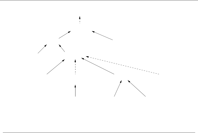
9.3 ELEMENTARY HARDNESS REDUCTIONS 323
all of NP
Satisfiability
Integer Programming
3−SAT
Vertex Cover
Integer PartitionIndependent Set
Clique
Inequivallence
of Programs
with Assignments
Hamiltonian
Cycle
Uniconnected
Subgraph
Generalized
Movie
Scheduling
Traveling
Salesman
Figure 9.2: A portion of the reduction tree for NP-complete problems. Solid lines denote the
reductions presented in this chapter
Sort(S)
For each i∈S, create point (i, i2).
Call subroutine convex-hull on this point set.
From the leftmost point in the hull,
read off the points from left to right.
What does this mean? Recall the sorting lower bound of Ω(nlg n). If we could
compute convex hull in better than nlg n, this reduction implies that we could sort
faster than Ω(nlg n), which violates our lower bound. Thus, convex hull must take
Ω(nlg n) as well! Observe that any O(nlg n) convex hull algorithm also gives us a
complicated but correct O(nlg n) sorting algorithm as well.
9.3 Elementary Hardness Reductions
The reductions in the previous section demonstrate transformations between pairs
of problems for which efficient algorithms exist. However, we are mainly concerned
with using reductions to prove hardness, by showing that a fast algorithm for
Bandersnatch would imply one that cannot exist for Bo-billy.
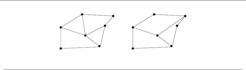
324 9. INTRACTABLE PROBLEMS AND APPROXIMATION ALGORITHMS
Figure 9.3: Graphs with (l) and without (r) Hamiltonian cycles
For now, I want you to trust me when I say that Hamiltonian cycle and vertex
cover are hard problems. The entire picture (presented in Figure 9.2) will become
clear by the end of the chapter.
9.3.1 Hamiltonian Cycle
The Hamiltonian cycle problem is one of the most famous in graph theory. It seeks
a tour that visits each vertex of a given graph exactly once. It has a long history
and many applications, as discussed in Section 16.5. Formally, it is defined as:
Problem: Hamiltonian Cycle
Input: An unweighted graph G.
Output: Does there exist a simple tour that visits each vertex of Gwithout repeti-
tion?
Hamiltonian cycle has some obvious similarity to the traveling salesman prob-
lem. Both problems seek a tour that visits each vertex exactly once. There are also
differences between the two problems. TSP works on weighted graphs, while Hamil-
tonian cycle works on unweighted graphs. The following reduction from Hamilto-
nian cycle to traveling salesman shows that the similarities are greater than the
differences:
HamiltonianCycle(G=(V, E))
Construct a complete weighted graph G=(V,E) where V=V.
n=|V|
for i=1tondo
for j=1tondo
if (i, j)∈Ethen w(i, j)=1elsew(i, j)=2
Return the answer to Traveling-Salesman-Decision-Problem(G,n).
The actual reduction is quite simple, with the translation from unweighted to
weighted graph easily performed in O(n2) time. Further, this translation is designed
to ensure that the answers of the two problems will be identical. If the graph G
has a Hamiltonian cycle {v1,...,v
n}, then this exact same tour will correspond to
nedges in E, each with weight 1. This gives a TSP tour in Gof weight exactly

9.3 ELEMENTARY HARDNESS REDUCTIONS 325
Figure 9.4: Circled vertices form a vertex cover, and the others form an independent set
n.IfGdoes not have a Hamiltonian cycle, then there can be no such TSP tour in
Gbecause the only way to get a tour of cost nin Gwould be to use only edges of
weight 1, which implies a Hamiltonian cycle in G.
This reduction is both efficient and truth preserving. A fast algorithm for TSP
would imply a fast algorithm for Hamiltonian cycle, while a hardness proof for
Hamiltonian cycle would imply that TSP is hard. Since the latter is the case, this
reduction shows that TSP is hard, at least as hard as the Hamiltonian cycle.
9.3.2 Independent Set and Vertex Cover
The vertex cover problem, discussed more thoroughly in Section 16.3 (page 530),
asks for a small set of vertices that contacts each edge in a graph. More formally:
Problem: Vertex Cover
Input: AgraphG=(V, E) and integer k≤|V|.
Output: Is there a subset Sof at most kvertices such that every e∈Econtains at
least one vertex in S?
It is trivial to find avertex cover of a graph, namely the cover that consists of
all the vertices. More tricky is to cover the edges using as small a set of vertices
as possible. For the graph in Figure 9.4, four of the eight vertices are sufficient to
cover.
A set of vertices Sof graph Gis independent if there are no edges (x, y) where
both x∈Sand y∈S. This means there are no edges between any two vertices
in independent set. As discussed in Section 16.2 (page 528), independent set arises
in facility location problems. The maximum independent set decision problem is
formally defined:
Problem: Independent Set
Input: AgraphGand integer k≤|V|.
Output: Does there exist an independent set of kvertices in G?

326 9. INTRACTABLE PROBLEMS AND APPROXIMATION ALGORITHMS
Both vertex cover and independent set are problems that revolve around finding
special subsets of vertices: the first with representatives of every edge, the second
with no edges. If Sis the vertex cover of G, the remaining vertices S−Vmust
form an independent set, for if an edge had both vertices in S−V, then Scould
not have been a vertex cover. This gives us a reduction between the two problems:
VertexCover(G, k)
G=G
k=|V|−k
Return the answer to IndependentSet(G,k
)
Again, a simple reduction shows that the two problems are identical. Notice
how this translation occurs without any knowledge of the answer. We transform
the input, not the solution. This reduction shows that the hardness of vertex cover
implies that independent set must also be hard. It is easy to reverse the roles of
the two problems in this particular reduction, thus proving that both problems are
equally hard.
Stop and Think: Hardness of General Movie Scheduling
Problem: Prove that the general movie scheduling problem is NP-complete, with
a reduction from independent set.
Problem: General Movie Scheduling Decision Problem
Input: AsetIof nsets of intervals on the line, integer k.
Output: Can a subset of at least kmutually nonoverlapping interval sets which can
be selected from I?
Solution: Recall the movie scheduling problem, discussed in Section 1.2 (page 9).
Each possible movie project came with a single time interval during which filming
took place. We sought the largest possible subset of movie projects such that no
two conflicting projects (i.e. , both requiring the actor at the same time) were
selected.
The general problem allows movie projects to have discontinuous schedules. For
example, Project Arunning from January-March and May-June does not intersect
Project Brunning in April and August, but does collide with Project Crunning
from June-July.
If we are going to prove general movie scheduling hard from independent set,
what is Bandersnatch and what is Bo-billy? We need to show how to translate all
independent set problems into instances of movie scheduling—i.e. , sets of disjointed
line intervals.
What is the correspondence between the two problems? Both problems involve
selecting the largest subsets possible—of vertices and movies, respectively. This
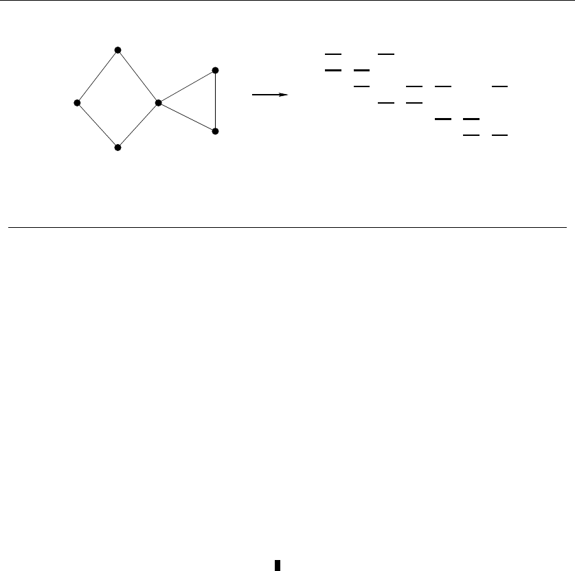
9.3 ELEMENTARY HARDNESS REDUCTIONS 327
1
2
4
3
AB
CD
E
F
G6
5
2
3
4
5
6
1
GFEDCBA
Figure 9.5: Reduction from independent set to generalized movie scheduling, with numbered
vertices and lettered edges
suggests we must translate vertices into movies. Further, both require the selected
elements not to interfere, by sharing an edge or overlapping an interval, respectively.
IndependentSet(G, k)
I=∅
For the ith edge (x, y), 1 ≤i≤m
Add interval [i, i +0.5] for movie Xto I
Add interval [i, i +0.5] for movie yto I
Return the answer to GeneralMovieScheduling(I,k)
My construction is as follows. Create an interval on the line for each of the m
edges of the graph. The movie associated with each vertex will contain the intervals
for the edges adjacent with it, as shown in Figure 9.5.
Each pair of vertices sharing an edge (forbidden to be in independent set)
defines a pair of movies sharing a time interval (forbidden to be in the actor’s
schedule). Thus, the largest satisfying subsets for both problems are the same, and
a fast algorithm for solving general movie scheduling gives us a fast algorithm for
solving independent set. Thus, general movie scheduling must be hard as hard as
independent set, and hence NP-complete.
9.3.3 Clique
A social clique is a group of mutual friends who all hang around together. A graph-
theoretic clique is a complete subgraph where each vertex pair has an edge between
them. Cliques are the densest possible subgraphs:
Problem: Maximum Clique
Input: AgraphG=(V, E) and integer k≤|V|.
Output: Does the graph contain a clique of kvertices; i.e. , is there a subset S⊂V,
where |S|≤k, such that every pair of vertices in Sdefines an edge of G?
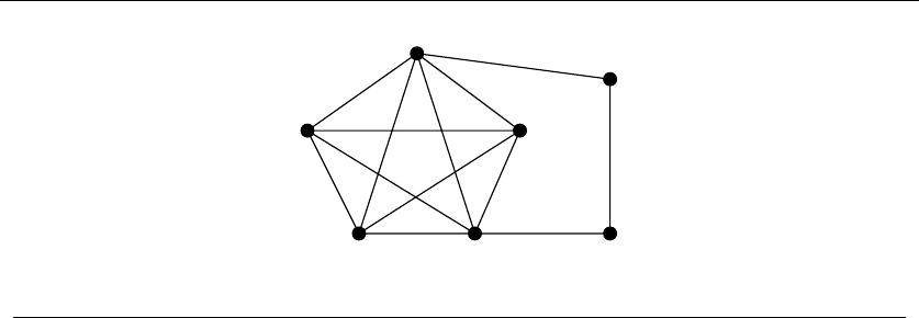
328 9. INTRACTABLE PROBLEMS AND APPROXIMATION ALGORITHMS
Figure 9.6: A small graph with a five-vertex clique
The graph in Figure 9.6 contains a clique of five vertices. Within the friendship
graph, we would expect to see large cliques corresponding to workplaces, neigh-
borhoods, religious organizations, and schools. Applications of cliques are further
discussed in Section 16.1 (page 525).
In the independent set problem, we looked for a subset Swith no edges between
two vertices of S. This contrasts with clique, where we insist that there always be an
edge between two vertices. A reduction between these problems follows by reversing
the roles of edges and nonedges—an operation known as complementing the graph:
IndependentSet(G, k)
Construct a graph G=(V,E) where V=V,and
For all (i, j) not in E, add (i, j)toE
Return the answer to Clique(G,k)
These last two reductions provide a chain linking of three different problems.
The hardness of clique is implied by the hardness of independent set, which is
implied by the hardness of vertex cover. By constructing reductions in a chain,
we link together pairs of problems in implications of hardness. Our work is done
as soon as all these chains begin with a single problem that is accepted as hard.
Satisfiability is the problem that will serve as the first link in this chain.
9.4 Satisfiability
To demonstrate the hardness of all problems using reductions, we must start with
a single problem that is absolutely, certifiably, undeniably hard. The mother of all
NP-complete problems is a logic problem named satisfiability:
Problem: Satisfiability
Input: A set of Boolean variables Vand a set of clauses Cover V.
Output: Does there exist a satisfying truth assignment for C—i.e. , a way to set
the variables v1,...,v
ntrue or false so that each clause contains at least one true
literal?

9.4 SATISFIABILITY 329
This can be made clear with two examples. Suppose that C={{v1, v2},{v1,v
2}}
over the Boolean variables V={v1,v
2}.Weusevito denote the complement of
the variable vi, so we get credit for satisfying a particular clause containing viif
vi= true, or a clause containing viif vi= false. Therefore, satisfying a particular
set of clauses involves making a series of ntrue or false decisions, trying to find
the right truth assignment to satisfy all of them.
These example clauses C={{v1, v2},{v1,v
2}} can be satisfied by either setting
v1=v2=trueorv1=v2= false. However, consider the set of clauses C=
{{v1,v
2},{v1, v2},{v1}}. Here there can be no satisfying assignment, because v1
must be false to satisfy the third clause, which means that v2must be false to
satisfy the second clause, which then leaves the first clause unsatisfiable. Although
you try, and you try, and you try, and you try, you can’t get no satisfaction.
For a combination of social and technical reasons, it is well accepted that satis-
fiability is a hard problem; one for which no worst-case polynomial-time algorithm
exists. Literally every top-notch algorithm expert in the world (and countless lesser
lights) have directly or indirectly tried to come up with a fast algorithm to test
whether a given set of clauses is satisfiable. All have failed. Furthermore, many
strange and impossible-to-believe things in the field of computational complexity
have been shown to be true if there exists a fast satisfiability algorithm. Satisfia-
bility is a hard problem, and we should feel comfortable accepting this. See Section
14.10 (page 472) for more on the satisfiability problem and its applications.
9.4.1 3-Satisfiability
Satisfiability’s role as the first NP-complete problem implies that the problem is
hard to solve in the worst case. But certain special-case instances of the problem
are not necessarily so tough. Suppose that each clause contains exactly one literal.
We must appropriately set that literal to satisfy such a clause. We can repeat this
argument for every clause in the problem instance. Thus only when we have two
clauses that directly contradict each other, such as C={{v1},{v1}}, will the set
not be satisfiable.
Since clause sets with only one literal per clause are easy to satisfy, we are
interested in slightly larger classes. How many literals per clause do you need to
turn the problem from polynomial to hard? This transition occurs when each clause
contains three literals, i.e.
Problem: 3-Satisfiability (3-SAT)
Input: A collection of clauses Cwhere each clause contains exactly 3 literals, over
a set of Boolean variables V.
Output: Is there a truth assignment to Vsuch that each clause is satisfied?
Since this is a restricted case of satisfiability, the hardness of 3-SAT implies
that satisfiability is hard. The converse isn’t true, since the hardness of general
satisfiability might depend upon having long clauses. We can show the hardness

330 9. INTRACTABLE PROBLEMS AND APPROXIMATION ALGORITHMS
of 3-SAT using a reduction that translates every instance of satisfiability into an
instance of 3-SAT without changing whether it is satisfiable.
This reduction transforms each clause independently based on its length,by
adding new clauses and Boolean variables along the way. Suppose clause Cicon-
tained kliterals:
•k= 1, meaning that Ci={z1}– We create two new variables v1,v
2and four
new 3-literal clauses: {v1,v
2,z
1},{v1, v2,z
1},{v1,v
2,z
1},{v1, v2,z
1}. Note
that the only way that all four of these clauses can be simultaneously satisfied
is if z1= true, which also means the original Ciwill be satisfied.
•k= 2, meaning that Ci={z1,z
2}– We create one new variable v1and two
new clauses: {v1,z
1,z
2},{v1,z
1,z
2}. Again, the only way to satisfy both of
these clauses is to have at least one of z1and z2be true, thus satisfying ci.
•k= 3, meaning that Ci={z1,z
2,z
3}–WecopyCiinto the 3-SAT instance
unchanged: {z1,z
2,z
3}.
•k>3, meaning that Ci={z1,z
2, ..., zn}– We create n−3 new variables and
n−2 new clauses in a chain, where for 2 ≤j≤n−3, Ci,j ={vi,j−1,z
j+1, vi,j },
Ci,1={z1,z
2, vi,1},andCi,n−2={vi,n−3,z
n−1,z
n}.
The most complicated case here is that of the large clauses. If none of the
original literals in Ciare true, then there are not enough new variables to be able
to satisfy all of the new subclauses. You can satisfy Ci,1by setting vi,1= false, but
this forces vi,2= false, and so on until finally Ci,n−2cannot be satisfied. However,
if any single literal zi= true, then we have n−3 free variables and n−3 remaining
3-clauses, so we can satisfy each of them.
This transform takes O(m+n) time if there were nclauses and mtotal literals
in the SAT instance. Since any SAT solution also satisfies the 3-SAT instance and
any 3-SAT solution describes how to set the variables giving a SAT solution, the
transformed problem is equivalent to the original.
Note that a slight modification to this construction would serve to prove that
4-SAT, 5-SAT, or any (k≥3)-SAT is also NP-complete. However, this construction
breaks down if we try to use it for 2-SAT, since there is no way to stuff anything
into the chain of clauses. It turns out that a depth-first search on an appropriate
graph can be used to give a linear-time algorithm for 2-SAT, as discussed in Section
14.10 (page 472).
9.5 Creative Reductions
Since both satisfiability and 3-SAT are known to be hard, we can use either of
them in reductions. Usually 3-SAT is the better choice, because it is simpler to
work with. What follows are a pair of more complicated reductions, designed to
serve as examples and also increase our repertoire of known hard problems. Many

9.5 CREATIVE REDUCTIONS 331
reductions are quite intricate, because we are essentially programming one problem
in the language of a significantly different problem.
One perpetual point of confusion is getting the direction of the reduction right.
Recall that we must transform every instance of a known NP-complete problem
into an instance of the problem we are interested in. If we perform the reduction
the other way, all we get is a slow way to solve the problem of interest, by using
a subroutine that takes exponential time. This always is confusing at first, for this
direction of reduction seems backwards. Make sure you understand the direction
of reduction now, and think back to this whenever you get confused.
9.5.1 Integer Programming
As discussed in Section 13.6 (page 411), integer programming is a fundamental
combinatorial optimization problem. It is best thought of as linear programming
with the variables restricted to take only integer (instead of real) values.
Problem: Integer Programming
Input: A set of integer variables V, a set of inequalities over V, a maximization
function f(V), and an integer B.
Output: Does there exist an assignment of integers to Vsuch that all inequalities
aretrueandf(V)≥B?
Consider the following two examples. Suppose
v1≥1,v
2≥0
v1+v2≤3
f(v):2v2,B=3
A solution to this would be v1=1,v2= 2. Not all problems have realizable
solutions, however. For the following problem:
v1≥1,v
2≥0
v1+v2≤3
f(v):2v2,B=5
The maximum possible value of f(v) given the constraints is 2 ×2 = 4, so there
can be no solution to the associated decision problem.
We show that integer programming is hard using a reduction from 3-SAT. For
this particular reduction, general satisfiability would work just as well, although
usually 3-SAT makes reductions easier.
In which direction must the reduction go? We want to prove integer program-
ming is hard, and know that 3-SAT is hard. If I could solve 3-SAT using integer

332 9. INTRACTABLE PROBLEMS AND APPROXIMATION ALGORITHMS
programming and integer programming were easy, this would mean that satisfia-
bility would be easy. Now the direction should be clear; we must translate 3-SAT
into integer programming.
What should the translation look like? Every satisfiability instance contains
Boolean (true/false) variables and clauses. Every integer programming instance
contains integer variables (values restricted to 0,1,2,. . . ) and constraints. A reason-
able idea is to make the integer variables correspond to Boolean variables and use
constraints to serve the same role as the clauses do in the original problem.
Our translated integer programming problem will have twice as many variables
as the SAT instance—one for each variable and one for its complement. For each
variable viin the set problem, we will add the following constraints:
•We restrict each integer programming variable Vito values of either 0 or 1,
but adding constraints 1 ≥Vi≥0 and 1 ≥Vi≥0. Thus coupled with
integrality, they correspond to values of true and false.
•We ensure that exactly one of the two integer programming variables as-
sociated with a given SAT variable is true, by adding constraints so that
1≥Vi+Vi≥1.
For each 3-SAT clause Ci={z1,z
2,z
3}, construct a constraint: V1+V2+V3≥1.
To satisfy this constraint, at least one of the literals per clause must be set to 1, thus
corresponding to a true literal. Satisfying this constraint is therefore equivalent to
satisfying the clause.
The maximization function and bound prove relatively unimportant, since we
have already encoded the entire 3-SAT instance. By using f(v)=V1and B=0,we
ensure that they will not interfere with any variable assignment satisfying all the
inequalities. Clearly, this reduction can be done in polynomial time. To establish
that this reduction preserves the answer, we must verify two things:
•Any SAT solution gives a solution to the IP problem – In any SAT solution,
a true literal corresponds to a 1 in the integer program, since the clause is
satisfied. Therefore, the sum in each clause inequality is ≥1.
•Any IP solution gives a solution to the original SAT problem – All variables
must be set to either 0 or 1 in any solution to this integer programming
instance. If Vi= 1, then set literal zi= true. If Vi= 0, then set literal
zi= false. This is a legal assignment which must also satisfy all the clauses.
The reduction works both ways, so integer programming must be hard. Notice
the following properties, which hold true in general for NP-completeness proofs:
1. This reduction preserved the structure of the problem. It did not solve the
problem, just put it into a different format.

9.5 CREATIVE REDUCTIONS 333
v1 v1 v2 v2 v3 v3 v4 v4
v1
v3
v4 v1 v4
v2
Figure 9.7: Reducing satisfiability instance {{v1,¯v3,¯v4},{¯v1,v
2,¯v4}} to vertex cover
2. The possible IP instances that can result from this transformation are only
a small subset of all possible IP instances. However, since some of them are
hard, the general problem must be hard.
3. The transformation captures the essence of why IP is hard. It has nothing to
do with having big coefficients or big ranges of variables, because restricting
them to 0/1 is enough. It has nothing to do with having inequalities with
large numbers of variables. Integer programming is hard because satisfying
a set of constraints is hard. A careful study of the properties needed for a
reduction can tell us a lot about the problem.
9.5.2 Vertex Cover
Algorithmic graph theory proves to be a fertile ground for hard problems. The pro-
totypical NP-complete graph problem is vertex cover, previously defined in Section
9.3.2 (page 325) as follows:
Problem: Vertex Cover
Input: AgraphG=(V, E) and integer k≤|V|.
Output: Is there a subset Sof at most kvertices such that every e∈Ehas at least
one vertex in S?
Demonstrating the hardness of vertex cover proves more difficult than the pre-
vious reductions we have seen, because the structure of the two relevant problems
is very different. A reduction from 3-satisfiability to vertex cover has to construct
agraphGand bound kfrom the variables and clauses of the satisfiability instance.
First, we translate the variables of the 3-SAT problem. For each Boolean vari-
able vi, we create two vertices viand ¯viconnected by an edge. At least nvertices
will be needed to cover all these edges, since no two of the edges will share a vertex.
Second, we translate the clauses of the 3-SAT problem. For each of the cclauses,
we create three new vertices, one for each literal in each clause. The three vertices
of each clause will be connected so as to form ctriangles. At least two vertices per

334 9. INTRACTABLE PROBLEMS AND APPROXIMATION ALGORITHMS
triangle must be included in any vertex cover of these triangles, for a total of 2c
cover vertices.
Finally, we will connect these two sets of components together. Each literal in
the vertex “gadgets” is connected to vertices in the clause gadgets (triangles) that
share the same literal. From a 3-SAT instance with nvariables and cclauses, this
constructs a graph with 2n+3cvertices. The complete reduction for the 3-SAT
problem {{v1,¯v3,¯v4},{¯v1,v
2,¯v4}} is shown in Figure 9.7.
This graph has been designed to have a vertex cover of size n+2cif and only
if the original expression is satisfiable. By the earlier analysis, every vertex cover
must have at least n+2cvertices, since adding the connecting edges to Gcannot
shrink the size of the vertex cover to less than that of the disconnected vertex and
clause gadgets. To show that our reduction is correct, we must demonstrate that:
•Every satisfying truth assignment gives a vertex cover – Given a satisfying
truth assignment for the clauses, select the nvertices from the vertex gadgets
that correspond to true literals to be members of the vertex cover. Since this
defines a satisfying truth assignment, a true literal from each clause must
cover at least one of the three cross edges connecting each triangle vertex to
a vertex gadget. Therefore, by selecting the other two vertices of each clause
triangle, we also pick up all remaining cross edges.
•Every vertex cover gives a satisfying truth assignment – In any vertex cover
Cof size n+2c, exactly nof the vertices must belong to the vertex gadgets.
Let these first stage vertices define the truth assignment, while the remaining
2ccover vertices must be distributed at two per clause gadget. Otherwise a
clause gadget edge must go uncovered. These clause gadget vertices can cover
only two of the three connecting cross edges per clause. Therefore, if Cgives
a vertex cover, at least one cross edge per clause must be covered, meaning
that the corresponding truth assignment satisfies all clauses.
This proof of the hardness of vertex cover, chained with the clique and inde-
pendent set reductions of Section 9.3.2 (page 325), gives us a library of hard graph
problems that we can use to make future hardness proofs easier.
Take-Home Lesson: A small set of NP-complete problems (3-SAT, vertex
cover, integer partition, and Hamiltonian cycle) suffice to prove the hardness
of most other hard problems.
9.6 The Art of Proving Hardness
Proving that problems are hard is a skill. But once you get the hang of it, reductions
can be surprisingly straightforward and pleasurable to do. Indeed, the dirty little
secret of NP-completeness proofs is that they are usually easier to create than
explain, in much the same way that it can be easier to rewrite old code than
understand and modify it.

9.6 THE ART OF PROVING HARDNESS 335
It takes experience to judge whether a problem is likely to be hard. Perhaps
the quickest way to gain this experience is through careful study of the catalog.
Slightly changing the wording of a problem can make the difference between it
being polynomial or NP-complete. Finding the shortest path in a graph is easy,
while finding the longest path in a graph is hard. Constructing a tour that visits
all the edges once in a graph is easy (Eulerian cycle), while constructing a tour
that visits all the vertices once is hard (Hamiltonian cycle).
The first thing to do when you suspect a problem might be NP-complete is look
in Garey and Johnson’s book Computers and Intractability [GJ79], which contains
a list of several hundred problems known to be NP-complete. Likely you will find
the problem you are interested in.
Otherwise I offer the following advice to those seeking to prove the hardness of
a given problem:
•Make your source problem as simple (i.e. , restricted) as possible.
Never try to use the general traveling salesman problem (TSP) as a source
problem. Better, use Hamiltonian cycle (i.e. , TSP) where all the weights are
1or∞. Even better, use Hamiltonian path instead of cycle, so you don’t
have to worry about closing up the cycle. Best of all, use Hamiltonian path
on directed planar graphs where each vertex has total degree 3. All of these
problems are equally hard, but the more you can restrict the problem that
you are reducing, the less work your reduction has to do.
As another example, never try to use full satisfiability to prove hardness. Start
with 3-satisfiability. In fact, you don’t even have to use full 3-satisfiability.
Instead, you can use planar 3-satisfiability, where there exists a way to draw
the clauses as a graph in the plane such that you can connect all instances of
the same literal together without edges crossing. This property tends to be
useful in proving the hardness of geometric problems. All these problems are
equally hard, and hence NP-completeness reductions using any of them are
equally convincing.
•Make your target problem as hard as possible.
Don’t be afraid to add extra constraints or freedoms to make your target
problem more general. Perhaps your undirected graph problem can be gener-
alized into a directed graph problem and can hence be easier to prove hard.
Once you have a proof of hardness for the general problem, you can then go
back and try to simplify the target.
•Select the right source problem for the right reason.
Selecting the right source problem makes a big difference in how difficult it
is to prove a problem hard. This is the first and easiest place to go wrong,
although theoretically any NP-complete problem works as well as any other.
When trying to prove that a problem is hard, some people fish around through

336 9. INTRACTABLE PROBLEMS AND APPROXIMATION ALGORITHMS
lists of dozens of problems, looking for the best fit. These people are amateurs;
odds are they never will recognize the problem they are looking for when they
see it.
I use four (and only four) problems as candidates for my hard source problem.
Limiting them to four means that I can know a lot about each of these
problems, such as which variants of the problems are hard and which are
not. My favorite source problems are:
–3-SAT: The old reliable. When none of the three problems below seem
appropriate, I go back to the original source.
–Integer partition: This is the one and only choice for problems whose
hardness seems to require using large numbers.
–Vertex cover: This is the answer for any graph problem whose hardness
depends upon selection. Chromatic number, clique, and independent set
all involve trying to select the correct subset of vertices or edges.
–Hamiltonian path: This is my choice for any graph problem whose hard-
ness depends upon ordering. If you are trying to route or schedule some-
thing, Hamiltonian path is likely your lever into the problem.
•Amplify the penalties for making the undesired selection.
Many people are too timid in their thinking about hardness proofs. You are
trying to translate one problem into another, while keeping the problems as
close to their original identities as as possible. The easiest way to do this is to
be bold with your penalties; to punish anyone for trying to deviate from your
intended solution. Your thinking should be, “if you select this element, then
you must pick up this huge set that prevents you from finding an optimal
solution.” The sharper the consequences for doing what is undesired, the
easier it is to prove the equivalence of the problems.
•Think strategically at a high level, then build gadgets to enforce tactics.
You should be asking yourself the following types of questions: “How can I
force that A or B is chosen but not both?” “How can I force that A is taken
before B?” “How can I clean up the things I did not select?” Once you have
an idea of what you want your gadgets to do, you can worry about how to
actually craft them.
•When you get stuck, alternate between looking for an algorithm or a reduction.
Sometimes the reason you cannot prove hardness is that there exists an effi-
cient algorithm to solve your problem! Techniques such as dynamic program-
ming or reducing problems to powerful but polynomial-time graph problems,
such as matching or network flow, can yield surprising algorithms. Whenever
you can’t prove hardness, it pays to alter your opinion occasionally to keep
yourself honest.

9.7 WAR STORY: HARD AGAINST THE CLOCK 337
9.7 War Story: Hard Against the Clock
My class’s attention span was running down like sand through an hourglass. Eyes
were starting to glaze, even in the front row. Breathing had become soft and regular
in the middle of the room. Heads were tilted back and eyes shut in the back.
There were twenty minutes left to go in my lecture on NP-completeness, and
I couldn’t really blame them. They had already seen several reductions like the
ones presented here. But NP-completeness reductions are easier to create than to
understand or explain. They had to watch one being created to appreciate how
things worked.
I reached for my trusty copy of Garey and Johnson’s book [GJ79], which con-
tains a list of over four hundred different known NP-complete problems in an
appendix in the back.
“Enough of this!” I announced loudly enough to startle those in the back row.
“NP-completeness proofs are sufficiently routine that we can construct them on
demand. I need a volunteer with a finger. Can anyone help me?”
A few students in the front held up their hands. A few students in the back
held up their fingers. I opted for one from the front row.
“Select a problem at random from the back of this book. I can prove the hard-
ness of any of these problems in the now seventeen minutes remaining in this class.
Stick your finger in and read me a problem.”
I had definitely gotten their attention. But I could have done that by offering to
juggle chain-saws. Now I had to deliver results without cutting myself into ribbons.
The student picked out a problem. “OK, prove that Inequivalence of Programs
with Assignments is hard,” she said.
“Huh? I’ve never heard of that problem before. What is it? Read me the entire
description of the problem so I can write it on the board.” The problem was as
follows:
Problem: Inequivalence of Programs with Assignments
Input: A finite set Xof variables, two programs P1and P2, each a sequence of
assignments of the form
x0←if (x1=x2) then x3else x4
where the xiare in X;andavaluesetV.
Output: Is there an initial assignment of a value from Vto each variable in Xsuch
that the two programs yield different final values for some variable in X?
I looked at my watch. Fifteen minutes to go. But now everything was on the
table. I was faced with a language problem. The input was two programs with
variables, and I had to test to see whether they always do the same thing.
“First things first. We need to select a source problem for our reduction. Do we
start with integer partition? 3-satisfiability? Vertex cover or Hamiltonian path?”
Since I had an audience, I tried thinking out loud. “Our target is not a graph
problem or a numerical problem, so let’s start thinking about the old reliable: 3-

338 9. INTRACTABLE PROBLEMS AND APPROXIMATION ALGORITHMS
satisfiability. There seem to be some similarities. 3-SAT has variables. This thing
has variables. To be more like 3-SAT, we could try limiting the variables in this
problem so they only take on two values—i.e. , V={true,false}. Yes. That seems
convenient.”
My watch said fourteen minutes left. “So, class, which way does the reduction
go? 3-SAT to language or language to 3-SAT?”
The front row correctly murmured, “3-SAT to language.”
“Right. So we have to translate our set of clauses into two programs. How
can we do that? We can try to split the clauses into two sets and write separate
programs for each of them. But how do we split them? I don’t see any natural way
do it, because eliminating any single clause from the problem might suddenly make
an unsatisfiable formula satisfiable, thus completely changing the answer. Instead,
let’s try something else. We can translate all the clauses into one program, and
then make the second program be trivial. For example, the second program might
ignore the input and always output either only true or only false. This sounds
better. Much better.”
I was still talking out loud to myself, which wasn’t that unusual. But I had
people listening to me, which was.
“Now, how can we turn a set of clauses into a program? We want to know
whether the set of clauses can be satisfied, or if there is an assignment of the
variables such that it is true. Suppose we constructed a program to evaluate whether
c1=(x1, x2,x
3) is satisfied.”
It took me a few minutes worth of scratching before I found the right program
to simulate a clause. I assumed that I had access to constants for true and false:
c1=if(x1= true) then true else false
c1=if(x2= false) then true else c1
c1=if(x3= true) then true else c1
“Great. Now I have a way to evaluate the truth of each clause. I can do the
same thing to evaluate whether all the clauses are satisfied.”
sat =if(c1= true) then true else false
sat =if(c2= true) then sat else false
.
.
.
sat =if(cn= true) then sat else false
Now the back of the classroom was getting excited. They were starting to see
a ray of hope that they would get to leave on time. There were two minutes left in
class.
“Great. So now we have a program that can evaluate to be true if and only
if there is a way to assign the variables to satisfy the set of clauses. We need a
second program to finish the job. What about sat = false? Yes, that is all we need.
Our language problem asks whether the two programs always output the same

9.8 WAR STORY: AND THEN I FAILED 339
thing, regardless of the possible variable assignments. If the clauses are satisfiable,
that means that there must be an assignment of the variables such that the long
program would output true. Testing whether the programs are equivalent is exactly
the same as asking if the clauses are satisfiable.”
I lifted my arms in triumph. “And so, the problem is neat, sweet, and NP-
complete.” I got the last word out just before the bell rang.
9.8 War Story: And Then I Failed
This exercise of picking a random NP-complete problem from the 400+ problems
in Garey and Johnson’s book and proving hardness on demand was so much fun
that I have repeated it each time I have taught the algorithms course. Sure enough,
I got it eight times in a row. But just as Joe DiMaggio’s 56-game hitting streak
came to an end, and Google will eventually have a losing quarter financially, the
time came for me to get my comeuppance.
The class had voted to see a reduction from the graph theory section of the
catalog, and a randomly selected student picked number 30. Problem GT30 turned
outtobe:
Problem: Uniconnected Subgraph
Input: Directed graph G=(V,A), positive integer k≤|A|.
Output: Is there a subset of arcs A∈Awith |A|≥ksuch that G=(V,A)has
at most one directed path between any pair of vertices?
“It is a selection problem,” I realized as soon as the problem was revealed. After
all, we had to select the largest possible subset of arcs so that there were no pair
of vertices with multiple paths between them. This meant that vertex cover was
the problem of choice.
I worked through how the two problems stacked up. Both sought subsets, al-
though vertex cover wanted subsets of vertices and uniconnected subgraph wanted
subsets of edges. Vertex cover wanted the smallest possible subset, while unidirected
subgraph wanted the largest possible subset. My source problem had undirected
edges while my target had directed arcs, so somehow I would have to add edge
direction into the reduction.
I had to do something to direct the edges of the vertex cover graph. I could try
to replace each undirected edge (x, y) with a single arc, say from yto x. But quite
different directed graphs would result depending upon which direction I selected.
Finding the “right” orientation of edges might be a hard problem, certainly too
hard to use in the translation phase of the reduction.
I realized I could direct the edges so the resulting graph was a DAG. But then,
so what? DAGs certainly can have many different directed paths between pairs of
vertices.
Alternately, I could try to replace each undirected edge (x, y) with two arcs,
from xto yand yto x. Now there was no need to chose the right arcs for my

340 9. INTRACTABLE PROBLEMS AND APPROXIMATION ALGORITHMS
reduction, but the graph certainly got complicated. I couldn’t see how to force
things to prevent vertex pairs from having unwanted multiple paths between them.
Meanwhile, the clock was running and I knew it. A sense of panic set in during
the last ten minutes of the class, and I realized I wasn’t going to get it this time.
There is no feeling worse for a professor than botching up a lecture. You stand
up there flailing away, knowing (1) that the students don’t understand what you
are saying, but (2) they do understand that you also don’t understand what you are
saying. The bell rang and the students left the room with faces either sympathetic
or smirking.
I promised them a solution for the next class, but somehow I kept getting stuck
in the same place each time I thought about it. I even tried to cheat and look
up the proof in a journal. But the reference that Garey and Johnson cited was a
30-year old unpublished technical report. It wasn’t on the web or in our library.
I dreaded the idea of returning to give my next class, the last lecture of the
semester. But the night before class the answer came to me in a dream. “Split the
edges,” the voice said. I awoke with a start and looked at the clock. It was 3:00
AM.
I sat up in bed and scratched out the proof. Suppose I replace each undirected
edge (x, y) with a gadget consisting of a new central vertex vxy with arcs going
from it to xand y, respectively. This is nice. Now, which vertices are capable of
having multiple paths between them? The new vertices had only outgoing edges,
so they can only serve as the source of multiple paths. The old vertices had only
incoming edges. There was at most one way to get from one of the new source
vertices to any of the original vertices of the vertex cover graph, so these could not
result in multiple paths.
But now add a sink node swith edges from all original vertices. There were
exactly two paths from each new source vertex to this sink—one through each of
the two original vertices it was adjacent to. One of these had to be broken to create
a uniconnected subgraph. How could we break it? We could pick one of these two
vertices to disconnect from the sink by deleting either arc (x, s)or(y, s) for new
vertex vxy. We maximize the size of our subgraph by finding the smallest number
of arcs to delete. We must delete the outgoing arc from at least one of the two
vertices defining each original edge. This is exactly the same as finding the vertex
cover in this graph! The reduction is illustrated in Figure 9.8.
Presenting this proof in class provided some personal vindication, but more to
the point validates the principles I teach for proving hardness. Observe that the
reduction really wasn’t all that difficult after all: just split the edges and add a sink
node. NP-completeness reductions are often surprisingly simple once you look at
them the right way.

9.9 P VS. NP 341
1
2
4
3
6
5
s
1
2
4
3
6
5
Figure 9.8: Reducing vertex cover to unidirected subgraph, by dividing edges and adding a
sink node
9.9 P vs. NP
The theory of NP-completeness rests on a foundation of rigorous but subtle defi-
nitions from automata and formal language theory. This terminology is typically
confusing to or misused by beginners who lack a mastery of these foundations.
It is not really essential to the practical aspects of designing and applying reduc-
tions. That said, the question “Is P=NP?” is the most profound open problem in
computer science, so any educated algorist should have some idea what the stakes
are.
9.9.1 Verification vs. Discovery
The primary question in P vs NP is whether verification is really an easier task
than initial discovery. Suppose that while taking an exam you “happen” to notice
the answer of the student next to you. Are you now better off? You wouldn’t dare
to turn it in without checking, since an able student such as yourself could answer
the question correctly if you took enough time to solve it. The issue is whether you
can really verify the answer faster than you could find it from scratch.
For the NP-complete decision problems we have studied here, the answer seems
obvious:
•Can you verify that a graph has a TSP tour of at most kweight given the
order of vertices on the tour? Sure. Just add up the weights of the edges on
the tour and show it is at most k. That is easier than finding the tour, isn’t
it?
•Can you verify that a given truth assignment represents a solution to a given
satisfiability problem? Sure. Just check each clause and make sure it contains

342 9. INTRACTABLE PROBLEMS AND APPROXIMATION ALGORITHMS
at least one true literal from the given truth assignment. That is easier than
finding the satisfying assignment, isn’t it?
•Can you verify that a graph Ghas a vertex cover of at most kvertices if given
the subset Sof at most kvertices forming such a cover? Sure. Just traverse
each edge (u, v)ofG, and check that either uor vis in S. That is easier than
finding the vertex cover, isn’t it?
At first glance, this seems obvious. The given solutions can be verified in linear
time for all three of these problems, while no algorithm faster than brute force
search is known to find the solutions for any of them. The catch is that we have no
rigorous lower bound proof that prevents the existence of fast algorithms to solve
these problems. Perhaps there are in fact polynomial algorithms (say O(n7)) that
we have just been too blind to see yet.
9.9.2 The Classes P and NP
Every well-defined algorithmic problem must have an asymptotically fastest-
possible algorithm solving it, as measured in the Big-Oh, worst-case sense of fastest.
We can think of the class Pas an exclusive club for algorithmic problems that
a problem can only join after demonstrating that there exists a polynomial-time
algorithm to solve it. Shortest path, minimum spanning tree, and the original movie
scheduling problem are all members in good standing of this class P.ThePstands
for polynomial-time.
A less-exclusive club welcomes all the algorithmic problems whose solutions can
be verified in polynomial-time. As shown above, this club contains traveling sales-
man, satisfiability, and vertex cover, none of which currently have the credentials
to join P. However, all the members of Pget a free pass into this less exclusive
club. If you can solve the problem from scratch in polynomial time, you certainly
can verify a solution that fast: just solve it from scratch and see if the solution you
get is as good as the one you were given.
We call this less-exclusive club NP. You can think of this as standing for not-
necessarily polynomial-time.1
The $1,000,000 question is whether there are in fact problems in NP that cannot
be members of P. If no such problem exists, the classes must be the same and
P=NP. If even one such a problem exists, the two classes are different and
P=NP. The opinion of most algorists and complexity theorists is that the classes
differ, meaning P=NP, but a much stronger proof than “I can’t find a fast enough
algorithm” is needed.
1In fact, it stands for nondeterministic polynomial-time. This is in the sense of nondeterministic automata,
if you happen to know about such things.

9.9 P VS. NP 343
9.9.3 Why is Satisfiability the Mother of All Hard Problems?
An enormous tree of NP-completeness reductions has been established that entirely
rests on the hardness of satisfiability. The portion of this tree demonstrated and/or
stated in this chapter (and proven elsewhere) is shown in Figure 9.2.
This may look like a delicate affair. What would it mean if someone does find
a polynomial-time algorithm for satisfiability? A fast algorithms for any given NP-
complete problem (say traveling salesman) implies fast algorithm for all the prob-
lems on the path in the reduction tree between TSP and satisfiability (Hamiltonian
cycle, vertex cover, and 3-SAT). But a fast algorithm for satisfiability doesn’t im-
mediately yield us anything because the reduction path from SAT to SAT is empty.
Fear not. There exists an extraordinary super-reduction (called Cook’s theorem)
reducing all the problems in NP to satisfiability. Thus, if you prove that satisfiability
(or equivalently any single NP-complete problem) is in P, then all other problems
in NP follow and P=NP. Since essentially every problem mentioned in this book
is in NP, this would be an enormously powerful and surprising result.
Cook’s theorem proves that satisfiability is as hard as any problem in NP.
Furthermore, it proves that every NP-complete problem is as hard as any other. Any
domino falling (i.e. , a polynomial-time algorithm for any NP-complete problem)
knocks them all down. Our inability to find a fast algorithm for any of these
problems is a strong reason for believing that they are all truly hard, and probably
P=NP.
9.9.4 NP-hard vs. NP-complete?
The final technicality we will discuss is the difference between a problem being
NP-hard and NP-complete. I tend to be somewhat loose with my terminology, but
there is a subtle (usually irrelevant) distinction between the two concepts.
We say that a problem is NP-hard if, like satisfiability, it is at least as hard
as any problem in NP. We say that a problem is NP-complete if it is NP-hard,
and also in NP itself. Because NP is such a large class of problems, most NP-hard
problems you encounter will actually be complete, and the issue can always be
settled by giving a (usually simple) verification strategy for the problem. All the
NP-hard problems we have encountered in this book are also NP-complete.
That said, there are problems that appear to be NP-hard yet not in NP. These
problems might be even harder than NP-complete! Two-player games such as chess
provide examples of problems that are not in NP. Imagine sitting down to play chess
with some know-it-all, who is playing white. He pushes his central pawn up two
squares to start the game, and announces checkmate. The only obvious way to show
he is right would be to construct the full tree of all your possible moves with his
irrefutable replies and demonstrate that you, in fact, cannot win from the current
position. This full tree will have a number of nodes exponential in its height, which
is the number of moves before you lose playing your most spirited possible defense.

344 9. INTRACTABLE PROBLEMS AND APPROXIMATION ALGORITHMS
Clearly this tree cannot be constructed and analyzed in polynomial time, so the
problem is not in NP.
9.10 Dealing with NP-complete Problems
For the practical person, demonstrating that a problem is NP-complete is never
the end of the line. Presumably, there was a reason why you wanted to solve it
in the first place. That application will not go away when told that there is no
polynomial-time algorithm. You still seek a program that solves the problem of
interest. All you know is that you won’t find one that quickly solves the problem
to optimality in the worst case. You still have three options:
•Algorithms fast in the average case – Examples of such algorithms include
backtracking algorithms with substantial pruning.
•Heuristics – Heuristic methods like simulated annealing or greedy approaches
can be used to quickly find a solution with no guarantee that it will be the
best one.
•Approximation algorithms – The theory of NP-completeness only stipulates
that it is hard to get close to the answer. With clever, problem-specific heuris-
tics, we can probably get close to the optimal answer on all possible instances.
Approximation algorithms return solutions with a guarantee attached, namely
that the optimal solution can never be much better than this given solution. Thus
you can never go too far wrong when using an approximation algorithm. No matter
what your input instance is and how lucky you are, you are doomed to do all right.
Furthermore, approximation algorithms realizing probably good bounds are often
conceptually simple, very fast, and easy to program.
One thing that is usually not clear, however, is how well the solution from an
approximation algorithm compares to what you might get from a heuristic that
gives you no guarantees. The answer could be worse or it could be better. Leaving
your money in a bank savings account guarantees you 3% interest without risk.
Still, you likely will do much better investing your money in stocks than leaving it
in the bank, even though performance is not guaranteed.
One way to get the best of approximation algorithms and heuristics is to run
both of them on the given problem instance and pick the solution giving the better
result. This way, you get a solution that comes with a guarantee and a second
chance to do even better. When it comes to heuristics for hard problems, sometimes
you can have it both ways.

9.10 DEALING WITH NP-COMPLETE PROBLEMS 345
Figure 9.9: Neglecting to pick the center vertex leads to a terrible vertex cover
9.10.1 Approximating Vertex Cover
As we have seen before, finding the minimum vertex cover of a graph is NP-
complete. However, a very simple procedure can efficiently find a cover that is
at most twice as large as the optimal cover:
VertexCover(G=(V,E))
While (E=∅)do:
Select an arbitrary edge (u, v)≤E
Add both uand vto the vertex cover
Delete all edges from Ethat are incident to either uor v.
It should be apparent that this procedure always produces a vertex cover, since
each edge is only deleted after an incident vertex has been added to the cover.
More interesting is the claim that any vertex cover must use at least half as many
vertices as this one. Why? Consider only the ≤n/2 edges selected by the algorithm
that constitute a matching in the graph. No two of these edges can share a vertex.
Therefore, any cover of just these edges must include at least one vertex per edge,
which makes it at least half the size of this greedy cover.
There are several interesting things to notice about this algorithm:
•Although the procedure is simple, it is not stupid – Many seemingly smarter
heuristics can give a far worse performance in the worst case. For example,
why not modify the above procedure to select only one of the two vertices
for the cover instead of both. After all, the selected edge will be equally
well covered by only one vertex. However, consider the star-shaped graph of
Figure 9.9. This heuristic will produce a two-vertex cover, while the single-
vertex heuristic can return a cover as large as n−1 vertices, should we get
unlucky and repeatedly select the leaf instead of the center as the cover vertex
we retain.
•Greedy isn’t always the answer – Perhaps the most natural heuristic for vertex
cover would repeatedly select and delete the vertex of highest remaining
degree for the vertex cover. After all, this vertex will cover the largest number
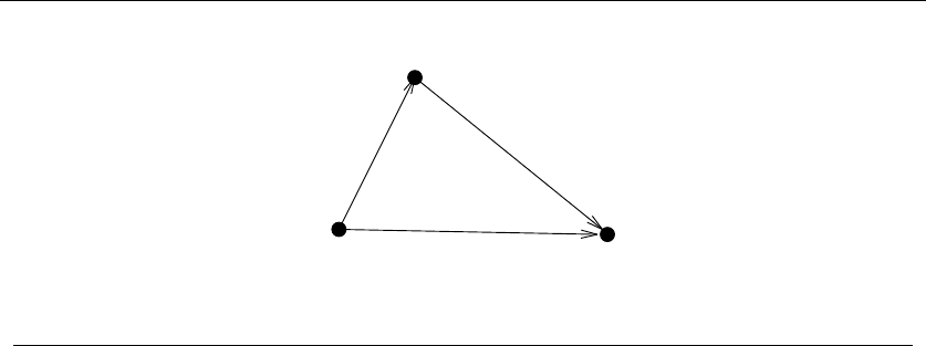
346 9. INTRACTABLE PROBLEMS AND APPROXIMATION ALGORITHMS
u
v
w
Figure 9.10: The triangle inequality (d(u, w)≤d(u, v)+d(v, w)) typically holds in geometric
and weighted graph problems
of possible edges. However, in the case of ties or near ties, this heuristic can
go seriously astray. In the worst case, it can yield a cover that is Θ(lg n) times
optimal.
•Making a heuristic more complicated does not necessarily make it better –It
is easy to complicate heuristics by adding more special cases or details. For
example, the procedure above does not specify which edge should be selected
next. It might seem reasonable to next select the edge whose endpoints have
the highest degree. However, this does not improve the worst-case bound and
just makes it more difficult to analyze.
•A postprocessing cleanup step can’t hurt – The flip side of designing sim-
ple heuristics is that they can often be modified to yield better-in-practice
solutions without weakening the approximation bound. For example, a post-
processing step that deletes any unnecessary vertex from the cover can only
improve things in practice, even though it won’t help the worst-case bound.
The important property of approximation algorithms is relating the size of the
solution produced directly to a lower bound on the optimal solution. Instead of
thinking about how well we might do, we must think about the worst case—i.e. ,
how badly we might perform.
9.10.2 The Euclidean Traveling Salesman
In most natural applications of the traveling salesman problem, direct routes are
inherently shorter than indirect routes. For example, if a graph’s edge weights were
the straight-line distances between pairs of cities, the shortest path from xto y
will always be “as the crow flies.”
The edge weights induced by Euclidean geometry satisfy the triangle inequality,
namely that d(u, w)≤d(u, v)+d(v, w) for all triples of vertices u,v,andw.The
general reasonableness of this condition is demonstrated in Figure 9.10. The cost
of airfare is an example of a distance function that violates the triangle inequality,
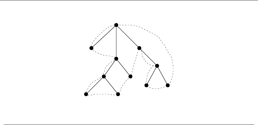
9.10 DEALING WITH NP-COMPLETE PROBLEMS 347
1
234
7
11
10
6
98
5
Figure 9.11: A depth-first traversal of a spanning tree, with the shortcut tour
since it is sometimes cheaper to fly through an intermediate city than to fly to the
destination directly. TSP remains hard when the distances are Euclidean distances
in the plane.
We can approximate the optimal traveling salesman tour using minimum span-
ning trees or graphs that obey the triangle inequality. First, observe that the weight
of a minimum spanning tree is a lower bound on the cost of the optimal tour. Why?
Deleting any edge from a tour leaves a path, the total weight of which must be no
greater than that of the original tour. This path has no cycles, and hence is a tree,
which means its weight is at least that of the minimum spanning tree. Thus the
weight of the minimum spanning tree gives a lower bound on the optimal tour.
Consider now what happens in performing a depth-first traversal of a spanning
tree. We will visit each edge twice, once going down the tree when discovering
the edge and once going up after exploring the entire subtree. For example, in the
depth-first search of Figure 9.11, we visit the vertices in order 1 −2−1−3−5−
8−5−9−5−3−6−3−1−4−7−10 −7−11 −7−4−1, thus using every
tree edge exactly twice. This tour repeats each edge of the minimum spanning tree
twice, and hence costs at most twice the optimal tour.
However, vertices will be repeated on this depth-first search tour. To remove the
extra vertices, we can take a shortest path to the next unvisited vertex at each step.
The shortcut tour for the tree above is 1 −2−3−5−8−9−6−4−7−10 −11 −1.
Because we have replaced a chain of edges by a single direct edge, the triangle
inequality ensures that the tour can only get shorter. Thus, this shortcut tour is also
within weight and twice that of optimal. Better, more complicated approximation
algorithms for Euclidean TSP exist, as described in Section 16.4 (page 533). No
approximation algorithms are known for TSPs that do not satisfy the triangle
inequality.

348 9. INTRACTABLE PROBLEMS AND APPROXIMATION ALGORITHMS
9.10.3 Maximum Acyclic Subgraph
Directed acyclic graphs (DAGs) are easier to work with than general digraphs.
Sometimes it is useful to simplify a given graph by deleting a small set of edges or
vertices that suffice to break all cycles. Such feedback set problems are discussed in
Section 16.11 (page 559).
Here we consider an interesting problem in this class where seek to retain as
many edges as possible while breaking all directed cycles:
Problem: Maximum Directed Acyclic Subgraph
Input: A directed graph G=(V,E).
Output: Find the largest possible subset E∈Esuch that G=(V,E) is acyclic.
In fact, there is a very simple algorithm that guarantees you a solution with at
least half as many edges as optimum. I encourage you to try to find it now before
peeking.
Construct any permutation of the vertices, and interpret it as a left-right or-
dering akin to topological sorting. Now some of the edges will point from left to
right, while the remainder point from right to left.
One of these two edge subsets must be at least as large as the other. This means
it contains at least half the edges. Furthermore each of these two edge subsets must
be acyclic for the same reason only DAGs can be topologically sorted—you cannot
form a cycle by repeatedly moving in one direction. Thus, the larger edge subset
must be acyclic and contain at least half the edges of the optimal solution!
This approximation algorithm is simple to the point of almost being stupid.
But note that heuristics can make it perform better in practice without losing this
guarantee. Perhaps we can try many random permutations, and pick the best. Or
we can try to exchange pairs of vertices in the permutations retaining those swaps,
which throw more edges onto the bigger side.
9.10.4 Set Cover
The previous sections may encourage a false belief that every problem can be
approximated to within a factor of two. Indeed, several catalog problems such as
maximum clique cannot be approximated to any interesting factor.
Set cover occupies a middle ground between these extremes, having a factor-
Θ(lg n) approximation algorithm. Set cover is a more general version of the vertex
cover problem. As defined in Section 18.1 (page 621),
Problem: Set Cover
Input: A collection of subsets S={S1,...,S
m}of the universal set U={1,...,n}.
Output: What is the smallest subset Tof Swhose union equals the universal set—
i.e. , ∪|T|
i=1Ti=U?
9.10 DEALING WITH NP-COMPLETE PROBLEMS 349
milestone class 6 5 4 3 2 1 0
uncovered elements 64 51 40 30 25 22 19 16 13 10 7 4 2 1
selected subset size 13 11 10 533333332 1 1
Figure 9.12: The coverage process for greedy on a particular instance of set cover
The natural heuristic is greedy. Repeatedly select the subset that covers the
largest collection of thus-far uncovered elements until everything is covered. In
pseudocode,
SetCover(S)
While (U=∅)do:
Identify the subset Siwith the largest intersection with U
Select Sifor the set cover
U=U−Si
One consequence of this selection process is that the number of freshly-covered
elements defines a nonincreasing sequence as the algorithm proceeds. Why? If not,
greedy would have picked the more powerful subset earlier if it, in fact, existed.
Thus we can view this heuristic as reducing the number of uncovered elements
from ndown to zero by progressively smaller amounts. A trace of such an execution
is shown in Figure 9.12.
An important milestone in such a trace occurs each time the number of remain-
ing uncovered elements reduces past a power of two. Clearly there can be at most
lg nsuch events.
Let widenote the number of subsets that were selected by the heuristic to
cover elements between milestones 2i+1 −1 and 2i. Define the width wto be the
maximum wi, where 0 ≤i≤lg2n. In the example of Figure 9.12, the maximum
width is given by the five subsets needed to go from 25−1downto2
4.
Since there are at most lg nsuch milestones, the solution produced by the
greedy heuristic must contain at most w·lg nsubsets. But I claim that the optimal
solution must contain at least wsubsets, so the heuristic solution is no worse than
lg ntimes optimal.
Why? Consider the average number of new elements covered as we move be-
tween milestones 2i+1 −1 and 2i. These 2ielements require wisubsets, so the
average coverage is μi=2
i/wi. More to the point, the last/smallest of these sub-
sets covers at most μisubsets. Thus, no subset exists in Sthat can cover more than
μiof the remaining 2ielements. So, to finish the job, we need at least 2i/μi=wi
subsets.
The somewhat surprising thing is that there do exist set cover instances where
this heuristic takes Ω(lg n) times optimal. The logarithmic factor is a property of
the problem/heuristic, not an artifact of weak analysis.

350 9. INTRACTABLE PROBLEMS AND APPROXIMATION ALGORITHMS
Take-Home Lesson: Approximation algorithms guarantee answers that are
always close to the optimal solution. They can provide a practical approach to
dealing with NP-complete problems.
Chapter Notes
The notion of NP-completeness was first developed by Cook [Coo71]. Satis-
fiability really is a $1,000,000 problem, and the Clay Mathematical Institute
has offered such a prize to any person who resolves the P=NP question. See
http://www.claymath.org/ for more on the problem and the prize.
Karp [Kar72] showed the importance of Cook’s result by providing reductions
from satisfiability to more than 20 important algorithmic problems. I recommend
Karp’s paper for its sheer beauty and economy—he reduces each reduction to three
line descriptions showing the problem equivalence. Together, these provided the
tools to resolve the complexity of literally hundreds of important problems where
no efficient algorithms were known.
The best introduction to the theory of NP-completeness remains Garey and
Johnson’s book Computers and Intractability. It introduces the general theory,
including an accessible proof of Cook’s theorem [Coo71] that satisfiability is as
hard as anything in NP. They also provide an essential reference catalog of more
than 300 NP-complete problems, which is a great resource for learning what is
known about the most interesting hard problems. The reductions claimed, but
missing from this chapter can be found in Garey and Johnson, or textbooks such
as [CLRS01].
A few catalog problems exist in a limbo state where it is not known whether
the problem has a fast algorithm or is NP-complete. The most prominent of these
are graph isomorphism (see Section 16.9 (page 550)) and integer factorization (see
Section 13.8 (page 420)). That this limbo list is so short is quite a tribute to the
state of the art in algorithm design and the power of NP-completeness. For almost
every important problem we either have a fast algorithm or a good solid reason for
why one doesn’t exist.
The war story problem on unidirected subgraph was originally proven hard in
[Mah76].
9.11 Exercises
Transformations and Satisfiability
9-1. [2] Give the 3-SAT formula that results from applying the reduction of SAT to
3-SAT for the formula:
(x+y+z+w+u+v)·(x+y+z+w+u+v)·(x+y+z+w+u+v)·(x+y)

9.11 EXERCISES 351
9-2. [3] Draw the graph that results from the reduction of 3-SAT to vertex cover for
the expression
(x+y+z)·(x+y+z)·(x+y+z)·(x+y+x)
9-3. [4] Suppose we are given a subroutine which can solve the traveling salesman
decision problem of page 318 in, say, linear time. Give an efficient algorithm to find
the actual TSP tour by making a polynomial number of calls to this subroutine.
9-4. [7] Implement a translator that translates satisfiability instances into equivalent
3-SAT instances.
9-5. [7] Design and implement a backtracking algorithm to test whether a set of formulae
are satisfiable. What criteria can you use to prune this search?
9-6. [8] Implement the vertex cover to satisfiability reduction, and run the resulting
clauses through a satisfiability testing code. Does this seem like a practical way to
compute things?
Basic Reductions
9-7. [4] An instance of the set cover problem consists of a set Xof nelements, a family
Fof subsets of X, and an integer k. The question is, does there exist ksubsets
from Fwhose union is X?
For example, if X={1,2,3,4}and F={{1,2},{2,3},{4},{2,4}}, there does not
exist a solution for k= 2, but there does for k= 3 (for example, {1,2},{2,3},{4}).
Prove that set cover is NP-complete with a reduction from vertex cover.
9-8. [4] The baseball card collector problem is as follows. Given packets P1,...,P
m, each
of which contains a subset of this year’s baseball cards, is it possible to collect all
the year’s cards by buying ≤kpackets?
For example, if the players are {Aaron, Mays, Ruth, Skiena}and the packets are
{{Aaron, M ays},{Mays,Ruth},{Skiena},{Mays, Skiena}},
there does not exist a solution for k= 2, but there does for k= 3, such as
{Aaron, Mays},{Mays,Ruth},{Skiena}
Prove that the baseball card collector problem is NP-hard using a reduction from
vertex cover.
9-9. [4] The low-degree spanning tree problem is as follows. Given a graph Gand an
integer k,doesGcontain a spanning tree such that all vertices in the tree have
degree at most k(obviously, only tree edges count towards the degree)? For example,
in the following graph, there is no spanning tree such that all vertices have a degree
less than three.
(a) Prove that the low-degree spanning tree problem is NP-hard with a reduction
from Hamiltonian path.
(b) Now consider the high-degree spanning tree problem, which is as follows. Given
agraphGand an integer k,doesGcontain a spanning tree whose highest
degree vertex is at least k? In the previous example, there exists a spanning
tree with a highest degree of 8. Give an efficient algorithm to solve the high-
degree spanning tree problem, and an analysis of its time complexity.

352 9. INTRACTABLE PROBLEMS AND APPROXIMATION ALGORITHMS
9-10. [4] Show that the following problem is NP-complete:
Problem: Dense subgraph
Input: AgraphG,andintegerskand y.
Output: Does Gcontain a subgraph with exactly kvertices and at least yedges?
9-11. [4] Show that the following problem is NP-complete:
Problem: Clique, no-clique
Input: An undirected graph G=(V, E) and an integer k.
Output: Does Gcontain both a clique of size kand an independent set of size k.
9-12. [5] An Eulerian cycle is a tour that visits every edge in a graph exactly once.
An Eulerian subgraph is a subset of the edges and vertices of a graph that has an
Eulerian cycle. Prove that the problem of finding the number of edges in the largest
Eulerian subgraph of a graph is NP-hard. (Hint: the Hamiltonian circuit problem
is NP-hard even if each vertex in the graph is incident upon exactly three edges.)
Creative Reductions
9-13. [5] Prove that the following problem is NP-complete:
Problem: Hitting Set
Input: A collection Cof subsets of a set S, positive integer k.
Output: Does Scontain a subset Ssuch that |S|≤kand each subset in Ccontains
at least one element from S?
9-14. [5] Prove that the following problem is NP-complete:
Problem: Knapsack
Input: AsetSof nitems, such that the ith item has value viand weight wi.Two
positive integers: weight limit Wand value requirement V.
Output: Does there exist a subset S∈Ssuch that i∈Swi≤Wand i∈Svi≥
V? (Hint: start from integer partition.)
9-15. [5] Prove that the following problem is NP-complete:
Problem: Hamiltonian Path
Input: AgraphG,andverticessand t.

9.11 EXERCISES 353
Output: Does Gcontainapathwhichstartsfroms, ends at t, and visits all vertices
without visiting any vertex more than once? (Hint: start from Hamiltonian cycle.)
9-16. [5] Prove that the following problem is NP-complete:
Problem: Longest Path
Input: AgraphGand positive integer k.
Output: Does Gcontain a path that visits at least kdifferent vertices without
visiting any vertex more than once?
9-17. [6] Prove that the following problem is NP-complete:
Problem: Dominating Set
Input: AgraphG=(V, E) and positive integer k.
Output: Is there a subset V∈Vsuch that |V|≤kwhere for each vertex x∈V
either x∈Vor there exists an edge (x, y), where y∈V.
9-18. [7] Prove that the vertex cover problem (does there exist a subset Sof kvertices
in a graph Gsuch that every edge in Gis incident upon at least one vertex in S?)
remains NP-complete even when all the vertices in the graph are restricted to have
even degrees.
9-19. [7] Prove that the following problem is NP-complete:
Problem: Set Packing
Input: A collection Cof subsets of a set S, positive integer k.
Output: Does Scontain at least kdisjoint subsets (i.e. , such that none of these
subsets have any elements in common?)
9-20. [7] Prove that the following problem is NP-complete:
Problem: Feedback Vertex Set
Input: AdirectedgraphG=(V,A) and positive integer k.
Output: Is there a subset V∈Vsuch that |V|≤k, such that deleting the vertices
of Vfrom Gleaves a DAG?
Algorithms for Special Cases
9-21. [5] A Hamiltonian path Pis a path that visits each vertex exactly once. The problem
of testing whether a graph Gcontains a Hamiltonian path is NP-complete. There
does not have to be an edge in Gfrom the ending vertex to the starting vertex of
P, unlike in the Hamiltonian cycle problem.
Give an O(n+m)-time algorithm to test whether a directed acyclic graph G(a
DAG) contains a Hamiltonian path. (Hint: think about topological sorting and
DFS.)
9-22. [8] The 2-SAT problem is, given a Boolean formula in 2-conjunctive normal form
(CNF), to decide whether the formula is satisfiable. 2-SAT is like 3-SAT, except

354 9. INTRACTABLE PROBLEMS AND APPROXIMATION ALGORITHMS
that each clause can have only two literals. For example, the following formula is
in 2-CNF:
(x1∨x2)∧(¯x2∨x3)∧(x1∨¯x3)
Give a polynomial-time algorithm to solve 2-SAT.
P=NP?
9-23. [4] Show that the following problems are in NP:
•Does graph Ghave a simple path (i.e. , with no vertex repeated) of length k?
•Is integer ncomposite (i.e. , not prime)?
•Does graph Ghave a vertex cover of size k?
9-24. [7] It was a long open question whether the decision problem “Is integer na com-
posite number, in other words, not prime?” can be computed in time polynomial
in the size of its input. Why doesn’t the following algorithm suffice to prove it is in
P, since it runs in O(n)time?
PrimalityTesting(n)
composite := false
for i := 2 to n−1do
if (nmod i)=0then
composite := true
Approximation Algorithms
9-25. [4] In the maximum-satisfiability problem, we seek a truth assignment that satisfies
as many clauses as possible. Give an heuristic that always satisfies at least half as
many clauses as the optimal solution.
9-26. [5] Consider the following heuristic for vertex cover. Construct a DFS tree of the
graph, and delete all the leaves from this tree. What remains must be a vertex cover
of the graph. Prove that the size of this cover is at most twice as large as optimal.
9-27. [5] The maximum cut problem for a graph G=(V, E) seeks to partition the vertices
Vinto disjoint sets Aand Bso as to maximize the number of edges (a, b)∈Esuch
that a∈Aand b∈B. Consider the following heuristic for max cut. First assign
v1to Aand v2to B. For each remaining vertex, assign it to the side that adds the
most edges to the cut. Prove that this cut is at least half as large as the optimal
cut.
9-28. [5] In the bin-packing problem, we are given nitems with weights w1,w
2, ..., wn,
respectively. Our goal is to find the smallest number of bins that will hold the n
objects, where each bin has capacity of at most one kilogram.
The first-fit heuristic considers the objects in the order in which they are given. For
each object, place it into first bin that has room for it. If no such bin exists, start a
new bin. Prove that this heuristic uses at most twice as many bins as the optimal
solution.
9-29. [5] For the first-fit heuristic described just above, give an example where the
packing it fits uses at least 5/3 times as many bins as optimal.

9.11 EXERCISES 355
9-30. [5] Avertex coloring of graph G=(V, E)isanassignmentofcolorstovertices
of Vsuch that each edge (x, y)impliesthatverticesxand yare assigned different
colors. Give an algorithm for vertex coloring Gusing at most Δ + 1 colors, where
Δ is the maximum vertex degree of G.
Programming Challenges
These programming challenge problems with robot judging are available at
http://www.programming-challenges.com or http://online-judge.uva.es.
Geometry
9-1. “The Monocycle” – Programming Challenges 111202, UVA Judge 10047.
9-2. “Dog and Gopher” – Programming Challenges 10310, UVA Judge 111301.
9-3. “Chocolate Chip Cookies” – Programming Challenges 111304, UVA Judge 10136.
9-4. “Birthday Cake” – Programming Challenges 111305, UVA Judge 10167.
Computational Geometry
9-5. “Closest Pair Problem” – Programming Challenges 111402, UVA Judge 10245.
9-6. “Chainsaw Massacre” – Programming Challenges 111403, UVA Judge 10043.
9-7. “Hotter Colder” – Programming Challenges 111404, UVA Judge 10084.
9-8. “Useless Tile Packers” – Programming Challenges 111405, UVA Judge 10065.
Note: These are not particularly relevant to NP-completeness, but are added
for completeness.

10
How to Design Algorithms
Designing the right algorithm for a given application is a major creative act—that
of taking a problem and pulling a solution out of the ether. The space of choices
you can make in algorithm design is enormous, leaving you plenty of freedom to
hang yourself.
This book is designed to make you a better algorithm designer. The techniques
presented in Part I of this book provide the basic ideas underlying all combinatorial
algorithms. The problem catalog of Part II will help you with modeling your ap-
plication, and tell you what is known about the relevant problems. However, being
a successful algorithm designer requires more than book knowledge. It requires a
certain attitude—the right problem-solving approach. It is difficult to teach this
mindset in a book, yet getting it is essential to becoming a successful designer.
The key to algorithm design (or any other problem-solving task) is to proceed
by asking yourself questions to guide your thought process. What if we do this?
What if we do that? Should you get stuck on the problem, the best thing to do is
move onto the next question. In any group brainstorming session, the most useful
person in the room is the one who keeps asking, “Why can’t we do it this way?”
not the person who later tells them why, because she will eventually stumble on
an approach that can’t be shot down.
Towards this end, we provide a sequence of questions to guide your search for
the right algorithm for your problem. To use it effectively, you must not only ask
the questions, but answer them. The key is working through the answers carefully
by writing them down in a log. The correct answer to “Can I do it this way?” is
never “no,” but “no, because. . . .” By clearly articulating your reasoning as to why
something doesn’t work, you can check whether you have glossed over a possibility
that you didn’t want to think hard enough about. It is amazing how often the reason
S.S. Skiena, The Algorithm Design Manual, 2nd ed., DOI: 10.1007/978-1-84800-070-4 10,
c
Springer-Verlag London Limited 2008

10. HOW TO DESIGN ALGORITHMS 357
you can’t find a convincing explanation for something is because your conclusion
is wrong.
The distinction between strategy and tactics is important to keep aware of
during any design process. Strategy represents the quest for the big picture—the
framework around which we construct our path to the goal. Tactics are used to win
the minor battles we must fight along the way. In problem-solving, it is important
to check repeatedly whether you are thinking on the right level. If you do not have
a global strategy of how you are going to attack your problem, it is pointless to
worry about the tactics. An example of a strategic question is “Can I model my
application as a graph algorithm problem?” A tactical question might be, “Should
I use an adjacency list or adjacency matrix data structure to represent my graph?”
Of course, such tactical decisions are critical to the ultimate quality of the solution,
but they can be properly evaluated only in light of a successful strategy.
Too many people freeze up in their thinking when faced with a design problem.
After reading or hearing the problem, they sit down and realize that they don’t
know what to do next. Avoid this fate. Follow the sequence of questions provided
below and in most of the catalog problem sections. We’ll tell you what to do next!
Obviously, the more experience you have with algorithm design techniques such
as dynamic programming, graph algorithms, intractability, and data structures, the
more successful you will be at working through the list of questions. Part I of this
book has been designed to strengthen this technical background. However, it pays
to work through these questions regardless of how strong your technical skills are.
The earliest and most important questions on the list focus on obtaining a detailed
understanding of your problem and do not require specific expertise.
This list of questions was inspired by a passage in [Wol79]—a wonderful book
about the space program entitled The Right Stuff. It concerned the radio transmis-
sions from test pilots just before their planes crashed. One might have expected
that they would panic, so ground control would hear the pilot yelling Ahhhhhhh-
hhhh —, terminated only by the sound of smacking into a mountain. Instead, the
pilots ran through a list of what their possible actions could be. I’ve tried the flaps.
I’ve checked the engine. Still got two wings. I’ve reset the —. They had “the Right
Stuff.” Because of this, they sometimes managed to miss the mountain.
I hope this book and list will provide you with “the Right Stuff” to be an
algorithm designer. And I hope it prevents you from smacking into any mountains
along the way.
1. Do I really understand the problem?
(a) What exactly does the input consist of?
(b) What exactly are the desired results or output?
(c) Can I construct an input example small enough to solve by hand? What
happens when I try to solve it?
(d) How important is it to my application that I always find the optimal
answer? Can I settle for something close to the optimal answer?

358 10. HOW TO DESIGN ALGORITHMS
(e) How large is a typical instance of my problem? Will I be working on 10
items? 1,000 items? 1,000,000 items?
(f) How important is speed in my application? Must the problem be solved
within one second? One minute? One hour? One day?
(g) How much time and effort can I invest in implementation? Will I be
limited to simple algorithms that can be coded up in a day, or do I have
the freedom to experiment with a couple of approaches and see which
is best?
(h) Am I trying to solve a numerical problem? A graph algorithm prob-
lem? A geometric problem? A string problem? A set problem? Which
formulation seems easiest?
2. Can I find a simple algorithm or heuristic for my problem?
(a) Will brute force solve my problem correctly by searching through all
subsets or arrangements and picking the best one?
i. If so, why am I sure that this algorithm always gives the correct
answer?
ii. How do I measure the quality of a solution once I construct it?
iii. Does this simple, slow solution run in polynomial or exponential
time? Is my problem small enough that this brute-force solution
will suffice?
iv. Am I certain that my problem is sufficiently well defined to actually
have a correct solution?
(b) Can I solve my problem by repeatedly trying some simple rule, like
picking the biggest item first? The smallest item first? A random item
first?
i. If so, on what types of inputs does this heuristic work well? Do these
correspond to the data that might arise in my application?
ii. On what types of inputs does this heuristic work badly? If no such
examples can be found, can I show that it always works well?
iii. How fast does my heuristic come up with an answer? Does it have
a simple implementation?
3. Is my problem in the catalog of algorithmic problems in the back of this
book?
(a) What is known about the problem? Is there an implementation available
that I can use?
(b) Did I look in the right place for my problem? Did I browse through all
pictures? Did I look in the index under all possible keywords?

10. HOW TO DESIGN ALGORITHMS 359
(c) Are there relevant resources available on the World Wide Web? Did I do
a Google web and Google Scholar search? Did I go to the page associated
with this book, http://www.cs.sunysb.edu/∼algorith?
4. Are there special cases of the problem that I know how to solve?
(a) Can I solve the problem efficiently when I ignore some of the input
parameters?
(b) Does the problem become easier to solve when I set some of the input
parameters to trivial values, such as 0 or 1?
(c) Can I simplify the problem to the point where I can solve it efficiently?
(d) Why can’t this special-case algorithm be generalized to a wider class of
inputs?
(e) Is my problem a special case of a more general problem in the catalog?
5. Which of the standard algorithm design paradigms are most relevant to my
problem?
(a) Is there a set of items that can be sorted by size or some key? Does this
sorted order make it easier to find the answer?
(b) Is there a way to split the problem in two smaller problems, perhaps
by doing a binary search? How about partitioning the elements into big
and small, or left and right? Does this suggest a divide-and-conquer
algorithm?
(c) Do the input objects or desired solution have a natural left-to-right
order, such as characters in a string, elements of a permutation, or leaves
of a tree? Can I use dynamic programming to exploit this order?
(d) Are there certain operations being done repeatedly, such as searching, or
finding the largest/smallest element? Can I use a data structure to speed
up these queries? What about a dictionary/hash table or a heap/priority
queue?
(e) Can I use random sampling to select which object to pick next? What
about constructing many random configurations and picking the best
one? Can I use some kind of directed randomness like simulated anneal-
ing to zoom in on the best solution?
(f) Can I formulate my problem as a linear program? How about an integer
program?
(g) Does my problem seem something like satisfiability, the traveling sales-
man problem, or some other NP-complete problem? Might the problem
be NP-complete and thus not have an efficient algorithm? Is it in the
problem list in the back of Garey and Johnson [GJ79]?

360 10. HOW TO DESIGN ALGORITHMS
6. Am I still stumped?
(a) Am I willing to spend money to hire an expert to tell me what to do? If
so, check out the professional consulting services mentioned in Section
19.4 (page 664).
(b) Why don’t I go back to the beginning and work through these questions
again? Did any of my answers change during my latest trip through the
list?
Problem-solving is not a science, but part art and part skill. It is one of the
skills most worth developing. My favorite book on problem-solving remains P´olya’s
How to Solve It [P´
57], which features a catalog of problem-solving techniques that
are fascinating to browse through, both before and after you have a problem.

11
A Catalog of Algorithmic Problems
This is a catalog of algorithmic problems that arise commonly in practice. It de-
scribes what is known about them and gives suggestions about how best to proceed
if the problem arises in your application.
What is the best way to use this catalog? First, think about your problem. If
you recall the name, look up the catalog entry in the index or table of contents
and start reading. Read through the entire entry, since it contains pointers to other
relevant problems. Leaf through the catalog, looking at the pictures and problem
names to see if something strikes a chord. Don’t be afraid to use the index, for
every problem in the book is listed there under several possible keywords and
applications. If you still don’t find something relevant, your problem is either not
suitable for attack by combinatorial algorithms or else you don’t fully understand
it. In either case, go back to step one.
The catalog entries contain a variety of different types of information that have
never been collected in one place before. Different fields in each entry present
information of practical and historical interest.
To make this catalog more easily accessible, we introduce each problem with
a pair of graphics representing the problem instance or input on the left and the
result of solving the problem in this instance on the right. We have invested con-
siderable thought in creating stylized examples that illustrate desired behaviors
more than just definitions. For example, the minimum spanning tree example illus-
trates how points can be clustered using minimum spanning trees. We hope that
people will be able to flip through the pictures and identify which problems might
be relevant to them. We augment these pictures with more formal written input
and problem descriptions to eliminate the ambiguity inherent in a purely pictorial
representation.
S.S. Skiena, The Algorithm Design Manual, 2nd ed., DOI: 10.1007/978-1-84800-070-4 11,
c
Springer-Verlag London Limited 2008

364 11. A CATALOG OF ALGORITHMIC PROBLEMS
Once you have identified your problem, the discussion section tells you what
you should do about it. We describe applications where the problem is likely to
arise and the special issues associated with data from them. We discuss the kind
of results you can hope for or expect and, most importantly, what you should do
to get them. For each problem, we outline a quick-and-dirty algorithm and provide
pointers to more powerful algorithms to try next if the first attempt is not sufficient.
For each problem, we identify available software implementations that are dis-
cussed in the implementation field of each entry. Many of these routines are quite
good, and they can perhaps be plugged directly into your application. Others
maybe inadequate for production use, but they hopefully can provide a good model
for your own implementation. In general, the implementations are listed in order
of descending usefulness, but we will explicitly recommend the best one available
for each problem if a clear winner exists. More detailed information for many of
these implementations appears in Chapter 19. Essentially all of the implemen-
tations are available via the WWW site associated with this book—reachable at
http://www.cs.sunysb.edu/∼algorith.
Finally, in deliberately smaller print, we discuss the history of each problem
and present results of primarily theoretical interest. We have attempted to report
the best results known for each problem and point out empirical comparisons of
algorithms or survey articles if they exist. This should be of interest to students
and researchers, and also to practitioners for whom our recommended solutions
prove inadequate and need to know if anything better is possible.
Caveats
This is a catalog of algorithmic problems. It is not a cookbook. It cannot be because
there are too many recipes and too many possible variations on what people want
to eat. My goal is to point you in the right direction so that you can solve your own
problems. I try to identify the issues you will encounter along the way—problems
that you will have to work out for yourself. In particular:
•For each problem, I suggest algorithms and directions to attack it. These
recommendations are based on my experiences, and are aimed toward what
I see as typical applications. I felt it was more important to make concrete
recommendations for the masses rather than to try to cover all possible sit-
uations. If you don’t agree with my advice, don’t follow it, but before you
ignore me, try to understand the reasoning behind my recommendations and
articulate a reason why your application violates my assumptions.
•The implementations I recommend are not necessarily complete solutions to
your problem. I point to an implementation whenever I feel it might be more
useful to someone than just a textbook description of the algorithm. Some
programs are useful only as models for you to write your own codes. Others
are embedded in large systems and so might be too painful to extract and run

11. A CATALOG OF ALGORITHMIC PROBLEMS 365
on their own. Assume that all of them contain bugs. Many are quite serious,
so beware.
•Please respect the licensing conditions for any implementations you use com-
mercially. Many of these codes are not open source and have licence restric-
tions. See Section 19.1 for a further discussion of this issue.
•I would be interested in hearing about your experiences with my recom-
mendations, both positive and negative. I would be especially interested in
learning about any other implementations that you know about. Feel free to
drop me a line at feedback@algorist.com.

12
Data Structures
Data structures are not so much algorithms as they are the fundamental constructs
around which you build your application. Becoming fluent in what the standard
data structures can do for you is essential to get full value from them.
This puts data structures slightly out of sync with the rest of the catalog. Per-
haps the most useful aspect of it will be the pointers to various implementations
and data structure libraries. Many of these data structures are nontrivial to im-
plement well, so the programs we point to will be useful as models even if they do
not do exactly what you need. Certain fundamental data structures, like kd-trees
and suffix trees, are not as well known as they should be. Hopefully, this catalog
will serve to better publicize them.
There are a large number of books on elementary data structures available. My
favorites include:
•Sedgewick [Sed98] – This comprehensive introduction to algorithms and data
structures stands out for the clever and beautiful images of algorithms in
action. It comes in C, C++, and Java editions.
•Weiss [Wei06] – A nice text, emphasizing data structures more than algo-
rithms. Comes in Java, C, C++, and Ada editions.
•Goodrich and Tamassia [GT05] – The Java edition makes particularly good
use of the author’s Java Data Structures Library (JDSL).
The Handbook of Data Structures and Applications [MS05] provides a compre-
hensive and up-to-date survey of research in data structures. The student who took
only an elementary course in data structures is likely to be impressed and surprised
by the volume of recent work on the subject.
S.S. Skiena, The Algorithm Design Manual, 2nd ed., DOI: 10.1007/978-1-84800-070-4 12,
c
Springer-Verlag London Limited 2008
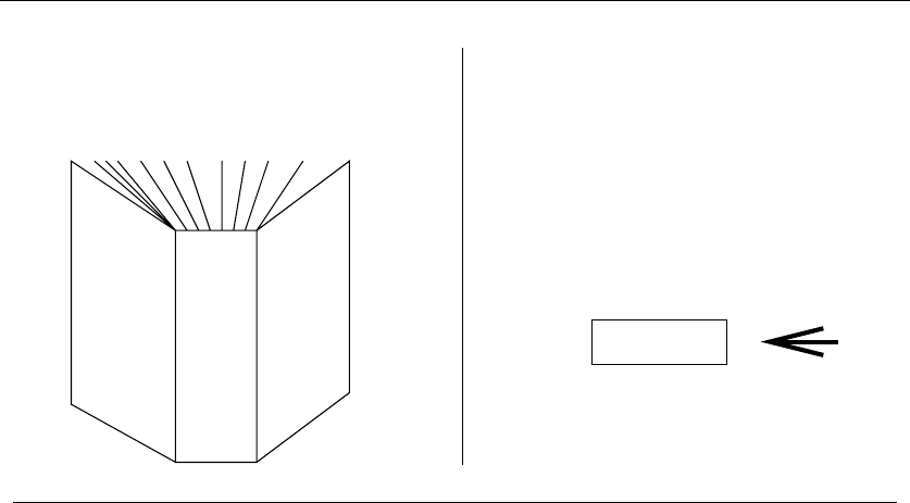
12.1 DICTIONARIES 367
Query ?
queries
quenching
quelling
quest
query
queried
.
.
.
.
.
.
.
.
INPUT OUTPUT
12.1 Dictionaries
Input description:Asetofnrecords, each identified by one or more key fields.
Problem description: Build and maintain a data structure to efficiently locate,
insert, and delete the record associated with any query key q.
Discussion: The abstract data type “dictionary” is one of the most impor-
tant structures in computer science. Dozens of data structures have been pro-
posed for implementing dictionaries, including hash tables, skip lists, and bal-
anced/unbalanced binary search trees. This means that choosing the best one can
be tricky. It can significantly impact performance. However, in practice, it is more
important to avoid using a bad data structure than to identify the single best option
available.
An essential piece of advice is to carefully isolate the implementation of the dic-
tionary data structure from its interface. Use explicit calls to methods or subrou-
tines that initialize, search, and modify the data structure, rather than embedding
them within the code. This leads to a much cleaner program, but it also makes
it easy to experiment with different implementations to see how they perform. Do
not obsess about the procedure call overhead inherent in such an abstraction. If
your application is so time-critical that such overhead can impact performance,
then it is even more essential that you be able to identify the right dictionary
implementation.

368 12. DATA STRUCTURES
In choosing the right data structure for your dictionary, ask yourself the follow-
ing questions:
•How many items will you have in your data structure? – Will you know this
number in advance? Are you looking at a problem small enough that a simple
data structure will suffice, or one so large that we must worry about running
out of memory or virtual memory performance?
•Do you know the relative frequencies of insert, delete, and search operations?
– Static data structures (like sorted arrays) suffice in applications when there
are no modifications to the data structure after it is first constructed. Semi-
dynamic data structures, which support insertion but not deletion, can have
significantly simpler implementations than fully dynamic ones.
•Can we assume that the access pattern for keys will be uniform and ran-
dom? – Search queries exhibit a skewed access distribution in many applica-
tions, meaning certain elements are much more popular than others. Further,
queries often have a sense of temporal locality, meaning elements are likely
to be repeatedly accessed in clusters instead of at fairly regular intervals.
Certain data structures (such as splay trees) can take advantage of a skewed
and clustered universe.
•Is it critical that individual operations be fast, or only that the total amount
of work done over the entire program be minimized? – When response time
is critical, such as in a program controlling a heart-lung machine, you can’t
wait too long between steps. When you have a program that is doing a lot of
queries over the database, such as identifying all criminals who happen to be
politicians, it is not as critical that you pick out any particular congressman
quickly as it is that you get them all with the minimum total effort.
An object-oriented generation has emerged as no more likely to write a container
class than fix the engine in their car. This is good; default containers should do
just fine for most applications. Still, it is good sometimes to know what you have
under the hood:
•Unsorted linked lists or arrays – For small data sets, an unsorted array is
probably the easiest data structure to maintain. Linked structures can have
terrible cache performance compared with sleek, compact arrays. However,
once your dictionary becomes larger than (say) 50 to 100 items, the linear
search time will kill you for either lists or arrays. Details of elementary dic-
tionary implementations appear in Section 3.3 (page 72).
A particularly interesting and useful variant is the self-organizing list. When-
ever a key is accessed or inserted, we always move it to head of the list. Thus,
if the key is accessed again sometime in the near future, it will be near the
front and so require only a short search to find it. Most applications exhibit

12.1 DICTIONARIES 369
both uneven access frequencies and locality of reference, so the average time
for a successful search in a self-organizing list is typically much better than
in a sorted or unsorted list. Of course, self-organizing data structures can be
built from arrays as well as linked lists and trees.
•Sorted linked lists or arrays – Maintaining a sorted linked list is usually
not worth the effort unless you are trying to eliminate duplicates, since we
cannot perform binary searches in such a data structure. A sorted array will
be appropriate if and only if there are not many insertions or deletions.
•Hash tables – For applications involving a moderate-to-large number of keys
(say between 100 and 10,000,000), a hash table is probably the right way to
go. We use a function that maps keys (be they strings, numbers, or what-
ever) to integers between 0 and m−1. We maintain an array of mbuckets,
each typically implemented using an unsorted linked list. The hash function
immediately identifies which bucket contains a given key. If we use a hash
function that spreads the keys out nicely, and a sufficiently large hash ta-
ble, each bucket should contain very few items, thus making linear searches
acceptable. Insertion and deletion from a hash table reduce to insertion and
deletion from the bucket/list. Section 3.7 (page 89) provides a more detailed
discussion of hashing and its applications.
A well-tuned hash table will outperform a sorted array in most applications.
However, several design decisions go into creating a well-tuned hash table:
–How do I deal with collisions?: Open addressing can lead to more concise
tables with better cache performance than bucketing, but performance
will be more brittle as the load factor (ratio of occupancy to capacity)
of the hash table starts to get high.
–How big should the table be?: With bucketing, mshould about the same
as the maximum number of items you expect to put in the table. With
open addressing, make it (say) 30% larger or more. Selecting mto be a
prime number minimizes the dangers of a bad hash function.
–What hash function should I use?: For strings, something like
H(S, j)=
m−1
i=0
αm−(i+1) ×char(si+j)modm
should work, where αis the size of the alphabet and char(x) is the
function that maps each character xto its ASCII character code. Use
Horner’s rule (or precompute values of αx) to implement this hash func-
tion computation efficiently, as discussed in Section 13.9 (page 423).
This hash function has the nifty property that
H(S, j +1)=(H(S, j)−αm−1char(sj))α+sj+m

370 12. DATA STRUCTURES
so hash codes of successive m-character windows of a string can be
computed in constant time instead of O(m).
Regardless of which hash function you decide to use, print statistics on the
distribution of keys per bucket to see how uniform it really is. Odds are the
first hash function you try will not prove to be the best. Botching up the
hash function is an excellent way to slow down any application.
•Binary search trees – Binary search trees are elegant data structures that
support fast insertions, deletions, and queries. They are reviewed in Section
3.4 (page 77). The big distinction between different types of trees is whether
they are explicitly rebalanced after insertion or deletion, and how this re-
balancing is done. In random search trees, we simply insert a node at the
leaf position where we can find it and no rebalancing takes place. Although
such trees perform well under random insertions, most applications are not
really random. Indeed, unbalanced search trees constructed by inserting keys
in sorted order are a disaster, performing like a linked list.
Balanced search trees use local rotation operations to restructure search trees,
moving more distant nodes closer to the root while maintaining the in-order
search structure of the tree. Among balanced search trees, AVL and 2/3 trees
are now pass´e, and red-black trees seem to be more popular. A particularly in-
teresting self-organizing data structure is the splay tree, which uses rotations
to move any accessed key to the root. Frequently used or recently accessed
nodes thus sit near the top of the tree, allowing faster searches.
Bottom line: Which tree is best for your application? Probably the one of
which you have the best implementation. The flavor of balanced tree is prob-
ably not as important as the skill of the programmer who coded it.
•B-trees – For data sets so large that they will not fit in main memory (say
more than 1,000,000 items) your best bet will be some flavor of a B-tree.
Once a data structure has to be stored outside of main memory, the search
time grows by several orders of magnitude. With modern cache architectures,
similar effects can also happen on a smaller scale, since cache is much faster
than RAM.
The idea behind a B-tree is to collapse several levels of a binary search tree
into a single large node, so that we can make the equivalent of several search
steps before another disk access is needed. With B-tree we can access enor-
mous numbers of keys using only a few disk accesses. To get the full benefit
from using a B-tree, it is important to understand how the secondary storage
device and virtual memory interact, through constants such as page size and
virtual/real address space. Cache-oblivious algorithms (described below) can
mitigate such concerns.

12.1 DICTIONARIES 371
Even for modest-sized data sets, unexpectedly poor performance of a data
structure may result from excessive swapping, so listen to your disk to help
decide whether you should be using a B-tree.
•Skip lists – These are somewhat of a cult data structure. A hierarchy of sorted
linked lists is maintained, where a coin is flipped for each element to decide
whether it gets copied into the next highest list. This implies roughly lg nlists,
each roughly half as large as the one above it. Search starts in the smallest
list. The search key lies in an interval between two elements, which is then
explored in the next larger list. Each searched interval contains an expected
constant number of elements per list, for a total expected O(lg n) query time.
The primary benefits of skip lists are ease of analysis and implementation
relative to balanced trees.
Implementations: Modern programming languages provide libraries offering
complete and efficient container implementations. The C++ Standard Template
Library (STL) is now provided with most compliers, and available with documen-
tation at http://www.sgi.com/tech/stl/. See Josuttis [Jos99], Meyers [Mey01], and
Musser [MDS01] for more detailed guides to using STL and the C++ standard
library.
LEDA (see Section 19.1.1 (page 658)) provides an extremely complete collection
of dictionary data structures in C++, including hashing, perfect hashing, B-trees,
red-black trees, random search trees, and skip lists. Experiments reported in [MN99]
identified hashing as the best dictionary choice, with skip lists and 2-4 trees (a
special case of B-trees) as the most efficient tree-like structures.
Java Collections (JC), a small library of data structures, is included in the
java.util package of Java standard edition (http://java.sun.com/javase/). The
Data Structures Library in Java (JDSL) is more comprehensive, and available for
non-commercial use at http://www.jdsl.org/. See [GTV05, GT05] for more detailed
guides to JDSL.
Notes:Knuth [Knu97a] provides the most detailed analysis and exposition on funda-
mental dictionary data structures, but misses certain modern data structures as red-black
and splay trees. Spending some time with his books is a worthwhile rite of passage for all
computer science students.
The Handbook of Data Structures and Applications [MS05] provides up-to-date surveys
on all aspects of dictionary data structures. Other surveys include Mehlhorn and Tsaka-
lidis [MT90b] and Gonnet and Baeza-Yates [GBY91]. Good textbook expositions on dic-
tionary data structures include Sedgewick [Sed98], Weiss [Wei06], and Goodrich/Tamassia
[GT05]. We defer to all these sources to avoid giving original references for each of the
data structures described above.
The 1996 DIMACS implementation challenge focused on elementary data struc-
tures, including dictionaries [GJM02]. Data sets, and codes are accessible from
http://dimacs.rutgers.edu/Challenges.
The cost of transferring data back and forth between levels of the memory hierarchy
(RAM-to-cache or disk-to-RAM) dominates the cost of actual computation for many

372 12. DATA STRUCTURES
problems. Each data transfer moves one block of size b, so efficient algorithms seek to
minimize the number of block transfers. The complexity of fundamental algorithm and
data structure problems on such an external memory model has been extensively studied
[Vit01]. Cache-oblivious data structures offer performance guarantees under such a model
without explicit knowledge of the block-size parameter b.Hence,goodperformancecan
be obtained on any machine without architecture-specific tuning. See [ABF05] for an
excellent survey on cache-oblivious data structures.
Several modern data structures, such as splay trees, have been studied using amortized
analysis, where we bound the total amount of time used by any sequence of operations.
In an amortized analysis, a single operation can be very expensive, but only because we
have already benefited from enough cheap operations to pay off the higher cost. A data
structure realizing an amortized complexity of O(f(n)) is less desirable than one whose
worst-case complexity is O(f(n)) (since a very bad operation might still occur) but better
than one with an average-case complexity O(f(n)), since the amortized bound will achieve
this average on any input.
Related Problems: Sorting (see page 436), searching (see page 441).
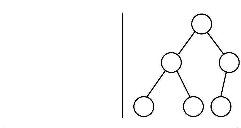
12.2 PRIORITY QUEUES 373
October 30
December 7
July 4
January 1
February 2
December 25
1/1
7/4 2/2
12/7 12/2510/30
INPUT OUTPUT
12.2 Priority Queues
Input description: A set of records with numerically or otherwise totally-ordered
keys.
Problem description: Build and maintain a data structure for providing quick
access to the smallest or largest key in the set.
Discussion: Priority queues are useful data structures in simulations, particularly
for maintaining a set of future events ordered by time. They are called “priority”
queues because they enable you to retrieve items not by the insertion time (as in
a stack or queue), nor by a key match (as in a dictionary), but by which item has
the highest priority of retrieval.
If your application will perform no insertions after the initial query, there is
no need for an explicit priority queue. Simply sort the records by priority and
proceed from top to bottom, maintaining a pointer to the last record retrieved. This
situation occurs in Kruskal’s minimum spanning tree algorithm, or when simulating
a completely scripted set of events.
However, if you are mixing insertions, deletions, and queries, you will need a
real priority queue. The following questions will help select the right one:
•What other operations do you need? – Will you be searching for arbitrary keys,
or just searching for the smallest? Will you be deleting arbitrary elements
from the data, or just repeatedly deleting the top or smallest element?

374 12. DATA STRUCTURES
•Do you know the maximum data structure size in advance? – The issue here
is whether you can preallocate space for the data structure.
•Might you change the priority of elements already in the queue? – Changing
the priority of elements implies that we must be able to retrieve elements
from the queue based on their key, in addition to being able to retrieve the
largest element.
Your choices are between the following basic priority queue implementations:
•Sorted array or list – A sorted array is very efficient to both identify the
smallest element and delete it by decrementing the top index. However, main-
taining the total order makes inserting new elements slow. Sorted arrays are
only suitable when there will be few insertions into the priority queue. Basic
priority queue implementations are reviewed in Section 3.5 (page 83).
•Binary heaps – This simple, elegant data structure supports both insertion
and extract-min in O(lg n) time each. Heaps maintain an implicit binary
tree structure in an array, such that the key of the root of any subtree is less
than that of all its descendents. Thus, the minimum key always sits at the
top of the heap. New keys can be inserted by placing them at an open leaf
and percolating the element upwards until it sits at its proper place in the
partial order. An implementation of binary heap construction and retrieval
in C appears in Section 4.3.1 (page 109)
Binary heaps are the right answer when you know an upper bound on the
number of items in your priority queue, since you must specify array size at
creation time. Even this constraint can be mitigated by using dynamic arrays
(see Section 3.1.1 (page 66)).
•Bounded height priority queue – This array-based data structure permits
constant-time insertion and find-min operations whenever the range of possi-
ble key values is limited. Suppose we know that all key values will be integers
between 1 and n.Wecansetupanarrayofnlinked lists, such that the ith
list serves as a bucket containing all items with key i. We will maintain a top
pointer to the smallest nonempty list. To insert an item with key kinto the
priority queue, add it to the kth bucket and set top = min(top, k). To extract
the minimum, report the first item from bucket top, delete it, and move top
down if the bucket has become empty.
Bounded height priority queues are very useful in maintaining the vertices of a
graph sorted by degree, which is a fundamental operation in graph algorithms.
Still, they are not as widely known as they should be. They are usually the
right priority queue for any small, discrete range of keys.
•Binary search trees – Binary search trees make effective priority queues, since
the smallest element is always the leftmost leaf, while the largest element is

12.2 PRIORITY QUEUES 375
always the rightmost leaf. The min (max) is found by simply tracing down
left (right) pointers until the next pointer is nil. Binary tree heaps prove
most appropriate when you need other dictionary operations, or if you have
an unbounded key range and do not know the maximum priority queue size
in advance.
•Fibonacci and pairing heaps – These complicated priority queues are designed
to speed up decrease-key operations, where the priority of an item already
in the priority queue is reduced. This arises, for example, in shortest path
computations when we discover a shorter route to a vertex vthan previously
established.
Properly implemented and used, they lead to better performance on very
large computations.
Implementations: Modern programming languages provide libraries offering
complete and efficient priority queue implementations. Member functions push,
top,andpop of the C++ Standard Template Library (STL) priority queue
template mirror heap operations insert,findmax,anddeletemax. STL is avail-
able with documentation at http://www.sgi.com/tech/stl/. See Meyers [Mey01] and
Musser [MDS01] for more detailed guides to using STL.
LEDA (see Section 19.1.1 (page 658)) provides a complete collection of priority
queues in C++, including Fibonacci heaps, pairing heaps, Emde-Boas trees, and
bounded height priority queues. Experiments reported in [MN99] identified simple
binary heaps as quite competitive in most applications, with pairing heaps beating
Fibonacci heaps in head-to-head tests.
The Java Collections PriorityQueue class is included in the java.util package of
Java standard edition (http://java.sun.com/javase/). The Data Structures Library
in Java (JDSL) provides an alternate implementation, and is available for non-
commercial use at http://www.jdsl.org/. See [GTV05, GT05] for more detailed
guides to JDSL.
Sanders [San00] did extensive experiments demonstrating that his sequence
heap, based on k-way merging, was roughly twice as fast as a well-implemented
binary heap. See http://www.mpi-inf.mpg.de/∼sanders/programs/spq/ for his im-
plementations in C++.
Notes:The Handbook of Data Structures and Applications [MS05] provides several up-
to-date surveys on all aspects of priority queues. Empirical comparisons between priority
queue data structures include [CGS99, GBY91, Jon86, LL96, San00].
Double-ended priority queues extend the basic heap operations to simultaneously sup-
port both find-min and find-max. See [Sah05] for a survey of four different implementations
of double-ended priority queues.
Bounded-height priority queues are useful data structures in practice, but do not
promise good worst-case performance when arbitrary insertions and deletions are permit-
ted. However, von Emde Boas priority queues [vEBKZ77] support O(lg lg n) insertion,
deletion, search, max, and min operations where each key is an element from 1 to n.

376 12. DATA STRUCTURES
Fibonacci heaps [FT87] support insert and decrease-key operations in constant amor-
tized time, with O(lg n) amortized time extract-min and delete operations. The constant-
time decrease-key operation leads to faster implementations of classical algorithms for
shortest-paths, weighted bipartite-matching, and minimum spanning tree. In practice,
Fibonacci heaps are difficult to implement and have large constant factors associated
with them. However, pairing heaps appear to realize the same bounds with less overhead.
Experiments with pairing heaps are reported in [SV87].
Heaps define a partial order that can be built using a linear number of comparisons.
The familiar linear-time merging algorithm for heap construction is due to Floyd [Flo64].
In the worst case, 1.625ncomparisons suffice [GM86] and 1.5n−O(lg n) comparisons are
necessary [CC92].
Related Problems: Dictionaries (see page 367), sorting (see page 436), shortest
path (see page 489).
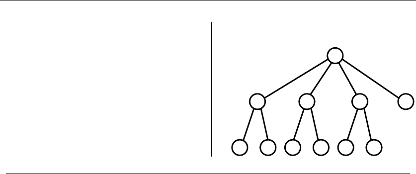
12.3 SUFFIX TREES AND ARRAYS 377
X Y Z X Y Z $
Y Z X Y Z $
Z X Y Z $
X Y Z $
Y Z $
Z $
$
XYZ
YZ Z
$
(7, 7)
7(3, 3)
$
(7, 7)
XYZ$
63 5 2 4 1
XYZ $
(2, 3)
XYZ
INPUT OUTPUT
12.3 Suffix Trees and Arrays
Input description: A reference string S.
Problem description: Build a data structure to quickly find all places where an
arbitrary query string qoccurs in S.
Discussion: Suffix trees and arrays are phenomenally useful data structures for
solving string problems elegantly and efficiently. Proper use of suffix trees often
speeds up string processing algorithms from O(n2) to linear time—likely the an-
swer. Indeed, suffix trees are the hero of the war story reported in Section 3.9 (page
94).
In its simplest instantiation, a suffix tree is simply a trie of the nsuffixes of an
n-character string S. A trie is a tree structure, where each edge represents one
character, and the root represents the null string. Thus, each path from the root
represents a string, described by the characters labeling the edges traversed. Any
finite set of words defines a trie, and two words with common prefixes branch off
from each other at the first distinguishing character. Each leaf denotes the end of
a string. Figure 12.1 illustrates a simple trie.
Tries are useful for testing whether a given query string qis in the set. We
traverse the trie from the root along branches defined by successive characters of
q. If a branch does not exist in the trie, then qcannot be in the set of strings.
Otherwise we find qin |q|character comparisons regardless of how many strings
are in the trie. Tries are very simple to build (repeatedly insert new strings) and
very fast to search, although they can be expensive in terms of memory.

378 12. DATA STRUCTURES
t
h
e
i
r
r
e
w
a
s
h
e
n
Figure 12.1: A trie on strings the, their, there, was, and when
Asuffix tree is simply a trie of all the proper suffixes of S. The suffix tree enables
you to test whether qis a substring of S, because any substring of Sis the prefix
of some suffix (got it?). The search time is again linear in the length of q.
The catch is that constructing a full suffix tree in this manner can require O(n2)
time and, even worse, O(n2) space, since the average length of the nsuffixes is n/2.
However, linear space suffices to represent a full suffix tree, if we are clever. Observe
that most of the nodes in a trie-based suffix tree occur on simple paths between
branch nodes in the tree. Each of these simple paths corresponds to a substring of
the original string. By storing the original string in an array and collapsing each
such path into a single edge, we have all the information of the full suffix tree in
only O(n) space. The label for each edge is described by the starting and ending
array indices representing the substring. The output figure for this section displays
a collapsed suffix tree in all its glory.
Even better, there exist O(n) algorithms to construct this collapsed tree, by
making clever use of pointers to minimize construction time. These additional
pointers can also be used to speed up many applications of suffix trees.
But what can you do with suffix trees? Consider the following applications. For
more details see the books by Gusfield [Gus97] or Crochemore and Rytter [CR03]:
•Find all occurrences of qas a substring of S– Just as with a trie, we can
walk from the root to the node nqassociated with q. The positions of all
occurrences of qin Sare represented by the descendents of nq, which can be
identified using a depth-first search from nq. In collapsed suffix trees, it takes
O(|q|+k) time to find the koccurrences of qin S.
•Longest substring common to a set of strings – Build a single collapsed suffix
tree containing all suffixes of all strings, with each leaf labeled with its original
string. In the course of doing a depth-first search on this tree, we can label
each node with both the length of its common prefix and the number of
distinct strings that are children of it. From this information, the best node
can be selected in linear time.

12.3 SUFFIX TREES AND ARRAYS 379
•Find the longest palindrome in S–Apalindrome is a string that reads the
same if the order of characters is reversed, such as madam. To find the longest
palindrome in a string S, build a single suffix tree containing all suffixes of
Sand the reversal of S, with each leaf identified by its starting position. A
palindrome is defined by any node in this tree that has forward and reversed
children from the same position.
Since linear time suffix tree construction algorithms are nontrivial, I recommend
using an existing implementation. Another good option is to use suffix arrays,
discussed below.
Suffix arrays do most of what suffix trees do, while using roughly four times
less memory. They are also easier to implement. A suffix array is in principle just
an array that contains all the nsuffixes of Sin sorted order. Thus a binary search
of this array for string qsuffices to locate the prefix of a suffix that matches q,
permitting an efficient substring search in O(lg n) string comparisons. With the
addition of an index specifying the common prefix length of all bounding suffixes,
only lg n+|q|character comparisons need be performed on any query, since we can
identify the next character that must be tested in the binary search. For example, if
the lower range of the search is cowabunga and the upper range is cowslip, all keys
in between must share the same first three letters, so only the fourth character
of any intermediate key must be tested against q. In practice, suffix arrays are
typically as fast or faster to search than suffix trees.
Suffix arrays use less memory than suffix trees. Each suffix is represented com-
pletely by its unique starting position (from 1 to n) and read off as needed using
a single reference copy of the input string.
Some care must be taken to construct suffix arrays efficiently, however, since
there are O(n2) characters in the strings being sorted. One solution is to first build
a suffix tree, then perform an in-order traversal of it to read the strings off in sorted
order! However, recent breakthroughs have lead to space/time efficient algorithms
for constructing suffix arrays directly.
Implementations: There now exist a wealth of suffix array implementations avail-
able. Indeed, all of the recent linear time construction algorithms have been im-
plemented and benchmarked [PST07]. Sch¨urmann and Stoye [SS07] provide an
excellent C implementation at http://bibiserv.techfak.uni-bielefeld.de/bpr/.
No less than eight different C/C++ implementations of compressed text indexes
appear at the Pizza&Chili corpus (http://pizzachili.di.unipi.it/). These data struc-
tures go to great lengths to minimize space usage, typically compressing the input
string to near the empirical entropy while still achieving excellent query times!
Suffix tree implementations are also readily available. A SuffixTree class is
provided in BioJava (ttp://www.biojava.org/)—an open source project providing
a Java framework for processing biological data. Libstree is a C implementa-
tion of Ukkonen’s algorithm, available at http://www.icir.org/christian/libstree/.

380 12. DATA STRUCTURES
Nelson’s C++ code [Nel96] is available from http://marknelson.us/1996/08/01/
suffix-trees/.
Strmat is a collection of C programs implementing exact pattern matching
algorithms in association with [Gus97], including an implementation of suffix trees.
It is available at http://www.cs.ucdavis.edu/∼gusfield/strmat.html.
Notes:Tries were first proposed by Fredkin [Fre62], the name coming from the cen-
tral letters of the word “retrieval.” A survey of basic trie data structures with extensive
references appears in [GBY91].
Efficient algorithms for suffix tree construction are due to Weiner [Wei73], McCreight
[McC76], and Ukkonen [Ukk92]. Good expositions on these algorithms include Crochmore
and Rytter [CR03] and Gusfield [Gus97].
Suffix arrays were invented by Manber and Myers [MM93], although an equivalent
idea called Pat trees due to Gonnet and Baeza-Yates appears in [GBY91]. Three teams
independently emerged with linear-time suffix array algorithms in 2003 [KSPP03, KA03,
KSB05], and progress has continued rapidly. See [PST07] for a recent survey covering all
these developments.
Recent work has resulted in the development of compressed full text indexes that offer
essentially all the power of suffix trees/arrays in a data structure whose size is proportional
to the compressed text string. Makinen and Navarro [MN07] survey these remarkable data
structures.
The power of suffix trees can be further augmented by using a data structure for
computing the least common ancestor (LCA) of any pair of nodes x, y in a tree in constant
time, after linear-time preprocessing of the tree. The original data structure due to Harel
and Tarjan [HT84], has been progressively simplified by Schieber and Vishkin [SV88] and
later Bender and Farach [BF00]. Expositions include Gusfield [Gus97]. The least common
ancestor of two nodes in a suffix tree or trie defines the node representing the longest
common prefix of the two associated strings. That we can answer such queries in constant
time is amazing, and proves useful as a building block for many other algorithms.
Related Problems: String matching (see page 628), text compression (see page
637), longest common substring (see page 650).
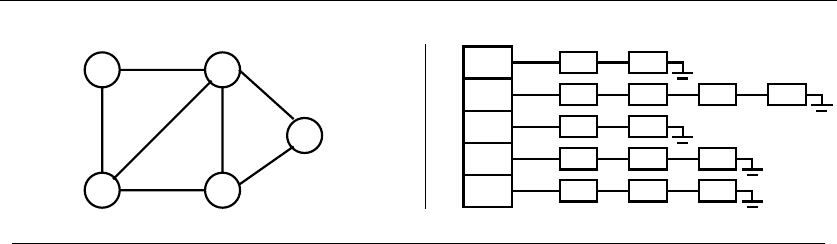
12.4 GRAPH DATA STRUCTURES 381
4
3
21
5
1
2
3
4
5
2
1345
24
35
241
2
5
INPUT OUTPUT
12.4 Graph Data Structures
Input description: A graph G.
Problem description: Represent the graph Gusing a flexible, efficient data struc-
ture.
Discussion: The two basic data structures for representing graphs are adjacency
matrices and adjacency lists. Full descriptions of these data structures appear in
Section 5.2 (page 151), along with an implementation of adjacency lists in C. In
general, for most things, adjacency lists are the way to go.
The issues in deciding which data structure to use include:
•How big will your graph be? – How many vertices will it have, both typically
and in the worse case? Ditto for the number of edges? Graphs with 1,000
vertices imply adjacency matrices with 1,000,000 entries. This seems too be
the boundary of reality. Adjacency matrices make sense only for small or very
dense graphs.
•How dense will your graph be? – If your graph is very dense, meaning that a
large fraction of the vertex pairs define edges, there is probably no compelling
reason to use adjacency lists. You will be doomed to using Θ(n2) space any-
way. Indeed, for complete graphs, matrices will be more concise due to the
elimination of pointers.
•Which algorithms will you be implementing? – Certain algorithms are more
natural on adjacency matrices (such as all-pairs shortest path) and others
favor adjacency lists (such as most DFS-based algorithms). Adjacency ma-
trices win for algorithms that repeatedly ask, “Is (i, j)inG?” However, most
graph algorithms can be designed to eliminate such queries.
•Will you be modifying the graph over the course of your application? –
Efficient static graph implementations can be used when no edge inser-
tion/deletion operations will done following initial construction. Indeed, more

382 12. DATA STRUCTURES
common than modifying the topology of the graph is modifying the attributes
of a vertex or edge of the graph, such as size, weight, label, or color. Attributes
are best handled as extra fields in the vertex or edge records of adjacency
lists.
Building a good general purpose graph type is a substantial project. For this rea-
son, we suggest that you check out existing implementations (particularly LEDA)
before hacking up your own. Note that it costs only time linear in the size of the
larger data structure to convert between adjacency matrices and adjacency lists.
This conversion is unlikely to be the bottleneck in any application, so you may de-
cide to use both data structures if you have the space to store them. This usually
isn’t necessary, but might prove simplest if you are confused about the alternatives.
Planar graphs are those that can be drawn in the plane so no two edges cross.
Graphs arising in many applications are planar by definition, such as maps of
countries. Others are planar by happenstance, like trees. Planar graphs are always
sparse, since any n-vertex planar graph can have at most 3n−6 edges. Thus they
should be represented using adjacency lists. If the planar drawing (or embedding)of
the graph is fundamental to what is being computed, planar graphs are best repre-
sented geometrically. See Section 15.12 (page 520) for algorithms for constructing
planar embeddings from graphs. Section 17.15 (page 614) discusses algorithms for
maintaining the graphs implicit in the arrangements of geometric objects like lines
and polygons.
Hypergraphs are generalized graphs where each edge may link subsets of more
than two vertices. Suppose we want to represent who is on which Congressional
committee. The vertices of our hypergraph would be the individual congressmen,
while each hyperedge would represent one committee. Such arbitrary collections of
subsets of a set are naturally thought of as hypergraphs.
Two basic data structures for hypergraphs are:
•Incidence matrices, which are analogous to adjacency matrices. They require
n×mspace, where mis the number of hyperedges. Each row corresponds to a
vertex, and each column to an edge, with a nonzero entry in M[i, j] iff vertex
iis incident to edge j. On standard graphs there are two nonzero entries
in each column. The degree of each vertex governs the number of nonzero
entries in each row.
•Bipartite incidence structures, which are analogous to adjacency lists, and
hence suited for sparse hypergraphs. There is a vertex of the incidence struc-
ture associated with each edge and vertex of the hypergraphs, and an edge
(i, j) in the incidence structure if vertex iof the hypergraph appears in edge
jof the hypergraph. Adjacency lists are typically used to represent this in-
cidence structure. Drawing the associated bipartite graph provides a natural
way to visualize the hypergraph.
Special efforts must be taken to represent very large graphs efficiently. How-
ever, interesting problems have been solved on graphs with millions of edges and

12.4 GRAPH DATA STRUCTURES 383
vertices. The first step is to make your data structure as lean as possible, by pack-
ing your adjacency matrix in a bit vector (see Section 12.5 (page 385)) or removing
unnecessary pointers from your adjacency list representation. For example, in a
static graph (which does not support edge insertions or deletions) each edge list
can be replaced by a packed array of vertex identifiers, thus eliminating pointers
and potentially saving half the space.
If your graph is extremely large, it may become necessary to switch to a hi-
erarchical representation, where the vertices are clustered into subgraphs that are
compressed into single vertices. Two approaches exist to construct such a hierar-
chical decomposition. The first breaks the graph into components in a natural or
application-specific way. For example, a graph of roads and cities suggests a natural
decomposition—partition the map into districts, towns, counties, and states. The
other approach runs a graph partition algorithm discussed as in Section 16.6 (page
541). If you have one, a natural decomposition will likely do a better job than some
naive heuristic for an NP-complete problem. If your graph is really unmanageably
large, you cannot afford to do a very good job of algorithmically partitioning it.
First verify that standard data structures fail on your problem before attempting
such heroic measures.
Implementations: LEDA (see Section 19.1.1 (page 658)) provides the best graph
data type currently implemented in C++. It is now a commercial product. You
should at least study the methods it provides for graph manipulation, so as to see
how the right level of abstract graph type makes implementing algorithms very
clean and easy.
The C++ Boost Graph Library [SLL02] (http://www.boost.org/libs/graph/doc)
is more readily available. Implementations of adjacency lists, matrices, and edge
lists are included, along with a reasonable library of basic graph algorithms. Its
interface and components are generic in the same sense as the C++ standard
template library (STL).
JUNG (http://jung.sourceforge.net/) is a Java graph library particularly popu-
lar in the social networks community. The Data Structures Library in Java (JDSL)
provides a comprehensive implementation with a decent algorithm library, and is
available for noncommercial use at http://www.jdsl.org/. See [GTV05, GT05] for
more detailed guides to JDSL. JGraphT (http://jgrapht.sourceforge.net/) is a more
recent development with similar functionality.
The Stanford Graphbase (see Section 19.1.8 (page 660)) provides a simple but
flexible graph data structure in CWEB, a literate version of the C language. It
is instructive to see what Knuth does and does not place in his basic data struc-
ture, although we recommend other implementations as a better basis for further
development.
My (biased) preference in C language graph types is the library from my book
Programming Challenges [SR03]. See Section 19.1.10 (page 661) for details. Simple
graph data structures in Mathematica are provided by Combinatorica [PS03], with
a library of algorithms and display routines. See Section 19.1.9 (page 661).

384 12. DATA STRUCTURES
Notes:The advantages of adjacency list data structures for graphs became apparent with
the linear-time algorithms of Hopcroft and Tarjan [HT73b, Tar72]. The basic adjacency
list and matrix data structures are presented in essentially all books on algorithms or
data structures, including [CLRS01, AHU83, Tar83]. Hypergraphs are presented in Berge
[Ber89]
The improved efficiency of static graph types was revealed by Naher and Zlotowski
[NZ02], who sped up certain LEDA graph algorithms by a factor of four by simply switch-
ing to a more compact graph structure.
An interesting question concerns minimizing the number of bits needed to represent
arbitrary graphs on nvertices, particularly if certain operations must be supported effi-
ciently. Such issues are surveyed in [vL90b].
Dynamic graph algorithms are data structures that maintain quick access to an invari-
ant (such as minimum spanning tree or connectivity) under edge insertion and deletion.
Sparsification [EGIN92] is a general approach to constructing dynamic graph algorithms.
See [ACI92, Zar02] for experimental studies on the practicality of dynamic graph algo-
rithms.
Hierarchically-defined graphs arise often in VLSI design problems, because design-
ers make extensive use of cell libraries [Len90]. Algorithms specifically for hierarchically-
defined graphs include planarity testing [Len89], connectivity [LW88], and minimum span-
ning trees [Len87a].
Related Problems: Set data structures (see page 385), graph partition (see page
541).
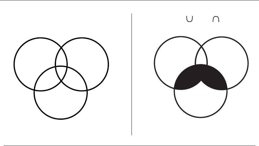
12.5 SET DATA STRUCTURES 385
XY
Z
Z(X Y)
Z
YX
INPUT OUTPUT
12.5 Set Data Structures
Input description: A universe of items U={u1,...,u
n}on which is defined a
collection of subsets S={S1,...,S
m}.
Problem description: Represent each subset so as to efficiently (1) test whether
ui∈Sj, (2) compute the union or intersection of Siand Sj, and (3) insert or delete
members of S.
Discussion: In mathematical terms, a set is an unordered collection of objects
drawn from a fixed universal set. However, it is usually useful for implementation
to represent each set in a single canonical order, typically sorted, to speed up or
simplify various operations. Sorted order turns the problem of finding the union
or intersection of two subsets into a linear-time operation—just sweep from left to
right and see what you are missing. It makes possible element searching in sublinear
time. Finally, printing the elements of a set in a canonical order paradoxically
reminds us that order really doesn’t matter.
We distinguish sets from two other kinds of objects: dictionaries and strings.
A collection of objects not drawn from a fixed-size universal set is best thought of
as a dictionary, discussed in Section 12.1 (page 367). Strings are structures where
order matters—i.e. , if {A, B, C}is not the same as {B, C,A}. Sections 12.3 and
18 discuss data structures and algorithms for strings.

386 12. DATA STRUCTURES
Multisets permit elements to have more than one occurrence. Data structures
for sets can generally be extended to multisets by maintaining a count field or
linked list of equivalent entries for each element.
If each subset contains exactly two elements, they can be thought of as edges
in a graph whose vertices represent the universal set. A system of subsets with no
restrictions on the cardinality of its members is called a hypergraph. It is worth
considering whether your problem has a graph-theoretical analogy, like connected
components or shortest path in a graph/hypergraph.
Your primary alternatives for representing arbitrary subsets are:
•Bit vectors –Ann-bit vector or array can represent any subset Son a uni-
versal set Ucontaining nitems. Bit iwill be 1 if i∈S, and 0 if not. Since
only one bit is needed per element, bit vectors can be very space efficient for
surprisingly large values of |U|. Element insertion and deletion simply flips
the appropriate bit. Intersection and union are done by “and-ing” or “or-
ing” the bits together. The only drawback of a bit vector is its performance
on sparse subsets. For example, it takes O(n) time to explicitly identify all
members of sparse (even empty) subset S.
•Containers or dictionaries – A subset can also be represented using a linked
list, array, or dictionary containing exactly the elements in the subset. No
notion of a fixed universal set is needed for such a data structure. For sparse
subsets, dictionaries can be more space and time efficient than bit vectors,
and easier to work with and program. For efficient union and intersection
operations, it pays to keep the elements in each subset sorted, so a linear-
time traversal through both subsets identifies all duplicates.
•Bloom filters – We can emulate a bit vector in the absence of a fixed universal
set by hashing each subset element to an integer from 0 to nand setting the
corresponding bit. Thus, bit H(e) will be 1 if e∈S. Collisons leave some
possibility for error under this scheme, however, because a different key might
have hashed to the same position.
Bloom filters use several (say k) different hash functions H1,...H
k, and set
all kbits Hi(e) upon insertion of key e.Noweis in Sonly if all kbits
are 1. The probability of false positives can be made arbitrarily low by in-
creasing the number of hash functions kand table size n. With the proper
constants, each subset element can be represented using a constant number
of bits independent of the size of the universal set.
This hashing-based data structure is much more space-efficient than dictio-
naries for static subset applications that can tolerate a small probability of
error. Many can. For instance, a spelling checker that left a rare random
string undetected would prove no great tragedy.
Many applications involve collections of subsets that are pairwise disjoint, mean-
ing that each element is in exactly one subset. For example, consider maintaining

12.5 SET DATA STRUCTURES 387
the connected components of a graph or the party affiliations of politicians. Each
vertex/hack is in exactly one component/party. Such a system of subsets is called
aset partition. Algorithms for generating partitions of a given set are provided in
Section 14.6 (page 456).
The primary issue with set partition data structures is maintaining changes
over time, perhaps as edges are added or party members defect. Typical queries
include “which set is a particular item in?” and “are two items in the same set?”
as we modify the set by (1) changing one item, (2) merging or unioning two sets,
or (3) breaking a set apart. Your basic options are:
•Collection of containers – Representing each subset in its own con-
tainer/dictionary permits fast access to all the elements in the subset, which
facilitates union and intersection operations. The cost comes in membership
testing, as we must search each subset data structure independently until we
find our target.
•Generalized bit vector – Let the ith element of an array denote the num-
ber/name of the subset that contains it. Set identification queries and single
element modifications can be performed in constant time. However, opera-
tions like performing the union of two subsets take time proportional to the
size of the universe, since each element in the two subsets must be identified
and (at least one subset’s worth) must have its name changed.
•Dictionary with a subset attribute – Similarly, each item in a binary tree
can be associated a field that records the name of the subset it is in. Set
identification queries and single element modifications can be performed in
the time it takes to search in the dictionary. However, union/intersection
operations are again slow. The need to perform such union operations quickly
provides the motivation for the . . .
•Union-find data structure – We represent a subset using a rooted tree where
each node points to its parent instead of its children. The name of each subset
will be the name of the item at the root. Finding out which subset we are in
is simple, for we keep traversing up the parent pointers until we hit the root.
Unioning two subsets is also easy. Just assign the root of one of two trees
to point to the other, so now all elements have the same root and hence the
same subset name.
Implementation details have a big impact on asymptotic performance here.
Always selecting the larger (or taller) tree as the root in a merger guarantees
logarithmic height trees, as presented with our implementation in Section
6.1.3 (page 198). Retraversing the path traced on each find and explicitly
pointing all nodes on the path to the root (called path compression) reduces
the tree to almost constant height. Union find is a fast, simple data structure
that every programmer should know about. It does not support breaking up
subsets created by unions, but usually this is not an issue.

388 12. DATA STRUCTURES
Implementations: Modern programming languages provide libraries offering
complete and efficient set implementations. The C++ Standard Template Li-
brary (STL) provides set and multiset containers. Java Collections (JC) contains
HashSet and TreeSet containers and is included in the java.util package of Java
standard edition.
LEDA (see Section 19.1.1 (page 658)) provides efficient dictionary data struc-
tures, sparse arrays, and union-find data structures to maintain set partitions, all
in C++.
Implementation of union-find underlies any implementation of Kruskal’s min-
imum spanning tree algorithm. For this reason, all the graph libraries of Section
12.4 (page 381) presumably contains an implementation. Minimum spanning tree
codes are described in Section 15.3 (page 484).
The computer algebra system REDUCE (http://www.reduce-algebra.com/)con-
tains SETS, a package supporting set-theoretic operations on both explicit and im-
plicit (symbolic) sets. Other computer algebra systems may support similar func-
tionality.
Notes:Optimal algorithms for such set operations as intersection and union were pre-
sented in [Rei72]. Raman [Ram05] provides an excellent survey on data structures for set
operations on a variety of different operations. Bloom filters are ably surveyed in [BM05],
with recent experimental results presented in [PSS07].
Certain balanced tree data structures support merge/meld/link/cut operations, which
permit fast ways to union and intersect disjoint subsets. See Tarjan [Tar83] for a nice
presentation of such structures. Jacobson [Jac89] augmented the bit-vector data structure
to support select operations (where is the ith 1 bit?) efficiently in both time and space.
Galil and Italiano [GI91] survey data structures for disjoint set union. The upper
bound of O(mα(m, n)) on munion-find operations on an n-element set is due to Tarjan
[Tar75], as is a matching lower bound on a restricted model of computation [Tar79]. The
inverse Ackerman function α(m, n) grows notoriously slowly, so this performance is close
to linear. An interesting connection between the worst-case of union-find and the length
of Davenport-Schinzel sequences—a combinatorial structure that arises in computational
geometry—is established in [SA95].
The power set of a set Sis the collection of all 2|S|subsets of S. Explicit manipulation
of power sets quickly becomes intractable due to their size. Implicit representations of
power sets in symbolic form becomes necessary for nontrivial computations. See [BCGR92]
for algorithms on and computational experience with symbolic power set representations.
Related Problems: Generating subsets (see page 452), generating partitions (see
page 456), set cover (see page 621), minimum spanning tree (see page 484).
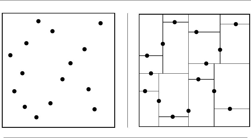
12.6 KD-TREES 389
INPUT OUTPUT
12.6 Kd-Trees
Input description:AsetSof npoints or more complicated geometric objects in
kdimensions.
Problem description: Construct a tree that partitions space by half-planes such
that each object is contained in its own box-shaped region.
Discussion: Kd-tree and related spatial data structures hierarchically decompose
space into a small number of cells, each containing a few representatives from an
input set of points. This provides a fast way to access any object by position. We
traverse down the hierarchy until we find the smallest cell containing it, and then
scan through the objects in this cell to identify the right one.
Typical algorithms construct kd-trees by partitioning point sets. Each node in
the tree is defined by a plane cutting through one of the dimensions. Ideally, this
plane equally partitions the subset of points into left/right (or up/down) subsets.
These children are again partitioned into equal halves, using planes through a
different dimension. Partitioning stops after lg nlevels, with each point in its own
leaf cell.
The cutting planes along any path from the root to another node defines a
unique box-shaped region of space. Each subsequent plane cuts this box into two
boxes. Each box-shaped region is defined by 2kplanes, where kis the number of
dimensions. Indeed, the “kd” in kd-tree is short for “k-dimensional.” We maintain

390 12. DATA STRUCTURES
the region of interest defined by the intersection of these half-spaces as we move
down the tree.
Flavors of kd-trees differ in exactly how the splitting plane is selected. Options
include:
•Cycling through the dimensions – partition first on d1, then d2,...,d
kbefore
cycling back to d1.
•Cutting along the largest dimension – select the partition dimension to make
the resulting boxes as square or cube-like as possible. Selecting a plane to
partition the points in half does not mean selecting a splitter in the middle
of the box-shaped regions, since all the points may lie in the left side of the
box.
•Quadtrees or Octtrees – Instead of partitioning with single planes, use all
axis-parallel planes that pass through a given partition point. In two dimen-
sions, this means creating four child cells; in 3D, this means eight child cells.
Quadtrees seem particularly popular on image data, where leaf cells imply
that all pixels in the regions have the same color.
•BSP-trees –Binary space partitions use general (i.e. , not just axis-parallel)
cutting planes to carve up space into cells so that each cell ends up contain-
ing only one object (say a polygon). Such partitions are not possible using
only axis-parallel cuts for certain sets of objects. The downside is that such
polyhedral cell boundaries are more complicated to work with than boxes.
•R-trees – This is another spatial data structure useful for geometric objects
that cannot be partitioned into axis-oriented boxes without cutting them
into pieces. At each level, the objects are partitioned into a small number
of (possibly-overlapping) boxes to construct searchable hierarchies without
partitioning objects.
Ideally, our partitions split both the space (ensuring fat, regular regions) and
the set of points (ensuring a log height tree) evenly, but doing both simultaneously
can be impossible on a given input. The advantages of fat cells become clear in
many applications of kd-trees:
•Point location – To identify which cell a query point qlies in, we start at
the root and test which side of the partition plane contains q. By repeating
this process on the appropriate child node, we travel down the tree to find
the leaf cell containing qin time proportional to its height. See Section 17.7
(page 587) for more on point location.
•Nearest neighbor search – To find the point in Sclosest to a query point q,we
perform point location to find the cell ccontaining q. Since cis bordered by
some point p, we can compute the distance d(p, q)frompto q. Point pis likely

12.6 KD-TREES 391
close to q, but it might not be the single closest neighbor. Why? Suppose q
lies right at the boundary of a cell. Then q’s nearest neighbor might lie just to
the left of the boundary in another cell. Thus, we must traverse all cells that
lie within a distance of d(p, q) of cell cand verify that none of them contain
closer points. In trees with nice, fat cells, very few cells should need to be
tested. See Section 17.5 (page 580) for more on nearest neighbor search.
•Range search – Which points lie within a query box or region? Starting from
the root, check whether the query region intersects (or contains) the cell
defining the current node. If it does, check the children; if not, none of the
leaf cells below this node can possibly be of interest. We quickly prune away
irrelevant portions of the space. Section 17.6 (page 584) focuses on range
search.
•Partial key search – Suppose we want to find a point pin S, but we do
not have full information about p. Say we are looking for someone of age 35
and height 5’8” but of unknown weight in a 3D-tree with dimensions of age,
weight, and height. Starting from the root, we can identify the correct de-
scendant for all but the weight dimension. To be sure we find the right point,
we must search both children of these nodes. The more fields we know the
better, but such partial key search can be substantially faster than checking
all points against the key.
Kd-trees are most useful for a small to moderate number of dimensions, say
from 2 up to maybe 20 dimensions. They lose effectiveness as the dimensional-
ity increases, primarily because the ratio of the volume of a unit sphere in k-
dimensions shrinks exponentially compared to the unit cube. Thus exponentially
many cells will have to be searched within a given radius of a query point, say for
nearest-neighbor search. Also, the number of neighbors for any cell grows to 2k
and eventually become unmanageable.
The bottom line is that you should try to avoid working in high-dimensional
spaces, perhaps by discarding (or projecting away) the least important dimensions.
Implementations:KDTREE 2 contains C++ and Fortran 95 implementations
of kd-trees for efficient nearest nearest neighbor search in many dimensions. See
http://arxiv.org/abs/physics/0408067.
Samet’s spatial index demos (http://donar.umiacs.umd.edu/quadtree/)provide
a series of Java applets illustrating many variants of kd-trees, in association with
his book [Sam06].
Terralib (http://www.terralib.org/) is an open source geographic information
system (GIS) software library written in C++. This includes an implementation
of spatial data structures.
The 1999 DIMACS implementation challenge focused on data structures
for nearest neighbor search [GJM02]. Data sets and codes are accessible from
http://dimacs.rutgers.edu/Challenges.

392 12. DATA STRUCTURES
Notes:Samet [Sam06] is the best reference on kd-trees and other spatial data structures.
All major (and many minor) variants are developed in substantial detail. A shorter survey
[Sam05] is also available. Bentley [Ben75] is generally credited with developing kd-trees,
although they have the murky history associated with most folk data structures.
The performance of spatial data structures degrades with high dimensionality. Pro-
jecting high-dimensional spaces onto a random lower-dimensional hyperplane has recently
emerged as a simple but powerful method for dimensionality reduction. Both theoretical
[IM04] and empirical [BM01] results indicate that this method preserves distances quite
nicely.
Algorithms that quickly produce a point provably close to the query point are a
recent development in higher-dimensional nearest neighbor search. A sparse weighted-
graph structure is built from the data set, and the nearest neighbor is found by starting
at a random point and walking greedily in the graph towards the query point. The closest
point found during several random trials is declared the winner. Similar data structures
hold promise for other problems in high-dimensional spaces. See [AM93, AMN+98].
Related Problems: Nearest-neighbor search (see page 580), point location (see
page 587), range search (see page 584).

13
Numerical Problems
If most problems you encounter are numerical in nature, there is an excellent
chance that you are reading the wrong book. Numerical Recipes [PFTV07] gives a
terrific overview to the fundamental problems in numerical computing, including
linear algebra, numerical integration, statistics, and differential equations. Different
flavors of the book include source code for all the algorithms in C++, Fortran, and
even Pascal. Their coverage is somewhat skimpier on the combinatorial/numerical
problems we consider in this section, but you should be aware of this book. Check
it out at http://www.nr.com.
Numerical algorithms tend to be different beasts than combinatorial algorithms
for at least two reasons:
•Issues of Precision and Error – Numerical algorithms typically perform re-
peated floating-point computations, which accumulate error at each operation
until, eventually, the results are meaningless. My favorite example [MV99]
concerns the Vancouver Stock Exchange, which over a twenty-two month pe-
riod accumulated enough round-off error to reduce its index to 574.081 from
the correct value of 1098.982.
A simple and dependable way to test for round-off errors in numerical pro-
grams is to run them both at single and double precision, and then think
hard whenever there is a disagreement.
•Extensive Libraries of Codes – Large, high-quality libraries of numerical rou-
tines have existed since the 1960s, which is still not yet the case for combina-
torial algorithms. There are several reasons for this, including (1) the early
emergence of Fortran as a standard for numerical computation, (2) the na-
ture of numerical computations to be recognizably independent rather than
S.S. Skiena, The Algorithm Design Manual, 2nd ed., DOI: 10.1007/978-1-84800-070-4 13,
c
Springer-Verlag London Limited 2008

394 13. NUMERICAL PROBLEMS
embedded within large applications, and (3) the existence of large scientific
communities needing general numerical libraries.
Regardless of why, you should exploit this software base. There is probably
no reason to implement algorithms for any of the problems in this section as
opposed to using existing codes. Searching Netlib (see Section 19.1.5) is an
excellent place to start.
Many scientist’s and engineer’s ideas about algorithms culturally derive from
Fortran programming and numerical methods. Computer scientists grow up pro-
gramming with pointers and recursion, and so are comfortable with the more so-
phisticated data structures required for combinatorial algorithms. Both sides can
and should learn from each other, since problems such as pattern recognition can
be modeled either numerically or combinatorially.
There is a vast literature on numerical algorithms. In addition to Numerical
Recipes, recommended books include:
•Chapara and Canale [CC05] – The contemporary market leader in numerical
analysis texts.
•Mak [Mak02] – This enjoyable text introduces Java to the world of numerical
computation, and visa versa. Source code is provided.
•Hamming [Ham87] – This oldie but goodie provides a clear and lucid treat-
ment of fundamental methods in numerical computation. It is available in a
low-priced Dover edition.
•Skeel and Keiper [SK00] – A readable and interesting treatment of basic
numerical methods, avoiding overly detailed algorithm descriptions through
its use of the computer algebra system Mathematica. I like it.
•Cheney and Kincaid [CK07] – A traditional Fortran-based numerical analysis
text, with discussions of optimization and Monte Carlo methods in addition
to such standard topics as root-finding, numerical integration, linear systems,
splines, and differential equations.
•Buchanan and Turner [BT92] – Thorough language-independent treatment
of all standard topics, including parallel algorithms. It is the most compre-
hensive of the texts described here.
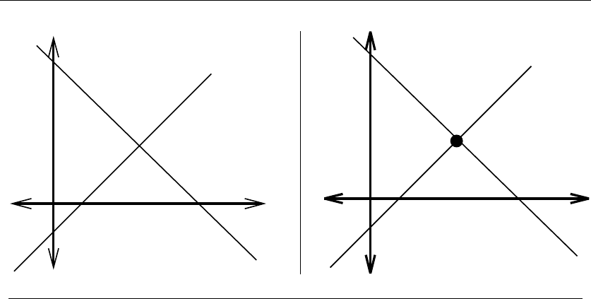
13.1 SOLVING LINEAR EQUATIONS 395
0
-1 1 2 3
y = -3x/2 + 4
1
2
3
y = x-1
0
-1 1 2 3
(2, 1)
3
2
1
INPUT OUTPUT
13.1 Solving Linear Equations
Input description:Anm×nmatrix Aand an m×1 vector b, together representing
mlinear equations on nvariables.
Problem description: What is the vector xsuch that A·x=b?
Discussion: The need to solve linear systems arises in an estimated 75% of all
scientific computing problems [DB74]. For example, applying Kirchhoff’s laws to
analyze electrical circuits generates a system of equations—the solution of which
puts currents through each branch of the circuit. Analysis of the forces acting on
a mechanical truss generates a similar set of equations. Even finding the point of
intersection between two or more lines reduces to solving a small linear system.
Not all systems of equations have solutions. Consider the equations 2x+3y=5
and 2x+3y= 6. Some systems of equations have multiple solutions, such as
2x+3y=5and4x+6y= 10. Such degenerate systems of equations are called
singular, and they can be recognized by testing whether the determinant of the
coefficient matrix is zero.
Solving linear systems is a problem of such scientific and commercial importance
that excellent codes are readily available. There is no good reason to implement
your own solver, even though the basic algorithm (Gaussian elimination) is one you
learned in high school. This is especially true when working with large systems.
Gaussian elimination is based on the observation that the solution to a system
of linear equations is invariant under scaling ( if x=y, then 2x=2y) and adding

396 13. NUMERICAL PROBLEMS
equations (the solution to x=yand w=zis the same as the solution to x=y
and x+w=y+z). Gaussian elimination scales and adds equations to eliminate
each variable from all but one equation, leaving the system in such a state that the
solution can be read off from the equations.
The time complexity of Gaussian elimination on an n×nsystem of equations is
O(n3), since to clear the ith variable we add a scaled copy of the n-term ith row to
each of the n−1 other equations. On this problem, however, constants matter. Al-
gorithms that only partially reduce the coefficient matrix and then backsubstitute
to get the answer use 50% fewer floating-point operations than the naive algorithm.
Issues to worry about include:
•Are roundoff errors and numerical stability affecting my solution? – Gaussian
elimination would be quite straightforward to implement except for round-
off errors. These accumulate with each row operation and can quickly wreak
havoc on the solution, particularly with matrices that are almost singular.
To eliminate the danger of numerical errors, it pays to substitute the solution
back into each of the original equations and test how close they are to the de-
sired value. Iterative methods for solving linear systems refine initial solutions
to obtain more accurate answers. Good linear systems packages will include
such routines.
The key to minimizing roundoff errors in Gaussian elimination is selecting
the right equations and variables to pivot on, and to scale the equations to
eliminate large coefficients. This is an art as much as a science, which is why
you should use a well-crafted library routine as described next.
•Which routine in the library should I use? – Selecting the right code is also
somewhat of an art. If you are taking your advice from this book, start with
the general linear system solvers. Hopefully they will suffice for your needs.
But search through the manual for more efficient procedures solving special
types of linear systems. If your matrix happens to be one of these special
types, the solution time can reduce from cubic to quadratic or even linear.
•Is my system sparse? – The key to recognizing that you have a special-case
linear system is establishing how many matrix elements you really need to
describe A. If there are only a few non-zero elements, your matrix is sparse
and you are in luck. If these few non-zero elements are clustered near the
diagonal, your matrix is banded and you are in even more luck. Algorithms
for reducing the bandwidth of a matrix are discussed in Section 13.2. Many
other regular patterns of sparse matrices can also be exploited, so consult the
manual of your solver or a better book on numerical analysis for details.
•Will I be solving many systems using the same coefficient matrix? – In appli-
cations such as least-squares curve fitting, we must solve A·x=brepeatedly
with different bvectors. We can preprocess Ato make this easier. The lower-
upper or LU-decomposition of Acreates lower- and upper-triangular matrices

13.1 SOLVING LINEAR EQUATIONS 397
Land Usuch that L·U=A. We can use this decomposition to solve A·x=b,
since
A·x=(L·U)·x=L·(U·x)=b
This is efficient since backsubstitution solves a triangular system of equations
in quadratic time. Solving L·y=band then U·x=ygives the solution x
using two O(n2) steps instead of one O(n3) step, after the LU-decomposition
has been found in O(n3) time.
The problem of solving linear systems is equivalent to that of matrix inversion,
since Ax =B↔A−1Ax =A−1B, where I=A−1Ais the identity matrix.
Avoid it however since matrix inversion proves to be three times slower than
Gaussian elimination. LU-decomposition proves useful in inverting matrices as well
as computing determinants (see Section 13.4 (page 404)).
Implementations: The library of choice for solving linear systems is apparently
LAPACK—a descendant of LINPACK [DMBS79]. Both of these Fortran codes, as
well as many others, are available from Netlib. See Section 19.1.5 (page 659).
Variants of LAPACK exist for other languages, like CLAPACK (C) and LA-
PACK++ (C++). The Template Numerical Toolkit is an interface to such routines
in C++, and is available at http://math.nist.gov/tnt/.
JScience provides an extensive linear algebra package (including determinants)
as part of its comprehensive scientific computing library. JAMA is another matrix
package written in Java. Links to both and many related libraries are available at
http://math.nist.gov/javanumerics/.
Numerical Recipes [PFTV07] (www.nr.com) provides guidance and routines for
solving linear systems. Lack of confidence in dealing with numerical procedures is
the most compelling reason to use these ahead of the free codes.
Notes:Golub and van Loan [GL96] is the standard reference on algorithms for linear
systems. Good expositions on algorithms for Gaussian elimination and LU-decomposition
include [CLRS01] and a host of numerical analysis texts [BT92, CK07, SK00]. Data struc-
tures for linear systems are surveyed in [PT05].
Parallel algorithms for linear systems are discussed in [Gal90, KSV97, Ort88]. Solving
linear systems is one of most important applications where parallel architectures are used
widely in practice.
Matrix inversion and (hence) linear systems solving can be done in matrix multiplica-
tion time using Strassen’s algorithm plus a reduction. Good expositions on the equivalence
of these problems include [AHU74, CLRS01].
Related Problems: Matrix multiplication (see page 401), determinant/permanent
(see page 404).
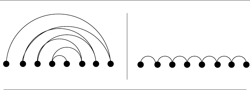
398 13. NUMERICAL PROBLEMS
1 2345678 16287345
INPUT OUTPUT
13.2 Bandwidth Reduction
Input description: A graph G=(V,E), representing an n×nmatrix Mof zero
and non-zero elements.
Problem description: Which permutation pof the vertices minimizes the length
of the longest edge when the vertices are ordered on a line—i.e. , minimizes
max(i,j)∈E|p(i)−p(j)|?
Discussion: Bandwidth reduction lurks as a hidden but important problem for
both graphs and matrices. Applied to matrices, bandwidth reduction permutes the
rows and columns of a sparse matrix to minimize the distance bof any non-zero
entry from the center diagonal. This is important in solving linear systems, because
Gaussian elimination (see Section 13.1 (page 395)) can be performed in O(nb2)on
matrices of bandwidth b. This is a big win over the general O(n3) algorithm if
b<<n.
Bandwidth minimization on graphs arises in more subtle ways. Arranging n
circuit components in a line to minimize the length of the longest wire (and hence
time delay) is a bandwidth problem, where each vertex of our graph corresponds
to a circuit component and there is an edge for every wire linking two components.
Alternatively, consider a hypertext application where we must store large objects
(say images) on a magnetic tape. Each image has a set of possible images to visit
next (i.e. , the hyperlinks). We seek to place linked images near each other on the
tape to minimize the search time. This is exactly the bandwidth problem. More
general formulations, such as rectangular circuit layouts and magnetic disks, inherit
the same hardness and classes of heuristics from the linear versions.
The bandwidth problem seeks a linear ordering of the vertices, which minimizes
the length of the longest edge, but there are several variations of the problem. In
linear arrangement, we seek to minimize the sum of the lengths of the edges. This

13.2 BANDWIDTH REDUCTION 399
has application to circuit layout, where we seek to position the chips to minimize
the total wire length. In profile minimization, we seek to minimize the sum of one-
way distances (i.e., for each vertex v) the length of the longest edge whose other
vertex is to the left of of v.
Unfortunately, bandwidth minimization and all these variants is NP-complete.
It stays NP-complete even if the input graph is a tree whose maximum vertex
degree is 3, which is about as strong a condition as I have seen on any problem.
Thus our only options are a brute-force search and heuristics.
Fortunately, ad hoc heuristics have been well studied and production-quality
implementations of the best heuristics are available. These are based on performing
a breadth-first search from a given vertex v, where vis placed at the leftmost
point of the ordering. All of the vertices that are distance 1 from vare placed
to its immediate right, followed by all the vertices at distance 2, and so forth
until all vertices in Gare accounted for. The popular heuristics differ according to
how many different start vertices are considered and how equidistant vertices are
ordered among themselves. Breaking ties with low-degree vertices over to the left
however seems to be a good idea.
Implementations of the most popular heuristics—the Cuthill-McKee and Gibbs-
Poole-Stockmeyer algorithms—are discussed in the implementation section. The
worst case of the Gibbs-Poole-Stockmeyer algorithm is O(n3), which would wash
out any possible savings in solving linear systems, but its performance in practice
is close to linear.
Brute-force search programs can find the exact minimum bandwidth by back-
tracking through the set of n! possible permutations of vertices. Considerable prun-
ing can be achieved to reduce the search space by starting with a good heuristic
bandwidth solution and alternately adding vertices to the left- and rightmost open
slots in the partial permutation.
Implementations: Del Corso and Manzini’s [CM99] code for exact solutions to
bandwidth problems is available at http://www.mfn.unipmn.it/∼manzini/bandmin.
Caprara and Salazar-Gonz´alez [CSG05] developed improved methods based on in-
teger programming. Their branch-and-bound implementation in C is available at
http://joc.pubs.informs.org/Supplements/Caprara-2/.
Fortran language implementations of both the Cuthill-McKee algorithm
[CGPS76, Gib76, CM69] and the Gibbs-Poole-Stockmeyer algorithm [Lew82,
GPS76] are available from Netlib. See Section 19.1.5 (page 659). Empirical evalu-
ations of these and other algorithms on a test suite of 30 matrices are discussed in
[Eve79b], showing Gibbs-Poole-Stockmeyer to be the consistent winner.
Petit [Pet03] performed an extensive experimental study on heuristics for
the minimum linear arrangement problem. His codes and data are available at
http://www.lsi.upc.edu/∼jpetit/MinLA/Experiments/.
Notes:Diaz et al. [DPS02] provide an excellent up-to-date survey on algorithms for
bandwidth and related graph layout problems. See [CCDG82] for graph-theoretic and
algorithmic results on bandwidth up to 1981.

400 13. NUMERICAL PROBLEMS
Ad hoc heuristics have been widely studied—a tribute to its importance in numerical
computation. Everstine [Eve79b] cites no less than 49 different bandwidth reduction al-
gorithms! Del Corso and Romani [CR01] investigate a new class of spectral heuristics for
bandwidth minimization.
The hardness of the bandwidth problem was first established by Papadimitriou
[Pap76b], and its hardness on trees of maximum degree 3 in [GGJK78]. There are al-
gorithms that run in polynomial time for fixed bandwidth k[Sax80]. Approximation
algorithms offering a polylogarithmic guarantee exist for the general problem [BKRV00].
Related Problems: Solving linear equations (see page 395), topological sorting
(see page 481).
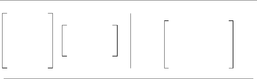
13.3 MATRIX MULTIPLICATION 401
23
34
4 5
2 3 4
3 4 5
13 18 23
18 25 32
23 32 41
INPUT OUTPUT
13.3 Matrix Multiplication
Input description:Anx×ymatrix Aand a y×zmatrix B.
Problem description: Compute the x×zmatrix A×B.
Discussion: Matrix multiplication is a fundamental problem in linear algebra. Its
main significance for combinatorial algorithms is its equivalence to many other
problems, including transitive closure/reduction, parsing, solving linear systems,
and matrix inversion. Thus, a faster algorithm for matrix multiplication implies
faster algorithms for all of these problems. Matrix multiplication arises in its own
right in computing the results of such coordinate transformations as scaling, rota-
tion, and translation for robotics and computer graphics.
The following tight algorithm computes the product of x×ymatrix Aand y×z
matrix Bruns in O(xyz). Remember to first initialize M[i, j] to 0 for all 1 ≤i≤x
and i≤j≤z:
for i=1toxdo
for j=1toz
for k=1toy
M[i, j]=M[i, j]+A[i, k]·A[k, j]
An implementation in C appears in Section 2.5.4 (page 45). This straightfor-
ward algorithm would seem to be tough to beat in practice. That said, observe
that the three loops can be arbitrarily permuted without changing the resulting
answer. Such a permutation will change the memory access patterns and thus how
effectively the cache memory is used. One can expect a 10-20% variation in run
time among the six possible implementations, but could not confidently predict
the winner (typically ikj) without running it on your machine with your given
matrices.
When multiplying bandwidth-bmatrices, where all non-zero elements of Aand
Blie within belements of the main diagonals, a speedup to O(xbz) is possible,
since zero elements cannot contribute to the product.

402 13. NUMERICAL PROBLEMS
Asymptotically faster algorithms for matrix multiplication exist, using clever
divide-and-conquer recurrences. However, these prove difficult to program, require
very large matrices to beat the trivial algorithm, and are less numerically stable to
boot. The most famous of these is Strassen’s O(n2.81) algorithm. Empirical results
(discussed next) disagree on the exact crossover point where Strassen’s algorithm
beats the simple cubic algorithm, but it is in the ballpark of n≈100.
There is a better way to save computation when you are multiplying a chain
of more than two matrices together. Recall that multiplying an x×ymatrix by a
y×zmatrix creates an x×zmatrix. Thus, multiplying a chain of matrices from
left to right might create large intermediate matrices, each taking a lot of time
to compute. Matrix multiplication is not commutative, but it is associative, so we
can parenthesize the chain in whatever manner we deem best without changing
the final product. A standard dynamic programming algorithm can be used to
construct the optimal parenthesization. Whether it pays to do this optimization
will depend upon whether your matrix dimensions are sufficiently irregular and
your chain multiplied often enough to justify it. Note that we are optimizing over
the sizes of the dimensions in the chain, not the actual matrices themselves. No
such optimization is possible if all your matrices are the same dimensions.
Matrix multiplication has a particularly interesting interpretation in counting
the number of paths between two vertices in a graph. Let Abe the adjacency matrix
of a graph G, meaning A[i, j] = 1 if there is an edge between iand j. Otherwise,
A[i, j] = 0. Now consider the square of this matrix, A2=A×A.IfA2[i, j]≥1.
This means that there must be a vertex ksuch that A[i, k]=A[k, j]=1,soito k
to jis a path of length 2 in G. More generally, Ak[i, j] counts the number of paths
of length exactly kbetween iand j. This count includes nonsimple paths, where
vertices are repeated, such as ito kto ito j.
Implementations: D’Alberto and Nicolau [DN07] have engineered a very efficient
matrix multiplication code, which switches from Strassen’s to the cubic algorithm
at the optimal point. It is available at http://www.ics.uci.edu/∼fastmm/. Earlier
experiments put the crossover point where Strassen’s algorithm beats the cubic
algorithm at about n= 128 [BLS91, CR76].
Thus, an O(n3) algorithm will likely be your best bet unless your matrices
are very large. The linear algebra library of choice is LAPACK, a descendant of
LINPACK [DMBS79], which includes several routines for matrix multiplication.
These Fortran codes are available from Netlib as discussed in Section 19.1.5 (page
659).
Algorithm 601 [McN83] of the Collected Algorithms of the ACM is a sparse ma-
trix package written in Fortran that includes routines to multiply any combination
of sparse and dense matrices. See Section 19.1.5 (page 659) for details.
Notes:Winograd’s algorithm for fast matrix multiplication reduces the number of mul-
tiplications by a factor of two over the straightforward algorithm. It is implementable,
although the additional bookkeeping required makes it doubtful whether it is a win. Ex-
positions on Winograd’s algorithm [Win68] include [CLRS01, Man89, Win80].

13.3 MATRIX MULTIPLICATION 403
In my opinion, the history of theoretical algorithm design began when Strassen [Str69]
published his O(n2.81)-time matrix multiplication algorithm. For the first time, improving
an algorithm in the asymptotic sense became a respected goal in its own right. Progressive
improvements to Strassen’s algorithm have gotten progressively less practical. The current
best result for matrix multiplication is Coppersmith and Winograd’s [CW90] O(n2.376)
algorithm, while the conjecture is that Θ(n2) suffices. See [CKSU05] for an alternate
approach that recently yielded an O(n2.41) algorithm.
Engineering efficient matrix multiplication algorithms requires careful management of
cache memory. See [BDN01, HUW02] for studies on these issues.
The interest in the squares of graphs goes beyond counting paths. Fleischner [Fle74]
proved that the square of any biconnected graph has a Hamiltonian cycle. See [LS95] for
results on finding the square roots of graphs—i.e. , finding Agiven A2.
The problem of Boolean matrix multiplication can be reduced to that of general matrix
multiplication [CLRS01]. The four-Russians algorithm for Boolean matrix multiplication
[ADKF70] uses preprocessing to construct all subsets of lg nrows for fast retrieval in
performing the actual multiplication, yielding a complexity of O(n3/lg n). Additional
preprocessing can improve this to O(n3/lg2n) [Ryt85]. An exposition on the four-Russians
algorithm, including this speedup, appears in [Man89].
Good expositions of the matrix-chain algorithm include [BvG99, CLRS01], where it
is given as a standard textbook example of dynamic programming.
Related Problems: Solving linear equations (see page 395), shortest path (see
page 489).
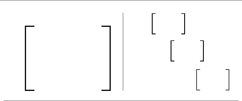
404 13. NUMERICAL PROBLEMS
2 1 3
4 -2 10
5 -3 13
det
-2 10
-3 13
+
4 10
5 13
+
4 -2
5 -3
= 0
2 * det
-1 * det
3 * det
INPUT OUTPUT
13.4 Determinants and Permanents
Input description:Ann×nmatrix M.
Problem description: What is the determinant |M|or permanent perm(M)of
the matrix m?
Discussion: Determinants of matrices provide a clean and useful abstraction in
linear algebra that can be used to solve a variety of problems:
•Testing whether a matrix is singular, meaning that the matrix does not have
an inverse. A matrix Mis singular iff |M|=0.
•Testing whether a set of dpoints lies on a plane in fewer than ddimensions.
If so, the system of equations they define is singular, so |M|=0.
•Testing whether a point lies to the left or right of a line or plane. This
problem reduces to testing whether the sign of a determinant is positive or
negative, as discussed in Section 17.1 (page 564).
•Computing the area or volume of a triangle, tetrahedron, or other simplicial
complex. These quantities are a function of the magnitude of the determinant,
as discussed in Section 17.1 (page 564).
The determinant of a matrix Mis defined as a sum over all n! possible permu-
tations πiof the ncolumns of M:
|M|=
n!
i=1
(−1)sign(πi)
n
j=1
M[j, πj]

13.4 DETERMINANTS AND PERMANENTS 405
where sign(πi) denotes the number of pairs of elements out of order (called inver-
sions) in permutation πi.
A direct implementation of this definition yields an O(n!) algorithm, as does the
cofactor expansion method I learned in high school. Better algorithms to evaluate
determinants are based on LU-decomposition, discussed in Section 13.1 (page 395).
The determinant of Mis simply the product of the diagonal elements of the LU-
decomposition of M, which can be found in O(n3) time.
A closely related function called the permanent arises in combinatorial prob-
lems. For example, the permanent of the adjacency matrix of a graph Gcounts the
number of perfect matchings in G. The permanent of a matrix Mis defined by
perm(M)=
n!
i=1
n
j=1
M[j, πj]
differing from the determinant only in that all products are positive.
Surprisingly, it is NP-hard to compute the permanent, even though the deter-
minant can easily be computed in O(n3) time. The fundamental difference is that
det(AB)=det(A)×det(B), while perm(AB)=perm(A)×perm(B). There are
permanent algorithms running in O(n22n) time that prove to be considerably faster
than the O(n!) definition. Thus, finding the permanent of a 20 ×20 matrix is not
out of the realm of possibility.
Implementations: The linear algebra package LINPACK contains a variety of
Fortran routines for computing determinants, optimized for different data types
and matrix structures. It can be obtained from Netlib, as discussed in Section
19.1.5 (page 659).
JScience provides an extensive linear algebra package (including determinants)
as part of its comprehensive scientific computing library. JAMA is another matrix
package written in Java. Links to both and many related libraries are available
from http://math.nist.gov/javanumerics/.
Nijenhuis and Wilf [NW78] provide an efficient Fortran routine to compute the
permanent of a matrix. See Section 19.1.10 (page 661). Cash [Cas95] provides a
C routine to compute the permanent, motivated by the Kekul´e structure count of
computational chemistry.
Two different codes for approximating the permanent are provided by Barvi-
nok. The first, based on [BS07], provides codes for approximating the permanent
and a Hafnian of a matrix, as well as the number of spanning forests in a graph.
See http://www.math.lsa.umich.edu/∼barvinok/manual.html. The second, based on
[SB01], can provide estimates of the permanent of 200 ×200 matrices in seconds.
See http://www.math.lsa.umich.edu/∼barvinok/code.html.
Notes:Cramer’s rule reduces the problems of matrix inversion and solving linear systems
to that of computing determinants. However, algorithms based on LU-determination are
faster. See [BM53] for an exposition on Cramer’s rule.

406 13. NUMERICAL PROBLEMS
Determinants can be computed in o(n3) time using fast matrix multiplication, as
shown in [AHU83]. Section 13.3 (page 401) discusses such algorithms. A fast algorithm
for computing the sign of the determinant—an important problem for performing robust
geometric computations—is due to Clarkson [Cla92].
The problem of computing the permanent was shown to be #P-complete by Valiant
[Val79], where #P is the class of problems solvable on a “counting” machine in polynomial
time. A counting machine returns the number of distinct solutions to a problem. Counting
the number of Hamiltonian cycles in a graph is a #P-complete problem that is trivially
NP-hard (and presumably harder), since any count greater than zero proves that the
graph is Hamiltonian. Counting problems can be #P-complete even if the corresponding
decision problem can be solved in polynomial time, as shown by the permanent and perfect
matchings.
Minc [Min78] is the primary reference on permanents. A variant of an O(n22n)-time
algorithm due to Ryser for computing the permanent is presented in [NW78].
Recently, probabilistic algorithms have been developed for estimating the permanent,
culminating in a fully-polynomial randomized approximation scheme that provides an
arbitrary close approximation in time that depends polynomially upon the input matrix
and the desired error [JSV01].
Related Problems: Solving linear systems (see page 395), matching (see page
498), geometric primitives (see page 564).
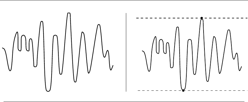
13.5 CONSTRAINED AND UNCONSTRAINED OPTIMIZATION 407
MAX
MIN
INPUT OUTPUT
13.5 Constrained and Unconstrained Optimization
Input description: A function f(x1,...,x
n).
Problem description: What point p=(p1,...,p
n) maximizes (or minimizes) the
function f?
Discussion: Most of this book concerns algorithms that optimize one thing or
another. This section considers the general problem of optimizing functions where,
due to lack of structure or knowledge, we are unable to exploit the problem-specific
algorithms seen elsewhere in this book.
Optimization arises whenever there is an objective function that must be tuned
for optimal performance. Suppose we are building a program to identify good stocks
to invest in. We have certain financial data available to analyze—such as the price-
earnings ratio, the interest rate, and the stock price—all as a function of time t.
The key question is how much weight we should give to each of these factors, where
these weights correspond to coefficients of a formula:
stock-goodness(t)=c1×price(t)+c2×interest(t)+c3×PE-ratio(t)
We seek the numerical values c1,c2,c3whose stock-goodness function does the
best job of evaluating stocks. Similar issues arise in tuning evaluation functions
for any pattern recognition task.
Unconstrained optimization problems also arise in scientific computation. Phys-
ical systems from protein structures to galaxies naturally seek to minimize their
“energy” or “potential function.” Programs that attempt to simulate nature thus
often define potential functions assigning a score to each possible object configu-
ration, and then select the configuration that minimizes this potential.

408 13. NUMERICAL PROBLEMS
Global optimization problems tend to be hard, and there are lots of ways to go
about them. Ask the following questions to steer yourself in the right direction:
•Am I doing constrained or unconstrained optimization? – In unconstrained
optimization, there are no limitations on the values of the parameters other
than that they maximize the value of f. However, many applications demand
constraints on these parameters that make certain points illegal, points that
might otherwise be the global optimum. For example, companies cannot em-
ploy less than zero employees, no matter how much money they think they
might save doing so. Constrained optimization problems typically require
mathematical programming approaches, like linear programming, discussed
in Section 13.6 (page 411).
•Is the function I am trying to optimize described by a formula? – Sometimes
the function that you seek to optimize is presented as an algebraic formula,
such as finding the minimum of f(n)=n2−6n+2
n+1. If so, the solution is
to analytically take its derivative f(n) and see for which points pwe have
f(p) = 0. These points are either local maxima or minima, which can be
distinguished by taking a second derivative or just plugging pback into fand
seeing what happens. Symbolic computation systems such as Mathematica
and Maple are fairly effective at computing such derivatives, although using
computer algebra systems effectively is somewhat of a black art. They are
definitely worth a try, however, and you can always use them to plot a picture
of your function to get a better idea of what you are dealing with.
•Is it expensive to compute the function at a given point? – Instead of a for-
mula, we are often given a program or subroutine that evaluates fat a given
point. Since we can request the value of any given point on demand by calling
this function, we can poke around and try to guess the maxima.
Our freedom to search in such a situation depends upon how efficiently we
can evaluate f. Suppose that f(x1,...,x
n) is the board evaluation function
in a computer chess program, such that x1is how much a pawn is worth, x2
is how much a bishop is worth, and so forth. To evaluate a set of coefficients
as a board evaluator, we must play a bunch of games with it or test it on
a library of known positions. Clearly, this is time-consuming, so we would
have to be frugal in the number of evaluations of fwe use to optimize the
coefficients.
•How many dimensions do we have? How many do we need? – The difficulty
in finding a global maximum increases rapidly with the number of dimensions
(or parameters). For this reason, it often pays to reduce the dimension by
ignoring some of the parameters. This runs counter to intuition, for the naive
programmer is likely to incorporate as many variables as possible into their
evaluation function. It is just too hard, however, to optimize such complicated

13.5 CONSTRAINED AND UNCONSTRAINED OPTIMIZATION 409
functions. Much better is to start with the three to five most important
variables and do a good job optimizing the coefficients for these.
•How smooth is my function? The main difficulty of global optimization is
getting trapped in local optima. Consider the problem of finding the highest
point in a mountain range. If there is only one mountain and it is nicely
shaped, we can find the top by just walking in whatever direction is up.
However, if there are many false summits, or other mountains in the area, it
is difficult to convince ourselves whether we really are at the highest point.
Smoothness is the property that enables us to quickly find the local optimum
from a given point. We assume smoothness in seeking the peak of the moun-
tain by walking up. If the height at any given point was a completely random
function, there would be no way we could find the optimum height short of
sampling every single point.
The most efficient algorithms for unconstrained global optimization use deriva-
tives and partial derivatives to find local optima, to point out the direction in which
moving from the current point does the most to increase or decrease the function.
Such derivatives can sometimes be computed analytically, or they can be estimated
numerically by taking the difference between the values of nearby points. A variety
of steepest descent and conjugate gradient methods to find local optima have been
developed—similar in many ways to numerical root-finding algorithms.
It is a good idea to try several different methods on any given optimization
problem. For this reason, we recommend experimenting with the implementations
below before attempting to implement your own method. Clear descriptions of
these algorithms are provided in several numerical algorithms books, in particular
Numerical Recipes [PFTV07].
For constrained optimization, finding a point that satisfies all the constraints
is often the difficult part of the problem. One approach is to use a method for
unconstrained optimization, but add a penalty according to how many constraints
are violated. Determining the right penalty function is problem-specific, but it
often makes sense to vary the penalties as optimization proceeds. At the end, the
penalties should be very high to ensure that all constraints are satisfied.
Simulated annealing is a fairly robust and simple approach to constrained opti-
mization, particularly when we are optimizing over combinatorial structures (per-
mutations, graphs, subsets). Techniques for simulated annealing are described in
Section 7.5.3 (page 254).
Implementations: The world of constrained/unconstrained optimization is suffi-
ciently confusing that several guides have been created to point people to the right
codes. Particularly nice is Hans Mittlemann’s Decision Tree for Optimization Soft-
ware at http://plato.asu.edu/guide.html. Also check out the selection at GAMS,
the NIST Guide to Available Mathematical Software, at http://gams.nist.gov.
NEOS (Network-Enabled Optimization System) provides a unique service—the
opportunity to solve your problem remotely on computers and software at Argonne

410 13. NUMERICAL PROBLEMS
National Laboratory. Linear programming and unconstrained optimization are
both supported. Check out http://www-neos.mcs.anl.gov/ when you need a solution
instead of a program.
Several of the Collected Algorithms of the ACM are Fortran codes for uncon-
strained optimization, most notably Algorithm 566 [MGH81] , Algorithm 702
[SF92] , and Algorithm 734 [Buc94] . Algorithm 744 [Rab95] does unconstrained
optimization in Lisp. They are all available from Netlib (see Section 19.1.5 (page
659)).
General purpose simulated annealing implementations are available, and prob-
ably are the best place to start experimenting with this technique for constrained
optimization. Feel free to try my code from Section 7.5.3 (page 254). Particularly
popular is Adaptive Simulated Annealing (ASA), written in C by Lester Ingber and
available at http://asa-caltech.sourceforge.net/.
Both the Java Genetic Algorithms Package (JGAP) (http://
jgap.sourceforge.net/) and the C Genetic Algorithm Utility Library (GAUL)
(http://gaul.sourceforge.net/) are designed to aid in the development of applica-
tions that use genetic/evolutionary algorithms. I am highly skeptical about genetic
algorithms (see Section 7.8 (page 266)), but other people seem to find them irre-
sistible.
Notes:Steepest-descent methods for unconstrained optimization are discussed in most
books on numerical methods, including [BT92, PFTV07]. Unconstrained optimization is
the topic of several books, including [Bre73, Fle80].
Simulated annealing was devised by Kirkpatrick et al. [KGV83] as a modern variation
of the Metropolis algorithm [MRRT53]. Both use Monte Carlo techniques to compute
the minimum energy state of a system. Good expositions on all local search variations,
including simulated annealing, appear in [AL97].
Genetic algorithms were developed and popularized by Holland [Hol75, Hol92]. More
sympathetic expositions on genetic algorithms include [LP02, MF00]. Tabu search [Glo90]
is yet another heuristic search procedure with a devoted following.
Related Problems: Linear programming (see page 411), satisfiability (see page
472).
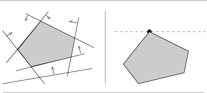
13.6 LINEAR PROGRAMMING 411
INPUT OUTPUT
13.6 Linear Programming
Input description:AsetSof nlinear inequalities on mvariables
Si:=
m
j=1
cij ·xj≥bi,1≤i≤n
and a linear optimization function f(X)=m
j=1 cj·xj.
Problem description: Which variable assignment Xmaximizes the objective
function fwhile satisfying all inequalities S?
Discussion: Linear programming is the most important problem in mathematical
optimization and operations research. Applications include:
•Resource allocation – We seek to invest a given amount of money to maximize
our return. Often our possible options, payoffs, and expenses can be expressed
as a system of linear inequalities such that we seek to maximize our possible
profit given the constraints. Very large linear programming problems are
routinely solved by airlines and other corporations.
•Approximating the solution of inconsistent equations –Asetofmlinear
equations on nvariables xi,1≤i≤nis overdetermined if m>n. Such
overdetermined systems are often inconsistent, meaning that there does not
exist an assignment to the variables that simultaneously solves all the equa-
tions. To find the assignment that best fits the equations, we can replace
each variable xiby x
i+iand solve the new system as a linear program,
minimizing the sum of the error terms.

412 13. NUMERICAL PROBLEMS
•Graph algorithms – Many of the graph problems described in this book, in-
cluding shortest path, bipartite matching, and network flow, can be solved
as special cases of linear programming. Most of the rest, including trav-
eling salesman, set cover, and knapsack, can be solved using integer linear
programming.
The simplex method is the standard algorithm for linear programming. Each
constraint in a linear programming problem acts like a knife that carves away a
region from the space of possible solutions. We seek the point within the remaining
region that maximizes (or minimizes) f(X). By appropriately rotating the solution
space, the optimal point can always be made to be the highest point in the region.
The region (simplex) formed by the intersection of a set of linear constraints is
convex, so unless we are at the top there is always a higher vertex neighboring any
starting point. When we cannot find a higher neighbor to walk to, we have reached
the optimal solution.
While the simplex algorithm is not too complex, there is considerable art to pro-
ducing an efficient implementation capable of solving large linear programs. Large
programs tend to be sparse (meaning that most inequalities use few variables), so
sophisticated data structures must be used. There are issues of numerical stability
and robustness, as well as choosing which neighbor we should walk to next (so-
called pivoting rules). There also exist sophisticated interior-point methods, which
cut through the interior of the simplex instead of walking along the outside, and
beat simplex in many applications.
The bottom line on linear programming is this: you are much better off using
an existing LP code than writing your own. Further, you are probably better off
paying money than surfing the Web. Linear programming is an algorithmic problem
of such economic importance that commercial implementations are far superior to
free versions.
Issues that arise in linear programming include:
•Do any variables have integrality constraints? – It is impossible to send 6.54
airplanes from New York to Washington each business day, even if that value
maximizes profit according to your model. Such variables often have natural
integrality constraints. A linear program is called an integer program if all its
variables have integrality constraints, or a mixed integer program if some of
them do.
Unfortunately, it is NP-complete to solve integer or mixed programs to op-
timality. However, there are integer programming techniques that work rea-
sonably well in practice. Cutting plane techniques solve the problem first as a
linear program, and then add extra constraints to enforce integrality around
the optimal solution point before solving it again. After sufficiently many
iterations, the optimum point of the resulting linear program matches that
of the original integer program. As with most exponential-time algorithms,

13.6 LINEAR PROGRAMMING 413
run times for integer programming depend upon the difficulty of the problem
instance and are unpredictable.
•Do I have more variables or constraints? – Any linear program with mvari-
ables and ninequalities can be written as an equivalent dual linear program
with nvariables and minequalities. This is important to know, because the
running time of a solver might be quite different on the two formulations.
In general, linear programs (LPs) with much more variables than constraints
should be solved directly. If there are many more constraints than variables,
it is usually better to solve the dual LP or (equivalently) apply the dual
simplex method to the primal LP.
•What if my optimization function or constraints are not linear? – In least-
squares curve fitting, we seek the line that best approximates a set of points
by minimizing the sum of squares of the distance between each point and the
line. In formulating this as a mathematical program, the natural objective
function is no longer linear, but quadratic. Although fast algorithms exist for
least squares fitting, general quadratic programming is NP-complete.
There are three possible courses of action when you must solve a nonlinear
program. The best is if you can model it in some other way, as is the case
with least-squares fitting. The second is to try to track down special codes
for quadratic programming. Finally, you can model your problem as a con-
strained or unconstrained optimization problem and try to solve it with the
codes discussed in Section 13.5 (page 407).
•What if my model does not match the input format of my LP solver? –Many
linear programming implementations accept models only in so-called stan-
dard form, where all variables are constrained to be nonnegative, the object
function must be minimized, and all constraints must be equalities (instead
of inequalities).
Do not fear. There exist standard transformations to map arbitrary LP mod-
els into standard form. To convert a maximization problem to a minimization
one, simply multiply each coefficient of the objective function by −1. The re-
maining problems can be solved by adding slack variables to the model. See
any textbook on linear programming for details. Modeling languages such as
AMPC can provide a nice interface to your solver and deal with these issues
for you.
Implementations: The USENET Frequently Asked Question (FAQ) list is a
very useful resource on solving linear programs. In particular, it provides a list
of available codes with descriptions of experiences. Check it out at http://www-
unix.mcs.anl.gov/otc/Guide/faq/.
There are at least three reasonable choices in free LP-solvers. Lp solve, writ-
ten in ANSI C by Michel Berkelaar, can also handle integer and mixed-integer

414 13. NUMERICAL PROBLEMS
problems. It is available at http://lpsolve.sourceforge.net/5.5/, and a substan-
tial user community exists. The simplex solver CLP produced under the Com-
putational Infrastructure for Operations Research is available (with other op-
timization software) at http://www.coin-or.org/. Finally, the GNU Linear Pro-
gramming Kit (GLPK) is intended for solving large-scale linear programming,
mixed integer programming (MIP), and other related problems. It is available at
http://www.gnu.org/software/glpk/. In recent benchmarks among free codes (see
http://plato.asu.edu/bench.html), CLP appeared to be fastest on on linear program-
ming problems and lp solve on mixed integer problems.
NEOS (Network-Enabled Optimization System) provides an opportunity to
solve your problem on computers and software at Argonne National Laboratory.
Linear programming and unconstrained optimization are both supported. This is
worth checking out at http://www.mcs.anl.gov/home/otc/Server/ if you need an
answer instead of a program.
Algorithm 551 [Abd80] and Algorithm 552 [BR80] of the Collected Algorithms
of the ACM are simplex-based codes for solving overdetermined systems of linear
equations in Fortran. See Section 19.1.5 (page 659) for details.
Notes:The need for optimization via linear programming arose in logistics problems in
World War II. The simplex algorithm was invented by George Danzig in 1947 [Dan63].
Klee and Minty [KM72] proved that the simplex algorithm is exponential in worst case,
but it is very efficient in practice.
Smoothed analysis measures the complexity of algorithms assuming that their inputs
are subject to small amounts of random noise. Carefully constructed worst-case instances
for many problems break down under such perturbations. Spielman and Teng [ST04] used
smoothed analysis to explain the efficiency of simplex in practice. Recently, Kelner and
Spielman developed a randomized simplex algorithm running in polynomial time [KS05b].
Khachian’s ellipsoid algorithm [Kha79] first proved that linear programming was poly-
nomial in 1979. Karmarkar’s algorithm [Kar84] is an interior-point method that has proven
to be both a theoretical and practical improvement of the ellipsoid algorithm, as well as
a challenge for the simplex method. Good expositions on the simplex and ellipsoid algo-
rithms for linear programming include [Chv83, Gas03, MG06].
Semidefinite programming deals with optimization problems over symmetric positive
semidefinite matrix variables, with linear cost function and linear constraints. Important
special cases include linear programming and convex quadratic programming with convex
quadratic constraints. Semidefinite programming and its applications to combinatorial
optimization problems are surveyed in [Goe97, VB96].
Linear programming is P-complete under log-space reductions [DLR79]. This makes it
unlikely to have an NC parallel algorithm, where a problem is in NC iff it can be solved on
a PRAM in polylogarithmic time using a polynomial number of processors. Any problem
that is P-complete under log-space reduction cannot be in NC unless P=NC. See [GHR95]
for a thorough exposition of the theory of P-completeness, including an extensive list of
P-complete problems.
Related Problems: Constrained and unconstrained optimization (see page 407),
network flow (see page 509).

13.7 RANDOM NUMBER GENERATION 415
?
HTHTHHTHHT
HHTTTTHTHT
HHHTTHHTTT
HTHHHTTHHT
HTTHHTTHTH
INPUT OUTPUT
13.7 Random Number Generation
Input description: Nothing, or perhaps a seed.
Problem description: Generate a sequence of random integers.
Discussion: Random numbers have an enormous variety of interesting and im-
portant applications. They form the foundation of simulated annealing and related
heuristic optimization techniques. Discrete event simulations run on streams of ran-
dom numbers, and are used to model everything from transportation systems to
casino poker. Passwords and cryptographic keys are typically generated randomly.
Randomized algorithms for graph and geometric problems are revolutionizing these
fields and establishing randomization as one of the fundamental ideas of computer
science.
Unfortunately, generating random numbers looks a lot easier than it really is.
Indeed, it is fundamentally impossible to produce truly random numbers on any
deterministic device. Von Neumann [Neu63] said it best: “Anyone who considers
arithmetical methods of producing random digits is, of course, in a state of sin.”
Thebestwecanhopeforarepseudorandom numbers, a stream of numbers that
appear as if they were generated randomly.
There can be serious consequences to using a bad random-number generator.
In one famous case, a Web browser’s encryption scheme was broken with the dis-
covery that the seeds of its random-number generator employed too few random
bits [GW96]. Simulation accuracy is regularly compromised or invalidated by poor
random number generation. This is an area where people shouldn’t mess around,
but they do. Issues to think about include:
•Should my program use the same “random” numbers each time it runs? –A
poker game that deals you the exact same hand each time you play quickly
loses interest. One common solution is to use the lower-order bits of the
machine clock as the seed or starting point for a stream of random numbers,
so that each time the program runs it does something different.

416 13. NUMERICAL PROBLEMS
Such methods are adequate for games, but not for serious simulations. There
are liable to be periodicities in the distribution of random numbers when-
ever calls are made in a loop. Also, debugging is seriously complicated when
program results are not repeatable. Should your program crash, you cannot
go back and discover why. A possible compromise is to use a deterministic
pseudorandom-number generator, but write the current seed to a file between
runs. During debugging, this file can be overwritten with a fixed initial value
of the seed.
•How good is my compiler’s built-in random number generator? – If you need
uniformly-generated random numbers, and won’t be betting the farm on the
accuracy of your simulation, my recommendation is simply to use what your
compiler provides. Your best opportunity to mess things up is with a bad
choice of starting seed, so read the manual for its recommendations.
If you are going to bet the farm on the results of your simulation, you had
better test your random number generator. Be aware that it is very difficult
to eyeball the results and decide whether the output is really random. This is
because people have very skewed ideas of how random sources should behave
and often see patterns that don’t really exist. Several different tests should be
used to evaluate a random number generator, and the statistical significance
of the results established. The National Institute of Standards and Technology
(NIST) has developed a test suite for evaluating random number generators,
discussed below.
•What if I must implement my own random-number generator? – The standard
algorithm of choice is the linear congruential generator. It is fast, simple,
and (if instantiated with the right constants) gives reasonable pseudorandom
numbers. The nth random number Rnis a function of the (n−1)st random
number:
Rn=(aRn−1+c)modm
In theory, linear congruential generators work the same way roulette wheels
do. The long path of the ball around and around the wheel (captured by
aRn−1+c) ends in one of a relatively small number of bins, the choice of
which is extremely sensitive to the length of the path (captured by the mod m-
truncation).
A substantial theory has been developed to select the constants a,c,m,
and R0. The period length is largely a function of the modulus m,whichis
typically constrained by the word length of the machine.
Note that the stream of numbers produced by a linear congruential gener-
ator repeats the instant the first number repeats. Further, computers are
fast enough to make 232 calls to a random-number generator in a few min-
utes. Thus, any 32-bit linear congruential generator is in danger of cycling,
motivating generators with significantly longer periods.

13.7 RANDOM NUMBER GENERATION 417
•What if I don’t want such large random numbers? – The linear congruential
generator produces a uniformly-distributed sequence of large integers that
can be easily scaled to produce other uniform distributions. For uniformly
distributed real numbers between 0 and 1, use Ri/m. Note that 1 cannot be
realized this way, although 0 can. If you want uniformly distributed integers
between land h,usel+(h−l+1)Ri/m.
•What if I need nonuniformly distributed random numbers? – Generating ran-
dom numbers according to a given nonuniform distribution can be a tricky
business. The most reliable way to do this correctly is the acceptance-rejection
method. We can bound the desired geometric region to sample from by a box
and then select a random point pfrom the box. This point can be generated
by selecting the xand ycoordinates independently at random. If it lies within
the region of interest, we can return pas being selected at random. Other-
wise we throw it away and repeat with another random point. Essentially, we
throw darts at random and report those that hit the target.
This method is correct, but it can be slow. If the volume of the region of
interest is small relative to that of the box, most of our darts will miss the
target. Efficient generators for Gaussian and other special distributions are
described in the references and implementations below.
Be cautious about inventing your own technique, however, since it can be
tricky to obtain the right probability distribution. For example, an incorrect
way to select points uniformly from a circle of radius rwould be to generate
polar coordinates by selecting an angle from 0 to 2πand a displacement
between 0 and r—both uniformly at random. In such a scheme, half the
generated points will lie within r/2 of the center, when only one-fourth of
them should be! This is different enough to seriously skew the results, while
being sufficiently subtle that it can easily escape detection.
•How long should I run my Monte Carlo simulation to get the best results?
– The longer you run a simulation, the more accurately the results should
approximate the limiting distribution, thus increasing accuracy. However,
this is true only until you exceed the period, or cycle length, of your random-
number generator. At that point, your sequence of random numbers repeats
itself, and further runs generate no additional information.
Instead of jacking up the length of a simulation run to the max, it is usually
more informative to do many shorter runs (say 10 to 100) with different
seeds and then consider the range of results you see. The variance provides
a healthy measure of the degree to which your results are repeatable. This
exercise corrects the natural tendency to see a simulation as giving “the”
correct answer.

418 13. NUMERICAL PROBLEMS
Implementations: See http://random.mat.sbg.ac.at for an excellent website on
random-number generation and stochastic simulation. It includes pointers to papers
and literally dozens of implementations of random-number generators.
Parallel simulations make special demands on random-number generators.
How can we ensure that random streams are independent on each machine?
L’Ecuyer et.al. [LSCK02] provide object-oriented generators with a period length
of approximately 2191. Implementations in C, C++, and Java are available at
http://www.iro.umontreal.ca/∼lecuyer/myftp/streams00/. Independent streams of
random numbers are supported for parallel applications. Another possibility is the
Scalable Parallel Random Number Generators Library (SPRNG) [MS00], available
at http://sprng.cs.fsu.edu/.
Algorithms 488 [Bre74], 599 [AKD83], and 712 [Lev92] of the Collected Algo-
rithms of the ACM are Fortran codes for generating non-uniform random numbers
according to several probability distributions, including the normal, exponential,
and Poisson distributions. They are available from Netlib (see Section 19.1.5 (page
659)).
The National Institute of Standards [RSN+01] has prepared an extensive sta-
tistical test suite to validate random number generators. Both the software and the
report describing it are available at http://csrc.nist.gov/rng/.
True random-number generators extract random bits by observing physical pro-
cesses. The website http://www.random.org makes available random numbers de-
rived from atmospheric noise that passes the NIST statistical tests. This is an
amusing solution if you need a small quantity of random numbers (say, to run a
lottery) instead a random-number generator.
Notes:Knuth [Knu97b] provides a thorough treatment of random-number generation,
which I heartily recommend. He presents the theory behind several methods, including
the middle-square and shift-register methods we have not described here, as well as a
detailed discussion of statistical tests for validating random-number generators.
That said, see [Gen04] for more recent developments in random number generation.
The Mersenne twister [MN98] is a fast random number generator of period 219937 −1.
Other modern methods include [Den05, PLM06]. Methods for generating nonuniform
random variates are surveyed in [HLD04]. Comparisons of different random-number gen-
erators in practice include [PM88].
Tables of random numbers appear in most mathematical handbooks as relics from the
days before there was ready access to computers. Most notable is [RC55], which provides
one million random digits.
The deep relationship between randomness, information, and compressibility is ex-
plored within the theory of Kolmogorov complexity, which measures the complexity of
a string by its compressibility. Truly random strings are incompressible. The string of
seemingly random digits of πcannot be random under this definition, since the entire
sequence is defined by any program implementing a series expansion for π.LiandVit´ani
[LV97] provide a thorough introduction to the theory of Kolmogorov complexity.


420 13. NUMERICAL PROBLEMS
8338169264555846052842102071
8338169264555846052842102071
22801763489
2038074743
179424673
*
INPUT OUTPUT
13.8 Factoring and Primality Testing
Input description: An integer n.
Problem description:Isna prime number, and if not what are its factors?
Discussion: The dual problems of integer factorization and primality testing have
surprisingly many applications for a problem long suspected of being only of math-
ematical interest. The security of the RSA public-key cryptography system (see
Section 18.6 (page 641)) is based on the computational intractability of factoring
large integers. As a more modest application, hash table performance typically im-
proves when the table size is a prime number. To get this benefit, an initialization
routine must identify a prime near the desired table size. Finally, prime numbers
are just interesting to play with. It is no coincidence that programs to generate
large primes often reside in the games directory of UNIX systems.
Factoring and primality testing are clearly related problems, although they are
quite different algorithmically. There exist algorithms that can demonstrate that
an integer is composite (i.e. , not prime) without actually giving the factors. To
convince yourself of the plausibility of this, note that you can demonstrate the
compositeness of any nontrivial integer whose last digit is 0, 2, 4, 5, 6, or 8 without
doing the actual division.
The simplest algorithm for both of these problems is brute-force trial division.
To factor n, compute the remainder of n/i for all 1 <i≤√n. The prime factoriza-
tion of nwill contain at least one instance of every isuch that n/i =n/i, unless
nis prime. Make sure you handle the multiplicities correctly, and account for any
primes larger than √n.
Such algorithms can be sped up by using a precomputed table of small primes to
avoid testing all possible i. Surprisingly large numbers of primes can be represented
in surprisingly little space by using bit vectors (see Section 12.5 (page 385)). A bit
vector of all odd numbers less than 1,000,000 fits in under 64 kilobytes. Even tighter
encodings become possible by eliminating all multiples of 3 and other small primes.

13.8 FACTORING AND PRIMALITY TESTING 421
Although trial division runs in O(√n) time, it is not a polynomial-time algo-
rithm. The reason is that it only takes lg2nbits to represent n, so trial division takes
time exponential in the input size. Considerably faster (but still exponential time)
factoring algorithms exist, whose correctness depends upon more substantial num-
ber theory. The fastest known algorithm, the number field sieve, uses randomness
to construct a system of congruences—the solution of which usually gives a factor
of the integer. Integers with as many as 200 digits (663 bits) have been factored
using this method, although such feats require enormous amounts of computation.
Randomized algorithms make it much easier to test whether an integer is prime.
Fermat’s little theorem states that an−1= 1(mod n) for all anot divisible by n,
provided nis prime. Suppose we pick a random value 1 ≤a<nand compute the
residue of an−1(mod n). If this residue is not 1, we have just proven that ncannot
be prime. Such randomized primality tests are very efficient. PGP (see Section 18.6
(page 641)) finds 300+ digit primes using hundreds of these tests in minutes, for
use as cryptographic keys.
Although the primes are scattered in a seemingly random way throughout the
integers, there is some regularity to their distribution. The prime number theo-
rem states that the number of primes less than n(commonly denoted by π(n)) is
approximately n/ ln n. Further, there never are large gaps between primes, so in
general, one would expect to examine about ln nintegers if one wanted to find the
first prime larger than n. This distribution and the fast randomized primality test
explain how PGP can find such large primes so quickly.
Implementations: Several general systems for computational number theory are
available. PARI is capable of handling complex number-theoretic problems on
arbitrary-precision integers (to be precise, limited to 80,807,123 digits on 32-bit
machines), as well as reals, rationals, complex numbers, polynomials, and matrices.
It is written mainly in C, with assembly code for inner loops on major architectures,
and includes more than 200 special predefined mathematical functions. PARI can
be used as a library, but it also possesses a calculator mode that gives instant access
to all the types and functions. PARI is available at http://pari.math.u-bordeaux.fr/
LiDIA (http://www.cdc.informatik.tu-darmstadt.de/TI/LiDIA/) is the acronym
for the C++ Library for Computational Number Theory. It implements several of
the modern integer factorization methods.
A Library for doing Number Theory (NTL) is a high-performance, portable
C++ library providing data structures and algorithms for manipulating signed,
arbitrary length integers, and for vectors, matrices, and polynomials over the inte-
gers and over finite fields. It is available at http://www.shoup.net/ntl/.
Finally, MIRACL (Multiprecision Integer and Rational Arithmetic C/C++
Library) implements six different integer factorization algorithms, including the
quadratic sieve. It is available at http://www.shamus.ie/.
Notes:Expositions on modern algorithms for factoring and primality testing include
Crandall and Pomerance [CP05] and Yan [Yan03]. More general surveys of computational
number theory include Bach and Shallit [BS96] and Shoup [Sho05].

422 13. NUMERICAL PROBLEMS
In 2002, Agrawal, Kayal, and Saxena [AKS04] solved a long-standing open problem
by giving the first polynomial-time deterministic algorithm to test whether an integer is
composite. Their algorithm, which is surprisingly elementary for such an important result,
involves a careful analysis of techniques from earlier randomized algorithms. Its existence
serves as somewhat of a rebuke to researchers (like me) who shy away from classical open
problems due to fear. Dietzfelbinger [Die04] provides a self-contained treatment of this
result.
The Miller-Rabin [Mil76, Rab80] randomized primality testing algorithm eliminates
problems with Carmichael numbers, which are composite integers that always satisfy
Fermat’s theorem. The best algorithms for integer factorization include the quadratic-
sieve [Pom84] and the elliptic-curve methods [Len87b].
Mechanical sieving devices provided the fastest way to factor integers surprisingly far
into the computing era. See [SWM95] for a fascinating account of one such device, built
during World War I. Hand-cranked, it proved the primality of 231 −1in15minutesof
sieving time.
An important problem in computational complexity theory is whether P = NP ∩
co-NP. The decision problem “is na composite number?” used to be the best candidate
for a counterexample. By exhibiting the factors of n, it is trivially in NP. It can be shown
to be in co-NP, since every prime has a short proof of its primality [Pra75]. The recent
proof that composite numbers testing is in P shot down this line of reasoning. For more
information on complexity classes, see [GJ79, Joh90].
The integer RSA-129 was factored in eight months using over 1,600 computers. This
was particularly noteworthy because in the original RSA paper [RSA78] they had origi-
nally predicted such a factorization would take 40 quadrillion years using 1970s technology.
Bahr, Boehm, Franke, and Kleinjung hold the current integer factorization record, with
their successful attack on the 200-digit integer RSA-200 in May 2005. This required the
equivalent of 55 years of computations on a single 2.2 GHz Opteron CPU.
Related Problems: Cryptography (see page 641), high precision arithmetic (see
page 423).

13.9 ARBITRARY-PRECISION ARITHMETIC 423
49578291287491495151508905425869578
74367436931237242727263358138804367
2
3
INPUT OUTPUT
13.9 Arbitrary-Precision Arithmetic
Input description: Two very large integers, xand y.
Problem description: What is x+y,x−y,x×y,andx/y?
Discussion: Any programming language rising above basic assembler supports
single- and perhaps double-precision integer/real addition, subtraction, multipli-
cation, and division. But what if we wanted to represent the national debt of the
United States in pennies? One trillion dollars worth of pennies requires 15 decimal
digits, which is far more than can fit into a 32-bit integer.
Other applications require much larger integers. The RSA algorithm for public-
key cryptography recommends integer keys of at least 1000 digits to achieve ade-
quate security. Experimenting with number-theoretic conjectures for fun or research
requires playing with large numbers. I once solved a minor open problem [GKP89]
by performing an exact computation on the integer 5906
2953≈9.93285 ×101775.
What should you do when you need large integers?
•Am I solving a problem instance requiring large integers, or do I have an
embedded application? – If you just need the answer to a specific problem
with large integers, such as in the number theory application above, you
should consider using a computer algebra system like Maple or Mathematica.
These provide arbitrary-precision arithmetic as a default and use nice Lisp-
like programming languages as a front end—together often reducing your
problem to a 5- to 10- line program.
If you have an embedded application requiring high-precision arithmetic in-
stead, you should use an existing arbitrary precision math library. You are
likely to get additional functions beyond the four basic operations for com-
puting things like greatest common divisor in the bargain. See the Implemen-
tations section for details.
•Do I need high- or arbitrary-precision arithmetic? – Is there an upper bound
on how big your integers can get, or do you really need arbitrary-precision—
i.e. , unbounded. This determines whether you can use a fixed-length array
to represent your integers as opposed to a linked-list of digits. The array is
likely to be simpler and will not prove a constraint in most applications.

424 13. NUMERICAL PROBLEMS
•What base should I do arithmetic in? – It is perhaps simplest to implement
your own high-precision arithmetic package in decimal, and thus represent
each integer as a string of base-10 digits. However, it is far more efficient
to use a higher base, ideally equal to the square root of the largest integer
supported fully by hardware arithmetic.
Why? The higher the base, the fewer digits we need to represent a number.
Compare 64 decimal with 1000000 binary. Since hardware addition usually
takes one clock cycle independent of value of the actual numbers, best per-
formance is achieved using the highest supported base. The factor limiting
us to base b=√maxint is the desire to avoid overflow when multiplying two
of these “digits” together.
The primary complication of using a larger base is that integers must be
converted to and from base-10 for input and output. The conversion is easily
performed once all four high-precision arithmetical operations are supported.
•How low-level are you willing to get for fast computation? – Hardware addi-
tion is much faster than a subroutine call, so you take a significant hit on
speed using high-precision arithmetic when low-precision arithmetic suffices.
High-precision arithmetic is one of few problems in this book where inner
loops in assembly language prove the right idea to speed things up. Similarly,
using bit-level masking and shift operations instead of arithmetical operations
can be a win if you really understand the machine integer representation.
The algorithm of choice for each of the five basic arithmetic operations is as
follows:
•Addition – The basic schoolhouse method of lining up the decimal points and
then adding the digits from right to left with “carries” runs to time linear in
the number of digits. More sophisticated carry-look-ahead parallel algorithms
are available for low-level hardware implementation. They are presumably
used on your microprocessor for low-precision addition.
•Subtraction – By fooling with the sign bits of the numbers, subtraction can be
a special considered case of addition: (A−(−B)) = (A+B). The tricky part
of subtraction is performing the “borrow.” This can be simplified by always
subtracting from the number with the larger absolute value and adjusting
the signs afterwards, so we can be certain there will always be something to
borrow from.
•Multiplication – Repeated addition will take exponential time on large inte-
gers, so stay away from it. The digit-by-digit schoolhouse method is reason-
able to program and will work much better, presumably well enough for your
application. On very large integers, Karatsuba’s O(n1.59) divide-and-conquer
algorithm wins. Dan Grayson, author of Mathematica’s arbitrary-precision
arithmetic, found that the switch-over happened at well under 100 digits.

13.9 ARBITRARY-PRECISION ARITHMETIC 425
Even faster for very large integers is an algorithm based on Fourier trans-
forms. Such algorithms are discussed in Section 13.11 (page 431).
•Division – Repeated subtraction will take exponential time, so the easiest
reasonable algorithm to use is the long-division method you hated in school.
This is fairly complicated, requiring arbitrary-precision multiplication and
subtraction as subroutines, as well as trial-and-error, to determine the correct
digit at each position of the quotient.
In fact, integer division can be reduced to integer multiplication, although in a
nontrivial way, so if you are implementing asymptotically fast multiplication,
you can reuse that effort in long division. See the references below for details.
•Exponentiation – We can compute anusing n−1 multiplications, by com-
puting a×a×... ×a. However, a much better divide-and-conquer algo-
rithm is based on the observation that n=n/2+n/2.Ifnis even, then
an=(an/2)2.Ifnis odd, then an=a(an/2)2. In either case, we have halved
the size of our exponent at the cost of at most two multiplications, so O(lg n)
multiplications suffice to compute the final value:
function power(a, n)
if (n= 0) return(1)
x= power(a, n/2)
if (nis even) then return(x2)
else return(a×x2)
High- but not arbitrary-precision arithmetic can be conveniently performed
using the Chinese remainder theorem and modular arithmetic. The Chinese re-
mainder theorem states that an integer between 1 and P=k
i=1 piis uniquely
determined by its set of residues mod pi, where each pi,p
jare relatively prime
integers. Addition, subtraction, and multiplication (but not division) can be sup-
ported using such residue systems, with the advantage that large integers can be
manipulated without complicated data structures.
Many of these algorithms for computations on long integers can be directly
applied to computations on polynomials. See the references for more details. A
particularly useful algorithm is Horner’s rule for fast polynomial evaluation. When
P(x)=n
i=0 ci·xiis blindly evaluated term by term, O(n2) multiplications will
be performed. Much better is observing that P(x)=c0+x(c1+x(c2+x(c3+...))),
the evaluation of which uses only a linear number of operations.
Implementations: All major commercial computer algebra systems incorporate
high-precision arithmetic, including Maple, Mathematica, Axiom, and Macsyma.
If you have access to one of these, this is your best option for a quick, nonembedded

426 13. NUMERICAL PROBLEMS
application. The rest of this section focuses on source code available for embedded
applications.
The premier C/C++ library for fast, arbitrary-precision is the GNU Multiple
Precision Arithmetic Library (GMP), which operates on signed integers, rational
numbers, and floating point numbers. It is widely used and well-supported, and
available at http://gmplib.org/.
The java.math BigInteger class provides arbitrary-precision analogues to all
of Java’s primitive integer operators. BigInteger provides additional operations
for modular arithmetic, GCD calculation, primality testing, prime generation, bit
manipulation, and a few other miscellaneous operations.
A lower-performance, less-tested, but more personal implementation of high-
precision arithmetic appears in the library from my book Programming Challenges
[SR03]. See Section 19.1.10 (page 661) for details.
Several general systems for computational number theory are available. Each
of these supports operations of arbitrary-precision integers. Information about the
PARI, LiDIA, NTL and MIRACL number-theoretic libraries can be found in Sec-
tion 13.8 (page 420).
ARPREC is a C++/Fortran-90 arbitrary precision package with an associ-
ated interactive calculator. MPFUN90 is a similar package written exclusively in
Fortran-90. Both are available at http://crd.lbl.gov/∼dhbailey/mpdist/. Algorithm
693 [Smi91] of the Collected Algorithms of the ACM is a Fortran implementation
of floating-point, multiple-precision arithmetic. See Section 19.1.5 (page 659).
Notes:Knuth [Knu97b] is the primary reference on algorithms for all basic arithmetic
operations, including implementations of them in the MIX assembly language. Bach and
Shallit [BS96] and Shoup [Sho05] provide more recent treatments of computational num-
ber theory.
ExpositionsontheO(n1.59)-time divide-and-conquer algorithm for multiplication
[KO63] include [AHU74, Man89]. An FFT-based algorithm multiplies two n-bit num-
bers in O(nlg nlg lg n) time and is due to Sch¨onhage and Strassen [SS71]. Expositions
include [AHU74, Knu97b]. The reduction between integer division and multiplication is
presented in [AHU74, Knu97b]. Applications of fast multiplication to other arithmetic
operations are presented by Bernstein [Ber04b]
Good expositions of algorithms for modular arithmetic and the Chinese remainder
theorem include [AHU74, CLRS01]. A good exposition of circuit-level algorithms for ele-
mentary arithmetic algorithms is [CLRS01].
Euclid’s algorithm for computing the greatest common divisor of two numbers is
perhaps the oldest interesting algorithm. Expositions include [CLRS01, Man89].
Related Problems: Factoring integers (see page 420), cryptography (see page
641).
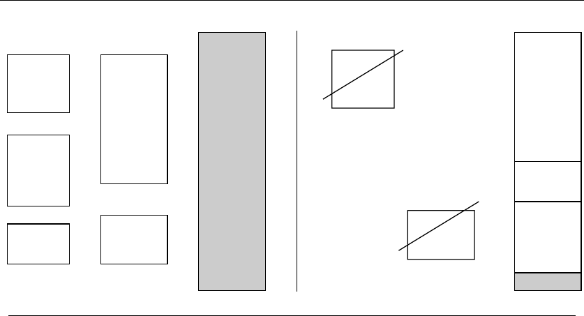
13.10 KNAPSACK PROBLEM 427
$90
$30
$40
$50
$100
$100
$90
$50
$40
$30
INPUT OUTPUT
13.10 Knapsack Problem
Input description: A set of items S={1,...,n}, where item ihas size siand
value vi. A knapsack capacity is C.
Problem description: Find the subset S⊂Sthat maximizes the value of
i∈Svi, given that i∈Ssi≤C; i.e. , all the items fit in a knapsack of size
C.
Discussion: The knapsack problem arises in resource allocation with financial
constraints. How do you select what things to buy given a fixed budget? Everything
has a cost and value, so we seek the most value for a given cost. The name knapsack
problem invokes the image of the backpacker who is constrained by a fixed-size
knapsack, and so must fill it only with the most useful and portable items.
The most common formulation is the 0/1 knapsack problem, where each item
must be put entirely in the knapsack or not included at all. Objects cannot be
broken up arbitrarily, so it is not fair taking one can of Coke from a six-pack or
opening a can to take just a sip. It is this 0/1 property that makes the knapsack
problem hard, for a simple greedy algorithm finds the optimal selection when we
are allowed to subdivide objects. We compute the “price per pound” for each item,
and take the most expensive item or the biggest part thereof until the knapsack is
full. Repeat with the next most expensive item. Unfortunately, the 0/1 constraint
is usually inherent in most applications.
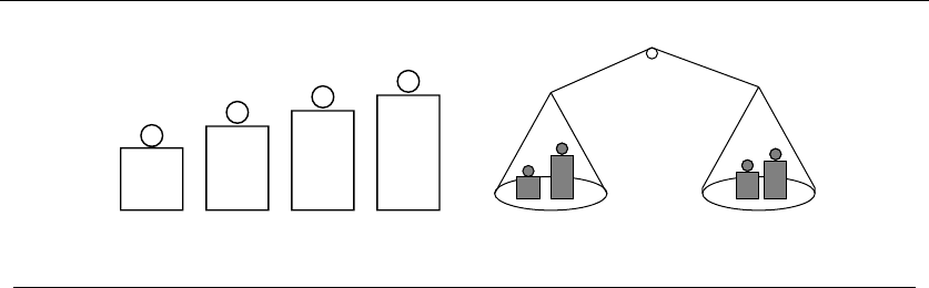
428 13. NUMERICAL PROBLEMS
45674
756
Figure 13.1: Integer partition is a special case of the knapsack problem
Issues that arise in selecting the best algorithm include:
•Does every item have the same cost/value or the same size? – When all
items are worth exactly the same amount, we maximize our value by taking
the greatest number of items. Therefore, the optimal solution is to sort the
items in order of increasing size and insert them into the knapsack in this
order until no more fit. The problem is similarly solved when each object has
the same size but the costs are different. Sort by cost, and take the cheapest
elements first. These are the easy cases of knapsack.
•Does each item have the same “price per pound”? – In this case, our problem
is equivalent to ignoring the price and just trying to minimize the amount
of empty space left in the knapsack. Unfortunately, even this restricted ver-
sion is NP-complete, so we cannot expect an efficient algorithm that always
solves the problem. Don’t lose hope, however, because knapsack proves to
be an “easy” hard problem, and one that can usually be handled with the
algorithms described below.
An important special case of a constant “price-per-pound” knapsack is the
integer partition problem, presented in cartoon form in Figure 13.1. Here,
we seek to partition the elements of Sinto two sets Aand Bsuch that
a∈Aa=b∈B, or alternately make the difference as small as possible.
Integer partition can be thought of as bin packing into two equal-sized bins
or knapsack with a capacity of half the total weight, so all three problems
are closely related and NP-complete.
The constant “price-per-pound” knapsack problem is often called the subset
sum problem, because we seek a subset of items that adds up to a specific
target number C; i.e. , the capacity of our knapsack.
•Are all the sizes relatively small integers? – When the sizes of the items and
the knapsack capacity Care all integers, there exists an efficient dynamic
programming algorithm to find the optimal solution in time O(nC)andO(C)
space. Whether this works for you depends upon how big Cis.Itisgreatfor
C≤1,000, but not so great for C≥10,000,000.

13.10 KNAPSACK PROBLEM 429
The algorithm works as follows: Let Sbe a set of items, and let C[i, S]be
true if and only if there is a subset of Swhose size adds up exactly to i.
Thus, C[i, ∅] is false for all 1 ≤i≤C. One by one we add a new item sjto S
and update the affected values of C[i, S]. Observe that C[i, S∪sj]=true
iff C[i, S]orC[i−sj,S] is true, since we either use sjin realizing the sum or
we don’t. We identify all sums that can be realized by performing nsweeps
through all Celements—one for each sj,1≤j≤n—and so updating the
array. The knapsack solution is given by the largest index of a true element
of the largest realizable size. To reconstruct the winning subset, we must also
store the name of the item number that turned C[i] from false to true for
each 1 ≤i≤Cand then scan backwards through the array.
This dynamic programming formulation ignores the values of the items. To
generalize the algorithm, use each element of the array to store the value of
the best subset to date summing up to i. We now update when the sum of
the cost of C[i−sj,S] plus the cost of sjis better than the previous cost of
C[i].
•What if I have multiple knapsacks? – When there are multiple knapsacks,
your problem might be better thought of as a bin-packing problem. Check
out Section 17.9 (page 595) for bin-packing/cutting-stock algorithms. That
said, algorithms for optimizing over multiple knapsacks are provided in the
Implementations section below.
Exact solutions for large capacity knapsacks can be found using integer pro-
gramming or backtracking. A 0/1 integer variable xiis used to denote whether
item iis present in the optimal subset. We maximize n
i=1 xi·vigiven the con-
straint that n
i=1 xi·si≤C. Integer programming codes are discussed in Section
13.6 (page 411).
Heuristics must be used when exact solutions prove too costly to compute.
The simple greedy heuristic inserts items according to the maximum “price per
pound” rule described previously. Often this heuristic solution is close to optimal,
but it can be arbitrarily bad depending upon the problem instance. The “price per
pound” rule can also be used to reduce the problem size in exhaustive search-based
algorithms by eliminating “cheap but heavy” objects from future consideration.
Another heuristic is based on scaling. Dynamic programming works well if the
knapsack capacity is a reasonably small integer, say ≤Cs. But what if we have a
problem with capacity C>C
s? We scale down the sizes of all items by a factor of
C/Cs, round the size down to the nearest integer, and then use dynamic program-
ming on the scaled items. Scaling works well in practice, especially when the range
of sizes of items is not too large.
Implementations: Martello and Toth’s collection of Fortran implementations
of algorithms for a variety of knapsack problem variants are available at
http://www.or.deis.unibo.it/kp.html. An electronic copy of the associated book
[MT90a] has also been generously made available.

430 13. NUMERICAL PROBLEMS
David Pisinger maintains a well-organized collection of C-language codes for
knapsack problems and related variants like bin packing and container loading.
These are available at http://www.diku.dk/∼pisinger/codes.html. The strongest
code is based on the dynamic programming algorithm of [MPT99].
Algorithm 632 [MT85] of the Collected Algorithms of the ACM is a Fortran code
for the 0/1 knapsack problem, with the twist that it supports multiple knapsacks.
See Section 19.1.5 (page 659).
Notes:Keller, Pferschy, and Pisinger [KPP04] is the most current reference on the knap-
sack problem and variants. Martello and Toth’s book [MT90a] and survey article [MT87]
are standard references on the knapsack problem, including both theoretical and experi-
mental results. An excellent exposition on integer programming approaches to knapsack
problems appears in [SDK83]. See [MPT00] for a computational study of algorithms for
0-1 knapsack problems.
A polynomial-time approximation scheme is an algorithm that approximates the op-
timal solution of a problem in time polynomial in both its size and the approximation
factor .
This very strong condition implies a smooth tradeoff between running time and ap-
proximation quality. Good expositions on polynomial-time approximation schemes [IK75]
for knapsack and subset sum includes [BvG99, CLRS01, GJ79, Man89].
The first algorithm for generalized public key encryption by Merkle and Hellman
[MH78] was based on the hardness of the knapsack problem. See [Sch96] for an exposition.
Related Problems: Bin packing (see page 595), integer programming (see page
411).
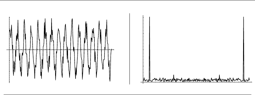
13.11 DISCRETE FOURIER TRANSFORM 431
50 100 150 200 250
-1.5
-1
-0.5
0.5
1
1.5
50 100 150 200 250
2
4
6
8
INPUT OUTPUT
13.11 Discrete Fourier Transform
Input description: A sequence of nreal or complex values hi,0≤i≤n−1,
sampled at uniform intervals from a function h.
Problem description: The discrete Fourier transform Hm=n−1
k=0 hke2πikm/n
for 0 ≤m≤n−1.
Discussion: Although computer scientists tend to be fairly ignorant about Fourier
transforms, electrical engineers and signal processors eat them for breakfast. Func-
tionally, Fourier transforms provide a way to convert samples of a standard time-
series into the frequency domain. This provides a dual representation of the function
in which certain operations become easier than in the time domain. Applications
of Fourier transforms include:
•Filtering – Taking the Fourier transform of a function is equivalent to rep-
resenting it as the sum of sine functions. By eliminating undesirable high-
and/or low-frequency components (i.e. , dropping some of the sine functions)
and taking an inverse Fourier transform to get us back into the time domain,
we can filter an image to remove noise and other artifacts. For example, the
sharp spike in the figure above represents the period of the single sine function
that closely models the input data. The rest is noise.
•Image compression – A smoothed, filtered image contains less information
than the original, while retaining a similar appearance. By eliminating the
coefficients of sine functions that contribute relatively little to the image, we
can reduce the size of the image at little cost in image fidelity.
•Convolution and deconvolution – Fourier transforms can efficiently compute
convolutions of two sequences. A convolution is the pairwise product of ele-
ments from two different sequences, such as in multiplying two n-variable

432 13. NUMERICAL PROBLEMS
polynomials fand gor comparing two character strings. Implementing
such products directly takes O(n2), while the fast Fourier transform led to a
O(nlg n) algorithm.
Another example comes from image processing. Because a scanner measures
the darkness of an image patch instead of a single point, the scanned input
is always blurred. A reconstruction of the original signal can be obtained by
deconvoluting the input signal with a Gaussian point-spread function.
•Computing the correlation of functions –Thecorrelation function of two
functions f(t)andg(t) is defined by
z(t)=∞
−∞
f(τ)g(t+τ)dτ
and can be easily computed using Fourier transforms. When two functions are
similar in shape but one is shifted relative to the other (such as f(t)=sin(t)
and g(t)=cos(t)), the value of z(t0) will be large at this shift offset t0.As
an application, suppose that we want to detect whether there are any funny
periodicities in our random-number generator. We can generate a large series
of random numbers, turn them into a time series (the ith number at time i),
and take the Fourier transform of this series. Any funny spikes will correspond
to potential periodicities.
The discrete Fourier transform takes as input ncomplex numbers hk,0≤
k≤n−1, corresponding to equally spaced points in a time series, and outputs
ncomplex numbers Hk,0≤k≤n−1, each describing a sine function of given
frequency. The discrete Fourier transform is defined by
Hm=
n−1
k=0
hke−2πikm/n
and the inverse Fourier transform is defined by
hm=1
n
n−1
k=0
Hke2πikm/n
which enables us move easily between hand H.
Since the output of the discrete Fourier transform consists of nnumbers, each
of which is computed using a formula on nnumbers, they can be computed in
O(n2) time. The fast Fourier transform (FFT) is an algorithm that computes the
discrete Fourier transform in O(nlog n). This is arguably the most important algo-
rithm known, for it opened the door to modern signal processing. Several different
algorithms call themselves FFTs, all of which are based on a divide-and-conquer
approach. Essentially, the problem of computing the discrete Fourier transform on

13.11 DISCRETE FOURIER TRANSFORM 433
npoints is reduced to computing two transforms on n/2 points each, and is then
applied recursively.
The FFT usually assumes that nis a power of two. If this is not the case,
you are usually better off padding your data with zeros to create n=2
kelements
rather than hunting for a more general code.
Many signal-processing systems have strong real-time constraints, so FFTs are
often implemented in hardware, or at least in assembly language tuned to the
particular machine. Be aware of this possibility if the codes prove too slow.
Implementations: FFTW is a C subroutine library for computing the discrete
Fourier transform in one or more dimensions, with arbitrary input size, and sup-
porting both real and complex data. It is the clear choice among freely avail-
able FFT codes. Extensive benchmarking proves it to be the “Fastest Fourier
Transform in the West.” Interfaces to Fortran and C++ are provided. FFTW
received the 1999 J. H. Wilkinson Prize for Numerical Software. It is available at
http://www.fftw.org/.
FFTPACK is a package of Fortran subprograms for the fast Fourier trans-
form of periodic and other symmetric sequences, written by P. Swartzrauber. It
includes complex, real, sine, cosine, and quarter-wave transforms. FFTPACK re-
sides on Netlib (see Section 19.1.5 (page 659)) at http://www.netlib.org/fftpack.The
GNU Scientific Library for C/C++ provides a reimplementation of FFTPACK. See
http://www.gnu.org/software/gsl/.
Algorithm 545 [Fra79] of the Collected Algorithms of the ACM is a Fortran im-
plementation of the fast Fourier transform optimizing virtual memory performance.
See Section 19.1.5 (page 659) for further information.
Notes:Bracewell [Bra99] and Brigham [Bri88] are excellent introductions to Fourier
transforms and the FFT. See also the exposition in [PFTV07]. Credit for inventing the
fast Fourier transform is usually given to Cooley and Tukey [CT65], but see [Bri88] for a
complete history.
A cache-oblivious algorithm for the fast Fourier transform is given in [FLPR99]. This
paper first introduced the notion of cache-oblivious algorithms. The FFTW is based on
this algorithm. See [FJ05] for more on the design of the FFTW.
An interesting divide-and-conquer algorithm for polynomial multiplication [KO63]
does the job in O(n1.59) time and is discussed in [AHU74, Man89]. An FFT-based algo-
rithm that multiplies two n-bit numbers in O(nlg nlg lg n) time is due to Sch¨onhage and
Strassen [SS71] and is presented in [AHU74].
It is an open question of whether complex variables are really fundamental to fast
algorithms for convolution. Fortunately, fast convolution can be used as a black box in
most applications. Many variants of string matching are based on fast convolution [Ind98].
In recent years, wavelets have been proposed to replace Fourier transforms in filtering.
See [Wal99] for an introduction to wavelets.
Related Problems: Data compression (see page 637), high-precision arithmetic
(see page 423).

14
Combinatorial Problems
We now consider several algorithmic problems of a purely combinatorial nature.
These include sorting and permutation generations, both of which were among
the first non-numerical problems arising on electronic computers. Sorting can be
viewed as identifying or imposing a total order on the keys, while searching and
selection involve identifying specific keys based on their position in this total order.
The rest of this section deals with other combinatorial objects, such as permuta-
tions, partitions, subsets, calendars, and schedules. We are particularly interested
in algorithms that rank and unrank combinatorial objects—i.e. , that map each dis-
tinct object to and from a unique integer. Rank and unrank operations make many
other tasks simple, such as generating random objects (pick a random number and
unrank) or listing all objects in order (iterate from 1 to nand unrank).
We conclude with the problem of generating graphs. Graph algorithms are more
fully presented in subsequent sections of the catalog.
Books on general combinatorial algorithms, in this restricted sense, include:
•Nijenhuis and Wilf [NW78] – This book specializes in algorithms for con-
structing basic combinatorial objects such as permutations, subsets, and par-
titions. Such algorithms are often very short but hard to locate and usually
are surprisingly subtle. Fortran programs for all of the algorithms are pro-
vided, as well as a discussion of the theory behind each of them. See Section
19.1.10 for details.
•Kreher and Stinson [KS99] – The most recent book on combinatorial genera-
tion algorithms, with additional particular focus on algebraic problems such
as isomorphism and dealing with symmetry.
S.S. Skiena, The Algorithm Design Manual, 2nd ed., DOI: 10.1007/978-1-84800-070-4 14,
c
Springer-Verlag London Limited 2008

14. COMBINATORIAL PROBLEMS 435
•Knuth [Knu97a, Knu98] – The standard reference on searching and sorting,
with significant material on combinatorial objects such as permutations. New
material on the generation of permutations [Knu05a], subsets and partitions
[Knu05b], and trees [Knu06] has been released on “fasciles,”—short paper-
back chunks of what is slated to be the mythical Volume 4.
•Stanton and White [SW86a] – An undergraduate combinatorics text with al-
gorithms for generating permutations, subsets, and set partitions. It contains
relevant programs in Pascal.
•Pemmaraju and Skiena [PS03] – This description of Combinatorica, a library
of over 400 Mathematica functions for generating combinatorial objects and
graph theory (see Section 19.1.9), provides a distinctive view of how different
algorithms can fit together. Its second author is considered qualified to write
a manual on algorithm design.
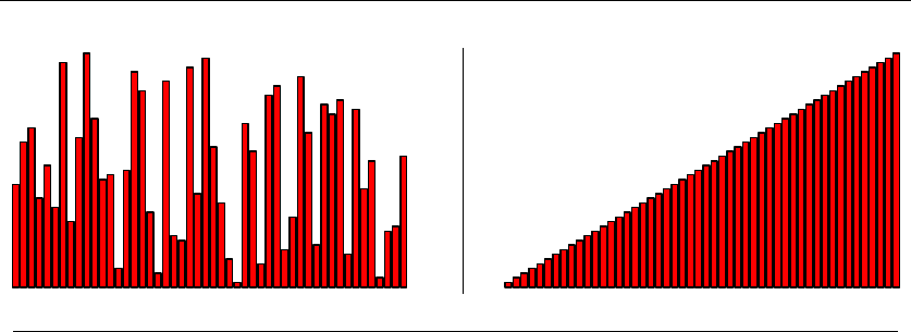
436 14. COMBINATORIAL PROBLEMS
INPUT OUTPUT
14.1 Sorting
Input description:Asetofnitems.
Problem description: Arrange the items in increasing (or decreasing) order.
Discussion: Sorting is the most fundamental algorithmic problem in computer
science. Learning the different sorting algorithms is like learning scales for a mu-
sician. Sorting is the first step in solving a host of other algorithm problems, as
shown in Section 4.2 (page 107). Indeed, “when in doubt, sort” is one of the first
rules of algorithm design.
Sorting also illustrates all the standard paradigms of algorithm design. The re-
sult is that most programmers are familiar with many different sorting algorithms,
which sows confusion as to which should be used for a given application. The
following criteria can help you decide:
•How many keys will you be sorting? – For small amounts of data (say n≤
100), it really doesn’t matter much which of the quadratic-time algorithms
you use. Insertion sort is faster, simpler, and less likely to be buggy than
bubblesort. Shellsort is closely related to, but much faster than, insertion
sort, but it involves looking up the right insert sequences in Knuth [Knu98].
When you have more than 100 items to sort, it is important to use an
O(nlg n)-time algorithm like heapsort, quicksort, or mergesort. There are
various partisans who favor one of these algorithms over the others, but since
it can be hard to tell which is fastest, it usually doesn’t matter.
Once you get past (say) 5,000,000 items, it is important to start thinking
about external-memory sorting algorithms that minimize disk access. Both
types of algorithm are discussed below.

14.1 SORTING 437
•Will there be duplicate keys in the data? – The sorted order is completely
defined if all items have distinct keys. However, when two items share the
same key, something else must determine which one comes first. In many
applications it doesn’t matter, so any sorting algorithm suffices. Ties are
often broken by sorting on a secondary key, like the first name or initial
when the family names collide.
Occasionally, ties need to be broken by their initial position in the data set.
Suppose the 5th and 27th items of the initial data set share the same key.
This means the 5th item must appear before the 27th in the final order.
Astable sorting algorithm preserves the original ordering in case of ties.
Most of the quadratic-time sorting algorithms are stable, while many of the
O(nlg n) algorithms are not. If it is important that your sort be stable, it is
probably better to explicitly use the initial position as a secondary key in your
comparison function rather than trust the stability of your implementation.
•What do you know about your data? – You can often exploit special knowledge
about your data to get it sorted faster or more easily. Of course, general
sorting is a fast O(nlg n) operation, so if the time spent sorting is really the
bottleneck in your application, you are a fortunate person indeed.
–Has the data already been partially sorted? If so, certain algorithms like
insertion sort perform better than they otherwise would.
–Do you know the distribution of the keys? If the keys are randomly or
uniformly distributed, a bucket or distribution sort makes sense. Throw
the keys into bins based on their first letter, and recur until each bin is
small enough to sort by brute force. This is very efficient when the keys
get evenly distributed into buckets. However, bucket sort would per-
form very badly sorting names on the membership roster of the “Smith
Society.”
–Are your keys very long or hard to compare? If your keys are long text
strings, it might pay to use a relatively short prefix (say ten characters)
of each key for an initial sort, and then resolve ties using the full key.
This is particularly important in external sorting (see below), since you
don’t want to waste your fast memory on the dead weight of irrelevant
detail.
Another idea might be to use radix sort. This always takes time linear
in the number of characters in the file, instead of O(nlg n) times the
cost of comparing two keys.
–Is the range of possible keys very small? If you want to sort a subset
of, say, n/2 distinct integers, each with a value from 1 to n, the fastest
algorithm would be to initialize an n-element bit vector, turn on the
bits corresponding to keys, then scan from left to right and report the
positions with true bits.

438 14. COMBINATORIAL PROBLEMS
•Do I have to worry about disk accesses? – In massive sorting problems, it may
not be possible to keep all data in memory simultaneously. Such a problem
is called external sorting, because one must use an external storage device.
Traditionally, this meant tape drives, and Knuth [Knu98] describes a variety
of intricate algorithms for efficiently merging data from different tapes. Today,
it usually means virtual memory and swapping. Any sorting algorithm will
run using virtual memory, but most will spend all their time swapping.
The simplest approach to external sorting loads the data into a B-tree (see
Section 12.1 (page 367)) and then does an in-order traversal of the tree to
read the keys off in sorted order. Real high-performance sorting algorithms are
based on multiway-mergesort. Files containing portions of the data are sorted
into runs using a fast internal sort, and then files with these sorted runs are
merged in stages using 2- or k-way merging. Complicated merging patterns
and buffer management based on the properties of the external storage device
can be used to optimize performance.
•How much time do you have to write and debug your routine? – If I had
under an hour to deliver a working routine, I would probably just implement
a simple selection sort. If I had an afternoon to build an efficient sort routine,
I would probably use heapsort, for it delivers reliable performance without
tuning.
The best general-purpose internal sorting algorithm is quicksort (see Section 4.2
(page 107)), although it requires tuning effort to achieve maximum performance.
Indeed, you are much better off using a library function instead of coding it your-
self. A poorly written quicksort will likely run more slowly than a poorly written
heapsort.
If you are determined to implement your own quicksort, use the following heuris-
tics, which make a big difference in practice:
•Use randomization – By randomly permuting (see Section 14.4 (page 448))
the keys before sorting, you can eliminate the potential embarrassment of
quadratic-time behavior on nearly-sorted data.
•Median of three – For your pivot element, use the median of the first, last,
and middle elements of the array to increase the likelihood of partitioning
the array into roughly equal pieces. Some experiments suggest using a larger
sample on big subarrays and a smaller sample on small ones.
•Leave small subarrays for insertion sort – Terminating the quicksort recursion
and switching to insertion sort makes sense when the subarrays get small,
say fewer than 20 elements. You should experiment to determine the best
switchpoint for your implementation.
•Do the smaller partition first – Assuming that your compiler is smart enough
to remove tail recursion, you can minimize run-time memory by processing

14.1 SORTING 439
the smaller partition before the larger one. Since successive stored calls are
at most half as large as the previous one, only O(lg n) stack space is needed.
Before you get started, see Bentley’s article on building a faster quicksort
[Ben92b].
Implementations: The best freely available sort program is presumably GNU
sort, part of the GNU core utilities library. See http://www.gnu.org/software/
coreutils/. Be aware that there are also commercial vendors of high-performance
external sorting programs. These include Cosort (www.cosort.com), Syncsort
(www.syncsort.com) and Ordinal Technology (www.ordinal.com).
Modern programming languages provide libraries offering complete and effi-
cient container implementations. Thus, you should never need to implement your
own sort routine. The C standard library contains qsort, a generic implementa-
tion of (presumably) quicksort. The C++ Standard Template Library (STL) pro-
vides both sort and stable sort methods. It is available with documentation
at http://www.sgi.com/tech/stl/. See Josuttis [Jos99], Meyers [Mey01] and Musser
[MDS01] for more detailed guides to using STL and the C++ standard library.
Java Collections (JC), a small library of data structures, is included in the
java.util package of Java standard edition (http://java.sun.com/javase/). In par-
ticular, SortedMap and SortedSet classes are provided.
For a C++ implementation of an cache-oblivious algorithm (funnelsort), check
out http://kristoffer.vinther.name/projects/funnelsort/. Benchmarks attest to its
excellent performance.
There are a variety of websites that provide applets/animations of all the ba-
sic sorting algorithms, including bubblesort, heapsort, mergesort, quicksort, radix
sort, and shellsort. Many of these are quite interesting to watch. Indeed, sort-
ing is the canonical problem for algorithm animation. Representative examples
include Harrison (http://www.cs.ubc.ca/spider/harrison/Java/sorting-demo.html)
and Bentley [Ben99] (http://www.cs.bell-labs.com/cm/cs/pearls/sortanim.html).
Notes:Knuth [Knu98] is the best book that has been written on sorting and indeed
is the best book that will ever be written on sorting. It is now over thirty years old,
but remains fascinating reading. One area that has developed since Knuth is sorting
under presortedness measures, surveyed in [ECW92]. A noteworthy reference on sorting
is [GBY91], which includes pointers to algorithms for partially sorted data and includes
implementations in C and Pascal for all of the fundamental algorithms.
Expositions on the basic internal sorting algorithms appear in every algorithms text.
Heapsort was first invented by Williams [Wil64]. Quicksort was invented by Hoare [Hoa62],
with careful analysis and implementation by Sedgewick [Sed78]. Von Neumann is credited
with having produced the first implementation of mergesort on the EDVAC in 1945. See
Knuth for a full discussion of the history of sorting, dating back to the days of punch-card
tabulating machines.
The primary competitive forum for high-performance sorting is an annual competition
initiated by the late Jim Gray. See http://research.microsoft.com/barc/SortBenchmark/
for current and previous results, which are are either inspiring or depressing depending

440 14. COMBINATORIAL PROBLEMS
upon how you look at it. The magnitude of progress is inspiring (the million-record in-
stances of the original benchmarks are now too small to bother with) but it is depressing
(to me) the extent that systems/memory management issues thoroughly trump the com-
binatorial/algorithmic aspects of sorting.
Modern attempts to engineer high-performance sort programs include work on both
cache-conscious [LL99] and cache-oblivious [BFV07] sorting.
Sorting has a well-known Ω(nlg n) lower bound under the algebraic decision tree model
[BO83]. Determining the exact number of comparisons required for sorting nelements,
for small values of n, has generated considerable study. See [Aig88, Raw92] for expositions
and Peczarski [Pec04, Pec07] for the latest results.
This lower-bound does not hold under different models of computation. Fredman and
Willard [FW93] present an O(n√lg n) algorithm for sorting under a model of computa-
tion that permits arithmetic operations on keys. See Andersson [And05] for a survey of
algorithms for fast sorting on such nonstandard models of computation.
Related Problems: Dictionaries (see page 367), searching (see page 441), topo-
logical sorting (see page 481).
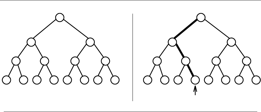
14.2 SEARCHING 441
H
D L
B
AC
F
EG
JN
IKMO
G ?
H
D L
B
AC
F
EG
JN
IKMO
G
INPUT OUTPUT
14.2 Searching
Input description:Asetofnkeys S, and a query key q.
Problem description: Where is qin S?
Discussion: “Searching” is a word that means different things to different people.
Searching for the global maximum or minimum of a function is the problem of
unconstrained optimization and is discussed in Section 13.5 (page 407). Chess-
playing programs select the best move to make via an exhaustive search of possible
moves using a variation of backtracking (see Section 7.1 (page 231)).
Here we consider the task of searching for a key in a list, array, or tree. Dictio-
nary data structures maintain efficient access to sets of keys under insertion and
deletion and are discussed in Section 12.1 (page 367). Typical dictionaries include
binary trees and hash tables.
We treat searching as a problem distinct from dictionaries because simpler
and more efficient solutions emerge when our primary interest is static searching
without insertion/deletion. These little data structures can yield large performance
improvements when properly employed in an innermost loop. Also, ideas such as
binary search and self-organization apply to other problems and well justify our
attention.
Our two basic approaches are sequential search and binary search. Both are
simple, yet have interesting and subtle variations. In sequential search, we start
from the front of our list/array of keys and compare each successive item against
the key until we find a match or reach the end. In binary search, we start with a
sorted array of keys. To search for key q, we compare qto the middle key Sn/2.Ifq
is before Sn/2, it must reside in the top half of our set; if not, it must reside in the

442 14. COMBINATORIAL PROBLEMS
bottom half of our set. By repeating this process on the correct half, we find the
key using lg ncomparisons. This is a big win over the n/2 comparisons we expect
with sequential search. See Section 4.9 (page 132) for more on binary search.
A sequential search is the simplest algorithm, and likely to be fastest on up to
about 20 elements. Beyond (say) 100 elements, binary search will clearly be more
efficient than sequential search, easily justifying the cost of sorting if there will be
multiple queries. Other issues come into play, however, in identifying the proper
variant of the algorithm:
•How much time can you spend programming? – A binary search is a noto-
riously tricky algorithm to program correctly. It took seventeen years after
its invention until the first correct version of a binary search was published!
Don’t be afraid to start from one of the implementations described below.
Test it completely by writing a driver that searches for every key in the set
Sas well as between the keys.
•Are certain items accessed more often than other ones? – Certain English
words (such as “the”) are much more likely to occur than others (such as
“defenestrate”). We can reduce the number of comparisons in a sequential
search by putting the most popular words on the top of the list and the
least popular ones at the bottom. Nonuniform access is usually the rule, not
the exception. Many real-world distributions are governed by power laws.A
classic example is word use in English, which is fairly accurately modeled by
Zipf’s law. Under Zipf ’s law,theith most frequently accessed key is selected
with probability (i−1)/i times the probability of the (i−1)st most popular
key, for all 1 ≤i≤n.
Knowledge of access frequencies is easy to exploit with sequential search.
But the issue is more complicated with binary trees. We want popular keys
close to the root (so we hit them quickly) but not at the expense of losing
balance and degenerating into sequential search. The answer is to employ a
dynamic programming algorithm to find the optimal binary search tree.The
key observation is that each possible root node ipartitions the space of keys
into those to the left of iand those to the right; each of which should be
represented by an optimal binary search tree on a smaller subrange of keys.
The root of the optimal tree is selected to minimize the expected search costs
of the resulting partition.
•Might access frequencies change over time? –Preorderingalistortreetoex-
ploit a skewed access pattern requires knowing the access pattern in advance.
For many applications, it can be difficult to obtain such information. Better
are self-organizing lists, where the order of the keys changes in response to the
queries. The best self-organizing scheme is move-to-front; that is, we move
the most recently searched-for key from its current position to the front of
the list. Popular keys keep getting boosted to the front, while unsearched-for

14.2 SEARCHING 443
keys drift towards the back of the list. There is no need to keep track of the
frequency of access; just move the keys on demand. Self-organizing lists also
exploit locality of reference, since accesses to a given key are likely to occur
in clusters. A hot key will be maintained near the top of the list during a
cluster of accesses, even if other keys have proven more popular in the past.
Self-organization can extend the useful size range of sequential search. How-
ever, you should switch to binary search beyond 100 elements. But consider
using splay trees. which are self-organizing binary search trees that rotate
each searched-for node to the root. They offer excellent amortized perfor-
mance guarantees.
•Is the key close by? – Suppose we know that the target key is to the right
of position p, and we think it is nearby. A sequential search is fast if we are
correct, but we will be punished severely when we guess wrong. A better idea
is to test repeatedly at larger intervals (p+1, p+2, p+4, p+8, p+ 16, ...)
to the right until we find a key to the right of our target. Now we have a
window containing the target and we can proceed with binary search.
Such a one-sided binary search finds the target at position p+lusing at most
2lg lcomparisons, so it is faster than binary search when l<<n,yetit
can never be much worse. One-sided binary search is particularly useful in
unbounded search problems, such as in numerical root finding.
•Is my data structure sitting on external memory? – Once the number of keys
grows too large, a binary search loses its status as the best search technique.
A binary search jumps wildly around the set of keys looking for midpoints to
compare, and so each comparison requires reading a new page in from external
memory. Much better are data structures such as B-trees (see Section 12.1
(page 367)) or Emde Boas trees (see notes below), which cluster the keys into
pages to minimize the number of disk accesses per search.
•Can I guess where the key should be? –Ininterpolation search, we exploit
our understanding of the distribution of keys to guess where to look next. An
interpolation search is probably a more accurate description of how we use
a telephone book than binary search. Suppose we are searching for Wash-
ington, George in a sorted telephone book. We would be safe making our
first comparison three-fourths of the way down the list, essentially doing two
comparisons for the price of one.
Although an interpolation search is an appealing idea, we caution against it
for three reasons: First, you have to work very hard to optimize your search
algorithm before you can hope for a speedup over binary search. Second, even
if you do beat a binary search, it is unlikely to be by enough to have justified
the exercise. Finally, your program will be much less robust and efficient when
the distribution changes, such as when your application gets ported to work
on French words instead of English.

444 14. COMBINATORIAL PROBLEMS
Implementations: The basic sequential and binary search algorithms are sim-
ple enough that you may consider implementing them yourself. That said,
the C standard library contains bsearch, a generic implementation of (pre-
sumably) a binary search. The C++ Standard Template Library (STL) pro-
vides find (sequential search) and binary search iterators. Java Collections
(JC), provides binarySearch in the java.util package of Java standard edition
(http://java.sun.com/javase/).
Many data structure textbooks provide extensive and illustrative imple-
mentations. Sedgewick (http://www.cs.princeton.edu/∼rs/) [Sed98] and Weiss
(http://www.cs.fiu.edu/∼weiss/) [Wei06] provide implementation of splay trees and
other search structures in both C++ and Java.
Notes:The Handbook of Data Structures and Applications [MS05] provides up-to-date
surveys on all aspects of dictionary data structures. Other surveys include Mehlhorn and
Tsakalidis [MT90b] and Gonnet and Baeza-Yates [GBY91]. Knuth [Knu97a] provides a
detailed analysis and exposition on all fundamental search algorithms and dictionary data
structures, but omits such modern data structures as red-black and splay trees.
The next position probed in linear interpolation search on an array of sorted numbers
is given by
next =(low −1) + q−S[low −1]
S[high +1]−S[low −1] ×(high −low +1)
where qis the query numerical key and Sthe sorted numerical array. If the keys are
drawn independently from a uniform distribution, the expected search time is O(lg lg n)
[DJP04, PIA78].
Nonuniform access patterns can be exploited in binary search trees by structuring
them so that popular keys are located near the root, thus minimizing search time. Dynamic
programming can be used to construct such optimal search trees in O(nlg n) time [Knu98].
Stout and Warren [SW86b] provide a slick algorithm to efficiently transform a binary tree
to a minimum height (optimally balanced) tree using rotations.
The Van Emde Boas layout of a binary tree (or sorted array) offers better external
memory performance than conventional binary search, at a cost of greater implementation
complexity. See the survey of Arge, et al. [ABF05] for more on this and other cache-
oblivious data structures.
Related Problems: Dictionaries (see page 367), sorting (see page 436).
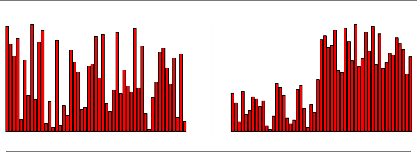
14.3 MEDIAN AND SELECTION 445
INPUT OUTPUT
14.3 Median and Selection
Input description:Asetofnnumbers or keys, and an integer k.
Problem description: Find the key smaller than exactly kof the nkeys.
Discussion: Median finding is an essential problem in statistics, where it provides
a more robust notion of average than the mean. The mean wealth of people who
have published research papers on sorting is significantly affected by the presence
of one William Gates [GP79], although his effect on the median wealth is merely
to cancel out one starving graduate student.
Median finding is a special case of the more general selection problem, which
asks for the kth element in sorted order. Selection arises in several applications:
•Filtering outlying elements – In dealing with noisy data, it is usually a good
idea to throw out (say) the 10% largest and smallest values. Selection can
be used to identify the items defining the 10th and 90th percentiles, and the
outliers then filtered out by comparing each item to the two selected bounds.
•Identifying the most promising candidates – In a computer chess program, we
might quickly evaluate all possible next moves, and then decide to study the
top 25% more carefully. Selection followed by filtering is the way to go.
•Deciles and related divisions – A useful way to present income distribution in
a population is to chart the salary of the people ranked at regular intervals,
say exactly at the 10th percentile, 20th percentile, etc. Computing these
values is simply selection on the appropriate position ranks.
•Order statistics – Particularly interesting special cases of selection include
finding the smallest element (k= 1), the largest element (k=n), and the
median element (k=n/2).

446 14. COMBINATORIAL PROBLEMS
The mean of nnumbers can be computed in linear time by summing the ele-
ments and dividing by n. However, finding the median is a more difficult problem.
Algorithms that compute the median can readily be generalized to arbitrary selec-
tion. Issues in median finding and selection include:
•How fast does it have to be? – The most elementary median-finding algorithm
sorts the items in O(nlg n) time and then returns the item occupying the
(n/2)nd position. The good thing is that this gives much more information
than just the median, enabling you to select the kth element (for any 1 ≤
k≤n) in constant time after the sort. However, there are faster algorithms
if all you want is the median.
In particular, there is an O(n)expected-time algorithm based on quicksort.
Select a random element in the data set as a pivot, and use it to partition
the data into sets of elements less than and greater than the pivot. From the
sizes of these sets, we know the position of the pivot in the total order, and
hence whether the median lies to the left or right of this point. Now we recur
on the appropriate subset until it converges on the median. This takes (on
average) O(lg n) iterations, with the cost of each iteration being roughly half
that of the previous one. This defines a geometric series that converges to
a linear-time algorithm, although if you are very unlucky it takes the same
time as quicksort, O(n2).
More complicated algorithms can find the median in worst-case linear time.
However, the expected-time algorithm will likely win in practice. Just make
sure to select random pivots to avoid the worst case.
•What if you only get to see each element once? – Selection and median finding
become expensive on large datasets because they typically require several
passes through external memory. In data-streaming applications, the volume
of data is often too large to store, making repeated consideration (and thus
exact median finding) impossible. Much better is computing a small summary
of the data for future analysis, say approximate deciles or frequency moments
(where the kth moment of stream xis defined as Fk=ixk
i).
One solution to such a problem is random sampling. Flip a coin for each value
to decide whether to store it, with the probability of heads set low enough
that you won’t overflow your buffer. Likely the median of your samples will
be close to that of the underlying data set. Alternately, you can devote some
fraction of memory to retaining (say) decile values of large blocks, and then
combine these decile distributions to yield more refined decile bounds.
•How fast can you find the mode? – Beyond mean and median lies a third
notion of average. The mode is defined to be the element that occurs the
greatest number of times in the data set. The best way to compute the mode
sorts the set in O(nlg n) time, which places all identical elements next to each
other. By doing a linear sweep from left to right on this sorted set, we can

14.3 MEDIAN AND SELECTION 447
count the length of the longest run of identical elements and hence compute
the mode in a total of O(nlg n) time.
In fact, there is no faster worst-case algorithm possible to compute the mode,
since the problem of testing whether there exist two identical elements in a
set (called element uniqueness) can be shown to have an Ω(nlog n) lower
bound. Element uniqueness is equivalent to asking whether the mode occurs
more than once. Possibilities exist, at least theoretically, for improvements
when the mode is large by using fast median computations.
Implementations: The C++ Standard Template Library (STL) provides a gen-
eral selection method (nth element) implemented using the linear expected-time
algorithm. It is available with documentation at http://www.sgi.com/tech/stl/. See
Josuttis [Jos99], Meyers [Mey01] and Musser [MDS01] for more detailed guides to
using STL and the C++ standard library.
Notes:The linear expected-time algorithm for median and selection is due to Hoare
[Hoa61]. Floyd and Rivest [FR75] provide an algorithm that uses fewer comparisons on
average. Good expositions on linear-time selection include [AHU74, BvG99, CLRS01,
Raw92], with [Raw92] being particularly enlightening.
Streaming algorithms have extensive applications to large data sets, and are well
surveyed by Muthukrishnan [Mut05].
A sport of considerable theoretical interest is determining exactly how many compar-
isons are sufficient to find the median of nitems. The linear-time algorithm of Blum et al.
[BFP+72] proves that c·nsuffice, but we want to know what cis. Dor and Zwick [DZ99]
proved that 2.95ncomparisons suffice to find the median. These algorithms attempt to
minimize the number of element comparisons but not the total number of operations, and
hence do not lead to faster algorithms in practice. They also hold the current best lower
bower bound of (2 + ) comparisons for median finding [DZ01].
Tight combinatorial bounds for selection problems are presented in [Aig88]. An opti-
mal algorithm for computing the mode is given by [DM80].
Related Problems: Priority queues (see page 373), sorting (see page 436).
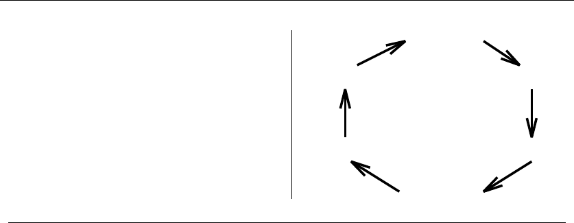
448 14. COMBINATORIAL PROBLEMS
{ 1, 2, 3 }
{ 1, 2, 3 }
{ 3, 2, 1 }
{ 2, 3, 1 }
{ 1, 3, 2 }
{ 3, 1, 2 }
{ 2, 1, 3 }
INPUT OUTPUT
14.4 Generating Permutations
Input description: An integer n.
Problem description: Generate (1) all, or (2) a random, or (3) the next permu-
tation of length n.
Discussion: A permutation describes an arrangement or ordering of items. Many
algorithmic problems in this catalog seek the best way to order a set of objects,
including traveling salesman (the least-cost order to visit ncities), bandwidth (order
the vertices of a graph on a line so as to minimize the length of the longest edge),
and graph isomorphism (order the vertices of one graph so that it is identical to
another). Any algorithm for solving such problems exactly must construct a series
of permutations along the way.
There are n! permutations of nitems. This grows so quickly that you can’t
really expect to generate all permutations for n>12, since 12! = 479,001,600.
Numbers like these should cool the ardor of anyone interested in exhaustive search
and help explain the importance of generating random permutations.
Fundamental to any permutation-generation algorithm is a notion of order, the
sequence in which the permutations are constructed from first to last. The most
natural generation order is lexicographic, the sequence they would appear if they
were sorted numerically. Lexicographic order for n=3is{1,2,3},{1,3,2},{2,1,3},
{2,3,1},{3,1,2}, and finally {3,2,1}. Although lexicographic order is aesthetically
pleasing, there is often no particular advantage to using it. For example, if you are
searching through a collection of files, it does not matter whether the filenames are
encountered in sorted order, so long as you eventually search through all of them.
Indeed, nonlexicographic orders lead to faster and simpler permutation generation
algorithms.

14.4 GENERATING PERMUTATIONS 449
There are two different paradigms for constructing permutations: rank-
ing/unranking and incremental change methods. The latter are more efficient,
but ranking and unranking can be applied to solve a much wider class of prob-
lems. The key is to define the functions rank and unrank on all permutations pand
integers n,m, where |p|=nand 0 ≤m≤n!.
•Rank(p) – What is the position of pin the given generation order? A typical
ranking function is recursive, such as basis case Rank({1}) = 0 with
Rank(p)=(p1−1) ·(|p|−1)! + Rank(p2,...,p
|p|)
Getting this right means relabeling the elements of the smaller permutation
to reflect the deleted first element. Thus
Rank({2,1,3})=1·2! + Rank({1,2})=2+0·1! + Rank({1})=2
•Unrank(m,n) – Which permutation is in position mof the n! permutations
of nitems? A typical unranking function finds the number of times (n−1)!
goes into mand proceeds recursively. Unrank(2,3) tells us that the first
element of the permutation must be ‘2’, since (2 −1) ·(3 −1)! ≤2 but
(3 −1) ·(3 −1)! >2. Deleting (2 −1) ·(3 −1)! from mleaves the smaller
problem Unrank(0,2). The ranking of 0 corresponds to the total order. The
total order on the two remaining elements (since 2 has been used) is {1,3},
so Unrank(2,3) = {2,1,3}.
What the actual rank and unrank functions are does not matter as much
as the fact that they must be inverses of each other. In other words, p=
Unrank(Rank(p),n) for all permutations p. Once you define ranking and unrank-
ing functions for permutations, you can solve a host of related problems:
•Sequencing permutations – To determine the next permutation that occurs
in order after p,wecanRank(p), add 1, and then Unrank(p). Similarly, the
permutation right before pin order is Unrank(Rank(p)−1,|p|). Counting
through the integers from 0 to n!−1 and unranking them is equivalent to
generating all permutations.
•Generating random permutations – Selecting a random integer from 0 to n!−1
and then unranking it yields a truly random permutation.
•Keep track of a set of permutations – Suppose we want to construct random
permutations and act only when we encounter one we have not seen before.
We can set up a bit vector (see Section 12.5 (page 385)) with n!bits,andset
bit ito 1 if permutation Unrank(i,n) has been seen. A similar technique was
employed with k-subsets in the Lotto application of Section 1.6 (page 23).

450 14. COMBINATORIAL PROBLEMS
This rank/unrank method is best suited for small values of n, since n!quickly
exceeds the capacity of machine integers unless arbitrary-precision arithmetic is
available (see Section 13.9 (page 423)). The incremental change methods work
by defining the next and previous operations to transform one permutation into
another, typically by swapping two elements. The tricky part is to schedule the
swaps so that permutations do not repeat until all of them have been generated.
The output picture above gives an ordering of the six permutations of {1,2,3}
using a single swap between successive permutations.
Incremental change algorithms for sequencing permutations are tricky, but they
are so concise that they can be expressed in a dozen-line program. See the imple-
mentation section for pointers to code. Because the incremental change is only a
single swap, these algorithms can be extremely fast—on average, constant time—
which is independent of the size of the permutation! The secret is to represent the
permutation using an n-element array to facilitate the swap. In certain applications,
only the change between permutations is important. For example, in a brute-force
program to search for the optimal TSP tour, the cost of the tour associated with
the new permutation will be that of the previous permutation, with the addition
and deletion of four edges.
Throughout this discussion, we have assumed that the items we are permuting
are all distinguishable. However, if there are duplicates (meaning our set is a multi-
set), you can save considerable time and effort by avoiding identical permutations.
For example, there are only ten distinct permutations of {1,1,2,2,2}, instead of
120. To avoid duplicates, use backtracking and generate the permutations in lexi-
cographic order.
Generating random permutations is an important little problem that people
often stumble across, and often botch up. The right way is to use the following
two-line, linear-time algorithm. We assume that Random[i,n] generates a random
integer between iand n, inclusive.
for i=1tondo a[i]=i;
for i=1ton−1doswap[a[i],a[Random[i, n]];
That this algorithm generates all permutations uniformly at random is not
obvious. If you think so, convincingly explain why the following algorithm does not
generate permutations uniformly:
for i=1tondo a[i]=i;
for i=1ton−1doswap[a[i],a[Random[1,n]];
Such subtleties demonstrate why you must be very careful with random gener-
ation algorithms. Indeed, we recommend that you try some reasonably extensive
experiments with any random generator before really believing it. For example,
generate 10,000 random permutations of length 4 and see whether all 24 distinct
permutations occur approximately the same number of times. If you know how to
measure statistical significance, you are in even better shape.

14.4 GENERATING PERMUTATIONS 451
Implementations: The C++ Standard Template Library (STL) provides two
functions (next permutation and prev permutation) for sequencing permuta-
tions in lexicographic order. Kreher and Stinson [KS99] provide implementa-
tions of minimum change and lexicographic permutation generation in C at
http://www.math.mtu.edu/∼kreher/cages/Src.html.
The Combinatorial Object Server (http://theory.cs.uvic.ca/) developed by
Frank Ruskey of the University of Victoria is a unique resource for generating per-
mutations, subsets, partitions, graphs, and other objects. An interactive interface
enables you to specify which objects you would like returned to you. Implementa-
tions in C, Pascal, and Java are available for certain types of objects.
C++ routines for generating an astonishing variety of combinatorial objects,
including permutations and cyclic permutations, are available at http://www.jjj.de/
fxt/.
Nijenhuis and Wilf [NW78] is a venerable but still excellent source on gen-
erating combinatorial objects. They provide efficient Fortran implementations of
algorithms to construct random permutations and to sequence permutations in
minimum-change order. Also included are routines to extract the cycle structure
of a permutation. See Section 19.1.10 (page 661) for details.
Combinatorica [PS03] provides Mathematica implementations of algorithms
that construct random permutations and sequence permutations in minimum
change and lexicographic orders. It also provides a backtracking routine to con-
struct all distinct permutations of a multiset, and it supports various permutation
group operations. See Section 19.1.9 (page 661).
Notes:The best recent reference on permutation generation is Knuth [Knu05a].
Sedgewick’s excellent survey on the topic is older [Sed77], but this is not a fast mov-
ing area. Good expositions include [KS99, NW78, Rus03].
Fast permutation generation methods make only a single swap between successive
permutations. The Johnson-Trotter algorithm [Joh63, Tro62] satisfies an even stronger
condition, namely that the two elements being swapped are always adjacent. Simple linear-
time ranking and unranking functions for permutations are given by Myrvold and Ruskey
[MR01].
In the days before ready access to computers, books with tables of random permu-
tations [MO63] were used instead of algorithms. The swap-based random permutation
algorithm presented above was first described in [MO63].
Related Problems: Random-number generation (see page 415), generating sub-
sets (see page 452), generating partitions (see page 456).
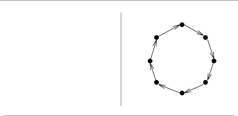
452 14. COMBINATORIAL PROBLEMS
{ 1, 2, 3 }
{ }
{1}
{1, 2}
{2}
{3}
{1, 3}
{1, 2, 3}
{2, 3}
INPUT OUTPUT
14.5 Generating Subsets
Input description: An integer n.
Problem description: Generate (1) all, or (2) a random, or (3) the next subset
of the integers {1,...,n}.
Discussion: A subset describes a selection of objects, where the order among them
does not matter. Many important algorithmic problems seek the best subset of a
group of things: vertex cover seeks the smallest subset of vertices to touch each
edge in a graph; knapsack seeks the most profitable subset of items of bounded
total size; while set packing seeks the smallest subset of subsets that together cover
each item exactly once.
There are 2ndistinct subsets of an n-element set, including the empty set as well
as the set itself. This grows exponentially, but at a considerably slower rate than
the n! permutations of nitems. Indeed, since 220 = 1,048,576, a brute-force search
through all subsets of 20 elements is easily manageable. Since 230 = 1,073,741,824,
you will certainly hit limits for slightly larger values of n.
By definition, the relative order among the elements does not distinguish differ-
ent subsets. Thus, {1,2,5}is the same as {2,1,5}. However, it is a very good idea
to maintain your subsets in a sorted or canonical order to speed up such operations
as testing whether or not two subsets are identical.
As with permutations (see Section 14.4 (page 448)), the key to subset generation
problems is establishing a numerical sequence among all 2nsubsets. There are three
primary alternatives:

14.5 GENERATING SUBSETS 453
•Lexicographic order – Lexicographic order means sorted order, and is often
the most natural way to generate combinatorial objects. The eight subsets of
{1,2,3}in lexicographic order are {},{1},{1,2},{1,2,3},{1,3},{2},{2,3},
and {3}. But it is surprisingly difficult to generate subsets in lexicographic
order. Unless you have a compelling reason to do so, don’t bother.
•Gray Code – A particularly interesting and useful subset sequence is the
minimum change order, wherein adjacent subsets differ by the insertion or
deletion of exactly one element. Such an ordering, called a Gray code, appears
in the output picture above.
Generating subsets in Gray code order can be very fast, because there is a
nice recursive construction. Construct a Gray code of n−1 elements Gn−1.
Reverse a second copy of Gn−1and add nto each subset in this copy. Then
concatenate them together to create Gn. Study the output example for clar-
ification.
Further, since only one element changes between subsets, exhaustive search
algorithms built on Gray codes can be quite efficient. A set cover program
would only have to update the change in coverage by the addition or deletion
of one subset. See the implementation section below for Gray code subset-
generation programs.
•Binary counting – The simplest approach to subset-generation problems is
based on the observation that any subset Sis defined by the items of that
Sare in S. We can represent Sby a binary string of nbits, where bit iis
1ifftheith element of Sis in S. This defines a bijection between the 2n
binary strings of length n,andthe2
nsubsets of nitems. For n= 3, binary
counting generates subsets in the following order: {},{3},{2},{2,3},{1},
{1,3},{1,2},{1,2,3}.
This binary representation is the key to solving all subset generation prob-
lems. To generate all subsets in order, simply count from 0 to 2n−1. For
each integer, successively mask off each of the bits and compose a subset of
exactly the items corresponding to 1 bits. To generate the next or previous
subset, increment or decrement the integer by one. Unranking a subset is ex-
actly the masking procedure, while ranking constructs a binary number with
1’s corresponding to items in Sand then converts this binary number to an
integer.
To generate a random subset, you might generate a random integer from 0
to 2n−1 and unrank, although how your random number generator rounds
things off might mean that certain subsets can never occur. Much better is
to flip a coin ntimes, with the ith flip deciding whether to include element i
in the subset. A coin flip can be robustly simulated by generating a random
real or large integer and testing whether it is bigger or smaller than half its
range. A Boolean array of nitems can thus be used to represent subsets as a
sort of premasked integer.

454 14. COMBINATORIAL PROBLEMS
Generation problems for two closely related problems arise often in practice:
•K-subsets – Instead of constructing all subsets, we may only be interested in
the subsets containing exactly kelements. There are n
ksuch subsets, which
is substantially less than 2n, particularly for small values of k.
The best way to construct all k-subsets is in lexicographic order. The ranking
function is based on the observation that there are n−f
k−1k-subsets whose
smallest element is f. Using this, it is possible to determine the smallest
element in the mth k-subset of nitems. We then proceed recursively for
subsequent elements of the subset. See the implementations below for details.
•Strings – Generating all subsets is equivalent to generating all 2nstrings of
true and false. The same basic techniques apply to generate all or random
strings on alphabets of size α, except there will be αnstrings in total.
Implementations: Kreher and Stinson [KS99] provide generators for both subsets
and k-subsets, including lexicographic and Gray code orders. These implementa-
tions in C are available at http://www.math.mtu.edu/∼kreher/cages/Src.html.
The Combinatorial Object Server (http://theory.cs.uvic.ca/), developed by
Frank Ruskey of the University of Victoria, is a unique resource for generating per-
mutations, subsets, partitions, graphs, and other objects. An interactive interface
enables you to specify which objects you would like returned to you. Implementa-
tions in C, Pascal, and Java are available for certain types of objects.
C++ routines for generating an astonishing variety of combinatorial objects,
including subsets and k-subsets (combinations), are available in the combinatorics
package at http://www.jjj.de/fxt/.
Nijenhuis and Wilf [NW78] is a venerable but still excellent source on gen-
erating combinatorial objects. They provide efficient Fortran implementations of
algorithms to construct random subsets and to sequence subsets in Gray code and
lexicographic order. They also provide routines to construct random k-subsets and
sequence them in lexicographic order. See Section 19.1.10 (page 661) for details on
ftp-ing these programs. Algorithm 515 [BL77] of the Collected Algorithms of the
ACM is another Fortran implementation of lexicographic k-subsets, available from
Netlib (see Section 19.1.5 (page 659)).
Combinatorica [PS03] provides Mathematica implementations of algorithms
to construct random subsets and sequence subsets in Gray code, binary, and lex-
icographic order. They also provide routines to construct random k-subsets and
strings, and sequence them lexicographically. See Section 19.1.9 (page 661) for
further information on Combinatorica.
Notes:The best reference on subset generation is Knuth [Knu05b]. Good expositions
include [KS99, NW78, Rus03]. Wilf [Wil89] provides an update of [NW78], including a
thorough discussion of modern Gray code generation problems.

14.5 GENERATING SUBSETS 455
Gray codes were first developed [Gra53] to transmit digital information in a robust
manner over an analog channel. By assigning the code words in Gray code order, the
ith word differs only slightly from the (i+ 1)st, so minor fluctuations in analog signal
strength corrupts only a few bits. Gray codes have a particularly nice correspondence to
Hamiltonian cycles on the hypercube. Savage [Sav97] gives an excellent survey of Gray
codes (minimum change orderings) for a large class of combinatorial objects, including
subsets.
The popular puzzle Spinout, manufactured by ThinkFun (formerly Binary Arts Cor-
poration), is solved using ideas from Gray codes.
Related Problems: Generating permutations (see page 448), generating parti-
tions (see page 456).
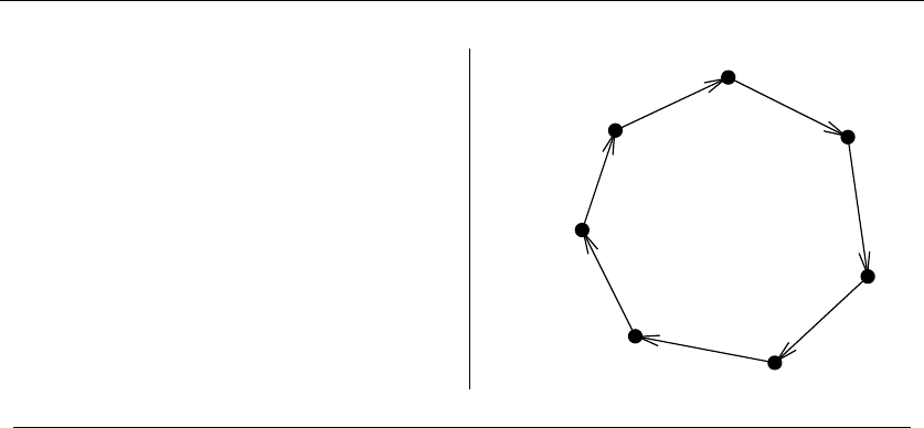
456 14. COMBINATORIAL PROBLEMS
N = 5
4+1
3+2
3
+1+1
1+1+1+1+1
5
2+2+1
2+1+1+1
INPUT OUTPUT
14.6 Generating Partitions
Input description: An integer n.
Problem description: Generate (1) all, or (2) a random, or (3) the next integer
or set partitions of length n.
Discussion: There are two different types of combinatorial objects denoted by
the word “partition,” namely integer partitions and set partitions. They are quite
different beasts, but it is a good idea to make both a part of your vocabulary:
•Integer partitions are multisets of nonzero integers that add up exactly to
n. For example, the seven distinct integer partitions of 5 are {5},{4,1},
{3,2},{3,1,1},{2,2,1},{2,1,1,1},and{1,1,1,1,1}. An interesting application
I encountered that required generating integer partitions was in a simulation
of nuclear fission. When an atom is smashed, the nucleus of protons and
neutrons is broken into a set of smaller clusters. The sum of the particles in
the set of clusters must equal the original size of the nucleus. As such, the
integer partitions of this original size represent all the possible ways to smash
an atom.
•Set partitions divide the elements 1,...,n into nonempty subsets. There are
15 distinct set partitions of n=4:{1234},{123,4},{124,3},{12,34},{12,3,4},
{134,2},{13,24},{13,2,4},{14,23},{1,234},{1,23,4},{14,2,3},{1,24,3},
{1,2,34},and{1,2,3,4}. Several algorithm problems return set partitions
as results, including vertex/edge coloring and connected components.

14.6 GENERATING PARTITIONS 457
Although the number of integer partitions grows exponentially with n, they do
so at a refreshingly slow rate. There are only 627 partitions of n= 20. It is even
possible to enumerate all integer partitions of n= 100, since there there are only
190,569,292 of them.
The easiest way to generate integer partitions is to construct them in lexi-
cographically decreasing order. The first partition is {n}itself. The general rule
is to subtract 1 from the smallest part that is >1 and then collect all the 1’s
so as to match the new smallest part >1. For example, the partition following
{4,3,3,3,1,1,1,1}is {4,3,3,2,2,2,1}, since the five 1’s left after 3 −1=2be-
comes the smallest part are best packaged as 2,2,1. When the partition is all 1’s,
we have completed one pass through all the partitions.
This algorithm is sufficiently intricate to program that you should consider
using one of the implementations below. In either case, test it to make sure that
you get exactly 627 distinct partitions for n= 20.
Generating integer partitions uniformly at random is a trickier business than
generating random permutations or subsets. This is because selecting the first (i.e.
largest) element of the partition has a dramatic effect on the number of possible
partitions that can be generated. Observe that no matter how large nis, there is
only one partition of nwhose largest part is 1. The number of partitions of nwith
largest part at most kis given by the recurrence
Pn,k =Pn−k,k +Pn,k−1
with the two boundary conditions Px−y,x =Px−y,x−yand Pn,1= 1. This function
can be used to select the largest part of your random partition with the correct
probabilities and, by proceeding recursively, to eventually construct the entire ran-
dom partition. Implementations are cited below.
Random partitions tend to have large numbers of fairly small parts, best visu-
alized by a Ferrers diagram as in Figure 14.1. Each row of the diagram corresponds
to one part of the partition, with the size of each part represented by that many
dots.
Set partitions can be generated using techniques akin to integer partitions. Each
set partition is encoded as a restricted growth function,a1,...,a
n, where a1=0
and ai≤1+max(a1,...,a
i), for i=2,...,n. Each distinct digit identifies a subset,
or block, of the partition, while the growth condition ensures that the blocks are
sorted into a canonical order based on the smallest element in each block. For
example, the restricted growth function 0,1,1,2,0,3,1 defines the set partition
{{1,5},{2,3,7},{4},{6}}.
Since there is a one-to-one equivalence between set partitions and restricted
growth functions, we can use lexicographic order on the restricted growth func-
tions to order the set partitions. Indeed, the fifteen partitions of {1,2,3,4}listed
above are sequenced according to the lexicographic order of their restricted growth
function (check it out).
We can use a similar counting strategy to generate random set partitions as we
did with integer partitions. The Stirling numbers of the second kind {n
k}count the
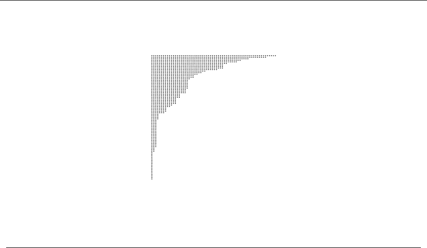
458 14. COMBINATORIAL PROBLEMS
Figure 14.1: The Ferrers diagram of a random partition of n= 1000
number of partitions of {1,...,n}with exactly kblocks. They are computed using
the recurrence
{n
k}={n−1
k−1}+k{n−1
k}
with the boundary conditions {n
n}={n
1}= 1. The reader is referred to the Notes
and Implementations section for more details.
Implementations: Kreher and Stinson [KS99] generate both integer and set par-
titions in lexicographic order, including ranking/unranking functions. These imple-
mentations in C are available at http://www.math.mtu.edu/∼kreher/cages/Src.html.
The Combinatorial Object Server (http://theory.cs.uvic.ca/) developed by
Frank Ruskey of the University of Victoria is a unique resource for generating
permutations, subsets, partitions, graphs, and other objects. An interactive inter-
face enables you to specify which objects you would like returned. Implementations
in C, Pascal, and Java are available for certain types of objects.
C++ routines for generating an astonishing variety of combinatorial objects,
including integer partitions and compositions, are available in the combinatorics
package at http://www.jjj.de/fxt/.
Nijenhuis and Wilf [NW78] is a venerable but still excellent source on gen-
erating combinatorial objects. They provide efficient Fortran implementations of
algorithms to construct random and sequential integer partitions, set partitions,
compositions, and Young tableaux. See Section 19.1.10 (page 661) for details.
Combinatorica [PS03] provides Mathematica implementations of algorithms
to construct random and sequential integer partitions, compositions, strings, and

14.6 GENERATING PARTITIONS 459
Young tableaux, as well as to count and manipulate these objects. See Section
19.1.9 (page 661).
Notes:The best reference on algorithms for generating both integer and set partitions is
Knuth [Knu05b]. Good expositions include [KS99, NW78, Rus03, PS03]. Andrews [And98]
is the primary reference on integer partitions and related topics, with [AE04] his more
accessible introduction.
Integer and set partitions are both special cases of multiset partitions, or set partitions
of nonnecessarily distinct numbers. In particular, the distinct set partitions on the multiset
{1,1,1,...,1}correspond exactly to integer partitions. Multiset partitions are discussed
in Knuth [Knu05b].
The (long) history of combinatorial object generation is detailed by Knuth [Knu06].
Particularly interesting are connections between set partitions and a Japanese incense
burning game, and the naming of all 52 set partitions for n= 5 with distinct chapters
from the oldest novel known, TheTaleofGenji.
Two related combinatorial objects are Young tableaux and integer compositions, al-
though they are less likely to emerge in applications. Generation algorithms for both are
presented in [NW78, Rus03, PS03].
Young tableaux are two-dimensional configurations of integers {1,...,n}where the
number of elements in each row is defined by an integer partition of n.Further,the
elements of each row and column are sorted in increasing order, and the rows are left-
justified. This notion of shape captures a wide variety of structures as special cases. They
have many interesting properties, including the existence of a bijection between pairs of
tableaux and permutations.
Compositions represent the possible assignments of a set of nindistinguishable balls
to kdistinguishable boxes. For example, we can place three balls into two boxes as {3,0},
{2,1},{1,2},or{0,3}. Compositions are most easily constructed sequentially in lexico-
graphic order. To construct them randomly, pick a random (k−1)-subset of n+k−1
items using the algorithm of Section 14.5 (page 452), and count the number of unselected
items between the selected ones. For example, if k= 5 and n= 10, the (5 −1) subset
{1,3,7,14}of 1,...,(n+k−1) = 14 defines the composition {0,1,3,6,0},sincethereare
no items to the left of element 1 nor right of element 14.
Related Problems: Generating permutations (see page 448), generating subsets
(see page 452).
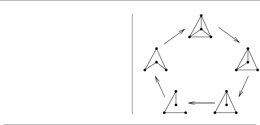
460 14. COMBINATORIAL PROBLEMS
N = 4
Connected
unlabeled
INPUT OUTPUT
14.7 Generating Graphs
Input description: Parameters describing the desired graph, including the num-
ber of vertices n, and the number of edges mor edge probability p.
Problem description: Generate (1) all, or (2) a random, or (3) the next graph
satisfying the parameters.
Discussion: Graph generation typically arises in constructing test data for pro-
grams. Perhaps you have two different programs that solve the same problem, and
you want to see which one is faster or make sure that they always give the same
answer. Another application is experimental graph theory, verifying whether a par-
ticular property is true for all graphs or how often it is true. It is much easier to
believe the four-color theorem after you have demonstrated four colorings for all
planar graphs on 15 vertices.
A different application of graph generation arises in network design. Suppose
you need to design a network linking ten machines using as few cables as possible,
such that this network can survive up to two vertex failures. One approach is to
test all the networks with a given number of edges until you find one that will
work. For larger graphs, heuristic approaches like simulated annealing will likely
be necessary.
Many factors complicate the problem of generating graphs. First, make sure
you know exactly what types of graphs you want to generate. Figure 5.2 on page
147 illustrates several important properties of graphs. For purposes of generation,
the most important questions are:

14.7 GENERATING GRAPHS 461
•Do I want labeled or unlabeled graphs? – The issue here is whether the names
of the vertices matter in deciding whether two graphs are the same. In gener-
ating labeled graphs, we seek to construct all possible labelings of all possible
graph topologies. In generating unlabeled graphs, we seek only one represen-
tative for each topology and ignore labelings. For example, there are only
two connected unlabeled graphs on three vertices—a triangle and a simple
path. However, there are four connected labeled graphs on three vertices—
one triangle and three 3-vertex paths, each distinguished by the name of their
central vertex. In general, labeled graphs are much easier to generate. How-
ever, there are so many more of them that you quickly get swamped with
isomorphic copies of the same few graphs.
•Do I want directed or undirected graphs? – Most natural generation algo-
rithms generate undirected graphs. These can be turned into directed graphs
by flipping coins to orient the edges. Any graph can be oriented to be directed
and acyclic (i.e. , a DAG) by randomly permuting the vertices on a line and
aiming each edge from left to right. With all such ideas, careful thought
must be given to decide whether you are generating all graphs uniformly at
random, and how much this matters to you.
You also must define what you mean by random. There are three primary mod-
els of random graphs, all of which generate graphs according to different probability
distributions:
•Random edge generation – The first model is parameterized by a given edge
probability p. Typically, p=0.5, although smaller values can be used to
construct sparser random graphs. In this model, a coin is flipped for each
pair of vertices xand yto decide whether to add an edge (x, y). All labeled
graphs will be generated with equal probability when p=1/2.
•Random edge selection – The second model is parameterized by the desired
number of edges m. It selects mdistinct edges uniformly at random. One
way to do this is by drawing random (x, y)-pairs and creating an edge if that
pair is not already in the graph. An alternative approach to computing the
same things constructs the set of n
2possible edges and selects a random
m-subset of them, as discussed in Section 14.5 (page 452).
•Preferential attachment – Under a rich-get-richer model, newly created edges
are likely to point to high-degree vertices than low-degree ones. Consider
new links (edges) being added to the graph of webpages. Under any realistic
web generation model, it is much more likely the next link will be to Google
than http://www.cs.sunysb.edu/∼algorith.1Selecting the next neighbor with
1Please link to us from your homepage to correct for this travesty.

462 14. COMBINATORIAL PROBLEMS
probability proportional to its degree yields graphs with power law properties
encountered in many real networks.
Which of these options best models your application? Probably none of them.
Random graphs have very little structure by definition. But graphs are used to
model relationships, which are often highly structured. Experiments conducted on
random graphs, although interesting and easy to perform, often fail to capture
what you are looking for.
An alternative to random graphs is “organic” graphs—graphs that reflect the
relationships among real-world objects. The Stanford GraphBase, discussed below,
is an outstanding source of organic graphs. Many raw sources of relationships are
available on the web that can be turned into interesting organic graphs with a
little programming and imagination. Consider the graph defined by a set of web-
pages, with any hyperlink between two pages defining an edge. Or, what about the
graph implicit in railroad, subway, or airline networks, with vertices being stations
and edges between two stations connected by direct service? As a final example,
every large computer program defines a call graph, where the vertices represent
subroutines, and there is an edge (x, y)ifxcalls y.
Two classes of graphs have particularly interesting generation algorithms:
•Trees –Pr¨ufer codes provide a simple way to rank and unrank labeled trees
and thus solve all standard generation problems (see Section 14.4 (page 448)).
There are exactly nn−2labeled trees on nvertices, and exactly that many
strings of length n−2 on the alphabet {1,2,...,n}.
The key to Pr¨ufer’s bijection is the observation that every tree has at least
two vertices of degree 1. Thus, in any labeled tree the vertex vincident on the
leaf with lowest label is well defined. We take vto be S1, the first character in
the code. We then delete the associated leaf and repeat the procedure until
only two vertices are left. This defines a unique code Sfor any given labeled
tree that can be used to rank the tree. To go from code to tree, observe that
the degree of vertex vin the tree is one more than the number of times v
occurs in S. The lowest-labeled leaf will be the smallest integer missing from
S, which when paired with S1determines the first edge of the tree. The entire
tree follows by induction.
Algorithms for efficiently generating unlabeled rooted trees are discussed in
the Implementation section.
•Fixed degree sequence graphs –Thedegree sequence of a graph Gis an integer
partition p=(p1,...,p
n), where piis the degree of the ith highest-degree
vertex of G. Since each edge contributes to the degree of two vertices, pis
an integer partition of 2m, where mis the number of edges in G.
Not all partitions correspond to degree sequences of graphs. However, there is
a recursive construction that constructs a graph with a given degree sequence
if one exists. If a partition is realizable, the highest-degree vertex v1can be

14.7 GENERATING GRAPHS 463
connected to the next p1highest-degree vertices in G, or the vertices corre-
sponding to parts p2,...,p
p1+1. Deleting p1and decrementing p2,...,p
p1+1
yields a smaller partition, which we recur on. If we terminate without ever
creating negative numbers, the partition was realizable. Since we always con-
nect the highest-degree vertex to other high-degree vertices, it is important
to reorder the parts of the partition by size after each iteration.
Although this construction is deterministic, a semi-random collection of
graphs realizing this degree sequence can be generated from Gusing edge-
flipping operations. Suppose edges (x, y) and (w, z)areinG, but (x, w)and
(y, z) are not. Exchanging these pairs of edges creates a different (not neces-
sarily connected) graph without changing the degrees of any vertex.
Implementations: The Stanford GraphBase [Knu94] is perhaps most useful as
an instance generator for constructing graphs to serve as test data for other pro-
grams. It incorporates graphs derived from interactions of characters in famous
novels, Roget’s Thesaurus, the Mona Lisa, expander graphs, and the economy
of the United States. It also contains routines for generating binary trees, graph
products, line graphs, and other operations on basic graphs. Finally, because of its
machine-independent, random-number generators, it provides a way to construct
random graphs such that they can be reconstructed elsewhere, thus making them
perfect for experimental comparisons of algorithms. See Section 19.1.8 (page 660)
for additional information.
Combinatorica [PS03] provides Mathematica generators for such graphs as
stars, wheels, complete graphs, random graphs and trees, and graphs with a
given degree sequence. Further, it includes operations to construct more interesting
graphs from these, including join, product, and line graph.
The Combinatorial Object Server (http://theory.cs.uvic.ca/) developed by
Frank Ruskey of the University of Victoria provides routines for generating both
free and rooted trees.
Viger [VL05] has made available a C++ implementation of his algorithm
to generate simple connected graphs with a prescribed degree sequence. See
http://www.liafa.jussieu.fr/∼fabien/generation/.
The graph isomorphism testing program Nauty (see Section 16.9 (page 550))
includes a suite of programs for generating nonisomorphic graphs, plus special
generators for bipartite graphs, digraphs, and multigraphs. They are available at
http://cs.anu.edu.au/∼bdm/nauty/.
The mathematicians Brendan McKay (http://cs.anu.edu.au/∼bdm/data/)and
Gordon Royle (http://people.csse.uwa.edu.au/gordon/data.html) provide exhaus-
tive catalogs of several families of graphs and trees up to the largest reasonable
number of vertices.
Nijenhuis and Wilf [NW78] provide efficient Fortran routines to enumerate all
labeled trees via Pr¨ufer codes and to construct random unlabeled rooted trees. See
Section 19.1.10 (page 661). Kreher and Stinson [KS99] generate labeled trees in C,

464 14. COMBINATORIAL PROBLEMS
with implementations available at http://www.math.mtu.edu/∼kreher/cages/Src.
html.
Notes:Extensive literature exists on generating graphs uniformly at random. Surveys
include [Gol93, Tin90]. Closely related to the problem of generating classes of graphs is
counting them. Harary and Palmer [HP73] survey results in graphical enumeration.
Knuth [Knu06] is the best recent reference on generating trees. The bijection between
n−2 strings and labeled trees is due to Pr¨ufer [Pr¨u18].
Random graph theory is concerned with the properties of random graphs. Threshold
laws in random graph theory define the edge density at which properties such as con-
nectedness become highly likely to occur. Expositions on random graph theory include
[Bol01, JLR00].
The preferential attachment model of graphical evolution has emerged relatively re-
cently in the study of networks. See [Bar03, Wat04] for introductions to this exciting
field.
An integer partition is graphic if there exists a simple graph with that degree sequence.
Erd˝os and Gallai [EG60] proved that a degree sequence is graphic if and only if the
sequence observes the following condition for each integer r<n:
r
i=1
di≤r(r−1) +
n
i=r+1
min(r, di)
Related Problems: Generating permutations (see page 448), graph isomorphism
(see page 550).

14.8 CALENDRICAL CALCULATIONS 465
December 21, 2012 ?
(Gregorian) 1934 Agrahayana 30 (Indian Civil)
13.0.0.0 (Mayan Long Count)
1434 Safar 7 (Islamic)
5773 Teveth 8 (Hebrew)
INPUT OUTPUT
14.8 Calendrical Calculations
Input description: A particular calendar date d, specified by month, day, and
year.
Problem description: Which day of the week did dfall on according to the given
calendar system?
Discussion: Many business applications need to perform calendrical calculations.
Perhaps we want to display a calendar of a specified month and year. Maybe we
need to compute what day of the week or year some event occurs, as in figuring
out the date on which a 180-day futures contract comes due. The importance of
correct calendrical calculations was perhaps best revealed by the furor over the
“Millennium bug”—the year 2000 crisis in legacy programs that allocated only
two digits for storing the year.
More complicated questions arise in international applications, because different
nations and ethnic groups use different calendar systems. Some of these, like the
Gregorian calendar used in most of the world, are based on the Sun, while others,
like the Hebrew calendar, are lunar calendars. How would you tell today’s date
according to the Chinese or Islamic calendar?
Calendrical calculations differ from other problems in this book because calen-
dars are historical objects, not mathematical ones. The algorithmic issues revolve
around specifying the rules of the calendrical system and implementing them cor-
rectly, rather than designing efficient shortcuts for the computation.
The basic approach underlying calendar systems is to start with a particular
reference date (called the epoch) and count up from there. The particular rules for
wrapping the count around into months and years is what distinguishes one system
from another. Implementing a calendar requires two functions, one that, given a
date, returns the integer number of days that have elapsed since the epoch, the
other of which takes an integer nand returns the calendar date exactly ndays

466 14. COMBINATORIAL PROBLEMS
from epoch. These are exactly analogous to the ranking and unranking rules for
combinatorial objects such as permutations (see Section 14.4 (page 448)).
That the solar year is not an integer number of days long is the major source of
complications in calendar systems. To keep a calendar’s annual dates in sync with
the seasons, leap days must be added at both regular and irregular intervals. Since
a solar year is 365 days and 5:49:12 hours long, adding a leap day every four years
leaves an extra 10 minutes and 48 seconds unaccounted for each year.
The original Julian calendar (from Julius Caesar) ignored these extra minutes,
which had accumulated to ten days by 1582. Pope Gregory XIII then proposed the
Gregorian calendar used today, by deleting the ten days and eliminating leap days
in years that are multiples of 100 but not 400. Supposedly, riots ensued because the
masses feared their lives were being shortened by ten days. Outside the Catholic
church, resistance to change slowed the reforms. The deletion of days did not occur
in England and America until September 1752, and not until 1927 in Turkey.
The rules for most calendrical systems are sufficiently complicated and pointless
that you should lift code from a reliable place rather than attempt to write your
own. We identify suitable implementations next.
There are a variety of “impress your friends” algorithms that enable you to
compute in your head what day of the week a particular date occurred. Such
algorithms often fail to work reliably outside the given century and certainly should
be avoided for computer implementation.
Implementations: Readily available calendar libraries exist in both C++ and
Java. The Boost time-data library provides a reliable implementation of the Gre-
gorian calendar in C++. See http://www.boost.org/doc/html/date time.html.The
Calendar class in java.util.Calendar implements the Gregorian calendar in Java.
Either of these will likely suffice for most applications.
Dershowitz and Reingold provide a uniform algorithmic presentation [RD01]
for a variety of different calendar systems, including the Gregorian, ISO, Chinese,
Hindu, Islamic, and Hebrew calendars, as well as other calendars of historical inter-
est. Calendrical is an implementation of these calendars in Common Lisp, Java, and
Mathematica, with routines to convert dates between calendars, day of the week
computations, and the determination of secular and religious holidays. Calendrical
is likely to be the most comprehensive and reliable calendrical routines available.
See their website at http://calendarists.com.
C and Java implementations of international calendars of unknown reliability
are readily available at SourceForge (http://sourceforge.net). Search for “Gregorian
calendar” to avoid the mass of datebook implementations.
Notes:A comprehensive discussion of calendrical computation algorithms appear in the
papers of Dershowitz and Reingold [DR90, RDC93], which have been superseded by their
book [RD01] that outlines algorithms for no less than 25 international and historical
calendars Three hundred years of calendars representing tabulations for all dates from
1900 to 2200 appear in [DR02].

14.8 CALENDRICAL CALCULATIONS 467
Concern exists in certain quarters whether December 21, 2012 represents the end
of the world. The argument rests on it being the date the Mayan calendar spins over to
13.0.0.0.0 after a 5,125 year cycle. The reader should rest assured, since I would never have
devoted so much effort to writing this book were the world to be ending so imminently.
The Mayan calendar is authoritatively described in [RD01].
Related Problems: Arbitrary-precision arithmetic (see page 423), generating per-
mutations (see page 448).

468 14. COMBINATORIAL PROBLEMS
$
I
H
G
F
D
C
B
A 1
2
A
B
C
D
F
G
H
I$
JAN FEB MAR APR MAY
INPUT OUTPUT
14.9 Job Scheduling
Input description: A directed acyclic graph G=(V,E), where vertices represent
jobs and edge (u, v) implies that task umust be completed before task v.
Problem description: What schedule of tasks completes the job using the mini-
mum amount of time or processors?
Discussion: Devising a proper schedule to satisfy a set of constraints is funda-
mental to many applications. Mapping tasks to processors is a critical aspect of
any parallel-processing system. Poor scheduling can leave all other machines sitting
idle while one bottleneck task is performed. Assigning people-to-jobs, meetings-to-
rooms, or courses-to-exam periods are all different examples of scheduling problems.
Scheduling problems differ widely in the nature of the constraints that must
be satisfied and the type of schedule desired. Several other catalog problems have
application to various kinds of scheduling:
•Topological sorting can construct a schedule consistent with the precedence
constraints. See Section 15.2 (page 481).
•Bipartite matching can assign a set of jobs to people who have the appropriate
skills for them. See Section 15.6 (page 498).
•Vertex and edge coloring can assign a set of jobs to time slots such that no
two interfering jobs are assigned the same time slot. See Sections 16.7 and
16.8.
•Traveling salesman can schedule select the most efficient route for a delivery
person to visit a given set of locations. See Section 16.4 (page 533).

14.9 JOB SCHEDULING 469
•Eulerian cycle can construct the most efficient route for a snowplow or mail-
man to completely traverse a given set of edges. See Section 15.7 (page 502).
Here we focus on precedence-constrained scheduling problems for directed acyclic
graphs. Suppose you have broken a big job into a large number of smaller tasks. For
each task, you know how long it should take (or perhaps an upper bound on how
long it might take). Further, for each pair of tasks you know whether it is essential
that one task be performed before the other. The fewer constraints we have to
enforce, the better our schedule can be. These constraints must define a directed
acyclic graph—acyclic because a cycle in the precedence constraints represents a
Catch-22 situation that can never be resolved.
We are interested in several problems on these networks:
•Critical path – The longest path from the start vertex to the completion
vertex defines the critical path. This can be important to know, for the only
way to shorten the minimum total completion time is to reduce the time of
one of the tasks on each critical path. The tasks on the critical paths can be
determined in O(n+m) time using the dynamic programming presented in
Section 15.4 (page 489).
•Minimum completion time – What is the fastest we can get this job completed
while respecting precedence constraints, assuming that we have an unlimited
number of workers. If there were no precedence constraints, each task could
be worked on by its own worker, and the total time would be that of the
longest single task. If there are such strict precedence constraints that each
task must follow the completion of its immediate predecessor, the minimum
completion time would be obtained by summing up the times for each task.
The minimum completion time for a DAG can be computed in O(n+m) time.
The completion time is defined by the critical path. To get such a schedule,
consider the jobs in topological order, and start each job on a new processor
the moment its latest prerequisite completes.
•What is the tradeoff between the number of workers and completion time? –
What we really are interested in is how best to complete the schedule with a
given number of workers. Unfortunately, this and most similar problems are
NP-complete.
Any real scheduling application is likely to present combinations of constraints
that will be difficult or impossible to model using these techniques. There are two
reasonable ways to deal with such problems. First, we can ignore constraints until
the problem reduces to one of the types that we have described here, solve it, and
then see how bad it is with respect to the other constraints. Perhaps the schedule
can be easily modified by hand to satisfy other esoteric constraints, like keeping
Joe and Bob apart so they won’t kill each other. Another approach is to formulate

470 14. COMBINATORIAL PROBLEMS
your scheduling problem via linear-integer programming (see Section 13.6 (page
411)) in all its complexity. I always recommend starting out with something simple
and see how it works before trying something complicated.
Another fundamental scheduling problem takes a set of jobs without precedence
constraints and assigns them to identical machines to minimize the total elapsed
time. Consider a copy shop with kXerox machines and a stack of jobs to finish
by the end of the day. Such tasks are called job-shop scheduling. They can be
modeled as bin-packing (see Section 17.9 (page 595)), where each job is assigned a
number equal to the number of hours it will take to complete, and each machine
is represented by a bin with space equal to the number of hours in a day.
More sophisticated variations of job-shop scheduling provide each task with
allowable start and required finishing times. Effective heuristics are known, based
on sorting the tasks by size and finishing time. We refer the reader to the references
for more information. Note that these scheduling problems become hard only when
the tasks cannot be broken up onto multiple machines or interrupted (preempted)
and then rescheduled. If your application allows these degrees of freedom, you
should exploit them.
Implementations: JOBSHOP is a collection of C programs for job-shop schedul-
ing created in the course of a computational study by Applegate and Cook [AC91].
They are available at http://www2.isye.gatech.edu/∼wcook/jobshop/.
Tablix (http://tablix.org) is an open source program for solving timetabling
problems faced by real schools. Support for parallel/cluster computation is pro-
vided.
LEKIN is a flexible job-shop scheduling system designed for educational
use [Pin02]. It supports single machine, parallel machines, flow-shop, flexi-
ble flow-shop, job-shop, and flexible job-shop scheduling, and is available at
http://www.stern.nyu.edu/om/software/lekin.
For commercial scheduling applications, ILOG CP is reflective of the state-of-
the-art. For more, see http://www.ilog.com/products/cp/.
Algorithm 520 [WBCS77] of the Collected Algorithms of the ACM is a For-
tran code for multiple-resource network scheduling. It is available from Netlib (see
Section 19.1.5 (page 659)).
Notes:The literature on scheduling algorithms is a vast one. Brucker [Bru07] and Pinedo
[Pin02] provide comprehensive overviews of the field. The Handbook of Scheduling [LA04]
provides an up-to-date collection of surveys on all aspects of scheduling.
A well-defined taxonomy exists covering thousands of job-shop scheduling variants,
which classifies each problem α|β|γaccordingto(α) the machine environment, (β) details
of processing characteristics and constraints, and (γ) the objectives to be minimized.
Surveys of results include [Bru07, CPW98, LLK83, Pin02].
Gantt charts provide visual representations of job-shop scheduling solutions, where
the x-axis represents time and rows represent distinct machines. The output figure above
illustrates a Gantt chart. Each scheduled job is represented as a horizontal block, thus
identifying its start-time, duration, and server. Project precedence-constrained scheduling

14.9 JOB SCHEDULING 471
techniques are often called PERT/CPM, for Program Evaluation and Review Tech-
nique/Critical Path Method. Both Gantt charts and PERT/CPM appear in most text-
books on operations research, including [Pin02].
Timetabling is a term often used in discussion of classroom and related schedul-
ing problems. PATAT (for Practice and Theory of Automated Timetabling)isabi-
annual conference reporting new results in the field. Its proceedings are available from
http://www.asap.cs.nott.ac.uk/patat/patat-index.shtml.
Related Problems: Topological sorting (see page 481), matching (see page 498),
vertex coloring (see page 544), edge coloring (see page 548), bin packing (see page
595).
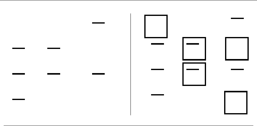
472 14. COMBINATORIAL PROBLEMS
( X1 or X2 or X3 )
( X1 or X2 or X3 )
( X1 or X2 or X3 )
( X1 or X2 or X3 ) ( X1 or X2 or X3 )
( X1 or X2 or X3 )
( X1 or X2 or X3 )
( X1 or X2 or X3 )
INPUT OUTPUT
14.10 Satisfiability
Input description: A set of clauses in conjunctive normal form.
Problem description: Is there a truth assignment to the Boolean variables such
that every clause is simultaneously satisfied?
Discussion: Satisfiability arises whenever we seek a configuration or object that
must be consistent with (i.e. , satisfy) a set of logical constraints. A primary ap-
plication is in verifying that a hardware or software system design works correctly
on all inputs. Suppose a given logical formula S(¯
X) denotes the specified result
on input variables ¯
X=X1,...,X
n, while a different formula C(¯
X) denotes the
Boolean logic of a proposed circuit for computing S(¯
X). This circuit is correct
unless there exists an ¯
Xsuch that S(¯
X)=C(¯
X).
Satisfiability (or SAT) is the original NP-complete problem. Despite its ap-
plications to constraint satisfaction, logic, and automatic theorem proving, it is
perhaps most important theoretically as the root problem from which all other
NP-completeness proofs originate. So much engineering has gone into today’s best
SAT solvers that they represent a reasonable starting point if one really needs to
solve an NP-complete problem exactly. That said, employing heuristics that give
good but nonoptimal solutions is usually the better approach in practice.
Issues in satisfiability testing include:
•Is your formula the AND of ORs (CNF) or the OR of ANDs (DNF)? –
In satisfiability, constraints are specified as a logical formula. There are two

14.10 SATISFIABILITY 473
primary ways of expressing logical formulas—conjunctive normal form (CNF)
and disjunctive normal form (DNF). In CNF formulas, we must satisfy all
clauses, where each clause is constructed by and-ing or’s of literals together,
such as
(v1or ¯v2) and (v2or v3)
In DNF formulas, we must satisfy any one clause, where each clause is con-
structed by or-ing ands of literals together. The formula above can be written
in DNF as
(¯v1and ¯v2and v3)or(¯v1and v2and ¯v3)or(¯v1and v2and v3)or(v1and ¯v2and v3)
Solving DNF-satisfiability is trivial, since any DNF formula can be satisfied
unless every clause contains both a literal and its complement (negation).
However, CNF-satisfiability is NP-complete. This seems paradoxical, since
we can use De Morgan’s laws to convert CNF-formulae into equivalent DNF-
formulae, and vice versa. The catch is that an exponential number of terms
might be constructed in the course of translation, so that the translation
itself does not run in polynomial time.
•How big are your clauses? –k-SAT is a special case of satisfiability when each
clause contains at most kliterals. The problem of 1-SAT is trivial, since we
must set true any literal appearing in any clause. The problem of 2-SAT is
not trivial, but can still be solved in linear time. This is interesting, because
certain problems can be modeled as 2-SAT using a little cleverness. The good
times end as soon as clauses contain three literals each (i.e. , 3-SAT) for 3-SAT
is NP-complete.
•Does it suffice to satisfy most of the clauses? – If you must solve it exactly,
there is not much you can do to solve satisfiability except by backtracking
algorithms such as the Davis-Putnam procedure. In the worst case, there
are 2mtruth assignments to be tested, but fortunately there are many ways
to prune the search. Although satisfiability is NP-complete, how hard it is
in practice depends on how the instances are generated. Naturally defined
“random” instances are often surprisingly easy to solve, and in fact it is
nontrivial to generate instances of the problem that are truly hard.
Still, we can benefit by relaxing the problem so that the goal becomes satis-
fying as many clauses as possible. Optimization techniques such as simulated
annealing can then be put to work to refine random or heuristic solutions. In-
deed, any random truth assignment to the variables will satisfy each k-SAT
clause with probability 1 −(1/2)k, so our first attempt is likely to satisfy
most of the clauses. Finishing off the job is the hard part. Finding an assign-
ment that satisfies the maximum number of clauses is NP-complete even for
nonsatisfiable instances.

474 14. COMBINATORIAL PROBLEMS
When faced with a problem of unknown complexity, proving it NP-complete
can be an important first step. If you think your problem might be hard, skim
through Garey and Johnson [GJ79] looking for your problem. If you don’t find
it, I recommend that you put the book away and try to prove hardness from
first principles, using the basic problems of 3-SAT, vertex cover, independent set,
integer partition, clique, and Hamiltonian cycle. I find it much easier to start from
these than some complicated problem in the book, and more insightful too, since
the reason for the hardness is not obscured by the hidden hardness proof for the
complicated problem. Chapter 9 focuses on strategies for proving hardness.
Implementations: Recent years have seen tremendous progress in the perfor-
mance of SAT solvers. An annual SAT competition identifies the top performing
solvers in each of three categories of instances (drawn from industrial, handmade,
and random problem instances, respectively).
The top three programs of the SAT 2007 industrial competition were Rsat
(http://reasoning.cs.ucla.edu/rsat/), PicoSAT (http://fmv.jku.at/picosat/)and
MiniSAT (http://www.cs.chalmers.se/Cs/Research/FormalMethods/MiniSat/).
The source code for all these solvers and more are available from the competi-
tion webpage (http://www.satcompetition.org/).
SAT Live! (http://www.satlive.org/) is the most up-to-date source for papers,
programs, and test sets for satisfiability and related logic optimization problems.
Notes:The most comprehensive overview of satisfiability testing is Kautz, et al.
[KSBD07]. The Davis-Putnam-Logemann-Loveland (DPLL) algorithm is a backtracking
algorithm introduced in 1962 for solving satisfiability problems. Local search techniques
work better on certain classes of problems that are difficult for DPLL solvers. Chaff
[MMZ+01] is a particularly influential solver, available at http://www.princeton.edu/
∼chaff/. See [KS07] for a survey of recent progress in the field of satisfiability testing.
An algorithm for solving 3-SAT in worst-case O∗(1.4802n) appears in [DGH+02]. Effi-
cient (but nonpolynomial) algorithms for NP-complete problems are surveyed in [Woe03].
The primary reference on NP-completeness is [GJ79], featuring a list of roughly 400
NP-complete problems. The book remains an extremely useful reference; it is perhaps the
book I reach for most often. An occasional column by David Johnson in the Journal of
Algorithms and (now) ACM Transactions on Algorithms provides updates.
Good expositions of Cook’s theorem [Coo71], where satisfiability is proven hard, in-
clude [CLRS01, GJ79, KT06]. The importance of Cook’s result became clear in Karp’s
paper [Kar72], showing the hardness of over 20 different combinatorial problems.
A linear-time algorithm for 2-SAT appears in [APT79]. See [WW95] for an interesting
application of 2-SAT to map labeling. The best heuristic known approximates maximum
2-SAT to within a factor of 1.0741 [FG95].
Related Problems: Constrained optimization (see page 407), traveling salesman
problem (see page 533).

15
Graph Problems: Polynomial-Time
Algorithmic graph problems constitute approximately one third of the problems
in this catalog. Problems from other sections could have been formulated equally
well in terms of graphs, such as bandwidth minimization and finite-state automata
optimization. Identifying the name of a graph-theoretic invariant or problem is one
of the primary skills of a good algorist. Indeed, the catalog will tell you exactly
how to proceed as soon as you figure out your particular problem’s name.
In this section, we deal only with problems for which there are efficient al-
gorithms to solve them. As there is often more than one way to model a given
application, it makes sense to look here before proceeding on to the harder formu-
lations.
The algorithms presented here have running times that grow polynomially with
the size of the graph. We adopt throughout the convention that nrefers to the
number of vertices in a graph, while mis the number of edges.
Graphs are often best understood as drawings. Many interesting graph proper-
ties follow from the nature of a particular type of drawing, such as planar graphs.
Thus, we also discuss algorithms for drawing graphs, trees, and planar graphs.
Most advanced graph algorithms are difficult to program. However, good im-
plementations are available if you know where to look. The best general sources
include LEDA [MN99] and the Boost Graph Library [SLL02]. However, better
special-purpose codes exist for many problems.
See the Handbook of Graph Algorithms [TNX08] for up-to-date surveys on all
areas of graph algorithms. Other excellent surveys include van Leeuwen [vL90a],
and several chapters in Atallah [Ata98]. Books specializing in graph algorithms
include:
•Sedgewick [Sed98] – The graph algorithms volume of this algorithms text
provides a comprehensive but gentle introduction to the field.
S.S. Skiena, The Algorithm Design Manual, 2nd ed., DOI: 10.1007/978-1-84800-070-4 15,
c
Springer-Verlag London Limited 2008

476 15. GRAPH PROBLEMS: POLYNOMIAL-TIME
•Ahuja, Magnanti, and Orlin [AMO93] – While purporting to be a book on
network flows, it covers the gamut of graph algorithms with an emphasis on
operations research. Strongly recommended.
•Gibbons [Gib85] – A good book on graph algorithms, including planarity test-
ing, matching, and Eulerian/Hamiltonian cycles, as well as more elementary
topics.
•Even [Eve79a] – An older but still respected advanced text on graph al-
gorithms, with a particularly thorough treatment of planarity-testing algo-
rithms.
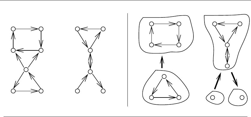
15.1 CONNECTED COMPONENTS 477
12
34
5
6 7
89
10
11
12 13
12
34
89
10
11
6 7
5
1312
INPUT OUTPUT
15.1 Connected Components
Input description: A directed or undirected graph G.
Problem description: Identify the different pieces or components of G, where
vertices xand yare members of different components if no path exists from xto
yin G.
Discussion: The connected components of a graph represent, in grossest terms,
the pieces of the graph. Two vertices are in the same component of Gif and only
if there exists some path between them.
Finding connected components is at the heart of many graph applications. For
example, consider the problem of identifying natural clusters in a set of items. We
represent each item by a vertex and add an edge between each pair of items deemed
“similar.” The connected components of this graph correspond to different classes
of items.
Testing whether a graph is connected is an essential preprocessing step for every
graph algorithm. Subtle, hard-to-detect bugs often result when an algorithm is run
only on one component of a disconnected graph. Connectivity tests are so quick
and easy that you should always verify the integrity of your input graph, even when
you know for certain that it has to be connected.
Testing the connectivity of any undirected graph is a job for either depth-first or
breadth-first search, as discussed in Section 5 (page 145). Which one you choose
doesn’t really matter. Both traversals initialize the component-number field for
each vertex to 0, and then start the search for component 1 from vertex v1.As
each vertex is discovered, the value of this field is set to the current component

478 15. GRAPH PROBLEMS: POLYNOMIAL-TIME
number. When the initial traversal ends, the component number is incremented,
and the search begins again from the first vertex whose component-number remains
0. Properly implemented using adjacency lists (as is done in Section 5.7.1 (page
166)) this runs in O(n+m) time.
Other notions of connectivity also arise in practice:
•What if my graph is directed? – There are two distinct notions of connected
components for directed graphs. A directed graph is weakly connected if it
would be connected by ignoring the direction of edges. Thus, a weakly con-
nected graph consists of a single piece. A directed graph is strongly connected
if there is a directed path between every pair of vertices. This distinction is
best made clear by considering the network of one- and two-way streets in
any city. The network is strongly connected if it is possible to drive legally
between every two positions. The network is weakly connected when it is
possible to drive legally or illegally between every two positions. The network
is disconnected if there is no possible way to drive from ato b.
Weakly and strongly connected components define unique partitions of the
vertices. The output figure at the beginning of this section illustrates a di-
rected graph consisting of two weakly or five strongly-connected components
(also called blocks of G).
Testing whether a directed graph is weakly connected can be done easily in
linear time. Simply turn all edges of Ginto undirected edges and use the
DFS-based connected components algorithm described previously. Tests for
strong connectivity are somewhat more complicated. The simplest linear-
time algorithm performs a search from some vertex vto demonstrate that
the entire graph is reachable from v. We then construct a graph Gwhere we
reverse all the edges of G. A traversal of Gfrom vsuffices to decide whether
all vertices of Gcan reach v.GraphGis strongly connected iff all vertices
can reach, and are reachable, from v.
All the strongly connected components of Gcan be extracted in linear time
using more sophisticated DFS-based algorithms. A generalization of the above
“two-DFS” idea is deceptively easy to program but somewhat subtle to un-
derstand exactly why it works:
1. Perform a DFS, starting from an arbitrary vertex in G, and labeling
each vertex in order of its completion (not discovery).
2. Reverse the direction of each edge in G, yielding G.
3. Perform a DFS of G, starting from the highest numbered vertex in G.
If this search does not completely traverse G, continue with the highest
numbered unvisited vertex.
4. Each DFS tree created in Step 3 is a strongly connected component.

15.1 CONNECTED COMPONENTS 479
My implementation of a single-pass algorithm appears in Section 5.10.2 (page
181). In either case, it is probably easier to start from an existing implemen-
tation than a textbook description.
•What is the weakest point in my graph/network? – A chain is only as strong
as its weakest link. Losing one or more internal links causes a chain to be-
come disconnected. The connectivity of graphs measures their strength—how
many edges or vertices must be removed to disconnect it. Connectivity is an
essential invariant for network design and other structural problems.
Algorithmic connectivity problems are discussed in Section 15.8 (page 505). In
particular, biconnected components are pieces of the graph that result from
cutting the edges incident on a single vertex. All biconnected components
can be found in linear time using DFS. See Section 5.9.2 (page 173) for an
implementation of this algorithm. Vertices whose deletion disconnects the
graph belong to more than one biconnected component, whose edges are
uniquely partitioned by components.
•Is the graph a tree? How can I find a cycle if one exists? – The problem of
cycle identification often arises, particularly with respect to directed graphs.
For example, testing if a sequence of conditions can deadlock often reduces
to cycle detection. If I am waiting for Fred, and Fred is waiting for Mary, and
Mary is waiting for me, there is a cycle and we are all deadlocked.
For undirected graphs, the analogous problem is tree identification. A tree
is, by definition, an undirected, connected graph without any cycles. As de-
scribed above, a depth-first search can be used to test whether it is connected.
If the graph is connected and has n−1 edges for nvertices, it is a tree.
Depth-first search can be used to find cycles in both directed and undirected
graphs. Whenever we encounter a back edge in our DFS—i.e. , an edge to an
ancestor vertex in the DFS tree—the back edge and the tree together define
a directed cycle. No other such cycle can exist in a directed graph. Directed
graphs without cycles are called DAGs (directed acyclic graphs). Topological
sorting (see Section 15.2 (page 481)) is the fundamental operation on DAGs.
Implementations: The graph data structure implementations of Section 12.4
(page 381) all include implementations of BFS/DFS, and hence connectiv-
ity testing to at least some degree. The C++ Boost Graph Library [SLL02]
(http://www.boost.org/libs/graph/doc) provides implementations of connected com-
ponents and strongly connected components. LEDA (see Section 19.1.1 (page 658))
provides these plus biconnected and triconnected components, breadth-first and
depth-first search, connected components and strongly connected components, all
in C++.
With respect to Java, JUNG (http://jung.sourceforge.net/) also provides bi-
connected component algorithms, while JGraphT (http://jgrapht.sourceforge.net/)
does strongly connected components.

480 15. GRAPH PROBLEMS: POLYNOMIAL-TIME
My (biased) preference for C language implementations of all basic graph con-
nectivity algorithms. including strongly connected components and biconnected
components, is the library associated with this book. See Section 19.1.10 (page
661) for details.
Notes:Depth-first search was first used to find paths out of mazes, and dates back to
the nineteenth century [Luc91, Tar95]. Breadth-first search was first reported to find the
shortest path by Moore in 1957 [Moo59].
Hopcroft and Tarjan [HT73b, Tar72] established depth-first search as a fundamen-
tal technique for efficient graph algorithms. Expositions on depth-first and breadth-first
search appear in every book discussing graph algorithms, with [CLRS01] perhaps the
most thorough description available.
The first linear-time algorithm for strongly connected components is due to Tarjan
[Tar72], with expositions including [BvG99, Eve79a, Man89]. Another algorithm—simpler
to program and slicker—for finding strongly connected components is due to Sharir and
Kosaraju. Good expositions of this algorithm appear in [AHU83, CLRS01]. Cheriyan and
Mehlhorn [CM96] propose improved algorithms for certain problems on dense graphs,
including strongly connected components.
Related Problems: Edge-vertex connectivity (see page 505), shortest path (see
page 489).
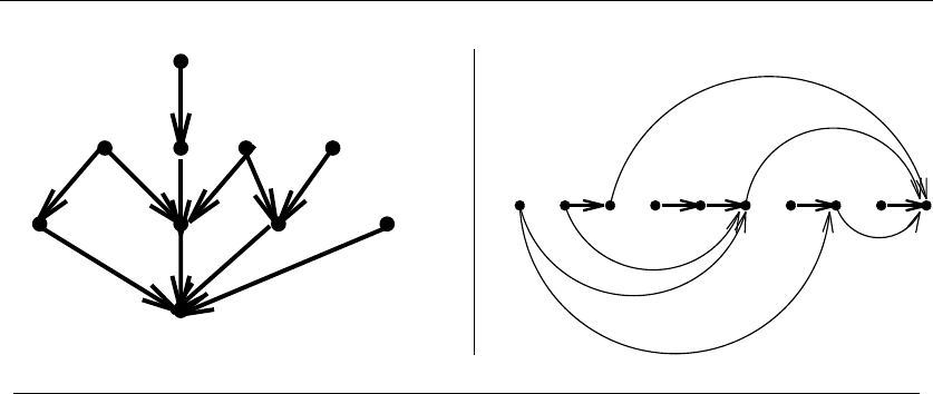
15.2 TOPOLOGICAL SORTING 481
8
4 69
7
1
32
5
10
6 10 5 8 4 2 9 3 7 1
INPUT OUTPUT
15.2 Topological Sorting
Input description: A directed acyclic graph G=(V, E), also known as a partial
order or poset.
Problem description: Find a linear ordering of the vertices of Vsuch that for
each edge (i, j)∈E, vertex iis to the left of vertex j.
Discussion: Topological sorting arises as a subproblem in most algorithms on
directed acyclic graphs. Topological sorting orders the vertices and edges of a DAG
in a simple and consistent way and hence plays the same role for DAGs that a
depth-first search does for general graphs.
Topological sorting can be used to schedule tasks under precedence constraints.
Suppose we have a set of tasks to do, but certain tasks have to be performed before
other tasks. These precedence constraints form a directed acyclic graph, and any
topological sort (also known as a linear extension) defines an order to do these
tasks such that each is performed only after all of its constraints are satisfied.
Three important facts about topological sorting are
1. Only DAGs can be topologically sorted, since any directed cycle provides an
inherent contradiction to a linear order of tasks.
2. Every DAG can be topologically sorted, so there must always be at least one
schedule for any reasonable precedence constraints among jobs.
3. DAGs can often be topologically sorted in many different ways, especially
when there are few constraints. Consider nunconstrained jobs. Any of the
n! permutations of the jobs constitutes a valid topological ordering.

482 15. GRAPH PROBLEMS: POLYNOMIAL-TIME
The conceptually simplest linear-time algorithm for topological sorting performs
a depth-first search of the DAG to identify the complete set of source vertices, where
source vertices are vertices of in-degree zero. At least one such source must exist in
any DAG. Source vertices can appear at the start of any schedule without violating
any constraints. Deleting all the outgoing edges of these source vertices will create
new source vertices, which can then sit comfortably to the immediate right of the
first set. We repeat until all vertices are accounted for. A modest amount of care
with data structures (adjacency lists and queues) is sufficient to make this run in
O(n+m) time.
An alternate algorithm makes use of the observation that ordering the vertices in
terms of decreasing DFS finishing time yields a linear extension. An implementation
of this algorithm with an argument for correctness is given in Section 5.10.1 (page
179).
Two special considerations with respect to topological sorting are:
•What if I need all the linear extensions, instead of just one of them? – In cer-
tain applications, it is important to construct all linear extensions of a DAG.
Beware, because the number of linear extensions can grow exponentially in
the size of the graph. Even the problem of counting the number of linear
extensions is NP-hard.
Algorithms for listing all linear extensions in a DAG are based on backtrack-
ing. They build all possible orderings from left to right, where each of the
in-degree zero vertices are candidates for the next vertex. The outgoing edges
from the selected vertex are deleted before moving on. An optimal algorithm
for listing (or counting) linear extensions is discussed in the notes.
Algorithms for constructing random linear extensions start from an arbitrary
linear extension. We then repeatedly sample pairs of vertices. These are ex-
changed if the resulting permutation remains a topological ordering. This
results in a random linear extension given enough random samples. See the
Notes section for details.
•What if your graph is not acyclic? – When a set of constraints contains
inherent contradictions, the natural problem becomes removing the smallest
set of items that eliminates all inconsistencies. The sets of offending jobs
(vertices) or constraints (edges) whose deletion leaves a DAG are known
as the feedback vertex set and the feedback arc set, respectively. They are
discussed in Section 16.11 (page 559). Unfortunately, both problems are NP-
complete.
Since the topological sorting algorithm gets stuck as soon as it identifies a
vertex on a directed cycle, we can delete the offending edge or vertex and
continue. This quick-and-dirty heuristic will eventually leave a DAG, but
might delete more things than necessary. Section 9.10.3 (page 348) describes
a better approach to the problem.

15.2 TOPOLOGICAL SORTING 483
Implementations: Essentially all the graph data structure implementations of
Section 12.4 (page 381) include implementations of topological sorting. This
means the Boost Graph Library [SLL02] (http://www.boost.org/libs/graph/doc)
and LEDA (see Section 19.1.1 (page 658)) for C++. For Java, the Data Struc-
tures Library in Java (JDSL) (http://www.jdsl.org/) includes a special routine
to compute a unit-weighted topological numbering. Also check out JGraphT
(http://jgrapht.sourceforge.net/).
The Combinatorial Object Server (http://theory.cs.uvic.ca/) provides C lan-
guage programs to generate linear extensions in both lexicographic and Gray code
orders, as well as count them. An interactive interface is also provided.
My (biased) preference for C language implementations of all basic graph algo-
rithms, including topological sorting, is the library associated with this book. See
Section 19.1.10 (page 661) for details.
Notes:Good expositions on topological sorting include [CLRS01, Man89]. Brightwell and
Winkler [BW91] prove that it is #P-complete to count the number of linear extensions
of a partial order. The complexity class #P includes NP, so any #P-complete problem is
at least NP-hard.
Pruesse and Ruskey [PR86] give an algorithm that generates linear extensions of a
DAG in constant amortized time. Further, each extension differs from its predecessor by
either one or two adjacent transpositions. This algorithm can be used to count the number
of linear extensions e(G)ofann-vertex DAG Gin O(n2+e(G)). Alternately, the reverse
search technique of Avis and Fukuda [AF96] can be employed to list linear extensions. A
backtracking program to generate all linear extensions is described in [KS74].
Huber [Hub06] gives an algorithm to sample linear extensions uniformly at random
from an arbitrary partial order in expected O(n3lg n) time, improving the result of [BD99].
Related Problems: Sorting (see page 436), feedback edge/vertex set (see page
559).
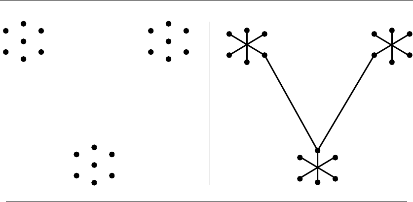
484 15. GRAPH PROBLEMS: POLYNOMIAL-TIME
INPUT OUTPUT
15.3 Minimum Spanning Tree
Input description: A graph G=(V,E) with weighted edges.
Problem description: The minimum weight subset of edges E⊂Ethat form a
tree on V.
Discussion: The minimum spanning tree (MST) of a graph defines the cheap-
est subset of edges that keeps the graph in one connected component. Telephone
companies are interested in minimum spanning trees, because the MST of a set of
locations defines the wiring scheme that connects the sites using as little wire as
possible. MST is the mother of all network design problems.
Minimum spanning trees prove important for several reasons:
•They can be computed quickly and easily, and create a sparse subgraph that
reflects a lot about the original graph.
•They provide a way to identify clusters in sets of points. Deleting the long
edges from an MST leaves connected components that define natural clusters
in the data set, as shown in the output figure above.
•They can be used to give approximate solutions to hard problems such as
Steiner tree and traveling salesman.
•As an educational tool, MST algorithms provide graphic evidence that greedy
algorithms can give provably optimal solutions.

15.3 MINIMUM SPANNING TREE 485
Three classical algorithms efficiently construct MSTs. Detailed implementations
of two of them (Prim’s and Kruskal’s) are given with correctness arguments in Sec-
tion 6.1 (page 192). The third somehow manages to be less well known despite being
invented first and (arguably) being both easier to implement and more efficient.
The contenders are
•Kruskal’s algorithm – Each vertex starts as a separate tree and these trees
merges together by repeatedly adding the lowest cost edge that spans two
distinct subtrees (i.e. , does not create a cycle).
Kruskal(G)
Sort the edges in order of increasing weight
count =0
while (count < n −1) do
get next edge (v, w)
if (component (v)= component(w))
add to T
component(v) = component(w)
The “which component?” tests can be efficiently implemented using the
union-find data structure (Section 12.5 (page 385)) to yield an O(mlg m)
algorithm.
•Prim’s algorithm – Starts with an arbitrary vertex vand “grows” a tree from
it, repeatedly finding the lowest-cost edge that links some new vertex into
this tree. During execution, we label each vertex as either in the tree, in the
fringe (meaning there exists an edge from a tree vertex), or unseen (meaning
the vertex is still more than one edge away from the tree).
Prim(G)
Select an arbitrary vertex to start
While (there are fringe vertices)
select minimum-weight edge between tree and fringe
add the selected edge and vertex to the tree
update the cost to all affected fringe vertices
This creates a spanning tree for any connected graph, since no cycle can be
introduced via edges between tree and fringe vertices. That it is in fact a
tree of minimum weight can be proven by contradiction. With simple data
structures, Prim’s algorithm can be implemented in O(n2) time.
•Boruvka’s algorithm – Rests on the observation that the lowest-weight edge
incident on each vertex must be in the minimum spanning tree. The union of
these edges will result in a spanning forest of at most n/2trees.Nowforeach
of these trees T, select the edge (x, y) of lowest weight such that x∈Tand

486 15. GRAPH PROBLEMS: POLYNOMIAL-TIME
y∈ T. Each of these edges must again be in an MST, and the union again
results in a spanning forest with at most half as many trees as before:
Boruvka(G)
Initialize spanning forest Fto nsingle-vertex trees
While (Fhas more than one tree)
for each Tin F, find the smallest edge from Tto G−T
add all selected edges to F, thus merging pairs of trees
The number of trees are at least halved in each round, so we get the MST
after at most lg niterations, each of which takes linear time. This gives an
O(mlog n) algorithm without using any fancy data structures.
MST is only one of several spanning tree problems that arise in practice. The
following questions will help you sort your way through them:
•Are the weights of all edges of your graph identical? – Every spanning tree
on npoints contains exactly n−1 edges. Thus, if your graph is unweighted,
any spanning tree will be a minimum spanning tree. Either breadth-first or
depth-first search can be used to find a rooted spanning tree in linear time.
DFS trees tend to be long and thin, while BFS trees better reflect the distance
structure of the graph, as discussed in Section 5 (page 145).
•Should I use Prim’s or Kruskal’s algorithm? – As implemented in Section 6.1
(page 192), Prim’s algorithm runs in O(n2), while Kruskal’s algorithm takes
O(mlog m) time. Thus Prim’s algorithm is faster on dense graphs, while
Kruskal’s is faster on sparse graphs.
That said, Prim’s algorithm can be implemented in O(m+nlg n) time using
more advanced data structures, and a Prim’s implementation using pairing
heaps would be the fastest practical choice for both sparse and dense graphs.
•What if my input is points in the plane, instead of a graph? – Geometric
instances, comprising npoints in d-dimensions, can be solved by constructing
the complete distance graph in O(n2) and then finding the MST of this
complete graph. However, for points in two dimensions, it is more efficient
to solve the geometric version of the problem directly. To find the minimum
spanning tree of npoints, first construct the Delaunay triangulation of these
points (see Sections 17.3 and 17.4). In two dimensions, this gives a graph
with O(n) edges that contains all the edges of the minimum spanning tree of
the point set. Running Kruskal’s algorithm on this sparse graph finishes the
job in O(nlg n) time.
•How do I find a spanning tree that avoids vertices of high degree? – Another
common goal of spanning tree problems is to minimize the maximum degree,

15.3 MINIMUM SPANNING TREE 487
typically to minimize the fan out in an interconnection network. Unfortu-
nately, finding a spanning tree of maximum degree 2 is NP-complete, since
this is identical to the Hamiltonian path problem. However, efficient algo-
rithms are known that construct spanning trees whose maximum degree is
at most one more than required. This is likely to suffice in practice. See the
references below.
Implementations: All the graph data structure implementations of Section 12.4
(page 381) should include implementations of Prim’s and/or Kruskal’s algorithms.
This includes the Boost Graph Library [SLL02] (http://www.boost.org/libs/graph/
doc) and LEDA (see Section 19.1.1 (page 658)) for C++. For some reason it does
not seem to include the Java graph libraries oriented around social networks, but
Prim and Kruskal are present in the Data Structures Library in Java (JDSL)
(http://www.jdsl.org/).
Timing experiments on MST algorithms produce contradicting results, sug-
gesting the stakes are really too low to matter. Pascal implementations of Prim’s,
Kruskal’s, and the Cheriton-Tarjan algorithm are provided in [MS91], along with
extensive empirical analysis proving that Prim’s algorithm with the appropriate
priority queue is fastest on most graphs. The programs in [MS91] are available
by anonymous FTP from cs.unm.edu in directory /pub/moret shapiro. Kruskal’s
algorithm proved the fastest of four different MST algorithms in the Stanford
GraphBase (see Section 19.1.8 (page 660)).
Combinatorica [PS03] provides Mathematica implementations of Kruskal’s
MST algorithm and quickly counting the number of spanning trees of a graph.
See Section 19.1.9 (page 661).
My (biased) preference for C language implementations of all basic graph algo-
rithms, including minimum spanning trees, is the library associated with this book.
See Section 19.1.10 (page 661) for details.
Notes:The MST problem dates back to Boruvka’s algorithm in 1926. Prim’s [Pri57] and
Kruskal’s [Kru56] algorithms did not appear until the mid-1950’s. Prim’s algorithm was
then rediscovered by Dijkstra [Dij59]. See [GH85] for more on the interesting history of
MST algorithms. Wu and Chao [WC04b] have written a monograph on MSTs and related
problems.
The fastest implementations of Prim’s and Kruskal’s algorithms use Fibonacci heaps
[FT87]. However, pairing heaps have been proposed to realize the same bounds with less
overhead. Experiments with pairing heaps are reported in [SV87].
A simple combination of Boruvka’s algorithm with Prim’s algorithm yields an
O(mlg lg n) algorithm. Run Borukva’s algorithm for lg lg niterations, yielding a forest
of at most n/ lg ntrees. Now create a graph Gwith one vertex for each tree in this
forest, with the weight of the edge between trees Tiand Tjset to the lightest edge (x, y),
where x∈Tiand y∈Tj.TheMSTofGcoupled with the edges selected by Boruvka’s
algorithm yields the MST of G. Prim’s algorithm (implemented with Fibonacci heaps)
will take O(n+m)timeonthisn/ lg nvertex, medge graph.

488 15. GRAPH PROBLEMS: POLYNOMIAL-TIME
The best theoretical bounds on finding MSTs tell a complicated story. Karger, Klein,
and Tarjan [KKT95] give a linear-time randomized algorithm for MSTs, based again
on Borukva’s algorithm. Chazelle [Cha00] gave a deterministic O(nα(m, n)) algorithm,
where α(m, n) is the inverse Ackerman function. Pettie and Ramachandran [PR02] give
an provably optimal algorithm whose exact running time is (paradoxically) unknown, but
lies between Ω(n+m)andO(nα(m, n)).
Aspanner S(G)ofagivengraphGis a subgraph that offers an effective compromise
between two competing network objectives. To be precise, they have total weight close
to the MST of G, while guaranteeing that the shortest path between vertices xand yin
S(G) approaches the shortest path in the full graph G. The monograph of Narasimhan
and Smid [NS07] provides a complete, up-to-date survey on spanner networks.
The O(nlog n) algorithm for Euclidean MSTs is due to Shamos, and discussed in
computational geometry texts such as [dBvKOS00, PS85].
F¨urer and Raghavachari [FR94] give an algorithm that constructs a spanning tree
whose maximum degree is almost minimized—indeed is at most one more than the lowest-
degree spanning tree. The situation is analogous to Vizing’s theorem for edge coloring,
which also gives an approximation algorithm to within additive factor one. A recent
generalization [SL07] gives a polynomial-time algorithm for finding a spanning tree of
maximum degree ≤k+ 1 whose cost is no more than that of the optimal minimum
spanning tree of maximum degree ≤k.
Minimum spanning tree algorithms have an interpretation in terms of matroids,which
are systems of subsets closed under inclusion. The maximum weighted independent set
in matroids can be found using a greedy algorithm. The connection between greedy algo-
rithms and matroids was established by Edmonds [Edm71]. Expositions on the theory of
matroids include [Law76, PS98].
Dynamic graph algorithms seek to maintain an graph invariant (such as the MST) effi-
ciently under edge insertion or deletion operations. Holm et al. [HdlT01] gives an efficient,
deterministic algorithm to maintain MSTs (and several other invariants) in amortized
polylogarithmic time per update.
Algorithms for generating spanning trees in order from minimum to maximum weight
are presented in [Gab77]. The complete set of spanning trees of an unweighted graph can
be generated in constant amortized time. See Ruskey [Rus03] for an overview of algorithms
for generating, ranking, and unranking spanning trees.
Related Problems: Steiner tree (see page 555), traveling salesman (see page 533).
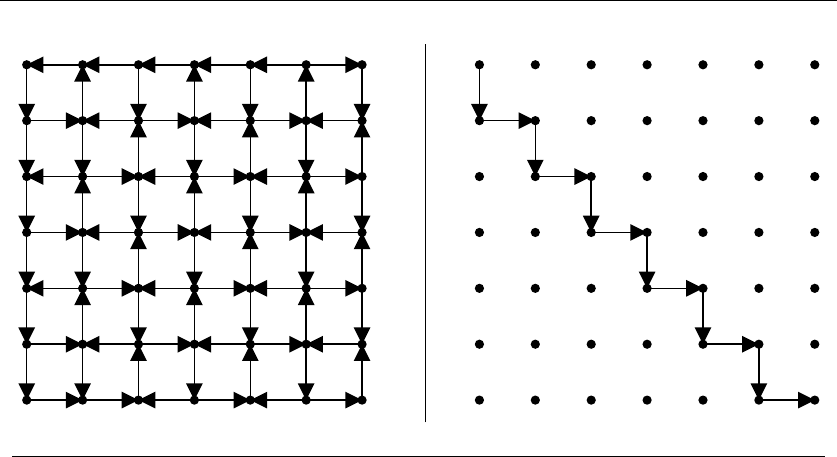
15.4 SHORTEST PATH 489
INPUT OUTPUT
15.4 Shortest Path
Input description: An edge-weighted graph G, with vertices sand t.
Problem description: Find the shortest path from sto tin G.
Discussion: The problem of finding shortest paths in a graph has several applica-
tions, some quite surprising:
•The most obvious applications arise in transportation or communications,
such as finding the best route to drive between Chicago and Phoenix or
figuring how to direct packets to a destination across a network.
•Consider the task of partitioning a digitized image into regions containing
distinct objects—a problem known as image segmentation. Separating lines
are needed to carve the space into regions, but what path should these lines
take through the grid? We may want a line that relatively directly goes from
xto y, but avoids cutting through object pixels as much as possible. This
grid of pixels can be modeled as a graph, with the cost of an edge reflecting
the color transitions between neighboring pixels. The shortest path from x
to yin this weighted graph defines the best separating line.
•Homophones are words that sound alike, such as to,two,andtoo. Distinguish-
ing between homophones is a major problem in speech recognition systems.

490 15. GRAPH PROBLEMS: POLYNOMIAL-TIME
The key is to bring some notion of grammatical constraints into the inter-
pretation. We map each string of phonemes (recognized sounds) into words
they might possibly match. We construct a graph whose vertices correspond
to these possible word interpretations, with edges between neighboring word-
interpretations. If we set the weight of each edge to reflect the likelihood of
transition, the shortest path across this graph defines the best interpretation
of the sentence. See Section 6.4 (page 212) for a more detailed account of a
similar application.
•Suppose we want to draw an informative visualization of a graph. The “cen-
ter” of the graph should appear near the center of the page. A good definition
of the graph center is the vertex that minimizes the maximum distance to
any other vertex in the graph. Identifying this center point requires knowing
the distance (i.e. , shortest path) between all pairs of vertices.
The primary algorithm for finding shortest paths is Dijkstra’s algorithm,which
efficiently computes the shortest path from a given starting vertex xto all n−1
other vertices. In each iteration, it identifies a new vertex vfor which the shortest
path from xto vis known. We maintain a set of vertices Sto which we currently
know the shortest path from v, and this set grows by one vertex in each iteration.
In each iteration, we identify the edge (u, v) where u, u∈Sand v, v∈V−Ssuch
that
dist(x, u)+weight(u, v) = min
(u,v)∈Edist(x, u)+weight(u,v
)
This edge (u, v) gets added to a shortest path tree, whose root is xand describes
all the shortest paths from x.
An O(n2) implementation of Dijkstra’s algorithm appears in in Section 6.3.1
(page 206). Theoretically faster times can be achieved using significantly more com-
plicated data structures, as described below. If we just need to know the shortest
path from xto y, terminate the algorithm as soon as yenters S.
Dijkstra’s algorithm is the right choice for single-source shortest path on posi-
tively weighted graphs. However, special circumstances dictate different choices:
•Is your graph weighted or unweighted? – If your graph is unweighted, a simple
breadth-first search starting from the source vertex will find the shortest path
to all other vertices in linear time. Only when edges have different weights
do you need more sophisticated algorithms. A breadth-first search is both
simpler and faster than Dijkstra’s algorithm.
•Does your graph have negative cost weights? – Dijkstra’s algorithm assumes
that all edges have positive cost. For graphs with edges of negative weight,
you must use the more general, but less efficient, Bellman-Ford algorithm.
Graphs with negative cost cycles are an even bigger problem. Observe that
the shortest xto ypath in such a graph is not defined because we can detour

15.4 SHORTEST PATH 491
from xto the negative cost cycle and repeatedly loop around it, making the
total cost arbitrarily small.
Note that adding a fixed amount of weight to make each edge positive does
not solve the problem. Dijkstra’s algorithm will then favor paths using a fewer
number of edges, even if those were not the shortest weighted paths in the
original graph.
•Is your input a set of geometric obstacles instead of a graph? –Manyap-
plications seek the shortest path between two points in a geometric setting,
such as an obstacle-filled room. The most straightforward solution is to con-
vert your problem into a graph of distances to feed to Dijkstra’s algorithm.
Vertices will correspond the vertices on the boundaries of the obstacles, with
edges defined only between pairs of vertices that “see” each other.
Alternately, there are more efficient geometric algorithms that compute the
shortest path directly from the arrangement of obstacles. See Section 17.14
(page 610) on motion planning and the Notes section for pointers to such
geometric algorithms.
•Is your graph acyclic—i.e. , a DAG? – Shortest paths in directed acyclic
graphs can be found in linear time. Perform a topological sort to order the
vertices such that all edges go from left to right starting from source s.The
distance from sto itself, d(s, s), clearly equals 0. We now process the vertices
from left to right. Observe that
d(s, j) = min
(x,i)∈Ed(s, i)+w(i, j)
since we already know the shortest path d(s, i) for all vertices to the left of j.
Indeed, most dynamic programming problems can be formulated as shortest
paths on specific DAGs. Note that the same algorithm (replacing min with
max) also suffices to find the longest path in a DAG, which is useful in many
applications like scheduling (see Section 14.9 (page 468)).
•Do you need the shortest path between all pairs of points? – If you are inter-
ested in the shortest path between all pairs of vertices, one solution is to run
Dijkstra ntimes, once with each vertex as the source. The Floyd-Warshall
algorithm is a slick O(n3) dynamic programming algorithm for all-pairs short-
est path, which is faster and easier to program than Dijkstra. It works with
negative cost edges but not cycles, and is presented with an implementa-
tion in Section 6.3.2 (page 210). Let Mdenote the distance matrix, where
Mij =∞if there is no edge (i, j):
D0=M
for k=1tondo
for i=1tondo
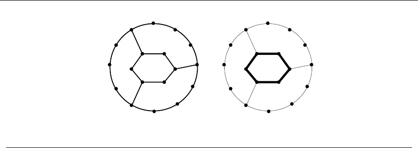
492 15. GRAPH PROBLEMS: POLYNOMIAL-TIME
Figure 15.1: The girth, or shortest cycle, in a graph
for j=1tondo
Dk
ij = min(Dk−1
ij ,D
k−1
ik +Dk−1
kj )
Return Dn
The key to understanding Floyd’s algorithm is that Dk
ij denotes “the length of
the shortest path from ito jthat goes through vertices 1,...,k as possible
intermediate vertices.” Note that O(n2) space suffices, since we only must
keep Dkand Dk−1around at time k.
•How do I find the shortest cycle in a graph? – One application of all-pairs
shortest path is to find the shortest cycle in a graph, called its girth. Floyd’s
algorithm can be used to compute dii for 1 ≤i≤n, which is the length of
the shortest way to get from vertex ito i—in other words, the shortest cycle
through i.
This might be what you want. The shortest cycle through xis likely to go
from xto yback to x, using the same edge twice. A simple cycle is one that
visits no edge or vertex twice. To find the shortest simple cycle, the easiest
approach is to compute the lengths of the shortest paths from ito all other
vertices, and then explicitly check whether there is an acceptable edge from
each vertex back to i.
Finding the longest cycle in a graph includes Hamiltonian cycle as a special
case (see Section 16.5), so it is NP-complete.
The all-pairs shortest path matrix can be used to compute several useful in-
variants related to the center of graph G.Theeccentricity of vertex vin a graph
is the shortest-path distance to the farthest vertex from v. From the eccentricity
come other graph invariants. The radius of a graph is the smallest eccentricity of
any vertex, while the center is the set of vertices whose eccentricity is the radius.
The diameter of a graph is the maximum eccentricity of any vertex.
Implementations: The highest performance shortest path codes are due to An-
drew Goldberg and his collaborators, at http://www.avglab.com/andrew/soft.html.

15.4 SHORTEST PATH 493
In particular, MLB is a C++ short path implementation for non-negative, integer-
weighted edges. See [Gol01] for details of the algorithm and its implementation.
Its running time is typically only 4-5 times that of a breadth-first search, and it
is capable of handling graphs with millions of vertices. High-performance C imple-
mentations of both Dijkstra and Bellman-Ford are also available [CGR99].
All the C++ and Java graph libraries discussed in Section 12.4 (page 381) in-
clude at least an implementation of Dijkstra’s algorithm. The C++ Boost Graph
Library [SLL02] (http://www.boost.org/libs/graph/doc) has a particularly broad
collection, including Bellman-Ford and Johnson’s all-pairs shortest-path algorithm.
LEDA (see Section 19.1.1 (page 658)) provides good implementations in C++ for
all of the shortest-path algorithms we have discussed, including Dijkstra, Bellman-
Ford, and Floyd’s algorithms. JGraphT (http://jgrapht.sourceforge.net/) provides
both Dijkstra and Bellman-Ford in Java. C language implementations of Dijkstra
and Floyd’s algorithms are provided in the library from this book. See Section
19.1.10 (page 661) for details.
Shortest-path algorithms was the subject of the 9th DIMACS Implementation
Challenge, held in October 2006. Implementations of efficient algorithms for sev-
eral aspects of finding shortest paths were discussed. The papers, instances, and
implementations are available at http://dimacs.rutgers.edu/Challenges/.
Notes:Good expositions on Dijkstra’s algorithm [Dij59], the Bellman-Ford algorithm
[Bel58, FF62], and Floyd’s all-pairs-shortest-path algorithm [Flo62] include [CLRS01].
Zwick [Zwi01] provides an up-to-date survey on shortest path algorithms. Geometric
shortest-path algorithms are surveyed by Mitchell [PN04].
The fastest algorithm known for single-source shortest-path for positive edge weight
graphs is Dijkstra’s algorithm with Fibonacci heaps, running in O(m+nlog n)time
[FT87]. Experimental studies of shortest-path algorithms include [DF79, DGKK79]. How-
ever, these experiments were done before Fibonacci heaps were developed. See [CGR99]
for a more recent study. Heuristics can be used to enhance the performance of Dijkstra’s
algorithm in practice. Holzer, et al. [HSWW05] provide a careful experimental study of
how four such heuristics interact together.
Online services like Mapquest quickly find at least an approximate shortest path
between two points in enormous road networks. This problem differs somewhat from the
shortest-path problems here in that (1) preprocessing costs can be amortized over many
point-to-point queries, (2) the backbone of high-speed, long-distance highways can reduce
the path problem to identifying the best place to get on and off this backbone, and (3)
approximate or heuristic solutions suffice in practice.
The A∗-algorithm performs a best-first search for the shortest path coupled with a
lower-bound analysis to establish when the best path we have seen is indeed the shortest-
path in the graph. Goldberg, Kaplan, and Werneck [GKW06, GKW07] describe an im-
plementation of A∗capable of answering point-to-point queries in one millisecond on
national-scale road networks after two hours of preprocessing.
Many applications demand multiple alternative short paths in addition to the optimal
path. This motivates the problem of finding the kshortest paths. Variants exist depending
upon whether the paths must be simple, or can contain cycles. Eppstein [Epp98] generates
an implicit representation of these paths in O(m+nlog n+k) time, from which each path

494 15. GRAPH PROBLEMS: POLYNOMIAL-TIME
can be reconstructed in O(n) time. Hershberger, et al. [HMS03] present a new algorithm
and experimental results.
Fast algorithms for computing the girth are known for both general [IR78] and planar
graphs [Dji00].
Related Problems: Network flow (see page 509), motion planning (see page 610).
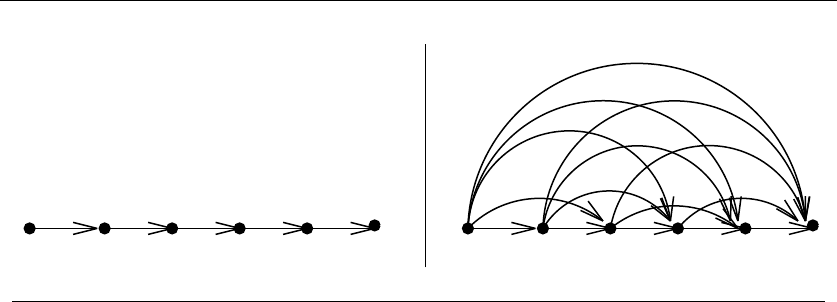
15.5 TRANSITIVE CLOSURE AND REDUCTION 495
1 2 3 4 5 6 1 2 3 4 5 6
INPUT OUTPUT
15.5 Transitive Closure and Reduction
Input description: A directed graph G=(V,E).
Problem description:Fortransitive closure, construct a graph G=(V,E) with
edge (i, j)∈Eiff there is a directed path from ito jin G.Fortransitive reduction,
construct a small graph G=(V, E) with a directed path from ito jin Giff there
is a directed path from ito jin G.
Discussion: Transitive closure can be thought of as establishing a data structure
that makes it possible to solve reachability questions (can I get to xfrom y?)
efficiently. After constructing the transitive closure, all reachability queries can be
answered in constant time by simply reporting the appropriate matrix entry.
Transitive closure is fundamental in propagating the consequences of modified
attributes of a graph G. For example, consider the graph underlying any spread-
sheet model whose vertices are cells and have an edge from cell ito cell jif the
result of cell jdepends on cell i. When the value of a given cell is modified, the
values of all reachable cells must also be updated. The identity of these cells is re-
vealed by the transitive closure of G. Many database problems reduce to computing
transitive closures, for analogous reasons.
There are three basic algorithms for computing transitive closure:
•The simplest algorithm just performs a breadth-first or depth-first search
from each vertex and keeps track of all vertices encountered. Doing nsuch
traversals gives an O(n(n+m)) algorithm, which degenerates to cubic time if
the graph is dense. This algorithm is easily implemented, runs well on sparse
graphs, and is likely the right answer for your application.
•Warshall’s algorithm constructs transitive closures in O(n3) using a simple,
slick algorithm that is identical to Floyd’s all-pairs shortest-path algorithm

496 15. GRAPH PROBLEMS: POLYNOMIAL-TIME
of Section 15.4 (page 489). If we are interested only in the transitive closure,
and not the length of the resulting paths, we can reduce storage by retaining
only one bit for each matrix element. Thus, Dk
ij =1iffjis reachable from i
using only vertices 1,...,k as intermediates.
•Matrix multiplication can also be used to solve transitive closure. Let M1be
the adjacency matrix of graph G. The non-zero matrix entries of M2=M×M
identify all length-2 paths in G. Observe that M2[i, j]=xM[i, x]·M[x, j],
so path (i, x, j) contributes to M2[i, j]. Thus, the union ∪n
iMiyields the
transitive closure T. Furthermore, this union can be computed using only
O(lg n) matrix operations using the fast exponentiation algorithm in Section
13.9 (page 423).
You might conceivably win for large nby using Strassen’s fast matrix multipli-
cation algorithm, although I for one wouldn’t bother trying. Since transitive
closure is provably as hard as matrix multiplication, there is little hope for a
significantly faster algorithm.
The running time of all three of these procedures can be substantially improved
on many graphs. Recall that a strongly connected component is a set of vertices for
which all pairs are mutually reachable. For example, any cycle defines a strongly
connected subgraph. All the vertices in any strongly connected component must
reach exactly the same subset of G. Thus, we can reduce our problem finding the
transitive closure on a graph of strongly connected components that should have
considerably fewer edges and vertices than G. The strongly connected components
of Gcan be computed in linear time (see Section 15.1 (page 477)).
Transitive reduction (also known as minimum equivalent digraph) is the inverse
operation of transitive closure, namely reducing the number of edges while main-
taining identical reachability properties. The transitive closure of Gis identical to
the transitive closure of the transitive reduction of G. The primary application of
transitive reduction is space minimization, by eliminating redundant edges from G
that do not effect reachability. Transitive reduction also arises in graph drawing,
where it is important to eliminate as many unnecessary edges as possible to reduce
the visual clutter.
Although the transitive closure of Gis uniquely defined, a graph may have
many different transitive reductions, including Gitself. We want the smallest such
reduction, but there are multiple formulations of the problem:
•A linear-time, quick-and-dirty transitive reduction algorithm identifies the
strongly connected components of G, replaces each by a simple directed cycle,
and adds these edges to those bridging the different components. Although
this reduction is not provably minimal, it is likely to be pretty close on typical
graphs.
One catch with this heuristic is that it might add edges to the transitive
reduction of Gthat are not in G. This may or may not be a problem depending
on your application.

15.5 TRANSITIVE CLOSURE AND REDUCTION 497
•If all edges of our transitive reduction must exist in G, we have to abandon
hope of finding the minimum size reduction. To see why, consider a directed
graph consisting of one strongly connected component so that every vertex
can reach every other vertex. The smallest possible transitive reduction will
be a simple directed cycle, consisting of exactly nedges. This is possible if
and only if Gis Hamiltonian, thus proving that finding the smallest subset
of edges is NP-complete.
A heuristic for finding such a transitive reduction is to consider each edge suc-
cessively and delete it if its removal does not change the transitive reduction.
Implementing this efficiently means minimizing the time spent on reachabil-
ity tests. Observe that a directed edge (i, j) can be eliminated whenever there
is another path from ito javoiding this edge.
•The minimum size reduction where we are allowed arbitrary pairs of vertices
as edges can be found in O(n3) time. See the references below for details.
However, the quick-and-dirty heuristic above will likely suffice for most ap-
plications, being easier to program as well as more efficient.
Implementations: The Boost implementation of transitive closure appears par-
ticularly well engineered, and relies on algorithms from [Nuu95]. LEDA (see Section
19.1.1 (page 658)) provides implementations of both transitive closure and reduc-
tion in C++ [MN99].
None of our usual Java libraries appear to contain implementations of either
transitive closure or reduction. However, Graphlib contains a Java Transitivity
library with both of them. See http://www-verimag.imag.fr/∼cotton/ for details.
Combinatorica [PS03] provides Mathematica implementations of transitive clo-
sure and reduction, as well as the display of partial orders requiring transitive
reduction. See Section 19.1.9 (page 661).
Notes:Van Leeuwen [vL90a] provides an excellent survey on transitive closure and re-
duction. The equivalence between matrix multiplication and transitive closure was proven
by Fischer and Meyer [FM71], with expositions including [AHU74].
There is a surprising amount of recent activity on transitive closure, much of it cap-
tured by Nuutila [Nuu95]. Penner and Prasanna [PP06] improved the performance of
Warshall’s algorithm [War62] by roughly a factor of two through a cache-friendly imple-
mentation.
The equivalence between transitive closure and reduction, as well as the O(n3)re-
duction algorithm, was established in [AGU72]. Empirical studies of transitive closure
algorithms include [Nuu95, PP06, SD75].
Estimating the size of the transitive closure is important in database query optimiza-
tion. A linear-time algorithm for estimating the size of the closure is given by Cohen
[Coh94].
Related Problems: Connected components (see page 477), shortest path (see
page 489).
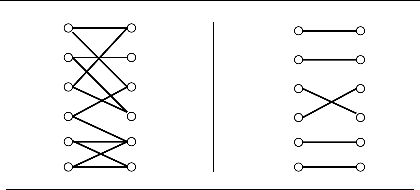
498 15. GRAPH PROBLEMS: POLYNOMIAL-TIME
INPUT OUTPUT
15.6 Matching
Input description: A (weighted) graph G=(V,E).
Problem description: Find the largest set of edges Efrom Esuch that each
vertex in Vis incident to at most one edge of E.
Discussion: Suppose we manage a group of workers, each of whom is capable of
performing a subset of the tasks needed to complete a job. Construct a graph with
vertices representing both the set of workers and the set of tasks. Edges link workers
to the tasks they can perform. We must assign each task to a different worker so
that no worker is overloaded. The desired assignment is the largest possible set of
edges where no employee or job is repeated—i.e. , a matching.
Matching is a very powerful piece of algorithmic magic, so powerful that it is
surprising that optimal matchings can be found efficiently. Applications arise often
once you know to look for them.
Marrying off a set of boys to a set of girls such that each couple is happy is
another bipartite matching problem, on a graph with an edge between any compat-
ible boy and girl. For a synthetic biology application [MPC+06], I need to shuffle
the characters in a string Sto maximize the number of characters that move. For
example, aaabc can be shuffled to bcaaa so that only one character stays fixed. This
is yet another bipartite matching problem, where the boys represent the multiset
of alphabet symbols and the girls are the positions in the string (1 to |S|). Edges
link symbols to all the string positions that originally contained a different symbol.
This basic matching framework can be enhanced in several ways, while remain-
ing essentially the same assignment problem:

15.6 MATCHING 499
•Is your graph bipartite? – Most matching problems involve bipartite graphs,
as in the classic assignment problem of jobs to workers. This is fortunate
because faster and simpler algorithms exist for bipartite matching.
•What if certain employees can be given multiple jobs? – Natural generaliza-
tions of the assignment problem include assigning certain employees more
than one task to do, or (equivalently) seeking multiple workers for a given
job. Here, we do not seek a matching so much as a covering with small “stars.”
Such desires can be modeled by replicating an employee vertex by as many
times as we want her to be matched. Indeed, we employed this trick in the
string permutation example above.
•Is your graph weighted or unweighted? – Many matching applications are
based on unweighted graphs. Perhaps we seek to maximize the total number
of tasks performed, where one task is as good as another. Here we seek a max-
imum cardinality matching—ideally a perfect matching where every vertex is
matched to another in the matching.
For other applications, however, we need to augment each edge with a weight,
perhaps reflecting the suitability of an employee for a given task. The problem
now becomes constructing a maximum weight matching—i.e. , the set of
independent edges of maximum total cost.
Efficient algorithms for constructing matchings work by constructing augment-
ing paths in graphs. Given a (partial) matching Min a graph G, an augmenting
path is a path of edges Pthat alternate (out-of-M,in-M, ..., out-of-M). We can
enlarge the matching by one edge given such an augmenting path, replacing the
even-numbered edges of Pfrom Mwith the odd-numbered edges of P. Berge’s
theorem states that a matching is maximum if and only if it does not contain any
augmenting path. Therefore, we can construct maximum-cardinality matchings by
searching for augmenting paths and stopping when none exist.
General graphs prove trickier because it is possible to have augmenting paths
that are odd-length cycles (i.e. , the first and last vertices are the same). Such
cycles (or blossoms) are impossible in bipartite graphs, which by definition do not
contain odd-length cycles.
The standard algorithms for bipartite matching are based on network flow,
using a simple transformation to convert a bipartite graph into an equivalent flow
graph. Indeed, an implementation of this is given in Section 6.5 (page 217).
Be warned that different approaches are needed to solve weighted matching
problems, most notably the matrix-oriented “Hungarian algorithm.”
Implementations: High-performance codes for both weighted and unweighted
bipartite matching have been developed by Andrew Goldberg and his collabo-
rators. CSA is a weighted bipartite matching code in C based on cost-scaling
network flow, developed by Goldberg and Kennedy [GK95]. BIM is a faster un-
weighted bipartite matching code based on augmenting path methods, developed

500 15. GRAPH PROBLEMS: POLYNOMIAL-TIME
by Cherkassky, et al. [CGM+98]. Both are available for noncommercial use from
http://www.avglab.com/andrew/soft.html.
The First DIMACS Implementation Challenge [JM93] focused on network flows
and matching. Several instance generators and implementations for maximum
weight and maximum cardinality matching were collected, and can be obtained by
anonymous FTP from dimacs.rutgers.edu in the directory pub/netflow/matching.
These include
•A maximum-cardinality matching solver in Fortran 77 by R. Bruce Mattingly
and Nathan P. Ritchey.
•A maximum-cardinality matching solver in C by Edward Rothberg, that im-
plements Gabow’s O(n3) algorithm.
•A maximum-weighted matching solver in C by Edward Rothberg. This is
slower but more general than his unweighted solver just described.
GOBLIN (http://www.math.uni-augsburg.de/∼fremuth/goblin.html)isanex-
tensive C++ library dealing with all of the standard graph optimization prob-
lems, including weighted bipartite matching. LEDA (see Section 19.1.1 (page 658))
provides efficient implementations in C++ for both maximum-cardinality and
maximum-weighted matching, on both bipartite and general graphs.
Blossum IV [CR99] is an efficient code in C for minimum-weight per-
fect matching available at http://www2.isye.gatech.edu/∼wcook/software.html.An
O(mnα(m, n)) implementation of maximum-cardinality matching in general graphs
(http://www.cs.arizona.edu/∼kece/Research/software.html) is due to Kececioglu
and Pecqueur [KP98].
The Stanford GraphBase (see Section 19.1.8 (page 660)) contains an imple-
mentation of the Hungarian algorithm for bipartite matching. To provide readily
visualized weighted bipartite graphs, Knuth uses a digitized version of the Mona
Lisa and seeks row/column disjoint pixels of maximum brightness. Matching is also
used to construct clever, resampled “domino portraits”.
Notes:Lov´asz and Plummer [LP86] is the definitive reference on matching theory and
algorithms. Survey articles on matching algorithms include [Gal86]. Good expositions on
network flow algorithms for bipartite matching include [CLRS01, Eve79a, Man89], and
those on the Hungarian method include [Law76, PS98]. The best algorithm for maxi-
mum bipartite matching, due to Hopcroft and Karp [HK73], repeatedly finds the shortest
augmenting paths instead of using network flow, and runs in O(√nm). The Hungarian
algorithm runs in O(n(m+nlog n)) time.
Edmond’s algorithm [Edm65] for maximum-cardinality matching is of great histori-
cal interest for provoking questions on what problems can be solved in polynomial time.
Expositions on Edmond’s algorithm include [Law76, PS98, Tar83]. Gabow’s [Gab76] im-
plementation of Edmond’s algorithm runs in O(n3) time. The best algorithm known for
general matching runs in O(√nm)[MV80].
Consider a matching of boys to girls containing edges (B1,G
1)and(B2,G
2), where
B1and G2in fact prefer each other to their own spouses. In real life, these two would

15.6 MATCHING 501
run off with each other, breaking the marriages. A marriage without any such couples is
said to be stable. The theory of stable matching is thoroughly treated in [GI89]. It is a
surprising fact that no matter how the boys and girls rate each other, there is always at
least one stable marriage. Further, such a marriage can be found in O(n2) time [GS62].
An important application of stable marriage occurs in the annual matching of medical
residents to hospitals.
The maximum matching is equal in size to the minimum vertex cover in bipartite
graphs. This implies that both the minimum vertex cover problem and maximum inde-
pendent set problems can be solved in polynomial time on bipartite graphs.
Related Problems: Eulerian cycle (see page 502), network flow (see page 509).
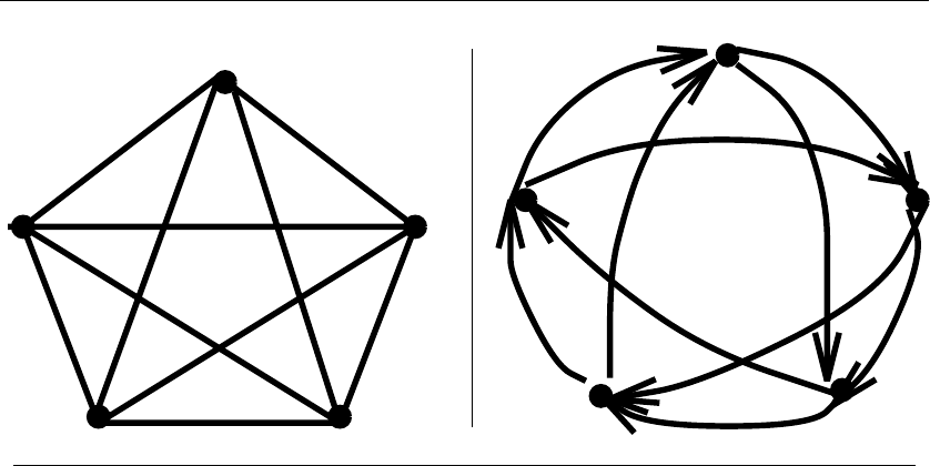
502 15. GRAPH PROBLEMS: POLYNOMIAL-TIME
INPUT OUTPUT
15.7 Eulerian Cycle/Chinese Postman
Input description: A graph G=(V,E).
Problem description: Find the shortest tour visiting each edge of Gat least
once.
Discussion: Suppose you are given the map of a city and charged with designing
the routes for garbage trucks, snow plows, or postmen. In each of these applications,
every road in the city must be completely traversed at least once in order to ensure
that all deliveries or pickups are made. For efficiency, you seek to minimize total
drive time, or (equivalently) the total distance or number of edges traversed.
Alternately, consider a human-factors validation of telephone menu systems.
Each “Press 4 for more information” option is properly interpreted as an edge
between two vertices in a graph. Our tester seeks the most efficient way to walk
over this graph and visit every link in the system at least once.
Such applications are variants of the Eulerian cycle problem, best characterized
by the puzzle that asks children to draw a given figure completely without (1)
without repeating any edges, or (2) lifting their pencil off the paper. They seek a
path or cycle through a graph that visits each edge exactly once.
Well-known conditions exist for determining whether a graph contains an Eu-
lerian cycle or path:
•An undirected graph contains an Eulerian cycle iff (1) it is connected, and (2)
each vertex is of even degree.

15.7 EULERIAN CYCLE/CHINESE POSTMAN 503
•An undirected graph contains an Eulerian path iff (1) it is connected, and (2)
all but two vertices are of even degree. These two vertices will be the start
and end points of any path.
•Adirected graph contains an Eulerian cycle iff (1) it is strongly-connected,
and (2) each vertex has the same in-degree as out-degree.
•Finally, a directed graph contains an Eulerian path from xto yiff (1) it is
connected, and (2) all other vertices have the same in-degree as out-degree,
with xand ybeing vertices with in-degree one less and one more than their
out-degrees, respectively.
This characterization of Eulerian graphs makes it is easy to test whether such a
cycle exists: verify that the graph is connected using DFS or BFS, and then count
the number of odd-degree vertices. Explicitly constructing the cycle also takes
linear time. Use DFS to find an arbitrary cycle in the graph. Delete this cycle and
repeat until the entire set of edges has been partitioned into a set of edge-disjoint
cycles. Since deleting a cycle reduces each vertex degree by an even number, the
remaining graph will continue to satisfy the same Eulerian degree-bound conditions.
These cycles will have common vertices (since the graph is connected), and so can
be spliced together in a “figure eight” at a shared vertex. By so splicing all the
extracted cycles together, we construct a single circuit containing all of the edges.
An Eulerian cycle, if one exists, solves the motivating snowplow problem, since
any tour that visits each edge only once must have minimum length. However, it is
unlikely that your road network happens to satisfy the Eulerian degree conditions.
Instead, we need to solve the more general Chinese postman problem, which mini-
mizes the length of a cycle that traverses every edge at least once. This minimum
cycle will never visit any edge more than twice, so good tours exist for any road
network.
The optimal postman tour can be constructed by adding the appropriate edges
to the graph Gto make it Eulerian. Specifically, we find the shortest path between
each pair of odd-degree vertices in G. Adding a path between two odd-degree
vertices in Gturns both of them to even-degree, moving Gcloser to becoming
an Eulerian graph. Finding the best set of shortest paths to add to Greduces to
identifying a minimum-weight perfect matching in a special graph G.
For undirected graphs, the vertices of Gcorrespond the odd-degree vertices
of G, with the weight of edge (i, j) defined to be the length of the shortest path
from ito jin G. For directed graphs, the vertices of Gcorrespond to the degree-
imbalanced vertices from G, with the bonus that all edges in Ggo from out-degree
deficient vertices to in-degree deficient ones. Thus, bipartite matching algorithms
suffice when Gis directed. Once the graph is Eulerian, the actual cycle can be
extracted in linear time using the procedure just described.
Implementations: Several graph libraries provide implementations of Eulerian
cycles, but Chinese postman implementations are rarer. We recommend the imple-

504 15. GRAPH PROBLEMS: POLYNOMIAL-TIME
mentation of directed Chinese postman by Thimbleby [Thi03]. This Java imple-
mentation is available at http://www.cs.swan.ac.uk/∼csharold/cpp/index.html.
GOBLIN (http://www.math.uni-augsburg.de/∼fremuth/goblin.html)isanex-
tensive C++ library dealing with all of the standard graph optimization problems,
including Chinese postman for both directed and undirected graphs. LEDA (see
Section 19.1.1 (page 658)) provides all the tools for an efficient implementation:
Eulerian cycles, matching, and shortest-paths bipartite and general graphs.
Combinatorica [PS03] provides Mathematica implementations of Eulerian cy-
cles and de Bruijn sequences. See Section 19.1.9 (page 661).
Notes:The history of graph theory began in 1736, when Euler [Eul36] first solved the
seven bridges of K¨onigsberg problem. K¨onigsberg (now Kaliningrad) is a city on the
banks of the Pregel river. In Euler’s day there were seven bridges linking the banks and
two islands, which can be modeled as a multigraph with seven edges and four vertices.
Euler sought a way to walk over each of the bridges exactly once and return home—i.e.
, an Eulerian cycle. Euler proved that such a tour is impossible, since all four of the
vertices had odd degrees. The bridges were destroyed in World War II. See [BLW76] for
a translation of Euler’s original paper and a history of the problem.
Expositions on linear-time algorithms for constructing Eulerian cycles [Ebe88] in-
clude [Eve79a, Man89]. Fleury’s algorithm [Luc91] is a direct and elegant approach to
constructing Eulerian cycles. Start walking from any vertex, and erase any edge that has
been traversed. The only criterion in picking the next edge is that we avoid using a bridge
(an edge whose deletion disconnects the graph) until no other alternative remains.
The Euler’s tour technique is an important paradigm in parallel graph algorithms.
Many parallel graph algorithms start by finding a spanning tree and then rooting the
tree, where the rooting is done using the Euler tour technique. See parallel algorithms
texts (e.g., [J´
92]) for an exposition, and [CB04] for recent experience in practice. Efficient
algorithms exist to count the number of Eulerian cycles in a graph [HP73].
The problem of finding the shortest tour traversing all edges in a graph was introduced
by Kwan [Kwa62], hence the name Chinese postman. The bipartite matching algorithm
for solving Chinese postman is due to Edmonds and Johnson [EJ73]. This algorithm works
for both directed and undirected graphs, although the problem is NP-complete for mixed
graphs [Pap76a]. Mixed graphs contain both directed and undirected edges. Expositions
of the Chinese postman algorithm include [Law76].
Ade Bruijn sequence Sof span non an alphabet Σ of size αis a circular string of
length αncontaining all strings of length nas substrings of S, each exactly once. For
example, for n= 3 and Σ = {0,1}, the circular string 00011101 contains the following
substrings in order: 000, 001, 011, 111, 110, 101, 010, 100. De Bruijn sequences can be
thought of as “safe cracker” sequences, describing the shortest sequence of dial turns with
αpositions sufficient to try out all combinations of length n.
De Bruijn sequences can be constructed by building a directed graph whose vertices
are all αn−1strings of length n−1, where there is an edge (u, v)iffu=s1s2...s
n−1
and v=s2...s
n−1sn. Any Eulerian cycle on this graph describes a de Bruijn sequence.
Expositions on de Bruijn sequences and their construction include [Eve79a, PS03].
Related Problems: Matching (see page 498), Hamiltonian cycle (see page 538).
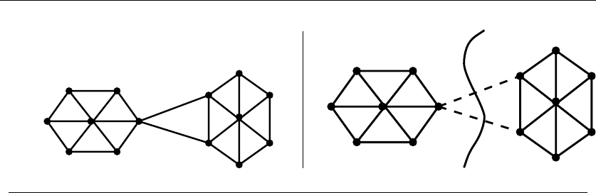
15.8 EDGE AND VERTEX CONNECTIVITY 505
X
INPUT OUTPUT
15.8 Edge and Vertex Connectivity
Input description: A graph G. Optionally, a pair of vertices sand t.
Problem description: What is the smallest subset of vertices (or edges) whose
deletion will disconnect G? Or which will separate sfrom t?
Discussion: Graph connectivity often arises in problems related to network relia-
bility. In the context of telephone networks, the vertex connectivity is the smallest
number of switching stations that a terrorist must bomb in order to separate the
network—i.e. , prevent two unbombed stations from talking to each other. The edge
connectivity is the smallest number of wires that need to be cut to accomplish the
same objective. One well-placed bomb or snipping the right pair of cables suffices
to disconnect the above network.
The edge (vertex) connectivity of a graph Gis the smallest number of edge
(vertex) deletions sufficient to disconnect G. There is a close relationship between
the two quantities. The vertex connectivity is always less than or equal to the
edge connectivity, since deleting one vertex from each edge in a cut set succeeds
in disconnecting the graph. But smaller vertex subsets may be possible. The mini-
mum vertex degree is an upper bound for both edge and vertex connectivity, since
deleting all its neighbors (or cutting the edges to all its neighbors) disconnects the
graph into one big and one single-vertex component.
Several connectivity problems prove to be of interest:
•Is the graph already disconnected? – The simplest connectivity problem is test-
ing whether the graph is in fact connected. A simple depth-first or breadth-
first search suffices to identify all connected components in linear time, as
discussed in Section 15.1 (page 477). For directed graphs, the issue is whether
the graph is strongly connected, meaning there is a directed path between any
pair of vertices. In a weakly connected graph, there may exist paths to nodes
from which there is no way to return.

506 15. GRAPH PROBLEMS: POLYNOMIAL-TIME
•Is there one weak link in my graph? – We say that Gis biconnected if no
single vertex deletion is sufficient to disconnect G. Any vertex that is such a
weak point is called an articulation vertex.Abridge is the analogous concept
for edges, meaning a single edge whose deletion disconnects the graph.
The simplest algorithms for identifying articulation vertices (or bridges) try
deleting vertices (or edges) one by one, and then use DFS or BFS to test
whether the resulting graph is still connected. More sophisticated linear-time
algorithms exist for both problems, based on depth-first search. Indeed, a full
implementation is given in Section 5.9.2 (page 173).
•What if I want to split the graph into equal-sized pieces? – What is often
sought is a small cut set that breaks the graph into roughly equal-sized pieces.
For example, suppose we want to split a big computer program into two
maintainable units. We can construct a graph whose the vertices represent
subroutines. Edges can be added between any two subroutines that interact,
namely where one calls the other. We now seek to partition the subroutines
into roughly equal-sized sets so that few pairs of interacting routines span
the divide.
This is the graph partition problem, further discussed in Section 16.6 (page
541). Although the problem is NP-complete, reasonable heuristics exist to
solve it.
•Are arbitrary cuts OK, or must I separate a given pair of vertices? – There
are two flavors of the general connectivity problem. One asks for the smallest
cut-set for the entire graph, the other for the smallest set to separate sfrom t.
Any algorithm for (s−t) connectivity can be used with each of the n(n−1)/2
possible pairs of vertices to give an algorithm for general connectivity. Less
obviously, n−1 runs suffice for testing edge connectivity, since we know that
vertex v1must end up in a different component from at least one of the other
n−1 vertices after deleting any cut set.
Edge and vertex connectivity can both be found using network-flow techniques.
Network flow, discussed in Section 15.9 (page 509), interprets a weighted graph as a
network of pipes where each edge has a maximum capacity and we seek to maximize
the flow between two given vertices of the graph. The maximum flow between vi,v
j
in Gis exactly the weight of the smallest set of edges to disconnect vifrom vj.
Thus the edge connectivity can be found by minimizing the flow between viand
each of the n−1 other vertices in an unweighted graph G. Why? After deleting
the minimum-edge cut set, viwill be separated from some other vertex.
Vertex connectivity is characterized by Menger’s theorem, which states that a
graph is k-connected if and only if every pair of vertices is joined by at least k
vertex-disjoint paths. Network flow can again be used to perform this calculation,
since a flow of kbetween a pair of vertices implies kedge-disjoint paths. To exploit
Menger’s theorem, we construct a graph Gsuch that any set of edge-disjoint paths

15.8 EDGE AND VERTEX CONNECTIVITY 507
in Gcorresponds to vertex-disjoint paths in G. This is done by replacing each
vertex viof Gwith two vertices vi,1and vi,2, such that edge (vi,1,v
i,2)∈Gfor all
vi∈G, and by replacing every edge (vi,x)∈Gby edges (vi,j ,x
k), j=k∈{0,1}
in G. Thus two edge-disjoint paths in Gcorrespond to each vertex-disjoint path
in G.
Implementations:MINCUTLIB is a collection of high-performance codes for sev-
eral different cut algorithms, including both flow and contraction-based meth-
ods. They were implemented by Chekuri, et al. as part of a substantial ex-
perimental study [CGK+97]. The codes are available for noncommercial use
at http://www.avglab.com/andrew/soft.html. Also included is the full version of
[CGK+97]—an excellent presentation of these algorithms and the heuristics needed
to make them run fast.
Most of the graph data structure libraries of Section 15.1 (page 477) include
routines for connectivity and biconnectivity testing. The C++ Boost Graph Library
[SLL02] (http://www.boost.org/libs/graph/doc) is distinguished by also including an
implementation of edge connectivity testing.
GOBLIN (http://www.math.uni-augsburg.de/∼fremuth/goblin.html)isanex-
tensive C++ library dealing with all of the standard graph optimization problems,
including both edge and vertex connectivity.
LEDA (see Section 19.1.1 (page 658)) contains extensive support for both low-
level connectivity testing (both biconnected and triconnected components) and
edge connectivity/minimum-cut in C++.
Combinatorica [PS03] provides Mathematica implementations of edge and ver-
tex connectivity, as well as connected, biconnected, and strongly connected com-
ponents with bridges and articulation vertices. See Section 19.1.9 (page 661).
Notes:Good expositions on the network-flow approach to edge and vertex connectivity
include [Eve79a, PS03]. The correctness of these algorithms is based on Menger’s theorem
[Men27] that connectivity is determined by the number of edge and vertex disjoint paths
separating a pair of vertices. The maximum-flow, minimum-cut theorem is due to Ford
and Fulkerson [FF62].
The theoretically fastest algorithms for minimum-cut/edge connectivity are based on
graph contraction, not network flows. Contracting an edge (x, y) in a graph Gmerges the
two incident vertices into one, removing self-loops but leaving multiedges. Any sequence
of such contractions can raise (but not lower) the minimum cut in G,andleavesthe
cut unchanged if no edge of the cut is contracted. Karger gave a beautiful randomized
algorithm for minimum cut, observing that the minimum cut is left unchanged with
nontrivial probability over the course of any random series of deletions. The fastest version
of Karger’s algorithm runs in (mlg3n) expected time [Kar00]. See Motwani and Raghavan
[MR95] for an excellent treatment of randomized algorithms, including a presentation of
Karger’s algorithm.
Nagamouchi and Ibaraki [NI92] give a deterministic contraction-based algorithm to
find the minimum cut in O(n(m+nlog n)). In each round, this algorithm identifies and
contracts an edge that is provably not in the minimum cut. See [CGK+97, NOI94] for
experimental comparisons of algorithms for finding minimum cuts.

508 15. GRAPH PROBLEMS: POLYNOMIAL-TIME
Minimum-cut methods have found many applications in computer vision, including
image segmentation. Boykov and Kolmogorov [BK04] report on an experimental evalua-
tion of minimum-cut algorithms in this context.
A nonflow-based algorithm for edge k-connectivity in O(kn2) is due to Matula [Mat87].
Faster k-connectivity algorithms are known for certain small values of k. All three-
connected components of a graph can be generated in linear time [HT73a], while O(n2)
suffices to test 4-connectivity [KR91].
Related Problems: Connected components (see page 477), network flow (see
page 509), graph partition (see page 541).
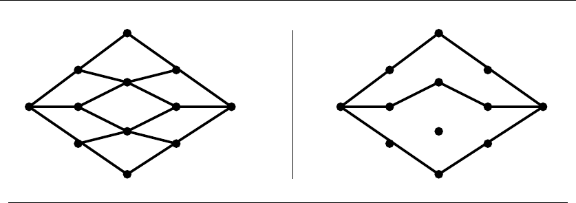
15.9 NETWORK FLOW 509
STST
INPUT OUTPUT
15.9 Network Flow
Input description: A directed graph G, where each edge e=(i, j) has a capacity
ce. A source node sand sink node t.
Problem description: What is the maximum flow you can route from sto twhile
respecting the capacity constraint of each edge?
Discussion: Applications of network flow go far beyond plumbing. Finding the
most cost-effective way to ship goods between a set of factories and a set of stores
defines a network-flow problem, as do many resource-allocation problems in com-
munications networks.
The real power of network flow is (1) that a surprising variety of linear pro-
gramming problems arising in practice can be modeled as network-flow problems,
and (2) that network-flow algorithms can solve these problems much faster than
general-purpose linear programming methods. Several graph problems we have dis-
cussed in this book can be solved using network flow, including bipartite matching,
shortest path, and edge/vertex connectivity.
The key to exploiting this power is recognizing that your problem can be mod-
eled as network flow. This requires experience and study. My recommendation is
that you first construct a linear programming model for your problem and then
compare it with linear programs for the two primary classes of network flow prob-
lems: maximum flow and minimum-cost flow:
•Maximum Flow – Here we seek the heaviest possible flow from sto t, given
the edge capacity constraints of G.Letxij be a variable accounting for the
flow from vertex ithrough directed edge (i, j). The flow through this edge is
constrained by its capacity cij ,so
0≤xij ≤cij for 1 ≤i, j ≤n

510 15. GRAPH PROBLEMS: POLYNOMIAL-TIME
Furthermore, an equal flow comes in as goes out at each nonsource or sink
vertex, so
n
j=1
xij −
n
j=1
xji =0for1≤i≤n
We seek the assignment that maximizes the flow into sink t, namely n
i=1 xit
•Minimum Cost Flow – Here we have an extra parameter for each edge (i, j),
namely the cost (dij ) of sending one unit of flow from ito j.Wealsohave
a targeted amount of flow fwe want to send from sto tat minimum total
cost. Hence, we seek the assignment that minimizes
n
j=1
dij ·xij
subject to the edge and vertex capacity constraints of maximum flow, plus
the additional restriction that n
i=1 xit =f.
Special considerations include:
•What if I have multiple sources and/or sinks? – No problem. We can handle
this by modifying the network to create a vertex to serve as a super-source
that feeds all the sources, and a super-sink that drains all the sinks.
•What if all arc capacities are identical, either 0 or 1? – Faster algorithms
exist for 0-1 network flows. See the Notes section for details.
•What if all my edge costs are identical? – Use the simpler and faster algo-
rithms for solving maximum flow as opposed to minimum-cost flow. Max-flow
without edge costs arises in many applications, including edge/vertex con-
nectivity and bipartite matching.
•What if I have multiple types of material moving through the network? –In
a telecommunications network, every message has a given source and desti-
nation. Each destination needs to receive exactly those calls sent to it, not
an equal amount of communication from arbitrary places. This can be mod-
eled as a multicommodity flow problem, where each call defines a different
commodity and we seek to satisfy all demands without exceeding the total
capacity of any edge.
Linear programming will suffice for multicommodity flow if fractional flows
are permitted. Unfortunately, integral multicommodity flow is NP-complete,
even for only two commodities.

15.9 NETWORK FLOW 511
Network flow algorithms can be complicated, and significant engineering is re-
quired to optimize performance. Thus, we strongly recommend that you use an
existing code rather than implement your own. Excellent codes are available and
described below. The two primary classes of algorithms are:
•Augmenting path methods – These algorithms repeatedly find a path of posi-
tive capacity from source to sink and add it to the flow. It can be shown that
the flow through a network is optimal if and only if it contains no augment-
ing path. Since each augmentation adds something to the flow, we eventually
find the maximum. The difference between network-flow algorithms is in how
they select the augmenting path. If we are not careful, each augmenting path
will add but a little to the total flow, and so the algorithm might take a long
time to converge.
•Preflow-push methods – These algorithms push flows from one vertex to an-
other, initially ignoring the constraint that in-flow must equal out-flow at each
vertex. Preflow-push methods prove faster than augmenting-path methods,
essentially because multiple paths can be augmented simultaneously. These
algorithms are the method of choice and are implemented in the best codes
described in the next section.
Implementations: High-performance codes for both maximum flow and mini-
mum cost flow were developed by Andrew Goldberg and his collaborators. The
codes HIPR and PRF [CG94] are provided for maximum flow, with the proviso that
HIPR is recommended in most cases. For minimum-cost flow, the code of choice
is CS [Gol97]. Both are written in C and available for noncommercial use from
http://www.avglab.com/andrew/soft.html.
GOBLIN (http://www.math.uni-augsburg.de/∼fremuth/goblin.html)isanex-
tensive C++ library dealing with all of the standard graph optimization problems,
including several different algorithms for both maximum flow and minimum-cost
flow. The same holds true for LEDA, if a commercial-strength solution is needed.
See Section 19.1.1 (page 658).
The First DIMACS Implementation Challenge on Network Flows and Matching
[JM93] collected several implementations and generators for network flow, which
can be obtained by anonymous FTP from dimacs.rutgers.edu in the directory
pub/netflow/maxflow. These include: (1) a preflow-push network flow implemen-
tation in C by Edward Rothberg, and (2) an implementation of eleven network
flow variants in C, including the older Dinic and Karzanov algorithms by Richard
Anderson and Joao Setubal.
Notes:The primary book on network flows and its applications is [AMO93]. Good
expositions on network flow algorithms old and new include [CCPS98, CLRS01, PS98].
Expositions on the hardness of multicommodity flow [Ita78] include [Eve79a].
There is a very close connection to maximum flow and edge connectivity in graphs.
The fundamental maximum-flow, minimum-cut theorem is due to Ford and Fulkerson

512 15. GRAPH PROBLEMS: POLYNOMIAL-TIME
[FF62]. See Section 15.8 (page 505) for simpler and more efficient algorithms to compute
the minimum cut in a graph.
Conventional wisdom holds that network flow should be computable in O(nm)time,
and there has been steady progress in lowering the time complexity. See [AMO93] for a
history of algorithms for the problem. The fastest known general network flow algorithm
runs in O(nm lg(n2/m)) time [GT88]. Empirical studies of minimum-cost flow algorithms
include [GKK74, Gol97].
Information flows through a network can be modeled as multicommodity flows through
a network, with the observation that replicating and manipulating information at internal
nodes can eliminate the need for distinct sources to sink paths when multiple sinks are
interested in the same information. The field of network coding [YLCZ05] uses such ideas
to achieve information flows through networks at the theoretical limits of the max-flow,
min-cut theorem.
Related Problems: Linear programming (see page 411), matching (see page 498),
connectivity (see page 505).
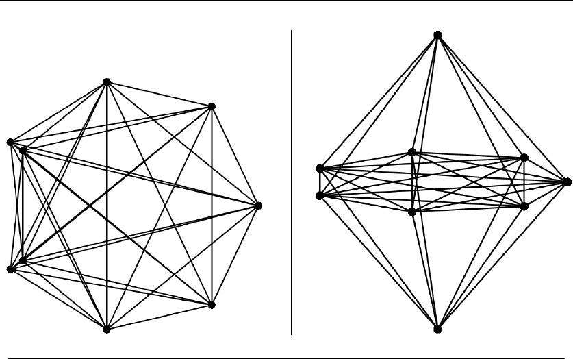
15.10 DRAWING GRAPHS NICELY 513
INPUT OUTPUT
15.10 Drawing Graphs Nicely
Input description: A graph G.
Problem description: Draw a graph Gso as to accurately reflect its structure.
Discussion: Graph drawing is a problem that constantly arises in applications,
yet it is inherently ill-defined. What exactly does a nice drawing mean? We seek
an algorithm that shows off the structure of the graph so the viewer can best
understand it. Simultaneously, we seek a drawing that looks aesthetically pleasing.
Unfortunately, these are “soft” criteria for which it is impossible to design
an optimization algorithm. Indeed, it is easy to come up with radically different
drawings of a given graph, each of which is most appropriate in a certain context.
Three different drawings of the Petersen graph are given on page 550. Which of
these is the “right” one?
Several “hard” criteria can partially measure the quality of a drawing:
•Crossings – We seek a drawing with as few pairs of crossing edges as possible,
since they are distracting.

514 15. GRAPH PROBLEMS: POLYNOMIAL-TIME
•Area – We seek a drawing that uses as little paper as possible, while ensuring
that no pair of vertices gets placed too close to each other.
•Edge length – We seek a drawing that avoids long edges, since they tend to
obscure other features of the drawing.
•Angular resolution – We seek a drawing avoiding small angles between two
edges incident on a given vertex, as the resulting lines tend to partially or
fully overlap.
•Aspect ratio – We seek a drawing whose aspect ratio (width/height) reflects
the desired output medium (typically a computer screen at 4/3) as closely as
possible.
Unfortunately, these goals are mutually contradictory, and the problem of finding
the best drawing under any nonempty subset of them is likely to be NP-complete.
Two final warnings before getting down to business. For graphs without inherent
symmetries or structure, it is likely that no really nice drawing exists. This is
especially for true for graphs with more than 10 to 15 vertices. The shear amount
of ink needed to draw any large, dense graph will overwhelm any display. A drawing
of the complete graph on 100 vertices (K100) contains approximately 5,000 edges.
On a 1000 ×1000 pixel display, this works out to 200 pixels per edge. What can
you hope to see except a black blob in the center of the screen?
Once all this is understood, it must be admitted that graph-drawing algorithms
can be quite effective and fun to play with. To help choose the right one, ask yourself
the following questions:
•Must the edges be straight, or can I have curves and/or bends? – Straight-line
drawing algorithms are relatively simple, but have their limitations. Orthog-
onal polyline drawings seem to work best to visualize complicated graphs
such as circuit designs. Orthogonal means that all lines must be drawn either
horizontal or vertical, with no intermediate slopes. Polyline means that each
graph edge is represented by a chain of straight-line segments, connected by
vertices or bends.
•Is there a natural, application-specific drawing? – If your graph represents a
network of cities and roads, you are unlikely to find a better drawing than
placing the vertices in the same position as the cities on a map. This same
principle holds for many different applications.
•Is your graph either planar or a tree? – If so, use one of the special planar
graph or tree drawing algorithms of Sections 15.11 and 15.12.
•Is your graph directed? – Edge direction has a significant impact on the nature
of the desired drawing. When drawing directed acyclic graphs (DAGs), it is
often important that all edges flow in a logical direction—perhaps left-right
or top-down.

15.10 DRAWING GRAPHS NICELY 515
•How fast must your algorithm be? – Your graph drawing algorithm had better
be very fast if it will be used for interactive update and display. You are
presumably limited to using incremental algorithms, which change the vertex
positions only in the immediate neighborhood of the edited vertex. You can
afford more time for optimization if instead you are printing a pretty picture
for extended study.
•Does your graph contain symmetries? – The output drawing above is attrac-
tive because the graph contains symmetries—namely two vertices identically
connected to a core K5. The inherent symmetries in a graph can be identified
by computing its automorphisms, or self-isomorphisms. Graph isomorphism
codes (see Section 16.9 (page 550)) can be readily used to find all automor-
phisms.
As a first quick and dirty drawing, I recommend simply spacing the vertices
evenly on a circle, and then drawing the edges as straight lines between vertices.
Such drawings are easy to program and fast to construct. They have the substantial
advantage that no two edges will obscure each other, since no three vertices will be
collinear. Such artifacts can be hard to avoid as soon as you allow internal vertices
into your drawing. An unexpected pleasure with circular drawings is the symmetry
sometimes revealed because vertices appear in the order they were inserted into
the graph. Simulated annealing can be used to permute the circular vertex order
to minimize crossings or edge length, and thus significantly improve the drawing.
A good, general purpose graph-drawing heuristic models the graph as a system
of springs and then uses energy minimization to space the vertices. Let adjacent
vertices attract each other with a force proportional to (say) the logarithm of their
separation, while all nonadjacent vertices repel each other with a force proportional
to their separation distance. These weights provide incentive for all edges to be
as short as possible, while spreading the vertices apart. The behavior of such a
system can be approximated by determining the force acting on each vertex at a
particular time and then moving each vertex a small amount in the appropriate
direction. After several such iterations, the system should stabilize on a reasonable
drawing. The input and output figures above demonstrate the effectiveness of the
spring embedding on a particular small graph.
If you need a polyline graph-drawing algorithm, my recommendation is that you
study the systems presented next or described in [JM03] to decide whether one of
them can do the job. You will have to do a significant amount of work before you
can hope to develop a better algorithm.
Drawing your graph opens another can of worms, namely where to place the
edge/vertex labels. We seek to position labels very close to the edges or vertices
they identify, and yet to place them such that they do not overlap each other or
other important graph features. Optimizing label placement can be shown to be
an NP-complete problem, but heuristics related to bin packing (see Section 17.9
(page 595)) can be effectively used.

516 15. GRAPH PROBLEMS: POLYNOMIAL-TIME
Implementations: GraphViz (http://www.graphviz.org) is a popular and well-
supported graph-drawing program developed by Stephen North of Bell Laborato-
ries. It represents edges as splines and can construct useful drawings of quite large
and complicated graphs. It has sufficed for all of my professional graph-drawing
needs over the years.
All of the graph data structure libraries of Section 12.4 (page 381) devote some
effort to visualizing graphs. The Boost Graph Library provides an interface to
GraphViz instead of reinventing the wheel. The Java graph libraries, most notably
JGraphT (http://jgrapht.sourceforge.net/), are particularly suitable for interactive
applications.
Graph drawing is a problem where very good commercial products ex-
ist, including those from Tom Sawyer Software (www.tomsawyer.com), yFiles
(www.yworks.com), and iLOG’s JViews (www.ilog.com/products/jviews/). Pajek
[NMB05] is a package particularly designed for drawing social networks, and avail-
able at http://vlado.fmf.uni-lj.si/pub/networks/pajek/. All of these have free trial
or noncommercial use downloads.
Combinatorica [PS03] provides Mathematica implementations of several graph-
drawing algorithms, including circular, spring, and ranked embeddings. See Section
19.1.9 (page 661) for further information on Combinatorica.
Notes:A significant community of researchers in graph drawing exists, fueled by or
fueling an annual conference on graph drawing. The proceedings of this conference are
published by Springer-Verlag’s Lecture Notes in Computer Science series. Perusing a
volume of the proceedings will provide a good view of the state-of-the-art and of what
kinds of ideas people are thinking about. The forthcoming Handbook of Graph Drawing
and Visualization [Tam08] promises to be the most comprehensive review of the field.
Two excellent books on graph-drawing algorithms are Battista, et al. [BETT99] and
Kaufmann and Wagner [KW01]. A third book by J¨unger and Mutzel [JM03] is organized
around systems instead of algorithms, but provides technical details about the drawing
methods each system employs. Map-labeling heuristics are described in [BDY06, WW95].
It is trivial to space npoints evenly along the boundary of a circle. However, the
problem is considerably more difficult on the surface of a sphere. Extensive tables of such
spherical codes for n≤130 have been constructed by Hardin, Sloane, and Smith [HSS07].
Related Problems: Drawing trees (see page 517), planarity testing (see page
520).
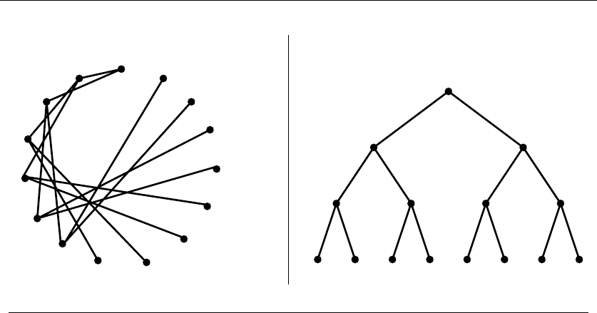
15.11 DRAWING TREES 517
1
2
3
4
5
6
10
11
12
13
14
15
7
98
1
23
467
891011 13141512
5
INPUT OUTPUT
15.11 Drawing Trees
Input description:AtreeT, which is a graph without any cycles.
Problem description: Create a nice drawing of the tree T.
Discussion: Many applications require drawing pictures of trees. Tree diagrams
are commonly used to display and traverse the hierarchical structure of file sys-
tem directories. My attempts to Google “tree drawing software” revealed special-
purpose applications for visualizing family trees, syntax trees (sentence diagrams),
and evolutionary phylogenic trees all in the top twenty links.
Different aesthetics follow from each application. That said, the primary issue
in tree drawing is establishing whether you are drawing free or rooted trees:
•Rooted trees define a hierarchical order, emanating from a single source node
identified as the root. Any drawing should reflect this hierarchical structure,
as well as any additional application-dependent constraints on the order in
which children must appear. For example, family trees are rooted, with sibling
nodes typically drawn from left to right in the order of birth.
•Free trees do not encode any structure beyond their connection topology.
There is no root associated with the minimum spanning tree (MST) of a
graph, so a hierarchical drawing will be misleading. Such free trees might
well inherit their drawing from that of the full underlying graph, such as the
map of the cities whose distances define the MST.

518 15. GRAPH PROBLEMS: POLYNOMIAL-TIME
Trees are always planar graphs, and hence can and should be drawn so no
two edges cross. Any of the planar drawing algorithms of Section 15.12 (page 520)
could be used to do so. However, such algorithms are overkill, because much simpler
algorithms can be used to construct planar drawings of trees. The spring-embedding
heuristics of Section 15.10 (page 513) work well on free trees, although they may
be too slow for certain applications.
The most natural tree-drawing algorithms assume rooted trees. However, they
can be used equally well with free trees, after selecting one vertex to serve as the
root of the drawing. This faux-root can be selected arbitrarily, or, even better, by
using a center vertex of the tree. A center vertex minimizes the maximum distance
to other vertices. For trees, the center always consists of either one vertex or two
adjacent vertices. This tree center can be identified in linear time by repeatedly
trimming all the leaves until only the center remains.
Your two primary options for drawing rooted trees are ranked and radial em-
beddings:
•Ranked embeddings – Place the root in the top center of your page, and then
partition the page into the root-degree number of top-down strips. Deleting
the root creates the root-degree number of subtrees, each of which is assigned
to its own strip. Draw each subtree recursively, by placing its new root (the
vertex adjacent to the old root) in the center of its strip a fixed distance down
from the top, with a line from old root to new root. The output figure above
is a nicely ranked embedding of a balanced binary tree.
Such ranked embeddings are particularly effective for rooted trees used to
represent a hierarchy—be it a family tree, data structure, or corporate lad-
der. The top-down distance illustrates how far each node is from the root.
Unfortunately, such repeated subdivision eventually produces very narrow
strips, until most of the vertices are crammed into a small region of the page.
Try to adjust the width of each strip to reflect the total number of nodes it
will contain, and don’t be afraid of expanding into neighboring region’s turf
once their shorter subtrees have been completed.
•Radial embeddings – Free trees are better drawn using a radial embedding,
where the root/center of the tree is placed in the center of the drawing.
The space around this center vertex is divided into angular sectors for each
subtree. Although the same problem of cramping will eventually occur, radial
embeddings make better use of space than ranked embeddings and appear
considerably more natural for free trees. The rankings of vertices in terms of
distance from the center is illustrated by the concentric circles of vertices.
Implementations: GraphViz (http://www.graphviz.org) is a popular and well-
supported graph-drawing program developed by Stephen North of Bell Laborato-
ries. It represents edges as splines and can construct useful drawings of quite large

15.11 DRAWING TREES 519
and complicated graphs. It has sufficed for all of my professional graph drawing
needs over the years.
Graph/tree drawing is a problem where very good commercial products ex-
ist, including those from Tom Sawyer Software (www.tomsawyer.com), yFiles
(www.yworks.com), and iLOG’s JViews (www.ilog.com/products/jviews/). All of
these have free trial or noncommercial use downloads.
Combinatorica [PS03] provides Mathematica implementations of several tree
drawing algorithms, including radial and rooted embeddings. See Section 19.1.9
(page 661) for further information on Combinatorica.
Notes:All books and surveys on graph drawing include discussions of specific tree-
drawing algorithms. The forthcoming Handbook of Graph Drawing and Visualization
[Tam08] promises to be the most comprehensive review of the field. Two excellent books
on graph drawing algorithms are Battista, et al. [BETT99] and Kaufmann and Wagner
[KW01]. A third book by J¨unger and Mutzel [JM03] is organized around systems instead
of algorithms, but provides technical details about the drawing methods each system
employs.
Heuristics for tree layout have been studied by several researchers [RT81, Moe90],
with Buchheim, et al. [BJL06] reflective of the state-of-the-art. Under certain aesthetic
criteria, the problem is NP-complete [SR83].
Certain tree layout algorithms arise from non-drawing applications. The Van Emde
Boas layout of a binary tree offers better external memory performance than conventional
binary search, at a cost of greater complexity. See the survey of Arge, et al. [ABF05] for
more on this and other cache-oblivious data structures.
Related Problems: Drawing graphs (see page 513), planar drawings (see page
520).
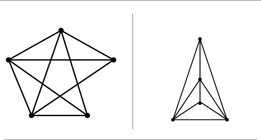
520 15. GRAPH PROBLEMS: POLYNOMIAL-TIME
13
2
54 15
2
4
3
INPUT OUTPUT
15.12 Planarity Detection and Embedding
Input description: A graph G.
Problem description: Can Gbe drawn in the plane such that no two edges cross?
If so, produce such a drawing.
Discussion: Planar drawings (or embeddings) make clear the structure of a given
graph by eliminating crossing edges, which can be confused as additional vertices.
Graphs defined by road networks, printed circuit board layouts, and the like are
inherently planar because they are completely defined by surface structures.
Planar graphs have a variety of nice properties that can be exploited to yield
faster algorithms for many problems. The most important fact to know is that
every planar graph is sparse. Euler’s formula shows that |E|≤3|V|−6 for every
nontrivial planar graph G=(V, E). This means that every planar graph contains
a linear number of edges, and further that every planar graph contains a vertex of
degree ≤5. Every subgraph of a planar graph is planar, so there must always a
sequence of low-degree vertices to delete from G, reducing it to the empty graph.
To gain a better appreciation of the subtleties of planar drawings, I encourage
the reader to construct a planar (noncrossing) embedding for the graph K5−e,
shown on the input figure above. Then try to construct such an embedding where
all the edges are straight. Finally, add the missing edge to the graph and try to do
the same for K5itself.

15.12 PLANARITY DETECTION AND EMBEDDING 521
The study of planarity has motivated much of the development of graph theory.
It must be confessed, however, that the need for planarity testing arises relatively
infrequently in applications. Most graph-drawing systems do not explicitly seek pla-
nar embeddings. “Planarity Detection” proved to be among the least frequently hit
pages of the Algorithm Repository (http://www.cs.sunysb.edu/∼algorith) [Ski99].
That said, it is still very useful to know how to deal with planar graphs when you
encounter them.
Thus, it pays to distinguish the problem of planarity testing (does a graph
have a planar drawing?) from constructing planar embeddings (actually finding
the drawing), although both can be done in linear time. Many efficient planar
graph algorithms do not make any use of the drawing, but instead exploit the
low-degree deletion sequence described above.
Algorithms for planarity testing begin by embedding an arbitrary cycle from the
graph in the plane and then considering additional paths in G, connecting vertices
on this cycle. Whenever two such paths cross, one must be drawn outside the cycle
and one inside. When three such paths mutually cross, there is no way to resolve
the problem, so the graph cannot be planar. Linear-time algorithms for planarity
detection are based on depth-first search, but they are subtle and complicated
enough that you are wise to seek an existing implementation.
Such path-crossing algorithms can be used to construct a planar embedding by
inserting the paths into the drawing one by one. Unfortunately, because they work
in an incremental manner, nothing prevents them from inserting many vertices and
edges into a relatively small area of the drawing. Such cramping is a major problem,
for it leads to ugly drawings that are hard to understand. Better algorithms have
been devised that construct planar-grid embeddings, where each vertex lies on a
(2n−4) ×(n−2) grid. Thus, no region can get too cramped and no edge can
get too long. Still, the resulting drawings tend not to look as natural as one might
hope.
For nonplanar graphs, what is often sought is a drawing that minimizes the
number of crossings. Unfortunately, computing the crossing number of a graph is
NP-complete. A useful heuristic extracts a large planar subgraph of G, embeds this
subgraph, and then inserts the remaining edges one by one to minimize the number
of crossings. This won’t do much for dense graphs, which are doomed to have a large
number of crossings, but it will work well for graphs that are almost planar, such
as road networks with overpasses or printed circuit boards with multiple layers.
Large planar subgraphs can be found by modifying planarity-testing algorithms to
delete troublemaking edges when encountered.
Implementations: LEDA (see Section 19.1.1 (page 658)) includes linear-time al-
gorithms for both planarity testing and constructing straight-line planar-grid em-
beddings. Their planarity tester returns an obstructing Kuratowski subgraph (see
notes) for any graph deemed nonplanar, yielding concrete proof of its nonplanarity.

522 15. GRAPH PROBLEMS: POLYNOMIAL-TIME
JGraphEd (http://www.jharris.ca/JGraphEd/) is a Java graph-drawing frame-
work that includes several planarity testing/embedding algorithms, including both
the Booth-Lueker PQ-tree algorithm and the modern straight-line grid embedding.
PIGALE (http://pigale.sourceforge.net/) is a C++ graph editor/algorithm li-
brary focusing on planar graphs. It contains a variety of algorithms for constructing
planar drawings as well as efficient algorithms to test planarity and identify an ob-
structing subgraph (K3,3or K5), if one exists.
Greedy randomized adaptive search (GRASP) heuristics for finding the largest
planar subgraph have been implemented by Ribeiro and Resende [RR99] as Algo-
rithm 797 of the Collected Algorithms of the ACM (see Section 19.1.6 (page 659)).
These Fortran codes are also available from http://www.research.att.com/∼mgcr/
src/.
Notes:Kuratowski [Kur30] gave the first characterization of planar graphs, namely that
they do not contain a subgraph homeomorphic to K3,3or K5. Thus, if you are still
working on the exercise to embed K5, now is an appropriate time to give it up. Fary’s
theorem [F´
48] states that every planar graph can be drawn in such a way that each edge
is straight.
Hopcroft and Tarjan [HT74] gave the first linear-time algorithm for drawing graphs.
Booth and Lueker [BL76] developed an alternate planarity-testing algorithm based on
PQ-trees. Simplified planarity-testing algorithms include [BCPB04, MM96, SH99]. Ef-
ficient 2n×nplanar grid embeddings were first developed by [dFPP90]. The book by
Nishizeki and Rahman [NR04] provide a good overview of the spectrum of planar draw-
ing algorithms.
Outerplanar graphs are those that can be drawn so all vertices lie on the outer face
of the drawing. Such graphs can be characterized as having no subgraph homeomorphic
to K2,3and can be recognized and embedded in linear time.
Related Problems: Graph partition (see page 541), drawing trees (see page 517).

16
Graph Problems: Hard Problems
A cynical view of graph algorithms is that “everything we want to do is hard.”
Indeed, no polynomial-time algorithms are known for any of the problems in
this section. All of them are provably NP-complete with the exception of graph
isomorphism—whose complexity status remains an open question.
The theory of NP-completeness demonstrates that all NP-complete problems
must have polynomial-time algorithms if any one of them does. This prospect is
sufficiently preposterous that an NP-completeness reduction suffices as de facto
proof that no efficient algorithm exists to solve the given problem.
Still, do not abandon hope if your problem resides in this chapter. We provide a
recommended line of attack for each problem, be it combinatorial search, heuristics,
approximation algorithms, or algorithms for restricted instances. Hard problems
require a different methodology to work with than polynomial-time problems, but
with care they can usually be dealt with successfully.
The following books will help you deal with NP-complete problems:
•Garey and Johnson [GJ79] – This is the classic reference on the theory of
NP-completeness. Most notably, it contains a concise catalog of over 400
NP-complete problems, with associated references and comments. Browse
through the catalog as soon as you question the existence of an efficient
algorithm for your problem. Indeed, this is the single book in my library that
I reach for most often.
•Crescenzi and Kann [ACG+03] – This book serves as the “Garey and
Johnson” for the world of approximation algorithms. Its reference section,
The Compendium of NP Optimization Problems, is maintained online at
www.nada.kth.se/∼viggo/problemlist/ and should be the first place to look
for a provably good heuristic for any given problem.
S.S. Skiena, The Algorithm Design Manual, 2nd ed., DOI: 10.1007/978-1-84800-070-4 16,
c
Springer-Verlag London Limited 2008

524 16. GRAPH PROBLEMS: HARD PROBLEMS
•Vazirani [Vaz04] – A complete treatment of the theory of approximation
algorithms by a highly regarded researcher in the field.
•Hochbaum [Hoc96] – This nice book was the first survey of approximation
algorithms for NP-complete problems, but rapid developments have left it
somewhat dated.
•Gonzalez [Gon07] – This Handbook of Approximation Algorithms and Meta-
heuristics contains current surveys on a variety of techniques for dealing with
hard problems, both applied and theoretical.
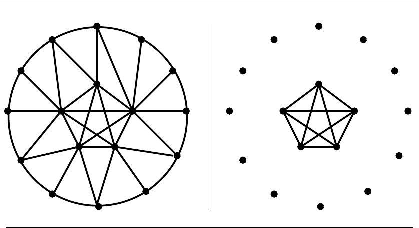
16.1 CLIQUE 525
INPUT OUTPUT
16.1 Clique
Input description: A graph G=(V,E).
Problem description: What is the largest S⊂Vsuch that for all x, y ∈S,
(x, y)∈E?
Discussion: In high school, everybody complained about the “clique,”—a group
of friends who all hung around together and seemed to dominate everything social.
Consider a graph representing the school’s social network. Vertices correspond to
people, with edges between any pair of people who are friends. Thus, the high
school clique defines a (complete subgraph) clique in this friendship graph.
Identifying “clusters” of related objects often reduces to finding large cliques in
graphs. An interesting example arose in a program the Internal Revenue Service
(IRS) developed to detect organized tax fraud. In this scam, large groups of phony
tax returns are submitted in the hopes of getting undeserved refunds. But generat-
ing large numbers of different phony tax returns is hard work. The IRS constructs
graphs with vertices corresponding to submitted tax forms and edges between any
two forms that appear suspiciously similar. Any large clique in this graph points
to fraud.
Since any edge in a graph represents a clique of two vertices, the challenge lies
not in finding a clique, but in finding a large clique. And it is indeed a challenge, for
finding a maximum clique is NP-complete. To make matters worse, it is provably

526 16. GRAPH PROBLEMS: HARD PROBLEMS
hard to approximate even to within a factor of n1/2−. Theoretically, clique is about
as hard as a problem in this book can get. So what can we hope to do about it?
•Will a maximal clique suffice? –Amaximal clique is a clique that cannot be
enlarged by adding any additional vertex. This doesn’t mean that it has to
be large relative to the largest possible clique, but it might be. To find a nice
maximal (and hopefully large) clique, sort the vertices from highest degree
to lowest degree, put the first vertex in the clique, and then test each of the
other vertices to see whether it is adjacent to all the clique vertices added
thus far. If so, add it; if not, continue down the list. By using a bit vector to
mark which vertices are currently in the clique, this can be made to run in
O(n+m) time. An alternative approach might incorporate some randomness
into the vertex ordering, and accept the largest maximal clique you find after
a certain number of trials.
•What if I will settle for a large, dense subgraph? – Insisting on cliques to define
clusters in a graph can be risky, since a single missing edge will eliminate a
vertex from consideration. Instead, we should seek large dense subgraphs—
i.e. , subsets of vertices that contain a large number of edges between them.
Cliques are, by definition, the densest subgraphs possible.
The largest set of vertices whose induced (defined) subgraph has minimum
vertex degree ≥kcan be found with a simple linear-time algorithm. Begin
by deleting all the vertices whose degree is less than k. This may reduce the
degree of other vertices below k, if they were adjacent to sufficiently deleted
low-degree vertices. Repeating this process until all remaining vertices have
degree ≥kconstructs the largest high-degree subgraph. This algorithm can
be implemented in O(n+m) time by using adjacency lists and the constant-
width priority queue of Section 12.2 (page 373). If we continue to delete the
lowest-degree vertices, we eventually end up with a clique or set of cliques, –
but they may be as small as two vertices.
•What if the graph is planar? – Planar graphs cannot have cliques of a size
larger than four, or else they cease to be planar. Since each edge defines
a clique of size 2, the only interesting cases are cliques of three and four
vertices. Efficient algorithms to find such small cliques consider the vertices
from lowest to highest degree. Any planar graph must contain a vertex of at
most 5 degrees (see Section 15.12 (page 520)), so there is only a constant-sized
neighborhood to check exhaustively for a clique containing it. We then delete
this vertex to leave a smaller planar graph, containing another low-degree
vertex. Repeat this check and delete processes until the graph is empty.
If you really need to find the largest clique in a graph, an exhaustive search via
backtracking provides the only real solution. We search through all k-subsets of the
vertices, pruning a subset as soon as it contains a vertex that is not adjacent to all
the rest. A simple upper bound on the maximum clique in Gis the highest vertex

16.1 CLIQUE 527
degree plus 1. A better upper bound comes from sorting the vertices in order of
decreasing degree. Let jbe the largest index such that degree of the jth vertex is
at least j−1. The largest clique in the graph contains no more than jvertices,
since no vertex of degree <(j−1) can appear in a clique of size j. To speed our
search, we should delete all such useless vertices from G.
Heuristics for finding large cliques based on randomized techniques such as
simulated annealing are likely to work reasonably well.
Implementations:Cliquer is a set of C routines for finding cliques in arbitrary
weighted graphs by Patric ¨
Ostergard. It uses an exact branch-and-bound algorithm,
and is available at http://users.tkk.fi/∼pat/cliquer.html.
Programs for finding cliques and independent sets were sought for the Second
DIMACS Implementation Challenge [JT96]. Programs and data from the challenge
are available by anonymous FTP from dimacs.rutgers.edu. Source codes are avail-
able under pub/challenge/graph and test data under pub/djs.dfmax.c implements
a simple-minded branch-and-bound algorithm similar to [CP90]. dmclique.c uses a
“semi-exhaustive greedy” scheme for finding large independent sets from [JAMS91].
Kreher and Stinson [KS99] provide branch-and-bound programs in C for
finding the maximum clique using a variety of lower-bounds, available at
http://www.math.mtu.edu/∼kreher/cages/Src.html.
GOBLIN (http://www.math.uni-augsburg.de/∼fremuth/goblin.html) impleme-
nts branch-and-bound algorithms for finding large cliques. They claim to be able
to work with graphs as large as 150 to 200 vertices.
Notes:Bomze, et al. [BBPP99] give the most comprehensive survey on the problem of
finding maximum cliques. Particularly interesting is the work from the operations research
community on branch-and-bound algorithms for finding cliques effectively. More recent
experimental results are reported in [JS01].
The proof that clique is NP-complete is due to Karp [Kar72]. His reduction (given in
Section 9.3.3 (page 327)) established that clique, vertex cover, and independent set are
very closely related problems, so heuristics and programs that solve one of them should
also produce reasonable solutions for the other two.
The densest subgraph problem seeks the subset of vertices whose induced subgraph has
the highest average vertex degree. A clique of kvertices is clearly the densest subgraph
of its size, but larger, noncomplete subgraphs may achieve higher average degree. The
problem is NP-complete, but simple heuristics based on repeatedly deleting the lowest-
degree vertex achieve reasonable approximation ratios [AITT00]. See [GKT05] for an
interesting application of densest subgraph, namely detecting link spam on the Web.
That clique cannot be approximated to within a factor of n1/2−unless P=NP (and
n1−under weaker assumptions) is shown in [Has82].
Related Problems: Independent set (see page 528), vertex cover (see page 530).
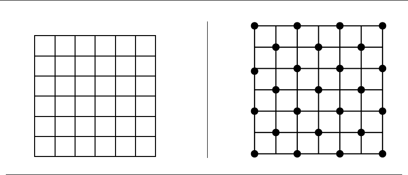
528 16. GRAPH PROBLEMS: HARD PROBLEMS
INPUT OUTPUT
16.2 Independent Set
Input description: A graph G=(V,E).
Problem description: What is the largest subset Sof vertices of Vsuch that for
each edge (x, y)∈E, either x∈ Eor y∈ E?
Discussion: The need to find large independent sets arises in facility dispersion
problems, where we seek a set of mutually separated locations. It is important
that no two locations of our new “McAlgorithm” franchise service be placed close
enough to compete with each other. We can construct a graph where the vertices
are the set of possible locations, and then add edges between any two locations
deemed close enough to interfere. The maximum independent set gives the largest
number of franchises we can sell without cannibalizing sales.
Independent sets (also known as stable sets) avoid conflicts between elements,
and hence arise often in coding theory and scheduling problems. Define a graph
whose vertices represent the set of possible code words, and add edges between
any two code words sufficiently similar to be confused due to noise. The maxi-
mum independent set of this graph defines the highest capacity code for the given
communication channel.
Independent set is closely related to two other NP-complete problems:
•Clique – Watch what you say, for a clique is what you get if you give an
independent set a complement. The complement of G=(V,E) is a graph
G=(V, E) where (i, j)∈Eiff (i, j) is not in E. In other words, we replace
each edge by a non-edge and vice versa. The maximum independent set in G
is exactly the maximum clique in G, so the two problems are algorithmically

16.2 INDEPENDENT SET 529
identical. Thus, the algorithms and implementations in Section 16.1 (page
525) can easily be used for independent set.
•Vertex coloring – The vertex coloring of a graph G=(V,E) is a partition of
Vinto a small number of sets (colors), where no two vertices of the same color
can have an edge between them. Each color class defines an independent set.
Many scheduling applications of independent set are really coloring problems,
since all tasks eventually must be completed.
Indeed, one heuristic to find a large independent set is to use any vertex col-
oring algorithm/heuristic, and take the largest color class. One consequence
of this observation is that all graphs with small chromatic numbers (such as
planar and bipartite graphs) have large independent sets.
The simplest reasonable heuristic is to find the lowest-degree vertex, add it to
the independent set, and then delete it and all vertices adjacent to it. Repeating
this process until the graph is empty gives a maximal independent set, in that it
can’t be made larger by just adding vertices. Using randomization or perhaps some
degree of exhaustive search might result in somewhat larger independent sets.
The independent set problem is in some sense dual to the graph-matching prob-
lem. The former asks for a large set of vertices with no edge in common, while the
latter asks for a large set of edges with no vertex in common. This suggests trying
to rephrase your problem as an efficiently-computable matching problem instead
of maximum independent set problem, which is NP-complete.
The maximum independent set of a tree can be found in linear time by (1)
stripping off the leaf nodes, (2) adding them to the independent set, (3) deleting
all adjacent nodes, and then (4) repeating from the first step on the resulting trees
until it is empty.
Implementations: Any program for computing the maximum clique in a graph
can find maximum independent sets by just complementing the input graph. There-
fore, we refer the reader to the clique-finding programs of Section 16.1 (page 525).
GOBLIN (http://www.math.uni-augsburg.de/∼fremuth/goblin.html) impleme-
nts a branch-and-bound algorithm for finding independent sets (called stable sets
in the manual).
Greedy randomized adaptive search (GRASP) heuristics for independent set
set have been implemented by Resende, et al. [RFS98] as Algorithm 787 of the
Collected Algorithms of the ACM (see Section 19.1.6 (page 659)). These Fortran
codes are also available from http://www.research.att.com/∼mgcr/src/.
Notes:The proof that independent set is NP-complete is due to Karp [Kar72]. It remains
NP-complete for planar cubic graphs [GJ79]. Independent set can be solved efficiently for
bipartite graphs [Law76]. This is not trivial—indeed the larger of the “part” of a bipartite
graph is not necessarily its maximum independent set.
Related Problems: Clique (see page 525), vertex coloring (see page 544), vertex
cover (see page 530).
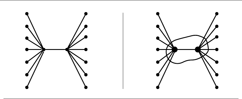
530 16. GRAPH PROBLEMS: HARD PROBLEMS
INPUT OUTPUT
16.3 Vertex Cover
Input description: A graph G=(V,E).
Problem description: What is the smallest subset of S⊂Vsuch that each edge
(x, y)∈Econtains at least one vertex of S?
Discussion: Vertex cover is a special case of the more general set cover problem,
which takes as input an arbitrary collection of subsets S=(S1,...,S
n)ofthe
universal set U={1,...,m}. We seek the smallest subset of subsets from Swhose
union is U. Set cover arises in many applications associated with buying things
sold in fixed lots or assortments. See Section 18.1 (page 621) for a discussion of set
cover.
To turn vertex cover into a set cover problem, let universal set Urepresent the
set Eof edges from G, and define Sito be the set of edges incident on vertex i.A
set of vertices defines a vertex cover in graph Giff the corresponding subsets define
a set cover in this particular instance. However, since each edge can be in only
two different subsets, vertex cover instances are simpler than general set cover.
Vertex cover is a relative lightweight among NP-complete problems, and can be
more effectively solved than general set cover.
Vertex cover and independent set are very closely related graph problems. Since
every edge in Eis (by definition) incident on a vertex in any cover S, there can be
no edge both endpoints are in V−S.Thus,V−Smust be an independent set.
Since minimizing Sis the same as maximizing V−S, the problems are equivalent.
This means that any independent set solver can be applied to vertex cover as well.
Having two ways of looking at your problem is helpful, since one may appear easier
in a given context.

16.3 VERTEX COVER 531
The simplest heuristic for vertex cover selects the vertex with highest degree,
adds it to the cover, deletes all adjacent edges, and then repeats until the graph is
empty. With the right data structures, this can be done in linear time, and should
“usually” produce a “pretty good” cover. However, this cover might be lg ntimes
worse than the optimal cover for certain input graphs.
Fortunately, we can always find a vertex cover whose size is at most twice as
large as optimal. Find a maximal matching Min the graph—i.e. , a set of edges no
two of which share a vertex in common and which cannot be enlarged by adding
additional edges. Such a maximal matching can be constructed incrementally, by
picking an arbitrary edge ein the graph, deleting any edge sharing a vertex with e,
and repeating until the graph is out of edges. Taking both of the vertices for each
edge in a maximal matching gives us a vertex cover. Why? Because any vertex
cover must contain at least one of the two vertices in each matching edge just to
cover the edges of M, this cover is at most twice as large as the minimum cover.
This heuristic can be tweaked to perform somewhat better in practice, if not
in theory. We can select the matching edges to “kill off” as many other edges as
possible, which should reduce the size of the maximal matching and hence the
number of pairs of vertices in the vertex cover. Also, some of the vertices from M
may in fact not be necessary, since all of their incident edges might also have been
covered using other selected vertices. We can identify and delete these losers by
making a second pass through our cover.
The vertex cover problem seeks to cover all edges using few vertices. Two other
important problems have similar sounding objectives:
•Cover all vertices using few vertices –Thedominating set problem seeks the
smallest set of vertices Dsuch that every vertex in V−Dis adjacent to at
least one vertex in the dominating set D. Every vertex cover of a nontrivial
connected graph is also a dominating set, but dominating sets can be much
smaller. Any single vertex represents the minimum dominating set of com-
plete graph Kn, while n−1 vertices are needed for a vertex cover. Dominating
sets tend to arise in communications problems, since they represent the hubs
or broadcast centers sufficient to communicate with all sites/users.
Dominating set problems can be easily expressed as instances of set cover (see
Section 18.1 (page 621)). Each vertex videfines a subset of vertices consisting
of itself plus all the vertices it is adjacent to. The greedy set cover heuris-
tic running on this instance yields a Θ(lg n) approximation to the optimal
dominating set.
•Cover all vertices using few edges –Theedge cover problem seeks the smallest
set of edges such that each vertex is included in one of the edges. In fact, edge
cover can be solved efficiently by finding a maximum cardinality matching
(see Section 15.6 (page 498)) and then selecting arbitrary edges to account
for the unmatched vertices.

532 16. GRAPH PROBLEMS: HARD PROBLEMS
Implementations: Any program for computing the maximum clique in a graph
can be applied to vertex cover by complementing the input graph and selecting the
vertices which do not appear in the clique. Therefore, we refer the reader to check
out the clique-finding programs of Section 16.1 (page 525).
COVER [RHG07] is a very effective vertex cover solver based on a stochastic local
search algorithm. It is available at http://www.nicta.com.au/people/richters/.
JGraphT (http://jgrapht.sourceforge.net/) is a Java graph library that contains
greedy and 2-approximate heuristics for vertex cover.
Notes:Karp [Kar72] first proved that vertex-cover is NP-complete. Several different
heuristics yield 2-approximation algorithms for vertex cover, including randomized round-
ing. Good expositions on these 2-approximation algorithms include [CLRS01, Hoc96,
Pas97, Vaz04]. The example that the greedy algorithm can be as bad as lg ntimes op-
timal is due to [Joh74] and presented in [PS98]. Experimental studies of vertex cover
heuristics include [GMPV06, GW97, RHG07].
Whether there exists a better than 2-factor approximation for vertex cover is one of
the major open problems in approximation algorithms. Hastad [Has97] proved there does
not exist a better than 1.1666-factor approximation algorithm for vertex cover.
The primary reference on dominating sets is the monograph of Haynes et al. [HHS98].
Heuristics for the connected dominating set problem are presented in [GK98]. Dominating
set cannot be approximated to better than the Ω(lg n) factor [ACG+03] of set cover.
Related Problems: Independent set (see page 528), set cover (see page 621).
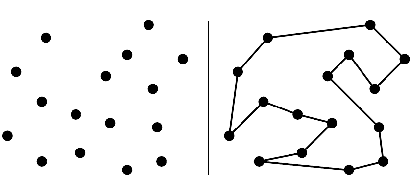
16.4 TRAVELING SALESMAN PROBLEM 533
INPUT OUTPUT
16.4 Traveling Salesman Problem
Input description: A weighted graph G.
Problem description: Find the cycle of minimum cost, visiting each vertex of G
exactly once.
Discussion: The traveling salesman problem is the most notorious NP-complete
problem. This is a function both of its general usefulness and the ease with which
it can be explained to the public at large. Imagine a traveling salesman planning a
car trip to visit a set of cities. What is the shortest route that will enable him to
do so and return home, thus minimizing his total driving?
The traveling salesman problem arises in many transportation and routing prob-
lems. Other important applications involve optimizing tool paths for manufacturing
equipment. For example, consider a robot arm assigned to solder all the connec-
tions on a printed circuit board. The shortest tour that visits each solder point
exactly once defines the most efficient route for the robot.
Several issues arise in solving TSPs:
•Is the graph unweighted? – If the graph is unweighted, or all the edges have
one of two possible cost values, the problem reduces to finding a Hamiltonian
cycle. See Section 16.5 (page 538) for a discussion of this problem.
•Does your input satisfy the triangle inequality? – Our sense of how proper
distance measures behave is captured by the triangle inequality. This prop-
erty states that d(i, j)≤d(i, k)+d(k, j) for all vertices i, j, k ∈V. Geometric

534 16. GRAPH PROBLEMS: HARD PROBLEMS
distances all satisfy the triangle inequality because the shortest distance be-
tween two points is as the crow flies. Commercial air fares do not satisfy the
triangle inequality, which is why it is so hard to find the cheapest airfare be-
tween two points. TSP heuristics work much better on sensible graphs that
do obey the triangle inequality.
•Are you given npoints as input or a weighted graph? – Geometric instances
are often easier to work with than a graph representation. Since pair of points
define a complete graph, there is never an issue of finding a feasible tour. We
can save space by computing these distances on demand, thus eliminating
the need to store an n×ndistance matrix. Geometric instances inherently
satisfy the triangle inequality, so they can exploit performance guarantees
from certain heuristics. Finally, one can take advantage of geometric data
structures like kd-trees to quickly identify close unvisited sites.
•Can you visit a vertex more than once? – The restriction that the tour not
revisit any vertex is irrelevant in many applications. In air travel, the cheapest
way to visit all vertices might involve repeatedly visiting an airport hub. Note
that this issue does not arise when the input observes the triangle inequality.
TSP with repeated vertices is easily solved by using any conventional TSP
code on a new cost matrix D, where D(i, j) is the shortest path distance from
ito j. This matrix can be constructed by solving an all-pairs shortest path
(see Section 15.4 (page 489)) and satisfies the triangle inequality.
•Is your distance function symmetric? – A distance function is asymmetric
when there exists x,ysuch that d(x, y)=d(y, x). The asymmetric traveling
salesman problem (ATSP) is much harder to solve in practice than symmet-
ric (STSP) instances. Try to avoid such pathological distance functions. Be
aware that there is a reduction converting ATSP instances to symmetric in-
stances containing twice as many vertices [GP07], that may be useful because
symmetric solvers are so much better.
•How important is it to find the optimal tour? – Usually heuristic solutions
will suffice for applications. There are two different approaches if you insist
on solving your TSP to optimality, however. Cutting plane methods model the
problem as an integer program, then solve the linear programming relaxation
of it. Additional constraints designed to force integrality are added if the
optimal solution is not at an integer point. Branch-and-bound algorithms
perform a combinatorial search while maintaining careful upper and lower
bounds on the cost of a tour. In the hands of professionals, problems with
thousands of vertices can be solved. Maybe you can too, if you use the best
solver available.
Almost any flavor of TSP is going to be NP-complete, so the right way to pro-
ceed is with heuristics. These typically come within a few percent of the optimal

16.4 TRAVELING SALESMAN PROBLEM 535
solution, which is close enough for engineering work. Unfortunately, literally dozens
of heuristics have been proposed for TSP, so the situation can be confusing. Empir-
ical results in the literature are sometime contradictory. However, we recommend
choosing from among the following heuristics:
•Minimum spanning trees – This heuristic starts by finding the minimum
spanning tree (MST) of the sites, and then does a depth-first search of the
resulting tree. In the course of DFS, we walk over each of the n−1 edges
exactly twice: once going down to discover a new vertex, and once going up
when we backtrack. Now define a tour by ordering the vertices by when they
were discovered. If the graph obeys the triangle inequality, the resulting tour
is at most twice the length of the optimal TSP tour. In practice, it is usually
better, typically 15% to 20% over optimal. Furthermore, the running time is
bounded by that of computing the MST, which is only O(nlg n) in the case
of points in the plane (see Section 15.3 (page 484)).
•Incremental insertion methods – A different class of heuristics starts from a
single vertex, and then inserts new points into this partial tour one at a time
until the tour is complete. The version of this heuristic that seems to work
best is furthest point insertion: of all remaining points, insert the point vinto
a partial tour Tsuch that
max
v∈V
|T|
min
i=1 (d(v, vi)+d(v, vi+1))
The “min” ensures that we insert the vertex in the position that adds the
smallest amount of distance to the tour, while the “max” ensures that we
pick the worst such vertex first. This seems to work well because it “roughs
out” a partial tour first before filling in details. Such tours are typically only
5% to 10% longer than optimal.
•K-optimal tours – Substantially more powerful are the Kernighan-Lin, or k-
opt, class of heuristics. The method applies local refinements to an initially
arbitrary tour in the hopes of improving it. In particular, subsets of kedges
are deleted from the tour and the kremaining subchains rewired to form
a different tour with hopefully a better cost. A tour is k-optimal when no
subset of kedges can be deleted and rewired to reduce the cost of the tour.
Two-opting a tour is a fast and effective way to improve any other heuristic.
Extensive experiments suggest that 3-optimal tours are usually within a few
percent of the cost of optimal tours. For k>3, the computation time increases
considerably faster than the solution quality. Simulated annealing provides
an alternate mechanism to employ edge flips to improve heuristic tours.
Implementations: Concorde is a program for the symmetric traveling salesman
problem and related network optimization problems, written in ANSI C. This

536 16. GRAPH PROBLEMS: HARD PROBLEMS
world record-setting program by Applegate, Bixby, Chvatal, and Cook [ABCC07]
has obtained the optimal solutions to 106 of TSPLIB’s 110 instances; the largest
of which has 15,112 cities. Concorde is available for academic research use from
http://www.tsp.gatech.edu/concorde. It is the clear choice among available TSP
codes. Their http://www.tsp.gatech.edu/ website features very interesting material
on the history and applications of TSP.
Lodi and Punnen [LP07] put together an excellent survey of available soft-
ware for solving TSP. Current links to all programs mentioned are maintained at
http://www.or.deis.unibo.it/research pages/tspsoft.html.
TSPLIB [Rei91] provides the standard collection of hard instances of TSPs
that arise in practice. The best-supported version of TSPLIB is available from
http://www.iwr.uni-heidelberg.de/groups/comopt/software/TSPLIB95/, although
the instances are also available from Netlib (see Section 19.1.5 (page 659)).
Tsp solve is a C++ code by Chad Hurwitz and Robert Craig that provides
both heuristic and optimal solutions. Geometric problems of size up to 100 points
are manageable. It is available from http://www.cs.sunysb.edu/∼algorith or by
e-mailing Chad Hurrwitz at churritz@cts.com. GOBLIN (http://www.math.uni-
augsburg.de/∼fremuth/goblin.html) implements branch-and-bound algorithms for
both symmetric and asymmetric TSP, as well as a variety of heuristics.
Algorithm 608 [Wes83] of the Collected Algorithms of the ACM is a Fortran
implementation of a heuristic for the quadratic assignment problem—a more gen-
eral problem that includes the traveling salesman as a special case. Algorithm 750
[CDT95] is a Fortran code for the exact solution of asymmetric TSP instances.
See Section 19.1.5 (page 659) for details.
Notes:The book by Applegate, Bixby, Chvatal, and Cook [ABCC07] documents the
techniques they used in their record-setting TSP solvers, as well as the theory and history
behind the problem. Gutin and Punnen [GP07] now offer the best reference on all aspects
and variations of the traveling salesman problem, displacing an older but much beloved
book by Lawler et al. [LLKS85].
Experimental results on heuristic methods for solving large TSPs include [Ben92a,
GBDS80, Rei94]. Typically, it is possible to get within a few percent of optimal with such
methods.
The Christofides heuristic [Chr76] is an improvement over the minimum-spanning
tree heuristic and guarantees a tour whose cost is at most 3/2timesoptimalonEu-
clidean graphs. It runs in O(n3), where the bottleneck is the time it takes to find a
minimum-weight perfect matching (see Section 15.6 (page 498)). The minimum spanning
tree heuristic is due to [RSL77].
Polynomial-time approximation schemes for Euclidean TSP have been developed by
Arora [Aro98] and Mitchell [Mit99], which offer 1 + factor approximations in polyno-
mial time for any >0. They are of great theoretical interest, although any practical
consequences remain to be determined.
The history of progress on optimal TSP solutions is inspiring. In 1954, Dantzig, Fulk-
erson, and Johnson solved a symmetric TSP instance of 42 United States cities [DFJ54].
In 1980, Padberg and Hong solved an instance on 318 vertices [PH80]. Applegate et al.
[ABCC07] have recently solved problems that are twenty times larger than this. Some of

16.4 TRAVELING SALESMAN PROBLEM 537
this increase is due to improved hardware, but most is due to better algorithms. The rate
of growth demonstrates that exact solutions to NP-complete problems can be obtained for
large instances if the stakes are high enough. Fortunately or unfortunately, they seldom
are.
Size is not the only criterion for hard instances. One can easily construct an enormous
graph consisting of one cheap cycle, for which it would be easy to find the optimal solution.
For sets of points in convex position in the plane, the minimum TSP tour is described by
its convex hull (see Section 17.2 (page 568)), which can be computed in O(nlg n)time.
Other easy special cases are known.
Related Problems: Hamiltonian cycle (see page 538), minimum spanning tree
(see page 484), convex hull (see page 568).

538 16. GRAPH PROBLEMS: HARD PROBLEMS
INPUT OUTPUT
16.5 Hamiltonian Cycle
Input description: A graph G=(V,E).
Problem description: Find a tour of the vertices using only edges from G, such
that each vertex is visited exactly once.
Discussion: Finding a Hamiltonian cycle or path in a graph Gis a special case of
the traveling salesman problem G—one where each edge in Ghas distance 1 in G.
Non-edge vertex pairs are separated by a greater distance, say 2. Such a weighted
graph has TSP tour of cost nin Giff Gis Hamiltonian.
Closely related is the problem of finding the longest path or cycle in a graph.
This arises often in pattern recognition problems. Let the vertices in the graph
correspond to possible symbols, with edges linking pairs of symbols that might
occur next to each other. The longest path through this graph is a good candidate
for the proper interpretation.
The problems of finding longest cycles and paths are both NP-complete, even
on very restrictive classes of unweighted graphs. There are several possible lines of
attack, however:
•Is there a serious penalty for visiting vertices more than once? – Reformulat-
ing the Hamiltonian cycle problem instead of minimizing the total number
of vertices visited on a complete tour turns it into an optimization problem.

16.5 HAMILTONIAN CYCLE 539
This allows possibilities for heuristics and approximation algorithms. Finding
a spanning tree of the graph and doing a depth-first search, as discussed in
Section 16.4 (page 533), yields a tour with at most 2nvertices. Using random-
ization or simulated annealing might bring the size of this down considerably.
•Am I seeking the longest path in a directed acyclic graph (DAG)? – The prob-
lem of finding the longest path in a DAG can be solved in linear time using
dynamic programming. Conveniently, the algorithm for finding the shortest
path in a DAG (presented in Section 15.4 (page 489)) does the job if we
replace min with max. DAGs are the most interesting case of longest path
for which efficient algorithms exist.
•Is my graph dense? – Sufficiently dense graphs always contain Hamiltonian
cycles. Further, the cycles implied by such sufficiency conditions can be effi-
ciently constructed. In particular, any graph where all vertices have degree
≥n/2 must be Hamiltonian. Stronger sufficient conditions also hold; see the
Notes section.
•Are you visiting all the vertices or all the edges? – Verify that you really have a
vertex-tour problem and not an edge-tour problem. With a little cleverness it
is sometimes possible to reformulate a Hamiltonian cycle problem in terms of
Eulerian cycles, which instead visit every edge of a graph. Perhaps the most
famous such instance is the problem of constructing de Bruijn sequences,
discussed in Section 15.7 (page 502). The benefit is that fast algorithms exist
for Eulerian cycles and many related variants, while Hamiltonian cycle is
NP-complete.
If you really must know whether your graph is Hamiltonian, backtracking with
pruning is your only possible solution. Certainly check whether your graph is bi-
connected (see Section 15.8 (page 505)). If not, this means that the graph has
an articulation vertex whose deletion will disconnect the graph and so cannot be
Hamiltonian.
Implementations: The construction described above (weight 1 for an edge and
2 for a non-edge) reduces Hamiltonian cycles to a symmetric TSP problem that
obeys the triangle inequality. Thus we refer the reader to the TSP solvers dis-
cussed in Section 16.4 (page 533). Foremost among them is Concorde, a program
for the symmetric traveling salesman problem and related network optimization
problems, written in ANSI C. Concorde is available for academic research use from
http://www.tsp.gatech.edu/concorde. It is the clear choice among available TSP
codes.
An effective program for solving Hamiltonian cycle problems resulted from the
masters thesis of Vandegriend [Van98]. Both the code and the thesis are available
from http://web.cs.ualberta.ca/∼joe/Theses/vandegriend.html.

540 16. GRAPH PROBLEMS: HARD PROBLEMS
Lodi and Punnen [LP07] put together an excellent survey of available TSP soft-
ware, including the special case of Hamiltonian cycle. Current links to all programs
are maintained at http://www.or.deis.unibo.it/research pages/tspsoft.html.
The football program of the Stanford GraphBase (see Section 19.1.8 (page 660))
uses a stratified greedy algorithm to solve the asymmetric longest-path problem.
The goal is to derive a chain of football scores to establish the superiority of one
football team over another. After all, if Virginia beat Illinois by 30 points, and
Illinois beat Stony Brook by 14 points, then by transitivity Virginia would beat
Stony Brook by 44 points if they played, right? We seek the longest simple path
in a graph where the weight of edge (x, y) denotes the number of points by which
xbeat y.
Nijenhuis and Wilf [NW78] provide an efficient routine to enumerate all Hamil-
tonian cycles of a graph by backtracking. See Section 19.1.10 (page 661). Algorithm
595 [Mar83] of the Collected Algorithms of the ACM is a similar Fortran code that
can be used as either an exact procedure or a heuristic by controlling the amount
of backtracking. See Section 19.1.5 (page 659).
Notes:Hamiltonian cycles apparently first arose in Euler’s study of the knight’s tour
problem, although they were popularized by Hamilton’s “Around the World” game in
1839. See [ABCC07, GP07, LLKS85] for comprehensive references on the traveling sales-
man problem, including discussions on Hamiltonian cycle.
Most good texts in graph theory review sufficiency conditions for graphs to be Hamil-
tonian. My favorite is West [Wes00].
Techniques for solving optimization problems in the laboratory using biological pro-
cesses have attracted considerable attention. In the original application of these “bio-
computing” techniques, Adleman [Adl94] solved a seven-vertex instance of the directed
Hamiltonian path problem. Unfortunately, this approach requires an exponential number
of molecules, and Avogadro’s number implies that such experiments are inconceivable for
graphs beyond n≈70.
Related Problems: Eulerian cycle (see page 502), traveling salesman (see page
533).
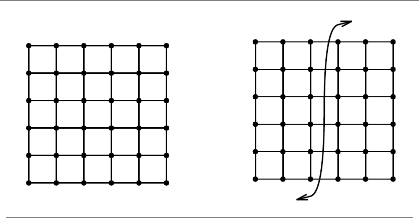
16.6 GRAPH PARTITION 541
INPUT OUTPUT
16.6 Graph Partition
Input description: A (weighted) graph G=(V, E) and integers kand m.
Problem description: Partition the vertices into mroughly equal-sized subsets
such that the total edge cost spanning the subsets is at most k.
Discussion: Graph partitioning arises in many divide-and-conquer algorithms,
which gain their efficiency by breaking problems into equal-sized pieces such that
the respective solutions can easily be reassembled. Minimizing the number of edges
cut in the partition usually simplifies the task of merging.
Graph partition also arises when we need to cluster the vertices into logical
components. If edges link “similar” pairs of objects, the clusters remaining after
partition should reflect coherent groupings. Large graphs are often partitioned into
reasonable-sized pieces to improve data locality or make less cluttered drawings.
Finally, graph partition is a critical step in many parallel algorithms. Consider
the finite element method, which is used to compute the physical properties (such
as stress and heat transfer) of geometric models. Parallelizing such calculations
requires partitioning the models into equal-sized pieces whose interface is small.
This is a graph-partitioning problem, since the topology of a geometric model is
usually represented using a graph.
Several different flavors of graph partitioning arise depending on the desired
objective function:
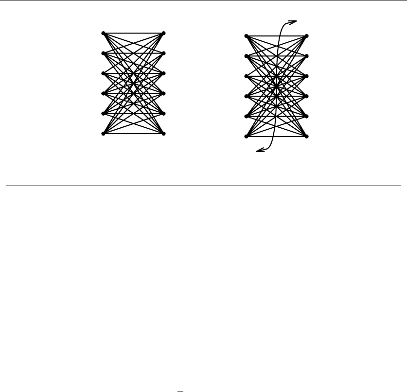
542 16. GRAPH PROBLEMS: HARD PROBLEMS
Figure 16.1: The maximum cut of a graph
•Minimum cut set –Thesmallest set of edges to cut that will disconnect a
graph can be efficiently found using network flow or randomized algorithms.
See Section 15.8 (page 505) for more on connectivity algorithms. The smallest
cutset might split off only a single vertex, so the resulting partition could be
very unbalanced.
•Graph partition – A better partition criterion seeks a small cut that parti-
tions the vertices into roughly equal-sized pieces. Unfortunately, this problem
is NP-complete. Fortunately, the heuristics discussed below work well in prac-
tice.
Certain special graphs always have small separators, that partition the ver-
tices into balanced pieces. For any tree, there always exists a single vertex
whose deletion partitions the tree so that no component contains more than
n/2 of the original nvertices. These components need not always be con-
nected; consider the separating vertex of a star-shaped tree. This separating
vertex can be found in linear time using depth first-search. Every planar
graph has a set of O(√n) vertices whose deletion leaves no component with
more than 2n/3 vertices. These separators provide a useful way to decompose
geometric models, which are often defined by planar graphs.
•Maximum cut – Given an electronic circuit specified by a graph, the maximum
cut defines the largest amount of data communication that can simultaneously
occur in the circuit. The highest-speed communications channel should thus
span the vertex partition defined by the maximum edge cut. Finding the
maximum cut in a graph is NP-complete [Kar72], however heuristics similar
to those of graph partitioning work well.
The basic approach for dealing with graph partitioning or max-cut problems
is to construct an initial partition of the vertices (either randomly or according

16.6 GRAPH PARTITION 543
to some problem-specific strategy) and then sweep through the vertices, deciding
whether the size of the cut would improve if we moved this vertex over to the other
side. The decision to move vertex vcan be made in time proportional to its degree,
by identifying which side of the partition contains more of v’s neighbors. Of course,
the desirable side for vmay change after its neighbors jump, so several iterations
are likely to be needed before the process converges on a local optimum. Even so,
such a local optimum can be arbitrarily far away from the global max-cut.
There are many variations of this basic procedure, by changing the order we
test the vertices in or moving clusters of vertices simultaneously. Using some form
of randomization, particularly simulated annealing, is almost certain to be a good
idea. When more than two components are desired, the partitioning heuristic should
be applied recursively.
Spectral partitioning methods use sophisticated linear algebra techniques to
obtain a good partitioning. The spectral bisection method uses the second-lowest
eigenvector of the Laplacian matrix of the graph to partition it into two pieces.
Spectral methods tend to do a good job of identifying the general area to partition,
but the results can be improved by cleaning up with a local optimization method.
Implementations: Chaco is a widely-used graph partitioning code designed to
partition graphs for parallel computing applications. It employs several differ-
ent partitioning algorithms, including both Kernighan-Lin and spectral methods.
Chaco is available at http://www.cs.sandia.gov/∼bahendr/chaco.html.
METIS (http://glaros.dtc.umn.edu/gkhome/views/metis) is another well-
regarded code for graph partitioning. It has successfully partitioned graphs with
over 1,000,000 vertices. Available versions include one variant designed to run
on parallel machines and another suitable for partitioning hypergraphs. Other
respected codes include Scotch (http://www.labri.fr/perso/pelegrin/scotch/)and
JOSTLE (http://staffweb.cms.gre.ac.uk/∼wc06/jostle/).
Notes:The fundamental local improvement heuristics for graph partitioning are due to
Kernighan-Lin [KL70] and Fiduccia-Mattheyses [FM82]. Spectral methods for graph par-
tition are discussed in [Chu97, PSL90]. Empirical results on graph partitioning heuristics
include [BG95, LR93].
The planar separator theorem and an efficient algorithm for finding such a separator
are due to Lipton and Tarjan [LT79, LT80]. For experiences in implementing planar
separator algorithms, see [ADGM04, HPS+05].
Any random vertex partition will expect to cut half of the edges in the graph, since the
probability that the two vertices defining an edge end up on different sides of the partition
is 1/2. Goemans and Williamson [GW95] gave an 0.878-factor approximation algorithm
for maximum-cut, based on semi-definite programming techniques. Tighter analysis of
this algorithm was followed by Karloff [Kar96].
Related Problems: Edge/vertex connectivity (see page 505), network flow (see
page 509).
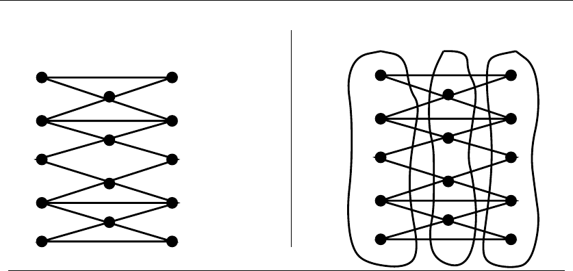
544 16. GRAPH PROBLEMS: HARD PROBLEMS
INPUT OUTPUT
16.7 Vertex Coloring
Input description: A graph G=(V,E).
Problem description: Color the vertices of Vusing the minimum number of
colors such that iand jhave different colors for all (i, j)∈E.
Discussion: Vertex coloring arises in many scheduling and clustering applications.
Register allocation in compiler optimization is a canonical application of coloring.
Each variable in a given program fragment has a range of times during which its
value must be kept intact, in particular after it is initialized and before its final
use. Any two variables whose life spans intersect cannot be placed in the same
register. Construct a graph where each vertex corresponds to a variable, with an
edge between any two vertices whose variable life spans intersect. Since none of
the variables assigned the same color clash, they all can be assigned to the same
register.
No conflicts will occur if each vertex is colored using a distinct color. But
computers have a limited number of registers, so we seek a coloring using the
fewest colors. The smallest number of colors sufficient to vertex-color a graph is its
chromatic number.
Several special cases of interest arise in practice:
•Can I color the graph using only two colors? – An important special case is
testing whether a graph is bipartite, meaning it can be colored using only
two different colors. Bipartite graphs arise naturally in such applications as
mapping workers to possible jobs. Fast, simple algorithms exist for problems

16.7 VERTEX COLORING 545
such as matching (see Section 15.6 (page 498)) when restricted to bipartite
graphs.
Testing whether a graph is bipartite is easy. Color the first vertex blue, and
then do a depth-first search of the graph. Whenever we discover a new, uncol-
ored vertex, color it opposite of its parent, since the same color would cause
a clash. The graph cannot be bipartite if we ever find an edge (x, y) where
both xand yhave been colored identically. Otherwise, the final coloring will
be a 2-coloring, constructed in O(n+m) time. An implementation of this
algorithm is given in Section 5.7.2 (page 167).
•Is the graph planar, or are all vertices of low degree? – The famous four-
color theorem states that every planar graph can be vertex colored using at
most four distinct colors. Efficient algorithms for finding a four-coloring on
planar graphs are known, although it is NP-complete to decide whether a
given planar graph is three-colorable.
There is a very simple algorithm to find a vertex coloring of a planar graph
using at most six colors. In any planar graph, there exists a vertex of at most
five degree. Delete this vertex and recursively color the graph. This vertex
has at most five neighbors, which means that it can always be colored using
one of the six colors that does not appear as a neighbor. This works because
deleting a vertex from a planar graph leaves a planar graph, meaning that it
must also have a low-degree vertex to delete. The same idea can be used to
color any graph of maximum degree Δ using ≤Δ + 1 colors in O(nΔ) time.
•Is this an edge-coloring problem? – Certain vertex coloring problems can be
modeled as edge coloring, where we seek to color the edges of a graph Gsuch
that no two edges are colored the same if they have a vertex in common.
The payoff is that there is an efficient algorithm that always returns a near-
optimal edge coloring. Algorithms for edge coloring are the focus of Section
16.8 (page 548).
Computing the chromatic number of a graph is NP-complete, so if you need an
exact solution you must resort to backtracking, which can be surprisingly effective
in coloring certain random graphs. It remains hard to compute a good approxima-
tion to the optimal coloring, so expect no guarantees.
Incremental methods are the heuristic of choice for vertex coloring. As in the
previously-mentioned algorithm for planar graphs, vertices are colored sequentially,
with the colors chosen in response to colors already assigned in the vertex’s neigh-
borhood. These methods vary in how the next vertex is selected and how it is
assigned a color. Experience suggests inserting the vertices in nonincreasing order
of degree, since high-degree vertices have more color constraints and so are most
likely to require an additional color if inserted late. Br`elaz’s heuristic [Br`e79] dy-
namically selected the uncolored vertex of highest color degree (i.e. , adjacent to
the most different colors), and colors it with the lowest-numbered unused color.

546 16. GRAPH PROBLEMS: HARD PROBLEMS
Incremental methods can be further improved by using color interchange.Tak-
ing a properly colored graph and exchanging two of the colors (painting the red
vertices blue and the blue vertices red) leaves a proper vertex coloring. Now sup-
pose we take a properly colored graph and delete all but the red and blue vertices.
We can repaint one or more of the resulting connected components, again leaving a
proper coloring. After such a recoloring, some vertex vpreviously adjacent to both
red and blue vertices might now be only adjacent to blue vertices, thus freeing v
to be colored red.
Color interchange is a win in terms of producing better colorings, at a cost
of increased time and implementation complexity. Implementations are described
next. Simulated annealing algorithms that incorporate color interchange to move
from state to state are likely to be even more effective.
Implementations: Graph coloring has been blessed with two useful Web re-
sources. Culberson’s graph coloring page, http://web.cs.ualberta.ca/∼joe/Coloring/,
provides an extensive bibliography and programs to generate and solve hard graph
coloring instances. Trick’s page, http://mat.gsia.cmu.edu/COLOR/color.html,pro-
vides a nice overview of graph coloring applications, an annotated bibliography,
and a collection of over 70 graph-coloring instances arising in applications such as
register allocation and printed circuit board testing. Both contain a C language
implementationoftheDSATURcoloringalgorithm.
Programs for the closely related problems of finding cliques and vertex col-
oring graphs were sought for at the Second DIMACS Implementation Challenge
[JT96], held in October 1993. Programs and data from the challenge are avail-
able by anonymous FTP from dimacs.rutgers.edu. Source codes are available un-
der pub/challenge/graph and test data under pub/djs, including a simple “semi-
exhaustive greedy” scheme used in the graph-coloring algorithm XRLF [JAMS91].
GraphCol (http://code.google.com/p/graphcol/) contains tabu search and sim-
ulated annealing heuristics for constructing colorings in C.
The C++ Boost Graph Library [SLL02] (http://www.boost.org/libs/graph/doc)
contains an implementation of greedy incremental vertex coloring heuristics.
GOBLIN (http://www.math.uni-augsburg.de/∼fremuth/goblin.html) implements a
branch-and-bound algorithm for vertex coloring.
Pascal implementations of backtracking algorithms for vertex coloring and sev-
eral heuristics, including largest-first and smallest-last incremental orderings and
color interchange, appear in [SDK83]. See Section 19.1.10 (page 662).
Nijenhuis and Wilf [NW78] provide an efficient Fortran implementation of chro-
matic polynomials and vertex coloring by backtracking. See Section 19.1.10 (page
661).
Combinatorica [PS03] provides Mathematica implementations of bipartite
graph testing, heuristic colorings, chromatic polynomials, and vertex coloring by
backtracking. See Section 19.1.9 (page 661).

16.7 VERTEX COLORING 547
Notes:An old but excellent source on vertex coloring heuristics is Syslo, Deo, and Kowa-
lik [SDK83], which includes experimental results. Classical heuristics for vertex coloring
include [Br`e79, MMI72, Tur88]; see [GH06, HDD03] for more recent results.
Wilf [Wil84] proved that backtracking to test whether a random graph has chromatic
number kruns in constant time, dependent on kbut independent of n. This is not as
interesting as it sounds, because only a vanishingly small fraction of such graphs are
indeed k-colorable. A number of provably efficient (but still exponential) algorithms for
vertex coloring are known. See [Woe03] for a survey.
Paschos [Pas03] reviews what is known about provably good approximation algorithms
for vertex coloring. On one hand, it is provably hard to approximate within a polynomial
factor [BGS95]. On the other hand, there are heuristics that offer some nontrivial guaran-
tees in terms of various parameters, such as Wigderson’s [Wig83] factor of n1−1/(χ(G)−1)
approximation algorithm, where χ(G) is the chromatic number of G.
Brook’s theorem states that the chromatic number χ(G)≤Δ(G) + 1, where Δ(G)is
the maximum degree of a vertex of G. Equality holds only for odd-length cycles (which
have chromatic number 3) and complete graphs.
The most famous problem in the history of graph theory is the four-color problem,
first posed in 1852 and finally settled in 1976 by Appel and Haken using a proof involving
extensive computation. Any planar graph can be five-colored using a variation of the color
interchange heuristic. Despite the four-color theorem, it is NP-complete to test whether a
particular planar graph requires four colors or if three suffice. See [SK86] for an exposition
on the history of the four-color problem and the proof. An efficient algorithm to four-color
a graph is presented in [RSST96].
Related Problems: Independent set (see page 528), edge coloring (see page 548).
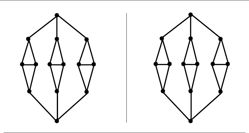
548 16. GRAPH PROBLEMS: HARD PROBLEMS
123
3
1
23
3
23
21
321
1
21312
INPUT OUTPUT
16.8 Edge Coloring
Input description: A graph G=(V,E).
Problem description: What is the smallest set of colors needed to color the edges
of Gsuch that no two same-color edges share a common vertex?
Discussion: The edge coloring of graphs arises in scheduling applications, typically
associated with minimizing the number of noninterfering rounds needed to complete
a given set of tasks. For example, consider a situation where we must schedule
a given set of two-person interviews, where each interview takes one hour. All
meetings could be scheduled to occur at distinct times to avoid conflicts, but it
is less wasteful to schedule nonconflicting events simultaneously. We construct a
graph whose vertices are people and whose edges represent the pairs of people who
need to meet. An edge coloring of this graph defines the schedule. The color classes
represent the different time periods in the schedule, with all meetings of the same
color happening simultaneously.
The National Football League solves such an edge-coloring problem each season
to make up its schedule. Each team’s opponents are determined by the records of
the previous season. Assigning the opponents to weeks of the season is an edge-
coloring problem, complicated by extra constraints of spacing out rematches and
making sure that there is a good game every Monday night.

16.8 EDGE COLORING 549
The minimum number of colors needed to edge color a graph is called its edge-
chromatic number by some and its chromatic index by others. Note that an even-
length cycle can be edge-colored with 2 colors, while odd-length cycles have an
edge-chromatic number of 3.
Edge coloring has a better (if less famous) theorem associated with it than ver-
tex coloring. Vizing’s theorem states that any graph with a maximum vertex degree
of Δ can be edge colored using at most Δ + 1 colors. To put this in perspective,
note that any edge coloring must have at least Δ colors, since all the edges incident
on any vertex must be distinct colors.
The proof of Vizing’s theorem is constructive, meaning it can be turned into
an O(nmΔ) algorithm to find an edge-coloring with Δ + 1 colors. Since deciding
whether we can get away using one less color than this is NP-complete, it hardly
seems worth the effort to worry about it. An implementation of Vizing’s theorem
is described below.
Any edge-coloring problem on Gcan be converted to the problem of finding a
vertex coloring on the line graph L(G), which has a vertex of L(G) for each edge
of GandanedgeofL(G) if and only if the two edges of Gshare a common vertex.
Line graphs can be constructed in time linear to their size, and any vertex-coloring
code can be employed to color them. That said, it is disappointing to go the vertex
coloring route. Vizing’s theorem is our reward for the extra thought needed to see
that we have an edge-coloring problem.
Implementations: Yan Dong produced an implementation of Vizing’s the-
orem in C++ as a course project for my algorithms course while a stu-
dent at Stony Brook. It can be found on the algorithm repository site at
http://www.cs.sunysb.edu/∼algorith.
GOBLIN (http://www.math.uni-augsburg.de/∼fremuth/goblin.html) impleme-
nts a branch-and-bound algorithm for edge coloring.
See Section 16.7 (page 544) for a larger collection of vertex-coloring codes and
heuristics, which can be applied to the line graph of your target graph. Combinator-
ica [PS03] provides Mathematica implementations of edge coloring in this fashion,
via the line graph transformation and vertex coloring routines. See Section 19.1.9
(page 661) for more information on Combinatorica.
Notes:Graph-theoretic results on edge coloring are surveyed in [FW77, GT94]. Vizing
[Viz64] and Gupta [Gup66] independently proved that any graph can be edge colored
using at most Δ + 1 colors. Misra and Gries give a simple constructive proof of this result
[MG92]. Despite these tight bounds, it is NP-complete to compute the edge-chromatic
number [Hol81]. Bipartite graphs can be edge-colored in polynomial time [Sch98].
Whitney, in introducing line graphs [Whi32], showed that with the exception of K3
and K1,3, any two connected graphs with isomorphic line graphs are isomorphic. It is an
interesting exercise to show that the line graph of an Eulerian graph is both Eulerian and
Hamiltonian, while the line graph of a Hamiltonian graph is always Hamiltonian.
Related Problems: Vertex coloring (see page 544), scheduling (see page 468).
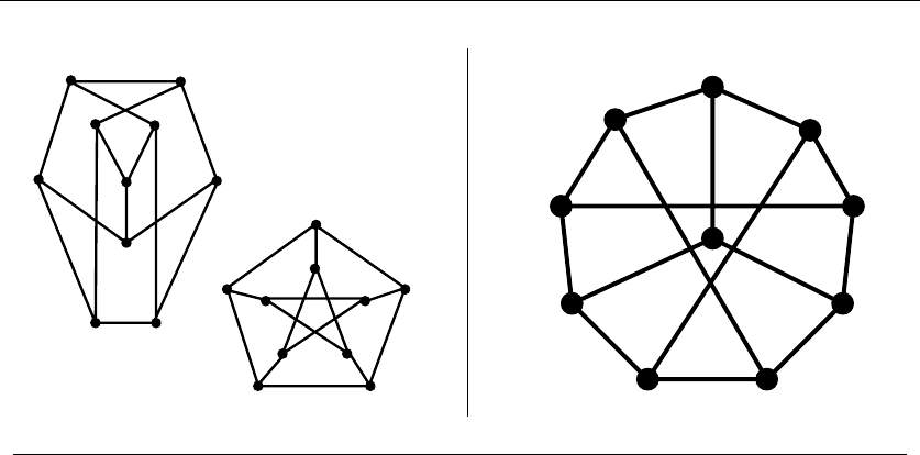
550 16. GRAPH PROBLEMS: HARD PROBLEMS
12
36
7
45
9
810
A
EB
JI
FH
G
DC
1A
2B
4C
7D
9J6H
10F
8I
3G
5E
INPUT OUTPUT
16.9 Graph Isomorphism
Input description: Two graphs, Gand H.
Problem description: Find a (or all) mapping ffrom the vertices of Gto the
vertices of Hsuch that Gand Hare identical; i.e. , (x, y) is an edge of Giff
(f(x),f(y)) is an edge of H.
Discussion: Isomorphism is the problem of testing whether two graphs are really
the same. Suppose we are given a collection of graphs and must perform some
operation on each of them. If we can identify which of the graphs are duplicates,
we can discard copies to avoid redundant work.
Certain pattern recognition problems are readily mapped to graph or subgraph
isomorphism detection. The structure of chemical compounds are naturally de-
scribed by labeled graphs, with each atom represented by a vertex. Identifying all
molecules in a structure database containing a particular functional group is an
instance of subgraph isomorphism testing.
We need some terminology to settle what is meant when we say two graphs
are the same. Two labeled graphs G=(Vg,E
g)andH=(Vh,E
h)areidentical
when (x, y)∈Egiff (x, y)∈Eh. The isomorphism problem consists of finding a
mapping from the vertices of Gto Hsuch that they are identical. Such a mapping
is called an isomorphism; the problem of finding the mapping is sometimes called
graph matching.
Identifying symmetries is another important application of graph isomorphism.
A mapping of a graph to itself is called an automorphism, and the collection of

16.9 GRAPH ISOMORPHISM 551
automorphisms (the automorphism group) provides a great deal of information
about symmetries in the graph. For example, the complete graph Knhas n!au-
tomorphisms (any mapping will do), while an arbitrary random graph is likely to
have few or perhaps only one, since Gis always identical to itself.
Several variations of graph isomorphism arise in practice:
•Is graph Gcontained in graph H?– Instead of testing equality, we are of-
ten interested in knowing whether a small pattern graph Gis a subgraph
of H. Such problems as clique, independent set, and Hamiltonian cycle are
important special cases of subgraph isomorphism.
There are two distinct graph-theoretic notions of “contained in.” Subgraph
isomorphism asks whether there is a subset of edges and vertices of Hthat is
isomorphic to a smaller graph G.Induced subgraph isomorphism asks whether
there is a subset of vertices of Hwhose deletion leaves a subgraph isomorphic
to a smaller graph G. For induced subgraph isomorphism, (1) all edges of G
must be present in H, and (2) no non-edges of Gcan be present in H. Clique
happens to be an instance of both subgraph isomorphism problems, while
Hamiltonian cycle is only an example of vanilla subgraph isomorphism.
Be aware of this distinction in your application. Subgraph isomorphism prob-
lems tend to be harder than graph isomorphism, while induced subgraph
problems tend to be even harder than subgraph isomorphism. Some flavor of
backtracking is your only viable approach.
•Are your graphs labeled or unlabeled? – In many applications, vertices or
edges of the graphs are labeled with some attribute that must be respected in
determining isomorphisms. For example, in comparing two bipartite graphs,
each with “worker” vertices and “job” vertices, any isomorphism that equated
a job with a worker would make no sense.
Labels and related constraints can be factored into any backtracking algo-
rithm. Further, such constraints significantly speed up the search, by creat-
ing many more opportunities for pruning whenever two vertex labels do not
match up.
•Are you testing whether two trees are isomorphic? – Faster algorithms ex-
ist for certain special cases of graph isomorphism, such as trees and planar
graphs. Perhaps the most important case is detecting isomorphisms among
trees, a problem that arises in language pattern matching and parsing appli-
cations. A parse tree is often used to describe the structure of a text; two
parse trees will be isomorphic if the underlying pair of texts have the same
structure.
Efficient algorithms for tree isomorphism begin with the leaves of both trees
and work inward toward the center. Each vertex in one tree is assigned a
label representing the set of vertices in the second tree that might possibly

552 16. GRAPH PROBLEMS: HARD PROBLEMS
be isomorphic to it, based on the constraints of labels and vertex degrees.
For example, all the leaves in tree T1are initially potentially equivalent to all
leaves of T2. Now, working inward, we can partition the vertices adjacent to
leaves in T1into classes based on how many leaves and non-leaves they are
adjacent to. By carefully keeping track of the labels of the subtrees, we can
make sure that we have the same distribution of labeled subtrees for T1and
T2. Any mismatch means T1=T2, while completing the process partitions the
vertices into equivalence classes defining all isomorphisms. See the references
below for more details.
•How many graphs do you have? – Many data mining applications involve
searching for all instances of a particular pattern graph in a big database
of graphs. The chemical structure mapping application described above falls
into this family. Such databases typically contain a large number of relatively
small graphs. This puts an onus on indexing the graph database by small
substructures (say five to ten vertex each), and doing expensive isomorphism
tests only against those containing the same substructures as the query graph.
No polynomial-time algorithm is known for graph isomorphism, but neither is
it known to be NP-complete. Along with integer factorization (see Section 13.8
(page 420)), it is one of the few important algorithmic problems whose rough
computational complexity is still not known. The conventional wisdom is that
isomorphism is a problem that lies between P and NP-complete if P =NP.
Although no worst-case polynomial-time algorithm is known, testing isomor-
phism is usually not very hard in practice. The basic algorithm backtracks through
all n! possible relabelings of the vertices of graph hwith the names of vertices
of graph g, and then tests whether the graphs are identical. Of course, we can
prune the search of all permutations with a given prefix as soon as we detect any
mismatch between edges whose vertices are both in the prefix.
However, the real key to efficient isomorphism testing is to preprocess the ver-
tices into “equivalence classes,” partitioning them into sets of vertices so that two
vertices in different sets cannot possibly be mistaken for each other. All vertices
in each equivalence class must share the same value of some invariant that is inde-
pendent of labeling. Possibilities include:
•Vertex degree – This simplest way to partition vertices is based on their
degree—the number of edges incident on the vertex. Two vertices of different
degrees cannot be identical. This simple partition can be a big win, but won’t
do much for regular (equal degree) graphs.
•Shortest path matrix – For each vertex v, the all-pairs shortest path matrix
(see Section 15.4 (page 489)) defines a multiset of n−1 distances representing
the distances between vand each of the other vertices. Any two identical
vertices must define the exact same multiset of distances, so we can partition
the vertices into equivalence classes defining identical distance multisets.

16.9 GRAPH ISOMORPHISM 553
•Counting length-kpaths – Taking the adjacency matrix of Gand raising it to
the kth power gives a matrix where Gk[i, j] counts the number of (nonsimple)
paths from ito j. For each vertex and each k, this matrix defines a multiset
of path-counts, which can be used for partitioning as with distances above.
You could try all 1 ≤k≤nor beyond, and use any single deviation as an
excuse to partition.
Using these invariants, you should be able to partition the vertices of most
graphs into a large number of small equivalence classes. Finishing the job off with
backtracking should then be short work. We assign each vertex the name of its
equivalence class as a label, and treat it as a labeled matching problem. It is harder
to detect isomorphisms between highly-symmetric graphs than it is with random
graphs because of the reduced effectiveness of these equivalence-class partitioning
heuristics.
Implementations: The best known isomorphism testing program is nauty (No
AUTomorphisms, Yes?)—a set of very efficient C language procedures for deter-
mining the automorphism group of a vertex-colored graph. Nauty is also able to
produce a canonically-labeled isomorph of the graph, to assist in isomorphism test-
ing. It was the basis of the first program to generate all 11-vertex graphs without
isomorphs, and can test most graphs with fewer than 100 vertices in well under a
second. Nauty has been ported to a variety of operating systems and C compilers.
It is available at http://cs.anu.edu.au/∼bdm/nauty/. The theory behind nauty is
described in [McK81].
The VFLib graph-matching library contains implementations for several dif-
ferent algorithms for both graph and subgraph isomorphism testing. This library
has been widely used and very carefully benchmarked [FSV01]. It is available at
http://amalfi.dis.unina.it/graph/.
GraphGrep [GS02] (http://www.cs.nyu.edu/shasha/papers/graphgrep/) is a rep-
resentative data mining tool for querying large databases of graphs.
Valiente [Val02] has made available the implementations of graph/subgraph
isomorphism algorithms for both trees and graphs in his book [Val02]. These C++
implementations run on top of LEDA (see Section 19.1.1 (page 658)), and are
available at http://www.lsi.upc.edu/∼valiente/algorithm/.
Kreher and Stinson [KS99] compute isomorphisms of graphs in addition to
more general group-theoretic operations. These implementations in C are available
at http://www.math.mtu.edu/∼kreher/cages/Src.html.
Notes:Graph isomorphism is an important problem in complexity theory. Monographs
on isomorphism detection include [Hof82, KST93]. Valiente [Val02] focuses on algorithms
for tree and subgraph isomorphism. Kreher and Stinson [KS99] take a more group-
theoretic approach to isomorphism testing. Graph mining systems and algorithms are
surveyed in [CH06]. See [FSV01] for performance comparisons between different graph
and subgraph isomorphism algorithms.
Polynomial-time algorithms are known for planar graph isomorphism [HW74] and for
graphs where the maximum vertex degree is bounded by a constant [Luk80]. The all-pairs

554 16. GRAPH PROBLEMS: HARD PROBLEMS
shortest path heuristic is due to [SD76], although there exist nonisomorphic graphs that
realize the exact same set of distances [BH90]. A linear-time tree isomorphism algorithm
for both labeled and unlabeled trees is presented in [AHU74].
A problem is said to be isomorphism-complete if it is provably as hard as isomorphism.
Testing the isomorphism of bipartite graphs is isomorphism-complete, since any graph
can be made bipartite by replacing each edge by two edges connected with a new vertex.
Clearly, the original graphs are isomorphic if and only if the transformed graphs are.
Related Problems: Shortest path (see page 489), string matching (see page 628).
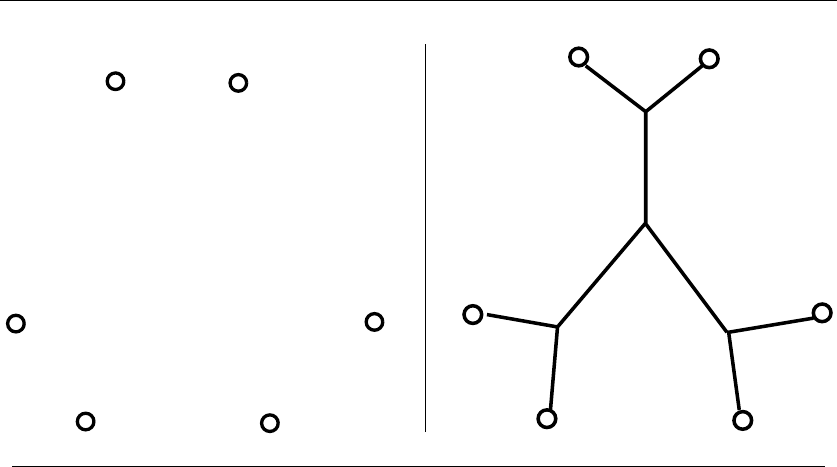
16.10 STEINER TREE 555
INPUT OUTPUT
16.10 Steiner Tree
Input description: A graph G=(V,E). A subset of vertices T∈V.
Problem description: Find the smallest tree connecting all the vertices of T.
Discussion: Steiner trees arise often in network design problems, since the mini-
mum Steiner tree describes how to connect a given set of sites using the smallest
amount of wire. Analogous problems occur when designing networks of water pipes
or heating ducts and in VLSI circuit design. Typical Steiner tree problems in VLSI
are to connect a set of sites to (say) ground under constraints such as material
cost, signal propagation time, or reducing capacitance.
The Steiner tree problem is distinguished from the minimum spanning tree
(MST) problem (see Section 15.3 (page 484)) in that we are permitted to construct
or select intermediate connection points to reduce the cost of the tree. Issues in
Steiner tree construction include:
•How many points do you have to connect? – The Steiner tree of a pair of
vertices is simply the shortest path between them (see Section 15.4 (page
489)). The Steiner tree of all the vertices, when S=V, simply defines the
MST of G. The general minimum Steiner tree problem is NP-hard despite
these special cases, and remains so under a broad range of restrictions.

556 16. GRAPH PROBLEMS: HARD PROBLEMS
•Is the input a set of geometric points or a distance graph? – Geometric ver-
sions of Steiner tree take a set of points as input, typically in the plane, and
seek the smallest tree connecting the points. A complication is that the set
of possible intermediate points is not given as part of the input but must be
deduced from the set of points. These possible Steiner points must satisfy
several geometric properties, which can be used to reduce the set of candi-
dates down to a finite number. For example, every Steiner point will have
a degree of exactly three in a minimum Steiner tree, and the angles formed
between any two of these edges must be exactly 120 degrees.
•Are there constraints on the edges we can use? – Many wiring problems cor-
respond to geometric versions of the problem, where all edges are restricted
to being either horizontal or vertical. This is the so-called rectilinear Steiner
problem. A different set of angular and degree conditions apply for rectilin-
ear Steiner trees than for Euclidean trees. In particular, all angles must be
multiples of 90 degrees, and each vertex is of a degree up to four.
•Do I really need an optimal tree? – Certain Steiner tree applications (e.g., cir-
cuit design and communications networks) justify investing large amounts of
computation to find the best possible Steiner tree. This implies an exhaustive
search technique such as backtracking or branch-and-bound. There are many
opportunities for pruning search based on geometric and graph-theoretic con-
straints.
Still, Steiner tree remains a hard problem. We recommend experimenting
with the implementations described below before attempting your own.
•How can I reconstruct Steiner vertices I never knew about? – A very special
type of Steiner tree arises in classification and evolution. A phylogenic tree
illustrates the relative similarity between different objects or species. Each
object represents (typically) a leaf/terminal vertex of the tree, with inter-
mediate vertices representing branching points between classes of objects.
For example, an evolutionary tree of animal species might have leaf nodes of
human, dog, snake and internal nodes corresponding to taxa (animal, mam-
mal, reptile). A tree rooted at animal with dog and human classified under
mammal implies that humans are closer to dogs than to snakes.
Many different phylogenic tree construction algorithms have been developed
that vary in (1) the data they attempt to model, and (2) the desired optimiza-
tion criterion. Each combination of reconstruction algorithm and distance
measure is likely to give a different answer, so identifying the “right” method
for any given application is somewhat a question of faith. A reasonable pro-
cedure is to acquire a standard package of implementations, discussed below,
and then see what happens to your data under all of them.
Fortunately, there is a good, efficient heuristic for finding Steiner trees that
works well on all versions of the problem. Construct a graph modeling your input,

16.10 STEINER TREE 557
setting the weight of edge (i, j) equal to the distance from point ito point j.Find
an MST of this graph. You are guaranteed a provably good approximation for both
Euclidean and rectilinear Steiner trees.
The worst case for a MST approximation of the Euclidean Steiner tree is three
points forming an equilateral triangle. The MST will contain two of the sides (for
a length of 2), whereas the minimum Steiner tree will connect the three points
using an interior point, for a total length of √3. This ratio of √3/2≈0.866 is
always achieved, and in practice the easily-computed MST is usually within a few
percent of the optimal Steiner tree. The rectilinear Steiner tree / MST ratio is
always ≥2/3≈0.667.
Such an MST can be refined by inserting a Steiner point whenever the edges
of the minimum spanning tree incident on a vertex form an angle of less than
120 degrees between them. Inserting these points and locally readjusting the tree
edges can move the solution a few more percent towards the optimum. Similar
optimizations are possible for rectilinear spanning trees.
Note that we are only interested in the subtree connecting the terminal vertices.
We may need to trim the MST if we add nonterminal vertices to the input of the
problem. We retain only the tree edges which lie on the (unique) path between
some pair of terminal nodes. The complete set of these can be found in O(n) time
by performing a BFS on the full tree starting from any single terminal node.
An alternative heuristic for graphs is based on shortest path. Start with a tree
consisting of the shortest path between two terminals. For each remaining terminal
t, find the shortest path to a vertex vin the tree and add this path to the tree. The
time complexity and quality of this heuristic depend upon the insertion order of the
terminals and how the shortest-path computations are performed, but something
simple and fairly effective is likely to result.
Implementations: GeoSteiner is a package for solving both Euclidean and rec-
tilinear Steiner tree problems in the plane by Warme, Winter, and Zachariasen
[WWZ00]. It also solves the related problem of MSTs in hypergraphs, and claims
to have solved problems as large as 10,000 points to optimality. It is available
from http://www.diku.dk/geosteiner/. This is almost certainly the best code for
geometric instances of Steiner tree.
FLUTE (http://home.eng.iastate.edu/∼cnchu/flute.html) computes rectilinear
Steiner trees, emphasizing speed. It contains a user-defined parameter to control
the tradeoff between solution quality and run time.
GOBLIN (http://www.math.uni-augsburg.de/∼fremuth/goblin.html) includes
both heuristics and search methods for finding Steiner trees in graphs.
The programs PHYLIP (http://evolution.genetics.washington.edu/phylip.html)
and PAUP (http://paup.csit.fsu.edu/) are widely-used packages for inferring phy-
logenic trees. Both contain over 20 different algorithms for constructing phylogenic
trees from data. Although many of them are designed to work with molecular se-
quence data, several general methods accept arbitrary distance matrices as input.

558 16. GRAPH PROBLEMS: HARD PROBLEMS
Notes:Recent monographs on the Steiner tree problem include Hwang, Richards, and
Winter [HRW92] and Pr¨omel and Steger [PS02]. Du, et al. [DSR00] is a collection of recent
surveys on all aspects of Steiner trees. Older surveys on the problem include [Kuh75].
Empirical results on Steiner tree heuristics include [SFG82, Vos92].
The Euclidean Steiner problem dates back to Fermat, who asked how to find a point p
in the plane minimizing the sum of the distances to three given points. This was solved by
Torricelli before 1640. Steiner was apparently one of several mathematicians who worked
the general problem for npoints, and was mistakenly credited with the problem. An
interesting, more detailed history appears in [HRW92].
Gilbert and Pollak [GP68] first conjectured that the ratio of the length of the minimum
Steiner tree over the MST is always ≥√3/2≈0.866. After twenty years of active research,
the Gilbert-Pollak ratio was finally proven by Du and Hwang [DH92]. The Euclidean MST
for npoints in the plane can be constructed in O(nlg n) time [PS85].
Arora [Aro98] gave a polynomial-time approximation scheme (PTAS) for Steiner trees
in k-dimensional Euclidian space. A 1.55-factor approximation for Steiner trees on graphs
is due to Robins and Zelikovsky [RZ05].
Expositions on the proof that the Steiner tree problem for graphs is hard [Kar72]
include [Eve79a]. Expositions on exact algorithms for Steiner trees in graphs include
[Law76]. The hardness of Steiner tree for Euclidean and rectilinear metrics was established
in [GGJ77, GJ77]. Euclidean Steiner tree is not known to be in NP, because of numerical
issues in representing distances.
Analogies can be drawn between minimum Steiner trees and minimum energy config-
urations in certain physical systems. The case that such analog systems—including the
behavior of soap films over wire frames—“solve” the Steiner tree problem is discussed in
[Mie58].
Related Problems: Minimum spanning tree (see page 484), shortest path (see
page 489).
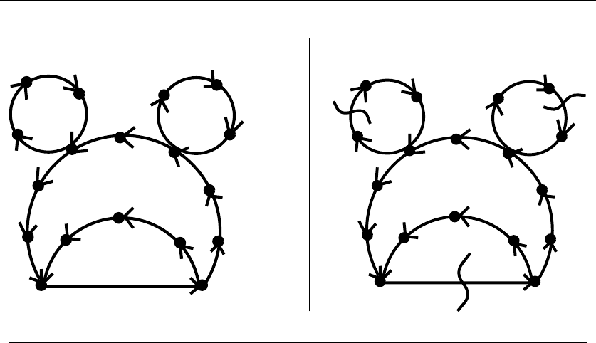
16.11 FEEDBACK EDGE/VERTEX SET 559
INPUT OUTPUT
16.11 Feedback Edge/Vertex Set
Input description: A (directed) graph G=(V, E).
Problem description: What is the smallest set of edges Eor vertices Vwhose
deletion leaves an acyclic graph?
Discussion: Feedback set problems arise because many things are easier to do
on directed acyclic graphs (DAGs) than general digraphs. Consider the problem
of scheduling jobs with precedence constraints (i.e. , job Amust come before job
B). When the constraints are all consistent, the resulting graph is a DAG, and
topological sort (see Section 15.2 (page 481)) can be used to order the vertices to
respect them. But how can you design a schedule when there are cyclic constraints,
such as Amust be done before B, which must be done before C,whichmustbe
done before A?
By identifying a feedback set, we identify the smallest number of constraints
that must be dropped to permit a valid schedule. In the feedback edge (or arc)
set problem, we drop individual precedence constraints. In the feedback vertex set
problem, we drop entire jobs and all constraints associated with them.
Similar considerations are involved in eliminating race conditions from elec-
tronic circuits. This explains why the problem is called “feedback” set. It is also
known as the maximum acyclic subgraph problem.

560 16. GRAPH PROBLEMS: HARD PROBLEMS
One final application has to do with ranking tournaments. Suppose we want to
rank order the skills of players at some two-player game, such as chess or tennis.
We can construct a directed graph where there is an arc from xto yif xbeats yin
a game. The higher-ranked player should be at the lower-ranked player, although
upsets often occur. A natural ranking is the topological sort resulting after deleting
the minimum set of feedback edges (upsets) from the graph.
Issues in feedback set problems include:
•Do any constraints have to be dropped? – No changes are needed if the graph is
already a DAG, which can be determined via topological sort. One way to find
a feedback set modifies the topological sorting algorithm to delete whatever
edge or vertex is causing the trouble whenever a contradiction is found. This
feedback set might be much larger than needed, however, since feedback edge
set and feedback vertex set are NP-complete on directed graphs.
•How can I find a good feedback edge set? – An effective linear-time heuristic
constructs a vertex ordering and then deletes any arc going in the wrong
direction. At least half the arcs must go either left-to-right or right-to-left for
any vertex order, so take the smaller partition as your feedback set.
But what is the right vertex order to start from? One natural order is to
sort the vertices in terms of edge-imbalance, namely in-degree minus out-
degree. Another approach starts by picking an arbitrary vertex v.Anyvertex
xdefined by an in-going edge (x, v) will be placed to the left of v.Anyx
defined by out-going edge (v, x) will analogously be placed to the right of v.
We can now recur on the left and right subsets to complete the vertex order.
•How can I find a good feedback vertex set? – The heuristics above yield vertex
orders defining (hopefully) few back edges. We seek a small set of vertices
that together cover these backedges. This is exactly a vertex cover problem,
the heuristics for which are discussed in Section 16.3 (page 530).
•What if I want to break all cycles in an undirected graph? – The problem of
finding feedback sets in undirected graphs is quite different from digraphs.
Trees are undirected graphs without cycles, and every tree on nvertices
contains exactly n−1 edges. Thus the smallest feedback edge set of any
undirected graph Gis |E|−(n−c), where cis the number of connected
components of G. The back edges encountered during a depth-first search of
Gqualified as a minimum feedback edge set.
The feedback vertex set problem remains NP-complete for undirected graphs,
however. A reasonable heuristic uses breadth-first search to identify the short-
est cycle in G. The vertices in this cycle are all deleted from G, and the
shortest remaining cycle identified. This find-and-delete procedure is em-
ployed until the graph is acyclic. The optimal feedback vertex set must con-
tain at least one vertex from each of these vertex-disjoint cycles, so the average
deleted-cycle length determines just how good our approximation is.

16.11 FEEDBACK EDGE/VERTEX SET 561
It may pay to refine any of these heuristic solutions using randomization or
simulated annealing. To move between states, we can modify the vertex permu-
tation by swapping pairs in order or insert/delete vertices to/from the candidate
feedback set.
Implementations: Greedy randomized adaptive search (GRASP) heuristics for
both feedback vertex and feedback edge set problems have been implemented
by Festa, et al. [FPR01] as Algorithm 815 of the Collected Algorithms of the
ACM (see Section 19.1.6 (page 659)). These Fortran codes are also available from
http://www.research.att.com/∼mgcr/src/.
GOBLIN (http://www.math.uni-augsburg.de/∼fremuth/goblin.html) includes
an approximation heuristic for minimum feedback arc set.
The econ order program of the Stanford GraphBase (see Section 19.1.8 (page
660)) permutes the rows and columns of a matrix so as to minimize the sum of
the numbers below the main diagonal. Using an adjacency matrix as the input and
deleting all edges below the main diagonal leaves an acyclic graph.
Notes:See [FPR99] for a survey on the feedback set problem. Expositions of the proofs
that feedback minimization is hard [Kar72] include [AHU74, Eve79a]. Both feedback
vertex and edge set remain hard even if no vertex has in-degree or out-degree greater
than two [GJ79].
Bafna, et al. [BBF99] gives a 2-factor approximation for feedback vertex set in undi-
rected graphs. Feedback edge sets in directed graphs can be approximated to within a
factor of O(log nlog log n) [ENSS98]. Heuristics for ranking tournaments are discussed in
[CFR06]. Experiments with heuristics are reported in [Koe05].
An interesting application of feedback arc set to economics is presented in [Knu94].
For each pair A, B of sectors of the economy, we are given how much money flows from
Ato B. We seek to order the sectors to determine which sectors are primarily producers
to other sectors, and which deliver primarily to consumers.
Related Problems: Bandwidth reduction (see page 398), topological sorting (see
page 481), scheduling (see page 468).

17
Computational Geometry
Computational geometry is the algorithmic study of geometric problems. Its emer-
gence coincided with application areas such as computer graphics, computer-aided
design/manufacturing, and scientific computing, which together provide much of
the motivation for geometric computing. The past twenty years have seen enor-
mous maturity in computational geometry, resulting in a significant body of useful
algorithms, software, textbooks, and research results.
Good books on computational geometry include:
•de Berg, et al. [dBvKOS00] – The “three Mark’s” book is the best general
introduction to the theory of computational geometry and its fundamental
algorithms.
•O’Rourke [O’R01] – This is the best practical introduction to compu-
tational geometry. The emphasis is on careful and correct implemen-
tation of geometric algorithms. C and Java code are available from
http://maven.smith.edu/∼orourke/books/compgeom.html.
•Preparata and Shamos [PS85] – Although somewhat out of date, this book
remains a good general introduction to computational geometry, stressing
algorithms for convex hulls, Voronoi diagrams, and intersection detection.
•Goodman and O’Rourke [GO04] – This recent collection of survey articles
provides a detailed overview of what is known in most every subfield of dis-
crete and computational geometry.
The leading conference in computational geometry is the ACM Symposium
on Computational Geometry, held annually in late May or early June. Although
the primary results presented at the conference are theoretical, there has been a
S.S. Skiena, The Algorithm Design Manual, 2nd ed., DOI: 10.1007/978-1-84800-070-4 17,
c
Springer-Verlag London Limited 2008

17. COMPUTATIONAL GEOMETRY 563
concerted effort on the part of the research community to increase the presence of
applied, experimental work through video reviews and poster sessions.
There is a growing body of implementations of geometric algorithms. We point
out specific implementations where applicable in the catalog, but the reader should
be particularly aware of CGAL (Computational Geometry Algorithms Library)—
a comprehensive library of geometric algorithms in C++ produced as a result of
a joint European project. Anyone with a serious interest in geometric computing
should check it out at http://www.cgal.org/.
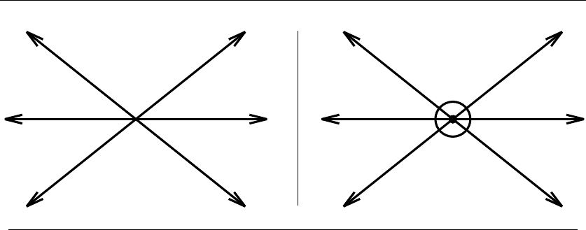
564 17. COMPUTATIONAL GEOMETRY
INPUT OUTPUT
17.1 Robust Geometric Primitives
Input description: A point pand line segment l, or two line segments l1,l2.
Problem description:Doesplie over, under, or on l?Doesl1intersect l2?
Discussion: Implementing basic geometric primitives is a task fraught with peril,
even for such simple tasks as returning the intersection point of two lines. It is
more complicated than you may think. What should you return if the two lines
are parallel, meaning they don’t intersect at all? What if the lines are identical,
so the intersection is not a point but the entire line? What if one of the lines is
horizontal, so that in the course of solving the equations for the intersection point
you are likely to divide by zero? What if the two lines are almost parallel, so that
the intersection point is so far from the origin as to cause arithmetic overflows?
These issues become even more complicated for intersecting line segments, since
there are many other special cases that must be watched for and treated specially.
If you are new to implementing geometric algorithms, I suggest that you study
O’Rourke’s Computational Geometry in C [O’R01] for practical advice and com-
plete implementations of basic geometric algorithms and data structures. You are
likely to avoid many headaches by following in his footsteps.
There are two different issues at work here: geometric degeneracy and numer-
ical stability. Degeneracy refers to annoying special cases that must be treated in
substantially different ways, such as when two lines intersect in more or less than
a single point. There are three primary approaches to dealing with degeneracy:
•Ignore it – Make as an operating assumption that your program will work
correctly only if no three points are collinear, no three lines meet at a point, no
intersections happen at the endpoints of line segments, etc. This is probably
the most common approach, and what I might recommend for short-term

17.1 ROBUST GEOMETRIC PRIMITIVES 565
projects if you can live with frequent crashes. The drawback is that interesting
data often comes from points sampled on a grid, and so is inherently very
degenerate.
•Fake it – Randomly or symbolically perturb your data so that it becomes
nondegenerate. By moving each of your points a small amount in a random
direction, you can break many of the existing degeneracies in the data, hope-
fully without creating too many new problems. This probably should be the
first thing to try once you decide that your program is crashing too often.
A problem with random perturbations is that they can change the shape
of your data in subtle ways, which may be intolerable for your application.
There also exist techniques to “symbolically” perturb your data to remove
degeneracies in a consistent manner, but these require serious study to apply
correctly.
•Deal with it – Geometric applications can be made more robust by writing
special code to handle each of the special cases that arise. This can work
well if done with care at the beginning, but not so well if kludges are added
whenever the system crashes. Expect to expend significant effort if you are
determined to do it right.
Geometric computations often involve floating-point arithmetic, which leads to
problems with overflows and numerical precision. There are three basic approaches
to the issue of numerical stability:
•Integer arithmetic – By forcing all points of interest to lie on a fixed-size inte-
ger grid, you can perform exact comparisons to test whether any two points
are equal or two line segments intersect. The cost is that the intersection
point of two lines may not be exactly representable as a grid point. This is
likely to be the simplest and best method, if you can get away with it.
•Double precision reals – By using double-precision floating point numbers, you
may get lucky and avoid numerical errors. Your best bet might be to keep all
the data as single-precision reals, and use double-precision for intermediate
computations.
•Arbitrary precision arithmetic – This is certain to be correct, but also to
be slow. This approach seems to be gaining favor in the research community.
Careful analysis can minimize the need for high-precision arithmetic and thus
the performance penalty. Still, you should expect high-precision arithmetic to
be several orders of magnitude slower than standard floating-point arithmetic.
The difficulties associated with producing robust geometric software are still
under attack by researchers. The best practical technique is to base your applica-
tions on a small set of geometric primitives that handle as much of the low-level
geometry as possible. These primitives include:

566 17. COMPUTATIONAL GEOMETRY
•Area of a triangle – Although it is well known that the area A(t) of a triangle
t=(a, b, c) is half the base times the height, computing the length of the
base and altitude is messy work with trigonometric functions. It is better to
use the determinant formula for twice the area:
2·A(t)=
axay1
bxby1
cxcy1=axby−aybx+aycx−axcy+bxcy−cxby
This formula generalizes to compute d! times the volume of a simplex in d
dimensions. Thus, 3! = 6 times the volume of a tetrahedron t=(a, b, c, d)in
three dimensions is
6·A(t)=
axayaz1
bxbybz1
cxcycz1
dxdydz1
Note that these are signed volumes and can be negative, so take the absolute
value first. Section 13.4 (page 404) explains how to compute determinants.
The conceptually simplest way to compute the area of a polygon (or polyhe-
dron) is to triangulate it and then sum up the area of each triangle. Imple-
mentations of a slicker algorithm that avoids triangulation are discussed in
[O’R01, SR03].
•Above-below-on test – Does a given point clie above, below, or on a given
line l? A clean way to deal with this is to represent las a directed line that
passes through point abefore point b, and ask whether clies to the left or
right of the directed line l. It is up to you to decide whether left means above
or below.
This primitive can be implemented using the sign of the triangle area as
computed above. If the area of t(a, b, c)>0, then clies to the left of ab.If
the area of t(a, b, c) = 0, then clies on ab. Finally, if the area of t(a, b, c)<0,
then clies to the right of ab. This generalizes naturally to three dimensions,
where the sign of the area denotes whether dlies above or below the oriented
plane (a, b, c).
•Line segment intersection – The above-below primitive can be used to test
whether a line intersects a line segment. It does iff one endpoint of the segment
is to the left of the line and the other is to the right. Segment intersection
is similar but more complicated. We refer you to implementations described
below. The decision as to whether two segments intersect if they share an
endpoint depends upon your application and is representative of the problems
with degeneracy.

17.1 ROBUST GEOMETRIC PRIMITIVES 567
•In-circle test – Does point dlie inside or outside the circle defined by points
a,b,andcin the plane? This primitive occurs in all Delaunay triangulation
algorithms, and can be used as a robust way to do distance comparisons.
Assuming that a,b,care labeled in counterclockwise order around the circle,
compute the determinant
incircle(a, b, c, d)=
axaya2
x+a2
y1
bxbyb2
x+b2
y1
cxcyc2
x+c2
y1
dxdyd2
x+d2
y1
In-circle will return 0 if all four points are cocircular—a positive value if dis
inside the circle, and negative if dis outside.
Check out the Implementations section before you build your own.
Implementations:CGAL(www.cgal.org) and LEDA (see Section 19.1.1 (page
658)) both provide very complete sets of geometric primitives for planar geom-
etry written in C++. LEDA is easier to learn and to work with, but CGAL is
more comprehensive and freely available. If you are starting a significant geometric
application, you should at least check them out before you try to write your own.
O’Rourke [O’R01] provides implementations in C of most of the primitives
discussed in this section. See Section 19.1.10 (page 662). These primitives were
implemented primarily for exposition rather than production use, but they should
be reliable and appropriate for small applications.
The Core Library (see http://cs.nyu.edu/exact/) provides an API, which sup-
ports the Exact Geometric Computation (EGC) approach to numerically robust
algorithms. With small changes, any C/C++ program can use it to readily support
three levels of accuracy: machine-precision, arbitrary-precision, and guaranteed.
Shewchuk’s [She97] robust implementation of basic geometric primitives in
C++ is available at http://www.cs.cmu.edu/∼quake/robust.html.
Notes:O’Rourke [O’R01] provides an implementation-oriented introduction to compu-
tational geometry which stresses robust geometric primitives. It is recommended reading.
LEDA [MN99] provides another excellent role model.
Yap [Yap04] gives a excellent survey on techniques for achieving robust geometric
computation, with a book [MY07] in preparation. Kettner, et al. [KMP+04] provides
graphic evidence of the troubles that arise when employing real arithmetic in geometric
algorithms such as convex hull. Controlled perturbation [MOS06] is a new approach for ro-
bust computation that is receiving considerable attention. Shewchuk [She97] and Fortune
and van Wyk [FvW93] present careful studies on the costs of using arbitrary-precision
arithmetic for geometric computation. By being careful about when to use it, reasonable
efficiency can be maintained while achieving complete robustness.
Related Problems: Intersection detection (see page 591), maintaining arrange-
ments (see page 614).

568 17. COMPUTATIONAL GEOMETRY
INPUT OUTPUT
17.2 Convex Hull
Input description:AsetSof npoints in d-dimensional space.
Problem description: Find the smallest convex polygon (or polyhedron) con-
taining all the points of S.
Discussion: Finding the convex hull of a set of points is the most important ele-
mentary problem in computational geometry, just as sorting is the most important
elementary problem in combinatorial algorithms. It arises because constructing the
hull captures a rough idea of the shape or extent of a data set.
Convex hull serves as a first preprocessing step to many, if not most, geometric
algorithms. For example, consider the problem of finding the diameter of a set
of points, which is the pair of points that lie a maximum distance apart. The
diameter must be between two points on the convex hull. The O(nlg n) algorithm
for computing diameter proceeds by first constructing the convex hull, then for
each hull vertex finding which other hull vertex lies farthest from it. The so-called
“rotating-calipers” method can be used to move efficiently from one-diametrically
opposed hull vertex to another by always proceeding in a clockwise fashion around
the hull.
There are almost as many convex hull algorithms as sorting algorithms. Answer
the following questions to help choose between them:

17.2 CONVEX HULL 569
•How many dimensions are you working with? – Convex hulls in two and
even three dimensions are fairly easy to work with. However, certain valid
assumptions in lower dimensions break down as the dimensionality increases.
For example, any n-vertex polygon in two dimensions has exactly nedges.
However, the relationship between the numbers of faces and vertices becomes
more complicated even in three dimensions. A cube has eight vertices and
six faces, while an octahedron has eight faces and six vertices. This has im-
plications for data structures that represent hulls—are you just looking for
the hull points or do you need the defining polyhedron? Be aware of these
complications of high-dimensional spaces if your problem takes you there.
Simple O(nlog n) convex-hull algorithms are available for the important spe-
cial cases of two and three dimensions. In higher dimensions, things get more
complicated. Gift-wrapping is the basic algorithm for constructing higher-
dimensional convex hulls. Observe that a three-dimensional convex polyhe-
dron is composed of two-dimensional faces, or facets, that are connected by
one-dimensional lines or edges. Each edge joins exactly two facets together.
Gift-wrapping starts by finding an initial facet associated with the lowest
vertex and then conducting a breadth-first search from this facet to discover
new, additional facets. Each edge edefining the boundary of a facet must be
shared with one other facet. By running through each of the npoints, we can
identify which point defines the next facet with e. Essentially, we “wrap” the
points one facet at a time by bending the wrapping paper around an edge
until it hits the first point.
The key to efficiency is making sure that each edge is explored only once.
Implemented properly in ddimensions, gift-wrapping takes O(nφd−1+
φd−2lg φd−2), where φd−1is the number of facets and φd−2is the number of
edges in the convex hull. This can be as bad as O(nd/2+1) when the convex
hull is very complex. I recommend that you use one of the codes described
below rather than roll your own.
•Is your data given as vertices or half-spaces? – The problem of finding the
intersection of a set of nhalf-spaces in ddimensions (each containing the
origin) is dual to that of computing convex hulls of npoints in ddimensions.
Thus, the same basic algorithm suffices for both problems. The necessary
duality transformation is discussed in Section 17.15 (page 614). The problem
of half-plane intersection differs from convex hull when no interior point is
given, since the instance may be infeasible (i.e., the intersection of the half-
planes empty).
•How many points are likely to be on the hull? – If your point set was generated
“randomly,” it is likely that most points lie within the interior of the hull.
Planar convex-hull programs can be made more efficient in practice using the
observation that the leftmost, rightmost, topmost, and bottommost points
all must be on the convex hull. This usually gives a set of either three or

570 17. COMPUTATIONAL GEOMETRY
four distinct points, defining a triangle or quadrilateral. Any point inside this
region cannot be on the convex hull and so can be discarded in a linear sweep
through the points. Ideally, only a few points will then remain to run through
the full convex-hull algorithm.
This trick can also be applied beyond two dimensions, although it loses ef-
fectiveness as the dimension increases.
•How do I find the shape of my point set? – Although convex hulls provide a
gross measure of shape, any details associated with concavities are lost. The
convex hull of the G from the example input would be indistinguishable from
the convex hull of O. Alpha-shapes are a more general structure that can be
parameterized so as to retain arbitrarily large concavities. Implementations
and references on alpha-shapes are included below.
The primary convex-hull algorithm in the plane is the Graham scan. Graham
scan starts with one point pknown to be on the convex hull (say the point with
the lowest x-coordinate) and sorts the rest of the points in angular order around
p. Starting with a hull consisting of pand the point with the smallest angle, we
proceed counterclockwise around vadding points. If the angle formed by the new
point and the last hull edge is less than 180 degrees, we add this new point to
the hull. If the angle formed by the new point and the last “hull” edge is greater
than 180 degrees, then a chain of vertices starting from the last hull edge must be
deleted to maintain convexity. The total time is O(nlg n), since the bottleneck is
the cost of sorting the points around v.
The basic Graham scan procedure can also be used to construct a nonself-
intersecting (or simple) polygon passing through all the points. Sort the points
around v, but instead of testing angles, simply connect the points in angular order.
Connecting this to vgives a polygon without self-intersection, although it typically
has many ugly skinny protrusions.
The gift-wrapping algorithm becomes especially simple in two dimensions, since
each “facet” becomes an edge, each “edge” becomes a vertex of the polygon, and
the “breadth-first search” simply walks around the hull in a clockwise or counter-
clockwise order. The 2D gift-wrapping (or Jarvis march) algorithm runs in O(nh)
time, where his the number of vertices on the convex hull. I recommend sticking
with Graham scan unless you really know in advance that there cannot be too
many vertices on the hull.
Implementations: The CGAL library (www.cgal.org) offers C++ implementa-
tions of an extensive variety of convex-hull algorithms for two, three, and arbitrary
numbers of dimensions. Alternate C++ implementations of planar convex hulls
includes LEDA (see Section 19.1.1 (page 658)).
Qhull [BDH97] is a popular low-dimensional, convex-hull code, optimized
for from two to about eight dimensions. It is written in C and can also con-
struct Delaunay triangulations, Voronoi vertices, furthest-site Voronoi vertices, and

17.2 CONVEX HULL 571
half-space intersections. Qhull has been widely used in scientific applications and
has a well-maintained homepage at http://www.qhull.org/.
O’Rourke [O’R01] provides a robust implementation of the Graham scan in two
dimensions and an O(n2) implementation of an incremental algorithm for convex
hulls in three dimensions. C and Java implementations are both available. See
Section 19.1.10 (page 662).
For excellent alpha-shapes code, originating from the work of Edelsbrunner and
Mucke [EM94], check out http://biogeometry.duke.edu/software/alphashapes/. Ken
Clarkson’s higher-dimensional convex-hull code Hull also does alpha-shapes, and
is available at http://www.netlib.org/voronoi/hull.html.
Different codes are needed for enumerating the vertices of intersecting half-
spaces in higher dimensions. Avis’s lhs (http://cgm.cs.mcgill.ca/∼avis/C/lrs.html)
is an arithmetically-robust ANSI C implementation of the Avis-Fukuda reverse
search algorithm for vertex enumeration/convex-hull problems. Since the polyhedra
is implicitly traversed but not explicitly stored in memory, even problems with very
large output sizes can sometimes be solved.
Notes:Planar convex hulls play a similar role in computational geometry as sorting
does in algorithm theory. Like sorting, convex hull is a fundamental problem for which
many different algorithmic approaches lead to interesting or optimal algorithms. Quickhull
and mergehull are examples of hull algorithms inspired by sorting algorithms [PS85]. A
simple construction involving points on a parabola presented in Section 9.2.4 (page 322)
reduces sorting to convex hull, so the information-theoretic lower bound for sorting implies
that planar convex hull requires Ω(nlg n) time to compute. A stronger lower bound is
established in [Yao81].
Good expositions of the Graham scan algorithm [Gra72] and the Jarvis march [Jar73]
include [dBvKOS00, CLRS01, O’R01, PS85]. The optimal planar convex-hull algorithm
[KS86] takes O(nlg h) time, where his the number of hull vertices that captures the
best performance of both Graham scan and gift wrapping and is (theoretically) better
in between. Planar convex hull can be efficiently computed in-place, meaning without
requiring additional memory in [BIK+04]. Seidel [Sei04] gives an up-to-date survey of
convex hull algorithms and variants, particularly for higher dimensions.
Alpha-hulls, introduced in [EKS83], provide a useful notion of the shape of a point set.
A generalization to three dimensions, with an implementation, is presented in [EM94].
Reverse-search algorithms for constructing convex hulls are effective in higher dimen-
sions [AF96]. Through a clever lifting-map construction [ES86], the problem of building
Voronoi diagrams in d-dimensions can be reduced to constructing convex hulls in (d+1)-
dimensions. See Section 17.4 (page 576) for more details.
Dynamic algorithms for convex-hull maintenance are data structures that permit in-
serting and deleting arbitrary points while always representing the current convex hull.
The first such dynamic data structure [OvL81] supported insertions and deletions in
O(lg2n) time. More recently, Chan [Cha01] reduced the cost of such operation of near-
logarithmic amortized time.
Related Problems: Sorting (see page 436), Voronoi diagrams (see page 576).
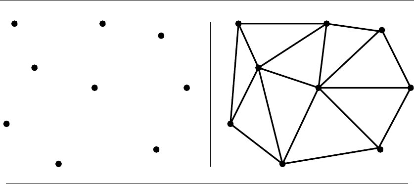
572 17. COMPUTATIONAL GEOMETRY
INPUT OUTPUT
17.3 Triangulation
Input description: A set of points or a polyhedron.
Problem description: Partition the interior of the point set or polyhedron into
triangles.
Discussion: The first step in working with complicated geometric objects is often
to break them into simple geometric objects. This makes triangulation a funda-
mental problem in computational geometry. The simplest geometric objects are
triangles in two dimensions, and tetrahedra in three. Classical applications of tri-
angulation include finite element analysis and computer graphics.
A particularly interesting application of triangulation is surface or function in-
terpolation. Suppose that we have sampled the height of a mountain at a certain
number of points. How can we estimate the height at any point qin the plane?
We can project the sampled points on the plane, and then triangulate them. This
triangulation partitions the plane into triangles, so we can estimate height by in-
terpolating between the heights of the three points of the triangle that contain q.
Furthermore, this triangulation and the associated height values define a mountain
surface suitable for graphics rendering.
A triangulation in the plane is constructed by adding nonintersecting chords
between the vertices until no more such chords can be added. Specific issues arising
in triangulation include:
•Are you triangulating a point set or a polygon? – Often we are given a set
of points to triangulate, as in the surface interpolation problem discussed

17.3 TRIANGULATION 573
earlier. This involves first constructing the convex hull of the point set and
then carving up the interior into triangles.
The simplest such O(nlg n) algorithm first sorts the points by x-coordinate.
It then inserts them from left to right as per the convex-hull algorithm of
page 105, building the triangulation by adding a chord to each point newly
cut off from the hull.
•Does the shape of the triangles in your triangulation matter? – There are
usually many different ways to partition your input into triangles. Consider a
set of npoints in convex position in the plane. The simplest way to triangulate
them would be to add to the convex-hull diagonals from the first point to all
of the others. However, this has the tendency to create skinny triangles.
Many applications seek to to avoid skinny triangles, or equivalently, mini-
mize small angles in the triangulation. The Delaunay triangulation of a point
set minimizes the maximum angle over all possible triangulations. This isn’t
exactly what we are looking for, but it is pretty close, and the Delaunay tri-
angulation has enough other interesting properties (including that it is dual
to the Voronoi diagram) to make it the quality triangulation of choice. Fur-
ther, it can be constructed in O(nlg n) time using implementations described
below.
•How can I improve the shape of a given triangulation? – Each internal edge of
any triangulation is shared between two triangles. The four vertices defining
these two triangles form either (1) a convex quadrilateral, or (2) a triangle
with a triangular bite taken out of it. The beauty of the convex case is that
exchanging the internal edge with a chord linking the other two vertices yields
a different triangulation.
This gives us a local “edge-flip” operation for changing and possibly im-
proving a given triangulation. Indeed, a Delaunay triangulation can be con-
structed from any initial triangulation by removing skinny triangles until no
locally-improving exchange remains.
•What dimension are we working in? – Three-dimensional problems are usu-
ally harder than two-dimensional problems. The three-dimensional general-
ization of triangulation involves partitioning the space into four-vertex tetra-
hedra by adding nonintersecting faces. One important difficulty is that there
is no way to tetrahedralize the interior of certain polyhedra without adding
extra vertices. Furthermore, it is NP-complete to decide whether such a tetra-
hedralization exists, so we should not feel afraid to add extra vertices to
simplify our problem.
•What constraints does the input have? – When we are triangulating a poly-
gon or polyhedra, we are restricted to adding chords that do not intersect
any of the boundary facets. In general, we may have a set of obstacles or

574 17. COMPUTATIONAL GEOMETRY
constraints that cannot be intersected by inserted chords. The best such tri-
angulation is likely to be the so-called constrained Delaunay triangulation.
Implementations are described next.
•Are you allowed to add extra points, or move input vertices? – When the shape
of the triangles does matter, it might pay to strategically add a small number
of extra “Steiner” points to the data set to facilitate the construction of a
triangulation (say) with no small angles. As discussed above, no triangulation
may exist for certain polyhedra without adding Steiner points.
To construct a triangulation of a convex polygon in linear time, just pick an
arbitrary starting vertex vand insert chords from vto each other vertex in the
polygon. Because the polygon is convex, we can be confident that none of the
boundary edges of the polygon will be intersected by these chords, and that all of
them lie within the polygon. The simplest algorithm for constructing general poly-
gon triangulations tries each of the O(n2) possible chords and inserts them if they
do not intersect a boundary edge or previously inserted chord. There are practical
algorithms that run in O(nlg n) time and theoretically interesting algorithms that
run in linear time. See the Implementations and Notes section for details.
Implementations: Triangle, by Jonathan Shewchuk, is an award-winning C lan-
guage code that generates Delaunay triangulations, constrained Delaunay triangu-
lations (forced to have certain edges), and quality-conforming Delaunay triangu-
lations (which avoid small angles by inserting extra points). It has been widely
used for finite element analysis and is fast and robust. Triangle is the first thing
I would try if I needed a two-dimensional triangulation code. It is available at
http://www.cs.cmu.edu/∼quake/triangle.html.
Fortune’s Sweep2 is a widely used 2D code for Voronoi diagrams and Delaunay
triangulations, written in C. This code may be simpler to work with if all you need
is the Delaunay triangulation of points in the plane. It is based on his sweepline
algorithm [For87] for Voronoi diagrams and is available from Netlib (see Section
19.1.5 (page 659)) at http://www.netlib.org/voronoi/.
Mesh generation for finite element methods is an enormous field. Steve Owen’s
Meshing Research Corner (http://www.andrew.cmu.edu/user/sowen/mesh.html)
provides a comprehensive overview of the literature, with links to an enormous
variety of software. QMG (http://www.cs.cornell.edu/Info/People/vavasis/qmg-
home.html) is a particularly recommended code.
Both the CGAL (www.cgal.org) and LEDA (see Section 19.1.1 (page 658)) li-
braries offer C++ implementations of an extensive variety of triangulation algo-
rithms for two and three dimensions, including constrained and furthest site De-
launay triangulations.
Higher-dimensional Delaunay triangulations are a special case of higher-
dimensional convex hulls. Qhull [BDH97] is a popular low-dimensional convex
hull code, say for from two to about eight dimensions. It is written in C and
can also construct Delaunay triangulations, Voronoi vertices, furthest-site Voronoi

17.3 TRIANGULATION 575
vertices, and half-space intersections. Qhull has been widely used in scientific ap-
plications and has a well-maintained homepage at http://www.qhull.org/. Another
choice is Ken Clarkson’s higher-dimensional convex-hull code, Hull, available at
http://www.netlib.org/voronoi/hull.html.
Notes:After a long search, Chazelle [Cha91] discovered a linear-time algorithm for tri-
angulating a simple polygon. This algorithm is sufficiently hopeless to implement that it
qualifies more as an existence proof. The first O(nlg n) algorithm for polygon triangula-
tion was given by [GJPT78]. An O(nlg lg n) algorithm by Tarjan and Van Wyk [TW88]
followed before Chazelle’s result. Bern [Ber04a] gives a recent survey on polygon and
point-set triangulation.
The International Meshing Roundtable is an annual conference for people interested in
mesh and grid generation. Excellent surveys on mesh generation include [Ber02, Ede06].
Linear-time algorithms for triangulating monotone polygons have been long known
[GJPT78], and are the basis of algorithms for triangulating simple polygons. A polygon
is monotone when there exists a direction dsuch that any line with slope dintersects the
polygon in at most two points.
A heavily studied class of optimal triangulations seeks to minimize the total length
of the chords used. The computational complexity of constructing this minimum weight
triangulation was resolved when Rote [MR06] proved it NP-complete. Thus interest has
shifted to provably good approximation algorithms. The minimum weight triangulation of
a convex polygon can be found in O(n3) time using dynamic programming, as discussed
in Section 8.6.1 (page 300).
Related Problems: Voronoi diagrams (see page 576), polygon partitioning (see
page 601).
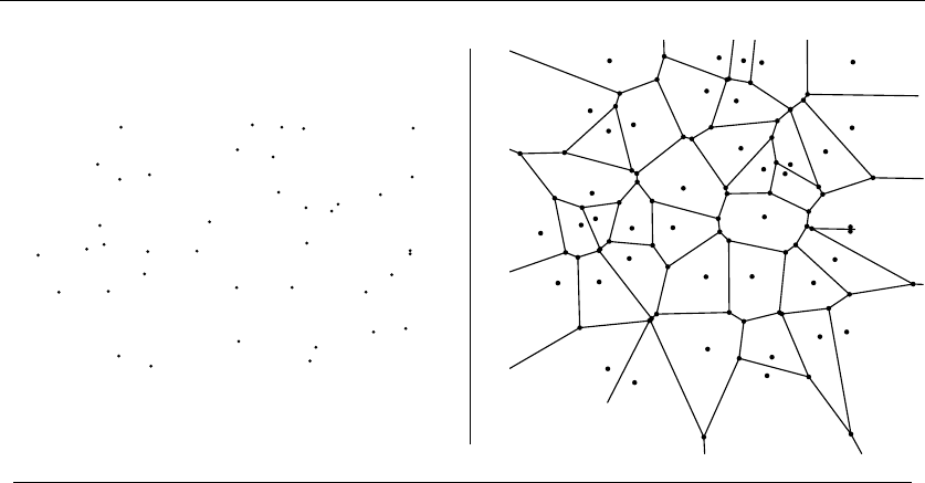
576 17. COMPUTATIONAL GEOMETRY
INPUT OUTPUT
17.4 Voronoi Diagrams
Input description:AsetSof points p1,...,p
n.
Problem description: Decompose space into regions around each point such that
all points in the region around piare closer to pithan any other point in S.
Discussion: Voronoi diagrams represent the region of influence around each of a
given set of sites. If these sites represent the locations of McDonald’s restaurants,
the Voronoi diagram partitions space into cells around each restaurant. For each
person living in a particular cell, the defining McDonald’s represents the closest
placetogetaBigMac.
Voronoi diagrams have a surprising variety of applications:
•Nearest neighbor search – Finding the nearest neighbor of query point qfrom
among a fixed set of points Sis simply a matter of determining the cell in
the Voronoi diagram of Sthat contains q. See Section 17.5 (page 580) for
more details.
•Facility location – Suppose McDonald’s wants to open another restaurant.
To minimize interference with existing McDonald’s, it should be located as
far away from the closest restaurant as possible. This location is always at
a vertex of the Voronoi diagram, and can be found in a linear-time search
through all the Voronoi vertices.

17.4 VORONOI DIAGRAMS 577
•Largest empty circle – Suppose you needed to obtain a large, contiguous, un-
developed piece of land on which to build a factory. The same condition used
to select McDonald’s locations is appropriate for other undesirable facilities,
namely that they be as far as possible from any relevant sites of interest.
A Voronoi vertex defines the center of the largest empty circle among the
points.
•Path planning – If the sites of Sare the centers of obstacles we seek to avoid,
the edges of the Voronoi diagram define the possible channels that maximize
the distance to the obstacles. Thus the “safest” path among the obstacles
will stick to the edges of the Voronoi diagram.
•Quality triangulations – In triangulating a set of points, we often desire nice,
fat triangles that avoid small angles and skinny triangles. The Delaunay trian-
gulation maximizes the minimum angle over all triangulations. Furthermore,
it is easily constructed as the dual of the Voronoi diagram. See Section 17.3
(page 572) for details.
Each edge of a Voronoi diagram is a segment of the perpendicular bisector of
two points in S, since this is the line that partitions the plane between the points.
The conceptually simplest method to construct Voronoi diagrams is randomized
incremental construction. To add another site to the diagram, we locate the cell
that contains it and add the perpendicular bisectors separating this new site from
all sites defining impacted regions. If the sites are inserted in random order, only
a small number of regions are likely to be impacted with each insertion.
However, the method of choice is Fortune’s sweepline algorithm, especially since
robust implementations of it are readily available. The algorithm works by project-
ing the set of sites in the plane into a set of cones in three dimensions such that
the Voronoi diagram is defined by projecting the cones back onto the plane. Ad-
vantages of Fortune’s algorithm include that (1) it runs in optimal Θ(nlog n) time,
(2) it is reasonable to implement, and (3) we need not store the entire diagram if
we can use it as we sweep over it.
There is an interesting relationship between convex hulls in d+1 dimensions and
Delaunay triangulations (or equivalently Voronoi diagrams) in d-dimensions. By
projecting each site in Ed(x1,x
2,...,x
d)intothepoint(x1,x
2,...,x
d,d
i=1 x2
i),
taking the convex hull of this (d+ 1)-dimensional point set and then projecting
back into ddimensions, we obtain the Delaunay triangulation. Details are given in
the Notes section, but this provides the best way to construct Voronoi diagrams
in higher dimensions. Programs that compute higher-dimensional convex hulls are
discussed in Section 17.2 (page 568).
Several important variations of standard Voronoi diagrams arise in practice.
See the references below for details:
•Non-Euclidean distance metrics – Recall that Voronoi diagrams decompose
space into regions of influence around each of the given sites. We have as-
sumed that Euclidean distance measures influence, but this is inappropriate

578 17. COMPUTATIONAL GEOMETRY
for certain applications. If people drive to McDonald’s, the time it takes to
get there depends upon where the major roads are. Efficient algorithms are
known for constructing Voronoi diagrams under a variety of different metrics,
and for curved or constrained objects.
•Power diagrams – These structures decompose space into regions of influence
around the sites, where the sites are no longer constrained to have all the
same power. Imagine a map of radio stations operating at a given frequency.
The region of influence around a station depends both on the power of its
transmitter and the position/power of neighboring transmitters.
•Kth-order and furthest-site diagrams – The idea of decomposing space into
regions sharing some property can be taken beyond closest-point Voronoi dia-
grams. Any point within a single cell of the kth-order Voronoi diagram shares
the same set of k’s closest points in S. In furthest-site diagrams, any point
within a particular region shares the same furthest point in S. Point location
(see Section 17.7 (page 587)) on these structures permits fast retrieval of the
appropriate points.
Implementations: Fortune’s Sweep2 is a widely used 2D code for Voronoi dia-
grams and Delaunay triangulations, written in C. This code is simple to work with
if all you need is the Voronoi diagram. It is based on his sweepline algorithm [For87]
for Voronoi diagrams and is available from Netlib (see Section 19.1.5 (page 659))
at http://www.netlib.org/voronoi/.
Both the CGAL (www.cgal.org) and LEDA (see Section 19.1.1 (page 658)) li-
braries offer C++ implementations of a variety of Voronoi diagram and Delaunay
triangulation algorithms in two and three dimensions.
Higher-dimensional and furthest-site Voronoi diagrams can be constructed
as a special case of higher-dimensional convex hulls. Qhull [BDH97] is a popu-
lar low-dimensional convex-hull code, useful for from two to about eight dimen-
sions. It is written in C and can also construct Delaunay triangulations, Voronoi
vertices, furthest-site Voronoi vertices, and half-space intersections. Qhull has
been widely used in scientific applications and has a well-maintained homepage
at http://www.qhull.org/. Another choice is Ken Clarkson’s higher-dimensional
convex-hull code, Hull, available at http://www.netlib.org/voronoi/hull.html.
Notes:Voronoi diagrams were studied by Dirichlet in 1850 and are occasionally referred
to as Dirichlet tessellations. They are named after G. Voronoi, who discussed them in a
1908 paper. In mathematics, concepts get named after the last person to discover them.
The book by Okabi, et al. [OBSC00] is the most complete treatment of Voronoi dia-
grams and their applications. Aurenhammer [Aur91] and Fortune [For04] provide excellent
surveys on Voronoi diagrams and associated variants such as power diagrams. The first
O(nlg n) algorithm for constructing Voronoi diagrams was based on divide-and-conquer
and is due to Shamos and Hoey [SH75]. Good expositions of both Fortune’s sweepline
algorithm [For87] for constructing Voronoi diagrams in O(nlg n) and the relationship

17.4 VORONOI DIAGRAMS 579
between Delaunay triangulations and (d+ 1)-dimensional convex hulls [ES86] include
[dBvKOS00, O’R01].
In a kth-order Voronoi diagram, we partition the plane such that each point in a
region is closest to the same set of ksites. Using the algorithm of [ES86], the complete set
of kth-order Voronoi diagrams can be constructed in O(n3) time. By doing point location
on this structure, the knearest neighbors to a query point can be found in O(k+lgn).
Expositions on kth-order Voronoi diagrams include [O’R01, PS85].
The smallest enclosing circle problem can be solved in O(nlg n) time using (n−1)st
order Voronoi diagrams [PS85]. In fact, there exists a linear-time algorithm based on low-
dimensional linear programming [Meg83]. A linear algorithm for computing the Voronoi
diagram of a convex polygon is given by [AGSS89].
Related Problems: Nearest neighbor search (see page 580), point location (see
page 587), triangulation (see page 572).
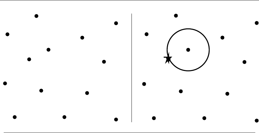
580 17. COMPUTATIONAL GEOMETRY
qq
INPUT OUTPUT
17.5 Nearest Neighbor Search
Input description:AsetSof npoints in ddimensions; a query point q.
Problem description:WhichpointinSis closest to q?
Discussion: The need to quickly find the nearest neighbor of a query point arises
in a variety of geometric applications. The classic example involves designing a
system to dispatch emergency vehicles to the scene of a fire. Once the dispatcher
learns the location of the fire, she uses a map to find the firehouse closest to this
point to minimize transportation delays. This situation occurs in any application
mapping customers to service providers.
A nearest-neighbor search is also important in classification. Suppose we are
given a collection of numerical data about people (say age, height, weight, years
of education, and income level) each of whom has been labeled as Democrat or
Republican. We seek a classifier to decide which way a given person is likely to
vote. Each of the people in our data set is represented by a party-labeled point in
d-dimensional space. A simple classifier can be built by assigning the new point to
the party affiliation of its nearest neighbor.
Such nearest-neighbor classifiers are widely used, often in high-dimensional
spaces. The vector-quantization method of image compression partitions an im-
age into 8 ×8 pixel regions. This method uses a predetermined library of several
thousand 8×8 pixel tiles and replaces each image region by the most similar library
tile. The most similar tile is the point in 64-dimensional space that is closest to

17.5 NEAREST NEIGHBOR SEARCH 581
the image region in question. Compression is achieved by reporting the identifier
of the closest library tile instead of the 64 pixels, at some loss of image fidelity.
Issues arising in nearest-neighbor search include:
•How many points are you searching? – When your data set contains only a
small number of points (say n≤100), or if only a few queries are ever destined
to be performed, the simple approach is best. Compare the query point q
against each of the ndata points. Only when fast queries are needed for large
numbers of points does it pay to consider more sophisticated methods.
•How many dimensions are you working in? – A nearest neighbor search gets
progressively harder as the dimensionality increases. The kd-tree data struc-
ture, presented in Section 12.6 (page 389), does a very good job in moderate-
dimensional spaces—even the plane. Still, above 20 dimensions or so, kd-tree
search degenerates pretty much to a linear search through the data points.
Searches in high-dimensional spaces become hard because a sphere of radius
r, representing all the points with distance ≤rfrom the center, progressively
fills up less volume relative to a cube as the dimensionality increases. Thus,
any data structure based on partitioning points into enclosing volumes will
become progressively less effective.
In two dimensions, Voronoi diagrams (see Section 17.4 (page 576)) provide
an efficient data structure for nearest-neighbor queries. The Voronoi diagram
of a point set in the plane decomposes the plane into regions such that the
cell containing data point pconsists of all points that are nearer to pthan
any other point in S. Finding the nearest neighbor of query point qreduces
to finding which Voronoi diagram cell contains qand reporting the data
point associated with it. Although Voronoi diagrams can be built in higher
dimensions, their size rapidly grows to the point of unusability.
•Do you really need the exact nearest neighbor? – Finding the exact nearest
neighbor in a very high dimensional space is hard work; indeed, you prob-
ably won’t do better than a linear (brute force) search. However, there are
algorithms/heuristics that can give you a reasonably close neighbor of your
query point fairly quickly.
One important technique is dimension reduction. Projections exist that map
any set of npoints in d-dimensions into a d=O(lg n/2)-dimensional space
such that distance to the nearest neighbor in the low-dimensional space is
within (1+) times that of the actual nearest neighbor. Projecting the points
onto a random hyperplane of dimension din Edwill likely do the trick.
Another idea is adding some randomness when you search your data struc-
ture. A kd-tree can be efficiently searched for the cell containing the query
point q—a cell whose boundary points are good candidates to be close neigh-
bors. Now suppose we search for a point q, which is a small random per-
turbations of q. It should land in a different but nearby cell, one of whose

582 17. COMPUTATIONAL GEOMETRY
boundary points might prove to be an even closer neighbor of q. Repeat-
ing such random queries gives us a way to productively use exactly as much
computing time as we are willing to spend to improve the answer.
•Is your data set static or dynamic? – Will there be occasional insertions
or deletions of new data points in your application? If these are very rare
events, it might pay to rebuild your data structure from scratch each time.
If they are frequent, select a version of the kd-tree that supports insertions
and deletions.
The nearest neighbor graph on a set Sof npoints links each vertex to its nearest
neighbor. This graph is a subgraph of the Delaunay triangulation, and so can be
computed in O(nlog n). This is quite a bargain, since it takes Θ(nlog n) time just
to discover the closest pair of points in S.
As a lower bound, the closest-pair problem reduces to sorting in one dimension.
In a sorted set of numbers, the closest pair corresponds to two numbers that lie
next to each other, so we need only check that which is the minimum gap between
the n−1 adjacent pairs. The limiting case occurs when the closest pair are zero
distance apart, meaning that the elements are not unique.
Implementations:ANN is a C++ library for both exact and approximate nearest
neighbor searching in arbitrarily high dimensions. It performs well for searches over
hundreds of thousands of points in up to about 20 dimensions. It supports all lp
distance norms, including Euclidean and Manhattan distance, and is available at
http://www.cs.umd.edu/∼mount/ANN/. It is the first code I would turn to for
nearest neighbor search.
Samet’s spatial index demos (http://donar.umiacs.umd.edu/quadtree/)pro-
vide a series of Java applets illustrating many variants of kd-trees, in associa-
tion with [Sam06]. KDTREE 2 contains C++ and Fortran 95 implementations
of kd-trees for efficient nearest nearest neighbor search in many dimensions. See
http://arxiv.org/abs/physics/0408067.
Ranger [MS93] is a tool for visualizing and experimenting with nearest-neighbor
and orthogonal-range queries in high-dimensional data sets, using multidimensional
search trees. Four different search data structures are supported by Ranger: naive
kd-trees, median kd-trees, nonorthogonal kd-trees, and the vantage point tree. It
is available in the algorithm repository http://www.cs.sunysb.edu/∼algorith.
Nearpt3 is a special-purpose code for nearest-neighbor search of extremely large
point sets in three dimensions. See http://wrfranklin.org/Research/nearpt3.
See Section 17.4 (page 576) for a complete collection of Voronoi diagram im-
plementations. In particular, CGAL (www.cgal.org) and LEDA (see Section 19.1.1
(page 658)) provide implementations of Voronoi diagrams in C++, as well as planar
point location to make effective use of them for nearest-neighbor search.
Notes:Indyk [Ind04] ably surveys recent results in approximate nearest neighbor search
in high dimensions based on random projection methods. Both theoretical [IM04] and
empirical [BM01] results indicate that the method preserves distances quite nicely.

17.5 NEAREST NEIGHBOR SEARCH 583
The theoretical guarantees underlying Ayra and Mount’s approximate nearest neigh-
bor code ANN [AM93, AMN+98] are somewhat different. A sparse weighted graph struc-
ture is built from the data set, and the nearest neighbor is found by starting at a random
point and greedily walking towards the query point in the graph. The closest point found
over several random trials is declared the winner. Similar data structures hold promise
for other problems in high-dimensional spaces. Nearest-neighbor search was a subject of
the Fifth DIMACS challenge, as reported in [GJM02].
Samet [Sam06] is the best reference on kd-trees and other spatial data structures. All
major (and many minor) variants are developed in substantial detail. A shorter survey
[Sam05] is also available. The technique of using random perturbations of the query point
is due to [Pan06].
Good expositions on finding the closest pair of points in the plane [BS76] include
[CLRS01, Man89]. These algorithms use a divide-and-conquer approach instead of just
selecting from the Delaunay triangulation.
Related Problems: Kd-trees (see page 389), Voronoi diagrams (see page 576),
range search (see page 584).
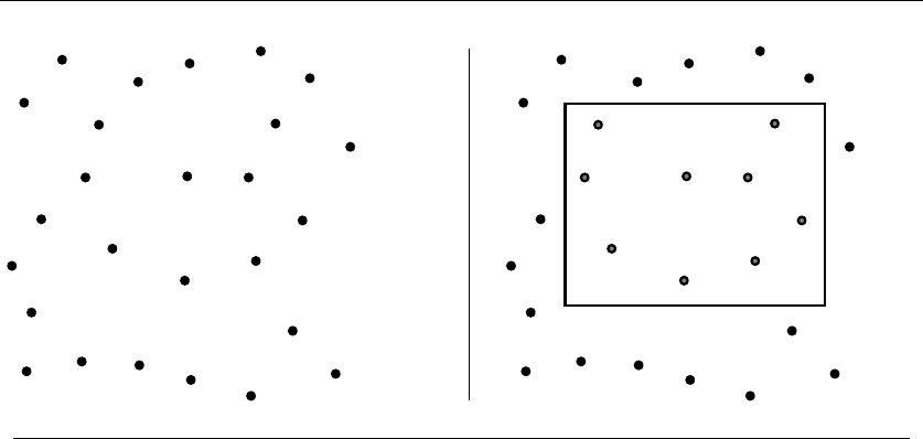
584 17. COMPUTATIONAL GEOMETRY
INPUT OUTPUT
17.6 Range Search
Input description:AsetSof npoints in Edand a query region Q.
Problem description: What points in Slie within Q?
Discussion: Range-search problems arise in database and geographic information
system (GIS) applications. Any data object with dnumerical fields, such as person
with height, weight, and income, can be modeled as a point in d-dimensional space.
Arange query describes a region in space and asks for all points or the number
of points in the region. For example, asking for all people with income between $0
and $10,000, with height between 6’0” and 7’0”, and weight between 50 and 140
lbs., defines a box containing people whose wallet and body are both thin.
The difficulty of range search depends on several factors:
•How many range queries are you going to perform? – The simplest approach
to range search tests each of the npoints one by one against the query polygon
Q. This works just fine when the number of queries will be small. Algorithms
to test whether a point is within a given polygon are presented in Section
17.7 (page 587).
•What shape is your query polygon? – The easiest regions to query against are
axis-parallel rectangles, because the inside/outside test reduces to verifying
whether each coordinate lies within a prescribed range. The input-output
figure illustrates such an orthogonal range query.

17.6 RANGE SEARCH 585
When querying against a nonconvex polygon, it will pay to partition your
polygon into convex pieces or (even better) triangles and then query the
point set against each one of the pieces. This works because it is quick and
easy to test whether a point lies inside a convex polygon. Algorithms for such
convex decompositions are discussed in Section 17.11 (page 601).
•How many dimensions? – A general approach to range queries builds a kd-tree
on the point set, as discussed in Section 12.6 (page 389). A depth-first traver-
sal of the kd-tree is performed for the query, with each tree node expanded
only if the associated rectangle intersects the query region. The entire tree
might have to be traversed for sufficiently large or misaligned query regions,
but in general kd-trees lead to an efficient solution. Algorithms with more
efficient worst-case performance are known in two dimensions, but kd-trees
are likely to work just fine in the plane. In higher dimensions, they provide
the only viable solution to the problem.
•Is your point set static, or might there be insertions/deletions? – A clever
practical approach to range search and many other geometric searching prob-
lems is based on Delaunay triangulations. Delaunay triangulation edges con-
nect each point pto nearby points, including its nearest neighbor. To perform
a range query, we start by using planar point location (see Section 17.7 (page
587)) to quickly identify a triangle within the region of interest. We then do a
depth-first search around a vertex of this triangle, pruning the search when-
ever it visits a point too distant to have interesting undiscovered neighbors.
This should be efficient, because the total number of points visited should be
roughly proportional to the number within the query region.
One nice thing about this approach is that it is relatively easy to employ
“edge-flip” operations to fix up a Delaunay triangulation following a point
insertion or deletion. See Section 17.3 (page 572) for more details.
•Can I just count the number of points in a region, or do I have to identify
them? – For many applications, it suffices to count the number of points
in a region instead of returning them. Harkening back to the introductory
example, we may want to know whether there are more thin/poor people or
rich/fat ones. The need to find the densest or emptiest region in space often
arises, and this problem can be solved by counting range queries.
A nice data structure for efficiently answering such aggregate range queries
is based on the dominance ordering of the point set. A point xis said to
dominate point yif ylies both below and to the left of x.LetDOM(p)bea
function that counts the number of points in Sthat are dominated by p.The
number of points min the orthogonal rectangle defined by xmin ≤x≤xmax
and ymin ≤y≤ymax is given by
m=DOM(xmax,y
max)−DOM(xmax,y
min)−DOM(xmin,y
max)+DOM(xmin,y
min)

586 17. COMPUTATIONAL GEOMETRY
The second additive term corrects for the points for the lower left-hand corner
that have been subtracted away twice.
To answer arbitrary dominance queries efficiently, partition the space into
n2rectangles by drawing a horizontal and vertical line through each of the n
points. The set of dominated points is identical for each point in any rectangle,
so the dominance count of the lower left-hand corner of each rectangle can
be precomputed, stored, and reported for any query point within it. Range
queries reduce to binary search and thus take O(lg n) time. Unfortunately,
this data structure takes quadratic space. However, the same idea can be
adapted to kd-trees to create a more space-efficient search structure.
Implementations: Both CGAL (www.cgal.org) and LEDA (see Section 19.1.1
(page 658)) use a dynamic Delaunay triangulation data structure to support cir-
cular, triangular, and orthogonal range queries. Both libraries also provide imple-
mentations of range tree data structures, which support orthogonal range queries
in O(k+lg
2n) time where nis the complexity of the subdivision and kis the
number of points in the rectangular region.
ANN is a C++ library for both exact and approximate nearest neighbor search-
ing in arbitrarily high dimensions. It performs well for searches over hundreds of
thousands of points in up to about 20 dimensions. It supports fixed-radius, nearest-
neighbor queries over all lpdistance norms, which can be used to approximate cir-
cular and orthogonal range queries under the l2and l1norms, respectively. ANN
is available at http://www.cs.umd.edu/∼mount/ANN/.
Ranger is a tool for visualizing and experimenting with nearest-neighbor and
orthogonal-range queries in high-dimensional data sets, using multidimensional
search trees. Four different search data structures are supported by Ranger: naive
kd-trees, median kd-trees, nonorthogonal kd-trees, and the vantage point tree. For
each of these, Ranger supports queries in up to 25 dimensions under any Minkowski
metric. It is available in the algorithm repository.
Notes:Good expositions on data structures with worst-case O(lg n+k) performance for
orthogonal-range searching [Wil85] include [dBvKOS00, PS85]. Exposition on kd-trees for
orthogonal range queries in two dimensions appear in [dBvKOS00, PS85]. Their worst-case
performance can be very bad; [LW77] describes an instance in two dimensions requiring
O(√n) time to report that a rectangle is empty.
The problem becomes considerably more difficult for nonorthogonal range queries,
where the query region is not an axis-aligned rectangle. For half-plane intersection queries,
O(lg n) time and linear space suffice [CGL85]; for range searching with simplex query
regions (such as a triangle in the plane), lower bounds preclude efficient worst-case data
structures. See Agrawal [Aga04] for a survey and discussion.
Related Problems: Kd-trees (see page 389), point location (see page 587).

17.7 POINT LOCATION 587
q
?
INPUT OUTPUT
17.7 Point Location
Input description: A decomposition of the plane into polygonal regions and a
query point q.
Problem description: Which region contains the query point q?
Discussion: Point location is a fundamental subproblem in computational geome-
try, usually needed as an ingredient to solve larger geometric problems. In a typical
police dispatch system, the city will be partitioned into different precincts or dis-
tricts. Given a map of regions and a query point (the crime scene), the system must
identify which region contains the point. This is exactly the problem of planar point
location. Variations include:
•Is a given point inside or outside of polygon P?– The simplest version of
point location involves only two regions, inside-Pand outside-P,andasks
which contains a given query point. For polygons with lots of narrow spirals,
this can be surprisingly difficult to tell by inspection. The secret to doing
it both by eye or machine is to draw a ray starting from the query point
and ending beyond the furthest extent of the polygon. Count the number of
times the polygon crosses through an edge. The query point will lie within
the polygon iff this number is odd. The case of the line passing through a
vertex instead of an edge is evident from context, since we are counting the
number of times we pass through the boundary of the polygon. Testing each
of the nedges for intersection against the query ray takes O(n) time. Faster

588 17. COMPUTATIONAL GEOMETRY
algorithms for convex polygons are based on binary search, and take O(lg n)
time.
•How many queries must be performed? – It is always possible to perform this
inside-polygon test separately on each region in a given planar subdivision.
However, it would be wasteful to perform many such point location queries
on the same subdivision. It would be much better to construct a grid-like or
tree-like data structure on top of our subdivision to get us near the correct
region quickly. Such search structures are discussed in more detail below.
•How complicated are the regions of your subdivision? – More sophisticated
inside-outside tests are required when the regions of your subdivision are
arbitrary polygons. By triangulating all polygonal regions first, each inside-
outside test reduces to testing whether a point is in a triangle. Such tests
can be made particularly fast and simple, at the minor cost of recording the
full polygon name for each triangle. An added benefit is that the smaller
your regions are, the better grid-like or tree-like superstructures are likely
to perform. Some care should be taken when you triangulate to avoid long
skinny triangles, as discussed in Section 17.3 (page 572).
•How regularly sized and spaced are your regions? – If all resulting triangles are
about the same size and shape, the simplest point location method imposes
a regularly-spaced k×kgrid of horizontal and vertical lines over the entire
subdivision. For each of the k2rectangular regions, we maintain a list of all the
regions that are at least partially contained within the rectangle. Performing
a point location query in such a grid file involves a binary search or hash
table lookup to identify which rectangle contains query point q, and then
searching each region in the resulting list to identify the right one.
Such grid files can perform very well, provided that each triangular region
overlaps only a few rectangles (thus minimizing storage space) and each rect-
angle overlaps only a few triangles (thus minimizing search time). Whether
it performs well depends on the regularity of your subdivision. Some flexi-
bility can be achieved by spacing the horizontal lines irregularly, depending
upon where the regions actually lie. The slab method, discussed below, is a
variation on this idea that guarantees worst-case efficient point location at
the cost of quadratic space.
•How many dimensions will you be working in? – In three or more dimensions,
some flavor of kd-tree will almost certainly be the point-location method of
choice. They may also be the right answer for planar subdivisions that are
too irregular for grid files.
Kd-trees, described in Section 12.6 (page 389), decompose the space into a
hierarchy of rectangular boxes. At each node in the tree, the current box is
split into a small number (typically 2, 4, or 2dfor dimension d) of smaller
boxes. Each leaf box is labeled with the (small) set regions that are at least

17.7 POINT LOCATION 589
partially contained in the box. The point location search starts at the root of
the tree and keeps traversing down the child whose box contains the query
point q. When the search hits a leaf, we test each of the relevant regions to
see which one of them contains q. As with grid files, we hope that each leaf
contains a small number of regions and that each region does not cut across
too many leaf cells.
•Am I close to the right cell? – Walking is a simple point-location technique
that might even work well beyond two dimensions. Start from an arbitrary
point pin an arbitrary cell, hopefully close to the query point q. Construct
the line (or ray) from pto qand identify which face of the cell this hits (a
so-called ray shooting query). Such queries take constant time in triangulated
arrangements.
Proceeding to the neighboring cell through this face gets us one step closer to
the target. The expected path length will be O(n1/d) for sufficiently regular
d-dimensional arrangements, although linear in the worst case.
The simplest algorithm to guarantee O(lg n) worst-case access is the slab
method, which draws horizontal lines through each vertex, thus creating n+1
“slabs” between the lines. Since the slabs are defined by horizontal lines, finding
the slab containing a particular query point can be done using a binary search on
the y-coordinate of q. Since there can be no vertices within any slab, the region
containing a point within a slab can be identified by a second binary search on the
edges that cross the slab. The catch is that a binary search tree must be maintained
for each slab, for a worst-case of O(n2) space. A more space-efficient approach based
on building a hierarchy of triangulations over the regions also achieves O(lg n)for
search and is discussed in the notes below.
Worst-case efficient computational geometry methods either require a lot of
storage or are fairly complicated to implement. We identify implementations of
worst-case methods below, which are worth at least experimenting with. However,
we recommend kd-trees for most general point-location applications.
Implementations: Both CGAL (www.cgal.org) and LEDA (see Section 19.1.1
(page 658)) provide excellent support for maintaining planar subdivisions in C++.
CGAL favors a jump-and-walk strategy, although a worst-case logarithmic search
is also provided. LEDA implements expected O(lg n) point location using partially
persistent search trees.
ANN is a C++ library for both exact and approximate nearest-neighbor
searching in arbitrarily high dimensions. It can be used to quickly iden-
tify a nearby cell boundary point to begin walking from. Check it out at
http://www.cs.umd.edu/∼mount/ANN/.
Arrange is a package for maintaining arrangements of polygons in either
the plane or on the sphere. Polygons may be degenerate, and hence rep-
resent arrangements of lines. A randomized incremental construction algo-
rithm is used, and efficient point location on the arrangement is supported.

590 17. COMPUTATIONAL GEOMETRY
Arrange is written in C by Michael Goldwasser and is available from
http://euler.slu.edu/∼goldwasser/publications/.
Routines (in C) to test whether a point lies in a simple polygon have been
provided by [O’R01, SR03].
Notes:Snoeyink [Sno04] gives an excellent survey of the state-of-the-art in point location,
both theoretical and practical. Very thorough treatments of deterministic planar-point
location data structures are provided by [dBvKOS00, PS85].
Tamassia and Vismara [TV01] use planar point location as a case study of geometric
algorithm engineering, in Java. An experimental study of algorithms for planar point
location is described in [EKA84]. The winner was a bucketing technique akin to the grid
file.
The elegant triangle refinement method of Kirkpatrick [Kir83] builds a hierarchy of
triangulations above the actual planar subdivision such that each triangle on a given
level intersects only a constant number of triangles on the following level. Since each
triangulation is a fraction of the size of the subsequent one, the total space is obtained
by summing up a geometric series and hence is linear. Furthermore, the height of the
hierarchy is O(lg n), ensuring fast query times. An alternative algorithm realizing the
same time bounds is [EGS86]. The slab method described above is due to [DL76] and
is presented in [PS85]. Expositions on the inside-outside test for simple polygons include
[Hai94, O’R01, PS85, SR03].
More recently, there has been interest in dynamic data structures for point location,
which support fast incremental updates of the planar subdivision (such as insertions and
deletions of edges and vertices) as well as fast point location. Chiang and Tamassia’s
[CT92] survey is an appropriate place to begin, with updated references in [Sno04].
Related Problems: Kd-trees (see page 389), Voronoi diagrams (see page 576),
nearest neighbor search (see page 580).
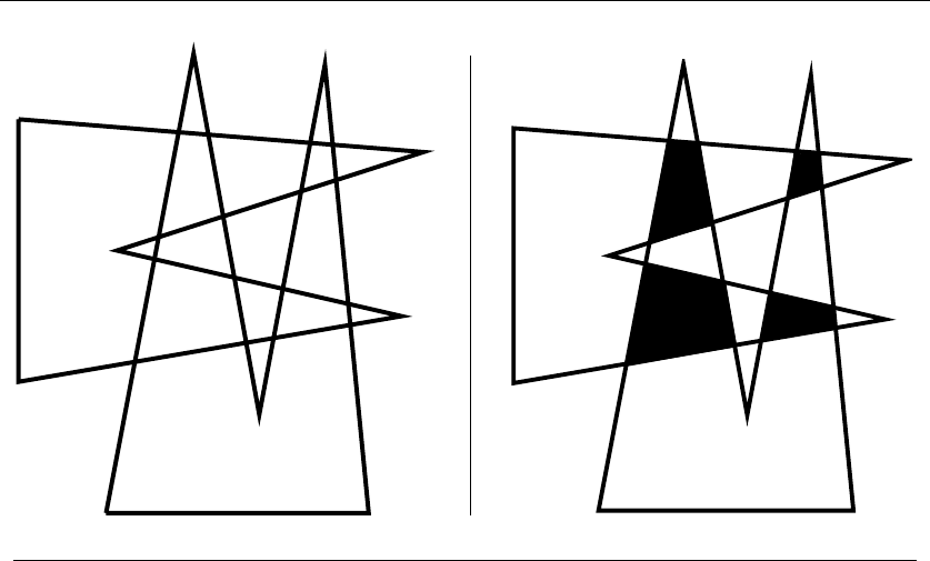
17.8 INTERSECTION DETECTION 591
INPUT OUTPUT
17.8 Intersection Detection
Input description:AsetSof lines and line segments l1,...,l
nor a pair of
polygons or polyhedra P1and P2.
Problem description: Which pairs of line segments intersect each other? What
is the intersection of P1and P2?
Discussion: Intersection detection is a fundamental geometric primitive with many
applications. Picture a virtual-reality simulation of an architectural model for
a building. The illusion of reality vanishes the instant the virtual person walks
through a virtual wall. To enforce such physical constraints, any such intersection
between polyhedral models must be immediately detected and the operator notified
or constrained.
Another application of intersection detection is design rule checking for VLSI
layouts. A minor design defect resulting in two crossing metal strips could short
out the chip, but such errors can be detected before fabrication, using programs to
find all intersections between line segments.
Issues arising in intersection detection include:
•Do you want to compute the intersection or just report it? – We distin-
guish between intersection detection and computing the actual intersection.

592 17. COMPUTATIONAL GEOMETRY
Detecting that an intersection exists can be substantially easier, and often
suffices. For the virtual-reality application, it might not be important to know
exactly where we hit the wall—just that we hit it.
•Are you intersecting lines or line segments? – The big difference here is that
any two lines with different slopes intersect in at exactly one point. All the
points of intersections can be found in O(n2) time by comparing each pair of
lines. Constructing the arrangement of the lines provides more information
than just the intersection points, and is discussed in Section 17.15 (page 614).
Finding all the intersections between nline segments is considerably more
challenging. Even the basic primitive of testing whether two line segments
intersect is not as trivial, as discussed in Section 17.1 (page 564). Of course,
we could explicitly test each line segment pair and thus find all intersections
in O(n2) time, but faster algorithms exist when there are few intersection
points.
•How many intersection points do you expect? – In VLSI design-rule checking,
we expect the set of line segments to have few if any intersections. What we
seek is an algorithm whose time is output sensitive, taking time proportional
to the number of intersection points.
Such output-sensitive algorithms exist for line-segment intersection. The
fastest algorithm takes O(nlg n+k) time, where kis the number of intersec-
tions. These algorithms are based on the planar sweepline approach.
•Can you see point xfrom point y?– Visibility queries ask whether vertex x
can see vertex yunobstructed in a room full of obstacles. This can be phrased
as the following line-segment intersection problem: does the line segment from
xto yintersect any obstacle? Such visibility problems arise in robot motion
planning (see Section 17.14) and in hidden-surface elimination for computer
graphics.
•Are the intersecting objects convex? – Better intersection algorithms exist
when the line segments form the boundaries of polygons. The critical issue
here becomes whether the polygons are convex. Intersecting a convex n-gon
with a convex m-gon can be done in O(n+m) time, using the sweepline
algorithm discussed next. This is possible because the intersection of two
convex polygons must form another convex polygon with at most n+m
vertices.
However, the intersection of two nonconvex polygons is not so well behaved.
Consider the intersection of two “combs” generalizing the Picasso-like fronts-
piece to this section. As illustrated, the intersection of nonconvex polygons
may be disconnected and have quadratic size in the worst case.

17.8 INTERSECTION DETECTION 593
Intersecting polyhedra is more complicated than polygons, because two poly-
hedra can intersect even when no edges do. Consider the example of a needle
piercing the interior of a face. In general, however, the same issues arise for
both polygons and polyhedra.
•Are you searching for intersections repeatedly with the same basic objects? –
In the walk-through application just described, the room and the objects in
it don’t change between one scene and the next. Only the person moves, and
intersections are rare.
One common technique is to approximate the objects in the scene by sim-
pler objects that enclose them, such as boxes. Whenever two enclosing boxes
intersect, then the underlying objects might intersect, and so further work
is necessary to decide the issue. However, it is much more efficient to test
whether simple boxes intersect than more complicated objects, so we win if
collisions are rare. Many variations on this theme are possible, but this idea
leads to large performance improvements for complicated environments.
Planar sweep algorithms can be used to efficiently compute the intersections
among a set of line segments, or the intersection/union of two polygons. These
algorithms keep track of interesting changes as we sweep a vertical line from left
to right over the data. At its leftmost position, the line intersects nothing, but as
it moves to the right, it encounters a series of events:
•Insertion – The leftmost point of a line segment may be encountered, and it
is now available to intersect some other line segment.
•Deletion – The rightmost point of a line segment is encountered. This means
that we have completely swept over the segment, and so it can be deleted
from further consideration.
•Intersection – If the active line segments that intersect the sweep line are
maintained as sorted from top to bottom, the next intersection must occur
between neighboring line segments. After this intersection, these two line
segments swap their relative order.
Keeping track of what is going on requires two data structures. The future is
maintained by an event queue, or a priority queue ordered by the x-coordinate of all
possible future events of interest: insertion, deletion, and intersection. See Section
12.2 (page 373) for priority queue implementations. The present is represented by
the horizon—an ordered list of line segments intersecting the current position of
the sweepline. The horizon can be maintained using any dictionary data structure,
such as a balanced tree.
To adapt this approach to compute the intersection or union of polygons, we
modify the processing of the three basic event types. This algorithm can be con-
siderably simplified for pairs of convex polygons, since (1) at most four polygon

594 17. COMPUTATIONAL GEOMETRY
edges intersect the sweepline, so no horizon data structure is needed, and (2) no
event-queue sorting is needed, since we can start from the leftmost vertex of each
polygon and proceed to the right by following the polygonal ordering.
Implementations: Both LEDA (see Section 19.1.1 (page 658)) and CGAL
(www.cgal.org) offers extensive support for line segment and polygonal intersec-
tion. In particular, they provide a C++ implementation of the Bentley-Ottmann
sweepline algorithm [BO79], finding all kintersection points between nline seg-
ments in the plane in O((n+k)lgn) time.
O’Rourke [O’R01] provides a robust program in C to compute the intersection
of two convex polygons. See Section 19.1.10 (page 662).
The University of North Carolina GAMMA group has produced several efficient
collision detection libraries, of which SWIFT++ [EL01] is the most recent member.
It can detect intersection, compute approximate/exact distances between objects,
and determine object-pair contacts in scenes composed of rigid polyhedral models.
See http://www.cs.unc.edu/∼geom/collide/ for pointers to all of these libraries.
Finding the mutual intersection of a collection of half-spaces is a special case
of the convex-hulls, and Qhull [BDH97] is convex hull code of choice for general
dimensions. Qhull has been widely used in scientific applications and has a well-
maintained homepage at http://www.qhull.org/.
Notes:Mount [Mou04] is an excellent survey of algorithms for computing intersections
of geometric objects such as line segments, polygons, and polyhedra. Books with chapters
discussing such problems include [dBvKOS00, CLRS01, PS85]. Preparata and Shamos
[PS85] provide a good exposition on the special case of finding intersections and unions
of axis-oriented rectangles—a problem that arises often in VLSI design.
An optimal O(nlg n+k) algorithm for computing line segment intersections is due to
Chazelle and Edelsbrunner [CE92]. Simpler, randomized algorithms achieving the same
time bound are thoroughly presented by Mulmuley [Mul94].
Lin and Manocha [LM04] survey techniques and software for collision detection.
Related Problems: Maintaining arrangements (see page 614), motion planning
(see page 610).
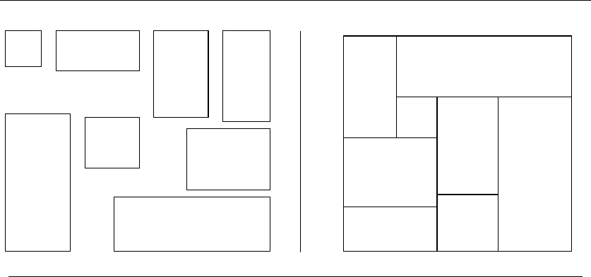
17.9 BIN PACKING 595
A B
C D
F
G
H
E
D
H
A
C
E
F
G
B
INPUT OUTPUT
17.9 Bin Packing
Input description:Asetofnitems with sizes d1,...,d
n.Asetofmbins with
capacity c1,...,c
m.
Problem description: Store all the items using the smallest number of bins.
Discussion: Bin packing arises in a variety of packaging and manufacturing prob-
lems. Suppose that you are manufacturing widgets cut from sheet metal or pants
cut from cloth. To minimize cost and waste, we seek to lay out the parts so as to
use as few fixed-size metal sheets or bolts of cloth as possible. Identifying which
part goes on which sheet in which location is a bin-packing variant called the cut-
ting stock problem. Once our widgets have been successfully manufactured, we are
faced with another bin-packing problem—namely how best to fit the boxes into
trucks to minimize the number of trucks needed to ship everything.
Even the most elementary-sounding bin-packing problems are NP-complete;
see the discussion of integer partition in Section 13.10 (page 427). Thus, we are
doomed to think in terms of heuristics instead of worst-case optimal algorithms.
Fortunately, relatively simple heuristics tend to work well on most bin-packing
problems. Further, many applications have peculiar, problem-specific constraints
that tend to frustrate sophisticated algorithms for bin packing. The following fac-
tors will affect the choice of heuristic:
•What are the shapes and sizes of the objects? – The character of a bin-packing
problem depends greatly on the shapes of the objects to be packed. Solving
a standard jigsaw puzzle is a much different problem than packing squares

596 17. COMPUTATIONAL GEOMETRY
into a rectangular box. In one-dimensional bin packing, each object’s size is
given simply as an integer. This is equivalent to packing boxes of equal width
into a chimney of that width, and makes it a special case of the knapsack
problem of Section 13.10 (page 427).
When all the boxes are of identical size and shape, repeatedly filling each row
gives a reasonable, but not necessarily optimal, packing. Consider trying to
fill a 3 ×3 square with 2 ×1 bricks. You can only pack three bricks using one
orientation, while four bricks suffice with two.
•Are there constraints on the orientation and placement of objects? –Many
boxes are labeled “this side up” (imposing an orientation on the box) or
“do not stack” (requiring them sit on top of any box pile). Respecting these
constraints restricts our flexibility in packing and hence will increase in the
number of trucks needed to send out certain shipments. Most shippers solve
the problem by ignoring the labels. Indeed, your task will be simpler if you
don’t have to worry about the consequences of them.
•Is the problem on-line or off-line? – Do we know the complete set of objects
to pack at the beginning of the job (an off-line problem)? Or will we get
them one at a time and deal with them as they arrive (an on-line problem)?
The difference is important, because we can do a better job packing when
we can take a global view and plan ahead. For example, we can arrange the
objects in an order that will facilitate efficient packing, perhaps by sorting
them from biggest to smallest.
The standard off-line heuristics for bin packing order the objects by size or
shape and then insert them into bins. Typical insertion rules are (1) select the first
or leftmost bin the object fits in, (2) select the bin with the most room, (3) select
the bin that provides the tightest fit, or (4) select a random bin.
Analytical and empirical results suggest that first-fit decreasing is the best
heuristic. Sort the objects in decreasing order of size, so that the biggest object
is first and the smallest last. Insert each object one by one into the first bin that
has room for it. If no bin has room, we must start another bin. In the case of
one-dimensional bin packing, this can never require more than 22% more bins than
necessary and usually does much better. First-fit decreasing has an intuitive appeal
to it, for we pack the bulky objects first and hope that little objects can fill up the
cracks.
First-fit decreasing is easily implemented in O(nlg n+bn) time, where b≤
min(n, m) is the number of bins actually used. Simply do a linear sweep through
the bins on each insertion. A faster O(nlg n) implementation is possible by using
a binary tree to keep track of the space remaining in each bin.
We can fiddle with the insertion order in such a scheme to deal with problem-
specific constraints. For example, it is reasonable to take “do not stack” boxes last
(perhaps after artificially lowering the height of the bins to leave some room up

17.9 BIN PACKING 597
top to work with) and to place fixed-orientation boxes at the beginning (so we can
use the extra flexibility later to stick boxes on top).
Packing boxes is much easier than packing arbitrary geometric shapes, enough
so that a general approach packs each part into its own box and then packs the
boxes. Finding an enclosing rectangle for a polygonal part is easy; just find the
upper, lower, left, and right tangents in a given orientation. Finding the orientation
and minimizing the area (or volume) of such a box is more difficult, but can be
done in both two and three dimensions [O’R85]. See the Implementations section
for a fast approximation to minimum enclosing box.
In the case of nonconvex parts, considerable useful space can be wasted in the
holes created by placing the part in a box. One solution is to find the maximum
empty rectangle within each boxed part and use this to contain other parts if it is
sufficiently large. More advanced solutions are discussed in the references.
Implementations: Martello and Toth’s collection of Fortran implementations
of algorithms for a variety of knapsack problem variants are available at
http://www.or.deis.unibo.it/kp.html. An electronic copy of [MT90a] has also been
generously made available.
David Pisinger maintains a well-organized collection of C-language codes for
knapsack problems and related variants like bin packing and container loading.
These are available at http://www.diku.dk/∼pisinger/codes.html.
A first step towards packing arbitrary shapes packs each in its own mini-
mum volume box. For a code to find an approximation to the optimal packing,
see http://valis.cs.uiuc.edu/∼sariel/research/papers/00/diameter/diam prog.html.
This algorithm runs in near-linear time [BH01].
Notes:See [CFC94, CGJ96, LMM02] for surveys of the extensive literature on bin pack-
ing and the cutting stock problem. Keller, Pferschy, and Psinger [KPP04] is the most
current reference on the knapsack problem and variants. Experimental results on bin-
packing heuristics include [BJLM83, MT87].
Efficient algorithms are known for finding the largest empty rectangle in a polygon
[DMR97] and point set [CDL86].
Sphere packing is an important and well-studied special case of bin packing, with ap-
plications to error-correcting codes. Particularly notorious was the “Kepler conjecture”—
the problem of establishing the densest packing of unit spheres in three dimensions. This
conjecture was finally settled by Hales and Ferguson in 1998; see [Szp03] for an exposition.
Conway and Sloane [CS93] is the best reference on sphere packing and related problems.
Milenkovic has worked extensively on two-dimensional bin-packing problems for the
apparel industry, minimizing the amount of material needed to manufacture pants and
other clothing. Reports of this work include [DM97, Mil97].
Related Problems: Knapsack problem (see page 427), set packing (see page 625).

598 17. COMPUTATIONAL GEOMETRY
INPUT OUTPUT
17.10 Medial-Axis Transform
Input description: A polygon or polyhedron P.
Problem description: What are the set of points within Pthat have more than
one closest point on the boundary of P?
Discussion: The medial-axis transformation is useful in thinning a polygon, or
as is sometimes said, finding its skeleton. The goal is to extract a simple, robust
representation of the shape of the polygon. The thinned versions of the letters A
and B capture the essence of their shape, and would be relatively unaffected by
changing the thickness of strokes or by adding font-dependent flourishes such as
serifs. The skeleton also represents the center of the given shape, a property that
leads to other applications like shape reconstruction and motion planning.
The medial-axis transformation of a polygon is always a tree, making it fairly
easy to use dynamic programming to measure the “edit distance” between the
skeleton of a known model and the skeleton of an unknown object. Whenever the
two skeletons are close enough, we can classify the unknown object as an instance
of our model. This technique has proven useful in computer vision and in optical
character recognition. The skeleton of a polygon with holes (like the A and B) is
not a tree but an embedded planar graph, but it remains easy to work with.
There are two distinct approaches to computing medial-axis transforms, de-
pending upon whether your input is arbitrary geometric points or pixel images:
•Geometric data – Recall that the Voronoi diagram of a point set S(see Section
17.4 (page 576)) decomposes the plane into regions around each point si∈S
such that points within the region around siare closer to sithan to any
other site in S. Similarly, the Voronoi diagram of a set of line segments L
decomposes the plane into regions around each line segment li∈Lsuch that
all points within the region around liare closer to lithan to any other site
in L.

17.10 MEDIAL-AXIS TRANSFORM 599
Any polygon is defined by a collection of line segments such that lishares
a vertex with li+1. The medial-axis transform of a polygon Pis simply the
portion of the line-segment Voronoi diagram that lies within P. Any line-
segment Voronoi diagram code thus suffices to do polygon thinning.
The straight skeleton is a structure related to the medial axis of a polygon,
except that the bisectors are not equidistant to its defining edges but instead
to the supporting lines of such edges. The straight skeleton, medial axis and
Voronoi diagram are all identical for convex polygons, but in general skeleton
bisectors may not be located in the center of the polygon. However, the
straight skeleton is quite similar to a proper medial axis transform but is
easier to compute. In particular, all edges in a straight skeleton are polygonal.
See the Notes section for references with more details on how to compute it.
•Image data – Digitized images can be interpreted as points sitting at the lat-
tice points on an integer grid. Thus, we could extract a polygonal description
from boundaries in an image and feed it to the geometric algorithms just
described. However, the internal vertices of the skeleton will most likely not
lie at grid points. Geometric approaches to image processing problems often
flounder because images are pixel-based and not continuous.
A direct pixel-based approach for constructing a skeleton implements the
“brush fire” view of thinning. Imagine a fire burning along all edges of the
polygon, racing inward at a constant speed. The skeleton is marked by all
points where two or more fires meet. The resulting algorithm traverses all the
boundary pixels of the object, identifies those vertices as being in the skeleton,
deletes the rest of the boundary, and repeats. The algorithm terminates when
all pixels are extreme, leaving an object only one or two pixels thick. When
implemented properly, this takes linear time in the number of pixels in the
image.
Algorithms that explicitly manipulate pixels tend to be easy to implement,
because they avoid complicated data structures. However, the geometry
doesn’t work out exactly right in such pixel-based approaches. For exam-
ple, the skeleton of a polygon is no longer always a tree or even necessar-
ily connected, and the points in the skeleton will be close-to-but-not-quite
equidistant to two boundary edges. Since you are trying to do continuous ge-
ometry in a discrete world, there is no way to solve the problem completely.
You just have to live with it.
Implementations:CGAL(www.cgal.org) includes a package for computing the
straight skeleton of a polygon P. Associated with it are routines for constructing
offset contours defining the polygonal regions within Pwhose points are at least
distance dfrom the boundary.
VRONI [Hel01] is a robust and efficient program for computing Voronoi di-
agrams of line segments, points, and arcs in the plane. It can readily compute

600 17. COMPUTATIONAL GEOMETRY
medial-axis transforms of polygons since it can construct Voronoi diagrams of
arbitrary line segments. VRONI has been tested on thousands of synthetic and
real-world data sets, some with over a million vertices. For more information,
see http://www.cosy.sbg.ac.at/∼held/projects/vroni/vroni.html. Other programs
for constructing Voronoi diagrams are discussed in Section 17.4 (page 576).
Programs that reconstruct or interpolate point clouds often are based on medial
axis transforms. Cocone (http://www.cse.ohio-state.edu/∼tamaldey/cocone.html)
constructs an approximate medial-axis transform of the polyhedral surface it in-
terpolates from points in E3. See [Dey06] for the theory behind Cocone.Power-
crust [ACK01a, ACK01b] constructs a discrete approximation to the medial-axis
transform, and then reconstructs the surface from this transform. When the point
samples are sufficiently dense, the algorithm is guaranteed to produce a geomet-
rically and topologically correct approximation to the surface. It is available at
http://www.cs.utexas.edu/users/amenta/powercrust/.
Notes:For a comprehensive survey of thinning approaches in image processing, see
[LLS92, Ogn93]. The medial axis transformation was introduced for shape similarity stud-
ies in biology [Blu67]. Applications of the medial-axis transformation in pattern recogni-
tion are discussed in [DHS00]. The medial axis transformation is fundamental to the power
crust algorithm for surface reconstruction from sampled points; see [ACK01a, ACK01b].
Good expositions on the medial-axis transform include [dBvKOS00, O’R01, Pav82].
The medial-axis of a polygon can be computed in O(nlg n) time for arbitrary n-
gons [Lee82], although linear-time algorithms exist for convex polygons [AGSS89]. An
O(nlg n) algorithm for constructing medial-axis transforms in curved regions was given
by Kirkpatrick [Kir79].
Straight skeletons were introduced in [AAAG95], with a subquadratic algorithm due
to [EE99]. See [LD03] for an interesting application of straight skeletons to defining the
roof structures in virtual building models.
Related Problems: Voronoi diagrams (see page 576), Minkowski sum (see page
617).

17.11 POLYGON PARTITIONING 601
INPUT OUTPUT
17.11 Polygon Partitioning
Input description: A polygon or polyhedron P.
Problem description: Partition Pinto a small number of simple (typically con-
vex) pieces.
Discussion: Polygon partitioning is an important preprocessing step for many
geometric algorithms, because geometric problems tend to be simpler on convex
objects than on nonconvex ones. It is often easier to work with a small number of
convex pieces than with a single nonconvex polygon.
Several flavors of polygon partitioning arise, depending upon the particular
application:
•Should all the pieces be triangles? – Triangulation is the mother of all polygon
partitioning problems, where we partition the interior of the polygon com-
pletely into triangles. Triangles are convex and have only three sides, making
them the most elementary possible polygon.
All triangulations of an n-vertex polygon contain exactly n−2 triangles.
Therefore, triangulation cannot be the answer if we seek a small number of
convex pieces. A “nice” triangulation is judged by the shape of the trian-
gles, not the count. See Section 17.3 (page 572) for a thorough discussion of
triangulation.

602 17. COMPUTATIONAL GEOMETRY
•Do I want to cover or partition my polygon? –Partitioning a polygon means
completely dividing the interior into nonoverlapping pieces. Covering a poly-
gon means that our decomposition is permitted to contain mutually over-
lapping pieces. Both can be useful in different situations. In decomposing a
complicated query polygon in preparation for a range search (Section 17.6
(page 584)), we seek a partitioning, so that each point we locate occurs in
exactly one piece. In decomposing a polygon for painting purposes, a cov-
ering suffices, since there is no difficulty with filling in a region twice. We
will concentrate here on partitioning, since it is simpler to do right, and any
application needing a covering will accept a partitioning. The only drawback
is that partitions can be larger than coverings.
•Am I allowed to add extra vertices? – A final issue is whether we are allowed
to add Steiner vertices to the polygon, either by splitting edges or adding
interior points. Otherwise, we are restricted to adding chords between two
existing vertices. The former may result in a smaller number of pieces, at the
cost of more complicated algorithms and perhaps messier results.
The Hertel-Mehlhorn heuristic for convex decomposition using diagonals is sim-
ple and efficient. It starts with an arbitrary triangulation of the polygon and then
deletes any chord that leaves only convex pieces. A chord deletion creates a non-
convex piece only if it creates an internal angle that is greater than 180 degrees.
The decision of whether such an angle will be created can be made locally from
the chords and edges surrounding the chord, in constant time. The result always
contains no more than four times the minimum number of convex pieces.
I recommend using this heuristic unless it is critical for you to minimize the
number of pieces. By experimenting with different triangulations and various dele-
tion orders, you may be able to obtain somewhat better decompositions.
Dynamic programming may be used to find the absolute minimum number of
diagonals used in the decomposition. The simplest implementation, which main-
tains the number of pieces for all O(n2) subpolygons split by a chord, runs in O(n4).
Faster algorithms use fancier data structures, running in O(n+r2min(r2,n)) time,
where ris the number of reflex vertices. An O(n3) algorithm that further reduces
the number of pieces by adding interior vertices is cited below, although it is com-
plex and presumably difficult to implement.
An alternate decomposition problem partitions polygons into monotone pieces.
The vertices of a y-monotone polygon can be divided into two chains such that any
horizontal line intersects either chain at most once.
Implementations: Many triangulation codes start by finding a trapezoidal or
monotone decomposition of polygons. Further, a triangulation is a simple form of
convex decomposition. Check out the codes in Section 17.3 (page 572) as a starting
point.
CGAL (www.cgal.org) contains a polygon-partitioning library that includes
(1) the Hertel-Mehlhorn heuristic for partitioning a polygon into convex pieces,

17.11 POLYGON PARTITIONING 603
(2) finding a optimal convex partitioning using the O(n4) dynamic programming
algorithm, and (3) an O(nlog n) sweepline heuristic for partitioning into monotone
polygons.
A triangulation code of particular relevance here is GEOMPACK—a suite of
Fortran 77 codes by Barry Joe for 2- and 3-dimensional triangulation and convex
decomposition problems. In particular, it does both Delaunay triangulation and
convex decompositions of polygonal and polyhedral regions, as well as arbitrary-
dimensional Delaunay triangulations.
Notes:Recent survey articles on polygon partitioning include [Kei00, OS04]. Keil and
Sack [KS85] give an excellent survey on what is known about partitioning and covering
polygons. Expositions on the Hertel-Mehlhorn heuristic [HM83] include [O’R01]. The
O(n+r2min(r2,n)) dynamic programming algorithm for minimum convex decomposition
using diagonals is due to Keil and Snoeyink [KS02]. The O(r3+n) algorithm minimizing
the number of convex pieces with Steiner points appears in [CD85]. Lien and Amato
[LA06] provide an efficient heuristic for decomposing polygons with holes into “almost
convex” polygons in O(nr) time, with later work generalizing this to polyhedra.
Art gallery problems are an interesting topic related to polygon covering, where we
seek to position the minimum number of guards in a given polygon such that every point in
the interior of the polygon is watched by at least one guard. This corresponds to covering
the polygon with a minimum number of star-shaped polygons. O’Rourke [O’R87] is a
beautiful (although sadly out of print) book that presents the art gallery problem and its
many variations.
Related Problems: Triangulation (see page 572), set cover (see page 621).
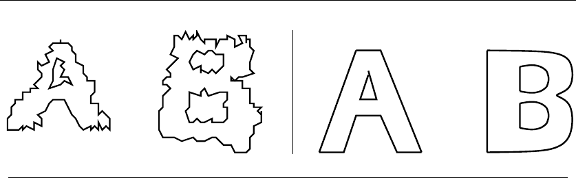
604 17. COMPUTATIONAL GEOMETRY
INPUT OUTPUT
17.12 Simplifying Polygons
Input description: A polygon or polyhedron p, with nvertices.
Problem description: Find a polygon or polyhedron pcontaining only nver-
tices, such that the shape of pis as close as possible to p.
Discussion: Polygon simplification has two primary applications. The first involves
cleaning up a noisy representation of a shape, perhaps obtained by scanning a
picture of an object. Simplifying it can remove the noise and reconstruct the original
object. The second involves data compression, where we seek to reduce detail on
a large and complicated object yet leave it looking essentially the same. This can
be a big win in computer graphics, where the smaller model might be significantly
faster to render.
Several issues arise in shape simplification:
•Do you want the convex hull? – The simplest simplification is the convex
hull of the object’s vertices (see Section 17.2 (page 568)). The convex hull
removes all internal concavities from the polygon. If you were simplifying
a robot model for motion planning, this is almost certainly a good thing.
But using the convex hull in an OCR system would be disastrous, because
the concavities of characters provide most of the interesting features. An ‘X’
would be identical to an ‘I’, since both hulls are boxes. Another problem is
that taking the convex hull of a convex polygon does nothing to simplify it
further.
•Am I allowed to insert or just delete points? – The typical goal of simplifi-
cation is to to represent the object as well as possible using a given number
of vertices. The simplest approaches do local modifications to the boundary
in order to reduce the vertex count. For example, if three consecutive ver-
tices form a small-area triangle or define an extremely large angle, the center

17.12 SIMPLIFYING POLYGONS 605
vertex can be deleted and replaced with an edge without severely distorting
the polygon.
Methods that only delete vertices quickly melt the shape into unrecogniz-
ability, however. More robust heuristics move vertices around to cover up
the gaps that are created by deletions. Such “split-and-merge” heuristics can
do a decent job, although nothing is guaranteed. Better results are likely by
using the Douglas-Peucker algorithm, described next.
•Must the resulting polygon be intersection-free? – A serious drawback of in-
cremental procedures is that they fail to ensure simple polygons, meaning
they are without self-intersections. Thus “simplified” polygons may have ugly
artifacts that may cause problems for subsequent routines. If simplicity is im-
portant, you should test all the line segments of your polygon for any pairwise
intersections, as discussed in Section 17.8 (page 591).
A polygon simplification approach that guarantees a simple approximation
involves computing minimum-link paths. The link distance of a path between
points sand tis the number of straight segments on the path. An as-the-crow-
flies path has a link distance of one, while in general the link distance is one
more than the number of turns on the path. The link distance between points
sand tin a scene with obstacles is defined by the minimum link distance
over all paths from sto t.
The link distance approach “fattens” the boundary of the polygon by some
acceptable error window (see Section 17.16 (page 617)) in order to construct
a channel around the polygon. The minimum-link cycle in this channel rep-
resents the simplest polygon that never deviates from the original boundary
by more than . An easy-to-compute approximation to link distance reduces
it to breadth-first search, by placing a discrete set of possible turn points
within the channel and connecting each pair of mutually visible points by an
edge.
•Are you given an image to clean up instead of a polygon to simplify? –The
conventional approach to cleaning up noise from a digital image is to take
the Fourier transform of the image, filter out the high-frequency elements,
and then take the inverse transform to recreate the image. See Section 13.11
(page 431) for details on the fast Fourier transform.
The Douglas-Puecker algorithm for shape simplification starts with a simple
approximation and then refines it, instead of starting with a complicated polygon
and trying to simplify it. Start by selecting two vertices v1and v2of polygon
P, and propose the degenerate polygon v1,v
2,v
1as a simple approximation P.
Scan through each of the vertices of P, and select the one that is farthest from
the corresponding edge of the polygon P. Inserting this vertex adds the triangle
to Pto minimize the maximum deviation from P. Points can be inserted until
satisfactory results are achieved. This takes O(kn) to insert kpoints when |P|=n.

606 17. COMPUTATIONAL GEOMETRY
Simplification becomes considerably more difficult in three dimensions. Indeed,
it is NP-complete to find the minimum-size surface separating two polyhedra.
Higher-dimensional analogies of the planar algorithms discussed here can be used
to heuristically simplify polyhedra. See the Notes section.
Implementations: The Douglas-Peucker algorithm is readily implemented.
Snoeyink provides a C implementation of his algorithm with efficient worst-case
performance [HS94] at http://www.cs.unc.edu/∼snoeyink/papers/DPsimp.arch.
Simplification envelopes are a technique for automatically generating level-of-
detail hierarchies for polygonal models. The user specifies a single error tolerance,
and the maximum surface deviation of the simplified model from the original model,
and a new, simplified model is generated. An implementation is available from
http://www.cs.unc.edu/∼geom/envelope.html. This code preserves holes and pre-
vents self-intersection.
QSlim is a quadric-based simplification algorithm that can produce high
quality approximations of triangulated surfaces quite rapidly. It is available at
http://graphics.cs.uiuc.edu/∼garland/software.html.
Yet another approach to polygonal simplification is based on simplifying
and expanding the medial-axis transform of the polygon. The medial-axis trans-
form (see Section 17.10 (page 598)) produces a skeleton of the polygon, which
can be trimmed before inverting the transform to yield a simpler polygon. Co-
cone (http://www.cse.ohio-state.edu/∼tamaldey/cocone.html) constructs an ap-
proximate medial-axis transform of the polyhedral surface it interpolates from
points in E3. See [Dey06] for the theory behind Cocone.Powercrust [ACK01a,
ACK01b] constructs a discrete approximation to the medial-axis transform,
and then reconstructs the surface from this transform. When the point sam-
ples are sufficiently dense, the algorithm is guaranteed to produce a geometri-
cally and topologically correct approximation to the surface. It is available at
http://www.cs.utexas.edu/users/amenta/powercrust/.
CGAL (www.cgal.org) provides support for the most extreme polygon/
polyhedral simplification, finding the smallest enclosing circle/sphere.
Notes:The Douglas-Peucker incremental refinement algorithm [DP73] is the basis for
most shape simplification schemes, with faster implementations due to [HS94, HS98]. The
link distance approach to polygon simplification is presented in [GHMS93]. Shape simpli-
fication problems become considerably more complex in three dimensions. Even finding
the minimum-vertex convex polyhedron lying between two nested convex polyhedra is
NP-complete [DJ92], although approximation algorithms are known [MS95b].
Heckbert and Garland [HG97] survey algorithms for shape simplification. Shape sim-
plification using medial-axis transformations (see 17.10) are presented in [TH03].
Testing whether a polygon is simple can be performed in linear time, at least in theory,
as a consequence of Chazelle’s linear-time triangulation algorithm [Cha91].
Related Problems: Fourier transform (see page 431), convex hull (see page 568).
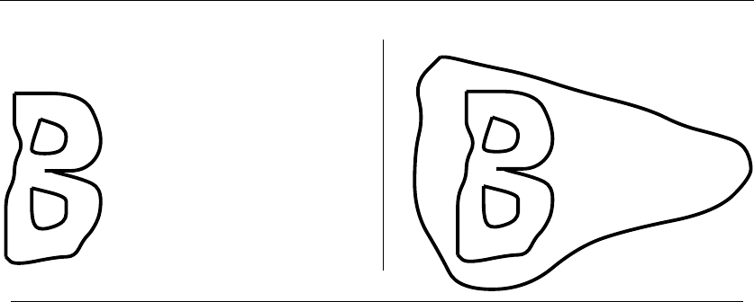
17.13 SHAPE SIMILARITY 607
?
A
B
C
A
B
C
=
INPUT OUTPUT
17.13 Shape Similarity
Input description: Two polygonal shapes, P1and P2.
Problem description: How similar are P1and P2?
Discussion: Shape similarity is a problem that underlies much of pattern recog-
nition. Consider a system for optical character recognition (OCR). We are given
a library of shape models representing letters, and unknown shapes obtained by
scanning a page. We seek to identify the unknown shapes by matching them to the
most similar shape models.
Shape similarity is an inherently ill-defined problem, because what “similar”
means is application dependent. Thus, no single algorithmic approach can solve all
shape-matching problems. Whichever method you select, expect to spend a large
chunk of time tweaking it to achieve maximum performance.
Among your possible approaches are
•Hamming distance – Assume that your two polygons have been overlaid one
on top of the other. Hamming distance measures the area of symmetric dif-
ference between the two polygons—in other words, the area lying within one
of the two polygons but not both of them. When two polygons are identical
and properly aligned, the Hamming distance is zero. If the polygons differ
only in a little noise at the boundary, then the Hamming distance of properly
aligned polygons will be small.
Computing the area of the symmetric difference reduces to finding the inter-
section or union of two polygons (discussed in Section 17.8 (page 591)) and
then computing areas (discussed in Section 17.1). But the difficult part of

608 17. COMPUTATIONAL GEOMETRY
computing Hamming distance is finding the right alignment of the two poly-
gons. This overlay problem is simplified in applications such as OCR because
the characters are inherently aligned within lines on the page and are not free
to rotate. Efficient algorithms for optimizing the overlap of convex polygons
without rotation are cited below. Simple but reasonably effective heuristics
are based on identifying reference landmarks on each polygon (such as the
centroid, bounding box, or extremal vertices) and then matching a subset of
these landmarks to define the alignment.
Hamming distance is particularly simple and efficient to compute on bit-
mapped images, since after alignment all we do is sum the differences of the
corresponding pixels. Although Hamming distance makes sense conceptually
and can be simple to implement, it captures only a crude notion of shape and
is likely to be ineffective in most applications.
•Hausdorff distance – An alternative distance metric is Hausdorff distance,
which identifies the point on P1that is the maximum distance from P2and
returns this distance. The Hausdorff distance is not symmetrical, for the tip of
a long but thin protrusion from P1can imply a large Hausdorff distance P1to
P2, even though every point on P2is close to some point on P1. A fattening
of the entire boundary of one of the models (as is liable to happen with
boundary noise) by a small amount may substantially increase the Hamming
distance yet have little effect on the Hausdorff distance.
Which is better, Hamming or Hausdorff? It depends upon your application.
As with Hamming distance, computing the right alignment between the poly-
gons can be difficult and time-consuming.
•Comparing Skeletons – A more powerful approach to shape similarity uses
thinning (see Section 17.10 (page 598)) to extract a tree-like skeleton for
each object. This skeleton captures many aspects of the original shape. The
problem now reduces to comparing the shape of two such skeletons, using
such features as the topology of the tree and the lengths/slopes of the edges.
This comparison can be modeled as a form of subgraph isomorphism (see
Section 16.9 (page 550)), with edges allowed to match whenever their lengths
and slopes are sufficiently similar.
•Support Vector Machines – A final approach for pattern recognition/matching
problems uses a learning-based technique such as neural networks or the
more powerful support vector machines. These prove a reasonable approach
to recognition problems when you have a lot of data to experiment with and
no particular ideas of what to do with it. First, you must identify a set of
easily computed features of the shape, such as area, number of sides, and
number of holes. Based on these features, a black-box program (the support
vector machine training algorithm) takes your training data and produces a
classification function. This classification function accepts as input the values

17.13 SHAPE SIMILARITY 609
of these features and returns a measure of what the shape is, or how close it
is to a particular shape.
How good are the resulting classifiers? It depends upon the application. Like
any ad hoc method, SVMs usually take a fair amount of tweaking and tuning
to realize their full potential.
There is one caveat. If you don’t know how/why black-box classifiers are
making their decisions, you can’t know when they will fail. An interesting
case was a system built for the military to distinguish between images of
cars and tanks. It performed very well on test images but disastrously in the
field. Eventually, someone realized that the car images had been filmed on
a sunnier day than the tanks, and the program was classifying solely on the
presence of clouds in the background of the image!
Implementations: A Hausdorff-based image comparison implementation in C is
available at http://www.cs.cornell.edu/vision/hausdorff/hausmatch.html. An alter-
nate distance metric between polygons can be based on its angle-turning function
[ACH+91]. An implementation in C of this turning function metric by Eugene K.
Ressler is provided at http://www.cs.sunysb.edu/∼algorith.
Several excellent support vector machine classifiers are available. These include
the kernal-machine library (http://www.terborg.net/research/kml/), SV Mlight
(http://svmlight.joachims.org/) and the widely used and well-supported LIBSVM
(http://www.csie.ntu.edu.tw/∼cjlin/libsvm/).
Notes:General books on pattern classification algorithms include [DHS00, JD88]. A
wide variety of computational geometry approaches to shape similarity testing have been
proposed, including [AMWW88, ACH+91, Ata84, AE83, BM89, OW85]. See the survey
by Alt and Guibas [AG00].
The optimal alignment of nand m-vertex convex polygons subject to translation
(but not rotation) can be computed in O((n+m) log(n+m)) time [dBDK+98]. An
approximation of the optimal overlap under translation and rotation is due to Ahn, et al.
[ACP+07].
A linear-time algorithm for computing the Hausdorff distance between two convex
polygons is given in [Ata83], with algorithms for the general case reported in [HK90].
Related Problems: Graph isomorphism (see page 550), thinning (see page 598).
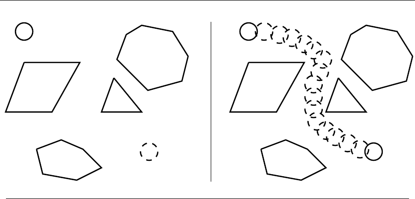
610 17. COMPUTATIONAL GEOMETRY
S
T
S
T
INPUT OUTPUT
17.14 Motion Planning
Input description: A polygonal-shaped robot starting in a given position sin a
room containing polygonal obstacles, and a goal position t.
Problem description: Find the shortest route taking sto twithout intersecting
any obstacles.
Discussion: That motion planning is a complex problem is obvious to anyone
who has tried to move a large piece of furniture into a small apartment. It also
arises in systems for molecular docking. Many drugs are small molecules that act
by binding to a given target model. Identifying which binding sites are accessible
to a candidate drug is clearly an instance of motion planning. Plotting paths for
mobile robots is another canonical motion-planning application.
Finally, motion planning provides a tool for computer animation. Given the set
of object models and where they appear in scenes s1and s2, a motion planning
algorithm can construct a short sequence of intermediate motions to transform s1
to s2. These motions can serve to fill in the intermediate scenes between s1and s2,
with such scene interpolation greatly reducing the workload on the animator.
Many factors govern the complexity of motion planning problems:
•Is your robot a point? – For point robots, motion planning becomes finding
the shortest path from sto taround the obstacles. This is also known as ge-
ometric shortest path. The most readily implementable approach constructs
the visibility graph of the polygonal obstacles, plus the points sand t. This

17.14 MOTION PLANNING 611
visibility graph has a vertex for each obstacle vertex and an edge between
two obstacle vertices iff they “see” each other without being blocked by some
obstacle edge.
The visibility graph can be constructed by testing each of the n
2vertex-pair
edge candidates for intersection against each of the nobstacle edges, although
faster algorithms are known. Assign each edge of this visibility graph with
weight equal to its length. Then the shortest path from sto tcan be found
using Dijkstra’s shortest-path algorithm (see Section 15.4 (page 489)) in time
bounded by the time required to construct the visibility graph.
•What motions can your robot perform? – Motion planning becomes consid-
erably more difficult when the robot becomes a polygon instead of a point.
Now all of the corridors that we use must be wide enough to permit the robot
to pass through.
The algorithmic complexity depends upon the number of degrees of freedom
that the robot can use to move. Is it free to rotate as well as to translate?
Does the robot have links that are free to bend or to rotate independently, as
in an arm with a hand? Each degree of freedom corresponds to a dimension in
the search space of possible configurations. Additional freedom makes it more
likely that a short path exists from start to goal, although it also becomes
harder to find this path.
•Can you simplify the shape of your robot? – Motion planning algorithms
tend to be complex and time-consuming. Anything you can do to simplify
your environment is a win. In particular, consider replacing your robot in an
enclosing disk. If there is a start-to-goal path for this disk, it defines such
a path for the robot inside of it. Furthermore, any orientation of a disk is
equivalent to any other orientation, so rotation provides no help in finding a
path. All movements can thus be limited to the simpler case of translation.
•Are motions limited to translation only? – When rotation is not allowed, the
expanded obstacles approach can be used to reduce the problem of polygonal
motion planning to the previously-resolved case of a point robot. Pick a
reference point on the robot, and replace each obstacle by its Minkowski sum
with the robot polygon (see Section 17.16 (page 617)). This creates a larger,
fatter obstacle, defined by the shadow traced as the robot walks a loop around
the object while maintaining contact with it. Finding a path from the initial
reference position to the goal amidst these fattened obstacles defines a legal
path for the polygonal robot in the original environment.
•Are the obstacles known in advance? – We have assumed that the robot
starts out with a map of its environment. But this can’t be true, say, in
applications where the obstacles move. There are two approaches to solving
motion-planning problems without a map. The first approach explores the

612 17. COMPUTATIONAL GEOMETRY
environment, building a map of what has been seen, and then uses this map
to plan a path to the goal. A simpler strategy proceeds like a sightless man
with a compass. Walk in the direction towards the goal until progress is
blocked by an obstacle, and then trace a path along the obstacle until the
robot is again free to proceed directly towards the goal. Unfortunately, this
will fail in environments of sufficient complexity.
The most practical approach to general motion planning involves randomly
sampling the configuration space of the robot. The configuration space defines the
set of legal positions for the robot using one dimension for each degree of freedom.
A planar robot capable of translation and rotation has three degrees of freedom,
namely the x-andy-coordinates of a reference point on the robot and the angle θ
relative to this point. Certain points in this space represent legal positions, while
others intersect obstacles.
Construct a set of legal configuration-space points by random sampling. For
each pair of points p1and p2, decide whether there exists a direct, nonintersecting
path between them. This defines a graph with vertices for each legal point and
edges for each such traversable pair. Motion planning now reduces to finding a
direct path from the initial/final position to some vertex in the graph, and then
solving a shortest-path problem between the two vertices.
There are many ways to enhance this basic technique, such as adding additional
vertices to regions of particular interest. Building such a road map provides a nice,
clean approach to solving problems that would otherwise get very messy.
Implementations:TheMotion Planning Toolkit (MPK) is a C++ library
and toolkit for developing single- and multi-robot motion planners. It includes
SBL, a fast single-query probabilistic roadmap path planner, and is available at
http://robotics.stanford.edu/∼mitul/mpk/.
The University of North Carolina GAMMA group has produced several
efficient collision detection libraries (not really motion planning) of which
SWIFT++ [EL01] is the most recent member of this family. It can detect in-
tersection, compute approximate/exact distances between objects, and deter-
mine object-pair contacts in scenes composed of rigid polyhedral models. See
http://www.cs.unc.edu/∼geom/collide/ for pointers to all of these libraries.
The computational geometry library CGAL (www.cgal.org) contains many al-
gorithms related to motion planning including visibility graph construction and
Minkowski sums. O’Rourke [O’R01] gives a toy implementation of an algorithm to
plot motion for a two-jointed robot arm in the plane. See Section 19.1.10 (page
662).
Notes:Latombe’s book [Lat91] describes practical approaches to motion planning, in-
cluding the random sampling method described above. Two other worthy books on motion
planning are available freely on line, by LaValle [LaV06] (http://planning.cs.uiuc.edu/)
and Laumond [Lau98] (http://www.laas.fr/∼jpl/book.html).

17.14 MOTION PLANNING 613
Motion planning was originally studied by Schwartz and Sharir as the “piano mover’s
problem.” Their solution constructs the complete free space of robot positions that do
not intersect obstacles, and then finds the shortest path within the proper connected
component. These free space descriptions are very complicated, involving arrangements
of higher-degree algebraic surfaces. The fundamental papers on the piano mover’s problem
appear in [HSS87], with [Sha04] a survey of current results.
The best general result for this free-space approach to motion planning is due to
Canny [Can87], who showed that any problem with ddegrees of freedom can be solved
in O(ndlg n), although faster algorithms exist for special cases of the general motion-
planning problem. The expanded obstacle approach to motion planning is due to Lozano-
Perez and Wesley [LPW79]. The heuristic, sightless man’s approach to motion planning
discussed previously has been studied by Lumelski [LS87].
The time complexity of algorithms based on the free-space approach to motion plan-
ning depends intimately on the combinatorial complexity of the arrangement of surfaces
defining the free space. Algorithms for maintaining arrangements are presented in Sec-
tion 17.15 (page 614). Davenport-Schinzel sequences often arise in the analysis of such ar-
rangements. Sharir and Agarwal [SA95] provide a comprehensive treatment of Davenport-
Schinzel sequences and their relevance to motion planning.
The visibility graph of nline segments with Epairs of visible vertices can be con-
structed in O(nlg n+E) time [GM91, PV96], which is optimal. Hershberger and Suri
[HS99] have an O(nlg n) algorithm for finding shortest paths for point-robots with polyg-
onal obstacles. Chew [Che85] provides an O(n2lg n) for finding shortest paths for a disk-
robot in such a scene.
Related Problems: Shortest path (see page 489), Minkowski sum (see page 617).
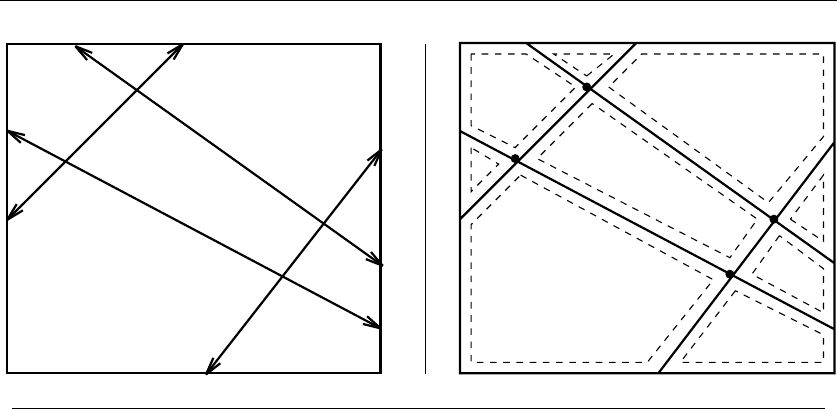
614 17. COMPUTATIONAL GEOMETRY
INPUT OUTPUT
17.15 Maintaining Line Arrangements
Input description: A set of lines and line segments l1,...,l
n.
Problem description: What is the decomposition of the plane defined by
l1,...,l
n?
Discussion: A fundamental problem in computational geometry is explicitly con-
structing the regions formed by the intersections of a set of nlines. Many problems
reduce to constructing and analyzing such an arrangement of a specific set of lines.
Examples include:
•Degeneracy testing –Givenasetofnlines in the plane, do any three of them
pass through the same point? Brute-force testing of all triples takes O(n3)
time. Instead, we can construct the arrangement of the lines and then walk
over each vertex and explicitly count its degree, all in quadratic time.
•Satisfying the maximum number of linear constraints – Suppose that we are
given a set of nlinear constraints, each of the form y≤aix+bi. Which point
in the plane satisfies the largest number of them? Construct the arrangement
of the lines. All points in any region or cell of this arrangement satisfy exactly
the same set of constraints, so we need to test only one point per cell to find
the global maximum.
Thinking of geometric problems in terms of features in an arrangement can
be very useful in formulating algorithms. Unfortunately, it must be admitted that

17.15 MAINTAINING LINE ARRANGEMENTS 615
arrangements are not as popular in practice as might be supposed. Primarily, this
is because some depth of understanding is required to apply them correctly. The
computational geometry library CGAL now provides a general and robust enough
implementation to justify the effort to do so. Issues arising in arrangements include
•What is the right way to construct a line arrangement? – Algorithms for
constructing arrangements are incremental. Begin with an arrangement of
one or two lines. Subsequent lines are inserted into the arrangement one at a
time, yielding larger and larger arrangements. To insert a new line, we start
on the leftmost cell containing the line and walk over the arrangement to the
right, moving from cell to neighboring cell and splitting into two pieces those
cells that contain the new line.
•How big will your arrangement be? – A geometric fact called the zone theorem
implies that the kth line inserted cuts through kcells of the arrangement,
and further that O(k) total edges form the boundary of these cells. This
means that we can scan through each edge of every cell we encounter on our
insertion walk, confident that only linear total work will be performed while
inserting the line into the arrangement. Therefore, the total time to insert all
nlines in constructing the full arrangement is O(n2).
•What do you want to do with your arrangement? – Given an arrangement and
a query point, we are often interested in identifying which cell of the arrange-
ment contains the point. This is the problem of point location, discussed in
Section 17.7 (page 587). Given an arrangement of lines or line segments, we
are often interested in computing all points of intersection of the lines. The
problem of intersection detection is discussed in Section 17.8 (page 591).
•Does your input consist of points instead of lines? – Although lines and
points seem to be different geometric objects, appearances can be misleading.
Through the use of duality transformations, we can turn line Linto point p
and vice versa:
L:y=2ax −b↔p:(a, b)
Duality is important because we can now apply line arrangements to point
problems, often with surprising results.
For example, suppose we are given a set of npoints, and we want to know
whether any three of them all lie on the same line. This sounds similar to the
degeneracy testing problem discussed above. In fact it is exactly the same,
with only the role of points and lines exchanged. We can dualize our points
into lines as above, construct the arrangement, and then search for a vertex
with three lines passing through it. The dual of this vertex defines the line
on which the three initial vertices lie.

616 17. COMPUTATIONAL GEOMETRY
It often becomes useful to traverse each face of an existing arrangement exactly
once. Such traversals are called sweepline algorithms, and are discussed in some
detail in Section 17.8 (page 591). The basic procedure sorts the intersection points
by x-coordinate and then walks from left to right while keeping track of all we have
seen.
Implementations:CGAL(www.cgal.org) provides a generic and robust package
for arrangements of curves (not just lines) in the plane. This should be the starting
point for any serious project using arrangements.
A robust code for constructing and topologically sweeping an arrangement in
C++ is provided at http://www.cs.tufts.edu/research/geometry/other/sweep/.An
extension of topological sweep to deal with the visibility complex of a collection of
pairwise disjoint convex planar sets has been provided in CGAL.
Arrange is a package for maintaining arrangements of polygons in ei-
ther the plane or on the sphere. Polygons may be degenerate, and hence
represent arrangements of lines. A randomized incremental construction al-
gorithm is used, and efficient point location on the arrangement is sup-
ported. Arrange is written in C by Michael Goldwasser and is available from
http://euler.slu.edu/∼goldwasser/publications/.
Notes:Edelsbrunner [Ede87] provides a comprehensive treatment of the combinato-
rial theory of arrangements, plus algorithms on arrangements with applications. It is an
essential reference for anyone seriously interested in the subject. Recent surveys of combi-
natorial and algorithmic results include [AS00, Hal04]. Good expositions on constructing
arrangements include [dBvKOS00, O’R01]. Implementation issues related to arrangements
as implemented in CGAL are discussed in [FWH04, HH00].
Arrangements generalize naturally beyond two dimensions. Instead of lines, the space
decomposition is defined by planes (or beyond 3-dimensions, hyperplanes). The zone the-
orem states that any arrangement of nd-dimensional hyperplanes has total complexity
O(nd), and any single hyperplane intersects cells of complexity O(nd−1). This provides
the justification for the incremental construction algorithm for arrangements. Walking
around the boundary of each cell to find the next cell that the hyperplane intersects takes
time proportional to the number of cells created by inserting the hyperplane.
The history of the zone theorem has become somewhat muddled, because the original
proofs were later found to be in error in higher dimensions. See [ESS93] for a discussion
and a correct proof. The theory of Davenport-Schinzel sequences is intimately tied into
the study of arrangements, which is presented in [SA95].
The naive algorithm for sweeping an arrangement of lines sorts the n2intersection
points by x-coordinate and hence requires O(n2lg n)time.Thetopological sweep [EG89,
EG91] eliminates the need to sort, and so traverses the arrangement in quadratic time.
This algorithm is readily implementable and can be applied to speed up many sweepline
algorithms. See [RSS02] for a robust implementation with experimental results.
Related Problems: Intersection detection (see page 591), point location (see page
587).
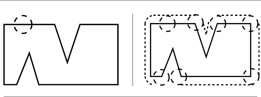
17.16 MINKOWSKI SUM 617
INPUT OUTPUT
17.16 Minkowski Sum
Input description: Point sets or polygons Aand B, containing nand mvertices
respectively.
Problem description: What is the convolution of Aand B—i.e. , the Minkowski
sum A+B={x+y|x∈A, y ∈B}?
Discussion: Minkowski sums are useful geometric operations that can fatten ob-
jects in appropriate ways. For example, a popular approach to motion planning
for polygonal robots in a room with polygonal obstacles (see Section 17.14 (page
610)) fattens each of the obstacles by taking the Minkowski sum of them with
the shape of the robot. This reduces the problem to the (more easily solved) case
of point robots. Another application is in shape simplification (see Section 17.12
(page 604)). Here we fatten the boundary of an object to create a channel around
it, and then let the minimum link path lying within this channel define the sim-
plified shape. Finally, convolving an irregular object with a small circle will help
smooth out the boundaries by eliminating minor nicks and cuts.
The definition of a Minkowski sum assumes that the polygons Aand Bhave
been positioned on a coordinate system:
A+B={x+y|x∈A, y ∈B}
where x+yis the vector sum of two points. Thinking of this in terms of translation,
the Minkowski sum is the union of all translations of Aby a point defined within
B. Issues arising in computing Minkowski sums include
•Are your objects rasterized images or explicit polygons? – The definition of
Minkowski summation suggests a simple algorithm if Aand Bare rasterized
images. Initialize a sufficiently large matrix of pixels by determining the size

618 17. COMPUTATIONAL GEOMETRY
of the convolution of the bounding boxes of Aand B. For each pair of points
in Aand B, sum up their coordinates and darken the appropriate pixel. These
algorithms get more complicated if an explicit polygonal representation of the
Minkowski sum is needed.
•Do you want to fatten your object by a fixed amount? – The most common
fattening operation expands a model Mby a given tolerance t, known as
offsetting. As shown in the figures above, this is accomplished by computing
the Minkowski sum of Mwith a disk of radius t. The basic algorithms still
work, although the offset is not a polygon. Its boundary is instead composed
of circular arcs and line segments.
•Are your objects convex or non-convex? – The complexity of computing
Minkowski sums depends in a serious way on the shape of the polygons.
If both Aand Bare convex, the Minkowski sum can be found in O(n+m)
time by tracing the boundary of one polygon with another. If one of them is
nonconvex, the size of the sum alone can be as large as Θ(nm). Even worse is
when both Aand Bare nonconvex, in which case the size of the sum can be
as large as Θ(n2m2). Minkowski sums of nonconvex polygons are often ugly
in a majestic sort of way, with holes either created or destroyed in surprising
fashion.
A straightforward approach to computing the Minkowski sum is based on trian-
gulation and union. First, triangulate both polygons, then compute the Minkowski
sum of each triangle of Aagainst each triangle of B. The sum of a triangle against
another triangle is easy to compute and is a special case of convex polygons, dis-
cussed below. The union of these O(nm) convex polygons will be A+B. Algorithms
for computing the union of polygons are based on plane sweep, as discussed in Sec-
tion 17.8 (page 591).
Computing the Minkowski sum of two convex polygons is easier than the general
case, because the sum will always be convex. For convex polygons it is easiest to
slide Aalong the boundary of Band compute the sum edge by edge. Partitioning
each polygon into a small number of convex pieces (see Section 17.11 (page 601)),
and then unioning the Minkowski sum for each pair of pieces, will usually be much
more efficient than working with two fully triangulated polygons.
Implementations: The CGAL (www.cgal.org) Minkowski sum package provides
an efficient and robust code to find the Minkowski sums of two arbitrary polygons,
as well as compute both exact and approximate offsets.
An implementation for computing the Minkowski sums of two convex polyhedra
in 3Dis described in [FH06] and available at http://www.cs.tau.ac.il/∼efif/CD/.
Notes:Good expositions on algorithms for Minkowski sums include [dBvKOS00, O’R01].
The fastest algorithms for various cases of Minkowski sums include [KOS91, Sha87].
The practical efficiency of Minkowski sum in the general case depends upon how the
polygons are decomposed into convex pieces. The optimal solution is not necessarily the

17.16 MINKOWSKI SUM 619
partition into the fewest number of convex pieces. Agarwal et al. [AFH02] give a through
study of decomposition methods for Minkowski sum.
The combinatorial complexity of the Minkowski sum of two convex polyhedra in three
dimensions is completely resolved in [FHW07]. An implementation of Minkowski sum for
such polyhedra is described in [FH06].
Kedem and Sharir [KS90] present an efficient algorithm for translational motion plan-
ning for polygonal robots, based on Minkowski sums.
Related Problems: Thinning (see page 598), motion planning (see page 610),
simplifying polygons (see page 604).

18
Set and String Problems
Sets and strings both represent collections of objects—the difference is whether
order matters. Sets are collections of symbols whose order is assumed to carry no
significance, while strings are defined by the sequence or arrangement of symbols.
The assumption of a fixed order makes it possible to solve string problems much
more efficiently than set problems, through techniques such as dynamic program-
ming and advanced data structures like suffix trees. The interest in and impor-
tance of string-processing algorithms have been increasing due to bioinformatics,
Web searches, and other text-processing applications. Recent books on string al-
gorithms include:
•Gusfield [Gus97] – To my taste, this remains is the best introduction to string
algorithms. It contains a thorough discussion on suffix trees, with clear and
innovative formulations of classical exact string-matching algorithms.
•Crochemore, Hancart, and Lecroq [CHL07] – A comprehensive treatment of
string algorithms, written by a true leader in the field. Translated from the
French, but clear and accessible.
•Navarro and Raffinot [NR07] – A concise but practical and implementation-
oriented treatment of pattern-matching algorithms, with particularly thor-
ough treatment of bit-parallel approaches.
•Crochemore and Rytter [CR03] – A survey of specialized topics in string
algorithmics emphasizing theory.
Theoreticians working in string algorithmics sometimes refer to their field as
Stringology. The annual Combinatorial Pattern Matching (CPM) conference is the
primary venue devoted to both practical and theoretical aspects of string algorith-
mics and related areas.
S.S. Skiena, The Algorithm Design Manual, 2nd ed., DOI: 10.1007/978-1-84800-070-4 18,
c
Springer-Verlag London Limited 2008
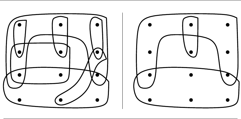
18.1 SET COVER 621
INPUT OUTPUT
18.1 Set Cover
Input description: A collection of subsets S={S1,...,S
m}of the universal set
U={1,...,n}.
Problem description: What is the smallest subset Tof Swhose union equals
the universal set—i.e. , ∪|T|
i=1Ti=U?
Discussion: Set cover arises when you try to efficiently acquire items that have
been packaged in a fixed set of lots. You seek a collection of at least one of each
distinct type of item, while buying as few lots as possible. Finding aset cover is
easy, because you can always buy one of each possible lot. However, identifying a
small set cover let you do the same job for less money. Set cover provided a natural
formulation of the Lotto ticket optimization problem discussed in Section 1.6 (page
23). There we seek to buy the smallest number of tickets needed to cover all of a
given set of combinations.
Boolean logic minimization is another interesting application of set cover. We
are given a particular Boolean function of kvariables, which describes whether
the desired output is 0 or 1 for each of the 2kpossible input vectors. We seek the
simplest circuit that exactly implements this function. One approach is to find a
disjunctive normal form (DNF) formula on the variables and their complements,
such as x1¯x2+¯x1¯x2. We could build one “and” term for each input vector and then
“or” them all together, but we might save considerably by factoring out common
subsets of variables. Given a set of feasible “and” terms, each of which covers a

622 18. SET AND STRING PROBLEMS
subset of the vectors we need, we seek to “or” together the smallest number of
terms that realize the function. This is exactly the set cover problem.
There are several variations of set cover problems to be aware of:
•Are you allowed to cover elements more than once? – The distinction here is
between set cover and set packing, which is discussed in Section 18.2 (page
625). We should take advantage of the freedom to cover elements multiple
times if we have it, as it usually results in a smaller covering.
•Are your sets derived from the edges or vertices of a graph? – Set cover is a
very general problem, and includes several useful graph problems as special
cases. Suppose instead that you seek the smallest set of edges in a graph that
will cover each vertex at least once. The solution is the maximum matching
in the graph (see Section 15.6 (page 498)), plus arbitrary edges to cover any
unmatched vertices. Now suppose instead that you seek the smallest set of
vertices that cover each edge at least once. This is the vertex cover problem,
discussed in Section 16.3 (page 530).
It is instructive to show how to model vertex cover as an instance of set
cover. Let the universal set Ucorrespond to the set of edges {e1,...,e
m}.
Construct nsubsets, with Siconsisting of the edges incident on vertex vi.
Although vertex cover is just an instance of set cover in disguise, you should
take advantage of the superior heuristics that exist for the more restricted
vertex cover problem.
•Do your subsets contain only two elements each? – You are in luck if all of
your subsets have at most two elements each. This special case can be solved
efficiently to optimality because it reduces to finding a maximum matching
in a graph. Unfortunately, the problem becomes NP-complete as soon as your
subsets have three elements each.
•Do you want to cover elements with sets, or sets with elements? –Inthe
hitting set problem, we seek a small number of items that together represent
each subset in a given population. Hitting set is illustrated in Figure 18.1.
The input is identical to set cover, but instead we seek the smallest subset
of elements T⊂Usuch that each subset Sicontains at least one element of
T.Thus,Si∩T=∅for all 1 ≤i≤m. Suppose we desire a small Congress
with at least one representative for each ethnic group. If each ethnic group
is defined by a subset of people, the minimum hitting set gives the smallest
possible politically correct Congress.
Hitting set is dual to set cover, meaning that it is exactly the same problem
in disguise. Replace each element of Uby a set of the names of the subsets
that contain it. Now Sand Uhave exchanged roles, for we seek a set of
subsets from Uto cover all the elements of S.Thisisexactlysetcover,sowe
can use any set cover code to solve hitting set after performing this simple
translation. See Figure 18.1 for an example.
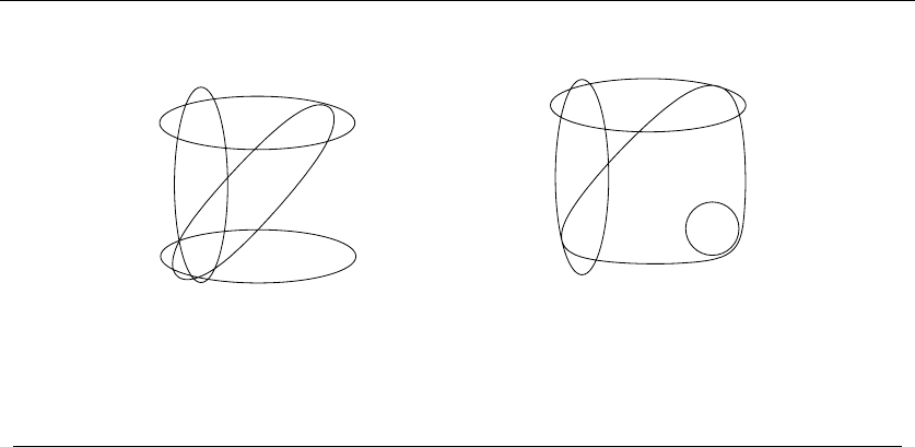
18.1 SET COVER 623
3
4
CD
2
1
BA
D
CB
A
4
2
3
1
Figure 18.1: A hitting set instance optimally solved by selecting elements 1 and 3 or 2 and 3
(l). This problem converted to a dual set cover instance optimally solved by selecting subsets
1and3or2and4(r).
Set cover must be at least as hard as vertex cover, so it is also NP-complete.
In fact, it is somewhat harder. Approximation algorithms do no worse than twice
optimal for vertex cover, but the best approximation algorithm for set cover is
Θ(lg n) times optimal.
Greedy is the most natural and effective heuristic for set cover. Begin by se-
lecting the largest subset for the cover, and then delete all its elements from the
universal set. We add the subset containing the largest number of remaining un-
covered elements repeatedly until all are covered. This heuristic always gives a set
cover using at most ln ntimes as many sets as optimal. In practice it usually does
a lot better.
The simplest implementation of the greedy heuristic sweeps through the entire
input instance of msubsets for each greedy step. However, by using such data
structures as linked lists and a bounded-height priority queue (see Section 12.2
(page 373)), the greedy heuristic can be implemented in O(S) time, where S=
∪m
i=1|Si|is the size of the input representation.
It pays to check whether or not there exist elements that exist in only a few
subsets—ideally only one. If so, we should select the biggest subsets containing
these elements at the very beginning. We must take such a subset eventually, and
they carry along other elements that we might have paid extra to cover if we wait
until later.
Simulated annealing is likely to produce somewhat better set covers than these
simple heuristics. Backtracking can be used to guarantee you an optimal solution,
but it is usually not worth the computational expense.

624 18. SET AND STRING PROBLEMS
An alternate and more powerful approach rests on the integer programming
formulation of set cover. Let the integer 0-1 variable sidenote whether subset Si
is selected for a given cover. Each universal set element xadds the constraint
x∈Si
si≥1
to ensure that it is covered by at least one selected subset. The minimum set
cover satisfies all constraints while minimizing isi. This integer program can be
easily generalized to weighted set cover (allowing nonuniform costs for different
subsets. Relaxing this to a linear program (i.e. , allowing 0 ≤si≤1 instead of
constricting each variable to be either 0 or 1) allows efficient and effective heuristics
using rounding techniques.
Implementations: Both the greedy heuristic and the above ILP formulation are
sufficiently simple in their respective worlds that one has to implement them from
scratch.
Pascal implementations of an exhaustive search algorithm for set packing, as
well as heuristics for set cover, appear in [SDK83]. See Section 19.1.10 (page 662).
SYMPHONY is a mixed-integer linear programming solver that includes a set
partitioning solver. It is available at http://branchandcut.org/SPP/
Notes:An old but classic survey article on set cover is [BP76], with more recent approx-
imation and complexity analysis surveyed in [Pas97]. See [CFT99, CFT00] for extensive
computational studies of integer programming-based set cover heuristics and exact algo-
rithms. An excellent exposition on algorithms and reduction rules for set cover is presented
in [SDK83].
Good expositions of the greedy heuristic for set cover include [CLRS01, Hoc96]. An
example demonstrating that the greedy heuristic for set cover can be as bad as lg nis
presented in [Joh74, PS98]. This is not a defect of the heuristic. Indeed, it is provably hard
to approximate set cover to within an approximation factor better than (1 −o(1)) ln n
[Fei98].
Related Problems: Matching (see page 498), vertex cover (see page 530), set
packing (see page 625).

18.2 SET PACKING 625
INPUT OUTPUT
18.2 Set Packing
Input description: A set of subsets S={S1,...,S
m}of the universal set U=
{1,...,n}.
Problem description: Select (an ideally small) collection of mutually disjoint
subsets from Swhose union is the universal set.
Discussion: Set-packing problems arise in applications where we have strong con-
straints on what is an allowable partition. The key feature of packing problems is
that no elements are permitted to be covered by more than one selected subset.
Some flavor of this is captured by the independent set problem in graphs, dis-
cussed in Section 16.2 (page 528). There we seek a large subset of vertices from
graph Gsuch that each edge is adjacent to at most one of the selected vertices.
To model this as set packing, let the universal set consist of all edges of G,and
subset Siconsist of all edges incident on vertex vi. Finally, define an additional
singleton set for each edge. Any set packing defines a set of vertices with no edge in
common—in other words, an independent set. The singleton sets are used to pick
up any edges not covered by the selected vertices.
Scheduling airline flight crews is another application of set packing. Each air-
plane in the fleet needs to have a crew assigned to it, consisting of a pilot, copilot,
and navigator. There are constraints on the composition of possible crews, based
on their training to fly different types of aircraft, personality conflicts, and work
schedules. Given all possible crew and plane combinations, each represented by a
subset of items, we need an assignment such that each plane and each person is

626 18. SET AND STRING PROBLEMS
in exactly one chosen combination. After all, the same person cannot be on two
different planes simultaneously, and every plane needs a crew. We need a perfect
packing given the subset constraints.
Set packing is used here to represent several problems on sets, all of which are
NP-complete:
•Must every element appear in exactly one selected subset? –Intheexact cover
problem, we seek some collection of subsets such that each element is covered
exactly once. The airplane scheduling problem above has the flavor of exact
covering, since every plane and crew has to be employed.
Unfortunately, exact cover puts us in a situation similar to that of Hamilto-
nian cycle in graphs. If we really must cover all the elements exactly once,
and this existential problem is NP-complete, then all we can do is exponen-
tial search. The cost will be prohibitive unless we happen to stumble upon a
solution quickly.
•Does each element have its own singleton set? – Things will be far better if
we can be content with a partial solution, say by including each element of
Uas a singleton subset of S. Thus, we can expand any set packing into an
exact cover by mopping up the unpacked elements of Uwith singleton sets.
Now our problem is reduced to finding a minimum-cardinality set packing,
which can be attacked via heuristics.
•What is the penalty for covering elements twice? – In set cover (see Section
18.1 (page 621)), there is no penalty for elements existing in many selected
subsets. In exact cover, any such violation is forbidden. For many applica-
tions, the truth lies somewhere in between. Such problems can be approached
by charging the greedy heuristic more to select a subset that contains previ-
ously covered elements.
The right heuristics for set packing are greedy, and similar to those of set cover
(see Section 18.1 (page 621)). If we seek a packing with many (few) sets, then
we repeatedly select the smallest (largest) subset, delete all subsets from Sthat
clash with it, and repeat. As usual, augmenting this approach with some exhaustive
search or randomization (in the form of simulated annealing) is likely to yield better
packings at the cost of additional computation.
An alternate and more powerful approach rests on an integer programming
formulation akin to that of set cover. Let the integer 0-1 variable sidenote whether
subset Siis selected for a given cover. Each universal set element xadds the
constraint
x∈Si
si=1
to ensure that it is covered by exactly one selected subset. Minimizing or maximizing
isiwhile respecting these constraints enables us modulate the desired number
of sets in the cover.

18.2 SET PACKING 627
Implementations: Since set cover is a more popular and more tractable problem
than set packing, it might be easier to find an appropriate implementation to solve
the cover problem. Such implementations discussed in Section 18.1 (page 621)
should be readily modifiable to support certain packing constraints.
Pascal implementations of an exhaustive search algorithm for set packing, as
well as heuristics for set cover, appear in [SDK83]. See Section 19.1.10 (page 662)
for details on FTP-ing these codes.
SYMPHONY is a mixed-integer linear programming solver that includes a set
partitioning solver. It is available at http://branchandcut.org/SPP/.
Notes:Survey articles on set packing include [BP76, Pas97]. Bidding strategies for
combinatorial auctions typically reduce to solving set-packing problems, as described in
[dVV03].
Set-packing relaxations for integer programs are presented in [BW00]. An excellent
exposition on algorithms and reduction rules for set packing is presented in [SDK83],
including the airplane scheduling application discussed previously.
Related Problems: Independent set (see page 528), set cover (see page 621).
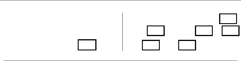
628 18. SET AND STRING PROBLEMS
love ?
" You will always have my love,
my love, for the love I love is
lovely as love itself." itself."lovely as loveis
loveI love , for the lovemy
,love" You will always have my
INPUT OUTPUT
18.3 String Matching
Input description:Atextstringtof length n. A pattern string pof length m.
Problem description: Find the first (or all) instances of pattern pin the text.
Discussion: String matching arises in almost all text-processing applications. Ev-
ery text editor contains a mechanism to search the current document for arbitrary
strings. Pattern-matching programming languages such as Perl and Python derive
much of their power from their built-in string matching primitives, making it easy
to fashion programs that filter and modify text. Spelling checkers scan an input
text for words appearing in the dictionary and reject any strings that do not match.
Several issues arise in identifying the right string matching algorithm for a given
application:
•Are your search patterns and/or texts short? – If your strings are sufficiently
short and your queries sufficiently infrequent, the simple O(mn)-time search
algorithm will suffice. For each possible starting position 1 ≤i≤n−m+1,
it tests whether the mcharacters starting from the ith position of the text
are identical to the pattern. An implementation of this algorithm (in C) is
given in Section 2.5.3 (page 43).
For very short patterns (say m≤5), you can’t hope to beat this simple
algorithm by much, so you shouldn’t try. Further, we expect much better
than O(mn) behavior for typical strings, because we advance the pattern the
instant we observe a text/pattern mismatch, Indeed, the trivial algorithm
usually runs in linear time. But the worst case certainly can occur, as with
pattern p=amand text t=(am−1b)n/m.
•What about longer texts and patterns? – String matching can in fact be per-
formed in worst-case linear time. Observe that we need not begin the search
from scratch on finding a character mismatch, since the pattern prefix and
text must exactly match up to the point of mismatch. Given a long partial

18.3 STRING MATCHING 629
match ending at position i, we jump ahead to the first character position in
the pattern/text that can provide new information about the text in position
i+ 1. The Knuth-Morris-Pratt algorithm preprocesses the search pattern to
construct such a jump table efficiently. The details are tricky to get correct,
but the resulting algorithm yields short, simple programs.
•Do I expect to find the pattern or not? – The Boyer-Moore algorithm matches
the pattern against the text from right to left, and can avoid looking at large
chunks of text on a mismatch. Suppose the pattern is abracadabra, and the
eleventh character of the text is x. This pattern cannot match in any of the
first eleven starting positions of the text, and so the next necessary position
to test is the 22nd character. If we get very lucky, only n/m characters need
ever be tested. The Boyer-Moore algorithm involves two sets of jump tables
in the case of a mismatch: one based on pattern matched so far, the other on
the text character seen in the mismatch.
Although somewhat more complicated than Knuth-Morris-Pratt, it is worth
it in practice for patterns of length m>5, unless the pattern is expected
to occur many times in the text. Its worst-case performance is O(n+rm),
where ris the number of occurrences of pin t.
•Will you perform multiple queries on the same text? – Suppose you are build-
ing a program to repeatedly search a particular text database, such as the
Bible. Since the text remains fixed, it pays to build a data structure to speed
up search queries. The suffix tree and suffix array data structures, discussed
in Section 12.3 (page 377), are the right tools for the job.
•Will you search many texts using the same patterns? – Suppose you are build-
ing a program to screen out dirty words from a text stream. Here, the set of
patterns remains stable, while the search texts are free to change. In such ap-
plications, we may need to find all occurrences of any of kdifferent patterns
where kcan be quite large.
Performing a linear-time scan for each pattern yields an O(k(m+n)) algo-
rithm. If kis large, a better solution builds a single finite automaton that
recognizes all of these patterns and returns to the appropriate start state
on any character mismatch. The Aho-Corasick algorithm builds such an au-
tomaton in linear time. Space savings can be achieved by optimizing the
pattern recognition automaton, as discussed in Section 18.7 (page 646). This
approach was used in the original version of fgrep.
Sometimes multiple patterns are specified not as a list of strings, but concisely
as a regular expression. For example, the regular expression a(a+b+c)∗a
matches any string on (a, b, c) that begins and ends with a distinct a.Thebest
way to test whether an input string is described by a given regular expres-
sion Rconstructs the finite automaton equivalent to Rand then simulates

630 18. SET AND STRING PROBLEMS
the machine on the string. Again, see Section 18.7 (page 646) for details on
constructing automata from regular expressions.
When the patterns are specified by context-free grammars instead of regular
expressions, the problem becomes one of parsing, discussed in Section 8.6
(page 298).
•What if our text or pattern contains a spelling error? – The algorithms dis-
cussed here work only for exact string matching. If you want to allow some
tolerance for spelling errors, your problem becomes approximate string match-
ing, which is thoroughly discussed in Section 18.4 (page 631).
Implementations: Strmat is a collection of C programs implementing ex-
act pattern matching algorithms in association with [Gus97], including sev-
eral variants of the KMP and Boyer-Moore algorithms. It is available at
http://www.cs.ucdavis.edu/∼gusfield/strmat.html.
SPARE Parts [WC04a] is a C++ string pattern recognition toolkit that provides
production-quality implementations of all major variants of the classical string-
matching algorithms for single patterns (both Knuth-Morris-Pratt and Boyer-
Moore) and multiple patterns (both Aho-Corasick and Commentz-Walter). It is
available at http://www.fastar.org/.
Several versions of the general regular expression pattern matcher (grep) are
readily available. GNU grep found at http://directory.fsf.org/project/grep/,and
supersedes variants such as egrep and fgrep.GNUgrep uses a fast lazy-state deter-
ministic matcher hybridized with a Boyer-Moore search for fixed strings.
The Boost string algorithms library provides C++ routines for basic operations
on strings, including search. See http://www.boost.org/doc/html/string algo.html.
Notes:All books on string algorithms contain thorough discussions of exact string match-
ing, including [CHL07, NR07, Gus97]. Good expositions on the Boyer-Moore [BM77] and
Knuth-Morris-Pratt algorithms [KMP77] include [BvG99, CLRS01, Man89]. The history
of string matching algorithms is somewhat checkered because several published proofs
were incorrect or incomplete. See [Gus97] for clarification.
Aho [Aho90] provides a good survey on algorithms for pattern matching in strings, par-
ticularly where the patterns are regular expressions instead of strings. The Aho-Corasick
algorithm for multiple patterns is described in [AC75].
Empirical comparisons of string matching algorithms include [DB86, Hor80, Lec95,
dVS82]. Which algorithm performs best depends upon the properties of the strings and
the size of the alphabet. For long patterns and texts, I recommend that you use the best
implementation of Boyer-Moore that you can find.
The Karp-Rabin algorithm [KR87] uses a hash function to perform string matching in
linear expected time. Its worst-case time remains quadratic, and its performance in prac-
tice appears somewhat worse than the character comparison methods described above.
This algorithm is presented in Section 3.7.2 (page 91).
Related Problems: Suffix trees (see page 377), approximate string matching (see
page 631).
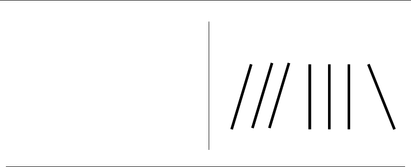
18.4 APPROXIMATE STRING MATCHING 631
misplace
misspelled
mislead
mispeld ?
m i s p e l d
m i s s p e l l e d
INPUT OUTPUT
18.4 Approximate String Matching
Input description:Atextstringtand a pattern string p.
Problem description: What is the minimum-cost way to transform tto pusing
insertions, deletions, and substitutions?
Discussion: Approximate string matching is a fundamental problem because we
live in an error-prone world. Spelling correction programs must be able to iden-
tify the closest match for any text string not found in a dictionary. By supporting
efficient sequence similarity (homology) searches on large databases of DNA se-
quences, the computer program BLAST has revolutionized the study of molecular
biology. Suppose you were interested in a particular gene in man, and discovered
that it is similar to the hemoglobin gene in rats. Likely this new gene also pro-
duces hemoglobin, and any differences are the result of genetic mutations during
evolution.
I once encountered approximate string matching when evaluating the perfor-
mance of an optical character-recognition system. We needed to compare the an-
swers produced by our system on a test document with the correct results. To
improve our system, we needed to identify (1) which letters were getting misiden-
tified and (2) gibberish when the program found letters that didn’t exist. The
solution was to do an alignment between the two texts. Insertions and deletions
corresponded to gibberish, while substitutions signaled errors in our recognizer.
This same principle is used in file difference programs, which identify the lines that
have changed between two versions of a file.
When no errors are permitted, our problem reduces to exact string matching,
which is presented in Section 18.3 (page 628). Here, we restrict our discussion to
matching with errors.

632 18. SET AND STRING PROBLEMS
Dynamic programming provides the basic approach to approximate string
matching. Let D[i, j] denote the cost of editing the first icharacters of the pattern
string pinto the first jcharacters of the text t. The recurrence follows because we
must have done something with the tail characters piand tj. Our only options are
matching / substituting one for the other, deleting pi, or inserting a match for tj.
Thus, D[i, j] is the minimum of the costs of these possibilities:
1. If pi=tjthen D[i−1,j −1] else D[i−1,j −1] + substitution cost.
2. D[i−1,j] + deletion cost of pi.
3. D[i, j −1] + deletion cost of tj.
A general implementation in C and more complete discussion appears in Section
8.2 (page 280). Several issues remain before we can make full use of this recurrence:
•Do I match the pattern against the full text, or against a substring? –The
boundary conditions of this recurrence distinguishes between algorithms for
string matching and substring matching. Suppose we want to align the full
pattern against the full text. Then the cost of D[i, 0] must be that of deleting
the first icharacters of the pattern, so D[i, 0] = i. Similarly, D[0,j]=j.
Now suppose that the pattern can occur anywhere within the text. The proper
cost of D[0,j] is now 0, since there should be no penalty for starting the
alignment in the jth position of the text. The cost of D[i, 0] remains i, because
the only way to match the first ipattern characters with nothing is to delete
all of them. The cost of the best substring pattern match against the text
will be given by minn
k=1 D[m, k].
•How should I select the substitution and insertion/deletion costs? – The basic
algorithm can be easily modified to use different costs for insertion, deletion,
and the substitutions of specific pairs of characters. Which costs you should
use depend on what you are planning to do with the alignment.
The most common cost assignment charges the same for insertion, deletion, or
substitution. Charging a substitution cost of more than insertion + deletion
ensures that substitutions never get performed, since it will always be cheaper
to edit both characters out of the string. If we just have insertion and deletion
to work with, the problem reduces to longest common subsequence, discussed
in Section 18.8 (page 650). It often pays to tweak the edit distance costs and
study the resulting alignments until you find the best parameters for the job.
•How do I find the actual alignment of the strings? – As thus far described,
the recurrence only gives the cost of the optimal string/pattern alignment,
not the sequence of editing operations to achieve it. To obtain such a tran-
script, we can work backwards from the complete cost matrix D. We had to
come from one of D[m−1,n] (pattern deletion/text insertion), D[m, n −1]

18.4 APPROXIMATE STRING MATCHING 633
(text deletion/pattern insertion), or D[m−1,n−1] (substitution/match) to
get to cell D[m, n]. The option which was chosen can be reconstructed from
these costs and the given characters pmand tn. By continuing to work back-
wards to the previous cell, we can reconstruct the entire alignment. Again,
an implementation in C appears in Section 8.2 (page 280).
•What if the two strings are very similar to each other? – The dynamic pro-
gramming algorithm finds a shortest path across an m×ngrid, where the
cost of each edge depends upon which operation it represents. To seek an
alignment involving a combination of at most dinsertions, deletions, and
substitutions, we need only traverse the band of O(dn) cells within a dis-
tance dof the central diagonal. If no low-cost alignment exists within this
band, then no low-cost alignment can exist in the full cost matrix.
Another idea we can use is filtration, quickly eliminating the parts of the
string where there is no hope of finding the pattern. Carve the m-length
pattern into d+ 1 pieces. If there is a match with at most ddifferences, then
at least one of these pieces must be an exact match in the optimal alignment.
Thus, we can identify all possible approximate match points by conducting an
exact multi-pattern search on the pieces, and then evaluate only the possible
candidates more carefully.
•Is your pattern short or long? – A recent approach to string-matching exploits
the fact that modern computers can do operations on (say) 64-bit words
in a single gulp. This is long enough to hold eight 8-bit ASCII characters,
providing motivation to design bit-parallel algorithms, which do more than
one comparison with each operation.
The basic idea is quite clever. Construct a bit-mask Bαfor each letter αof
the alphabet, such that ith-bit Bα[i]=1ifftheith character of the pattern
is α. Now suppose you have a match bit-vector Mjfor position jin the text
string, such that Mj[i] = 1 iff the first ibits of the pattern exactly match
the (j−i+ 1)st through jth character of the text. We can find all the bits of
Mj+1 using just two operations by (1) shifting Mjone bit to the right, and
then (2) doing a bitwise AND with Bα, where αis the character in position
j+ 1 of the text.
The agrep program, discussed below, uses such a bit-parallel algorithm gen-
eralized to approximate matching. Such algorithms are easy to program and
many times faster than dynamic programming.
•How can I minimize the required storage? – The quadratic space used to store
the dynamic programming table is usually a more serious problem than its
running time. Fortunately, only O(min(m, n)) space is needed to compute
D[m, n]. We need only maintain two active rows (or columns) of the matrix
to compute the final value. The entire matrix will be required only if we need
to reconstruct the actual sequence alignment.

634 18. SET AND STRING PROBLEMS
We can use Hirschberg’s clever recursive algorithm to efficiently recover the
optimal alignment in linear space. During one pass of the linear-space al-
gorithm above to compute D[m, n], we identify which middle-element cell
D[m/2,x] was used to optimize D[m, n]. This reduces our problem to finding
the best paths from D[1,1] to D[m/2,x]andfromD[m/2,x]toD[m/2,n],
both of which can be solved recursively. Each time we remove half of the
matrix elements from consideration, so the total time remains O(mn). This
linear-space algorithm proves to be a big win in practice on long strings,
although it is somewhat more difficult to program.
•Should I score long runs of indels differently? – Many string matching applica-
tions look more kindly on alignments where insertions/deletions are bunched
in a small number of runs or gaps. Deleting a word from a text should presum-
ably cost less than a similar number of scattered single-character deletions,
because the word represents a single (albeit substantial) edit operation.
String matching with gap penalties provides a way to properly account for
such operations. Typically, we assign a cost of A+Bt for each indel of t
consecutive characters, where Ais the cost of starting the gap and Bis the
per-character deletion cost. If Ais large relative to B, the alignment has
incentive to create relatively few runs of deletions.
String matching under such affine gap penalties can be done in the same
quadratic time as regular edit distance. We will use separate insertion and
deletion recurrences Eand Fto encode the cost of being in gap mode, mean-
ing we have already paid the cost of initiating the gap:
V(i, j) = max(E(i, j),F(i, j),G(i, j))
G(i, j)=V(i−1,j−1) + match(i, j)
E(i, j) = max(E(i, j −1),V(i, j −1) −A)−B
F(i, j) = max(F(i−1,j),V(i−1,j)−A)−B
With a constant amount of work per cell, this algorithm takes O(mn) time,
same as without gap costs.
•Does similarity mean strings that sound alike? – Other models of approx-
imate pattern matching become more appropriate for certain applications.
Particularly interesting is Soundex, a hashing scheme that attempts to pair
up English words that sound alike. This can be useful in testing whether
two names that have been spelled differently are likely to be the same. For
example, my last name is often spelled “Skina”, “Skinnia”, “Schiena”, and
occasionally “Skiena.” All of these hash to the same Soundex code, S25.

18.4 APPROXIMATE STRING MATCHING 635
The algorithm drops vowels and silent letters, removes doubled letters, and
then assigns the remaining letters numbers from the following classes: BFPV
gets a 1, CGJKQSXZ gets a 2, DT gets a 3, Lgets a 4, MN gets a 5, and R
gets a 6. The code starts with the first letter and contains at most three digits.
Although this sounds very hokey, experience shows that it works reasonably
well. Experience indeed: Soundex has been used since the 1920’s.
Implementations: Several excellent software tools are available for approximate
pattern matching. Manber and Wu’s agrep [WM92a, WM92b] (approximate general
regular expression pattern matcher) is a tool supporting text search with spelling
errors. A recent version is available from http://www.tgries.de/agrep/. Navarro’s
nrgrep [Nav01b] combines bit-parallelism and filtration, resulting in running times
that are more constant than agrep, although not always faster. It is available at
http://www.dcc.uchile.cl/∼gnavarro/software/.
TRE is a general regular-expression matching library for exact and approxi-
mate matching, which is more general than agrep. The worst-case complexity is
O(nm2), where mis the list of the regular expressions involved. TRE is available
at http://laurikari.net/tre/.
Wikipedia gives programs for computing edit (Levenshtein) distance in a dizzy-
ing array of languages (including Ada, C++, Emacs Lisp, Io, JavaScript, Java,
PHP, Python, Ruby VB, and C#) Check it out at:
http://en.wikibooks.org/wiki/Algorithm implementation/Strings/Levenshtein distance
Notes:There have been many recent advances in approximate string matching, partic-
ularly in bit-parallel algorithms. Navarro and Raffinot [NR07] is the best reference on
these recent techniques, which are also treated in other recent books on string algorith-
mics [CHL07, Gus97]. String matching with gap penalties is particularly well treated in
[Gus97].
The basic dynamic programming alignment algorithm is attributed to [WF74], al-
though it is apparently folklore. The wide range of applications for approximate string
matching was made apparent in Sankoff and Kruskal’s book [SK99], which remains a use-
ful historical reference for the problem. Surveys on approximate pattern matching include
[HD80, Nav01a]. The edit distance between two strings is sometimes referred to as the
Levenshtein distance. Expositions of Hirschberg’s linear-space algorithm [Hir75] include
[CR03, Gus97].
Masek and Paterson [MP80] compute the edit distance between m-andn-length
strings in time O(mn/ log(min{m, n})) for constant-sized alphabets, using ideas from the
four Russians algorithm for Boolean matrix multiplication [ADKF70].
The shortest path formulation leads to a variety of algorithms that are good when the
edit distance is small, including an O(nlg n+d2) algorithm due to Myers [Mye86] and
an O(dn) algorithm due to Landau and Vishkin [LV88]. Longest increasing subsequence
can be done in O(nlg n) time [HS77], as presented in [Man89].
Bit-parallel algorithms for approximate matching include Myers’s [Mye99b] algorithm
for approximate matching in O(mn/w) time, where wisthenumberofbitsinthecom-
puter word. Experimental studies of bit-parallel algorithms include [FN04, HFN05, NR00].

636 18. SET AND STRING PROBLEMS
Soundex was invented and patented by M. K. Odell and R. C. Russell. Expositions on
Soundex include [BR95, Knu98]. Metaphone is a recent attempt to improve on Soundex
[BR95, Par90]. See [LMS06] for an application of such phonetic hashing techniques to the
problem entity name unification.
Related Problems: String matching (see page 628), longest common substring
(see page 650).
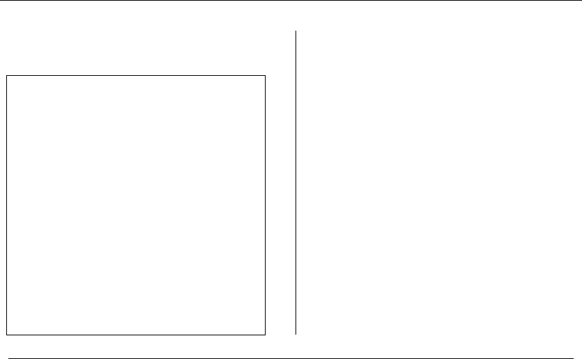
18.5 TEXT COMPRESSION 637
people shall not perish from the earth.
freedom and that government of the people by the people for the
died in vain that this nation under God shall have a new birth of
of devotion that we here highly resolve that these dead shall not have
devotion to that cause for which they here gave the last full measure
remaining before us that from these honored dead we take increased
advanced. It is rather for us to be here dedicated to the great task
what they did here. It is for us the living here have thus far so nobly
note nor long remember what we say here but it can never forget
it for above our poor power to add or detract. The world will little
The brave men living and dead who struggled here have consecrated
fitting and we can not consecrate we can not hallow this groud.
who here gave their lives that the nation might live. It is altogether
dedicate a portion of that field as a final resting place for those
met on a great battlefield of that war. We have come to
nation so conceived and so dedicated can long endure. We are
engaged in a great civil war testing whether that nation or any
to the proposition that all men are created equal. Now we are
this continent a new nation conceived in Liberty and dedicated
Fourscore and seven years ago our father brought forth on Fourscore and seven years ago our father brought forth on
this continent a new nation conceived in Liberty and dedicated
to the proposition that all men are created equal. Now we are
engaged in a great civil war testing whether that nation or any
nation so conceived and so dedicated can long endure. We are
met on a great battlefield of that war. We have come to
dedicate a portion of that field as a final resting place for those
who here gave their lives that the nation might live. It is altogether
fitting and we can not consecrate we can not hallow this groud.
The brave men living and dead who struggled here have consecrated
it for above our poor power to add or detract. The world will little
note nor long remember what we say here but it can never forget
what they did here. It is for us the living here have thus far so nobly
advanced. It is rather for us to be here dedicated to the great task
remaining before us that from these honored dead we take increased
devotion to that cause for which they here gave the last full measure
of devotion that we here highly resolve that these dead shall not have
died in vain that this nation under God shall have a new birth of
freedom and that government of the people by the people for the
people shall not perish from the earth.
INPUT OUTPUT
18.5 Text Compression
Input description:AtextstringS.
Problem description: Create a shorter text string Ssuch that Scanbecorrectly
reconstructed from S.
Discussion: Secondary storage devices fill up quickly on every computer system,
even though their capacity continues to double every year. Decreasing storage prices
only seem to have increased interest in data compression, probably because there
is more data to compress than ever before. Data compression is the algorithmic
problem of finding space-efficient encodings for a given data file. The rise of com-
puter networks provided a new mission for data compression, that of increasing the
effective network bandwidth by reducing the number of bits before transmission.
People seem to like inventing ad hoc data-compression methods for their par-
ticular application. Sometimes these outperform general methods, but often they
don’t. Several issues arise in selecting the right compression algorithm:
•Must we recover the exact input text after compression? –Lossy versus loss-
less encoding is the primary issue in data compression. Document storage
applications typically demand lossless encodings, as users become disturbed

638 18. SET AND STRING PROBLEMS
whenever their data files are altered. Fidelity is not such an issue in image
or video compression, because the presence of small artifacts are impercep-
tible to the viewer. Significantly greater compression ratios can be obtained
using lossy compression, which is why most image/video/audio compression
algorithms exploit this freedom.
•Can I simplify my data before I compress it? – The most effective way to free
space on a disk is to delete files you don’t need. Likewise, any preprocess-
ing you can do to reduce the information content of a file pays off later in
better compression. Can we eliminate redundant white space from the file?
Might the document be converted entirely to uppercase characters, or have
formatting information removed?
A particularly interesting simplification results from applying the Burrows-
Wheeler transform to the input string. This transform sorts all ncyclic shifts
of the ncharacter input, and then reports the last character of each shift. As
an example, the cyclic shifts of ABAB are ABAB,BABA,ABAB,andBABA.
After sorting, these become ABAB,ABAB,BABA,andBABA. Reading the
last character of each of these strings yields the transform result: BBAA.
Provided the last character of the input string is unique (e.g., end-of-string),
this transform is perfectly reversible to the original input! The Burrows-
Wheeler string is typically 10-15% more compressible than the original text,
because repeated words turn into blocks of repeated characters. Further, this
transform can be computed in linear time.
•Does it matter whether the algorithm is patented? – Certain data compres-
sion algorithms have been patented—most notoriously the LZW variation of
the Lempel-Ziv algorithm discussed below. Mercifully, this patent has now
expired, although legal battles are still being fought over JPEG. Typically
there are unrestricted variations of any compression algorithm that perform
about as well as the patented variant.
•How do I compress image data – The simplest lossless compression algorithm
for image data is run-length coding. Here we replace runs of identical pixel
values with a single instance of the pixel and an integer giving the length
of the run. This works well on binary images with large contiguous regions
of similar pixels, like scanned text. It performs badly on images with many
quantization levels and random noise. Correctly selecting (1) the number of
bits to allocate to the count field, and (2) the right traversal order to reduce
a two-dimensional image into a stream of pixels, has a surprisingly important
impact on compression.
For serious audio/image/video compression applications, I recommend that
you use a popular lossy coding method and not fool around with implement-
ing it yourself. JPEG is the standard high-performance image compression

18.5 TEXT COMPRESSION 639
method, while MPEG is designed to exploit the frame-to-frame coherence of
video.
•Must compression run in real time? – Fast decompression is often more im-
portant than fast compression. A YouTube video is compressed only once,
but decompressed every time someone plays it. In contrast, an operating sys-
tem that increases effective disk capacity by automatically compressing files
will need a symmetric algorithm with fast compression times, as well.
Literally dozens of text compression algorithms are available, but they can be
classified into two distinct approaches. Static algorithms, such as Huffman codes,
build a single coding table by analyzing the entire document. Adaptive algorithms,
such as Lempel-Ziv, build a coding table on the fly that adapts to the local character
distribution of the document. Adaptive algorithms usually prove to be the correct
answer:
•Huffman codes – Huffman codes replace each alphabet symbol by a variable-
length code string. Using eight bits-per-symbol to encode English text is
wasteful, since certain characters (such as “e”) occur far more frequently
than others (such as “q”). Huffman codes assign “e” a short code word, and
“q” a longer one to compress text.
Huffman codes can be constructed using a greedy algorithm. Sort the symbols
in increasing order by frequency. We merge the two least-frequently used
symbols xand yinto a new symbol xy, whose frequency is the sum of the
frequencies of its two child symbols. Replacing xand yby xy leaves a smaller
set of symbols. We now repeat this operation n−1 times until all symbols
have been merged. These merging operations define a rooted binary tree, with
the original alphabet symbols as leaves. The left or right choices on the root-
to-leaf path define the bits of the binary code word for each symbol. Priority
queues can efficiently maintain the symbols by frequency during construction,
yielding Huffman codes in O(nlg n) time.
Huffman codes are popular but have three disadvantages. Two passes must
be made over the document on encoding, first to build the coding table, and
then to actually encode the document. The coding table must be explicitly
stored with the document to decode it, which eats into any space savings
on short documents. Finally, Huffman codes only exploit nonuniform sym-
bol distributions, while adaptive algorithms can recognize the higher-order
redundancies such as in 0101010101. . . .
•Lempel-Ziv algorithms – Lempel-Ziv algorithms (including the popular LZW
variant) compress text by building a coding table on the fly as we read the
document. The coding table changes at every position in the text. A clever
protocol ensures that the encoder and decoder are both always working with
the exact same code table, so no information is lost.

640 18. SET AND STRING PROBLEMS
Lempel-Ziv algorithms build coding tables of frequent substrings, which can
get arbitrarily long. Thus they can exploit often-used syllables, words, and
phrases to build better encodings. It adapts to local changes in the text
distribution, which is important because many documents exhibit significant
locality of reference.
The truly amazing thing about the Lempel-Ziv algorithm is how robust it is
on different types of data. It is quite difficult to beat Lempel-Ziv by using
an application-specific algorithm. My recommendation is not to try. If you
can eliminate application-specific redundancies with a simple preprocessing
step, go ahead and do it. But don’t waste much time fooling around. You are
unlikely to get significantly better text compression than with gzip or some
other popular program, and you might well do worse.
Implementations: Perhaps the most popular text compression program is
gzip, which implements a public domain variation of the Lempel-Ziv algorithm.
It is distributed under the GNU software license and can be obtained from
http://www.gzip.org.
There is a natural tradeoff between compression ratio and compression time.
Another choice is bzip2, which uses the Burrows-Wheeler transform. It produces
tighter encodings than gzip at somewhat greater cost in running time. Going to
the extreme, other compression algorithms devote enormous run times to squeeze
every bit out of a file. Representative programs of this genre are collected at
http://www.cs.fit.edu/∼mmahoney/compression/.
Reasonably authoritative comparisons of compression programs are presented
at http://www.maximumcompression.com/, including links to all available software.
Notes:A large number of books on data compression are available. Recent and com-
prehensive books include Sayood [Say05] and Salomon [Sal06]. Also recommended is the
older book by Bell, Cleary, and Witten [BCW90]. Surveys on text compression algorithms
include [CL98].
Good expositions on Huffman codes [Huf52] include [AHU83, CLRS01, Man89]. The
Lempel-Ziv algorithm and variants are described in [Wel84, ZL78]. The Burrows-Wheeler
transform was introduced in [BW94].
The annual IEEE Data Compression Conference (http://www.cs.brandeis.edu/∼dcc/)
is the primary research venue in this field. This is a mature technical area where most
current work is shooting for fairly marginal improvements, particularly in the case of
text compression. More encouragingly, we note that the conference is held annually at a
world-class ski resort in Utah.
Related Problems: Shortest common superstring (see page 654), cryptography
(see page 641).

18.6 CRYPTOGRAPHY 641
The magic words are
Squeamish Ossifrage.
I5&AE<&UA9VEC’=0
<F1s"F%R92!3<75E96UI<V
V@*3W-S:69R86=E+@K_
INPUT OUTPUT
18.6 Cryptography
Input description: A plaintext message Tor encrypted text E, and a key k.
Problem description: Encode T(decode E)usingkgiving E(T).
Discussion: Cryptography has grown substantially in importance as computer
networks make confidential documents more vulnerable to prying eyes. Cryptog-
raphy increases security by making messages difficult to read even if they fall into
the wrong hands. Although the discipline of cryptography is at least two thou-
sand years old, its algorithmic and mathematical foundations have only recently
solidified to the point where provably secure cryptosystems can be envisioned.
Cryptographic ideas and applications go beyond the commonly known con-
cepts of “encryption” and “authentication.” The field now includes such important
mathematical constructs such as cryptographic hashes, digital signatures, and use-
ful primitive protocols that provide associated security assurances.
There are three classes of cryptosystems everyone should be aware of:
•Caesar shifts – The oldest ciphers involve mapping each character of the
alphabet to a different letter. The weakest such ciphers rotate the alphabet
by some fixed number of characters (often 13), and thus have only 26 possible
keys. Better is to use an arbitrary permutation of the letters, giving 26!
possible keys. Even so, such systems can be easily attacked by counting the
frequency of each symbol and exploiting the fact that “e” occurs more often
than “z”. While there are variants that will make this more difficult to break,
none will be as secure as AES or RSA.
•Block Shuffle Ciphers – This class of algorithms repeatedly shuffle the bits
of your text as governed by the key. The classic example of such a cipher is
the Data Encryption Standard (DES). Although approved as a Federal Infor-
mation Processing Standard in 1976, its 56-bit key length is now considered
too short for applications requiring substantial levels of security. Indeed, a
special purpose machine named “Deep Crack” demonstrated that it is pos-
sible to decrypt messages without a key in less than a day. As of May 19,

642 18. SET AND STRING PROBLEMS
2005, DES has been officially withdrawn as a federal standard, replaced by
the stronger Advanced Encryption Standard (AES).
However, a simple variant called triple DES permits an effective key length
of 112 bits by using three rounds of DES with two 56-bit keys. In particular,
first encrypt with key1, then decrypt with key2, before finally encrypting with
key1. There is a mathematical reason for using three rounds instead of two;
the encrypt-decrypt-encrypt pattern is used so that the scheme is equivalent
to single DES when key1=key2. This is enough to keep “Deep Crack” at
bay. Indeed, triple DES has recently been approved by the National Institute
of Standards and Technology (NIST) for sensitive government information
through the year 2030.
•Public Key Cryptography – If you fear bad guys reading your messages, you
should be afraid to tell anyone else the key needed to decrypt them. Public-
key systems use different keys to encode and decode messages. Since the
encoding key is of no help in decoding, it can be made public at no risk to
security. This solution to the key distribution problem is literally its key to
success.
RSA is the classic example of a public key cryptosystem, named after its
inventors Rivest, Shamir, and Adelman. The security of RSA is based on the
relative computational complexities of factoring and primality testing (see
Section 13.8 (page 420)). Encoding is (relatively) fast because it relies on
primality testing to construct the key, while the hardness of decryption follows
from that of factoring. Still, RSA is slow relative to other cryptosystems—
roughly 100 to 1,000 times slower than DES.
The critical issue in selecting a cryptosystem is identifying your paranoia level—
i.e. , deciding how much security you need. Who are you trying to stop from
reading your stuff: your grandmother, local thieves, the Mafia, or the NSA? If
you can use an accepted implementation of AES or RSA, you should feel pretty
safe against anybody, at least for now. Increasing computer power often lays waste
to cryptosystems surprisingly quickly; recall that DES lived less than 30 years
as a strong system. Be sure to use the longest possible keys and keep abreast
of algorithmic development if you are a planning long-term storage of criminal
material.
That said, I will confess that I use DES to encrypt my final exam each semester.
It proved more than sufficient the time an ambitious student broke into my office
looking for it. The story would have been different had the NSA had been breaking
in, but it is important to understand that the most serious security holes are human,
not algorithmic. Ensuring that your password is long enough, hard to guess, and not
written down is far more important than obsessing about the encryption algorithm.
Most symmetric key encryption mechanisms are harder to crack than public
key ones for the same key size. This means one can get away with much shorter
key lengths for symmetric key than for public key encryption. NIST and RSA Labs

18.6 CRYPTOGRAPHY 643
both provide schedules of recommended key sizes for secure encryption, and as
of this writing they recommend 80-bit symmetric keys as equivalent to 1024-bit
asymetric keys. This difference helps explain why symmetric key algorithms are
typically orders of magnitude faster than public key algorithms.
Simple ciphers like the Caesar shift are fun and easy to program. For this reason,
it is healthy to use them for applications needing only a casual level of security
(such as hiding the punchlines of jokes). Since they are easy to break, they should
never be used for serious security applications.
Another thing you should never do is try to develop your own novel cryptosys-
tem. The security of triple DES and RSA is accepted because these systems have
survived many years of public scrutiny. In this time, many other cryptosystems
have been proposed, proven vulnerable to attack, and then abandoned. This is not
a field for amateurs. If you are charged with implementing a cryptosystem, care-
fully study a respected program such as PGP to see how they handle issues such
as key selection and key distribution. Any cryptosystem is as strong as its weakest
link.
Certain other problems related to cryptography arise often in practice:
•How can I validate the integrity of data against random corruption? – There
is often a need to validate that transmitted data is identical to that which has
been received. One solution is for the receiver to transmit the data back to the
source and have the original sender confirm that the two texts are identical.
This fails when the exact inverse of an error is made in the retransmission,
but a more serious problem is that your available bandwidth is cut in half
with such a scheme.
A more efficient method uses a checksum, a simple mathematical function
that hashes a long text down to a simple number or digit. We then transmit
the checksum along with the text. The checksum can be recomputed on the
receiving end and bells set off if the computed checksum is not identical to
what was received. The simplest checksum scheme just adds up the byte
or character values and takes the sum modulo of some constant, say 28=
256. Unfortunately, an error transposing two or more characters would go
undetected under such a scheme, since addition is commutative.
Cyclic-redundancy check (CRC) provides a more powerful method for com-
puting checksums that is used in most communications systems and inter-
nally in computers to validate disk drive transfers. These codes compute the
remainder in the ratio of two polynomials, the numerator of which is a func-
tion of the input text. The design of these polynomials involves considerable
mathematical sophistication, but ensures that all reasonable errors are de-
tected. The details of efficient computation are sufficiently complicated that
we recommend that you start from an existing implementation, described
below.

644 18. SET AND STRING PROBLEMS
•How can I validate the integrity of data against deliberate corruption? –CRC
is good at detecting random errors, but not malicious changes to a document.
Cryptographic hashing functions such as MD5 and SHA-256 are (in principle)
easy to compute for a document but hard to invert. This means that given
a particular hash code value x, it is difficult to construct a document dsuch
that H(d)=x. The property makes them valuable for digital signatures and
other applications.
•How can I prove that a file has not been changed? – If I send you a contract
in electronic form, what is to stop you from editing the file and then claiming
that your version was what we had really agreed to? I need a way to prove
that any modification to a document is fraudulent. Digital signatures are a
cryptographic way for me to stamp my document as genuine.
Given a file, I can compute a checksum for it, and then encrypt this checksum
using my own private key. I send you the file and the encrypted checksum. You
can now edit the file, but to fool the judge you must also edit the encrypted
checksum such that it can be decrypted to yield the correct checksum. With
a suitably good checksum function, designing a file that yields the same
checksum becomes an insurmountable problem. For full security, we need a
trusted third party to authenticate the timestamp and associate the private
key with me.
•How can I restrict access to copyrighted material? – An important emerg-
ing application for cryptography is digital rights management for audio and
video. A key issue here is speed of decryption, as it must keep up with data
transmission or retrieval in real time. Such stream ciphers usually involve ef-
ficiently generating a stream of pseudorandom bits, say using a shift-register
generator. The exclusive-or of these bits with the data stream gives the en-
crypted sequence. The original data is recovered by exclusive-oring the result
with the same stream of pseudorandom bits.
High-speed cryptosystems have proven to be relatively easy to break. The
state-of-the-art solution to this problem involves erecting laws like the Digital
Millennium Copyright Act to make it illegal to try to break them.
Implementations:Nettle is a comprehensive low-level cryptographic library in
C. Cryptographic hash functions include MD5 and SHA-256. Block ciphers include
DES, AES, and some more recently developed codes. An implementation of RSA
is also provided. Nettle is available at http://www.lysator.liu.se/∼nisse/nettle.
A comprehensive overview of cryptographic algorithms with assessments of
strength is available at http://www.cryptolounge.org/wiki/Category:Algorithm. See
http://csrc.nist.gov/groups/ST/toolkit for related cryptographic resources provided
by NIST.
Crypto++ is a large C++ class library of cryptographic schemes, including all
we have mentioned in this section. It is available at http://www.cryptopp.com/.

18.6 CRYPTOGRAPHY 645
Many popular open source utilities employ serious cryptography, and serve as
good models of current practice. GnuPG, an open source version of PGP, is avail-
able at http://www.gnupg.org/.OpenSSL, for authenticating access to computer
systems, is available at http://www.openssl.org/.
The Boost CRC Library provides multiple implementations of cyclic redundancy
check algorithms. It is available at http://www.boost.org/libs/crc/.
Notes:The Handbook of Applied Cryptography [MOV96] provides technical surveys
of all aspects of cryptography, and has been generously made available online at
http://www.cacr.math.uwaterloo.ca/hac/. Schneier [Sch96] provides a thorough overview
of different cryptographic algorithms, with [FS03] as perhaps a better introduction. Kahn
[Kah67] presents the fascinating history of cryptography from ancient times to 1967 and
is particularly noteworthy in light of the secretive nature of the subject.
Expositions on the RSA algorithm [RSA78] include [CLRS01]. The RSA Laboratories
home page http://www.rsa.com/rsalabs/ is very informative.
Of course, the NSA (National Security Agency) is the place to go to learn the real state
of the art in cryptography. The history of DES is well presented in [Sch96]. Particularly
controversial was the decision by the NSA to limit key length to 56 bits.
MD5 [Riv92] is the hashing function used by PGP to compute digital signatures.
Expositions include [Sch96, Sta06]. Serious problems with the security of MD5 have
recently been exposed [WY05]. The SHA family of hash functions appears more secure,
particularly SHA-256 and SHA-512.
Related Problems: Factoring and primality testing (see page 420), text compres-
sion (see page 637)).
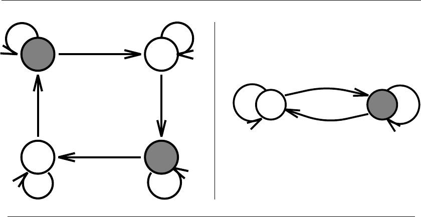
646 18. SET AND STRING PROBLEMS
TT
H
H
HH
TT
H
H
TT
INPUT OUTPUT
18.7 Finite State Machine Minimization
Input description: A deterministic finite automaton M.
Problem description: Create the smallest deterministic finite automaton M
such that Mbehaves identically to M.
Discussion: Constructing and minimizing finite state machines arises repeatedly in
software and hardware design applications. Finite state machines are very useful for
specifying and recognizing patterns. Modern programming languages such as Java
and Python provide built-in support for regular expressions, a particularly natural
way of defining automata. Control systems and compilers often use finite state
machines to encode the current state and possible associated actions/transitions.
Minimizing the size of these automata reduces both the storage and execution costs
of dealing with such machines.
Finite state machines are defined by directed graphs. Each vertex represents a
state, and each character-labeled edge defines a transition from one state to another
on receipt of the given alphabet symbol. The automata shown analyzes a sequence
of coin tosses, with dark states signifying that an even number of heads have been
observed. Such automata can be represented using any graph data structure (see
Section 12.4 (page 381)), or by an n×|Σ|transition matrix where |Σ|is the size
of the alphabet.
Finite state machines are often used to specify search patterns in the guise
of regular expressions, which are patterns formed by and-ing, or-ing, and looping

18.7 FINITE STATE MACHINE MINIMIZATION 647
over smaller regular expressions. For example, the regular expression a(a+b+c)∗a
matches any string on (a, b, c) that begins and ends with distinct as. The best way
to test whether a string sis recognized by a given regular expression Rconstructs
the finite automaton equivalent to R, and then simulates this machine on S. See
Section 18.3 (page 628) for alternative approaches to string matching.
We consider three different problems on finite automata:
•Minimizing deterministic finite state machines – Transition matrices for fi-
nite automata become prohibitively large for sophisticated machines, thus
fueling the need for tighter encodings. The most direct approach is to elim-
inate redundant states in the automaton. As the example above illustrates,
automata of widely varying sizes can compute the same function.
Algorithms for minimizing the number of states in a deterministic finite au-
tomaton (DFA) appear in any book on automata theory. The basic approach
partitions the states into gross equivalence classes and then refines the parti-
tion. Initially, the states are partitioned into accepting, rejecting, and other
classes. The transitions from each node now branch to a given class on a given
symbol. Whenever two states s,tfrom the same class Cbranch to elements
of different classes, the class Cmust be partitioned into two subclasses, one
containing s, the other containing t.
This algorithm makes a sweep though all the classes looking for a new par-
tition, and repeats the process from scratch if it finds one. This yields an
O(n2) algorithm, since at most n−1 sweeps need ever be performed. The
final equivalence classes correspond to the states in the minimum automaton.
In fact, a more efficient O(nlog n) algorithm is known. Implementations are
cited below.
•Constructing deterministic machines from nondeterministic machines –
DFAs are simple to work with, because the machine is always in exactly
one state at any given time. Nondeterministic automata (NFAs) can be in
multiple states at a time, so their current “state” represents a subset of all
possible machine states.
In fact, any NFA can be mechanically converted to an equivalent DFA, which
can then be minimized as above. However, converting an NFA to a DFA
might cause an exponential blowup in the number of states, which perversely
might then be eliminated when minimizing the DFA. This exponential blowup
makes most NFA minimization problems PSPACE-hard, which is even worse
than NP-complete.
The proofs of equivalence between NFAs, DFAs, and regular expressions are
elementary enough to be covered in undergraduate automata theory classes.
However, they are surprisingly nasty to actually code. Implementations are
discussed below.

648 18. SET AND STRING PROBLEMS
•Constructing machines from regular expressions – There are two approaches
for translating a regular expression to an equivalent finite automaton. The
difference is whether the output automaton will be a nondeterministic or
deterministic machine. NFAs are easier to construct but less efficient to sim-
ulate.
The nondeterministic construction uses -moves, which are optional transi-
tions that require no input to fire. On reaching a state with an -move, we
must assume that the machine can be in either state. Using -moves, it is
straightforward to construct an automaton from a depth-first traversal of the
parse tree of the regular expression. This machine will have O(m) states, if
mis the length of the regular expression. Furthermore, simulating this ma-
chine on a string of length ntakes O(mn) time, since we need consider each
state/prefix pair only once.
The deterministic construction starts with the parse tree for the regular ex-
pression, observing that each leaf represents an alphabet symbol in the pat-
tern. After recognizing a prefix of the text, we can be left in some subset
of these possible positions, which would correspond to a state in the finite
automaton. The derivatives method builds up this automaton state by state
as it is needed. Even so, some regular expressions of length mrequire O(2m)
states in any DFA implementing them, such as (a+b)∗a(a+b)(a+b)...(a+b).
There is no way to avoid this exponential space blowup. Fortunately it takes
linear time to simulate an input string on any DFA, regardless of the size of
the automaton.
Implementations:Grail+ is a C++ package for symbolic computation with fi-
nite automata and regular expressions. Grail enables one to convert between dif-
ferent machine representations and to minimize automata. It can handle large ma-
chines defined on large alphabets. All code and documentation are accessible from
http://www.csd.uwo.ca/Research/grail, as well as pointers to a variety of other
automaton packages. Commercial use of Grail is not allowed without approval,
although it is freely available to students and educators.
The AT&T Finite State Machine Library (FSM) is a set of general-purpose
UNIX software tools for building, combining, optimizing, and searching weighted
finite-state acceptors and transducers. It supports automata with more than ten
million states and transitions. See http://www.research.att.com/∼fsmtools/fsm/.
JFLAP (Java Formal Languages and Automata Package) is a package of graphi-
cal tools for learning the basic concepts of automata theory. Included are functions
to convert between DFAs, NFAs, and regular expressions, and minimize the re-
sulting automata. High-level automata are also supported, including context-free
languages and Turing machines. JFLAP is available at http://www.jflap.org/.A
related book [RF06] is also available.
FIRE Engine provides production-quality implementations of finite
automata and regular expression algorithms. Several finite automaton

18.7 FINITE STATE MACHINE MINIMIZATION 649
minimization algorithms have been implemented, including Hopcroft’s O(nlg n)
algorithm. Both deterministic and nondeterministic automata are supported.
It is available at http://www.fastar.org/ and, with certain enhancements, at
www.eti.pg.gda.pl/∼jandac/minim.html.
Notes:Aho [Aho90] provides a good survey on algorithms for pattern matching, with
a particularly clear exposition for the case where the patterns are regular expressions.
The technique for regular expression pattern matching with -moves is due to Thomp-
son [Tho68]. Other expositions on finite automaton pattern matching include [AHU74].
Expositions on finite automata and the theory of computation include [HMU06, Sip05]
The major annual meeting of interest in this field is the Conference on Implementa-
tions and Applications of Automata (CIAA). Pointers to current and previous meetings
with associated software are available at http://tln.li.univ-tours.fr/ciaa/.
Hopcroft [Hop71] gave an optimal O(nlg n) algorithm for minimizing the number of
states in DFAs. The derivatives method of constructing a finite state machine from a
regular expression is due to Brzozowski [Brz64] and has been expanded upon in [BS86].
Expositions on the derivatives method includes Conway [Con71]. Recent work on incre-
mental construction and optimization of automata includes [Wat03]. The problems of
compressing a DFA to a minimum NFA [JR93] and testing the equivalence of two nonde-
terministic finite state machines [SM73] are both PSPACE-complete.
Related Problems: Satisfiability (see page 472). string matching (see page 628).
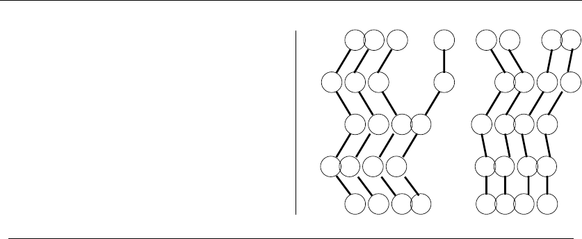
650 18. SET AND STRING PROBLEMS
C A A G G T T A T A T A
G C A A T T C T A T A A
C A A T T G A T A T A A
G C A A T C A T A T A T
G C A A G T C T A A T A
C A A G G T T A T A T A
G C A A T T C T A T A A
C A A T T G A T A T A A
G C A A T C A T A T A T
G C A A G T C T A A T A
INPUT OUTPUT
18.8 Longest Common Substring/Subsequence
Input description:AsetSof strings S1,...,S
n.
Problem description: What is the longest string Ssuch that all the characters
of Sappear as a substring or subsequence of each Si,1≤i≤n?
Discussion: The problem of longest common substring/subsequence arises when-
ever we search for similarities across multiple texts. A particularly important ap-
plication is finding a consensus among biological sequences. The genes for building
proteins evolve with time, but the functional regions must remain consistent in
order for them to work correctly. The longest common subsequence of the same
gene in different species provides insight into what has been conserved over time.
The longest common subsequence problem for two strings is a special case of
edit distance (see Section 18.4 (page 631)), when substitutions are forbidden and
exact character match, insert, and delete are the only allowable edit operations.
Under these conditions, the edit distance between Pand Tis n+m−2|lcs(P, T)|,
since we can delete the missing characters from Pto the lcs(P, T) and insert the
missing characters from Tto transform Pto T.
Issues arising include
•Are you looking for a common substring? – In detecting plagiarism, we might
need to find the longest phrase shared between two or more documents. Since
phrases are strings of consecutive characters, here we need the longest com-
mon substring between the texts.
The longest common substring of a set of strings can be identified in linear
time using suffix trees, as discussed in Section 12.3 (page 377). The trick is
to build a suffix tree containing all the strings, label each leaf with the input

18.8 LONGEST COMMON SUBSTRING/SUBSEQUENCE 651
string it represents, and then do a depth-first traversal to identify the deepest
node with descendants from each input string.
•Are you looking for a common scattered subsequence? – For the rest of our dis-
cussion here, we restrict attention to finding common scattered subsequences.
This algorithm is a special case of the dynamic program edit-distance com-
putation. Indeed, an implementation in C is given on page 288.
Let M[i, j] denote the number of characters in the longest common substring
of S[1],...,S[i]andT[1],...,T[j]. When S[i]=T[j], there is no way the last
pair of characters could match, so M[i, j] = max(M[i, j −1],M[i−1,j]). But
if S[i]=T[j], we have the option to select this character for our substring,
so M[i, j] = max(M[i−1,j−1] + 1,M[i−1,j],M[i, j −1]).
This recurrence computes the length of the longest common subsequence
in O(nm) time. We can reconstruct the actual common substring by walk-
ing backward from M[n, m] and establishing which characters were matched
along the way.
•What if there are relatively few sets of matching characters? – There is a
faster algorithm for strings that do not contain too many copies of the same
character. Let rbe the number of pairs of positions (i, j) such that Si=Tj.
Thus, rcan be as large as mn if both strings consist entirely of the same
character, but r=nif both strings are permutations of {1,...,n}. This
technique treats the pairs of ras defining points in the plane.
The complete set of rsuch points can be found in O(n+m+r) time using
bucketing techniques. We create a bucket for each alphabet symbol cand
each string (Sor T), then partition the positions of each character of the
string into the appropriate bucket. We then create a point (s, t) from every
pair s∈Scand t∈Tcin the buckets Scand Tc.
A common subsequence describes a monotonically nondecreasing path
through these points, meaning the path only moves up and to the right.
The longest such path can be found in O((n+r)lgn) time. We sort the
points in order of increasing x-coordinate, breaking ties in favor of increasing
y-coordinate. We insert points one by one in this order, and maintain the
minimum terminal y-coordinate of any path going through exactly kpoints
for each k,for1≤k≤n. The new point (px,p
y) changes exactly one of
these paths, either identifying a new longest subsequence or reducing the
y-coordinate of the shortest path whose endpoint lies above py.
•What if the strings are permutations? – Permutations are strings without
repeating characters. Two permutations define npairs of matching char-
acters, and so the above algorithm runs in O(nlg n) time. A particularly
important case occurs in finding the longest increasing subsequence of a nu-
merical sequence. Sorting the sequence and then replacing each number by

652 18. SET AND STRING PROBLEMS
its rank defines a permutation p. The longest common subsequence of pand
{1,2,3,...,n}gives the longest increasing subsequence.
•What if we have more than two strings to align? – The basic dynamic pro-
gramming algorithm can be generalized to kstrings, taking O(2knk) time,
where nis the length of the longest string. This algorithm is exponential in
the number of strings k, and so it will likely be too expensive for more than
a few strings. Furthermore, the problem is NP-complete, so no better exact
algorithm is destined to come along soon.
Many heuristics have been proposed for multiple sequence alignment. They
often start by computing the pairwise alignment for each of the k
2pairs
of strings. One approach then replaces the two most similar sequences with
a single merged sequence, and repeats until all these alignments have been
merged into one. The catch is that two strings often have many different
alignments of optimal cost. The “right” alignment to pick depends upon the
remaining sequences to merge, and is hence unknowable to the heuristic.
Implementations: Several programs are available for multiple sequence align-
ment of DNA/protein sequence data. ClustalW [THG94] is a popular and
well-regarded program for multiple alignment of protein sequences. It is avail-
able at http://www.ebi.ac.uk/Tools/clustalw/. Another respectable option is the
MSA package for multiple sequence alignment [GKS95], which is available at
http://www.ncbi.nlm.nih.gov/CBBresearch/Schaffer/msa.html.
Any of the dynamic programming-based approximate string matching programs
of Section 18.4 (page 631) can be used to find the longest common subsequence of
two strings. More specialized implementations in Perl, Java, and C are available at
http://www.bioalgorithms.info/downloads/code/.
Combinatorica [PS03] provides a Mathematica implementation of an algorithm
to construct the longest increasing subsequence of a permutation, which is a special
case of longest common subsequence. This algorithm is based on Young tableaux
rather than dynamic programming. See Section 19.1.9 (page 661).
Notes:Surveys of algorithmic results on longest common subsequence (LCS) problems
include [BHR00, GBY91]. The algorithm for the case where all the characters in each
sequence are distinct or infrequent is due to Hunt and Szymanski [HS77]. Expositions
of this algorithm include [Aho90, Man89]. There has been a surprising amount of recent
work on this problem, including efficient bit-parallel algorithms for LCS [CIPR01]. Masek
and Paterson [MP80] solve longest common subsequence in O(mn/ log(min{m, n})) for
constant-sized alphabets, using the four Russians technique.
Construct two random n-character strings on an alphabet of size α. What is the
expected length of their LCS? This problem has been extensively studied, with an excellent
survey by Dancik [Dan94].
Multiple sequence alignment for computational biology is large field, with the books
of Gusfield [Gus97] and Durbin [DEKM98] serving as excellent introductions. See [Not02]

18.8 LONGEST COMMON SUBSTRING/SUBSEQUENCE 653
for a more recent survey. The hardness of multiple sequence alignment follows from that
of shortest common subsequence for large sets of strings [Mai78].
We motivated the problem of longest common substring with the application of plagia-
rism detection. See [SWA03] for the interesting details of how to implement a plagiarism
detector for computer programs.
Related Problems: Approximate string matching (see page 631), shortest com-
mon superstring (see page 654).

654 18. SET AND STRING PROBLEMS
A B R A C
A C A D A
A D A B R
D A B R A
R A C A D
A B R A C
R A C A D
A C A D A
A D A B R
D A B R A
A B R A C A D A B R A
INPUT OUTPUT
18.9 Shortest Common Superstring
Input description: A set of strings S={S1,...,S
m}.
Problem description: Find the shortest string Sthat contains each string Sias
a substring of S.
Discussion: Shortest common superstring arises in a variety of applications. A
casino gambling addict once asked me how to reconstruct the pattern of symbols on
the wheels of a slot machine. On every spin, each wheel turns to a random position,
displaying the selected symbol as well as the symbols immediately before/after it.
Given enough observations of the slot machine, the symbol order for each wheel
can be determined as the shortest common (circular) superstring of the observed
symbol triples.
Another application of shortest common superstring is data/matrix compres-
sion. Suppose we are given a sparse n×mmatrix M, meaning that most elements
are zero. We can partition each row into m/k runs of kelements, and construct
the shortest common superstring Sof all these runs. We can now represent the
matrix by this superstring plus an n×m/k array of pointers denoting where each
of these runs starts in S. Any particular element M[i, j] can still be accessed in
constant time, but there will be substantial space savings when |S|<< mn.
Perhaps the most compelling application is in DNA sequence assembly. Ma-
chines readily sequence fragments of about 500 base pairs or characters of DNA,
but the real interest is in sequencing large molecules. Large-scale “shotgun” se-
quencing clones many copies of the target molecule, breaks them randomly into
fragments, sequences the fragments, and then proposes the shortest superstring of
the fragments as the correct sequence.
Finding a superstring of a set of strings is not difficult, since we can simply
concatenate them together. Finding the shortest such string is what’s problematic.

18.9 SHORTEST COMMON SUPERSTRING 655
Indeed, shortest common superstring is NP-complete for all reasonable classes of
strings.
Finding the shortest common superstring can easily be reduced to the traveling
salesman problem (see Section 16.4 (page 533)). Create an overlap graph Gwhere
vertex virepresents string Si. Assign edge (vi,v
j) weight equal to the length of Si
minus the overlap of Sjwith Si.Thus,w(vi,v
j)=1forSi=abc and Sj=bcd.
The minimum weight path visiting all the vertices defines the shortest common
superstring. These edge weights are not symmetric; note that w(vj,v
i) = 3 for the
example above. Unfortunately, asymmetric TSP problems are much harder to solve
in practice than symmetric instances.
The greedy heuristic provides the standard approach to approximating shortest
common superstring. Identify which pair of strings have the maximum overlap.
Replace them by the merged string, and repeat until only one string remains.
This heuristic can actually be implemented in linear time. The seemingly most
time-consuming part is in building the overlap graph. The brute-force approach to
finding the maximum overlap of two length-lstrings takes O(l2) for each of O(n2)
string pairs. However, faster times are possible by using suffix trees (see Section
12.3 (page 377)). Build a tree containing all suffixes of all strings of S. String Si
overlaps with Sjiff a suffix of Simatches the prefix of Sj—an event defined by
a vertex of the suffix tree. Traversing these vertices in order of distance from the
root defines the appropriate merging order.
How well does the greedy heuristic perform? It can certainly be fooled into
creating a superstring that is twice as long as optimal. The optimal merging order
for strings c(ab)k,(ba)k, and (ab)kcis left to right. But greedy starts by merging
the first and third string, leaving the middle one no overlap possibility. The greedy
superstring can never be worse than 3.5 times optimal, and usually will be a lot
better in practice.
Building superstrings becomes more difficult when given both positive and neg-
ative strings, where each of the negative strings are forbidden to be a substring
of the final result. The problem of deciding whether any such consistent substring
exists is NP-complete, unless you are allowed to add an extra character to the
alphabet to use as a spacer.
Implementations: Several high-performance programs for DNA sequence assem-
bly are available. Such programs correct for sequencing errors, so the final result is
not necessarily a superstring of the input reads. At the very least, they will serve
as excellent models if you really need a short proper superstring.
CAP3 (Contig Assembly Program) [HM99] and PCAP [HWA+03] are the latest
in a series of assemblers by Xiaoqiu Huang and his collaborators, which are available
from http://seq.cs.iastate.edu/. They have been used on mammalian scale assembly
projects involving hundreds of millions of bases.
The Celera assembler that originally sequenced the human genome is now avail-
able as open source. See http://sourceforge.net/projects/wgs-assembler/.

656 18. SET AND STRING PROBLEMS
Notes:The shortest common superstring (SCS) problem and its application to DNA
shotgun assembly are ably surveyed in [MKT07, Mye99a]. Kececioglu and Myers [KM95]
report on an algorithm for this more general version of shortest common superstring,
where the strings are assumed to have character substitution errors. Their paper is rec-
ommended reading to anyone interested in fragment assembly.
Blum et al. [BJL+94] gave the first constant-factor approximation algorithms for
shortest common superstring, using a variation of the greedy heuristic. More recent re-
search has beaten this constant down to 2.5 [Swe99], progress towards the expected factor-
two result. The best approximation ratio so far proven for the standard greedy heuristic
is 3.5 [KS05a]. Fast implementations of such heuristics are described in [Gus94].
Experiments on shortest common superstring heuristics are reported in [RBT04],
which suggest that greedy heuristics typically produce solutions within 1.4% of opti-
mal for a reasonable class of inputs. Experiments with genetic algorithm approaches are
reported in [ZS04]. Analytical results [YZ99] demonstrate very little compression on the
SCS of random sequences largely because the expected overlap length of any two random
strings is small.
Related Problems: Suffix trees (see page 377), text compression (see page 637).

19
Algorithmic Resources
This chapter briefly describes resources that the practical algorithm designer should
be familiar with. Although some of this information has appeared elsewhere in the
catalog, the most important pointers are collected here for general reference.
19.1 Software Systems
In this section, we describe several particularly comprehensive implementations
of combinatorial algorithms, all of which are downloadable over the Internet. Al-
though these codes are mentioned in the relevant sections of the catalog, they are
substantial enough to warrant further attention.
A good algorithm designer does not reinvent the wheel, and a good programmer
does not rewrite code that other people have written. Picasso put it best: “Good
artists borrow. Great artists steal.”
However, here is a word of caution about stealing. Many of the codes described
in this book have been made available for research or educational use only. Com-
mercial use may require a licensing arrangement with the author. I urge you to
respect this. Licensing terms from academic institutions are usually quite modest.
The recognition that industry is using a particular code is important to the au-
thors, often more important than the money involved. This can lead to enhanced
support or future releases of the software. Do the right thing and get a license.
Information about terms or whom to contact is usually available embedded within
the documentation, or available at the source’s website.
Although many of the systems we describe here may be available by accessing
our algorithm repository, http://www.cs.sunysb.edu/∼algorith we encourage you to
get them from the original sites instead of Stony Brook. There are three reasons.
First, the version on the original site is much more likely to be up-to-date. Second,
S.S. Skiena, The Algorithm Design Manual, 2nd ed., DOI: 10.1007/978-1-84800-070-4 19,
c
Springer-Verlag London Limited 2008

658 19. ALGORITHMIC RESOURCES
there are often supporting files and documentation that we did not download that
may be of interest to you. Finally, many authors monitor the downloads of their
codes, and so you deny them a well-earned thrill if you don’t take them from the
homepage.
19.1.1 LEDA
LEDA,forLibrary of Efficient Data types and Algorithms, is perhaps the best single
resource available to support combinatorial computing. LEDA was originally devel-
oped by a group at Max-Planck-Instutut in Saarbr¨ucken, Germany, including Kurt
Mehlhorn, Stefan N¨aher, Stefan Schirra, Christian Uhrig, and Christoph Burnikel.
LEDA is unique because of (1) the algorithmic sophistication of its developers, and
(2) the level of continuity and resources invested in the project.
What LEDA offers is a complete collection of well-implemented C++ data
structures and types. Particularly useful is the graph type, which supports all the
basic operations one needs in an intelligent way, although this generality comes
at some cost in size and speed over handcrafted implementations. A useful library
of graph algorithms is included, which illustrates how cleanly and concisely these
algorithms can be implemented using the LEDA data types. Good implementations
of the most important data structures supporting such common data types as
dictionaries and priority queues are provided. There are also algorithms and data
structures for computational geometry, including support for visualization. For
more, see the book [MN99].
Since 2001, LEDA has been exclusively available from Algorithmic So-
lutions Software GmbH (http://www.algorithmic-solutions.com/). This ensures
professional-quality support, and new releases appear often. The great news is
that a free edition containing all the basic data structures (including dictionar-
ies, priority queues, graphs, and numerical types) was released February 2008. No
source code or advanced algorithms are provided with the free edition. However,
the licencing fees for the full library are not outlandish and free trial downloads
are available.
19.1.2 CGAL
The Computational Geometry Algorithms Library or CGAL provides efficient and
reliable geometric algorithms in C++. It is extremely comprehensive, offering a rich
variety of triangulations, Voronoi diagrams, operations on polygons and polyhedra,
line/curve arrangements, alpha-shapes, convex-hull algorithms, geometric search
structures, and more. Many work in three dimensions and some beyond.
CGAL (www.cgal.org) should be the first place to go for serious geometric com-
puting, although you should expect to spend some start-up time getting oriented
to the CGAL way of thinking. CGAL is distributed under a dual-license scheme.
It can be used together with open source software free of charge but using CGAL
in other contexts requires obtaining a commercial license.

19.1 SOFTWARE SYSTEMS 659
19.1.3 Boost Graph Library
Boost (www.boost.org) provides a well-regarded collection of free peer-reviewed
portable C++ source libraries. The Boost license encourages both commercial and
noncommercial use.
The Boost Graph Library [SLL02] (http://www.boost.org/libs/graph/doc) is per-
haps most relevant for the readers of this book. Implementations of adjacency lists,
matrices, and edge lists are included, along with a reasonable library of basic graph
algorithms. Its interface and components are generic in the same sense as the C++
Standard Template Library (STL). Other Boost libraries of interest include those
for string/text processing and math/numeric computation.
19.1.4 GOBLIN
The Graph Object Library for Network Programming Problems (GOBLIN) is a
C++ class library that broadly focuses on graph optimization problems. These in-
clude several varieties of shortest path, minimum spanning tree, and connected
component algorithms, plus particularly strong coverage of network flows and
matching. Finally, a generic branch-and-bound module is used to solve such hard
problems as independent set and vertex coloring.
GOBLIN was written and is maintained by Christian Fremuth-Paeger at the
University of Augsberg. It is available under GNU lesser public licence from
http://www.math.uni-augsburg.de/∼fremuth/goblin.html. A spiffy Tcl/Tk interface
is provided. GOBLIN is presumably not as robust as Boost or LEDA, but contains
several algorithms not present in either of them.
19.1.5 Netlib
Netlib (www.netlib.org) is an online repository of mathematical software that con-
tains a large number of interesting codes, tables, and papers. Netlib is a compilation
of resources from a variety of places, with fairly detailed indices and search mech-
anisms. Netlib is important because of its breadth and ease of access. Whenever
you need a specialized piece of mathematical software, you should look here first.
The Guide to Available Mathematical Software (GAMS), is an indexing service
for Netlib and other related software repositories that can help you find what you
want. Check it out at http://gams.nist.gov. GAMS is a service of the National
Institute of Standards and Technology (NIST).
19.1.6 Collected Algorithms of the ACM
An early mechanism for the distribution of useful algorithm implementations was
the Collected Algorithms of the ACM (CALGO). It first appeared in Communica-
tions of the ACM in 1960, covering such famous algorithms as Floyd’s linear-time
build heap algorithm. More recently, it has been the province of the ACM Trans-
actions on Mathematical Software. Each algorithm/implementation is described

660 19. ALGORITHMIC RESOURCES
in a brief journal article, with the implementation validated and collected. These
implementations are maintained at http://www.acm.org/calgo/ and at Netlib.
Over 850 algorithms have appeared to date. Most of the codes are in Fortran
and are relevant to numerical computing, although several interesting combinatorial
algorithms have slithered their way into CALGO. Since the implementations have
been refereed, they are presumably more reliable than most comparable software.
19.1.7 SourceForge and CPAN
SourceForge (http://sourceforge.net/) is the largest open source software develop-
ment website, with over 160,000 registered projects. Most are of highly limited
interest, but there is a lot of good stuff to be found. These include graph libraries
such as JUNG and JGraphT, optimization engines such as lpsolve and JGAP,and
much more.
CPAN (http://www.cpan.org/) is the Comprehensive Perl Archive Network.
This enormous collection of Perl modules and scripts is where you should look
before trying to implement anything in Perl.
19.1.8 The Stanford GraphBase
The Stanford GraphBase is an interesting program for several reasons. First, it
was composed as a “literate program,” meaning that it was written to be read. If
anybody’s programs deserve to be read, it is Knuth’s, and [Knu94] contains the
full source code of the system. The programming language/environment is CWEB,
which permits the mixing of text and code in particularly expressive ways.
The GraphBase contains implementations of several important combinatorial
algorithms, including matching, minimum spanning trees, and Voronoi diagrams,
as well as specialized topics like constructing expander graphs and generating
combinatorial objects. Finally, it contains programs for several recreational prob-
lems, including constructing word ladders (flour-floor-flood-blood-brood-broad-
bread) and establishing dominance relations among football teams. Check it out
at http://www-cs-faculty.stanford.edu/∼knuth/sgb.html.
Although the GraphBase is fun to play with, it is not really suited for building
general applications on top of. The GraphBase is perhaps most useful as an instance
generator for constructing a wide variety of graphs to serve as test data. It incor-
porates graphs derived from interactions of characters in famous novels, Roget’s
thesaurus, the Mona Lisa, and the economy of the United States. Furthermore,
because of its machine-independent random number generators, the GraphBase
provides a way to construct random graphs that can be reconstructed elsewhere,
making them perfect for experimental comparisons of algorithms.

19.1 SOFTWARE SYSTEMS 661
19.1.9 Combinatorica
Combinatorica [PS03] is a collection of over 450 algorithms for combinatorics and
graph theory written in Mathematica. These routines have been designed to work
together, enabling one to readily experiment with discrete structures. Combinator-
ica has been widely used for both research and education.
Although (in my totally unbiased opinion) Combinatorica is more comprehen-
sive and better integrated than other libraries of combinatorial algorithms, it is also
the slowest such system available. Credit for all of these properties is largely due to
Mathematica, which provides a very high-level, functional, interpreted, and thus
inefficient programming language. Combinatorica is best for finding quick solutions
to small problems, and (if you can read Mathematica code) as a terse exposition
of algorithms for translation into other languages.
Check out http://www.combinatorica.com for the latest release and associated
resources. It is also included with the standard Mathematica distribution in the
directory Packages/DiscreteMath/Combinatorica.m.
19.1.10 Programs from Books
Several books on algorithms include working implementations of the algorithms in a
real programming language. Although these implementations are intended primar-
ily for exposition, they can also be useful for computation. Since they are typically
small and clean, they can prove the right foundation for simple applications.
The most useful codes of this genre are described below. Most are available
from the algorithm repository, http://www.cs.sunysb.edu/∼algorith.
Programming Challenges
If you like the C code that appeared in the first half of the text, you should check
out the programs I wrote for my book Programming Challenges [SR03]. Perhaps
most useful are additional examples of dynamic programming, computational ge-
ometry routines like convex hull, and a bignum integer arithmetic package. This
algorithm library is available at http://www.cs.sunysb.edu/∼skiena/392/programs/
or at http://www.programming-challenges.com.
Combinatorial Algorithms for Computers and Calculators
Nijenhuis and Wilf [NW78] specializes in algorithms for constructing basic com-
binatorial objects such as permutations, subsets, and partitions. Such algorithms
are often very short, but they are hard to locate and usually surprisingly subtle.
Fortran routines for all of the algorithms are provided, as well as a discussion of
the theory behind each of them. The programs are usually short enough that it is
reasonable to translate them directly into a more modern programming language,
as I did in writing Combinatorica (see Section 19.1.9). Both random and sequential

662 19. ALGORITHMIC RESOURCES
generation algorithms are provided. Descriptions of more recent algorithms for sev-
eral problems, without code, are provided in [Wil89].
These programs are now available from our algorithm repository website. We
tracked them down from Neil Sloane, who had them on a magnetic tape, while the
original authors did not! In [NW78], Nijenhuis and Wilf set the proper standard
of statistically testing the output distribution of each of the random generators to
establish that they really appear uniform. We encourage you to do the same before
using these programs to verify that nothing has been lost in transit.
Computational Geometry in C
O’Rourke [O’R01] is perhaps the best practical introduction to computational
geometry, because of its careful and correct C language implementations of all
the main algorithms of computational geometry. Fundamental geometric prim-
itives, convex hulls, triangulations, Voronoi diagrams, and motion planning are
all included. Although they were implemented primarily for exposition rather
than production use, they should be quite reliable. The codes are available from
http://maven.smith.edu/∼orourke/code.html.
Algorithms in C++
Sedgewick’s popular algorithms text [Sed98, SS02] comes in several different lan-
guage editions, including C, C++, and Java. This book distinguishes itself through
its use of algorithm animation and in its broad topic coverage, including numerical,
string, and geometric algorithms.
The language-specific parts of the text consist of many small code fragments,
instead of full programs or subroutines. They are best thought of as models, instead
of working implementations. Still, the program fragments from the C++ edition
have been made available from http://www.cs.princeton.edu/∼rs/.
Discrete Optimization Algorithms in Pascal
This is a collection of 28 programs for solving discrete optimization problems, ap-
pearing in the book by Syslo, Deo, and Kowalik [SDK83]. The package includes
programs for integer and linear programming, the knapsack and set cover problems,
traveling salesman, vertex coloring, and scheduling, as well as standard network op-
timization problems. They have been made available from the algorithm repository
at http://www.cs.sunysb.edu/∼algorith.
This package is noteworthy for the operations-research flavor of the problems
and algorithms selected. The algorithms have been selected to solve problems,
rather than purely expository purposes.

19.2 DATA SOURCES 663
19.2 Data Sources
It is often important to have interesting data to feed your algorithms, to serve as
test data to ensure correctness or to compare different algorithms for raw speed.
Finding good test data can be surprisingly difficult. Here are some pointers:
•TSPLIB – This well-respected library of test instances for the traveling
salesman problem [Rei91] provides the standard collection of hard instances
of TSPs. TSPLIB instances are large, real-world graphs, derived from ap-
plications such as circuit boards and networks. TSPLIB is available from
http://www.iwr.uni-heidelberg.de/groups/comopt/software/TSPLIB95/.
Somewhat older instances are also available from Netlib.
•Stanford GraphBase – Discussed in Section 19.1.8, this suite of programs
by Knuth provides portable generators for a wide variety of graphs. These
include graphs arising from distance matrices, arts, and literature, as well as
graphs of more theoretical interest.
•DIMACS Challenge data – A series of DIMACS Challenge workshops have
focused on evaluating algorithm implementations of graph, logic, and data
structure problems. Instance generators for each problem have been de-
veloped, with the focus on constructing difficult or representative test
data. The products of the DIMACS Challenges are all available from
http://dimacs.rutgers.edu/Challenges.
19.3 Online Bibliographic Resources
The Internet has proven to be a fantastic resource for people interested in algo-
rithms, as it has for many other subjects. What follows is a highly selective list of
the resources that I use most often. All should be in the tool chest of every algorist.
•ACM Digital Library – This collection of bibliographic references provides
links to essentially every technical paper ever published in computer science.
Check out what is available at http://portal.acm.org/.
•Google Scholar – This free resource (http://scholar.google.com/) restricts Web
searches to things that look like academic papers, often making it a sounder
search for serious information than a general Web search. Particularly useful
is the ability to see which papers cite a given paper. This lets you update an
old reference to see what has happened since publication, and helps to judge
the significance of a particular article.
•Amazon.com – This comprehensive catalog of books (www.amazon.com)is
surprisingly useful for finding relevant literature for algorithmic problems,
particularly since many recent books have been digitized and placed in it’s
index.

664 19. ALGORITHMIC RESOURCES
19.4 Professional Consulting Services
Algorist Technologies (http://www.algorist.com) is a consulting firm that provides
its clients with short-term, expert help in algorithm design and implementation.
Typically, an Algorist consultant is called in for one to three days worth of intensive,
onsite discussion and analysis with the client’s own development staff. Algorist has
built an impressive record of performance improvements with several companies
and applications. We provide longer-term consulting and contracting services as
well.
Call 212-222-9891 or email info@algorist.com for more information on services
provided by Algorist Technologies.
Algorist Technologies
215 West 92nd St. Suite 1F
New York, NY 10025
http://www.algorist.com

Bibliography
[AAAG95] O. Aichholzer, F. Aurenhammer, D. Alberts, and B. Gartner. A novel type
of skeleton for polygons. J. Universal Computer Science, 1:752–761, 1995.
[ABCC07] D. Applegate, R. Bixby, V. Chvatal, and W. Cook. The Traveling Salesman
Problem: A computational study. Princeton University Press, 2007.
[Abd80] N. N. Abdelmalek. A Fortran subroutine for the L1solution of overdeter-
mined systems of linear equations. ACM Trans. Math. Softw., 6(2):228–230,
June 1980.
[ABF05] L. Arge, G. Brodal, and R. Fagerberg. Cache-oblivious data structures. In
D. Mehta and S. Sahni, editors, Handbook of Data Structures and Applica-
tions, pages 34:1–34:27. Chapman and Hall / CRC, 2005.
[AC75] A. Aho and M. Corasick. Efficient string matching: an aid to bibliographic
search. Communications of the ACM, 18:333–340, 1975.
[AC91] D. Applegate and W. Cook. A computational study of the job-shop schedul-
ing problem. ORSA Journal on Computing, 3:149–156, 1991.
[ACG+03] G. Ausiello, P. Crescenzi, G. Gambosi, V. Kann, S. Marchetti-Spaccamela,
and M. Protasi. Complexity and Approximation: Combinatorial Optimiza-
tion Problems and Their Approximability Properties. Springer, 2003.
[ACH+91] E. M. Arkin, L. P. Chew, D. P. Huttenlocher, K. Kedem, and J. S. B.
Mitchell. An efficiently computable metric for comparing polygonal shapes.
IEEE Trans. PAMI, 13(3):209–216, 1991.
[ACI92] D. Alberts, G. Cattaneo, and G. Italiano. An empirical study of dynamic
graph algorithms. In Proc. Seventh ACM-SIAM Symp. Discrete Algorithms
(SODA), pages 192–201, 1992.
[ACK01a] N. Amenta, S. Choi, and R. Kolluri. The power crust. In Proc. 6th ACM
Symp. on Solid Modeling, pages 249–260, 2001.

666 BIBLIOGRAPHY
[ACK01b] N. Amenta, S. Choi, and R. Kolluri. The power crust, unions of balls, and the
medial axis transform. Computational Geometry: Theory and Applications,
19:127–153, 2001.
[ACP+07] H. Ahn, O. Cheong, C. Park, C. Shin, and A. Vigneron. Maximizing the
overlap of two planar convex sets under rigid motions. Computational Ge-
ometry: Theory and Applications, 37:3–15, 2007.
[ADGM04] L. Aleksandrov, H. Djidjev, H. Guo, and A. Maheshwari. Partitioning planar
graphs with costs and weights. In Algorithm Engineering and Experiments:
4th International Workshop, ALENEX 2002, 2004.
[ADKF70] V. Arlazarov, E. Dinic, M. Kronrod, and I. Faradzev. On economical con-
struction of the transitive closure of a directed graph. Soviet Mathematics,
Doklady, 11:1209–1210, 1970.
[Adl94] L. M. Adleman. Molecular computations of solutions to combinatorial prob-
lems. Science, 266:1021–1024, November 11, 1994.
[AE83] D. Avis and H. ElGindy. A combinatorial approach to polygon similarity.
IEEE Trans. Inform. Theory, IT-2:148–150, 1983.
[AE04] G. Andrews and K. Eriksson. Integer Partitions. Cambridge Univ. Press,
2004.
[AF96] D. Avis and K. Fukuda. Reverse search for enumeration. Disc. Applied
Math., 65:21–46, 1996.
[AFH02] P. Agarwal, E. Flato, and D. Halperin. Polygon decomposition for efficient
construction of Minkowski sums. Computational Geometry: Theory and Ap-
plications, 21:39–61, 2002.
[AG00] H. Alt and L. Guibas. Discrete geometric shapes: Matching, interpolation,
and approximation. In J. Sack and J. Urrutia, editors, Handbook of Com-
putational Geometry, pages 121–153. Elsevier, 2000.
[Aga04] P. Agarwal. Range searching. In J. Goodman and J. O’Rourke, editors,
Handbook of Discrete and Computational Geometry, pages 809–837. CRC
Press, 2004.
[AGSS89] A. Aggarwal, L. Guibas, J. Saxe, and P. Shor. A linear-time algorithm for
computing the Voronoi diagram of a convex polygon. Discrete and Compu-
tational Geometry, 4:591–604, 1989.
[AGU72] A. Aho, M. Garey, and J. Ullman. The transitive reduction of a directed
graph. SIAM J. Computing, 1:131–137, 1972.
[Aho90] A. Aho. Algorithms for finding patterns in strings. In J. van Leeuwen, edi-
tor, Handbook of Theoretical Computer Science: Algorithms and Complexity,
volume A, pages 255–300. MIT Press, 1990.
[AHU74] A. Aho, J. Hopcroft, and J. Ullman. The Design and Analysis of Computer
Algorithms. Addison-Wesley, Reading MA, 1974.
[AHU83] A. Aho, J. Hopcroft, and J. Ullman. Data Structures and Algorithms.
Addison-Wesley, Reading MA, 1983.
[Aig88] M. Aigner. Combinatorial Search. Wiley-Teubner, 1988.

BIBLIOGRAPHY 667
[AITT00] Y. Asahiro, K. Iwama, H. Tamaki, and T. Tokuyama. Greedily finding a
dense subgraph. J. Algorithms, 34:203–221, 2000.
[AK89] E. Aarts and J. Korst. Simulated annealing and Boltzman machines: A
stochastic approach to combinatorial optimization and neural computing.
John Wiley and Sons, 1989.
[AKD83] J. H. Ahrens, K. D. Kohrt, and U. Dieter. Sampling from gamma and Pois-
son distributions. ACM Trans. Math. Softw., 9(2):255–257, June 1983.
[AKS04] M. Agrawal, N. Kayal, and N. Saxena. PRIMES is in P. Annals of Mathe-
matics, 160:781–793, 2004.
[AL97] E. Aarts and J. K. Lenstra. Local Search in Combinatorial Optimization.
John Wiley and Sons, West Sussex, England, 1997.
[AM93] S. Arya and D. Mount. Approximate nearest neighbor queries in fixed di-
mensions. In Proc. Fourth ACM-SIAM Symp. Discrete Algorithms (SODA),
pages 271–280, 1993.
[AMN+98] S. Arya, D. Mount, N. Netanyahu, R. Silverman, and A. Wu. An optimal
algorithm for approximate nearest neighbor searching in fixed dimensions.
J. ACM, 45:891 – 923, 1998.
[AMO93] R. Ahuja, T. Magnanti, and J. Orlin. Network Flows. Prentice Hall, Engle-
wood Cliffs NJ, 1993.
[AMWW88] H. Alt, K. Mehlhorn, H. Wagener, and E. Welzl. Congruence, similarity and
symmetries of geometric objects. Discrete Comput. Geom., 3:237–256, 1988.
[And98] G. Andrews. The Theory of Partitions. Cambridge Univ. Press, 1998.
[And05] A. Andersson. Searching and priority queues in o(log n) time. In D. Mehta
and S. Sahni, editors, Handbook of Data Structures and Applications, pages
39:1–39:14. Chapman and Hall / CRC, 2005.
[AP72] A. Aho and T. Peterson. A minimum distance error-correcting parser for
context-free languages. SIAM J. Computing, 1:305–312, 1972.
[APT79] B. Aspvall, M. Plass, and R. Tarjan. A linear-time algorithm for testing the
truth of certain quantified boolean formulas. Info. Proc. Letters, 8:121–123,
1979.
[Aro98] S. Arora. Polynomial time approximations schemes for Euclidean TSP and
other geometric problems. J. ACM, 45:753–782, 1998.
[AS00] P. Agarwal and M. Sharir. Arrangements. In J. Sack and J. Urrutia, editors,
Handbook of Computational Geometry, pages 49–119. Elsevier, 2000.
[Ata83] M. Atallah. A linear time algorithm for the Hausdorff distance between
convex polygons. Info. Proc. Letters, 8:207–209, 1983.
[Ata84] M. Atallah. Checking similarity of planar figures. Internat. J. Comput. In-
form. Sci., 13:279–290, 1984.
[Ata98] M. Atallah. Algorithms and Theory of Computation Handbook. CRC, 1998.
[Aur91] F. Aurenhammer. Voronoi diagrams: a survey of a fundamental data struc-
ture. ACM Computing Surveys, 23:345–405, 1991.

668 BIBLIOGRAPHY
[Bar03] A. Barabasi. Linked: How Everything Is Connected to Everything Else and
What It Means. Plume, 2003.
[BBF99] V. Bafna, P. Berman, and T. Fujito. A 2-approximation algorithm for the
undirected feedback vertex set problem. SIAM J. Discrete Math., 12:289–
297, 1999.
[BBPP99] I. Bomze, M. Budinich, P. Pardalos, and M. Pelillo. The maximum clique
problem. In D.-Z. Du and P.M. Pardalos, editors, Handbook of Combinato-
rial Optimization, volume A sup., pages 1–74. Kluwer, 1999.
[BCGR92] D. Berque, R. Cecchini, M. Goldberg, and R. Rivenburgh. The SetPlayer
system for symbolic computation on power sets. J. Symbolic Computation,
14:645–662, 1992.
[BCPB04] J. Boyer, P. Cortese, M. Patrignani, and G. Di Battista. Stop minding your
p’s and q’s: Implementing a fast and simple DFS-based planarity testing
and embedding algorithm. In Proc. Graph Drawing (GD ’03), volume 2912
LNCS, pages 25–36, 2004.
[BCW90] T. Bell, J. Cleary, and I. Witten. Text Compression. Prentice Hall, Engle-
wood Cliffs NJ, 1990.
[BD99] R. Bubley and M. Dyer. Faster random generation of linear extensions. Disc.
Math., 201:81–88, 1999.
[BDH97] C. Barber, D. Dobkin, and H. Huhdanpaa. The Quickhull algorithm for
convex hulls. ACM Trans. on Mathematical Software, 22:469–483, 1997.
[BDN01] G. Bilardi, P. D’Alberto, and A. Nicolau. Fractal matrix multiplication: a
case study on portability of cache performance. In Workshop on Algorithm
Engineering (WAE), 2001.
[BDY06] K. Been, E. Daiches, and C. Yap. Dynamic map labeling. IEEE Trans.
Visualization and Computer Graphics, 12:773–780, 2006.
[Bel58] R. Bellman. On a routing problem. Quarterly of Applied Mathematics,
16:87–90, 1958.
[Ben75] J. Bentley. Multidimensional binary search trees used for associative search-
ing. Communications of the ACM, 18:509–517, 1975.
[Ben90] J. Bentley. More Programming Pearls. Addison-Wesley, Reading MA, 1990.
[Ben92a] J. Bentley. Fast algorithms for geometric traveling salesman problems.
ORSA J. Computing, 4:387–411, 1992.
[Ben92b] J. Bentley. Software exploratorium: The trouble with qsort. UNIX Review,
10(2):85–93, February 1992.
[Ben99] J. Bentley. Programming Pearls. Addison-Wesley, Reading MA, second edi-
tion edition, 1999.
[Ber89] C. Berge. Hypergraphs. North-Holland, Amsterdam, 1989.
[Ber02] M. Bern. Adaptive mesh generation. In T. Barth and H. Deconinck, editors,
Error Estimation and Adaptive Discretization Methods in Computational
Fluid Dynamics, pages 1–56. Springer-Verlag, 2002.

BIBLIOGRAPHY 669
[Ber04a] M. Bern. Triangulations and mesh generation. In J. Goodman and
J. O’Rourke, editors, Handbook of Discrete and Computational Geometry,
pages 563–582. CRC Press, 2004.
[Ber04b] D. Bernstein. Fast multiplication and its applications. http://cr.yp.to/arith.
html, 2004.
[BETT99] G. Di Battista, P. Eades, R. Tamassia, and I. Tollis. Graph Drawing: Algo-
rithms for the Visualization of Graphs. Prentice-Hall, 1999.
[BF00] M. Bender and M. Farach. The LCA problem revisited. In Proc. 4th Latin
American Symp. on Theoretical Informatics, pages 88–94. Springer-Verlag
LNCS vol. 1776, 2000.
[BFP+72] M. Blum, R. Floyd, V. Pratt, R. Rivest, and R. Tarjan. Time bounds for
selection. J. Computer and System Sciences, 7:448–461, 1972.
[BFV07] G. Brodal, R. Fagerberg, and K. Vinther. Engineering a cache-oblivious
sorting algorithm. ACM J. of Experimental Algorithmics, 12, 2007.
[BG95] J. Berry and M. Goldberg. Path optimization and near-greedy analysis for
graph partitioning: An empirical study. In Proc. 6th ACM-SIAM Symposium
on Discrete Algorithms, pages 223–232, 1995.
[BGS95] M Bellare, O. Goldreich, and M. Sudan. Free bits, PCPs, and non-
approximability – towards tight results. In Proc. IEEE 36th Symp. Founda-
tions of Computer Science, pages 422–431, 1995.
[BH90] F. Buckley and F. Harary. Distances in Graphs. Addison-Wesley, Redwood
City, Calif., 1990.
[BH01] G. Barequet and S. Har-Peled. Efficiently approximating the minimum-
volume bounding box of a point set in three dimensions. J. Algorithms,
38:91–109, 2001.
[BHR00] L. Bergroth, H. Hakonen, and T. Raita. A survey of longest common sub-
sequence algorithms. In Proc. String Processing and Information Retreival
(SPIRE), pages 39–48, 2000.
[BIK+04] H. Bronnimann, J. Iacono, J. Katajainen, P. Morin, J. Morrison, and
G. Toussaint. Space-efficient planar convex hull algorithms. Theoretical
Computer Science, 321:25–40, 2004.
[BJL+94] A. Blum, T. Jiang, M. Li, J. Tromp, and M. Yanakakis. Linear approxima-
tion of shortest superstrings. J. ACM, 41:630–647, 1994.
[BJL06] C. Buchheim, M. J¨unger, and S. Leipert. Drawing rooted trees in linear
time. Software: Practice and Experience, 36:651–665, 2006.
[BJLM83] J. Bentley, D. Johnson, F. Leighton, and C. McGeoch. An experimental
study of bin packing. In Proc. 21st Allerton Conf. on Communication, Con-
trol, and Computing, pages 51–60, 1983.
[BK04] Y. Boykov and V. Kolmogorov. An experimental comparison of min-
cut/max-flow algorithms for energy minimization in vision. IEEE Trans.
Pattern Analysis and Machine Intelligence (PAMI), 26:1124–1137, 2004.

670 BIBLIOGRAPHY
[BKRV00] A. Blum, G. Konjevod, R. Ravi, and S. Vempala. Semi-definite relaxations
for minimum bandwidth and other vertex-ordering problems. Theoretical
Computer Science, 235:25–42, 2000.
[BL76] K. Booth and G. Lueker. Testing for the consecutive ones property, inter-
val graphs, and planarity using PQ-tree algorithms. J. Computer System
Sciences, 13:335–379, 1976.
[BL77] B. P. Buckles and M. Lybanon. Generation of a vector from the lexicograph-
ical index. ACM Trans. Math. Softw., 3(2):180–182, June 1977.
[BLS91] D. Bailey, K. Lee, and H. Simon. Using Strassen’s algorithm to accelerate
the solution of linear systems. J. Supercomputing, 4:357–371, 1991.
[Blu67] H. Blum. A transformation for extracting new descriptions of shape. In
W. Wathen-Dunn, editor, Models for the Perception of Speech and Visual
Form, pages 362–380. MIT Press, 1967.
[BLW76] N. L. Biggs, E. K. Lloyd, and R. J. Wilson. Graph Theory 1736-1936.Claren-
don Press, Oxford, 1976.
[BM53] G. Birkhoff and S. MacLane. A survey of modern algebra. Macmillian, New
York, 1953.
[BM77] R. Boyer and J. Moore. A fast string-searching algorithm. Communications
of the ACM, 20:762–772, 1977.
[BM89] J. Boreddy and R. N. Mukherjee. An algorithm to find polygon similarity.
Inform. Process. Lett., 33(4):205–206, 1989.
[BM01] E. Bingham and H. Mannila. Random projection in dimensionality reduc-
tion: applications to image and text data. In Proc. ACM Conf. Knowledge
Discovery and Data Mining (KDD), pages 245–250, 2001.
[BM05] A. Broder and M. Mitzenmacher. Network applications of bloom filters: A
survey. Internet Mathematics, 1:485–509, 2005.
[BO79] J. Bentley and T. Ottmann. Algorithms for reporting and counting geomet-
ric intersections. IEEE Transactions on Computers, C-28:643–647, 1979.
[BO83] M. Ben-Or. Lower bounds for algebraic computation trees. In Proc. Fifteenth
ACM Symp. on Theory of Computing, pages 80–86, 1983.
[Bol01] B. Bollobas. Random Graphs. Cambridge Univ. Press, second edition, 2001.
[BP76] E. Balas and M. Padberg. Set partitioning – a survey. SIAM Review, 18:710–
760, 1976.
[BR80] I. Barrodale and F. D. K. Roberts. Solution of the constrained L1linear ap-
proximation problem. ACM Trans. Math. Softw., 6(2):231–235, June 1980.
[BR95] A. Binstock and J. Rex. Practical Algorithms for Programmers. Addison-
Wesley, Reading MA, 1995.
[Bra99] R. Bracewell. The Fourier Transform and its Applications. McGraw-Hill,
third edition, 1999.
[Bre73] R. Brent. Algorithms for minimization without derivatives. Prentice-Hall,
Englewood Cliffs NJ, 1973.

BIBLIOGRAPHY 671
[Bre74] R. P. Brent. A Gaussian pseudo-random number generator. Comm. ACM,
17(12):704–706, December 1974.
[Br`e79] D. Br`elaz. New methods to color the vertices of a graph. Comm. ACM,
22:251–256, 1979.
[Bri88] E. Brigham. The Fast Fourier Transform. Prentice Hall, Englewood Cliffs
NJ, facimile edition, 1988.
[Bro95] F. Brooks. The Mythical Man-Month. Addison-Wesley, Reading MA, 20th
anniversary edition, 1995.
[Bru07] P. Brucker. Scheduling Algorithms. Springer-Verlag, fifth edition, 2007.
[Brz64] J. Brzozowski. Derivatives of regular expressions. J. ACM, 11:481–494, 1964.
[BS76] J. Bentley and M. Shamos. Divide-and-conquer in higher-dimensional space.
In Proc. Eighth ACM Symp. Theory of Computing, pages 220–230, 1976.
[BS86] G. Berry and R. Sethi. From regular expressions to deterministic automata.
Theoretical Computer Science, 48:117–126, 1986.
[BS96] E. Bach and J. Shallit. Algorithmic Number Theory: Efficient Algorithms,
volume 1. MIT Press, Cambridge MA, 1996.
[BS97] R. Bradley and S. Skiena. Fabricating arrays of strings. In Proc. First Int.
Conf. Computational Molecular Biology (RECOMB ’97), pages 57–66, 1997.
[BS07] A. Barvinok and A. Samorodnitsky. Random weighting, asymptotic count-
ing and inverse isoperimetry. Israel Journal of Mathematics, 158:159–191,
2007.
[BT92] J. Buchanan and P. Turner. Numerical methods and analysis. McGraw-Hill,
New York, 1992.
[Buc94] A. G. Buckley. A Fortran 90 code for unconstrained nonlinear minimization.
ACM Trans. Math. Softw., 20(3):354–372, September 1994.
[BvG99] S. Baase and A. van Gelder. Computer Algorithms. Addison-Wesley, Read-
ing MA, third edition, 1999.
[BW91] G. Brightwell and P. Winkler. Counting linear extensions. Order, 3:225–242,
1991.
[BW94] M. Burrows and D. Wheeler. A block sorting lossless data compression al-
gorithm. Technical Report 124, Digital Equipment Corporation, 1994.
[BW00] R. Borndorfer and R. Weismantel. Set packing relaxations of some integer
programs. Math. Programming A, 88:425–450, 2000.
[Can87] J. Canny. The complexity of robot motion planning. MIT Press, Cambridge
MA, 1987.
[Cas95] G. Cash. A fast computer algorithm for finding the permanent of adjacency
matrices. J. Mathematical Chemistry, 18:115–119, 1995.
[CB04] C. Cong and D. Bader. The Euler tour technique and parallel rooted span-
ning tree. In Int. Conf. Parallel Processing (ICPP), pages 448–457, 2004.
[CC92] S. Carlsson and J. Chen. The complexity of heaps. In Proc. Third ACM-
SIAM Symp. on Discrete Algorithms, pages 393–402, 1992.

672 BIBLIOGRAPHY
[CC97] W. Cook and W. Cunningham. Combinatorial Optimization. Wiley, 1997.
[CC05] S. Chapra and R. Canale. Numerical Methods for Engineers. McGraw-Hill,
fifth edition, 2005.
[CCDG82] P. Chinn, J. Chv´atolv´a, A. K. Dewdney, and N. E. Gibbs. The bandwidth
problem for graphs and matrices – a survey. J. Graph Theory, 6:223–254,
1982.
[CCPS98] W. Cook, W. Cunningham, W. Pulleyblank, and A. Schrijver. Combinato-
rial Optimization. Wiley, 1998.
[CD85] B. Chazelle and D. Dobkin. Optimal convex decompositions. In G. Tous-
saint, editor, Computational Geometry, pages 63–133. North-Holland, Am-
sterdam, 1985.
[CDL86] B. Chazelle, R. Drysdale, and D. Lee. Computing the largest empty rectan-
gle. SIAM J. Computing, 15:300–315, 1986.
[CDT95] G. Carpento, M. Dell’Amico, and P. Toth. CDT: A subroutine for the ex-
act solution of large-scale, asymmetric traveling salesman problems. ACM
Trans. Math. Softw., 21(4):410–415, December 1995.
[CE92] B. Chazelle and H. Edelsbrunner. An optimal algorithm for intersecting line
segments. J. ACM, 39:1–54, 1992.
[CFC94] C. Cheng, B. Feiring, and T. Cheng. The cutting stock problem — a survey.
Int. J. Production Economics, 36:291–305, 1994.
[CFR06] D. Coppersmith, L. Fleischer, and A. Rudrea. Ordering by weighted number
of wins gives a good ranking for weighted tournaments. In Proc. 17th ACM-
SIAM Symp. Discrete Algorithms (SODA), pages 776–782, 2006.
[CFT99] A. Caprara, M. Fischetti, and P. Toth. A heuristic method for the set cov-
ering problem. Operations Research, 47:730–743, 1999.
[CFT00] A. Caprara, M. Fischetti, and P. Toth. Algorithms for the set covering
problem. Annals of Operations Research, 98:353–371, 2000.
[CG94] B. Cherkassky and A. Goldberg. On implementing push-relabel method
for the maximum flow problem. Technical Report 94-1523, Department of
Computer Science, Stanford University, 1994.
[CGJ96] E. G. Coffman, M. R. Garey, and D. S. Johnson. Approximation algorithms
for bin packing: a survey. In D. Hochbaum, editor, Approximation algo-
rithms. PWS Publishing, 1996.
[CGJ98] C.R. Coullard, A.B. Gamble, and P.C. Jones. Matching problems in selective
assembly operations. Annals of Operations Research, 76:95–107, 1998.
[CGK+97] C. Chekuri, A. Goldberg, D. Karger, M. Levine, and C. Stein. Experimental
study of minimum cut algorithms. In Proc. Symp. on Discrete Algorithms
(SODA), pages 324–333, 1997.
[CGL85] B. Chazelle, L. Guibas, and D. T. Lee. The power of geometric duality. BIT,
25:76–90, 1985.
[CGM+98] B. Cherkassky, A. Goldberg, P. Martin, J. Setubal, and J. Stolfi. Augment
or push: a computational study of bipartite matching and unit-capacity flow
algorithms. J. Experimental Algorithmics, 3, 1998.

BIBLIOGRAPHY 673
[CGPS76] H. L. Crane Jr., N. F. Gibbs, W. G. Poole Jr., and P. K. Stockmeyer. Matrix
bandwidth and profile reduction. ACM Trans. Math. Softw., 2(4):375–377,
December 1976.
[CGR99] B. Cherkassky, A. Goldberg, and T. Radzik. Shortest paths algorithms:
theory and experimental evaluation. Math. Prog., 10:129–174, 1999.
[CGS99] B. Cherkassky, A. Goldberg, and C. Silverstein. Buckets, heaps, lists, and
monotone priority queues. SIAM J. Computing, 28:1326–1346, 1999.
[CH06] D. Cook and L. Holder. Mining Graph Data. Wiley, 2006.
[Cha91] B. Chazelle. Triangulating a simple polygon in linear time. Discrete and
Computational Geometry, 6:485–524, 1991.
[Cha00] B. Chazelle. A minimum spanning tree algorithm with inverse-Ackerman
type complexity. J. ACM, 47:1028–1047, 2000.
[Cha01] T. Chan. Dynamic planar convex hull operations in near-logarithmic amor-
tized time. J. ACM, 48:1–12, 2001.
[Che85] L. P. Chew. Planing the shortest path for a disc in O(n2lg n)time.InProc.
First ACM Symp. Computational Geometry, pages 214–220, 1985.
[CHL07] M. Crochemore, C. Hancart, and T. Lecroq. Algorithms on Strings. Cam-
bridge University Press, 2007.
[Chr76] N. Christofides. Worst-case analysis of a new heuristic for the traveling
salesman problem. Technical report, Graduate School of Industrial Admin-
istration, Carnegie-Mellon University, Pittsburgh PA, 1976.
[Chu97] F. Chung. Spectral Graph Theory. AMS, Providence RI, 1997.
[Chv83] V. Chvatal. Linear Programming. Freeman, San Francisco, 1983.
[CIPR01] M Crochemore, C. Iliopolous, Y. Pinzon, and J. Reid. A fast and practical
bit-vector algorithm for the longest common subsequence problem. Info.
Processing Letters, 80:279–285, 2001.
[CK94] A. Chetverin and F. Kramer. Oligonucleotide arrays: New concepts and
possibilities. Bio/Technology, 12:1093–1099, 1994.
[CK07] W. Cheney and D. Kincaid. Numerical Mathematics and Computing.
Brooks/Cole, Monterey CA, sixth edition, 2007.
[CKSU05] H. Cohn, R. Kleinberg, B. Szegedy, and C. Umans. Group-theoretic algo-
rithms for matrix multiplication. In Proc. 46th Symp. Foundations of Com-
puter Science, pages 379–388, 2005.
[CL98] M. Crochemore and T. Lecroq. Text data compression algorithms. In M. J.
Atallah, editor, Algorithms and Theory of Computation Handbook, pages
12.1–12.23. CRC Press Inc., Boca Raton, FL, 1998.
[Cla92] K. L. Clarkson. Safe and effective determinant evaluation. In Proc. 31st
IEEE Symposium on Foundations of Computer Science, pages 387–395,
Pittsburgh, PA, 1992.
[CLRS01] T. Cormen, C. Leiserson, R. Rivest, and C. Stein. Introduction to Algo-
rithms. MIT Press, Cambridge MA, second edition, 2001.

674 BIBLIOGRAPHY
[CM69] E. Cuthill and J. McKee. Reducing the bandwidth of sparse symmetric
matrices. In Proc. 24th Nat. Conf. ACM, pages 157–172, 1969.
[CM96] J. Cheriyan and K. Mehlhorn. Algorithms for dense graphs and networks
on the random access computer. Algorithmica, 15:521–549, 1996.
[CM99] G. Del Corso and G. Manzini. Finding exact solutions to the bandwidth
minimization problem. Computing, 62:189–203, 1999.
[Coh94] E. Cohen. Estimating the size of the transitive closure in linear time. In
35th Annual Symposium on Foundations of Computer Science, pages 190–
200. IEEE, 1994.
[Con71] J. H. Conway. Regular Algebra and Finite Machines. Chapman and Hall,
London, 1971.
[Coo71] S. Cook. The complexity of theorem proving procedures. In Proc. Third
ACM Symp. Theory of Computing, pages 151–158, 1971.
[CP90] R. Carraghan and P. Pardalos. An exact algorithm for the maximum clique
problem. In Operations Research Letters, volume 9, pages 375–382, 1990.
[CP05] R. Crandall and C. Pomerance. Prime Numbers: A Computational Perspec-
tive. Springer, second edition, 2005.
[CPW98] B. Chen, C. Potts, and G. Woeginger. A review of machine scheduling:
Complexity, algorithms and approximability. In D.-Z. Du and P. Pardalos,
editors, Handbook of Combinatorial Optimization, volume 3, pages 21–169.
Kluwer, 1998.
[CR76] J. Cohen and M. Roth. On the implementation of Strassen’s fast multipli-
cation algorithm. Acta Informatica, 6:341–355, 1976.
[CR99] W. Cook and A. Rohe. Computing minimum-weight perfect matchings. IN-
FORMS Journal on Computing, 11:138–148, 1999.
[CR01] G. Del Corso and F. Romani. Heuristic spectral techniques for the reduction
of bandwidth and work-bound of sparse matrices. Numerical Algorithms,
28:117–136, 2001.
[CR03] M. Crochemore and W. Rytter. Jewels of Stringology. World Scientific, 2003.
[CS93] J. Conway and N. Sloane. Sphere packings, lattices, and groups. Springer-
Verlag, New York, 1993.
[CSG05] A. Caprara and J. Salazar-Gonz´alez. Laying out sparse graphs with provably
minimum bandwidth. INFORMS J. Computing, 17:356–373, 2005.
[CT65] J. Cooley and J. Tukey. An algorithm for the machine calculation of complex
Fourier series. Mathematics of Computation, 19:297–301, 1965.
[CT92] Y. Chiang and R. Tamassia. Dynamic algorithms in computational geome-
try. Proc. IEEE, 80:1412–1434, 1992.
[CW90] D. Coppersmith and S. Winograd. Matrix multiplication via arithmetic pro-
gressions. J. Symbolic Computation, pages 251–280, 1990.
[Dan63] G. Dantzig. Linear programming and extensions. Princeton University Press,
Princeton NJ, 1963.

BIBLIOGRAPHY 675
[Dan94] V. Dancik. Expected length of longest common subsequences. PhD. thesis,
Univ. of Warwick, 1994.
[DB74] G. Dahlquist and A. Bjorck. Numerical Methods. Prentice-Hall, Englewood
Cliffs NJ, 1974.
[DB86] G. Davies and S. Bowsher. Algorithms for pattern matching. Software –
Practice and Experience, 16:575–601, 1986.
[dBDK+98] M. de Berg, O. Devillers, M. Kreveld, O. Schwarzkopf, and M. Teillaud.
Computing the maximum overlap of two convex polygons under transla-
tions. Theoretical Computer Science, 31:613–628, 1998.
[dBvKOS00] M. de Berg, M. van Kreveld, M. Overmars, and O. Schwarzkopf. Compu-
tational Geometry: Algorithms and Applications. Springer-Verlag, Berlin,
second edition, 2000.
[DEKM98] R. Durbin, S. Eddy, A. Krough, and G. Mitchison. Biological Sequence Anal-
ysis. Cambridge University Press, 1998.
[Den05] L. Y. Deng. Efficient and portable multiple recursive generators of large
order. ACM Trans. on Modeling and Computer Simulation, 15:1–13, 2005.
[Dey06] T. Dey. Curve and Surface Reconstruction: Algorithms with Mathematical
Analysis. Cambridge Univ. Press, 2006.
[DF79] E. Denardo and B. Fox. Shortest-route methods: 1. reaching, pruning, and
buckets. Operations Research, 27:161–186, 1979.
[DFJ54] G. Dantzig, D. Fulkerson, and S. Johnson. Solution of a large-scale traveling-
salesman problem. Operations Research, 2:393–410, 1954.
[dFPP90] H. de Fraysseix, J. Pach, and R. Pollack. How to draw a planar graph on a
grid. Combinatorica, 10:41–51, 1990.
[DGH+02] E. Dantsin, A. Goerdt, E. Hirsch, R. Kannan, J. Kleinberg, C. Papadim-
itriou, P. Raghavan, and U. Sch¨oning. A deterministic (2 −2/(k+1))n
algorithm for k-SAT based on local search. Theoretical Computer Science,
289:69–83, 2002.
[DGKK79] R. Dial, F. Glover, D. Karney, and D. Klingman. A computational analysis
of alternative algorithms and labeling techniques for finding shortest path
trees. Networks, 9:215–248, 1979.
[DH92] D. Du and F. Hwang. A proof of Gilbert and Pollak’s conjecture on the
Steiner ratio. Algorithmica, 7:121–135, 1992.
[DHS00] R. Duda, P. Hart, and D. Stork. Pattern Classification. Wiley-Interscience,
New York, second edition, 2000.
[Die04] M. Dietzfelbinger. Primality Testing in Polynomial Time: From Randomized
Algorithms to “PRIMES Is in P”. Springer, 2004.
[Dij59] E. W. Dijkstra. A note on two problems in connection with graphs. Nu-
merische Mathematik, 1:269–271, 1959.
[DJ92] G. Das and D. Joseph. Minimum vertex hulls for polyhedral domains. The-
oret. Comput. Sci., 103:107–135, 1992.

676 BIBLIOGRAPHY
[Dji00] H. Djidjev. Computing the girth of a planar graph. In Proc. 27th Int. Collo-
quium on Automata, Languages and Programming (ICALP), pages 821–831,
2000.
[DJP04] E. Demaine, T. Jones, and M. Patrascu. Interpolation search for non-
independent data. In Proc. 15th ACM-SIAM Symp. Discrete Algorithms
(SODA), pages 522–523, 2004.
[DL76] D. Dobkin and R. Lipton. Multidimensional searching problems. SIAM J.
Computing, 5:181–186, 1976.
[DLR79] D. Dobkin, R. Lipton, and S. Reiss. Linear programming is log-space hard
for P. Info. Processing Letters, 8:96–97, 1979.
[DM80] D. Dobkin and J. I. Munro. Determining the mode. Theoretical Computer
Science, 12:255–263, 1980.
[DM97] K. Daniels and V. Milenkovic. Multiple translational containment. part I:
an approximation algorithm. Algorithmica, 19:148–182, 1997.
[DMBS79] J. Dongarra, C. Moler, J. Bunch, and G. Stewart. LINPACK User’s Guide.
SIAM Publications, Philadelphia, 1979.
[DMR97] K. Daniels, V. Milenkovic, and D. Roth. Finding the largest area axis-
parallel rectangle in a polygon. Computational Geometry: Theory and Ap-
plications, 7:125–148, 1997.
[DN07] P. D’Alberto and A. Nicolau. Adaptive Strassen’s matrix multiplication. In
Proc. 21st Int. Conf. on Supercomputing, pages 284–292, 2007.
[DP73] D. H. Douglas and T. K. Peucker. Algorithms for the reduction of the num-
ber of points required to represent a digitized line or its caricature. Canadian
Cartographer, 10(2):112–122, December 1973.
[DPS02] J. Diaz, J. Petit, and M. Serna. A survey of graph layout problems. ACM
Computing Surveys, 34:313–356, 2002.
[DR90] N. Dershowitz and E. Reingold. Calendrical calculations. Software – Prac-
tice and Experience, 20:899–928, 1990.
[DR02] N. Dershowitz and E. Reingold. Calendrical Tabulations: 1900-2200. Cam-
bridge University Press, New York, 2002.
[DRR+95] S. Dawson, C. R. Ramakrishnan, I. V. Ramakrishnan, K. Sagonas, S. Skiena,
T. Swift, and D. S. Warren. Unification factoring for efficient execution of
logic programs. In 22nd ACM Symposium on Principles of Programming
Languages (POPL ’95), pages 247–258, 1995.
[DSR00] D. Du, J. Smith, and J. Rubinstein. Advances in Steiner Trees.Kluwer,
2000.
[DT04] M. Dorigo and T.Stutzle. Ant Colony Optimization. MIT Press, Cambridge
MA, 2004.
[dVS82] G. de V. Smit. A comparison of three string matching algorithms. Software
– Practice and Experience, 12:57–66, 1982.
[dVV03] S. de Vries and R. Vohra. Combinatorial auctions: A survey. Informs J.
Computing, 15:284–309, 2003.

BIBLIOGRAPHY 677
[DY94] Y. Deng and C. Yang. Waring’s problem for pyramidal numbers. Science in
China (Series A), 37:377–383, 1994.
[DZ99] D. Dor and U. Zwick. Selecting the median. SIAM J. Computing, pages
1722–1758, 1999.
[DZ01] D. Dor and U. Zwick. Median selection requires (2+)ncomparisons. SIAM
J. Discrete Math., 14:312–325, 2001.
[Ebe88] J. Ebert. Computing Eulerian trails. Info. Proc. Letters, 28:93–97, 1988.
[ECW92] V. Estivill-Castro and D. Wood. A survey of adaptive sorting algorithms.
ACM Computing Surveys, 24:441–476, 1992.
[Ede87] H. Edelsbrunner. Algorithms for Combinatorial Geometry. Springer-Verlag,
Berlin, 1987.
[Ede06] H. Edelsbrunner. Geometry and Topology for Mesh Generation. Cambridge
Univ. Press, 2006.
[Edm65] J. Edmonds. Paths, trees, and flowers. Canadian J. Math., 17:449–467, 1965.
[Edm71] J. Edmonds. Matroids and the greedy algorithm. Mathematical Program-
ming, 1:126–136, 1971.
[EE99] D. Eppstein and J. Erickson. Raising roofs, crashing cycles, and playing
pool: applications of a data structure for finding pairwise interactions. Disc.
Comp. Geometry, 22:569–592, 1999.
[EG60] P. Erd˝os and T. Gallai. Graphs with prescribed degrees of vertices. Mat.
Lapok (Hungarian), 11:264–274, 1960.
[EG89] H. Edelsbrunner and L. Guibas. Topologically sweeping an arrangement. J.
Computer and System Sciences, 38:165–194, 1989.
[EG91] H. Edelsbrunner and L. Guibas. Corrigendum: Topologically sweeping an
arrangement. J. Computer and System Sciences, 42:249–251, 1991.
[EGIN92] D. Eppstein, Z. Galil, G. F. Italiano, and A. Nissenzweig. Sparsification: A
technique for speeding up dynamic graph algorithms. In Proc. 33rd IEEE
Symp. on Foundations of Computer Science (FOCS), pages 60–69, 1992.
[EGS86] H. Edelsbrunner, L. Guibas, and J. Stolfi. Optimal point location in a mono-
tone subdivision. SIAM J. Computing, 15:317–340, 1986.
[EJ73] J. Edmonds and E. Johnson. Matching, Euler tours, and the Chinese post-
man. Math. Programming, 5:88–124, 1973.
[EK72] J. Edmonds and R. Karp. Theoretical improvements in the algorithmic ef-
ficiency for network flow problems. J. ACM, 19:248–264, 1972.
[EKA84] M. I. Edahiro, I. Kokubo, and T. Asano. A new point location algorithm and
its practical efficiency – comparison with existing algorithms. ACM Trans.
Graphics, 3:86–109, 1984.
[EKS83] H. Edelsbrunner, D. Kirkpatrick, and R. Seidel. On the shape of a set of
points in the plane. IEEE Trans. on Information Theory, IT-29:551–559,
1983.

678 BIBLIOGRAPHY
[EL01] S. Ehmann and M. Lin. Accurate and fast proximity queries between poly-
hedra using convex surface decomposition. Comp. Graphics Forum, 20:500–
510, 2001.
[EM94] H. Edelsbrunner and E. M¨ucke. Three-dimensional alpha shapes. ACM
Transactions on Graphics, 13:43–72, 1994.
[ENSS98] G. Even, J. Naor, B. Schieber, and M. Sudan. Approximating minimum
feedback sets and multi-cuts in directed graphs. Algorithmica, 20:151–174,
1998.
[Epp98] D. Eppstein. Finding the kshortest paths. SIAM J. Computing, 28:652–673,
1998.
[ES86] H. Edelsbrunner and R. Seidel. Voronoi diagrams and arrangements. Dis-
crete and Computational Geometry, 1:25–44, 1986.
[ESS93] H. Edelsbrunner, R. Seidel, and M. Sharir. On the zone theorem for hyper-
plane arrangements. SIAM J. Computing, 22:418–429, 1993.
[ESV96] F. Evans, S. Skiena, and A. Varshney. Optimizing triangle strips for fast
rendering. In Proc. IEEE Visualization ’96, pages 319–326, 1996.
[Eul36] L. Euler. Solutio problematis ad geometriam situs pertinentis. Commentarii
Academiae Scientiarum Petropolitanae, 8:128–140, 1736.
[Eve79a] S. Even. Graph Algorithms. Computer Science Press, Rockville MD, 1979.
[Eve79b] G. Everstine. A comparison of three resequencing algorithms for the reduc-
tion of matrix profile and wave-front. Int. J. Numerical Methods in Engr.,
14:837–863, 1979.
[F´
48] I. F´ary. On straight line representation of planar graphs. Acta. Sci. Math.
Szeged, 11:229–233, 1948.
[Fei98] U. Feige. A threshold of ln nfor approximating set cover. J. ACM, 45:634–
652, 1998.
[FF62] L. Ford and D. R. Fulkerson. Flows in Networks. Princeton University Press,
Princeton NJ, 1962.
[FG95] U. Feige and M. Goemans. Approximating the value of two prover proof
systems, with applications to max 2sat and max dicut. In Proc. 3rd Israel
Symp. on Theory of Computing and Systems, pages 182–189, 1995.
[FH06] E. Fogel and D. Halperin. Exact and efficient construction of Minkowski
sums for convex polyhedra with applications. In Proc. 6th Workshop on
Algorithm Engineering and Experiments (ALENEX), 2006.
[FHW07] E. Fogel, D. Halperin, and C. Weibel. On the exact maximum complexity of
minkowski sums of convex polyhedra. In Proc. 23rd Symp. Computational
Geometry, pages 319–326, 2007.
[FJ05] M. Frigo and S. Johnson. The design and implementation of FFTW3. Proc.
IEEE, 93:216–231, 2005.
[FJMO93] M. Fredman, D. Johnson, L. McGeoch, and G. Ostheimer. Data structures
for traveling salesmen. In Proc. 4th 7th Symp. Discrete Algorithms (SODA),
pages 145–154, 1993.

BIBLIOGRAPHY 679
[Fle74] H. Fleischner. The square of every two-connected graph is Hamiltonian. J.
Combinatorial Theory, B, 16:29–34, 1974.
[Fle80] R. Fletcher. Practical Methods of Optimization: Unconstrained Optimiza-
tion, volume 1. John Wiley, Chichester, 1980.
[Flo62] R. Floyd. Algorithm 97 (shortest path). Communications of the ACM, 7:345,
1962.
[Flo64] R. Floyd. Algorithm 245 (treesort). Communications of the ACM, 18:701,
1964.
[FLPR99] M. Frigo, C. Leiserson, H. Prokop, and S. Ramachandran. Cache-oblivious
algorithms. In Proc. 40th Symp. Foundations of Computer Science, 1999.
[FM71] M. Fischer and A. Meyer. Boolean matrix multiplication and transitive clo-
sure. In IEEE 12th Symp. on Switching and Automata Theory, pages 129–
131, 1971.
[FM82] C. Fiduccia and R. Mattheyses. A linear time heuristic for improving net-
work partitions. In Proc. 19th IEEE Design Automation Conf., pages 175–
181, 1982.
[FN04] K. Fredriksson and G. Navarro. Average-optimal single and multiple ap-
proximate string matching. ACM J. of Experimental Algorithmics, 9, 2004.
[For87] S. Fortune. A sweepline algorithm for Voronoi diagrams. Algorithmica,
2:153–174, 1987.
[For04] S. Fortune. Voronoi diagrams and Delauney triangulations. In J. Goodman
and J. O’Rourke, editors, Handbook of Discrete and Computational Geom-
etry, pages 513–528. CRC Press, 2004.
[FPR99] P. Festa, P. Pardalos, and M. Resende. Feedback set problems. In D.-Z.
Du and P.M. Pardalos, editors, Handbook of Combinatorial Optimization,
volume A. Kluwer, 1999.
[FPR01] P. Festa, P. Pardalos, and M. Resende. Algorithm 815: Fortran subroutines
for computing approximate solution to feedback set problems using GRASP.
ACM Transactions on Mathematical Software, 27:456–464, 2001.
[FR75] R. Floyd and R. Rivest. Expected time bounds for selection. Communica-
tions of the ACM, 18:165–172, 1975.
[FR94] M. F¨urer and B. Raghavachari. Approximating the minimum-degree Steiner
tree to within one of optimal. J. Algorithms, 17:409–423, 1994.
[Fra79] D. Fraser. An optimized mass storage FFT. ACM Trans. Math. Softw.,
5(4):500–517, December 1979.
[Fre62] E. Fredkin. Trie memory. Communications of the ACM, 3:490–499, 1962.
[Fre76] M. Fredman. How good is the information theory bound in sorting? Theo-
retical Computer Science, 1:355–361, 1976.
[FS03] N. Ferguson and B. Schneier. Practical Cryptography. Wiley, 2003.
[FSV01] P. Foggia, C. Sansone, and M. Vento. A performance comparison of five
algorithms for graph isomorphism. In 3rd IAPR TC-15 Workshop on Graph-
based Representations in Pattern Recognition, 2001.

680 BIBLIOGRAPHY
[FT87] M. Fredman and R. Tarjan. Fibonacci heaps and their uses in improved
network optimization algorithms. J. ACM, 34:596–615, 1987.
[FvW93] S. Fortune and C. van Wyk. Efficient exact arithmetic for computational
geometry. In Proc. 9th ACM Symp. Computational Geometry, pages 163–
172, 1993.
[FW77] S. Fiorini and R. Wilson. Edge-colourings of graphs. Research Notes in
Mathematics 16, Pitman, London, 1977.
[FW93] M. Fredman and D. Willard. Surpassing the information theoretic bound
with fusion trees. J. Computer and System Sci., 47:424–436, 1993.
[FWH04] E. Folgel, R. Wein, and D. Halperin. Code flexibility and program efficiency
by genericity: Improving CGAL’s arrangements. In Proc. 12th European
Symposium on Algorithms (ESA’04), pages 664–676, 2004.
[Gab76] H. Gabow. An efficient implementation of Edmond’s algorithm for maxi-
mum matching on graphs. J. ACM, 23:221–234, 1976.
[Gab77] H. Gabow. Two algorithms for generating weighted spanning trees in order.
SIAM J. Computing, 6:139–150, 1977.
[Gal86] Z. Galil. Efficient algorithms for finding maximum matchings in graphs.
ACM Computing Surveys, 18:23–38, 1986.
[Gal90] K. Gallivan. Parallel Algorithms for Matrix Computations. SIAM, Philadel-
phia, 1990.
[Gas03] S. Gass. Linear Programming: Methods and Applications. Dover, fifth edi-
tion, 2003.
[GBDS80] B. Golden, L. Bodin, T. Doyle, and W. Stewart. Approximate traveling
salesman algorithms. Operations Research, 28:694–711, 1980.
[GBY91] G. Gonnet and R. Baeza-Yates. Handbook of Algorithms and Data Struc-
tures. Addison-Wesley, Wokingham, England, second edition, 1991.
[Gen04] J. Gentle. Random Number Generation and Monte Carlo Methods. Springer,
second edition, 2004.
[GGJ77] M. Garey, R. Graham, and D. Johnson. The complexity of computing
Steiner minimal trees. SIAM J. Appl. Math., 32:835–859, 1977.
[GGJK78] M. Garey, R. Graham, D. Johnson, and D. Knuth. Complexity results for
bandwidth minimization. SIAM J. Appl. Math., 34:477–495, 1978.
[GH85] R. Graham and P. Hell. On the history of the minimum spanning tree
problem. Annals of the History of Computing, 7:43–57, 1985.
[GH06] P. Galinier and A. Hertz. A survey of local search methods for graph color-
ing. Computers and Operations Research, 33:2547–2562, 2006.
[GHMS93] L. J. Guibas, J. E. Hershberger, J. S. B. Mitchell, and J. S. Snoeyink. Ap-
proximating polygons and subdivisions with minimum link paths. Internat.
J. Comput. Geom. Appl., 3(4):383–415, December 1993.
[GHR95] R. Greenlaw, J. Hoover, and W. Ruzzo. Limits to Parallel Computation:
P-completeness theory. Oxford University Press, New York, 1995.

BIBLIOGRAPHY 681
[GI89] D. Gusfield and R. Irving. The Stable Marriage Problem: structure and al-
gorithms. MIT Press, Cambridge MA, 1989.
[GI91] Z. Galil and G. Italiano. Data structures and algorithms for disjoint set
union problems. ACM Computing Surveys, 23:319–344, 1991.
[Gib76] N. E. Gibbs. A hybrid profile reduction algorithm. ACM Trans. Math.
Softw., 2(4):378–387, December 1976.
[Gib85] A. Gibbons. Algorithmic Graph Theory. Cambridge Univ. Press, 1985.
[GJ77] M. Garey and D. Johnson. The rectilinear Steiner tree problem is NP-
complete. SIAM J. Appl. Math., 32:826–834, 1977.
[GJ79] M. R. Garey and D. S. Johnson. Computers and Intractability: A Guide to
the theory of NP-completeness. W. H. Freeman, San Francisco, 1979.
[GJM02] M. Goldwasser, D. Johnson, and C. McGeoch, editors. Data Structures,
Near Neighbor Searches, and Methodology: Fifth and Sixth DIMACS Imple-
mentation Challenges, volume 59. AMS, Providence RI, 2002.
[GJPT78] M. Garey, D. Johnson, F. Preparata, and R. Tarjan. Triangulating a simple
polygon. Info. Proc. Letters, 7:175–180, 1978.
[GK95] A. Goldberg and R. Kennedy. An efficient cost scaling algorithm for the
assignment problem. Math. Programming, 71:153–177, 1995.
[GK98] S. Guha and S. Khuller. Approximation algorithms for connected dominat-
ing sets. Algorithmica, 20:374–387, 1998.
[GKK74] F. Glover, D. Karney, and D. Klingman. Implementation and computational
comparisons of primal-dual computer codes for minimum-cost network flow
problems. Networks, 4:191–212, 1974.
[GKP89] R. Graham, D. Knuth, and O. Patashnik. Concrete Mathematics. Addison-
Wesley, Reading MA, 1989.
[GKS95] S. Gupta, J. Kececioglu, and A. Sch¨affer. Improving the practical space
and time efficiency of the shortest-paths approach to sum-of-pairs multiple
sequence alignment. J. Computational Biology, 2:459–472, 1995.
[GKT05] D. Gibson, R. Kumar, and A. Tomkins. Discovering large dense subgraphs
in massive graphs. In Proc. 31st Int. Conf on Very Large Data Bases, pages
721–732, 2005.
[GKW06] A. Goldberg, H. Kaplan, and R. Werneck. Reach for A∗: Efficient point-to-
point shortest path algorithms. In Proc. 8th Workshop on Algorithm Engi-
neering and Experimentation (ALENEX), 2006.
[GKW07] A. Goldberg, H. Kaplan, and R. Werneck. Better landmarks within reach. In
Proc. 9th Workshop on Algorithm Engineering and Experimentation (ALEN
EX), pages 38–51, 2007.
[GL96] G. Golub and C. Van Loan. Matrix Computations. Johns Hopkins University
Press, third edition, 1996.
[Glo90] F. Glover. Tabu search: A tutorial. Interfaces, 20 (4):74–94, 1990.
[GM86] G. Gonnet and J. I. Munro. Heaps on heaps. SIAM J. Computing, 15:964–
971, 1986.

682 BIBLIOGRAPHY
[GM91] S. Ghosh and D. Mount. An output-sensitive algorithm for computing visi-
bility graphs. SIAM J. Computing, 20:888–910, 1991.
[GMPV06] F. Gomes, C. Meneses, P. Pardalos, and G. Viana. Experimental analysis of
approximation algorithms for the vertex cover and set covering problems.
Computers and Operations Research, 33:3520–3534, 2006.
[GO04] J. Goodman and J. O’Rourke, editors. Handbook of Discrete and Computa-
tional Geometry. CRC Press, second edition, 2004.
[Goe97] M. Goemans. Semidefinite programming in combinatorial optimization.
Mathematical Programming, 79:143–161, 1997.
[Gol93] L. Goldberg. Efficient Algorithms for Listing Combinatorial Structures.
Cambridge University Press, 1993.
[Gol97] A. Goldberg. An efficient implementation of a scaling minimum-cost flow
algorithm. J. Algorithms, 22:1–29, 1997.
[Gol01] A. Goldberg. Shortest path algorithms: Engineering aspects. In 12th In-
ternational Symposium on Algorithms and Computation, number 2223 in
LNCS, pages 502–513. Springer, 2001.
[Gol04] M. Golumbic. Algorithmic Graph Theory and Perfect Graphs,volume57of
Annals of Discrete Mathematics. North Holland, second edition, 2004.
[Gon07] T. Gonzalez. Handbook of Approximation Algorithms and Metaheuristics.
Chapman-Hall / CRC, 2007.
[GP68] E. Gilbert and H. Pollak. Steiner minimal trees. SIAM J. Applied Math.,
16:1–29, 1968.
[GP79] B. Gates and C. Papadimitriou. Bounds for sorting by prefix reversals. Dis-
crete Mathematics, 27:47–57, 1979.
[GP07] G. Gutin and A. Punnen. The Traveling Salesman Problem and Its Varia-
tions. Springer, 2007.
[GPS76] N. Gibbs, W. Poole, and P. Stockmeyer. A comparison of several bandwidth
and profile reduction algorithms. ACM Trans. Math. Software, 2:322–330,
1976.
[Gra53] F. Gray. Pulse code communication. US Patent 2632058, March 17, 1953.
[Gra72] R. Graham. An efficient algorithm for determining the convex hull of a finite
planar point set. Info. Proc. Letters, 1:132–133, 1972.
[Gri89] D. Gries. The Science of Programming. Springer-Verlag, 1989.
[GS62] D. Gale and L. Shapely. College admissions and the stability of marriages.
American Math. Monthly, 69:9–14, 1962.
[GS02] R. Giugno and D. Shasha. Graphgrep : A fast and universal method
for querying graphs. In International Conference on Pattern Recognition
(ICPR), volume 2, pages 112–115, 2002.
[GT88] A. Goldberg and R. Tarjan. A new approach to the maximum flow problem.
J. ACM, pages 921–940, 1988.
[GT94] T. Gensen and B. Toft. Graph Coloring Problems. Wiley, 1994.

BIBLIOGRAPHY 683
[GT05] M. Goodrich and R. Tamassia. Data Structures and Algorithms in Java.
Wiley, fourth edition, 2005.
[GTV05] M. Goodrich, R. Tamassia, and L. Vismara. Data structures in JDSL. In
D. Mehta and S. Sahni, editors, Handbook of Data Structures and Applica-
tions, pages 43:1–43:22. Chapman and Hall / CRC, 2005.
[Gup66] R. P. Gupta. The chromatic index and the degree of a graph. Notices of the
Amer. Math. Soc., 13:719, 1966.
[Gus94] D. Gusfield. Faster implementation of a shortest superstring approximation.
Info. Processing Letters, 51:271–274, 1994.
[Gus97] D. Gusfield. Algorithms on Strings, Trees, and Sequences: Computer Science
and Computational Biology. Cambridge University Press, 1997.
[GW95] M. Goemans and D. Williamson. .878-approximation algorithms for MAX
CUT and MAX 2SAT. J. ACM, 42:1115–1145, 1995.
[GW96] I. Goldberg and D. Wagner. Randomness and the Netscape browser. Dr.
Dobb’s Journal, pages 66–70, 1996.
[GW97] T. Grossman and A. Wool. Computational experience with approximation
algorithms for the set covering problem. European J. Operational Research,
101, 1997.
[Hai94] E. Haines. Point in polygon strategies. In P. Heckbert, editor, Graphics
Gemes IV, pages 24–46. Academic Press, 1994.
[Hal04] D. Halperin. Arrangements. In J. Goodman and J. O’Rourke, editors, Hand-
book of Discrete and Computational Geometry, chapter 24, pages 529–562.
CRC Press, Boca Raton, FL, 2004.
[Ham87] R. Hamming. Numerical Methods for Scientists and Engineers. Dover, sec-
ond edition, 1987.
[Has82] H. Hastad. Clique is hard to approximate within n1−.Acta Mathematica,
182:105–142, 182.
[Has97] J. Hastad. Some optimal inapproximability results. In Proc. 29th ACM
Symp. Theory of Comp., pages 1–10, 1997.
[HD80] P. Hall and G. Dowling. Approximate string matching. ACM Computing
Surveys, 12:381–402, 1980.
[HDD03] M. Hilgemeier, N. Drechsler, and R. Drchsler. Fast heuristics for the edge
coloring of large graphs. In Proc. Euromicro Symp. on Digital Systems De-
sign, pages 230–239, 2003.
[HdlT01] J. Holm, K. de lichtenberg, and M. Thorup. Poly-logarithmic deterministic
fully-dynamic algorithms for connectivity, minimum spanning tree, 2-edge,
and biconnectivity. J. ACM, 48:723–760, 2001.
[Hel01] M. Held. VRONI: An engineering approach to the reliable and efficient com-
putation of Voronoi diagrams of points and line segments. Computational
Geometry: Theory and Applications, 18:95–123, 2001.
[HFN05] H. Hyyro, K. Fredriksson, and G. Navarro. Increased bit-parallelism for
approximate and multiple string matching. ACM J. of Experimental Algo-
rithmics, 10, 2005.

684 BIBLIOGRAPHY
[HG97] P. Heckbert and M. Garland. Survey of polygonal surface simplification
algorithms. SIGGRAPH 97 Course Notes, 1997.
[HH00] I. Hanniel and D. Halperin. Two-dimensional arrangements in CGAL and
adaptive point location for parametric curves. In Proc. 4th International
Workshop on Algorithm Engineering (WAE), LNCS v. 1982, pages 171–
182, 2000.
[HHS98] T. Haynes, S. Hedetniemi, and P. Slater. Fundamentals of Domination in
Graphs. CRC Press, Boca Raton, 1998.
[Hir75] D. Hirschberg. A linear-space algorithm for computing maximum common
subsequences. Communications of the ACM, 18:341–343, 1975.
[HK73] J. Hopcroft and R. Karp. An n5/3algorithm for maximum matchings in
bipartite graphs. SIAM J. Computing, 2:225–231, 1973.
[HK90] D. P. Huttenlocher and K. Kedem. Computing the minimum Hausdorff
distance for point sets under translation. In Proc. 6th Annu. ACM Sympos.
Comput. Geom., pages 340–349, 1990.
[HLD04] W. H¨ormann, J. Leydold, and G. Derfinger. Automatic Nonuniform Random
Variate Generation. Springer, 2004.
[HM83] S. Hertel and K. Mehlhorn. Fast triangulation of simple polygons. In Proc.
4th Internat. Conf. Found. Comput. Theory, pages 207–218. Lecture Notes
in Computer Science, Vol. 158, 1983.
[HM99] X. Huang and A. Madan. Cap3: A DNA sequence assembly program.
Genome Research, 9:868–877, 1999.
[HMS03] J. Hershberger, M. Maxel, and S. Suri. Finding the k shortest simple paths:
A new algorithm and its implementation. In Proc. 5th Workshop on Algo-
rithm Engineering and Experimentation (ALEN EX), 2003.
[HMU06] J. Hopcroft, R. Motwani, and J. Ullman. Introduction to Automata Theory,
Languages, and Computation. Addison-Wesley, third edition, 2006.
[Hoa61] C. A. R. Hoare. Algorithm 63 (partition) and algorithm 65 (find). Commu-
nications of the ACM, 4:321–322, 1961.
[Hoa62] C. A. R. Hoare. Quicksort. Computer Journal, 5:10–15, 1962.
[Hoc96] D. Hochbaum, editor. Approximation Algorithms for NP-hard Problems.
PWS Publishing, Boston, 1996.
[Hof82] C. M. Hoffmann. Group-theoretic algorithms and graph isomorphism, vol-
ume 136 of Lecture Notes in Computer Science. Springer-Verlag Inc., New
York, 1982.
[Hol75] J. H. Holland. Adaptation in Natural and Artificial Systems.Universityof
Michigan Press, Ann Arbor, 1975.
[Hol81] I. Holyer. The NP-completeness of edge colorings. SIAM J. Computing,
10:718–720, 1981.
[Hol92] J. H. Holland. Genetic algorithms. Scientific American, 267(1):66–72, July
1992.

BIBLIOGRAPHY 685
[Hop71] J. Hopcroft. An nlog nalgorithm for minimizing the states in a finite au-
tomaton. In Z. Kohavi, editor, The theory of machines and computations,
pages 189–196. Academic Press, New York, 1971.
[Hor80] R. N. Horspool. Practical fast searching in strings. Software – Practice and
Experience, 10:501–506, 1980.
[HP73] F. Harary and E. Palmer. Graphical enumeration. Academic Press, New
York, 1973.
[HPS+05] M. Holzer, G. Prasinos, F. Schulz, D. Wagner, and C. Zaroliagis. Engineering
planar separator algorithms. In Proc. 13th European Symp. on Algorithms
(ESA), pages 628–637, 2005.
[HRW92] R. Hwang, D. Richards, and P. Winter. The Steiner Tree Problem, volume 53
of Annals of Discrete Mathematics. North Holland, Amsterdam, 1992.
[HS77] J. Hunt and T. Szymanski. A fast algorithm for computing longest common
subsequences. Communications of the ACM, 20:350–353, 1977.
[HS94] J. Hershberger and J. Snoeyink. An O(nlog n) implementation of the
Douglas-Peucker algorithm for line simplification. In Proc. 10th Annu. ACM
Sympos. Comput. Geom., pages 383–384, 1994.
[HS98] J. Hershberger and J. Snoeyink. Cartographic line simplification and poly-
gon CSG formulae in O(nlog∗n)time.Computational Geometry: Theory
and Applications, 11:175–185, 1998.
[HS99] J. Hershberger and S. Suri. An optimal algorithm for Euclidean shortest
paths in the plane. SIAM J. Computing, 28:2215–2256, 1999.
[HSS87] J. Hopcroft, J. Schwartz, and M. Sharir. Planning, geometry, and complexity
of robot motion. Ablex Publishing, Norwood NJ, 1987.
[HSS07] R. Hardin, N. Sloane, and W. Smith. Maximum volume spherical codes.
http://www.research.att.com/∼njas/maxvolumes/, 2007.
[HSWW05] M. Holzer, F. Schultz, D. Wagner, and T. Willhalm. Combining speed-up
techniques for shortest-path computations. ACM J. of Experimental Algo-
rithmics, 10, 2005.
[HT73a] J. Hopcroft and R. Tarjan. Dividing a graph into triconnected components.
SIAM J. Computing, 2:135–158, 1973.
[HT73b] J. Hopcroft and R. Tarjan. Efficient algorithms for graph manipulation.
Communications of the ACM, 16:372–378, 1973.
[HT74] J. Hopcroft and R. Tarjan. Efficient planarity testing. J. ACM, 21:549–568,
1974.
[HT84] D. Harel and R. E. Tarjan. Fast algorithms for finding nearest common
ancestors. SIAM J. Comput., 13:338–355, 1984.
[Hub06] M. Huber. Fast perfect sampling from linear extensions. Disc. Math.,
306:420–428, 2006.
[Huf52] D. Huffman. A method for the construction of minimum-redundancy codes.
Proc. of the IRE, 40:1098–1101, 1952.

686 BIBLIOGRAPHY
[HUW02] E. Haunschmid, C. Ueberhuber, and P. Wurzinger. Cache oblivious high
performance algorithms for matrix multiplication, 2002.
[HW74] J. E. Hopcroft and J. K. Wong. Linear time algorithm for isomorphism
of planar graphs. In Proc. Sixth Annual ACM Symposium on Theory of
Computing, pages 172–184, 1974.
[HWA+03] X. Huang, J. Wang, S. Aluru, S. Yang, and L. Hillier. PCAP: A whole-
genome assembly program. Genome Research, 13:2164–2170, 2003.
[HWK94] T. He, S. Wang, and A. Kaufman. Wavelet-based volume morphing. In Proc.
IEEE Visualization ’94, pages 85–92, 1994.
[IK75] O. Ibarra and C. Kim. Fast approximation algorithms for knapsack and sum
of subset problems. J. ACM, 22:463–468, 1975.
[IM04] P. Indyk and J. Matousek. Low-distortion embeddings of finite metric
spaces. In J. Goodman and J. O’Rourke, editors, Handbook of Discrete and
Computational Geometry. CRC Press, 2004.
[Ind98] P. Indyk. Faster algorithms for string matching problems: matching the
convolution bound. In Proc. 39th Symp. Foundations of Computer Science,
1998.
[Ind04] P. Indyk. Nearest neighbors in high-dimensional spaces. In J. Goodman and
J. O’Rourke, editors, Handbook of Discrete and Computational Geometry,
pages 877–892. CRC Press, 2004.
[IR78] A. Itai and M. Rodeh. Finding a minimum circuit in a graph. SIAM J.
Computing, 7:413–423, 1978.
[Ita78] A. Itai. Two commodity flow. J. ACM, 25:596–611, 1978.
[J´
92] J. J´aJ´a. An Introduction to Parallel Algorithms. Addison-Wesley, 1992.
[Jac89] G. Jacobson. Space-efficient static trees and graphs. In Proc. Symp. Foun-
dations of Computer Science (FOCS), pages 549–554, 1989.
[JAMS91] D. Johnson, C. Aragon, C. McGeoch, and D. Schevon. Optimization by
simulated annealing: an experimental evaluation; part II, graph coloring
and number partitioning. In Operations Research, volume 39, pages 378–
406, 1991.
[Jar73] R. A. Jarvis. On the identification of the convex hull of a finite set of points
in the plane. Info. Proc. Letters, 2:18–21, 1973.
[JD88] A. Jain and R. Dubes. Algorithms for Clustering Data. Prentice-Hall, En-
glewood Cliffs NJ, 1988.
[JLR00] S. Janson, T. Luczak, and A. Rucinski. Random Graphs. Wiley, 2000.
[JM93] D. Johnson and C. McGeoch, editors. Network Flows and Matching: First
DIMACS Implementation Challenge, volume 12. American Mathematics So-
ciety, Providence RI, 1993.
[JM03] M. J¨unger and P. Mutzel. Graph Drawing Software. Springer-Verlag, 2003.
[Joh63] S. M. Johnson. Generation of permutations by adjacent transpositions.
Math. Computation, 17:282–285, 1963.

BIBLIOGRAPHY 687
[Joh74] D. Johnson. Approximation algorithms for combinatorial problems. J. Com-
puter and System Sciences, 9:256–278, 1974.
[Joh90] D. S. Johnson. A catalog of complexity classes. In J. van Leeuwen, editor,
Handbook of Theoretical Computer Science: Algorithms and Complexity, vol-
ume A, pages 67–162. MIT Press, 1990.
[Jon86] D. W. Jones. An empirical comparison of priority-queue and event-set im-
plementations. Communications of the ACM, 29:300–311, 1986.
[Jos99] N. Josuttis. The C++ Standard Library: A tutorial and reference. Addison-
Wesley, 1999.
[JR93] T. Jiang and B. Ravikumar. Minimal NFA problems are hard. SIAM J.
Computing, 22:1117–1141, 1993.
[JS01] A. Jagota and L. Sanchis. Adaptive, restart, randomized greedy heuristics
for maximum clique. J. Heuristics, 7:1381–1231, 2001.
[JSV01] M. Jerrum, A. Sinclair, and E. Vigoda. A polynomial-time approximation
algorithm for the permanent of a matrix with non-negative entries. In Proc.
33rd ACM Symp. Theory of Computing, pages 712–721, 2001.
[JT96] D. Johnson and M. Trick. Cliques, Coloring, and Satisfiability: Second DI-
MACS Implementation Challenge, volume 26. AMS, Providence RI, 1996.
[KA03] P. Ko and S. Aluru. Space-efficient linear time construction of suffix arrays,.
In Proc. 14th Symp. on Combinatorial Pattern Matching (CPM), pages 200–
210. Springer-Verlag LNCS, 2003.
[Kah67] D. Kahn. The Code breakers: the story of secret writing. Macmillan, New
York, 1967.
[Kar72] R. M. Karp. Reducibility among combinatorial problems. In R. Miller and
J. Thatcher, editors, Complexity of Computer Computations, pages 85–103.
Plenum Press, 1972.
[Kar84] N. Karmarkar. A new polynomial-time algorithm for linear programming.
Combinatorica, 4:373–395, 1984.
[Kar96] H. Karloff. How good is the Goemans-Williamson MAX CUT algorithm?
In Proc. Twenty-Eighth Annual ACM Symposium on Theory of Computing,
pages 427–434, 1996.
[Kar00] D. Karger. Minimum cuts in near-linear time. J. ACM, 47:46–76, 200.
[Kei00] M. Keil. Polygon decomposition. In J.R. Sack and J. Urrutia, editors, Hand-
book of Computational Geometry, pages 491–518. Elsevier, 2000.
[KGV83] S. Kirkpatrick, C. D. Gelatt, Jr., and M. P. Vecchi. Optimization by simu-
lated annealing. Science, 220:671–680, 1983.
[Kha79] L. Khachian. A polynomial algorithm in linear programming. Soviet Math.
Dokl., 20:191–194, 1979.
[Kir79] D. Kirkpatrick. Efficient computation of continuous skeletons. In Proc. 20th
IEEE Symp. Foundations of Computing, pages 28–35, 1979.
[Kir83] D. Kirkpatrick. Optimal search in planar subdivisions. SIAM J. Computing,
12:28–35, 1983.

688 BIBLIOGRAPHY
[KKT95] D. Karger, P. Klein, and R. Tarjan. A randomized linear-time algorithm to
find minimum spanning trees. J. ACM, 42:321–328, 1995.
[KL70] B. W. Kernighan and S. Lin. An efficient heuristic procedure for partitioning
graphs. The Bell System Technical Journal, pages 291–307, 1970.
[KM72] V. Klee and G. Minty. How good is the simplex algorithm. In Inequalities
III, pages 159–172, New York, 1972. Academic Press.
[KM95] J. D. Kececioglu and E. W. Myers. Combinatorial algorithms for DNA se-
quence assembly. Algorithmica, 13(1/2):7–51, January 1995.
[KMP77] D. Knuth, J. Morris, and V. Pratt. Fast pattern matching in strings. SIAM
J. Computing, 6:323–350, 1977.
[KMP+04] L. Kettner, K. Mehlhorn, S. Pion, S. Schirra, and C. Yap. Classroom
examples of robustness problems in geometric computations. In Proc.
12th European Symp. on Algorithms (ESA’04), pages 702–713. www.mpi-
inf.mpg.de/∼mehlhorn/ftp/ClassRoomExamples.ps, 2004.
[KMS96] J. Komlos, Y. Ma, and E. Szemeredi. Matching nuts and bolts in o(nlog n)
time. In Proc. 7th Symp. Discrete Algorithms (SODA), pages 232–241, 1996.
[KMS97] S. Khanna, M. Muthukrishnan, and S. Skiena. Efficiently partitioning ar-
rays. In Proc. ICALP ’97, volume 1256, pages 616–626. Springer-Verlag
LNCS, 1997.
[Knu94] D. Knuth. The Stanford GraphBase: a platform for combinatorial comput-
ing. ACM Press, New York, 1994.
[Knu97a] D. Knuth. The Art of Computer Programming, Volume 1: Fundamental
Algorithms. Addison-Wesley, Reading MA, third edition, 1997.
[Knu97b] D. Knuth. The Art of Computer Programming, Volume 2: Seminumerical
Algorithms. Addison-Wesley, Reading MA, third edition, 1997.
[Knu98] D. Knuth. The Art of Computer Programming, Volume 3: Sorting and
Searching. Addison-Wesley, Reading MA, second edition, 1998.
[Knu05a] D. Knuth. The Art of Computer Programming, Volume 4 Fascicle 2: Gen-
erating All Tuples and Permutations. Addison Wesley, 2005.
[Knu05b] D. Knuth. The Art of Computer Programming, Volume 4 Fascicle 3: Gen-
erating All Combinations and Partitions. Addison Wesley, 2005.
[Knu06] D. Knuth. The Art of Computer Programming, Volume 4 Fascicle 4: Gener-
ating All Trees; History of Combinationatorial Generation. Addison Wesley,
2006.
[KO63] A. Karatsuba and Yu. Ofman. Multiplication of multi-digit numbers on
automata. Sov. Phys. Dokl., 7:595–596, 1963.
[Koe05] H. Koehler. A contraction algorithm for finding minimal feedback sets. In
Proc. 28th Australasian Computer Science Conference (ACSC), pages 165–
174, 2005.
[KOS91] A. Kaul, M. A. O’Connor, and V. Srinivasan. Computing Minkowski sums of
regular polygons. In Proc. 3rd Canad. Conf. Comput. Geom., pages 74–77,
1991.

BIBLIOGRAPHY 689
[KP98] J. Kececioglu and J. Pecqueur. Computing maximum-cardinality matchings
in sparse general graphs. In Proc. 2nd Workshop on Algorithm Engineering,
pages 121–132, 1998.
[KPP04] H. Kellerer, U. Pferschy, and P. Pisinger. Knapsack Problems. Springer,
2004.
[KR87] R. Karp and M. Rabin. Efficient randomized pattern-matching algorithms.
IBM J. Research and Development, 31:249–260, 1987.
[KR91] A. Kanevsky and V. Ramachandran. Improved algorithms for graph four-
connectivity. J. Comp. Sys. Sci., 42:288–306, 1991.
[Kru56] J. B. Kruskal. On the shortest spanning subtree of a graph and the traveling
salesman problem. Proc. of the American Mathematical Society, 7:48–50,
1956.
[KS74] D.E. Knuth and J.L. Szwarcfiter. A structured program to generate all
topological sorting arrangements. Information Processing Letters, 2:153–
157, 1974.
[KS85] M. Keil and J. R. Sack. Computational Geometry: Minimum decomposition
of geometric objects, pages 197–216. North-Holland, 1985.
[KS86] D. Kirkpatrick and R. Siedel. The ultimate planar convex hull algorithm?
SIAM J. Computing, 15:287–299, 1986.
[KS90] K. Kedem and M. Sharir. An efficient motion planning algorithm for a
convex rigid polygonal object in 2-dimensional polygonal space. Discrete
and Computational Geometry, 5:43–75, 1990.
[KS99] D. Kreher and D. Stinson. Combinatorial Algorithms: Generation, Enumer-
ation, and Search. CRC Press, 1999.
[KS02] M. Keil and J. Snoeyink. On the time bound for convex decomposition of
simple polygons. Int. J. Comput. Geometry Appl., 12:181–192, 2002.
[KS05a] H. Kaplan and N. Shafrir. The greedy algorithm for shortest superstrings.
Info. Proc. Letters, 93:13–17, 2005.
[KS05b] J. Kelner and D. Spielman. A randomized polynomial-time simplex algo-
rithm for linear programming. Electronic Colloquim on Computational Com-
plexity, 156:17, 2005.
[KS07] H. Kautz and B. Selman. The state of SAT. Disc. Applied Math., 155:1514–
1524, 2007.
[KSB05] J. K¨arkk¨ainen, P. Sanders, and S. Burkhardt. Linear work suffix array con-
struction. J. ACM, 2005.
[KSBD07] H. Kautz, B. Selman, R. Brachman, and T. Dietterich. Satisfiability Testing.
Morgan and Claypool, 2007.
[KSPP03] D Kim, J. Sim, H. Park, and K. Park. Linear-time construction of suffix
arrays. In Proc. 14th Symp. Combinatorial Pattern Matching (CPM), pages
186–199, 2003.
[KST93] J. K¨obler, U. Sch¨oning, and J. T´uran. The Graph Isomorphism Problem: its
structural complexity. Birhauser, Boston, 1993.

690 BIBLIOGRAPHY
[KSV97] D. Keyes, A. Sameh, and V. Venkatarishnan. Parallel Numerical Algorithms.
Springer, 1997.
[KT06] J. Kleinberg and E. Tardos. Algorithm Design. Addison Wesley, 2006.
[Kuh75] H. W. Kuhn. Steiner’s problem revisited. In G. Dantzig and B. Eaves, ed-
itors, Studies in Optimization, pages 53–70. Mathematical Association of
America, 1975.
[Kur30] K. Kuratowski. Sur le probl`eme des courbes gauches en topologie. Fund.
Math., 15:217–283, 1930.
[KW01] M. Kaufmann and D. Wagner. Drawing Graphs: Methods and Models.
Springer-Verlag, 2001.
[Kwa62] M. Kwan. Graphic programming using odd and even points. Chinese Math.,
1:273–277, 1962.
[LA04] J. Leung and J. Anderson, editors. Handbook of Scheduling: Algorithms,
Models, and Performance Analysis. CRC/Chapman-Hall, 2004.
[LA06] J. Lien and N. Amato. Approximate convex decomposition of polygons.
Computational Geometry: Theory and Applications, 35:100–123, 2006.
[Lam92] J.-L. Lambert. Sorting the sums (xi+yj)ino(n2) comparisons. Theoretical
Computer Science, 103:137–141, 1992.
[Lat91] J.-C. Latombe. Robot Motion Planning. Kluwer Academic Publishers,
Boston, 1991.
[Lau98] J. Laumond. Robot Motion Planning and Control. Springer-Verlag, Lectures
Notes in Control and Information Sciences 229, 1998.
[LaV06] S. LaValle. Planning Algorithms. Cambridge University Press, 2006.
[Law76] E. Lawler. Combinatorial Optimization: Networks and Matroids. Holt, Rine-
hart, and Winston, Fort Worth TX, 1976.
[LD03] R. Laycock and A. Day. Automatically generating roof models from building
footprints. In Proc. 11th Int. Conf. Computer Graphics, Visualization and
Computer Vision (WSCG), 2003.
[Lec95] T. Lecroq. Experimental results on string matching algorithms. Software –
Practice and Experience, 25:727–765, 1995.
[Lee82] D. T. Lee. Medial axis transformation of a planar shape. IEEE Trans. Pat-
tern Analysis and Machine Intelligence, PAMI-4:363–369, 1982.
[Len87a] T. Lengauer. Efficient algorithms for finding minimum spanning forests of
hierarchically defined graphs. J. Algorithms, 8, 1987.
[Len87b] H. W. Lenstra. Factoring integers with elliptic curves. Annals of Mathemat-
ics, 126:649–673, 1987.
[Len89] T. Lengauer. Hierarchical planarity testing algorithms. J. ACM, 36(3):474–
509, July 1989.
[Len90] T. Lengauer. Combinatorial Algorithms for Integrated Circuit Layout. Wiley,
Chichester, England, 1990.

BIBLIOGRAPHY 691
[Lev92] J. L. Leva. A normal random number generator. ACM Trans. Math. Softw.,
18(4):454–455, December 1992.
[Lew82] J. G. Lewis. The Gibbs-Poole-Stockmeyer and Gibbs-King algorithms for
reordering sparse matrices. ACM Trans. Math. Softw., 8(2):190–194, June
1982.
[LL96] A. LaMarca and R. Ladner. The influence of caches on the performance of
heaps. ACM J. Experimental Algorithmics, 1, 1996.
[LL99] A. LaMarca and R. Ladner. The influence of caches on the performance of
sorting. J. Algorithms, 31:66–104, 1999.
[LLK83] J. K. Lenstra, E. L. Lawler, and A. Rinnooy Kan. Theory of Sequencing and
Scheduling. Wiley, New York, 1983.
[LLKS85] E. Lawler, J. Lenstra, A. Rinnooy Kan, and D. Shmoys. The Traveling
Salesman Problem. John Wiley, 1985.
[LLS92] L. Lam, S.-W. Lee, and C. Suen. Thinning methodologies – a comprehensive
survey. IEEE Trans. Pattern Analysis and Machine Intelligence, 14:869–885,
1992.
[LM04] M. Lin and D. Manocha. Collision and proximity queries. In J. Goodman
and J. O’Rourke, editors, Handbook of Discrete and Computational Geom-
etry, pages 787–807. CRC Press, 2004.
[LMM02] A. Lodi, S. Martello, and M. Monaci. Two-dimensional packing problems:
A survey. European J. Operations Research, 141:241–252, 2002.
[LMS06] L. Lloyd, A. Mehler, and S. Skiena. Identifying co-referential names across
large corpora. In Combinatorial Pattern Matching (CPM 2006), pages 12–
23. Lecture Notes in Computer Science, v.4009, 2006.
[LP86] L. Lov´asz and M. Plummer. Matching Theory. North-Holland, Amsterdam,
1986.
[LP02] W. Langdon and R. Poli. Foundations of Genetic Programming. Springer,
2002.
[LP07] A. Lodi and A. Punnen. TSP software. In G. Gutin and A. Punnen, edi-
tors, The Traveling Salesman Problem and Its Variations, pages 737–749.
Springer, 2007.
[LPW79] T. Lozano-Perez and M. Wesley. An algorithm for planning collision-free
paths among polygonal obstacles. Comm. ACM, 22:560–570, 1979.
[LR93] K. Lang and S. Rao. Finding near-optimal cuts: An empirical evaluation. In
Proc. 4th Annual ACM-SIAM Symposium on Discrete Algorithms (SODA
’93), pages 212–221, 1993.
[LS87] V. Lumelski and A. Stepanov. Path planning strategies for a point mobile
automaton moving amidst unknown obstacles of arbitrary shape. Algorith-
mica, 3:403–430, 1987.
[LS95] Y.-L. Lin and S. Skiena. Algorithms for square roots of graphs. SIAM J.
Discrete Mathematics, 8:99–118, 1995.

692 BIBLIOGRAPHY
[LSCK02] P. L’Ecuyer, R. Simard, E. Chen, and W. D. Kelton. An object-oriented
random-number package with many long streams and substreams. Opera-
tions Research, 50:1073–1075, 2002.
[LT79] R. Lipton and R. Tarjan. A separator theorem for planar graphs. SIAM
Journal on Applied Mathematics, 36:346–358, 1979.
[LT80] R. Lipton and R. Tarjan. Applications of a planar separator theorem. SIAM
J. Computing, 9:615–626, 1980.
[Luc91] E. Lucas. R´ecr´eations Math´ematiques. Gauthier-Villares, Paris, 1891.
[Luk80] E. M. Luks. Isomorphism of bounded valence can be tested in polynomial
time. In Proc. of the 21st Annual Symposium on Foundations of Computing,
pages 42–49. IEEE, 1980.
[LV88] G. Landau and U. Vishkin. Fast string matching with kdifferences. J. Com-
put. System Sci., 37:63–78, 1988.
[LV97] M. Li and P. Vit´anyi. An introduction to Kolmogorov complexity and its
applications. Springer-Verlag, New York, second edition, 1997.
[LW77] D. T. Lee and C. K. Wong. Worst-case analysis for region and partial region
searches in multidimensional binary search trees and balanced quad trees.
Acta Informatica, 9:23–29, 1977.
[LW88] T. Lengauer and E. Wanke. Efficient solution of connectivity problems on
hierarchically defined graphs. SIAM J. Computing, 17:1063–1080, 1988.
[Mah76] S. Maheshwari. Traversal marker placement problems are NP-complete.
Technical Report CU-CS-09276, Department of Computer Science, Univer-
sity of Colorado, Boulder, 1976.
[Mai78] D. Maier. The complexity of some problems on subsequences and superse-
quences. J. ACM, 25:322–336, 1978.
[Mak02] R. Mak. Java Number Cruncher: The Java Programmer’s Guide to Numer-
ical Computing. Prentice Hall, 2002.
[Man89] U. Manber. Introduction to Algorithms. Addison-Wesley, Reading MA, 1989.
[Mar83] S. Martello. An enumerative algorithm for finding Hamiltonian circuits in
a directed graph. ACM Trans. Math. Softw., 9(1):131–138, March 1983.
[Mat87] D. W. Matula. Determining edge connectivity in O(nm). In 28th Ann. Symp.
Foundations of Computer Science, pages 249–251. IEEE, 1987.
[McC76] E. McCreight. A space-economical suffix tree construction algorithm. J.
ACM, 23:262–272, 1976.
[McK81] B. McKay. Practical graph isomorphism. Congressus Numerantium, 30:45–
87, 1981.
[McN83] J. M. McNamee. A sparse matrix package – part II: Special cases. ACM
Trans. Math. Softw., 9(3):344–345, September 1983.
[MDS01] D. Musser, G. Derge, and A. Saini. STL Tutorial and Reference Guide:
C++ Programming with the Standard Template Library. Addison-Wesley
Professional, second edition, 2001.

BIBLIOGRAPHY 693
[Meg83] N. Megiddo. Linear time algorithm for linear programming in r3and related
problems. SIAM J. Computing, 12:759–776, 1983.
[Men27] K. Menger. Zur allgemeinen Kurventheorie. Fund. Math., 10:96–115, 1927.
[Mey01] S. Meyers. Effective STL: 50 Specific Ways to Improve Your Use of the
Standard Template Library. Addison-Wesley Professional, 2001.
[MF00] Z. Michalewicz and D. Fogel. How to Solve it: Modern Heuristics. Springer,
Berlin, 2000.
[MG92] J. Misra and D. Gries. A constructive proof of Vizing’s theorem. Info. Pro-
cessing Letters, 41:131–133, 1992.
[MG06] J. Matousek and B. Gartner. Understanding and Using Linear Program-
ming. Springer, 2006.
[MGH81] J. J. Mor´e, B. S. Garbow, and K. E. Hillstrom. Fortran subroutines for
testing unconstrained optimization software. ACM Trans. Math. Softw.,
7(1):136–140, March 1981.
[MH78] R. Merkle and M. Hellman. Hiding and signatures in trapdoor knapsacks.
IEEE Trans. Information Theory, 24:525–530, 1978.
[Mie58] W. Miehle. Link-minimization in networks. Operations Research, 6:232–243,
1958.
[Mil76] G. Miller. Riemann’s hypothesis and tests for primality. J. Computer and
System Sciences, 13:300–317, 1976.
[Mil97] V. Milenkovic. Multiple translational containment. part II: exact algorithms.
Algorithmica, 19:183–218, 1997.
[Min78] H. Minc. Permanents, volume 6 of Encyclopedia of Mathematics and its
Applications. Addison-Wesley, Reading MA, 1978.
[Mit99] J. Mitchell. Guillotine subdivisions approximate polygonal subdivisions: A
simple polynomial-time approximation scheme for geometric TSP, k-mst,
and related problems. SIAM J. Computing, 28:1298–1309, 1999.
[MKT07] E. Mardis, S. Kim, and H. Tang, editors. Advances in Genome Sequencing
Technology and Algorithms. Artech House Publishers, 2007.
[MM93] U. Manber and G. Myers. Suffix arrays: A new method for on–line string
searches. SIAM J. Computing, pages 935–948, 1993.
[MM96] K. Mehlhorn and P. Mutzel. On the embedding phase of the Hopcroft and
Tarjan planarity testing algorithm. Algorithmica, 16:233–242, 1996.
[MMI72] D. Matula, G. Marble, and J. Isaacson. Graph coloring algorithms. In
R. C. Read, editor, Graph Theory and Computing, pages 109–122. Academic
Press, 1972.
[MMZ+01] M. Moskewicz, C. Madigan, Y. Zhao, L. Zhang, and S. Malik. Chaff: En-
gineering an efficient SAT solver. In 39th Design Automation Conference
(DAC), 2001.
[MN98] M. Matsumoto and T. Nishimura. Mersenne twister: A 623-dimensionally
equidistributed uniform pseudorandom number generator. ACM Trans. on
Modeling and Computer Simulation, 8:3–30, 1998.

694 BIBLIOGRAPHY
[MN99] K. Mehlhorn and S. Naher. LEDA: A platform for combinatorial and geo-
metric computing. Cambridge University Press, 1999.
[MN07] V. Makinen and G. Navarro. Compressed full text indexes. ACM Computing
Surveys, 39, 2007.
[MO63] L. E. Moses and R. V. Oakford. Tables of Random Permutations. Stanford
University Press, Stanford, Calif., 1963.
[Moe90] S. Moen. Drawing dynamic trees. IEEE Software, 7-4:21–28, 1990.
[Moo59] E. F. Moore. The shortest path in a maze. In Proc. International Symp.
Switching Theory, pages 285–292. Harvard University Press, 1959.
[MOS06] K. Mehlhorn, R. Osbild, and M. Sagraloff. Reliable and efficient compu-
tational geometry via controlled perturbation. In Proc. Int. Coll. on Au-
tomata, Languages, and Programming (ICALP), volume 4051, pages 299–
310. Springer Verlag, Lecture Notes in Computer Science, 2006.
[Mou04] D. Mount. Geometric intersection. In J. Goodman and J. O’Rourke, editors,
Handbook of Discrete and Computational Geometry, pages 857–876. CRC
Press, 2004.
[MOV96] A. Menezes, P. Oorschot, and S. Vanstone. Handbook of Applied Cryptogra-
phy. CRC Press, Boca Raton, 1996.
[MP80] W. Masek and M. Paterson. A faster algorithm for computing string edit
distances. J. Computer and System Sciences, 20:18–31, 1980.
[MPC+06] S. Mueller, D. Papamichial, J.R. Coleman, S. Skiena, and E. Wimmer. Re-
duction of the rate of poliovirus protein synthesis through large scale codon
deoptimization causes virus attenuation of viral virulence by lowering spe-
cific infectivity. J. of Virology, 80:9687–96, 2006.
[MPT99] S. Martello, D. Pisinger, and P. Toth. Dynamic programming and strong
bounds for the 0-1 knapsack problem. Management Science, 45:414–424,
1999.
[MPT00] S. Martello, D. Pisinger, and P. Toth. New trends in exact algorithms for the
0-1 knapsack problem. European Journal of Operational Research, 123:325–
332, 2000.
[MR95] R. Motwani and P. Raghavan. Randomized Algorithms. Cambridge Univer-
sity Press, New York, 1995.
[MR01] W. Myrvold and F. Ruskey. Ranking and unranking permutations in linear
time. Info. Processing Letters, 79:281–284, 2001.
[MR06] W. Mulzer and G. Rote. Minimum weight triangulation is NP-hard. In Proc.
22nd ACM Symp. on Computational Geometry, pages 1–10, 2006.
[MRRT53] N. Metropolis, A. W. Rosenbluth, M. N. Rosenbluth, and A. H. Teller. Equa-
tion of state calculations by fast computing machines. Journal of Chemical
Physics, 21(6):1087–1092, June 1953.
[MS91] B. Moret and H. Shapiro. Algorithm from P to NP: Design and Efficiency.
Benjamin/Cummings, Redwood City, CA, 1991.

BIBLIOGRAPHY 695
[MS93] M. Murphy and S. Skiena. Ranger: A tool for nearest neighbor search in high
dimensions. In Proc. Ninth ACM Symposium on Computational Geometry,
pages 403–404, 1993.
[MS95a] D. Margaritis and S. Skiena. Reconstructing strings from substrings in
rounds. Proc. 36th IEEE Symp. Foundations of Computer Science (FOCS),
1995.
[MS95b] J. S. B. Mitchell and S. Suri. Separation and approximation of polyhedral
objects. Comput. Geom. Theory Appl., 5:95–114, 1995.
[MS00] M. Mascagni and A. Srinivasan. Algorithm 806: Sprng: A scalable library
for pseudorandom number generation. ACM Trans. Mathematical Software,
26:436–461, 2000.
[MS05] D. Mehta and S. Sahni. Handbook of Data Structures and Applications.
Chapman and Hall / CRC, Boca Raton, FL, 2005.
[MT85] S. Martello and P. Toth. A program for the 0-1 multiple knapsack problem.
ACM Trans. Math. Softw., 11(2):135–140, June 1985.
[MT87] S. Martello and P. Toth. Algorithms for knapsack problems. In S. Martello,
editor, Surveys in Combinatorial Optimization, volume 31 of Annals of Dis-
crete Mathematics, pages 213–258. North-Holland, 1987.
[MT90a] S. Martello and P. Toth. Knapsack problems: algorithms and computer im-
plementations. Wiley, New York, 1990.
[MT90b] K. Mehlhorn and A. Tsakalidis. Data structures. In J. van Leeuwen, edi-
tor, Handbook of Theoretical Computer Science: Algorithms and Complexity,
volume A, pages 301–341. MIT Press, 1990.
[MU05] M. Mitzenmacher and E. Upfal. robability and Computing: Randomized Al-
gorithms and Probabilistic Analysis. Cambridge University Press, 2005.
[Mul94] K. Mulmuley. Computational Geometry: an introduction through randomized
algorithms. Prentice-Hall, New York, 1994.
[Mut05] S. Muthukrishnan. Data Streams: Algorithms and Applications. Now Pub-
lishers, 2005.
[MV80] S. Micali and V. Vazirani. An o(|V||e|) algorithm for finding maximum
matchings in general graphs. In Proc. 21st. Symp. Foundations of Comput-
ing, pages 17–27, 1980.
[MV99] B. McCullough and H. Vinod. The numerical reliability of econometical
software. J. Economic Literature, 37:633–665, 1999.
[MY07] K. Mehlhorn and C. Yap. Robust Geometric Computation. manuscript,
http://cs.nyu.edu/yap/book/egc/, 2007.
[Mye86] E. Myers. An O(nd) difference algorithm and its variations. Algorithmica,
1:514–534, 1986.
[Mye99a] E. Myers. Whole-genome DNA sequencing. IEEE Computational Engineer-
ing and Science, 3:33–43, 1999.
[Mye99b] G. Myers. A fast bit-vector algorithm for approximate string matching based
on dynamic progamming. J. ACM, 46:395–415, 1999.

696 BIBLIOGRAPHY
[Nav01a] G. Navarro. A guided tour to approximate string matching. ACM Comput-
ing Surveys, 33:31–88, 2001.
[Nav01b] G. Navarro. Nr-grep: a fast and flexible pattern matching tool. Software
Practice and Experience, 31:1265–1312, 2001.
[Nel96] M. Nelson. Fast searching with suffix trees. Dr. Dobbs Journal, August 1996.
[Neu63] J. Von Neumann. Various techniques used in connection with random digits.
In A. H. Traub, editor, John von Neumann, Collected Works, volume 5.
Macmillan, 1963.
[NI92] H. Nagamouchi and T. Ibaraki. Computing edge-connectivity in multigraphs
and capacitated graphs. SIAM J. Disc. Math, 5:54–55, 1992.
[NMB05] W. Nooy, A. Mrvar, and V. Batagelj. Exploratory Social Network Analysis
with Pajek. Cambridge University Press, 2005.
[NOI94] H. Nagamouchi, T. Ono, and T. Ibaraki. Implementing an efficient minimum
capacity cut algorithm. Math. Prog., 67:297–324, 1994.
[Not02] C. Notredame. Recent progress in multiple sequence alignment: a survey.
Pharmacogenomics, 3:131–144, 2002.
[NR00] G. Navarro and M. Raffinot. Fast and flexible string matching by combining
bit-parallelism and suffix automata. ACM J. of Experimental Algorithmics,
5, 2000.
[NR04] T. Nishizeki and S. Rahman. Planar Graph Drawing. World Scientific, 2004.
[NR07] G. Navarro and M. Raffinot. Flexible Pattern Matching in Strings: Practical
On-Line Search Algorithms for Texts and Biological Sequences. Cambridge
University Press, 2007.
[NS07] G. Narasimhan and M. Smid. Geometric Spanner Networks. Cambridge
Univ. Press, 2007.
[Nuu95] E. Nuutila. Efficient transitive closure computation in large digraphs.
http://www.cs.hut.fi/∼enu/thesis.html, 1995.
[NW78] A. Nijenhuis and H. Wilf. Combinatorial Algorithms for Computers and
Calculators. Academic Press, Orlando FL, second edition, 1978.
[NZ80] I. Niven and H. Zuckerman. An Introduction to the Theory of Numbers.
Wiley, New York, fourth edition, 1980.
[NZ02] S. N¨aher and O. Zlotowski. Design and implementation of efficient data
types for static graphs. In European Symposium on Algorithms (ESA), pages
748–759, 2002.
[OBSC00] A. Okabe, B. Boots, K. Sugihara, and S. Chiu. Spatial Tessellations: Con-
cepts and Applications of Voronoi Diagrams. Wiley, 2000.
[Ogn93] R. Ogniewicz. Discrete Voronoi Skeletons. Hartung-Gorre Verlag, Konstanz,
Germany, 1993.
[O’R85] J. O’Rourke. Finding minimal enclosing boxes. Int. J. Computer and Infor-
mation Sciences, 14:183–199, 1985.
[O’R87] J. O’Rourke. Art Gallery Theorems and Algorithms. Oxford University
Press, Oxford, 1987.

BIBLIOGRAPHY 697
[O’R01] J. O’Rourke. Computational Geometry in C. Cambridge University Press,
New York, second edition, 2001.
[Ort88] J. Ortega. Introduction to Parallel and Vector Solution of Linear Systems.
Plenum, New York, 1988.
[OS04] J. O’Rourke and S. Suri. Polygons. In J. Goodman and J. O’Rourke, editors,
Handbook of Discrete and Computational Geometry, pages 583–606. CRC
Press, 2004.
[OvL81] M. Overmars and J. van Leeuwen. Maintenance of configurations in the
plane. J. Computer and System Sciences, 23:166–204, 1981.
[OW85] J. O’Rourke and R. Washington. Curve similarity via signatures. In G. T.
Toussaint, editor, Computational Geometry, pages 295–317. North-Holland,
Amsterdam, Netherlands, 1985.
[P´
57] G. P´olya. How to Solve It. Princeton University Press, Princeton NJ, second
edition, 1957.
[Pan06] R. Panigrahy. Hashing, Searching, Sketching. PhD thesis, Stanford Univer-
sity, 2006.
[Pap76a] C. Papadimitriou. The complexity of edge traversing. J. ACM, 23:544–554,
1976.
[Pap76b] C. Papadimitriou. The NP-completeness of the bandwidth minimization
problem. Computing, 16:263–270, 1976.
[Par90] G. Parker. A better phonetic search. C Gazette, 5-4, June/July 1990.
[Pas97] V. Paschos. A survey of approximately optimal solutions to some covering
and packing problems. Computing Surveys, 171-209:171–209, 1997.
[Pas03] V. Paschos. Polynomial approximation and graph-coloring. Computing,
70:41–86, 2003.
[Pav82] T. Pavlidis. Algorithms for Graphics and Image Processing. Computer Sci-
ence Press, Rockville MD, 1982.
[Pec04] M. Peczarski. New results in minimum-comparison sorting. Algorithmica,
40:133–145, 2004.
[Pec07] M. Peczarski. The Ford-Johnson algorithm still unbeaten for less than 47
elements. Info. Processing Letters, 101:126–128, 2007.
[Pet03] J. Petit. Experiments on the minimum linear arrangement problem. ACM
J. of Experimental Algorithmics, 8, 2003.
[PFTV07] W. Press, B. Flannery, S. Teukolsky, and W. T. Vetterling. Numerical
Recipes: the art of scientific computing. Cambridge University Press, third
edition, 2007.
[PH80] M. Padberg and S. Hong. On the symmetric traveling salesman problem: a
computational study. Math. Programming Studies, 12:78–107, 1980.
[PIA78] Y. Perl, A. Itai, and H. Avni. Interpolation search – a log log nsearch.
Comm. ACM, 21:550–554, 1978.
[Pin02] M. Pinedo. Scheduling: Theory, Algorithms, and Systems. Prentice Hall,
second edition, 2002.

698 BIBLIOGRAPHY
[PL94] P. A. Pevzner and R. J. Lipshutz. Towards DNA sequencing chips. In 19th
Int. Conf. Mathematical Foundations of Computer Science, volume 841,
pages 143–158, Lecture Notes in Computer Science, 1994.
[PLM06] F. Panneton, P. L’Ecuyer, and M. Matsumoto. Improved long-period gen-
erators based on linear recurrences modulo 2. ACM Trans. Mathematical
Software, 32:1–16, 2006.
[PM88] S. Park and K. Miller. Random number generators: Good ones are hard to
find. Communications of the ACM, 31:1192–1201, 1988.
[PN04] Shortest Paths and Networks. J. Mitchell. In J. Goodman and J. O’Rourke,
editors, Handbook of Discrete and Computational Geometry, pages 607–641.
CRC Press, 2004.
[Pom84] C. Pomerance. The quadratic sieve factoring algorithm. In T. Beth, N. Cot,
and I. Ingemarrson, editors, Advances in Cryptology, volume 209, pages
169–182. Lecture Notes in Computer Science, Springer-Verlag, 1984.
[PP06] M. Penner and V. Prasanna. Cache-friendly implementations of transitive
closure. ACM J. of Experimental Algorithmics, 11, 2006.
[PR86] G. Pruesse and F. Ruskey. Generating linear extensions fast. SIAM J. Com-
puting, 23:1994, 373-386.
[PR02] S. Pettie and V. Ramachandran. An optimal minimum spanning tree algo-
rithm. J. ACM, 49:16–34, 2002.
[Pra75] V. Pratt. Every prime has a succinct certificate. SIAM J. Computing, 4:214–
220, 1975.
[Pri57] R. C. Prim. Shortest connection networks and some generalizations. Bell
System Technical Journal, 36:1389–1401, 1957.
[Pr¨u18] H. Pr¨ufer. Neuer Beweis eines Satzes ¨uber Permutationen. Arch. Math.
Phys., 27:742–744, 1918.
[PS85] F. Preparata and M. Shamos. Computational Geometry. Springer-Verlag,
New York, 1985.
[PS98] C. Papadimitriou and K. Steiglitz. Combinatorial Optimization: Algorithms
and Complexity. Dover Publications, 1998.
[PS02] H. Pr¨omel and A. Steger. The Steiner Tree Problem: a tour through graphs,
algorithms, and complexity. Friedrick Vieweg and Son, 2002.
[PS03] S. Pemmaraju and S. Skiena. Computational Discrete Mathematics: Combi-
natorics and Graph Theory with Mathematica. Cambridge University Press,
New York, 2003.
[PSL90] A. Pothen, H. Simon, and K. Liou. Partitioning sparse matrices with eigen-
vectors of graphs. SIAM J. Matrix Analysis, 11:430–452, 1990.
[PSS07] F. Putze, P. Sanders, and J. Singler. Cache-, hash-, and space-efficient bloom
filters. In Proc. 6th Workshop on Experimental Algorithms (WEA), LNCS
4525, pages 108–121, 2007.
[PST07] S. Puglisi, W. Smyth, and A. Turpin. A taxonomy of suffix array construc-
tion algorithms. ACM Computing Surveys, 39, 2007.

BIBLIOGRAPHY 699
[PSW92] T. Pavlides, J. Swartz, and Y. Wang. Information encoding with two-
dimensional bar-codes. IEEE Computer, 25:18–28, 1992.
[PT05] A. Pothen and S. Toledo. Cache-oblivious data structures. In D. Mehta
and S. Sahni, editors, Handbook of Data Structures and Applications, pages
59:1–59:29. Chapman and Hall / CRC, 2005.
[Pug86] G. Allen Pugh. Partitioning for selective assembly. Computers and Industrial
Engineering, 11:175–179, 1986.
[PV96] M. Pocchiola and G. Vegter. Topologically sweeping visibility complexes via
pseudo-triangulations. Discrete and Computational Geometry, 16:419–543,
1996.
[Rab80] M. Rabin. Probabilistic algorithm for testing primality. J. Number Theory,
12:128–138, 1980.
[Rab95] F. M. Rabinowitz. A stochastic algorithm for global optimization with con-
straints. ACM Trans. Math. Softw., 21(2):194–213, June 1995.
[Ram05] R. Raman. Data structures for sets. In D. Mehta and S. Sahni, editors,
Handbook of Data Structures and Applications, pages 33:1–33:22. Chapman
and Hall / CRC, 2005.
[Raw92] G. Rawlins. Compared to What? Computer Science Press, New York, 1992.
[RBT04] H. Romero, C. Brizuela, and A. Tchernykh. An experimental comparison
of approximation algorithms for the shortest common superstring problem.
In Proc. Fifth Mexican Int. Conf. in Computer Science (ENC’04), pages
27–34, 2004.
[RC55] Rand-Corporation. A million random digits with 100,000 normal deviates.
The Free Press, Glencoe, IL, 1955.
[RD01] E. Reingold and N. Dershowitz. Calendrical Calculations: The Millennium
Edition. Cambridge University Press, New York, 2001.
[RDC93] E. Reingold, N. Dershowitz, and S. Clamen. Calendrical calculations II:
Three historical calendars. Software – Practice and Experience, 22:383–404,
1993.
[Rei72] E. Reingold. On the optimality of some set algorithms. J. ACM, 19:649–659,
1972.
[Rei91] G. Reinelt. TSPLIB – a traveling salesman problem library. ORSA J. Com-
puting, 3:376–384, 1991.
[Rei94] G. Reinelt. The traveling salesman problem: Computational solutions for
TSP applications. In Lecture Notes in Computer Science 840, pages 172–
186. Springer-Verlag, Berlin, 1994.
[RF06] S. Roger and T. Finley. JFLAP: An Interactive Formal Languages and Au-
tomata Package. Jones and Bartlett, 2006.
[RFS98] M. Resende, T. Feo, and S. Smith. Algorithm 787: Fortran subroutines for
approximate solution of maximum independent set problems using GRASP.
ACM Transactions on Mathematical Software, 24:386–394, 1998.

700 BIBLIOGRAPHY
[RHG07] S. Richter, M. Helert, and C. Gretton. A stochastic local search approach
to vertex cover. In Proc. 30th German Conf. on Artificial Intelligence (KI-
2007), 2007.
[RHS89] A. Robison, B. Hafner, and S. Skiena. Eight pieces cannot cover a chess-
board. Computer Journal, 32:567–570, 1989.
[Riv92] R. Rivest. The MD5 message digest algorithm. RFC 1321, 1992.
[RR99] C.C. Ribeiro and M.G.C. Resende. Algorithm 797: Fortran subroutines for
approximate solution of graph planarization problems using GRASP. ACM
Transactions on Mathematical Software, 25:341–352, 1999.
[RS96] H. Rau and S. Skiena. Dialing for documents: an experiment in information
theory. Journal of Visual Languages and Computing, pages 79–95, 1996.
[RSA78] R. Rivest, A. Shamir, and L. Adleman. A method for obtaining digital signa-
tures and public-key cryptosystems. Communications of the ACM, 21:120–
126, 1978.
[RSL77] D. Rosenkrantz, R. Stearns, and P. M. Lewis. An analysis of several heuris-
tics for the traveling salesman problem. SIAM J. Computing, 6:563–581,
1977.
[RSN+01] A. Rukihin, J. Soto, J. Nechvatal, M. Smid, E. Barker, S. Leigh, M. Leven-
son,M.Vangel,D.Banks,A.Heckert,J.Dray,andS.Vo.Astatisticaltest
suite for the validation of random number generators and pseudo random
number generators for cryptographic applications. Technical Report Special
Publication 800-22, NIST, 2001.
[RSS02] E. Rafalin, D. Souvaine, and I. Streinu. Topological sweep in degenerate
cases. In Proc. 4th Workshop on Algorithm Engineering and Experiments
(ALENEX), pages 273–295, 2002.
[RSST96] N. Robertson, D. Sanders, P. Seymour, and R. Thomas. Efficiently four-
coloring planar graphs. In Proc. 28th ACM Symp. Theory of Computing,
pages 571–575, 1996.
[RT81] E. Reingold and J. Tilford. Tidier drawings of trees. IEEE Trans. Software
Engineering, 7:223–228, 1981.
[Rus03] F. Ruskey. Combinatorial Generation. Manuscript in preparation. Draft
available at http://www.1stworks.com/ref/RuskeyCombGen.pdf, 2003.
[Ryt85] W. Rytter. Fast recognition of pushdown automata and context-free lan-
guages. Information and Control, 67:12–22, 1985.
[RZ05] G. Robins and A. Zelikovsky. Improved Steiner tree approximation in
graphs. Tighter Bounds for Graph Steiner Tree Approximation, pages 122–
134, 2005.
[SA95] M. Sharir and P. Agarwal. Davenport-Schinzel sequences and their geometric
applications. Cambridge University Press, New York, 1995.
[Sah05] S. Sahni. Double-ended priority queues. In D. Mehta and S. Sahni, editors,
Handbook of Data Structures and Applications, pages 8:1–8:23. Chapman
and Hall / CRC, 2005.

BIBLIOGRAPHY 701
[Sal06] D. Salomon. Data Compression: The Complete Reference. Springer-Verlag,
fourth edition, 2006.
[Sam05] H. Samet. Multidimensional spatial data structures. In D. Mehta and
S. Sahni, editors, Handbook of Data Structures and Applications, pages 16:1–
16:29. Chapman and Hall / CRC, 2005.
[Sam06] H. Samet. Foundations of Multidimensional and Metric Data Structures.
Morgan Kaufmann, 2006.
[San00] P. Sanders. Fast priority queues for cached memory. ACM Journal of Ex-
perimental Algorithmics, 5, 2000.
[Sav97] C. Savage. A survey of combinatorial gray codes. SIAM Review, 39:605–629,
1997.
[Sax80] J. B. Saxe. Dynamic programming algorithms for recognizing small-
bandwidth graphs in polynomial time. SIAM J. Algebraic and Discrete
Methods, 1:363–369, 1980.
[Say05] K. Sayood. Introduction to Data Compression. Morgan Kaufmann, third
edition, 2005.
[SB01] A. Samorodnitsky and A. Barvinok. The distance approach to approximate
combinatorial counting. Geometric and Functional Analysis, 11:871–899,
2001.
[Sch96] B. Schneier. Applied Cryptography: Protocols, Algorithms, and Source Code
in C. Wiley, New York, second edition, 1996.
[Sch98] A. Schrijver. Bipartite edge-coloring in O(δm) time. SIAM J. Computing,
28:841–846, 1998.
[SD75] M. Syslo and J. Dzikiewicz. Computational experiences with some transitive
closure algorithms. Computing, 15:33–39, 1975.
[SD76] D. C. Schmidt and L. E. Druffel. A fast backtracking algorithm to test
directed graphs for isomorphism using distance matrices. J. ACM, 23:433–
445, 1976.
[SDK83] M. Syslo, N. Deo, and J. Kowalik. Discrete Optimization Algorithms with
Pascal Programs. Prentice Hall, Englewood Cliffs NJ, 1983.
[Sed77] R. Sedgewick. Permutation generation methods. Computing Surveys, 9:137–
164, 1977.
[Sed78] R. Sedgewick. Implementing quicksort programs. Communications of the
ACM, 21:847–857, 1978.
[Sed98] R. Sedgewick. Algorithms in C++, Parts 1-4: Fundamentals, Data Struc-
tures, Sorting, Searching, and Graph Algorithms. Addison-Wesley, Reading
MA, third edition, 1998.
[Sei04] R. Seidel. Convex hull computations. In J. Goodman and J. O’Rourke,
editors, Handbook of Discrete and Computational Geometry, pages 495–512.
CRC Press, 2004.
[SF92] T. Schlick and A. Fogelson. TNPACK – a truncated Newton minimization
package for large-scale problems: I. algorithm and usage. ACM Trans. Math.
Softw., 18(1):46–70, March 1992.

702 BIBLIOGRAPHY
[SFG82] M. Shore, L. Foulds, and P. Gibbons. An algorithm for the Steiner problem
in graphs. Networks, 12:323–333, 1982.
[SH75] M. Shamos and D. Hoey. Closest point problems. In Proc. Sixteenth IEEE
Symp. Foundations of Computer Science, pages 151–162, 1975.
[SH99] W. Shih and W. Hsu. A new planarity test. Theoretical Computer Science,
223(1–2):179–191, 1999.
[Sha87] M. Sharir. Efficient algorithms for planning purely translational collision-
free motion in two and three dimensions. In Proc. IEEE Internat. Conf.
Robot. Autom., pages 1326–1331, 1987.
[Sha04] M. Sharir. Algorithmic motion planning. In J. Goodman and J. O’Rourke,
editors, Handbook of Discrete and Computational Geometry, pages 1037–
1064. CRC Press, 2004.
[She97] J. R. Shewchuk. Robust adaptive floating-point geometric predicates. Disc.
Computational Geometry, 18:305–363, 1997.
[Sho05] V. Shoup. A Computational Introduction to Number Theory and Algebra.
Cambridge University Press, 2005.
[Sip05] M. Sipser. Introduction to the Theory of Computation. Course Technology,
second edition, 2005.
[SK86] T. Saaty and P. Kainen. The Four-Color Problem. Dover, New York, 1986.
[SK99] D. Sankoff and J. Kruskal. Time Warps, String Edits, and Macromolecules:
the theory and practice of sequence comparison. CSLI Publications, Stanford
University, 1999.
[SK00] R. Skeel and J. Keiper. Elementary Numerical computing with Mathematica.
Stipes Pub Llc., 2000.
[Ski88] S. Skiena. Encroaching lists as a measure of presortedness. BIT, 28:775–784,
1988.
[Ski90] S. Skiena. Implementing Discrete Mathematics. Addison-Wesley, Redwood
City, CA, 1990.
[Ski99] S. Skiena. Who is interested in algorithms and why?: lessons from the stony
brook algorithms repository. ACM SIGACT News, pages 65–74, September
1999.
[SL07] M. Singh and L. Lau. Approximating minimum bounded degree spanning
tree to within one of optimal. In Proc. 39th Symp. Theory Computing
(STOC), pages 661–670, 2007.
[SLL02] J. Siek, L. Lee, and A. Lumsdaine. The Boost Graph Library: user guide
and reference manual. Addison Wesley, Boston, 2002.
[SM73] L. Stockmeyer and A. Meyer. Word problems requiring exponential time.
In Proc. Fifth ACM Symp. Theory of Computing, pages 1–9, 1973.
[Smi91] D. M. Smith. A Fortran package for floating-point multiple-precision arith-
metic. ACM Trans. Math. Softw., 17(2):273–283, June 1991.
[Sno04] J. Snoeyink. Point location. In J. Goodman and J. O’Rourke, editors, Hand-
book of Discrete and Computational Geometry, pages 767–785. CRC Press,
2004.

BIBLIOGRAPHY 703
[SR83] K. Supowit and E. Reingold. The complexity of drawing trees nicely. Acta
Informatica, 18:377–392, 1983.
[SR03] S. Skiena and M. Revilla. Programming Challenges: The Programming Con-
test Training Manual. Springer-Verlag, 2003.
[SS71] A. Sch¨onhage and V. Strassen. Schnelle Multiplikation grosser Zahlen. Com-
puting, 7:281–292, 1971.
[SS02] R. Sedgewick and M. Schidlowsky. Algorithms in Java, Parts 1-4: Fun-
damentals, Data Structures, Sorting, Searching, and Graph Algorithms.
Addison-Wesley Professional, third edition, 2002.
[SS07] K. Schurmann and J. Stoye. An incomplex algorithm for fast suffix array
construction. Software: Practice and Experience, 37:309–329, 2007.
[ST04] D. Spielman and S. Teng. Smoothed analysis: Why the simplex algorithm
usually takes polynomial time. J. ACM, 51:385–463, 2004.
[Sta06] W. Stallings. Cryptography and Network Security: Principles and Practice.
Prentice Hall, fourth edition, 2006.
[Str69] V. Strassen. Gaussian elimination is not optimal. Numerische Mathematik,
14:354–356, 1969.
[SV87] J. Stasko and J. Vitter. Pairing heaps: Experiments and analysis. Commu-
nications of the ACM, 30(3):234–249, 1987.
[SV88] B. Schieber and U. Vishkin. On finding lowest common ancestors: simpli-
fication and parallelization. SIAM J. Comput., 17(6):1253–1262, December
1988.
[SW86a] D. Stanton and D. White. Constructive Combinatorics. Springer-Verlag,
New York, 1986.
[SW86b] Q. Stout and B. Warren. Tree rebalancing in optimal time and space. Comm.
ACM, 29:902–908, 1986.
[SWA03] S. Schlieimer, D. Wilkerson, and A. Aiken. Winnowing: Local algorithms
for document fingerprinting. In Proc. ACM SIGMOD Int. Conf. on Man-
agement of data, pages 76–85, 2003.
[Swe99] Z. Sweedyk. A 2.5-approximation algorithm for shortest superstring. SIAM
J. Computing, 29:954–986, 1999.
[SWM95] J. Shallit, H. Williams, and F. Moraine. Discovery of a lost factoring ma-
chine. The Mathematical Intelligencer, 17-3:41–47, Summer 1995.
[Szp03] G. Szpiro. Kepler’s Conjecture: How Some of the Greatest Minds in History
Helped Solve One of the Oldest Math Problems in the World. Wiley, 2003.
[Tam08] R. Tamassia. Handbook of Graph Drawing and Visualization. Chapman-Hall
/ CRC, 2008.
[Tar95] G. Tarry. Le probl`emedelabyrinthes.Nouvelles Ann. de Math., 14:187,
1895.
[Tar72] R. Tarjan. Depth-first search and linear graph algorithms. SIAM J. Com-
puting, 1:146–160, 1972.

704 BIBLIOGRAPHY
[Tar75] R. Tarjan. Efficiency of a good but not linear set union algorithm. J. ACM,
22:215–225, 1975.
[Tar79] R. Tarjan. A class of algorithms which require non-linear time to maintain
disjoint sets. J. Computer and System Sciences, 18:110–127, 1979.
[Tar83] R. Tarjan. Data Structures and Network Algorithms. Society for Industrial
and Applied Mathematics, Philadelphia, 1983.
[TH03] R. Tam and W. Heidrich. Shape simplification based on the medial axis
transform. In Proc. 14th IEEE Visualization (VIS-03), pages 481–488, 2003.
[THG94] J. Thompson, D. Higgins, and T. Gibson. CLUSTAL W: improving the sen-
sitivity of progressive multiple sequence alignment through sequence weight-
ing, position-specific gap penalties and weight matrix choice. Nucleic Acids
Research, 22:4673–80, 1994.
[Thi03] H. Thimbleby. The directed chinese postman problem. Software Practice
and Experience,, 33:1081–1096, 2003.
[Tho68] K. Thompson. Regular expression search algorithm. Communications of the
ACM, 11:419–422, 1968.
[Tin90] G. Tinhofer. Generating graphs uniformly at random. Computing, 7:235–
255, 1990.
[TNX08] K. Thulasiraman, T. Nishizeki, and G. Xue. The Handbook of Graph Algo-
rithms and Applications, volume 1: Theory and Optimization. Chapman-
Hall/CRC, 2008.
[Tro62] H. F. Trotter. Perm (algorithm 115). Comm. ACM, 5:434–435, 1962.
[Tur88] J. Turner. Almost all k-colorable graphs are easy to color. J. Algorithms,
9:63–82, 1988.
[TV01] R. Tamassia and L. Vismara. A case study in algorithm engineering for
geometric computing. Int. J. Computational Geometry and Applications,
11(1):15–70, 2001.
[TW88] R. Tarjan and C. Van Wyk. An O(nlg lg n) algorithm for triangulating a
simple polygon. SIAM J. Computing, 17:143–178, 1988.
[Ukk92] E. Ukkonen. Constructing suffix trees on-line in linear time. In Intern. Fed-
eration of Information Processing (IFIP ’92), pages 484–492, 1992.
[Val79] L. Valiant. The complexity of computing the permanent. Theoretical Com-
puter Science, 8:189–201, 1979.
[Val02] G. Valiente. Algorithms on Trees and Graphs. Springer, 2002.
[Van98] B. Vandegriend. Finding hamiltonian cycles: Algorithms, graphs and per-
formance. M.S. Thesis, Dept. of Computer Science, Univ. of Alberta, 1998.
[Vaz04] V. Vazirani. Approximation Algorithms. Springer, 2004.
[VB96] L. Vandenberghe and S. Boyd. Semidefinite programming. SIAM Review,
38:49–95, 1996.
[vEBKZ77] P. van Emde Boas, R. Kaas, and E. Zulstra. Design and implementation of
an efficient priority queue. Math. Systems Theory, 10:99–127, 1977.

BIBLIOGRAPHY 705
[Vit01] J. Vitter. External memory algorithms and data structures: Dealing with
massive data. ACM Computing Surveys, 33:209–271, 2001.
[Viz64] V. Vizing. On an estimate of the chromatic class of a p-graph (in Russian).
Diskret. Analiz, 3:23–30, 1964.
[vL90a] J. van Leeuwen. Graph algorithms. In J. van Leeuwen, editor, Handbook of
Theoretical Computer Science: Algorithms and Complexity, volume A, pages
525–631. MIT Press, 1990.
[vL90b] J. van Leeuwen, editor. Handbook of Theoretical Computer Science: Algo-
rithms and Complexity, volume A. MIT Press, 1990.
[VL05] F. Viger and M. Latapy. Efficient and simple generation of random simple
connected graphs with prescribed degree sequence. In Proc. 11th Conf. on
Computing and Combinatorics (COCOON), pages 440–449, 2005.
[Vos92] S. Voss. Steiner’s problem in graphs: heuristic methods. Discrete Applied
Mathematics, 40:45 – 72, 1992.
[Wal99] J. Walker. A Primer on Wavelets and Their Scientific Applications.CRC
Press, 1999.
[War62] S. Warshall. A theorem on boolean matrices. J. ACM, 9:11–12, 1962.
[Wat03] B. Watson. A new algorithm for the construction of minimal acyclic DFAs.
Science of Computer Programming, 48:81–97, 2003.
[Wat04] D. Watts. Six Degrees: The Science of a Connected Age.W.W.Norton,
2004.
[WBCS77] J. Weglarz, J. Blazewicz, W. Cellary, and R. Slowinski. An automatic revised
simplex method for constrained resource network scheduling. ACM Trans.
Math. Softw., 3(3):295–300, September 1977.
[WC04a] B. Watson and L. Cleophas. Spare parts: a C++ toolkit for string pattern
recognition. Software—Practice and Experience,, 34:697–710, 2004.
[WC04b] B. Wu and K Chao. Spanning Trees and Optimization Problems. Chapman-
Hall / CRC, 2004.
[Wei73] P. Weiner. Linear pattern-matching algorithms. In Proc. 14th IEEE Symp.
on Switching and Automata Theory, pages 1–11, 1973.
[Wei06] M. Weiss. Data Structures and Algorithm Analysis in Java. Addison Wesley,
second edition, 2006.
[Wel84] T. Welch. A technique for high-performance data compression. IEEE Com-
puter, 17-6:8–19, 1984.
[Wes83] D. H. West. Approximate solution of the quadratic assignment problem.
ACM Trans. Math. Softw., 9(4):461–466, December 1983.
[Wes00] D. West. Introduction to Graph Theory. Prentice-Hall, Englewood Cliffs NJ,
second edition, 2000.
[WF74] R. A. Wagner and M. J. Fischer. The string-to-string correction problem.
J. ACM, 21:168–173, 1974.
[Whi32] H. Whitney. Congruent graphs and the connectivity of graphs. American J.
Mathematics, 54:150–168, 1932.

706 BIBLIOGRAPHY
[Wig83] A. Wigerson. Improving the performance guarantee for approximate graph
coloring. J. ACM, 30:729–735, 1983.
[Wil64] J. W. J. Williams. Algorithm 232 (heapsort). Communications of the ACM,
7:347–348, 1964.
[Wil84] H. Wilf. Backtrack: An O(1) expected time algorithm for graph coloring.
Info. Proc. Letters, 18:119–121, 1984.
[Wil85] D. E. Willard. New data structures for orthogonal range queries. SIAM J.
Computing, 14:232–253, 1985.
[Wil89] H. Wilf. Combinatorial Algorithms: an update. SIAM, Philadelphia PA,
1989.
[Win68] S. Winograd. A new algorithm for inner product. IEEE Trans. Computers,
C-17:693–694, 1968.
[Win80] S. Winograd. Arithmetic Complexity of Computations. SIAM, Philadelphia,
1980.
[WM92a] S. Wu and U. Manber. Agrep – a fast approximate pattern-matching tool.
In Usenix Winter 1992 Technical Conference, pages 153–162, 1992.
[WM92b] S. Wu and U. Manber. Fast text searching allowing errors. Comm. ACM,
35:83–91, 1992.
[Woe03] G. Woeginger. Exact algorithms for NP-hard problems: A survey. In Com-
binatorial Optimization - Eureka! You shrink!, volume 2570 Springer-Verlag
LNCS, pages 185–207, 2003.
[Wol79] T. Wolfe. The Right Stuff. Bantam Books, Toronto, 1979.
[WW95] F. Wagner and A. Wolff. Map labeling heuristics: provably good and prac-
tically useful. In Proc. 11th ACM Symp. Computational Geometry, pages
109–118, 1995.
[WWZ00] D. Warme, P. Winter, and M. Zachariasen. Exact algorithms for plane
Steiner tree problems: A computational study. In D. Du, J. Smith, and
J. Rubinstein, editors, Advances in Steiner Trees, pages 81–116. Kluwer,
2000.
[WY05] X. Wang and H. Yu. How to break MD5 and other hash functions. In EU-
ROCRYPT, LNCS v. 3494, pages 19–35, 2005.
[Yan03] S. Yan. Primality Testing and Integer Factorization in Public-Key Cryptog-
raphy. Springer, 2003.
[Yao81] A. C. Yao. A lower bound to finding convex hulls. J. ACM, 28:780–787,
1981.
[Yap04] C. Yap. Robust geometric computation. In J. Goodman and J. O’Rourke,
editors, Handbook of Discrete and Computational Geometry, pages 607–641.
CRC Press, 2004.
[YLCZ05] R Yeung, S-Y. Li, N. Cai, and Z. Zhang. Network Coding Theory.
http://www.nowpublishers.com/, Now Publishers, 2005.
[You67] D. Younger. Recognition and parsing of context-free languages in time
O(n3). Information and Control, 10:189–208, 1967.

BIBLIOGRAPHY 707
[YS96] F. Younas and S. Skiena. Randomized algorithms for identifying minimal
lottery ticket sets. Journal of Undergraduate Research, 2-2:88–97, 1996.
[YZ99] E. Yang and Z. Zhang. The shortest common superstring problem: Aver-
age case analysis for both exact and approximate matching. IEEE Trans.
Information Theory, 45:1867–1886, 1999.
[Zar02] C. Zaroliagis. Implementations and experimental studies of dynamic graph
algorithms. In Experimental algorithmics: from algorithm design to robust
and efficient software, pages 229–278. Springer-Verlag LNCS, 2002.
[ZL78] J. Ziv and A. Lempel. A universal algorithm for sequential data compression.
IEEE Trans. Information Theory, IT-23:337–343, 1978.
[ZS04] Z. Zaritsky and M. Sipper. The preservation of favored building blocks in
the struggle for fitness: The puzzle algorithm. IEEE Trans. Evolutionary
Computation, 8:443–455, 2004.
[Zwi01] U. Zwick. Exact and approximate distances in graphs – a survey. In Proc.
9th Euro. Symp. Algorithms (ESA), pages 33–48, 2001.

Index
-moves, 648
#P-completeness, 406, 483
0/1 knapsack problem, 427
2/3 tree, 370
3-SAT, 329
above-below test, 404, 566
abracadabra, 629
abstract graph type, 383
academic institutions – licensing, 657
acceptance-rejection method, 417
Ackerman function, 388
acyclic graph, 148
acyclic subgraph, 559
Ada, 366
adaptive compression algorithms, 639
Adaptive Simulated Annealing (ASA),
410
addition, 423
adjacency list, 152, 381
adjacency matrix, 151, 381
adjacent swaps, 451
Advanced Encryption Standard, 642
advice – caveat, 364
aesthetically pleasing drawings, 513
aggregate range queries, 585
agrep, 635
Aho-Corasick algorithm, 629
air travel pricing, 118
airline distance metric, 347
airline scheduling, 411, 626
algorist, 23
Algorist Technologies, 664
algorithm design, 356
algorithmic resources, 657
aligning DNA sequences, 650
alignment costs, 632
all-pairs shortest path, 210, 381, 491
alpha-beta pruning, 268, 441
alpha-shapes, 570
amortized analysis, 372
analog channel, 455
ancestor, 20
angular resolution, 514
animation – motion planning, 610
animation – sorting, 439
approximate nearest neighbor search, 392,
583
approximate string matching, 280, 630,
631, 650
approximate string matching – related
problems, 630, 653
approximation algorithms, 344, 399
approximation scheme, 430, 536
arbitrary-precision arithmetic, 423
arbitrary-precision arithmetic – geometry,
565

710 INDEX
arbitrary-precision arithmetic – related
problems, 467
architectural models, 591
area computations – applications, 608
area computations – triangles, 566
area minimization, 514
arm, robot, 612
around the world game, 540
Arrange, 590, 616
arrangement, 19, 382, 613
arrangement of objects, 448
arrangements of lines, 614
array, 368
array searching, 441
art gallery problems, 603
articulation vertex, 174, 177, 506
artists steal, 657
ASA, 410
ASCII, 370
aspect ratio, 514
assembly language, 424, 433
assignment problem, 498
associative operation, 402
asymmetric longest path problem, 540
asymmetric TSPs, 536, 655
asymptotic analysis, 31
atom smashing, 456
attitude of the algorithm designer, 356
attribute, 387
attribute – graph, 382
augmenting path, 499, 511
automorphisms, 551
average, 445
average-case analysis, 372
average-case complexity, 33
AVL tree, 370
Avogadro’s number, 540
awk, 628
Axiom, 425
axis-oriented rectangles, 584, 594
axis-parallel planes, 390
B-tree, 370, 438, 443
back edge, 170
backpacker, 427
backsubstitution, 396
backtracking, 231, 450, 482, 526, 539, 545,
551, 623, 626
backtracking – applications, 429, 556
backtracking – bandwidth problem, 399
balanced search tree, 82, 367, 370
banded systems, 396, 398
bandersnatch problem, 317
bandwidth, 396, 448
bandwidth – matrix, 401
bandwidth reduction, 398
bandwidth reduction – related problems,
561
bar codes, 307
base – arithmetic, 424
base – conversion, 424
base of logarithm, 51
Bellman-Ford algorithm, 490, 493
Berge’s theorem, 499
best-case complexity, 33
BFS, 169
Bible – searching the, 629
bibliographic databases, 663
biconnected components, 479
biconnected graph, 177
biconnected graphs, 403, 506, 539
Big Oh notation, 34, 59
bijection, 453
bin packing, 595
bin packing – applications, 470, 515
bin packing – knapsack problem, 429
bin packing – related problems, 430, 471
binary heap, 374
binary representation – subsets, 453
binary search, 46, 132, 441
binary search – applications, 379, 651
binary search – counting occurrences, 133
binary search – one-sided, 134, 443
binary search tree, 77, 370, 375, 589
binary search tree - applications, 79
binary search tree – computational
experience, 96
binomial coefficients, 278
biocomputing, 540
biology, 95
bipartite graph, 218, 544
bipartite graph recognition, 168
bipartite incidence structures, 382
bipartite matching, 218, 376, 412, 499,
545

INDEX 711
bipartite matching – applications, 224,
468
bit representation of graphs, 384
bit vector, 383, 386, 437, 449
bit vector – applications, 25, 420
blackmail graph, 212
blind man’s algorithm, 612
block – set partition, 457
blossoms, 499
board evaluation function, 408
bookshelves, 294
Boolean logic minimization, 530, 622
Boolean matrix multiplication, 403
Boost graph library, 155
borrowing, 424
Boruvka’s algorithm, 487
boss’s delight, 6
bottleneck spanning tree, 201
boundaries, 20
boundary conditions, dynamic
programming, 287
bounded height priority queue, 374
bounding boxes, 593
Boyer-Moore algorithm, 629
brainstorming, 356
branch-and-bound search, 527, 534, 556
breadth-first search, 162, 169, 477, 486,
490
breadth-first search – applications, 399
bridge, 506
bridge edge, 177
bridgesofK¨onigsberg, 504
Brook’s theorem, 547
Brooks, Mel, 206
brush fire, 599
brute-force search, 415
bubblesort, 436, 439
bucket sort, 437
bucketing techniques, 129, 369, 590
bucketing techniques – graphics, 224
budget, fixed, 427
built-in random number generator, 416
buying fixed lots, 621
C language, 413, 421, 433, 492, 500, 507,
511, 527, 546, 553, 571, 574,
575, 578, 582, 586, 590, 594,
616, 655
C sorting library, 108
C++, 366, 371, 375, 383, 388, 405, 479,
483, 487, 493, 500, 504, 507,
511, 521, 536, 549, 567, 582,
586, 589, 594, 630, 649, 662
C++ templates, 658
cache, 32
cache-oblivious algorithms, 370
Caesar shifts, 641
calendrical calculations, 465
call graph, 462, 506
canonical order, 385, 452, 620
canonically-labeled graphs, 553
CAP3, 655
Carmichael numbers, 422
cars and tanks, 609
cartoons, 20
casino analysis, 33
casino poker, 415
catalog WWW site, 364
Catch-22 situation, 469
caveat, 364
CD-ROM, 370, 443
center vertex, 490, 492, 518
CGAL, 563, 594, 658
chain of matrices, 402
chaining, 89
characters, 20
checksum, 643
chess program, 407, 445
chessboard coverage, 244
Chinese calendar, 465
Chinese postman problem, 502
Chinese remainder theorem, 425
Christofides heuristic, 536
chromatic index, 549
chromatic number, 544
chromatic polynomials, 546
cipher, 641
circle, 417
circuit analysis, 395
circuit board assembly, 5
circuit board placement – simulated
annealing, 259
circuit layout, 398
circuit testing, 230
circular embeddings, 515

712 INDEX
classification, 556
classification – nearest-neighbor, 580
clauses, 473
clique, 525
clique – definition, 328
clique – hardness proof, 328
clique – related problems, 529
clock, 415
closest pair heuristic, 7
closest point, 580
closest-pair problem, 104, 582
closure, 495
clothing – manufacturing, 597
cloudy days, 609
cluster, 19
cluster identification, 477, 484
clustered access, 443
clustering, 204, 363, 525
co-NP, 422
coding theory, 528
coefficients, 408
cofactor method, 405
coin flip, 453
collapsing dense subgraphs, 541
Collected Algorithms of the ACM, 402,
409, 414, 418, 426, 430, 433,
454, 470, 536, 540, 660
collection, 19
color interchange, 546
coloring graphs, 544
combinatorial generation, 459
combinatorial generation algorithms, 662
combinatorial geometry, 615
combinatorial problems, 405, 434
Combinatorica, 383, 435, 451, 454, 459,
463, 487, 497, 504, 507, 519,
546, 549, 652, 661
Commentz-Walter algorithm, 630, 649
commercial implementations, 412
committee, 19
committee – congressional, 382
common substrings, 650
communication in circuits, 542
communications networks, 489, 509
compaction, 637
comparison function, 108
comparisons – minimizing, 447
compiler, 416
compiler construction, 646
compiler optimization, 304, 544
compiler optimization – performance, 54
complement, 381
complement graph, 528
completion time – minimum, 469
complexity classes, 422
composite integer, 420
compositions, 459
compression, 637
compression – image, 431
computational biology, 95
computational complexity, 552
computational geometry, 562
computational number theory, 421, 426
computer algebra system, 408, 423
computer chess, 268
computer graphics, 401
computer graphics – applications, 85, 291
computer graphics – rendering, 604
computer vision, 598
concatenation – string, 655
concavities, 570
concavity elimination, 604
configuration space, 612
configurations, 20
conjugate gradient methods, 409
conjunctive normal form (CNF), 473
connected component, 166, 174
connected components, 167, 387, 456, 477
connected components – related problems,
497, 508
connectivity, 174, 479, 505
consensus sequences, 650
consistent schedule, 468
constrained Delaunay triangulation, 574
constrained optimization, 407, 413, 414,
474
constraint elimination, 559
consulting services, 360, 664
container, 71, 386
context-free grammars, 630
Contig Assembly Program, 655
control systems – minimization, 646
convex decomposition, 585, 601
convex hull, 105, 568, 577

INDEX 713
convex hull – related problems, 537, 606
convex polygons, 618
convex polygons – intersection, 592
convex region, 412
convolution – polygon, 618
convolution – sequences, 431
cookbook, 364
cooling schedules, 255
coordinate transformations, 401
coplanar points, 404
copying a graph, 161
corporate ladder, 518
correctness – algorithm, 4
correlation function, 432
counterexample construction, 8
counting edges and vertices, 161
counting Eulerian cycles, 504
counting integer partitions, 457
counting linear extensions, 482
counting matchings, 405
counting paths, 402, 553
counting set partitions, 457
counting spanning trees, 488
covering polygons with convex pieces, 602
covering set elements, 621
Cramer’s rule, 405
CRC, 643
critical path method, 471
crossing number, 521
crossings, 513
cryptography, 641
cryptography – keys, 415
cryptography – related problems, 422,
426, 640
CS, 511
CSA, 500, 507
cubic regions, 390
curve fitting, 413
cut set, 506, 542
Cuthill-McKee algorithm, 399
cutting plane methods, 412, 534
cutting stock problem, 595
CWEB, 660
cycle – shortest, 492
cycle breaking, 560
cycle detection, 170, 479
cycle in graph, 148
cycle length, 417
cycle structure of permutations, 451
cyclic-redundancy check (CRC), 643
DAG, 148, 179, 348
DAG – longest path in, 539
DAG – shortest path in, 491
data compression, 308
Data Encryption Standard (DES), 642
data filtering, 445
data records, 20
data structures, 65, 366
data transmission, 637
data validation, 643
database algorithms, 628
database application, 584
database query optimization, 497
Davenport-Schinzel sequences, 388, 613,
616
Davis-Putnam procedure, 473
day of the week calculation, 465
de Bruijn sequence, 504, 539
De Morgan’s laws, 473
deadlock, 479
debugging graph algorithms, 477
debugging parallel programs, 268
debugging randomized algorithms, 416
debugging time, 438
debugging tools, 517
decimal arithmetic, 424
decompose space, 389
decomposing polygons, 572
deconvolution, 431
decrease-key, 375
decreasing subsequence, 289
decryption, 641
Deep Blue, 268
defenestrate, 442
degeneracy, 564
degeneracy testing, 614
degenerate configuration, 404
degenerate system of equations, 395
degree sequence, 462
degree, vertex, 150, 552
degrees of freedom, 611
Delaunay triangulation, 573, 577, 582
Delaunay triangulation – applications,
486

714 INDEX
deletion from binary search tree, 81
deletions – text, 631
deliveries and pickups, 502
delivery routing, 469
Democrat/Republican identification, 580
dense graphs, 150, 381, 539
dense subgraph, 526
densest sphere packing, 597
depth-first search, 172, 178, 378, 381, 477,
481, 486, 495, 505, 539
depth-first search – applications, 347, 503,
521, 535, 545, 650
depth-first search – backtracking, 231
dequeue, 72
derangement, 270
derivatives – automata, 648
derivatives – calculus, 408
DES, 642
descendent, 20
design process, 356
design rule checking, 591
determinant, 395
determinant – related problems, 397
determinants and permanents, 404
deterministic finite automata (DFA), 646
DFA, 646
DFS, 172
diameter of a graph, 492
diameter of a point set, 568
dictionaries – related problems, 440, 444
dictionary, 72, 367, 373, 386
dictionary – applications, 88
dictionary – related problems, 376
dictionary – searching, 441
diff – how it works, 631
digital geometry, 599
digital signatures, 644
digitized images, 489
Dijkstra’s algorithm, 206, 490, 493
DIMACS, 371, 391
DIMACS Challenge data, 663
DIMACS Implementation Challenge, 500,
511, 527, 546
Dinic’s algorithm, 511
directed acyclic graph (DAG), 148, 469,
481, 559
directed cycle, 481
directed graph, 146, 149
directed graphs – automata, 646
directory file structures, 517
disclaimer, 364
discrete event simulation, 415
discrete Fourier transform, 431, 432
discrete mathematics software, 661
discussion section, 364
disjoint paths, 506
disjoint set union, 388
disjoint subsets, 386
disjunctive normal form, 473, 622
disk access, 370
disk drives, 637, 643
dispatching emergency vehicles, 580, 587
dispersion problems, 528
distance graph, 534
distance metrics, 205
distinguishable elements, 450
distribution sort, 129, 437
divide and conquer, 425, 433, 541
divide-and-conquer, 122, 135
division, 420, 423
DNA, 94
DNA sequence comparisons, 650
DNA sequencing, 223, 263, 654
dominance orderings, 20, 585
DOS file names, 224
double-precision arithmetic, 393, 423, 565
Douglas-Puecker algorithm, 605
drawing graphs – related problems, 519
drawing graphs nicely, 513
drawing puzzles, 502
drawing trees, 517
drawing trees – related problems, 516, 522
driving time minimization, 533
drug discovery, 610
DSATUR, 546
dual graph, 86, 159
duality, 431, 569
duality transformations, 615
duplicate elimination, 369
duplicate elimination – graphs, 550
duplicate elimination – permutations, 449
duplicate keys, 437
dynamic convex hulls, 571
dynamic data structures, 582, 590

INDEX 715
dynamic graph algorithms, 384
dynamic programming, 273, 403, 428,
491, 539, 575, 651
dynamic programming – applications,
291, 602, 631
dynamic programming – initialization,
632
dynamic programming – shortest paths,
217
dynamic programming – space efficiency,
289
dynamic programming traceback, 285
eccentricity of a graph, 492
economics – applications to, 561
edge, 146
edge and vertex connectivity, 505
edge chromatic number, 549
edge coloring, 545, 548
edge coloring – applications, 468
edge coloring – related problems, 471, 547
edge connectivity, 177
edge cover, 531, 622
edge disjoint paths, 506
edge flipping operation, 463
edge labeled graphs, 646
edge length, 514
edge tour, 539
edge/vertex connectivity – related
problems, 480, 512, 543
edit distance, 280, 650
Edmond’s algorithm, 500
efficiency of algorithms, 4
electrical engineers, 431
electronic circuit analysis, 395
electronic circuits, 145
element uniqueness problem, 104, 447
elimination ordering, 520
ellipsoid algorithm, 414
elliptic-curve method, 422
embedded graph, 148
embeddings – planar, 520
Emde Boas priority queue, 375
empirical results, 497, 547
empirical results – heuristics, 558
empirical results – string matching, 630
employees to jobs – matching, 498
empty circle – largest, 577
empty rectangle, 597
enclosing boxes, 593
enclosing disk, 611
enclosing rectangle, 597
encryption, 641
energy function, 407
energy minimization, 515, 558
English language, 12, 442
English to French, 443
enqueue, 72
epsilon-moves, 648
equilateral triangle, 557
equivalence classes, 552
equivalence classes – automata states, 647
Erd˝os-Gallai conditions, 464
error, 393
estimating closure sizes, 497
ethnic groups in Congress, 622
Euclid’s algorithm, 426
Euclidean minimum spanning tree, 535
Euclidean traveling salesman, 346
Euler’s formula, 520
Eulerian cycle, 502
Eulerian cycle – applications, 469
Eulerian cycle – line graphs, 549
Eulerian cycle – related problems, 501,
540
Eulerian path, 502
evaluation function, 407
even-degree vertices, 503
even-length cycles, 499
event queue, 593
evolutionary tree, 556
exact cover problem, 626
exact string matching, 631
exam scheduling, 548
exercises, 27, 57, 98, 139, 184, 225, 270,
310, 350
exhaustive search, 25, 448
exhaustive search – application, 8
exhaustive search – empirical results, 537
exhaustive search – subsets, 452
expanded obstacles approach, 611
expander graphs, 660
expected-time, linear, 446
experimental analysis – set cover, 624

716 INDEX
experimental graph theory, 460
explicit graph, 148
exponential distribution, 418
exponential time, 282
exponential-time algorithms, 230, 523
exponentiation, 48, 425
external memory, 443
external-memory sorting, 436, 438
facets, 569
facility location, 528, 576
factorial function, 136
factoring and primality testing, 420
factoring and primality testing – related
problems, 426, 645
factory location, 577
family tree, 20, 517
fan out minimization for networks, 487
FAQfile,413
Fary’s theorem, 522
fast Fourier transform (FFT), 433
fat cells, 390
fattening polygons, 617
feature sets, 609
Federal Sentencing Guidelines, 49
feedback edge/vertex set, 482, 559
feedback edge/vertex set – related
problems, 483
Fermat, 558
Fermat’s theorem, 421
Ferrer’s diagram, 457
FFT, 426, 433
FFTPACK, 433
fgrep, 629
Fibonacci heap, 375, 376, 487, 493
Fibonacci numbers, 136, 274
FIFO, 72
FIFO queue, 163
file difference comparison, 631
file layout, 398
filtering outlying elements, 445
filtering signals, 431
final examination, 642
financial constraints, 427
find operation, 387
finite automata, 646
finite automata minimization, 629
finite element analysis, 574
finite state machine minimization, 646
FIRE Engine, 649
firehouse, 580
first in, first out (FIFO), 72
first-fit – decreasing, 596
fixed degree sequence graphs, 462
flat-earth model, 32
Fleury’s algorithm, 504
flight crew scheduling, 626
flight ticket pricing, 118
floating-point arithmetic, 565
Floyd’s algorithm, 210, 491, 493, 496
football program, 540
football scheduling, 548
Ford-Fulkerson algorithm, 220
Fortran, 394, 397, 399, 402, 405, 409, 414,
418, 426, 429, 433, 451, 454,
458, 464, 470, 500, 536, 540,
546, 597, 603, 660, 662
Fortune’s algorithm, 577
four Russians algorithm, 403, 635, 652
four-color problem, 460, 547
Fourier transform – applications, 605
Fourier transform – multiplication, 425
Fourier transform – related problems, 606
fragment ordering, 223
fraud – tax, 525
free space, 613
free trees, 517
freedom to hang yourself, 356
frequency distribution, 105
frequency domain, 431
friendship graph, 149, 525
function interpolation, 572
furniture moving, 610
furthest-point insertion heuristic, 535
furthest-site diagrams, 578
future events, 373
game-tree search, 441
game-tree search – parallel, 268
games directory, 420
GAMS, 409, 659
gaps between primes, 421
garbage trucks, 502
Garey and Johnson, 474

INDEX 717
Gates, William, 445
Gaussian distribution, 417, 432
Gaussian elimination, 395, 398
Genbank searching, 631
generating graphs, 460
generating partitions, 456
generating partitions – related problems,
388, 419, 451, 455
generating permutations, 448
generating permutations – related
problems, 419, 455, 459, 464,
467
generating subsets, 452
generating subsets – applications, 25
generating subsets – related problems,
388, 419, 451, 459
genetic algorithms, 266, 410
geographic information systems, 584
geometric data structure, 94
geometric degeneracy, 564
geometric primitives – related problems,
406
geometric shortest path, 491, 611
geometric spanning tree, 486
geometric Steiner tree, 556
geometric traveling salesman problem, 5
geometric TSP, 534
GEOMPACK, 603
Gettysburg Address, 213
Gibbs-Poole-Stockmeyer algorithm, 399
gift-wrapping algorithm, 569
Gilbert and Pollak conjecture, 558
girth, 492
global optimization, 408
Graham scan, 570
Grail, 648
graph, 145
graph algorithms, 145, 374
graph algorithms – bandwidth problem,
398
graph complement, 381
graph data structures, 94, 191, 381
graph data structures – applications, 646
graph data structures – Boost, 155
graph data structures – LEDA, 155, 658
graph density, 381
graph drawings – clutter, 496
graph embedding, 382
graph isomorphism, 448, 463, 550
graph isomorphism – related problems,
464, 609
graph partition, 383, 506, 541
graph partition – related problems, 384,
508, 522
graph products, 463
graph theory, 146
graph theory packages, 661
graph traversal, 161
GraphBase, 383, 462, 463, 487, 500, 540,
561, 660
graphic partitions, 464
graphical enumeration, 464
graphs, 20
Gray code, 453, 455
greatest common divisor, 423
greedy heuristic, 87, 192, 305, 429, 529,
623, 626
greedy heuristic – Huffman codes, 639
greedy heuristic – minimum spanning
trees, 484
Gregorian calendar, 466
grid embeddings, 521
grid file, 588
Grinch, The, 139
group – automorphism, 551
growth rates, 38
guarantees – importance of, 344
guarding art galleries, 603
Guide to Available Mathematical
Software, 659
gzip, 640
had-sex-with graph, 149, 168
half-space intersection, 569
Hamiltonian cycle, 403, 497, 533, 538
Hamiltonian cycle – applications, 469
Hamiltonian cycle – counting, 406
Hamiltonian cycle – hardness proof, 324
Hamiltonian cycle – hypercube, 455
Hamiltonian cycle – line graphs, 549
Hamiltonian cycle – related problems,
504, 537
Hamiltonian path, 487
Hamiltonian path – applications, 86

718 INDEX
Hamming distance, 607
hardness of approximation, 525
hardware arithmetic, 424
hardware design applications, 646
hardware implementation, 433
hash function, 369
hash tables, 89, 369
hash tables – computational experience,
96
hash tables – size, 420
Hausdorff distance, 608
heap, 374
heap construction, 136
heapsort, 109, 436, 439
heard-of graph, 149
heart-lung machine, 368
heating ducts, 555
Hebrew calendar, 465
Hertel-Mehlhorn heuristic, 602
heuristics, 247, 595
heuristics – empirical results, 535
hidden-surface elimination, 592
hierarchical decomposition, 383, 390
hierarchical drawings, 517
hierarchical graph structures, 383, 384
hierarchy, 20
high school algebra, 395
high school cliques, 525
high-precision arithmetic – need for, 450
high-precision arithmetic – related
problems, 422, 433
higher-dimensional data structures, 389
higher-dimensional geometry, 569, 577,
581
hill climbing, 409
HIPR, 511
historical objects, 465
history, 364, 439
history – cryptography, 645
history – graph theory, 504
hitting set, 622
HIV virus, 266
homeomorphism, 522
homophones, 489
horizon, 593
Horner’s rule, 370, 425
How to Solve It, 360
hub site, 534
Huffman codes, 639
human genome, 94
Hungarian algorithm, 500
hypercube, 269, 455
hypergraph, 382, 384, 386
hyperlinks, 462
hyperplanes, 616
hypertext layout, 398
identical graphs, 550
IEEE Data Compression Conference, 640
image compression, 580, 604, 638
image data, 390
image features, 609
image filtering, 431
image processing, 598
image segmentation, 489
image simplification, 605
implementation challenges, 30, 64, 102,
144, 189, 229, 272, 315, 355,
371, 391
implementations, caveats, 364
implicit binary tree, 374
implicit graph, 148
impress your friends algorithms, 466
in-circle test, 567
in-order traversal, 170
inapproximability results, 624
incidence matrices, 382
inconsistent linear equations, 411
increasing subsequences, 289, 652
incremental algorithms, 515
incremental change methods, 449
incremental insertion algorithms –
arrangements, 615
incremental insertion algorithms –
coloring, 545
incremental insertion algorithms – graph
drawing, 521
incremental insertion algorithms – sorting,
117
incremental insertion algorithms – suffix
trees, 379
incremental insertion algorithms – TSP,
535
independent set, 224, 528

INDEX 719
independent set – alternate formulations,
625
independent set – hardness proof, 325
independent set – related problems, 527,
532, 547, 627
independent set – simulated annealing,
259
index – how to use, 363
index manipulation, 287
induced subgraph, 526, 546
induced subgraph isomorphism, 551
induction and recursion, 15
inequivalence of programs with
assignments, 337
information retrieval, 441
information theory, 418
input/output graphics, 363
insertion into binary search tree, 80
insertion sort, 3, 117, 436, 438
insertions – text, 631
inside/outside polygon, 588
instance – definition, 3
instance generator, 660
integer arithmetic, 565
integer compositions, 459
integer factorization, 552, 642
integer partition, 428, 456, 462, 595
integer programming, 412
integer programming – applications, 429,
470
Integer programming – hardness proof,
331
integer programming – related problems,
430
integrality constraints, 412
interfering tasks, 548
interior-point methods, 412
Internal Revenue Service (IRS), 525
Internet, 415, 663
interpolation search, 443
intersection – halfspaces, 412
intersection – set, 385
intersection detection, 591
intersection detection – applications, 608
intersection detection – related problems,
567, 616
intersection point, 395
interview scheduling, 548
invariant – graph, 552
inverse Ackerman function, 388
inverse Fourier transform, 431
inverse matrix, 397, 404
inverse operations, 449
inversions, 405
isomorphism, 463
isomorphism – graph, 550
isomorphism-complete, 554
iterative methods – linear systems, 396
JFLAP, 648
jigsaw puzzle, 595
job matching, 498
job scheduling, 468
job-shop scheduling, 470
Journal of Algorithms, 474
JPEG, 638
Julian calendar, 466
K5, 520
K3,3, 522
k-optimal tours, 535
k-subsets, 454, 459
k-subsets – applications, 461
K¨onigsberg, 504
Karatsuba’s algorithm, 424
Karazanov’s algorithm, 511
Karmarkar’s algorithm, 414
Karp-Rabin algorithm, 630
kd-trees, 389, 581
kd-trees – applications, 585
kd-trees – related problems, 583, 586, 590
Kepler conjecture, 597
Kernighan-Lin heuristic, 535, 543
key length, 642
key search, 391
Kirchhoff’s laws, 395
knapsack, 412
knapsack problem, 427, 452
knapsack problem – applications, 53
knapsack problem – related problems, 597
Knuth-Morris-Pratt algorithm, 629
Kolmogorov complexity, 418
Kruskal’s algorithm, 196, 373, 388, 485,
487
kth-order Voronoi diagrams, 578

720 INDEX
Kuratowski’s theorem, 522
L∞metric, 205
label placement, 515
labeled graphs, 149, 461, 551
labels, 20
language pattern matching, 551
LAPACK, 397, 402
large graphs – representation, 383
largest element, 445
last in, first out, 71
layered printed circuit boards, 521
LCA – least common ancestor, 380
leap year, 466
least common ancestor, 380
least-squares curve fitting, 413
leaves – tree, 462
LEDA, 155, 371, 375, 383, 388, 405, 479,
483, 487, 493, 497, 500, 504,
507, 511, 521, 567, 570, 574,
578, 582, 586, 589, 594, 658
left-right test, 404
left-to-right ordering, 301
Lempel-Ziv algorithms, 638, 639
lexicographic order, 448, 453, 454, 457
lhs, 571
libraries, 394
licensing arrangements, 657
LIFO, 71
lifting-map construction, 571
line arrangements, 614
line graph, 463, 549
line intersection, 564, 592
line segment intersection, 566
line segment Voronoi diagram, 598
line-point duality, 615
linear algebra, 401, 404
linear arrangement, 398
linear congruential generator, 416
linear constraint satisfaction, 614
linear extension, 481
linear interpolation search, 444
linear partitioning, 294
linear programming, 408, 411
linear programming – models, 509
linear programming – related problems,
410, 512
linear programming – relaxation, 534
linear programming – special cases, 509
linear-time graph algorithms, 384
link distance, 605, 617
linked lists vs. arrays, 72, 368
LINPACK, 397, 402, 405
LISP, 409
list searching, 441
literate program, 660
little oh notation, 57
local optima, 409
locality of reference, 368, 443
locations, 20
logarithms, 47
logic minimization, 622
logic programming, 304
long division, 425
long keys, 437
longest common prefix, 380
longest common subsequence, 288
longest common substring, 378, 650
longest common substring – related
problems, 380, 636
longest cycle, 492, 538
longest increasing subsequence, 289, 635
longest path, 491, 538
longest path, DAG, 180, 469
loop, 31, 150
lossless encodings, 638
lossy encodings, 638
lottery problems, 23
Lotto problem, 449
low-degree spanning tree, 487, 488
lower bound, 35, 142, 447, 571
lower bound – range searching, 586
lower bound – sorting, 440
lower triangular matrix, 396
lp solve, 413
LU-decomposition, 396, 405
lunar calendar, 465
LZW algorithm, 638, 639
machine clock, 415
machine-independent random number
generator, 660
Macsyma, 425
mafia, 642

INDEX 721
magnetic tape, 398
mail routing, 502
maintaining arrangements – related
problems, 567, 594
maintaining line arrangements, 614
Malawi, 118
manufacturing applications, 533, 595
map making, 612
Maple, 423
marriage problems, 498
master theorem, 137
matching, 218, 498, 622
matching – applications, 536
matching – dual to, 529
matching – number of perfect, 405
matching – related problems, 406, 471,
504, 512, 624
matching shapes, 607
Mathematica, 383, 394, 423, 451, 454,
459, 463, 497, 504, 507, 519,
546, 549, 652, 661
mathematical notation, 31
mathematical programming, 408, 411
mathematical software – netlib, 659
matrix bandwidth, 398
matrix compression, 654
matrix inversion, 397, 401
matrix multiplication, 136, 401, 496
matrix multiplication – applications, 406
matrix multiplication – related problems,
397
matrix-tree theorem, 488
matroids, 488
max-cut, 542
max-flow, min-cut theorem, 507
maxima, 408
maximal clique, 526
maximal matching, 531
maximum acyclic subgraph, 348, 559
maximum cut – simulated annealing, 258
maximum spanning tree, 201
maximum-cardinality matchings, 499
maze, 161, 480
McDonald’s restaurants, 576
MD5, 645
mean, 445
mechanical computers, 422
mechanical truss analysis, 395
medial-axis transform, 600
medial-axis transformation, 598
median – application, 438
median and selection, 445
medical residents to hospitals – matching,
501
memory accesses, 487
mems, 487
Menger’s theorem, 506
mergesort, 122, 135, 436, 439
merging subsets, 387
merging tapes, 438
mesh generation, 572, 577
Metaphone, 636
Metropolis algorithm, 410
middle-square method, 418
millennium bug, 465
Miller-Rabin algorithm, 422
mindset, 356
minima, 408
minimax search, 268
minimizing automata, 647
minimum change order – subsets, 453
minimum equivalent digraph, 496
minimum product spanning tree, 201
minimum spanning tree (MST), 192, 363,
373, 388, 484, 539
minimum spanning tree – applications,
204, 347
minimum spanning tree – drawing, 517
minimum spanning tree – related
problems, 388, 537, 558
minimum weight triangulation, 575
minimum-change order, 451
Minkowski sum, 611, 617
Minkowski sum – applications, 605
Minkowski sum – related problems, 600,
613
MIX assembly language, 426
mixed graphs, 504
mixed-integer programming, 412
mode, 139, 446
mode-switching, 308
modeling, 357
modeling algorithm problems, 19
modeling graph problems, 222

722 INDEX
models of computation, 440
Modula-3, 662
modular arithmetic, 425
molecular docking, 610
molecular sequence data, 557
Mona Lisa, 463, 500
monotone decomposition, 602
monotone polygons, 575
monotone subsequence, 289
Monte Carlo techniques, 410, 415
month and year, 465
morphing, 291
motion planning, 491, 610
motion planning – related problems, 494,
594, 619
motion planning – shape simplification,
604
mountain climbing, 409
move to front rule, 369, 442
moving furniture, 610
MPEG, 638
multicommodity flow, 510
multiedge, 147
multigraph, 150
multiple knapsacks, 429
multiple precision arithmetic, 426
multiple sequence alignment, 652
multiplication, 423, 432
multiplication algorithms, 63
multiplication, matrix, 402
multiset, 270, 450
musical scales, 436
name variations, recognizing, 634
naming concepts, 578
nanosecond, 38
national debt, 423
National Football League (NFL), 548
National Security Agency (NSA), 642
nauty, 463, 553
NC – Nick’s class, 414
nearest neighbor – related problems, 579
nearest neighbor graph, 534, 582
nearest neighbor search, 390, 576, 580
nearest neighbor search – related
problems, 392, 590
nearest-neighbor heuristic, 6
negation, 473
negative-cost cycle, 490
negative-cost edges, 209, 490
NEOS, 410, 414
Netlib, 394, 397, 399, 402, 433, 454, 574,
578, 659, 660
network, 20
network design, 174, 460, 555
network design – minimum spanning tree,
484
network flow, 217, 412, 506, 509
network flow – applications, 542
network flow – related problems, 414, 494,
501, 508, 543
network reliability, 479, 505
Network-Enabled Optimization System
(NEOS), 410
next subset, 453
Nobel Prize, 52, 269
noisy channels, 528
noisy images, 604, 608
non-Euclidean distance metrics, 578
noncrossing drawing, 520
nondeterministic automata, 647
nonnumerical problems, 434
nonself intersecting polygons, 570
nonuniform access, 442
normal distribution, 418
notorious NP-complete problem, 533
NP, 342, 422
NP-complete problem, 428, 469, 497, 542
NP-complete problem – bandwidth, 399
NP-complete problem – crossing number,
521
NP-complete problem – NFA
minimization, 647
NP-complete problem – satisfiability, 472
NP-complete problem – set packing, 626
NP-complete problem – superstrings, 655
NP-complete problem – tetrahedraliza-
tion, 573
NP-complete problem – tree drawing, 519
NP-complete problem – trie minimization,
306
NP-completeness, 316
NP-completeness – definition of, 342
NP-completeness – theory of, 329

INDEX 723
NP-hard problems, 405
nuclear fission, 456
number field sieve, 421
number theory, 420, 423
numerical analysis, 399
numerical precision, 565
Numerical Recipes, 393, 397
numerical root finding, 409
numerical stability, 396, 412
O-notation, 34
objective function, 407
obstacle-filled rooms, 491
OCR, 307
octtree, 390
odd-degree vertices, 503
odd-length cycles, 499, 547
off-line problem, 596
oligonucleotide arrays, 263
on-line problem, 596
one million, 230
one-sided binary search, 134, 443
online algorithm resources, 663
open addressing, 90
OpenGL graphics library, 86
operations research, 411
optical character recognition, 225, 598,
603, 607
optical character recognition – system
testing, 631
optimal binary search trees, 444
optimization, 407
order statistics, 445
ordered set, 385
ordering, 19, 448
organ transplant, 65
organic graphs, 462
orthogonal planes, 390
orthogonal polyline drawings, 514
orthogonal range query, 584
outerplanar graphs, 522
outlying elements, 445
output-sensitive algorithms, 592
overdetermined linear systems, 411
overlap graph, 655
overpasses – highway, 521
Oxford English Dictionary, 23
P, 342
P-completeness, 414
packaging, 19
packaging applications, 595
packing vs. covering, 622
paging, 370, 383
pairing heap, 375, 376
palindrome, 379
paradigms of algorithms design, 436
parallel algorithms, 267, 397
parallel algorithms – graphs, 504
parallel lines, 564
parallel processor scheduling, 468
paranoia level, 642
parenthesization, 402
PARI, 421
parse trees, 551
parsing, 630
partial key search, 391
partial order, 376, 434
partitioning automata states, 647
partitioning point sets, 389
partitioning polygons into convex pieces,
602
partitioning problems, 294, 625
party affiliations, 387
Pascal, 487, 546, 582, 624, 627
password, 415, 642
Pat tree, 380
patented algorithms, 638
path, 477
path generation – backtracking, 236
path planning, 577
path reconstruction, 285
paths – counting, 402, 553
paths across a grid, counting, 278
paths in graphs, 165
pattern matching, 628, 631, 647, 649
pattern recognition, 538, 607
pattern recognition – automata, 629
patterns, 20
PAUP, 557
PDF-417, 307
penalty costs, 286
penalty functions, 409
perfect hashing, 371
perfect matching, 499

724 INDEX
performance guarantee, 531
performance in practice, 8
period, 417
periodicities, 432
perl, 628
permanent, 405
permutation, 19, 405
permutation comparisons, 651
permutation generation, 448
permutation generation – backtracking,
235
perpendicular bisector, 577
personality conflicts – avoiding, 626
PERT/CPM, 471
Petersen graph, 513
PGP, 421, 643
phone company, 484
PHYLIP, 557
phylogenic tree, 556, 557
piano mover’s problem, 613
Picasso, P., 592, 657
pieces of a graph, 477
pilots, 357
pink panther, 223
pivoting rules, 396, 412
pixel geometry, 599, 608
planar drawings, 382, 518
planar drawings – related problems, 519
planar graph, 382, 514
planar graph – clique, 526
planar graph – coloring, 545
planar graph – isomorphism, 553
planar separators, 542
planar subdivisions, 589
planar sweep algorithms, 593
planarity detection and embedding, 520
planarity testing – related problems, 516
plumbing, 509
point in polygon, 588
point location, 390, 587
point location – related problems, 392,
579, 586, 616
point robots, 611
point set clusters, 484
point-spread function, 432
pointer manipulation, 65
points, 20
Poisson distribution, 418
polygon partitioning, 601
polygon partitioning – related problems,
575
polygon triangulation, 574
polygonal data structure, 94
polygons, 20
polyhedral simplification, 606
polyline graph drawings, 514
polynomial evaluation, 425
polynomial multiplication, 432
polynomial-time approximation scheme
(PTAS), 430
polynomial-time problems, 475
poor thin people, 584
pop, 72
popular keys, 442
porting code, 224
positions, 20
potential function, 407
power diagrams, 578
power set, 388
powers of graphs, 553
Pr¨ufer codes, 462, 464
precedence constraints, 481, 559
precedence-constrained scheduling, 468
precision, 393
preemptive scheduling, 470
prefix – string, 377
preflow-push methods, 511
preprocessing – graph algorithms, 477
presortedness measures, 439
previous subset, 453
PRF, 511
price-per-pound, 427
pricing rules, 118
Prim’s algorithm, 193, 194, 207, 485
primality testing, 420, 642
prime number, 369
prime number theorem, 421
principle of optimality, 303
printed circuit boards, 202, 533
printing a graph, 161
priority queues, 84, 373
priority queues – applications, 88, 109,
593, 623
priority queues – arithmetic model, 440

INDEX 725
priority queues – related problems, 447
problem – definition, 3
problem descriptions, 363
problem instance, 3
problem-solving techniques, 356, 360
problem-specific algorithms, 407
procedure call overhead, 367
producer/consumer sectors, 561
profile minimization, 399
profit maximization, 411
Program Evaluation and Review
Technique, 471
program flow graph, 146
program libraries, 394
program structure, 506
programming languages, 12
programming time, 438, 442
Prolog, 304
proof of correctness, 5
propagating consequences, 495
pruning – backtracking, 238, 399, 552
pseudocode, 12
pseudorandom numbers, 415
psychic lotto prediction, 23
PTAS, 430
public key cryptography, 423, 430, 642
push, 72
Qhull, 571, 575, 578, 594
qsort(), 108
quadratic programming, 413
quadratic-sieve method, 422
quadtree, 390
quality triangulations, 577
questions, 357
queue, 72, 373
queue – applications, 169
quicksort, 123, 436, 438, 439
quicksort – applications, 446
rabbits, 274
radial embeddings, 518
radio stations, 578
radius of a graph, 492
radix sort, 437, 439
RAM, 370
Random Access Machine (RAM), 31
random generation – testing, 662
random graph theory, 464, 547
random graphs – generation, 461
random permutations, 449, 451
random perturbations, 565
random sampling – applications, 612
random search tree, 370
random subset, 453
random-number generation, 415, 432, 463
random-number generation – related
problems, 451
randomization, 123
randomized algorithms, 415, 421, 488,
507, 543
randomized incremental algorithms, 577,
590, 594, 616
randomized quicksort, 438
randomized search – applications, 25
range search, 391, 584
range search – related problems, 392, 583
Ranger, 582, 586
ranked embedding, 518
ranking and unranking operations, 25,
449, 466
ranking combinatorial objects, 434
ranking permutations, 449
ranking subsets, 453
rasterized images, 618
reachability problems, 495
reading graphs, 153
rebalancing, 370
recommendations, caveat, 364
rectangle, 597
rectilinear Steiner tree, 556
recurrence relation, basis case, 279
recurrence relations, 135, 274
recurrence relations – evaluation, 278
recursion, 165, 171
recursion – applications, 634
recursion and induction, 15
red-black tree, 370
reduction, 317, 530
reduction – direction of, 331
reflex vertices, 602
region of influence, 576
regions, 20
regions formed by lines, 614
register allocation, 544

726 INDEX
regular expressions, 630, 647
relationship, 20
reliability, network, 479
repeated vertices, 539
replicating vertices, 499
representative selection, 622
resource allocation, 411, 427
resources – algorithm, 657
restricted growth function, 457
retrieval, 380, 441
reverse-search algorithms, 571
Right Stuff, The, 357
riots ensuing, 466
Rivest-Shamir-Adelman, 642
road network, 145, 146, 478, 514
robot assembly, 5, 533
robot motion planning, 592, 610, 617
robust geometric computations, 406, 564
Roget’s Thesaurus, 463, 660
root finding algorithms, 134, 394, 409
rooted tree, 387, 517
rotating-calipers method, 568
rotation, 370
rotation – polygon, 611
roulette wheels, 416
round-off error, 393, 396
RSA algorithm, 420, 423, 642
RSA-129, 422
rules of algorithm design, 357
run-length coding, 638
s-t connectivity, 506
safe cracker sequence, 504
satisfiability, 328
satisfiability – related problems, 410, 649
satisfying constraints, 409
SBH, 95
scaling, 396, 429
scanner, OCR, 432
scattered subsequences, 651
scene interpolation, 610
scheduling, 180, 468, 559
scheduling – precedence constraints, 481
scheduling – related problems, 528, 549,
561
scheduling problems, 509
schoolhouse method, 424
scientific computing, 394, 395, 407
search time minimization – magnetic
media, 398
search tree, 370, 375
searching, 441
searching – related problems, 372, 440
secondary key, 437
secondary storage devices, 637
secure hashing function, 645
security, 415, 641
seed, 416
segment intersection, 592
segmentation, 225, 489
selection, 19, 105, 445
selection – subsets, 452
selection sort, 109, 438
self-intersecting polygons, 605
self-organizing list, 369, 442
self-organizing tree, 370, 444
semi-exhaustive greedy algorithm, 546
semidefinite programming, 543
sentence structure, 490
separation problems, 528
separator theorems, 542
sequence, 19
sequencing by hybridization (SBH), 95
sequencing permutations, 449
sequential search, 441, 581
set, 385
set algorithms, 620
set cover, 412, 530, 621
set cover – applications, 24
set cover – exact, 626
set cover – related problems, 388, 532,
603, 627
set data structures, 75, 94, 385
set data structures – applications, 25
set data structures – related problems,
384
set packing, 452, 625
set packing – related problems, 597, 624
set partition, 387, 456
shape of a point set, 568
shape representation, 598
shape similarity, 607
shape simplification, 604

INDEX 727
shape simplification – applications, 588,
611
shapes, 20
shellsort, 436, 439
Shifflett, 129
shift-register sequences, 418
shipping applications, 595
shipping problems, 509
shortest common superstring, 654
shortest common superstring – related
problems, 640, 653
shortest cycle, 492
shortest path, 206, 375, 412, 489, 509
shortest path – applications, 215, 225
shortest path – definition, 206
shortest path – geometric, 223, 577
shortest path – related problems, 376,
403, 480, 497, 554, 558, 613
shortest path, unweighted graph, 166
shortest-path matrix, 552
shotgun sequencing, 654
shuffling, 642
sieving devices – mechanical, 422
sign – determinant, 406
sign – permutation, 405
signal processing, 431
signal propagation minimization, 398
simple cycle, 492
simple graph, 147, 150
simple polygon – construction, 570
simple polygons, 605
simplex method, 412
simplicial complex, 404
simplicity testing, 606
simplification envelopes, 606
simplifying polygons, 604
simplifying polygons – related problems,
619
simulated annealing, 409, 410, 415, 515,
527, 535, 539, 543, 546, 561,
623, 626
simulated annealing – satisfiability, 473
simulated annealing – theory, 254
simulations, 373
simulations – accuracy, 415
sin, state of, 415
sine functions, 431
single-precision numbers, 393, 423
single-source shortest path, 490
singular matrix, 395, 404
sink vertex, 482
sinks – multiple, 510
sites, 20
size of graph, 381
skeleton, 598, 608
skewed distribution, 368
Skiena, Len, viii, 20
skiing, 640
skinny triangles, 573
skip list, 371
slab method, 588
slack variables, 413
smallest element, 445
smallest enclosing circle problem, 579
Smith Society, 437
smoothing, 431, 617
smoothness, 409
snow plows, 502
soap films, 558
social networks, 149
software engineering, 506
software tools, 517
solar year, 466
solving linear equations, 395
solving linear equations – related
problems, 400, 403, 406
sorted array, 369, 374
sorted linked list, 369, 374
sorting, 3, 373, 436
sorting X+Y, 119
sorting - applications, 104
sorting – applications, 428, 446
sorting – cost of, 442
sorting – rationales for, 103
sorting – related problems, 372, 376, 444,
447, 483, 571
sorting – strings, 379
sound-alike strings, 634
Soundex, 634, 636
source vertex, 482
sources – multiple, 510
space decomposition, 389
space minimization – digraphs, 496
space minimization – string matching, 633

728 INDEX
space-efficient encodings, 637
spanning tree, 484
SPARE Parts, 630, 649
sparse graph, 150, 381, 520
sparse matrices, 402
sparse matrices – compression, 654
sparse subset, 386
sparse systems, 396
sparsification, 384
spatial data structure, 94
special-purpose hardware, 645
speech recognition, 489
speedup – parallel, 268
spelling correction, 280, 630, 631
sphere packing, 597
spikes, 432
Spinout puzzle, 455
spiral polygon, 588
splay tree, 370
splicing cycles, 503
splines, 394
split-and-merge algorithm, 605
spreadsheet updates, 495
spring embedding heuristics, 515, 518
square of a graph, 187, 402, 403
square root of a graph, 403
square roots, 134
stable marriages, 501
stable sorting, 437
stack, 71, 373
stack – applications, 169
stack size, 439
standard form, 413
Stanford GraphBase, 383, 660
star-shaped polygon decomposition, 603
state elimination, automata, 647
static tables, 441
statistical significance, 450
statistics, 445
steepest descent methods, 409
Steiner points, 574
Steiner ratio, 557
Steiner tree, 555
Steiner tree – related problems, 488
Steiner vertices, 602
Stirling numbers, 457
stock exchange, 393
stock picking, 407
Stony Brook class projects, 549
straight-line graph drawings, 514, 522
Strassen’s algorithm, 397, 402, 403, 496
strategy, 357
strength of a graph, 479
string, 385
string algorithms, 620
string data structures, 94, 377, 629
string matching, 377, 628
string matching – related problems, 380,
554, 636, 649
string overlaps, 655
strings, 20
strings – combinatorial, 462
strings – generating, 454
strongly connected component, 181
strongly connected graphs, 478, 505
subgraph isomorphism, 551
subgraph isomorphism – applications, 608
subroutine call overhead, 367, 424
subset, 19
subset generation, 452
subset generation – backtracking, 233
subset sum problem, 428
substitution cipher, 641
substitutions, text, 631
substring matching, 288, 377, 632
subtraction, 423
suffix arrays, 377, 379
suffix trees, 94, 377, 629
suffix trees – applications, 650, 655
suffix trees – computational experience,
96
suffix trees – related problems, 630, 656
sunny days, 609
supercomputer, 51
superstrings – shortest common, 654
support vector machines – classification,
609
surface interpolation, 572
surface structures, 520
swap elements, 450
swapping, 371
sweepline algorithms, 577, 593, 616
Symbol Technologies, 307
symbolic computation, 408

INDEX 729
symbolic set representation, 388
symmetric difference, 607
symmetry detection, 550
symmetry removal, 238
tabu search, 410
tactics, 357
tail recursion, 438
tape drive, 438
taxonomy, 20
technical skills, 357
telephone books, 46, 129, 443
telephone dialing, 212
terrorist, 174, 505
test data, 460
test pilots, 357
testing planarity, 521
tetrahedralization, 572
text, 20
text compression, 308, 418, 637
text compression – related problems, 380,
433, 645, 656
text data structures, 377, 629
text processing algorithms, 628
text searching with errors, 631
textbooks, 661
thermodynamics, 254
thinning, 598
thinning – related problems, 609, 619
three-points-on-a-line, 615
tight bound, 35
time slot scheduling, 468
time-series analysis, 431
tool path optimization, 533
topological graph, 148
topological sorting, 179, 481
topological sorting – applications, 223,
468
topological sorting – related problems,
400, 440, 471, 561
topological sweep, 616
tour, 19
traceback, dynamic programming, 285
transition matrix, 646
transitive closure, 212, 401
transitive reduction, 401, 495
translation – polygon, 611
transmitter power, 578
transportation problems, 462, 489, 533
transposition, 450
trapezoidal decomposition, 602
traveling salesman, 8, 412, 448
traveling salesman – applications, 203,
655
traveling salesman – approximation
algorithms, 346
traveling salesman – decision problem,
317
traveling salesman – related problems,
474, 488, 540
traveling salesman problem (TSP), 533
tree edge, 170
tree identification, 479
trees, 20, 382
trees – acyclic graphs, 560
trees – drawings, 514
trees – generation, 462
trees – hard problem in, 400
trees – independent set, 529
trees – matching, 551
trees – partition, 542
trial division, 420
Triangle, 574
triangle inequality, 346, 533
triangle refinement method, 590
triangle strips, 85, 159
triangulated surfaces, 85
triangulation, 572
triangulation – applications, 585, 588,
601, 618
triangulation – minimum weight, 300
triangulation – related problems, 579, 603
triconnected components, 508
trie, 304, 377
trigram statistics, 213
TSP, 533
tsp solve, 536
TSPLIB, 536, 663
turnpike reconstruction problem, 271
twenty questions, 133
two-coloring, 168
unbounded search, 134, 443
unconstrained optimization, 408, 413, 441

730 INDEX
unconstrained optimization – related
problems, 419
undirected graph, 146, 149
uniform distribution, 368, 417, 450
union of polygons, 593
union of polygons – applications, 618
union, set, 385
union-find data structure, 387
union-find data structure – applications,
485
unit cube, 391
unit sphere, 391
universal set, 385
unknown data structures, 366
unlabeled graphs, 149, 461, 551
unranking combinatorial objects, 434
unranking permutations, 449
unranking subsets, 453
unsorted array, 368
unsorted list, 368
unweighted graph, 147
unweighted graphs – spanning trees, 486
upper bound, 35
upper triangular matrix, 396
Utah, 640
validation, 643
Vancouver Stock Exchange, 393
variable elimination, 396
variable length encodings, 639
vector quantification, 580
vector sums, 617
vertex, 146
vertex coloring, 224, 456, 544, 549
vertex coloring – applications, 468
vertex coloring – bipartite graphs, 167
vertex coloring – related problems, 471,
529, 549
vertex connectivity, 177
vertex cover, 452, 530
vertex cover – approximation algorithm,
345
vertex cover – hardness proof, 325, 333
vertex cover – related problems, 527, 529,
624
vertex degree, 374, 462
vertex disjoint paths, 506
vertex ordering, 398
video – algorithm animation, 582
video compression, 638
virtual memory, 370, 433, 438
virtual memory – performance, 541
virtual reality applications, 591
visibility graphs, 592, 611
Viterbi algorithm, 217
Vizing’s theorem, 488, 549
VLSI circuit layout, 555, 591
VLSI design problems, 384
volume computations, 404, 566
von Emde Boas queue, 375
von Neumann, J., 439
Voronoi diagram, 573, 576
Voronoi diagrams – nearest neighbor
search, 581
Voronoi diagrams – related problems, 571,
575, 583, 590, 600
walk-through, 591
war story, 22, 23, 158, 202, 212, 263, 268,
291, 304, 337
Waring’s problem, 52, 268
Warshall’s algorithm, 496
water pipes, 555
wavelets, 433
weakly-connected graphs, 478, 505
web, 20
Website, 364
weighted graph, 147
weighted graphs, applications, 499
Winograd’s algorithm, 402
wire length minimization, 398
wiring layout problems, 555
word ladders, 660
worker assignment – scheduling, 469
worst-case complexity, 33
Xerox machines – scheduling, 470
XRLF, 546
Young tableaux, 459, 652
Zipf’s law, 442
zone theorem, 615, 616
