The Definitive Guide To SQLite 2nd Edition
the_definitive_guide_to_sqlite
User Manual: Pdf
Open the PDF directly: View PDF ![]() .
.
Page Count: 463 [warning: Documents this large are best viewed by clicking the View PDF Link!]
- The Definitive Guide to SQLite
- Contents
- CHAPTER 1 Introducing SQLite
- CHAPTER 2 Getting Started
- CHAPTER 3 The Relational Model
- CHAPTER 4 SQL
- CHAPTER 5 Design and Concepts
- CHAPTER 6 The Core C API
- CHAPTER 7 The Extension C API
- CHAPTER 8 Language Extensions
- CHAPTER 9 SQLite Internals
- APPENDIX A SQL Reference
- APPENDIX B C API Reference
- APPENDIX C Codd’s 12 Rules
- INDEX

The Definitive Guide to SQLite
Copyright © 2006 by Michael Owens
All rights reserved. No part of this work may be reproduced or transmitted in any form or by any means,
electronic or mechanical, including photocopying, recording, or by any information storage or retrieval
system, without the prior written permission of the copyright owner and the publisher.
ISBN-13: 978-1-59059-673-9
ISBN-10: 1-59059-673-0
Printed and bound in the United States of America 9 8 7 6 5 4 3 2 1
Trademarked names may appear in this book. Rather than use a trademark symbol with every occurrence
of a trademarked name, we use the names only in an editorial fashion and to the benefit of the trademark
owner, with no intention of infringement of the trademark.
Lead Editors: Jason Gilmore, Keir Thomas
Technical Reviewer: Preston Hagar
Editorial Board: Steve Anglin, Ewan Buckingham, Gary Cornell, Jason Gilmore, Jonathan Gennick,
Jonathan Hassell, James Huddleston, Chris Mills, Matthew Moodie, Dominic Shakeshaft, Jim Sumser,
Keir Thomas, Matt Wade
Project Manager: Beth Christmas
Copy Edit Manager: Nicole LeClerc
Copy Editor: Liz Welch
Assistant Production Director: Kari Brooks-Copony
Production Editor: Katie Stence
Compositor: Susan Glinert
Proofreader: April Eddy
Indexer: Toma Mulligan
Artist: Kinetic Publishing Services, LLC
Cover Designer: Kurt Krames
Manufacturing Director: Tom Debolski
Distributed to the book trade worldwide by Springer-Verlag New York, Inc., 233 Spring Street, 6th Floor,
New York, NY 10013. Phone 1-800-SPRINGER, fax 201-348-4505, e-mail orders-ny@springer-sbm.com, or
visit http://www.springeronline.com.
For information on translations, please contact Apress directly at 2560 Ninth Street, Suite 219, Berkeley, CA
94710. Phone 510-549-5930, fax 510-549-5939, e-mail info@apress.com, or visit http://www.apress.com.
The information in this book is distributed on an “as is” basis, without warranty. Although every precaution
has been taken in the preparation of this work, neither the author(s) nor Apress shall have any liability to
any person or entity with respect to any loss or damage caused or alleged to be caused directly or indirectly
by the information contained in this work.
The source code for this book is available to readers at http://www.apress.com in the Source Code section.
Owens_6730 FRONT.fm Page ii Friday, April 21, 2006 1:38 PM
www.it-ebooks.info

v
Contents at a Glance
Foreword . . . . . . . . . . . . . . . . . . . . . . . . . . . . . . . . . . . . . . . . . . . . . . . . . . . . . . . . . . . . . . . . . . . . . xv
About the Author . . . . . . . . . . . . . . . . . . . . . . . . . . . . . . . . . . . . . . . . . . . . . . . . . . . . . . . . . . . . . . xvii
About the Technical Reviewer . . . . . . . . . . . . . . . . . . . . . . . . . . . . . . . . . . . . . . . . . . . . . . . . . . . . xix
Acknowledgments . . . . . . . . . . . . . . . . . . . . . . . . . . . . . . . . . . . . . . . . . . . . . . . . . . . . . . . . . . . . . xxi
■CHAPTER 1 Introducing SQLite . . . . . . . . . . . . . . . . . . . . . . . . . . . . . . . . . . . . . . . . . . . . 1
■CHAPTER 2 Getting Started . . . . . . . . . . . . . . . . . . . . . . . . . . . . . . . . . . . . . . . . . . . . . . 17
■CHAPTER 3 The Relational Model . . . . . . . . . . . . . . . . . . . . . . . . . . . . . . . . . . . . . . . . 47
■CHAPTER 4 SQL . . . . . . . . . . . . . . . . . . . . . . . . . . . . . . . . . . . . . . . . . . . . . . . . . . . . . . . . 73
■CHAPTER 5 Design and Concepts . . . . . . . . . . . . . . . . . . . . . . . . . . . . . . . . . . . . . . . 171
■CHAPTER 6 The Core C API . . . . . . . . . . . . . . . . . . . . . . . . . . . . . . . . . . . . . . . . . . . . . 205
■CHAPTER 7 The Extension C API . . . . . . . . . . . . . . . . . . . . . . . . . . . . . . . . . . . . . . . . 255
■CHAPTER 8 Language Extensions . . . . . . . . . . . . . . . . . . . . . . . . . . . . . . . . . . . . . . . 301
■CHAPTER 9 SQLite Internals . . . . . . . . . . . . . . . . . . . . . . . . . . . . . . . . . . . . . . . . . . . . 341
■APPENDIX A SQL Reference . . . . . . . . . . . . . . . . . . . . . . . . . . . . . . . . . . . . . . . . . . . . . 365
■APPENDIX B C API Reference . . . . . . . . . . . . . . . . . . . . . . . . . . . . . . . . . . . . . . . . . . . . 395
■APPENDIX C Codd’s 12 Rules . . . . . . . . . . . . . . . . . . . . . . . . . . . . . . . . . . . . . . . . . . . . 423
■INDEX . . . . . . . . . . . . . . . . . . . . . . . . . . . . . . . . . . . . . . . . . . . . . . . . . . . . . . . . . . . . . . . . . . . . 425
Owens_6730 FRONT.fm Page v Friday, April 21, 2006 1:38 PM
www.it-ebooks.info

vii
Contents
Foreword . . . . . . . . . . . . . . . . . . . . . . . . . . . . . . . . . . . . . . . . . . . . . . . . . . . . . . . . . . . . . . . . . . . . . xv
About the Author . . . . . . . . . . . . . . . . . . . . . . . . . . . . . . . . . . . . . . . . . . . . . . . . . . . . . . . . . . . . . . xvii
About the Technical Reviewer . . . . . . . . . . . . . . . . . . . . . . . . . . . . . . . . . . . . . . . . . . . . . . . . . . . . xix
Acknowledgments . . . . . . . . . . . . . . . . . . . . . . . . . . . . . . . . . . . . . . . . . . . . . . . . . . . . . . . . . . . . . xxi
■CHAPTER 1 Introducing SQLite . . . . . . . . . . . . . . . . . . . . . . . . . . . . . . . . . . . . . . . . . 1
An Embedded Database . . . . . . . . . . . . . . . . . . . . . . . . . . . . . . . . . . . . . . . . . 1
A Developer’s Database . . . . . . . . . . . . . . . . . . . . . . . . . . . . . . . . . . . . . . . . . 2
An Administrator’s Database . . . . . . . . . . . . . . . . . . . . . . . . . . . . . . . . . . . . . 3
SQLite History . . . . . . . . . . . . . . . . . . . . . . . . . . . . . . . . . . . . . . . . . . . . . . . . . 3
Who Uses SQLite . . . . . . . . . . . . . . . . . . . . . . . . . . . . . . . . . . . . . . . . . . . . . . . 4
Architecture . . . . . . . . . . . . . . . . . . . . . . . . . . . . . . . . . . . . . . . . . . . . . . . . . . . 5
The Interface . . . . . . . . . . . . . . . . . . . . . . . . . . . . . . . . . . . . . . . . . . . . . . 6
The Compiler. . . . . . . . . . . . . . . . . . . . . . . . . . . . . . . . . . . . . . . . . . . . . . 6
The Virtual Machine . . . . . . . . . . . . . . . . . . . . . . . . . . . . . . . . . . . . . . . . 6
The Back-end . . . . . . . . . . . . . . . . . . . . . . . . . . . . . . . . . . . . . . . . . . . . . 7
Utilities and Test Code . . . . . . . . . . . . . . . . . . . . . . . . . . . . . . . . . . . . . . 8
SQLite’s Features and Philosophy . . . . . . . . . . . . . . . . . . . . . . . . . . . . . . . . . 8
Zero Configuration . . . . . . . . . . . . . . . . . . . . . . . . . . . . . . . . . . . . . . . . . 8
Portability. . . . . . . . . . . . . . . . . . . . . . . . . . . . . . . . . . . . . . . . . . . . . . . . . 8
Compactness. . . . . . . . . . . . . . . . . . . . . . . . . . . . . . . . . . . . . . . . . . . . . . 8
Simplicity. . . . . . . . . . . . . . . . . . . . . . . . . . . . . . . . . . . . . . . . . . . . . . . . . 9
Flexibility . . . . . . . . . . . . . . . . . . . . . . . . . . . . . . . . . . . . . . . . . . . . . . . . . 9
Liberal Licensing. . . . . . . . . . . . . . . . . . . . . . . . . . . . . . . . . . . . . . . . . . . 9
Reliability . . . . . . . . . . . . . . . . . . . . . . . . . . . . . . . . . . . . . . . . . . . . . . . . 10
Convenience . . . . . . . . . . . . . . . . . . . . . . . . . . . . . . . . . . . . . . . . . . . . . 10
Performance and Limitations . . . . . . . . . . . . . . . . . . . . . . . . . . . . . . . . . . . 11
Who Should Read This Book . . . . . . . . . . . . . . . . . . . . . . . . . . . . . . . . . . . . 14
How This Book Is Organized . . . . . . . . . . . . . . . . . . . . . . . . . . . . . . . . . . . . 14
Additional Information . . . . . . . . . . . . . . . . . . . . . . . . . . . . . . . . . . . . . . . . . 16
Summary . . . . . . . . . . . . . . . . . . . . . . . . . . . . . . . . . . . . . . . . . . . . . . . . . . . . 16
Owens_6730 FRONT.fm Page vii Friday, April 21, 2006 1:38 PM
www.it-ebooks.info
viii ■CONTENTS
■CHAPTER 2 Getting Started . . . . . . . . . . . . . . . . . . . . . . . . . . . . . . . . . . . . . . . . . . . . 17
Where to Get SQLite . . . . . . . . . . . . . . . . . . . . . . . . . . . . . . . . . . . . . . . . . . . 17
SQLite on Windows . . . . . . . . . . . . . . . . . . . . . . . . . . . . . . . . . . . . . . . . . . . . 18
Getting the Command-Line Program . . . . . . . . . . . . . . . . . . . . . . . . . 18
Getting the SQLite DLL. . . . . . . . . . . . . . . . . . . . . . . . . . . . . . . . . . . . . 20
Compiling the SQLite Source Code on Windows. . . . . . . . . . . . . . . . 21
Building the SQLite DLL with Microsoft Visual C++ . . . . . . . . . . . . . 25
Building a Dynamically Linked SQLite Client with Visual C++ . . . . 28
Building SQLite with MinGW . . . . . . . . . . . . . . . . . . . . . . . . . . . . . . . . 29
SQLite on POSIX Systems . . . . . . . . . . . . . . . . . . . . . . . . . . . . . . . . . . . . . . 31
Binaries and Packages. . . . . . . . . . . . . . . . . . . . . . . . . . . . . . . . . . . . . 31
Compiling SQLite from Source . . . . . . . . . . . . . . . . . . . . . . . . . . . . . . 33
Working with SQLite Databases . . . . . . . . . . . . . . . . . . . . . . . . . . . . . . . . . 34
The CLP in Shell Mode . . . . . . . . . . . . . . . . . . . . . . . . . . . . . . . . . . . . . 34
The CLP in Command-Line Mode. . . . . . . . . . . . . . . . . . . . . . . . . . . . 41
Database Administration . . . . . . . . . . . . . . . . . . . . . . . . . . . . . . . . . . . . . . . 42
Creating, Backing Up, and Dropping Databases . . . . . . . . . . . . . . . . 42
Getting Database File Information. . . . . . . . . . . . . . . . . . . . . . . . . . . . 43
Other SQLite Tools . . . . . . . . . . . . . . . . . . . . . . . . . . . . . . . . . . . . . . . . . . . . 45
Summary . . . . . . . . . . . . . . . . . . . . . . . . . . . . . . . . . . . . . . . . . . . . . . . . . . . . 45
■CHAPTER 3 The Relational Model . . . . . . . . . . . . . . . . . . . . . . . . . . . . . . . . . . . . . 47
Background . . . . . . . . . . . . . . . . . . . . . . . . . . . . . . . . . . . . . . . . . . . . . . . . . . 47
The Three Components . . . . . . . . . . . . . . . . . . . . . . . . . . . . . . . . . . . . 48
SQL and the Relational Model. . . . . . . . . . . . . . . . . . . . . . . . . . . . . . . 48
The Structural Component . . . . . . . . . . . . . . . . . . . . . . . . . . . . . . . . . . . . . 49
The Information Principle. . . . . . . . . . . . . . . . . . . . . . . . . . . . . . . . . . . 49
The Sanctity of the Logical Level . . . . . . . . . . . . . . . . . . . . . . . . . . . . 50
The Anatomy of the Logical Level. . . . . . . . . . . . . . . . . . . . . . . . . . . . 51
Tuples . . . . . . . . . . . . . . . . . . . . . . . . . . . . . . . . . . . . . . . . . . . . . . . . . . 52
Relations . . . . . . . . . . . . . . . . . . . . . . . . . . . . . . . . . . . . . . . . . . . . . . . . 52
Tables: Relation Variables . . . . . . . . . . . . . . . . . . . . . . . . . . . . . . . . . . 56
Views: Virtual Tables . . . . . . . . . . . . . . . . . . . . . . . . . . . . . . . . . . . . . . 58
The System Catalog . . . . . . . . . . . . . . . . . . . . . . . . . . . . . . . . . . . . . . . 59
Owens_6730 FRONT.fm Page viii Friday, April 21, 2006 1:38 PM
www.it-ebooks.info
■CONTENTS ix
The Integrity Component . . . . . . . . . . . . . . . . . . . . . . . . . . . . . . . . . . . . . . . 60
Primary Keys . . . . . . . . . . . . . . . . . . . . . . . . . . . . . . . . . . . . . . . . . . . . . 60
Foreign Keys . . . . . . . . . . . . . . . . . . . . . . . . . . . . . . . . . . . . . . . . . . . . . 61
Constraints . . . . . . . . . . . . . . . . . . . . . . . . . . . . . . . . . . . . . . . . . . . . . . 62
Null Values. . . . . . . . . . . . . . . . . . . . . . . . . . . . . . . . . . . . . . . . . . . . . . . 63
Normalization . . . . . . . . . . . . . . . . . . . . . . . . . . . . . . . . . . . . . . . . . . . . . . . . 63
Normal Forms . . . . . . . . . . . . . . . . . . . . . . . . . . . . . . . . . . . . . . . . . . . . 64
First Normal Form. . . . . . . . . . . . . . . . . . . . . . . . . . . . . . . . . . . . . . . . . 64
Functional Dependencies. . . . . . . . . . . . . . . . . . . . . . . . . . . . . . . . . . . 64
Second Normal Form . . . . . . . . . . . . . . . . . . . . . . . . . . . . . . . . . . . . . . 65
Third Normal Form . . . . . . . . . . . . . . . . . . . . . . . . . . . . . . . . . . . . . . . . 67
The Manipulative Component . . . . . . . . . . . . . . . . . . . . . . . . . . . . . . . . . . . 68
Relational Algebra and Calculus . . . . . . . . . . . . . . . . . . . . . . . . . . . . . 68
Relational Query Language . . . . . . . . . . . . . . . . . . . . . . . . . . . . . . . . . 69
The Advent of SQL . . . . . . . . . . . . . . . . . . . . . . . . . . . . . . . . . . . . . . . . 70
The Meaning of Relational . . . . . . . . . . . . . . . . . . . . . . . . . . . . . . . . . . . . . . 71
Summary . . . . . . . . . . . . . . . . . . . . . . . . . . . . . . . . . . . . . . . . . . . . . . . . . . . . 71
References . . . . . . . . . . . . . . . . . . . . . . . . . . . . . . . . . . . . . . . . . . . . . . . . . . . 72
■CHAPTER 4 SQL . . . . . . . . . . . . . . . . . . . . . . . . . . . . . . . . . . . . . . . . . . . . . . . . . . . . . . . . 73
The Relational Model . . . . . . . . . . . . . . . . . . . . . . . . . . . . . . . . . . . . . . . . . . 73
Query Languages . . . . . . . . . . . . . . . . . . . . . . . . . . . . . . . . . . . . . . . . . 74
The Growth of SQL . . . . . . . . . . . . . . . . . . . . . . . . . . . . . . . . . . . . . . . . 74
The Example Database . . . . . . . . . . . . . . . . . . . . . . . . . . . . . . . . . . . . . . . . . 75
Installation . . . . . . . . . . . . . . . . . . . . . . . . . . . . . . . . . . . . . . . . . . . . . . . 76
Running the Examples . . . . . . . . . . . . . . . . . . . . . . . . . . . . . . . . . . . . . 76
Syntax . . . . . . . . . . . . . . . . . . . . . . . . . . . . . . . . . . . . . . . . . . . . . . . . . . . . . . 77
Commands . . . . . . . . . . . . . . . . . . . . . . . . . . . . . . . . . . . . . . . . . . . . . . 79
Literals . . . . . . . . . . . . . . . . . . . . . . . . . . . . . . . . . . . . . . . . . . . . . . . . . . 79
Keywords and Identifiers . . . . . . . . . . . . . . . . . . . . . . . . . . . . . . . . . . . 80
Comments . . . . . . . . . . . . . . . . . . . . . . . . . . . . . . . . . . . . . . . . . . . . . . . 80
Creating a Database . . . . . . . . . . . . . . . . . . . . . . . . . . . . . . . . . . . . . . . . . . . 80
Creating Tables. . . . . . . . . . . . . . . . . . . . . . . . . . . . . . . . . . . . . . . . . . . 80
Altering Tables . . . . . . . . . . . . . . . . . . . . . . . . . . . . . . . . . . . . . . . . . . . 82
Owens_6730 FRONT.fm Page ix Friday, April 21, 2006 1:38 PM
www.it-ebooks.info
x■CONTENTS
Querying the Database . . . . . . . . . . . . . . . . . . . . . . . . . . . . . . . . . . . . . . . . . 82
Relational Operations . . . . . . . . . . . . . . . . . . . . . . . . . . . . . . . . . . . . . . 82
The Operational Pipeline . . . . . . . . . . . . . . . . . . . . . . . . . . . . . . . . . . . 84
Filtering . . . . . . . . . . . . . . . . . . . . . . . . . . . . . . . . . . . . . . . . . . . . . . . . . 87
Limiting and Ordering. . . . . . . . . . . . . . . . . . . . . . . . . . . . . . . . . . . . . . 93
Functions and Aggregates . . . . . . . . . . . . . . . . . . . . . . . . . . . . . . . . . . 94
Grouping . . . . . . . . . . . . . . . . . . . . . . . . . . . . . . . . . . . . . . . . . . . . . . . . 97
Removing Duplicates . . . . . . . . . . . . . . . . . . . . . . . . . . . . . . . . . . . . . 101
Joining Tables. . . . . . . . . . . . . . . . . . . . . . . . . . . . . . . . . . . . . . . . . . . 101
Names and Aliases . . . . . . . . . . . . . . . . . . . . . . . . . . . . . . . . . . . . . . . 109
Subqueries. . . . . . . . . . . . . . . . . . . . . . . . . . . . . . . . . . . . . . . . . . . . . . 111
Compound Queries. . . . . . . . . . . . . . . . . . . . . . . . . . . . . . . . . . . . . . . 114
Conditional Results. . . . . . . . . . . . . . . . . . . . . . . . . . . . . . . . . . . . . . . 117
The Thing Called Null . . . . . . . . . . . . . . . . . . . . . . . . . . . . . . . . . . . . . 119
Set Operations. . . . . . . . . . . . . . . . . . . . . . . . . . . . . . . . . . . . . . . . . . . 122
Modifying Data . . . . . . . . . . . . . . . . . . . . . . . . . . . . . . . . . . . . . . . . . . . . . . 123
Inserting Records . . . . . . . . . . . . . . . . . . . . . . . . . . . . . . . . . . . . . . . . 123
Updating Records . . . . . . . . . . . . . . . . . . . . . . . . . . . . . . . . . . . . . . . . 127
Deleting Records. . . . . . . . . . . . . . . . . . . . . . . . . . . . . . . . . . . . . . . . . 128
Data Integrity . . . . . . . . . . . . . . . . . . . . . . . . . . . . . . . . . . . . . . . . . . . . . . . . 128
Entity Integrity . . . . . . . . . . . . . . . . . . . . . . . . . . . . . . . . . . . . . . . . . . . 128
Domain Integrity . . . . . . . . . . . . . . . . . . . . . . . . . . . . . . . . . . . . . . . . . 133
Storage Classes . . . . . . . . . . . . . . . . . . . . . . . . . . . . . . . . . . . . . . . . . 136
Manifest Typing . . . . . . . . . . . . . . . . . . . . . . . . . . . . . . . . . . . . . . . . . 139
Type Affinity. . . . . . . . . . . . . . . . . . . . . . . . . . . . . . . . . . . . . . . . . . . . . 141
Transactions . . . . . . . . . . . . . . . . . . . . . . . . . . . . . . . . . . . . . . . . . . . . . . . . 147
Transaction Scopes . . . . . . . . . . . . . . . . . . . . . . . . . . . . . . . . . . . . . . 147
Conflict Resolution . . . . . . . . . . . . . . . . . . . . . . . . . . . . . . . . . . . . . . . 148
Database Locks. . . . . . . . . . . . . . . . . . . . . . . . . . . . . . . . . . . . . . . . . . 151
Deadlocks . . . . . . . . . . . . . . . . . . . . . . . . . . . . . . . . . . . . . . . . . . . . . . 151
Transaction Types . . . . . . . . . . . . . . . . . . . . . . . . . . . . . . . . . . . . . . . 152
Database Administration . . . . . . . . . . . . . . . . . . . . . . . . . . . . . . . . . . . . . . 153
Views . . . . . . . . . . . . . . . . . . . . . . . . . . . . . . . . . . . . . . . . . . . . . . . . . . 153
Indexes. . . . . . . . . . . . . . . . . . . . . . . . . . . . . . . . . . . . . . . . . . . . . . . . . 155
Triggers . . . . . . . . . . . . . . . . . . . . . . . . . . . . . . . . . . . . . . . . . . . . . . . . 158
Attaching Databases. . . . . . . . . . . . . . . . . . . . . . . . . . . . . . . . . . . . . . 163
Cleaning Databases . . . . . . . . . . . . . . . . . . . . . . . . . . . . . . . . . . . . . . 164
Database Configuration . . . . . . . . . . . . . . . . . . . . . . . . . . . . . . . . . . . 165
The System Catalog . . . . . . . . . . . . . . . . . . . . . . . . . . . . . . . . . . . . . . 168
Viewing Query Plans. . . . . . . . . . . . . . . . . . . . . . . . . . . . . . . . . . . . . . 168
Summary . . . . . . . . . . . . . . . . . . . . . . . . . . . . . . . . . . . . . . . . . . . . . . . . . . . 169
Owens_6730 FRONT.fm Page x Friday, April 21, 2006 1:38 PM
www.it-ebooks.info
■CONTENTS xi
■CHAPTER 5 Design and Concepts . . . . . . . . . . . . . . . . . . . . . . . . . . . . . . . . . . . . 171
The API . . . . . . . . . . . . . . . . . . . . . . . . . . . . . . . . . . . . . . . . . . . . . . . . . . . . . 171
What’s New in SQLite Version 3 . . . . . . . . . . . . . . . . . . . . . . . . . . . . 172
The Principal Data Structures . . . . . . . . . . . . . . . . . . . . . . . . . . . . . . 172
The Core API . . . . . . . . . . . . . . . . . . . . . . . . . . . . . . . . . . . . . . . . . . . . 174
Operational Control. . . . . . . . . . . . . . . . . . . . . . . . . . . . . . . . . . . . . . . 182
The Extension API. . . . . . . . . . . . . . . . . . . . . . . . . . . . . . . . . . . . . . . . 183
Transactions . . . . . . . . . . . . . . . . . . . . . . . . . . . . . . . . . . . . . . . . . . . . . . . . 186
Transaction Lifecycles . . . . . . . . . . . . . . . . . . . . . . . . . . . . . . . . . . . . 186
Lock States . . . . . . . . . . . . . . . . . . . . . . . . . . . . . . . . . . . . . . . . . . . . . 187
Read Transactions . . . . . . . . . . . . . . . . . . . . . . . . . . . . . . . . . . . . . . . 188
Write Transactions . . . . . . . . . . . . . . . . . . . . . . . . . . . . . . . . . . . . . . . 189
Tuning the Page Cache . . . . . . . . . . . . . . . . . . . . . . . . . . . . . . . . . . . 192
Waiting for Locks . . . . . . . . . . . . . . . . . . . . . . . . . . . . . . . . . . . . . . . . 194
Code . . . . . . . . . . . . . . . . . . . . . . . . . . . . . . . . . . . . . . . . . . . . . . . . . . . . . . . 197
Using Multiple Connections . . . . . . . . . . . . . . . . . . . . . . . . . . . . . . . . 197
Table Locks . . . . . . . . . . . . . . . . . . . . . . . . . . . . . . . . . . . . . . . . . . . . . 198
Fun with Temporary Tables. . . . . . . . . . . . . . . . . . . . . . . . . . . . . . . . 199
The Importance of Finalizing . . . . . . . . . . . . . . . . . . . . . . . . . . . . . . . 201
Shared Cache Mode . . . . . . . . . . . . . . . . . . . . . . . . . . . . . . . . . . . . . . 202
Summary . . . . . . . . . . . . . . . . . . . . . . . . . . . . . . . . . . . . . . . . . . . . . . . . . . . 203
■CHAPTER 6 The Core C API . . . . . . . . . . . . . . . . . . . . . . . . . . . . . . . . . . . . . . . . . . . 205
Wrapped Queries . . . . . . . . . . . . . . . . . . . . . . . . . . . . . . . . . . . . . . . . . . . . 205
Connecting and Disconnecting . . . . . . . . . . . . . . . . . . . . . . . . . . . . . 206
The exec Query. . . . . . . . . . . . . . . . . . . . . . . . . . . . . . . . . . . . . . . . . . 207
String Handling . . . . . . . . . . . . . . . . . . . . . . . . . . . . . . . . . . . . . . . . . . 211
The Get Table Query. . . . . . . . . . . . . . . . . . . . . . . . . . . . . . . . . . . . . . 213
Prepared Queries . . . . . . . . . . . . . . . . . . . . . . . . . . . . . . . . . . . . . . . . . . . . 214
Compilation . . . . . . . . . . . . . . . . . . . . . . . . . . . . . . . . . . . . . . . . . . . . . 216
Execution . . . . . . . . . . . . . . . . . . . . . . . . . . . . . . . . . . . . . . . . . . . . . . . 216
Finalization and Reset . . . . . . . . . . . . . . . . . . . . . . . . . . . . . . . . . . . . 217
Fetching Records . . . . . . . . . . . . . . . . . . . . . . . . . . . . . . . . . . . . . . . . 219
Parameterized Queries. . . . . . . . . . . . . . . . . . . . . . . . . . . . . . . . . . . . 224
Errors and the Unexpected . . . . . . . . . . . . . . . . . . . . . . . . . . . . . . . . . . . . 229
Handling Errors . . . . . . . . . . . . . . . . . . . . . . . . . . . . . . . . . . . . . . . . . . 229
Handling Busy Conditions . . . . . . . . . . . . . . . . . . . . . . . . . . . . . . . . . 232
Handling Schema Changes . . . . . . . . . . . . . . . . . . . . . . . . . . . . . . . . 233
Owens_6730 FRONT.fm Page xi Friday, April 21, 2006 1:38 PM
www.it-ebooks.info
xii ■CONTENTS
Operational Control . . . . . . . . . . . . . . . . . . . . . . . . . . . . . . . . . . . . . . . . . . . 235
Commit Hooks. . . . . . . . . . . . . . . . . . . . . . . . . . . . . . . . . . . . . . . . . . . 235
Rollback Hooks . . . . . . . . . . . . . . . . . . . . . . . . . . . . . . . . . . . . . . . . . . 236
Update Hooks . . . . . . . . . . . . . . . . . . . . . . . . . . . . . . . . . . . . . . . . . . . 236
Authorizer Functions. . . . . . . . . . . . . . . . . . . . . . . . . . . . . . . . . . . . . . 237
Threads . . . . . . . . . . . . . . . . . . . . . . . . . . . . . . . . . . . . . . . . . . . . . . . . . . . . 246
Shared Cache Mode . . . . . . . . . . . . . . . . . . . . . . . . . . . . . . . . . . . . . . 247
Threads and Memory Management . . . . . . . . . . . . . . . . . . . . . . . . . 252
Summary . . . . . . . . . . . . . . . . . . . . . . . . . . . . . . . . . . . . . . . . . . . . . . . . . . . 253
■CHAPTER 7 The Extension C API . . . . . . . . . . . . . . . . . . . . . . . . . . . . . . . . . . . . . 255
The API . . . . . . . . . . . . . . . . . . . . . . . . . . . . . . . . . . . . . . . . . . . . . . . . . . . . . 256
Registering Functions. . . . . . . . . . . . . . . . . . . . . . . . . . . . . . . . . . . . . 256
The Step Function. . . . . . . . . . . . . . . . . . . . . . . . . . . . . . . . . . . . . . . . 258
Return Values . . . . . . . . . . . . . . . . . . . . . . . . . . . . . . . . . . . . . . . . . . . 258
Functions . . . . . . . . . . . . . . . . . . . . . . . . . . . . . . . . . . . . . . . . . . . . . . . . . . . 259
Return Values . . . . . . . . . . . . . . . . . . . . . . . . . . . . . . . . . . . . . . . . . . . 262
A Complete Example . . . . . . . . . . . . . . . . . . . . . . . . . . . . . . . . . . . . . 264
A Practical Application . . . . . . . . . . . . . . . . . . . . . . . . . . . . . . . . . . . . 267
Aggregates . . . . . . . . . . . . . . . . . . . . . . . . . . . . . . . . . . . . . . . . . . . . . . . . . 278
A Practical Example . . . . . . . . . . . . . . . . . . . . . . . . . . . . . . . . . . . . . . 280
Collating Sequences . . . . . . . . . . . . . . . . . . . . . . . . . . . . . . . . . . . . . . . . . . 283
Collation Defined. . . . . . . . . . . . . . . . . . . . . . . . . . . . . . . . . . . . . . . . . 284
A Simple Example. . . . . . . . . . . . . . . . . . . . . . . . . . . . . . . . . . . . . . . . 286
Collation on Demand . . . . . . . . . . . . . . . . . . . . . . . . . . . . . . . . . . . . . 291
A Practical Application . . . . . . . . . . . . . . . . . . . . . . . . . . . . . . . . . . . . 292
Summary . . . . . . . . . . . . . . . . . . . . . . . . . . . . . . . . . . . . . . . . . . . . . . . . . . . 299
■CHAPTER 8 Language Extensions . . . . . . . . . . . . . . . . . . . . . . . . . . . . . . . . . . . . 301
Selecting an Extension . . . . . . . . . . . . . . . . . . . . . . . . . . . . . . . . . . . . . . . . 302
Perl . . . . . . . . . . . . . . . . . . . . . . . . . . . . . . . . . . . . . . . . . . . . . . . . . . . . . . . . 303
Installation . . . . . . . . . . . . . . . . . . . . . . . . . . . . . . . . . . . . . . . . . . . . . . 303
Connecting. . . . . . . . . . . . . . . . . . . . . . . . . . . . . . . . . . . . . . . . . . . . . . 304
Query Processing . . . . . . . . . . . . . . . . . . . . . . . . . . . . . . . . . . . . . . . . 304
Parameter Binding . . . . . . . . . . . . . . . . . . . . . . . . . . . . . . . . . . . . . . . 306
User-Defined Functions and Aggregates . . . . . . . . . . . . . . . . . . . . . 307
Python . . . . . . . . . . . . . . . . . . . . . . . . . . . . . . . . . . . . . . . . . . . . . . . . . . . . . 310
PySQLite . . . . . . . . . . . . . . . . . . . . . . . . . . . . . . . . . . . . . . . . . . . . . . . 310
APSW . . . . . . . . . . . . . . . . . . . . . . . . . . . . . . . . . . . . . . . . . . . . . . . . . . 316
Owens_6730 FRONT.fm Page xii Friday, April 21, 2006 1:38 PM
www.it-ebooks.info
■CONTENTS xiii
Ruby . . . . . . . . . . . . . . . . . . . . . . . . . . . . . . . . . . . . . . . . . . . . . . . . . . . . . . . 319
Installation . . . . . . . . . . . . . . . . . . . . . . . . . . . . . . . . . . . . . . . . . . . . . . 319
Connecting. . . . . . . . . . . . . . . . . . . . . . . . . . . . . . . . . . . . . . . . . . . . . . 319
Query Processing . . . . . . . . . . . . . . . . . . . . . . . . . . . . . . . . . . . . . . . . 320
User-Defined Functions and Aggregates . . . . . . . . . . . . . . . . . . . . . 322
Java . . . . . . . . . . . . . . . . . . . . . . . . . . . . . . . . . . . . . . . . . . . . . . . . . . . . . . . 324
Installation . . . . . . . . . . . . . . . . . . . . . . . . . . . . . . . . . . . . . . . . . . . . . . 325
Connecting. . . . . . . . . . . . . . . . . . . . . . . . . . . . . . . . . . . . . . . . . . . . . . 325
Query Processing . . . . . . . . . . . . . . . . . . . . . . . . . . . . . . . . . . . . . . . . 326
User-Defined Functions and Aggregates . . . . . . . . . . . . . . . . . . . . . 328
JDBC . . . . . . . . . . . . . . . . . . . . . . . . . . . . . . . . . . . . . . . . . . . . . . . . . . 329
Tcl . . . . . . . . . . . . . . . . . . . . . . . . . . . . . . . . . . . . . . . . . . . . . . . . . . . . . . . . . 331
Installation . . . . . . . . . . . . . . . . . . . . . . . . . . . . . . . . . . . . . . . . . . . . . . 331
Connecting. . . . . . . . . . . . . . . . . . . . . . . . . . . . . . . . . . . . . . . . . . . . . . 331
Query Processing . . . . . . . . . . . . . . . . . . . . . . . . . . . . . . . . . . . . . . . . 332
User-Defined Functions . . . . . . . . . . . . . . . . . . . . . . . . . . . . . . . . . . . 334
PHP . . . . . . . . . . . . . . . . . . . . . . . . . . . . . . . . . . . . . . . . . . . . . . . . . . . . . . . . 335
Installation . . . . . . . . . . . . . . . . . . . . . . . . . . . . . . . . . . . . . . . . . . . . . . 336
Connections. . . . . . . . . . . . . . . . . . . . . . . . . . . . . . . . . . . . . . . . . . . . . 336
Queries. . . . . . . . . . . . . . . . . . . . . . . . . . . . . . . . . . . . . . . . . . . . . . . . . 336
User-Defined Functions and Aggregates . . . . . . . . . . . . . . . . . . . . . 339
Summary . . . . . . . . . . . . . . . . . . . . . . . . . . . . . . . . . . . . . . . . . . . . . . . . . . . 340
■CHAPTER 9 SQLite Internals . . . . . . . . . . . . . . . . . . . . . . . . . . . . . . . . . . . . . . . . . . 341
The Virtual Database Engine . . . . . . . . . . . . . . . . . . . . . . . . . . . . . . . . . . . 341
The Stack. . . . . . . . . . . . . . . . . . . . . . . . . . . . . . . . . . . . . . . . . . . . . . . 343
Program Body . . . . . . . . . . . . . . . . . . . . . . . . . . . . . . . . . . . . . . . . . . . 343
Program Startup and Shutdown . . . . . . . . . . . . . . . . . . . . . . . . . . . . 345
Instruction Types . . . . . . . . . . . . . . . . . . . . . . . . . . . . . . . . . . . . . . . . 347
The B-Tree and Pager Modules . . . . . . . . . . . . . . . . . . . . . . . . . . . . . . . . 349
Database File Format . . . . . . . . . . . . . . . . . . . . . . . . . . . . . . . . . . . . . 349
The B-Tree API . . . . . . . . . . . . . . . . . . . . . . . . . . . . . . . . . . . . . . . . . . 353
The Compiler . . . . . . . . . . . . . . . . . . . . . . . . . . . . . . . . . . . . . . . . . . . . . . . . 355
The Tokenizer . . . . . . . . . . . . . . . . . . . . . . . . . . . . . . . . . . . . . . . . . . . 355
The Parser . . . . . . . . . . . . . . . . . . . . . . . . . . . . . . . . . . . . . . . . . . . . . . 357
The Code Generator . . . . . . . . . . . . . . . . . . . . . . . . . . . . . . . . . . . . . . 358
The Optimizer . . . . . . . . . . . . . . . . . . . . . . . . . . . . . . . . . . . . . . . . . . . 360
Summary . . . . . . . . . . . . . . . . . . . . . . . . . . . . . . . . . . . . . . . . . . . . . . . . . . 362
Owens_6730 FRONT.fm Page xiii Friday, April 21, 2006 1:38 PM
www.it-ebooks.info
xiv ■CONTENTS
■APPENDIX A SQL Reference . . . . . . . . . . . . . . . . . . . . . . . . . . . . . . . . . . . . . . . . . . . 365
■APPENDIX B C API Reference . . . . . . . . . . . . . . . . . . . . . . . . . . . . . . . . . . . . . . . . . . 395
■APPENDIX C Codd’s 12 Rules . . . . . . . . . . . . . . . . . . . . . . . . . . . . . . . . . . . . . . . . . . 423
■INDEX . . . . . . . . . . . . . . . . . . . . . . . . . . . . . . . . . . . . . . . . . . . . . . . . . . . . . . . . . . . . . . . . . . . . 425
Owens_6730 FRONT.fm Page xiv Friday, April 21, 2006 1:38 PM
www.it-ebooks.info

xv
Foreword
When I first began coding SQLite in the spring of 2000, I never imagined that it would be so
enthusiastically received by the programming community. Today, there are millions and millions
of copies of SQLite running unnoticed inside computers and gadgets made by hundreds of
companies from around the world. You have probably used SQLite before without realizing it.
SQLite might be inside your new cell phone or MP3 player or in the set-top box from your cable
company. At least one copy of SQLite is probably found on your home computer; it comes built
in on Apple’s Mac OS X and on most versions of Linux, and it gets added to Windows when you
install any of dozens of third-party software titles. SQLite backs many websites thanks in part to
its inclusion in the PHP5 programming language. And SQLite is also known to be used in aircraft
avionics, modeling and simulation programs, industrial controllers, smart cards, decision-support
packages, and medical information systems. Since there are no reporting requirements on the
use of SQLite, there are without doubt countless other deployments that are unknown to me.
Much credit for the popularity of SQLite belongs to Michael Owens. Mike’s articles on
SQLite in The Linux Journal (June 2003) and in The C/C++ Users Journal (March 2004) intro-
duced SQLite to countless programmers. The traffic at the SQLite website jumped noticeably
after each of these articles appeared. It is good to see Mike apply his expository talents in a
larger work: the book you now peruse. I am sure you will not be disappointed. This volume
contains everything you are likely to ever need to know about SQLite. You will do well to keep
it within arm’s reach.
SQLite is free software. Free as in freedom. Though I am its architect and principal coder,
SQLite is not my program. SQLite does not belong to anyone. It is not covered by copyright.
Everyone who has ever contributed code to the SQLite project has signed an affidavit releasing
their contributions to the public domain and I keep the originals to those affidavits in the fire-
safe at my office. I have also taken great care to ensure that no patented algorithms are used in
SQLite. These precautions mean that you are free to use SQLite in any way you wish without
having to pay royalties or license fees or abide by any other restrictions.
SQLite continues to improve and advance. But the other SQLite developers and I are
committed to maintaining its core values. We will keep the code small—never exceeding 250KB
for the core library. We will maintain backward compatibility both in the published API and the
database file format. And we will continue to work to make sure SQLite is thoroughly tested and
as bug-free as possible. We want you to always be able to drop newer versions of SQLite into
your older programs, in order to take advantage of the latest features and optimizations, with
little or no code change on your part and without having to do any additional debugging. We
did break backward compatibility on the transition from version 2 to version 3 in 2004, but
since then we have achieved all of these goals and plan to continue doing so into the future.
There are no plans for a SQLite version 4.
Owens_6730 FRONT.fm Page xv Friday, April 21, 2006 1:38 PM
www.it-ebooks.info
xvi ■FOREWORD
I hope that you find SQLite to be useful. On behalf of all the contributors to SQLite, I charge
you to use it well: make good and beautiful things that are fast, reliable, and simple to use. Seek
forgiveness for yourself and forgive others. And since you have received SQLite for free, please
give something for free to someone else in return. Volunteer in your community, contribute to
some other software project, or find some other way to pay the debt forward.
Richard Hipp
Charlotte, NC
April 11, 2006
Owens_6730 FRONT.fm Page xvi Friday, April 21, 2006 1:38 PM
www.it-ebooks.info

xvii
About the Author
■MICHAEL OWENS is the IT director for a major real estate firm in Fort Worth,
Texas, where he’s charged with the development and management of the
company’s core systems. His prior experience includes time spent at
Oak Ridge National Laboratory as a process design engineer, and at
Nova Information Systems as a C++ programmer. He is the original
creator of PySQLite, the Python extension for SQLite. Michael earned
his bachelor’s degree in chemical engineering from the University of
Tennessee in Knoxville.
Michael enjoys jogging, playing guitar, snow skiing, and hunting
with his buddies in the Texas panhandle. He lives with his wife, two
daughters, and two rat terriers in Fort Worth, Texas.
Owens_6730 FRONT.fm Page xvii Friday, April 21, 2006 1:38 PM
www.it-ebooks.info

xix
About the Technical Reviewer
■PRESTON HAGAR has a broad range of computer skills and experience.
He has served as a system administrator, consultant, DBA, programmer,
and web developer. He currently works for one of the largest single office
real estate companies in the country, where he focuses on programming
and database administration. He is lead developer and maintainer of
iBroker3, a QT/C++ real estate software suite that manages all facets of
a real estate business. Preston is also author of PNF and a partner in
Linterra, a consulting company whose primary focus is to provide Linux
server solutions for small- to medium-sized businesses.
Preston enjoys skiing and playing tennis. He lives with his wife in
North Richland Hills, Texas.
Owens_6730 FRONT.fm Page xix Friday, April 21, 2006 1:38 PM
www.it-ebooks.info

xxi
Acknowledgments
First and foremost, thanks to my family for putting up with all the nights, weekends, vacations,
and holidays that I have spent working on this book. I recall seeing so many instances in other
books where authors beg the forgiveness of their loved ones, and now I understand why.
Thanks to my employer and hunting buddy, Mike Bowman, for his support throughout
this project, and for the years of satisfaction that have come from using open source software to
run the company. He’s given me the most enjoyable job I’ve ever had.
I am grateful to Jamis Buck, Roger Binns, Wez Furlong (Dr. Evil), and Christian Werner for
their comments on the various language extensions. I am also greatful to Vladimir Vukicevic for
telling me how the Mozilla project uses SQLite, Eric Kustarz for his input on NFS, as well as
David Gleason and Ernest Prabhakar at Apple for information on Mac OS X.
I am deeply indebted to Richard Hipp, the creator of SQLite, for his feedback from
reviewing countless drafts, answering endless emails at all hours of the day, and for being very
supportive throughout the project. His suggestions, advice, and encouragement made all the
difference.
Thanks to Stéphane Faroult for his input on the book, especially the relational model and
SQL chapters. Thanks also to Jonathan Gennick who from the start has patiently but firmly
forced me to confront my addiction to passive construction. An ongoing battle it is.
Thanks to all the great people who write open source software. All of the code for this book
was developed using open source software: Gentoo and Ubuntu Linux, KDE, GCC, Emacs,
Firefox, OpenOffice, Ruby. . . the list goes on. I want to specifically thank the creators of the Dia
drawing program. It has been invaluable for creating the conceptual illustrations for this book.
I am also greatful to my colleague, John Starke, for introducing me to it.
To all the people at Apress, who have consistently provided me with more support than I
could ever need and then some. Thank you! Jason, Keir, Beth, Liz, Katie, and Julie, you have all
been a pleasure to work with.
Finally, to my wife, Gintana, who’s been my partner in crime for 14 years now. You are the
reason I ever stuck with anything, the reason I even tried.
Owens_6730 FRONT.fm Page xxi Friday, April 21, 2006 1:38 PM
fa938d55a4ad028892b226aef3fbf3dd
www.it-ebooks.info

1
■ ■ ■
CHAPTER 1
Introducing SQLite
SQLite is an open source embedded relational database. Originally released in 2000, it was
designed to provide a convenient way for applications to manage data without the overhead
that often comes with dedicated relational database management systems. SQLite has a reputation
for being highly portable, easy to use, compact, efficient, and reliable.
An Embedded Database
SQLite is an embedded database. Rather than running independently as a standalone process,
it symbiotically coexists inside the application it serves—within its process space. Its code is
intertwined, or embedded, as a part of the program that hosts it. To an outside observer, it
would never be apparent that such a program had a relational database management system
(RDBMS) on board. The program would just do its job and manage its data somehow, making
no fanfare about how it went about doing so. But inside, there is a complete, self-contained
database engine at work.
One advantage of having a database server inside your program is that no network config-
uration or administration is required. Both client and server run together in the same process.
This reduces overhead related to network calls, simplifies database administration, and makes
it easier to deploy your application. Everything you need is compiled right into your program.
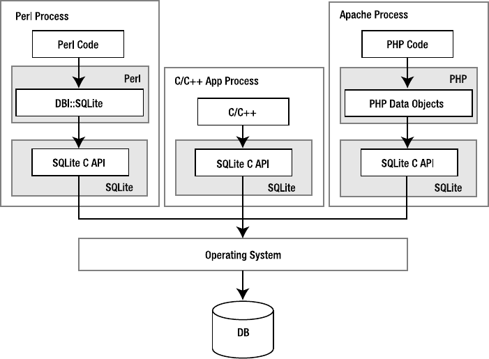
Consider the processes found in Figure 1-1. One is a Perl script, another is a standard C/C++
program, and the other is an Apache process with PHP, all using SQLite. The Perl script imports
the DBI::SQLite module, which in turn is linked to the SQLite C API, pulling in the SQLite library.
The PHP library works similarly, as does the C++ program. Ultimately, all three processes inter-
face with the SQLite C API. All three therefore have SQLite embedded in their process spaces,
and all three are independent database servers in and of themselves. Furthermore, even though
each process represents an independent server, they can still operate on the same database
file(s), as SQLite uses the operating system to manage synchronization and locking.
Today there is a wide variety of relational database products on the market specifically
designed for embedded use—products such as Sybase SQL Anywhere, InterSystems Caché,
Pervasive PSQL, and Microsoft’s Jet Engine. Some vendors have retrofitted their large-scale
databases to create embedded variants. Examples of these include IBM’s DB2 Everyplace,
Oracle’s 10g, and Microsoft’s SQL Server Desktop Engine. The open source databases MySQL
and Firebird both offer embedded versions as well. Of all these products, only two are both
open source and unencumbered by licensing fees: Firebird and SQLite. Of these remaining
two, only one is designed exclusively for use as an embedded database: SQLite.
Owens_6730 C01.fm Page 1 Monday, April 17, 2006 7:13 AM
www.it-ebooks.info
2CHAPTER 1 ■ INTRODUCING SQLITE
Figure 1-1. SQLite embedded in host processes
A Developer’s Database
SQLite is quite versatile. It is a database, a programming library, and a command-line tool, as
well an excellent learning tool that provides a good introduction to relational databases. There
are indeed many ways to use it—in embedded environments, websites, operating system
services, scripts, and applications. For programmers, SQLite is like digital duct tape, providing
an easy way to bind applications and their data. Like duct tape, there is no end to its potential
uses. In a web environment, SQLite can help with managing complex session information. Rather
than serializing session data into one big blob, individual pieces can be selectively written to
and read from individual session databases. SQLite also serves as a good stand-in relational
database for development and testing: there are no external RDBMSs or networking to configure,
or usernames and passwords to bother with. SQLite might also serve as a cache, hold configuration
data, or because of its binary compatibility across platforms, even work as an application
file format.
Besides being just a storage receptacle, SQLite can serve as a purely functional tool as well
for general data processing. Depending on size and complexity, it may be easier to represent
some application data structures as a table or tables in an in-memory database. This way, you
can operate on the data relationally, using SQLite to do the heavy lifting rather than having to
write your own algorithms to manipulate and sort data structures. If you are a programmer,
Owens_6730 C01.fm Page 2 Monday, April 17, 2006 7:13 AM
www.it-ebooks.info
CHAPTER 1 ■ INTRODUCING SQLITE 3
imagine how much code it would take to implement the following SQL statement in your
program:
SELECT AVG(z-y) FROM table GROUP BY x
HAVING x > MIN(z) OR x < MAX(y)
ORDER BY y DESC LIMIT 10 OFFSET 3;
If you are already familiar with SQL, imagine coding the equivalent of a subquery, compound
query, GROUP BY clause or multiway join—in C. SQLite embeds all of this functionality into your
application with minimal cost. With a database engine integrated directly into your code, you
can begin to think of SQL as a domain-specific language in which to implement complex
sorting algorithms in your program. This approach becomes more appealing as the size of your
data set grows or as your algorithms become more complex. What’s more, SQLite can be config-
ured to use a fixed amount of RAM and then offload data to disk if it exceeds the specified limit.
This is even harder to do if you write your own algorithms. With SQLite, this limit is instituted
with a single SQL command.
SQLite is also a great learning tool for programmers—a cornucopia for studying computer
science topics. From parser generators, tokenizers, virtual machines, B-tree algorithms, caching,
program architecture, and more, it is a fantastic vehicle for exploration of many well-established
computer science concepts. Its modularity, small size, and simplicity make it easy to present
each topic as an isolated case study that any one individual could easily follow.
An Administrator’s Database
But SQLite is not just a programmer’s database. It is a useful tool for system administrators as
well. It is small, compact, and elegant like a regular expression or a Unix utility such as find,
rsync, or grep. SQLite has a command-line utility that can be used within shell scripts. However,
it works even better with a large variety of scripting languages such as Perl, Python, and Ruby.
Together the two can help with a wide variety of tasks, such as aggregating log file data, monitoring
disk quotas, or performing bandwidth accounting in stateful firewalls. Furthermore, since SQLite
databases are ordinary operating system files, they are easy to work with, transport, and back up.
Also, SQLite is a convenient learning tool. It is an ideal beginner’s database with which to
learn about relational concepts. It can be installed quickly and easily on almost any platform,
and its database files share freely between them without the need for conversion. It is full
featured but not daunting. And it—both the program and the database—can be carried around
on a floppy disk or Universal Serial Bus (USB) stick.
SQLite History
SQLite was conceived on a battleship... well, sort of. SQLite’s author, D. Richard Hipp, was
working for General Dynamics on a program for the U.S. Navy developing software for use on
board guided missile destroyers. The program originally ran on Hewlett-Packard Unix (HPUX)
and used an Informix database as the back-end. For their particular application, Informix was
somewhat overkill. For an experienced database administrator (DBA), it could take almost an
entire day to install or upgrade. To the uninitiated application programmer, it might take forever.
What was really needed was a self-contained database that was easy to use and that could travel
Owens_6730 C01.fm Page 3 Monday, April 17, 2006 7:13 AM
www.it-ebooks.info
4CHAPTER 1 ■ INTRODUCING SQLITE
with the program and run anywhere regardless of what other software was or wasn’t installed
on the system.
In January 2000, Hipp and a colleague discussed the idea of creating a simple embedded
SQL database that would use the GNU DBM B-Tree library (gdbm) as a back-end, one that would
require no installation or administrative support whatsoever. Later, when some free time opened
up, Hipp started work on the project, and in August 2000, SQLite 1.0 was released.
As planned, SQLite 1.0 used gdbm as its storage manager. However, Hipp soon replaced
it with his own B-tree implementation that supported transactions and stored records in key
order. With the first major upgrade in hand, SQLite began a steady evolution, growing in both
features and users. By mid-2001 many projects—both open source and commercial alike—
started to use it. In the years that followed, other members of the open source community
started to write SQLite extensions for their favorite scripting languages and libraries. One by
one, new extensions—an Open Database Connectivity (ODBC) interface followed by exten-
sions for Perl, Python, Ruby, Java and other mainstays—fell into place and testified to SQLite’s
wide application and utility.
SQLite began a major upgrade from version 2 to 3 in 2004. Its primary goal was enhanced
internationalization supporting UTF-8 and UTF-16 text as well as user-defined text-collating
sequences. While 3.0 was originally slated for release in summer 2005, America Online provided
the necessary funding to see that it was completed by July 2004. Besides internationalization,
version 3 brought many other new features such as a revamped C API, a more compact format
for database files (a 25 percent size reduction), manifest typing, Binary Large Object (BLOB)
support, 64-bit ROWIDs, autovacuum, and improved concurrency. In spite of the many new
features, the overall library footprint was still less than 240 kilobytes. Another improvement in
version 3 was a good code cleanup—revisiting and rewriting, or otherwise throwing out extra-
neous stuff accumulated in the 2.x series.
SQLite continues to grow feature-wise while still remaining true to its initial design goals:
simplicity, flexibility, compactness, speed, and overall ease of use. At the time this book went
to press, SQLite added enforcement of CHECK constraints. Next on the docket are recursive trig-
gers and foreign keys. What’s next after that? Well, it all depends. Perhaps you or your company
will sponsor the next big feature that makes this little database even better.
Who Uses SQLite
Today, SQLite is used in a wide variety of software and products. It is used in Apple’s Mac OS X
operating system as a part of their CoreData application framework. It is also used in the system’s
Safari web browser, Mail.app email program, RSS manager, as well as Apple’s Aperture photog-
raphy software. SQLite can be found in Sun’s Solaris operating environment, specifically the
database backing the Service Management Facility that debuted with Solaris 10, a core compo-
nent of its predictive self-healing technology. SQLite is in the Mozilla Project’s mozStorage
C++/JavaScript API layer, which will be the backbone of personal information storage for
Firefox, Thunderbird, and Sunbird. SQLite has been added as part of the PHP 5 standard
library. It also ships as part of Trolltech’s cross-platform Qt C++ application framework, which
is the foundation of the popular KDE window manager, and many other software applications.
SQLite is especially popular in embedded platforms. Much of Richard Hipp’s SQLite-related
business has been porting SQLite to various proprietary embedded platforms. Symbian uses
SQLite to provide SQL support in the native Symbian OS platform. SQLite is also a core
Owens_6730 C01.fm Page 4 Monday, April 17, 2006 7:13 AM
www.it-ebooks.info
CHAPTER 1 ■ INTRODUCING SQLITE 5
component in the new Linux-based Palm OS, targeted for smart phones. It is also included in
commercial development products for cell phone applications.
Although it is rarely advertised, SQLite is also used in a variety of consumer products, as
some tech-savvy consumers have discovered in the course of poking around under the hood.
Examples include the D-Link Media Lounge, Slim Devices Squeezebox music player, and the
Philips GoGear personal music player. I recently saw online that some clever consumers found
a SQLite database embedded in the Complete New Yorker DVD set—a digital library of every
issue of the New Yorker magazine—apparently used by its accompanying search software.
You can find SQLite as an alternate back-end storage facility for a wide array of open source
projects such as Yum—the package manager for Fedora Core, Movable Type, DSPAM, Edgewall
Software’s excellent Trac SCM and project management system, and KDE’s Amarok audio
player, to name just a few. Even parts of SQLite’s core utilities can be found in other open source
projects. One such example is its Lemon parser generator, which the lighttpd web server project
uses for generating the parser code for reading its configuration file. Indeed there seems to be
such a variety of uses for SQLite that Google took notice and awarded Richard Hipp with “Best
Integrator” at O’Reilly’s 2005 Open Source Convention.
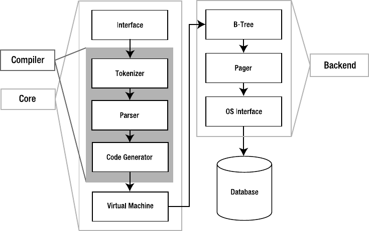
Architecture
SQLite has an elegant, modular architecture that takes some rather unique approaches to rela-
tional database management. It consists of eight separate modules grouped within three major
subsystems (as shown in Figure 1-2). These modules divide query processing into discrete tasks
that work like an assembly line. The top of the stack compiles the query, the middle executes it,
and the bottom handles storage and interfacing with the operating system.
Figure 1-2. SQLite’s architecture
Owens_6730 C01.fm Page 5 Monday, April 17, 2006 7:13 AM
www.it-ebooks.info
6CHAPTER 1 ■ INTRODUCING SQLITE
The Interface
The interface is the top of the stack and consists of the SQLite C API. It is the means through
which programs, scripting languages, and libraries alike interact with SQLite.
The Compiler
The compilation process starts with the tokenizer and parser. They basically work together to
take a Structured Query Language (SQL) statement in text form, validate its syntax, and then
convert it to a hierarchical data structure that the lower layers can more easily work with. SQLite’s
tokenizer is handcoded. Its parser is generated by SQLite’s custom parser generator, which is
called Lemon. The Lemon parser generator is designed for high performance and takes special
precautions to guard against memory leaks. Once the statement has been broken into tokens,
evaluated, and recast in the form of a parse tree, the parser passes the tree down to the code
generator.
The code generator translates the parse tree into a kind of assembly language specific to
SQLite. This assembly language is made up of instructions that are executable by its virtual
machine. The code generator’s sole job is to convert the parse tree into a complete mini-program
written in this assembly and hand it off to the virtual machine for processing.
The Virtual Machine
At the center of the stack is the virtual machine, also called the virtual database engine (VDBE).
The VDBE works on byte code—like a Java virtual machine or scripting language interpreter.
The VDBE’s byte code (or virtual machine language) consists of 128 opcodes, which are all
centered around database operations. The VDBE is a virtual machine designed specifically for
data processing. Every instruction in its instruction set either accomplishes a specific database
operation (like opening a cursor on a table, making a record, extracting a column, or beginning
a transaction) or manipulates the stack in some way to prepare for such an operation. All together
and in the right order, the VDBE’s instruction set can satisfy any SQL command, however
complex. Every SQL statement in SQLite—from selecting and updating rows to creating tables,
views, and indexes—is first compiled into this virtual machine language, forming a standalone
program that defines how to perform the given command. For example, take the statement
SELECT name FROM episodes LIMIT 10;
This compiles into the VDBE program shown in Listing 1-1.
Listing 1-1. VDBE Assembly
0 Integer 10 0
1 MustBeInt 0 0
2 Negative 0 0
3 MemStore 0 1
4 Goto 0 15
5 Integer 0 0
6 OpenRead 0 2
7 SetNumColumns 0 4
8 Rewind 0 13
Owens_6730 C01.fm Page 6 Monday, April 17, 2006 7:13 AM
www.it-ebooks.info
CHAPTER 1 ■ INTRODUCING SQLITE 7
9 MemIncr 0 13
10 Column 0 3
11 Callback 1 0
12 Next 0 9
13 Close 0 0
14 Halt 0 0
15 Transaction 0 0
16 VerifyCookie 0 190
17 Goto 0 5
18 Noop 0 0
The program consists of 18 instructions. These instructions, performed in this particular order
with the given operands, will return the name field of the first ten records in the episodes table
(which is a part of the example database included with this book).
In many ways the VDBE is the heart of SQLite: all of the modules above it work to create a
VDBE program, while all modules below it exist to execute that program, one instruction at a time.
The Back-end
The back-end is made up of the B-tree, page cache, and OS interface. The B-tree and page
cache (pager) work together as information brokers. Their currency is database pages, which
are uniformly sized blocks of data that, like freight cars, are made for transportation. Inside the
pages are the goods: more interesting bits of information such as records and columns and
index entries. Neither the B-tree nor the pager has any knowledge of the contents. They only
move and order pages; they don’t care what’s inside.
The B-tree’s job is order. It maintains many complex and intricate relationships between
pages, which keeps everything connected and easy to locate. It organizes pages into tree-like
structures (hence the name), which are highly optimized for searching. The pager serves the B-tree,
feeding it pages. Its job is transportation and efficiency. The pager transfers pages to and from
disk at the B-tree’s behest. Disk operations are by far the slowest thing a computer has to do.
Therefore, the pager tries to speed this up by keeping frequently used pages cached in memory
and thus minimizes the number of times it has to deal directly with the hard drive. It uses special
techniques to guess which pages will be needed in the future and thus gambles on the B-tree’s
behalf to keep pages flying as fast a possible. Also in the pager’s job description is transaction
management, database locking, and crash recovery. Many of these jobs are mediated by the
OS interface.
Things like file locking are often implemented differently in different operating systems.
The OS interface provides an abstraction layer that hides these differences from the other SQLite
modules. The end result is that the other modules see a single consistent interface with which
to do things like file locking. So the pager, for example, doesn’t have to worry about doing file
locking one way on Windows and doing it another way on different operating systems such as
Unix. It lets the OS interface worry about this. It just says to the OS interface “lock this file,” and
the OS interface figures out how to do that based on the operating system it happens to be
running on. The OS interface not only keeps code simple and tidy in the other modules, but it
also keeps the messy issues cleanly organized in one place. This makes it easier to port (adapt)
SQLite to different operating systems—all of the OS issues that must be addressed are clearly
identified and documented in the OS interface’s API.
Owens_6730 C01.fm Page 7 Monday, April 17, 2006 7:13 AM
www.it-ebooks.info
8CHAPTER 1 ■ INTRODUCING SQLITE
Utilities and Test Code
Miscellaneous utilities and common services such as memory allocation, string comparison,
and Unicode conversion routines are kept in the utilities module. This is basically a catchall
module for services that multiple modules need to use or share. The testing module contains a
myriad of regression tests designed to examine every little corner of the database code. This
module is one of the reasons SQLite is so reliable: it performs a lot of regression testing.
SQLite’s Features and Philosophy
SQLite offers a surprising range of features and capabilities despite its small size. It supports a
large subset of ANSI SQL92 (transactions, views, check constraints, correlated subqueries, and
compound queries) along with many other features found in relational databases, such as trig-
gers, indexes, autoincrement columns, and the LIMIT/OFFSET clause. It also has many unique
features, such as in-memory databases, dynamic typing, and something called conflict resolution
(explained in a moment).
As mentioned at the beginning of this chapter, SQLite has a number of governing principles
or characteristics that serve to more or less define its philosophy and implementation. Let’s
expand on these issues next.
Zero Configuration
From its initial conception, SQLite has been designed with the specific absence of a DBA in
mind. Configuring and administering SQLite is as simple as it gets. SQLite contains just enough
features to fit in a single programmer’s brain, and like its library, requires as small a footprint
in the gray matter as it does in RAM.
Portability
SQLite was designed specifically with portability in mind. It compiles and runs on Windows,
Linux, BSD, Mac OS X, commercial Unix systems such as Solaris, HPUX, and AIX, as well as
many embedded platforms such as QNX, VxWorks, Symbian, Palm OS, and Windows CE. It works
seamlessly on 16-, 32-, and 64-bit architectures with both big and little endian byte orders.
Portability doesn’t stop with the software either: SQLite’s database files are as portable as its
code. The database file format is binary compatible across all supported operating systems,
hardware architectures, and byte orders. You can create a SQLite database on a Sun SPARC
workstation and use it on a Mac or Windows machine—even cell phone—without any conversion
or modification. Furthermore, SQLite databases can hold up to 2 terabytes of data (limited only
by the operating system’s maximum file size) and natively support both UTF-8 and UTF-16
encoding.
Compactness
SQLite was designed to be lightweight and self-contained: one header file, one library, and you’re
relational, no external database server required. Everything—client, server, virtual machine—
packs into a tidy quarter megabyte, which at the moment is smaller than the home page of the
publishers of this book: www.apress.com (the home page weighing around 260 kilobytes). If you
Owens_6730 C01.fm Page 8 Monday, April 17, 2006 7:13 AM
www.it-ebooks.info
CHAPTER 1 ■ INTRODUCING SQLITE 9
really work at it and disable unneeded features at compile time, you can further shrink the
library down to under 170 kilobytes (on x86 hardware compiled with the GNU C compiler).
Furthermore, there is a proprietary version of SQLite that is as small is 69 kilobytes, capable of
running on smart cards (see the “Additional Information” section for more details).
Equally compact are SQLite databases. They are ordinary operating system files. Regard-
less of your system, all objects in your SQLite database—tables, triggers, schema, indexes, and
views—are contained in a single operating system file. Furthermore, SQLite uses variable-length
records, allocating only the minimum amount of data needed to hold each field. A 2-byte field
sitting in a varchar(100) column only takes up 3 bytes of space, not 100 (the extra byte is used
to record its type information).
Simplicity
As a programming library, SQLite’s API is one of the simplest and easiest to use. The API is both
well documented and intuitive. It is designed to help you customize SQLite in many ways, such
as implementing your own custom SQL functions in C. Better yet, the open source community
has a created a vast number of language and library interfaces with which to use SQLite. There
are extensions for Perl, Python, Ruby, Tcl/Tk, Java, PHP, Visual Basic, ODBC, Delphi, Microsoft
.NET, Smalltalk, Ada, Objective C, Eiffel, Rexx, Lisp, Scheme, Lua, Pike, Objective Camel, Qt,
WxWindows, REALBASIC, and others. An exhaustive list can be found on the SQLite Wiki:
www.sqlite.org/cvstrac/wiki?p=SqliteWrappers.
Architecturally, SQLite has a modular design. This design includes many innovative ideas
that enable it to be full featured and extensible while at the same time retaining a great degree
of simplicity throughout its code base. Each module is a specialized, independent system that
performs a specific task. This modularity makes it much easier to develop each system indepen-
dently, and to debug queries as they pass from one module to the next—from compilation and
planning to execution and materialization. The end result is that there is a crisp, well-defined
separation between the front-end (SQL compiler) and back-end (storage system), allowing the
two to be coded independently of each other. This design makes it easier to add new features
to the database engine, is faster to debug, and results in better overall reliability.
Flexibility
Several factors work together to make SQLite a very flexible database. As an embedded database,
it offers the best of both worlds: the power and flexibility of a relational database front-end,
with the simplicity and compactness of a B-tree back-end. With it, there are no large database
servers to configure, no networking or connectivity problems to worry about, no platform limi-
tations, no baroque APIs to learn, and no license fees or royalties to pay. Rather, you get simple
SQL support dropped right into your application.
Liberal Licensing
All of SQLite’s code is in the public domain. There is no license. No claim of copyright is made
on any part of the core source code. All contributors to this code are required to sign affidavits
specifically disavowing any copyright interest in contributed code. Thus there are no legal
restrictions on how you may use the source code in any form: you can modify, incorporate,
distribute, sell, and use the code for any purpose—commercial or otherwise—without any
royalty fees or restrictions.
Owens_6730 C01.fm Page 9 Monday, April 17, 2006 7:13 AM
www.it-ebooks.info
10 CHAPTER 1 ■ INTRODUCING SQLITE
Reliability
But the source code is more than just free; it also happens to be well written. SQLite’s code base
consists of about 30,000 lines of standard ANSI C, which is clean, modular, and well commented.
It is designed to be approachable, easy to understand, easy to customize, and generally very
accessible. It is easily within the ability of a competent C programmer to follow any part of
SQLite or the whole of it with sufficient time and study.
Additionally, SQLite’s code offers a full-featured API specifically for customizing and
extending SQLite through the addition of user-defined functions, aggregates, and collating
sequences along with support for operational security.
While SQLite’s modular design significantly contributes to its overall reliability, its
source code is also well tested. Whereas the core software (library and utilities) consists of
about 30,000 lines of code, the distribution also includes an extensive test suite consisting of
over 30,000 lines of regression test code, which covers over 97 percent of the core code. That is,
over half of the SQLite project’s total code is devoted exclusively to regression testing. Another
way of saying this is for every line of database code written, there is approximately one line of
test code written as well.
Convenience
SQLite also has a number of unique features that provide a great degree of convenience. These
include dynamic typing, conflict resolution, and the ability to “attach” multiple databases to a
single session.
SQLite’s dynamic typing is somewhat akin to that found in scripting languages (e.g., “duck
typing” in Ruby). Specifically, the type of a variable is determined by its value, not by a declara-
tion as employed in statically typed languages. You could say that where most database systems
work like statically typed languages, SQLite works like a dynamically typed language. That is,
most database systems restrict a field’s value to the type declared in its respective column. For
example, each field in an integer column can hold only integers. In SQLite, while a column can
have a declared type, fields are free to deviate from them, just as a variable in a scripting language
can be reassigned a value with a different type. This can be especially helpful for prototyping:
since SQLite does not force you to explicitly change a column’s type, you need only change
how your program stores information in that column rather than continually having to update
the schema and reload your data.
Conflict resolution is another unique feature. It can make writing SQL, as easy as it is, even
easier. This feature is built into many SQL operations and can be made to perform what I call
“lazy updates.” Say you have a record you need to insert, but you are not sure whether one just
like it already exists in the database. Rather than write a SELECT statement to look for a match, and
then recast your INSERT to an UPDATE if it does, conflict resolution lets you say to SQLite, “Here, try
to insert this record, and if you find one with the same key, just update it with these values
instead.” Now you’ve gone from having to code three different SQL statements to cover all the
bases (i.e., SELECT, INSERT, and possibly UPDATE) to just one: INSERT ON CONFLICT REPLACE (...).
Better yet, you can build this conflict resolution into the table definition itself and dispense with
Owens_6730 C01.fm Page 10 Monday, April 17, 2006 7:13 AM
www.it-ebooks.info
CHAPTER 1 ■ INTRODUCING SQLITE 11
the need to ever specify it again on future INSERT statements. In fact, you can dispense with
ever having to write UPDATE statements to this table again—just write INSERT statements and let
SQLite do the dirty work of figuring out what to do using the conflict resolution rules defined in
the schema.
Finally, SQLite lets you “attach” external databases to your current session. Say you are
connected to one database (foo.db) and need to work on another (bar.db). Rather than opening
a separate connection and fumbling back and forth between them, you can simply attach the
database of interest to your current connection with a single SQL command:
ATTACH database bar.db as bar;
All of the tables in bar.db are now accessible as if they existed in foo.db. You can detach it just
as easily when you’re done. This makes all sorts of things like copying tables between databases
even easier than it already is.
Performance and Limitations
SQLite is a speedy database. But the words “speedy,” “fast,” “peppy,” or “quick” are rather
subjective, ambiguous terms. To be perfectly honest, there are things SQLite can do quicker
than other databases, and there are things that it cannot. Suffice it to say, within the parameters
for which it has been designed, SQLite can be said to be consistently fast and efficient across
the board. SQLite uses B-trees for indexes and B+-trees for tables, the same as most other data-
base systems. For searching a single table, it is as fast if not faster than any other database on
average. Simple SELECT, INSERT, and UPDATE statements are extremely quick—virtually at the
speed of RAM (for in-memory databases) or disk. Here SQLite is often faster than other data-
bases, as it has less overhead to deal with in starting a transaction or generating a query plan,
and it doesn’t incur the overhead of making a network call to the server. Its simplicity here
makes it fast. As queries become larger and more complex, however, query time overshadows
the network call or transaction overhead, and the game goes to the database with the best opti-
mizer. This is where larger, more sophisticated databases begin to shine. While SQLite can
certainly do complex queries, it does not have a sophisticated optimizer or query planner. It
knows how to use indexes to be sure, but it doesn’t keep elaborate table statistics. If you perform
a 17-way join, SQLite will join the tables and give you the result. What it won’t do is try to determine
optimal paths by computing various alternate query plans and selecting the fastest candidate, as
you might expect from Oracle or PostgreSQL. Thus if you are running complex queries on large
data sets, odds are that SQLite is not going to be as fast as databases with sophisticated query
planners.
So there are situations where SQLite is not as fast as larger databases. But many if not all
of these conditions are to be expected. SQLite is an embedded database designed for small to
medium-sized applications. These limitations are in line with its intended purpose. Many new
users make the mistake of assuming that they can use SQLite as a drop-in replacement for
larger relational databases. Sometimes you can; sometimes you can’t. It all depends on what
you are trying to do.
Owens_6730 C01.fm Page 11 Monday, April 17, 2006 7:13 AM
www.it-ebooks.info
12 CHAPTER 1 ■ INTRODUCING SQLITE
In general, there are three major variables that define SQLite’s main limitations. These
variables are:
•Concurrency. SQLite has coarse-grained locking, which allows multiple readers but
only one writer at a time. Writers exclusively lock the database during writes and no one
else has access during that time. SQLite does take steps to minimize the amount of time
in which exclusive locks are held. Generally, locks in SQLite are kept for only a few milli-
seconds. But as a general rule of thumb, if your application has high write concurrency
(many connections competing to write to the same database) and it is time critical, you
probably need another database. It is really a matter of testing your application to know
what kind of performance you can get. I have seen SQLite handle over 500 transactions
per second for 100 concurrent connections in simple web applications. But even the
notion of a transaction is vague. Transactions are a function of the number of records
being modified, as well as the number and complexity of the queries involved. Acceptable
concurrency all depends on your particular application, and can only be determined
empirically by direct testing. In general, this is true with any database: you don’t know
what kind of performance your application will get until you do real-world tests.
•Database size. While SQLite’s databases can scale to 2 terabytes, there are memory
(RAM) costs associated with large databases. When SQLite begins a transaction, it allo-
cates a bitmap for tracking dirty pages, which assists in managing its rollback journal. To
do this, it requires 256 bytes of RAM for every 1MB of database. Thus, when databases
become very large, the size of the bitmap allocated in each transaction can become
significant. A 100GB database would require 25MB of RAM to be allocated before each
transaction. This directly affects the rate at which transactions can be performed regardless
of their complexity. So in reality, the practical limits on database size are in the tens of
gigabytes. They can be much bigger, but keep in mind that the overhead associated with
transaction startup will increase linearly with the database size.
•Networking. While SQLite databases can be shared over network file systems, the latency
associated with such file systems can cause performance to suffer. Worse, bugs in network
file system implementations can also make it error prone. If the file system’s locking
does not work properly, two clients may be allowed to simultaneously modify the same
database file, which will almost certainly result in database corruption. It is not that
SQLite is incapable of working over a network file system because of anything in its
implementation—indeed, it uses standard locking mechanisms such as POSIX advisory
locks on Unix and the equivalent system calls on Windows. Rather, it is simply impos-
sible for SQLite to officially confirm that any given network file system is without bugs
that may adversely affect its operation. It has been claimed that certain network file system
implementations (such are Solaris NFS v4) work just fine and reliably implement the
requisite locking mechanisms needed by SQLite. However, the SQLite developers have
neither the time nor resources to certify that any given network file system works flawlessly
in all cases. Therefore, the official position is that it is safe to use SQLite over a network
file system only if there is no more than one connection operating on a given database at
a time—which is to say when no locking is required.
Owens_6730 C01.fm Page 12 Monday, April 17, 2006 7:13 AM
www.it-ebooks.info
CHAPTER 1 ■ INTRODUCING SQLITE 13
Again, most of these limitations are intentional—they are a result of SQLite’s design.
Supporting high write concurrency, for example, brings with it great deal of complexity and
this runs counter to SQLite’s simplicity in design. Similarly, being an embedded database,
SQLite intentionally does not support networking. This should come as no surprise. In short,
what SQLite can’t do is a direct result of what it can. It was designed to operate as a modular,
simple, compact, and easy-to-use embedded relational database whose code base is within the
reach of the programmers using it. And in many respects it can do what many other data-
bases cannot, such as run in embedded environments where actual power consumption is a
limiting factor.
While SQLite’s SQL implementation is quite good, there are some things it currently does
not implement. These are as follows:
•Foreign key constraints. Foreign keys are the foundation of referential integrity in relational
databases. While SQLite parses them, it currently does not have support for foreign keys.
It does support check constraints, and foreign key support is estimated to be completed
by sometime in 2006.
•Complete trigger support. There is some support for triggers but it is not complete. Missing
features include FOR EACH STATEMENT triggers (currently all triggers must be FOR EACH ROW),
INSTEAD OF triggers on tables (currently INSTEAD OF triggers are only allowed on views),
and recursive triggers—triggers that trigger themselves. Recursive triggers are needed in
order to implement foreign key constraints.
•Complete ALTER TABLE support. Only the RENAME TABLE and ADD COLUMN variants of the
ALTER TABLE command are supported. Other kinds of ALTER TABLE operations such as
DROP COLUMN, ALTER COLUMN, and ADD CONSTRAINT are not implemented.
•Nested transactions. SQLite allows only a single transaction to be active at one time.
Nested transactions allow for fine-grained control over larger, more complex operations
in that parts of a transaction can be defined and rolled back in case of an error rather
than the entire transaction.
•RIGHT and FULL OUTER JOIN. LEFT OUTER JOIN is implemented, but RIGHT OUTER JOIN
and FULL OUTER JOIN are not. LEFT OUT JOIN can be implemented as a right outer join by
simply reversing the order of the tables and modifying the join constraint. Furthermore,
FULL OUTER JOIN can be implemented as a combination of other relational operations
supported by SQLite.
•Updatable views. VIEWs in SQLite are read-only. You may not execute a DELETE, INSERT,
or UPDATE statement on a view. But you can create a trigger that fires on an attempt to
DELETE, INSERT, or UPDATE a view and do what you need in the body of the trigger.
•GRANT and REVOKE. Since SQLite reads and writes an ordinary disk file, the only access
permissions that can be applied are the normal file access permissions of the underlying
operating system. GRANT and REVOKE commands in general are aimed at much higher-
end systems where there are multiple users who have varying access levels to data in the
database. In the SQLite model, the application is the main user and has access to the
entire database. Access in this model is defined at the application level—specifically,
what applications have access to the database file.
Owens_6730 C01.fm Page 13 Monday, April 17, 2006 7:13 AM
www.it-ebooks.info
14 CHAPTER 1 ■ INTRODUCING SQLITE
In addition to what is listed here, there is a page on the SQLite Wiki devoted to reporting
unsupported SQL. It is located at www.sqlite.org/cvstrac/wiki?p=UnsupportedSql.
Who Should Read This Book
As SQLite has many uses, it also has many audiences. Whether you are a programmer, web
developer, systems administrator, or just casual user looking to learn about relational databases,
this book aims at helping you understand and get the most out of your particular use for SQLite.
SQLite is a terrific database to start on if you are new to relational databases. For new data-
base users, this book assumes nothing. If you have never touched a relational database before,
if you have never issued a single SQL statement, this book will help you not only get started
with SQLite but also become a competent user of SQL. It will prepare you to get the most out of
SQLite, as well as provide you with a good foundation with which to move on to larger relational
systems and explore more advanced features and topics.
For programmers, this book assumes only that you know the programming language in
which you intend to use SQLite. Furthermore, it does more than document APIs. If anything,
that is the least of what it does, as API documentation only illustrates how an interface works.
As with any database, you have to have some idea of how that database works internally to get
the most out of it. Every database has unique architectural aspects, specific relational features,
and important limitations, all of which good programmers learn about and take into consider-
ation when writing their code. SQLite, though simple and straightforward, is no exception. As
a programmer, you need to know something about how it processes data internally to get it to
work well with your application. This book shows you how. It covers the API and explores how
it works in relation to SQLite’s architecture, allowing C programmers, web developers, and
scriptwriters alike to write more informed code. This helps you better understand not only
what SQLite can do, but also what it can’t. Your knowledge of the architecture will tell you better
than any list of rules when SQLite is or isn’t a good fit for what you are trying to accomplish.
You’ll know if, when, and where you need to consider another approach.
And that underscores one of the most important aims in this book: to teach concepts over
recipes—to adequately address both how and why. There simply is no substitute for conceptually
understanding how something works. To that end, this book includes both historical and theoret-
ical material where appropriate to help frame complicated, technical, or abstract concepts. At
the same time, it tries to be ruthlessly practical. Intermixed in the writing are many figures and
examples designed specifically to illustrate the topics at hand and provide real-world value.
To help accommodate both those who want to know why in addition to those who want to
know how, the theoretical and the practical are arranged orthogonally in chapters. Those who
don’t care for theory can simply skip past the theoretical chapters. While the practical chapters
draw on some of this material, they are in no way dependent upon them.
How This Book Is Organized
This book is divided into three parts: SQLite the database, SQLite the programming library, and
reference material. The database aspects of SQLite are covered in Chapters 2, 3, and 4. The
programming aspects of SQLite are covered in Chapters 5–8. A brief chapter outline is as follows:
Owens_6730 C01.fm Page 14 Monday, April 17, 2006 7:13 AM
www.it-ebooks.info
CHAPTER 1 ■ INTRODUCING SQLITE 15
Chapter 1, “Introducing SQLite,” introduces the main features of SQLite, its origin and
history, as well as the scope and objectives of this book.
Chapter 2, “Getting Started,” covers how to obtain and use SQLite. It illustrates how to get
SQLite in binary and source form, as well as how to compile and build it on a variety of
platforms. It explains how to use the SQLite command-line utility to create and work with
databases.
Chapter 3, “The Relational Model,” provides some background behind SQL. It illustrates
the historical and theoretical basis that led to the formation of SQL and helps explain why
it is the way it is today. It highlights the 30-year history of the relational model in the context
of Codd’s famous 12 rules.
Chapter 4, “SQL,” provides a complete introduction to SQL as implemented by SQLite. It
assumes no prior experience with SQL. It starts with the fundamentals and works through
constructing complex queries and explores every aspect of all commands in SQLite’s SQL
implementation.
Chapter 5, “Design and Concepts,” lays the groundwork for programming with SQLite.
It illustrates the SQLite API, its architecture, and how the two work in relation to one another.
It addresses important topics related to programming such as transactions and locking.
It provides programmers of all languages with a clear understanding of how SQLite works
internally and what to keep in mind when writing programs that use it.
Chapter 6, “The Core C API,” covers the part of the SQLite C API related to executing
queries. From connecting to databases, executing queries, obtaining data, and managing
transactions, this chapter covers all parts of the API related to query and data processing.
Chapter 7, “The Extension C API,” covers the remaining part of the C API devoted to custom-
izing and extending SQLite. SQLite provides facilities for implementing user-defined SQL
functions, aggregates, and collations. This chapter illustrates how to implement each of
these features and provides practical examples of their use.
Chapter 8, “Language Extensions,” uses the basic concepts outlined in Chapter 5 and
provides a concise introduction to SQLite programming in six popular languages: Perl,
Python, Ruby, Java, Tcl, and PHP.
Chapter 9, “SQLite Internals,” explores the inner workings of SQLite. It is a high-level over-
view of the source code and provides a glimpse into how the major subsystems are imple-
mented. This provides programmers with a deeper understanding of SQLite’s design
decisions, assumptions, and trade-offs, as well as a point of departure for developers who
want to work on SQLite.
Finally, complete references for the SQLite C API and SQL syntax are included in the
appendices.
Owens_6730 C01.fm Page 15 Monday, April 17, 2006 7:13 AM
www.it-ebooks.info

16 CHAPTER 1 ■ INTRODUCING SQLITE
DATABASE EXAMPLES
The example databases accompanying this book are available online and can be downloaded from the Apress
website (www.apress.com). Each database is in SQL format and you can simply follow the procedures
covered in Chapter 2 to create them using the SQLite command-line program. The example databases are
further explained and illustrated as they are introduced in this book.
The source code for all examples is also available online. All examples compile and run on both Windows
and Unix. For each example, makefiles are included for Unix environments and Visual C++ projects have been
created for Windows users. MinGW users can use the Unix makefiles.
Additional Information
The SQLite website has a wealth of information, including the official documentation, mailing
lists, Wiki, and other general information. It is located at www.sqlite.org. The SQLite community is
very helpful, and you may find everything you need on SQLite’s mailing list. Additionally, SQLite’s
author offers professional training and support for SQLite, which includes custom program-
ming (porting to embedded platforms, etc.), and enhanced versions of SQLite, which include
native encryption and extremely small versions optimized for embedded applications. More
information can be found at www.hwaci.com/sw/sqlite/prosupport.html.
Summary
SQLite is not to be confused with other larger databases like Oracle or PostgreSQL. Whereas
dedicated relational databases such as these are electronic backhoes, SQLite is a digital Swiss
Army Knife. Whereas large-scale dedicated relational databases are designed for thousands of
users, SQLite is designed for thousands of uses. It is more than a database. Although a tool in
its own right, it is a tool for making tools as well. It is a true utility, engineered to enable you—
the programmer, user, or administrator—to quickly and easily shape those disparate piles of
data into order, and manipulate them to your liking with minimal effort.
SQLite is public domain software. Free. You can do anything with it or its source code you
like. No licenses, no install programs, no restrictions. Just copy and run. It is also portable, well
tested, and reliable. It has a clean, modular design that helps keep the system simple, easy to
develop, and easy to debug. In addition to good design, it has good testing. There is more code
written to test SQLite than there is SQLite code to test. It should not be too surprising, then,
that SQLite has proven itself to be a solid, reliable database over its five-year history.
Finally, SQLite is fun. At least I think so. It is a unique and interesting piece of software that
I have found many uses for over the years. I hope that you will find it equally useful and enjoyable.
If you have any comments or suggestions on this book or its examples, please feel free
to send me an email at sqlitebook@gmail.com. I will also keep additional information related to
the book at www.mikesclutter.com.
Owens_6730 C01.fm Page 16 Monday, April 17, 2006 7:13 AM
www.it-ebooks.info

17
■ ■ ■
CHAPTER 2
Getting Started
On the whole, it’s easy to begin using SQLite no matter what operating system you are using.
For the vast majority of users, SQLite can be installed and running with a new database in hand
in under 5 minutes, regardless of experience. This chapter covers everything you need to know
in order to install SQLite and work with databases. You will have a working knowledge of where
to obtain SQLite software or source code and how to install or compile it on multiple platforms.
By the time you finish this chapter, you will have a new SQLite database with tables, views, and
indexes that you can query, back up, and restore. Furthermore, you will learn everything you
need to know about managing SQLite databases, including how to create, view, and examine
their contents. Finally, you will be introduced to several tools with which to work with SQLite
in various environments. This chapter does include some examples that use SQL to introduce
the SQLite command-line program. If you are not yet familiar with SQL, you should still be able
to follow the examples without much trouble. SQL is addressed in detail in Chapter 4.
Where to Get SQLite
The SQLite website (www.sqlite.org) provides both precompiled binaries of SQLite as well as
source code. Binaries are available for both Windows and Linux.
There are several binary packages to choose from, each of which is specific to a particular
way of using SQLite. The binary packages are as follows:
•Statically linked command-line program (CLP). This version of the SQLite command-
line program has the database engine compiled in and is a self-contained, standalone
program. This provides a convenient way to work with SQLite databases from the command
line without having to worry about whether or not the SQLite shared library is installed
on your system or located in the right place.
•SQLite dynamic link library (DLL). This is the SQLite database engine packaged into a
shared library, or Windows DLL. Use this with programs that dynamically link to SQLite.
This form makes it easier to upgrade SQLite without having to recompile the software
that depends on it.
•Tcl extension. This is a Tcl extension library that enables you to connect to SQLite from
within the Tcl language. SQLite’s author, Richard Hipp, happens to be the author and
maintainer for the Tcl extension.
Owens_6730 C02.fm Page 17 Tuesday, April 11, 2006 1:01 PM
www.it-ebooks.info
18 CHAPTER 2 ■ GETTING STARTED
SQLite’s source code is provided in two forms that vary by platform. One form is for
compiling on Windows and the other is for compiling on POSIX platforms such as Linux, BSD,
and Solaris. The source code itself does not differ between source distributions. Rather, the two
distributions simply include different conveniences that make it easier to work within their
respective environments. The Windows distribution, for example, has the preprocessing and
code generation performed by GNU Autoconf and other associated Unix build tools already
added to the source files, freeing Windows users from having to bother with them.
SQLite on Windows
Whether you are using SQLite as an end user, or you are writing programs that use it, SQLite
can be installed on Windows with a minimum of fuss. In this section, we will cover all the options—
from installing the available binary packages to building everything from source using the most
popular compilers. Let’s start with the easy things first and progress to things more technically
challenging.
Getting the Command-Line Program
The SQLite command-line program (hereafter referred to as the CLP) is by far the easiest way
to get started using SQLite. Follow these steps to obtain the CLP:
1. Open your favorite browser and navigate to the SQLite home page: www.sqlite.org.
2. Click the download link on the top right of the page. This will take you to the
download page.
3. Under the section Precompiled Binaries For Windows, there should be a file whose
name is of the form sqlite-3_x_y.zip, where x and y are the minor version numbers.
There should be a comment beside it that reads A command-line program for accessing
and modifying SQLite databases. Download this file to a temporary folder.
4. Unzip the file. In Windows XP and Me, you can right-click on the file and a context
menu should appear. Select Extract All from the menu. This will bring up the Windows
Extraction Wizard. Follow the instructions and extract the file to a folder of your choosing.
The wizard will then place a copy of the statically linked CLP in the specified folder. The
file’s name should be sqlite3.exe. If you have an older version of Windows, you may
need to obtain a compression utility, such as WinZip (www.winzip.com), to unzip the file.
To run the CLP from any directory in the Windows shell, you need to copy it to a folder
that is in your Windows system path. A suitable default that should work on all versions
of Windows is the \windows\system32 folder on your root partition (C:\ for most systems).
Owens_6730 C02.fm Page 18 Tuesday, April 11, 2006 1:01 PM
www.it-ebooks.info
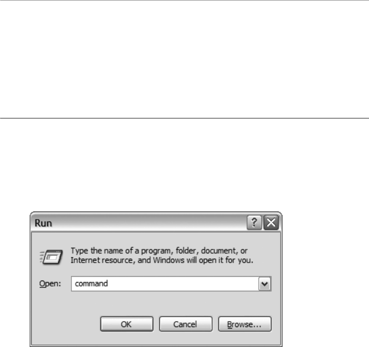
CHAPTER 2 ■ GETTING STARTED 19
■Note If you don’t know what your Windows system path is, here is how to find it. Click Start ➤ Control
Panel. (If you are using Windows XP, look at the Control Panel dialog box at the left side of the window. It will
either say “Switch to Classic View” or “Switch to Category View.” If you see the former, then click it. This will
put the view into Classic View.) Double-click the System icon. In the resulting dialog box, select the Advanced
tab and click the Environmental Variables button. In the System Variables list box, double-click the Path entry.
This will open the Edit System Variables dialog box. The Values text box contains a long list of paths delimited
by semicolons. All of the folders listed here are part of your system path. You can add an additional folder to
this path if you like by simply appending a semicolon to the end of the line and typing the new path.
5. Open a command shell. You can do this different ways, depending on your version of
Windows. Using the Windows Start menu, select Start ➤ Run. Type cmd in the Open
drop-down box (or command if you are using a version of Windows 98/Me). Click OK
(Figure 2-1). This will open a Windows command shell. If this doesn’t work, try going
to Start ➤ All Programs ➤ Accessories ➤ Command Prompt.
Figure 2-1. Opening a Windows command shell
6. Within the shell, type sqlite3 on the command line and press Enter. This should bring
up a SQLite command prompt. (If you get an error, then the sqlite3.exe executable has
not been copied to a folder in your system path. Recheck your path, and place a copy of
the program somewhere within it.) When the SQLite shell appears, type .help on the
command line. This will display a list of commands with their associated descriptions
similar to the one in Figure 2-2. Type .exit to exit the program. You now have a working
copy of the SQLite CLP installed on your system.
Owens_6730 C02.fm Page 19 Tuesday, April 11, 2006 1:01 PM
www.it-ebooks.info
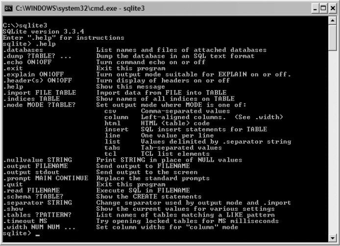
20 CHAPTER 2 ■ GETTING STARTED
Figure 2-2. The SQLite shell on Windows
If you are especially eager to work with SQLite at this point, you may want to skip ahead to
the section “The CLP in Shell Mode;” the next few sections are geared to developers who want
to write programs that use SQLite.
Getting the SQLite DLL
The SQLite DLL is used for software that has been compiled to link dynamically to SQLite. Most
software that uses SQLite in this fashion usually includes its own copy of the SQLite DLL and
installs it automatically with the software.
If you are going to be programming with SQLite, using the DLL is probably the easiest way
to start. The SQLite DLL can be obtained as follows:
1. Go to the SQLite home page, www.sqlite.com. On the upper right of the page, click the
download link. This will take you to the download page.
2. On the download page, find the section Precompiled Binaries For Windows.
3. Locate the DLL zip file. This file will have the description This is a DLL of the SQLite
library without the TCL bindings. The filename will have the form sqlitedll-3_x_y.zip,
where x and y are the minor versions. If you want Tcl support included, select the file
with the name of the form tclsqlitedll-3_x_y.zip.
Owens_6730 C02.fm Page 20 Tuesday, April 11, 2006 1:01 PM
www.it-ebooks.info
CHAPTER 2 ■ GETTING STARTED 21
4. Download and unzip the file. The extracted contents should include two files: the
actual DLL file (sqlite3.dll) accompanied by another file called sqlite3.def. The
SQLite DLL provided here is thread safe. That is, it was compiled with the THREADSAFE
preprocessor flag defined. You can therefore use this DLL in multithreaded programs.
In order to use the DLL, it needs to be either in the same folder with programs that use it or
placed somewhere in the system’s path (see the note on the Windows System path in the
previous section).
If you want to write programs that use the SQLite DLL, you will need to create an import
library with which to link your programs. This is quite simple to do using the sqlite3.def
mentioned earlier. If you are using Microsoft Visual C++, open a shell, change the directory to
the SQLite distribution, and simply run the command
LIB /DEF:sqlite3.def
If you are using MinGW (see the section “Building SQLite with MinGW” later in this chapter),
run the command
dlltool --def sqlite3.def --dllname sqlite3.dll --output-lib sqlite3.lib
Running either of these commands will create an import library called sqlite3.lib with which
you can link your programs. By linking your programs to this import library, they will load and
use the SQLite DLL upon execution.
Compiling the SQLite Source Code on Windows
Building SQLite from source within Windows is straightforward. Depending on the compiler
you are using and what you are trying to achieve, there are several approaches to compiling
SQLite. The most common scenarios on Windows include using either Microsoft Visual C++ or
MinGW. Both are addressed here. Information on how to compile SQLite with other compilers
can be found on the SQLite Wiki (www.sqlite.org/cvstrac/wiki?p=HowToCompile).
The Stable Source Distribution
Stable versions of SQLite’s source code can be obtained in zip files from the SQLite website.
Bleeding-edge versions can be obtained from anonymous CVS. Unless you are familiar with
CVS, using the source distribution is the easiest way to go. To download a stable source distri-
bution, follow these steps:
1. Go to the SQLite website, www.sqlite.org. Follow the download link, which will take
you to the download page.
2. On the download page, find the Source Code section.
3. The first two files should be zip files containing the source code for Windows. The file
you want to download should have a name with the form sqlite-source-3-x_y.zip,
where x and y are the minor version numbers. The important thing here is that you
want sqlite-source-3-x_y.zip, which corresponds to SQLite version 3, not
sqlite-source2-x_y.zip, which corresponds to SQLite version 2.
Owens_6730 C02.fm Page 21 Tuesday, April 11, 2006 1:01 PM
www.it-ebooks.info

22 CHAPTER 2 ■ GETTING STARTED
■Note The Windows zip archive and the other (POSIX) tarballs on the download page differ slightly in their
contents. While they contain identical source code, the SQLite distribution uses some POSIX build tools (sed,
awk, etc.) to dynamically generate some C source code in the build process. These build tools are not available
by default on Windows systems. Therefore, the Windows source archive includes all of the preprocessing and
generated code as a matter of convenience to Windows users who lack the build support infrastructure of
Unix. This is why Windows users should use the zip archives rather than the POSIX tarballs on the download
page. It is still possible to build the tarballs on Windows, but you need the requisite POSIX build tools (which
are included in the MSYS/MinGW distributions covered in a moment).
4. Extract/unzip the file to a directory of your choosing. The extracted contents will be the
complete SQLite version 3 source code for Windows.
Anonymous CVS
If you want to play with the latest features or participate in SQLite development, then retrieving
SQLite from anonymous CVS makes the most sense. Anonymous CVS provides read access to
the CVS repository—you can check out the code but you cannot commit any changes you may
make in your local copy back to the repository. CVS allows you to maintain the absolutely latest
version of the SQLite source code. If you want, you can keep your copy of the code synced up
to the day, hour, or minute to stay current with changes as they are committed. Thus, if you see
an important bug fix or feature posted that you want to take advantage of, all you need to do
is perform a CVS update and recompile your copy of the code. Also note that the version in
CVS corresponds to that found in the POSIX tarballs: it still requires the code-generation and
preprocessing steps before the code can be built under Windows. You must therefore have the
requisite POSIX build tools mentioned in the previous note in order to build SQLite from CVS
on Windows.
Obtaining SQLite from CVS on Windows is perhaps easiest by using WinCVS. WinCVS
(shown in Figure 2-3) is a well-written graphical application that makes working with CVS
repositories easy and intuitive. WinCVS can be obtained at www.wincvs.org.
Owens_6730 C02.fm Page 22 Tuesday, April 11, 2006 1:01 PM
www.it-ebooks.info
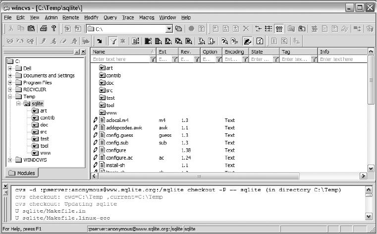
CHAPTER 2 ■ GETTING STARTED 23
Figure 2-3. WinCVS
Once it’s installed, you can configure WinCVS to connect to SQLite’s CVS repository
as follows:
1. Create a folder in which to check out the SQLite source code (e.g., C:\Temp).
2. Open WinCVS. On the left pane, navigate to the folder you created.
3. From the main menu, select Admin ➤ Login. In the CVSROOT text box, type
:pserver:anonymous@www.sqlite.org:/sqlite, and click OK. This will bring up a dialog
box requesting the home folder. Use the folder you created earlier (C:\Temp in this example).
Next a password dialog box will appear. For the password, enter “anonymous”, and click
OK. If you log in successfully, then the output pane will display the following:
cvs -d :pserver:anonymous@www.sqlite.org:/sqlite login
Logging in to :pserver:anonymous@www.sqlite.org:2401:/sqlite
***** CVS exited normally with code 0 *****
4. In the main menu, select Remote ➤ Checkout Module (Figure 2-4). In the
Module Name And Path On Server box, type sqlite. In the CVSROOT box,
type :pserver:anonymous@www.sqlite.org:/sqlite.
Owens_6730 C02.fm Page 23 Tuesday, April 11, 2006 1:01 PM
www.it-ebooks.info
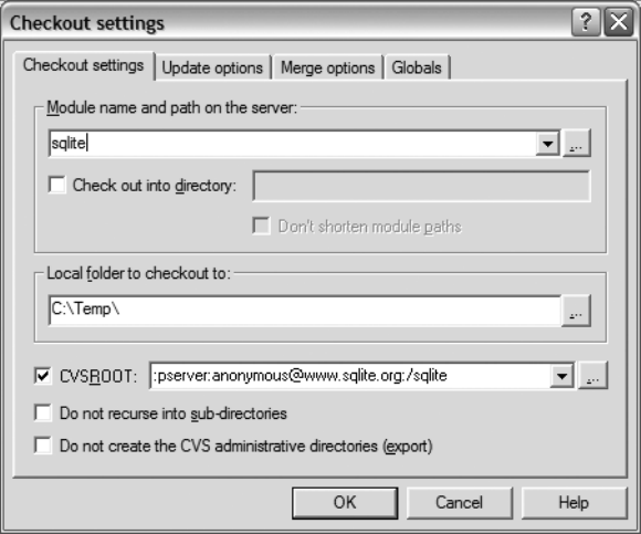
24 CHAPTER 2 ■ GETTING STARTED
Figure 2-4. WinCVS Checkout Settings dialog box
5. Note that the Local Folder To Checkout To text box should already contain the path to
the folder you created to store the source code. Click OK. You should see a long list of
files appear in the output pane, the first part of which looks like this:
cvs -d :pserver:anonymous@www.sqlite.org:/sqlite checkout -P sqlite (in
directory C:\Temp\sqlite)
cvs checkout: cwd=C:\Temp\sqlite ,current=C:\Temp\sqlite
cvs checkout: Updating sqlite
U sqlite/Makefile.in
U sqlite/Makefile.linux-gcc
U sqlite/README
U sqlite/VERSION
U sqlite/aclocal.m4
Once completed, the latest version of SQLite should be checked out in your local SQLite folder.
Owens_6730 C02.fm Page 24 Tuesday, April 11, 2006 1:01 PM
www.it-ebooks.info
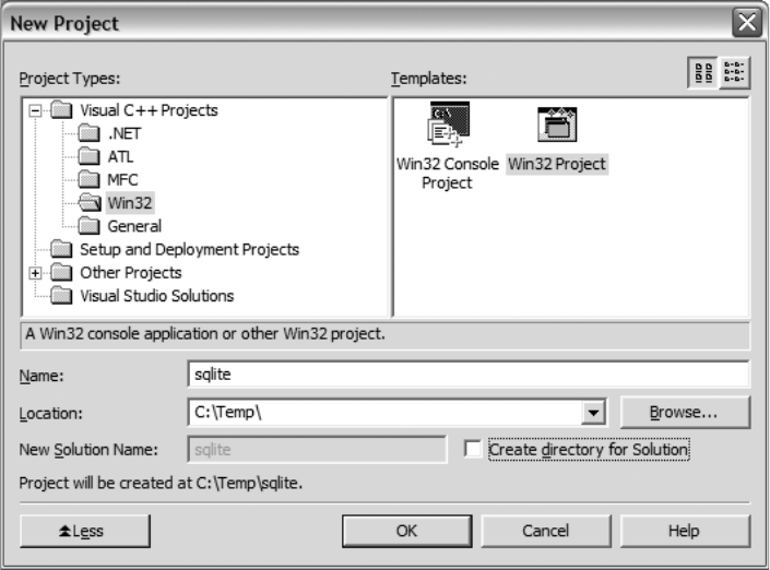
CHAPTER 2 ■ GETTING STARTED 25
Building the SQLite DLL with Microsoft Visual C++
To build the SQLite DLL from source using Visual C++, follow these steps:
1. Start Visual Studio. Create a new DLL project within the unpacked SQLite source
directory. Do this by going to File ➤ New ➤ Project. Under Project Types (Figure 2-5),
select Visual C++ Projects, and then select Win32. Choose the Win32 Project template.
In the Location text box, enter the folder name that contains your SQLite source folder.
In this example, it would be C:\Temp. In the Name text box, enter the name of the folder
containing the SQLite source code—sqlite in this example. This will create the Visual
C++ project inside the existing SQLite source folder (C:\Temp\sqlite). Click OK.
Figure 2-5. Creating a new Visual C++ project
2. Next, the Win 32 Application Wizard will automatically open (Figure 2-6). Choose
Application Settings and set the application type to DLL. Be sure to check the Empty
Project box. Click Finish, and this will create a blank DLL project.
Owens_6730 C02.fm Page 25 Tuesday, April 11, 2006 1:01 PM
www.it-ebooks.info
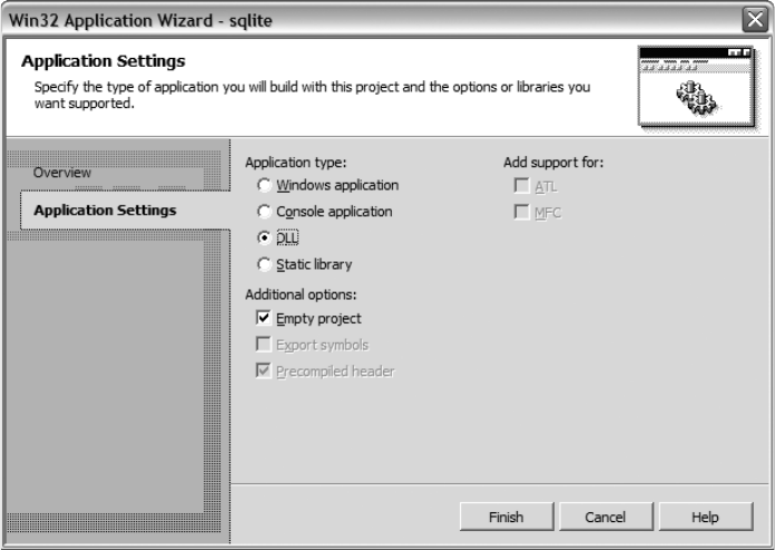
26 CHAPTER 2 ■ GETTING STARTED
Figure 2-6. The Win32 Application Wizard
3. Add SQLite source files and headers to the project. Select Project ➤ Add Existing Item.
Add all .c and .h files in the directory except for two files: tclsqlite.c and shell.c.
(The first is for Tcl support; the second is for creating the SQLite shell, neither of which
we want in this case.)
4. If you want to build the DLL with thread safety, you need to make sure that you have the
preprocessor flag THREADSAFE defined in the project. To do this, select Project ➤ Prop-
erties and under the C/C++ item in the left tree view, select Preprocessor (Figure 2-7).
Click on the Preprocessor Definitions cell. A small button will appear to the right. Click
this button to open the dialog box shown in Figure 2-8. Add THREADSAFE to the bottom of
the list and click OK. Also, you will need to make sure that you use the multithreaded
Microsoft C runtime library DLL. Specify this by selecting the Code Generation item
(Figure 2-7) and under Runtime Library select Multi-threaded Debug (/MTd).
Owens_6730 C02.fm Page 26 Tuesday, April 11, 2006 1:01 PM
www.it-ebooks.info
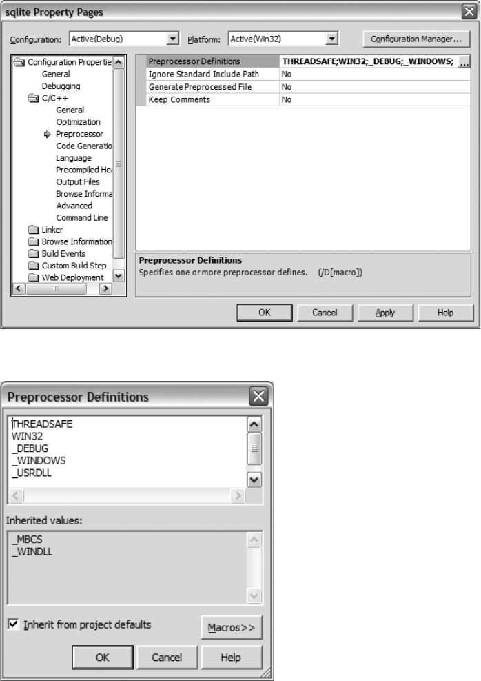
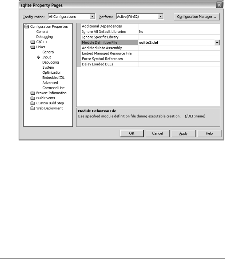
28 CHAPTER 2 ■ GETTING STARTED
5. Specify an export or a module definition (.def) file. This file defines what symbols (or
functions) to export (make visible) to programs that link to the library. SQLite’s source
distribution is kind enough to include such a file (sqlite3.def) for this very purpose.
Also within the Property Pages dialog box, select All Configurations in the Configuration
drop-down box (Figure 2-9). Then click the Linker folder and click the Input submenu.
In the Module Definition File property page, type sqlite3.def. You are now ready to
build the DLL.
Figure 2-9. Project properties
6. From the main menu, select Build ➤ Build sqlite to build the DLL.
7. Once you have built the DLL, be sure to create the import library as described in the
section “Getting the SQLite DLL.”
Building a Dynamically Linked SQLite Client with Visual C++
The binary for a static CLP is available on the SQLite website, but what if you want a version
that uses the SQLite DLL? To build such a version in Visual C++, do the following:
■Note Many of the steps are very similar to the process of building a DLL, mentioned earlier—you may
want to use some of the figures listed there for reference.
Owens_6730 C02.fm Page 28 Tuesday, April 11, 2006 1:01 PM
www.it-ebooks.info

CHAPTER 2 ■ GETTING STARTED 29
1. From the main menu, select File ➤ New ➤ Project. Under Project Types, select Visual
C++ Projects, and then select Win32. Choose the Win32 Project template. Name the
project (shell, for example) and click OK.
2. After this, the Win 32 Application Wizard will automatically open. Choose Application
Settings and set the application type to Console Application, and be sure to check the
Empty Project box. Click Finish to create a blank executable project.
3. Next you want to add the SQLite shell source file. Select Project ➤ Add Existing Item. In
the dialog box that appears, add the source file shell.c.
4. Tell Visual C++ to link against the SQLite DLL. Select Project ➤ Properties. In the dialog
box that appears, select All Configurations in the Configuration drop-down box. Next
select the Linker folder. Select the Input submenu and within the Additional Dependencies
property page, add sqlite3.lib. You are now ready to build the program. Note that the
SQLite DLL needs to be either in the same directory as the command-line program or in
the Windows system path.
■Note If you build the SQLite DLL with threading enabled or you obtain the DLL from the SQLite website,
you need to use the multithreaded Microsoft C runtime library DLL when building the CLP. To do this, refer to
the second half of step 4 in “Building the SQLite DLL with Microsoft Visual C++.” It contains two informative
figures that make it easy to set this option.
Building SQLite with MinGW
MinGW (www.mingw.org) is a very nice distribution of the GNU Compiler Collection (GCC) for
Windows. It also includes freely available Windows-specific header files and libraries that you
can use to create native Windows programs that do not rely on any third-party C runtime DLLs.
Put simply, it is a free C/C++ compiler for Windows, and a very good one at that. It is usually
used in conjunction with MSYS, which is a portable POSIX environment that makes Unix users
feel at home on Windows. Together, the two provide a powerful environment with which to
compile and build software on Windows. With this build environment, you can build both the
tarball archives as well as the source directly from CVS.
To build the SQLite DLL from source with MinGW, do the following:
1. Open your favorite browser and navigate to the MinGW website: www.mingw.org.
2. On the left side of the page, click the Download link, which will take you to the main
download page.
3. On the download page, look for the FileList section. There will be a link to SF File Releases
page, which at the time of this writing is located above the long listing of files. Follow
that link. It will take you to the SourceForge download page for MinGW. Scroll down to
the MinGW section and download the latest release (MinGW-5.0.2.exe at the time of this
writing).
Owens_6730 C02.fm Page 29 Tuesday, April 11, 2006 1:01 PM
www.it-ebooks.info
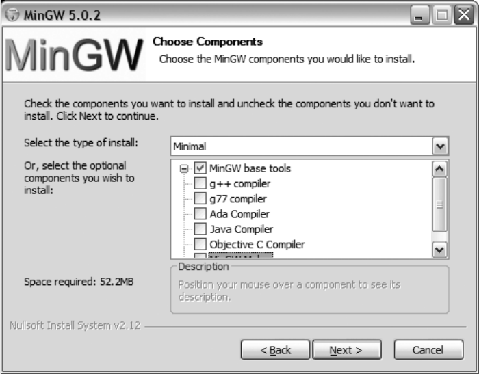
30 CHAPTER 2 ■ GETTING STARTED
4. After downloading the file, click Back a few times to return to the initial SourceForge
download page. Look for the MSYS section and download the current version
(MSYS-1.0.11-2004.04.30.exe at the time of this writing).
5. Install MinGW, followed by MSYS. The MinGW installer will prompt you for a mirror
site. Choose the one that is closest to you. In the next dialog box (the Choose Components
dialog box shown in Figure 2-10), make sure you also select the second option—g++
compiler—in addition to the default (if you forget you can always rerun the MinGW
installer and select this component). Select the defaults for all other screens. Double-
click the respective files, which will invoke installers for each package. Follow the directions
provided by the installers.
Figure 2-10. MinGW installation components
6. Download the Linux/Unix SQLite source code distribution. Navigate to www.sqlite.org
and click on the download link. On the download page, find the Source Code section.
The file you are looking for is the POSIX source distribution and should have a name of
the form sqlite-3.x.y.tar.gz, where x and y are the minor version numbers (at the
time of this writing, the current filename is sqlite-3.3.4.tar.gz). In Unix parlance,
this kind of source archive is called a tarball (akin to a Windows zip file). Download the
tarball and place it in a temporary directory (e.g., C:\Temp).
7. MSYS will have placed an icon on your desktop. Double-click that icon to open the
environment.
Owens_6730 C02.fm Page 30 Tuesday, April 11, 2006 1:01 PM
www.it-ebooks.info
CHAPTER 2 ■ GETTING STARTED 31
8. Navigate to your temporary directory in which you downloaded the SQLite source
distribution. Since this is a Unix-like environment, you will need to use Unix file system
conventions. For example, to get to c:\Temp, you would type cd /c/Temp.
9. Unpack the SQLite tarball. Issue this command:
tar -xzvf sqlite-3.3.4.tar.gz
10. Move into the unpacked directory:
cd sqlite-3.3.4
11. Create the Makefile. For a single-threaded DLL, run
./configure
12. If you want to create a multithreaded DLL, run
./configure --enable-threads
13. Build the source:
make
14. Create the SQLite DLL:
dllwrap --dllname sqlite3.dll --def sqlite3.def *.o
15. Create the import library:
dlltool --def sqlite3.def --dllname sqlite3.dll --output-lib sqlite3.lib
You now have a functional SQLite DLL and import library. To build a version of the SQLite
CLP that links against the SQLite DLL you just created, within the MSYS environment run the
command
gcc -I . src/shell.c -o sqlite3.exe sqlite3.lib
Now from Windows Explorer, navigate to the temporary folder and double-click on sqlite3.exe.
You now have a working SQLite CLP, which uses the SQLite DLL you created.
SQLite on POSIX Systems
SQLite compiles and builds identically on POSIX systems such as Linux, Mac OS X, FreeBSD,
NetBSD, OpenBSD, Solaris, and others. SQLite binaries can be obtained in a variety of ways
depending on the particular operating system.
Binaries and Packages
If you are using Mac OS 10.4 (“Tiger”) or greater, you already have SQLite installed on your
system. If not, there are several routes you can take to install it. The easiest way is to use one of
the following Mac-specific package management systems, all of which include packages or
ports for SQLite:
Owens_6730 C02.fm Page 31 Tuesday, April 11, 2006 1:01 PM
www.it-ebooks.info
32 CHAPTER 2 ■ GETTING STARTED
•Metadistribution. Metadistribution is a Gentoo-based package management system
based on Gentoo’s Portage. All packages are fetched from the Internet and built
from source using a single command, emerge. You can find the Mac version at www.
metadistribution/macos/.
•Fink. Fink is a Debian-based package management system that uses Debian utilities
such as dpkg, dselect, and apt-get, in addition to its own utility—fink. You can down-
load Fink from http://fink.sourceforge.net. With Fink, it is possible to install straight
from precompiled binaries. No compilation step is needed.
•Darwin Ports. Darwin Ports is a package system written in Tcl, which like Metadistribution,
installs from source. More information can be obtained from http://darwinports.
opendarwin.org.
BSD users will have no trouble installing SQLite either. FreeBSD, OpenBSD, and NetBSD
all have packages and/or ports for SQLite, all of which are very easy to install. As I write this,
each distribution has ports for very recent versions of SQLite 3.x.
Solaris 10 uses SQLite as part of the OS; however at the time of this writing it uses version
SQLite 2.x. An easy way to install SQLite in Solaris (and other open source software as well) is
to use Blastwave’s pkg-get utility. Blastwave is a Debian-based package management system
for Solaris that makes installing free software on Solaris simple. You can get more information
on Blastwave from www.blastwave.org.
As mentioned earlier, binaries for Linux are available directly from the SQLite website.
The download page on SQLite’s website provides the following binaries:
•Statically linked command-line program. The filename is of the form
sqlite3-3.x.y.bin.gz, where x and y are the minor version numbers.
•Shared library. Two forms of the shared library exist. One form includes the Tcl bindings;
the other does not. The name of the shared library with Tcl bindings has the form
tclsqlite-3.3.x.y.so.gz, where again x and y are the minor version numbers. The
name of the shared library without Tcl bindings is of the form sqlite-3.x.y.so.gz. Note
that the shared libraries provided are not thread safe. If you need a thread-safe version,
you will have to compile the library from source. See the section “Compiling SQLite from
Source” for more details.
•SQLite Analyzer. This is a command-line program that provides detailed information
about the contents of a SQLite database. You’ll find information on this program in the
section “Getting Database File Information.”
Various RPM-based Linux distributions may include RPMs for SQLite, but may not include
the most recent versions. Fedora and Mandriva don’t appear to include RPMs for SQLite at all.
Perhaps the best way to find the most recent versions of SQLite in RPM form is to consult the
Internet. RPM PBone Search (http://rpm.pbone.net) and RPMFind (http://rpmfind.net) are
two good places to start.
Debian-based distributions will have no trouble getting up-to-date versions of SQLite.
SQLite 3 packages are available online in both Ubuntu and Debian repositories, among others.
Owens_6730 C02.fm Page 32 Tuesday, April 11, 2006 1:01 PM
www.it-ebooks.info
CHAPTER 2 ■ GETTING STARTED 33
Compiling SQLite from Source
Compiling SQLite from source on POSIX systems follows very closely the MinGW instructions
given earlier for the Windows platform (actually it is more the other way around; MinGW
installation apes Linux source installation!). To build SQLite on POSIX systems, you need to
ensure that you have the GNU Compiler Collection (GCC) installed, including Autoconf,
Automake, and Libtool. Most of the systems already discussed include all of these by default.
With this software in place, you can build SQLite by doing the following:
1. Download the Linux/Unix SQLite tarball (source code) from the SQLite website. At the
time of this writing, the current version is sqlite-3.3.4.tar.gz. Place it in a directory
(e.g., /tmp).
2. Navigate to your build directory:
cd /tmp
3. Unpack the SQLite tarball:
tar -xzvf sqlite-3.3.4.tar.gz
4. Move into the unpacked directory:
cd sqlite-3.3.4
5. Create the Makefile:
./configure
6. If you want to create a multithreaded shared library, run
./configure -–enable-threads
7. Other options, such as the installation directory, are also available. For a complete list of
configure options, run
./configure --help
8. Build the source:
make
9. As root, install:
make install
You now have a functional SQLite installation on your system that includes both the SQLite
shared library and a dynamically linked CLP (which uses the SQLite shared library). If you have
GNU Readline installed on you system, the CLP should be compiled with Readline support.
Test it out by running it from the command line:
root@linux # sqlite3
This will invoke the CLP using an in-memory database. Type .help for a list of shell commands.
Type .exit to close the application, or press Ctrl+D.
Owens_6730 C02.fm Page 33 Tuesday, April 11, 2006 1:01 PM
www.it-ebooks.info

34 CHAPTER 2 ■ GETTING STARTED
Working with SQLite Databases
The SQLite CLP is the most common means you can use to work with and manage SQLite data-
bases. It runs on as many platforms as the SQLite library, so learning how to use it ensures you
will always have a common and familiar way to manage your databases. The CLP is really two
programs in one. It can run from the command line to perform various administration tasks, or
it can be run in shell mode and act as an interactive query processor.
The CLP in Shell Mode
Open a shell and change directory to some temporary folder—say C:\Temp if you are on Windows
or /tmp if you’re in Unix. This will be your current working directory. All files you create in the
course of working with the shell will be created in this directory.
■Note To get a command line on Windows, go to Start ➤ Programs ➤ Accessories ➤ Command Prompt.
To invoke the CLP as in shell mode, type sqlite3 from a command line, followed by an
optional database name. If you do not specify a database name, SQLite will use an in-memory
database (the contents of which will be lost when the CLP exits).
Using the CLP as an interactive shell, you can issue queries, obtain schema information,
import and export data, and perform other miscellaneous database tasks. The shell will consider
any statement issued as a query, except for commands that begin with a period (.). These
commands are reserved for specific shell operations, a complete list of which can be obtained
by typing .help as shown:
mike@linux tmp $ sqlite3
SQLite version 3.3.4
Enter ".help" for instructions
sqlite> .h
.databases List names and files of attached databases
.dump ?TABLE? ... Dump the database in a SQL text format
.echo ON|OFF Turn command echo on or off
.exit Exit this program
.explain ON|OFF Turn output mode suitable for EXPLAIN on or off.
.header(s) ON|OFF Turn display of headers on or off
.help Show this message
.import FILE TABLE Import data from FILE into TABLE
.indices TABLE Show names of all indices on TABLE
.mode MODE ?TABLE? Set output mode where MODE is one of:
csv Comma-separated values
column Left-aligned columns. (See .width)
html HTML <table> code
insert SQL insert statements for TABLE
Owens_6730 C02.fm Page 34 Tuesday, April 11, 2006 1:01 PM
www.it-ebooks.info

CHAPTER 2 ■ GETTING STARTED 35
line One value per line
list Values delimited by .separator string
tabs Tab-separated values
tcl TCL list elements
.nullvalue STRING Print STRING in place of NULL values
.output FILENAME Send output to FILENAME
.output stdout Send output to the screen
.prompt MAIN CONTINUE Replace the standard prompts
.quit Exit this program
.read FILENAME Execute SQL in FILENAME
.schema ?TABLE? Show the CREATE statements
.separator STRING Change separator used by output mode and .import
.show Show the current values for various settings
.tables ?PATTERN? List names of tables matching a LIKE pattern
.timeout MS Try opening locked tables for MS milliseconds
.width NUM NUM ... Set column widths for "column" mode
sqlite>.exit
You can just as easily type .h for short. Many of the commands can be similarly abbrevi-
ated, such as .e—short for .exit—to exit the shell.
Let’s start by creating a database that we will call test.db. From the command line, open
the CLP in shell mode by typing the following:
sqlite3 test.db
Even though we have provided a database name, SQLite does not actually create the database
(yet) if it doesn’t already exist. SQLite will defer creating the database until you actually create
something inside it, such as a table or view. The reason for this is so that you have the opportunity
to set various permanent database settings (such as page size) before the database structure is
committed to disk. Some settings such as page size and character encoding (UTF-8, UTF-16,
etc.) cannot be changed once the database is created, so this interim is where you have a chance
to specify them. We will go with the default settings here, so to actually create the database on
disk, we need only to create a table. Issue the following statement from the shell:
sqlite> create table test (id integer primary key, value text);
Now you have a database file on disk called test.db, which contains one table called test. This
table, as you can see, has two columns:
• A primary key column called id, which has an autoincrement attribute. Wherever you
define a column of type integer primary key, SQLite will apply an autoincrement function
for the column. That is, if no value is provided for the column in an INSERT statement,
SQLite will automatically generate one by finding the next integer value specific to that
column.
• A simple text field called value.
Owens_6730 C02.fm Page 35 Tuesday, April 11, 2006 1:01 PM
www.it-ebooks.info

36 CHAPTER 2 ■ GETTING STARTED
Let’s add a few rows to the table:
sqlite> insert into test (value) values('eenie');
sqlite> insert into test (value) values('meenie');
sqlite> insert into test (value) values('miny');
sqlite> insert into test (value) values('mo');
Now fetch them back:
sqlite> .mode col
sqlite> .headers on
sqlite> SELECT * FROM test;
id value
---------- ----------
1 eenie
2 meenie
3 miny
4 mo
The two commands preceding the SELECT statement (.headers and .mode) are used to improve
the formatting a little (both of which are covered later). We can see that SQLite provided
sequential integer values for the id column, which we did not provide in the INSERT statements.
While on the topic of autoincrement columns, you might be interested to know that the value of the
last inserted autoincrement value can be obtained using the SQL function last_insert_rowid():
sqlite> select last_insert_rowid();
last_insert_rowid()
-------------------
4
Before we quit, let’s add an index and a view to the database. These will come in handy in
the illustrations that follow:
sqlite> create index test_idx on test (value);
sqlite> create view schema as select * from sqlite_master;
To exit the shell, issue the .exit command:
sqlite> .exit
C:\Temp>
On Windows, you can also terminate the shell by using the key sequence Ctrl+C. On Unix, you
can use Ctrl+D.
Owens_6730 C02.fm Page 36 Tuesday, April 11, 2006 1:01 PM
www.it-ebooks.info

CHAPTER 2 ■ GETTING STARTED 37
Getting Database Schema Information
There are several shell commands for obtaining information about the contents of a database.
You can retrieve a list of tables (and views) using .tables [pattern], where [pattern] can be
any pattern that the SQL LIKE operator understands (we cover LIKE in Chapter 4 if you are
unfamiliar with it). All tables and views matching the given pattern will be returned. If no
pattern is supplied, all tables and views are returned:
sqlite> .tables
schema test
Here we see our table named test and our view named schema. Similarly, indexes for a given
table can be printed using .indices [table name]:
sqlite> .indices test
test_idx
Here we see the index we created earlier on test, called test_idx. The SQL definition or data
definition language (DDL) for a table or view can be obtained using .schema [table name].
If no table name is provided, the SQL definitions of all database objects (tables, indexes, views,
and indexes) are returned:
sqlite> .schema test
CREATE TABLE test (id integer primary key, value text);
CREATE INDEX test_idx on test (value);
sqlite> .schema
CREATE TABLE test (id integer primary key, value text);
CREATE VIEW schema as select * from sqlite_master;
CREATE INDEX test_idx on test (value);
More detailed schema information can be had from SQLite’s one and only system view,
sqlite_master. This view is a simple system catalog of sorts. Its schema is described in Table 2-1.
Querying sqlite_master for our current database returns the following (don’t forget to use the
.mode col and .headers on commands first to manually set the column format and headers):
Owens_6730 C02.fm Page 37 Tuesday, April 11, 2006 1:01 PM
www.it-ebooks.info

38 CHAPTER 2 ■ GETTING STARTED
sqlite> .mode col
sqlite> .headers on
sqlite> select type, name, tbl_name, sql from sqlite_master order by type;
type name tbl_name sql
---------- ---------- ---------- -------------------------------------
index test_idx test CREATE INDEX test_idx on test (value)
table test test CREATE TABLE test (id integer primary
view schema schema CREATE VIEW schema as select * from s
We see a complete inventory of test.db contents: one table, one index, and one view, each with
their respective SQL definitions.
There are few additional commands for obtaining schema information through SQLite’s
PRAGMA commands, table_info, index_info, and index_list, which are covered in Chapter 4.
■Tip Don’t forget that most shells keep a history of the commands that you execute. To rerun a previous
command, you can hit the Up Arrow key to scroll through your previous commands.
Exporting Data
You can export database objects to SQL format using the .dump command. Without any argu-
ments, .dump will export the entire database. If you provide arguments, the shell interprets
them as table names or views. Any tables or views matching the given arguments will be exported.
Those that don’t are simply ignored. In shell mode, the output from the .dump command is
directed to the screen by default. If you want to redirect output to a file, use the .output [filename]
command. This command redirects all output to the file filename. To restore output back to
the screen, simply issue .output stdout. So, to export the current database to a file file.sql,
you simply do the following:
sqlite> .output file.sql
sqlite> .dump
sqlite> .output stdout
Table 2-1. SQLite Master Table Schema
Name Description
type The object’s type (table, index, view, trigger)
name The object’s name
tbl_name The table the object is associated with
rootpage The object’s root page index in the database (where it begins)
sql The object’s SQL definition (DDL)
Owens_6730 C02.fm Page 38 Tuesday, April 11, 2006 1:01 PM
www.it-ebooks.info

CHAPTER 2 ■ GETTING STARTED 39
This will create the file file.sql in your current working directory if it does not already exist.
If a file by that name does exist, it will be overwritten.
By combining redirection with SQL and the various shell formatting options (covered later),
you have a great deal of control over exporting data. You can export specific subsets of tables
and views in various formats using the delimiter of your choice, which can later be imported using
the .import command described next.
Importing Data
There are two ways to import data, depending on the format of the file to import. If the file is
composed of SQL, you can use the .read command to import (execute) the file. If the file
contains comma-separated values (CSV) or other delimited data, you can use the .import
[file][table] command. This command will parse the specified file and attempt to insert it
into the specified table. It does this by parsing each line in the file using the pipe character (|)
as the delimiter and inserting the parsed columns into the table. Naturally, the number of
parsed fields in the file should match up with the number of columns in the table. You can
specify a different delimiter using the .separator command. To see the current value set for the
separator, use the .show command. This will show all user-defined settings for the shell, among
them the current default separator:
sqlite> .show
echo: off
explain: off
headers: on
mode: column
nullvalue: ""
output: stdout
separator: "|"
width:
The .read command is the way to import files created by the .dump command. Using
file.sql created earlier as a backup, we can drop the existing database objects (the test table
and schema view) and reimport it as follows:
sqlite> drop table test;
sqlite> drop view schema;
sqlite> .read file.csv
Formatting
The shell offers a number of formatting options. The simplest are .echo, which echoes the last
run command after issuing a command, and .headers, which includes column names for queries
when set to on. The text representation of null values can be set with .nullvalue. For instance,
if you want null values to appear as NULL, simply issue the command .nullvalue NULL. By default,
this value is an empty string. Also, the shell prompt can be changed using .prompt [value]:
Owens_6730 C02.fm Page 39 Tuesday, April 11, 2006 1:01 PM
www.it-ebooks.info
40 CHAPTER 2 ■ GETTING STARTED
sqlite> .prompt 'sqlite3> '
sqlite3>
Result data can be formatted several ways using the .mode command. The current options
are csv, column, html, insert, line, list, tabs, and tcl, each of which is helpful in different ways.
The default is .list. For instance, list mode displays results with the columns separated by the
default separator. Thus, if you wanted to dump a table in a CSV format, you could do the following:
sqlite3> .output file.csv
sqlite3> .separator ,
sqlite3> select * from test;
sqlite3> .output stdout
The contents of file.csv are now
1,eenie
2,meenie
3,miny
4,mo
Actually, since there is a CSV mode already defined in the shell, it is just as easy to use it in this
particular example instead:
sqlite3> .output file.csv
sqlite3> .mode csv
sqlite3> select * from test;
sqlite3> .output stdout
and obtain similar results. The difference is that CSV mode will wrap field values with double
quotes, whereas list mode (the default) does not.
Putting It All Together
Combining the previous three sections on exporting, importing, and formatting data, we now
have an easy way to export and import data in delimited form. For example, to export only the
rows of the test table whose value fields start with the letter “m” to a file called test.csv in
comma-separated values, do the following:
sqlite> .output text.csv
sqlite> .separator ,
sqlite> select * from test where value like 'm%';
sqlite> .output stdout
If you want to then import this CSV data into a similar table with the same structure as the test
table (call it test2), do the following:
sqlite> create table test2(id integer primary key, value text);
sqlite> .import text.csv test2
The CLP, therefore, makes it easy to both import and export text-delimited data to and from
the database.
Owens_6730 C02.fm Page 40 Tuesday, April 11, 2006 1:01 PM
www.it-ebooks.info

CHAPTER 2 ■ GETTING STARTED 41
The CLP in Command-Line Mode
The CLP can be used from the command line for tasks such as importing and exporting data,
returning result sets, and performing general batch processing. It is ideal for use in shell scripts
for automated database administration. To see what the CLP offers in command-line mode,
invoke it from the shell (Windows or Unix) with the –help switch, as shown here:
mike@linux tmp $ sqlite3 -help
Usage: sqlite3 [OPTIONS] FILENAME [SQL]
Options are:
-init filename read/process named file
-echo print commands before execution
-[no]header turn headers on or off
-column set output mode to 'column'
-html set output mode to HTML
-line set output mode to 'line'
-list set output mode to 'list'
-separator 'x' set output field separator (|)
-nullvalue 'text' set text string for NULL values
-version show SQLite version
-help show this text, also show dot-commands
The CLP in command-line mode takes the following arguments:
• A list of options (optional)
• A database filename (required)
• A SQL command to execute (optional)
Most of the options control output formatting except for the init switch, which specifies a
batch file of SQL commands to process. The database filename is required. The SQL command
is optional with a few caveats.
There are actually two ways to invoke the CLP in command-line mode. The first is to provide
a SQL command. However, “SQL command” is somewhat misleading as you can provide SQLite
shell commands as well, such as .dump and .schema. Any valid SQL or SQLite shell command
will do. When it’s provided, SQLite will simply execute the specified command, print the result
to standard output, and exit. For example, to dump the test.db database from the command
line, issue the command
sqlite3 test.db .dump
To make it useful, we should redirect the output to a file:
sqlite3 test.db .dump > test.sql
The file test.sql now contains the complete human-readable (SQL) representation of test.db.
Similarly, to select all records for the test table, issue
sqlite3 test.db "select * from test"
Owens_6730 C02.fm Page 41 Tuesday, April 11, 2006 1:01 PM
www.it-ebooks.info
42 CHAPTER 2 ■ GETTING STARTED
The second way to invoke the CLP in command-line mode is to redirect a file as an input
stream. For instance, to create a new database test2.db from our database dump test.sql, do
the following:
sqlite3 test2.db < test.sql
The CLP will read the file as standard input, then process and apply all SQL commands within
it to the test2.db database file.
So, in order for command-line mode to be invoked, either a SQL command or an input
stream must be provided to the CLP. To further illustrate this, yet another way to create a data-
base from the test.sql file is to use the init option and provide the test.sql as an argument:
sqlite3 –init test.sql test3.db
The CLP will process test.sql, create the test3.db database, and then go into shell mode. Why?
The invocation included no SQL command or input stream. To get around this, you need to
provide a SQL command. For example:
sqlite3 –init test.sql test3.db .exit
The .exit command prompts the CLP to run in command-line mode and does as little as
possible. All things considered, redirection is perhaps the easiest method for processing files
from the command line.
Database Administration
All database administration tasks can be performed within the shell and on the command line.
Typically, the command line is easier to use for many general administration tasks, but it is
really a matter of taste. Many of the common database administration tasks have been touched
upon through the examples provided thus far. For the sake of completeness, I will nevertheless
list the most common tasks along with the typical ways of performing them.
Creating, Backing Up, and Dropping Databases
Backing up a database can be done in two ways, depending on the type of backup you desire.
A SQL dump is perhaps the most portable form for keeping backups. The standard way to
generate one is using the CLP .dump command. From the command line, this is done as follows:
sqlite3 test.db .dump > test.sql
Within the shell, you can redirect output to an external file, issue the command, and restore
output to the screen as follows:
sqlite> .output file.sql
sqlite> .dump
sqlite> .exit
Likewise, importing a database is most easily done by providing the SQL dump as an input
stream to the CLP:
sqlite3 test.db < test.sql
Owens_6730 C02.fm Page 42 Tuesday, April 11, 2006 1:01 PM
www.it-ebooks.info

CHAPTER 2 ■ GETTING STARTED 43
This assumes that test.db does not already exist. If it does, then things may still work if the
contents of test.sql are different from those of test.db. You will of course get errors if test.sql
contains objects that already reside within test.db.
Making a binary backup of a database is little more than a file copy. One small operation
you may want to perform beforehand is a database vacuum, which will free up any unused
space created from deleted objects. This will provide you with a more compact binary copy:
sqlite3 test.db VACUUM
cp test.db test.backup
As a general rule, binary backups are not as portable as SQL backups. On the whole, SQLite
does have good backward compatibility and is binary compatible across all platforms for a
given database format. However, for long-term backups, it is always a good idea to use SQL
form. If size is an issue, SQL format (raw text) usually yields a good compression ratio.
Finally, if you’ve worked with other databases, “dropping” a database in SQLite, like
binary backups, is a simple file operation: you simply delete the database file you wish to drop.
Getting Database File Information
As mentioned earlier, the primary means by which to obtain database information is using
the sqlite_master view, which provides detailed information about all objects contained in
a given database.
If you want information on the physical database structure, you can use a tool called
SQLite Analyzer, which can be downloaded in binary form from the SQLite website. SQLite
Analyzer provides detailed technical information about the on-disk structure of a SQLite data-
base. This information includes a detailed breakdown of database, table, and index statistics
for individual objects and in aggregate. It provides everything from database properties such as
page size, number of tables, indexes, file size, and average page density (utilization) to detailed
descriptions of individual database objects. Following the report is a detailed list of definitions
explaining all terms used within the report. A partial output of sqlite_analyzer is as follows:
mike@linux tmp $ sqlite3_analyzer test.db
/** Disk-Space Utilization Report For test.db
*** As of 2005-May-07 20:26:23
Page size in bytes.................... 1024
Pages in the whole file (measured).... 3
Pages in the whole file (calculated).. 3
Pages that store data................. 3 100.0%
Pages on the freelist (per header).... 0 0.0%
Pages on the freelist (calculated).... 0 0.0%
Pages of auto-vacuum overhead......... 0 0.0%
Number of tables in the database...... 2
Number of indices..................... 1
Number of named indices............... 1
Automatically generated indices....... 0
Size of the file in bytes............. 3072
Bytes of user payload stored.......... 26 0.85%
Owens_6730 C02.fm Page 43 Tuesday, April 11, 2006 1:01 PM
www.it-ebooks.info

44 CHAPTER 2 ■ GETTING STARTED
*** Page counts for all tables with their indices ********************
TEST.................................. 2 66.7%
SQLITE_MASTER......................... 1 33.3%
*** All tables and indices *******************************************
Percentage of total database.......... 100.0%
Number of entries..................... 11
Bytes of storage consumed............. 3072
Bytes of payload...................... 235 7.6%
Average payload per entry............. 21.36
Average unused bytes per entry........ 243.00
Maximum payload per entry............. 72
Entries that use overflow............. 0 0.0%
Primary pages used.................... 3
Overflow pages used................... 0
Total pages used...................... 3
Unused bytes on primary pages......... 2673 87.0%
Unused bytes on overflow pages........ 0
Unused bytes on all pages............. 2673 87.0%
*** Table TEST and all its indices ***********************************
Percentage of total database.......... 66.7%
Number of entries..................... 8
Bytes of storage consumed............. 2048
Bytes of payload...................... 60 2.9%
Average payload per entry............. 7.50
Average unused bytes per entry........ 243.00
Maximum payload per entry............. 10
Entries that use overflow............. 0 0.0%
Primary pages used.................... 2
Overflow pages used................... 0
Total pages used...................... 2
Unused bytes on primary pages......... 1944 94.9%
Unused bytes on overflow pages........ 0
Unused bytes on all pages............. 1944 94.9%
SQLite Analyzer is provided in binary form on the SQLite website for Linux and Windows.
On POSIX platforms, or with MinGW, SQLite Analyzer can be built from the source using the
Unix makefile provided. From the build directory, issue the command
make sqlite3_analyzer
You must, however, have Tcl support configured in the build settings as SQLite Analyzer uses
the Tcl extension to perform most of its work. Refer to “Compiling SQLite from Source” for
more information.
Owens_6730 C02.fm Page 44 Tuesday, April 11, 2006 1:01 PM
www.it-ebooks.info
CHAPTER 2 ■ GETTING STARTED 45
Other SQLite Tools
There are many other open source and commercial programs available with which to work
with SQLite. Good graphical, cross-platform tools include
•SQLite Database Browser (http://sqlitebrowser.sourceforge.net) is a program devel-
oped with Qt. With it users can manage databases, tables, and indexes, as well as import
and export them. Users can interactively run SQL queries and inspect the results, as well
as examine a log of all SQL commands issued. Users can also browse tables and modify
their records.
• SQLite Control Center (http://bobmanc.home.comcast.net/sqlitecc.html) is a cross-
platform program that uses the wxWindows C++ GUI framework. It does many of the
same things as SQLite Database Browser, including general management of databases,
tables, indexes, and triggers. Likewise, it also allows users to edit table data in a grid
display and construct queries using a syntax-highlighting text editor.
• SQLiteManager (www.sqlabs.net/sqlitemanager.php) is a commercial software package
designed for working with and administering SQLite. Users can manage database objects,
execute queries, and save SQL, as well as create reports with flexible report templates.
These are just the cross-platform tools. Many more tools are available that can be used with
PHP and other specific environments. You can find more information on such packages on the
SQLite Wiki (www.sqlite.org/cvstrac/wiki?p=SqliteTools).
Summary
No matter what platform you work on, SQLite is quite easy to install and build. Windows and
Linux users can obtain binaries directly from the SQLite website. Users of many other operating
systems can also obtain binaries using their native—or even third-party—package systems.
The common way to work with SQLite across all platforms is using the SQLite command-
line program (CLP). This program operates as both a command-line tool and an interactive
shell. You can issue queries and do essential database administration tasks such as creating
tables, indexes, and views as well as exporting and importing data. SQLite databases are contained
in single operating system files, so doing things like binary backups are very simple—just copy
the file. For long-term backups, however, it is always best to dump the database in SQL format,
as this is portable across SQLite versions.
In the next few chapters, you will be using the CLP to explore SQL and the database aspects
of SQLite. The next chapter provides a great deal of background to SQL. It is almost entirely
theoretical. However, if you have previously used relational databases and SQL, you may find
it very informative. It provides not only the basic theory underlying SQL but also a good bit of
history as well. If you don’t care for theory and want to dive right in, you may want to skip
ahead to Chapter 4, where you will be able to put the CLP to immediate use.
Owens_6730 C02.fm Page 45 Tuesday, April 11, 2006 1:01 PM
www.it-ebooks.info

47
■ ■ ■
CHAPTER 3
The Relational Model
SQL has a very practical exterior but a very theoretical interior. That interior is the relational
model. The relational model came before SQL and created a need for SQL. The power of SQL
lies not in the language itself but in the concepts set forth in the relational model. These concepts
form the basis of SQL’s design and operation.
The relational model is a powerful and elegant idea that has pervaded not only computer
science but our daily lives as well, whether we know it or not. Like the automobile, or penicillin,
it is one of the many great examples of human thought and discovery that has fundamentally
impacted the way the world works. The relational model has spawned a billion-dollar industry,
and has become an integral part of almost every other industry. You’ll see the relational model
at work nearly everywhere that deals with information of any kind—in Fortune 500 companies,
universities, hospitals, grocery stores, websites, routers, MP3 players, cell phones, and even
smart cards. It is truly pervasive.
Background
The relational model was born in 1969, inside of IBM. A researcher named E. F. Codd distributed
an internal paper titled “Derivability, Redundancy, and Consistency of Relations Stored in
Large Data Banks,” which defined the basic theory of the relational model. This paper was
circulated internally and not widely distributed. In 1970, Codd published a more refined version of
this paper in Communications of the ACM called “A Relational Model for Large Shared Data
Banks,” which is more widely recognized as the seminal work on relational theory. This is the
paper that changed the industry.
Despite the enormous influence of this paper, the relational model in its entirety did not
appear overnight, or within the scope of a single historic paper. It evolved, grew, and expanded
over time and was the product of many minds, not just Codd alone. For example, the term
“relational model” wasn’t coined until 1979, nine years after publication of the paper proposing
it (see Date, 1999, in the References section). Codd’s 12 rules, now famous as the working defi-
nition of relational, weren’t posited until 1985, appearing in a two-part series published by
Computerworld magazine. Thus, while there was a seminal paper proposing the general concept,
much of the relational model as we know it today is actually the result of a series of papers, articles,
and debates by many people over a 30-year period, and indeed continues to develop to this
very day. That is also why in some of the various quotes included in this chapter you may see
terms such as “data base,” which may initially appear to be a typo. They aren’t. At the time
these statements were made, the terminology still had not congealed and all sorts of various
terms were being thrown around.
Owens_6730 C03.fm Page 47 Wednesday, April 12, 2006 11:21 AM
www.it-ebooks.info
48 CHAPTER 3 ■ THE RELATIONAL MODEL
The Three Components
By 1980, enough was known about the relational model for Codd to identify three principle
components:
•The structural component: This component defines how information is structured, or
represented. Specifically, all information is represented as relations, which are composed of
tuples, which in turn are composed of attribute and value components. The relation is
the sole data structure used to represent all information in the database. Relations as
defined in the relational model are derived from relations in set theory, a branch of
mathematics, and share many of their properties. They are formally defined in Codd’s
1970 paper.
•The integrity component: This component defines methods that enforce relationships
within and between relations (or tables) in the structural component. These methods
are called constraints, and are expressed in the form of rules. There are three principle
types of integrity: domain integrity, governing values in columns; entity integrity, governing
rows in tables; and referential integrity, governing how tables relate to one another. Integrity
has no analog in set theory, but rather is unique to relational theory. It was initially
addressed in Codd’s 1970 paper and greatly expanded upon in the 1980s by Codd
and others.
•The manipulative component: This aspect defines the methods with which to operate
on or manipulate information. Like relations, these operations also have their roots in
mathematics. They are formalized in relational algebra and relational calculus as origi-
nally presented in Codd’s 1972 paper “Relational Completeness of Data Base
Sublanguages.”
SQL, likewise, is structured similarly along these lines—so similarly, in fact, that it is hard
to talk about SQL without addressing the relational model to some degree, directly or indirectly.
It is true that SQL is for the most part a straightforward language, which to many people appears as
an island unto itself. But in reality, it is the offspring of the relational model, and in many ways
is clearly a reflection of it.
SQL and the Relational Model
This chapter presents the theoretical roots of SQL, and examines the power and elegance
behind SQL. It prepares you to deal with SQL not in isolation but in the context of the relational
model. If nothing else, it should give you an appreciation for how elegant, powerful, and complex
a beast a relational database really is. You may be surprised by what even the most rudimentary
relational databases are capable of.
You don’t have to read this chapter in order to understand SQL; it merely provides a theoretical
and historical backdrop. To this end, I present the theoretical aspects in terms of several influential
papers and articles written by Codd between 1970 and 1985 that define the essence of the relational
model, along with the ideas and work of other contributors to the field. Two of Codd’s papers
mentioned here are available online, and are listed in the References section at the end of the
chapter. Again, others contributed to the development of the relational model, but this chapter
will draw primarily from Codd’s work.
Owens_6730 C03.fm Page 48 Wednesday, April 12, 2006 11:21 AM
www.it-ebooks.info
CHAPTER 3 ■ THE RELATIONAL MODEL 49
This chapter is not an exhaustive treatment of the relational model, or a complete history
of it. It is merely an appetizer. The SQL chapter that follows is the main course. This chapter
presents only the minimal material needed to get an appreciation of the origin and theoretical
underpinnings of SQL. We illustrate the relational model in terms of both its three components
in general and in the context of Codd’s 12 rules in particular. The relational model in its full
splendor is far beyond the scope of this book, and I have neither the qualifications nor the
stamina to fully describe it. See the References section at the end of this chapter if you want to
learn more. The rules as they are presented here are taken directly from Codd’s October 14, 1985,
Computerworld article.
The Structural Component
The structural component of the relational model lays the foundation upon which the other
components build. It defines the form in which information is represented. It is defined by the
first of Codd’s 12 rules, which is the cornerstone of the relational model.
The Information Principle
The first rule, called the Information Rule, is also known as the Information Principle. It is
defined as follows:
1. The Information Rule. All information in a relational data base is represented
explicitly at the logical level and in exactly one way—by values in tables.
Date summarizes this rule as follows:
The entire information content of the database is represented in one and only one way,
namely as explicit values in column positions in rows in tables.
There are two import expressions here: “logical level” and “values in tables.” The logic level, or
logical representation, refers to the way that you, the user, see the database and information
within it. It is a kind of ideal worldview for information. The logical level is a consistent, uniform
depiction of data, which has two important properties:
• The view presented in the logical level consists of tables, made up of rows, which in turn
are made up of values.
• The view is completely independent of the database system—the technology (software
or hardware) that enables it.
The logical representation is a world unto itself, which is completely distinct from how the
database is implemented, or how it stores data physically, or how it operates internally. These
latter components—software, operating system, and hardware—are referred to as the physical
representation—the technology of the system. If the database vendor decides to store database
tables in a different way on disk, the Information Principle mandates that such a change in
physical representation can in no way affect or change the logical representation of that data—
the way in which you (or your programs) see that data. The logical representation is indepen-
dent of physical representation. A result of the Information Principle is that it is possible to
Owens_6730 C03.fm Page 49 Wednesday, April 12, 2006 11:21 AM
www.it-ebooks.info
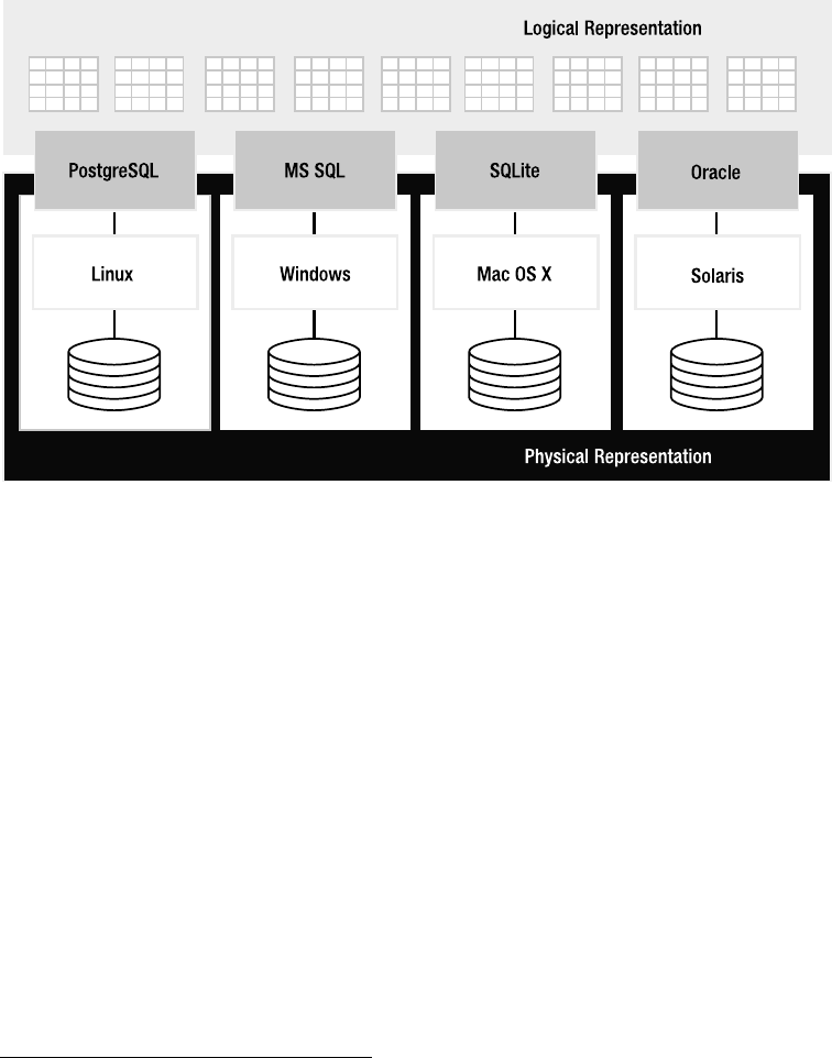
50 CHAPTER 3 ■ THE RELATIONAL MODEL
represent the same information in the same way across multiple database implementations on
multiple operating systems on different hardware, as shown in Figure 3-1.
Figure 3-1. Logical and physical representation
You can create a relation (or table) in Oracle on Solaris that is represented in exactly the
same way as a table in PostgreSQL on Linux, or SQLite on Mac OS X.1 The Information Principle
guarantees you a consistent logical view of information regardless of how the database soft-
ware is implemented, or the operating system or hardware it runs on.
The Sanctity of the Logical Level
So important are these two constraints in the relational model that they are expanded upon
and reinforced in several other rules (8, 9, 11, and 12) so as to eliminate any possible ambiguity.
In short, Codd says:
8. Physical Data Independence. The logical view can in no way be impaired by the
underlying software or hardware.
9. Logical Data Independence. Application programs and terminal activities remain
logically unimpaired when information-preserving changes of any kind that theoretically
permit un-impairment are made to the base tables.
1. In reality, this is not 100 percent true (it’s more like 95 percent true). There are slight differences in database
implementations so that relations in one database may contain features not present in other data-
bases. Nevertheless, they still all adhere to the same general structure: relations made of tuples made
of values.
Owens_6730 C03.fm Page 50 Wednesday, April 12, 2006 11:21 AM
www.it-ebooks.info
CHAPTER 3 ■ THE RELATIONAL MODEL 51
11. Distribution Independence. Even if the database is spread across various locations,
it cannot impact the logical view of data.
12. Nonsubversion Rule. The database software may not provide any facility which can
subvert the integrity constraints of the logical view.
The separation of logical from physical was very important to Codd from the outset. In the
opening of his original paper he had strong words concerning this separation:
Future users of large data banks must be protected from having to know how the data
is organized in the machine (the internal representation)… Activities of users at
terminals and most application programs should remain unaffected when the
internal representation of data is changed and even when some aspects of the external
representation are changed.
The relational model was in part a reaction to the database systems of the day, which closely
tied applications to both database implementation and data format on disk. Codd’s relational
model challenged this:
It provides a means of describing data with its natural structure only—that is, without
superimposing any additional structure for machine representation purposes. Accordingly,
it provides a basis for a high level data language which will yield maximal independence
between programs on the one hand and machine representation and organization of
data on the other.
So in the relational model, the Information Principle provides a level of abstraction through
which information can be represented in a consistent way. The user sees and works with data
exclusively in terms of this logical representation. This representation is completely insulated
from the underlying technology. It cannot be undermined, influenced, or affected by it in any
way. As stated before, the Information Principle is the foundation of the relational model.
The Anatomy of the Logical Level
The logical level is made up of more than relations. It is made up of tables, rows, columns, and
types. In relational parlance, these are often referred to more formally as relation variables, tuples,
values, and domains, respectively. SQL, for example, uses many of the former, and relational
theory tends to use many of the latter. Throughout the literature, however, you will see these
terms used almost interchangeably. Even in Codd’s papers, both sets of terms are used. Interest-
ingly, there is one term that both lexicons have in common: relations. (In case you’re wondering,
tables and relations are not the same thing; we’ll address the difference later in this chapter.)
This big soup of terminology comprises the anatomy of the relational body, which will be
explained in detail over the next several sections. The relationships between all of these terms
are illustrated in Figure 3-2.
At the center of everything is the relation. It is the central object around which the structural,
integrity, and manipulative components of the relational model are built. All of the fundamental
operations in the relational model are expressed in terms of relations, and all integrity constraints
are defined within relations. Your understanding of the relational model is only as good as your
understanding of relations themselves. To have a good grasp of relations, however, you must
first understand tuples.
Owens_6730 C03.fm Page 51 Wednesday, April 12, 2006 11:21 AM
www.it-ebooks.info
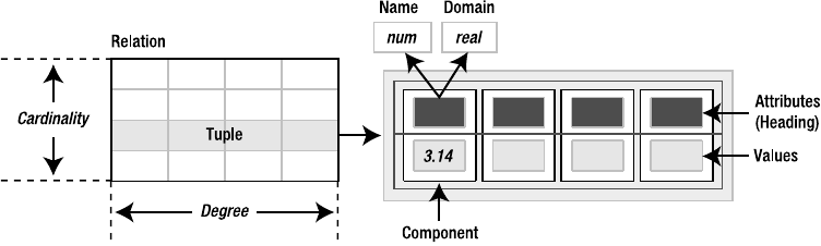
52 CHAPTER 3 ■ THE RELATIONAL MODEL
Figure 3-2. The logical representation of data
Tuples
A tuple is a set of values, each of which has an associated attribute. An attribute defines a value’s
name and domain. The attribute’s name is used to identify the value in the tuple, and its domain
defines the kind of information stored within it. The combination of attribute and value is called
a component. In Figure 3-2, you can see that the first component is named num, and that it has a
value of 3.14 and a domain of real (as in real numbers).
A component is kind of a tidy, self-contained unit of data. It has three essential ingredients:
a name, a domain, and a value. Its name gives it identity, its domain a description of its content,
and its value the content itself. Together, components aggregate into larger structures such as
tables and relations, and their qualities propagate into those structures, imparting to them
identity, description, and content as well.
The name and value parts of a component are easy enough to understand, but what exactly is
a domain? The word domain, like the words relation and tuple, comes from mathematics. In
mathematics, the domain of a function is the set of all values for which the function is defined.
Some familiar domains in mathematics are the sets of all integers, rational numbers, real numbers,
and complex numbers. Generally, the term domain corresponds to a set of permissible values.
A domain is sometimes referred to as a type, and is synonymous to a data type in programming
languages. A domain, especially in the relational sense, also implies a set of operators that can
be used to operate on its associated values. For example, common operators associated with
integers are addition, subtraction, multiplication, and division.
So the job of a domain is to define a finite or an infinite set of permissible values along with
ways of operating on them. In a way, the domain controls or restricts the value of an attribute,
but it does so only by providing information. The database actually restricts an attribute’s value
so that it conforms to its associated domain. As you will see later, this particular restriction is
defined in the integrity component of the relational model, and is called domain integrity. The
group of collective attributes in a tuple is called its heading. Just as an attribute defines the
properties of its associated value, the heading defines the properties of its tuple.
Relations
A relation, simply enough, is a set of one or more tuples that share the same heading. Just as
domains have analogs in programming languages, so do tuples and relations. And even if you
are not a programmer, the analogy is quite helpful in illustrating the relationship between
tuples, relations, and headings.
Owens_6730 C03.fm Page 52 Wednesday, April 12, 2006 11:21 AM
www.it-ebooks.info
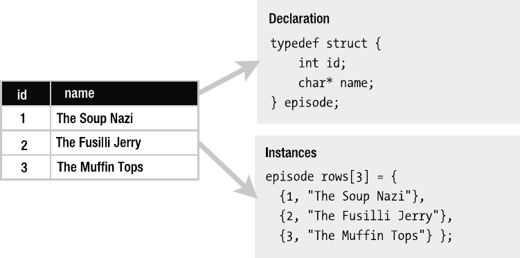
CHAPTER 3 ■ THE RELATIONAL MODEL 53
For example, consider the relation and its C equivalent shown in Figure 3-3. You could say
that a tuple is similar to a C structure. They both are made up of attributes that have a name
and a type. As shown in the figure, a C structure’s attributes are defined in its declaration, just
as a tuple’s attributes are defined in its heading. The declaration and heading both provide
information about the contents of their respective data structures.
Figure 3-3. Header as declaration; tuple as instance
Similarly, a tuple’s values are analogous to an instance of a C structure. Its values form a
composite data structure that corresponds to the attributes defined in its heading. Each value
in the structure is identifiable by an attribute name, and each value is restricted by an attribute
domain.
Thus, tuples are more than just rows of amorphous values like what you might find in a
spreadsheet. They are well-defined data structures with a high degree of specificity over the
information within them. They have more in common with constructs in programming languages
than with rows in a spreadsheet.
But the analogy doesn’t stop there. As also shown in Figure 3-3, a relation is the C equivalent
of an array of structures. Each structure in the array along with the array itself shares the same
type, just as relations and their tuples share the same heading.
The bottom line is that relations and tuples are highly structured. Furthermore, this structure
is defined by their common heading.
Degree and Cardinality
Associated with tuples and relations are the notions of degree and cardinality. These are just
fancy words for width and height, respectively. You could say a relation’s width is the number
of attributes in its heading. This is called the degree. Its height is the number of tuples it contains;
this is called cardinality. These terms are illustrated in Figure 3-2. A relation with four attributes
and five tuples would be said to be of degree 4 and cardinality 5.
Owens_6730 C03.fm Page 53 Wednesday, April 12, 2006 11:21 AM
www.it-ebooks.info

54 CHAPTER 3 ■ THE RELATIONAL MODEL
While tuples don’t have cardinality, they nonetheless have their own fancy terms. A tuple
of degree 1 is said to be a unary tuple. Tuples of degree 2, 3, and 4 are said to be binary, ternary,
and quaternary, respectively. Generally, a tuple of degree N is said to be an N-ary tuple. In fact,
the word tuple is taken from the N-ary form. In the strictest sense, a unary tuple is called a
monad, a binary tuple a pair, a ternary tuple a triple, a quaternary tuple a tetrad, and so on,
as shown in Table 3-1.
Typically, the term tuple is used as a generic catchall for tuples of all degrees, and using
terms like monad and triad is often more confusing than it is precise. As with tuples, a relation
composed of binary tuples is a binary relation. A relation composed of N-ary tuples is an N-ary
relation, and so forth.
Mathematical Relations
The notion of a relation in relational theory is taken directly from the relation in set theory,
with a few modifications. To really understand relations, as defined in relational theory, you
must understand their predecessors in mathematics.
Just as in relational theory, mathematical relations are sets of mathematical tuples. Like
mathematical relations, mathematical tuples also differ somewhat from their relational name-
sakes. In mathematics, tuples are ordered sequences and relations are unordered sets. Sets by
their very nature are ambivalent to order. That is, the order of elements in a set does not affect
the fundamental identity of that set, whereas the order of items in a sequence does affect its
identity.
To begin with, every value in a tuple has a specific domain associated with it. Suppose we
have a tuple composed of the following two domains:
• The domain of all integers {...,-1,0,1,...}, denoted by I
• The domain of the first names of all Seinfeld characters {‘Jerry’, ‘Cosmo’, ‘Newman’, ...},
denoted by F
Now, suppose we have a relation composed of such tuples. The relation then is also composed
of the domains I and F (in that order). The first column of the relation must consist of integer
values, and the second column must consist of the first names of Seinfeld characters. Using
this as an example, the formal definition of a relation can be expressed as follows:
Table 3-1. Tuple Terminology
Degree Qualification Designation Example
1 Unary Monad 1
2 Binary Pair, twin (0, 1)
3 Ternary Triple, triad (0, 1, 2)
4 Quaternary Quadruple, tetrad (0, 1, 2, 3)
NN-ary N-tuple (tuple) (0, 1, 2, … N)
Owens_6730 C03.fm Page 54 Wednesday, April 12, 2006 11:21 AM
www.it-ebooks.info
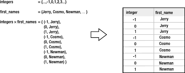
CHAPTER 3 ■ THE RELATIONAL MODEL 55
A relation over I and F is any subset of the cross product of I and F, represented by I×F.
This is a somewhat annoying definition because it defines a relation in terms of another perhaps
unfamiliar concept: the cross product. The cross product, also called the Cartesian product, is
quite simple, however. It is the combination of every value in every domain with every value in
every other domain. To compute I×F, for example, you take each integer i in I, and pair it with
each name f in F. This yields an infinitely large set of (i,f) tuples (binary tuples), as illustrated in
Figure 3-4. Note that the figure is somewhat simplistic and depicts the set of all integers as the
values to {-1, 0, 1}.
Figure 3-4. The cross product of integers and Seinfeld character first names
What does the cross product do here? Why is it used? The cross product of domains I and F
is a set containing every tuple that could ever exist by the combination of these two domains.
That is, every tuple that has an integer as its first value and the first name of a Seinfeld character
as its second value is contained in the cross product I×F. The cross product is itself just a set,
albeit a very big one. It is a set defining the limit of every tuple that could ever be formed from
the domains I and F. That being said, any subset of this cross product is a relation, specifically
a “relation over I and F.” That is a mathematical relation: any subset of a cross project.
Put more simply, a relation is defined in terms of its constituent domains—it is a portion
(or subset) of their cross product. This cross product is a superset containing every possible
tuple that could ever appear in the relation. (I know this seems circuitous.) The proper way of
expressing a relation is to speak of a relation R over the domains X, Y, and Z. If we were to expand
our relation to include the domain of all Seinfeld episodes, denoted by E, it would then be “a
relation R over I, F, and E”—represented by I×F×E, which in turn is an even larger set than I×F.
Relational Relations
There is one fundamental difference between tuples in mathematics and tuples in relational
theory. In mathematics, the order of values in a tuple is significant; in relational theory it isn’t.
This is because members (attributes) of relational tuples have names, which are used to iden-
tify them. Mathematical ones do not. Therefore, mathematical tuples in relations over I×F are
always of the form (i,f) because this is the only way to identify them—by ordinal positions. This
convention is not needed in relational tuples because they have attributes that have names to
Owens_6730 C03.fm Page 55 Wednesday, April 12, 2006 11:21 AM
www.it-ebooks.info
56 CHAPTER 3 ■ THE RELATIONAL MODEL
identify them, rather than ordinal positions. Order, then, in a relational tuple offers no real
advantage. The same applies to relational relations, as they share the same attributes through
their common heading.
In his original paper, Codd differentiated mathematical relations (which he called domain-
ordered relations) from his relational relations (called domain-unordered relations) by referring to
the latter as “relationships”:
Accordingly, we propose that users deal, not with relations which are domain-ordered,
but with relationships which are their domain-unordered counterparts. To accomplish
this, domains must be uniquely identifiable at least within any given relation, without
using their position.
Domains (or attributes) are uniquely identifiable through attribute names. Therefore, both
column and row order do not matter in the relational model. This is the principal way in which
the relations of set theory and the relations of relational theory differ. In all other respects,
tuples and relations in the relational theory share all the same properties of their counterparts
in set theory.
And that is a relation. It is the fundamental object upon which relational theory is built. If
you understand it, you are well on your way to understanding the core mechanics of relational
theory. Relational theory is fitted so as to mirror the true mathematical relation as closely as
possible. The reason is that the closer the relational model fits the mathematical model, the
more it benefits from other facets of mathematics already well established. A prime example is
relational algebra, which is part of the manipulative component of the relational model. Many
of the operations defined for relations in set theory carry over to relational algebra because
relational relations are sufficiently similar. The same is true for relational calculus, which employs
methods of formal logic. As Codd put it
Moreover, the (relational) approach has a close tie to first-order predicate logic—a logic
on which most of mathematics is based, hence a logic which can be expected to have
strength, endurance, and many applications.
Codd recognized not only that the elegance of mathematics is beneficial as a basis to build
upon, but that it also offers a vast reservoir of existing knowledge that can be harnessed as well.
Tables: Relation Variables
A relation, though it contains values, is itself just a value, just like an integer or a string. The
value of a relation is given by the particular set of tuples it contains. Likewise, the value of each
tuple in turn is given by the specific values within it. Thus, the value of a relation is determined
by the sum of its parts. Figure 3-5 illustrates this. It depicts three relations, represented by R1,
R2, and R3, taken over I×F. Each represents a different value, or relation.
R1, R2, and R3 are not relations but rather relation variables. They represent relations.
Codd referred to them as named relations. Date (2003) calls them relvars. SQL calls them tables.
They are also known as base tables. The bottom line is that they are simply variables whose
values are relations. I will simply refer to them here as tables, as that is what you will be dealing
with in SQL.
Owens_6730 C03.fm Page 56 Wednesday, April 12, 2006 11:21 AM
www.it-ebooks.info
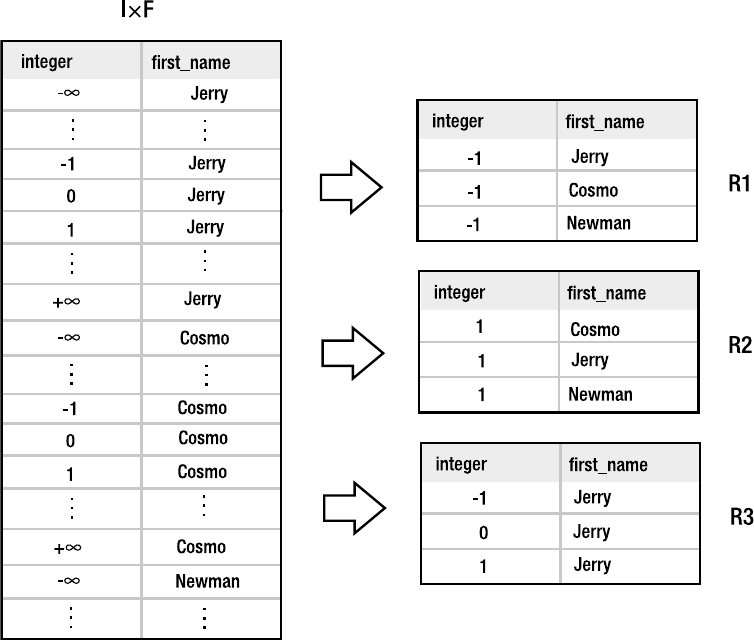
CHAPTER 3 ■ THE RELATIONAL MODEL 57
Figure 3-5. Relations over I×F
In practice, the precise meaning of “relation” can sometimes be a bit murky. Relations are
often referred to in the same context as tables. However, they are not the same thing. One is a
value; the other is a variable. A relation is a value, like an integer value is 1, 2, or 3. A table is a
variable—to which relations are assigned. Tables, like variables, have both a name and a value.
Their name is just a symbol. Their value is a relation. They are no different than variables in
algebra, such as x and y in the equation of a line. Tables share all the properties of relations
(heading, degree, cardinality, etc.) just as integer variables share the properties of integers.
With this in mind, what does it mean to update or modify a table? If you are familiar with
SQL, you probably think of it in terms of modifying a single value, or a few rows. You see it the
same as changing cells in a spreadsheet. You modify parts of the spreadsheet. You see those
parts as individual values. The relational view is different. In the relational view, you don’t
modify parts of a table. A table is a variable holding an entire relation as its value. If you change
anything, you change the entire relation—no matter how small the difference might be. You
aren’t changing a row or column; you are actually swapping one relation with an entirely new
one, where the new relation contains the rows or columns you want changed.
I know that it may seem like frivolous semantics. But just as you don’t modify part of an
integer variable, you don’t modify part of a relation variable either. There is nothing wrong
Owens_6730 C03.fm Page 57 Wednesday, April 12, 2006 11:21 AM
www.it-ebooks.info
58 CHAPTER 3 ■ THE RELATIONAL MODEL
with thinking in terms of the SQL view—where you are changing values in a row. It is logically
equivalent: in a SQL update, you are articulating the change you want to make in a statement,
and that statement produces a new relation. But that is where you should make the distinction:
the change produces a new relation, not a patched-up version of the old one. That new relation
becomes a new value that the table holds.
Be aware that when you talk about tables in a database, you are referring to variables,
specifically relation variables—not relations. If a database were composed strictly of relations,
then its contents would be fixed values, not subject to change. But databases are dynamic. And
the reason is because their contents—tables—are relation variables, which are subject to change.
They change by assigning those relation variables new relation values, not by adding, subtracting,
or changing tuples.
Views: Virtual Tables
Views are virtual tables. They look like tables and act like tables, but they’re not. Views are rela-
tional expressions that yield relations. It is like saying that the algebraic expression x+y is not a
number per se, though it can yield a number if the expression is evaluated, provided we have
specific values for x and y. The same is true for views. Codd (1980) described them as follows:
A view is a virtual relation (table) defined by means of an expression or sequence of
commands. Although not directly supported by actual data, a view appears to a user as
if were an additional base table kept up-to-date and in the state of integrity with other
base tables. Views are useful for permitting application programs and users at terminals to
interact with constant view structures, even when the base tables themselves are under-
going structural changes at the logical level...
Logical Data Independence
In one sense, views are simply a matter of convenience. They let you assign a name to a set of
operations and treat the result like a relation. They are a kind of shorthand. This is perhaps the
most common use of views. Another use was for security. In some systems, views can be used
to selectively present parts of tables, while excluding other sensitive or restricted parts. But the
original intent of views was much more than these two applications. The main application for
views was facilitating what is called logical data independence, which is defined as follows:
9. Logical Data Independence. Application programs and terminal activities remain
logically unimpaired when information-preserving changes of any kind that theoretically
permit un-impairment are made to the base tables.
Logical data independence means that applications and users should theoretically be able to
see the same logical structure (e.g., the same attributes in a relation), even if it is changed (e.g.,
an attribute in that relation is moved to another relation). An example is when a relation is
decomposed into two relations for the sake of normalization, as described in the section
“Normalization.”
More precisely, logical data independence means that users and applications should be
able to be insulated from changes at the logical level of the database. That doesn’t mean the
database is supposed to automatically shield users and programs from the database adminis-
trator (DBA) doing something really bone-headed like dropping a table and going home for the
Owens_6730 C03.fm Page 58 Wednesday, April 12, 2006 11:21 AM
www.it-ebooks.info
CHAPTER 3 ■ THE RELATIONAL MODEL 59
day. Rather, it means that the relational model provides a means for the administrator to
bridge the gap if she wants to make substantive changes at the logical level that would impact
the logical view seen by users and applications. For instance, if the DBA decomposes a table
into two smaller ones, she can create a view that looks like the original table, though it is in
reality a relational expression that combines (joins) the two new tables. The users and applica-
tions know no differently.
Updatable Views
But logical data independence entails more than just viewing data. Many people who are
familiar with views understand them as read-only. However, the relational model clearly states
that you should be able to write to views as well, just as if they were ordinary tables. While logical
data independence would seem to imply this, Rule 6 makes it explicit:
6. View Updating Rule. All views that are theoretically updatable are also updatable by
the system.
Rule 6 is essential for logical data independence. “Theoretically updatable” means the view is
constructed in such a way that it is theoretically possible to map changes made on it to its
respective base tables. That is, if it can be done in theory, the system should be able to do it.
That said, Rule 6 and updatable views (sometimes referred to as materialized views) are
not fully supported in all relational databases, simply because they are not easy to implement.
Programming a system to know what is “theoretically updatable” in relational algebra and/or
calculus is not exactly a weekend project. On the other hand, read-only views are extremely
common. In fact, it is almost hard to find relational databases today that don’t support them.
The System Catalog
As a database is composed of tables and views, you might at some point wonder how you can
find out exactly what is in a given database. As it turns out, a relational database contains tables
and views describing its tables and views—information about the information. That is, all tables,
views, constraints, and other database objects belonging in a database are registered in what is
referred to as the system catalog. Per Rule 4:
Rule 4. Dynamic On-Line Catalog Based on the Relational Model. The data base
description is represented at the logical level in the same way as ordinary data, so that
authorized users can apply the same relational language to its interrogation as they
apply to the regular data.
The system catalog is subject to the Information Principle: it is required to be represented in
a relational format that can be queried in the same way as other relations in the system. This
means that even metadata (information about information) in a database has to be represented
relationally. In many database products, many of the tables in the system catalog are often
implemented as views. The beauty of views and the system catalog is that together they enable
you to extend or enhance the catalog itself. You can create your own catalog views that contain
information you find useful or informative. Those views in turn may even use catalog tables as
a basis.
Owens_6730 C03.fm Page 59 Wednesday, April 12, 2006 11:21 AM
www.it-ebooks.info
60 CHAPTER 3 ■ THE RELATIONAL MODEL
The Integrity Component
While the structural aspect of the model relates to the structure of information, the integrity
aspect relates to the information within the structure. Information can be arranged in relations
in a way that gives rise to various relationships, both within columns of a single relation and
between columns of different relations. These relationships provide additional structure and
indeed add even more information to what is already present.
The integrity aspect of the relational model provides a way to explicitly define and protect
such relationships. Although their use in a database is entirely optional, the degree to which
they are employed can ultimately determine the consistency of your data.
Primary Keys
Codd’s second rule is the starting point of data integrity, and deals with the nature of data
within relations. This rule is called the Guaranteed Access Rule and is defined as follows:
2. Guaranteed Access Rule. Each and every datum (atomic value) in a relational data
base is guaranteed to be logically accessible by resorting to a combination of table
name, primary key value and column name.
The relational model requires that every relation have a primary key. The primary key is the set
of attributes in a relation that uniquely identifies each tuple within it. This rule carries with it
an important corollary: relations may not contain duplicate tuples.
The Guaranteed Access Rule states that every field (or value in a tuple) in a relational data-
base must be addressable. To be addressable, it must be identifiable. To be identifiable, each
tuple must be distinguishable in some way from all other tuples in the relation, which is to say
unique (thus, duplicate tuples would violate this constraint).
Uniqueness is the business of the primary key. A key is a designated attribute (or group of
attributes) in a relation such that
1. The value (or combined values) of that attribute (or attributes) is unique for every tuple
in the relation.
2. If the key is composed of more than one attribute, all of the attributes that define the
key must be necessary to ensure uniqueness. That is, every attribute in the key is sufficient
to ensure uniqueness, but also necessary as well—if one were absent, then the uniqueness
condition would not hold.
If both conditions 1 and 2 are met, then the resulting attribute or group of attributes is a key
(also called a candidate key). If condition 1 is met but not condition 2, then the attribute (or
group of attributes) is called a superkey. It is a key that could stand to lose some weight. That is,
it has more attributes than necessary to ensure uniqueness: a smaller key containing fewer
attributes could be defined that still guarantees uniqueness.
A relation may have one or more candidate keys. If it does, then which one of them that is
defined as the primary key is arbitrary:
Whenever a relation has two or more nonredundant primary keys, one of them is
arbitrarily selected and called the primary key of the relation.
Owens_6730 C03.fm Page 60 Wednesday, April 12, 2006 11:21 AM
www.it-ebooks.info
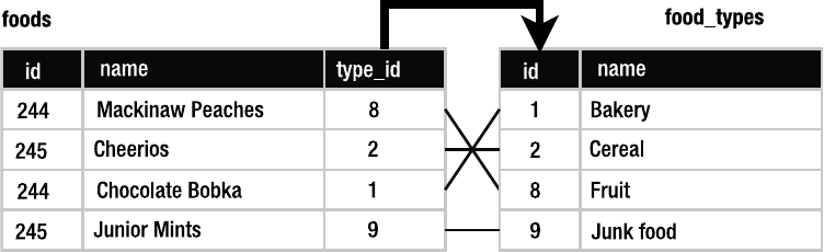
CHAPTER 3 ■ THE RELATIONAL MODEL 61
The primary key is just a rule that requires that every relation have at least one candidate key. The
definition of a primary key serves more as an affirmation of the Guaranteed Access Rule than it
does in defining a new relational concept.
Foreign Keys
With keys comes more than simply identification. While keys define relationships between
tuples within a single relation (you might say vertically), they can also define relationships
between tuples in different relations (horizontally). A key’s identification property allows a
tuple in one relation to identify (or reference) a specific tuple in another relation by way of a
common key value. This is called a foreign key relationship. Specifically, a key in one table
corresponds to, or references, the primary key in another table (the foreign key), thereby relating
the tuples in each table. Take, for example, the foods and food_types tables, as shown in Figure 3-6.
Each row in foods corresponds to a distinct food item (Junior Mints, Mackinaw Peaches, etc.),
the name of which is stored in the name attribute. Each row in food_types stores various food
classifications (e.g., Junk Food, Fruit, etc.). Each row in foods references a row in food_types by
using a common key. foods contains a key called type_id, every value of which corresponds to
a value in the primary key (id) of the food_types, as illustrated by the arrow in Figure 3-6.
Figure 3-6. Foreign key relationship between foods and food_types
From a relational standpoint, this is merely a foreign key relationship. But in reality it is
more than that. This relationship models a relationship in the real world. It has a basis in reality,
has real meaning, and adds information above and beyond the information contained in the
individual tables. Therefore, it is a critical part of the information itself.
It is easy to see that such relationships, if not properly maintained, can be precarious. If an
application comes to assume this relationship, and its normal operation depends on the fact
that a tuple in foods always has a corresponding tuple in food_types, what happens if someone
deletes all the tuples from food_types? Where does that leave the type_id values in the foods
tuples pointing to now? What has become of this relationship?
For that matter, what is to stop a user from just ignoring the primary key rule and jamming
a thousand identical food_types tuples back into the database? If there is nothing in place to
protect and ensure these relationships, they can be as destructive as they are beneficial. Such
rules, like laws, are worthless without enforcement.
Owens_6730 C03.fm Page 61 Wednesday, April 12, 2006 11:21 AM
www.it-ebooks.info
62 CHAPTER 3 ■ THE RELATIONAL MODEL
Constraints
Enter the constraint. Constraints are relational cops. They enforce database rules and relation-
ships and preserve order in general. They bring consistency and uniformity to information
within a database. With constraints, you can rest assured that tuples in the foods table will
always reference legitimate tuples in food_types. Primary keys will always exist in tables, and
their values will always be unique. This kind of uniformity and consistency is called data integrity.
It is the integrity component of the relational model.
Constraints work by governing database operations. Like the precogs in Minority Report,
they stop bad things before they happen. If a user or an application issues a request that would
result in an inconsistent relationship or data, the database refuses to carry out the operation
and issues an error, called a constraint violation. In the relational model, constraints fall into
four general classes of integrity:
•Domain integrity: Domain integrity is the relationship between attribute values and
their associated domains. In the relational model, domain integrity is instituted through
domain constraints. A domain constraint requires that each attribute value in a tuple
exist within its associated domain. For example, if the type_id attribute in the foods table is
declared as an integer, then the corresponding values of type_id in all tuples in the foods
table must be integer values—not floating-point numbers or strings. Domain integrity is
also referred to as attribute integrity—it pertains to the attributes of a relation. Domain
integrity is not limited to just checking that a given value resides in a given domain.
It includes additional constraints as well, such as CHECK constraints. CHECK constraints
(which are covered in Chapter 4) can define arbitrarily complex rules on what constitutes a
permissible value for a given attribute.
•Entity integrity: This form of integrity is mandated by the Guaranteed Access Rule: each
tuple in a relation must be uniquely identifiable. Whereas domain integrity is concerned
with a relation’s attribute values, entity integrity is concerned with its tuples. The term
“entity” here is a rather loose term for table. It originates from database modeling (i.e.,
entity-relationship diagrams). In this particular context, an entity simply refers to anything
in the real world that must be represented in a database.
•Referential integrity: This form of integrity pertains to relationships between tables,
specifically the preservation of foreign key relationships. Whereas entity integrity
pertains to tuples in a relation, referential integrity pertains to tuples between relations.
•User-defined integrity: User-defined integrity encompasses any form of integrity not
defined in the other forms. Many relational databases offer various facilities that go
beyond the normal constraint mechanisms. One such example is triggers, which are
covered in Chapter 4.
The relational model requires that databases and query languages support integrity constraints.
Furthermore, these constraints, like all other data and metadata in the database, must also be
defined directly in the database, specifically in the system catalog:
10. Integrity Independence. Integrity constraints specific to a particular relational data
base must be definable in the relational data sub-language and storable in the catalog,
not in the application programs.
Owens_6730 C03.fm Page 62 Wednesday, April 12, 2006 11:21 AM
www.it-ebooks.info
CHAPTER 3 ■ THE RELATIONAL MODEL 63
Null Values
Closely associated with data integrity in the relational model is a special value (or lack thereof),
which exists both inside and outside of every domain. This special value denotes the absence of
a value and is called a null value, or null for short. Nulls are prescribed in Codd’s third rule:
3. Systematic Treatment of Null Values. Null values (distinct from the empty character
string or a string of blank characters and distinct from zero or any other number) are
supported in fully relational DBMS for representing missing information and inapplicable
information in a systematic way, independent of data type.
There are multiple interpretations for what null values mean. The prevailing view of null seems
to be “unknown.” But there are others. For example, a tuple containing employee information
may have an attribute for the employee’s middle name. But not everyone has a middle name.
A tuple for a person without a middle name might use a null value for that particular attribute.
In this case, the null value doesn’t necessarily mean “unknown” but rather “not applicable.”
Thus, a value may be null because it is either missing (a value exists but was not input) or
uncertain (it is not known whether a value exists at all), or it is simply not applicable for the
tuple (or employee) in question.
The inclusion of nulls in the relational model has been a source of controversy for many
years, and there are people on both sides of the debate who feel very strongly for their positions.
Codd, for example, felt the need for nulls:
In general, controversy still surrounds the problem of missing and inapplicable infor-
mation in data bases. It seems to me that those who complain loudly about the
complexities of manipulating nulls are overlooking the fact that handling missing
information and inapplicable information is inherently complicated.
Date, Codd’s colleague and well-known authority on the relational model, is opposed to them:
…we should make it very clear that in our opinion (and in that of many other writers
too, we hasten to add), nulls and 3VL are a serious mistake and have no place in a clean
formal system like the relational model.
The “3VL” acronym in the quote stands for “three-valued logic,” which corresponds to how
nulls are evaluated in logical expressions. This is addressed in Chapter 4.
Normalization
The implication of no duplicate tuples provided by the Guaranteed Access Rule gives rise to an
important concept in database design called normalization. Normalization concerns itself
with the organization of attributes within relations so as to minimize duplication of data. Data
duplication, as you will see, has more deleterious effects than just taking up unnecessary space.
It increases the opportunity for database inconsistencies to arise. Normalization is about designing
your database to be more resistant to the ill effects of thoughtless users and buggy programs.
While based on principles of the relational model, normalization is somewhat a subject
(some even say an art) in itself. It can become quite complicated, introducing a considerable
Owens_6730 C03.fm Page 63 Wednesday, April 12, 2006 11:21 AM
www.it-ebooks.info
64 CHAPTER 3 ■ THE RELATIONAL MODEL
amount of new concepts and terminology. A proper treatment of the subject is beyond the
scope of this book. What follows is a very brief introduction.
Normal Forms
As stated, the chief aim of normalization is to eradicate duplication. Relations that have dupli-
cation removed are said to be normalized. However, there are degrees of normalization. These
degrees are called normal forms. The first degree is called first normal form, followed by second
normal form, and so on. They are abbreviated 1NF, 2NF, 3NF, and so on. Each normal form
defines specific conditions a relation must meet in order to be so classified. Thus a relation that
meets the conditions of first normal form is said to be “in first normal form.” Normal forms
build on each other so that higher normal forms require all the conditions of lower forms as
prerequisites. For data to be in 2NF, it must also be in 1NF. Essentially, the higher the normal
form of a relation, the less duplication it has, and the more resistant it is to inconsistencies. The
most common and perhaps most widely used normal form is 3NF, although there are even
more advanced normal forms such as Boyce-Codd normal form (BCNF), 4NF, 5NF, and higher.
The first three normal forms are easy enough to describe.
First Normal Form
First normal form simply states that all attributes in a relation use domains that are made up of
atomic values. The working definition of “atomic” is the same as other disciplines, meaning
simply “that which cannot be broken down further.” For example, integer values would seem
to be atomic, as you can’t break them down further. But you could argue that integer values
could be decomposed into their prime factors. Atomicity, then, is determined by the method of
decomposition, which can be a subjective matter. For all practical purposes, it is the database
management system that decides what is atomic. And the domains provided by the system can
safely be considered as such.
That said, first normal form basically means that a single attribute cannot hold more than
a single value. For example, take the episodes table shown in Table 3-2 in the next section. 1NF
states that you couldn’t store both the values 1992 and 1993 (two integer values) in a year attribute
of a single tuple. It sounds so silly that it can be kind of hard to imagine. But it’s that simple.
It is so simple, in fact, that you have to work at violating 1NF; most databases won’t even give
you the means to do it.
Functional Dependencies
To understand second and third normal form, you have to first understand functional depen-
dencies. The simple definition of a functional dependency is a correlation between columns in
a table. If the values of one column (or set of columns) correlate to the values of another, then
they have a functional dependency. More precisely, a functional dependency describes a relation-
ship between two or more attributes in a relation such that the value of one attribute (or set of
attributes) can be inferred from the value of another attribute (or attributes) for every tuple in
the relation. This is more easily illustrated by example. Consider the table, called episodes,
shown in Table 3-2.
There is a functional dependency between season and year. For any given value of season,
you will find the same value of year. If you ever come across a tuple with a value of 4 for season,
you know the value for year will be 1992. If you know the former, you can determine the latter.
Owens_6730 C03.fm Page 64 Wednesday, April 12, 2006 11:21 AM
www.it-ebooks.info

CHAPTER 3 ■ THE RELATIONAL MODEL 65
Many times, functional dependencies are a warning sign that duplication lurks within a
table. And already you can see in this example how inconsistencies can crop up. If there is in
fact a correlation between year and season, what happens to that relationship if someone
modifies the first row so that its value for year is 1999 (but fails to do so for the second row)?
That relationship has been compromised. It is inconsistent. One tuple with season=4 has
year=1992, and another with season=4 has year=1999. How can season 4 have happened in
both 1992 and 1999? This is logically inconsistent, and the functional dependency (or lack of
sufficient normalization) is what made it possible to introduce this inconsistency. What is even
more interesting is that there is no standard integrity constraint designed to guard against this
problem. It is purely the result of bad design.
Functional dependencies always involve exactly two sets of attributes: one set (the deter-
minant) determines (or relates to) the value of another (the dependent). Call the attribute(s)
making up the determinant A and the attribute(s) making up the dependent B. With this in
place, you can express this relationship using the following two (equivalent) statements:
1. B is functionally dependent upon A.
2. A functionally determines B.
There is even a fancy notation for this as well: A → B. The bottom line: for any value of A, the
value of B has some kind of correlation.
Second Normal Form
Second normal form is defined in terms of functional dependencies. It requires that a relation
be in first normal form and that all non-key attributes be functionally dependent upon all
attributes of the primary key (not just part of them). Remember that normalization is about
cutting out duplication, so while this sounds like an arbitrary rule, it is in fact aimed at weeding
out duplication.
You have already seen what duplication looks like when 2NF is not followed, using episodes
as an example. The primary key in episodes is composed of both season and week. You know
that year is functionally dependent on season, which in turn is only part of the primary key
(red-flag). Specifically, for every season=x (e.g., 4) you have the same year=y (e.g., 1992). There
is no reason to include the year attribute in the relation if its value is correlated with season.
That’s duplication. It must go.
Table 3-2. The Unnormalized episodes Table
season week year name
4 1 1992 The Junior Mint
4 2 1992 The Smelly Car
5 1 1993 The Mango
5 2 1993 The Puffy Shirt
6 21 1994 The Fusilli Jerry
6251994The Understudy
Owens_6730 C03.fm Page 65 Wednesday, April 12, 2006 11:21 AM
www.it-ebooks.info

66 CHAPTER 3 ■ THE RELATIONAL MODEL
So what do you do? You decompose the table into two tables. Cut out year, and move it to
its own table: call it the seasons table. Now episodes is decomposed into two tables with a foreign
key relationship where episodes.season references seasons.season (see Tables 3-3 and 3-4).
This is like factoring out a common variable in an algebraic expression. Now episodes is in
2NF. Furthermore, no information is lost because year is functionally determined by season.
But look what else you get: the new design allows referential integrity to back you up: you have
a foreign key constraint guarding this relationship (the correlation between season and year),
which you couldn’t get in the previous form. What was previously only implied is now both
explicit and enforceable.
Now consider the specific case mentioned earlier where someone modifies the first row.
The logical inconsistency is no longer possible: it is impossible to mess up the year, because it
is not in episodes. If someone changes year=1992 to 1999 in seasons, it may be inaccurate, but
it is still logically consistent. That is, both rows that refer to it in episodes (season=4) will still be
in agreement about the year in which season 4 took place. Normalization cannot make you get
your facts right, but it can ensure that at least your data is consistent about them.
Second normal form works by tightening the specificity between the primary key and the
non-key attributes. If the values of a non-key attribute correlate to only part of the primary key,
then logically that attribute can introduce duplication. Why? Because only part of a primary
key is not unique (all of the primary key is required for uniqueness, as mentioned earlier), and
a correspondence between two columns, neither of which is unique, opens the possibility for
duplication, and duplication invites inconsistency.
Table 3-3. The episodes Table in Second Normal Form
season week name
4 1 The Junior Mint
4 2 The Smelly Car
51The Mango
52The Puffy Shirt
621The Fusilli Jerry
625The Understudy
Table 3-4. The seasons Table from Normalizing episodes
season year
41992
51993
61994
Owens_6730 C03.fm Page 66 Wednesday, April 12, 2006 11:21 AM
www.it-ebooks.info

CHAPTER 3 ■ THE RELATIONAL MODEL 67
Third Normal Form
Third normal form shifts attention from functional dependencies on the primary key to depen-
dencies on any other non-key attributes in a relation. It roots out a special class of functional
dependencies called transitive dependencies. A transitive dependency is just a chain of two or
more functional dependencies spanning two or more attribute groups (two or more correlations).
For example, say you have a relation with three sets of attributes, A, B, and C, where A is the
primary key, and B is a candidate key. If A → B and B → C, then C is transitively dependent on
A: it depends on A indirectly through its relationship with B. Transitive dependencies harbor
duplication. Third normal form dictates that a relation must be in second normal form and
also have no transitive dependencies.
To picture this, let’s rig the original episodes table to have an integer primary key called id, and
the candidate key is now the combination of season and week. This relation is shown in Table 3-5.
In this version of episodes, year is functionally dependent on season, which in turn is
functionally dependent on id. So we have id → season → year. How do you know this? Work
backwards. Ask yourself if you can determine season from id. Yes. Then can you determine year
from season? Yes. Therefore, you have a transitive dependency: id functionally determines season
and season functionally determines year. To be in third normal form, year, which is functionally
dependent on a non-key attribute, must go. And as with the previous example, you relegate year
into its own table, again splitting episodes into two tables, as shown in Tables 3-6 and 3-7.
Table 3-5. An Unormalized episodes Table with an Integer Primary Key
id season week year name
1 4 1 1992 The Junior Mint
24 2 1992 The Smelly Car
35 1 1993 The Mango
4 5 2 1993 The Puffy Shirt
5 6 21 1994 The Fusilli Jerry
6 6 25 1994 The Understudy
Table 3-6. The episodes Table in Third Normal Form
id season week name
1 4 1 The Junior Mint
2 4 2 The Smelly Car
35 1 The Mango
4 5 2 The Puffy Shirt
56 21 The Fusilli Jerry
66 25 The Understudy
Owens_6730 C03.fm Page 67 Wednesday, April 12, 2006 11:21 AM
www.it-ebooks.info

68 CHAPTER 3 ■ THE RELATIONAL MODEL
Just as in the 2NF example, decomposition made an implicit relationship explicit.
Since functional dependencies between non-key attributes are not allowed in a table, you
may wonder why it is okay for functional dependencies to exist between keys. The answer is
simple: uniqueness. Even if there is a correlation between one key and another, the fact that
they are unique guarantees that their correlation is also unique; therefore, no duplication exists.
In the end, 2NF and 3NF aim not to introduce confusing rules, but to seek out and destroy
duplication and the inconsistencies that can arise from it. It is essential to proper database
design. The more important your data, the more attention you should pay to ensure that your
database is properly designed and normalized.
The Manipulative Component
The manipulative component of the relational model defines the ways in which information
can be manipulated and changed. It is the dynamic part of the model that connects the data in
the logical view to the outside world.
Relational Algebra and Calculus
In his original paper, Codd described a language that could be used to operate on data:
The adoption of a relational model of data, as described above, permits the development
of a universal data sublanguage based on an applied predicate calculus… Such a
language would provide a yardstick of linguistic power for all other proposed data
languages, and would itself be a strong candidate for embedding (with appropriate
syntactic modification) in a variety of host languages (programming, command- or
problem-oriented).
This “universal data sublanguage” would have a sound mathematical basis. Codd defined this
basis in the form of relational algebra and relational calculus, illustrated in his 1972 paper
“Relational Completeness of Data Base Sublanguages.” As described in the abstract of that paper:
In the near future, we can expect a great variety of languages to be proposed for interro-
gating and updating data bases. This paper attempts to provide a theoretical basis
which may be used to determine how complete a selection capability is provided in a
proposed data sublanguage independently of any host language in which the sublan-
guage may be embedded.
Table 3-7. The seasons Table from Normalizing episodes
season year
41992
51993
61994
Owens_6730 C03.fm Page 68 Wednesday, April 12, 2006 11:21 AM
www.it-ebooks.info
CHAPTER 3 ■ THE RELATIONAL MODEL 69
A relational algebra and relational calculus are defined. Then, an algorithm is
presented for reducing an arbitrary relation-defining expression (based on the
calculus) into a semantically equivalent expression of the relational algebra.
Finally, some opinions are stated regarding the relative merits of calculus-oriented
versus algebra-oriented sublanguages from the standpoint of optimal search and
highly discriminating authorization schemes.
These two “pure” languages—relational algebra and calculus—focused on mathematical
theory rather than a particular language syntax. The latter is the job of the “data sublanguage,”
or “query language,” as we know it today. Like the structural part of the relational model, the
manipulative part drew heavily from mathematics. Relational algebra has its basis in set theory.
Likewise, relational calculus has its basis in predicate calculus. From a computer science
perspective, relational algebra can be considered more of a procedural language while rela-
tional calculus is more of a declarative language. The meanings of these terms are explained in
more detail in Chapter 4.
As stated in the quote, while the particular forms of expression in the two languages are
different, they are nevertheless logically equivalent. That is, any operation in relational algebra
can also be expressed in terms of calculus, and vice versa. Another way of saying this is that the
two languages have the same expressive power—the same fundamental operations can be
performed or expressed in either system.
Relational Query Language
Together, relational algebra and calculus serve as a guideline, or a yardstick as Codd describes
it, for query languages implemented in relational databases. Any query language that can express
all of the fundamental operations set forth in relational algebra and/or calculus is said to be
relationally complete.
The query language must also address the other aspects (structural and integrity) of the
relational model as well. This is summed up in Codd’s fifth rule, defined as follows:
5. Comprehensive Data Sublanguage Rule. A relational system may support several
languages and various modes of terminal use (for example, the fill-in-the-blanks
mode). However, there must be at least one language whose statements are expressible,
per some well-defined syntax, as character strings and that is comprehensive in
supporting all the following items:
Data Definition, View Definition, Data Manipulation (Interactive and by program),
Integrity Constraints, and Authorization, Transaction boundaries (begin, commit,
and rollback).
Additionally, Codd’s seventh rule requires that the database (and by extension the query
language) not only use relations for storage, manipulation, and retrieval, but also as operands
for the purpose of modifying the database:
7. High Level Insert, Update, and Delete. The system must support set at a time insert,
update, and delete operators.
Owens_6730 C03.fm Page 69 Wednesday, April 12, 2006 11:21 AM
www.it-ebooks.info

70 CHAPTER 3 ■ THE RELATIONAL MODEL
A user then should be able to insert tuples by providing a relation composed of the tuples to be
inserted, and similarly for updating and deleting information within the system. While this rule
keeps things consistent—using relations—its primary intent at the time was actually in optimizing
database performance. The idea was that in some cases the database could make better opti-
mizations by seeing modifications together as a set than it could by processing them individually.
So, first, a relational database must provide at least one query language that addresses the
structural, integrity, and manipulative aspects of the relational model. And with respect to the
manipulative aspect, it must be capable of expressing the mathematical concepts set forth in
relational algebra and/or calculus. Furthermore, it must accept relations as a means for modi-
fying data in the system. Note that Codd never mandated a particular query language. He only
mandated that a relational database provide one and what it must do.
The Advent of SQL
Thus, over the years, there have been multiple competing query languages. However, the most
popular and widely adopted of these languages today is undoubtedly SQL. SQL is a relationally
complete query language that exhibits aspects of both relational algebra and relational calculus.
That is, it has both declarative features (calculus) and procedural features (algebra). In fact, as
you will see in the next chapter, SQL includes almost all of the operators defined in relational
algebra.
SQL also reflects each aspect of the relational model. Part of its language is dedicated to
working with the structural aspect of the model, specifically to creating, altering, and destroying
tables. This part of the language is called data definition language (DDL). Within DDL lies also
the integrity aspect, allowing the creation of keys and various database constraints. Likewise,
part of the language is dedicated to the operational aspect, called data manipulation language
(DML). And as stated, it includes ideas from both relational algebra and calculus.
Ironically, despite the clear influence of the relational model on SQL, the current SQL standard
does not mention the relational model or use relational terminology.2 And while SQL is relationally
complete, in many ways it falls short of the true power of the relational model. Although it was
primarily inspired by relational calculus, some have claimed that there are ways in which SQL
also violates it. Furthermore, SQL lacks some relational operations that some consider impor-
tant, such as relational assignment, and has a number of redundant features. Part of the reason
for this was that the organization(s) responsible for creating the SQL standard felt that it was
more important to release a standard as early as possible in order to establish a base that data-
base implementations could build upon (Connolly, 2001). Thus, when the initial standard was
released in 1987, though practical, it was found wanting in many ways by researchers involved
with the relational model (Codd included). Among other things, it omitted some relational
operations and included no mention of referential integrity constraints. Subsequent standards
filled in some of the gaps here and there, but this seems to have done little to appease its detractors
or deter database vendors from “extending” their SQL dialects to include proprietary features.
Entire books and websites are devoted to both SQL’s inadequacies as well as what an ideal
query language should be. Furthermore, alternative query languages have been proposed and
implemented (both before and after SQL) that in the minds of their creators are more expressive
and better reflect the principles and intent of the relational model.3
2. See http://en.wikipedia.org/wiki/Relational_model.
3. Tutorial D is one such example. See www.thethirdmanifesto.com for more information.
Owens_6730 C03.fm Page 70 Wednesday, April 12, 2006 11:21 AM
www.it-ebooks.info
CHAPTER 3 ■ THE RELATIONAL MODEL 71
Despite its criticisms and shortcomings, however, SQL is what we have to work with. It is
undoubtedly the most popular and widely adopted query language in the industry, and given
its longstanding dominance in the marketplace, it is unlikely that its position will change any
time in the near future.
The Meaning of Relational
Given all this information, what exactly is relational? It is a common misconception that relational
databases derive the name “relational” from their ability to “relate” a column in one table to a
column in another through a foreign key relationship. The true meaning of relational, however,
stems from the central structural component of the relational model: the relation, which itself
is based on the mathematical concept. First and foremost, a relational database is one that uses
relations as the sole structural unit in which to represent information, as mandated by the
Information Principle.
A more specific definition of relational, however, is provided by Codd’s Rule Zero:
Rule Zero. For any system that is advertised as, or claimed to be, a relational data base
management system, that system must be able to manage data bases entirely through
its relational capabilities.
For a database to be called relational, it must provide all of the facilities required by the rela-
tional model. That is, it must conform to all of the other 12 rules. And believe it or not, you have
covered every one of them. You therefore should have a good idea at this point what it means
to be relational. Don’t get too cocky, though, as Codd later expanded the 12 rules to over 300.
Summary
This was a nickel tour through the relational model. While our discussion isn’t definitive, my
goal was to give you enough history to make the topic enjoyable and enough theory for you to
understand some of the thinking behind SQL—why it works the way it does. The relational
model has clearly influenced its design and has provided it with a solid theoretical foundation.
The relational model has proven itself over its 30-year history. It has had an enormous
impact not only on computing but on the way we do business. Today, it can be found in a wide
array of electronic machinery, ranging from mainframes to cell phones.
The relational model was created to provide a logical, consistent representation of data
that is independent of hardware and software. The model built on well-founded theory set
forth in mathematics. This model provides database users with a consistent, unchanging view
of information, powerful methods to operate on it, and mechanisms to protect and ensure its
consistency and integrity.
There are many more aspects to the relational model, and much that builds on it. It is the
subject of entire books, some of which I have included in the “References” section. While it is a
large subject, its core concepts are logical and straightforward. These concepts ground, frame,
and form the basis of the subject covered in the next chapter: SQL.
If you are new to SQL and you’ve patiently endured this chapter, you should have a much
easier time grasping the concepts in the next chapter. You will see SQL not as an arbitrary language
but as a gateway into a powerful database management system. You will find that its syntax is
heavily geared to what you’ve learned here in this chapter.
Owens_6730 C03.fm Page 71 Wednesday, April 12, 2006 11:21 AM
www.it-ebooks.info
72 CHAPTER 3 ■ THE RELATIONAL MODEL
References
Codd, E. F. 1970. “A relational model for large shared data banks.” Communications
of ACM, 13(6): 377–387.
Codd, E. F. 1972. Relational Completeness of Data Base Sublanguages in Data Base
Systems. In Rustin, R. J. (ed.), Data Base Systems, Courant Computer Symposia Series, v. 6.
Englewood Cliffs, NJ: Prentice-Hall.
Codd, E. F. 1979. “Extending the Database Relational Model to capture more meaning.”
ACM Transactions on Database Systems. 4(4): 397–434.
Codd, E. F. 1980. Data Models in Database Management. In Proceedings of the 1980
Workshop on Data Abstraction, Databases and Conceptual Modeling (Pingree Park, CO,
June 23–26, 1980). New York: ACM Press, 112–114.
Codd, E. F. 1982. “Relational database: a practical foundation for productivity.”
Communications of ACM 25(2): 109–117.
Codd, E. F. 1985. “Is your DBMS really relational?,” Computerworld (Part 1: October 14, 1985,
Part 2: October 21, 1985).
Connolly, C. E. B. 2001. Database Systems: A Practical Approach to Design, Implementation
and Management. Boston: Addison-Wesley.
Date, C. J. 1999. Thirty Years of Relational: Relational (series of 12 articles), Intelligent
Enterprise 1, Nos. 1–3 and 2, Nos. 1–9 (October 1998 onward). Note: Most installments
after the first publication in the online portion of the magazine at
www.intelligententerprise.com, accessed on March 16, 2006.
Date, C. J. 2003. An Introduction to Database Systems, 8th ed. Boston: Addison-Wesley.
Grimaldi, R. P. 1998. Discrete and Combinatorial Mathematics, 4th ed. Boston:
Addison-Wesley.
Reiter, R. 1978. On Closed World Data Bases. In Gallaire, H. and Minker, J. (eds.), Logic and
Data Bases. New York: Plenum, 119–140.
Silberschatz, A., H. F. Korth, and S. Sidharshan. 2002. Database System Concepts. New
York: McGraw Hill.
Owens_6730 C03.fm Page 72 Wednesday, April 12, 2006 11:21 AM
www.it-ebooks.info

73
■ ■ ■
CHAPTER 4
SQL
This chapter is a complete introduction to SQL in general, and SQLite’s implementation of it
in particular. It assumes no previous experience with either SQL or the relational model. If you
are new to SQL, SQLite should serve as an excellent springboard to entering the world of rela-
tional databases. It will give you a good grounding in the fundamentals. While the previous
chapter on the relational model was a little theoretical and stuffy, this chapter is much more
relaxed and practical. We’re not here to prove theories; we’re here to get things done. So if you
didn’t read the previous chapter, that’s perfectly fine. You should still have no trouble with the
material covered in this chapter. An understanding of the relational model is edifying, but not
necessary to learn SQL.
SQL is the sole (and almost universal) means by which to communicate with a relational
database. It is a language exclusively devoted to information processing. It is designed for
structuring, reading, writing, sorting, filtering, protecting, calculating, generating, grouping,
aggregating, and in general managing information.
SQL is an intuitive, user-friendly language. It can be fun to use and is quite powerful. One
of the fun things about SQL is that regardless of whether you are an expert or a novice, it seems
that you can always continue to learn new ways of doing things (for better or worse). There are
often many ways to tackle a given problem, and you may find yourself taking delight in trying
to find more efficient ways to get what you need, either through more compact expressions or
more elegant approaches, as if solving a puzzle. And you can continue to explore dusty corners
of the language you never took notice of before with which to further hone your skills, no matter
your experience.
The goal of this chapter is to teach you to use SQL well—to expose you to good techniques,
and perhaps a few cheap tricks along the way. As you can already tell, there are many different
aspects to SQL. This chapter breaks them down into discrete parts and presents them in a
logical order that should be relatively easy to follow. Nevertheless, SQL is a big subject and
there is a lot of ground to cover. It will take some time and more than one cup of coffee to get
through this chapter. But by the time you are done, you should be well equipped to put a dent
in a database.
The Relational Model
As you’ll remember from Chapter 3, SQL is a consequence of the relational model, which was
originally proposed by E. F. Codd in 1969. The relational model requires that relational data-
bases provide a query language, and over the years SQL rose to become the lingua franca.
Owens_6730 C04.fm Page 73 Monday, April 17, 2006 7:16 AM
www.it-ebooks.info
74 CHAPTER 4 ■ SQL
The relational model consists of three essential parts: form, function, and consistency.
Form refers to the structure of information. There is but one single data structure used to
represent all information. This structure is called a relation (known in SQL as a table), which is
made up of tuples (known in SQL as rows), which in turn are made up of attributes (known in
SQL as columns).
The relational model’s form is a logical representation of information. This logical repre-
sentation is a pristine, abstract view of information unaffected by anything outside of it. It is
like a mathematical concept: clean and consistent, governed by a well-defined set of determin-
istic rules that are not subject to change. The logical representation is completely independent
of the physical representation, which refers to how database software stores this information
on the physical level (e.g., disk). The two representations are thus distinct: nothing that occurs
in the physical level can change or affect anything at the logical level. The logical level is unin-
hibited by hardware, software, vendor, or technology.
The second essential part of the model—the functional part—is also called the manipula-
tive component. It defines ways of operating on information at the logical level. This was formally
introduced in Codd’s 1972 paper titled “Relational Completeness of Data Base Sublanguages.”
It added the functional part to the relational model by defining relational algebra and relational
calculus. These are two formal, or “pure,” query languages with a heavy basis in mathematics.
Relations, as described in the data model, are mathematical sets (with a few additional proper-
ties). Relational algebra and calculus, in turn, build on this model by adding operations from
set theory and formal logic, thus forming the functional component of the relational model. So
both the form and function prescribed in the relational model come directly from concepts in
mathematics. Each derivative, however, adds a little something to better adapt it to computers
and information processing.
Query Languages
A query language connects the outside world with the abstract logical representation, and
allows the two to interact. It provides a way to retrieve and modify information. It is the
dynamic part of the relational model.
Codd intended relational algebra and calculus to serve as a baseline for other query
languages. Relational algebra and calculus employ a highly mathematical notation that, while
good for defining theory, is not terribly user-friendly in practice. Their purpose was thus to
define the mathematical or relational requirements that a more user-friendly query language
should support. Query languages that met these minimum requirements were called relationally
complete. This user-friendly query language then provides a more tractable and intuitive way for a
person to work with relational data, while at the same time adhering to a sound theoretical basis.
The Growth of SQL
Perhaps the first such query language that was to be so employed was that of IBM’s System R, a
relational database research project that was a direct outgrowth of Codd’s papers. It was originally
called SEQUEL, which stands for “Structured English Query Language.” It was later shortened
to SQL, or “Structured Query Language.”
Other companies such as Oracle followed suit (in fact, Oracle beat IBM to market with the
first SQL product), and pretty soon SQL was the de facto standard. There were other query
languages, such as Ingres’s QUEL, but in time SQL won out. The reasons SQL emerged as the
Owens_6730 C04.fm Page 74 Monday, April 17, 2006 7:16 AM
www.it-ebooks.info
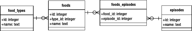
CHAPTER 4 ■ SQL 75
standard may have had more to do with the dynamics of the marketplace than anything else.
But the reasons why it is special today are perhaps a little clearer. There are (among others)
standardization, wide adoption, and general ease of use.
SQL has been accepted as the standard language for relational databases by the American
National Standards Institute (ANSI), the International Standards Organization (ISO), and the
International Electrotechnical Commission (IEC). It has a well-defined standard that specifies
what SQL is and does, and this standard has continued to evolve over the past two decades. To
date, five versions of the standard have been published over the years (1986, 1989, 1992, 1999,
and 2003). The standards are cumulative. Each version of the standard has built on the
previous one, adding new features. So in effect, there is only one standard that has continued
to grow and evolve over time. The first versions—SQL86 and SQL89—are collectively referred
to as SQL1. SQL92 is commonly referred to as SQL2, and SQL99 as SQL3. The ANSI standard, as
a whole, is very large. The SQL92 standard alone is over 600 pages. No one database product
conforms to the entire standard. Nevertheless, the standard goes a long way in bringing a great
deal of uniformity to relational databases.
SQL’s wide adoption today is patently obvious: Oracle, Microsoft SQL Server, DB2, Informix,
Sybase, PostgreSQL, MySQL, Firebird, Teradata, Intersystems Caché, and SQLite are but some
of the relational databases that use SQL as their query language.
The Example Database
Before diving into syntax, let’s get situated with the obligatory example database. The database
used in this chapter (and the rest of this book for that matter) consists of all the foods in every
episode of Seinfeld. If you’ve ever watched Seinfeld, you can’t help but notice a slight preoccu-
pation with food. There are more than 412 different foods mentioned in the 180 episodes of its
history (according to the data I found on the Internet). That’s over two new foods every show.
Subtract commercial time and that’s virtually a new food introduced every 10 minutes.
As it turns out, this preoccupation with food works out nicely as it makes for a database
that illustrates all the requisite concepts. The database tables are shown in Figure 4-1.
Figure 4-1. The Seinfeld food database
The database schema, as defined in SQLite, is defined as follows:
create table episodes (
id integer primary key,
season int,
name text );
Owens_6730 C04.fm Page 75 Monday, April 17, 2006 7:16 AM
www.it-ebooks.info
76 CHAPTER 4 ■ SQL
create table foods(
id integer primary key,
type_id integer,
name text );
create table food_types(
id integer primary key,
name text );
create table foods_episodes(
food_id integer,
episode_id integer );
The main table is foods. Each row in foods corresponds to a distinct food item, the name of
which is stored in the name attribute. The type_id attribute references the food_types table,
which stores the various food classifications (e.g., baked goods, drinks, or junk food). Finally,
the foods_episodes table links foods in foods with the episodes in episodes.
Installation
The food database is located in the examples zip file accompanying this book. It is available on
the Apress website (www.apress.com) in the Source Code section. To create the database, first
locate the foods.sql file in the root directory of the unpacked zip file. To create a new database
from scratch from the command line, navigate to the examples directory and run the following
command:
sqlite3 foods.db < foods.sql
This will create a database file called foods.db. If you are not familiar with how to use the
SQLite command-line program, refer to Chapter 2.
Running the Examples
For your convenience, all of the SQL examples in the chapter are available in the file sql.sql in
the root directory of the examples zip file. So instead of typing them by hand, simply open the
file and locate the SQL you want to try out.
A convenient way to run the longer queries in this chapter is to copy them into your favorite
editor and save them in a separate file, which you can run from the command line. For example,
copy a long query in test.sql to try out. You simply use the same method to run it as you did
to create your database earlier:
sqlite3 foods.db < test.sql
The results will be printed to the screen. This also makes it easier to experiment with these
queries without having to retype them or edit them from inside the SQLite shell. You just make
your changes in the editor, save the file, and rerun the command line.
For maximum readability of the output, you may want to put the following commands at
the beginning of the file:
Owens_6730 C04.fm Page 76 Monday, April 17, 2006 7:16 AM
www.it-ebooks.info
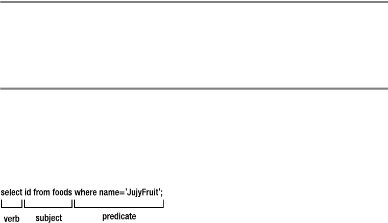
CHAPTER 4 ■ SQL 77
.echo on
.mode col
.headers on
.nullvalue NULL
This causes the command-line program to 1) echo the SQL as it is executed, 2) print results in
column mode, 3) include the column headers, and 4) print null values as NULL. The output of all
examples in this chapter is formatted with these specific settings. Another option you may
want to set for various examples is the .width option, which sets the respective column widths
of the output. These vary from example to example.
For better readability, the examples are presented in two different formats. For short queries,
I show the SQL and output as it would be shown from within the SQLite shell. For example:
sqlite> SELECT * FROM foods WHERE name='JujyFruit' AND type_id=9;
id type_id name
---------- ---------- ----------
244 9 JujyFruit
Occasionally, as in the previous example, I take the liberty of adding an extra line between the
command and its output (in the shell, the output immediately follows the command). For
longer queries, I show just the SQL in code format separated from the results by gray lines, as
in the following example:
SELECT f.name name, types.name type FROM foods f
INNER JOIN (SELECT * FROM food_types WHERE id=6) types
ON f.type_id=types.id;
name type
------------------------- -----
Generic (as a meal) Dip
Good Dip Dip
Guacamole Dip Dip
Hummus Dip
Syntax
SQL’s declarative syntax reads a lot like a natural language. Statements are expressed in the
imperative mood, beginning with the verb describing the action. Following it are the subject
and predicate, as illustrated in Figure 4-2.
Figure 4-2. General SQL syntax structure
Owens_6730 C04.fm Page 77 Monday, April 17, 2006 7:16 AM
www.it-ebooks.info
78 CHAPTER 4 ■ SQL
As you can see, it reads like a normal sentence. SQL was designed specifically with nontech-
nical people in mind, and was thus meant to be very simple and easy to understand.
Part of SQL’s ease of use comes from its being (for the most part) a declarative language, as
opposed to an imperative language such as C or Perl. A declarative language is one in which
you describe what you want whereas an imperative language is one in which you specify how
to get it. For example, consider the process of ordering a cheeseburger. As a customer, you use
a declarative language to articulate your order. That is, you simply declare to the person behind
the counter what you want:
Give me a double meat Whataburger with jalapeños and cheese, hold the mayo.
The order is passed back to chef who, on the other hand, fulfills the order using a program
written in an imperative language—the recipe. He follows a series of well-defined steps that must
be executed in a specific order to create the cheeseburger per your (declarative) specifications:
1. Get ground beef from the third refrigerator on the left.
2. Make a patty.
3. Cook for three minutes.
4. Flip.
5. Cook three more minutes.
6. Repeat steps 1–5 for second patty.
7. Add mustard to top bun.
8. Add patties to bottom bun.
9. Add cheese, lettuce, tomatoes, onions, and jalapeños to burger, but not mayo.
10. Combine top and bottom buns, and wrap in yellow paper.
As you can see, declarative languages tend to be more succinct than imperative ones. In
this example, it took the declarative burger language (DBL) one step to materialize the cheese-
burger, while it took the imperative chef language (ICL) 10 steps. Declarative languages do
more with less. In fact, SQL’s ease of use is not far from this example. A suitable SQL equivalent
to the DBL statement above might be something along the lines of
SELECT burger FROM kitchen WHERE patties=2 AND toppings='jalopenos'
AND condiment != 'mayo' LIMIT 1;
Pretty simple. As we’ve mentioned, SQL was designed to be a user-friendly language. In the
early days, SQL was targeted specifically for end users for tasks such as ad hoc queries and
report generation (unlike today where it is almost exclusively the domain of developers and
database administrators).
Owens_6730 C04.fm Page 78 Monday, April 17, 2006 7:16 AM
www.it-ebooks.info

CHAPTER 4 ■ SQL 79
Commands
SQL is made up of commands. Commands are typically terminated by a semicolon, which
marks the end of the command. For example, the following are three distinct commands:
SELECT id, name FROM foods;
INSERT INTO foods VALUES (NULL, 'Whataburger');
DELETE FROM foods WHERE id=413;
■Note The semicolon, or command terminator, is associated primarily with interactive programs designed
for letting users execute queries against a database. While the command terminator is commonly a semicolon,
it nevertheless varies by both database system and query program. Some systems, for example, use \g or
even the word go; SQLite, however, uses the semicolon as its command terminator in its command-line
program and in the C API.
Commands, in turn, are composed of a series of tokens. Tokens can be literals, keywords,
identifiers, expressions, or special characters. Tokens are separated by white space, such as
spaces, tabs, and newlines.
Literals
Literals, also called constants, denote explicit values. There are three kinds: string constants,
numeric constants, and binary constants. String constants are one or more alphanumeric
characters surrounded by single quotes. Examples include
'Jerry'
'Newman'
'JujyFruit'
String values are delimited by single or double quotes. If single quotes are part of the string
value, they must be represented as two successive single quotes. For example, Kenny’s chicken
would be expressed as:
'Kenny''s chicken'
Numeric constants are represented in integer, decimal, or scientific notation. Examples
include
-1
3.142
6.0221415E23
Binary values are represented using the notation x'0000', where each digit is a hexadec-
imal value. Binary values must be expressed in by multiples of 2 hexadecimal values (8 bits).
Here are some examples:
Owens_6730 C04.fm Page 79 Monday, April 17, 2006 7:16 AM
www.it-ebooks.info
80 CHAPTER 4 ■ SQL
x'01'
X'0fff'
x'0F0EFF'
X'0f0effab'
Keywords and Identifiers
Keywords are words that have a specific meaning in SQL. These include words like SELECT,
UPDATE, INSERT, CREATE, DROP, and BEGIN. Identifiers refer to specific objects within the database,
such as tables or indexes. Keywords are reserved words, and may not be used as identifiers.
SQL is case insensitive with respect to keywords and identifiers. The following are equivalent
statements:
SELECT * from foo;
SeLeCt * FrOm FOO;
Throughout this chapter, all SQL keywords are represented in uppercase and all identifiers
in lowercase for clarity. By default, SQLite is case sensitive with respect to string values, so the
value 'Mike' is not the same as the value 'mike'.
Comments
Comments in SQL are denoted by two consecutive hyphens (--), which comment the
remaining line, or by the multiline C-style notation (/* */), which can span multiple lines. For
example:
-- This is a comment on one line
/* This is a comment spanning
two lines */
Creating a Database
Before you can do anything, you have to understand tables. If you don’t have a table, you have
nothing to work on. The table is the standard unit of information in a relational database.
Everything revolves around tables. Tables are composed of rows and columns. And while that
sounds simple, the sad truth is that tables are not simple. Tables bring along with them all
kinds of other concepts, concepts that can’t be nicely summarized in a few tidy paragraphs.
In fact, it takes almost the whole chapter. So what we are going to do here is the 2-minute over-
view of tables—just enough for you to create a simple table, and get rid of it if you want to. And
once we have that out of the way, all of the other parts of this chapter will have something to
build on.
Creating Tables
Like the relational model, SQL is made up of several parts. It has a structural part, for example,
which is designed to create and destroy database objects. This part of the language is generally
referred to as a data definition language (DDL). Similarly, it has a functional part for performing
operations on those objects (e.g., retrieving and manipulating data). This part of the language
Owens_6730 C04.fm Page 80 Monday, April 17, 2006 7:16 AM
www.it-ebooks.info
CHAPTER 4 ■ SQL 81
is referred to as a data manipulation language (DML). Creating tables falls under DDL, the
structural part.
You create a table with the CREATE TABLE command, which is defined as follows:
CREATE [TEMP] TABLE table_name (column_definitions [, constraints]);
The TEMP or TEMPORARY keyword creates a temporary table. This kind of table is, well, temporary—
it will only last as long your session. As soon as you disconnect, it will be destroyed (if you haven’t
already destroyed it manually). The brackets around the TEMP denote that it is an optional part
of the command. Whenever you see any syntax in brackets, it means that the contents within
them are optional. Furthermore, the pipe symbol (|) denotes an alternative (think of the word
or). Take, for example, the syntax
CREATE [TEMP|TEMPORARY] TABLE … ;
This means that either the TEMP or TEMPORARY keyword may be optionally used. You could say
CREATE TEMP table foo…, or CREATE TEMPORARY TABLE foo…. In this case, they mean the same thing.
If you don’t create a temporary table, then CREATE TABLE creates a base table. The term base
table refers to a table that is a named, persistent table in the database. This is the most common
kind of table. There are other kinds of tables, such as system tables and views, which can exist in
the database as well. But they aren’t important right now. In general, the term base table is
used to differentiate tables created by CREATE TABLE from all of the other kinds.
The minimum required information for CREATE TABLE is a table name and a column name.
The name of the table, given by table_name, must be unique among all other identifiers. In the
body, column_definitions consists of a comma-separated list of column definitions composed
of a name, a domain, and a comma-separated list of column constraints. A domain, sometimes
referred to as a type, is synonymous with a data type in a programming language. It denotes the
type of information that is stored in the column. There are five native types in SQLite: INTEGER,
REAL, TEXT, BLOB, and NULL. All of these domains are covered in the section called “Storage Classes”
later in this chapter. Constraints are constructs that control what kind of values can be placed
in the table or in individual columns. For instance, you can ensure that only unique values
are placed in a column by using a UNIQUE constraint. Constraints are covered in the section
“Data Integrity.”
Following that, you can include a list of additional column constraints, denoted by
constraints. Consider the following example:
CREATE TABLE contacts ( id INTEGER PRIMARY KEY,
name TEXT NOT NULL COLLATE NOCASE,
phone TEXT NOT NULL DEFAULT 'UNKNOWN',
UNIQUE (name,phone) );
Column id is declared to have type INTEGER and constraint PRIMARY KEY. As it turns out, the
combination of this type and constraint has a special meaning in SQLite. INTEGER PRIMARY KEY
basically turns the column into an autoincrement column (as explained in the section “Primary
Key Constraints” later in this chapter). Column name is declared to be of type TEXT and has two
constraints: NOT NULL and COLLATE NOCASE. Column phone is of type TEXT and has two constraints
defined as well. After that, there is a table-level constraint of UNIQUE, which is defined for columns
name and phone together.
Owens_6730 C04.fm Page 81 Monday, April 17, 2006 7:16 AM
www.it-ebooks.info
82 CHAPTER 4 ■ SQL
This is a lot of information to absorb all at once, but it will all be explained in due course.
I warned you that tables bring a lot of baggage with them. The only important thing here, however,
is that you understand the general format of the CREATE TABLE statement.
Altering Tables
You can change parts of a table with the ALTER TABLE command. SQLite’s version of ALTER TABLE
can either rename a table or add columns. The general form of the command is
ALTER TABLE table { RENAME TO name | ADD COLUMN column_def }
Note that there is some new notation here: {}. Braces enclose a list of options, where one
option is required. In this case, we have to use either ALTER TABLE table RENAME… or ALTER TABLE
table ADD COLUMN…. That is, you can either rename the table using the RENAME clause, or add a
column with the ADD COLUMN clause. To rename a table, you simply provide the new name given
by name.
If you add a column, the column definition, denoted by column_def, follows the form in the
CREATE TABLE statement. It is a name, followed by an optional domain and list of constraints.
For example:
sqlite> ALTER TABLE contacts
ADD COLUMN email TEXT NOT NULL DEFAULT '' COLLATE NOCASE;
sqlite> .schema contacts
CREATE TABLE contacts ( id INTEGER PRIMARY KEY,
name TEXT NOT NULL COLLATE NOCASE,
phone TEXT NOT NULL DEFAULT 'UNKNOWN',
email TEXT NOT NULL DEFAULT '' COLLATE NOCASE,
UNIQUE (name,phone) );
To view the table definition from with the SQLite command-line program, use the .schema
shell command followed by the table name. It will print the current table definition. If you
don’t provide a table name, then .schema will print the entire database schema.
Tables can also be created from SELECT statements, allowing you to create not only the
structure but also the data at the same time. This particular use of the CREATE TABLE statement
is covered later in the section “Inserting Records.”
Querying the Database
As mentioned previously in the section “Creating a Database,” the manipulative component of
SQL is called Data Manipulation Language (DML). DML, in turn has two basic parts: data
retrieval and data modification. Data retrieval is the domain of the SELECT command. It is the
sole command for querying the database. SELECT is by far the largest and most complex command
in SQL. SELECT derives many of its operations from relational algebra, and encompasses a large
portion of it.
Relational Operations
There are 13 relational operations used in SELECT, which are divided into three categories:
Owens_6730 C04.fm Page 82 Monday, April 17, 2006 7:16 AM
www.it-ebooks.info
CHAPTER 4 ■ SQL 83
• Fundamental Operations
• Restriction
•Projection
• Cartesian Product
•Union
• Difference
• Rename
• Additional Operations
• Intersection
• Natural Join
• Assign
• Extended Operations
• Generalized Projection
•Left Outer Join
• Right Outer Join
•Full Outer Join
The fundamental operations are just that: fundamental. They define the basic relational
operations, and all of them (with the exception of rename) have their basis in set theory. The
additional operations are for convenience. They can be expressed (or performed) in terms of
the fundamental operations. They simply offer a shorthand way of performing frequently used
combinations of the fundamental operations. Finally, the extended operations add features to
the fundamental and additional operations. The generalized projection operation adds arithmetic
expressions, aggregates, and grouping features to the fundamental projection operations. The
outer joins extend the join operations and allow additional information and/or incomplete
information to be retrieved from the database.
In ANSI SQL, SELECT can perform every one of these relational operations. These operations
in turn make up all of the original relational operators defined by Codd (and then some) with one
exception—divide. SQLite supports all of the relational operations in ANSI SQL with the exception
of right and full outer joins (although these operations can be performed by other indirect means).
All of these operations are defined in terms of relations. They take one or more relations as
their inputs, and produce a relation as their output. It means that the fundamental structure of
information never changes as a result of the operations performed upon it. Relational operations
take only relations and produce only relations. This property is called closure. Closure makes
possible relational expressions. The output of one operation, being a relation, can therefore
serve as the input to another operation. Thus, operations can take as their arguments not only
relations but also other operations (as they will produce relations). This allows operations to be
strung together into relational expressions. Relational expressions can therefore be created to
Owens_6730 C04.fm Page 83 Monday, April 17, 2006 7:16 AM
www.it-ebooks.info

84 CHAPTER 4 ■ SQL
arbitrary complexity. For example, the output of a SELECT operation (a relation) can be fed as
the input to another, as follows:
SELECT name FROM (SELECT name, type_id FROM (SELECT * FROM foods));
Here, the output of the innermost SELECT is fed to the next SELECT, whose output is in turn fed
to the outermost SELECT. It is all a single relational expression.
The end result is that relational operations are not only powerful in their own right but can be
combined to make even more powerful and elaborate expressions. As it turns out, the additional
operators, as mentioned earlier, are in fact relational expressions composed of fundamental oper-
ations. For example, the intersection operation is defined in terms of two difference operations.
The Operational Pipeline
Syntactically, the SELECT command incorporates many of the relational operations through a
series of clauses. Each clause corresponds to specific relational operation. Almost all of the
clauses are optional, so you can selectively employ only the operations you need to obtain the
data you are looking for.
SELECT is a very large command. A very general form of SELECT (without too much distracting
syntax) can be represented as follows:
SELECT DISTINCT heading FROM tables WHERE predicate
GROUP BY columns HAVING predicate
ORDER BY columns LIMIT count,offset;
Each keyword—DISTINCT, FROM, WHERE, HAVING—is a separate clause. Each clause is made
up of the keyword (represented in uppercase) followed by arguments (represented in italics).
The syntax of the particular arguments varies according to the clause. The clauses, their corre-
sponding relational operations, and their various arguments are listed in Table 4-1. The ORDER BY
clause does not correspond to a formal relational operation as it only reorders rows—that is the
meaning of the double hyphens in the Operation column. From here on out, I will in most cases
refer to these clauses simply by name. That is, rather than “the WHERE clause,” I will simply use
WHERE. While there is both a SELECT command and a SELECT clause, I will refer to the command
as the SELECT command, and the clause by the convention.
Table 4-1. SELECT Clauses
Order Clause Operation Input
1FROM Join List of tables
2WHERE Restriction Logical predicate
3ORDER BY -- List of columns
4GROUP BY Restriction List of columns
5HAVING Restriction Logical predicate
6SELECT Projection List of columns or expressions
7DISTINCT Restriction List of columns
8LIMIT Restriction Integer value
9OFFSET Restriction Integer value
Owens_6730 C04.fm Page 84 Monday, April 17, 2006 7:16 AM
www.it-ebooks.info
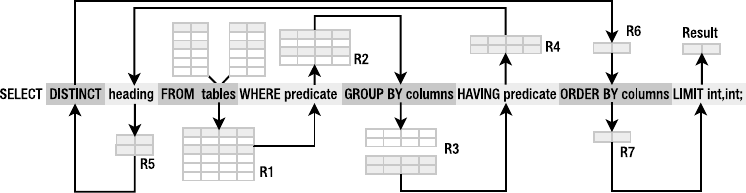
CHAPTER 4 ■ SQL 85
Operationally, the SELECT command is like a pipeline that processes relations. This pipeline
has optional processes that you can plug into it as you need them. Regardless of whether you
include or exclude a particular operation, the relative operations is always the same. This order
is shown in Figure 4-3.
The SELECT command starts with FROM, which takes one or more input relations, combines
them into a single composite relation, and passes it through the subsequent chain of operations.
Each subsequent operation takes exactly one relation as input and produces exactly one relation
as output.
Figure 4-3. SELECT phases
All operations are optional with the exception of SELECT. You must always provide at least
this clause to make a valid SELECT command. By far the most common invocation of the SELECT
command consists of three clauses: SELECT, FROM, and WHERE. This basic syntax and its associated
clauses are shown as follows:
SELECT heading FROM tables WHERE predicate;
The FROM clause is a comma-separated list of one or more tables (represented by the variable
tables in Figure 4-3). If more than one table is specified, they will be combined to form a single
relation (represented by R1 in Figure 4-3). This is done by one of the join operations. The
resulting relation produced by FROM serves as the initial material. All subsequent operations
will either work directly from it or from derivatives of it.
The WHERE clause filters rows in R1. In a way, it determines the number of rows (or cardinality)
of the result. WHERE is a restriction operation, which (somewhat confusingly) is also known as
selection. Restriction takes a relation and produces a row-wise subset of that relation. The argu-
ment of WHERE is a predicate, or logical expression, which defines the selection criteria by which
rows in R1 are included in (or excluded from) the result. The selected rows from the WHERE clause
form a new relation R2, as shown in Figure 4-3. R2 is a restriction of R1.
In this particular example, R2 passes through the other operations unscathed until it reaches
the SELECT clause. The SELECT clause filters the columns in R2. Its argument consists of a
comma-separated list of columns or expressions that define the result. This is called the projection
list, or heading of the result. The number of columns in the heading is called the degree of the
result. The SELECT clause is a projection operation, which is the process of producing a column-
wise subset of a relation. Figure 4-4 illustrates a projection operation. The input is a relation
composed of five columns, including the columns 1, 2, and 3. The projection operation as
represented by the arrow produces a new relation by extracting these columns and discarding
the others.
Owens_6730 C04.fm Page 85 Monday, April 17, 2006 7:16 AM
www.it-ebooks.info
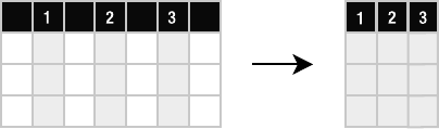
86 CHAPTER 4 ■ SQL
Figure 4-4. Projection
Consider the following example:
sqlite> SELECT id, name FROM food_types;
id name
---------- ----------
1 Bakery
2 Cereal
3 Chicken/Fowl
4 Condiments
5 Dairy
6 Dip
7 Drinks
8 Fruit
9 Junkfood
10 Meat
11 Rice/Pasta
12 Sandwiches
13 Seafood
14 Soup
15 Vegetables
There is no WHERE clause to filter rows. The SELECT clause specifies all of the columns in
food_types, and the FROM clause does not join tables. So there really isn’t much taking place.
The result is an exact copy of food_types. The input relation and the result relation are the
same. If you want to include all possible columns in the result, rather than listing them one by
one, you can use a shorthand notation—an asterisk (*)—instead. Thus, the previous example
can just as easily be expressed as
SELECT * FROM food_types;
This is almost the simplest SELECT command. In reality, the simplest SELECT command requires
only a SELECT clause, and the SELECT clause requires only a single argument. Therefore, the
simplest SELECT command is
sqlite> SELECT NULL;
NULL
----
NULL
The result is a relation composed of one row and one column, with an unknown value—NULL.
NULL is covered later in the section “The Thing Called Null.”
Owens_6730 C04.fm Page 86 Monday, April 17, 2006 7:16 AM
www.it-ebooks.info
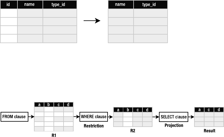
CHAPTER 4 ■ SQL 87
Now let’s look at an example that actually does something operationally. Consider the
following:
SELECT name, type_id FROM foods;
This performs a projection on foods, selecting two of its three columns—name and type_id.
The id column is thrown out, as shown in Figure 4-5.
Figure 4-5. A projection of foods
Let’s summarize: the FROM clause takes the input relations and performs a join, which
combines them into a single relation R1. The WHERE clause takes R1 and filters it via restriction,
producing a new relation R2. The SELECT clause takes R2 and performs projection, producing
the final result. This process is shown in Figure 4-6.
Figure 4-6. Restriction and projection in SELECT
With this simple example, you can begin to see how a query language in general and SQL
in particular ultimately operates in terms of relational operations. There is real math under
the hood.
Filtering
If the SELECT command is the most complex command in SQL, then the WHERE clause is the
most complex clause in SELECT. And, just as the SELECT command pulls in aspects of set theory,
the WHERE clause also pulls in aspects of formal logic. By and large, the WHERE clause is usually
the part of the SELECT command that harbors the most complexity. But it also does most of the
work. Having a solid understanding of its mechanics will most likely bring the best overall
returns in your day-to-day use of SQL.
The database applies the WHERE clause to each row of the relation produced by the FROM
clause (R1). As stated earlier, WHERE—a restriction—is a filter. The argument of WHERE is a logical
predicate. A predicate, in the simplest sense, is just an assertion about something. Consider the
following statement:
The dog (subject) is purple and has a toothy grin (predicate).
Owens_6730 C04.fm Page 87 Monday, April 17, 2006 7:16 AM
www.it-ebooks.info
88 CHAPTER 4 ■ SQL
The dog is the subject and the predicate consists of the two assertions (color is purple and grin
is toothy). This statement may be true or false, depending on the dog the predicate is applied
to. In the terminology of formal logic, a statement consisting of a subject and a predicate is
called a proposition. All propositions are either true or false.
A predicate then says something about a subject. The subject in the WHERE clause is a row.
The row is the logical subject. The WHERE clause is the logical predicate. Together (as in a gram-
matical sentence) they form a logical proposition, which evaluates to true or false. This proposition
is formulated and evaluated for every row in R1. Each row in which the proposition evaluates
to true is included (or selected) as part of the result (R2). Each row in which it is false is excluded.
So the dog proposition translated into a relational equivalent would look something like this:
SELECT * FROM dogs WHERE color='purple' AND grin='toothy';
The database will take each row in relation dogs (the subject) and apply the WHERE clause (the
predicate) to form the logical proposition:
This row has color='purple' AND grin='toothy'.
This is either true of the given row, or it is false—nothing more. If it is true, then the row (or dog)
is indeed purple and toothy, and it is included in the result. If the proposition is false, then the
row may be purple but not toothy, or toothy but not purple, or neither purple nor toothy. In
any case, the proposition is false and the row is therefore excluded.
WHERE is a powerful filter. It provides you with a great degree of control over the conditions
with which to include (or exclude) rows in (or from) the result. As a logical predicate, it is also
a logical expression. A logical expression is an expression that evaluates to exactly one of two
possible logical outcomes: true or false. A logical predicate then is just a logical expression that
is used in a specific way—to qualify a subject and form a proposition.
At their simplest, logical expressions consist of two values or value expressions compared
by relational operators. Value expressions are built from values and operators.
A relational operator referred to here is a relational operator in the mathematical sense.
It is different from a relational operator in the relational sense, as defined in relational algebra.
A relational operator in math is an operator that relates two values and evaluates to true or false
(e.g., x>y, x<=y ). A relational operator in relational algebra is an operator that takes two or more
relations and produces a new relation. To minimize confusion, the scope of this discussion is
limited to one relational operation—restriction—as implemented by the WHERE clause in SQL.
The WHERE clause is expressed in terms of logical propositions, which use relational (in the
mathematical sense) operators. For the remainder of this section, “relational operator” refers
specifically to that in the mathematical sense.
Values
Everything begins with values, which represent some kind of data in the real world. Values can be
classified by their domain (or type), such as a numerical value (1, 2, 3, etc.) or string value (“Jujy-
Fruit”). Values can be expressed as literal values (an explicit quantity such as 1, 2, 3 or “JujyFruit”),
variables (often in the form of column names like foods.name), expressions (3+2/5), or the results of
functions (COUNT(foods.name))—which are covered later.
Owens_6730 C04.fm Page 88 Monday, April 17, 2006 7:16 AM
www.it-ebooks.info
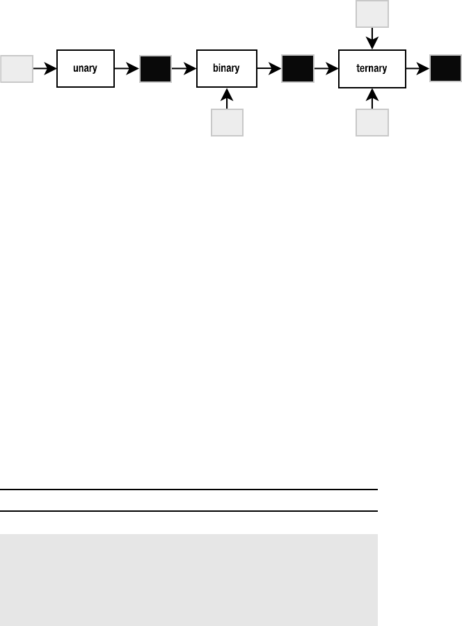
CHAPTER 4 ■ SQL 89
Operators
An operator takes one or more values as input and produces a value as output. An operator is
so named because it performs some kind of operation, producing some kind of result. Binary
operators are operators that take two input values (or operands). Ternary operators take three
operands, unary operators take just one, and so on.
Many operators produce the same kind of information they consume (operators that
operate on numbers produce numbers, etc.). Such operators can be strung together, feeding
the output of one operator into the input of another (Figure 4-7), forming value expressions.
Figure 4-7. Unary, binary, and ternary operators
By stringing operators together, you can create value expressions that are expressed in
terms of yet other value expressions to arbitrary complexity. For example:
x = count(episodes.name)
y = count(foods.name)
z = y/x * 11
Binary Operators
Binary operators are by far the most common of all operators in SQL. Table 4-2 lists the binary
operators supported in SQLite by precedence, from highest to lowest. Operators in each color
group have equal precedence. Precedence determines the default order of evaluation in an
expression with multiple operators. For example, take the expression 4+3*7. It evaluates to 25.
The multiplication operator has higher precedence than addition, and is therefore evaluated
first. So the expression is computed (3*7)+4. Precedence can be overridden using parentheses. The
expression (4+3)*7 is not 25. Here, the parentheses have declared an explicit order of operation.
Table 4-2. Binary Operators
Operator Type Action
|| String Concatenation
*Arithmetic Multiply
/Arithmetic Divide
%Arithmetic Modulus
+Arithmetic Add
Owens_6730 C04.fm Page 89 Monday, April 17, 2006 7:16 AM
www.it-ebooks.info

90 CHAPTER 4 ■ SQL
Arithmetic operators (e.g., addition, subtraction, division) are binary operators that take numeric
values and produce a numeric value. Relational operators (e.g., >, <, =) are binary operators that
compare values and value expressions and return a logical value (also called a truth value),
which is either true or false. Relational operators form logical expressions, for example:
x > 5
1 < 2
A logical expression is any expression that returns a truth value. In SQLite, false is represented
by the number 0, while true is represented by anything else. For example:
sqlite> SELECT 1 > 2;
1 > 2
----------
0
– Arithmetic Subtract
<< Bitwise Right shift
>> Bitwise Left shift
&Logical And
|Logical Or
<Relational Less than
<= Relational Less than or equal to
>Relational Greater than
>= Relational Greater than or equal to
=Relational Equal to
== Relational Equal to
<> Relational Not equal to
!= Relational Not equal to
IN Logical In
AND Logical And
OR Logical Or
LIKE Relational String matching
GLOB Relational Filename matching
Table 4-2. Binary Operators (Continued)
Operator Type Action
Owens_6730 C04.fm Page 90 Monday, April 17, 2006 7:16 AM
www.it-ebooks.info

CHAPTER 4 ■ SQL 91
sqlite> SELECT 1 < 2;
1 < 2
----------
1
sqlite> SELECT 1 = 2;
1 = 2
----------
0
sqlite> SELECT -1 AND 1;
-1 AND 1
----------
1
Logical Operators
Logical operators (AND, OR, NOT, IN) are binary operators that operate on truth values or logical
expressions. They produce a specific truth value depending on their inputs. They are used to
build more complex logical expressions from simpler expressions, such as
(x > 5) AND (x != 3)
(y < 2) OR (y > 4) AND NOT (y = 0)
(color='purple') AND (grin='toothy')
The truth value produced by a logical operator for a given pair of arguments depends on
the operator. For example, logical AND requires that both input values evaluate to true in order
for it to return true. Logical OR, on the other hand, only requires that one input value evaluate
to true in order for it to return true. All possible outcomes for a given logical operator are defined in
what is known as a truth table. The truth tables for AND and OR are shown in Tables 4-3 and 4-4,
respectively.
Table 4-3. Truth Table for Logical And
Argument 1 Argument 2 Result
True True True
True False False
False False False
Owens_6730 C04.fm Page 91 Monday, April 17, 2006 7:16 AM
www.it-ebooks.info

92 CHAPTER 4 ■ SQL
This is the stuff the WHERE clause is made of. Using logical operators, you can create a
complex logical predicate. The predicate is what defines how WHERE’s relational restriction
operation restricts. For example:
sqlite> SELECT * FROM foods WHERE name='JujyFruit' AND type_id=9;
id type_id name
---------- ---------- ----------
244 9 JujyFruit
The restriction here works according to the expression (name='JujyFruit') AND (type_id=9),
which consists of two logical expressions joined by logical AND. Both of these conditions must
be true for any record in foods to be included in the result.
The LIKE Operator
A particularly useful relational operator is LIKE. LIKE is similar to equals (=), but is used for
matching string values against patterns. For example, to select all rows in foods whose names
begin with the letter “J,” you could do the following:
sqlite> SELECT id, name FROM foods WHERE name LIKE 'J%';
id name
----- --------------------
156 Juice box
236 Juicy Fruit Gum
243 Jello with Bananas
244 JujyFruit
245 Junior Mints
370 Jambalaya
A percent symbol (%) in the pattern matches any sequence of zero or more characters in the
string. An underscore (_) in the pattern matches any single character in the string. The percent
symbol is greedy. It will eat everything between two characters except those characters. If it is
on the extreme left or right of a pattern, it will consume everything on each respective side.
Consider the following examples:
Table 4-4. Truth Table for Logical Or
Argument 1 Argument 2 Result
True True True
True False True
False False False
Owens_6730 C04.fm Page 92 Monday, April 17, 2006 7:16 AM
www.it-ebooks.info
CHAPTER 4 ■ SQL 93
sqlite> SELECT id, name FROM foods WHERE name LIKE '%ac%P%';
id name
----- --------------------
127 Guacamole Dip
168 Peach Schnapps
198 Mackinaw Peaches
Another useful trick is to use NOT to negate a pattern:
sqlite> SELECT id, name FROM foods
WHERE name like '%ac%P%' AND name NOT LIKE '%Sch%'
id name
----- --------------------
38 Pie (Blackberry) Pie
127 Guacamole Dip
198 Mackinaw peaches
Limiting and Ordering
You can limit the size and particular range of the result using the LIMIT and OFFSET keywords.
LIMIT specifies the maximum number of records to return. OFFSET specifies the number of
records to skip. For example, the following statement obtains the Cereal record (the second
record in food_types) using LIMIT and OFFSET:
SELECT * FROM food_types LIMIT 1 OFFSET 1 ORDER BY id;
The OFFSET clause skips one row (the Bakery row) and the LIMIT clause returns a maximum of
one row (the Cereal row).
But there is something else here as well: ORDER BY. This clause sorts the result by a column
or columns before it is returned. The reason it is important in this example is because the rows
returned from SELECT are never guaranteed to be in any specific order—the SQL standard
declares this. Thus, the ORDER BY clause is essential if you need to count on the result being in any
specific order. The syntax of the ORDER BY clause is similar to the SELECT clause: it is a comma-
separated list of columns. Each entry may be qualified with a sort order—ASC (ascending, the
default) or DESC (descending). For example:
sqlite> SELECT * FROM foods WHERE name LIKE 'B%'
ORDER BY type_id DESC, name LIMIT 10;
id type_id name
----- -------- --------------------
382 15 Baked Beans
383 15 Baked Potato w/Sour
384 15 Big Salad
385 15 Broccoli
362 14 Bouillabaisse
328 12 BLT
Owens_6730 C04.fm Page 93 Monday, April 17, 2006 7:16 AM
www.it-ebooks.info

94 CHAPTER 4 ■ SQL
327 12 Bacon Club (no turke
326 12 Bologna
329 12 Brisket Sandwich
274 10 Bacon
Typically you only need to order by a second (third, etc.) column when there are duplicate
values in the first (second, etc.) ordered column(s). Here, there were many duplicate type_ids.
I wanted to group them together, and then arrange the foods alphabetically within these groups.
■Note LIMIT and OFFSET are not standard SQL keywords as defined in the ANSI standard. Nevertheless,
they are found on several other databases, such as MySQL and PostgreSQL. Oracle, MS SQL, and Firebird also
have functional equivalents, although they use different syntax.
If you use both LIMIT and OFFSET together, you can use a comma notation in place of the
OFFSET keyword. For example, the following SQL
SELECT * FROM foods WHERE name LIKE 'B%'
ORDER BY type_id DESC, name LIMIT 1 OFFSET 2;
can be expressed equivalently with
sqlite> SELECT * FROM foods WHERE name LIKE 'B%'
ORDER BY type_id DESC, name LIMIT 1,2;
id type_id name
----- -------- --------------------
384 15 Big Salad
Here, the comma following LIMIT 1 adds the OFFSET of 2 to the clause. Also, note that OFFSET
depends on LIMIT. That is, you can use LIMIT without using OFFSET but not the other way around.
Notice that LIMIT and OFFSET are dead last in the operational pipeline. One common miscon-
ception of LIMIT/OFFSET is that it speeds up a query by limiting the number of rows that must be
collected by the WHERE clause. This is not true. If it were, then ORDER BY would not work properly.
For ORDER BY to do its job, it must have the entire result in hand to provide the correct order.
ORDER BY, on the other hand, works after WHERE but before SELECT. How do I know this? The
following statement works:
SELECT name FROM foods ORDER BY id;
I am asking SQLite to order by a column that is not in the result. The only way this could happen
is if the ordering takes place before projection (while the id column is still in the set). While this
works in SQLite, it is also specified in SQL2003.
Functions and Aggregates
Relational algebra supports the notion of functions and aggregates through the extended opera-
tion known as generalized projection. The SELECT clause is a generalized projection rather than
Owens_6730 C04.fm Page 94 Monday, April 17, 2006 7:16 AM
www.it-ebooks.info
CHAPTER 4 ■ SQL 95
just a fundamental projection. The fundamental projection operation only accepts column
names in the projection list as a means to produce a column-wise subset. Generalized projec-
tion accepts this as well as arithmetic expressions, functions, and aggregates in the projection
list, in addition to other features such as GROUP BY and HAVING, all of which are covered here and
in the subsequent sections.
SQLite comes with various built-in functions and aggregates that can be used within various
clauses. Function types range from mathematical functions such as ABS(), which computes the
absolute value, to string formatting functions such as UPPER() and LOWER(), which convert text
to upper- and lowercase, respectively. For example:
sqlite> SELECT UPPER('hello newman'), LENGTH('hello newman'), ABS(-12);
UPPER('hello newman') LENGTH('hello newman') ABS(-12)
--------------------- -------------------- ----------
HELLO NEWMAN 12 12
Notice that the function names are case insensitive (i.e., upper() and UPPER() refer to the same
function). Functions can accept column values as their arguments:
sqlite> SELECT id, UPPER(name), LENGTH(name) FROM foods
WHERE type_id=1 LIMIT 10;
id UPPER(name) LENGTH(name)
----- -------------------------- ------------
1 BAGELS 6
2 BAGELS, RAISIN 14
3 BAVARIAN CREAM PIE 18
4 BEAR CLAWS 10
5 BLACK AND WHITE COOKIES 23
6 BREAD (WITH NUTS) 17
7 BUTTERFINGERS 13
8 CARROT CAKE 11
9 CHIPS AHOY COOKIES 18
10 CHOCOLATE BOBKA 15
Since functions can be a part of any expression, they can also be used in the WHERE clause:
sqlite> SELECT id, UPPER(name), LENGTH(name) FROM foods
WHERE LENGTH(name) < 5 LIMIT 5;
id upper(name) length(name)
----- -------------------- --------------------
36 PIE 3
48 BRAN 4
56 KIX 3
57 LIFE 4
80 DUCK 4
Just for reinforcement, let’s go through the relational operations performed to carry out
the preceding statement:
Owens_6730 C04.fm Page 95 Monday, April 17, 2006 7:16 AM
www.it-ebooks.info
96 CHAPTER 4 ■ SQL
1. FROM clause (join)
The FROM clause in this case does not join tables; it only produces a relation R1 con-
taining all the rows in foods.
2. WHERE clause (restriction)
For each row in R1:
a. Apply the predicate LENGTH(name) < 5 to the row. That is, evaluate the proposition
“row has LENGTH(name) < 5.”
b. If true, add the row to R2.
3. SELECT clause (projection)
For each row in R2:
a. Create a new row r in R3.
b. Copy the value of the id field in restriction into the first column of r.
c. Copy the result of the expression UPPER(row.name) to the second column of r.
d. Copy the result of the expression LENGTH(row.name) to the third column or r.
4. LIMIT clause (restriction)
Restrict R3 to just the first five records.
Aggregates are a special class of functions that calculate a composite (or aggregate) value
over a group of rows (or relation). According to Webster, an aggregate, by definition, is a value
“formed by the collection of units or particles into a body, mass, or amount.” The particles here
are rows in a table. Standard aggregate functions include SUM(), AVG(), COUNT(), MIN(), and
MAX(). For example, to get a count of the number of foods that are baked goods (type_id=1), we
can use the COUNT aggregate as follows:
sqlite> SELECT COUNT(*) FROM foods WHERE type_id=1;
count
-----
47
The COUNT aggregate returns a count of every row in the relation. Whenever you see an aggregate,
you should automatically think, “For each row in a table, do something.” It is the computed
value obtained from doing something with each row in the table. For example, COUNT might be
expressed in terms of the following pseudocode:
int COUNT():
count = 0;
for each row in Relation:
count = count + 1
return count;
Owens_6730 C04.fm Page 96 Monday, April 17, 2006 7:16 AM
www.it-ebooks.info
CHAPTER 4 ■ SQL 97
Aggregates can aggregate not only column values, but any expression—including functions.
For example, to get the average length of all food names, you can apply the AVG aggregate to the
LENGTH(name) expression as follows:
sqlite> SELECT AVG(LENGTH(name)) FROM foods;
AVG(LENGTH(name))
-----------------
12.58
Aggregates operate within the SELECT clause. They compute their values on the rows selected
by the WHERE clause—not from all rows selected by the FROM clause. The SELECT command filters
first, then aggregates.
While SQLite comes with a standard set of common SQL functions and aggregates, it is
worth noting that the SQLite C API allows you to create custom functions and aggregates as
well. See Chapter 7 for more information. For reference, a complete list of the built-in functions
and aggregates in SQLite can be found in Appendix A.
Grouping
An essential part of aggregation is grouping. That is, in addition to computing aggregates over
an entire result, you can also split that result into groups of rows with like values, and compute
aggregates on each group—all in one step. This is the job of the GROUP BY clause. For example:
sqlite> SELECT type_id FROM foods GROUP BY type_id;
type_id
----------
1
2
3
.
.
.
15
GROUP BY is a bit different than the other parts of SELECT, so you need to use your imagina-
tion a little to wrap your head around it. The process is illustrated in Figure 4-8. Operationally,
GROUP BY sits in between the WHERE clause and the SELECT clause. GROUP BY takes the output
of WHERE and splits it into groups of rows that share a common value (or values) for a specific
column (or columns). These groups are then passed to the SELECT clause. In the example, there
are 15 different food types (type_id ranges from 1 to 15), and therefore GROUP BY organizes all
rows in foods into 15 groups varying by type_id. SELECT takes each group and extracts its common
type_id value and puts it into a separate row. Thus, there are 15 rows in the result, one for
each group.
Owens_6730 C04.fm Page 97 Monday, April 17, 2006 7:16 AM
www.it-ebooks.info
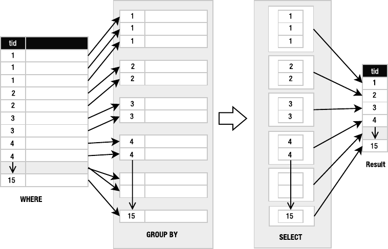
98 CHAPTER 4 ■ SQL
Figure 4-8.GROUP BY process
When GROUP BY is used, the SELECT clause applies aggregates to each group separately, rather
than the entire result as a whole. Since aggregates produce a single value from a group of values,
they collapse these groups of rows into single rows. For example, consider applying the COUNT
aggregate to the preceding example to get the number of records in each type_id group:
sqlite> SELECT type_id, COUNT(*) FROM foods GROUP BY type_id;
type_id COUNT(*)
---------- ----------
1 47
2 15
3 23
4 22
5 17
6 4
7 60
8 23
9 61
10 36
11 16
12 23
13 14
14 19
15 32
Owens_6730 C04.fm Page 98 Monday, April 17, 2006 7:16 AM
www.it-ebooks.info
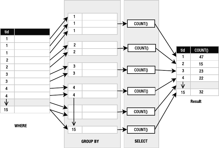
CHAPTER 4 ■ SQL 99
Here, COUNT() was applied 15 times—once for each group, as illustrated in Figure 4-9. Note that
in the diagram the actual number of records in each group is not represented literally (e.g., it
doesn’t show 47 records in the group for type_id=1).
Figure 4-9. GROUP BY and aggregation
The number of records with type_id=1 (Baked Goods) is 47. The number with type_id=2
(Cereal) is 15. The number with type_id=3 (Chicken/Fowl) is 23, and so forth. So, to get this
information, you could run 15 queries as follows:
select count(*) from foods where type_id=1;
select count(*) from foods where type_id=2;
select count(*) from foods where type_id=3;
.
.
.
select count(*) from foods where type_id=15;
Or, you get the results using the single SELECT with a GROUP BY as follows:
SELECT type_id, COUNT(*) FROM foods GROUP BY type_id;
But there is more. Since GROUP BY has to do all this work to create groups with like values,
it seems a pity not to let you filter these groups before handing them off to the SELECT clause.
That is the purpose of HAVING, a predicate that you apply to the result of GROUP BY. It filters the
groups from GROUP BY in the same way that the WHERE clause filters rows from the FROM clause.
Owens_6730 C04.fm Page 99 Monday, April 17, 2006 7:16 AM
www.it-ebooks.info
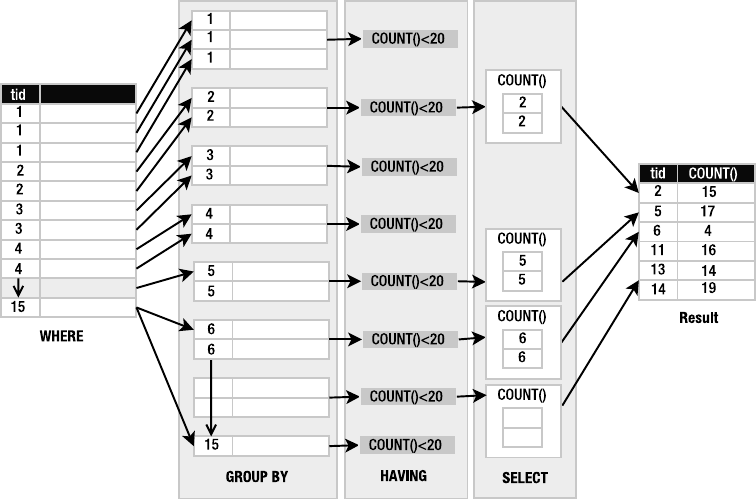
100 CHAPTER 4 ■ SQL
The only difference is that the WHERE clause’s predicate is expressed in terms of individual row
values, and HAVING’s predicate is expressed in terms of aggregate values.
Take the previous example, but this time say you are only interested in looking at the food
groups that have fewer than 20 foods in them:
sqlite> SELECT type_id, COUNT(*) FROM foods
GROUP BY type_id HAVING COUNT(*) < 20;
type_id COUNT(*)
---------- ----------
2 15
5 17
6 4
11 16
13 14
14 19
Here, HAVING applies the predicate COUNT(*)<20 to all of the groups. Any group that does not
satisfy this condition (that has 20 or more foods in it) is not passed on to the SELECT clause.
Figure 4-10 illustrates this restriction.
Figure 4-10. HAVING as group restriction
The third column in the figure shows groups of rows ordered by type_id. The values
shown are the type_id values. The actual number of rows shown in each group is not exact, but
figurative. I have only shown two rows in each group to represent the group as a whole.
Owens_6730 C04.fm Page 100 Monday, April 17, 2006 7:16 AM
www.it-ebooks.info
CHAPTER 4 ■ SQL 101
So GROUP BY and HAVING work as additional restriction phases. GROUP BY takes the restriction
produced by the WHERE clause and breaks it into groups of rows that share a common value for
a given column. HAVING then applies a filter to each of these groups. The groups that make it
through are passed on to the SELECT clause for aggregation and projection.
Removing Duplicates
The next operation in the pipeline is yet another restriction: DISTINCT. DISTINCT takes the result
of the SELECT clause and filters out duplicate rows. For example, you’d use this to get all distinct
type_id values from foods:
sqlite> SELECT DISTINCT type_id FROM foods;
type_id
----------
1
2
3
.
.
.
15
This statement works as follows: the WHERE clause returns the entire foods table (all 412 records).
The SELECT clause pulls out just the type_id column, and finally DISTINCT removes duplicate
rows, reducing the number from 412 rows to 15 rows, all unique. This particular example
produces the same result as the GROUP BY example, but it goes about it in a completely different
manner. DISTINCT simply compares all columns of all rows listed in the SELECT clause and
removes duplicates. There is no grouping on a particular column or columns, nor do you use
any predicates. DISTINCT is just a uniqueness filter.
Joining Tables
Your current knowledge of SELECT so far is based entirely on its filtering capabilities: start with
something, remove rows, remove columns, aggregate, remove duplicates, and perhaps limit
the number of rows even more. The SELECT, WHERE, GROUP BY, HAVING, DISTINCT, and LIMIT clauses
are all filters of some sort.
Filtering, however, is only half of the picture. SELECT has two essential parts: collect and
refine. Up until now you’ve only seen the refining, or filtering, part. The source of all this refine-
ment has been only a single table. But SELECT is not limited to filtering just a single table; it can
link tables together. SELECT can construct a larger and more detailed picture made of different
parts of different tables, and treat that composite as your input table. Then you apply the various
filters to whittle it down and isolate the parts you’re interested in. This process of linking tables
together is called joining. Joining is the work of the FROM clause.
Joins are the first operation(s) of the SELECT command. They produce the initial information to
be filtered and processed by the remaining parts of the statement. The result of a join is a composite
relation (or table), which I will refer to as the input relation. It is the relation that is provided as the
input or starting point for all subsequent (filtering) operations in the SELECT command.
Owens_6730 C04.fm Page 101 Monday, April 17, 2006 7:16 AM
www.it-ebooks.info

102 CHAPTER 4 ■ SQL
It is perhaps easiest to start with an example. The foods table has a column type_id. As it
turns out, the values in this column correspond to values in the id column in the food_types
table. A relationship exists between the two tables. Any value in the foods.type_id column
must correspond to a value in the food_types.id column, and the id column is the primary key
(described later) of food_types. The foods.type_id column, by virtue of this relationship, is
called a foreign key: it contains (or references) values in the primary key of another table. This
relationship is called a foreign key relationship.
Using this relationship, it is possible to join the foods and food_type tables on these two
columns to make a new relation, which provides more detailed information, namely the
food_types.name for each food in the foods table. This is done with the following SQL:
sqlite> SELECT foods.name, food_types.name
FROM foods, food_types
WHERE foods.type_id=food_types.id LIMIT 10;
name name
------------------------- ---------------
Bagels Bakery
Bagels, raisin Bakery
Bavarian Cream Pie Bakery
Bear Claws Bakery
Black and White cookies Bakery
Bread (with nuts) Bakery
Butterfingers Bakery
Carrot Cake Bakery
Chips Ahoy Cookies Bakery
Chocolate Bobka Bakery
You can see the foods.name in the first column of the result, followed by the food_types.name
in the second. Each row in the former is linked to its associated row in the latter using the
foods.type_id → food_types.id relationship (Figure 4-11).
■Note I am using a new notation in this example to specify the columns in the SELECT clause. Rather than
specifying just the column names, I am using the notation table_name.column_name. The reason is
because I have multiple tables in the SELECT statement. The database is smart enough to figure out which
table a column belongs to—as long as that column name is unique among all tables. If you use a column
whose name is also defined in other tables of the join, the database will not be able to figure out which of the
columns you are referring to, and will return an error. In practice, when you are joining tables, it is always a
good idea to use the table_name.column_name notation to avoid any possible ambiguity. This is explained
in detail in the section “Names and Aliases.”
To carry out the join, the database finds these matched rows. For each row in the first
table, the database finds all rows in the second table that have the same value for the joined
Owens_6730 C04.fm Page 102 Monday, April 17, 2006 7:16 AM
www.it-ebooks.info
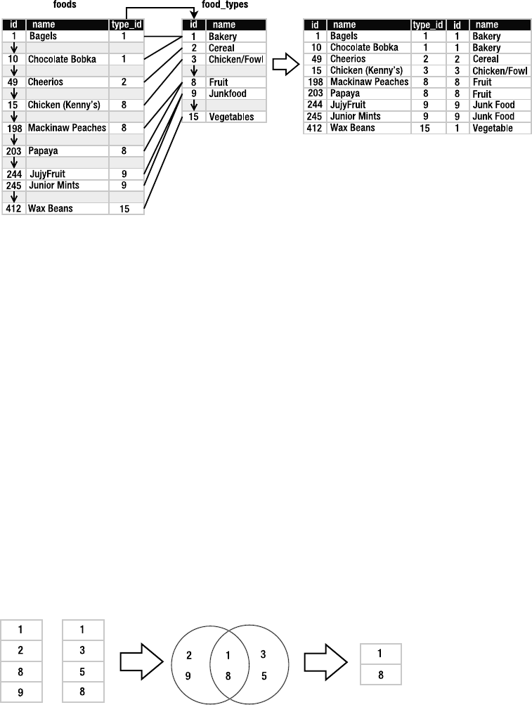
CHAPTER 4 ■ SQL 103
columns and includes them in the input relation. So in this example, the FROM clause built a
composite relation by joining the rows of two tables.
Figure 4-11. foods and food_types join
The subsequent operations (WHERE, GROUP BY, etc.) work exactly the same. It is only the
input that has changed through joining tables. However, the predicate in the WHERE clause
(foods.type_id=food_types.id) controls what records are returned from the join. This happens
in restriction. You might be wondering how this can be if restriction takes place after joining.
Well, the short answer is that the database picks up on this by seeing two tables specified in the
FROM clause. But this still doesn’t explain how anything in the WHERE clause can have any effect
on anything in the FROM clause, which is performed before it. You’ll find out shortly.
As it turns out, there are six different kinds of joins. The one just described, called an inner
join, is the most common.
Inner Joins
An inner join is where two tables are joined by a relationship between two columns in the
tables, as in this previous example. It is the most common (and perhaps most generally useful)
type of join.
An inner join uses another set operation in relational algebra, called an intersection. An
intersection of two sets produces a set containing elements that exist in both sets. Figure 4-12
illustrates this. The intersection of the set {1, 2, 8, 9} and the set {1, 3, 5, 8} is the set {1, 8}. The
intersection operation is represented by a Venn diagram showing the common elements of
both sets.
Figure 4-12. Set intersection
Owens_6730 C04.fm Page 103 Monday, April 17, 2006 7:16 AM
www.it-ebooks.info
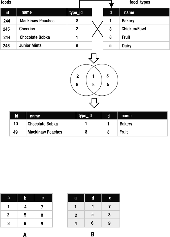
104 CHAPTER 4 ■ SQL
This is precisely how an inner join works, but the sets in a join are common elements
of the related columns. Pretend that the left-hand set in Figure 4-12 represents values in the
foods.type_id column and the right-hand set represents values of the food_types.id column.
Given the matching columns, an inner join finds the rows from both sides that contain like
values and combines them to form the rows of the result (Figure 4-13). Note that this example
assumes that the records shown are the only records in foods and food_types.
Figure 4-13. Food join as intersection
Inner joins only return rows that satisfy the given column relationship, also called the join
condition. They answer the question, “What rows of B match rows in A given the following relation-
ship?” Consider the two hypothetical tables shown in Figure 4-14. They both have three columns,
with one in common (named a). Table B is shaded just for illustration purposes.
Figure 4-14. Two hypothetical tables
Owens_6730 C04.fm Page 104 Monday, April 17, 2006 7:16 AM
www.it-ebooks.info
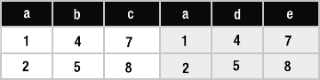
CHAPTER 4 ■ SQL 105
You can see that two rows in B match two rows in A with respect to column a. This is the
inner join:
SELECT * FROM A, B where A.a=B.a;
The result is shown in Figure 4-15.
Figure 4-15. Inner join of A and B
Notice that the third row of B does not match any row in A for this condition (and vice
versa). Therefore only two rows are included in the result. The join condition (e.g., A.a=B.a) is
what makes this an inner join as opposed to another type of join.
Cross Joins
Imagine for a moment that there were no join condition. What would you get? In this case, if
the two tables were not related in any way, SELECT would produce a more fundamental kind of
join (the most fundamental), which is called a cross join or Cartesian join (if you read Chapter 3,
you will know this as the cross product or Cartesian product). The Cartesian join is one of the
fundamental relational operations. It is a brute-force, almost nonsensical join that results in
the combination of all rows from the first table with all rows in the second. A cross join of tables
A and B can be expressed with the following pseudocode:
for each record a in A
for each record b in B
make record a + b
In SQL, the cross join of A and B is expressed as follows:
SELECT * FROM A,B;
FROM, in the absence of anything else, produces a cross join. The result is shown in Figure 4-16.
Every row in A is combined with every row in B. In a cross join, no relationship exists between
the rows; there is no join condition but they are simply jammed together.
This, then, is what the WHERE clause was filtering with the (inner) join condition in the
preceding example. It was removing all those rows in the cross join that had no sensible relation-
ship. An inner join is a subset of a cross join. A cross join contains every possible combination
of rows in two tables, whereas an inner join contains only those rows that satisfy a specific rela-
tionship between columns in the two tables.
Owens_6730 C04.fm Page 105 Monday, April 17, 2006 7:16 AM
www.it-ebooks.info
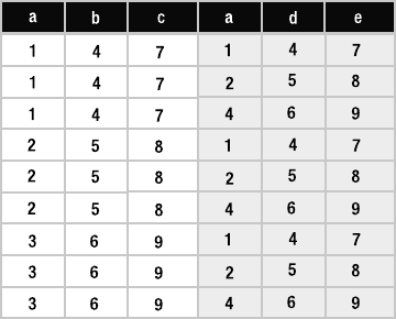
106 CHAPTER 4 ■ SQL
Figure 4-16. Cross join of tables A and B
From a purely relational sense, a join is composed of the following set operations, in order:
1. Cross join: Take the cross product of all tables in the source list.
2. Restrict: Apply the join condition (and any other restrictions) to the cross product to
narrow it down. An inner join takes the intersection of related columns to select matching
rows. Other joins use other criteria.
3. Project: Select the desired columns from the restriction.
In this sense, all joins then begin as a cross join of all tables in the FROM clause, producing a
set of every combination of rows therein. This is the mathematical process. It is most certainly
not the process used by relational databases. It would be wasteful, to say the least, for databases to
blindly start every join by computing the cross product of all tables listed in the FROM clause.
There are many ways databases optimize this process so as to avoid combining rows that will
simply be thrown out by the WHERE clause. Thus, the mathematical concept and the database
implementation are completely different. However, the end results are logically equivalent.
Outer Joins
Three of the remaining four joins are called outer joins. An inner join selects rows across tables
according to a given relationship. An outer join selects all of the rows of an inner join plus some
rows outside of the relationship. The three outer join types are called left, right, and full. A left
join operates with respect to the “left table” in the SQL command. For example, in the command
SELECT * FROM A LEFT JOIN B ON A.a=B.a;
table A is the left table here. The left join favors it. It is the table of significance in a left join. The
left join tries to match every row of A with every row in B per the join condition (A.a=B.a). All
such matching rows are included in the result. However, the remaining rows of A that don’t
match B are still included in the result. In this case, these rows have empty values for the B columns.
The result is shown in Figure 4-17.
Owens_6730 C04.fm Page 106 Monday, April 17, 2006 7:16 AM
www.it-ebooks.info
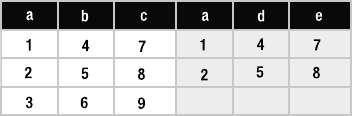
CHAPTER 4 ■ SQL 107
Figure 4-17. Left join of A and B
Remember that the third row of A has no matching row in B with respect to column a.
Despite this, the left join includes all rows of A, matching or not.
The right join works similarly, except the right table is the one whose rows are included,
matching or not. Operationally, left and right joins are identical; they do the same thing. They
differ only in order and syntax. You could argue that there never is any need to do a right join
as the only thing it does is swap the arguments in a left join.
A full outer join is the combination of a left and right outer join. It includes all matching
records, followed by unmatched records in the right and left tables. Currently, both right and
full outer joins are not supported in SQLite. However, as mentioned earlier, a right join can be
replaced with a left join, and a full outer join can be performed using compound queries (see
the section “Compound Queries” later in this chapter).
Natural Joins
The last join on the list is called a natural join. It is actually an inner join in disguise, but with a
little syntax and convention thrown in. A natural join joins two tables by their common column
names. Thus, using the natural join you can get the inner join of A and B without having to add
the join condition A.a=B.a:
sqlite> SELECT * FROM A NATURAL JOIN B;
a b c d e
---------- ---------- ---------- ---------- ----------
1 4 7 4 7
2 5 8 5 8
Here, the natural join automatically detects the common column names in A and B (in this case
just column a) and links them together. In practice, it is a good idea to avoid natural joins in
your applications if you can. Natural joins will join all columns by the same name in both tables.
Just the process of adding to or removing a column from a table can drastically change the
results of a natural join query. Say a program uses a natural join query on A and B. Then suppose
someone comes along and adds a new column e to A. That will cause the natural join (and thus
the program) to produce completely different results. It’s always better to explicitly define the
join conditions of your queries than rely on the semantics of the table schema.
Owens_6730 C04.fm Page 107 Monday, April 17, 2006 7:16 AM
www.it-ebooks.info
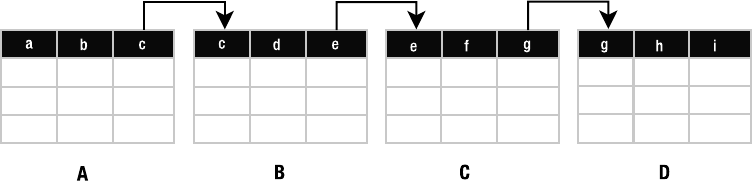
108 CHAPTER 4 ■ SQL
Preferred Syntax
Syntactically, there are various ways of specifying a join. The inner join example of A and B
illustrates performing a join implicitly in the WHERE clause:
SELECT * FROM A,B WHERE A.a=B.a;
When the database sees more than one table listed, it knows there will be a join—at the very
least a cross join. The WHERE clause here calls for an inner join.
This implicit form, while rather clean, is actually an older form of syntax that you should
avoid. The politically correct way (per SQL92) to express a join in SQL is using the JOIN keyword.
The general form is
SELECT heading FROM LEFT_TABLE join_type RIGHT_TABLE ON join_condition;
This explicit form can be used for all join types. For example:
SELECT * FROM A INNER JOIN B ON A.a=B.a;
SELECT * FROM A LEFT JOIN B ON A.a=B.a;
SELECT * FROM A NATURAL JOIN B ON A;
SELECT * FROM A CROSS JOIN B ON A;
Finally, when the join condition is based on columns that share the same name, it can be
simplified with the USING keyword. USING simply names the common column (or columns) to
include in the join condition:
SELECT * FROM A INNER JOIN B USING(a);
The argument of USING is a comma-separated list of column names within parentheses.
Joins are processed from left to right. Consider the mutliway join shown in Figure 4-18.
Figure 4-18. Multiway join
Using the preferred form, you simply keep tacking on additional tables by adding more
join expressions to the end of the statement:
SELECT * FROM A JOIN B USING (c) JOIN C USING (e) JOIN D USING (g);
The first relation, R1, is from A join B on c. The second relation, R2, is R1 join C on e. The
final relation, R3, is R2 join D on g. This is shown in Figure 4-19.
Owens_6730 C04.fm Page 108 Monday, April 17, 2006 7:16 AM
www.it-ebooks.info
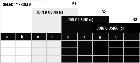
CHAPTER 4 ■ SQL 109
Figure 4-19. A politically correct multiway join construction
Names and Aliases
When joining tables, column names can become ambiguous. For example, A and B as defined
in Figure 4-14 both have a column a. What if they have another column named name, and you just
want to select the name column of B but not A? To help with this type of task, you can qualify column
names with their table names to remove any ambiguity. So in this example, you could write
SELECT B.name FROM A JOIN B USING (a);
Another useful feature is aliases. If your table name is particularly long, and you don’t want
to have to use its name every time you qualify a column, you can use an alias. Aliasing is actually a
fundamental relational operation called rename. The rename operation simply assigns a new
name to a relation. For example, consider the statement:
SELECT foods.name, food_types.name FROM foods, food_types
WHERE foods.type_id=food_types.id LIMIT 10;
There is a good bit of typing here. You can rename the tables in the source clause by simply
including the new name directly after the table name, as in the following example:
SELECT f.name, t.name FROM foods f, food_types t
WHERE f.type_id=t.id LIMIT 10;
Here, the foods table is assigned the alias f, and the food_types table is assigned the alias t.
Now, every other reference to foods or food_types in the statement must use the alias f and t,
respectively. Aliases make it possible to do self-joins—joining a table with itself. For example,
say you want to know what foods in season 4 are mentioned in other seasons. You would first
need to get a list of episodes and foods in season 4, which you would obtain by joining episodes
and episodes_foods. But then you would need a similar list for foods outside of season 4. Finally,
you would combine the two lists based on their common foods. The following query uses self-
joins to do the trick:
SELECT f.name as food, e1.name, e1.season, e2.name, e2.season
FROM episodes e1, foods_episodes fe1, foods f,
episodes e2, foods_episodes fe2
Owens_6730 C04.fm Page 109 Monday, April 17, 2006 7:16 AM
www.it-ebooks.info
110 CHAPTER 4 ■ SQL
WHERE
-- Get foods in season 4
(e1.id = fe1.episode_id AND e1.season = 4) AND fe1.food_id = f.id
-- Link foods with all other epsisodes
AND (fe1.food_id = fe2.food_id)
-- Link with their respective episodes and filter out e1's season
AND (fe2.episode_id = e2.id AND e2.season != e1.season)
ORDER BY f.name;
food name season name season
-------------------- ----------------- ------ ----------------------- ------
Bouillabaisse The Shoes 4 The Stake Out 1
Decaf Cappuccino The Pitch 4 The Good Samaritan 3
Decaf Cappuccino The Ticket 4 The Good Samaritan 3
Egg Salad The Trip 1 4 Male Unbonding 1
Egg Salad The Trip 1 4 The Stock Tip 1
Mints The Trip 1 4 The Cartoon 9
Snapple The Virgin 4 The Abstinence 8
Tic Tacs The Trip 1 4 The Merv Griffin Show 9
Tic Tacs The Contest 4 The Merv Griffin Show 9
Tuna The Trip 1 4 The Stall 5
Turkey Club The Bubble Boy 4 The Soup 6
Turkey Club The Bubble Boy 4 The Wizard 9
I have put comments in the SQL to better explain what is going on. This example uses two self-
joins. There are two instances of episodes and foods_episodes, but they are treated as if they
are two independent tables. The query joins foods_episodes back on itself to link the two instances
of episodes. Furthermore, the two episodes instances are related to each other by an inequality
condition to ensure that they are in different seasons.
You can alias column names and expressions in the same way. For example, to get the top
ten episodes with the most foods, nicely labeled, you’d use this:
sqlite> SELECT e.name AS Episode, COUNT(f.id) AS Foods
FROM foods f
JOIN foods_episodes fe on f.id=fe.food_id
JOIN episodes e on fe.episode_id=e.id
GROUP BY e.id
ORDER BY Foods DESC
LIMIT 10;
Episode Foods
-------------------- -----
The Soup 23
The Fatigues 14
The Bubble Boy 12
The Finale 1 10
The Merv Griffin Show 9
The Soup Nazi 9
Owens_6730 C04.fm Page 110 Monday, April 17, 2006 7:16 AM
www.it-ebooks.info
CHAPTER 4 ■ SQL 111
The Wink 9
The Dinner Party 9
The Glasses 9
The Mango 9
Note that the AS keyword is optional. I just use it because it seems more legible that way to me.
Column aliases will change the column headers returned in the result set. You may refer to
columns or expressions by their aliases elsewhere in the statement if you wish (as in the ORDER
BY clause in the preceding example), but you are not required to do so like you are with tables.
Subqueries
Subqueries are SELECTs within SELECTs. They are also called subselects. Subqueries are useful in
many ways, they work anywhere normal expressions work, and they can therefore be used in a
variety of places in a SELECT statement. Subqueries are useful in other commands as well.
Perhaps the most common use of subqueries is in the WHERE clause, specifically using the
IN operator. The IN operator is a binary operator that takes an input value and a list of values
and returns true if the input value exists in the list, or false otherwise. Here’s an example:
sqlite> SELECT 1 IN (1,2,3);
1
sqlite> SELECT 2 IN (3,4,5);
0
sqlite> SELECT COUNT(*) FROM foods WHERE type_id IN (1,2);
62
Using a subquery, you can rewrite the last statement in terms of names from the food_types:
sqlite> SELECT COUNT(*) FROM foods WHERE type_id
IN (SELECT id FROM food_types WHERE name='Bakery' OR name='Cereal');
62
Subqueries in the SELECT clause can be used to add additional data from other tables to the
result set. For example, to get the number of episodes each food appears in, the actual count
from foods_episodes can be performed in a subquery in the SELECT clause:
sqlite> SELECT name,
(SELECT COUNT(id) FROM foods_episodes WHERE food_id=f.id) count
FROM foods f ORDER BY count DESC LIMIT 10;
name count
---------- ----------
Hot Dog 5
Pizza 4
Ketchup 4
Kasha 4
Shrimp 3
Lobster 3
Turkey Sandwich 3
Owens_6730 C04.fm Page 111 Monday, April 17, 2006 7:16 AM
www.it-ebooks.info

112 CHAPTER 4 ■ SQL
Turkey Club 3
Egg Salad 3
Tic Tacs 3
The ORDER BY and LIMIT clauses here serve to create a top ten list, with hot dogs at the top.
Notice that the subquery’s predicate references a table in the enclosing SELECT command:
food_id=f.id. The variable f.id exists in the outer query. The subquery in this example is
called a correlated subquery because it references, or correlates to, a variable in the outer
(enclosing) query.
Subqueries in the SELECT clause are also helpful with computing percentages of aggregates.
For example, the following SQL breaks foods down by types and their respective percentages:
SELECT (SELECT name FROM food_types WHERE id=f.type_id) Type,
COUNT(type_id) Items,
COUNT(type_id)*100.0/(SELECT COUNT(*) FROM foods) as Percentage
FROM foods f GROUP BY type_id ORDER BY Percentage DESC;
Type Items Percentage
-------------- ------- --------------
Junkfood 61 14.76997578692
Drinks 60 14.52784503631
Bakery 48 11.62227602905
Meat 36 8.716707021791
Vegetables 32 7.748184019370
Chicken/Fowl 23 5.569007263922
Fruit 23 5.569007263922
Sandwiches 23 5.569007263922
Condiments 22 5.326876513317
Soup 19 4.600484261501
Dairy 17 4.116222760290
Rice/Pasta 16 3.874092009685
Cereal 15 3.631961259079
Seafood 14 3.389830508474
Dip 4 0.968523002421
Here, a subquery must be used as the divisor rather than COUNT() because the statement uses a
GROUP BY. Remember that aggregates in GROUP BY are applied to groups, not the entire result set;
therefore the subquery’s COUNT() must be used to get the total rows in foods.
Subqueries can be used in the ORDER BY clause as well. The following SQL groups foods by
the size of their respective food groups, from greatest to least:
SELECT * FROM foods f
ORDER BY (SELECT COUNT(type_id)
FROM foods WHERE type_id=f.type_id) DESC;
ORDER BY in this case does not refer to any specific column in the result. How does this work
then? The ORDER BY subquery is run for each row, and the result is associated with the given
row. You can think of it as an invisible column in the result set, which is used to order rows.
Owens_6730 C04.fm Page 112 Monday, April 17, 2006 7:16 AM
www.it-ebooks.info

CHAPTER 4 ■ SQL 113
Finally, we have the FROM clause. There may be times when you want to join only part of a
table rather than all of it. Yet another job for a subquery:
SELECT f.name, types.name FROM foods f
INNER JOIN (SELECT * FROM food_types WHERE id=6) types
ON f.type_id=types.id;
name name
------------------------- -----
Generic (as a meal) Dip
Good Dip Dip
Guacamole Dip Dip
Hummus Dip
Notice that the use of a subquery in the FROM clause requires a rename operation. In this
case, the subquery was named types. This query could have been written using a full join
of food_types, of course, but it may have incurred more overhead as there would have been
more records to match.
Another use of subqueries is in reducing the number of rows in an aggregating join. Consider
the following query:
SELECT e.name name, COUNT(fe.food_id) foods FROM episodes e
INNER JOIN foods_episodes fe ON e.id=fe.episode_id
GROUP BY e.id
ORDER BY foods DESC
LIMIT 10;
name foods
-------------- -------
The Soup 23
The Fatigues 14
The Bubble Boy 12
The Finale 1 10
The Mango 9
The Glasses 9
The Dinner Par 9
The Wink 9
The Soup Nazi 9
The Merv Griff 9
This query lists the top ten shows with the most food references. The join here must match
181 rows in episodes with 502 rows in foods_episodes (181/502). Then it has to compute the
aggregate. The fewer rows it has to match, the less work it has to do and the more efficient (and
faster) the query becomes. Aggregation collapses rows, right? Then a great way to reduce the
number of rows the join must match is to aggregate before the join. The only way to do this is
with a subquery:
Owens_6730 C04.fm Page 113 Monday, April 17, 2006 7:16 AM
www.it-ebooks.info
114 CHAPTER 4 ■ SQL
SELECT e.name, agg.foods FROM episodes e
INNER JOIN
(SELECT fe.episode_id as eid, count(food_id) as foods
FROM foods_episodes fe
GROUP BY episode_id ) agg
ON e.id=agg.eid
ORDER BY agg.foods DESC
LIMIT 10;
This query moves aggregation into a subquery that is run before the join, the results of which
are joined to the episodes table for the final result. The subquery produces one aggregate (the
number of foods) per episode. There are 181 episodes. Thus, this query reduces the join size
from 181:502 to 181:181. However, since we are only looking for the top ten food-referencing
episodes, we can also move the LIMIT 10 clause into the subquery as well and reduce the number
still, to 181:10:
SELECT e.name, agg.foods FROM episodes e
INNER JOIN
(SELECT fe.episode_id as eid, count(food_id) as foods
FROM foods_episodes fe
GROUP BY episode_id
ORDER BY foods DESC LIMIT 10) agg
ON e.id=agg.eid
ORDER BY agg.foods DESC;
This subquery returns only ten rows, which correspond to the top ten food shows. The join
disrupts the descending order of the subquery so another ORDER BY is required in the main
query to reestablish it.
The thing to remember about subqueries is that they can be used anywhere a relational
expression can be used. A good way to learn how, where, and when to use them is to just play
around with them and see what you can get away with. There is often more than one way to
skin a cat in SQL. When you understand the big picture, you can make more informed decisions on
when a query might be rewritten to run more efficiently.
Compound Queries
Compound queries are kind of the inverse of subqueries. A compound query is a query that
processes the results of multiple queries using three specific relational operations: union,
intersection, and difference. In SQL, these are defined using the UNION, INTERSECT, and EXCEPT
keywords, respectively.
Compound query operations require a few things of their arguments:
• The relations involved must have the same number of columns (degree).
• There can only be one ORDER BY clause, which is at the end of the compound query,
and applies to the combined result.
Furthermore, relations in compound queries are processed from left to right.
Owens_6730 C04.fm Page 114 Monday, April 17, 2006 7:16 AM
www.it-ebooks.info

CHAPTER 4 ■ SQL 115
The INTERSECT operation takes two relations A and B, and selects all rows in A that also exist
in B. The following SQL uses INTERSECT to find the all-time top ten foods that appear in seasons 3
through 5:
SELECT f.* FROM foods f
INNER JOIN
(SELECT food_id, count(food_id) as count FROM foods_episodes
GROUP BY food_id
ORDER BY count(food_id) DESC LIMIT 10) top_foods
ON f.id=top_foods.food_id
INTERSECT
SELECT f.* FROM foods f
INNER JOIN foods_episodes fe ON f.id = fe.food_id
INNER JOIN episodes e ON fe.episode_id = e.id
WHERE e.season BETWEEN 3 and 5
ORDER BY f.name;
id type_id name
----- ------- --------------------
4 1 Bear Claws
146 7 Decaf Cappuccino
153 7 Hennigen's
55 2 Kasha
94 4 Ketchup
164 7 Naya Water
317 11 Pizza
To produce the top ten foods, I needed an ORDER BY in the first SELECT statement. Since
compound queries only allow one ORDER BY at the end of the statement, I got around this by
performing an inner join on a subquery in which I computed the top ten most common foods.
Subqueries can have ORDER BY clauses because they run independently of the compound query.
The inner join then produces a relation containing the top ten foods. The second query returns
a relation containing all foods in episodes 3 through 5. The INTERSECT operation then finds all
matching rows.
The EXCEPT operation takes two relations A and B and finds all rows in A that are not in B.
By changing the INTERSECT to EXCEPT in the previous example, you can find which top ten foods
are not in seasons 3 through 5:
SELECT f.* FROM foods f
INNER JOIN
(SELECT food_id, count(food_id) AS count FROM foods_episodes
GROUP BY food_id
ORDER BY count(food_id) DESC LIMIT 10) top_foods
ON f.id=top_foods.food_id
Owens_6730 C04.fm Page 115 Monday, April 17, 2006 7:16 AM
www.it-ebooks.info

116 CHAPTER 4 ■ SQL
EXCEPT
SELECT f.* FROM foods f
INNER JOIN foods_episodes fe ON f.id = fe.food_id
INNER JOIN episodes e ON fe.episode_id = e.id
WHERE e.season BETWEEN 3 and 5
ORDER BY f.name;
id type_id name
----- ------- --------
192 8 Banana
133 7 Bosco
288 10 Hot Dog
As mentioned earlier, what is called the EXCEPT operation in SQL is referred to as the difference
operation in relational algebra.
The UNION operation takes two relations, A and B, and combines them into a single relation
containing all distinct rows of A and B. In SQL, UNION combines the results of two SELECT state-
ments. By default, UNION eliminates duplicates. If you want duplicates included in the result,
then use UNION ALL. For example, the following SQL finds the single most and single least
frequently mentioned foods:
SELECT f.*, top_foods.count FROM foods f
INNER JOIN
(SELECT food_id, count(food_id) AS count FROM foods_episodes
GROUP BY food_id
ORDER BY count(food_id) DESC LIMIT 1) top_foods
ON f.id=top_foods.food_id
UNION
SELECT f.*, bottom_foods.count FROM foods f
INNER JOIN
(SELECT food_id, count(food_id) AS count FROM foods_episodes
GROUP BY food_id
ORDER BY count(food_id) LIMIT 1) bottom_foods
ON f.id=bottom_foods.food_id
ORDER BY top_foods.count DESC;
id type_id name top_foods.count
----- ------- --------- ---------------
288 10 Hot Dog 5
1 1 Bagels 1
Owens_6730 C04.fm Page 116 Monday, April 17, 2006 7:16 AM
www.it-ebooks.info
CHAPTER 4 ■ SQL 117
Both queries return only one row. The only difference in the two is which way they sort their
results. The UNION simply combines the two rows into a single relation.
UNION ALL also provides a way to implement a full outer join. You simply perform a left join
in the first SELECT, a right join (written in the form of a left join) in the second, and the result is
a full outer join.
Compound queries are useful when you need to process similar data sets that are materi-
alized in different ways. Basically, if you cannot express everything you want in a single SELECT
statement, you can use a compound query to get part of what you want in one SELECT state-
ment and part in another (and perhaps more), and process the sets accordingly. For example,
the INTERSECT example earlier compared two lists of foods that could not be materialized with
a single SELECT statement. One list contained the top ten foods, and the second contained all
foods that appeared in specific seasons. And I wanted the top ten foods that appeared in the
specific seasons. A compound query was the only way to get this information. The same was
true in the UNION example. It is not possible to select just the first and last records of a result set.
The UNION took two slight variations of a query to get the first and last records and combined
the results. Also, as with joins, you can string as many SELECT commands together as you like by
using any of these compound operations.
Conditional Results
The CASE expression allows you to handle various conditions within a SELECT statement. There
are two forms. The first and simplest form takes a static value and lists various case values
linked to return values:
CASE value
WHEN x THEN value_x
WHEN y THEN value_y
WHEN z THEN value_z
ELSE default_value
END
Here’s a simple example:
SELECT name || CASE type_id
WHEN 7 THEN ' is a drink'
WHEN 8 THEN ' is a fruit'
WHEN 9 THEN ' is junkfood'
WHEN 13 THEN ' is seafood'
ELSE NULL
END description
FROM foods
WHERE description IS NOT NULL
ORDER BY name
LIMIT 10;
Owens_6730 C04.fm Page 117 Monday, April 17, 2006 7:16 AM
www.it-ebooks.info

118 CHAPTER 4 ■ SQL
description
---------------------------------------------
All Day Sucker is junkfood
Almond Joy is junkfood
Apple is a fruit
Apple Cider is a drink
Apple Pie is a fruit
Arabian Mocha Java (beans) is a drink
Avocado is a fruit
Banana is a fruit
Beaujolais is a drink
Beer is a drink
The CASE expression in this example handles a few different type_id values, returning a string
appropriate for each one. The returned value is called description, as qualified after the END
keyword. This string is concatenated to name by the string concatenation operator (||), making
a complete sentence. For all type_ids not specified in a WHEN condition, CASE returns NULL. The
SELECT statement filters out such NULL values in the WHERE clause, so all that is returned are rows
that the CASE expression does handle.
The second form of CASE allows for expressions in the WHEN condition. It has the following
form:
CASE
WHEN condition1 THEN value1
WHEN condition2 THEN value2
WHEN condition3 THEN value3
ELSE default_value
END
CASE works equally well in subselects comparing aggregates. The following SQL picks out
frequently mentioned foods:
SELECT name,(SELECT
CASE
WHEN count(*) > 4
THEN 'Very High'
WHEN count(*) = 4
THEN 'High'
WHEN count(*) IN (2,3)
THEN 'Moderate'
ELSE 'Low'
END
FROM foods_episodes
WHERE food_id=f.id) frequency
FROM foods f
WHERE frequency LIKE '%High'
Owens_6730 C04.fm Page 118 Monday, April 17, 2006 7:16 AM
www.it-ebooks.info

CHAPTER 4 ■ SQL 119
name frequency
--------- ----------
Kasha High
Ketchup High
Hot Dog Very High
Pizza High
This query runs a subquery for each row in foods that classifies the food by the number of episodes
it appears in. The result of this subquery is included as a column called frequency. The WHERE
predicate filters frequency values that have the word “High” in them.
Only one condition is executed in a CASE expression. If more than one condition is satisfied,
only the first of them is executed. If no conditions are satisfied and no ELSE condition is defined,
CASE returns NULL.
The Thing Called Null
Most relational databases support a special value called NULL. NULL is a placeholder for missing
information. NULL is not a value per se. Rather, NULL is the absence of a value. Better yet, it is a
value denoting the absence of a value. Some say it stands for “unknown,” “not applicable,” or
“not known.” But truth be told, NULL is still rather vague and mysterious. Try as you may to nail
it down, NULL can still play with your mind: NULL is not nothing; NULL is not something; NULL is
not true; NULL is not false; NULL is not zero. Simply put, NULL is resolutely what it is: NULL. And not
everyone can agree on what that means. To some, NULL is a four-letter word. NULL rides a Harley,
sports racy tattoos, and refuses to conform. To others, it is a necessary evil and serves an impor-
tant role in society. You may love it. You may hate it. But it’s here to stay. And if you are going to
keep company with NULL, you’d better know what you are getting yourself into.
Based on what you already know, it should come as no surprise to learn that even the SQL
standard is not completely clear on how to deal with NULL in all cases. Regardless, the SQLite
community came to a consensus by evaluating how a number of other major relational data-
bases handled NULL in particular ways. The result was that there was some but not total consistency
in how they all worked. Oracle, PostgreSQL, and DB2 were almost identical with respect to NULL
handling, so SQLite’s approach was to be compatible with them.
Working with NULL is appreciably different than working with any other kind of value. For
example, if you are looking for rows in foods whose name is NULL, the following SQL is useless:
SELECT * FROM foods WHERE foods.name=NULL;
It won’t return any rows, period. The problem here is that the expression anything=NULL evaluates
to NULL (even the expression NULL=NULL is NULL). And NULL is not true (nor is it false), so the WHERE
clause will never evaluate to true, and therefore no rows will be selected by the query in its current
form. In order to get it to work as intended, you must recast the query to use the IS operator:
SELECT * FROM foods WHERE foods.name IS NULL;
The IS operator properly checks for a NULL and returns true if it finds one. If you want values
that are not NULL, then use IS NOT NULL.
But this is just the beginning of our NULL fun. NULL has a kind of Midas-like quality in that
everything it touches turns to NULL. For example:
Owens_6730 C04.fm Page 119 Monday, April 17, 2006 7:16 AM
www.it-ebooks.info

120 CHAPTER 4 ■ SQL
sqlite> SELECT NULL=NULL;
NULL
sqlite> SELECT NULL OR NULL;
NULL
sqlite> SELECT NULL AND NULL;
NULL
sqlite> SELECT NOT NULL;
NULL
sqlite> SELECT 9E9 - 1E-9*NULL;
NULL
Additionally, it is important to note that COUNT(*) and COUNT(column) are distinctly different
with respect to how they handle NULL. COUNT(*) counts rows, regardless of any particular column
value, so NULL has no effect on it. COUNT(column), on the other hand, only counts the rows with
non-NULL values in column, and rows where column is NULL are ignored.
In order to accommodate NULL in logical expressions, SQL uses something called three-value
(or tristate) logic, where NULL is one of the truth values. The truth table for logical AND and logical
OR with NULL thrown into the mix is shown in Table 4-5.
Since a single NULL can nullify an entire expression, it seems that there should be some way
to specify a suitable default in case a NULL crops up. To that end, SQLite provides a function for
dealing with NULL, called COALESCE, which is part of the SQL99 standard. COALESCE takes a list of
values and returns the first non-NULL in the list. Take the following example:
SELECT item.price–(SELECT SUM(amount) FROM discounts WHERE id=item.id)
FROM products WHERE …
This is a hypothetical example of a query that needs to calculate the price of an item with any
discounts applied. But what if the subquery returns NULL? Then the whole calculation and
therefore the price becomes NULL. That’s not good. COALESCE provides a barrier through which
NULL may not pass:
SELECT item.price–(SELECT COALESCE(SUM(amount),0)
FROM discounts WHERE id=item.id)
FROM products WHERE …
Table 4-5. AND and OR with NULL
x y x AND y y OR y
True True True True
True False False True
True NULL NULL True
False False False False
False NULL False NULL
NULL NULL NULL NULL
Owens_6730 C04.fm Page 120 Monday, April 17, 2006 7:16 AM
www.it-ebooks.info
CHAPTER 4 ■ SQL 121
In this case if SUM(amount) turns out to be NULL, COALESCE will return 0 instead, taking the teeth
out of NULL.
Conversely, the NULLIF function takes two arguments and returns NULL if they have the
same values; otherwise, it returns the first argument:
sqlite> SELECT NULLIF(1,1);
NULL
sqlite> SELECT NULLIF(1,2);
1
If you use NULL, you need to take special care in queries that refer to columns that may
contain NULL in their predicates and aggregates. NULL can do quite a number on aggregates if
you are not careful. Consider the following example:
sqlite> CREATE TABLE sales (product_id int, amount real, discount real);
sqlite> INSERT INTO sales VALUES (1, 10.00, 1.00);
sqlite> INSERT INTO sales VALUES (2, 10000.00, NULL);
sqlite> SELECT * FROM sales;
product_id amount discount
---------- ---------- ----------
1 10 1
2 10000 NULL
You have a sales table that contains the products sold throughout the day. It holds the product ID,
the price, and the total discounts that were included in the sale. There are two sales in the table:
one is a $10 purchase with a $1 discount. Another is a $10,000 purchase with no discount,
represented by a NULL, as in “not applicable.” At the end of the day you want to tabulate net
sales after discounts. You try the following:
sqlite> SELECT SUM(amount-discount) FROM sales;
SUM(amount-discount)
--------------------
9.0
Where did the $10,000 sale go? Well, 10,000 minus NULL is NULL. NULLs are weeded out by the
WHERE clause, and therefore contribute nothing to an aggregate, so it simply disappears. Your
calculation is off by 99.9 percent. So, knowing better, you investigate and specifically look for
the missing sale using the following SQL:
sqlite> SELECT SUM(amount) from sales WHERE amount-discount > 100.00;
NULL
What’s the problem here? Well, when the database evaluates the WHERE clause for the record
of interest, the expression becomes 10,000 – NULL > 100.00. Breaking this down, the predicate
evaluates to NULL:
(10000 – NULL > 100.00) → (NULL > 100.00) → NULL
Owens_6730 C04.fm Page 121 Monday, April 17, 2006 7:16 AM
www.it-ebooks.info
122 CHAPTER 4 ■ SQL
Again, NULLs don’t pass through WHERE, so the $10,000 row seems invisible.
If you are going to stay in the black, you will need to handle NULL better. If NULLs will be
allowed in the discount column, then the queries that use that column have to be NULL-aware:
sqlite> SELECT SUM(amount-COALESCE(discount,0)) FROM sales;
10009
sqlite> SELECT SUM(amount) from sales
WHERE amount-COALESCE(discount,0) > 100.00;
10000.0
So, NULL can be useful, and can indeed have a very specific meaning, but using it without
understanding the full implications can lead to unpleasant surprises.
Set Operations
Congratulations, you have learned the SELECT command. Not only have you learned how the
command works, but you’ve covered a large part of relational algebra in the process. SELECT
contains 12 out of 14 operations defined in relational algebra. Here is a list of all of these oper-
ations, along with the parts of SELECT that employ them:
•Restriction: Restriction takes a single relation and produces a row-wise subset of it.
Restriction is performed by the WHERE, HAVING, DISTINCT, and LIMIT clauses.
•Projection: Projection produces a column-wise subset of its input relation. Projection is
performed by the SELECT clause.
•Cartesian product: The Cartesian product takes two relations, A and B, and produces a
relation whose rows are the composite of the two relations by combining every row of A
with every other row in B. SELECT performs the Cartesian product when multiple tables
are listed in the FROM clause and no join condition is provided.
•Union: The union operation takes two relations, A and B, and creates a new relation
containing all distinct rows from both A and B. Both A and B must have the same degree
(number of columns). SELECT performs union operations in compound queries, which
employ the UNION keyword.
•Difference: The difference operation takes two relations, A and B, and produces a relation
whose rows consist of the rows in A that are not in B. SELECT performs difference in
compound queries that employ the EXCEPT operator.
•Rename: The rename operation takes a single relation and assigns it a new name. Rename
is used in the FROM clause.
•Intersection: The intersection operation takes two relations, A and B, and produces a
relation whose rows are contained in both A and B. SELECT performs the intersection
operation in compound queries that employ the INTERSECT operator.
•Natural join: A natural join takes two relations and performs an inner join on them by
equating the commonly named columns as the join condition. SELECT performs a natural
join with joins that use the NATURAL JOIN clause.
Owens_6730 C04.fm Page 122 Monday, April 17, 2006 7:16 AM
www.it-ebooks.info
CHAPTER 4 ■ SQL 123
•Generalized projection: The generalized projection operation is an extension of the
projection operation, which allows the use of arithmetic expressions, functions, and
aggregates in the projection list. Generalized projection is used in the SELECT clause.
Associated with aggregates is the concept of grouping, whereby rows with similar column
values can be separated into individual groups. This is expressed in the SELECT command
using the GROUP BY clause. Furthermore, groups can be filtered using the HAVING clause,
which consists of a predicate similar to that of the WHERE clause. The predicate in HAVING
is expressed in terms of aggregate values.
•Left outer join: The left outer join operation takes two relations, A and B, and returns the
inner join of A and B along with the unmatched rows of A. A is the first relation defined
in the FROM clause, and is hence the left relation. The left join includes the unmatched
rows of the left relation along with the matched columns in the result.
•Right and full outer join: The right outer join operation is similar to the left join, only it
includes the unmatched rows of the right relation. The full outer join includes
unmatched rows from both relations.
Modifying Data
Compared to the SELECT command, the statements used to modify data are quite easy to use
and understand. There are three DML statements for modifying data—INSERT, UPDATE, and
DELETE—and they do pretty much what their names imply.
Inserting Records
You insert records into a table using the INSERT command. INSERT works on a single table, and
can both insert one row at a time or many rows at once using a SELECT command. The general
form of the INSERT command is as follows:
INSERT INTO table (column_list) VALUES (value_list);
The variable table specifies which table—the target table—to insert into. The variable column_list
is a comma-separated list of column names, all of which must exist in the target table. The variable
value_list is a comma-separated list of values that correspond to the names given in column_list.
The order of values in value_list must correspond to the order of columns in column_list. For
example, you’d use this to insert a row into foods:
sqlite> INSERT INTO foods (name, type_id) VALUES ('Cinnamon Bobka', 1);
This statement inserts one row, specifying two column values. 'Cinnamon Bobka'—the first
value in the value list—corresponds to the column name—the first column in the column list.
Similarly, the value 1 corresponds to type_id, which is listed second. Notice that id was not
mentioned. In this case, the database uses the default value. Since id is declared as INTEGER
PRIMARY KEY, it will be automatically generated and associated with the record (as explained in
the section “Primary Key Constraints”). The inserted record can be verified with a simple SELECT:
Owens_6730 C04.fm Page 123 Monday, April 17, 2006 7:16 AM
www.it-ebooks.info
124 CHAPTER 4 ■ SQL
sqlite> SELECT * FROM foods WHERE name='Cinnamon Bobka';
id type_id name
---------- ---------- --------------
413 1 Cinnamon Bobka
sqlite> SELECT MAX(id) from foods;
MAX(id)
----------
413
sqlite> SELECT last_insert_rowid();
last_insert_rowid()
-------------------
413
Notice that the value 413 was automatically generated for id, which is the largest value in the
column. Thus, SQLite provided a monotonically increasing value. You can confirm this with
the built-in SQL function last_insert_rowid(), which returns the last automatically generated
key value, as shown in the example.
If you provide a value for every column of a table in INSERT, then the column list can be
omitted. In this case, the database assumes that the order of values provided in the value list
correspond to the order of columns as declared in the CREATE TABLE statement. For example:
sqlite> INSERT INTO foods VALUES(NULL, 1, 'Blueberry Bobka');
sqlite> SELECT * FROM foods WHERE name LIKE '%Bobka';
id type_id name
---------- ---------- ---------------
10 1 Chocolate Bobka
413 1 Cinnamon Bobka
414 1 Blueberry Bobka
Notice here the order of arguments. 'Blueberry Bobka' came after 1 in the value list. This is
because of the way the table was declared. To view the table’s schema, type .schema foods at
the shell prompt:
sqlite> .schema foods
CREATE TABLE foods(
id integer primary key,
type_id integer,
name text );
CREATE INDEX foods_name_idx on foods (name COLLATE NOCASE);
The first column is id, followed by type_id, followed by name. This, therefore, is the order you
must list values in INSERT statements on foods. Why did I use a NULL value for id in the preceding
INSERT statement? Because SQLite knows that id in foods is an autoincrement column, and
Owens_6730 C04.fm Page 124 Monday, April 17, 2006 7:16 AM
www.it-ebooks.info

CHAPTER 4 ■ SQL 125
specifying a NULL is the equivalent of not providing a value at all. This triggers the automatic key
generation. It’s just a convenient trick. There is no deeper meaning or theoretical basis behind
it. We will look at the subtleties of autoincrement columns later in this chapter.
Subqueries can be used in INSERT statements, both as components of the value list and as
a complete replacement of the value list. Here’s an example:
INSERT INTO foods
VALUES (NULL,
(SELECT id FROM food_types WHERE name='Bakery'),
'Blackberry Bobka');
SELECT * FROM foods WHERE name LIKE '%Bobka';
id type_id name
---------- ---------- ----------------
10 1 Chocolate Bobka
413 1 Cinnamon Bobka
414 1 Blueberry Bobka
415 1 Blackberry Bobka
Here, rather than hard-coding the type_id value, I had SQLite look it up for me. Here’s another
example:
INSERT INTO foods
SELECT last_insert_rowid()+1, type_id, name FROM foods
WHERE name='Chocolate Bobka';
SELECT * FROM foods WHERE name LIKE '%Bobka';
id type_id name
---------- ---------- ----------------
10 1 Chocolate Bobka
413 1 Cinnamon Bobka
414 1 Blueberry Bobka
415 1 Blackberry Bobks
416 1 Chocolate Bobka
This query completely replaces the value list with a SELECT statement. As long as the number of
columns in the SELECT clause matches the number of columns in the table (or the number of
columns in the columns list, if provided), INSERT will work just fine. Here, I added another
chocolate bobka and used the expression last_insert_rowid()+1 as the id value. I could have just
as easily used NULL instead. In fact, I probably should have used NULL rather than
last_insert_rowid(), as last_insert_rowid() will return 0 if you have not previously inserted
a row in the current session. I could safely assume that this would work properly for these
examples, but it would not be a good idea to make this assumption in a program.
There is nothing stopping you from inserting multiple rows at a time using the SELECT form
of INSERT. As long as the number of columns matches, INSERT will insert every row in the result.
For example:
Owens_6730 C04.fm Page 125 Monday, April 17, 2006 7:16 AM
www.it-ebooks.info

126 CHAPTER 4 ■ SQL
sqlite> CREATE TABLE foods2 (id int, type_id int, name text);
sqlite> INSERT INTO foods2 SELECT * FROM foods;
sqlite> SELECT COUNT(*) FROM foods2;
COUNT(*)
--------------------
418
This creates a new table foods2 and inserts into it all of the records from foods.
However, there is an easier way to do this. The CREATE TABLE statement has a special syntax
for creating tables from SELECT statements. The previous example could have been performed
in one step using this syntax:
sqlite> CREATE TABLE foods2 AS SELECT * from foods;
sqlite> SELECT COUNT(*) FROM list;
COUNT(*)
--------
418
CREATE TABLE does both steps in one fell swoop. This can be especially useful for creating
temporary tables:
CREATE TEMP TABLE list AS
SELECT f.name Food, t.name Name,
(SELECT COUNT(episode_id)
FROM foods_episodes WHERE food_id=f.id) Episodes
FROM foods f, food_types t
WHERE f.type_id=t.id;
SELECT * FROM list;
Food Name Episodes
-------------------- ---------- ----------
Bagels Bakery 1
Bagels, raisin Bakery 2
Bavarian Cream Pie Bakery 1
Bear Claws Bakery 3
Black and White cook Bakery 2
Bread (with nuts) Bakery 1
Butterfingers Bakery 1
Carrot Cake Bakery 1
Chips Ahoy Cookies Bakery 1
Chocolate Bobka Bakery 1
When using this form of CREATE TABLE, be aware that any constraints defined in the source
table are not created in the new table. Specifically, the autoincrement columns will not be
created in the new table, nor will indexes, UNIQUE constraints, and so forth.
Owens_6730 C04.fm Page 126 Monday, April 17, 2006 7:16 AM
www.it-ebooks.info

CHAPTER 4 ■ SQL 127
It is also worth mentioning here that you have to be aware of UNIQUE constraints when
inserting rows. If you add duplicate values on columns that are declared as UNIQUE, SQLite will
stop you in your tracks:
sqlite> SELECT MAX(id) from foods;
MAX(id)
-------
416
sqlite> INSERT INTO foods VALUES (416, 1, 'Chocolate Bobka');
SQL error: PRIMARY KEY must be unique
Updating Records
You update records in a table using the UPDATE command. The UPDATE command modifies one
or more columns within one or more rows in a table. UPDATE has the general form
UPDATE table SET update_list WHERE predicate;
The update_list is a list of one or more column assignments of the form column_name=value. The
WHERE clause works exactly as in SELECT. Half of UPDATE is really a SELECT statement. The WHERE
clause identifies rows to be modified using a predicate. Those rows then have the update list
applied to them. For example:
UPDATE foods SET name='CHOCOLATE BOBKA'
WHERE name='Chocolate Bobka';
SELECT * FROM foods WHERE name LIKE 'CHOCOLATE%';
id type_ name
----- ----- ------------------------------
10 1 CHOCOLATE BOBKA
11 1 Chocolate Eclairs
12 1 Chocolate Cream Pie
222 9 Chocolates, box of
223 9 Chocolate Chip Mint
224 9 Chocolate Covered Cherries
UPDATE is a very simple and direct command, and this is pretty much the extent of its use.
As in INSERT, you must be aware of any UNIQUE constraints, as they will stop UPDATE every bit as
much as INSERT:
sqlite> UPDATE foods SET id=11 where name='CHOCOLATE BOBKA';
SQL error: PRIMARY KEY must be unique
This is true for any constraint, however.
Owens_6730 C04.fm Page 127 Monday, April 17, 2006 7:16 AM
www.it-ebooks.info
128 CHAPTER 4 ■ SQL
Deleting Records
You delete records from a table using the DELETE command. The DELETE command deletes rows
from a table. DELETE has the general form
DELETE FROM table WHERE predicate;
Syntactically, DELETE is a watered-down UPDATE statement. Remove the SET clause from
UPDATE and you have DELETE. The WHERE clause works exactly as in SELECT, except that it identifies
rows to be deleted. For example:
DELETE FROM foods WHERE name='CHOCOLATE BOBKA';
Data Integrity
Data integrity is concerned with defining and protecting relationships within and between
tables. There are four general types: domain integrity, entity integrity, referential integrity, and
user-defined integrity. Domain integrity involves controlling values within columns. Entity
integrity involves controlling rows in tables. Referential integrity involves controlling rows
between tables—specifically foreign key relationships. And user-defined integrity is a catchall
for everything else.
Data integrity is implemented using constraints. A constraint is a control measure used to
restrict the values that can be stored in a column or columns. Going by just the values in columns,
the database can enforce all four types of integrity constraints. In SQLite, constraints also include
support for conflict resolution. Conflict resolution is covered in detail later in this chapter.
This section is a logical continuation of the “Creating a Database” section at the beginning
of this chapter. As such, the examples in this section use the same contacts table defined there.
It is listed again here for convenience:
CREATE TABLE contacts ( id INTEGER PRIMARY KEY,
name TEXT NOT NULL COLLATE NOCASE,
phone TEXT NOT NULL DEFAULT 'UNKNOWN',
UNIQUE (name,phone) );
As you know by now, constraints are a part of a table’s definition. They can be associated
with a column definition, or defined independently in the body of the table definition. Column-
level constraints include NOT NULL, UNIQUE, PRIMARY KEY, CHECK, and COLLATE. Table-level constraints
include PRIMARY KEY, UNIQUE, and CHECK. All of these constraints are covered in the following
sections according to their respective integrity types.
The reason this material was not addressed earlier is because it requires familiarity with
the UPDATE, INSERT, and DELETE commands. Just as these commands operate on data, constraints
operate on them, making sure that they work within the guidelines defined in the tables they
modify.
Entity Integrity
Entity integrity stems from the Guaranteed Access Rule, as explained in Chapter 3. It requires
that every field in every table be addressable. That is, every field in the database must be
uniquely identifiable and capable of being located. In order for a field to be addressable, its
Owens_6730 C04.fm Page 128 Monday, April 17, 2006 7:16 AM
www.it-ebooks.info

CHAPTER 4 ■ SQL 129
corresponding row must also be addressable. And for that, the row must be unique in some
way. This is the job of the primary key.
The primary key consists of least one column, or a group of columns with a UNIQUE constraint.
The UNIQUE constraint, as you will soon see, simply requires that every value in a column (or
group of columns) be distinct. Therefore, the primary key ensures that each row is somehow
distinct from all other rows in a table, ultimately ensuring that every field is also addressable.
Entity integrity basically keeps data organized in a table. After all, what good is a field if you
can’t find it?
UNIQUE Constraints
Since primary keys are based on UNIQUE constraints, we’ll start with them. A UNIQUE constraint
simply requires that all values in a column or a group of columns are distinct from one another,
or unique. If you attempt to insert a duplicate value, or update a value to another value that
already exists in the column, the database will issue a constraint violation and abort the oper-
ation. UNIQUE constraints can be defined at the column or the table level. When defined at the
table level, UNIQUE constraints can be applied across multiple columns. In this case, the combined
value of the columns must be unique. In contacts, there is a unique constraint on both name
and phone together. See what happens if I attempt to insert another 'Jerry' record with a phone
value 'UNKNOWN':
sqlite> INSERT INTO contacts (name,phone) VALUES ('Jerry','UNKNOWN');
SQL error: columns name, phone are not unique
sqlite> INSERT INTO contacts (name) VALUES ('Jerry');
SQL error: columns name, phone are not unique
sqlite> INSERT INTO contacts (name,phone) VALUES ('Jerry', '555-1212');
In the first case, I explicitly specified name and phone. This matched the values of the existing
record and the UNIQUE constraint kicked in and did not let me do it. The third INSERT illustrates
that the UNIQUE constraint applies to name and phone combined, not individually. It inserted
another row with 'Jerry' as the value for name, which did not cause an error, because name by
itself it not unique—only name and phone together.
NULL AND UNIQUE
Pop quiz: Based on what you know about NULL and UNIQUE, how many NULL values can you put in a column
that is declared UNIQUE? Answer: It depends on which database you are using. PostgreSQL and Oracle say as
many as you want. Informix and Microsoft SQL Server say only one. DB2, SQL Anywhere, and Borland Inter-
Base say none at all. SQLite follows Oracle and PostgreSQL—you can put as many NULLs as you want in a
unique column. This is another classic case of NULL befuddling everyone. On one side, you can argue that one
NULL value is never equal to another NULL value because you don’t have enough information about either to
know if they are equal. On the other side, you don’t really have enough information to prove that they are different
either. The consensus in SQLite is to assume that they are all different, so you can have a whole unique column
stuffed full of NULLs if you like.
Owens_6730 C04.fm Page 129 Monday, April 17, 2006 7:16 AM
www.it-ebooks.info

130 CHAPTER 4 ■ SQL
Primary Key Constraints
In SQLite, a primary key column is always defined when you create a table, whether you define
one or not. This column is a 64-bit integer value called ROWID. It has two aliases, _ROWID_ and
OID, which can be used to refer to it as well. Default values are automatically generated for it in
monotonically increasing order.
SQLite provides an autoincrement feature for primary keys, should you want to define
your own. If you define a column’s type as INTEGER PRIMARY KEY, SQLite will create a DEFAULT
value on that column, which will provide a monotonically increasing integer value that is guar-
anteed to be unique in that column. In reality, however, this column will simply be an alias for
ROWID. They will all refer to the same value. Since SQLite uses a 64-bit number for the primary key,
the maximum value for this column is 9,223,372,036,854,775,807.
■Note You may be wondering where the maximum value of a key value comes from. It is based on the
limits of a 64-bit integer. A 64-bit integer has 64 bits of storage that can be used to represent a number. That
is, 264 (or 18,446,744,073,709,551,616) possible values can be represented with 64 bits. Think of this as a
range of values. An unsigned integer basically defines this range starting at 0. The range is therefore exclu-
sively positive values, and therefore needs no sign to designate it—hence “unsigned.” The maximum value
of an unsigned 64-bit integer is therefore 18,446,744,073,709,551,615 (one less because the range starts at 0,
not 1). However, SQLite uses signed integers. A signed integer splits the range so that half of it is less than
zero and half is greater than zero. The range of a signed 64-bit integer is -9,223,372,036,854,775,808 to
+9,223,372,036,854,775,807 (which is a range of 18,446,744,073,709,551,616 values). Key values in SQLite are
signed 64-bit integers. Therefore, the maximum value of a key in SQLite is +9,223,372,036,854,775,807.
Even if you manage to reach this limit, SQLite will simply start searching for unique values
that are not in the column for subsequent INSERTs. When you delete rows from the table, ROWIDs
may be recycled and reused on subsequent INSERTs. As a result, newly created ROWIDs might not
always be in strictly ascending order.
In the examples so far I have managed to insert two records into contacts. Not once did
I ever specify a value for id. As mentioned before, this is because id is declared as INTEGER
PRIMARY KEY. Therefore, SQLite supplied an incremental integer value for each INSERT automat-
ically, as you can see here:
sqlite> SELECT * FROM contacts;
id name phone
--- ----- --------
1 Jerry UNKNOWN
2 Jerry 555-1212
Notice that the primary key is accessible from all the aforementioned aliases, in addition to id:
sqlite> SELECT ROWID, OID,_ROWID_,id, name, phone FROM CONTACTS;
Owens_6730 C04.fm Page 130 Monday, April 17, 2006 7:16 AM
www.it-ebooks.info
CHAPTER 4 ■ SQL 131
id id id id name phone
-- -- -- -- ---- -----
1 1 1 1 Jerry UNKNOWN
2 2 2 2 Jerry 555-1212
If you include the keyword AUTOINCREMENT after INTEGER PRIMARY KEY, SQLite will use a
different key generation algorithm for the column. This algorithm basically prevents ROWIDs
from being recycled. It guarantees that only new (not recycled) ROWIDs are provided for every
INSERT. When a table is created with a column containing the AUTOINCREMENT constraint, SQLite
will keep track of that column’s maximum ROWID in a system table called sqlite_sequence. It
will only use values greater than that maximum on all subsequent INSERTs. If you ever reach the
absolute maximum, then SQLite will return a SQLITE_FULL error on subsequent INSERTs. For
example:
sqlite> CREATE TABLE maxed_out(id INTEGER PRIMARY KEY AUTOINCREMENT, x text);
sqlite> INSERT INTO maxed_out VALUES (9223372036854775807, 'last one');
sqlite> SELECT * FROM sqlite_sequence;
name seq
---------- -------------------
maxed_out 9223372036854775807
sqlite> INSERT INTO maxed_out VALUES (NULL, 'wont work');
SQL error: database is full
Here, I provided the primary key value. SQLite then stored this value as the maximum for
maxed_out.id in sqlite_sequence. I supplied the very last (maximum) 64-bit value before wrap-
around. In the next INSERT, I used the generated default value, which must be a monotonically
increasing value. This wrapped around to 0, and SQLite issued a SQLITE_FULL error.
While SQLite tracks the maximum value for an AUTOINCREMENT column in the
sqlite_sequence table, it does not prevent you from providing your own values for it in the
INSERT command. The only requirement is that the value you provide must be unique within
the column. For example:
sqlite> DROP TABLE maxed_out;
sqlite> CREATE TABLE maxed_out(id INTEGER PRIMARY KEY AUTOINCREMENT, x text);
sqlite> INSERT INTO maxed_out values(10, 'works');
sqlite> SELECT * FROM sqlite_sequence;
name seq
---------- ----------
maxed_out 10
sqlite> INSERT INTO maxed_out values(9, 'works');
sqlite> SELECT * FROM sqlite_sequence;
name seq
---------- ----------
maxed_out 10
Owens_6730 C04.fm Page 131 Monday, April 17, 2006 7:16 AM
www.it-ebooks.info
132 CHAPTER 4 ■ SQL
sqlite> INSERT INTO maxed_out VALUES (9, 'fails');
SQL error: PRIMARY KEY must be unique
sqlite> INSERT INTO maxed_out VALUES (NULL, 'should be 11');
sqlite> SELECT * FROM maxed_out;
id x
---------- ------------
9 works
10 works
11 should be 11
sqlite> SELECT * FROM sqlite_sequence;
name seq
---------- ----------
maxed_out 11
Here, I dropped and re-created the maxed_out table, and inserted a record with an explicitly
defined ROWID of 10. Then I inserted a record with a ROWID less than 10, which worked. I tried it
again with the same value and it failed, due to the UNIQUE constraint. Finally, I inserted another
record using the default key value, and SQLite provided the next monotonically increasing
value—10+1.
In summary, AUTOINCREMENT prevents SQLite from recycling primary key values (ROWIDs)
and stops when the ROWID reaches the maximum (signed) 64-bit integer value. This feature was
added for specific applications that required this behavior. Unless you have such a specific need in
your application, it is perhaps best to just use INTEGER PRIMARY KEY for autoincrement columns.
Like UNIQUE constraints, PRIMARY KEY constraints can be defined over multiple columns.
You don’t have to use an integer value for your primary key. If you choose to use another value,
SQLite will still maintain the ROWID column internally, but it will also place a UNIQUE constraint
on your declared primary key. For example:
sqlite> CREATE TABLE pkey(x text, y text, PRIMARY KEY(x,y));
sqlite> INSERT INTO pkey VALUES ('x','y');
sqlite> INSERT INTO pkey VALUES ('x','x');
sqlite> SELECT ROWID, x, y FROM pkey;
rowid x y
---------- ---------- ----------
1 x y
2 x x
sqlite> INSERT INTO pkey VALUES ('x','x');
SQL error: columns x, y are not unique
The primary key here is technically just a UNIQUE constraint across two columns, nothing more.
As stated before, the concept of a primary key is more or less just lip service to the relational
Owens_6730 C04.fm Page 132 Monday, April 17, 2006 7:16 AM
www.it-ebooks.info
CHAPTER 4 ■ SQL 133
model—SQLite always provides one whether you do or not. If you do define you own primary
key, it is in reality just another UNIQUE constraint, nothing more.
Domain Integrity
The simplest definition of domain integrity is the conformance of a column’s values to its
assigned domain. That is, every value in a column should exist within that column’s defined
domain. However, the term domain is a little vague. Domains are often compared to types in
programming languages, such as strings or floats. And while that is not a bad analogy, domain
integrity is actually much broader than that.
Domain constraints make it possible for you to start with a simple type—like an integer—
and add additional constraints to create a more restricted set of acceptable values for a column. For
example, you can create a column with an integer type and add the constraint that only three
such values are allowed: {-1, 0. 1}. In this case, you have modified the range of acceptable values
(from the domain of all integers to just three integers), but not the data type itself. You are
dealing with two things: a type and a range.
Consider another example: the name column in the contacts table. It is declared as follows:
name TEXT NOT NULL COLLATE NOCASE
The domain TEXT defines the type and initial range of acceptable values. Everything following
it serves to restrict and qualify that range even further. The name column is then the domain of
all TEXT values that do not include NULL values where uppercase letters and lowercase letters
have equal value. It is still TEXT, and operates as TEXT, but its range of acceptable values is further
restricted from that of TEXT.
You might say that a column’s domain is not the same thing as its type. Rather, its domain
is a combination of two things: a type and a range. The column’s type defines the representa-
tion and operators of its values—how they are stored and how you can operate on them—sort,
search, add, subtract, and so forth. A column’s range is its set of acceptable values you can
store in it, which is not necessarily the same as its declared type. The type’s range represents a
maximum range of values. The column’s range—as you have seen—can be restricted through
constraints. So for all practical purposes, you can think of a column’s domain as a type with
constraints tacked on.
Similarly, there are essentially two components to domain integrity: type checking and
range checking. While SQLite supports many of the standard domain constraints for range
checking (NOT NULL, CHECK, etc.), its approach to type checking is where things diverge from
other databases. In fact, SQLite’s approach to types and type checking is one of its most contro-
versial, misunderstood, and disputed features.
But before we get into how SQLite handles types, let’s cover the easy stuff first: default
values, NOT NULL constraints, CHECK constraints, and collations.
Default Values
The DEFAULT keyword provides a default value for a column if one is not provided in an INSERT
command. DEFAULT is not a constraint, because it doesn’t enforce anything. It simply steps in
when needed. However, it does fall within domain integrity because it provides a policy for
handling NULL values in a column. If a column doesn’t have a default value, and you don’t provide
a value for it in an INSERT statement, then SQLite will insert NULL for that column. For example,
contacts.name has a default value of 'UNKNOWN'. With this in mind, consider the following example:
Owens_6730 C04.fm Page 133 Monday, April 17, 2006 7:16 AM
www.it-ebooks.info

134 CHAPTER 4 ■ SQL
sqlite> INSERT INTO contacts (name) VALUES ('Jerry');
sqlite> SELECT * FROM contacts;
id name phone
---------- ---------- ----------
1 Jerry UNKNOWN
The INSERT command inserted a row, specifying a value for name but not phone. As you can see
from the resulting row, the default value for phone kicked in and provided the string 'UNKNOWN'.
If phone did not have a default value, then in this example, the value for phone in this row would
have been NULL instead.
DEFAULT also accepts three predefined ANSI/ISO reserved words for generating default
dates and times. CURRENT_TIME will generate the current local time in ANSI/ISO time format
(HH:MM:SS). CURRENT_DATE will generate the current date (in YYYY-MM-DD format). CURRENT_TIMESTAMP
will produce a combination of these two (in YYYY-MM-DD HH:MM:SS format). For example:
CREATE TABLE times ( id int,
time NOT NULL DEFAULT CURRENT_DATE
time NOT NULL DEFAULT CURRENT_TIME,
time NOT NULL DEFAULT CURRENT_TIMESTAMP );
INSERT INTO times(1);
INSERT INTO times(2);
SELECT * FROMS times;
id date time timestamp
--- ---------- ---------- -------------------
1 2006-03-15 23:30:25 2006-03-15 23:30:25
2 2006-03-15 23:30:40 2006-03-15 23:30:40
These defaults come in quite handy for tables that need to log or timestamp events.
NOT NULL Constraints
If you are one of those people who are not fond of NULL, then the NOT NULL constraint is for you.
NOT NULL ensures that values in the column may never be NULL. INSERT commands may not add
NULL in the column, and UPDATE commands may not change existing values to NULL. Oftentimes,
you will see NOT NULL raise its ugly head in INSERT statements. Specifically, a NOT NULL constraint
without a DEFAULT constraint will prevent any unspecified values from being used in the INSERT
(because the default values provided in this case are NULL). In the preceding example, the NOT
NULL constraint on name requires that an INSERT command always provide a value for that column.
For example:
sqlite> INSERT INTO contacts (phone) VALUES ('555-1212');
SQL error: contacts.name may not be NULL
This INSERT command specified a phone value, but not a name. The NOT NULL constraint on name
kicked in and forbade the operation.
Owens_6730 C04.fm Page 134 Monday, April 17, 2006 7:16 AM
www.it-ebooks.info
CHAPTER 4 ■ SQL 135
The way to shut NOT NULL up is to also include a DEFAULT constraint in a column. This is the
case for phone. While phone has a NOT NULL constraint, it has a DEFAULT constraint as well. If an
INSERT command does not specify a value for phone, the DEFAULT constraint steps in and provides
the value 'UNKNOWN', thus satisfying the NOT NULL constraint. To this end, people often use
DEFAULT constraints in conjunction with NOT NULL constraints so that INSERT commands can
safely use default values while at the same time keeping NULL out of the column.
CHECK Constraints
CHECK constraints allow you to define expressions to test values whenever they are inserted into
or updated within a column. If the values do not meet the criteria set forth in the expression,
the database issues a constraint violation. Thus, it allows you to define additional data integrity
checks beyond UNIQUE or NOT NULL to suit your specific application. An example of a CHECK
constraint might be to ensure that the value of a phone number field is at least seven characters
long. To do this, you can either add the constraint to the column definition of phone, or as a
standalone constraint in the table definition as follows:
CREATE TABLE contacts ( id INTEGER PRIMARY KEY,
name TEXT NOT NULL COLLATE NOCASE,
phone TEXT NOT NULL DEFAULT 'UNKNOWN',
UNIQUE (name,phone),
CHECK(LENGTH(phone)>=7) );
Here, any attempt to insert or update a value for phone less than seven characters will result in
a constraint violation. You can use any expression in a CHECK constraint that you would in a
WHERE clause. For example, say you have the table foo defined as follows:
CREATE TABLE foo( x integer,
y integer CHECK(y>x),
z integer CHECK(z>ABS(y)) );
In this table, every value of z must always be greater than y, which in turn must be greater
than x. To show illustrate this, try the following:
INSERT into foo values (-2, -1, 2);
INSERT into foo values (-2, -1, 1);
SQL error: constraint failed
UPDATE foo SET y=-3 WHERE x=-3;
SQL error: constraint failed
The CHECK constraints for all columns are evaluated before any modification is made. For the
modification to succeed, the expressions for all constraints must evaluate to true.
Functionally, triggers can be used just as effectively as check constraints for data integrity.
In fact, triggers can do much more. If you find that you can’t quite express what you need in a
CHECK constraint, then triggers are a good alternative. Triggers are covered later in this chapter
in the section “Triggers.”
Owens_6730 C04.fm Page 135 Monday, April 17, 2006 7:16 AM
www.it-ebooks.info
136 CHAPTER 4 ■ SQL
Collations
Collation is related to domain integrity in that it defines what constitutes unique text values.
Collation specifically refers to how text values are compared. Different collations employ different
comparison methods. For example, one collation might be case insensitive, so the strings
'JujyFruit' and 'JUJYFRUIT' are considered the same. Another collation might be case sensitive,
in which case the strings would be considered different.
SQLite has three built-in collations. The default is BINARY, which compares text values byte
by byte using a specific C function called memcmp(). This happens to work nicely for many Western
languages such as English. NOCASE is basically a case-insensitive collation for the 26 ASCII characters
used in English. Finally there is REVERSE, which is the reverse of the BINARY collation. REVERSE is
more for testing (and perhaps illustration) than anything else.
The SQLite C API provides a way to create custom collations. This feature allows developers
to support languages and/or locales that are not well served by the BINARY collation. See
Chapter 7 for more information.
The COLLATE keyword defines the collation for a column. For example, the collation for
contacts.name is defined as NOCASE, which means that it is case insensitive. Thus, if I try to
insert another row with a name value of 'JERRY' and a phone value of '555-1212' it should fail:
sqlite> INSERT INTO contacts (name,phone) VALUES ('JERRY','555-1212');
SQL error: columns name, phone are not unique
According to name’s collation, 'JERRY' is the same as 'Jerry', and there is already a row with
that value. Therefore, a new row with name='JERRY' would be a duplicate value. By default,
collation in SQLite is case sensitive. The previous example would have worked had I not
defined NOCASE on name.
Storage Classes
As mentioned earlier, SQLite does not work like other databases when it comes to handling
data types. It differs in the types it supports, and in how they are stored, compared, enforced,
and assigned. The following sections explore SQLite’s radically different but surprisingly flexible
approach to data types and its relation to domain integrity.
With respect to types, SQLite’s domain integrity is better described as domain affinity.
In SQLite, it is referred to as type affinity. To understand type affinity, however, you must first
understand storage classes and something called manifest typing.
Internally, SQLite has five primitive data types, which are referred to as storage classes. The
term storage class refers to the format in which a value is stored on disk. Regardless, it is still
synonymous with type, or data type. The five storage classes are described in Table 4-6.
Owens_6730 C04.fm Page 136 Monday, April 17, 2006 7:16 AM
www.it-ebooks.info

CHAPTER 4 ■ SQL 137
SQLite infers a value’s type from its representation. The following inference rules are used
to do this:
• A value specified as a literal in SQL statements is assigned class TEXT if it is enclosed by
single or double quotes.
• A value is assigned class INTEGER if the literal is specified as an unquoted number with no
decimal point or exponent.
• A value is assigned class REAL if the literal is an unquoted number with a decimal point
or an exponent.
• A value is assigned class NULL if its value is NULL.
• A value is assigned class BLOB if it is of the format X'ABCD', where ABCD are hexadecimal
numbers. The X prefix and values can be either uppercase or lowercase.
The typeof() SQL function returns the storage class of a value based on its representation.
Using this function, the following SQL illustrates type inference in action:
sqlite> select typeof(3.14), typeof('3.14'),
typeof(314), typeof(x'3142'), typeof(NULL);
typeof(3.14) typeof('3.14') typeof(314) typeof(x'3142') typeof(NULL)
------------ -------------- ----------- --------------- ------------
real text integer blob null
Table 4-6. SQLite Storage Classes
Name Description
INTEGER Integer values are whole numbers (positive and negative). They can
vary in size: 1, 2, 3, 4, 6, or 8 bytes. The maximum integer range (8 bytes) is
{-9223372036854775808,-1,0,1, -9223372036854775807}. SQLite automatically
handles the integer sizes based on the numeric value.
REAL Real values are real numbers with decimal values. SQLite uses 8-byte floats to store
real numbers.
TEXT Text is character data. SQLite supports various character encodings, which include
UTF-8 and UTF-16 (big and little endian). The maximum string value in SQLite
is unlimited.
BLOB Binary large object (BLOB) data is any kind of data. The maximum size for BLOBs in
SQLite is unlimited.
NULL NULL values represent missing information. SQLite has full support for NULL values.
Owens_6730 C04.fm Page 137 Monday, April 17, 2006 7:16 AM
www.it-ebooks.info
138 CHAPTER 4 ■ SQL
Here are all of the five internal storage classes invoked by specific representations of data. The
value 3.14 looks like a REAL, and therefore is a REAL. The value '3.14' looks like TEXT, and there-
fore is TEXT, and so on.
A single column in SQLite may contain different values of different storage classes.
Consider the following example:
sqlite> DROP TABLE domain;
sqlite> CREATE TABLE domain(x);
sqlite> INSERT INTO domain VALUES (3.142);
sqlite> INSERT INTO domain VALUES ('3.142');
sqlite> INSERT INTO domain VALUES (3142);
sqlite> INSERT INTO domain VALUES (x'3142');
sqlite> INSERT INTO domain VALUES (NULL);
sqlite> SELECT ROWID, x, typeof(x) FROM domain;
rowid x typeof(x)
---------- ---------- ----------
1 3.142 real
2 3.142 text
3 3142 integer
4 1B blob
5 NULL null
This raises a few questions. How are the values in a column sorted or compared? How do you
sort a column with INTEGER, REAL, TEXT, BLOB, and NULL values? How do you compare an INTEGER
with a BLOB? Which is greater? Can they ever be equal?
As it turns out, values in a column with different storages classes can be sorted. And they
can be sorted because they can be compared. There are well-defined rules to do so. Storage
classes are sorted by using their respective class values, which are defined as follows:
1. The NULL storage class has the lowest class value. A value with a NULL storage class is
considered less than any other value (including another value with storage class NULL).
Within NULL values, there is no specific sort order.
2. INTEGER or REAL storage classes have higher value than NULLs, and share equal class
value. INTEGER and REAL values are compared numerically.
3. The TEXT storage class has higher value than INTEGER or REAL. A value with an INTEGER or
a REAL storage class will always be less than a value with a TEXT storage class no matter
its value. When two TEXT values are compared, the comparison is determined by the
collation defined for the values.
4. The BLOB storage class has the highest value. Any value that is not of class BLOB will always
be less than a value of class BLOB. BLOB values are compared using the C function memcmp().
So when SQLite sorts a column, it first groups values according to storage class—first NULLs,
then INTEGERs and REALs, next TEXT, and finally BLOBs. It then sorts the values within each group.
NULLs are not ordered at all, INTEGERs and REALs are compared numerically, TEXT is arranged by
the appropriate collation, and BLOBs are sorted using memcmp(). Figure 4-20 illustrates a hypo-
thetical column sorted in ascending order.
Owens_6730 C04.fm Page 138 Monday, April 17, 2006 7:16 AM
www.it-ebooks.info
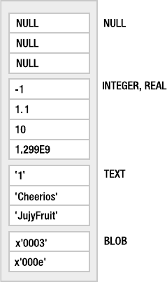
CHAPTER 4 ■ SQL 139
Figure 4-20. Storage class sort order
The following SQL illustrates the differences between storage class values:
sqlite> SELECT 3 < 3.142, 3.142 < '3.142', '3.142' < x'3000',
x'3000' < x'3001';
3 < 3.142 3.142 < '3.142' '3.142' < x'3000' x'3000' < x'3001'
--------- --------------- ----------------- ------------------
1 1 1 1
INTEGERs and REALs are compared numerically and are both less than TEXTs, and TEXTs are less
than BLOBs.
Manifest Typing
SQLite uses manifest typing. If you do a little research, you will find that the term manifest typing is
subject to multiple interpretations. In programming languages, manifest typing refers to how the
type of a variable or value is defined and/or determined. There are two main interpretations:
Manifest typing means that a variable’s type must be explicitly declared in the code. By this
definition, languages such as C/C++, Pascal, and Java would be said to use manifest typing.
Dynamically typed languages such as Perl, Python, and Ruby, on the other hand, are the
direct opposite as they do not require that a variable’s type be declared.
Manifest typing means that variables don’t have types at all. Rather, only values have types.
This seems to be in line with dynamically typed languages. Basically, a variable can hold
any value, and the type of that variable at any point in time is determined by its value at
that moment. Thus if you set variable x=1, then x at that moment is of type INTEGER. If you
then set x='JujyFruit', it is then of type TEXT. That is, if it looks like an INTEGER, and it acts
like an INTEGER, it is an INTEGER.
Owens_6730 C04.fm Page 139 Monday, April 17, 2006 7:16 AM
www.it-ebooks.info
140 CHAPTER 4 ■ SQL
For the sake of brevity, I will refer to the first interpretation as MT 1 and the second as MT 2. At
first glance, it may not be readily apparent as to which interpretation best fits SQLite. For example,
consider the following table:
CREATE TABLE foo( x integer,
y text,
z real );
Say we now insert a record into this table as follows:
INSERT INTO foo VALUES ('1', '1', '1');
When SQLite creates the record, what type is stored internally for x, y, and z? The answer:
INTEGER, TEXT, and REAL. Then it seems that SQLite uses MT 1: variables have declared types.
But wait a second; column types in SQLite are optional, so we could have just as easily defined
foo as follows:
CREATE TABLE foo(x, y, z);
Now let’s do the same INSERT:
INSERT INTO foo VALUES ('1', '1', '1');
What type are x, y, and z now? The answer: TEXT, TEXT, and TEXT. Well, maybe SQLite is just
setting columns to TEXT by default. If you think that, then consider the following INSERT state-
ment on the same table:
INSERT INTO foo VALUES (1, 1.0, x'10');
What are x, y, and z in this row? INTEGER, REAL, and BLOB. This looks like MT 2, where the value
itself determines its type.
So which one is it? The short answer: neither and both. The long answer is a little more
involved. With respect to MT 1, SQLite lets you declare columns to have types if you want to.
This looks and feels like what other databases do. But you don’t have to, thereby violating this
interpretation as well. This is because in all situations SQLite can take any value and infer a type
from it. It doesn’t need the type declared in the column to help it out. With respect to MT 2, SQLite
allows the type of the value to “influence” (maybe not completely determine) the type that gets
stored in the column. But you can still declare the column with a type and that type will exert
some influence, thereby violating this interpretation as well—that types come from values only.
What we really have here is the MT 3—the SQLite interpretation. It borrows from both MT 1
and MT 2.
But interestingly enough, manifest typing does not address the whole issue with respect to
types. It seems to be concerned with only declaring and resolving types. What about type checking?
That is, if you declare a column to be type integer, what exactly does that mean?
First let’s consider what most other relational databases do. They enforce strict type checking
as a standard part of standard domain integrity. First you declare a column’s type. Then only
values of that type can go in it. End of story. You can use additional domain constraints if you
want, but under no conditions can you ever insert values of other types. Consider the following
example with Oracle:
Owens_6730 C04.fm Page 140 Monday, April 17, 2006 7:16 AM
www.it-ebooks.info
CHAPTER 4 ■ SQL 141
SQL> create table domain(x int, y varchar(2));
Table created.
SQL> INSERT INTO domain VALUES ('pi', 3.14);
INSERT INTO domain VALUES ('pi', 3.14)
*
ERROR at line 1:
ORA-01722: invalid number
The value 'pi' is not an integer value. And column x was declared to be of type int. I don’t even
get to hear about the error in column y because the whole INSERT is aborted due to the integrity
violation on x. When I try this in SQLite,
sqlite> CREATE TABLE domain (x int, y varchar(2));
sqlite> INSERT INTO domain VALUES ('pi', 3.14);
sqlite> SELECT * FROM domain;
x y
---- -----
pi 3.14
there’s no problem. I said one thing and did another, and SQLite didn’t stop me. SQLite’s domain
integrity does not include strict type checking. So what is going on? Does a column’s declared type
count for anything? Yes. Then how is it used? It is all done with something called type affinity.
In short, SQLite’s manifest typing states that 1) columns can have types and 2) that types
can be inferred from values. Type affinity addresses how these two things relate to one another.
Type affinity is a delicate balancing act that sits between strict typing and dynamic typing.
Type Affinity
In SQLite, columns don’t have types or domains. While a column can have a declared type,
internally it only has a type affinity. Declared type and type affinity are two different things.
Type affinity determines the storage class SQLite uses to store values within a column. The
actual storage class a column uses to store a given value is a function of both the value’s storage
class and the column’s affinity. Before getting into how this is done, however, let’s first talk
about how a column gets its affinity.
Column Types and Affinities
To begin with, every column has an affinity. There are four different kinds: NUMERIC, INTEGER,
TEXT, and NONE. A column’s affinity is determined directly from its declared type (or lack thereof).
Therefore, when you declare a column in a table, the type you choose to declare it as will ulti-
mately determine that column’s affinity. SQLite assigns a column’s affinity according to the
following rules:
• By default, a column’s default affinity is NUMERIC. That is, if a column is not INTEGER, TEXT,
or NONE, then it is automatically assigned NUMERIC affinity.
• If a column’s declared type contains the string 'INT' (in uppercase or lowercase), then
the column is assigned INTEGER affinity.
Owens_6730 C04.fm Page 141 Monday, April 17, 2006 7:16 AM
www.it-ebooks.info

142 CHAPTER 4 ■ SQL
• If a column’s declared type contains any of the strings 'CHAR', 'CLOB', or 'TEXT' (in
uppercase or lowercase), then that column is assigned TEXT affinity. Notice that 'VARCHAR'
contains the string 'CHAR' and thus will confer TEXT affinity.
• If a column’s declared type contains the string 'BLOB' (in uppercase or lowercase), or if
it has no declared type, then it is assigned NONE affinity.
■Note Pay attention to defaults. If you don’t declare a column’s type, then its affinity will be NONE, in which
case all values will be stored using their given storage class (or inferred from their representation). If you are
not sure what you want to put in a column, or want to leave it open to change, this is the best affinity to use.
However, be careful of the scenario where you declare a type that does not match any of the rules for NONE,
TEXT, or INTEGER. While you might intuitively think the default should be NONE, it is actually NUMERIC.
For example, if you declare a column of type JUJYFRUIT, it will not have affinity NONE just because SQLite
doesn’t recognize it. Rather it will have affinity NUMERIC. (Interestingly, the scenario also happens when you
declare a column’s type to be numeric for the same reason.) Rather than using an unrecognized type that
ends up as numeric, you may prefer to leave the column’s declared type out altogether, which will ensure it
has affinity NONE.
Affinities and Storage
Each affinity influences how values are stored in its associated column. The rules governing
storage are as follows:
•A NUMERIC column may contain all five storage classes. A NUMERIC column has a bias
toward numeric storage classes (INTEGER and REAL). When a TEXT value is inserted into a
NUMERIC column, it will attempt to convert it to an INTEGER storage class. If this fails, it will
attempt to convert it to a REAL storage class. Failing that, it stores the value using the TEXT
storage class.
•An INTEGER column tries to be as much like a NUMERIC column as it can. An INTEGER column
will store a REAL value as REAL. However, if a REAL value has no fractional component, then
it will be stored using an INTEGER storage class. INTEGER column will try to store a TEXT
value as REAL if possible. If that fails, they try to store it as INTEGER. Failing that, TEXT values are
stored as TEXT.
•A TEXT column will convert all INTEGER or REAL values to TEXT.
•A NONE column does not attempt to convert any values. All values are stored using their
given storage class.
• No column will ever try to convert NULL or BLOB values—regardless of affinity. NULL and
BLOB values are always stored as is in every column.
These rules may initially appear somewhat complex, but their overall design goal is simple: to
make it possible for SQLite to mimic other relational databases if you need it to. That is, if you
treat columns like a traditional database, type affinity rules will store values in the way you
expect. If you declare a column of type INTEGER, and put integers into it, they will be stored as
Owens_6730 C04.fm Page 142 Monday, April 17, 2006 7:16 AM
www.it-ebooks.info
CHAPTER 4 ■ SQL 143
INTEGER. If you declare a column to be of type TEXT, CHAR, or VARCHAR and put integers into it,
they will be stored as TEXT. However, if you don’t follow these conventions, SQLite will still find
a way to store the value.
Affinities in Action
Let’s look at a few examples to get the hang of how affinity works. Consider the following:
sqlite> CREATE TABLE domain(i int, n numeric, t text, b blob);
sqlite> INSERT INTO domain VALUES (3.142,3.142,3.142,3.142);
sqlite> INSERT INTO domain VALUES ('3.142','3.142','3.142','3.142');
sqlite> INSERT INTO domain VALUES (3142,3142,3142,3142);
sqlite> INSERT INTO domain VALUES (x'3142',x'3142',x'3142',x'3142');
sqlite> INSERT INTO domain VALUES (null,null,null,null);
sqlite> SELECT ROWID,typeof(i),typeof(n),typeof(t),typeof(b) FROM domain;
rowid typeof(i) typeof(n) typeof(t) typeof(b)
---------- ---------- ---------- ---------- ----------
1 real real text real
2 real real text text
3 integer integer text integer
4 blob blob blob blob
5 null null null null
The first INSERT inserts a REAL value. You can see this both by the format in the INSERT statement
and by the resulting type shown in the typeof(b) column returned in the SELECT statement.
Remember that BLOB columns have storage class NONE, which does not attempt to convert the
storage class of the input value, so column b uses the same storage class that was defined in the
INSERT statement. Column i keeps the NUMERIC storage class, because it tries to be NUMERIC when
it can. Column n doesn’t have to convert anything. Column t converts it to TEXT. Column b stores
it exactly as given in the context. In each subsequent INSERT, you can see how the conversion
rules are applied in each varying case.
The following SQL illustrates storage class sort order and interclass comparison (which are
governed by the same set of rules):
sqlite> SELECT ROWID, b, typeof(b) FROM domain ORDER BY b;
rowid b typeof(b)
----- ------ ---------
5 NULL null
1 3.142 real
3 3142 integer
2 3.142 text
4 1B blob
Here, you see that NULLs sort first, followed by INTEGERs and REALs, followed by TEXTs, then
BLOBs. The following SQL shows how these values compare with the integer 1,000. The INTEGER
and REAL values in b are less than 1,000 because they are numerically compared, while TEXT and
BLOB are greater than 1,000 because they are in a higher storage class.
Owens_6730 C04.fm Page 143 Monday, April 17, 2006 7:16 AM
www.it-ebooks.info
144 CHAPTER 4 ■ SQL
sqlite> SELECT ROWID, b, typeof(b), b<1000 FROM domain ORDER BY b;
rowid b typeof(b) b<1000
----- ----- -------- ----------
5 NULL null NULL
1 3.142 real 1
3 3142 integer 1
2 3.142 text 0
4 1B blob 0
The primary difference between type affinity and strict typing is that type affinity will never
issue a constraint violation for incompatible data types. SQLite will always find a data type to
put any value into any column. The only question is what type it will use to do so. The only role
of a column’s declared type in SQLite is simply to determine its affinity. Ultimately, it is the
column’s affinity that has any bearing on how values are stored inside of it. However, SQLite does
provide facilities for ensuring that a column may only accept a given type, or range of types.
You do this using CHECK constraints, explained in the sidebar “Makeshift Strict Typing,” later in
this section.
Storage Classes and Type Conversions
Another thing to note about storage classes is that they can sometimes influence how values
are compared as well. Specifically, SQLite will sometimes convert values between numeric
storage classes (INTEGER and REAL) and TEXT before comparing them. For binary comparisons,
it uses the following rules:
• When a column value is compared to the result of an expression, the affinity of the
column is applied to the result of the expression before the comparison takes place.
• When two column values are compared, if one column has INTEGER or NUMERIC affinity
and the other doesn’t, then NUMERIC affinity is applied to TEXT values in the non-NUMERIC
column.
• When two expressions are compared, SQLite does not make any conversions. The results
are compared as is. If the expressions are of like storage class, then the comparison function
associated with that storage class is used to compare values. Otherwise, they are compared
on the basis of their storage class.
Note that the term expression here refers to any scalar expression or literal other than a column
value. To illustrate the first rule, consider the following:
sqlite> select ROWID,b,typeof(i),i>'2.9' from domain ORDER BY b;
rowid b typeof(i i>'2.9'
----- ----- -------- ------------
5 NULL null NULL
1 3.142 real 1
3 3142 integer 1
2 3.142 real 1
4 1B blob 1
Owens_6730 C04.fm Page 144 Monday, April 17, 2006 7:16 AM
www.it-ebooks.info
CHAPTER 4 ■ SQL 145
The expression '2.9', while being TEXT, is converted to INTEGER before the comparison. So the
column interprets the value in light of what it is. What if '2.9'was a non-numeric string? Then
SQLite falls back to comparing storage class, in which INTEGER and NUMERIC types are always less
than TEXT:
sqlite> SELECT ROWID,b,typeof(i),i>'text' FROM domain ORDER BY b;
rowid b typeof(i i>'text'
----- ----- -------- ------------
5 NULL null NULL
1 3.14 real 0
3 314 integer 0
2 3.14 real 0
4 1B blob 1
The second rule simply states that when comparing a numeric and non-numeric column,
where possible SQLite will try to convert the non-numeric column to numeric format:
sqlite> CREATE TABLE rule2(a int, b text);
sqlite> insert into rule2 values(2,'1');
sqlite> insert into rule2 values(2,'text');
sqlite> select a, typeof(a),b,typeof(b), a>b from rule2;
a typeof(a) b typeof(b) a>b
---------- ---------- ---------- ---------- ----------
2 integer 1 text 1
2 integer text text 0
Column a is an INTEGER, b is TEXT. When evaluating the expression a>b, SQLite tries to coerce b
to INTEGER where it can. In the first row, b is '1', which can be coerced to INTEGER. SQLite makes
the conversion and compares integers. In the second row, b is 'text' and can’t be converted.
SQLite then compares storage classes INTEGER and TEXT.
The third rule just reiterates that storage classes established by context are compared at
face value. If what looks like a TEXT type is compared with what looks like an INTEGER type, then
TEXT is greater.
Additionally, you can manually convert the storage type of a column or an expression
using the CAST function. Consider the following example:
sqlite> SELECT typeof(3.14), typeof(CAST(3.14 as TEXT));
typeof(3.14) typeof(CAST(3.14 as TEXT))
------------ --------------------------
real text
Owens_6730 C04.fm Page 145 Monday, April 17, 2006 7:16 AM
www.it-ebooks.info

146 CHAPTER 4 ■ SQL
MAKESHIFT STRICT TYPING
If you need something stronger than type affinity for domain integrity, then CHECK constraints can help. You
can implement pseudo strict typing directly using a single built-in function and a CHECK constraint. As mentioned
earlier, SQLite has a function which returns the inferred storage class of a value—typeof(). You can use
typeof() in any relational expression to test for a values type. For example:
sqlite> select typeof(3.14) = 'text';
0
sqlite> select typeof(3.14) = 'integer';
0
sqlite> select typeof(3.14) = 'real';
1
sqlite> select typeof(3) = 'integer';
1
sqlite> select typeof('3') = 'text';
1
Therefore, you can use this function to implement a CHECK constraint that limits the acceptable types allowed
in a column:
sqlite> create table domain (x integer CHECK(typeof(x)='integer'));
sqlite> INSERT INTO domain VALUES('1');
SQL error: constraint failed
sqlite> INSERT INTO domain VALUES(1.1);
SQL error: constraint failed
sqlite> INSERT INTO domain VALUES(1);
sqlite> select x, typeof(x) from domain;
x typeof(x)
-- ----------
1 integer
sqlite> update domain set x=1.1;
SQL error: constraint failed
The only catch here is that you are limited to checking for SQLite’s native storage classes (or what can
be implemented using other built-in SQL functions). However, if you are a programmer and either use a language
extension that supports SQLite’s user-defined functions (e.g., Perl, Python, or Ruby) or use the SQLite C API
directly, you can implement even more elaborate functions for type checking, which can be called from within
CHECK constraints. Chapter 5 covers this in more detail.
Owens_6730 C04.fm Page 146 Monday, April 17, 2006 7:16 AM
www.it-ebooks.info
CHAPTER 4 ■ SQL 147
Transactions
Transactions define boundaries around a group of SQL commands such that they either all
successfully execute together or not at all. A classic example of the rationale behind transactions
is a money transfer. Say a bank program is transferring money from one account to another. The
money transfer program can do this in one of two ways: first insert (credit) the funds into account 2
then delete (debit) it from account 1, or first delete it from account 1 and insert it into account 2.
Either way, the transfer is a two-step process: an INSERT followed by a DELETE, or a DELETE followed
by an INSERT.
Now, say the program is in the process of making a transfer. The first SQL command
completes successfully, and then the database server suddenly crashes or the power goes out.
Whatever the case, the second operation does not complete. Now the money either exists in
both accounts (the first scenario) or has been completely lost altogether (second scenario).
Either way, someone’s not going to be happy. And the database is in an inconsistent state.
The point here is that these two operations must either happen together or not at all. That
is what transactions are for. Now let’s replay the example with transactions. In the new scenario,
the program first starts a transaction in the database, completes the first SQL operation, and
then the lights go out. When they come back on and the database comes back up, it sees an
incomplete transaction. It then undoes the changes of the first SQL operation, which brings it
back into a consistent state—back where it started before the transfer.
Transaction Scopes
Transactions are issued with three commands: BEGIN, COMMIT, and ROLLBACK. BEGIN starts a transac-
tion. Every operation following a BEGIN can be potentially undone, and will be undone if a COMMIT is
not issued before the session terminates. The COMMIT command commits the work performed
by all operations since the start of the transaction. Similarly, the ROLLBACK command undoes all
of the work performed by all operations since the start of the transaction. A transaction is a
scope in which operations are performed together and committed, or completely reversed.
Consider the following example:
sqlite> BEGIN;
sqlite> DELETE FROM foods;
sqlite> ROLLBACK;
sqlite> SELECT COUNT(*) FROM foods;
COUNT(*)
--------
412
I started a transaction, deleted all the rows in foods, changed my mind, and reversed those
changes by issuing a ROLLBACK. The SELECT statement shows that nothing was changed.
By default, every SQL command in SQLite is run under its own transaction. That is, if
you do not define a transaction scope with BEGIN…COMMIT/ROLLBACK, SQLite will implicitly wrap
every individual SQL command with a BEGIN…COMMIT/ROLLBACK. In that case, every command
that completes successfully is committed. Likewise, every command that encounters an error
is rolled back. This mode of operation (implicit transactions) is referred to as autocommit mode:
Owens_6730 C04.fm Page 147 Monday, April 17, 2006 7:16 AM
www.it-ebooks.info
148 CHAPTER 4 ■ SQL
SQLite automatically runs each command in its own transaction, and if the command does not
fail, its changes are automatically committed.
Conflict Resolution
As you’ve seen in previous examples, constraint violations cause the command that committed
the violation to terminate. What exactly happens when a command terminates in the middle of
making a bunch of changes to the database? In most databases, all of the changes are undone.
That is the way the database is programmed to handle a constraint violation—end of story.
SQLite, however, has a unique feature that allows you to specify different ways to handle
(or recover from) constraint violations. It is called conflict resolution. Take, for example, the
following UPDATE:
sqlite> UPDATE foods SET id=800-id;
SQL error: PRIMARY KEY must be unique
This results in a UNIQUE constraint violation because once the UPDATE statement reaches the
388th record, it attempts to update its id value to 800-388=412. But a row with an id of 412
already exists, so it aborts the command. But SQLite already updated the first 387 rows before
it reached this constraint violation. What happens to them? The default behavior is to termi-
nate the command and reverse all of the changes it made, while leaving the transaction intact.
But what if you wanted these 387 changes to stick despite the constraint violation? Well,
believe it or not, you can have it that way too, if you want. You just need to use the appropriate
conflict resolution. There are five possible resolutions, or policies, that can be applied to address
a conflict (constraint violation): REPLACE, IGNORE, FAIL, ABORT, and ROLLBACK. These five resolu-
tions define a spectrum of error tolerance or sensitivity. On one end of the spectrum is REPLACE,
which will effectively allow a statement to plow through almost every possible constraint violation.
On the other end is ROLLBACK, which will terminate the entire transaction upon the first viola-
tion of any kind. The resolutions are defined as follows in order of their severity:
•REPLACE: When a UNIQUE constraint violation is encountered, SQLite removes the row (or
rows) that caused the violation, and replaces it (them) with the new row from the INSERT
or UPDATE. The SQL operation continues without error. If a NOT NULL constraint violation
occurs, the NULL value is replaced by the default value for that column. If the column has
no default value, then SQLite applies the ABORT policy. It is important to note that when
this conflict resolution strategy deletes rows in order to satisfy a constraint, it does not
invoke delete triggers on those rows. This behavior, however, is subject to change in a
future release.
•IGNORE: When a constraint violation is encountered, SQLite allows the command to
continue, and leaves the row that triggered the violation unchanged. Other rows before
and after the row in question continue to be modified by the command. Thus, all rows in
the operation that trigger constraint violations are simply left unchanged, and the
command proceeds without error.
Owens_6730 C04.fm Page 148 Monday, April 17, 2006 7:16 AM
www.it-ebooks.info
CHAPTER 4 ■ SQL 149
•FAIL: When a constraint violation is encountered, SQLite terminates the command but
does not restore the changes it made prior to encountering the violation. That is, all
changes within the SQL command up to the violation are preserved. For example, if an
UPDATE statement encountered a constraint violation on the 100th row it attempts to
update, then the changes to the first 99 rows already modified remain intact, but changes
to rows 100 and beyond never occur as the command is terminated.
•ABORT: When a constraint violation is encountered, SQLite restores all changes the
command made and terminates it. ABORT is the default resolution for all operations in
SQLite. It is also the behavior defined in the SQL standard. As a side note, ABORT is also
the most expensive conflict resolution policy—requiring extra work even if no conflicts
ever occur.
•ROLLBACK: When a constraint violation is encountered, SQLite performs a ROLLBACK—
aborting the current command along with the entire transaction. The net result is that all
changes made by the current command and all previous commands in the transaction
are rolled back. This is the most drastic level of conflict resolution where a single violation
results in a complete reversal of everything performed in a transaction.
Conflict resolution can be specified within SQL commands as well as within table and
index definitions. Specifically, conflict resolution can be specified in INSERT, UPDATE, CREATE
TABLE, and CREATE INDEX. Furthermore, it has specific implications within triggers. The syntax
for conflict resolution in INSERT and UPDATE is as follows:
INSERT OR resolution INTO table (column_list) VALUES (value_list);
UPDATE OR resolution table SET (value_list) WHERE predicate;
The conflict resolution policy comes right after the INSERT or UPDATE command and is prefixed
with OR. Also, the INSERT OR REPLACE expression can be abbreviated as just REPLACE.
In the preceding UPDATE example, the updates made to the 387 records were rolled back
because the default resolution is ABORT. If you wanted the updates to stick, you could use the
FAIL resolution. To illustrate this, in the following example I copy foods into a new table test
and use it as the guinea pig. I add an additional column to test called modified, the default
value of which is 'no'. In the UPDATE, I change this to 'yes' to track which records are updated
before the constraint violation occurs. Using the FAIL resolution, these updates will remain
unchanged, and I can track afterward how many records were updated.
CREATE TABLE test AS SELECT * FROM foods;
CREATE UNIQUE INDEX test_idx on test(id);
ALTER TABLE test ADD COLUMN modified text NOT NULL DEFAULT 'no';
SELECT COUNT(*) FROM test WHERE modified='no';
COUNT(*)
--------------------
412
Owens_6730 C04.fm Page 149 Monday, April 17, 2006 7:16 AM
www.it-ebooks.info
150 CHAPTER 4 ■ SQL
UPDATE OR FAIL test SET id=800-id, modified='yes';
SQL error: column id is not unique
SELECT COUNT(*) FROM test WHERE modified='yes';
COUNT(*)
--------------------
387
DROP TABLE test;
There is one consideration with FAIL that you need to be aware of. The order that records
are updated is nondeterministic. That is, you cannot be certain of the order of the records in
the table or the order in which SQLite processes them. You might assume that it follows the
order of the ROWID column, but this is not a safe assumption to make: there is nothing in the
documentation that says so. The point is, if you are going to use FAIL, in many cases it might be
better to use IGNORE. IGNORE will finish the job and modify all records that can be modified rather
than bailing out on the first violation.
When defined within tables, conflict resolution is specified for individual columns.
For example:
sqlite> CREATE TEMP TABLE cast(name text UNIQUE ON CONFLICT ROLLBACK);
sqlite> INSERT INTO cast VALUES ('Jerry');
sqlite> INSERT INTO cast VALUES ('Elaine');
sqlite> INSERT INTO cast VALUES ('Kramer');
The cast table has a single column name with a UNIQUE constraint and conflict resolution set to
ROLLBACK. Any INSERT or UPDATE that triggers a constraint violation on name will be arbitrated by
the ROLLBACK resolution rather than the default ABORT. The result will not only abort the state-
ment but the entire transaction as well:
sqlite> BEGIN;
sqlite> INSERT INTO cast VALUES('Jerry');
SQL error: uniqueness constraint failed
sqlite> COMMIT;
SQL error: cannot commit - no transaction is active
COMMIT failed here because the name’s conflict resolution already aborted the transaction.
CREATE INDEX works the same way. Conflict resolution within tables and indices changes the
default behavior of the operation from ABORT to that defined for the specific columns when
those columns are the source of the constraint violation.
Conflict resolution at statement level (DML) overrides that defined at object level (DDL).
Working from the previous example:
sqlite> BEGIN;
sqlite> INSERT OR REPLACE INTO cast VALUES('Jerry');
sqlite> COMMIT;
The REPLACE resolution in the INSERT overrides the ROLLBACK resolution defined on cast.name.
Owens_6730 C04.fm Page 150 Monday, April 17, 2006 7:16 AM
www.it-ebooks.info
CHAPTER 4 ■ SQL 151
Database Locks
Locking is closely associated with transactions in SQLite. In order to use transactions effectively,
you need to know a little something about how it does locking.
SQLite has coarse-grained locking. When a session is writing to the database, all other
sessions are locked out until the writing session completes its transaction. To help with this,
SQLite has a locking scheme that helps defer writer locks until the last possible moment in
order to maximize concurrency.
SQLite uses a lock escalation policy whereby a connection gradually obtains exclusive
access to a database in order to write to it. There are five different locking states in SQLite:
unlocked, shared, reserved, pending, or exclusive. Each database session (or connection) can be
in only one of these states at any given time. Furthermore, there is a corresponding lock for
each state, except for unlocked—there is no lock required to be in the unlocked state.
To begin with, the most basic state is unlocked. In this state, no session is accessing data
from the database. When you connect to a database, or even initiate a transaction with BEGIN,
your connection is in the unlocked state.
The next state beyond unlocked is shared. In order for a session to read from the database
(not write), it must first enter the shared state, and must therefore acquire a shared lock. Multiple
sessions can simultaneously acquire and hold shared locks at any given time. Therefore, multiple
sessions can read from a common database at any given time. However, no session can write
to the database during this time—while any shared locks are active.
If a session wants to write to the database, it must first acquire a reserved lock. Only one
reserved lock may be held at one time for a given database. Shared locks can coexist with a
reserved lock. A reserved lock is the first phase of writing to a database. It does not block
sessions with shared locks from reading, nor does it prevent sessions from acquiring new
shared locks.
Once a session has a reserved lock, it can begin the process of making modifications; however,
these modifications are cached and not actually written to disk. The reader’s changes are
stored in a memory cache (see the discussion of the cache_size pragma in the section “Database
Configuration,” later in this chapter, for more information).
When the session wants to commit the changes (or transaction) to the database, it begins
the process of promoting its reserved lock to an exclusive lock. In order to get an exclusive lock,
it must first promote its reserved lock to a pending lock. A pending lock starts a process of attri-
tion whereby no new shared locks can be obtained. That is, other sessions with existing shared
locks are allowed to continue as normal, but other sessions cannot acquire new shared locks.
At this point, the session with the pending lock is waiting for the other sessions with shared
locks to finish what they are doing and release them.
Once all of shared locks are released, the session with the pending lock can promote it to
an exclusive lock. It is then free to make changes to the database. All of the previously cached
changes are written to the database file.
Deadlocks
While you may find all of this interesting, you are probably wondering at this point why any of
this matters. Why do you need to know this? Because if you don’t know what you are doing, you
can end up in a deadlock.
Owens_6730 C04.fm Page 151 Monday, April 17, 2006 7:16 AM
www.it-ebooks.info

152 CHAPTER 4 ■ SQL
Consider the following scenario illustrated in Table 4-7. Two sessions, A and B—completely
oblivious to one another—are working on the same database at the same time. Session A issues
the first command, B the second and third, A the fourth, and so on.
Both sessions wind up in a deadlock. Session B was the first to try to write to the database,
and therefore has a pending lock. A attempts to write, but fails when INSERT tries to promote its
shared lock to a reserved lock.
For the sake of argument, let’s say that A decides to just wait around for the database to
become writable. So does B. Then at this point, everyone else is effectively locked out too. If you
try to open a third session, it won’t even be able to read from the database. The reason is that B
has a pending lock, which prevents any sessions from acquiring shared locks. So not only are A
and B deadlocked, they have locked everyone else out of the database as well. Basically, you
have a shared lock and one pending lock that don’t want to relinquish control, and until one
does, nobody can do anything.
So how do you avoid this? It’s not like A and B can sit down in a meeting and work it out
with their lawyers. A and B don’t even know each other exists. The answer is to pick the right
transaction type for the job.
Transaction Types
SQLite has three different transaction types that start transactions in different locking states.
Transactions can be started as DEFERRED, IMMEDIATE, or EXCLUSIVE. A transaction’s type is
specified in the BEGIN command:
BEGIN [ DEFERRED | IMMEDIATE | EXCLUSIVE ] TRANSACTION;
A deferred transaction does not acquire any locks until it has to. Thus with a deferred trans-
action, the BEGIN statement itself does nothing—it starts in the unlocked state. This is the
default. If you simply issue a BEGIN, then your transaction is DEFERRED, and therefore sitting in
the unlocked state. Multiple sessions can simultaneously start DEFERRED transactions at the
same time without creating any locks. In this case, the first read operation against a database
acquires a shared lock and similarly the first write operation attempts to acquire a reserved lock.
Table 4-7. A Portrait of a Deadlock
Session A Session B
sqlite> BEGIN;
sqlite> BEGIN;
sqlite> INSERT INTO foo VALUES ('x');
sqlite> SELECT * FROM foo;
sqlite> COMMIT;
SQL error: database is locked
sqlite> INSERT INTO foo VALUES ('x');
SQL error: database is locked
Owens_6730 C04.fm Page 152 Monday, April 17, 2006 7:16 AM
www.it-ebooks.info
CHAPTER 4 ■ SQL 153
An immediate transaction attempts to obtain a reserved lock as soon as the BEGIN command is
executed. If successful, BEGIN IMMEDIATE guarantees that no other session will be able to write
to the database. As you know, other sessions can continue to read from the database, but the
reserved lock prevents any new sessions from reading. Another consequence of the reserved
lock is that no other sessions will be able to successfully issue a BEGIN IMMEDIATE or BEGIN
EXCLUSIVE command. SQLite will return a SQLITE_BUSY error. During this time, you can make
some modifications to the database, but you may not necessarily be able to commit them. When
you call COMMIT, you could get SQLITE_BUSY. This means that there are other readers active, as in
the earlier example. Once they are gone, you can commit the transaction.
An exclusive transaction obtains an exclusive lock on the database. This works similarly to
IMMEDIATE, but when you successfully issue it, EXCLUSIVE guarantees that no other session is
active in the database and that you can read or write with impunity.
The crux of the problem in the preceding example is that both sessions ultimately wanted
to write to the database but they made no attempt to relinquish their locks. Ultimately, it was
the shared lock that caused the problem. If both sessions had started with BEGIN IMMEDIATE,
then the deadlock would not have occurred. In this case, only one of the sessions would have
been able to enter BEGIN IMMEDIATE at one time, while the other would have to wait. The one
that has to wait could keep retrying with the assurance that it would eventually get in. BEGIN
IMMEDIATE and BEGIN EXCLUSIVE, if used by all sessions that want to write to the database,
provide a synchronization mechanism, thereby preventing deadlocks. For this approach to
work, though, everyone has to follow the rules.
The bottom line is this: if you are using a database that no other connections are using,
then a simple BEGIN will suffice. If, however, you are using a database that other connections
are also writing to, both you and they should use BEGIN IMMEDIATE or BEGIN EXCLUSIVE to initiate
transactions. It works out best that way for both of you. Transactions and locks are covered in
more detail in Chapter 5.
Database Administration
Database administration is generally concerned with controlling how a database operates.
From a SQL perspective, this includes various topics such as views, triggers, and indexes. Addi-
tionally, SQLite includes some unique administrative features of its own, such the means to
“attach” multiple databases to a single session, as well as database pragmas, which can be used
for setting various configuration parameters.
Views
Views are virtual tables. They are also known as derived tables, as their contents are derived
from other tables. While views look and feel like base tables, they aren’t. The contents of base
tables are persistent whereas the contents of views are dynamically generated when they are
used. Specifically, a view is composed of relational expressions that take other tables and produce
a new table. The syntax to create a view is as follows:
CREATE VIEW name AS sql;
The name of the view is given by name and its definition by sql. The resulting view will look like
a base table named name. Imagine you had a query you ran all the time, so much that you get
sick of writing it. Views are the cure for this particular sickness. Say your query was as follows:
Owens_6730 C04.fm Page 153 Monday, April 17, 2006 7:16 AM
www.it-ebooks.info
154 CHAPTER 4 ■ SQL
SELECT f.name, ft.name, e.name
FROM foods f
INNER JOIN food_types ft on f.type_id=ft.id
INNER JOIN foods_episodes fe ON f.id=fe.food_id
INNER JOIN episodes e ON fe.episode_id=e.id;
This returns the name of every food, its type, and every episode it was in. It is one big table of
504 rows with just about every food fact. Rather than having to write out (or remember) the
previous query every time you want these results, you can tidily restate it in the form of a view.
Let’s name it details:
CREATE VIEW details AS
SELECT f.name AS fd, ft.name AS tp, e.name AS ep, e.season as ssn
FROM foods f
INNER JOIN food_types ft on f.type_id=ft.id
INNER JOIN foods_episodes fe ON f.id=fe.food_id
INNER JOIN episodes e ON fe.episode_id=e.id;
Now you can query details just as you would a table. For example:
sqlite> SELECT fd as Food, ep as Episode
FROM details WHERE ssn=7 AND tp like 'Drinks';
Food Episode
-------------------- --------------------
Apple Cider The Bottle Deposit 1
Bosco The Secret Code
Cafe Latte The Postponement
Cafe Latte The Maestro
Champagne Coolies The Wig Master
Cider The Bottle Deposit 2
Hershey's The Secret Code
Hot Coffee The Maestro
Latte The Maestro
Mellow Yellow soda The Bottle Deposit 1
Merlot The Rye
Orange Juice The Wink
Tea The Hot Tub
Wild Turkey The Hot Tub
The contents of views are dynamically generated. Thus, every time you use details, its associ-
ated SQL will be reexecuted, producing results based on the data in the database at that moment.
Views also have other purposes, such as security, although this particular kind of security
does not exist in SQLite. Some databases offer row- and column-level security in which only
specific users, groups, or roles can view or modify specific parts of tables. In such databases,
views can be defined on tables to exclude sensitive columns, allowing users with less security
privileges to access parts of tables that are not secured. For example, say you have a table secure,
defined as follows:
Owens_6730 C04.fm Page 154 Monday, April 17, 2006 7:16 AM
www.it-ebooks.info
CHAPTER 4 ■ SQL 155
CREATE TABLE secure (id int, public_data text, restricted_data text);
You may want to allow users access to the first two columns but not the third. In other databases,
you would limit access to secure to just the users who can access all columns. You would then
create a view that contains just the first two columns that everyone else can look at:
CREATE VIEW public_secure AS SELECT id, public_data FROM secure;
Some of this kind of security is available if you program with SQLite, using its operational
control facilities. This is covered in Chapters 5 and 6.
Finally, to drop a view, use the DROP VIEW command:
DROP VIEW name;
The name of the view to drop is given by name.
Materialized Views
The relational model calls for updatable views, sometimes referred to as materialized views.
These are views that you can modify. You can run INSERT or UPDATE statements on them, for
example, and the respective changes are applied directly to their underlying tables. Materialized
views are not supported in SQLite. However, using triggers, you can create something that
looks like materialized views. These are covered in the section “Triggers.”
Indexes
Indexes are a construct designed to speed up queries under certain conditions. Consider the
following query:
SELECT * FROM foods WHERE name='JujyFruit';
When a database searches for matching rows, the default method it uses to perform this is called
a sequential scan. That is, it literally searches (or scans) every row in the table to see if its name
attribute matches 'JujyFruit'.
However, if this query is used frequently, and foods was very large, there is another method
available that can be much faster, called an index scan. An index is a special disk-based data
structure (called a B-tree), which stores the values for an entire column (or columns) in a highly
organized way that is optimized for searching.
The search speed of these two methods can be represented mathematically. The search
speed of a sequential scan is proportional to the number of rows in the table: the more rows,
the longer the scan. This relationship—bigger table, longer search—is called linear time, as in
“the search method operates in linear time.” It is represented mathematically using what is
called the Big O notation, which in this case is O(n), where n stands for the number of elements
(or rows) in the set. The index scan, on the other hand, has O(log(n)) search time, or logarithmic
time. This is much faster. If you have a table of 10,000 records, a sequential scan will read all
10,000 rows to find all matches, while an index scan will read 4 rows (log(10,000)) to find the
first match (and from that point on it would be linear time to find all subsequent matches). This
is quite a speed-up.
Owens_6730 C04.fm Page 155 Monday, April 17, 2006 7:16 AM
www.it-ebooks.info
156 CHAPTER 4 ■ SQL
But there is no such thing as a free lunch. Indexes also increase the size of the database.
They literally keep a copy of all columns they index. If you index every column in a table, you
effectively double the size of the table. Another consideration is that indexes must be main-
tained. When you insert, update, or delete records, in addition to modifying the table, the
database must modify each and every index on that table as well. So indexes can slow down
inserts, updates, and similar operations.
But in moderation, indexes can make a huge performance difference. Whether or not to
add an index is more subjective than anything else. Different people have different criteria for
what is acceptable. Indexes illustrate one of the great things about SQL: you only need to
specify what to get and not how to get it. Because of this, you can often optimize your database
(such as by adding or removing indexes) without having to rewrite your code. Just create an
index in the right place.
The command to create an index is as follows:
CREATE INDEX [UNIQUE] index_name ON table_name (columns)
The variable index_name is the name of the index, and must be unique, and table_name is the
name of the table containing the column(s) to index. The variable columns is either a single
column or a comma-separated list of columns.
If you use the UNIQUE keyword, then the index will have the added constraint that all values
in the index must be unique. This applies to both the index, and by extension, to the column or
columns it indexes. The UNIQUE constraint covers all columns defined in the index, and it is
their combined values (not individual values) that must be unique. For example:
sqlite> CREATE TABLE foo(a text, b text);
sqlite> CREATE UNIQUE INDEX foo_idx on foo(a,b);
sqlite> INSERT INTO foo VALUES ('unique', 'value');
sqlite> INSERT INTO foo VALUES ('unique', 'value2');
sqlite> INSERT INTO foo VALUES ('unique', 'value');
SQL error: columns a, b are not unique
You can see here that uniqueness is defined by both columns collectively, not individually.
Notice that collation plays an important role here as well.
To remove an index, use the DROP INDEX command, which is defined as follows:
DROP INDEX index_name;
Collation
Each column in the index can have a collation associated with it. For example, to create a case-
insensitive index on foods.name, you’d use the following:
CREATE INDEX foods_name_idx on foods (name COLLATE NOCASE);
This means that values in the name column will sort without respect to case. You can list the
indexes for a table in the SQLite command-line program by using the .indices shell command.
For example:
Owens_6730 C04.fm Page 156 Monday, April 17, 2006 7:16 AM
www.it-ebooks.info
CHAPTER 4 ■ SQL 157
sqlite> .indices foods
foods_name_idx
For more information, you can use the .schema shell command as well:
sqlite> .schema foods
CREATE TABLE foods(
id integer primary key,
type_id integer,
name text );
CREATE INDEX foods_name_idx on foods (name COLLATE NOCASE);
You can also obtain this information by querying the sqlite_master table, described later in
this section.
Index Utilization
It is important to understand when indexes are used and when they aren’t. There are very
specific conditions in which SQLite will decide to use an index. SQLite will use a single column
index, if available, for the following expressions in the WHERE clause:
column {=|>|>=|<=|<} expression
expression {=|>|>=|<=|<} column
column IN (expression-list)
column IN (subquery)
Multicolumn indexes have more specific conditions before they are used. This is perhaps
best illustrated by example. Say you have a table defined as follows:
CREATE TABLE foo (a,b,c,d);
Furthermore, you create a multicolumn index as follows:
CREATE INDEX foo_idx on foo (a,b,c,d);
The columns of foo_idx can only be used sequentially from left to right. That is, in the query
SELECT * FROM foo WHERE a=1 AND b=2 AND d=3
only the first and second conditions will use the index. The reason the third condition was
excluded is because there was no condition that used c to bridge the gap to d. Basically, when
SQLite uses a multicolumn index, it works from left to right column-wise. It starts with the left
column and looks for a condition using that column. It moves to the second column, and so on.
It continues until either it fails to find a valid condition in the WHERE clause that uses it or there
are no more columns in the index to use.
But there is one more requirement. SQLite will use a multicolumn index only if all of the
conditions use either the equality (=) or IN operator for all index columns except for the right-
most index column. For that column, you can specify up to two inequalities to define its upper
and lower bounds. Consider, for example:
SELECT * FROM foo WHERE a>1 AND b=2 AND c=3 AND d=4
Owens_6730 C04.fm Page 157 Monday, April 17, 2006 7:16 AM
www.it-ebooks.info

158 CHAPTER 4 ■ SQL
SQLite will only do an index scan on column a. The a>1 expression becomes the rightmost
index column because it uses the inequality. All columns after it are not eligible to be used as
a result. Similarly,
SELECT * FROM foo WHERE a=1 AND b>2 AND c=3 AND d=4
will use the index columns a and b and stop there as b>2 becomes the rightmost index term by
its use of an inequality operator.
An off-the-cuff way to time a query within a SQL statement is to use a subselect in the FROM
clause returning the current time, which will be joined to your input relation(s). Then select the
current time in the SELECT clause. The time in the FROM clause will be computed at the start of
the query. The time in the SELECT clause will be computed as each row is processed. Therefore,
the difference between the two times in the last row of the result set will be your relative query
time. For example, the following SQL is a triple Cartesian join on food_types. It’s quite slow, as
it should be. The results display the last five records of the result set.
SELECT CAST(strftime('%s','now') as INTEGER)-CAST(time.start as INTEGER) time,
ft1.id, ft2.id, ft3.id, ft4.id
FROM food_types ft1, food_types ft2, food_types ft3, food_types ft4,
(SELECT strftime('%s','now') start) time;
18 15 15 15 11
18 15 15 15 12
18 15 15 15 13
18 15 15 15 14
18 15 15 15 15
The first column is the elapsed time in seconds. This query took 18 seconds. Although this
doesn’t represent the actual query time because there is timing overhead, relative query time
is all you need to judge an index’s worth. If this were an actual slow query that you were trying
to optimize, you would now add the index you think might help and rerun the query. Is it
significantly faster? If so, then you may have a useful index.
In short, when you create an index, have a reason for creating it. Make sure there is a specific
performance gain you are getting before you take on the overhead that comes with it. Well-
chosen indexes are a wonderful thing. Indexes that are thoughtlessly scattered here and there
in the vain hope of performance are of dubious value.
Triggers
Triggers execute specific SQL commands when specific database events transpire on specific
tables. The general syntax for creating a trigger is as follows:
CREATE [TEMP|TEMPORARY] TRIGGER name [BEFORE|AFTER]
[INSERT|DELETE|UPDATE|UPDATE OF columns] ON table
action
A trigger is defined by a name, an action, and a table. The action, or trigger body, consists
of a series of SQL commands. Triggers are said to fire when such events take place. Furthermore,
Owens_6730 C04.fm Page 158 Monday, April 17, 2006 7:16 AM
www.it-ebooks.info

CHAPTER 4 ■ SQL 159
triggers can be made to fire before or after the event using the BEFORE or AFTER keyword, respec-
tively. Events include DELETE, INSERT, and UPDATE commands issued on the specified table.
Triggers can be used to create your own integrity constraints, log changes, update other tables,
and many other things. They are limited only by what you can write in SQL.
UPDATE Triggers
UPDATE triggers, unlike INSERT and DELETE triggers, may be defined for specific columns in a
table. The general form of this kind of trigger is as follows:
CREATE TRIGGER name [BEFORE|AFTER] UPDATE OF column ON table
action
The following is a SQL script that shows an UPDATE trigger in action:
.h on
.m col
.w 50
.echo on
CREATE TEMP TABLE log(x);
CREATE TEMP TRIGGER foods_update_log UPDATE of name ON foods
BEGIN
INSERT INTO log VALUES('updated foods: new name=' || NEW.name);
END;
BEGIN;
UPDATE foods set name='JUJYFRUIT' where name='JujyFruit';
SELECT * FROM log;
ROLLBACK;
This script creates a temporary table called log, as well as a temporary UPDATE trigger on
foods.name that inserts a message into log when it fires. The action takes place inside the trans-
action that follows. The first step of the transaction updates the name column of the row whose
name is 'JUJYFRUIT'. This causes the UPDATE trigger to fire. When it fires, it inserts a record into the
log. Next, the transaction reads log, which shows that the trigger did indeed fire. The transaction
then rolls back the change, and when the session ends, the log table and the UPDATE trigger are
destroyed. Running the script produces the following output:
mike@linux tmp # sqlite3 foods.db < trigger.sql
CREATE TEMP TABLE log(x);
CREATE TEMP TRIGGER foods_update_log AFTER UPDATE of name ON foods
BEGIN
INSERT INTO log VALUES('updated foods: new name=' || NEW.name);
END;
Owens_6730 C04.fm Page 159 Monday, April 17, 2006 7:16 AM
www.it-ebooks.info

160 CHAPTER 4 ■ SQL
BEGIN;
UPDATE foods set name='JUJYFRUIT' where name='JujyFruit';
SELECT * FROM log;
x
--------------------------------------------------
updated foods: new name=JUJYFRUIT
ROLLBACK;
SQLite provides access to both the old (original) row and the new (updated) row in UPDATE
triggers. The old row is referred to as OLD and the new row as NEW. Notice in the script how the
trigger refers to NEW.name. All attributes of both rows are available in OLD and NEW using the dot
notation. I could have just as easily recorded NEW.type_id or OLD.id.
Error Handling
Defining a trigger before an event takes place gives you the opportunity to stop the event from
happening. BEFORE triggers enable you to implement new integrity constraints. SQLite provides a
special SQL function for triggers called RAISE(), which allows them to raise an error within the
trigger body. RAISE is defined as follows:
RAISE(resolution, error_message);
The first argument is a conflict resolution policy (ABORT, FAIL, IGNORE, ROLLBACK, etc.). The second
argument is an error message. If you use IGNORE, the remainder of the current trigger along with
the SQL statement that caused the trigger to fire, as well as any subsequent triggers that would
have been fired, are all terminated. If the SQL statement that caused the trigger to fire is itself
part of another trigger, then that trigger resumes execution at the beginning of the next SQL
command in the trigger action.
Conflict Resolution
If a conflict resolution policy is defined for a SQL statement that causes a trigger to fire, then
that policy supersedes the policy defined within the trigger. If, on the other hand, the SQL
statement does not have any conflict resolution policy defined, and the trigger does, then the
trigger’s policy is used.
Updatable Views
Triggers make it possible to create something like materialized views, as mentioned earlier in
this chapter. In reality, they aren’t true materialized views but rather more like updatable views.
With true materialized views, the view is updatable all by itself—you define the view and it
figures out how to map all changes to its underlying base tables. This is not a simple thing. Nor
is it supported in SQLite. However, using triggers, we can create the appearance of a material-
ized view.
The idea here is that you create a view and then create a trigger that handles update events
on that view. SQLite supports triggers on views using the INSTEAD OF keywords in the trigger
definition. To illustrate this, let’s create a view that combines foods with food_types:
Owens_6730 C04.fm Page 160 Monday, April 17, 2006 7:16 AM
www.it-ebooks.info

CHAPTER 4 ■ SQL 161
CREATE VIEW foods_view AS
SELECT f.id fid, f.name fname, t.id tid, t.name tname
FROM foods f, food_types t;
This view joins the two tables according to their foreign key relationship. Notice that I have
created aliases for all column names in the view. This allows me to differentiate the respective
id and name columns in each table when I reference them from inside the trigger. Now, let’s
make the view updatable by creating an UPDATE trigger on it:
CREATE TRIGGER on_update_foods_view
INSTEAD OF UPDATE ON foods_view
FOR EACH ROW
BEGIN
UPDATE foods SET name=NEW.fname WHERE id=NEW.fid;
UPDATE food_types SET name=NEW.tname WHERE id=NEW.tid;
END;
Now if you try to update the foods_view, this trigger gets called. The trigger simply takes the
values provided in the UPDATE statement and uses them to update the underlying base tables
foods and food_types. Testing it out yields the following:
.echo on
-- Update the view within a transaction
BEGIN;
UPDATE foods_view SET fname='Whataburger', tname='Fast Food' WHERE fid=413;
-- Now view the underlying rows in the base tables:
SELECT * FROM foods f, food_types t WHERE f.type_id=t.id AND f.id=413;
-- Roll it back
ROLLBACK;
-- Now look at the original record:
SELECT * FROM foods f, food_types t WHERE f.type_id=t.id AND f.id=413;
BEGIN;
UPDATE foods_view SET fname='Whataburger', tname='Fast Food' WHERE fid=413;
SELECT * FROM foods f, food_types t WHERE f.type_id=t.id AND f.id=413;
id type_id name id name
--- ------- -------------- --- ---------
413 1 Whataburger 1 Fast Food
ROLLBACK;
SELECT * FROM foods f, food_types t WHERE f.type_id=t.id AND f.id=413;
id type_id name id name
--- ------- -------------- --- -------
413 1 Cinnamon Bobka 1 Bakery
You can just as easily add INSERT and DELETE triggers and have the rough equivalent of a
materialized view.
Owens_6730 C04.fm Page 161 Monday, April 17, 2006 7:16 AM
www.it-ebooks.info
162 CHAPTER 4 ■ SQL
Foreign Key Constraints Using Triggers
One of the most interesting applications of triggers in SQLite I have seen is the implementation
of foreign key constraints, originally posted on the SQLite Wiki (www.sqlite.org/contrib). To
further explore triggers, I will use this idea to implement foreign key constraints between foods
and food_types.
As mentioned earlier, foods.type_id references food_types.id. Therefore, every value in
foods.type_id should correspond to some value in food_types.id. The first step in enforcing
this constraint lies in controlling what can be inserted into foods. This is accomplished with the
following INSERT trigger:
CREATE TRIGGER foods_insert_trg
BEFORE INSERT ON foods
BEGIN
SELECT CASE
WHEN (SELECT id FROM food_types WHERE id=NEW.type_id) IS NULL
THEN RAISE( ABORT,
'Foreign Key Violation: foods.type_id is not in food_types.id')
END;
END;
This trigger runs a subquery that checks for the value of NEW.type_id in foods_types.id. If no
match is found, the subquery returns NULL, which triggers the WHEN condition, calling the RAISE
function.
After installing the trigger, the following SQL tries to insert a record with an invalid type_id
(the maximum id value in food_types is 15):
sqlite> INSERT INTO foods VALUES (NULL, 20, 'Blue Bell Ice Cream');
SQL error: Foreign Key Violation: foods.type_id is not in food_types.id
Next is UPDATE. The only thing that matters on UPDATE of foods is the type_id field, so the
trigger will be defined on that column alone. Aside from this and the trigger’s name, the trigger
is identical to INSERT:
CREATE TRIGGER foods_update_trg
BEFORE UPDATE OF type_id ON foods
BEGIN
SELECT CASE
WHEN (SELECT id FROM food_types WHERE id=NEW.type_id) IS NULL
THEN RAISE(ABORT,
'Foreign Key Violation: foods.type_id is not in food_types.id')
END;
END;
Testing this trigger reveals the same results:
sqlite> UPDATE foods SET type_id=20 WHERE name='Chocolate Bobka';
SQL error: Foreign Key Violation: foods.type_id is not in food_types.id
The final piece of the puzzle is DELETE. Deleting rows in foods doesn’t affect the relation-
ship with food_types. Deleting rows in food_types, however, does affect the relationship with
Owens_6730 C04.fm Page 162 Monday, April 17, 2006 7:16 AM
www.it-ebooks.info
CHAPTER 4 ■ SQL 163
foods. If a row is deleted in food_types, then there could potentially be rows in foods that may
reference it, in which case the relationship has been compromised. Therefore, we need a DELETE
trigger on food_types that does not allow the deletion of a row if there are rows in foods that
reference it. To that end, the DELETE trigger is defined as follows:
CREATE TRIGGER foods_delete_trg
BEFORE DELETE ON food_types
BEGIN
SELECT CASE
WHEN (SELECT COUNT(type_id) FROM foods WHERE type_id=OLD.id) > 0
THEN RAISE(ABORT,
'Foreign Key Violation: foods rows reference row to be deleted.')
END;
END;
After installing this trigger, if I try to delete the 'Bakery' row in food_types I get:
sqlite> DELETE FROM food_types WHERE name='Bakery';
SQL error: Foreign Key Violation: foods rows reference row to be deleted.
To make sure this works under the correct conditions:
sqlite> BEGIN;
sqlite> DELETE FROM foods WHERE type_id=1;
sqlite> DELETE FROM food_types WHERE name='Bakery';
sqlite> ROLLBACK;
The DELETE trigger allows the delete if there are no rows in foods referencing it.
So there you have it: simple, trigger-based foreign key constraints. As mentioned earlier,
while SQLite does support CHECK constraints, triggers can pretty much do everything CHECK
constraints can and then some.
Attaching Databases
SQLite allows you to “attach” multiple databases to the current session using the ATTACH
command. When you attach a database, all of its contents are accessible in the global scope
of the current database file. ATTACH has the following syntax:
ATTACH [DATABASE] filename AS database_name;
Here, filename refers to the path and name of the SQLite database file, and database_name
refers to the logical name with which to reference that database and its objects. The main data-
base is automatically assigned the name main. If you create any temporary objects, then SQLite
will create an attached database name temp. (You can see these objects using the database_list
pragma, described later.) The logical name may be used to reference objects within the attached
database. If there are tables or other database objects that share the same name in both data-
bases, then the logical name is required to reference such objects in the attached database. For
example, if both databases have a table called foo, and the logical name of the attached data-
base is db2, then the only way to query foo in db2 is by using the fully qualified name foo.db2,
as follows:
Owens_6730 C04.fm Page 163 Monday, April 17, 2006 7:16 AM
www.it-ebooks.info
164 CHAPTER 4 ■ SQL
sqlite> ATTACH DATABASE '/tmp/db' as db2;
sqlite> SELECT * FROM db2.foo;
x
----------
bar
If you really want to, you can qualify objects in the main database using the name main:
sqlite> SELECT * FROM main.foods LIMIT 2;
id type_id name
---------- ---------- --------------
1 1 Bagels
2 1 Bagels, raisin
The same is true with the temporary database:
sqlite> CREATE TEMP TABLE foo AS SELECT * FROM food_types LIMIT 3;
sqlite> SELECT * FROM temp.foo;
id name
--- -------------
1 Bakery
2 Cereal
3 Chicken/Fowl
You detach databases with the DETACH DATABASE command, defined as follows:
DETACH [DATABASE] database_name;
This command takes the logical name of the attached database (given by database_name) and
detaches the associated database file. You get a list of attached databases using the database_list
pragma, explained in the section “Database Configuration.”
Cleaning Databases
SQLite has two commands designed for cleaning—REINDEX and VACUUM. REINDEX is used to rebuild
indexes. It has two forms:
REINDEX collation_name;
REINDEX table_name|index_name;
The first form rebuilds all indexes that use the collation name given by collation_name. It is
only needed when you change the behavior of a user-defined collating sequence (e.g., multiple
sort orders in Chinese). All indexes in a table (or a particular index given its name) can be rebuilt
with the second form.
VACUUM cleans out any unused space in the database by rebuilding the database file. VACUUM
will not work if there are any open transactions. An alternative to manually running VACUUM
statements is autovacuum. This feature is enabled using the auto_vacuum pragma, described in
the next section.
Owens_6730 C04.fm Page 164 Monday, April 17, 2006 7:16 AM
www.it-ebooks.info
CHAPTER 4 ■ SQL 165
Database Configuration
SQLite doesn’t have a configuration file. Rather, all of its configuration parameters are imple-
mented using pragmas. Pragmas work in different ways. Some are like variables; others are like
commands. They cover many aspects of the database, such as runtime information, database
schema, versioning, file format, memory use, and debugging. Some pragmas are read and set
like variables, while others require arguments and are called like functions. Many pragmas
have both temporary and permanent forms. Temporary forms affect only the current session
for the duration of its lifetime. The permanent forms are stored in the database and affect every
session. The cache size is one such example.
This section covers the most commonly used pragmas. A complete list of all SQLite pragmas
can be found in Appendix A.
The Connection Cache Size
The cache size pragmas control how many database pages a session can hold in memory.
To set the default cache size for the current session, you use the cache_size pragma:
sqlite> PRAGMA cache_size;
cache_size
---------------
2000
sqlite> PRAGMA cache_size=10000;
sqlite> PRAGMA cache_size;
cache_size
---------------
10000
You can permanently set the cache size for all sessions using the default_cache_size
pragma. This setting is stored in the database. This will only take effect for sessions created
after the change, not for currently active sessions.
One of the uses for the cache is in storing pending changes when a session is in a RESERVED
state (it has a RESERVED lock), as described earlier in the section “Transactions.” If the session
fills up the cache, it will not be able to continue further modifications until it gets an EXCLUSIVE
lock, which means that it may have to first wait for readers to clear.
If you or your program(s) perform many updates or deletes on a database that is being
used by many other sessions, it may help you to increase the cache size. The larger the cache
size, the more modifications a session can cache change before it has to get an EXCLUSIVE lock.
This not only allows a session to get more work done before having to wait, it also cuts down on
the time the exclusive locks needs to be held, as all the work is done up front. In this case, the
EXCLUSIVE lock only needs to be held long enough to flush the changes in the cache to disk.
Some tips for tuning the cache size are covered in Chapter 5.
Owens_6730 C04.fm Page 165 Monday, April 17, 2006 7:16 AM
www.it-ebooks.info
166 CHAPTER 4 ■ SQL
Getting Database Information
You can obtain database information using the database schema pragmas, defined as follows:
•database_list: Lists information about all attached databases.
•index_info: Lists information about the columns within an index. It takes an index name
as an argument.
•index_list: Lists information about the indexes in a table. It takes a table name as
an argument.
•table_info: Lists information about all columns in a table.
The following illustrates some information provided by these pragmas:
sqlite> PRAGMA database_list;
seq name file
---- ------- --------------------
0 main /tmp/foods.db
2 db2 /tmp/db
sqlite> CREATE INDEX foods_name_type_idx ON foods(name,type_id);
sqlite> PRAGMA index_info(foods_name_type_idx);
seqn cid name
---- ------- --------------------
0 2 name
1 1 type_id
sqlite> PRAGMA index_list(foods);
seq name unique
----- ------------------- ---------------
0 foods_name_type_idx 0
sqlite> PRAGMA table_info(foods);
cid name type notn dflt pk
----- --------------- --------------- ---- ---- ----------
0 id integer 0 1
1 type_id integer 0 0
2 name text 0 0
Synchronous Writes
Normally, SQLite commits all changes to disk at critical moments to ensure transaction durability.
However, it is possible to turn this off for performance gains. You do this with the synchronous
pragma. There are three settings: FULL, NORMAL, and OFF. They are defined as follows:
Owens_6730 C04.fm Page 166 Monday, April 17, 2006 7:16 AM
www.it-ebooks.info
CHAPTER 4 ■ SQL 167
•FULL: SQLite will pause at critical moments to make sure that data has actually been
written to the disk surface before continuing. This ensures that if the operating system
crashes or if there is a power failure, the database will be uncorrupted after rebooting.
FULL synchronous is very safe, but it is also slow.
•NORMAL: SQLite will still pause at the most critical moments, but less often than in FULL
mode. There is a very small (though non-zero) chance that a power failure at just the
wrong time could corrupt the database in NORMAL mode. But in practice, you are more
likely to suffer a catastrophic disk failure or some other unrecoverable hardware fault.
•OFF: SQLite continues operation without pausing as soon as it has handed data off to the
operating system. This can speed up some operations as much as 50 or more times. If
the application running SQLite crashes, the data will be safe. However, if the operating
system crashes or the computer loses power, the database may be corrupted.
There is no persistent form of the synchronous pragma. Chapter 5 explains this setting’s crucial
role in transaction durability and how it works.
Temporary Storage
Temporary storage is where SQLite keeps transient data such as temporary tables, indexes, and
other objects. By default, SQLite uses a compiled-in location, which varies between platforms.
There are two pragmas that govern temporary storage: temp_store and temp_store_directory.
The first pragma determines whether SQLite uses memory or disk for temporary storage. There
are actually three possible values: DEFAULT, FILE, or MEMORY. DEFAULT uses the compiled-in default,
FILE uses an operating system file, and MEMORY uses RAM. If FILE is set as the storage medium,
then the second pragma, temp_store_directory, can be used to set the directory in which the
temporary storage file is placed.
Page Size, Encoding, and Autovacuum
The database page size, encoding, and autovacuuming must be set before a database is created.
That is, in order to alter the defaults, you must first set these pragmas before creating any database
objects in a new database. The defaults are a 1,024-byte page size and UTF-8 encoding. SQLite
supports page sizes ranging from 512 to 32,786 bytes, in powers of 2. Supported encodings are
UTF-8, UTF-16le (little-endian UTF-16 encoding), and UTF-16be (big-endian UTF-16 encoding).
A database’s size can be automatically kept to a minimum using the auto_vacuum pragma.
Normally, when a transaction that deletes data from a database is committed, the database file
remains the same size. When the auto_vacuum pragma is enabled, the database file shrinks
when a transaction that deletes data is committed. To support this functionality, the database
stores extra information internally, resulting in slightly larger database files than would other-
wise be possible. The VACUUM command has no effect on databases that use auto_vacuum.
Debugging
There are four pragmas for various debugging purposes. The integrity_check pragma looks
for out-of-order records, missing pages, malformed records, and corrupted indexes. If any
problems are found, then a single string is returned describing the problems. If everything is in
order, SQLite returns ok. The other pragmas are used for tracing the parser and virtual database
Owens_6730 C04.fm Page 167 Monday, April 17, 2006 7:16 AM
www.it-ebooks.info
168 CHAPTER 4 ■ SQL
engine and can only be enabled if SQLite is compiled with debugging information. Detailed
information on these pragmas can be found in Chapter 9.
The System Catalog
The sqlite_master table is a system table that contains information about all the tables, views,
indexes, and triggers in the database. For example, the current contents of the foods database
are as follows:
sqlite> SELECT type, name, rootpage FROM sqlite_master;
type name rootpage
---------- ------------------------- ----------
table episodes 2
table foods 3
table foods_episodes 4
table food_types 5
index foods_name_idx 30
table sqlite_sequence 50
trigger foods_update_trg 0
trigger foods_insert_trg 0
trigger foods_delete_trg 0
The type column refers to the type of object, name is of course the name of the object, and
rootpage refers to the first B-tree page of the object in the database file. This latter column
is only relevant for tables and indexes.
The sqlite_master table also contains another column called sql, which stores the DML
used to create the object. For example:
sqlite> SELECT sql FROM sqlite_master WHERE name='foods_update_trg';
CREATE TRIGGER foods_update_trg
BEFORE UPDATE OF type_id ON foods
BEGIN
SELECT CASE
WHEN (SELECT id FROM food_types WHERE id=NEW.type_id) IS NULL
THEN RAISE( ABORT,
'Foreign Key Violation: foods.type_id is not in food_types.id')
END;
END
Viewing Query Plans
You can view the way SQLite goes about executing a query by using the EXPLAIN command.
EXPLAIN lists the VDBE program that would be used to carry out a SQL command. The VDBE
is the virtual machine in SQLite that carries out all of its database operations. Every query in
SQLite is executed by first compiling the SQL into VDBE byte code and then running the byte
code. For example:
Owens_6730 C04.fm Page 168 Monday, April 17, 2006 7:16 AM
www.it-ebooks.info
CHAPTER 4 ■ SQL 169
sqlite> EXPLAIN SELECT * FROM foods;
addr opcode p1 p2 p3
---- --------------- ---- ---- ----
0 Goto 0 12
1 Integer 0 0
2 OpenRead 0 3
3 SetNumColumns 0 3
4 Rewind 0 10
5 Rowid 0 0
6 Column 0 1
7 Column 0 2
8 Callback 3 0
9 Next 0 5
10 Close 0 0
11 Halt 0 0
12 Transaction 0 0
13 VerifyCookie 0 134
14 Goto 0 1
15 Noop 0 0
Studying these query plans is not for the faint of heart. The average person is not going to find
a VDBE program very intuitive. However, for those who are willing to try, the VDBE, its op codes,
and theory of operation are covered in Chapter 9.
Summary
SQL may be a simple language to use, but there is quite a bit of it. But that shouldn’t be too
surprising, as it is the sole interface through which to interact with a relational database. Whether
you are a casual user, system administrator, or developer, you have to know SQL if you are going to
work with a relational database.
SQL is a thin wrapper around the relational model. It is composed of three essential parts:
form, function, and integrity. Form relates to how information is represented. In SQL, this is
done with the table. The table is the sole unit of information, and is composed of rows and
columns. The database is made up of other objects as well, such as views, indexes, and triggers.
Views provide a convenient way to represent information in tables in different forms. Indexes
work to speed up queries. Triggers enable you to associate programming logic with specific
database events as they transpire on tables. All of these objects are created using data definition
language (DDL). DDL is the part of SQL reserved for creating and destroying database objects.
Furthermore, all objects in a database are listed in the sqlite_master system table.
The functional part of SQL pertains to how information is manipulated. The part of SQL
reserved for this is called data manipulation language (DML). DML is composed of the SELECT,
UPDATE, INSERT, and DELETE commands. SELECT is the largest and most complicated command
in the language. SELECT employs 12 of the 14 operations defined in relational algebra. It arranges
those operations in a customizable pipeline. You can use those operations as needed to combine,
filter, order, and aggregate information within tables.
Owens_6730 C04.fm Page 169 Monday, April 17, 2006 7:16 AM
www.it-ebooks.info
170 CHAPTER 4 ■ SQL
The integrity part of SQL controls how data is inserted and modified. It protects informa-
tion and relationships by ensuring that the values in columns conform to specific rules. It is
implemented using constraints, such as UNIQUE, CHECK, and NOT NULL.
SQLite has a unique way of handling data types, unlike most other relational databases. All
values have a storage class. SQLite has five storage classes: INTEGER, REAL, TEXT, BLOB, and NULL.
These classes specify how values are stored and manipulated in the database. Furthermore, all
columns have an affinity, which determines how values are stored within them. SQLite has
four kinds of affinity: NUMERIC, INTEGER, TEXT, and NONE. When SQLite stores a value in a column,
it uses both the column’s affinity and the value’s storage class to determine how to store the
value. For those who have to have strict type checking on a column, it can be implemented
using the typeof() function and a CHECK constraint.
If you are programming with SQLite, then you should be off to a good start on the SQL side
of things. Now you need to know a little about how SQLite goes about executing all of these
commands. This is where Chapter 5 should prove useful. It will introduce you to the API and
show you how it works in relation to the way SQLite functions internally.
Owens_6730 C04.fm Page 170 Monday, April 17, 2006 7:16 AM
www.it-ebooks.info

171
■ ■ ■
CHAPTER 5
Design and Concepts
This chapter sets the stage for the next three chapters, which are exclusively devoted to
programming with SQLite. It addresses the things that you as a programmer should know
about SQLite when using it in your code. Whether you are programming with SQLite in its
native C, or in your favorite scripting language, it helps to understand not only its API, but also
a little about its architecture and implementation. Armed with this knowledge, you will be
better equipped to write code that runs faster and avoids potential pitfalls such as deadlocks or
unexpected errors. You will see how SQLite works in relation to your code, and you can be
more confident that you are attacking the problem from the right direction.
You don’t have to comb through the bowels of the source to understand these things, nor
do you have to be a C programmer. SQLite’s design and concepts are all very straightforward
and easy to understand. And there are only a few things you need to know. This chapter lays
them out for you.
Obviously, you need to know how the API works. So this chapter starts with a conceptual
introduction to the API, illustrating its major data structures, its general design, as well as its
major functions. It also looks at some of the major SQLite subsystems that play important roles
in query processing.
Beyond just knowing what functions do what, you also need look above the API, seeing
how everything operates in terms of transactions. Everything involving a SQLite database is
done within the context of a transaction. Then you need to look beneath the API, to see how
transactions work in terms of locks. Locks can cause problems if you don’t know how they
operate. By understanding locks, not only can you avoid potential concurrency problems, you
can also optimize your queries by controlling how your program uses them.
Finally, you have to understand how all of these things apply to writing code. The last part
of the chapter brings all three topics—the API, transactions, and locks—together and looks at
different examples of good and bad code. It specifically identifies scenarios that could cause
problems and provides some insight on how to address them.
With these things in order, you will be well on your way to conquering the C API, or the API
of any language extension.
The API
Functionally, the SQLite API can be separated into two general parts: the core API and exten-
sion API. The core API consists of all the functions used to perform basic database operations:
connecting to the database, processing SQL, and iterating through results. It also includes
Owens_6730 C05.fm Page 171 Tuesday, April 18, 2006 7:01 AM
www.it-ebooks.info
172 CHAPTER 5 ■ DESIGN AND CONCEPTS
various utility functions that help with tasks such as string formatting, operational control,
debugging, and error handling. The extension API offers different ways to extend SQLite by
creating your own user-defined SQL extensions, which you can integrate into SQLite’s SQL dialect.
What’s New in SQLite Version 3
Before we get started, let’s talk about some of the features that have been added to SQLite
version 3, as it introduced many major improvements to all major subsystems.
To begin with, SQLite’s API has been completely redesigned, and has many new features.
It grew from approximately 15 functions in version 2 to 88 functions in version 3. The new API
includes native support for UTF-8 and UTF-16 encodings along with many new utility functions. It
has a more flexible query model that makes prepared queries easier and supports new parameter
binding methods. It also added user-defined collating sequences, CHECK constraints, 64-bit key
values, and a new query optimizer.
The backend has dramatically improved concurrency and performance. It has a new locking
system that introduces a lock escalation model. This system solves the writer starvation problem
in SQLite 2, where new readers can continually prevent writers from getting exclusive access to
the database. The new model ensures that writers gain exclusive access on a first-come, first-
served basis. Furthermore, writers can even begin performing work before acquiring exclusive
access to the database by storing changes in a temporary buffer. The new model has been
shown to increase performance for write-intensive applications by as much as 400 percent
over version 2.
SQLite 3 includes an improved B-tree module, which now uses B+-trees for tables. B+-trees
yield better overall search performance, store larger data fields more efficiently, and omit unused
fields from disk. As a result, database files are typically 25–35 percent smaller and offer better
overall performance. The B-tree module is covered in more detail in Chapter 9.
SQLite 3 significantly changed its storage model. It went from text-only in version 2 to a
new model that supports five native data types, in addition to manifest typing and type affinity
as explained in Chapter 4. Each type is optimized for better overall search performance and
also uses less storage space. Integer and floating point values, for example, are stored in binary
format rather than ASCII and therefore don’t have to be converted for evaluation in WHERE
clause expressions, as in version 2. Manifest typing gives you the option of declaring a column’s
types in a meaningful way or not at all. Type affinity determines the format in which a value is
stored in a column, based on the value’s representation and the column’s affinity. Type affinity
is directly related to manifest typing—a column’s affinity is determined by its declared type, or
lack thereof.
In many ways, SQLite version 3 is a completely different database from SQLite version 2
and offers numerous advantages in flexibility, features, and performance.
The Principal Data Structures
As you saw in Chapter 1, there are many components in SQLite—parser, tokenizer, virtual
machine, etc. But from a programmer’s point of view, the main things to know about are
connections, statements, the B-tree, and the pager. Their relationships to one another are
shown in Figure 5-1. These objects collectively address the three principal things you must
know about SQLite to write good code: the API, transactions, and locks.
Owens_6730 C05.fm Page 172 Tuesday, April 18, 2006 7:01 AM
www.it-ebooks.info
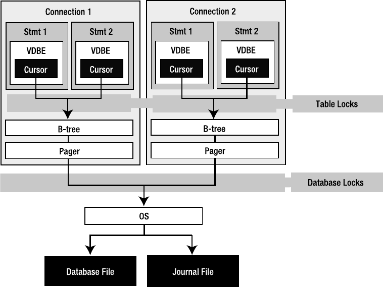
CHAPTER 5 ■ DESIGN AND CONCEPTS 173
Figure 5-1. SQLite C API object model
Technically, the B-tree and pager are not part of the API; they are off limits. But they play a
critical role in transactions and locks. We will explore their involvement in these matters here
in this section and later in the section “Transactions.”
Connections and Statements
The two fundamental data structures in the API associated with query processing are the
connection and the statement. In most language extensions you will see both a connection
object and a statement object, which are used to execute queries. In the C API, they correspond
directly to the sqlite3 and the sqlite3_stmt handles, respectively. Every major operation in
the API is done using one of these two structures.
A connection represents a single connection to a database as well as a single transaction
context. Statements are derived from connections. That is, every statement has an associated
connection object. A statement represents a single compiled SQL statement. Internally, it is
expressed in the form of VDBE byte code—a program that when executed will carry out the
SQL command. Statements contain everything needed to execute a command. They include
resources to hold the state of the VDBE program as it is executed in a stepwise fashion, B-tree
cursors that point to records on disk, and other things such as bound parameters, which are
addressed later in the section “Parameter Binding.” While they contain many different things,
Owens_6730 C05.fm Page 173 Tuesday, April 18, 2006 7:01 AM
www.it-ebooks.info
174 CHAPTER 5 ■ DESIGN AND CONCEPTS
you can simply think of them as cursors with which to iterate through a result set, or as opaque
handles referencing a single SQL command.
The B-tree and Pager
Each connection can have multiple database objects—one main database followed by any
attached databases. Each database object has one B-tree object, which in turn has one pager
object.
Statements use their connection’s B-tree and pager objects to read and write data to and
from the database. Statements that read the database iterate over B-trees using cursors. Cursors
iterate over records, and records are stored in pages. As a cursor traverses records, it also traverses
pages. For a cursor to access a page, it must first be loaded from disk into memory. This is the
pager’s job. Whenever the B-tree needs a particular page in the database, it asks the pager to
fetch it from disk. The pager then loads the page into its page cache, which is a memory buffer.
Once it is in the page cache, the B-tree and its associated cursor can get to the records inside
the page.
If the cursor modifies the page, then the pager must also take special measures to preserve
the original page in the event of a transaction rollback. Thus, the pager is responsible for reading
and writing to and from the database, maintaining a memory cache or pages, as well as managing
transactions. In addition to this, it manages locks and crash recovery. All of these responsibilities
are covered later in “Transactions.”
There are two things you should know about connections and transactions in general.
First, when it comes to any operation on the database, a connection always operates under a
transaction. Second, a connection never has more than one transaction open at a time. Basically,
whenever a connection does anything with a database, it always operates under exactly one
transaction, no more, no less. You can’t avoid it.
Therefore, all statements derived from a given connection operate within the same trans-
action context. So if you allocate two statements from the same connection, and the first issues
a BEGIN and the second issues a COMMIT, then they collectively completed a single transaction.
The first statement started it and the second ended it. If you want the two statements to run in
separate transactions, then you have to use multiple connections—one connection for each
transaction context.
The Core API
As mentioned earlier, the core API is concerned with executing SQL commands. It is made of
various functions for performing queries as well as various utility functions for managing other
aspects of the database. There are two essential methods for executing SQL commands: prepared
queries and wrapped queries. Prepared queries are the way in which SQLite ultimately executes
all commands, both in the API and internally. It is a three-phase process consisting of preparation,
execution, and finalization. There is a single API function associated with each phase. Associated
with the execution phase are functions with which to obtain record and column information
from result sets.
In addition to the standard query method, there are two wrapper functions, which wrap
the three phases into a single function call. They provide a convenient way to execute a SQL
command all at once. These functions are just a few of the many miscellaneous utility functions in
the API. We will look at all of the query methods along with their associated utility functions in
this section. Before we do however, let’s first look at how to connect to a database.
Owens_6730 C05.fm Page 174 Tuesday, April 18, 2006 7:01 AM
www.it-ebooks.info
CHAPTER 5 ■ DESIGN AND CONCEPTS 175
The Connection Lifecycle
Connections are the sole means through which to operate on a database. The connection life-
cycle consists of three phases:
1. Connect to the database. Connecting involves creating a database connection object of
some sort. The connection object manages transactions (through its associated pager),
often performs simple one-step queries (using the wrapped query functions), and
creates statement objects for prepared queries.
2. Perform transactions. As you know, all commands are executed within transactions. By
default, a database connection runs in autocommit mode. This means that every SQL
command it executes runs under its own independent transaction. The alternative is to
manually declare transactions using BEGIN..COMMIT. In this scenario, multiple commands
can run together within the same transaction.
3. Disconnect from the database. Disconnecting from a database involves closing the
database file and the files of any attached databases.
Other activities involved with query processing include handling errors, busy conditions, and
schema changes, all of which are done through the utility functions covered in the following
sections.
Connecting to a Database
Connecting to a database involves little more than opening a file. Every SQLite database is stored in
a single operating system file—one database to one file. The function used to connect, or open, a
database in the C API is sqlite3_open(), and is basically just a system call for opening a file.
SQLite can also create in-memory databases. In most extensions, if you use :memory: or an
empty string as the name for the database, it will create the database in RAM. The database will
only be accessible to the connection that created it (it cannot be shared with other connections).
Furthermore, the database will only last for the duration of the connection. It is deleted from
memory when the connection closes.
When you connect to a database on disk, SQLite opens a file, if it exists. If you try to open
a file that doesn’t exist, SQLite will assume that you want to create a new database. In this case,
SQLite doesn’t immediately create a new operating system file. It will only create a new file if
you put something into the new database—create a table or view or other database object. If
you just open a new database, do nothing, and close it, SQLite does not bother with creating a
database file—it would just be an empty file anyway.
There is also another reason for not creating a new file right away. Certain database options,
such as encoding, page size, and autovacuum, can only be set before you create a database. By
default, SQLite uses a 1,024-byte page size. However, you can use different page sizes ranging
from 512 to 32,768 bytes by powers of 2. You might want to use different page sizes for performance
reasons. For example, setting the page size to match the operating system’s page size can
sometimes make I/O more efficient. Sometimes larger page sizes help with applications that
deal with a lot of binary data. You set the database page size using the page_size pragma.
Encoding is another permanent database setting. You specify a database’s encoding using the
encoding pragma, which can be UTF-8, UTF-16, UTF-16le (little endian), and UTF-16be (big endian).
Owens_6730 C05.fm Page 175 Tuesday, April 18, 2006 7:01 AM
www.it-ebooks.info
176 CHAPTER 5 ■ DESIGN AND CONCEPTS
Finally there is autovacuum, which you set with the auto_vacuum pragma. When a transac-
tion deletes data from a database, SQLite’s default behavior is to keep the deleted pages around
for recycling. The database file remains the same size. To free the pages, you must explicitly
issue a VACUUM command to reclaim the unused space. The autovacuum feature causes SQLite
to automatically shrink the database file when data is deleted. This feature is often more useful
in embedded applications where storage is a premium.
Once you open a database—file or memory—it will be represented internally by an opaque
sqlite3 connection handle. This handle represents a single connection to a database. Connection
objects in extensions abstract this handle, and sometimes implement methods that correspond to
API functions that take the handle as an argument.
Executing Prepared Queries
As stated earlier, the prepared query method is the actual process by which SQLite executes all
SQL commands. Executing a SQL command is a three-step process:
•Preparation: The parser, tokenizer, and code generator prepare the SQL statement by
compiling it into VDBE byte code. In the C API, this is performed by the sqlite3_prepare()
function, which talks directly to the compiler. The compiler creates a sqlite3_stmt
handle (statement handle) that contains the byte code and all other resources needed to
execute the command and iterate over the result set (if the command produces one).
•Execution: The VDBE executes the byte code. Execution is a stepwise process. In the
C API, each step is initiated by sqlite3_step(), which causes the VDBE to step through
the byte code. The first call to sqlite3_step() usually acquires a lock of some kind, which
varies according to what the command does (reads or writes). For SELECT statements,
each call to sqlite3_step() positions the statement handle’s cursor on the next row
of the result set. For each row in the set, it returns SQLITE_ROW until it reaches the end,
whereupon it returns SQLITE_DONE. For other SQL statements (INSERT, UPDATE, DELETE,
etc.), the first call to sqlite3_step() causes the VDBE to process the entire command.
•Finalization: The VDBE closes the statement and deallocates resources. In the C API, this
is performed by sqlite3_finalize(), which causes the VDBE to terminate the program
and close the statement handle. However, if a transaction is manually started, it must be
manually committed or rolled back, or sqlite3_finalize() will return an error. When
sqlite3_finalize() is successful, all resources associated with the statement object are
freed. In autocommit mode, it also releases the associated database lock.
Each step—preparation, execution, finalization—corresponds to a respective statement
handle state—prepared, active, or finalized. Prepared means that all necessary resources have
been allocated and the statement is ready to be executed, but nothing has been started. No lock
has been acquired, nor will a lock be acquired until the first call to sqlite3_step(). The active
state starts with the first call to sqlite3_step(). At that point the statement is in the process of
being executed and some kind of lock is in play. Finalized means that the statement is closed
and all associated resources have been freed. These steps and states are illustrated in Figure 5-2.
Owens_6730 C05.fm Page 176 Tuesday, April 18, 2006 7:01 AM
www.it-ebooks.info
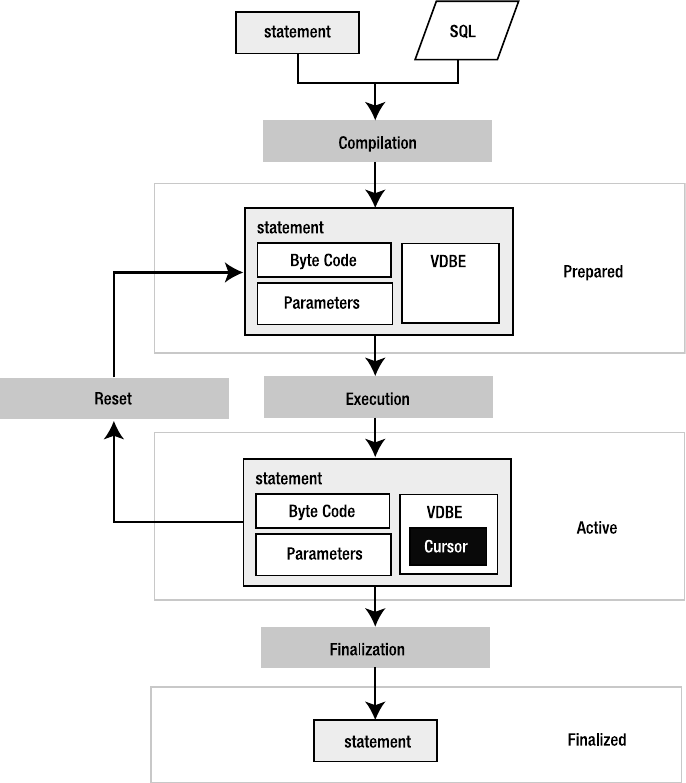
CHAPTER 5 ■ DESIGN AND CONCEPTS 177
Figure 5-2. Statement processing
The following pseudocode illustrates the general process of executing a query in SQLite:
# 1. Open the database, create a connection object (db)
db = open('foods.db')
# 2.A. Prepare a statement
stmt = db.prepare('SELECT * FROM episodes')
# 2.B. Execute. Call step() is until cursor reaches end of result set.
while stmt.step() == SQLITE_ROW
print stmt.column('name')
end
Owens_6730 C05.fm Page 177 Tuesday, April 18, 2006 7:01 AM
www.it-ebooks.info

178 CHAPTER 5 ■ DESIGN AND CONCEPTS
# 2.C. Finalize. Release read lock.
stmt.finalize()
# 3. Insert a record
stmt = db.prepare('INSERT INTO foods VALUES (…)')
stmt.step()
stmt.finalize()
# 4. Close database connection.
db.close()
This pseudocode is an object-oriented analog of the API, similar to what you might find in a
scripting language. The methods all correspond to SQLite API functions. For example, prepare()
mirrors sqlite3_prepare(), and so on. This example performs a SELECT, iterating over all returned
rows, followed by an INSERT, which is processed by a single call to step().
TEMPORARY STORAGE
Temporary storage is an important part of query processing. SQLite occasionally needs to store intermediate
results produced in the process of executing commands—for instance, when results need to be sorted for an
ORDER BY clause, or rows in one table are joined with rows in another table. This information is often stored in
temporary storage. Temporary storage is kept either in RAM or in a file. While SQLite has suitable defaults for all plat-
forms, you may want to control how and where it uses this storage. The temp_store pragma lets you specify
whether to use RAM or file-based storage. If you use file-based storage, you can use the temp_store_directory
pragma to specify where the storage file is created.
Using Parameterized SQL
SQL statements can contain parameters. Parameters are placeholders in which values may be
provided (or “bound”) at a later time after compilation. The following statements are examples
of parameterized queries:
INSERT INTO foods (id, name) VALUES (?,?);
INSERT INTO episodes (id, name) (:id, :name);
These statements represent two forms of parameter binding: positional and named. The first
command uses positional parameters and the second command uses named parameters.
Positional parameters are defined by the position of the question mark in the statement.
The first question mark has position 1, the second 2, and so on. Named parameters use actual
variable names, which are prefixed with a colon. When sqlite3_prepare() compiles a state-
ment with parameters, it allocates placeholders for the parameters in the resulting statement
handle. It then expects values to be provided for these parameters before the statement is
executed. If you don’t bind a value to a parameter, SQLite will use NULL as the default when it
executes the statement.
The advantage of parameter binding is that you can execute the same statement multiple
times without having to recompile it. You just reset the statement, bind a new set of values,
Owens_6730 C05.fm Page 178 Tuesday, April 18, 2006 7:01 AM
www.it-ebooks.info
CHAPTER 5 ■ DESIGN AND CONCEPTS 179
and reexecute. This is where resetting rather than finalizing a statement comes in handy: it avoids
the overhead of SQL compilation. By resetting a statement, you are reusing the compiled SQL
code. You completely avoid the tokenizing, parsing, and code generation overhead. Resetting
a statement is implemented in the API by the sqlite3_reset() function.
The other advantage of parameters is that SQLite takes care of escaping the string values
you bind to parameters. For example, if you had a parameter value such as 'Kenny's Chicken',
the parameter binding process will automatically convert it to 'Kenny''s Chicken'—escaping
the single quote for you, helping you avoid syntax errors and possible SQL injection attacks
(covered in the section “Formatting SQL Statements”). The following pseudocode illustrates
the basic process of using bound parameters:
db = open('foods.db')
stmt = db.prepare('INSERT INTO episodes (id, name) VALUES (:id, :name)')
stmt.bind('id', '1')
stmt.bind('name', 'Soup Nazi')
stmt.step()
# Reset and use again
stmt.reset()
stmt.bind('id', '2')
stmt.bind('name', 'The Junior Mint')
# Done
stmt.finalize()
db.close()
Here, reset() simply deallocates the statement’s resources, but leaves its VDBE byte code and
parameters intact. The statement is ready to run again without the need for another call to
prepare(). This can significantly improve performance of repetitive queries such as this because
the compiler completely drops out of the equation.
Executing Wrapped Queries
As mentioned earlier, there are two very useful utility functions that wrap the prepared query
process, allowing you to execute SQL commands in a single function call. One function—
sqlite3_exec()—is typically for queries that don’t return data. The other—sqlite3_get_table()—
is typically for queries that do. In many language extensions you will see analogs to both functions.
Most extensions refer to the first method simply as exec(), and the second as just get_table().
The exec() function is a quick and easy way to execute INSERT, UPDATE, and DELETE state-
ments or DDL statements for creating and destroying database objects. It works straight from
the database connection, taking a sqlite3 handle to an open database along with a string
containing one or more SQL statements. That’s right; exec() is capable of processing a string
of multiple SQL statements delimited by semicolons and running them all together.
Internally, exec() parses the SQL string, identifies individual statements, and then processes
them one by one. It allocates its own statement handles and prepares, executes, and finalizes
Owens_6730 C05.fm Page 179 Tuesday, April 18, 2006 7:01 AM
www.it-ebooks.info
180 CHAPTER 5 ■ DESIGN AND CONCEPTS
each statement. If multiple statements are passed to it and one of them fails, exec() terminates
execution on that command, returning the associated error code. Otherwise, it returns a success
code. The following pseudocode illustrates conceptually how exec() works in an extension:
db = open('foods.db')
db.exec("INSERT INTO episodes (id, name) VALUES (1, 'Soup Nazi')")
db.exec("INSERT INTO episodes (id, name) VALUES (2, 'The Fusilli Jerry')")
db.exec("BEGIN; DELETE from episodes; ROLLBACK")
db.close()
While you can also use exec() to process records returned from SELECT, it involves subtle methods
for doing so that are generally supported only by the C API.
The second query function, sqlite3_get_table(), is somewhat of a misnomer as it is
not restricted to just querying a single table. Rather, its name refers to the tabular results of a
SELECT query. You can certainly process joins with it just as well. In many respects, get_table()
works in the same way as exec(), but it returns a complete result set in memory. This result set is
represented in various ways depending on the extension. The following pseudocode illustrates
how it is typically used:
db = open('foods.db')
table = db.get_table("SELECT * FROM episodes LIMIT 10")
for i=0; i < table.rows; i++
for j=0; j < table.cols; j++
print table[i][j]
end
end
db.close()
The upside of get_table() is that it provides a one-step method to query and get results.
The downside is that it stores the results completely in memory. So the larger the result set, the
more memory it consumes. Not surprisingly, then, it is not a good idea to use get_table() to
retrieve large result sets. The prepared query method, on the other hand, only holds one record
(actually its associated database page) in memory at a time, so it is much better suited for
traversing large result sets.
Notice that while these functions buy you convenience, you also lose a bit of control
simply by not having access to a statement handle. For example, you can’t use parameterized
SQL statements with either of them. So they are not going to be as efficient for repetitive tasks
that could benefit from parameters. Also, the API includes functions that work with statement
handles that provide lots of information about columns in a result set—both data and meta-
data. These are not available with wrapped queries either. Wrapped queries have their uses, to
be sure. But prepared queries do as well.
Handling Errors
The previous examples are greatly oversimplified to illustrate the basic parts of query processing.
In real life, you always have to consider the possibility of errors. Almost every function you have
seen so far can encounter errors of some sort. Common error codes you need to be prepared to
Owens_6730 C05.fm Page 180 Tuesday, April 18, 2006 7:01 AM
www.it-ebooks.info
CHAPTER 5 ■ DESIGN AND CONCEPTS 181
handle include SQLITE_ERROR, SQLITE_BUSY, and SQLITE_SCHEMA. The latter two error codes refer
to busy conditions that arise when either a connection can’t get a lock or the database schema
changes between the time a statement is compiled and executed. Busy conditions are addressed
in the “Transactions” section while schema errors are covered in detail in Chapter 6.
Many language extensions often handle schema errors differently. Some transparently
report them as busy conditions. Others return the actual error code. In any case, when you
encounter a schema error, it means that some other connection has changed the database
schema and your current statement is no longer valid. You simply have to recompile the state-
ment in order to execute it. Schema errors can only occur between a call to prepare() and the
first call to step(). If your first call to step() succeeds, then you do not have to worry about
schema errors for subsequent calls to step(), as your connection has a lock on the database
that prevents other connections from changing the database schema during that time.
With regard to general errors, the API provides the return code of the last called function
with the sqlite3_errcode() function. You can get more specific error information using the
sqlite3_errmsg() function, which provides a text description of the last error. Most language
extensions support this function in some way or another.
With this in mind, each call in the previous example should check for the appropriate
errors using something like the following:
# Check and report errors
if db.errcode() != SQLITE_SUCCESS
print db.errmsg(stmt)
end
In general, error handling is not difficult. The way you handle any error depends on what
exactly you are trying to do. The easiest way to approach error handling is the same as with any
other API—read the documentation on the function you are using and code defensively.
Formatting SQL Statements
Another nice convenience function you may see some extensions support is sqlite3_mprintf(). It
is a variant of the standard C library sprintf(). It has special substitutions that are specific to
SQL that can be very handy. These substitutions are denoted %q and %Q, and escape SQL-specific
values. %q works like %s in that it substitutes a null-terminated string from the argument list.
But it also doubles every single-quote character as well as every backslash, making your life
easier and helping guard against SQL injection attacks (see the sidebar “SQL Injection Attacks”).
For example:
char* before = "Hey, at least %q no pig-man.";
char* after = sqlite3_mprintf(before, "\he's\");
The value after produced here is 'Hey, at least \\he''s\\ no pig-man'. The single quote
in he’s is doubled along with the backslashes around it, making it acceptable as a string literal
in a SQL statement. The %Q formatting does everything %q does, but it additionally encloses the
resulting string in single quotes. Furthermore, if the argument for %Q is a NULL pointer (in C), it
produces the string NULL without single quotes. For more information, see the
sqlite3_mprintf() documentation in the C API reference in Appendix B.
Owens_6730 C05.fm Page 181 Tuesday, April 18, 2006 7:01 AM
www.it-ebooks.info

182 CHAPTER 5 ■ DESIGN AND CONCEPTS
SQL INJECTION ATTACKS
If your application relies on any user input with which to construct SQL statements, you could be vulnerable to
a SQL injection attack. If you are not careful to filter user input, it could be possible for someone to craft input
that could alter the SQL statement, injecting a new SQL statement into the string. For example, say your program
uses user input to fill in the value of the following SQL statement:
SELECT * FROM foods WHERE name='%s';
You replace the %s with whatever the user supplies. If the user has any knowledge of your database, he or she
could provide input that can dramatically alter the SQL statement. For example, say the user were to provide
the following string value for the name input:
nothing' LIMIT 0; SELECT name FROM sqlite_master WHERE name='%
After substituting the user’s input into your SQL statement, the new statement turns into two statements:
SELECT * FROM foods WHERE name='nothing' LIMIT 0; SELECT name FROM
sqlite_master WHERE name='%';
The first statement will return nothing and the second will return the names of all objects in your database.
Granted, the odds of this happening require quite a bit of knowledge on the attacker’s part, but it is nevertheless
possible. Some major (commercial) web applications have been known to keep SQL statements embedded in
their JavaScript, which can provide plenty of hints about the database being used. In the previous example, all
a malicious user has to do now is insert DROP TABLE statements for every table found in sqlite_master
and you could find yourself fumbling through backups.
Operational Control
The API includes a variety of commands that allow you to monitor, control, or generally limit
what can happen in a database. SQLite implements them in the form of filters, or callback
functions that you can register to be called for specific events. There are three “hook”
functions: sqlite3_commit_hook(), which monitors transaction commits on a connection;
sqlite3_rollback_hook(), which monitors rollbacks; and sqlite3_update_hook(), which
monitors changes to rows from INSERT, UPDATE, and DELETE operations. These hooks are called
at runtime—while a command is executed. Each hook allows you to register a callback func-
tion on a connection-by-connection basis, and lets you provide some kind of application-
specific data to be passed to the callback as well. The general use of operational control functions
is as follows:
def commit_hook(cnx)
log('Attempted commit on connection %x', cnx)
return -1
end
db = open('foods.db')
db.set_commit_hook(rollback_hook, cnx)
db.exec("BEGIN; DELETE from episodes; ROLLBACK")
db.close()
Owens_6730 C05.fm Page 182 Tuesday, April 18, 2006 7:01 AM
www.it-ebooks.info
CHAPTER 5 ■ DESIGN AND CONCEPTS 183
A hook’s return value has the power to alter the event in specific ways, depending on the hook.
In this example, because the commit hook returns a non-zero value, the commit will be rolled back.
Additionally, the API provides a very powerful compile time hook called
sqlite3_set_authorizer(). This function provides you with fine-grained control over almost
everything that happens in the database as well as the ability to limit both access and modifi-
cation on a database, table, and column basis. This function is covered in detail in Chapter 6.
Using Threads
SQLite has a number of functions for using it in a multithreaded environment. With version
3.3.1, SQLite introduced a unique operational mode called shared cache mode, which is designed
for multithreaded embedded servers. This model provides a way for a single thread to host multiple
connections that share a common page cache, thus lowering the overall memory footprint of
the server. It also employs a different concurrency model. Included with this feature are various
functions for managing memory and fine-tuning the server. This operational mode is explained
further later in the section “Shared Cache Mode,” and in full detail in Chapter 6.
The Extension API
The extension API in the SQLite C API offers support for user-defined functions, aggregates,
and collations. A user-defined function is a SQL function that maps to some handler function
that you implement in C or another language. When using the C API, you implement this handler
in C or C++. In language extensions, you implement the handler in the same language as the
extension.
User-defined extensions must be registered on a connection-by-connection basis as they
are stored in program memory. That is, they are not stored in the database, like stored procedures
in larger relational database systems. They are stored in your program. When your program or
script starts up, it is responsible for registering the desired user-defined extensions for each
connection that it intends to use them.
Creating User-Defined Functions
Implementing a user-defined function is a two-step process. First, you write the handler. The
handler does something that you want to perform from SQL. Next, you register the handler,
providing its SQL name, its number of arguments, and a pointer (or reference) to the handler.
For example, say you wanted to create a special SQL function called hello_newman(),
which returns the text 'Hello Jerry'. In the SQLite C API, you would first create a C function
to implement this, such as the following:
void hello_newman(sqlite3_context* ctx, int nargs, sqlite3_value** values)
{
/* Create Newman's reply */
const char *msg = "Hello Jerry";
/* Set the return value. Have sqlite clean up msg w/ sqlite_free(). */
sqlite3_result_text(ctx, msg, strlen(msg), sqlite3_free);
}
Owens_6730 C05.fm Page 183 Tuesday, April 18, 2006 7:01 AM
www.it-ebooks.info
184 CHAPTER 5 ■ DESIGN AND CONCEPTS
Don’t worry if you don’t know C or the C API. This handler just returns 'Hello Jerry'. Next, to
actually use it, you register this handler using the sqlite3_create_function() (or the equivalent
function in your language):
sqlite3_create_function(db, "hello_newman", 0, hello_newman);
The first argument (db) is the database connection. The second argument is the name of the
function as it will appear in SQL, and the third argument means that the function takes 0 argu-
ments. (If you provide -1, then it means that the function accepts a variable number of
arguments.) The last argument is a pointer to the hello_newman() C function, which will be
called when the SQL function is called.
Once registered, SQLite knows that when it encounters the SQL function hello_newman(),
it needs to call the C function hello_newman() to obtain the result. Now, you can execute SELECT
hello_newman() within your program and it will return a single row with one column containing
the text 'Hello Jerry'.
As mentioned, many language extensions allow you to implement user-defined functions
in their respective language. For example, the Java interface provides you with the means to
implement hello_newman() in Java, Perl in Perl, and likewise in many other extensions. Different
extensions register user-defined functions in different ways, sometimes employing specific
features of their respective languages to do so. In Ruby, for example, you implement a user-
defined function using a block—one of its particular language constructs. Consider the following
Ruby program, which creates a user-defined function called bool():
db = SQLite3::Database.new(':memory:')
db.create_function('bool', 1) do |func, *args|
if args[0].to_s.upcase == 'TRUE' or args[0].to_s.upcase == 'FALSE'
func.result = 1
else
func.result = 0
end
end
def execute(db, sql)
begin
db.query(sql)
rescue Exception
puts "Statement failed: #{$!}"
end
end
execute(db, 'create table domain (x CHECK(bool(x)))')
execute(db, "insert into domain values ('true')")
execute(db, "insert into domain values ('JujyFruit')")
The bool() function takes a single argument and returns 1 (true) if the argument meets its defi-
nition of a Boolean value or 0 (false) if not. The code then uses this function in a CHECK constraint to
impose these Boolean values on a column and tests it out. The first INSERT command succeeds,
while the second one does not. UPDATE commands will be subject to this CHECK constraint
Owens_6730 C05.fm Page 184 Tuesday, April 18, 2006 7:01 AM
www.it-ebooks.info
CHAPTER 5 ■ DESIGN AND CONCEPTS 185
as well. As mentioned in Chapter 5, user-defined functions are a handy way to implement special-
ized domain constraints by embedding them in CHECK constraints.
Creating User-Defined Aggregates
Aggregate functions are functions that are applied to all records in a result set and compute
some kind of aggregate value from them. SUM(), COUNT(), and AVG() are examples of standard
SQL aggregate functions in SQLite.
Implementing user-defined aggregates is a three-step process in which you register the
aggregate, implement a step function to be called for each record in the result set, and imple-
ment a finalize function to be called after record processing. The finalize function allows you to
compute the final aggregate value and do any necessary cleanup.
The following is an example of implementing a simple SUM() aggregate called pysum in one
of the SQLite Python extensions:
connection=apsw.Connection("foods.db")
def step(context, *args):
context['value'] += args[0]
def finalize(context):
return context['value']
def pysum():
return ({'value' : 0}, step, finalize)
connection.createaggregatefunction("pysum", pysum)
c = connection.cursor()
print c.execute("select pysum(id) from foods").next()[0]
The createaggregatefunction() function registers the aggregate, passing in the step function
and the finalize function. SQLite passes step() a context, which it uses to store the interme-
diate value between calls to step(). In this case, it is the running sum. SQLite calls finalize()
after it has processed the last record. Here, finalize() just returns the aggregated sum. SQLite
automatically takes care of cleaning up the context.
Creating User-Defined Collations
Collations define how string values are compared. User-defined collations therefore provide a
way to create different text comparison and sorting methods. This is done in the API by the
sqlite3_create_collation() function. SQLite provides three default collations: BINARY, NOCASE,
and REVERSE. BINARY compares string values using the C function memcmp() (which for all intents
and purposes is case sensitive). NOCASE is just the opposite—its sorting is case insensitive.
REVERSE is just an arbitrary method used for testing, and does the direct opposite of BINARY.
User-defined collations are especially helpful for locales that are not well served by the
default BINARY collation, or those that need support for UTF-16. They can also be helpful in
specific applications such as sorting date formats that don’t lend themselves to both lexico-
Owens_6730 C05.fm Page 185 Tuesday, April 18, 2006 7:01 AM
www.it-ebooks.info
186 CHAPTER 5 ■ DESIGN AND CONCEPTS
graphical and chronological order. Chapter 7 illustrates implementing a user-defined collation
to sort Oracle dates natively in SQLite.
Transactions
By now you should have a good picture of how the API is laid out. You’ve seen different ways to
execute SQL commands along with some helpful utility functions. Executing SQL commands,
however, involves more than just knowing what’s in the API. Transactions and locks are closely
intertwined with query processing. Queries are always performed within transactions, transac-
tions involve locks, and locks can cause problems if you don’t watch what you are doing. You
can control both the type and duration of locks by how you use SQL and the way you write code.
Chapter 4 illustrated a specific scenario where deadlocks can arise just by the way that two
connections manage transactions through SQL alone. As a programmer, you will have another
variable to juggle—code—which can contain multiple connections in multiple states with
multiple statement handles on multiple tables at any given time. All it takes is a single state-
ment handle and your code may be holding an EXCLUSIVE lock without you even realizing it,
preventing other connections from getting anything done.
That is why it is critical that you have good grasp of how both transactions and locks work,
and how they relate to the various API functions used to perform queries. Ideally, you should
be able to look at the code you write and tell what transaction states it will be in, or at least be
able to spot potential problems. In this section we will explore the mechanics behind transac-
tions and locks, and in the next section observe them at work in actual code.
Transaction Lifecycles
There are a couple of things to consider with code and transactions. First there is the issue of
knowing which objects run under which transactions. Next there is the question of duration—
when does a transaction start and when does it end, and at what point does it start to affect
other connections? The first question relates directly to the API. The second relates to SQL in
general and SQLite’s implementation in particular.
As you know, multiple statement handles can be allocated from a single connection. As
shown in Figure 5-2, each connection has exactly one B-tree and one pager object associated
with it per database. The pager plays a bigger role than the connection in this discussion
because it manages transactions, locks, the memory cache, and crash recovery—all of which
will be covered in the next few sections. You could just as easily say that the connection object
handles all of this, but in reality it is the pager within it, and that is the object I will oftentimes
refer to. The important thing to remember is that when you write to the database, you do so
with one connection, one transaction at a time. Thus all statement objects run within the single
transaction context of the connections they are derived from. This answers the first question.
As for the second question, transaction duration (or the transaction lifecycle) is as short as
a single statement, or as long as you like—until you say stop. By default, a connection operates
in autocommit mode, which means that every command you issue runs under a separate
transaction. Conversely, when you issue a BEGIN, the transaction endures until you call either a
COMMIT or a ROLLBACK, or until one of your SQL commands causes a constraint violation that
results in a ROLLBACK. The next question is how transactions relate to locks.
Owens_6730 C05.fm Page 186 Tuesday, April 18, 2006 7:01 AM
www.it-ebooks.info
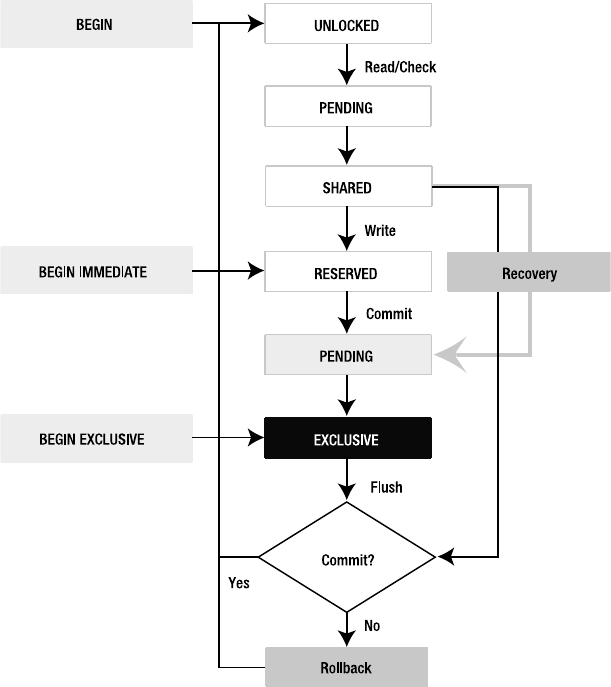
CHAPTER 5 ■ DESIGN AND CONCEPTS 187
Lock States
For the most part, lock duration shadows transaction duration. While the two don’t always
start together, they do always finish together. When you conclude a transaction, you free its
associated lock. A better way of saying this is that a lock is never released until its associated
transaction concludes or, in the worse case, the program crashes. And if the program or system
crashes, the transaction doesn’t conclude in which case there is still an implicit lock on the
database that will be resolved by the next connection to access it. This is covered later in the
sidebar “Locking and Crash Recovery.”
There are five different locks states in SQLite, and a connection is always in one of them no
matter what it’s doing. SQLite’s lock states and transitions are shown in Figure 5-3. This diagram
details every possible lock state a connection can be in as well as every path it can take through
the life of a transaction. The diagram is represented in terms of lock states, lock transitions, and
transaction lifecycles. What you are really looking at in the figure are the lives of transactions in
terms of locks.
Figure 5-3. SQLite lock transitions
Owens_6730 C05.fm Page 187 Tuesday, April 18, 2006 7:01 AM
www.it-ebooks.info
188 CHAPTER 5 ■ DESIGN AND CONCEPTS
Each state has a corresponding lock with the exception of UNLOCKED. So you can say a
connection “has a RESERVED lock,” or “is in the RESERVED state,” or just “is in RESERVED,” and it all
means the same thing. With the exception of UNLOCKED, for a connection to be in a given state it
must first obtain the associated lock.
Every transaction starts at UNLOCKED, RESERVED, or EXCLUSIVE. By default, everything begins
in UNLOCKED, as you can see in Figure 5-3. The locks states in white—UNLOCKED, PENDING, SHARED,
and RESERVED—can all exist at the same time between connections in a database. Starting with
PENDING in gray, however, things become more restrictive. The gray PENDING state represents
the lock being held by a single connection—namely a writer that wants to get to EXCLUSIVE.
Conversely, the white PENDING state represents a path where connections acquire and release
the lock on their way to SHARED. Despite all of these different lock states, every transaction in
SQLite boils down to one of two types: transactions that read, and transactions that write. That
ultimately is what paints the locking picture: readers versus writers, and how they get along
with each other.
Read Transactions
To start with, let’s go through the lock process of a SELECT statement. Its path is very simple.
A connection that executes a SELECT statement starts a transaction, which goes from UNLOCKED
to SHARED and upon COMMIT back to UNLOCKED. End of story.
Now, out of curiosity, what happens when you execute two statements? What is the lock
path then? Well, it depends on whether you are running in autocommit or not. Consider the
following example:
db = open('foods.db')
db.exec('BEGIN')
db.exec('SELECT * FROM episodes')
db.exec('SELECT * FROM episodes')
db.exec('COMMIT')
db.close()
Here, with an explicit BEGIN, the two SELECT commands execute within a single transaction and
therefore are executed in the same SHARED state. The first exec() runs, leaving the connection
in SHARED, and then the second exec() runs. Finally, the manual COMMIT takes the connection
from SHARED back to UNLOCKED. The code’s lock path would be as follows:
UNLOCKED→PENDING→SHARED→UNLOCKED
Now consider the case where there are no BEGIN and COMMIT lines in the example. Then the
two SELECT commands run in autocommit mode. They will therefore go through the entire
path independently. The lock path for the code now would be as follows:
UNLOCKED→PENDING→SHARED→UNLOCKED→PENDING→ SHARED→UNLOCKED
Since the code is just reading data, it may not make much of a difference, but it does have
to go through twice the file locks in autocommit mode than it does otherwise. And, as you
will see, a writer could sneak in between the two SELECT commands and modify the database
between exec() calls, so you can’t be sure that the two commands will return the same results.
With BEGIN..COMMIT, on the other hand, they are guaranteed to be identical in their results.
Owens_6730 C05.fm Page 188 Tuesday, April 18, 2006 7:01 AM
www.it-ebooks.info
CHAPTER 5 ■ DESIGN AND CONCEPTS 189
Write Transactions
Now let’s consider a statement that writes to the database, such as an UPDATE. First, the connection
has to follow the same path as SELECT and get to SHARED. Every operation—read or write—has
to start by going through UNLOCKED→PENDING→SHARED. PENDING, as you will soon see, is a
gateway lock.
The Reserved State
The moment the connection tries to write anything to the database, it has to go from SHARED to
RESERVED. If it gets the RESERVED lock, then it is ready to start making modifications. Even though
the connection cannot actually modify the database at this point, it can store modifications in
a localized memory cache inside the pager, called the page cache, mentioned earlier. This cache
is the same cache you configure with the cache_size pragma, as described in Chapter 4.
When the connection enters RESERVED, the pager initializes the rollback journal. This is a
file (shown in Figure 5-1) that is used in rollbacks and crash recovery. Specifically, it holds the
database pages needed to restore the database to its original state before the transaction. These
database pages are put there by the pager when the B-tree modifies a page. In this example, for
every record the UPDATE command modifies, the pager takes the database page associated with
the original record and copies it out to the journal. The journal then holds some of the contents
of the database before the transaction. Therefore, all the pager has to do in order to undo any
transaction is to simply copy the contents in the journal back into the database file. Then the
database is restored to its state before the transaction.
In the RESERVED state there are actually three sets of pages that the pager manages: modi-
fied pages, unmodified pages, and journal pages. Modified pages are just that—pages containing
records that the B-tree has changed. These are stored in the page cache. Unmodified pages are
pages the B-tree read but did not change. These are a product of commands such as SELECT.
Finally, there are journal pages, which are the original versions of modified pages. These are
not stored in the page cache, but rather written to the journal before the B-tree modifies a page.
Because of the page cache, a writing connection can indeed get real work done in the
RESERVED state without interfering with other (reading) connections. Thus, SQLite can effec-
tively have multiple readers and one writer both working on the same database at the same
time. The only catch is that the writing connection has to store its modifications in its page
cache, not in the database file. Note also that there can only be one connection in RESERVED
or EXCLUSIVE for a given database at a given time—multiple readers, but only one writer.
The Pending State
When the connection finishes making changes for the UPDATE, and the time comes to commit
the transaction, the pager begins the process of entering the EXCLUSIVE state. You already know
how this works from Chapter 4, but I will repeat it for the sake of completeness. From the
RESERVED state, the pager tries to get a PENDING lock. Once it does, it holds onto it, preventing
any other connections from getting a PENDING lock. Look at Figure 5-3 and see what effect this
has. Remember I told you that PENDING was a gateway lock. Now you see why. Since the writer
is holding onto the PENDING lock, nobody else can get to SHARED from UNLOCKED anymore. The
result is that no new connections can enter the database: no new readers, no new writers. This
PENDING state is the attrition phase. The writer is guaranteed that it can wait in line for the data-
base and—as long as everyone behaves properly—get it. Only other sessions that already have
Owens_6730 C05.fm Page 189 Tuesday, April 18, 2006 7:01 AM
www.it-ebooks.info

190 CHAPTER 5 ■ DESIGN AND CONCEPTS
SHARED locks can continue to work as normal. In PENDING, the writer waits for these connections
to finish and release their locks. What’s involved with waiting for locks is a separate issue,
which will be addressed shortly in the section “Waiting for Locks.”
When the other connections release their locks, the database then belongs to the writer.
Then, the pager moves from PENDING to EXCLUSIVE.
The Exclusive State
During EXCLUSIVE, the main job is to flush the modified pages from the page cache to the data-
base file. This is when things get serious, as the pager is going to actually modify the database.
It goes about this with extreme caution.
Before the pager begins writing the modified pages, it first tends to the journal. It checks
that the complete contents of the journal have been written to disk. At this point, it is very likely
that even though the pager has written pages to the journal file, the operating system has buff-
ered many if not all of them in memory. The pager tells the operating system to literally write
all of these pages to the disk. This is where the synchronous pragma comes into play, as described
in Chapter 4. The method specified by synchronous determines how careful the pager is to ensure
that the operating system commits journal pages to disk. The normal setting is to perform a
single “sync” before continuing, telling the operating system to confirm that all buffered journal
pages are written to the disk surface. If synchronous is set to FULL, then the pager does two full
“syncs” before proceeding. If synchronous is set to NONE, the pager doesn’t bother with the
journal at all (and while it can be 50 times faster, you can kiss transaction durability goodbye).
The reason that committing the journal to disk is so important is that if the program or
system crashes while the pager is writing to the database file, the journal is the only way to
restore the database file later on. If the journal’s pages weren’t completely written to disk before
a system crash, then the database cannot be restored fully to its original state, because the
journal pages that were in memory were lost in the crash. In this case, you have an inconsistent
database at best, and a corrupted one at worse.
■Caution Even if you use the most conservative setting for the synchronous pragma, you still may not be
guaranteed that the journal is truly committed to disk. This is no fault of SQLite, but rather of certain types of hard-
ware and operating systems. SQLite uses the fsync() system call on Unix and FlushFileBuffers() on
Windows to force journal pages to disk. But it has been reported that these functions don’t always work, espe-
cially with cheap IDE disks. Apparently, some manufacturers of IDE disks use controller chips that tend to
bend the truth about actually committing data to disk. In some cases, the chips cache the data in volatile
memory while reporting that they wrote it to the drive surface. Also, there have been (unconfirmed) reports
that Windows occasionally ignores FlushFileBuffers(). If you have hardware or software that lies to you,
your transactions may not be as durable as you might think.
Once the journal is taken care of, the pager then copies all of the modified pages to the
database file. What happens next depends on the transaction mode. If, as in this case, the
transaction autocommits, then the pager cleans up the journal, clears the page cache, and
proceeds from EXCLUSIVE to UNLOCKED. If the transaction does not commit, then the pager
Owens_6730 C05.fm Page 190 Tuesday, April 18, 2006 7:01 AM
www.it-ebooks.info
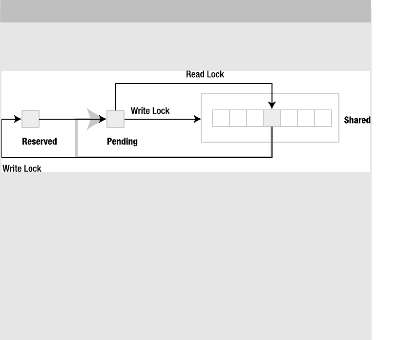
CHAPTER 5 ■ DESIGN AND CONCEPTS 191
continues to hold the EXCLUSIVE lock and the journal stays in play until either a COMMIT or
ROLLBACK is issued.
Autocommit and Efficiency
With all this in mind, consider what happens with UPDATEs that run in an explicit transaction
versus ones that run in autocommit. In autocommit, every command that modifies the data-
base runs in a separate transaction and travels through the following path:
UNLOCKED→PENDING→SHARED→RESERVED→PENDING→ EXCLUSIVE→UNLOCKED
Additionally, each trip through this path involves creating, committing, and clearing out
the rollback journal. This all adds up. Although running multiple SELECTs in autocommit mode
is perhaps not that big of a deal performance-wise, you should really rethink autocommit mode
for frequent writes. And, as mentioned in the SELECT case, when running multiple commands in
autocommit, there is nothing stopping another connection from coming along and modifying
the database in between commands. If you have two updates that depend on specific values in
the database, you should always run them in the same transaction for this reason.
LOCKING AND CRASH RECOVERY
SQLite’s lock implementation is based on standard file locking. SQLite keeps three different file locks on the
database file: a reserved byte, a pending byte, and a shared region.
Everything starts at the pending byte. To move from UNLOCKED to SHARED, a connection first attempts
to get a read-lock on the pending byte. If successful, it gets a read lock on a random byte in the shared region
and releases the read lock on the pending byte. To move from SHARED to RESERVED, a connection attempts
to obtain a write lock on the reserved byte. To get from RESERVED to EXCLUSIVE, a connection attempts to
get a write lock on the pending byte. If successful, this is what causes the attrition process, as it is no longer
possible for other connections to get a read lock on the pending byte to enter SHARED. Finally, to get the
EXCLUSIVE lock, the connection attempts to get a write lock on the entire shared region. Since the shared
region holds read locks by all other active connections, this step guarantees that an EXCLUSIVE lock is only
granted after all other SHARED locks are first released.
SQLite’s crash recovery mechanism uses the reserved byte to determine when a database needs to be
restored. Since the journal file and the RESERVED lock go hand in hand, if the pager sees the former without the
latter, then something is wrong. Every time the pager opens a database file or tries to fetch a page from the
Owens_6730 C05.fm Page 191 Tuesday, April 18, 2006 7:01 AM
www.it-ebooks.info

192 CHAPTER 5 ■ DESIGN AND CONCEPTS
database, it does a simple consistency check. If it finds a journal file but no RESERVED lock on the database, then
the process that created the journal file must have crashed, or the system went down. In this case, the journal is
called a hot journal, and the database is potentially in an inconsistent state. To make things right, the journal
needs to be “played back” to restore the database to its original state before the interrupted transaction.
To start the play back, the pager puts the database into recovery mode. To do this, it goes directly from
SHARED to PENDING as shown by the gray line in the illustration (and also in Figure 5-3). This is the only time
it ever makes this transition. The reason it skips the reserved lock is twofold. First, by locking the pending byte,
it keeps all new connections out of the database. Second, connections that are already in the database (in
SHARED) will also see the hot journal the next time they try to access a page. Those connections will attempt
to go into recovery mode and replay the journal as well. However, they won’t be able to because the first
connection already has the PENDING lock. Thus, by going straight from SHARED to PENDING, the first connec-
tion ensures that (1) no new connections can enter the database and (2) active connections in SHARED cannot
go into recovery mode. Everyone but the restoring connection is temporarily suspended.
Basically, a hot journal is an implicit EXCLUSIVE lock. If a writer crashes, no further activity can transpire
in the database until some connection restores it. The next pager to access a page will see the hot journal, lock
everyone out, and start recovery. If there are no other active connections, then the first program to connect to
the database will detect the hot journal and start recovery.
Tuning the Page Cache
Go back to the beginning of the previous example and say that it started with a BEGIN, followed
by the UPDATE, and in the middle of making all those modifications the page cache fills up (runs
out of memory). That is, the UPDATE results in more modified pages than will fit in the page cache.
What happens now?
Transitioning to Exclusive
The real question is: when exactly does the pager move from RESERVED to EXCLUSIVE and why?
There are two scenarios, and you’ve just seen them both. Either the connection reaches the
commit point and deliberately enters EXCLUSIVE, or the page cache fills up and it has no other
option. We just looked at the commit point scenario. So what happens when the page cache
fills up? Put simply, the pager can no longer store any more modified pages, and therefore can
no longer do any work. It is forced to move into EXCLUSIVE in order to continue. In reality, this
is not entirely true as there is a soft limit and a hard limit.
The soft limit corresponds to the first time the page cache fills up. At this point, the cache
is a mixed bag of modified and unmodified pages. In this case, the pager tries to clean out the
page cache. It goes through the cache page by page looking for unmodified pages and clearing
them out. Once it does that, it can sputter along with what memory has freed up until the cache
fills up again. It repeats the process until the cache is completely made up of modified pages.
And that is that hard limit. At this point, the pager has no other recourse but to proceed into
EXCLUSIVE.
The RESERVED state, then, is where the cache_size pragma makes a difference. Just as
explained in Chapter 4, cache_size controls the size of the page cache. The bigger the page
cache, the more modified pages the pager can store, and the more work the connection can do
before having to enter EXCLUSIVE. Also, as mentioned, by doing all the database work in RESERVED,
Owens_6730 C05.fm Page 192 Tuesday, April 18, 2006 7:01 AM
www.it-ebooks.info
CHAPTER 5 ■ DESIGN AND CONCEPTS 193
you minimize the time in EXCLUSIVE. If you get all your work done in RESERVED, then EXCLUSIVE
is only held long enough to flush modified pages to disk—not compile more queries and
process more results and then write to disk. Doing the processing in RESERVED can significantly
increase overall concurrency. Ideally, if you have a large transaction or a congested database,
and you can spare the memory, try to ensure that your cache size is large enough to hold your
connection in RESERVED as long as possible.
Sizing the Page Cache
So how do you determine what the cache size should be? It depends on what you are doing. Say
that you want to update every record in the episodes table. In this case, you know that every
page in the table will be modified. Therefore, you figure out how many pages are in episodes
and adjust the cache size accordingly. You can get all the information you need on episodes
using sqlite_analyzer. For each table it will dump detailed statistics, including the total page
count. For example, if you run it on the foods database, you get the following information
about episodes:
*** Table EPISODES ***************************************************
Percentage of total database.......... 20.0%
Number of entries..................... 181
Bytes of storage consumed............. 5120
Bytes of payload...................... 3229 63.1%
Average payload per entry............. 17.84
Average unused bytes per entry........ 5.79
Average fanout........................ 4.00
Maximum payload per entry............. 38
Entries that use overflow............. 0 0.0%
Index pages used...................... 1
Primary pages used.................... 4
Overflow pages used................... 0
Total pages used...................... 5
Unused bytes on index pages........... 990 96.7%
Unused bytes on primary pages......... 58 1.4%
Unused bytes on overflow pages........ 0
Unused bytes on all pages............. 1048 20.5%
The total page count is 5. But of those, only 4 pages of actual table are used—1 page is an
index. Since the default cache size is 2,000 pages, you’ve got nothing to worry about. There are
about 400 records in episodes, which means there are about 100 records per page. You wouldn’t
have to worry about adjusting the page cache before updating every record unless there were
at least 196,000 rows in episodes. And remember, you would only need to do this in environ-
ments where there are other connections using the database and concurrency is an issue.
If you are the only one using the database, then it really wouldn’t matter.
Owens_6730 C05.fm Page 193 Tuesday, April 18, 2006 7:01 AM
www.it-ebooks.info
194 CHAPTER 5 ■ DESIGN AND CONCEPTS
Waiting for Locks
We talked earlier about the pager waiting to go from PENDING to EXCLUSIVE. What exactly is
involved with waiting on a lock? First, any call to exec() or step() can involve waiting on a lock.
Whenever SQLite encounters a situation where it can’t get a lock, the default behavior is to
return Delete SQLITE_BUSY to the function that caused it to seek the lock. Regardless of the
command you execute, you can potentially encounter SQLITE_BUSY. SELECT commands, as you
know by now, can fail to get a SHARED lock if a writer is pending or writing. The simple thing to
do when you get SQLITE_BUSY is to just retry the call. However, we will see shortly that this is not
always the best course of action.
Using a Busy Handler
Instead of just retrying the call over and over, you can use a busy handler. Rather than having
the API return SQLITE_BUSY if a connection cannot get a lock, you can get it to call the busy
handler instead.
A busy handler is a function you create that kills time, or does whatever else you want it
to do—it can send spam to your mother-in-law for all SQLite cares. It’s just going to get called
when SQLite can’t get a lock. The only thing the busy handler has to do is provide a return
value, telling SQLite what to do next. By convention, if the handler returns true, then SQLite
will continue to try for the lock. If it returns false, SQLite will then return SQLITE_BUSY to the
function requesting the lock. Consider the following example:
counter = 1
def busy()
counter = counter + 1
if counter == 2
return 0
end
spam_mother_in_law(100)
return 1
end
db.busy_handler(busy)
stmt = db.prepare('SELECT * FROM episodes;')
stmt.step()
stmt.finalize()
The implementation of spam_mother_in_law() is left as an exercise for the reader.
The step() function has to get a SHARED lock on the database to perform the SELECT.
However, say there is a writer active. Normally, step() would return SQLITE_BUSY. However, in
this case it doesn’t. The pager (which is one that deals with locks) calls the busy() function instead,
because it has been registered as the busy handler. busy() increments a counter, forwards your
mother-in-law 100 random messages from your spam folder, and returns 1, which the pager
Owens_6730 C05.fm Page 194 Tuesday, April 18, 2006 7:01 AM
www.it-ebooks.info

CHAPTER 5 ■ DESIGN AND CONCEPTS 195
interprets as true—keep trying to get the lock. The pager then tries again to get the SHARED lock.
Say the database is still locked. The pager calls the busy handler again. Only this time, busy()
returns 0, which the pager interprets as false. In this case, rather than retrying the lock, the
pager sends SQLITE_BUSY up the stack and that’s what step() ends up returning.
If you just want to kill time waiting for a lock, you don’t have to write your own busy handler.
The SQLite API has one for you. It is a simple busy handler that sleeps for a given period of time
waiting for a lock. In the API, the function is called sqlite3_busy_timeout(), and it is supported
by some extension libraries. You can essentially say “try sleeping for 10 seconds when you can’t
get a lock,” and the pager will do that for you. If it sleeps for 10 seconds and still can’t get the
lock, then it will return SQLITE_BUSY.
Using the Right Transaction
Let’s consider the previous example again, but this time the command is an UPDATE rather than
a SELECT. What does SQLITE_BUSY actually mean now? In SELECT, it just means, “I can’t get a
SHARED lock.” But what does is mean for an UPDATE? The truth is, you don’t really know what it
means. SQLITE_BUSY could mean that the connection failed to get a SHARED lock because there is
a writer pending. It could also mean that it got a SHARED lock but couldn’t get to RESERVED. The
point is you don’t know the state of the database, or the state of your connection for that matter. In
autocommit mode, SQLITE_BUSY for a write operation is completely indeterminate. So what do
you do next? Should you just keep calling step() over and over until the command goes through?
Here’s the thing to think about. Suppose SQLITE_BUSY was the result of you getting a SHARED
lock but not RESERVED, and now you are holding up a connection in RESERVED from getting to
EXCLUSIVE. Again, you don’t know the state of the database. And just using a brute-force method
to push your transaction through is not necessarily going to work, for you or any other connec-
tion. If you just keep calling step(), you are just going to butt heads with the connection that
has the RESERVED lock, and if neither of you backs down, you’ll deadlock.
■Note SQLite tries to help with deadlock prevention in this particular scenario by ignoring the busy handler
of the offending connection. The SHARED connection’s busy handler will not be invoked if it is preventing a
RESERVED connection from proceeding. However, it is up to the code to get the hint. The code can still just
repeatedly call step() over and over, in which case there is nothing more SQLite can do to help.
Since you know you want to write to the database, then you need to start by issuing BEGIN
IMMEDIATE. If you get a SQLITE_BUSY, then at least you know what state you’re in. You know you
can safely keep trying without holding up another connection. And once you finally do succeed,
you know what state you are in then as well—RESERVED. Now you can use brute force if you have
to because you are the one in the right. If you start with a BEGIN EXCLUSIVE, on the other hand,
then you are assured that you won’t have any busy conditions to deal with at all. Just remember
that in this case you are doing your work in EXCLUSIVE, which is not as good for concurrency as
doing the work in RESERVED.
Owens_6730 C05.fm Page 195 Tuesday, April 18, 2006 7:01 AM
www.it-ebooks.info

196 CHAPTER 5 ■ DESIGN AND CONCEPTS
LOCKS AND NETWORK FILE SYSTEMS
At this point, you should have a good appreciation for what can go wrong when a database is shared over a
network file system. SQLite handles concurrency by placing file locks on the database file. It is very important
that these locks be both set and released at the right times. SQLite is completely dependent on the file system
to manage locks correctly for concurrent use. SQLite uses the same locking mechanisms regardless of
whether it is running on a normal file system or network file system. It uses POSIX advisory locks on Unix and
the LockFile(), LockFileEx(), and UnlockFile() system calls on Windows. These calls are standard
system calls, and work correctly on normal file systems. It is the network file system’s job to emulate a normal
file system. And unfortunately, this doesn’t always work correctly with some implementations. And even if the
network file system works correctly, there still other things to consider.
Take NFS, for example. It’s a great network file system. However, many original NFS implementations
were known to have buggy or in some cases unimplemented locking. And with a SQLite database, this can
cause serious problems. Without locking, two connections can get an EXCLUSIVE lock on the same database
and write to it at the same time, leading to an almost certain database corruption. Or perhaps locking is imple-
mented and a bug does not release the reserved byte or pending byte in a timely manner, or at all. The prob-
lems range from delays to database corruption. This is not a problem with the NFS protocol in general, but with
some implementations of it in particular. Eric Kustarz, a Sun engineer who has worked on NFS for five years,
says the following on his blog regarding NFS locking:
The protocol behind locking (NLM) for NFSv2/v3 is not broken*, but rather some of the
implementations were broken—especially early on (people spent time on making the
NFS protocol work, but NLM was more complex—an after thought)… Running a
Solaris client against a Solaris server will find that NFSv3 + NLM works great, and is not
broken. Thankfully, NFSv4 fixed this by integrating locking into the one and only
protocol. Now, locking has to work or you don’t have a NFSv4 implementation.
Now consider a footnote on the same page:
*OK, there are a couple very edge cases in NLM that got sorted out in NFSv4. The easiest
example is recovery of a client crash…if the client never comes back up, and another
client needs to lock the same file? You need administrative intervention at this point.
Since NFSv4’s state is lease based, no intervention is necessary—if the client doesn’t
reclaim its state within the allotted time, the locks are lost.
NFS can still have issues with locking if one of the clients goes down (taking their database lock with it) and
does not come back up. For NFSv3, a locked file would need administrative intervention to clear it. For NFSv4,
there would be a timeout period. But how long is the timeout? Thirty seconds? A minute? The real issue is not
NFS, but specific applications of it. Network file systems, even if perfectly implemented, are not necessarily
going to work exactly like a local file system.
The bottom line is, if you are going to mix concurrency and network file systems, there are many issues
to consider, even if you are using the best network file system out there. It’s not as simple as running on a local
file system. There are new variables introduced when any application runs over a network. The real issue is
not that SQLite doesn’t work on network file systems. It can. Nor is the real issue that network file systems
don’t work reliably. Any valid implementation of NFS does. The issue is what your application does, what envi-
ronment it is running in, what network file system(s) it is using (e.g., Linux client and Solaris server), how many
other connections are hitting the database, what the specific performance requirements are... the list goes on.
Owens_6730 C05.fm Page 196 Tuesday, April 18, 2006 7:01 AM
www.it-ebooks.info

CHAPTER 5 ■ DESIGN AND CONCEPTS 197
No one can definitively say, “Yes, this network file system will work for you,” or “No, SQLite doesn’t work.”
These are only two of many possible variables in the equation—an equation that only you can solve based on
your resources and requirements.
Code
By now, you have a pretty good picture of the API, transactions, and locks. To finish up, let’s put
all three of these things together in the context of your code, and consider a few scenarios that
you might want to watch for.
Using Multiple Connections
If you have written code that uses other relational databases, you may have made some
assumptions that might have worked with those databases that will not work with SQLite.
Many times I have used multiple connections with other databases that work concurrently in a
single block of code. The classic example is having one connection iterate over a table while
another connection modifies records in place.
In SQLite, using multiple connections in the same block of code can cause problems.
You have to be careful of how you go about it. Consider the following example:
c1 = open('foods.db')
c2 = open('foods.db')
stmt = c1.prepare('SELECT * FROM episodes')
while stmt.step()
print stmt.column('name')
c2.exec('UPDATE episodes SET …)
end
stmt.finalize()
c1.close()
c2.close()
I’ll bet you can easily spot the problem here. In the while loop, c2 attempts an UPDATE while c1
has a SHARED lock open. That SHARED lock won’t be released until stmt is finalized after the while
loop. Therefore, it is impossible to write to the database within the while loop. Either the updates
will silently fail, or if you have a busy handler then it will only delay the program. The best thing
to do here is to use one connection for the job, and to run it under a single BEGIN IMMEDIATE
transaction. The new version might be
Owens_6730 C05.fm Page 197 Tuesday, April 18, 2006 7:01 AM
www.it-ebooks.info
198 CHAPTER 5 ■ DESIGN AND CONCEPTS
c1 = open('foods.db')
# Keep trying until we get it
while c1.exec('BEGIN IMMEDIATE') != SQLITE_SUCCESS
end
stmt = c1.prepare('SELECT * FROM episodes')
while stmt.step()
print stmt.column('name')
c1.exec('UPDATE episodes SET …)
end
stmt.finalize()
c1.exec('COMMIT')
c1.close()
In cases like this, you should use statements from a single connection for reading or writing.
Then you won’t have to worry about database locks causing problems. However, as it turns out,
this particular example still won’t work. If you are iterating over a table with one statement and
updating it with another, there is an additional locking issue that you need to know about as
well, which we’ll cover next.
Table Locks
Even if you are using just one connection, there is a special edge case that sometimes trips
people up. While you would think that two statements from the same connection could work
on the database with impunity, there is one important exception.
When you execute a SELECT command on a table, the resulting statement object creates a
B-tree cursor on that table. As long as there is a B-tree cursor active on a table, other statements—
even in the same connection—cannot modify it. If they try, they will get SQLITE_BUSY. Consider
the following example:
c = sqlite.open("foods.db")
stmt1 = c.compile('SELECT * FROM episodes LIMIT 10')
while stmt1.step() do
# Try to update the row
row = stm1.row()
stmt2 = c.compile('UPDATE episodes SET …')
# Uh oh: ain't gonna happen
stmt2.step()
end
stmt1.finalize()
stmt2.finalize ()
c.close()
Owens_6730 C05.fm Page 198 Tuesday, April 18, 2006 7:01 AM
www.it-ebooks.info

CHAPTER 5 ■ DESIGN AND CONCEPTS 199
We are only using one connection here. Regardless, when stmt2.step() is called, it won’t
work because stmt1 has a cursor on the episodes table. In this case, stmt2.step() may actually
succeed in promoting the connection’s database lock to EXCLUSIVE, but it will still return
SQLITE_BUSY. The cursor on episodes prevents it from modifying the table. In order to get around
this, you can do one of two things:
• Iterate over the results with one statement, storing the information you need in memory.
Then finalize the reading statement, and then do the updates.
• Store the SELECT results in a temporary table (as described in a moment) and open the
read cursor on it. In this case you can have both a reading statement and a writing state-
ment working at the same time. The reading statement’s cursor will be on a different
table—the temporary table—and won’t block the updates on the main table from the
second statement. Then when you are done, simply drop the temporary table.
When a statement is open on a table, its B-tree cursor will be removed from the table when
one of two things happens:
• The statement reaches the end of the result set. When this happens, step() will automat-
ically close the statement’s cursor(s). In VDBE terms, when the end of the results set is
reached, the VDBE encounters a Close instruction, which causes all associated cursors
to be closed.
• The statement is finalized. The program explicitly calls finalize(), thereby removing all
associated cursors.
In many extensions, the call to sqlite3_finalize() is done automatically in the statement
object’s close() function, or something similar.
■Note As a matter of interest, there are exceptions to these scenarios where you could theoretically get
away with reading and writing to the same table at the same time. In order to do so, you would have to
convince the optimizer to use a temporary table, using something like an ORDER BY, for example. When this
happens, the optimizer will automatically create a temporary table for the SELECT statement and place the
reading statement’s cursor on it rather than the actual table itself. In this case, it is technically possible for a
writer to then modify the real table because the reader’s cursor is on a temporary table. The problem with this
approach is that the decision to use temporary tables is made by the optimizer. It is not safe to presume what
the optimizer will and will not do. Unless you like to gamble, or are just intimately acquainted with the ins and
outs of the optimizer, it is best to just follow the general rule of thumb: don’t read and write to the same table
at the same time.
Fun with Temporary Tables
Temporary tables let you bend the rules. If you absolutely have to have two connections going
in the same block of code, or two statements operating on the same table, you can safely do so
if you use temporary tables. When a connection creates or writes to a temporary table, it does
not have to get a RESERVED lock, because temporary tables are maintained outside of the database
Owens_6730 C05.fm Page 199 Tuesday, April 18, 2006 7:01 AM
www.it-ebooks.info
200 CHAPTER 5 ■ DESIGN AND CONCEPTS
file. There are two ways of going about this, depending on how you want to manage concurrency.
Consider the following example:
c1 = open('foods.db')
c2 = open('foods.db')
c2.exec('CREATE TEMPORARY TABLE temp_epsidodes as SELECT * from episodes')
stmt = c1.prepare('SELECT * FROM episodes')
while stmt.step()
print stmt.column('name')
c2.exec('UPDATE temp_episodes SET …')
end
stmt.finalize()
c2.exec('BEGIN IMMEDIATE')
c2.exec('DELETE FROM episodes')
c2.exec('INSERT INTO episodes SELECT * FROM temp_episodes')
c2.exec('COMMIT')
c1.close()
c2.close()
This example uses a temporary table based on episodes to make modifications within the
while loop. Both connections are actually running in SHARED. Again, this is because temporary
tables are maintained outside of the database. Therefore, temp_episodes and all of the operations
on it don’t require that c2 gets a RESERVED or an EXCLUSIVE lock. Once stmt is finalized, then c1’s
SHARED lock is gone and c2 can safely write to the database all that it collected in the temporary table.
Notice also that this example uses the original episodes table rather than dropping it and
re-creating it from temp_episodes using a CREATE TABLE AS SELECT…. If you did it this way, then
you would lose any integrity constraints and indexes defined on the original episodes table.
The advantage of the previous example is that it minimizes the duration of RESERVED and
EXCLUSIVE locks on the database. Everything is kept in a temporary table during the iteration,
so it does not affect other reading connections. Then everything is copied over in one single
transaction. The code could be simplified somewhat, but at the cost of decreased concurrency
as follows:
c1 = open('foods.db')
c2 = open('foods.db')
c1.exec('CREATE TEMPORARY TABLE temp_episodes as SELECT * from episodes')
stmt = c1.prepare('SELECT * FROM temp_episodes')
Owens_6730 C05.fm Page 200 Tuesday, April 18, 2006 7:01 AM
www.it-ebooks.info
CHAPTER 5 ■ DESIGN AND CONCEPTS 201
while stmt.step()
print stmt.column('name')
c2.exec('UPDATE episodes SET …') # What about SQLITE_BUSY?
end
stmt.finalize()
c1.exec('DROP TABLE temp_episodes')
c1.close()
c2.close()
This example stores the result set into the temporary table, iterates over it, and performs
the updates to the main table. While this code is a little cleaner, keep in mind that you now have
additional concurrency issues to deal with. First, there will now be RESERVED and EXCLUSIVE locks
associated with each UPDATE where there weren’t any before. Second, you have to guard the
updates against SQLITE_BUSY conditions (not shown in the example). Finally, if you run the
whole thing under a single transaction, it may have an EXCLUSIVE lock on the database during
the entire iteration, depending on how much is updated and the size of the page cache. All in
all, the first example, while involving a little more code, may be the better approach in general.
The Importance of Finalizing
A common gotcha in processing SELECT statements is the failure to realize that the SHARED lock
is not released until finalize() is called—well, most of the time. Consider the following example:
stmt = c1.prepare('SELECT * FROM episodes')
while stmt.step()
print stmt.column('name')
end
c2.exec('BEGIN IMMEDIATE; UPDATE episodes SET …; COMMIT;')
stmt.finalize()
While you should never do this in practice, you might end up doing it anyway by accident
simply because you can get away with it. If you write the equivalent of this program in the C API,
it will actually work. Even though finalize() has not been called, the second connection can
modify the database without any problem. Before I tell you why, consider this next example:
c1 = open('foods.db')
c2 = open('foods.db')
stmt = c1.prepare('SELECT * FROM episodes')
Owens_6730 C05.fm Page 201 Tuesday, April 18, 2006 7:01 AM
www.it-ebooks.info
202 CHAPTER 5 ■ DESIGN AND CONCEPTS
stmt.step()
stmt.step()
stmt.step()
c2.exec('BEGIN IMMEDIATE; UPDATE episodes SET …; COMMIT;')
stmt.finalize()
Let’s say that episodes has 100 records. And the program only stepped through three of them.
What happens here? The second connection will get SQLITE_BUSY.
In the first example, SQLite released the SHARED lock when the statement reached the end
of the result set. That is, in the final call to step(), where the API returns SQLITE_DONE, the VDBE
encountered the Close instruction and SQLite closed the cursor and dropped the SHARED lock.
Thus, c2 was able to push its INSERT through even though c1 had not called finalize().
In the second case, the statement had not reached the end of the set. The next call to
step() would have returned SQLITE_RESULT, which means there are more rows in the results
set, and that the SHARED lock is still active. Thus, c2 could not get the INSERT through this time
because of the SHARED lock from c1.
The moral of the story is don’t do this, even though sometimes you can. Always call
finalize() before you write with another connection. The other thing to remember is that in
autocommit mode step() and finalize() are more or less transaction and lock boundaries.
They start and end transactions. They acquire and release locks. You should be very careful
about what you do with other connections in between these functions.
Shared Cache Mode
Now that you are clear on the concurrency rules, I will give you something new to confuse you.
SQLite offers an alternative concurrency model called shared cache mode, which relates to how
connections can operate within individual threads.
In shared cache mode, a thread can create multiple connections that share the same page
cache. Furthermore, this group of connections can have multiple readers and a single writer (in
EXCLUSIVE) working on the same database at the same time. The catch is that these connections
cannot be shared across threads—they are strictly limited to the thread (running specifically in
shared cache mode) that created them. Furthermore, writers and readers have to be prepared
to handle a special condition involving table locks.
When readers read tables, SQLite automatically puts table locks on them. This prevents
writers from modifying those tables. If a writer tries to modify a read-locked table, it will get
SQLITE_LOCKED. The same logic applies to readers trying to read from write-locked tables. However,
in this latter case, readers can still go ahead and read tables that are being modified by a writer
if they run in read-uncommitted mode, which is enabled by the read_uncommitted pragma. In
this case, SQLite does not place read locks on the tables read by these readers. As a result, these
readers don’t interfere with writers at all. However, these readers can get inconsistent query
results, as a writer can modify tables as the readers read them.
Shared cache mode is designed for embedded servers that need to conserve memory and
have slightly higher concurrency under certain conditions. More information on using it with
the C API can be found in Chapter 6.
Owens_6730 C05.fm Page 202 Tuesday, April 18, 2006 7:01 AM
www.it-ebooks.info
CHAPTER 5 ■ DESIGN AND CONCEPTS 203
Summary
The SQLite API is flexible, intuitive, and easy to use. It has two basic parts: the core API and the
extension API. The core API revolves around two basic data structures used to execute SQL
commands: the connection and the statement. Commands are executed in three steps: compi-
lation, execution, and finalization. SQLite’s wrapper functions exec() and get_table() wrap
these steps into a single function call, automatically handling the associated statement object
for you. Other parts of the core API include support for string handling, operational control,
and other miscellaneous utility functions.
The extension API provides you with the means to customize SQLite in three difference
ways: user defined functions, user-defined aggregates, and user-defined collations. Both user-
defined functions and aggregates can be implemented in different languages and called
directly from SQL. User-defined collations allow SQLite to be more usable in different locales.
Because SQLite’s concurrency model is somewhat different from other databases, it is
important that you understand a bit about how it manages transactions and locks, how they
work behind the scenes and within your code. Overall, the concepts are not difficult to under-
stand, and there are just a few simple rules to keep in mind when you write code that uses
SQLite.
The next three chapters will draw heavily on what you’ve have learned here, as these
concepts apply not only to the C API, but to language extensions as well as they are built on top
of the C API.
Owens_6730 C05.fm Page 203 Tuesday, April 18, 2006 7:01 AM
www.it-ebooks.info

205
■ ■ ■
CHAPTER 6
The Core C API
This chapter covers the part of the SQLite API used to work with databases. You already have
a good idea of how the API works from Chapter 5. Now let’s concentrate on the specifics.
Starting with a few trivial examples, we will take an in-depth tour through the C API and
expand upon the examples, filling in various details with a variety of useful functions. As we go
along, you should see the C equivalents of the model all fall into place, with some additional
features you may not have seen before—features that primarily exist only in the C API. By the
time we reach the end of this chapter, you should have seen every API function related to running
commands, managing transactions, fetching records, handling errors, and many other tasks
related to general database work.
The SQLite version 3 API consists of approximately 80 functions. Only about eight functions,
however, are needed to actually connect, process queries, and disconnect from a database.
The remaining functions can be arranged into small groups that specialize in accomplishing
specific tasks.
As mentioned in Chapter 5, quite a few things have changed in the API between versions 2
and 3. One of the most notable is the addition of UTF support. All functions that accept char-
acter strings as function arguments, or produce them as return values, have both UTF-8 and
UTF-16 analogs. For example, sqlite3_open(), which is used to open a database, takes a UTF-8
string containing a database filename as an argument. Its counterpart—sqlite3_open16()—
has the exact same signature, but accepts the same argument in UTF-16 encoding. With the
exception of the first section, I refer only to the UTF-8 functions, as the UTF-16 versions differ
only slightly by their names.
While it is best to read the chapter straight through, if at any point you want more detailed
information on a particular function, you can consult Appendix B, which contains the complete C
API documentation.
All examples in this chapter can be found in self-contained example programs, the source
files of which are located in the ch6 folder of the examples zip file, available on the Apress website
at www.apress.com. For every example presented, I specifically identify the name of the corre-
sponding source file from which the example was taken.
Wrapped Queries
You are already familiar with the way that SQLite executes queries, as well as its various wrapper
functions for executing SQL commands in a single function call. We will start with the C API
versions of these wrappers because they are simple, self-contained, and easy to use. They are a
Owens_6730 C06.fm Page 205 Tuesday, April 18, 2006 7:09 AM
www.it-ebooks.info

206 CHAPTER 6 ■ THE CORE C API
good starting point, which will let you have some fun and not get too bogged down with details.
Along the way, I’ll introduce some other handy functions that go hand in hand with query
processing. By the end of this section, you will be able connect, disconnect, and query a data-
base using the wrapped queries.
Connecting and Disconnecting
Before you can execute SQL commands, you first have to connect to a database. Connecting to
a database is perhaps best described as opening a database, as SQLite databases are contained
in single operating system files (one file to one database). Similarly, the preferred term for
disconnecting would be closing the database.
You open a database with the sqlite3_open() or sqlite3_open16() functions, which have
the following declaration(s):1
int sqlite3_open(
const char *filename, /* Database filename (UTF-8) */
sqlite3 **ppDb /* OUT: SQLite db handle */
);
int sqlite3_open16(
const void *filename, /* Database filename (UTF-16) */
sqlite3 **ppDb /* OUT: SQLite db handle */
);
The filename argument can be the name of an operating system file, the text string ':memory:',
or an empty string (NULL pointer). If you use NULL or ':memory:', sqlite3_open() will create an
in-memory database in RAM that lasts only for the duration of the session. If filename is not
NULL, sqlite3_open() attempts to open the database file by using its value. If no file by that
name exists, sqlite3_open() will open a new database file by that name.
■Note When SQLite creates a new database, it does not actually write anything to disk until the first data-
base object is created. Therefore, if you specify a new database file but do not create a table, view, trigger, or
other database object, when you close the database the database file by that name will still not exist in the
file system. Therefore, to actually create a new database, you must first create something in it before you
close it. Other important considerations associated with creating new databases are covered in Chapter 5.
Upon completion, sqlite3_open() will initialize the sqlite3 structure passed into it by the
ppDb argument. This structure should be considered as an opaque handle representing a single
connection to a database. This is more of a connection handle than a database handle since it
1. Here I have included both the UTF-8 and UTF-16 declarations for sqlite3_open(). From here on out,
I will refer to the UTF-8 declarations only for the sake of brevity. Therefore, please keep in mind that
there are many functions in the API that have UTF-16 forms. All of these forms are listed in the API
documentation in Appendix B.
Owens_6730 C06.fm Page 206 Tuesday, April 18, 2006 7:09 AM
www.it-ebooks.info

CHAPTER 6 ■ THE CORE C API 207
is possible to attach multiple databases to a single connection. However, this connection still
represents exactly one transaction context regardless of how many databases are attached.
If a connection’s transaction context is not explicitly defined using BEGIN, COMMIT, and
ROLLBACK, SQLite will by default operate in autocommit mode, where every statement issued to
the connection is run under a separate transaction.
You close a connection by using the sqlite3_close() function, which is declared as
follows:
int sqlite3_close(sqlite3*);
In order for sqlite3_close() to complete successfully, all prepared queries associated
with the connection must be finalized. If any queries remain that have not been finalized,
sqlite3_close() will return SQLITE_BUSY with the error message Unable to close due to
unfinalized statements.
■Note If there is a transaction open on a connection when it is closed by sqlite3_close(), the trans-
action will automatically be rolled back.
The exec Query
The sqlite3_exec() function provides a quick, easy way to execute SQL commands and is
especially handy for commands that modify the database (i.e., don’t return any data). This
function has the following declaration:
int sqlite3_exec(
sqlite3*, /* An open database */
const char *sql, /* SQL to be executed */
sqlite_callback, /* Callback function */
void *data /* 1st argument to callback function */
char **errmsg /* Error msg written here */
);
The SQL provided in the sql argument can consist of more than one SQL command.
sqlite3_exec() will parse and execute every command in the sql string until it reaches the
end of the string or encounters an error. Listing 6-1 (taken from create.c.) illustrates using
sqlite3_exec().
Listing 6-1.Using sqlite3_exec() for Simple Commands
int main(int argc, char **argv)
{
sqlite3 *db;
char *zErr;
int rc;
char *sql;
Owens_6730 C06.fm Page 207 Tuesday, April 18, 2006 7:09 AM
www.it-ebooks.info
208 CHAPTER 6 ■ THE CORE C API
rc = sqlite3_open("test.db", &db);
if(rc) {
fprintf(stderr, "Can't open database: %s\n", sqlite3_errmsg(db));
sqlite3_close(db);
exit(1);
}
sql = "create table episodes(id int, name text)";
rc = sqlite3_exec(db, sql, NULL, NULL, &zErr);
if(rc != SQLITE_OK) {
if (zErr != NULL) {
fprintf(stderr, "SQL error: %s\n", zErr);
sqlite3_free(zErr);
}
}
sql = "insert into episodes values (10, 'The Dinner Party')";
rc = sqlite3_exec(db, sql, NULL, NULL, &zErr);
sqlite3_close(db);
return 0;
}
This example opens a database test.db and creates within it a single table called episodes.
After that, it inserts one record. The CREATE TABLE command will physically create the database
file if it does not already exist.
Processing Records
As mentioned in Chapter 5, it is actually possible to get records from sqlite3_exec(), although
you don’t see it implemented much outside of the C API. sqlite3_exec() contains a callback
mechanism that provides a way to obtain results from SELECT statements. This mechanism
is implemented by the third and fourth arguments of the function. The third argument is
a pointer to a callback function. If it’s provided, SQLite will call the function for each record
processed in each SELECT statement executed within the sql argument. The callback function
has the following declaration:
typedef int (*sqlite3_callback)(
void*, /* Data provided in the 4th argument of sqlite3_exec() */
int, /* The number of columns in row */
char**, /* An array of strings representing fields in the row */
char** /* An array of strings representing column names */
);
The fourth argument to sqlite3_exec() is a void pointer to any application-specific data
you want to supply to the callback function. SQLite will pass this data as the first argument of
the callback function.
Owens_6730 C06.fm Page 208 Tuesday, April 18, 2006 7:09 AM
www.it-ebooks.info
CHAPTER 6 ■ THE CORE C API 209
The final argument (errmsg) is a pointer to a string to which an error message can be written
should an error occur during processing. Thus, sqlite3_exec() has two sources of error infor-
mation. The first is the return value. The other is the human-readable string, assigned to errmsg. If
you pass in a NULL for errmsg, then SQLite will not provide any error message. Note that if you
do provide a pointer for errmsg, the memory used to create the message is allocated on the
heap. You should therefore check for a non-NULL value after the call and use sqlite3_free() to
free the memory used to hold the errmsg string if an error occurs.
Putting it all together, sqlite3_exec() allows you to issue a batch of commands, and you
can collect all of the returned data by using the callback interface. For example, let’s insert a
record into the episodes table and then select all of its records, all in a single call to sqlite3_exec().
The complete code, shown in Listing 6-2, is taken from exec.c.
Listing 6-2. Using sqlite3_exec() for Record Processing
int callback(void* data, int ncols, char** values, char** headers);
int main(int argc, char **argv)
{
sqlite3 *db;
int rc;
char *sql;
char *zErr;
rc = sqlite3_open("test.db", &db);
if(rc) {
fprintf(stderr, "Can't open database: %s\n", sqlite3_errmsg(db));
sqlite3_close(db);
exit(1);
}
const char* data = "Callback function called";
sql = "insert into episodes (cid, name) values (11,'Mackinaw Peaches');"
"select * from episodes;";
rc = sqlite3_exec(db, sql, callback, data, &zErr);
if(rc != SQLITE_OK) {
if (zErr != NULL) {
fprintf(stderr, "SQL error: %s\n", zErr);
sqlite3_free(zErr);
}
}
sqlite3_close(db);
return 0;
}
Owens_6730 C06.fm Page 209 Tuesday, April 18, 2006 7:09 AM
www.it-ebooks.info

210 CHAPTER 6 ■ THE CORE C API
int callback(void* data, int ncols, char** values, char** headers)
{
int i;
fprintf(stderr, "%s: ", (const char*)data);
for(i=0; i < ncols; i++) {
fprintf(stderr, "%s=%s ", headers[i], values[i]);
}
fprintf(stderr, "\n");
return 0;
}
SQLite parses the sql string; runs the first command, which inserts a record; and then runs
the second command, consisting of the SELECT statement. For the second command, SQLite
calls the callback function for each record returned. Running the program produces the
following output:
Callback function called: id=10 name=The Dinner Party
Callback function called: id=11 name=Mackinaw Peaches
Notice that the callback function returns 0. This return value actually exerts some control over
sqlite3_exec(). If the callback function returns a non-zero value, then sqlite3_exec() will
abort (in other words, it will terminate all processing of this and subsequent commands in the
sql string).
So sqlite3_exec() provides not only an easy way to modify the database but an interface
with which to process records as well. Why then should you bother with prepared queries?
Well, as you will see in the next section, there are quite a few advantages to using the latter:
• Prepared queries don’t require a callback interface, which makes coding simple and
more linear.
• Prepared queries have associated functions that provide better column information.
You can obtain a column’s storage type, declared type, schema name (if it is aliased),
table name, and database name. sqlite3_exec()’s callback interface provides just the
column names.
• Prepared queries provide a way to obtain field/column values in other data types
besides text, in native C data types such as int and double, whereas sqlite3_exec()’s
callback interface only provides fields as string values.
• Prepared queries can be rerun, allowing you to reuse the compiled SQL.
• Prepared queries support parameterized SQL statements.
As a matter of history, sqlite3_exec()’s callback interface is reminiscent of the old
SQLite 2.x API.2 In that API, the callback interface was the way you performed all queries
2. It is interesting to note that sqlite3_exec() is implemented in a source file called legacy.c.
Owens_6730 C06.fm Page 210 Tuesday, April 18, 2006 7:09 AM
www.it-ebooks.info

CHAPTER 6 ■ THE CORE C API 211
and retrieved all records. The new approach is a refinement of this interface, which works more
like other database client libraries.
EXAMINING CHANGES
If you are performing an UPDATE or a DELETE, you may want to know how many records were affected. You
can get this information from sqlite3_changes(). It provides the number of affected records for the last
executed UPDATE, INSERT, or DELETE statement. Obviously, if you are running a batch of queries (multiple
commands in the sql argument of sqlite3_exec()), this function will only be good for the last command
in the batch. There are a few other caveats as well:
• Auxiliary changes caused by triggers are not counted. In order to obtain affected records from triggers,
use the sqlite3_total_changes() function.
• When deleting all records in a table (delete from xyz), sqlite3_changes() will return 0 records.
The reason for this is that SQLite optimizes this statement by dropping and re-creating the table in ques-
tion rather than deleting individual records. If you need to know the actual number of deleted records,
modify your DELETE statement to the form DELETE FROM table_name WHERE 1. This will disable
the drop/re-create optimization and return the actual number of deleted records. Of course, you could
also perform a SELECT count()... on the table in question before deleting all records to get the
number of deleted records.
If you are performing an INSERT on a table with an autoincrement column, odds are you will
eventually want to know the primary key value of an inserted record. In such cases, you can use
sqlite3_last_insert_rowid() to obtain this value. You can also do this from within SQL as well
via the last_insert_rowid() SQL function.
String Handling
As discussed in Chapter 5, SQLite includes functions for string handling. If your program has to
deal with user input or parameters, some extremely handy functions to know about are SQLite’s
formatting functions, which are declared as follows:
char *sqlite3_mprintf(const char* sql, arg1, arg2, ...);
char *sqlite3_vmprintf(const char*, va_list);
The first function, sqlite3_mprintf(), works like sprintf(), but has features specific to SQL
formatting. The handy argument here is %q, which is an enhanced %s. When used, %q will auto-
matically escape SQL-sensitive characters in the substituted string. Consider the following code:
char *sql;
char *trouble = "'Here's trouble'";
sql = sqlite3_mprintf("insert into x values('%q')", trouble);
/* do something */
sqlite3_free(sql);
The result sql will contain
Owens_6730 C06.fm Page 211 Tuesday, April 18, 2006 7:09 AM
www.it-ebooks.info
212 CHAPTER 6 ■ THE CORE C API
insert into x values('''Here''s trouble''')
The %Q format does everything %q does, but it also encloses the resulting string in single quotes.
Furthermore, if the argument for the %Q formatting options is a NULL pointer, sqlite3_mprintf()
will produce the string NULL without single quotes. Furthermore, the string produced by
sqlite3_mprintf() is written into memory obtained from malloc() so that there is never a
possibility of a buffer overflow.
You may find sqlite3_mprintf() so handy that you may want to create your own modified
version of sqlite3_exec() that takes a variable number of arguments and substitutes them into
the SQL string automatically. This is where sqlite3_vmprintf() comes in. It allows you to do
that very thing. In fact, this is how the execute() function in the common library included with
the examples is implemented (see Listing 6-3).
Listing 6-3. Using sqlite3_vmprintf()
int execute(sqlite3 *db, const char* sql, ...)
{
char *err, *tmp;
va_list ap;
va_start(ap, sql);
tmp = sqlite3_vmprintf(sql, ap);
va_end(ap);
int rc = sqlite3_exec(db, tmp, NULL, NULL, &err);
if(rc != SQLITE_OK) {
if (err != NULL) {
fprintf(stdout, "execute() : Error %i : %s\n", rc, err);
sqlite3_free(err);
}
}
sqlite3_free(tmp);
return rc;
}
The execute() function takes an arbitrary number of arguments and substitutes them into
the sql argument according to its specification. Using this function, you can put together a
properly formatted, parameterized SQL statement without having to do any string processing,
as shown in the following example:
int cid = 1;
char* sql insert into episodes (cid, name) values (%i,'%q');
execute(db, sql, 1, "Here's trouble");
Owens_6730 C06.fm Page 212 Tuesday, April 18, 2006 7:09 AM
www.it-ebooks.info
CHAPTER 6 ■ THE CORE C API 213
This simple wrapper function provides protection against buffer overflows, performs
automatic character escaping, and handles memory management, in addition to all the other
useful features of sprintf()—all credit due to sqlite3_vmprintf().
The Get Table Query
The sqlite3_get_table() function returns an entire result set of a command in a single func-
tion call. Just as sqlite3_exec() wraps the prepared query API functions, allowing you to run
them all at once, sqlite3_get_table() wraps sqlite3_exec() for commands that return data
with just as much convenience. Using sqlite3_get_table(), you don’t have to bother with the
sqlite3_exec() callback function, thus making it easier to fetch records. sqlite3_get_table()
has the following declaration:
int sqlite3_get_table(
sqlite3*, /* An open database */
const char *sql, /* SQL to be executed */
char ***resultp, /* Result written to a char *[] that this points to */
int *nrow, /* Number of result rows written here */
int *ncolumn, /* Number of result columns written here */
char **errmsg /* Error msg written here */
);
This function takes all of the records returned from the SQL statement in sql and stores
them in the resultp argument using memory declared on the heap (using malloc()). The
memory must be freed using sqlite3_free_table(), which takes the resultp pointer as its sole
argument. The first record in resultp is actually not a record, but the names of the columns in
the result set. Consider the code in Listing 6-4 (taken from get_table.c).
Listing 6-4. Using sqlite3_get_table
int main(int argc, char **argv)
{
/* Connect to database, etc. */
char *result[];
sql = "select * from episodes;";
rc = sqlite3_get_table(db, sql, &result, &nrows, &ncols, &zErr);
/* Do something with data */
/* Free memory */
sqlite3_free_table(result)
}
If, for example, the result set returned is of the form
Owens_6730 C06.fm Page 213 Tuesday, April 18, 2006 7:09 AM
www.it-ebooks.info
214 CHAPTER 6 ■ THE CORE C API
name | id
-----------------------
The Junior Mint | 43
The Smelly Car | 28
The Fusilli Jerry | 21
then the format of the result array will be structured as follows:
result [0] = "name";
result [1] = "id";
result [2] = "The Junior Mint";
result [3] = "43";
result [4] = "The Smelly Car";
result [5] = "28";
result [6] = "The Fusilli Jerry";
result [7] = "21";
The first two elements contain the column headings of the result set. Therefore, you can think
of the result set indexing as 1-based with respect to rows, but 0-based with respect to columns.
An example may help clarify this. The code to print out each column of each row in the result
set is shown in Listing 6-5.
Listing 6-5. Iterating Through sqlite3_get_table() Results
rc = sqlite3_get_table(db, sql, &result, &nrows, &ncols, &zErr);
for(i=0; i < nrows; i++) {
for(j=0; j < ncols; j++) {
/* the i+1 term skips over the first record,
which is the column headers */
fprintf(stdout, "%s", result[(i+1)*ncols + j]);
}
}
Prepared Queries
As you saw in Chapter 5, SQLite’s approach to executing SQL commands consists of the prepare,
step, and finalize functions. This section covers all aspects of this process, including stepping
through result sets, fetching records, and using parameterized queries.
The wrapper functions simply wrap all of these steps into a single function call, making it
more convenient in some situations to run specific commands. Each query function provides
its own way of getting at rows and columns. As a general rule, the more packaged the method
is, the less control you have over execution and results. Therefore, prepared queries offer the
most features, the most control, and the most information. Following that is sqlite3_exec();
following that is sqlite3_get_table().
Prepared queries use a special group of functions to access field and column information
from a row. You get column values using sqlite3_column_xxx(), where xxx represents the data
type of the value to be returned (e.g., int, double, blob). You can retrieve data in whatever format
Owens_6730 C06.fm Page 214 Tuesday, April 18, 2006 7:09 AM
www.it-ebooks.info
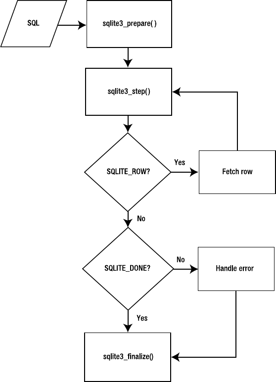
CHAPTER 6 ■ THE CORE C API 215
you like. You can also obtain the declared types of columns (as they are defined in the CREATE
TABLE statement) and other miscellaneous metadata such as storage format and both associ-
ated table and database names. sqlite3_exec(), by comparison, provides only a fraction of
this information through its callback function. The same is true with sqlite3_get_table(),
which only includes the result set’s column headers with the data.
In practice you will find that each query method has its uses. sqlite3_exec() is especially
good for running commands that modify the database (CREATE, DROP, INSERT, UPDATE, and DELETE).
One function call and it’s done. Prepared queries are typically better for SELECT statements
because they offer so much more information, more linear coding (no callback functions), and
more control by using cursors to iterate over results.
As you’ll recall from Chapter 5, prepared queries are performed in three basic steps:
compilation, execution, and finalization. This process is illustrated in Figure 6-1.
Figure 6-1. Prepared query processing
Owens_6730 C06.fm Page 215 Tuesday, April 18, 2006 7:09 AM
www.it-ebooks.info
216 CHAPTER 6 ■ THE CORE C API
You compile the query with sqlite3_prepare(), execute it step by step using sqlite3_step(),
and close it using sqlite3_finalize(), or you can reuse it using sqlite3_reset(). This process
and the individual steps are all explained in detail in the following sections.
Compilation
Compilation, or preparation, takes a SQL statement and compiles it into byte code readable by the
virtual database engine (VDBE). It is performed by sqlite3_prepare(), which is declared as follows:
int sqlite3_prepare(
sqlite3 *db, /* Database handle */
const char *zSql, /* SQL text, UTF-8 encoded */
int nBytes, /* Length of zSql in bytes. */
sqlite3_stmt **ppStmt, /* OUT: Statement handle */
const char **pzTail /* OUT: Pointer to unused portion of zSql */
);
sqlite3_prepare() compiles the first SQL statement in the zSQL string (which can contain
multiple SQL statements) into VDBE byte code. It allocates all the resources necessary to
execute the statement and associates it along with the byte code into a single statement handle
(also referred to as simply a statement), designated by the out parameter ppStmt, which is a
sqlite3_stmt structure. From the programmer’s perspective, this structure is little more than
an opaque handle used to execute a SQL statement and obtain its associated records. However,
this data structure contains the command’s byte code, bound parameters, B-tree cursors,
VDBE execution context, and any other data sqlite3_step() needs to manage the state of the
query during execution.
sqlite3_prepare() does not affect the connection or database in any way. It does not start
a transaction or get a lock. It works directly with the compiler, which simply prepares the query
for execution. Statement handles are highly dependent on the database schema they were
compiled with. If another connection alters the database schema, between the time you
prepare a statement and the time you actually run it, your statement will expire. Your first call
to sqlite3_step() with the statement will lead to a SQLITE_SCHEMA error, which is discussed
later in the section “Errors and the Unexpected.” Then you will have to finalize or reset the
statement, recompile, and try again.
Execution
Once you prepare the query, the next step is to execute it using sqlite3_step(), declared
as follows:
int sqlite3_step(sqlite3_stmt *pStmt);
sqlite3_step() takes the statement handle and talks directly to the VDBE. The VDBE reads the
statement handle’s byte code and steps through its instructions one by one to carry out the
SQL statement. On the first call to sqlite3_step(), the VDBE obtains the requisite database
lock needed to perform the command. If it can’t get the lock, sqlite3_step() will return
SQLITE_BUSY, if there is no busy handler installed. If one is installed, it will call that handler
instead.
For SQL statements that don’t return data, the first call to sqlite3_step() executes the
command in its entirety, returning a result code indicating the outcome. For SQL statements
Owens_6730 C06.fm Page 216 Tuesday, April 18, 2006 7:09 AM
www.it-ebooks.info
CHAPTER 6 ■ THE CORE C API 217
that do return data, such as SELECT, the first call to sqlite3_step() positions the statement’s
B-tree cursor on the first record. Subsequent calls to sqlite3_step() position the cursor on
subsequent records in the result set. sqlite3_step() returns SQLITE_ROW for each record in the
set until it reaches the end, whereupon it returns SQLITE_DONE, indicating that the cursor has
reached the end of the set.
All other API functions related to data access use the statement’s cursor to obtain informa-
tion about the current record. For example, the sqlite3_column_xxx() functions all use the
statement handle, specifically its cursor, to fetch the current record’s fields.
Finalization and Reset
Once the statement has reached the end of execution, it must be finalized. You can either
finalize or reset the statement using one of the following functions:
int sqlite3_finalize(sqlite3_stmt *pStmt);
int sqlite3_reset(sqlite3_stmt *pStmt);
sqlite3_finalize() will close out the statement. It frees resources and commits or rolls back
any implicit transactions (if the connection is in autocommit mode), clearing the journal file
and freeing the associated lock.
If you want to reuse the statement, you can do so using sqlite3_reset(). It will keep the
compiled SQL statement (and any bound parameters), but commits any changes related to the
current statement to the database. It also releases its lock and clears the journal file if auto-
commit is enabled. The primary difference between sqlite3_finalize() and sqlite3_reset()
is that the latter preserves the resources associated with the statement so that it can be executed
again, avoiding the need to call sqlite3_prepare() to compile the SQL command.
A Practical Example
Now that you’ve seen the whole process, let’s go through an example. A simple, complete program
using a prepared query is listed in Listing 6-6. It is taken from select.c in the examples.
Listing 6-6. Using Prepared Queries
int main(int argc, char **argv)
{
int rc, i, ncols;
sqlite3 *db;
sqlite3_stmt *stmt;
char *sql;
const char *tail;
rc = sqlite3_open("foods.db", &db);
if(rc) {
fprintf(stderr, "Can't open database: %s\n", sqlite3_errmsg(db));
sqlite3_close(db);
exit(1);
}
Owens_6730 C06.fm Page 217 Tuesday, April 18, 2006 7:09 AM
www.it-ebooks.info
218 CHAPTER 6 ■ THE CORE C API
sql = "select * from episodes;";
rc = sqlite3_prepare(db, sql, strlen(sql), &stmt, &tail);
if(rc != SQLITE_OK) {
fprintf(stderr, "SQL error: %s\n", sqlite3_errmsg(db));
}
rc = sqlite3_step(stmt);
ncols = sqlite3_column_count(stmt);
while(rc == SQLITE_ROW) {
for(i=0; i < ncols; i++) {
fprintf(stderr, "'%s' ", sqlite3_column_text(stmt, i));
}
fprintf(stderr, "\n");
rc = sqlite3_step(stmt);
}
sqlite3_finalize(stmt);
sqlite3_close(db);
return 0;
}
This example connects to the foods.db database, queries the episodes table, and prints out
all columns of all records within it. Keep in mind this is a simplified example—there are a few
other things we need to check for when calling sqlite3_step(), such as errors and busy condi-
tions, but we will address them later.
Like sqlite3_exec(), sqlite3_prepare() can accept a string containing multiple SQL state-
ments. However, unlike sqlite3_exec(), it will only process the first statement in the string. But
it does make it easy for you to process subsequent SQL statements in the string by providing the
pzTail out parameter. After you call sqlite3_prepare(), it will point this parameter (if provided) to
the starting position of the next statement in the zSQL string. Using pzTail, processing a batch
of SQL commands in a given string can be executed in a loop as follows:
while(sqlite3_complete(sql) {
rc = sqlite3_prepare(db, sql, strlen(sql), &stmt, &tail);
/* Process query results */
/* Skip to next command in string. */
sql = tail;
}
Owens_6730 C06.fm Page 218 Tuesday, April 18, 2006 7:09 AM
www.it-ebooks.info
CHAPTER 6 ■ THE CORE C API 219
This example makes use of another API function not yet covered—sqlite3_complete(),
which does as its name suggests: it takes a string and returns true (1) if there is at least one
complete (but necessarily valid) SQL statement in it, and false otherwise.
Fetching Records
So far, you have seen how to obtain records and columns from sqlite3_exec() and
sqlite3_get_table(). Prepared queries, by comparison, offer many more options when
it comes to getting information from records in the database.
For a statement that returns records, the number of columns in the result set can be obtained
using sqlite3_column_count() and sqlite3_data_count(), which are declared as follows:
int sqlite3_column_count(sqlite3_stmt *pStmt);
int sqlite3_data_count(sqlite3_stmt *pStmt);
sqlite3_column_count() returns the number of columns associated with a statement handle.
You can call it on a statement handle before it is actually executed. If the query in question is
not a SELECT statement, sqlite3_column_count() will return 0. Similarly, sqlite3_data_count()
returns the number of columns for the current record, after sqlite3_step() returns SQLITE_ROW.
This function will only work if the statement handle has an active cursor.
Getting Column Information
You can obtain the name of each column in the current record using sqlite3_column_name(),
which is declared as follows:
const char *sqlite3_column_name( sqlite3_stmt*, /* statement handle */
int iCol /* column ordinal */);
Similarly, you can get the associated storage class for each column using
sqlite3_column_type(), which is declared as follows:
int sqlite3_column_type( sqlite3_stmt*, /* statement handle */
int iCol /* column ordinal */);
This function returns an integer value that corresponds to one of five storage class codes,
defined as follows:
#define SQLITE_INTEGER 1
#define SQLITE_FLOAT 2
#define SQLITE_TEXT 3
#define SQLITE_BLOB 4
#define SQLITE_NULL 5
These are SQLite’s native data types, or storage classes as described in Chapter 4. All data
stored within a SQLite database is stored in one of these five forms, depending on its initial
representation and the affinity of the column. For our purposes, the terms storage class and
data type are synonymous. For more information on storage classes, see the sections “Storage
Classes” and “Type Affinity” in Chapter 4.
You can obtain the declared data type of a column as it is defined in the table’s schema
using the sqlite3_column_decltype() function, which is declared as follows:
Owens_6730 C06.fm Page 219 Tuesday, April 18, 2006 7:09 AM
www.it-ebooks.info

220 CHAPTER 6 ■ THE CORE C API
const char *sqlite3_column_decltype( sqlite3_stmt*, /* statement handle */
int /* column ordinal */);
If a column in a result set does not correspond to an actual table column (say, for example, the
column is the result of a literal value, expression, function, or aggregate), this function will
return NULL as the declared type of that column. For example, suppose you have a table in your
database defined as
CREATE TABLE t1(c1 INTEGER);
Then you execute the following query:
SELECT c1 + 1, 0 FROM t1;
In this case, sqlite3_column_decltype() will return INTEGER for the first column and NULL for
the second.
In addition to the declared type, you can obtain other information on a column using the
following functions:
const char *sqlite3_column_database_name(sqlite3_stmt *pStmt, int iCol);
const char *sqlite3_column_table_name(sqlite3_stmt *pStmt, int iCol);
const char *sqlite3_column_origin_name(sqlite3_stmt *pStmt, int iCol);
The first function will return the database associated with a column, the second its table, and
the last function returns the column’s actual name as defined in the schema. That is, if you
assigned the column an alias in the SQL statement, sqlite3_column_origin_name() will return
its actual name as defined in the schema. Note that these functions are only available if you
compile SQLite with the SQLITE_ENABLE_COLUMN_METADATA preprocessor directive.
COLUMN METADATA
Detailed information about a column can be obtained independently from a query using the
sqlite3_table_column_metadata() function, declared as follows:
int sqlite3_table_column_metadata(
sqlite3 *db, /* Connection handle */
const char *zDbName, /* Database name or NULL */
const char *zTableName, /* Table name */
const char *zColumnName, /* Column name */
char const **pzDataType, /* OUTPUT: Declared data type */
char const **pzCollSeq, /* OUTPUT: Collation sequence name */
int *pNotNull, /* OUTPUT: True if NOT NULL
constraint exists */
int *pPrimaryKey, /* OUTPUT: True if column part of PK */
int *pAutoinc /* OUTPUT: True if colums is
auto-increment */
);
Owens_6730 C06.fm Page 220 Tuesday, April 18, 2006 7:09 AM
www.it-ebooks.info

CHAPTER 6 ■ THE CORE C API 221
This function is a combination of input and output parameters. It does not work from a statement handle,
but rather from a combination of connection handle, database name, table name, and column name.
The optional database name refers to the logical name of an attached database (e.g., “main” or “temp”).
If no database name is provided (the argument is NULL), then the function will search all attached databases
for matching columns. Both table name and column name are required. The information for the matched column
is provided to the memory locations of arguments 5 through 9. The memory for the pzDataType and pzCollSeq
out parameters is valid only until the next API call. If no matching column can be found, then
sqlite3_table_column_metadata() returns SQLITE_ERROR.
Getting Column Values
You can obtain the values for each column in the current record using the
sqlite3_column_xxx() functions, which are of the general form
xxx sqlite3_column_xxx( sqlite3_stmt*, /* statement handle */
int iCol /* column ordinal */);
Here xxx is the data type you want the data represented in (e.g., int, blob, double, etc.). The
complete list of the sqlite3_column_xxx() functions is as follows:
int sqlite3_column_int(sqlite3_stmt*, int iCol);
double sqlite3_column_double(sqlite3_stmt*, int iCol);
long long int sqlite3_column_int64(sqlite3_stmt*, int iCol);
const void *sqlite3_column_blob(sqlite3_stmt*, int iCol);
const unsigned char *sqlite3_column_text(sqlite3_stmt*, int iCol);
const void *sqlite3_column_text16(sqlite3_stmt*, int iCol);
For each function, SQLite converts the internal representation (storage class in the
column) to the type specified in the function name. There are a number of rules SQLite uses to
convert the internal data type representation to that of the requested type. These rules are
listed in Table 6-1.
Table 6-1. Column Type Conversion Rules
Internal Type Requested Type Conversion
NULL INTEGER Result is 0.
NULL FLOAT Result is 0.0.
NULL TEXT Result is a NULL pointer.
NULL BLOB Result is a NULL pointer.
INTEGER FLOAT Convert from integer to float.
INTEGER TEXT Result is the ASCII rendering of the integer.
INTEGER BLOB Result is the ASCII rendering of the integer.
FLOAT INTEGER Convert from float to integer.
Owens_6730 C06.fm Page 221 Tuesday, April 18, 2006 7:09 AM
www.it-ebooks.info

222 CHAPTER 6 ■ THE CORE C API
Like the sqlite3_bind_xxx() functions described later, BLOBs require a little more work in
that you must specify their length in order to copy them. For BLOB columns, you can get the
actual length of the data using sqlite3_column_bytes(), which is declared as follows:
int sqlite3_column_bytes( sqlite3_stmt*, /* statement handle */
int /* column ordinal */);
Once you get the length, you can copy the binary data using sqlite3_column_blob(). For
example, say the first column in the result set contains binary data. One way to get a copy of
that data would be as follows:
int len = sqlite3_column_bytes(stmt,0);
void* data = malloc(len);
memcpy(data, len, sqlite3_column_blob(stmt,0));
A Practical Example
To help solidify all of these column functions, Listing 6-7 (taken from columns.c) illustrates
using the functions we’ve described to retrieve column information and values for a simple
SELECT statement.
Listing 6-7. Obtaining Column Information
int main(int argc, char **argv)
{
int rc, i, ncols, id, cid;
char *name, *sql;
sqlite3 *db;
sqlite3_stmt *stmt;
sql = "select id, name from episodes";
sqlite3_open("test.db", &db);
FLOAT TEXT Result is the ASCII rendering of the float.
FLOAT BLOB Result is the ASCII rendering of the float.
TEXT INTEGER Use atoi().
TEXT FLOAT Use atof().
TEXT BLOB No change.
BLOB INTEGER Convert to TEXT and then use atoi().
BLOB FLOAT Convert to TEXT and then use atof().
BLOB TEXT Add a \000 terminator if needed.
Table 6-1. Column Type Conversion Rules (Continued)
Internal Type Requested Type Conversion
Owens_6730 C06.fm Page 222 Tuesday, April 18, 2006 7:09 AM
www.it-ebooks.info

CHAPTER 6 ■ THE CORE C API 223
setup(db);
sqlite3_prepare(db, sql, strlen(sql), &stmt, NULL);
ncols = sqlite3_column_count(stmt);
rc = sqlite3_step(stmt);
/* Print column information */
for(i=0; i < ncols; i++) {
fprintf(stdout, "Column: name=%s, storage class=%i, declared=%s\n",
sqlite3_column_name(stmt, i),
sqlite3_column_type(stmt, i),
sqlite3_column_decltype(stmt, i));
}
fprintf(stdout, "\n");
while(rc == SQLITE_ROW) {
id = sqlite3_column_int(stmt, 0);
cid = sqlite3_column_int(stmt, 1);
name = sqlite3_column_text(stmt, 2);
if(name != NULL){
fprintf(stderr, "Row: id=%i, cid=%i, name='%s'\n", id,cid,name);
} else {
/* Field is NULL */
fprintf(stderr, "Row: id=%i, cid=%i, name=NULL\n", id,cid);
}
rc = sqlite3_step(stmt);
}
sqlite3_finalize(stmt);
sqlite3_close(db);
return 0;
}
This example connects to the database, selects records from the episodes table, and prints
the column information and the fields for each row (using their internal storage class). Running the
program produces the following output:
Column: name=id, storage class=1, declared=integer
Column: name=name, storage class=3, declared=text
Row: id=1, name='The Dinner Party'
Row: id=2, name='The Soup Nazi'
Row: id=3, name='The Fusilli Jerry'
Owens_6730 C06.fm Page 223 Tuesday, April 18, 2006 7:09 AM
www.it-ebooks.info

224 CHAPTER 6 ■ THE CORE C API
FINDING A STATEMENT’S CONNECTION
In practice you may find yourself writing code where some of your functions only have access to the statement
handle, not the connection handle. If these functions encounter an error while working with the statement
handle, they will not have a way to get error information from sqlite3_errmsg(), as it requires a connec-
tion handle to work. This is where sqlite3_db_handle() comes in handy. It is declared as follows:
int sqlite3_db_handle(sqlite3_stmt*);
Given a statement handle, sqlite3_db_handle() returns the associated connection handle. This
way, you don’t need to worry about having to pass the connection handle along with the statement handle
everywhere you process query results.
Parameterized Queries
The API includes support for designating parameters in a SQL statement, allowing you to
provide (or “bind”) values for them at a later time. Bound parameters are used in conjunction
with sqlite3_prepare(). For example, you could create a SQL statement like the following:
insert into foo values (?,?,?);
Then you can, for example, bind the integer value 2 to the first parameter (designated by the
first ? character), the string value 'pi' to the second parameter, and the double value 3.14 for
the third parameter, as illustrated in the following code (taken from parameters.c):
const char* sql = "insert into foo values(?,?,?)";
sqlite3_prepare(db, sql, strlen(sql), &stmt, &tail);
sqlite3_bind_int(stmt, 1, 2);
sqlite3_bind_text(stmt, 2, "pi");
sqlite3_bind_double(stmt, 3, 3.14);
sqlite3_step(stmt);
sqlite3_finalize(stmt);
This generates and executes the statement
insert into foo values (2, 'pi', 3.14)
This process is illustrated in Figure 6-2. This particular method of binding uses positional
parameters (as described in Chapter 5) where each parameter is designated by a question
mark (?) character, and later identified by its index or relative position in the SQL statement.
Before delving into the other parameter methods, it is helpful to first understand the
process by which parameters are defined, bound, and evaluated. When you write a parameter-
ized statement such as the following, the parameters within it are identified when
sqlite3_prepare() compiles the query:
insert into episodes (id,name) values (?,?)
Owens_6730 C06.fm Page 224 Tuesday, April 18, 2006 7:09 AM
www.it-ebooks.info
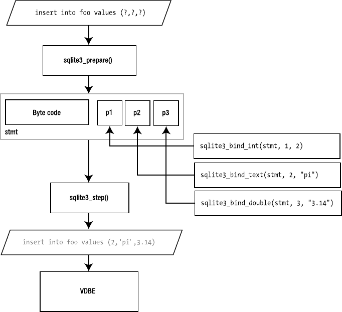
CHAPTER 6 ■ THE CORE C API 225
sqlite3_prepare() recognizes that there are parameters in a SQL statement. Internally, it
assigns each parameter a number to uniquely identify it. In the case of positional parameters,
it starts with 1 for the first parameter found and uses sequential integer values for subsequent
parameters. It stores this information in the resulting statement handle (sqlite3_stmt struc-
ture), which will then expect a specific number of values to be bound to the given parameters
before execution. If you do notbind a value to a parameter, sqlite3_step() will use NULL for its
value by default when the statement is executed.
Figure 6-2. SQL parameter binding
After you prepare the statement, you then bind values to it. You do this using the
sqlite3_bind_xxx() functions, which have the general form
sqlite3_bind_xxx( sqlite3_stmt*, /* statement handle */
int i, /* parameter number */
xxx value /* value to be bound */
);
The xxx in the function name represents the data type of the value to bind. For example, to
bind a double value to a parameter, you would use sqlite3_bind_double(), which is declared
as follows:
Owens_6730 C06.fm Page 225 Tuesday, April 18, 2006 7:09 AM
www.it-ebooks.info
226 CHAPTER 6 ■ THE CORE C API
sqlite3_bind_double(sqlite3_stmt* stmt, int i, double value);
The complete list of bind functions is as follows:
int sqlite3_bind_int(sqlite3_stmt*, int, int);
int sqlite3_bind_double(sqlite3_stmt*, int, double);
int sqlite3_bind_int64(sqlite3_stmt*, int, long long int);
int sqlite3_bind_null(sqlite3_stmt*, int);
int sqlite3_bind_blob( sqlite3_stmt*, int, const void*,
int n, void(*)(void*));
int sqlite3_bind_text( sqlite3_stmt*, int, const char*,
int n, void(*)(void*));
int sqlite3_bind_text16( sqlite3_stmt*, int, const void*,
int n, void(*)(void*));
In general, the bind functions can be divided into two classes, one for scalar values (int,
double, int64, and NULL), and the other for arrays (blob, text, and text16). They differ only in
that the array bind functions require a length argument and a pointer to a cleanup function.
Also, sqlite3_bind_text() automatically escapes quote characters like sqlite3_mprintf().
Using the BLOB variant, the array bind function has the following declaration:
int sqlite3_bind_blob( sqlite3_stmt*, /* statement handle */
int, /* ordinal */
const void*, /* pointer to blob data */
int n, /* length (bytes) of data */
void(*)(void*)); /* cleanup hander */
There are two predefined values for the cleanup handler provided by the API that have special
meanings, defined as follows:
#define SQLITE_STATIC ((void(*)(void *))0)
#define SQLITE_TRANSIENT ((void(*)(void *))-1)
Each value designates a specific cleanup action. SQLITE_STATIC tells the array bind function
that the array memory resides in unmanaged space, so SQLite does not attempt to clean it up.
SQLITE_TRANSIENT tells the bind function that the array memory is subject to change, so SQLite
makes its own private copy of the data, which it automatically cleans up when the statement is
finalized. The third option is to provide a pointer to your own cleanup function, which must be
of the form
void cleanup_fn(void*)
If provided, SQLite will call your cleanup function, passing in the array memory when the
statement is finalized.
Owens_6730 C06.fm Page 226 Tuesday, April 18, 2006 7:09 AM
www.it-ebooks.info

CHAPTER 6 ■ THE CORE C API 227
■Note Bound parameters remain bound throughout the lifetime of the statement handle. They remain
bound even after a call to sqlite3_reset() and are only freed when the statement is finalized (by calling
sqlite3_finalize()).
Once you have bound all of the parameters you want, you can then execute the statement.
You do this using the next function in the sequence: sqlite3_step(). sqlite3_step() will take
the bound values, substitute them for the parameters in the SQL statement, and then begin
executing the command.
Also, as a matter of convenience, bindings can be transferred from one statement to
another using sqlite3_transfer_bindings(), which is declared as follows:
int sqlite3_transfer_bindings( sqlite3_stmt*, /* source statement */
sqlite3_stmt*); /* dest statement */
This function is useful if you want to prepare the same query using another statement, without
having to repeat all of the binding steps. This function is especially useful for dealing with
SQLITE_SCHEMA errors, described later.
Now that you understand the binding process, the four parameter-binding methods differ
only by
• The way in which parameters are represented in the SQL statement (using a positional
parameter, explicitly defined parameter number, or alphanumeric parameter name)
• The way in which parameters are assigned numbers
For positional parameters, sqlite3_prepare() assigns numbers using sequential integer
values starting with 1 for the first parameter. In the previous example, the first ? parameter is
assigned 1, and the second ? parameter is assigned 2. With positional parameters, it is your job
to keep track of which number corresponds to which parameter (or question mark) in the SQL
statement and correctly specify that number in the bind functions.
Numbered Parameters
Numbered parameters, on the other hand, allow you to specify your own numbers for parameters,
rather than use an internal sequence. The syntax for numbered parameters uses a question
mark followed by the parameter number. Take, for example, the following piece of code (taken
from parameters.c):
name = "Mackinaw Peaches";
sql = "insert into episodes (id, cid, name) "
"values (?100,?100,?101)";
rc = sqlite3_prepare(db, sql, strlen(sql), &stmt, &tail);
if(rc != SQLITE_OK) {
fprintf(stderr, "sqlite3_prepare() : Error: %s\n", tail);
return rc;
}
Owens_6730 C06.fm Page 227 Tuesday, April 18, 2006 7:09 AM
www.it-ebooks.info

228 CHAPTER 6 ■ THE CORE C API
sqlite3_bind_int(stmt, 100, 10);
sqlite3_bind_text(stmt, 101, name, strlen(name), SQLITE_TRANSIENT);
sqlite3_step(stmt);
sqlite3_finalize(stmt);
This example uses 100 and 101 for its parameter numbers. Parameter number 100 has the
integer value 10 bound to it. Parameter 101 has the string value 'Mackinaw Peaches' bound to
it. Note how numbered parameters come in handy when you need to bind a single value in more
than one place in a SQL statement. Consider the values part of the previous SQL statement:
insert into episodes (id, cid, name) values (?100,?100,?101)";
Parameter 100 is being used twice—once for id and again for cid. Thus, numbered parameters
save time when you need to use a bound value in more than one place.
■Note When using numbered parameters in a SQL statement, keep in mind that the allowable range
consists of the integer values 1–999.
Named Parameters
The third parameter binding method is using named parameters. Whereas you can assign your
own numbers using numbered parameters, you can assign alphanumeric names with named
parameters. Likewise, as numbered parameters are prefixed with a question mark (?), you identify
named parameters by prefixing a colon (:) to the parameter name. Consider the following code
snippet (taken from parameters.c):
name = "Mackinaw Peaches";
sql = "insert into episodes (id, cid, name) values (:cosmo,:cosmo,:newman)";
rc = sqlite3_prepare(db, sql, strlen(sql), &stmt, &tail);
sqlite3_bind_int( stmt,
sqlite3_bind_parameter_index(stmt, ":cosmo"), 10);
sqlite3_bind_text( stmt,
sqlite3_bind_parameter_index(stmt, ":newman"),
name,
strlen(name), SQLITE_TRANSIENT );
sqlite3_step(stmt);
sqlite3_finalize(stmt);
This example is identical to the previous example using numbered parameters, except it
uses two named parameters called cosmo and newman instead. Like positional parameters,
named parameters are automatically assigned numbers by sqlite3_prepare(). While the
numbers assigned to each parameter are unknown, you can resolve them using
sqlite3_bind_parameter_index(), which takes a parameter name and returns the corresponding
Owens_6730 C06.fm Page 228 Tuesday, April 18, 2006 7:09 AM
www.it-ebooks.info

CHAPTER 6 ■ THE CORE C API 229
parameter number. This is the number you use to bind the value to its parameter. All in all,
named parameters mainly help with legibility more than anything else.
PARAMETER INDEXES
While the function sqlite3_bind_parameter_index() seems to refer to a parameter number as an
index, for all intents and purposes the two terms (number and index) are synonymous. I have settled on the
term number rather than index for parameter positions as a result of some discussion on the SQLite mailing
list, which has suggested that number is perhaps a better description. The term index was used when parameter
binding was limited only to positional parameters. With the addition of numbered parameters, referring to
parameter positions as (sequential) indexes can be somewhat misleading.
Tcl Parameters
The final parameter scheme is called Tcl parameters and is specific more to the Tcl extension
than it is to the C API. Basically, it works identically to named parameters except that rather
than using alphanumeric values for parameter names, it uses Tcl variable names. In the Tcl
extension, when the Tcl equivalent of sqlite3_prepare() is called, the Tcl extension automati-
cally searches for Tcl variables with the given parameter names in the active Tcl program
environment and binds them to their respective parameters. Despite its current application in
the Tcl interface, nothing prohibits this same mechanism from being applied to other language
interfaces, which can in turn implement the same feature. In this respect, referring to this
parameter method solely as Tcl parameters may be a bit of a misnomer. The Tcl extension just
happened to be the first application that utilized this method. Basically, the Tcl parameter
syntax does little more than provide an alternate syntax to named parameters—rather than
prefixing the parameters with a colon (:), it uses a dollar sign ($).
Errors and the Unexpected
Up to now, we have looked at the API from a rather optimistic viewpoint, as if nothing could
ever go wrong. But things do go wrong, and there is a part of the API devoted to that. The three
things you always have to guard against in your code are errors, busy conditions, and my personal
favorite: schema changes.
Handling Errors
Many of the API functions return integer result codes. That means they can potentially return
error codes of some sort. The most common functions to watch are typically the most frequently
used, such as sqlite3_open(), sqlite3_prepare() and friends, as well as sqlite3_exec(). You
should always program defensively and review every API function (documented in Appendix B)
before you use it to ensure that you deal with every possible error condition that can arise.
There are about 23 different errors defined in the API. Only a fraction of them will really matter
to your application in practice. All of the SQLite return codes are listed in Table 6-2. All of the
API functions that can return them are listed as follows:
Owens_6730 C06.fm Page 229 Tuesday, April 18, 2006 7:09 AM
www.it-ebooks.info

230 CHAPTER 6 ■ THE CORE C API
sqlite3_bind_xxx()
sqlite3_close()
sqlite3_create_collation()
sqlite3_collation_needed()
sqlite3_create_function()
sqlite3_prepare()
sqlite3_exec()
sqlite3_finalize()
sqlite3_get_table()
sqlite3_open()
sqlite3_reset()
sqlite3_step()
sqlite3_transfer_bindings()
You can get extended information on a given error using sqlite3_errmsg(), which is declared
as follows:
const char *sqlite3_errmsg(sqlite3*);
It takes a connection handle as its only argument and returns the most recent error resulting
from an API call on that connection. If no error has been encountered, it returns the string “not
an error”.
Table 6-2. SQLite Return Codes
Code Description
SQLITE_OK The operation was successful.
SQLITE_ERROR General SQL error or missing database. It may be possible to obtain
more error information depending on the error condition
(SQLITE_SCHEMA, for example).
SQLITE_PERM Access permission denied. Cannot read or write to the database file.
SQLITE_ABORT A callback routine requested an abort.
SQLITE_BUSY The database file is locked.
SQLITE_LOCKED A table in the database is locked.
SQLITE_NOMEM A call to malloc() has failed within a database operation.
SQLITE_READONLY An attempt was made to write to a read-only database.
SQLITE_INTERRUPT Operation was terminated by sqlite3_interrupt().
SQLITE_IOERR Some kind of disk I/O error occurred.
SQLITE_CORRUPT The database disk image is malformed. This will also occur if an attempt
is made to open a non-SQLite database file as a SQLite database.
SQLITE_FULL Insertion failed because the database is full. There is no more space
on the file system or the database file cannot be expanded.
Owens_6730 C06.fm Page 230 Tuesday, April 18, 2006 7:09 AM
www.it-ebooks.info

CHAPTER 6 ■ THE CORE C API 231
While it is very uncommon outside of embedded systems, one of the most critical errors
you can encounter is SQLITE_NOMEM, which means that no memory can be allocated on the heap
(e.g., malloc() failed). Normally, after a single malloc() call fails, the SQLite library refuses to
function (all major calls can return SQLITE_NOMEM). If the application is able to recover from an
out-of-memory condition, it may still be possible to restore the state of the SQLite library using
sqlite3_global_recover(), which is declared as follows:
int sqlite3_global_recover();
This function restores the library state so that it can be used again. You must finalize or
reset all active statements (sqlite3_stmt pointers) before calling this function. Otherwise it will
return SQLITE_BUSY. This function will also return SQLITE_ERROR if you are using any in-memory
databases, either as a main or TEMP. (The TEMP database is where temporary data is stored—see
ATTACH DATABASE in Appendix A for details.) In either case, SQLite will not reset the library and
it will remain unusable.
SQLITE_CANTOPEN SQLite was unable to open the database file.
SQLITE_PROTOCOL The database is locked or there has been a protocol error.
SQLITE_EMPTY (Internal only) The database table is empty.
SQLITE_SCHEMA The database schema has changed.
SQLITE_CONSTRAINT Abort due to constraint violation. This constant is returned if the SQL
statement would have violated a database constraint (such as attempting
to insert a value into a unique index that already exists in the index).
SQLITE_MISMATCH Data type mismatch. An example of this is an attempt to insert non-
integer data into a column labeled INTEGER PRIMARY KEY. For most
columns, SQLite ignores the data type and allows any kind of data to
be stored. But an INTEGER PRIMARY KEY column is only allowed to
store integer data.
SQLITE_MISUSE Library was used incorrectly. This error might occur if one or more of
the SQLite API routines is used incorrectly. Examples of incorrect
usage include calling sqlite3_exec() after the database has been
closed using sqlite3_close() or calling sqlite3_exec() with the same
database pointer simultaneously from two separate threads.
SQLITE_NOLFS Uses OS features not supported on host. This value is returned if the
SQLite library was compiled with large file support (LFS) enabled but
LFS isn’t supported on the host operating system.
SQLITE_AUTH Authorization denied. This occurs when a callback function installed
using sqlite3_set_authorizer() returns SQLITE_DENY.
SQLITE_ROW sqlite3_step() has another row ready.
SQLITE_DONE sqlite3_step() has finished executing.
Table 6-2. SQLite Return Codes
Code Description
Owens_6730 C06.fm Page 231 Tuesday, April 18, 2006 7:09 AM
www.it-ebooks.info

232 CHAPTER 6 ■ THE CORE C API
■Caution sqlite3_global_recover() is not thread safe. Calling it from within a threaded application
when threads other than the caller have used SQLite is dangerous and will almost certainly result in malfunc-
tions. SQLite includes memory management functions specifically for threads. These are covered later in the
section “Threads and Memory Management.”
The sqlite3_global_recover() function is aimed at embedded applications where memory is
scarcer than normal applications. It can be omitted from SQLite at compile time by defining
the SQLITE_OMIT_GLOBALRECOVER preprocessor directive.
Handling Busy Conditions
Two important functions related to processing queries are sqlite3_busy_handler() and
sqlite3_busy_timeout(). If your program uses a database on which there are other active
connections, odds are it will eventually have to wait for a lock, and therefore will have to deal
with SQLITE_BUSY. Whenever you call an API function that causes SQLite to seek a lock and
SQLite is unable to get it, the function will return SQLITE_BUSY. There are three ways to deal
with this:
•Handle SQLITE_BUSY yourself, either by rerunning the statement or taking some other action.
• Have SQLite call a busy handler.
• Ask SQLite to wait (block or sleep) for some period of time for the lock to clear.
The last option involves using sqlite3_busy_timeout(). This function tells SQLite how long to
wait for a lock to clear before returning SQLITE_BUSY. While it can ultimately result in you still
having to handle SQLITE_BUSY, in practice setting this value to a sufficient period of time (say
30 seconds) usually provides enough time for even the most intensive transaction to complete.
Nevertheless, you should still have some contingency plan in place to handle SQLITE_BUSY.
User-Defined Busy Handlers
The second option entails using sqlite3_busy_handler(). This function provides a way to call
a user-defined function rather than blocking or returning SQLITE_BUSY right away. It’s declared
as follows:
int sqlite3_busy_handler(sqlite3*, int(*)(void*,int), void*);
The second argument is a pointer to a function to be called as the busy handler, and the
third argument is a pointer to application-specific data to be passed as the first argument to the
handler. The second argument to the busy handler is the number of prior calls made to the handler
for the same lock.
Such a handler might call sleep() for a period to wait out the lock, or it may send some
kind of notification. It may do whatever you like, as it is yours to implement. Be warned, though,
that registering a busy handler does not guarantee that it will always be called. As mentioned in
Chapter 5, SQLite will forego calling a busy handler for a connection if it perceives a deadlock
might result. Specifically, if your connection in SHARED is interfering with another connection in
Owens_6730 C06.fm Page 232 Tuesday, April 18, 2006 7:09 AM
www.it-ebooks.info

CHAPTER 6 ■ THE CORE C API 233
RESERVED, SQLite will not invoke your busy handler, hoping you will take the hint. In this case,
you are trying to write to the database from SHARED (starting the transaction with BEGIN) when
you really should be starting from RESERVED (starting the transaction with BEGIN IMMEDIATE).
The only restriction on busy handlers is that they may not close the database. Closing the
database from within a busy handler can delete critical data structures out from under the
executing query and result in crashing your program.
Advice
All things considered, the best route may be to set the timeout to a reasonable value and then
take some precaution if and when you receive a SQLITE_BUSY value. In general, if you are going
to write to the database, start in RESERVED. If you don’t do this, then the next best thing is to
install a busy handler, set the timeout to a known value, and if SQLite returns SQLITE_BUSY,
check the response time. If the time is less than the busy handler’s delay, then SQLite is telling
you that your query (and connection) is preventing a writer from proceeding. If you want to
write to the database at this point, you should finalize or reset, then reexecute the statement,
this time starting with BEGIN IMMEDIATE.
Handling Schema Changes
Whenever a connection changes the database schema, all other prepared statements that were
compiled before the change are invalidated. The result is that the first call to sqlite3_step()
for such statements returns SQLITE_ERROR. From a locking standpoint, the schema change
occurs between the time a reader calls sqlite3_prepare() to compile a statement and calling
sqlite3_step() to execute it.
When this happens, the only course of action for you is to finalize or reset the query and
start over. However, you must confirm that the error is in fact due to a schema change. To do
so, whenever sqlite3_step() returns SQLITE_ERROR, you should call sqlite3_reset() to see if it
returns SQLITE_SCHEMA. Another way to check for this condition is to call sqlite3_expired(),
which takes the statement handle as its only argument.
■Note It’s important that you understand that when a schema change occurs, sqlite3_step()
never returns SQLITE_SCHEMA directly. It always returns SQLITE_ERROR. You then have to call
sqlite3_finalize(), sqlite3_reset(), or sqlite3_expired() to determine if the error was
due to SQLITE_SCHEMA. You should always check for this condition whenever you use sqlite3_step().
Several events can cause SQLITE_SCHEMA errors:
• Detaching databases
• Modifying or installing user-defined functions or aggregates
• Modifying or installing user-defined collations
• Modifying or installing authorization functions
• Vacuuming the database
Owens_6730 C06.fm Page 233 Tuesday, April 18, 2006 7:09 AM
www.it-ebooks.info
234 CHAPTER 6 ■ THE CORE C API
The reason the SQLITE_SCHEMA condition exists ultimately relates to the VDBE. When a
connection changes the schema, other compiled queries may have VDBE code that points to
database objects that no longer exist, or are in a different location in the database. Rather than
running the risk of a bizarre runtime error later, SQLite invalidates all statements that have
been compiled but not executed. They must be recompiled.
SQLITE_SCHEMA can only occur on the first call to sqlite3_step(). This is because
sqlite3_step(), when successful, always gets a lock on the database. Once you have a lock on
the database, it is impossible for any other connection to write to or alter the database. So if the
first call is successful, you are guaranteed that all subsequent calls to sqlite3_step() will not
encounter SQLITE_SCHEMA. One possible way provided by the SQLite FAQ to handle SQLITE_SCHEMA
is shown in Listing 6-8.
Listing 6-8. Handling SQLITE_SCHEMA
int rc;
sqlite3_stmt *pStmt;
char zSql[] = "SELECT .....";
do {
/* Compile the statement from SQL. Assume success. */
sqlite3_prepare(pDb, zSql, -1, &pStmt, 0);
while( SQLITE_ROW==sqlite3_step(pStmt) ) {
/* Do something with the row of available data */
}
/* Finalize the statement. If a SQLITE_SCHEMA error has
** occurred, then the above call to sqlite3_step() will have
** returned SQLITE_ERROR. sqlite3_finalize() will return
** SQLITE_SCHEMA. In this case the loop will execute again.
*/
rc = sqlite3_finalize(pStmt);
} while( rc==SQLITE_SCHEMA );
A possible variation is to take into consideration bound parameters. These parameters can
be automatically transferred to the new compiled query using sqlite3_transfer_bindings(),
as shown in Listing 6-9.
Listing 6-9. Handling SQLITE_SCHEMA with sqlite3_transfer_bindings()
int rc, processed, skip;
sqlite3_stmt *pStmt = NULL;
sqlite3_stmt *plastStmt = NULL;
char zSql[] = "SELECT .....";
do {
sqlite3_prepare(pDb, zSql, -1, &pStmt, 0);
Owens_6730 C06.fm Page 234 Tuesday, April 18, 2006 7:09 AM
www.it-ebooks.info

CHAPTER 6 ■ THE CORE C API 235
/* If there was a lastStmt, transfer bindings from it */
if(plastStmt != NULL){
sqlite3_transfer_bindings(plastStmt, pStmt);
}
/* Keep track of the current stmt */
plastStmt = pStmt;
while( SQLITE_ROW==sqlite3_step(pStmt) ) {
/* Do something with the row of available data */
processed++;
}
rc = sqlite3_finalize(pStmt);
} while( rc==SQLITE_SCHEMA );
Another option for checking for SQLITE_SCHEMA without finalizing (destroying) the query
is to call sqlite3_reset() instead of sqlite3_finalize(). This will provide you with the
SQLITE_SCHEMA error if it exists. However, if the error is not schema related, you avoid the cost
of having to recompile the query since sqlite3_reset() leaves the query in a state where it can
still be executed.
TRACING SQL
If you are having a hard time figuring out exactly what your program is doing with the database, you can track
what SQL statements it has executed using sqlite3_trace(). Its declaration is as follows:
void *sqlite3_trace(sqlite3*, void(*xTrace)(void*,const char*), void*);
This function is analogous to putting a wiretap on a connection. You can use it to generate a log file of all
SQL executed on a given connection as well provide helpful debugging information. Every SQL statement that
is processed is passed to the callback function specified in the second argument. SQLite passes the data
provided in the third argument of sqlite3_trace() to the first argument of the callback function.
Operational Control
The API provides several functions you can use to monitor and/or manage SQL commands at
compile time and runtime. These functions allow you to install callback functions with which
to monitor and control various database events as they happen.
Commit Hooks
The sqlite3_commit_hook() function allows you to monitor when transactions commit on a
given connection. It is declared as follows:
Owens_6730 C06.fm Page 235 Tuesday, April 18, 2006 7:09 AM
www.it-ebooks.info

236 CHAPTER 6 ■ THE CORE C API
void *sqlite3_commit_hook( sqlite3 *cnx, /* database handle */
int(*xCallback)(void *data), /* callback function */
void *data); /* application data */
This function registers the callback function xCallback, which will be invoked whenever a
transaction commits on the connection given by cnx. The third argument (data) is a pointer to
application-specific data, which SQLite passes to the callback function. If the callback function
returns a non-zero value, then the commit is converted into a rollback.
Passing a NULL value in for the callback function effectively disables the currently registered
callback (if any). Also, only one callback can be registered at a time for a given connection. The
return value for sqlite3_commit_hook() is NULL unless another callback function was previously
registered, in which case the previous data value is returned.
■Note The sqlite3_commit_hook() function is currently marked as experimental and is therefore
subject to change. However, according SQLite’s author, this is extremely unlikely as this function has been in
the API for some time now.
Rollback Hooks
Rollback hooks are similar to commit hooks except that they watch for rollbacks for a given
connection. Rollback hooks are registered with the following function:
void *sqlite3_rollback_hook(sqlite3 *cnx, void(*xCallback)(void *data), void *data);
This function registers the callback function xCallback, which will be invoked in the event
of a rollback on cnx, whether by an explicit ROLLBACK command or an implicit error or constraint
violation. The callback is not invoked if a transaction is automatically rolled back due to the
database connection being closed. The third argument (data) is a pointer to application-specific
data, which SQLite passes to the callback function.
As in sqlite3_commit_hook(), each time you call sqlite3_rollback_hook(), the new call-
back function you provide will replace any currently registered callback function. If a callback
function was previously registered, sqlite3_rollback_hook() returns the previous data argument.
Update Hooks
The sqlite3_update_hook() is used to monitor all UPDATE, INSERT, and DELETE operations on
rows for a given database connection. It has the following form:
void *sqlite3_update_hook(
sqlite3 *cnx,
void(*)(void *, int, char const*, char const*, sqlite_int64),
void *data);
The first argument of the callback function is a pointer to application-specific data, which you
provide in the third argument. The callback function has the following form:
Owens_6730 C06.fm Page 236 Tuesday, April 18, 2006 7:09 AM
www.it-ebooks.info
CHAPTER 6 ■ THE CORE C API 237
void callback ( void * data,
int operation_code,
char const *db_name,
char const *table_name,
sqlite_int64 rowid),
The operation_code argument corresponds to SQLITE_INSERT, SQLITE_UPDATE, and
SQLITE_DELETE for INSERT, UPDATE, and DELETE operations, respectively. The third and fourth
arguments correspond to the database name and table name the operation took place on. The
final argument is the ROWID of the affected row. The callback is not invoked for operations on
system tables (e.g., sqlite_master and sqlite_sequence). The return value is a pointer to the
previously registered callback function's data argument, if it exists.
Authorizer Functions
Perhaps the most powerful event filter is sqlite3_set_authorizer(). It allows you to monitor
and control queries as they are compiled. This function is declared as follows:
int sqlite3_set_authorizer(
sqlite3*,
int (*xAuth)( void*,int,
const char*, const char*,
const char*,const char*),
void *pUserData
);
This routine registers a callback function that serves as an authorization function. SQLite
will invoke the callback function at statement compile time (not at execution time) for various
database events. The intent of the function is to allow applications to safely execute user-supplied
SQL. It provides a way to restrict such SQL from certain operations (e.g., anything that changes
the database) or to deny access to specific tables or columns within the database.
For clarity, the form of the authorization callback function is as follows:
int auth( void*, /* user data */
int, /* event code */
const char*, /* event specific */
const char*, /* event specific */
const char*, /* database name */
const char* /* trigger or view name */ );
The first argument is a pointer to application-specific data, which is passed in on the
fourth argument of sqlite3_set_authorizer(). The second argument to the authorization
function will be one of the defined constants listed in Table 6-3. These values signify what kind
of operation is to be authorized. The third and fourth arguments to the authorization function
are specific to the event code. These arguments are listed with their respective event codes in
Table 6-3.
The fifth argument is the name of the database (“main”, “temp”, etc.) if applicable. The
sixth argument is the name of the innermost trigger or view that is responsible for the access
attempt or NULL if this access attempt is directly from top-level SQL.
Owens_6730 C06.fm Page 237 Tuesday, April 18, 2006 7:09 AM
www.it-ebooks.info

238 CHAPTER 6 ■ THE CORE C API
The return value of the authorization function should be one of the constants SQLITE_OK,
SQLITE_DENY, or SQLITE_IGNORE. The meaning of the first two values is consistent for all events—
permit or deny the SQL statement. SQLITE_DENY will abort the entire SQL statement and
generate an error.
The meaning of SQLITE_IGNORE is specific to the event in question. Statements that read or
modify records generate SQLITE_READ or SQLITE_UPDATE events for each column the statement
attempts to operate on. In this case, if the callback returns SQLITE_IGNORE, the column in ques-
tion will be excluded from the operation. Specifically, attempts to read data from this column
yield only NULL values, and attempts to update it will silently fail.
Table 6-3. SQLite Authorization Events
Event Code Argument 3 Argument 4
SQLITE_CREATE_INDEX Index name Table name
SQLITE_CREATE_TABLE Table name NULL
SQLITE_CREATE_TEMP_INDEX Index name Table name
SQLITE_CREATE_TEMP_TABLE Table name NULL
SQLITE_CREATE_TEMP_TRIGGER Trigger name Table name
SQLITE_CREATE_TEMP_VIEW View name NULL
SQLITE_CREATE_TRIGGER Trigger name Table name
SQLITE_CREATE_VIEW View name NULL
SQLITE_DELETE Table name NULL
SQLITE_DROP_INDEX Index name Table name
SQLITE_DROP_TABLE Table name NULL
SQLITE_DROP_TEMP_INDEX Index name Table name
SQLITE_DROP_TEMP_TABLE Table name NULL
SQLITE_DROP_TEMP_TRIGGER Trigger name Table name
SQLITE_DROP_TEMP_VIEW View name NULL
SQLITE_DROP_TRIGGER Trigger name Table name
SQLITE_DROP_VIEW View name NULL
SQLITE_INSERT Table name NULL
SQLITE_PRAGMA Pragma name First argument or NULL
SQLITE_READ Table name Column name
SQLITE_SELECT NULL NULL
SQLITE_TRANSACTION NULL NULL
SQLITE_UPDATE Table name Column name
SQLITE_ATTACH Filename NULL
SQLITE_DETACH Database name NULL
Owens_6730 C06.fm Page 238 Tuesday, April 18, 2006 7:09 AM
www.it-ebooks.info
CHAPTER 6 ■ THE CORE C API 239
To illustrate this, the following example (the complete source of which is in authorizer.c)
will create a table foo, defined as follows:
create table foo(x int, y int, z int)
It registers an authorizer function, which will
• Block reads of column z
• Block updates to column x
•Monitor ATTACH and DETACH database events
• Log database events as they happen
This is a rather long example, which uses the authorizer function to filter many different data-
base events, so for clarity I am going to break the code into pieces. The authorizer function has
the general form shown in Listing 6-10.
Listing 6-10. Example Authorizer Function
int auth( void* x, int type,
const char* a, const char* b,
const char* c, const char* d )
{
const char* operation = a;
printf( " %s ", event_description(type));
/* Filter for different database events
** from SQLITE_TRANSACTION to SQLITE_INSERT,
** UPDATE, DELETE, ATTACH, etc. and either allow or deny
** them.
*/
return SQLITE_OK;
}
The first thing the authorizer looks for is a change in transaction state. If it finds a change,
it prints a message:
if((a != NULL) && (type == SQLITE_TRANSACTION)) {
printf(": %s Transaction", operation);
}
Next the authorizer filters events that result in a schema change:
switch(type) {
case SQLITE_CREATE_INDEX:
case SQLITE_CREATE_TABLE:
case SQLITE_CREATE_TRIGGER:
case SQLITE_CREATE_VIEW:
Owens_6730 C06.fm Page 239 Tuesday, April 18, 2006 7:09 AM
www.it-ebooks.info
240 CHAPTER 6 ■ THE CORE C API
case SQLITE_DROP_INDEX:
case SQLITE_DROP_TABLE:
case SQLITE_DROP_TRIGGER:
case SQLITE_DROP_VIEW:
{
// Schema has been modified somehow.
printf(": Schema modified");
}
The next filter looks for read attempts (which are fired on a column-by-column basis).
Here, all read attempts are allowed unless the column name is z, in which case the function
returns SQLITE_IGNORE. This will cause SQLite to return NULL for any field in column z, effectively
blocking access to its data.
if(type == SQLITE_READ) {
printf(": Read of %s.%s ", a, b);
/* Block attempts to read column z */
if(strcmp(b,"z")==0) {
printf("-> DENIED\n");
return SQLITE_IGNORE;
}
}
Next come INSERT and UPDATE filters. All INSERT statements are allowed. However, UPDATE
statements that attempt to modify column x are denied. This will not block the UPDATE state-
ment from executing; rather, it will simply filter out any attempt to update column x.
if(type == SQLITE_INSERT) {
printf(": Insert records into %s ", a);
}
if(type == SQLITE_UPDATE) {
printf(": Update of %s.%s ", a, b);
/* Block updates of column x */
if(strcmp(b,"x")==0) {
printf("-> DENIED\n");
return SQLITE_IGNORE;
}
}
Finally, the authorizer filters DELETE, ATTACH, and DETACH statements and simply issues noti-
fications when it encounters them:
if(type == SQLITE_DELETE) {
printf(": Delete from %s ", a);
}
Owens_6730 C06.fm Page 240 Tuesday, April 18, 2006 7:09 AM
www.it-ebooks.info
CHAPTER 6 ■ THE CORE C API 241
if(type == SQLITE_ATTACH) {
printf(": %s", a);
}
if(type == SQLITE_DETACH) {
printf("-> %s", a);
}
printf("\n");
return SQLITE_OK;
}
The (abbreviated) program is implemented as follows. As with the authorizer function,
I will break it into pieces. The first part of the program connects to the database and registers
the authorization function:
int main(int argc, char **argv)
{
sqlite3 *db, *db2;
char *zErr, *sql;
int rc;
/** Setup */
/* Connect to test.db */
rc = sqlite3_open("test.db", &db);
/** Authorize and test
/* 1. Register the authorizer function */
sqlite3_set_authorizer(db, auth, NULL);
Step 2 illustrates the transaction filter:
/* 2. Test transactions events */
printf("program : Starting transaction\n");
sqlite3_exec(db, "BEGIN", NULL, NULL, &zErr);
printf("program : Committing transaction\n");
sqlite3_exec(db, "COMMIT", NULL, NULL, &zErr);
Step 3 tests schema modifications by creating the test table foo:
/* 3. Test table events */
printf("program : Creating table\n");
sqlite3_exec(db, "create table foo(x int, y int, z int)", NULL, NULL, &zErr);
Step 4 tests read (SELECT) and write (INSERT / UPDATE) control. It inserts a test record, selects it,
updates it, and selects it again to observe the results of the UPDATE.
Owens_6730 C06.fm Page 241 Tuesday, April 18, 2006 7:09 AM
www.it-ebooks.info
242 CHAPTER 6 ■ THE CORE C API
/* 4. Test read/write access */
printf("program : Inserting record\n");
sqlite3_exec(db, "insert into foo values (1,2,3)", NULL, NULL, &zErr);
printf("program : Selecting record (value for z should be NULL)\n");
print_sql_result(db, "select * from foo");
printf("program : Updating record (update of x should be denied)\n");
sqlite3_exec(db, "update foo set x=4, y=5, z=6", NULL, NULL, &zErr);
printf("program : Selecting record (notice x was not updated)\n");
print_sql_result (db, "select * from foo");
printf("program : Deleting record\n");
sqlite3_exec(db, "delete from foo", NULL, NULL, &zErr);
printf("program : Dropping table\n");
sqlite3_exec(db, "drop table foo", NULL, NULL, &zErr);
Several things are going on here. The program selects all records in the table, one of which is
column z. We should see in the output that column z’s value is NULL. All other fields should
contain data from the table. Next, the program attempts to update all fields, the most impor-
tant of which is column x. The update should succeed, but the value in column x should be
unchanged, as the authorizer denies it. This is confirmed on the following SELECT statement,
which shows that all columns were updated except for column x, which is unchanged. The
program then drops the foo table, which should issue a schema change notification from the
previous filter.
Step 5 tests the ATTACH and DETACH database commands. The thing to notice here is how the
authorizer function is provided with the name of the database and that you can distinguish the
operations being performed under the attached database as opposed to the main database.
/* 5. Test ATTACH/DETACH */
/* Connect to test2.db */
rc = sqlite3_open("test2.db", &db2);
if(rc) {
fprintf(stderr, "Can't open database: %s\n", sqlite3_errmsg(db2));
sqlite3_close(db2);
exit(1);
}
sqlite3_exec(db2, "drop table foo2", NULL, NULL, &zErr);
sqlite3_exec(db2, "create table foo2(x int, y int, z int)",
NULL, NULL, &zErr);
printf("program : Attaching database test2.db\n");
sqlite3_exec(db, "attach 'test2.db' as test2", NULL, NULL, &zErr);
Owens_6730 C06.fm Page 242 Tuesday, April 18, 2006 7:09 AM
www.it-ebooks.info

CHAPTER 6 ■ THE CORE C API 243
printf("program : Selecting record from attached database test2.db\n");
sqlite3_exec(db, "select * from foo2", NULL, NULL, &zErr);
printf("program : Detaching table\n");
sqlite3_exec(db, "detach test2", NULL, NULL, &zErr);
Again for clarity, I will break up the program output into pieces. Upon executing it, the first
thing we see is the transaction filter catching changes in transaction state:
program : Starting transaction
SQLITE_TRANSACTION : BEGIN Transaction
program : Committing transaction
SQLITE_TRANSACTION : COMMIT Transaction
program : Starting transaction
SQLITE_TRANSACTION : BEGIN Transaction
program : Aborting transaction
SQLITE_TRANSACTION : ROLLBACK Transaction
Next we see a schema change notification as the result of creating the test table foo. The
interesting thing to notice here is all the other events that transpire in the sqlite_master table
as a result of creating the table:
program : Creating table
SQLITE_INSERT : Insert records into sqlite_master
SQLITE_CREATE_TABLE : Schema modified
SQLITE_READ : Read of sqlite_master.name
SQLITE_READ : Read of sqlite_master.rootpage
SQLITE_READ : Read of sqlite_master.sql
SQLITE_UPDATE : Update of sqlite_master.type
SQLITE_UPDATE : Update of sqlite_master.name
SQLITE_UPDATE : Update of sqlite_master.tbl_name
SQLITE_UPDATE : Update of sqlite_master.rootpage
SQLITE_UPDATE : Update of sqlite_master.sql
SQLITE_READ : Read of sqlite_master.ROWID
SQLITE_READ : Read of sqlite_master.name
SQLITE_READ : Read of sqlite_master.rootpage
SQLITE_READ : Read of sqlite_master.sql
SQLITE_READ : Read of sqlite_master.tbl_name
Next the program inserts a record, which the authorizer detects:
program : Inserting record
SQLITE_INSERT : Insert records into foo
Owens_6730 C06.fm Page 243 Tuesday, April 18, 2006 7:09 AM
www.it-ebooks.info

244 CHAPTER 6 ■ THE CORE C API
Now here is where things get more interesting. We are going to be able to see the autho-
rizer block access to individual columns. The program selects all records from the foo table. We
see the SQLITE_SELECT event take place, followed by the subsequent SQLITE_READ events gener-
ated for each attempted access of each column in the SELECT statement. When it comes to
column z, the authorizer denies access. Immediately following that, SQLite executes the state-
ment and print_sql_result() prints the column information and rows for the result set:
program : Selecting record (value for z should be NULL)
SQLITE_SELECT
SQLITE_READ : Read of foo.x
SQLITE_READ : Read of foo.y
SQLITE_READ : Read of foo.z -> DENIED
Column: x (1/int)
Column: y (1/int)
Column: z (5/(null))
Record: '1' '2' '(null)'
Look at what goes on with column z. Its value is NULL, which confirms that the authorizer
blocked access. But also look at the column information. While SQLite revealed the storage
class of column z, it denied access to its declared type in the schema.
Next comes the update. Here we are interested in column x. The UPDATE statement will
attempt to change every value in the record. But update of column x will be denied:
program : Updating record (update of x should be denied)
SQLITE_UPDATE : Update of foo.x -> DENIED
SQLITE_UPDATE : Update of foo.y
SQLITE_UPDATE : Update of foo.z
To confirm this, the program then selects the record to show what happened. The UPDATE
did execute, but column x was not changed. Even more interestingly, while z was updated
(trust me, it was), the authorizer will not let us see its value:
program : Selecting record (notice x was not updated)
SQLITE_SELECT
SQLITE_READ : Read of foo.x
SQLITE_READ : Read of foo.y
SQLITE_READ : Read of foo.z -> DENIED
Column: x (1/int)
Column: y (1/int)
Column: z (5/(null))
Record: '1' '5' '(null)'
Next the program deletes the record and drops the table. The latter operation generates all
sorts of events on the sqlite_master table, just as when the table was created:
Owens_6730 C06.fm Page 244 Tuesday, April 18, 2006 7:09 AM
www.it-ebooks.info

CHAPTER 6 ■ THE CORE C API 245
program : Deleting record
SQLITE_DELETE : Delete from foo
program : Dropping table
SQLITE_DELETE : Delete from sqlite_master
SQLITE_DROP_TABLE : Schema modified
SQLITE_DELETE : Delete from foo
SQLITE_DELETE : Delete from sqlite_master
SQLITE_READ : Read of sqlite_master.tbl_name
SQLITE_READ : Read of sqlite_master.type
SQLITE_UPDATE : Update of sqlite_master.rootpage
SQLITE_READ : Read of sqlite_master.rootpage
Finally, the program creates another database on a separate connection and then attaches
it on the main connection. The main connection then selects records from a table in the attached
database, and we can see how the authorizer reports these operations as happening in the
attached database:
program : Attaching database test2.db
SQLITE_ATTACH : test2.db
SQLITE_READ : Read of sqlite_master.name
SQLITE_READ : Read of sqlite_master.rootpage
SQLITE_READ : Read of sqlite_master.sql
program : Selecting record from attached database test2.db
SQLITE_SELECT
SQLITE_READ : Read of foo2.x
SQLITE_READ : Read of foo2.y
SQLITE_READ : Read of foo2.z -> DENIED
program : Detaching table
SQLITE_DETACH -> test2
As you can see, sqlite3_set_authorizer() and its event-filtering capabilities are quite
powerful. It gives you a great deal of control over what the user can and cannot do on a given
database. You can monitor events and, if you wish, stop them before they happen. Or, you can
allow them to proceed, but impose specific restrictions on them. sqlite3_set_authorizer()
can be a helpful tool for dealing with SQLITE_SCHEMA conditions. If you know you don’t need any
changes to your database schema in your application, you can simply install an authorizer
function to deny any operations that attempt to modify the schema in certain ways.
■Caution Keep in mind that denying schema changes in an authorizer is by no means a cure-all for
SQLITE_SCHEMA events. You need to be careful about all of the implications of denying various changes
to the schema. Just blindly blocking all events resulting in a schema change can restrict other seemingly
legitimate operations such as VACUUM.
Owens_6730 C06.fm Page 245 Tuesday, April 18, 2006 7:09 AM
www.it-ebooks.info

246 CHAPTER 6 ■ THE CORE C API
HELP FOR INTERACTIVE PROGRAMS
SQLite provides two functions that make it easier to work with interactive programs. The first is
sqlite3_interrupt(), which is declared as follows:
void sqlite3_interrupt(sqlite3* /* connection handle */);
sqlite3_interrupt() causes any pending database operation on the given connection to abort and
return at its earliest opportunity. This routine is design to be called in response to a user interrupt action such
as clicking a Cancel button in a graphical application or pressing Ctrl+C in a command-line program. It is
intended to make it easier to accommodate cases where the user wants a long query operation to halt imme-
diately. For a command-line program, you might put this function in a signal handler, or an event handler in a
graphical application.
Another function that can be useful for interactive programs is sqlite3_progress_handler(). It is
somewhat related in functionality to the sqlite3_interrupt() function, but with a few twists. It is declared
as follows:
void sqlite3_progress_handler( sqlite3*, /* connection handle */
int frq, /* frequency of callback */
int(*)(void*), /* callback function */
void*); /* application data */
This function installs a callback function that will be invoked during calls to sqlite3_exec(),
sqlite3_step(), and sqlite3_get_table(). The intent of this function is to give applications a way to
provide feedback to the user during long-running queries.
The second argument (frq) specifies the frequency of the callback in terms of VDBE instructions. That
is, the progress callback (provided in the third argument) will be called for every frq VDBE instruction performed
in query execution. If a call to sqlite3_exec(), sqlite3_step(), or sqlite3_get_table() requires
less than frq instructions to be executed, then the progress callback will not be invoked. The fourth argument
is a pointer to application-specific data, which is passed back to the progress handler (as its one and only
argument). If NULL is provided for the callback function argument, then the currently installed progress handler
(if any) is disabled.
If the progress callback returns a non-zero value, the current query will be immediately terminated and
any database changes rolled back. If the query was part of a larger transaction, then the transaction is not
rolled back and remains active. The sqlite3_exec() call in that case will return SQLITE_ABORT.
Threads
There are a few basic rules to follow when using SQLite in a multithreaded environment. The
first thing to be aware of, as mentioned in Chapter 2, is that you have compiled SQLite with
thread support.
Before SQLite version 3.3.1, the general rule of thumb for using SQLite with threads was
that a connection handle (sqlite3 structure) can only be created, used, and destroyed within a
given thread. It could not be safely passed around to other threads. This seems to be due mainly
to limitations in specific thread implementations of some operating systems. Starting with
3.3.1, you can pass connections around between threads as long as they are in the UNLOCKED
state at the time of the transfer (the connection has no transaction open).
Owens_6730 C06.fm Page 246 Tuesday, April 18, 2006 7:09 AM
www.it-ebooks.info
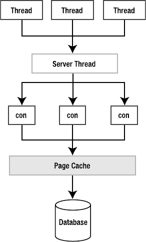
CHAPTER 6 ■ THE CORE C API 247
One other limitation that is somewhat thread-related pertains to the fork() system call on
Unix. You should never try to pass a connection across a fork() call to a child process. It will
not work correctly.
Shared Cache Mode
Starting with SQLite version 3.3.0, SQLite supports something called shared cache mode, which
allows multiple connections in a single thread to use a common page cache, as shown in
Figure 6-3. This feature is designed for embedded servers where a single thread can efficiently
manage multiple database connections on behalf of other threads. The connections in this case
share a single page cache as well as a different concurrency model. Because of the shared cache,
the server thread can operate with significantly lower memory usage and better concurrency
than if each thread were to manage its own connection. Normally, each connection allocates
enough memory to hold 2,000 pages in the page cache. Rather than each thread consuming that
much memory with its own connection, it shares that memory with other threads using a single
page cache.
In this model, threads rely on a server thread to manage their database connections for
them. A thread sends SQL statements to the server through some communication mechanism;
the server executes them using the thread’s assigned connection, and then sends the results
back. The thread can still issue commands and control its own transactions; only its actual
connection exists in, and is managed by, another thread.
Figure 6-3. The shared cache model
Owens_6730 C06.fm Page 247 Tuesday, April 18, 2006 7:09 AM
www.it-ebooks.info
248 CHAPTER 6 ■ THE CORE C API
Connections in shared cache mode use a different concurrency model and isolation level.
Connections in a shared cache are strictly limited to the thread that created them. They cannot
be passed around to other threads like normal connections can. Furthermore, connections in
a shared cache can see what their kindred connections have changed. That is, there can be
both multiple readers and an active writer in the database at the same time. That writer can
write to the database—performing complete write transactions—without having to wait for
other readers to clear. Therefore, data can change in the database within a reader’s transaction.
While SQLite normally runs in a serialized isolation level, meaning that readers and writers
always see a consistent view of the database, in shared cache mode, readers are subject to the
database changing underneath them.
There are some control measures in place to keep connections out of one another’s way.
By default, shared cache mode uses table locks to keep reader connections and writer connections
separated. Table locks are not the same as database locks, and exist only within connections of the
shared cache. Whenever a connection reads a table, SQLite first tries to get a read lock on it.
The same is true for writing to a table. A connection may not write to a table that another
connection has a read lock on, and vice versa. Furthermore, table locks are tied to their
respective connection and last for the duration of its transaction.
A Practical Example
To make all this clear, let’s go through an example. Say we have two threads, Thread A and
Thread B. These threads communicate with a server thread, which we will represent as the
program thread. Consider the first part of program in Listing 6-11, which represents the server
thread starting up.
Listing 6-11. Shared Cache Mode Example
int main(int argc, char **argv)
{
int rc, i, ncols;
sqlite3 *db1;
sqlite3 *db2;
sqlite3_stmt *stmt;
sqlite3_stmt *stmt2;
char *sql;
char *zErr;
const char *tail;
/* Enable shared cache mode */
sqlite3_enable_shared_cache(1);
It’s that simple. This program starts up and goes into shared cache mode by calling
sqlite3_enable_shared_cache(). This function takes a single integer argument where 0 turns
shared cache mode off for the thread, and any non-zero argument turns it on.
Owens_6730 C06.fm Page 248 Tuesday, April 18, 2006 7:09 AM
www.it-ebooks.info
CHAPTER 6 ■ THE CORE C API 249
Next it simulates receiving a request from Thread A, which wants to connect to the data-
base, query the episodes table, and put a cursor on the first row. This will get both a SHARED lock
on the database and a table lock on episodes. The code for this step is shown in Listing 6-12.
Listing 6-12. Thread A Initial Request
sqlite3_open("foods.db", &db1);
sqlite3_exec(db1, "BEGIN", NULL, NULL, &zErr);
fprintf(stderr, "Thread A: Connected\n");
fprintf(stderr, "Thread A: BEGIN TRANSACTION\n");
sql = "select * from episodes;";
rc = sqlite3_prepare(db1, sql, strlen(sql), &stmt, &tail);
rc = sqlite3_step(stmt);
/* Send row back to A and wait for further instructions */
fprintf(stderr, "Thread A: SHARED lock on database, table lock on episodes\n");
The server thread connects to the database, manually starts a transaction, runs a SELECT on
episodes, sits on the first record, and then pretends to send the first row back to Thread A.
Next, Thread B’s request comes in. It tries to delete any rows in foods by the name of
'Whataburger'. Next, it tries to insert a row with the name of 'Whataburger'. After that, in order
to illustrate table locks, it tries to insert a 'Whataburger' row into episodes, which shouldn’t
work. It then closes its connection and exits. The code for this step is listed in Listing 6-13.
Listing 6-13. Thread B Modifying the Database
/* Request comes in from Thread B. Modify the foods table in auto-commit. */
sqlite3_open("foods.db", &db2);
fprintf(stderr, "Thread B: Connected\n");
sql = "delete from foods where name='Whataburger'";
rc = sqlite3_exec(db2, sql, NULL, NULL, &zErr);
if(rc != SQLITE_OK) {
if (zErr != NULL) {
fprintf(stderr, "Thread B: SQL error: %s\n", zErr);
sqlite3_free(zErr);
}
}
else {
fprintf(stderr, "Thread B: TRANSACTION: ");
fprintf(stderr, "Deleted any Whataburger rows from foods\n");
}
Owens_6730 C06.fm Page 249 Tuesday, April 18, 2006 7:09 AM
www.it-ebooks.info
250 CHAPTER 6 ■ THE CORE C API
sql = "insert into foods values (NULL, 12, 'Whataburger')";
rc = sqlite3_exec(db2, sql, NULL, NULL, &zErr);
if(rc != SQLITE_OK) {
if (zErr != NULL) {
fprintf(stderr, "Thread B: SQL error: %s\n", zErr);
sqlite3_free(zErr);
}
}
else {
fprintf(stderr, "Thread B: TRANSACTION: ");
fprintf(stderr, "Inserted Whataburger row into foods\n");
}
/* Try to insert a record into episodes.
** This should not work b/c of Thread A's table lock. */
fprintf(stderr, "Thread B: Trying to insert Whataburger row into episodes\n");
sql = "insert into episodes values (NULL, 12, 'Whataburger')";
rc = sqlite3_exec(db2, sql, NULL, NULL, &zErr);
if(rc != SQLITE_OK) {
if (zErr != NULL) {
fprintf(stderr, "Thread B: SQL error: %s\n", zErr);
sqlite3_free(zErr);
}
}
else {
fprintf(stderr, "Thread B: Inserted Whataburger row into episodes\n");
}
sqlite3_close(db2);
fprintf(stderr, "Thread B: Disconnected\n");
Finally, Thread A finalizes its initial statement and searches for the row that Thread B
inserted into foods. The code for this step is shown in Listing 6-14.
Listing 6-14. Thread A Reading Thread B’s Modifications
/* Close the last statement and look for Thread B's row. */
sqlite3_finalize(stmt);
fprintf(stderr, "Thread A: Querying foods for Whataburger record\n");
sql = "select id as foo, type_id, name from foods where name='Whataburger'";
rc = sqlite3_prepare(db1, sql, strlen(sql), &stmt, &tail);
rc = sqlite3_step(stmt);
ncols = sqlite3_column_count(stmt);
Owens_6730 C06.fm Page 250 Tuesday, April 18, 2006 7:09 AM
www.it-ebooks.info

CHAPTER 6 ■ THE CORE C API 251
fprintf(stderr, "Thread A: Results: ");
for(i=0; i < ncols; i++) {
fprintf(stderr, "'%s' ", sqlite3_column_origin_name(stmt, i));
fprintf(stderr, "'%s' ", sqlite3_column_text(stmt, i));
}
fprintf(stderr, "\n", ncols);
sqlite3_finalize(stmt);
rc = sqlite3_exec(db1, "COMMIT", NULL, NULL, &zErr);
fprintf(stderr, "Thread A: COMMIT\n");
sqlite3_close(db1);
fprintf(stderr, "Thread A: Exiting\n", ncols);
Running the program produces the following results:
Thread A: Connected
Thread A: BEGIN TRANSACTION
Thread A: SHARED lock on database, table lock on episodes
Thread B: Connected
Thread B: TRANSACTION: Deleted any Whataburger rows from foods
Thread B: TRANSACTION: Inserted Whataburger row into foods
Thread B: Trying to insert Whataburger row into episodes
Thread B: SQL error: database table is locked: episodes
Thread B: Disconnected
Thread A: Querying foods for Whataburger record
Thread A: Results: 'id' '413' 'type_id' '12' 'name' 'Whataburger'
Thread A: COMMIT
Thread A: Exiting
So what happened? In shared cache mode, both threads worked concurrently in the same
database. Thread A got a table lock on episodes, and a SHARED lock on the database. Thread B
came along and modified foods. It did two full write transactions—DELETE and INSERT—on
foods in autocommit mode, each of which went all the way from UNLOCKED to EXCLUSIVE and
back to UNLOCKED. When each transaction completed, its associated table lock on foods was
released. Thread B couldn’t modify episodes, however, because of Thread A’s table lock. After
Thread B exited, Thread A could read from foods and see Thread B’s changes from within the
same transaction.
Read Uncommitted Isolation Level
While table locks help keep connections in shared cache mode out of one another’s way, it is
possible for connections to elect not to be in the way at all. That is, a connection can choose to
have a read-uncommitted isolation level by using the read_uncommitted pragma. If it is set to
true, then the connection will not put read locks on the tables it reads. Therefore, another
writer can actually change a table as the connection reads it. While this can lead to inconsistent
Owens_6730 C06.fm Page 251 Tuesday, April 18, 2006 7:09 AM
www.it-ebooks.info

252 CHAPTER 6 ■ THE CORE C API
query results, it also means that a connection in read-uncommitted mode can neither block
nor be blocked by any other connections.
It would be easy to modify the previous example to illustrate this kind of behavior. I will
simply paraphrase it; you can code it if you want to. In this case, Thread A would go into read-
committed isolation level, do a SELECT..ORDER BY id, and hold a cursor on the first row of
the result set. Then Thread B would delete the second row of episodes (id=2). Then you have
Thread A position its cursor to the next row and see that it is in fact is the third row in episodes
and not the second.
SCHEMA CHANGES IN SHARED CACHE MODE
There are additional things to consider in shared cache mode when a thread wants to modify the database schema.
As it turns out, before SQLite issues a table lock, it first gets a read table lock on the sqlite_master table.
In order for a thread to alter the schema, it must first get a write table lock on sqlite_master. It can only do
this if there are no read locks on it from other tables. When a thread does get a write lock on sqlite_master, then
no other threads are allowed to compile SQL statements during that time. They will get SQLITE_SCHEMA errors.
Threads and Memory Management
Since shared cache mode is about conserving memory, SQLite has several functions associated
with threads and memory management. They allow you to specify an advisory heap limit—a
soft heap limit—as well as manually initiate memory cleanups. These functions are as follows:
void sqlite3_soft_heap_limit(int N);
int sqlite3_release_memory(int N);
void sqlite3_thread_cleanup(void);
The sqlite3_soft_heap_limit() function sets the current soft heap limit of the calling
thread to N bytes. If the thread’s heap usage exceeds N, then SQLite automatically calls
sqlite3_release_memory(), which attempts to free at least N bytes of memory from the
caches of all database connections associated with the calling thread. The return value of
sqlite3_release_memory() is the number of bytes actually freed.
If you use it, you must also set sqlite3_soft_heap_limit() back to zero (the default) prior
to shutting down a thread or else it will leak memory. Alternatively, you can use
sqlite3_thread_cleanup(), which ensures that a thread has released any thread-local storage
it may have allocated. When the API is used properly, thread-local storage should be managed
automatically, and you shouldn’t need to call sqlite3_thread_cleanup(). However, it is provided
as a precaution and a potential work-around for future thread-related memory leaks.
These routines are only available if you have enabled memory management by compiling
SQLite with the SQLITE_ENABLE_MEMORY_MANAGEMENT preprocessor directive.
Owens_6730 C06.fm Page 252 Tuesday, April 18, 2006 7:09 AM
www.it-ebooks.info
CHAPTER 6 ■ THE CORE C API 253
Summary
The core C API contains everything you need to process SQL commands and then some. It
contains a variety of convenient query methods that are useful in different ways. These include
sqlite3_exec() and sqlite3_get_table(), which allow you to execute commands in a single
function call. The API includes many utility functions as well, allowing you to determine the
number of affected records in a query, get the last inserted ROWID of an INSERT statement, trace
SQL commands run on a connection, and conveniently format strings for SQL statements.
The sqlite3_prepare(), sqlite3_step(), and sqlite3_finalize() methods provide you
with a lot of flexibility and control over statement execution through the use of statement handles.
Statement handles provide more detailed row and column information, the convenience of
bound parameters, as well as the ability to reuse prepared statements, avoiding the overhead
of query compilation.
SQLite provides a variety of ways to manage runtime events through the use of event
filters. Its commit, rollback, and update hooks allow you to monitor and control specific changes
in database state. You can watch changes to rows and columns as they happen, and use an
authorizer function to monitor and restrict what queries can do as they are compiled.
SQLite has support for threads as well, and offers a higher concurrency model for multi-
threaded environments through the use of shared cache mode. This mode enables connections
created by a single thread to share a common page cache, allowing the program to be more
memory efficient. Furthermore, it is possible for multiple readers and one writer to work in the
same database at the same time.
And believe it or not, you’ve only seen half of the API! Actually, you’ve seen more like
three-quarters, but you are likely to find that what is in the next chapter—user-defined func-
tions, aggregates, and collations—is every bit as useful and interesting as what is in this one.
Owens_6730 C06.fm Page 253 Tuesday, April 18, 2006 7:09 AM
www.it-ebooks.info

255
■ ■ ■
CHAPTER 7
The Extension C API
This chapter is about teaching SQLite new tricks. The previous chapter dealt with generic
database work; this chapter is about being creative. The latter half of the API—the Extension
API—offers three basic ways to extend (or customize) SQLite, through the creation of user-
defined functions, aggregates, and collation sequences.
User-defined functions are SQL functions that map to some implementation that you write.
They are callable from within SQL. For example, you could create a function hello_newman()
that returns the string 'Hello Jerry' and, once it is registered, call it from SQL as follows:
sqlite > select hello_newman() as reply;
reply
------------------
'Hello Jerry'
This is a special version of the SQLite command-line program I customized myself that includes
hello_newman(). When I get bored, I call it occasionally.
Aggregates are a special form of function and work in much the same way except that they
operate on sets of records and return aggregated values or expressions computed over a partic-
ular column in the set. Or they may be computed from multiple columns. Standard aggregates
that are built into SQLite include SUM(), COUNT(), and AVG(), for example.
Collations are methods of comparing and sorting text. That is, given two strings, a Collation
would decide which one is greater, or whether the two are equal. The default Collation in SQLite
is BINARY—it compares strings byte by byte using memcmp(). While this collation happens to work
well for words in the English language (and other languages that use UTF-8 encoding), it
doesn’t necessarily work so well for other languages that use different encodings. This is why
SQLite version 3 introduced user-defined collations.
This chapter covers each of these three user-defined extension facilities and their associ-
ated API functions. As you will see, when combined with other facilities such as triggers and
conflict resolution, the user-defined extensions API can prove to be a powerful tool for creating
nontrivial features that extend SQLite.
All of the code in this chapter is included in examples that you can obtain online from the
Apress website (www.apress.com). The examples for this particular chapter are located in the
ch7 subdirectory of the examples folder. I will specifically point out all the source files corre-
sponding to the examples as they are introduced in the text. Some of the error-checking code
in the figures has been taken out for the sake of clarity.
Owens_6730 C07.fm Page 255 Tuesday, April 18, 2006 2:16 PM
www.it-ebooks.info
256 CHAPTER 7 ■ THE EXTENSION C API
Also, many examples in this chapter use simple convenience functions from a common
library I wrote that helps simplify the examples. I will point out these functions and explain
what they do as they are introduced in the text. The common code is located in the common
subdirectory of the examples folder, and must first be built before the examples are built. Please
refer to the README file in the examples folder for details on building the common library.
Finally, to clear up any confusion, the terms storage class and data type are interchangeable.
You know that SQLite stores data internally using five different data types, or storage classes.
These classes are INTEGER, FLOAT, TEXT, BLOB, and NULL, as described in Chapter 4. Throughout
the chapter, I try to use the term that best fits the context. When speaking generally, I use the
term data type, as it seems the most appropriate. When speaking about how SQLite handles a
specific value internally, I find that the term storage class seems to work better. In either case,
you can equate either term as describing a specific form or representation of data.
The API
The basic method for implementing functions, aggregates, and collations consists of imple-
menting a callback function and then registering it in your program. Once registered, they can
be used from SQL. Functions and aggregates use the same registration function and similar
callback functions. Collation sequences, while using a separate registration function, are
almost identical and can be thought of as a particular class of user-defined function.
The lifetime of user-defined aggregates, functions, and collations is transient. They are
registered on a connection-by-connection basis; they are not stored in the database. It is up to
you to ensure that your application loads your custom extensions and registers them on each
connection. Sometimes you may find yourself thinking of your extensions in terms of stored
procedures and completely forget about the fact that they don’t actually reside in the database.
Extensions exist in libraries, not in databases, and are restricted to the life of your program. If
you don’t grasp this concept, you may do something like try to create a trigger (which is stored
in the database) that references your extensions (which aren’t stored in the database) and then
turn around and try to call it from the SQLite shell or from an application that knows nothing
of your extensions. In this case, you will find that either it triggers an error or nothing happens.
Extensions require your program to register them on each and every connection; otherwise,
that connection’s SQL syntax will know nothing about them.
Registering Functions
That said, you can register functions and aggregates on a connection using the
sqlite3_create_function(), which is declared as follows:
int sqlite3_create_function(
sqlite3 *cnx, /* connection handle */
const char *zFunctionName, /* function/aggregate name in SQL */
int nArg, /* number of arguments. -1 = unlimited. */
int eTextRep, /* encoding (UTF8, 16, etc.) */
void *pUserData, /* application data, passed to callback */
void (*xFunc)(sqlite3_context*,int,sqlite3_value**),
void (*xStep)(sqlite3_context*,int,sqlite3_value**),
void (*xFinal)(sqlite3_context*)
);
Owens_6730 C07.fm Page 256 Tuesday, April 18, 2006 2:16 PM
www.it-ebooks.info
CHAPTER 7 ■ THE EXTENSION C API 257
int sqlite3_create_function16(
sqlite3 *cnx,
const void *zFunctionName,
int nArg,
int eTextRep,
void *pUserData,
void (*xFunc)(sqlite3_context*, int args, sqlite3_value**),
void (*xStep)(sqlite3_context*, int args, sqlite3_value**),
void (*xFinal)(sqlite3_context*)
);
As in the previous chapter, I have included both the UTF-8 and UTF-16 versions of this
function to underscore the fact that the SQLite API has functions that support both encodings.
However, from now on, I will only refer to the UTF-8 versions for the sake of brevity.
The arguments for sqlite3_create_function() are defined as follows:
•cnx: The connection handle. Functions and aggregates are connection specific. They
must be registered on the connection as it is opened in order to be used.
•zFunctionName: The function name as it will be called in SQL.
•nArg: The number of arguments required by the function. SQLite will enforce this as
the exact number of arguments that must be provided to the function. However, if you
specify -1 for this value, SQLite will allow a variable number of arguments.
•eTextRep: The encoding. Allowable values are SQLITE_UTF8, SQLITE_UTF16, SQLITE_UTF16BE,
SQLITE_UTF16LE, and SQLITE_ANY. SQLITE_ANY is for a single function implementation that
can negotiate any kind of text representation provided.
•pUserData: Application-specific data. This data is made available through the callback
functions specified in xFunc, xStep, and xFinal. Unlike other functions, which receive
the data as a void pointer in the argument list, these functions must use a special API
function to obtain this data
•xFunc: The function callback. This is the actual implementation of the SQL function.
Functions only provide this callback and leave the xStep and xFinal function pointers
NULL. These latter two callbacks are exclusively for aggregate implementations.
•xStep: The aggregate step function. Each time SQLite processes a row in an aggregated
result set, it calls xStep to allow the aggregate to process the relevant field value(s) of that
row and include the result in its aggregate computation.
•xFinal: The aggregate finalize function. When all rows have been processed, SQLite calls
this function to allow the aggregate to conclude its processing, which usually consists of
computing the final value and optionally cleaning up.
With regard to encoding, you can register multiple versions of the same function differing only
in the encoding (eTextRep argument) and SQLite will automatically select the best version of
the function for the case in hand.
Owens_6730 C07.fm Page 257 Tuesday, April 18, 2006 2:16 PM
www.it-ebooks.info

258 CHAPTER 7 ■ THE EXTENSION C API
The Step Function
The function and aggregate step functions are identical, and are declared as
void fn(sqlite3_context* ctx, int nargs, sqlite3_value** values)
The ctx argument is the function/aggregate context. It holds state for a particular function
call instance and is the means through which you obtain the application data (pUserData) argu-
ment provided in sqlite3_create_function(). The user data is obtained from the context using
sqlite3_user_data(), which is declared as follows:
void *sqlite3_user_data(sqlite3_context*);
For functions, this data is shared among all calls to like functions, so it is not really unique to a
particular instance of function call. That is, the same pUserData is passed or shared among all
instances of a given function. Aggregates, however, can allocate their own state for each particular
instance using sqlite3_aggregate_context(), declared as follows:
void *sqlite3_aggregate_context(sqlite3_context*, int nBytes);
The first time this routine is called for a particular aggregate, a chunk of memory of size
nBytes is allocated, zeroed, and associated with that context. On subsequent calls with the
same context (for the same aggregate instance), this allocated memory is returned. Using this,
aggregates have a way to store state in between calls in order to accumulate data. When the
aggregate completes the final() callback, the memory is automatically freed by SQLite.
■Note One of the things you will see throughout the API is the use of user data in void pointers. Since many
parts of the API involve callback functions, these simply serve as a convenience to help you maintain state
when implementing said callback functions.
The nargs argument of the callback function contains the number of arguments passed to
the function.
Return Values
The values argument is an array of SQLite value structures that are handles to the
actual argument values. The actual data for these values is obtained using the family of
sqlite3_value_xxx() functions, which have the following form:
xxx sqlite3_value_xxx(sqlite3_value* value);
where xxx is the C data type to be returned from the value argument. If you read Chapter 6, you
may be thinking that these functions have a striking resemblance to the sqlite3_column_xxx()
family of functions—and you’d be right. They work in exactly the same way, even down to the
difference between the way scalar and array values are obtained. The functions for obtaining
scalar values are as follows:
Owens_6730 C07.fm Page 258 Tuesday, April 18, 2006 2:16 PM
www.it-ebooks.info
CHAPTER 7 ■ THE EXTENSION C API 259
int sqlite3_value_int(sqlite3_value*);
long long int sqlite3_value_int64(sqlite3_value*);
double sqlite3_value_double(sqlite3_value*);
The functions used to obtain array values are as follows:
int sqlite3_value_bytes(sqlite3_value*);
const void *sqlite3_value_blob(sqlite3_value*);
const unsigned char *sqlite3_value_text(sqlite3_value*);
The sqlite3_value_bytes() function returns the amount of data in the value buffer for a BLOB. The
sqlite3_value_blob() function returns a pointer to that data. Using the size and the pointer,
you can then copy out the data. For example, if the first argument in your function was a BLOB,
and you wanted to make a copy, you would do something like this:
int len;
void* data;
len = sqlite3_value_bytes(values[0]);
data = malloc(len);
memcpy(data, sqlite3_value_blob(values[0]), len);
Just as the sqlite3_column_xxx() functions have sqlite_column_type() to provide the
column types, the sqlite3_value_xxx() functions likewise have sqlite3_value_type(), which
works in the same way. It is declared as follows:
int sqlite3_value_type(sqlite3_value*);
This function returns one of the following values, which correspond to SQLite’s internal, storage
classes (data types), defined as
#define SQLITE_INTEGER 1
#define SQLITE_FLOAT 2
#define SQLITE_TEXT 3
#define SQLITE_BLOB 4
#define SQLITE_NULL 5
This covers the basic workings of the function/aggregate interface. We can now dive
into some examples and even a few practical applications. The Collation interface is so similar
that rather than previewing it here, we will just address it in full after we cover functions and
aggregates.
Functions
Let’s start with a trivial example, one that is very easy to follow. Let’s implement hello_newman(),
but with a slight twist. I want to include using function arguments in the example, so
hello_newman() will take one argument: the name of the person addressing him. It will thus
work as follows:
Owens_6730 C07.fm Page 259 Tuesday, April 18, 2006 2:16 PM
www.it-ebooks.info
260 CHAPTER 7 ■ THE EXTENSION C API
sqlite > select hello_newman('Jerry') as reply;
reply
------------------
Hello Jerry
sqlite > select hello_newman('Kramer') as reply;
reply
------------------
Hello Kramer
sqlite > select hello_newman('George') as reply;
reply
------------------
Hello George
The basic program (taken from hello_newman.c) is shown in Listing 7-1. Some of the error-
checking code has been removed for clarity.
Listing 7-1. The hello_newman() Test Program
int main(int argc, char **argv)
{
int rc; sqlite3 *db;
sqlite3_open("test.db", &db);
sqlite3_create_function( db, "hello_newman", 1, SQLITE_UTF8, NULL,
hello_newman, NULL, NULL);
/* Log SQL as it is executed. */
log_sql(db,1);
/* Call function with one text argument. */
fprintf(stdout, "Calling with one argument.\n");
print_sql_result(db, "select hello_newman('Jerry')");
/* Call function with two arguments. This will fail as we registered the
** function as taking only one argument. */
fprintf(stdout, "\nCalling with two arguments.\n");
print_sql_result(db, "select hello_newman ('Jerry', 'Elaine')");
/* Call function with no arguments. This will fail too */
fprintf(stdout, "\nCalling with no arguments.\n");
print_sql_result(db, "select hello_newman()");
/* Done */
sqlite3_close(db);
return 0;
}
Owens_6730 C07.fm Page 260 Tuesday, April 18, 2006 2:16 PM
www.it-ebooks.info

CHAPTER 7 ■ THE EXTENSION C API 261
This program connects to the database, registers the function, and then calls it three times.
The callback function is implemented as follows:
void hello_newman(sqlite3_context* ctx, int nargs, sqlite3_value** values)
{
const char *msg;
/* Generate Newman's reply */
msg = sqlite3_mprintf("Hello %s", sqlite3_value_text(values[0]));
/* Set the return value. Have sqlite clean up msg w/ sqlite_free(). */
sqlite3_result_text(ctx, msg, strlen(msg), sqlite3_free);
}
Running the program yields the following output:
Calling with one argument.
TRACE: select hello_newman('Jerry')
hello_newman('Jerry')
---------------------
Hello Jerry
Calling with two arguments.
execute() Error: wrong number of arguments to function hello_newman()
Calling with no arguments.
execute() Error: wrong number of arguments to function hello_newman()
The first call consists of just one argument. Since the example registered the function as taking
exactly one argument, it succeeds. The second call attempts to use two arguments, which fails.
The third call uses no arguments, and also fails.
And there you have it: a SQLite extension function. This does bring up a few new functions
that I have not addressed yet. The first few functions are specific to the common code. The function
log_sql() simply calls sqlite3_trace(), passing in a tracing function that prefixes the traced
SQL with the word TRACE. I use this so you can see what is happening in the example as the SQL
is executed. The second function is print_sql_result(), which has the following declaration:
int print_sql_result(sqlite3 *db, const char* sql, ...)
This is a simple wrapper around sqlite3_prepare() and friends that executes a SQL statement
and prints the results.
Owens_6730 C07.fm Page 261 Tuesday, April 18, 2006 2:16 PM
www.it-ebooks.info
262 CHAPTER 7 ■ THE EXTENSION C API
Return Values
This example introduces a new SQLite function: sqlite3_result_text().This function is just
one of a family of sqlite_result_xxx() functions used to set return values for user-defined
functions and aggregates. The scalar functions are as follows:
void sqlite3_result_double(sqlite3_context*, double);
void sqlite3_result_int(sqlite3_context*, int);
void sqlite3_result_int64(sqlite3_context*, long long int);
void sqlite3_result_null(sqlite3_context*);
These functions simply take a (second) argument of the type specified in the function name
and set it as the return value of the function. The array functions are
void sqlite3_result_text(sqlite3_context*, const char*, int n, void(*)(void*));
void sqlite3_result_blob(sqlite3_context*, const void*, int n, void(*)(void*));
These functions take array data and set that data as the return value for the function. They have
the general form
void sqlite3_result_xxx(
sqlite3_context *ctx, /* function context */
const xxx* value, /* array value */
int len, /* array length */
void(*free)(void*)); /* array cleanup function */
Here xxx is the particular array type—void for BLOBs or char for TEXT. Again, if you read
Chapter 6, you may find these functions suspiciously similar to the sqlite3_bind_xxx() functions,
which they are. Setting a return value for a function is, for all intents and purposes, identical
to binding a value to a parameterized SQL statement. You could even perhaps refer to it as
“binding a return value.”
Arrays and Cleanup Handlers
Just as in binding array values to SQL statements, these functions work in the same way as
sqlite3_bind_xxx(). They require a pointer to the array, the length (or size) of the array, and
a function pointer to a cleanup function. This cleanup function pointer can be assigned the
same predefined meanings as in sqlite3_bind_xxx():
#define SQLITE_STATIC ((void(*)(void *))0)
#define SQLITE_TRANSIENT ((void(*)(void *))-1)
SQLITE_STATIC means that the array memory resides in unmanaged space, and therefore
SQLite should not attempt to clean it up. SQLITE_TRANSIENT tells SQLite that the array data is
subject to change, and therefore SQLite needs to make its own copy. In this case, SQLite will
copy the data and free it after the function returns. The third option is to pass in an actual function
pointer to a cleanup function of the form
void cleanup(void*);
Owens_6730 C07.fm Page 262 Tuesday, April 18, 2006 2:16 PM
www.it-ebooks.info
CHAPTER 7 ■ THE EXTENSION C API 263
In this case, SQLite will call the cleanup function after the user-defined function completes.
This is the method used in the previous example: I used sqlite3_mprintf() to generate Newman’s
reply, which allocated a string on the heap. I then passed in sqlite3_free() as the cleanup
function to sqlite3_result_text(), which could free the string memory when the extension
function completed.
Error Conditions
Sometimes functions encounter errors, in which case the return value should be set appropriately.
This is what sqlite3_result_error() is for. It is declared as follows:
void sqlite3_result_error(
sqlite3_context *ctx, /* the function context */
const char *msg, /* the error message */
int len); /* length of the error message */
This tells SQLite that there was an error, the details of which are contained in msg. SQLite will
abort the command that called the function and set the error message to the value contained
in msg.
Returning Input Values
Sometimes, you may want to pass back an argument as the return value in the exact same form.
Rather than your having to determine the argument’s type, extract its value with the corre-
sponding sqlite3_column_xxx() function, and then turn right around and set the return value
with the appropriate sqlite3_result_xxx() function, the API offers sqlite3_result_value() so
you can do all of this in one fell swoop. It is declared as follows:
void sqlite3_result_value(
sqlite3_context *ctx, /* the function context */
sqlite3_value* value); /* the argument value */
For example, say you wanted to create a function echo() that spits back its first argument.
The implementation is as follows:
void echo(sqlite3_context* ctx, int nargs, sqlite3_value** values)
{
sqlite3_result_value(ctx, values[0]);
}
It would work from SQL as follows:
sqlite > select echo('Hello Jerry') as reply;
reply
------------------
Hello Jerry
Even better, echo() works equally well with arguments of any storage class, and returns them
accordingly:
Owens_6730 C07.fm Page 263 Tuesday, April 18, 2006 2:16 PM
www.it-ebooks.info
264 CHAPTER 7 ■ THE EXTENSION C API
sqlite> select echo(3.14) as reply, typeof(echo(3.14)) as type;
reply type
---------- ----------
3.14 real
sqlite> select echo(X'0128') as reply, typeof(echo(X'0128')) as type;
reply type
---------- ----------
(? blob
sqlite> select echo(NULL) as reply, typeof(echo(NULL)) as type;
reply type
---------- ----------
null
A Complete Example
Let’s move on to a complete example that uses most of the API functions described earlier. This
will give you a better feel for all that is available to you in one place. We will implement a function
called function(), which takes a variable number of arguments. It will print the argument types
and return an integer value. If, however, the first argument is the string value 'fail', it will call
the error handler, returning an error message.
The main function, shown in Listing 7-2, is much the same as the previous example (the
complete example is located in func.c). Again, some of the error handling has been excised for
clarity.
Listing 7-2. The main Function
int main(int argc, char **argv)
{
int rc;
sqlite3 *db;
const char* sql;
sqlite3_open("test.db", &db);
sqlite3_create_function( db, "function", -1, SQLITE_UTF8, NULL,
function, NULL, NULL);
/* Turn on SQL logging */
log_sql(db, 1);
/* Call function with one text argument. */
execute(db, "select function(1)");
/* Call function with several arguments of various types. */
execute(db, "select function(1, 2.71828)");
Owens_6730 C07.fm Page 264 Tuesday, April 18, 2006 2:16 PM
www.it-ebooks.info
CHAPTER 7 ■ THE EXTENSION C API 265
/* Call function with variable arguments, the first argument's value
** being 'fail'. This will trigger the function to call
** sqlite3_result_error(). */
execute(db, "select function('fail', 1, 2.71828, 'three', X'0004', NULL)");
/* Done */
sqlite3_close(db);
return 0;
}
Note the -1 value for the nArg argument in sqlite3_create_function(). This corresponds
to the number of required arguments that must be provided to the function. Using -1 tells SQLite
that the function accepts a variable number of arguments. Note that there is a new convenience
function here called execute(). This is just a thin wrapper around sqlite3_exec() that executes a
SQL command and reports any errors to standard error, if any. It was listed in Chapter 6 and is
part of the common library. The function’s implementation is shown in Listing 7-3.
Listing 7-3. A Vanilla User-Defined Function
void function(sqlite3_context* ctx, int nargs, sqlite3_value** values)
{
int i; const char *msg;
fprintf(stdout, "function() : Called with %i arguments\n", nargs);
for(i=0; i < nargs; i++) {
fprintf( stdout, " arg %i: value=%-7s type=%i\n", i,
sqlite3_value_text(values[i]),
sqlite3_value_type(values[i]));
}
if(strcmp(sqlite3_value_text(values[0]), "fail") == 0) {
msg = "function() : Failing because you told me to.";
sqlite3_result_error(ctx, msg, strlen(msg));
fprintf(stdout, "\n");
return;
}
fprintf(stdout, "\n");
sqlite3_result_int(ctx, 0);
}
Running the program produces the following output:
Owens_6730 C07.fm Page 265 Tuesday, April 18, 2006 2:16 PM
www.it-ebooks.info

266 CHAPTER 7 ■ THE EXTENSION C API
TRACE: select function(1)
function() : Called with 1 arguments
arg 0: value=1 type=1
TRACE: select function(1, 2.71828)
function() : Called with 2 arguments
arg 0: value=1 type=1
arg 1: value=2.71828 type=2
TRACE: select function('fail', 1, 2.71828, 'three', X'0004', NULL)
function() : Called with 6 arguments
arg 0: value=fail type=3
arg 1: value=1 type=1
arg 2: value=2.71828 type=2
arg 3: value=three type=3
arg 4: value= type=4
arg 5: value=(null) type=5
execute() Error: function() : Failing because you told me to.
First, we can see that SQLite classifies the values provided as arguments into five possible
data types or storage classes. These possible types correspond to SQLite’s five internal data
types, which, again, are defined as
#define SQLITE_INTEGER 1
#define SQLITE_FLOAT 2
#define SQLITE_TEXT 3
#define SQLITE_BLOB 4
#define SQLITE_NULL 5
Each call passes in an increasing number of arguments and types to illustrate this. In the
final call to function(), one of each storage class is passed in as an argument, and the function’s
output confirms that SQLite has typed them accordingly. Note that the X'0004' is an example
of SQLite’s string representation for binary data. The X (which is case insensitive) followed by
hexadecimal values delimited by single quotes denotes binary data (a BLOB representation).
The first thing to notice in this example is that the function API provides a way to determine
the number of arguments passed to a function, their respective storage classes, and their values.
Second, the function API provides a way to fetch argument values according to their storage
class, if so desired. Since all storages classes have respective text representations—even binary
data—you can always count on being able to get function arguments in text form, regardless of
their internal representation.
Finally, just as you can receive values in their native storage class, you can also return them
that way. One special case of return value is the error return value, which is always in text form,
and causes the SQL command calling it to fail.
Owens_6730 C07.fm Page 266 Tuesday, April 18, 2006 2:16 PM
www.it-ebooks.info
CHAPTER 7 ■ THE EXTENSION C API 267
A Practical Application
Now let’s move on to a real application of user-defined functions. In the introduction I made
the claim that when combined with other SQLite features such as triggers, user-defined exten-
sions can be quite a powerful tool. By design, SQLite uses manifest typing, which in many cases
is very useful and convenient. But what if there are some critical columns in a table for which
you just have to have strict typing? You might have an integer column that must always hold
only integer values. No inserts or updates should be allowed to put any other kind of data type
into this column.
In this example (strict_typing.c), we will combine user-defined functions with triggers
to implement strict typing in SQLite. Furthermore, we will be able to apply this strict typing to
entire tables, if so desired, and for an unlimited number of data types (that is, even for data
types that SQLite knows nothing about). All that is required is that we implement validation
functions for each respective data type that is to be enforced under the strict typing policy.
To start with, say we have a table episodes, defined as follows:
create table episodes (
id integer primary key,
cid integer not null default 0, -- main character id
name text, -- episode name
rating float not null default 0 –- scale 1-10 );
The cid column is the main character ID, which corresponds to the id column in the character
table, which is defined as follows:
create table characters (
id integer primary key, -- character id
name text -- character name );
We can infer from these tables that the episodes.cid column should always be an integer.
Furthermore, we want to enforce this in our application. We know that in order to do this, we
have to be able to control INSERT and UPDATE operations that target this column.
Validation Triggers
This is where triggers come in. We will define two triggers to do this, shown in Listing 7-4.
Listing 7-4. Validation Triggers
/-- INSERT trigger
CREATE TRIGGER episodes_insert_cid_typecheck_tr
BEFORE INSERT ON episodes
BEGIN
SELECT CASE
WHEN(SELECT validate_int(new.cid) != 1)
THEN RAISE(ABORT, 'invalid int value for episodes.cid ')
END;
END;
Owens_6730 C07.fm Page 267 Tuesday, April 18, 2006 2:16 PM
www.it-ebooks.info

268 CHAPTER 7 ■ THE EXTENSION C API
CREATE TRIGGER episodes_update_cid_typecheck_tr
BEFORE UPDATE OF cid ON episodes
FOR EACH ROW BEGIN
SELECT CASE
WHEN(SELECT validate_int(new.cid) != 1)
THEN RAISE(ABORT, 'invalid int value for episodes.cid ')
END;
END;
Thus, each UPDATE and INSERT on the episodes table will fire a before trigger, which will take
the proposed cid value being submitted and call validate_int()—a user-defined function that
simply tests whether a value (provided as the single argument) is in fact an integer. If the value
is an integer, validate_int() returns true (1); otherwise, it returns false (0). The trigger evaluates
the returned value in the WHEN clause and if it is not true, the trigger raises an abort. Therefore,
only integer values can pass through the trigger and therefore all INSERTs and UPDATEs are only
allowed to provide integer values to episodes.cid, giving us strict typing for this column.
■Note This implementation makes an assumption you should be aware of. It assumes that INSERT state-
ments always provide a value for the column to be validated. In this example, it assumes that all INSERT
statements will always provide a value for cid. If one is not provided, the trigger will fail. To get around this,
simply provide a default value for the column in the table definition so that a suitable value will be provided
for INSERT statements that don’t provide a cid value. If you notice, the definition for cid in this example
is cid integer not null default 0. Another thing to remember is that while INSERT triggers can
only be defined for entire records, UPDATE triggers can be defined for specific columns, so they do not have
this problem.
The Validation Function
The validate_int() function is quite simple. It is shown in Listing 7-5.
Listing 7-5. The validate_int() Validation Function
void validate_int_udf(sqlite3_context* ctx, int nargs, sqlite3_value** values)
{
sqlite3 *db;
const char *value;
char *tmp;
db = (sqlite3*)sqlite3_user_data(ctx);
value = sqlite3_value_text(values[0]);
/* Assume NULL values for type-checked columns are not allowed */
if(value == NULL) {
sqlite3_result_int(ctx, 0);
return;
}
Owens_6730 C07.fm Page 268 Tuesday, April 18, 2006 2:16 PM
www.it-ebooks.info
CHAPTER 7 ■ THE EXTENSION C API 269
/* Validate */
tmp = NULL;
strtol(value, &tmp, 0);
if(*tmp != '\0') {
/* Value does not conform to type */
sqlite3_result_int(ctx, 0);
return;
}
/* If we got this far, the value is valid. */
sqlite3_result_int(ctx, 1);
}
It just uses strtol() to look for errors in the conversion. The actual implementation is
arbitrary. You can create whatever criteria you want to validate an integer value. Using this
function as a template, you can create user-defined functions for any data type—float, double,
varchar, date, timestamp, whatever you like. They only differ in how they test the input value for
validity. This example uses three general data type tests for integer, float, and text values. It
then registers them under various SQL function names:
/* Type Validation: Called to validate text. */
sqlite3_create_function( db, "validate_text", 1, SQLITE_UTF8, db,
validate_text_udf, NULL, NULL);
/* Type Validation: Called to validate integer. */
sqlite3_create_function( db, "validate_int", 1, SQLITE_UTF8, db,
validate_int_udf, NULL, NULL);
/* Type Validation: Called to validate long integer. Same UDF as above,
* different SQL function name. */
sqlite3_create_function( db, "validate_long", 1, SQLITE_UTF8, db,
validate_int_udf, NULL, NULL);
/* Type Validation: Called to validate double. */
sqlite3_create_function( db, "validate_double", 1, SQLITE_UTF8, db,
validate_double_udf, NULL, NULL);
/* Type Validation: Called to validate float. Same UDF as above,
* different SQL function name. */
sqlite3_create_function( db, "validate_float", 1, SQLITE_UTF8, db,
validate_double_udf, NULL,
Both the validate_int() and validate_long() SQL functions map to the same validate_int_udf()
callback function. Their validity test is the same, so why write two callback functions to do the
same thing? Likewise, the validate_float() and validate_double() SQL functions call the same
validate_double_udf() callback function to validate their respective values.
Owens_6730 C07.fm Page 269 Tuesday, April 18, 2006 2:16 PM
www.it-ebooks.info
270 CHAPTER 7 ■ THE EXTENSION C API
Installation Functions
So far, so good. Before creating a test program, let’s take the example a step further. Instead of
having to write and maintain our own triggers for each column we want to control, let’s write
another user-defined function to do it for us. Actually, we need two such functions: one to create
the triggers and one to remove them (in case we don’t want type checking any more on a given
column). The callback function to add the triggers is called add_strict_type_check_udf(). Its
corresponding SQL function is called add_strict_type_check(). The callback function is
implemented as shown in Listing 7-6.
Listing 7-6. The strict_type_check() User-Defined Function
void add_strict_type_check_udf( sqlite3_context* ctx, int nargs,
sqlite3_value** values )
{
sqlite3 *db; sqlite3_stmt *stmt;
int rc;
const char *table, *column, *sql, *tmp, *tail, *err;
db=(sqlite3*)sqlite3_user_data(ctx);
table = sqlite3_value_text(values[0]);
column = sqlite3_value_text(values[1]);
/* If the column name is an asterisk */
if(strncmp(column,"*",1) == 0) {
/* Install type checking on all columns */
sql = "pragma table_info(%s)";
tmp = sqlite3_mprintf(sql, table);
rc = sqlite3_prepare(db, tmp, strlen(tmp), &stmt, &tail);
sqlite3_free((void*)tmp);
if(rc != SQLITE_OK) {
err = sqlite3_errmsg(db);
sqlite3_result_error(ctx, err, strlen(err));
}
rc = sqlite3_step(stmt);
while(rc == SQLITE_ROW) {
/* If not primary key */
if(sqlite3_column_int(stmt, 5) != 1) {
column = sqlite3_column_text(stmt, 1);
install_type_trigger(db, ctx, table, column);
}
Owens_6730 C07.fm Page 270 Tuesday, April 18, 2006 2:16 PM
www.it-ebooks.info
CHAPTER 7 ■ THE EXTENSION C API 271
rc = sqlite3_step(stmt);
}
sqlite3_finalize(stmt);
}
else {
/* Column name specified, just install on that one column. */
if(install_type_trigger(db, ctx, table, column) != 0) {
return;
}
}
sqlite3_result_int(ctx, 0);
}
This function installs triggers on either all columns or on a single column specified by
column. If the value passed in column is an asterisk (*), it installs the triggers on all columns in
the table (with the exception of the primary key column), using PRAGMA table_info() to obtain
column information. Whether one or many columns, the real work is ultimately passed on to a
helper function install_type_trigger(), which does the trigger installation. It is shown in
Listing 7-7.
Listing 7-7. The Trigger Installation Helper Function
int install_type_trigger( sqlite3* db, sqlite3_context* ctx,
const char* table, const char* column )
{
int rc;
char buf[256];
char *tmp;
const char *type, *sql, *emsg;
char* err;
/* Get the column's declared type */
type = column_type(db, table, column);
/* Check to see if corresponding validation function exists */
sql = "select validate_%s(null)";
tmp = sqlite3_mprintf(sql, type);
rc = sqlite3_exec(db, tmp, NULL, NULL, &err);
sqlite3_free(tmp);
if(rc != SQLITE_OK && err != NULL) {
emsg = "No validator exists for column type";
sqlite3_result_error(ctx, emsg, strlen(emsg));
sqlite3_free((void*)type);
Owens_6730 C07.fm Page 271 Tuesday, April 18, 2006 2:16 PM
www.it-ebooks.info
272 CHAPTER 7 ■ THE EXTENSION C API
sqlite3_free(err);
return 1;
}
/* Create INSERT trigger */
sql = "CREATE TRIGGER %s_insert_%s_typecheck_tr \n"
"BEFORE INSERT ON %s \n"
"BEGIN \n"
" SELECT CASE \n"
" WHEN(SELECT validate_%s(new.%s) != 1) \n"
" THEN RAISE(ABORT, 'invalid %s value for %s.%s') \n"
" END; \n"
"END;";
tmp = sqlite3_mprintf(sql, table, column, table, type,
column, type, table, column);
rc = sqlite3_exec(db, tmp, NULL, NULL, &err);
sqlite3_free(tmp);
if(rc != SQLITE_OK && err != NULL) {
strncpy(&buf[0], err, 255);
buf[256] = '\0';
sqlite3_result_error(ctx, &buf[0], strlen(&buf[0]));
sqlite3_free((void*)type);
return 1;
}
/* Create UPDATE trigger */
sql = "CREATE TRIGGER %s_update_%s_typecheck_tr \n"
"BEFORE UPDATE OF %s ON %s \n"
"FOR EACH ROW BEGIN \n"
" SELECT CASE \n"
" WHEN(SELECT validate_%s(new.%s) != 1) \n"
" THEN RAISE(ABORT, 'invalid %s value for %s.%s') \n"
" END; \n"
"END;";
tmp = sqlite3_mprintf(sql, table, column, column, table,
type, column, type, table, column);
rc = sqlite3_exec(db, tmp, NULL, NULL, &err);
sqlite3_free(tmp);
sqlite3_free((void*)type);
Owens_6730 C07.fm Page 272 Tuesday, April 18, 2006 2:16 PM
www.it-ebooks.info
CHAPTER 7 ■ THE EXTENSION C API 273
if(rc != SQLITE_OK && err != NULL) {
strncpy(&buf[0], err, 255);
buf[256] = '\0';
sqlite3_result_error(ctx, &buf[0], strlen(&buf[0]));
sqlite3_free(err);
return 1;
}
return 0;
}
As stated, this function does all the real work. First, it gets the column’s declared type
through another user-defined function column_type(), which in turn just prepares a query
with the given column and uses sqlite3_column_decltype() to fetch its declared type. With the
type, install_type_trigger() assumes that all validation functions will follow the naming
convention validate_xxx(), where xxx is the data type to be validated. If, for example, the
column’s declared type is int, install_type_trigger() tests for the existence of the respective
validation function by executing the query
select validate_int(1);
Exactly one of two things can happen here: the query will fail or succeed. It can only fail if the
function does not exist. It doesn’t matter if the argument 1 is of the correct type; even if the
validate_int() function exists, it will return false (0) and the query will still succeed as the
query constitutes as a valid SQL statement. That is, sqlite3_exec() will return SQLITE_OK if
validate_int() exists. Otherwise, it will return an error. That is all it needs—a test for existence
that answers the question: has a validate_xxx() user-defined function been registered? Yes or
no? If the validation function exists, install_type_trigger() proceeds to build the trigger
statements (as illustrated earlier) and runs them.
Likewise, the user-defined function to remove the triggers is called
drop_strict_type_check_udf(), and works in exactly the same way, except that it executes SQL
to drop the triggers. It too uses a helper function to do most of the work.
The Test Program
Putting it all together, strict typing can now be applied to a column using something like
select add_strict_type_check('episodes', 'cid');
It can be imposed on the entire table using an asterisk for the column argument:
select add_strict_type_check('episodes', '*');
Similarly, it can be removed with either of the following:
select remove_strict_type_check('episodes', 'cid');
select remove_strict_type_check('characters', '*');
As a part of the implementation, there is also a handy function with which to get a column’s
declared type:
Owens_6730 C07.fm Page 273 Tuesday, April 18, 2006 2:16 PM
www.it-ebooks.info
274 CHAPTER 7 ■ THE EXTENSION C API
select column_type('episodes', 'rating') as type;
It returns the declared type for the column as defined in the CREATE TABLE definition. The example
in strict_typing.c includes all of this code and presents a working model. The complete test
program is implemented in Listing 7-8.
Listing 7-8. The strict_typing Program
int main(int argc, char **argv)
{
int rc; sqlite3 *db; char *sql;
rc = sqlite3_open("test.db", &db);
/* I. Register SQL functions --------------------------------------------*/
/* Generates and installs validation triggers. */
rc = sqlite3_create_function( db, "add_strict_type_check", 2, SQLITE_UTF8, db,
add_strict_type_check_udf, NULL, NULL);
/* Removes validation triggers. */
sqlite3_create_function( db, "drop_strict_type_check", 2, SQLITE_UTF8, db,
drop_strict_type_check_udf, NULL, NULL);
/* Convenience function for pulling a column's type from sqlite_master.
* It is a fine-grained 'PRAGMA table_info()'.*/
sqlite3_create_function( db, "column_type", 2, SQLITE_UTF8, db,
column_type_udf, NULL, NULL);
/* Type Validation: Called to validate text values. */
sqlite3_create_function( db, "validate_text", 1, SQLITE_UTF8, db,
validate_text_udf, NULL, NULL);
/* Type Validation: Called to validate integer values. */
sqlite3_create_function( db, "validate_int", 1, SQLITE_UTF8, db,
validate_int_udf, NULL, NULL);
/* Type Validation: Called to validate long integer values. It uses
** the same C UDF as above, only a different SQL function name. */
sqlite3_create_function( db, "validate_long", 1, SQLITE_UTF8, db,
validate_int_udf, NULL, NULL);
/* Type Validation: Called to validate double values. */
sqlite3_create_function( db, "validate_double", 1, SQLITE_UTF8, db,
validate_double_udf, NULL, NULL);
Owens_6730 C07.fm Page 274 Tuesday, April 18, 2006 2:16 PM
www.it-ebooks.info
CHAPTER 7 ■ THE EXTENSION C API 275
/* Type Validation: Called to validate float values. It uses the
** same as above, and has only a different SQL function name. */
sqlite3_create_function( db, "validate_float", 1, SQLITE_UTF8, db,
validate_double_udf, NULL, NULL);
/* II. Test SQL functions ---------------------------------------------------*/
/* Turn on SQL tracing */
log_sql(db, 1);
/* Add strict type checks to all columns in table episodes */
printf("1. Add strict typing:\n");
execute(db, "select add_strict_type_check('episodes', '*')");
printf("\n");
/* Insert a record with valid values */
printf("2. Insert valid values -- should succeed:\n");
execute(db, "insert into episodes (name,cid,rating) "
"values ('Fusilli Jerry', 1, 9.5)");
printf("\n");
/* Update with invalid values */
printf("3. Update with invalid values -- should fail:\n");
execute(db, "update episodes set cid = 'text'");
execute(db, "update episodes set rating = 'text'");
printf("\n");
/* Remove static type checks for table episodes */
printf("4. Remove strict type checks on table episodes\n");
execute(db, "select drop_strict_type_check('episodes', '*')");
printf("\n");
/* Insert a record with invalid values */
printf("5. Update rating with non-float value -- should succeed:\n");
execute(db, "update episodes set rating = 'Two thumbs up'");
printf("\n");
printf("6. Select records, show update results:\n");
print_sql_result(db, "select * from episodes");
printf("\n");
/* Test column_type() function:*/
printf("7. Test column_type() UDF\n");
sql = "select column_type('episodes', 'id') as 'id',\n"
" column_type('episodes', 'name') as 'name',\n"
" column_type('episodes', 'cid') as 'cid',\n"
" column_type('episodes', 'rating') as 'rating'";
Owens_6730 C07.fm Page 275 Tuesday, April 18, 2006 2:16 PM
www.it-ebooks.info

276 CHAPTER 7 ■ THE EXTENSION C API
print_sql_result(db, sql);
printf("\n");
sqlite3_close(db);
return 0;
}
Results
This program produces the following output:
1. Add strict typing:
TRACE: select add_strict_type_check('episodes', '*')
TRACE: pragma table_info(episodes)
TRACE: select validate_int(null)
TRACE: CREATE TRIGGER episodes_insert_cid_typecheck_tr
BEFORE INSERT ON episodes
BEGIN
SELECT CASE
WHEN(SELECT validate_int(new.cid) != 1)
THEN RAISE(ABORT, 'invalid int value for episodes.cid')
END;
END;
TRACE: CREATE TRIGGER episodes_update_cid_typecheck_tr
BEFORE UPDATE OF cid ON episodes
FOR EACH ROW BEGIN
SELECT CASE
WHEN(SELECT validate_int(new.cid) != 1)
THEN RAISE(ABORT, 'invalid int value for episodes.cid')
END;
END;
TRACE: select validate_text(null)
TRACE: CREATE TRIGGER episodes_insert_name_typecheck_tr
BEFORE INSERT ON episodes
BEGIN
SELECT CASE
WHEN(SELECT validate_text(new.name) != 1)
THEN RAISE(ABORT, 'invalid text value for episodes.name')
END;
END;
TRACE: CREATE TRIGGER episodes_update_name_typecheck_tr
BEFORE UPDATE OF name ON episodes
Owens_6730 C07.fm Page 276 Tuesday, April 18, 2006 2:16 PM
www.it-ebooks.info
CHAPTER 7 ■ THE EXTENSION C API 277
FOR EACH ROW BEGIN
SELECT CASE
WHEN(SELECT validate_text(new.name) != 1)
THEN RAISE(ABORT, 'invalid text value for episodes.name')
END;
END;
TRACE: select validate_float(null)
TRACE: CREATE TRIGGER episodes_insert_rating_typecheck_tr
BEFORE INSERT ON episodes
BEGIN
SELECT CASE
WHEN(SELECT validate_float(new.rating) != 1)
THEN RAISE(ABORT, 'invalid float value for episodes.rating')
END;
END;
TRACE: CREATE TRIGGER episodes_update_rating_typecheck_tr
BEFORE UPDATE OF rating ON episodes
FOR EACH ROW BEGIN
SELECT CASE
WHEN(SELECT validate_float(new.rating) != 1)
THEN RAISE(ABORT, 'invalid float value for episodes.rating')
END;
END;
2. Insert valid values -- should succeed:
TRACE: insert into episodes (name,cid,rating) values ('Fusilli Jerry', 1, 9.5)
3. Update with invalid values -- should fail:
TRACE: update episodes set cid = 'text'
execute() : Error 19 : invalid int value for episodes.cid
TRACE: update episodes set rating = 'text'
execute() : Error 19 : invalid float value for episodes.rating
4. Remove strict type checks on table episodes
TRACE: select drop_strict_type_check('episodes', '*')
TRACE: pragma table_info(episodes)
TRACE: DROP TRIGGER episodes_insert_cid_typecheck_tr
TRACE: DROP TRIGGER episodes_update_cid_typecheck_tr
TRACE: DROP TRIGGER episodes_insert_name_typecheck_tr
TRACE: DROP TRIGGER episodes_update_name_typecheck_tr
TRACE: DROP TRIGGER episodes_insert_rating_typecheck_tr
TRACE: DROP TRIGGER episodes_update_rating_typecheck_tr
5. Update rating with non-float value -- should succeed:
TRACE: update episodes set rating = 'Two thumbs up'
Owens_6730 C07.fm Page 277 Tuesday, April 18, 2006 2:16 PM
www.it-ebooks.info

278 CHAPTER 7 ■ THE EXTENSION C API
6. Select records, show update results:
TRACE: select * from episodes
id cid name rating
-- --- ---------------- -------------
1 1 Chocolate Babka Two thumbs up
2 2 Mackinaw Peaches Two thumbs up
3 3 Soup Nazi Two thumbs up
4 4 Pig Man Two thumbs up
5 1 Fusilli Jerry Two thumbs up
7. Test column_type() UDF
TRACE: select column_type('episodes', 'id') as 'id',
column_type('episodes', 'name') as 'name',
column_type('episodes', 'cid') as 'cid',
column_type('episodes', 'rating') as 'rating'
id name cid rating
------- ---- --- ------
integer text int float
Step 1 adds static typing constraints on the table, at which point we see a barrage of CREATE
TRIGGER statements in which there is one INSERT and one UPDATE trigger for each column. Step 2
simply inserts a valid record. The absence of an error confirms that this operation completed
successfully. Step 3 attempts to update with invalid values by providing text values for the
integer cid and float rating columns in two consecutive updates. It is rebuffed both times.
Steps 2 and 3 indicate that both of the triggers (INSERT and UPDATE) and their respective valida-
tion functions (float, text, and int) are working as intended. Step 4 removes the strict typing
constraints on all columns, whereupon we see a parade of DROP TRIGGER statements. Step 5
then attempts what step 3 couldn’t manage—sticking text values in a non-text column—and
succeeds. Step 6 shows off step 5’s handiwork. And finally, step 7 demonstrates the utility func-
tion column_type() for good measure.
To sum up, there are certainly other ways to go about implementing strict typing. This
example is simplistic at best. But it does illustrate the mileage you can get out of SQLite’s user-
defined functions. At first glance, I never suspected that I could do something like strict typing
until I sat down and started working with the version 3 API. Better yet, I’ve seen a number of
clever ideas on various blogs and on the SQLite mailing list on how to use similar techniques
and other useful features.
Aggregates
After the function workout, you should be pretty well versed on the extension process in general.
Aggregates and collation sequences work so similarly to functions that you will have no trouble
with the remaining parts of this chapter. You are nearing the end of the C API.
Aggregates are only slightly more involved than functions. Whereas you only had to imple-
ment one callback function to do the work in user-defined functions, you have to implement
both a step function to compute the ongoing value as well as a finalizing function to finish
Owens_6730 C07.fm Page 278 Tuesday, April 18, 2006 2:16 PM
www.it-ebooks.info
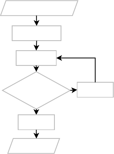
CHAPTER 7 ■ THE EXTENSION C API 279
everything off and clean up. The general process is shown in Figure 7-1. It still isn’t hard, though.
Like functions, one good example will be all you need to get the gist of it.
Figure 7-1. Query processing with aggregates
Registration Function
As mentioned before, aggregates and functions use the same registration function,
sqlite3_create_function(), which is listed here again for convenience:
int sqlite3_create_function(
sqlite3 cnx*, /* connection handle */
const char *zFunctionName, /* function/aggregate name in SQL */
int nArg, /* number of arguments. -1 = unlimited. */
int eTextRep, /* encoding (UTF8, 16, etc.) */
void *pUserData, /* application data, passed to callback */
void (*xFunc)(sqlite3_context*,int,sqlite3_value**),
void (*xStep)(sqlite3_context*,int,sqlite3_value**),
void (*xFinal)(sqlite3_context*)
);
You do exactly the same thing here as you do with functions, but rather than proving a callback
for xFunc, you leave it NULL and provide functions for xStep and xFinal.
sqlite_prepare()
sqlite_step()
SQLITE_ROW xStep()
xFinal()
select sum(id) from foo;
sum(id)
Yes
No
Owens_6730 C07.fm Page 279 Tuesday, April 18, 2006 2:16 PM
www.it-ebooks.info
280 CHAPTER 7 ■ THE EXTENSION C API
A Practical Example
The best way to illustrate implementing aggregates is by example. Here we will implement the
aggregate SUM(). Yes, SQLite already has this aggregate built in, but SUM() is simple and to the
point. To avoid collision, ours will be called sum_int(). Also, this example is a little watered down
as it sums only integers. But there is little value in getting caught up in what we are aggregating—
you can do that later. The goal here is how to aggregate. The example program looks almost
identical to that of the func.c example, and is shown in Listing 7-9 (taken from aggregate.c).
Listing 7-9. The sum_int() Test Program
int main(int argc, char **argv)
{
int rc; sqlite3 *db; char *sql;
sqlite3_open("test.db", &db);
/* Register aggregate. */
fprintf(stdout, "Registering aggregate sum_int()\n");
/* Turn SQL tracing on. */
log_sql(db, 1);
/* Register aggregate. */
sqlite3_create_function( db, "sum_int", 1, SQLITE_UTF8, db,
NULL, step, finalize);
/* Test. */
fprintf(stdout, "\nRunning query: \n");
sql = "select sum_int(id) from aggregate";
print_sql_result(db, sql);
sqlite3_close(db);
return 0;
}
Things to note here are that our step function is called step(), and our finalizing function
is called finalize(). Also, this aggregate is registered as taking only one argument.
The Step Function
The step() function is shown in Listing 7-10.
Owens_6730 C07.fm Page 280 Tuesday, April 18, 2006 2:16 PM
www.it-ebooks.info
CHAPTER 7 ■ THE EXTENSION C API 281
Listing 7-10. The sum_int() Step Function
void step(sqlite3_context* ctx, int ncols, sqlite3_value** values)
{
sum* s;
int x;
s = (sum*)sqlite3_aggregate_context(ctx, sizeof(sum));
if(sqlite3_aggregate_count(ctx) == 1) {
s->x = 0;
}
x = sqlite3_value_int(values[0]);
s->x += x;
fprintf(stdout, "step() : value=%i, total=%i\n", x, s->x);
}
The value sum is a struct that is specific to this example and is defined as follows:
typedef struct {
int x;
} sum;
It’s just a glorified integer. This structure serves as our state between aggregate iterations (calls
to the step function).
The Aggregate Context
The first order of business is to retrieve the structure for the given aggregate instance. This is done
using sqlite3_aggregate_context(). As mentioned earlier, the first call to this function allocates
the data for the given context and subsequent calls retrieve it. The structure memory is automati-
cally freed when the aggregate completes (after finalize() is called). In the step() function, the
value to be aggregated is retrieved from the first argument using sqlite3_value_int(). This value
is then added to the x member of the sum struct, which stores the intermediate summation.
The Finalize Function
Each record in the materialized result set triggers a call to step(). After the last record is processed,
SQLite calls finalize(), which is implemented as shown in Listing 7-11.
Listing 7-11. The sum_int() Finalize Function
void finalize(sqlite3_context* ctx)
{
sum* s;
s = (sum*)sqlite3_aggregate_context(ctx, sizeof(sum));
sqlite3_result_int(ctx, s->x);
Owens_6730 C07.fm Page 281 Tuesday, April 18, 2006 2:16 PM
www.it-ebooks.info

282 CHAPTER 7 ■ THE EXTENSION C API
fprintf(stdout, "finalize() : total=%i\n\n", s->x);
}
This function retrieves the sum struct and sets the aggregate’s return value to the value
stored in the struct’s x member using sqlite3_result_int(). The finalize() function basically
works just like a user-defined function callback.
Results
The program produces the following output:
Dropping table aggregate, if exists.
TRACE: select count(*) from sqlite_master where name='aggregate'
TRACE: drop table aggregate
Creating table aggregate.
TRACE: create table aggregate(id integer)
Populating table aggregate.
TRACE: insert into aggregate values (1)
TRACE: insert into aggregate values (2)
TRACE: insert into aggregate values (3)
Registering aggregate sum_int()
Running query:
TRACE: select sum_int(id) from aggregate
step() : value=1, total=1
step() : value=2, total=3
step() : value=3, total=6
finalize() : total=6
sum_int(id)
-----------
6
I included some output from the setup code in this example (which creates and populates
the aggregate table) to better illustrate how this example works. As you can see, the SELECT state-
ment pulls back a total of three records, which results in three calls to step(). After the last step
function comes finalize(), which provides the value returned by sum_int(). In this case the
value is 6.
And that is the concept of aggregates in a nutshell. They are so similar to functions that
there isn’t much to talk about once you are familiar with functions.
Owens_6730 C07.fm Page 282 Tuesday, April 18, 2006 2:16 PM
www.it-ebooks.info

CHAPTER 7 ■ THE EXTENSION C API 283
Collations
As stated before, the purpose of Collations is to sort strings. But before starting down that path, it is
important to recall that SQLite’s manifest typing scheme allows varying data types to coexist in the
same column. For example, consider the following SQL (located in collate1.sql):
.headers on
.m col
create table foo(x);
insert into foo values (1);
insert into foo values (2.71828);
insert into foo values ('three');
insert into foo values (X'0004');
insert into foo values (null);
select quote(x), typeof(x) from foo;
Feeding it to the SQLite CLP will produce the following:
C:\temp\examples\ch7> sqlite3 < collate.sql
quote(x) typeof(x)
---------- ----------
1 integer
2.71828 real
'three' text
X'0004' blob
NULL null
You’ve got every one of SQLite’s native storage classes sitting in column x. Naturally, the question
arises as to what happens when you try to sort this column. That is, before we can talk about
how to sort strings, we need to review how different data types are sorted first.
When SQLite sorts a column in a result set (when it uses a comparison operator like < or >=
on the values within that column), the first thing it does is arrange the column’s values according to
storage class. Then within each storage class, it sorts the values according to methods specific
to that class. Storages classes are sorted in the following order, from first to last:
1. NULL values
2. INTEGER and REAL values
3. TEXT values
4. BLOB values
Now let’s modify the SELECT statement in the preceding example to include an ORDER BY clause
such that the SQL is as follows:
select quote(x), typeof(x) from foo order by x;
Owens_6730 C07.fm Page 283 Tuesday, April 18, 2006 2:16 PM
www.it-ebooks.info

284 CHAPTER 7 ■ THE EXTENSION C API
Rerunning the query (located in collate2.sql) confirms this ordering:
C:\temp\examples\ch7> sqlite3 < collate.sql
quote(x) typeof(x)
---------- ----------
NULL null
1 integer
2.71828 real
'three' text
X'0004' blob
NULLs are first, INTEGER and REAL next (in numerical order), followed by TEXT, and then BLOBs last.
SQLite employs specific sorting methods for each storage class. NULLs are obvious—there
is no sort order. Numeric values are sorted numerically—integers and floats alike are compared
based on their respective quantitative values. BLOBs are sorted by binary value. Text, finally, is
where Collations come in.
Collation Defined
Collation is the method by which strings are compared. According to Wikipedia,1 collation is
defined as
In library and information science and computer science, collation is the assembly of
written information into a standard order. In common usage, this is called alphabet-
ization, though collation is not limited to ordering letters of the alphabet. Collating lists
of words or names into alphabetical order is the basis of most office filing systems,
library catalogues, and books of reference.
According to IBM’s glossary of Unicode terms, collation is defined as
Text comparison using language-sensitive rules as opposed to bitwise comparison of
numeric character codes.
In general, collation has to do with the arranging of strings and the arranging of characters.
Collation methods usually employ collation sequences. A collation sequence is just a list of
characters, each of which is assigned some numerical value to denote its position in the list.
The list in turn is used to dictate how characters are ordered. Given any two characters, the
Collation (list) can resolve which would come first, or if they are the same.
How Collation Works
Normally, a collation method compares two strings by breaking them down and comparing
their respective characters using a Collation. They do this by lining the strings up and comparing
characters from left to right (Figure 7-2). For example, the strings 'jerry' and 'jello' would be
compared by first comparing the first letter in each string (both j in this case). If one letter’s
1. See http://en.wikipedia.org/wiki/Collation.
Owens_6730 C07.fm Page 284 Tuesday, April 18, 2006 2:16 PM
www.it-ebooks.info
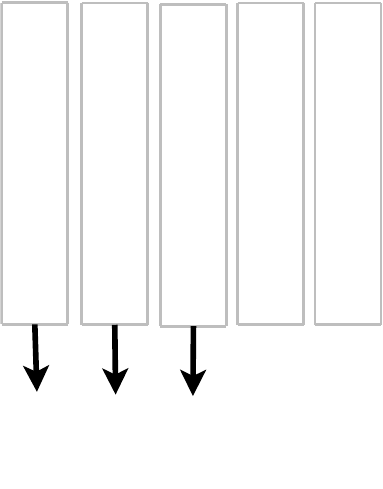
CHAPTER 7 ■ THE EXTENSION C API 285
numerical value according to the collation sequence is larger than the other, the comparison is
over: the string with the larger letter is deemed greater and no further comparison is required.
If, on the other hand, the letters have the same value, then the process continues on to the
second letter in each string, and to the third, and so on until some difference is found (or no
difference is found, in which case the strings are considered equal). If one string runs out of
letters before the other, then it is up to the collation method to determine what this means.
Figure 7-2. Binary collation
In this example, the Collation is the ASCII character set. Each character’s numeric ASCII value
in the figure is displayed underneath it. Using the collation method just described, string
comparison continues to the third character, whereupon 'jerry' wins out, as it has an r with
the value 114 whereas 'jello' has the inferior 'l' with the value 108. According to this colla-
tion method using the ASCII Collation, 'jerry' > 'jello'.
Had 'jerry' been 'Jerry', then 'jello' would have won out, as big J’s little 74 pales to
little j’s big 106, so the comparison would have been resolved on the first character—the prize
going to 'jello'. In short, 'jello' > 'Jerry'.
However, to continue the example, we could use a different Collation wherein uppercase
values are assigned the same numbers as their lowercase counterparts (a case-insensitive
collation sequence). Then the comparison between 'Jerry' and 'jello' would go back to
'Jerry' as in this new Collation J and j are the same, pulling the rug out from under 'jello'’s
lowercase j superiority.
But enough about Collations. You get the picture. A sequence is a sequence. Ultimately, it’s
not the collation sequence that matters, but the collation method. Collation methods don’t have to
j
106
j
106
0
e
101
e
101
0
r
114
l
108
[r]
Done
r
114
l
108
y
121
o
111
Owens_6730 C07.fm Page 285 Tuesday, April 18, 2006 2:16 PM
www.it-ebooks.info
286 CHAPTER 7 ■ THE EXTENSION C API
use sequences. They can do whatever they want. A collation method is called a method for a
reason; it can do whatever it wants, even if its chosen method may be madness.
Odds are that you are really confused by now and are just ready for a summary. So here it
is. Think of collation methods as the way that strings are compared. Think of collation sequences
as the way characters are compared. Ultimately, all that matters in SQLite is how strings are
compared, and the two terms refer to just that. Therefore, the two terms collation method and
collation sequence should just be thought of as string comparison. If you read collation, think
string comparison. If you read Collation, think string comparison. All in all, just think string
comparison. That is the way the API is geared. When you create a custom Collation, SQLite
hands it two strings, a and b, and the Collation returns whether string a is less than, equal to, or
greater than string b. That’s it, plain and simple.
Standard Collation Types
SQLite comes with a single built-in Collation named BINARY, which is implemented applying
the memcmp() routine from the standard C library to the two strings to be compared. The BINARY
collation happens to work well for English text. For other languages or locales, alternate Collation
may be preferred. SQLite also offers an alternate collation called NOCASE, which does not distin-
guish between cases, and another called REVERSE, which as you may have guessed compares
everything backwards (according to binary value).
Collations are applied by associating them with columns in a table or an index definition,
or by specifying them in a query. For example, to create a case-insensitive column bar in foo,
you would define foo as follows:
create table foo (bar text COLLATE NOCASE, baz text);
To create a REVERSE index on baz, you would do something like this:
create index bar_rev_idx on foo (baz) COLLATE REVERSE;
From that point on, whenever SQLite deals with a bar it will use the NOCASE collation. When it
uses an index for baz, it will follow the REVERSE collation.
If you prefer not to attach a Collation to a database object, but would rather specify it as
needed on a query-by-query basis, you can specify them directly in queries, as in the following:
select * from foo order by bar COLLATE NOCASE;
At the time of this writing, there are plans under way to include standard CAST() syntax to allow
the collation of an expression to be defined.
A Simple Example
To jump into collations, let’s begin with a simple example to get the big picture. Let’s imple-
ment a collation called POLITICAL. POLITICAL will take two strings and decide which one is
greater depending on the day. One Mondays, 'Jello' might be greater than 'jerry'. On Tuesdays,
it may be a different story entirely.
Collations are registered with SQLite through the sqlite3_create_collation() function,
which is declared as follows:
Owens_6730 C07.fm Page 286 Tuesday, April 18, 2006 2:16 PM
www.it-ebooks.info

CHAPTER 7 ■ THE EXTENSION C API 287
int sqlite3_create_collation(
sqlite3* db, /* database handle */
const char *zName, /* collation name in SQL */
int pref16, /* encoding */
void* pUserData, /* application data */
int(*xCompare)(void*,int,const void*,int,const void*)
);
It looks pretty similar to sqlite3_create_function(). There is the standard database handle,
the collation name as it will be addressed in SQL (similar to the function/aggregate name), and
the encoding, which pertains to the format of the comparison strings when passed to the
comparison function.
■Note Just as in aggregates and functions, separate collation comparison functions can be registered
under the same collation name for each of the UTF-8, UTF-16LE, and UTF-16BE encodings. SQLite will auto-
matically select the best comparison function for the given collation based on the strings to be compared.
Finally, the application data pointer is another API mainstay. The pointer provided there
is passed on to the callback function. Basically, sqlite3_create_collation() is a stripped-down
version of sqlite3_create_function(), which takes exactly two arguments (both of which are
text) and returns an integer value. It also has the aggregate callback function pointers stripped out.
The Compare Function
The xCompare argument is really the only new thing here. It points to the actual comparison
function that will resolve the text values. The comparison function must have the form
int compare( void* data, /* application data */
int len1, /* length of string 1 */
const void* str1, /* string 1 */
int len2, /* length of string 2 */
const void* str2) /* string 2 */
The function should return negative, zero, or positive if the first string is less than, equal to, or
greater than the second string, respectively.
As stated, the political collation is a bit wishy-washy. Its implementation is shown in
Listing 7-12.
Listing 7-12. The Political Collation Function
int political_collation( void* data, int l1, const void* s1,
int l2, const void* s2 )
{
int result, opinion; struct tm* t; time_t rt;
Owens_6730 C07.fm Page 287 Tuesday, April 18, 2006 2:16 PM
www.it-ebooks.info
288 CHAPTER 7 ■ THE EXTENSION C API
/* Get the unpolitical comparison result */
result = strcmp(s1,s2);
/* Get the date and time */
time(&rt);
t = localtime(&rt);
/* Form an opinion: is s1 really < or = to s2 ? */
switch(t->tm_wday) {
case 0: /* Monday yes */
opinion = result;
break;
case 1: /* Tuesday no */
opinion = -result;
break;
case 2: /* Wednesday bigger is better */
opinion = l1 >= l2 ? -1:1;
break;
case 3: /* Thursday strongly no */
opinion = -100;
break;
case 4: /* Friday strongly yes */
opinion = 100;
break;
case 5: /* Saturday golf, everything's the same */
opinion = 0;
break;
default: /* Sunday - Meet the Press, opinion changes
every minute */
opinion = 2*sin(t->tm_min*180);
}
/* Now change it on a whim */
opinion = rand()-(RAND_MAX/2) > 0 ? -1:1;
return opinion;
}
The Test Program
All that remains is to illustrate it in a program. The example program (political.c) implemen-
tation is shown in Listing 7-13.
Owens_6730 C07.fm Page 288 Tuesday, April 18, 2006 2:16 PM
www.it-ebooks.info
CHAPTER 7 ■ THE EXTENSION C API 289
Listing 7-13. The Political Collation Test Program
int main(int argc, char **argv)
{
char *sql; sqlite3 *db; int rc;
/* For forming more consistent political opinions. */
srand((unsigned)time(NULL));
sqlite3_open("test.db", &db);
/* Create issues table, add records. */
setup(db);
/* Register Collation. */
fprintf(stdout, "1. Register political Collation\n\n");
sqlite3_create_collation( db, "POLITICAL",
SQLITE_UTF8, db,
political_collation );
/* Turn SQL logging on. */
log_sql(db, 1);
/* Test default collation. */
fprintf(stdout, "2. Select records using default collation.\n");
sql = "select * from issues order by issue";
print_sql_result(db, sql);
/* Test Political collation. */
fprintf(stdout, "\nSelect records using political collation. \n");
sql = "select * from issues order by issue collate POLITICAL";
print_sql_result(db, sql);
fprintf(stdout, "\nSelect again using political collation. \n");
print_sql_result(db, sql);
/* Done. */
sqlite3_close(db);
return 0;
}
Owens_6730 C07.fm Page 289 Tuesday, April 18, 2006 2:16 PM
www.it-ebooks.info

290 CHAPTER 7 ■ THE EXTENSION C API
Results
Running the program yields the following results:
1. Register political Collation
2. Select records using default collation.
TRACE: select * from issues order by issue
issue
-----------------
Defense
Deficit
Economy
Education
Environment
Foreign Policy
Health Care
National Security
Social Security
Unemployment
Select records using political collation.
TRACE: select * from issues order by issue collate POLITICAL
issue
-----------------
Health Care
Foreign Policy
National Security
Economy
Social Security
Unemployment
Environment
Defense
Education
Deficit
Select again using political collation.
TRACE: select * from issues order by issue collate POLITICAL
issue
-----------------
National Security
Defense
Unemployment
Deficit
Foreign Policy
Education
Social Security
Owens_6730 C07.fm Page 290 Tuesday, April 18, 2006 2:16 PM
www.it-ebooks.info

CHAPTER 7 ■ THE EXTENSION C API 291
Health Care
Environment
Economy
Step 1 registers the political collation sequence. Step 2 selects records using SQLite’s default
binary collation, which returns records in alphabetical order. Step 3 selects records twice using
the political Collation, obtaining different results each time. As the results indicate, we are right
on the mark. In fact, the more times you select using the POLITICAL collation, the more you are
apt to find that the results continually change. Politics can be very complicated.
Collation on Demand
SQLite provides a way to defer collation registration until it is actually needed. So if you are
not sure your application is going to need something like the POLITICAL collation, you can
use the sqlite3_collation_needed() function to defer its registration to the last possible
moment (which incidentally seems befitting of this particular collation). You simply provide
sqlite3_collation_needed() with a callback function, which SQLite can rely on to register
unknown collation sequences as needed, given their name. It is a callback for a callback, so
to speak. Better yet, it’s like saying to SQLite, “Here, if you are ever asked to use a Collation that
you don’t recognize, call this function, and it will register the unknown sequence, then you can
continue your work.”
The sqlite3_collation_needed() function is declared as follows:
int sqlite3_collation_needed(
sqlite3* db, /* connection handle */
void* data, /* application data */
void(*crf)(void*,sqlite3*,int eTextRep,const char*)
);
The crf argument (the collation registration function as I call it) points to the function that will
register the unknown Collation. For clarity, it is defined as follows:
void crf( void* data, /* application data */
sqlite3* db, /* database handle */
int eTextRep, /* encoding */
const char*) /* collation name */
The db and data arguments of crf() are the values passed into the first and second arguments
of sqlite3_collation_needed(), respectively. To make it all clear, say we want to defer all collation
registration. A possible implementation that anticipates the POLITCAL Collation and uses some
default binary comparison function for all other unknown Collations would be implemented as
shown in Listing 7-14.
Owens_6730 C07.fm Page 291 Tuesday, April 18, 2006 2:16 PM
www.it-ebooks.info
292 CHAPTER 7 ■ THE EXTENSION C API
Listing 7-14. Collation Registration Function
void crf( void* data, sqlite3* db,
int eTextRep, const char* cname)
{
if(strcmp(collation_name, "POLITICAL") == 0) {
/* Political collation has not been registered and is now needed */
sqlite3_create_collation( db, "POLITICAL",
SQLITE_UTF8, db,
political_collation );
} else {
/* Punt: Use some default comparison function this collation. */
sqlite3_create_collation( db, collation_name,
SQLITE_UTF8, db,
default_collation );
}
}
Thus POLITCAL will get registered only if it is ever referenced. Likewise, if SQLite encounters
something like
select * from issues order by issue COLLATE EMOTIONAL;
our crf() handler will just install a generic comparison function default_collation()
(which I just made up) as the comparison function for EMOTIONAL collations. Bottom line:
the sqlite3_collation_needed() handler’s job is to take a Collation name and register a
Collation to associate with it.
A Practical Application
We will conclude this chapter with an application of Collations that may prove a little more
useful than the previous example (if not more consistent). We will combine what we’ve learned
from functions to create a collation that helps out with date formats. Now, it turns out that ISO
dates by virtue of their format happen to sort both lexicographically and chronologically. That
is, if you sort a set of ISO dates alphabetically, they will end up in the correct chronological
order. As a result, ISO dates tend to work just fine in SQLite.
Let’s say you that have some data that you want to pass back and forth between SQLite and
an Oracle database. And in your data you have to deal with Oracle style dates. Oracle dates, of
the form DD-MONTH-YY, don’t simultaneously sort lexicographically and chronologically. It’s one
or the other, but not both.
And while it’s possible to get Oracle to use ISO or ANSI dates, rather than bumbling with
converting back and forth, you would rather just have SQLite be able to sort Oracle dates as
well as it does ISO dates. This is a perfect job for a user-defined Collation.
The Comparison Function
Rather than using a string compare, we parse the date format, breaking it down into its indi-
vidual parts, and sort them numerically. The comparison function is simple, as you can see in
Listing 7-15.
Owens_6730 C07.fm Page 292 Tuesday, April 18, 2006 2:16 PM
www.it-ebooks.info
CHAPTER 7 ■ THE EXTENSION C API 293
Listing 7-15. Oracle Date Collation Function
int oracle_date_collation( void* data,
int len1, const void* arg1,
int len2, const void* arg2 )
{
int len;
date d1;
date d2;
strncpy(&zDate2[0], arg2, len);
zDate2[len] = '\0';
/* Convert dates to date struct */
oracle_date_str_to_struct(arg1, &d1);
oracle_date_str_to_struct(arg2, &d2);
fprintf(stdout, "collate_fn() : date1=%s, date2=%s\n", zDate1, zDate2);
/* Compare structs */
if(d1.year < d2.year) {
return -1;
}
else if(d1.year > d2.year) {
return 1;
}
/* If this far, years are equal. */
if(d1.month < d2.month) {
return -1;
}
else if(d1.month > d2.month) {
return 1;
}
/* If this far, months are equal. */
if(d1.day < d2.day) {
return -1;
}
else if(d1.day > d2.day) {
return 1;
}
Owens_6730 C07.fm Page 293 Tuesday, April 18, 2006 2:16 PM
www.it-ebooks.info
294 CHAPTER 7 ■ THE EXTENSION C API
/* If this far, dates are equal. */
return 0;
}
Date Parsing
This function uses another function, called oracle_date_str_to_struct(), to parse the dates
and populate a generic date struct. This function is implemented as shown in Listing 7-16.
Listing 7-16. The Oracle Date Parsing Function
int oracle_date_str_to_struct(const char* value, date* d)
{
const char* date, *tmp;
char *start, *end, zDay[3], zMonth[4], zYear[3];
date = get_date(value);
if(date == NULL) {
fprintf(stderr, "Invalid date\n");
return -1;
}
/* Find first '-' */
start = strchr(date,'-');
/* Find last '-' */
end = strchr(start+1,'-');
/* Extract day part, convert to int*/
strncpy(zDay, date,2);
zDay[2] = '\0';
d->day = atoi(zDay);
/* Extract month part, convert to int*/
strncpy(zMonth, start+1,3);
zMonth[3] = 0;
tmp = uppercase(zMonth);
d->month = month_num(tmp);
free((void*)tmp);
/* Extract year part, convert to int*/
strncpy(zYear, end+1,2);
zYear[2] = '\0';
d->year = atoi(zYear);
Owens_6730 C07.fm Page 294 Tuesday, April 18, 2006 2:16 PM
www.it-ebooks.info
CHAPTER 7 ■ THE EXTENSION C API 295
free((void*)date);
return 0;
}
This function uses another function, get_date(), to extract the minimum part of the string,
which makes up a complete Oracle date format. It uses Perl Compatible Regular Expressions to
do this. Using a regular expression to define the date format makes it easier to tweak without
having to do any additional coding. Using get_date() to extract a date value from a string along
with a flexible regex allows us some flexibility to deal with sloppy dates, if needed. The get_date()
function is defined in Listing 7-17.
Listing 7-17. The get_date() Function
#define ORACLE_DATE_REGEX "[0-9]{1,2}-[a-zA-Z]{3,3}-[0-9]{2,2}";
const char* get_date(const char* value)
{
pcre *re;
const char *error, *pattern;
int erroffset;
int ovector[3];
int value_length;
int rc, substring_length;
char* result, *substring_start;
pattern = ORACLE_DATE_REGEX;
re = pcre_compile(
pattern, /* the pattern */
0, /* default options */
&error, /* for error message */
&erroffset, /* for error offset */
NULL); /* use default character tables */
/* Compilation failed */
if (re == NULL) {
return NULL;
}
value_length = (int)strlen(value);
rc = pcre_exec(
re, /* the compiled pattern */
NULL, /* no extra data - we didn't study the pattern */
value, /* the value string */
value_length, /* the length of the value */
0, /* start at offset 0 in the value */
Owens_6730 C07.fm Page 295 Tuesday, April 18, 2006 2:16 PM
www.it-ebooks.info
296 CHAPTER 7 ■ THE EXTENSION C API
0, /* default options */
ovector, /* output vector for substring information */
3); /* number of elements in the output vector */
if (rc < 0) {
/* Match error */
return NULL;
}
substring_start = (char*)value + ovector[0];
substring_length = ovector[1] - ovector[0];
result = malloc(substring_length);
strncpy(result, substring_start, substring_length);
result[substring_length] = '\0';
return result;
}
The Test Program
All three of the above functions work together to collate Oracle dates in chronological order.
Our example program is shown in Listing 7-18.
Listing 7-18. The Oracle Collation Test Program
int main(int argc, char **argv)
{
int rc;
sqlite3 *db;
char *sql;
sqlite3_open("test.db", &db);
/* Install oracle related date functions. */
install_date_functions(db);
/* Register Collation. */
fprintf(stdout, "Registering collation sequence oracle_date\n");
sqlite3_create_collation( db, "oracle_date",
SQLITE_UTF8, db,
oracle_date_collation );
/* Create dates table, add records. */
setup(db);
/* Turn SQL logging on. */
log_sql(db, 1);
Owens_6730 C07.fm Page 296 Tuesday, April 18, 2006 2:16 PM
www.it-ebooks.info

CHAPTER 7 ■ THE EXTENSION C API 297
/* Test default collation. */
fprintf(stdout, "Select records. Use default collation.\n");
sql = "select * from dates order by date";
print_sql_result(db, sql);
/* Test Oracle collation. */
fprintf(stdout, "\nSelect records. Use Oracle data collation. \n");
sql = "select * from dates order by date collate oracle_date";
print_sql_result(db, sql);
/* Done. */
sqlite3_close(db);
return 0;
}
Results
Running the program yields the following output:
Registering collation sequence oracle_date
Select records. Use default collation.
TRACE: select * from dates order by date
id date
-- ----------
4 1-APR-05
8 1-AUG-05
12 1-DEC-05
2 1-FEB-05
1 1-JAN-05
7 1-JUL-05
6 1-JUN-05
3 1-MAR-05
5 1-MAY-05
11 1-NOV-05
10 1-OCT-05
9 1-SEP-05
Select records. Use Oracle data collation.
TRACE: select * from dates order by date collate oracle_date
collate_fn() : date1=1-DEC-05, date2=1-NOV-05
collate_fn() : date1=1-OCT-05, date2=1-SEP-05
collate_fn() : date1=1-NOV-05, date2=1-SEP-05
collate_fn() : date1=1-NOV-05, date2=1-OCT-05
collate_fn() : date1=1-AUG-05, date2=1-JUL-05
collate_fn() : date1=1-JUN-05, date2=1-MAY-05
collate_fn() : date1=1-JUL-05, date2=1-MAY-05
Owens_6730 C07.fm Page 297 Tuesday, April 18, 2006 2:16 PM
www.it-ebooks.info

298 CHAPTER 7 ■ THE EXTENSION C API
collate_fn() : date1=1-JUL-05, date2=1-JUN-05
collate_fn() : date1=1-SEP-05, date2=1-MAY-05
collate_fn() : date1=1-SEP-05, date2=1-JUN-05
collate_fn() : date1=1-SEP-05, date2=1-JUL-05
collate_fn() : date1=1-SEP-05, date2=1-AUG-05
collate_fn() : date1=1-APR-05, date2=1-MAR-05
collate_fn() : date1=1-FEB-05, date2=1-JAN-05
collate_fn() : date1=1-MAR-05, date2=1-JAN-05
collate_fn() : date1=1-MAR-05, date2=1-FEB-05
collate_fn() : date1=1-MAY-05, date2=1-JAN-05
collate_fn() : date1=1-MAY-05, date2=1-FEB-05
collate_fn() : date1=1-MAY-05, date2=1-MAR-05
collate_fn() : date1=1-MAY-05, date2=1-APR-05
id date
-- ----------
1 1-JAN-05
2 1-FEB-05
3 1-MAR-05
4 1-APR-05
5 1-MAY-05
6 1-JUN-05
7 1-JUL-05
8 1-AUG-05
9 1-SEP-05
10 1-OCT-05
11 1-NOV-05
12 1-DEC-05
So there you have it. If I were really serious about all this, I would implement strict type
checking for columns that had Oracle-style dates. I would implement a validate_oradate()
SQL function that calls get_date() to determine if the date is legitimate. I would then declare
all related columns in my tables as oradate. Included in their declaration would be the
oracle_date collation. For example:
create table log ( id autoincrement,
date oradate COLLATE oracle_date CHECK(get_date(date)),
entry text );
Notice that I use a CHECK constraint for strict typing in this case. It works just as easily (if not
more easily) than the trigger functions used earlier for checking a single column (while the
trigger approach can be easier for checking all columns in an entire table). Working together,
these user-defined functions ensure that the oracle_date collation is always presented with
properly formatted dates to compare.
Owens_6730 C07.fm Page 298 Tuesday, April 18, 2006 2:16 PM
www.it-ebooks.info
CHAPTER 7 ■ THE EXTENSION C API 299
Summary
As I hope some of the examples in this chapter demonstrate, user-defined functions, aggregates,
and Collations can be surprisingly useful. And while it certainly helps that SQLite is an open
source library, meaning that you are free to dig in and modify it to your heart’s content, the
extensions part of the C API goes a long way in providing a friendly, easy-to-user interface that
makes it possible to implement a wide range of powerful extensions and customizations, espe-
cially when combined with other features already present in SQLite.
In the next chapter, you will see how many extension languages take advantage of this.
They use the C API to make it possible to implement user-defined functions, aggregates, and
collations in different languages.
Owens_6730 C07.fm Page 299 Tuesday, April 18, 2006 2:16 PM
www.it-ebooks.info

301
■ ■ ■
CHAPTER 8
Language Extensions
SQLite’s native language is C. It is written in C and has its own C API. The open source
community, however, has provided many extensions for SQLite that make it accessible to
many programming languages and libraries such as Perl, Python, Ruby, Java, Qt, and ODBC. In
many cases there are multiple extensions to choose from for a given language, developed by
different people to meet different needs.
Many extensions conform to various API standards. One of the SQLite Perl extensions, for
example, follows the Perl DBI—Perl’s standard interface for database access. Similarly, one of
the Python extensions conforms to Python’s DB API specification, as does at least one of the
Java extensions to JDBC. Regardless of their particular APIs, internally all extensions work on
top of the same SQLite C API, which has its own unique features and design. And to some
degree, all extensions reflect this design. Some extensions provide both a standard interface
that conforms to their particular API standard as well as an alternative interface that better
reflects the design of the SQLite API. Therefore, in such cases you can choose which interface
works best for you based on your requirements.
In general, all extensions have the same comparative anatomy regardless of their partic-
ular API. They follow a similar pattern. Once you understand this pattern, every interface will
start to look similar in many respects. There is some kind of connection object representing a
single connection to the database, and some kind of cursor object representing a SQL query
from which you can both execute commands and iterate over results. Conceptually, it is quite
simple. Internally, you are looking at a sqlite3 structure and a sqlite3_stmt structure, and
from reading Chapter 5 you should have a good feel for how these work. The same rules apply
for language extensions as for the C API.
This chapter covers language extensions for six popular languages: Perl, Python, Ruby,
Java, Tcl, and PHP. The intent is to provide you with a convenient introduction with which to
quickly get started using SQLite in a variety of different languages. Coverage for each language
follows a common outline composed of four topics that pertain to both general database work
and specific SQLite features:
• Connecting to databases
•Executing queries
• Using bound parameters
• Implementing user-defined functions and aggregates
Owens_6730 C08.fm Page 301 Tuesday, April 18, 2006 2:21 PM
www.it-ebooks.info
302 CHAPTER 8 ■ LANGUAGE EXTENSIONS
Together these topics constitute the vast majority of what you will ever use in any particular
SQLite extension. Not every extension supports all of these topics. For instance, some don’t
offer bound parameters. Conversely, some extensions offer unique features that are outside of
the topics covered here. The aim here is to provide a consistent, straightforward process with
which to easily get started using SQLite in a wide variety of languages. Once you get started
with any extension, it is usually easy to pick up any special features available in that extension.
Where appropriate, this chapter addresses how different extensions use various parts of
the C API in order to help you understand what is going on under the hood. If you have not read
Chapter 5, I strongly recommend that you do so. No matter what language you program in, it
will almost always be helpful to understand how SQLite works in order to make the most of it and
thus write good code. It will help you select the most suitable query methods, understand the
scope of transactions, and know how to anticipate, deal with, or avoid locks, among other things.
This chapter is not a language reference. I assume that you know how to program and are
familiar with your particular language of interest. SQLite is first and foremost a programmer’s
database, and that is the assumption I’ve made here—you are a programmer and I need not
cover what you already know.
Selecting an Extension
In some cases multiple interfaces are available for some languages. In such cases (with the
exception of Python), I cover the interface that best fits the following criteria:
• Support for SQLite 3
• Good documentation
•Stability
• Portability
Despite these criteria, there were multiple candidates in some cases that met all the qual-
ifications. In such cases the tiebreaker was more a matter of personal preference than anything
else. But the purpose here is not to favor a particular extension. It is to teach concepts so that
you can easily pick any extension in any language and quickly put it and SQLite to good use.
And the reasons I chose a particular extension may not be the reasons you would. There
are quite a few things to consider when you select a particular extension. You will have require-
ments that must be satisfied when choosing an extension. Some of the things you might want
to take into consideration include the following:
•License compatibility: The extension’s license can directly affect how you can use it.
If you are writing code for a commercial product, you definitely need to take this into
consideration.
•Data type mapping: Another important point is how the extension maps SQLite’s
storage classes to the language’s native types. Are all values returned as text? If not, is
there an easy way to determine the mappings? Do you have any control over how the
mapping is done?
Owens_6730 C08.fm Page 302 Tuesday, April 18, 2006 2:21 PM
www.it-ebooks.info
CHAPTER 8 ■ LANGUAGE EXTENSIONS 303
•Query methods: Three different query methods are supported in the C API. Which one
does the extension use? Ideally it supports all three. You are already familiar with the
pros and cons of each approach, and it’s nice to have all three methods in different
situations.
•API coverage: How well does the extension cover other areas that don’t easily map to
many standard database interfaces? For example, does it allow you to call the SQL trace
function, or operational security functions? Are these something you need?
•Linkage and distribution: How easy is it to use the extension with a particular version of
SQLite? Does it include a version of SQLite in the distribution? Does it use a shared library
or is it statically linked to a particular version? What if you need to upgrade SQLite; how
easily can you do this with the extension?
There are other considerations as well, such as community support, mailing list activity, main-
tainer support and responsiveness, regression testing, code quality... the list goes on. All of
these things may play an important role in your decision to use a particular extension. Only
you can answer these questions for yourself.
The SQLite Wiki has a page that provides an exhaustive list of language interfaces, located
at www.sqlite.org/cvstrac/wiki?p=SqliteWrappers. All of the interfaces covered here were
taken from this list. The source code for all of the examples in this chapter is located in the ch8
directory of the examples zip file, available at the Apress website.
Perl
There are two SQLite extensions for Perl. The one covered here is written by Matt Sergeant, and
can be found on CPAN (http://search.cpan.org/~msergeant/). This extension follows very
closely the Perl DBI standard; therefore, if you understand DBI, you will have no trouble using
the extension. The full documentation for Perl DBI can be obtained by typing man DBI on POSIX
systems, or online at http://search.cpan.org/search?module=DBI.
Installation
The current version supporting SQLite 3 at the time of this writing is DBD-SQLite-1.11. You can
install it by using CPAN or by manually building the package from source. The prerequisites for
the SQLite DBD module are of course Perl, a C compiler, as well as the DBI module. To install
DBD::SQLite using CPAN, invoke the CPAN shell from the command line as follows:
mike@linux # cpan
cpan> install DBD::SQLite
To install from source in Linux/Unix, change to a temporary directory and do the following:
mike@linux # wget http://search.cpan.org/CPAN/authors/id/M/MS/MSERGEANT/
DBD-SQLite-1.11.tar.gz
... lots of wget gibberish ...
Owens_6730 C08.fm Page 303 Tuesday, April 18, 2006 2:21 PM
www.it-ebooks.info
304 CHAPTER 8 ■ LANGUAGE EXTENSIONS
mike@linux # tar xzvf DBD-SQLite-1.11.tar.gz
... lots of tar gibberish ...
mike@linux # cd DBD-SQLite-1.11
mike@linux DBD-SQLite-1.11 # perl Makefile.PL
... lots of perl gibberish ...
Checking installed SQLite version...
Looks good
mike@linux DBD-SQLite-1.11 # make install
... more perl gibberish ...
The SQLite Perl extension includes its own copy of the SQLite 3, so there is no need to
compile and install SQLite beforehand. SQLite is embedded in the extension.
Connecting
To ensure that you have the SQLite driver installed, you can use the DBI available_drivers()
within Perl:
print "Drivers: " . join(", ", DBI->available_drivers()), "\n";
You connect to a database using the standard DBI::connect function, as follows:
use DBI;
my $dbh = DBI->connect( "dbi:SQLite:dbname=foods.db", "", "",
{ RaiseError => 1 });
$dbh->disconnect;
The second and third arguments correspond to the driver name and database name. The third
and fourth correspond to username and password, which are not applicable to SQLite.
The function returns a database handle object representing the database connection. Inter-
nally, this corresponds to a single sqlite3 structure. You can create in-memory databases by
passing :memory: for the name of the database. In this case, all tables and database objects will
then reside in memory for the duration of the session, and will be destroyed when the connec-
tion is closed. You close the database using the database handle’s disconnect method.
Query Processing
Queries are performed using the standard DBI interface as well. You can use the prepare(),
execute(), fetch(), or selectrow() functions of the database connection handle. All of these
are fully documented in the DBI man page. An example of using queries is shown in Listing 8-1.
Owens_6730 C08.fm Page 304 Tuesday, April 18, 2006 2:21 PM
www.it-ebooks.info
CHAPTER 8 ■ LANGUAGE EXTENSIONS 305
Listing 8-1. Executing Queries in Perl
use DBI;
# Connect to database
my $dbh = DBI->connect( "dbi:SQLite:dbname=foods.db", "", "",
{ RaiseError => 1 });
# Prepare the statment
my $sth = $dbh->prepare("SELECT name FROM foods LIMIT 3");
# Execute
print "\nArray:\n\n";
$sth->execute;
# Iterate over results and print
while($row = $sth->fetchrow_arrayref) {
print @$row[0] . "\n";
}
# Do the same thing, this time using hashref
print "\nHash:\n\n";
$sth->execute;
while($row = $sth->fetchrow_hashref) {
print @$row{'name'} . "\n";
}
# Finalize the statement
$sth->finish;
#Disconnect
$dbh->disconnect;
Internally, the prepare() method corresponds to the sqlite3_prepare() method. Similarly,
execute() calls the first sqlite3_step() method. It automatically figures out if there is data to
be returned. If there is no data (e.g., non-SELECT statements), it automatically finalizes the
query. The fetchrow_array(), fetchrow_hashref(), and fetch() methods call sqlite3_step()
as well, returning a single row in the result set, if one is available.
Additionally, you can run non-SELECT statements in one step using the database object’s
do() method. Listing 8-2 illustrates this using an in-memory database.
Listing 8-2. The do() Method
use DBI;
my $dbh = DBI->connect("dbi:SQLite:dbname=:memory:", "", "", { RaiseError => 1 });
$dbh->do("CREATE TABLE cast (name)");
$dbh->do("INSERT INTO cast VALUES ('Elaine')");
$dbh->do("INSERT INTO cast VALUES ('Jerry')");
$dbh->do("INSERT INTO cast VALUES ('Kramer')");
Owens_6730 C08.fm Page 305 Tuesday, April 18, 2006 2:21 PM
www.it-ebooks.info

306 CHAPTER 8 ■ LANGUAGE EXTENSIONS
$dbh->do("INSERT INTO cast VALUES ('George')");
$dbh->do("INSERT INTO cast VALUES ('Newman')");
my $sth = $dbh->prepare("SELECT * FROM cast");
$sth->execute;
while($row = $sth->fetch) {
print join(", ", @$row), "\n";
}
$sth->finish;
$dbh->disconnect;
The statement handle object’s finish() method will call sqlite3_finalize() on the query
object, if it has not already done so. This program produces the following output:
Elaine
Jerry
Kramer
George
Newman
Parameter Binding
Parameter binding follows the method defined in the DBI specification. While SQLite supports
both positional and named parameters, the Perl interface uses only positional parameters, as
illustrated in Listing 8-3.
Listing 8-3. Parameter Binding in Perl
use DBI;
my $dbh = DBI->connect( "dbi:SQLite:dbname=foods.db", "", "",
{ RaiseError => 1 });
my $sth = $dbh->prepare("SELECT * FROM foods where name like :1");
$sth->execute('C%');
while($row = $sth->fetchrow_hashref) {
print @$row{'name'} . "\n";
}
$sth->finish;
$dbh->disconnect;
The execute() method takes the parameter values defined in prepare().
Owens_6730 C08.fm Page 306 Tuesday, April 18, 2006 2:21 PM
www.it-ebooks.info
CHAPTER 8 ■ LANGUAGE EXTENSIONS 307
User-Defined Functions and Aggregates
User-defined functions and aggregates are implemented using private methods of the driver.
They follow closely to their counterparts in the SQLite C API. Functions are registered using the
following private method:
$dbh->func( $name, $argc, $func_ref, "create_function" )
Here $name specifies the SQL function name, $argc the number of arguments, and $func_ref
a reference to the Perl function that provides the implementation. Listing 8-4 illustrates an
implementation of hello_newman() in Perl.
Listing 8-4. hello_newman() in Perl
use DBI;
sub hello_newman {
return "Hello Jerry";
}
# Connect
my $dbh = DBI->connect( "dbi:SQLite:dbname=foods.db", "", "",
{ RaiseError => 1 });
# Register function
$dbh->func('hello_newman', 0, \&hello_newman, 'create_function');
# Call it
print $dbh->selectrow_arrayref("SELECT hello_newman()")->[0] . "\n";
$dbh->disconnect;
If you provide -1 as the number of arguments, then the function will accept a variable
number of arguments. Listing 8-5 has Newman replying to each of the names supplied as argu-
ments. If no arguments are provided, he simply replies “Hello Jerry.”
Listing 8-5. hello_newman() in Perl with Variable Arguments
use DBI;
sub hello_newman {
if (@_ == 0) {
return "Hello Jerry";
}
return "Hello " . join ", ", @_;
}
Owens_6730 C08.fm Page 307 Tuesday, April 18, 2006 2:21 PM
www.it-ebooks.info

308 CHAPTER 8 ■ LANGUAGE EXTENSIONS
# Connect
my $dbh = DBI->connect( "dbi:SQLite:dbname=foods.db", "", "",
{ RaiseError => 1 });
# Register function
$dbh->func('hello_newman', -1, \&hello_newman, 'create_function');
# Call it
print $dbh->selectrow_arrayref("SELECT hello_newman()")->[0] . "\n";
print $dbh->selectrow_arrayref(
"SELECT hello_newman('Elaine', 'Jerry')")->[0] . "\n";
print $dbh->selectrow_arrayref(
"SELECT hello_newman('Elaine', 'Jerry', 'George')")->[0] . "\n";
$dbh->disconnect;
The hello_newman() function is passed all the arguments provided in the SQL statement in
the @_ variable. This example produces the following output:
Hello Jerry
Hello Elaine
Hello Elaine, Jerry
Hello Elaine, Jerry, George
Aggregates
User-defined aggregates are implemented as packages. Each package implements a step function
and a finalize function. The step function is called for each row that is selected. The first value
supplied to the function is the context, which is a persistent value maintained between calls to
the function. The remaining values are the arguments to the aggregate function supplied in the
SQL statement. The finalize function is provided the same context as the step function. The
following example implements a simple SUM aggregate called perlsum. The aggregate is imple-
mented in a package called perlsum.pm, shown in Listing 8-6.
Listing 8-6. The perlsum() Aggregate
package perlsum;
sub new { bless [], shift; }
sub step {
my ( $self, $value ) = @_;
@$self[0] += $value;
}
Owens_6730 C08.fm Page 308 Tuesday, April 18, 2006 2:21 PM
www.it-ebooks.info
CHAPTER 8 ■ LANGUAGE EXTENSIONS 309
sub finalize {
my $self = $_[0];
return @$self[0];
}
sub init {
$dbh = shift;
$dbh->func( "perlsum", 1, "perlsum", "create_aggregate" );
}
1;
The init function is used to register the aggregate in the database connection. Listing 8-7
is a simple program illustrating its use.
Listing 8-7. A perlsum() Test Program
use DBI;
use perlsum;
# Connect
my $dbh = DBI->connect( "dbi:SQLite:dbname=foods.db", "", "",
{ RaiseError => 1 });
perlsum::init($dbh);
# Call it
print $dbh->selectrow_arrayref("SELECT perlsum(id) from foods")->[0] . "\n";
$dbh->disconnect;
There are two other private methods in the driver. One is last_insert_rowid(), used for
obtaining the last primary key value generated by an autoincrement key in an INSERT state-
ment, and the other is for setting the busy timeout. These are demonstrated in Listing 8-8.
Listing 8-8. The last_insert_rowid() and busy_timeout() Methods
use DBI;
use perlsum;
# Connect
my $dbh = DBI->connect( "dbi:SQLite:dbname=foods.db", "", "",
{ RaiseError => 1 });
# Set timeout to 5 seconds
print $dbh->func(5, 'busy_timeout') . "\n";
print $dbh->func('busy_timeout') . "\n";
Owens_6730 C08.fm Page 309 Tuesday, April 18, 2006 2:21 PM
www.it-ebooks.info
310 CHAPTER 8 ■ LANGUAGE EXTENSIONS
$dbh->do("INSERT INTO foods (type_id, name) values (9, 'Junior Mints')");
# Print the last generated autoincrement key value
print $dbh->func('last_insert_rowid') . "\n";
$dbh->disconnect;
Python
There are two SQLite wrappers for Python: PySQLite and APSW. PySQLite was one of the first
SQLite extensions for Python. Currently, it is a Python DB API 2–compliant extension that
supports both SQLite version 2 and version 3 databases. It follows the Python database API
specification very closely and includes many additional features as well.
APSW, short for “Another Python SQLite Wrapper,” was built specifically to take advan-
tage of Python’s newer language features such as iterators, which weren’t around when the
Python Database API specification was drafted. It uses these language features to provide a
simpler way to work with SQLite, often resulting in cleaner, more concise code. Unlike
PySQLite, APSW only supports SQLite 3 databases and does not conform to the Python DB API
specification, nor does it have any intention of ever doing so.
The reason I cover both extensions is because APSW capitalizes on new language features
(iterators and generators) that make for a simpler and more powerful database interface. To be
fair, PySQLite version 2, written after APSW, supports these language features as well. One of
the other arguments for APSW is its small footprint and simplicity. Which extension you choose
depends on your requirements and/or personal preference. Both extensions compile and run
on Windows and POSIX systems alike.
PySQLite
I wrote the original version of PySQLite and started the project in 2002, which then was written
using the SQLite 2.x API. Gerhard Häring has since taken over the project and completely
rewritten it for PySQLite version 2, which supports SQLite version 3. Project information for
PySQLite can be found at http://pysqlite.org. Both the source code and native Windows
binaries are available for download.
Installation
Windows users are encouraged to use the provided binaries rather than building them by
hand. On POSIX systems, you build and install PySQLite using Python’s distutils package.
The prerequisites are a C compiler, Python 2.3 or later, and SQLite 3.1 or later. After unpacking
the source code, compile the code with the following command:
python setup.py build
distutils will normally be able to figure out where everything is on your system. If not, you will
get an error, in which case you need to edit the setup.cfg file in the main directory to point out
where things are. If everything goes well, you should see “Creating library...” in the output,
indicating a successful build. Next install the library:
Owens_6730 C08.fm Page 310 Tuesday, April 18, 2006 2:21 PM
www.it-ebooks.info
CHAPTER 8 ■ LANGUAGE EXTENSIONS 311
python setup.py install
To test the install, change to another directory and do the following:
mike@linux # python
>>> from pysqlite2 import test
>>> test.test()
...................................................................................
............
----------------------------------------------------------------------
Ran 101 tests in 0.182s
You should not see any errors. If you do, report them to the PySQLite bug tracker at http://
initd.org/tracker/pysqlite.
For Windows systems, simply download the binary distribution and run the installer. The
only prerequisite in this case is that SQLite 3.2 or higher be installed on your system.
Connecting
The PySQLite package is in pysqlite2. The DB API module is located in dbapi2. You connect to
a database using the module’s connect() function, passing in the relative name or complete file
path of the database file you wish to open, as follows:
from pysqlite2 import dbapi2 as sqlite
db = sqlite.connect("foods.db")
The usual rules apply: you can use in-memory databases by passing in the name :memory: as
the database name; new databases are created for new files; and so forth.
Query Processing
Query execution is done according to the Python DB API Specification 2. You create a cursor
object with which to run the query and obtain results. Internally, a cursor object holds a
sqlite3_stmt handle. Listing 8-9 illustrates executing a basic query.
Listing 8-9. A Basic Query in PySQLite
from pysqlite2 import dbapi2 as sqlite
# Connect
con = sqlite.connect("foods.db")
# Prepare a statement and execute. This calls sqlite3_prepare() and sqlite3_step()
cur = con.cursor()
cur.execute('SELECT * FROM foods LIMIT 10')
Owens_6730 C08.fm Page 311 Tuesday, April 18, 2006 2:21 PM
www.it-ebooks.info

312 CHAPTER 8 ■ LANGUAGE EXTENSIONS
# Iterate over results, print the name field (row[2])
row = cur.fetchone()
while row:
print row[2]
# Get next row
row = cur.fetchone()
cur.close()
con.close()
Running this code produces the following output:
Bagels
Bagels, raisin
Bavarian Cream Pie
Bear Claws
Black and White cookies
Bread (with nuts)
Butterfingers
Carrot Cake
Chips Ahoy Cookies
Chocolate Bobka
Query compilation and the first step of execution are performed together in Cursor.execute().
It calls sqlite3_prepare() followed by sqlite3_step(). For modifying queries, this completes
the query (short of finalizing the statement handle). For SELECT statements, it fetches the first
row of the result. The close() method finalizes the statement handle.
PySQLite 2 supports iterator-style result sets, similar to APSW. For example, Listing 8-9
could be rewritten as shown in Listing 8-10.
Listing 8-10. An Iterator-Style Query
from pysqlite2 import dbapi2 as sqlite
con = sqlite.connect("foods.db")
cur = con.cursor()
cur.execute('SELECT * FROM foods LIMIT 10')
for row in cur:
print row[2]
Parameter Binding
PySQLite supports parameter binding by both position and name. You do this by using
Cursor.execute(). Compilation, binding, and the first step of execution are performed in the one
call to execute(). You specify positional parameters by passing a tuple as the second argument
Owens_6730 C08.fm Page 312 Tuesday, April 18, 2006 2:21 PM
www.it-ebooks.info
CHAPTER 8 ■ LANGUAGE EXTENSIONS 313
to execute(). You specify named parameters by passing a dictionary rather than a tuple.
Listing 8-11 illustrates both forms of parameter binding.
Listing 8-11. Parameter Binding in PySQLite
from pysqlite2 import dbapi2 as sqlite
con = sqlite.connect("foods.db")
cur = con.cursor()
cur.execute('INSERT INTO episodes (name) VALUES (?)', ('Soup Nazi'))
cur.close()
cur = con.cursor()
cur.execute('INSERT INTO episodes (name) VALUES (:name)', {'name':'Soup Nazi'})
cur.close()
This model does not support reuse of compiled queries (sqlite3_reset()). To do this, use
Cursor.executemany(). While the DB API specifies that executemany should take a list of param-
eters, PySQLite extends it to accommodate iterators and generators as well. For example, the
canonical form is shown in Listing 8-12.
Listing 8-12. The executemany() Method
from pysqlite2 import dbapi2 as sqlite
con = sqlite.connect("foods.db")
cur = con.cursor()
episodes = ['Soup Nazi', 'The Fusilli Jerry']
cur.executemany('INSERT INTO episodes (name) VALUES (?)', episodes)
cur.close()
con.commit()
But you could just as easily use a generator, as shown in Listing 8-13.
Listing 8-13. The executemany() Method with a Generator
from pysqlite2 import dbapi2 as sqlite
con = sqlite.connect("foods.db")
cur = con.cursor()
def episode_generator():
episodes = ['Soup Nazi', 'The Fusilli Jerry']
for episode in episodes:
yield (episode,)
cur.executemany('INSERT INTO episodes (name) VALUES (?)', episode_generator())
cur.close()
con.commit()
Owens_6730 C08.fm Page 313 Tuesday, April 18, 2006 2:21 PM
www.it-ebooks.info

314 CHAPTER 8 ■ LANGUAGE EXTENSIONS
In both Listing 8-12 and Listing 8-13, the query is compiled only once and reused for each
item in the sequence or iterator. This improves overall performance when you are running a
large batch of identical queries.
TRANSACTION HANDLING IN PYSQLITE
It is important to notice the con.commit() lines in the previous examples. Don’t forget them if you use
PySQLite. If you don’t include them, then all transactions in the examples will be rolled back. This behavior
differs from both the SQLite C API and other extensions, and it might surprise you. By default, SQLite runs in
autocommit mode. This means that if you don’t explicitly start a transaction, then every statement is automat-
ically run in its own transaction. Thus, if you execute a successful INSERT, the record is inserted, end of story.
PySQLite, however, starts and finishes transactions behind the scenes, using its own logic to determine when
to start and commit transactions based on what kind of SQL you execute. Before passing your SQL statement
to SQLite, PySQLite analyzes it. If you issue an INSERT, UPDATE, DELETE, or REPLACE, PySQLite will implic-
itly start a transaction (issue a BEGIN). Then, if you issue any other kind of command following it, PySQLite will
automatically issue a COMMIT before executing that command. Therefore, if you issue an INSERT statement,
and then close the connection, your INSERT will never make it to the database unless you manually commit
it, or strangely enough—run a SELECT statement after it. Furthermore, this transaction logic places an addi-
tional constraint on your code in that you cannot use ON CONFLICT ROLLBACK; otherwise it interferes with
PySQLite’s monitoring of your transactions.
However, it is possible to turn off this behavior and restore the default SQLite behavior. To do so, you
must explicitly turn autocommit mode back on by setting isolation_level of the database connection to
None, as follows:
from pysqlite2 import dbapi2 as sqlite
# Turn on autocommit mode
con = sqlite.connect("foods.db", isolation_level=None)
User-Defined Functions and Aggregates
You register user-defined functions using create_function(), defined as follows:
con.create_function(name, args, pyfunc)
Here name is the SQL name of the function, args the number of arguments accepted by the
function, and pyfync the Python function that implements the SQL function. Listing 8-14
shows a Python implementation of hello_newman() using PySQLite.
Listing 8-14. hello_newman() in PySQLite
from pysqlite2 import dbapi2 as sqlite
def hello_newman():
return 'Hello Jerry'
Owens_6730 C08.fm Page 314 Tuesday, April 18, 2006 2:21 PM
www.it-ebooks.info

CHAPTER 8 ■ LANGUAGE EXTENSIONS 315
con = sqlite.connect(":memory:")
con.create_function("hello_newman", 0, hello_newman)
cur = con.cursor()
cur.execute("select hello_newman()")
print cur.fetchone()[0]
If you use -1 as the number of arguments, then the function will accept a variable number
of arguments. A rendition accepting multiple arguments is illustrated in Listing 8-15.
Listing 8-15. hello_newman() in PySQLite with Variable Arguments
import string
from pysqlite2 import dbapi2 as sqlite
def hello_newman(*args):
if len(args) > 0:
return 'Hello %s' % string.join(args, ', ')
return 'Hello Jerry'
con = sqlite.connect(":memory:")
con.create_function("hello_newman", -1, hello_newman)
cur = con.cursor()
cur.execute("select hello_newman()")
print cur.fetchone()[0]
cur.execute("select hello_newman('Elaine')")
print cur.fetchone()[0]
cur.execute("select hello_newman('Elaine', 'Jerry')")
print cur.fetchone()[0]
cur.execute("select hello_newman('Elaine', 'Jerry', 'George')")
print cur.fetchone()[0]
This produces the following output:
Hello Jerry
Hello Elaine
Hello Elaine, Jerry
Hello Elaine, Jerry, George
Owens_6730 C08.fm Page 315 Tuesday, April 18, 2006 2:21 PM
www.it-ebooks.info
316 CHAPTER 8 ■ LANGUAGE EXTENSIONS
Aggregates
PySQLite implements user-defined aggregates as Python classes. These classes must implement
step() and finalize() methods. You register aggregates using Connection::create_aggregate(),
which takes three arguments: the function’s SQL name, the number of arguments, and the
class name that implements the aggregate. Listing 8-16 implements a simple SUM aggregate
called pysum.
Listing 8-16. The pysum() Aggregate in PySQLite
from pysqlite2 import dbapi2 as sqlite
class pysum:
def init(self):
self.sum = 0
def step(self, value):
self.sum += value
def finalize(self):
return self.sum
con = sqlite.connect("foods.db")
con.create_aggregate("pysum", 1, pysum)
cur = con.cursor()
cur.execute("select pysum(id) from foods")
print cur.fetchone()[0]
APSW
APSW is written and maintained by Roger Binns. Detailed information on APSW can be found
at www.rogerbinns.com/apsw.html. Among the other information you will find there is a longer,
more detailed list of differences between APSW and PySQLite.
Installation
Like PySQLite, building APSW requires that you have a working C compiler installed on your
system, Python, and SQLite version 3. Similarly, once the source is unpacked, building with
Python on POSIX systems can be performed by a single command.
python setup.py install
Building with MinGW on Windows is about as simple:
python setup.py build --compile=mingw32 install
This creates a single extension—apsw.so (Linux/Mac) or apsw.pyd (Windows)—which can either
be installed in the Python site packages directory or simply dropped into the same directory as
the scripts that use it.
Owens_6730 C08.fm Page 316 Tuesday, April 18, 2006 2:21 PM
www.it-ebooks.info
CHAPTER 8 ■ LANGUAGE EXTENSIONS 317
Connecting
You create a database connection by instantiating a Connection object, passing it the name of
the database file as the constructor’s sole argument:
connection=apsw.Connection("foods.db")
All of the normal connection rules apply—the name follows the conventions for filenames on
the system; a database name of :memory: creates an in-memory database; and so forth.
Query Processing
You execute commands using Cursor objects, which are obtained from Connection.cursor().
These are very similar to cursors in PySQLite. They are thin wrappers over SQLite statement
handles. Cursor.execute() can be used as an iterator with which to traverse records in the
result set:
import apsw
connection=apsw.Connection("foods.db")
cursor=connection.cursor()
for row in cursor.execute("SELECT * FROM foods LIMIT 10"):
print row[2]
You can use a more traditional loop to obtain records through Cursor.next(), which returns a
tuple containing the fields of the next record.
APSW automatically converts SQLite internal storage classes to similar Python types.
Listing 8-17 illustrates this mapping.
Listing 8-17. Type Mapping in APSW
import apsw
connection=apsw.Connection(":memory:")
cursor=connection.cursor()
c = connection.cursor()
c.execute('create table types(i int, f float, t text, b blob, n)')
c.execute("insert into types values (1, 1.1, '1.1', X'01', NULL)")
for row in cursor.execute('SELECT * FROM types'):
d = cursor.getdescription()
i = 0
for field in row:
print "%s %5s %-6s %-10s" % ( d[i][0],
d[i][1],
str(field),
type(field) )
i += 1
Owens_6730 C08.fm Page 317 Tuesday, April 18, 2006 2:21 PM
www.it-ebooks.info

318 CHAPTER 8 ■ LANGUAGE EXTENSIONS
This produces the following output:
i int 1 <type 'int'>
f float 1.1 <type 'float'>
t text 1.1 <type 'str'>
b blob <type 'buffer'>
n None None <type 'NoneType'>
User-Defined Functions and Aggregates
You create user-defined functions using Connection.createscalarfunction(), which takes two
arguments: the SQL function name and the Python function name. The number of arguments
is always variable. Listing 8-18 illustrates an example of hello_newman() using APSW.
Listing 8-18. hello_newman() in APSW
import apsw, string
connection=apsw.Connection(":memory:")
def hello_newman(*args):
if len(args) > 0:
return 'Hello %s' % string.join(args, ', ')
return 'Hello Jerry'
connection.createscalarfunction("hello_newman", hello_newman)
c = connection.cursor()
print c.execute("select hello_newman()").next()[0]
print c.execute("select hello_newman('Elaine')").next()[0]
print c.execute("select hello_newman('Elaine', 'Jerry')").next()[0]
print c.execute("select hello_newman('Elaine', 'Jerry', 'George')").next()[0]
Aggregates
You register aggregates using a factory function that specifies the step and finalize functions.
The best way to demonstrate this is by example. Consider the example shown in Listing 8-19.
Listing 8-19. The pysum() Aggregate in APSW
import apsw, string
connection=apsw.Connection("foods.db")
def step(context, *args):
context['value'] += args[0]
Owens_6730 C08.fm Page 318 Tuesday, April 18, 2006 2:21 PM
www.it-ebooks.info
CHAPTER 8 ■ LANGUAGE EXTENSIONS 319
def finalize(context):
return context['value']
def pysum():
return ({'value' : 0}, step, finalize)
connection.createaggregatefunction("pysum", pysum)
c = connection.cursor()
print c.execute("select pysum(id) from foods").next()[0]
The pysum function is used to define the step and finalize functions as well as initialize a
context. The context here is a dictionary with one entry called 'value' , whose initial value is 0.
The step function adds to this value the first argument passed to the function. The finalize
function simply returns the value built up over the step function iterations.
Ruby
The Ruby extension was written by Jamis Buck of 37 Signals. Detailed information on the
extension as well as the source code can be obtained at http://rubyforge.org/projects/
sqlite-ruby. There are extensions for both SQLite 2 and 3 databases. The complete documen-
tation for the SQLite 3 extension can be found at http://sqlite-ruby.rubyforge.org/sqlite3/
whereas SQLite 2 is at http://sqlite-ruby.rubyforge.org/sqlite/.
Installation
The extension can be built in two ways: with or without SWIG. The Ruby configuration script
will automatically figure out if SWIG is available on your system. You should build the exten-
sion with SWIG (the C extension), as that implementation is more stable.
At the time of this writing, the current version of sqlite-ruby is 1.1.0. To build from source,
fetch the tarball from http://rubyforge.org/projects/sqlite-ruby. On POSIX systems, simply
unpack the tarball and run three setup commands:
mike@linux $ tar xjvf sqlite3-ruby-1.1.0.tar.bz2
mike@linux $ cd sqlite3-ruby-1.1.0
mike@linux $ ruby setup.rb config
mike@linux $ ruby setup.rb setup
mike@linux $ ruby setup.rb install
If you have Ruby gems installed, you can get Ruby to do everything for you in one step:
mike@linux $ gem install --remote sqlite3-ruby
Connecting
To load the SQLite extension, you must import the sqlite3 module, using either load or require,
as follows:
require 'sqlite3'
Owens_6730 C08.fm Page 319 Tuesday, April 18, 2006 2:21 PM
www.it-ebooks.info
320 CHAPTER 8 ■ LANGUAGE EXTENSIONS
You connect to a database by instantiating a SQLite3::Database object, passing in the name
of the database file. By default, columns in result sets are accessible by their ordinal. However,
they can be accessed by column name by setting Database::results_as_hash to true:
require 'sqlite3'
db = SQLite3::Database.new("foods.db")
db.results_as_hash = true
Query Processing
The Ruby extension follows the SQLite API quite closely. It offers both prepared queries and
wrapped queries.
Prepared queries are performed via Database::prepare(), which passes back a Statement
object, which holds a sqlite3_stmt structure. You execute the query using Statement’s execute
method, which produces a ResultSet object. You can pass the Statement a block, in which case
it will yield the ResultSet object to the block. If you don’t use a block, then the Statement will
provide the ResultSet object as a return value. ResultSet is used to iterate over the returned
rows. Internally, it uses sqlite3_step(). You can get at the rows in ResultSet either through a
block using the each() iterator, or by using a conventional loop with the next() method, which
returns the next record in the form of an array, or nil if it has reached the end of the set.
Listing 8-20 illustrates prepared queries in Ruby.
Listing 8-20. Prepared Queries in Ruby
#!/usr/bin/env ruby
require 'sqlite3'
db = SQLite3::Database.new('/tmp/foods.db')
stmt = db.prepare('SELECT name FROM episodes')
stmt.execute do | result |
result.each do | row |
puts row[0]
end
end
result = stmt.execute()
result.each do | row |
puts row[0]
end
stmt.close()
It is important to call Statement.close() when you are done to finalize the query.
As a Statement object holds a sqlite3_stmt structure internally, each subsequent call to
execute thus reuses the same query, avoiding the need to recompile the query.
Owens_6730 C08.fm Page 320 Tuesday, April 18, 2006 2:21 PM
www.it-ebooks.info
CHAPTER 8 ■ LANGUAGE EXTENSIONS 321
Parameter Binding
The Ruby extension supports both positional and named parameter binding. You bind param-
eters using Statement::bind_param() and/or Statement::bind_params(). bind_param() has the
following form:
bind_param(param, value)
If param is a Fixnum, then it represents the position (index) of the parameter. Otherwise, it
is used as the name of the parameter. bind_params() takes a variable number of arguments. If
the first argument is a hash, then it uses it to map parameter names to values. Otherwise, it uses
each argument as a positional parameter. Listing 8-21 illustrates both forms of parameter binding.
Listing 8-21. Parameter Binding in Ruby
require 'sqlite3'
db = SQLite3::Database.new("foods.db")
db.results_as_hash = true
# Named paramters
stmt = db.prepare('SELECT * FROM foods where name like :name')
stmt.bind_param(':name', '%Peach%')
stmt.execute() do |result|
result.each do |row|
puts row['name']
end
end
# Positional paramters
stmt = db.prepare('SELECT * FROM foods where name like ? OR type_id = ?')
stmt.bind_params('%Bobka%', 1)
stmt.execute() do |result|
result.each do |row|
puts row['name']
end
end
# Free read lock
stmt.close()
If you don’t need to use parameters, a shorter way to process queries is using
Database::query(), which cuts out the Statement object and just returns a ResultSet,
as shown in Listing 8-22.
Owens_6730 C08.fm Page 321 Tuesday, April 18, 2006 2:21 PM
www.it-ebooks.info
322 CHAPTER 8 ■ LANGUAGE EXTENSIONS
Listing 8-22. Using the Database::query() Method in Ruby
require 'sqlite3'
db = SQLite3::Database.new("foods.db")
db.results_as_hash = true
result = db.query('SELECT * FROM foods limit 10')
result.each do |row|
puts row['name']
end
result.reset()
while row = result.next
puts row['name']
end
result.close()
Like Statement objects, Result objects are also thin wrappers over statement handles,
and therefore represent compiled queries. They can be rerun with a call to reset, which calls
sqlite3_reset() internally and reexecutes the query. Unlike Statement objects however, they
cannot be used for bound parameters.
Other, even shorter, query methods include Database::get_first_row(), which returns
the first row of a query, and Database::get_first_value(), which returns the first column of
the first row of a query.
User-Defined Functions and Aggregates
User-defined functions are implemented using Database::create_function(), which has the
following form:
create_function( name, args, text_rep=Constants::TextRep::ANY ) {|func, *args| ...}
Here name is the name of the SQL function, args the number of arguments (-1 is variable), and
text_rep corresponds to the UTF encoding. Values are UTF8, UTF16LE, UTF16BE, UTF16, and ANY.
Finally, the function implementation is defined in the block. Listing 8-23 illustrates a Ruby
implementation of hello_newman().
Listing 8-23. hello_newman() in Ruby
require 'sqlite3'
db = SQLite3::Database.new(':memory:')
db.create_function('hello_newman', -1 ) do |func, *args|
if args.length == 0
func.result = 'Hello Jerry'
Owens_6730 C08.fm Page 322 Tuesday, April 18, 2006 2:21 PM
www.it-ebooks.info

CHAPTER 8 ■ LANGUAGE EXTENSIONS 323
else
func.result = 'Hello %s' % [args.join(', ')]
end
end
puts db.get_first_value("SELECT hello_newman()")
puts db.get_first_value("SELECT hello_newman('Elaine')")
puts db.get_first_value("SELECT hello_newman('Elaine', 'Jerry')")
puts db.get_first_value("SELECT hello_newman('Elaine', 'Jerry', 'George')")
This program produces the following output:
Hello Jerry
Hello Elaine
Hello Elaine, Jerry
Hello Elaine, Jerry, George
Aggregates
There are two ways to implement aggregates. One uses blocks, and the other a class. The block
approach has embedded in it both the step function and the finalize function. Listing 8-24
illustrates this approach.
Listing 8-24. The rubysum() Aggregate
require 'sqlite3'
db = SQLite3::Database.new(':memory:')
db.create_aggregate( "rubysum", 1 ) do
step do |func, value|
func[ :total ] ||= 0
func[ :total ] += value.to_i
end
finalize do |func|
func.set_result( func[ :total ] || 0 )
end
end
puts db.get_first_value( "SELECT rubysum(id) FROM episodes " )
Owens_6730 C08.fm Page 323 Tuesday, April 18, 2006 2:21 PM
www.it-ebooks.info
324 CHAPTER 8 ■ LANGUAGE EXTENSIONS
The class approach is similar to PySQLite and Perl, in which you create an
aggregate class that has a step and a finalize method. You register the class using
Database::create_aggregate_handler(). The class implements methods that provide all the
needed information to register and run the aggregate. Two class methods and two instance
methods are required. The class methods are
•name(): This specifies the name of the SQL function. The handler must implement
this message.
•arity(): This is optional, and specifies the arity (number of arguments) of the function.
If the handler does not respond to it, the function will have an arity of -1.
The instance methods are the step function and finalize function. Listing 8-25 illustrates
this approach.
Listing 8-25. A Class Implementation of rubysum()
class RubySumAggregateHandler
def self.arity; 1; end
def self.name; "rubysum"; end
def initialize
@total = 0
end
def step( ctx, name )
@total += ( name ? name.length : 0 )
end
def finalize( ctx )
ctx.set_result( @total )
end
end
db.create_aggregate_handler(RubySumAggregateHandler)
puts db.get_first_value("SELECT rubysum(id) FROM episodes")
Java
Several Java extensions are available for SQLite. The one covered here is written by Christian
Werner, who wrote the SQLite ODBC driver as well. It includes both a JDBC driver and a native
JNI extension, which closely shadows the SQLite C API. The extension can be downloaded from
www.ch-werner.de/javasqlite/overview-summary.html#jdbc_driver.
The main class in the JNI extension is SQLiteDatabase. Most of its methods are implemented
using callbacks that reference the following interfaces:
Owens_6730 C08.fm Page 324 Tuesday, April 18, 2006 2:21 PM
www.it-ebooks.info
CHAPTER 8 ■ LANGUAGE EXTENSIONS 325
•SQLite.Callback
•SQLite.Function
•SQLite.Authorizer
•SQLite.Trace
•SQLite.ProgressHandler
The SQLite.Callback interface is used to process result sets through row handlers, as well as
column and type information. SQLite.Authorizer is a thin wrapper over the SQLite C API
function sqlite3_set_authorizer(), with which you can intercept database events before
they happen. SQLite.Trace is used to view SQL statements as they are compiled, and wraps
sqlite3_trace(). SQLite.ProgressHandler wraps sqlite3_progress_handler(), which is used
to issue progress events after a specified number of VDBE instructions have been processed.
Installation
The current version requires JDK 1.1 or higher. The extension uses GNU Autoconf, so building
and installing requires only three steps:
mike@linux $ javasqlite-20050608.tar.gz
mike@linux $ ./configure
mike@linux $ make
mike@linux $ make install
The configure script will look for SQLite and the JDK in several default locations. However,
to explicitly specify where to look for SQLite and the JDK, use the command-line options
--with-sqlite=DIR, --with-sqlite3=DIR, and --with-jdk=DIR. To specify the place where the
resulting library should be installed (libsqlite_jni.so file), use the --prefix=DIR option. On
POSIX systems, the default location is /usr/local/lib (i.e., the prefix defaults to /usr/local).
To specify where the sqlite.jar is to be installed, use the --with-jardir=DIR option. On POSIX
systems, the default is /usr/local/share/java. This file contains the high-level part and the
JDBC driver. At runtime, it is necessary to tell the JVM both places with the -classpath and
-Djava.library.path=.. command-line options.
For Windows, the makefiles javasqlite.mak and javasqlite3.mak are provided in the
distribution. They contain some build instructions and use the J2SE 1.4.2 from Sun and
Microsoft Visual C++ 6.0. A DLL with the native JNI part (including SQLite 3.2.1) and the JAR file
with the Java part can be downloaded from the website.
Connecting
You connect to a database using SQLiteDatabase::open(), which takes the name of the data-
base and the file mode, as shown in Listing 8-26. The file mode is an artifact from SQLite 2 API
and is no longer used. You can provide any value to satisfy the function. The code in Listing 8-26
is taken from the example SQLiteJNIExample.java, which illustrates all main facets of database
operations: connecting, querying, using functions, and so forth.
Owens_6730 C08.fm Page 325 Tuesday, April 18, 2006 2:21 PM
www.it-ebooks.info
326 CHAPTER 8 ■ LANGUAGE EXTENSIONS
Listing 8-26. The JavaSQLite Test Program
import SQLite.*;
public class SQLiteJNIExample
{
public static void main(String args[])
{
SQLite.Database db = new SQLite.Database();
try
{
db.open("foods.db", 700);
// Trace SQL statements
db.trace(new SQLTrace());
// Query example
query(db);
// Function example
user_defined_function(db);
// Aggregate example
user_defined_aggregate(db);
db.close();
}
catch (java.lang.Exception e)
{
System.err.println("error: " + e);
}
}
...
}
Query Processing
You perform queries using SQLiteDatabase::compile(). This function can process a string
containing multiple SQL statements. It returns a VM (virtual machine) object that holds all of
the statements.
The VM object parses each individual SQL statement on each call to compile(), returning
true if a complete SQL statement was compiled, and false otherwise. You can therefore iterate
through all SQL statements in a loop, breaking when the VM has processed the last statement.
When the VM has compiled a statement, you can execute it using VM::step(). This function
takes a single object, which implements a SQLite.Callback interface. The example uses a class
called Row for this purpose, which is shown in Listing 8-27.
Owens_6730 C08.fm Page 326 Tuesday, April 18, 2006 2:21 PM
www.it-ebooks.info
CHAPTER 8 ■ LANGUAGE EXTENSIONS 327
Listing 8-27. The Row Class
class Row implements SQLite.Callback
{
private String row[];
public void columns(String col[]) {}
public void types(String types[]) {}
public boolean newrow(String data[])
{
// Copy to internal array
row = data;
return false;
}
public String print()
{
return "Row: [" + StringUtil.join(row, ", ") + "]";
}
}
The SQLite.Callback interface has three methods: columns(), types(), and newrow(). They
process the column names, column types, and row data, respectively. Each call to VM::step()
updates all of the column, type, and row information.
The use of VM is illustrated in the query() function of the example, which is listed in Listing 8-28.
Listing 8-28. The query() Function
public static void query(SQLite.Database db)
throws SQLite.Exception
{
System.out.println("\nQuery Processing:\n");
Row row = new Row();
db.set_authorizer(new AuthorizeFilter());
Vm vm = db.compile( "select * from foods LIMIT 5;" +
"delete from foods where id = 5;" +
"insert into foods (type_id, name) values (5, 'Java');" +
"select * from foods LIMIT 5" );
do
{
while (vm.step(row))
{
System.err.println(row.print());
}
}
while (vm.compile());
}
Owens_6730 C08.fm Page 327 Tuesday, April 18, 2006 2:21 PM
www.it-ebooks.info
328 CHAPTER 8 ■ LANGUAGE EXTENSIONS
The SQLite.Database::exec() performs self-contained queries and has the following form:
void exec(String sql, Callback cb, String[] params)
The params array corresponds to %q or %Q parameters in the SQL statement. An example is
shown in Listing 8-29.
Listing 8-29. The exec_query() Function
public static void exec_query(SQLite.Database db)
throws SQLite.Exception
{
System.out.println("\nExec Query:\n");
String sql = "insert into foods (type_id, name) values (5, '%q')";
ResultSet result = new ResultSet();
String params[] = {"Java"};
db.exec(sql, result, params);
System.out.println("Result: last_insert_id(): " + db.last_insert_rowid());
System.out.println("Result: changes(): " + db.changes());
}
Note that this is not the same thing as parameter binding. Rather, this is sprintf style
substitution using sqlite3_vmprintf() in the SQLite C API.
User-Defined Functions and Aggregates
The SQLite.Function interface is used to implement both user-defined functions and user-
defined aggregates. The hello_newman() function in Java is illustrated in Listing 8-30.
Listing 8-30. hello_newman() in Java
class HelloNewman implements SQLite.Function
{
public void function(FunctionContext fc, String args[])
{
if (args.length > 0)
{
fc.set_result("Hello " + StringUtil.join(args, ", "));
}
else
{
fc.set_result("Hello Jerry");
}
}
Owens_6730 C08.fm Page 328 Tuesday, April 18, 2006 2:21 PM
www.it-ebooks.info
CHAPTER 8 ■ LANGUAGE EXTENSIONS 329
public void step(FunctionContext fc, String args[]){}
public void last_step(FunctionContext fc)
{
fc.set_result(0);
}
}
Notice that the step() and last_step() functions, while specific to aggregates, must also
be implemented even though they do nothing in user-defined functions. This is because the
SQLite.Function interface defines methods for both functions and aggregates. This class is
registered using SQLite.Database.create_function(). The function’s return type must also
be registered using SQLite.Database.function_type(). Listing 8-31 illustrates using the Java
implementation of hello_newman().
Listing 8-31. The hello_newman() Test Code
// Register function
db.create_function("hello_newman", -1, new HelloNewman());
// Set return type
db.function_type("hello_newman", Constants.SQLITE_TEXT);
// Test
PrintResult r = new PrintResult();
db.exec("select hello_newman()", r);
db.exec("select hello_newman('Elaine', 'Jerry')", r);
db.exec("select hello_newman('Elaine', 'Jerry', 'George')", r);
JDBC
The Java extension also includes support for JDBC. To use the driver, specify SQLite.
JDBCDriver as the JDBC driver’s class name. Also, make sure that you have sqlite.jar in your
class path and the native library in your Java library path. The JDBC URLs to connect to a
SQLite database have the format jdbc:sqlite:/path, where path has to be specified as the path
name to the SQLite database, for example
jdbc:sqlite://dirA/dirB/dbfile
jdbc:sqlite:/DRIVE:/dirA/dirB/dbfile
jdbc:sqlite:///COMPUTERNAME/shareA/dirB/dbfile
Currently, the supported data types on SQLite tables are java.lang.String, short, int,
float, and double. Some support exists for java.sql.Date, java.sql.Time, and java.sql.
Timestamp although it is mostly untested. The data type mapping depends mostly on the avail-
ability of the SQLite pragmas show_datatypes and table_info. Enough basic database metadata
methods are implemented such that it is possible to access SQLite databases with JDK 1.3 or
higher and the iSQL-Viewer tool.
Listing 8-32 is a simple example (located in SQLiteJDBCExample.java) of using the JDBC
driver to query the foods table.
Owens_6730 C08.fm Page 329 Tuesday, April 18, 2006 2:21 PM
www.it-ebooks.info
330 CHAPTER 8 ■ LANGUAGE EXTENSIONS
Listing 8-32. The SQLite JDBC Test Program
import java.sql.*;
import SQLite.JDBCDriver;
public class SQLiteJDBCExample {
public static void main ( String [ ] args )
{
try
{
Class.forName("SQLite.JDBCDriver");
Connection c = DriverManager.getConnection( "jdbc:sqlite://tmp/foods.db",
"" // username (NA),
"" // password (NA));
Statement s = c.createStatement();
ResultSet rs = s.executeQuery ("SELECT * FROM foods LIMIT 10");
int cols = (rs.getMetaData()).getColumnCount();
while (rs.next())
{
String fields[] = new String[cols];
for(int i=0; i<cols; i++)
{
fields[i] = rs.getString(i+1);
}
System.out.println("[" + join(fields, ", ") + "]");
}
}
catch( Exception x )
{
x.printStackTrace();
}
}
static String join( String[] array, String delim )
{
StringBuffer sb = join(array, delim, new StringBuffer());
return sb.toString();
}
static StringBuffer join( String[] array, String delim, StringBuffer sb )
{
Owens_6730 C08.fm Page 330 Tuesday, April 18, 2006 2:21 PM
www.it-ebooks.info

CHAPTER 8 ■ LANGUAGE EXTENSIONS 331
for ( int i=0; i<array.length; i++ )
{
if (i!=0) sb.append(delim);
sb.append("'" + array[i] + "'");
}
return sb;
}
}
This example produces the following output:
['1', '1', 'Bagels']
['2', '1', 'Bagels, raisin']
['3', '1', 'Bavarian Cream Pie']
['4', '1', 'Bear Claws']
['6', '1', 'Bread (with nuts)']
['7', '1', 'Butterfingers']
['8', '1', 'Carrot Cake']
['9', '1', 'Chips Ahoy Cookies']
['10', '1', 'Chocolate Bobka']
['11', '1', 'Chocolate Eclairs']
Tcl
SQLite’s author wrote and maintains the Tcl extension. All of SQLite’s testing code (more than
30,000 lines) is implemented in Tcl, and thus uses the SQLite Tcl extension. It is safe to say that
this extension is both stable and well tested itself. The Tcl extension is included as a part of the
SQLite source distribution. Complete documentation for this extension can be found on the
SQLite website: www.sqlite.org/tclsqlite.html.
Installation
The SQLite GNU Autoconf script will automatically search for Tcl and build the Tcl extension if
it finds it. So simply having Tcl installed before you build SQLite should provide you with the
SQLite Tcl extension. Nevertheless, precompiled bindings for the Tcl extension for both Linux
and Windows are available on the SQLite website.
Connecting
The SQLite extension is located in the sqlite3 package, which must be loaded using the
package require directive. To connect to a database, use the sqlite3 command to create a
database handle. This command takes two arguments: the first is the name of the database
handle to be created and the second is the path to the database file. The following example
illustrates connecting to a database:
Owens_6730 C08.fm Page 331 Tuesday, April 18, 2006 2:21 PM
www.it-ebooks.info

332 CHAPTER 8 ■ LANGUAGE EXTENSIONS
#!/usr/bin/env tclsh
package require sqlite3
puts "\nConnecting."
sqlite3 db ./foods.db
The usual database connection rules apply: passing :memory: will create an in-memory
database; passing in the name of a new file will create a new database; and so forth. The data-
base handle returned corresponds to a connection to the specified database; however, it is not
yet open—it does not open the connection until you try to use it. The database handle is the
sole object through which you work with the database.
To disconnect, use the close method of the database handle. This will automatically roll
back any pending transactions.
Query Processing
The extension executes queries using the eval method, which can process one or more queries
at a time. eval can be used in several ways. The first way is to iterate through all records in a
script following the SQL code. The script will be executed once for each row returned in the
result set. The fields for each row are set as local variables within the script. For example:
puts "\nSelecting 5 records."
db eval {SELECT * FROM foods LIMIT 5} {
puts "$id $name"
}
There is another form in which you can assign the field values to an array. To do this, specify
the array name after the SQL and before the script. For example:
puts "\nSelecting 5 records."
db eval {SELECT * FROM foods LIMIT 5} values {
puts "$values(id) $values(name)"
}
Both of the above code snippets produce the following output:
Selecting 5 records.
1 Bagels
2 Bagels, raisin
3 Bavarian Cream Pie
4 Bear Claws
5 Black and White cookies
eval will return the result set if no script is provided. The result set is returned as one long list
of values, and you must determine the record boundaries. For example, consider the following
statement:
set x [db eval {SELECT * FROM foods LIMIT 2}]
Owens_6730 C08.fm Page 332 Tuesday, April 18, 2006 2:21 PM
www.it-ebooks.info

CHAPTER 8 ■ LANGUAGE EXTENSIONS 333
This will return a list in variable $x that is six elements long:
[1, 1, 'Bagels', 2, 1, 'Bagels, raisin']
This corresponds to two records, each of which has three fields (id, type_id, and name).
For non-SELECT statements, eval returns information regarding modified records, as illus-
trated in Listing 8-33.
Listing 8-33. Examining Changes in Tcl
db eval BEGIN
puts "\nUpdating all rows."
db eval { UPDATE foods set type_id=0 }
puts "Changes : [db changes]"
puts "\nDeleting all rows."
# Delete all rows
db eval { DELETE FROM foods }
puts "\nInserting a row."
# Insert a row
db eval { INSERT INTO foods (type_id, name) VALUES (9, 'Junior Mints') }
puts "Changes : [db changes]"
puts "last_insert_rowid() : [db last_insert_rowid]"
puts "\nRolling back transaction."
db eval ROLLBACK
The code in Listing 8-33 produces the following output:
Updating all rows.
Changes : 415
Deleting all rows.
Inserting a row.
Changes : 1
last_insert_rowid() : 1
Rolling back transaction.
Total records : 415
Transaction scope can be automatically handled within Tcl code using the transaction
method. If all code inside the transaction method’s script runs without error, the transaction
method will commit; otherwise, it will roll back. For example, if you wanted to perform the code
from Listing 8-33 in a single transaction, you would have to check the status of each command
Owens_6730 C08.fm Page 333 Tuesday, April 18, 2006 2:21 PM
www.it-ebooks.info
334 CHAPTER 8 ■ LANGUAGE EXTENSIONS
after it is executed, and if it failed, then you would roll back the transaction and abort any
further commands. The more commands you have to run in the transaction, the messier the
code will get. However, all of this can be done automatically with the transaction method, as
illustrated in Listing 8-34.
Listing 8-34. Transaction Scope in Tcl
db transaction {
puts "\nUpdating all rows."
db eval { UPDATE foods set type_id=0 }
puts "Changes : [db changes]"
puts "\nDeleting all rows."
# Delete all rows
db eval { DELETE FROM foods }
puts "\nInserting a row."
# Insert a row
db eval { INSERT INTO foods (type_id, name) VALUES (9, 'Junior Mints') }
puts "Changes : [db changes]"
puts "last_insert_rowid() : [db last_insert_rowid]"
}
Now, if any of the commands fail, transaction will roll back all commands without having
to check any return codes. Furthermore, transaction also works with existing transactions.
That is, if a transaction is already started, it will work within that transaction, and not attempt
a commit or rollback. If an error occurs, it just aborts the script, returning the appropriate
error code.
User-Defined Functions
User-defined functions are created using the function method, which takes the name of the
function and a Tcl method that implements the function. Listing 8-35 illustrates an implemen-
tation of hello_newman() in Tcl.
Listing 8-35. hello_newman() in Tcl
proc hello_newman {args} {
set l [llength $args]
if {$l == 0} {
return "Hello Jerry"
Owens_6730 C08.fm Page 334 Tuesday, April 18, 2006 2:21 PM
www.it-ebooks.info

CHAPTER 8 ■ LANGUAGE EXTENSIONS 335
} else {
return "Hello [join $args {, } ]"
}
}
db function hello_newman hello_newman
puts [db onecolumn {select hello_newman()}]
puts [db onecolumn {select hello_newman('Elaine')}]
puts [db onecolumn {select hello_newman('Elaine', 'Jerry')}]
puts [db onecolumn {select hello_newman('Elaine', 'Jerry', 'George')}]
This code produces the following output:
Hello Jerry
Hello Elaine
Hello Elaine, Jerry
Hello Elaine, Jerry, George
PHP
Starting with PHP version 5, SQLite became part of the PHP standard library. If you have PHP 5,
you have SQLite installed on your system as well. As of PHP 5.1, there are three interfaces in
PHP that allow you to work with SQLite.
The first extension—the SQLite extension introduced in version 5—is specific to SQLite
version 2 and reflects its API. This extension provides two interfaces: a procedural interface and
an object-oriented (OO) interface. For the most part, both interfaces are logically equivalent.
The OO interface seems to help in writing simpler, cleaner code, but it doesn’t encapsulate all
of the functions of the procedural interface.
Since this extension is written explicitly around SQLite version 2 exclusively, there are
some slight differences in the way this extension works compared to the other extensions
covered in this book.
PHP 5.1 introduced a new database abstraction layer called PHP Data Objects, or PDO for
short. This API uses drivers to support a standard database interface. PDO has drivers for both
SQLite versions 2 and 3; therefore, SQLite version 3 is accessible via PHP. The PDO interface is
an OO interface that is very similar to the OO interface in the SQLite extension. Since PDO is an
abstraction layer, it is meant to accommodate many different databases and is therefore some-
what generic. Despite this, it is still possible for PDO drivers to provide access to database specific
features as well. As a result, the PDO drivers provide a complete OO interface that works equally
well with both SQLite version 2 and version 3.
Because this book is about using SQLite version 3, this section covers the PHP PDO exten-
sion for SQLite version 3.
Owens_6730 C08.fm Page 335 Tuesday, April 18, 2006 2:21 PM
www.it-ebooks.info
336 CHAPTER 8 ■ LANGUAGE EXTENSIONS
Installation
Installation of PHP, while straightforward, is beyond the scope of this book. Detailed instructions
on building and installing PHP can be found in the documentation on the PHP website:
www.php.net.
Connections
There are two important issues to consider before you open a database: location and permissions.
By default, the file path in PHP is relative to the directory in which the script is run (unless you
provide a full path, relative to the root filesystem). So if you specify just a database name, you
are opening or creating a database within the public area of your website, and the security of
that database file depends on how the web server is configured. Since SQLite databases are
normal operating system files just like HTML documents or images, it may be possible for
someone to fetch them just like a regular document. This could be a potential security problem,
depending on the sensitivity of your data. As a general security precaution, it may be a good
idea to keep database files outside of public folders, so that only PHP scripts can access them.
With regard to permissions, the relevant file and folder permissions must allow the web
server process running PHP both read and write access to the database files. Both of these are
administrative details that must be addressed on a case-by-case basis.
In PDO, connections are encapsulated in the PDO class. The constructor takes a single argu-
ment called a data source name (DSN). The DSN is a colon-delimited string composed of two
parameters. The first parameter is the driver name, which is either sqlite (which corresponds
to SQLite version 3) or sqlite2 (which corresponds to SQLite version 2). The second parameter
is the path to the database file. If the connection attempt fails for any reason, the constructor
will throw a PDOException. The following example connects to a SQLite version 3 database
(foods.db):
<?php
try {
$dbh = new PDO("sqlite:foods.db");
} catch (PDOException $e) {
echo 'Connection failed: ' . $e->getMessage();
}?>
Queries
PDO is made up of two basic classes—PDO and PDOStatement. The first represents a connection,
which internally contains a sqlite3 structure, and the other a statement handle, which inter-
nally contains a sqlite3_stmt structure. The query methods in the PDO class closely follow the
methods in the SQLite C API. There are three ways to execute queries:
•exec(): Executes queries that don’t return any data. Returns the number of affected
rows, or FALSE if there is an error. This mirrors sqlite3_exec().
•query(): Executes a query and returns a PDOStatement object representing the result set,
or FALSE if there is an error.
•prepare(): Compiles a query and returns a PDOStatement object or FALSE if there is an
error. This offers better performance than query() for statements that need to be
executed multiple times, as it can be reset, avoiding the need to recompile the query.
Owens_6730 C08.fm Page 336 Tuesday, April 18, 2006 2:21 PM
www.it-ebooks.info
CHAPTER 8 ■ LANGUAGE EXTENSIONS 337
Additionally, transaction management in PDO can be performed through a method invocation
using beginTransaction(), commit(), and rollback(). Listing 8-36 shows a basic example of
using the PDO class to open a database and perform basic queries within a transaction.
Listing 8-36. Basic Queries with PDO
<?php
try {
$dbh = new PDO("sqlite:foods.db");
} catch (PDOException $e) {
echo 'Connection failed: ' . $e->getMessage();
}
$dbh->beginTransaction();
$sql = 'SELECT * FROM foods LIMIT 10';
foreach ($dbh->query($sql) as $row) {
print $row['type_id'] . " ";
print $row['name'] . "<br>";
}
$dressing = $dbh->quote("Newman's Own Vinegarette");
$dbh->exec("INSERT into FOODS values (NULL, 4, $dressing)");
echo $dbh->lastInsertId();
$dbh->rollback();
?>
PDO uses the setAttribute() and getAttribute() methods to set various database connec-
tion parameters. Currently, the only parameter that applies to SQLite is PDO_ATTR_TIMEOUT,
which sets the busy timeout.
The prepare() method uses a SQLite statement to navigate through a result set. It also
supports both bound and positional parameters. To bind a SQL parameter, there must be
some associated variable in PHP to bind it to. PHP variables are bound to parameters using
PDOStatement::bindParam(), which has the following declaration:
nool bindParam ( mixed parameter, mixed &variable,
int data_type, int length,
mixed driver_options );
The parameter argument specifies the SQL parameter. For numbered parameters, this is an
integer value. For named parameters, it is a string. The variable argument is a reference to a
PHP variable to bind. The data_type argument specifies the data type of the variable. Finally,
the length argument specifies the length of the value if the variable is a string. The value spec-
ifies the maximum length of the string to return. Listing 8-37 is a complete example of using
positional parameters.
Owens_6730 C08.fm Page 337 Tuesday, April 18, 2006 2:21 PM
www.it-ebooks.info
338 CHAPTER 8 ■ LANGUAGE EXTENSIONS
Listing 8-37. Positional Parameters with PDO
<?php
$dbh = new PDO("sqlite:foods.db");
$sql = 'SELECT * from FOODS WHERE type_id=? And name=?';
$stmt = $dbh->prepare($sql);
$type_id = 9;
$name = 'JujyFruit';
$stmt->bindParam(1, $type_id, PDO_PARAM_INT);
$stmt->bindParam(1, $name, PDO_PARAM_STR, 50);
$stmt->execute();
?>
Named parameters work similarly. When you bind these parameters, you identify them by
their names (rather than integers). Listing 8-38 is a modification of the previous example using
named parameters.
Listing 8-38. Named Parameters with PDO
<?php
$dbh = new PDO("sqlite:foods.db");
$sql = 'SELECT * from FOODS WHERE type_id=:type And name=:name;';
$stmt = $dbh->prepare($sql);
$type_id = 9;
$name = 'JujyFruit';
$stmt->bindParam('type', $type_id, PDO_PARAM_INT);
$stmt->bindParam('name', $name, PDO_PARAM_STR, 50);
$stmt->execute();
?>
PDO also allows you to bind columns of result sets to PHP variables. This is done using
PDOStatement::bindColumn(), which has the following declaration:
bool bindColumn (mixed column, mixed ¶m, int type)
The column argument refers to either the name of the column or its index in the SELECT clause. The
param argument is a reference to a PHP variable, and the type argument specifies the type of the
PHP variable. The following example binds two variables $name and $type_id to a result set:
<?php
$dbh = new PDO("sqlite:foods.db");
$sql = 'SELECT * from FOODS LIMIT 10';
$stmt = $dbh->prepare($sql);
$stmt->execute();
$name;
$type_id;
$stmt->bindColumn('type_id', $type_id, PDO_PARAM_INT);
$stmt->bindColumn('name', $name, PDO_PARAM_STR);
Owens_6730 C08.fm Page 338 Tuesday, April 18, 2006 2:21 PM
www.it-ebooks.info
CHAPTER 8 ■ LANGUAGE EXTENSIONS 339
while ($row = $stmt->fetch()) {
print "$type_id $name <br>";
}
User-Defined Functions and Aggregates
User-defined functions are implemented using sqliteCreateFunction(). Aggregates are imple-
mented using sqliteCreateAggregate(). sqliteCreateFunction() has the following form:
void PDO::createFunction ( string function_name,
callback callback,
int num_args );
The arguments are defined as follows:
•function_name: The name of the function as it is to appear in SQL
•callback: The PHP (callback) function to be invoked when the SQL function is called
•num_args: The number of arguments the function takes
The following example is a PHP implementation of hello_newman():
<?php
function hello_newman() {
return 'Hello Jerry';
}
$db = new PDO("sqlite:foods.db");
$db->createFunction('hello_newman', hello_newman, 0);
$row = $db->query('SELECT hello_newman()')->fetch();
print $row[0]
?>
You create aggregates in a similar fashion using the sqliteCreateAggregate function, declared
as follows:
void PDO::createAggregate ( string function_name,
callback step_func,
callback finalize_func,
int num_args )
The following code is a simple implementation of the above SUM aggregate, called phpsum:
<?php
function phpsum_step(&$context, $value) {
$context = $context + $value;
}
function phpsum_finalize(&$context) {
return $context;
}
Owens_6730 C08.fm Page 339 Tuesday, April 18, 2006 2:21 PM
www.it-ebooks.info
340 CHAPTER 8 ■ LANGUAGE EXTENSIONS
$db = new PDO("sqlite:foods.db");
$db->createAggregate('phpsum', phpsum_step, phpsum_finalize);
$row = $db->query('SELECT phpsum(id) from food_types')->fetch();
print $row[0]
?>
Summary
This has been a brief survey of several different language extensions and how they work with
SQLite. While using SQLite with the C API is quite straightforward, using SQLite in language
extensions is considerably easier. Many of the concepts are very similar. As you can see, there
are many things in common even in cases where an extension conforms to a language-specific
database API. All queries ultimately involve a connection object of some kind, which maps to
an internal sqlite3 structure, and a statement or cursor object, which internally maps to a
sqlite3_stmt structure.
These extensions, developed by the open source community, make using SQLite convenient
and easy, making it accessible to many more applications ranging from system administration
to website development. There are plenty more extensions for these and more languages with
which to use SQLite. As mentioned earlier, you need only to look on the SQLite Wiki to find
them: www.sqlite.org/cvstrac/wiki?p=SqliteWrappers.
Owens_6730 C08.fm Page 340 Tuesday, April 18, 2006 2:21 PM
www.it-ebooks.info

341
■ ■ ■
CHAPTER 9
SQLite Internals
This chapter is a brief tour through SQLite’s major subsystems. It was inspired from a SQLite
presentation given by Richard Hipp at a convention I attended. Much of the material presented
here was taken directly from the handouts. Even if you never look at SQLite’s source code, you
may find the material in this chapter quite interesting, as I did. While some of the material is
apt to change with ongoing SQLite development, the major concepts presented here are not
likely to change too dramatically.
By now, you should be familiar with the major components of SQLite’s architecture.
Chapter 1 provides a general description of each major component, and Chapter 5 elaborated
a little on the B-tree and pager in the process of query execution and transaction management.
Therefore, I will forgo any further introductions and dive right in. We will start with the virtual
database engine, which is the heart of SQLite; proceed through the storage layer; and then
finish with the compiler, which is perhaps the most complex part of the system.
The Virtual Database Engine
The VDBE is the center of the stack and is where execution takes place. To understand the system
as a whole, it is easiest to start with the VDBE, as the modules above and below it essentially
exist to serve it.
The VDBE is implemented in six source files: vbde.c, vdbe.h, vdbeapi.c, vdbeInt.h, and
vdbemem.c. As explained in Chapter 5, a statement handle essentially represents a complete
VDBE program to carry out a single SQL command. The statement holds everything needed to
run the program, which includes the following:
•The VDBE program
• The program counter
• The names and data types of all result columns
• Bound parameter values
• The execution stack and a fixed number of numbered memory cells
• Other runtime state information, such as B-tree cursors
Owens_6730 C09.fm Page 341 Tuesday, April 18, 2006 2:23 PM
www.it-ebooks.info
342 CHAPTER 9 ■ SQLITE INTERNALS
The VDBE is a virtual machine, and its program instructions resemble that of an assembly
language. Each instruction in that language is composed of an opcode and three operands —P1,
P2, and P3. The opcode, or operation code, it similar to a function. It performs a discrete task,
and uses the operands as information needed to carry out that task. P1 is a 32-bit signed integer,
P2 is a 31-bit unsigned integer, and P3 is a pointer to a string or structure. There are a total of
128 opcodes in SQLite at the time of this writing. The number and nature of opcodes are subject
to change over time as they often adapt to support new features in SQLite. Unlike the C API,
VDBE opcodes are always subject to change. Therefore, it is not safe for you to generate your
own VDBE programs and try to run them across different versions of SQLite.
There are several C API functions that work directly with the VDBE:
•sqlite3_bind_xxx() functions
•sqlite3_step()
•sqlite3_reset()
•sqlite3_column_xxx() functions
•sqlite3_finalize()
Basically, all of the API calls used to execute a query and step through the results are associated
with the VDBE. They all have one thing in common: they take a statement handle as an argu-
ment. This is because they all need either the VDBE code within the statement handle or its
associated resources to carry out their job. Note that sqlite3_prepare() works with the front
end (compiler) to produce the VDBE program. It has no part in execution.
The VDBE program for any SQL command can be obtained by prefixing the command
with the EXPLAIN keyword. For example:
sqlite> .m col
sqlite> .h on
sqlite> .w 4 15 3 3 15
sqlite> explain select * from episodes;
addr opcode p1 p2 p3
---- --------------- --- --- ---------------
0 Goto 0 12
1 Integer 0 0
2 OpenRead 0 2 # episodes
3 SetNumColumns 0 3
4 Rewind 0 10
5 Recno 0 0
6 Column 0 1
7 Column 0 2
8 Callback 3 0
9 Next 0 5
10 Close 0 0
11 Halt 0 0
12 Transaction 0 0
13 VerifyCookie 0 10
14 Goto 0 1
15 Noop 0 0
Owens_6730 C09.fm Page 342 Tuesday, April 18, 2006 2:23 PM
www.it-ebooks.info
CHAPTER 9 ■ SQLITE INTERNALS 343
I included the first four commands in the listing for debugging and formatting. Also, I have
compiled SQLite with the SQLITE_DEBUG option. This option provides more detailed information on
the execution stack, such as including table names in the P3 operand as shown in the listing.
The Stack
A VDBE program is composed of different sections that accomplish specific tasks. In each section,
there are usually a number of instructions that manipulate the stack, followed by an instruc-
tion that uses what is on the stack to carry out a task. Why is this so? Different instructions take
different numbers of arguments. Some instructions only take one argument, and can use any
of the operands to store it. Some instructions take no arguments. Some instructions take a vari-
able number of arguments, in which case they cannot rely on just three operands to suffice.
In such cases, those instructions use the stack to supply their arguments. Thus, these instruc-
tions never operate by themselves, but with the help of other instructions that run before them,
which load the stack with the needed arguments. In addition to the stack, the VDBE uses some-
thing called memory cells to hold intermediate values as well. This is useful for information that
does not directly apply to the operation of subsequent instructions—such as record structures.
Both stack entries and memory cells use the same underlying Mem data structure, defined in
vdbeInt.h (Int is short for internal).
Program Body
For example, take the process of opening the episodes table for reading in the previous example.
It is accomplished by a section of instructions, specifically instructions 1 through 3. The first
instruction—Integer—prepares the stack for instruction 2. OpenRead takes the stack value and
does something. Here’s how it works.
As you know, SQLite can open multiple database files in the same connection using the
ATTACH command. When SQLite opens a database, it assigns it an index. The main database is
assigned index 0, the first attached database 1, and so on. The Integer instruction above OpenRead
loads the database index on the stack. In this example, it loads 0 for the main database. The
OpenRead instruction pulls this value off the stack and uses it to figure out which database to
operate on. It uses the P2 operand to identify the location (the root page) of the table to open.
It then opens a B-tree cursor on the given table within the given database. All of this is explained
in the VDBE opcode documentation. For example, the OpenRead instruction is documented
as follows:
Open a read-only cursor for the database table whose root page is P2 in a database file.
The database file is determined by an integer from the top of the stack. 0 means the
main database and 1 means the database used for temporary tables. Give the new
cursor an identifier of P1. The P1 values need not be contiguous but all P1 values should
be small integers. It is an error for P1 to be negative.
If P2==0 then take the root page number from off of the stack.
There will be a read lock on the database whenever there is an open cursor. If the data-
base was unlocked prior to this instruction then a read lock is acquired as part of this
instruction. A read lock allows other processes to read the database but prohibits any
other process from modifying the database. The read lock is released when all cursors
are closed. If this instruction attempts to get a read lock but fails, the script terminates
with an SQLITE_BUSY error code.
Owens_6730 C09.fm Page 343 Tuesday, April 18, 2006 2:23 PM
www.it-ebooks.info
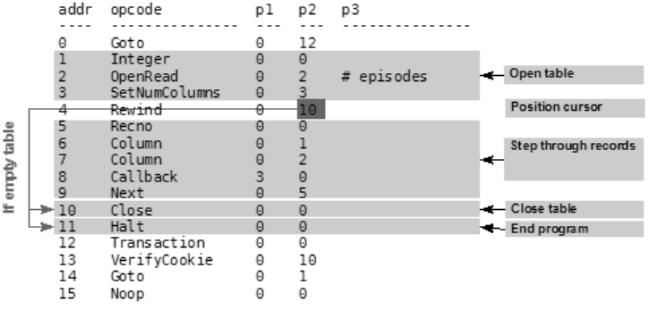
344 CHAPTER 9 ■ SQLITE INTERNALS
The P3 value is a pointer to a KeyInfo structure that defines the content and collating
sequence of indices. P3 is NULL for cursors that are not pointing to indices.
This documentation for OpenRead as well as all other instructions can be found directly in the
source code, specifically in vdbe.c.
Finally, the SetNumColumns instruction sets the number of columns the cursor will hold,
which corresponds to the number of columns in the table it points to. It uses operands P1 and
P2. P1 specifies the cursor index (0 in this case, which is the index of the cursor just opened). P2
specifies the number of columns. The episodes table has three columns.
Continuing the example, the Rewind instruction places the cursor at the beginning of the
table. It checks to ensure that the table is not empty (it has no records). If the table is empty, it
will place the instruction pointer on the instruction specified in the P2 operand. In this case P2
is 10, so Rewind will jump to instruction 10 if the table is empty—in this example, the Close
instruction (Figure 9-1).
Once Rewind has set the cursor position, the next section of instructions (instructions 5–9)
takes over. This section’s job is to iterate over all of the records in the table. Recno pushes the
key value of the record onto the stack pointed to by the cursor identified in P1. The Column
instruction pushes the value of the column with the ordinal given by P2 of the cursor given by
P1. Together instructions 5, 6, and 7 place the id (primary key), season, and name fields onto the
stack—all three fields of the episodes table—for the record that cursor 0 is pointing to. Notice
that the P1 operand for all three instructions is 0. This refers to cursor 0. Next, the Callback
instruction takes three values off the stack (specified by P1) and forms an array (or record)
structure, which is stored in a memory cell. Callback will then suspend VDBE operation, yielding
control back to sqlite3_step(), which will then return SQLITE_ROW.
Figure 9-1. VDBE steps: Open and Read
Once the VDBE has created the record structure, it too is associated with the statement
handle. The program can then use the sqlite3_column_xxx() functions to retrieve the fields
from the record structure. On the next call to sqlite3_step(), the instruction pointer will be
pointing to the Next instruction. The Next instruction advances the cursor to the next row in the
Owens_6730 C09.fm Page 344 Tuesday, April 18, 2006 2:23 PM
www.it-ebooks.info
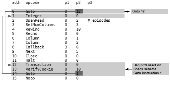
CHAPTER 9 ■ SQLITE INTERNALS 345
table. If there is another record, it jumps to the instruction given in P2, which in this case is
instruction 5, which corresponds to the Recno instruction. Thus, it will go through another iter-
ation, creating a new record structure, and sqlite3_step() will return SQLITE_ROW, indicating
that there is another row to read. However, if there is not another row in the table, Next will fall
through to the next instruction, which in this case is the Close instruction. Close will close the
cursor and fall through to the Halt instruction, terminating the VDBE program, and sqlite3_step()
will return SQLITE_DONE.
Program Startup and Shutdown
Now that we’ve seen the core of the program, let’s look at the remaining sections, which relate
to startup and initialization. These sections are shown in Figure 9-2. The first instruction is a
Goto. Goto jumps to the instruction given in P2, which in this case is instruction 12.
Instruction 12 is a Transaction instruction, which starts a new transaction. It falls through
to VerifyCookie, whose job is to ensure that the database schema has not changed since
the VDBE program was compiled. This is an important concept in SQLite. Between the time
SQL is compiled into VDBE code in sqlite3_prepare() and the time it is actually executed in
sqlite3_step(), another SQL command could have run that changed the database schema
(such as ALTER TABLE, DROP TABLE, or CREATE TABLE). When this happens, the schema version
changes and it invalidates all statements that were compiled before the change. The current
database schema is recorded at all times in the root page of the database file. Similarly, each
statement object maintains a copy of the schema version it was compiled under for comparison.
VerifyCookie’s job is to check that they match, and if they don’t, to take appropriate action.
Figure 9-2. VDBE steps: program startup
VerifyCookie compares the database schema version on disk with the schema version
given in P2—which corresponds to the statement’s version referenced by the compiled code.
If the schema has not changed since compile, the two will match. If they don’t match, then the
VDBE program (specifically the statement object that holds it) is no longer valid; it does not
correspond to the most recent database schema. In this case, VerifyCookie will terminate the
Owens_6730 C09.fm Page 345 Tuesday, April 18, 2006 2:23 PM
www.it-ebooks.info
346 CHAPTER 9 ■ SQLITE INTERNALS
VDBE program and arrange a SQLITE_SCHEMA error to be issued. In this case, the application
needs to recompile the SQL statement, generating a new VDBE program based on the new
schema. Recompiling could very well result in a different program. For example, what if someone
dropped the episodes table and created a new table, which reused some of episodes’ recycled
pages? If the VDBE were to execute the invalid statement now, it would look for episodes
(which no longer exists) starting at root page 2 (which has been recycled), and try to read
records that no longer exist. The application would get junk for data.
However, when the schema versions do match, then the program counter steps from
VerifyCookie to the following instruction—in this case Goto. Goto positions the program
counter on instruction 1, which takes us to the main part of the program—opening the table
and reading the records, as covered earlier. There are a few things to note here:
•The Transaction instruction doesn’t acquire any locks in itself. It is the logical equivalent
of a simple BEGIN. The actual shared lock is created by the OpenRead instruction. The lock
is are freed when the transaction closes. This is determined by the Halt instruction,
which cleans everything up. The action it takes depends on whether the connection is in
autocommit mode or not.
• All of the storage space needed for the statement object (VDBE program) is determined
before the start of the program. This is due primarily to two important facts. First, the
depth of the stack is never greater than the number of instructions in the program. Second,
the number of memory cells is never greater than the number of instructions (and is usually
much less). Thus, even though SQL is dynamic in nature, SQLite can always compute
how much memory a query will require and can allocate all of the resources before
running the VDBE program.
Instruction Types
And this is how the VDBE works—one instruction at a time. Each instruction accomplishes a
simple task and is often intertwined with instructions preceding or following it. If you look at
the instruction set, you will see that opcodes fall into three general categories:
•Value manipulation: These instructions perform things like arithmetic operations (add,
subtract, divide, etc.), logical operations (bitwise OR and AND), and string manipulation.
•Data management: These instructions manipulate data in memory and on disk. Memory
instructions do things like stack manipulation and transfer data between stack entries
and memory cells, and vice versa. Disk operations control the B-tree and pager modules—
opening and manipulating cursors, beginning and ending transactions, and so forth.
•Control flow: Control instructions move the instruction pointer around both condition-
ally and unconditionally.
Once you become familiar with the instruction set, it is not hard to see what is going on. If nothing
else, you can get a general feel for how the stack is used by some instructions to prepare the
way for other instructions.
Owens_6730 C09.fm Page 346 Tuesday, April 18, 2006 2:23 PM
www.it-ebooks.info
CHAPTER 9 ■ SQLITE INTERNALS 347
A Practical Example
Let’s look at the example again, this time performing a VDBE trace on it. This will show us
directly how the stack is being used between instructions. The first part of the program from
startup to the first record is as follows:
sqlite> pragma vdbe_trace=on;
sqlite> select * from episodes;
VDBE Execution Trace:
SQL: [select * from episodes;]
0 Goto 0 12
12 Transaction 0 0
13 VerifyCookie 0 10
14 Goto 0 1
1 Integer 0 0
Stack: i:0
2 OpenRead 0 2 # episodes
3 SetNumColumns 0 3
4 Rewind 0 10
5 Recno 0 0
Stack: i:0
6 Column 0 1
Stack: NULL i:0
7 Column 0 2
Stack: s18[Good News Bad N](8) NULL i:0
8 Callback 3 0
0||Good News Bad News
9 Next 0 5
You can see the startup in the first four steps, followed by the Integer command, which
specifies on the stack the database index upon which to open the cursor. OpenRead will pop it
from the stack and open a cursor on the table with root page 2 (given by P2). Step down into the
loop part and you see Recno and Column instructions pushing field values of the current record
onto the stack. Callback then pops all of them off the stack and uses them to form a record struc-
ture, which is then stored in the statement handle. sqlite3_step() returns a SQLITE_ROW, indicating
that a row is available for reading. The application accesses the data with sqlite3_column_xxx(),
and proceeds to the next record by calling sqlite3_step() again. sqlite3_step() then resumes
VDBE execution at the Next instruction, which moves on to the next record. And so on and
so forth.
So not only can you see the stack at work, but you can also get some idea as to how the
SQLite C API functions are intertwined within VDBE code. From here on out, it is a matter of
just playing with the VDBE to see what the instructions do. For instance:
Owens_6730 C09.fm Page 347 Tuesday, April 18, 2006 2:23 PM
www.it-ebooks.info
348 CHAPTER 9 ■ SQLITE INTERNALS
sqlite> explain BEGIN;
addr opcode p1 p2 p3
---- --------------- --- --- ---------------
0 AutoCommit 0 0
1 Halt 0 0
2 Noop 0 0
sqlite> explain COMMIT;
addr opcode p1 p2 p3
---- --------------- --- --- ---------------
0 AutoCommit 1 0
1 Halt 0 0
2 Noop 0 0
sqlite> explain ROLLBACK;
addr opcode p1 p2 p3
---- --------------- --- --- ---------------
0 AutoCommit 1 1
1 Halt 0 0
2 Noop 0 0
You can see here that transactions work by toggling the AutoCommit instruction. This instruction
must therefore be related to initiating the transfer of modified pages to disk. Try different
things and see what happens. After a little practice, you may very well be able to recognize
enough of the instruction patterns to use EXPLAIN to optimize queries.
The B-Tree and Pager Modules
The B-tree provides the VDBE with O(logN) lookup, insert, and delete as well as O(1) bidirectional
traversal of records. It is self-balancing, and automatically manages both defragmentation and
space reclamation. The B-tree itself has no notion of reading or writing to disk. It only concerns
itself with the relationship between pages. The B-tree notifies the pager when it needs a page,
and also notifies it when it is about to modify a page. When modifying a page, the pager ensures
that the original page is first copied out to the journal file. Similarly, the B-tree notifies the
pager when it is done writing, and the pager determines what needs to be done based on the
transaction state.
Owens_6730 C09.fm Page 348 Tuesday, April 18, 2006 2:23 PM
www.it-ebooks.info
CHAPTER 9 ■ SQLITE INTERNALS 349
Database File Format
All pages in a database are numbered sequentially, beginning with 1. A database is composed
of multiple B-trees—one B-tree for each table and index (B+trees are used for tables, B-trees for
indexes). Each table or index in a database has a root page that defines the location of its first
page. The root pages for all indexes and tables are stored in the sqlite_master table.
The first page in the database—Page 1—is special. The first 100 bytes of Page 1 contain a
special header (the file header) that describes the database file. It includes such information as
the library version, schema version, page size, encoding, whether or not autovacuum is enabled—
all of the permanent database settings you configure when creating a database along with any
other parameters that have been set by various pragmas. The exact contents of the header are
documented in btree.c. Page 1 is also the root page of the sqlite_master table.
Page Reuse and Vacuum
SQLite recycles pages using a free list. That is, when all of the records are deleted out of a page,
the page is placed on a list reserved for reuse. When new information is later added, nearby
pages are first selected before any new pages are created (expanding the database file). Running
a VACUUM command purges the free list and thereby shrinks the database. In actuality, it rebuilds the
database in a new file so that all in-use pages are copied over, while free-list pages are not.
The end result is a new, compacted database. When autovacuum is enabled in a database,
SQLite doesn’t use a free list, and automatically shrinks the database upon each commit.
B-Tree Records
Pages in a B-tree are made up of B-tree records, also called payloads. They are not database
records in the sense you might think—formatted with the columns in a table. They are more
primitive than that. A B-tree record, or payload, has only two fields: a key field and a data field.
The key field is the ROWID value, or primary key value that is present for every table in the data-
base. The data field, from the B-tree perspective, is an amorphous blob that can contain anything.
Ultimately, the database records are stored inside the data fields. The B-tree’s job is order and
navigation, and it primarily needs only the key field to do its work (although there is one excep-
tion in B+trees, which is addressed next). Furthermore, payloads are variable size, as are their
internal key and data fields. On average, each page usually holds multiple payloads; however,
it is possible for a payload to span multiple pages if it is too large to fit on one page (e.g., records
containing BLOBs).
B+Trees
B-tree records are stored in key order. All keys must be unique within a single B-tree (this is
automatically guaranteed as the keys correspond to the ROWID primary key, and SQLite takes
care of that field for you). Tables use B+trees, which do not contain table data (database records)
in the internal pages. An example B+tree representation of a table is shown in Figure 9-3.
Owens_6730 C09.fm Page 349 Tuesday, April 18, 2006 2:23 PM
www.it-ebooks.info
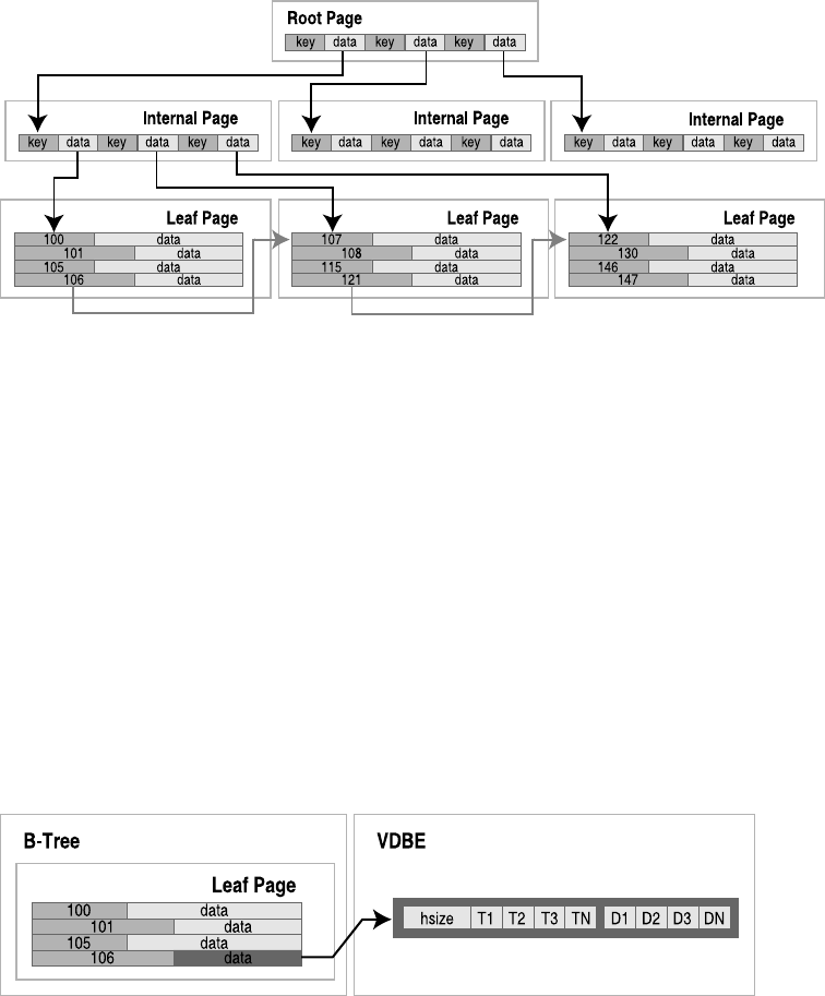
350 CHAPTER 9 ■ SQLITE INTERNALS
Figure 9-3. B+tree organization (tables)
The root page and internal pages in B+trees are all about navigation. The data fields in
these pages are all pointers to the pages below them—they contain keys only. All database
records are stored on the leaf pages. On the leaf level, records and pages are arranged in key
order so it is possible for B-tree cursors to traverse records (horizontally), both forward and
backward, using only the leaf pages. This is what makes traversal possible in O(1) time.
Records and Fields
The database records in the data fields of the leaf pages are managed by the VDBE (as in the
Callback instruction described earlier). The database record is stored in binary form using
a specialized record format that describes all of the fields in the record. The record format consists
of a contiguous stream of bytes organized into a logical header and a data segment. The header
segment includes the header size (represented as a variable-sized 64-bit integer value) and an
array of types (also variable 64-bit integers), which describe each field stored in the data segment,
as shown in Figure 9-4. Variable 64-bit integers are implemented using a Huffman code.
Figure 9-4. Record structure
The number of type entries corresponds to the number of fields in the record. Further-
more, each index in the type array corresponds to the same index in the field array. A type entry
specifies the data type and size of its corresponding field value. The possible types and their
meanings are listed in Table 9-1.
Owens_6730 C09.fm Page 350 Tuesday, April 18, 2006 2:23 PM
www.it-ebooks.info
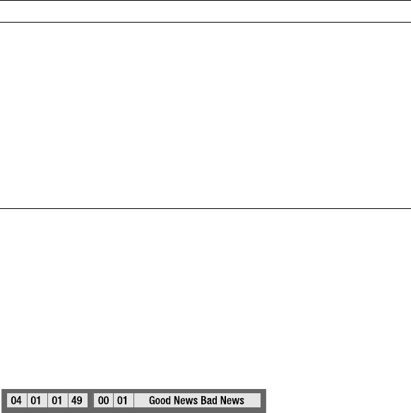
CHAPTER 9 ■ SQLITE INTERNALS 351
For example, take the first record in the episodes table:
sqlite> SELECT * FROM episodes ORDER BY id LIMIT 1;
id season name
--- ------ --------------------
0 1 Good News Bad News
The internal record format for this record is shown in Figure 9-5.
Figure 9-5. First record in the episodes table
The header is 4 bytes long. The header size reflects this and itself is encoded as a single
byte. The first type, corresponding to the id field, is a 1-byte signed integer. The second type,
corresponding to the season field, is as well. The name type entry is an odd number, meaning it
is a text value. Its size is therefore given by (49-13)/2=17 bytes. With the information, the VDBE
can parse the data segment of the record and extract the individual fields.
Hierarchical Data Organization
Basically, each module in the stack deals with a specific unit of data. From the bottom up, data
becomes more refined and more specific. From the top down, it becomes more aggregated and
amorphous. Specifically, the C-API deals in field values, the VDBE in records, the B-tree in keys
and data, the pager in pages, the OS interface in binary data and raw storage. This is illustrated
in Figure 9-6.
Table 9-1. Field Type Values
Type Value Meaning Length of Data
0NULL 0
N in 1..4 Signed integer N
5 Signed integer 6
6 Signed integer 8
7 IEEE float 8
8-11 Reserved for future use N/A
N>12 and even BLOB (N-12)/2
N>13 and odd TEXT (N-13)/2
Owens_6730 C09.fm Page 351 Tuesday, April 18, 2006 2:23 PM
www.it-ebooks.info
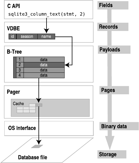
352 CHAPTER 9 ■ SQLITE INTERNALS
Figure 9-6. Modules and their associated data
Each module takes part in managing its own specific portion of the data in the database,
and relies on the layer below it to supply it with a more crude form from which to extract its
respective pieces.
Overflow Pages
As mentioned earlier, payloads and their contents can have variable sizes. However, pages are
fixed in size. Therefore, there is always the possibility that a given payload could be too large to
fit in a single page. When this happens, the excess payload is spilled out onto a linked list of
overflow pages. From this point on, the payload takes on the form of a linked list of sorts, as
shown in Figure 9-7.
The fourth payload in the figure is too large to fit on the page. As a result, the B-tree module
creates an overflow page to accommodate. It turns out that one page won’t suffice, so it links a
second. This is essentially the way binary large objects are handled. One thing to keep in mind
when you are using really large BLOBs is that they are ultimately being stored as a linked list of
pages. If the BLOB is large enough, this can become inefficient, in which case you might consider
dedicating an external file for the BLOB and keeping this filename in the record instead.
Owens_6730 C09.fm Page 352 Tuesday, April 18, 2006 2:23 PM
www.it-ebooks.info
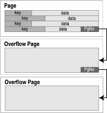
CHAPTER 9 ■ SQLITE INTERNALS 353
Figure 9-7. Overflow pages
The B-Tree API
The B-tree module has its own API, which is separate from and can be used independently of
the C API. That is, you could use it as a standalone B-tree library, or access tables in a SQLite
database directory, if you wish. An added benefit of SQLite’s B-tree module is that it includes
native support for transactions. Everything you know about the transactions, locks, and journal
file are handled by the pager, which serves the B-tree module. The API can be grouped into
functions according to general purpose.
Access and Transaction Functions
Database and transaction routines include the following:
•sqlite3BtreeOpen: Opens a new database file. Returns a B-tree object.
•sqlite3BtreeClose: Closes a database.
•sqlite3BtreeBeginTrans: Starts a new transaction.
•sqlite3BtreeCommit: Commits the current transaction.
•sqlite3BtreeRollback: Rolls back the current transaction.
•sqlite3BtreeBeginStmt: Starts a statement transaction.
•sqlite3BtreeCommitStmt: Commits a statement transaction.
•sqlite3BtreeRollbackStmt: Rolls back a statement transaction.
Owens_6730 C09.fm Page 353 Tuesday, April 18, 2006 2:23 PM
www.it-ebooks.info
354 CHAPTER 9 ■ SQLITE INTERNALS
Table Functions
Table management routines include the following:
•sqlite3BtreeCreateTable: Creates a new, empty B-tree in a database file. Flags in the
argument determine whether to use a table format (B+tree) or index format (B-tree).
•sqlite3BtreeDropTable: Destroys a B-tree in a database file.
•sqlite3BtreeClearTable: Removes all data from a B-tree, but keeps the B-tree intact.
Cursor Functions
Cursor functions include the following:
•sqlite3BtreeCursor: Creates a new cursor pointing to a particular B-tree. Cursors can be
either a read cursor or a write cursor. Read and write cursors may not exist in the same
B-tree at the same time.
•sqlite3BtreeCloseCursor: Closes the B-tree cursor.
•sqlite3BtreeFirst: Moves the cursor to the first element in a B-tree.
•sqlite3BtreeLast: Moves the cursor to the last element in a B-tree.
•sqlite3BtreeNext: Moves the cursor to the next element after the one it is currently
pointing to.
•sqlite3BtreePrevious: Moves the cursor to the previous element before the one it is
currently pointing to.
•sqlite3BtreeMoveto: Moves the cursor to an element that matches the key value passed
in as a parameter. If there is no match, leaves the cursor pointing to an element that
would be on either side of the matching element, had it existed.
Record Functions
Key and record functions include the following:
•sqlite3BtreeDelete: Deletes the record that the cursor is pointing to.
•sqlite3BtreeInsert: Inserts a new element in the appropriate place of the B-tree.
•sqlite3BtreeKeySize: Returns the number of bytes in the key of the record that the
cursor is pointing to.
•sqlite3BtreeKey: Returns the key of the record the cursor is currently pointing to.
•sqlite3BtreeDataSize: Returns the number of bytes in the data record that the cursor is
currently pointing to.
•sqlite3BtreeData: Returns the data in the record the cursor is currently pointing to.
Owens_6730 C09.fm Page 354 Tuesday, April 18, 2006 2:23 PM
www.it-ebooks.info
CHAPTER 9 ■ SQLITE INTERNALS 355
Configuration Functions
Functions to set various parameters include the following:
•sqlite3BtreeSetCacheSize: Controls the page cache size as well as the synchronous
writes (as defined in the synchronous pragma).
•sqlite3BtreeSetSafetyLevel: Changes the way data is synced to disk in order to increase
or decrease how well the database resists damage due to OS crashes and power failures.
Level 1 is the same as asynchronous (no syncs() occur and there is a high probability of
damage). This is the equivalent to pragma synchronous=OFF. Level 2 is the default. There
is a very low but non-zero probability of damage. This is the equivalent to pragma
synchronous=NORMAL. Level 3 reduces the probability of damage to near zero but with a
write performance reduction. This is the equivalent to pragma synchronous=FULL.
•sqlite3BtreeSetPageSize: Sets the database page size.
•sqlite3BtreeGetPageSize: Returns the database page size.
•sqlite3BtreeSetAutoVacuum: Sets the autovacuum property of the database.
•sqlite3BtreeGetAutoVacuum: Returns whether the database uses autovacuum.
•sqlite3BtreeSetBusyHandler: Sets the busy handler.
There are more functions, all of which are very well documented in btree.h and btree.c,
but those listed here give you some idea of the parts of the API that are implemented in the
B-tree layer, as well as what this layer can do in its own right.
The Compiler
So far, you have seen how things operate from the VDBE down the stack through the storage
and OS layers. Now let’s look at how the VDBE program is constructed to begin with. This is the
job of the front end. The front end takes a single SQL command as an input and ends with a
complete, optimized VDBE program. This happens in three stages: tokenizing, parsing, and
code generation.
The Tokenizer
The first step of compilation is tokenizing the SQL command. The tokenizer splits a command
into a stream of individual tokens. A token is simply a character or sequence of characters that
has a specific meaning (in this case some meaning within SQL). Each token has an associated
token class, which is simply a numeric identifier describing what the token is. For example, a
left parenthesis token is classified as TK_LP, and the SELECT keyword is classified as TK_SELECT.
All token classes are defined in parse.h. For instance, the SQL statement
SELECT rowid FROM foo where name='bar' LIMIT 1 ORDER BY rowid;
would be processed by the tokenizer as shown in part in Table 9-2.
In short, the tokenizer breaks up each unit of text, classifies it, and sends it to the parser
(discarding white space).
Owens_6730 C09.fm Page 355 Tuesday, April 18, 2006 2:23 PM
www.it-ebooks.info

356 CHAPTER 9 ■ SQLITE INTERNALS
Keywords
The tokenizer is hand-coded and located in tokenize.c. While it is hand-coded, it does use
generated code to classify SQL keywords, which are defined in keywordhash.h. This file is an
optimization that compacts all SQL keywords into the smallest possible buffer by overlapping
common character sequences in keywords. SQLite identifies keyword entries using arrays that
define the offsets and size of each keyword. The method is a space optimization intended to
help embedded applications. An example of the generated buffer is as follows:
static int keywordCode(const char *z, int n){
static const char zText[537] =
"ABORTABLEFTEMPORARYADDATABASELECTHENDEFAULTRANSACTIONATURALTER"
"AISEACHECKEYAFTEREFERENCESCAPELSEXCEPTRIGGEREGEXPLAINITIALLYANALYZE"
"XCLUSIVEXISTSTATEMENTANDEFERRABLEATTACHAVINGLOBEFOREIGNOREINDEX"
"AUTOINCREMENTBEGINNERENAMEBETWEENOTNULLIKEBYCASCADEFERREDELETE"
"CASECASTCOLLATECOLUMNCOMMITCONFLICTCONSTRAINTERSECTCREATECROSS"
"CURRENT_DATECURRENT_TIMESTAMPLANDESCDETACHDISTINCTDROPRAGMATCH"
"FAILIMITFROMFULLGROUPDATEIFIMMEDIATEINSERTINSTEADINTOFFSETISNULL"
"JOINORDEREPLACEOUTERESTRICTPRIMARYQUERYRIGHTROLLBACKROWHENUNION"
"UNIQUEUSINGVACUUMVALUESVIEWHERE";
The keywordhash.h file includes a routine sqlite3KeywordCode(), which allows the tokenizer to
quickly match the keyword with its appropriate token class with minimal space. So, the tokenizer
first tries to match a token with what it knows, and failing that, it resorts to sqlite3KeywordCode(),
which will return either a keyword token class or a generic TK_ID.
Table 9-2. A Tokenized SELECT statement
Text Token Class Action
SELECT TK_SELECT Sent to parser
" " TK_SPACE Discarded
Rowid TK_ID Sent to parser
" " TK_SPACE Discarded
FROM TK_FROM Sent to parser
" " TK_SPACE Discarded
foo TK_ID Sent to parser
"" TK_SPACE Discarded
WHERE TK_WHERE Sent to parser
" " TK_SPACE Discarded
name TK_ID Sent to parser
= TK_EQ Sent to parser
Owens_6730 C09.fm Page 356 Tuesday, April 18, 2006 2:23 PM
www.it-ebooks.info
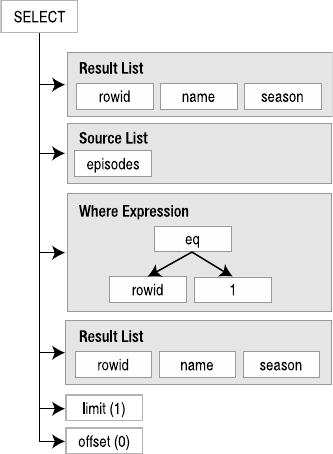
CHAPTER 9 ■ SQLITE INTERNALS 357
The tokenizer and parser work hand in hand, one token at a time. As the tokenizer resolves
each token, it passes the token to the parser. The parser takes the tokens and builds a parse
tree, which is a hierarchical representation of the statement.
The Parser
The parser is generated from SQLite’s custom parser generator—the Lemon parser generator.
The parser uses grammar rules defined in parse.y to organize the tokens into a parse tree. The
theory behind the parser is beyond the scope of this chapter—there are many textbooks that
cover the topic. The point is that the parser converts a stream of tokens into a hierarchical data
structure, called a parse tree, which represents the SQL command.
The parse tree is primarily composed of expressions and lists of expressions. An expres-
sion itself is a recursive structure that can contain subexpressions under it. For example, the
WHERE clause in a SELECT parse tree is represented by a single expression. The SELECT clause, on
the other hand, is represented as a list of expressions; each expression is a column that will be
returned in the result set. For example, a very simplified representation of the statement
SELECT rowid, name, season FROM episodes WHERE rowid=1 LIMIT 1
might be arranged into a parse tree as shown in Figure 9-8.
Figure 9-8. Simplified parse tree representation
Once the statement has been completely tokenized and parsed, the parse tree is passed to
the code generator.
Owens_6730 C09.fm Page 357 Tuesday, April 18, 2006 2:23 PM
www.it-ebooks.info
358 CHAPTER 9 ■ SQLITE INTERNALS
The Code Generator
The code generator is the largest and most complex part of SQLite. Unlike most other modules,
the code generator does not have a well-defined interface, but is rather closely tied to the parser.
It is made up of many source files, most of which are specific to SQL operations. For example,
the code to generate SELECT statements is kept in select.c. Other source files include update.c,
insert.c, delete.c, trigger.c, and so on.
The code generator takes the parse tree and produces the VDBE program to execute the
statement. Each part of the tree more or less is handled by a specific routine that generates a
sequence of VDBE instructions to accomplish a specific task. The values for the operands are
taken from the data structures associated with the parse tree. For example, the function to
open a table for reading is implemented as follows:
/*
** Generate code that will open a table for reading.
*/
void sqlite3OpenTableForReading(
Vdbe *v, /* Generate code into this VDBE */
int iCur, /* The cursor number of the table */
Table *pTab /* The table to be opened */
){
sqlite3VdbeAddOp(v, OP_Integer, pTab->iDb, 0);
sqlite3VdbeAddOp(v, OP_OpenRead, iCur, pTab->tnum);
VdbeComment((v, "# %s", pTab->zName));
sqlite3VdbeAddOp(v, OP_SetNumColumns, iCur, pTab->nCol);
}
The sqlite3vdbeAddOp function takes three arguments: a VDBE instance (to which it will
add instructions), an instruction (or opcode), and two operands. It adds exactly one instruction
to the VDBE instance’s program. In this case, sqlite3OpenTableForReading adds the three
instructions (1–3) to open a B-tree table for reading, just as it was shown in Figure 9-1, which
are listed here again for convenience:
sqlite> explain select * from episodes;
addr opcode p1 p2 p3
---- --------------- --- --- ---------------
0 Goto 0 12
1 Integer 0 0
2 OpenRead 0 2 # episodes
3 SetNumColumns 0 3
4 Rewind 0 10
5 Recno 0 0
6 Column 0 1
7 Column 0 2
8 Callback 3 0
9 Next 0 5
10 Close 0 0
11 Halt 0 0
12 Transaction 0 0
Owens_6730 C09.fm Page 358 Tuesday, April 18, 2006 2:23 PM
www.it-ebooks.info
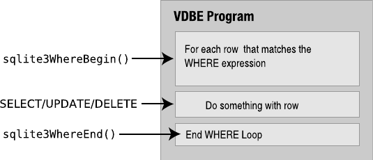
CHAPTER 9 ■ SQLITE INTERNALS 359
13 VerifyCookie 0 10
14 Goto 0 1
15 Noop 0 0
For example, the second line of sqlite3OpenTableForReading is
sqlite3VdbeAddOp(v, OP_OpenRead, iCur, pTab->tnum);
This creates instruction 3 in the program. The P2 value refers to the root page of the table to be
opened. This is provided by the table data structure pointed to by pTab, specifically the tnum
member, which holds the table’s root page number. So whenever a parse tree calls for a table
to be opened, it calls sqlite3OpenTableForReading to add the corresponding VDBE instructions
to do so.
In short, code generation is done by many different routines across many different files
in the code. The routines analyze a specific portion of the parse tree and create corresponding
VDBE instructions to accomplish a specific task. The code generator contains a wide variety of
routines for generating instructions. General functions are available that are used in many
places; sqlite3ExprCode, for example, takes an expression and generates the instructions
needed to evaluate it. Likewise, there are highly specific routines that accomplish unique tasks,
such as sqlite3FinishTrigger, which generates the VDBE instructions to complete the process
of building a trigger.
The Optimizer
The code generator does more than just code generation, however. It performs query optimi-
zation as well. The optimizer is part of the code generator, and lives in where.c. Code that
creates the WHERE clause is shared by other modules, such as select.c, update.c, and delete.c.
Each of these modules calls sqlite3WhereBegin() to generate the WHERE clause code to produce
the search instructions, and then add their own VDBE code after it to process the rows that are
returned. They then conclude that code with sqlite3WhereEnd(), which adds the VDBE instruc-
tions that concludes the WHERE clause code. The general structure is shown in Figure 9-9.
Figure 9-9. WHERE clause VDBE code generation
Optimizations take place in sqlite3WhereBegin(). Based on what is being done, it looks for
indexes that might be used, expressions that can be rewritten, and so forth.
To get a feel for how this works, let’s start with a simple SELECT with no WHERE clause, as
shown in Figure 9-10.
Owens_6730 C09.fm Page 359 Tuesday, April 18, 2006 2:23 PM
www.it-ebooks.info
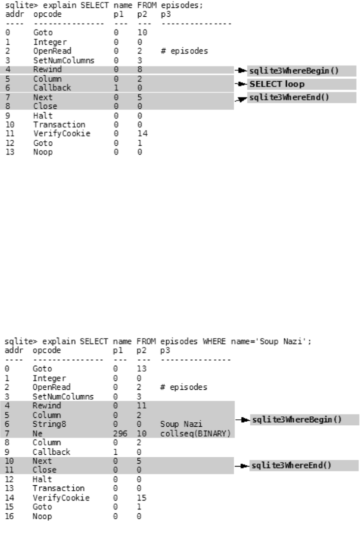
360 CHAPTER 9 ■ SQLITE INTERNALS
Figure 9-10. A SELECT statement with no WHERE clause
By now, you can start to recognize the various code generation sections. Instructions 1–3
open episodes for reading, and instructions 4–9 iterate through all records, selecting the name
column (identified here by the Column instruction). Even though there was no WHERE clause
here, sqlite3WhereBegin() and sqlite3WhereEnd() are called and generate instructions. Here,
the query calls for a table scan. sqlite3WhereBegin() adds the Rewind instruction, which places
the cursor at the beginning of the table. Following that, instructions 5–6 are from the select
code, and sqlite3WhereEnd() concludes with instructions 7–8. Instructions 0 and 10–13 are the
standard prologue instructions for executing a command.
Next, let’s look at what a WHERE clause does (Figure 9-11).
Figure 9-11. Instructions relating to a WHERE clause
Owens_6730 C09.fm Page 360 Tuesday, April 18, 2006 2:23 PM
www.it-ebooks.info
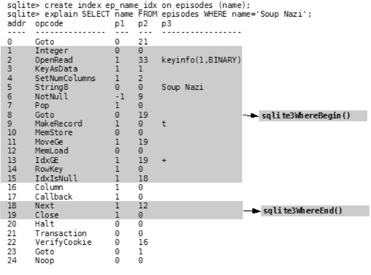
CHAPTER 9 ■ SQLITE INTERNALS 361
Instructions 4–6, produced by sqlite3WhereBegin(), add the constraint name='Soup Nazi'.
Everything else is unchanged. In both cases the WHERE clause performs a full table scan, as is
evidenced by the Next instruction in the WhereEnd segment.
Now, create an index on the name column and see what happens (Figure 9-12).
Now, sqlite3WhereBegin() sees that there is an index it can use and writes in VDBE
instructions to do so. This is essentially how the optimizer works: as the WHERE component
of the code generator.
Figure 9-12. Instructions relating to index use in the WHERE clause
Summary
And that concludes our journey through SQLite, not only in this chapter, but the book as well.
I hope you have enjoyed it. As you’ve seen in Chapter 1, SQLite is more than merely a free data-
base. It is a well-written software library with a wide range of applications. It is a database, a
utility, and a helpful programming tool.
What you have seen in this chapter barely scratches the surface, but it should give you a
better idea about how things work nonetheless. And it also gives you an appreciation for how
elegantly SQLite approaches a very complex problem. You know firsthand how big SQL is, and
you’ve seen the complexity of the relational model behind it. Yet SQLite is a small library and
manages to put many of these concepts to work in a small amount of code. It does this by breaking
query processing down into discrete tasks. Each of its modules accomplishes a specific task
Owens_6730 C09.fm Page 361 Tuesday, April 18, 2006 2:23 PM
www.it-ebooks.info
362 CHAPTER 9 ■ SQLITE INTERNALS
and works closely with the modules above and below it. This design keeps things simple,
manageable, and reliable. Add to this a large and thorough testing suite and that is how SQLite
packs a lot of relational power into a very small package.
From a programming standpoint, SQLite is not only useful in its own right, but there is a
lot you can learn from it as well. Even though it is small, it employs quite a variety of different
concepts: tokenizing, parsing, virtual machines, B-trees and B+trees, caching, locking, transac-
tions, memory management, and more. Not only does it implement all of these things, it does
so while also satisfying tough design constraints: portability, flexibility, simplicity, efficiency,
and reliability. Therefore, by looking at SQLite’s implementation, you can study not only a
particular concept but also how it is implemented from this perspective. And if a particular
implementation works for you, the code is yours for the taking.
Owens_6730 C09.fm Page 362 Tuesday, April 18, 2006 2:23 PM
www.it-ebooks.info

363
■ ■ ■
APPENDIX A
SQL Reference
The SQLite library understands most of the standard SQL language. But it does omit some
features while at the same time adding a few features of its own. This reference is an overview
of the SQL syntax implemented by SQLite, taken directly from the original documentation on
the SQLite website (www.sqlite.org/lang.html) and slightly edited. Many low-level productions
are omitted. For detailed information on the language that SQLite understands, refer to the
source code and the grammar file parse.y in the source distribution.
In all of the syntax diagrams that follow, literal text is shown in bold. Nonterminal symbols
are shown in italic. Operators that are part of the syntactic markup itself are shown as regular,
unformatted text.
ALTER TABLE
sql-statement ::= ALTER TABLE [database-name .] table-name alteration
alteration ::= RENAME TO new-table-name
alteration ::= ADD [COLUMN] column-def
SQLite’s version of the ALTER TABLE command allows the user to rename or add a new column
to an existing table. It is not possible to remove a column from a table.
ANALYZE
sql-statement ::= ANALYZE
sql-statement ::= ANALYZE database-name
sql-statement ::= ANALYZE [database-name .] table-name
The ANALYZE command gathers statistics about indexes and stores them in a special table in the
database where the query optimizer can use them to help make better index choices. If no
arguments are given, all indexes in all attached databases are analyzed. If a database name is
given as the argument, all indexes in that one database are analyzed. If the argument is a table
name, then only indexes associated with that one table are analyzed.
The initial implementation stores all statistics in a single table named sqlite_stat1. Future
enhancements may create additional tables with the same name pattern except with the “1”
changed to a different digit. The sqlite_stat1 table cannot be dropped, but all the content can
be deleted, which has the same effect.
Owens_6730 AppA.fm Page 363 Tuesday, April 18, 2006 4:05 PM
www.it-ebooks.info
364 APPENDIX A ■ SQL REFERENCE
The RENAME TO syntax is used to rename the table identified by database-name.table-name
to new-table-name. This command cannot be used to move a table between attached databases,
but only to rename a table within the same database.
If the table being renamed has triggers or indexes, then these remain attached to the table
after it has been renamed. However, if there are any view definitions, or statements executed
by triggers that refer to the table being renamed, these are not automatically modified to use
the new table name. If this is required, the triggers or view definitions must be dropped and
re-created to use the new table name by hand.
The ADD COLUMN syntax is used to add a new column to an existing table. The new column
is always appended to the end of the list of existing columns. column-def may take any of the
forms permissible in a CREATE TABLE statement, with the following restrictions:
• The column may not have a PRIMARY KEY or UNIQUE constraint.
• The column may not have a default value of CURRENT_TIME, CURRENT_DATE, or
CURRENT_TIMESTAMP.
•If a NOT NULL constraint is specified, then the column must have a default value other
than NULL.
The execution time of the ALTER TABLE command is independent of the amount of data in
the table. The ALTER TABLE command runs as quickly on a table with 10 million rows as it does
on a table with 1 row.
After ADD COLUMN has been run on a database, that database will not be readable by SQLite
version 3.1.3 and earlier until the database is vacuumed (see VACUUM).
ATTACH DATABASE
sql-statement ::= ATTACH [DATABASE] database-filename AS database-name
The ATTACH DATABASE statement adds a preexisting database file to the current database connec-
tion. If the filename contains punctuation characters it must be quoted. The names “main” and
“temp” refer to the main database and the database used for temporary tables. These cannot
be detached. Attached databases are removed using the DETACH DATABASE statement.
You can read from and write to an attached database and you can modify the schema of
the attached database. This is a new feature of SQLite version 3.0. In SQLite 2.8, schema changes to
attached databases were not allowed.
You cannot create a new table with the same name as a table in an attached database, but
you can attach a database that contains tables whose names are duplicates of tables in the
main database. It is also permissible to attach the same database file multiple times.
Tables in an attached database can be referred to using the syntax database-name.table-name.
If an attached table doesn’t have a duplicate table name in the main database, it doesn’t require
a database name prefix. When a database is attached, all of its tables that don’t have duplicate
names become the default table of that name. Any tables of that name attached afterward
require the table prefix. If the default table of a given name is detached, then the last table of
that name attached becomes the new default.
Transactions involving multiple attached databases are atomic, assuming that the main
database is not :memory:. If the main database is :memory:, then transactions continue to be
Owens_6730 AppA.fm Page 364 Tuesday, April 18, 2006 4:05 PM
www.it-ebooks.info
APPENDIX A ■ SQL REFERENCE 365
atomic within each individual database file. But if the host computer crashes in the middle of a
COMMIT where two or more database files are updated, some of those files might get the changes
where others might not. Atomic commit of attached databases is a new feature of SQLite
version 3.0. In SQLite version 2.8, all commits to attached databases behaved as if the main
database were :memory:.
The maximum number of databases that can be attached to a given session is 10. This is
a compile-time limit: the limit can be increased by altering the value in the source code and
recompiling SQLite.
BEGIN TRANSACTION
sql-statement ::= BEGIN [ DEFERRED | IMMEDIATE | EXCLUSIVE ] [TRANSACTION [name]]
sql-statement ::= END [TRANSACTION [name]]
sql-statement ::= COMMIT [TRANSACTION [name]]
sql-statement ::= ROLLBACK [TRANSACTION [name]]
Beginning in version 2.0, SQLite supports transactions with rollback and atomic commit.
The optional transaction name is ignored. SQLite currently does not allow nested transactions.
No changes can be made to the database except within a transaction. Any command that
changes the database (basically, any SQL command other than SELECT) will automatically start
a transaction if one is not already in effect. Automatically started transactions are committed at
the conclusion of the command.
Transactions can be started manually using the BEGIN command. Such transactions usually
persist until the next COMMIT or ROLLBACK command. But a transaction will also ROLLBACK if the
database is closed or if an error occurs and the ROLLBACK conflict resolution algorithm is specified.
See the documentation on the ON CONFLICT clause for additional information about the ROLLBACK
conflict resolution algorithm.
In SQLite version 3.0.8 and later, transactions can be deferred, immediate, or exclusive.
Deferred means that no locks are acquired on the database until the database is first accessed.
Thus with a deferred transaction, the BEGIN statement itself does nothing. Locks are not acquired
until the first read or write operation. The first read operation against a database creates a SHARED
lock and the first write operation creates a RESERVED lock. Because the acquisition of locks is
deferred until they are needed, it is possible that another thread or process could create a separate
transaction and write to the database after the BEGIN on the current thread has executed. If the
transaction is immediate, then RESERVED locks are acquired on all databases as soon as the
BEGIN command is executed, without waiting for the database to be used. After a BEGIN
IMMEDIATE, you are guaranteed that no other thread or process will be able to write to the data-
base or do a BEGIN IMMEDIATE or BEGIN EXCLUSIVE. Other processes can continue to read from the
database, however. An exclusive transaction causes EXCLUSIVE locks to be acquired on all data-
bases. After a BEGIN EXCLUSIVE, you are guaranteed that no other thread or process will be able
to read or write the database until the transaction is complete.
SHARED, RESERVED, and EXCLUSIVE locks are described in detail in Chapters 4 and 5.
The default behavior for SQLite version 3.0.8 is a deferred transaction. For SQLite version 3.0.0
through 3.0.7, deferred is the only kind of transaction available. For SQLite version 2.8 and
earlier, all transactions are exclusive.
Owens_6730 AppA.fm Page 365 Tuesday, April 18, 2006 4:05 PM
www.it-ebooks.info
366 APPENDIX A ■ SQL REFERENCE
The COMMIT command does not actually perform a commit until all pending SQL commands
finish. Thus if two or more SELECT statements are in the middle of processing and a COMMIT is
executed, the commit will not actually occur until all SELECT statements finish.
An attempt to execute COMMIT might result in an SQLITE_BUSY return code. This indicates
that another thread or process had a read lock on the database that prevented the database
from being updated. When COMMIT fails in this way, the transaction remains active and the
COMMIT can be retried later after the reader has had a chance to clear.
comment
comment ::= SQL-comment | C-comment
SQL-comment ::= -- single-line
C-comment ::= /* multiple-lines [*/]
Comments aren’t SQL commands, but can occur in SQL queries. They are treated as white
space by the parser. They can begin anywhere white space can be found, including inside
expressions that span multiple lines.
SQL comments only extend to the end of the current line.
C comments can span any number of lines. If there is no terminating delimiter, they extend
to the end of the input. This is not treated as an error. A new SQL statement can begin on a line
after a multiline comment ends. C comments can be embedded anywhere white space can
occur, including inside expressions, and in the middle of other SQL statements. C comments
do not nest. SQL comments inside a C comment will be ignored.
COMMIT TRANSACTION
See “BEGIN TRANSACTION.”
COPY
sql-statement ::= COPY [ OR conflict-algorithm ] [database-name .]
table-name FROM filename [ USING DELIMITERS delim ]
The COPY command is available in SQLite version 2.8 and earlier. The COPY command has been
removed from SQLite version 3.0 due to complications in trying to support it in a mixed
UTF-8/16 environment. In version 3.0, the command-line shell contains a new command
.import that can be used as a substitute for COPY.
The COPY command is an extension used to load large amounts of data into a table. It is
modeled after a similar command found in PostgreSQL. In fact, the SQLite COPY command is
specifically designed to be able to read the output of the PostgreSQL dump utility pg_dump so
that data can be easily transferred from PostgreSQL into SQLite.
The table-name is the name of an existing table that is to be filled with data. The filename
is a string or an identifier that names a file from which data will be read. The filename can be
the STDIN to read data from standard input.
Owens_6730 AppA.fm Page 366 Tuesday, April 18, 2006 4:05 PM
www.it-ebooks.info
APPENDIX A ■ SQL REFERENCE 367
Each line of the input file is converted into a single record in the table. Columns are sepa-
rated by tabs. If a tab occurs as data within a column, then that tab is preceded by a backslash
(\) character. A backslash in the data appears as two backslashes in a row. The optional USING
DELIMITERS clause can specify a delimiter other than a tab.
If a column consists of the characters \N, that column is filled with the value NULL.
The optional conflict-clause allows the specification of an alternative constraint conflict
resolution algorithm to use this one command. See the section “ON CONFLICT” for additional
information.
When the input data source is STDIN, the input can be terminated by a line that contains
only a backslash and a dot (\.).
CREATE INDEX
sql-statement ::= CREATE [UNIQUE] INDEX [database-name .] index-name
ON table-name ( column-name [, column-name]* )
[ ON CONFLICT conflict-algorithm ]
column-name ::= name [ COLLATE collation-name] [ ASC | DESC ]
The CREATE INDEX command consists of the keywords CREATE INDEX followed by the name of the
new index, the keyword ON, the name of a previously created table that is to be indexed, and a
parenthesized list of names of columns in the table that are used for the index key. Each column
name can be followed by either the ASC or DESC keyword to indicate sort order, but the sort order
is ignored in the current implementation. Sorting is always done in ascending order.
The COLLATE clause following each column name defines a collating sequence used for text
entries in that column. The default collating sequence is the collating sequence defined for that
column in the CREATE TABLE statement. Or if no collating sequence is otherwise defined, the
built-in BINARY collating sequence is used.
There are no arbitrary limits on the number of indexes that can be attached to a single
table, nor on the number of columns in an index.
If the UNIQUE keyword appears between CREATE and INDEX, then duplicate index entries are
not allowed. Any attempt to insert a duplicate entry will result in an error.
The optional conflict-clause allows the specification of an alternative default constraint
conflict resolution algorithm for this index. This only makes sense if the UNIQUE keyword is used
since otherwise there are no constraints on the index. The default algorithm is ABORT. If a COPY,
INSERT, or UPDATE statement specifies a particular conflict resolution algorithm, that algorithm
is used in place of the default algorithm specified here. See the section “ON CONFLICT” for
additional information.
The exact text of each CREATE INDEX statement is stored in the sqlite_master or
sqlite_temp_master table, depending on whether the table being indexed is temporary. Every
time the database is opened, all CREATE INDEX statements are read from the sqlite_master table
and used to regenerate SQLite’s internal representation of the index layout.
Indexes are removed with the DROP INDEX command.
Owens_6730 AppA.fm Page 367 Tuesday, April 18, 2006 4:05 PM
www.it-ebooks.info
368 APPENDIX A ■ SQL REFERENCE
CREATE TABLE
sql-command ::= CREATE [TEMP | TEMPORARY] TABLE table-name (
column-def [, column-def]* [, constraint]* )
sql-command ::= CREATE [TEMP | TEMPORARY] TABLE [database-name.]
table-name AS select-statement
column-def ::= name [type] [[CONSTRAINT name] column-constraint]*
type ::= typename | typename ( number ) | typename (number, number)
column-constraint ::= NOT NULL [ conflict-clause ] |
PRIMARY KEY [sort-order] [ conflict-clause ] [AUTOINCREMENT] |
UNIQUE [ conflict-clause ] |
CHECK ( expr ) [ conflict-clause ] |
DEFAULT value |
COLLATE collation-name
constraint ::= PRIMARY KEY ( column-list ) [ conflict-clause ] |
UNIQUE ( column-list ) [ conflict-clause ] |
CHECK ( expr ) [ conflict-clause ]
conflict-clause ::= ON CONFLICT conflict-algorithm
A CREATE TABLE statement is basically the keywords CREATE TABLE followed by the name of a new
table and a parenthesized list of column definitions and constraints. The table name can be
either an identifier or a string. Table names that begin with sqlite_ are reserved for use by SQLite.
Each column definition is the name of the column followed by the data type for that column,
then one or more optional column constraints. The data type for the column does not restrict
what data may be put in that column. The UNIQUE constraint causes an index to be created on
the specified columns. This index must contain unique keys. The COLLATE clause specifies what
text collating function to use when comparing text entries for the column. The built-in BINARY
collating function is used by default.
The DEFAULT constraint specifies a default value to use when doing an INSERT. The value
may be NULL, a string constant, or a number. Starting with version 3.1.0, the default value
may also be one of the special case-independent keywords CURRENT_TIME, CURRENT_DATE, or
CURRENT_TIMESTAMP. If the value is NULL, a string constant, or number, it is literally inserted into
the column whenever an INSERT statement that does not specify a value for the column is executed.
If the value is CURRENT_TIME, CURRENT_DATE, or CURRENT_TIMESTAMP, then the current UTC date and/or
time is inserted into the columns. For CURRENT_TIME, the format is HH:MM:SS. For CURRENT_DATE, it
is YYYY-MM-DD. The format for CURRENT_TIMESTAMP is YYYY-MM-DD HH:MM:SS.
Specifying a PRIMARY KEY normally just creates a UNIQUE index on the corresponding columns.
However, if the primary key is on a single column that has data type INTEGER, then that column
is used internally as the actual key of the B-tree for the table. This means that the column may
only hold unique integer values. (Except in this one case, SQLite ignores the data type specifi-
cation of columns and allows any kind of data to be put in a column regardless of its declared
Owens_6730 AppA.fm Page 368 Tuesday, April 18, 2006 4:05 PM
www.it-ebooks.info
APPENDIX A ■ SQL REFERENCE 369
data type.) If a table does not have an INTEGER PRIMARY KEY column, then the B-tree key will be
an automatically generated integer. The B-tree key for a row can always be accessed using
one of the special names ROWID, OID, or _ROWID_. This is true regardless of whether there is an
INTEGER PRIMARY KEY. An INTEGER PRIMARY KEY column may also include the keyword AUTOINCREMENT.
The AUTOINCREMENT keyword modified the way that B-tree keys are automatically generated. For
additional information on AUTOINCREMENT, see the “Autoincrement Values” section later in
this appendix.
If the TEMP or TEMPORARY keyword occurs in between CREATE and TABLE, then the table that is
created is only visible to the process that opened the database and is automatically deleted
when the database is closed. Any indexes created on a temporary table are also temporary.
Temporary tables and indexes are stored in a separate file distinct from the main database file.
If a database-name is specified, then the table is created in the named database. It is an
error to specify both a database-name and the TEMP keyword, unless the database-name is “temp”.
If no database name is specified, and the TEMP keyword is not present, the table is created in the
main database.
The optional conflict-clause following each constraint allows the specification of an
alternative default constraint conflict resolution algorithm for that constraint. The default is
ABORT. Different constraints within the same table may have different default conflict resolu-
tion algorithms. If a COPY, INSERT, or UPDATE command specifies a different conflict resolution
algorithm, then that algorithm is used in place of the default algorithm specified in the CREATE
TABLE statement. See “ON CONFLICT” for additional information.
CHECK constraints are implemented in SQLite version 3.3.0 and later. As of version 2.3.0,
only NOT NULL, PRIMARY KEY, and UNIQUE constraints are supported.
There are no arbitrary limits on the number of columns or on the number of constraints
in a table. The total amount of data in a single row is limited to about 1MB in version 2.8. In
version 3.0 there is no arbitrary limit on the amount of data in a row.
The CREATE TABLE AS form defines the table to be the result set of a query. The names of the
table columns are the names of the columns in the result.
The exact text of each CREATE TABLE statement is stored in the sqlite_master table. Every
time the database is opened, all CREATE TABLE statements are read from the sqlite_master table
and used to regenerate SQLite’s internal representation of the table layout. If the original
command was a CREATE TABLE AS, then an equivalent CREATE TABLE statement is synthesized and
stored in sqlite_master in place of the original command. The text of CREATE TEMPORARY TABLE
statements is stored in the sqlite_temp_master table.
Tables are removed using the DROP TABLE statement.
Autoincrement Values
In SQLite, every row of every table has an integer ROWID. The ROWID for each row is unique
among all rows in the same table. In SQLite version 2.8 the ROWID is a 32-bit signed integer.
Version 3.0 of SQLite expanded the ROWID to be a 64-bit signed integer.
You can access the ROWID of a SQLite table using one of the special column names ROWID,
_ROWID_, or OID. Unless you declare an ordinary table column to use one of those special names,
the use of that name will refer to the declared column and not to the internal ROWID.
If a table contains a column of type INTEGER PRIMARY KEY, then that column becomes an
alias for the ROWID. You can then access the ROWID using any of four different names, the original
Owens_6730 AppA.fm Page 369 Tuesday, April 18, 2006 4:05 PM
www.it-ebooks.info
370 APPENDIX A ■ SQL REFERENCE
three names described earlier or the name given to the INTEGER PRIMARY KEY column. All these
names are aliases for one another and work equally well in any context.
When a new row is inserted into a SQLite table, the ROWID can either be specified as part of
the INSERT statement or it can be assigned automatically by the database engine. To specify a
ROWID manually, just include it in the list of values to be inserted. For example:
CREATE TABLE test1(a INT, b TEXT);
INSERT INTO test1(rowid, a, b) VALUES(123, 5, 'hello');
If no ROWID is specified on the insert, an appropriate ROWID is created automatically. The
usual algorithm is to give the newly created row a ROWID that is 1 larger than the largest ROWID in
the table prior to the insert. If the table is initially empty, then a ROWID of 1 is used. If the largest
ROWID is equal to the largest possible integer (9223372036854775807 in SQLite version 3.0 and
later), then the database engine starts picking candidate ROWIDs at random until it finds one
that is not previously used.
The normal ROWID selection algorithm described here will generate monotonically increasing
unique ROWIDs as long as you never use the maximum ROWID value and you never delete the
entry in the table with the largest ROWID. If you ever delete rows or if you ever create a row with
the maximum possible ROWID, then ROWIDs from previously deleted rows might be reused when
creating new rows and newly created ROWIDs might not be in strictly ascending order.
The AUTOINCREMENT Keyword
If a column has the type INTEGER PRIMARY KEY AUTOINCREMENT, then a slightly different ROWID
selection algorithm is used. The ROWID chosen for the new row is 1 larger than the largest ROWID
that has ever before existed in that same table. If the table has never before contained any data,
then a ROWID of 1 is used. If the table has previously held a row with the largest possible ROWID,
then new INSERTs are not allowed and any attempt to insert a new row will fail with a
SQLITE_FULL error.
SQLite keeps track of the largest ROWID that a table has ever held using the special
sqlite_sequence table. The sqlite_sequence table is created and initialized automatically
whenever a normal table that contains an AUTOINCREMENT column is created. The content of the
sqlite_sequence table can be modified using ordinary UPDATE, INSERT, and DELETE statements.
But making modifications to this table will likely perturb the AUTOINCREMENT key generation
algorithm. Make sure you know what you are doing before you undertake such changes.
The behavior implemented by the AUTOINCREMENT keyword is subtly different from the
default behavior. With AUTOINCREMENT, rows with automatically selected ROWIDs are guaranteed
to have ROWIDs that have never been used before by the same table in the same database. And
the automatically generated ROWIDs are guaranteed to be monotonically increasing. These are
important properties in certain applications. But if your application does not need these prop-
erties, you should probably stay with the default behavior since the use of AUTOINCREMENT
requires additional work to be done as each row is inserted and thus causes INSERTs to run a
little slower.
Owens_6730 AppA.fm Page 370 Tuesday, April 18, 2006 4:05 PM
www.it-ebooks.info
APPENDIX A ■ SQL REFERENCE 371
CREATE TRIGGER
sql-statement ::= CREATE [TEMP | TEMPORARY] TRIGGER trigger-name
[ BEFORE | AFTER ] database-event ON [database-name .] table-name
trigger-action
sql-statement ::= CREATE [TEMP | TEMPORARY] TRIGGER trigger-name
INSTEAD OF database-event ON [database-name .] view-name
trigger-action
database-event ::= DELETE | INSERT | UPDATE | UPDATE OF column-list
trigger-action ::= [ FOR EACH ROW | FOR EACH STATEMENT ]
[ WHEN expression ]
BEGIN
trigger-step ; [ trigger-step ; ]*
END
trigger-step ::= update-statement | insert-statement |
delete-statement | select-statement
The CREATE TRIGGER statement is used to add triggers to the database schema. Triggers are data-
base operations (the trigger-action) that are automatically performed when a specified database
event (the database-event) occurs.
A trigger may be specified to fire whenever a DELETE, INSERT, or UPDATE of a particular data-
base table occurs, or whenever an UPDATE of one or more specified columns of a table are
updated.
At this time SQLite supports only FOR EACH ROW triggers, not FOR EACH STATEMENT triggers.
Hence explicitly specifying FOR EACH ROW is optional. FOR EACH ROW implies that the SQL state-
ments specified as trigger-steps may be executed (depending on the WHEN clause) for each
database row being inserted, updated, or deleted by the statement causing the trigger to fire.
Both the WHEN clause and the trigger-steps may access elements of the row being inserted,
deleted, or updated using references of the form NEW.column-name and OLD.column-name, where
column-name is the name of a column from the table that the trigger is associated with. OLD and
NEW references may only be used in triggers on trigger-events for which they are relevant,
as follows:
•INSERT: NEW references are valid
•UPDATE: NEW and OLD references are valid
•DELETE: OLD references are valid
If a WHEN clause is supplied, the SQL statements specified as trigger-steps are only executed
for rows for which the WHEN clause is true. If no WHEN clause is supplied, the SQL statements are
executed for all rows.
The specified trigger time determines when the trigger-steps will be executed relative to
the insertion, modification, or removal of the associated row.
Owens_6730 AppA.fm Page 371 Tuesday, April 18, 2006 4:05 PM
www.it-ebooks.info
372 APPENDIX A ■ SQL REFERENCE
An ON CONFLICT clause may be specified as part of an UPDATE or INSERT trigger-step.
However, if an ON CONFLICT clause is specified as part of the statement causing the trigger to fire,
then this conflict-handling policy is used instead.
Triggers are automatically dropped when the table that they are associated with is dropped.
Triggers may be created on views, as well as ordinary tables, by specifying INSTEAD OF in the
CREATE TRIGGER statement. If one or more ON INSERT, ON DELETE, or ON UPDATE triggers are defined
on a view, then it is not an error to execute an INSERT, DELETE, or UPDATE statement on the view,
respectively. Thereafter, executing an INSERT, DELETE, or UPDATE on the view causes the associated
triggers to fire. The real tables underlying the view are not modified (except possibly explicitly,
by a trigger program).
For example, assuming that customer records are stored in the customers table, and that
order records are stored in the orders table, the following trigger ensures that all associated
orders are redirected when a customer changes his or her address:
CREATE TRIGGER update_customer_address UPDATE OF address ON customers
BEGIN
UPDATE orders SET address = new.address WHERE customer_name = old.name;
END;
With this trigger installed, executing the statement
UPDATE customers SET address = '1 Main St.' WHERE name = 'Jack Jones';
causes the following to be automatically executed:
UPDATE orders SET address = '1 Main St.' WHERE customer_name = 'Jack Jones';
Note that currently triggers may behave oddly when created on tables with INTEGER
PRIMARY KEY fields. If a BEFORE trigger program modifies the INTEGER PRIMARY KEY field of a row
that will be subsequently updated by the statement that causes the trigger to fire, then the update
may not occur. The workaround is to declare the table with a PRIMARY KEY column instead of an
INTEGER PRIMARY KEY column.
A special SQL function RAISE() may be used within a trigger program, with the following
syntax:
raise-function ::= RAISE ( ABORT, error-message ) |
RAISE ( FAIL, error-message ) |
RAISE ( ROLLBACK, error-message ) |
RAISE ( IGNORE )
When one of the first three forms is called during trigger program execution, the specified
ON CONFLICT processing is performed (either ABORT, FAIL, or ROLLBACK) and the current query
terminates. An error code of SQLITE_CONSTRAINT is returned to the user, along with the specified
error message.
When RAISE(IGNORE) is called, the remainder of the current trigger program, the statement
that caused the trigger program to execute, and any subsequent trigger programs that would
have been executed are abandoned. No database changes are rolled back. If the statement that
caused the trigger program to execute is itself part of a trigger program, then that trigger program
resumes execution at the beginning of the next step.
Triggers are removed using the DROP TRIGGER statement.
Owens_6730 AppA.fm Page 372 Tuesday, April 18, 2006 4:05 PM
www.it-ebooks.info
APPENDIX A ■ SQL REFERENCE 373
CREATE VIEW
sql-command ::= CREATE [TEMP | TEMPORARY] VIEW [database-name.]
view-name AS select-statement
The CREATE VIEW command assigns a name to a prepackaged SELECT statement. Once the view
is created, it can be used in the FROM clause of another SELECT in place of a table name.
If the TEMP or TEMPORARY keyword occurs in between CREATE and VIEW, then the view that is
created is only visible to the process that opened the database and is automatically deleted
when the database is closed.
If a database-name is specified, then the view is created in the named database. It is an error
to specify both a database-name and the TEMP keyword, unless the database-name is “temp”. If
no database name is specified, and the TEMP keyword is not present, the table is created in the
main database.
You cannot COPY, DELETE, INSERT, or UPDATE a view. Views are read-only in SQLite. However,
in many cases you can use a TRIGGER on the view to accomplish the same thing. Views are removed
with the DROP VIEW command.
DELETE
sql-statement ::= DELETE FROM [database-name .] table-name [WHERE expr]
The DELETE command is used to remove records from a table. The command consists of the
DELETE FROM keywords followed by the name of the table from which records are to be removed.
Without a WHERE clause, all rows of the table are removed. If a WHERE clause is supplied, then only
those rows that match the expression are removed.
DETACH DATABASE
sql-command ::= DETACH [DATABASE] database-name
This statement detaches an additional database connection previously attached using the
ATTACH DATABASE statement. It is possible to have the same database file attached multiple times
using different names, and detaching one connection to a file will leave the others intact.
This statement will fail if SQLite is in the middle of a transaction.
DROP INDEX
sql-command ::= DROP INDEX [IF EXISTS] [database-name .] index-name
The DROP INDEX statement removes an index added with the CREATE INDEX statement. The index
named is completely removed from the disk. The only way to recover the index is to reenter the
appropriate CREATE INDEX command.
The DROP INDEX statement does not reduce the size of the database file in the default mode.
Empty space in the database is retained for later INSERTs. To remove free space in the database,
use the VACUUM command. If AUTOVACUUM mode is enabled for a database, then space will be
freed automatically by DROP INDEX.
Owens_6730 AppA.fm Page 373 Tuesday, April 18, 2006 4:05 PM
www.it-ebooks.info
374 APPENDIX A ■ SQL REFERENCE
DROP TABLE
sql-command ::= DROP TABLE [IF EXISTS] [database-name.] table-name
The DROP TABLE statement removes a table added with the CREATE TABLE statement. The name
specified is the table name. It is completely removed from the database schema and the disk
file. The table cannot be recovered. All indexes associated with the table are also deleted.
The DROP TABLE statement does not reduce the size of the database file in the default mode.
Empty space in the database is retained for later INSERTs. To remove free space in the database,
use the VACUUM command. If AUTOVACUUM mode is enabled for a database, then space will be
freed automatically by DROP TABLE.
The optional IF EXISTS clause suppresses the error that would normally result if the table
does not exist.
DROP TRIGGER
sql-statement ::= DROP TRIGGER [database-name .] trigger-name
The DROP TRIGGER statement removes a trigger created by the CREATE TRIGGER statement. The
trigger is deleted from the database schema. Note that triggers are automatically dropped
when the associated table is dropped.
DROP VIEW
sql-command ::= DROP VIEW view-name
The DROP VIEW statement removes a view created by the CREATE VIEW statement. The name specified
is the view name. It is removed from the database schema, but no actual data in the underlying
base tables is modified.
END TRANSACTION
See “BEGIN TRANSACTION.”
EXPLAIN
sql-statement ::= EXPLAIN sql-statement
The EXPLAIN command modifier is a nonstandard extension. The idea comes from a similar
command found in PostgreSQL, but the operation is completely different.
If the EXPLAIN keyword appears before any other SQLite SQL command, then instead of
actually executing the command, the SQLite library will report back the sequence of virtual
machine instructions it would have used to execute the command had the EXPLAIN keyword
not been present. For additional information about virtual machine instructions, see Chapter 9.
Owens_6730 AppA.fm Page 374 Tuesday, April 18, 2006 4:05 PM
www.it-ebooks.info
APPENDIX A ■ SQL REFERENCE 375
expression
expr ::= expr binary-op expr |
expr [NOT] like-op expr [ESCAPE expr] |
unary-op expr |
( expr ) |
column-name |
table-name . column-name |
database-name . table-name . column-name |
literal-value |
parameter |
function-name ( expr-list | * ) |
expr ISNULL |
expr NOTNULL |
expr [NOT] BETWEEN expr AND expr |
expr [NOT] IN ( value-list ) |
expr [NOT] IN ( select-statement ) |
expr [NOT] IN [database-name .] table-name |
[EXISTS] ( select-statement ) |
CASE [expr] ( WHEN expr THEN expr )+ [ELSE expr] END |
CAST ( expr AS type )
like-op ::= LIKE | GLOB | REGEXP
This section is different from the others. Whereas the other sections discuss a particular SQL
command, this section does not focus on a standalone command but on “expressions,” which
are subcomponents of most other commands.
SQLite understands the following binary operators, in order from highest to lowest
precedence:
||
* / %
+ -
<< >> & |
< <= > >=
= == != <> IN
AND
OR
Supported unary operators include the following:
- + ! ~
Note that there are two variations of the equals and non-equals operators. Equals can be
either = or ==. The non-equals operator can be either != or <>. The || operator is “concatenate”—
it joins together the two strings of its operands. The operator % outputs the remainder of its left
operand modulo its right operand.
The result of any binary operator is a numeric value, except for the || concatenation operator,
which gives a string result.
Owens_6730 AppA.fm Page 375 Tuesday, April 18, 2006 4:05 PM
www.it-ebooks.info

376 APPENDIX A ■ SQL REFERENCE
A literal value is an integer number or a floating-point number. Scientific notation is
supported. The . character is always used as the decimal point even if the locale setting specifies,
for this role—the use of , for the decimal point would result in syntactic ambiguity. A string
constant is formed by enclosing the string in single quotes ('). A single quote within the string
can be encoded by putting two single quotes in a row—as in Pascal. C-style escapes using the
backslash character are not supported because they are not standard SQL. BLOB literals are string
literals containing hexadecimal data and are preceded by a single x or X character. For example:
X'53514697465'
A literal value can also be the token NULL.
A parameter specifies a placeholder in the expression for a literal value that is filled in at
runtime using the sqlite3_bind() API. Parameters can take several forms, as Table A-1 shows.
Parameters that are not assigned values using sqlite3_bind() are treated as NULL.
The LIKE operator does a pattern matching comparison. The operand to the right contains
the pattern, and the left-hand operand contains the string to match against the pattern. A percent
symbol (%) in the pattern matches any sequence of zero or more characters in the string. An
underscore in the pattern matches any single character in the string. Any other character matches
itself or its lower/upper case equivalent (i.e., case-insensitive matching). (A bug: SQLite only
understands upper/lowercase for 7-bit Latin characters. Hence the LIKE operator is case sensitive
for 8-bit ISO8859 characters or UTF-8 characters. For example, the expression 'a' LIKE 'A' is
true but 'æ' LIKE 'Æ' is false.)
If the optional ESCAPE clause is present, then the expression following the ESCAPE keyword
must evaluate to a string consisting of a single character. This character may be used in the
LIKE pattern to include literal percent or underscore characters. The escape character followed
by a percent symbol, underscore, or itself matches a literal percent symbol, underscore, or
escape character in the string, respectively.
The LIKE operator is not case sensitive and will match uppercase characters on one side
against lowercase characters on the other.
Table A-1. Parameter Forms
Format Meaning
?NNN A question mark followed by a number NNN holds a spot for the NNN-th parameter.
NNN must be between 1 and 999.
?A question mark that is not followed by a number holds a spot for the next
unused parameter.
:AAAA A colon followed by an identifier name holds a spot for a named parameter with the
name AAAA. Named parameters are also numbered. The number assigned is the next
unused number. To avoid confusion, it is best to avoid mixing named and numbered
parameters.
$AAAA A dollar sign followed by an identifier name also holds a spot for a named parameter
with the name AAAA. The identifier name in this case can include one or more occur-
ances of :: and a suffix enclosed in (...) containing any text at all. This syntax is the
form of a variable name in the Tcl programming language.
Owens_6730 AppA.fm Page 376 Tuesday, April 18, 2006 4:05 PM
www.it-ebooks.info
APPENDIX A ■ SQL REFERENCE 377
The infix LIKE operator is implemented by calling the user function like(X,Y). If an ESCAPE
clause is present, it adds a third parameter to the function call. The functionality of LIKE can be
overridden by defining an alternative implementation of the like() SQL function.
The GLOB operator is similar to LIKE but uses the UNIX file globbing syntax for its wildcards.
Also, GLOB is case sensitive, unlike LIKE. Both GLOB and LIKE may be preceded by the NOT keyword
to invert the sense of the test. The infix GLOB operator is implemented by calling the user function
glob(X,Y) and can be modified by overriding that function.
The REGEXP operator is a special syntax for the regexp() user function. No regexp() user
function is defined by default and so use of the REGEXP operator will normally result in an error
message. If a user-defined function named “regexp” is defined at runtime, that function will be
called in order to implement the REGEXP operator.
A column name can be any of the names defined in the CREATE TABLE statement or one of
the following special identifiers: ROWID, OID, or_ROWID_. These special identifiers all describe the
unique random integer key (the “row key”) associated with every row of every table. The special
identifiers only refer to the row key if the CREATE TABLE statement does not define a real column
with the same name. Row keys act like read-only columns. A row key can be used anywhere a
regular column can be used, except that you cannot change the value of a row key in an UPDATE
or INSERT statement. SELECT * ... does not return the row key.
SELECT statements can appear in expressions as either the right-hand operand of the IN
operator, as a scalar quantity, or as the operand of an EXISTS operator. As a scalar quantity or
the operand of an IN operator, the SELECT should have only a single column in its result. Compound
SELECTs (connected with keywords like UNION or EXCEPT) are allowed. With the EXISTS operator,
the columns in the result set of the SELECT are ignored and the expression returns true if one or
more rows exist and false if the result set is empty. If no terms in the SELECT expression refer to
value in the containing query, then the expression is evaluated once prior to any other processing
and the result is reused as necessary. If the SELECT expression does contain variables from the
outer query, then the SELECT is reevaluated every time it is needed.
When a SELECT is the right operand of the IN operator, the IN operator returns true if the
result of the left operand is any of the values generated by the SELECT. The IN operator may be
preceded by the NOT keyword to invert the sense of the test.
When a SELECT appears within an expression but is not the right operand of an IN operator,
then the first row of the result of the SELECT becomes the value used in the expression. If the
SELECT yields more than one result row, all rows after the first are ignored. If the SELECT yields
no rows, then the value of the SELECT is NULL.
A CAST expression changes the data type of a column value into the type specified by type,
which can be any non-empty type name that is valid for the type in a column definition of a
CREATE TABLE statement.
Both simple and aggregate functions are supported. A simple function can be used in any
expression. Simple functions return a result immediately based on their inputs. Aggregate
functions may only be used in a SELECT statement. Aggregate functions compute their result
across all rows of the result set.
The functions shown in Table A-2 are available by default. Additional functions may be
written in C and added to the database engine using the sqlite3_create_function() API.
The aggregate functions shown in Table A-3 are available by default. Additional aggregate
functions written in C may be added using the sqlite3_create_function() API.
Owens_6730 AppA.fm Page 377 Tuesday, April 18, 2006 4:05 PM
www.it-ebooks.info

378 APPENDIX A ■ SQL REFERENCE
Table A-2. Built-in SQL Functions
Function Description
abs(X) Return the absolute value of argument X.
coalesce(X,Y,...) Return a copy of the first non-NULL argument. If all arguments are NULL
then NULL is returned. There must be at least two arguments.
glob(X,Y) This function is used to implement the X GLOB Y syntax of SQLite.
The sqlite3_create_function() interface can be used to override this
function and thereby change the operation of the GLOB operator.
ifnull(X,Y) Return a copy of the first non-NULL argument. If both arguments are
NULL then NULL is returned. This behaves the same as coalesce() above.
last_insert_rowid() Return the ROWID of the last row insert from this connection to the
database. This is the same value that would be returned from the
sqlite_last_insert_rowid() API function.
length(X) Return the string length of X in characters. If SQLite is configured to
support UTF-8, then the number of UTF-8 characters is returned, not
the number of bytes.
like(X,Y [,Z]) This function is used to implement the X LIKE Y [ESCAPE Z] syntax
of SQL. If the optional ESCAPE clause is present, then the user function
is invoked with three arguments. Otherwise, it is invoked with two
arguments only. The sqlite_create_function() interface can be used
to override this function and thereby change the operation of the LIKE
operator. When doing this, it may be important to override both the
two and three argument versions of the like() function. Otherwise,
different code may be called to implement the LIKE operator depending
on whether or not an ESCAPE clause was specified.
lower(X) Return a copy of string X with all characters converted to lowercase.
The C library tolower() routine is used for the conversion, which
means that this function might not work correctly on UTF-8 characters.
max(X,Y,...) Return the argument with the maximum value. Arguments may be
strings in addition to numbers. The maximum value is determined by
the usual sort order. Note that max() is a simple function when it has
two or more arguments but converts to an aggregate function if given
only a single argument.
min(X,Y,...) Return the argument with the minimum value. Arguments may be
strings in addition to numbers. The minimum value is determined by
the usual sort order. Note that min() is a simple function when it has
two or more arguments but converts to an aggregate function if given
only a single argument.
nullif(X,Y) Return the first argument if the arguments are different; otherwise
return NULL.
quote(X) This routine returns a string that is the value of its argument suitable
for inclusion into another SQL statement. Strings are surrounded by
single quotes with escapes on interior quotes as needed. BLOBs are
encoded as hexadecimal literals. The current implementation of VACUUM
uses this function. The function is also useful when writing triggers to
implement undo/redo functionality.
random(*) Return a random integer between -2147483648 and +2147483647.
Owens_6730 AppA.fm Page 378 Tuesday, April 18, 2006 4:05 PM
www.it-ebooks.info

APPENDIX A ■ SQL REFERENCE 379
In any aggregate function that takes a single argument, that argument can be preceded by
the keyword DISTINCT. In such cases, duplicate elements are filtered before being passed into
the aggregate function. For example, the function count(distinct X) will return the number of
distinct values of column X instead of the total number of non-NULL values in column X.
round(X),
round(X,Y)
Round off the number X to Y digits to the right of the decimal point.
If the Y argument is omitted, 0 is assumed.
soundex(X) Compute the soundex encoding of the string X. The string “?000” is
returned if the argument is NULL. This function is omitted from SQLite
by default. It is only available if the -DSQLITE_SOUNDEX=1 compiler
option is used when SQLite is built.
sqlite_version(*) Return the version string for the SQLite library that is running.
Example: “2.8.0”
substr(X,Y,Z) Return a substring of input string X that begins with the Y-th character
and that is Z characters long. The leftmost character of X is number 1.
If Y is negative, then the first character of the substring is found by
counting from the right rather than the left. If SQLite is configured to
support UTF-8, then characters indexes refer to actual UTF-8 charac-
ters, not bytes.
typeof(X) Return the type of the expression X. The only return values are “null”,
“integer”, “real”, “text”, and “blob”.
upper(X) Return a copy of input string X converted to all uppercase letters. The
implementation of this function uses the C library routine toupper(),
which means it may not work correctly on UTF-8 strings.
Table A-3. SQLite Built-in Aggregate Functions
Function Description
avg(X) Return the average value of all non-NULL X within a group. String and BLOB values
that do not look like numbers are interpreted as 0. The result of avg() is always a
floating-point value even if all inputs are integers.
count(X),
count(*)
The first form returns a count of the number of times that X is not NULL in a group.
The second form returns the total number of rows in the group.
max(X) Return the maximum value of all values in the group. The usual sort order is used
to determine the maximum.
min(X) Return the minimum non-NULL value of all values in the group. The usual sort order
is used to determine the minimum. NULL is only returned if all values in the group
are NULL.
sum(X),
total(X)
Return the numeric sum of all non-NULL values in the group. If there are no non-NULL
input rows, then sum() returns NULL but total() returns 0.0. NULL is not normally a
helpful result for the sum of no rows but the SQL standard requires it and most other
SQL database engines implement sum() that way so SQLite does it in the same way
in order to be compatible. The nonstandard total() function is provided as a conve-
nient way to work around this design problem in the SQL language.
Table A-2. Built-in SQL Functions
Function Description
Owens_6730 AppA.fm Page 379 Tuesday, April 18, 2006 4:05 PM
www.it-ebooks.info
380 APPENDIX A ■ SQL REFERENCE
The result of total() is always a floating-point value. The result of sum() is an integer value
if all non-NULL inputs are integers and the sum is exact. If any input to sum() is neither an integer nor
a NULL, or if an integer overflow occurs at any point during the computation, then sum() returns
a floating-point value that might be an approximation to the true sum.
INSERT
sql-statement ::= INSERT [OR conflict-algorithm]
INTO [database-name .] table-name [(column-list)] VALUES(value-list) |
INSERT [OR conflict-algorithm] INTO [database-name .]
table-name [(column-list)] select-statement
The INSERT statement comes in two basic forms. The first form (with the VALUES keyword) creates a
single new row in an existing table. If no column-list is specified then the number of values
must be the same as the number of columns in the table. If column-list is specified, then the
number of values must match the number of specified columns. Columns of the table that do
not appear in the column-list are filled with the default value, or with NULL if no default value
is specified.
The second form of the INSERT statement takes its data from a SELECT statement. The number
of columns in the result of the SELECT must exactly match the number of columns in the table
if no column list is specified, or it must match the number of column named in the column list.
A new entry is made in the table for every row of the SELECT result. The SELECT may be simple or
compound. If the SELECT statement has an ORDER BY clause, the ORDER BY is ignored.
The optional conflict-clause allows the specification of an alternative constraint conflict
resolution algorithm to use during this one command. See the section “ON CONFLICT” for
additional information. For compatibility with MySQL, the parser allows the use of the single
keyword REPLACE as an alias for INSERT OR REPLACE.
ON CONFLICT
conflict-clause ::= ON CONFLICT conflict-algorithm
conflict-algorithm ::= ROLLBACK | ABORT | FAIL | IGNORE | REPLACE
The ON CONFLICT clause is not a separate SQL command. It is a nonstandard clause that can
appear in many other SQL commands. It is given its own section in the Appendix because it is
not part of standard SQL and therefore might not be familiar.
The syntax for the ON CONFLICT clause is as shown for the CREATE TABLE command. For the
INSERT and UPDATE commands, the keywords ON CONFLICT are replaced by OR, to make the syntax
seem more natural. For example, instead of INSERT ON CONFLICT IGNORE we have INSERT OR IGNORE.
The keywords change but the meaning of the clause is the same either way.
The ON CONFLICT clause specifies an algorithm used to resolve constraint conflicts. There
are five choices: ROLLBACK, ABORT, FAIL, IGNORE, and REPLACE. The default algorithm is ABORT.
Table A-4 shows what they mean.
When this conflict resolution strategy deletes rows in order to satisfy a constraint, it does
not invoke delete triggers on those rows. But that may change in a future release.
Owens_6730 AppA.fm Page 380 Tuesday, April 18, 2006 4:05 PM
www.it-ebooks.info

APPENDIX A ■ SQL REFERENCE 381
The algorithm specified in the OR clause of an INSERT or UPDATE overrides any algorithm
specified in a CREATE TABLE. If no algorithm is specified anywhere, the ABORT algorithm is used.
PRAGMA
sql-statement ::= PRAGMA name [= value] |
PRAGMA function(arg)
The PRAGMA command is a special command used to modify the operation of the SQLite library
or to query the library for internal (non-table) data. The PRAGMA command is issued using the
same interface as other SQLite commands (e.g., SELECT, INSERT) but is different in the following
important respects:
• Specific pragma statements may be removed and others added in future releases of
SQLite. Use with caution!
• No error messages are generated if an unknown pragma is issued. Unknown pragmas
are simply ignored. This means that if there is a typo in a pragma statement the library
does not inform the user of the fact.
Table A-4. Conflict Resolution Algorithms
Algorithm Description
ROLLBACK When a constraint violation occurs, an immediate ROLLBACK occurs, thus ending
the current transaction, and the command aborts with a return code of
SQLITE_CONSTRAINT. If no transaction is active (other than the implied transaction
that is created on every command), then this algorithm works the same as ABORT.
ABORT When a constraint violation occurs, the command backs out any prior changes it
might have made and aborts with a return code of SQLITE_CONSTRAINT. But no
ROLLBACK is executed so changes from prior commands within the same transaction
are preserved. This is the default behavior.
FAIL When a constraint violation occurs, the command aborts with a return code
SQLITE_CONSTRAINT. But any changes to the database that the command made
prior to encountering the constraint violation are preserved and are not backed
out. For example, if an UPDATE statement encountered a constraint violation on
the 100th row that it attempts to update, then the first 99 row changes are preserved
but changes to rows 100 and beyond never occur.
IGNORE When a constraint violation occurs, the one row that contains the constraint
violation is not inserted or changed. But the command continues executing
normally. Other rows before and after the row that contained the constraint
violation continues to be inserted or updated normally. No error is returned.
REPLACE When a UNIQUE constraint violation occurs, the preexisting rows that are causing
the constraint violation are removed prior to inserting or updating the current row.
Thus the insert or update always occurs. The command continues executing
normally. No error is returned. If a NOT NULL constraint violation occurs, the NULL
value is replaced by the default value for that column. If the column has no default
value, then the ABORT algorithm is used.
Owens_6730 AppA.fm Page 381 Tuesday, April 18, 2006 4:05 PM
www.it-ebooks.info
382 APPENDIX A ■ SQL REFERENCE
• Some pragmas take effect during the SQL compilation stage, not the execution
stage. This means if you are using the C-language sqlite3_compile(), sqlite3_step(),
or sqlite3_finalize() API (or similar in a wrapper interface), the pragma may be
applied to the library during the sqlite3_compile() call.
• The pragma command is not likely to be compatible with any other SQL engine.
The available pragmas fall into four basic categories:
• Pragmas used to query the schema of the current database
• Pragmas used to modify the library operation of the SQLite in some manner, or to query
for the current mode of operation
• Pragmas used to query or modify the databases two version values, the schema-version
and the user-version
• Pragmas used to debug the library and verify that database files are not corrupted
The pragmas that take an integer value also accept symbolic names. The strings “on”,
“true”, and “yes” are equivalent to 1. The strings “off”, “false”, and “no” are equivalent to 0.
These strings are case insensitive, and do not require quotes. An unrecognized string will be
treated as 1, and will not generate an error. When the value is returned it is as an integer.
The following entries list all of the pragmas implemented in SQLite, arranged by category.
PRAGMA auto_vacuum (library operation)
PRAGMA auto_vacuum = 0 | 1;
Query or set the auto_vacuum flag in the database.
Normally, when a transaction that deletes data from a database is committed, the data-
base file remains the same size. Unused database file pages are marked as such and reused
later on, when data is inserted into the database. In this mode the VACUUM command is used to
reclaim unused space.
When the auto_vacuum flag is set, the database file shrinks when a transaction that deletes
data is committed. (The VACUUM command is not useful in a database with the auto_vacuum flag
set.) To support this functionality the database stores extra information internally, resulting in
slightly larger database files than would otherwise be possible.
It is only possible to modify the value of the auto_vacuum flag before any tables have been
created in the database. No error message is returned if an attempt to modify the auto_vacuum
flag is made after one or more tables have been created.
PRAGMA cache_size (library operation)
PRAGMA cache_size = Number-of-pages;
Query or change the maximum number of database disk pages that SQLite will hold in memory
at once. Each page uses about 1.5K of memory. The default cache size is 2000. If you are doing
UPDATEs or DELETEs that change many rows of a database and you do not mind if SQLite uses
more memory, you can increase the cache size for a possible speed improvement.
Owens_6730 AppA.fm Page 382 Tuesday, April 18, 2006 4:05 PM
www.it-ebooks.info
APPENDIX A ■ SQL REFERENCE 383
When you change the cache size using the cache_size pragma, the change only endures
for the current session. The cache size reverts to the default value when the database is closed
and reopened. Use the default_cache_size pragma to check the cache size permanently.
PRAGMA case_sensitive_like (library operation)
PRAGMA case_sensitive_like = 0 | 1;
The default behavior of the LIKE operator is to ignore case for Latin1 characters. Hence, by
default 'a' LIKE 'A' is true. The case_sensitive_like pragma can be turned on to change this
behavior. When case_sensitive_like is enabled, 'a' LIKE 'A' is false but 'a' LIKE 'a' is still
true.
PRAGMA count_changes (library operation)
PRAGMA count_changes = 0 | 1;
Query or change the count_changes flag. Normally, when the count_changes flag is not set,
INSERT, UPDATE, and DELETE statements return no data. When count_changes is set, each of these
commands returns a single row of data consisting of one integer value—the number of rows
inserted, modified, or deleted by the command. The returned change count does not include
any insertions, modifications, or deletions performed by triggers.
PRAGMA default_cache_size (library operation)
PRAGMA default_cache_size = Number-of-pages;
Query or change the maximum number of database disk pages that SQLite will hold in memory
at once. Each page uses 1KB on disk and about 1.5KB in memory. This pragma works like the
cache_size pragma with the additional feature that it changes the cache size persistently. With
this pragma, you can set the cache size once and that setting is retained and reused every time
you reopen the database.
PRAGMA default_synchronous (library operation)
This pragma was available in version 2.8 but was removed in version 3.0. It is a dangerous
pragma whose use is discouraged. To help dissuade users of version 2.8 from employing this
pragma, the documentation will not tell you what it does.
PRAGMA empty_result_callbacks (library operation)
PRAGMA empty_result_callbacks = 0 | 1;
Query or change the empty_result_callbacks flag.
The empty_result_callbacks flag affects the sqlite3_exec() API only. Normally, when the
empty_result_callbacks flag is cleared, the callback function supplied to the sqlite3_exec()
call is not invoked for commands that return zero rows of data. When empty_result_callbacks
is set in this situation, the callback function is invoked exactly once, with the third parameter
Owens_6730 AppA.fm Page 383 Tuesday, April 18, 2006 4:05 PM
www.it-ebooks.info
384 APPENDIX A ■ SQL REFERENCE
set to 0 (NULL). This is to enable programs that use the sqlite3_exec() API to retrieve column
names even when a query returns no data.
PRAGMA encoding (library operation)
PRAGMA encoding = "UTF-8";
PRAGMA encoding = "UTF-16";
PRAGMA encoding = "UTF-16le";
PRAGMA encoding = "UTF-16be";
If the main database has already been created, then this pragma returns the text encoding used
by the main database, one of “UTF-8”, “UTF-16le” (little-endian UTF-16 encoding), or “UTF-16be”
(big-endian UTF-16 encoding). If the main database has not already been created, then the
value returned is the text encoding that will be used to create the main database, if it is created
by this session.
The second and subsequent forms of this pragma are only useful if the main database has
not already been created. In this case the pragma sets the encoding that the main database will
be created with if it is created by this session. The string “UTF-16” is interpreted as “UTF-16
encoding using native machine byte-ordering.” If the second and subsequent forms are used
after the database file has already been created, they have no effect and are silently ignored.
Once an encoding has been set for a database, it cannot be changed.
Databases created by the ATTACH command always use the same encoding as the main
database.
PRAGMA full_column_names (library operation)
PRAGMA full_column_names = 0 | 1;
Query or change the full_column_names flag. This flag affects the way SQLite names columns of
data returned by SELECT statements when the expression for the column is a table-column name
or the wildcard (*). Normally, such result columns are named table-name/alias.column-name if the
SELECT statement joins two or more tables together or simply column-name if the SELECT state-
ment queries a single table. When the full_column_names flag is set, such columns are always
named table-name/alias.column-name regardless of whether a join is performed.
If both the short_column_names and full_column_names are set, then the behavior associ-
ated with the full_column_names flag is exhibited.
PRAGMA fullfsync (library operation)
PRAGMA fullfsync = 0 | 1;
Query or change the fullfsync flag. This flag determines whether the F_FULLFSYNC syncing
method is used on systems that support it. The default value is off. As of this writing only Mac
OS X supports F_FULLFSYNC.
Owens_6730 AppA.fm Page 384 Tuesday, April 18, 2006 4:05 PM
www.it-ebooks.info
APPENDIX A ■ SQL REFERENCE 385
PRAGMA page_size (library operation)
PRAGMA page_size = bytes;
Query or set the page_size of the database. The page_size may only be set if the database
has not yet been created. The page_size must be a power of 2 greater than or equal to 512 and
less than or equal to 8192. The upper limit may be modified by setting the value of the macro
SQLITE_MAX_PAGE_SIZE during compilation. The maximum upper bound is 32768.
PRAGMA read_uncommitted (library operation)
PRAGMA read_uncommitted = 0 | 1;
Query, set, or clear read uncommitted isolation. The default isolation level for SQLite is serial-
izable. Any process or thread can select read uncommitted isolation, but serializable will still
be used except between connections that share a common page and schema cache. Cache
sharing is enabled using the sqlite3_enable_shared_cache() API and is only available between
connections running the same thread. Cache sharing is off by default.
PRAGMA short_column_names (library operation)
PRAGMA short_column_names = 0 | 1;
Query or change the short_column_names flag. This flag affects the way SQLite names columns
of data returned by SELECT statements when the expression for the column is a table or column
name or the wildcard (*). Normally, such result columns are named table_name/alias.
column_name if the SELECT statement joins two or more tables together or simply column_name if
the SELECT statement queries a single table. When the short_column_names flag is set, such columns
are always named column_name regardless of whether a join is performed.
If both the short_column_names and full_column_names are set, then the behavior associ-
ated with the full_column_names flag is exhibited.
PRAGMA synchronous (library operation)
PRAGMA synchronous = FULL; (2)
PRAGMA synchronous = NORMAL; (1)
PRAGMA synchronous = OFF; (0)
Query or change the setting of the synchronous flag. The first (query) form will return the setting
as an integer. When synchronous is FULL (2), the SQLite database engine will pause at critical
moments to make sure that data has actually been written to the disk surface before continuing.
This ensures that if the operating system crashes or if there is a power failure, the database
will be uncorrupted after rebooting. FULL synchronous is very safe, but it is also slow. When
synchronous is NORMAL, the SQLite database engine will still pause at the most critical moments,
but less often than in FULL mode. There is a very small (though non-zero) chance that a power
failure at just the wrong time could corrupt the database in NORMAL mode. But in practice, you
are more likely to suffer a catastrophic disk failure or some other unrecoverable hardware fault.
With synchronous OFF (0), SQLite continues without pausing as soon as it has handed data off
Owens_6730 AppA.fm Page 385 Tuesday, April 18, 2006 4:05 PM
www.it-ebooks.info

386 APPENDIX A ■ SQL REFERENCE
to the operating system. If the application running SQLite crashes, the data will be safe, but the
database might become corrupted if the operating system crashes or the computer loses power
before that data has been written to the disk surface. On the other hand, some operations are
as much as 50 or more times faster with synchronous OFF.
In SQLite version 2, the default value is NORMAL. For version 3, the default was changed to
FULL.
PRAGMA temp_store (library operation)
PRAGMA temp_store = DEFAULT; (0)
PRAGMA temp_store = FILE; (1)
PRAGMA temp_store = MEMORY; (2)
Query or change the setting of the temp_store parameter. When temp_store is DEFAULT (0), the
compile-time C preprocessor macro TEMP_STORE is used to determine where temporary tables
and indexes are stored. When temp_store is MEMORY (2), temporary tables and indexes are kept
in memory. When temp_store is FILE (1), temporary tables and indexes are stored in a file. The
temp_store_directory pragma can be used to specify the directory containing this file. When
the temp_store setting is changed, all existing temporary tables, indexes, triggers, and views are
immediately deleted.
It is possible for the library compile-time C preprocessor symbol TEMP_STORE to override
this pragma setting. Table A-5 summarizes the interaction of the TEMP_STORE preprocessor
macro and the temp_store pragma.
PRAGMA temp_store_directory (library operation)
PRAGMA temp_store_directory = 'directory-name';
Query or change the setting of the temp_store_directory—the directory where files used for
storing temporary tables and indexes are kept. This setting lasts for the duration of the current
connection only and resets to its default value for each new connection opened.
Table A-5. Temporary Storage Pragma Options
TEMP_STORE PRAGMA temp_store Storage Used for TEMP Tables and Indexes
0 any file
1 0 file
1 1 file
1 2 memory
2 0 memory
2 1 file
2 2 memory
3 any memory
Owens_6730 AppA.fm Page 386 Tuesday, April 18, 2006 4:05 PM
www.it-ebooks.info
APPENDIX A ■ SQL REFERENCE 387
When the temp_store_directory setting is changed, all existing temporary tables, indexes,
triggers, and viewers are immediately deleted. In practice, temp_store_directory should be set
immediately after the database is opened.
The value directory-name should be enclosed in single quotes. To revert the directory to
the default, set the directory-name to an empty string, for example, PRAGMA
temp_store_directory =. An error is raised if directory-name is not found or is not writable.
The default directory for temporary files depends on the OS. For Unix/Linux/Mac OS X,
the default is the first writable directory found in the list of /var/tmp, /usr/tmp, /tmp, and the
current working directory. For Windows NT, the default directory is determined by Windows,
generally C:\Documents and Settings\user-name\Local Settings\Temp\. Temporary files
created by SQLite are unlinked immediately after opening, so that the operating system can
automatically delete the files when the SQLite process exits. Thus, temporary files are not
normally visible through ls or dir commands.
PRAGMA database_list (database schema)
For each open database, invoke the callback function once with information about that database.
Arguments include the index and the name the database was attached with. The first row will
be for the main database. The second row will be for the database used to store temporary tables.
PRAGMA foreign_key_list(table-name) (database schema)
For each foreign key that references a column in the argument table, invoke the callback function
with information about that foreign key. The callback function will be invoked once for each
column in each foreign key.
PRAGMA index_info(index-name) (database schema)
For each column that the named index references, invoke the callback function once with
information about that column, including the column name, and the column number.
PRAGMA index_list(table-name) (database schema)
For each index on the named table, invoke the callback function once with information about
that index. Arguments include the index name and a flag to indicate whether the index must be
unique.
PRAGMA table_info(table-name) (database schema)
For each column in the named table, invoke the callback function once with information about
that column, including the column name, data type, whether the column can be NULL, and the
default value for the column.
PRAGMA [database.] (database version)
PRAGMA [database.]schema_version;
PRAGMA [database.]schema_version = integer ;
PRAGMA [database.]user_version;
PRAGMA [database.]user_version = integer ;
Owens_6730 AppA.fm Page 387 Tuesday, April 18, 2006 4:05 PM
www.it-ebooks.info
388 APPENDIX A ■ SQL REFERENCE
The pragmas schema_version and user_version are used to set or get the value of the
schema_version and user_version, respectively. Both the schema_version and the user_version
are 32-bit signed integers stored in the database header.
The schema_version is usually only manipulated internally by SQLite. It is incremented by
SQLite whenever the database schema is modified (by creating or dropping a table or an index).
The schema_version is used by SQLite each time a query is executed to ensure that the internal
cache of the schema used when compiling the SQL query matches the schema of the database
against which the compiled query is actually executed. Subverting this mechanism by using
PRAGMA schema_version to modify the schema-version is potentially dangerous and may lead to
program crashes or database corruption. Use with caution!
The user-version is not used internally by SQLite. It may be used by applications for any
purpose.
PRAGMA integrity_check (debugging)
The command does an integrity check of the entire database. It looks for out-of-order records,
missing pages, malformed records, and corrupt indexes. If any problems are found, then a
single string is returned which is a description of all problems. If everything is in order, “ok”
is returned.
PRAGMA parser_trace (debugging)
PRAGMA parser_trace = ON; (1)
PRAGMA parser_trace = OFF; (0)
Turn tracing of the SQL parser inside the SQLite library on and off. This is used for debugging.
This only works if the library is compiled without the NDEBUG macro.
PRAGMA vdbe_trace (debugging)
PRAGMA vdbe_trace = ON; (1)
PRAGMA vdbe_trace = OFF; (0)
Turn tracing of the virtual database engine inside of the SQLite library on and off. This is used
for debugging. See the VDBE documentation for more information.
PRAGMA vdbe_listing (debugging)
PRAGMA vdbe_listing = ON; (1)
PRAGMA vdbe_listing = OFF; (0)
Turn listings of virtual machine programs on and off. When listing is on, the entire contents of
a program are printed just prior to beginning execution. This is like automatically executing an
EXPLAIN prior to each statement. The statement executes normally after the listing is printed.
This is used for debugging. See the VDBE documentation for more information.
Owens_6730 AppA.fm Page 388 Tuesday, April 18, 2006 4:05 PM
www.it-ebooks.info
APPENDIX A ■ SQL REFERENCE 389
REINDEX
sql-statement ::= REINDEX collation name
sql-statement ::= REINDEX [database-name .] table/index-name
The REINDEX command is used to delete and re-create indexes from scratch. This is useful when
the definition of a collation sequence has changed.
In the first form, all indexes in all attached databases that use the named collation sequence
are re-created. In the second form, if [database-name.]table/index-name identifies a table,
then all indexes associated with the table are rebuilt. If an index is identified, then only this
specific index is deleted and re-created.
If no database-name is specified and there exists both a table or an index and a collation
sequence of the specified name, then indexes associated with the collation sequence only are
reconstructed. This ambiguity may be dispelled by always specifying a database-name when
reindexing a specific table or index.
REPLACE
sql-statement ::= REPLACE INTO [database-name .]
table-name [( column-list )] VALUES ( value-list ) |
REPLACE INTO [database-name .] table-name [( column-list )] select-statement
The REPLACE command is an alias for the INSERT OR REPLACE variant of the INSERT command.
This alias is provided for compatibility with MySQL. See the INSERT command documentation
for additional information.
ROLLBACK TRANSACTION
See “BEGIN TRANSACTION.”
SELECT
sql-statement ::= SELECT [ALL | DISTINCT] result [FROM table-list]
[WHERE expr]
[GROUP BY expr-list]
[HAVING expr]
[compound-op select]*
[ORDER BY sort-expr-list]
[LIMIT integer [( OFFSET | , ) integer]]
result ::= result-column [, result-column]*
result-column ::= * | table-name . * | expr [ [AS] string ]
Owens_6730 AppA.fm Page 389 Tuesday, April 18, 2006 4:05 PM
www.it-ebooks.info
390 APPENDIX A ■ SQL REFERENCE
table-list ::= table [join-op table join-args]*
table ::= table-name [AS alias] | ( select ) [AS alias]
join-op ::= , | [NATURAL] [LEFT | RIGHT | FULL] [OUTER | INNER | CROSS] JOIN
join-args ::= [ON expr] [USING ( id-list )]
sort-expr-list ::= expr [sort-order] [, expr [sort-order]]*
sort-order ::= [ COLLATE collation-name ] [ ASC | DESC ]
compound_op ::= UNION | UNION ALL | INTERSECT | EXCEPT
The SELECT statement is used to query the database. The result of a SELECT is zero or more rows
of data where each row has a fixed number of columns. The number of columns in the result is
specified by the expression list in between the SELECT and FROM keywords. Any arbitrary expression
can be used as a result. If a result expression is * then all columns of all tables are substituted for
that one expression. If the expression is the name of a table followed by .* then the result is all
columns in that one table.
The DISTINCT keyword causes a subset of result rows to be returned, in which each result
row is different. NULL values are not treated as distinct from each other. The default behavior is
that all result rows be returned, which can be made explicit with the keyword ALL.
The query is executed against one or more tables specified after the FROM keyword. If
multiple table names are separated by commas, then the query is against the cross join of the
various tables. The full SQL-92 join syntax can also be used to specify joins. A subquery in
parentheses may be substituted for any table name in the FROM clause. The entire FROM clause
may be omitted, in which case the result is a single row consisting of the values of the expres-
sion list.
The WHERE clause can be used to limit the number of rows over which the query operates.
The GROUP BY clause causes one or more rows of the result to be combined into a single row
of output. This is especially useful when the result contains aggregate functions. The expres-
sions in the GROUP BY clause do not have to be expressions that appear in the result. The HAVING
clause is similar to WHERE except that HAVING applies after grouping has occurred. The HAVING
expression may refer to values, even aggregate functions, that are not in the result.
The ORDER BY clause causes the output rows to be sorted. The argument to ORDER BY is a list
of expressions that are used as the key for the sort. The expressions do not have to be part of the
result for a simple SELECT, but in a compound SELECT each sort expression must exactly match
one of the result columns. Each sort expression may be optionally followed by a COLLATE
keyword and the name of a collating function used for ordering text and/or keywords ASC or
DESC to specify the sort order.
The LIMIT clause places an upper bound on the number of rows returned in the result. A
negative LIMIT indicates no upper bound. The optional OFFSET following LIMIT specifies how
many rows to skip at the beginning of the result set. In a compound query, the LIMIT clause
may only appear on the final SELECT statement. The limit is applied to the entire query not to
the individual SELECT statement to which it is attached. Note that if the OFFSET keyword is used
Owens_6730 AppA.fm Page 390 Tuesday, April 18, 2006 4:05 PM
www.it-ebooks.info
APPENDIX A ■ SQL REFERENCE 391
in the LIMIT clause, then the limit is the first number and the offset is the second number. If a
comma is used instead of the OFFSET keyword, then the offset is the first number and the limit
is the second number. This seeming contradiction is intentional—it maximizes compatibility
with legacy SQL database systems.
A compound SELECT is formed from two or more simple SELECTs connected by one of the
operators UNION, UNION ALL, INTERSECT, or EXCEPT. In a compound SELECT, all the constituent
SELECTs must specify the same number of result columns. There may be only a single ORDER BY
clause at the end of the compound SELECT. The UNION and UNION ALL operators combine the
results of the SELECTs to the right and left into a single big table. The difference is that in UNION
all result rows are distinct where in UNION ALL there may be duplicates. The INTERSECT operator
takes the intersection of the results of the left and right SELECTs. EXCEPT takes the result of left
SELECT after removing the results of the right SELECT. When three or more SELECTs are
connected into a compound, they group from left to right.
UPDATE
sql-statement ::= UPDATE [ OR conflict-algorithm ] [database-name .]
table-name SET assignment [, assignment]* [WHERE expr]
assignment ::= column-name = expr
The UPDATE statement is used to change the value of columns in selected rows of a table. Each
assignment in an UPDATE specifies a column name to the left of the equals sign and an arbitrary
expression to the right. The expressions may use the values of other columns. All expressions
are evaluated before any assignments are made. A WHERE clause can be used to restrict which
rows are updated.
The optional conflict-clause allows the specification of an alternative conflict resolution
algorithm to use during this one command. See the section “ON CONFLICT” for additional
information.
VACUUM
sql-statement ::= VACUUM [index-or-table-name]
The VACUUM command is a SQLite extension modeled after a similar command found in
PostgreSQL. If VACUUM is invoked with the name of a table or an index, then it is supposed to
clean up the named table or index. In version 1.0 of SQLite, the VACUUM command would
invoke gdbm_reorganize() to clean up the backend database file.
VACUUM became a no-op when the GDBM backend was removed from SQLite in version 2.0.0.
VACUUM was reimplemented in version 2.8.1. The index or table name argument is now ignored.
When an object (table, index, or trigger) is dropped from the database, it leaves behind
empty space. This makes the database file larger than it needs to be, but can speed up inserts.
In time inserts and deletes can leave the database file structure fragmented, which slows down
disk access to the database contents. The VACUUM command cleans the main database by copying
its contents to a temporary database file and reloading the original database file from the copy.
Owens_6730 AppA.fm Page 391 Tuesday, April 18, 2006 4:05 PM
www.it-ebooks.info
392 APPENDIX A ■ SQL REFERENCE
This eliminates free pages, aligns table data to be contiguous, and otherwise cleans up the
database file structure. It is not possible to perform the same process on an attached database file.
This command will fail if there is an active transaction. This command has no effect on an
in-memory database.
As of SQLite version 3.1, an alternative to using the VACUUM command is autovacuum mode,
enabled using the auto_vacuum pragma.
Owens_6730 AppA.fm Page 392 Tuesday, April 18, 2006 4:05 PM
www.it-ebooks.info

393
■ ■ ■
APPENDIX B
C API Reference
This appendix covers all functions in the SQLite version 3 API as covered in Chapter 6 and
Chapter 7. Each function is indexed by its name, followed by its declaration, followed by the
description of what it does.
Return Codes
Many of the API functions return integer result codes. There are 26 different return codes defined
in the API, 23 of which correspond to errors. All of the SQLite return codes are listed in Table B-1.
The API functions that return these codes are listed as follows:
sqlite3_bind_xxx()
sqlite3_close()
sqlite3_create_collation()
sqlite3_collation_needed()
sqlite3_create_function()
sqlite3_prepare()
sqlite3_exec()
sqlite3_finalize()
sqlite3_get_table()
sqlite3_open()
sqlite3_reset()
sqlite3_step()
sqlite3_transfer_bindings()
Table B-1. SQLite Return Codes
Code Description
SQLITE_OK The operation was successful.
SQLITE_ERROR There is a general SQL error or missing database. It may be possible to
obtain more error information depending on the error condition
(SQLITE_SCHEMA, for example).
SQLITE_PERM Access permission is denied. It is not possible to read or write to the
database file.
Owens_6730 AppB.fm Page 393 Tuesday, April 18, 2006 4:07 PM
www.it-ebooks.info

394 APPENDIX B ■ C API REFERENCE
SQLITE_ABORT A callback routine requested an abort.
SQLITE_BUSY The database file is locked.
SQLITE_LOCKED A table in the database is locked.
SQLITE_NOMEM A call to malloc() has failed within a database operation.
SQLITE_READONLY An attempt was made to write to a read-only database.
SQLITE_INTERRUPT An operation was terminated by sqlite3_interrupt().
SQLITE_IOERR Some kind of disk I/O error occurred.
SQLITE_CORRUPT The database disk image is malformed. This will also occur if an attempt
is made to open a non-SQLite database file as a SQLite database.
SQLITE_FULL Insertion failed because the database is full. There is no more space on
the file system, or the database file cannot be expanded.
SQLITE_CANTOPEN SQLite is unable to open the database file.
SQLITE_PROTOCOL There is a database lock protocol error.
SQLITE_EMPTY (Internal only) The database table is empty.
SQLITE_SCHEMA The database schema has changed.
SQLITE_CONSTRAINT The operation is aborted due to constraint violation. This constant is
returned if the SQL statement would have violated a database constraint
(such as attempting to insert a value into a unique index that already
exists in the index).
SQLITE_MISMATCH There is a data type mismatch. An example of this is an attempt to
insert noninteger data into a column labeled INTEGER PRIMARY KEY. For
most columns, SQLite ignores the data type and allows any kind of data
to be stored. But an INTEGER PRIMARY KEY column is only allowed to
store integer data.
SQLITE_MISUSE The library is used incorrectly. This error might occur if one or more
of the SQLite API routines are used incorrectly. Examples of incorrect
usage include calling sqlite3_exec() after the database has been
closed using sqlite3_close() or calling sqlite3_exec() with the same
database pointer simultaneously from two separate threads.
SQLITE_NOLFS This value is returned if the SQLite library is compiled with large file
support (LFS) enabled but LFS isn’t supported on the host operating
system.
SQLITE_AUTH Authorization is denied. This occurs when a callback function installed
using sqlite3_set_authorizer() returns SQLITE_DENY.
SQLITE_ROW sqlite3_step() has another row ready.
SQLITE_DONE sqlite3_step() has finished executing.
Table B-1. SQLite Return Codes (Continued)
Code Description
Owens_6730 AppB.fm Page 394 Tuesday, April 18, 2006 4:07 PM
www.it-ebooks.info
APPENDIX B ■ C API REFERENCE 395
Glossary of Functions
sqlite3_aggregate_context
void *sqlite3_aggregate_context(sqlite3_context*, int nBytes);
Aggregate functions use this function to allocate a structure for storing state (for accumulating
data). The first time this routine is called for a particular aggregate, a new structure of size
nBytes is allocated, zeroed, and returned. On subsequent calls (for the same aggregate instance) the
same buffer is returned. The buffer is automatically freed by SQLite when the aggregate is finalized.
sqlite3_bind
int sqlite3_bind_blob(sqlite3_stmt*, int, const void*, int n, void(*)(void*));
int sqlite3_bind_double(sqlite3_stmt*, int, double);
int sqlite3_bind_int(sqlite3_stmt*, int, int);
int sqlite3_bind_int64(sqlite3_stmt*, int, long long int);
int sqlite3_bind_null(sqlite3_stmt*, int);
int sqlite3_bind_text(sqlite3_stmt*, int, const char*, int n, void(*)(void*));
int sqlite3_bind_text16(sqlite3_stmt*, int, const void*, int n, void(*)(void*));
#define SQLITE_STATIC ((void(*)(void *))0)
#define SQLITE_TRANSIENT ((void(*)(void *))-1)
In a SQL statement, one or more literals can be replaced by a parameter (also called a host
parameter name) of the forms ?, :name, and $var. The parameter of the form ? is called a positional
parameter. The parameter of the form :name is called a named parameter, where name is an
alphanumeric identifier. The parameter of the form $var is called a TCL parameter, where var
is a variable name according to the syntax rules of the TCL programming language.
The sqlite3_bind_xxx() functions assign (or bind) values to parameters in a prepared
SQL statement. (A prepared SQL statement is a string containing SQL commands passed to
sqlite3_prepare() or sqlite3_prepare16()).
The first argument to sqlite3_bind_xxx() always is a pointer to the sqlite3_stmt structure
returned from sqlite3_prepare().
The second argument is the index of the parameter to be set. All parameters are identified
by an index or a number. Positional parameters, for example, are numbered using sequential
integer values, starting with 1 for the first parameter. Take for example the following statement
that uses positional parameters:
insert into foo values (?,?,?);
The first positional parameter (represented by the first question mark) is assigned index 1; the
second, index 2; and the third, index 3. When it comes time to bind values to these parameters, they
will be identified in the sqlite3_bind_xxx() functions using their index values. The index values for
named parameters can be looked up using the sqlite3_bind_parameter_name(). The third argu-
ment to sqlite3_bind_xxx() is the value to bind to the parameter.
Owens_6730 AppB.fm Page 395 Tuesday, April 18, 2006 4:07 PM
www.it-ebooks.info

396 APPENDIX B ■ C API REFERENCE
In those sqlite3_bind_xxx() variants that have a fourth argument, its value is the number
of bytes (or the size) of the value. This is the number of characters for UTF-8 strings and the
number of bytes for UTF-16 strings and blobs. The number of bytes does not include the zero-
terminator at the end of strings. If the fourth parameter is negative, the length of the string is
computed using strlen().
The fifth argument to sqlite3_bind_blob(), sqlite3_bind_text(), and
sqlite3_bind_text16() is a destructor used to dispose of the BLOB or TEXT after SQLite has
finished with it. If the fifth argument is the special value SQLITE_STATIC, then the library assumes
that the information is in static, unmanaged space and does not need to be freed. If the fifth
argument has the value SQLITE_TRANSIENT, then SQLite makes its own private copy of the data
before returning (and automatically cleans it up when the query is finalized).
The sqlite3_bind_xxx() routines must be called after sqlite3_prepare() or sqlite3_reset()
and before sqlite3_step(). Bindings are not cleared by the sqlite3_reset() routine. Unbound
parameters are interpreted as NULL.
sqlite3_bind_parameter_count
int sqlite3_bind_parameter_count(sqlite3_stmt*);
This function returns the number of parameters in the precompiled statement given as
the argument.
sqlite3_bind_parameter_index
int sqlite3_bind_parameter_index(sqlite3_stmt*, const char *zName);
This function returns the index of the parameter with the given name (in zName). The name
must match exactly. If there is no parameter with the given name, the function returns zero.
■Note The string for the zName argument is always in UTF-8 encoding.
sqlite3_bind_parameter_name
const char *sqlite3_bind_parameter_name(sqlite3_stmt*, int n);
This function returns the name of the nth parameter in the precompiled statement. Parameters
of the form :name or $var have a name that is the string :name or $var. In other words, the initial
: or $ is included as part of the name returned. Positional parameters (parameters of the form
?) have no name.
If the value for argument n is out of range or if the nth parameter is nameless, then NULL
is returned.
Owens_6730 AppB.fm Page 396 Tuesday, April 18, 2006 4:07 PM
www.it-ebooks.info

APPENDIX B ■ C API REFERENCE 397
■Note The returned string is always in UTF-8 encoding.
sqlite3_busy_handler
int sqlite3_busy_handler( sqlite3 *db, /* db handle */
int(*)(void*,int), /* callback */
void*); /* application data */
This function registers a callback function that can be invoked whenever an attempt is made by
an API function to open a database table that another thread or process has locked. If a callback
function is registered, SQLite may call it rather than having the API function return SQLITE_BUSY.
The callback function has two arguments. The first argument is a pointer to the application
data passed in as the third argument to sqlite3_busy_handler(), and the second is the number
of prior calls to the callback for the same lock. If the callback returns zero, then no additional
attempts are made to access the database, and the blocked API call will return SQLITE_BUSY.
If the callback returns non-zero, then another attempt is made by the API function to open the
database for reading, and the cycle repeats itself.
If the callback argument in sqlite3_busy_handler() is set to NULL, then this will effectively
remove any callback function (if one was previously registered). Then if an API function encounters
a lock, it will immediately return SQLITE_BUSY.
The presence of a busy handler does not guarantee that it will be invoked whenever there
is lock contention. If SQLite determines that invoking the busy handler could result in a deadlock,
it will return SQLITE_BUSY instead. Consider a scenario where one process is holding a read lock that
it is trying to promote to a reserved lock, and a second process is holding a reserved lock that it
is trying to promote to an exclusive lock. The first process cannot proceed because it is blocked
by the second and the second process cannot proceed because it is blocked by the first. If both
processes invoke the busy handlers, neither will make any progress. Therefore, SQLite returns
SQLITE_BUSY for the first process, hoping that this will induce the first process to release its read
lock and allow the second process to proceed.
Since SQLite is re-entrant, the busy handler could in theory start a new query. However,
the busy handler may not close the database. Closing the database from a busy handler will
delete data structures out from under the executing query and will probably result in crashing
the program.
sqlite3_busy_timeout
int sqlite3_busy_timeout( sqlite3 *db, /* db handle */
int ms); /* time to sleep */
This function sets a busy handler that sleeps for a while when a table is locked. The handler will
sleep multiple times until at least ms milliseconds have elapsed. After that time, the handler
returns zero which causes the blocked API function to return SQLITE_BUSY. Calling this routine
with an argument less than or equal to zero turns off all busy handlers.
Owens_6730 AppB.fm Page 397 Tuesday, April 18, 2006 4:07 PM
www.it-ebooks.info
398 APPENDIX B ■ C API REFERENCE
sqlite3_changes
int sqlite3_changes(sqlite3*);
This function returns the number of database rows that were changed (or inserted or deleted) by
the most recently completed INSERT, UPDATE, or DELETE statement. Only changes that are directly
specified by the INSERT, UPDATE, or DELETE statement are counted. Auxiliary changes caused by
triggers are not counted. To obtain the figure with these changes, use the sqlite3_total_changes()
function. It provides the total number of changes including changes caused by triggers.
If called within a trigger, sqlite3_changes() reports the number of rows that were changed
for the most recently completed INSERT, UPDATE, or DELETE statement within that trigger.
SQLite implements the command DELETE FROM table (without a WHERE clause) by dropping
and recreating the table. This is an optimization that is much faster than going through and
deleting individual records from the table. Because of this optimization, the change count for
DELETE FROM table will be zero regardless of the number of records that were originally in the
table. To obtain the actual number of deleted rows, use DELETE FROM table WHERE 1 instead,
which disables the optimization.
sqlite3_clear_bindings
int sqlite3_clear_bindings(sqlite3_stmt*);
This function (re)sets all the parameters in the compiled SQL statement to NULL.
sqlite3_close
int sqlite3_close(sqlite3 *db);
This function closes the connection given by db. If the operation is successful, the function
returns SQLITE_OK. If the db argument is not a valid connection pointer returned by sqlite3_open(),
or if the connection pointer has been closed previously, sqlite3_close() will return SQLITE_ERROR.
If there are prepared statements that have not been finalized, sqlite3_close() will return
SQLITE_BUSY.
sqlite3_collation_needed
int sqlite3_collation_needed(
sqlite3*,
void*,
void(*)(void*,sqlite3*,int eTextRep,const char*)
);
int sqlite3_collation_needed16(
sqlite3 *db, /* database handle */
void*, /* application data */
void(*crf)(void*,sqlite3*,int eTextRep,const void*)
);
Owens_6730 AppB.fm Page 398 Tuesday, April 18, 2006 4:07 PM
www.it-ebooks.info
APPENDIX B ■ C API REFERENCE 399
This function allows the program to defer registration of custom collating sequences until they
are actually needed at runtime.
It does this by registering a single callback function with the database handle whose job is
to register undefined collation sequences (using sqlite3_create_collation()) when they are
called upon at runtime.
From thereon out, when SQLite encounters an undefined collating sequence, it will call
the callback function, pass it the name of the undefined collation sequence, and expect the
callback to register a collating sequence by that name. Once complete, SQLite resumes the
query requiring the custom collating sequence, using the function that the callback registered.
If sqlite3_collation_needed16() is used, the collating sequence name is passed as UTF-16
encoding in machine native byte order.
The callback function has the following declaration:
void crf( void*, /* application data */
sqlite3*, /* db handle */
int eTextRep, /* encoding */
const void*) /* collating sequence name */
The third argument is one of SQLITE_UTF8, SQLITE_UTF16BE, or SQLITE_UTF16LE, indicating
the most desirable form of the collation sequence function required.
sqlite3_column
const void *sqlite3_column_blob(sqlite3_stmt*, int iCol);
int sqlite3_column_bytes(sqlite3_stmt*, int iCol);
int sqlite3_column_bytes16(sqlite3_stmt*, int iCol);
double sqlite3_column_double(sqlite3_stmt*, int iCol);
int sqlite3_column_int(sqlite3_stmt*, int iCol);
long long int sqlite3_column_int64(sqlite3_stmt*, int iCol);
const unsigned char *sqlite3_column_text(sqlite3_stmt*, int iCol);
const void *sqlite3_column_text16(sqlite3_stmt*, int iCol);
int sqlite3_column_type(sqlite3_stmt*, int iCol);
These functions return information about the value in a single column of the current row in a
result set. In every case the first argument is a pointer to the SQL statement that is being executed
(the statement handle returned from sqlite3_prepare()). The second argument (iCol) is the
zero-based index of the column for which information should be returned. The left-most
column has an index of zero.
If the statement handle is not currently pointing to a valid row, or if the column index is
out of range, the result is undefined.
SQLite has five internal storage formats, also known as storage classes. These are defined
in the API as follows:
#define SQLITE_INTEGER 1
#define SQLITE_FLOAT 2
#define SQLITE_TEXT 3
#define SQLITE_BLOB 4
#define SQLITE_NULL 5
Owens_6730 AppB.fm Page 399 Tuesday, April 18, 2006 4:07 PM
www.it-ebooks.info

400 APPENDIX B ■ C API REFERENCE
The sqlite3_column_xxx() routines attempt to convert the internal format to the external
xxx format requested in the respective function. For example, if the internal representation is
FLOAT, and a TEXT result is requested (by sqlite3_column_text()), then sprintf() is used inter-
nally to do the conversion. SQLite’s type conversion rules are listed in Table B-2.
If the result is a BLOB then the sqlite3_column_bytes() routine returns the number of bytes
in that BLOB. No type conversions occur. If the result is a string (or a number, since a number
can be converted into a string) sqlite3_column_bytes() converts the value into a UTF-8 string
and returns the number of bytes in the resulting string. The value returned does not include the
NULL (\000) terminator at the end of the string. The sqlite3_column_bytes16() routine converts
the value into UTF-16 encoding and returns the number of bytes (not characters) in the resulting
string. The NULL (\u0000) terminator is not included in this count.
sqlite3_column_count
int sqlite3_column_count(sqlite3_stmt *pStmt);
Table B-2. Type Conversion Rules
Internal Type Requested Type Conversion
NULL INTEGER Result is 0
NULL FLOAT Result is 0.0
NULL TEXT Result is an empty string
NULL BLOB Result is a zero-length BLOB
INTEGER FLOAT Convert from integer to float
INTEGER TEXT ASCII rendering of the integer
INTEGER BLOB Same as for INTEGER to TEXT
FLOAT INTEGER Convert from float to integer
FLOAT TEXT ASCII rendering of the float
FLOAT BLOB Same as FLOAT to TEXT
TEXT INTEGER Use atoi()
TEXT FLOAT Use atof()
TEXT BLOB No change
BLOB INTEGER Convert to TEXT then use atoi()
BLOB FLOAT Convert to TEXT then use atof()
BLOB TEXT Add a \000 terminator if needed
Owens_6730 AppB.fm Page 400 Tuesday, April 18, 2006 4:07 PM
www.it-ebooks.info
APPENDIX B ■ C API REFERENCE 401
This function returns the number of columns in the result set returned by the prepared SQL
statement. It returns zero if pStmt is an SQL statement that does not return data (an UPDATE
statement for example).
sqlite3_column_database_name
const char *sqlite3_column_database_name(sqlite3_stmt *pStmt, int iCol);
const void *sqlite3_column_database_name16(sqlite3_stmt *pStmt, int iCol);
If the nth column returned by statement pStmt is a column reference, this function may be used
to access the name of the database (either main, temp, or the name of an attached database) that
contains the column. If the iColth column is not a column reference, NULL is returned.
See the description of function sqlite3_column_decltype() for exactly which expressions
are considered column references.
Function sqlite3_column_database_name() returns a pointer to a UTF-8 encoded string.
sqlite3_column_database_name16() returns a pointer to a UTF-16 encoded string.
sqlite3_column_decltype
const char *sqlite3_column_decltype(sqlite3_stmt *stmt, int iCol);
const void *sqlite3_column_decltype16(sqlite3_stmt*,int iCol);
This function returns the declared type of a column, as it is defined in the CREATE TABLE state-
ment. The first argument is a statement handle (from a prepared SQL statement). The second
argument is the column ordinal in the SQL statement. If the column does not correspond to an
actual table column (but is, for example, a literal value, or the result of an expression) the function
returns a NULL pointer.
The returned string is UTF-8 encoded for sqlite3_column_decltype() and UTF-16
encoded for sqlite3_column_decltype16(). For example, consider the following table:
CREATE TABLE t1(c1 INTEGER);
If you compile the following statement
SELECT c1, 1 + 1 FROM t1;
this routine would return the string INTEGER for the first column (iCol=0) and a NULL pointer for
the second column (iCol=1).
sqlite3_column_name
const char *sqlite3_column_name(sqlite3_stmt*,int iCol);
const void *sqlite3_column_name16(sqlite3_stmt*,int iCol);
This function returns the column name in a prepared SQL statement. The first argument is the
statement handle. The second argument is the column ordinal. The string returned is UTF-8
for sqlite3_column_name() and UTF-16 for sqlite3_column_name16().
Owens_6730 AppB.fm Page 401 Tuesday, April 18, 2006 4:07 PM
www.it-ebooks.info
402 APPENDIX B ■ C API REFERENCE
sqlite3_column_origin_name
const char *sqlite3_column_origin_name(sqlite3_stmt *pStmt, int iCol);
const void *sqlite3_column_origin_name16(sqlite3_stmt *pStmt, int iCol);
If the nth column returned by statement pStmt is a column reference, these functions may be
used to access the schema name of the referenced column in the database schema. If the iColth
column is not a column reference, NULL is returned.
See the description of function sqlite3_column_decltype() for exactly which expressions
are considered column references.
Function sqlite3_column_origin_name() returns a pointer to a UTF-8 encoded string.
sqlite3_column_origin_name16() returns a pointer to a UTF-16 encoded string.
sqlite3_column_table_name
const char *sqlite3_column_table_name(sqlite3_stmt *pStmt, int iCol);
const void *sqlite3_column_table_name16(sqlite3_stmt *pStmt, int iCol);
If the iColth column returned by statement pStmt is a column reference. These functions may
be used to access the name of the table that contains the column. If the nth column is not a
column reference, NULL is returned.
See the description of function sqlite3_column_decltype() for exactly which expressions
are considered column references.
Function sqlite3_column_table_name() returns a pointer to a UTF-8 encoded string.
sqlite3_column_table_name16() returns a pointer to a UTF-16 encoded string.
sqlite3_column_type
int sqlite3_column_type(sqlite3_stmt*, int iCol);
Returns the storage class of a given column with ordinal iCol in the result set sqlite3_stmt. See
also sqlite3_column.
sqlite3_commit_hook
void *sqlite3_commit_hook(
sqlite3 *db, /* db handle */
int(*xCallback)(void*), /* callback function ptr */
void *pArg); /* application data */
This function registers a callback function (pointed to by xCallback) to be invoked whenever a
new transaction is committed. The pArg argument is a pointer to application data which is
passed back as the first and only argument of the callback function. If the callback function
returns non-zero, then the commit is converted into a rollback.
If another function was previously registered, its pArg value is returned. Otherwise NULL
is returned.
Owens_6730 AppB.fm Page 402 Tuesday, April 18, 2006 4:07 PM
www.it-ebooks.info

APPENDIX B ■ C API REFERENCE 403
Registering a NULL function disables the callback. Only a single commit-hook callback can
be registered at a time.
■Note sqlite3_commit_hook() is currently marked as experimental. However, it is unlikely to change
at this point since it has been in the API for so long.
sqlite3_complete
int sqlite3_complete(const char *sql);
int sqlite3_complete16(const void *sql);
These functions return true if the given input string sql comprises one or more complete SQL
statements. The argument must be a NULL-terminated UTF-8 string for sqlite3_complete()
and a NULL-terminated UTF-16 string for sqlite3_complete16().
sqlite3_create_collation
int sqlite3_create_collation(
sqlite3*,
const char *zName,
int pref16,
void*,
int(*xCompare)(void*,int,const void*,int,const void*)
);
int sqlite3_create_collation16(
sqlite3*,
const char *zName,
int pref16,
void*,
int(*xCompare)(void*,int,const void*,int,const void*)
);
These functions register new collation sequences.
The second argument (zName) is the name of the new collation sequence. It is provided as
a UTF-8 string for sqlite3_create_collation() and as a UTF-16 string for
sqlite3_create_collation16().
The third argument must be one of the constants defined as follows:
#define SQLITE_UTF8 1
#define SQLITE_UTF16BE 2
#define SQLITE_UTF16LE 3
#define SQLITE_UTF16 4
Owens_6730 AppB.fm Page 403 Tuesday, April 18, 2006 4:07 PM
www.it-ebooks.info
404 APPENDIX B ■ C API REFERENCE
It specifies the encoding to use when passing strings to the xCompare functions. The
SQLITE_UTF16 constant indicates that text strings are expected in UTF-16 in the native byte
order of the host machine.
The fourth argument is a pointer to application-specific data that is passed back as the first
argument in the xCompare function.
The fifth argument is the comparison routine (xCompare). If NULL provides for this argument,
it deletes the collation sequence (so SQLite cannot call it anymore). The comparison function
has the following form:
int xCompare( void*, /* application data */
int, const void*, /* string 1 info */
int, const void*) /* string 2 info */
The remaining four arguments after the application data argument correspond to the two
strings, each represented by a [length, data] pair and encoded in the encoding specified in the
pref16 (third) argument of sqlite3_create_collation(). The comparison function should
return negative, zero, or positive if the first string is less than, equal to, or greater than the
second string, respectively (i.e., string1-string2).
sqlite3_create_function
int sqlite3_create_function(
sqlite3 *,
const char *zFunctionName,
int nArg,
int eTextRep,
void *pUserData,
void (*xFunc)(sqlite3_context*,int,sqlite3_value**),
void (*xStep)(sqlite3_context*,int,sqlite3_value**),
void (*xFinal)(sqlite3_context*)
);
int sqlite3_create_function16(
sqlite3*,
const void *zFunctionName,
int nArg,
int eTextRep,
void *pUserData,
void (*xFunc)(sqlite3_context*,int,sqlite3_value**),
void (*xStep)(sqlite3_context*,int,sqlite3_value**),
void (*xFinal)(sqlite3_context*)
);
#define SQLITE_UTF8 1
#define SQLITE_UTF16 2
#define SQLITE_UTF16BE 3
#define SQLITE_UTF16LE 4
#define SQLITE_ANY 5
Owens_6730 AppB.fm Page 404 Tuesday, April 18, 2006 4:07 PM
www.it-ebooks.info
APPENDIX B ■ C API REFERENCE 405
These functions register custom SQL functions and aggregates implemented in C.
The first argument is the database handle to which the new function or aggregate is to be
registered. If a single program uses more than one database handle internally, then user functions
or aggregates must be added individually to each database handle with which they will be used.
The second argument (zFunctionName) is the function or aggregate name, as it will be
addressed in SQL. It is encoded in UTF-8 for sqlite3_create_function() and UTF-16 for
sqlite3_create_function16() (in fact this is the only way in which the two functions differ).
The third argument (nArg) is the number of arguments that the function or aggregate
takes. If this nArg is -1, then the function or aggregate may take any number of arguments.
The fourth argument, eTextRep, specifies what type of text arguments this function prefers
to receive. Any function should be able to work with UTF-8, UTF-16le, or UTF-16be. But some
implementations may be more efficient with one representation than another. Users are allowed
to specify separate implementations for the same function. A specific implementation is called
depending on the text representation of the arguments. SQLite will select the implementation that
provides the best match for the given situation. If there is only a single implementation that
works for any text representation, the fourth argument should be set to SQLITE_ANY.
The fifth argument is a pointer to application-specific data. The function implementations
can gain access to this pointer using the sqlite3_user_data() function.
The sixth, seventh, and eighth arguments (xFunc, xStep and xFinal) are pointers to user-
implemented C functions that implement the user function or aggregate. User-defined functions
must provide an implementation for the xFunc callback only, and pass NULL pointers to xStep
and xFinal arguments. Likewise, user-defined aggregates must provide implementations for
xStep and xFinal, and pass NULL for xFunc.
If NULL is passed in all three function callbacks, it will delete (or unregister) the existing
user-defined function or aggregate by that name.
sqlite3_create_function() will return SQLITE_ERROR if there is an inconsistent set of call-
back values specified, such as an xFunc and an xFinal, or an xStep but no xFinal.
sqlite3_data_count
int sqlite3_data_count(sqlite3_stmt *pStmt);
This function returns the number of values in the current row of the result set.
After a call to sqlite3_step() which returns SQLITE_ROW, sqlite3_data_count() will return
the same value as the sqlite3_column_count() function.
If called before sqlite3_step() has been called on a prepared SQL statement,
sqlite3_data_count() will return zero. Likewise, if called after sqlite3_step() has returned an
SQLITE_DONE, SQLITE_BUSY, or an error code, sqlite3_data_count() will also return zero.
sqlite3_db_handle
int sqlite3_db_handle(sqlite3_stmt*);
This function returns the database handle corresponding to the prepared statement handle
provided as the first (and only) argument. That is, this is the database handle used by
sqlite3_prepare() to create the statement handle provided as the argument.
Owens_6730 AppB.fm Page 405 Tuesday, April 18, 2006 4:07 PM
www.it-ebooks.info
406 APPENDIX B ■ C API REFERENCE
This function comes in handy when implementing query processing functions that have
access to the statement handle, but not the database handle. If errors arise in the query processing,
the query processing function will need the database handle in order to call sqlite3_errmsg() or
sqlite3_errcode() for additional error information. This is where sqlite3_db_handle() helps out.
sqlite3_enable_shared_cache
int sqlite3_enable_shared_cache(int val);
This routine enables or disables the sharing of the database cache and schema data structures
between connections to the same database. Sharing is enabled if the argument is true (val!=0)
and disabled if the argument is false (val=0).
Cache sharing is enabled and disabled on a thread-by-thread basis. Each call to this routine
enables or disables cache sharing only for connections created in the same thread in which this
routine is called. There is no mechanism for sharing cache between database connections
running in different threads.
Sharing must be disabled prior to shutting down a thread, or else the thread will leak memory.
Call this routine with an argument of zero to turn off sharing. Or use the sqlite3_thread_cleanup()
API.
This routine must not be called when any database connections are active in the current
thread. Enabling or disabling shared cache while there are active database connections will
result in memory corruption.
When the shared cache is enabled, the following routines must always be called from
the same thread: sqlite3_open(), sqlite3_prepare(), sqlite3_step(), sqlite3_reset(),
sqlite3_finalize(), and sqlite3_close(). This is due to the fact that the shared cache makes
use of thread-specific storage so it will be available for sharing with other connections.
This routine returns SQLITE_OK if shared cache is enabled or disabled successfully. An error
code is returned otherwise.
Shared cache is disabled by default for backward compatibility.
sqlite3_errcode
int sqlite3_errcode(sqlite3 *db);
This function returns the error code for the most recently failed API call associated with the
database handle provided in the argument. If a prior API call fails but the most recent API call
succeeds, the return value from this function is undefined.
Calls to many API functions set the error code and string returned by sqlite3_errcode(),
sqlite3_errmsg(), and sqlite3_errmsg16() (overwriting the previous values). Note that calls to
sqlite3_errcode(), sqlite3_errmsg(), and sqlite3_errmsg16() themselves do not affect the
results of future invocations. Calls to API routines that do not return an error code (for example,
sqlite3_data_count() or sqlite3_mprintf()) do not change the error code returned by this
routine.
Assuming no other intervening API calls are made, the error code returned by this
function is associated with the same error as the strings returned by sqlite3_errmsg()
and sqlite3_errmsg16().
Owens_6730 AppB.fm Page 406 Tuesday, April 18, 2006 4:07 PM
www.it-ebooks.info
APPENDIX B ■ C API REFERENCE 407
sqlite3_errmsg
const char *sqlite3_errmsg(sqlite3*);
const void *sqlite3_errmsg16(sqlite3*);
This function returns a pointer to a UTF-8 encoded string (sqlite3_errmsg) or a UTF-16 encoded
string (sqlite3_errmsg16) describing in English the error condition for the most recent API call.
The returned string is always terminated by a 0x00 byte.
The string not an error is returned when the most recent API call is successful.
sqlite3_exec
int sqlite3_exec(
sqlite3*, /* An open database */
const char *sql, /* SQL to be executed */
sqlite_callback, /* Callback function */
void *, /* 1st argument to callback function */
char **errmsg /* Error msg written here */
);
This function executes one or more statements of SQL contained in the second (sql) argument.
If one or more of the SQL statements are queries, then the callback function specified by
the third argument is invoked once for each row of the query result. This callback should normally
return zero. If the callback returns a non-zero value then the query is aborted, all subsequent
SQL statements are skipped, and the sqlite3_exec() function returns the SQLITE_ABORT.
The fourth argument is an arbitrary pointer to application-specific data that is passed back
to the callback function as its first argument.
The second argument to the callback function is the number of columns in the query result.
The third argument to the callback is an array of strings holding the values for each column.
The fourth argument to the callback is an array of strings holding the names of each column.
The callback function may be NULL, even for queries. A NULL callback is not an error. It just
means that no callback will be invoked.
If an error occurs while parsing or evaluating the SQL (but not while executing the callback)
then an appropriate error message is written into memory obtained from malloc(), and errmsg
is made to point to that message. The calling function is responsible for freeing the memory
that holds the error message, using sqlite3_free(). If errmsg is set to NULL, then no error
message will be provided.
If all SQL commands succeed, the function returns SQLITE_OK, otherwise it will return the
appropriate error code. The particular return value depends on the type of error. If the query
could not be executed because a database file is locked or busy, then this function returns
SQLITE_BUSY. This behavior can be modified somewhat using the sqlite3_busy_handler() and
sqlite3_busy_timeout() functions.
sqlite3_expired
int sqlite3_expired(sqlite3_stmt*);
Owens_6730 AppB.fm Page 407 Tuesday, April 18, 2006 4:07 PM
www.it-ebooks.info
408 APPENDIX B ■ C API REFERENCE
This function returns true (non-zero) if the statement supplied as an argument needs to be
recompiled. A statement needs to be recompiled whenever the execution environment changes
in a way that would alter the program that sqlite3_prepare() generates—for example, if new
functions or collating sequences are registered, or if an authorizer function is added or changed.
sqlite3_finalize
int sqlite3_finalize(sqlite3_stmt *pStmt);
This function deletes a prepared SQL statement obtained by a previous call to sqlite3_prepare()
or sqlite3_prepare16(). If the statement is executed successfully, or not executed at all, then
SQLITE_OK is returned. If execution of the statement fails then the corresponding error code
is returned.
All prepared statements must be finalized before sqlite3_close() is called, otherwise
sqlite3_close() will fail and return SQLITE_BUSY.
This function can be called at any point during the execution of the virtual machine. If the
virtual machine has not completed execution when this routine is called, it is like encountering
an error or an interrupt (see sqlite3_interrupt()). In this case, incomplete updates may be
rolled back and transactions canceled, depending on the circumstances, and sqlite3_finalize()
will return SQLITE_ABORT.
sqlite3_free
void sqlite3_free(char *z);
This function frees memory obtained from sqlite3_mprintf(), sqlite3_vmprintf(), or error
messages generated from sqlite3_exec().
sqlite3_get_table, sqlite3_free_table
int sqlite3_get_table(
sqlite3*, /* An open database */
const char *sql, /* SQL to be executed */
char ***resultp, /* Result written to a char *[] that this points to */
int *nrow, /* Number of result rows written here */
int *ncolumn, /* Number of result columns written here */
char **errmsg /* Error msg written here */
);
void sqlite3_free_table(char **result);
This function is just a wrapper around sqlite3_exec(). Instead of invoking a user-supplied
callback function for each row of the result, this function stores each row of the result in memory
obtained from malloc(), and returns the entire result of the query.
Owens_6730 AppB.fm Page 408 Tuesday, April 18, 2006 4:07 PM
www.it-ebooks.info

APPENDIX B ■ C API REFERENCE 409
For example, suppose the query result were the following:
Name | Age
------------+----------
Alice | 43
Bob | 28
Cindy | 21
If the third argument is &azResult, for example, after sqlite3_get_table() returns,
azResult will contain the following data:
azResult[0] = "Name";
azResult[1] = "Age";
azResult[2] = "Alice";
azResult[3] = "43";
azResult[4] = "Bob";
azResult[5] = "28";
azResult[6] = "Cindy";
azResult[7] = "21";
Notice that there is an extra row of data containing the column headers. But the *nrow
return value is still 3. *ncolumn is set to 2. In general, the number of values inserted into azResult
will be ((*nrow) + 1)*(*ncolumn).
After the calling function has finished using the result, it should pass the result data pointer
to sqlite3_free_table() in order to release the memory that was allocated. Because of the way
the malloc() happens, the calling function must not try to free the memory itself, but rather call
sqlite3_free_table() to release the memory properly and safely.
The return value of this routine is the same as from sqlite3_exec().
sqlite3_get_autocommit
int sqlite3_get_autocommit(sqlite3*);
This function returns whether or not the database handle provided as the argument is in auto-
commit mode. It returns true (non-zero) if it is and false (zero) if not.
By default, auto-commit mode is on. Auto-commit is disabled by a BEGIN statement and
re-enabled by the next COMMIT or ROLLBACK.
sqlite3_global_recover
int sqlite3_global_recover();
This function is called to recover from a malloc() failure within the SQLite library. Normally,
after a single malloc() fails the library refuses to function (all major calls return SQLITE_NOMEM).
This function restores the library state so it can be used again.
Owens_6730 AppB.fm Page 409 Tuesday, April 18, 2006 4:07 PM
www.it-ebooks.info
410 APPENDIX B ■ C API REFERENCE
All existing statement handles must be finalized or reset before this call is made. Otherwise,
SQLITE_BUSY is returned. If any in-memory databases are in use, either as a main or a temp
database, SQLITE_ERROR is returned. In either of these cases, the library is not reset and remains
unusable.
This function is not thread safe. Calling this from within a threaded application when
threads other than the caller have used SQLite is dangerous and will almost certainly result in
malfunctions.
This functionality can be omitted from a build by defining the SQLITE_OMIT_GLOBALRECOVER
at compile time.
sqlite3_interrupt
void sqlite3_interrupt(sqlite3*);
This function causes any pending database operation on a given database handle to abort and
return at its earliest opportunity. This routine is typically called in response to a user action
such as pressing Cancel or CTRL-C where the user wants a long query operation to halt
immediately.
sqlite3_last_insert_rowid
long long int sqlite3_last_insert_rowid(sqlite3*);
This function returns the autoincrement primary key value generated from the last successful
INSERT statement.
Each entry in a SQLite table has a unique integer key. (The key is the value of the INTEGER
PRIMARY KEY column if there is such a column, otherwise the key is generated at random. The
unique key is always available as the ROWID, OID, or _ROWID_ column.)
This function is similar to the mysql_insert_id() function from MySQL.
sqlite3_libversion
const char *sqlite3_libversion(void);
This function returns a pointer to a string, which contains the version number of the library.
The same string is available in the global variable named sqlite3_version within SQL. This
interface is provided since Microsoft Windows is unable to access global variables in DLLs.
sqlite3_mprintf
char *sqlite3_mprintf(const char*,...);
char *sqlite3_vmprintf(const char*, va_list);
These functions are variants of the sprintf() from the standard C library. The resulting string
is written into memory obtained from malloc() so that there is never a possibility of buffer
Owens_6730 AppB.fm Page 410 Tuesday, April 18, 2006 4:07 PM
www.it-ebooks.info
APPENDIX B ■ C API REFERENCE 411
overflow. These routines also implement some additional formatting options that are useful
for constructing SQL statements.
The strings returned by these routines should be freed by calling sqlite3_free().
All of the usual printf() formatting options apply. In addition, there is a %q option. This
option works like %s in that it substitutes a NULL-terminated string from the argument list. But
%q also doubles every single quote character ('). The %q option is designed for use inside a string
literal. By doubling each single quote character, it escapes that character and allows it to be
inserted into the string.
For example, say some string variable contains the following text:
char *zText = "It's a happy day!";
One can use this text in a SQL statement as follows:
sqlite3_exec_printf( db, "INSERT INTO table VALUES('%q')",
callback1, 0, 0, zText);
Because the %q format string is used, the single quote character in zText is escaped and the
SQL generated is as follows:
INSERT INTO table1 VALUES('It''s a happy day!')
This is correctly formatted SQL. Had we used %s instead of %q, the generated SQL would
have looked like this:
INSERT INTO table1 VALUES('It's a happy day!');
This would result in a SQL syntax error. As a general rule, you should always use %q instead
of %s when inserting text into a string literal.
sqlite3_open
int sqlite3_open(
const char *filename, /* Database filename (UTF-8) */
sqlite3 **ppDb /* OUT: SQLite db handle */
);
int sqlite3_open16(
const void *filename, /* Database filename (UTF-16) */
sqlite3 **ppDb /* OUT: SQLite db handle */
);
This function opens the SQLite database file specified in filename. The filename argument is
UTF-8 encoded for sqlite3_open() and UTF-16 encoded in the native byte order for
sqlite3_open16(). A database handle is returned in the ppDb argument even if an error occurs.
If the database is opened (or created) successfully, then SQLITE_OK is returned. Otherwise an
error code is returned. The sqlite3_errmsg() or sqlite3_errmsg16() routines can be used to
obtain an English language description of the error.
If the database file does not exist, then a new database will be created as needed. The encoding
for the database will be UTF-8 if sqlite3_open() is called and UTF-16 if sqlite3_open16 is used.
Owens_6730 AppB.fm Page 411 Tuesday, April 18, 2006 4:07 PM
www.it-ebooks.info
412 APPENDIX B ■ C API REFERENCE
Resources associated with the database handle should be released by passing it to
sqlite3_close() when it is no longer required whether or not an error occurs when it is opened.
sqlite3_prepare
int sqlite3_prepare(
sqlite3 *db, /* Database handle */
const char *zSql, /* SQL statement, UTF-8 encoded */
int nBytes, /* Length of zSql in bytes. */
sqlite3_stmt **ppStmt, /* OUT: Statement handle */
const char **pzTail /* OUT: Pointer to unused portion of zSql */
);
int sqlite3_prepare16(
sqlite3 *db, /* Database handle */
const void *zSql, /* SQL statement, UTF-16 encoded */
int nBytes, /* Length of zSql in bytes. */
sqlite3_stmt **ppStmt, /* OUT: Statement handle */
const void **pzTail /* OUT: Pointer to unused portion of zSql */
);
This function prepares a SQL statement for execution by compiling it into a byte-code program
readable by the SQLite virtual machine.
The first argument is an open SQLite database handle.
The second argument (zSql) is the statement to be compiled. The only difference
between the two functions is that this argument is assumed to be encoded in UTF-8 for
the sqlite3_prepare() and UTF-16 for sqlite3_prepare16().
If the third argument (nBytes) is less than zero, then zSql is read up to the first NULL termi-
nator. If nBytes is not less than zero, then it should be the length of the zSql string in bytes (not
characters).
The pzTail argument is made to point to the first byte past the end of the first SQL state-
ment in zSql. This routine only compiles the first statement in zSql, so *pzTail is left pointing
to what remains uncompiled.
The fourth argument (*ppStmt) is left pointing to a compiled SQL statement that can be
executed using sqlite3_step(). If there is an error, *ppStmt may be set to NULL. If the input
text contained no SQL (if the input is an empty string or a comment) then *ppStmt is set to
NULL. The calling procedure is responsible for deleting this compiled SQL statement using
sqlite3_finalize() after it has finished with it.
On success, sqlite3_prepare() returns SQLITE_OK. Otherwise the appropriate error code
is returned.
Owens_6730 AppB.fm Page 412 Tuesday, April 18, 2006 4:07 PM
www.it-ebooks.info

APPENDIX B ■ C API REFERENCE 413
sqlite3_progress_handler
void sqlite3_progress_handler(sqlite3*, int n, int(*)(void*), void*);
This function configures a callback function (the progress callback) that is invoked periodically
during long running calls to sqlite3_exec(), sqlite3_step(), and sqlite3_get_table(). An
example usage of this API would be to keep a GUI updated during a large query.
The progress callback is invoked once for every n virtual machine opcode, where n is the
second argument to this function. The progress callback itself is identified by the third argument to
this function. The fourth argument to this function is a void pointer passed to the progress call-
back function each time it is invoked.
If a call to sqlite3_exec(), sqlite3_step(), or sqlite3_get_table() results in less than n
opcodes being executed, then the progress callback is not invoked.
To remove the progress callback altogether, pass NULL as the third argument to this function.
If the progress callback returns a result other than zero, the current query is immediately
terminated and any database changes are rolled back. If the query is part of a larger transaction, the
transaction is not rolled back and remains active. The sqlite3_exec() call returns SQLITE_ABORT.
■Note sqlite3_progress_handler() is currently marked as experimental. However, it is unlikely to
change at this point since it has been in the API for so long.
sqlite3_reset
int sqlite3_reset(sqlite3_stmt *pStmt);
This function resets a prepared SQL statement obtained by a previous call to sqlite3_prepare() or
sqlite3_prepare16() back to its initial state. The statement handle is then ready to be re-executed.
Any SQL parameters that have values bound to them will retain their values on the subsequent
execution.
sqlite3_result_xxx
void sqlite3_result_blob(sqlite3_context*, const void*, int n, void(*)(void*));
void sqlite3_result_double(sqlite3_context*, double);
void sqlite3_result_error(sqlite3_context*, const char*, int);
void sqlite3_result_error16(sqlite3_context*, const void*, int);
void sqlite3_result_int(sqlite3_context*, int);
void sqlite3_result_int64(sqlite3_context*, long long int);
void sqlite3_result_null(sqlite3_context*);
void sqlite3_result_text(sqlite3_context*, const char*, int n, void(*)(void*));
void sqlite3_result_text16(sqlite3_context*, const void*, int n, void(*)(void*));
void sqlite3_result_text16be(sqlite3_context*, const void*, int n, void(*)(void*));
void sqlite3_result_text16le(sqlite3_context*, const void*, int n, void(*)(void*));
void sqlite3_result_value(sqlite3_context*, sqlite3_value*);
Owens_6730 AppB.fm Page 413 Tuesday, April 18, 2006 4:07 PM
www.it-ebooks.info

414 APPENDIX B ■ C API REFERENCE
These functions are used to set the return value for user-defined functions. The
sqlite3_result_value() routine is used to return an exact copy of one of the arguments
as the function return value.
The operation of these routines is very similar to the operation of sqlite3_bind_blob()
and its cousins. Refer to the documentation of those functions for additional information.
sqlite3_rollback_hook
void *sqlite3_rollback_hook(sqlite3*, void(*)(void *), void*);
Register a callback to be invoked whenever a transaction is rolled back.
The new callback function overrides any existing rollback-hook callback. If there was an
existing callback, then its pArg value (the third argument to sqlite3_rollback_hook() when it
was registered) is returned. Otherwise, NULL is returned.
For the purposes of this API, a transaction is said to have been rolled back if an explicit
ROLLBACK statement is executed, or an error or constraint causes an implicit rollback to occur.
The callback is not invoked if a transaction is automatically rolled back because the database
connection is closed.
sqlite3_set_authorizer
int sqlite3_set_authorizer(
sqlite3*,
int (*xAuth)(void*,int,const char*,const char*,const char*,const char*),
void *pUserData
); */
This function registers a callback with the SQLite library, which can be used to monitor and
control database events. The callback is invoked (at query compile-time, not at run-time) for
each attempt to access a column of a table in the database. The callback should return SQLITE_OK if
access is allowed, SQLITE_DENY if the entire SQL statement should be aborted with an error, and
SQLITE_IGNORE if the column should be treated as a NULL value.
The second argument to the access authorization function will be one of the defined
constants shown. These values signify the kind of operation to be authorized. The third and
fourth arguments to the authorization function will be arguments or NULL, depending on which
of the following codes is used as the second argument. These are listed in Table B-3.
Table B-3. SQLite Authorization Events
Event Code Argument 3 Argument 4
SQLITE_CREATE_INDEX Index name Table name
SQLITE_CREATE_TABLE Table name NULL
SQLITE_CREATE_TEMP_INDEX Index name Table name
SQLITE_CREATE_TEMP_TABLE Table name NULL
Owens_6730 AppB.fm Page 414 Tuesday, April 18, 2006 4:07 PM
www.it-ebooks.info

APPENDIX B ■ C API REFERENCE 415
The fifth argument is the name of the database (main, temp, etc.) if applicable. The sixth
argument is the name of the inner-most trigger or view that is responsible for the access attempt,
or NULL if this access attempt is directly from input SQL code.
The return value of the authorization function should be one of the constants SQLITE_OK,
SQLITE_DENY, or SQLITE_IGNORE.
The intent of this routine is to allow applications to safely execute user-entered SQL. An
appropriate callback can deny the user-entered SQL access to certain operations (e.g., anything
that changes the database), or to deny access to certain tables or columns within the database.
SQLITE_CREATE_TEMP_TRIGGER Trigger name Table name
SQLITE_CREATE_TEMP_VIEW View name NULL
SQLITE_CREATE_TRIGGER Trigger name Table name
SQLITE_CREATE_VIEW View name NULL
SQLITE_DELETE Table name NULL
SQLITE_DROP_INDEX Index name Table name
SQLITE_DROP_TABLE Table name NULL
SQLITE_DROP_TEMP_INDEX Index name Table name
SQLITE_DROP_TEMP_TABLE Table name NULL
SQLITE_DROP_TEMP_TRIGGER Trigger name Table name
SQLITE_DROP_TEMP_VIEW View name NULL
SQLITE_DROP_TRIGGER Trigger name Table name
SQLITE_DROP_VIEW View name NULL
SQLITE_INSERT Table name NULL
SQLITE_PRAGMA Pragma name First argument or NULL
SQLITE_READ Table name Column name
SQLITE_SELECT NULL NULL
SQLITE_TRANSACTION NULL NULL
SQLITE_UPDATE Table name Column name
SQLITE_ATTACH Filename NULL
SQLITE_DETACH Database name NULL
Table B-3. SQLite Authorization Events
Event Code Argument 3 Argument 4
Owens_6730 AppB.fm Page 415 Tuesday, April 18, 2006 4:07 PM
www.it-ebooks.info
416 APPENDIX B ■ C API REFERENCE
sqlite3_sleep
int sqlite3_sleep(int ms);
This function sleeps for a little while. The argument is the number of milliseconds to sleep.
If the operating system does not support sleep requests with millisecond time resolution,
the time will be rounded up to the nearest second. The number of milliseconds of sleep actu-
ally requested from the operating system is returned.
sqlite3_soft_heap_limit
void sqlite3_soft_heap_limit(int n);
This routine sets the soft heap limit for the current thread to n. If the total heap usage by SQLite
in the current thread exceeds n, then sqlite3_release_memory() is called to try to reduce the
memory usage below the soft limit.
Prior to shutting down a thread, sqlite3_soft_heap_limit() must be set to zero (the default)
or else the thread will leak memory. Alternatively, use the sqlite3_thread_cleanup() API.
A negative or zero value for n means that there is no soft heap limit and
sqlite3_release_memory() will only be called when memory is exhausted. The default value for
the soft heap limit is zero.
SQLite makes a best effort to honor the soft heap limit. But if it is unable to reduce memory
usage below the soft limit, execution will continue without error or notification. This is why the
limit is called a “soft” limit. It is advisory only.
This routine is only available if memory management has been enabled by compiling with
the SQLITE_ENABLE_MEMORY_MANAGMENT macro.
sqlite3_step
int sqlite3_step(sqlite3_stmt*);
This function executes a prepared query.
After a SQL query has been prepared with a call to either sqlite3_prepare() or
sqlite3_prepare16(), this function must be called one or more times to execute the statement.
The return value will be either SQLITE_BUSY, SQLITE_DONE, SQLITE_ROW, SQLITE_ERROR, or
SQLITE_MISUSE.
SQLITE_BUSY means that the database engine attempted to open a locked database and
there is no busy callback registered. Call sqlite3_step() again to retry the open.
SQLITE_DONE means that the statement has finished executing successfully. sqlite3_step()
should not be called again on this virtual machine without first calling sqlite3_reset() to reset
the virtual machine back to its initial state.
If the SQL statement being executed returns any data, then SQLITE_ROW is returned each
time a new row of data is ready for processing by the caller. The values may be accessed using
the sqlite3_column() functions. Subsequent rows are retrieved by calling sqlite3_step().
Owens_6730 AppB.fm Page 416 Tuesday, April 18, 2006 4:07 PM
www.it-ebooks.info

APPENDIX B ■ C API REFERENCE 417
SQLITE_ERROR means that a run-time error (such as a constraint violation) has occurred.
sqlite3_step() should not be called again in this situation. More information on the error may
be found by calling sqlite3_errmsg().
SQLITE_MISUSE means that the function was called inappropriately. This could happen if it
was called with a statement handle that had already been finalized or with one that had previously
returned SQLITE_ERROR or SQLITE_DONE. Or it could be the case that the same database connection is
being used simultaneously by two or more threads.
sqlite3_column_meta_data
int sqlite3_table_column_metadata(
sqlite3 *db, /* Connection handle */
const char *zDbName, /* Database name or NULL */
const char *zTableName, /* Table name */
const char *zColumnName, /* Column name */
char const **pzDataType, /* OUTPUT: Declared data type */
char const **pzCollSeq, /* OUTPUT: Collation sequence name */
int *pNotNull, /* OUTPUT: True if NOT NULL constraint exists */
int *pPrimaryKey, /* OUTPUT: True if column part of PK */
int *pAutoinc /* OUTPUT: True if columns is auto-increment */
);
This routine is used to obtain meta information about a specific column of a specific database
table accessible using the connection handle passed as the first function argument.
The column is identified by the second, third, and fourth parameters to this function. The
second parameter is either the name of the database (i.e., main, temp, or an attached database)
containing the specified table, or NULL. If it is NULL, all attached databases are searched for the
table, using the same algorithm the database engine uses to resolve unqualified table references.
The third and fourth parameters to this function are the table and column name of the
desired column, respectively. Neither of these parameters may be NULL.
Meta information is returned by writing to the memory locations passed as the fifth and
subsequent parameters to this function, which are defined in Table B-4. Any of these arguments
may be NULL, in which case the corresponding element of meta information is omitted.
Table B-4. Out Parameters for sqlite3_column_meta_data
Parameter Output Type Description
5const char* Declared data type
6const char* Name of the column’s default collation sequence
7int True if the column has a NOT NULL constraint
8int True if the column is part of the PRIMARY KEY
9int True if the column is AUTOINCREMENT
Owens_6730 AppB.fm Page 417 Tuesday, April 18, 2006 4:07 PM
www.it-ebooks.info
418 APPENDIX B ■ C API REFERENCE
The memory pointed to by the character pointers returned for the declaration type and
collation sequence is valid only until the next call to any SQLite API function.
This function may load one or more schemas from database files. If an error occurs during
this process, or if the requested table or column cannot be found, an error code is returned and
an error message is left in the database handle (to be retrieved using sqlite3_errmsg()). Specifying
an SQL view instead of a table as the third argument is also considered an error.
If the specified column is ROWID, OID, or _ROWID_ and an INTEGER PRIMARY KEY column has
been explicitly declared, the output parameters are set for the explicitly declared column. If
there is no explicitly declared INTEGER PRIMARY KEY column, then the data-type is INTEGER, the
collation sequence is BINARY, and the primary-key flag is set. Both the not-NULL and the autoin-
crement flags are clear.
This API is only available if the library is compiled with the SQLITE_ENABLE_COLUMN_METADATA
preprocessor directive defined.
sqlite3_thread_cleanup
void sqlite3_thread_cleanup(void);
This routine ensures that a thread that has used SQLite in the past has released any thread-
local storage it might have allocated. When the rest of the API is used properly, the cleanup of
thread-local storage should be completely automatic. You should never really need to invoke
this API. It is provided to you as a precaution and as a potential workaround for future thread-
related memory leaks.
sqlite3_total_changes
int sqlite3_total_changes(sqlite3*);
This function returns the total number of database rows that have to be modified, inserted,
or deleted, since the database connection was created using sqlite3_open(). All changes are
counted, including changes by triggers, and changes to temp and auxiliary databases. Changes
to the sqlite_master table (caused by statements such as CREATE TABLE) are not counted.
Changes counted when an entire table is deleted using DROP TABLE are not counted either.
SQLite implements the command DELETE FROM table (without a WHERE clause) by dropping
and recreating the table. This is much faster than going through and deleting individual elements
from the table. Because of this optimization, the change count for DELETE FROM table will be
zero regardless of the number of elements that were originally in the table. To get an accurate
count of the number of rows deleted, use DELETE FROM table WHERE 1 instead.
See also sqlite3_changes().
Owens_6730 AppB.fm Page 418 Tuesday, April 18, 2006 4:07 PM
www.it-ebooks.info
APPENDIX B ■ C API REFERENCE 419
sqlite3_trace
void *sqlite3_trace(
sqlite3*, /* database handle */
void(*xTrace)(void*,const char*), /* callback function */
void*); /* application data */
This function registers a callback function that will be called each time an SQL statement
is evaluated on a given connection. The callback function is invoked on the first call to
sqlite3_step(), after calls to sqlite3_prepare() or sqlite3_reset(). This function can be
used (for example) to generate a log file of all SQL executed against a database. This can be
useful when debugging an application that uses SQLite.
sqlite3_transfer_bindings
int sqlite3_transfer_bindings(sqlite3_stmt*, sqlite3_stmt*);
This function moves all bindings from the first prepared statement over to the second. This
function is useful, for example, if the first prepared statement fails with an SQLITE_SCHEMA error.
In this case, the same SQL can be prepared in the second statement. Then all of the bindings
can be transferred to that statement before the first statement is finalized.
sqlite3_update_hook
void *sqlite3_update_hook(
sqlite3*,
void(*)(void* pArg,int ,char const *,char const *,sqlite_int64),
void *pArg
);
Register a callback function with the database connection identified by the first argument to be
invoked whenever a row is updated, inserted, or deleted. Any callback set by a previous call to
this function for the same database connection is overridden.
The second argument is a pointer to the function to invoke when a row is updated,
inserted, or deleted. The first argument to the callback is a copy of the third argument to
sqlite3_update_hook. The second callback argument is one of SQLITE_INSERT, SQLITE_DELETE,
or SQLITE_UPDATE, depending on the operation that caused the callback to be invoked. The
third and fourth arguments to the callback contain pointers to the database and table name
containing the affected row. The final callback parameter is the ROWID of the row. In the case of
an update, this is the ROWID after the update takes place.
The update hook is not invoked when internal system tables are modified (i.e.,
sqlite_master and sqlite_sequence).
If another function was previously registered, its pArg value is returned. Otherwise NULL is
returned.
See also sqlite3_commit_hook() and sqlite3_rollback_hook().
Owens_6730 AppB.fm Page 419 Tuesday, April 18, 2006 4:07 PM
www.it-ebooks.info
420 APPENDIX B ■ C API REFERENCE
sqlite3_user_data
void *sqlite3_user_data(sqlite3_context*);
This function returns the application data specific to a user-defined function or aggregate. The
data returned corresponds to the pUserData argument provided to sqlite3_create_function()
or sqlite3_create_function16() when the function or aggregate was registered.
sqlite3_value_xxx
const void *sqlite3_value_blob(sqlite3_value*);
int sqlite3_value_bytes(sqlite3_value*);
int sqlite3_value_bytes16(sqlite3_value*);
double sqlite3_value_double(sqlite3_value*);
int sqlite3_value_int(sqlite3_value*);
long long int sqlite3_value_int64(sqlite3_value*);
const unsigned char *sqlite3_value_text(sqlite3_value*);
const void *sqlite3_value_text16(sqlite3_value*);
const void *sqlite3_value_text16be(sqlite3_value*);
const void *sqlite3_value_text16le(sqlite3_value*);
int sqlite3_value_type(sqlite3_value*);
This group of functions returns information about arguments passed to a user-defined function.
Function implementations use these routines to access their arguments. These routines are the
same as the sqlite3_column() routines except that these routines take a single sqlite3_value
pointer instead of a sqlite3_stmt pointer along with an integer column number.
See the documentation under sqlite3_column_blob() for additional information.
sqlite3_vmprintf
char *sqlite3_vmprintf(const char*, va_list);
See sqlite3_mprintf().
Owens_6730 AppB.fm Page 420 Tuesday, April 18, 2006 4:07 PM
www.it-ebooks.info

421
■ ■ ■
APPENDIX C
Codd’s 12 Rules
The following rules are taken directly from Codd’s 1985 article, “Is your DBMS really relational?”
in Computerworld magazine. They describe the essential characteristics of the relational model. All
of these rules are covered in detail in Chapter 3.
0. Rule Zero:
For any system that is advertised as, or claimed to be, a relational data base management
system, that system must be able to manage data bases entirely through its relational
capabilities.
1. The information rule:
All information in a relational data base is represented explicitly at the logical level and
in exactly one way—by values in tables.
2. The guaranteed access rule:
Each and every datum (atomic value) in a relational data base is guaranteed to be
logically accessible by resorting to a combination of table name, primary key value, and
column name.
3. Systematic treatment of null values:
Null values (distinct from the empty character string or a string of blank characters
and distinct from zero or any other number) are supported in fully relational DBMS for
representing missing information and inapplicable information in a systematic way,
independent of data type.
4. Dynamic online catalog based on the relational model:
The data base description is represented at the logical level in the same way as ordinary
data, so that authorized users can apply the same relational language to its interrogation as
they apply to the regular data.
5. The comprehensive data sublanguage rule:
A relational system may support several languages and various modes of terminal use
(for example, the fill-in-the-blanks mode). However, there must be at least one language
Owens_6730 AppC.fm Page 421 Tuesday, April 18, 2006 5:27 PM
www.it-ebooks.info
422 APPENDIX C ■ CODD’S 12 RULES
whose statements are expressible, per some well-defined syntax, as character strings
and that is comprehensive in supporting all the following items:
(a) Data Definition
(b) View Definition
(c) Data Manipulation (interactive and by program)
(d) Integrity Constraints, and Authorization
(e) Transaction boundaries (begin, commit, and rollback)
6. The view updating rule:
All views that are theoretically updatable are also updatable by the system.
7. High-level insert, update, and delete:
The capability of handling a base relation or a derived relation as a single operand applies
not only to the retrieval of data but also to the insertion, update, and deletion of data.
8. Physical data independence:
Application programs and terminal activities remain logically unimpaired whenever
any changes are made in either storage representations or access methods.
9. Logical data independence:
Application programs and terminal activities remain logically unimpaired when infor-
mation-preserving changes of any kind that theoretically permit un-impairment are
made to the base tables.
10. Integrity independence:
Integrity constraints specific to a particular relational data base must be definable in the
relational data sub-language and storable in the catalog, not in the application programs.
11. Distribution independence:
A fully relational DBMS that does not support distributed data bases has the capability
of being extended to provide that support while leaving application programs and
terminal activities logically unimpaired, both at the time of initial distribution and
whenever later redistribution is made.
12. The nonsubversion rule:
If a relational system has a low-level (single-record-at-a-time) language, that low level
cannot be used to subvert or bypass the integrity rules and constraints expressed in the
higher level relational language (multiple-records-at-a-time).
Owens_6730 AppC.fm Page 422 Tuesday, April 18, 2006 5:27 PM
www.it-ebooks.info

423
Index
■A
aggregates
calling finalize(), 281–282
calling step(), 280–281
defined, 255
implementing the step and finalizing
functions, 278
implementing the sum_int() test program,
280–282
registering, 256
SELECT clause and, 97
sqlite3_aggregate_context(), 281
sqlite3_aggregate_context(), declaration
arguments, 258
sqlite3_create_function(), 279
sqlite3_create_function(), declaration
arguments, 256–257
sqlite3_user_data(), declaration
arguments, 258
sqlite3_value_type(), declaration
arguments, 259
sqlite3_value_xxx(), declaration
arguments, 258
step functions, declaring, 258
values argument, 258
See also functions
ANSI SQL92, 8
APSW
Binns, Roger, 316
connecting to a database, 317
Connection.createscalarfunction(), 318
creating user-defined functions, 318
Cursor objects, 317
hello_newman() program, 318
installing on POSIX systems, 316
installing on Windows systems, 316
obtaining records using Cursor.next(), 317
pysum() aggregate, 318–319
registering aggregates, 318
type mapping, 317–318
using Cursor.execute() as an iterator, 317
website of, 316
architecture
B-tree, 7
C API interface, 6, 79, 97, 136, 146
code generator, 6
compiler, 6
Lemon parser generator, 6
modular design, 5, 9
OS interface, 7
page cache (pager), 7
testing module, 8
tokenizer, 6
utilities module, 8
virtual database engine (VDBE), 6–7
virtual machine, 6
autoincrement columns, 36
■B
B-tree
B-tree records (payloads), 349
database records, structure and format
of, 350
field type values, table of, 351
functions of, 348
handling of large BLOBs, 352
indexes and B-trees, 349
internal pages, 350
leaf pages and database records, 350
overflow pages, 352
root page, 350
tables and B+trees, 349
Owens_6730 INDEX.fm Page 423 Friday, April 21, 2006 3:48 PM
www.it-ebooks.info
424 ■INDEX
B-tree API
access and transaction functions, 353
configuration functions, 355
cursor functions, 354
as independent of the C API, 353
native support for transactions, 353
record and key functions, 354
table-management functions, 354
busy conditions
registering vs. calling a busy handler, 232
responding to the SQLITE_BUSY error
code, 232
restriction on busy handlers, 233
setting the busy handler’s delay, 233
sleep(), uses of, 232
sqlite3_busy_handler(), 232
sqlite3_busy_timeout(), 232
user-defined busy handlers, 232
■C
C API
authorization events, 414–415
functions returning result codes, 393
result codes, 393–394
sqlite3_aggregate_context(), 395
sqlite3_bind(), 395
sqlite3_bind_parameter_count(), 396
sqlite3_bind_parameter_index(), 396
sqlite3_bind_parameter_name(), 396
sqlite3_busy_handler(), 397
sqlite3_busy_timeout(), 397
sqlite3_changes(), 398
sqlite3_clear_bindings(), 398
sqlite3_close(), 398
sqlite3_collation_needed(), 398
sqlite3_column(), 399
sqlite3_column_count(), 400
sqlite3_column_database_name(), 401
sqlite3_column_decltype(), 401
sqlite3_column_meta_data(), 417
sqlite3_column_name(), 401
sqlite3_column_origin_name(), 402
sqlite3_column_table_name(), 402
sqlite3_column_type(), 402
sqlite3_commit_hook(), 402
sqlite3_complete(), 403
sqlite3_create_collation(), 403
sqlite3_create_function(), 404
sqlite3_data_count(), 405
sqlite3_db_handle(), 405
sqlite3_enable_shared_cache(), 406
sqlite3_errcode(), 406
sqlite3_errmsg(), 407
sqlite3_exec(), 407
sqlite3_expired(), 407
sqlite3_finalize(), 408
sqlite3_free(), 408
sqlite3_free_table(), 408
sqlite3_get_autocommit(), 409
sqlite3_get_table, 408
sqlite3_global_recover(), 409
sqlite3_interrupt(), 410
sqlite3_last_insert_rowid(), 410
sqlite3_libversion(), 410
sqlite3_mprintf(), 410
sqlite3_open(), 411
sqlite3_prepare(), 412
sqlite3_progress_handler(), 413
sqlite3_reset(), 413
sqlite3_result_xxx(), 413
sqlite3_rollback_hook(), 414
sqlite3_set_authorizer(), 414
sqlite3_sleep(), 416
sqlite3_soft_heap_limit(), 416
sqlite3_step(), 416
sqlite3_thread_cleanup(), 418
sqlite3_total_changes(), 418
sqlite3_trace(), 419
sqlite3_transfer_bindings(), 419
sqlite3_update_hook(), 419
sqlite3_user_data(), 420
sqlite3_value_xxx(), 420
sqlite3_vmprintf(), 420
type conversion rules, 400
CASE expression
END keyword, 118
returning NULL, 118–119
SELECT statement and, 117–118
WHEN condition and, 118–119
Owens_6730 INDEX.fm Page 424 Friday, April 21, 2006 3:48 PM
www.it-ebooks.info

425
■INDEX
Find it faster at http://superindex.apress.com
closing a database
finalizing all queries before closing, 207
SQLITE_BUSY error code, 207
sqlite3_close(), 207
Codd's 12 Rules
Rule 0: Relational Model, 71, 421
Rule 1: Information Rule, 49, 51, 59, 421
Rule 2: Guaranteed Access Rule, 60,
128, 421
Rule 3: Systematic Treatment Of Null
Values, 63, 421
Rule 4: Dynamic On-Line Catalog Based
On The Relational Model, 59, 421
Rule 5: Comprehensive Data Sublanguage
Rule, 69, 421
Rule 6: View Updating Rule, 59, 422
Rule 7: High Level Insert, Update, And
Delete, 69, 422
Rule 8: Physical Data Independence,
50, 422
Rule 9: Logical Data Independence, 50,
58–59, 422
Rule 10: Integrity Independence, 62, 422
Rule 11: Distribution Independence,
51, 422
Rule 12: Nonsubversion Rule, 51, 422
Codd, E. F., 47, 74
collating sequences
collation methods, 284–286
collation sequence, defined, 284
collation, defined, 255
deferring collation registration until
needed, 291
get_date(), 295–296
implementing the collation registration
function, 292
manifest typing scheme, 283
memcmp() C function, 286
Oracle collation test program, 296–298
political test program, 288–291
sorting data types, 283–284
sorting ISO dates, 292
sorting Oracle-style dates, 292
specifying in queries, 286
sqlite3_collation_needed(), declaration
arguments, 291
sqlite3_create_collation(), declaration
arguments, 286–287
standard collation types, 286
UTF encoding types and, 287
command-line program (CLP)
creating a database, 35
creating a table, 35
data definition language (DDL), 37
.dump command, 38–39, 42
.echo command, 39
.exit command, 35–36
exporting data, 38–40
formatting options, 39–40
getting database schema information,
37–38
.headers command, 36–37, 39
.help command, 34
-help switch, 41
.import command, 39
importing data, 39–40
init switch, 41
invoking in command-line mode, 41–42
.mode command, 36–37, 40
.nullvalue command, 39
.output command, 38
printing indices for a table, 37
.prompt command, 39
.read command, 39
retrieving a list of tables, 37
running in shell mode, 34
.separator command, 39
.show command, 39
specifying initial database settings, 35
using the sqlite_master view, 37, 43
command-line utility
use within shell scripts, 3
compiler
code generation process, 358–359
code generator, associated source files, 358
Lemon parser generator, 357
optimizer, operations of, 359–361
parse tree, composition of, 357
parser, function of, 357
query optimization, 359
space optimization of SQL keywords, 356
token classes, 355
Find it faster at http://superindex.apress.com
Owens_6730 INDEX.fm Page 425 Friday, April 21, 2006 3:48 PM
www.it-ebooks.info
426 ■INDEX
tokenizer, 355
tokenizer and parser interaction, 357
tokenizing a SQL command, 356
compound query
defined, 114
EXCEPT keyword, 114
EXCEPT operation, 115
INTERSECT keyword, 114
INTERSECT operation, 115
requirements of, 114
SELECT command, 117
UNION ALL operation, 116–117
UNION keyword, 114
UNION operation, 116–117
uses of, 117
connecting to a database. See opening
a database
core API
auto_vacuum pragma, 176
binding a value to a parameter, 178
B-tree, 174
connecting to a database, 175–176
connection lifecycle, phases of, 175
connection, defined, 173
connection, statements, and transaction
context, 174
creating in-memory databases, 175
cursors, 174
database objects, 174
encoding pragma, 175
error handling, 180–181
error return codes, 230–231
exec(), 179–180, 194
execution (active) phase, 176
finalization phase, 176
formatting SQL statements, 181
function of, 171, 174
functions returning error codes, 229
get_table(), 179–180
named parameters, 178
operational control (hook), 182
page cache, 174, 189
page_size pragma, 175
pager, 174, 190
parameter binding, 178
parameter binding, advantages of,
178–179
parameterized SQL, 178–179, 212
positional parameters, 178, 224
preparation phase, 176
prepared queries, 174, 176
pseudocode showing query execution,
177–178
registering a callback function, 182
resetting a statement, 179
schema errors, 181
setting page size, 175
SQL injection attacks, 182
SQLITE_BUSY error code, 181, 194
SQLITE_BUSY error code, as
indeterminate, 195
SQLITE_ERROR error code, 181
SQLITE_OMIT_GLOBALRECOVER
preprocessor directive, 232
SQLITE_SCHEMA error code, 181
sqlite3 connection handle, 176
sqlite3_commit_hook(), 182
sqlite3_errcode(), 181
sqlite3_errmsg(), 181
sqlite3_exec(), 179
sqlite3_finalize(), 176
sqlite3_get_table(), 179–180
sqlite3_global_recover(), 231–232
sqlite3_mprintf(), 181
sqlite3_open(), 175
sqlite3_prepare(), 176, 178
sqlite3_reset(), 179
sqlite3_rollback_hook(), 182
sqlite3_set_authorizer(), 183
sqlite3_step(), 176
sqlite3_stmt handle, 176
sqlite3_trace(), 235
sqlite3_update_hook(), 182
statement, defined, 173
step(), 194
transactions, 174
transactions and autocommit mode, 175
VDBE byte code, 173, 176
wrapped queries, 174
wrapped queries, executing, 179–180
See also extension API
Owens_6730 INDEX.fm Page 426 Friday, April 21, 2006 3:48 PM
www.it-ebooks.info

427
■INDEX
Find it faster at http://superindex.apress.com
■D
data integrity
affinities and value storage, 142–143
affinities, examples of, 143–144
AUTOINCREMENT keyword, 131–132
BINARY collation, 136, 185
BLOB (binary large object) data, 137
CAST function, 145
CHECK constraints, 135, 144, 146
CHECK constraints and user-defined
functions, 185
COLLATE keyword, 136
collation, defined, 136
column types and affinities, 141–142
column-level constraints, 128
constraint violation, 135
constraints, defined, 128
CURRENT_TIMESTAMP reserved
word, 134
custom collations, 136
DEFAULT keyword, 133, 135
default values and NULL, 133
defined, 128
domain constraints, examples of, 133
domain integrity, 128, 133
domain, defined, 133
entity integrity, 128
having different storage classes in a
column, 138
INTEGER PRIMARY KEY, 130–132
INTEGER values, 137
lack of strict type checking in SQLite, 141
manifest typing and SQLite, 139–141
memcmp() C function, 136, 138, 185
NOCASE collation, 136, 185
NOT NULL constraint, 134
NULL values, 137
NULL values and UNIQUE columns, 129
primary key, 129
primary key column and SQLite, 130
PRIMARY KEY constraints, 132
REAL values, 137
referential integrity, 128
REVERSE collation, 136, 185
ROWID in SQLite, 130–131
sorting different storage classes, 138–139
SQLITE_FULL error, 131
sqlite_sequence system table, 131
storage class inference rules, 137
storage classes (data types) in SQLite, 136,
256, 266
storage classes and type conversions,
144–145
string representation of binary (BLOB)
data, 266
table-level constraints, 128
TEXT character data, 137
type affinity, 141
type affinity in SQLite, 136
type affinity vs. strict typing, 144
type and range checking in domain
integrity, 133
typeof() SQL function, 137, 146
UNIQUE constraints, 129, 132
user-defined integrity, 128
database administration
ATTACH command, 163
attaching databases, 163–164
autovacuum, 167, 349
backing up a database, 42
cache_size pragma, 165, 189, 192
cleaning databases, 164
database pages and memory cache, 165
database_list pragma, 163–164, 166
default_cache_size pragma, 165
DETACH DATABASE command, 164
dropping a database, 43
encoding, 167
EXPLAIN command, 168
file header, contents of, 349
first database page, contents of, 349
free list, 349
increasing overall concurrency, 193
increasing the cache size, 165
index_info pragma, 166
index_list pragma, 166
integrity_check pragma, 167
making a binary backup, 43
obtain database information, 166
page size, 167
performing a database vacuum, 43
performing a SQL dump, 42
Owens_6730 INDEX.fm Page 427 Friday, April 21, 2006 3:48 PM
www.it-ebooks.info
428 ■INDEX
pragmas, operation of, 165
read-uncommitted mode, 202
rebuilding a database file, 164
rebuilding indexes, 164
recovery mode, 192
recycling pages, 349
REINDEX command, 164
root page, 349
shared cache mode, 202
sqlite_master table, 168, 349
stack, modules, and associated data, 351
synchronous pragma and transaction
durability, 166–167, 190
synchronous writes, 166
system catalog, 168
table_info pragma, 166
temp_store pragma, 167
temp_store_directory pragma, 167
transient data and temporary storage, 167
tuning the page cache, 192–193
VACUUM command, 164, 349
VDBE program in SQLite, 168
viewing query plans, 168
disconnecting from a database. See closing
a database
■E
embedded databases, examples of, 1
error handling
API functions returning error codes, 229
error return codes, 230–231
schema errors, 181
SQLITE_BUSY error code, 181, 194, 207,
216, 231
SQLITE_BUSY error code, as
indeterminate, 195
SQLITE_ERROR error code, 181, 231
SQLITE_NOMEM and out-of-memory
conditions, 231
SQLITE_OMIT_GLOBALRECOVER
preprocessor directive, 232
SQLITE_SCHEMA error code, 181
sqlite3_errcode(), 181
sqlite3_errmsg(), 181, 224, 230
sqlite3_global_recover(), 231–232
sqlite3_interrupt(), 230
sqlite3_interrupt(), declaration
arguments, 246
sqlite3_interrupt(), uses of, 246
sqlite3_progress_handler(), declaration
arguments, 246
sqlite3_progress_handler(), uses of, 246
sqlite3_trace(), 235
example database
installation, 76
output formatting of queries, 76–77
running queries from the command
line, 76
schema of, 75–76
tables in, 75
exec query
callback function, 208–210
freeing memory with sqlite3_free(), 209
sqlite3_exec() and records processing,
208–211
sqlite3_exec(), declaration arguments, 207
sqlite3_exec(), using, 207–208
extension API
callback functions, implementing and
registering, 256
defined, 172
extensions, storing and registering, 256
registering the handler, 183
sqlite3_create_collation(), 185
sqlite3_create_function(), 184
user data in void pointers, 258
user-defined aggregates, creating, 185
user-defined collations, creating, 185
user-defined functions and CHECK
constraints, 185
user-defined functions, creating, 183–184
writing the handler, 183
See also core API
■F
foreign key, 102
functions
accepting column values as arguments, 95
aggregates and, 96–97
AVG(), 96
COUNT(), 96
function names as case insensitive, 95
Owens_6730 INDEX.fm Page 428 Friday, April 21, 2006 3:48 PM
www.it-ebooks.info

429
■INDEX
Find it faster at http://superindex.apress.com
mathematical, 95
MAX(), 96
MIN(), 96
string formatting, 95
SUM(), 96
use in a WHERE clause, 95
See also aggregates; user-defined
functions
■G
get table query
sqlite3_get_table(), declaration
arguments, 213
sqlite3_get_table(), using, 213–214
GNU DBM B-Tree library (gdbm), 4
■H
Hipp, D. Richard, 3, 17
■I
indexes
Big O notation, 155
B-tree, 155
column collation and, 156
creating, 156
disadvantages of, 156
DROP INDEX command, 156
index scan, 155
.indices shell command, 156
inequality operators and the rightmost
index column, 158
multicolumn indexes, requirements for, 157
performance gains from, 155, 158
rebuilding, 164
REINDEX command, 164
removing, 156
search methods and linear vs. logarithmic
time, 155
sequential scan, 155
SQLite’s use of, 157
timing a query, 158
installing SQLite on POSIX systems
BSD users, 32
compiling from source code, 33
GNU Compiler Collection (GCC),
installing, 33
Mac OS users, 31
RPM-based Linux distributions, 32
shared library, 32
Solaris 10 users, 32
statically linked command-line
program, 32
installing SQLite on Windows
building a dynamically linked client with
Visual C++, 28–29
building the DLL from source using
MinGW, 29–31
building the DLL from source using Visual
C++, 25–26, 28
command-line program (CLP), 18–19, 20
downloading the source code, 21–22
dynamic link library (DLL), 20–21
retrieving source code from anonymous
CVS, 22–24
WinCVS, obtaining and using, 22
integrity component
candidate key, 60
constraint violation, 62
constraints, 62
data integrity, 62
domain integrity and domain
constraints, 62
entity integrity, 62
foreign keys, 61
Guaranteed Access Rule (Codd's Rule 2),
60, 128
Integrity Independence (Codd's Rule 10),
62
key, defined, 60
null values, 63
primary keys, 60–61
referential integrity, 62
superkey, 60
Systematic Treatment of Null Values
(Codd's Rule 3), 63
user-defined integrity, 62
■J
Java, 4
connecting to a database, 325
exec_query(), 328
hello_newman() program, 328–329
hello_newman() test code, 329
Owens_6730 INDEX.fm Page 429 Friday, April 21, 2006 3:48 PM
www.it-ebooks.info
430 ■INDEX
implementing user-defined functions and
aggregates, 328
installing on POSIX systems, 325
installing on Windows systems, 325
installing using GNU Autoconf, 325
interfaces referenced, 324
iSQL-Viewer tool, 329
JavaSQLite test program, 326
JDBC support, 329
JDK requirements, 325
query processing, 326
query(), 327
SQLite JDBC test program, 330–331
SQLite tables, supported data types, 329
SQLite.Callback interface, example of,
326–327
SQLite.Function interface, 328–329
VM (virtual machine) object, 326
Werner, Christian, 324
joining tables
aliases, 109–111
AS keyword, 111
composite relation, 101
cross (Cartesian) join, 105–106
example of, 102
foreign key, 102
FROM clause, 101
implicit and explicit syntax, 108
inner join as subset of cross join, 105
inner joins, 103–104
input relation, 101
intersection, 103
join condition, 104–105
JOIN keyword, 108
joining, defined, 101
left join, 106
mutliway join, 108
natural join, 107
outer joins, 106–107
primary key, 102
qualifying column names with table
names, 109
rename operation, 109
right join, 107
SELECT command, 101
self-joins, 109
table vs. column aliases, 111
USING keyword, 108
using table_name.column_name
notation, 102
WHERE clause, 108
See also tables
■L
language extensions
availability of multiple interfaces, 302
C API and, 301
criteria for selecting, 302–303
similarity of, 301
lock states
EXCLUSIVE state, 188–192
EXCLUSIVE state and concurrency, 195
locks and network file systems, 196–197
PENDING state, 188–190
RESERVED state, 188–189, 192, 199
RESERVED state and journal file, 191
SHARED state, 188
table locks, 198–199
transaction duration and, 187
UNLOCKED state, 188, 190
waiting for locks, 194
logical expressions
evaluation of, 88
relational operators, 88
value expressions, 88
WHERE clause and, 88
■M
manipulative component
Comprehensive Data Sublanguage Rule
(Codd's Rule 5), 69
High Level Insert, Update, and Delete
(Codd's Rule 7), 69
relational algebra and calculus, 68–69, 74
relational query language, 69–70
Structured Query Language (SQL), 70–71
MinGW, obtaining and using, 29
Owens_6730 INDEX.fm Page 430 Friday, April 21, 2006 3:48 PM
www.it-ebooks.info

431
■INDEX
Find it faster at http://superindex.apress.com
■N
normalization
Boyce-Codd normal form (BCNF), 64
first normal form, 64
functional dependencies, 64–65
normal forms, 64
second normal form, 65–66
third normal form, 67–68
transitive dependencies, 67
NULL
attempts at a definition, 119
COALESCE function, 120
COUNT(*) and COUNT(column), 120
IS operator and, 119
with logical AND and logical OR, 120
making NULL-aware queries, 122
NULLIF function, 121
SQLite’s handling of, 119
three-value (tristate) logic, 120
working with, 119–122
■O
obtaining SQLite
dynamic link library (DLL), 17
source code for POSIX platforms, 18
source code for Windows, 18
SQLite home page, 17
statically linked command-line program
(CLP), 17
Tcl extension library, 17
See also SQLite
opening a database
creating a temporary in-memory
database, 206
declaring the filename argument, 206
defining a connection’s transaction
context, 207
initializing the passed sqlite3
structure, 206
operating in autocommit mode, 207
sqlite3_open(), 206
operational control
authorizer function and event
filtering, 237
authorizer function, program example,
239–245
commit hooks, 235
rollback hooks, 236
SQLite authorization events, table of, 238
SQLITE_DENY constant, 238
SQLITE_IGNORE constant, 238
SQLITE_OK constant, 238
sqlite3_commit_hook(), declaration
arguments, 235
sqlite3_rollback_hook(), declaration
arguments, 236
sqlite3_set_authorizer(), declaration
arguments, 237
sqlite3_set_authorizer(), uses of, 245
sqlite3_update_hook(), declaration
arguments, 236
update hooks, 236
operators
arithmetic, 90
binary operators, 89
IS operator, 119
LIKE, 92
logical AND, 91
logical NOT, 93
logical OR, 91
logical, defined, 90–91
overriding precedence with
parentheses, 89
percent symbol (%) in string pattern
matches, 92
relational, 90
returning a logical (truth) value, 90
string concatenation (||), 118
ternary operators, 89
truth tables, 91
unary operators, 89
underscore (_) in string pattern
matches, 92
value expressions and, 89
WHERE clause and logical operators, 92
■P
pager
functions of, 348
journal file and, 348, 353
parameterized queries
array bind functions, declaration
arguments, 226
assigning named parameters, 228–229
Owens_6730 INDEX.fm Page 431 Friday, April 21, 2006 3:48 PM
www.it-ebooks.info
432 ■INDEX
assigning numbered parameters, 227–228
bind functions for scalar values, 226
binding values using the
sqlite3_bind_xxx(), 225–226
bound parameters and
sqlite3_prepare(), 224
bound parameters, example of, 224
designating parameters in a SQL
statement, 224
executing a statement with the
sqlite3_step(), 227
numbered parameters, allowable
range, 228
parameter-binding methods, 227
positional parameters, 224, 227
SQLITE_STATIC and SQLITE_TRANSIENT
cleanup handlers, 226
sqlite3_bind_parameter_index(), 228–229
sqlite3_transfer_bindings(), declaration
arguments, 227
Tcl parameters, 229
transferring bindings between
statements, 227
Perl, 3, 4
busy_timeout() method, 309
connecting to databases, 304
creating in-memory databases, 304
DBI available_drivers(), 304
do() method, using, 305–306
hello_newman() program, 307–308
installing using CPAN, 303–304
last_insert_rowid() method, 309
parameter binding, 306
Perl DBI, 303
perlsum() aggregate, 308–309
perlsum() test program, 309
perlsum.pm package, 308
query processing, example of, 304–305
registering functions, 307
Sergeant, Matt, 303
SQLite 3 and, 304
PHP
binding columns of result sets to PHP
variables, 338–339
bound and positional parameters, 337
connecting to a database, 336
data source name (DSN), 336
differences in versions 5 and 5.1, 335
hello_newman() program, 339
implementing user-defined functions and
aggregates, 339
interfaces provided, 335
PDO class, basic queries in, 337
PDO class, named parameters in, 338
PDO class, positional parameters in, 338
PDO class, query methods in, 336
PDO class, transaction management in, 337
PDOStatement class, 336
PHP Data Objects (PDO), 335
security precautions, 336
sqliteCreateAggregate(), 339
sqliteCreateFunction(), 339
prepared queries
advantages of, 210, 214
column functions, program example,
222–223
column type conversion rules, 221–222
compilation (preparation) step, 216
execution step, 216
finalization step, 217
program example, 217–218
reset step, 217
SELECT statements and, 215
SQLITE_BUSY error code, 216
SQLITE_DONE result code, 217
SQLITE_ENABLE_COLUMN_METADATA
preprocessor directive, 220
SQLITE_ROW return value, 217
SQLITE_SCHEMA error and, 216
sqlite3_column_blob(), copying binary
data with, 222
sqlite3_column_bytes(), declaration
arguments, 222
sqlite3_column_count(), declaration
arguments, 219
sqlite3_column_database_name(),
declaration arguments, 220
sqlite3_column_decltype(), declaration
arguments, 219
sqlite3_column_decltype(), using, 220
sqlite3_column_name(), declaration
arguments, 219
Owens_6730 INDEX.fm Page 432 Friday, April 21, 2006 3:48 PM
www.it-ebooks.info

433
■INDEX
Find it faster at http://superindex.apress.com
sqlite3_column_origin_name(),
declaration arguments, 220
sqlite3_column_table_name(),
declaration arguments, 220
sqlite3_column_type(), declaration
arguments, 219
sqlite3_column_xxx(), 214, 217
sqlite3_column_xxx(), declaration
arguments, 221
sqlite3_complete(), 219
sqlite3_data_count(), declaration
arguments, 219
sqlite3_db_handle(), declaration
arguments, 224
sqlite3_exec(), uses of, 215
sqlite3_finalize(), declaration
arguments, 217
sqlite3_prepare() and pzTail out
paramenter, 218–219
sqlite3_prepare(), declaration
arguments, 216
sqlite3_reset(), declaration
arguments, 217
sqlite3_step(), declaration arguments, 216
sqlite3_table_column_metadata(),
declaration arguments, 220
virtual database engine (VDBE) byte
code, 216
primary key, 35, 102
program features
ALTER TABLE support, 13
ANSI SQL92 support, 8
application-level access, 13
attaching/detaching external
databases, 11
compactness, 8
concurrency and coarse-grained
locking, 12
conflict resolution, 10
customizable and reliable source code, 10
database size and memory allocation, 12
dynamic typing, 10
easy-to-use API, 9
file and platform portability, 8
flexibility, 9
foreign key constraints, 13
nested transactions, 13
network file systems and data safety, 12
open source extensions, 4, 9
public domain code, 9
RIGHT and FULL OUTER JOIN, 13
speed and performance limitations, 11
trigger support, 13
updatable views, 13
UTF-8 and UTF-16 support, 8
variable-length records, 9
zero configuration, 8
PySQLite
connect(), using, 311
create_function(), declaration
arguments, 314
distutils package, 310
executemany() method, 313
Häring, Gerhard, 310
hello_newman() program, 314
hello_newman() program with variable
arguments, 315
installing on POSIX systems, 310–311
installing on Windows systems, 311
iterator-style query, 312
parameter binding, 312–313
pysum() aggregate, 316
query processing, example of, 311–312
registering user-defined aggregates, 316
registering user-defined functions, 314
setting the connection's isolation_level, 314
transaction handling differences from
SQLite, 314
Python, 3, 4
APSW, 310
PySQLite, 310
Python DB API specification, 310
■Q
queries. See compound query; exec query;
parameterized queries; prepared
queries; Structured Query Language
(SQL); Structured Query Language
(SQL) syntax; subqueries (subselects)
query languages
explained, 74
as relationally complete, 74
System R, 74
Owens_6730 INDEX.fm Page 433 Friday, April 21, 2006 3:48 PM
www.it-ebooks.info
434 ■INDEX
■R
records
automatic key generation, 123, 125
CREATE TABLE command, 126
DELETE command, 128
INSERT command, 123–127
last_insert_rowid(), 124–125
triggers and sqlite3_total_changes(), 211
UNIQUE constraints, 127
UPDATE command, 127
using a NULL value, 124
relational model
attribute and value components, 48
Codd’s 12 Rules, 47
constraints, 48
domain integrity, 48
entity integrity, 48
history of, 47
integrity component, 48
logical representation of information, 74
manipulative component, 48
pervasiveness of, 47
physical representation of information, 74
referential integrity, 48
relational, defined, 71
relations, 48, 74
structural component, 48
Structured Query Language (SQL), 48–49
tuples, 48
Ruby, 3, 4
Buck, Jamis, 319
building with or without SWIG, 319
connecting to a database, 319
hello_newman() program, 322–323
implementing aggregates, 323
implementing user-defined functions, 322
installing on POSIX systems, 319
installing with Ruby gems, 319
parameter binding, positional and
named, 321
prepared queries, 320
query methods, 321–322
rubysum aggregate, 323
rubysum(), class implementation, 324
website for obtaining source code, 319
■S
schema changes
finalizing or resetting a query, 233
SQLITE_SCHEMA errors and
sqlite3_reset(), 233
SQLITE_SCHEMA errors and
sqlite3_step(), 234
SQLITE_SCHEMA errors and
sqlite3_transfer_bindings(), 234–235
SQLITE_SCHEMA errors, causes of, 233
SQLITE_SCHEMA errors, handling, 234
sqlite3_expired(), 233
sqlite3_reset() and query execution, 235
VDBE byte code and, 234
SELECT command
additional operations, 83
ASC (ascending) or DESC (descending)
sort order, 93
asterisk (*), use of, 86
CASE expression, 117
clauses, defined, 84
closure and relational expressions, 83
DISTINCT restriction, 101
extended operations, 83
FROM clause, 85, 87, 96
fundamental operations, 83
GROUP BY clause, 97–101
grouping, defined, 97
HAVING predicate, 99–100
LIMIT clause, 96
LIMIT keyword, 93–94
logical expressions, evaluation of, 88
OFFSET keyword, 93–94
ORDER BY clause, 93–94
order of operations, 85
projection list (heading) of the result, 85
projection operation, defined, 85
projection operation, example of, 86
relational algebra and, 122
relational operations used in, 82
restriction operation, 85
SELECT clause, 85, 87, 96
SELECT clause, as a generalized
projection, 94
subqueries (subselects), 111
Owens_6730 INDEX.fm Page 434 Friday, April 21, 2006 3:48 PM
www.it-ebooks.info

435
■INDEX
Find it faster at http://superindex.apress.com
syntax of, 84
WHERE clause, 85, 87, 96
WHERE clause, as logical predicate, 88
WHERE clause, filtering with, 87
set operations
Cartesian product, 122
difference, 122
generalized projection, 123
intersection, 122
left outer join, 123
natural join, 122
projection, 122
rename, 122
restriction, 122
right and full outer join, 123
union, 122
SQLite
ATTACH command, 343
database recovery mode, 192
as an embedded database engine, 1
Hipp, D. Richard, 3, 5, 17
history and development, 3–4
as an ideal beginner's database, 3
language extensions, 301–302
as a learning tool for programmers, 3
opcode, defined, 342
open-source and commercial tools for, 45
porting to different operating systems, 7
programming advantages of, 2
read-uncommitted mode, 202
restoring a database to its original state, 192
serialized isolation level, 248
shared cache mode, 202
software applications using, 4
SQLITE_ENABLE_MEMORY_MANAGEM
ENT preprocessor directive, 252
as a system administration tool, 3
as a tool for general data processing, 2
uses of, 1
using in a multithreaded environment, 183
website and community, 16
Wiki for, 9, 14
See also obtaining SQLite
SQLite Analyzer
database information provided, 43–44
downloading, 43
platforms supported, 44
using, 193
SQLite Control Center, 45
SQLite Database Browser, 45
SQLite version 3
changed storage model, 172
improved B-tree module, 172
lock escalation model, 172
manifest typing, 172
new features, 172
redesigned API, 172
type affinity, 172
UTF-8 and UTF-16 support, 172, 257
SQLite Wiki, 162, 303, 340
statement handle, defined, 341
storage classes
BLOB (binary large object) data, 137
data types and, 256, 266
INTEGER values, 137
NULL values, 137
REAL values, 137
TEXT character data, 137
string handling
automatic escaping of SQL sensitive
characters, 211
execute(), 212
formatting functions, 211
sqlite3_mprintf() and buffer overflow
protection, 212
sqlite3_mprintf(), declaration
arguments, 211
sqlite3_vmprintf(), using, 212–213
structural component
attributes, 52
base tables, 56
cardinality, 53
columns, 51
components, 52
cross (Cartesian) product, 55
degree, 53
Distribution Independence
(Codd's Rule 11), 51
Owens_6730 INDEX.fm Page 435 Friday, April 21, 2006 3:48 PM
www.it-ebooks.info
436 ■INDEX
domain integrity, 52
domains, 51–52
Dynamic On-Line Catalog
(Codd's Rule 4), 59
five native data types, 81
headings, 52
Information Rule (Codd's Rule 1), 49,
51, 59
Logical Data Independence (Codd's
Rule 9), 50, 58–59
logical level, 49–51
mathematical tuples, 54–55
modifying a table, 57
names, 52
Nonsubversion Rule (Codd's Rule 12), 51
Physical Data Independence
(Codd's Rule 8), 50
physical representation, 49
relation variables, 51, 56–58
relational algebra and calculus, 56
relational relations, 55–56
relations, 51–53
rows, 51
system catalog, 59
tables, 51
tuples, 51–52, 54
types, 51
unary tuple, 54
values, 51–52
View Updating Rule (Codd's Rule 6), 59
views as virtual tables, 58–59
Structured Query Language (SQL)
adoption of, 75
benefits of, 75
columns, 74
conversion by tokenizer and parser, 6
data definition language (DDL), 70–80
data manipulation language (DML), 81–82
as a declarative language, 78
ease of use, 78
formatting SQL statements, 181
growth of, 74
as an information processing language, 73
INSERT statement, 35
LIKE operator, 37
parameterized SQL, 178–179
relational model and, 48–49, 73
repetitive queries, improving
performance of, 179
rows, 74
SELECT statement, 36
SQL injection attacks, 182
SQLite support of ANSI SQL, 83
table, 74
Structured Query Language (SQL) syntax
% operator, 375
ALL keyword, 390
ALTER TABLE command, 363
ANALYZE command, 363
ASC keyword, 367, 390
ATTACH DATABASE statement, 364
auto_vacuum pragma, 382
AUTOINCREMENT keyword, 369–370
autoincrement values, 369
BEGIN command, 365
binary operators, 375
binary values, 79
BLOB literals, 376
braces, use of, 82
built-in aggregate functions, 379
built-in SQL functions, 378–379
cache_size pragma, 382
case sensitivity of string values in
SQLite, 80
case_sensitive_like pragma, 383
CAST expression, 377
COLLATE keyword, 390
commands, 79
comments, 80
COMMIT command, 365
concatenation operator (||), 375
conflict resolution algorithms, 381
COPY command, 366
count_changes pragma, 383
CREATE INDEX command, 367
CREATE TABLE statement, 368
CREATE TRIGGER statement, 371
CREATE VIEW command, 373
database_list pragma, 387
default_cache_size pragma, 383
default_synchronous pragma, 383
Owens_6730 INDEX.fm Page 436 Friday, April 21, 2006 3:48 PM
www.it-ebooks.info

437
■INDEX
Find it faster at http://superindex.apress.com
DELETE command, 373
DESC keyword, 367, 390
DETACH DATABASE statement, 373
DISTINCT keyword, 379, 390
DROP INDEX statement, 373
DROP TABLE statement, 374
DROP TRIGGER statement, 374
DROP VIEW statement, 374
empty_result_callbacks pragma, 383
encoding pragma, 384
equals operator (= or ==), 375
ESCAPE keyword, 376
EXCEPT keyword, 377
EXISTS operator, 377
EXPLAIN command, 374
EXPLAIN keyword, 374
expressions, 375
foreign_key_list pragma, 387
FROM keyword, 390
full_column_names pragma, 384
fullfsync pragma, 384
GLOB operator, 377
identifiers, 80
IN operator, 377
index_list pragma, 387
INSERT statement, 380
integrity_check pragma, 388
keywords, 80
LIKE operator, 376
literal value, 376
literals (constants), 79
non-equals operator (!= or <>), 375
NOT keyword, 377
NULL, 376
numeric constants, 79
OFFSET keyword, 390
ON CONFLICT clause, 380
ON keyword, 367
page_size pragma, 385
parameter forms, 376
parser_trace pragma, 388
pipe symbol (|), use of, 81
PRAGMA command, 381
read_uncommitted pragma, 385
REGEXP operator, 377
REINDEX command, 389
REPLACE command, 389
REPLACE keyword, 380
ROLLBACK command, 365
.schema shell command, 82, 124
schema_version pragma, 388
semicolon as command terminator, 79
SELECT keyword, 390
SELECT statement, 389
short_column_names pragma, 385
square brackets, use of, 81
SQL comments, 366
string constants, 79, 376
structure of, 77–78
synchronous pragma, 385
TEMP or TEMPORARY keyword, 81, 369
temp_store pragma, 386
temp_store_directory pragma, 386
tokens, 79
unary operators, 375
UNION keyword, 377
UNIQUE keyword, 367
UPDATE statement, 391
user_version pragma, 388
VACUUM command, 391
VALUES keyword, 380
vdbe_listing pragma, 388
vdbe_trace pragma, 388
subqueries (subselects)
aggregating joins and, 113–114
correlated subquery, 112
FROM clause, 113
IN operator, 111
ORDER BY clause, 112
SELECT clause, 111–112
WHERE clause, 111
■T
tables
adding a column, 82
ALTER TABLE command, 82
altering, 82
base table, defined, 81
braces, use of, 82
column constraints, defined, 81
column name requirement, 81
CREATE TABLE command, 81, 126
Owens_6730 INDEX.fm Page 437 Friday, April 21, 2006 3:48 PM
www.it-ebooks.info
438 ■INDEX
creating, 80–82
creating temporary tables, 81
domain (type), defined, 81
renaming, 82
.schema shell command, 82, 124
sqlite3_last_insert_rowid(), 211
table name requirement, 81
TEMP or TEMPORARY keyword, 81
temporary, 199–201
See also joining tables
Tcl
connecting to a database, 331
creating user-defined functions, 334
disconnecting using the close method, 332
eval method, using, 332–333
function method, 334
handling transaction scope, 333
hello_newman() program, 334–335
installing using the SQLite GNU Autoconf
script, 331
query processing, 332
SQLite Tcl extension, 331
sqlite3 command, 331
transaction method, 333–334
temporary storage
query processing and, 178
temp_store pragma, 178
temp_store_directory, 178
threads
advisory (soft) heap limit, 252
memory management and, 252
read_uncommitted pragma, 251–252
read-uncommitted isolation level, 251
rules of thumb for using, 246
server thread and database
connections, 247
shared cache mode and concurrency
model, 247–248
shared cache mode, program example,
248–251
SQLITE_ENABLE_MEMORY_MANAGEM
ENT preprocessor directive, 252
sqlite3_enable_shared_cache(), 248
sqlite3_release_memory(), 252
sqlite3_soft_heap_limit(), 252
sqlite3_thread_cleanup(), 252
table locks on the sqlite_master table, 252
table locks, 248
Unix fork() system call, 247
transactions
ABORT resolution, 148–149
autocommit mode, 147, 188, 191
BEGIN command, 147
coarse-grained locking, 151
COMMIT command, 147
committing the journal to disk, 190
conflict resolution, 148–150
constraint violations and terminated
commands, 148
deadlocks, 151–152
deadlocks, preventing, 195
DEFERRED transaction, 152
delete triggers, 148
exclusive lock, 151
EXCLUSIVE transaction, 152–153
explanation of, 147
FAIL resolution, 148–150
filled page cache and, 192
hot journal and crash recovery, 192
IGNORE resolution, 148, 150
IMMEDIATE transaction, 152–153
implicit transactions, 147
importance of calling finalize(), 201–202
journal pages, 189
lock states and, 151, 187
locks and network file systems, 196–197
modified pages, 189
multiple connections in the same code
block, 197–198
objects running under transactions, 186
page cache, 189
pager and database recovery mode, 192
pager and undoing transactions, 189
pending lock, 151
read, 188–189
read-uncommitted mode, 202
REPLACE resolution, 148
reserved lock, 151
ROLLBACK command, 147
Owens_6730 INDEX.fm Page 438 Friday, April 21, 2006 3:48 PM
www.it-ebooks.info

439
■INDEX
Find it faster at http://superindex.apress.com
rollback journal, 189, 191
ROLLBACK resolution, 148–150
as scopes, 147
shared cache mode, 202
shared lock, 151
SQLITE_BUSY error, 153
sqlite3_busy_timeout(), 195
storing modifications in memory cache, 151
table locks, 198–199
transaction duration, 186
transaction types, 152–153
Unix fsync() system call, 190
unlocked state, 151
unmodified pages, 189
using a busy handler, 194–195
using the right transaction, 195
Windows FlushFileBuffers() system call, 190
write, 189
triggers
action (trigger body), 158
AFTER keyword, 159
BEFORE keyword, 159
BEFORE triggers and error handling, 160
CHECK constraints and, 163
conflict resolution policies and, 160
defined, 158
firing of, 158
foreign key constraints, 162–163
INSTEAD OF keywords, 160
RAISE() in SQLite, 160, 162
updatable views, 160–161
UPDATE trigger, 159–160
■U
user-defined functions
arrays and cleanup handlers, 262–263
defining validation triggers, 267–268
echo(), declaration arguments, 263
error conditions, 263
example of, 255
execute(), 265
hello_newman() test program, 259–261
hello_newman() test program, callback
function, 261
implementing strict typing in SQLite, 267
implementing the function() example,
264–266
install_type_trigger() trigger installation
function, 271–273
installing column triggers using
add_strict_type_check_udf(),
270–271
log_sql(), 261
PRAGMA table_info(), 271
print_sql_result(), declaration
arguments, 261
registering, 256
removing column triggers using
drop_strict_type_check_udf(), 273
returning input values, 263
running the strict_typing.c program,
273–278
SQLITE_STATIC cleanup handler, 262
SQLITE_TRANSIENT cleanup handler,
262
sqlite3_create_function(), 265
sqlite3_create_function(), declaration
arguments, 256–257
sqlite3_exec(), 265
sqlite3_free(), 263
sqlite3_result_error(), declaration
arguments, 263
sqlite3_result_text(), 262
sqlite3_result_value(), declaration
arguments, 263
sqlite3_trace(), 261
sqlite3_user_data(), declaration
arguments, 258
sqlite3_value_type(), declaration
arguments, 259
sqlite3_value_xxx(), declaration
arguments, 258
step functions, declaring, 258
validate_int() validation function, 268–269
validating any data type, 269
values argument, 258
See also functions
Owens_6730 INDEX.fm Page 439 Friday, April 21, 2006 3:48 PM
www.it-ebooks.info
440 ■INDEX
■V
values
classified by their domain (type), 88
functions, 88
literal values, 88
variables, 88
views
DROP VIEW command, 155
as dynamically generated, 154
limiting access through, 154
materialized views, 155
using, 153–155
as virtual (derived) tables, defined, 153
virtual database engine (VDBE)
associated C API functions, 342
associated source files, 341
byte code, 6
checking for database schema
changes, 345
examining program instructions, 347–348
EXPLAIN keyword, 342, 348
instruction set, 6
instruction types, 346
Mem data structure, 343
memory cells, 343, 346
obtaining documentation on program
instructions, 344
opcode, categories of, 346
opcode, defined, 342
operands (P1, P2, P3), 342
performing a VDBE trace, 347
program body explained, 343–345
program startup and shutdown explained,
345–346
SQLITE_DEBUG option, 343
sqlite3_prepare() and compiler, 342
stack entries and instruction
arguments, 343
statement handle, 341–342
transactions and the AutoCommit
instruction, 348
■W
WinCVS, obtaining and using, 22
Windows command line, displaying, 34
Windows System path, determining, 19
Owens_6730 INDEX.fm Page 440 Friday, April 21, 2006 3:48 PM
www.it-ebooks.info
