UQTk V3.0.4 Manual
User Manual: Pdf
Open the PDF directly: View PDF ![]() .
.
Page Count: 106 [warning: Documents this large are best viewed by clicking the View PDF Link!]

SANDIA REPORT
SAND2017-11051
Unlimited Release
Printed Oct, 2017
UQTk Version 3.0.4 User Manual
Khachik Sargsyan, Cosmin Safta, Kenny Chowdhary, Sarah Castorena,
Sarah de Bord, Bert Debusschere
Prepared by
Sandia National Laboratories
Albuquerque, New Mexico 87185 and Livermore, California 94550
Sandia National Laboratories is a multimission laboratory managed and operated by National Technology and
Engineering Solutions of Sandia, LLC., a wholly owned subsidiary of Honeywell International, Inc, for the
U.S. Department of Energy’s National Nuclear Security Administration under contract DE-NA0003525.
Approved for public release; further dissemination unlimited.

Issued by Sandia National Laboratories, operated for the United States Department of Energy
by National Technology and Engineering Solutions of Sandia, LLC.
NOTICE: This report was prepared as an account of work sponsored by an agency of the United
States Government. Neither the United States Government, nor any agency thereof, nor any
of their employees, nor any of their contractors, subcontractors, or their employees, make any
warranty, express or implied, or assume any legal liability or responsibility for the accuracy,
completeness, or usefulness of any information, apparatus, product, or process disclosed, or rep-
resent that its use would not infringe privately owned rights. Reference herein to any specific
commercial product, process, or service by trade name, trademark, manufacturer, or otherwise,
does not necessarily constitute or imply its endorsement, recommendation, or favoring by the
United States Government, any agency thereof, or any of their contractors or subcontractors.
The views and opinions expressed herein do not necessarily state or reflect those of the United
States Government, any agency thereof, or any of their contractors.
Printed in the United States of America. This report has been reproduced directly from the best
available copy.
Available to DOE and DOE contractors from
U.S. Department of Energy
Office of Scientific and Technical Information
P.O. Box 62
Oak Ridge, TN 37831
Telephone: (865) 576-8401
Facsimile: (865) 576-5728
E-Mail: reports@adonis.osti.gov
Online ordering: http://www.osti.gov/bridge
Available to the public from
U.S. Department of Commerce
National Technical Information Service
5285 Port Royal Rd
Springfield, VA 22161
Telephone: (800) 553-6847
Facsimile: (703) 605-6900
E-Mail: orders@ntis.fedworld.gov
Online ordering: http://www.ntis.gov/help/ordermethods.asp?loc=7-4-0#online
D
E
P
A
R
T
M
E
N
T
O
F
E
N
E
R
G
Y
• •
U
N
I
T
E
D
S
T
A
T
E
S
O
F
A
M
E
R
I
C
A
2
SAND2017-11051
Unlimited Release
Printed Oct, 2017
UQTk Version 3.0.4 User Manual
Khachik Sargsyan, Cosmin Safta, Kenny Chowdhary, Sarah Castorena,
Sarah de Bord, Bert Debusschere
Abstract
The UQ Toolkit (UQTk) is a collection of libraries and tools for the quantification of un-
certainty in numerical model predictions. Version 3.0.4 offers intrusive and non-intrusive
methods for propagating input uncertainties through computational models, tools for sen-
sitivity analysis, methods for sparse surrogate construction, and Bayesian inference tools
for inferring parameters from experimental data. This manual discusses the download and
installation process for UQTk, provides pointers to the UQ methods used in the toolkit, and
describes some of the examples provided with the toolkit.
3
4

Contents
1 Overview 7
2 Download and Installation 9
Requirements......................................................... 9
Download............................................................ 9
DirectoryStructure.................................................... 10
External Software and Libraries . . . . . . . . . . . . . . . . . . . . . . . . . . . . . . . . . . . . . . . . . . 11
PyUQTk........................................................ 11
Installation .......................................................... 12
Configurationflags................................................ 12
Installationexample............................................... 13
3 Theory and Conventions 17
Polynomial Chaos Expansions . . . . . . . . . . . . . . . . . . . . . . . . . . . . . . . . . . . . . . . . . . . 17
4 Source Code Description 19
Applications ......................................................... 19
}generate quad: ................................................ 20
}gen mi: ....................................................... 20
}gp regr: ...................................................... 21
}model inf: .................................................... 22
}pce eval: ..................................................... 26
}pce quad: ..................................................... 27
5

}pce resp: ..................................................... 29
}pce rv: ....................................................... 30
}pce sens: ..................................................... 30
}pdf cl: ....................................................... 30
}regression: .................................................. 31
}sens: ........................................................ 33
5 Examples 35
ElementaryOperations................................................. 35
Forward Propagation of Uncertainty . . . . . . . . . . . . . . . . . . . . . . . . . . . . . . . . . . . . . . 38
NumericalIntegration.................................................. 44
Forward Propagation of Uncertainty with PyUQTk . . . . . . . . . . . . . . . . . . . . . . . . . . 54
Expanded Forward Propagation of Uncertainty - PyUQTk . . . . . . . . . . . . . . . . . . . 61
Theory.......................................................... 62
Heat Transfer - Dual Pane Window . . . . . . . . . . . . . . . . . . . . . . . . . . . . 62
Bayesian Inference of a Line . . . . . . . . . . . . . . . . . . . . . . . . . . . . . . . . . . . . . . . . . . . . . 69
Surrogate Construction and Sensitivity Analysis . . . . . . . . . . . . . . . . . . . . . . . . . . . . 72
Global Sensitivity Analysis via Sampling . . . . . . . . . . . . . . . . . . . . . . . . . . . . . . . . . . 77
Karhunen-Lo`eve Expansion of a Stochastic Process . . . . . . . . . . . . . . . . . . . . . . . . . . 83
6 Support 99
References 100
6
Chapter 1
Overview
The UQ Toolkit (UQTk) is a collection of libraries and tools for the quantification of
uncertainty in numerical model predictions. In general, uncertainty quantification (UQ)
pertains to all aspects that affect the predictive fidelity of a numerical simulation, from the
uncertainty in the experimental data that was used to inform the parameters of a chosen
model, and the propagation of uncertain parameters and boundary conditions through that
model, to the choice of the model itself.
In particular, UQTk provides implementations of many probabilistic approaches for UQ
in this general context. Version 3.0.4 offers intrusive and non-intrusive methods for propagat-
ing input uncertainties through computational models, tools for sensitivity analysis, methods
for sparse surrogate construction, and Bayesian inference tools for inferring parameters from
experimental data.
The main objective of UQTk is to make these methods available to the broader scientific
community for the purposes of algorithmic development in UQ or educational use. The most
direct way to use the libraries is to link to them directly from C++ programs. Alternatively,
in the examples section, many scripts for common UQ operations are provided, which can be
modified to fit the users’ purposes using existing numerical simulation codes as a black-box.
The next chapter in this manual discusses the download and installation process for
UQTk, followed by some pointers to the UQ methods used in the toolkit, and a description
of some of the examples provided with the toolkit.
7
8
Chapter 2
Download and Installation
Requirements
The core UQTk libraries are written in C++, with some dependencies on FORTRAN
numerical libraries. As such, to use UQTk, a compatible C++ and FORTRAN compiler
will be needed. UQTk is installed and built most naturally on a Unix-like platform, and
has been tested on Mac OS X and Linux. Installation and use on Windows machines under
Cygwin is possible, but has not been tested extensively.
Many of the examples rely on Python, including NumPy, SciPy, and matplotlib packages
for postprocessing and graphing. As such, Python version 2.7.x with compatible NumPy,
SciPy, and matplotlib are recommended. Further the use of XML for input files requires
the Expat XML parser library to be installed on your system. Note, if you will be linking
the core UQTk libraries directly to your own codes, and do not plan on using the UQTk
examples, then those additional dependencies are not required.
Download
The most recent version of UQTk, currently 3.0.4, can be downloaded from the following
location:
http://www.sandia.gov/UQToolkit
After download, extract the tar file into the directory where you want to keep the UQTk
source directory.
% tar -xzvf UQTk_v3.0.tgz
Make sure to replace the name of the tar file in this command with the name of the most
recent tar file you just downloaded, as the file name depends on the version of the toolkit.
9
Directory Structure
After extraction, there will be a new directory UQTk_v3.0 (version number may be dif-
ferent). Inside this top level directory are the following directories:
config Configuration files
cpp C++ source code
app C++ apps
lib C++ libraries
tests Tests for C++ libraries
dep External dependencies
ann Approximate Nearest Neighbors library
blas Netlib’s BLAS library (linear algebra)
cvode-2.7.0 SUNDIALS’ CVODE library (ODE solvers)
dsfmt dsfmt library (random number generators)
figtree Fast Improved Gauss Transform library
lapack Netlib’s LAPACK library (linear algebra)
lbfgs lbfgs library (optimization)
slatec Netlib’s SLATEC library (general purpose math)
doc Documentation
examples Examples with C++ libraries and apps
fwd_prop forward propagation with a heat transfer example
kle_ex1 Karhunen-Loeve expansion example
line_infer calibrate parameters of a linear model
muq interface between MUQ and UQTk
num_integ quadrature and Monte Carlo integrations
ops operations with Polynomial Chaos expansions
pce_bcs construct sparse Polynomial Chaos expansions
sensMC Monte-Carlo based sensitivity index computation
surf_rxn surface reaction example for forward and inverse UQ
uqpc construct Polynomial Chaos surrogates for multiple
outputs/functions
PyUQTk Python scripts and interface to C++ libraries
array interface to array class
bcs interface to Bayesian compressive sensing library
dfi interface to data-free inference class
inference Python Markov Chain Monte Carlo (MCMC) scripts
kle interface to Karhunen-Loeve expansion class
mcmc interface to MCMC class
pce interface to Polynomial Chaos expansion class
plotting Python plotting scripts
pytests
quad interface to Quad class
sens Python global sensitivity analysis scripts
10

tools interface to UQTk tools
utils interface to UQTk utils
External Software and Libraries
The following software and libraries are required to compile UQTK
1. C++/Fortran compilers. Please note that C++ and Fortran compilers need to
be compatible with each other. Please see the table below for a list of platforms and
compilers we have tested so far. For OS X these compilers were installed either using
MacPorts, or Homebrew, or directly built from source code.
Platform Compiler
OS X 10.9 GNU 4.8, 4.9, 5.2, Intel 14.0.3
OS X 10.10 GNU 5.2, 5.3
OS X 10.11 GNU 5.2–4, 6.1, 6.2, Intel 14.0.3, OpenMPI 1.10
Linux x86 64 (Red Hat) GNU 4.8
Linux ia-64 (Suse) Intel 10.1.021
2. CMake. We switched to a CMake-based build/install configuration in version 3.0.
The configuration files require a CMake version 2.6.x or higher.
3. Expat library. The Expat XML Parser is installed together with other XCode tools
on OS X. It is also fairly common on Linux systems, with installation scripts available
for several platforms. Alternatively this library can be downloaded from http://
expat.sourceforge.net
PyUQTk
The following additional software and libraries are not required to compile UQTK, but
are necessary for the full Python interface to UQTk called PyUQTk.
1. Python, NumPy, SciPy, and Matplotlib. We have successfully compiled PyUQTk
with Python 2.6.x and Python 2.7.x, NumPy 1.8.1, SciPy 0.14.0, and Matplotlib 1.4.2.
Note that we have not tried using Python 3 or higher. Note that it is important
that all of these packages be compatible with each other. Sometimes, your OS may
come with a default version of Python but not SciPy or NumPy. When adding those
packages afterwards, it can be hard to get them to all be compatible with each other.
To avoid issues, it is recommended to install Python, NumPy, and SciPy all from the
same package manager (e.g. get them all through MacPorts or Homebrew on OS X).
2. SWIG. PyUQTk has been tested with SWIG 3.0.2.
11

Installation
We define the following keywords to simplify build and install descriptions in this section.
•sourcedir - directory containing UQTk source files, i.e. the top level directory men-
tioned in Section 2.
•builddir - directory where UQTk library and its dependencies will be built. This
directory should not be the same as sourcedir.
•installdir - directory where UQTk libraries are installed and header and script files are
copied
To generate the build structure, compile, test, and install UQTk:
(1) >mkdir builddir ; cd builddir
(2) >cmake <flags>sourcedir
(3) >make
(4) >ctest
(5) >make install
Configuration flags
A (partial) list of configuration flags that can be set at step (2) above is provided below:
•CMAKE INSTALL PREFIX : set installdir.
•CMAKE C COMPILER : C compiler
•CMAKE CXX COMPILER : C++ compiler
•CMAKE Fortran COMPILER : Fortran compiler
•IntelLibPath: For Intel compilers: path to libraries if different than default system
paths
•PyUQTk: If ON, then build PyUQTk’s Python to C++ interface. Default: OFF
Several pre-set config files are available in the “sourcedir/config” directory. Some of these
shell scripts also accept arguments, e.g. config-teton.sh, to switch between several configura-
tions. Type, for example “config-teton.sh –help” to obtain a list of options. For a basic setup
using default system settings for GNU compilers, see “config-gcc-base.sh”. The user is en-
couraged to copy of one these script files and edit to match the desired configuration. Then,
12
step no. 2 above (cmake <flags>sourcedir) should be replaced by a command executing a
particular shell script from the command line, e.g.
(2) >../UQTk_v3.0.1/config/config-gcc-base.sh
In this example, the configuration script is executed from the build directory, while it is
assumed that the configuration script still sits in the configuration directory, in this case
version 3.0.1, of the UQTk source code tree.
If all goes well, there should be no errors. Two log files in the “config” directory contain
the output for Steps (2) and (3) above, for compilation and installation on OS X 10.9.5 using
GNU 4.8.3 compilers:
(2) >../UQTk/config/config-teton.sh -c gnu -p ON >& cmake-mac-gnu.log
(3) >make >& make-gnu.log ; make install >>& make-gnu.log
After compilation ends, the installdir will be contain the following sub-directories:
PyUQTk Python scripts and, if PyUQTk=ON, interface to C++ classes
bin app’s binaries
cpp tests for C++ libraries
examples examples on using UQTk
include UQTk header files
examples UQTk libraries, including for external dependencies
To use the UQTk libraries, your program should link in the libraries in installdir/lib
and add installdir/include/uqtk and installdir/include/dep directories to the com-
piler include path. The apps are standalone programs that perform UQ operations, such as
response surface construction, or sampling from random variables. For more details, see the
Examples section.
Installation example
In this section, we will take the user through the installation of UQTk and PyUQTk on
a Mac OSX 10.11 system with the GNU compilers. The following example uses GNU 6.1
installed under /opt/local/gcc61. For the compilation of PyUQTk, we are using Python
version 2.7.10 with SciPy 0.14.0, Matplotlib 1.4.2, NumPy 1.8.1, and SWIG 3.0.2. Note that
you will need to install both swig and swig-python libraries if you install SWIG via Macports.
If you install SWIG from source, you do not need to install a separate swig-python library.
It will be cleaner to keep the source directory separate from the build and install direc-
tories. For simplicity, we will create a UQTk-build directory in the same parent folder as
the source directory, UQTk . While in the source directory, create the build directory and cd
into it:
13
$ mkdir ../UQTk-build
$ cd ../UQTk-build
It is important to note that the CMake compilation uses the cc and c++ defined compilers
by default. This may not be the compilers you want when installing UQTk. Luckily, CMake
allows you to specify which compilers you want, similar to autoconf. Thus, we type
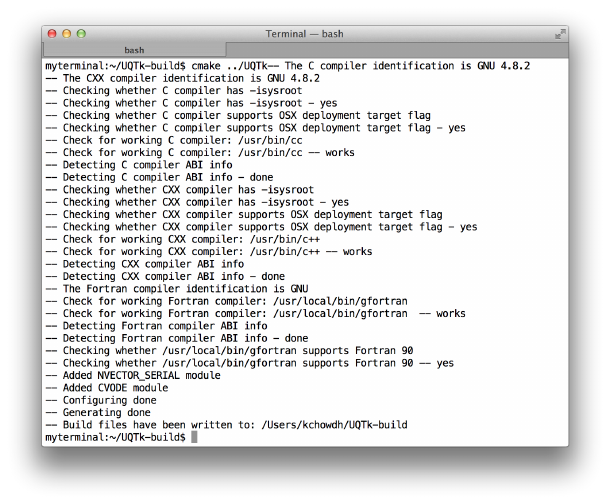
$ cmake -DCMAKE_INSTALL_PREFIX:PATH=$PWD/../UQTk-install \
-DCMAKE_Fortran_COMPILER=/opt/local/gcc61/bin/gfortran-6.1.0 \
-DCMAKE_C_COMPILER=/opt/local/gcc61/bin/gcc-6.1.0 \
-DCMAKE_CXX_COMPILER=/opt/local/gcc61/bin/g++-6.1.0 ../UQTk
Note that this will configure CMake to compile UQTk without the Python interface. Also,
we specified the installation directory to be UQTk-install in the same parent directory at
UQTk and UQTk-build. Figure 2.1 shows what CMake prints to the screen. To turn on the
Figure 2.1: CMake configuration without the Python interface.
Python interface just set the CMake flag, PyUQTk, on, i.e.,
$ cmake -DPyUQTk=ON \
-DCMAKE_INSTALL_PREFIX:PATH=$PWD/../UQTk-install \
-DCMAKE_Fortran_COMPILER=/opt/local/gcc61/bin/gfortran-6.1.0 \
-DCMAKE_C_COMPILER=/opt/local/gcc61/bin/gcc-6.1.0 \
-DCMAKE_CXX_COMPILER=/opt/local/gcc61/bin/g++-6.1.0 ../UQTk
14
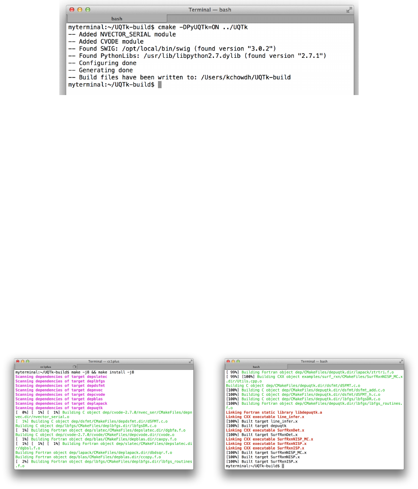
Figure 2.2 shows the additional output to screen after the Python interface flag is turned
on.
Figure 2.2: CMake configuration with the Python interface.
If the CMake command has executed without error, you are now ready to build UQTk.
While in the build directory, type
$ make
or, for a faster compilation using Nparallel threads,
$ make -j N
where one can replace Nwith the number of virtual cores on your machine, e.g. 8. This will
build in the UQTK-build/ directory. The screen should look similar to Figure 2.3 with or
without the Python interface when building.
Figure 2.3: Start and end of build without Python interface.
To verify that the build was successful, run the ctest command from the UQTK-build/
directory to execute C++ and Python (only if building PyUQTk) test scripts.
$ ctest
15
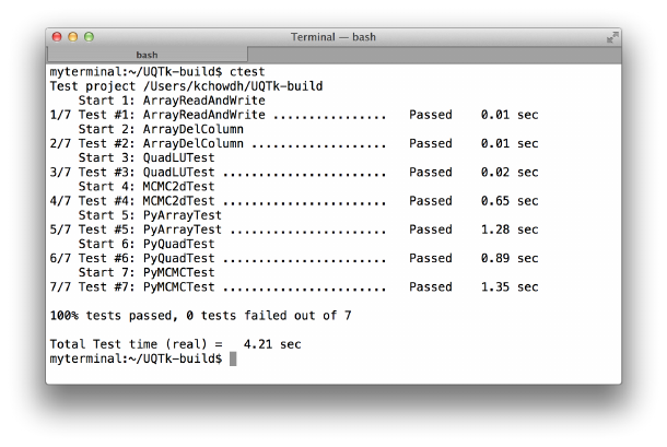
Figure 2.4: Result of ctest after successful build and install. Note that if you do not build
PyUQTk, those tests will not be run.
The output should look similar to Figure 2.4.
If the Python tests fail, even though the compilation went well, a common issue that the
configure script may have found a different version of the Python libraries than the one is
used when you issue Python from the command line. To avoid this, specify the path to your
Python executable and libraries to the configuration process. For example (on OS X):
cmake -DCMAKE_INSTALL_PREFIX:PATH=$PWD/../UQTk-install \
-DCMAKE_Fortran_COMPILER=/opt/local/gcc61/bin/gfortran-6.1.0 \
-DCMAKE_C_COMPILER=/opt/local/gcc61/bin/gcc-6.1.0 \
-DCMAKE_CXX_COMPILER=/opt/local/gcc61/bin/g++-6.1.0 ../UQTk
-DPYTHON_EXECUTABLE:FILEPATH=/opt/local/bin/python \
-DPYTHON_LIBRARY:FILEPATH=/opt/local/Library/Frameworks/Python.framework/Versions/2.7/lib/libpython2.7.dylib \
-DPyUQTk=ON \
../UQTk
If all looks good, you are now ready to install UQTk. While in the build directory, type
$ make install
which installs the libraries, headers, apps, examples, and such in the specified installation
directory. Additionally, if you are building the Python interface, the install command will
copy over the python scripts and SWIG modules (*.so) over to PyUQTk/.
As a reminder, commonly used configure options are illustrated in the scripts that are
provided in the “sourcedir/config” folder.
16
Chapter 3
Theory and Conventions
UQTk implements many probabilistic methods found in the literature. For more details
on the methods, please refer to the following papers and books on Polynomial Chaos methods
for uncertainty propagation [3, 17], Karhunen-Lo`eve (KL) expansions [7], numerical quadra-
ture (including sparse quadrature) [13, 2, 9, 31, 6], Bayesian inference [30, 4, 18], Markov
Chain Monte Carlo [5, 8, 10, 11], Bayesian compressive sensing [1], and the Rosenblatt
transformation [23].
Below, some key aspects and conventions of UQTk Polynomial Chaos expansions are
outlined in order to connect the tools in UQTk to the broader theory.
Polynomial Chaos Expansions
•The default ordering of PCE terms in the multi-index in UQTk is the canonical ordering
for total order truncation
•The PC basis functions in UQTk are not normalized
•The Legendre-Uniform PC Basis type is defined on the interval [-1, 1], with weight
function 1/2
17
18
Chapter 4
Source Code Description
For more details on the actual source code in UQTk, HTML documentation is also
available in the doc_cpp/html folder.
Applications
The following command-line applications are available (source code is in cpp/app )
}generate_quad : Quadrature point/weight generation
}gen_mi : Polynomial multiindex generation
}gp_regr : Gaussian process regression
}model_inf : Model parameter inference
}pce_eval : PC evaluation
}pce_quad : PC generation from samples
}pce_resp : PC projection via quadrature integration
}pce_rv : PC-related random variable generation
}pce_sens : PC sensitivity extraction
}pdf_cl : Kernel Density Estimation
}regression : Linear parametric regression
}sens : Sobol sensitivity indices via Monte-Carlo sampling
Below we detail the theory behind all the applications. For specific help in running an
app, type app_name -h.
19

}generate quad:
This utility generates isotropic quadrature (both full tensor product or sparse) points of
given dimensionality and type. The keyword options are:
Quadrature types: -g <quadType>
•LU : Legendre-Uniform
•HG : Gauss-Hermite
•LG : Gamma-Laguerre
•SW : Stieltjes-Wiegert
•JB : Beta-Jacobi
•CC : Clenshaw-Curtis
•CCO : Clenshaw-Curtis Open (endpoints not included)
•NC : Newton-Cotes (equidistant)
•NCO : Newton-Cotes Open (endpoints not included)
•GP3 : Gauss-Patterson
•pdf : Custom PDF
Sparsity types: -x <fsType>
•full : full tensor product
•sparse : Smolyak sparse grid construction
Note that one can create an equidistant multidimensional grid by using ‘NC’ quadrature
type and ‘full’ sparsity type.
}gen mi:
This utility generates multi index set of a given type and dimensionality. The keyword
options are:
Multiindex types: -x <mi_type>
20

•TO : Total order truncation, i.e. α= (α1, . . . , αd), where α1+···+αd=||α||1≤p,
for given order pand dimensionality d. The number of multiindices is NT O
p,d = (p+
d)!/(p!d!).
•TP : Tensor product truncation, i.e. α= (α1, . . . , αd), where αi≤pi, for i=
1, . . . , d. The dimension-specific orders are given in a file with a name specified as a
command-line argument (-f). The number of multiindices is NT P
p1,...,pd=Qd
i=1(pi+ 1).
•HDMR : High-Dimensional Model Representation, where, for each k,k-variate mul-
tiindices are truncated up to a given order. That is, if ||α||0=k(i.e. the num-
ber of non-zero elements is equal to k), then ||α||1≤pk, for k= 1, . . . , kmax. The
variate-specific orders pkare given in a file with a name specified as a command-line
argument (-f). The number of multiindices constructed in this way is NHDMR
p0,...,pkmax =
Pkmax
k=0 (pk+k)!/(pk!k!).
}gp regr:
This utility performs Gaussian process regression [22], in particular using the Bayesian
perspective of constructing GP emulators, see e.g. [12, 20]. The data is given as pairs D=
{(x(i), y(i))}N
i=1, where x∈Rd. The function to be found, f(x) is endowed with a Gaussian
prior with mean h(x)Tcand a predefined covariance C(x, x0) = σ2c(x, x0). Currently, only
a squared-exponential covariance is implemented, i.e. c(x, x0) = e−(x−x0)TB(x−x0). The mean
trend basis vector h(x) = (L0(x), . . . , LK−1(x)) consists of Legendre polynomials, while c
and σ2are hyperparameters with a normal inverse gamma (conjugate) prior
p(c, σ2) = p(c|σ2)p(σ2)∝e−(c−c0)TV−1(c−c0)
2σ2
σ
e−β
σ2
σ2(α+1) .
The parameters c0, V −1and Bare fixed for the duration of the regression. Conditioned on
yi=f(xi), the posterior is a student-t process
f(x)|D,c0, V −1, B, α, β ∼St-t(µ∗(x),ˆσc∗(x, x0))
with mean and covariance defined as
µ∗(x) = h(x)Tˆ
c+t(x)TA−1(y−Hˆ
c),
c∗(x, x0) = c(x, x0)−t(x)TA−1t(x0)+[h(x)T−t(x)TA−1H]V∗[h(x0)T−t(x0)TA−1H]T,
where yT= (y(1), . . . , y(N)) and
ˆ
c=V∗(V−1c0+HTA−1y) ˆσ2=2β+cT
0V−1c0+yTA−1y−ˆ
cT(V∗)−1ˆ
c
N+ 2α−K−2
t(x)T= (c(x, x(1)), . . . , c(x, x(N))) V∗= (V−1+HTA−1H)−1
H= (h(x(1))T,...,h(x(N))T)Amn =c(x(m), x(n))
(4.1)
21

Note that currently the commonly used prior p(c, σ2)∝σ−2is implemented which is a
special case with α=β= 0 and c0=0,V−1= 0K×K. Also, a small nugget of size 10−6
is added to the diagonal of matrix Afor numerical purposes, playing a role of ‘data noise’.
Finally, the covariance matrix Bis taken to be diagonal, with the entries either fixed or
found before the regression by maximizing marginal posterior [20]. More flexibility in trend
basis and covariance structure selection is a matter of current work.
The app builds the Student-t process according to the computations detailed above, and
evaluates its mean and covariance at a user-defined grid of points x.
}model inf:
This utility perform Bayesian inference for several generic types of models. Consider a
dataset D={(x(i), y(i))}N
i=1 of pairs of x-ymeasured values from some unknown ‘truth’
function g(·), i.e. y(i)=g(x(i))+meas.errors. For example, y(i)can be measurements at
spatial locations x(i), or at time instances x(i), or x(i)=isimply enumerating several ob-
servables. We call elements of x∈IRSdesign or controllable parameters. Assume, generally,
that gis not deterministic, i.e. the vector of measurements y(i)at each icontains Rin-
stances/replicas/measurements of the true output g(x). Furthermore, consider a model of
interest f(λ;x) as a function of model parameters λ∈IRDproducing a single output. We
are interested in calibrating the model f(λ;x) with respect to model parameters λ, seeking
an approximate match of the model to the truth:
f(λ;x)≈g(x).(4.2)
The full error budget takes the following form
y(i)=f(λ;x(i)) + δ(x(i)) + i,(4.3)
where δ(x) is the model discrepancy term, and iis the measurement error for the i-th data
point. The most common assumption for the latter is an i.i.d Gaussian assumption with
vanishing mean
i∼N(0, σ2),for all i= 1, . . . , N. (4.4)
Concerning model error δ(x), we envision three scenarios:
•when the model discrepancy term δ(x) is ignored, one arrives at the classical construc-
tion y(i)−f(λ;x(i))∼N(0, σ2) with likelihood described below in Eq. (4.12).
•when the model discrepancy δ(x) is modeled explicitly as a Gaussian process with
a predefined, typically squared-exponential covariance term with parameters either
fixed apriori or inferred as hyperparameters, together with λ. This approach has been
established in [15], and is referred to as “Kennedy-O’Hagan”, koh approach.
•embedded model error approach is a novel strategy when model error is embedded
into the model itself. For detailed discussion on the advantages and challenges of
22

the approach, see [26]. This method leads to several likelihood options (keywords abc,
abcm, gausmarg, mvn, full, marg), many of which are topics of current research and are
under development. In this approach, one augments some of the parameters in λwith a
probabilistic representation, such as multivariate normal, and infers parameters of this
representation instead. Without loss of generality, and for the clarity of illustration,
we assumed that the first Mcomponents of λare augmented with a random variable.
To this end, λis augmented by a multivariate normal random variable as
λ→Λ=λ+A(α)~
ξ, (4.5)
where
A(α) =
α11 0 0 . . . 0
α21 α22 0. . . 0
α31 α32 α33 . . . 0
.
.
..
.
..
.
.....
.
.
αM1αM2αM3. . . αMM
0 0 0 . . . 0
.
.
..
.
..
.
.....
.
.
0 0 0 . . . 0
0 0 0 . . . 0
D×M
,and ~
ξ=
ξ1
ξ2
.
.
.
ξM
(4.6)
Here ~
ξis a vector of independent identically distributed standard normal variables,
and α= (α11, . . . , αMM ) is the vector of size M(M+ 1)/2 of all non-zero entries in the
matrix A. The set of parameters describing the random vector Λis ˆ
λ= (λ,α) The
full data model then is written as
y(i)=f(λ+A(α)~
ξ;x(i)) + i(4.7)
or
y(i)=fˆ
λ(x(i);~
ξ) + σ2ξM+i,(4.8)
where fˆ
λ(x;~
ξ) is a random process induced by this model error embedding. The mean
and variance of this process are defined as µˆ
λ(x) and σ2
ˆ
λ(x), respectively. To represent
this random process and allow easy access to its first two moments, we employ a
non-intrusive spectral projection (NISP) approach to propagate uncertainties in fvia
Gauss-Hermite PC expansion,
y(i)=
K−1
X
k=0
fik(λ,α)Ψk(~
ξ) + σ2ξM+i,(4.9)
for a fixed order pexpansion, leading to K= (p+M)!/(p!M!) terms.
The parameter estimation problem for λis now reformulated as a parameter estimation for
ˆ
λ= (λ,α). This inverse problem is solved via Bayesian machinery. Bayes’ formula reads
p(ˆ
λ|D)
| {z }
posterior
∝p(D|ˆ
λ)
| {z }
likelihood
p(ˆ
λ)
|{z}
prior
,(4.10)
23

where the key function is the likelihood function
LD(ˆ
λ) = p(D|ˆ
λ) (4.11)
that connects the prior distribution of the parameters of interest to the posterior one. The
options for the likelihood are given further in this section. For details on the likelihood
construction, see [26]. To alleviate the invariance with respect to sign-flips, we use a prior
that enforces αMi >0 for i= 1, . . . , M. Also, one can either fix σ2or infer it together with
ˆ
λ.
Exact computation of the potentially high-dimensional posterior (4.10) is usually prob-
lematic, therefore we employ Markov chain Monte Carlo (MCMC) algorithm for sampling
from the posterior. Model fand the exact form of the likelihood are determined using
command line arguments. Below we detail the currently implemented model types.
Model types: -f <modeltype>
•prop : for x∈IR1and λ∈IR1, the function is defined as f(λ;x) = λx.
•prop_quad : for x∈IR1and λ∈IR2, the function is defined as f(λ;x) = λ1x+λ2x2.
•exp : for x∈IR1and λ∈IR2, the function is defined as f(λ;x) = eλ1+λ2x.
•exp_quad : for x∈IR1and λ∈IR3, the function is defined as f(λ;x) = eλ1+λ2x+λ3x2.
•const : for any x∈IRnand λ∈IR1, the function is defined as f(λ;x) = λ.
•linear : for x∈IR1and λ∈IR2, the function is defined as f(λ;x) = λ1+λ2x.
•bb : the model is a ‘black-box’ executed via system-call of a script named
bb.x that takes files p.dat (matrix R×Dfor λ) and x.dat (matrix N×Sfor x) and
returns output y.dat (matrix R×Nfor f). This effectively simulates f(λ;x) at R
values of λand Nvalues of x.
•heat_transfer1 : a custom model designed for a tutorial case of a heat conduction
problem: for x∈IR1and λ∈IR1, the model is defined as f(λ;x) = xdw
Awλ+T0, where
dw= 0.1, Aw= 0.04 and T0= 273.
•heat_transfer2 : a custom model designed for a tutorial case of a heat conduction
problem: for x∈IR1and λ∈IR2, the model is defined as f(λ;x) = xQ
Awλ1+λ2, where
Aw= 0.04 and Q= 20.0.
•frac_power : a custom function for testing. For x∈IR1and λ∈IR4, the function is
defined as f(λ;x) = λ0+λ1x+λ2x2+λ3(x+ 1)3.5.
•exp_sketch : exponential function to enable the sketch illustrations of model error
embedding approach, for x∈IR1and λ∈IR2, the model is defined as f(λ;x) =
λ2eλ1x−2.
24

•inp : a function that produces the input components as output. That is f(λ;x(i)) =
λi, for x∈IR1and λ∈IRd, assuming exactly dvalues for the design variables x(these
are usually simply indices xi=ifor i= 1, . . . , d).
•pcl : the model is a Legendre PC expansion that is linear with respect to coefficients
λ,i.e. f(λ;x) = Pα∈S λαΨα(x).
•pcx : the model is a Legendre PC expansion in both xand λ,i.e. z= (λ,x), and
f(λ;x) = Pα∈S cαΨα(z)
•pc : the model is a set of Legendre polynomial expansions for each value of x:i.e.
f(λ;x(i)) = Pα∈S cα,iΨα(λ).
•pcs : same as pc, only the multi-index set Scan be different for each x(i),i.e.
f(λ;x(i)) = Pα∈Sicα,iΨα(λ).
Likelihood construction is the key step and the biggest challenge in model parameter
inference.
Likelihood types: -l <liktype>
•classical : No α, or M= 0. This is a classical, least-squares likelihood
log LD(λ) = −
N
X
i=1
(y(i)−f(λ;x(i)))2
2σ2−N
2log (2πσ2),(4.12)
•koh : Kennedy-O’Hagan likelihood with explicit additive representation of
model discrepancy [15].
•full : This is the exact likelihood
LD(ˆ
λ) = πhˆ
λ(y(1), . . . , y(N)),(4.13)
where hˆ
λis the random vector with entries fˆ
λ(x(i);~
ξ) + σ2ξM+i. When there is no
data noise, i.e. σ= 0, this likelihood is degenerate [26]. Typically, computation of this
likelihood requires a KDE step for each ˆ
λto evaluate a high-d PDF πhˆ
λ(·).
•marg : Marginal approximation of the exact likelihood
LD(ˆ
λ) =
N
Y
i=1
πhˆ
λ,i (y(i)),(4.14)
where hˆ
λ,i is the i-th component of hˆ
λ. This requires one-dimensional KDE estimates
performed for all Ndimensions.
25

•mvn : Multivariate normal approximation of the full likelihood
log LD(ˆ
λ) = −1
2(y−µˆ
λ)TΣ−1
ˆ
λ(y−µˆ
λ)−N
2log (2π)−1
2log (det Σˆ
λ),(4.15)
where mean vector µˆ
λand covariance matrix Σˆ
λare defined as µi
ˆ
λ=µˆ
λ(x(i)) and
Σˆ
λ
ij =E(hˆ
λ,i −µˆ
λ(x(i)))(hˆ
λ,j −µˆ
λ(x(j)))T, respectively.
•gausmarg : This likelihood further assumes independence in the gaussian approxi-
mation, leading to
log LD(ˆ
λ) = −
N
X
i=1
(y(i)−µˆ
λ(x(i)))2
2σ2
ˆ
λ(x(i)) + σ2−1
2
N
X
i=1
log 2πσ2
ˆ
λ(x(i)) + σ2.(4.16)
•abcm : This likelihood enforces the mean of fˆ
λto match the mean of data
log LD(ˆ
λ) = −
N
X
i=1
(y(i)−µˆ
λ(x(i)))2
22−1
2log (2π2),(4.17)
•abc : This likelihood enforces the mean of fˆ
λto match the mean of data and
the standard deviation to match the average spread of data around mean within some
factor γ
log LD(ˆ
λ) = −
N
X
i=1
(y(i)−µˆ
λ(x(i)))2+γ|y(i)−µˆ
λ(x(i))| − qσ2
ˆ
λ(x(i)) + σ22
22−1
2log (2π2),
(4.18)
}pce eval:
This utility evaluates PC-related functions given input file xdata.dat and return the
evaluations in an output file ydata.dat. The keyword options are:
Function types: -f <fcn_type>
•PC : Evaluates the function f(~
ξ) = PK
k=0 ckΨk(~
ξ) given a set of ~
ξ, the PC type,
dimensionality, order and coefficients.
•PC_mi : Evaluates the function f(~
ξ) = PK
k=0 ckΨk(~
ξ) given a set of ~
ξ, the PC type,
multiindex and coefficients.
•PCmap : Evaluates ‘map’ functions from a germ of one PC type to another. That is
PC1 to PC2 is a function ~η =f(~
ξ) = C−1
2C1(~
ξ1), where C1and C2are the cumulative
distribution functions (CDFs) associated with the PDFs of PC1 and PC2, respectively.
For example, HG→LU is a map from standard normal random variable to a uniform
random variable in [−1,1].
26

}pce quad:
This utility constructs a PC expansion from a given set of samples. Given a set of N
samples {x(i)}N
i=1 of a random d-variate vector ~
X, the goal is to build a PC expansion
~
X'
K
X
k=0
ckΨk(~
ξ),(4.19)
where dis the stochastic dimensionality, i.e. ~
ξ= (ξ1, . . . , ξd). We use orthogonal projection
method, i.e.
ck=h~
XΨk(~
ξ)i
hΨ2
k(~
ξ)i=h~
G(~
ξ)Ψk(~
ξ)i
hΨ2
k(~
ξ)i.(4.20)
The denominator can be precomputed analytically or numerically with high precision. The
key map ~
G(~
ξ) in the numerator is constructed as follows. We employ the Rosenblatt trans-
formation, constructed by shifted and scaled successive conditional cumulative distribution
functions (CDFs),
η1= 2F1(X1)−1
η2= 2F2|1(X2|X1)−1
η3= 2F3|2,1(X3|X2, X1)−1 (4.21)
.
.
.
ηd= 2Fd|d−1,...,1(Xd|Xd−1, . . . , X1)−1.
maps any joint random vector to a set of independent standard Uniform[-1,1] random vari-
ables. Rosenblatt transformation is the multivariate generalization of the well-known CDF
transformation, stating that F(X) is uniformly distributed if F(·) is the CDF of random
variable X. The shorthand notation is ~η =~
R(~
X). Now denote the shifted and scaled uni-
variate CDF of the ‘germ’ ξiby H(·), so that by the CDF transformation reads as ~
H(~
ξ) = ~η.
For example, for Legendre-Uniform PC, the germ itself is uniform and H(·) is identity, while
for Gauss-Hermite PC the function H(·) is shifted and scaled version of the normal CDF.
Now, we can write the connection between ~
Xand ~
ξby
~
R(~
X) = ~
H(~
ξ),or ~
X=~
R−1◦~
H
|{z }
~
G
(~
ξ) (4.22)
While the computation of ~
His done analytically or numerically with high precision,
the main challenge is to estimate ~
R−1. In practice the exact joint cumulative distribution
F(x1,...,xd) is generally not available and is estimated using a standard Kernel Density
Estimator (KDE) using the samples available. Given Nsamples {x(i)}N
i=1 , the KDE estimate
of its joint probability density function is a sum of Nmultivariate gaussian functions centered
27

at each data point x(i):
p~
X(x) = 1
Nσd(2π)d/2
N
X
i=1
exp −(x−x(i))T(x−x(i))
2σ2(4.23)
or
p~
X1,..., ~
Xd(x1,...,xd) = 1
Nσd(2π)d/2
N
X
i=1
exp −(x1−x(i)
1)2+··· + (xd−x(i)
d)2
2σ2!,(4.24)
where the bandwidth σshould be chosen to balance smoothness and accuracy, see [28, 29]
for discussions of the choice of σ. Note that ideally σshould be chosen to be dimension-
dependent, however the current implementation uses the same bandwidth for all dimensions.
Now the conditional CDF is KDE-estimated by
Fk|k−1,...,1(xk|xk−1,...,x1) = Zxk
−∞
pk|k−1,...,1(x0
k|xk−1,...,x1)dx0
k
=Zxk
−∞
pk,...,1(x0
k,xk−1,...,x1)
pk−1,...,1(xk−1,...,x1)dx0
k
≈1
σ√2πZxk
−∞
N
X
i=1
exp −(x1−x(i)
1)2+···+(x0
k−x(i)
k)2
2σ2
N
X
i=1
exp −(x1−x(i)
1)2+···+(xk−1−x(i)
k−1)2
2σ2dx0
k
=Zxk
−∞
N
X
i=1
exp −(x1−x(i)
1)2+···+(xk−1−x(i)
k−1)2
2σ2×1
σ√2πexp −(x0
k−x(i)
k)2
2σ2
N
X
i=1
exp −(x1−x(i)
1)2+···+(xk−1−x(i)
k−1)2
2σ2dx0
k
=
N
X
i=1
exp −(x1−x(i)
1)2+···+(xk−1−x(i)
k−1)2
2σ2×Φxk−x(i)
k
σ
N
X
i=1
exp −(x1−x(i)
1)2+···+(xk−1−x(i)
k−1)2
2σ2,(4.25)
where Φ(z) is the CDF of a standard normal random variable. Note that the numerator in
(4.25) differs from the denominator only by an extra factor Φ xk−x(i)
k
σin each summand,
allowing an efficient computation scheme.
28

The above Rosenblatt transformation maps the random vector xto a set of i.i.d. uniform
random variables ~η = (η1, . . . , ηd). However, the formula (4.22) requires the inverse of
the Rosenblatt transformation. Nevertheless, the approximate conditional distributions are
monotonic, hence they are guaranteed to have an inverse function, and it can be evaluated
rapidly with a bisection method.
With the numerical estimation of the map (4.22) available, we can proceed to evaluation
the numerator of the orthogonal projection (4.20)
h~
G(~
ξ)Ψk(~
ξ)i=Z~
ξ
~
G(x)Ψk(x)π~
ξ(~
ξ)d~
ξ, (4.26)
where π~
ξ(~
ξ) is the PDF of ~
ξ. The projection integral (4.26) is computed via quadrature
integration
Z~
ξ
~
G(~
ξ)Ψk(~
ξ)π~
ξ(~
ξ)d~
ξ≈
Q
X
q=1
~
G(~
ξq)Ψk(~
ξq)wq=
Q
X
q=1
~
R−1(~
H(~
ξq))Ψk(~
ξq)wq,(4.27)
where (~
ξq, wq) are Gaussian quadrature point-weight pairs for the weight function π~
ξ(~
ξ).
}pce resp:
This utility performs orthogonal projection given function evaluations at quadrature
points, in order to arrive at polynomial chaos coefficients for a Total-Order PC expansion
f(~
ξ)≈X
||α||1≤p
cαΨα(~
ξ)≡g(~
ξ).(4.28)
The orthogonal projection computed by this utility is
cα=1
hΨ2
αiZ~
ξ
f(~
ξ)Ψα(~
ξ)π~
ξ(~
ξ)d~
ξ≈1
hΨ2
αi
Q
X
q=1
wqf(~
ξ(q))Ψα(~
ξ(q)).(4.29)
Given the function evaluations f(~
ξ(q)) and precomputed quadrature (~
ξ(q), wq), this utility
outputs the PC coefficients cα, PC evaluations at the quadrature points g(~
ξ(q)) as well as, if
requested by a command line flag, a quadrature estimate of the relative L2error
||f−g||2
||f||2≈v
u
u
tPQ
q=1 wq(f(~
ξ(q))−g(~
ξ(q)))2
PQ
q=1 wqf(~
ξ(q))2.(4.30)
Note that the selected quadrature may not compute the error accurately, since the integrated
functions are squared and can be higher than the quadrature is expected to integrate accu-
rately. In such cases, one can use the pce_eval app to evaluate the PC expansion separately
and compare to the function evaluations with an `2norm instead.
29

}pce rv:
This utility generates PC-related random variables (RVs). The keyword options are:
RV types: -w <type>
•PC : Generates samples of univariate random variable PK
k=0 ckΨk(~
ξ) given the PC
type, dimensionality, order and coefficients.
•PCmi : Generates samples of univariate random variable PK
k=0 ckΨk(~
ξ) given the PC
type, multiindex and coefficients.
•PCvar : Generates samples of multivariate random variable ~
ξthat is the germ of a
given PC type and dimensionality.
}pce sens:
This utility evaluates Sobol sensitivity indices of a PC expansion with a given multiindex
and a coefficient vector. It computes main, total and joint sensitivities, as well as variance
fraction of each PC term individually. Given a PC expansion PIcαΨα(~
ξ), the computed
moments and sensitivity indices are:
•mean: m=c~
0
•total variance: V=Pα6=~
0c2
αhΨ2
αi
•variance fraction for the basis term α:Vα=c2
αhΨ2
αi
V
•main Sobol sensitivity index for dimension i:Si=1
VPα∈IS
ic2
αhΨ2
αi, where IS
iis the
set of multiindices that include only dimension i.
•total Sobol sensitivity index for dimension i:ST
i=1
VPα∈IT
ic2
αhΨ2
αi, where IT
iis the
set of multiindices that include dimension i, among others.
•joint-total Sobol sensitivity index for dimension pair (i, j): ST
ij =1
VPα∈IT
ij c2
αhΨ2
αi,
where IT
ij is the set of multiindices that include dimensions iand j,among others.
Note that this is somewhat different from the conventional definition of joint sensitivity
indices, which presumes terms that include only dimensions iand j.
}pdf cl:
Kernel density estimation (KDE) with Gaussian kernels given a set of samples to eval-
uate probability distribution function (PDF). The procedure relies on approximate nearest
30
neighbors algorithm with fast improved Gaussian transform to accelerate KDE by only com-
puting Gaussians of relevant neighbors. Our tests have shown 10-20x speedup compared to
Python’s default KDE package. Also, the app allows clustering enhancement to the data
set to enable cluster-specific bandwidth selection - particularly useful for multimodal data.
User provides the samples’ file, and either a) number of grid points per dimension for density
evaluation, or b) a file with target points where the density is evaluated, or c) a file with a
hypercube limits in which the density is evaluated.
}regression:
This utility performs regression with respect to a linear parametric expansions such as
PCs or RBFs. Consider a dataset (x(i), y(i))N
i=1 that one tries to fit a basis expansion with:
y(i)≈
K
X
k=1
ckPk(x(i)),(4.31)
for a set of basis functions Pk(x). This is a linear regression problem, since the object of
interest is the vector of coefficients c= (c1, . . . , ck), and the summation above is linear in
c. This app provides various methods of obtaining the expansion coefficients, using different
kinds of bases.
The key implemented command line options are
Basis types: -f <basistype>
•PC : Polynomial Chaos bases of total-order truncation
•PC_MI : Polynomial Chaos bases of custom multiindex truncation
•POL : Monomial bases of total-order truncation
•POL_MI : Monomial bases of custom multiindex truncation
•RBF : Radial Basis Functions, see e.g. [21]
Regression methods: -f <meth>
•lsq : Bayesian least-squares, see [25] and more details below.
•wbcs : Weighted Bayesian compressive sensing, see [27].
Although the standard least squares is commonly used and well-documented elsewhere,
we detail here the specific implementation in this app, including the Bayesian interpretation.
31

Define the data vector y= (y(1), . . . , y(N)), and the measurement matrix Pof size N×K
with entries Pik =Pk(x(i)). The regularized least-squares problem is formulated as
arg min
c||y−P c||2+||Λc||2
| {z }
R(c)
(4.32)
with a closed form solution
ˆ
c= (PTP+Λ)−1
| {z }
Σ
PTy(4.33)
where Λ=diag(√λ1,...,√λK) is a diagonal matrix of non-negative regularization weights
λi≥0.
The Bayesian analog of this, detailed in [25], infers coefficient vector cand data noise
variance σ2, given data y, employing Bayes’ formula
Posterior
z }| {
p(c, σ2|y)∝
Likelihood
z }| {
p(y|c, σ2)
Prior
z }| {
p(c, σ2) (4.34)
The likelihood function is associated with i.i.d. Gaussian noise model y−P c ∼N(0, σ2IN),
and is written as,
p(y|c, σ2)≡Lc,σ2(y) = (2πσ2)−N
2exp −1
2σ2||y−P c||2(4.35)
Further, the prior p(c, σ2) is written as a product of a zero-mean Gaussian prior on cand
an inverse-gamma prior on σ2:
p(c, σ2) = K
Y
k=1
λk
2π!1
2
exp −1
2||Λc||2
| {z }
p(c)
(σ2)−α−1exp −β
σ2
| {z }
p(σ2)
(4.36)
The posterior distribution then takes a form of normal-scaled inverse gamma distribution
which, after some re-arranging, is best described as
p(c|σ2,y)∼MV N(ˆ
c, σ2Σ),(4.37)
p(σ2|y)∼IG
α+N−K
2
| {z }
α∗
, β +R(ˆ
c)
2
| {z }
β∗
(4.38)
where ˆ
cand Σ, as well as the residual R(·) are defined via the classical least-squares prob-
lem (4.32) and (4.33). Thus, the mean posterior value of data variance is ˆσ2=β+R(ˆ
c)
2
α+N−K
2−1.
32

Also, note that the residual can be written as R(ˆ
c) = yTIN−PPTP+Λ−1PTy.
One can integrate out σ2from (4.36) to arrive at a multivariate t-distribution
p(c|y)∼MV T ˆ
c,β∗
α∗Σ,2α∗(4.39)
with a mean ˆ
cand covariance α∗
α∗−2Σ.
Now, the pushed-forward process at new values xwould be, defining P(x) = (P1(x), . . . , Pk(x)),
a Student-t process with mean µ(x) = P(x)ˆ
c, scale C(x, x0) = β∗
α∗P(x)ΣP(x0) and degrees-
of-freedom 2α∗.
Note that, currently, Jeffrey’s prior for p(σ2)=1/σ2is implemented, which corresponds
to the case of α=β= 0. We are currently implementing more flexible user-defined input
for αand β. In particular, in the limit of β=σ2
0α→ ∞, one recovers the case with a fixed,
predefined data noise variance σ2
0.
}sens:
This utility performs a series of tasks for for the computation of Sobol indices. Some
theoretical background on the statistical estimators employed here is given in Chapter 5. This
utility can be used in conjunction with utility trdSpls which generates truncated normal
or log-normal random samples. It can also be used to generate uniform random samples by
selecting a truncated normal distribution and a suitably large standard deviation.
In addition to the -h flag, it has the following command line options:
•-a <action>: Action to be performed by this utility
–splFO: assemble samples for first order Sobol indices
–idxFO: compute first order Sobol indices
–splTO: assemble samples for total order Sobol indices
–idxTO: compute total order Sobol indices
–splJnt: assemble samples for joint Sobol indices
–idxJnt: compute joint Sobol indices
•-d <ndim>: Number of dimensions
•-n <ndim>: Number of dimensions
•-u <spl1>: name of file holding the first set of samples, nspl×ndim
•-v <spl2>: name of file holding the second set of samples, nspl×ndim
33
•-x <mev>: name of file holding model evaluations
•-p <pfile>: name of file possibly holding a custom list of parameters for Sobol
indices
34
Chapter 5
Examples
The primary intended use for UQTk is as a library that provides UQ functionality to
numerical simulations. To aid the development of UQ-enabled simulation codes, some ex-
amples of programs that perform common UQ operations with UQTk are provided with
the distribution. These examples can serve as a template to be modified for the user’s pur-
poses. In some cases, e.g. in sampling-based approaches where the simulation code is used
as a black-box entity, the examples may provide enough functionality to be used directly,
with only minor adjustments. Below is a brief description of the main examples that are
currently in the UQTk distribution. For all of these, make sure the environment variable
UQTK_INS is set and points upper level directory of the UQTk install directory, e.g. the
keyword installdir described in the installation section. This path also needs to be added to
environment variable PYTHONPATH.
Elementary Operations
Overview
This set of examples is located under examples/ops. It illustrates the use of UQTk
for elementary operations on random variables that are represented with Polynomial Chaos
(PC) expansions.
Description
This example can be run from command-line:
./Ops.x
followed by
./plot_pdf.py samples.a.dat
./plot_pdf.py samples.loga.dat
35

to plot select probability distributions based on samples from Polynomial Chaos Expan-
sions (PCE) utilized in this example.
Ops.x step-by-step
•Wherever relevant the PCSet class implements functions that take either “double *” ar-
guments or array container arguments. The array containers, named “Array1D”, “Ar-
ray2D”, and“Array3D”, respectively, are provided with the UQTk library to streamline
the management of data structures.
1. Instantiate a PCSet class for a 2nd order 1D PCE using Hermite-Gauss chaos.
int ord = 2;
int dim = 1;
PCSet myPCSet("ISP",ord,dim,"HG");
2. Initialize coefficients for HG PCE expansion ˆagiven its mean and standard deviation:
double ma = 2.0; // Mean
double sa = 0.1; // Std Dev
myPCSet.InitMeanStDv(ma,sa,a);
ˆa=
P
X
k=0
akΨk(ξ), a0=µ, a1=σ
phψ2
1i, a2=a3=. . . = 0
3. Initialize ˆ
b= 2.0ψ0(ξ)+0.2ψ1(ξ)+0.01ψ2(ξ) and subtract ˆ
bfrom ˆa:
b[0] = 2.0;
b[1] = 0.2;
b[2] = 0.01;
myPCSet.Subtract(a,b,c);
The subtraction is a term by term operation: ck=ak−bk
4. Product of PCE’s, ˆc= ˆa·ˆ
b:
myPCSet.Prod(a,b,c);
ˆc=
P
X
k=0
ckΨk(ξ) = P
X
k=0
akΨk(ξ)! P
X
k=0
bkΨk(ξ)!
ck=
P
X
i=0
P
X
j=0
Cijkaibj, Cijk =hψiψjψki
hψ2
ki
The triple product Cijk is computed and stored when the PCSet class is instantiated.
36

5. Exponential of a PCE, ˆc= exp(ˆa) is computed using a Taylor series approach
myPCSet.Exp(a,c);
ˆc= exp(ˆa) = exp(a0) 1 +
NT
X
n=0
ˆ
dn
n!!(5.1)
where
ˆ
d= ˆa−a0=
P
X
k=1
ak(5.2)
The number of terms NTin the Taylor series expansion are incremented adaptively
until an error criterion is met (relative magnitude of coefficients compared to the mean)
or the maximum number of terms is reached. Currently, the default relative tolerance
and maximum number of Taylor terms are 10−6and 500. This values can be changed by
the user using public PCSet methods SetTaylorTolerance and SetTaylorTermsMax,
respectively.
6. Division, ˆc= ˆa/ˆ
b:
myPCSet.Div(a,b,c);
Internally the division operation is cast as a linear system, see item 4, ˆa=ˆ
b·ˆc, with
unknown coefficients ckand known coefficients akand bk. The linear system is sparse
and it is solved with a GMRES iterative solver provided by NETLIB
7. Natural logarithm, ˆc= log(ˆa):
myPCSet.Log(a,c);
Currently, two methodologies are implemented to compute the logarithm of a PCE:
Taylor series expansion and an integration approach. For more details see Debusschere
et. al. [3].
8. Draw samples from the random variable ˆarepresented as a PCE:
myPCSet.DrawSampleSet(aa,aa_samp);
Currently “Ops.x” draws sample from both ˆaand log(ˆa) and saves the results to files
“samples.a.dat” and “samples.loga.dat”, respectively.
9. The directory contains a python script that computes probability distributions from
samples via Kernel Density Estimate (KDE, also see Lecture #1) and generates two
plots, “samples.a.dat.pdf” and “samples.loga.dat.pdf”, also shown in Fig. 5.1.
37
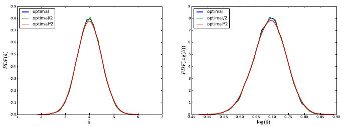
Figure 5.1: Probability densities for ˆaand log(ˆa) computed via KDE. Results generated
using several KDE bandwidths. This feature is available in the Python’s SciPy package
starting with version 0.11
Forward Propagation of Uncertainty
Overview
•Located in examples/surf_rxn
•Several examples of propagating uncertainty in input parameters through a model for
surface reactions, consisting of three Ordinary Differential Equations (ODEs). Two
approaches are illustrated:
–Direct linking to the C++ UQTk libraries from a C++ simulation code:
∗Propagation of input uncertainties with Intrusive Spectral Projection (ISP),
Non Intrusive Spectral Projection (NISP) via quadrature , and NISP via
Monte Carlo (MC) sampling.
∗For more documentation, see a detailed description below
∗An example can be run with ./forUQ_sr.py
–Using simulation code as a black box forward model:
∗Propagation of uncertainty in one input parameter with NISP quadrature
approach.
∗For more documentation, see a detailed description below
∗An example can be run with ./forUQ_BB_sr.py
Simulation Code Linked to UQTk Libraties
The example script forUQ_sr.py, provided with this example can perform parametric
uncertainty propagation using three methods
•NISP: Non-intrusive spectral projection using quadrature integration
38

•ISP: Intrusive spectral projection
•NISP MC: Non-intrusive spectral projection using Monte-Carlo integration
The command-line usage for this example is
./forUQ_sr.py <pctype> <pcord> <method1> [<method2>] [<method3>]
The script requires the xml input template file forUQ surf rxn.in.xml.templ. In this tem-
plate, the default setting for param b is uncertain normal random variable with a standard
deviation set to 10% of the mean.
The following parameters are defined at the beginning of the file:
•pctype: The type of PC, supports ’HG’, ’LU’, ’GLG’, ’JB’
•pcord: The order of output PC expansion
•methodX: NISP, ISP or NISP MC
•nsam: Number of samples requested for NISP Monte-Carlo (currently hardwired in
the script)
Description of Non-Intrusive Spectral Projection utilities (SurfRxnNISP.cpp and
SurfRxnNISP MC.cpp)
f(~
ξ) = X
k
ckΨk(~
ξ)ck=hf(~
ξ)Ψk(~
ξ)i
hΨ2
k(~
ξ)i
hf(~
ξ)Ψk(~
ξ)i=Zf(~
ξ)Ψk(~
ξ)π(~
ξ)d~
ξ≈"X
q
f(~
ξq)Ψk(~
ξq)wq#
| {z }
NISP
or "1
NX
s
f(~
ξs)Ψk(~
ξs)#
| {z }
NISP MC
These codes implement the following workflows
1. Read XML file
2. Create a PC object with or without quadrature
•NISP: PCSet myPCSet("NISP",order,dim,pcType,0.0,1.0)
•NISP MC: PCSet myPCSet("NISPnoq",order,dim,pcType,0.0,1.0)
3. Get the quadrature points or generate Monte-Carlo samples
39

•NISP: myPCSet.GetQuadPoints(qdpts)
•NISP MC: myPCSet.DrawSampleVar(samPts)
4. Create input PC objects and evaluate input parameters corresponding to quadrature
points
5. Step forward in time
- Collect values for all input parameter samples
- Perform Galerkin projection or Monte-Carlo integration
- Write the PC modes and derived first two moments to files
Description of Intrusive Spectral Projection utility (SurfRxnISP.cpp)
This code implement the following workflows
1. Read XML file
2. Create a PC object for intrusive propagation
PCSet myPCSet("ISP",order,dim,pcType,0.0,1.0)
3. Represent state variables and all parameters with their PC coefficients
•u→ {uk},v→ {vk},w→ {wk},z→ {zk},
•a→ {ak},b→ {bk},c→ {ck},d→ {dk},e→ {ek},f→ {fk}.
4. Step forward in time according to PC arithmetics, e.g.
a·u→ {(a·u)k}with
a·u= X
i
aiΨi(~
ξ)! X
j
ujΨj(~
ξ)!=X
k X
i,j
aiujhΨiΨjΨki
hΨ2
ki!
| {z }
(a·u)k
Ψk(~
ξ)
Postprocessing Utilities - time series
./plSurfRxnMstd.py NISP
./plSurfRxnMstd.py ISP
./plSurfRxnMstd.py NISP_MC
These commands plot the time series of mean and standard deviations of all three species
with all three methods. Sample results are shown in Fig. 5.2.
Postprocessing Utilities - PDFs
40
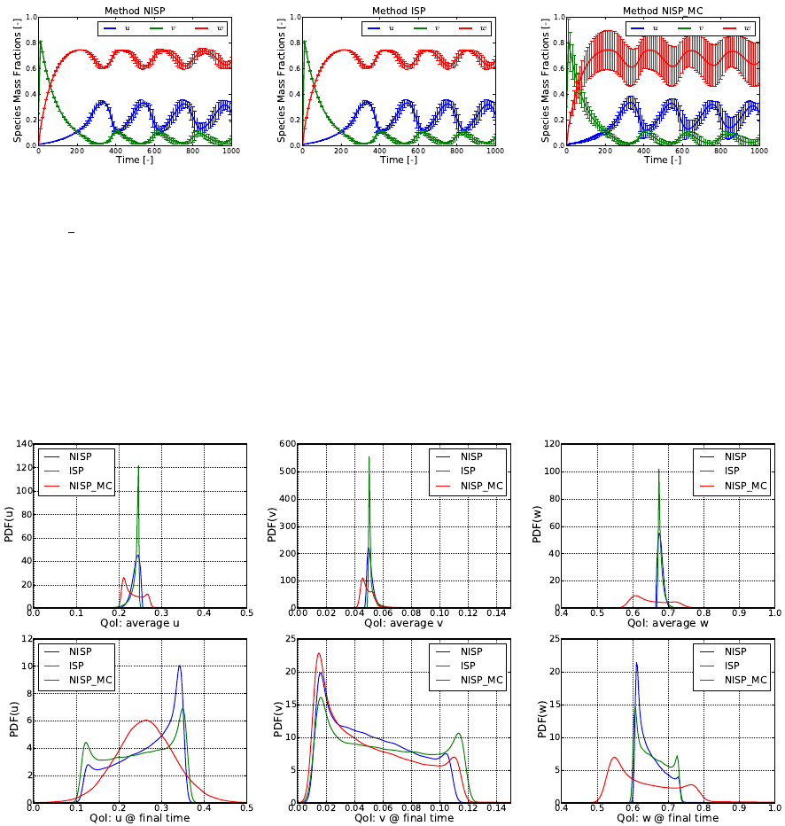
Figure 5.2: Time series of mean and standard deviations for u,v, and wwith NISP, ISP,
and NISP MC, respectively.
./plPDF_method.py <species> <qoi> <pctype> <pcord> <method1> [<method2>] [<method3>]
e.g.
./plPDF_method.py u ave HG 3 NISP ISP
This script samples the PC representations, then computes the PDFs of time-average
(ave) or the final time value (tf) for all three species. Sample results are shown in Fig. 5.3.
Figure 5.3: PDFs for u,v, and w; Top row shows results for average u,v, and w; Bottom
row shows results corresponding to values at the last integration step (final time).
Simulation Code Employed as a Black Box
The command-line usage for the script implementing this example is given as
./forUQ_BB_sr.py --nom nomvals -s stdfac -d dim -l lev -o ord -q sp --npdf npdf
--npces npces
The following parameters can be controlled by the user
41

•nomvals: List of nominal parameter values, separated by comma if more than one
value, and no spaces. Default is one value, 20.75
•stdfac: Ratio of standard deviation/nominal parameter values. Default value: 0.1
•dim: number of uncertain input parameters. Currently this example can only handle
dim = 1
•lev: No. of quadrature points per dimension (for full quadrature) or sparsity level (for
sparse quadrature). Default value: 21.
•ord: PCE order. Default value: 20
•sp: Quadrature type “full” or “sparse”. Default value: “full”
•npdf: No. of grid points for Kernel Density Estimate evaluations of output model
PDF’s. Default value 100
•npces: No. of PCE evaluations to estimate output densitie. Default value 105
Note: This example assumes Hermite-Gauss chaos for the model input
parameters.
This script uses the following utilities, located in the bin directory under the UQTk
installation path
•generate quad: Generate quadrature points for full/sparse quadrature and several types
of rules.
•pce rv: Generate samples from a random variable defined by a Polynomial Chaos
expansion (PCE)
•pce eval: Evaluates PCE for germ samples saved in input file “xdata.dat”.
•pce resp: Constructs PCE by Galerkin projection
Sequence of computations:
1. forUQ BB sr.py
saves the input parameters’ nominal values and standard deviations in a diagonal
matrix format in file “pcfile”. First it saves the matrix of nominal values, then the
matrix of standard deviations. This information is sufficient to define a PCE for a
normal random variable in terms of a standard normal germ. For a one parameter
problem, this file has two lines.
42

2. generate quad:
Generate quadrature points for full/sparse quadrature and several types of rules. The
usage with default script arguments generate_quad -d1 -g’HG’ -xfull -p21 > logQuad.dat
This generates Hermite-Gauss quadrature points for a 21-point rule in one dimension.
Quadrature points locations are saved in “qdpts.dat” and weights in “wghts.dat” and
indices of points in the 1D space in “indices.dat”. At the end of “generate quad”
execution file “qdpts.dat” is copied over “xdata.dat”
3. pce eval:
Evaluates PCE of input parameters at quadrature points, saved previously in “xdata.dat”.
The evaluation is dimension by dimension, and for each dimension the correspond-
ing column from “pcfile” is saved in “pccf.dat”. See command-line arguments below.
pce_eval -x’PC’ -p1 -q1 -f’pccf.dat’ -sHG >> logEvalInPC.dat
At the end of this computation, file “input.dat” contains a matrix of PCE evaluations.
The number of lines is equal to the number of quadrature points and the number of
columns to the dimensionality of input parameter space.
4. Model evaluations:
funcBB("input.dat","output.dat",xmltpl="surf_rxn.in.xml.tp3",
xmlin="surf_rxn.in.xml")
The Python function “funcBB” is defined in file “prob3 utils.py”. This evaluates the
forward model at sets of input parameters in file “input.dat” and saves the model
output in “output.dat”. For each model evaluation, specific parameters are inserted in
the xml file “surf rxn.in.xml” which is a copy of the template in “surf rxn.in.xml.tp3”.
At the end “output.dat” is copied over “ydata.dat”
5. pce resp:
pce_resp -xHG -o20 -d1 -e > logPCEresp.dat
Computes a Hermite-Gauss PCE of the model output via Galerkin projection. The
model evaluations are taken from “ydata.dat”, and the quadrature point locations from
“xdata.dat”. PCE coefficients are saved in “PCcoeff quad.dat”, the multi-index list in
“mindex.dat” and these files are pasted together in “mipc.dat”
(average uas a function of parameter b values. Location of quadrature points is
shown with circles.)
43
6. pce rv:
pce_rv -w’PCvar’ -xHG -d1 -n100 -p1 -q0 > logPCrv.dat
Draw a 100 samples from the germ of the HG PCE. Samples are saved in file “rvar.dat”
and also copied to file “xdata.dat”
7. pce eval:
pce_eval -x’PC’ -p1 -q1 -f’pccf.dat’ -sHG >> logEvalInPCrnd.dat See item 3 for de-
tails. Results are saved “input val.dat”.
8. Evaluate both the forward model (through the black-box script “funcBB”, see item 4)
and its PCE surrogate (see item 3) and save results to files “output val.dat” and
“output val pc.dat”. Compute L2error between the two sets of values using function
“compute err” defined in “utils.py”
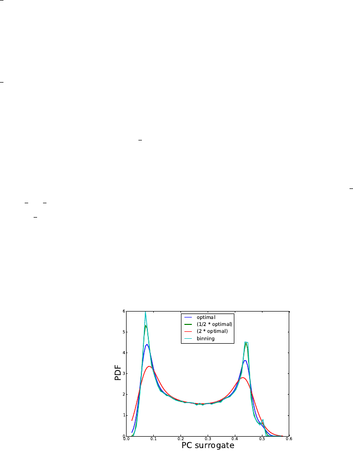
9. Sample output PCE and plot the PDF of these samples computed using either a Kernel
Density Estimate approach with several kernel bandwidths or by binning:
Numerical Integration
Overview
This example is located in examples/num_integ. It contains a collection of Python
scripts that can be used to perform numerical integration on six Genz functions: oscillatory,
exponential, continuous, Gaussian, corner-peak, and product-peak. Quadrature and Monte
Carlo integration methods are both employed in this example.
44

Theory
In uncertainty quantification, forward propagation of uncertain inputs often involves eval-
uating integrals that cannot be computed analytically. Such integrals can be approximated
numerically using either a random or a deterministic sampling approach. Of the two inte-
gration methods implemented in this example, quadrature methods are deterministic while
Monte Carlo methods are random.
Quadrature Integration
The general quadrature rule for integrating a function u(ξ) is given by:
Zu(ξ)dξ ≈
Nq
X
i=1
qiu(ξi) (5.3)
where the Nqξiare quadrature points with corresponsing weights qi.
The accuracy of quadrature integration relies heavily on the choice of the quadrature
points. There are countless quadrature rules that can be used to generate quadrature points,
such as Gauss-Hermite, Gauss-Legendre, and Clenshaw-Curtis.
When performing quadrature integration, one can use either full tensor product or sparse
quadrature methods. While full tensor product quadrature methods are effective for func-
tions of low dimension, they suffer from the curse of dimensionality. Full tensor product
quadrature integration methods require Ndquadrature points to integrate a function of di-
mension dwith Nquadrature points per dimension. Thus, for functions of high dimension
the number of quadrature points required quickly becomes too large for these methods to
be practical. Therefore, in higher dimensions sparse quadrature approaches, which require
far fewer points, are utilized. When performing sparse quadrature integration, rather than
determining the number of quadrature points per dimension, a level is selected. Once a level
is selected, the total number of quadrature points can be determined from the dimension of
the function. For more information on quadrature integration see reference here.
Monte Carlo Integration
One random sampling approach that can be used to evaluate integrals numerically is
Monte Carlo integration. To use Monte Carlo integration methods to evaluate the integral
of a general function u(ξ) on the d-dimensional [0,1]dthe following equation can be used:
Zu(ξ)dξ ≈1
Ns
Ns
X
i=1
u(ξi) (5.4)
The Nsξiare random sampling points chosen from the region of integration according to
the distribution of the inputs. In this example, we are assuming the inputs have uniform
45

distribution. One advantage of using Monte Carlo integration is that any number of sam-
pling points can be used, while quadrature integration methods require a certain number of
sampling points. One disadvantage of using Monte Carlo integration methods is that there
is slow convergence. However, this O(1
√Ns) convergence rate is independent of the dimension
of the integral.
Genz Functions
The functions being integrated in this example are six Genz functions, and they are
integrated over the d-dimensional [0,1]d. These functions, along with their exact integrals,
are defined as follows. The Genz parameters wirepresent weight parameters and uirepresent
shift parameters. In the current example, the parameters wiand uiare set to 1, with one
exception. The parameters wiand uiare instead set to 0.1 for the Corner-peak function in
the sparse_quad.py file.
Model Formula: f(λ) Exact Integral: R
[0,1]d
f(λ)dλ
Oscillatory cos(2πu1+
d
P
i=1
wiλi) cos (2πu1+1
2
d
P
i=1
wi)
d
Q
i=1
2 sin( wi
2)
wi
Exponential exp(
d
P
i=1
wi(λi−ui))
d
Q
i=1
1
wi(exp(wi(1 −ui)) −exp(−wiui))
Continuous exp(−
d
P
i=1
wi|λi−ui|)
d
Q
i=1
1
wi(2 −exp(−wiui)−exp(wi(ui−1)))
Gaussian exp(−
d
P
i=1
w2
i(λi−ui)2)
d
Q
i=1
√π
2wi(erf(wi(1 −ui)) + erf(wiui))
Corner-peak (1 +
d
P
i=1
wiλi)−(d+1) 1
d!
d
Q
i=1
wiP
r{0,1}d
(−1)||r||1
1+
d
P
i=1
wiri
Product-peak
d
Q
i=1
w2
i
1+w2
i(λi−ui)2
d
Q
i=1
wi(arctan(wi(1 −ui)) + arctan(wiui))
Implementation
The script set consists of three files:
•full_quad.py: a script to compare full quadrature and Monte Carlo integration meth-
ods.
•sparse_quad.py: a script to compare sparse quadrature and Monte Carlo integration
methods.
•quad_tools.py: a script containing functions called by full_quad.py and sparse_quad.py.
46

full quad.py
This script will produce a graph comparing full quadrature and Monte Carlo integration
methods. Use the command ./full_quad.py to run this file. Upon running the file, the
user will be prompted to select a model from the Genz functions listed.
Please enter desired model from choices:
genz_osc
genz_exp
genz_cont
genz_gaus
genz_cpeak
genz_ppeak
The six functions listed correspond to the Genz functions defined above. After the user
selects the desired model, he/she will be prompted to enter the desired dimension.
Please enter desired dimension:
The dimension should be entered as an integer without any decimal points. As full quadra-
ture integration is being implemented, this script should not be used for functions of high di-
mension. If you wish to integrate a function of high dimension, instead use sparse_quad.py.
After the user enters the desired dimension, she/he will be prompted to enter the desired
maximum number of quadrature points per dimension.
Enter the desired maximum number of quadrature points per dimension:
Again, this number should be entered as an integer without any decimal points. Several
quadrature integrations will be performed, with the first beginning with 1 quadrature point
per dimension. For subsequent quadrature integrations, the number of quadrature points
will be incremented by one until the maximum number of quadrature points per dimension,
as specified by the user, is reached. For example, if the user has requested a maximum
of 4 quadrature points per dimension, 4 quadrature integrations will be performed: one
with 1 quadrature point per dimension, another with 2 quadrature points per dimension, a
third with 3 quadrature points per dimension, and a fourth with 4 quadrature points per
dimension.
Next, the script will call the function generate_qw from the quad_tools.py script to
generate quadrature points as well as the corresponding weights.
Then, the exact integral for the chosen function is computed by calling the integ_exact
function in quad_tools.py. This function calculates the exact integral according to the
47

formulas found in the above Theory section. The error between the exact integral and the
quadrature approximation is then calculated and stored in a list of errors.
Now, for each quadrature integration performed, a Monte Carlo integration is also per-
formed with the same number of sampling points as the total number of quadrature points.
To account for the random nature of the Monte Carlo sampling approach, ten Monte Carlo
integrations are performed and their errors from the exact integral are averaged. To perform
these Monte Carlo integrations and calculate the error in these approximations, the function
find_error found in quad_tools.py is called. Although we are integrating over [0,1]d, the
sampling points will be uniformly random points in [−1,1]d. We do this so the same function
func can be used to evaluate the model at these points and the quadrature points, which
are generated in [−1,1]d. The function func takes points in [−1,1]das input and maps these
points to points in [0,1]dbefore the function is evaluated at these new points
Finally, the data from both the quadrature and Monte Carlo integrations are plotted.
A log-log graph is created that displays the total number of sampling points versus the
absolute error in the integral approximation. The graph will be displayed and will be saved
as quad_vs_mc.pdf as well.
sparse quad.py
This script is similar to the full_quad.py file and will produce a graph comparing
sparse quadrature and Monte Carlo integration methods. Sparse quadrature integration
rules should be utilized for functions of high dimension, as they do not obey full tensor
product rules. Use the command ./sparse_quad.py to run this script. Upon running the
file, the user will be prompted to select a model from the Genz functions listed.
Please enter desired model from choices:
genz_osc
genz_exp
genz_cont
genz_gaus
genz_cpeak
genz_ppeak
After the user selects the desired model, he/she will be prompted to enter the desired di-
mension.
Please enter desired dimension:
The dimension should be entered as an integer without any decimal points. After the user
enters the desired dimension, she/he will be prompted to enter the maximum desired level.
48

Enter the maximum desired level:
Again, this number should be entered as an integer without any decimal points. Multiple
quadrature integrations will be performed, with the first beginning at level 1. For subsequent
quadrature integrations, the level will increase by one until the maximum desired level, as
specified by the user, is reached.
Next, the script will call the function generate_qw from the quad_tools.py script to
generate quadrature points as well as the corresponding weights.
Then, the exact integral for the chosen function is computed by calling the integ_exact
function in quad_tools.py. The error between the exact integral and the quadrature ap-
proximation is then calculated and stored in a list of errors.
Now, for each quadrature integration performed, a Monte Carlo integration is also per-
formed with the same number of sampling points as the total number of quadrature points.
This is done in the same manner as in the full_quad.py script.
Lastly, the data from both the sparse quadrature and Monte Carlo integration are plotted.
A log-log graph is created that displays the total number of sampling points versus the
absolute error in the integral approximation. The graph will be displayed and will be saved
as sparse_quad.pdf.
quad tools.py
This script contains four functions called by the full_quad.py and sparse_quad.py
files.
•generate_qw(ndim,param,sp=’full’,type=’LU’): This function generates quadra-
ture points and corresponding weights. The quadrature points will be generated in the
d-dimensional [−1,1]d.
–ndim: The number of dimensions as specified by the user.
–param: Equal to the number of quadrature points per dimension when full quadra-
ture integration is being performed. When sparse quadrature integration is being
performed, param represents the level.
–sp: The sparsity, which can be set to either full or sparse. The default is set as
sp=’full’, and to change to sparse quadrature one can pass sp=’sparse’ as a
parameter to the function.
–type: The quadrature type. The default rule is Legendre-Uniform (’LU’). To
change the quadrature type, one can pass a different type to the function. For ex-
ample, to change to a Gauss-Hermite quadrature rule, pass type=’HG’ to the func-
tion. For a complete list of the available quadrature types see the generate_quad
subsection in the Applications section of Chapter 3 of the manual.
49

•func(xdata,model,func_params): This function evaluates the Genz functions at the
selected sampling points.
–xdata: These will either be the quadrature points generated by generate_qw
or the uniform random points generated in the find_error function. The points
specified as xdata into this function will be in [−1,1]dand thus will first be mapped
to points in [0,1]dbefore the function can be evaluated at these new points.
–model: The Genz function specified by the user.
–func params: The parameters, wiand ui, of the Genz function selected. In the
full_quad.py file, all Genz parameters are set to 1. In the sparse_quad.py
file, all Genz parameters are set to 1 for all models except genz_cpeak. For the
genz_cpeak model, the Genz parameters are set to 0.1.
•integ_exact(model,func_params): This function computes the exact integral R
[0,1]d
f(λ)dλ
of the selected Genz function, f(λ).
–model: The Genz function selected by the user.
–func params: The parameters, wiand ui, of the Genz function selected. In the
full_quad.py file, all Genz parameters are set to 1. In the sparse_quad.py
file, all Genz parameters are set to 1 for all models except genz_cpeak. For the
genz_cpeak model, the Genz parameters are set to 0.1.
•find_error: This function performs 10 Monte Carlo integrations, and returns their
average error from the exact integral. The function takes inputs: pts, ndim, model,
integ ex, and func params.
–pts: The number of uniform random points that will be generated. Equal to the
total number of quadrature points used.
–ndim: The number of dimensions as specified by the user.
–model: The Genz function selected by the user.
–integ ex : The exact integral R
[0,1]d
f(λ)dλ of the selected Genz function returned
by the integ_exact function.
–func params: The parameters, wiand ui, of the Genz function selected. In the
full_quad.py file, all Genz parameters are set to 1. In the sparse_quad.py
file, all Genz parameters are set to 1 for all models except genz_cpeak. For the
genz_cpeak model, the Genz parameters are set to 0.1.
50
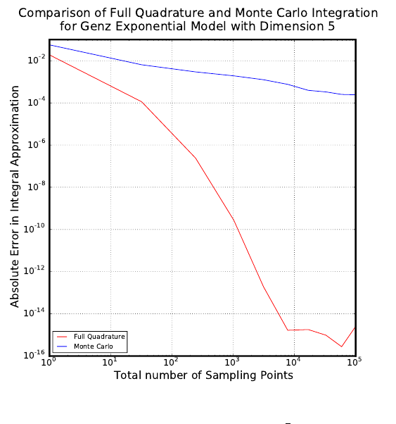
Sample Results
Try running the full_quad.py file with the following input:
Please enter desired model from choices:
genz_osc
genz_exp
genz_cont
genz_gaus
genz_cpeak
genz_ppeak
genz_exp
Please enter desired dimension: 5
Enter the desired maximum number of quadrature points per dimension: 10
Your graph should look similar to the one in the figure below. Although the Monte Carlo
integration curve may vary due to the random nature of the sampling, your quadrature curve
should be identical to the one pictured.
Figure 5.4: Sample results of full quad.py
51
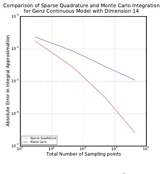
Now try running the sparse_quad.py file with the following input:
Please enter desired model from choices:
genz_osc
genz_exp
genz_cont
genz_gaus
genz_cpeak
genz_ppeak
genz_cont
Please enter desired dimension: 14
Enter the maximum desired level: 4
While the quadrature integrations are being performed, the current level will be printed to
your screen. Your graph should look similar to the figure below. Again, the Monte Carlo
curve may differ but the quadrature curve should be the same as the one pictured.
Figure 5.5: Samples results of sparse quad.py
52
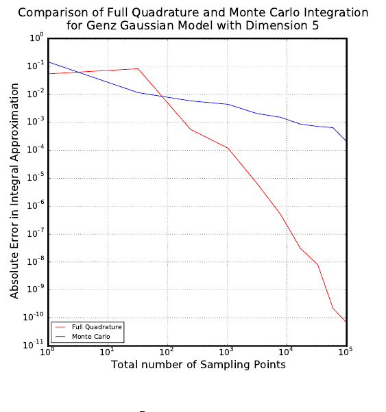
Next, try running full_quad.py with a quadrature rule other than the default Legendre-
Uniform. Locate the line in full_quad.py that calls the function generate_quad. It should
read:
xpts,wghts=generate_qw(ndim,quad_param)
Now, change this line to read:
xpts,wghts=generate_qw(ndim,quad_param, type= ’CC’)
This will change the quadrature rule to Clenshaw-Curtis. Then run the file with input:
genz_gaus, 5, 10. Sample results can be found in the figure below.
Figure 5.6: Sample results of full quad.py with Clenshaw-Curtis quadrature rule.
53
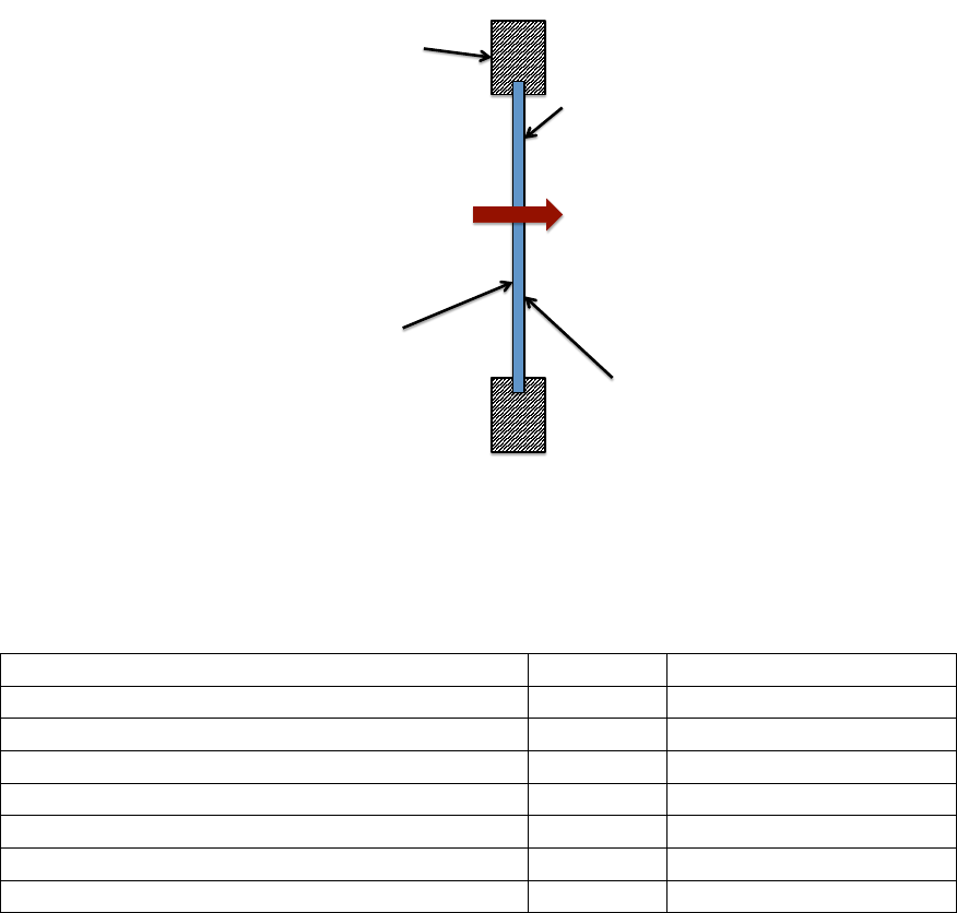
Forward Propagation of Uncertainty with PyUQTk
Overview
This example is located in examples/fwd_prop. It contains a pair of Python scripts that
propagate uncertainty in input parameters through a heat transfer model using both a Monte
Carlo sampling approach and a non-intrusive spectral projection (NISP) via quadrature
methods.
Theory
Heat Transfer
Glass%
T2%
T1%
Q%
Wall%
Ti%
To%
TA%
In this example, the heat transfer through a window is calculated using samples of seven
uncertain Gaussian parameters. These parameters, along with their means and standard
deviations are defined below.
Parameter Mean Standard deviation (%)
Ti: Room temperature 293 K 0.5
To: Outside temperature 273 K 0.5
dw: Window thickness 0.01 m 1
kw: Window conductivity 1 W/mK 5
hi: Inner convective heat transfer coefficient 2 W/m2K 15
ho: Outer convective heat transfer coefficient 6 W/m2K 15
TA: Atmospheric temperature 150 K 10
54

Once we have samples of the 7 parameters, the following forward model is used to calcu-
late heat flux Q:
Q=hi(Ti−T1) = kw
T1−T2
dw
=ho(T2−To) + σ(T4
2−T4
A)
T1represents the inner window temperature and T2represents the outer window temperature.
is the emissivity of uncoated glass, which we take to be 0.95, and σis the Stefan-Boltzmann
constant.
Polynomial Chaos Expansion
In this example, the forward propagation requires the representation of heat flux Q with
a multidimensional Polynomial Chaos Expansion (PCE). This representation can be defined
as follows:
Q=
P
X
k=0
QkΨk(ξ1, ..., ξn)
•Q: Random variable represented with multi-D PCE
•Qk: PC coefficients
•Ψk: Multi-D orthogonal polynomials up to order p
•ξi: Gaussian random variable known as the germ
•n: Dimensionality = number of uncertain model parameters
•P + 1: Number of PC terms = (n+p)!
n!p!
Non-Intrusive Spectral Projection (NISP)
Having specified a PCE form for our heat flux Q, we must determine the PC coefficients.
We do so through a non-intrusive Galerkin Projection. The coefficients are determined using
the following formula:
Qk=hQΨki
hΨ2
ki=1
hΨ2
kiZQΨk(ξ)w(ξ)dξ
In this example we use quadrature methods to evaluate this projection integral to determine
the PC coefficients.
55

Kernel Density Estimation
Once we have a large number of heat flux samples, to obtain a probability density function
(PDF) curve, a kernel density estimation (KDE) is performed. When performing KDE, the
following formula is used to evaluate the PDF at point Q:
P DF (Q) = 1
Nsh
Ns
X
i=1
KQ−Qi
h
Qiare samples of the heat flux, Nsis the number of sample points, K represents the kernel,
a non-negative function, and h > 0 is the bandwidth. In this example we use the Gaussian
kernel, K(x) = 1
√2πe−x2
2. The results rely heavily on the choice of bandwidth, and there are
many rules that can be used to calculate the bandwidth. In our example, the built-in SciPy
function employed automatically determines the bandwidth using Scott’s rule of thumb.
Implementation
The script set consists of two files:
•rad_heat_transfer_atm_pce.py: the main script
•heat_transfer_pce_tools.py: functions called by rad_heat_transfer_atm_pce.py
rad heat transfer atm pce.py
This script will produce a graph comparing PDFs of heat flux generated using NISP full
and sparse quadrature methods and a Monte Carlo sampling method. Use the command
./rad_heat_transfer_atm_pce.py to run this file
The top section of the script has some flags that are useful to consider:
•main verbose: set this parameter to 1 for intermediate print statements, otherwise set
to 0.
•compute rad: set to True to include radiation; use False to not use radiation. Note,
radiation is used, the nonlinear solver in Python sometimes has a hard time converging,
in which case you will see a warning message pop up.
•nord: the order of the PCE
•ndim: the number of dimensions of the PCE
•pc type: indicates the polynomial type and weighting function. The default is set to
”HG”, Hermite-Gauss.
56

•pc alpha and pc beta: Free parameters greater than -1. Used with Gamma-Laguerre
and Beta-Jacobi PC types.
•param: The parameter used for quadrature point generation. Equal to the number of
quadrature points per dimension for full quadrature or the level for sparse quadrature
methods. This parameter is generally set to nord + 1 in order to have the right
polynomial exactness.
Monte Carlo Sampling Methods
The script begins by assigning the input parameters and their means and standard deviations.
Using this information, a large number of random parameter samples (default is 100,000)
is generated. With these samples and our forward model, the function compute_heat_flux
then calculates the heat flux assuming that no radiative heat transfer occurs. This simply
requires solving a system of three linear equations. Then, using the values of Q,T1, and
T2obtained from compute_heat_flux as initial guesses, the function r_heat_flux calcu-
lates the total heat flux (including radiative heat transfer) using the SciPy nonlinear solver
optimize.fsolve. Using the heat flux samples, a kernel density estimation is then per-
formed using function KDE.
NISP Quadrature Methods
After the Monte Carlo sampling process is complete, forward propagation using projection
methods will take place. At the beginning of this section of the script, the following variables
are defined:
While running the file, a statement similar to the following will print indicating that PC
objects are being instantiated.
Instantiating PC Objects
Generating 4^7 = 16384 quadrature points.
Used 4 quadrature points per dimension for initialization.
Generating 4^7 = 16384 quadrature points.
Used 4 quadrature points per dimension for initialization.
Level 0 / 4
Level 1 / 4
Level 2 / 4
Level 3 / 4
Level 4 / 4
Instantiation complete
These PC objects contain all of the information needed about the polynomial chaos expan-
sion, such as the number of dimensions, the order of the expansion, and the sparsity (full or
sparse) of the quadrature methods to be implemented.
57

Next, a NumPy array of quadrature points is generated, using the function get_quadpts.
Then, the quadrature points in ξare converted to equivalent samples of the input parameters,
taking advantage of the fact that the inputs are assumed to be Gaussian. If we let µrepresent
the mean of an input parameter, σrepresent its standard deviation, and qdpts be a vector of
quadrature points, the following equation is used to convert these samples in ξto equivalent
samples of the input parameter:
parameter samples =µ+σ(qdpts)
Now that we have samples of all the input parameters, these samples are run through
the forward model to obtain values of Q using the function fwd_model. Then the actual
Galerkin projection is performed on these function evaluations to obtain the PC coefficients,
using the function GalerkinProjection.
Next, to create a PDF of the output Q from its PCE, germ samples are generated and
the PCE is evaluated at these sample points using the function evaluate_pce. Lastly, using
our PCE evaluations, a kernel density estimation is performed using function KDE
This entire process is done twice, once with full tensor product quadrature points and
again with sparse quadrature points.
Printing and Graphing
Next, statements indicating the total number of sampling points used for each forward
propagation method will be printed.
Monte Carlo sampling used 100000 points
Full quadrature method used 16384 points
Sparse quadrature method used 6245 points
Finally, a graph is created which displays the three different heat flux PDFs on the same
figure. It will be saved under the file name heat_flux_pce.pdf.
heat transfer pce tools.py
This script contains several functions called by the rad_heat_transfer_atm_pce.py file.
•compute_heat_flux(Ti, To, dw, kw, hi, ho): This function calculates heat flux
Q, assuming no radiative heat transfer occurs.
–Ti, To, dw, kw, hi, ho: Sample values (scalars) of the input parameters
•r_heat_flux(Ti,To,dw,kw,hi,ho,TA,estimates): This function calculates heat flux
Q, assuming radiative heat transfer occurs. The SciPy non-linear solver optimize.fsolve
is employed.
58

–Ti, To, dw, kw, hi, ho, TA: Sample values (scalars) of the input parameters
–estimates: Estimates of Q,T1, and T2required to solve the nonlinear system. For
these estimates, we use the output of the function compute_heat_flux, which
solves the system assuming no radiative heat transfer occurs.
•get_quadpts(pc_model,ndim): This function generates a NumPy array of either full
tensor product or sparse quadrature points. Returns number of quadrature points,
totquat, as well.
–pc model: PC object with information about the PCE, including the desired
sparsity for quadrature point generation.
–ndim: Number of dimensions of the PCE
•fwd_model(Ti_samples,To_samples,dw_samples,kw_samples,hi_samples,
ho_samples,verbose):
This function returns a NumPy array of evaluations of the forward model. This func-
tion calls the functions compute_heat_flux and r_heat_flux.
–Ti samples, To samples, dw samples, kw samples, hi samples, ho samples: 1D
NumPy arrays (vectors) of parameter sample values.
•fwd_model_rad(Ti_samples,To_samples,dw_samples,kw_samples,hi_samples,
ho_samples,TA_samples,verbose):
Same as fwd_model but with radiation enabled, and an extra argument for the samples
of TA.
•GalerkinProjection(pc_model,f_evaluations): This function returns a 1D NumPy
array with the PC coefficients.
–pc model: PC object with information about the PCE.
–f evaluations: 1D NumPy array (vector) with function to be projected, evaluated
at the quadrature points.
•evaluate_pce(pc_model,pc_coeffs,germ_samples): This function evaluates the PCE
at a set of samples of the germ.
–pc model: PC object with information about the PCE.
–pc coeffs: 1D NumPy array with PC coefficients. This array is the output of the
function GalerkinProjection
–germ samples: NumPy array with samples of the PCE germ at which the random
variable is to be evaluated.
•KDE(fcn_evals): This function performs a kernel density estimation. It returns a
NumPy array of points at which the PDF was estimated, as well as a NumPy array of
the corresponding estimated PDF values.
–fcn evals: A NumPy array of evaluations of the forward model (values of heat
flux Q).
59
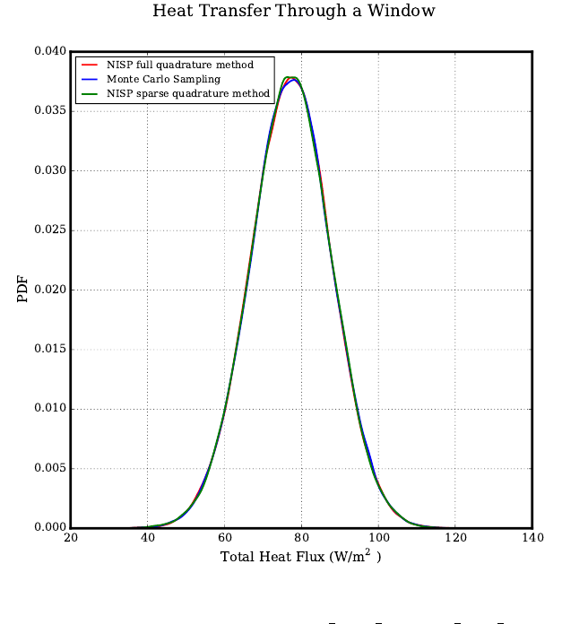
Sample Results
Run the file rad_heat_transfer_atm_pce.py with the default settings. You should
expect to see the following print statement, and your graph should look similar to the one
found in the figure below.
Monte Carlo sampling used 100000 points
Full quadrature method used 16384 points
Sparse quadrature method used 6245 points
Figure 5.7: Sample results of rad heat transfer atm pce.py
Now trying changing one of the default settings. Find the line that reads nord = 3 and
change it to read nord = 2. This will change the order of the PCE to 2, rather than 3. You
should expect to see the following print statement, and a sample graph is found in the figure
below.
Monte Carlo sampling used 100000 points
Full quadrature method used 2187 points
Sparse quadrature method used 1023 points
60
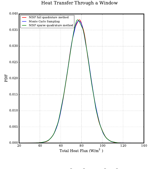
Figure 5.8: Sample results of rad heat transfer atm pce.py with nord = 2
The user can also change the default pc_type = "HG". For example, to use Legendre-
Uniform PC type, change this line to read pc_type = "LU".
Expanded Forward Propagation of Uncertainty - PyUQTk
Overview
This example is contains two pairs of python files, each pair consists of a main script
and a tools file that holds functions to be called from the main script. They are located
in UQTk/examples/window. This example is an expanded version of the previous forward
propagation problem, it utilizes a more complex model that provides additional parameters.
One pair of scripts produces a probability density function of the heat flux for a twelve
dimension model, using fourth order PCE’s and sparse quadrature. The other pair produces
a probability density function of the heat flux for a fifth dimension model, using fourth
order PCE’s. This script compares the results of using sparse and full quadrature, as well
as Monte Carlo sampling. It also produces a separate plot showing the spectral decay of the
61
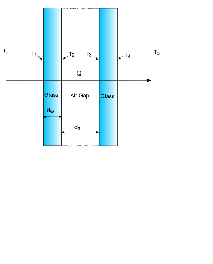
PC coefficients.
Theory
Heat Transfer - Dual Pane Window
The heat flux calculations are implemented using random samples from the normal dis-
tribution of each of the uncertain Gaussian parameters. The standard deviations assigned
are estimates. These parameters are defined in the table below:
The forward model that was developed relies on the same set of steady state heat transfer
equations from the first example, with the addition of a combined equation for conduction
and convection for the air gap. This is defined as conductance, and was implemented in order
to provide an alternative to determining the convection coefficient for this region, which can
be challenging[2].
Q=hi(Ti−T1) = kw
T1−T2
dw
= 0.41ka
dagβρ2da3
µ2|T2−T3|0.16
(T2−T3) = kw
T3−T4
dw
=ho(T4−To) + σ(T4
4−T4
s)
[1] Leonard, John H. IV, Leinhard, John H. V. A Heat Transfer Textbook - 4th edition. pg
579. Phlogiston Press. 2011 [2] Rubin, Michael.Calculating Heat Transfer Through Windows.
Energy Research. Vol. 6, pg 341-349. 1982.
62

Parameter Definition Mean Value Standard Deviation %
TiInside temperature 293 K0.5
ToOutside temperature 273 K0.5
TsSky Temperature[1] 263 K10
kwConduction constant for glass 1 W/m2K5
kaConduction constant for air 0.024 W/m2K5
hiInside convection coefficient 2 W/m2K15
hoOutside convection coefficient 6 W/m215
dwWidth of the glass 5 mm 1
daWidth of the air gap 1 cm 1
µViscosity or air 1.86x10⁻⁵kg/m s 5
ρDensity of air 1.29 kg/m35
βThermal expansion coefficient 3.67x10⁻³¹/K 5
T1represents the glass temperature of the outer facing surface for the first glass layer,
and T2represents the temperature of the inner surface for the first glass layer, T3represents
the temperature of the inner surface of the second glass layer, T4represents the outer facing
surface of the second glass layer. is the emissivity of uncoated glass, which we take to be
0.95, and σis the Stefan-Boltzmann constant.
Polynomial Chaos Expansion*
Non-Intrusive Spectral Projection (NISP)*
Kernel Density Estimation*
*Please see previous example.
Implementation
The first set of scripts:
•5D_fwd_prop.py: the main script
•fwd_prop_tools.py: functions called by 5D_fwd_prop.py
63
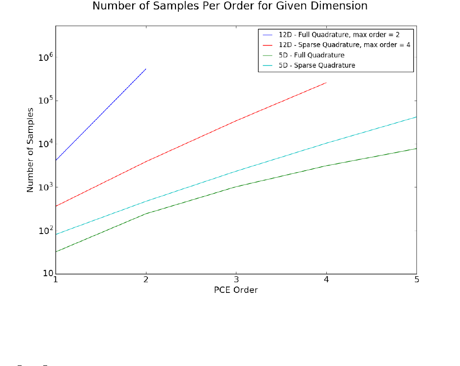
Figure 5.9: Increase in number of samples with change in order.
5D fwd prop.py
This script will produce a plot comparing the probability density function of the heat flux
using three methods. Non-intrusive spectral projection full and sparse quadrature methods,
and Monte Carlo sampling. It also produces a plot showing the spectral decay of the PC
coefficient magnitude in relation to the PC order. This plot illustrates the how the pro-
jection converges to give a precise representation of the model. Changing the order of this
script (nord) may alter the results of the second plot, since it has elements that are not
dynamically linked. Use the command python 5D_fwd_prop.py to run this file from the
window directory.
The second set of scripts:
•highd_sparse.py: the main script
•tools_conductance_dp_pce_wrad.py: functions called by highd_sparse.py
64

highd sparse.py
This script will produce of the probability density function of the heat flux in twelve
dimensions, using only non-intrusive spectral projection with sparse quadrature. Use the
command python highd_sparse.py to run this file from the window directory. Adjust-
ments may be made to nord if desired, though the number of points produced increases
dramatically with an increase in order, as illustrated by figure 5.9.
Monte Carlo Sampling Methods
This is very similar to the previous example with the exception of compute_heat_flux
producing T1,T2,T3,T4and Q. This function consists of a solved set of five linear equations,
our forward model neglecting convection for the air gap and radiative heat transfer, which
are evaluated for the parameter samples. The values obtained are used as initial inputs for
r_heat_flux, which calculates the total heat flux for all heat transfer modes, using the SciPy
nonlinear solver optimize.fsolve. Using the heat flux samples, a kernel density estimation
is then performed using function KDE.
NISP Quadrature Methods
Please see previous example.
Printing and Graphing
Next, statements indicating the total number of sampling points used for each forward
propagation method will be printed. The number of Monte Carlo points is fixed, but the
number of points produced by quadrature method will vary with the number of uncertain
parameters and the order of the PCE.
Monte Carlo sampling used 100000 points
Full quadrature method used xxxxxxx points
Sparse quadrature method used xxxxxxx points
Finally, a graph is created which displays the three different heat flux PDFs on the same
figure. It will be saved under the file name heat_flux_pce.pdf.
fwd prop tools.py and tools conductance dp pce wrad.py
This scripts contain several functions called by the 5D_fwd_prop.py and highd_sparse.py
files. The five dimension example uses the five parameters with the highest uncertainty,
Ts,hi,ho,kw,ka.
65

•compute_heat_flux(Ti,To,dw,da,kw,ka,hi,ho): This function calculates heat flux
Q, assuming no radiative heat transfer occurs and no convective heat transfer occurs
in the air gap.
–Ti, To, dw, da, kw, ka, hi, ho: Sample values (scalars) of the input parameters
•r_heat_flux(Ti,To,Ts,dw,da,kw,ka,hi,ho,beta,rho,mu,estimates): This func-
tion calculates heat flux Q, assuming radiative heat transfer, and convective heat trans-
fer for the air gap occurs. The SciPy non-linear solver optimize.fsolve is employed.
–Ti, To, Ts, dw, da, kw, ka, hi, ho, beta, rho, mu: Sample values (scalars) of the
input parameters
–estimates: Estimates of Q,T1,T2,T3, and T4are required to solve the nonlinear
system. For these estimates, we use the output of the function compute_heat_flux,
which solves the system assuming no radiative or convective heat transfer for the
air gap occurs.
•get_quadpts(pc_model,ndim)*
•fwd_model(Ti_samples,To_samples,Ts_samples,dw_samples,da_samples,kw_samples,
ka_samples,hi_samples,ho_samples,beta_samples,rho_samples,mu_samples):
This function returns a NumPy array of evaluations of the forward model. This func-
tion calls the functions compute_heat_flux and r_heat_flux.
–Ti samples, To samples,Ts samples, dw samples, da samples, kw samples, ka samples,
hi samples, ho samples, beta samples, rho samples, mu samples: 1D NumPy ar-
rays (vectors) of parameter sample values.
•GalerkinProjection(pc_model,f_evaluations)*
•evaluate_pce(pc_model,pc_coeffs,germ_samples)*:
•KDE(fcn_evals)*:
•get_multi_index(pc_model,ndim) This function computes the multi indices to be
used in the inverse relationship plot.
–pc model: Contains information about the PC set.
–ndim: Number of model dimensions.
•plot_mi_dims(pc_model,c_k,ndim) This function produces the inverse relationship
plot using the multi indices produced in the previous function, and the value of the
PC coefficients.
–pc model: Contains information about the PC set.
–ndim: Number of model dimensions.
–c k: Numpy array of PC coefficients.
*Please see previous example.
66
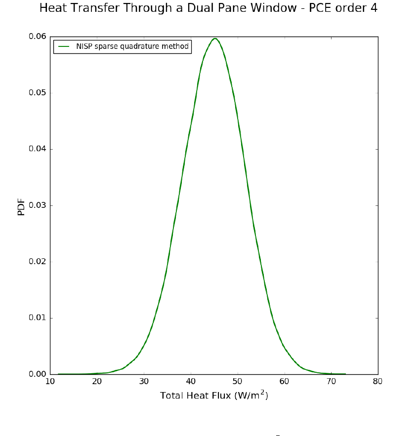
Sample Results
Run the file highd_sparse.py with the default settings. You should expect to see the
following print statement, and your graph should look similar to the one found in the figure
below. This sample is for a problem with twelve dimensions, the PCE is fourth order. The
following will print to the terminal:
Sparse quadrature method used 258681 points
Figure 5.10: Sample results of highd sparse.py
The next two figures show the two results of the five dimension example with a fourth
order PCE. The following will print to the terminal:
67
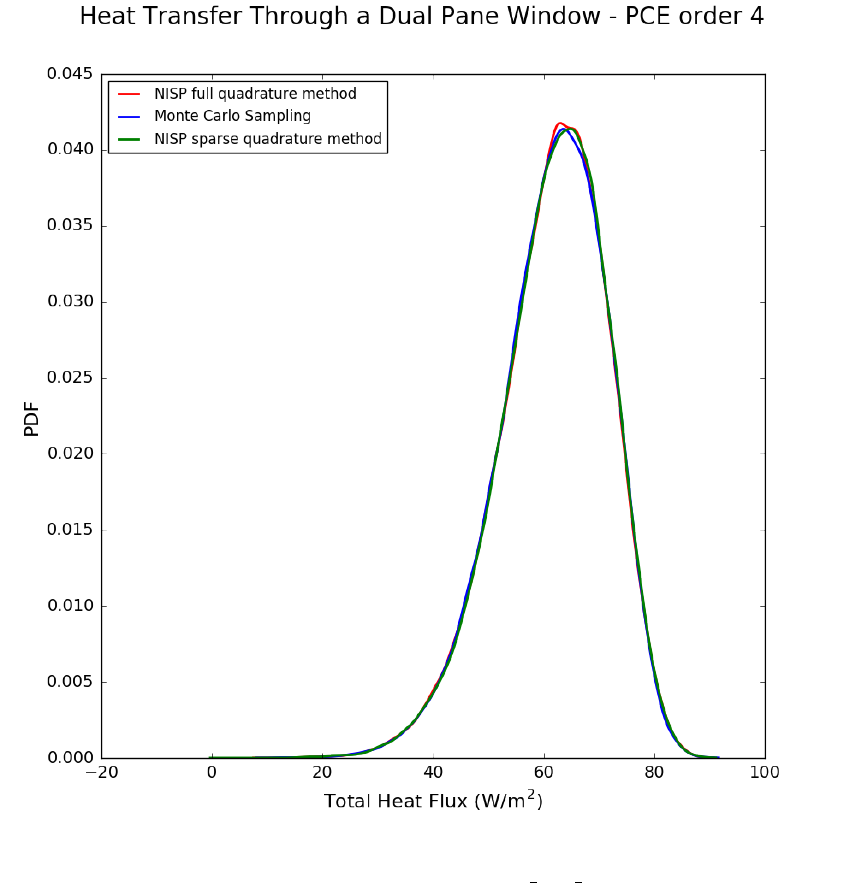
Monte Carlo sampling used 100000 points
Full quadrature method used 3125 points
Sparse quadrature method used 10363 points
Figure 5.11: Sample results of 5D fwd prop.py
68
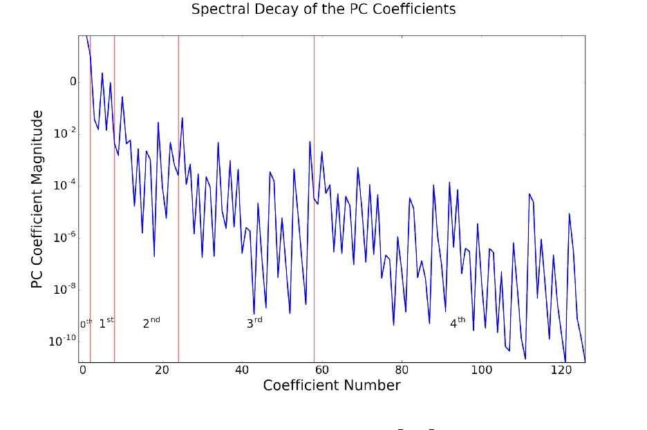
Figure 5.12: Sample results of 5D fwd prop.py
Bayesian Inference of a Line
Overview
This example is located in examples/line_infer It infers the slope and intercept of
a line from noisy data using Bayes’ rule. The C++ libraries are called directly from the
driver program. By changing the likelihood function and the input data, this program can
be tailored to other inference problems.
To run an example, type ./line_infer.py directly. This file contains quite a bit of
inline documentation about the various settings and methods used. To get a listing of all
command line options, type ./line_infer.py -h". A typical run, with parameters changed
from command-line, is as follows:
./line_infer.py --nd 5 --stats
This will run the inference problem with 5 data points, generate plots of the posterior
distributions, and generate statistics of the MCMC samples. If no plots are desired, also
give the --noplots argument.
69
More details
After setting a number of default values for the example problem overall, the line_infer.py
script sets the proper inference inputs in the file line_infer.xml, starting from a set of de-
faults in line_infer.xml.templ. The file line_infer.xml is read in by the C++ code
line_infer.x, which does the actual Bayesian inference. After that, synthetic data is gen-
erated, either from a linear, or cosine model, with added noise.
Then, the script calls the C++ line inference code line_infer.x to infer the two pa-
rameters (slope and intercept) of a line that best fits the artificial data. (Note, one can also
run the inference code directly by manually editing the file line_infer.xml and typing the
command ./line_infer.x)
The script then reads in the MCMC posterior samples file, and performs some postpro-
cessing. Unless the flag --noplots is specified, the script computes and plots the following:
•The pushed-forward and posterior predictive error bars
–Generate a dense grid of x-values
–Evaluate the linear model y=a+bx for all posterior samples (a, b) after the
burn-in
–Pushed-forward distribution: compute the sample mean and standard deviation
of using the sampled models
–Posterior predictive distribution: combine pushed-forward distribution with the
noise model
•The MCMC chain for each variable, as well as a scatter plot for each pair of variables
•The marginal posterior distribution for each variable, as well as the marginal joint
distribution for each pair of variables
If the flag --stats is specified, the following statistics are also computed:
•The mean, MAP (Maximum A Posteriori), and standard deviations of all parameters
•The covariance matrix
•The average acceptance probability of the chain
•The effective sample sizes for each variable in the chain
Sample Results
70
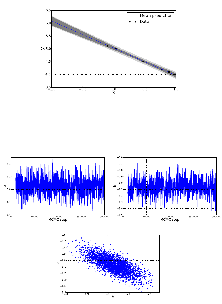
Figure 5.13: The pushed forward posterior distribution (dark grey) and posterior predictive
distribution (light grey).
Figure 5.14: MCMC chains for parameters a and b, as well as a scatter plot for a and b
71
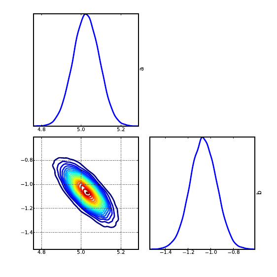
Figure 5.15: Marginal posterior distributions for all variables, as well as marginal joint
posteriors
Surrogate Construction and Sensitivity Analysis
Overview
•Located in examples/uqpc
•A collection of scripts that construct a PC surrogate for a computational model which
is specified as a black box simulation code. Also provides tools for sensitivity analysis
of the outputs of this black box model with respect to its input parameters.
Theory
Consider a function f(λ;x) where λ= (λ1, . . . , λd) are the model input parameters of
interest, while x∈Rrare design parameters with controllable values. For example, xcan
denote a spatial coordinate or a time snapshot, or it can simply enumerate multiple quantities
of interest. Furthermore, we assume known domains for each input parameter, i.e.
λi∈[ai, bi] for i= 1, . . . .d. (5.5)
72

The goal is to build a Polynomial Chaos (PC) surrogate function for each value of design
parameter x, i.e. for l= 1, . . . , L,
f(λ;xl)≈g(λ;xl) =
K−1
X
k=0
cklΨk(ξ) (5.6)
with respect to scaled inputs
ξi=λi−bi−ai
2
bi+ai
2∈[−1,1] for i= 1, . . . .d. (5.7)
Here Ψk(ξ) = Ψk(ξ1, . . . , ξd) are multivariate normalized Legendre polynomials, defined as
products of univariate normalized Legendre polynomials ψki(ξi) as follows:
Ψk(ξ) = ψk1(ξ1). . . ψkd(ξd).(5.8)
A typical truncation rule in (5.6) is defined according to the total order of the basis terms,
i.e. only polynomials with the total order ≤pare retained for some positive integer order p,
implying |k1|+···+|kd| ≤ p, and K= (d+p)!/(d!p!). The scalar index kis simply counting
the multi-indices (k1, . . . , kd).
After computing the PC coefficients ckl, one can extract the global sensitivity information,
also called Sobol indices or variance-based decomposition. For example, the main sensitivity
index with respect to the dimension i(or variable ξi) is
Si(xl) = Pk∈Iic2
kl
PK−1
k=1 c2
kl
,(5.9)
where Iiis the indices of basis terms that involve only the variable ξi, i.e. the one-dimensional
monomials ψ1(ξi), ψ2(ξi), .... In other words, these are basis terms corresponding to multi-
indices with the only non-zero entry at the i-th location.
The two generic methods of finding the PC coefficients ckl are detailed below.
Projection
The basis orthonormality enables the projection formulae
ckl =ZΩ
f(λ(ξ); xl)Ψk(ξ)1
2ddξ (5.10)
where Ω = [−1,1]dand λ(ξ) simply denotes the linear scaling relation in (5.7).
The projection integral can be taken by
73
•Quadrature integration
ckl ≈
Q
X
q=1
f(λ(ξ(q)); xl)Ψk(ξ(q)),(5.11)
where ξ(q)are Gauss-Legendre quadrature points in the d-dimensional Ω = [−1,1]d.
•Monte-Carlo integration [to be implemented]
ckl ≈
M
X
m=1
f(λ(ξ(m)); xl)Ψk(ξ(m)),(5.12)
where ξ(m)are uniformly random points in the d-dimensional Ω = [−1,1]d.
Inference
[to be implemented]
Implementation
The script set consists of three files are
•uq_pc.py : the main script
•model.py : black-box example model
•plot.py : plotting
The apps employed
•generate_quad : Quadrature point/weight generation
•gen_mi : PC multiindex generation
•pce_resp : Projection via quadrature integration
•pce_sens : Sensitivity extraction
•pce_eval : PC evaluation
Main script: The syntax of the main script is
74
% uq_pc.py -r <run_regime>
% -p <pdomain_file> -m <method> -o <ord> -s <sam_method> -n <nqd> -v <nval>
Also one can run uq_pc.py -h for help in the terminal and to check the defaults.
The list of arguments:
•-r <run_regime>: The regime in which the workflow is employed. The options are
online : Black-box model, which is in model.py, is run directly as param-
eter ensemble becomes available. User can provide their own model.py or simply use
the current one as an example.
offline_prep : Prepare the input parameter ensemble and store in ytrain.dat
and, if validation is requested, yval.dat.
The user then should run the model (model.py ptrain.dat ytrain.dat and per-
haps model.py pval.dat yval.dat) in order to provide ensemble output for the
offline_post stage.
offline_post : Postprocess the output ensemble, assuming the model is run offline
with input ensemble provided in the offline_prep stage producing ytrain.dat and,
if validation is requested, yval.dat. The rest of the arguments should remain the same
as in the offline_post stage.
•-p <domain_file>: A file with drows and 2 columns, where d is the number of
parameters and each row consists of the lower and upper bound of the corresponding
parameter.
•-m <method>: The method of finding the PC surrogate coefficients. The options are
proj : Projection method outlined in (5.10) and (5.11)
lsq : Least-squares.
bcs : Bayesian compressive sensing.
•-o <ord>: Total order pof the requested PC surrogates.
•-s <sam_method>: The input parameter sampling method. The options are
Q: Quadrature points. This sampling scheme works with the projection method
only, described in (5.11)
U: Uniformly random points. To be implemented.
•-n <nqd>: Number of samples requested if sam_method=U, or the number of quadrature
points per dimension, if sam_method=Q.
•-v <nval>: Number of uniformly random samples generated for PC surrogate valida-
tion, can be equal to 0 to skip validation.
Generated output files are:
75

•allsens.dat and allsens_sc.dat :The main effect sensitivity indices in a format
Lxd, where each row corresponds to a single value for the design parameter, and each
column corresponds to the sensitivity index of a parameter. The second file stores the
same results, only the sensitivity indices are scaled to sum to one for each parameter.
•results.pk : Python pickle file that includes surrogate, sensitivity and error informa-
tion. It is loaded in plotting utilities.
•*.log : Log files of the apps that have been employed, for reference.
•mi.dat : PC multiindex, for reference, in a matrix form of size Kxd, see (5.8).
•designPar.dat : A file containing values for the design parameters, for reference.
Black-box model: The syntax of the model script is
% model.py <modelPar_file> <output_file>
Also one can run model.py -h for help in the terminal and to check the defaults.
The list of arguments:
•<modelPar_file> : A file with Nrows and dcolumns that stores the input parameter
ensemble of N samples.
•<output_file> : The file where output is stored, with Nrows (number of input
parameter samples) and Lcolumns (number of outputs, or number of design parameter
values).
model.py is the file that needs to be modified/provided by the user according to the model
under study. Currently, a simple example function f(λ;x) = Pd
i=1 λiPd
i=1
λi+λ2
i
ix+1 is
implemented that also produces the file designPar.dat for design parameters xl=lfor
l= 0,...,6. The default dimensionality is set to d= 3.
A user-created black-box model.py should accept an input parameter file <modelPar_file>
and should produce an output file <output_file> with the formats described above, in order
to be consistent with the expected I/O.
Visualization: The syntax of the plotting script is
% plot.py <plotid>
The user is encouraged to enhance or change the visualization scripts. The current defaults,
explained below, are simply for illustration purposes. The options for the only argument
<plotid> are
76
sens : Plots the sensitivity information.
dm : Plots model-vs-data for one of the values of the design parameter.
idm : Plots model and data values on the same axis, for one of the values of the
design parameter.
For the visualization script above, make sure the PYTHONPATH environment variable con-
tains the directory UQTK_INS.
Sample run:
In order to run a simple example, use the prepared an input domain file which is the
default domain file, pdomain_3d.dat, and run
•Online mode: uq_pc.py -r online -v111
•Offline mode: uq_pc.py -r offline_prep -v111,
followed by model evaluations
model.py ptrain.dat ytrain.dat and model.py pval.dat yval.dat,
and the postprocessing stage uq_pc.py -r offline_post -v111
After finishing, run plot.py sens or plot.py dm or plot.py idm to visualize some
results.
Global Sensitivity Analysis via Sampling
Overview
•Located in PyUQTk/sens
•A collection of Python functions that generate input samples for black-box models,
followed by functions that post-process model outputs to generate total, first-order,
and joint effect Sobol indices
Theory
Let X= (X1,··· , Xn):Ω→ X ⊂ IRnbe an n−dimensional Random Variable in
L2(Ω,S, P ) with probability density X∼pX(x). Let x= (x1,··· , xn)∈ X be a sample
drawn from this density, with X=X1⊗ X2⊗ ··· ⊗ Xn, and Xi⊂IR is the range of Xi.
Let X−i= (X1,··· , Xi−1, Xi+1,··· , Xn) : Ω → X−i⊂IRn−1, where X−i∼pX−i|Xi(x−i|xi) =
pX(x)/pXi(xi), pXi(xi) is the marginal density of Xi,x−i= (x1,··· , xi−1, xi+1,··· , xn), and
X−i=X1⊗ ··· ⊗ Xi−1⊗ Xi+1 ⊗ ··· ⊗ Xn.
77

Consider a function Y=f(X) : Ω →IR, with Y∈L2(Ω,S, P ). Further, let Y∼pY(y),
with y=f(x). Given the variance of fis finite , one can employ the law of total variance1,2
to decompose the variance of fas
V[f] = Vxi[E[f|xi]] + Exi[V[f|xi]] (5.13)
The conditional mean, E[f|xi]≡E[f(X)|Xi=xi], and conditional variance, V[f|xi] =
V[f(X)|Xi=xi], are defined as
hfi−i≡E[f|xi] = ZX−i
f(x)pX−i|Xi(x−i|xi)dx−i(5.14)
V[f|xi] = E[(f− hfi−i)2|xi]
=E[(f2−2fhfi−i+hfi2
−i)|xi]
=E[f2|xi]−2hfi−ihfi−i+hfi2
−i
=ZX−i
f(x)2pX−i|Xi(x−i|xi)dx−i− hfi2
−i(5.15)
The terms in the rhs of Eq. (5.13) can be written as
Vxi[E[f|xi]] = Exi[ (E[f|xi]−Exi[E[f|xi]])2] (5.16)
=Exi[ (E[f|xi]−f0)2]
=Exi[ (E[f|xi])2]−f2
0
=ZXi
E[f|xi]2pXi(xi)dxi−f2
0
where f0=E[f] = Exi[E[f|xi]] is the expectation of f, and
Exi[V[f|xi]] = ZXi
V[f|xi]pXi(xi)dxi(5.17)
The ratio
Si=Vxi[E[f|xi]]
V[f](5.18)
is called the first-order Sobol index [32] and
ST
−i=Exi[V[f|xi]]
V[f](5.19)
is the total effect Sobol index for x−i. Using Eq. (5.13), the sum of the two indices defined
above is
Si+ST
−i=S−i+ST
i= 1 (5.20)
Joint Sobol indices Sij are defined as
Sij =Vxi,xj[E[f|xi, xj]]
V[f]−Si−Sj(5.21)
1en.wikipedia.org/wiki/Law_of_total_variance
2en.wikipedia.org/wiki/Law_of_total_expectation
78

for i, j = 1,2...,n and i6=j.
Sican be interpreted as the fraction of the variance in model fthat can be attributed
to the i-th input parameter only, while Sij is the variance fraction that is due to the joint
contribution of i-th and j-th input parameters. ST
imeasures the fractional contribution to
the total variance due to parameter xiand its interactions with all other model parameters.
The Sobol indices are numerically estimated using Monte Carlo (MC) algorithms pro-
posed by Saltelli [24] and Kucherenko et al [16]. Let xk= (x1,··· , xn)kbe a sample of X
drawn from pX. Let x0k
−ibe a sample from the conditional distribution pX−i|Xi(x0
−i|xk
i), and
x00k
ia sample from the conditional distribution pXi|X−i(x00
i|xk
−i).
The expectation f0=E[f] and variance V=V[f] are estimated using the xksamples as
f0≈1
N
N
X
k=1
f(xk), V ≈1
N
N
X
k=1
f(xk)2−f2
0(5.22)
where Nis the total number of samples. The first-order Sobol indices Siare estimated as
Si≈1
V 1
N
N
X
k=1
f(xk)f(x0k
−i∪xk
i)−f2
0!(5.23)
The joint Sobol indices are estimated as
Sij ≈1
V 1
N
N
X
k=1
f(xk)f(x0k
−(i,j)∪xk
i,j)−f2
0!−Si−Sj(5.24)
For ST
i, UQTk offers two alternative MC estimators. In the first approach, ST
iis estimated
as
ST
i= 1 −S−i≈1−1
V 1
N
N
X
k=1
f(xk)f(x00k
i∪xk
−i)−f2
0!(5.25)
In the second approach, ST
iis estimated as
ST
i≈1
2V 1
N
N
X
k=1 f(xk)−f(xk
−i∪x00k
i)2!(5.26)
Implementation
Directory pyUQTk/sensitivity contains two Python files
•gsalib.py : set of Python functions implementing the MC sampling and estimators
for Sobol indices
•gsatest.py : workflow illustrating the computation of Sobol indices for a toy problem
79
gsalib.py implements the following functions
•genSpl_Si(nspl,ndim,abrng,**kwargs) : generates samples for Eq. (5.23). The
input parameters are as follows
nspl: number of samples N,
ndim: dimensionality nof the input parameter space ,
abrng: a 2-dimensional array n×2, containing the range for each component xi.
The following optional parameters can also be specified
splout: name of ascii output file for MC samples
matfile: name of binary output file for select MC samples. These samples are
used in subsequent calculations of joint Sobol indices
verb: verbosity level
nd: number of significant digits for ascii output
The default values for optional parameters are listed in gsalib.py
•genSens_Si(modeval,ndim,**kwargs) : computes first-order Sobol indices using Eq. (5.23).
The input parameters are as follows
modeval: name of ascii file with model evaluations,
ndim: dimensionality nof the input parameter space
The following optional parameter can also be specified
verb: verbosity level
The default value for the optional parameter is listed in gsalib.py
•genSpl_SiT(nspl,ndim,abrng,**kwargs) : generates samples for Eqs. (5.25-5.26).
The input parameters are as follows
nspl: number of samples N,
ndim: dimensionality nof the input parameter space ,
abrng: an 2-dimensional array n×2, containing the range for each component xi.
The following optional parameters can also be specified
splout: name of ascii output file for MC samples
matfile: name of binary output file for select MC samples. These samples are
used in subsequent calculations of Sobol indices
verb: verbosity level
nd: number of significant digits for ascii output
The default values for optional parameters are listed in gsalib.py
80
•genSens_SiT(modeval,ndim,**kwargs) : computes total Sobol indices using either
Eq. (5.25) or Eq. (5.26). The input parameters are as follows
modeval: name of ascii file with model evaluations,
ndim: dimensionality nof the input parameter space
The following optional parameter can also be specified
type: specifies wether to use Eq. (5.25) for type = ”type1” or Eq. (5.26) for
type 6= ”type1”
verb: verbosity level
The default value for the optional parameter is listed in gsalib.py
•genSpl_Sij(ndim,**kwargs) : generates samples for Eq. (5.24). The input parame-
ters are as follows
ndim: dimensionality nof the input parameter space ,
The following optional parameters can also be specified
splout: name of ascii output file for MC samples
matfile: name of binary output file for select MC samples saved by genSpl_Si.
verb: verbosity level
nd: number of significant digits for ascii output
The default values for optional parameters are listed in gsalib.py
•genSens_Sij(sobolSi,modeval,**kwargs) : computes joint Sobol indices using Eq. (5.24).
The input parameters are as follows
sobolSi: array with values for first-order Sobol indices Si
modeval: name of ascii file with model evaluations.
The following optional parameter can also be specified
verb: verbosity level
The default value for the optional parameter is listed in gsalib.py
gsatest.py provides the workflow for the estimation of Sobol indices for a simple model
given by
f(x1, x2, . . . , xn) =
n
X
i=1
xi+
n−1
X
i=1
i2xixi+1 (5.27)
In the example provided in this file, n(ndim in the file) is set equal to 4, and the number of
samples N(nspl in the file) to 104. Figures 5.16 and 5.17 show results based on an ensemble
of 10 runs. To generate these results run the example workflow:
python gsatest.py
81
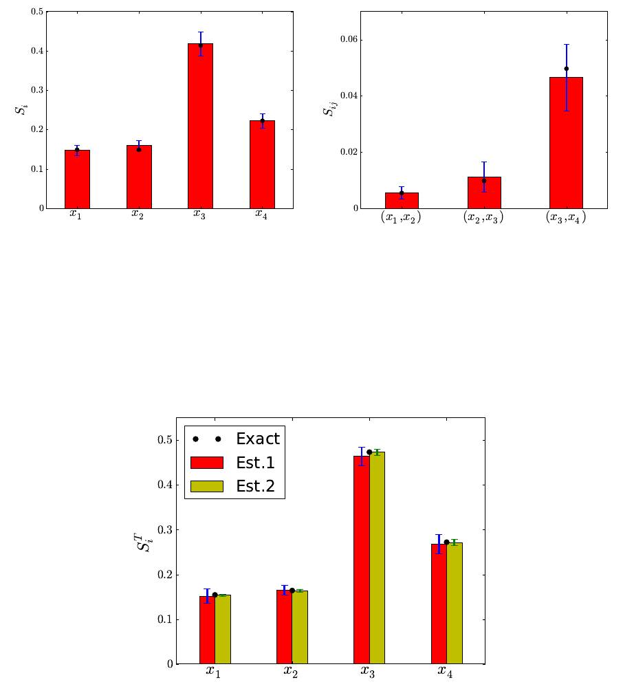
Figure 5.16: First-order (left frame) and joint (right frame) Sobol indices for the model
given in Eq. (5.27). The black circles show the theorerical values, computed analytically,
and the error bars correspond to ±σcomputed based on an ensemble of 10 runs.
Figure 5.17: Total-order Sobol indices for the model given in Eq. (5.27). The red bars
shows results based on Eq. (5.25) while the yellow bars are based on Eq. (5.26). The black
circles show the theorerical values, computed analytically, and the error bars correspond to
±σcomputed based on an ensemble of 10 runs. For this model, Eq. (5.26) provides more
accurate estimates for ST
icompared to results based on Eq. (5.25).
82

Karhunen-Lo`eve Expansion of a Stochastic Process
•Located in examples/kle_ex1
•Some examples of the construction of 1D and 2D Karhunen-Lo`eve (KL) expansions of
a Gaussian stochastic process, based on sample realizations of this stochastic process.
Theory
Assume stochastic process F(x, ω) : D×Ω→Ris L2random field on D, with covariance
function C(x, y). Then Fcan be written as
F(x, ω) = hF(x, ω)iω+∞
X
k=1 pλkfk(x)ξk(5.28)
where fk(x) are eigenfunctions of C(x, y) and λkare corresponding eigenvalues (all positive).
Random variables ξkare uncorrelated with unit variance. Projecting realizations of Fonto
fkleads to samples of ξk. These samples are generally not independent. In the special case
when Fis a Gaussian random process, ξkare i.i.d. normal random variables.
The KL expansion is optimal, i.e. of all possible orthonormal bases for L2(D×Ω) the
above {fk(x)|k= 1,2, . . .}minimize the mean-square error in a finite linear representation
of F(·). If known, the covariance matrix can be specified analytically, e.g. the square-
exponential form
C(x, y) = exp −|x−y|2
c2
l!(5.29)
where |x−y|is the distance between xand yand clis the correlation length. The covariance
matrix can also be estimated from realizations, e.g.
C(x, y) = 1
NωX
ω
(F(x, ω)− hF(x, ω)iω)(F(y, ω)− hF(y, ω)iω) (5.30)
where Nωis the number of samples, and hF(x, ω)iωis the mean over the random field
realizations at x.
The eigenvalues and eigenvectors in Eq. (5.28) are solutions of the Fredholm equation of
second kind: ZC(x, y)f(y)dy =λf(x) (5.31)
One can employ the Nystrom algorithm [19] to discretize of the integral in the left-hand side
of Eq. (5.31)
Np
X
i=1
wiC(x, yi)f(yi) = λf(x) (5.32)
83

Here wiare the weights for the quadrature rule that uses Nppoints yiwhere realizations are
provided. In a 1D configuration, one can employ the weights corresponding to the trapezoidal
rule:
wi=
y2−y1
2if i= 1,
yi+1−yi−1
2if 2 ≤i<Np,
yNp−yNp−1
2if i=Np,
(5.33)
After further manipulation, Eq. (5.32) is written as
Ag =λg
where A=W KW and g=W f, with Wbeing the diagonal matrix Wii =√wiand Kij =
C(xi, yj). Since matrix Ais symmetric, one can employ efficient algorithms to compute its
eigenvalues λkand eigenvectors gk. Currently UQTk relies on the dsyevx function provided
by the LAPACK library.
The KL eigenvectors are computed as fk=W−1gkand samples of random variables ξk
are obtained by projecting realizations of the random process Fon the eigenmodes fk
ξk|ωl=hF(x, ωl)− hF(x, ω)iω, fk(x)ix/pλk
Numerically, these projections can be estimated via quadrature
ξk|ωl=
Np
X
i=1
wi(F(xi, ωl)− hF(xi, ω)iω)fk(xi)/pλk(5.34)
If Fis a Gaussian process, ξkare i.i.d. normal RVs, i.e. automatically have first order
Wiener-Hermite Polynomial Chaos Expansions (PCE). In general however, the KL RVs can
be converted to PCEs (not shown in the current example).
1D Examples
In this section we are presenting 1D RFs generated with kl 1D.x. The RFs are generated
on a non-uniform 1D grid, with smaller grid spacing near x= 0 and larger grid spacing
towards x= 1. This grid is computed using an algebraic expression [14]
xi=Lβ+ 1 −(β−1)ri
ri+ 1 , ri=β+ 1
β−11−ηi
, ηi=i−1
Np−1, i = 1,2, . . . , Np(5.35)
The β > 1 factor in the above expression controls the compression near x= 0. It results in
higher compression as βgets closer to 1. The examples shown in this section are based on
default values for the parameters that control the grid definition in kl 1D:
β= 1.1, L = 1, Np= 129
84
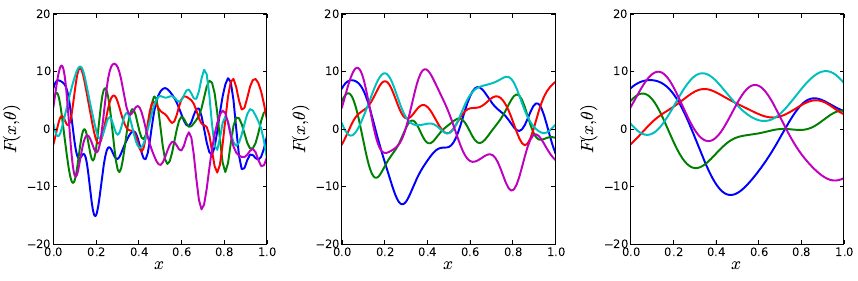
Figure 5.18 shows sample realizations for 1D random fields (RF) generated with a square-
exponential covariance matrix employing several correlation lenghts cl. These figures were
generated with
./mkplots.py samples 0.05
./mkplots.py samples 0.10
./mkplots.py samples 0.20
(a) cl= 0.05 (b) cl= 0.10 (c) cl= 0.20
Figure 5.18: Sample 1D random field realizations for several correlation lengths cl.
Once the RF realizations are generated the covariance matrix is discarded and a “numer-
ical” covariance matrix is estimated based on the available realizations. Figure 5.19 shows
shaded illustration of covariance matrices computed using several sets of 1D RF samples.
These figures were generated with
./mkplots.py numcov 0.05 512 ./mkplots.py numcov 0.20 512
./mkplots.py numcov 0.05 8192 ./mkplots.py numcov 0.20 8192
./mkplots.py numcov 0.05 131072 ./mkplots.py numcov 0.20 131071
These matrices employ RF samples generated on a non-uniform grid with higher densitiy
of points near the left boundary. Hence, the matrix entries near the diagonal in the upper
right corner show larger values. Grids grow further apart away from the left boundary hence
the region near the diagonal grows thinner for these grid points.
Figure 5.20 shows the eigenvalue solution of Fredholm equation (5.31) in its discretized
form given by Eq. (5.32). This figure was generated with
./mkplots.py pltKLeig1D 512 131072
For this 1D example problem, 29= 512 RF realizations are sufficient to estimate the
KLE eigenvalue spectrum. As the correlation length decreases the eigenvalues decrease
more slowly suggesting that more terms are needed to represent RF fluctuations.
Figure 5.21 shows first four KL eigenvectors corresponding to cl= 0.05, scaled by the
square rood of the corresponding eigenvalue. These plots were generated with
./mkplots.py numKLevec 0.05 512 on
85
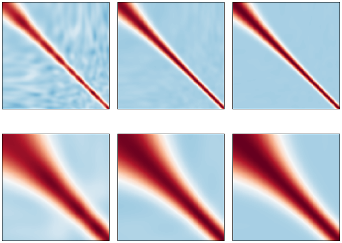
(a) cl= 0.05, Nω= 29(b) cl= 0.05, Nω= 213 (c) cl= 0.05, Nω= 217
(d) cl= 0.20, Nω= 29(e) cl= 0.20, Nω= 213 (f) cl= 0.20, Nω= 217
Figure 5.19: Illustration of covariance matrices computed from 1D RF realizations. Red
corresponds to large values, close to 1, while blue corresponds to small values, close to 0.
./mkplots.py numKLevec 0.05 8192 off
./mkplots.py numKLevec 0.05 131072 off
Unlike the eigenvalue spectrum, the eigenvectors are very sensitive to the covariance
matrix entries. For cl= 0.05, a large number of RF realizations, e.g. Nω= 217 in Fig. 5.21c,
are required for computing a covariance matrix with KL modes that are close to the ones
based on analytical covariance matrix (analytical modes not shown).
Figure 5.22 shows first four KL eigenvectors corresponding to cl= 0.20, scaled by the
square rood of the corresponding eigenvalue. These plots were generated with
./mkplots.py numKLevec 0.20 512 on
./mkplots.py numKLevec 0.20 8192 off
./mkplots.py numKLevec 0.20 131072 off
For larger correlation lengths, a smaller number of samples is sufficient to estimate a
covariance matrix and subsequently the KL modes. The results based on Nω= 213 = 8192
RF realizations, in Fig. 5.22b, are close to the ones based on a much larger number of
realizations, Nω= 217 = 131072 in Fig. 5.22c.
One can explore the orthogonality of the KLE modes to compute samples of germ ξk,
introduced in Eq. (5.28). These samples are computed via Eq. (eq:xirealiz) and are saved
in files xidata* in the corresponding run directories. Using the ξsamples, one can estimate
their density via Kernel Density Estimate (KDE). Figures 5.23 and 5.24. These figures were
86
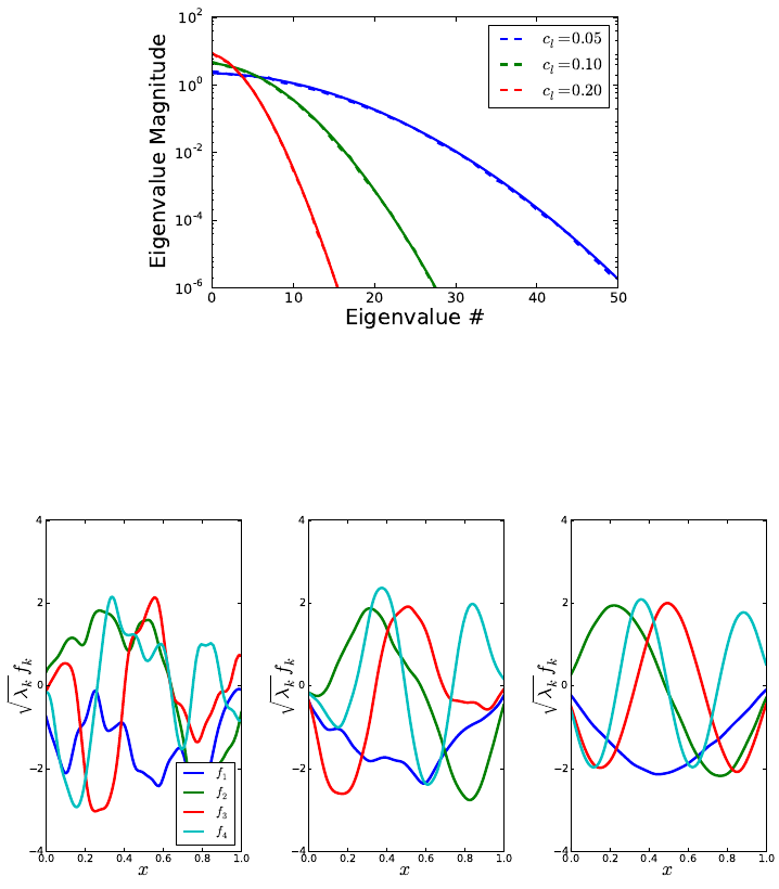
Figure 5.20: KL eigenvalues estimated with two sets of RF realizations: 29= 512 (dashed
lines) and 217 = 131072 (solid lines).
(a) Nω= 29(b) Nω= 213 (c) Nω= 217
Figure 5.21: Illustration of first 4 KL modes, computed based on a numerical covariance
matrices using three sets of RF realizations with cl= 0.05
generated with
./mkplots.py xidata 0.05 512 ./mkplots.py xidata 0.20 512
./mkplots.py xidata 0.05 131072 ./mkplots.py xidata 0.20 131072
Independent of the correlation length, a relatively large number of samples is required
for “converged” estimates for the density of ξ.
Figures 5.25 and 5.26 show reconstructions of select RF realizations. As observed in the
figure showing the decay in the magnitude of the KL eigenvalues, more terms are needed to
represents small scale features occuring for smaller correlation lengths, in Fig. 5.25, compared
to RF with larger correlation lengths, e.g. the example shown in Fig. 5.26. The plots shown
in Figs. 5.25 and 5.26 were generated with
87
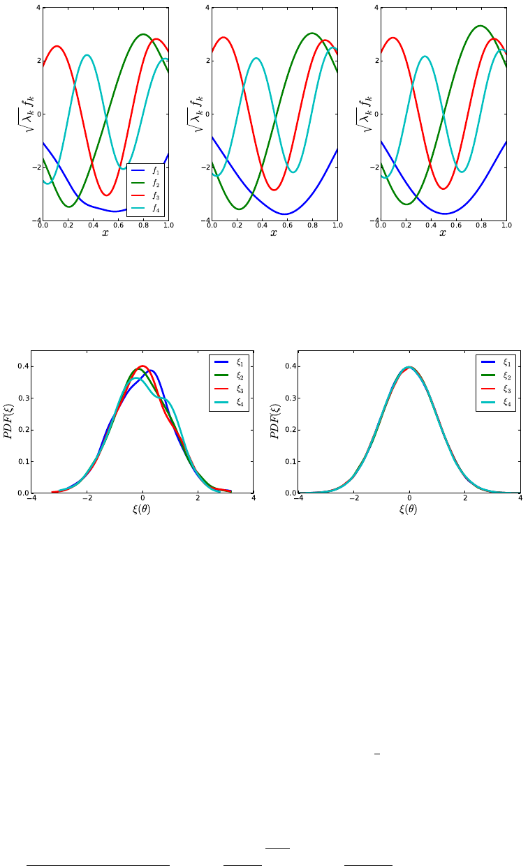
(a) Nω= 29(b) Nω= 213 (c) Nω= 217
Figure 5.22: Illustration of first 4 KL modes, computed based on a numerical covariance
matrices using three sets of RF realizations with cl= 0.20
(a) Nω= 29(b) Nω= 217
Figure 5.23: Probability densities for ξkobtained via KDE using samples obtained by
projecting RF realizations onto KL modes. Results correspond to cl= 0.05.
./mkplots.py pltKLrecon1D 0.05 21 51 10
./mkplots.py pltKLrecon1D 0.10 63 21 4
2D Examples on Structured Grids
In this section we are presenting 2D RFs generated with kl 2D.x. The RFs are generated
on a non-uniform structured 2D grid [0, Lx]×[0, Ly], with smaller grid spacing near the
boundaries and larger grid spacing towards the center of the domain. This grid is computed
using an algebraic expression [14]. The first coordinate is computed via
xi=Lx
(2α+β)ri+ 2α−β
(2α+ 1) (1 + ri), ri=β+ 1
β−1
ηi−α
1−α, ηi=i−1
Np−1, i = 1,2, . . . , Nx(5.36)
88
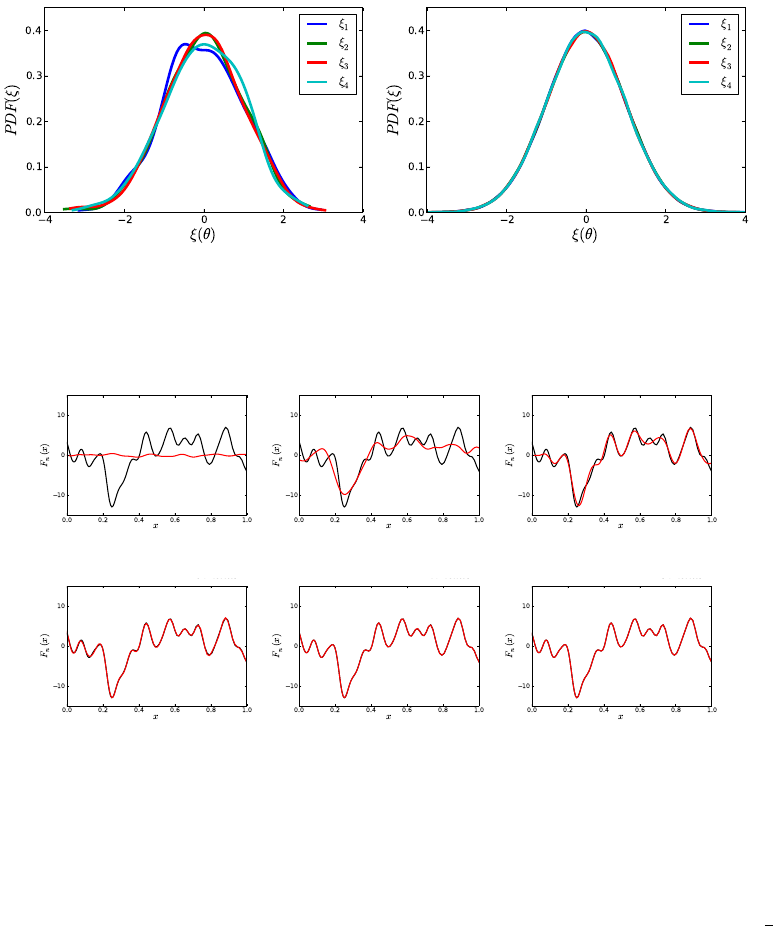
(a) Nω= 29(b) Nω= 217
Figure 5.24: Probability densities for ξkobtained via KDE using samples obtained by
projecting RF realizations onto KL modes. Results correspond to cl= 0.20.
(a) Mean (b) Mean + 10 terms (c) Mean + 20 terms
(d) Mean + 30 terms (e) Mean + 40 terms (f) Mean + 50 terms
Figure 5.25: Reconstructing realizations with an increasing number of KL expansion terms
for cl= 0.05
The β > 1 factor in the above expression controls the compression near x= 0 and x=Lx,
while α∈[0,1] determines where the clustering occurs. The examples shown in this section
are based on default values for the parameters that control the grid definition in kl 2D.x:
α= 1/2, β = 1.1, Lx1=Lx2=L= 1, Nx1=Nx2= 65
Figure 5.27 shows the 2D computational grid created with these parameters. This figure was
generated with the Python script “pl2Dsgrid.py”
./pl2Dsgrid.py cvspl2D_0.1_4096
Figure 5.28 shows 2D RF realizations with correlation lengths cl= 0.1 and cl= 0.2.
As the correlation length increases the realizations become smoother. These figure were
generated with
./mkplots.py samples2D 0.1 4096 2 (Figs. 5.28a,5.28b)
89
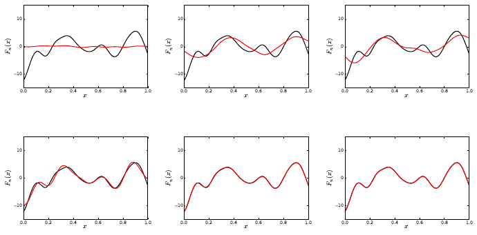
(a) Mean (b) Mean + 4 terms (c) Mean + 8 terms
(d) Mean + 12 terms (e) Mean + 16 terms (f) Mean + 20 terms
Figure 5.26: Reconstructing realizations with an increasing number of KL expansion terms
for cl= 0.10
./mkplots.py samples2D 0.2 4096 2 (Figs. 5.28c,5.28d)
In a 2D configuration the rhs of Eq. (eq:fredint) is discretized using a 2D finite volume
approach:
ZCov(x, y)f(y)dy ≈
Nx1−1
X
i=1
Nx2−1
X
j=1
(Cov(x, y)f(y)) |ij Aij (5.37)
Here, Aij is the area of rectangle (ij) with lower left corner (i, j) and upper right corner
(i+ 1, j + 1), and (Cov(x, y)f(y)) |ij is the average over rectangle (ij) computed as the
arithmetic average of values at its four vertices. Eq. (5.37) can be further cast as
ZCov(x, y)f(y)dy ≈
Nx1
X
i=1
Nx2
X
j=1
(Cov(x, y)f(y))i,j wi,j ,(5.38)
where wi,j is a quarter of the area of all rectangles that surround vertex (i, j).
Figures 5.29 and 5.30 shows first 8 KL modes computed based on covariance matrices that
where estimated from 212 = 4096 and 216 = 65536 number of RF samples, respectively, and
correlation length cl= 0.1 for both sets. The results in Fig. 5.30 are close to the KL modes
corresponding to the analytical covariance matrix (results not shown), while the results in
Fig. 5.29 indicate that 212 RF realizations is not sufficient to generate converged KL modes.
These figures were generated with
./mkplots.py numKLevec2D 0.1 4096 (Fig. 5.29)
./mkplots.py numKLevec2D 0.1 65536 (Fig. 5.30)
Figure 5.31 shows first 8 KL modes computed based on a covariance matrix that was
90
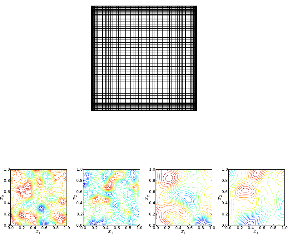
Figure 5.27: Structured grid employed for 2D RF examples.
(a) cl= 0.1 (b) cl= 0.1 (c) cl= 0.2 (d) cl= 0.2
Figure 5.28: Sample 2D random field realizations for cl= 0.1 and cl= 0.2.
estimated from 212 = 4096 number of RF samples. For these results, with correlation length
cl= 0.5, 212 samples are sufficient to estimate the covariance matrix and subsequently KL
modes that are close to analytical results (results not shown). The plots in Fig. 5.31 were
generated with
./mkplots.py numKLevec2D 0.5 4096
Figures 5.32 and 5.33 show reconstructions of select 2D RF realizations. As observed in
the previous section for 1D RFs, more terms are needed to represents small scale features
occuring for smaller correlation lengths, in Fig. 5.32, compared to RF with larger correlation
lengths, e.g. the example shown in Fig. 5.33. The plots shown in Figs. 5.32 and 5.33 were
generated with
./mkplots.py pltKLrecon2D 0.2 3 85 12 (Fig. 5.32)
./mkplots.py pltKLrecon2D 0.5 37 36 5 (Fig. 5.33)
91
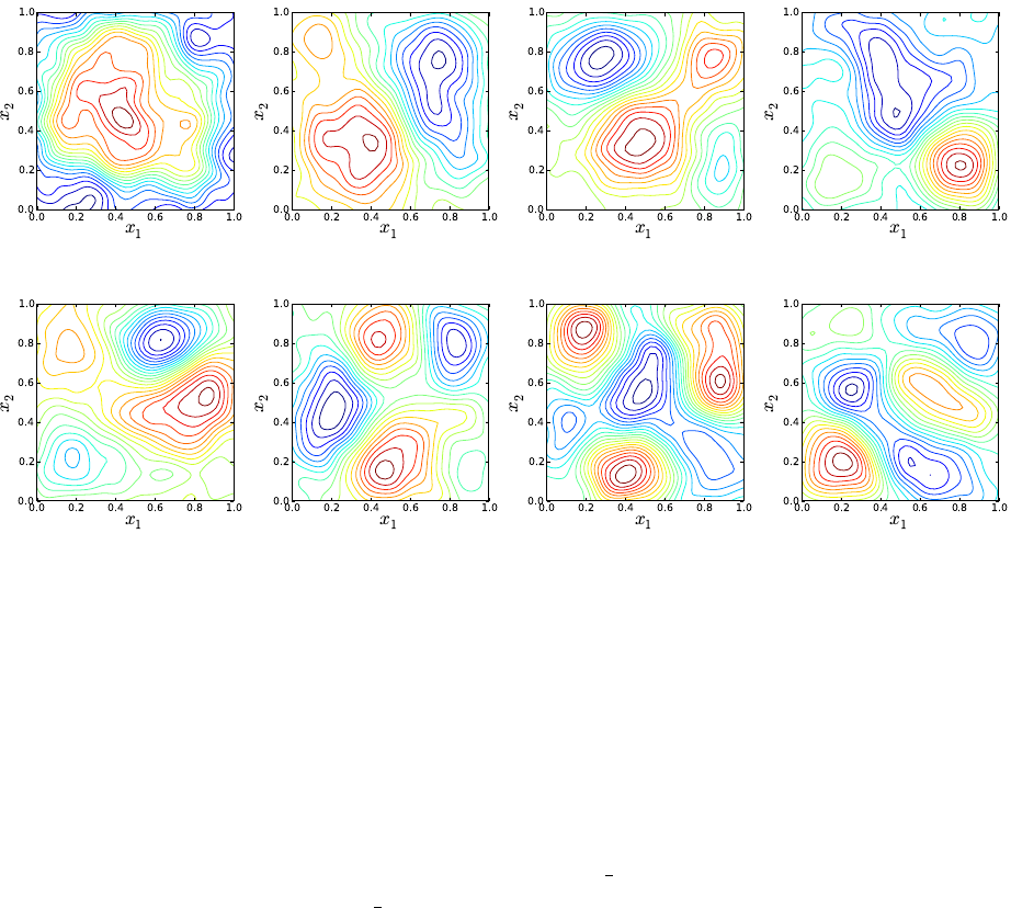
(a) Mode 1 (b) Mode 2 (c) Mode 3 (d) Mode 4
(e) Mode 5 (f) Mode 6 (g) Mode 7 (h) Mode 8
Figure 5.29: Illustration of first 8 KL modes, computed based on a numerical covariance
matrix estimated using 212 2D RF realizations with cl= 0.1
2D Examples on Unstructured Grids
For this example we choose a computational domain that resembles the shape of Cali-
fornia. A number of 212 = 4096 points were randomly distributed inside this computational
domain, and a triangular grid with 8063 triangles was generated via Delaunay triangulation.
The 2D grid point locations are provided in “data/cali grid.dat” and the grid point connec-
tivities are provided in “data/cali tria.dat”. Figure 5.34 shows the placement of these grid
points, including an inset plot with the triangular grid connectivities. This figure shows the
grids on a uniform scale in terms of latitude and longitude degrees and was generated with
./pl2Dugrid.py
Figure 5.35 shows 2D RF realizations with correlation lengths cl= 0.5◦and cl= 2◦.
These figure were generated with
./mkplots.py samples2Du 0.5 4096 2 (Figs. 5.35a,5.35b)
./mkplots.py samples2Du 2.0 4096 2 (Figs. 5.35c,5.35d)
Figure 5.36 shows first 16 KL modes computed based on a covariance matrix that was
estimated from 216 = 65536 number of RF samples, with correlation length cl= 0.5◦.
The KL modes corresponding to an analytically estimated covariance matrix with the same
correlation length are shown in Fig. 5.37. For this example, it seems that 216 samples are
sufficient to estimate the first 12 to 13 modes accurately. Please note that some of the
92
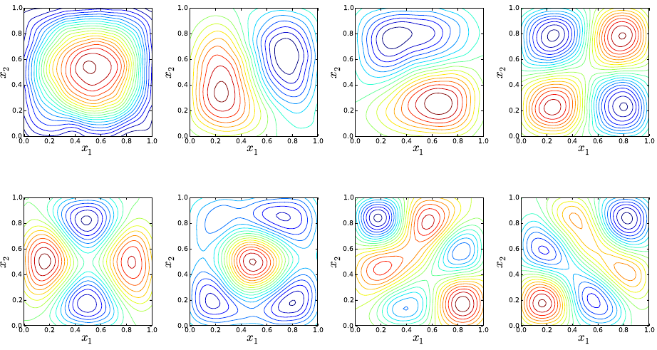
(a) Mode 1 (b) Mode 2 (c) Mode 3 (d) Mode 4
(e) Mode 5 (f) Mode 6 (g) Mode 7 (h) Mode 8
Figure 5.30: Illustration of first 8 KL modes, computed based on a numerical covariance
matrix estimated using 216 2D RF realizations with cl= 0.1
modes can differ up to a multiplicative factor of −1, hence the colorscheme will be reversed.
Higher order modes start diverging from analytical estimates, e.g. modes 14 through 16 in
this example. Figure 5.38 shows KL modes corresponding to a covariance matrix estimated
from RF realizations with cl= 2◦. For this correlation length, 216 samples are sufficient to
generate KL modes that are very close to analytical results (not shown). These figures were
generated with
./mkplots.py numKLevec2Du 0.5 65536 (Fig. 5.36)
./mkplots.py anlKLevec2Du SqExp 0.5 (Fig. 5.37)
./mkplots.py numKLevec2Du 2.0 65536 (Fig. 5.38)
93
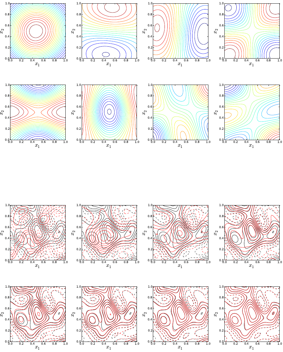
(a) Mode 1 (b) Mode 2 (c) Mode 3 (d) Mode 4
(e) Mode 5 (f) Mode 6 (g) Mode 7 (h) Mode 8
Figure 5.31: Illustration of first 8 KL modes, computed based on a numerical covariance
matrix estimated using 212 2D RF realizations with cl= 0.5
(a) Mean (b) Mean + 12 terms (c) Mean + 24 terms (d) Mean + 36 terms
(e) Mean + 48 terms (f) Mean + 60 terms (g) Mean + 72 terms (h) Mean + 84 terms
Figure 5.32: Reconstructing 2D realizations with an increasing number of KL expansion
terms for cl= 0.2
94
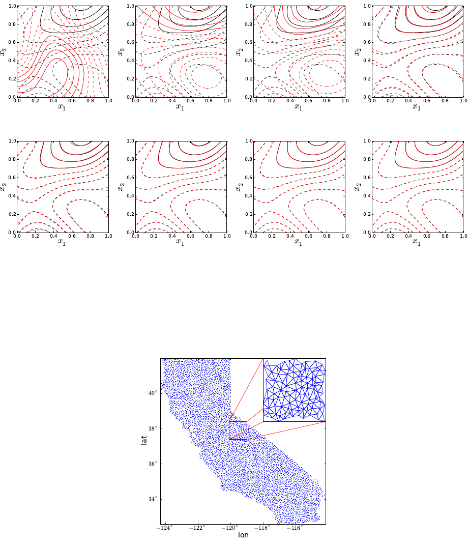
(a) Mean (b) Mean + 5 terms (c) Mean + 10 terms (d) Mean + 15 terms
(e) Mean + 20 terms (f) Mean + 25 terms (g) Mean + 30 terms (h) Mean + 35 terms
Figure 5.33: Reconstructing 2D realizations with an increasing number of KL expansion
terms for cl= 0.5
Figure 5.34: Unstructured grid generated via Delaunay traingulation overlaid over Califor-
nia.
95
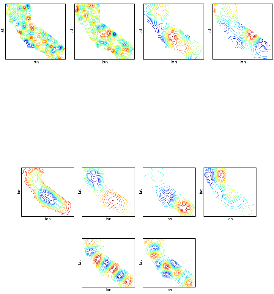
(a) cl= 0.5◦(b) cl= 0.5◦(c) cl= 2◦(d) cl= 2◦
Figure 5.35: Sample 2D random field realizations on an unstructured grid for cl= 0.5◦and
cl= 2◦.
(a) Mode 1 (b) Mode 2 (c) Mode 3 (d) Mode 6
(e) Mode 10 (f) Mode 16
Figure 5.36: Illustration of seclect KL modes, computed based on a numerical covariance
matrix estimated using 216 2D RF realizations on an unstructured grid with cl= 0.5◦.
96
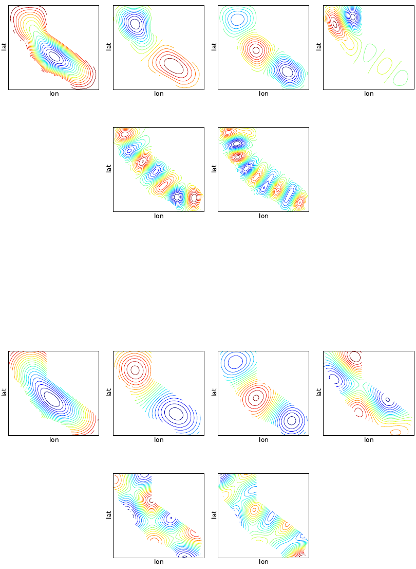
(a) Mode 1 (b) Mode 2 (c) Mode 3 (d) Mode 6
(e) Mode 10 (f) Mode 16
Figure 5.37: Illustration of select KL modes, computed based on an analytical covariance ma-
trix for 2D RF realizations on an unstructured grid with cl= 0.5◦and a square-exponential
form.
(a) Mode 1 (b) Mode 2 (c) Mode 3 (d) Mode 6
(e) Mode 10 (f) Mode 16
Figure 5.38: Illustration of select KL modes, computed based on a numerical covariance
matrix estimated using 216 2D RF realizations on an unstructured grid with cl= 2◦.
97
98
Chapter 6
Support
UQTk is the subject of continual development and improvement. If you have questions
about or suggestions for UQTk, feel free to e-mail the UQTk Users list, at uqtk-users@
software.sandia.gov. You can sign up for this mailing list at https://software.sandia.
gov/mailman/listinfo/uqtk-users.
99
100
References
[1] S. Babacan, R. Molina, and A. Katsaggelos. Bayesian compressive sensing using Laplace
priors. IEEE Transactions on Image Processing, 19(1):53–63, 2010.
[2] C. W. Clenshaw and A. R. Curtis. A method for numerical integration on an automatic
computer. Numerische Mathematik, 2:197–205, 1960.
[3] B.J. Debusschere, H.N. Najm, P.P. P´ebay, O.M. Knio, R.G. Ghanem, and O.P. Le
Maˆıtre. Numerical challenges in the use of polynomial chaos representations for stochas-
tic processes. SIAM Journal on Scientific Computing, 26(2):698–719, 2004.
[4] Andrew Gelman, John B. Carlin, Hal S. Stern, and Donald B. Rubin. Bayesian Data
Analysis. Chapman & Hall CRC, 2 edition, 2003.
[5] Stuart Geman and D. Geman. Stochastic Relaxation, Gibbs Distributions, and the
Bayesian Restoration of Images. Pattern Analysis and Machine Intelligence, IEEE
Transactions on, PAMI-6(6):721–741, 1984.
[6] Thomas Gerstner and Michael Griebel. Numerical integration using sparse grids. Nu-
merical Algorithms, 18(3-4):209–232, 1998. (also as SFB 256 preprint 553, Univ. Bonn,
1998).
[7] R.G. Ghanem and P.D. Spanos. Stochastic Finite Elements: A Spectral Approach.
Springer Verlag, New York, 1991.
[8] W. R. Gilks, S. Richardson, and D. J. Spiegelhalter. Markov Chain Monte Carlo in
Practice. Chapman & Hall, London, 1996.
[9] G. H. Golub and J. H. Welsch. Calculation of Gauss quadrature rules. Math. Comp.,
23:221–230, 1969.
[10] H. Haario, E. Saksman, and J. Tamminen. An adaptive Metropolis algorithm. Bernoulli,
7:223–242, 2001.
[11] Heikki Haario, Marko Laine, Antonietta Mira, and Eero Saksman. Dram: Efficient
adaptive mcmc. Statistics and Computing, 16(4):339–354, 2006.
[12] R.G. Haylock and A. O’Hagan. On inference for outputs of computationally expensive
algorithms with uncertainty on the inputs. Bayesian statistics, 5:629–637, 1996.
[13] F.B. Hildebrand. Introduction to Numerical Analysis. Dover, 1987.
[14] K.A Hoffmann and S.T. Chiang. Computational Fluid Dynamics, volume 1, chapter 9,
pages 358–426. EES, 2000.
101
[15] M. C. Kennedy and A. O’Hagan. Bayesian calibration of computer models. Journal of
the Royal Statistical Society: Series B, 63(3):425–464, 2001.
[16] S. Kucherenko, S. Tarantola, and P. Annoni. Estimation of global sensitivity indices
for models with dependent variables. Computer Physics Communications, 183:937–946,
2012.
[17] O.P. Le Maˆıtre and O.M. Knio. Spectral Methods for Uncertainty Quantification: With
Applications to Computational Fluid Dynamics (Scientific Computation). Springer, 1st
edition. edition, April 2010.
[18] Y. M. Marzouk and H. N. Najm. Dimensionality reduction and polynomial chaos ac-
celeration of Bayesian inference in inverse problems. Journal of Computational Physics,
228(6):1862–1902, 2009.
[19] E.J. Nystr¨om. ¨
Uber die praktische au߬osung von integralgleichungen mit anwendungen
auf randwertaufgaben. Acta Mathematica, 54(1):185–204, 1930.
[20] J. Oakley and A. O’Hagan. Bayesian inference for the uncertainty distribution of com-
puter model outputs. Biometrika, 89(4):769–784, 2002.
[21] Mark Orr. Introduction to radial basis function networks. Technical Report, Center for
Cognitive Science, University of Edinburgh, 1996.
[22] C. E. Rasmussen and C. K. I. Williams. Gaussian Processes for Machine Learning.
MIT Press, 2006.
[23] M. Rosenblatt. Remarks on a multivariate transformation. Annals of Mathematical
Statistics, 23(3):470 – 472, 1952.
[24] A. Saltelli. Making best use of model evaluations to compute sensitivity indices. Com-
puter Physics Communications, 145:280–297, 2002.
[25] K. Sargsyan. Surrogate models for uncertainty propagation and sensitivity analysis. In
R. Ghanem, D. Higdon, and H. Owhadi, editors, Handbook of Uncertainty Quantifica-
tion. Springer, 2016.
[26] K. Sargsyan, H. N. Najm, and R. Ghanem. On the Statistical Calibration of Physical
Models. International Journal for Chemical Kinetics, 47(4):246–276, 2015.
[27] K. Sargsyan, C. Safta, H. Najm, B. Debusschere, D. Ricciuto, and P. Thornton. Dimen-
sionality reduction for complex models via Bayesian compressive sensing. International
Journal of Uncertainty Quantification, 4(1):63–93, 2014.
[28] D.W. Scott. Multivariate Density Estimation. Theory, Practice and Visualization. Wi-
ley, New York, 1992.
[29] B.W. Silverman. Density Estimation for Statistics and Data Analysis. Chapman and
Hall, London, 1986.
102
[30] D.S. Sivia. Data Analysis: A Bayesian Tutorial. Oxford Science, 1996.
[31] S. A. Smolyak. Quadrature and interpolation formulas for tensor products of certain
classes of functions. Soviet Mathematics Dokl., 4:240–243, 1963.
[32] I. M. Sobol. Sensitivity estimates for nonlinear mathematical models. Math. Modeling
and Comput. Exper., 1:407–414, 1993.
103
DISTRIBUTION:
1 MS 0899 Technical Library, 8944 (electronic copy)
104
v1.40
105

106
