User Manual
User Manual: Pdf
Open the PDF directly: View PDF ![]() .
.
Page Count: 8

Introduction
A piece of cake to build different kinds of kinship matrix.
Gmat64 is written by C to build different kinds of kinship matrix
including additive, dominant and epistatic. The program start from
PLINK binary file, and five command-line arguments are needed.
Note: Missing genotype is replaced by a random value in the program,
which has little influence on results for relative low missing rate (eg. Less
than 0.05 for each SNP).
Dependencies
Intel® Math Kernel Library (Intel MKL)
Using the binary of REMMA for Linux, users do need to install Intel
MKL ( https://software.intel.com/en-us/intel-mkl ). However, it is
recommended to install Intel® Parallel Studio XE
( https://software.intel.com/en-us/intel-parallel-studio-xe ), which
simplifies the progress of compiling the source code.
Quick start

Gmat64 --help
Gmat64 --bfile plink_file_prefix --inv 1 --normMat 1 --outformat 1 --
Gmat addGmat
Theory
We introduce basic theory of different kinds of kinship matrix in this part.
Additive kinship
Additive kinship matrix is built with the method by VanRaden (2008).
Let Z be the standardized additive marker matrix. Matrix Z is constructed
as follows,
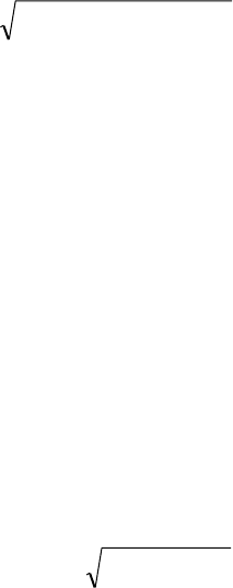
,)1(2/),,,,,( 21 jjmj ppzzzzZ
(1)
where pj is the allele frequency of allele A for the jth SNP, and zj is the jth
SNP vector with elements defined as
.
20
21
22
aap
Aap
AAp
j
j
j
j
z
(2)
Then the additive kinship is the matrix product Ka = ZZ’.
Dominant kinship
There are two kinships of dominant kinship matrices in the program and
please refer to Vitezica, et al. (2013) for detailed theory.

(1) Let H be the standardized dominant marker matrix. Matrix H is
constructed as follows,
,)21(2/),,,,,( 21 jjjjmj qpqphhhhH
(3)
where pj is the allele frequency of allele A for the jth SNP, and hj is the jth
SNP vector with elements defined as
.
20
21
20
aaqp
Aaqp
AAqp
jj
jj
jj
j
h
(4)
Then the dominant kinship is the matrix product Kd1 = HH’.
(2) Let W be the standardized dominant marker matrix. Matrix W is
constructed as follows,
,)2(/),,,,,( 2
21
jjmj qpwwwwW
(5)
where pj is the allele frequency of allele A for the jth SNP, and wj is the jth
SNP vector with elements defined as
.
2
2
2
2
2
aap
Aaqp
AAq
j
jj
j
j
w
(6)
Then the dominant kinship is the matrix product Kd2 = WW’.
Note: The second method is recommended as the first method
underestimates the additive genetic variance and overestimates the
dominance variance (Vitezica, et al., 2013).
Additive-by-additive (AxA) epistatic kinship
The simplest method to build AxA epistatic kinship matrix is Ka # Ka,
where # represents the Hadamard matrix product (Henderson, 1985).
However, the equation included interactions of loci with themselves. The
accurate and efficient form (Jiang and Reif, 2015) used in the program is
)'.#)(#(# ZZZZKKK aaaa
(7)
Additive-by- dominant (AxD) epistatic kinship
Two kinds of epistatic kinship are provided.
(1)
)'.#)(#(# 11 HZHZKKK daad
(8)
(2)
)'.#)(#(# 22 WZWZKKK daad
(9)
Note: Similar to dominant kinship, the second method is recommended.
Dominant -by- dominant (DxD) epistatic kinship
Two kinds of epistatic kinship are provided.
(1)
)'.#)(#(# 1111 HHHHKKK dddd
(10)
(2)
)'.#)(#(# 2222 WWWWKKK dddd
(11)
Note: Similar to dominant kinship, the second method is recommended.
Parameters
--bfile: string; The path of the prefix for the PLINK binary file
--inv: 0 or 1; whether to calculate and output the inversion of kinship
matrix. 0 means NO while 1 means YES.
--normMat: 0 or 1; whether to output the standardized additive (equation
1) or dominant (equation 3 or 5) marker matrix. 0 means NO while 1
means YES. The parameter only works for building additive and
dominant kinship matrix. It must be provided for other kinds of kinship
although it means nothing.
--outformat: 0, 1 or 2; the output format of kinship matrix.
When the value is 0, the output format is square matrix of order n (the
number of individuals).
When the value is 1, the program outputs the lower triangle elements of
kinship matrix. The output file includes three columns of row, column,
and value. It is sorted column within row.
When the value is 2, the program outputs the lower triangle elements of
kinship matrix. The output file includes three columns of ID, ID, and
value.
--Gmat: string; the type of kinship matrix. Please refer to Theory part for
detailed information.
addGmat: additive kinship matrix;
domGmat_AS: the first kinship of dominant kinship in Theory part;
domGmat_GS: the second (recommended) kinship of dominant kinship;
epiGmatAA: Additive-by-additive (AxA) epistatic kinship;
epiGmatAD_AS: the first kinship of additive-by-dominant (AxD)
epistatic kinship in Theory part;
epiGmatAD_GS: the second (recommended) kinship of additive-by-
dominant (AxD) epistatic kinship;
epiGmatDD_AS: the first kinship of dominant-by-dominant (DxD)
epistatic kinship in Theory part;
epiGmatDD_GS: the second (recommended) kinship of dominant-by-
dominant (DxD) epistatic kinship.
Output files
The program generates 1-3 output files depend on parameters.
FILE 1: kinship matrix; prefix.type.grm0/1/2. The ‘prefix’ is the same to
the prefix of PLINK binary file; ‘type’ is the type of kinship matrix
defined by parameter --Gmat; ‘grm0’, ‘grm1’ or ‘grm2’ means different
kinds of output format defined by parameter --outformat.
FILE 2: The standardized marker matrix; optional; generate when --
normMat 1; Binary format of double precision. prefix.
addMarkerMat.bin, prefix.domMarkerMat_AS.bin or
prefix.domMarkerMat_GS.bin.
FILE 3: The inversion of kinship matrix; optional; generate when --inv 1.
It has similar format as FILE1. prefix.type.giv0/1/2.
Reference
Henderson, C. (1985) Best linear unbiased prediction of nonadditive genetic merits, J.
Anim. Sci, 60, 111-117.
Jiang, Y. and Reif, J.C. (2015) Modeling Epistasis in Genomic Selection, Genetics,
201, 759-768.
VanRaden, P.M. (2008) Efficient methods to compute genomic predictions, Journal of
dairy science, 91, 4414-4423.
Vitezica, Z.G., Varona, L. and Legarra, A. (2013) On the additive and dominant
variance and covariance of individuals within the genomic selection scope, Genetics,
195, 1223-1230.
