Wiley And SAS Business Series : Fraud Analytics Using Descriptive, Predictive, Social Network Techniques A Guide To Data S (Wiley Series) Bart Baesens, Veronique Van Vlasselaer, Wouter Verbeke Analyti
User Manual: Pdf
Open the PDF directly: View PDF ![]() .
.
Page Count: 402 [warning: Documents this large are best viewed by clicking the View PDF Link!]
- Cover
- Title Page
- Copyright
- Contents
- List of Figures
- Foreword
- Preface
- Acknowledgments
- Chapter 1 Fraud: Detection, Prevention, and Analytics!
- Chapter 2 Data Collection, Sampling, and Preprocessing
- Introduction
- Types of Data Sources
- Merging Data Sources
- Sampling
- Types of Data Elements
- Visual Data Exploration and Exploratory Statistical Analysis
- Benford's Law
- Descriptive Statistics
- Missing Values
- Outlier Detection and Treatment
- Red Flags
- Standardizing Data
- Categorization
- Weights of Evidence Coding
- Variable Selection
- Principal Components Analysis
- RIDITs
- PRIDIT Analysis
- Segmentation
- References
- Chapter 3 Descriptive Analytics for Fraud Detection
- Chapter 4 Predictive Analytics for Fraud Detection
- Introduction
- Target Definition
- Linear Regression
- Logistic Regression
- Variable Selection for Linear and Logistic Regression
- Decision Trees
- Neural Networks
- Support Vector Machines
- Ensemble Methods
- Multiclass Classification Techniques
- Evaluating Predictive Models
- Other Performance Measures for Predictive Analytical Models
- Developing Predictive Models for Skewed Data Sets
- Fraud Performance Benchmarks
- References
- Chapter 5 Social Network Analysis for Fraud Detection
- Chapter 6 Fraud Analytics: Post-Processing
- Chapter 7 Fraud Analytics: A Broader Perspective
- About the Authors
- Index
- EULA

Fraud Analytics Using
Descriptive, Predictive,
and Social Network
Techniques

Wiley & SAS Business
Series
The Wiley & SAS Business Series presents books that help senior-level
managers with their critical management decisions.
Titles in the Wiley & SAS Business Series include:
Analytics in a Big Data World: The Essential Guide to Data Science and Its
Applications by Bart Baesens
Bank Fraud: Using Technology to Combat Losses by Revathi Subrama-
nian
Big Data Analytics: Turning Big Data into Big Money by Frank Ohlhorst
Big Data, Big Innovation: Enabling Competitive Differentiation through
Business Analytics by Evan Stubbs
Business Analytics for Customer Intelligence by Gert Laursen
Business Intelligence Applied: Implementing an Effective Information and
Communications Technology Infrastructure by Michael Gendron
Business Intelligence and the Cloud: Strategic Implementation Guide by
Michael S. Gendron
Business Transformation: A Roadmap for Maximizing Organizational
Insights by Aiman Zeid
Connecting Organizational Silos: Taking Knowledge Flow Management to
the Next Level with Social Media by Frank Leistner
Data-Driven Healthcare: How Analytics and BI Are Transforming the
Industry by Laura Madsen
Delivering Business Analytics: Practical Guidelines for Best Practice by
Evan Stubbs
Demand-Driven Forecasting: A Structured Approach to Forecasting,
second edition by Charles Chase
Demand-Driven Inventory Optimization and Replenishment: Creating a
More Efficient Supply Chain by Robert A. Davis
Developing Human Capital: Using Analytics to Plan and Optimize Your
Learning and Development Investments by Gene Pease, Barbara Beres-
ford, and Lew Walker
The Executive’s Guide to Enterprise Social Media Strategy: How Social Net-
works Are Radically Transforming Your Business by David Thomas and
Mike Barlow
Economic and Business Forecasting: Analyzing and Interpreting Economet-
ric Results by John Silvia, Azhar Iqbal, Kaylyn Swankoski, Sarah
Watt, and Sam Bullard
Financial Institution Advantage and The Optimization of Information
Processing by Sean C. Keenan
Foreign Currency Financial Reporting from Euros to Yen to Yuan: A Guide
to Fundamental Concepts and Practical Applications by Robert Rowan
Harness Oil and Gas Big Data with Analytics: Optimize Exploration and
Production with Data Driven Models by Keith Holdaway
Health Analytics: Gaining the Insights to Transform Health Care by Jason
Burke
Heuristics in Analytics: A Practical Perspective of What Influences Our Ana-
lytical World by Carlos Andre Reis Pinheiro and Fiona McNeill
Human Capital Analytics: How to Harness the Potential of Your Organi-
zation’s Greatest Asset by Gene Pease, Boyce Byerly, and Jac Fitz-enz
Implement, Improve and Expand Your Statewide Longitudinal Data Sys-
tem: Creating a Culture of Data in Education by Jamie McQuiggan and
Armistead Sapp
Killer Analytics: Top 20 Metrics Missing from Your Balance Sheet by Mark
Brown
Predictive Analytics for Human Resources by Jac Fitz-enz and John
Mattox II
Predictive Business Analytics: Forward-Looking Capabilities to Improve
Business Performance by Lawrence Maisel and Gary Cokins
Retail Analytics: The Secret Weapon by Emmett Cox
Social Network Analysis in Telecommunications by Carlos Andre Reis
Pinheiro
Statistical Thinking: Improving Business Performance, second edition by
Roger W. Hoerl and Ronald D. Snee
Taming the Big Data Tidal Wave: Finding Opportunities in Huge Data
Streams with Advanced Analytics by Bill Franks
Too Big to Ignore: The Business Case for Big Data by Phil Simon
The Value of Business Analytics: Identifying the Path to Profitability by
Evan Stubbs
The Visual Organization: Data Visualization, Big Data, and the Quest for
Better Decisions by Phil Simon
Understanding the Predictive Analytics Lifecycle by Al Cordoba
Unleashing Your Inner Leader: An Executive Coach Tells All by Vickie
Bevenour
Using Big Data Analytics: Turning Big Data into Big Money by Jared
Dean
Win with Advanced Business Analytics: Creating Business Value from Your
Data by Jean Paul Isson and Jesse Harriott
For more information on these and other titles in the series, please
visit www.wiley.com.

Fraud Analytics
Using Descriptive,
Predictive, and
Social Network
Techniques
A Guide to Data Science
for Fraud Detection
Bart Baesens
Véronique Van Vlasselaer
Wouter Verbeke
Copyright © 2015 by John Wiley & Sons, Inc. All rights reserved.
Published by John Wiley & Sons, Inc., Hoboken, New Jersey.
Published simultaneously in Canada.
No part of this publication may be reproduced, stored in a retrieval system, or
transmitted in any form or by any means, electronic, mechanical, photocopying,
recording, scanning, or otherwise, except as permitted under Section 107 or 108 of the
1976 United States Copyright Act, without either the prior written permission of the
Publisher, or authorization through payment of the appropriate per-copy fee to the
Copyright Clearance Center, Inc., 222 Rosewood Drive, Danvers, MA 01923, (978)
750-8400, fax (978) 646-8600, or on the Web at www.copyright.com. Requests to the
Publisher for permission should be addressed to the Permissions Department, John
Wiley & Sons, Inc., 111 River Street, Hoboken, NJ 07030, (201) 748-6011, fax (201)
748-6008, or online at http://www.wiley.com/go/permissions.
Limit of Liability/Disclaimer of Warranty: While the publisher and author have used
their best efforts in preparing this book, they make no representations or warranties
with respect to the accuracy or completeness of the contents of this book and
specifically disclaim any implied warranties of merchantability or fitness for a particular
purpose. No warranty may be created or extended by sales representatives or written
sales materials. The advice and strategies contained herein may not be suitable for your
situation. You should consult with a professional where appropriate. Neither the
publisher nor author shall be liable for any loss of profit or any other commercial
damages, including but not limited to special, incidental, consequential, or other
damages.
For general information on our other products and services or for technical support,
please contact our Customer Care Department within the United States at (800)
762-2974, outside the United States at (317) 572-3993 or fax (317) 572-4002.
Wiley publishes in a variety of print and electronic formats and by print-on-demand.
Some material included with standard print versions of this book may not be included
in e-books or in print-on-demand. If this book refers to media such as a CD or DVD
that is not included in the version you purchased, you may download this material at
http://booksupport.wiley.com. For more information about Wiley products, visit
www.wiley.com.
Library of Congress Cataloging-in-Publication Data:
Baesens, Bart.
Fraud analytics using descriptive, predictive, and social network techniques : a guide
to data science for fraud detection / Bart Baesens, Veronique Van Vlasselaer, Wouter
Verbeke.
pages cm. — (Wiley & SAS business series)
Includes bibliographical references and index.
ISBN 978-1-119-13312-4 (cloth) — ISBN 978-1-119-14682-7 (epdf) —
ISBN 978-1-119-14683-4 (epub)
1. Fraud—Statistical methods. 2. Fraud—Prevention. 3. Commercial
crimes—Prevention. I. Title.
HV6691.B34 2015
364.16
′
3015195—dc23
2015017861
Cover Design: Wiley
Cover Image: ©iStock.com/aleksandarvelasevic
Printed in the United States of America
10987654321
To my wonderful wife, Katrien, and kids, Ann-Sophie, Victor,
and Hannelore.
To my parents and parents-in-law.
To my husband and soul mate, Niels, for his never-ending
support.
To my parents, parents-in-law, and siblings-in-law.
To Luit and Titus.

Contents
List of Figures xv
Foreword xxiii
Preface xxv
Acknowledgments xxix
Chapter 1 Fraud: Detection, Prevention, and Analytics! 1
Introduction 2
Fraud! 2
Fraud Detection and Prevention 10
Big Data for Fraud Detection 15
Data-Driven Fraud Detection 17
Fraud-Detection Techniques 19
Fraud Cycle 22
The Fraud Analytics Process Model 26
Fraud Data Scientists 30
A Fraud Data Scientist Should Have Solid Quantitative
Skills 30
A Fraud Data Scientist Should Be a Good Programmer 31
A Fraud Data Scientist Should Excel in
Communication and Visualization Skills 31
A Fraud Data Scientist Should Have a Solid Business
Understanding 32
A Fraud Data Scientist Should Be Creative 32
A Scientific Perspective on Fraud 33
References 35
Chapter 2 Data Collection, Sampling, and Preprocessing 37
Introduction 38
Types of Data Sources 38
Merging Data Sources 43
Sampling 45
Types of Data Elements 46
ix

xCONTENTS
Visual Data Exploration and Exploratory Statistical
Analysis 47
Benford’s Law 48
Descriptive Statistics 51
Missing Values 52
Outlier Detection and Treatment 53
Red Flags 57
Standardizing Data 59
Categorization 60
Weights of Evidence Coding 63
Variable Selection 65
Principal Components Analysis 68
RIDITs 72
PRIDIT Analysis 73
Segmentation 74
References 75
Chapter 3 Descriptive Analytics for Fraud Detection 77
Introduction 78
Graphical Outlier Detection Procedures 79
Statistical Outlier Detection Procedures 83
Break-Point Analysis 84
Peer-Group Analysis 85
Association Rule Analysis 87
Clustering 89
Introduction 89
Distance Metrics 90
Hierarchical Clustering 94
Example of Hierarchical Clustering Procedures 97
k-Means Clustering 104
Self-Organizing Maps 109
Clustering with Constraints 111
Evaluating and Interpreting Clustering Solutions 114
One-Class SVMs 117
References 118
Chapter 4 Predictive Analytics for Fraud Detection 121
Introduction 122
Target Definition 123
Linear Regression 125
Logistic Regression 127
Basic Concepts 127
Logistic Regression Properties 129
Building a Logistic Regression Scorecard 131

CONTENTS xi
Variable Selection for Linear and Logistic Regression 133
Decision Trees 136
Basic Concepts 136
Splitting Decision 137
Stopping Decision 140
Decision Tree Properties 141
Regression Trees 142
Using Decision Trees in Fraud Analytics 143
Neural Networks 144
Basic Concepts 144
Weight Learning 147
Opening the Neural Network Black Box 150
Support Vector Machines 155
Linear Programming 155
The Linear Separable Case 156
The Linear Nonseparable Case 159
The Nonlinear SVM Classifier 160
SVMs for Regression 161
Opening the SVM Black Box 163
Ensemble Methods 164
Bagging 164
Boosting 165
Random Forests 166
Evaluating Ensemble Methods 167
Multiclass Classification Techniques 168
Multiclass Logistic Regression 168
Multiclass Decision Trees 170
Multiclass Neural Networks 170
Multiclass Support Vector Machines 171
Evaluating Predictive Models 172
Splitting Up the Data Set 172
Performance Measures for Classification Models 176
Performance Measures for Regression Models 185
Other Performance Measures for Predictive Analytical
Models 188
Developing Predictive Models for Skewed Data Sets 189
Varying the Sample Window 190
Undersampling and Oversampling 190
Synthetic Minority Oversampling Technique (SMOTE) 192
Likelihood Approach 194
Adjusting Posterior Probabilities 197
Cost-sensitive Learning 198
Fraud Performance Benchmarks 200
References 201

xii CONTENTS
Chapter 5 Social Network Analysis for Fraud Detection 207
Networks: Form, Components, Characteristics, and Their
Applications 209
Social Networks 211
Network Components 214
Network Representation 219
Is Fraud a Social Phenomenon? An Introduction to
Homophily 222
Impact of the Neighborhood: Metrics 227
Neighborhood Metrics 228
Centrality Metrics 238
Collective Inference Algorithms 246
Featurization: Summary Overview 254
Community Mining: Finding Groups of Fraudsters 254
Extending the Graph: Toward a Bipartite Representation 266
Multipartite Graphs 269
Case Study: Gotcha! 270
References 277
Chapter 6 Fraud Analytics: Post-Processing 279
Introduction 280
The Analytical Fraud Model Life Cycle 280
Model Representation 281
Traffic Light Indicator Approach 282
Decision Tables 283
Selecting the Sample to Investigate 286
Fraud Alert and Case Management 290
Visual Analytics 296
Backtesting Analytical Fraud Models 302
Introduction 302
Backtesting Data Stability 302
Backtesting Model Stability 305
Backtesting Model Calibration 308
Model Design and Documentation 311
References 312
Chapter 7 Fraud Analytics: A Broader Perspective 313
Introduction 314
Data Quality 314
Data-Quality Issues 314
Data-Quality Programs and Management 315
Privacy 317
The RACI Matrix 318
Accessing Internal Data 319

CONTENTS xiii
Label-Based Access Control (LBAC) 324
Accessing External Data 325
Capital Calculation for Fraud Loss 326
Expected and Unexpected Losses 327
Aggregate Loss Distribution 329
Capital Calculation for Fraud Loss Using Monte Carlo
Simulation 331
An Economic Perspective on Fraud Analytics 334
Total Cost of Ownership 334
Return on Investment 335
In Versus Outsourcing 337
Modeling Extensions 338
Forecasting 338
Text Analytics 340
The Internet of Things 342
Corporate Fraud Governance 344
References 346
About the Authors 347
Index 349

List of Figures
Figure 1.1 Fraud Triangle 7
Figure 1.2 Fire Incident Claim-Handling Process 13
Figure 1.3 The Fraud Cycle 23
Figure 1.4 Outlier Detection at the Data Item Level 25
Figure 1.5 Outlier Detection at the Data Set Level 25
Figure 1.6 The Fraud Analytics Process Model 26
Figure 1.7 Profile of a Fraud Data Scientist 33
Figure 1.8 Screenshot of Web of Science Statistics for
Scientific Publications on Fraud between 1996
and 2014 34
Figure 2.1 Aggregating Normalized Data Tables into a
Non-Normalized Data Table 44
Figure 2.2 Pie Charts for Exploratory Data Analysis 49
Figure 2.3 Benford’s Law Describing the Frequency
Distribution of the First Digit 50
Figure 2.4 Multivariate Outliers 54
Figure 2.5 Histogram for Outlier Detection 54
Figure 2.6 Box Plots for Outlier Detection 55
Figure 2.7 Using the z-Scores for Truncation 57
Figure 2.8 Default Risk Versus Age 60
Figure 2.9 Illustration of Principal Component Analysis in a
Two-Dimensional Data Set 68
Figure 3.1 3D Scatter Plot for Detecting Outliers 80
Figure 3.2 OLAP Cube for Fraud Detection 80
Figure 3.3 Example Pivot Table for Credit Card Fraud
Detection 82
xv

xvi LIST OF FIGURES
Figure 3.4 Break-Point Analysis 84
Figure 3.5 Peer-Group Analysis 86
Figure 3.6 Cluster Analysis for Fraud Detection 91
Figure 3.7 Hierarchical Versus Nonhierarchical Clustering
Techniques 91
Figure 3.8 Euclidean Versus Manhattan Distance 92
Figure 3.9 Divisive Versus Agglomerative Hierarchical
Clustering 94
Figure 3.10 Calculating Distances between Clusters 95
Figure 3.11 Example for Clustering Birds. The Numbers
Indicate the Clustering Steps 96
Figure 3.12 Dendrogram for Birds Example. The Thick Black
Line Indicates the Optimal Clustering 96
Figure 3.13 Screen Plot for Clustering 97
Figure 3.14 Scatter Plot of Hierarchical Clustering Data 98
Figure 3.15 Output of Hierarchical Clustering Procedures 98
Figure 3.16 k-Means Clustering: Start from Original Data 105
Figure 3.17 k-Means Clustering Iteration 1: Randomly
Select Initial Cluster Centroids 105
Figure 3.18 k-Means Clustering Iteration 1: Assign Remaining
Observations 106
Figure 3.19 k-Means Iteration Step 2: Recalculate Cluster
Centroids 107
Figure 3.20 k-Means Clustering Iteration 2: Reassign
Observations 107
Figure 3.21 k-Means Clustering Iteration 3: Recalculate
Cluster Centroids 108
Figure 3.22 k-Means Clustering Iteration 3: Reassign
Observations 108
Figure 3.23 Rectangular Versus Hexagonal SOM Grid 109
Figure 3.24 Clustering Countries Using SOMs 111
Figure 3.25 Component Plane for Literacy 112

LIST OF FIGURES xvii
Figure 3.26 Component Plane for Political Rights 113
Figure 3.27 Must-Link and Cannot-Link Constraints in
Semi-Supervised Clustering 113
Figure 3.28 𝛿-Constraints in Semi-Supervised Clustering 114
Figure 3.29 𝜀-Constraints in Semi-Supervised Clustering 114
Figure 3.30 Cluster Profiling Using Histograms 115
Figure 3.31 Using Decision Trees for Clustering
Interpretation 116
Figure 3.32 One-Class Support Vector Machines 117
Figure 4.1 A Spider Construction in Tax Evasion Fraud 124
Figure 4.2 Regular Versus Fraudulent Bankruptcy 124
Figure 4.3 OLS Regression 126
Figure 4.4 Bounding Function for Logistic Regression 128
Figure 4.5 Linear Decision Boundary of Logistic Regression 130
Figure 4.6 Other Transformations 131
Figure 4.7 Fraud Detection Scorecard 133
Figure 4.8 Calculating the p-Value with a Student’s
t-Distribution 135
Figure 4.9 Variable Subsets for Four Variables V1,V2,V3,
and V4135
Figure 4.10 Example Decision Tree 137
Figure 4.11 Example Data Sets for Calculating Impurity 138
Figure 4.12 Entropy Versus Gini 139
Figure 4.13 Calculating the Entropy for Age Split 139
Figure 4.14 Using a Validation Set to Stop Growing a
Decision Tree 140
Figure 4.15 Decision Boundary of a Decision Tree 142
Figure 4.16 Example Regression Tree for Predicting the
Fraud Percentage 142
Figure 4.17 Neural Network Representation of Logistic
Regression 145

xviii LIST OF FIGURES
Figure 4.18 A Multilayer Perceptron (MLP) Neural Network 145
Figure 4.19 Local Versus Global Minima 148
Figure 4.20 Using a Validation Set for Stopping Neural
Network Training 149
Figure 4.21 Example Hinton Diagram 151
Figure 4.22 Backward Variable Selection 152
Figure 4.23 Decompositional Approach for Neural Network
Rule Extraction 153
Figure 4.24 Pedagogical Approach for Rule Extraction 154
Figure 4.25 Two-Stage Models 155
Figure 4.26 Multiple Separating Hyperplanes 157
Figure 4.27 SVM Classifier for the Perfectly Linearly
Separable Case 157
Figure 4.28 SVM Classifier in Case of Overlapping
Distributions 159
Figure 4.29 The Feature Space Mapping 160
Figure 4.30 SVMs for Regression 162
Figure 4.31 Representing an SVM Classifier as a Neural
Network 163
Figure 4.32 One-Versus-One Coding for Multiclass Problems 171
Figure 4.33 One-Versus-All Coding for Multiclass Problems 172
Figure 4.34 Training Versus Test Sample Set Up for
Performance Estimation 173
Figure 4.35 Cross-Validation for Performance Measurement 174
Figure 4.36 Bootstrapping 175
Figure 4.37 Calculating Predictions Using a Cut-Off 176
Figure 4.38 The Receiver Operating Characteristic Curve 178
Figure 4.39 Lift Curve 179
Figure 4.40 Cumulative Accuracy Profile 180
Figure 4.41 Calculating the Accuracy Ratio 181
Figure 4.42 The Kolmogorov-Smirnov Statistic 181

LIST OF FIGURES xix
Figure 4.43 A Cumulative Notch Difference Graph 184
Figure 4.44 Scatter Plot: Predicted Fraud Versus Actual
Fraud 185
Figure 4.45 CAP Curve for Continuous Targets 187
Figure 4.46 Regression Error Characteristic (REC) Curve 188
Figure 4.47 Varying the Time Window to Deal with Skewed
Data Sets 190
Figure 4.48 Oversampling the Fraudsters 191
Figure 4.49 Undersampling the Nonfraudsters 191
Figure 4.50 Synthetic Minority Oversampling Technique
(SMOTE) 193
Figure 5.1a Köningsberg Bridges 210
Figure 5.1b Schematic Representation of the Köningsberg
Bridges 211
Figure 5.2 Identity Theft. The Frequent Contact List of a
Person is Suddenly Extended with Other Contacts
(Light Gray Nodes). This Might Indicate that a
Fraudster (Dark Gray Node) Took Over that
Customer’s Account and “shares” his/her
Contacts 213
Figure 5.3 Network Representation 214
Figure 5.4 Example of a (Un)Directed Graph 215
Figure 5.5 Follower–Followee Relationships in a Twitter
Network 215
Figure 5.6 Edge Representation 216
Figure 5.7 Example of a Fraudulent Network 218
Figure 5.8 An Egonet. The Ego is Surrounded by Six Alters,
of Whom Two are Legitimate (White Nodes) and
Four are Fraudulent (Gray Nodes) 218
Figure 5.9 Toy Example of Credit Card Fraud 220

xx LIST OF FIGURES
Figure 5.10 Mathematical Representation of (a) a Sample
Network: (b) the Adjacency or Connectivity Matrix;
(c) the Weight Matrix; (d) the Adjacency List; and
(e) the Weight List 221
Figure 5.11 A Real-Life Example of a Homophilic Network 224
Figure 5.12 A Homophilic Network 225
Figure 5.13 Sample Network 229
Figure 5.14a Degree Distribution 230
Figure 5.14b Illustration of the Degree Distribution for a
Real-Life Network of Social Security Fraud.
The Degree Distribution Follows a Power Law
(log-log axes) 230
Figure 5.15 A4-regular Graph 231
Figure 5.16 Example Social Network for a Relational Neighbor
Classifier 233
Figure 5.17 Example Social Network for a Probabilistic
Relational Neighbor Classifier 235
Figure 5.18 Example of Social Network Features for a
Relational Logistic Regression Classifier 236
Figure 5.19 Example of Featurization with Features
Describing Intrinsic Behavior and Behavior of
the Neighborhood 237
Figure 5.20 Illustration of Dijkstra’s Algorithm 241
Figure 5.21 Illustration of the Number of Connecting Paths
Between Two Nodes 242
Figure 5.22 Illustration of Betweenness Between Communities
of Nodes 245
Figure 5.23 Pagerank Algorithm 247
Figure 5.24 Illustration of Iterative Process of the PageRank
Algorithm 249
Figure 5.25 Sample Network 254
Figure 5.26 Community Detection for Credit Card Fraud 259
Figure 5.27 Iterative Bisection 261

LIST OF FIGURES xxi
Figure 5.28 Dendrogram of the Clustering of Figure 5.27 by
the Girvan-Newman Algorithm. The Modularity
Qis Maximized When Splitting the Network into
Two Communities ABC – DEFG 262
Figure 5.29 Complete (a) and Partial (b) Communities 264
Figure 5.30 Overlapping Communities 265
Figure 5.31 Unipartite Graph 266
Figure 5.32 Bipartite Graph 267
Figure 5.33 Connectivity Matrix of a Bipartite Graph 268
Figure 5.34 A Multipartite Graph 269
Figure 5.35 Sample Network of Gotcha! 270
Figure 5.36 Exposure Score of the Resources Derived by a
Propagation Algorithm. The Results are Based
on a Real-life Data Set in Social Security Fraud 273
Figure 5.37 Egonet in Social Security Fraud. A Company Is
Associated with its Resources 274
Figure 5.38 ROC Curve of the Gotcha! Model, which
Combines both Intrinsic and Relational Features 275
Figure 6.1 The Analytical Model Life Cycle 280
Figure 6.2 Traffic Light Indicator Approach 282
Figure 6.3 SAS Social Network Analysis Dashboard 293
Figure 6.4 SAS Social Network Analysis Claim Detail
Investigation 294
Figure 6.5 SAS Social Network Analysis Link Detection 295
Figure 6.6 Distribution of Claim Amounts and Average
Claim Value 297
Figure 6.7 Geographical Distribution of Claims 298
Figure 6.8 Zooming into the Geographical Distribution
of Claims 299
Figure 6.9 Measuring the Efficiency of the Fraud-Detection
Process 300
Figure 6.10 Evaluating the Efficiency of Fraud Investigators 301

xxii LIST OF FIGURES
Figure 7.1 RACI Matrix 318
Figure 7.2 Anonymizing a Database 321
Figure 7.3 Different SQL Views Defined for a Database 323
Figure 7.4 Aggregate Loss Distribution with Indication
of Expected Loss, Value at Risk (VaR) at
99.9 Percent Confidence Level and Unexpected
Loss 331
Figure 7.5 Snapshot of a Credit Card Fraud Time Series
Data Set and Associated Histogram of the Fraud
Amounts 332
Figure 7.6 Aggregate Loss Distribution Resulting from a
Monte Carlo Simulation with Poisson
Distributed Monthly Fraud Frequency and
Associated Pareto Distributed Fraud Loss 334

Foreword
Fraud will always be with us. It is linked both to organized crime and to
terrorism, and it inflicts substantial economic damage. The perpetrators
of fraud play a dynamic cat and mouse game with those trying to stop
them. Preventing a particular kind of fraud does not mean the fraud-
sters give up, but merely that they change their tactics: they are con-
stantly on the lookout for new avenues for fraud, for new weaknesses
in the system. And given that our social and financial systems are
forever developing, there are always new opportunities to be exploited.
This book is a clear and comprehensive outline of the current state-
of-the-art in fraud-detection and prevention methodology. It describes
the data necessary to detect fraud, and then takes the reader from
the basics of fraud-detection data analytics, through advanced pattern
recognition methodology, to cutting-edge social network analysis and
fraud ring detection.
If we cannot stop fraud altogether, an awareness of the contents of
this book will at least enable readers to reduce the extent of fraud, and
make it harder for criminals to take advantage of the honest. The read-
ers’ organizations, be they public or private, will be better protected if
they implement the strategies described in this book. In short, this book
is a valuable contribution to the well-being of society and of the people
within it.
Professor David J. Hand
Imperial College, London
xxiii

Preface
It is estimated that a typical organization loses about 5 percent of its
revenues due to fraud each year. In this book, we will discuss how
state-of-the-art descriptive, predictive and social network analytics can
be used to fight fraud by learning fraud patterns from historical data.
The focus of this book is not on the mathematics or theory, but
on the practical applications. Formulas and equations will only be
included when absolutely needed from a practitioner’s perspective.
It is also not our aim to provide exhaustive coverage of all analytical
techniques previously developed but, rather, give coverage of the ones
that really provide added value in a practical fraud detection setting.
Being targeted at the business professional in the first place, the
book is written in a condensed, focused way. Prerequisite knowledge
consists of some basic exposure to descriptive statistics (e.g., mean,
standard deviation, correlation, confidence intervals, hypothesis
testing), data handling (using for example, Microsoft Excel, SQL,
etc.), and data visualization (e.g., bar plots, pie charts, histograms,
scatter plots, etc.). Throughout the discussion, many examples of
real-life fraud applications will be included in, for example, insurance
fraud, tax evasion fraud, and credit card fraud. The authors will also
integrate both their research and consulting experience throughout
the various chapters. The book is aimed at (senior) data analysts,
(aspiring) data scientists, consultants, analytics practitioners, and
researchers (e.g., PhD candidates) starting to explore the field.
Chapter 1 sets the stage on fraud detection, prevention, and analyt-
ics. It starts by defining fraud and then zooms into fraud detection and
prevention. The impact of big data for fraud detection and the fraud
analytics process model are reviewed next. The chapter concludes by
summarizing the key skills of a fraud data scientist.
Chapter 2 provides extensive discussion on the basic ingredient
of any fraud analytical model: data! It introduces various types of
xxv

xxvi PREFACE
data sources and discusses how to merge and sample them. The next
sections discuss the different types of data elements, visual exploration,
Benford’s law, and descriptive statistics. These are all essential tools
to start understanding the characteristics and limitations of the data
available. Data preprocessing activities are also extensively covered:
handling missing values, detecting and treating outliers, defining red
flags, standardizing data, categorizing variables, weights of evidence
coding, and variable selection. Principal component analysis is out-
lined as a technique to reduce the dimensionality of the input data.
This is then further illustrated with RIDIT and PRIDIT analysis. The
chapter ends by reviewing segmentation and the risks thereof.
Chapter 3 continues by exploring the use of descriptive analytics
for fraud detection. The idea here is to look for unusual patterns or
outliers in a fraud data set. Both graphical and statistical outlier detec-
tion procedures are reviewed first. This is followed by an overview of
break-point analysis, peer group analysis, association rules, clustering,
and one-class SVMs.
Chapter 4 zooms into predictive analytics for fraud detection. We
start from a labeled data set of transactions whereby each transaction
has a target of interest that can either be binary (e.g., fraudulent or
not) or continuous (e.g., amount of fraud). We then discuss various
analytical techniques to build predictive models: linear regression,
logistic regression, decision trees, neural networks, support vector
machines, ensemble methods, and multiclass classification techniques.
A next section reviews how to measure the performance of a pre-
dictive analytical model by first deciding on the data set split-up and
then on the performance metric. The class imbalance problem is
also extensively elaborated. The chapter concludes by giving some
performance benchmarks.
Chapter 5 introduces the reader to social network analysis and
its use for fraud detection. Stating that the propensity to fraud is
often influenced by the social neighborhood, we describe the main
components of a network and illustrate how transactional data sources
can be transformed in networks. In the next section, we elaborate
on featurization, the process on how to extract a set of meaningful
features from the network. We distinguish between three main types
of features: neighborhood metrics, centrality metrics, and collective

PREFACE xxvii
inference algorithms. We then zoom into community mining, where
we aim at finding groups of fraudsters closely connected in the
network. By introducing multipartite graphs, we address the fact that
fraud often depends on a multitude of different factors and that the
inclusion of all these factors in a network representation contribute to
a better understanding and analysis of the detection problem at hand.
The chapter is concluded with a real-life example of social security
fraud.
Chapter 6 deals with the postprocessing of fraud analytical models.
It starts by giving an overview of the analytical fraud model lifecycle. It
then discusses the traffic light indicator approach and decision tables as
two popular model representations. This is followed by a set of guide-
lines to appropriately select the fraud sample to investigate. Fraud alert
and case management are covered next. We also illustrate how visual
analytics can contribute to the postprocessing activities. We describe
how to backtest analytical fraud models by considering data stability,
model stability, and model calibration. The chapter concludes by giving
some guidelines about model design and documentation.
Chapter 7 provides a broader perspective on fraud analytics. We
provide some guidelines for setting up and managing data quality
programs. We zoom into privacy and discuss various ways to ensure
appropriate access to both internal and external data. We discuss how
analytical fraud estimates can be used to calculate both expected and
unexpected losses, which can then help to determine provisioning
and capital buffers. A discussion of total cost of ownership and return
on investment provides an economic perspective on fraud analytics.
This is followed by a discussion of in- versus outsourcing of analytical
model development. We briefly zoom into some interesting modeling
extensions, such as forecasting and text analytics. The potential and
danger of the Internet of Things for fraud analytics is also covered.
The chapter concludes by giving some recommendations for corporate
fraud governance.

Acknowledgments
It is a great pleasure to acknowledge the contributions and assistance of
various colleagues, friends, and fellow analytics lovers to the writing of
this book. This book is the result of many years of research and teaching
in analytics, risk management, and fraud. We first would like to thank
our publisher, John Wiley & Sons, for accepting our book proposal less
than one year ago.
We are grateful to the active and lively analytics and fraud detec-
tion community for providing various user fora, blogs, online lectures,
and tutorials, which proved very helpful.
We would also like to acknowledge the direct and indirect contribu-
tions of the many colleagues, fellow professors, students, researchers,
and friends with whom we collaborated during the past years.
Last but not least, we are grateful to our partners, parents, and
families for their love, support, and encouragement.
We have tried to make this book as complete, accurate, and
enjoyable as possible. Of course, what really matters is what you, the
reader, think of it. Please let us know your views by getting in touch.
The authors welcome all feedback and comments—so do not hesitate
to let us know your thoughts!
Bart Baesens
Véronique Van Vlasselaer
Wouter Verbeke
August 2015
xxix

Fraud Analytics Using
Descriptive, Predictive,
and Social Network
Techniques
CHAPTER 1
Fraud: Detection,
Prevention, and
Analytics!
1
INTRODUCTION
In this first chapter, we set the scene for what’s ahead by introducing
fraud analytics using descriptive, predictive, and social network tech-
niques. We start off by defining and characterizing fraud and discuss
different types of fraud. Next, fraud detection and prevention is dis-
cussed as a means to address and limit the amount and overall impact of
fraud. Big data and analytics provide powerful tools that may improve
an organization’s fraud detection system. We discuss in detail how and
why these tools complement traditional expert-based fraud-detection
approaches. Subsequently, the fraud analytics process model is intro-
duced, providing a high-level overview of the steps that are followed
in developing and implementing a data-driven fraud-detection sys-
tem. The chapter concludes by discussing the characteristics and skills
of a good fraud data scientist, followed by a scientific perspective on
the topic.
FRAUD!
Since a thorough discussion or investigation requires clear and precise
definitions of the subject of interest, this first section starts by defining
fraud and by highlighting a number of essential characteristics. Sub-
sequently, an explanatory conceptual model will be introduced that
provides deeper insight in the underlying drivers of fraudsters, the
individuals committing fraud. Insight in the field of application—or
in other words, expert knowledge—is crucial for analytics to be suc-
cessfully applied in any setting, and matters eventually as much as
technical skill. Expert knowledge or insight in the problem at hand
helps an analyst in gathering and processing the right information in
the right manner, and to customize data allowing analytical techniques
to perform as well as possible in detecting fraud.
The Oxford Dictionary defines fraud as follows:
Wrongful or criminal deception intended to result in
financial or personal gain.
On the one hand, this definition captures the essence of fraud
and covers the many different forms and types of fraud that will be
2

FRAUD: DETECTION, PREVENTION, AND ANALYTICS! 3
discussed in this book. On the other hand, it does not very precisely
describe the nature and characteristics of fraud, and as such, does not
provide much direction for discussing the requirements of a fraud
detection system. A more useful definition will be provided below.
Fraud is definitely not a recent phenomenon unique to modern
society, nor is it even unique to mankind. Animal species also engage
in what could be called fraudulent activities, although maybe we should
classify the behavior as displayed by, for instance, chameleons, stick
insects, apes, and others rather as manipulative behavior instead of fraud-
ulent activities, since wrongful or criminal are human categories or con-
cepts that do not straightforwardly apply to animals. Indeed, whether
activities are wrongful or criminal depends on the applicable rules or
legislation, which defines explicitly and formally these categories that
are required in order to be able to classify behavior as being fraudulent.
A more thorough and detailed characterization of the multifaceted
phenomenon of fraud is provided by Van Vlasselaer et al. (2015):
Fraud is an uncommon, well-considered,
imperceptibly concealed, time-evolving and often
carefully organized crime which appears in many
types of forms.
This definition highlights five characteristics that are associated
with particular challenges related to developing a fraud-detection
system, which is the main topic of this book. The first emphasized
characteristic and associated challenge concerns the fact that fraud
is uncommon. Independent of the exact setting or application, only
a minority of the involved population of cases typically concerns
fraud, of which furthermore only a limited number will be known to
concern fraud. This makes it difficult to both detect fraud, since the
fraudulent cases are covered by the nonfraudulent ones, as well as to
learn from historical cases to build a powerful fraud-detection system
since only few examples are available.
In fact, fraudsters exactly try to blend in and not to behave different
from others in order not to get noticed and to remain covered by non-
fraudsters. This effectively makes fraud imperceptibly concealed,since
fraudsters do succeed in hiding by well considering and planning how

4FRAUD ANALYTICS
to precisely commit fraud. Their behavior is definitely not impulsive
and unplanned, since if it were, detection would be far easier.
They also adapt and refine their methods, which they need to do
in order to remain undetected. Fraud-detection systems improve and
learn by example. Therefore, the techniques and tricks fraudsters adopt
evolve in time along with, or better ahead of fraud-detection mecha-
nisms. This cat-and-mouse play between fraudsters and fraud fighters
may seem to be an endless game, yet there is no alternative solution
so far. By adopting and developing advanced fraud-detection and pre-
vention mechanisms, organizations do manage to reduce losses due to
fraud because fraudsters, like other criminals, tend to look for the easy
way and will look for other, easier opportunities. Therefore, fighting
fraud by building advanced and powerful detection systems is defi-
nitely not a pointless effort, but admittedly, it is very likely an effort
without end.
Fraud is often as well a carefully organized crime, meaning that
fraudsters often do not operate independently, have allies, and may
induce copycats. Moreover, several fraud types such as money laun-
dering and carousel fraud involve complex structures that are set up in
order to commit fraud in an organized manner. This makes fraud not
to be an isolated event, and as such in order to detect fraud the context
(e.g., the social network of fraudsters) should be taken into account.
Research shows that fraudulent companies indeed are more connected
to other fraudulent companies than to nonfraudulent companies, as
shown in a company tax-evasion case study by Van Vlasselaer et al.
(2015). Social network analytics for fraud detection, as discussed
in Chapter 5, appears to be a powerful tool for unmasking fraud by
making clever use of contextual information describing the network or
environment of an entity.
A final element in the description of fraud provided by Van
Vlasselaer et al. indicates the many different types of forms in which
fraud occurs. This both refers to the wide set of techniques and
approaches used by fraudsters as well as to the many different settings
in which fraud occurs or economic activities that are susceptible to
fraud. Table 1.1 provides a nonexhaustive overview and description of
a number of important fraud types—important being defined in terms of
frequency of occurrence as well as the total monetary value involved.

FRAUD: DETECTION, PREVENTION, AND ANALYTICS! 5
Table 1.1 Nonexhaustive List of Fraud Categories and Types
Credit card fraud In credit card fraud there is an unauthorized taking of another’s credit.
Some common credit card fraud subtypes are counterfeiting credit cards
(for the definition of counterfeit, see below), using lost or stolen cards, or
fraudulently acquiring credit through mail (definition adopted from
definitions.uslegal.com). Two subtypes can been identified, as described
by Bolton and Hand (2002): (1) Application fraud, involving individuals
obtaining new credit cards from issuing companies by using false
personal information, and then spending as much as possible in a short
space of time; (2) Behavioral fraud, where details of legitimate cards are
obtained fraudulently and sales are made on a “Cardholder Not Present”
basis. This does not necessarily require stealing the physical card, only
stealing the card credentials. Behavioral fraud concerns most of the credit
card fraud. Also, debit card fraud occurs, although less frequent. Credit
card fraud is a form of identity theft, as will be defined below.
Insurance fraud Broad category-spanning fraud related to any type of insurance, both from
the side of the buyer or seller of an insurance contract. Insurance fraud
from the issuer (seller) includes selling policies from nonexistent
companies, failing to submit premiums and churning policies to create
more commissions. Buyer fraud includes exaggerated claims (property
insurance: obtaining payment that is worth more than the value of the
property destroyed), falsified medical history (healthcare insurance: fake
injuries), postdated policies, faked death, kidnapping or murder (life
insurance fraud), and faked damage (automobile insurance: staged
collision) (definition adopted from www.investopedia.com).
Corruption Corruption is the misuse of entrusted power (by heritage, education,
marriage, election, appointment, or whatever else) for private gain. This
definition is similar to the definition of fraud provided by the Oxford
Dictionary discussed before, in that the objective is personal gain. It is
different in that it focuses on misuse of entrusted power. The definition
covers as such a broad range of different subtypes of corruption, so does
not only cover corruption by a politician or a public servant, but also, for
example, by the CEO or CFO of a company, the notary public, the team
leader at a workplace, the administrator or admissions-officer to a private
school or hospital, the coach of a soccer team, and so on (definition
adopted from www.corruptie.org).
Counterfeit An imitation intended to be passed off fraudulently or deceptively as
genuine. Counterfeit typically concerns valuable objects, credit cards,
identity cards, popular products, money, etc. (definition adopted from
www.dictionary.com).
(continued)

6FRAUD ANALYTICS
Table 1.1 (Continued)
Product warranty
fraud
A product warranty is a type of guarantee that a manufacturer or similar
party makes regarding the condition of its product, and also refers to the
terms and situations in which repairs or exchanges will be made in the
event that the product does not function as originally described or
intended (definition adopted from www.investopedia.com). When a
product fails to offer the described functionalities or displays deviating
characteristics or behavior that are a consequence of the production
process and not a consequence of misuse by the customer, compensation
or remuneration by the manufacturer or provider can be claimed. When
the conditions of the product have been altered due to the customer’s use
of the product, then the warranty does not apply. Intentionally wrongly
claiming compensation or remuneration based on a product warranty is
called product warranty fraud.
Healthcare fraud Healthcare fraud involves the filing of dishonest healthcare claims in
order to make profit. Practitioner schemes include: individuals obtaining
subsidized or fully covered prescription pills that are actually unneeded
and then selling them on the black market for a profit; billing by
practitioners for care that they never rendered; filing duplicate claims for
the same service rendered; billing for a noncovered service as a covered
service; modifying medical records, and so on. Members can commit
healthcare fraud by providing false information when applying for
programs or services, forging or selling prescription drugs, loaning or
using another’s insurance card, and so on (definition adopted from
www.law.cornell.edu).
Telecommunica-
tions fraud
Telecommunication fraud is the theft of telecommunication services
(telephones, cell phones, computers, etc.) or the use of
telecommunication services to commit other forms of fraud (definition
adopted from itlaw.wikia.com). An important example concerns cloning
fraud (i.e. the cloning of a phone number and the related call credit by a
fraudster), which is an instance of superimposition fraud in which
fraudulent usage is superimposed on (added to) the legitimate usage of
an account (Fawcett and Provost 1997).
Money
laundering
The process of taking the proceeds of criminal activity and making them
appear legal. Laundering allows criminals to transform illegally obtained
gain into seemingly legitimate funds. It is a worldwide problem, with an
estimated $300 billion going through the process annually in the United
States (definition adopted from legal-dictionary.thefreedictionary.com).
Click fraud Click fraud is an illegal practice that occurs when individuals click on a
website’s click-through advertisements (either banner ads or paid text
links) to increase the payable number of clicks to the advertiser. The
illegal clicks could either be performed by having a person manually click
the advertising hyperlinks or by using automated software or online bots
that are programmed to click these banner ads and pay-per-click text ad
links (definition adopted from www.webopedia.com).

FRAUD: DETECTION, PREVENTION, AND ANALYTICS! 7
Table 1.1 (Continued)
Identity theft The crime of obtaining the personal or financial information of another
person for the purpose of assuming that person’s name or identity in order
to make transactions or purchases. Some identity thieves sift through
trash bins looking for bank account and credit card statements; other more
high-tech methods involve accessing corporate databases to steal lists of
customer information (definition adopted from www.investopedia.com).
Tax evasion Tax evasion is the illegal act or practice of failing to pay taxes that are
owed. In businesses, tax evasion can occur in connection with income
taxes, employment taxes, sales and excise taxes, and other federal, state,
and local taxes. Examples of practices that are considered tax evasion
include knowingly not reporting income or underreporting income (i.e.,
claiming less income than you actually received from a specific source)
(definition adopted from biztaxlaw.about.com).
Plagiarism Plagiarizing is defined by Merriam Webster’s online dictionary as to steal
and pass off (the ideas or words of another) as one’s own, to use
(another’s production) without crediting the source, to commit literary
theft, to present as new and original an idea or product derived from an
existing source. It involves both stealing someone else’s work and lying
about it afterward (definition adopted from www.plagiarism.org).
In the end, fraudulent activities are intended to result in gains or
benefits for the fraudster, as emphasized by the definition of fraud pro-
vided by the Oxford Dictionary. The potential, usually monetary, gain or
benefit forms in the large majority of cases the basic driver for commit-
ting fraud.
The so-called fraud triangle as depicted in Figure 1.1 provides a
more elaborate explanation for the underlying motives or drivers for
Pressure
RationalizationOpportunity
Fraud Triangle
Figure 1.1 Fraud Triangle

8FRAUD ANALYTICS
committing occupational fraud. The fraud triangle originates from a
hypothesis formulated by Donald R. Cressey in his 1953 book Other
People’s Money: A Study of the Social Psychology of Embezzlement:
Trusted persons become trust violators when they conceive
of themselves as having a financial problem which is
non-shareable, are aware this problem can be secretly
resolved by violation of the position of financial trust, and
are able to apply to their own conduct in that situation
verbalizations which enable them to adjust their
conceptions of themselves as trusted persons with their
conceptions of themselves as users of the entrusted funds
or property.
This basic conceptual model explains the factors that together cause
or explain the drivers for an individual to commit occupational fraud,
yet provides a useful insight in the fraud phenomenon from a broader
point of view as well. The model has three legs that together institute
fraudulent behavior:
1. Pressure is the first leg and concerns the main motivation for
committing fraud. An individual will commit fraud because a
pressure or a problem is experienced of financial, social, or any
other nature, and it cannot be resolved or relieved in an autho-
rized manner.
2. Opportunity is the second leg of the model, and concerns
the precondition for an individual to be able to commit
fraud. Fraudulent activities can only be committed when
the opportunity exists for the individual to resolve or relieve
the experienced pressure or problem in an unauthorized but
concealed or hidden manner.
3. Rationalization is the psychological mechanism that explains
why fraudsters do not refrain from committing fraud and think
of their conduct as acceptable.
An essay by Duffield and Grabosky (2001) further explores
the motivational basis of fraud from a psychological perspective.

FRAUD: DETECTION, PREVENTION, AND ANALYTICS! 9
It concludes that a number of psychological factors may be present
in those persons who commit fraud, but that these factors are also
associated with entirely legitimate forms of human endeavor. And so
fraudsters cannot be distinguished from nonfraudsters purely based
on psychological characteristics or patterns.
Fraud is a social phenomenon in the sense that the potential bene-
fits for the fraudsters come at the expense of the victims. These victims
are individuals, enterprises, or the government, and as such society as
a whole. Some recent numbers give an indication of the estimated size
and the financial impact of fraud:
◾A typical organization loses 5 percent of its revenues to fraud
each year (www.acfe.com).
◾The total cost of insurance fraud (non–health insurance) in the
United States is estimated to be more than $40 billion per year
(www.fbi.gov).
◾Fraud is costing the United Kingdom £73 billion a year (National
Fraud Authority).
◾Credit card companies “lose approximately seven cents per
every hundred dollars of transactions due to fraud” (Andrew
Schrage, Money Crashers Personal Finance, 2012).
◾The average size of the informal economy, as a percent of offi-
cial GNI in the year 2000, in developing countries is 41 percent,
in transition countries 38 percent, and in OECD countries 18
percent (Schneider 2002).
Even though these numbers are rough estimates rather than exact
measurements, they are based on evidence and do indicate the impor-
tance and impact of the phenomenon, and therefore as well the need
for organizations and governments to actively fight and prevent fraud
with all means they have at their disposal. As will be further elaborated
in the final chapter, these numbers also indicate that it is likely worth-
while to invest in fraud-detection and fraud-prevention systems, since
a significant financial return on investment can be made.
The importance and need for effective fraud-detection and fraud-
prevention systems is furthermore highlighted by the many different

10 FRAUD ANALYTICS
forms or types of fraud of which a number have been summarized in
Table 1.1, which is not exhaustive but, rather, indicative, and which
illustrates the widespread occurrence across different industries and
product and service segments. The broad fraud categories enlisted and
briefly defined in Table 1.1 can be further subdivided into more specific
subtypes, which, although interesting, would lead us too far into the
particularities of each of these forms of fraud. One may refer to the fur-
ther reading sections at the end of each chapter of this book, providing
selected references to specialized literature on different forms of fraud.
A number of particular fraud types will also be further elaborated in
real-life case studies throughout the book.
FRAUD DETECTION AND PREVENTION
Two components that are essential parts of almost any effective strat-
egy to fight fraud concern fraud detection and fraud prevention.Fraud
detection refers to the ability to recognize or discover fraudulent activ-
ities, whereas fraud prevention refers to measures that can be taken
to avoid or reduce fraud. The difference between both is clear-cut; the
former is an ex post approach whereas the latter an ex ante approach.
Both tools may and likely should be used in a complementary manner
to pursue the shared objective, fraud reduction.
However, as will be discussed in more detail further on, preventive
actions will change fraud strategies and consequently impact detection
power. Installing a detection system will cause fraudsters to adapt and
change their behavior, and so the detection system itself will impair
eventually its own detection power. So although complementary, fraud
detection and prevention are not independent and therefore should be
aligned and considered a whole.
The classic approach to fraud detection is an expert-based approach,
meaning that it builds on the experience, intuition, and business
or domain knowledge of the fraud analyst. Such an expert-based
approach typically involves a manual investigation of a suspicious
case, which may have been signaled, for instance, by a customer
complaining of being charged for transactions he did not do. Such
a disputed transaction may indicate a new fraud mechanism to have
been discovered or developed by fraudsters, and therefore requires

FRAUD: DETECTION, PREVENTION, AND ANALYTICS! 11
a detailed investigation for the organization to understand and sub-
sequently address the new mechanism.
Comprehension of the fraud mechanism or pattern allows extend-
ing the fraud detection and prevention mechanism that is often imple-
mented as a rule base or engine, meaning in the form of a set of If-Then
rules, by adding rules that describe the newly detected fraud mecha-
nism. These rules, together with rules describing previously detected
fraud patterns, are applied to future cases or transactions and trigger
an alert or signal when fraud is or may be committed by use of this
mechanism. A simple, yet possibly very effective, example of a fraud
detection rule in an insurance claim fraud setting goes as follows:
IF:
◾Amount of claim is above threshold OR
◾Severe accident, but no police report OR
◾Severe injury, but no doctor report OR
◾Claimant has multiple versions of the accident OR
◾Multiple receipts submitted
THEN:
◾Flag claim as suspicious AND
◾Alert fraud investigation officer.
Such an expert approach suffers from a number of disadvantages.
Rule bases or engines are typically expensive to build, since they
require advanced manual input by the fraud experts, and often turn
out to be difficult to maintain and manage. Rules have to be kept
up to date and only or mostly trigger real fraudulent cases, since
every signaled case requires human follow-up and investigation.
Therefore, the main challenge concerns keeping the rule base lean
and effective—in other words, deciding when and which rules to add,
remove, update, or merge.
It is important to realize that fraudsters can, for instance by trial
and error, learn the business rules that block or expose them and will
devise inventive workarounds. Since the rules in the rule-based detec-
tion system are based on past experience, new emerging fraud pat-
terns are not automatically flagged or signaled. Fraud is a dynamic

12 FRAUD ANALYTICS
phenomenon, as will be discussed below in more detail, and therefore
needs to be traced continuously. Consequently, a fraud detection and
prevention system also needs to be continuously monitored, improved,
and updated to remain effective.
An expert-based fraud-detection system relies on human expert
input, evaluation, and monitoring, and as such involves a great deal
of labor intense human interventions. An automated approach to
build and maintain a fraud-detection system, requiring less human
involvement, could lead to a more efficient and effective system
for detecting fraud. The next section in this chapter will introduce
several alternative approaches to expert systems that leverage the
massive amounts of data that nowadays can be gathered and pro-
cessed at very low cost, in order to develop, monitor, and update a
high-performing fraud-detection system in a more automated and
efficient manner. These alternative approaches still require and build
on expert knowledge and input, which remains crucial in order to
build an effective system.
EXAMPLE CASE: EXPERT-BASED APPROACH TO
INTERNAL FRAUD DETECTION IN AN INSURANCE
CLAIM-HANDLING PROCESS
EXAMPLE CASE
An example expert-based detection and prevention system to signal potential
fraud committed by claim handling officers concerns the business process
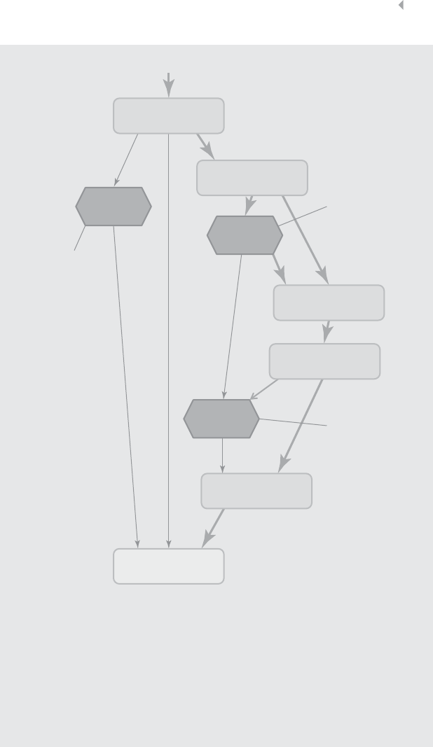
depicted in Figure 1.2, illustrating the handling of fire incident claims without
any form of bodily injury (including death) (Caron et al. 2013). The process
involves the following types of activities:
◾Administrative activities
◾Evaluation-related activities
◾In-depth assessment by internal and external experts
◾Approval activities
◾Leniency-related activities
◾Fraud investigation activities
FRAUD: DETECTION, PREVENTION, AND ANALYTICS! 13
Additional evaluation
activities
Leniency-related
activities
Approval cycle
Update provision
complete
0.380
Discard provisions
complete
0.660
Compensate complete
0.415
Cluster 37
2 elements
–0.092
Register compensation
agreement complete
0.413
Cluster 38
7 elements
–0.033
Send claim acceptance
letter complete
0.369
Consult Policy complete
0.518
Cluster 33
5 elements
–0.033
Figure 1.2 Fire Incident Claim-Handling Process
A number of harmful process deviations and related risks can be
identified regarding these activities:
◾Forgetting to discard provisions
◾Multiple partial compensations (exceeding limit)

14 FRAUD ANALYTICS
◾Collusion between administrator and experts
◾Lack of approval cycle
◾Suboptimal task allocation
◾Fraud investigation activities
◾Processing rejected claim
◾Forced claim acceptance, absence of a timely primary evaluation
Deviations marked in bold may relate to and therefore indicate fraud. By
adopting business policies as a governance instrument and prescribing
procedures and guidelines, the insurer may reduce the risks involved in
processing the insurance claims. For instance:
Business policy excerpt 1 (customer relationship
management related): If the insured requires immediate assistance (e.g.,
to prevent the development of additional damage), arrangements will be made
for a single partial advanced compensation (maximum x% of expected
covered loss).
◾Potential risk: The expected (covered) loss could be exceeded
through partial advanced compensations.
Business policy excerpt 2 (avoid financial loss): Settlements
need to be approved.
◾Potential risk: Collusion between the drafter of the settlement and
the insured
Business policy excerpt 3 (avoid financial loss): The proposal of
a settlement and its approval must be performed by different actors.
◾Potential risk: A person might hold both the team-leader and the
expert role in the information system.
Business policy excerpt 4 (avoid financial loss): After approval of
the decision (settlement or claim rejection) no changes may occur.
◾Potential risk: The modifier and the insured might collude.
◾Potential risk: A rejected claim could undergo further processing.

FRAUD: DETECTION, PREVENTION, AND ANALYTICS! 15
Since detecting fraud based on specified business rules requires prior
knowledge of the fraud scheme, the existence of fraud issues will be the direct
result of either:
◾An inadequate internal control system (controls fail to prevent
fraud); or
◾Risks accepted by the management (no preventive or corrective
controls are in place).
Some examples of fraud-detection rules that can be derived from these
business policy excerpts and process deviations, and that may be added to the
fraud-detection rule engine are as follows:
Business policy excerpt 1:
◾IF multiple advanced payments for one claim, THEN suspicious
case.
Business policy excerpt 2:
◾IF settlement was not approved before it was paid, THEN suspi-
cious case.
Business policy excerpt 3:
◾IF settlement is proposed AND approved by the same person, THEN
suspicious case.
Business policy excerpt 4:
◾IF settlement is approved AND changed afterward, THEN suspi-
cious case.
◾IF claim is rejected AND processed afterward (e.g., look for a set-
tlement proposal, payment,…activity), THEN suspicious case.
BIG DATA FOR FRAUD DETECTION
When fraudulent activities have been detected and confirmed to effec-
tively concern fraud, two types of measures are typically taken:
1. Corrective measures, that aim to resolve the fraud and correct the
wrongful consequences—for instance by means of pursuing

16 FRAUD ANALYTICS
restitution or compensation for the incurred losses. These cor-
rective measures might also include actions to retrospectively
detect and subsequently address similar fraud cases that made
use of the same mechanism or loopholes in the fraud detection
and prevention system the organization has in place.
2. Preventive measures, which may both include actions that aim at
preventing future fraud by the caught fraudster (e.g., by ter-
minating a contractual agreement with a customer, as well as
actions that aim at preventing fraud of the same type by other
individuals). When an expert-based approach is adopted, an
example preventive measure is to extend the rule engine by
incorporating additional rules that allow detecting and prevent-
ing the uncovered fraud mechanism to be applied in the future.
A fraud case must be investigated thoroughly so the underlying
mechanism can be unraveled, extending the available expert
knowledge and allowing it to prevent the fraud mechanism to
be used again in the future by making the organization more
robust and less vulnerable to fraud by adjusting the detection
and prevention system.
Typically, the sooner corrective measures are taken and therefore
the sooner fraud is detected, the more effective such measures may
be and the more losses can be avoided or recompensed. On the other
hand, fraud becomes easier to detect the more time has passed, for a
number of particular reasons.
When a fraud mechanism or path exists—meaning a loophole in the
detection and prevention system of an organization—the number of
times this path will be followed (i.e., the fraud mechanism used) grows
in time and therefore as well the number of occurrences of this partic-
ular type of fraud. The more a fraud path is taken the more apparent it
becomes and typically, in fact statistically, the easier to detect. The num-
ber of occurrences of a particular type of fraud can be expected to grow
since many fraudsters appear to be repeat offenders. As the expression
goes, “Once a thief, always a thief.” Moreover, a fraud mechanism may
well be discovered by several individuals or the knowledge shared
between fraudsters. As will be shown in Chapter 5 on social network
analytics for fraud detection, certainly some types of fraud tend to

FRAUD: DETECTION, PREVENTION, AND ANALYTICS! 17
spread virally and display what are called social network effects,
indicating that fraudsters share their knowledge on how to commit
fraud. This effect, too, leads to a growing number of occurrences and,
therefore, a higher risk or chance, depending on one’s perspective, of
detection.
Once a case of a particular type of fraud has been revealed, this will
lead to the exposition of similar fraud cases that were committed in the
past and made use of the same mechanism. Typically, a retrospective
screening is performed to assess the size or impact of the newly detected
type of fraud, as well as to resolve (by means of corrective measures,
cf. supra) as much as possible fraud cases. As such, fraud becomes
easier to detect the more time has passed, since more similar fraud
cases will occur in time, increasing the probability that the particular
fraud type will be uncovered, as well as because fraudsters committing
repeated fraud will increase their individual risk of being exposed. The
individual risk will increase the more fraud a fraudster commits for the
same basic reason: The chances of getting noticed get larger.
A final reason why fraud becomes easier to detect the more time
has passed is because better detection techniques are being developed,
are getting readily available, and are being implemented and applied by
a growing amount of organizations. An important driver for improve-
ments with respect to detection techniques is growing data availability.
The informatization and digitalization of almost every aspect of society
and daily life leads to an abundance of available data. This so-called big
data can be explored and exploited for a range of purposes including
fraud detection (Baesens 2014), at a very low cost.
DATA-DRIVEN FRAUD DETECTION
Although classic, expert-based fraud-detection approaches as discussed
before are still in widespread use and definitely represent a good start-
ing point and complementary tool for an organization to develop an
effective fraud-detection and prevention system, a shift is taking place
toward data-driven or statistically based fraud-detection methodolo-
gies for three apparent reasons:
1. Precision. Statistically based fraud-detection methodologies offer
an increased detection power compared to classic approaches.

18 FRAUD ANALYTICS
By processing massive volumes of information, fraud patterns
may be uncovered that are not sufficiently apparent to the
human eye. It is important to notice that the improved power
of data-driven approaches over human processing can be
observed in similar applications such as credit scoring or cus-
tomer churn prediction. Most organizations only have a limited
capacity to have cases checked by an inspector to confirm
whether or not the case effectively concerns fraud. The goal
of a fraud-detection system may be to make the most optimal
use of the limited available inspection capacity, or in other
words to maximize the fraction of fraudulent cases among
the inspected cases (and possibly in addition, the detected
amount of fraud). A system with higher precision, as delivered
by data-based methodologies, directly translates in a higher
fraction of fraudulent inspected cases.
2. Operational efficiency. In certain settings, there is an increasing
amount of cases to be analyzed, requiring an automated pro-
cess as offered by data-driven fraud-detection methodologies.
Moreover, in several applications, operational requirements
exist, imposing time constraints on the processing of a case.
For instance, when evaluating a transaction with a credit
card, an almost immediate decision is required with respect to
approve or block the transaction because of suspicion of fraud.
Another example concerns fraud detection for customs in a
harbor, where a decision has to be made within a confined
time window whether to let a container pass and be shipped
inland, or whether to further inspect it, possibly causing delays.
Automated data-driven approaches offer such functionality and
are able to comply with stringent operational requirements.
3. Cost efficiency. As already mentioned in the previous section,
developing and maintaining an effective and lean expert-based
fraud-detection system is both challenging and labor intensive.
A more automated and, as such, more efficient approach to
develop and maintain a fraud-detection system, as offered
by data-driven methodologies, is preferred. Chapters 6 and
7 discuss the cost efficiency and return on investment of
data-driven fraud-detection models.

FRAUD: DETECTION, PREVENTION, AND ANALYTICS! 19
An additional driver for the development of improved fraud-
detection technologies concerns the growing amount of interest that
fraud detection is attracting from the general public, the media, gov-
ernments, and enterprises. This increasing awareness and attention
for fraud is likely due to its large negative social as well as financial
impact, and leads to growing investments and research into the
matter, both from academia, industry, and government.
Although fraud-detection approaches have gained significant
power over the past years by adopting potent statistically based
methodologies and by analyzing massive amounts of data in order
to discover fraud patterns and mechanisms, still fraud remains hard
to detect. It appears the Pareto principle holds with respect to the
required effort and difficulty of detecting fraud: It appears the prin-
ciple of decreasing returns holds with respect to the required effort
and so forth. In order to explain the hardness and complexity of
the problem, it is important to acknowledge the fact that fraud is a
dynamic phenomenon, meaning that its nature changes in time. Not
only fraud-detection mechanisms evolve, but also fraudsters adapt
their approaches and are inventive in finding more refined and less
apparent ways to commit fraud without being exposed. Fraudsters
probe fraud-detection and prevention systems to understand their
functioning and to discover their weaknesses, allowing them to adapt
their methods and strategies.
FRAUD-DETECTION TECHNIQUES
Indeed, fraudsters develop advanced strategies to cleverly cover their
tracks in order to avoid being uncovered. Fraudsters tend to try and
blend in as much as possible into the surroundings. Such an approach
reminds of camouflage techniques as used by the military or by ani-
mals such as chameleons and stick insects. This is clearly no fraud by
opportunity, but rather, is carefully planned, leading to a need for new
techniques that are able to detect and address patterns that initially
seem to comply with normal behavior, but in reality instigate fraudu-
lent activities.
Detection mechanisms based on unsupervised learning techniques
or descriptive analytics, as discussed in Chapter 3, typically aim at

20 FRAUD ANALYTICS
finding behavior that deviates from normal behavior, or in other words
at detecting anomalies. These techniques learn from historical obser-
vations, and are called unsupervised since they do not require these
observations to be labeled as either a fraudulent or a nonfraudulent
example case. An example of behavior that does not comply with
normal behavior in a telecommunications subscription fraud setting
is provided by the transaction data set with call detail records of a
particular subscriber shown in Table 1.2 (Fawcett and Provost 1997).
Remark that the calls found to be fraudulent (last column in the table
indicating bandit) are not suspicious by themselves; however, they are
deviating from normal behavior for this particular subscriber.
Outlier-detection techniques have great value and allow detecting
a significant fraction of fraudulent cases. In particular, they might
allow detecting fraud that is different in nature from historical fraud,
or in other words fraud that makes use of new, unknown mechanisms
resulting in a novel fraud pattern. These new patterns are not discovered
by expert systems, and as such descriptive analytics may be a first
Table 1.2 Call Detail Records of a Customer with Outliers Indicating Suspicious Activity
(deviating behavior starting at a certain moment in time) at the Customer Subscription
(Fawcett and Provost 1997)
Date (m/d) Time Day Duration Origin Destination Fraud
1/01 10:05:01 Mon 13 mins Brooklyn, NY Stamford, CT
1/05 14:53:27 Fri 5mins Brooklyn, NY Greenwich, CT
1/08 09:42:01 Mon 3mins Bronx, NY White Plains, NY
1/08 15:01:24 Mon 9mins Brooklyn, NY Brooklyn, NY
1/09 15:06:09 Tue 5mins Manhattan, NY Stamford, CT
1/09 16:28:50 Tue 53 sec Brooklyn, NY Brooklyn, NY
1/10 01:45:36 Wed 35 sec Boston, MA Chelsea, MA Bandit
1/10 01:46:29 Wed 34 sec Boston, MA Yonkers, MA Bandit
1/10 01:50:54 Wed 39 sec Boston, MA Chelsea, MA Bandit
1/10 11:23:28 Wed 24 sec White Plains, NY Congers, NY
1/11 22:00:28 Thu 37 sec Boston, MA East Boston, MA Bandit
1/11 22:04:01 Thu 37 sec Boston, MA East Boston, MA Bandit

FRAUD: DETECTION, PREVENTION, AND ANALYTICS! 21
complementary tool to be adopted by an organization in order to
improve its expert rule–based fraud-detection system.
Descriptive techniques however show to be prone to deception,
exactly by the camouflage-like fraud strategies already discussed.
Therefore, the detection system can be further improved by com-
plementing it by a tool that is able to unmask fraudsters adopting a
camouflage-like technique.
Therefore, in Chapter 4, a second type of techniques is introduced.
Supervised learning techniques or predictive analytics aim to learn
from historical information or observations in order to retrieve
patterns that allow differentiating between normal and fraudulent
behavior. These techniques exactly aim at finding silent alarms, the
parts of their tracks that fraudsters cannot cover up. Supervised
learners can be applied to predict or detect fraud as well as to estimate
the amount of fraud.
Predictive analytics has limitations as well, probably the most
important one being that they need historical examples to learn from
(i.e., a labeled data set of historically observed fraud behavior). This
reduces their detection power with respect to drastically different
fraud types making use of new mechanisms or methods, and which
have not been detected thus far and are therefore not included in the
historical database of fraud cases from which the predictive model
was learned. As already discussed, descriptive analytics may perform
better with respect to detecting such new fraud mechanisms, at
least if a new fraud mechanism leads to detectable deviations from
normality. This illustrates the complementarity of supervised and
unsupervised methods and motivates the use of both types of methods
as complementary tools in developing a powerful fraud-detection and
prevention system.
A third type of complementary tool concerns social network
analysis, which further extends the abilities of the fraud-detection
system by learning and detecting characteristics of fraudulent behavior
in a network of linked entities. Social network analytics is the newest
tool in our toolbox to fight fraud, and proofs to be a very powerful
means as will appear from the discussion and presented case study

22 FRAUD ANALYTICS
in Chapter 5. Social network analytics allows including an extra
source of information in the analysis, being the relationships between
entities, and as such may contribute in uncovering particular patterns
indicating fraud.
It is important to stress that these three different types of tech-
niques may complement each other since they focus on different
aspects of fraud and are not to be considered as exclusive alternatives.
An effective fraud-detection and prevention system will make use of
and combine these different tools, which have different possibilities
and limitations and therefore reinforce each other when applied in
a combined setup. When developing a fraud-detection system, an
organization will likely follow the order in which the different tools
have been introduced; as a first step an expert-based rule engine
may be developed, which in a second step may be complemented
by descriptive analytics, and subsequently by predictive and social
network analytics. Developing a fraud-detection system in this order
allows the organization to gain expertise and insight in a stepwise
manner, hereby facilitating each next step. However, the exact order
of adopting the different techniques may depend on the characteristics
of the type of fraud an organization is faced with.
FRAUD CYCLE
Figure 1.3 introduces the fraud cycle, and depicts four essential activities:
◾Fraud detection: Applying detection models on new, unseen
observations and assigning a fraud risk to every observation.
◾Fraud investigation: A human expert is often required to
investigate suspicious, flagged cases given the involved subtlety
and complexity.
◾Fraud confirmation: Determining true fraud label, possibly
involving field research.
◾Fraud prevention: Preventing fraud to be committed in the
future. This might even result in detecting fraud even before
the fraudster knows s/he will commit fraud, which is exactly the
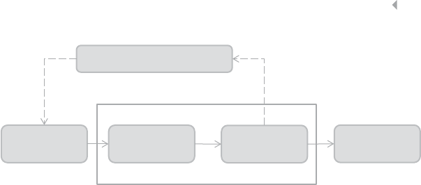
FRAUD: DETECTION, PREVENTION, AND ANALYTICS! 23
Fraud
detection
Fraud
investigation
Fraud
confirmation
Fraud
prevention
Automated detection algorithm
Current process
Figure 1.3 The Fraud Cycle
premise of the 1956 science fiction short story Minority Report by
Philip K. Dick.
Remark the feedback loop in Figure 1.3 from the fraud confirma-
tion activity toward the fraud-detection activity. Newly detected cases
should be added (as soon as possible!) to the database of historical
fraud cases, which is used to learn or induce the detection model.
The fraud-detection model may not be retrained every time a new
case is confirmed; however, a regular update of the model is recom-
mendable given the dynamic nature of fraud and the importance of
detecting fraud as soon as possible. The required frequency of retrain-
ing or updating the detection model depends on several factors:
◾The volatility of the fraud behavior
◾The detection power of the current model, which is related to
the volatility of the fraud behavior
◾The amount of (similar) confirmed cases already available in the
database
◾The rate at which new cases are being confirmed
◾The required effort to retrain the model
Depending on the emerging need for retraining as determined
by these factors, as well as possible additional factors, an automated
approach such as reinforcement learning may be considered which
continuously updates the detection model by learning from the
newest observations.

24 FRAUD ANALYTICS
EXAMPLE CASE: SUPERVISED AND UNSUPERVISED
LEARNING FOR DETECTING CREDIT CARD FRAUD
EXAMPLE CASE
In order to fight fraud and given the abundant data availability, credit card
companies have been among the early adopters of big data approaches to
develop effective fraud-detection and prevention systems. A typical credit card
transaction is registered in the systems of the credit card company by logging
up to a hundred or more characteristics describing the details of a transaction.
Table 1.3 provides for illustrative purposes a number of such characteristics
or variables that are being captured (Hand 2007).
Table 1.3 Example Credit Card Transaction Data Fields
Transaction ID Transaction type Date of transaction
Time of transaction Amount Currency
Local currency amount Merchant ID Merchant category
Card issuer ID ATM ID Cheque account prefix
By logging this information over a period of time, a dataset is being
created that allows applying descriptive analytics. This includes outlier
detection techniques, which allow detecting abnormal or anomalous behavior
and/or characteristics in a data set. So-called outliers may indicate suspicious
activities, and may occur at the data item level or the data set level.
Figure 1.4 provides an illustration of outliers at the data item level, in this
example transactions that deviate from the normal behavior by a customer.
The scatter plot clearly shows three clusters of regular, frequently occurring
types as characterized by the time and place dimension of transactions for one
particular customer, as well as two deviating transactions marked in black.
These outliers are suspicious and possibly concern fraudulent transactions,
and therefore may be flagged for further human investigation.
An outlier at the data set level means that the behavior of a person or
instance does not comply with the overall behavior. Figure 1.5 plots the age
and income characteristics of customers as provided when applying for a
credit card. The two outliers marked in black in the plot may indicate so-called
subscription fraud (cf. Table 1.1, definition of credit card fraud), since these
combinations of age and income strongly deviate from the normal behavior.
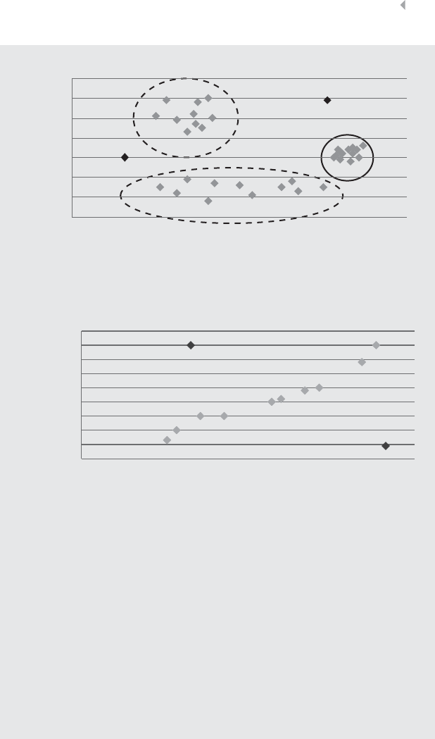
FRAUD: DETECTION, PREVENTION, AND ANALYTICS! 25
0
10
20
30
40
50
60
70
0 20406080 100 120 140 160
Time
Place
Time versus Place
Figure 1.4 Outlier Detection at the Data Item Level
0
500
1000
1500
2000
2500
3000
3500
4000
4500
010203040506070
Income
Age
Income versus Age
Figure 1.5 Outlier Detection at the Data Set Level
The addition of a field in the available transaction data set that indicates
whether a transaction was fraudulent allows predictive analytics to be applied
to yield a model predicting or classifying an instance as being fraudulent or
not. As will be discussed in the next section as well as in Chapter 4, such
models may be interpreted to understand the underlying credit card fraud
behavior patterns that lead the model to predict whether a transaction might be
fraudulent. Such patterns may be:
◾Small purchase followed by a big one
◾Large number of online purchases in a short period

26 FRAUD ANALYTICS
◾Spending as much as possible as quickly as possible
◾Spending smaller amounts, spread across time
Such pattern may be harder to detect and concern advanced methods
adopted by fraudsters and developed exactly to avoid detection.
THE FRAUD ANALYTICS PROCESS MODEL
Figure 1.6 provides a high-level overview of the analytics process
model (Han and Kamber 2011; Hand, Mannila, and Smyth 2001; Tan,
Steinbach, and Kumar 2005). As a first step, a thorough definition of
the business problem is needed to be solved with analytics. Next, all
source data must be identified that could be of potential interest. This
is a very important step, as data are the key ingredient to any analytical
exercise and the selection of data will have a deterministic impact on
the analytical models that will be built in a subsequent step. All data
will then be gathered in a staging area that could be a data mart or data
warehouse. Some basic exploratory analysis can be considered here
using for instance OLAP (online analytical processing, see Chapter 3)
facilities for multidimensional data analysis (e.g., roll-up, drill down,
slicing and dicing). This will be followed by a data-cleaning step to
Identify
Business
Problem
Identify
Data
Sources
Select
the
Data
Clean
the
Data
Transform
the
Data
Analyze
the
Data
Intepret,
Evaluate,
and Deploy
the Model
Analytics
Preprocessing
Post-
processing
Figure 1.6 The Fraud Analytics Process Model

FRAUD: DETECTION, PREVENTION, AND ANALYTICS! 27
get rid of all inconsistencies, such as missing values and duplicate
data. Additional transformations may also be considered, such as
binning, alphanumeric to numeric coding, geographical aggregation,
and so on. In the analytics step, an analytical model will be estimated
on the preprocessed and transformed data. In this stage, the actual
fraud-detection model is built. Finally, once the model has been built,
it will be interpreted and evaluated by the fraud experts.
Trivial patterns that may be detected by the model, for instance
similar to expert rules, are interesting as they provide some valida-
tion of the model. But of course, the key issue is to find the unknown
yet interesting and actionable patterns (sometimes also referred to as
knowledge diamonds) that can provide added insight and detection
power. Once the analytical model has been appropriately validated and
approved, it can be put into production as an analytics application (e.g.,
decision support system, scoring engine). Important to consider here
is how to represent the model output in a user-friendly way, how to
integrate it with other applications (e.g., detection and prevention sys-
tem, risk engines), and how to make sure the analytical model can
be appropriately monitored and backtested on an ongoing basis. These
post-processing steps will be discussed in detail in Chapter 6.
It is important to note that the process model outlined in Figure 1.6
is iterative in nature in the sense that one may have to go back to
previous steps during the exercise. For example, during the analyt-
ics step, the need for additional data may be identified, which may
necessitate additional cleaning, transformation, and so on. The most
time-consuming step typically is the data selection and preprocessing
step, which usually takes around 80 percent of the total efforts needed
to build an analytical model.
A fraud-detection model must be thoroughly evaluated before
being adopted. Depending on the exact setting and usage of the model,
different aspects may need to be assessed during evaluation in order
to ensure the model to be acceptable for implementation. Table 1.4
reviews several key characteristics of successful fraud analytics models
that may or may not apply, depending on the exact application.
A number of particular challenges may present themselves when
developing and implementing a fraud-detection model, possibly
leading to difficulties in meeting the objectives as expressed by the

28 FRAUD ANALYTICS
Table 1.4 Key Characteristics of Successful Fraud Analytics Models
Statistical
accuracy
Refers to the detection power and the correctness of the statistical model in
flagging cases as being suspicious. Several statistical evaluation criteria
exist and may be applied to evaluate this aspect, such as the hit rate, lift
curves, AUC, etc. A number of suitable measures will be discussed in detail
in Chapter 4. Statistical accuracy may also refer to statistical significance,
meaning that the patterns that have been found in the data have to be real and
not the consequence of coincidence. In other words, we need to make sure
that the model generalizes well and is not overfitted to the historical data set.
Interpretability When a deeper understanding of the detected fraud patterns is required, for
instance to validate the model before it is adopted for use, a fraud-detection
model may have to be interpretable. This aspect involves a certain degree of
subjectivism, since interpretability may depend on the user’s knowledge. The
interpretability of a model depends on its format, which, in turn, is
determined by the adopted analytical technique. Models that allow the user
to understand the underlying reasons why the model signals a case to be
suspicious are called white-box models, whereas complex incomprehensible
mathematical models are often referred to as black-box models. It may well
be in a fraud-detection setting that black-box models are acceptable,
although in most settings some level of understanding and in fact validation
which is facilitated by interpretability is required for the management to have
confidence and allow the effective operationalization of the model.
Operational
efficiency
Operational efficiency refers to the time that is required to evaluate the
model, or in other words, the time required to evaluate whether a case is
suspicious or not. When cases need to be evaluated in real time, for instance
to signal possible credit card fraud, operational efficiency is crucial and is a
main concern during model performance assessment. Operational efficiency
also entails the efforts needed to collect and preprocess the data, evaluate the
model, monitor and backtest the model, and reestimate it when necessary.
Economical
cost
Developing and implementing a fraud-detection model involves a significant
cost to an organization. The total cost includes the costs to gather,
preprocess, and analyze the data, and the costs to put the resulting analytical
models into production. In addition, the software costs, as well as human
and computing resources, should be taken into account. Possibly also
external data has to be bought to enrich the available in-house data. Clearly,
it is important to perform a thorough cost-benefit analysis at the start of the
project, and to gain insight in the constituent factors of the returns on
investment of building an advanced fraud-detection system.
Regulatory
compliance
Depending on the context there may be internal or organization-specific and
external regulation and legislation that applies to the development and
application of a model. Clearly, a fraud-detection model should be in line
and comply with all applicable regulation and legislation, for instance with
respect to privacy, the use of cookies in a web-browser, etc.

FRAUD: DETECTION, PREVENTION, AND ANALYTICS! 29
characteristics discussed in Table 1.4. A first key challenge concerns
the dynamic nature of fraud. Fraudsters constantly try to beat
detection and prevention systems by developing new strategies and
methods. Therefore, adaptive analytical models and detection and
prevention systems are required, in order to detect and resolve fraud
as soon as possible. Detecting fraud as early as possible is crucial, as
discussed before.
Clearly, it is also crucial to detect fraud as accurately as possible,
and not to miss out on too many fraud cases, especially on fraud cases
involving a large amount or financial impact. The cost of missing a
fraudulent case or a fraud mechanism may be significant. Related to
having good detection power is the requirement of having at the same
time a low false alarm rate, since we also want to avoid harassing
good customers and prevent accounts or transactions to be blocked
unnecessarily.
In developing analytical models with good detection power and
low false alarm rate, an additional difficulty concerns the skewedness
of the data, meaning that we typically have plenty of historical
examples of nonfraudulent cases, but only a limited number of
fraudulent cases. For instance, in a credit card fraud setting, typically
less than 0.5 percent of transactions are fraudulent. Such a problem is
commonly referred to as a needle-in-a-haystack problem and might
cause an analytical technique to experience difficulties in learning an
accurate model. A number of approaches to address the skewedness
of the data will be discussed in Chapter 4.
Depending on the exact application, also operational efficiency
may be a key requirement, meaning that the fraud-detection system
might only have a limited amount of time available to reach a decision
and let a transaction pass or not. As an example, in a credit card
fraud-detection setting the decision time has to be typically less than
eight seconds. Such a requirement clearly impacts the design of the
operational IT systems, but also the design of the analytical model.
The analytical model should not take too long to be evaluated, and
the information or the variables that are used by the model should not
take too long to be gathered or calculated. Calculating trend variables
in real time, for instance, may not be feasible from an operational
perspective, since this is taking too much valuable time. This also

30 FRAUD ANALYTICS
relates to the final challenge of dealing with the massive volumes of
data that are available and need to be processed.
FRAUD DATA SCIENTISTS
Whereas in the previous section we discussed the characteristics of a
good fraud-detection model, in this paragraph we will elaborate on the
key characteristics of a good fraud data scientist from the perspective
of the hiring manager. It is based on our consulting and research expe-
rience, having collaborated with many companies worldwide on the
topic of big data, analytics, and fraud detection.
A Fraud Data Scientist Should Have Solid
Quantitative Skills
Obviously, a fraud data scientist should have a thorough background
in statistics, machine learning and/or data mining. The distinction
between these various disciplines is getting more and more blurred
and is actually not that relevant. They all provide a set of quantita-
tive techniques to analyze data and find business relevant patterns
within a particular context such as fraud detection. A data scientist
should be aware of which technique can be applied when and how.
He/she should not focus too much on the underlying mathematical
(e.g., optimization) details but, rather, have a good understanding
of what analytical problem a technique solves, and how its results
should be interpreted. In this context, the education of engineers
in computer science and/or business/industrial engineering should
aim at an integrated, multidisciplinary view, with graduates formed
in both the use of the techniques, and with the business acumen
necessary to bring new endeavors to fruition. Also important is to
spend enough time validating the analytical results obtained so as
to avoid situations often referred to as data massage and/or data
torture whereby data is (intentionally) misrepresented and/or too
much focus is spent discussing spurious correlations. When selecting
the optimal quantitative technique, the fraud data scientist should

FRAUD: DETECTION, PREVENTION, AND ANALYTICS! 31
take into account the specificities of the context and the problem
or fraud-detection application at hand. Typical requirements for
fraud-detection models have been discussed in the previous section
and the fraud data scientist should have a basic understanding and
feeling for all of those. Based on a combination of these requirements,
the data scientist should be capable of selecting the best analytical
technique to solve the particular business problem.
A Fraud Data Scientist Should Be a Good Programmer
As per definition, data scientists work with data. This involves plenty
of activities such as sampling and preprocessing of data, model estima-
tion and post-processing (e.g., sensitivity analysis, model deployment,
backtesting, model validation). Although many user-friendly software
tools are on the market nowadays to automate and support these tasks,
every analytical exercise requires tailored steps to tackle the specifici-
ties of a particular business problem and setting. In order to successfully
perform these steps, programming needs to be done. Hence, a good
data scientist should possess sound programming skills (e.g., SAS, R,
Python, etc.). The programming language itself is not that important
as such, as long as he/she is familiar with the basic concepts of pro-
gramming and knows how to use these to automate repetitive tasks or
perform specific routines.
A Fraud Data Scientist Should Excel in Communication
and Visualization Skills
Like it or not, analytics is a technical exercise. At this moment, there
is a huge gap between the analytical models and the business users.
To bridge this gap, communication and visualization facilities are
key. Hence, data scientists should know how to represent analytical
models and their accompanying statistics and reports in user-friendly
ways using traffic-light approaches, OLAP (online analytical pro-
cessing) facilities, If-then business rules, and so on. They should be
capable of communicating the right amount of information without

32 FRAUD ANALYTICS
getting lost into complex (e.g., statistical) details, which will inhibit a
model’s successful deployment. By doing so, business users will better
understand the characteristics and behavior in their (big) data which
will improve their attitude toward and acceptance of the resulting
analytical models. Educational institutions must learn to balance,
since many academic degrees form students who are skewed to either
too much analytical or too much practical knowledge.
A Fraud Data Scientist Should Have a Solid Business
Understanding
While this might be obvious, we have witnessed (too) many data sci-
ence projects that failed because the respective analyst did not under-
stand the business problem at hand. By “business” we refer to the
respective application area. Several examples of such application areas
of fraud-detection techniques were summarized in Table 1.1. Each of
those fields has its own particularities that are important for a fraud
data scientist to know and understand in order to be able to design and
implement a customized fraud-detection system. The more aligned the
detection system with the environment, the better its performance will
be, as evaluated on each of the dimensions already discussed.
A Fraud Data Scientist Should Be Creative
A data scientist needs creativity on at least two levels. First, on a techni-
cal level, it is important to be creative with regard to feature selection,
data transformation, and cleaning. These steps of the standard ana-
lytics process have to be adapted to each particular application, and
often the “right guess” could make a big difference. Second, big data
and analytics is a fast-evolving field. New problems, technologies, and
corresponding challenges pop up on an ongoing basis. Moreover, also
fraudsters are very creative and adapt their tactics and methods on an
ongoing basis. Therefore, it is crucial that a fraud data scientist keeps up
with these new evolutions and technologies and has enough creativity
to see how they can create new opportunities.
Figure 1.7 summarizes the key characteristics and strengths con-
stituting the ideal fraud data scientist profile.

FRAUD: DETECTION, PREVENTION, AND ANALYTICS! 33
0
5
10
15
20
25
30
35
Programmer
Modeling
CommunicationBusiness
Creative
"Close to ideal"
"Too specialized"
Figure 1.7 Profile of a Fraud Data Scientist
A SCIENTIFIC PERSPECTIVE ON FRAUD
To conclude this chapter, let’s provide a scientific perspective about
the research on fraud. Figure 1.8 shows a screenshot of the Web of
Science statistics when querying all scientific publications between
1996 and 2014 for the key term fraud. It shows the total number of
papers published each year, the number of citations and the top five
most-cited papers.
A couple of conclusions can be drawn as follows:
◾6,174 scientific papers have been published on the topic of fraud
during the period reported.
◾The h-index is 44, implying that there are at least 44 papers with
44 citations on the topic of fraud.
◾The number of publications is steadily increasing, which shows
a growing interest from the academic community and research
on the topic.
◾The citations are exponentially growing, which is associated
with the increasing number of publications.
◾Two of the five papers mentioned study the use of analytics for
fraud detection, clearly illustrating the growing attention in the
field for data-driven approaches.
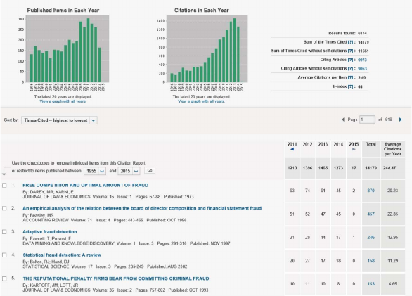
34
Figure 1.8 Screenshot of Web of Science Statistics for Scientific Publications on Fraud between 1996 and 2014

FRAUD: DETECTION, PREVENTION, AND ANALYTICS! 35
REFERENCES
Armstrong, J. S. (2001). Selecting Forecasting Methods. In J.S. Armstrong, ed.
Principles of Forecasting: A Handbook for Researchers and Practitioners.New
York: Springer Science +Business Media, pp. 365–386.
Baesens, B. (2014). Analytics in a Big Data World: The Essential Guide to Data Science
and Its Applications. Hoboken, NJ: John Wiley & Sons.
Bolton, R. J., & Hand, D. J. (2002). Statistical Fraud Detection: A Review.
Statistical Science,17 (3): 235–249.
Caron, F., Vanden Broucke, S., Vanthienen, J., & Baesens, B. (2013). Advanced
Rule-Based Process Analytics: Applications for Risk Response Decisions
and Management Control Activities. Expert Systems with Applications,
Submitted.
Chakraborty, G., Murali, P., & Satish, G. (2013). Text Mining and Analysis: Prac-
tical Methods, Examples, and Case Studies Using SAS. Cary, NC: SAS Institute.
Cressey, D. R. (1953). Other People’s Money; A Study of the Social Psychology of
Embezzlement. New York: Free Press.
Duffield, G., & Grabosky, P. (2001). The Psychology of Fraud. In Trends and
Issues in Crime and Criminal Justice, Australian Institute of Criminology (199).
Elder IV,, J., & Thomas, H. (2012). Practical Text Mining and Statistical Analysis for
Non-Structured Text Data Applications. New York: Academic Press.
Fawcett, T., & Provost, F. (1997). Adaptive Fraud Detection. Data Mining and
Knowledge Discovery 1–3 (3): 291–316.
Grabosky, P., & Duffield, G. (2001). Red Flags of Fraud. Trends and Issues in Crime
and Criminal Justice, Australian Institute of Criminology (200).
Han, J., & Kamber, M. (2011). Data Mining: Concepts and Techniques, Third
Edition: Morgan Kaufmann.
Hand, D. (2007, September). Statistical Techniques for Fraud Detection, Prevention,
and Evaluation. Paper presented at the NATO ASI: Mining Massive Data
sets for Security, London, England.
Hand, D. J., Mannila, H., & Smyth, P. (2001). Principles of Data Mining.
Cambridge, MA: Bradford.
Jamain, A. (2001). Benford’s Law. London: Imperial College.
Junqué de Fortuny, E., Martens, D., & Provost, F. (2013). Predictive Modeling
with Big Data: Is Bigger Really Better? Big Data 1 (4): 215–226.
Little, R. J. A., & Rubin, D. B. (2002). Statistical Analysis with Missing Data
(2nd ed.). Hoboken, NJ: Wiley.
Maydanchik, A. (2007). Data Quality Assessment. Bradley Beach, NC: Technics
Publications.

36 FRAUD ANALYTICS
Navarette, E. (2006). Practical Calculation of Expected and Unexpected Losses
in Operational Risk by Simulation Methods (Banca & Finanzas: Documen-
tos de Trabajo, 1(1): pp. 1–12).
Petropoulos, F., Makridakis, S., Assimakopoulos, V., & Nikolopoulos, K. (2014).
“Horses for courses” in demand forecasting. European Journal of Operational
Research,237 (1): 152–163.
Schneider, F. (2002). Size and Measurement of the Informal Economy in 110
Countries around the World. In Workshop of Australian National Tax Centre,
ANU, Canberra, Australia.
Tan, P.-N. N., Steinbach, M., & Kumar, V. (2005). Introduction to Data Mining.
Boston: Addison Wesley.
Van Gestel, T., & Baesens, B. (2009). Credit Risk Management: Basic Concepts:
Financial Risk Components, Rating Analysis, Models, Economic and Regulatory
Capital. Oxford: Oxford University Press.
Van Vlasselaer, V., Eliassi-Rad, T., Akoglu, L., Snoeck, M., & Baesens, B. (2015).
Gotcha! Network-based Fraud Detection for Social Security Fraud. Man-
agement Science, Submitted.
Verbeke, W., Dejaeger, K., Martens, D., Hur, J., & Baesens, B. (2012). New
Insights into Churn Prediction in the Telecommunication Sector: A Profit
Driven Data Mining Approach. European Journal of Operational Research
218: 211–229.
CHAPTER 2
Data Collection,
Sampling, and
Preprocessing
37
INTRODUCTION
Data is a key ingredient for any analytical exercise. Hence, it is of
key importance to thoroughly consider and list all data sources that
are potentially of interest and relevant before starting the analysis.
Large experiments as well as a broad experience in different fields
indicate that when it comes to data, bigger is better (see de Fortuny,
Martens, & Provost, 2013). However, real-life data can be (typically is)
dirty because of inconsistencies, incompleteness, duplication, merging,
and many other problems. Hence, throughout the analytical modeling
steps, various data-filtering mechanisms will be applied to clean up
and reduce the data to a manageable and relevant size. Worth men-
tioning here is the garbage in, garbage out (GIGO) principle, which
essentially states that messy data will yield messy analytical models.
Hence, it is of utmost importance that every data preprocessing step is
carefully justified, carried out, validated, and documented before pro-
ceeding with further analysis. Even the slightest mistake can make the
data totally unusable for further analysis and the results invalid and
of no use whatsoever. In what follows, we will elaborate on the most
important data preprocessing steps that should be considered during
an analytical modeling exercise to build a fraud detection model. But
first, let us have a closer look at what data to gather.
TYPES OF DATA SOURCES
Data can originate from a variety of different sources and provide
different types of information that might be useful for the purpose of
fraud detection, as will be further discussed in this section. Do remark
that the provided mixed discussion of different sources and types
of data concerns a broad, non-exhaustive and non-mutually exclusive
categorization, respectively in the sense that the most prominent data
sources and types of information as available in a typical organization
are listed, but clearly not all possible data sources and types of infor-
mation are discussed, and possibly some overlap exists between the
enlisted categories.
38

DATA COLLECTION, SAMPLING, AND PREPROCESSING 39
Transactional data is a first important source of data. It consists
of structured and detailed information capturing the key characteristics
of a customer transaction (e.g., a purchase, claim, cash transfer, credit
card payment). It is usually stored in massive OLTP (online tran-
saction processing) relational databases. This data can also be
summarized over longer time horizons by aggregating it into averages,
(absolute or relative) trends, maximum or minimum values, etc.
An important type of such aggregated transactional information in
a fraud detection setting concern RFM variables, which stands for
recency (R), frequency (F), and monetary (M) variables. RFM vari-
ables are often used for clustering in fraud detection, as will be
discussed in Chapter 3, but are useful as well in a supervised learning
setting as will be discussed in Chapter 4. RFM variables have been
originally introduced in a marketing setting (Cullinan, 1977), but they
clearly may also come in handy for fraud detection.
RFM variables can be operationalized in various ways. Let us take
the example of credit card fraud detection. The recency can be mea-
sured in a continuous way such as how much time elapsed since the
most recent transaction, or in a binary way such as was there a transac-
tion made during the past day, week, month, and so on. The frequency
can be quantified as the number of transactions per day, week, month,
and so on. Similarly, the monetary variable can be quantified as the
minimum, maximum, average, median, or most recent value of a
transaction. Although these variables can be meaningful when inter-
preted individually (e.g., fraudsters make more frequent transactions
than nonfraudsters), also their interaction can be very useful for fraud
detection. For example, credit card fraudsters often try out a stolen
credit card for a low amount to see whether it works, before making a
big purchase, resulting in a recent and low monetary value transaction
followed by a recent and high monetary value transaction. RFM
variables can also prove their worth in an anti-money laundering
context by considering recency, frequency, and amount of cash
transfers between accounts, which possibly allows uncovering charac-
teristic money laundering patterns. A final illustration concerns RFM
variables which may be operationalized for insurance claim fraud

40 FRAUD ANALYTICS
detection by constructing variables such as time since previous claim,
number of claims submitted in the previous twelve months,andtotal monetary
amount of claims since subscription of insurance contract.
Contractual, subscription, or account data may complement
transactional data if a contractual relation exists, which is often the
case for utilities such as gas, electricity, telecommunication, and so on.
Examples of subscription data are the start date of the relation, infor-
mation on subscription renewals, characteristics of a subscription such
as type of services or products delivered, levels of service, cost of ser-
vice, product guarantees and insurances, and so on. The moment when
customers subscribe to a service offers a unique opportunity for organi-
zations to get to know their customers. Unique in the sense that it may
be the only time when a direct contact exists between an employee
and the customer, either in person, over the phone, or online, and as
such offers the opportunity for the organization to gather additional
information that is nonessential to the contract but may be useful
for purposes such as marketing but as well for fraud detection. Such
information is typically stored in an account management or customer
relationship management (CRM) database.
Subscription data may also be a source of sociodemographic
information, since typically subscription or registration requires iden-
tification. Examples of socioeconomic characteristics of a population
consisting of individuals are age,gender,marital status,income level,edu-
cation level,occupation,religion, and so on. Although not very advanced
or complex measures, sociodemographic information may signifi-
cantly relate to fraudulent behavior. For instance, it appears that both
gender as well as age is very often related to an individual’s likelihood
to commit fraud: female and older individuals are less likely to commit
fraud than male and younger individuals. Similar characteristics can
also be defined when the basic entities for which fraud is to be detected
do not concern individuals but instead companies or organizations.
In such a setting one rather speaks of slow-moving data dimensions,
factual data or static characteristics. Examples include the address,
year of foundation, industrial sector, activity type, and so on. These do
not change over time at all or as often as do other characteristics such
as turnover, solvency, number of employees, etc. These latter variables
are examples of what we will call below behavioral information.

DATA COLLECTION, SAMPLING, AND PREPROCESSING 41
Several data sources may be consulted for retrieving sociodemo-
graphic or factual data, including subscription data sources as
discussed above, and data poolers, survey data, and publicly available
data sources as discussed below.
Nowadays, data poolers are getting more and more important
in the industry. Examples are Experian, Equifax, CIFAS, Dun &
Bradstreet, Thomson Reuters, etc. The core business of these compa-
nies is to gather data (e.g., sociodemographic information) in particular
settings or for particular purposes (e.g., fraud detection, credit risk
assessment, and marketing) and sell it to interested customers looking
to enrich or extend their data sources. Additionally to selling data,
these data poolers typically also build predictive models themselves
and sell the output of these models as risk scores. This is a common
practice in credit risk, for instance, in the United States the FICO score
is a credit score ranging between 300 and 850 provided by the three
most important credit data poolers or credit bureaus: Experian, Equifax
and Transunion. Many financial institutions as well as commercial
vendors that give credit to customers use these FICO scores either as
their final internal model to assess creditworthiness, or to benchmark
it against an internally developed credit scorecard to better understand
the weaknesses of the latter. The use of generic, pre-defined fraud
risk scores is not yet common practice, but may become possible in
the near future.
Surveys are another source of data—that is, survey data. Such data
are gathered by inquiring the target population by means of an offline
(via mail, letter, etc.) or online (via phone call or the Internet, which
offers different contact channels such as the organization’s website, the
online helpdesk, social media profiles such as Facebook, LinkedIn, or
Twitter) survey. Surveys may aim at gathering sociodemographic data,
but also behavioral information.
Behavioral information concerns any information describing
the behavior of an individual or an entity in the particular context
under research. Such data are also called fast-moving data or dynamic
characteristics. Examples of behavioral variables include information
with regards to preferences of customers, usage information, fre-
quencies of events, trend variables, and so on. When dealing with
organizations, examples of behavioral characteristics or dynamic

42 FRAUD ANALYTICS
characteristics are turnover,solvency,number of employees,andsoon.
Marketing data results from monitoring the impact of marketing
actions on the target population, and concerns a particular type of
behavioral information.
Also, unstructured data embedded in text documents (e.g.,
emails, Web pages, claim forms) or multimedia content can be inter-
esting to analyze. However, these sources typically require extensive
preprocessing before they can be successfully included in an analytical
exercise. Analyzing textual data is the goal of a particular branch of
analytics, called text analytics. Given the high level of specialization
involved, this book does not provide an extensive discussion of text
mining techniques, although a brief introduction is provided in the
final chapter of the book. For more information on this topic, one
may refer to academic textbooks on the subject (Chakraborty, Murali,
& Satish 2013).
A second type of unstructured information is contextual or
network information, meaning the context of a particular entity.
An example of such contextual information concerns relations of
a particular type that exist between an entity and other entities of
the same type or of another type. How to gather and represent such
information, as well as how to make use of it will be described in
detail in Chapter 5, which will focus on social network analytics for
fraud detection.
Another important source of data is qualitative, expert-based
data. An expert is a person with a substantial amount of subject
matter expertise within a particular setting (e.g., credit portfolio man-
ager, brand manager). The expertise stems from both common sense
and business experience and it is important to elicit this knowledge
as much as possible before the analytical model building exercise is
started. It will allow steering the modeling in the right direction and
interpret the analytical results from the right perspective. A popular
example of applying expert-based validation is checking the univariate
signs of a regression model. For instance, an example already discussed
before concerns the observation that a higher age often results in
a lower likelihood of being fraudulent. Consequently, a negative
sign is expected when including age in a fraud prediction model

DATA COLLECTION, SAMPLING, AND PREPROCESSING 43
yielding the probability of an individual committing fraud. If this turns
out not to be the case due to whatever reason (e.g., bad data
quality, multicollinearity), the expert or business user will not be
tempted to use the analytical model at all, since it contradicts prior
expectations.
A final source of information concerns publicly available data
sources that can provide for instance, external information.Thisis
contextual information that is not related to a particular entity, such
as macroeconomic data (GDP, inflation, unemployment, etc.), and
weather observations. By enriching the data set with such information
one may see for example how the model and the model outputs vary
as a function of the state of the economy. Possibly fraud rates and
total amounts of fraud increase during economic downturn periods,
although no scientific evidence (or counter evidence, for that matter)
of such an effect is, to our knowledge, available (yet) in the scientific
literature. Also social media data from, for example, Facebook, Twitter,
LinkedIn, and so on, and that are publicly available can be an impor-
tant source of information. However, one needs to be careful in both
gathering and using such data and make sure that local and interna-
tional privacy regulations are respected at all times. Privacy concerns
in a data analytics context will be discussed in the final chapter.
MERGING DATA SOURCES
The application of both descriptive and predictive analytics typically
requires or presumes the data to be presented in a single table contain-
ing and representing all the data in a structured manner. A structured
data table allows straightforward processing and analysis. (Learning
from multiple tables that are related—that is, learning directly from
relational databases without merging the normalized tables—is a par-
ticular branch within the field of data mining called relational learning,
and shares techniques and approaches with social network analytics as
discussed in Chapter 5.)
Typically, the rows of a data table represent the basic entities to
which the analysis applies (e.g., customers, transactions, enterprises,
claims, cases). The rows are referred to as instances, observations, or

44 FRAUD ANALYTICS
lines. The columns in the data table contain information about the basic
entities. Plenty of synonyms are used to denote the columns of the data
table, such as (explanatory) variables, fields, characteristics, attributes,
indicators, features, and so on.
In order to construct the aggregated, non-normalized data table to
facilitate further analysis, often several normalized source data tables
have to be merged. Merging tables involves selecting information
from different tables related to an individual entity, and copying it
to the aggregated data table. The individual entity can be recognized
and selected in the different tables by making use of keys,which
are attributes that have exactly been included in the table to allow
identifying and relating observations from different source tables per-
taining to the same entity. Figure 2.1 illustrates the process of merging
two tables—that is, transactions data and customer data, into a single
non-normalized data table by making use of the key attribute ID, which
allows connecting observations in the transactions table with observa-
tions in the customer table. The same approach can be taken to merge
as many tables as required, but clearly the more tables are merged,
the more duplicate data might be included in the resulting table.
When merging data tables, it is crucial that no errors happen, so
some checks should be applied to control the resulting table and to
make sure that all information is correctly integrated.
ID Date Amount
XWV 2/01/2015 52 €
XWV 6/02/2015 21 €
XWV 3/03/2015 13 €
BBC 17/02/2015 45 €
BBC 1/03/2015 75 €
VVQ 2/03/2015 56 €
Transactions
ID Age Start date
XWV 31 1/01/2015
BBC 49 10/02/2015
VVQ 21 15/02/2015
Customer data
ID Date Amount Age Start date
XWV 2/01/2015 52 € 31 1/01/2015
XWV 6/02/2015 21 € 31 1/01/2015
XWV 3/03/2015 13 € 31 1/01/2015
BBC 17/02/2015 45 € 49 10/02/2015
BBC 1/03/2015 75 € 49 10/02/2015
VVQ 2/03/2015 56 € 21 15/02/2015
Non-normalized data table
Figure 2.1 Aggregating Normalized Data Tables into a Non-Normalized Data Table

DATA COLLECTION, SAMPLING, AND PREPROCESSING 45
SAMPLING
The aim of sampling is to take a subset of historical data (e.g., past
transactions) and use that to build an analytical model. A first obvi-
ous question that comes to mind concerns the need for sampling.
Obviously, with the availability of high-performance computing facili-
ties (e.g., grid and cloud computing), one could also try to directly
analyze the full data set. However, a key requirement for a good sam-
ple is that it should be representative for the future entities on which
the analytical model will be run. Hence, the timing aspect becomes
important since for instance transactions of today are more similar
to transactions of tomorrow than transactions of yesterday. Choosing
the optimal time window of the sample involves a trade-off between
lots of data (and hence a more robust analytical model) and recent
data (which may be more representative). The sample should also be
taken from an average business period to get as accurate as possible a
picture of the target population.
It speaks for itself that sampling bias should be avoided as much as
possible. However, this is not always that straightforward. For instance,
in a credit card context one may take a month’s data as input, which
will already result in a substantial amount of data to be processed.
But which month is representative for future months? Clearly,
customers may use their credit card differently during the month of
December when buying gifts for the holiday period. When looking at
this example more closely, we discover in fact two sources of bias or
deviations from normal business periods. Credit card customers may
spend more during this period, both in total as well as on individual
products. Additionally, different types of products may be bought in
different stores usually frequented by the customer.
Let us consider two concrete solutions to address such a season-
ality effect or bias, although other solutions may exist. Since every
month may in fact deviate from normal, if normal is defined as average,
it could make sense to build separate models for different months, or
for homogeneous time frames. This is a rather complex and demanding
solution from an operational perspective, since multiple models have
to be developed, run, maintained, and monitored.

46 FRAUD ANALYTICS
Alternatively, a sample may be gathered by sampling observations
over a period covering a full business cycle. Then only a single model
has to be developed, run, maintained, and monitored, which may pos-
sibly come at a cost of reduced fraud detection power since less tailored
to a particular time frame, yet clearly will be less complex and costly
to operate.
The sample to be gathered as such depends on the choice that is
made between these two alternative solutions in addressing poten-
tial sampling bias. This example illustrates the importance and direct
impact of sampling, not in the least on the performance of the model
that is built based on the gathered sample (i.e., the fraud detection
power).
In stratified sampling, a sample is taken according to predefined
strata. In a fraud detection context data sets are typically very skew
(e.g., 99 percent nonfraudulent and 1 percent fraudulent transactions).
When stratifying according to the target fraud indicator, the sample
will contain exactly the same percentages of (non-) fraudulent trans-
actions as in the original data. Additional stratification can be applied
on predictor variables as well—for instance, in order for the number
of observations across different product categories to closely resemble
the real product transaction distribution. However, as long as no large
deviations exist with respect to the sample and observed distribution
of predictor variables, it will usually be sufficient to limit stratification
to the target variable.
TYPES OF DATA ELEMENTS
It is important to appropriately consider the different types of data
elements at the start of the analysis. The following types of data
elements can be considered:
◾Continuous data
◾These are data elements that are defined on an interval,
which can be both limited and unlimited.
◾A distinction is sometimes made between continuous data
with and without a natural zero value, and which are respec-
tively referred to as ratio (e.g., amounts) and interval data

DATA COLLECTION, SAMPLING, AND PREPROCESSING 47
(e.g., temperature in degrees Celsius or Fahrenheit). In the
latter case, you cannot make a statement like, “It is double or
twice as hot as last month”; since the value zero has no mean-
ing you cannot take the ratio of two values, hence explaining
the name ratio data for data measured on a scale with a nat-
ural zero value. Most continuous data in a fraud detection
setting concerns ratio data, since often we are dealing with
amounts.
◾Examples: amount of transaction; balance on savings
account; (dis-) similarity index
◾Categorical data
◾Nominal
◾These are data elements that can only take on a limited set
of values with no meaningful ordering in between.
◾Examples: marital status; payment type; country of origin
◾Ordinal
◾These are data elements that can only take on a limited set
of values with a meaningful ordering in between.
◾Examples: age coded as young, middle-aged, and old
◾Binary
◾These are data elements that can only take on two values.
◾Examples: daytime transaction (yes/no); online transaction
(yes/no)
Appropriately distinguishing between these different data elements
is of key importance to start the analysis when importing the data
into an analytics tool. For example, if marital status would be incor-
rectly specified as a continuous data element, then the software would
calculate its mean, standard deviation, and so on, which is obviously
meaningless and may perturb the analysis.
VISUAL DATA EXPLORATION AND EXPLORATORY
STATISTICAL ANALYSIS
Visual data exploration is a very important part of getting to know
your data in an “informal” way. It allows gaining some initial insights

48 FRAUD ANALYTICS
into the data, which can then be usefully adopted throughout the
modeling stage. Different plots/graphs can be useful here. Pie charts
are a popular example. A pie chart represents a variable’s distribution
as a pie, whereby each section represents the portion of the total
percent taken by each value of the variable. Figure 2.2 represents a
pie chart for a variable payment type with possible values credit card,
debit card,orcheque. A separate pie chart analysis for the fraudsters and
nonfraudsters indicates that for payment type cheque relatively more
fraud occurs, which can be a very useful starting insight. Bar charts
represent the frequency of each of the values (either absolute or
relative) as bars. Other handy visual tools are histograms and scatter
plots. A histogram provides an easy way to visualize the central
tendency and to determine the variability or spread of the data.
It also allows to contrast the observed data with standard known
distributions (e.g., normal distribution). Scatter plots allow users to
visualize one variable against another to see whether there are any
correlation patterns in the data. Also, OLAP based multidimensional
data analysis can be usefully adopted to explore patterns in the data
(see Chapter 3).
A next step after visual analysis could be inspecting some basic
statistical measurements such as averages, standard deviations, min-
imum, maximum, percentiles, confidence intervals, and so on. One
could calculate these measures separately for each of the target classes
(e.g., fraudsters versus nonfraudsters) to see whether there are any
interesting patterns present (e.g., do fraudsters usually have a lower
average age than nonfraudsters?).
BENFORD’S LAW
A both visual and numerical data exploration technique that is
particularly interesting in a fraud detection setting relates to what is
commonly known as Benford’s law. This law describes the frequency
distribution of the first digit in many real-life data sets and is shown
in Figure 2.3. When comparing the expected distribution following
Benford’s law with the observed distribution in a data set, strong
deviations from the expected frequencies may indicate the data to be
suspicious and possibly manipulated. For instance, government aid or

DATA COLLECTION, SAMPLING, AND PREPROCESSING 49
Total population
Fraudsters
Credit card
Debit card
Check
Credit card
Debit card
Check
Nonfraudsters
Credit card
Debit card
Check
Figure 2.2 Pie Charts for Exploratory Data Analysis
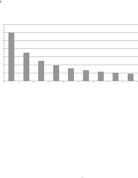
50 FRAUD ANALYTICS
-
0.05
0.10
0.15
0.20
0.25
0.30
0.35
123456789
First digit distribution
Figure 2.3 Benford’s Law Describing the Frequency Distribution of the First Digit
support eligibility typically depends on whether the applicant meets
certain requirements, such as an income below a certain threshold.
Therefore, data may be tampered with in order for the application
to comply with these requirements. It is exactly such types of fraud
that are prone to detection using Benford’s law, since the manipulated
or made-up numbers will not comply with the expected observed
frequency of the first digit as expressed by Benford’s law.
The mathematical formula describing this law expresses the
probability P(d) of the leading digit dto occur to be equal to:
P(d)=log10 1+1
d
Benford’s law can be used as a screening tool for fraud detection
(Jamain 2001). It is a partially negative rule, like many other rules,
meaning that if Benford’s law is not satisfied, then it is probable that
the involved data were manipulated and further investigation or
testing is required. Conversely, if a data set complies with Benford’s
law, it can still be fraudulent. Note that Benford’s law applies to a
data set, meaning that a sufficient amount of numbers related to an
individual case need to be gathered in order for Benford’s law to be
meaningful, which is typically the case when dealing with financial
statements, for instance.
A deviation from Benford’s law does not necessarily mean that
the data have been tampered with. It may also attract the analyst’s

DATA COLLECTION, SAMPLING, AND PREPROCESSING 51
attention toward data quality issues resulting from merging several
data sets in a single structured data table, toward duplicate data,
and so on. Hence, it may definitely be worthwhile for several pur-
poses to control compliance with Benford’s law during the data-
preprocessing phase.
DESCRIPTIVE STATISTICS
Similar to Benford’s law and in addition to the preparatory visual
data exploration, several descriptive statistics might be calculated
that provide basic insight or feeling for the data. Plenty of descriptive
statistics exist to summarize or provide information with respect
to a particular characteristic of the data, and therefore descriptive
statistics should be assessed together—in support and completion of
each other.
Basic descriptive statistics are the mean and median value of con-
tinuous variables, with the median value less sensitive to extreme val-
ues but then as well not providing as much information with respect to
the full distribution. Complementary to the mean value, the variation
or the standard deviation provide insight with respect to how much
the data is spread around the mean value. Likewise, percentile values
such as the 10, 25, 75, and 90 percentile, provide further information
with respect to the distribution and as a complement to the median
value.
Specific descriptive statistics exist to express the symmetry or
asymmetry of a distribution, such as the skewness measure, as well
as the peakedness or flatness of a distribution—for example, the
kurtosis measure. However, the exact values of these measures are
likely a bit harder to interpret than for instance the value of the mean
and standard deviation. This limits their practical use. Instead, one
could more easily assess these aspects by inspecting visual plots of the
distributions of the involved variables.
When dealing with categorical variables, instead of the median and
the mean value one may calculate the mode, which is the most fre-
quently occurring value. In other words, the mode is the most typical
value for the variable at hand. The mode is not necessarily unique,
since multiple values can result in the same maximum frequency.

52 FRAUD ANALYTICS
MISSING VALUES
Missing values can occur because of various reasons. The information
can be nonapplicable. For example, when modeling amount of fraud
for users, then this information is only available for the fraudulent
accounts and not for the nonfraudulent accounts since it is not appli-
cable there. The information can also be undisclosed. For example, a
customer decided not to disclose his or her income because of privacy.
Missing data can also originate because of an error during merging
(e.g., typos in name or ID).
Some analytical techniques (e.g., decision trees) can deal directly
with missing values. Other techniques need some additional prepro-
cessing. The following are the most popular schemes to deal with
missing values (Little and Rubin 2002).
◾Replace (Impute)
This implies replacing the missing value with a known
value. For example, consider the example in Table 2.1. One
could impute the missing credit bureau scores with the average
or median of the known values. For marital status, the mode can
then be used. One could also apply regression-based imputation
whereby a regression model is estimated to model a target vari-
able (e.g., credit bureau score) based on the other information
available (e.g., age, income). The latter is more sophisti-
cated, although the added value from an empirical viewpoint
(e.g., in terms of model performance) is questionable.
◾Delete
This is the most straightforward option and consists of delet-
ing observations or variables with lots of missing values. This, of
course, assumes that information is missing at random and has
no meaningful interpretation and/or relationship to the target.
◾Keep
Missing values can be meaningful. For example, a customer
did not disclose his/her income because he/she is currently
unemployed. This fact may have a relation with fraud and
needs to be considered as a separate category.

DATA COLLECTION, SAMPLING, AND PREPROCESSING 53
Table 2.1 Dealing with Missing Values
ID Age Income Marital Status Credit Bureau Score Fraud
134 1,800 ?620 Yes
228 1,200 Single ?No
322 1,000 Single ?No
460 2,200 Widowed 700 Yes
558 2,000 Married ?No
644 ? ? ? No
722 1,200 Single ?No
826 1,500 Married 350 No
934 ?Single ?Yes
10 50 2,100 Divorced ?No
As a practical way of working, one can first start with statistically
testing whether missing information is related to the target variable or
not (using, e.g., a Chi-squared test, see the section on categorization).
If yes, then we can adopt the keep strategy and make a special cate-
gory for it. If not, one can depending on the number of observations
available, decide to either delete or impute.
OUTLIER DETECTION AND TREATMENT
Outliers are extreme observations that are very dissimilar to the rest of
the population. Actually, two types of outliers can be considered:
◾Valid observations, e.g., salary of boss is US$1,000,000
◾Invalid observations, e.g., age is 300 years
Both are univariate outliers in the sense that they are outlying on
one dimension. However, outliers can be hidden in unidimensional
views of the data. Multivariate outliers are observations that are outly-
ing in multiple dimensions. For example, Figure 2.4 gives an example
of two outlying observations considering both the dimensions of
income and age.
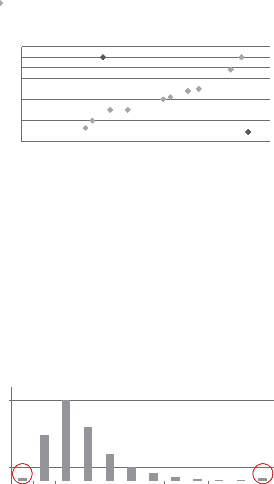
54 FRAUD ANALYTICS
0
500
1000
1500
2000
2500
3000
3500
4000
4500
0 10203040506070
Income
Age
Income versus age
Figure 2.4 Multivariate Outliers
Two important steps in dealing with outliers are detection and
treatment. A first obvious check for outliers is to calculate the min-
imum and maximum values for each of the data elements. Various
graphical tools can be used to detect outliers. Histograms are a first
example. Figure 2.5 presents an example of a distribution for age
whereby the circled areas clearly represent outliers.
Another useful visual mechanism is a box plot. A box plot repre-
sents three key quartiles of the data: the first quartile (25 percent of
the observations have a lower value), the median (50 percent of the
observations have a lower value), and the third quartile (75 percent
0
500
0–5
20–25
25–30
30–35
35–40
40–45
45–50
50–55
55–60
60–65
65–70
150–200
1000
1500
2000
2500
3000
3500
Frequency distribution age
Figure 2.5 Histogram for Outlier Detection

DATA COLLECTION, SAMPLING, AND PREPROCESSING 55
of the observations have a lower value). All three quartiles are rep-
resented as a box. The minimum and maximum value are then also
added unless they are too far away from the edges of the box. Too far
away is then quantified as more than 1.5 ×Interquartile Range (IQR =
Q3–Q1). Figure 2.6 gives an example of a box plot where three outliers
can be seen.
Another way is to calculate z-scores, measuring how many stan-
dard deviations an observation lies away from the mean, as follows:
zi=xi−𝜇
𝜎,
where 𝜇represents the average of the variable and 𝜎its standard devi-
ation. An example is given in Table 2.2. Note that, by definition, the
z-scores will have a mean of zero and unit standard deviation.
1,5 × IQR
Min Q1Q3
M
Outliers
Figure 2.6 Box Plots for Outlier Detection
Table 2.2 z-Scores for Outlier Detection
ID Age z-Score
130 (30 – 40)/10 =–1
250 (50 – 40)/10 =+1
310 (10 – 40)/10 =–3
440 (40 – 40)/10 =0
560 (60 – 40)/10 =+2
680 (80 – 40)/10 =+4
…
𝜇=40
𝜎=10
𝜇=0
𝜎=1

56 FRAUD ANALYTICS
A practical rule of thumb, then, defines outliers when the absolute
value of the z-score |z| is bigger than three. Note that the z-score relies
on the normal distribution.
These methods all focus on univariate outliers. Multivariate
outliers can be detected by fitting regression lines and inspecting the
observations with large errors (using, e.g., a residual plot). Alternative
methods are clustering or calculating the Mahalanobis distance. Note,
however, that although potentially useful, multivariate outlier detec-
tion is typically not considered in many modeling exercises due to the
typical marginal impact on model performance.
Some analytical techniques (e.g., decision trees, neural networks,
SVMs) are fairly robust with respect to outliers. Others (e.g., linear/
logistic regression) are more sensitive to them. Various schemes exist
to deal with outliers. It highly depends on whether the outlier repre-
sents a valid or invalid observation. For invalid observations (e.g., age
is 300 years), one could treat the outlier as a missing value using any of
the schemes discussed in the previous section. For valid observations
(e.g., income is US$1,000,000), other schemes are needed. A popular
scheme is truncation/capping/winsorizing. One hereby imposes both
a lower and upper limit on a variable and any values below/above
are brought back to these limits. The limits can be calculated using
the z-scores (see Figure 2.7), or the IQR (which is more robust than the
z-scores) as follows:
Upper/Lower limit =M±3s, with M=median and s=IQR/(2 ×
0.6745) (Van Gestel and Baesens 2009). A sigmoid transformation
ranging between 0 and 1 can also be used for capping as follows:
f(x)= 1
1+e−x
In addition, expert-based limits based on business knowledge
and/or experience can be imposed.
An important remark concerning outliers is the fact that not all
invalid values are outlying and, as such, may go unnoted if not explic-
itly looked into. For instance, a clear issue exists when observing cus-
tomers with values gender =male and pregnant =yes. Which value is
invalid, either the value for gender or pregnant, cannot be determined,
but it needs to be noted that both values are not outlying and therefore
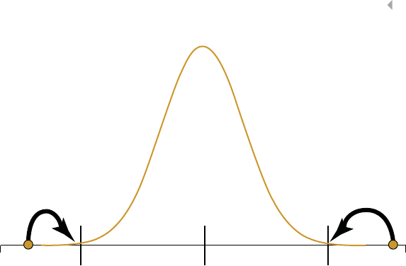
DATA COLLECTION, SAMPLING, AND PREPROCESSING 57
μμ–3σμ+3σ
Figure 2.7 Using the z-Scores for Truncation
such a conflict will not be noted by the analyst unless some explicit
precautions are taken. In order to detect particular invalid combina-
tions, one may construct a set of rules that are formulated based on
expert knowledge and experience (similar to a fraud detection rule
engine in fact), which is applied to the data to check and alert for
issues. In this particular context, a network representation of the vari-
ables may be of use to construct the rule set and reason upon relations
that exist between the different variables, with links representing con-
straints that apply to the combination of variable values and resulting
in rules added to the rule set.
RED FLAGS
An important remark with respect to outlier treatment is to be made,
which particularly holds in a fraud detection setting. As discussed
in the introductory chapter, fraudsters may be detected by the very
fact that their behavior is different or deviant from nonfraudsters,
although most likely only slightly or in a complex (multivariate)
manner since they will cover their tracks to remain undetected.
These deviations from normality are called red flags of fraud and are
probably the most successful and widespread tool that is being used

58 FRAUD ANALYTICS
to detect fraud. As discussed in Grabosky and Duffield (2001) in the
broadest terms, the fundamental red flag of fraud is the anomaly,
that is, a variation from predictable patterns of behavior or, simply,
something that seems out of place. Some examples of red flags follow:
Tax evasion fraud red flags:
◾An identical financial statement, since fraudulent companies
copy financial statements of nonfraudulent companies to look
less suspicious
◾Name of an accountant is unique, since this might concern a
nonexisting accountant
Credit card fraud red flags:
◾A small payment followed by a large payment immediately after,
since a fraudster might first check whether the card is still active
before placing a bet
◾Regular rather small payments, which is a technique to avoid
getting noticed
Telecommunications-related fraud may be reflected in the
following red-flag activities (Grabosky and Duffield 2001):
◾Long-distance access followed by reverse call charges accepted
from overseas
◾High-volume usage over short periods before disconnection
◾A large volume of calls where one call begins shortly after the
termination of another
◾The nonpayment of bills
Such red-flag activities are typically translated in expert rules and
included in a rule engine as discussed in Chapter 1. When red flags
and expert rules are defined, the reasoning behind the red flag or
rule should be documented in order to inform the inspectors about
the underlying reasons or causes of suspicion underlying the red flag
that is raised, so they can focus their investigations on these causes
for suspicion.
Descriptive or unsupervised learning techniques will be discussed
in Chapter 3, including several approaches that aim at detecting
such slight or complex deviations from regular behavior associated

DATA COLLECTION, SAMPLING, AND PREPROCESSING 59
with fraud. When handling valid outliers in the data set using the
treatment techniques discussed before, we may impair in fact the
ability of descriptive analytics in finding anomalous fraud patterns.
Therefore, one should be extremely careful in treating valid outliers
when applying unsupervised learning techniques to build a fraud
detection model. This is true even when handling univariate outliers,
since these might be not by themselves but in combination with other
variables in a multivariate manner related to and as such be used to
uncover fraud. Invalid outliers, on the contrary, can straightforwardly
be treated as discussed above as missing values, preferably by including
an indicator that the value was missing or even more precisely an
invalid outlier. This allows users to test if there is any relation at all
between an invalid value and fraud.
STANDARDIZING DATA
Standardizing data is a data preprocessing activity targeted at scaling
variables to a similar range. Consider, for example, two variables gen-
der (coded as 0/1) and income (ranging between 0 and US$1,000,000).
When building logistic regression models using both information ele-
ments, the coefficient for income might become very small. Hence,
it could make sense to bring them back to a similar scale. The following
standardization procedures could be adopted:
◾Min/Max standardization
Xnew =Xold −min(Xold)
max(Xold)−min(Xold)(newmax −newmin)+newmin,
whereby newmax and newmin are the newly imposed maxi-
mum and minimum (e.g., 1 and 0).
◾z-score standardization
◾Calculate the z-scores (see the previous section).
◾Decimal scaling
◾Divide by a power of 10 as follows: Xnew =Xold
10n,withnthe
number of digits of the maximum absolute value.
Again, note that standardization is especially useful for regression-
based approaches but is not needed for decision trees, for example.

60 FRAUD ANALYTICS
CATEGORIZATION
Categorization (also known as coarse-classification, classing, grouping,
or binning) can be done for various reasons. For categorical vari-
ables, it is needed to reduce the number of categories. Consider, for
example, the variable country of origin having 50 different values. When
this variable would be put into a regression model, one would need
49 dummy variables (50 – 1 because of the collinearity), which would
necessitate the estimation of 49 parameters for only one variable. With
categorization, one would create categories of values such that less
parameters will have to be estimated and a more robust model is
obtained.
For continuous variables, categorization may also be very benefi-
cial. Consider, for example, the age variable and the observed amount
of fraudulent cases as depicted in Figure 2.8. Clearly, there is a non-
monotonous relation between risk of fraud and age. If a nonlinear
model (e.g., neural network, support vector machine) would be used,
then the nonlinearity can be perfectly modeled. However, if a regres-
sion model would be used (which is typically more common because
of its interpretability), then since it can only fit a line, it will miss out
on the nonmonotonicity. By categorizing the variable into ranges, part
of the nonmonotonicity can be taken into account in the regression.
Hence, categorization of continuous variables can be useful to model
nonlinear effects into linear models.
0
0.005
0.01
0.015
0.02
0.025
0.03
0.035
15 25 35 45 55 65 75
Fraud risk versus age
Figure 2.8 Default Risk Versus Age

DATA COLLECTION, SAMPLING, AND PREPROCESSING 61
Various methods can be used to do categorization. Two very basic
methods are equal interval binning and equal frequency binning.
Consider, for example, the income values 1,000, 1,200, 1,300, 2,000,
1,800, 1,400. Equal interval binning would create two bins with the
same range, Bin 1: 1,000, 1,500 and Bin 2: 1,500, 2,000, whereas equal
frequency binning would create two bins with the same number of
observations as follows, Bin 1: 1,000, 1,200, 1,300, Bin 2: 1,400, 1,800,
2,000. However, both methods are quite basic and do not take into
account a target variable (e.g., churn, fraud, credit risk).
Many analytics software tools have built-in facilities to do categori-
zation using Chi-squared analysis. A very handy and simple approach
(available in Microsoft Excel) is to use pivot tables. Consider the
examples in Tables 2.3 and 2.4.
Table 2.3 Coarse Classifying the Product Type Variable
Customer ID Age Product Type …Fraud
C1 44 clothes No
C2 20 books No
C3 58 music Yes
C4 26 clothes No
C5 30 electro Yes
C6 32 games No
C7 48 books Yes
C8 60 clothes No
…
Table 2.4 Pivot Table for Coarse Classifying the Product Type
Variable
Clothes Books Music Electro Games …
Good 1,000 2,000 3,000 100 5,000
Bad 500 100 200 80 800
Odds 220 15 1.25 6.25

62 FRAUD ANALYTICS
One can then construct a pivot table and calculate the odds as
follows:
We can then categorize the values based on similar odds. For exam-
ple, category 1 (clothes, electro), category 2 (games), and category 3
(books and music).
Chi-squared analysis is a more sophisticated way to do coarse clas-
sification. Consider, for example, Table 2.5 for coarse classifying a vari-
able product type.
Suppose we want three categories and consider the following
options:
◾Option 1: clothes; books and music; others
◾Option 2: clothes; electro; others
Both options can now be investigated using Chi-squared analy-
sis. The purpose hereby is to compare the empirically observed with
the independence frequencies. For option 1, the empirically observed
frequencies are depicted in Table 2.6.
The independence frequencies can be calculated as follows. The
number of nonfraud observations given that the odds are the same as
in the whole population is 6,300/10,000 ×9,000/10,000 ×10,000 =
5,670. One then obtains Table 2.7.
Table 2.5 Coarse Classifying the Product Type Variable
Attribute Clothes Books Music Electro Games Movies Total
No-fraud 6,000 1,600 350 950 90 10 9,000
Fraud 300 400 140 100 50 10 1,000
No-fraud: Fraud odds 20:1 4:1 2.5:1 9.5:1 1.8:1 1:1 9:1
Table 2.6 Empirical Frequencies Option 1 for Coarse
Classifying Product Type
Attribute Clothes Books & Music Others Total
No-fraud 6,000 1,950 1,050 9000
Fraud 300 540 160 1,000
Total 6,300 2,490 1,210 10,000

DATA COLLECTION, SAMPLING, AND PREPROCESSING 63
Table 2.7 Independence Frequencies Option 1 for Coarse
Classifying Product Type
Attribute Clothes Books & Music Others Total
No-fraud 5,670 2,241 1,089 9,000
Fraud 630 249 121 1,000
Total 6,300 2,490 1,210 10,000
The more the numbers in both tables differ, the less independence,
hence better dependence and a better coarse classification. Formally,
one can calculate the Chi-squared distance as follows:
◾𝜒2=(6000 −5670)2
5670 +(300 −630)2
630 +(1950 −2241)2
2241
+(540 −249)2
249 +(1050 −1089)2
1089 +(160 −121)2
121 =583
Likewise, for option 2, the calculation becomes:
◾𝜒2=(6000 −5670)2
5670 +(300 −630)2
630 +(950 −945)2
945
+(100 −105)2
105 +(2050 −2385)2
2385 +(600 −265)2
265 =662
So, based on the Chi-squared values, option 2 is the better cate-
gorization. Note that formally, one needs to compare the value with
a Chi-squared distribution with k−1 degrees of freedom with kthe
number of values of the characteristic.
WEIGHTS OF EVIDENCE CODING
Categorization reduces the number of categories for categorical vari-
ables. For continuous variables, categorization will introduce new
variables. Consider, for example, a regression model with age (four
categories, so three parameters) and product type (five categories, so
four parameters) characteristics. The model then looks as follows:
Y=𝛽0+𝛽1Age1+𝛽2Age2+𝛽3Age3+𝛽4Prod1+𝛽5Prod2+𝛽6Prod3
+𝛽7Prod4

64 FRAUD ANALYTICS
Despite having only two characteristics, the model still needs
eight parameters to be estimated. It would be handy to have a mono-
tonic transformation f(.) such that our model could be rewritten
as follows:
Y=𝛽0+𝛽1f(Age1,Age2,Age3)+𝛽2f(Prod1,Prod2,Prod3,Prod4)
The transformation should have a monotonically increasing or
decreasing relationship with Y. Weights-of-evidence coding is one
example of a transformation that can be used for this purpose. This is
illustrated in Table 2.8.
The WOE is calculated as: ln(Dist No-fraud/Dist Fraud). Because of
the logarithmic transformation, a positive (negative) WOE means Dist
No-fraud >(<) Dist Fraud. The WOE transformation thus implements
a transformation monotonically related to the target variable.
The model can then be reformulated as follows:
Y=𝛽0+𝛽1WOEage +𝛽2WOEproduct-type
This gives a more concise model than the model that we started
this section with. However, note that the interpretability of the model
becomes somewhat less straightforward when WOE variables are
being used.
Table 2.8 Calculating Weights of Evidence (WOE)
Age Count Distr. Count No-fraud Distr No-fraud Fraud Distr Fraud WOE
Missing 50 2.50% 42 2.33% 84.12% −57.28%
18–22 200 10.00% 152 8.42% 48 24.74% −107.83%
23–26 300 15.00% 246 13.62% 54 27.84% −71.47%
27–29 450 22.50% 405 22.43% 45 23.20% −3.38%
30–35 500 25.00% 475 26.30% 25 12.89% 71.34%
35–44 350 17.50% 339 18.77% 11 5.67% 119.71%
44+150 7.50% 147 8.14% 31.55% 166.08%
2,000 1,806 194

DATA COLLECTION, SAMPLING, AND PREPROCESSING 65
VARIABLE SELECTION
Many analytical modeling exercises start with tons of variables, of
which typically only a few actually contribute to the prediction of
the target variable. For example, the average fraud model in fraud
detection has somewhere between 10 and 15 variables. The key ques-
tion is how to find these variables. Filters are a very handy variable
selection mechanism. They work by measuring univariate correlations
between each variable and the target. As such, they allow for a quick
screening of which variables should be retained for further analysis.
Various filter measures have been suggested in the literature. One can
categorize them as depicted in Table 2.9.
The Pearson correlation 𝜌Pis calculated as follows:
𝜌P=n
i=1(Xi−X)(Yi−Y)
n
i=1(Xi−X)2n
i=1(Yi−Y)2
It measures a linear dependency between two variables and always
varies between −1and+1. To apply it as a filter, one could select
all variables for which the Pearson correlation is significantly differ-
ent from 0 (according to the p-value), or for example, the ones where
ρP>0.50.
The Fisher score can be calculated as follows:
XG−XB
s2
G+s2
B
,
Table 2.9 Filters for Variable Selection
Continuous Target
(e.g., CLV, LGD)
Categorical Target (e.g.,
churn, fraud, credit risk)
Continuous variable Pearson correlation Fisher score
Categorical variable Fisher score/ANOVA Information value
Cramer’s V
Gain/entropy

66 FRAUD ANALYTICS
where XG(XB)represents the average value of the variable for the non-
fraudsters (fraudsters) and s2
G(s2
B)the corresponding variances. High
values of the Fisher score indicate a predictive variable. To apply it as
a filter, one could, for example, keep the top 10 percent. Note that
the Fisher score may generalize to a well-known analysis of variance
(ANOVA) in case a variable has multiple categories.
The information value (IV) filter is based on weights of evidence
and is calculated as follows:
IV =
k
i=1
(Dist Goodi−Dist Badi)×WOEi,
whereby krepresents the number of categories of the variable. For the
example discussed in Table 2.10, the calculation becomes as shown.
The following rules of thumb apply for the information value:
◾<0.02: unpredictive
◾0.02 – 0.1: weak predictive
◾0.1 – 0.3: medium predictive
◾+0.3: strong predictive
Note that the information value assumes that the variable has been
categorized. It can actually also be used to adjust/steer the catego-
rization so as to optimize the IV. Many software tools will provide
Table 2.10 Calculating the Information Value Filter Measure
Age Count Distr. No-fraud Distr Fraud Distr WOE IV
Count No-fraud Fraud
Missing 50 2.50% 42 2.33% 84.12% −57.28% 0,0103
18–22 200 10.00% 152 8.42% 48 24.74% −107.83% 0,1760
23–26 300 15.00% 246 13.62% 54 27.84% −71.47% 0,1016
27–29 450 22.50% 405 22.43% 45 23.20% −3.38% 0,0003
30–35 500 25.00% 475 26.30% 25 12.89% 71.34% 0,0957
35–44 350 17.50% 339 18.77% 11 5.67% 119.71% 0,1568
44+150 7.50% 147 8.14% 31.55% 166.08% 0,1095
Information Value 0,6502

DATA COLLECTION, SAMPLING, AND PREPROCESSING 67
interactive support to do this, whereby the modeler can adjust the
categories and gauge the impact on the IV. To apply it as a filter,
one can calculate the information value of all (categorical) variables
and only keep those for which the IV >0.1 or, for example, the top
10 percent.
Another filter measure based on Chi-squared analysis is Cramer’s V.
Consider, for example, the contingency table depicted in Table 2.11 for
online/offline transaction versus nonfraud/fraud.
Similar to the example discussed in the section on categorization,
the Chi-squared value for independence can then be calculated as
follows:
𝜒2=(500 −480)2
480 +(100 −120)2
120 +(300 −320)2
320 +(100 −80)2
80
=10.41
This follows a Chi-squared distribution with k– 1 degrees of
freedom, with kbeing the number of classes of the characteristic.
The Cramer’s V measure can then be calculated as follows:
Cramer′sV =𝜒2
n=0.10,
with nthe number of observations in the data set. Cramer’s V is always
bounded between 0 and 1 and higher values indicate better predictive
power. As a rule of thumb, a cut-off of 0.1 is commonly adopted. One
can then again select all variables where Cramer’s V is bigger than 0.1,
or consider, for example, the top 10 percent. Note that the Informa-
tion Value and Cramer’s V typically consider the same characteristics
as most important.
Table 2.11 Contingency Table for Marital Status
versus Good/Bad Customer
Nonfraud Fraud Total
Offline 500 100 600
Online 300 100 400
Total 800 200 1000
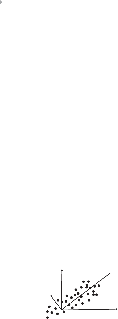
68 FRAUD ANALYTICS
Filters are very handy, as they allow reduction in the number
of dimensions of the data set early in the analysis in a quick way.
Their main drawback is that they work univariately and typically
do not consider correlation between the dimensions individually,
for example. Hence, a follow-up input selection step during the
modeling phase will be necessary to further refine the characteristics.
Also worth mentioning here is that other criteria may play a role in
selecting variables, such as regulatory compliance and privacy issues.
Note that different regulations may apply in different geographical
regions and hence should be checked. Also operational issues could be
considered. For example, trend variables could be very predictive but
might require too much time to be computed in a real-time, online
fraud detection environment.
PRINCIPAL COMPONENTS ANALYSIS
An alternative method for input or variable selection is principal com-
ponent analysis, which is a technique to reduce the dimensionality of
data by forming new variables that are linear composites of the orig-
inal variables. These new variables describe the main components or
dimensions that are present in the original data set, hence its name.
The main dimensions may and often are different from the imposed
measurement dimensions, and as such are obtained as a linear com-
bination of those. Figure 2.9 provides a two-dimensional illustration
of this. The two measurement dimensions represented by the Xand Y
axes do not adequately capture the actual dimensions or components
present in the data. These are clearly situated in a 45-degree angle
X
YPC1
PC2
Figure 2.9 Illustration of Principal Component Analysis in a Two-Dimensional Data Set

DATA COLLECTION, SAMPLING, AND PREPROCESSING 69
compared to the Xand Ydimensions and are described or captured
by the two principal components PC1and PC2.
The maximum number of new variables that can be formed or
derived from the original data (i.e., the number of principal compo-
nents) is equal to the number of original variables. However, when the
aim is data reduction, then typically a reduced set of principal compo-
nents is sufficient to replace the original larger set of variables, since
most of the variance in the original set of variables will be explained
by a limited number of principal components. In other words, most
of the information that is contained in the large set of original vari-
ables typically can be summarized by a small number of new variables.
To explain all the variance in the original data set, the full set of prin-
cipal components is needed, but some of these will only account for a
very small fraction of variance and therefore can be left out, leading to
a reduced dimensionality or number of variables in the data set.
Example: A data set contains 80 financial ratio variables describ-
ing the financial situation or health of a firm, which may be indica-
tive or relevant for detecting fraud. However, many of these financial
ratios are typically strongly correlated. In other words, many of these
ratios overlap, meaning that they basically express the same informa-
tion. This may be explained by the fact that these ratios are derived
from and summarize the same basic information. Therefore, one could
prefer to combine or summarize the original large set of ratios by a
reduced number of financial indices, as can be done by performing a
principal component analysis.
Moreover, the new limited set of financial indices should prefer-
ably be uncorrelated, such they can be included in a fraud-detection
model without causing the final model to become unstable. Correlation
among the explanatory or predictor variables, which is called multi-
collinearity, may result in unstable models. The stability or robustness
of a model refers to the stability of the exact values of the param-
eters of the model that are being estimated based on the sample of
observations. If the values of these parameters heavily depend on the
exact sample of observations used to induce the model, then the model
is called unstable. The values of the parameters, in fact, express the
relation between the explanatory or predictor variables and the depen-
dent or target variable. When the exact relation differs strongly for

70 FRAUD ANALYTICS
different samples of observations, then questions arise with respect to
the exact nature and reliability of this presumed relation. When the
explanatory variables included in a model are correlated, typically, the
resulting model is unstable. Therefore, an input selection procedure is
often performed—for example, using the filter approach discussed in
the previous paragraph, or alternatively a new set of factors may be
derived using principal component analysis to address this problem,
since the resulting new variables (i.e., the principal components, will
be uncorrelated among themselves).
Principal components are calculated by making use of the
eigenvector decomposition (which will not be explained within
the scope of this book; interested readers may refer to specialized
literature on principal component analysis and eigenvector decompo-
sition). Let X1,X2,…,Xpbe the mean-corrected, standardized original
variables, and ˝ =cov(X)the corresponding covariance matrix. Let
𝜆1≥𝜆2≥…≥𝜆p≥0bethepeigenvalues of ˝ and e1,e2,…,epthe
corresponding eigenvectors. The principal components PCj,j=1…p,
corresponding with and in fact replacing the variables X1,X2,…,Xp
are then given by:
PCj=e′jX=ej1X1+ej2X2+···+ejpXp=X′ej
The eigenvectors express the importance of each of the original
variables in the construction of the new variables. The eigenvectors
determine how the original variables are combined into new variables,
and in what proportions.
The observed variance in data set Xthat is explained by principal
component PCjis equal to the corresponding eigenvalue 𝜆j.Thetotal
variance or information in the data will not change and remain con-
stant as the sum of the variances of the principal components—that
is, the new variables—is equal to the sum of the variances of the origi-
nal variables. Also note that the covariance or correlation between two
principal components is equal to zero, cov(PCi,PCj)=0fori≠j.
For each observation in the data set, the values for the new vari-
ables can be calculated. These values are called the PC scores and can
be calculated by making use of the eigenvectors as weights on the
mean-corrected data.

DATA COLLECTION, SAMPLING, AND PREPROCESSING 71
Example: A data set consists of two original variables X1and X2,
which we will replace by two principal components. The first step
consists of calculating the two eigenvectors e1and e2of the covariance
matrix Σ, which can be done straightforwardly using the avail-
able observations in the data set. As such, we get e1=(e11,e12)=
(0.562,0.345)and e2=(e21,e22)=(−0.345,0.562). Subsequently, in
a second step the PC scores for the two principal components (i.e.,
the two new variables) are calculated as a function of the original,
mean-corrected, values (x1,x2):
PC1=e11x1+e12x2=0.562x1+0.345x2
PC2=e21x1+e22x2=−0.345x1+0.562x2
Filling out the values x1and x2for the two original variables for
each observation in the data set then gives the new observations with
the values for the new variables.
How does the transformation of the two original variables in the
above example lead to reducing the data set and to select inputs?
By looking at the eigenvalues, one may decide about leaving out new
variables. If in the above example the eigenvalue corresponding to PC1
is significantly larger than the eigenvalue corresponding to PC2(i.e., if
𝜆1≫𝜆
2), then it can be decided to drop PC2from the further analysis.
Note from this simple example that replacing the original variables
with a (reduced) set of uncorrelated principal components comes at
a price—reduced interpretability. The principal component variables
derived from the original set of variables cannot easily be interpreted,
since they are calculated as a weighted linear combination of the origi-
nal variables. In the previous example, only two original variables were
combined into principal components, still allowing some interpretation
of the resulting principal components. But when the analysis spans
tens or even hundreds or thousands of variables, then any interpre-
tation of the resulting components is clearly prohibited. As discussed
in Chapter 1, in certain settings this might be unacceptable, since the
analysts using the resulting model can no longer interpret it. However,
when interpretability is no concern, then principal component analysis
is a powerful data reduction tool that will yield a better model in terms
of stability as well as predictive performance.

72 FRAUD ANALYTICS
RIDITS
As an alternative to weights of evidence values, one may adopt another
approach to assign numerical values to categorical ordinal variables,
called RIDIT scoring, introduced by Bross (1958), who coined the term
RIDIT in analogy to logit and probit. The following discussion of RIDITs
and PRIDITs is based on a study by Brocket et al. (2002), who adopted
and adapted RIDITs for fraud detection in an unsupervised setting.
The RIDIT scoring mechanism incorporates the ranked nature of
responses, that is, categories of an ordinal categorical variable. Assume
the different response categories are ordered in decreasing likelihood of
fraud suspicion so that a higher categorical response indicates a lesser
suspicion of fraud. In ranking the categories from high- to low-fraud
risk, one may use expert input or historical observed fraud rates. The
RIDIT score for a categorical response value ito variable t,witĥ
ptj indi-
cating the proportion of the population having value ifor variable t,is
then calculated as follows:
Bti =
j<i
̂
ptj −
j>i
̂
ptj i=1,2,…,kt
The above formula transforms a set of categorical responses into
a set of meaningful numerical values in the interval [–1,1], reflect-
ing the relative abnormality of a particular response. Intuitively, the
RIDIT score can be interpreted to be an adjusted or transformed percen-
tile score.
Example: A binary response fraud indicator variable with value yes
occurring for 10 percent of the cases and considered by experts more
indicative of fraud than a value no, occurring for the other 90 percent of
the cases, results in RIDIT scores Bt1(“yes”)=−0.9andBt2(“no”)=0.1.
For a similar binary fraud indicator with 50 percent of the cases having
a value “yes” and 50 percent having a value “no,” the resulting RIDIT
scores are Bt1(“yes”)=−0.5andBt2(“no”)=0.5. This clearly indicates
that a response “yes” on the first indicator variable is more abnormal
or indicative of fraud than a response “yes” on the second indicator,
and as such the transformation yields RIDIT scores that can be easily
included in a quantitative model and make sense from an operational
or expert perspective.

DATA COLLECTION, SAMPLING, AND PREPROCESSING 73
Also for ordinal categorical variables with more than two categor-
ical values RIDIT scores can be calculated using the above formula.
RIDIT scores may be used to replace the categorical fraud indicator
values, and as such allow these categorical variables to be directly
integrated in any numerical analysis for fraud detection.
Remark that for calculating RIDIT scores the actual target values do
not have to be known, as required for weights of evidence calculation.
Therefore, RIDIT scores can be used in an unsupervised learning setting
and when no labeled historical observations are available.
PRIDIT ANALYSIS
PRIDIT analysis combines the two techniques described in the two
previous paragraphs and results in overall fraud suspicion scores calcu-
lated from a set of ordinal categorical fraud indicators. As such, PRIDIT
analysis may be used to assemble these indicators into a single variable
that can be included in any further analysis. Alternatively, PRIDIT anal-
ysis can be used as a filter approach to reduce the number of indicator
variables included in the further analysis, as well as the final outputted
fraud suspicion score. Given the two first uses, we include PRIDIT
analysis in this chapter although it could be considered an unsuper-
vised learning technique for fraud detection as discussed in Chapter 3.
The reader may refer to Brocket et al. (2002) for an extensive dis-
cussion regarding the mathematical derivation and interpretation of
PRIDIT scores.
Assume that only a set of ordinal categorical fraud indicators is
available, transformed into RIDIT scores as discussed in the above
section. Let F=(fit)denote the matrix of individual RIDIT variable
scores for each of the variables t=1,2,…,m, for each of the cases
i=1,2,…,nto be analyzed and scored for fraud. A straightforward
overall fraud suspicion score aggregating these individual RIDIT scores
for the available fraud indicator variables can simply be calculated
by summing all the individual RIDITs. We then get the PRIDIT score
vector by multiplying the matrix Fwith a unity weight vector W=
(1,1,…,1)′, with the prime indicating the transposed vector, that is:
S=FW

74 FRAUD ANALYTICS
Note that these simple aggregated suspicion scores are equally
dependent on each of the indicator variables, since the weights in
vector W, which determine the impact of an indicator on the resulting
score are all set equal to one. However, clearly not every indicator is
equally related to fraud and therefore serves as a predictor or warning
signal of fraud. Hence, an effective overall suspicion score should not
necessarily assign equal importance to each indicator, on the contrary.
A smarter aggregation of the individual indicators assesses the relative
importance and weighs the indicators accordingly when aggregating
them into a single overall suspicion score.
The intuition underlying the calculation of PRIDIT scores is to
adapt the weights according to the correlation or consistency between
the individual RIDIT scores and the resulting overall score. Basically,
PRIDIT scores assign higher weights to an individual fraud indicator
variable if the RIDIT scores of this variable over all cases included in
the analysis are in line with the resulting overall suspicion score. On
the other hand, when a variable is less consistent with the overall
score, then it receives a lower weight. As elaborated in Brocket et al.
(2002), a meaningful set of weights can be obtained by calculating the
first principal component, as discussed in a previous section, of the
matrix F′F. The first principal component is the weight vector that is
used in calculating the PRIDIT scores, assigning a relative importance
to each indicator according to the intuitive consistency principle
discussed in this paragraph.
The PRIDIT approach can as such be used for variable selection,
since indicators receiving weights that are not significantly different
from zero may be removed from the data set. Alternatively, similar to
principal component analysis to variable reduction, the set of ordinal
indicators aggregated into the PRIDIT score may be replaced by this
score, depending on the purpose and setup of the analysis.
SEGMENTATION
Sometimes the data are segmented before the analytical modeling
starts. A first reason for this could be strategic. For example, banks
might want to adopt special strategies to specific segments of cus-
tomers. It could also be motivated from an operational viewpoint.

DATA COLLECTION, SAMPLING, AND PREPROCESSING 75
For example, new customers must have separate models because the
characteristics in the standard model do not make sense operationally
for them. Segmentation could also be needed to take into account
significant variable interactions. For example, if one variable strongly
interacts with a number of others, it might be sensible to segment
according to this variable.
The segmentation can be conducted using the experience and
knowledge from a business expert, or it could be based on statisti-
cal analysis using, for example, decision trees (cf. infra), k-means
clustering or self-organising maps (cf. infra).
Segmentation is a very useful preprocessing activity since one
can now estimate different analytical models each tailored to a
specific segment. However, one needs to be careful with it since, by
segmenting, the number of analytical models to estimate will increase,
which will obviously also increase the production, monitoring, and
maintenance costs.
REFERENCES
Armstrong, J. S. (2001). Selecting Forecasting Methods. In J.S. Armstrong,
ed. Principles of Forecasting: A Handbook for Researchers and Practitioners.
New York: Springer Science +Business Media, pp. 365–386.
Baesens, B. (2014). Analytics in a Big Data World: The Essential Guide to Data Science
and Its Applications. Hoboken, NJ: John Wiley & Sons.
Bolton, R. J., & Hand, D. J. (2002). Statistical Fraud Detection: A Review.
Statistical Science,17 (3): 235–249.
Caron, F., Vanden Broucke, S., Vanthienen, J., & Baesens, B. (2013). Advanced
Rule-Based Process Analytics: Applications for Risk Response Decisions
and Management Control Activities. Expert Systems with Applications,
Submitted.
Chakraborty, G., Murali, P., & Satish, G. (2013). Text Mining and Analysis: Prac-
tical Methods, Examples, and Case Studies Using SAS. Cary, N.C.: SAS Institute.
Cressey, D. R. (1953). Other People’s Money; A Study of the Social Psychology of
Embezzlement. New York: Free Press.
Cullinan, G. J. (1977). Picking Them by Their Batting Averages’ Recency–Frequency–
Monetary Method of Controlling Circulation, Manual Release 2103. New York:
Direct Mail/Marketing Association.
Duffield, G., & Grabosky, P. (2001). The Psychology of Fraud. In Trends and
Issues in Crime and Criminal Justice, Australian Institute of Criminology (199).

76 FRAUD ANALYTICS
Elder IV, J., & Thomas, H. (2012). Practical Text Mining and Statistical Analysis for
Non-Structured Text Data Applications. New York: Academic Press.
Fawcett, T., & Provost, F. (1997). Adaptive Fraud Detection. Data Mining and
Knowledge Discovery 1–3(3): 291–316.
Grabosky, P., & Duffield, G. (2001). Red Flags of Fraud. Trends and Issues in Crime
and Criminal Justice, Australian Institute of Criminology (200).
Han, J., & Kamber, M. (2007). Data Mining: Concepts and Techniques, Third
Edition: Morgan Kaufmann.
Hand, D. (2007, September). Statistical Techniques for Fraud Detection,
Prevention, and Evaluation. Paper presented at the NATO ASI: Mining
Massive Data sets for Security, London, England.
Hand, D. J., Mannila, H., & Smyth, P. (2001). Principles of Data Mining.Cam-
bridge, MA: Bradford.
Jamain, A. (2001). Benford’s Law. London: Imperial College.
Junqué de Fortuny, E., Martens, D., & Provost, F. (2013). Predictive Modeling
with Big Data: Is Bigger Really Better? Big Data 1(4): 215–226.
Little, R. J. A., & Rubin, D. B. (2002). Statistical Analysis with Missing Data, Second
Edition, New York: John Wiley & Sons, p. 408.
Maydanchik, A. (2007). Data Quality Assessment. Bradley Beach, NC: Technics
Publications.
Navarette, E. (2006). Practical Calculation of Expected and Unexpected Losses
in Operational Risk by Simulation Methods (Banca & Finanzas: Documen-
tos de Trabajo, 1(1): pp. 1–12).
Petropoulos, F., Makridakis, S., Assimakopoulos, V., & Nikolopoulos, K. (2014).
“Horses for Courses” in Demand Forecasting. European Journal of Opera-
tional Research.
Schneider, F. (2002). Size and measurement of the informal economy in 110
countries around the world. In Workshop of Australian National Tax Centre,
ANU, Canberra, Australia.
Tan, P.-N. N., Steinbach, M., & Kumar, V. (2005). Introduction to Data Mining.
Boston: Addison Wesley.
Van Gestel, T., & Baesens, B. (2009). Credit Risk Management: Basic Concepts:
Financial Risk Components, Rating Analysis, Models, Economic and Regulatory
Capital. Oxford: Oxford University Press.
Van Vlasselaer, V., Eliassi-Rad, T., Akoglu, L., Snoeck, M., & Baesens, B.
(2015). Gotcha! Network-based Fraud Detection for Social Security
Fraud. Management Science, Submitted.
Verbeke, W., Dejaeger, K., Martens, D., Hur, J., & Baesens, B. (2012). New
Insights into Churn Prediction in the Telecommunication Sector: A Profit
Driven Data Mining Approach. European Journal of Operational Research
218: 211–229.
CHAPTER 3
Descriptive
Analytics for
Fraud Detection
77
INTRODUCTION
Descriptive analytics or unsupervised learning aims at finding unusual
anomalous behavior deviating from the average behavior or norm
(Bolton and Hand 2002). This norm can be defined in various ways.
It can be defined as the behavior of the average customer at a
snapshot in time, or as the average behavior of a given customer
across a particular time period, or as a combination of both. Predictive
analytics or supervised learning, as will be discussed in the following
chapter, assumes the availability of a historical data set with known
fraudulent transactions. The analytical models built can thus only
detect fraud patterns as they occurred in the past. Consequently, it
will be impossible to detect previously unknown fraud. Predictive
analytics can however also be useful to help explain the anomalies
found by descriptive analytics, as we will discuss later.
When used for fraud detection, unsupervised learning is often
referred to as anomaly detection, since it aims at finding anomalous
and thus suspicious observations. In the literature, anomalies are com-
monly described as outliers or exceptions. One of the first definitions
of an outlier was provided by Grubbs (1969), as follows:
“An outlying observation, or outlier, is one that appears to
deviate markedly from other members of the sample in
which it occurs.”
A first challenge when using unsupervised learning is to define the
average behavior or norm. Typically, this will highly depend on the
application field considered. Also the boundary between the norm and
the outliers is typically not clear-cut. As said earlier, fraudsters will try
to blend into the average or norm as good as possible, hereby substan-
tially complicating their detection and the corresponding definition of
the norm. Furthermore, the norm may change over time, so the ana-
lytical models built need to be continuously monitored and updated,
possibly in real-time. Finally, anomalies do not necessarily represent
fraudulent observations. Hence, the usage of unsupervised learning
for fraud detection requires extensive follow-up and validation of the
identified, suspicious observations.
78

DESCRIPTIVE ANALYTICS FOR FRAUD DETECTION 79
Unsupervised learning can be useful for organizations that start
doing fraud detection and thus have no labeled historical data set
available. It can also be used in existing fraud models by uncovering
new fraud mechanisms. This is especially relevant in environments
where fraudsters are continuously adapting their strategies to beat
the detection methods. A first example of this is credit card fraud
whereby fraudsters continuously try out new ways of committing
fraud. Another example is intrusion detection in a cyber-fraud setting.
Supervised methods are based on known intrusion patterns, whereas
unsupervised methods or anomaly detection can identify emerging
cyber threats.
In this chapter, we will explore various unsupervised techniques
to detect fraud.
GRAPHICAL OUTLIER DETECTION PROCEDURES
To detect one-dimensional outliers, a histogram or box plot can be used
(see Chapter 2). Two-dimensional outliers can be detected using a scat-
ter plot. The latter can also be extended to a three-dimensional setting,
whereby spinning facilities can be handy to rotate the graph so as to
facilitate finding the outliers. This is illustrated in Figure 3.1. The plot
clearly shows three outliers marked by asterisks (*) representing claims
with an unusually high amount, a high number of cars of the claimant,
and a small number of days since the previous claim. Clearly, these
claims are suspicious and should be further investigated.
Ideally, graphical methods should be complemented with multidi-
mensional data analysis and online analytical processing (OLAP) facil-
ities. Figure 3.2 shows an example of an OLAP cube representing the
distribution or count of claims based on amount of claim, number of
cars, and recency of previous claim. Once the cube has been popu-
lated from a data warehouse or transactional data source, the following
OLAP operations can be performed:
◾Roll-up: The idea here is to aggregate across one or more dimen-
sions. An example of this is the distribution of amount of claim
and recency aggregated across all number of cars (roll up of
number of cars dimension). Another example is the distribution
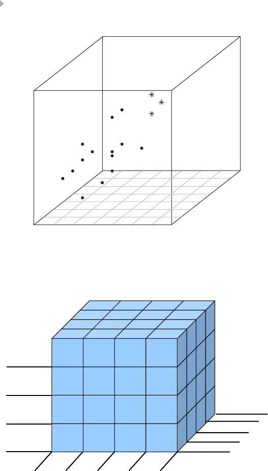
80 FRAUD ANALYTICS
Amount of claim
Number of cars
Number of days
since
previous claim
Figure 3.1 3D Scatter Plot for Detecting Outliers
< 1 month
Between 3 and 6 months
> 6 months
Between 1 and 3 months
≥4
123
Number of cars
Amount of claim
<1,000
Between 1,000
and 5,000
Between 5,000
and 10,000
> 10,000 Count
Most recent claim
Figure 3.2 OLAP Cube for Fraud Detection

DESCRIPTIVE ANALYTICS FOR FRAUD DETECTION 81
of amount of claim aggregated across all number of cars and all
number of days since previous claim (roll up of number of cars
and number of days since previous claim dimensions).
◾Drill-down: This is the opposite of roll-up whereby more detail
is asked for by adding another dimension to the analysis.
◾Slicing: The idea here is to pick a slice along one of the dimen-
sions. An example is to show the distribution of amount and
recency for all claims where the claimant has more than or equal
to four cars (slice along the number of cars dimension).
◾Dicing: The idea here is to fix values for all the dimensions
and create a sub-cube. An example is to show the distribution
of amount, number of cars, and recency for all claims where
amount is between 1,000 and 10,000, number of cars is two or
three, and recency is between one and six months.
Many software tools are available to support OLAP analysis. They
excel in offering powerful visualizations, sometimes even augmented
with virtual reality technology for better detecting relationships in
the data. OLAP tools will also typically implement pivot tables for
multidimensional data analysis. Pivot tables allow analysts to summa-
rize tabular data by cross-tabulating user specified dimensions using
a drag and drop interface. This is illustrated in Figure 3.3 for a credit
card fraud detection data set analyzed in Microsoft Excel. You can see
that the data set has 2,397 observations with 2,364 nonfrauds and
33 frauds. The columns depict the average for the recency, frequency,
and monetary (RFM) variables. Note that the data depicted has
been filtered to non-EU transactions as depicted in the upper-left
corner cell B2. From the results, it can be seen that when looking at
non EU-transactions, fraudulent transactions have a lower average
recency, higher average frequency, and higher average monetary
value when compared to nonfraudulent transactions. These are very
interesting starting insights to further explore fraud patterns in the
data. The pivot table can be easily manipulated using the panel to the
right. Other filters can be defined, columns and rows can be added,
and descriptive statistics or summarization measures can be varied
(e.g., count, minimum, maximum).
Graphical and OLAP methods are handy and easy to work with.
They are ideal tools to explore the data and get preliminary insights.

82
Figure 3.3 Example Pivot Table for Credit Card Fraud Detection

DESCRIPTIVE ANALYTICS FOR FRAUD DETECTION 83
However, they are less formal and only limited to a few dimensions.
They require active involvement of the end-user in detecting the
anomalies. In other words, the user should select the dimensions and
decide on the OLAP routines to be performed. For a large dimensional
data set, this may be a cumbersome exercise. Besides being used dur-
ing preprocessing, OLAP facilities are getting more and more popular
for model post-processing and monitoring, as we will discuss later.
STATISTICAL OUTLIER DETECTION PROCEDURES
A first well-known statistical outlier detection method is calculating
the z-scores, as previously discussed in Chapter 2. Remember, obser-
vations for which the absolute value of the z-score is bigger than 3 can
be considered as outliers. A more formal test is the Grubbs test, which
is formulated as follows (see Grubbs 1950):
H0: There are no outliers in the data set.
HA: There is at least one outlier in the data set.
It starts by calculating the z-score for every observation. Let’s say
that the maximum absolute value of the observed z-scores equals G.
The corresponding observation is then considered an outlier at signifi-
cance level 𝛼if:
G>N−1
N
t2𝛼
2N,N−2
N−2+t2𝛼
2N,N−2
,
where Nrepresents the number of observations, and t2𝛼
2N,N−2is the
critical value of a Student’s t-distribution with N– 2 degrees of free-
dom and significance level equal to α/(2N). If an outlier is detected, it
is removed from the data set and the test can be run again. The test
can also be run for multivariate outliers whereby the z-score can be
replaced by the Mahalanobis distance defined as follows:
(x−x)tS−1(x−x),
where xrepresents the observation, xthe mean vector, and Sthe
covariance matrix. A key weakness of this test is that it assumes an
underlying normal distribution, which is not always the case.
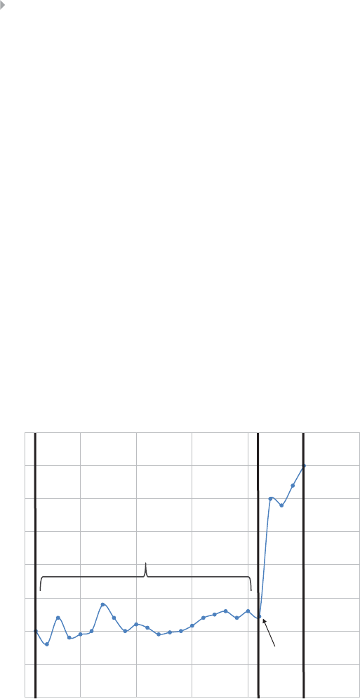
84 FRAUD ANALYTICS
Other statistical procedures fit a distribution, or mixture of distri-
butions (using, e.g., maximum likelihood or expectation-maximization
procedures) and label the observations with small values for the prob-
ability density function as outliers.
Break-Point Analysis
Break-point analysis is an intra-account fraud detection method
(Bolton and Hand, 2001). A break point indicates a sudden change in
account behavior, which merits further inspection. The method starts
from defining a fixed time window. This time window is then split into
an old and new part. The old part represents the local model or profile
against which the new observations will be compared. For example, in
(Bolton and Hand 2001), the time window was set to 24 transactions
whereby 20 transactions made up the local model, and 4 transactions
were used for testing. A Student’s t-test can be used to compare the
averages of the new and old parts. Observations can then be ranked
according to their value of the t-statistic. This is illustrated in Figure 3.4.
0 5 10 15 20 25 30
Amount spent
Time
Local model
Break
point
Figure 3.4 Break-Point Analysis

DESCRIPTIVE ANALYTICS FOR FRAUD DETECTION 85
Peer-Group Analysis
Peer-group analysis was also introduced by Bolton and Hand (2001).
A peer group is a group of accounts that behave similarly to the target
account. When the behavior of the latter starts to deviate substantially
from its peers, an anomaly can be signaled. Peer-group analysis pro-
ceeds in two steps. In step 1, the peer group of a particular account
needs to be identified. This can be accomplished either by using prior
business knowledge or in a statistical way.
For example, in an employee fraud context, people sharing similar
jobs can be grouped as peers. Another example is healthcare fraud
detection, whereby the aim is to detect fraudulent claim behavior of
doctors across geographical regions. Suppose the target observation is
a cardiologist in San Francisco; then its peers are defined as all other
cardiologists in San Francisco. Statistical similarity metrics can also be
used to define peers, but these are typically application specific. Popular
examples here are Euclidean-based metrics (see, e.g., Bolton and Hand
2001; Weston et al. 2008). The number of peers should be carefully
selected. It cannot be too small, or the method becomes too local and
thus sensitive to noise, and also not too large, or the method becomes
too global and thus insensitive to local important irregularities.
In step 2, the behavior of the target account is contrasted with its
peers using a statistical test such a Student’s t-test, or a distance metric
such as the Mahalanobis distance, which works similar.
Let’s work out an example in a credit card context. Assume our
target account has the following time series:
y1,y2,....yn−1,yn
where yirepresents the amount spent at time (e.g., day or week) i.
The aim is now to verify whether the amount spent at time n,yn,is
anomalous. We start by identifying the kpeers of the target account.
These are depicted in gray in the Table 3.1 below, whereby all accounts
have been sorted according to their similarity to the target.
To see whether ynis an outlier, a t-score can be calculated as follows:
yn−x1∶k,n
s,
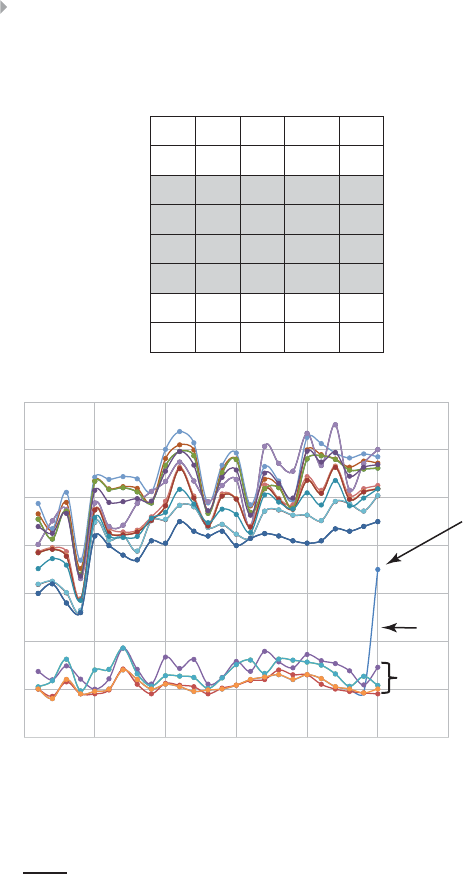
86 FRAUD ANALYTICS
Table 3.1 Transaction Data Set
for Peer-Group Analysis
xm,1 xm,2 …xm,n-1 xm,n
…
xk,1xk,2 xk,n-1 xk,n
…
x2,1 x2,2 x2,n-1 x2,n
x1,1 x1,2 x1,n-1 x1,n
y1y2yn-1 yn
…
Outlier
Peer group
Target account
0 5 10 15 20 25 30
Amount spent
Time
Figure 3.5 Peer-Group Analysis
where x1∶k,nrepresents the average of x1,n,…,xk,nand sthe corre-
sponding standard deviation. Although a Student’s t-distribution can
be used for statistical interpretation, it is recommended to simply order
the observations in terms of their t-score and further inspect the ones
with the highest scores. This is illustrated in Figure 3.5.
A key advantage of peer-group analysis when compared to break-
point analysis is that it tracks anomalies by considering inter-account
instead of intra-account behavior. For example, if one was to compare

DESCRIPTIVE ANALYTICS FOR FRAUD DETECTION 87
transaction amounts for a particular account with previous amounts
on that same account (intra-account), then the spending behavior dur-
ing Christmas will definitely be flagged as anomalous. By considering
peers instead (inter-account), this problem is avoided. It is important
to note that both break-point and peer-group analysis will detect local
anomalies rather than global anomalies. In other words, patterns or
sequences that are not unusual in the global population might still be
flagged as suspicious when they appear to be unusual compared to
their local profile or peer behavior.
Association Rule Analysis
Association rules detect frequently occurring relationships between
items (Agrawal, Imielinski et al. 1993). They were originally intro-
duced in a market basket analysis context to detect which items are
frequently purchased together. The key input is a transactions database
Dconsisting of a transaction identifier and a set of items {i1,i2,…,in}
selected from all possible items I. An association rule is then an
implication of the form XY, whereby x⊂I,Y⊂Iand x∩Y=∅.
xis referred to as the rule antecedent whereas Yis referred to as the
rule consequent. Examples of association rules could be:
◾If a customer has a car loan and car insurance, then the customer
has a checking account in 80 percent of the cases.
◾If a customer buys spaghetti, then the customer buys red wine
in 70 percent of the cases.
◾If a customer visits web page A, then the customer will visit web
page Bin 90 percent of the cases.
It is hereby important to note that association rules are stochastic
in nature. This means that they should not be interpreted as a univer-
sal truth, and are characterized by statistical measures quantifying the
strength of the association. Furthermore, the rules measure correla-
tional associations and should not be interpreted in a causal way.
In a fraud setting, association rules can be used to detect fraud
rings in insurance. The transaction identifier then corresponds to a
claim identifier and the items to the various parties involved such as
the insured, claim adjuster, police officer and claim service provider

88 FRAUD ANALYTICS
Table 3.2 Transactions Database for Insurance Fraud Detection
Claim Identifier Parties Involved
1 insured A, police officer X, claim adjuster 1, auto repair shop 1
2 insured A, claim adjuster 2, police officer X
3 insured A, police officer Y, auto repair shop 1
4 insured A, claim adjuster 1, claim adjuster 1, police officer Y
5 insured B, claim adjuster 2, auto repair shop 2, police officer Z
6 insured A, auto repair shop 2, auto repair shop 1, police officer X
7 insured C, police officer X, auto repair shop 1
8 insured A, auto repair shop 1, police officer Z
9 insured A, auto repair shop 1, police officer X, claim adjuster 1
10 insured B, claim adjuster 3, auto repair shop 1
(e.g., auto repair shop, medical provider, home repair contractor,
etc.). Let’s consider an example of a transactions database as depicted
in Table 3.2.
The goal is now to find frequently occurring relationships or asso-
ciation rules between the various parties involved in the handling of
the claim. This will be solved using a two-step procedure. In step 1,
the frequent item sets will be identified. The frequency of an item set
is measured by means of its support, which is the percentage of total
transactions in the database that contains the item set. Hence, the item
set X has support sif 100×spercent of the transactions in Dcontain X.
It can be formally defined as follows:
support(X)= number of transactions supporting (X)
total number of transactions
Consider the item set {insured A, police officer X, auto repair
shop 1}. This item set occurs in transactions 1, 6, and 9 hereby giving a
support of 3/10 or 30 percent. A frequent item set can now be defined
as an item set of which the support is higher than a minimum value
as specified by the data scientist (e.g., 10 percent). Computationally
efficient procedures have been developed to identify the frequent item
sets (Agrawal, Imielinski et al. 1993).

DESCRIPTIVE ANALYTICS FOR FRAUD DETECTION 89
Once the frequent item sets have been found, the association rules
can be derived in step 2. Multiple association rules can be defined based
on the same item set. Consider the item set {insured A, police officer
X, auto repair shop 1}. Example association rules could be:
If insured AAnd police officer X ⇒auto repair shop 1
If insured AAnd auto repair shop 1 ⇒police officer X
If insured A⇒auto repair shop 1 And police officer X
The strength of an association rule can be quantified by means of
its confidence. The confidence measures the strength of the association
and is defined as the conditional probability of the rule consequent,
given the rule antecedent. The rule X⇒Yhas confidence c if 100×c
percent of the transactions in Dthat contain Xalso contain Y. It can be
formally defined as follows:
confidence (X→Y)=P(YX)= support (X∪Y)
support(X)
Consider the association rule “If insured A And police officer X
⇒auto repair shop 1.” The antecedent item set {insured A, police
officer X} occurs in transactions 1, 2, 6, and 9. Out of these four trans-
actions, three also include the consequent item set {auto repair shop
1}, which results into a confidence of three-fourths, or 75 percent.
Again, the data scientist has to specify a minimum confidence in order
for an association rule to be considered interesting.
Once all association rules have been found, they can be closer
inspected and validated. In our example, the association “If insured
AAnd police officer X⇒auto repair shop 1” does not necessarily
imply a fraud ring, but it’s a least worth the effort to further inspect
the relationship between these parties.
CLUSTERING
Introduction
The aim of clustering is to split up a set of observations into segments
such that the homogeneity within a segment is maximized (cohesive),

90 FRAUD ANALYTICS
and the heterogeneity between segments is maximized (separated)
(Everitt, Landau et al. 2010). Examples of applications in fraud
detection include:
◾Clustering transactions in a credit card setting
◾Clustering claims in an insurance setting
◾Clustering tax statements in a tax-inspection setting
◾Clustering cash transfers in an anti-money laundering setting
Various types of clustering data can be used, such as customer char-
acteristics (e.g., sociodemographic, behavioral, lifestyle, …), account
characteristics, transaction characteristics, etc. A very popular sets of
transaction characteristics used for clustering in fraud detection are
the recency, frequency, and monetary (RFM) variables, as introduced
in Chapter 2.
Note that besides structured information, also unstructured infor-
mation such as emails, call records, and social media information might
be considered. As always in analytics, it is important to carefully select
the data for clustering. The more data the better, although care should
be taken to avoid excessive amounts of correlated data by applying
unsupervised feature selection methods. One very simple approach
here is to simply calculate the Pearson correlation between each pair
of data characteristics and only retain one characteristic in case of a
significant correlation.
When used for fraud detection, a possible aim of clustering may
be to group anomalies into small, sparse clusters. These can then be
further analyzed and inspected in terms of their characteristics and
potentially fraudulent behavior (see Figure 3.6).
Different types of clustering techniques can be applied for fraud
detection. At a high level, they can be categorized as either hierarchical
or nonhierarchical (see Figure 3.7).
Distance Metrics
As said, the aim of clustering is to group observations based on simi-
larity. Hence, a distance metric is needed to quantify similarity. Various
distance metrics have been introduced in the literature for both con-
tinuous and categorical data.

DESCRIPTIVE ANALYTICS FOR FRAUD DETECTION 91
Anomalies
Recency
Frequency
Figure 3.6 Cluster Analysis for Fraud Detection
Clustering
Hierarchical Nonhierarchical
Agglomerative Divisive k-means SOM
Figure 3.7 Hierarchical Versus Nonhierarchical Clustering Techniques
For continuous data, the Minkowski distance or Lpnorm between
two observations xiand xjcan be defined as follows:
D(xi;xj)=n
k=1xik −xjk
p1∕p,
where nrepresents the number of variables. When pequals 1, the
Minkowski distance is also referred to the Manhattan or City block
distance. When pequals 2, the Minkowski distance becomes the
well-known Euclidean distance. Both are illustrated in Figure 3.8. For
the example depicted, the distance measures become:
Euclidean ∶(1500 −1000)2+(10 −5)2̃=500
Manhattan ∶1500 −100+10 −5=505

92 FRAUD ANALYTICS
Manhattan
Euclidean
Manhattan
30 50
10
20
Monetary
Recency
Figure 3.8 Euclidean Versus Manhattan Distance
From this example, it is clear that the amount variable clearly dom-
inates the distance metric since it is measured on a larger scale than
the recency variable. Hence, to appropriately take this into account, it
is recommended to scale both variables to a similar range using any of
the standardization procedures we discussed in Chapter 2. It is obvious
that the Euclidean distance will always be shorter than the Manhat-
tan distance. The Euclidean metric is the most popular metric used for
quantifying the distance between continuous variables. Other less fre-
quently used distance measures are based on the Pearson correlation
or cosine measure.
Besides continuous variables, also categorical variables can be used
for clustering. Let’s first discuss the case of binary variables. These are
often used in insurance fraud detection methods, which are typically
based on a series of red-flag indicators to label a claim as suspicious
or not. Assume we have the following data set with binary red-flag
indicators.
Poor Driving
Record
Premium
Paid
in Cash
Car Purchase
Information
Available
Coverage
Increased
Car Was Never
Inspected
or Seen
Claim 1 Yes No Yes Yes No
Claim 2 Yes Yes No No No
…
A first way to calculate the distance or similarity between claim 1
and 2 is to use the simple matching coefficient (SMC), which simply

DESCRIPTIVE ANALYTICS FOR FRAUD DETECTION 93
calculates the number of identical matches between the variable values
as follows:
SMC(Claim 1,Claim 2)=2∕5.
A tacit assumption behind the SMC is that both states of the vari-
able (Yes versus No) are equally important and should thus both be
considered. Another option is to use the Jaccard index whereby the
No-No match is left out of the computation as follows:
Jaccard(Claim 1,Claim 2)=1∕4.
The Jaccard index measures the similarity between both claims
across those red flags that where raised at least once. It is especially use-
ful in those situations where many red-flag indicators are available and
typically only a few are raised. Consider, for example, a fraud-detection
system with 100 red-flag indicators, of which on average 5 are raised.
If you would use the simple matching coefficient, then typically all
claims would be very similar since the 0–0 matches would dominate
the count, hereby creating no meaningful clustering solution. By using
the Jaccard index a better idea of the claim similarity can be obtained.
The Jaccard index has actually been very popular in fraud detection.
Let’s now consider the case of categorical variables with more
than two values. Assume we have the following data in a medical
insurance setting.
Treatment
Day
Distance between
Clinic and Subject’s
Home
Type of
Diagnosis
Risk
Class
Claim
Submitted by
Claim 1 Sunday Medium Severe CPhone
Claim 2 Wednesday Medium Life
threatening
CEmail
…
A first option here is to code the categorical variables as 0/1 dum-
mies and apply the Manhattan or Euclidean distance metrics discussed
earlier. However, this may be cumbersome in case of categorical vari-
ables with lots of values. Coarse classification might be considered to
reduce the number of dummy variables, but, remember, since we don’t
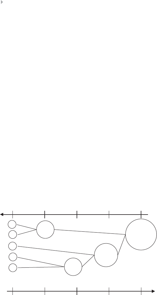
94 FRAUD ANALYTICS
have a target variable in this unsupervised setting, it should be based on
expert knowledge. Another option would be to use the simple match-
ing coefficient (SMC) and count the number of identical matches. In
our case, the SMC would become 2/5.
Many data sets will contain both continuous and categorical vari-
ables, which complicates the distance calculation. One option here is
to code the categorical variables as 0/1 dummies and use a continuous
distance measure. Another option is to use a (weighted) combination
of distance measures, although this is less straightforward and thus less
frequently used.
Hierarchical Clustering
Once the distance measures have been chosen, the clustering process
can start. A first popular set of techniques are hierarchical clustering
methods. Depending on the starting point of the analysis, divisive or
agglomerative hierarchical clustering methods can be used. Divisive
hierarchical clustering starts from the whole data set in one cluster,
and then breaks this up in each time smaller clusters until one obser-
vation per cluster remains (right to left in Figure 3.9). Agglomerative
C2
C3
C4
C5
C1
C2
C3
C4
C5
C4
C5
C1
C2
C3
C4
C5
Step 3 Step 2 Step 1 Step 0Step 4
Step 1 Step 2 Step 3 Step 4Step 0
Agglomerative
Divisive
C1
Figure 3.9 Divisive Versus Agglomerative Hierarchical Clustering

DESCRIPTIVE ANALYTICS FOR FRAUD DETECTION 95
clustering works the other way around, and starts from each obser-
vation in one cluster, and then continues to merge the ones that are
most similar until all observations make up one big cluster (left to right
in Figure 3.9). The optimal clustering solution then lies somewhere in
between the extremes to the left and right, respectively.
Although we have earlier discussed various distance metrics to
quantify the distance between individual observations, we haven’t
talked about how to measure distances between clusters. Also here,
various options are available, as depicted in Figure 3.10. The single
linkage method defines the distance between two clusters as the
smallest possible distance, or the distance between the two most simi-
lar objects. The complete linkage method defines the distance between
two clusters as the biggest distance, or the distance between the two
most dissimilar objects. The average linkage method calculates the
average of all possible distances. The centroid method calculates the
distance between the centroids of both clusters. Finally, Ward’s distance
between two clusters Ciand Cjis calculated as the difference between
the total within cluster sum of squares for the two clusters separately,
and the total within cluster sum of squares obtained from merging the
clusters Ciand Cjinto one cluster Cij. It is calculated as follows:
DWard (Ci,Cj)=
x∈Ci
(x−ci)2+
x∈Cj
(x−cj)2−
x∈Cij
(x−cij)2,
where ci,cj,cij is the centroid of cluster Ci,Cj,andCij, respectively.
Single linkage
Complete linkage
Average linkage
Centroid method
Figure 3.10 Calculating Distances between Clusters

96 FRAUD ANALYTICS
In order to decide on the optimal number of clusters, one could use
a dendrogram or screen plot. A dendrogram is a tree-like diagram that
records the sequences of merges. The vertical (or horizontal scale) then
gives the distance between two clusters amalgamated. One can then
cut the dendrogram at the desired level to find the optimal clustering.
This is illustrated in Figure 3.11 and Figure 3.12 for a birds clustering
1
6
2
4
3
5
chicken
duck
pigeon
parrot
owl
eagle
canary
Figure 3.11 Example for Clustering Birds. The Numbers Indicate the Clustering Steps
chicken pigeonduck owl eaglecanaryparrot
1 2
3
4
5
6
Figure 3.12 Dendrogram for Birds Example. The Thick Black Line Indicates the Optimal
Clustering
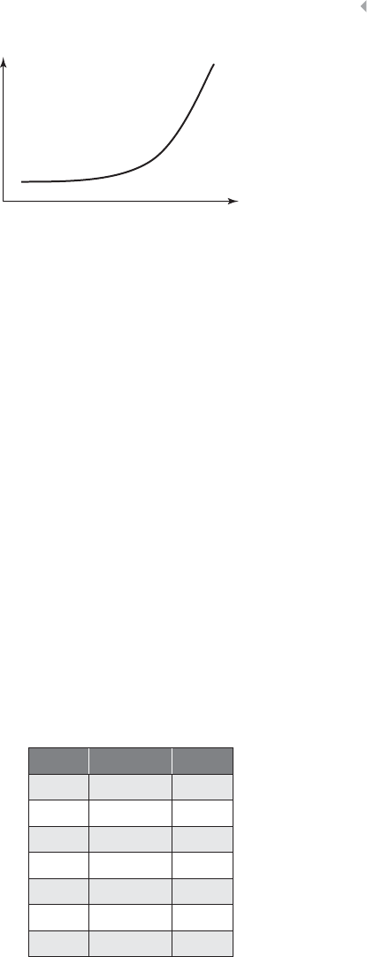
DESCRIPTIVE ANALYTICS FOR FRAUD DETECTION 97
Number of clusters
Distance
Figure 3.13 Scree Plot for Clustering
example. A scree plot is a plot of the distance at which clusters are
merged. The elbow point then indicates the optimal clustering. This is
illustrated in Figure 3.13.
A key advantage of hierarchical clustering is that the number of
clusters does not need to be specified prior to the analysis. A disadvan-
tage is that the methods do not scale very well to large data sets. Also,
the interpretation of the clusters is often subjective and depends on the
business expert and/or data scientist.
Example of Hierarchical Clustering Procedures
To illustrate the various hierarchical clustering procedures discussed,
suppose we have a data set of seven observations, as depicted in
Table 3.3. Figure 3.14 displays the corresponding scatter plot.
The output of the various hierarchical clustering procedures is
depicted in Figure 3.15. As it can be observed, single linkage results
Table 3.3 Data Set for
Hierarchical Clustering
X Y
A 4 4
B 5 4
C 7 5
D 8 5
E11 5
F 2 7
G 1 3
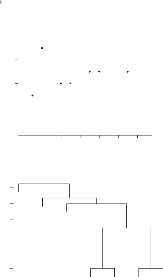
98 FRAUD ANALYTICS
02468
02
AB
CDE
F
G
46810 12
Figure 3.14 Scatter Plot of Hierarchical Clustering Data
Single Linkage: Dendogram
Height
1.0 1.5 2.0 2.5 3.0 3.5
G
F
E
A
B
C
D
Figure 3.15 Output of Hierarchical Clustering Procedures
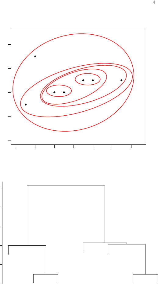
DESCRIPTIVE ANALYTICS FOR FRAUD DETECTION 99
1
2 3
4
5
6
Single Linkage
AB
D
CE
F
G
0246810 12
02468
Complete Linkage: Dendogram
Height
0246810
G
F
E
A
B
C
D
Figure 3.15 (Continued)
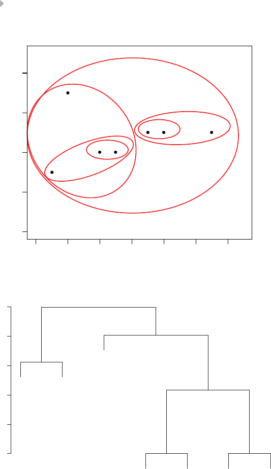
100 FRAUD ANALYTICS
Complete Linkage
1
2
3
4 5
6
F
G
AB
CDE
0246810 12
02468
Average Linkage: Dendogram
Height
123456
F
G
E
A
B
C
D
Figure 3.15 (Continued)
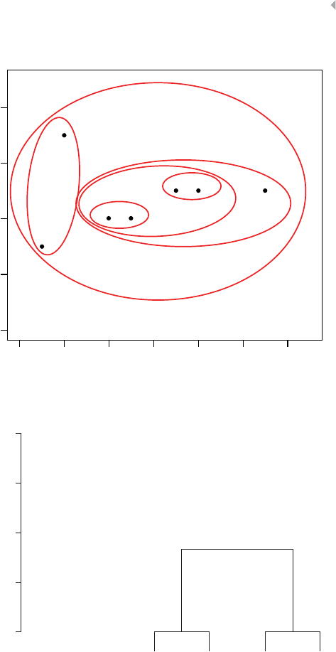
DESCRIPTIVE ANALYTICS FOR FRAUD DETECTION 101
Average Linkage
1 2
3
5 4
6
0246810 12
02468
F
G
AB
CD E
Centroid Method: Dendogram
Height
02345
A
B
C
D
Figure 3.15 (Continued)
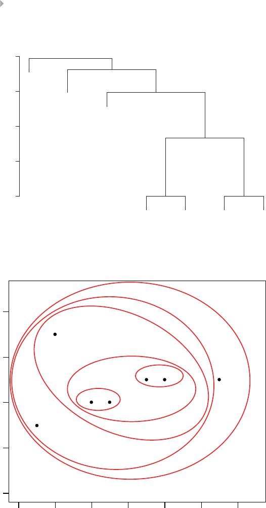
102 FRAUD ANALYTICS
Centroid Method: Dendogram
Height
02345
E
G
F
A
B
C
D
2
1
3
4 5
6
F
G
AB
C D E
Centroid Method
0246810 12
02468
Figure 3.15 (Continued)
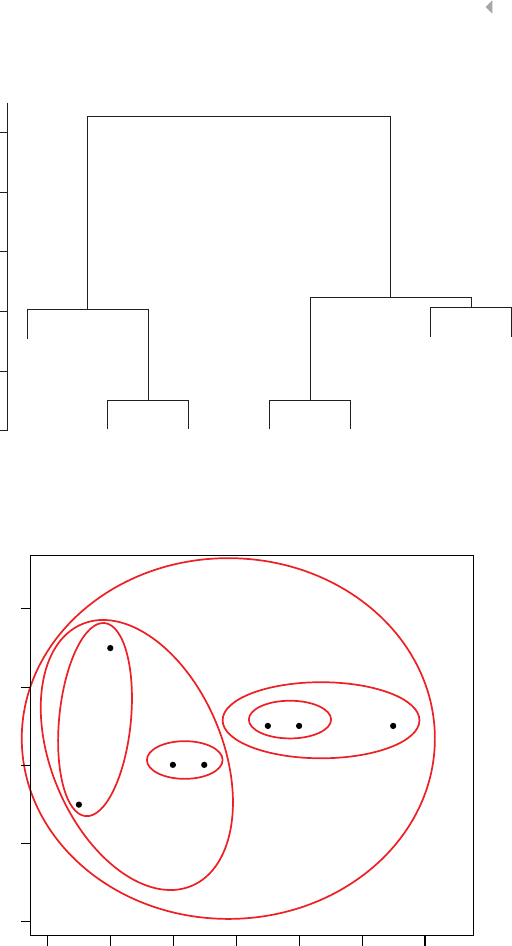
DESCRIPTIVE ANALYTICS FOR FRAUD DETECTION 103
Ward’s Method: Dendogram
Height
02
E
C
D
A
B
F
G
46810
Ward’s Method
2
1
3
4
5
6
F
G
AB
C D E
0246810 12
02468
Figure 3.15 (Continued)

104 FRAUD ANALYTICS
in thin, long, and elongated clusters since dissimilar objects are not
accounted for. Complete linkage will make the cluster tighter, more
balanced and spherical, which is often more desirable. Average linkage
prefers to merge clusters with small variances, which often results in
clusters with similar variance. Although the centroid method seems
similar at first sight, the resulting clustering solution is different as
depicted in the figure. Ward’s method prefers to merge clusters with a
small number of observations and often results into balanced clusters.
k-Means Clustering
k-means clustering is a nonhierarchical procedure that works along the
following steps (see Jain 2010; MacQueen 1967):
1. Select kobservations as initial cluster centroids (seeds).
2. Assign each observation to the cluster that has the closest
centroid (for example, in Euclidean sense).
3. When all observations have been assigned, recalculate the posi-
tions of the kcentroids.
4. Repeat until the cluster centroids no longer change or a fixed
number of iterations is reached.
A key requirement here is that, as opposed to hierarchical cluster-
ing, the number of clusters, k, needs to be specified before the start
of the analysis. This decision can be made using expert based input
or based on the result of another (e.g., hierarchical) clustering pro-
cedure. Typically, multiple values of kare tried out and the result-
ing clusters evaluated in terms of their statistical characteristics and
interpretation. It is also advised to try out different seeds to verify the
stability of the clustering solution. Note that the mean is sensitive to
outliers, which are especially relevant in a fraud detection setting. A
more robust alternative is to use the median instead (k-medoid clus-
tering). In case of categorical variables, the mode can be used (k-mode
clustering). As mentioned, k-means is most often used in combination
with a Euclidean distance metric, which typically results into spherical
or ball-shaped clusters. See Figures 3.16 to 3.22.
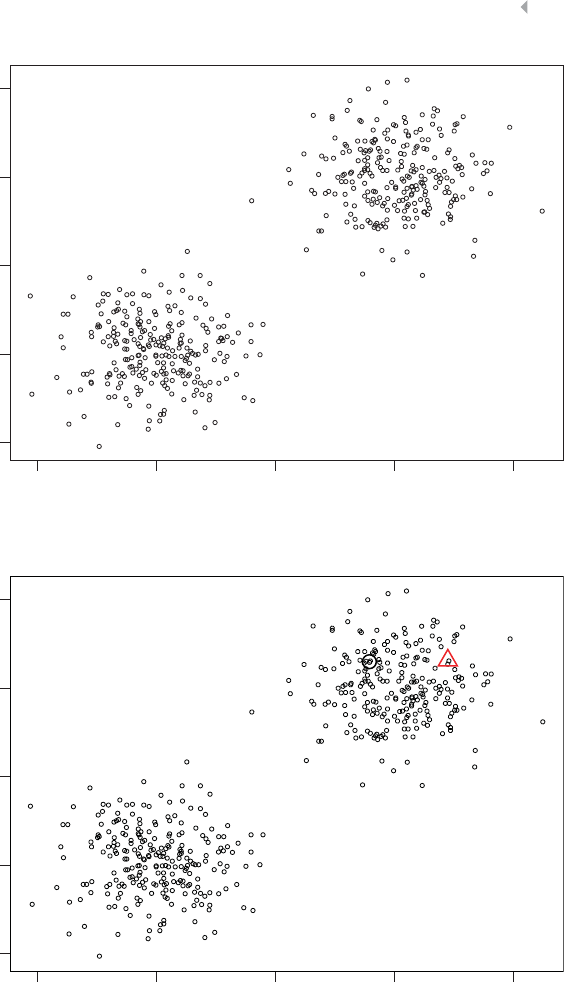
DESCRIPTIVE ANALYTICS FOR FRAUD DETECTION 105
1.51.00.50.0–0.5
–0.5 0.0 0.5 1.0 1.5
Figure 3.16 k-Means Clustering: Start from Original Data
1.51.00.50.0–0.5
–0.5 0.0 0.5 1.0 1.5
Figure 3.17 k-Means Clustering Iteration 1: Randomly Select Initial Cluster Centroids
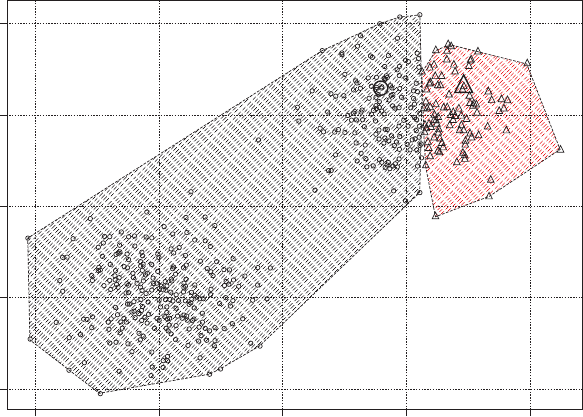
106
0.0 0.5 1.0 1.5‒0.5
‒0.5 0.5 1.51.00.0
Figure 3.18 k-Means Clustering Iteration 1: Assign Remaining Observations
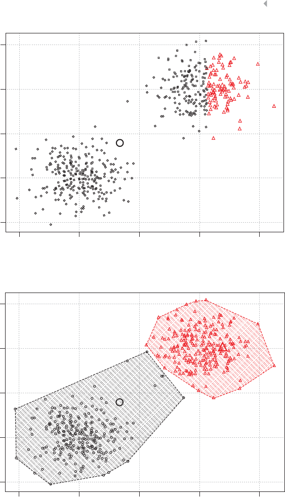
DESCRIPTIVE ANALYTICS FOR FRAUD DETECTION 107
0.0 0.5 1.0 1.5‒0.5
‒0.5 0.5 1.51.00.0
Figure 3.19 k-Means Iteration Step 2: Recalculate Cluster Centroids
0.0 0.5 1.0 1.5‒0.5
‒0.5 0.5 1.51.00.0
Figure 3.20 k-Means Clustering Iteration 2: Reassign Observations
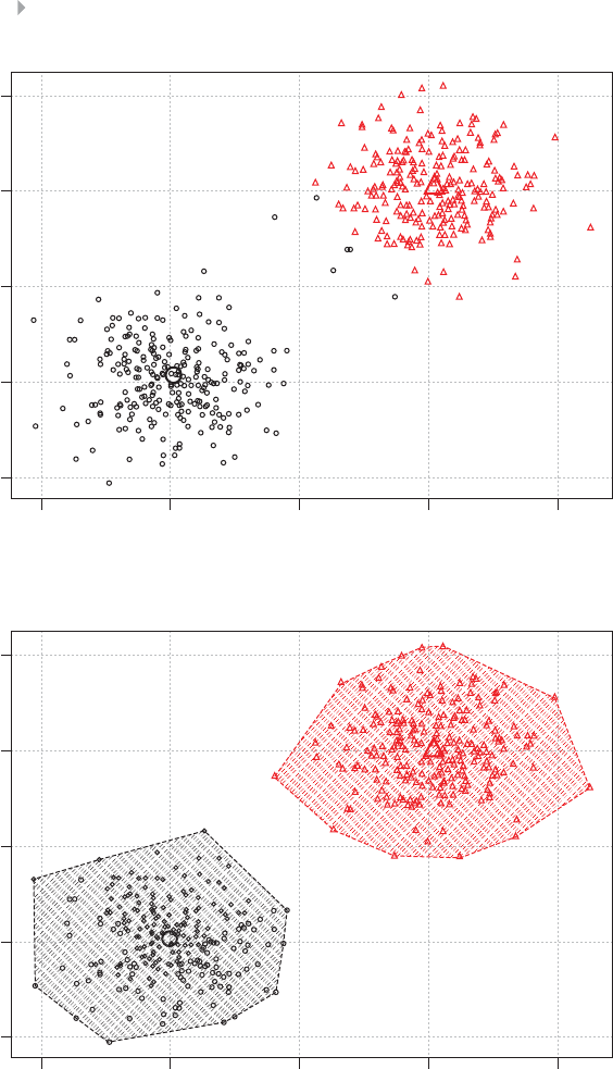
108 FRAUD ANALYTICS
0.0 0.5 1.0 1.5‒0.5
‒0.5 0.5 1.51.00.0
Figure 3.21 k-Means Clustering Iteration 3: Recalculate Cluster Centroids
0.0 0.5 1.0 1.5‒0.5
‒0.5 0.5 1.51.00.0
Figure 3.22 k-Means Clustering Iteration 3: Reassign Observations

DESCRIPTIVE ANALYTICS FOR FRAUD DETECTION 109
Self-Organizing Maps
A self-organizing map (SOM) is an unsupervised learning algorithm
that allows users to visualize and cluster high-dimensional data on
a low-dimensional grid of neurons (Kohonen 2000; Huysmans et al.
2006; Seret et al. 2012). A SOM is a feedforward neural network with
two layers: an input and an output layer. The neurons from the output
layer are usually ordered in a two-dimensional rectangular or hexag-
onal grid (see Figure 3.23). For the former, every neuron has at most
eight neighbors, whereas for the latter, every neuron has at most six
neighbors.
Each input is connected to all neurons in the output layer with
weights w=[w1,…,wN],withNthe number of variables. All weights
are randomly initialized. When a training vector xis presented, the
weight vector wcof each neuron cis compared with x,usingfor
example, the Euclidean distance metric (beware to standardize the
data first!):
d(x,wc)=N
i=1(xi−wci)2.
The neuron that is most similar to xin Euclidean sense is called
the best matching unit (BMU). The weight vector of the BMU
and its neighbors in the grid are then adapted using the following
learning rule:
wi(t+1)=wi(t)+hci (t)[x(t)−wi(t)],
where trepresents the time index during training and hci(t)defines
the neighborhood of the BMU c, specifying the region of influence.
Rectangular SOM Grid Hexagonal SOM Grid
Figure 3.23 Rectangular Versus Hexagonal SOM Grid

110 FRAUD ANALYTICS
The neighborhood function hci(t)should be a nonincreasing function
of time and the distance from the BMU. Some popular choices are:
hci(t)=𝛼(t)exp −rc−ri2
2𝜎2(t),
hci(t)=𝛼(t)if rc−ri2≤threshold,0otherwise,
where rcand rirepresent the location of the BMU and neuron ion
the map, 𝜎2(t)represents the decreasing radius, and 0 ≤𝛼(t)≤1the
learning rate (e.g., 𝛼(t)=A∕(t+B),𝛼(t)=exp(–At)). The decreasing
learning rate and radius will give a stable map after a certain amount of
training. The neurons will then move more and more toward the input
observations and interesting segments will emerge. Training is stopped
when the BMUs remain stable, or after a fixed number of iterations
(e.g., 500 times the number of SOM neurons).
SOMs can be visualized by means of a U-matrix or component
plane:
◾AU (unified distance)-matrix essentially superimposes a
height Zdimension on top of each neuron visualizing the
average distance between the neuron and its neighbors,
whereby typically dark colors indicate a large distance and can
be interpreted as cluster boundaries.
◾Acomponent plane visualizes the weights between each spe-
cific input variable and its output neurons, and as such pro-
vides a visual overview of the relative contribution of each input
attribute to the output neurons.
Figure 3.24 provides a SOM example for clustering countries based
on a Corruption Perception Index (CPI). This is a score between 0
(highly corrupt) and 10 (highly clean), assigned to each country in
the world. The CPI is combined with demographic and macroeconomic
information for the years 1996, 2000, and 2004. Uppercase countries
(e.g., BEL) denote the situation in 2004, lowercase (e.g., bel) in 2000,
and sentence case (e.g., Bel) in 1996. It can be seen that many of the
European countries are situated in the upper-right corner of the map.
Figure 3.25 provides the component plane for literacy whereby
darker regions score worse on literacy. Figure 3.26 provides the

DESCRIPTIVE ANALYTICS FOR FRAUD DETECTION 111
sgp
SGP
Hkg
hkg
HKG
Swe
nor
Nor
NOR
fin
swe
FIN
SWE
Gbr
FRA
DEU Dnk
dnk
DNK
Fin gbr
fra
CHEAUS
isr
can
TWN
ISR CHL
Chl
chl
Arg
arg
mex
Kor
kor KOR Prt
Cze
cze
pol
Esp CZE
Twn
twn
jor
JOR Mys
MYS
Ven
mys
VENCOL
ECU bra
Bra bgd
BGD
nga
NGA
Egy
egy
Ecu
ecu
pak
PAK
ZafBOLPHL
Col
col
IDN
idn bol Pak
ven
Chn
CHN
Idn
EGY
Phl
phl
Ken
ken
Cmr
Nga
cmr
Uga
uga
UGA
Chn Tur Jor Bol CMR
Bgd
tur ind lnd KEN
MEX IND
MEX
ARG THA
BRA
Tha
TUR
zaf
ZAF
tha
hun
HUN
POL
jap Deu
PRT GRC
Nzl
nzl
NZL
Can
aus
Che
che
Aut
aut
Bel
ESP
Fra
deu
ITA
Aus
CAN
bel
Nld
nld
AUT
BEL
JPN
NLD
GBR
Sgp
Usa
usa
USA
Isr
Figure 3.24 Clustering Countries Using SOMs
component plane for political rights whereby darker regions cor-
respond to better political rights. It can be seen that many of the
European countries score good on both literacy and political rights.
SOMs are a very handy tool for clustering high-dimensional data
sets because of the visualization facilities. However, since there is no
real objective function to minimize, it is harder to compare various
SOM solutions against each other. Also, experimental evaluation and
expert interpretation is needed to decide on the optimal size of the
SOM. Unlike k-means clustering, a SOM does not force the number of
clusters to be equal to the number of output neurons.
Clustering with Constraints
In many fraud application domains, the expert(s) will have prior
knowledge about existing fraud patterns and/or anomalous behavior.
This knowledge can originate from both experience as well as existing

112 FRAUD ANALYTICS
Figure 3.25 Component Plane for Literacy
literature. It will be handy if this background knowledge can be incor-
porated to guide the clustering. This is the idea of semi-supervised
clustering or clustering with constraints (Basu, Davidson et al. 2012).
The idea here is to bias the clustering with expert knowledge such
that the clusters can be found quicker and with the desired properties.
Various types of constraints can be thought of. A first set of con-
straints is observation-level constraints. As the name suggests, these
constraints are set for individual observations. A must-link constraint
enforces that two observations should be assigned to the same cluster,
whereas a cannot-link constraint will put them into different clusters
(see Figure 3.27). This could be handy in a fraud-detection setting
if the fraud behavior of only a few observations is known as these
can then be forced into the same cluster. Cluster-level constraints
are defined at the level of the cluster. A minimum separation or 𝛿
constraint specifies that the distance between any pair of observations

DESCRIPTIVE ANALYTICS FOR FRAUD DETECTION 113
Figure 3.26 Component Plane for Political Rights
must link
cannot link
must link
Figure 3.27 Must-Link and Cannot-Link Constraints in Semi-Supervised Clustering
in two different clusters must be at least 𝛿(see Figure 3.28). This will
allow data scientists to create well-separated clusters. An 𝜀-constraint
specifies that each observation in a cluster with more than one
observation must have another observation within a distance of at
most 𝜀(see Figure 3.29). Another example of a constraint includes the
requirement to have balanced clusters, whereby each cluster contains
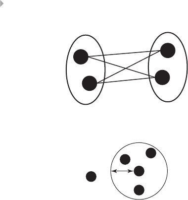
114 FRAUD ANALYTICS
≥δ
Figure 3.28 𝛿-Constraints in Semi-Supervised Clustering
ε
Figure 3.29 𝜀-Constraints in Semi-Supervised Clustering
the same amount of observations. Negative background information
can also be provided whereby the aim is to find a clustering which is
different from a given clustering.
The constraints can be enforced during the clustering process.
For example, in a k-means clustering setup, the cluster seeds will
be chosen such that the constraints are respected. Each time an
observation is (re-)assigned, the constraints will be verified and the
(re-)assignment halted in case violations occur. In a hierarchical
clustering procedure, a must-link constraint can be enforced by setting
the distance between two observations to 0, whereas a cannot-link
constraint can be enforced by setting the distance to a very high value.
Evaluating and Interpreting Clustering Solutions
Evaluating a clustering solution is by no means a trivial exercise since
there exists no universal criterion. From a statistical perspective, the
sum of squared errors (SSE) can be computed as follows:
SSE =K
i=1x∈Ci
dist2(x,mi),
where Krepresents the number of clusters and mithe centroid (e.g.,
mean) of cluster i. When comparing two clustering solutions, the one
with the lowest SSE can then be chosen. Besides a statistical evaluation,
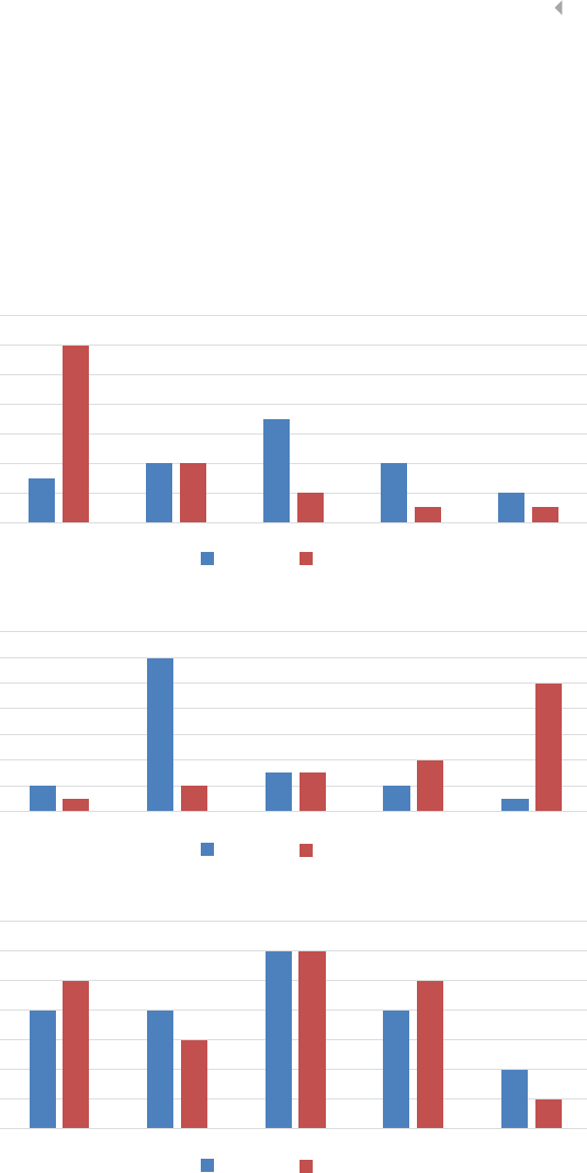
DESCRIPTIVE ANALYTICS FOR FRAUD DETECTION 115
a clustering solution will also be evaluated in terms of its interpretation.
To facilitate the interpretation of a clustering solution, various options
are available. A first one is to compare cluster distributions with pop-
ulation distributions across all variables on a cluster-by-cluster basis.
This is illustrated in Figure 3.30 whereby the distribution of a cluster
C1is contrasted with the overall population distribution for the RFM
0
10
20
30
40
50
60
70
Recency
0
10
20
30
40
50
60
70
<1 1–2 2–3 3–4 4+
<1,000 1,000–5,000 5,000–10,000 10,000–100,000 100,000+
Monetary
0
5
10
15
20
25
30
35
<5 5–10 10–20 20–50 50+
Frequency
Population Cluster C1
Population Cluster C1
Population Cluster C1
Figure 3.30 Cluster Profiling Using Histograms

116 FRAUD ANALYTICS
Table 3.4 Output from a k-Means Clustering Exercise (k=4)
Claim Recency Frequency Monetary .... ClusterID
Claim1 Cluster2
Claim2 Cluster4
Claim3 Cluster3
Claim4 Cluster2
Claim5 Cluster1
Claim6 Cluster4
…
variables. It can be clearly seen that cluster C1has observations with
low recency values and high monetary values, whereas the frequency
is relatively similar to the original population.
Another way to explain a given clustering solution is by building a
decision tree with the ClusterID as the target variable. We will discuss
how to build decision trees in the next chapter, but for the moment
it suffices to understand how they should be interpreted. Assume we
have the following output from a k-means clustering exercise with k
equal to 4. (See Table 3.4)
We can now build a decision tree with the ClusterID as the target
variable as follows.
The decision tree in Figure 3.31 gives us a clear insight into the
distinguishing characteristics of the various clusters. For example,
cluster 2 is characterized by observations having recency <1 day and
monetary >1,000. Hence, using decision trees, we can easily assign
new observations to the existing clusters. This is an example of how
supervised or predictive techniques can be used to explain the solution
from a descriptive analytics exercise.
Recency < 1 day
Frequency > 5 Monetary >1000
No
No No
Cluster1
Yes
Cluster3
Yes
Cluster4Cluster2
Yes
Figure 3.31 Using Decision Trees for Clustering Interpretation
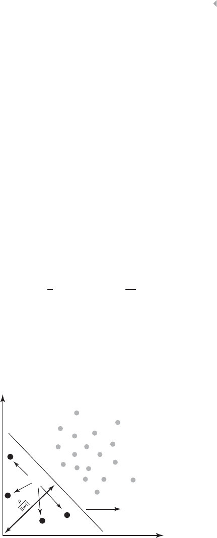
DESCRIPTIVE ANALYTICS FOR FRAUD DETECTION 117
ONE-CLASS SVMS
One-class SVMs try to maximize the distance between a hyperplane
and the origin (Schölkopf et al. 2001). The idea is to separate the
majority of the observations from the origin. The observations that
lie on the other side of the hyperplane, closest to the origin, are then
considered as outliers. This is illustrated in Figure 3.32.
Let’s define the hyperplane as follows:
wT𝜑(x)−𝜌=0.
Normal observations lie above the hyperplane and outliers below
it, or in other words normal observations (outliers) will return a posi-
tive (negative) value for:
f(x)=sign(wT𝜑(x)−𝜌).
One-class SVMs then aim at solving the following optimization
function:
Minimize 1
2N
i=1w2
i−𝜌+1
𝜐nn
i=1ei
subject towT𝜑(xk)≥𝜌−ek,k=1…n
ek≥0.
The error variables eiare introduced to allow observations to lie on
the side of the hyperplane closest to the origin. The parameter 𝜐is a
wT φ(x) – ρ = 0
Outliers
Figure 3.32 One-Class Support Vector Machines

118 FRAUD ANALYTICS
regularization term. Mathematically, it can be shown that the distance
between the hyperplane and the origin equals 𝜌
w (see Figure 3.32).
This distance is now maximized by minimizing 1
2N
i=1w2
i–𝜌,whichis
the first part in the objective function. The second part of the objective
function then accounts for errors, or thus outliers. The constraints force
the majority of observations to lie above the hyperplane. The parame-
ter 𝜐ranges between 0 and 1, and sets an upper bound on the fraction
of outliers. A lower (higher) value of the regularization parameter 𝜐
will increase (decrease) the weight assigned to errors and thus decrease
(increase) the number of outliers. Given the importance of this param-
eter, one-class SVMs are sometimes also referred to as 𝜐-SVMs.
As with SVMs for supervised learning (see Chapter 4), the opti-
mization problem can be solved by formulating its dual variant, which
also here yields a quadratic programming (QP) problem, and applying
the kernel trick. By again using Lagrangian optimization, the following
decision function is obtained
f(x)=sign(wT𝜑(x)−𝜌)=sign n
i=1
𝛼iKx,xi−𝜌,
where αirepresent the Lagrange multipliers, and K(x,xi)the kernel
function. See Schölkopf et al. (2001) for more details.
REFERENCES
Agrawal, R., Imielinski, T., & Swami, A. (1993). Mining Association Rules
between Sets of Items in Massive Databases, Proceedings of the ACM SIGMOD
International Conference on Management of Data. Washington, D.C.
Basu, S., Davidson, I., & Wagstaff, K. L. (2012). Constrained Clustering: Advances
in Algorithms, Theory, and Applications, Boca Raton, FL: Chapman & Hall/
CRC.
Bolton, R. J., & Hand, D. J. (2002). Statistical Fraud Detection: A Review,
Statistical Science 17 (3): 235–255.
Cullinan, G. J. (1977). Picking Them by Their Batting Averages’ Recency–Frequency–
Monetary Method of Controlling Circulation, Manual Release 2103. New York:
Direct Mail/Marketing Association.
Everitt, B. S., Landau, S., Leese, M., & Stahl, D. (2010). Cluster Analysis,5thed.
Hoboken, NJ: John Wiley & Sons.

DESCRIPTIVE ANALYTICS FOR FRAUD DETECTION 119
Grubbs, F. E. (1950). Sample Criteria for Testing Outlying Observations, The
Annals of Mathematical Statistics 21(1): 27–58.
Grubbs, F. E. (1969). Procedures for Detecting Outlying Observations in
Samples, Technometrics 11(1): 1–21.
Huysmans, J., Baesens, B., Van Gestel, T., & Vanthienen, J. (2006). Failure Pre-
diction with Self Organizing Maps, Expert Systems with Applications, Special
Issue on Intelligent Information Systems for Financial Engineering 30(3):
479–487.
Jain, A. K. (2010). Data Clustering: 50 Years Beyond K-Means, Pattern Recog-
nition Letters 31(8): 651–666.
Kohonen, T. (2000). Self-Organizing Maps. New York: Springer.
MacQueen, J. (1967). Some Methods for classification and Analysis of
Multivariate Observations, Proceedings of 5th Berkeley Symposium on Math-
ematical Statistics and Probability, Berkeley: University of California Press,
pp. 281–297.
Schölkopf, B., and Platt, J. C., Shawe-Taylor, J., Smola, A., & Williamson, R. C.
(2001). Estimating the support of a high-dimensional distribution, Neural
Computation 13(7): 1443–1471.
Seret, A., Verbraken, T., Versailles, S., & Baesens, B. (2012). A New SOM-Based
Method for Profile Generation: Theory and an Application in Direct Mar-
keting, European Journal of Operational Research 220 (1): 199–209.
Weston, D. J., Hand, D. J., Adams, N. M., Whitrow, C., & Juszczak, P. (2008).
Plastic card fraud detection using peer group analysis, Advances in Data
Analysis and Classification 2(1): 45–62.
CHAPTER 4
Predictive
Analytics for
Fraud Detection
121
INTRODUCTION
In predictive analytics, the aim is to build an analytical model pre-
dicting a target measure of interest (Baesens 2014; Duda et al. 2001;
Flach 2012; Han and Kamber 2001; Hastie et al. 2001; Tan et al.
2006). The target is then typically used to steer the learning process
during an optimization procedure. Two types of predictive analytics
can be distinguished depending on the measurement level of the
target: regression and classification. In regression, the target variable is
continuous and varies along a predefined interval. This interval can
be limited (e.g., between 0 and 1) or unlimited (e.g., between 0 and
infinity). A typical example in a fraud detection setting is predicting
the amount of fraud. In classification, the target is categorical which
means that it can only take on a limited set of predefined values.
In binary classification, only two classes are considered (e.g., fraud
versus no-fraud) whereas in multiclass classification, the target can
belong to more than two classes (e.g., severe fraud, medium fraud,
no fraud).
In fraud detection, both classification and regression models can
be used simultaneously. Consider, for example, an insurance fraud set-
ting. The expected loss due to fraud can be calculated as follows
Expected fraud loss (EFL)=PF ×LGF +(1−PF)×0=PF ×LGF
where PF represents the probability of fraud and LGF the loss given
fraud. The latter can be expressed as an amount or as a percentage
of a maximum amount (e.g., the maximum insured amount). PF can
then be estimated using a classification technique whereas for LGF,a
regression model will be estimated.
Different types of predictive analytics techniques have been
developed in the literature originating from a variety of different
disciplines such as statistics, machine learning, artificial intelligence,
pattern recognition, and data mining. The distinction between
those disciplines is getting more and more blurred and is actu-
ally not that relevant. In what follows, we will discuss a selection
of techniques with a particular focus on the fraud practitioner’s
perspective.
122

PREDICTIVE ANALYTICS FOR FRAUD DETECTION 123
TARGET DEFINITION
Since the target variable plays an important role in the learning pro-
cess, it is of key importance that it is appropriately defined. In fraud
detection, the target fraud indicator is usually hard to determine since
one can never be fully sure that a certain transaction (e.g., credit card
fraud), claim (e.g., insurance fraud), or company (e.g., tax evasion
fraud) is fraudulent.
Let’s take the example of insurance fraud (Viaene et al. 2002). If
an applicant files a claim, the insurance company will perform various
checks to flag the claim as suspicious or nonsuspicious. When the claim
is considered as suspicious, the insurance firm will first decide whether
it’s worthwhile the effort to pursue the investigation. Obviously, this
will also depend on the amount of the claim, such that small amount
claims are most likely not further considered, even if they are fraudu-
lent. When the claim is considered worthwhile to investigate, the firm
might start a legal procedure resulting into a court judgment and/or
legal settlement flagging the claim as fraudulent or not. It is clear that
also this procedure is not 100 percent error-proof and thus nonfraud-
ulent claims might end up being flagged as fraudulent, or vice versa.
Another example is tax evasion fraud. An often-used fraud mech-
anism in this setting is a spider construction, as depicted in Figure 4.1
(Van Vlasselaer et al. 2013 and 2015).
The key company in the middle represents the firm who is the key
perpetrator of the fraud. It starts up a side company (Side Company
1), which makes revenue but deliberately does not pay its taxes and
hence intentionally goes bankrupt. On bankruptcy, its resources (e.g.,
employees, machinery, equipment, buyers, suppliers, physical address,
and other assets) are shifted toward a new side company (e.g., Side
Company 2), which repeats the fraud behavior and thus again goes
bankrupt. As such, a web of side companies evolves around the key
company. It is clear that in this setting it becomes hard to distinguish
a regular bankruptcy due to insolvency from a fraudulent bankruptcy
due to malicious intent. In other words, all fraudulent companies
go bankrupt, but not all bankrupt companies are fraudulent. This is
depicted in Figure 4.2. Although suspension is seen as a normal way of
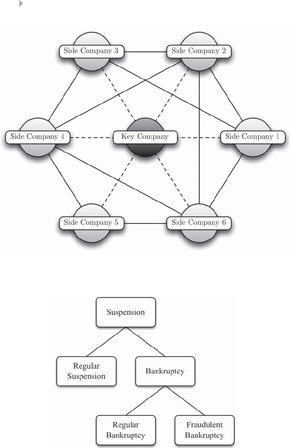
124 FRAUD ANALYTICS
Figure 4.1 A Spider Construction in Tax Evasion Fraud
Figure 4.2 Regular Versus Fraudulent Bankruptcy
stopping a company’s activities (i.e., all debts redeemed), bankruptcy
indicates that the company did not succeed to pay back all its cred-
itors. Distinguishing between regular and fraudulent bankruptcies is
subtle and hard to establish. Hence, it can be expected that some reg-
ular bankruptcies are in fact undetected fraudulent bankruptcies.

PREDICTIVE ANALYTICS FOR FRAUD DETECTION 125
Also, the intensity of the fraud when measured as an amount might
be hard to determine since one has to take into account direct costs,
indirect costs, reputation damage, and the time value of the money
(e.g., by discounting).
To summarize, in supervised fraud detection the target labels are
typically not noise-free hereby complicating the analytical modeling
exercise. It is thus important for analytical techniques to be able to
cope with this.
LINEAR REGRESSION
Linear regression is undoubtedly the most commonly used technique
to model a continuous target variable. For example, in a car insurance
fraud detection context, a linear regression model can be defined to
model the amount of fraud in terms of the age of the claimant, claimed
amount, severity of the accident, and so on.
Amount of fraud =𝛽0+𝛽1Age +𝛽2ClaimedAmount +𝛽3Severity +…
The general formulation of the linear regression model then
becomes:
Y=𝛽0+𝛽1X1+…+𝛽NXN,
where Yrepresents the target variable, and X1,…,XNthe explanatory
variables. The 𝛽parameters measure the impact on the target variable
Yof each of the individual explanatory variables.
Let’s now assume we start with a data set with nobservations and
Nexplanatory variables structured as depicted in Table 4.1.
Table 4.1 Data Set for Linear Regression
Observation X𝟏X𝟐…XNY
1X11 X21 …XN1Y1
2X12 X22 …XN2Y2
…
nX1nX2n…XNn Yn
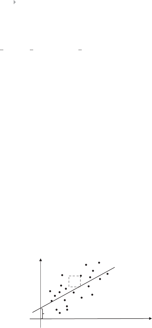
126 FRAUD ANALYTICS
The 𝛽parameters of the linear regression model can then be esti-
mated by minimizing the following squared error function:
1
2n
i=1e2
i=1
2n
i=1(Yi−̂
Yi)2=1
2n
i=1(Yi−(𝛽0+𝛽1X1i+…+𝛽NXNi))2,
where Yirepresents the target value for observation iand ̂
Yithe predic-
tion made by the linear regression model for observation i. Graphically,
this idea corresponds to minimizing the sum of all error squares as rep-
resented in Figure 4.3.
Straightforward mathematical calculus then yields the following
closed-form formula for the weight parameter vector ̂
𝛽:
̂
𝛽=
̂
𝛽0
̂
𝛽1
…
̂
𝛽N
=(XTX)−1XTY,
where Xrepresents the matrix with the explanatory variable values
augmented with an additional column of ones to account for the inter-
cept term 𝛽0,andYrepresents the target value vector (see Table 4.1).
This model and corresponding parameter optimization procedure are
often referred to as ordinary least squares (OLS) regression.
A key advantage of OLS regression is that it is simple and thus easy
to understand. Once the parameters have been estimated, the model
can be evaluated in a straightforward way, hereby contributing to its
operational efficiency.
X
Y
ei
Y = β0 + β1X
β0
Figure 4.3 OLS Regression

PREDICTIVE ANALYTICS FOR FRAUD DETECTION 127
Note that more sophisticated variants have been suggested in
the literature, such as ridge regression, lasso regression, time series
models (ARIMA, VAR, GARCH), multivariate adaptive regression
splines (MARS), and so on. Most of these relax the linearity assumption
by introducing additional transformations, however, at the cost of
increased complexity.
LOGISTIC REGRESSION
Basic Concepts
Consider a classification data set in a tax-evasion setting as depicted in
Table 4.2.
When modeling the binary fraud target using linear regression,
one gets:
Y=𝛽0+𝛽1Revenue +𝛽2Employees +𝛽3VATCompliant
When estimating this using OLS, two key problems arise:
1. The errors/target are not normally distributed but follow a
Bernoulli distribution with only two values;
2. There is no guarantee that the target is between 0 and 1, which
would be handy since it can then be interpreted as a probability.
Consider now the following bounding function:
f(z)= 1
1+e−z
which is shown in Figure 4.4.
Table 4.2 Example Classification Data Set
Company Revenue Employees VATCompliant …Fraud Y
ABC 3,000k 400 YNo 0
BCD 200k 800 NNo 0
CDE 4,2000k 2,200 NYes 1
…
XYZ 34k 50 NYes 1

128 FRAUD ANALYTICS
0
0,1
0,2
0,3
0,4
0,5
0,6
0,7
0,8
0,9
1
–7–5–3–11 3 5 7
Figure 4.4 Bounding Function for Logistic Regression
For every possible value of z, the outcome is always between 0
and 1. Hence, by combining the linear regression with the bounding
function, we get the following logistic regression model:
P(fraud =yesRevenue,Employees,VATCompliant)
=1
1+e−(𝛽0+𝛽1Revenue+𝛽2Employees+𝛽3VATcompliant)
The outcome of the above model is always bounded between 0 and
1, no matter which values of revenue, employees, and VAT compliant
are being used, and can as such be interpreted as a probability.
The general formulation of the logistic regression model then
becomes (Allison 2001):
P(Y=1X1,…,Xn)= 1
1+e−(𝛽0+𝛽1X1+…+𝛽NXN),
or alternatively,
P(Y=0X1,…,XN)=1−P(Y=1X1,…,XN)
=1−1
1+e−(𝛽0+𝛽1X1+…+𝛽NXN)=1
1+e(𝛽0+𝛽1X1+…+𝛽NXN)

PREDICTIVE ANALYTICS FOR FRAUD DETECTION 129
Hence, both P(Y=1X1,…,XN)and P(Y=0X1,…,XN)are
bounded between 0 and 1.
Reformulating in terms of the odds, the model becomes:
P(Y=1X1,…,XN)
P(Y=0X1,…,XN)=e(𝛽0+𝛽1X1+…+𝛽NXN)
or in terms of the log odds (logit),
ln PY=1X1,…,XN
P(Y=0X1,…,XN)=𝛽0+𝛽1X1+…+𝛽NXN
The 𝛽iparameters of a logistic regression model are then estimated
using the idea of maximum likelihood. Maximum likelihood optimiza-
tion choses the parameters in such a way as to maximize the probability
of getting the sample at hand. First, the likelihood function is con-
structed. For observation i, the probability of observing either class
equals:
P(Y=1X1i,…,XNi)Yi(1−P(Y=1X1i,…,XNi)1−Yi,
where Yirepresents the target value (either 0 or 1) for observation i.
The likelihood function across all nobservations then becomes:
n
i=1P(Y=1X1i,…,XNi)Yi(1−P(Y=1X1i,…,XNi)1−Yi.
To simplify the optimization, the logarithmic transformation of the
likelihood function is taken and the corresponding log-likelihood can
then be optimized using for instance the Newton-Raphson method.
Logistic Regression Properties
Since logistic regression is linear in the log odds (logit), it basically
estimates a linear decision boundary to separate both classes. This is
illustrated in Figure 4.5 whereby Frepresents fraudulent firms and L
indicates legitimate or thus nonfraudulent firms.

130 FRAUD ANALYTICS
Employees
Revenue
L
L
L L
L
L
L
L
L
L
L
L
L
L L
L L L
L
L
L L
L
L
L
L
L
L
L L
L
L L
F
F
L
L
L
L L
L
L
L
L
L
L L
L
F
F
L
F
F
F F
F F F
L
L
L
L
L
L
L
F
L
Figure 4.5 Linear Decision Boundary of Logistic Regression
To interpret a logistic regression model, one can calculate the odds
ratio. Suppose variable Xiincreases with one unit with all other vari-
ables being kept constant (ceteris paribus), then the new logit becomes
the old logit with 𝛽iadded. Likewise, the new odds become the old odds
multiplied by e𝛽i.The latter represents the odds ratio, that is, the multi-
plicative increase in the odds when Xiincreases by 1 (ceteris paribus).
Hence,
◾𝛽i>0 implies e𝛽i>1 and the odds and probability increase
with Xi
◾𝛽i<0 implies e𝛽i<1 and the odds and probability decrease
with Xi
Another way of interpreting a logistic regression model is by cal-
culating the doubling amount. This represents the amount of change
required for doubling the primary outcome odds. It can be easily seen
that for a particular variable Xi, the doubling amount equals log(2)∕𝛽i.
Note that next to the f(z)transformation, other transformations
have been suggested in the literature. Popular examples are the probit
and cloglog transformation as follows:
f(z)= 1
2𝜋∫z
−∞e−t2
2dt,
f(z)=1−e−ez.
These transformations are visualized in Figure 4.6.

PREDICTIVE ANALYTICS FOR FRAUD DETECTION 131
0
0,2
0,4
0,6
0,8
1
–
3
–
11 3
linear
logit
probit
cloglog
Figure 4.6 Other Transformations
Note, however, that empirical evidence suggests that all three
transformations typically perform equally well.
Building a Logistic Regression Scorecard
Logistic regression is a very popular supervised fraud-detection tech-
nique due to its simplicity and good performance. Just as with linear
regression, once the parameters have been estimated, it can be eval-
uated in a straightforward way, hereby contributing to its operational
efficiency. From an interpretability viewpoint, it can be easily trans-
formed into an interpretable, user friendly points based fraud score-
card. Let’s assume we start from the following logistic regression model
whereby the explanatory variables have been coded using weight of
evidence coding:
P(fraud =yesRevenue,Employees,VATCompliant,…)
=1
1+e−(𝛽0+𝛽1WOERevenue+𝛽2WOEEmployees+𝛽3WOEVATCompliant+…).
As discussed earlier, this model can be easily reexpressed in a linear
way, in terms of the log odds as follows:
log P(fraud =yesRevenue,Employees,VATCompliant,…)
P(fraud =noRevenue,Employees,VATCompliant,…)
=𝛽0+𝛽1WOERevenue +𝛽2WOEEmployees +𝛽3WOEVATCompliant +… .

132 FRAUD ANALYTICS
A scaling can then be introduced by calculating a fraud score, which
is linearly related to the log odds as follows:
Fraud score =Offset +Factor ×log(odds).
Assume that we want a fraud score of 100 for odds of 50:1, and a
fraud score of 120 for odds of 100:1. This gives the following:
100 =Offset +Factor ×log(50)
120 =Offset +Factor ×log(100)
The offset and factor then become:
Factor =20∕ln(2)=28.85
Offset =100 −Factor ×ln(50)=–12.87
Once these values are known, the fraud score becomes:
Fraud score =N
i=1WOEi×𝛽i+𝛽0×Factor +Offset
Fraud score =N
i=1WOEi×𝛽i+𝛽0
N×Factor +Offset
Fraud score =N
i=1WOEi×𝛽i+𝛽0
N×Factor +Offset
N
Hence, the points for each attribute are calculated by multiplying
the weight of evidence of the attribute with the regression coefficient
of the characteristic, then adding a fraction of the regression intercept,
multiplying the result by the factor, and finally adding a fraction of
the offset. The corresponding fraud scorecard can then be visualized as
depicted in Figure 4.7.
The fraud scorecard is very easy to work with. Suppose a new firm
with the following characteristics needs to be scored:
Revenue =750.000,Employees =420,VAT Compliant =No,…

PREDICTIVE ANALYTICS FOR FRAUD DETECTION 133
Characteristic Name Attribute Points
Revenue 1 Up to 100.000 80
Revenue 2 100.000–500.000 120
Revenue 3 500.000–1.000000 160
Revenue 4 1.000.000+ 240
Employees 1 Up to 50 5
Employees 2 50–500 20
Employees 3 500+ 80
VAT Compliant Yes 100
VAT Compliant No140
…
Figure 4.7 Fraud Detection Scorecard
The score for this firm can then be calculated as follows: 160 +20
+140 +… This score can then be compared against a critical cut-off
to help decide whether the firm is fraudulent. A key advantage of the
fraud scorecard is its interpretability. One can clearly see which are
the most risky categories and how they contribute to the overall fraud
score. Hence, this is a very useful technique in fraud detection settings
where interpretability is a key concern.
VARIABLE SELECTION FOR LINEAR AND LOGISTIC
REGRESSION
Variable selection aims at reducing the number of variables in a
model. It will make the model more concise and faster to evalu-
ate, which is especially relevant in a fraud detection setting. Both
linear and logistic regressions have built-in procedures to perform
variable selection. These are based on statistical hypotheses tests to
verify whether the coefficient of a variable iis significantly different
from zero:
H0∶β
i=0
HA∶β
i≠0

134 FRAUD ANALYTICS
In linear regression, the test statistic becomes:
t=̂
𝛽i
s.e.(̂
𝛽i),
and follows a Student’s t-distribution with n−2 degrees of freedom,
whereas in logistic regression, the test statistic is:
𝜒2=̂
𝛽i
s.e.̂
𝛽i2
and follows a Chi-squared distribution with 1 degree of freedom. Note
that both test statistics are intuitive in the sense that they will reject
the null hypothesis H0if the estimated coefficient ̂
𝛽iis high in absolute
value compared to its standard error s.e.(̂
𝛽i). The latter can be easily
obtained as a byproduct of the optimization procedure. Based on the
value of the test statistic, one calculates the p-value, which is the prob-
ability of a getting a more extreme value than the one observed. This
is visualized in Figure 4.8 assuming a value of 3 for the test statistic.
Note that since the hypothesis test is two-sided, the p-value adds the
areas to the right of 3 and to the left of –3.
In other words, a low (high) p-value represents an (in)significant
variable. From a practical viewpoint, the p-value can be compared
against a significance level. Table 4.3 presents some commonly used
values to decide on the degree of variable significance.
Various variable selection procedures can now be used based on
the p-value. Suppose one has four variables V1,V2,V3,and V4(e.g.,
amount of transaction, currency, transaction type, and merchant cat-
egory). The number of optimal variable subsets equals 24−1 or 15, as
displayed in Figure 4.9.
When the number of variables is small, an exhaustive search
amongst all variable subsets can be performed. However, as the
number of variables increases, the search space grows exponentially
and heuristic search procedures are needed. Using the p-values, the
variable space can be navigated in three possible ways. Forward
regression starts from the empty model and always adds variables
based on low p-values. Backward regression starts from the full
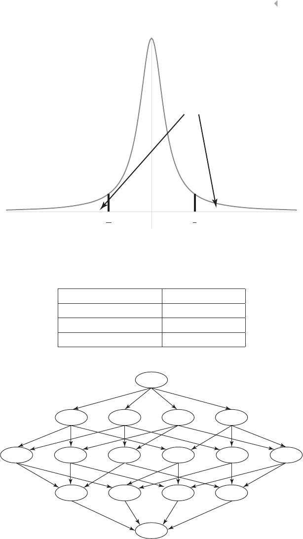
PREDICTIVE ANALYTICS FOR FRAUD DETECTION 135
–0.03
0.02
0.07
0.12
0.17
0.22
0.27
0.32
–10 –8–6–4–20246810
3
–3
p-value
Figure 4.8 Calculating the p-Value with a Student’s t-Distribution
Table 4.3 Reference Values for Variable Significance
p-value <0.01 Highly significant
0.01 <p-value <0.05 Significant
0.05 <p-value <0.10 Weakly significant
p-value >0.10 Not significant
{V1}
{V1,V2}
{V1, V2, V3}{V
1, V2, V4}{V
1, V3, V4}{V
2, V3, V4}
{V1, V2, V3, V4}
{V1,V3}{V
2,V3}{V
1,V4}{V
2,V4}{V
3,V4}
{V2}{V
3}{V
4}
{}
Figure 4.9 Variable Subsets for Four Variables V1,V2,V3,andV4

136 FRAUD ANALYTICS
model and always removes variables based on high p-values. Stepwise
regression is a mix between both. It starts off like forward regression,
but once the second variable has been added, it will always check
the other variables in the model and remove them if they turn out
to be insignificant according to their p-value. Obviously, all three
procedures assume preset significance levels, which should be set by
the user before the variable selection procedure starts.
In fraud detection, it is very important to be aware that statistical
significance is only one evaluation criterion to do variable selection. As
mentioned before, interpretability is also an important criterion. In both
linear and logistic regression, this can be easily evaluated by inspecting
the sign of the regression coefficient. It is hereby highly preferable that
a coefficient has the same sign as anticipated by the business expert,
otherwise he/she will be reluctant to use the model.
Coefficients can have unexpected signs due to multicollinearity
issues, noise or small sample effects. Sign restrictions can be easily
enforced in a forward regression setup by preventing variables with
the wrong sign from entering the model. Another criterion for variable
selection is operational efficiency. This refers to the amount of resources
that are needed for the collection and preprocessing of a variable.
For example, although trend variables are typically very predictive,
they require a lot of effort to be calculated and may thus not be
suitable to be used in an online, real-time fraud scoring environment
such as credit card fraud detection. The same applies to external
data, where the latency might hamper a timely decision. In both
cases, it might be worthwhile to look for a variable that is correlated
and less predictive but easier to collect and calculate. Finally, also
legal issues need to be properly taken into account. Some variables
cannot be used in fraud-detection applications because of privacy or
discrimination concerns.
DECISION TREES
Basic Concepts
Decision trees are recursive-partitioning algorithms (RPAs) that come
up with a tree-like structure representing patterns in an underlying
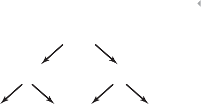
PREDICTIVE ANALYTICS FOR FRAUD DETECTION 137
Transaction amount > $100,000
Previous fraud Unemployed
No
No No
Yes Ye s
Fraud No Fraud No FraudFraud
Yes
Figure 4.10 Example Decision Tree
data set (Duda et al. 2001). Figure 4.10 provides an example of a deci-
sion tree in a fraud-detection setting.
The top node is the root node specifying a testing condition, of
which the outcome corresponds to a branch leading up to an internal
node. The terminal nodes of the tree assign the classifications (in our
case fraud labels) and are also referred to as the leave nodes. Many
algorithms have been suggested in the literature to construct decision
trees. Among the most popular are: C4.5 (See5) (Quinlan 1993), CART
(Breiman et al. 1984), and CHAID (Hartigan 1975). These algorithms
differ in their way of answering the key decisions to build a tree:
◾Splitting decision: Which variable to split at what value (e.g.,
Transaction amount is >$100,000 or not, Previous fraud is yes
or no, unemployed is yes or no)
◾Stopping decision: When to stop adding nodes to the tree?
◾Assignment decision: What class (e.g., fraud or no fraud) to
assign to a leave node?
Usually, the assignment decision is the most straightforward to
make since one typically looks at the majority class within the leave
node to make the decision. This idea is also referred to as winner-take-
all learning. The other two decisions are less straightforward to be
made and are elaborated on in what follows.
Splitting Decision
In order to answer the splitting decision, one must define the con-
cept of impurity or chaos. Consider, for example, the three data
sets of Figure 4.11 each containing good (unfilled circles) and bad
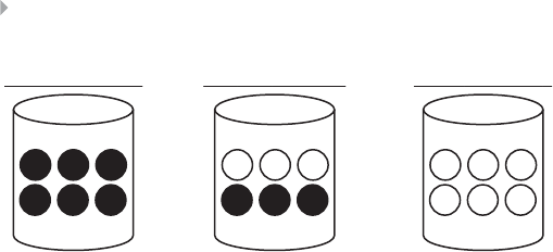
138 FRAUD ANALYTICS
Minimal ImpurityMinimal Impurity Maximal Impurity
Figure 4.11 Example Data Sets for Calculating Impurity
(filled circles) customers. Quite obviously, the good customers are
nonfraudulent, whereas the bad customers are fraudulent. Minimal
impurity occurs when all customers are either good or bad. Maximal
impurity occurs when one has the same number of good and bad
customers (i.e., the data set in the middle).
Decision trees will now aim at minimizing the impurity in the data.
In order to do so appropriately, one needs a measure to quantify impu-
rity. Various measures have been introduced in the literature and the
most popular are:
◾Entropy: E(S)=–pGlog 2(pG)−pBlog 2(pB)(C4.5/See5)
◾Gini: Gini(S)=2pGpB(CART)
◾Chi-squared analysis (CHAID)
with pGand pBbeing the proportions of good and bad, respectively.
Both measures are depicted in Figure 4.12 where it can be clearly seen
that the entropy (gini) is minimal when all customers are either good
or bad, and maximal in case of the same number of good and bad
customers.
In order to answer the splitting decision, various candidate splits
will now be evaluated in terms of their decrease in impurity. Consider
a split on age, as depicted in Figure 4.13.
The original data set had maximum entropy since the amount of
goods and bads were the same. The entropy calculations now become:
◾Entropy top node =−1∕2×log2(1∕2)−1∕2×log2(1∕2)=1
◾Entropy left node =−1∕3×log2(1∕3)−2∕3×log2(2∕3)=0.91
◾Entropy right node =−1×log2(1)−0×log2(0)=0
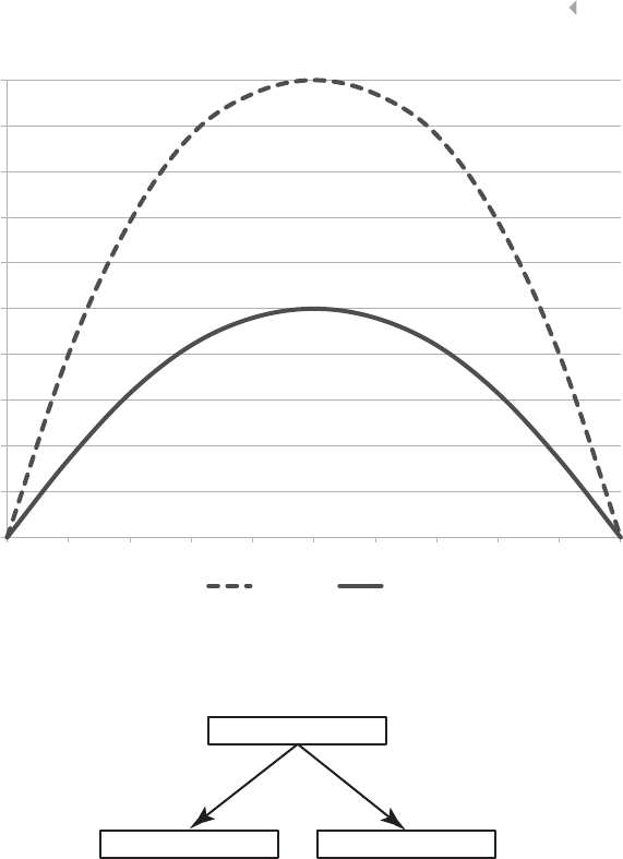
PREDICTIVE ANALYTICS FOR FRAUD DETECTION 139
0
0.1
0.2
0.3
0.4
0.5
0.6
0.7
0.8
0.9
1
0 0.1 0.2 0.3 0.4 0.5 0.6 0.7 0.80.9 1
Entropy Gini
Figure 4.12 Entropy Versus Gini
200 0
GB
GB
GB
Age < 30 Age ≥ 30
400 400
200 400
Figure 4.13 Calculating the Entropy for Age Split
The weighted decrease in entropy, also known as the gain, can then
be calculated as follows:
Gain =1−(600∕800)×0.91 −(200∕800)×0=0.32
The gain measures the weighted decrease in entropy thanks to the
split. It speaks for itself that a higher gain is to be preferred. The decision
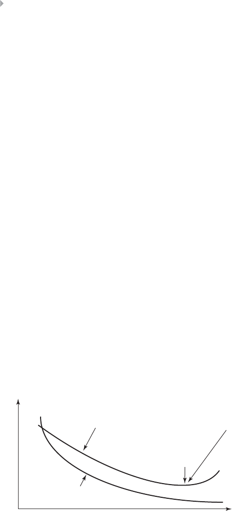
140 FRAUD ANALYTICS
tree algorithm will now consider different candidate splits for its root
node and adopt a greedy strategy by picking the one with the biggest
gain. Once the root node has been decided on, the procedure continues
in a recursive way, each time adding splits with the biggest gain. In
fact, this can be perfectly parallelized and both sides of the tree can
grow in parallel, hereby increasing the efficiency of the tree construction
algorithm.
Stopping Decision
The third decision relates to the stopping criterion. Obviously, if the tree
continues to split, it will become very detailed with leaf nodes contain-
ing only a few observations. In the most extreme case, the tree will
have one leaf node per observation and as such perfectly fit the data.
However, by doing so, the tree will start to fit the specificities or noise
in the data, which is also referred to as overfitting. In other words, the
tree has become too complex and fails to correctly model the noise free
pattern or trend in the data. As such, it will generalize poorly to new
unseen data. In order to avoid this from happening, the data will be
split into a training sample and a validation sample. The training sam-
ple will be used to make the splitting decision. The validation sample is
an independent sample, set aside to monitor the misclassification error
(or any other performance metric such as a profit-based measure) as
the tree is grown. A commonly used split up is a 70 percent training
sample and 30 percent validation sample. One then typically observes
a pattern as depicted in Figure 4.14.
Validation set
Training
set
minimum
Misclassification error
STOP Growing tree!
Number of tree nodes
Figure 4.14 Using a Validation Set to Stop Growing a Decision Tree

PREDICTIVE ANALYTICS FOR FRAUD DETECTION 141
The error on the training sample keeps on decreasing as the splits
become more and more specific and tailored towards it. On the val-
idation sample, the error will initially decrease, which indicates that
the tree splits generalize well. However, at some point the error will
increase since the splits become too specific for the training sample as
the tree starts to memorize it. Where the validation set curve reaches its
minimum, the procedure should be stopped, as otherwise overfitting
will occur. Note that, as already mentioned, besides classification error,
one might also use accuracy or profit based measures on the Y-axis
to make the stopping decision. Also note that sometimes, simplicity is
preferred above accuracy, and one can select a tree that does not neces-
sarily have minimum validation set error, but a lower number of nodes.
Decision Tree Properties
In the example of Figure 4.10, every node had only two branches.
The advantage of this is that the testing condition can be implemented
as a simple yes/no question. Multiway splits allow for more than
two branches and can provide trees that are wider but less deep. In a
read-once decision tree, a particular attribute can be used only once
in a certain tree path. Every tree can also be represented as a rule set
since every path from a root note to a leave node makes up a simple
if-then rule. For the tree depicted in Figure 4.10, the corresponding
rules are:
If Transaction amount >$100,000 And Unemployed =No
Then no fraud
If Transaction amount >$100,000 And Unemployed =Yes Then
fraud
If Transaction amount ≤$100,000 And Previous fraud =Yes
Then fraud
If Transaction amount ≤$100,000 And Previous fraud =No
Then no fraud
These rules can then be easily implemented in all kinds of software
packages (e.g., Microsoft Excel).
Decision trees essentially model decision boundaries orthogonal to
the axes. This is illustrated in Figure 4.15 for an example decision tree.

142 FRAUD ANALYTICS
F
1200
30 Recency
Amount
Recency
Amount NF
NFF
≤ 1200 > 1200
≤ 30 > 30
NF
NF
NF
NF
NF
NF
NF
NF
NF
NFNF
NF
NF
NF
NF
NF
NF
NFNF
NF
NF
NF
NF
NF
NF
NFNF
NF
NF
NF
NFNF
NFNF
NFNF
NFNF
NF
NF
FF
F
F
F
F
F
NF
NF
NF
NF
Figure 4.15 Decision Boundary of a Decision Tree
Regression Trees
Decision trees can also be used to predict continuous targets. Consider
the example of Figure 4.16 where a regression tree is used to predict
the fraud percentage (FP). The latter can be expressed as the percentage
of a predefined limit based on, for example, the maximum transac-
tion amount.
Other criteria need now be used to make the splitting decision since
the impurity will need to be measured in another way. One way to
measure impurity in a node is by calculating the mean squared error
(MSE)asfollows: 1
nn
i=1(Yi−Y)2,
where nrepresents the number of observations in a leave node, Yi
the value of observation i,andY, the average of all values in the leave
node. Obviously, it is desirable to have a low MSE in a leave node since
this indicates that the node is more homogeneous.
Credit class
FP = 64%FP = 38%
Merchant known FP = 22%Previous fraud
FP = 6% FP = 82%
Low
Medium
High
NoYes No
Yes
Figure 4.16 Example Regression Tree for Predicting the Fraud Percentage

PREDICTIVE ANALYTICS FOR FRAUD DETECTION 143
Another way to make the splitting decision is by conducting a sim-
ple analysis of variance (ANOVA) test and calculating an F-statistic as
follows:
F=SSbetween∕(B−1)
SSwithin∕(n−B)∼Fn−B,B−1,
whereby
SSbetween =
B
b=1
nb(Yb−Y)2
SSwithin =
B
b=1
nb
i=1
(Ybi −Yb)2
with Bthe number of branches of the split, nbthe number of obser-
vations in branch b,Ybthe average in branch b,Ybi the value of
observation iin branch b,andYthe overall average. Good splits favor
homogeneity within a node (low SSwithin) and heterogeneity between
nodes (high SSbetween). In other words, good splits should have a high
F-value, or low corresponding p-value.
The stopping decision can be made in a similar way as for clas-
sification trees but using a regression based performance measure
(e.g., mean squared error, mean absolute deviation, R-squared) on the
Y-axis. The assignment decision can be made by assigning the mean
(or median) to each leave node. Note that standard deviations and thus
confidence intervals may also be computed for each of the leaf nodes.
Using Decision Trees in Fraud Analytics
Decision trees can be used for various purposes in fraud analytics. First,
they can be used for variable selection as variables that occur at the top
of the tree are more predictive of the target. One could also simply cal-
culate the gain of a characteristic to gauge its predictive power. As an
alternative, remember that we already discussed the information value
in Chapter 2 to measure the predictive strength of a variable. Typically,
both the gain and information value consider similar attributes to be
predictive, so one can just choose the measure that is readily available
in the analytics software. Decision trees can also be used for high-level
segmentation. One then typically builds a tree two or three levels deep

144 FRAUD ANALYTICS
as the segmentation scheme and then uses second-stage logistic regres-
sion models for further refinement. Finally, decision trees can also be
used as the final analytical fraud model to be used directly into the busi-
ness environment. A key advantage here is that the decision tree gives
a white-box model with a clear explanation behind how it reaches its
classifications.
Many software tools will also allow to grow trees interactively by
providing at each level of the tree a top two (or more) of splits among
which the fraud modeler can choose. This allows users to choose splits
not only based on impurity reduction, but also on the interpretabil-
ity and/or computational complexity of the split criterion. Hence, the
modeler may favor a split on a less predictive variable, but which is
easier to collect and/or interpret.
Decision trees are very powerful techniques and allow for more
complex decision boundaries than a logistic regression. As discussed,
they are also interpretable and operationally efficient. They are also
nonparametric in the sense that no normality or independence assump-
tions were needed to build a decision tree. Their most important disad-
vantage is that they are highly dependent on the sample that was used
for tree construction. A small variation in the underlying sample might
yield a totally different tree. In a later section, we will discuss how this
shortcoming can be addressed using the idea of ensemble learning.
NEURAL NETWORKS
Basic Concepts
A first perspective on the origin of neural networks states that they
are mathematical representations inspired by the functioning of the
human brain. Although this may sound appealing, another more
realistic perspective sees neural networks as generalizations of existing
statistical models (Bishop 1995; Zurada 1992). Let’s take logistic
regression as an example:
P(Y=1X1,…,XN)= 1
1+e−(𝛽0+𝛽1X1+…+𝛽NXN),
We could visualize this model as shown in Figure 4.17.
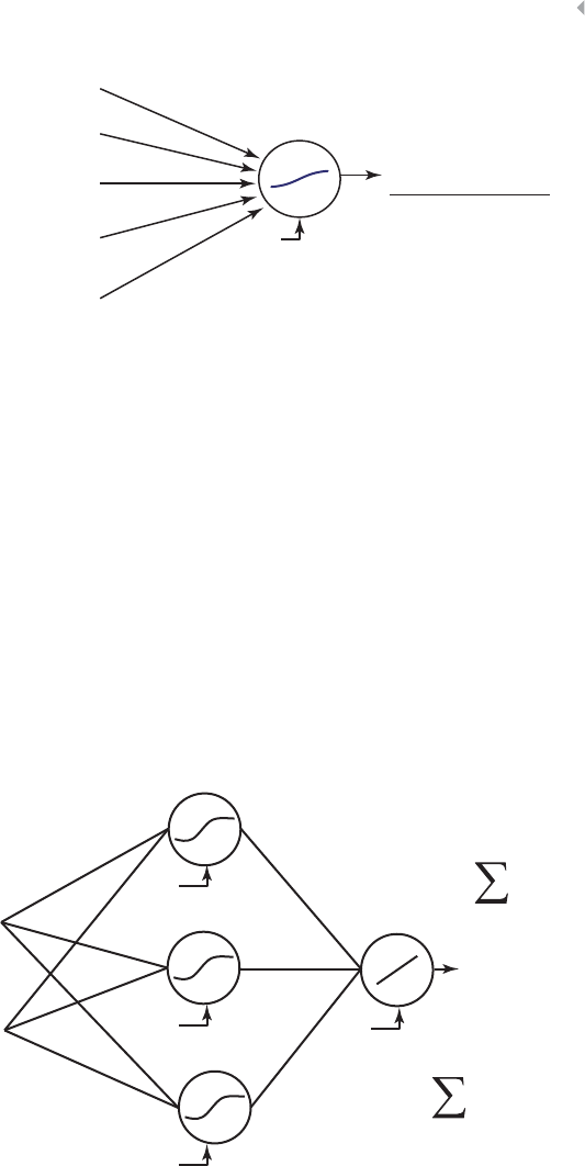
PREDICTIVE ANALYTICS FOR FRAUD DETECTION 145
...
1 + e–(β0 + β1X1 +...+βNXN)
1
P(Y | X1,..., XN) =
X1β1
XN–1
XN
X2
βN–1
βN
β0
β2
Figure 4.17 Neural Network Representation of Logistic Regression
The processing element or neuron in the middle basically per-
forms two operations: it takes the inputs and multiplies them with
the weights (including the intercept term 𝛽0, which is called the
bias term in neural networks) and then puts this into a nonlinear
transformation function similar to the one we discussed in the section
on logistic regression. So logistic regression is a neural network with
one neuron. Similarly, we could visualize linear regression as a one
neuron neural network with the identity transformation f(z)=z.
We can now generalize the above picture to a multilayer perceptron
(MLP) neural network by adding more layers and neurons, as shown
in Figure 4.18 (Bishop 1995; Zurada 1992).
h1
h2
h3
W11
W23
x1
x2
v1
v2
v3
b1
b2b4
b3
2
i=1
hj = f ( xiwij + bj)
3
j=1
y = vjhj + b4
Figure 4.18 A Multilayer Perceptron (MLP) Neural Network

146 FRAUD ANALYTICS
The example in Figure 4.18 is an MLP with one input layer, one hid-
den layer, and one output layer. The hidden layer essentially works like
a feature extractor by combining the inputs into features that are then
subsequently offered to the output layer to make the optimal prediction.
The hidden layer has a nonlinear transformation function f() and the
output layer a linear transformation function. The most popular trans-
formation functions (also called squashing, activation functions) are:
◾Logistic, f(z)= 1
1+e−z, ranging between 0 and 1
◾Hyperbolic tangent, f(z)= ez−e−z
ez+e−z, ranging between –1 and +1
◾Linear, f(z)=z, ranging between −∞ and +∞
Although theoretically the activation functions may differ per neu-
ron, they are typically fixed for each layer. For classification (e.g., fraud
detection), it is common practice to adopt a logistic transformation in
the output layer, since the outputs can then be interpreted as prob-
abilities (Baesens et al. 2002). For regression targets (e.g., amount of
fraud), one could use any of the transformation functions listed above.
Typically, one will use the hyperbolic tangent activation function in the
hidden layer.
In terms of hidden layers, theoretical works have shown that neu-
ral networks with one hidden layer are universal approximators, capa-
ble of approximating any function to any desired degree of accuracy on
a compact interval (Hornik et al. 1989). Only for discontinuous func-
tions (e.g., a saw tooth pattern) or in a deep learning context, it could
make sense to try out more hidden layers. Note, however, that these
complex patterns rarely occur in practice. In a fraud setting, it is rec-
ommended to continue the analysis with one hidden layer.
In terms of data preprocessing, it is advised to standardize the
continuous variables using, for example, the z-scores. For categorical
variables, categorization can be used to reduce the number of cate-
gories, which can then be coded using, for example, dummy variables
or weight of evidence coding. Note that it is important to only consider
categorization for the categorical variables, and not for the continuous
variables. The latter can be categorized to model nonlinear effects
into linear models (e.g., linear or logistic regression), but since neural
networks are capable of modeling nonlinear relationships, it is not
needed here.

PREDICTIVE ANALYTICS FOR FRAUD DETECTION 147
Weight Learning
As discussed earlier, for simple statistical models such as linear regres-
sion, there exists a closed-form mathematical formula for the optimal
parameter values. However, for neural networks, the optimization is a
lot more complex and the weights sitting on the various connections
need to be estimated using an iterative algorithm. The algorithm then
optimizes a cost-function. Similarly to linear regression, when the tar-
get variable is continuous, a mean squared error (MSE) cost function
will be optimized as follows:
1
2n
i=1e2
i=1
2n
i=1(Yi−̂
Yi)2,
where Yinow represents the neural network prediction for observa-
tion i. In case of a binary target variable, a maximum likelihood cost
function can be optimized as follows:
n
i=1P(Y=1X1i,…,XNi)Yi(1−P(Y=1X1i,…,XNi )1−Yi,
where P(Y=1X1i,…,XNi)represents the probability prediction from
the neural network.
The optimization procedure typically starts from a set of random
weights (e.g., drawn from a standard normal distribution), which are
then iteratively adjusted to the patterns in the data using an optimiza-
tion algorithm. Popular optimization algorithms here are back propa-
gation learning, conjugate gradient, and Levenberg-Marquardt. See for
more details (Bishop 1995). A key issue to note here is the curvature
of the objective function, which is not convex and may be multimodal
as illustrated in Figure 4.19. The error function can thus have multi-
ple local minima but typically only one global minimum. Hence, if the
starting weights are chosen in a suboptimal way, one may get stuck in a
local minimum, which is clearly undesirable. One way to deal with this
is to try out different starting weights, start the optimization procedure
for a few steps, and then continue with the best intermediate solution.
This approach is sometimes referred to as preliminary training. The
optimization procedure then continues until the error function shows
no further progress, the weights stop changing substantially, or after a
fixed number of optimization steps (also called epochs).
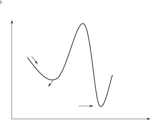
148 FRAUD ANALYTICS
w
E
Local minimum!
Global minimum!
Figure 4.19 Local Versus Global Minima
Although multiple output neurons could be used (e.g., predict-
ing fraud and fraud amount simultaneously), it is highly advised to
use only one to make sure that the optimization task is well focused.
The hidden neurons, however, should be carefully tuned and depend
on the nonlinearity in the data. More complex, nonlinear patterns
will require more hidden neurons. Although various procedures (e.g.,
cascade correlation, genetic algorithms, Bayesian methods) have been
suggested in the scientific literature to do this, the most straightfor-
ward, yet efficient procedure is as follows (Moody and Utans 1994):
1. Split the data into a training, validation, and test set.
2. Vary the number of hidden neurons from 1 to 10 in steps of one
or more.
3. Train a neural network on the training set and measure the per-
formance on the validation set (may be train multiple neural
networks to deal with the local minimum issue).
4. Choose the number of hidden neurons with optimal validation
set performance.
5. Measure the performance on the independent test set.
Note that for fraud detection, the number of hidden neurons
typically varies between 6 and 12.
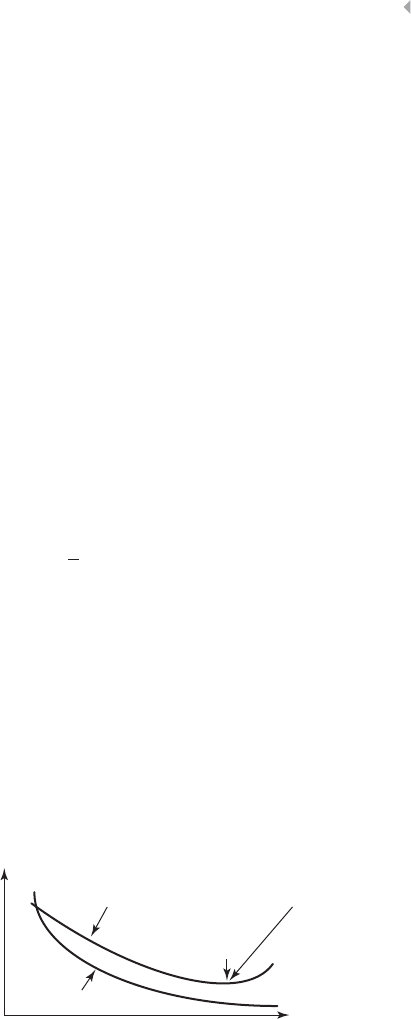
PREDICTIVE ANALYTICS FOR FRAUD DETECTION 149
Neural networks can model very complex patterns and decision
boundaries in the data and are as such very powerful. Just as with
decision trees, they are so powerful that they can even model the
noise in the training data, which is something that definitely should be
avoided. One way to avoid this overfitting is by using a validation set
in a similar way as with decision trees. This is illustrated in Figure 4.20.
The training set is used here to estimate the weights and the vali-
dation set is again an independent data set used to decide when to
stop training.
Another scheme to prevent a neural network from overfitting is
weight regularization, whereby the idea is to keep the weights small in
absolute sense since otherwise they may be fitting the noise in the data.
This is then implemented by adding a weight size term (e.g., Euclidean
norm) to the objective function of the neural network (Bartlett 1997).
In case of a continuous output (and thus mean squared error), the
objective function then becomes:
1
2n
i=1e2
i+𝜆k
j=1w2
j,
where krepresents the number of weights in the network and 𝜆a
weight decay (also referred to as weight regularization) parameter to
weigh the importance of error versus weight minimization. Setting 𝜆
too low will cause overfitting, whereas setting it to high will cause
underfitting. A practical approach to determining 𝜆is to try out dif-
ferent values on an independent validation set and select the one with
the best performance.
Validation set
Training
set
minimum
Error STOP training !
Training steps
Figure 4.20 Using a Validation Set for Stopping Neural Network Training

150 FRAUD ANALYTICS
Opening the Neural Network Black Box
Although neural networks have their merits in terms of modeling
power, they are commonly described as black-box techniques since
they relate the inputs to the outputs in a mathematically complex,
nontransparent, and opaque way. They have been successfully applied
as high-performance analytical tools in settings where interpretability
is not a key concern (e.g., credit card fraud detection).
However, in application areas where insight into the fraud behavior
is important, one needs to be careful with neural networks (Baesens,
Martens et al. 2011). In what follows, we will discuss the following
three ways of opening the neural network black box:
1. Variable selection
2. Rule extraction
3. Two-stage models
A first way to get more insight into the functioning of a neural
network is by doing variable selection. As previously, the aim here
is to select those variables that actively contribute to the neural net-
work output. In linear and logistic regression, the variable importance
was evaluated by inspecting the p-values. Unfortunately, in neural net-
works this is not that easy, as no p-values are readily available. One easy
and attractive way to do it is by visualizing the weights in a Hinton
diagram. A Hinton diagram visualizes the weights between the inputs
and the hidden neurons as squares, whereby the size of the square is
proportional to the size of the weight and the color of the square rep-
resents the sign of the weight (e.g., black colors represent a negative
weight and white colors a positive weight). Clearly, when all weights
connecting a variable to the hidden neurons are close to zero, it does
not contribute very actively to the neural network’s computations, and
one may consider leaving it out. Figure 4.21 shows an example of a
Hinton diagram for a neural network with four hidden neurons and
five variables. It can be clearly seen that the income variable has a
small negative and positive weight when compared to the other vari-
ables and can thus be considered for removal from the network. A very
straightforward variable selection procedure is:
1. Inspect the Hinton diagram and remove the variable whose
weights are closest to zero.
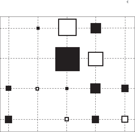
PREDICTIVE ANALYTICS FOR FRAUD DETECTION 151
1
2
3
4
Age Income Claim
amount
Time since
previous
claim
Accident
severity
Hidden neuron
Figure 4.21 Example Hinton Diagram
2. Reestimate the neural network with the variable removed. To
speed up the convergence, it could be beneficial to start from
the previous weights.
3. Continue with step 1 until a stopping criterion is met. The stop-
ping criterion could be a decrease of predictive performance or
a fixed number of steps.
Another way to do variable selection is by using the following back-
ward variable selection procedure:
1. Build a neural network with all Nvariables.
2. Remove each variable in turn and reestimate the network. This
will give Nnetworks each having N– 1 variables.
3. Remove the variable whose absence gives the best performing
network (e.g., in terms of misclassification error, mean squared
error).
4. Repeat this procedure until the performance decreases signifi-
cantly.
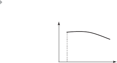
152 FRAUD ANALYTICS
Variables
Performance
N
Figure 4.22 Backward Variable Selection
When plotting the performance against the number of variables, a
pattern as depicted in Figure 4.22 will likely be obtained. Initially, the
performance will stagnate, or may even increase somewhat. When
important variables are being removed, the performance will start
decreasing. The optimal number of variables can then be situated
around the elbow region of the plot and can be decided in combi-
nation with a business expert. Sampling can be used to make the
procedure less resource intensive and more efficient. Note that this
performance-driven way of variable selection can easily be adopted
with other analytical techniques such as linear or logistic regression
or support vector machines (see next section).
Although variable selection allows users to see which variables are
important to the neural network and which ones are not, it does not
offer a clear insight into its internal workings. The relationship between
the inputs and the output remains nonlinear and complex. A first way
to get more transparency is by performing rule extraction, as will be
discussed next.
The purpose of rule extraction is to extract if-then classification
rules, mimicking the behavior of the neural network (Baesens 2003;
Baesens et al. 2003; Setiono et al. 2009). Two important approaches
here are decompositional and pedagogical techniques. Decomposi-
tional rule extraction approaches decompose the network’s internal
workings by inspecting weights and/or activation values. A typical
approach here could be (Lu et al. 1995; Setiono et al. 2011):
1. Train a neural network and do variable selection to make it as
concise as possible.
2. Categorize the hidden unit activation values by using clustering.

PREDICTIVE ANALYTICS FOR FRAUD DETECTION 153
3. Extract rules that describe the network output in terms of the
categorized hidden unit activation values.
4. Extract rules that describe the categorized hidden unit activation
values in terms of the network inputs.
5. Merge the rules obtained in step 3 and 4 to directly relate the
inputs to the outputs.
This is illustrated in Figure 4.23.
Pedagogical rule extraction techniques consider the neural net-
work as a black box and use the neural network predictions as input
to a white-box analytical technique such as decision trees (Craven and
Shavlik 1996). This is illustrated in Figure 4.24.
In this approach, the learning data set can be further augmented
with artificial data, which is then labeled (e.g., classified or predicted)
by the neural network, so as to further increase the number of observa-
tions to make the splitting decisions when building the decision tree.
Note that since the pedagogical approach does not make use of the
parameters or internal model representation, it can essentially be used
Customer
Emma 281000
Will 44 1500
Dan 30 1200
Bob 582400
Y
N
N
Y
Emma 281000
Will 44 1500
Dan 30 1200
Bob 582400
Y
N
N
Y
No
Yes
No
Yes
No
Yes
No
Yes
–1.20 2,34 0,66 1 3 2
0,781,22 0,822 3 2
2,1 –0,180,16 3 1 2
–0,1 0,8–2,34 1 2 1
If h1 = 1 and h2 = 3 Then Fraud = No
If h2 = 2 Then Fraud = Yes
If Age < 28 and Income < 1000 Then h1 = 1
If Known Customer = Y Then h2 = 3
If Age > 34 and Income > 1500 Then h2 = 2
If Age < 28 and Income < 1000 and Known Customer = Y Then Fraud = No
If Age > 34 and Income > 1500 Then Fraud = Yes
Step 1: Start from original data
Step 2: Build a neural network
(e.g., 3 hidden neurons)
Step 3: Categorize hidden unit
activations
Step 4: Extract rules relating
network outputs to categorized
hidden units
Step 5: Extract rules relating
categorized hidden units to
inputs
Step 6: Merge
both rule sets
Age Income Known Customer
Customer Age Income Known Customer
…Fraud
h1 h2 h3 h1 h2 h3 Fraud
Figure 4.23 Decompositional Approach for Neural Network Rule Extraction

154 FRAUD ANALYTICS
Customer Age Income
Known
Customer
Network
Prediction Fraud
Step 1: Start from original data
Step 2: Build a neural network
Step 3: Get the network predictions
and add them to the data set
Step 4: Extract rules relating network
predictions to original inputs. Generate
additional data where necessary.
Customer
Emma 281000
Will 44 1500
Dan 30 1200
Bob 582400
Y
N
N
Y
Emma 281000
Will 44 1500
Dan 30 1200
Bob 582400
Y
N
N
Y
No
Yes
No
Yes
No
Yes
No
Yes
No
Yes
Yes
Yes
Age Income Known Customer … Fraud
Age > 40
Known Customer Income > 2000
No
No No
NN prediction:
No Fraud
Yes
NN prediction:
Fraud
Yes
NN prediction:
No Fraud
NN prediction:
Fraud
Yes
Figure 4.24 Pedagogical Approach for Rule Extraction
with any underlying algorithm, such as regression techniques, or SVMs
(see later).
When using either decompositional or pedagogical rule extraction
approaches, the rule sets should be evaluated in terms of their accuracy,
conciseness (e.g., number of rules, number of conditions per rule), and
fidelity. The latter measures to what extent the extracted rule set suc-
ceeds in mimicking the neural network and is calculated as follows:
Neural Network Classification
Rule Set Classification No Fraud Fraud
No Fraud a b
Fraud c d
Fidelity =(a+d)∕(b+c).
It is also important to always benchmark the extracted rules/trees
with a tree built directly on the original data to see the benefit of going
through the neural network.
Another approach to make neural networks more interpretable is
by using a two-stage model setup (Van Gestel et al. 2005, 2006). The

PREDICTIVE ANALYTICS FOR FRAUD DETECTION 155
Customer Age Income Known Customer … Fraud
Emma 281000 Y No
Will 44 1500 NYes
Dan 30 1200 NNo
Bob 582400 Y Yes
Customer Age Income Known
Customer …Fraud
Logistic
Regression
output
Emma 281000 Y No (=0) 0.44
Will 44 1500 NYes (=1) 0.76
Dan 30 1200 NNo (=0) 0.18
Bob 582400 Y Yes(=1) 0.88
Customer Age Income Known
Customer …Fraud
Logistic
Regression
output
Emma 281000 Y No (=0) 0.44
Will 44 1500 NYes (=1) 0.76
Dan 30 1200 NNo (=0) 0.18
Bob 582400 Y Yes(=1) 0.88
Error
–0.44
0.24
–0.18
0.12
Customer Age Income Known
Customer …
Logistic
Regression
output
NN
output Finaloutput
Bart 281000 Y 0.680.14 0.82
Step 1: Start from original data
Step 2: Build Logistic Regression Model
Step 3: Calculate errors from Logistic
Regression Model
Step 4: Build NN predicting errors from
Logistic Regression Model
Step 5: Score new observations by adding up
logistic regression and NN scores
Figure 4.25 Two-Stage Models
idea here is to estimate an easy-to-understand model first (e.g., linear
regression, logistic regression). This will give us the interpretability part.
In a second stage, a neural network is used to predict the errors made
by the simple model using the same set of predictors. This will give us
the additional performance benefit of using a nonlinear model. Both
models are then combined in an additive way, for example as follows:
◾Target =Linear regression (X1,X2,…XN)+Neural network
(X1,X2,…XN)
◾Score =Logistic regression (X1,X2,…XN)+Neural network
(X1,X2,…XN)
This setup provides an ideal balance between model interpretabil-
ity (which comes from the first part) and model performance (which
comes from the second part). This is illustrated in Figure 4.25.
SUPPORT VECTOR MACHINES
Linear Programming
Two key shortcomings of neural networks are the fact that the
objective function is nonconvex (and hence may have multiple

156 FRAUD ANALYTICS
local minima) and the effort that is needed to tune the number of
hidden neurons. Support vector machines (SVMs) deal with both of
these issues (Cristianini and Taylor 2000; Schölkopf and Smola 2001;
Vapnik 1995).
The origins of classification SVMs date back to the early dates
of linear programming (Mangasarian 1965). Consider, for example,
the following linear program (LP) for classification in a fraud
setting:
min e1+e2+…+ennf +…ennf +nf
subject to
w1xi1 +w2xi2 +…+wNxiN ≥c−ei,1≤i≤nnf ,
w1xi1+w2xi2+…+wNxiN ≤c+ei,nnf +1≤i≤nnf +nf,
ei≥0,
with xij the value of variable jfor observation i,andnnf and nf
the number of no frauds and frauds, respectively. The LP assigns
the no frauds a score above the cut-off value c, and the frauds
a score below c. The error variables eiare needed to be able to
solve the program since perfect separation will typically not be
possible. Linear programming has been very popular in the early
days of credit scoring. One of its key benefits is that it is easy to
include domain or business knowledge by adding extra constraints
to the model. Suppose prior business experience indicates that age
(variable 1) is more important than income (variable 2). This can
be easily enforced by adding the constraint w1≥w2to the linear
program.
A key problem with linear programming is that it can estimate
multiple optimal decision boundaries as illustrated in Figure 4.26 for a
perfectly linearly separable case, where class 1 represents the fraudsters
and class 2 the non-fraudsters.
The Linear Separable Case
SVMs add an extra objective to the analysis. Consider the situation
depicted in Figure 4.27 with two variables x1 (e.g, age) and x2
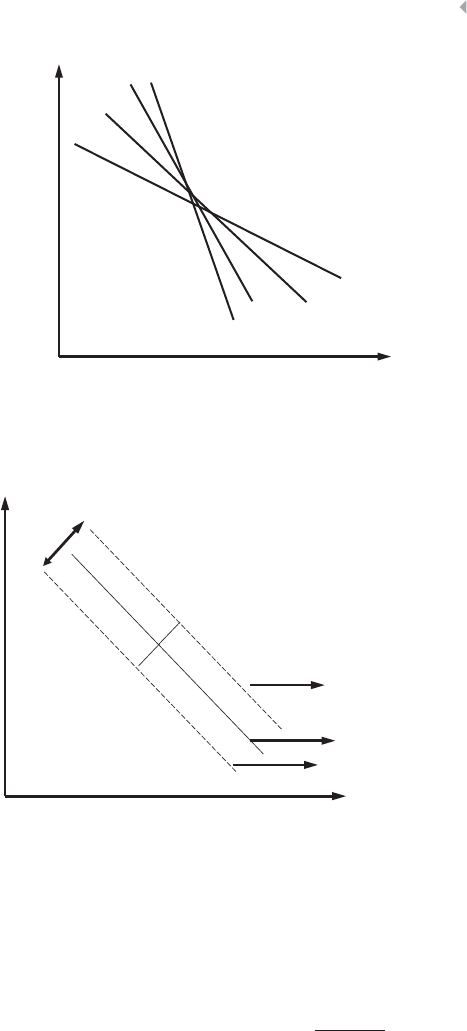
PREDICTIVE ANALYTICS FOR FRAUD DETECTION 157
x
x
x
x x
x
x
x
+ +
+
+
+
+
+
+
Class 1
Class 2
x1
x2
Figure 4.26 Multiple Separating Hyperplanes
x1
x
x
x
xx
x
x
x
++
+
+
+
+
+
+
Class 1
Class 2
x2
H1: wT x+b=+1
H0: wT x+b=0
H2: wT x+b=–1
2/||w||
Figure 4.27 SVM Classifier for the Perfectly Linearly Separable Case
(e.g, income). It has two hyperplanes sitting at the edges of both
classes, and a hyperplane in between which will serve as the classifi-
cation boundary. The perpendicular distance from the first hyperplane
H1to the origin equals b−1∕w, whereby w represents the
Euclidean norm of wcalculated as w=w2
1+w2
2. Likewise, the
perpendicular distance from H2to the origin equals b+1∕w.

158 FRAUD ANALYTICS
Hence, the margin between both hyperplanes equals 2∕w.SVMs
will now aim at maximizing this margin to pull both classes as far
apart as possible. Maximizing the margin is similar to minimizing
w, or minimizing 1
2N
i=1w2
i. In case of perfect linear separation, the
SVM classifier then becomes as follows.
Consider a training set: {xk,yk}n
k=1with xk∈RNand yk∈{−1;+1}
The goods (e.g., class +1) should be above hyperplane H1,andthe
bads (e.g., class –1) below hyperplane H2, which gives:
wTxk+b≥1,if yk=+1
wTxk+b≤−1,if yk=−1
Both can be combined as follows:
yk(wTxk+b)≥1.
The optimization problem then becomes:
Minimize 1
2
N
i=1
w2
i
subject to yk(wTxk+b)≥1,k=1…n.
This quadratic programming (QP) problem can now be solved
using Lagrangian optimization (Cristianini and Taylor 2000; Schölkopf
and Smola 2001; and Vapnik 1995). Important to note is that
the optimization problem has a quadratic cost function, giving a
convex optimization problem with no local minima and only one
global minimum. Training points that lie on one of the hyperplanes
H1or H2are called support vectors and are essential to the clas-
sification. The classification hyperplane itself is H0and for new
observations, it needs to be checked whether they are situated above
H0in which case the prediction is +1 or below (prediction −1).
This can be easily accomplished using the sign operator as fol-
lows: y(x)=sign(wTx+b). Remember, sign(x)is +1ifx≥0, and –1,
otherwise.
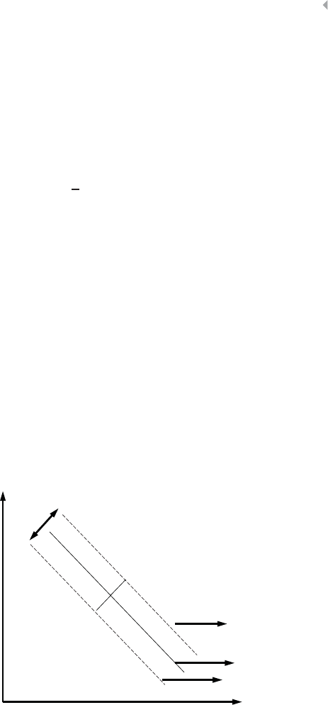
PREDICTIVE ANALYTICS FOR FRAUD DETECTION 159
The Linear Nonseparable Case
The SVM classifier discussed thus far assumed perfect separation is pos-
sible, which will, of course, be rarely the case for real-life data sets. In
case of overlapping class distributions (as illustrated in Figure 4.28),
the SVM classifier can be extended with error terms eias follows:
Minimize 1
2
N
i=1
w2
i+C
n
i=1
ei
subject to yk(wTxk+b)≥1−ek,k=1…n
ek≥0.
The error variables ekare needed to allow for misclassifications. The
Chyperparameter in the objective function balances the importance of
maximizing the margin versus minimizing the error on the data. A high
(low) value of Cimplies a higher (lower) risk of overfitting. Note the
similarity with the idea of weight regularization discussed in the section
on neural networks. Also, there the objective function consisted out of
an error term and the sum of the squared weights. We will discuss
procedures to determine the optimal value of Claterinthissection.
Just as before, the problem is a quadratic programming (QP) problem,
which can be solved using Lagrangian optimization.
x
x
x
xx
x
x
x
++
+
+
+
+
+
+
Class 1
Class 2
x2
H1: wT x+b=+1
H0: wT x+b=0
H2: wT x+b= –1
2/||w||
x
+
x1
Figure 4.28 SVM Classifier in Case of Overlapping Distributions
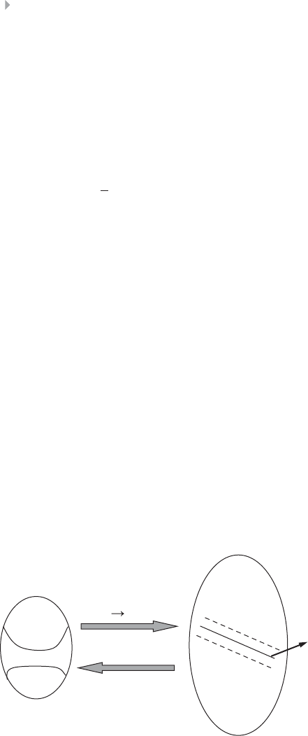
160 FRAUD ANALYTICS
The Nonlinear SVM Classifier
Finally, the nonlinear SVM classifier will first map the input data to
a higher dimensional feature space using some mapping 𝜑(x).Thisis
illustrated in Figure 4.29.
The SVM problem formulation now becomes:
Minimize 1
2
N
i=1
w2
i+C
n
i=1
ei
subject to yk(wT𝜑(xk)+b)≥1−ek,k=1…n
ek≥0.
When working out the Lagrangian optimization (Cristianini and
Taylor 2000; Schölkopf and Smola 2001; and Vapnik 1995), it turns
out that the mapping 𝜑(x)is never explicitly needed, but only implic-
itly by means of the kernel function Kdefined as follows K(xk,xl)=
𝜑(xk)T𝜑(xl). Hence, the feature space does not need to be explicitly
specified. The nonlinear SVM classifier then becomes:
y(x)=sign n
k=1
𝛼kykKx,xk+b,
where 𝛼kare the Lagrangian multipliers stemming from the optimiza-
tion. Support vectors will have nonzero 𝛼ksince they are needed to
X
X
X
X
X X
X
O O O
O
O O
X
X
O
Input Space
X X
X
X
X
X
X
X X
X
X
X
X
O
O
O
O
O
O
O
O
O
O
O
O
O
Feature Space
K(x1,x2) = φ(x1)T φ(x2)
x φ(x)
wTφ(xi) + b = 0
Figure 4.29 The Feature Space Mapping

PREDICTIVE ANALYTICS FOR FRAUD DETECTION 161
construct the classification hyperplane. All other observations have
zero 𝛼k, which is often referred to as the sparseness property of SVMs.
Different types of kernel functions can be used. The most popular are:
◾Linear kernel: K(x,xk)=xT
kx
◾Polynomial kernel: K(x,xk)=(1+xT
kx)d
◾Radial basis function (RBF) kernel: K(x,xk)=exp{−x−xk2∕
𝜎2}
Empirical evidence has shown that the RBF kernel usually per-
forms best, but note that it includes an extra parameter 𝜎to be tuned
(Van Gestel et al. 2004).
A key question to answer when building SVM classifiers is the tun-
ing of the hyperparameters. For example, suppose one has an RBF
SVM, which has two hyperparameters Cand 𝜎. Both can be tuned
using the following procedure (Van Gestel et al. 2004):
1. Partition the data into 40%∕30%∕30%training, validation and
test data.
2. Build an RBF SVM classifier for each (𝜎,C) combination from
the sets 𝜎∈{0.5, 5, 10, 15, 25, 50, 100, 250, 500} and C∈{0.01,
0.05, 0.1, 0.5, 1, 5, 10, 50, 100, 500}.
3. Choose the (𝜎,C) combination with the best validation set per-
formance.
4. Build an RBF SVM classifier with the optimal (𝜎,C) combination
on Combined training +Validation data set.
5. Calculate the performance of the estimated RBF SVM classifier
on the test set.
In case of linear or polynomial kernels, a similar procedure can be
adopted.
SVMs for Regression
SVMs can also be used for regression applications with a continuous
target. The idea here is to find a function f(x)that has at most 𝜀devia-
tion from the actual targets yifor all the training data, and is at the same
time as flat as possible. Hence, the loss function will tolerate (penalize)
errors less (higher) than 𝜀. This is visualized in Figure 4.30.
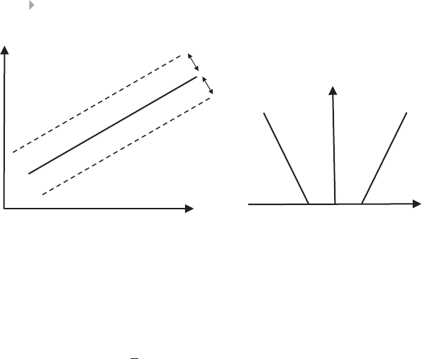
162 FRAUD ANALYTICS
x
x
x
x
x
x
x
x
x
x
x
x
x
x
x
+ε
ε
ε
–ε
Loss
function
Figure 4.30 SVMs for Regression
Consider a training set: {xk,yk}n
k=1with xk∈RNand yk∈R
The SVM formulation then becomes:
Minimize 1
2
N
i=1
w2
i+C
n
i=1
(𝜀k+𝜀∗
k)
subject to
yk−wT𝜑(xk)−b≤𝜀+𝜀k
wT𝜑(xk)+b−yk≤𝜀+𝜀∗
k
𝜀, 𝜀k,𝜀
∗
k≥0.
The hyperparameter Cdetermines the trade-off between the flat-
ness of fand the amount to which deviations larger than 𝜀are tolerated.
Note the feature space mapping 𝜑(x), which is also used here. Using
Lagrangian optimization, the resulting nonlinear regression function
becomes:
f(x)=
n
i=1
(𝛼k−𝛼∗
k)K(xk,x)+b,
where 𝛼kand 𝛼∗
krepresent the Lagrangian multipliers. The hyperpa-
rameters Cand 𝜀can be tuned using a procedure similar to the one
outlined for classification SVMs.
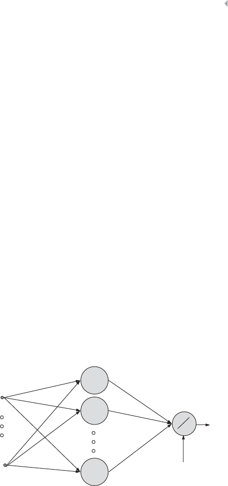
PREDICTIVE ANALYTICS FOR FRAUD DETECTION 163
Opening the SVM Black Box
Similar to neural networks, SVMs have a universal approximation
property. As an extra benefit, they do not require tuning of the num-
ber of hidden neurons and are characterized by convex optimization.
However, they are also very complex to be used in settings where
interpretability is important. Just as with neural networks, procedures
can be used to provide more transparency by opening up the SVM
black box.
Variable selection can be performed using the backward variable
selection procedure discussed in the section on neural networks. This
will essentially reduce the variables but not provide any additional
insight into the workings of the SVM. Rule extraction approaches can
then be used in a next step. In order to apply decompositional rule
extraction approaches, the SVM can be represented as a neural net-
work as depicted in Figure 4.31.
The hidden layer uses kernel activation functions, whereas the out-
put layer uses a linear activation function. Note that the number of
hidden neurons now corresponds to the number of support vectors
and follows automatically from the optimization. This is in strong con-
trast to neural networks where the number of hidden neurons needs
to be tuned manually. The decompositional approach can then pro-
ceed by first extracting If-Then rules relating the output to the hidden
K(x,x1)
K(x,x2)
K(x,xns)
x
1
xnb
αns
α2
α1
Figure 4.31 Representing an SVM Classifier as a Neural Network

164 FRAUD ANALYTICS
unit activation values. In a next step, rules are extracted relating the
hidden unit activation values to the inputs, followed by the merger of
both rule sets.
Since a pedagogical approach considers the underlying model as a
black box, it can be easily combined with SVMs. Just as in the neural
network case, the SVM is first used to construct a data set with SVM
predictions for each of the observations. This data set is then given
to a decision tree algorithm to build a decision tree. Also here, addi-
tional training set observations can be generated to facilitate the tree
construction process.
Finally, also two-stage models can be used to provide more com-
prehensibility. Remember, in this approach a simple model (e.g., linear
or logistic regression) is estimated first, followed by an SVM to correct
the errors of the latter.
ENSEMBLE METHODS
Ensemble methods aim at estimating multiple analytical models
instead of using only one. The idea here is that multiple models can
cover different parts of the data input space and as such complement
each other’s deficiencies. In order to successfully accomplish this, the
analytical technique needs to be sensitive to changes in the underlying
data. This is especially the case for decision trees and that’s why they
are commonly used in ensemble methods. In what follows, we will
discuss bagging, boosting, and random forests.
Bagging
Bagging (Bootstrap aggregating) starts by taking B bootstraps from the
underlying sample (Breiman 1996). Note that a bootstrap is a sample
with replacement (see section on evaluating predictive models). The
idea is then to build a classifier (e.g., decision tree) for every bootstrap.
For classification, a new observation will be classified by letting all B
classifiers vote, using, for example, a majority voting scheme whereby
ties are resolved arbitrarily. For regression, the prediction is the average
of the outcome of the B models (e.g., regression trees). Note that here
also a standard error and thus confidence interval can be calculated.

PREDICTIVE ANALYTICS FOR FRAUD DETECTION 165
The number of bootstraps B can either be fixed (e.g., 30) or tuned via
an independent validation data set.
The key element for bagging to be successful is the instability of
the analytical technique. If perturbing the data set by means of the
bootstrapping procedure can alter the model constructed, then bagging
will improve the accuracy (Breiman 1996). However, for models that
are robust with respect to the underlying data set, it will not give much
added value.
Boosting
Boosting works by estimating multiple models using a weighted sample
of the data (Freund and Schapire 1997, 1999). Starting from uniform
weights, boosting will iteratively reweight the data according to the
classification error whereby misclassified cases get higher weights. The
idea here is that difficult observations should get more attention. Either
the analytical technique can directly work with weighted observations,
or if not, we can just sample a new data set according to the weight
distribution. The final ensemble model is then a weighted combination
of all the individual models. A popular implementation of this is the
Adaptive boosting/Adaboost procedure, which works as follows:
1. Given the following observations: (x1,y1),…,(xn,yn)where xiis
the attribute vector of observation iand yi∈{1,–1}
2. Initialize the weights as follows: W1(i)=1∕n,i=1,…,n
3. For t=1…T
a. Train a weak classifier (e.g., decision tree) using the
weights Wt
b. Get weak classifier Ctwith classification error 𝜀t
c. Choose 𝛼t=1
2ln 1−𝜀t
𝜀t
d. Update the weights as follows:
i. Wt+1(i)= Wt(i)
Zt
e−𝛼tif Ct(x)=yi
ii. Wt+1(i)= Wt(i)
Zt
e𝛼tif Ct(x)≠yi
4. Output the final ensemble model: E(x)=sign T
t=1𝛼tCt(x)

166 FRAUD ANALYTICS
Note that in this procedure, Trepresents the number of boosting
runs, 𝛼tmeasures the importance that is assigned to classifier Ctand
increases as 𝜀tgets smaller, Ztis a normalization factor needed to make
sure that the weights in step tmake up a distribution and as such
sum to 1, and Ct(x)represents the classification of the classifier built
in step tfor observation x. Multiple loss functions may be used to cal-
culate the error 𝜀talthough the misclassification rate is undoubtedly
the most popular. In substep i of step d, it can be seen that correctly
classified observations get lower weights, whereas substep ii assigns
higher weights to the incorrectly classified cases. Again, the number
of boosting runs Tcan be fixed or tuned using an independent vali-
dation set. Note that various variants of this Adaboost procedure exist,
such as Adaboost.M1, Adaboost.M2 (both for multiclass classification),
and Adaboost.R1, Adaboost.R2 (both for regression). See Freund and
Schapire (1997 and 1999) for more details. A key advantage of boosting
is that it is really easy to implement. A potential drawback is that there
may be a risk of overfitting to the hard (potentially noisy) examples in
the data, which will get higher weights as the algorithm proceeds. This
is especially relevant in a fraud detection setting because, as mentioned
earlier, the target labels in a fraud setting are typically quite noisy.
Random Forests
The technique of random forests was first introduced by Breiman
(2001). It creates a forest of decision trees as follows:
1. Given a data set with n observations and Ninputs.
2. m=constant chosen on beforehand.
3. For t=1,…,T
a. Take a bootstrap sample with nobservations.
b. Build a decision tree whereby for each node of the tree,
randomly choose mvariables on which to base the splitting
decision.
c. Split on the best of this subset.
d. Fully grow each tree without pruning.

PREDICTIVE ANALYTICS FOR FRAUD DETECTION 167
Common choices for mare 1, 2, or floor (log2(N)+1), which is rec-
ommended. Random forests can be used with both classification trees
and regression trees. Key in this approach is the dissimilarity amongst
the base classifiers (i.e., decision trees), which is obtained by adopting
a bootstrapping procedure to select the training samples of the indi-
vidual base classifiers, the selection of a random subset of attributes at
each node, and the strength of the individual base models. As such the
diversity of the base classifiers creates an ensemble that is superior in
performance compared to the single models.
More recently, an alternative to random forests was proposed: rota-
tion forests. This ensemble technique takes the idea of random forests
one step further. It combines the idea of pooling a large number of
decision trees built on a subset of the attributes and data, with the
application of principal component analysis prior to decision tree build-
ing, explaining its name. Rotating the axes prior to model building was
found to enhance base classifier accuracy at the expense of losing the
ability of ranking individual attributes by their importance (Rodriguez
et al. 2006).
Evaluating Ensemble Methods
Various benchmarking studies have shown that random forests can
achieve excellent predictive performance. Actually, they generally
rank amongst the best performing models across a wide variety of
prediction tasks (Dejaeger et al. 2012). They are also perfectly capable
of dealing with data sets having only a few observations, but with lots
of variables. They are highly recommended when high performing
analytical methods are needed for fraud detection. However, the price
that is paid for this, is that they are essentially black-box models. Due
to the multitude of decision trees that make up the ensemble, it is
very hard to see how the final classification is made. One way to shed
some light on the internal workings of an ensemble is by calculating
the variable importance. A popular procedure to do so is as follows:
1. Permute the values of the variable under consideration (e.g., Xj)
on the validation or test set.

168 FRAUD ANALYTICS
2. For each tree, calculate the difference between the error on the
original, unpermuted data and the error on the data with Xjper-
muted as follows:
VI (Xj)= 1
ntree
t
(errort(D)−errort(̃
Dj)),
whereby ntree represents the number of trees in the ensemble,
Dthe original data, and ̃
Djthe data with variable Xjpermuted.
In a regression setting, the error can be the mean squared error
(MSE), whereas in a classification setting, the error can be the
misclassification rate.
3. Order all variables according to their VI value. The variable with
the highest VI value is the most important.
MULTICLASS CLASSIFICATION TECHNIQUES
In the introduction of this chapter, we already discussed the difficulty of
appropriately determining the target label in a fraud detection setting.
One way to deal with this is by creating more than two target val-
ues, e.g., as follows: clear fraud, doubt case, no fraud. These values are
nominal, implying that there is no meaningful order between them.
As an alternative, the target values can also be ordinal: severe fraud,
medium fraud, light fraud, no fraud. All of the classification techniques
discussed earlier in this chapter can be easily extended to a multiclass
setting whereby more than two target values or classes are present.
Multiclass Logistic Regression
When estimating a multiclass logistic regression model, one first needs
to know whether the target variable is nominal or ordinal. For nominal
target variables, one of the target classes (say class K) will be chosen as
the base class as follows (Allison 2001):
P(Y=1X1,…,XN)
P(Y=KX1,…,XN)=e(𝛽1
0+𝛽1
1X1+𝛽1
2X2+…𝛽1
NXN)
P(Y=2X1,…,XN)
P(Y=KX1,…,XN)=e(𝛽2
0+𝛽2
1X1+𝛽2
2X2+…𝛽2
NXN)
…

PREDICTIVE ANALYTICS FOR FRAUD DETECTION 169
P(Y=K−1X1,…,XN)
P(Y=KX1,…,XN)=e(𝛽K−1
0+𝛽K−1
1X1+𝛽K−1
2X2+…𝛽K−1
NXN)
Using the fact that all probabilities must sum to one, one can then
obtain the following:
P(Y=1X1,…,XN)= e(𝛽1
0+𝛽1
1X1+𝛽1
2X2+…𝛽1
NXN)
1+K−1
k=1e(𝛽k
0+𝛽k
1X1+𝛽k
2X2+…𝛽k
NXN)
P(Y=2X1,…,XN)= e(𝛽2
0+𝛽2
1X1+𝛽2
2X2+…𝛽2
NXN)
1+K−1
k=1e(𝛽k
0+𝛽k
1X1+𝛽k
2X2+…𝛽k
NXN)
P(Y=KX1,…,XN)= 1
1+K−1
k=1e(𝛽k
0+𝛽k
1X1+𝛽k
2X2+…𝛽k
NXN)
The 𝛽parameters are then usually estimated using maximum apos-
teriori estimation, which is an extension of maximum likelihood esti-
mation. As with binary logistic regression, the procedure comes with
standard errors, confidence intervals, and p-values.
In case of ordinal targets, one could estimate a cumulative logistic
regression as follows (Allison 2001):
P(Y≤1)= 1
1+e−𝜃1+𝛽1X1+…+𝛽NXN
P(Y≤2)= 1
1+e−𝜃2+𝛽1X1+…+𝛽NXN
…
P(Y≤K−1)= 1
1+e−𝜃K−1+𝛽1X1+…+𝛽NXN
or,
P(Y≤1)
1−P(Y≤1)=e−𝜃1+𝛽1X1+…+𝛽NXN
P(Y≤2)
1−P(Y≤2)=e−𝜃2+𝛽1X1+…+𝛽NXN
…

170 FRAUD ANALYTICS
P(Y≤K−1)
1−P(Y≤K−1)=e−𝜃K−1+𝛽1X1+…+𝛽NXN.
Note that since P(Y≤K)=1, 𝜃K=+∞.
The individual probabilities can then be obtained as follows:
P(Y=1)= P(Y≤1)
P(Y=2)= P(Y≤2)–P(Y≤1)
…
P(Y=K)=1–P(Y≤K–1).
Also for this model, the 𝛽parameters can be estimated using a max-
imum likelihood procedure.
Multiclass Decision Trees
Decision trees can be easily extended to a multiclass setting. For the
splitting decision, assuming Kclasses, the impurity criteria become:
Entropy(S)=−
K
k=1
pklog2(pk)
Gini(S)=
K
k=1
pk(1−pk).
The stopping decision can be made in a similar way as for binary
target decision trees by using a training set for making the splitting
decision, and an independent validation data set on which the misclas-
sification error rate is monitored. The assignment decision then looks
for the most prevalent class in each of the leave nodes.
Multiclass Neural Networks
A straightforward option for training a multiclass neural network for K
classes, is to create Koutput neurons, one for each class. An observa-
tion is then assigned to the output neuron with the highest activation
value (winner-take-all learning). Another option is to use a softmax
activation function (Bishop 1995).
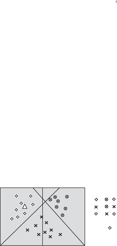
PREDICTIVE ANALYTICS FOR FRAUD DETECTION 171
Multiclass Support Vector Machines
A common practice to estimate a multiclass support vector machine is
to map the multiclass classification problem to a set of binary classifi-
cation problems. Two well-known schemes here are One-versus-One
and One-versus-All coding (Van Gestel et al. 2015).
For Kclasses, One-versus-One coding estimates K(K−1)∕2binary
SVM classifiers contrasting every possible pair of classes. Every classi-
fier as such can cast a vote on the target class and the final classification
is then the result of a (weighted) voting procedure. Ties are resolved
arbitrarily. This is illustrated in Figure 4.32 whereby the aim is to clas-
sify the white triangle.
For Kclasses, One-versus-All coding estimates Kbinary SVM clas-
sifiers each time contrasting one particular class against all the other
ones. A classification decision can then be made by assigning a par-
ticular observation to the class for which one of the binary classifiers
assigns the highest posterior probability. Ties are less likely to occur
with this scheme. This is illustrated in Figure 4.33, whereby the aim
is to classify the white triangle. Note that for more than three classes,
One-versus-All coding estimates less classifiers than One-versus-One
coding. However, in One-versus-One coding the binary classifiers are
estimated on a reduced subset of the data (i.e., each time contrasting
only two classes), whereas in One-versus-All coding, all binary classi-
fiers are estimated on the entire data set (i.e., each time contrasting a
class against all the rest).
x2
x1
a) or :
b) or :
c) or :
Class is !
Figure 4.32 One-Versus-One Coding for Multiclass Problems
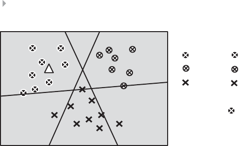
172 FRAUD ANALYTICS
x2
x1
a) or other; p( ) = 0.92
b) or other; p( ) = 0.18
c) or other; p( ) = 0.30
Class is !
Figure 4.33 One-Versus-All Coding for Multiclass Problems
Both One-versus-One and One-versus-All coding are meta
schemes that can be used with other base classifiers (e.g., neural
networks) as well.
EVALUATING PREDICTIVE MODELS
Splitting Up the Data Set
When evaluating predictive models, two key decisions need to be
made. A first decision concerns the data set split up, which specifies
on what part of the data the performance will be measured. A second
decision concerns the performance metric. In what follows, we will
elaborate on both.
The decision how to split up the data set for performance mea-
surement depends on its size. In case of large data sets (say, more
than 1,000 observations), the data can be split up into a training and
a test sample. The training sample (also called development or estima-
tion sample) will be used to build the model whereas the test sample
(also called the hold out sample) will be used to calculate its perfor-
mance (see Figure 4.34). A commonly applied split up is a 70 percent
training sample and a 30 percent test sample. There should be a strict
separation between training and test sample. No observation that was
used for model development, can be used for independent testing.
Note that in case of decision trees or neural networks, the validation
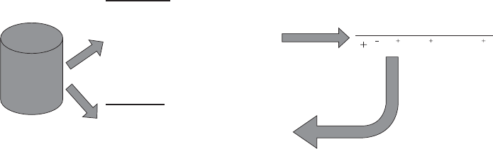
173
Data
Build Model
Apply
Model
Customer Age Income Gender …
…
Fraud Score
Emma 281,000 F No0,44
Will 44 1,500 M Yes 0,76
Dan 30 1,200 M No0,18
Bob 582,400 M
Customer Age Income Gender
John 30 1,200 M
Sarah 25 800 F
Sophie 52 2,200 F
David 482,000 M
Peter 34 1,800 M
Yes
No
No
Yes
No
1
0
0
1
0
Yes
Fraud Target
0,88
Train data
Test data
...)0034.050.010.0(
1
1
incomeage
e
P(Fraud | age, income,...)
=
Figure 4.34 Training Versus Test Sample Set Up for Performance Estimation

174 FRAUD ANALYTICS
sample is a separate sample since it is actively being used during model
development (i.e., to make the stopping decision). A typical split-up in
this case is a 40 percent training sample, 30 percent validation sam-
ple and 30 percent test sample. A stratified split-up ensures that the
fraudsters/nonfraudsters are equally distributed amongst the various
samples.
In case of small data sets (say, less than 1,000 observations), special
schemes need to be adopted. A very popular scheme is cross-validation.
In cross-validation, the data is split into Kfolds (e.g., 5 or 10). An
analytical model is then trained on K– 1 training folds and tested
on the remaining validation fold. This is repeated for all possible val-
idation folds resulting in Kperformance estimates, which can then
be averaged. Note that also a standard deviation and/or confidence
interval can be calculated if desired. Common choices for Kare5and
10. In its most extreme case, cross-validation becomes leave-one-out
cross-validation whereby every observation is left out in turn and a
model is estimated on the remaining K– 1 observations. This gives
Kanalytical models in total. In stratified cross validation, special care is
taken to make sure the no fraud/fraud odds are the same in each fold
(see Figure 4.35).
A key question to answer when doing cross-validation is what
should be the final model that is being outputted from the procedure.
Since cross-validation gives multiple models, this is not an obvious
question. Of course, one could let all models collaborate in an ensem-
ble setup by using a (weighted) voting procedure. A more pragmatic
Validation fold
Training fold
Figure 4.35 Cross-Validation for Performance Measurement

PREDICTIVE ANALYTICS FOR FRAUD DETECTION 175
answer would be to do leave one out cross-validation and pick one of
the models at random. Since the models differ up to one observation
only, they will be quite similar anyway. Alternatively, one may also
choose to build one final model on all observations but report the
performance coming out of the cross-validation procedure as the best
independent estimate.
For small samples, one may also adopt bootstrapping procedures
(Efron 1979). In bootstrapping, one takes samples with replacement
from a data set D (see Figure 4.36).
The probability that a customer is sampled equals 1/n,withnthe
number of observations in the data set. Hence, the probability that a
customer is not sampled equals 1 – 1/n. Assuming a bootstrap with n
samples, the fraction of customers that is not sampled equals:
1−1
nn.
We then have:
lim
n→∞1−1
nn
=e−1=0.368
where the approximation already works well for small values of n. So,
0.368 is the probability that a customer does not appear in the sample
and 0.632 the probability that a customer does appear. If we then take
the bootstrap sample as the training set, and the test set as all sam-
ples in Dbut not in the bootstrap, we can calculate the performance
as follows:
Error estimate =0.368 Error (Training)+0.632 Error (Test),
whereby obviously a higher weight is being put on the test set
performance.
Bootstrap 1
C1
C2
C3
C4
C5 C3C2C3 C2
C2 C1C4C1 C2
C5
Bootstrap 2
Figure 4.36 Bootstrapping

176 FRAUD ANALYTICS
Performance Measures for Classification Models
Consider the following fraud detection example for a five-customer
data set. The first column in Table 4.4 depicts the fraud status, whereas
the second column the fraud score as it comes from a logistic regression,
decision tree, neural network, and so on.
One can now map the scores to a predicted classification label by
assuming a default cut-off of 0.5 as shown in Figure 4.37.
A confusion matrix can now be calculated as shown in Table 4.5.
Based on this matrix, one can now calculate the following perfor-
mance measures:
◾Classification accuracy =(TP +TN)∕(TP +FP +FN +TN)=3∕5
◾Classification error =(FP +FN)∕(TP +FP +FN +TN)=2∕5
Table 4.4 Example Data Set for Performance Calculation
Fraud Fraud Score
John Yes 0.72
Sophie No 0.56
David Yes 0.44
Emma No 0.18
Bob No 0.36
Cut-Off = 0.50
Fraud Fraud Score
John Yes 0.72
Sophie No 0.56
David Yes 0.44
Emma No 0.18
Bob No 0.36
Fraud Fraud Score Predicted
John Yes 0.72 Yes
Sophie No 0.56 Yes
David Yes 0.44 No
Emma No 0.18No
Bob No 0.36 No
Figure 4.37 Calculating Predictions Using a Cut-Off
Table 4.5 Confusion Matrix
Actual Status
Positive (Fraud) Negative (No Fraud)
Predicted status Positive (Fraud) True Positive (John) False Positive (Sophie)
Negative (No Fraud) False Negative (David) True Negative (Emma, Bob)

PREDICTIVE ANALYTICS FOR FRAUD DETECTION 177
◾Sensitivity =Recall =Hit rate =TP∕(TP +FN)=1∕2
◾Specificity =TN∕(FP +TN)=2∕3
◾Precision =TP∕(TP +FP)=1∕2
◾F-measure =2×(Precision ×Recall)∕(Precision +Recall)=
1∕2
The classification accuracy is the percentage of correctly classified
observations. The classification error is the complement thereof and
also referred to as the misclassification rate. The sensitivity, recall or
hit rate measures how many of the fraudsters are correctly labeled
by the model as a fraudster. The specificity looks at how many of
the nonfraudsters are correctly labeled by the model as nonfraudster.
Theprecision indicateshow manyof thepredicted fraudstersare actually
fraudsters.
Note that all these classification measures depend on the cut-off.
For example, for a cut-off of 0 (1), the classification accuracy becomes
40 percent (60 percent), the error 60 percent (40 percent), the sen-
sitivity 100 percent (0), the specificity 0 (100 percent), the precision
40 percent (0) and the F-measure 0.57 (0). Given this dependence, it
would be nice to have a performance measure that is independent from
the cut-off. One could construct a table with the sensitivity, specificity,
and 1-specificity for various cut-offs as shown in Table 4.6.
The receiver operating characteristic (ROC) curve then plots the
sensitivity versus 1-specificity as illustrated in Figure 4.38 (Fawcett
2003).
Table 4.6 Table for ROC Analysis
Cut-off Sensitivity Specificity 1-Specificity
0 1 0 1
0.01
0.02
....
0.99
1 0 1 0
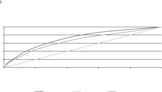
178 FRAUD ANALYTICS
0
0,2
0,4
0,6
0,8
1
0 0,2 0,4 0,6 0,81
Sensitivity
(1 - Specificity)
ROC Curve
Mode l - ARandom Mode l - B
Figure 4.38 The Receiver Operating Characteristic Curve
Note that a perfect model detects all the fraudsters and nonfraud-
sters at the same time, which results into a sensitivity of 1, and a speci-
ficity of 1 and is thus represented by the upper-left corner. The closer the
curve approaches this point, the better the performance. In Figure 4.38,
model A has a better performance than model B. A problem, however,
arises if the curves intersect. In this case, one can calculate the area
under the ROC curve (AUC) as a performance metric. The AUC provides
a simple figure-of-merit for the performance of the constructed classi-
fier. The higher the AUC, the better the performance. The AUC is always
bounded between 0 and 1 and can be interpreted as a probability. In
fact, it represents the probability that a randomly chosen fraudster gets a
higher score than a randomly chosen nonfraudster (DeLong et al. 1988;
Hanley and McNeil 1982). Note that the diagonal represents a random
scorecard whereby sensitivity equals 1-specificity for all cut-off points.
Hence, a good classifier should have an ROC above the diagonal and
AUC bigger than 50 percent.
A lift curve is another important performance metric. It starts by
sorting the population from high score to low score. Suppose now that
in the top 10 percent highest scores, there are 60 percent fraudsters
whereas the total population has 10 percent fraudsters. The lift value
in the top decile then becomes 60 percent/10 percent, or 6. In other
words, the lift value represents the cumulative percentage of fraudsters
per decile, divided by the overall population percentage of fraud-
sters. Using no model, or a random sorting, the fraudsters would be
equally spread across the entire range and the lift value would always
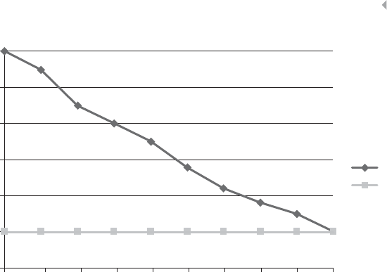
PREDICTIVE ANALYTICS FOR FRAUD DETECTION 179
6
5
4
3
2
10 20 30 40 50 60
% of sorted population
model
baseline
70 8090100
1
0
Figure 4.39 Lift Curve
equal 1. Obviously, the lift curve always decreases as one considers
bigger deciles, until it will reach 1. This is illustrated in Figure 4.39.
Note that a lift curve can also be expressed in a noncumulative way,
and is also often summarized as the top decile lift.
The cumulative accuracy profile (CAP), Lorenz or Power curve is
very closely related to the lift curve (see Figure 4.40). It also starts by
sorting the population from high score to low score and then measures
the cumulative percentage of fraudsters for each decile on the Y-axis.
The perfect models gives a linearly increasing curve up to the sam-
ple fraud rate and then flattens out. The diagonal again represents the
random model.
The CAP curve can be summarized in an accuracy ratio (AR) as
depicted in Figure 4.41.
The accuracy ratio is then defined as follows (see Figure 4.41):
(Area below power curve for current model – Area below power
curve for random model)∕(Area below power curve for
perfect model −Area below power curve for random model)
A perfect model will thus have an AR of 1 and a random model
an AR of 0. Note that the accuracy ratio is also often referred to as the
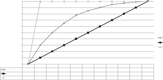
180
0 10% 20% 30% 40% 50% 60% 70% 80% 90% 100%
scorecard 0% 30% 50% 65% 78%85% 90% 95% 97% 99% 100%
random model 0% 10% 20% 30% 40% 50% 60% 70% 80% 90% 100%
perfect model 0% 100% 100% 100% 100% 100% 100% 100% 100% 100% 100%
0%
10%
20%
30%
40%
50%
60%
70%
80%
90%
100%
Percentage of fraudsters
Percentage of sorted population
scorecard
random model
perfect model
Figure 4.40 Cumulative Accuracy Profile
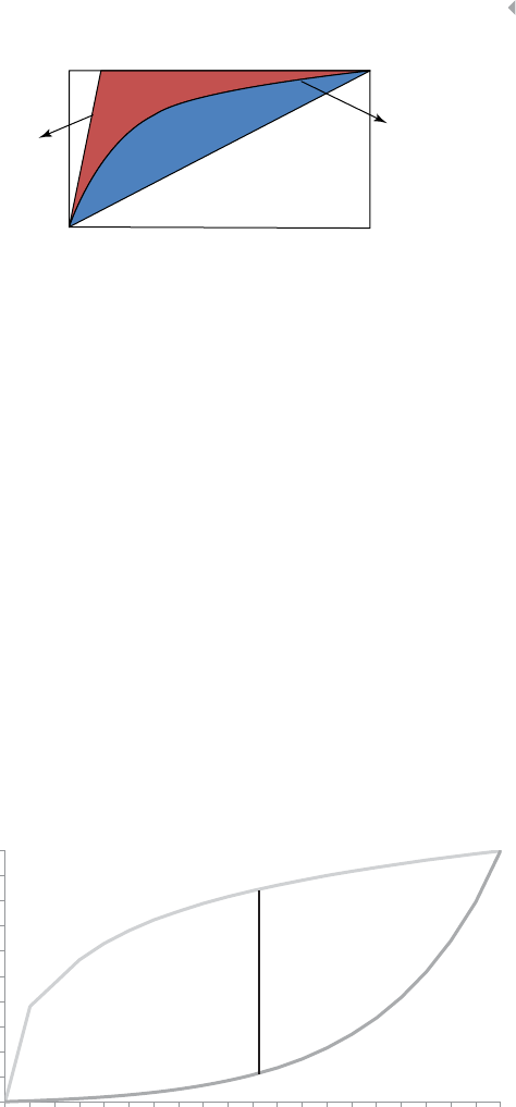
PREDICTIVE ANALYTICS FOR FRAUD DETECTION 181
Perfect model
Current model
AR=B/(A+B)
A
B
Figure 4.41 Calculating the Accuracy Ratio
Gini coefficient. There is also a linear relation between the AR and the
AUC as follows: AR =2×AUC −1.
The Kolmogorov-Smirnov distance is a separation measure
calculating the maximum distance between the cumulative score
distributions of the nonfraudsters P(sNF)and fraudsters P(sF)defined
as follows,
P(sF)=
x≤s
p(xF)
P(sNF)=
x≤s
p(xNF).
Note that by definition P(sF)equals 1 – Sensitivity, and P(sNF)
equals the specificity. Hence, it can easily be verified that the KS
distance can also be measured on an ROC graph. It fact, it is equal
to the maximum vertical distance between the ROC curve and the
0
0.1
0.2
0.3
0.4
0.5
0.6
0.7
0.8
0.9
1
Score
P(s|NF)
P(s|F)
KS distance
Figure 4.42 The Kolmogorov-Smirnov Statistic

182 FRAUD ANALYTICS
diagonal. The KS statistic ranges between 0 and 1. If there exists a
cut-off ssuch that all fraudsters have a score higher than sand all
nonfraudsters a score lower than s, then perfect separation is achieved
and the KS-statistic will equal 1.
Another performance measure is the Mahalanobis distance M
between the score distributions defined as follows:
M=𝜇F−𝜇NF
𝜎,
where 𝜇NF (𝜇F)represents the mean score of the nonfraudsters (fraud-
sters) and 𝜎the pooled standard deviation. Obviously, a high Maha-
lanobis distance is preferred since it means both score distributions are
well separated. Closely related is the divergence metric Dcalculated as
follows:
D=(𝜇NF −𝜇F)2
1
2(𝜎2
NF +𝜎2
F).
For both Mand Dthe minimum value is zero and there is no the-
oretical upper bound.
The Brier score (BS) measures the quality of the fraud probability
estimates as follows:
BS =n
i=1(PFi−𝜃i)2,
where PFiis the probability of fraud for observation i,andθiabinary
indicator (θiequals 1 if fraud; 0 otherwise). The Brier score is always
bounded between 0 and 1 and lower values indicate better discrimina-
tion ability.
In case of multiclass targets, other performance measures need to
be adopted. Assume we have developed an analytical fraud detection
model with four classes: A, B, C, and D. A first performance measure is
the multiclass confusion matrix, which contrasts the predicted classes
versus the actual classes as depicted in Table 4.7.
The on-diagonal elements correspond to the correct classifications.
Off-diagonal elements represent errors. For Table 4.7, the classifica-
tion accuracy becomes (50 +20 +10 +4)∕100, or 84 percent, and thus

PREDICTIVE ANALYTICS FOR FRAUD DETECTION 183
Table 4.7 Multiclass Confusion Matrix
Actual class
A B C D
Predicted class A50 2 1 1
B 3 20 2 1
C 1 2 10 0
D 1 0 2 4
the classification error equals 16 percent. Note that the sensitivity and
specificity are no longer uniquely defined and need to be considered
for each class separately. For example, for class A, 50 out of the 55
observations are correctly classified or 91 percent. Also the precision
needs to be considered for each class individually. For example, for the
26 class B predictions, 20 are correct, or thus 77 percent.
Assume now that the ratings are ordinal, A =severe fraud, B =
medium fraud, C =light fraud, D =no fraud. In this case, not all errors
have equal impact. Given the ordinal nature of the target variable, the
further away from the diagonal, the bigger the impact of the error. For
example, when target class A is predicted as B, this is a less severe error
than when target class A is predicted as D. One could summarize this
in a notch difference graph, which is a bar chart depicting the cumula-
tive accuracy for increasing notch differences. For our example, at the
0 notch difference level the cumulative accuracy equals 84 percent, at
the one-notch difference level 95 percent, at the two-notch difference
level 98 percent, and at the three-notch difference level 100 percent.
Figure 4.43 gives the corresponding notch difference graph. Obviously,
the cumulative accuracy always increases as the notch level increases
and will become 100 percent eventually.
Although ROC analysis was originally introduced in the context
of binary classification, several multiclass extensions have been
developed in the literature, in line with the One-versus-All or One-
versus-One setups of casting a multiclass problem to several binary
ones, as discussed earlier (Hand 2001). A first approach is to generate
an ROC curve using each class in turn as the positive class and merging
all other classes into one negative class (similar to One-versus-All
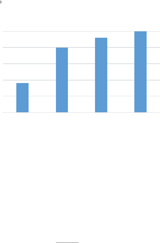
184 FRAUD ANALYTICS
75%
80%
85%
90%
95%
100%
0 notch 1 notch 2 notch 3 notch
cumulative notch difference
Figure 4.43 A Cumulative Notch Difference Graph
coding). The multiclass AUC, AUCm, can then be computed as the
sum of the binary AUCs weighted by the class distribution as follows:
AUCm=m
i=1AUC(ci)p(ci),
where mis the number of classes, AUC(ci)the AUC obtained from con-
sidering class cias the reference class, and p(ci)the prior probability
of class ci. Another approach is based on the pairwise discriminabil-
ity of classes and computes the multiclass AUC as follows (similar to
One-versus-One coding):
AUCm=2
m(m−1)i<jAUC(ci,cj),
where AUC(ci,cj)is the area under the two-class ROC curve involving
classes ciand cj. The summation is averaged over all m(m−1)∕2 possible
pairs of classes.
Note that in case of ordinal targets, also rank order statistics such
as Spearman’s rank order correlation, Kendall’s tau, and Goodman-
Kruskal’s gamma can be computed, as we will discuss later.
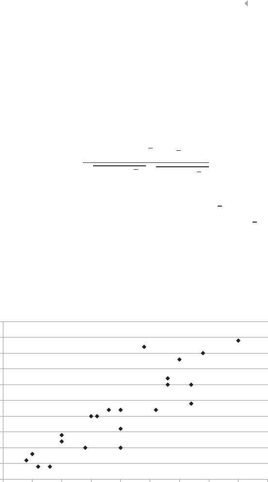
PREDICTIVE ANALYTICS FOR FRAUD DETECTION 185
Performance Measures for Regression Models
A first way to evaluate the predictive performance of a regression
model is by visualizing the predicted target against the actual target
using a scatter plot (see Figure 4.44). The more the plot approaches
a straight line through the origin, the better the performance of the
regression model. It can be summarized by calculating the Pearson
correlation coefficient as follows:
corr(̂
y,y)= n
i=1(̂
yi−̂
y)(yi−y)
n
i=1(̂
yi−̂
y)2n
i=1(yi−y)2
,
where ̂
yirepresents the predicted value for observation i,̂
ythe average
of the predicted values, yithe actual value for observation i,andythe
average of the actual values. The Pearson correlation always varies
between –1 and +1. Values closer to +1 indicate better agreement
and thus better fit between the predicted and actual values of the
target variable.
0
5
10
15
20
25
30
35
40
45
50
0 5 10 15 20 25 30 35 40 45
Actual Fraud
Predicted Fraud
Figure 4.44 Scatter Plot: Predicted Fraud Versus Actual Fraud

186 FRAUD ANALYTICS
Another key performance metric is the coefficient of determination
or R2defined as follows:
R2=n
i=1(̂
yi−y)2
n
i=1(yi−y)2=1−n
i=1(yi−̂
yi)2
n
i=1(yi−y)2,
The R2always varies between 0 and 1, and higher values are to
be preferred. Basically, this measure tells us how much better we can
predict by using the analytical model to compute ̂
yithan by using the
mean yas predictor. To compensate for the variables in the model, an
adjusted R2,R2
adj, has been suggested as follows:
R2
adj =1−n−1
n−p−1(1−R2)=1−n−1
n−p−1n
i=1(yi−̂
yi)2
n
i=1(yi−y)2,
where prepresents the number of variables in the model. Note that
when the R2is measured on a test set, negative values are possible
if the average value of the target on the training set differs from the
average value of the target on the test set.
Two other popular measures are the mean squared error (MSE)
and mean absolute deviation (MAD) defined as follows:
MSE =n
i=1(yi−̂
yi)2
n,
MAD =n
i=1yi−̂
yi
n.
A perfect model would have an MSE and MAD of 0. Higher values
for both MSE and MAD indicate less good performance. Note that the
MSE is sometimes also reported as the root mean squared error (RMSE)
whereby RMSE =MSE.
Also, CAP curves can be used to visualize and calculate the
performance of regression models. Just as in classification, the X-axis
represents the percentage of the sorted population, but now sorted
based on the outcome of the regression model. For the Y-axis, a
binary variable needs to be defined. One option is to create a binary
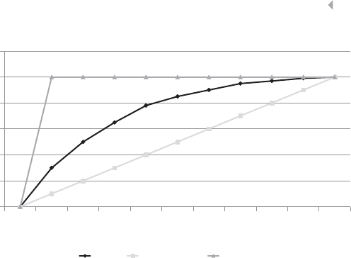
PREDICTIVE ANALYTICS FOR FRAUD DETECTION 187
0%
20%
40%
60%
80%
100%
120%
0 10% 20% 30% 40% 50% 60% 70% 80% 90% 100%
Percentage of fraud amounts lower
than average
Percentage of sorted population
model Random model Perfect Model
Figure 4.45 CAP Curve for Continuous Targets
outcome representing whether the observed fraud amount is lower
than the average fraud amount. This is illustrated in Figure 4.45. The
corresponding CAP plot and accuracy ratio will then indicate how
much better the analytical model predicts than the average. Another
option would be to create a binary variable indicating whether the
observed fraud amount is smaller than the 25th (75th) percentile of the
distribution, in which case the CAP curve and corresponding accuracy
ratio will indicate how much better the analytical model allows to
predict small (high) fraud amounts.
Another popular visual representation is the regression error char-
acteristic (REC) curve (Bi and Bennett 2003). This is a regression vari-
ant of the ROC curve in classification and plots the error tolerance on
the X-axis versus the percentage of points predicted within the toler-
ance on the Y-axis. The resulting curve estimates the cumulative dis-
tribution function of the error. The error on the X-axis can be defined
as the squared error (yi−̂
yi)2or the absolute deviation yi−̂
yi.Justas
with the ROC curve, the perfect model is situated in the upper-left cor-
ner. Hence, the quicker the curve approaches this point, the better the
model. The area above the curve then represents an overall error mea-
sure, which should preferably be as small as possible. As an example,
consider the data represented in Table 4.8.
The corresponding REC curve is depicted in Figure 4.46.
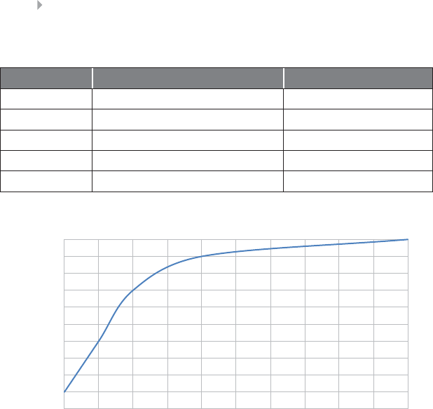
188 FRAUD ANALYTICS
Table 4.8 Data for REC Curve
Tolerance (X) Correct Predictions (Cumulative) Cumulative Accuracy (Y)
0 1 10%
0,05 440%
0,1 770%
0,2 990%
0,5 10 100%
0%
10%
20%
30%
40%
50%
60%
70%
80%
90%
100%
0 0.05 0.1 0.15 0.2 0.25 0.3 0.35 0.4 0.45 0.5
Cumulative Accuracy
Tolerance (MAD)
Figure 4.46 Regression Error Characteristic (REC) Curve
OTHER PERFORMANCE MEASURES FOR PREDICTIVE
ANALYTICAL MODELS
As already mentioned in Chapter 1, statistical performance is just one
aspect of model performance. Other important criteria are comprehen-
sibility, justifiability, and operational efficiency.
Although comprehensibility is subjective and depends on the
background and experience of the fraud analyst, linear and logistic
regression, and decision trees are commonly referred to as white-box,
comprehensible techniques. Neural networks, SVMs, and ensemble
methods are essentially opaque models and thus much harder to
understand. However, in fraud settings where statistical performance
is superior to interpretability, they are the method of choice.

PREDICTIVE ANALYTICS FOR FRAUD DETECTION 189
Remember, justifiability goes one step further and verifies to what
extent the relationships modeled are in line with prior business knowl-
edge and/or expectations. In a practical setting, this often boils down
to verifying the univariate impact of a variable on the model’s out-
put. For example, for a linear/logistic regression model, the signs of
the regression coefficients will be verified.
Finally, the operational efficiency can also be an important
evaluation criterion to consider when selecting the optimal analytical
model. Operational efficiency represents the ease with which one can
implement, use, and monitor the final model. For example, in a (near)
real-time fraud environment, it is important to be able to quickly
evaluate the fraud model. With regards to implementation, rule-based
models excel since implementing rules can be done very easily, even in
spreadsheet software. Linear models are also quite easy to implement
whereas nonlinear models are much more difficult to implement, due
to the complex transformations that are being used by the model.
DEVELOPING PREDICTIVE MODELS
FORSKEWEDDATASETS
Fraud-detection data sets often have a very skew target class distri-
bution whereby typically only about 1 percent or even less of the
transactions are fraudulent. Obviously, this creates problems for the
analytical techniques discussed earlier since they are being flooded by
all nonfraudulent observations and will thus tend toward classifying
every observation as nonfraudulent. Think about decision trees, for
example. If they start from a data set with 99 percent/1 percent
nonfraudulent/fraudulent observations, then the entropy is already
very low and, hence, it is very likely that the decision tree does not
find any useful split and classifies all observations as nonfraudulent,
hereby achieving a classification accuracy of 99 percent, but essentially
detecting none of the fraudsters. It is thus recommended to increase
the number of fraudulent observations or their weight, such that
the analytical techniques can pay better attention to them. Various
procedures are possible to do this and will be outlined in what
follows.

190 FRAUD ANALYTICS
Varying the Sample Window
A first way to increase the number of fraudsters is by increasing the
time horizon for prediction. For example, instead of predicting fraud
with a six-month forward-looking time horizon, a 12-month time
horizon can be adopted. This is likely to add more fraudsters to the
sample and thus enable the analytical techniques to find a meaningful
discrimination. Another approach works by sampling every fraudster
twice (or more) as depicted in Figure 4.47. Let’s assume we predict
fraud with a one-year forward-looking time horizon using informa-
tion from a one year backward looking time horizon. By shifting the
observation point earlier or later, the same fraudulent observation can
be sampled twice. Obviously, the variables collected will be similar
but not perfectly the same, since they are measured on a different
(although overlapping) time frame. This added variability can then
come in handy for the analytical techniques to better discriminate
between the fraudsters and nonfraudsters. Note that depending on the
skewness of the target, multiple observation points can be considered
such that the number of fraudsters is multiplied by 2, 3, 4,…Finding
the optimal number is subject to a trial-and-error exercise.
Undersampling and Oversampling
Another way to increase the weight of the fraudsters is by either over-
sampling them or by undersampling the nonfraudsters. Oversampling
is illustrated in Figure 4.48. Here, the idea is to replicate the fraud-
sters two or more times so as to make the distribution less skew. In our
Obs. point Fraud
1 year
1 year
Obs. point Fraud
1 year
1 year
Figure 4.47 Varying the Time Window to Deal with Skewed Data Sets

PREDICTIVE ANALYTICS FOR FRAUD DETECTION 191
ID Variables Class
1 Fraud
2No Fraud
3No Fraud
4 Fraud
5No Fraud
6No Fraud
7No Fraud
8No Fraud
9 Fraud
10 No Fraud
ID Variables Class
1 Fraud
1 Fraud
2No Fraud
3No Fraud
4 Fraud
4 Fraud
5No Fraud
6No Fraud
7No Fraud
8No Fraud
9 Fraud
10 No Fraud
Train
Tes t
Train
Tes t
Original data Oversampled data
Figure 4.48 Oversampling the Fraudsters
example, observations 1 and 4, both fraudsters, have been replicated
so as to create an equally balanced training sample having the same
amount of fraudsters and nonfraudsters, respectively.
Undersampling is illustrated in Figure 4.49. Here, observations
number 2 and 5, which are both nonfraudulent, have been left out
so as to create an equally balanced training sample. The undersam-
pling can be done based on business experience whereby obviously
legitimate observations are removed. Also, low-value transactions or
inactive accounts can be considered for removal.
ID Variables Class
1 Fraud
2No Fraud
3No Fraud
4 Fraud
5No Fraud
6No Fraud
7No Fraud
8No Fraud
9 Fraud
10 No Fraud
ID Variables Class
1Fraud
3No Fraud
4Fraud
6No Fraud
7No Fraud
8No Fraud
9Fraud
10 No Fraud
Train
Tes t
Train
Tes t
Original data Undersampled data
Figure 4.49 Undersampling the Nonfraudsters

192 FRAUD ANALYTICS
Under- and oversampling can also be combined. In the literature, it
has been shown that undersampling usually results in better classifiers
than oversampling (Chawla et al. 2002).
It is very important to note that both oversampling and undersam-
pling should be conducted on the training data and not on the test
data. Remember, the latter should remain untouched during model
development in order to give an unbiased view on model performance.
A practical question concerns the optimal nonfraud/fraud odds, which
should be aimed for by doing under- or oversampling. Although work-
ing toward a balanced sample with the same number of fraudsters
and nonfraudsters seems attractive, it severely biases the probabili-
ties, which will be output by the analytical technique. Hence, it is
recommended to stay as close as possible to the original class distribu-
tion to avoid unnecessary bias. One practical approach to determine
the optimal class distribution works as follows. In the first step, an
analytical model is built on the original data set with the skew class
distribution (e.g., 95%/5% nonfraudsters/fraudsters). The AUC of this
model is recorded (possibly on an independent validation data set). In
a next step, over- or undersampling is used to change the class distri-
bution by 5 percent (e.g., 90%/10%). Again, the AUC of the model
is recorded. Subsequent models are built on samples of 85%/15%,
80%/20%, 75%/25%, hereby each time recording their AUC. Once
the AUC starts to stagnate (or drop), the procedure stops and the opti-
mal odds ratio has been found. Although it does depend on the data
characteristics and quality, practical experience has shown that the
ratio 80%/20% is quite commonly used in the industry.
Synthetic Minority Oversampling Technique (SMOTE)
Rather than replicating the minority observations (e.g., fraudsters),
Synthetic Minority Oversampling works by creating synthetic observa-
tions based on the existing minority observations (Chawla et al. 2001).
This is illustrated in Figure 4.50 where the circles represent the major-
ity class and the squares the minority class. For each minority class
observation, SMOTE calculates the knearest neighbors. Let’s assume
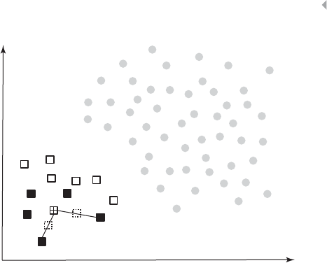
PREDICTIVE ANALYTICS FOR FRAUD DETECTION 193
Figure 4.50 Synthetic Minority Oversampling Technique (SMOTE)
we consider the crossed square and pick the 5 nearest neighbors repre-
sented by the black squares. Depending on the amount of oversampling
needed, one or more of the k-nearest neighbors are selected to create
the synthetic examples.
Let’s say our oversampling percentage is set at 200 percent. In this
case, two of the five nearest neighbors are selected at random. The
next step is then to randomly create two synthetic examples along the
line connecting the observation under investigation (crossed square)
with the two random nearest neighbors. These two synthetic examples
are represented by dashed squares in the figure. As an example, con-
sider an observation with characteristics (e.g., age and income) of 30
and 1,000, and its nearest neighbor with corresponding characteristics
62 and 3,200. We generate a random number between 0 and 1—let’s
say, 0.75. The synthetic example then has age 30 +0.75 ×(62 –30),
or 54, and income 1000 +0.75 ×(3200 −1000)=2,650. SMOTE then
combines the synthetic oversampling of the minority class with under-
sampling the majority class. Note that in their original paper, Chawla
et al. (2001) developed an extension of SMOTE to work with categori-
cal variables. Empirical evidence has shown that SMOTE usually works
better than either under- or oversampling. Also, for fraud detection it
has proven to be very valuable (Van Vlasselaer et al. 2013, 2015).

194 FRAUD ANALYTICS
Likelihood Approach
Another interesting approach to work with a low number of fraud-
sters is the likelihood approach developed by Pluto and Tasche (2005).
Although it was originally developed in a credit-risk modeling setting
to tackle the issue of low-default portfolios, it can be easily transferred
to a fraud-detection setting.
Let’s start with the most extreme example of a skewed data set,
which is a data set with no fraudsters at all. Obviously, none of the
sampling approaches discussed so far will work for this. Assume
now that we have an expert-based fraud detection system that can
discriminate the observations into fraud risk classes A, B, and C using
a set of predefined business rules. Although these three classes allow
analysts to discriminate the observations in terms of their fraud risk,
it would also be handy to accompany each of these classes with fraud
probability estimates. These probabilities can be used to calculate
the expected fraud loss. Remember, Expected fraud loss (EFL)=
Probability of fraud (PF)×Loss given fraud (LGF). The EFL can then
be used for provisioning purposes whereby a firm anticipates future
losses by setting aside provisions.
In a first step, we will try to calculate the probability of fraud (PF)
for class A, PFA. A key assumption we will make is that fraud occurs
independently. Although this assumption might seem naïve at first
sight, it allows us to derive probability estimates in a fairly straight-
forward way given this complex setting with no data about fraud-
sters. More specifically, we will first assume that the ranking of the
observations across the three fraud risk classes is correct, or in other
words: PFA≤PFB≤PFC. The most prudent estimate (sometimes also
referred to as the most conservative estimate) is then obtained under
the temporary assumption that PFA=PFB=PFC. Hence, the probabil-
ity of being fraudulent equals PFAfor every observation. Given that we
have nAobservations in class A, nBobservations in class B, nCobser-
vations in class C, and that fraud occurs independently, the likelihood
of not observing any fraudster in the total data set equals:
(1−PFA)nA+nB+nC

PREDICTIVE ANALYTICS FOR FRAUD DETECTION 195
Table 4.9 Values for PFAfor a Data Set with No Fraudsters
α50% 75% 90% 95% 99% 99.9%
PFA0,20% 0,39% 0,65% 0,85% 1,31% 1,95%
Table 4.10 Values for PFBfor a Data Set with No Fraudsters
α50% 75% 90% 95% 99% 99.9%
PFB0,28% 0,55% 0,92% 1,19% 1,82% 2,72%
We can now specify a confidence region for PFA,whichisthe
region of all values of PFAsuch that the probability of not observing
any fraudster is higher than 1 −𝛼, or in other words:
1−𝛼≤(1−PFA)nA+nB+nC,
or
PFA≤1−(1−𝛼)1∕(nA+nB+nC).
Assume we have 100 observations in class A, 200 in class B, and
50 in class C. Table 4.9 illustrates the values obtained for PFAby vary-
ing the confidence level from 50 percent to 99.9 percent. As can be
observed, PFAincreases as the confidence level increases.
We can now continue this same procedure to compute PFB.We
have nB+nCobservations left. The most prudent estimate of PFBis
obtained by again assuming PFB=PFC. Hence, we have:
1−𝛼≤(1−PFB)nB+nC,
or
PFB≤1−(1−𝛼)1∕(nB+nC).
For our data set, this gives the values reported in Table 4.10.
Finally, we can calculate PFCas follows:
1−𝛼≤(1−PFC)nC,

196 FRAUD ANALYTICS
Table 4.11 Values for PFCfor a Data Set with No Fraudsters
α50% 75% 90% 95% 99% 99.9%
PFC1,38% 2,73% 4,50% 5,81% 8,80% 12,90%
or
PFC≤1−(1−𝛼)1∕nC.
This gives the values reported in Table 4.11.
Note that despite having no fraudsters in the data, PFCat the 99.9
percent confidence level equals 12.90 percent, which is quite high.
Also observe that for a given confidence level, PFA≤PFB≤PFCas
required at the outset. An obvious question is what confidence level to
adopt. Before answering this question, we will extend the procedure
by assuming a few fraudsters occur in the data.
Let’s now assume we have one fraudster in class A, 2 in class B, and
4 in class C. We first determine PFAusing again the most prudent esti-
mate principle: PFA=PFB=PFC. By using the binomial distribution to
calculate the probability of observing less than seven fraudsters, PFA
can be found as follows:
1−𝛼≤7
i=0nA+nB+nC
iPFi
A(1−PFA)nA+nB+nC−i.
Likewise, PFBand PFCcan be found as follows:
1−𝛼≤6
i=0nB+nC
iPFi
B(1−PFB)nB+nC−i,
1−𝛼≤4
i=0nC
iPFi
C(1−PFC)nC−i.
Table 4.12 displays the values obtained depending on the confi-
dence levels. Again, note that the probabilities increase for increasing
confidence levels. Just as in the previous examples, also observe that
PFA≤PFB≤PFCas required at the outset.

PREDICTIVE ANALYTICS FOR FRAUD DETECTION 197
Table 4.12 Values for PFA,PFB, and PFCfor a Data Set with Fraudsters
α50% 75% 90% 95% 99% 99.9%
PFA2,19% 2,76% 3,34% 3,72% 4,51% 5,51%
PFB2,66% 3,41% 4,17% 4,68% 5,73% 7,05%
PFC9,28% 12,26% 15,35% 17,38% 21,50% 26,56%
As already mentioned, a key question to answer when adopting
this approach is the setting of the confidence level. Obviously, this
depends on how conservative the estimates should be. As said, a higher
confidence level results into a higher probability estimate. In their orig-
inal paper, Pluto and Tasche suggest not exceeding 95 percent. In a
credit-risk setting, Benjamin et al. (2006) suggested adopting confi-
dence levels between 50 and 75 percent.
Adjusting Posterior Probabilities
The key idea of undersampling, oversampling and SMOTE is to adjust
the class priors to enable the analytical technique to come up with a
meaningful model discriminating the fraudsters from the nonfraud-
sters. By doing so, the class posteriors will also become biased. This is
no problem in case the fraud analyst is only interested in ranking the
observations in terms of their fraud risk. However, if well-calibrated
fraud probabilities are needed (e.g., to accurately calculate expected
fraud losses), then the posterior probabilities need to be adjusted.
One straightforward way to do this is by using the following formula
(Saerens et al. 2002):
p(Cix)=
p(Ci)
pr(Ci)pr(Cix)
2
j=1
p(Cj)
pr(Cj)pr(Cjx)
,
whereby Cirepresents class i(e.g., class 1 for the fraudsters and 2
for the nonfraudsters), p(Ci)the prior probability (e.g., p(C1)=1%and
p(C2)=99%),p
r(Ci)the resampled prior probability due to oversam-
pling, undersampling or other resampling procedures (e.g., pr(C1)=
20%and pr(C2)=80%),andp
r(Cix)represents the posterior probability

198 FRAUD ANALYTICS
Table 4.13 Adjusting the Posterior Probability
Posteriors Using
Resampled Data
Posteriors Re-Calibrated
to Original Data
P(Fraud) P(No Fraud) P(Fraud) P(No Fraud)
Customer 1 0.1 0.9 0.004 0.996
Customer 2 0.3 0.7 0.017 0.983
Customer 3 0.5 0.5 0.039 0.961
Customer 4 0.6 0.4 0.057 0.943
Customer 5 0.85 0.15 0.186 0.814
Customer 6 0.9 0.1 0.267 0.733
for observation xas calculated by the analytical technique using the
resampled data. Note that the formula can be easily extended to more
than two classes.
Table 4.13 shows an example of adjusting the posterior probabil-
ity, whereby p(C1)=0,01;p(C2)=0,99,pr(C1)=0,20;and pr(C2)=
0,80. It can be easily verified that the rank ordering of the customers
in terms of their fraud risk remains preserved after the adjustment.
Cost-sensitive Learning
Cost-sensitive learning is another alternative to deal with highly
skewed data sets. The idea is to assign higher misclassification costs to
the minority class, which is, in our case, the fraudsters. These costs
are then taken into account during classifier estimation or evaluation.
Table 4.14 gives the overview of the costs in a binary classification
Table 4.14 Misclassification Costs
Predicted Class
Positive Negative
Actual class Positive C(+,+) C(–,+)
Negative C(+,–) C(–,–)

PREDICTIVE ANALYTICS FOR FRAUD DETECTION 199
setting whereby C(i,j) represents the cost of misclassifying an example
from class jinto class i.
Note that usually C(+,+) = C(–,–)=0, and C(–,+) >C(+,–).The
costs are typically also determined on an aggregated basis, rather than
on an observation-by-observation basis.
A first straightforward way to make a classifier cost-sensitive is by
adopting a cost-sensitive cut-off to map the posterior class probabilities
to class labels. In other words, an observation xwill be assigned to the
class that minimizes the expected misclassification cost:
argminij∈{−,+}P(jx).C(i,j),
where P(jx)is the posterior probability of observation xto belong to
class j. As an example, consider a fraud detection setting whereby class
1 are the fraudsters and class 2 the nonfraudsters. An observation xwill
be classified as a fraudster (class 1) if
P(1x).C(1,1)+P(2x).C(1,2)<P(1x).C(2,1)+P(2x).C(2,2)
P(1x).C(2,1)>P(2x).C(1,2)
P(1x).C(2,1)>(1−P(1x)).C(1,2)
P(1x)>C(1,2)
C(1,2)+C(2,1)
P(1x)>1
1+C(2,1)
C(1,2)
So, the cut-off only depends on the ratio of the misclassification
costs, which may be easier to determine than the individual misclassi-
fication costs themselves.
Another approach to cost-sensitive learning works by directly
minimizing the misclassification cost during classifier learning.
Again assuming there is no cost for correct classifications, the total
misclassification cost is then as follows:
Total cost =C(–,+) × FN +C(+,–)×FP,

200 FRAUD ANALYTICS
whereby FN and FP represent the number of false negatives and
positives, respectively. Various cost-sensitive versions of existing classi-
fication techniques have been introduced in the literature. Ting (2002)
introduced a cost-sensitive version of the C4.5 decision tree algorithm
where the splitting and stopping decisions are based on the misclassifi-
cation cost. Veropolous et al. (1999) developed a cost-sensitive version
of SVMs whereby the misclassification costs are taken into account
in the objective function of the SVM. Domingos (1999) introduced
MetaCost, which is a meta-algorithm capable of turning any classifier
into a cost-sensitive classifier by first relabeling observations with their
estimated minimal-cost classes and then estimating a new classifier
on the relabeled data set. Fan et al. (1999) developed AdaCost, a
cost-sensitive variant of AdaBoost, which uses the misclassification
costs to update the weights in successive boosting runs.
To summarize, cost-sensitive learning approaches are usually
more complex to work with than the sampling approaches discussed
earlier. López et al. (2012) conducted a comparison of sampling versus
cost-sensitive learning approaches for imbalanced data sets and found
both methods are good and equivalent. Hence, from a pragmatic
viewpoint, it is recommended to use the sampling approaches in a
fraud-detection setting.
FRAUD PERFORMANCE BENCHMARKS
To conclude this chapter, Table 4.15 provides some references of scien-
tific papers discussing fraud detection across a diversity of settings. The
type of fraud, size of data set used, class distribution, and performance
are reported. To facilitate the comparison, only papers that report the
area under the ROC curve (AUC) are included. The following conclu-
sions can be drawn:
◾Credit card, financial statement, and telecommunications fraud
case studies report the highest AUC.
◾Insurance and social security fraud report the lowest AUC.
◾All case studies, except for financial statement fraud, start from
highly skewed data sets.

PREDICTIVE ANALYTICS FOR FRAUD DETECTION 201
Table 4.15 Performance Benchmarks for Fraud Detection
Reference Type of Fraud Size of Data Class Performance
Set Used Distribution
Ortega,
Figuerora et al.
(2006)
Medical
Insurance
8,819 5% fraud AUC: 74%
Šubelj, Furlan
et al. (2011)
Automobile
Insurance fraud
3,451 1.3% fraud AUC: 71%–
92%
Bhattacharyya,
Jha et al.
(2011)
Credit card fraud 50 million
transactions on
about 1 million
credit cards
from a single
country
0.005%
fraud
AUC: 90,8%–
95,3%
Whitrow, Hand
et al. (2009)
Credit card fraud 33,000–36,000
activity records
0.1% fraud Gini: 85%
(∼ AUC =
92.5%)
Van Vlasselaer,
Bravo et al.
(2015)
Credit card fraud 3,3 million
transactions
<1% fraud AUC: 98.6%
Dongshan and
Girolami
(2007)
Telecommunica-
tions fraud
809,395 calls
from 1,087
accounts
0.024%
fraud
AUC: 99.5%
Van Vlasselaer,
Meskens et al.
(2013)
Social security
fraud
2000
observations
1% fraud AUC: 80–85%
Ravisankar,
Ravi et al.
(2011)
Financial
statement fraud
202 companies 50% fraud AUC: 98.09%
REFERENCES
Allison, P D. (2001). Logistic Regression Using the SAS® System: Theory and
Application. Hoboken, NJ: John Wiley-SAS.
Baesens, B. (2014). Analytics in a Big Data World. Hoboken, NJ: John Wiley
& Sons.
Baesens, B., Martens, D., Setiono, R., & Zurada, J. (2011). White Box Nonlin-
ear Prediction Models, editorial special issue, IEEE Transactions on Neural
Networks 22 (12): 2406–2408.

202 FRAUD ANALYTICS
Baesens, B., Mues, C., Martens, D., & Vanthienen, J. (2009). 50 Years of Data
Mining and OR: Upcoming Trends and Challenges. Journal of the Opera-
tional Research Society 60: 16–23.
Baesens, B., Setiono, R., Mues, C., & Vanthienen, J. (March 2003). Using
Neural Network Rule Extraction and Decision Tables for Credit-Risk
Evaluation. Management Science 49 (3): 312–329.
Baesens, B., Van Gestel, T., Viaene, S., Stepanova, M., Suykens, J., & Van-
thienen, J. (2003). Benchmarking State of the Art Classification Algo-
rithms for Credit Scoring. Journal of the Operational Research Society 54 (6):
627–635.
Baesens, B., Viaene, S., Van den Poel, D., Vanthienen, J., & Dedene, G. (2002).
Bayesian Neural Network Learning for Repeat Purchase Modelling
in Direct Marketing. European Journal of Operational Research 138 (1):
191–211.
Bartlett P. L. (1997). For Valid Generalization, the Size of the Weights Is More
Important than the Size of the Network. In M. C. Mozer, M. I. Jordan,
and T. Petsche (Eds.), Advances in Neural Information Processing Systems 9.
Cambridge, MA: MIT Press, pp. 134–140.
Benjamin, N., Cathcart, A., & Ryan, K. (2006). Low Default Portfolios: A Pro-
posal for Conservative Estimation of Default Probabilities; Discussion
paper, Financial Services Authority.
Bhattacharyya, S., Jha, S. K., Tharakunnel, K. K., & Westland, J. C. (2011).
Data Mining for Credit Card Fraud: A Comparative Study, Decision Support
Systems 50 (3): 602–613.
Bi, J., & Bennett, K. P. (2003). Regression Error Characteristic Curves, Proceed-
ings of the 20th International Conference on Machine Learning (ICML),
pp. 43–50.
Bishop, C. M. (1995). Neural Networks for Pattern Recognition. Oxford: Oxford
University Press.
Breiman, L. (1996). Bagging Predictors. Machine Learning 24 (2): 123–140.
Breiman, L., Friedman, J. H., Olshen, R. A., Stone, C. J. (1984). Classification
and Regression Trees. Monterey, CA: Wadsworth & Brooks/Cole Advanced
Books & Software.
Breiman, L., (2001). Random Forests. Machine Learning 45 (1): 5–32.
Chawla, N. V., Bowyer, K.W., Hall, L. O., Kegelmeyer, W. P. (2002). SMOTE:
Synthetic Minority Over-sampling Technique. Journal of Artificial Intelli-
gence Research 16: 321–357.
Craven, M., & Shavlik, J. (1996). Extracting Tree-Structured Representations
of Trained Networks. In D. S. Touretzky, M. C. Mozer, and M. E. Hasselmo

PREDICTIVE ANALYTICS FOR FRAUD DETECTION 203
(Eds.), Advances in Neural Information Processing Systems 8. Cambridge, MA:
MIT Press, pp. 24–30.
Cristianini, N., Taylor J. S. (2000). An Introduction to Support Vector Machines
and Other Kernel-Based Learning Methods Cambridge: Cambridge University
Press.
Dejaeger, K., Verbeke, W., Martens, D., & Baesens, B. (2012). Data Mining
Techniques for Software Effort Estimation: A Comparative Study, IEEE
Transactions on Software Engineering 38 (2): 375–397.
Domingos, P. (1999). MetaCost: A General Method for Making Classifiers Cost-
Sensitive, Proceedings of the Fifth International Conference on Knowledge
Discovery and Data Mining. New York: ACM Press, pp. 155–164.
Dongshan X., & Girolami M. (2007). Employing Latent Dirichlet Allocation
for Fraud Detection in Telecommunications. Pattern Recognition Letters 28:
1727–1734.
Duda, R. O., Hart, P. E., & Stork, D. G. (2001). Pattern Classification.NewYork:
John Wiley & Sons.
Efron B. (1979). Bootstrap Methods: Another Look at the Jackknife. The Annals
of Statistics 7 (1): 1–26.
Fan, W., Stolfo, S. J., Zhang J., & Chan P. K. (1999). AdaCost: Misclassifi-
cation Cost-sensitive Boosting. Proceedings of the Sixteenth International
Conference on Machine Learning (ICML). Waltham, MA: Morgan Kaufmann,
pp. 97–105.
Fawcett, T. (2003). ROC Graphs: Notes and Practical Considerations for
Researchers, HP Labs Tech Report HPL-2003–4.
Flach P. (2012). Machine Learning: The Art and Science of Algorithms that Make Sense
of Data. Cambridge: Cambridge University Press.
Freund, Y., & Schapire, R. E. (August 1997). A Decision-Theoretic General-
ization of On-line Learning and an Application to Boosting. Journal of
Computer and System Sciences 55 (1):119–139.
Freund, Y., & Schapire, R. E. (September 1999). A Short Introduction to Boost-
ing. Journal of Japanese Society for Artificial Intelligence 14 (5): 771–780.
Han, J., & Kamber, M. (2006). Data Mining: Concepts and Techniques, 2nd ed.
Waltham, MA: Morgan Kaufmann.
Hand, D., Till, R. J. (2001). A Simple Generalization of the Area under the
ROC Curve to Multiple Class Classification Problems. Machine Learning 45
(2):171–186.
Hand, D. J., Mannila, H., & Smyth, P. (2001). Principles of Data Mining.
Cambridge, MA: MIT Press.
Hanley, J. A., & McNeil, B. J. (1982). The Meaning and Use of Area under the
ROC Curve. Radiology 143: 29–36.

204 FRAUD ANALYTICS
Hartigan, J. A. (1975). Clustering Algorithms. New York: John Wiley & Sons.
Hastie, T., Tibshirani, R., & Friedman, J. (2001). Elements of Statistical Learning:
Data Mining, Inference and Prediction. New York: Springer-Verlag.
Hornik, K., Stinchcombe, M., & White, H. (1989). Multilayer Feedfor-
ward Networks Are Universal Approximators. Neural Networks 2 (5):
359–366.
Huysmans, J., Baesens, B., Van Gestel, T., & Vanthienen, J. (April 2006). Using
Self-Organizing Maps for Credit Scoring. Expert Systems with Applications,
Special Issue on Intelligent Information Systems for Financial Engineering 30 (3):
479–487.
Kass, G. V. (1980). An Exploratory Technique for Investigating Large Quantities
of Categorical Data. Applied Statistics 29 (2): 119–127.
López, V., Fernández, A., Moreno-Torres, J., & Herrera, F. (2012). Analysis of
Preprocessing vs. Cost-Sensitive Learning for Imbalanced Classification.
Open Problems on Intrinsic Data Characteristics. Expert Systems with Appli-
cations 39: 6585–6608.
Lu, H., Setiono, R., & Liu, H. (September 1995). NeuroRule: a Connectionist
Approach to Data Mining. In Proceedings of 21st International Conference on
Very Large Data Bases, Zurich, Switzerland, pp. 478–489.
Mangasarian, O. L. (May–June 1965). Linear and Nonlinear Separation of
Patterns by Linear Programming, Operations Research 13: 444–452.
Martens, D., Baesens, B., & Van Gestel, T. (2009). Decompositional Rule
Extraction from Support Vector Machines by Active Learning. IEEE
Transactions on Knowledge and Data Engineering 21 (1): 178–191.
Martens, D., Baesens, B., Van Gestel, T., & Vanthienen, J. (2007). Comprehen-
sible Credit Scoring Models Using Rule Extraction from Support Vector
Machines. European Journal of Operational Research 183: 1466–1476.
Martens, D., Vanthienen, J., Verbeke, W., & Baesens, B. (2011). Performance
of Classification Models from a User Perspective. Decision Support Systems,
Special Issue on Recent Advances in Data, Text, and Media Mining & Information
Issues in Supply Chain and in Service System Design 51 (4): 782–793.
Moody, J., & Utans, J. (1994). Architecture Selection Strategies for
Neural Networks: Application to Corporate Bond Rating Prediction.
In Apostolos-Paul Refenes (Ed.), Neural Networks in the Capital Markets.
New York: John Wiley & Sons.
Ortega, P.A., Figueora C.J., & Ruz. G. A. (2006). Medical Claim Fraud/Abuse
Detection System based on Data Mining: A Case Study in Chile, Proceedings
of the 2006 International Conference on Data Mining, DMIN.

PREDICTIVE ANALYTICS FOR FRAUD DETECTION 205
Pluto, K., & Tasche, D. (2005). Estimating Probabilities of Default for Low
Default Portfolios. In B. Engelmann and R. Rauhmeier (Eds.), The Basel
II Risk Parameters. New York: Springer.
Quinlan, J. R. (1993). C4.5 Programs for Machine Learning. Waltham, MA:
Morgan Kauffman Publishers.
Ravisankar, P., Ravi, V., Rao, G. R., & Bose, I. (2011). Detection of Financial
Statement Fraud and Feature Selection Using Data Mining Techniques,
Decision Support Systems 50: 491–500.
Saerens M., Latinne P., & Decaestecker C. (2002). Adjusting the Outputs of a
Classifier to New a Priori Probabilities: A Simple Procedure. Neural Compu-
tation 14 (1): 21–41.
Schölkopf B., & Smola A. (2002). Learning with Kernels. Cambridge: MIT Press.
Setiono R. Baesens B., & Mues C. (2009). A Note on Knowledge Discovery
Using Neural Networks and Its Application to Credit Card Screening. Euro-
pean Journal of Operational Research 192 (1): 326–332.
Setiono R., Baesens B. & Mues C. (2011). Rule Extraction from Minimal Neural
Network for Credit Card Screening. International Journal of Neural Systems
21 (4): 265–276.
Šubelj L., Furlan S., & Bajec M. An Expert System for Detecting Automobile
Insurance Fraud Using Social Network Analysis. Expert Systems with Appli-
cations 38 (1): 1039–1052.
Tan P. N., Steinbach M., & Kumar V. (2006). Introduction to Data Mining.New
York: Pearson.
Ting K. M. (2002). An Instance-Weighted Method to Induce Cost-Sensitive
Trees, IEEE Transactions on Knowledge and Data Engineering 14: 659–665.
Van Gestel, T., & Baesens B. (2009). Credit Risk Management: Basic Concepts: Finan-
cial Risk Components, Rating Analysis, Models, Economic and Regulatory Capital.
Oxford: Oxford University Press.
Van Gestel, T., Baesens B., & Martens D. (2015). Predictive Analytics: Techniques
and Applications in Credit Risk Modeling. Oxford: Oxford University Press,
forthcoming.
Van Gestel, T., Baesens, B., Van Dijcke, P., Suykens, J., Garcia, J., and & Alder-
weireld, T. (2005). Linear and Nonlinear Credit Scoring by Combining
Logistic Regression and Support Vector Machines. Journal of Credit Risk 1 (4).
Van Gestel, T., Suykens J., Baesens B., Viaene S., Vanthienen J., Dedene G., De
Moor B., & Vandewalle J. (January 2004). Benchmarking Least Squares
Support Vector Machine Classifiers. Machine Learning 54 (1): 5–32.
Van Vlasselaer, V., Akoglu L., Eliassi-Rad T., Snoeck M., & Baesens B.
(2015). Guilt-by-Constellation: Fraud Detection by Suspicious Clique

206 FRAUD ANALYTICS
Memberships, Proceedings of 48 Annual Hawaii International Conference on
System Sciences, HICSS-48, Kauai (Hawaii), January 5–8.
Van Vlasselaer, V., Bravo C., Caelen O., Eliassi-Rad T., Akoglu L., Snoeck M.,
& Baesens B. (2015). APATE: A novel approach for automated credit card
transaction fraud detection using network-based extensions. Decision Sup-
port Systems 75: 38–48.
Van Vlasselaer, V., Meskens J., Van Dromme D., & Baesens B. (2013). Using
Social Network Knowledge for Detecting Spider Constructions in Social
Security Fraud. Proceedings of the 2013 IEEE/ACM International Conference on
Advances in Social Network Analysis and Mining, Niagara Falls.
Vapnik, V. (1995). The Nature of Statistical Learning Theory, New York:
Springer-Verlag.
Veropoulos, K., Campbell, C., Cristianini N. (1999). Controlling the Sensitivity
of Support Vector Machines. Proceedings of the International Joint Conference
on AI, pp. 55–60.
Viaene, S., Derrig, R., Baesens, B., Dedene, G. (2002). A Comparison of
State-of-the-Art Classification Techniques for Expert Automobile Insur-
ance Fraud Detection. Journal of Risk and Insurance, Special issue on Fraud
Detection 69 (3): 433–443.
Whitrow, C., Hand, D. J., Juszczak, P., Weston, D., Adams, N.M. (2009). Trans-
action Aggregation as a Strategy for Credit Card Fraud Detection. Data
Mining and Knowledge Discovery 18: 30–55.
Zurada, J.M. (1992). Introduction to Artificial Neural Systems. Boston: PWS
Publishing.
CHAPTER 5
Social Network
Analysis for Fraud
Detection
207
In the last decade, the use of social media websites in everybody’s
daily life is booming. People can continue their conversations on
online social network sites like Facebook, Twitter, LinkedIn, Google+,
Instagram, and so on and share their experiences with their acquain-
tances, friends, family, and others. It only takes one click to update
your whereabouts to the rest of the world. Plenty of options exist to
broadcast your current activities: by picture, video, geo-location, links,
or just plain text. You are on the top of the world—and everybody’s
watching. And this is where it becomes interesting.
Users of online social network sites explicitly reveal their relation-
ships with other people. As a consequence, social network sites are
a (almost) perfect mapping of the relationships that exist in the real
world. We know who you are, what your hobbies and interests are, to
whom you are married, how many children you have, your buddies
with whom you run every week, your friends at the wine club, etc. This
whole interconnected network of people knowing each other, some-
how, is an extremely interesting source of information and knowledge.
Marketing managers no longer have to guess who might influence
whom to create the appropriate campaign. It is all there—and that is
exactly the problem. Social network sites acknowledge the richness of
the data sources they have, and are not willing to share them as such
and free of cost. Moreover, those data are often privatized and regu-
lated, and well-hidden from commercial use. On the other hand, social
network sites offer many good built-in facilities to managers and other
interested parties to launch and manage their marketing campaigns by
exploiting the social network, without publishing the exact network
representation.
However, companies often forget that they can reconstruct (a
part of) the social network using in-house data. Telecommunication
providers, for example, have a massive transactional data base where
they record call behavior of their customers. Under the assumption
that good friends call each other more often, we can recreate the
network and indicate the tie strength between people based on the
frequency and/or duration of calls. Internet infrastructure providers
might map the relationships between people using their customers’
IP-addresses. IP-addresses that frequently communicate are repre-
sented by a stronger relationship. In the end, the IP-network will
208

SOCIAL NETWORK ANALYSIS FOR FRAUD DETECTION 209
envisage the relational structure between people from another point
of view, but to a certain extent as observed in reality. Many more
examples can be found in the banking, retail, and online gaming
industry.
Also, the fraud detection domain might benefit from the analysis
of social networks. In this chapter, we underline the social character
of fraud. This means that we assume that the probability of someone
committing fraud depends on the people (s)he is connected to. These
are the so-called guilt-by-associations (Koutra et al. 2011). If we know
that five friends of Bob are fraudsters, what would we say about Bob?
Is he also likely to be a fraudster? If these friends are Bob’s only friends,
is it more likely that Bob will be influenced to commit fraud? What if
Bob has 200 other friends, will the influence of these five fraudsters be
the same?
In this chapter, we will briefly introduce the reader to networks
and their applications in a fraud detection setting. One of the main
questions answered in this chapter is how unstructured network infor-
mation can be translated into useful and meaningful characteristics of
a subject. We will analyze and extract features from the direct neigh-
borhood (i.e., the direct associates of a certain person or subject) as
well as the network as a whole (i.e., collective inferencing). Those
network-based features can serve as an enrichment of traditional data
analysis techniques.
NETWORKS: FORM, COMPONENTS, CHARACTERISTICS,
AND THEIR APPLICATIONS
Networks are everywhere. Making a telephone call requires setting up
a communication over a wired network of all possible respondents by
sending voice packages between the caller and the callee. The supply
of water, gas, and electricity for home usage is a complex distribution
network that consists of many source, intermediary, and destination
points where sources need to produce enough output such that they
meet the demand of the destination points. Delivery services need to
find the optimal route to make sure that all the packages are delivered
at their final destination as efficiently as possible. Even a simple trip to
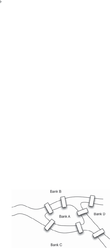
210 FRAUD ANALYTICS
the store involves the processing of many networks. What is the best
route to drive from home to the store given the current traffic? Given
a shopping list, how can I efficiently visit the store such that I have
every product on my list?
One of humans’ talents is exactly the processing of these networks.
Subliminally, people have a very good sense in finding an efficient
way through a network. Consider your home-to-work connection.
Depending on the time and the day, you might change your route to
go from home to work without explicitly drawing the network and
running some optimization algorithm. Reaching other people, even
without the telecommunication media of nowadays like telephone
and internet, is often an easy task for people. There is always a friend
of a friend who knows the guy you are looking for.
The mathematical study of optimizing network-related problems
has been introduced many years ago by Euler (1736). He formulated
the problem of the Köningsberg bridges. Köningsberg (now Kaliningrad)
was a city in Lithuania that was divided into four parts by the river
Pregel. Seven bridges connected the four banks of the city (see
Figure 5.1a and Figure 5.1b). The problem is as follows, “Does there
exist a walking route that crosses all seven bridges exactly once?” A
path that can traverse all edges (here: bridges) of a network exactly
once, is a Eulerian path. Euler proved that such a path cannot exist
for the Köningsberg bridge problem. More specifically, an Eulerian
path only exists when all nodes (here: banks) are reached by an
even number of edges, except for the source and sink node of the
Figure 5.1a Köningsberg Bridges
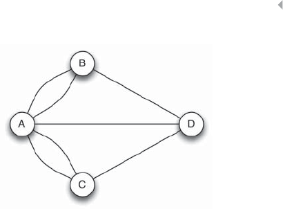
SOCIAL NETWORK ANALYSIS FOR FRAUD DETECTION 211
Figure 5.1b Schematic Representation of the Köningsberg Bridges
path which should have an odd number of bridges pointing to it.
Analogously, a Hamiltonian path in the network is a path that visits
each node exactly once. For example, the Traveling Salesman Problem
(TSP) tries to find a Hamiltonian path in the network. Given a set of
cities, the idea is that a salesman has to visit each city (i.e., node)
exactly once to deliver the packages. As this is an NP-hard problem,
research mainly focuses on finding good heuristics to solve the TSP.
Social Networks
Although in the previous example networks are built and developed
by humans, they are not social. A key question here is, “What makes
a network social?” In general, we might say that a network is social
whenever the actors are people or groups of people. A connection
between actors is based on any form of social interaction between
them, such as a friendship. As in the real world, social networks are
also able to reflect the intensity of a relationship between people.
How well do you know your contacts? The relationship between two
best friends completely differs from the relationship between two
distant acquaintances. Those relationships and their intensity are an
important source of information exchange.
The psychologist Stanley Milgram measured in 1967 how social
the whole world is. He conducted a Small World experiment whereby he
distributed 100 letters to random people all over the world. The task
at hand was to return the letter to a specified destination, which was

212 FRAUD ANALYTICS
one of Milgram’s friends. Rather than sending the letter back by mail,
people could only pass the letter to someone they knew. This person,
on their turn, had to forward the letter to one of his/her contacts, and
so on …until the letter reached its final destination. Milgram showed
that, on average, each letter reached its destination within six hops.
That is, less than six people are necessary to connect two random peo-
ple in the network. This is the average path length of the network. The
result of the experiment is widely known as the six degrees of separation
theorem. Milgram also found that many letters reached their target
destination within three steps. This is the so-called funneling effect. Some
people are known and know many other people, often from highly
diverse contact groups (e.g., work, friends, hobby). Those people are
sociometric superstars, connecting different parts of the network to
each other. Many paths in the network pass through these people, giv-
ing them a high betweenness score (see section on Centrality metrics).
While the six degrees of separation theorem is based on results in
real-life, many studies already proved that an average path length of six
is an overestimation in online social networks. Those studies reported
an average path length of approximately four hops between any two
random people in an online social network (Kwak et al. 2010). Online
social networks are thus denser than real-life networks. However, the
intensity between the relationships might strongly differ.
Social networks are an important element in the analysis of fraud.
Fraud is often committed through illegal set-ups with many accom-
plices. When traditional analytical techniques fail to detect fraud due
to a lack of evidence, social network analysis might give new insights by
investigating how people influence each other. These are the so-called
guilt-by-associations, where we assume that fraudulent influences run
through the network. For example, insurance companies often have
to deal with groups of fraudsters, trying to swindle by resubmitting the
same claim using different people. Suspicious claims often involve the
same claimers, claimees, vehicles, witnesses, and so on. By creating and
analyzing an appropriate network, inspectors might gain new insights
in the suspiciousness of the claim and can prevent pursuit of the claim.
In social security fraud, employers try to avoid paying their tax
contributions to the government by intentionally going bankrupt.
Bankrupt employers are not capable of redeeming their tax debts to

SOCIAL NETWORK ANALYSIS FOR FRAUD DETECTION 213
the government, and are discharged from their obligations. However,
social network analysis can reveal that the employer is refounded
using almost the same structure a couple of weeks later. As such,
experts can declare the foundation of the new employer unlawful
and still recover the outstanding debts. Opinion fraud occurs when
people untruthfully praise or criticize a product in a review. Especially
online reviews lack control to establish the genuineness of the review.
Matching people to their reviews and comparing the reviews with
others using a network representation, enables review websites to
detect the illicit reviews.
Identity theft is a special form of social fraud, as introduced in
Chapter 1, where an illicit person adopts another person’s profile.
Examples of identity theft can be found in telecommunications fraud
where fraudsters “share” an account with a legitimate customer. This
is depicted in Figure 5.2. As fraudsters cannot withstand to call their
family, friends, acquaintances, and so on, the network clearly links the
account with the fraudster’s previous (or current) account. Once the
fraudster takes over a new customers’ account, the contact list of the
customer is extended by other contacts who were never called before.
The frequent contact list of the fraudster is a strong indicator for fraud.
Figure 5.2 Identity Theft. The Frequent Contact List of a Person is Suddenly Extended
with Other Contacts (Light Gray Nodes). This Might Indicate that a Fraudster (Dark Gray
Node) Took Over that Customer’s Account and “shares” his/her Contacts
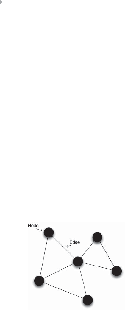
214 FRAUD ANALYTICS
While networks are a powerful visualization tool, they mainly
serve to support the findings by automated detection techniques.
We will focus on how to extend the detection process by extracting
useful and meaningful features from the network. The network
representation can be used afterward to verify the obtained results.
Network Components
This section will introduce the reader to graph theory, the mathemat-
ical foundation for the analysis and representation of networks.
Complex network analysis (CNA) studies the structure, charac-
teristics, and dynamics of networks that are irregular, complex, and
dynamically evolving in time (Boccaletti et al. 2006). Those networks
often consist of millions of closely interconnected units. Most real-life
networks are complex. CNA uses graph theory to extract useful statis-
tics from the network. Boccaletti et al. (2006) define graph theory as
the natural framework for the exact mathematical treatment of com-
plex networks, and, they state that formally, a complex network is
represented as a graph.
A graph 𝓖=(𝓥,𝓔)consists of a set 𝓥of vertices or nodes (the
points) and a set 𝓔of edges or links (the lines connecting the points).
This is illustrated in Figure 5.3. A node 𝓋∈𝓥represents real-world
objects such as people, computers or activities. An edge 𝓋∈𝓔connects
Figure 5.3 Network Representation
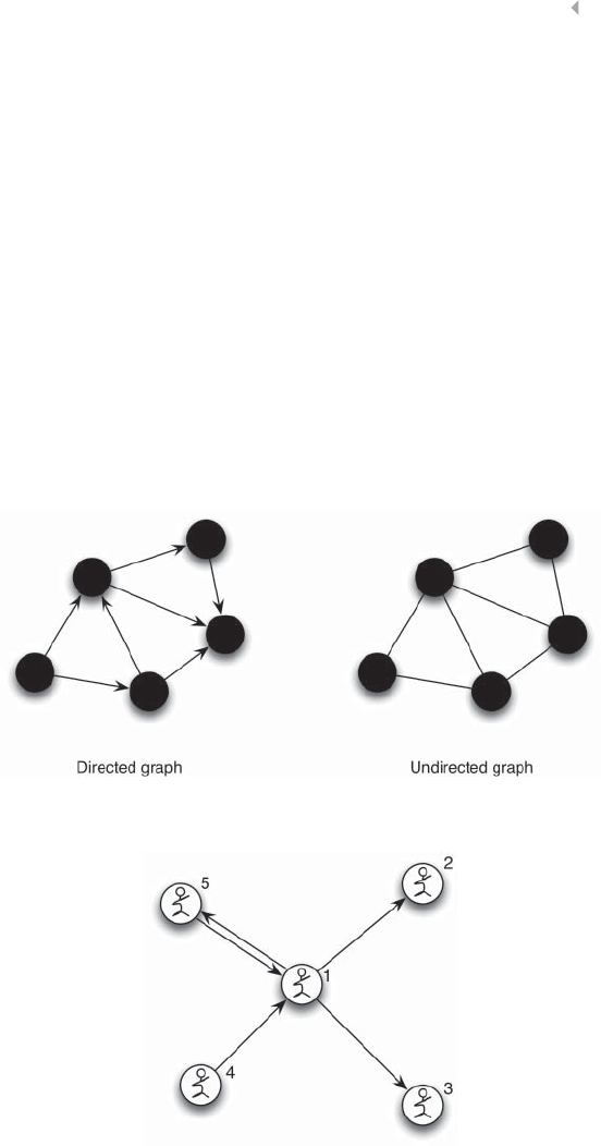
SOCIAL NETWORK ANALYSIS FOR FRAUD DETECTION 215
two nodes in the network, and
e(𝓋1,𝓋2)e∈𝓔&𝓋i∈𝓥.
An edge represents a relationship between the nodes it connects,
such as a friendship (between people), a physical connection (between
computers), or attendance (of a person to an event).
A graph where the edges impose an order or direction between
the nodes in the network is a directed graph. If there is no order in
the network, we say that the graph is undirected. This is shown in
Figure 5.4. The social network website Twitter can be represented as
a directed graph. Users follow other users, without necessarily being
refollowed. This is expressed by the follower–followee relationships,
and is illustrated in Figure 5.5. User 1 follows User 2, 3, and 5 (follower
Figure 5.4 Example of a (Un)Directed Graph
Figure 5.5 Follower–Followee Relationships in a Twitter Network
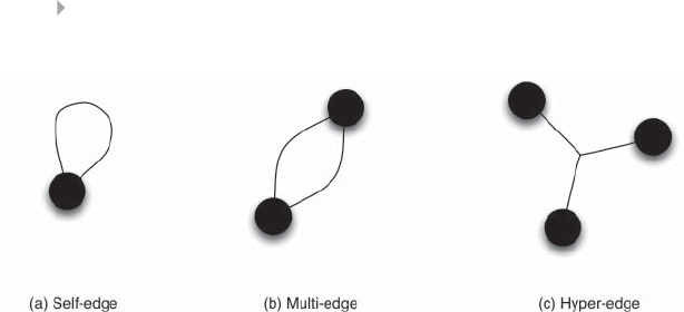
216 FRAUD ANALYTICS
Figure 5.6 Edge Representation
relationships), and is followed by User 4 and 5 (followee relationship).
There is a mutual relationship between User 1 and 5.
In general, edges connect two nodes to each other. However, some
special variants are sometimes required to accurately map the reality
(see Figure 5.6):
◾Self-edge: A self-edge is a connection between the node and
itself. For example, a person who transfers money from his/her
account to another account s/he owns.
◾Multi-edge: A multi-edge exists when two nodes are con-
nected by more than one edge. For example, in credit card
transaction fraud, a credit card holder is linked to a merchant
by a multi-edge if multiple credit card transactions occurred
between them.
◾Hyper-edge: A hyper-edge is an edge that connects more than
one node in the network. For example, three people who went
to the same event.
A graph where the edges express the intensity of the relationships,
is a weighted graph 𝓖w=(𝓥,𝓔).
◾Binary weight: This is the standard network representation.
Here, the edge weight is either 0 or 1, and reflects whether or
not a link exists between two nodes. An extension of the binary
weighted graphs are the signed graphs where the edge weight
is negative (–1), neutral (0), or positive (1). Negative weights
are used to represent animosity, and positive weights are used
to represent friendships. Neutral weights represent an “I don’t
know you” relationship.

SOCIAL NETWORK ANALYSIS FOR FRAUD DETECTION 217
◾Numeric weight: A numeric edge weight expresses the affinity
of a person to other persons s/he is connected to. High values
indicate a closer affiliation. As people do not assign a weight
to each of their contacts by themselves, many approaches are
proposed to define an edge weight between nodes. A popular
way is the Common Neighbor approach. That is, the edge weight
equals the total number of common activities or events both
people attended. An activity/event should be interpreted in a
broad sense: the total number of messages sent between them,
common friends, likes on Facebook, and so on.
◾Normalized weight: The normalized weight is a variant of the
numeric weight where all the outgoing edges of a node sum up
to 1. The normalized weight is often used in influence propaga-
tion over a network.
◾Jaccard weight: The edge weight depends on how “social”
both nodes are (Gupte and Eliassi-Rad 2012), and
w(𝓋1,𝓋2)= 𝚪(𝓋1)∩𝚪(𝓋2)
𝚪(𝓋1)∪𝚪(𝓋2)
with 𝚪(𝓋i)the number of events node 𝓋iattended. For example,
assume that person A attended 10 events and person B attended 5
events. They both went to 3 common events. Then, according to the
Jaccard Index, their edge weight equals 1/4.
Edge weights represent the connectivity within a network, and
are in some way a measure of the sociality between the nodes in the
network. Nodes, on the other hand, use labels to express the local char-
acteristics. Those characteristics are mostly proper to the node and may
include, for example, demographics, preferences, interests, beliefs, and
so on. When analyzing fraud networks, we integrate the fraud label of
the nodes into the network. A node can be fraudulent or legitimate,
depending on the condition of the object it represents. For example,
Figure 5.7 shows a fraud network where the legitimate and fraudu-
lent people are represented by white- and black-colored nodes, respec-
tively. Given this graph, we know that node A and B committed fraud
beforehand. Node C is a friend of node A and is influenced by the
actions of node A. On the other hand, node D is influenced by both
node A and B. A simple conclusion would be that node D has the
highest probability of perpetrating fraud, followed by node C.
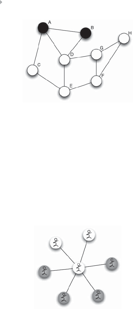
218 FRAUD ANALYTICS
Figure 5.7 Example of a Fraudulent Network
While real-life networks often contain billions of nodes and mil-
lions of links, sometimes the direct neighborhood of nodes provides
enough information to base decisions on. An ego-centered network or
egonet represents the one-hop neighborhood of the node of interest.
In other words, an egonet consists of a particular node and its immedi-
ate neighbors. The center of the egonet is the ego, and the surround-
ing nodes are the alters. An example of an egonet is illustrated in
Figure 5.8. Such networks are also called the first-order neighborhood
of a node. Analogously, the n-order neighborhood of a node encom-
passes all the nodes that can be reached within nhops from the node
of interest.
Figure 5.8 An Egonet. The Ego is Surrounded by Six Alters, of Whom Two are Legitimate
(White Nodes) and Four are Fraudulent (Gray Nodes)

SOCIAL NETWORK ANALYSIS FOR FRAUD DETECTION 219
Network Representation
Transactional data sources often contain information about how
entities relate to each other (e.g., call record data, bank transfer data).
An example transactional data source of credit card fraud is given
in Table 5.1. Each line in the transactional data source represents
a money transfer between two actors: a credit card holder and a
merchant. Despite the structured representation of the data, the
relationships between credit card holders and merchants are hard to
capture. Real-life data sources contain billions of transactions, making
it impossible to extract correlations and useful insights. Network visu-
alization tools offer a powerful solution to make information hidden
in networks easy to interpret and understand. Inspecting the visual
representation of a network can be part of the preprocessing phase
as it familiarizes the user with the data and can often quickly result
in some first findings and insights. In the post-processing phase, the
network is a useful representation to verify the obtained results and
understand the rationale. In general, a network can be represented in
two ways:
◾Graphically
◾Mathematically
Table 5.1 Example of Credit Card Transaction Data
Credit Card Merchant Merchant Country Amount Date Accept Fraud
Category
8202092217124626 207005 056 USA 112.99 2013-11-06
00:28:38
TRUE FALSE
1887940000202544 105930 234 IRL 3.58 2013-11-06
00:28:40
TRUE FALSE
2070050002009251 79768 612 BEL 149.50 2013-11-06
00:28:47
TRUE FALSE
1809340000672044 11525 056 BEL 118.59 2013-11-06
00:28:49
FALSE FALSE
4520563752703209 323158 056 USA 22.27 2013-11-06
00:28:50
TRUE TRUE
5542610001561826 68080 735 FRA 50.00 2013-11-06
00:28:51
TRUE FALSE
…

220 FRAUD ANALYTICS
The graphical representation of a network, or sociogram,isthe
most intuitive and straightforward visualization of a network. A toy
example of a credit card fraud network is shown in Figure 5.9. Credit
card holders are modeled by rectangles, the merchants by circles.
The thin (thick) edges represent legitimate (fraudulent) transactions.
Based on the figure, we expect that the credit card of user Y is stolen
and that merchant 1 acts suspiciously. The sociogram can be used to
present results at different levels in an organization: the operational,
tactical, and strategic management all benefit from interpreting the
network representation by evaluating how to detect and monitor
suspicious business processes (operational), how to act on it (tactical)
and how to deal with fraud in the future and take prevention measures
(strategic).
While graphical network representations are mainly appropriate
for visualization purposes, it is an unstructured form of data and
cannot be used to compute useful statistics and extract meaningful
Figure 5.9 Toy Example of Credit Card Fraud
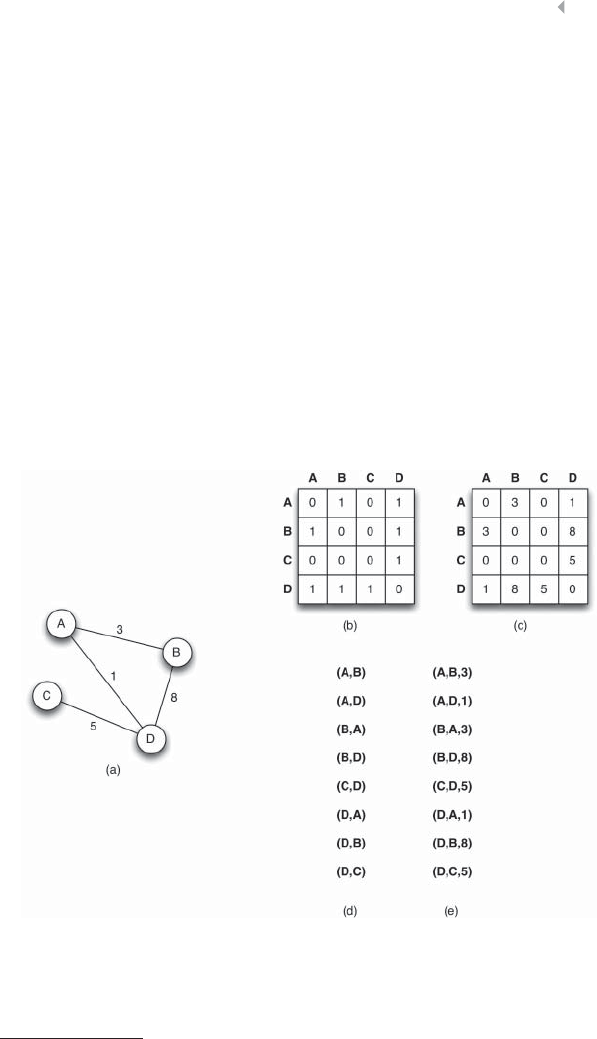
SOCIAL NETWORK ANALYSIS FOR FRAUD DETECTION 221
characteristics. As a consequence, there is an urge to represent the
network in a mathematically interesting way. The adjacency matrix
and the adjacency list are two network representations that fulfill
these requirements. The adjacency or connectivity matrix An×nis a matrix
of size n×nwith nthe number of nodes in the network; and ai,j=1if
a link exists between node iand j,andai,j=0 otherwise. Figure 5.10a
shows an example of a small network. The corresponding adjacency
matrix is depicted in Figure 5.10b. Note that the adjacency matrix is
asparse matrix, containing many zero values. This is often the case
in real-life situations. Social networks have millions of members, but
people are only connected to a small number of friends—for example,
Twitter has 500 million users, and each user follows approximately
200 other users.1The adjacency matrix of a network records which
Figure 5.10 Mathematical Representation of (a) a Sample Network: (b) the Adjacency or
Connectivity Matrix; (c) the Weight Matrix; (d) the Adjacency List; and (e) the Weight List
1http://news.yahoo.com/twitter-statistics-by-the-numbers-153151584.html, retrieved
on December 2014.

222 FRAUD ANALYTICS
nodes are connected to each other, irrespective of the edge weight.
The weight matrix Wn×nexpresses the edge weight between the nodes
of a network, and wi,j∈ℝif a link exists between node iand j,and
wi,j=0 otherwise. The weight matrix of the sample network is given
in Figure 5.10c. The adjacency list is an abstract representation of the
adjacency matrix, and provides a list of all the connections present in
the network. A relationship between node viand node vjis denoted
as (vi,vj). This is illustrated in Figure 5.10d. The weight list extends the
adjacency matrix by specifying the weights of the relationships, and
has the following format (vi,vj,wi,j)with wi,jthe weight between node
viand node vj(see Figure 5.10e).
IS FRAUD A SOCIAL PHENOMENON? AN INTRODUCTION
TO HOMOPHILY
One of the essential questions before analyzing the network regarding
fraud, is deciding whether the detection models might benefit from
CNA (complex network analysis). In other words, do the relationships
between people play an important role in fraud, and is fraud a conta-
gious effect in the network? Are fraudsters randomly spread over the
network, or are there observable effects indicating that fraud is a social
phenomenon, that is, fraud tends to cluster together. We look for evi-
dence that fraudsters are possibly exchanging knowledge about how
to commit fraud using the social structure. Fraudsters can be linked
together as they seem to attend the same events/activities, are involved
in the same crimes, use the same set of resources, or even are some-
times one and the same person (see also identity theft).
Homophily is a concept borrowed from sociology and boils down to
the expression: “Birds of a feather flock together.” People have a strong
tendency to associate with others whom they perceive as being simi-
lar to themselves in some way (Newman 2010). Friendships are mostly
built because of similar interests, same origin, high school, neighbor-
hood, hobbies, etc, or even the tendency to commit fraud. Relation-
ships determine which people are influenced by whom and the extent
to which information is exchanged.

SOCIAL NETWORK ANALYSIS FOR FRAUD DETECTION 223
A network is homophilic if nodes with label x(e.g., fraud) are to a
larger extent connected to other nodes with label x. In marketing, the
concept of homophily is frequently exploited to assess how individuals
influence each other, and to determine which people are likely respon-
ders and should be targeted with a marketing incentive. For example,
if all John’s friends are connected to telecom provider Beta, John is
likely to sign a same contract with provider Beta. A network that is not
homophilic is heterophilic.
The same reasoning holds in fraud. We define a homophilic net-
work as a network where fraudsters are more likely to be connected
to other fraudsters, and legitimate people are more likely to be con-
nected to other legitimate people. A homophilic network is shown in
Figure 5.11. The gray (white) nodes represent fraudsters (legit people).
Visually, gray nodes are grouped together, the so-called web of frauds.
Legitimate nodes are also clustered together. Remark that the network
is not perfectly homophilic: fraudulent nodes are not uniquely con-
nected to other fraudulent nodes, but connect to legitimate nodes as
well. Also, Figure 5.11 illustrates how small webs of frauds exist in the
network, for example, subgraphs of less than one or two nodes.
Advanced network techniques take into account the time dimen-
sion. Few fraudulent nodes that are popping up together in the net-
work might indicate a newly originating web of fraud, while subgraphs
characterized with many fraudulent nodes are far-evolved structures.
Preventing the growth of new webs and the expansion of existing webs
are important challenges that both need to be addressed in the fraud
detection models.
We already showed that a graphical representation of the fraud
network can give a first indication of the homophilic character of the
network, and thus whether network analysis might make sense in the
fraud detection task at hand. Mathematically, a network is homophilic
if fraudulent nodes are significantly more connected to other fraud-
ulent nodes, and as a consequence, legitimate nodes connect signif-
icantly more to other legitimate nodes. More concretely, let lbe the
fraction of legitimate nodes in the network and fthe fraction of fraud-
ulent nodes in the network, then 2lf is the expected probability that
an edge connects two dissimilar labeled nodes. These edges are called
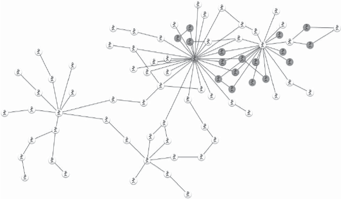
224
Figure 5.11 A Real-Life Example of a Homophilic Network

SOCIAL NETWORK ANALYSIS FOR FRAUD DETECTION 225
cross-labeled edges. A network is homophilic if the observed fraction of
cross-labeled edges
ris significantly less than the expected probability
2lf , i.e. if the null hypothesis
H0∶
r≥2lf
can be rejected. Consider Figure 5.12. The black (white) nodes are
the fraudsters (legitimate people). The network consists in total of
12 nodes: 8 legitimate nodes and 4 fraudulent nodes. The fraction
land fequal 8
12 and 4
12 , respectively. In a random network, we
would expect that 2lf =2⋅8
12 ⋅4
12 =8
18 edges are cross-labeled. The
network in Figure 5.12 has 5 cross-labeled edges, and 3 fraud and
Figure 5.12 A Homophilic Network

226 FRAUD ANALYTICS
10 legit same-labeled edges. The observed fraction of cross-labeled
edges is thus
r=5
18 . We expect to see 8 edges in the network that are
cross-labeled, instead of the 5 edges we observe. The null hypothesis
H0is rejected with a significance level of =0.05 (p-value of 0.02967)
using a one-tailed proportion test with a normal approximation. The
network is homophilic.
Other measures to assess whether there are significant patterns of
homophily present in the network include dyadicity and heterophilic-
ity (Park and Barabási 2007). In many systems, the number of links
between nodes sharing a common property is larger than if the char-
acteristics were distributed randomly in the network. This is the dyadic
effect. For a network where the labels can only take two values, 1
(Fraud) and 0(Legitimate), let n1(n0) be the number of fraudulent
(legitimate) nodes and N=n0+n1. Now, we can define three types of
dyads: (1 −1),(1 −0),and(0 −0), indicating the label (Fraud-Fraud),
(Fraud-Legitimate)and(Legitimate-Legitimate) of two end points con-
nected by a link. The total number of dyads of each kind are repre-
sented as m11,m10 and m00 respectively, and M=m11 +m10 +m00.If
nodes are randomly connected to other nodes regardless of their labels,
then the expected values of m11 and m10 equal:
m11 =n1
2p=n1(n1−1)p
2
m10 =n1
1n0
1p=n1(N−n1)p
with p=2M/(N(N–1))theconnectance, representing the probability
that two nodes are connected. If p=1, all nodes in the network are
connected to each other. Dyadicity and heterophilicity can then be
defined as:
D=m11
m11
H=m10
m10
A network is dyadic if D>1, indicating that fraudulent nodes
tend to connect more densely among themselves than expected for

SOCIAL NETWORK ANALYSIS FOR FRAUD DETECTION 227
a random configuration. A network is heterophobic (opposite of
heterophilic) if H<1, meaning that fraud nodes have fewer connec-
tions to legitimate nodes than expected randomly (Park and Barabási
2007). The network represented in Figure 5.12 is dyadic and hetero-
phobic. If a network is dyadic and heterophobic, it exhibits homophily;
a network that is anti-dyadic and heterophilic, is inverse-homophilic.
A network that exhibits evidence of homophily, is worthwhile to
investigate more thoroughly. For each instance of interest, we extract
features that characterize the instance based on its relational structure.
IMPACT OF THE NEIGHBORHOOD: METRICS
In this section, we will discuss the main metrics to measure the impact
of the social environment on the nodes of interest. In general, we dis-
tinguish between three types of analysis techniques:
◾Neighborhood metrics
◾Centrality metrics
◾Collective Inference algorithms
Neighborhood metrics characterize the target of interest based on its
direct associates. The n-order neighborhood around a node consists of
the nodes that are nhops apart from that node. Due to scalability issues,
many detection models integrate features derived from the egonet or
first-order neighborhood (see the section on Network components).
That is, the node and its immediate contacts. Neighborhood metrics
include degree, triangles, density, relational neighbor, and probabilistic
relational neighbor.
Centrality metrics quantify the importance of an individual in a
social network (Boccaletti 2006). Centrality metrics are typically
extracted based on the whole network structure, or a subgraph.
We discuss geodesic paths, betweenness, closeness, and the graph
theoretic center.
Given a network with known fraudulent nodes, how can we use
this knowledge to infer a primary fraud probability for all the unlabeled
nodes (i.e., the currently legitimate nodes)? As opposed to neighbor-
hood and centrality metrics, collective inference algorithms compute the
probability that a node is exposed to fraud and thus the probability

228 FRAUD ANALYTICS
that fraud influences a certain node. Collective inference algorithms
are designed such that the whole network is simultaneously updated.
As a result, long-distance propagation is possible (Hill, Provost, and
Volinsky 2007). We consider PageRank, and briefly explain Gibbs
sampling, iterative classification, relaxation labeling, and loopy belief
propagation.
Neighborhood Metrics
Neighborhood metrics are derived from a node’s n-hop neighbor-
hood. We discuss degree, triangles, density, relational neighbor, and
probabilistic relational neighbor. For a graph of Nnodes and Medges
Table 5.2 summarizes each of the metrics. Figure 5.13 shows a toy
example, which is used to illustrate how each metric is derived from
the network. In this section, we will use the egonet to extract the
features. This is the one-hop neighborhood of the target node.
Degree
The degree of a node summarizes how many neighbors the node
has. In fraud, it is often useful to distinguish between the number
of fraudulent and legitimate neighbors. This is the fraudulent and
Table 5.2 Overview of Neighborhood Metrics
Degree Number of connections of a
node (in- versus out-degree if
the connections are directed)
Triangles Number of fully connected
subgraphs consisting of three
nodes.
Density The extent to which the nodes
are connected to each other
(reciprocal of farness). d=2M
N(N−1)
Relational
Neighbor
Relative number of neighbors
that belong to class c(e.g., to
class fraud)
P(cn)=
1
Z{nj∈Neighborhoodnclass(nj)=c}w(n,nj),
Probabilistic
Relational
Neighbor
Probability to belong to class
cgiven the posterior class
probabilities of the neighbors
P(cn)=
1
Z{nj∈Neighborhoodn}w(n,nj)P(cnj)

SOCIAL NETWORK ANALYSIS FOR FRAUD DETECTION 229
Figure 5.13 Sample Network
legitimate degree. In the toy example of Figure 5.13, node A has a
degree of 6, which is the highest degree in the network. Recall that we
derive the degree for the egonet of each node. Node G has a fraudulent
degree of 3 and is thus highly influenced by fraud. The degree of each
node is given in Table 5.3.
In case of a directed network, we can distinguish between the
in-degree and the out-degree. The in-degree specifies how many nodes
are pointing toward the target of interest. The out-degree describes
the number of nodes that can be reached from the target of interest.
Table 5.3 Summary of the Total, Fraudulent, and Legitimate Degree
NODE A B C D E F G H I J
Total Degree 63 1 4 2 3 4 2 4 1
Fraud Degree 1 1 0 2 2 2 30 0 0
Legit Degree 5 2 1 2 0 1 1 2 4 1
NODE K L M N O P Q R S T
Total Degree 3 2 2 3 3 1 3 1 1 1
Fraud Degree 1 0 0 1 0 0 0 0 0 0
Legit Degree 2 2 2 2 3 1 3 1 1 1

230 FRAUD ANALYTICS
The degree distribution of a network describes the probability
distribution of the degree in the network. The degree distribution in
real-life networks follows in general a power law. That is, many nodes
are only connected with few other nodes while only few nodes in the
network link to many other nodes. Figure 5.14a illustrates the degree
distribution of the network in Figure 5.14b gives an example of the
degree distribution (log-log scale) of a real-life fraud network of a
social security institution (Van Vlasselaer et al. 2015a).
Networks with a constant degree distribution are k-regular graphs.
Each node in the network has the same degree. An example of a
4-regular graph is given in Figure 5.15.
Figure 5.14a Degree Distribution
Figure 5.14b Illustration of the Degree Distribution for a Real-Life Network of Social
Security Fraud. The Degree Distribution Follows a Power Law (log-log axes)

SOCIAL NETWORK ANALYSIS FOR FRAUD DETECTION 231
Figure 5.15 A4-regular Graph
Triangles
A triangle in a network is a subgraph that consists of three nodes that
are all connected to each other. A triangle investigates the influential
effect of closely connected groups of individuals. Nodes that are part of
a group are to a larger extent affected by the beliefs, interests, opinions,
and so on of that group. In an egonet a triangle includes the ego and
two alters. If the two alters are both fraudulent (legitimate), we say that
the triangle is fraudulent (legitimate). If only one of the two alters are
fraudulent, the triangle is semi-fraudulent. In the network, there are
four triangles: A-G-I, L-M-N, D-F-G, and D-E-F. The egonet analysis
with regard to triangles is given in Table 5.4. The analysis of triangles
can easily be extended to quadrangles, pentagons, hexagons, and so on.

232 FRAUD ANALYTICS
Table 5.4 Summary of the Number of Legitimate, Fraudulent, and
Semi-Fraudulent Triangles
NODE A B C D E F G H I J
Total 1 0 0 2 1 2 2 0 1 0
Fraud 0 0 0 1 1 1 1 0 0 0
Legit 0 0 0 0 0 0 0 0 1 0
Semi-Fraud 1 0 0 1 0 1 1 0 0 0
NODE K L M N O P Q R S T
Total 0 1 1 1 0 0 0 0 0 0
Fraud 0 0 0 0 0 0 0 0 0 0
Legit 0 1 1 1 0 0 0 0 0 0
Semi-Fraud 0 0 0 0 0 0 0 0 0 0
Density
Another neighborhood metric is the network’s density. The density
measures the extent to which nodes in a network are connected to
each other. A fully connected network of Nnodes has N
2=N(N−1)
2
edges. That is, each node is connected to every other node in the
network. The density measures the number of observed edges to the
maximum possible number of edges in the graph:
d=M
N
2=2M
N(N−1)
with Mand Nthe number of edges and nodes in the network
respectively. Remark that a triangle is a subgraph with density 1. An
egonet with degree 1, has also a density of 1. The density derives how
closely connected the group is. A high density might correspond to
an intensive information flow between the instances, which might
indicate that the nodes extensively influence each other. This may
be important in the analysis of fraud. The combination of a high
fraudulent degree and a high density can drastically increase a node’s
probability to commit fraud in the future. The density for each node
in the toy example (see Figure 5.13) is given in Table 5.5.
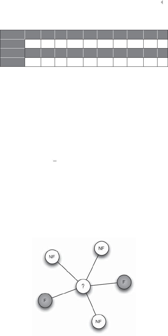
SOCIAL NETWORK ANALYSIS FOR FRAUD DETECTION 233
Table 5.5 Summary of the Density
NODE A B C D E F G H I J
Density 0.33 0.5 10.6 10.83 0.6 0.66 0.5 1
NODE K L M N O P Q R S T
Density 0.5 1 1 0.66 0.5 10.5 1 1 1
Relational Neighbor Classifier
The relational neighbor classifier makes use of the homophily assump-
tion which states that connected nodes have a propensity to belong
to the same class. This idea is also referred to as guilt-by-association.
If two nodes are associated, they tend to exhibit similar behavior.
The posterior class probability for node n to belong to class c is then
calculated as follows:
P(cn)= 1
Z
{nj∈Neighborhoodnclass(nj)=c}
w(n,nj),
whereby Neighborhoodnrepresents the neighborhood of node n,
w(n,nj)the weight of the connection between nand nj,andZis a
normalization factor to make sure all probabilities sum to one.
Consider, for example, the sample network depicted in Figure 5.16
whereby Fand NF represent fraudulent and non-fraudulent nodes,
respectively.
Figure 5.16 Example Social Network for a Relational Neighbor Classifier

234 FRAUD ANALYTICS
The calculations then become:
P(F?) = 1
Z(1+1)
P(NF?) = 1
Z(1+1+1)
Since both probabilities have to sum to 1, Zequals 5, so the prob-
abilities become:
P(F?) = 2
5
P(NF?) = 3
5
The relational neighbor probabilities for the network in Figure 5.13
are depicted in Table 5.6. Remark that these probabilities can be added
as an additional feature to local models—that is, detection models
that do not use network variables. Another possibility is to use the
relational neighbor as a classifier. The final probabilities are then used
to distinguish between fraud and nonfraud. A high value indicates a
high likelihood that the node will be influenced to commit fraud as
well. A cut-off value separates legitimate and fraudulent nodes.
Probabilistic Relational Neighbor Classifier
The probabilistic relational neighbor classifier is a straightforward
extension of the relational neighbor classifier whereby the posterior
class probability for node nto belong to class cis calculated as follows:
P(cn)= 1
Z
{nj∈Neighborhoodn}
w(n,nj)P(cnj).
Table 5.6 Summary of Relational Neighbor Probabilities
NODE A B C D E F G H I J
P(NF?) 0.80 0.66 10.50 00.33 0.25 1 1 1
P(F?) 0.20 0.33 00.50 10.66 0.75 0 0 0
NODE K L M N O P Q R S T
P(NF?) 0.66 1 1 0.66 1 1 1 1 1 1
P(F?) 0.33 0 0 0.33 0 0 0 0 0 0
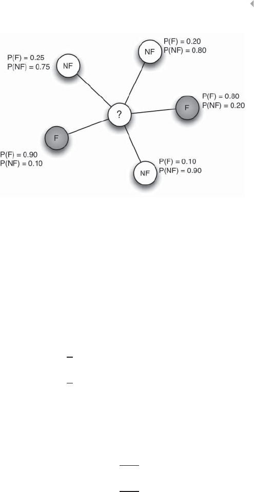
SOCIAL NETWORK ANALYSIS FOR FRAUD DETECTION 235
Figure 5.17 Example Social Network for a Probabilistic Relational Neighbor Classifier
Note that the summation now ranges over the entire neighborhood
of nodes. The probabilities P(cnj)can be the result of a local model,
or of a previously applied network model. Consider the network of
Figure 5.17.
The calculations then become:
P(F?) = 1
Z(0.25 +0.20 +0.80 +0.10 +0.90)
P(NF?) = 1
Z(0.75 +0.80 +0.20 +0.90 +0.10)
Since both probabilities have to sum to 1, Zequals 5, so the prob-
abilities become:
P(F?) = 2.25
5=0.45
P(NF?) = 2.75
5=0.55
Analogously to the relational neighbor, the probabilities returned
by the probabilistic relational neighbor can be used as an additional
variable in local models, or as a classifier.
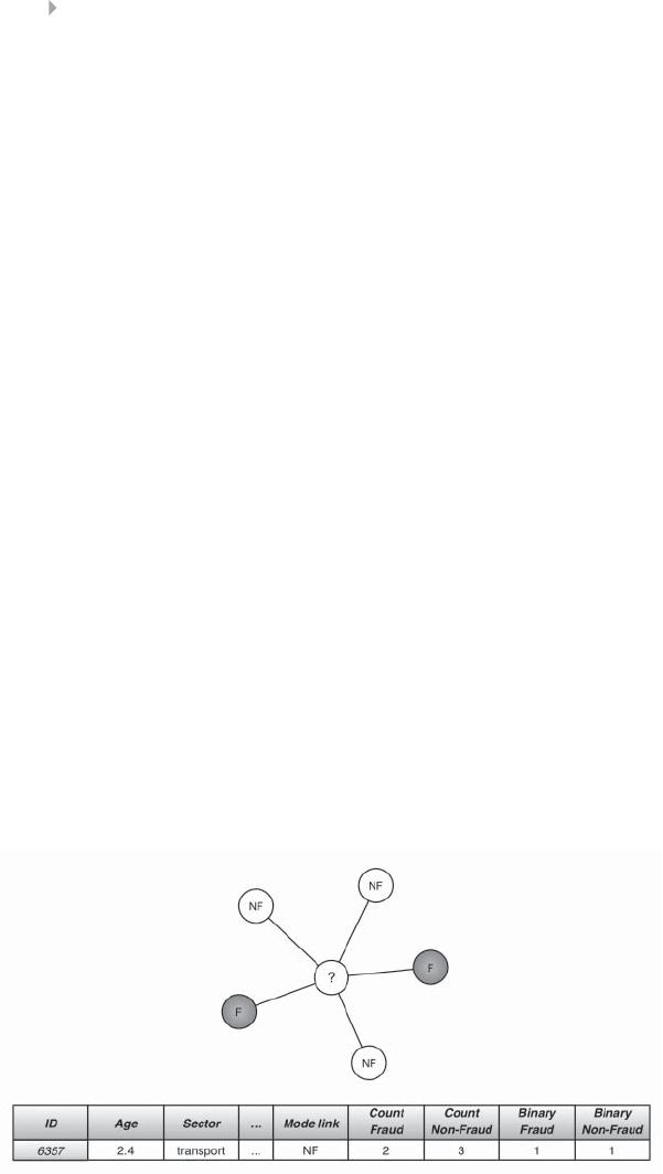
236 FRAUD ANALYTICS
Relational Logistic Regression Classifier
Relational logistic regression was introduced by Lu and Getoor (2003).
It basically starts off from a data set with local node-specific charac-
teristics. These node-specific characteristics are the so-called intrinsic
variables. Examples of intrinsic features in a social security fraud con-
text include a company’s age, sector, legal form, and so on. The data
set is enriched with network characteristics, as follows:
◾Most frequently occurring class of neighbor (mode-link)
◾Frequency of the classes of the neighbors (count-link)
◾Binary indicators indicating class presence (binary-link)
The network characteristics are illustrated in Figure 5.18. Remark
that the count equals the degree.
A logistic regression model is then estimated using the data set
which contains both intrinsic and network features. Note that there is
some correlation between the network characteristics added, which
should be filtered out during an input selection procedure (e.g.,
using stepwise logistic regression). This idea is also referred to as
featurization, since the network characteristics are basically added
as special features to the data set. These features can measure the
behavior of the neighbors in terms of the target variables (e.g., fraud or
not) or in terms of the intrinsic characteristics (e.g., age, sector, profit).
Figure 5.19 provides an example of social security fraud, aiming to
Figure 5.18 Example of Social Network Features for a Relational Logistic Regression
Classifier
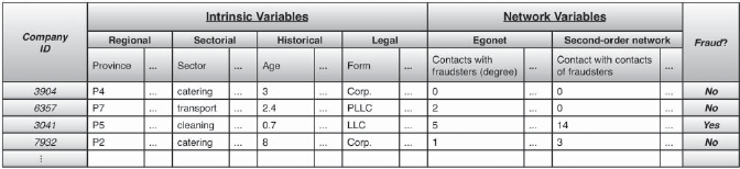
237
Figure 5.19 Example of Featurization with Features Describing Intrinsic Behavior and Behavior of the Neighborhood

238 FRAUD ANALYTICS
Table 5.7 Summary of Relational Features by Lu and Getoor (2003)
NODE A B C D E F G H I J
Mode link NF NF NF NF/F F F F NF NF NF
Count fraud 1 1 0 2 2 2 30 0 0
Count non-fraud 5 2 1 2 011241
Binary fraud 1 1 0 1 1 1 1 0 0 0
Binary non-fraud 1 1 1 1 011111
NODE K L M N O P Q R S T
Mode link NF NF NF NF NF NF NF NF NF NF
Count fraud 1 0 0 1 0 0 0 0 0 0
Count non-fraud 2 2 2 2 3 1 3 1 1 1
Binary fraud 1 0 0 1 0 0 0 0 0 0
Binary non-fraud 1 1 1 1 1 1 1 1 1 1
detect fraudulent companies. Both intrinsic and network features are
added to describe target behavior (i.e., fraud). Table 5.7 summarizes the
features extracted from the network using the approach as suggested
by Lu and Getoor (2003) for the toy example of Figure 5.13.
The set of network features as suggested by the relational logistic
regression classifier can in a straightforward manner be extended with
other metrics discussed in this and the next sections (Neighborhood
Metrics, Centrality Metrics, and Collective Inference Algorithms).
Centrality Metrics
Centrality metrics are useful in fraud to prevent the expansion of future
fraudulent activities. They tend to find the central node(s), that is, nodes
that might impact many other nodes. These metrics include geodesic
path, degree (see Section Neighborhood Metrics), closeness, between-
ness and graph theoretic center. Assume a network with nnodes vi,
i=1,…,n. The geodesic represents the shortest path between two
nodes. gjk represents the number of geodesics from node jto node k,
whereas gjk(vi)represents the number of geodesics from node jto node
kpassing through node vi. The centrality measures are summarized in
Table 5.8. The formulas each time calculate the metric for node vi.A
toy example is given in Figure 5.13.

SOCIAL NETWORK ANALYSIS FOR FRAUD DETECTION 239
Table 5.8 Centrality Metrics
Geodesic path Shortest path between two nodes in the
network. d(vi,vj)
Degree Number of connections of a node (in-
versus out-degree if the connections are
directed). See previous section.
Closeness The average distance of a node to all other
nodes in the network (reciprocal of
farness).
j=1(j≠i)
d(vi,vj)
n−1−1
Betweenness Counts the number of times a node or
connection lies on the shortest path
between any two nodes in the network. j<k
gjk(vi)
gjk
Graph theoretic center The node with the smallest maximum
distance to all other nodes in the network
(see section Geodesic path).
Geodesic Path
The geodesic path or shortest path computes the minimum distance
needed to reach a node from a target node. A key question in fraud
is: How far is any fraudulent node in the network removed from the
target node? If a fraudulent node is in the close neighborhood, fraud
might impact that node more intensively and contaminate the target
of interest.
Geodesic path calculations are nevertheless computationally
expensive. Dijkstra (1959) formulated a solution to compute the
shortest path from one node to all other nodes.
-- Initialization --
1. Assign a label of zero to the source node (let’s say node v1), and
initialize all other nodes in the network with a temporary label
of ∞.
2. The set of permanent labeled nodes is P={v1}; the set of unla-
beled nodes Ucontains all other nodes of the network.
3. u∶= v1
-- Main loop --

240 FRAUD ANALYTICS
while Uis not empty do
1. Updating for each node adjacent to a permanent node u, replace
the temporary label of node viwith:
min node vi’s current temporary label
node u’s permanent label +edge weight eu,vi
2. Adding to permanent labeled set add the node with the smallest
temporary label v−to the permanent labeled set P.
3. Reassign u u:=v−
end
Figure 5.20 illustrates Dijkstra’s algorithm to calculate the shortest
path from node Ato the other nodes in a directed graph. The weights
of the shortest paths between any two nodes in the network are:
Shortest paths =
02448137
40236115
24014 9 3
13509114
57340 5 1
68451 0 2
46236 7 0
Analogously, the shortest path between any two nodes in an undi-
rected graph can be computed. Remark that Dijkstra’s algorithm is only
applicable to networks with non-negative edge weights.
Closely related to the geodesic path, is the graph theoretic center.The
graph theoretic center is the node with the smallest, maximum distance
to all other nodes. This node is the most central node in the network. In
terms of information diffusion, the graph theoretic center is the node
which influences other nodes the fastest. The example in Figure 5.20
has two graph theoretic centers: node Eand G, each with a maximum
distance of 7 hops to another node in the network.
The average path length of a network is the length one needs to tra-
verse on average to reach one node from another. The average path
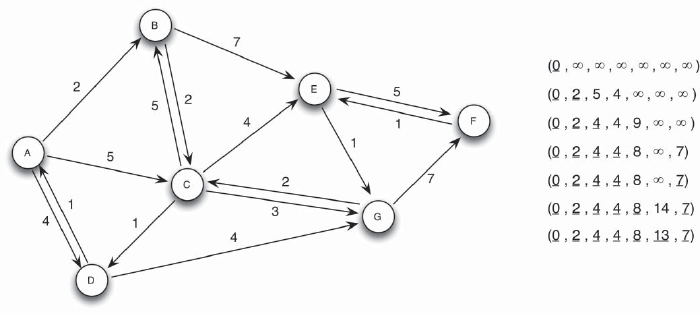
241
Figure 5.20 Illustration of Dijkstra’s Algorithm
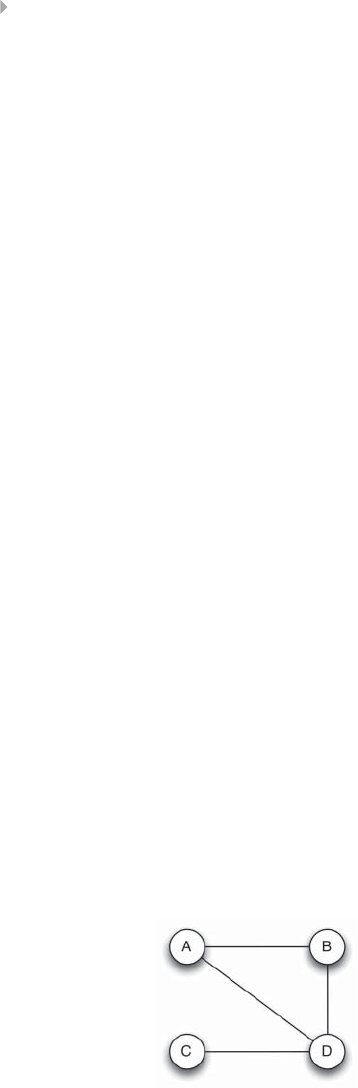
242 FRAUD ANALYTICS
length of Figure 5.20 is 4.1. Note that the average path length corre-
sponds to the “degrees of separation” in the section Social Networks.
In fraud, it is often interesting to know whether there are paths
between fraudulent nodes and legitimate nodes. If more paths exist
between two nodes, there is a higher chance that (fraudulent) influ-
ence will eventually reach the target node. Starting from the adjacency
matrix of a network, the number of connecting paths between any two
nodes is easily computed through matrix exponentiation.
Consider the small network as illustrated in Figure 5.21. The cor-
responding adjacency matrix is
A=
0101
1001
0001
1110
The adjacency matrix represents how many one-hop paths exist
between two nodes. For example, node A can reach node D by exactly
one path of one hop. If we raise the matrix to the power of x,the
resulting matrix contains how many x-hop paths exist between two
nodes. This is Seidel’s algorithm (Seidel 1995). For example,
A2=
0101
1001
0001
1110
0101
1001
0001
1110
=
2111
1211
1110
1103
A3=
0101
1001
0001
1110
2111
1211
1110
1103
=
2314
3214
1103
4432
Figure 5.21 Illustration of the Number of Connecting Paths Between Two Nodes

SOCIAL NETWORK ANALYSIS FOR FRAUD DETECTION 243
In the toy example of Figure 5.21, there is exactly one two-hop
path between node A and node D (through node B), one two-hop path
between node B and node D (through node A) and three two-hop
paths between node D and itself (D-A-D, D-B-D, and D-C-D). There
is no two-hop path that connects node C and node D. This is exactly
what A2represents. An overview of the three-hop paths between any
two nodes is reported in A.3
For the sample network in Figure 5.13, Table 5.9 contains the
geodesic path length of each node to fraudulent nodes, as well as the
number of n-hop paths toward fraudulent nodes. The graph theoretic
center of Figure 5.13 is node A, which is at most three hops removed
from all other nodes in the network. This means that node A is the
most influential node of the network and extra attention should be
devoted in order to prevent this node to commit fraud. Whenever the
graph theoretic center is contaminated with fraud, fraud might rapidly
flow throughout the rest of the network.
Closeness
Closeness centrality measures the mean distance from a node to each
other node in the network. The distance d(vivj)between a node and
another node corresponds to the geodesic or shortest path (see below).
Given a network with nnodes, the mean geodesic distance or farness
ℊ(vi)from a node ito the other nodes is computed as follows:
ℊ(vi)=
j=1(j≠i)
d(vivj)
n−1
Table 5.9 Summary of Geodesic Paths to Fraudulent Nodes
NODE A B C D E F G H I J
Geodesic path 1 1 2 0 0 0 1 2 0 2
# 1-hop paths 1 1 0 2 2 2 30 0 0
# 2-hop paths 4 3 1 8 4 7 52 6 1
# 3-hop paths 18 13 319 15 17 25 4 9 0
NODE K L M N O P Q R S T
Geodesic path 1 2 2 1 2 3 3 4 4 2
# 1-hop paths 1 0 0 1 0 0 0 0 0 0
# 2-hop paths 0 1 1 0 1 0 0 0 0 1
# 3-hop paths 9 1 1 8 4 1 1 0 0 4

244 FRAUD ANALYTICS
A low value of farness indicates that the node easily reaches other
nodes in the network, and thus has a stronger impact on other nodes.
If a fraudulent node in a (sub)graph has a low value for ℊ(vi),fraud
might easily spread through the (sub)network and contaminate other
nodes. The distance to the node itself is excluded in the computation
of farness.2
Closeness centrality is the inverse of farness. A node is more central
in the network, if it has a higher value, and
Closeness Centrality(vi)=
j=1(j≠i)
d(vivj)
n−1
−1
In general, two problems arise. First, the values of the closeness
centralities for all the nodes in the network might lie closely together,
and it is therefore often important to inspect the decimals. Second,
if the geodesic distance between two nodes is infinite, the closeness
centrality of both nodes is lim
x→∞1
x=0. To overcome this problem,
closeness centrality often excludes the distances to nodes that cannot
be reached.
The closeness centralities for the nodes in Figure 5.13 are summa-
rized in Table 5.10. Node A is the closest connected to all other nodes in
the network; node R and S are the farthest away from all other nodes.
Betweenness
Betweenness measures the extent to which a node lies on the geodesic
paths connecting any two nodes in the network. This can be inter-
preted as the extent to which information passes through this node.
A node with a high betweenness possibly connects communities
(i.e., subgraphs in the network) with each other. This is depicted
in Figure 5.22. In the figure, the shaded node connects the three
communities with each other and has the highest betweenness. If this
2The closeness of a node is sometimes calculated by including the node itself.
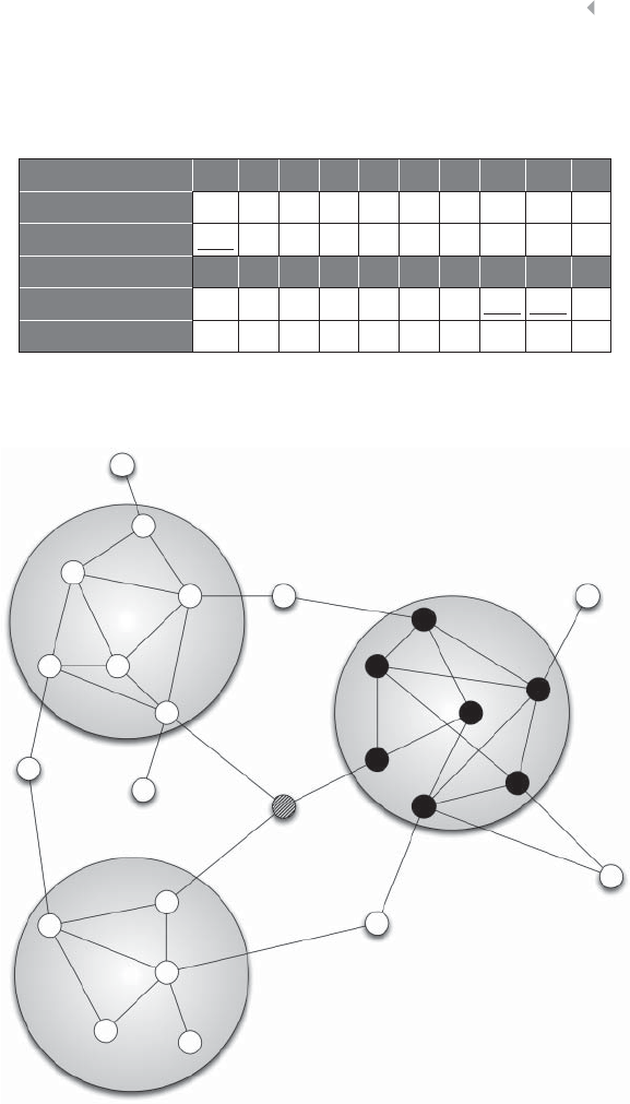
SOCIAL NETWORK ANALYSIS FOR FRAUD DETECTION 245
Table 5.10 Summary of Closeness and Closeness Centrality for Each Node
of the Network in Figure 5.13
NODE A B C D E F G H I J
Farness 22.57 3.53 2.89 3.79 3.00 2.32 2.74 2.21 3.89
Closeness Centrality 0.50 0.39 0.28 0.35 0.26 0.33 0.43 0.37 0.45 0.26
NODE K L M N O P Q R S T
Farness 2.95 3.84 3.84 2.95 2.53 3.47 3.26 4.21 4.21 2.95
Closeness Centrality 0.34 0.26 0.26 0.34 0.40 0.29 0.31 0.24 0.24 0.34
Figure 5.22 Illustration of Betweenness Between Communities of Nodes

246 FRAUD ANALYTICS
Table 5.11 Summary of the Betweenness Centrality for Each Node of the Network in
Figure 5.13
NODE A B C D E F G H I J
Betweenness 104 24.67 013.83 06.167 35.33 965 0
NODE K L M N O P Q R S T
Betweenness 20 0 0 34 63 035 0 0 0
node is infected by fraud from one community, fraud can easily pass on
toward the other communities. One option is, for example, to remove
this node from the network to prevent that fraud contaminates the
other communities. Let gjk be the number of shortest paths between
node jand node k,andgjk(vi)the number of shortest paths between
node jand node kthat pass through node vi, then the betweenness
becomes
j<k
gjk(vi)
gjk
Table 5.11 contains the betweenness centralities of the nodes in the
network of Figure 5.13. Again, node A is the most central node.
Collective Inference Algorithms
Given a semi-labeled network with few labeled legitimate and fraudu-
lent nodes and many unknown nodes, a collective inference procedure
infers a set of class labels/probabilities for the unknown nodes by tak-
ing into account the fact that inferences about nodes can mutually
affect one another. Some popular examples of collective inference pro-
cedures are:
◾PageRank(Page and Brin 1999)
◾Gibbs sampling (Geman and Geman 1984)
◾Iterative classification algorithm (Lu and Getoor 2003)
◾Relaxation labeling (Chakrabarti et al. 1998)
◾Loopy belief propagation (Pearl 1986)
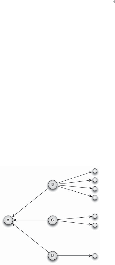
SOCIAL NETWORK ANALYSIS FOR FRAUD DETECTION 247
PageRank Algorithm
The PageRank algorithm was introduced by Page and Brin in 1999 and
is the basis of Google’s famous search engine algorithm for ranking web
pages (Page and Brin 1999). The PageRank algorithm tries to simulate
surfing behavior. Figure 5.23 represents a network of web pages linking
to each other. Given the figure, what is the probability that a surfer will
visit web page A? Assume for now that a surfer only browses to web
pages by following the links on the web page s/he is currently visiting.
The figure shows that web page A has three incoming links. A surfer
that is currently visiting web page B, will visit web page A next with a
probability of 20 percent (=1/5). This is because web page B has 5 links
to web pages, among which is web page A. Analogously, if a surfer is
currently on web page C or D, there is a probability of 33.33 percent
and 50 percent, respectively, that web page A will be visited next. The
probability of visiting a web page is called the pagerank of that web
page. In order to know the pagerank of web page A, we need to know
the pagerank of web page B, C, and D. This is collective inference: the
ranking of one web page depends on the ranking of other web pages;
Figure 5.23 PageRank Algorithm

248 FRAUD ANALYTICS
and a change in the ranking of one web page might impact the ranking
of all other web pages.
Specifically, the main idea is that important web pages (i.e., web
pages that appear at the top of the search results) have many incoming
links from other (important) web pages. The ranking of a web page
depends on (a) the ranking of web pages pointing towards that web
page, and (b) the out-degree of the linking web pages. However, visit-
ing web pages by following a random link on the current web page is
not a realistic assumption. Surfers’ behavior is more random: instead
of following one of the links on a web page, they might randomly visit
another web page. Therefore, the PageRank algorithm includes the
random surfer model, which assumes that surfers often get bored, and
randomly jump to another web page. With a probability of the surfer
will follow a link on the web page s/he is currently visiting. However,
with a probability 1 −, the surfer visits a random other web page.
The PageRank algorithm is expressed as follows:
PR(A)=
i∈NA
PR(i)
Dout,i
+(1−)⋅eA
with PR(i) the ranking of web page i,Dout,ithe out-degree of web page
i,(1−)the restart probability, and eAthe restart value for web page
A, which is often uniformly distributed among all web pages. This
equation requires the ranking of the neighboring web pages. One
option is to start with a random pagerank value for every web page
and iteratively update the pagerank scores until a predefined number
of iterations is reached or a stopping criterion is met (e.g., when the
change in the ranking is marginal).
The above equation can be rewritten such that ranking is computed
for all web pages simultaneously, and
r=⋅A⋅
r+(1−)⋅
e
with
ra vector of size ncontaining the pageranks of all nweb pages,
Athe column-normalized adjacency matrix of size n×n,(1−)the
restart probability and
ethe restart vector. The restart vector is generally
uniformly distributed among all web pages, and normalized afterward.
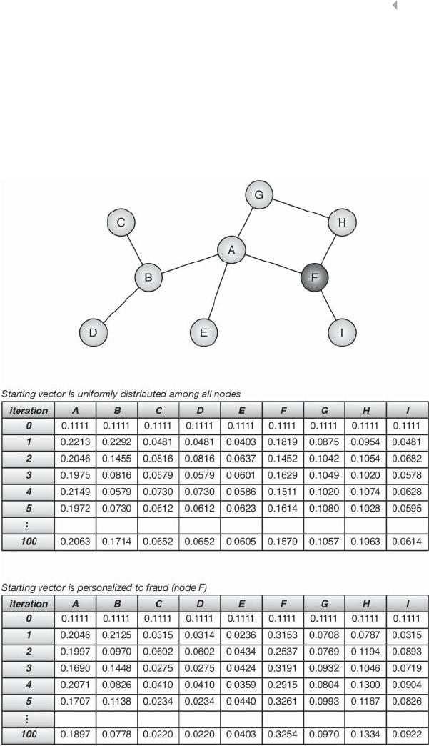
SOCIAL NETWORK ANALYSIS FOR FRAUD DETECTION 249
This equation can only be solved by matrix inversion, which is often
unfeasible in practice. One of the most widely used ways to execute the
algorithm is the power-iteration method, iterating the above equation
until convergence (Tong et al. 2007). Convergence is reached when
the change in the importance score is insignificant or after a maximum
number of iteration steps. Figure 5.24 illustrates the iterative procedure
Figure 5.24 Illustration of Iterative Process of the PageRank Algorithm

250 FRAUD ANALYTICS
of PageRank. During the first iteration, the ranking of node A is calcu-
lated as follows:
r(A)1=0.85 1
3⋅1
9+1⋅1
9+1
2⋅1
9+1
3⋅1
9+0.15 ⋅1
9
Page and Brin (1999) included an extension of the PageRank algo-
rithm by personalizing the search to the user. This is done by changing
the restart vector
efrom a uniform distribution to a vector that com-
plies with a user’s search interests. A higher score of the ith value of the
restart vector corresponds to a higher interest that a user might have
for the ith web page.
The PageRank algorithm can be seen as a propagation of page influ-
ence through the network. The same reasoning can be used to prop-
agate fraud through the network. That is, we personalize the ranking
algorithm by fraud. Instead of web pages, the adjacency matrix Arep-
resents a fraud network (e.g., a people-to-people network). As fraud
detection infers a labeled graph (i.e., we know which nodes are fraud-
ulent), we inject fraud in the network through the restart vector. That
is, the ith entry of vector
eis 1 if the ith node is fraudulent, and 0,
otherwise. The vector
eis normalized afterward. The vector
rcontains
the fraud ranking of each node. The higher the ranking, the more the
node is influenced by fraud compared to the other nodes. Recall that
the equation is often solved through iteration. In that case, the vector
rkincludes the fraud ranking after kiterations, with
r0a random vector
with values between [0,1].
We note that the final ranking assigned to each node should be
interpreted as a ranking and not as a score. The top-ranked nodes are
the most influenced by fraud.
The PageRank scores for the toy example of Figure 5.13 are
computed (a) without emphasizing the fraud labels (PageRankbase),
and (b) with emphasis on fraud (PageRankfraud). In the first case,
the restart vector
eis uniformly distributed among all nodes. For
the PageRankfraud case, the restart vector
ehas a zero value for each
legitimate node, and a non-zero value for the fraudulent nodes. The
results are presented in Table 5.12. The highest ranking is assigned to
node A when applying PageRankbase. This is not that remarkable, as
node A has the highest degree in the network. Studies proved that

SOCIAL NETWORK ANALYSIS FOR FRAUD DETECTION 251
Table 5.12 PageRank Algorithm
NODE A B C D E
PageRankbase 0.1084 0.0577 0.0238 0.0684 0.0367
PageRankfraud 0.0877 0.0635 0.0180 0.1685 0.1144
NODE F G H I J
PageRankbase 0.0519 0.0671 0.0400 0.0706 0.0246
PageRankfraud 0.1452 0.1094 0.0236 0.0941 0.0112
NODE K L M N O
PageRankbase 0.0604 0.0415 0.0415 0.0578 0.0667
PageRankfraud 0.0396 0.0169 0.0169 0.0344 0.0206
NODE P Q R S T
PageRankbase 0.0264 0.0755 0.0289 0.0289 0.0229
PageRankfraud 0.0058 0.0112 0.0032 0.0032 0.0124
there is an interplay between the nodes’ degree and the PageRank
score (Fortunato et al. 2008). As can be seen from the results, the
basic PageRank algorithm is not useful for fraud detection. There is
no correlation between fraud (or fraud influence) and the ranking.
However, when personalizing the restart vector to fraud using the
adapted PageRank algorithm PageRankfraud, the nodes with the
highest ranking are nodes D, F, E. These results are not surprising,
as those nodes were directly attributed to fraud. Node G receives a
high fraud ranking as well, indicating that this node is affected by
the influences of fraudulent nodes in its neighborhood. Notice that
legitimate node G has a higher ranking than fraudulent node I.
Gibbs Sampling
Gibbs sampling (Geman and Geman, 1984) is a collective inference
procedure that uses a local classifier to infer a posterior class probability
in order to initialize the node labels in the network. More concretely,
the original semi-labeled graph is transformed in a (fully) labeled graph
by sampling the posterior probabilities of the local classifier. The pre-
dictive features of a local classifier consist of only intrinsic variables
(see Relational Logistic Regression Classifier). Notice that the labels of

252 FRAUD ANALYTICS
the unknown nodes in the graph express an expectation of the true
class value. An iterative procedure continually updates the expected
class labels of the unknown nodes. The first iterbsteps of the proce-
dure approach a stationary distribution. This is the so-called burn-in
period, where no statistics are recorded. During the last itercsteps,
the algorithm keeps track of which class labels are assigned to each
node. The final class probability estimate is computed as the normalized
count of the number of times each class is assigned to a particular node.
The algorithm is explained in more detail below.
-- Input --
Semi-labeled graph 𝓖with known and unknown nodes.
-- Initialization --
Assign posterior probabilities P(c=k)with k∈{Fraud,Legitimate}
to each unknown node using a local classifier.
Given the posterior probabilities P(c=k), sample the class value
Lj∈{Fraud,Legitimate}of each unknown node j. Each node in the
graph is now labeled.
-- Main loop –
for i=0toiterb+itercdo
1. Learning phase: Apply a relational learner (e.g., Relational
Neighbor, Probabilistic Relational learner …) to each unknown
node of the network to obtain new posterior probabilities P′(c=
k).
2. Sampling phase: Given the posterior probabilities P′(c=k),
sample the class value Lj∈{Fraud,Legitimate}for each
unknown node j.
end
For each unknown node, count the number of times each class
label is assigned to that node during the iteration iterb+1anditerc.
The normalized counts represent the final class probability estimates.

SOCIAL NETWORK ANALYSIS FOR FRAUD DETECTION 253
Iterative Classification Algorithm
Like Gibbs sampling, iterative classification initializes the semi-labeled
graph by using a local classifier (Lu and Getoor 2003). Based on the
local model’s output, the most probable class label is assigned to each
unknown node. This is the bootstrap phase. During the iteration phase,
a relational learner updates the class labels of each unknown node
based on the outcome of a relational logistic regression model (see
Relational Logistic Regression Classifier). The input features are com-
puted as link statistics of the current label assignments. Link statistics
include, for example, mode (most occurring label of the neighboring
nodes), count (number of neighboring fraud nodes), binary (atleastone
of the neighboring nodes are fraudulent). Nodes that are not yet clas-
sified are ignored. A new class label is assigned to each unknown node
based on the largest posterior probability. This step is repeated until a
stopping criterion is met. The final class label corresponds to the class
label estimate generated during the last iteration.
Relaxation Labeling
Relaxation labeling starts from a local classifier to initialize a node’s
class label. Previous approaches assigned a hard label (i.e., either legit-
imate or fraud) to each node. Relaxation labeling starts with assigning
to each node a probability that indicates the likelihood of a node to
belong to a certain class. This is soft labeling. Next, the probability class
labels are used to iteratively update the class probability using a rela-
tional model. The class estimates of the last iteration are the final class
label estimates.
Loopy Belief Propagation
Loopy belief propagation is a collective inference procedure based on
iterative message passing (Pearl 1988). The main idea is that the belief
of each node to be in state x(let’s say fraud) depends on the messages
it receives from its neighbors. The belief of a node to be in state xis the
normalized product of the received messages. The message as well as
the belief is continuously updated during the algorithm.
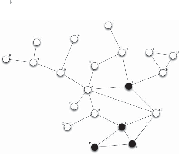
254 FRAUD ANALYTICS
Figure 5.25 Sample Network
Featurization: Summary Overview
Given all aforementioned metrics, we are able to extract features from
the network for every node of interest. The featurization process entails
the mapping of an unstructured data source like a network into use-
ful and meaningful characteristics of each node. For each node in the
network of Figure 5.25, all the metrics are computed. Table 5.13 sum-
marizes the different variables. Although most network-based features
already give a good indication which nodes might be fraudulent in the
future, these network-based characteristics can be combined with local
(or intrinsic) features into a classification model, as defined in the pre-
vious chapters.
COMMUNITY MINING: FINDING GROUPS OF FRAUDSTERS
Social networks are a powerful visualization technique to reveal the
individual relationships among people by means of the links in the net-
work. In the previous sections, the neighboring nodes were treated as

Table 5.13 Featurization Process. The Unstructured Network Is Mapped into Structured Data Variables
NODE A B C D E F G H I J
Total Degree 63 1 4 2 3 4 2 4 1
Fraud Degree 1 1 0 2 2 2 30 0 0
Legit Degree 5 2 1 2 0 1 1 2 4 1
Total Triangles 1 0 0 2 1 2 2 0 1 0
Fraud Triangles 0 0 0 1 1 1 1 0 0 0
Legit Triangles 0 0 0 0 0 0 0 0 1 0
Semi-Fraud Triangles 1 0 0 1 0 1 1 0 0 0
Density 0.33 0.5 10.6 10.83 0.6 0.66 0.5 1
Rel. Neighbor P(NF|?) 0.80 0.66 10.50 00.33 0.25 1 1 1
Rel. Neighbor P(F|?) 0.20 0.33 00.50 10.66 0.75 0 0 0
Mode link NF NF NF NF/F F F F NF NF NF
Count fraud 1 1 0 2 2 2 30 0 0
Count non-fraud 5 2 1 2 01 1 2 4 1
Binary fraud 1 1 0 1 1 1 1 0 0 0
Binary non-fraud 1 1 1 1 0 1 1 1 1 1
Geodesic path 11 2 0 0 0 1 2 0 2
# 1-hop paths 1 1 0 2 2 2 30 0 0
# 2-hop paths 4 3 1 8 4 7 52 6 1
(continued)
255

Table 5.13 (Continued)
NODE A B C D E F G H I J
# 3-hop paths 18 13 319 15 17 25 4 9 0
Farness 22.57 3.53 2.89 3.79 3.00 2.32 2.74 2.21 3.89
Closeness Centrality 0.50 0.39 0.28 0.35 0.26 0.33 0.43 0.37 0.45 0.26
Betweenness 104 24.67 013.83 06.167 35.33 965 0
PageRankbase 0.1084 0.0577 0.0238 0.0684 0.0367 0.0519 0.0671 0.0400 0.0706 0.0246
PageRankfraud 0.0877 0.0635 0.0180 0.1685 0.1144 0.1452 0.1094 0.0236 0.0941 0.0112
NODE K L M N O P Q R S T
Total Degree 3 2 2 3 3 1 3 1 1 1
Fraud Degree 1 0 0 1 0 0 0 0 0 0
Legit Degree 2 2 2 2 3 1 3 1 1 1
Total Triangles 0 1 1 1 0 0 0 0 0 0
Fraud Triangles 0 0 0 0 0 0 0 0 0 0
Legit Triangles 0 1 1 1 0 0 0 0 0 0
Semi-Fraud Triangles 0 0 0 0 0 0 0 0 0 0
Density 0.5 1 1 0.66 0.5 10.5 1 1 1
Rel. Neighbor P(NF|?) 0.66 1 1 0.66 1 1 1 1 1 1
Rel. Neighbor P(F|?) 0.33 0 0 0.33 0 0 0 0 0 0
(continued)
256

Table 5.13 (Continued)
NODE K L M N O P Q R S T
Mode link NF NF NF NF NF NF NF NF NF NF
Count fraud 1 0 0 1 0 0 0 0 0 0
Count non-fraud 2 2 2 2 3 1 3 1 1 1
Binary fraud 1 0 0 1 0 0 0 0 0 0
Binary non-fraud 1 1 1 1 1 1 1 1 1 1
Geodesic path 1 2 2 1 2 3 3 4 4 2
# 1-hop paths 1 0 0 1 0 0 0 0 0 0
# 2-hop paths 0 1 1 0 1 0 0 0 0 1
# 3-hop paths 9 1 1 8 4 1 1 0 0 4
Farness 2.95 3.84 3.84 2.95 2.53 3.47 3.26 4.21 4.21 2.95
Closeness Centrality 0.34 0.26 0.26 0.34 0.40 0.29 0.31 0.24 0.24 0.34
Betweenness 20 0 0 34 63 035 0 0 0
PageRankbase 0.0604 0.0415 0.0415 0.0578 0.0667 0.0264 0.0755 0.0289 0.0289 0.0229
PageRankfraud 0.0396 0.0169 0.0169 0.0344 0.0206 0.0058 0.0112 0.0032 0.0032 0.0124
257

258 FRAUD ANALYTICS
separate entities, and the relationships among the neighborhoods were
neglected. Whereas these individual relationships might uncover many
interesting flows of influence through individuals, groups of nodes
in the network might have a higher impact in terms of information
exchange like fraudulent influence. A friend group, for example, is a
community in a social network where the friends of your friends are
each other’s friends. A similar opinion created within a group of friends
might be more convincing than the opinion of only one friend. A com-
munity is a subgraph in the network with a higher number and more
intensive relationships among the members of the community than a
random other subgraph in the network. Such communities can play
an important role in influence dispersion. Groups often share, rein-
force, and complement ideas and alternatives on how to perpetrate
fraud. The analysis or mining of communities in a network captures
the effect of peer pressure. In a fraudulent environment, peer pressure
can strengthen the tendency to commit fraud. That is, community min-
ing in a fraud context is the process of finding groups of fraudsters in
the network in order to identify subgraphs in which fraud occurs with a
higher probability than in the rest of the graph, and tries to answer the
following questions: Are people more likely to commit fraud if they are
influenced by a whole community than if they were influenced by only
one fraudulent individual? The answer is mostly yes. In many appli-
cations, the discovery of such communities can result in the detection
of hidden fraudulent structures or the curtailment of existing fraudu-
lent groups.
Figure 5.26 illustrates the usefulness of the detection of fraudu-
lent groups in credit card fraud. Stores are represented by circles. All
transactions between stores and credit cards are fraudulent. Fraudsters
tend to behave in the same way. Often, fraudsters use stolen credit
cards in the same stores. As a result, some stores are more sensitive
to fraud, regardless of the fraudulent involvement of the store itself.
Rather than implementing fraud detection on individual store level,
community mining will expose which stores are often related to the
same stolen credit cards. A known fraud pattern in credit card fraud
is that the stolen card is used in many stores for a small amount of
money. Community detection allows to identify the set of stores that
are commonly associated to fraud with the same credit card. The use of
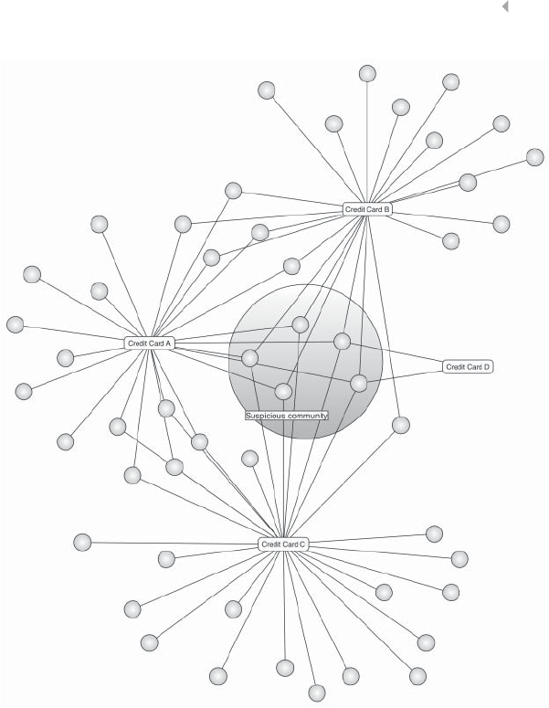
SOCIAL NETWORK ANALYSIS FOR FRAUD DETECTION 259
Figure 5.26 Community Detection for Credit Card Fraud
a card in more than one of these stores might drastically increase the
risk of credit card theft.
One prevalent technique for community mining is graph parti-
tioning. Graph partitioning approaches try to split the whole graph
into a predetermined number of clusters by optimizing the ratio
between the within-community and between-community edges. The
within-community edges for a certain community are the edges that
occur inside that community. The between-community edges designate

260 FRAUD ANALYTICS
the edges that connect different communities with each other. There
are different techniques to achieve the optimal cut within a graph.
One of such techniques is Iterative Bisection. A bisection splits the
given graph into two groups using the minimum cut size. The cut size
quantifies the between-community edges. The two groups that are
connected by the minimum number of between-community edges are
maintained. Each group is thereafter subdivided in two groups, and
so forth. The process is iteratively repeated until the required number
of communities is found. Graph partitioning methods often derive
clusters of equal size to avoid separating one node with the lowest
degree from all the others. Another technique is spectral clustering
where the Laplacian eigenvectors and eigenvalues of the connectivity
matrix are used to find the optimal cut to split the network into clusters
or communities. To gauge a single split, a set of evaluation metrics
are proposed:
MinCut: Given all possible splits, the MinCut evaluation metric
will split the graph 𝓖in communities 𝓢and 𝓣where the weight of
between-community edges is minimal. The objective function is then,
ΓMinCut =min Cut(𝓢,𝓣)
whereby Cut(𝓢,𝓣)indicates the sum of the weight of between-
community edges. Remark that this metric does not take into account
the size of the clusters. In the most extreme case, the optimal cut
might be one that separates one node from the others.
RatioCut: The RatioCut metric evaluates a cut by including the
size of the clusters, and can be seen as an improvement of the MinCut
evaluation metric. In the end, the obtained clusters are more balanced.
The corresponding objective function is then,
ΓRatioCut =min Cut(𝓢,𝓣)1
𝓢+1
𝓣
with 𝓢and 𝓣the size of each community, favoring communities
that have similar sizes and thus are more balanced.

SOCIAL NETWORK ANALYSIS FOR FRAUD DETECTION 261
MinMaxCut: a shortcoming of the previous metrics is that the
within-community edges are neglected. The MinMaxCut takes both
the between- and within-community edges into consideration. A
graph 𝓖is split into communities 𝓢and 𝓣if both communities have
a low weight of between-community edges and a high weight of
within-community edges. The objective function is then
ΓMinMaxCut =min Cut(𝓢,𝓣)1
Cut (𝓢,𝓢)+1
Cut(𝓣,𝓣)
with Cut(𝓢,𝓢)the sum of the weight of the within-community edges.
The difference with the RatioCut metric is that the MinMaxCut met-
ric uses the number of edges to determine the cluster size, while the
RatioCut metric uses the number of nodes.
A toy example is given in Figure 5.27. For all aforementioned met-
rics, the optimal cut divides the network in communities 𝓐and 𝓑
as indicated in the figure. The MinCut(𝓐,𝓑), RatioCut(𝓐,𝓑),and
MinMaxCut(𝓐,𝓑)equal 4, 7
∕
3and 1
∕
3, respectively.
Another algorithm to find communities in a network is the
Girvan-Newman algorithm. The algorithm progressively removes
edges from the original graph, and is therefore a divisive hierarchical
clustering algorithm. The edges with the highest betweenness are
removed first. Note that in the Section Centrality metrics, betweenness
is measured on node level. The betweenness of an edge is computed
Figure 5.27 Iterative Bisection
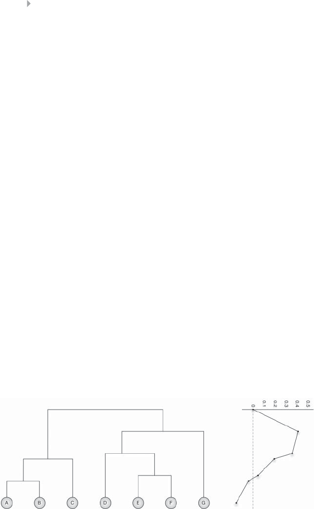
262 FRAUD ANALYTICS
as the number of shortest paths between pairs of nodes that contain
the edge of interest. It starts from the idea that the communities of a
network are connected by only a few edges. All shortest paths between
nodes from different communities must go along these edges, which
result in a high betweenness. The algorithm proceeds as follows:
1. Calculate the betweenness of all edges in the full network.
2. Remove the edge with the highest betweenness.
3. Recalculate the betweenness of the affected edges.
4. Repeat step 2 and 3 until no edges remain.
As with clustering, the result of the Girvan-Newman algorithm is a
dendrogram. A dendrogram of the Girvan-Newman algorithm applied
to Figure 5.27 is illustrated in Figure 5.28.
One major drawback of graph partitioning methods is that the
number of clusters needs to be determined upfront which is often
unfeasible for large networks. A metric that comes in very handy in
assessing the optimal number of communities, is the modularity Q.The
best community split is achieved when the modularity Qis maximized.
The modularity Qevaluates a community split by identifying whether
the nodes inside each community “communicate” to a higher extent to
each other than to other communities. The modularity Qis computed
as follows. Suppose we split the network into kcommunities. We
now define a k×ksymmetric matrix Ewhere each entry ei,jspecifies
the fraction of all edges in the network linking nodes in community
Figure 5.28 Dendrogram of the Clustering of Figure 5.27 by the Girvan-Newman
Algorithm. The Modularity Qis Maximized When Splitting the Network into Two
Communities ABC – DEFG

SOCIAL NETWORK ANALYSIS FOR FRAUD DETECTION 263
ito nodes in community j. The trace of this matrix is the sum of the
diagonal elements
Trace(E)=
ii
eii
and represents the fraction of edges in the network that connect nodes
in the same community. A good division into communities or modu-
larity should have a high value for the trace. In case all nodes would
be put in their own community, a maximal value of the trace equal to
1 would be obtained. Clearly, this is not desirable. Hence, let’s define
the row (or column) sum
ai=
j
ei,j
which represents the fraction of edges in the network connecting to
nodes in community i. In case that the communities would be ran-
domly connected, we would have ei,j=ai⋅aj. The modularity Qis then
Q=
i
(eii −a2
i)
Hence, it measures the fraction of within-community edges in the
network which is Trace(E) minus the fraction of within-community
edges in a network that has the same communities, but with ran-
dom connections between the nodes. For strong communities, Qwill
approach 1. The community split in Figure 5.27 has a modularity Q
equal to 0.41, and is computed as follows
Q𝒜ℬ =40
108 −44
1082
community 𝓐
+60
108 −64
1082
community 𝓑
The modularity Qis computed for each community split of the
Girvan-Newman algorithm in Figure 5.28.
Upon applying community mining to a fraud context, we are inter-
ested in fraudulent communities instead of extracting all communities.
That is, bottom-up approaches might be more suitable in contrast to
top-down approaches as discussed above. In bottom-up clustering, one
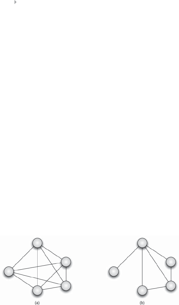
264 FRAUD ANALYTICS
starts with one node (e.g., a fraudulent node) and adds more nodes to
the community based on the links of this node. The extracted com-
munities can be either complete or partial communities. A complete
community is a subgraph in the network where each node is connected
to each other node in the subgraph. When constructing complete com-
munities, a node is added to a community if it has a link to all the nodes
in the community. An example of a complete community is given in
Figure 5.29a. Partial communities are more loosely defined and do not
require that each node in the subgraph is connected to each other node.
A node is added to a partial community if it has connections to at least
x% of all nodes in that community. A partial community is shown in
Figure 5.29b.
Note that graph partitioning algorithms do not generate overlap-
ping communities. These are communities where some nodes belong
to more than one community. In graph partitioning, the graph is itera-
tively divided into small subgraphs that all have a set of unique nodes.
These are the so-called maximal communities. Splitting a network
in maximal or nonoverlapping communities is often not realistic.
People are typically associated with different friend groups (e.g., from
high school, the sport club, colleagues) with diverse backgrounds and
beliefs. Overlapping communities reveal the various communities to
which a certain person belongs. Bottom-up approaches are able to
create overlapping communities. Figure 5.30 shows an example where
node A belongs to different communities. While community 𝓐and 𝓒
are “innocent” communities, community 𝓑is highly associated with
Figure 5.29 Complete (a) and Partial (b) Communities
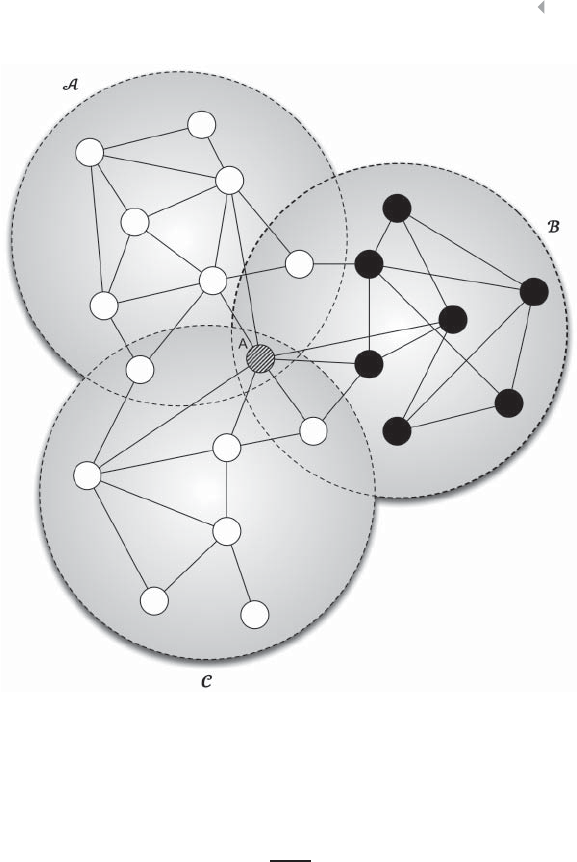
SOCIAL NETWORK ANALYSIS FOR FRAUD DETECTION 265
Figure 5.30 Overlapping Communities
fraud. A membership function describes the extent to which a node
(here: a person) is influenced by fraud through its communities, and
MA=1
𝓒A
i∈𝓒A
i
with MAthe exposure of node A to fraud, 𝓒Athe communities to
which node A belongs and ithe fraudulent influence of community
i. The effect of one fraudulent community on a node is diminished if
the node belongs to many legitimate communities. The membership
exposure score can be used as a separate feature in the analytical mod-
eling part.
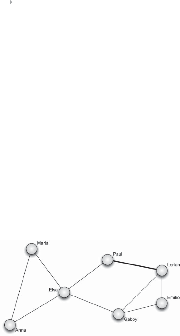
266 FRAUD ANALYTICS
EXTENDING THE GRAPH: TOWARD A BIPARTITE
REPRESENTATION
All networks in the previous sections only consist of one node type
representing for example, people connected to other people by means
of a friendship relation. Such networks are unipartite graphs.The
intensity of the relationship between the nodes in unipartite graphs
often depends on the count of shared events. In call behavior data for
example, two customers are more strongly connected to each other
if they call each other more often. Co-authoring many papers with
the same researchers defines a stronger relationship among them.
Companies rely more on each other when they share more resources.
In unipartite graphs, this information is aggregated in the link weight.
The higher the weight, the more intense the relationship is. The link
weight is often correlated with the influence that two objects have
on each other. Two nodes are more influenced by each other if their
relationship is more intense, and thus has a higher link weight. A
unipartite graph of a people-to-people network is represented in
Figure 5.31. The thickness of the links represents the edge weight.
Specifically, the relationship between Paul and Lorian is stronger
than the relationship between, say, Anna and Maria. Also, remark
that there are two triangles in this network: Anna-Maria-Elsa and
Lorian-Emilio-Gabby. Given the current representation, both triangles
are equally sensitive to influence.
Figure 5.31 Unipartite Graph

SOCIAL NETWORK ANALYSIS FOR FRAUD DETECTION 267
In many applications, it might be useful to integrate a second node
type in the network. Affiliation or bipartite networks represent the reason
why people connect to each other, and include the events that network
objects—like people or companies—attend or share. An event can for
example refer to a paper (scientific fraud), a resource (social security
fraud), an insurance claim (insurance fraud), a store (credit card
fraud), and so on. Adding a new type of nodes to the network does
not only enrich the imaginative power of graphs, but also creates new
insights in the network structure and provides additional information
neglected before. On the other hand, including a second type of node
results in an increasing complexity of the analysis. The extended
network representation of Figure 5.31 is depicted in Figure 5.32.
Paul and Lorian are more closely connected to each other because
they both attended two shared events. The triangle Maria-Anna-Elsa
can quickly be influenced by fraud, as it is enough to disperse fraud
through event 1. In order to affect the triangle Lorian-Emilio-Gaby, at
least two events should be contaminated by fraud.
Mathematically, a bipartite graph is represented by an n×mcon-
nectivity matrix Mwith nand mthe total number of people and events
respectively. The rows specify type-one nodes, while the columns
specify type-two nodes. The connectivity matrix corresponding to the
bipartite network in Figure 5.32 is presented in Figure 5.33.
Recall that the edge weight in the unipartite graph of Figure 5.31
aggregates the frequency that both nodes were associated to the
Figure 5.32 Bipartite Graph

268 FRAUD ANALYTICS
Figure 5.33 Connectivity Matrix of a Bipartite Graph
same event. In a bipartite graph, this is implicitly specified by the
newly introduced node types. Instead of using a binary link between
two node types in a bipartite graph (e.g., attended or not attended),
the edge weights now allow to enrich the network with additional
information, like the recency, the intensity, information exchange,
and so on of the relationships between the people and the events.
For example, the edge weight in Figure 5.32 might indicate the
time person xspent at event y. Suppose that event 1 is a fraudulent
event and that Maria attended event 1 longer than Anna. Maria is
then more influenced by fraudulent event 1 than Anna. Another
example is a credit card fraud network where credit card holders
are connected to stores. A link between a credit card holder and
a store exists if that credit card holder made a purchase in that
store. The link weight might be proportional to the time passed
since the transaction has been pursued and gradually decreases over
time. The spread (or propagation) of influence, such as fraud, by
collective inference algorithms as discussed in the section Collective
Inference Algorithms is weighted over time. Nodes neighboring
to a fraudulent node will be affected more intensively by fraud
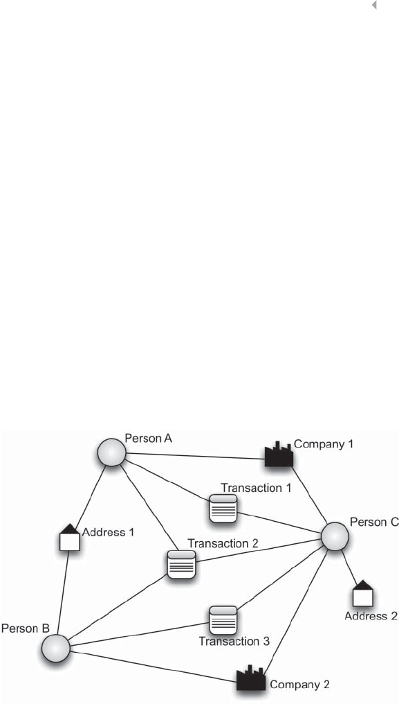
SOCIAL NETWORK ANALYSIS FOR FRAUD DETECTION 269
if the relationship between the node and the fraudulent node is
more recent.
Multipartite Graphs
Whenever a network integrates multiple node types, we say that
the network is a multipartite graph or a multigraph. Those networks
closely reflect the true reality, but simultaneously introduce a lot of
complexity in the network. The network can quickly grow to immense
sizes, and the need for scalable and efficient algorithms to process
huge unstructured data sources is indisputable. Network sampling
by splitting the network into small egonets, one for each node of
interest, is one solution that can help to deal with scalability issues.
Although the processing of such networks may be challenging, their
visualization might shed light on new fraud patterns and result into
valuable insights about which influentials play an important role in
the spread of fraud through networks. An example of a multipartite
graph is depicted in Figure 5.34.
Figure 5.34 A Multipartite Graph
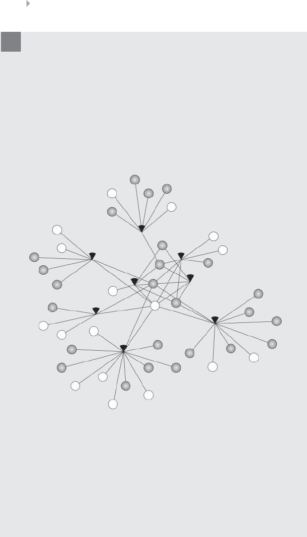
270 FRAUD ANALYTICS
CASE STUDY: GOTCHA!
CASE STUDY
This section discusses a real-life application of network analysis for fraud
detection (Van Vlasselaer et al. 2015a). The data under consideration are
governmental tax data where companies try to avoid contributing their tax
obligations. Companies use resources to perform their activities. Resources
can be, for example, buyers, suppliers, customers, employees, machinery,
accountants, etc. For reasons of interpretability, we do not distinguish between
the different types of resources in the analysis.
Figure 5.35 Sample Network of Gotcha!
A sample network is given in Figure 5.35. The companies and resources
are represented by circles and wedges, respectively. Recall that this is a
bipartite network. Rather than connecting the companies directly to each other
by means of the resources they share, the resources are included in the
network as separate entities. By doing so, the network reflects reality more

SOCIAL NETWORK ANALYSIS FOR FRAUD DETECTION 271
closely and provides more details about the intensity of the connections
between companies and their resources. It will also be clear in the remainder
of this section, that some resources are important instigators of fraud.
Given the experts’ perceptions, companies set up illegal constructions to
avoid tax contributions and closely work together to perpetrate fraud. In
general, companies that are part of a fraudulent setup are organized in such a
way that they do not gain enough profit to redeem their tax debts to the
government. The real profit is pruned away by other companies in the setup.
Once the company files for bankruptcy and is not capable of continuing its
activities, the resources of the company are moved toward other existing
companies, or to newly founded companies. The use of network analysis
allows to follow the trail of resources from one bankrupt company to another,
in order to uncover the fraudulent setups in the network. Those fraudulent
setups are the so-called spider constructions. The companies in the spider
construction form a web of fraud and are all closely connected to each other
by means of the resources they share or transfer. The task at hand is then the
following: Given a network of companies and resources, how can we use the
label of a few confirmed fraudulent companies to infer a fraud probability for
all the other (yet legitimate) companies in the network.
Gotcha! is a fraud detection technique designed to find individual
company fraud by combining evidence from different sources: (1) the isolated
environment of the company and (2) the relations among other companies.
Gotcha! combines three types of data features:
1. Intrinsic (or local) features: these features comprise the
characteristics of each observation (here: company) as if the
observation was treated in isolation. Example features include the
age of the company, the sector in which the company is operating,
financial statements, address, and so on.
2. Direct network features: these features characterize the direct
neighborhood or egonet of a company. Recall that the social
security network is a bipartite graph of companies and resources.
The direct neighborhood of a company is the company together
with its current (and its past) resources. Remark, however, that
fraud is only attributed to companies and that the resources and
(yet) legitimate companies are initially unlabeled. Indirect network

272 FRAUD ANALYTICS
features (see below) extract a primary indication of the fraudulence
of each network object.
3. Indirect network features: a propagation algorithm is used to
infer a fraud probability for each unlabeled resource and company.
The propagation algorithm is based on Google’s PageRank (see
section PageRank Algorithm) and treats fraud as a virus moving
throughout the network. A node in the network that is highly
exposed to fraud receives a high exposure score.
Intrinsic features are extracted from the so-called factual data sets
and historical data sets. A factual data set reflects the current situation
of each observation. The factual data set in a social security context
describes the as-is state of each company: In which sector is the
company currently active? How long does the company already
exist? Changes in the factual data set are kept in the historical data
sets. Historical data sets log the previous states of the factual data
set. For each company, the following past behavior is known: Did
the company operate in another sector before? Did the company
grow during the last xyears, and if so, by how much? Those features
characterize the company as if it was an isolated entity.
Transactional data sets comprise the interactions with other compa-
nies by means of their resources. Which resources were assigned to
a specific company at what period in time? Remark that the transac-
tional data set provides time-related data. Whereas a resource might
be associated with a certain company in year t2, it could be utilized
by another company in year t1. The transactional data set is used to
create the network of companies and resources. As temporal informa-
tion is available in the data set, the link weights between a company
and a resource might express the recency of the relationship, vary-
ing between [0,1]. A link weight of 1 indicates a current association
of the resource with the company. Rather than directly removing a
past connection between a company and a resource, the link weight
decreases over time using, for example, a linear or exponential decay.
For example, a link weight of 0.8 might indicate that the resource was
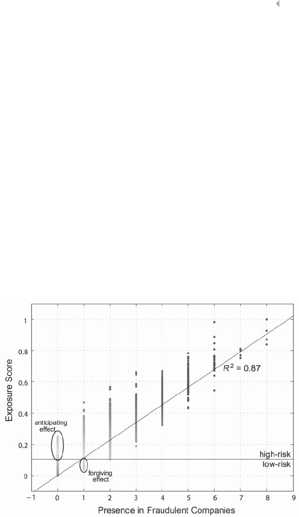
SOCIAL NETWORK ANALYSIS FOR FRAUD DETECTION 273
associated to the company six months ago. This is temporal weighing.As
such, the network dynamically adjusts over time.
Given the temporally weighted network of companies and
resources, and knowing that a limited set of companies are labeled
as fraud, a propagation algorithm infers an exposure score for each
unlabeled network object. It implements an iterative approach where
each resource and company simultaneously spread and absorb fraud.
Recall that the network is bipartite. Each fraudulent company spreads
fraud toward its neighboring resources. Each resource absorbs fraud
from its neighboring companies. In a next phase, each resource
spreads fraud toward its neighboring companies and each company
absorbs fraud from its neighboring resources. This process is iterated
until convergence or until a stopping criterion is met (see section
Collective Inference Algorithms). As a result, each unlabeled node
in the network receives an exposure score. The exposure scores of
the resources are depicted in Figure 5.36. This figure represents the
exposure score of the resources in terms of the number of fraudulent
Figure 5.36 Exposure Score of the Resources Derived by a Propagation Algorithm. The
Results are Based on a Real-life Data Set in Social Security Fraud

274 FRAUD ANALYTICS
companies they were associated with. There is a positive correlation
between the derived exposure score and the association to fraudulent
companies. However, some resources receive a rather high exposure
score although they were never connected to fraudulent companies.
This is the anticipating effect and takes into account that fraud is
approaching the resource node. On the other hand, some resources
that were associated to fraud receive a low exposure score. This is
the forgiving effect and is due to the incorporation of time into the
network. The exposure scores of the companies can be used as an
indirect network feature. The exposure scores of the resources are
used to characterize the direct neighborhood of each company to infer
the direct network features.
The direct network features characterize a company based on
its direct neighborhood or egonet. In a bipartite network, these
are the resources associated with the company. An example of a
company’s egonet is given in Figure 5.37. Features derived from the
egonet include among others the count or proportion of suspicious
resources connected to the company. In Figure 5.37, suspicious
resources are shaded. The company has two suspicious resources and
a suspiciousness ratio of 1:3.
The combination of all features (i.e., intrinsic and network fea-
tures) is fed to the machine learning algorithms. This is the Gotcha!
model. As the creation of network features drastically increases the
number of features to learn from, ensemble methods like Random
Figure 5.37 Egonet in Social Security Fraud. A Company Is Associated with its Resources
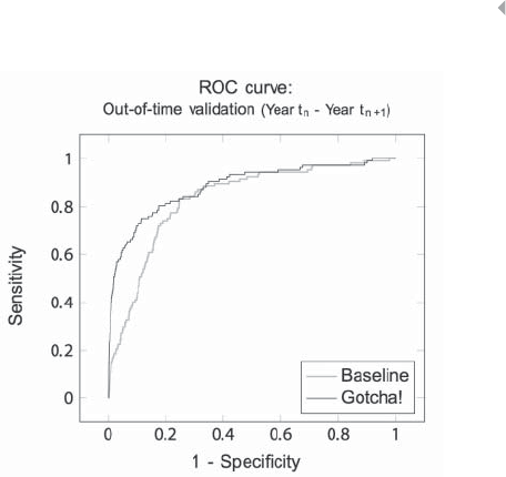
SOCIAL NETWORK ANALYSIS FOR FRAUD DETECTION 275
Figure 5.38 ROC Curve of the Gotcha! Model, which Combines both Intrinsic and
Relational Features
Forest are used to train the models. Figure 5.38 shows the ROC
curve for an out-of-time validation of the model. That is, the model
is trained on timestamp tnand evaluated on timestamp tn+1.Thisis
exactly how the model will be implemented in practice. The ROC
curve shows that the model performs better when including network
features (the Gotcha! model), then when solely relying on intrinsic
features (Baseline). As fraud is often inspected manually afterward,
only a limited number of fraudulent companies can be outputted by
the models. Given that at each timestamp only 100 companies can be
investigated by domain experts, how many fraudulent companies does
the model actually detect? This corresponds to the model’s precision
(see Chapter 3). The results of an out-of-time validation are included
in Table 5.14. Each model is evaluated according to the extent to
which it is capable to detect fraud on short term (ST—fraud within six
months), medium term (MT—fraud between six months and one year
from now) and long term (LT—fraud after one year). The Gotcha!
model outperforms the baseline for each time window of analysis.
Furthermore, in the outputted list many bankruptcies are included.
Recall how fraud is perpetrated through pruning away the profits of
the company and filing for bankruptcy. Consequently, experts expect

276 FRAUD ANALYTICS
Table 5.14 Overview of the 100 Companies with the Highest Score as Output by the
Detection Model
Total ST
Fraud
MT
Fraud
LT
Fraud
Total
Fraud
Bankrupt Nonactive Active % detected
Year t1Baseline 100 10 5 9 24% 24 16 36 48%
Gotcha! 100 24 713 44% 27 524 71%
Year t2Baseline 100 6 2 11 19% 14 16 51 33%
Gotcha! 100 18 514 37% 24 732 61%
Year t3Baseline 100 11 1 1 13% 4 4 79 17%
Gotcha! 100 29 9 6 44% 15 437 59%
that the identified companies were undetected fraudulent companies.
The remaining companies are investigated whether they are still
active or not. Note that nonactive means that the company is regularly
suspended and that all debts are redeemed. No fraud can be attributed
to these companies. Given all confirmed fraudulent companies and
the expectation of the experts that the found bankruptcies might also
be fraudulent, the table indicates that the enrichment of traditional
models (baseline) with network features might detect up to 71 percent
fraudulent companies.
Gotcha! can easily be mapped to other fraud detection applications,
like credit card fraud detection. The requirements of a fraud detection
model in credit card fraud are stricter. In order to achieve sufficient
Quality of Service (QoS) levels, credit card issuers apply a “six second
rule of decision.” This means that the processing of a credit card trans-
action might take at most six seconds. Most credit card transactions are
liable to two checks: an acceptance check and a sanity check. During
the first phase, the transaction processing system checks for example
whether the user entered the right PIN or whether the spending
amount is still sufficient. The sanity check often consists of an offline
and online component. The offline check is not liable to the “six-second
rule of decision” and is done when the transaction is already pursued.
The online component happens in real-time, and decides whether
the transaction contains signs of suspicious behavior. Network effects
might have a huge impact on the detection model performance.
The network in credit card transaction fraud is a bipartite
graph connecting merchants with credit card holders by means of
transactions. Given a set of few fraudulent transactions, how can we

SOCIAL NETWORK ANALYSIS FOR FRAUD DETECTION 277
propagate fraud through the network? Collective inference algorithms
initialize the nodes of the network. In credit card fraud, the edges are
labeled. In order to introduce fraud in the network, one possibility is
to include a new node type: the transaction. Every edge (transaction)
in the network is replaced by a transaction node and two edges, to
retain the connections between the merchant and the credit card
holder. As a consequence, the labeled transaction nodes start the fraud
propagation. Remark that fraud propagation affects all nodes in the
network, and results in an exposure score for all merchants, credit
card holders and transactions.
The network features are enriched with intrinsic features. An inter-
esting approach in credit card fraud is to derive features using the
RFM framework (recency, frequency, and monetary value). Given past
transactional behavior of a certain customer (let’s say, during the last
day), RFM assesses for each transaction the (a) recency or the time
passed since the previous transaction, (b) frequency or the number of
transactions pursued, and (c) monetary value or the average amount
of past transactions. A good approach is to derive the RFM variables
at different levels of aggregation: merchant level, merchant category
level, global level, country level, and currency level. Applied on the fre-
quency, this means that one counts the number of transactions made
at the merchant, the merchant category (e.g., groceries), overall, the
country (e.g., Belgium) and the currency (e.g., euro). The combina-
tion of both intrinsic and network variables infers the Gotcha! model.
Results have shown that the combined model achieves the best perfor-
mance (Van Vlasselaer et al. 2015b).
REFERENCES
Koutra,D.,Ke,T.Y.,Kang,U.,Chau,D.H.P.,Pao,H.K.K.,&Faloutsos,C.
(2011). Unifying Guilt-by-Association Approaches: Theorems and Fast
Algorithms. In D. Gunopulos, T. Hofmann, D. Malerba, and M. Vazirgian-
nis (Eds.), Machine Learning and Knowledge Discovery in Databases. Berlin:
Springer Berlin Heidelberg, pp. 245–260.
Kwak, H., Lee, C., Park, H., & Moon, S. (2010, April). What Is Twitter, a Social
Network or a News Media? In Proceedings of the 19th international conference
on World Wide Web. ACM, pp. 591–600.
Boccaletti, S., Latora, V., Moreno, Y., Chavez, M., & Hwang, D. U. (2006). Com-
plex Networks: Structure and Dynamics. Physics Reports 424 (4): 175–308.

278 FRAUD ANALYTICS
Gupte, M., & Eliassi-Rad, T. (2012). Measuring Tie Strength in Implicit Social
Networks. In Proceedings of the 3rd Annual ACM Web Science Conference.ACM,
pp. 109–118.
Newman, M. (2010). Networks: An Introduction. New York: Oxford University
Press.
Park, J., & Barabási, A. L. (2007). Distribution of Node Characteristics in
Complex Networks. Proceedings of the National Academy of Sciences 104 (46):
17916–17920.
Hill, S., Provost, F., & Volinsky, C. (2007, August). Learning and inference in
massive social networks. In: The Fifth International Workshop on Mining and
Learning with Graphs. Florence, Italy.
Dijkstra, E. W. (1959). A Note on Two Problems in Connection with Graphs.
Numerische Mathematic 1 (1): 269271.
Seidel, R. (1995). On the All-Pairs-Shortest-Path Problem in Unweighted
Undirected Graphs. Journal of Computer and System Sciences 51 (3): 400–403.
Page, L., Brin, S., Motwani, R., & Winograd, T. (1999). The PageRank citation
ranking: Bringing order to the web (Technical Report, Standford Digital
Library Technologies Project). Retrieved from http://ilpubs.stanford.edu:
8090/422/1/1999-66.pdf.
Geman, S., & Geman, D. (1984). Stochastic Relaxation, Gibbs Distributions,
and the Bayesian Restoration of Images. IEEE Transactions on Pattern Anal-
ysis and Machine Intelligence (6): 721–741.
Lu, Q., & Getoor, L. (August 2003). Link-based Classification. In ICML 3:
496–503.
Chakrabarti, S., Dom, B., & Indyk, P. (1998, June). Enhanced Hypertext Cate-
gorization Using Hyperlinks. In ACM SIGMOD Record 27 (2): 307–318. ACM.
Pearl, J. (1986). Fusion, Propagation, and Structuring in Belief Networks. Arti-
ficial Intelligence,29 (3): 241–288.
Tong, H., Faloutsos, C., & Pan, J. Y. (2007). Fast Random Walk with Restart and
Its Applications. Knowledge and Information System: An International Journal
(KAIS).
Fortunato, S., Boguñá, M., Flammini, A., & Menczer, F. (2008). Approximat-
ing PageRank from in-degree. In Algorithms and Models for the Web-Graph.
Berlin: Springer Berlin Heidelberg, pp. 59–71.
Van Vlasselaer, V., Eliassi-Rad, T., Akoglu, L., Snoeck, M., & Baesens, B.
(2015a). Gotcha! Network-based Fraud Detection for Social Security
Fraud. Under review.
Van Vlasselaer, V., Bravo, C., Caelen, O., Eliassi-Rad, T., Akoglu, L., Snoeck,
M., Baesens, B. (2015b). APATE A Novel Approach for Automated Credit
Card Transaction Fraud Detection Using Network-Based Extensions.
Decision Support Systems 75 (2015): 38–48.
CHAPTER 6
Fraud Analytics:
Post-Processing
279

INTRODUCTION
The result of the analytics step is an analytical fraud model built using
either a descriptive, predictive, social network or combined technique.
Essentially, the analytical model reduces to a mathematical formula
predicting the fraud occurrence or fraud amount. In a next step, this
model or formula needs to be integrated into the existing business envi-
ronment and ICT architecture. In order to successfully complete this
exercise, it is of key importance to perfectly understand the business
requirements, which are usually specified by the end users of the ana-
lytical model(s). Furthermore, after the models have been put to work,
they need to be closely monitored such that any deviation in perfor-
mance due to changing fraud behavior can be detected in a timely way
and corresponding actions can be undertaken. In this chapter, we will
discuss various issues that arise when deploying, using, and monitoring
analytical fraud models within a specific business context.
THE ANALYTICAL FRAUD MODEL LIFE CYCLE
In previous chapters, we discussed how to develop analytical fraud
models using descriptive, predictive, and social network analytics.
Once the model development has been completed, the analytical model
can proceed to the next step in the model life cycle (see Figure 6.1).
During model testing, it will first be verified whether the model
can satisfy all requirements needed to solve the business problem. For
example, in a credit card fraud-detection setting, it will be verified
whether the model can come up with a fraud score in a sufficient
amount of time (e.g., less than 5 seconds). It can also be checked how
the model behaves in case of missing or extreme inputs. Some dummy
fraud cases can be used to verify the model’s outcome.
Model
development
Model
testing
Model
staging
Model
production
Model
retirement
Figure 6.1 The Analytical Model Life Cycle
280

FRAUD ANALYTICS: POST-PROCESSING 281
Upon successful completion of the model testing, it can proceed to a
staging step. Here, the model can run in parallel with the old model for
a specific period of time (e.g., 1 month). A champion-challenger strat-
egy can be adopted whereby the old model is the current champion
and the new model the challenger.
In case the challenger beats the champion in performance, the
model can proceed to the production step and the old model can
be replaced. Various replacement strategies can be adopted. In a
direct changeover strategy, the old model is immediately replaced
by the new model. Obviously, this should be carefully planned by
making sure all stakeholders have been appropriately informed and
trained, and back-up facilities are available. Another alternative could
be a phased-implementation strategy. The idea here is to gradually
introduce the new model. For example, in a car insurance fraud
setting, the new analytical model can be used to score all claims with
claim amount below 5.000 euro, whereas the ones with claim amount
above 5.000 euro are scored with the old model. If the new model
works well on the low amount claims, it can then step-by-step be
further migrated to handling all claim amounts.
Finally, a parallel strategy can also be adopted whereby the new
and old model run in parallel in production during a transition period
(e.g., 3 months). The overall fraud score is then a weighted combina-
tion of the scores of the new and old model, whereby gradually more
weight is put on the new score such that at the end of the transition
period the old score has been fully replaced by the new score.
The final step in a model’s lifecycle is its retirement. The idea here
is to bring the model out of the production environment and store it
in a model repository, where it can be consulted later. Retired models
can be useful for benchmarking or tracking purposes.
MODEL REPRESENTATION
When deploying a fraud analytics model, it is of crucial importance that
the representation used is easily understandable and readable. Depend-
ing on how the analytical models were built, various representations

282 FRAUD ANALYTICS
may be adopted. In what follows, we will discuss the traffic light indi-
cator approach and decision tables.
Traffic Light Indicator Approach
A first way to represent the output of a fraud analytics model could
be based on traffic light indicator coding (Van Gestel, Baesens, and
Martin 2015). In this approach, colors are assigned to the outcome of
the analytical model. These colors directly correspond to the probabil-
ity of a customer being a fraudster. When using logistic regression, the
outcome probabilities can be categorized and colors can be assigned
to each category. This is illustrated in Figure 6.2. Green light indicates
that the customer is low risk, whereas the red light corresponds to high
probability of fraud. The colors in between can then be interpreted
accordingly. The arrow shifts from left to right and indicates the color
assigned to the customer under study. The number of colors and their
encoding can be decided by the fraud analyst and business expert.
In many settings, a crisp decision is needed to classify an obser-
vation as fraudulent or not. A first alternative is to use a hard cut-off
method. For example, the observation is considered a fraudster when
the probability of fraud exceeds 0.5 and a nonfraudster otherwise.
Alternatively, the fraud-scoring model can be used in semi-automated
mode. The idea here is that observations belonging to the dark green,
light green, orange, and red zone are automatically classified as
nonfraudsters and fraudsters, respectively. The yellow zone is used
as a referral zone, whereby these observations will be evaluated
Dark green Light green OrangeYellow Red
Customer
0 1
Figure 6.2 Traffic Light Indicator Approach

FRAUD ANALYTICS: POST-PROCESSING 283
manually by one or more fraud analysts. These fraud analysts may
then also decide to overrule the fraud scorecard.
Decision Tables
Decision tables provide an alternative way of representing rule-based
patterns (Baesens et al. 2003; Mues 2002). These patterns can be
obtained either from the business expert as If-Then business rules or
from the data by using a decision tree or rule extraction algorithm for
example.
Decision tables (DTs) are a tabular representation used to describe
and analyze decision situations such as fraud detection, where the state
of a number of conditions jointly determines the execution of a set of
actions. The conditions correspond to the antecedents of the If-Then
rules whereas the actions correspond to the outcome classes (e.g.,
customer =fraudster or not).
Essentially, a DT consists of four quadrants, separated by
double-lines, both horizontally and vertically. The horizontal line
divides the table into a condition part (above) and an action part
(below). The vertical line separates subjects (left) from entries (right).
The condition subjects are the criteria that are relevant to the decision
making. Each condition entry describes a relevant subset of values
(called a state) for a given condition subject (attribute), or contains a
hyphen symbol (-) if its value is irrelevant within the context of that
column. Every column in the entry part of the DT thus comprises a
classification rule, indicating what actions apply to a certain combi-
nation of condition states. If each column contains only simple states
(no contracted or irrelevant entries), the table is called an expanded
DT. Otherwise, the table is called a contracted DT. Table contraction can
be achieved by combining columns, which leads to the same action
configuration. The number of columns in the contracted table can
then be further minimized by changing the order of the conditions.
It is obvious that a DT with a minimal number of columns is to be
preferred because it provides a more compact and comprehensible
representation of the extracted knowledge than an expanded DT. Let’s
illustrate this with an example in a fraud-detection setting.

284 FRAUD ANALYTICS
Suppose we have the following set of eight If-Then rules to detect
fraud in a credit card fraud detection setting.
If Suspicious merchant =yes And Transaction amount ≤1000
And Card present =yes Then Fraud =no
If Suspicious merchant =yes And Transaction amount ≤1000
And Card present =no Then Fraud =yes
If Suspicious merchant =yes And Transaction amount >1000
And Card present =yes Then Fraud =yes
If Suspicious merchant =yes And Transaction amount >1000
And Card present =no Then Fraud =yes
If Suspicious merchant =no And Transaction amount ≤1000 And
Card present =yes Then Fraud =no
If Suspicious merchant =no And Transaction amount ≤1000 And
Card present =no Then Fraud =yes
If Suspicious merchant =no And Transaction amount >1000 And
Card present =yes Then Fraud =no
If Suspicious merchant=No And Transaction amount >1000 And
Card present =no Then Fraud =yes
These rules can now be represented in an expanded decision table,
as depicted in Table 6.1.
When inspecting the expanded decision table more closely, it can
be seen that both columns 3 and 4, and columns 5, 6, 7, and 8 can be
contracted, resulting into the contracted decision table as depicted in
Table 6.2.
The size of the decision table can then be further minimized by
rearranging the order of the conditions as represented in Table 6.3.
Table 6.1 Fully Expanded Decision Table
Suspicious merchant Yes No
Transaction amount ≤1000 >1000 ≤1000 >1000
Card present Yes No Yes No Yes No Yes No
Fraud =yes x x x x x
Fraud =no x x x
1 2 3 4 5 6 7 8

FRAUD ANALYTICS: POST-PROCESSING 285
Table 6.2 Contracted Decision Table
Suspicious merchant Yes No
Transaction amount ≤1000 >1000 -
Card present Yes No -Yes No
Fraud =yes x x x
Fraud =no x x
1 2 3 4 5
Table 6.3 Minimized Decision Table
Card present Yes No
Suspicious merchant Yes No -
Transaction amount ≤1000 >1000 - -
Fraud =yes x x
Fraud =no x x
1 2 3 4
Note that the minimized decision table only has four columns or
classification rules, which is a substantial reduction when compared
to the original table, which had eight columns or classification rules.
The minimized decision table also gives some interesting additional
insights, which were not that obvious from the original rule set. As an
example, it is now clear that if Card Present is No then the transaction
will always be classified as fraud. Similarly, if Card Present is Yes and
Suspicious merchant is No then the transaction will not be considered
fraudulent.
It is already clear now that decision tables come in handy for visu-
alizing rule sets in an intuitive and user-friendly way. They can also be
used to check rule sets for completeness and anomalies. As an example,
consider the following rule set in an insurance fraud setting:
R1. If Age <25 And Unemployed =Yes And Recent claims >3,
Then Fraud =yes
R2. If Age <25 And Unemployed =No Then Fraud =yes
R3. If Age ≥25 And Unemployed =Yes, Then Fraud =no
R4. If Age <25 And Recent Claims ≤3, Then Fraud =no

286 FRAUD ANALYTICS
Table 6.4 Decision Table for Rule Verification
Age <25 ≥25
Unemployed Yes No Yes No
Recent claims ≤3>3≤3>3≤3>3≤3>3
Fraud =yes x x x
Fraud =no x x x x
1 2 3 4 5 6 7 8
R4 R1 R2; R4 R2 R3 R3
These rules can now be represented in a decision table as depicted
in Table 6.4.
From the decision table, various anomalies can be observed. In col-
umn 4, both rules R2 and R4 apply, resulting in the conflicting action
entries Fraud =yes and Fraud =no simultaneously. The decision table
also indicates missing entries in columns 7 and 8 where no action is
specified in case Age ≥25 and Unemployed =No. These anomalies
should be addressed before the decision table can be used in a produc-
tion environment.
Although decision tables provide powerful rule visualization and
verification facilities, not many commercial tools are available that
provide support for them. Amongst the most popular is Prologa. See
https://feb.kuleuven.be/prologa/ for more details.
SELECTING THE SAMPLE TO INVESTIGATE
In many organizations, a fraud-detection system is being used as a deci-
sion support system that helps in selecting the suspicious cases that
require further investigation, for instance by using a traffic light indi-
cator system as discussed above. In other words, the system helps in
allocating the limited amount of resources that are available to further
(manually) inspect cases and to confirm whether or not they actually
concern fraud, as discussed in Chapter 1.
The available resources are typically limited and set by the man-
agement based on qualitative or semi-quantitative grounds. Therefore,
only a fraction of all (suspicious) cases can be further inspected. The
aim of adopting a data-driven fraud-detection system is to allocate the

FRAUD ANALYTICS: POST-PROCESSING 287
limited resources more efficiently, or in other words, to improve the hit
rate. In this context, the hit rate is the fraction of actual fraudulent cases
among the cases that are further investigated by the inspectors. A hit
rate of 100 percent means that all inspected cases concern fraud, and
as such indicates that very efficient use is being made of the available
resources, since they are not being spent on investigating nonfraudu-
lent cases. However, a high hit rate may as well indicate that too few
cases are being investigated and as such point toward an insufficient
amount of resources to be available to facilitate the effective investiga-
tion of all suspicious cases.
Typically, a fraud-detection system is used to score all cases and
rank them from low to high suspiciousness. Subsequently, inspectors
are provided a draft list of cases that are to be further investigated based
on this ranking. In a next step, a further manual screening and selec-
tion is performed by the inspectors, primarily based on experience and
expertise as well as plain common sense.
The inspectors may be familiar with some of the cases in the list,
as well as the reasons why they are being scored high by the system.
For instance, when a firm has been inspected only recently and was
found not to commit fraud, this firm might still be ranked high because
no change occurred with respect to the fraud score drivers (i.e., with
respect to the data values that are used by the fraud detection model
to calculate a risk score).
The first screening may also be based on a preliminary, high-level
investigation that looks into the drivers underlying the high fraud score
that was assigned to a case by the system. This preliminary investi-
gation may look into which exact pieces of information have led the
detection system to rank a particular case to be highly suspicious—in
other words, look into why the case scores are high and subsequently
analyze whether the high score effectively raises cause for suspicion.
Either the particular nature of a case or just pure coincidence may
cause a case to be scored as highly suspicious. A preliminary investiga-
tion may detect this, and as such avoid unnecessary inquiries to be per-
formed. This allows the inspectors to focus on truly suspicious cases and
increase the hit rate, efficiency, and effectiveness of the inspections.
Note that in order for the scores to be interpretable for the inspectors,
the model needs to be represented or implemented in a manner that
facilitates and supports such preliminary investigation and screening.

288 FRAUD ANALYTICS
When many cases among the highly scored cases concern, in fact,
nonsuspicious cases, the system may have to be recalibrated, updated,
or fully retrained, since it appears to be no longer very precise with
respect to the ranking it provides. In fact, the expertise and experience
used by the inspectors during such a screening and preliminary inves-
tigation should be captured as much as possible by the system, or built
in the underlying model. This can be done by including the informa-
tion that is used during the screening in the data set for model building
or analysis.
A dynamic interface or dashboard allowing inspectors to drill down
on information related to particular cases as well as into the model
scores may help them conduct a meaningful screening based on the
scoring of the system, and to select cases that require further investi-
gation. As such, the system becomes a decision support system in the
true sense of the word.
With respect to deciding on the amount of resources an organi-
zation should allocate to further investigate suspicious cases and fight
fraud, several elements have to be taken into account. A quantitative
approach could be adopted to guide this decision. A first and important
step in such a quantitative approach concerns the attribution of mon-
etary value or utility to each possible outcome or event. Investigating
a case comes at a certain cost (e.g., time of the inspector), which may
vary from case to case, depending on the complexity of the case and
the amount of resources required to investigate the case.
When the investigated case concerns a nonfraudulent case, clearly
not as much value or utility has been generated by the inspection as
when the case would concern fraud. Still, some utility may be gener-
ated, in creating a scare-off effect and making fraudsters aware of the
fact that inspections do take place. Although possibly challenging, a
monetary value could and should be attributed to such an outcome, as
well as to the detection and investigation of an effectively fraudulent
case. To such a positive outcome, a utility can be attributed equal to
the sum of a number of components:
◾The fraud amount
◾All involved costs such as legal costs, cost of investigation, cost
of the fraud detection infrastructure, etc.

FRAUD ANALYTICS: POST-PROCESSING 289
◾A penalty or fine
◾A noneconomic value attributed to detecting fraud, represent-
ing the social benefits associated with a reduction of fraud
Which of these elements or possibly other factors to take into
account in calculating a utility for a detected fraud case, as well as the
exact value to assign, depends on the particular setting and application.
On the other hand, a utility must be assigned to not investigating a
nonfraudulent case (positive utility) and to not investigating a fraud-
ulent case (strongly negative utility). The amount of resources that is
spent on investigating cases will determine how many cases and, as
such, how many of each of these four types of outcomes will occur.
Therefore, a total utility can be calculated for each possible amount of
resources allocated by multiplying the number of outcomes with the
associated utility of the outcome. The amount of resources that are
required to maximize the total utility represents the optimal amount
from the utility perspective, and as such may provide guidance in
deciding about how much an organization should invest in inspection
resources.
The values of the outcome utilities will clearly have a direct impact
on the optimal amount or resources according to this approach. There-
fore, it is important to stress that they may and should include noneco-
nomic value or utilities when meaningful. These noneconomic utilities,
however, do have to be expressed in monetary units—for instance, the
utility of not detecting a fraudulent case may be assigned a very high
value, since this is unacceptable from a societal point of view. This,
however, is not always straightforward and should be determined by
senior management.
Next to the utilities associated with the different outcomes also the
power of the detection model will determine the optimal amount of
resources to invest. The more accurate the ranking and the stronger the
ability to rank fraudulent cases highly, the more return the investiga-
tions will generate since more true fraudulent cases will be addressed.
This approach to maximize the return of the fraud investigations
is similar to an approach adopted in marketing, where the optimal
fraction of customers to target in a marketing campaign is determined
based on the estimated returns and the involved costs and benefits, as
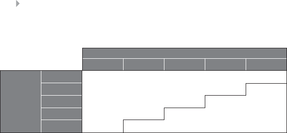
290 FRAUD ANALYTICS
Table 6.5 Using the Expected Fraud Amount to Decide on Further Investigation
Fraud Probability
0–0.2 0.2–0.4 0.4–0.6 0.6–0.80.8+
Fraud Amount
0–100
100–500 Do Not Investigate
500–2,000
2,000–5,000 Investigate
5,000+
well as on the predicted probability to respond to the campaign, the
incentive that is offered and the effect it resorts, together with the pre-
dictive performance of the model (Verbeke, Dejaeger, Martens, Hur, &
Baesens, 2012).
A complementary approach to deciding which cases to further
investigate is to rank cases by combining the fraud probability with
the intensity of the fraud or fraud amount, and computing as such the
expected fraud amount. The idea here is that if the fraud probability
is high (e.g., 90%) but the fraud amount is low (e.g., 10 euros), then
the expected fraud amount (e.g., 90% ×10 euros or 9 euros) is small,
making it not worthwhile to start an investigation. On the contrary,
when the fraud probability is low (e.g., 25%) and the fraud amount
is high (e.g., 10,000 euros), then the expected fraud amount is high
(e.g., 2,500 euros), and a further investigation can be considered.
This is illustrated in Table 6.5, where the claim amount and fraud
probability have been categorized. The stepwise black line indicates
the separation between further and no further investigation.
FRAUD ALERT AND CASE MANAGEMENT
In case the analytical model flags a transaction or observation as
suspicious an alert with corresponding priority should be triggered.
The priority is set based on the severity of the fraud as predicted by the
analytical model. Alerts can be generated on a 24/7/365 basis. Depend-
ing on the setting, the prioritized alerts can then be further manually
inspected and processed by business experts working in investigative
units. The assignment and routing of alerts to investigators can be
done in an automated way by using a set of predefined business rules.

FRAUD ANALYTICS: POST-PROCESSING 291
It may be decided that further follow-up is not necessary because the
intensity of the potential fraud (e.g., claim or transaction amount) is
below a specific threshold, hereby not justifying the cost of additional
investigation.
In case further follow-up is desirable, all necessary actions to fur-
ther mitigate the fraud should be taken first, followed by notifying the
parties involved. Examples of actions could be: Block credit card or
money transfer, deny access to resources, and freeze account. Next, the
fraud victim(s) must be informed via phone call, SMS, or email. A fully
automated multichannel strategy can be adopted. For example, send
email first, followed by SMS if no reaction after 5 minutes, followed
by a phone call if no reaction after 10 minutes. Finally, the fraudsters
should be dealt with. In case of strong evidence, the fraudsters can be
prosecuted although some firms might not prefer to do this because
of bad publicity or because legal action is simply not possible. As an
alternative, the firm might consider a settlement with the fraudsters.
Every fraud alert should be appropriately tracked using a case
management environment, which accurately records all investigation
workflows, documentation, communication between the parties
involved and actions undertaken. Ideally, this should be implemented
using a browser-based digital dashboard hereby facilitating real-time
fraud alert monitoring and management oversight. Every investi-
gator can log on to the case management environment and get a
personalized list of activities to be performed depending on his/her
expertise. Summary and detail reports can be generated. Popular
examples are a confirmed fraud report (e.g., daily and monthly),
suspicious activity report, fraud alert year-to-date activity report,
fraud recovery report, fraud trends report, investigator performance
report, heat maps showing geographical fraud hotspots, and so on.
Also, a complete audit trail of each alert and/or case can be requested
including an overview of which investigator performed what action.
To facilitate the creation of the various reports, the case management
environment should offer advanced visualization and summarization
facilities. It should offer online analytical processing (OLAP) function-
ality to allow for multidimensional analysis with roll-up, drill-down,
slice and dice operations as we discussed earlier in the chapter on
data preprocessing. Ideally, it should also implement link analysis to

292 FRAUD ANALYTICS
visually map and analyze the links between various alerts, entities,
transactions, and so on.
Figure 6.3 shows an example of the SAS Social Network Analysis
dashboard in a car insurance fraud detection setting. It shows various
characteristics such as ClaimID, Alert Type, and Claim score.
As depicted in Figure 6.4, every claim can then be further investi-
gated in terms of linked documents, linked entities, relevant suspicion
rules, and so on.
The investigation can then be further augmented with link analysis
as depicted in Figure 6.5.
It shows the links between various types of nodes such as claims,
claimant, house address, car, bank account, and phone. Facilities can
be provided to show how the network grows in time, both cumulative
whereby previous links are maintained as well as marginal whereby
only new links are visualized. This allows to uncover more complex
fraud patterns and fraud rings. As an example, assume claimant A
shares the same address, car, bank account, and phone as claimant B.
If claimant A has filed a fraudulent claim before, then all new claims
filed by claimant B should be flagged as suspicious and an alert must be
generated since most likely, claimant A and claimant B are the same
person. These complex fraud patterns can be easily visualized using
link analysis. Furthermore, the link analysis should be complemented
with other applications such as Google Street View. By clicking an
address node representing the home address of the claimant or loca-
tion of the car accident, an inspector can immediately verify whether
it’s legitimate or not.
The case management environment should also provide precon-
figured templates for sending out automated correspondence (e.g.,
emails, SMS, voice calls). When relevant (e.g., in anti-money laun-
dering), it should also allow the generation of regulatory compliance
reports, which can then be sent to the federal or law enforcement
authorities involved. This is especially useful in case legal prosecutions
are pursued.
Finally, once a particular fraud alert case can be closed, the result
of the investigation should be fed back to the analytical models. This
will allow the loop to close and to determine whether any adjustments
to the analytical fraud models are necessary.
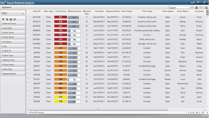
293
Figure 6.3 SAS Social Network Analysis Dashboard
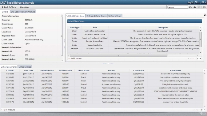
294
Figure 6.4 SAS Social Network Analysis Claim Detail Investigation
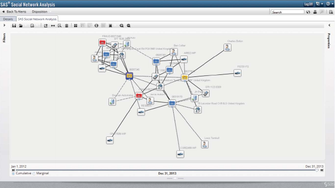
295
Figure 6.5 SAS Social Network Analysis Link Detection

296 FRAUD ANALYTICS
VISUAL ANALYTICS
Visual analytics refers to the use of advanced visualization mechanisms
supported by interactive interfaces to facilitate the various steps of
the analytical model development, implementation, and monitoring
process. It was originally introduced in the context of data preprocess-
ing, such as to conduct exploratory data analysis, online analytical
processing (OLAP) or multidimensional data analysis. It is nowadays
also being actively used to support analytical model building and the
post-processing activities. It has great potential for fraud detection,
since it allows fraud analysts to disentangle complex fraud patterns
hereby giving additional insights, which can then be appropriately
translated to future fraud prevention strategies. Let’s discuss an
example of SAS Visual Analytics. Figure 6.6 shows an example of the
distribution of claim counts and average claim value during October
2012 for a particular insurance company. You can immediately notice
the peak in claims on day 20. When selecting this particular date, it
can be seen in the pie chart left below in Figure 6.6 that most of the
claims were filed due to a flood or storm event, whereas in the pie
chart to the right, it can be seen that about half of the claims are still
open and thus need to be processed further.
We can now further zoom into the flood-and-storm-related claims
and look at the geographical distribution thereof. Figure 6.7 illustrates
a map of France and its neighboring countries. The dots indicate geo-
graphical concentrations of flood and storm claims and are colored
according to the average claim value.
It is then possible to drill down and look at specific regions and/or
cities into more detail, as depicted in Figure 6.8.
We can also use visual analytics to evaluate the efficiency of
the fraud detection process and identify performance bottlenecks.
Figure 6.9 shows the distribution of the total number of investigated
fraud claims and the corresponding hit rate for the year 2012, together
with the fraud statistics by claim type and a pie chart of the fraud
outcomes (fraud proven, fraud suspected, and investigated nonfraud).
Figure 6.10 shows a tree map displaying the efficiency of the fraud
investigators. The size of the rectangles is proportional to the number
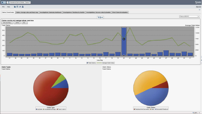
297
Figure 6.6 Distribution of Claim Amounts and Average Claim Value
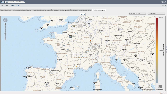
298
Figure 6.7 Geographical Distribution of Claims
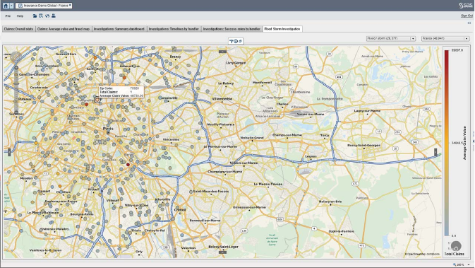
299
Figure 6.8 Zooming into the Geographical Distribution of Claims
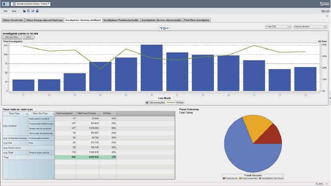
300
Figure 6.9 Measuring the Efficiency of the Fraud-Detection Process
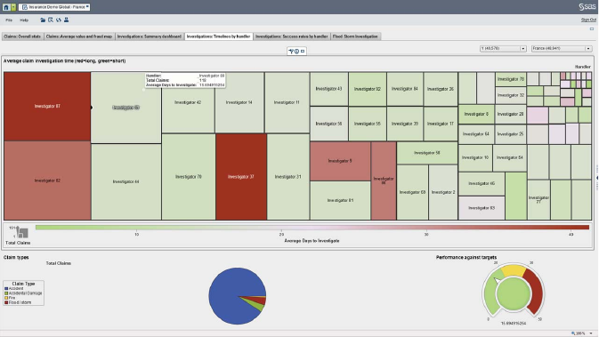
301
Figure 6.10 Evaluating the Efficiency of Fraud Investigators

302 FRAUD ANALYTICS
of claims handled, whereas the color reflects the average days needed
to investigate. For example, it can be easily seen that Investigators 87
and 37 take the most the time to investigate. The highlighted Inves-
tigator 89 handled 118 claims with an average of about 15 days. This
corresponds to a good performance according to the gauge depicted in
the lower-right corner.
BACKTESTING ANALYTICAL FRAUD MODELS
Introduction
Backtesting is an important model-monitoring activity that aims at
contrasting ex-ante made predictions with ex-post realized outcomes
(Baesens 2014). The key idea here is to verify whether the fraud model
still performs satisfactory. Fraudsters will try to constantly outsmart
fraud analytical models by continuously changing their strategies. This
creates concept drift implying that the relationship between the tar-
get fraud indicator and the data available changes on an ongoing basis.
Hence, it is important to closely follow-up the performance of the ana-
lytical model such that concept drift and any related performance devi-
ation can be detected in a timely way.
Depending on the type of model and its purpose, various back-
testing activities can be undertaken. In what follows, we will discuss
backtesting data stability, model stability, and model calibration.
Backtesting Data Stability
When backtesting data stability, one should check whether internal
or external environmental changes will impact the analytical model.
Examples of external environmental changes are new developments
in economic, political or legal environment, changes in commercial
law, or new bankruptcy procedures. Examples of internal environ-
mental changes are changes of business strategy, exploration of new
market segments, or changes in internal organizational structure due
to a merger or acquisition. Also, changing fraud patterns may give

FRAUD ANALYTICS: POST-PROCESSING 303
instability problems. To backtest data stability, a two-step approach can
be suggested, as follows:
◾Step 1: Check whether the population on which the model is
currently being used is similar to the population that was used
to develop the model.
◾Step 2: If differences occur in Step 1, verify the stability of the
individual variables.
For step 1, a system stability index (SSI) can be calculated as
follows.
SSI =k
i=1(observedi−expectedi).ln observedi
expectedi
.
This is illustrated in Table 6.6.
In case of a classification or regression exercise, the first column
contains the categorized target value such as the predicted fraud score
or predicted fraud amount. For a clustering exercise, the first column
consists of the various clusters. The second column represents the
distribution of the sample observed during training or model devel-
opment. The third column gives the currently observed or actual
Table 6.6 Calculating the System Stability Index (SSI)
Score Range Expected (Training)% Observed (Actual)% SSI
0–169 6% 7% 0.0015
170–179 10% 8% 0.0045
180–189 9% 7% 0.0050
190–199 12% 9% 0.0086
200–209 12% 11% 0.0009
210–219 8% 11% 0.0096
220–229 7% 10% 0.0107
230–239 8% 12% 0.0162
240–249 12% 11% 0.0009
250+16% 14% 0.0027
100% 100% 0.0605

304 FRAUD ANALYTICS
population. The SSI then measures the difference between column
2 and 3. A higher SSI implies a population shift and instability. A
practical rule of thumb is as follows:
◾SSI <0.10: no significant shift (green traffic light)
◾0.10 ≤SSI <0.25: moderate shift (yellow traffic light)
◾SSI ≥0.25: significant shift (red traffic light)
Note that the system stability index is also referred to as the devi-
ation index. It is identical to the information value measure discussed
in Chapter 2 for variable screening.
It is also recommended to monitor the SSI through time as illus-
trated in Table 6.7. This will allow easy verification during which sub-
sequent time periods instability issues started to arise.
When population instability has been diagnosed, one can then ver-
ify the stability of the individual variables. Again a system stability
index can be calculated at the variable level as illustrated in Table 6.8.
Note that also histograms and/or t-tests can be used for this purpose.
Table 6.7 Monitoring the SSI through Time
Score Range Expected
(Training) %
Observed
(Actual) % at t
Observed
(Actual) % at t+1
0–169 6% 7% 6%
170–179 10% 8% 7%
180–189 9% 7% 10%
190–199 12% 9% 11%
200–209 12% 11% 10%
210–219 8% 11% 9%
220–229 7% 10% 11%
230–239 8% 12% 11%
240–249 12% 11% 10%
250+16% 14% 15%
SSI versus Expected 0.0605 0.0494
SSI versus t−10.0260

FRAUD ANALYTICS: POST-PROCESSING 305
Table 6.8 Calculating the SSI for Individual Variables
Range Expected
(Training)%
Observed
(Actual)% at t
Observed
(Actual) % at t+1
Fraud Amount 0–1,000 16% 18% 10%
1,001–2,000 23% 25% 12%
2,001–3,000 22% 20% 20%
3,001–4,000 19% 17% 25%
4,001–5,000 15% 12% 20%
5,000+5% 8% 13%
SSI Reference 0.029 0.208
SSI t−10.238
Years client Unknown client 15% 10% 5%
0–2 years 20% 25% 15%
2–5 years 25% 30% 40%
5–10 years 30% 30% 20%
10+years 10% 5% 20%
SSI Reference 0,075 0.304
SSI t−10.362
Backtesting Model Stability
Besides data stability, also the stability of the model needs to be eval-
uated and backtested. This refers to the volatility of the model per-
formance. The idea here is to track the model performance using a
report as depicted in Table 6.9. The first row contains the performance
metric (PM), the number of observations on which it was calculated,
the number of frauds and a corresponding traffic light as they were
obtained during model development. Subsequent rows then represent
how these numbers change during subsequent periods. Once a suffi-
cient number of periods has been monitored, averages can be com-
puted and contrasted (using, e.g., Student’s t-tests) as indicated in the
bottom two rows. The purpose of this report is to see when the model
starts to degrade in performance and a new model needs to be built.

306 FRAUD ANALYTICS
Table 6.9 Monitoring the Performance Metric of a Fraud Model
Performance
Metric (PM)
No. of
Observations
No. of
Frauds
Traffic
Light
PM model
PM year t
PM year t+1
PM year t+2
…
Average PM period 1
Average PM period 2
Obviously, the performance metric adopted depends on the goal
of the model. In case of a classification model, the performance can
be tracked by means of the area under the ROC curve, accuracy ratio,
Kolmogorov-Smirnov statistic, top decile lift, and so on. For a regres-
sion model, the mean squared error (MSE), mean absolute deviation
(MAD), correlation, area above the REC curve, and so on, can be used.
In case of a clustering model, it can be monitored how the distance
measures have changed on the new observations. This can be nicely
summarized in an F-statistic comparing the intra-cluster similarity to
the inter-cluster similarity. For association rules, the support and con-
fidence of the rules on the new observations can be computed and
tracked.
The traffic light coding procedure can be implemented in various
ways. A first option is to look at absolute changes in the performance
metric. As an example, the following procedure might be adopted:
◾If the performance metric change is less than 5 percent, then
assign green traffic light.
◾If the performance metric change is between 5 percent and 10
percent then assign yellow traffic light.
◾If the performance metric change is more than 10 percent then
assign red traffic light.

FRAUD ANALYTICS: POST-PROCESSING 307
Alternatively, also a bootstrapping procedure can be adopted. Since
the theoretical distributions of most of the performance metrics (e.g.,
Area under the ROC curve, MSE, MAD, R-squared) are either unknown
or hard to specify, it is not that straightforward to use them in a statisti-
cal way for backtesting. The idea of using bootstrapping is to statistically
test the difference between a performance metric, PM, calculated on
the training or model development data set, and the same PM measure
calculated on an out-of-time test set. In other words, the null hypothe-
sis H0becomes: PMtrain =PMout-of-time and the two-sided alternative
hypothesis then becomes PMtrain ≠PMout-of-time. The bootstrapping
procedure then proceeds as follows (Loterman et al. 2014):
◾Pool the training and out-of-time test observations with the pre-
dicted PM into one larger sample.
◾Draw a training and a test set bootstrap sample with the same
size as the original training and out-of-time test set. Remember,
as discussed earlier, that a bootstrap sample is a sample with
replacement. The same observations can thus occur multiple
times in the bootstrap sample.
◾Calculate the difference for PM between the bootstrap training
and the bootstrap test sample.
◾Repeat 1,000 or more times to get the distribution and statisti-
cally test whether the difference is zero.
This procedure will allow fraud analysts to obtain the distribution
of the performance metric. A traffic light procure can then be adopted
as follows:
◾If no significant difference at the 95 percent level, then assign
green traffic light.
◾If significant difference at the 95 percent but not at the 99 per-
cent level, then assign yellow traffic light.
◾If significant difference at the 99 percent level, then assign red
traffic light.
Depending on the application and/or business requirements, more
or less traffic lights can be used.

308 FRAUD ANALYTICS
Backtesting Model Calibration
In case of classification or regression models, the aim of the model
might be to come up with well-calibrated estimates of fraud proba-
bilities or fraud amounts. In this case, also the calibration itself needs
to be monitored in time.
Let’s assume that we have a classification model, which assigns
fraud probabilities to various pools of customers. The pools can cor-
respond to the leave nodes of a decision tree or can be the result of
categorizing the outcome of a logistic regression or other predictive
model. Each of the pools has a corresponding calibrated probability, as
it was calculated during model development. The idea now is to see
how these probabilities evolve in time and whether they remain sta-
ble. This is depicted in Table 6.10. The first row gives the calibrated
fraud probabilities during model development for each of the pools.
Subsequent rows then indicate the observed fraud rates for each of the
pools during successive years. The bottom two rows depict averages for
bigger time periods.
The binomial test is a popular statistical test to backtest the cali-
bration of fraud probabilities. It assumes an experiment with only two
outcomes (e.g., fraud or no fraud, in our case), whereby the experi-
ment is repeated multiple times, and the individual outcomes are inde-
pendent. Although the last assumption is not perfectly fulfilled in our
fraud setting because of social network effects, as we discussed earlier,
Table 6.10 Monitoring the Calibration of a Classification Model
Pool A Pool B Pool C Pool D Pool E Pool F
Model fraud probability
Observed fraud rate year t
Observed fraud rate year t+1
Observed fraud rate year t+2
…
Average observed fraud rate period 1
Average observed fraud rate period 2

FRAUD ANALYTICS: POST-PROCESSING 309
the binomial test is often used as a heuristic for evaluating the quality
of the calibration. It evaluates the following hypothesis:
H0: The calibrated fraud probability ̂
Pequals the true fraud proba-
bility P.
HA: The calibrated fraud probability ̂
Pis bigger/smaller/not equal
to the true fraud probability.
Assuming a right-tailed test and given a significance level 𝛼, (e.g.,
𝛼=99%), H0is rejected if the number of frauds is greater than or equal
to k*, which is obtained as follows:
k∗=min k
n
i=kn
k̂
Pi(1−̂
P)i≤1−𝛼.
For large n, n̂
P>5andn(1−̂
P)>5, the binomial distribution can be
approximated by a normal distribution as N(n̂
P,n̂
P(1−̂
P)). Hence, we
obtain:
P
z≤k∗−n̂
P
n̂
P1−̂
P
=𝛼,
with za standard normally distributed variable. The critical value k*
can then be obtained as follows:
k∗=n̂
P+N−1(𝛼)n̂
P(1−̂
P),
with N−1(𝛼)the inverse cumulative standard normal distribution. In
terms of a critical fraud rate p*, one then has:
p∗=̂
P+N−1(𝛼)̂
P(1−̂
P)
n.
H0can then be rejected at significance level 𝛼, if the observed fraud
rate is higher than p*. Remember that the binomial test assumes that

310 FRAUD ANALYTICS
all observations are independent. If the observations are correlated,
then it can be shown that the binomial test has a higher probability to
erroneously reject H0(type I error) so that’s why it is often used as an
early-warning system. It can be coded using traffic lights as follows:
◾Green: no statistical difference at 90%.
◾Yellow: statistical difference at 90% but not at 95%.
◾Orange: statistical difference at 95% but not at 99%.
◾Red: statistical difference at 99%.
The Hosmer-Lemeshow test is a closely related test that will test
calibrated versus observed fraud rates across multiple pools simultane-
ously. It also assumes independence of the events and the test statistic
is defined as follows:
𝜒2(k)=
k
i=1
(nî
Pi−𝜃i)2
nî
Pi(1−̂
Pi),
where niis the number of observations in pool i,̂
Piis the calibrated
fraud probability for pool i,and𝜃iis the number of observed frauds.
The test statistic follows a Chi-squared distribution with kdegrees of
freedom. It can be coded using traffic lights in a similar way as for the
binomial test.
To backtest the calibration of regression models, a parametric Stu-
dent’s t-test can be used. Table 6.11 gives an example report for mon-
itoring a model predicting fraud amounts. Again, the output of the
Table 6.11 Monitoring the Calibration of a Regression Model
Pool A Pool B Pool C Pool D Pool E Pool F
Model fraud amount
Observed fraud amount year t
Observed fraud amount year t+1
Observed fraud amount year t+2
…
Average observed fraud amount period 1
Average observed fraud amount period 2

FRAUD ANALYTICS: POST-PROCESSING 311
regression model has been categorized into pools. As previously, these
could be the leave nodes of a regression model or the result of catego-
rizing the outcome of a linear regression or other analytical model.
A parametric Student’s t-test can be used to evaluate the signifi-
cance of the error defined as the difference between the amount pre-
dicted and observed. The t-test verifies whether the mean out-of-time
error μEequals zero or not. The null hypothesis then becomes H0∶
μE=0 versus the alternative hypothesis HA∶μ
E≠0. The test statistic
is defined as follows:
T=e
se
n
and follows a Student’s t-distribution with n– 1 degrees of freedom.
Note that erepresents the average of the error, and sethe corresponding
standard deviation. A p-value can then be computed and represented
as a traffic light as discussed previously.
MODEL DESIGN AND DOCUMENTATION
All aspects related to the design of the fraud model should be well
defined and documented. Some example questions that need to be
answered from a model design perspective are:
◾When was the model designed, and by who?
◾What is the perimeter of the model (e.g., counterparty types,
geographical region, industry sectors)?
◾What are the key inputs and output(s) of the model?
◾What are the strengths and weaknesses of the model?
◾What data were used to build the model? How was the sample
constructed? What is the time horizon of the sample?
◾Is human judgment used, and if so, how?
It is important that all aspects of the model design, usage, and mon-
itoring are appropriately documented. A model manual with accompa-
nying FAQ section should also be available. All documentation should
be transparent and comprehensive. It is advised to use document man-
agement systems with appropriate versioning facilities to keep track

312 FRAUD ANALYTICS
of the different versions of the documents. An ambitious goal here
is to aim for a documentation test, which verifies whether a newly
hired analytical team could use the existing documentation to continue
development or production of the existing analytical fraud model(s).
REFERENCES
Baesens, B. (2014). Analytics in a Big Data World: The Essential Guide to Data Science
and Its Applications. Hoboken, NJ: John Wiley & Sons.
Baesens, B., Setiono, R., Mues, C., & Vanthienen, J. (March 2003). Using Neu-
ral Network Rule Extraction and Decision Tables for Credit-Risk Evalua-
tion. Management Science 49 (3): 312–329.
Loterman, G., Debruyne, M., Vanden Branden, K., Van Gestel, T., & Mues C.
(2014). A Proposed Framework for Backtesting Loss Given Default Models.
The Journal of Risk Model Validation 8.
Mues, C. (2002). On the Use of Decision Tables and Diagrams in Knowledge Modeling
and Verification. PhD thesis. Katholieke Universiteit Leuven.
Van Gestel, T., Baesens, B., & Martens, D. (2015). Predictive Analytics, Techniques
and Applications in Credit Risk Modelling. Oxford: Oxford University Press,
forthcoming.
Verbeke, W., Dejaeger, K., Martens, D., Hur, J., & Baesens, B. (2012). New
Insights into Churn Prediction in the Telecommunication Sector: A Profit
Driven Data Mining Approach. European Journal of Operational Research 218:
211–229.
CHAPTER 7
Fraud Analytics:
A Broader
Perspective
313
INTRODUCTION
In this chapter, we will zoom out on fraud analytics and discuss some
issues from a much broader perspective. The availability of more
and more data across a diversity of channels along which a customer
interacts with a firm necessitates a thorough reflection about two
key issues: data quality and privacy. This is especially relevant for
a mission critical application like fraud detection. A key usage of
analytical fraud-detection models is the calculation of both expected
and unexpected fraud losses, which serve to determine a company’s
provisions and equity buffers. A thorough economical insight into
the total cost of ownership and return on investment of analytical
fraud models is also required from both a managerial and investment
perspective. Both will be key inputs to decide whether a company
should build the analytical skillset in house, or consider outsourcing
as an alternative. We also briefly zoom into some modeling extensions
such as text analytics and forecasting, and discuss the impact of the
Internet of Things on fraud. The chapter is concluded with a discussion
about corporate fraud governance.
DATA QUALITY
Data-Quality Issues
A broad perspective toward data quality covers both the fitness of data
for its intended use as well as the correctness of the data with respect
to representing, describing, or measuring real-world entities or events.
The fitness of its use will not be discussed in depth in this section, since
it was already covered in this book when discussing sampling methods
as well as input selection procedures.
Also, the correctness of the data has been discussed before in the
data preprocessing chapter, when discussing methods to prepare data
for further analytical processing and dealing with issues such as missing
values, outliers, etc. Indeed, issues such as missing values and outliers
may be indicative for poor data quality.
Quality of data is key to the success of any analytical exercise, in the
sense that the quality of the data has a direct and measurable impact
314

FRAUD ANALYTICS: A BROADER PERSPECTIVE 315
on the quality of the results—in our case, on the ability to detect fraud.
The importance of what data quality is in essence about is captured by
the well-known GIGO, or garbage in, garbage out principle.
Most organizations are becoming aware of this importance and are
acting to improve data quality along with the increased awareness and
use of the potential benefits of leveraging big data and analytics. How-
ever, improving and managing data quality often turn out to be harder
than expected, more costly than planned, and definitely not a one-off
project but, rather, a lasting challenge.
The causes of data-quality issues are often deeply rooted within
the core organizational processes and culture, as well as the IT
infrastructure and architecture. Whereas often only data analysts
are directly confronted with the consequences of poor data quality,
resolving these issues and importantly their causes typically involves
and requires cooperation and commitment from almost every level
and department within the organization. It most definitely requires
support and sponsorship from senior executive management in order
to increase awareness and setup data-quality governance structures to
tackle data quality in a sustainable and effective manner, as well as to
create incentives for everyone in the organization to commit and take
their responsibilities.
Data-Quality Programs and Management
Data preprocessing activities such as handling missing values are correc-
tive measures for dealing with data-quality issues. These are, however,
short-term remedies against a lasting disease, and data analysts will
have to keep applying such solutions until the root causes of the issues
they are confronted with are resolved. In order to do so, data-quality
programs may be developed that in the first instance aim to detect
issues as if looking for possible symptoms of a disease. A logical next
step, then, is investigating these issues and, more specifically, how
exactly these have been caused or where they originate from, in order
to find and resolve the problems at their very origin and, as such, to
take preventive actions in complement of corrective measures.
A wide range of data-quality indicators can be designed and evalu-
ated to detect possible issues with data, covering different aspects of the

316 FRAUD ANALYTICS
broad concept quality as well as taking into account the proper nature
of the data and the particular context at hand. A good set of indicators
preferably has a high detection power and a low false alarm rate. A
high detection power allows detecting almost any possible issue with
the data, and a low false alarm rate ensures that the indicators do not
falsely warn us about issues that in fact do not exist. As such, a good
set of indicators allows us to direct our efforts and investigations into
data-quality root causes in an efficient manner (in fact, almost as if
these concerned fraud). However, designing such a good set of indica-
tors is a challenging task, since the selection of the optimal set and the
exact definition of the indicators should be customized to the data and
the particular context.
A large body of literature exists providing extensive listings of
data-quality indicators, covering different aspects of quality such as
accuracy, completeness, timeliness, and so on. For further information,
one may refer to a seminal book on data-quality assessment authored
by Maydanchik (2007). A powerful detection system by itself is, in
fact, powerless and will not resolve data-quality issues. Therefore, a
data governance structure should be put in place assigning clear roles
and responsibilities with respect to data quality. We will discuss briefly
two roles that are essential in rolling out a data-quality program and
structure—that is, data stewards and data owners.
Data stewards are data-quality experts who are in charge of assess-
ing data quality by performing extensive and regular data-quality
checks. These checks involve, among other evaluation steps, the
application or calculation of the data-quality indicators. Clearly, they
are also in charge of taking initiative and to further act on the results of
these assessments. A first type of action to be taken is the application
of corrective measures. However, data stewards are not in charge of
correcting data themselves—this is the task of the data owner. Every
data field in every database in the organization indeed should be
owned by a data owner, who is able to fill in or update its value, which
means that the data owner has knowledge about the meaning of the
field and can look up the current correct value (e.g., by contacting
a customer, by looking into a file). Data owners can be requested

FRAUD ANALYTICS: A BROADER PERSPECTIVE 317
by data stewards to check or complete the value of a field, as such
correcting the issue.
A second type of action to be taken on the results of the data
quality assessment by the data stewards concerns a deeper inves-
tigation into the root causes of the data-quality issues that were
detected. Understanding these causes may allow designing preventive
measures that aim at eradicating data-quality issues. Preventive
measures may include for instance modifications to the operational
information systems where the data originate from, for example,
making fields mandatory, providing drop-down lists of possible values,
and rationalizing the interface. Also, values entered in the system may
immediately be checked for validity and the user requested to correct
if not. For instance, a corporate tax portal may require employees to be
identified based on their social security number, which can be checked
in real-time by contacting the social security number database. Imple-
menting such preventive measures will obviously require the close
involvement of the IT department in charge of the application.
Although designing and implementing preventive measures will
initially require more effort in terms of investment, commitment, and
involvement than applying corrective measures, they are the only type
of actions that will improve data quality in a sustainable manner, and
as such the return on investment in analytics and big data.
PRIVACY
Privacy of data is an important concern when developing, implement-
ing, using and maintaining fraud detection models. In general, there
are two parties involved: the business and the data scientists. The own-
ership of the data is acquired by the business. This means that the
business has a complete view of the data, how it is collected and how
they have to interpret the data attribute values. Data scientist are not
provided with the full data set, but only the data that might be use-
ful for the detection models. It is the business that decides which data
the data scientist may see and use, for how long, and on which level
of detail.

318 FRAUD ANALYTICS
RESPONSIBLE ACCOUNTABLE
CONSULTED INFORMED
Figure 7.1 RACI Matrix
The RACI Matrix
The different roles in model development can be fit into the RACI
matrix (see Figure 7.1). According to Drugescu and Etges (2006), the
acronym RACI stands for:
◾Responsible: Whoever is responsible to develop the fraud detec-
tion model. These are the data scientists. The data scientists need
to get the necessary input from other parties.
◾Accountable: This role refers to the people who delegate the
work and decide what should be done. They approve the task at
hand and provide the required data to the data scientists. This
part is especially fulfilled by the business (e.g., the management,
government).
◾Consulted: Often, a profound domain expertise is necessary to
tune and polish detection models. Experts and (field) inspec-
tors advise the business and data scientists with their valuable
expertise and insights.
◾Informed: Certain people should be kept up-to-date of the out-
put of the work, as the result might impact their working pro-
cess. Customer service, for example, has to be informed about
the changes in fraud detection and investigation.
Remark that the role of certain people can overlap (e.g., business
people that also fulfill the consulting role) and change over time
(e.g., certain inspectors are consultants in earlier phases of model
development and should only be informed during later phases). As
the RACI matrix is dynamic, the different roles should be reevaluated

FRAUD ANALYTICS: A BROADER PERSPECTIVE 319
on a regular basis. The RACI matrix can be extended to the RASCI
or CAIRO matrix. The RASCI matrix includes the role of support (S)
to indicate whoever helps to complete the fraud detection model.
Out-of-the-loop (O) explicitly leaves specific people out of model
development in the CAIRO matrix.
Accessing Internal Data
Before a data scientist starts an analysis for the development of fraud
detection models, s/he has to file for a data access request. The data
access request specifies what data are needed for which purpose and
for which time period. A request to access internal data is approved
by the internal privacy commission of the company. The privacy com-
mission investigates whether the request can be granted or not, and
answers the following questions:
◾Which variables are sensitive?
◾Action: Anonymization
◾Which variables (columns) and instances (rows) should be shared?
◾Action: Creating SQL views
◾Which user or user group should be authorized to access the data?
◾Action: LBAC
Anonymization
Anonymization is the process of transforming sensitive data attributes
such that the exact value cannot be recovered by other parties like the
data scientist. Unique or key attributes are often converted into other
(numeric) values. Key attributes are needed to link different databases
to each other. For example, a company’s VAT number uniquely iden-
tifies the company in various databases. The VAT number is a public
given which is available in many other data sources, like on the com-
pany’s website, in company registers, etc. Providing the VAT number
enables to de-anonymize and identify the company. The conversion of
a VAT number into another random number (ID) prevents the misuse
of the data. The untransformed key is the natural key and reveals the
true identity of the instance. The technical key is a conversion of the

320 FRAUD ANALYTICS
natural key such that databases can be joined with each other, but
protects the true identity of the instance. Remark that it is extremely
important to preserve consistency among the different databases. The
conversion of a natural key (e.g., VAT number) in database A should
result in the same technical key as the conversion of the natural key
(VAT number) in database B. Also, the conversion should be random
and cannot follow the order in which the data appears in the database.
New data instances are often inserted at the end of the database. In our
company example, this means that the oldest companies appear at the
top of the list, while the youngest companies end the list. Incremen-
tally increasing the ID value is therefore strongly discouraged, as this
can reveal the sequence in which companies were founded.
To anonymize other attributes, different techniques can be used:
◾Aggregation
◾Discretization
◾Value distortion
◾Generalization
If the privacy commission approves the request, they decide
whether to provide raw or aggregated data. Aggregated data reports
summary statistics of the data without compromising data about indi-
viduals. Summary statistics that are derived include a.o. minimum,
mean, maximum, standard deviation, pth percentile, count, and so
on. Raw data contains data of each individual/instance in the data
set. In order to preserve privacy of raw data items, the data should be
further anonymized.
Anonymization of numeric attributes can be achieved by discretiza-
tion. Instead of specifying the exact value of each attribute, the attribute
is partitioned into a set of disjoint, mutually exclusive classes (Agrawal
and Srikant 2000). For example, rather than providing the exact
income of a person, the income can be discretized by specifying the
interval in which the value lies. Those intervals (mean, quantiles, quin-
tiles, deciles, etc.) can be defined using an internal mapping schema
or regional, national, or global summary statistics.1Alternatively, data
1Summary statistics for countries in the EU can be found at http://appsso.eurostat
.ec.europa.eu/nui/show.do?dataset=ilc_di01&lang=en.
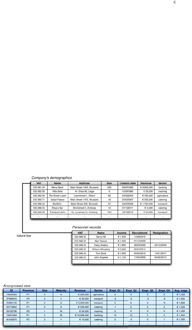
FRAUD ANALYTICS: A BROADER PERSPECTIVE 321
can be anonymized by adding noise to sensitive data attributes. Value
distortion is achieved by returning a value xi+einstead of xi(Agrawal
and Srikant 2000). The value of eis randomly drawn from a predefined
distribution (e.g., uniform, Gaussian …). Another approach is to gen-
eralize a specific value description into a less specific but semantically
consistent description (Fung et al. 2007). The use of address records,
for example, might positively impact the fraud detection models, but
allows to identify a person/company. Therefore, the address is general-
ized into the corresponding city, region, country, etc. (In Van Vlasselaer
et al. 2015) credit card fraud detection models are fed with three
dummy attributes to express the locational information of the trans-
actions on three levels: the transaction is pursued in (1) the issuing
country, (2) the European Union, or (3) the rest of the world (ROW).
Figure 7.2 illustrates the anonymization process for social security
fraud (i.e., tax evasion by companies). The business has two databases
at their disposal. One contains the company’s demographics, the other
reports the company’s personnel records. Both databases are linked to
Figure 7.2 Anonymizing a Database

322 FRAUD ANALYTICS
each other by means of the VAT number. Before they can be used safely
by the data scientists, the databases need to be anonymized. The com-
pany’s demographics are converted as follows: The VAT is converted
into a new identifier (ID), randomly chosen. The name of the com-
pany is excluded from the data scientists’ view. The company size is
categorized in discrete intervals ranging from 1 to 5. The creation date
is converted into three categories: young, adolescent, and mature. The
mapping of both the size and the age is defined by the business, but is
concealed for the data scientists. The value of the company’s revenue
is distorted by rounding the revenue using experts’ domain knowl-
edge. The address is generalized into the province. The sector is directly
included in the view without any changes. The company’s personnel
records are aggregated on company level. It now specifies quarterly
employee turnover, and their average wage. Remark that the rows in
the anonymized table are sorted according to the randomly generated
ID, and do not follow the sequence of the base tables.
SQL Views
SQL views enable users to extract part of the data tables and share the
data authorized by the internal privacy commission. SQL views can be
seen as virtual tables, without physical data (see Figure 7.3). A view
definition consists of a formula that determines which attributes from
the base tables are to be shown on invocation of the view. The view’s
content is generated on this invocation. The SQL view corresponding
to Figure 7.2 is created as follows:
CREATE VIEW FRAUD_INPUT
AS SELECT C.ANON_VAT, C.PROVINCE, C.ANON_SIZE,
C.ANON_REVENUE, C.SECTOR, C.ANON_AGE, AVG(P.WAGE),
COUNT(*)
FROM COMPANIES C, PERSONNEL P
WHERE C.ANON_VAT = P.ANON_VAT
GROUP BY C.ANON_VAT;
Some views can be updated by the user (here: the data scientist).
In that case, the view serves as a “window” through which updates
are propagated to the underlying base table. Updatable views require
that INSERT, UPDATE, and DELETE instructions on the view can be
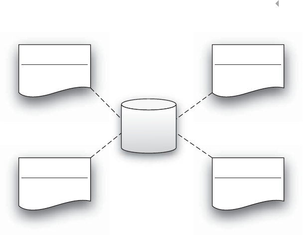
FRAUD ANALYTICS: A BROADER PERSPECTIVE 323
Data scientist A
VIEW
Data scientist B
VIEW
Customer service
VIEW
Database
Inspector VIEW
Figure 7.3 Different SQL Views Defined for a Database
mapped unambiguously to INSERTs, UPDATEs, and DELETEs on a base
table. If this property of an unambiguous mapping does not hold, the
view is read only. If rows are inserted or updated through an updat-
able view, there is the chance that such row does not satisfy the view
definition after the update (i.e., the row cannot be retrieved through
the view). The WITH CHECK option allows users to avoid such “un-
expected” effects: UPDATE and INSERT statements are checked for
conformity with the view definition. Assume, for example, that data
scientists only have access to data from the transport sector. The cor-
responding view WITH CHECK option then becomes
CREATE VIEW FRAUD_INPUT
AS SELECT C.ANON_VAT, C.PROVINCE, C.ANON_SIZE,
C.ANON_REVENUE, C.SECTOR, C.ANON_AGE, AVG(P.WAGE),
COUNT(*)
FROM COMPANIES C, PERSONNEL P
WHERE C.ANON_VAT = P.ANON_VAT AND C.SECTOR =
‘TRANSPORT’
GROUP BY C.ANON_VAT
WITH CHECK OPTION;

324 FRAUD ANALYTICS
If the user changes the sector to, for example, “construction,” the
tuple will disappear from the view without a WITH CHECK option. The
WITH CHECK option prevents this type of behavior.
Label-Based Access Control (LBAC)
LBAC is a control mechanism to protect your data against unautho-
rized access and is able to differentiate between the level of authoriza-
tion that is granted to users. LBAC can be used to grant read and write
access to specific tables, rows, and columns. For example, data items
(e.g., individual rows) that are inserted by users with a higher security
level cannot be seen by users with a lower security level. The use of
LBAC comes in very handy when there are many views on a table,
and when specific users can only access data with the same security
level or lower. LBAC is implemented on databases by many govern-
ments and companies that use hierarchical classification labels such as
CONFIDENTIAL,SECRET,andTOP SECRET, depending on the sensitivity of
the data.2
In order to manage the internal access control of data, LBAC makes
a distinction between security label components, security policies,andsecu-
rity labels. A security label is a collection of security label components.
Each security label component defines a criterion that should be ful-
filled when a user wants to access (a part of) the data. A security label
component, for example, can distinguish between the sensitivity of
individual rows. The following security label component indicates the
hierarchical order between SECRET and CONFIDENTIAL.
CREATE SECURITY LABEL COMPONENT LEVEL
ARRAY [SECRET,CONFIDENTIAL];
Rows inserted by users who are granted the SECRET security label
can only be seen by other users with a SECRET security label. Rows
inserted by users who are granted the CONFIDENTIAL security label can
be seen by all users labeled with a CONFIDENTIAL or SECRET security label.
2http://www.drdobbs.com/understanding-label-based-access-control/199201852.

FRAUD ANALYTICS: A BROADER PERSPECTIVE 325
A security policy is assigned to a table and dictates how the table
is protected. A security policy consists of a set of security label compo-
nents. Each table has exactly one security policy associated with it if
it is LBAC protected. The same security policy can be used to protect
multiple tables. The following security policy sec_policy consists of one
security label component and states that users who have a SECRET role
can access all the data. Users that have a CONFIDENTIAL role can only
access data created by other users with a CONFIDENTIAL role.
CREATE SECURITY POLICY sec_policy
COMPONENTS LEVEL
WITH DB2LBACRULES;
The security policy is included in the create statement.
A security label is assigned to users and depicts which users are
allowed to view or modify protected data. Assume the following state-
ments.
CREATE SECURITY LABEL data_access.ds
COMPONENT LEVEL CONFIDENTIAL;
GRANT SECURITY LABEL data_access.ds TO USER
data_scientist1 FOR ALL ACCESS;
CREATE SECURITY LABEL data_access.bs
COMPONENT LEVEL SECRET;
GRANT SECURITY LABEL data_access.bs TO USER manager1
FOR READ ACCESS;
Given that a table is protected by sec_policy, data scientist 1 has
read and write access to all data labeled as CONFIDENTIAL. The manager
can read (not write) all data with a SECRET or CONFIDENTIAL label.
Accessing External Data
The use and sharing of external data must be approved by a national
(and sometimes international) privacy commission. The privacy com-
mission oversees which data companies can store and how they should
protect it. It makes sure that individuals are able to claim, change, and
retrieve their personal data.

326 FRAUD ANALYTICS
One of the most important EU regulations enforced by the EU pri-
vacy commission is the right to be forgotten. The right to be forgotten
originates from 1995 and specifies that a person can ask to remove
his/her personal data. The 1995 privacy regulation is only applicable
to EU companies. With the rise of e-sales, the 1995 regulation has
become outdated, as EU citizens use more and more non-EU services.
The Court of Justice of the European Union recently issued a new reg-
ulation that extends the privacy regulation to non-EU companies that
offer services to European customers.
Although umbrella EU rules try to unify the privacy regulation
within the European Union, there is still a lack of an international
agreement on privacy. The regulation between countries strongly dif-
fers, making the European (global) privacy regulation extremely frag-
mented. There is a strong need for a unified organism that regulates
cross-border privacy and data protection with a focus on integration
and transparency.
CAPITAL CALCULATION FOR FRAUD LOSS
Fraud may cause an organization to incur significant financial losses,
and as such concern a substantial threat to the very existence of an
organization. In order to plan and cover for these losses, and in fact
more generally for all kinds of risks an organization is exposed to, cap-
ital can be set aside to serve as a buffer and to absorb financial shocks.
Setting aside capital to cover for risks may be a stringent requirement
imposed by legislation. This is the case for financial organizations
such as banks and insurance companies, who are subject to elaborate
regulation (e.g., Basel and Solvency accords), as well as monitoring
and control by national and supranational regulatory institutions, and
requiring them to perform advanced analyses to assess and evaluate
different kinds of risk they are exposed to. The objective of these
regulations is amongst others for financial institutions to calculate and
set aside a sufficient level of capital, primarily to make sure financial
institutions individually, and as such, the entire financial system
that is prone to systemic risk, are protected against financial shocks
and can absorb the unexpected losses (UL) resulting from these shocks.
Determining how much is sufficient is an extremely challenging and

FRAUD ANALYTICS: A BROADER PERSPECTIVE 327
complex task, for which several approaches exist, one of which will
be elaborated in detail in the following paragraphs.
Expected and Unexpected Losses
Whereas expected loss (EL) is the average loss an organization experi-
ences over a certain period of time, unexpected loss refers to the loss
above the expected loss level. Expected loss can be calculated in a
straightforward way, for instance, as the average observed value over a
sufficiently long or suitable historical time window. Clearly, any orga-
nization confronted with regular losses due to its commercial activities
should take these into account as a cost when pricing the services it
delivers or the products it sells, as such covering a priori for these fore-
seen or expected losses.
However, due to random effects, but possibly as well due to
non-random effects which a firm is not aware of or cannot take into
account in calculating expected loss, losses may occur in a confined
time window (e.g., a month or year) that exceed the expected
loss level for that time window. Small, unexpected losses, such as
losses exceeding the expected level only slightly, may occur rather
frequently and can easily be covered for. However, also loss peaks may
occur. It is exactly to cover for these rather exceptional but severe
unexpected losses that a sufficient level of capital has to be calculated.
Because these losses are exceptional, calculating unexpected loss and a
sufficient protection level is challenging and requires a more complex
approach than can be adopted for calculating expected loss.
Risk in a business setting can be simply defined as the chance
or probability of financial loss. Causes of possible losses may differ
in nature and are typically categorized to make a distinction with
respect to the origin of the risk, as well as with respect to the approach
followed to handle the risk. Losses due to fraud are typically catego-
rized as an operational risk, meaning that the risk results from the
daily operations or activities an organization undertakes in creating
products or delivering services.
A first step in dealing with risk is describing the involved uncer-
tainty (i.e., the probability that a loss occurs). This is certainly not
self-evident and is typically done by gathering time series data—that is,

328 FRAUD ANALYTICS
historical observations regarding the occurrence and characteristics of
losses. Such data allow analysts to describe the chance of losses occur-
ring by fitting a probability distribution to the observed data. The shape
or functional form of the probability distribution may be chosen, or
in other words an appropriate theoretical probability distribution may
be selected, based on knowledge regarding the statistical nature of the
uncertain phenomenon that is to be described or captured. The param-
eters of the selected distribution are then estimated to fit as good as
possible the observed data. The analysis of a fraud data time series will
be presented further on in this section to illustrate the process of fitting
a distribution.
Alternatively, one could think of adopting an empirical proba-
bility distribution to describe the involved uncertainty, based on the
observed historical frequency histogram. Such an empirical proba-
bility distribution, however, may significantly be underestimating
the probability of extreme events or values with low probability to
occur, certainly if the loss observations relate to a limited historical
time window. Moreover, when adopting empirical distributions, one
should not bother to separately describe frequency and severity, but,
rather, immediately describe the overall loss distribution.
In order to calculate unexpected loss due to operational risk,
typically the frequency and severity components of the overall
loss distribution are assessed separately, meaning that a separate
probability distribution is fitted to describe the frequency component
and the severity component. The frequency component of the loss
distribution is expressed in number of loss events per time unit and
describes how often losses may occur. The severity of a loss event
refers to the actual financial impact, measured in monetary units.
These two components are considered to be independent, meaning
that the number of loss events occurring during a particular time
window is considered to be not related to the actual severity of these
events. Therefore, separate probability distributions are fitted, which
in a next step are combined to describe the aggregate loss distribution.
The frequency component can be described by a discrete proba-
bility distribution, since the number of events or loss occurrences due
to fraud in a confined time window is a discrete stochastic variable.
Usually a Poisson distribution is adopted for this purpose, which is a

FRAUD ANALYTICS: A BROADER PERSPECTIVE 329
theoretical probability distribution describing the probability of observ-
ing a number of events during the adopted unit of time, given the
average number of events over time. The average number of events
is the only parameter that determines the exact shape of the distribu-
tion. The severity component on the other hand is typically described
by a continuous distribution, since the loss expressed in monetary units
associated with the occurrence of fraud is considered a continuous
stochastic variable.
Aggregate Loss Distribution
In order to calculate a sufficient capital level, we need in fact a prob-
ability distribution describing the probability of incurring a particular
loss during a particular unit of time. This overall or aggregated loss dis-
tribution can be obtained by combining the probability distributions of
the frequency and severity components of losses. This is however not
straightforward to do since these two distributions are very different
in nature. The frequency distribution is discrete whereas the severity
is continuous.
Basically, there are two approaches that can be adopted in com-
bining the two distributions to derive the overall loss distribution: a
closed-form and open-form solution (Navarette 2006).
The closed-form solutions involve solving complex analytical
formulas. The most direct closed form solution to the particular prob-
lem at hand is to combine distributions by means of a mathematical
operation called convolution. However, to elaborate this operation
complicated integrals need to be solved. An alternative approach to
reach a closed-form solution (i.e., an exact formula describing the
aggregated loss distribution) makes use of Fourier transformations,
which allows to manipulate the frequency and severity distribu-
tions that we aim to combine more efficiently. The inverse Fourier
transformation finally allows users to reach the closed form of the
aggregate loss distribution after combining the distributions in the
frequency domain. These closed-form solutions require statistical and
mathematical expertise that is not always readily available.
An alternative, open-form solution, may be derived to obtain the
aggregate loss distribution by making use of Monte Carlo simulation,

330 FRAUD ANALYTICS
which is an approach that is, depending on one’s knowledge and skills,
more accessible and easier to implement than the closed form solutions
as discussed. Monte Carlo simulation boils down to making use of brute
computational force to simulate a system and observe how it behaves
for a large number of randomly chosen values (according to the deter-
mined probability distributions) of the inputs, in order to observe the
probability of a certain output. The inputs in our case are the frequency
and the severity, whereas the output is the total loss resulting from the
number of fraud events that occur in a time unit and the associated
losses for each of these events.
Monte Carlo simulation generates a large amount of artificial loss
observations. The probability distributions of the frequency and sever-
ity component can be used to generate random observations of loss,
with a probability in line with these distributions. When a sufficient
amount of observations are generated, straightforward derivation of
the empirical distribution from these observations results in the aggre-
gate loss distribution. Sufficient in this setting means that the resulting
aggregate loss distribution remains stable with respect to the number
of observations used to generate the distribution.
Once the aggregate loss distribution is obtained, a value for the
unexpected loss can be determined as a function of the confidence
level that is selected. The confidence level determines the level of
protection by fixing the largest loss peak that can be covered for by
the capital, and as such expresses the probability of observing an even
higher loss peak for which capital will not be sufficient. The value of
the total loss associated with the selected confidence level is called the
operational value at risk (VaR). As shown in Figure 7.4, the difference
between the VaR at the selected confidence level (99.9 percent in the
figure) and the expected loss equals the unexpected loss.
Deciding on an appropriate confidence level and as such on the
capital level is not self-evident. Intuitively, this confidence level cor-
responds to the probability that an organization will not go bankrupt
because of extreme losses. From that perspective, a confidence level
equal to or very close to 100 percent is preferred. However, since a
confidence level of (very close to) 100 percent may be associated with
a very high VaR and, consequently, a very high unexpected loss, set-
ting aside the required capital to cover for such significant loss may be
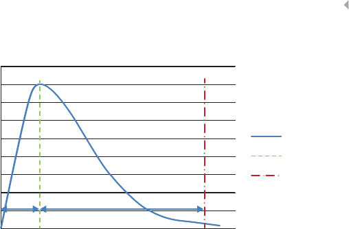
FRAUD ANALYTICS: A BROADER PERSPECTIVE 331
Aggregate loss distribution
Probability density
Loss distribution
Mean Loss
VAR (P99.9%)
Aggregate loss
EL UL
Figure 7.4 Aggregate Loss Distribution with Indication of Expected Loss, Value at Risk
(VaR) at 99.9 Percent Confidence Level and Unexpected Loss
impossible or not desirable. Risk is inherent to any economic undertak-
ing. Excluding and covering for all types of risk is not the goal of setting
aside capital to cover for shocks. Therefore, setting the confidence level
below 100 percent is definitely acceptable. The only question remain-
ing, then, is at what exact level. But this is a question to which no gen-
eral answer can be given, since it’s dependent on many factors, many
of which are specific to the organization, sector or industry, country,
management, and so on. Usually, though, confidence levels in risk
management lie in the range from 95 to 99 percent and higher.
Capital Calculation for Fraud Loss Using
Monte Carlo Simulation
This section provides a practical illustration of capital calculation
using Monte Carlo simulation as explained in the above sections.
The example is based on a case study presented in Navarette (2006).
Figure 7.5 provides a snapshot of a time series data set with two
variables describing historical credit card fraud cases over a time
horizon of one year—that is, the date of the fraud event and the
involved fraud amount (€).
The date information allows analysts to fit a Poisson distribution to
the frequency data. In order to do so the only parameter to be estimated

332
600 or less
700
800
900
1000
1100
1200
1300
1400
1500
1600
1700
1800
1900
2000
More
Fraud amount (€)
€
€
€
€
€
€
€
€
€
€
2/01/2014 963,82
618,02
549,45
1.732,30
1.929,02
748,33
672,70
858,13
529,57
2.104,16
2/01/2014
3/01/2014
4/01/2014
8/01/2014
29/12/2014
... ...
29/12/2014
30/12/2014
30/12/2014
30/12/2014
Fraud amountDate
0
20
40
60
80
100
120
140
160
Fraequency
Figure 7.5 Snapshot of a Credit Card Fraud Time Series Data Set and Associated Histogram of the Fraud Amounts

FRAUD ANALYTICS: A BROADER PERSPECTIVE 333
or calculated is the average event rate 𝜆, that is, the average num-
ber of fraud cases per month, which is equal to 41.67. In the Monte
Carlo simulation, we will hence use a Poisson distribution with Pois-
son parameter equal to 41.67 to generate random yet realistic monthly
event rates (i.e., the monthly number of fraud cases). Note that we
adopted one month to be the base unit of time in our analysis. Hence,
the aggregated loss distribution resulting from the Monte Carlo sim-
ulation will give us the distribution of potential monthly losses with
associated probability density.
A second, continuous distribution needs to be estimated from the
available data to describe the severity of the losses that occur. Sev-
eral theoretical distributions such as the lognormal, exponential, and
so on may be fitted. In this case, a Pareto distribution fits best (ranked
according to the Chi-squared test statistic) to the observed historical
loss distribution displayed in Figure 7.5. The estimated parameters for
the Pareto severity distribution are a=500 and b=2.75.
The estimated Poisson frequency distribution and Pareto severity
distribution allow analysts to generate a large number (in this case,
10,000 observations were generated) of simulated monthly observations
with a randomly generated event rate and losses associated with the
individual fraud events following the estimated distributions. As such,
we get an extensive time series data set with artificial, pseudo-realistic
observations of total monthly fraud losses. The frequency histogram of
these monthly losses allows analysts to derive the aggregate loss distri-
bution, as shown in Figure 7.6.
Figure 7.6 indicates both the expected loss—that is, the average
monthly loss due to fraud (EL =32,730€)—as well as the 99 percent
value-at-risk figure—that is, the fraud loss for a confidence level equal
to 99 percent (99 percent VaR =49,449€). The difference between
the 99 percent VaR and the EL is the unexpected loss (UL), which
should be covered by capital that is to be set aside (UL =16,718€).
If we would raise the confidence level to 99.9 percent, the associate
VaR figure rises to a value 99.9 percent VaR =57,542€, and the UL
increases to 24,812€.
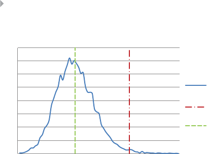
334 FRAUD ANALYTICS
Aggregate loss distribution
0.00
0.10
0.20
0.30
0.40
0.50
0.60
0.70
0.80
15 25 35 45 55 65
Values in 10–4
Values in thousands (€/month)
Aggregate loss
distribution
99% Value at Ris
k
Expected loss
Figure 7.6 Aggregate Loss Distribution Resulting from a Monte Carlo Simulation
with Poisson Distributed Monthly Fraud Frequency and Associated Pareto Distributed
Fraud Loss
AN ECONOMIC PERSPECTIVE ON FRAUD ANALYTICS
In this section, we will zoom into the economic aspects of an analytical
fraud model. We will first discuss the total cost of ownership and then
elaborate on the return on investment.
TotalCostofOwnership
The total cost of ownership (TCO) of a fraud analytical model refers
to the cost of owning and operating the analytical model over its
expected lifetime, from inception to retirement. It should consider
both quantitative and qualitative costs and is a key input to make
strategic decisions about how to optimally invest in fraud analytics.
The costs involved can be decomposed into: acquisition costs, owner-
ship and operation costs, and post ownership costs, as illustrated with
some examples in Table 7.1.
The goal of TCO analysis is to get a comprehensive view of
all costs involved. From an economic perspective, this should also
include the timing of the costs through proper discounting using, for
example, the weighted average cost of capital (WACC) as the discount
factor. Furthermore, it should help identifying any potential hidden
and/or sunk costs. In many fraud analytical projects, the combined

FRAUD ANALYTICS: A BROADER PERSPECTIVE 335
Table 7.1 Example Costs for Calculating Total Cost of Ownership (TCO)
Acquisition Costs Ownership and Operation Post Ownership
Costs Costs
◾Software costs, including
initial purchase, upgrade,
intellectual property, and
licensing fees
◾Hardware costs including
initial purchase price and
maintenance
◾Network and security costs
◾Data costs including costs
for purchasing external data
◾Model developer costs such
as salaries and training
◾Model migration and change
management costs
◾Model setup costs
◾Model execution costs
◾Model monitoring costs
◾Support costs
(troubleshooting, helpdesk,
etc.)
◾Insurance costs
◾Model staffing costs such as
salaries and training
◾Model upgrade costs
◾Model downtime costs
◾Deinstallation and
disposal costs
◾Replacement costs
cost of hardware and software is subordinate to the people cost that
comes with the development and usage of the analytical models
(e.g., training, employment, and management costs). Furthermore,
TCO analysis allows pinpointing cost problems before they become
material. For example, the change management costs to migrate from
a legacy fraud model to a new analytical fraud model are often largely
underestimated. TCO analysis is a key input for strategic decisions such
as vendor selection, buy versus lease decisions, in- versus outsourcing,
overall budgeting, and capital calculation. Note that when making
these investment decisions, it is also very important to include the
benefits in the analysis since TCO only considers the cost perspective.
Return on Investment
Return on investment (ROI) is defined as the ratio of a return (benefit
or net profit) over the investment of resources that generated this
return. Both the return and the investment are typically expressed
in monetary units, whereas the ROI is calculated as a percentage. In
this section, we discuss how to calculate the ROI of fraud detection,

336 FRAUD ANALYTICS
which may be less straightforward to calculate than the ROI of a
financial product, but nonetheless, can provide useful insights to an
organization.
The returns of a fraud detection system have been discussed before
in Chapter 6 in the section on selecting the sample to investigate.
The optimal amount of resources to allocate to fraud investigation
and as such the sample to investigate was defined as the amount of
resources that maximized the total utility associated with inspecting
a sample. This sample was selected either as a top-fraction of most
suspicious cases with the highest scores assigned by the detection
model, or as a top-fraction of the cases with the highest expected fraud
amount (defined as the probability to be fraudulent times the estimated
fraud amount).
The utility of different outcomes is expressed as a net monetary
value, either positive or negative, representing the costs and benefits
to an organization (of any nature, both economic and noneconomic,
yet always expressed in monetary units) associated with the decision
to inspect or not to inspect either a fraudulent or nonfraudulent case.
The investment required to generate the total returns or total util-
ity can be assumed equal to the total cost of ownership as discussed
in the previous section. The total cost of ownership includes costs of
diverse nature, covering the full investment required to build, operate,
and maintain a fraud-detection system. However, the total cost of own-
ership does not include costs related to resources that are required to
further act on the outputs of the detection system (i.e., inspecting and
handling suspicious cases). All these costs together will be denoted as
the Total Cost of Fraud Handling, and include inspection costs, legal costs,
and so on. Clearly, calculating the total cost of fraud handling may be
a cumbersome task, yet indispensable to calculate the ROI.
Hence, we get to the final ROI formula:
Return on investment =Total utility
Totalcostofownership+Total cost of fraud handling

FRAUD ANALYTICS: A BROADER PERSPECTIVE 337
IN VERSUS OUTSOURCING
The growing interest and need for big data and analytics, combined
with the shortage of skilled talent and data scientists in Western Europe
and the United States, has triggered the question regarding outsourc-
ing analytical activities. This need is further amplified by competitive
pressure on reduced time to market and lower costs. Companies need
to choose between insourcing or building the analytical skillset inter-
nally, either at the corporate or business line level, outsourcing all
analytical activities, or going for an intermediate solution whereby only
part of the analytical activities are outsourced. The dominant play-
ers in the outsourcing analytics market are India, China, and Eastern
Europe, with some other countries (e.g., Philippines, Russia, South
Africa) gaining ground as well.
Various analytical activities can be considered for outsourcing,
ranging from the heavy lifting grunt work (e.g., data collection,
cleaning, and preprocessing), set-up of analytical platforms (hardware
and software), training and education, to the more complex analytical
model construction, visualization, evaluation, monitoring, and main-
tenance. Companies may choose to grow conservatively and start by
outsourcing the analytical activities step by step, or immediately go
for the full package of analytical services. It speaks for itself that the
latter strategy has more risk associated with it and should thus be
more carefully and critically evaluated.
Despite the benefits of outsourcing analytics, it should be
approached with a clear strategic vision and critical reflection with
awareness of all risks involved. First of all, the difference between
outsourcing analytics and traditional ICT services is that analytics
concerns a company’s front-end strategy, whereas many ICT services
are part of a company’s back-end operations. Another important risk
is the exchange of confidential information. Intellectual property
(IP) rights and data security issues should be clearly investigated,
addressed and agreed on. Moreover, all companies have access to
the same analytical techniques, so they are only differentiated by
the data they provide. Hence, an outsourcer should provide clear
guidelines and guarantees about how intellectual property and data
will be managed and protected (using, e.g., encryption techniques

338 FRAUD ANALYTICS
and firewalls), especially if the outsourcer collaborates with various
companies operating in the same industry sector. Another important
risk concerns the continuity of the partnership. Offshore outsourcing
companies are often subject to mergers and acquisitions, not seldom
with other outsourcing companies collaborating with the competition,
hereby diluting any competitive advantage realized. Furthermore,
many of these outsourcers face high employee turnover due to inten-
sive work schedules, the boredom of performing low-level activities
on a daily basis, and aggressive headhunters chasing these hard to
find data science profiles. This attrition problem seriously inhibits a
long-term thorough understanding of a customer’s analytical business
processes and needs. Another often-cited complexity concerns the
cultural mismatch (e.g., time management, different languages, local
versus global issues) between the buyer and outsourcer. Exit strate-
gies should also be clearly agreed on. Many analytical outsourcing
contracts have a maturity of three to four years. When these contracts
expire, it should be clearly agreed on how the analytical models and
knowledge can be transferred to the buyer thereof to ensure business
continuity. Finally, the shortage of data scientists in the United States
and Western Europe will also apply, and might even be worse, in the
countries providing outsourcing services. These countries typically
have universities with good statistical education and training pro-
grams, but their graduates lack the necessary business skills, insights,
and experience to make a strategic contribution with analytics.
Given the above considerations, many firms currently adopt a
partial outsourcing strategy, whereby baseline, operational analytical
activities such as query and reporting, multidimensional data anal-
ysis, and OLAP are outsourced, whereas the advanced descriptive,
predictive, and social network analytical skills are developed and
managed in house.
MODELING EXTENSIONS
Forecasting
Chapter 4 introduced predictive learning techniques which allow esti-
mating a target variable. Two types of predictive analytics have been

FRAUD ANALYTICS: A BROADER PERSPECTIVE 339
distinguished—that is, regression and classification, depending on the
type of target variable. In case of regression a continuous target vari-
able is estimated (either over a limited or unlimited interval), whereas
in case of classification the target is categorical. A third type of pre-
dictive analytics, which is not covered in this book, is forecasting or
time series regression, which concerns the prediction of a continuous
target variable as a function of time. The value of the target variable
in a forecasting problem moves or changes over time, as such adding a
dimension to the prediction problem. Plenty of techniques are available
to provide time-dependent estimates, which are different in nature
compared to the techniques discussed and also come with different
challenges. For further information on time series modeling, one may
refer to seminal books and articles dedicated to the subject of fore-
casting (Armstrong 2001; Petropoulos, Makridakis, Assimakopoulos,
& Nikolopoulos 2014). Although less common and straightforward, in
a fraud-detection setting forecasting may be used for particular appli-
cations or purposes, either directly or indirectly related to fraud.
A first example of a possible use of forecasting techniques in a
fraud-detection setting concerns the detection of deviations between
forecasted (i.e., expected) values and observed values. Such deviations
may be indicative of fraud. For instance, one particular type of fraud
concerns avoidance of import taxes by shipping goods from the coun-
try of origin to the country of destination via a third country. The goods
are relabeled in the third country, as if they were produced and expe-
dited from that country to the destination country in order to avoid or
reduce the import taxes that are to be paid in the destination country,
and that are lower for goods originating from the third country than if
originating from the true origin country. By forecasting the expected
amount of import—typically per specific product category—a deviation
will be observed between the expected and observed amount of import
both from the true and the false origin countries, respectively, a neg-
ative deviation or lower amount of import than expected for the true
origin country, and a positive deviation or higher amount of import
than expected for the false origin country.
A second example use of forecasting methods in fraud concerns
the estimation of the evolution of fraud losses as a function of time.
Losses due to fraud, as discussed previously, may vary over time due to

340 FRAUD ANALYTICS
random effects, but as well due to structural effects, meaning that other
factors might partially explain the evolution or variation of observed
fraud losses in time. For instance, the economic cycle might have a
substantial impact, since it could be expected to observe more fraud
during economic downturn times than during economic upturn times.
Seasonal effects may be observed for particular types of fraud—for
example, losses due to credit card fraud might be higher in the month
of December since overall credit card spending is higher due to the
holiday season and the associated shopping pattern. Also, the over-
all amount of insurance claims, and as such the amount of fraudulent
claims may depend on the season or the weather, causing the total
fraud loss to be seasonally dependent. These seasonal effects can be
easily modeled using forecasting techniques.
Text Analytics
An additional and potentially very rich source of information that
might be explored when building a fraud detection system concerns
textual data. Text, such as reports, emails, text messages, tweets, docu-
ments on the Internet, blogs, reviews, financial statements, and so on,
is an unstructured source of data. Unstructured data are not organized
or fitted nicely into a table consisting of rows and columns, which
can be explored by applying the techniques discussed in Chapters 3
and 4. Therefore, text is less evident to include in an analysis and
to exploit in order to detect or predict fraud, although it potentially
contains valuable information that may be of good use. Challenges
encountered when analyzing text are plenty, and include the difficulty
to recognize and interpret irony, synonyms, homonyms, and so on.
Other sources or types of unstructured data include images such
as pictures, photographs and video, audio data, and (social) network
data. Indeed, also network information can be considered to be unstruc-
tured in nature since the very essence of a network cannot be captured
easily in a structured data table. As discussed in Chapter 5, with some
effort and expertise networks may be turned into structured data tables,
subsequently allowing analysis using the techniques discussed in this
book. Chapter 5 also discussed techniques that have been specifically
designed to deal with the particular nature and format of network data.

FRAUD ANALYTICS: A BROADER PERSPECTIVE 341
The same two approaches exist to handle textual data. The goal
of both approaches is to identify patterns and associations between
words and phrases. Specific techniques have been developed that allow
deriving insights and patterns directly from text. Usually, however,
these techniques are adopted to turn textual data into structured data,
subsequently allowing application of techniques designed to analyze
structured data. As such, text-mining insights are added to structured
analysis in order to improve decision making.
Text can be mapped into numeric representations that summarize
document collections and become inputs to a full range of predictive
and data mining modeling techniques. For instance, text data may
first be transformed into a set of numerical components called singular
value decomposition (SVD) components, which collectively represent
the text documents. These components are then used as additional
inputs along with the structured input attributes to help improving
the predictive power of the existing models.
An example application of text analytics in a fraud-detection
setting concerns the analysis of car accident reports and claim notes
in order to detect insurance claim fraud (e.g., staged collisions, see
Chapter 1). In fact, unstructured data can represent up to 80 per-
cent of claims data. This information can be used to help reduce
investigation costs and optimize recovery operations. In fact, some
firms reported the existence of a U-shaped relation between emotion
and level of detail in the report, as measured by counting particular
adjectives, either expressing strong feelings or describing in a very
detailed manner the accident and the probability for the claim to be
fraudulent. Both the absence and abundance of emotion and level of
detail in the report appeared to be indicative for fraud. This may not
be very surprising, since one can imagine that indeed it might prove
hard not to include emotion and detail, but notice, that fraudsters
must also mimic exactly the right amount of emotion and level of detail
when falsifying a statement or report.
From this example, it might be clear that it is exactly the ambigu-
ity and complexity that is present in textual data, and that makes text
so hard to analyze using automated approaches. These factors make
it such an interesting and rich source of information to explore. Since
analyzing text is a rather challenging exercise, requiring advanced and

342 FRAUD ANALYTICS
dedicated techniques and approaches, good software support is indis-
pensable. Given the specificity of the topic, text analytics will not be
covered further in this book. The reader may refer to the literature on
text mining for more information (Chakraborty et al. 2013).
THE INTERNET OF THINGS
The Internet of Things (IoT) refers to the network of interconnected
things such as electronics devices, sensors, software, IT infrastructure
that creates and adds value by exchanging data with various stakehold-
ers such as manufacturers, service providers, customers, other devices,
and so on, hereby using the World Wide Web technology stack (e.g.,
Wi-Fi, IPv6). In terms of devices, you can think about heartbeat mon-
itors; motion, noise, or temperature sensors; smart meters measuring
utility (e.g., electricity, water) consumption, and so on. Some examples
of applications follow:
◾Smart parking: automatically monitoring free parking spaces in
acity
◾Smart lighting: automatically adjusting street lights to weather
conditions
◾Smart traffic: optimize driving and walking routes based on traf-
fic and congestion
◾Smart grid: automatically monitoring energy consumption
◾Smart supply chains: automatically monitoring goods as they
move through the supply chain
It speaks for itself that the amount of data generated is enormous
and offers an unseen potential for analytical applications. As with all
new technologies, the Internet of Things creates both new treats as well
as emerging opportunities from a fraud perspective.
Some examples of new fraud treats are:
◾Fraudsters might force access to web configurable devices (e.g.,
automated teller machines (ATMs)) and set up fraudulent trans-
actions.

FRAUD ANALYTICS: A BROADER PERSPECTIVE 343
◾Device hacking whereby fraudsters change operational param-
eters of connected devices (e.g., smart meters are manipulated
to make them under register actual usage).
◾Denial of service (DoS) attacks whereby fraudsters massively
attack a connected device to stop it from functioning.
◾Data breach whereby a user’s log-in information is obtained in
a malicious way, resulting in identity theft.
◾Gadget fraud also referred to as gadget lust whereby fraudsters
file fraudulent claims to either obtain a new gadget or free
upgrade.
◾Cyber espionage is where data are eavesdropped by an intelli-
gence agency or used by a company for commercial purposes.
More than ever before, fraud will be dynamic and continuously
changing in an IoT context. From an analytical perspective this implies
that supervised techniques will continuously lag behind since they are
based on a historical data set with known fraud patterns. Hence, as
soon as the supervised model (e.g., classification or regression model)
has been estimated, it will become outdated even before it has been put
into production. Unsupervised methods such as anomaly detection,
peer group and break-point analysis will gain in importance. These
methods should be capable of analyzing evolving data streams and per-
form incremental learning to deal with concept drift. To facilitate (near)
real-time fraud detection, the data and algorithms should be processed
in-memory instead of relying on slow secondary storage. Furthermore,
based on the results of these analytical models, it should be possible to
take fully automated actions such as the shutdown of a smart meter
or ATM.
Besides threats, the IoT will also bring new opportunities for
improved fraud detection. Telematics is one example of an IoT appli-
cation in an insurance setting. The idea here is to equip a car with
a special device called black box, which continuously monitors the
driving behavior by gathering data and streaming it to the insurance
provider. Examples of telematics data that are collected in each trip
are: the distance driven, the time of day, duration of the trip, the
location, the speed, harsh or smooth breaking, aggressive acceleration
or deceleration, and cornering and parking skills. This can then further

344 FRAUD ANALYTICS
be augmented with road maps and weather and traffic information. By
carefully analyzing all these data elements, the insurance provider can
provide better risk assessment and work out personalized premiums
based on individual driving data by reducing the cost for low-mileage
clients and good drivers. It also enables hotspot analysis based on
vehicle and accident location. However, telematics data can also be
usefully adopted to improve fraud detection. When an insurance claim
is filed, the facts provided can now be more carefully checked. For
example, was the driver respecting the speed limit? Did the accident
occur at the claimed location? Did the driver brake in a timely man-
ner? Was the driving behavior different compared to recent driving
behavior, possibly suggesting a different driver or alcohol intoxication?
Furthermore, using telematics data, it becomes possible to re-enact
car accidents. This is not only handy to define who is at fault, but also
to identify fake accidents resulting into fraudulent claims.
CORPORATE FRAUD GOVERNANCE
Since fraud is a key treat to a firm’s revenues and consequently its
existence, it is important that senior management and the board of
directors are actively involved in detecting, preventing, and managing
fraud. In other words, they should demonstrate active involvement
on an ongoing basis, assign clear responsibilities, and put into place
organizational structures, procedures, and policies that will allow the
proper and sound management of fraud. Example questions that need
to be addressed are as follows:
◾Do we adopt a reactive, proactive, or combined strategy toward
fraud detection and prevention?
◾What are the internal anti-fraud controls that allow us to miti-
gate fraud?
◾Do we invest in continuous education and fraud awareness
training?
◾Do we provide adequate whistle blowing or hotline facilities,
and how are they managed?
◾Do we periodically conduct fraud vulnerability reviews?

FRAUD ANALYTICS: A BROADER PERSPECTIVE 345
◾Do we adopt a closed-loop fraud-management strategy?
◾How do we manage fraud from a regulatory compliance view-
point?
To address all these questions, it is highly recommended that an
anti-fraud steering group be set up, comprising employees from various
business units and hierarchical levels in order to get a comprehen-
sive, corporatewide view on fraud. The board of directors should then
appoint one executive-level member to oversee the activities of this
group, and regularly brief management regarding its activities.
It should be clear by now that analytics plays a pivotal role
in managing fraud. Assuming a firm wants to build the analytical
expertise in-house rather than outsourcing, a key question is how the
analytical teams should be embedded in the organization structure. A
first option would be to centralize all analytical teams and resources
into a firm-wide analytical service center of excellence. The idea
here is to create cross-fertilization opportunities across the firm
and efficiently leverage the various resources available. However,
given the close interaction that is needed between the data scientists
and the business, this centralized structure may be suboptimal. A
better alternative could be to organize analytics using the principle
of subsidiarity. This principle states that the company should have
a subsidiary function performing only those analytical tasks, which
cannot be performed by the local business units. More specifically,
each business unit where fraud is an issue can be complemented
with small teams of data scientists (e.g., 2 to 5). This will facilitate
the constant interaction needed to quickly and adequately respond
to new fraud challenges. Companywide, transversal standards can
then be developed to deal with issues such as software, privacy,
model management, and documentation. For example, from a model
management perspective, it may be enforced that every fraud model
should be managed by a model board, which takes full responsibility
for a model’s development, usage, and monitoring.
Given that analytics continues to permeate every aspect of a firm’s
business, it is highly recommended that it be elevated to a corporate
level and that executive leadership be assigned to it. Some companies

346 FRAUD ANALYTICS
already added a chief analytics officer (CAO) to their C-suite. This per-
son is responsible for overseeing all analytical model development and
monitoring efforts across the entire enterprise.
REFERENCES
Agrawal, Rakesh, and Ramakrishnan Srikant (2000). “Privacy-Preserving Data
Mining.” ACM SIGMOD Record 29 (2).
Armstrong, J. S. (2001). Selecting Forecasting Methods. In J.S. Armstrong
(ed.) Principles of Forecasting: A Handbook for Researchers and Practitioners.
New York: Springer Science +Business Media, pp. 365–386.
Chakraborty, G., Murali, P., & Satish, G. (2013). Text Mining and Analysis: Prac-
tical Methods, Examples, and Case Studies Using SAS. Cary, NC: SAS Institute.
Drugescu, Cezar, and Rafael, Etges (2006). “Maximizing the Return on Invest-
ment on Information Security Programs: Program Governance and Met-
rics.” Information Systems Security 15 (6): 30–40.
Maydanchik, A. (2007). Data Quality Assessment. Bradley Beach, NC: Technics
Publications.
Navarette, E. (2006). Practical Calculation of Expected and Unexpected Losses
in Operational Risk by Simulation Methods (Banca & Finanzas: Documen-
tos de Trabajo, 1(1), pp. 1–12).
Petropoulos, F., Makridakis, S., Assimakopoulos, V., & Nikolopoulos, K. (2014).
“Horses for courses” in demand forecasting. European Journal of Operational
Research 237 (1): 152–163.
Van Vlasselaer, V., Eliassi-Rad, T., Akoglu, L., Snoeck, M., & Baesens, B. (2015).
Gotcha! Network-based Fraud Detection for Social Security Fraud. Man-
agement Science, Submitted.

About the Authors
Professor Bart Baesens is a professor at KU Leuven (Belgium) and a
lecturer at the University of Southampton (United Kingdom). He has
done extensive research on big data and analytics, fraud detection,
customer relationship management, web analytics, and credit risk
management. His findings have been published in well-known inter-
national journals (e.g., Machine Learning, Management Science, IEEE
Transactions on Neural Networks, IEEE Transactions on Knowledge and
Data Engineering, IEEE Transactions on Evolutionary Computation, Journal
of Machine Learning Research) and presented at international top con-
ferences. He is also author of the books Credit Risk Management: Basic
Concepts (http://goo.gl/T6FNOn), published by Oxford University Press
in 2008; Analytics in a Big Data World (http://goo.gl/k3kBrB), published
by John Wiley & Sons in 2014, and Beginning Java Programming:
The Object-Oriented Approach (http://goo.gl/qHXmk1), published by
John Wiley & Sons in 2015. His research is summarized at www
.dataminingapps.com. He also regularly tutors, advises, and provides
consulting support to international firms with respect to their big
data and analytics strategy.
Véronique Van Vlasselaer graduated magna cum laude as master
information systems engineer at the faculty of business and economics,
KU Leuven (Belgium). For her master’s thesis topic, “Mining Data on
Twitter,” she received the best thesis award from the faculty’s student
branch. In 2012, Véronique started as a PhD candidate with Profes-
sor Baesens at the faculty of business and economics of KU Leuven,
department of decision sciences and information management. During
her PhD, she developed advanced network-based fraud detection
approaches for the Belgian government and the financial sector. Her
main research topics include social network analytics, fraud detection,
and net lift modeling.
Wouter Verbeke, PhD is an assistant professor of business informat-
ics and business analytics at VU Brussel (Belgium). Previously, he was
347

348 ABOUT THE AUTHORS
a lecturer at the University of Edinburgh Business School and a risk
business analyst at Dexia Bank. He graduated in 2007 as a civil engi-
neer and obtained a PhD in applied economics at KU Leuven (Belgium)
in 2012. His research is situated in the field of predictive analytics
and complex network analysis, and is driven by real-life business
problems including applications in marketing, credit risk, supply-chain
management, mobility, and human resource management. Wouter
teaches several courses on information systems and advanced mod-
eling for decision making to business students, and tutors courses
on fraud analytics, credit-risk modeling, and customer analytics to
business professionals. His work has been published in established
international scientific journals such as IEEE Transactions on Knowledge
and Data Engineering, IEEE Transactions on Software Engineering, European
Journal of Operational Research, International Journal of Forecasting, and
Expert Systems with Applications.

Index
A
Absolute deviation, 187
Account data, 40
Account management database,
information storage, 40
Accuracy ratio (AR), 179
AUC, linear relation, 181
calculation, example, 181f
Acquisition costs, 334t
Activation functions, 146
Actual fraud, predicted fraud
(contrast), 185f
Adaptive boosting (Adaboost)
procedure, 165–166
Adjacency list, 221f, 222
Adjacency matrix, 221, 242, 250
mathematical representation,
221f
Administrative activities (fire incident
claims), 12
Administrators, experts (collusion), 14
Affiliation networks, 267
Age
default risk, contrast, 60f
regression model, 63–64
split, entropy (calculation), 139f
Agglomerative hierarchical clustering
divisive hierarchical clustering,
contrast, 94f
methods, usage, 95–96
Aggregate loss distribution, 329–331
description, 328–329
indicators, 331f
Monte Carlo simulation, 333
Alert Type, 292
Analysis of variance (ANOVA)
test, 143
Analytical fraud models
backtesting, 302–311
calibration, backtesting, 308
design/documentation, 311–312
life cycle, 280–281
performance metric, monitoring,
306t
stability, backtesting, 305–307
Analytical model life cycle, 280f
Analytics, strategic contribution,
337–338
Anomaly detection, 343
Anticipating effect, 274
Anti-fraud steering group, 345
Anti-money laundering setting, cash
transfers (clustering), 90
Approval activities (fire incident
claims), 12
Approval cycle, absence, 14
AR. See Accuracy ratio
Area under the ROC curve (AUC), 192.
See also Multiclass area under the
ROC curve
calculation (performance metric),
178
Assignment decision. See Decision trees
Association rule analysis, 88–89
Association rules
consideration, 89
examples, 88
Attrition, problem, 338
AUC. See Area under the ROC curve
Autoregressive integrated moving
average (ARIMA), 127
Average claim value, distribution, 297f
Average path length, 212
network, 240, 242
B
Backward looking time horizon, 190
Backward variable selection, 152f
procedure, usage, 151
Bagging, 164–165
Bankruptcy
contrast, 124f
filing, 271
Base class, 168–169
Bayesian methods, 148
349

350 INDEX
Behavioral characteristics, example,
41–42
Behavioral information, 41–42
Benford’s law, 48–51
deviation, 50–51
example, 50f
Best matching unit (BMU)
location, 110
weight vector, 109
Between-community edges,
259–260
quantification, 260
weight, sum, 260
Betweenness, 227, 239t, 244–246
centrality, 246t
illustration, 245f
recalculation, 262
Binary classification, 198–199
Binary fraud target (modeling),
linear regression (usage),
127
Binary link
statistics, 253
usage, 268–269
Binary logistic regression, 169
Binary red-flag indicators, 93
Binary weight, 216
Binomial distribution, usage, 196
Binomial test, usage, 309–310
Bipartite graph, 267
connectivity matrix, 268f
example, 267f
node types, 268–269
usage, 276–277
Bipartite networks, 267, 273
Bipartite representation,
266–269
Birds, clustering (example), 96f
dendrogram, 96f
BMU. See Best matching unit
Boosting, 165–166. See also Adaptive
boosting
Bootstrapping, 175, 175f
procedure
adoption, 307
usage, 307
Bootstraps, 164–165
Bottom-up approaches, 263–264
Bottom-up clustering, 263–264
Bounding function. See Logistic
regression
Break-point analysis, 343
intra-account fraud detection
method, 84
example, 85f
Brier score (BS), measurement, 182
Browser-based digital dashboard,
usage, 291–292
Business policy, 15
customer relationship management,
example, 14
Business rules, set (usage), 290–291
C
C4.5 (decision tree), 137
CAIRO matrix, 319
Call detail records, example, 20t
Cannot-link constraints. See
Semi-supervised clustering
CAP. See Cumulative accuracy profile
Capital, sufficient level, 326–327
CART (decision tree), 137
Cascade correlation, 148
Case management, 290–295
environment, 292
Categorical data, 47
Categorization, 60–63
Chi-squared analysis, usage, 61
Centrality. See Closeness
metrics, 227, 238–246
components, 239t
CHAID (decision tree), 137
Chief analytics officer (CAO), addition,
346
Chi-squared analysis, usage, 61
Chi-squared distance, calculation, 63
Chi-squared distribution, 134
test statistic, relationship, 310
Chi-squared test statistic, 333
Claim
amounts, distribution, 297f
geographical distribution, 298f
enlargement, 299f
score, 292
value, distribution. See Average claim
value.
ClaimID, 292
Classification, 122. See also Binary
classification
accuracy, 176, 189
data set, example, 127t
error, 176

INDEX 351
measures, dependence, 177
model, 342
calibration, monitoring, 308t
SVMs, procedure, 162
techniques. See Multiclass
classification techniques.
Classifier. See Probabilistic relational
neighbor
cost sensitivity, 199
relational neighbor classifier,
233–234
Click fraud, 6t
Closed-form solutions, 329
Closed-loop fraud-management
strategy, adoption, 345
Closeness, 227, 239t, 243–244
centrality, 243–244
summary, 245t
Cluster centroids
random selection, 105f
recalculation, 107f, 108f
stability, 104
ClusterID, 116
Clustering, 90–116. See also Spectral
clustering
claims, 90
constraints, usage, 111–114
countries, SOMs (usage), 111f
dendrogram, 262f
distance metrics, 91–94
example. See Birds.
interpretation, decision trees
(usage), 116f
screen plot, 97f
semi-supervised clustering,
must-link/cannot-link constraints,
113f
solutions, evaluation/interpretation,
114–116
steps, indication, 96f
techniques, contrast, 92f, 95f
transactions, 90
Cluster profiling, histograms (usage),
115f
Clusters
analysis, usage. See Fraud detection.
distances, calculation, 95f
CNA. See Complex network analysis
Coefficient of determination (R2),
performance metric, 186
Collective inference algorithms,
227–228, 238, 246–254
Column-normalized adjacency matrix,
248–249
Common Neighbor approach, 217
Communities. See Complete
communities; Partial communities
connection, 244, 246
detection. See Credit card fraud.
fraudulent influence, 265
mining, 254–265
split (evaluation), modularity Q
(usage), 262–263
Company overview, detection model
basis (example), 276t
Complete communities, 264
example, 264f
Complex network analysis (CNA)
benefit, 222
usage, 214
Component plane, usage, 110. See also
Literacy; Political rights
Confidence
calculation, 89
Confidence level
function, 330
indication, 331f
selection, decision, 330–331
CONFIDENTIAL role, 325
Confusion matrix. See Multiclass
confusion matrix
calculation, 176
example, 176t
Connectance, 226
Connectivity matrix, 221. See also
Bipartite graph
mathematical representation, 221f
Constraints. See Minimum separation
constraint; Must-link constraint
Constraints, usage, 111–114
Contextual information, 42
Contingency table, 67t
Continuous data, 46–47
Continuous targets, CAP curve (usage),
187f
Contracted DT, 283, 285t
Contractual data, 40
Convergence, 249–250
Convolution, 329
Corporate fraud governance, 343–345

352 INDEX
Corrective measures, complement
(preventive actions), 315
Corruption, 5t
Corruption Perception Index (CPI), 110
Cosine measure, basis, 93
Cost efficiency, 18
Cost-sensitive classifier, 199–200
Cost-sensitive cut-off, adoption, 199
Cost-sensitive learning, 198–200
function, 199–200
Counterfeit, 5t
Count link statistics, 253
Court of Justice (European Union), 326
Cramer’s V, filter measure
(Chi-squared analysis basis), 67
Credit card
context, time series, 86
holder, store (link), 268–269
setting, clustering transactions, 90
transfer, blocking, 291
Credit card fraud, 5t
AUC level, 200
behavior patterns, 25–26
community detection, 259f
detection
pivot table, example, 82f
setting, 284
supervised/unsupervised learning,
example, 24–26
historical cases, 331
losses, 9
red flags, 58
time series data set, 332f
toy example, 220f
Credit card transaction
data
example, 219t
fields, 24t
fraud, network (bipartite graph),
276–277
processing, 279
Cressey, Donald R., 8
Criminal, wrongful category, 3
Critical fraud rate, 309
Cross-border privacy, regulation, 326
Cross-labeled edges, 225
Cross-validation. See Performance
procedure, 174–175
Cumulative accuracy profile (CAP),
179
curves, usage, 186–187. See also
Continuous targets.
example, 180f
Cumulative logistic regression,
estimation, 169–170
Cumulative notch difference graph,
184f
Customer relationship management
(CRM) database, information
storage, 40
Cut-off, 177
adoption. See Cost-sensitive cut-off.
usage, 176f
Cyber espionage, 343
D
Data. See Fraud data scientists
account data, 40
analysis, pie charts. See Exploratory
data analysis.
breach, 343
categorical data, 47
continuous data, 46–47
contractual data, 40
correctness, 314
data-driven fraud detection, 17–19
data item level, outlier detection, 25f
data set level, outlier detection, 25f
elements, types, 46–47
embedding. See Unstructured data.
external data, access, 325–326
features, 271–272
importance, 38
information, 331–333
internal data, access, 319–324
missing values, 52–53
owners, 316
poolers, importance, 41
privacy, 317–326
protection, 326
qualitative, expert-based data, 42–43
security issues, 337
sources. See Publicly available data.
merging, 43–44
types, 38–43
stability, backtesting, 302–304
two-step approach, 303
standardization, 59
stewards, 316–317
subscription data, 40
surveys, 41

INDEX 353
table, aggregation. See Normalized
data tables.
textual data, handling (approaches),
340
transactional data, 39–40
unstructured source, 339–340
Data-driven fraud detection system
adoption, 286–287
implementation, 2
Data quality, 314–317
indicators
design/evaluation, 315–316
listings, 316
issues, 314–315
causes, 315
programs/management, 315–317
results, action, 316–317
root causes, investigation, 316
Data set. See Hierarchical clustering;
Linear regression
example, 69. See also Classification,
Impurity; Performance.
factual data sets, 272
historical data sets, 272
observed variance, 70
outliers, absence/presence, 84
predictive models, development. See
Skewed data sets.
principal component analysis,
illustration. See Two-dimensional
data set.
splitting, 172–175
transactional data sets, 272–273
values, 195f–197f
Decimal scaling, 59
Decision boundaries, modeling,
141–142
Decision tables (DTs), 283–284
anomalies, observation, 286
contracted DT, 283, 285t
expansion, 284t
minimization, 285t
quadrants, 283
tabular representation, usage, 283
usage. See Rule verification.
Decision trees, 75, 136–144
assignment decision, 137
boundaries, 142f
building, ClusterID (usage), 116
concepts, 136–137
error, difference, 168
example, 137f
forest, creation, 166
growth (cessation), validation set
(usage), 140f
multiclass decision trees, 170
power, 144
properties, 141–142
splitting decision, 137
stopping decision, 137
usage, 116f
Decompositional approach, 153f, 163
Default risk, age (contrast), 60f
Degree, 228, 239t
distribution, 230, 230f
illustration, 230f
fraudulent degree, 228
in-degree, 229
legitimate degree, 229
out-degree, 229
types, 229t
Degrees of separation, 242
theorem. See Six degrees of
separation theorem.
Delete, missing value scheme, 52
Delta-constraints. See Semi-supervised
clustering
Dendrogram
example, 97f
impact, 262
Denial of service (DoS) attacks, 343
Density, 228t, 232
summary, 233t
Descriptive analytics, 78
Descriptive statistics, 51
Detection model, basis (example), 276t
Device hacking, 343
Dicing (OLAP operation), 81
Dick, Philip K., 23
Dijkstra’s algorithm, 241
illustration, 241f
Directed network, 229–230
Direct network features, 271–272
Dispersion, influence, 258
Distance metrics, 91–94
Divergence metric, 182
Divisive hierarchical clustering
agglomerative hierarchical
clustering, contrast, 94f
initiation, 95–96
DoS. See Denial of service
Drill-down (OLAP operation), 81

354 INDEX
DTs. See Decision tables
Dyadicity, 226
Dyadic network, 226–227
Dynamic characteristics, examples,
41–42
Dynamic interface/dashboard, usage,
288
E
Economic cycle, impact, 340
Edge. See Cross-labeled edges;
Hyper-edge; Multi-edge;
Self-edge
betweenness, calculation, 262
expected probability, 223–225
ratio. See Within-community edges.
removal, 262
representation, example, 216
weight, representation, 217, 222
EFL. See Expected fraud loss
Ego-centered network (egonet)
nodes, 218f
representation, 218
usage. See Social security fraud.
Eigenvalues, usage, 70
Eigenvectors, usage, 70
EL. See Expected loss
Empirical probability distribution,
adoption, 328
Employee numbers, behavioral/
dynamic characteristic,
41–42
Encryption techniques, 337
Ensemble methods, 164–168, 188
bagging, 164–165
boosting, 165–166
evaluation, 167–168
random forests, 166–167
Entropy, 138–139
calculation. See Age.
equation, 170
Gini, contrast, 139f
nodes, 138
weighted decrease, 139
Epochs, 147
Epsilon-constraint (𝜀-constraint),
113–114. See also Semi-
supervised clustering
Error
estimate, calculation, 177
type I error, impact, 310
Error variables
necessity, 159
usage, 117–118
E-sales, rise, 326
Euclidean distance
example, 92
Manhattan distance, contrast, 92f
metrics, 94–95, 104, 109
Eulerian path, 210
European Union (Court of Justice), 326
Evaluation-related activities (fire
incident claims), 12
Evidence coding, weights, 63–64
Expected fraud amount, 336
usage, 290t
Expected fraud loss (EFL), 122
calculation, 194
Expected loss (EL), 327–329, 333
indication, 331f
Expected misclassification cost,
minimization, 199
Expert-based approach, 10–11
Expert-based fraud detection
approaches, 2
Expert-based limits, business
knowledge basis, 56
Exploratory data analysis, pie charts,
49f
Exploratory statistical analysis, 47–48
Exposure score, 273
External data, access, 325–326
External experts, in-depth assessment
(fire incident claims), 12
External information, 43
Extracted rules/trees, benchmark, 154
F
Factual data sets, 272
Farness, inverse, 244
Feature space mapping, example, 160f
Featurization
example, 237f
overview, 254
process, 254
unstructured network, mapping,
255t–257t
FICO score, 41
Financial loss, avoidance, 14
Financial shocks, absorption, 316
Financial statement fraud, AUC level,
200

INDEX 355
Fire incident claims, handling, 12
process, example, 13f
Firewalls, 337
First digit (frequency distribution
description), Benford’s law
(usage), 50f
Follower-followee relationships, 215
usage. See Twitter network.
Forced claim acceptance, 14
Forecasting, 338–339
Forgiving effect, 274
Forward looking time horizon, 190
4-regular graph, 231f
Fourier transformations, usage, 329
FP. See Fraud percentage
Fraud
alert, 290–295
audit trail, 291–292
tracking, 291–292
amount, 125, 333
histogram, 332f
usage. See Expected fraud
amount.
analysts, performance metric
(usage), 307
analytics, economic perspective,
333–336
average monthly loss, impact, 333
awareness training, 344
behavior, volatility, 23
call detail records, example, 20t
case management, 290–295
categories/types, 5t–7t
commitment, 258
concealment, 3–4
confirmation, 22
contrast, scatter plot, 185f
corrective measures, 15–16
cost, 9
efficiency, 18
crime, organization, 4
cycle, 22–23
flowchart, 23f
data time series, analysis, 328
defining, 2–3
detection, 10
financial impact, 9
forecasting, usage, 338–339
forms, 4–5
investigators, efficiency (evaluation),
301f
management, 344
mechanism, 10–11
comprehension, 11
existence, 16–17
models. See Analytical fraud models.
motivational basis, 8–9
networks, analysis, 217
nonfraud, contrast, 234
operational efficiency, 18
opportunity, 7f, 8
path, existence, 16–17
performance benchmarks, 200–201
pressure, 7f, 8
prevention, 10–12, 22
preventive measures, 16
probability, 290. See also Probability
of fraud.
calibration, 309
propagation, 250
questions, 343–344
rate. See Critical fraud rate.
rationalization, 7f, 8
revenues, loss, 9
scientific perspective, 32–34
conclusions, 34
scientific publications, statistics, 33f
score, assumption, 132
setting, association rules, 88–89
size, estimation, 9
social phenomenon, 9, 222–227
treats, examples, 342
triangle, 7f
uncommonness, 3
vulnerability reviews, 344
Fraud analytics
decision trees, usage, 143–144
process model, 26–30
connections, 26f
Fraud analytics model
characteristics, 28t
economical cost, 28t
interpretability, 28t
operational efficiency, 28t
regulatory compliance, 28t
representation, 281–286
statistical accuracy, 28t
traffic light indicator approach,
282–286
Fraud data scientists, 30–32
business comprehension, 32
communication/visualization skills,
31–32

356 INDEX
Fraud data scientists (Continued)
creativity, 32
profile, 33f
programming expertise, 31
quantitative skills, 30–31
Fraud detection, 10–12, 22. See also
Data-driven fraud detection
big data, 15–17
capability, 275–276
cluster analysis, 91f
domain, benefits, 209
expert-based approach, 10–11
improvement, 343
mission critical application, 314
model
basis, example, 276t
retraining/updating frequency, 23
OLAP cube, 81f
PageRank algorithm, impact, 251
performance benchmarks, 201t
potential, 296
power, 23
precision, 17–18
process, efficiency (measurement),
300f
rule, example, 11
sample, investigation, 286–290
scorecard, example, 133f
system, 94
data-driven fraud detection
system, adoption, 286–287
operation/maintenance,
335–336
usage, 287
techniques, 19–22, 271–272
Fraud-Fraud label, 226
Fraud investigation, 22
activities, 14
fire incident claims, 12
Fraud-Legitimate label, 226
Fraud loss
capital calculation, 326–333
Monte Carlo simulation, usage,
331–333
evolution/variation, explanation,
339
observation, 333–334
Pareto distributed fraud loss, 333f
Fraud percentage (FP)
prediction, 142
regression tree, usage, 142f
Fraudsters
absence, data set values, 195t, 196f
contact list, 213–214
exploratory data analysis, 49f
groups, discovery, 254–265
oversampling, 191f
presence, data set values, 197t
representation, 226
techniques/tricks, evolution, 4
Fraudulent bankruptcy, regular
bankruptcy (contrast), 124f
Fraudulent degree, summary, 229t
Fraudulent network, example, 218f
Fraudulent node, 217
geodesic paths, 243t
non-zero values, 250–251
Fraudulent triangles, 232t
Frequency
component, description, 328–329
domain, 329
Friend group, 264
impact, 258
F-statistic
calculation, 143
intra-cluster similarity, comparison,
306
Fully connected network (nodes),
235
Fully expanded decision table, 284t
Funneling effect, 212
G
Gadget fraud, 343
Garbage in, garbage out (GIGO)
principle, 315
Generalized autoregressive conditional
heteroskedasticity (GARCH), 127
Genetic algorithms, 148
Geodesic paths, 227, 239–243. See also
Fraudulent node
calculations, computation expense,
239
Geodesics, number, 238
Gibbs sampling, 246, 251–252
GIGO. See Garbage in, garbage out
Gini
coefficient, 181
entropy, contrast, 139f
equation, 170
Girvan-Newman algorithm, 261–262
clustering, dendrogram, 262f

INDEX 357
community split, 263
result, dendrogram (impact), 262
Global minima, local minima
(contrast), 148
Graph, 215
example. See (Un)directed graph.
extension, bipartite representation,
266–269
4-regular graph, 231f
partitioning, 259–260
algorithms, 264–265
methods, 262–263
splitting. See Whole graph.
theoretic center, 239t, 240
Graphical outlier detection procedures,
80–83
Graph theoretic center, 227
Guilt-by-association, 209, 212, 233
H
Healthcare fraud, 6t
Heterogeneity, 143
Heterophilicity, 226
Heterophobic network, 227
Hexagonal SOM grid, rectangular SOM
grid (contrast), 110f
Hidden layer, 146
Hidden neurons
number
selection, 148
variation, 148
squares, 150
tuning, 148
Hidden unit activation values, 163–164
categorization, clustering (usage),
152
Hierarchical clustering, 94–97
data, scattering plot (usage), 99f
data set, 97t
initiation. See Divisive hierarchical
clustering.
methods, usage. See Agglomerative
hierarchical clustering methods.
procedures
example, 97–104
output, 98f–103f
techniques, nonhierarchical
clustering techniques (contrast),
92f
Hinton diagram
example, 151f
inspection, 150
usage, 150
Histograms, usage, 115f
Historical data sets, 272
Hit rate, improvement, 287
Homogeneity, 143
Homophilic network, 223, 225f
real-life example, 224f
Homophily, 222–227
concept, 222
Hosmer-Lemeshow test, 310
Hyper-edge, 216
Hyperplane. See Multiple separating
hyperplanes
defining, 117
perpendicular distance, 157–158
I
ICT architecture, 280
ICT services, 336–337
Identity theft, 7t
frequent contact list, 213f
social fraud, 213–214
If-then classification rules, extraction,
152–153
If-then rules, 163–164
usage, example, 284
Impurity (calculation), data sets
(example), 138f
In-degree, 229–230
Independent test set, performance
(measurement), 148
Indirect network features, 272
Informal economy, average size, 9
Information. See Behavioral
information
contextual information, 42
diffusion, 240
exchange, 211–212
external information, 43
network information, 42
storage, 40
value filter measure, calculation, 66t
Information value (IV) filter, weight of
evidence basis, 66
Innocent communities, 264–265
Insourcing, outsourcing (contrast),
336–338
Insurance claim
filing, 343
fraud detection rule, example, 11

358 INDEX
Insurance claim (Continued)
handling process, internal fraud
detection (expert-based approach
example), 12–15
Insurance fraud, 5t
AUC level, 200
cost, 9
detection, transactions database, 88t
example, 125
setting, rule set, 285–286
Insurance setting, clustering claims,
90
Intellectual property (IP) rights, 337
Intercept term (𝛽0), 145
Inter-cluster similarity, 306
Internal anti-fraud controls, 344
Internal data, access, 319–324
Internal experts, in-depth assessment
(fire incident claims), 12
Internet of Things (IoT), 342–344
impact, 314
Interpretability, 136
Intra-account detection method, 85
Intra-cluster similarity, F-statistic
(comparison), 306
Intrinsic behavior, description, 237f
Intrinsic (local) data feature, 261
Intrinsic features, relational features
(combination), 275f
Intrinsic variables, 236
Invalid observations, outlier type, 53
IP. See Intellectual property
Iterative algorithm, usage, 147
Iterative bisection, 260
example, 261f
Iterative classification algorithm, 246,
253
J
Jaccard index, usage, 93
Jaccard weight, 217
K
Keep, missing value scheme, 52
k-means clustering, 75, 104–108
cluster centroids, recalculation, 107f
exercise, output, 116t
iteration, 105f
cluster centroids, recalculation,
108f
iteration observations
assignation, 106f
reassignation, 108f, 107f
original data start, 105f
setup, 114
k-nearest neighbors, selection, 193
Kolmogorov-Smirnov distance, 181
example, 181f
Kolmogorov-Smirnov statistic, range,
182
Köningsberg bridges, 210, 210f
schematic representation, 211f
L
Label-based access control (LBAC),
324–325
protection, 325
Lagrange multipliers, 118
Lagrangian multipliers, usage, 160
Lagrangian optimization, usage, 118,
158, 162
Laplacian eigenvectors/eigenvalues,
260
Lasso regression, 127
LBAC. See Label-based access control
Leading digit, occurrence
(mathematical formula), 50
Leave node, 143
observations, 142
Legitimate degree, summary, 229t
Legitimate-Legitimate fraud, 226
Legitimate node, 217
Legitimate triangles, 232t
Leniency-related activities (fire
incident claims), 12
LGF. See Loss given fraud
Lift curve, 178–179
example, 179f
Likelihood approach, 194–197
Linear decision boundary, 130f
Linear kernel, 161
Linear programming, 155–156
problem, 156
Linear regression, 125–127
data set, 125t
test statistic, 134
usage, 127
variable selection, 133–136
Linear separable case, 156–159
Link statistics, types, 253
Literacy, component plane (usage), 112

INDEX 359
Local classifier, posterior probabilities,
251–252
Local minima, 155–156
global minima, contrast, 148f
Logistic regression, 129–133. See also
Multiclass logistic regression
bounding function, 128f
concepts, 127–129
formulation, 128
linear decision boundary, 130f
model, 128
estimation, 236, 238
neural network representation, 145f
properties, 129–131
reformulation, 129
scorecard, building, 131–133
variable selection, 133–136
Log-log axes, 230
Log odds (logit), 129
Loopy belief propagation, 246, 253
Lorenz curve, 179
Loss
peaks, 327
random observations, 330
Loss distribution
closed-form solution, 329
derivation, approaches, 329–330
frequency/severity components,
328–329
open-form solution, 329–330
Loss given fraud (LGF), 194
M
MAD. See Mean absolute deviation
Mahalanobis distance
defining, 83
performance measure, 182
Manhattan (city block) distance, 92
Euclidean distance, contrast, 92f
metrics, 94–95
Margin, maximization, 158
Marital status, good/bad customer
(contingency table), 67t
Market basket analysis, 88
MARS. See Multivariate adaptive
regression splines
Maximum likelihood, usage, 129
Mean absolute deviation (MAD), 306,
307
definition, 186
Mean-corrected values, 61
Mean squared error (MSE), 168, 306,
307
calculation, 142
cost function, optimization, 147
measure, 186
MetaCost, introduction, 200
Milgram, Stanley, 211
MinCut, 260
Minima, contrast, 148f
Minimized decision table, 285t
Minimum separation (𝛿)constraint,
usage, 112–114
Minkowski distance, 91
MinMaxCut, 261–265
metric, 261
Min/Max standardization, 59
Minority Report (Dick), 23
Misclassifications
costs, 198t
error variables, usage, 159
expected cost, minimization, 199
Missing values, 52–53
schemes, 52
usage, example, 53t
MLP. See Multilayer perceptron
Modeling, extensions, 338–341
Mode link statistics, 253
Modularity Q, 262
calculation, 263
maximization, 262f
usage, 262–263
Monetary value, 277
Money laundering, 6t
Monte Carlo simulation
impact, 333
usage, 329–333
MSE. See Mean squared error
Multiclass area under the ROC curve,
186
Multiclass classification techniques,
168–172
Multiclass confusion matrix, 183t
Multiclass decision trees, 170
Multiclass logistic regression, 168–170
Multiclass neural networks, 170
Multiclass problems
one-versus-all coding, example, 172f
one-versus-one coding, example,
171f
Multiclass support vector machines,
171–172

360 INDEX
Multiclass targets, performance
measures, 182
Multicollinearity, 69–70
Multidimensional data analysis, 296
Multi-edge, 216
Multilayer perceptron (MLP) neural
network, 145
example, 145f
hidden layer, 146
output layer, 146
Multipartite graphs, 269, 269f
Multiple separating hyperplanes,
157f
Multivariate adaptive regression splines
(MARS), 127
Multivariate outliers, 54f
Multiway splits, 141
Must-link constraint, 112–114. See also
Semi-supervised clustering
N
Negative background information,
provision, 114
Negative utility, 289
Neighborhood, 233
behavior, description, 237f
impact, metrics, 227–254
Neighborhood metrics, 227, 228–238
degree, 228–230
overview, 228t
Networks, 209–222
affiliate networks, 267
analysis, case study, 270–277
average path length, 212, 240, 242
bipartite networks, 267
central node, 240
characteristics/applications, 209–222
components, 209, 214–218
degree distribution, 230
directed network, 229–230
dyadicity, 226–227
form, 209–222
fraudulent network, example, 218f
graphical representation, 220
heterophobic network, 227
homophilic character, 226
homophily, 223
information, 42
mathematical representation, 221f
nodes
betweenness centrality, 246t
closeness/closeness centrality,
245t
groups, 258
initialization, 277
processing, 210
relational neighbor probabilities,
234
representation, 214f, 219–222. See
also Ego-centered network
(egonet), representation.
sample, 229f, 254f, 270f
social networks, 211–214
Neural networks, 144–155, 188. See
also Multiclass neural networks
black box, opening, 150–155
building, 151
concepts, 144–146
overfitting, prevention, 149
reestimation, 151
representation, 163f. See also Logistic
regression.
rule extraction
decompositional approach, 153f
pedagogical approach, 154f
shortcomings, 155–156
training, 148, 152
stopping, validation set (usage),
149f
usage, 149
Nodes
communities, betweenness, 245f
connecting paths, number, 242f
degree, 228
edges, 216
fully connected network, 235
influence, 266
initialization, 277
links, 292
relationship, 215
types, 217
integration, 269
value, 244
Nonfraudsters
exploratory data analysis, 49f
model, 177
undersampling, 191f
Nonhierarchical clustering techniques,
hierarchical clustering techniques
(contrast), 92f
Nonlinear regression function, 162
Nonlinear SVM classifier, 160–161

INDEX 361
Non-normalized data table, example,
44f
n-order neighborhood, 227
Normality, deviations, 57–58
Normalized data tables, aggregation,
44f
Normalized weight, 217
Null hypothesis, 311
Numerical components, usage, 341
Numeric weight, 217
O
Observations, 165
assignation, 106f
classification, necessity, 282–283
posterior probability, 199
reassignation, 107f, 108f
Occupational fraud, committing, 8
OLS. See Ordinary least squares
On-diagonal elements, 182–183
One-class SVMs, 117–118
example, 117f
One-hop neighborhood, 228
One-versus-all coding
estimates, 171
example. See Multiclass problems.
meta schemes, 172
One-versus-one coding, 184
estimates, 171
example, 171f
meta schemes, 172
Online analytical process (OLAP), 26,
296
cube. See Fraud detection.
dicing, 81
drill-down, 81
functionality, impact, 291–292
OLAP-based multidimensional data
analysis, 48
operations, 79, 81
outsourcing, 337–338
roll-up, 79, 81
slicing, 81
Online social network sites, usage, 208
Online transaction processing (OLTP),
39
Open-form solutions, 329–330
Operational efficiency, 18, 189
variable selection criterion, 136
Operational risk, 327
impact, 328
Operation costs, 334t
Opportunity. See Fraud
Optimization
problem, 158
procedure, 147
Ordinary least squares (OLS)
regression, 126
Ordinary least squares (OLS), usage,
127
Organization structure, analytical
teams (embedding), 344
Other People’s Money (Cressey), 8
Outcome utilities, 335
values, 289
Out-degree, 229–230
Outlier detection, 25f, 53–57
box plots, 55f
histogram, 54f
procedures
graphical outlier detection
procedures, 80–83
statistical outlier detection
procedures, 83–89
techniques, 24
3D scatter plot, 80f
z-scores, usage, 55t
Outliers
definition, 78
multivariate outliers, 54f
treatment, 53–57
red flags, 57–59
t-score, 86–87
types, 53
Out-of-the-loop (O), 319
Output layer, 146
Outsourcing
analytics, benefits, 336–337
insourcing, contrast, 336–338
Overfitting, 140
cause, 149
prevention, 149
risk, 159
Overlapping communities, 264–265
example, 265f
Overlapping distributions, SVM
classifier (usage), 159f
Oversampling, 190–192. See Fraudsters
percentage, level, 193
undersampling, combination, 192
understanding, 197
Ownership costs, 334t

362 INDEX
P
PageRank, 246
algorithm, 247–251
example, 247f, 251t
expression, 248
extension, 250
iterative process, illustration, 249f
scores, 250–251
Parametric Student’s t-test, usage, 311
Pareto distributed fraud loss, 333f
Pareto distribution, 333
Pareto severity distribution, 333–334
Partial communities, 264
example, 264f
Partially negative rule, 50
Pearson correlation
basis, 93
calculation, 65
coefficient, calculation, 185
Pedagogical approach, 154f
Peer-group analysis, 85–87
advantage, 87–88
example, 87f
transaction data set, 86t
Peer pressure, effect, 258
People-to-people network, 250
representation, 266
Perfectly linearly separable case, SVM
classifier (usage), 157f
Performance
benchmarks. See Fraud detection.
calculation, data set (example), 176t
estimation, training/test sample
setup (contrast), 173f
measurement, 188–189
cross-validation, 174f
data set, splitting, 172, 174
Performance metric (PM), 178,
305–306
distributions, 307
monitoring, 306t
statistic test, 307
PF. See Probability of fraud
Plagiarism, 7t
PM. See Performance metric
Poisson distribution
adoption, 328–329
fitting, 331–332
monthly fraud frequency, 333f
usage, 332
Poisson frequency distribution,
332–333
Political rights, component plane, 113
Polynomial kernel, 161
Population shift/instability, SSI
implication, 304
Positive utility, 289
Posterior probabilities, adjustment,
197–198
example, 198f
Post ownership costs, 334t
Power curve, 179
Power law, 230
Predicted fraud, actual fraud (contrast),
185f
Predictions (calculation), cut-off
(usage), 176f
Predictive analytics, 122
classification, 122
models, performance measures,
188–189
regression, 122
types, 122, 338
Predictive learning, techniques, 338
Predictive models, evaluation, 172–188
Pressure. See Fraud
Pridits, 72
analysis, 73–74
score, 73–74
Principal components analysis, 68–71
illustration, 68f
Principal components, calculation, 70
Privacy, 317–326
cross-border privacy, regulation, 326
Probabilistic relational neighbor, 228t
classifier, 234–235
social network, 235f
Probability
distribution, adoption. See Empirical
probability distribution.
estimates, representation, 252
Probability of fraud (PF), 194
Product type variable, coarse
classification, 61t, 62t
empirical frequencies, options, 62t
independence frequencies, options,
63t
pivot table, 61t
Product warranty fraud, 6t
Propagation algorithm, 273
example, 273f
Pseudo-realistic observations, 332–333
Publicly available data, sources, 43

INDEX 363
p-values, 134, 136, 143
availability, 150
calculation, student’s t-distribution
(usage), 135f
computation/representation, 311
Q
Quadratic programming (QP) problem,
118
solution, Lagrangian optimization
(usage), 158
Qualitative, expert-based data, 42–43
Quality of Service (QoS) levels,
achievement, 276
R
RACI. See Responsible Accountable
Consulted Informed
Radial basis function (RBF) kernel, 161
Random forests, 166–167
alternative, 167
Random surfer model, 248
RASCI. See Responsible Approve
Support Consult Inform
RatioCut, 260
metric, 261
Rationalization. See Fraud
Ratios, overlap, 69
RBF. See Radial basis function
REC. See Regression error characteristic
Receiver operating characteristic (ROC)
analysis
introduction, 183–184
table, 177t
curve, 177, 178f
example, 275f
graph, usage, 181
Recency frequency and monetary
(RFM) variables, 39, 90
depiction, 82
framework, usage, 277
population distribution, 115–116
Rectangular SOM grid, hexagonal SOM
grid (contrast), 109f
Recursive-partitioning algorithms
(RPAs), 136–137
Red flags, 57–59
indicators, 93, 94
Regression, 122
classifier. See Relational logistic
regression classifier.
nonlinear regression function, 162
SVMs, usage, 161–162, 162f
time series regression, 339
trees, 142–143, 164
usage, 142f
Regression error characteristic (REC)
curve, 187
area, 306, 307
data, 188t
example, 188f
Regression models, 306, 342
calibration
backtesting, 310–311
monitoring, 310t
performance measures, 185–188
Regular bankruptcy, fraudulent
bankruptcy (contrast), 124f
Rejected claims, processing, 14
Relational features, 238t
intrinsic features, combination, 275f
Relational logistic regression classifier,
236–238
social network features, 236f
Relational neighbor, 228t, 235
classifier, 233–234
social network, example, 233f
probabilities, 234t
Relaxation labeling, 246, 253
Replace (impute), missing value
scheme, 52
Resources, exposure score, 273f
Responsible Accountable Consulted
Informed (RACI) matrix, 318–319
example, 318f
Responsible Approve Support Consult
Inform (RASCI) matrix, 319
Return on investment (ROI), 335–336
formula, calculation, 336
RFM. See Recency frequency and
monetary
Ridge regression, 127
Ridits, 72–73
example, 72–73
scores, 73–74
Right-tailed test, usage, 309
Risk
defining, 327
operational risk, 327
RMSE. See Root mean squared error
ROC. See Receiver operating
characteristic

364 INDEX
ROI. See Return on investment
Roll-up (OLAP operation), 79, 81
Root mean squared error (RMSE), 186
RPAs. See Recursive-partitioning
algorithms
R-squared, 307
Rule extraction, 150
approaches, 163
Rule set. See Insurance fraud
Rule verification, decision table
(usage), 286t
S
Same-labeled edges, 226
Sample window, variation, 190
Sampling, 45–46
SAS Social Network Analysis
claim detail investigation, 294f
dashboard, 292, 293f
link detection, 295f
SAS Visual Analytics, 296
Scaling, introduction, 132
Scatter plot, usage, 99f
Screen plot, usage (example), 97f
Section Centrality metrics, 261–262
Security labels, 324–325
components, 324
Security policies, 324–325
Segmentation, 74–75
Seidel’s algorithm, 242
Self-edge, 216
Self-organizing maps (SOMs), 75,
109–116
grids, contrast, 109f
usage. See Clustering.
visualization methods, 110
Semi-fraudulent triangles, 232t
Semi-labeled graph, 251–252
Semi-labeled network, 246
Semi-supervised clustering
delta-constraints (𝛿-constraints),
114f
epsilon-constraints (𝜀-constraints),
114f
must-link/cannot-link constraints,
113f
Shared events, count, 266
Shortest path, 239
Sigmoid transformation, 56
Simple matching coefficient (SMC),
usage, 92–94
Simulated monthly observations,
332–333
Singular value decomposition (SVD),
components, 341
Sink node, 210–211
Six degrees of separation theorem, 212
Skewed data sets
oversampling, 190–192
predictive models, development,
189–200
sample window, variation, 190
time window, variation, 190f
undersampling, 190–192
Slicing (OLAP operation), 81
Small World experiment (Milgram),
211–212
SMC. See Simple matching coefficient
SMOTE. See Synthetic minority
oversampling technique
SMS, usage, 291
Social networking sites, 208
Social networks, 211–214
example. See Relational neighbor.
features. See Relational logistic
regression classifier.
members, connection, 221–222
probabilistic relational neighbor
classifier, 235f
Social security fraud, 212–213
AUC level, 200
egonet, usage, 277f
real-life data set, basis, 273f
real-life network, degree
distribution, 230f
Sociodemographic information,
subscription data source, 40–41
Soft labeling, 253
Solvency, behavioral/dynamic
characteristic, 41–42
SOMs. See Self-organizing maps
Source node, 210–211
Sparse matrix, 221
Spectral clustering, 260
Spider constructions, 271. See also Tax
evasion fraud
Splitting decision, 137–140. See also
Decision trees
Squared error, 187
Squashing functions, 146
SSEs. See Sum of squared errors
SSI. See System stability index

INDEX 365
Standardization procedures, adoption,
59
State, term (usage), 283
Statistical outlier detection procedures,
83–89
Stepwise logistic regression, usage,
236
Stopping decision, 140–141. See also
Decision trees
execution, 170
Structured data variables,
255t–257t
Student’s t-distribution, 136
usage, 135f
Student’s t-test, 85, 305
usage. See Parametric Student’s
t-test.
Suboptimal task allocation, 14
Subscription data, 40
Sum of squared errors (SSEs),
computation, 115
Supervised model, 343
Support vector machines (SVMs), 56,
155–164, 188. See also Multiclass
support vector machines;
One-class SVMs; 𝜐-SVMs
black box, opening, 163–164
classification SVMs, origins, 156
classifier, 159. See also Nonlinear
SVM classifier.
building, 161
usage, 159f. See also Perfectly
linearly separable case.
classifier, neural network
representation, 163f
formulation, 162
linear programming, 155–156
problem formulation, 160
usage, 161–162, 162f
Surveys, 41
Suspicious activity, call detail records
(example), 20t
Synthetic minority oversampling
technique (SMOTE), 192–193
example, 193f
understanding, 197
System stability index (SSI)
calculation, 303. See also Variables.
example, 303t
level, elevation (implication), 304
monitoring, 304t
T
Target definition, 123–125
Tax evasion, 7t
Tax evasion fraud
example, 122
red flags, 58
spider construction, 124f
Tax-inspection setting, tax statements
(clustering), 90
TCO. See Totalcostofownership
Telecommunications fraud, 6t
AUC level, 200
Telecommunications-related fraud,
red-flag activities, 58
Telematics, 343
Temporal weighing, 273
Text analytics, 339–341
Text data, transformation, 341
Text mapping, 340
Textual data
ambiguity/complexity, presence, 341
handling, approaches, 343
Time series regression, 338
Timestamp, usage, 275
Time window, variation, 190f
Total cost of fraud handling, 336
Total cost of ownership (TCO),
333–335
analysis, goal, 334–335
calculation, costs (example), 334t
Total degree, summary, 229t
Trace value, 263
Traffic light coding procedure,
implementation, 306–307
Traffic light indicator approach,
282–283
representation, 282f
Training set, 158
Transactional data, 39–40
sets, 272–273
Transaction data
example. See Credit card.
set. See Peer-group analysis.
Transactions
database, 88t
number, 277
Transformations, 130
example, 131f
Transversal standards, development,
345–346
Traveling Salesman Problem (TSP), 211
Tree map, display, 296, 302

366 INDEX
Triangles, 228t, 231
types, 232t
Truncation, z-scores (usage), 57f
Trusted violators, 8
t-score, calculation, 86–87
TSP. See Traveling Salesman Problem
t-statistic, value, 85
t-test, impact, 311
Turnover, behavioral/dynamic
characteristic, 41–42
Twitter network, follower-followee
relationships, 215f
Two-dimensional data set, principal
component analysis (illustration),
68
Two-hop path, 243
Two-stage models, 150
example, 155f
Type I error, impact, 310
U
UL. See Unexpected loss
Uncertainty, description, 327–328
Uncommon fraud, 3
Undersampling, 190–192. See also
Nonfraudsters
oversampling, combination, 192
understanding, 197
(Un)directed graph, example, 215f
Unexpected loss (UL), 327–329, 333
absorption, 326–327
calculation, operational risk
(impact), 328
indication, 331f
Unified distance (U)-matrix, 111
Unipartite graphs, 266
example, 266f
United Kingdom, fraud (impact), 9
Unstructured data
embedding, 42
sources/types, 339–340
Unstructured information, 42
Unstructured network
information, translation, 209
mapping, 255t–257t
Unsupervised learning, 78
usefulness, 79
𝜐-SVMs, 118
Utility
assignation, 289
components, sum (equivalence),
288–289
negative utility, 289
positive utility, 289
values. See Outcome utilities.
V
Validation set, usage, 140f, 149f
Valid observations, outlier type, 53
Value at Risk (VAR), 127, 330
indication, 331f
Variables. See Intrinsic variables
linear dependency, 65
significance, reference values, 135t
SSI calculation, 305t
subsets, 135f
values, permutation, 167
Variables selection, 65–68, 150
criteria, 135–136
filters, 65t
performing, 133–134
procedure, 150–151
Visual analytics, 296–302
Visual data exploration, 47–48
W
WACC. See Weighted average cost of
capital
Ward’s distance, 95
Ward’s method, 104
Web configurable devices, access
(force), 342
Web of frauds, 223
Web page
links, 248
rank, 247
Weight. See Binary weight; Jaccard
weight; Normalized weight;
Numeric weight
list, 221f, 222
matrix
edge weight expression, 222
mathematical representation, 221f
Weighted average cost of capital
(WACC), 334–335
Weight learning, 147–149
Weight of evidence (WOE)
calculations, 64t
coding, 63–64
usage, 131–132

INDEX 367
Weight parameter vector (𝛽),
closed-form formula, 126
Weight regularization, 149
White-box analytical technique, 153
White-box model, 144
Whole graph, splitting, 259
WITH CHECK option, 324
Within-community edges, 263
between-community edges, ratio,
259–260
World Wide Web technology stack,
342
Wrongful, human category, 3
Z
Z-scores
calculation, 55, 84
standardization, 59
usage. See Outlier detection;
Truncation.
