Chebfun Guide
User Manual: Pdf
Open the PDF directly: View PDF ![]() .
.
Page Count: 212 [warning: Documents this large are best viewed by clicking the View PDF Link!]

!
!
!
Chebfun Guide
1st Edition!
For Chebfun version 5
!
!
!
!
!
!
!
!
!
!
!
!
!
!
Edited by:!
Tobin A. Driscoll,!
Nicholas Hale,!
and Lloyd N. Trefethen!
!
!
!

Copyright 2014 by Tobin A. Driscoll, Nicholas Hale, and Lloyd N. Trefethen. All rights reserved.
For information, write to help@chebfun.org.!
!
!
!
MATLAB is a registered trademark of The MathWorks, Inc. For MATLAB product information,
please write to info@mathworks.com."

!
!
!
!
!
!
!
!
Dedicated to the Chebfun developers of the past, present, and future."

!

Table of Contents!
!
Preface!
!
Part I: Functions of one variable!
!
1. Getting started with Chebfun#
Lloyd N. Trefethen!
2. Integration and differentiation#
Lloyd N. Trefethen!
3. Rootfinding and minima and maxima"
Lloyd N. Trefethen!
4. Chebfun and approximation theory#
Lloyd N. Trefethen!
5. Complex Chebfuns#
Lloyd N. Trefethen!
6. Quasimatrices and least squares#
Lloyd N. Trefethen!
7. Linear differential operators and equations#
Tobin A. Driscoll!
8. Chebfun preferences#
Lloyd N. Trefethen!
9. Infinite intervals, infinite function values, and singularities#
Lloyd N. Trefethen!
10. Nonlinear ODEs and chebgui!
Lloyd N. Trefethen"
"
Part II: Functions of two variables (Chebfun2)!
!
11. Chebfun2: Getting started#
Alex Townsend!
12. Integration and differentiation#
Alex Townsend!
13. Rootfinding and optimisation#
Alex Townsend!
14. Vector calculus#
Alex Townsend!
15. 2D surfaces in 3D space#
Alex Townsend#

!

!
Preface!
!
This guide is an introduction to the use of Chebfun, an open source software package that aims
to provide “numerical computing with functions.” Chebfun extends MATLAB’s inherent facilities
with vectors and matrices to functions and operators. For those already familiar with MATLAB,
much of what Chebfun does will hopefully feel natural and intuitive. Conversely, for those new to
MATLAB, much of what you learn about Chebfun can be applied within native MATLAB too. !
!
Some of the chapters give clues about how Chebfun does its work, but that is not an emphasis
of this guide. For the mathematical underpinnings of Chebfun, the best source is Approximation
Theory and Approximation Practice, by Lloyd N. Trefethen (Society for Industrial and Applied
Mathematics, 2013). For the algorithmic backstory, refer to the list of publications maintained at
www.chebfun.org.!
!
We gratefully acknowledge the Engineering and Physical Sciences Research Council of the UK,
The MathWorks, Inc., and the European Research Council, whose generous support has
helped the project grow and thrive. We also acknowledge the support of the University of Oxford
and the University of Delaware. !
!
Most especially we acknowledge and praise the many contributors to Chebfun. As of version 5,
the code consists of over 100,000 lines produced over the course of the past twelve years. In
addition to writing code, many individuals have contributed their time to the design, testing,
review, and debugging of code written by others. For their development efforts, we thank
Anthony Austin, Zachary Battles, Ásgeir Birkisson, Pedro Gonnet, Stefan Güttel, Hrothgar,
Mohsin Javed, Georges Klein, Hadrien Montanelli, Ricardo Pachón, Rodrigo Platte, Mark
Richardson, Alex Townsend, Grady Wright, and Kuan Xu. Others who have made key
contributions include Jean-Paul Berrut, Folkmar Bornemann, Yuji Nakatsukasa, Vanni Noferini,
Sheehan Olver, Joris Van Deun, and Marcus Webb.!
!
!
!!!!!!Toby Driscoll, Nick Hale, and Nick Trefethen"
!!!!!!June 2014!
!

!

!
!
!
!
!
!
!
!
!
Part I
Functions of one variable"

1. Getting Started with Chebfun
Lloyd N. Trefethen, October 2009, latest revision June 2014
Contents
•1.1 What is a chebfun?
•1.2 Constructing simple chebfuns
•1.3 Operations on chebfuns
•1.4 Piecewise smooth chebfuns
•1.5 Infinite intervals and infinite function values
•1.6 Periodic functions
•1.7 Rows, columns, and quasimatrices
•1.8 Chebfun features not in this Guide
•1.9 How this Guide is produced
•1.10 References
1.1 What is a chebfun?
A chebfun is a function of one variable defined on an interval [a, b]. The syntax for chebfuns is almost
exactly the same as the usual MATLAB syntax for vectors, with the familiar MATLAB commands
for vectors overloaded in natural ways. Thus, for example, whereas sum(f) returns the sum of the
entries when fis a vector, it returns a definite integral when fis a chebfun.
Chebfun with a capital C is the name of the software system.
The aim of Chebfun is to ”feel symbolic but run at the speed of numerics”. More precisely our vision
is to achieve for functions what floating-point arithmetic achieves for numbers: rapid computation
in which each successive operation is carried out exactly apart from a rounding error that is very
small in relative terms [Trefethen 2007].
The implementation of Chebfun is based on the mathematical fact that smooth functions can be
represented very efficiently by polynomial interpolation in Chebyshev points, or equivalently, thanks
to the Fast Fourier Transform, by expansions in Chebyshev polynomials. For a simple function,
20 or 30 points often suffice, but the process is stable and effective even for functions complicated
enough to require 1000 or 1,000,000 points. Chebfun makes use of adaptive procedures that aim to
find the right number of points automatically so as to represent each function to roughly machine
precision, that is, about 15 digits of relative accuracy. (Originally Chebfun stored function values
at Chebyshev points; in Version 5 it switched to storing Chebyshev expansion coefficients.)
The mathematical foundations of Chebfun are for the most part well established by results scattered
throughout the 20th century. A key early figure, for example, was Bernstein in the 1910s. Much of
1
2Chebfun Guide
the relevant material can be found collected in the Chebfun-based book Approximation Theory and
Approximation Practice[Trefethen 2013].
Chebfun was originally created by Zachary Battles and Nick Trefethen at Oxford during 2002-2005
[Battles & Trefethen 2004]. Battles left the project in 2005, and soon four new members were
added to the team: Ricardo Pachon (from 2006), Rodrigo Platte (from 2007), and Toby Driscoll and
Nick Hale (from 2008). In 2009, Asgeir Birkisson and Mark Richardson also became involved, and
other contributors included Pedro Gonnet, Joris Van Deun, and Georges Klein. Nick Hale served
as Director of the project during 2010-2014. The Chebfun Version 5 rewrite was directed by Nick
Hale during 2013-2014, and the team included Anthony Austin, Asgeir Birkisson, Toby Driscoll,
Hrothgar, Mohsin Javed, Hadrien Montanelli, Alex Townsend, Nick Trefethen, Grady Wright, and
Kuan Xu. Further information about Chebfun history is available at the Chebfun web site,
http://www.chebfun.org
.
This Guide is based on Chebfun Version 5, released in June 2014. Chebfun is available at
http://www.chebfun.org
.
1.2 Constructing simple chebfuns
The chebfun command constructs a chebfun from a specification such as a stringorananonymous
function. If you don’t specify an interval, then the default interval[−1,1] is used. For example, the
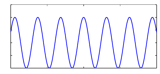
following command makes a chebfun corresponding to cos(20x)on[−1,1] and plots it.
f = chebfun(’cos(20*x)’);
plot(f)
−1−0.5 0 0.5 1
−1
−0.5
0
0.5
1
1.5
From this little experiment, you cannot see that fis represented by a polynomial. One way to see
this is to find the length of f:
length(f)
ans =
61
1. Getting Started with Chebfun 3
Another is to remove the semicolon that suppresses output:
f
f=
chebfun column (1 smooth piece)
interval length endpoint values
[ -1, 1] 61 0.41 0.41
Epslevel = 2.183626e-15. Vscale = 1.000000e+00.
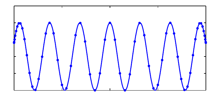
These results tell us that fis represented by a polynomial interpolant through 61 Chebyshev points,
i.e., a polynomial of degree 60. These numbers have been determined by an adaptive process. We
can see the data points by plotting f|with the |’.-’ option:
plot(f,’.-’)
−1−0.5 0 0.5 1
−1
−0.5
0
0.5
1
1.5
The formula for N+ 1 Chebyshev points in [−1,1] is
x(j)=−cos(jπ/N),j=0:N,
and in the figure we can see that the points are clustered accordingly near 1 and −1. Note that in
the middle of the grid, there are about 5 points per wavelength, which is evidently what it takes to
represent this cosine to 15 digits of accuracy. For intervals other than [−1,1], appropriate Chebyshev
points are obtained by a linear scaling.
The curve between the data points is the polynomial interpolant, which is evaluated by the barycen-
tric formula introduced by Salzer [Berrut & Trefethen 2004, Salzer 1972]. This method of evaluating
polynomial interpolants is stable and efficient even if the degree is in the millions [Higham 2004].
What is the integral of ffrom −1 to 1? Here it is:
sum(f)
ans =
0.091294525072763
4Chebfun Guide
This number was computed by integrating the polynomial (Clenshaw-Curtis quadrature – see Section
2.1), and it is interesting to compare it to the exact answer from calculus:
exact = sin(20)/10
exact =
0.091294525072763
Here is another example, now with the chebfun defined by an anonymous function instead of a string.
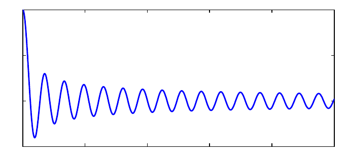
In this case the interval is specified as [0,100].
g = chebfun(@(t) besselj(0,t),[0,100]);
plot(g), ylim([-.5 1])
0 20 40 60 80 100
−0.5
0
0.5
1
The function looks complicated, but it is actually a polynomial of surprisingly small degree:
length(g)
ans =
89
Is it accurate? Well, here are three random points in [0,100]:
format long
x = 100*rand(3,1)
x=
59.616523414856850
87.537260012975111
11.789355152760882
Let’s compare the chebfun to the true Bessel function at these points:
exact = besselj(0,x);
error = g(x) - exact;
[g(x) exact error]
1. Getting Started with Chebfun 5
ans =
-0.067323383971824 -0.067323383971825 0.000000000000000
0.029772796120858 0.029772796120858 0.000000000000001
-0.000506642933742 -0.000506642933741 -0.000000000000001
If you want to know the first 5 zeros of the Bessel function, here they are:
r = roots(g); r = r(1:5)
r=
2.404825557695772
5.520078110286314
8.653727912911007
11.791534439014285
14.930917708487790
Notice that we have just done something nontrivial and potentially useful. How else would you find
zeros of the Bessel function so readily? As always with numerical computation, we cannot expect
the answers to be exactly correct, but they will usually be very close. In fact, these computed zeros
are accurate to close to machine precision:
besselj(0,r)
ans =
1.0e-14 *
0.026212433453684
0.111311651748761
0.154471710674566
0.071369727817872
-0.092296985262750
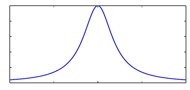
Most often we get a chebfun by operating on other chebfuns. For example, here is a sequence that
uses plus, times, divide, and power operations on an initial chebfun xto produce a famous function
of Runge:
x = chebfun(’x’);
f = 1./(1+25*x.^2);
length(f)
clf, plot(f)
ans =
181
6Chebfun Guide
−1−0.5 0 0.5 1
0
0.2
0.4
0.6
0.8
1
1.3 Operations on chebfuns
There are more than 200 commands that can be applied to a chebfun. For a list of many of them
you can type methods:
methods chebfun
Methods for class chebfun:
abs cotd jaccoeffs range
acos coth join rank
acosd cov jump rdivide
acosh csc kron real
acot cscd ldivide reallog
acotd csch le realpow
acoth ctranspose legcoeffs realsqrt
acsc cumprod legpoly rem
acscd cumsum length remez
acsch cylinder log repmat
airy diff log10 residue
all dirac log1p restrict
and disp log2 roots
angle display logical round
any domain loglog sec
arcLength ellipj lt secd
area ellipke lu sech
asec end mat2cell semilogx
asecd epslevel max semilogy
asech eq mean sign
asin erf measure simplify
asind erfc merge sin
asinh erfcinv mesh sinc
atan erfcx min sind
atan2 erfinv minandmax sinh
atan2d exp minus size
atand expm1 mldivide sound
1. Getting Started with Chebfun 7
atanh feval mod spy
besselh fill movie sqrt
besseli find mrdivide std
besselj fix mtimes subsasgn
besselk fliplr ne subspace
bessely flipud newDomain subsref
bvp4c floor nextpow2 sum
bvp5c fourcoeffs norm surf
cat fred normal surface
ceil ge normest surfc
cf get not svd
cheb2cell gmres null tan
cheb2quasi gt num2cell tand
chebcoeffs heaviside or tanh
chebellipseplot horzcat orth times
chebfun hscale overlap transpose
chebpade hypot pde15s uminus
chebpoly imag permute unwrap
chebtune innerProduct pinv uplus
circconv integral plot vander
comet inv plot3 var
comet3 isdelta plotcoeffs vertcat
complex isempty plus volt
compose isequal poly vscale
cond isfinite polyfit waterfall
conj ishappy pow2 why
conv isinf power xor
cos isnan prod
cosd isreal qr
cosh issing quantumstates
cot iszero quasi2cheb
Static methods:
interp1 ode15s spline
lagrange ode45 update
ode113 pchip
To find out what a command does, you can use help.
help chebfun/sum
SUM Definite integral of a CHEBFUN.
SUM(F) is the integral of a column CHEBFUN F over its domain of definition.
SUM(F, A, B), where A and B are scalars, integrates a column CHEBFUN F over
[A, B], which must be a subdomain of F.domain:
B
/
8Chebfun Guide
SUM(F) = | F(t) dt.
/
A
SUM(F, A, B), where A and B are CHEBFUN objects, returns a CHEBFUN S which
satisfies
B(s)
/
S(s) = | F(t) dt.
/
A(s)
SUM(F, DIM), where DIM is one of 1, 2, sums F over the dimension DIM. If F
is a column CHEBFUN and DIM = 1 or if F is a row CHEBFUN and DIM = 2 then
this integrates in the continuous dimension of F, as described above.
Otherwise, SUM(F, DIM) sums across the columns (rows) of the column (row)
CHEBFUN F.
See also CUMSUM, DIFF.
Most of the commands in the list above exist in ordinary MATLAB; some exceptions are domain,
restrict,chebpoly,andremez. We have already seen length and sum in action. In fact we have
already seen subsref too, since that is the MATLAB command for (among other things) evaluating
arguments in parentheses. Here is another example of its use:
f(0.5)
ans =
0.137931034482759
Here for comparison is the true result:
1/(1+25/4)
ans =
0.137931034482759
In this Runge function example, we have also implicitly seen times,plus,power,andrdivide, all
of which have been overloaded from their usual MATLAB uses to apply to chebfuns.
In the next part of this tour we shall explore many of these commands systematically. First, however,
we should see that chebfuns are not restricted to smooth functions.
1.4 Piecewise smooth chebfuns
Many functions of interest are not smooth but piecewise smooth. In this case a chebfun may consist of
a concatenation of smooth pieces, each with its own polynomial representation. Each of the smooth
1. Getting Started with Chebfun 9
pieces is called a ”fun”. This enhancement of Chebfun was developed initially by Ricardo Pachon
during 2006-2007, then also by Rodrigo Platte starting in 2007 [Pachon, Platte and Trefethen 2010].
Essentially funs are the ”classic chebfuns” for smooth functions on[−1,1] originally implemented
by Zachary Battles in Chebfun Version 1.
Later we shall describe the options in greater detail, but for the moment let us see some examples.
One way to get a piecewise smooth function is directly from the constructor, taking advantage of its
capability of automatic edge detection. For example, in the default ”splitting off” mode a function
with a jump in its derivative produces a warning message,
f = chebfun(’abs(x-.3)’);
Warning: Function not resolved using 65537 pts. Have you tried ’splitting on’?
The same function can be successfully captured with splitting on:
f = chebfun(’abs(x-.3)’,’splitting’,’on’);
The length command reveals that fis defined by four data points, two for each linear interval:
length(f)
ans =
4
We can see the structure of fin more detail by typing fwithout a semicolon:
f
f=
chebfun column (2 smooth pieces)
interval length endpoint values
[ -1, 0.3] 2 1.3 2.2e-16
[ 0.3, 1] 2 1.1e-16 0.7
Epslevel = 1.110223e-15. Vscale = 1.300000e+00. Total length = 4.
This output confirms that f consists of two funs, each defined by two points and two corresponding
function values. The functions live on intervals defined by breakpoints at −1, 1, and a number very
close to 0.3. The Vscale field is related to the maximum absolute value of fand Epslevel gives
some rough information about its relative accuracy.
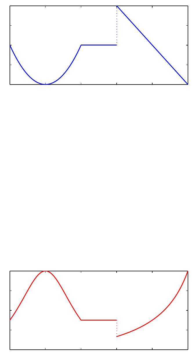
Another way to make a piecewise smooth chebfun is to construct it explicitly from various pieces.
For example, the following command specifies three functions x2,1,and4−x, together with a vector
of endpoints indicating that the first function applies on [−1,1], the second on [1,2], and the third
on [2,4]:
f = chebfun({@(x) x.^2, 1, @(x) 4-x},[-1 1 2 4]);
plot(f)
10 Chebfun Guide
−1 0 1 2 3 4
0
0.5
1
1.5
2
We exp ect fto consist of three pieces of lengths 3, 1, and 2, and this is indeed thecase:
f
f=
chebfun column (3 smooth pieces)
interval length endpoint values
[-1, 1] 3 1 1
[1,2] 1 1 1
[ 2, 4] 2 2 -1.1e-16
Epslevel = 1.110223e-15. Vscale = 2. Total length = 6.
Our eyes see pieces, but to Chebfun, fis just another function. For example, here is its integral.
sum(f)
ans =
3.666666666666667
Here is an algebraic transformation of f, which we plot in another color for variety.
plot(1./(1+f),’r’)
−1 0 1 2 3 4
0.2
0.4
0.6
0.8
1
1. Getting Started with Chebfun 11
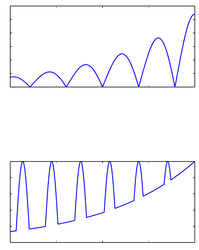
Some Chebfun commands naturally introduce breakpoints in a chebfun. For example, the abs
command first finds zeros of a function and introduces breakpoints there. Here is a chebfun consisting
of 6 funs:
f = abs(exp(x).*sin(8*x));
plot(f)
−1−0.5 0 0.5 1
0
0.5
1
1.5
2
2.5
3
And here is an example where breakpoints are introduced by the max command, leading to a chebfun
with 13 pieces:
f = sin(20*x);
g = exp(x-1);
h = max(f,g);
plot(h)
−1−0.5 0 0.5 1
0
0.2
0.4
0.6
0.8
1
As always, hmay look complicated to a human, but to Chebfun it is just a function. Here are its
mean, standard deviation, minimum, and maximum:
mean(h)
ans =
0.578242020778010
12 Chebfun Guide
std(h)
ans =
0.280937455806246
min(h)
ans =
0.135335283236613
max(h)
ans =
1.000000000000000
A final note about piecewise smooth chebfuns is that the automatic edge detection or ”splitting”
feature, when it is turned on, may subdivide functions even though they do not have clean point
singularities, and this may be desirable or undesirable depending on the application. For example,
considering sin(x) over [0,1000] with splitting on, we end up with a chebfun with many pieces:
tic, f = chebfun(’sin(x)’,[0 1000*pi],’splitting’,’on’),toc
f=
chebfun column (32 smooth pieces)
interval length endpoint values
[ 0, 98] 87 3e-14 -0.71
[ 98, 2e+02] 88 -0.71 1
[ 2e+02, 2.9e+02] 88 1 -0.71
[ 2.9e+02, 3.9e+02] 87 -0.71 1.7e-13
[ 3.9e+02, 4.9e+02] 87 3.1e-13 0.71
[ 4.9e+02, 5.9e+02] 87 0.71 -1
[ 5.9e+02, 6.9e+02] 86 -1 0.71
[ 6.9e+02, 7.9e+02] 85 0.71 -7.6e-13
[ 7.9e+02, 8.8e+02] 86 -1.3e-12 -0.71
[ 8.8e+02, 9.8e+02] 86 -0.71 1
[ 9.8e+02, 1.1e+03] 86 1 -0.71
[ 1.1e+03, 1.2e+03] 86 -0.71 -3.2e-13
[ 1.2e+03, 1.3e+03] 85 -6.7e-13 0.71
[ 1.3e+03, 1.4e+03] 86 0.71 -1
[ 1.4e+03, 1.5e+03] 86 -1 0.71
[ 1.5e+03, 1.6e+03] 85 0.71 -1.6e-12
[ 1.6e+03, 1.7e+03] 86 -1.3e-12 -0.71
[ 1.7e+03, 1.8e+03] 86 -0.71 1
[ 1.8e+03, 1.9e+03] 86 1 -0.71
[ 1.9e+03, 2e+03] 85 -0.71 8.3e-13
[ 2e+03, 2.1e+03] 85 2.2e-12 0.71
[ 2.1e+03, 2.2e+03] 86 0.71 -1
[ 2.2e+03, 2.3e+03] 86 -1 0.71
1. Getting Started with Chebfun 13
[ 2.3e+03, 2.4e+03] 87 0.71 -1.7e-12
[ 2.4e+03, 2.5e+03] 85 1.5e-12 -0.71
[ 2.5e+03, 2.6e+03] 86 -0.71 1
[ 2.6e+03, 2.7e+03] 84 1 -0.71
[ 2.7e+03, 2.7e+03] 85 -0.71 -3.2e-12
[ 2.7e+03, 2.8e+03] 85 -2.5e-13 0.71
[ 2.8e+03, 2.9e+03] 84 0.71 -1
[ 2.9e+03, 3e+03] 86 -1 0.71
[ 3e+03, 3.1e+03] 85 0.71 -3.7e-12
Epslevel = 3.487391e-13. Vscale = 1.000000e+00. Total length = 2748.
Elapsed time is 0.637316 seconds.
In this case it is more efficient – and more interesting mathematically – to omit the splitting and
construct one global chebfun:
tic, f2 = chebfun(’sin(x)’,[0 1000*pi]), toc
f2 =
chebfun column (1 smooth piece)
interval length endpoint values
[ 0, 3.1e+03] 1684 -1.8e-14 -3.1e-13
Epslevel = 3.487867e-13. Vscale = 9.999862e-01.
Elapsed time is 0.025475 seconds.
Splitting on and offare discussed further in Section 8.3.
1.5 Infinite intervals and infinite function values
A major change from Chebfun Version 2 to Version 3 was the generalization of chebfuns to allow
certain functions on infinite intervals or which diverge to infinity; the initial credit for these innova-
tions belongs to Nick Hale, Rodrigo Platte, and Mark Richardson. For example, here is a function
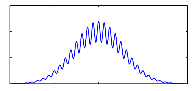
on the whole real axis,
f = chebfun(’exp(-x.^2/16).*(1+.2*cos(10*x))’,[-inf,inf]);
plot(f)
−10 −5 0 5 10
0
0.5
1
1.5
and here is its integral:
14 Chebfun Guide
sum(f)
ans =
7.089815403621257
Here’s the integral of a function on [1,inf]:
sum(chebfun(’1./x.^4’,[1 inf]))
ans =
0.333333333305146
Notice that several digits of accuracy have been lost here. Be careful! – operations involving infinities
in Chebfun are not always as accurate and robust as their finite counterparts.
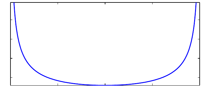
Here is an example of a function that diverges to infinity, which we can capture with the ’exps’
flag; see Chapter 7 for details:
h = chebfun(’(1/pi)./sqrt(1-x.^2)’,’exps’,[-.5 -.5]);
plot(h)
−1−0.5 0 0.5 1
0.4
0.6
0.8
1
In this case the integral comes out just right:
sum(h)
ans =
1
For more on the treatment of infinities in Chebfun, see Chapter 9.
1.6 Periodic functions
Until 2014, Chebfun used only nonperiodic representations, based on Chebyshev polynomials. Begin-
ning with Version 5, there is a new capability of representing sufficiently smooth periodic functions
by trigonometric polynomials instead, that is, Fourier series. Such an object is still called a chebfun,
1. Getting Started with Chebfun 15
but it is a periodic one. These features were added by Grady Wright in the first half of 2014, and
will undoubtedly be developed further in the future.
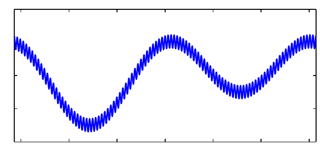
For example, here is a periodic function on [−π,π] represented in the usual way by a Chebyshev
series.
ff = @(t) sin(t)/2 + cos(2*t) + 0.2*cos(100*t);
f = chebfun(ff,[-pi,pi]);
max(f)
plot(f)
ans =
1.231249778347126
−3−2−1 0 1 2 3
−2
−1
0
1
2
Its length, very roughly, is 100 ×π,
length(f)
ans =
383
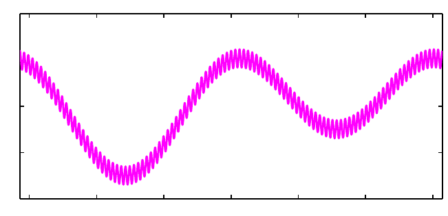
Here is the same function represented by a Fourier series:
f2 = chebfun(ff,[-pi,pi],’periodic’)
max(f2)
plot(f2,’m’)
f2 =
chebfun column (1 smooth piece)
interval length endpoint values periodic
[ -3.1, 3.1] 201 1.2 1.2
Epslevel = 3.739287e-15. Vscale = 1.640723e+00.
ans =
1.231249778347129
16 Chebfun Guide
−3−2−1 0 1 2 3
−2
−1
0
1
2
Its length is now only about 100 ×2 (exactly 201). This improvement by a factor of about π/2 is
typical.
length(f2)
ans =
201
We can confirm that the two functions agree like this:
norm(f-chebfun(f2,[-pi, pi]))
ans =
1.303017177476116e-14
Readers may be interested to compare plotcoeffs applied to the first and second versions of f.
Rather than display that here we shall turn to a simpler example involving a shorter Fourier series.
Consider the function
f = chebfun(’7 + sin(t) + exp(1)*cos(2*t)’,[-pi,pi],’periodic’)
f=
chebfun column (1 smooth piece)
interval length endpoint values periodic
[ -3.1, 3.1] 5 9.7 9.7
Epslevel = 6.661338e-16. Vscale = 9.718282e+00.
Here are the coefficients of fas an expansion in sines and cosines:
[a,b] = fourcoeffs(f)
a=
2.718281828459045 0.000000000000001 7.000000000000000
b=
0 1.000000000000000
1. Getting Started with Chebfun 17
Here they are as an expansion in complex exponentials:
c = fourcoeffs(f)
c=
Column 1
1.359140914229522 + 0.000000000000000i
Column 2
0.000000000000000 - 0.500000000000000i
Column 3
7.000000000000000 + 0.000000000000000i
Column 4
0.000000000000000 + 0.500000000000000i
Column 5
1.359140914229522 + 0.000000000000000i
Bookkeeping of Fourier coefficients can often be a headache. If these examples don’t make the
patterns clear, details can be found with help fourcoeffs.
For a mathematically less trivial example, here is the cosine expansion of a function whose Fourier
series coefficients are known to be values of a Bessel function:
f = chebfun(’exp(cos(t))’,[-pi pi],’periodic’);
[a,b] = fourcoeffs(f);
n = floor(length(f)/2);
exact = 2*besseli(n:-1:0,1); exact(end) = exact(end)/2;
disp(’ computed exact’)
disp([a’ exact’])
computed exact
0.000000000000040 0.000000000000040
0.000000000001039 0.000000000001039
0.000000000024980 0.000000000024980
0.000000000550590 0.000000000550590
0.000000011036772 0.000000011036772
0.000000199212481 0.000000199212481
0.000003198436462 0.000003198436462
0.000044977322954 0.000044977322954
0.000542926311914 0.000542926311914
0.005474240442094 0.005474240442094
0.044336849848664 0.044336849848664
0.271495339534077 0.271495339534077
1.130318207984970 1.130318207984970
1.266065877752008 1.266065877752008
1.7 Rows, columns, and quasimatrices
MATLAB doesn’t only deal with column vectors: there are also row vectors and matrices. The same
is true of Chebfun. The chebfuns shown so far have all been in column orientation, which is the
default, but one can also take the transpose, compute inner products, and so on:
18 Chebfun Guide
x = chebfun(@(x) x)
x=
chebfun column (1 smooth piece)
interval length endpoint values
[-1, 1] 2 -1 1
Epslevel = 1.110223e-15. Vscale = 1.
x’
ans =
chebfun row (1 smooth piece)
interval length endpoint values
[-1, 1] 2 -1 1
Epslevel = 1.110223e-15. Vscale = 1.
x’*x
ans =
0.666666666666667
One can also make matrices whose columns are chebfuns or whose rows are chebfuns, like this:
A=[1xx.^2]
A=
chebfun column1 (1 smooth piece)
interval length endpoint values
[-1, 1] 3 1 1
Epslevel = 2.220446e-15. Vscale = 1.
chebfun column2 (1 smooth piece)
interval length endpoint values
[-1, 1] 3 -1 1
Epslevel = 1.110223e-15. Vscale = 1.
chebfun column3 (1 smooth piece)
interval length endpoint values
[-1, 1] 3 1 1
Epslevel = 2.220446e-15. Vscale = 1.
A’*A
ans =
2.000000000000000 -0.000000000000000 0.666666666666667
-0.000000000000000 0.666666666666667 0
0.666666666666667 0 0.400000000000000
These are called quasimatrices, and they are discussed in Chapter 6.
1. Getting Started with Chebfun 19
1.8 Chebfun features not in this Guide
Some of Chebfun’s most remarkable features haven’t made it into this edition of the Guide. Here
are some of our favorites:
oleg2cheb and cheb2leg for fast Legendre-Chebyshev conversions,
oconv and circconv for convolution,
oThe’equi’ flag to the Chebfun constructor for equispaced data,
opolyfit for least-squares fitting in the continuous context,
oinv for computing the inverse of a chebfun,
opde15s for PDEs in one space and one time variable.
To learn about any of these options, try the appropriate help command. Just as a taster, here’s a
hint of how fast Chebfun can convert a ten-thousand coefficient Chebyshev expansion to Legendre
coefficients and back again using an algorithm from [Hale & Townsend 2013]:
tic
ccheb = randn(10000,1);
cleg = cheb2leg(ccheb);
ccheb2 = leg2cheb(cleg);
norm(ccheb-ccheb2,inf)
toc
ans =
3.428191064358543e-11
Elapsed time is 0.501795 seconds.
1.9 How this Guide is produced
This guide is produced in MATLAB using the publish command with a style sheet somewhat
different from the usual; the output of publish is then processed by Markdown. To publish a chapter
for yourself, make sure the chebfun guide directory is in your path and then type, for example,
open(publish(’guide1’)). The formatting may not be exactly right but it should certainly be
intelligible.
1.10 References
[Battles & Trefethen 2004] Z. Battles and L. N. Trefethen, ”An extension of MATLAB to continuous
functions and operators”, SIAM Journal on Scientific Computing, 25 (2004), 1743-1770.
[Berrut & Trefethen 2005] J.-P. Berrut and L. N. Trefethen, ”Barycentric Lagrange interpolation”,
SIAM Review 46, (2004), 501-517.
[Hale & Townsend 2013] N. Hale and A. Townsend, A fast, simple, and stable Chebyshev–Legendre
transform using an asymptotic formula, SIAM Journal on Scientific Computing, 36 (2014), A148-
A167.
20 Chebfun Guide
[Higham 2004] N. J. Higham, ”The numerical stability of barycentric Lagrange interpolation”, IMA
Journal of Numerical Analysis, 24 (2004), 547-556.
[Pachon, Platte & Trefethen 2010] R. Pachon, R. B. Platte and L. N. Trefethen, ”Piecewise-smooth
chebfuns”, IMA J. Numer. Anal., 30 (2010), 898-916.
[Salzer 1972] H. E. Salzer, ”Lagrangian interpolation at the Chebyshev points cos(nu pi/n), nu =
0(1)n; some unnoted advantages”, Computer Journal 15 (1972), 156-159.
[Trefethen 2007] L. N. Trefethen, ”Computing numerically with functions instead of numbers”,
Mathematics in Computer Science 1 (2007), 9-19.
[Trefethen 2013] L. N. Trefethen, Approximation Theory and Approximation Practice,SIAM,2013.
2. Integration and Differentiation
Lloyd N. Trefethen, November 2009, latest revision June 2014
Contents
•2.1 sum
•2.2 norm,mean,std,var
•2.3 cumsum
•2.4 diff
•2.5 Integrals in two dimensions
•2.6 Gauss and Gauss-Jacobi quadrature
•2.7 References
2.1 sum
We have seen that the sum command returns the definite integral of a chebfun over its range of defi-
nition. The integral is normally calculated by an FFT-based version of Clenshaw-Curtis quadrature,
as described first in [Gentleman 1972]. This formula is applied on each fun (i.e., each smooth piece
of the chebfun), and then the results are added up.
Here is an example whose answer is known exactly:
f = chebfun(@(x) log(1+tan(x)),[0 pi/4]);
format long
I = sum(f)
Iexact = pi*log(2)/8
I=
0.272198261287950
Iexact =
0.272198261287950
Here is an example whose answer is not known exactly, given as the first example in the section
”Numerical Mathematics in Mathematica” in The Mathematica Book [Wolfram 2003].
f = chebfun(’sin(sin(x))’,[0 1]);
sum(f)
ans =
0.430606103120691
1
2Chebfun Guide
All these digits match the result 0.4306061031206906049 ...reported by Mathematica.
Here is another example:
F = @(t) 2*exp(-t.^2)/sqrt(pi);
f = chebfun(F,[0,1]);
I = sum(f)
I=
0.842700792949715
The reader may recognize this as the integral that defines the error function evaluated at t=1:
Iexact = erf(1)
Iexact =
0.842700792949715
It is interesting to compare the times involved in evaluating this number in various ways. MATLAB’s
specialized erf code is the fastest:
tic, erf(1), toc
ans =
0.842700792949715
Elapsed time is 0.000040 seconds.
Using MATLAB’s various quadrature commands is understandably slower:
tol = 3e-14;
tic, I = quad(F,0,1,tol); t = toc;
fprintf(’ QUAD: I = %17.15f time = %6.4f secs\n’,I,t)
tic, I = quadl(F,0,1,tol); t = toc;
fprintf(’ QUADL: I = %17.15f time = %6.4f secs\n’,I,t)
tic, I = quadgk(F,0,1,’abstol’,tol,’reltol’,tol); t = toc;
fprintf(’QUADGK: I = %17.15f time = %6.4f secs\n’,I,t)
QUAD: I = 0.842700792949715 time = 0.0204 secs
QUADL: I = 0.842700792949715 time = 0.0146 secs
QUADGK: I = 0.842700792949715 time = 0.0253 secs
The timing for Chebfun comes out competitive:
tic, I = sum(chebfun(F,[0,1])); t = toc;
fprintf(’CHEBFUN: I = %17.15f time = %6.4f secs\n’,I,t)
CHEBFUN: I = 0.842700792949715 time = 0.0055 secs
2. Integration and Differentiation 3
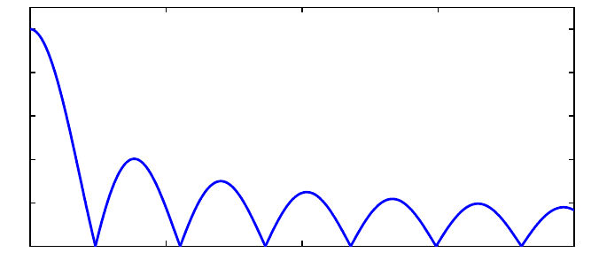
Here is a similar comparison for a function that is more difficult, because of the absolute value,
which leads with ”splitting on” to a chebfun consisting of a number of funs.
F = @(x) abs(besselj(0,x));
f = chebfun(@(x) abs(besselj(0,x)),[0 20],’splitting’,’on’);
plot(f), ylim([0 1.1])
0 5 10 15 20
0
0.2
0.4
0.6
0.8
1
tol = 3e-14;
tic, I = quad(F,0,20,tol); t = toc;
fprintf(’ QUAD: I = %17.15f time = %5.3f secs\n’,I,t)
tic, I = quadl(F,0,20,tol); t = toc;
fprintf(’ QUADL: I = %17.15f time = %5.3f secs\n’,I,t)
tic, I = quadgk(F,0,20,’abstol’,tol,’reltol’,tol); t = toc;
fprintf(’ QUADGK: I = %17.15f time = %5.3f secs\n’,I,t)
tic, I = sum(chebfun(@(x) abs(besselj(0,x)),[0,20],’splitting’,’on’)); t = toc;
fprintf(’CHEBFUN: I = %17.15f time = %5.3f secs\n’,I,t)
QUAD: I = 4.445031603001505 time = 0.077 secs
QUADL: I = 4.445031603001576 time = 0.046 secs
QUADGK: I = 4.445031603001578 time = 0.016 secs
CHEBFUN: I = 4.445031603001567 time = 1.208 secs
This last example highlights the piecewise-smooth aspect of Chebfun integration. Here is another
example of a piecewise smooth problem.
x = chebfun(’x’);
f = sech(3*sin(10*x));
g = sin(9*x);
h = min(f,g);
plot(h)
4Chebfun Guide
−1−0.5 0 0.5 1
−1
−0.5
0
0.5
1
Here is the integral:
tic, sum(h), toc
ans =
-0.381556448850250
Elapsed time is 0.000860 seconds.
For another example of a definite integral we turn to an integrand given as example F21F in [Kahaner
1971]. We treat it first in the default mode of splitting off:
ff = @(x) sech(10*(x-0.2)).^2 + sech(100*(x-0.4)).^4 + sech(1000*(x-0.6)).^6;
f = chebfun(ff,[0,1])
f=
chebfun column (1 smooth piece)
interval length endpoint values
[ 0, 1] 12318 0.071 4.5e-07
Epslevel = 4.547474e-13. Vscale = 1.070659e+00.
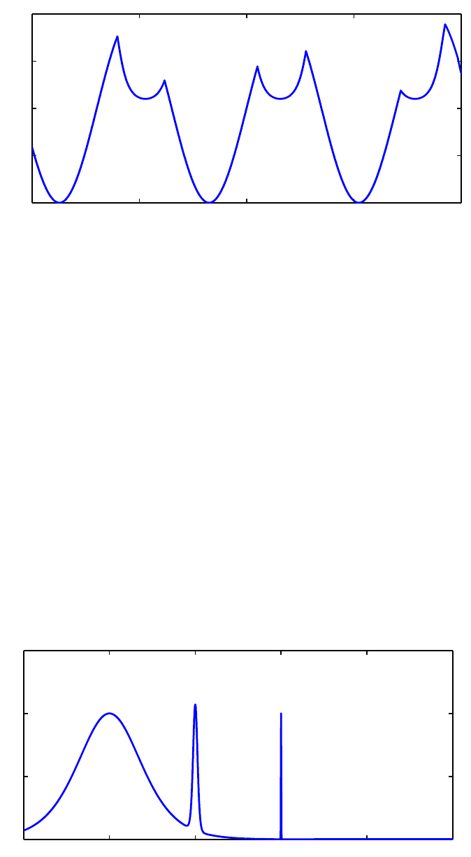
The function has three spikes, each ten times narrower than the last:
plot(f)
0 0.2 0.4 0.6 0.8 1
0
0.5
1
1.5
2. Integration and Differentiation 5
The length of the global polynomial representation is accordingly quite large, but the integral comes
out correct to full precision:
length(f)
sum(f)
ans =
12318
ans =
0.210802735500549
With splitting on, Chebfun misses the narrowest spike, and the integral comes out too small:
f = chebfun(ff,[0,1],’splitting’,’on’);
length(f)
sum(f)
ans =
228
ans =
0.209736068833883
We can fix the problem by forcing finer initial sampling in the Chebfun constructor with the
minSamples flag:
f = chebfun(ff,[0,1],’splitting’,’on’,’minSamples’,100);
length(f)
sum(f)
ans =
373
ans =
0.210802735500549
Now the integral is correct again, and note that the length of the chebfun is much smaller than with
the original global representation. For more about minSamples, see Section 8.6.
As mentioned in Chapter 1 and described in more detail in Chapter 9, Chebfun has some capability
of dealing with functions that blow up to infinity. Here for example is a familiar integral:
f = chebfun(@(x) 1./sqrt(x),[0 1],’blowup’,2);
sum(f)
ans =
2.000000000000000
Certain integrals over infinite domains can also be computed, though the error is often large:

6Chebfun Guide
f = chebfun(@(x) 1./x.^2.5,[1 inf]);
sum(f)
Warning: Result may not be accurate as the function decays slowly at infinity.
ans =
0.666666674295143
Chebfun is not a specialized item of quadrature software; it is a general system for manipulating
functions in which quadrature is just one of many capabilities. Nevertheless Chebfun compares
reasonably well as a quadrature engine against specialized software. This was the conclusion of
an Oxford MSc thesis by Phil Assheton [Assheton 2008], which compared Chebfun experimentally
to quadrature codes including MATLAB’s quad and quadl, Gander and Gautschi’s adaptsim and
adaptlob, Espelid’s modsim,modlob,coteda,andcoteglob, QUADPACK’s QAG and QAGS,andthe
NAG Library’s d01ah. In both reliability and speed, Chebfun was found to be competitive with
these alternatives. The overall winner was coteda [Espelid 2003], which was typically about twice
as fast as Chebfun. For further comparisons of quadrature codes, together with the development
of some improved codes based on a philosophy that has something in common with Chebfun, see
[Gonnet 2009]. See also ”Battery test of Chebfun as an integrator” in the Quadrature section of the
Chebfun Examples collection.
2.2 norm,mean,std,var
A special case of an integral is the norm command, which for a chebfun returns by default the 2-norm,
i.e., the square root of the integral of the square of the absolute value over the region of definition.
Here is a well-known example:
norm(chebfun(’sin(pi*theta)’))
ans =
1
If we take the sign of the sine, the norm increases to √2:
norm(chebfun(’sign(sin(pi*theta))’,’splitting’,’on’))
ans =
1.414213562373095
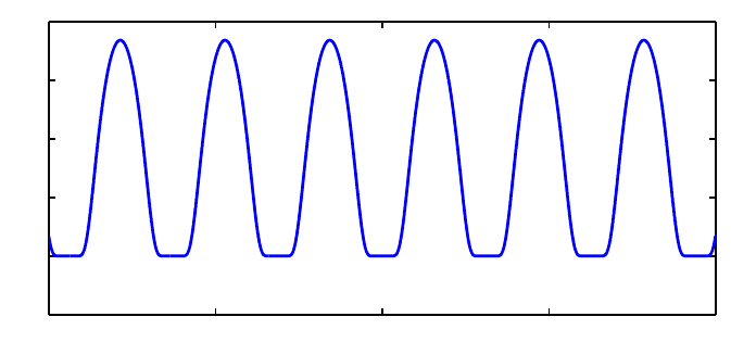
Here is a function that is infinitely differentiable but not analytic.
f = chebfun(’exp(-1./sin(10*x).^2)’);
plot(f)
2. Integration and Differentiation 7
−1−0.5 0 0.5 1
−0.1
0
0.1
0.2
0.3
0.4
Here are the norms of fand its tenth power:
norm(f), norm(f.^10)
ans =
0.292873834331035
ans =
2.187941295308666e-05
2.3 cumsum
In MATLAB, cumsum gives the cumulative sum of a vector,
v=[1235]
cumsum(v)
v=
1235
ans =
13611
The continuous analogue of this operation is indefinite integration. If fis a fun of length n,then
cumsum(f) is a fun of length n+ 1. For a chebfun consisting of several funs, the integration is
performed on each piece.
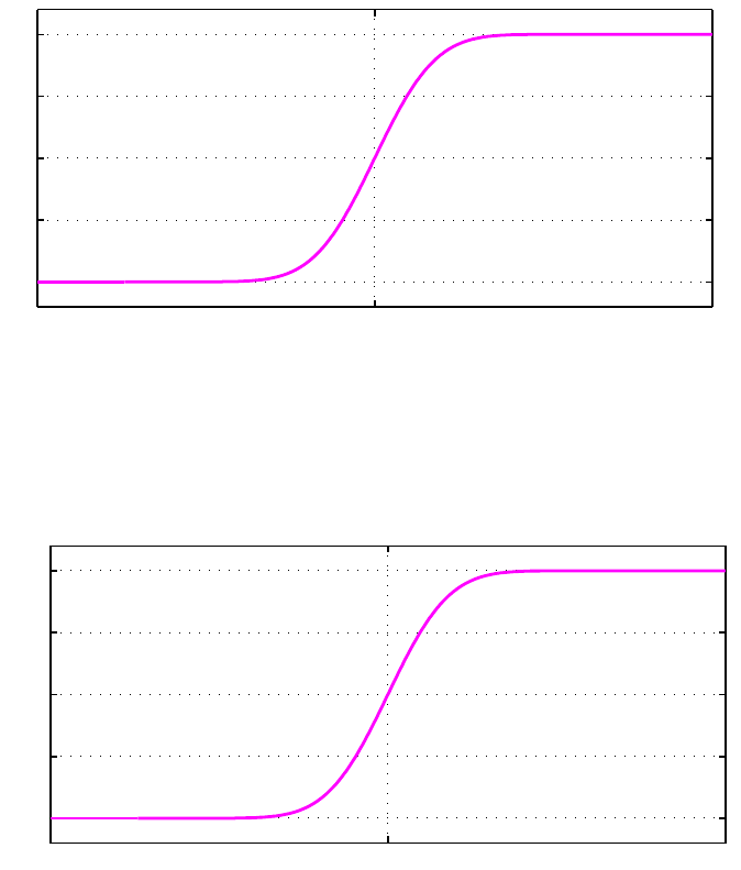
For example, returning to an integral computed above, we can make our own error function like this:
t = chebfun(’t’,[-5 5]);
f = 2*exp(-t.^2)/sqrt(pi);
fint = cumsum(f);
plot(fint,’m’)
ylim([-0.2 2.2]), grid on
8Chebfun Guide
−5 0 5
0
0.5
1
1.5
2
The default indefinite integral takes the value 0 at the left endpoint, but in this case we would like
0toappearatt=0:
fint = fint - fint(0);
plot(fint,’m’)
ylim([-1.2 1.2]), grid on
−5 0 5
−1
−0.5
0
0.5
1
The agreement with the built-in error function is convincing:
[fint((1:5)’) erf((1:5)’)]
ans =
0.842700792949715 0.842700792949715
0.995322265018953 0.995322265018953
0.999977909503002 0.999977909503001
0.999999984582742 0.999999984582742
0.999999999998463 0.999999999998463
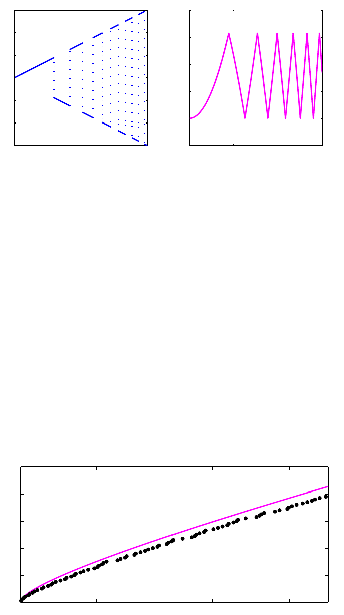
Here is the integral of an oscillatory step function:
x = chebfun(’x’,[0 6]);
f = x.*sign(sin(x.^2)); subplot(1,2,1), plot(f)
g = cumsum(f); subplot(1,2,2), plot(g,’m’)
2. Integration and Differentiation 9
0 2 4 6
−6
−4
−2
0
2
4
6
0 2 4 6
−0.5
0
0.5
1
1.5
2
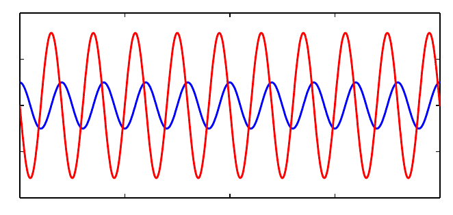
And here is an example from number theory. The logarithmic integral, Li(x), is the indefinite
integral from 0 to xof 1/log(s). It is an approximation to π(x), the number of primes less than or
equal to x. To avoid the singularity at x= 0 we begin our integral at the point µ=1.451... where
Li(x) is zero, known as Soldner’s constant. The test value Li(2) is correct except in the last digit:
mu = 1.45136923488338105; % Soldner’s constant
xmax = 400;
Li = cumsum(chebfun(@(x) 1./log(x),[mu xmax]));
lengthLi = length(Li)
Li2 = Li(2)
lengthLi =
392
Li2 =
1.045163780117242
(Chebfun has no trouble if xmax is increased to 105or 1010.) Here is a plot comparing Li(x) with
π(x):
clf, plot(Li,’m’)
p = primes(xmax);
hold on, plot(p,1:length(p),’.k’)
50 100 150 200 250 300 350 400
0
20
40
60
80
100
10 Chebfun Guide
The Prime Number Theorem implies that π(x)∼Li(x)asx→∞. Littlewood proved in 1914 that
although Li(x) is greater than π(x) at first, the two curves eventually cross each other infinitely
often. It is known that the first crossing occurs somewhere between x=10
14 and x=2×10316
[Kotnik 2008].
The mean,std,andvar commands have also been overloaded for chebfuns and are based on integrals.
For example,
mean(chebfun(’cos(x).^2’,[0,10*pi]))
ans =
0.500000000000000
2.4 diff
In MATLAB, diff gives finite differences of a vector:
v=[1235]
diff(v)
v=
1235
ans =
112
The continuous analogue of this operation is differentiation. For example:
f = chebfun(’cos(pi*x)’,[0 20]);
fprime = diff(f);
hold off, plot(f)
hold on, plot(fprime,’r’)
0 5 10 15 20
−4
−2
0
2
4
If the derivative of a function with a jump is computed, then a delta function is introduced. Consider
for example this function defined piecewise:
2. Integration and Differentiation 11
f = chebfun({@(x) x.^2, 1, @(x) 4-x, @(x) 4./x},0:4);
hold off, plot(f)
0 0.5 1 1.5 2 2.5 3 3.5 4
0
0.5
1
1.5
2
Here is the derivative:
fprime = diff(f);
plot(fprime,’r’), ylim([-2,3])
0 0.5 1 1.5 2 2.5 3 3.5 4
−2
−1
0
1
2
3
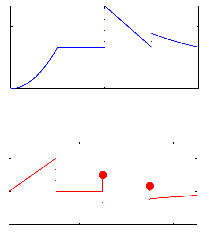
The first segment of f′is linear, since fis quadratic here. Then comes a segment with f′=0,
since fis constant. At the end of this second segment appears a delta function of amplitude 1,
corresponding to the jump of fby 1. The third segment has constant value f′=−1. Finally
another delta function, this time with amplitude 1/3, takes us to the final segment.
Thanks to the delta functions, cumsum and diff are essentially inverse operations. It is no surprise
that differentiating an indefinite integral returns us to the original function:
norm(f-diff(cumsum(f)))
ans =
2.387305176974604e-15
More surprising is that integrating a derivative does the same, as long as we add in the value at the
left endpoint:
12 Chebfun Guide
d = domain(f);
f2 = f(d(1)) + cumsum(diff(f));
norm(f-f2)
ans =
1.000000000000000
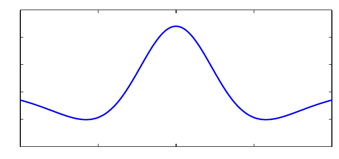
Multiple derivatives can be obtained by adding a second argument to diff. Thus for example,
f = chebfun(’1./(1+x.^2)’);
g = diff(f,4); plot(g)
−1−0.5 0 0.5 1
−20
−10
0
10
20
30
However, one should be cautious about the potential loss of information in repeated differentiation.
For example, if we evaluate this fourth derivative at x=0wegetananswerthatmatchesthecorrect
value 24 only to 11 places:
g(0)
ans =
24.000000000055742
For a more extreme example, suppose we define a chebfun for exp(x)on[−1,1]:
f = chebfun(’exp(x)’);
length(f)
ans =
15
Differentiation is a notoriously ill-posed problem, and since fis a polynomial of low degree, it cannot
help but lose information rather fast as we differentiate. In fact, differentiating 15 times eliminates
the function entirely.
for j = 0:length(f)
fprintf(’%6d %19.12f\n’, j,f(1))
f = diff(f);
end

2. Integration and Differentiation 13
0 2.718281828459
1 2.718281828459
2 2.718281828460
3 2.718281828476
4 2.718281828599
5 2.718281824149
6 2.718281637734
7 2.718277739843
8 2.718221404644
9 2.717612947873
10 2.712588330520
11 2.680959565421
12 2.532851885655
13 2.043523780708
14 1.020835497184
15 0.000000000000
Is such behavior ”wrong”? Well, that is an interesting question. Chebfun is behaving correctly in
the sense mentioned in the second paragraph of Section 1.1: the operations are individually stable
in that each differentiation returns the exact derivative of a function very close to the right one.
The trouble is that because of the intrinsically ill-posed nature of differentiation, the errors in these
stable operations accumulate exponentially as successive derivatives are taken.
2.5 Integrals in two dimensions
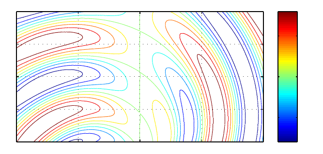
Chebfun can often do a pretty good job with integrals over rectangles. Here for example is a colorful
function:
r = @(x,y) sqrt(x.^2+y.^2); theta = @(x,y) atan2(y,x);
f = @(x,y) sin(5*(theta(x,y)-r(x,y))).*sin(x);
x = -2:.02:2; y = 0.5:.02:2.5; [xx,yy] = meshgrid(x,y);
clf, contour(x,y,f(xx,yy),-1:.2:1)
axis([-2 2 0.5 2.5]), colorbar, grid on
−2−1 0 1 2
0.5
1
1.5
2
2.5
−0.5
0
0.5
Using 1D Chebfun technology, we can compute the integral over the box like this. Notice the use of
the flag vectorize to construct a chebfun from a function only defined for scalar arguments.
14 Chebfun Guide
Iy = @(y) sum(chebfun(@(x) f(x,y),[-2 2]));
tic, I = sum(chebfun(@(y) Iy(y),[0.5 2.5],’vectorize’)); t=toc;
fprintf(’CHEBFUN: I = %16.14f time = %5.3f secs\n’,I,t)
CHEBFUN: I = 0.02041246545700 time = 0.261 secs
Here for comparison is MATLAB’s dblquad/quadl with a tolerance of 10−11:
tic, I = dblquad(f,-2,2,0.5,2.5,1e-11,@quadl); t = toc;
fprintf(’DBLQUAD/QUADL: I = %16.14f time = %5.3f secs\n’,I,t)
DBLQUAD/QUADL: I = 0.02041246545700 time = 2.625 secs
This example of a 2D integrand is smooth, so both Chebfun and dblquad can handle it to high
accuracy.
A much better approach for this problem, however, is to use Chebfun2, which is described in Chapters
11-15. With this method we can compute the integral quickly,
tic
f2 = chebfun2(f,[-2 2 0.5 2.5]);
sum2(f2)
toc
ans =
0.020412465456999
Elapsed time is 0.220325 seconds.
and we can plot the function without the need for meshgrid:
contour(f2,-1:.2:1), colorbar, grid on
−2−1 0 1 2
0.5
1
1.5
2
2.5
−0.5
0
0.5
2. Integration and Differentiation 15
2.6 Gauss and Gauss-Jacobi quadrature
For quadrature experts, Chebfun contains some powerful capabilities due to Nick Hale and Alex
Townsend [Hale & Townsend 2013]. To start with, suppose we wish to carry out 4-point Gauss
quadrature over [−1,1]. The quadrature nodes are the zeros of the degree 4 Legendre polynomial
legpoly(4), which can be obtained from the Chebfun command legpts, and if two output argu-
ments are requested, legpts provides weights also:
[s,w] = legpts(4)
s=
-0.861136311594053
-0.339981043584856
0.339981043584856
0.861136311594053
w=
Columns 1 through 3
0.347854845137454 0.652145154862546 0.652145154862546
Column 4
0.347854845137454
To compute the 4-point Gauss quadrature approximation to the integral of exp(x)from−1to1,for
example, we could now do this:
x = chebfun(’x’);
f = exp(x);
Igauss = w*f(s)
Iexact = exp(1) - exp(-1)
Igauss =
2.350402092156377
Iexact =
2.350402387287603
There is no need to stop at 4 points, however. Here we use 1000 Gauss quadrature points:
tic
[s,w] = legpts(1000); Igauss = w*f(s)
toc
Igauss =
2.350402387287603
Elapsed time is 0.066921 seconds.
Even 100,000 points doesn’t take very long:
tic
[s,w] = legpts(100000); Igauss = w*f(s)
toc
16 Chebfun Guide
Igauss =
2.350402387287603
Elapsed time is 0.155497 seconds.
Traditionally, numerical analysts computed Gauss quadrature nodes and weights by the eigenvalue
algorithm of Golub and Welsch [Golub & Welsch 1969]. However, the Hale-Townsend algorithms
are both more accurate and much faster [Hale & Townsend 2013]. Closely related fast algorithms
developed independently are presented in [Bogaert, Michiels & Fostier 2012].
For Legendre polynomials, Legendre points, and Gauss quadrature, use legpoly and legpts.For
Chebyshev polynomials, Chebyshev points, and Clenshaw-Curtis quadrature, use chebpoly and
chebpts and the built-in Chebfun commands such as sum. A third variant is also available: for
Jacobi polynomials, Gauss-Jacobi points, and Gauss-Jacobi quadrature, see jacpoly and jacpts.
These arise in integration of functions with singularities at one or both endpoints, and are used
internally by Chebfun for integration of chebfuns with singularities (Chapter 9).
As explained in the help texts, all of these operators work on general intervals [a, b], not just on
[−1,1].
2.7 References
[Assheton 2008] P. Assheton, Comparing Chebfun to Adaptive Quadrature Software, dissertation,
MSc in Mathematical Modelling and Scientific Computing, Oxford University, 2008.
[Bogaert, Michiels, and Fostier, ”O(1) computation of Legendre polynomials and Legendre nodes
and weights for parallel computing”, SIAM Journal on Scientific Computing,34 (2012), C83-C101.
[Espelid 2003] T. O. Espelid, ”Doubly adaptive quadrature routines based on Newton-Cotes rules”,
BIT Numerical Mathematics, 43 (2003), 319-337.
[Gentleman 1972] W. M. Gentleman, ”Implementing Clenshaw-Curtis quadrature I and II”, Journal
of the ACM, 15 (1972), 337-346 and 353.
[Golub & Welsch 1969] G. H. Golub and J. H. Welsch, ”Calculation of Gauss quadrature rules”,
Mathematics of Computation, 23 (1969), 221-230.
[Gonnet 2009] P. Gonnet, Adaptive Quadrature Re-Revisited, ETH dissertation no. 18347, Swiss
Federal Institute of Technology, 2009.
[Hale & Townsend 2013] N. Hale and A. Townsend, Fast and accurate computation of Gauss-
Legendre and Gauss-Jacobi quadrature nodes and weights, SIAM Journal on Scientific Computing,
35 (2013), A652-A674.
[Hale & Trefethen 2012] N. Hale and L. N. Trefethen, Chebfun and numerical quadrature, Science
in China, 55 (2012), 1749-1760.
[Kahaner 1971] D. K. Kahaner, ”Comparison of numerical quadrature formulas”, in J. R. Rice, ed.,
Mathematical Software, Academic Press, 1971, 229-259.
[Kotnik 2008] T. Kotnik, ”The prime-counting function and its analytic approximations”, Advances
in Computational Mathematics, 29 (2008), 55-70.
2. Integration and Differentiation 17
[Wolfram 2003] S. Wolfram, The Mathematica Book, 5th ed., Wolfram Media, 2003.

!
3. Rootfinding and Minima and
Maxima
Lloyd N. Trefethen, October 2009, latest revision June 2014
Contents
•3.1 roots
•3.2 min,max,abs,sign,round,floor,ceil
•3.3 Local extrema
•3.4 Global extrema: max and min
•3.5 norm(f,1) and norm(f,inf)
•3.6 Roots in the complex plane
•3.7 References
3.1 roots
Chebfun comes with a global rootfinding capability – the ability to find all the zeros of a function
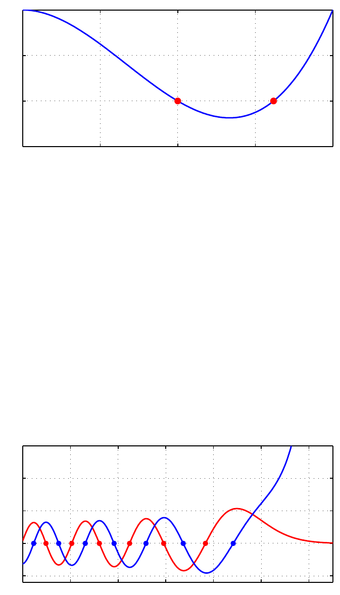
in its region of definition. For example, here is a polynomial with two roots in [−1,1]:
x = chebfun(’x’);
p=x.^3+x.^2-x;
r = roots(p)
r=
0
0.618033988749895
We can plot pand its roots like this:
plot(p), grid on
MS = ’markersize’;
hold on, plot(r,p(r),’.r’,MS,20)
1
2Chebfun Guide
−1−0.5 0 0.5 1
−0.5
0
0.5
1
Of course, one does not need Chebfun to find roots of a polynomial. The MATLAB roots command
works from a polynomial’s coefficients and computes estimates of all the roots, not just those in a
particular interval.
roots([1 1 -1 0])
ans =
0
-1.618033988749895
0.618033988749895
A more substantial example of rootfinding involving a Bessel function was considered in Sections
1.2 and 2.4. Here is a similar calculation for the Airy functions Ai and Bi, modeled after the page
on Airy functions at WolframMathWorld.
Ai = chebfun(@(x) airy(0,x),[-10,3]);
Bi = chebfun(@(x) airy(2,x),[-10,3]);
hold off, plot(Ai,’r’)
hold on, plot(Bi,’b’)
rA = roots(Ai); plot(rA,Ai(rA),’.r’,MS,16)
rB = roots(Bi); plot(rB,Bi(rB),’.b’,MS,16)
axis([-10 3 -.6 1.5]), grid on
−10 −8−6−4−2 0 2
−0.5
0
0.5
1
1.5
Here for example are the three roots of Ai and Bi closest to 0:
3. Rootfinding and Minima and Maxima 3
[rA(end-2:end) rB(end-2:end)]
ans =
-5.520559828095558 -4.830737841662006
-4.087949444130973 -3.271093302836356
-2.338107410459772 -1.173713222709129
Chebfun finds roots by a method due to Boyd and Battles [Boyd 2002, Battles 2006]. If the chebfun
is of degree greater than about 50, it is broken into smaller pieces recursively. On each small piece
zeros are then found as eigenvalues of a ”colleague matrix”, the analogue for Chebyshev polynomials
of a companion matrix for monomials [Specht 1960, Good 1961]. This method can be startlingly
fast and accurate. For example, here is a sine function with 11 zeros:
f = chebfun(’sin(pi*x)’,[0 10]);
lengthf = length(f)
tic, r = roots(f); toc
r
lengthf =
44
Elapsed time is 0.003508 seconds.
r=
0
0.999999999999997
1.999999999999999
3.000000000000000
4.000000000000000
4.999999999999999
6.000000000000001
7.000000000000000
8.000000000000004
9.000000000000002
10.000000000000000
A similar computation with 101 zeros comes out equally well:
f = chebfun(’sin(pi*x)’,[0 100]);
lengthf = length(f)
tic, r = roots(f); toc
fprintf(’%22.14f\n’,r(end-4:end))
lengthf =
214
Elapsed time is 0.011363 seconds.
96.00000000000000
97.00000000000000
98.00000000000001
99.00000000000000
100.00000000000000
4Chebfun Guide
And here is the same on an interval with 1001 zeros.
f = chebfun(’sin(pi*x)’,[0 1000]);
lengthf = length(f)
tic, r = roots(f); toc
fprintf(’%22.13f\n’,r(end-4:end))
lengthf =
1684
Elapsed time is 0.184578 seconds.
996.0000000000000
996.9999999999999
998.0000000000000
999.0000000000000
1000.0000000000000
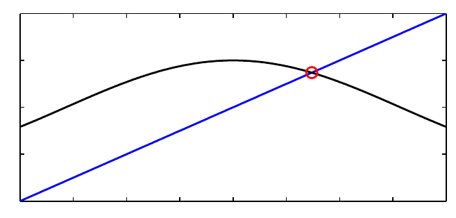
With the ability to find zeros, we can solve a variety of nonlinear problems. For example, where do
the curves xand cos(x) intersect? Here is the answer.
x = chebfun(’x’,[-2 2]);
hold off, plot(x)
f = cos(x);
hold on, plot(f,’k’)
r = roots(f-x)
plot(r,f(r),’or’,MS,8)
r=
0.739085133215160
−2−1.5 −1−0.5 0 0.5 1 1.5 2
−2
−1
0
1
2
All of the examples above concern chebfuns consisting of a single fun. If there are several funs, then
roots are included at jumps as necessary. The following example shows a chebfun with 26 pieces. It
has nine zeros: one within a fun, eight at jumps between funs.
x = chebfun(’x’,[-2 2]);
f = x.^3 - 3*x - 2 + sign(sin(20*x));
hold off, plot(f), grid on
r = roots(f);
hold on, plot(r,0*r,’.r’,MS,16)
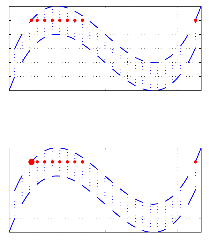
3. Rootfinding and Minima and Maxima 5
−2−1.5 −1−0.5 0 0.5 1 1.5 2
−5
−4
−3
−2
−1
0
1
If one prefers only the ”genuine” roots, omitting those at jumps, they can be computed like this:
r = roots(f,’nojump’);
plot(r,0*r,’.r’,MS,30)
−2−1.5 −1−0.5 0 0.5 1 1.5 2
−5
−4
−3
−2
−1
0
1
3.2 min,max,abs,sign,round,floor,ceil
Rootfinding is more central to Chebfun than one might at first imagine, because a number of
commands, when applied to smooth chebfuns, must produce non-smooth results, and it is rootfinding
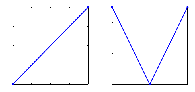
that tells us where to put the discontinuities. For example, the abs command introduces breakpoints
wherever the argument goes through zero. Here we see that xconsists of a single piece, whereas
abs(x) consists of two pieces.
x = chebfun(’x’)
absx = abs(x)
subplot(1,2,1), plot(x,’.-’)
subplot(1,2,2), plot(absx,’.-’)
x=
chebfun column (1 smooth piece)
interval length endpoint values
[-1, 1] 2 -1 1
6Chebfun Guide
Epslevel = 1.110223e-15. Vscale = 1.
absx =
chebfun column (2 smooth pieces)
interval length endpoint values
[-1, 0] 2 1 0
[0,1] 2 0 1
Epslevel = 1.110223e-15. Vscale = 1. Total length = 4.
−1−0.5 0 0.5 1
−1
−0.5
0
0.5
1
−1−0.5 0 0.5 1
0
0.2
0.4
0.6
0.8
1
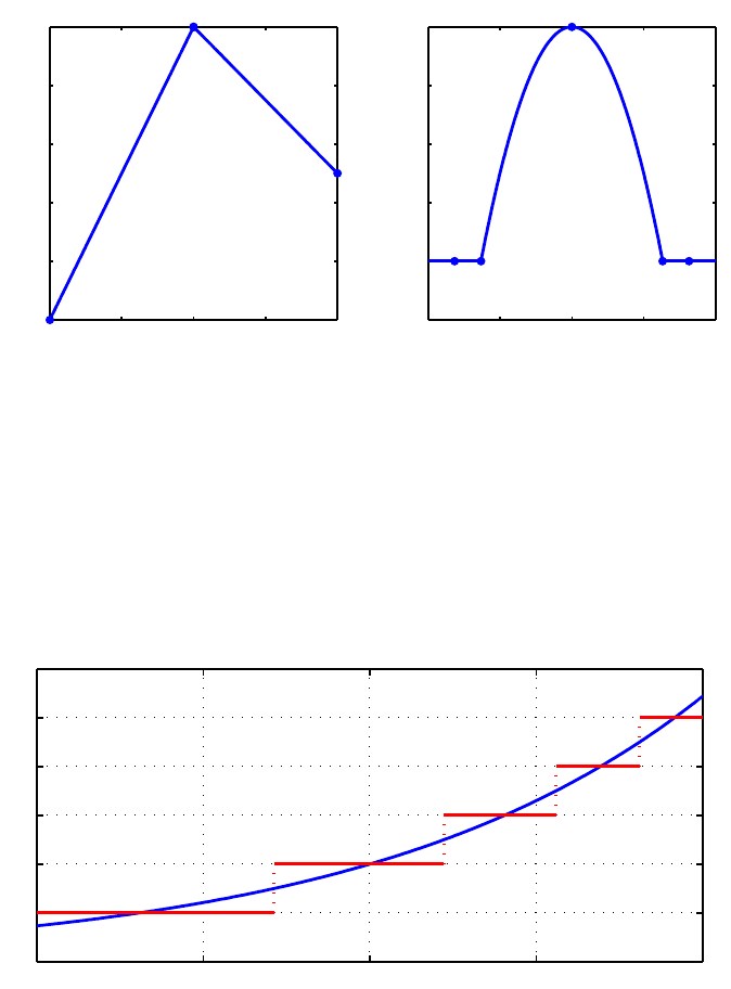
We saw this effect already in Section 1.4. Another similar effect shown in that section occurs with
min(f,g) or max(f,g). Here, breakpoints are introduced at points where f-g is zero:
f = min(x,-x/2), subplot(1,2,1), plot(f,’.-’)
g = max(.6,1-x.^2), subplot(1,2,2), plot(g,’.-’), ylim([.5,1])
f=
chebfun column (2 smooth pieces)
interval length endpoint values
[-1, 0] 2 -1 0
[0,1] 2 0-0.5
Epslevel = 1.332268e-15. Vscale = 1. Total length = 4.
g=
chebfun column (3 smooth pieces)
interval length endpoint values
[ -1, -0.63] 1 0.6 0.6
[ -0.63, 0.63] 3 0.6 0.6
[ 0.63, 1] 1 0.6 0.6
Epslevel = 2.220446e-16. Vscale = 1. Total length = 5.
3. Rootfinding and Minima and Maxima 7
−1−0.5 0 0.5 1
−1
−0.8
−0.6
−0.4
−0.2
0
−1−0.5 0 0.5 1
0.5
0.6
0.7
0.8
0.9
1
The function sign also introduces breaks, as illustrated in the last section. The commands round,
floor,andceil behave like this too. For example, here is exp(x) rounded to nearest multiples of
0.5:
g = exp(x);
clf, plot(g)
gh = 0.5*round(2*g);
hold on, plot(gh,’r’);
grid on
−1−0.5 0 0.5 1
0
0.5
1
1.5
2
2.5
3
3.3 Local extrema
Local extrema of smooth functions can be located by finding zeros of the derivative. For example,
here is a variant of the Airy function again, with all its extrema in its range of definition located
and plotted.
f = chebfun(’exp(real(airy(x)))’,[-15,0]);
clf, plot(f)
r = roots(diff(f));
hold on, plot(r,f(r),’.r’), grid on
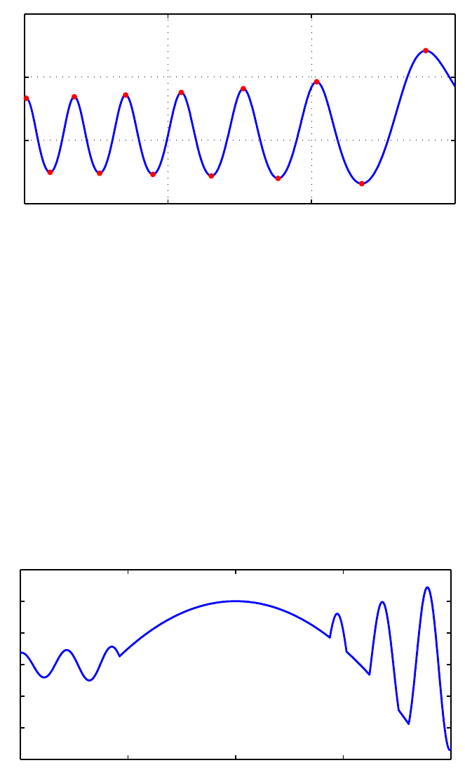
8Chebfun Guide
−15 −10 −5 0
0.5
1
1.5
2
Chebfun users don’t have to compute the derivative explicitly to find extrema, however. An alter-
native is to type
[ignored,r2] = minandmax(f,’local’);
which returns both interior local extrema and also the endpoints of f. Similarly one can type
min(f,’local’) and max(f,’local’).
These methods will find non-smooth extrema as well as smooth ones, since these correspond to
”zeros” of the derivative where the derivative jumps from one sign to the other. Here is an example.
x = chebfun(’x’);
f = exp(x).*sin(30*x);
g = 2-6*x.^2;
h = max(f,g);
clf, plot(h)
−1−0.5 0 0.5 1
−3
−2
−1
0
1
2
3
Here are all the local extrema, smooth and nonsmooth:
[ignored,extrema] = minandmax(h,’local’);
hold on, plot(extrema,h(extrema),’.r’)
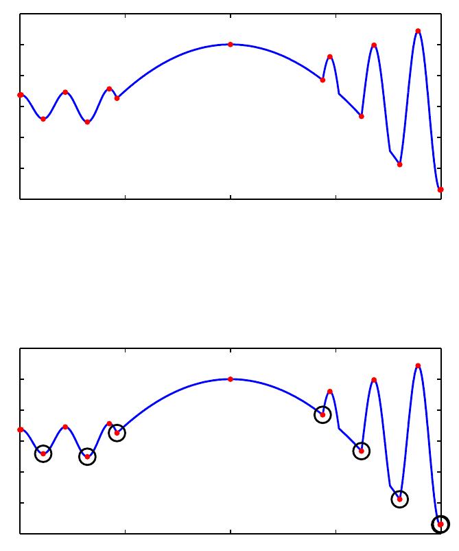
3. Rootfinding and Minima and Maxima 9
−1−0.5 0 0.5 1
−3
−2
−1
0
1
2
3
Suppose we want to pick out the local extrema that are actually local minima. We can do that by
hand by checking for the second derivative to be positive:
h2 = diff(h,2);
maxima = extrema(h2(extrema)>0);
plot(maxima,h(maxima),’ok’,MS,12)
−1−0.5 0 0.5 1
−3
−2
−1
0
1
2
3
Or we could do it implicitly with local,
[maxval,maxpos] = min(h,’local’)
plot(maxpos,maxval,’.k’,MS,24)
maxval =
0.363476521730995
-0.410835468002949
-0.506554704820389
0.257807200650400
0.848004324296445
-0.324870829559027
-1.882251804443052
-2.705787848740123
maxpos =
-1.000000000000000
-0.889007218654500
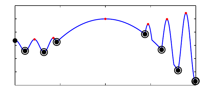
10 Chebfun Guide
-0.679567708415180
-0.538855701053878
0.438177223602422
0.622477687626771
0.804389189016844
0.995948373499376
−1−0.5 0 0.5 1
−3
−2
−1
0
1
2
3
3.4 Global extrema: max and min
If min or max is applied to a single chebfun, it returns its global minimum or maximum. For example:
f = chebfun(’1-x.^2/2’);
[min(f) max(f)]
ans =
0.500000000000000 1.000000000000000
Chebfun computes such a result by checking the values of fat all endpoints and at zeros of the
derivative.
As with standard MATLAB, one can find the location of the extreme point by supplying two output
arguments:
[minval,minpos] = min(f)
minval =
0.500000000000000
minpos =
-1
Note that just one position is returned even though the minimum is attained at two points. This is
consistent with the behavior of standard MATLAB.
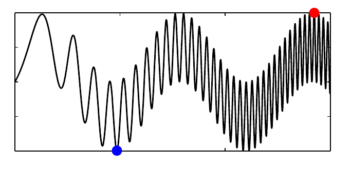
This ability to do global 1D optimization in Chebfun is rather remarkable. Here is a nontrivial
example.
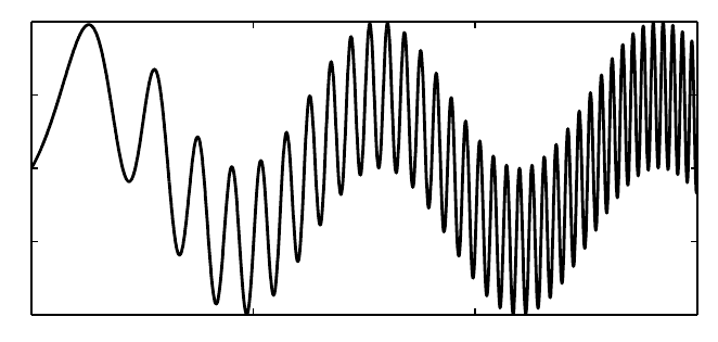
3. Rootfinding and Minima and Maxima 11
f = chebfun(’sin(x)+sin(x.^2)’,[0,15]);
hold off, plot(f,’k’)
0 5 10 15
−2
−1
0
1
2
The length of this chebfun is not as great as one might imagine:
length(f)
ans =
216
Here are its global minimum and maximum:
[minval,minpos] = min(f)
[maxval,maxpos] = max(f)
hold on
plot(minpos,minval,’.b’,MS,30)
plot(maxpos,maxval,’.r’,MS,30)
minval =
-1.990085468159411
minpos =
4.852581429906174
maxval =
1.995232599437864
maxpos =
14.234791972306914
12 Chebfun Guide
0 5 10 15
−2
−1
0
1
2
For larger chebfuns, it is inefficient to compute the global minimum and maximum separately like
this – each one must compute the derivative and find all its zeros. The alternative minandmax code
mentioned above provides a faster alternative:
[extremevalues,extremepositions] = minandmax(f)
extremevalues =
-1.990085468159411
1.995232599437864
extremepositions =
4.852581429906174
14.234791972306914
3.5 norm(f,1) and norm(f,inf)
The default, 2-norm form of the norm command was considered in Section 2.2. In standard MAT-
LAB one can also compute 1-, ∞-, and Frobenius norms with norm(f,1),norm(f,inf),and
norm(f,’fro’). These have been overloaded in Chebfun, and in the first two cases, rootfinding
is part of the implementation. (The 2- and Frobenius norms are equal for a single chebfun but differ
for quasimatrices; see Chapter 6.) The 1-norm norm(f,1) is the integral of the absolute value, and
Chebfun computes this by adding up segments between zeros, at which |f(x)|will typically have a
discontinuous slope. The ∞-norm is computed from the formula ∥f∥∞=max(max(f),−min(f)).
For example:
f = chebfun(’sin(x)’,[103 103+4*pi]);
norm(f,inf)
norm(f,1)
ans =
1.000000000000004
ans =
7.999999999999984
3. Rootfinding and Minima and Maxima 13
3.6 Roots in the complex plane
Chebfuns live on real intervals, and the funs from which they are made live on real subintervals.
But a polynomial representing a fun may have roots outside the interval of definition, which may be
complex. Sometimes we may want to get our hands on these roots, and the roots command makes
this possible in various ways through the flags ’all’,’complex’,and’norecursion’.
The simplest example is a chebfun that is truly intended to correspond to a polynomial. For example,
the chebfun
f = 1+16*x.^2;
has no roots in [−1,1]:
roots(f)
ans =
Empty matrix: 0-by-1
We can extract its complex roots with the command
roots(f,’all’)
ans =
0.000000000000000 - 0.250000000000000i
0.000000000000000 + 0.250000000000000i
The situation for more general chebfuns is more complicated. For example, the chebfun
g = exp(x).*f(x);
also has no roots in [-1,1],
roots(g)
ans =
Empty matrix: 0-by-1
but it has plenty of roots in the complex plane:
roots(g,’all’)
ans =
-0.000000000000005 - 0.249999999999983i
-0.000000000000005 + 0.249999999999983i
-4.513839611821153 + 0.000000000000000i
-4.304953574643823 - 1.512787764786624i
-4.304953574643823 + 1.512787764786624i
-3.665238911771629 - 2.987288348279861i
14 Chebfun Guide
-3.665238911771629 + 2.987288348279861i
-2.550107949077733 - 4.375390939226574i
-2.550107949077733 + 4.375390939226574i
-0.861360687347932 - 5.603012177418021i
-0.861360687347932 + 5.603012177418021i
1.622627117319532 - 6.531305785733470i
1.622627117319532 + 6.531305785733470i
5.548850506877216 - 6.812852935529656i
5.548850506877216 + 6.812852935529656i
Most of these are spurious. What has happened is that gis represented by a polynomial chosen for
its approximation properties on [−1,1]. Inevitably that polynomial will have roots in the complex
plane, even if they have little to do with g. (See the discussion of the Walsh and Blatt-Safftheorems
in Chapter 18 of [Trefethen 2013].)
One cannot expect Chebfun to solve this problem perfectly – after all, it is working on a real interval,
not in the complex plane, and analytic continuation from the one to the other is well known to be
an ill-posed problem. Nevertheless, Chebfun may do a pretty good job of selecting genuine complex
(and real) roots near the interval of definition if you use the ’complex’ flag:
roots(g,’complex’)
ans =
-0.000000000000005 - 0.249999999999983i
-0.000000000000005 + 0.249999999999983i
We will not go into detail here of how this is done, but the idea is that associated with any fun is
a family of ”Chebfun ellipses” in the complex plane, with foci at the endpoints, inside which one
may expect reasonably good accuracy of the fun. Assuming the interval is [−1,1] and the fun has
length L, the Chebfun ellipse associated with a parameter δ≪1 is the region in the complex plane
bounded by the image under the map (z+1/z)/2 of the circle |z|=r,whereris defined by the
condition r−L=δ. (See Chapter 8 of [Trefethen 2013].) The command roots(g,’complex’) first
effectively does roots(g,’all’), then returns only those roots lying inside a particular Chebfun
ellipse – we take the one corresponding to delta equal to the square root of the Chebfun tolerance
parameter eps.
One must expect complex roots of chebfuns to lose accuracy as one moves away from the interval of
definition. Here’s an example:
f = exp(exp(x)).*(x-0.1i).*(x-.3i).*(x-.6i).*(x-1i);
roots(f,’complex’)
ans =
-0.000000000001405 + 0.099999999998765i
0.000000000832193 + 0.300000000573215i
-0.000001488909431 + 0.599999277205987i
Notice that the first three imaginary roots are located with about 11, 8, and 5 digits of accuracy,
while the fourth does not appear in the list at all.
Here is a more complicated example:
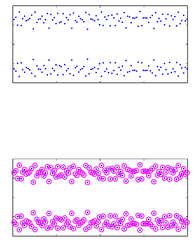
3. Rootfinding and Minima and Maxima 15
F = @(x) 4+sin(x)+sin(sqrt(2)*x)+sin(pi*x);
f = chebfun(F,[-100,100]);
This function has a lot of complex roots lying in strips on either side of the real axis.
r = roots(f,’complex’);
hold off, plot(r,’.’,MS,8)
−100 −50 0 50 100
−1
−0.5
0
0.5
1
If you are dealing with complex roots of complicated chebfuns like this, it may be safer to add a flag
’norecursion’ to the roots call, at the cost of slowing down the computation. This turns offthe
Boyd-Battles recursion mentioned above, lowering the chance of missing a few roots near interfaces
of the recursion. If we try that here we find that the results look almost the same as before in a
plot:
r2 = roots(f,’complex’,’norecursion’);
hold on, plot(r,’om’,MS,8)
−100 −50 0 50 100
−1
−0.5
0
0.5
1
However, the accuracy has improved:
norm(F(r))
norm(F(r2))
ans =
3.498622420314460e-08
16 Chebfun Guide
ans =
4.818930650722706e-09
To find poles in the complex plane as opposed to zeros, see Section 4.8.Moreadvancedmethods
of rootfinding and polefinding are based on rational approximations rather than polynomials, an
area where Chebfun has significant capabilities; see the next chapter of this guide, Chapter 28 of
[Trefethen 2013], and [Webb 2013].
3.7 References
[Battles 2006] Z. Battles, Numerical Linear Algebra for Continuous Functions, DPhil thesis, Oxford
University Computing Laboratory, 2006.
[Boyd 2002] J. A. Boyd, ”Computing zeros on a real interval through Chebyshev expansion and
polynomial rootfinding”, SIAM Journal on Numerical Analysis, 40 (2002), 1666-1682.
[Good 1961] I. J. Good, ”The colleague matrix, a Chebyshev analogue of the companion matrix”,
Quarterly Journal of Mathematics, 12 (1961), 61-68.
[Specht 1960] W. Specht, ”Die Lage der Nullstellen eines Polynoms. IV”, Mathematische
Nachrichten, 21 (1960), 201-222.
[Trefethen 2013] L. N. Trefethen, Approximation Theory and Approximation Practice,SIAM,2013.
[Webb 2011] M. Webb, ”Computing complex singularities of differential equations with Chebfun”,
SIAM Undergraduate Research Online,6(2013),
http://dx.doi.org/10.1137/12S011520
.
4. Chebfun and Approximation
Theory
Lloyd N. Trefethen, November 2009, latest revision June 2014
Contents
•4.1 Chebyshev series and interpolants
•4.2 chebcoeffs and poly
•4.3 chebfun(...,N) and the Gibbs phenomenon
•4.4 Smoothness and rate of convergence
•4.5 Five theorems
•4.6 Best approximations and the Remez algorithm
•4.7 The Runge phenomenon
•4.8 Rational approximations
•4.9 References
4.1 Chebyshev series and interpolants
Chebfun is founded on the mathematical subject of approximation theory, and in particular, on
Chebyshev series and interpolants. Conversely, it provides a simple environment in which to demon-
strate these approximants and other approximation ideas.
The history of ”Chebyshev technology” goes back to the 19th century Russian mathematician
Pafnuty Chebyshev (1821-1894) and his mathematical descendants such as Zolotarev and Bernstein
(1880-1968). These men realized that just as Fourier series provide an efficient way to represent a
smooth periodic function, series of Chebyshev polynomials can do the same for a smooth nonperiodic
function. A number of excellent textbooks and monographs have been published on approximation
theory, including [Davis 1963], [Cheney 1966], [Meinardus 1967], [Lorentz 1986], and Powell [Powell,
1981], and in addition there are books devoted entirely to Chebyshev polynomials, including [Rivlin
1974] and [Mason & Handscomb 2003]. A Chebfun-based book on approximation theory and its
computational applications is particularly relevant for Chebfun users [Trefethen 2013].
From the dates of publication above it will be clear that approximation theory flourished in the
early computer era, and in the 1950s and 1960s a number of numerical methods were developed
based on Chebyshev polynomials by Lanczos [Lanczos 1957], Fox [Fox & Parker 1966], Clenshaw,
Elliott, Mason, Good, and others. The Fast Fourier Transform came in 1965 and Salzer’s barycentric
interpolation formula for Chebyshev points in 1972 [Salzer 1972]. Then in the 1970s Orszag and
Gottlieb introduced spectral methods, based on the application of Chebyshev and Fourier technology
to the solution of PDEs. The subject grew rapidly, and it is in the context of spectral methods that
1
2Chebfun Guide
Chebyshev techniques are particularly well known today [Boyd 2001], [Trefethen 2000], [Canuto et
al. 2006/7].
We must be clear about terminology. We shall rarely use the term Chebyshev approximation,
for that expression refers specifically to an approximation that is optimal in the minimax sense.
Chebyshev approximations are fascinating, and in Section 4.6 we shall see that Chebfun makes it
easy to compute them, but the core of Chebfun is built on the different techniques of polynomial
interpolation in Chebyshev points and expansion in Chebyshev polynomials. These approximations
are not quite optimal, but they are nearly optimal and much easier to compute.
By Chebyshev points we shall mean the set of points in [−1,1] defined by
xj=−cos(jπ/N ),0≤j≤N,
where N≥1 is an integer. (If N=0,wetakex0= 0.) A fuller name is that these are Chebyshev
points of the second kind. (Chebfun also enables computations based on Chebyshev points ofthe
first kind; see Section 8.9.) Through any data values fjat these points there is a unique polynomial
interpolant p(x)ofdegree≤N, which we call the Chebyshev interpolant. In particular, if the
data are fj=(−1)n−j,thenp(x) is TN(x), the degree NChebyshev polynomial, which can also be
defined by the formula TN(x)=cos(Ncos−1(x)). In Chebfun, the command chebpoly(N) returns a
chebfun corresponding to TN,andpoly returns coefficients in the monomial basis 1,x,x
2,....Thus
we can print the coefficients of the first few Chebyshev polynomials like this:
for N = 0:8
disp(poly(chebpoly(N)))
end
1
10
20-1
40-30
80-801
16 0 -20 0 5 0
32 0 -48 0 18 0 -1
64 0 -112 0 56 0 -7 0
128 0 -256 0 160 0 -32 0 1
Note that that output of poly follows the pattern for MATLAB’s standard poly command: it is a
row vector, and the high-order coefficients come first. Thus, for example, the fourth row above tells
us that T3(x)=4x3−3x.
Here are plots of T2,T3,T15,andT50.
subplot(2,2,1), plot(chebpoly(2))
subplot(2,2,2), plot(chebpoly(3))
subplot(2,2,3), plot(chebpoly(15))
subplot(2,2,4), plot(chebpoly(50))
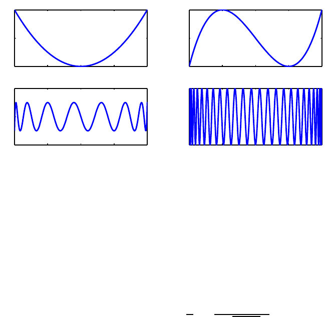
4. Chebfun and Approximation Theory 3
−1−0.5 0 0.5 1
−1
0
1
−1−0.5 0 0.5 1
−1
0
1
−1−0.5 0 0.5 1
−2
0
2
−1−0.5 0 0.5 1
−1
0
1
AChebyshev series is an expansion
f(x)=
∞
!
k=0
akTk(x),
and the akare known as Chebyshev coefficients. So long as fis continuous and at least a little
bit smooth (Lipschitz continuity is enough), it has a unique expansion of this form, which converges
absolutely and uniformly, and the coefficients are given by the integral
ak=2
π"1
−1
f(x)Tk(x)dx
√1−x2
except that for k=0,theconstantchangesfrom2/πto 1/π. One way to approximate a function is
to form the polynomials obtained by truncating its Chebyshev expansion,
fN(x)=
N
!
k=0
akTk(x).
This isn’t quite what Chebfun does, however, since it does not compute exact Chebyshev coeffi-
cients. Instead Chebfun constructs its approximations via Chebyshev interpolants, which can also
be regarded as finite series in Chebyshev polynomials for some coefficients ck:
pN(x)=
N
!
k=0
ckTk(x).
Each coefficient ckwill converge to akas N→∞(apart from the effects of rounding errors), but for
finite N,ckand akare different. Chebfun versions 1-4 stored functions via their values at Chebyshev
points, whereas version 5 switched to Chebyshev coefficients, but this hardly matters to the user,
and both representations are exploited for various purposes internally in the system.
4Chebfun Guide
4.2 chebcoeffs and poly
We have just seen that the command chebpoly(N) returns a chebfun corresponding to the Chebyshev
polynomial TN. Conversely, if fis a chebfun, then chebcoeffs(f) is the vector of its Chebyshev
coefficients. (Before Version 5, the command for this was chebpoly.) For example, here are the
Chebyshev coefficients of x3:
x = chebfun(@(x) x);
c = chebcoeffs(x.^3)
c=
Columns 1 through 3
0.250000000000000 0 0.750000000000000
Column 4
0
Like poly,chebcoeffs returns a row vector with the high-order coefficients first. Thus this compu-
tation reveals the identity x3=(1/4)T3(x)+(3/4)T1(x).
If we apply chebcoeffs to a function that is not ”really” a polynomial, we will usually get a vector
whose first entry (i.e., highest order) is just above machine precision. This reflects the adaptive
nature of the Chebfun constructor, which always seeks to use a minimal number of points.
chebcoeffs(sin(x))
ans =
Columns 1 through 3
0.000000000000039 0 -0.000000000023960
Columns 4 through 6
0 0.000000010498500 0
Columns 7 through 9
-0.000003004651635 0 0.000499515460422
Columns 10 through 12
0 -0.039126707965337 0
Columns 13 through 14
0.880101171489867 0
Of course, machine precision is defined relative to the scale of the function:
chebcoeffs(1e100*sin(x))
ans =
1.0e+99 *
Columns 1 through 3
0.000000000000385 0 -0.000000000239601
Columns 4 through 6
0 0.000000104985004 0
Columns 7 through 9
-0.000030046516349 0 0.004995154604224
Columns 10 through 12
4. Chebfun and Approximation Theory 5
0 -0.391267079653368 0
Columns 13 through 14
8.801011714898671 0
By using poly we can print the coefficients of such a chebfun in the monomial basis. Here for
example are the coefficients of the Chebyshev interpolant of exp(x) compared with the Taylor series
coefficients:
cchebfun = flipud(chebcoeffs(exp(x))’);
ctaylor = 1./gamma(1:length(cchebfun))’;
disp(’ chebfun Taylor’)
disp([cchebfun ctaylor])
chebfun Taylor
1.266065877752008 1.000000000000000
1.130318207984970 1.000000000000000
0.271495339534077 0.500000000000000
0.044336849848664 0.166666666666667
0.005474240442094 0.041666666666667
0.000542926311914 0.008333333333333
0.000044977322954 0.001388888888889
0.000003198436462 0.000198412698413
0.000000199212481 0.000024801587302
0.000000011036772 0.000002755731922
0.000000000550590 0.000000275573192
0.000000000024980 0.000000025052108
0.000000000001039 0.000000002087676
0.000000000000040 0.000000000160590
0.000000000000001 0.000000000011471
The fact that these differ is not an indication of an error in the Chebfun approximation. On the
contrary, the Chebfun coefficients do a better job of approximating than the truncated Taylor series.
If fwere a function like 1/(1 + 25x2), the Taylor series would not converge at all.
4.3 chebfun(...,N) and the Gibbs phenomenon
We can examine the approximation qualities of Chebyshev interpolantsbymeansofacommand
of the form chebfun(...,N). When an integer Nis specified in this manner, it indicates that a
Chebyshev interpolant is to be constructed of precisely length Nrather than by the usual adaptive
process.
Let us begin with a function that cannot be well approximated by polynomials, the step function
sign(x). To start with we interpolate it in 10 or 20 points, taking Nto be even to avoid including a
value 0 at the middle of the step.
f = chebfun(’sign(x)’,10);
subplot(1,2,1), plot(f,’.-’), grid on
f = chebfun(’sign(x)’,20);
subplot(1,2,2), plot(f,’.-’), grid on
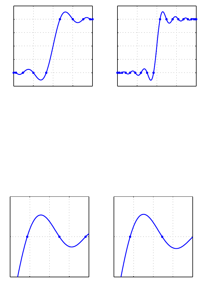
6Chebfun Guide
−1−0.5 0 0.5 1
−1.5
−1
−0.5
0
0.5
1
1.5
−1−0.5 0 0.5 1
−1.5
−1
−0.5
0
0.5
1
1.5
There is an overshoot problem here, known as the Gibbs phenomenon, that does not go away as
N→∞. We can zoom in on the overshoot region by resetting the axes:
subplot(1,2,1), axis([0 .8 .5 1.5])
subplot(1,2,2), axis([0 .4 .5 1.5])
0 0.2 0.4 0.6 0.8
0.5
1
1.5
0 0.1 0.2 0.3 0.4
0.5
1
1.5
Here are analogous results with N= 100 and 1000.
f = chebfun(’sign(x)’,100);
subplot(1,2,1), plot(f,’.-’), grid on, axis([0 .08 .5 1.5])
f = chebfun(’sign(x)’,1000);
subplot(1,2,2), plot(f,’.-’), grid on, axis([0 .008 .5 1.5])
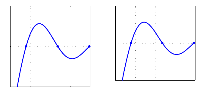
4. Chebfun and Approximation Theory 7
0 0.02 0.04 0.06 0.08
0.5
1
1.5
0 2 4 6 8
x 10−3
0.5
1
1.5
What is the amplitude of the Gibbs overshoot for Chebyshev interpolation of a step function? We
can find out by using max:
for N = 2.^(1:8)
gibbs = max(chebfun(’sign(x)’,N));
fprintf(’%5d %13.8f\n’, N, gibbs)
end
2 1.00000000
4 1.18807518
8 1.26355125
16 1.27816423
32 1.28131717
64 1.28204939
128 1.28222585
256 1.28226917
This gets a bit slow for larger N, but knowing that the maximum occurs around x=3/N ,wecan
speed it up by using Chebfun’s {}notation to work on subintervals:
for N = 2.^(4:12)
f = chebfun(’sign(x)’,N);
fprintf(’%5d %13.8f\n’, N, max(f{0,5/N}))
end
16 1.27816423
32 1.28131717
64 1.28204939
128 1.28222585
256 1.28226917
512 1.28227990
1024 1.28228257
2048 1.28228323
4096 1.28228340
The overshoot converges to a number 1.282283455775 ...[Helmberg & Wagner 1997].
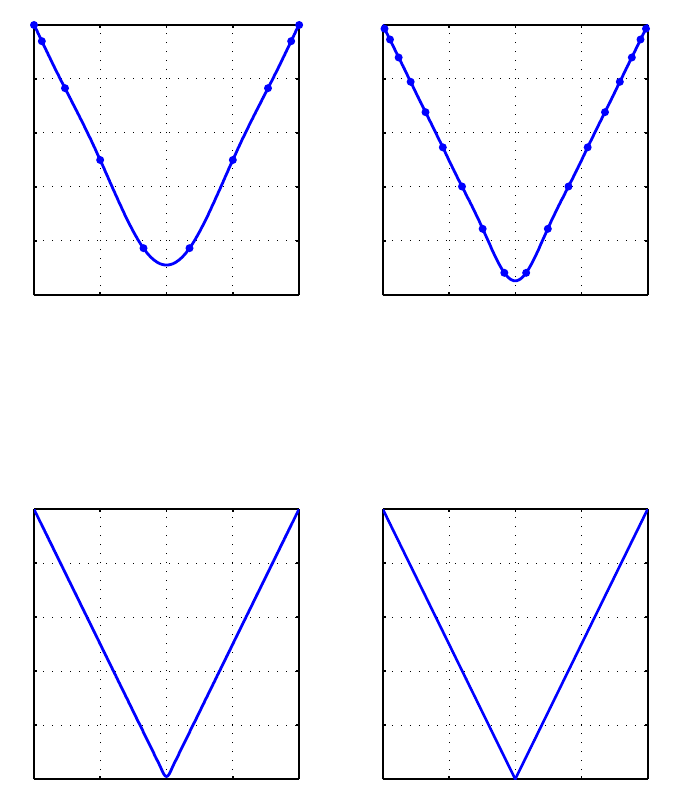
8Chebfun Guide
4.4 Smoothness and rate of convergence
The central dogma of approximation theory is this: the smoother the function, the faster the conver-
gence as N→∞. What this means for Chebfun is that so long as a function is twice continuously
differentiable, it can usually be approximated to machine precision for a workable value of N,even
without subdivision of the interval.
After the step function, a function with ”one more derivative” of smoothness would be the absolute
value. Here if we interpolate in Npoints, the errors decrease at the rate O(N−1). For example:
clf
f10 = chebfun(’abs(x)’,10);
subplot(1,2,1), plot(f10,’.-’), ylim([0 1]), grid on
f20 = chebfun(’abs(x)’,20);
subplot(1,2,2), plot(f20,’.-’), ylim([0 1]), grid on
−1−0.5 0 0.5 1
0
0.2
0.4
0.6
0.8
1
−1−0.5 0 0.5 1
0
0.2
0.4
0.6
0.8
1
Chebfun has no difficulty computing interpolants of much higher order:
f100 = chebfun(’abs(x)’,100);
subplot(1,2,1), plot(f100), ylim([0 1]), grid on
f1000 = chebfun(’abs(x)’,1000);
subplot(1,2,2), plot(f1000), ylim([0 1]), grid on
−1−0.5 0 0.5 1
0
0.2
0.4
0.6
0.8
1
−1−0.5 0 0.5 1
0
0.2
0.4
0.6
0.8
1
Such plots look good to the eye, but they do not achieve machine precision. We can confirm this by
using splitting on to compute a true absolute value and then measuring some norms.
4. Chebfun and Approximation Theory 9
fexact = chebfun(’abs(x)’,’splitting’,’on’);
err10 = norm(f10-fexact,inf)
err100 = norm(f100-fexact,inf)
err1000 = norm(f1000-fexact,inf)
err10 =
0.111111111111111
err100 =
0.010101010101010
err1000 =
0.001001001001002
Notice the clean linear decrease of the error as N increases.
If fis a bit smoother, polynomial approximation to machine precision becomes practical:
length(chebfun(’abs(x).*x’))
length(chebfun(’abs(x).*x.^2’))
length(chebfun(’abs(x).*x.^3’))
length(chebfun(’abs(x).*x.^4’))
ans =
32092
ans =
2935
ans =
884
ans =
419
Of course, these particular functions would be easily approximated by piecewise smooth chebfuns.
It is interesting to plot convergence as a function of N. Here is an example from [Battles & Trefethen
2004] involving the next function from the sequence above.
s = ’abs(x).^5’;
exact = chebfun(s,’splitting’,’off’);
NN = 1:100; e = [];
for N = NN
e(N) = norm(chebfun(s,N)-exact);
end
clf
subplot(1,2,1)
loglog(e), ylim([1e-10 10]), title(’loglog scale’)
hold on, loglog(NN.^(-5),’--r’), grid on
text(6,4e-7,’N^{-5}’,’color’,’r’,’fontsize’,16)
subplot(1,2,2)
semilogy(e), ylim([1e-10 10]), grid on, title(’semilog scale’)
hold on, semilogy(NN.^(-5),’--r’), grid on
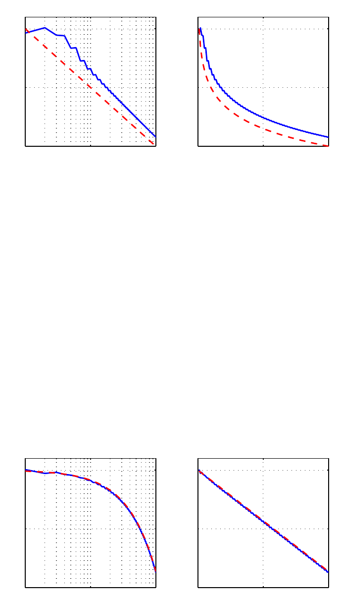
10 Chebfun Guide
100101102
10−10
10−5
100
loglog scale
N−5
0 50 100
10−10
10−5
100
semilog scale
The figure reveals very clean convergence at the rate N−5. According to Theorem 2 of the next
section, this happens because fhas a fifth derivative of bounded variation.
Here is an example of a smoother function, one that is in fact analytic. According to Theorem
3 of the next section, if fis analytic, its Chebyshev interpolants converge geometrically. In this
example we take fto be the Runge function, for which interpolants in equally spaced points would
not converge at all (in fact they diverge exponentially – see Section 4.7).
s = ’1./(1+25*x.^2)’;
exact = chebfun(s);
for N = NN
e(N) = norm(chebfun(s,N)-exact);
end
clf, subplot(1,2,1)
loglog(e), ylim([1e-10 10]), grid on, title(’loglog scale’)
c = 1/5 + sqrt(1+1/25);
hold on, loglog(c.^(-NN),’--r’), grid on
subplot(1,2,2)
semilogy(e), ylim([1e-10 10]), title(’semilog scale’)
hold on, semilogy(c.^(-NN),’--r’), grid on
text(45,1e-3,’C^{-N}’,’color’,’r’,’fontsize’,16)
100101102
10−10
10−5
100
loglog scale
0 50 100
10−10
10−5
100
semilog scale
C−N

4. Chebfun and Approximation Theory 11
This time the convergence is equally clean but quite different in nature. Now the straight line
appears on the semilogy axes rather than the loglog axes, revealing the geometric convergence.
4.5 Five theorems
The mathematics of Chebfun can be captured in five theorems about interpolants in Chebyshev
points. The first three can be found in [Battles & Trefethen 2004], and all are discussed in [Trefethen
2013]. Let fbe a continuous function on [−1,1], and let pdenote its interpolant in NChebyshev
points and p∗its best degree Napproximation with respect to the maximum norm ∥·∥.
The first theorem asserts that Chebyshev interpolants are ”near-best” [Ehlich & Zeller 1966].
THEOREM 1.
∥f−p∥≤(2 + (2/π) log(N))∥f−p∗∥.
This theorem implies that even if Nis as large as 100,000, one can lose no more than one digit by
using pinstead of \\(pˆ\*\\). Whereas Chebfun will readily compute such a p, it is unlikely that
anybody has ever computed a nontrivial p∗for a value of Nso large.
The next theorem asserts that if fis ktimes differentiable, roughly speaking, then the Chebyshev
interpolants converge at the algebraic rate 1/N k[Mastroianni & Szabados 1995].
THEOREM 2.Letf,f′,...,f(k−1) be absolutely continuous for some k≥1, and let f(k)be a
function of bounded variation. Then ∥f−p∥=O(N−k)asN→∞.
Smoother than this would be a C∞function, i.e. infinitely differentiable, and smoother still would
be a function analytic on [−1,1], i.e., one whose Taylor series at each point of [−1,1] converges at
least in a small neighborhood of that point. For analytic functions the convergence is geometric.
The essence of the following theorem is due to Bernstein in 1912, though it is not clear where an
explicit statement first appeared in print.
THEOREM 3.Iffis analytic and bounded in the ”Bernstein ellipse” of foci 1 and −1 with
semimajor and semiminor axis lengths summing to r,then∥f−p∥=O(r−N)asN→∞.
More precisely, if |f(z)|≤Min the ellipse, then the bound on the right can be taken as 4Mr−n/(r−
1).
The next theorem asserts that Chebyshev interpolants can be computed by the barycentric formula
[Salzer 1972]. The sumation with a double prime denotes the sum from k=0tok=Nwith both
terms k=0andk=Nmultiplied by 1/2.
THEOREM 4.
p(x)=
N
!
k=0
”(−1)kf(xk)
x−xk#N
!
k=0
”(−1)k
x−xk
.
See [Berrut & Trefethen 2005] and [Trefethen 2013] for information about barycentric interpolation.
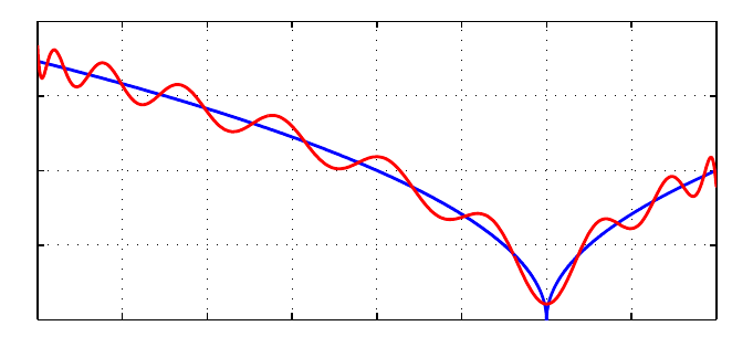
12 Chebfun Guide
The final theorem asserts that the barycentric formula has no difficulty with rounding errors. Our
”theorem” is really just an advertisement; see [Higham 2004] for a precise statement and proof.
Earlier work on this subject appeared in [Rack & Reimer 1982].
THEOREM 5. The barycentric formula of Theorem 4 is numerically stable.
This stability result may seem surprising when one notes that for xclose to xk, the barycentric
formula involves divisions by numbers that are nearly zero. Nevertheless it is provably stable. If xis
exactly equal to some xk, then one bypasses the formula and returns the exact value p(x)=f(xk).
4.6 Best approximations and the Remez algorithm
For practical computations, it is rarely worth the trouble to compute a best (minimax) approximation
rather than simply a Chebyshev interpolant. Nevertheless best approximations are a beautiful and
well-established idea, and it is certainly interesting to be able to compute them. Chebfun makes this
possible with the command remez, named after Evgeny Remez, who devised the standard algorithm
for computing these approximations in 1934. This capability is due to Ricardo Pachon; see [Pachon
& Trefethen 2009].
For example, here is a function on the interval [0,4] together with its best approximation by a
polynomial of degree 20:
f = chebfun(’sqrt(abs(x-3))’,[0,4],’splitting’,’on’);
p = remez(f,20);
clf, plot(f,’b’,p,’r’), grid on
0 0.5 1 1.5 2 2.5 3 3.5 4
0
0.5
1
1.5
2
A plot of the error curve (f−p)(x) shows that it equioscillates between 20 + 2 = 22 alternating
extreme values. Note that a second output argument from remez returns the error as well as the
polynomial.
[p,err] = remez(f,20);
plot(f-p,’m’), hold on
plot([0 4],err*[1 1],’--k’), plot([0 4],-err*[1 1],’--k’)
ylim(3*err*[-1,1])
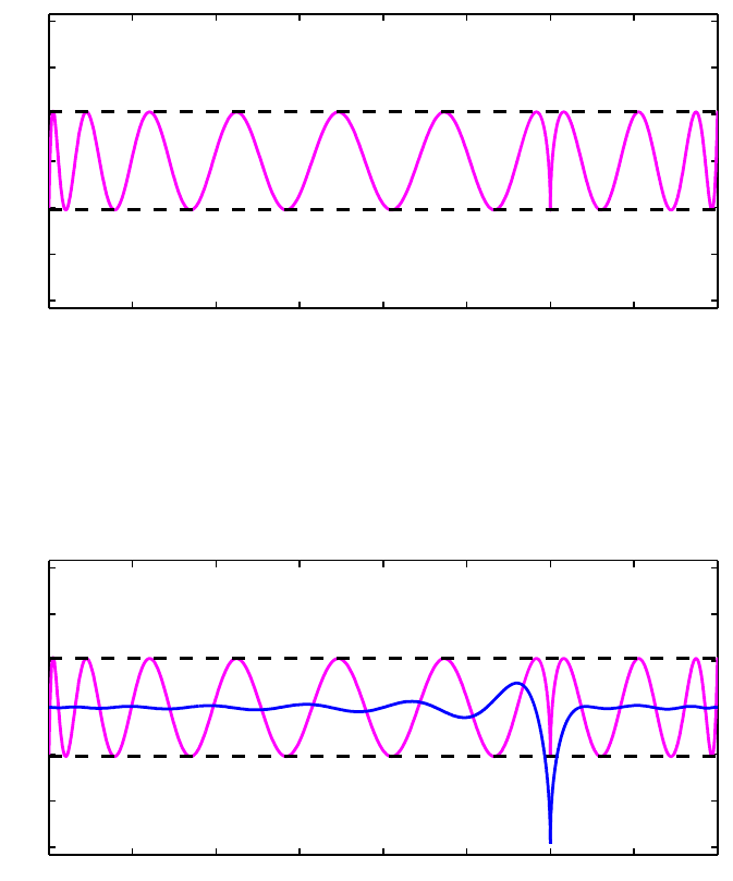
4. Chebfun and Approximation Theory 13
0 0.5 1 1.5 2 2.5 3 3.5 4
−0.3
−0.2
−0.1
0
0.1
0.2
0.3
Let’s add the error curve for the degree 20 (i.e. 21-point) Chebyshev interpolant to the same plot:
pinterp = chebfun(f,[0,4],21);
plot(f-pinterp,’b’)
0 0.5 1 1.5 2 2.5 3 3.5 4
−0.3
−0.2
−0.1
0
0.1
0.2
0.3
Notice that although the best approximation has a smaller maximum error, it is a worse approxi-
mation for most values of x.
Chebfun’s remez command can compute certain rational best approximants too, though it is some-
what fragile. If your function is smooth, a possibly more robust approach to computing best ap-
proximations is Caratheodory-Fejer approximation, implemented in the code cf due to Joris Van
Deun [Van Deun & Trefethen 2011]. For example:
f = chebfun(’exp(x)’);
[p,q] = cf(f,5,5);
r = p./q;
err = norm(f-r,inf);
clf, plot(f-r,’c’), hold on
plot([-1 1],err*[1 1],’--k’), plot([-1 1],-err*[1 1],’--k’)
ylim(2e-13*[-1 1])
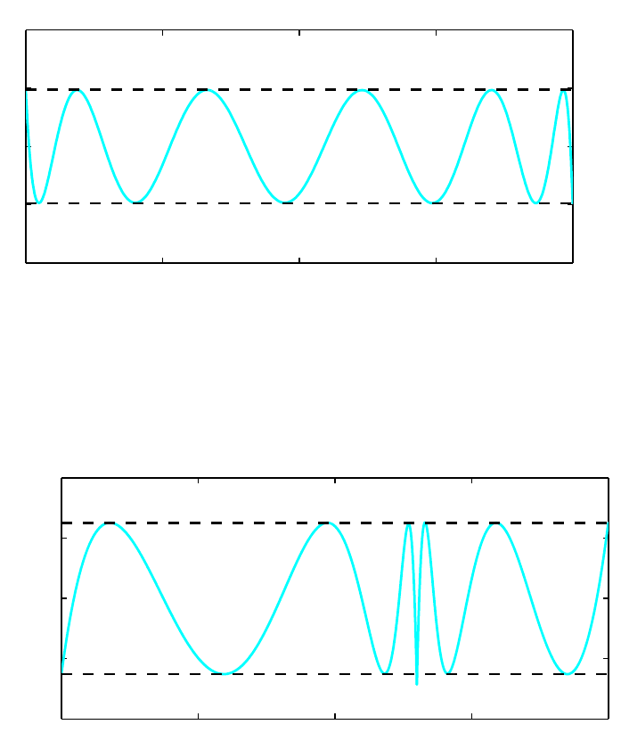
14 Chebfun Guide
−1−0.5 0 0.5 1
−2
−1
0
1
2x 10⁻¹³
CF approximation often comes close to optimal for non-smooth functions too, provided you specify
a fourth argument to tell the system which Chebyshev grid to use:
f = abs(x-.3);
[p,q,r_handle,lam] = cf(f,5,5,300);
clf, plot(f-p./q,’c’), hold on
plot([-1 1],lam*[1 1],’--k’), plot([-1 1],-lam*[1 1],’--k’)
−1−0.5 0 0.5 1
−0.01
−0.005
0
0.005
0.01
4.7 The Runge phenomenon
Chebfun is based on polynomial interpolants in Chebyshev points, not equispaced points. It has
been known for over a century that the latter choice is disastrous, even for interpolation of smooth
functions [Runge 1901]. One should never use equispaced polynomial interpolants for practical work
(unless you will only need the result near the center of the interval of interpolation), but like best
approximations, they are certainly interesting.
In Chebfun, we can compute them with the interp1 command. For example, here is an analytic
function and its equispaced interpolant of degree 9:
f = tanh(10*x);
s = linspace(-1,1,10);
p = chebfun.interp1(s,f(s)); hold off
plot(f), hold on, plot(p,’r’), grid on, plot(s,p(s),’.r’)
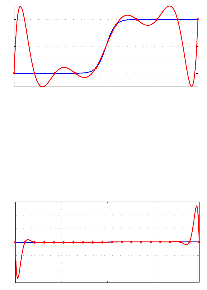
4. Chebfun and Approximation Theory 15
−1−0.5 0 0.5 1
−1.5
−1
−0.5
0
0.5
1
1.5
Perhaps this doesn’t look too bad, but here is what happens for degree 19. Note the vertical scale.
s = linspace(-1,1,20);
p = chebfun.interp1(s,f(s)); hold off
plot(f), hold on, plot(p,’r’), grid on, plot(s,p(s),’.r’)
−1−0.5 0 0.5 1
−150
−100
−50
0
50
100
150
Approximation experts will know that one of the tools used in analyzingeffects like this is known as
the Lebesgue function associated with a given set of interpolation points. Chebfun has a command
lebesgue for computing these functions. The problem with interpolation in 20 equispaced points is
reflected in a Lebesgue function of size 104– note the semilog scale:
clf, semilogy(lebesgue(s))
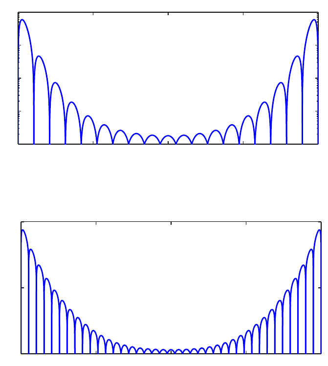
16 Chebfun Guide
−1−0.5 0 0.5 1
100
101
102
103
104
For 40 points it is much worse:
semilogy(lebesgue(linspace(-1,1,40)))
−1−0.5 0 0.5 1
100
105
1010
As the degree increases, polynomial interpolants in equispaced points diverge exponentially, and no
other method of approximation based on equispaced data can completely get around this problem
[Platte, Trefethen & Kuijlaars 2011].
4.8 Rational approximations
Chebfun contains four different programs, at present, for computing rational approximants to a
function f. We say that a rational function is of type (m, n) if it can be written as a quotient of one
polynomial of degree at most mand another of degree at most n.
To illustrate the possibilities, consider the function
f = chebfun(’tanh(pi*x/2) + x/20’,[-10,10]);
length(f)
plot(f)
ans =
350
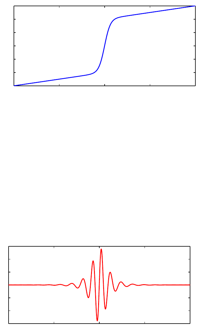
4. Chebfun and Approximation Theory 17
−10 −5 0 5 10
−1.5
−1
−0.5
0
0.5
1
1.5
We can use the command chebpade, developed by Ricardo Pachon, to compute a Chebyshev-Pade
approximant, defined by the condition that the Chebyshev series of p/q should match that of fas
far as possible [Baker & Graves-Morris 1996]. (This is the so-called ”Clenshaw-Lord” Chebyshev-
Pade approximation; if the flag maehly is specified the code alternatively computes the linearized
variation known as the ”Maehly” approximation.) Chebyshev-Pade approximation is the analogue
for functions defined on an interval of Pade approximation for functions defined in a neighborhood
of a point.
[p,q] = chebpade(f,40,4);
r = p./q;
The functions fand rmatch to about 8 digits:
norm(f-r)
plot(f-r,’r’)
ans =
4.884639793650636e-09
−10 −5 0 5 10
−6
−4
−2
0
2
4
6x 10⁻⁹
Mathematically, fhas poles in the complex plane at ±i,±3i,±5i, and so on. We can obtain
approximations to these values by looking at the roots of q:
roots(q,’complex’)
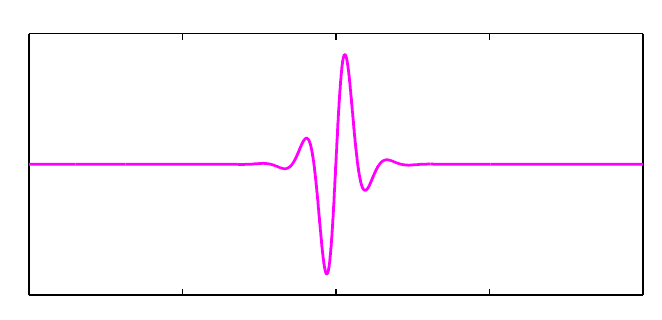
18 Chebfun Guide
ans =
0.000000000000000 - 1.000000750727884i
0.000000000000000 + 1.000000750727884i
0.000000000000000 - 3.004284960255872i
0.000000000000000 + 3.004284960255872i
A similar but perhaps faster and more robust approach to rational interpolation is encoded in the
command ratinterp, which computes a type (m, n) interpolant through m+n+1 Chebyshev points
(or, optionally, a different set of points). This capability was developed by Ricardo Pachon, Pedro
Gonnet and Joris Van Deun [Pachon, Gonnet & Van Deun 2012]. The results are similar:
[p,q] = ratinterp(f,40,4);
r = p./q;
norm(f-r)
plot(f-r,’m’)
ans =
3.501041670519031e-07
−10 −5 0 5 10
−5
0
5x 10⁻⁷
Again the poles are not bad:
roots(q,’complex’)
ans =
0.000000000000000 - 1.000011080641719i
0.000000000000000 + 1.000011080641719i
0.000000000000000 - 3.010648453090407i
0.000000000000000 + 3.010648453090407i
The third and fourth options for rational approximation, as mentioned in Section 4.6, are best
approximants computed by remez and Caratheodory-Fejer approximants computed by cf [Trefethen
& Gutknecht 1983, Van Deun & Trefethen 2011]. As mentioned in Section 4.6, CF approximants
often agree with best approximations to machine precision if fis smooth. We explore the same
function yet again, and this time obtain an equioscillating error curve:
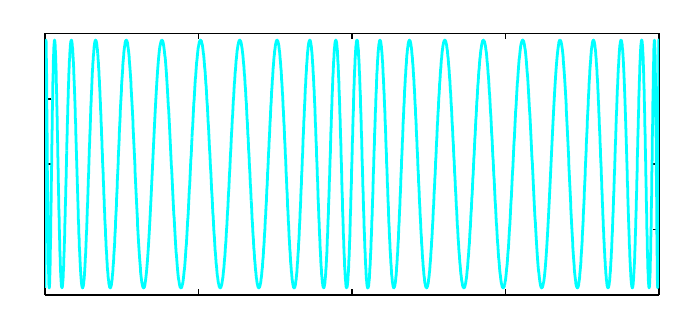
4. Chebfun and Approximation Theory 19
[p,q] = cf(f,40,4);
r = p./q;
norm(f-r)
plot(f-r,’c’)
ans =
2.999172427815131e-10
−10 −5 0 5 10
−0.5
0
0.5
x 10−10
And the poles:
roots(q,’complex’)
ans =
0.000000000000004 - 1.000000066684812i
0.000000000000004 + 1.000000066684812i
0.000000000002217 - 3.001936139233654i
0.000000000002217 + 3.001936139233654i
It is tempting to vary parameters and functions to explore more poles and what accuracy can be
obtained for them. But rational approximation and analytic continuation are very big subjects and
we shall resist the temptation. See Chapter 28 of [Trefethen 2013] and [Webb, Trefethen & Gonnet
2012].
4.9 References
[Baker and Graves-Morris 1996] G. A. Baker, Jr. and P. Graves-Morris, Pade Approximants,2nd
ed., Cambridge U. Press, 1996.
[Battles & Trefethen 2004] Z. Battles and L. N. Trefethen, ”An extension of MATLAB to continuous
functions and operators”, SIAM Journal on Scientific Computing, 25 (2004), 1743-1770.
[Berrut & Trefethen 2005] J.-P. Berrut and L. N. Trefethen, ”Barycentric Lagrange interpolation”,
SIAM Review, 46 (2004), 501-517.
[Boyd 2001] J. P. Boyd, Chebyshev and Fourier Spectral Methods, 2nd ed., Dover, 2001.
20 Chebfun Guide
[Canuto et al. 2006/7] C. Canuto, M. Y. Hussaini, A. Quarteroni andT.A.Zang,Spectral Methods,
2 vols., Springer, 2006 and 2007.
[Cheney 1966] E. W. Cheney, Introduction to Approximation Theory, McGraw-Hill 1966 and
AMS/Chelsea, 1999.
[Davis 1963] P. J. Davis, Interpolation and Approximation, Blaisdell, 1963 and Dover, 1975.
[Ehlich & Zeller 1966] H. Ehlich and K. Zeller, ”Auswertung der Normen von Interpolationsopera-
toren”, Mathematische Annalen, 164 (1966), 105-112.
[Fox & Parker 1966] L. Fox and I. B. Parker, Chebyshev Polynomials in Numerical Analysis,Oxford
U. Press, 1968.
[Helmberg & Wagner 1997] G. Helmberg & P. Wagner, ”Manipulating Gibbs’ phenomenon for Fourier
interpolation”, Journal of Approximation Theory, 89 (1997), 308-320.
[Higham 2004] N. J. Higham, ”The numerical stability of barycentric Lagrange interpolation”, IMA
Journal of Numerical Analysis, 24 (2004), 547-556.
[Lanczos 1956] C. Lanczos, Applied Analysis, Prentice-Hall, 1956 and Dover, 1988.
[Lorentz 1986] G. G. Lorentz, The Approximation of Functions, American Mathematical Society,
1986.
[Mason & Handscomb 2003] J. C. Mason and D. C. Handscomb, Chebyshev Polynomials,CRCPress,
2003.
[Mastroianni & Szabados 1995] G. Mastroianni and J. Szabados, ”Jackson order of approximation
by Lagrange interpolation”, Acta Mathematica Hungarica, 69 (1995), 73-82.
[Meinardus 1967] G. Meinardus, Approximation of Functions: Theory and Numerical Methods,
Springer, 1967.
[Pachon, Gonnet & Van Deun 2012] R. Pachon, P Gonnet and J. Van Deun, ”Fast and stable rational
interpolation in roots of unity and Chebyshev points”, SIAM Journal on Numerical Analysis,50
(2011), 1713-1734.
[Pachon & Trefethen 2009] R. Pachon and L. N. Trefethen, ”Barycentric-Remez algorithms for best
polynomial approximation in the chebfun system”, BIT Numerical Mathematics, 49 (2009), 721-741.
[Platte, Trefethen & Kuijlaars 2011] R. P. Platte, L. N. Trefethen and A. B. J. Kuijlaars, ”Impos-
sibility of fast stable approximation of analytic functions from equispaced samples”, SIAM Review,
53 (2011), 308-318.
[Powell 1981] M. J. D. Powell, Approximation Theory and Methods, Cambridge University Press,
1981.
[Rack & Reimer 1982] H.-J. Rack and M. Reimer, ”The numerical stability of evaluation schemes
for polynomials based on the Lagrange interpolation form”, BIT Numerical Mathematics,22(1982),
101-107.
[Rivlin 1974] T. J. Rivlin, The Chebyshev Polynomials, Wiley, 1974 and 1990.
4. Chebfun and Approximation Theory 21
[Runge 1901] C. Runge, ”Ueber empirische Funktionen und die Interpolation zwischen aequidistanten
Ordinaten”, Zeitschrift fuer Mathematik und Physik, 46 (1901), 224-243.
[Salzer 1972] H. E. Salzer, ”Lagrangian interpolation at the Chebyshev points cos(nu pi/n), nu =
0(1)n; some unnoted advantages”, Computer Journal, 15 (1972),156-159.
[Trefethen 2000] L. N. Trefethen, Spectral Methods in MATLAB,SIAM,2000.
[Trefethen 2013] L. N. Trefethen, Approximation Theory and Approximation Practice,SIAM,2013.
[Trefethen & Gutknecht 1983] L. N. Trefethen and M. H. Gutknecht, ”The Caratheodory-Fejer
method for real rational approximation”, SIAM Journal on Numerical Analysis, 20 (1983), 420-436.
[Van Deun & Trefethen 2011] J. Van Deun and L. N. Trefethen, A robust implementation of the
Caratheodory-Fejer method for rational approximation, BIT Numerical Mathematics,51(2011),
1039-1050.
[Webb, Trefethen & Gonnet 2012] M. Webb, L. N. Trefethen, and P. Gonnet, ”Stability of barycentric
interpolation formulas for extrapolation”, SIAM Journal on Scientific Computing, 34 (2013), A3009-
A3015.

!
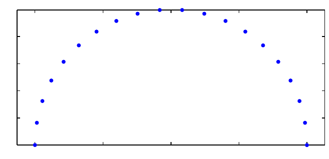
5. Complex Chebfuns
Lloyd N. Trefethen, November 2009, latest revision June 2014
Contents
•5.1 Complex functions of a real variable
•5.2 Analytic functions and conformal maps
•5.3 Contour integrals
•5.4 Cauchy integrals and locating zeros and poles
•5.5 Alphabet soup
•5.6 References
5.1 Complex functions of a real variable
One of the attractive features of MATLAB is that it handles complex arithmetic well. For example,
here are 20 points on the upper half of the unit circle in the complex plane:
s = linspace(0,pi,20);
f = exp(1i*s);
plot(f,’.’)
axis equal
−1−0.5 0 0.5 1
0
0.2
0.4
0.6
0.8
In MATLAB, both the variables iand jare initialized as i,thesquarerootof−1, but this code uses
1i instead (just as one might write, for example, 3+2i or 2.2-1.1i). Writing the imaginary unit
in this fashion is a common trick among MATLAB programmers, for it avoids the risk of surprises
caused by ior jhaving been overwritten by other values. The axis equal command ensures that
the real and imaginary axes are scaled equally.
1
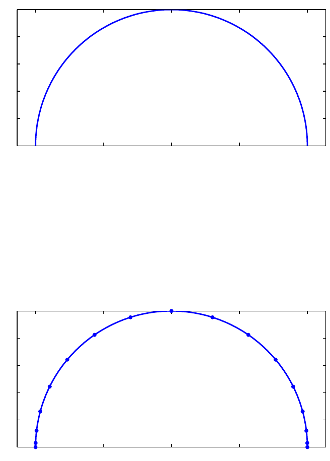
2Chebfun Guide
Here is a Chebfun analogue.
s = chebfun(@(s) s,[0 pi]);
f = exp(1i*s);
plot(f)
axis equal
−1−0.5 0 0.5 1
0
0.2
0.4
0.6
0.8
1
The Chebfun semicircle is represented by a polynomial of low degree:
length(f)
plot(f,’.-’)
axis equal
ans =
17
−1−0.5 0 0.5 1
0
0.2
0.4
0.6
0.8
1
We can have fun with variations on the theme:
subplot(1,2,1), g = s.*exp(10i*s); plot(g), axis equal
subplot(1,2,2), h = exp(2i*s)+.3*exp(20i*s); plot(h), axis equal
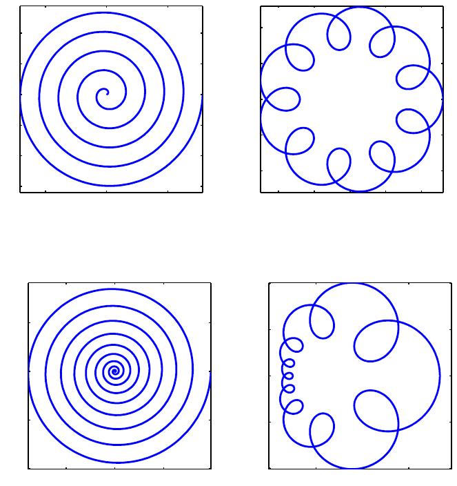
5. Complex Chebfuns 3
−2 0 2
−3
−2
−1
0
1
2
−1−0.5 0 0.5 1
−1
−0.5
0
0.5
1
subplot(1,2,1), plot(g.^2), axis equal
subplot(1,2,2), plot(exp(h)), axis equal
−5 0 5
−10
−5
0
5
0 1 2 3
−2
−1
0
1
2
Such plots make pretty pictures, but as always with Chebfun, the underlying operations involve
precise mathematics carried out to many digits of accuracy. For example, the integral of gis
−πi/10,
sum(g)
ans =
0.000000000000000 - 0.314159265358979i
and the integral of his zero:
sum(h)
ans =
-2.430648284784403e-18 - 1.522474749680446e-16i
Piecewise smooth complex chebfuns are also possible. For example, the following starts from a
chebfun zdefined as (1 + 0.5i)sfor son the interval [0,1] and 1 + 0.5i−2(s−1) for son the interval
[1,2].
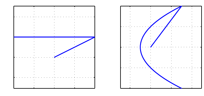
4Chebfun Guide
z = chebfun({@(s) (1+.5i)*s, @(s) 1+.5i-2*(s-1)},[0 1 2]);
subplot(1,2,1), plot(z), axis equal, grid on
subplot(1,2,2), plot(z.^2), axis equal, grid on
−0.5 0 0.5 1
−0.5
0
0.5
1
−0.5 0 0.5 1
−0.5
0
0.5
1
Actually, this way of constructing a piecewise chebfun is rather clumsy. An easier method is to use
the join command, in which a construction like join(f,g,h) constructs a single chebfun with the
same values as f,g,andh, but on a domain concatenated together. Thus if the domains of f,g,
hare [a, b], [c, d], and [e, f], then join(f,g,h) has three pieces with domains [a, b], [b, b +(d−c)],
[b+(d−c),b+(d−c)+(f−e)]. Using this trick, we can construct the chebfun zabove in the
following alternative manner:
s = chebfun(@(s) s,[0 1]);
zz = join((1+.5i)*s, 1+.5i-2*s);
norm(z-zz)
ans =
1.281975124255710e-16
5.2 Analytic functions and conformal maps
A function is analytic if it is differentiable in the complex sense, or equivalently, if it has a convergent
Taylor series near each point in its domain of definition. Analytic functions do interesting things in
the complex plane. In particular, away from points where the derivative is zero, they are conformal
maps, which means that though they may scale and rotate an infinitesimal region, they preserve
angles between intersecting curves.
For example, suppose we define Rto be a chebfun corresponding to the four sides of a rectangle and
we define Xto be another chebfun corresponding to a cross inside R.
s = chebfun(’s’,[0 1]);
R = join(1+s, 2+2i*s, 2+2i-s, 1+2i-2i*s);
LW = ’linewidth’; lw1 = 2; lw2 = 3;
clf, subplot(1,2,1), plot(R,LW,lw2), grid on, axis equal
X = join(1.3+1.5i+.4*s, 1.5+1.3i+.4i*s);
hold on, plot(X,’r’,LW,lw2)
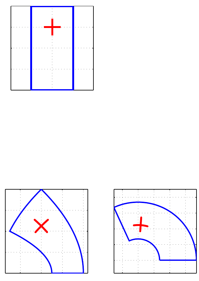
5. Complex Chebfuns 5
1 1.5 2
0
0.5
1
1.5
2
Here we see what happens to Rand Xunder the maps z2and exp(z):
clf
subplot(1,2,1), plot(R.^2,LW,lw1), grid on, axis equal
hold on, plot(X.^2,’r’,LW,lw2)
subplot(1,2,2), plot(exp(R),LW,lw1), grid on, axis equal
hold on, plot(exp(X),’r’,LW,lw2)
−2 0 2 4
0
2
4
6
8
−2 0 2 4 6
0
2
4
6
8
We can take the same idea further and construct a grid in the complex plane, each segment of which
is a piece of a chebfun that happens to be linear. In this case we accumulate the various pieces as
successive columns of a quasimatrix, i.e., a ”matrix” whose columns arechebfuns.
x = chebfun(@(x) x);
S = chebfun; % make an empty chebfun
for d = -1:.2:1
S = [S d+1i*x 1i*d+x]; % add 2 more lines to the collection
end
clf,
subplot(1,2,1), plot(S), axis equal
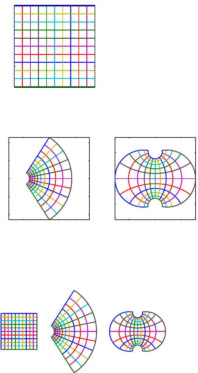
6Chebfun Guide
−1−0.5 0 0.5 1
−1
−0.5
0
0.5
1
Here are the exponential and tangent of the grid:
subplot(1,2,1), plot(exp(S)), axis equal
subplot(1,2,2), plot(tan(S)), axis equal
0 1 2 3
−2
−1
0
1
2
−1 0 1
−1.5
−1
−0.5
0
0.5
1
1.5
Here is a sequence that puts all three images together on a single scale:
clf
plot(S), hold on
plot(1.6+exp(S))
plot(6.6+tan(S))
axis equal, axis off
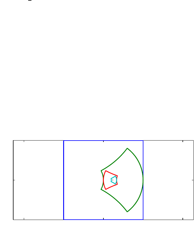
5. Complex Chebfuns 7
A particularly interesting set of conformal maps are the Moebius transformations, the rational
functions of the form (az +b)/(cz +d)forconstantsa, b, c, d. For example, here is a square and
its image under the map w=1/(1 + z), and the image of the image under the same map, and the
image of the image of the image. We also plot the limit point given by the equation z=1/(1 + z),
i.e., z=(
√5−1)/2.
moebius = @(z) 1./(1+z);
s = chebfun(@(s) s,[0 1]);
S = join(-.5i+s, 1-.5i+1i*s, 1+.5i-s, .5i-1i*s);
clf
for j = 1:3
S = [S moebius(S(:,j))];
end
plot(S)
hold on, axis equal
plot((sqrt(5)-1)/2,0,’.k’,’markersize’,4)
−0.5 0 0.5 1 1.5
−0.5
0
0.5
Here’s a prettier version of the same image using the Chebfun fill command.
S = join(-.5i+s, 1-.5i+1i*s, 1+.5i-s, .5i-1i*s);
clf
fill(real(S),imag(S),[.5 .5 1]), axis equal, hold on
S = moebius(S); fill(real(S),imag(S),[.5 1 .5])
S = moebius(S); fill(real(S),imag(S),[1 .5 .5])
S = moebius(S); fill(real(S),imag(S),[.5 1 1 ])
plot((sqrt(5)-1)/2,0,’.k’,’markersize’,4)
axis off
8Chebfun Guide
5.3 Contour integrals
If sis a real parameter and z(s) is a complex function of s, then we can define a contour integral in
the complex plane like this:
!f(z(s))z′(s)ds.
The contour in question is the curve described by z(s)assvaries over its range.
For example, in the example at the end of Section 5.1 the contour consists of two straight segments
that begin at 0 and end at −1+.5i. We can compute the integral of exp(−z2) over the contour like
this:
f = exp(-z.^2);
I = sum(f.*diff(z))
I=
-0.842544559526136 + 0.166587147924074i
Notice how easily the contour integral is realized in Chebfun, even over a contour consisting of
several pieces. This particular integral is related to the complex error function [Weideman 1994].
According to Cauchy’s theorem, the integral of an analytic function around a closed curve is zero,
or equivalently, the integral between two points z1and z2is path-independent. To verify this, we
can compute the same integral over the straight segment going directly from 0 to −1+0.5i:
w = chebfun(’(-1+.5i)*s’,[0 1]);
f = exp(-w.^2);
I2 = sum(f.*diff(w))
I2 =
-0.842544559526136 + 0.166587147924074i
5. Complex Chebfuns 9
Ameromorphic function is a function that is analytic in a region of interest in the complex plane
apart from possible poles. According to the Cauchy integral formula,1/2πitimes the integral of
a meromorphic function faround a closed contour is equal to the sum of the residues of fassociated
with any poles it may have in the enclosed region. The residue of fat a point z0is the coefficient of
the degree −1 term in its Laurent expansion at z0. For example, the function exp(z)/z3has Laurent
series z−3+z−2+(1/2)z−1+(1/6)z0+... at the origin, and so its residue there is 1/2. We can
confirm this by computing the contour integral around a circle:
z = chebfun(’exp(1i*s)’,[0 2*pi]);
f = exp(z)./z.^3;
I = sum(f.*diff(z))/(2i*pi)
I=
0.500000000000000 + 0.000000000000000i
Notice that we have just computed the degree 2 Taylor coefficient ofexp(z).
When Chebfun integrates around a circular contour like this, it does not automatically take ad-
vantage of the fact that the integrand is periodic. That would be Fourier analysis as opposed to
Chebyshev analysis, and beginning with Version 5, a ”Fourfun” approach to such problems has been
available, at least when the arguments are smooth (compare [Davis 1959]). For example, we could
repeat the above calculation in Fourier mode like this:
z = chebfun(’exp(1i*s)’,[0 2*pi],’periodic’);
f = exp(z)./z.^3;
I = sum(f.*diff(z))/(2i*pi)
I=
0.500000000000002 + 0.000000000000000i
Chebyshev methods are more flexible, as a rule, but Fourier methods have advantages sometimes of
efficiency (up to a factor of π/2 per dimension) and accuracy. For techniques that recover some of
that factor of π/2 even for nonperiodic problems, see [Hale & Trefethen 2008].
The contour does not have to have radius 1, or be centered at the origin:
z = chebfun(’1+2*exp(1i*s)’,[0 2*pi],’periodic’);
f = exp(z)./z.^3;
I2 = sum(f.*diff(z))/(2i*pi)
I2 =
0.500000000000000 + 0.000000000000000i
Nor does the contour have to be smooth. Here let us compute the same result by integration over a
square (reverting to Chebyshev rather than Fourier technology).
s = chebfun(’s’,[-1 1]);
z = join(1+1i*s, 1i-s, -1-1i*s, -1i+s);
f = exp(z)./z.^3;
I3 = sum(f.*diff(z))/(2i*pi)
10 Chebfun Guide
I3 =
0.500000000000000 + 0.000000000000000i
In Chebfun one can also construct more interesting contours of the kind that appear in complex
variables texts. Here is an example involving a ”keyhole” contour:
c = [-2+.05i, -.2+.05i, -.2-.05i, -2-.05i]; % 4 corners
s = chebfun(’s’,[0 1]);
z = join(c(1)+s*(c(2)-c(1)), c(2)*c(3).^s./c(2).^s, ...
c(3)+s*(c(4)-c(3)), c(4)*c(1).^s./c(4).^s);
clf, plot(z), axis equal, axis off
The integral of f(z) = log(z)tanh(z) around this contour will be equal to 2πitimes the sum of the
residues at the poles of fat ±πi/2.
f = log(z).*tanh(z);
I = sum(f.*diff(z))
Iexact = 4i*pi*log(pi/2)
I=
0.000000000000005 + 5.674755637702216i
Iexact =
0.000000000000000 + 5.674755637702224i
5.4 Cauchy integrals and locating zeros and poles
Here are some further examples of computations with Cauchy integrals. The Bernoulli number Bk
is k! times the kth Taylor coefficient of z/((exp(z)−1). Here is B10 compared with its exact value
5/66.
k=10;
z = chebfun(’5*exp(1i*s)’,[0 2*pi]);
f = z./((exp(z)-1));
B10 = factorial(k)*sum((f./z.^(k+1)).*diff(z))/(2i*pi)
exact = 5/66

5. Complex Chebfuns 11
B10 =
0.075757575757581 - 0.000000000000004i
exact =
0.075757575757576
Notice that we have taken zto be a circle of radius 5. If the radius is 1, the accuracy is a good deal
lower:
z = chebfun(’exp(1i*s)’,[0 2*pi]);
f = z./((exp(z)-1));
B10 = factorial(k)*sum((f./z.^(k+1)).*diff(z))/(2i*pi)
B10 =
0.075757575477819 - 0.000000000113937i
This problem of numerical instability would arise no matter how one calculated the integral over
the unit circle; it is not the fault of Chebfun. For a study of how to pick the optimal radius, see
[Bornemann 2009].
Another use of Cauchy integrals is to count zeros or poles of functions in specified regions. According
to the principle of the argument, the number of zeros minus the number of poles of fin a region
is
N=1
2πi!f′(z)
f(z)dz,
where the integral is taken over the boundary. Since f′=df / d z =(df / d s )(ds/dz), we can rewrite
this as
N=1
2πi!1
f
df
dsds.
For example, the function f(z) = sin(z)3+cos(z)3clearly has no poles; how many zeros does it have
in the disk about 0 of radius 2? The following calculation shows that the answer is 3:
z = chebfun(’2*exp(1i*s)’,[0 2*pi]);
f = sin(z).^3 + cos(z).^3;
N = sum((diff(f)./f))/(2i*pi)
N=
2.999999999999998 + 0.000000000000000i
What is really going on here is a calculation of the change of the argument of fas the boundary
is traversed. Another way to find that number is with the Chebfun overloads of the MATLAB
commands angle and unwrap:

12 Chebfun Guide
anglef = unwrap(angle(f));
N = (anglef(end)-anglef(0))/(2*pi)
N=
2.999999999999999
Variations on this idea enable one to locate zeros and poles as well as count them. For example, we
can locate a single zero with the formula
r=1
2πi!z(df / d s )/fds
[McCune 1966]. Here is the zero of the function above in the unit disk:
z = chebfun(’exp(1i*s)’,[0 2*pi],’periodic’);
f = sin(z).^3 + cos(z).^3;
r = sum(z.*(diff(f)./f))/(2i*pi)
r=
-0.785398163397449 - 0.000000000000000i
We can check the result by a more ordinary Chebfun calculation:
x = chebfun(’x’);
f = sin(x).^3 + cos(x).^3;
r = roots(f)
r=
-0.785398163397449
To find multiple zeros via Cauchy integrals, and for many other generalizations of the ideas in this
chapter, see [Austin, Kravanja & Trefethen 2013].
5.5 Alphabet soup
The Chebfun command scribble returns a piecewise linear complex chebfun corresponding to a
word spelled out in capital letters. For example:
f = scribble(’Oxford University’);
LW = ’linewidth’; lw = 2;
plot(f,LW,lw), xlim(1.1*[-1 1]), axis equal
5. Complex Chebfuns 13
−1−0.5 0 0.5 1
−0.4
−0.2
0
0.2
0.4
This chebfun happens to have 67 pieces:
length(domain(f))-1
ans =
67
Though its applications are unlikely to be mathematical, fis a precisely defined mathematical object
just like any other chebfun. If we wish, we can compute with it:
f(0), norm(f)
ans =
0.129411764705882
ans =
0.847576500999202
Perhaps more interesting is that we can apply functions to it and learn something in the process:
plot(exp(3i*f),’m’,LW,lw), ylim(1.2*[-1 1]), axis equal
−2−1 0 1 2
−1
−0.5
0
0.5
1
Does putting a box around enhance the image? (We do this by adding a second column of a Chebfun
quasimatrix – see Chapter 6.)
14 Chebfun Guide
L = f.ends(end);
s = chebfun(@(x) 2*x+2,[-1 -0.5]);
box = join(-1.1-.05i+2.2*s,1.1-.05i+.22i*s,1.1+.17i-2.2*s,-1.1+.17i-.22i*s);
f = [f box];
plot(f,LW,lw), xlim(1.2*[-1 1]), axis equal
−1−0.5 0 0.5 1
−0.4
−0.2
0
0.2
0.4
clf, plot(exp((1+.2i)*f),LW,lw), axis equal, axis off
plot(tan(f),LW,lw), axis equal, axis off
Next May 16, you might wish to write a greeting card for Pafnuty Lvovich Chebyshev, accurate as
always to 15 digits:
f = scribble(’Happy Birthday Pafnuty!’);
L = f.ends(end);
g = @(z) exp(-2.2i+(2.5i+.4)*z);
clf, plot(g(f),’r’,LW,lw), axis equal, axis off
circle = 1.12*chebfun(@(x) exp(2i*pi*x/L),[0 L]);

5. Complex Chebfuns 15
ellipse = 1.2*(circle + 1./circle)/2 + 1i*mean(imag(f));
hold on, plot(g(ellipse),’b’,LW,lw)
axis auto equal off
You can find an example ”Birthday cards and analytic function” in the Complex Variables section
of the Chebfun Examples collection, and further related explorations in the Geometry section.
5.6 References
[Austin, Kravanja & Trefethen 2013] A. P. Austin, P. Kravanja and L. N. Trefethen, ”Numerical al-
gorithms based on analytic function values at roots of unity”, SIAM Journal on Numerical Analysis,
to appear.
[Bornemann 2009] F. Bornemann, ”Accuracy and stability of computing high-order derivatives of
analytic functions by Cauchy integrals”, Foundations of Computational Mathematics,11(2011),
1-63.
[Davis 1959] P. J. Davis, ”On the numerical integration of periodic analytic functions”, in R. E.
Langer, ed., On Numerical Integration, Math. Res. Ctr., U. of Wisconsin, 1959, pp. 45-59.
[Hale & Trefethen 2008] N. Hale and L. N. Trefethen, ”New quadrature formulas from conformal
maps”, SIAM Journal on Numerical Analysis, 46 (2008), 930-948.
[McCune 1966] J. E. McCune, ”Exact inversion of dispersion relations”, Physics of Fluids,9(1966),
2082-2084.
[Weideman 1994] J. A. C. Weideman, ”Computation of the complex error function”, SIAM Journal
on Numerical Analysis, 31 (1994), 1497-1518.

!
6. Quasimatrices and
Least-Squares
Lloyd N. Trefethen, November 2009, latest revision June 2014
Contents
•6.1 Quasimatrices and spy
•6.2 Backslash and least-squares
•6.3 QR factorization
•6.4 svd,norm,cond
•6.5 Other norms
•6.6 rank,null,orth,pinv
•6.7 Array-valued chebfuns vs. arrays of chebfuns
•6.8 References
6.1 Quasimatrices and spy
A chebfun can have more than one column, or if it is transposed, it canhavemorethanonerow.In
these cases we get a quasimatrix, a ”matrix” in which one of the dimensions is discrete as usual
but the other is continuous. Our default choice will be that of an ” ∞×n” quasimatrix consisting
of ncolumns, each of which is a chebfun. When it is important to specify the orientation we use the
term column quasimatrix or row quasimatrix.
Here for example is the quasimatrix consisting of the first six powers of xon the interval [−1,1].
The command size can be used to identify the continuous dimension, and to find the numbers of
rows or columns:
x = chebfun(’x’);
A = [1 x x.^2 x.^3 x.^4 x.^5];
size(A)
size(A,2)
ans =
Inf 6
ans =
6
Here is the third column of Aevaluated at the point x=0.5:
1
2Chebfun Guide
A(0.5,3)
ans =
0.250000000000000
Here are the column sums, i.e., the integrals of 1,x,...,x
5from −1to1:
format short, sum(A), format long
ans =
2.0000 0 0.6667 0 0.4000 0
And here is a plot of the columns:
LW = ’linewidth’;
plot(A,LW,1.6), grid on, ylim([-1.1 1.1])
−1−0.5 0 0.5 1
−1
−0.5
0
0.5
1
The term quasimatrix comes from [Stewart 1998], and the same idea appears with different termi-
nology in [de Boor 1991] and [Trefethen & Bau 1997, pp. 52-54]. The idea is a natural one, since so
much of applied linear algebra deals with discrete approximations to the continuous, but it seems not
to have been discussed explicitly very much until the appearance of Chebfun [Battles & Trefethen
2004, Battles 2006].
If fand gare column chebfuns, then f’*g is a scalar, their inner product. For example, here is the
inner product of x2and x4over [−1,1] (equal to 2/7):
A(:,3)’*A(:,5)
ans =
0.285714285714286
More generally, if Aand Bare column quasimatrices with mand ncolumns, respectively, then A’*B
is the m×nmatrix of inner products of those columns. Here is the 6 ×6 example corresponding to
B=A:
format short, A’*A, format long
6. Quasimatrices and Least-Squares 3
ans =
2.0000 0.0000 0.6667 0 0.4000 0.0000
0.0000 0.6667 0 0.4000 0.0000 0.2857
0.6667 0 0.4000 0 0.2857 0
0 0.4000 0 0.2857 0 0.2222
0.4000 0.0000 0.2857 0 0.2222 0
0.0000 0.2857 0 0.2222 0 0.1818
You can get an idea of the shape of a quasimatrix with the overloaded spy command
subplot(1,2,1), spy(A), title A
subplot(1,2,2), spy(A’), title(’A’’’)
1 2 3 4 5 6
−1
1
A
−1 1
1
2
3
4
5
6
A’
6.2 Backslash and least-squares
In MATLAB, the command c=A\bcomputes the solution to the system of equations Ac =bif A
is a square matrix, whereas if Ais rectangular, with more rows than columns, it computes the least
squares solution, the vector cthat minimizes ∥Ac −b∥. A quasimatrix is always rectangular, and \
has accordingly been overloaded to carry out the appropriate continuous least-squares computation.
(The actual MATLAB command that handles backslash is mldivide.)
For example, continuing with the same chebfun xand quasimatrix Aas above, consider the following
sequence:
f = exp(x).*sin(6*x);
c=A\f
c=
0.309654988398407
4.640757102742464
-2.157249816336408
-20.041645425109152
1.073963006923383
15.477982292827999
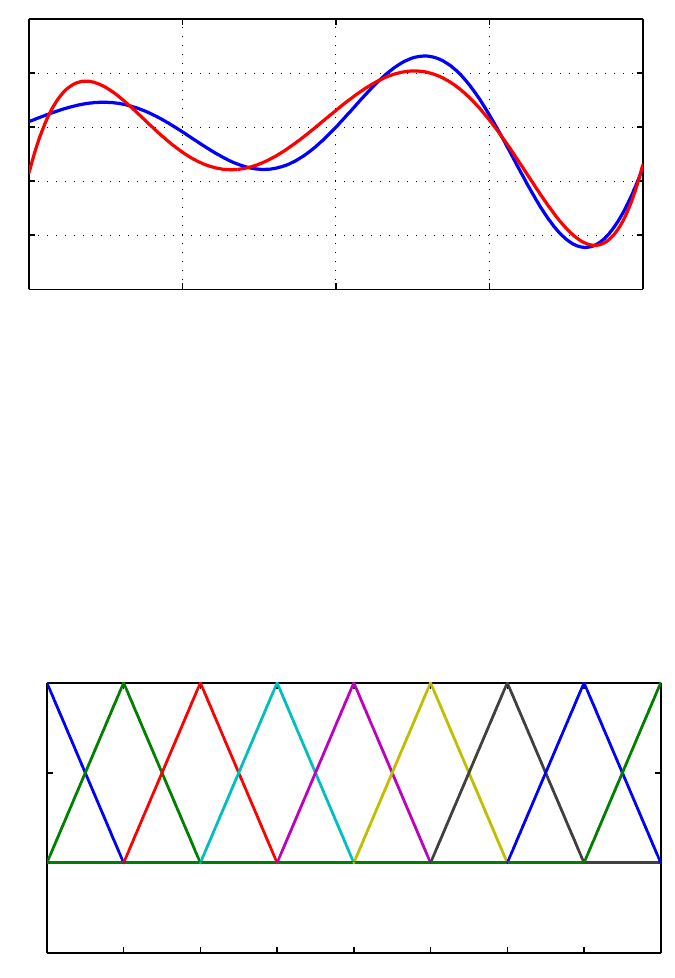
4Chebfun Guide
The vector ccan be interpreted as the vector of coefficients of the least-squares fit to fby a
linear combination of the functions 1,x,...,x
5. Here is a plot of f(in blue) and the least-squares
approximation (in red), which we label ffit.
ffit = A*c;
clf, plot(f,’b’,ffit,’r’,LW,1.6), grid on
error = norm(f-ffit)
error =
0.356073976001434
−1−0.5 0 0.5 1
−3
−2
−1
0
1
2
It is a general result that the least-squares approximation by a polynomial of degree nto a continuous
function fmust intersect fat least n+ 1 times in the interval of approximation.
Here is quite a different quasimatrix whose columns can be used to fit f. The columns correspond
to hat functions located at points equally spaced from −1 to 1, and they are realized as piecewise
smooth chebfuns.
A2 = [];
for j = 0:8
xj = -1 + j/4;
A2 = [A2 max(0,1-4*abs(x-xj))];
end
plot(A2)
set(gca,’xtick’,-1:.25:1)
−1−0.75 −0.5 −0.25 0 0.25 0.5 0.75 1
−0.5
0
0.5
1
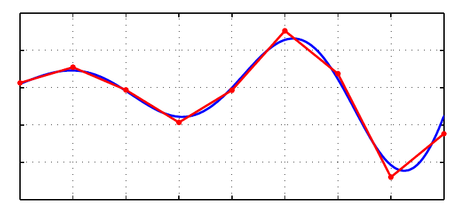
6. Quasimatrices and Least-Squares 5
A linear combination of these columns is a piecewise linear function with breakpoints at
−0.75,−0.50,...,0.75. Here is the least-squares fit by such functions to f. Remember that al-
though we happen to be fitting here by a function with a discrete flavor, all the operations are
continuous ones involving integrals, not point evaluations.
c = A2\f;
ffit = A2*c;
plot(f,’b’,ffit,’.-r’,LW,1.6), grid on
set(gca,’xtick’,-1:.25:1)
error = norm(f-ffit)
error =
0.148137345378415
−1−0.75 −0.5 −0.25 0 0.25 0.5 0.75 1
−3
−2
−1
0
1
2
6.3 QR factorization
Matrix least-squares problems are ordinarily solved by QR factorization, and in the quasimatrix case,
they are solved by quasimatrix QR factorization. This is the technology underlying the backslash
operator described in the last section.
A quasimatrix QR factorization takes this form:
A=QR,
with
A:∞×n, Q :∞×n, R :n×n.
The columns of Aare arbitrary, the columns of Qare orthonormal, and Ris an n×nupper-triangular
matrix. This factorization corresponds to what is known in various texts as the ”reduced”, ”economy
size”, ”skinny”, ”abbreviated”, or ”condensed” QR factorization, since Qis rectangular rather than
square and Ris square rather than rectangular. In MATLAB the syntax for computing such things
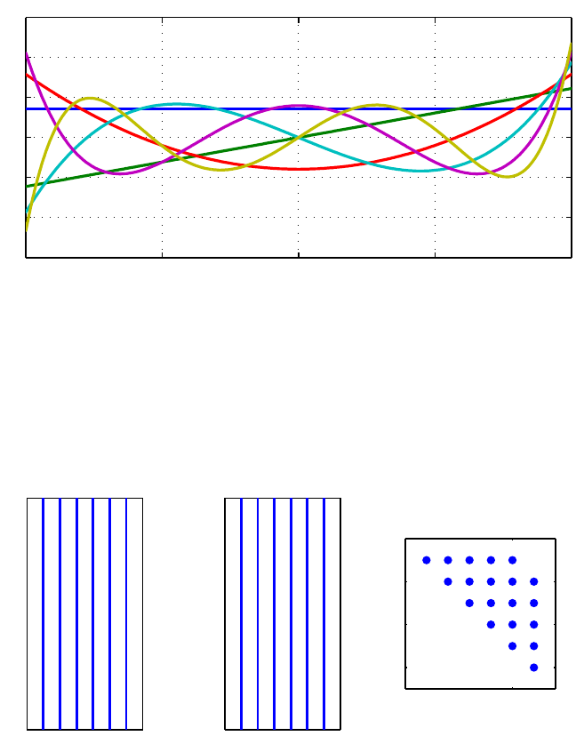
6Chebfun Guide
is [Q,R] = qr(A,0), and the same command has been overloaded for chebfuns. The computation
makes use of a quasimatrix analogue of Householder triangularization [Trefethen 2010]. Alternatively
one can simply write [Q,R] = qr(A):
[Q,R] = qr(A);
plot(Q,LW,1.6), grid on
−1−0.5 0 0.5 1
−3
−2
−1
0
1
2
3
The spy command confirms the shape of these various matrices. In principle half the dots in the
upper-triangle should be zero because of the fact that the columnsofAalternate even and odd
functions, but rounding errors introduce nonzeros.
subplot(1,3,1), spy(A), title A
subplot(1,3,2), spy(Q), title Q
subplot(1,3,3), spy(R), title R
1 2 3 4 5 6
−1
1
A
1 2 3 4 5 6
−1
1
Q
0 5
0
2
4
6
nz = 20
R
The plot shows orthogonal polynomials, namely the orthogonalizations of the monomials
1,x,...,x
5over [−1,1]. These are the famous Legendre polynomials Pk[Abramowitz & Stegun
1972], except that the latter are conventionally normalized by the condition P(1) = 1 rather than
by having norm 1. We can renormalize to impose this condition as follows:
for j = 1:size(A,2)
R(j,:) = R(j,:)*Q(1,j);
Q(:,j) = Q(:,j)/Q(1,j);
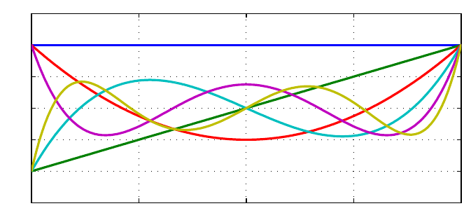
6. Quasimatrices and Least-Squares 7
end
clf, plot(Q,LW,1.6), grid on
−1−0.5 0 0.5 1
−1.5
−1
−0.5
0
0.5
1
1.5
(A slicker way to produce this plot in Chebfun would be to execute plot(legpoly(0:5)).)
If A=QR,thenAR−1=Q, and here is R−1:
format short, inv(R), format long
ans =
1.0000 -0.0000 -0.5000 0.0000 0.3750 -0.0000
0 1.0000 0.0000 -1.5000 -0.0000 1.8750
0 0 1.5000 -0.0000 -3.7500 0.0000
0 0 0 2.5000 0.0000 -8.7500
0 0 0 0 4.3750 -0.0000
000007.8750
Column kof R−1is the vector of coefficients of the expansion of column kof Qas a linear combination
of the columns of A, that is, the monomials 1,x,x
2,.... In other words, column kof R−1is the
vector of coefficients of the degree kLegendre polynomial. For example, we see from the matrix that
P3(x)=2.5x3−1.5x.
Here is what the hat functions look like after orthonormalization:
[Q2,R2] = qr(A2);
plot(Q2,LW,1.6)
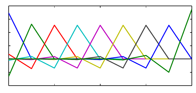
8Chebfun Guide
−1−0.5 0 0.5 1
−2
−1
0
1
2
3
4
6.4 svd,norm,cond
An m×nmatrix Adefines a map from Rnto Rm, and in particular, Amaps the unit ball in Rnto
a hyperellipsoid of dimension ≤nin Rm. The (reduced, skinny, condensed,...) SVD or singular
value decomp osition exhibits this map by providing a factorization AV =US or equivalently A=
USV∗,whereUis m×nwith orthonormal columns, Sis diagonal with nonincreasing nonnegative
diagonal entries known as the singular values,andVis n×nand orthogonal. Amaps vj,thej
th column of Vor the jth right singular vector,tosjtimes uj,thejth column of Uor the jth
left singular vector, which is the vector defining the jth largest semiaxis of the hyperellipsoid.
See Chapters 4 and 5 of [Trefethen & Bau 1997].
If A is an ∞×nquasimatrix, everything is analogous:
A=USV′,A:∞×n, U :∞×n, S :n×n, V :n×n.
The image of the unit ball in Rnunder Ais still a hyperellipsoid of dimension ≤n, which now lies
within an infinite-dimensional function space. The columns of Qare orthonormal functions and S
and Vhave the same properties as in the matrix case.
For example, here are the singular values of the matrix A defined earlier with columns 1,x,...,x
5:
s = svd(A,0)
s=
1.532062889375340
1.032551897396699
0.518125864967969
0.258419769500035
0.080938947808205
0.035425077461572
The largest singular value is equal to the norm of the quasimatrix, which is defined by ∥A∥=
maxx∥Ax∥/∥x∥.
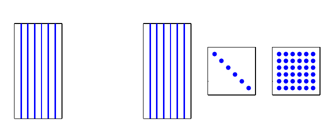
6. Quasimatrices and Least-Squares 9
norm(A,2)
ans =
1.532062889375340
(Note that we must include the argument 2here: for reasons of speed, the default for quasimatrices,
unlike the usual MATLAB matrices, is the Frobenius norm rather than the 2-norm.) The SVD
enables us to identify exactly what vectors are involved in achieving this maximum ratio. The
optimal vector xis v1, the first right singular vector of A,
[U,S,V] = svd(A);
v1 = V(:,1)
v1 =
0.913034433780914
0.000000000000000
0.344611116356111
0.000000000000000
0.218200140270718
0.000000000000000
We can use spy to confirm the shapes of the matrices. As with spy( R) earlier, here spy(V) should
in principle show a checkerboard, but nonzeros are introduced by rounding errors.
subplot(1,5,1), spy(A), title A
subplot(1,5,3), spy(U), title U
subplot(1,5,4), spy(S), title S
subplot(1,5,5), spy(V), title V
1 2 3 4 5 6
−1
1
A
1 2 3 4 5 6
−1
1
U
0 5
0
5
nz = 6
S
0 5
0
5
nz = 36
V
We confirm that the norm of v1is 1:
norm(v1)
ans =
1.000000000000000
This vector is mapped by Ato the chebfun s1u1:
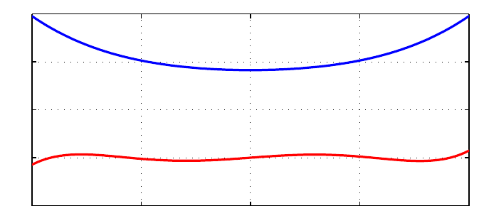
10 Chebfun Guide
u1 = U(:,1);
norm(u1)
ans =
1
s1 = S(1,1)
s1 =
1.532062889375340
norm(A*v1)
ans =
1.532062889375341
norm(A*v1-s1*u1)
ans =
4.142554461132179e-16
Similarly, the minimal singular value and corresponding singular vectors describe the minimum
amount that Acan enlarge an input. The following commands plot the extreme functions Av1
(blue) and Avn(red). We can interpret these as the largest and smallest degree 5 polynomials, as
measured in the 2-norm over [−1,1], whose coefficient vectors have 2-norm equal to 1.
clf, plot(A*v1,LW,1.6), grid on, hold on
vn = V(:,end);
plot(A*vn,’r’,LW,1.6), hold off
−1−0.5 0 0.5 1
−0.5
0
0.5
1
1.5
The ratio of the largest and smallest singular values – the eccentricity of the hyperellipsoid – is the
condition number of A:
max(s)/min(s)
6. Quasimatrices and Least-Squares 11
ans =
43.247975704139762
cond(A)
ans =
43.247975704139762
The fact that cond(A) is a good deal greater than 1 reflects the ill-conditioning of the monomials
1,x,...,x
5as a basis for degree 5 polynomials in [−1,1]. The effect becomes rapidly stronger as we
take more terms in the sequence:
cond([A x.^6 x.^7 x.^8 x.^9 x.^10 x.^11 x.^12 x.^13 x.^14 x.^15])
ans =
2.298938277191532e+05
By contrast a quasimatrix formed of suitably normalized Legendre polynomials has condition number
1, since they are orthonormal:
cond(legpoly(0:15,’norm’))
ans =
1.000000000000002
A quasimatrix of Chebyshev polynomials doesn’t quite achieve condition number 1, but it comes
close:
cond(chebpoly(0:15))
ans =
4.597747107616717
Chebyshev polynomials form an excellent basis for expansions on [−1,1], a fact that is at the heart
of Chebfun.
6.5 Other norms
The definition ∥A∥=max
x∥Ax∥/∥x∥makes sense in other norms besides the 2-norm, and the
particularly important alternatives are the 1-norm and the ∞-norm. The 1-norm of a column
quasimatrix is the ”maximum column sum”, i.e., the maximum of the 1-norms of its columns. In
the case of our quasimatrix A, the maximum is attained by the first column, which has norm 2:
norm(A,1)
ans =
2
12 Chebfun Guide
The ∞-norm is the ”maximum row sum”, which for a column quasimatrix corresponds to the
maximum of the chebfun obtained by adding the absolute values of the columns. In the case of A,
the sum is 1 + |x|+···+|x|5, which attains its maximum value 6 at x=−1and1:
norm(A,inf)
ans =
6.000000000000002
The norms of row quasimatrices are analogous, with norm(A’,inf) = norm(A,1) and norm(A’,1)
= norm(A,inf). Like MATLAB itself applied to a rectangular matrix, Chebfun does notdefine
cond(A,1) or cond(A,inf) if Ais a quasimatrix.
The Frobenius or Hilbert-Schmidt norm is equal to the square root ofthesumofthesquaresofthe
singular values:
norm(A,’fro’)
ans =
1.938148951041007
6.6 rank,null,orth,pinv
Chebfun also contains overloads for some further MATLAB operations related to orthogonal matrix
factorizations. Perhaps the most useful of these is rank(A), which computes the singular values of A
and makes a judgement as to how many of them are significantly different from zero. For example,
with xstill defined as before, here is an example showing that the functions1,sin(x)2,andcos(x)2
are linearly dependent:
B = [1 sin(x).^2 cos(x).^2];
rank(B)
ans =
2
Since Bis rank-deficient, is has a nontrivial nullspace, and the command null(B) will find an
orthonormal basis for it:
null(B)
ans =
-0.577350269189626
0.577350269189626
0.577350269189626
Similarly the command orth(B) finds an orthonormal basis for the range of B, which in this case
has dimension 2:
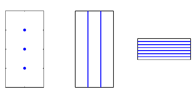
6. Quasimatrices and Least-Squares 13
orth(B)
ans =
chebfun column1 (1 smooth piece)
interval length endpoint values
[ -1, 1] 17 0.61 0.61
Epslevel = 2.340672e-16. Vscale = 7.634146e-01.
chebfun column2 (1 smooth piece)
interval length endpoint values
[ -1, 1] 17 -1.4 -1.4
Epslevel = 1.555489e-15. Vscale = 1.425588e+00.
If Ais an ∞×ncolumn quasimatrix, the command pinv(A) computes the pseudoinverse of A,an
n×∞row quasimatrix such that pinv(A)*c = A\c.
Here is a summary of the dimensions of these objects:
subplot(1,3,1), spy(null(B)), title null(B)
subplot(1,3,2), spy(orth(B)), title orth(B)
subplot(1,3,3), spy(pinv(A)), title pinv(A)
0 1 2
0
1
2
3
4
nz = 3
null(B)
1 2
−1
1
orth(B)
−1 1
1
2
3
4
5
6
pinv(A)
6.7 Array-valued chebfuns vs. arrays of chebfuns
In Chebfun, quasimatrices are actually implemented in two different ways. When its columns are
smooth functions, a quasimatrix is normally represented as an array-valued chebfun. If a quasi-
matrix has singularities, or breakpoints that differ from one column to another, it is represented in
a different fashion as an array of chebfuns. This representation is more flexible, though slower for
some operations. In principle, users should never see the difference.
6.8 References
[Abramowitz & Stegun 1972] M. A. Abramowitz and I. A. Stegun, eds., Handbook of Mathematical
Functions with Formulas, Graphs, and Mathematical Tables, 9th printing, Dover, 1972.
[Battles 2006] Z. Battles, Numerical Linear Algebra for Continuous Functions, DPhil thesis, Oxford
University Computing Laboratory, 2006.
14 Chebfun Guide
[Battles & Trefethen 2004] Z. Battles and L. N. Trefethen, ”An extension of Matlab to continuous
functions and operators”, SIAM Journal on Scientific Computing, 25 (2004), 1743-1770.
[de Boor 1991] C. de Boor, ”An alternative approach to (the teaching of) rank, basis, and dimension”,
Linear Algebra and its Applications, 146 (1991), 221-229.
[Stewart 1998] G. W. Stewart, Afternotes Goes to Graduate School: Lectures on Advanced Numerical
Analysis,SIAM,1998.
[Trefethen 2008] L. N. Trefethen, ”Householder triangularization of a quasimatrix”, IMA Journal of
Numerical Analysis, 30 (2010), 887-897.
[Trefethen & Bau 1997] L. N. Trefethen and D. Bau, III, Numerical Linear Algebra,SIAM,1997.
7. Linear Differential Operators
and Equations
Tobin A. Driscoll, November 2009, latest revision June 2014
Contents
•7.1 Introduction
•7.2 About linear chebops
•7.3 Chebop syntax
•7.4 Solving differential and integral equations
•7.5 Eigenvalue problems: eigs
•7.6 Exponential of a linear operator: expm
•7.7 Algorithms: rectangular collocation vs. ultraspherical
•7.8 Block operators and systems of equations
•7.9 Nonlinear equations by Newton iteration
•7.10 BVP systems with unknown parameters
•7.11 References
7.1 Introduction
Chebfun has powerful capabilities for solving ordinary differential equations as well as partial dif-
ferential equations involving one space and one time variable. The present chapter is devoted to
chebops, the fundamental Chebfun tools for solving differential (or integral) equations. In particular
we focus here on the linear case. We shall see that one can solve a linear two-point boundary value
problem to high accuracy by a single backslash command. Nonlinear extensions are described in
Section 7.9 and in Chapter 10, and for PDEs, try help pde15s.
7.2 About linear chebops
A chebop represents a differential or integral operator that acts on chebfuns. This chapter focusses
on the linear case, though from a user’s point of view, linear and nonlinear problems are quite similar.
One thing that makes linear operators special is that eigs and expm can be applied to them, as we
shall describe in Sections 7.5 and 7.6.
Like chebfuns, chebops start from premise of approximation by piecewise polynomial interpolants; in
the context of differential equations, such techniques are called spectral collocation methods. As with
chebfuns, the discretizations are chosen automatically to achieve the maximum possible accuracy
available from double precision arithmetic. In fact, beginning with version 5, Chebfun actually offers
two different methods for solving these problems, which go by the names of rectangular collocation
1
2Chebfun Guide
(or Driscoll-Hale) spectral methods and ultraspherical (or Olver-Townsend) spectral metho ds. See
Sections 7.7 and 8.10.
The linear part of the chebop package was conceived at Oxford by Bornemann, Driscoll, and Tre-
fethen [Driscoll, Bornemann & Trefethen 2008], and the implementation is due to Driscoll, Hale,
and Birkisson [Birkisson & Driscoll 2011, Driscoll & Hale 2014] . Much of the functionality of linear
chebops is actually implemented in various classes built around the idea of what we call a ”linop”,
but users generally do not deal with linops and related structures directly.
7.3 Chebop syntax
A chebop has a domain, an operator, and sometimes boundary conditions. For example, here is the
chebop corresponding to the second-derivative operator on [−1,1]:
L = chebop(-1, 1);
L.op = @(x,u) diff(u,2);
(For scalar operators like this, one may dispense with the xand just write L.op = @(u) diff(u,2).)
This operator can now be applied to chebfuns defined on [−1,1]. For example, taking two derivatives
of sin(3x) multiplies its amplitude by 9:
u = chebfun(’sin(3*x)’);
norm(L(u), inf)
ans =
9.000000000000084
Both the notations L*u and L(u) are allowed, with the same meaning.
min(L*u)
ans =
-9.000000000000084
Mathematicians generally prefer Lu if Lis linear and L(u) if it is nonlinear.
A chebop can also have left and/or right boundary conditions. For a Dirichlet boundary condition
it’s enough to specify a number:
L.lbc = 0;
L.rbc = 1;
More complicated boundary conditions can be specified with anonymous functions, which are then
forced to take zero values at the boundary. For example, the following sequence imposes the condi-
tions u= 0 at the left boundary and u′= 1 at the right:
L.lbc = @(u) u;
L.rbc = @(u) diff(u) - 1;
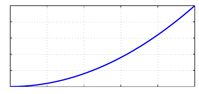
7. Linear Differential Operators and Equations 3
We can see a summary of Lby typing the name without a semicolon:
L
L=
Linear operator:
diff(u,2) = 0
operating on chebfun objects defined on:
[-1 1]
with
left boundary conditions:
u=0
right boundary conditions:
@(u)diff(u)-1 = 0
Boundary conditions are needed for solving differential equations, but they have no effect when a
chebop is simply applied to a chebfun. Thus, despite the boundary conditions just specified, L*u
gives the same answer as before:
norm(L*u, inf)
ans =
9.000000000000084
Here is an example of an integral operator, the operator that maps udefined on [0,1] to its indefinite
integral:
L = chebop(0, 1);
L.op = @(x,u) cumsum(u);
For example, the indefinite integral of xis x2/2:
x = chebfun(’x’, [0, 1]);
LW = ’linewidth’;
hold off, plot(L*x, LW, 2), grid on
0 0.2 0.4 0.6 0.8 1
0
0.1
0.2
0.3
0.4
0.5
Chebops can be specified in various ways, including all in a single line. For example we could write
4Chebfun Guide
L = chebop(@(x,u) diff(u) + diff(u,2), [-1, 1])
L=
Linear operator:
diff(u)+diff(u,2) = 0
operating on chebfun objects defined on:
[-1 1]
Or we could include boundary conditions:
L = chebop(@(x,u) diff(u) + diff(u,2), [-1, 1], 0, @(u) diff(u))
L=
Linear operator:
diff(u)+diff(u,2) = 0
operating on chebfun objects defined on:
[-1 1]
with
left boundary conditions:
u-BC = 0
right boundary conditions:
@(u)diff(u) = 0
For operators applying to more than one variable (needed for solving systems of differential equa-
tions), see Section 7.8.
7.4 Solving differential and integral equations
In MATLAB, if Ais a square matrix and bis a vector, then the command x=A\bsolves the linear
system of equations Ax =b. Similarly in Chebfun, if Lis a differential operator with appropriate
boundary conditions and fis a Chebfun, then u=L\fsolves the differential equation L(u)=f.More
generally Lmight be an integral or integro-differential operator. (Of course, just as you can solve
Ax =bonly if Ais nonsingular, you can solve L(u)=fonly if the problem is well-posed.)
For example, suppose we want to solve the differential equation u′′ +x3u= 1 on the interval [−3,3]
with Dirichlet boundary conditions. Here is a Chebfun solution:
L = chebop(-3, 3);
L.op = @(x,u) diff(u,2) + x.^3.*u;
L.lbc = 0; L.rbc = 0;
u = L\1; plot(u, LW, 2), grid on
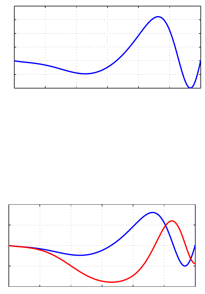
7. Linear Differential Operators and Equations 5
−3−2−1 0 1 2 3
−1
−0.5
0
0.5
1
1.5
2
We confirm that the computed usatisfies the differential equation to high accuracy:
norm(L(u) - 1)
ans =
1.812483165209799e-11
Let’s change the right-hand boundary condition to u′= 0 and see how this changes the solution:
L.rbc = @(u) diff(u);
u=L\1;
hold on, plot(u, ’r’, LW, 2)
−3−2−1 0 1 2 3
−2
−1
0
1
2
An equivalent to backslash is the solvebvp command.
v = solvebvp(L, 1);
norm(u - v)
ans =
0
Periodic boundary conditions can be imposed with the special boundary condition string
L.bc=’periodic’, which will find a periodic solution, provided that the right-side function is also
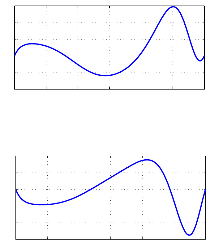
6Chebfun Guide
periodic. At the moment Chebfun does not include truly periodic spectral discretizations based on
Fourier series, though we hope to introduce this feature before long.
L.bc = ’periodic’;
u=L\1;
hold off, plot(u, LW, 2), grid on
−3−2−1 0 1 2 3
−1.5
−1
−0.5
0
0.5
1
A command like L.bc=100 imposes the corresponding numerical Dirichlet condition at both endsof
the domain:
L.bc = 100;
plot(L\1, LW, 2), grid on
−3−2−1 0 1 2 3
−200
−100
0
100
200
300
Boundary conditions can also be specified in a single line, as noted above:
L = chebop( @(x,u) diff(u,2) + 10000*u, [-1,1], 0, @(u) diff(u) );
Thus it is possible to set up and solve a differential equation and plot the solution with a single line
of Chebfun:
plot( chebop(@(x,u) diff(u,2) + 50*(1 + sin(x)).*u, [-20,20], 0, 0) \ 1 )
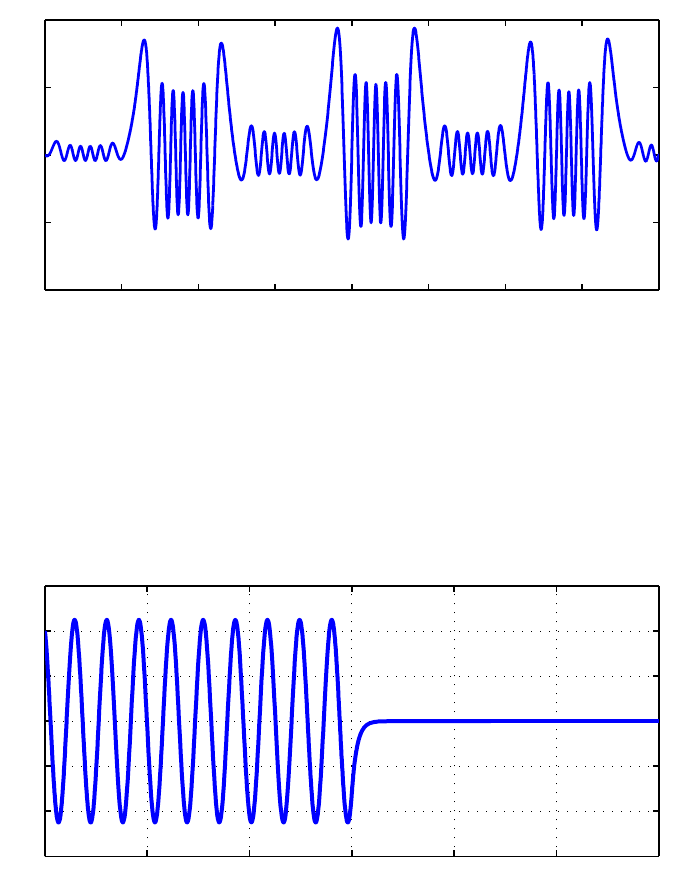
7. Linear Differential Operators and Equations 7
−20 −15 −10 −5 0 5 10 15 20
−1
−0.5
0
0.5
1
When Chebfun solves differential or integral equations, the coefficients may be piecewise smooth
rather than globally smooth. For example, here is a 2nd order problem involving a coefficient that
jumps from +1 (oscillation) for x<0to−1(growth/decay)forx>0:
L = chebop(-60, 60);
L.op = @(x,u) diff(u,2) - sign(x).*u;
L.lbc = 1; L.rbc = 0;
u=L\0;
plot(u, LW, 2), grid on
−60 −40 −20 0 20 40 60
−1.5
−1
−0.5
0
0.5
1
1.5
Further examples of Chebfun solutions of differential equations with discontinuous coefficients can
be found in the Demos menu of chebgui.
7.5 Eigenvalue problems: eigs
In MATLAB, eig finds all the eigenvalues of a matrix whereas eigs finds some of them. A differential
or integral operator normally has infinitely many eigenvalues, so one could not expect an analog of
eig for chebops. eigs, however, has been overloaded. Just like MATLAB eigs,Chebfuneigs
finds six eigenvalues by default, together with eigenfunctions if requested. (For details see [Driscoll,
Bornemann & Trefethen 2008].) Here is an example involving sine waves.
L = chebop( @(x,u) diff(u,2), [0, pi] );
L.bc = 0;
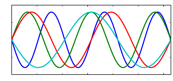
8Chebfun Guide
[V, D] = eigs(L);
diag(D)
clf, plot(V(:,1:4), LW, 2), ylim([-1 1])
ans =
-35.999999999996355
-25.000000000000519
-16.000000000003798
-9.000000000001164
-4.000000000000875
-1.000000000000230
0 0.5 1 1.5 2 2.5 3
−1
−0.5
0
0.5
1
By default, eigs tries to find the six eigenvalues whose eigenmodes are ”most readily converged to”,
which approximately means the smoothest ones. You can change the number sought and tell eigs
where to look for them. Note, however, that you can easily confuse eigs if you ask for something
unreasonable, like the largest eigenvalues of a differential operator.
Here we compute 10 eigenvalues of the Mathieu equation and plot the 9th and 10th corresponding
eigenfunctions, known as an elliptic cosine and sine. Note the imposition of periodic boundary
conditions.
q=10;
A = chebop(-pi, pi);
A.op = @(x,u) diff(u,2) - 2*q*cos(2*x).*u;
A.bc = ’periodic’;
[V, D] = eigs(A, 16, ’LR’); % eigenvalues with largest real part
d = diag(D); [d, ii] = sort(d, ’descend’); V = V(:, ii’);
subplot(1,2,1), plot(V(:, 9), LW, 2), ylim([-.8 .8]), title(’elliptic cosine’)
subplot(1,2,2), plot(V(:,10), LW, 2), ylim([-.8 .8]), title(’elliptic sine’)
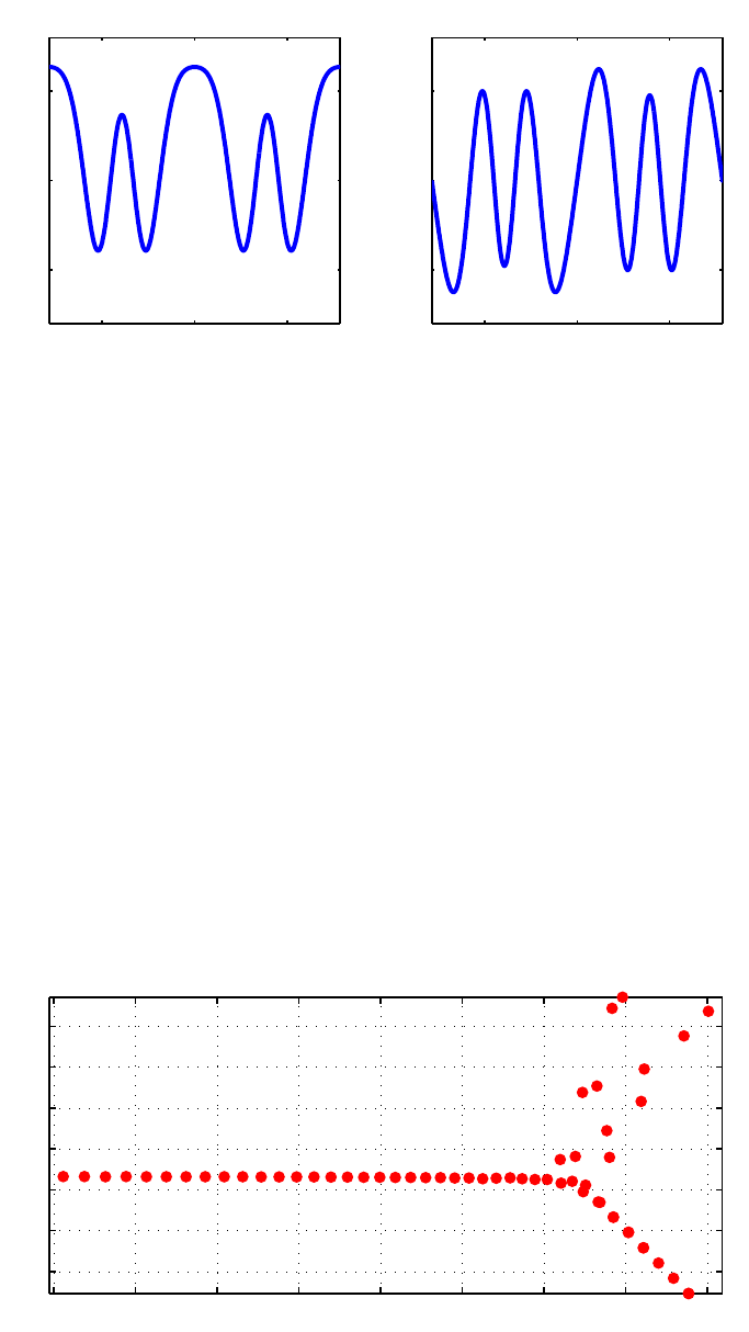
7. Linear Differential Operators and Equations 9
−2 0 2
−0.5
0
0.5
elliptic cosine
−2 0 2
−0.5
0
0.5
elliptic sine
eigs can also solve generalized eigenproblems, that is, problems of the form Au =λBu.Forthese
one must specify two linear chebops Aand B, with the boundary conditions all attached to A. Here is
an example of eigenvalues of the Orr-Sommerfeld equation of hydrodynamic linear stability theory at
a Reynolds number close to the critical value for eigenvalue instability [Schmid & Henningson 2001].
This is a fourth-order generalized eigenvalue problem, requiring two conditions at each boundary.
Re = 5772;
B = chebop(-1, 1);
B.op = @(x,u) diff(u,2) - u;
A = chebop(-1, 1);
A.op = @(x,u) (diff(u,4) - 2*diff(u, 2) + u)/Re - ...
1i*(2*u + (1 - x.^2).*(diff(u, 2) - u));
A.lbc = @(u) [u; diff(u)];
A.rbc = @(u) [u; diff(u)];
lam = eigs(A, B, 60, ’LR’);
MS = ’markersize’;
clf, plot(lam, ’r.’, MS, 16), grid on, axis equal
spectral_abscissa = max(real(lam))
spectral_abscissa =
0.002462425127391
−1.6 −1.4 −1.2 −1−0.8 −0.6 −0.4 −0.2 0
−0.9
−0.8
−0.7
−0.6
−0.5
−0.4
−0.3
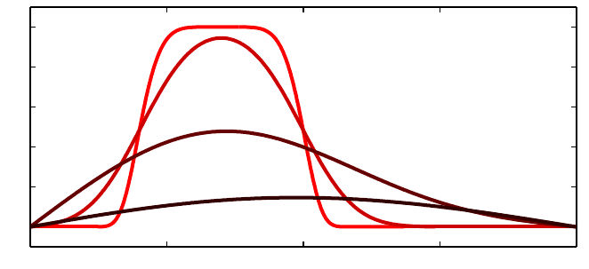
10 Chebfun Guide
7.6 Exponential of a linear operator: expm
In MATLAB, expm computes the exponential of a matrix, and this command has been overloaded
in Chebfun to compute the exponential of a linear operator. If Lis a linear operator and E(t)=
exp(tL), then the partial differential equation ut=Lu has solution u(t)=E(t)u(0). Thus by
taking Lto be the 2nd derivative operator, for example, we can use expm to solve the heat equation
ut=uxx:
A = chebop(@(x,u) diff(u,2), [-1, 1], 0);
f = chebfun(’exp(-1000*(x+0.3).^6)’);
clf, plot(f, ’r’, LW, 2), hold on, c = [0.8 0 0];
for t = [0.01 0.1 0.5]
u = expm(A, t, f);
plot(u,’color’, c, LW, 2), c = 0.5*c;
ylim([-.1 1.1])
end
−1−0.5 0 0.5 1
0
0.2
0.4
0.6
0.8
1
Here is a more fanciful analogous computation with a complex initial function obtained from the
scribble command introduced in Chapter 5.
f = exp(.02i)*scribble(’BLUR’); clf
D = chebop(@(x,u) diff(u,2), [-1 1]);
D.bc = ’neumann’;
k=0;
for t = [0 .0001 .001]
k = k + 1; subplot(3,1,k)
if t==0, u = f; else u = expm(D, t, f); end
plot(u, ’linewidth’, 3, ’color’, [.6 0 1])
xlim(1.05*[-1 1]), axis equal
text(0.01, .46, sprintf(’t = %6.4f’, t), ’fontsize’, 10), axis off
end
7. Linear Differential Operators and Equations 11
t = 0.0000
t = 0.0001
t = 0.0010
7.7 Algorithms: rectangular collocation vs. ultraspherical
Let us say a word about how Chebfun carries out these computations. Until Chebfun version 5, the
methods involved were all Chebyshev spectral methods on automatically chosen grids. The general
ideas are presented in [Trefethen 2000], [Driscoll, Bornemann & Trefethen 2008], and [Driscoll 2010],
but Chebfun actually uses modifications of these methods described in [Driscoll & Hale 2014] involv-
ing a novel mix of Chebyshev grids of the first and second kinds. These rectangular collocation or
Driscoll-Hale spectral discretizations start from the idea that a differential operator is discretized
as a rectangular matrix that maps from one grid to another with fewer points. The matrix is then
made square again by the incorporation of boundary conditions. When a differential equation is
solved in Chebfun, the problem is solved on a sequence of grids of size 33,65,... until convergence
is achieved in the usual Chebfun sense defined by decay of Chebyshev expansion coefficients.
One matter you might not guess was challenging is the determination ofwhetherornotanoperator
is linear! This is important since if an operator is linear, special actions are possible possible such as
application of eigs and expm and solution of differential equations in a single step without iteration.
Chebfun includes special devices to determine whether a chebop is linear so that these effects can
be realized [Birkisson 2014].
As mentioned, the discretization length of a Chebfun solution is chosen automatically according
to the intrinsic resolution requirements. However, the matrices that arise in Chebyshev spectral
methods are notoriously ill-conditioned. Thus the final accuracy in solving differential equations in
Chebfun’s default mode is rarely close to machine precision. Typically one loses two or three digits
for second-order differential equations and five or six for fourth-order problems.
This problem of ill-conditioning was one of the motivations for the development of the other dis-
cretization method used by Chebfun, known as ultraspherical or Olver-Townsend spectral dis-
cretizations [Olver & Townsend 2013]. Here, rather than a single Chebyshev basis, several different
bases of ultraspherical polynomials are used, depending on the order of the differential operator.
This leads to better conditioned matrices that are also sparser, especially for linear problems with
constant or smooth coefficients. By default, Chebfun uses rectangular collocation discretizations,
but most problems can equally be solved in ultraspherical mode, and the results may be more accu-
rate. For example, here we solve a problem whose exact solution is cos(x) in the rectangular fashion
and check the error at x=5:
tic
u = chebop(@(x, u) diff(u, 2) + u, [-10,10], cos(10), cos(10))\0;
toc
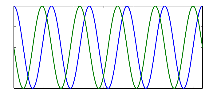
12 Chebfun Guide
error = u(5) - cos(5)
Elapsed time is 0.099327 seconds.
error =
-2.159383782895930e-14
We can switch to ultraspherical mode and run the same experiment again like this:
cheboppref.setDefaults(’discretization’, @ultraS)
tic
u = chebop(@(x,u) diff(u,2) + u, [-10,10], cos(10), cos(10))\0;
toc
error = u(5) - cos(5)
cheboppref.setDefaults(’factory’) % reset to standard mode
Elapsed time is 0.227108 seconds.
error =
-8.326672684688674e-16
7.8 Block operators and systems of equations
Some problems involve several variables coupled together. In Chebfun, these are treated with the
use of quasimatrices, that is, chebfuns with several columns, as described in Chapter 6.
For example, suppose we want to solve the coupled system u′=v,v′=−uwith initial data u=1
and v= 0 on the interval [0,10π]. (This comes from writing the equation u′′ =−uin first-order
form, with v=u′.) We can solve the problem like this:
L = chebop(0, 10*pi);
L.op = @(x, u, v) [diff(u) - v; diff(v) + u];
L.lbc = @(u, v) [u-1; v];
rhs = [0; 0];
U = L\rhs;
The solution Uis an ∞×2 Chebfun quasimatrix with columns u=U(:,1) and v=U(:,2). Here is a
plot:
clf, plot(U)
0 5 10 15 20 25 30
−1
−0.5
0
0.5
1

7. Linear Differential Operators and Equations 13
The overloaded spy command helps clarify the structure of this operator we just made use of:
spy(L)
This image shows that Lmaps a pair of functions [u;v] to a pair of functions [w;y], where the
dependences of won uand yon vare global (because of the derivative) whereas the dependences
of won vand yon uare local (diagonal).
To illustrate the solution of an eigenvalue problem involving a block operator, we can take much the
same idea. The eigenvalue problem u′′ =c2uwith u= 0 at the boundaries can be written in first
order form as u′=cv,v′=cu.
L = chebop(0, 10*pi);
L.op = @(x, u, v) [diff(v); diff(u)];
L.lbc = @(u,v) u;
L.rbc = @(u,v) u;
The operator in this eigenvalue problem has a simpler structure than before:
clf, spy(L)
Here are the first 7 eigenvalues:
[eigenfunctions,D] = eigs(L, 7);
eigenvalues = diag(D)
14 Chebfun Guide
eigenvalues =
-0.000000000000001 + 0.000000000000000i
-0.000000000000001 - 0.100000000000001i
-0.000000000000001 + 0.100000000000001i
-0.000000000000000 - 0.200000000000000i
-0.000000000000000 + 0.200000000000000i
-0.000000000000002 - 0.300000000000000i
-0.000000000000002 + 0.300000000000000i
The eigenfunctions result has the first seven eigenfunctions for each of the two variables, u and
v:
eigenfunctions
eigenfunctions =
2 x 7 chebmatrix of block types:
’<a href="matlab: disp(eigenfunctions{1,1})">chebfun</a>’ ’<a href="matlab: disp(eigenfunction
’<a href="matlab: disp(eigenfunctions{2,1})">chebfun</a>’ ’<a href="matlab: disp(eigenfunction
It’s often convenient to convert a chebmatrix result to a chebfun. In this case, we want to extract
the u and v variables separately:
U = chebfun( eigenfunctions(1,:) );
V = chebfun( eigenfunctions(2,:) );
size(V)
ans =
Inf 7
Both Uand Vare complex, but only due to roundoff:
normRealU = norm(real(U))
normImagV = norm(imag(V))
normRealU =
3.860309020791207e-11
normImagV =
3.860165926729633e-11
This fact makes it easy to plot them.
subplot(2,1,1)
plot(imag(U)), ylabel(’imag(U)’)
subplot(2,1,2)
plot(real(V)), ylabel(’real(V)’)
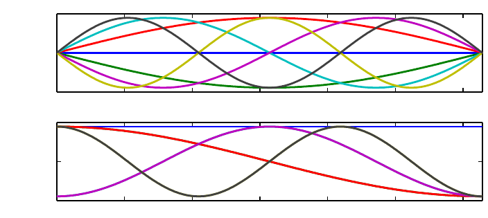
7. Linear Differential Operators and Equations 15
0 5 10 15 20 25 30
−0.2
0
0.2
imag(U)
0 5 10 15 20 25 30
−0.2
0
0.2
real(V)
7.9 Nonlinear equations by Newton iteration
As mentioned at the beginning of this chapter, nonlinear differential equations are discussed in
Chapter 10. As an indication of some of the possibilities, however, we now illustrate how a sequence
of linear problems may be useful in solving nonlinear problems. For example, the nonlinear BVP
0.001u′′ −u3=0,u(−1) = 1,u(1) = −1
could be solved by Newton iteration as follows.
L = chebop(-1, 1);
L.op = @(x,u) 0.001*diff(u, 2);
J = chebop(-1, 1);
x = chebfun(’x’);
u = -x; nrmdu = Inf;
while nrmdu > 1e-10
r = L*u - u.^3;
J.op = @(du) .001*diff(du, 2) - 3*u.^2.*du;
J.bc = 0;
du = -(J\r);
u = u + du; nrmdu = norm(du)
end
clf, plot(u)
nrmdu =
0.260668532007021
nrmdu =
0.164126069559937
nrmdu =
0.098900892365439
nrmdu =
0.053787171683932
nrmdu =
0.021518152858429
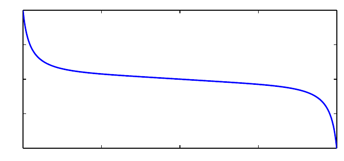
16 Chebfun Guide
nrmdu =
0.003586696693250
nrmdu =
8.951602488918563e-05
nrmdu =
5.357404593788955e-08
nrmdu =
2.063725137129868e-14
−1−0.5 0 0.5 1
−1
−0.5
0
0.5
1
Note the beautifully fast convergence, as one expects with Newton’s method. The chebop Jdefined in
the *while* loop is a Jacobian operator (=Frechet derivative), which we have constructed explicitly
by differentiating the nonlinear operator defining the ODE. In Section 10.4 we shall see that this
whole Newton iteration can be automated by use of Chebfun’s ”nonlinear backslash” capability,
which utilizes automatic differentiation to construct the Frechet derivative automatically. In fact,
all you need to type is
N = chebop(-1, 1);
N.op = @(x,u) 0.001*diff(u, 2) - u.^3;
N.lbc = 1; N.rbc = -1;
v=N\0;
The result is the same as before to many digits of accuracy:
norm(u - v)
ans =
3.141073177047297e-13
7.10 BVP systems with unknown parameters
Sometimes ODEs or systems of ODEs contain unknown parameter values that must be computed
for as part of the solution. An example of this is MATLAB’s built-in mat4bvp example. These
parameters can always be included in system as unknowns with zero derivatives, but this can be
computationally inefficient. Chebfun allows the option of explicit treatment of the parameters.
Often the dependence of the solution on these parameters is nonlinear (as in the case below), and
this discussion might better have been left to Chapter 10, but since, from the user perspective, there
is little difference in this case, we include it here.
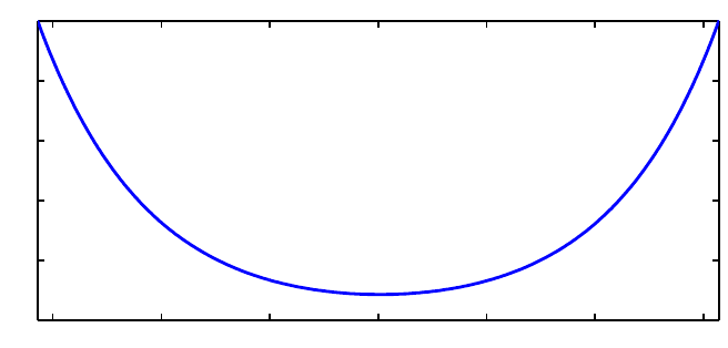
7. Linear Differential Operators and Equations 17
Below is an example of such a parameterised problem, which is represents a linear pendulum with a
forcing sine-wave term of an unknown frequency T. The task is to compute the solution for which
u(−pi)=u(pi)=u′(pi)=1
.
N = chebop(@(x, u , T) diff(u,2) - u - sin(T.*x/pi), [-pi pi]);
N.lbc = @(u,T) u - 1;
N.rbc = @(u,T) [u - 1; diff(u) - 1];
uT = N\0;
Here, the output uT is a chebmatrix – an object that is amongst other features able to vertically
concatenate chebfuns and scalar. The first entry corresponds to the chebfun uwhile the second is
the scalar T. We can access the elements of uT via curly-brackets syntax as follows:
u = uT{1}; T = uT{2}
plot(u)
T=
0.005438812795289
−3−2−1 0 1 2 3
0
0.2
0.4
0.6
0.8
1
As the system is nonlinear in T, we can expect that there will be more than one solution. Indeed,
if we choose a different initial guess for T, we can converge to one of these.
N.init = [chebfun(1, [-pi pi]); 4];
uT = N\0;
u = uT{1}; T = uT{2}
plot(u)
T=
4.044049959218974
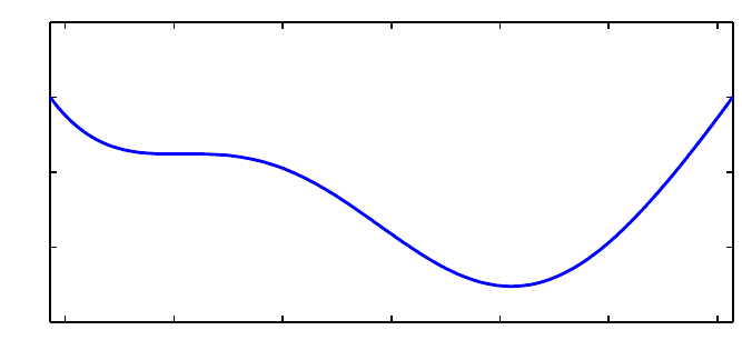
18 Chebfun Guide
−3−2−1 0 1 2 3
−0.5
0
0.5
1
1.5
7.11 References
[Birkisson 2014] A. Birkisson, Numerical Solution of Nonlinear Boundary Value Problems forOr-
dinary Differential Equations in the Continuous Framework, D. Phil. thesis, University of Oxford,
2014.
[Birkisson & Driscoll 2011] A. Birkisson and T. A. Driscoll, Automatic Frechet differentiation for
the numerical solution of boundary-value problems, ACM Transactions on Mathematical Software,
38 (2012), 1-26.
[Driscoll 2010] T. A. Driscoll, Automatic spectral collocation for integral, integro-differential, and
integrally reformulated differential equations, Journal of Computational Physics, 229 (2010), 5980-
5998.
[Driscoll, Bornemann & Trefethen 2008] T. A. Driscoll, F. Bornemann,andL.N.Trefethen,”The
chebop system for automatic solution of differential equations”, BIT Numerical Mathematics,46
(2008), 701-723.
[Driscoll & Hale 2014] T. A. Driscoll and N. Hale, Rectangular spectral collocation, manuscript,
2014.
[Fornberg 1996] B. Fornberg, APracticalGuidetoPseudospectralMethods, Cambridge University
Press, 1996.
[Olver & Townsend 2013] S. Olver and A. Townsend, A fast and well-conditioned spectral method,
SIAM Review, 55 (2013), 462-489.
[Schmid & Henningson 2001] P. J. Schmid and D. S. Henningson, Stability and Transition in Shear
Flows, Springer, 2001.
[Trefethen 2000] L. N. Trefethen, Spectral Methods in MATLAB,SIAM,2000.
8. Chebfun Preferences
Lloyd N. Trefethen, November 2009, last revised June 2014
Contents
•8.1 Introduction
•8.2 domain: the default domain
•8.3 splitting: breaking into subintervals or not
•8.4 splitLength: length limit in splitting on mode
•8.5 maxLength: maximum length
•8.6 minSamples: minimum number of sample points
•8.7 resampling: exploiting nested grids or not
•8.8 eps: Chebfun constructor tolerance
•8.9 Chebyshev grids of first or second kind
•8.10 Rectangular or ultraspherical spectral discretizations
•8.11 Chebfun2 preferences
•8.12 Additional preferences
8.1 Introduction
Like any software package, Chebfun is based on certain design decisions. Some of these can be
adjusted by the user, like the maximum number of points at which a function will be sampled before
Chebfun gives up trying to resolve it. Extensive information about these possibilities can be found
by executing help chebfunpref, or for chebops, as used to solve integral and differential equations,
help cheboppref. To see the list of preferences and their current values, execute chebfunpref or
cheboppref:
chebfunpref
chebfunpref object with the following preferences:
domain: [-1, 1]
splitting: 0
splitPrefs
splitLength: 160
splitMaxLength: 6000
blowup: 0
blowupPrefs
exponentTol: 1.100000e-11
maxPoleOrder: 20
defaultSingType: ’sing’
1
2Chebfun Guide
enableDeltaFunctions: 1
deltaPrefs
deltaTol: 1.000000e-09
proximityTol: 1.000000e-11
cheb2Prefs
maxRank: 513
sampleTest: 1
tech: @chebtech2
<a href="matlab: help chebtech2/techPref">techPrefs</a>
eps: 2.220446049250313e-16
minSamples: 17
maxLength: 65537
fixedLength: NaN
extrapolate: 0
sampleTest: 1
refinementFunction: ’nested’
happinessCheck: ’classic’
More detailed information from further down in the preference structure will come from, for example,
help chebtech/techpref.
To ensure that all preferences are set to their factory values, execute
chebfunpref.setDefaults(’factory’)
In this chapter we explore some of these adjustable preferences, showing how special effects can be
achieved by modifying them. Besides showing offsome useful techniques, this review will also serve
to deepen the user’s understanding of Chebfun by poking about a bit at its edges.
A general point to be emphasized is the distinction between creating a chebfun directly from the
constructor and creating one by operating on previous chebfuns. In the former case we can include
preferences directly in the constructor command, and we recommend this as good practice:
f = chebfun(’x.^x’,[0,1],’splitting’,’on’);
In the latter case, however, one can turn the preference on and offagain.
x = chebfun(’x’,[0,1]);
chebfunpref.setDefaults(’splitting’,true)
f = x.^x;
chebfunpref.setDefaults(’splitting’,false)
8.2 domain:thedefaultdomain
Like Chebyshev polynomials themselves, chebfuns are defined by default on the domain [−1,1] if no
other domain is specified. However, this default choice of the default domain can be modified. For
example, we can work with trigonometric functions on [0,2π] conveniently like this:
chebfunpref.setDefaults(’domain’,[0 2*pi])
f = chebfun(@(t) sin(19*t));
g = chebfun(@(t) cos(20*t));
plot(f,g), axis equal, axis off
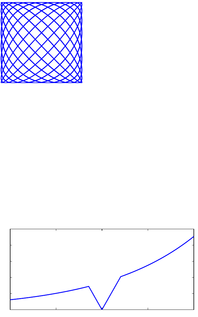
8. Chebfun Preferences 3
8.3 splitting:breakingintosubintervalsornot
Perhaps the preference that users wish to control most often is the choice of splitting offor on.
Splitting offis the factory default.
In both splitting offand splitting on modes, a chebfun may consist of a number of pieces, called
funs. For example, even in splitting offmode, the following sequence makes a chebfun with four
funs:
chebfunpref.setDefaults(’factory’);
x = chebfun(@(x) x);
f = min(abs(x),exp(x)/6);
format short, f.ends
plot(f)
ans =
-1.0000 -0.1443 0 0.2045 1.0000
−1−0.5 0 0.5 1
0
0.1
0.2
0.3
0.4
0.5
One breakpoint is introduced at x= 0, where the constructor determines that |x|has a zero, and
two more breakpoints are introduced at −0.1443 and at 0.2045, where it recognizes that |x|and
exp(x)/6 will intersect.
The difference between splitting offand splitting on pertains to additional breakpoints that may be
introduced in the more basic chebfun construction process, when the constructor makes a chebfun
solely by sampling point values. For example, suppose we try to make the same chebfun as above
4Chebfun Guide
from scratch, by sampling an anonymous function, in splitting offmode. We get a warning message:
ff = @(x) min(abs(x),exp(x)/6);
f = chebfun(ff);
Warning: Function not resolved using 65537 pts. Have you tried ’splitting on’?
With splitting on, Chebfun’s built-in edge detector quickly finds the singular points and introduces
breakpoints there:
f = chebfun(ff,’splitting’,’on’);
f.ends
ans =
-1.0000 -0.1443 0.0000 0.2045 1.0000
This example involves specific points of singularity, which the constructor has duly located. In
addition to this, in splitting on mode the constructor will subdivide intervals recursively at non-
singular points when convergence is not taking place fast enough. For example, with splitting offwe
cannot successfully construct a chebfun for the square root function on [0,1] (unless we use singular
exponents as described in the next chapter):
f = chebfun(@(x) sqrt(x),[0 1]);
Warning: Function not resolved using 65537 pts. Have you tried ’splitting on’?
With splitting on, however, all is well:
f = chebfun(@(x) sqrt(x),[0 1],’splitting’,’on’);
length(f)
format long, f((.1:.1:.5)’.^2)
ans =
515
ans =
0.100000000057989
0.200000000011776
0.300000000012712
0.400000000008074
0.500000000010248
Inspection reveals that Chebfun has broken the interval into a succession of pieces, each 100 times
smaller than the next:
f.ends
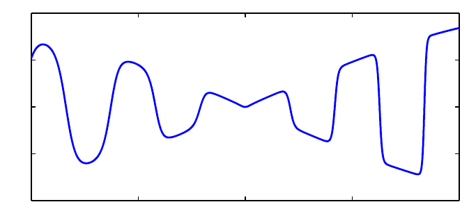
8. Chebfun Preferences 5
ans =
Columns 1 through 3
0 0.000000000100000 0.000000010000000
Columns 4 through 6
0.000001000000000 0.000100000000000 0.010000000000000
Column 7
1.000000000000000
In this example the subdivisions have occurred near an endpoint, fortheedgedetectorhasdeter-
mined that the difficulty of resolution lies there. For other functions, however, splitting will take
place at midpoints. For example, here is a function that is complicated throughout [−1,1], especially
for larger values of x.
ff = @(x) sin(x).*tanh(3*exp(x).*sin(15*x));
With splitting off, it gets resolved by a global polynomial of rather high degree.
f = chebfun(ff);
length(f)
plot(f)
ans =
1346
−1−0.5 0 0.5 1
−1
−0.5
0
0.5
1
With splitting on, the function is broken up into pieces, and there is some reduction in the overall
length:
f = chebfun(ff,’splitting’,’on’);
length(f)
format short, f.ends
ans =
825
ans =
Columns 1 through 7
-1.0000 -0.7500 -0.5000 -0.2500 0 0.2500 0.3750
Columns 8 through 12
0.5000 0.6250 0.8125 0.8750 1.0000
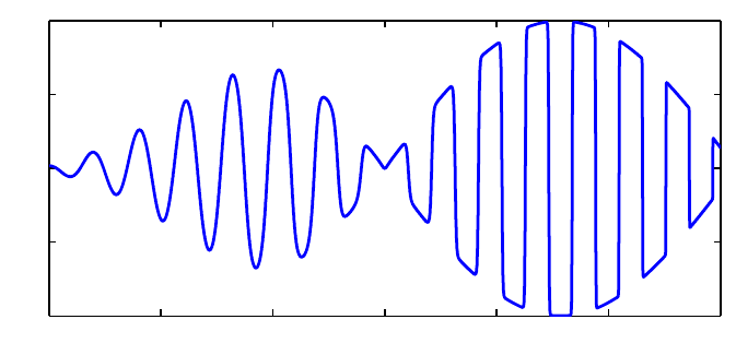
6Chebfun Guide
When should one use splitting off, and when splitting on? If the goal is simply to represent compli-
cated functions, especially when they are more complicated in some regions than others, splitting
on sometimes has advantages. An example is given by the function above posed on [−3,3] instead
of [−1,1]. With splitting off, the global polynomial has a degree in the tens of thousands:
f3 = chebfun(ff,[-3 3]);
length(f3)
plot(f3)
ans =
16009
−3−2−1 0 1 2 3
−1
−0.5
0
0.5
1
With splitting on the representation is much more compact:
f3 = chebfun(ff,[-3 3],’splitting’,’on’);
length(f3)
ans =
2828
On the other hand, splitting offmode has advantages of robustness. In particular, operations
involving derivatives generally work better when functions are represented by global polynomials,
and chebops for the most part require this. Also, for educational purposes, it is very convenient
that Chebfun can be used so easily to study the properties of pure polynomial representations even
of very high degree.
8.4 splitLength:lengthlimitinsplittingonmode
When intervals are subdivided in splitting on mode, as just illustrated, the parameter splitLength
determines where this will happen. With the factory value splitLength=160, splitting will take
place if a polynomial of length 160 proves insufficient to resolve a fun. (Actually, when Chebfun uses
Chebyshev points of the second kind as it does by default, this number is rounded down to 1 more
than a power of 2.) Let us confirm for the chebfun fconstructed a moment ago that the lengths of
the individual funs are all less than or equal to 160 (actually 129):
f.funs
8. Chebfun Preferences 7
ans =
Columns 1 through 4
[66x1 bndfun] [78x1 bndfun] [90x1 bndfun] [90x1 bndfun]
Columns 5 through 8
[124x1 bndfun] [31x1 bndfun] [96x1 bndfun] [62x1 bndfun]
Columns 9 through 11
[79x1 bndfun] [74x1 bndfun] [35x1 bndfun]
Alternatively, suppose we wish to allow individual funs to have length upto513. Wecandothat
like this:
f = chebfun(ff,’splitting’,’on’,’splitLength’,513);
length(f)
format short, f.ends
f.funs
ans =
1183
ans =
-1.0000 0 0.5000 0.7500 1.0000
ans =
[353x1 bndfun] [307x1 bndfun] [246x1 bndfun] [277x1 bndfun]
8.5 maxLength:maximumlength
As just mentioned, in splitting offmode, the constructor tries to make a global chebfun from the
given string or anonymous function. For a function like |x|or sign(x), this will typically not be
possible and we must give up somewhere. The parameter maxLength,setto2
16 + 1 in the factory,
determines this giving-up point.
For example, here’s what happens normally if we try to make a chebfun for sign(x).
f = chebfun(’sign(x)’);
Warning: Function not resolved using 65537 pts. Have you tried ’splitting on’?
Suppose we wish to examine the interpolant to this function through 50 points instead of 65537.
One way is like this:
f = chebfun(’sign(x)’,50);
length(f)
plot(f)
ans =
50
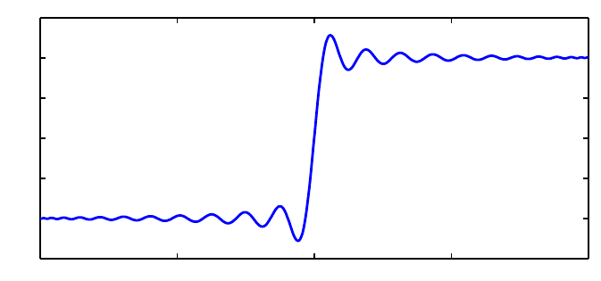
8Chebfun Guide
−1−0.5 0 0.5 1
−1.5
−1
−0.5
0
0.5
1
1.5
Notice that no warning message is produced since we have asked explicitly for exactly 50 points.
On the other hand we could also change the default maximum to this number (or more precisely
the default degree to one less than this number), giving the same effect though now with another
warning message:
f = chebfun(’sign(x)’,’maxLength’,50);
length(f)
Warning: Function not resolved using 50 pts. Have you tried ’splitting on’?
ans =
33
Perhaps more often one might wish to adjust this preference to enable use of especially high degrees.
On the machines of 2014, Chebfun is perfectly capable of working with polynomials of degrees in the
millions. The function |x|5/4on [−1,1] provides an example, for it is smooth enough to be resolved
by a global polynomial, provided it is of rather high degree:
tic
f = chebfun(’abs(x).^1.25’,’maxLength’,1e6);
lengthf = length(f)
format long, sumf = sum(f)
plot(f)
toc
lengthf =
105185
sumf =
0.888888888881000
Elapsed time is 0.796616 seconds.
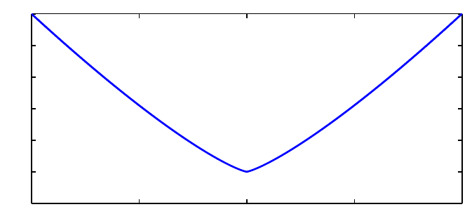
8. Chebfun Preferences 9
−1−0.5 0 0.5 1
−0.2
0
0.2
0.4
0.6
0.8
1
(More efficient ways of resolving this function, by eliminating the singularity, are described in Chap-
ter 9.)
8.6 minSamples:minimumnumberofsamplepoints
At the other end of the spectrum, the preference minSamples determines the minimum number of
points at which a function is sampled during the chebfun construction process, and the factory value
of this parameter is 17. This does not mean that all chebfuns have length at least 17. For example, if
fis a cubic, then it will be sampled at 17 points, Chebyshev expansion coefficients will be computed,
and 13 of these will be found to be of negligible size and discarded. So the resulting chebfun is a
cubic, even though the constructor never sampled at fewer than 17 points.
f = chebfun(’x.^3’);
lengthf = length(f)
lengthf =
4
More generally a function is sampled at 17,33,65,...points until a set of Chebyshev coefficients are
obtained with a tail judged to be negligible.
Like any process based on sampling, this one can fail. For example, here is a success:
f = chebfun(’-x -x.^2 + exp(-(30*(x-.47)).^2)’);
length(f)
plot(f)
ans =
309
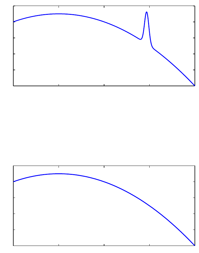
10 Chebfun Guide
−1−0.5 0 0.5 1
−2
−1.5
−1
−0.5
0
0.5
But if we change the exponent to 4, we get a failure:
f = chebfun(’-x -x.^2 + exp(-(30*(x-.47)).^4)’);
length(f)
plot(f)
ans =
3
−1−0.5 0 0.5 1
−2
−1.5
−1
−0.5
0
0.5
What has happened can be explained as follows. The function being sampled has a narrow spike
near x=0.47, and the closest grid points lie near 0.383 and 0.556. In the case of the exponent 2,
we note that at x=0.383 and x=0.556, exp(−(30(x−.47)2)) takes values of about 0.001, which
are easily large enough to be noticed by the Chebfun constructor. On the other hand in the case of
exponent 4, the values at these points shrink to less than 10−19, which is below machine precision.
So in the latter case the constructor thinks it has a quadratic and does not try a finer grid.
If we increase minSamples, the correct chebfun is found:
f = chebfun(’-x -x.^2 + exp(-(30*(x-.48)).^4)’,’minSamples’,33);
length(f)
plot(f)
ans =
1021
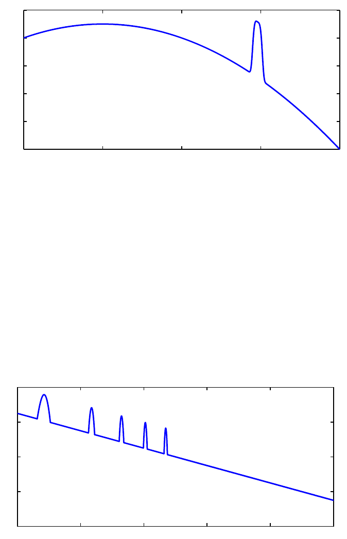
8. Chebfun Preferences 11
−1−0.5 0 0.5 1
−2
−1.5
−1
−0.5
0
0.5
Incidentally, if the value of minSamples specified is not one greater than a power of 2, it is rounded
up to the next such value.
The factory value minSamples=17 was chosen as a compromise between efficiency and reliability.
(Until Version 5, the choice was |minSamples=9’.) In practice it rarely seems to fail, but perhaps it
is most vulnerable when applied in splitting on mode to functions with narrow spikes. For example,
the following chebfun is missing most of the spikes that should be there:
ff = @(x) max(.85,sin(x+x.^2)) - x/20;
f = chebfun(ff,[0,10],’splitting’,’on’);
plot(f)
0 2 4 6 8 10
0.2
0.4
0.6
0.8
1
Increasing minSamples fills them in:
f = chebfun(ff,[0,10],’splitting’,’on’,’minsamples’,33);
plot(f)
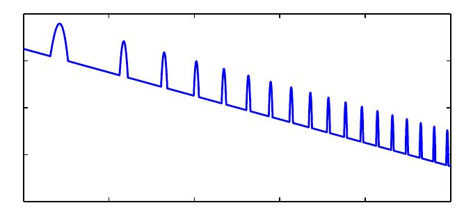
12 Chebfun Guide
0 2 4 6 8 10
0.2
0.4
0.6
0.8
1
8.7 resampling:exploitingnestedgridsornot
We now turn to a particularly interesting preference for Chebfun geeks, relating to the very idea of
what it means to sample a function.
When a chebfun is constructed, a function is normally sampled at 17,33,65,... Chebyshev points
until convergence is achieved. (We are speaking here of the process for Chebyshev points of the
second kind; for first-kind points the details are different.) Now Chebyshev grids are nested, so the
33-point grid, for example, only contains 16 points that are not in the 17-point grid. By default,
the Chebfun constructor takes advantage of this property so as not to recompute values that have
already been computed. (The default went the other way until 2009.)
For example, here is a chebfun constructed in the usual factory mode:
ff = @(x) besselj(x,exp(x))
tic, f = chebfun(ff,[0 8]); toc
length(f)
ff =
@(x)besselj(x,exp(x))
Elapsed time is 0.038966 seconds.
ans =
3777
There is little difference, even in the timing, if we set ’resampling on’, so that previously computed
values are not reused:
tic, f = chebfun(ff,[0 8],’resampling’,’on’); toc
length(f)
Elapsed time is 0.049952 seconds.
ans =
3782
One might wonder why ’resampling on’ is an option at all, but in fact, it introduces some very
interesting possibilities. What if the ”function” being sampled is not actually a fixed function, but
depends on the grid? For example, consider this prescription:
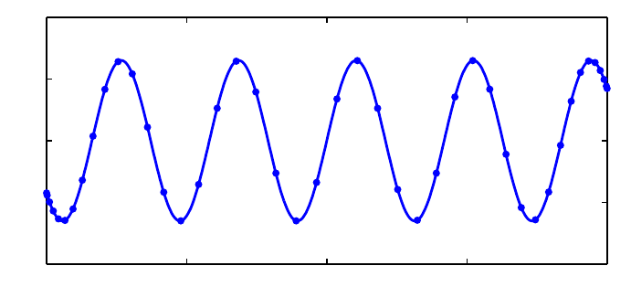
8. Chebfun Preferences 13
ff = @(x) length(x)*sin(15*x);
The values of fat any particular point will depend on the length of the vector in which it is
embedded! What will happen if we try to make a chebfun, disabling the ”sampleTest” feature that
is usually applied by the constructor as a safety test? The constructor tries the 17-point Chebyshev
grid, then the 33-point grid, then the 65-point grid. On the last of these it finds the Chebyshev
coefficients are sufficiently small, and proceeds to truncate to length 44. We end up with a chebfun
of length 44 that precisely matches the function 65 sin(15x).
f = chebfun(ff,’sampleTest’,0,’resampling’,’on’);
length(f)
max(f)
plot(f,’.-’)
ans =
44
ans =
65
−1−0.5 0 0.5 1
−100
−50
0
50
100
This rather bizarre example encourages us to play further. What if we change length(x)*sin(15*x)
to sin(length(x)*x)? Now there is no convergence, for no matter how fine the grid is, the function is
underresolved.
hh = @(x) sin(length(x)*x);
h = chebfun(hh,’sampleTest’,0,’resampling’,’on’);
Warning: Function not resolved using 65537 pts. Have you tried ’splitting on’?
Here is an in-between case where convergence is achieved on the grid of length 65, and the resulting
chebfun then trimmed to length 46.
kk = @(x) sin(length(x).^(2/3)*x);
k = chebfun(kk,’sampleTest’,0,’resampling’,’on’);
length(k)
plot(k,’.-’)
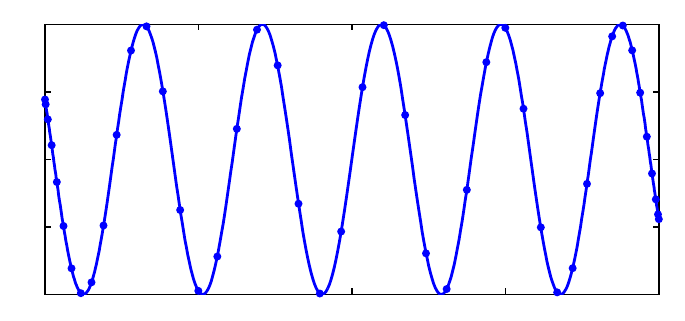
14 Chebfun Guide
ans =
46
−1−0.5 0 0.5 1
−1
−0.5
0
0.5
1
Are such curious effects of any use? Yes indeed, they are at the heart of Chebop. When the chebop
system solves a differential equation by a command like u=L\f, for example, the chebfun uis
determined by a ”sampling” process in which a matrix problem obtained by Chebyshev spectral
discretization is solved on grids of increasing sizes. The matrices change with the grids, so the
sample values for uare crucially grid-dependent. Without resampling, chebops would notwork.
8.8 eps:Chebfunconstructortolerance
One of the controllable preferences is all too tempting: you can weaken the tolerance used in con-
structing a chebfun. The chebfunpref parameter eps is set by default to machine precision:
p = chebfunpref;
p.eps
ans =
2.220446049250313e-16
However, one can change this with a command like chebfunpref.setDefaults(’eps’,1e-6).
There are cases where weakening the tolerance makes a big difference. For example, this happens
in certain applications in 2D and in certain applications involving differential equations. (Indeed,
the Chebfun differential equations commands have their own tolerance control strategies.) However,
Chebfun does such a good job at resolving many functions that the eps-adjustment feature is not as
useful as you might imagine, and we recommend that users not change eps unless they are having
real problems with standard precision.
8.9 Chebyshev grids of first or second kind
Beginning with Version 5, Chebfun includes capabilities for carrying out almost all computations
with Chebyshev points of either the first kind (cos((j+1/2)π/(n+1)),0≤j≤n, implemented
in the chebtech1 class) or the second kind (cos(jπ/n),0≤j≤n, implemented in the chebtech2
class). These capabilities were included to further our research into the pros and cons of different
8. Chebfun Preferences 15
kinds of algorithms, and most users can ignore this choice entirely. You can query which kind of
Chebyshev points is in use with
t = chebkind
t=
2
and you can set it with, for example,
chebkind(1)
or
chebkind 1
An equivalent would be the command
chebfunpref.setDefaults(’tech’,@chebtech1)
Let us return to factory settings:
chebfunpref.setDefaults(’factory’)
8.10 Rectangular or ultraspherical spectral discretizations
Chebfun’s factory default for spectral discretizations is rectangular collocation in Chebyshev points
of the second kind, which corresponds to
cheboppref.setDefaults(’discretization’,’colloc2’)
To change the preference to first-kind points, one can execute
cheboppref.setDefaults(’discretization’,’colloc1’)
and for Olver-Townsend ultraspherical discretizations,
cheboppref.setDefaults(’discretization’,’ultraspherical’)
Let us undo these changes:
cheboppref.setDefaults(’factory’)
8.11 Chebfun2 preferences
The Chebfun2 preference that users may be most interested in is MaxRank, which determines the
maximum rank of a low-rank approximation used to represent a function on a rectangle. The current
factory default is 512, and this can be changed for example with
chebfunpref.setDefaults({’cheb2Prefs’,’maxRank’},1024);
Let us undo this change:
chebfunpref.setDefaults(’factory’)
16 Chebfun Guide
8.12 Additional preferences
Information about additional Chebfun preferences can be found by executing chebfunpref or help
chebfunpref. In general the most reliable values to use in setting preferences are are 1or true’
and |0or false (not ’on’ and ’off’).
For example, ’sampleTest’ controls whether a function is evaluated at an extra point as a safety
check of convergence. With the default ’on’ value, this test is indeed carried out.
Another example is that ’blowup’ relates to the construction of chebfuns that diverge to infinity, as
described in Chapter 9. blowup=0 is used for no singularities, blowup=1 if for functions with poles
(blowups with a negative integer power) and blowup=2 for functions with branch points (blowups
with an arbitrary power).
9. Infinite Intervals, Infinite
Function Values, and Singularities
Lloyd N. Trefethen, November 2009, latest revision June 2014
Contents
•9.1 Infinite intervals
•9.2 Poles
•9.3 Singularities other than poles
•9.4 Another approach to singularities
•9.5 References
This chapter presents some features of Chebfun that are less robust than what is described in the first
eight chapters. With classic bounded chebfuns on a bounded interval [a, b], you can do amazingly
complicated things often without encountering any difficulties. Now we are going to let the intervals
and the functions diverge to infinity – but please lower your expectations! These features are not
always as accurate or reliable.
9.1 Infinite intervals
If a function converges reasonably rapidly to a constant at ∞, you can define a corresponding
chebfun. Here are a couple of examples on [0,∞]. First we plot a function and find its maximum:
f = chebfun(’0.75 + sin(10*x)./exp(x)’,[0 inf]);
LW = ’linewidth’; MS = ’markersize’;
plot(f,LW,1.6)
maxf = max(f)
maxf =
1.608912750768336
1
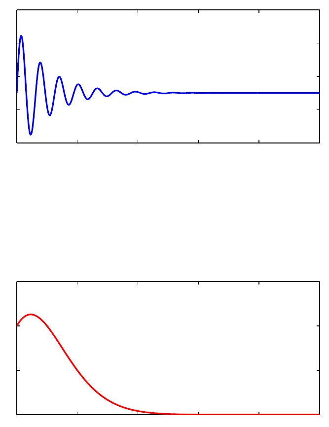
2Chebfun Guide
0 2 4 6 8 10
0
0.5
1
1.5
2
Next we plot another function and integrate it from 0 to ∞:
g = chebfun(’1./(gamma(x+1))’,[0 inf]);
sumg = sum(g)
plot(g,’r’,LW,1.6)
sumg =
2.266534507699834
0 2 4 6 8 10
0
0.5
1
1.5
Where do fand gintersect? We can find out using roots:
plot(f,’b’,g,’r’,LW,1.2), hold on
r = roots(f-g)
plot(r,f(r),’.k’,MS,18)
r=
0.027639744894513
0.265714132607450
0.706922132176979
0.862331877000826
1.297442594652156
1.594466987072374
1.781855556974647
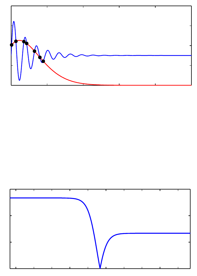
9. Infinite Intervals, Infinite Function Values, and Singularities 3
0 2 4 6 8 10
0
0.5
1
1.5
2
Here’s an example on (−∞,∞) with a calculation of the location and value of the minimum:
g = chebfun(@(x) tanh(x-1),[-inf inf]);
g = abs(g-1/3);
clf, plot(g,LW,1.6)
[minval,minpos] = min(g)
minval =
0
minpos =
1.346573590279974
−8−6−4−2 0 2 4 6 8 10
0
0.5
1
1.5
Notice that a function on an infinite domain is by default plotted on an interval like [0,10] or
[−10,10]. You can use an extra ’interval’ flag to plot on other intervals, as shown by this
example of a function of small norm whose largest values are near x=30:
hh = @(x) cos(x)./(1e5+(x-30).^6);
h = chebfun(hh,[0 inf]);
plot(h,LW,1.6,’interval’,[0 100])
normh = norm(h)
normh =
2.441961683577728e-05
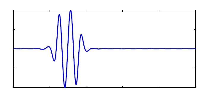
4Chebfun Guide
0 20 40 60 80 100
−1
−0.5
0
0.5
1
x 10−5
Chebfun provides a convenient tool for the numerical evaluation of integrals over infinite domains:
g = chebfun(’(2/sqrt(pi))*exp(-x.^2)’,[0 inf]);
sumg = sum(g)
sumg =
0.999999999999992
The cumsum operator applied to this integrand gives us the error function, which matches the
MATLAB erf function reasonably well:
errorfun = cumsum(g)
disp(’ erf errorfun’)
for n = 1:6, disp([erf(n) errorfun(n)]), end
errorfun =
chebfun column (1 smooth piece)
interval length endpoint values
[0,Inf]97 0 1
Epslevel = 2.220446e-16. Vscale = 1.000000e+00.
erf errorfun
0.842700792949715 0.842700792948944
0.995322265018953 0.995322265017458
0.999977909503001 0.999977909500824
0.999999984582742 0.999999984579919
0.999999999998463 0.999999999995027
1.000000000000000 0.999999999995981
One should be cautious in evaluating integrals over infinite intervals, however, for as mentioned in
Section 1.5, the accuracy is sometimes disappointing, especially for functions that do not decay very
quickly:
sum(chebfun(’(1/pi)./(1+s.^2)’,[-inf inf]))
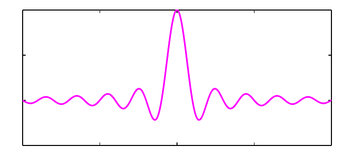
9. Infinite Intervals, Infinite Function Values, and Singularities 5
ans =
0.999999999998234
Here’s an example of a function whose wiggles decay too slowly to be fully resolved:
sinc = chebfun(’sin(pi*x)./(pi*x)’,[-inf inf]);
plot(sinc,’m’,LW,1.6,’interval’,[-10 10])
Warning: Function not resolved using 65537 pts. Have you tried ’splitting on’?
−10 −5 0 5 10
−0.5
0
0.5
1
Chebfun’s capability of handling infinite intervals was introduced by Rodrigo Platte in 2008-09. The
details of the implementation then changed considerably with the introduction of version 5 in 2014.
The use of mappings to transform an unbounded domain to a bounded one is an idea that has been
employed many times over the years. One of the references we have benefitted especially from, which
also contains pointers to other works in this area, is the book [Boyd 2001].
9.2 Poles
Chebfun can handle certain ”vertical” as well as ”horizontal” infinities – especially, functions that
blow up according to an integer power, i.e., with a pole. If you know the nature of the blowup, it is
a good idea to specify it using the ’exps’ flag. For example, here’s a function with a simple pole at
0. We use ’exps’ to tell the constructor that the function looks like x−1at the left endpoint and
x0(i.e., smooth) at the right endpoint.
f = chebfun(’sin(50*x) + 1./x’,[0 4],’exps’,[-1,0]);
plot(f,LW,1.6), ylim([-5 30])
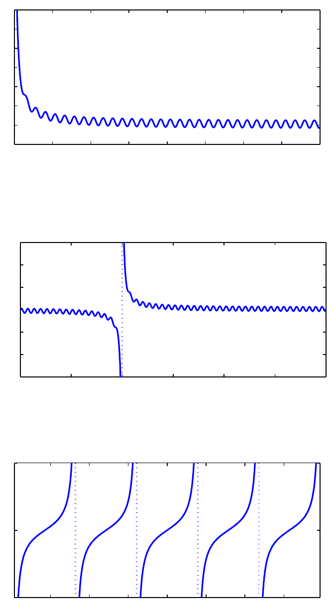
6Chebfun Guide
0 0.5 1 1.5 2 2.5 3 3.5 4
−5
0
5
10
15
20
25
30
Here’s the same function but over a domain that contains the singularity in the middle. We tell the
constructor where the pole is and what the singularity looks like:
f = chebfun(’sin(50*x) + 1./x’,[-2 0 4],’exps’,[0,-1,0]);
plot(f,LW,1.6), ylim([-30 30])
−2−1 0 1 2 3 4
−30
−20
−10
0
10
20
30
Here’s the tangent function:
f = chebfun(’tan(x)’, pi*((-5/2):(5/2)), ’exps’, -ones(1,6));
plot(f,LW,1.6), ylim([-5 5])
−6−4−2 0 2 4 6
−5
0
5
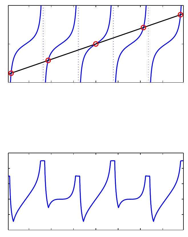
9. Infinite Intervals, Infinite Function Values, and Singularities 7
Rootfinding works as expected:
x2 = chebfun(’x/2’,pi*(5/2)*[-1 1]);
hold on, plot(x2,’k’,LW,1.6)
r = roots(f-x2,’nojump’); plot(r,x2(r),’or’,LW,1.6,’markersize’,8)
−6−4−2 0 2 4 6
−5
0
5
And we can manipulate the function in various other familiar ways:
g = sin(2*x2)+min(abs(f+2),6);
hold off, plot(g,LW,1.6)
−6−4−2 0 2 4 6
−2
0
2
4
6
8
If you don’t know what singularities your function may have, Chebfun has some ability to find them
if the flags ’blowup’and’splitting’areon:
gam = chebfun(’gamma(x)’,[-4 4],’splitting’,’on’,’blowup’,1);
plot(gam,LW,1.6), ylim([-10 10])
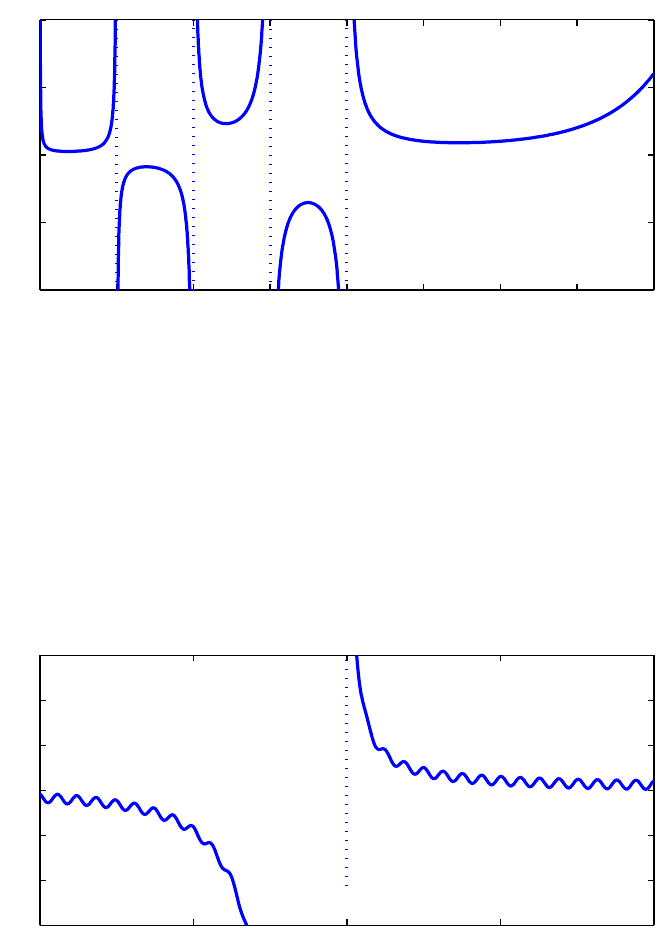
8Chebfun Guide
−4−3−2−1 0 1 2 3 4
−10
−5
0
5
10
But it’s always better to specify the breakpoints and powers if you know them:
gam = chebfun(’gamma(x)’,[-4:0 4],’exps’,[-1 -1 -1 -1 -1 0]);
It’s also possible to have poles of different strengths on two sides of a singularity. In this case, you
specify two exponents at each internal breakpoint rather than one:
f = chebfun(@(x) cos(100*x)+sin(x).^(-2+sign(x)),[-1 0 1],’exps’,[0 -3 -1 0]);
plot(f,LW,1.6), ylim([-30 30])
−1−0.5 0 0.5 1
−30
−20
−10
0
10
20
30
9.3 Singularities other than poles
Less reliable but also sometimes useful is the possibility of working with functions with algebraic
singularities that are not poles. Here’s a function with inverse square root singularities at each end:
w = chebfun(’(2/pi)./(sqrt(1-x.^2))’,’exps’,[-.5 -.5]);
plot(w,’m’,LW,1.6), ylim([0 10])
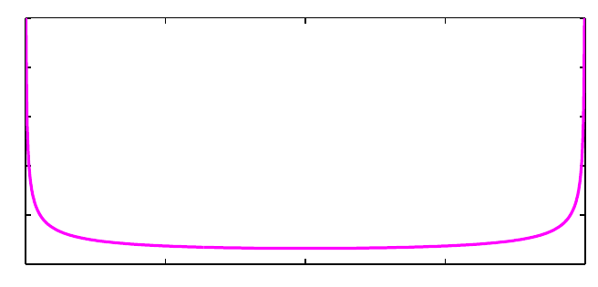
9. Infinite Intervals, Infinite Function Values, and Singularities 9
−1−0.5 0 0.5 1
0
2
4
6
8
10
The integral is 2:
sum(w)
ans =
2
We pick this example because Chebyshev polynomials are the orthogonal polynomials with respect
to this weight function, and Chebyshev coefficients are defined by inner products against Chebyshev
polynomials with respect to this weight. For example, here we compute inner products of x4+x5
against the Chebyshev polynomials T0,...,T
5. (The integrals in these inner products are calculated
by Gauss-Jacobi quadrature using methods due to Hale and Townsend; for more on this subject see
the command jacpts.)
x = chebfun(’x’);
T = chebpoly(0:5)’;
f = x.^4 + x.^5;
chebcoeffs1 = T*(w.*f)
chebcoeffs1 =
0.750000000000000
0.625000000000000
0.500000000000000
0.312500000000000
0.125000000000000
0.062500000000000
Here for comparison are the Chebyshev coefficients as obtained from chebcoeffs:
chebcoeffs2 = flipud(chebcoeffs(f)’)
chebcoeffs2 =
0.375000000000000
0.625000000000000
0.500000000000000
0.312500000000000
0.125000000000000
0.062500000000000
10 Chebfun Guide
Notice the excellent agreement except for coefficient a0. As mentioned in Section 4.1, in this special
case the result from the inner product must be multiplied by 1/2.
You can specify singularities for functions that don’t blow up, too. For example, suppose we want
to work with (xexp(x))1/2on the interval [0,2]. A first try fails completely:
ff = @(x) sqrt(x.*exp(x));
d = [0,2];
f = chebfun(ff,d)
Warning: Function not resolved using 65537 pts. Have you tried ’splitting on’?
f=
chebfun column (1 smooth piece)
interval length endpoint values
[ 0, 2] 65537 3.6e-15 3.8
Epslevel = 6.814598e-11. Vscale = 3.844231e+00.
We could turn splitting on and resolve the function by many pieces, as illustrated in Section 8.3:
f = chebfun(ff,d,’splitting’,’on’)
f=
chebfun column (6 smooth pieces)
interval length endpoint values
[ 0, 2e-10] 43 1.2e-07 1.4e-05
[ 2e-10, 2e-08] 62 1.4e-05 0.00014
[ 2e-08, 2e-06] 91 0.00014 0.0014
[ 2e-06, 0.0002] 111 0.0014 0.014
[ 0.0002, 0.02] 123 0.014 0.14
[ 0.02, 2] 84 0.14 3.8
Epslevel = 4.572597e-10. Vscale = 3.844231e+00. Total length = 514.
A better representation, however, is constructed if we tell Chebfun about the singularity at x=0:
f = chebfun(ff,d,’exps’,[.5 0])
plot(f,LW,1.6)
f=
chebfun column (1 smooth piece)
interval length endpoint values endpoint exponents
[ 0, 2] 12 0 3.8 [0.5 0]
Epslevel = 1.000000e-14. Vscale = 3.844231e+00.
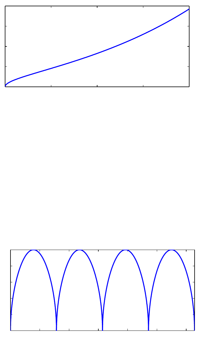
9. Infinite Intervals, Infinite Function Values, and Singularities 11
0 0.5 1 1.5 2
0
1
2
3
4
Under certain circumstances Chebfun will introduce singularities like this of its own accord. For
example, just as abs(f) introduces breakpoints at roots of f,sqrt(abs(f)) introduces breakpoints
and also singularities at such roots:
theta = chebfun(’t’,[0,4*pi]);
f = sqrt(abs(sin(theta)))
plot(f,LW,1.6)
sumf = sum(f)
f=
chebfun column (4 smooth pieces)
interval length endpoint values endpoint exponents
[ 0, 3.1] 19 0 0 [0.5 0.5]
[ 3.1, 6.3] 19 0 0 [0.5 0.5]
[ 6.3, 9.4] 19 0 0 [0.5 0.5]
[ 9.4, 13] 19 0 0 [0.5 0.5]
Epslevel = 1.408355e-15. Vscale = 1. Total length = 76.
sumf =
9.585121877884735
0 2 4 6 8 10 12
0
0.2
0.4
0.6
0.8
1
If you have a function that blows up but you don’t know the nature of the singularities, even whether
they are poles or not, Chebfun will try to figure them out automatically if you run in ’blowup 2’
mode. Here’s an example
12 Chebfun Guide
f = chebfun(’x.*(1+x).^(-exp(1)).*(1-x).^(-pi)’,’blowup’,2)
f=
chebfun column (1 smooth piece)
interval length endpoint values endpoint exponents
[ -1, 1] 30 -Inf Inf [-2.7 -3.1]
Epslevel = 1.000000e-14. Vscale = Inf.
Notice that the ’exps’ field shows values close to −eand −π, as is confirmed by looking at the
numbers to higher precision:
get(f, ’exps’)
ans =
-2.718281828460000 -3.141592653590000
The treatment of blowups in Chebfun was initiated by Mark Richardson in an MSc thesis at Oxford
[Richardson 2009], then further developed by Richardson in collaboration with Rodrigo Platte and
Nick Hale.
9.4 Another approach to singularities
Chebfun version 4 offered an alternative singmap approach to singularities based on mappings of
the xvariable. This is no longer available in version 5.
9.5 References
[Boyd 2001] J. P. Boyd, Chebyshev and Fourier Spectral Methods, 2nd ed., Dover, 2001.
[Richardson 2009] M. Richardson, Approximating Divergent Functions in the Chebfun System, thesis,
MSc in Mathematical Modelling and Scientific Computing, Oxford University, 2009.
10. Nonlinear ODEs and Chebgui
Lloyd N. Trefethen, November 2009, latest revision June 2014
Contents
•10.1 ode45,ode15s,ode113
•10.2 bvp4c,bvp5c
•10.3 Automatic differentiation
•10.4 Nonlinear backslash and solvebvp
•10.5 Graphical user interface: Chebgui
•10.6 References
Chapter 7 described the chebop capability for solving linear ODEs (ordinary differential equations)
by the backslash command. We will now describe extensions of chebops to nonlinear problems, as
well as other methods for nonlinear ODEs:
o Initial-value problems: ode45,ode113,ode15s
o Boundary-value problems: bvp4c,bvp5c
o Both kinds of problems via chebops: nonlinear backslash (=|solvebvp|)
In this chapter we outline the use of these methods; for fuller details, see the help documentation
and especially the online Chebfun Examples. The last of the methods listed, nonlinear backslash or
solvebvp, represents a ”pure Chebfun” approach in which Newton’s method is applied on chebfuns,
with the necessary derivative operators calculated by Chebfun’s built-in capabilities of Automatic
Differentiation (AD). This is the main Chebfun method recommended for solving boundary-value
problems.
We use the abbreviations IVP for initial-value problem and BVP for boundary-value problem.
For time-dependent PDEs, try help pde15s.
10.1 ode45,ode15s,ode113
MATLAB has a highly successful suite of ODE IVP solvers introduced originally by Shampine and
Reichelt [Shampine & Reichelt 1997]. The codes are called ode23,ode45,ode113,ode15s,ode23s,
ode23t,andode23tb, and are adapted to various mixes of accuracy requirements and stiffness.
Chebfun includes versions of ode45 (for medium accuracy), ode113 (for high accuracy), and ode15s
(for stiffproblems) originally created by Toby Driscoll and Rodrigo Platte. These codes operate
1
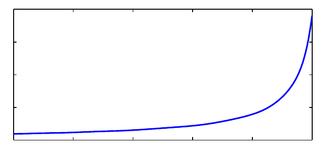
2Chebfun Guide
by calling their MATLAB counterparts, then converting the result toachebfun. Thankstothe
Chebfun framework of dealing with functions, their use is very natural and simple.
For example, here is a solution of u′=u2over [0,1] with initial condition u(0) = 0.95.
fun = @(t,u) u.^2;
u = chebfun.ode45(fun, [0, 1], 0.95);
LW = ’linewidth’; lw = 1.6;
plot(u,LW,lw)
0 0.2 0.4 0.6 0.8 1
0
5
10
15
20
The first argument to ode45 defines the equation, the second defines the domain for the independent
variable, and the third provides the initial condition.
To find out where the solution takes the value 10, for example, we can write
roots(u-10)
ans =
0.952926047089523
As a second example, let us consider the linear second-order equation u′′ =−u, whose solutions
are sines and cosines. We convert this to first-order form by using avectorvwith v(1) = uand
v(2) = u′and solve the problem again using ode45:
fun = @(t, v) [v(2); -v(1)];
v = chebfun.ode45(fun, [0 10*pi], [1 0]);
plot(v,LW,lw)
ylim([-1 1])
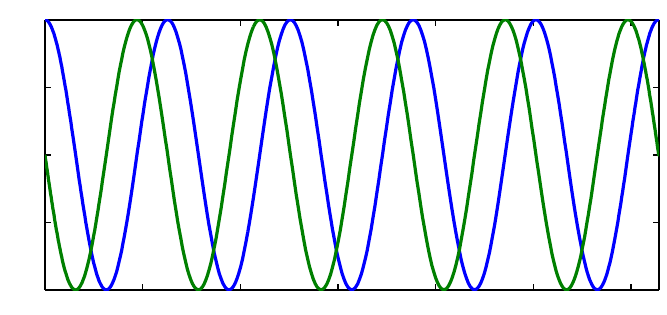
10. Nonlinear ODEs and Chebgui 3
0 5 10 15 20 25 30
−1
−0.5
0
0.5
1
Here are the minimum and maximum values attained by u:
u = v(:,1); uprime = v(:,2);
minandmax(u)
ans =
-1.000068010175644
1.000039406904860
Evidently the accuracy is only around five digits. The reason is that the chebfun ode45 code uses
the same default tolerances as the original ode45. We can tighten the tolerance using the standard
MATLAB odeset command, switching also to ode113 since it is more efficient for high-accuracy
computations:
opts = odeset(’abstol’,3e-14,’reltol’,3e-14);
v = chebfun.ode113(fun, [0 10*pi], [1 0], opts);
minandmax(v(:,1))
ans =
-0.999999999999994
1.000000000000000
As a third example we solve the van der Pol equation for a nonlinear oscillator. Following the example
in the MATLAB ODE documentation, we take u′′ = 1000(1−u2)u′−uwith initial conditions u=2,
u′= 0. This is a highly stiffproblem whose solution contains very rapid transitions, so we use ode15s
in ”splitting on” mode:
opts = odeset(’abstol’,1e-8,’reltol’,1e-8);
fun = @(t,v) [v(2); 1000*(1 - v(1)^2)*v(2) - v(1)];
chebfunpref.setDefaults(’splitting’,’on’)
v = chebfun.ode15s(fun, [0 3000], [2 0], opts);
chebfunpref.setDefaults(’factory’)
u = v(:,1); plot(u,LW,lw)
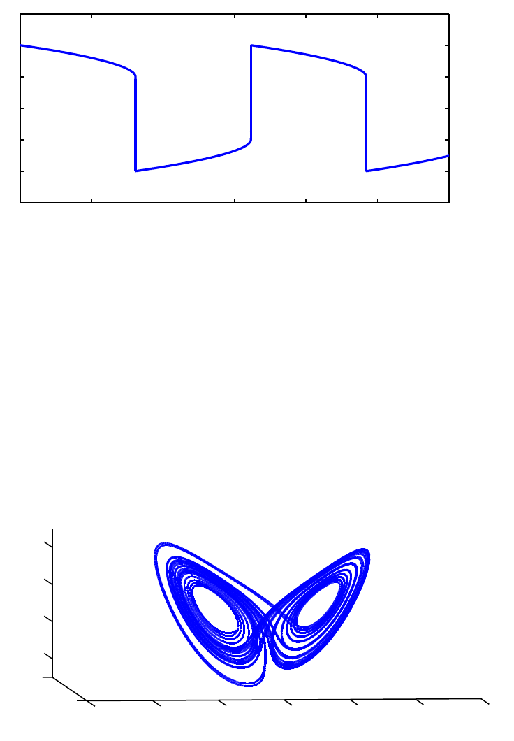
4Chebfun Guide
0 500 1000 1500 2000 2500 3000
−3
−2
−1
0
1
2
3
Here is a pretty good estimate of the period of the oscillator:
diff(roots(u))
ans =
1.0e+02 *
8.072000511670380
8.072001250877227
Finally here is an illustration of the Lorenz equations:
fun = @(t,u) [10*(u(2)-u(1)); 28*u(1)-u(2)-u(1)*u(3); u(1)*u(2)-(8/3)*u(3)];
u = chebfun.ode15s(fun, [0 30], [-5 -7 21], opts);
plot3(u(:,1), u(:,2), u(:,3)), view(-5,9)
axis([-30 30 -50 50 5 45])
xlabel x, ylabel y, zlabel z
−30 −20 −10 010 20 30
−50
0
50
10
20
30
40
x
y
z
10.2 bvp4c,bvp5c
MATLAB also has well-established codes bvp4c and bvp5c for solving BVPs, and these too have
been replicated in Chebfun. Again the Chebfun usage becomes somewhat simpler than the original.
In particular, there is no need to call bvpinit; the initial guess and associated mesh are both
determined by an input initial guess u0.
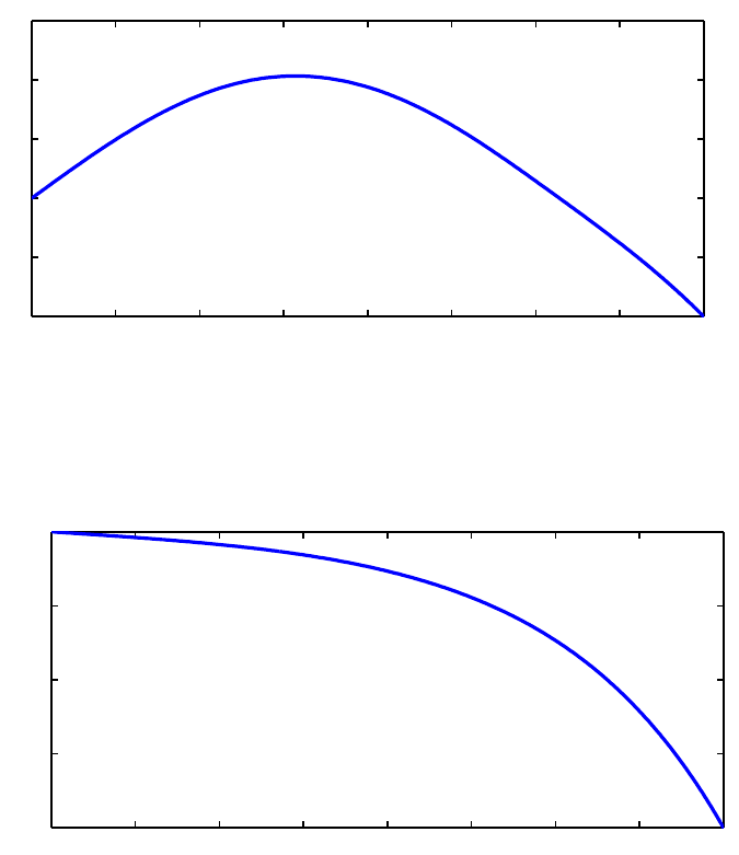
10. Nonlinear ODEs and Chebgui 5
For example, here is the problem labeled twoode in the MATLAB bvp4c documentation. The
domain is [0,4], the equation is u′′ +|u|= 0, and the boundary conditions are u(0) = 0, u(4) = −2.
We get one solution from the initial condition u=1:
twoode = @(x,v) [v(2); -abs(v(1))];
twobc = @(va,vb) [va(1); vb(1)+2];
d = [0,4];
one = chebfun(1, d);
v0 = [one 0*one];
v = bvp4c(twoode, twobc, v0);
u = v(:,1); plot(u,LW,lw)
0 0.5 1 1.5 2 2.5 3 3.5 4
−2
−1
0
1
2
3
The initial guess u=−1 gives another valid solution:
v0 = [-one 0*one];
v = bvp4c(twoode,twobc,v0);
u = v(:,1); plot(u,LW,lw)
0 0.5 1 1.5 2 2.5 3 3.5 4
−2
−1.5
−1
−0.5
0
Here is an example with a variable coefficient, a problem due to George Carrier described in Sec.
9.7 of the book [Bender & Orzsag 1978]. On [−1,1], we seek a function usatisfying
εu′′ +2(1−x2)u+u2=1,u(−1) = u(1) = 0.
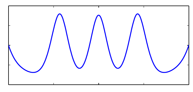
6Chebfun Guide
with ε=0.01. Here is a solution with bvp4c, just one of many solutions of this problem.
ep = 0.01;
ode = @(x,v) [v(2); (1-v(1)^2-2*(1-x^2)*v(1))/ep];
bc = @(va,vb) [va(1); vb(1)];
d = [-1,1];
one = chebfun(1,d);
v0 = [0*one 0*one];
v = bvp4c(ode, bc, v0);
u = v(:,1); plot(u, LW, lw)
−1−0.5 0 0.5 1
−2
−1
0
1
2
10.3 Automatic differentiation
The options described in the last two sections rely on standard numerical discretizations, whose
results are then converted to Chebfun form. It is natural, however, to want to be able to solve ODEs
fully within the Chebfun context, operating always at the level of functions. If the ODE is nonlinear,
this will lead to Newton iterations for functions, also known as Newton-Kantorovich iterations. As
with any Newton method, this will require a derivative, which in this case becomes a linear operator:
an infinite-dimensional Jacobian, or more properly a Frechet derivative.
Chebfun contains features for making such explorations possible. This means that with Chebfun,
you can explore Newton iterations at the function level. The enabling tool is Chebfun Automatic
Differentiation (AD), introduced by Asgeir Birkisson and Toby Driscoll [Birkisson 2014, Birkisson
& Driscoll 2011].
To illustrate Chebfun AD, consider the sequence of computations
x = chebfun(’x’, [0 1]);
u = x.^2;
v = exp(x) + u.^3;
w = u + diff(v);
Suppose we ask, how does one of these variables depend on another one earlier in the sequence? If
the function uis perturbed by an infinitesimal function du, for example, what will the effect be on
v?
As mathematicians we can answer this question as follows. The variation takes the form dv/du =
3u2=3x4.Inotherwords,dv/du is the linear operator that multiplies a function on [0,1] by 3x4.
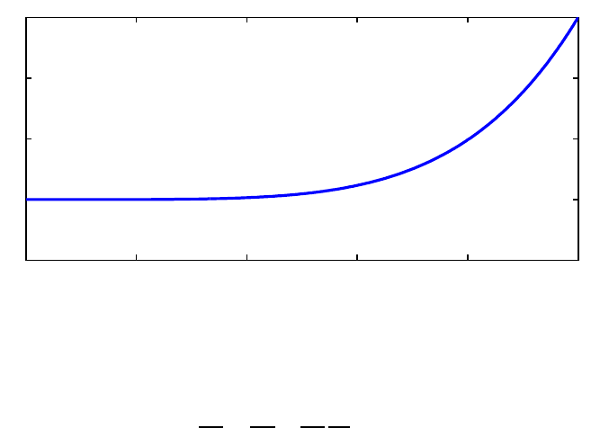
10. Nonlinear ODEs and Chebgui 7
In Chebfun, to compute this operator, we need to select a variable to act as a basis variable for
derivative computations, and seed its derivative. (This procedure has changed with Version 5.) To
compute derivatives with respect to u, we convert it to an object known as an adchebfun and redo
the computations:
u = adchebfun(u);
v = exp(x) + u.^3;
w = u + diff(v);
We can now obtain the derivative of vwith respect to uby accessing the .jacobian field of v:
dvdu = v.jacobian;
The result dvdu is a linear chebop of the kind discussed in Chapter 7. For example, dvdu*x is 3x4
times x,or3x5:
plot(dvdu*x, LW, lw)
0 0.2 0.4 0.6 0.8 1
−1
0
1
2
3
Notice that dvdu is a multiplication operator, acting on a function just by pointwise multiplication.
(The technical term is multiplier operator.)
What about dw/du? To do this on paper we must think a little more carefully and compute
dw
du =∂w
∂u+∂w
∂v
∂v
∂u=I+D(3u2)=I+D(3x4),
where Iis the identity operator and Dis the differentiation operator with respect to x. If we apply
dw/du to x, for example, the result will be x+(3x5)′=x+15x4. The following computation
confirms that Chebfun reaches this result automatically.
dwdu = w.jacobian;
norm(dwdu*x - (x+15*x.^4))
ans =
8.422556560155997e-16
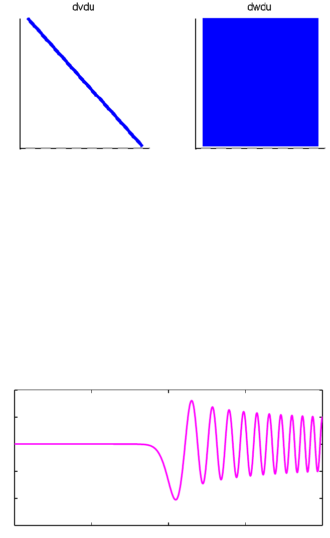
8Chebfun Guide
We can use use the overloaded spy command to see at a glance that the first of our Frechet derivatives
is a multiplier operator while the others are non-diagonal:
subplot(1,2,1), spy(linop(dvdu)), title dvdu
subplot(1,2,2), spy(linop(dwdu)), title dwdu
We now look at how AD enables Chebfun users to solve nonlinear ODE problems with backslash,
just like the linear ones solved in Chapter 7.
10.4 Nonlinear backslash and solvebvp
In Chapter 7, we realized linear operators as chebops constructed by commands like these:
L = chebop(-1, 1);
L.op = @(x,u) 0.0001*diff(u,2) + x.*u;
We could then solve a BVP:
L.lbc = 0;
L.rbc = 1;
u=L\0;
clf, plot(u, ’m’, LW, lw)
−1−0.5 0 0.5 1
−3
−2
−1
0
1
2
10. Nonlinear ODEs and Chebgui 9
What’s going on in such a calculation is that Lis a prescription for constructing matrices of arbitrary
dimensions which are spectral approximations to the operator in question. When backslash is
executed, the problem is solved on successively finer grids until convergence is achieved.
The object Lwe have created is a chebop, with these fields:
disp(L)
Linear operator:
0.0001*diff(u,2)+x.*u = 0
operating on chebfun objects defined on:
[-1 1]
with
left boundary conditions:
u-BC = 0
right boundary conditions:
@(u)u-BC = 0
Notice that one of the fields is called init, which may hold an initial guess for an iteration if one
is specified. If a guess is not specified, then a low-order polynomial function is used that matches
the boundary conditions. To solve a nonlinear ODE, Chebfun uses a Newton or damped Newton
iteration starting at the given initial guess. Each step of the iteration requires the solution of a linear
problem specified by a Jacobian operator (Frechet derivative) evaluated at the current estimated
solution. This is provided by the AD facility, and the linear problem is then solved by chebops.
In Section 7.9 we hand-coded our own Newton iteration to solve the nonlinear BVP
0.001u′′ −u3=0,u(−1) = 1,u(1) = −1.
However, since the required Jacobian information is now computed by AD, construction of the
Jacobian operator Jis taken care of by linearize(L,u), which returns the derivative of the operator
Jwhen it is linearized around the function u. Compare the code below to that in Section 7.9.
L = chebop(@(x,u) 0.001*diff(u,2) - u.^3);
L.lbc = 1; L.rbc = -1;
u = chebfun(’-x’); nrmdu = Inf;
while nrmdu > 1e-10
r=L*u;
J = linearize(L,u);
du = -(J\r);
u = u + du; nrmdu = norm(du)
end
clf, plot(u)
nrmdu =
0.260668532007021
nrmdu =
0.164126069559936
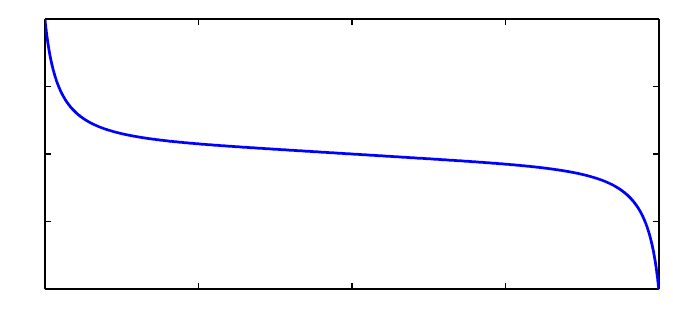
10 Chebfun Guide
nrmdu =
0.098900892365438
nrmdu =
0.053787171683933
nrmdu =
0.021518152858428
nrmdu =
0.003586696693251
nrmdu =
8.951602488748837e-05
nrmdu =
5.357404846072875e-08
nrmdu =
2.500515198784863e-14
−1−0.5 0 0.5 1
−1
−0.5
0
0.5
1
However, it is not necessary to construct such Newton iterations by hand! The code above is a
much simplified version of what happens under-the-hood when |nonlinear backslash’ is called to
solve nonlinear differential equations. A few examples of this are demonstrated below.
Let us reconsider some of the examples of the last three sections. First in Section 10.1 we had the
nonlinear IVP
u′=u2,u(0) = 0.95.
This can be solved in chebop formulation like this:
N = chebop(0, 1);
N.op = @(x,u) diff(u) - u.^2;
N.lbc = 0.95;
u=N\0;
plot(u,’m’,LW,lw)
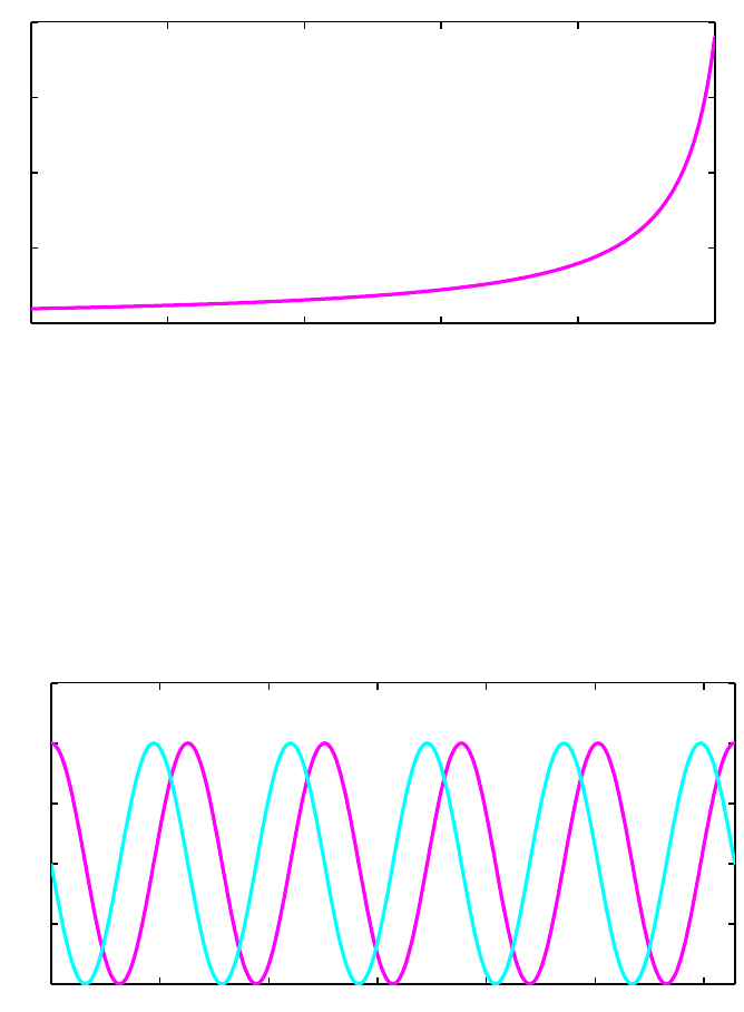
10. Nonlinear ODEs and Chebgui 11
0 0.2 0.4 0.6 0.8 1
0
5
10
15
20
Next came the linear equation u′′ =−u. With chebops, there is no need to reformulate the problem
as a first-order system. There are two boundary conditions at the left, which can be imposed by
making N.lbc a function returning an array.
N = chebop(0, 10*pi);
N.op = @(x,u) diff(u,2) + u;
N.lbc = @(u) [u-1; diff(u)];
u=N\0;
plot(u, ’m’, diff(u), ’c’, LW, lw)
0 5 10 15 20 25 30
−1
−0.5
0
0.5
1
1.5
The van der Pol problem of Section 10.1 cannot be solved by chebops;thestiffness causes failure of
the Newton iteration.
Here is the Carrier problem of section 10.2:
ep = 0.01;
N = chebop(-1, 1);
N.op = @(x,u) ep*diff(u,2) + 2*(1 - x.^2).*u + u.^2;
N.bc = ’dirichlet’;
x = chebfun(’x’);
N.init = 2*(x.^2 - 1).*(1 - 2./(1 + 20*x.^2));
u = N\1; plot(u, ’m’, LW, lw)
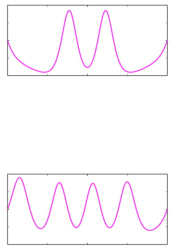
12 Chebfun Guide
−1−0.5 0 0.5 1
−2
−1
0
1
2
We get a different solution from the one we got before! This one is correct too; the Carrier problem
has many solutions. If we multiply this solution by 2 sin(x/2) and take the result as a new initial
guess, we converge to a third solution:
N.init= u.*sin(pi*x/2);
[u, info] = solvebvp(N, 1);
plot(u,’m’,LW,lw)
−1−0.5 0 0.5 1
−2
−1
0
1
2
This time, we called the method solvebvp with two output arguments. The second output is
a MATLAB struct, which contains data showing the norms of the updates during the Newton
iteration, revealing in this case a troublesome initial phase followed by eventual rapid convergence.
nrmdu = info.normDelta;
semilogy(nrmdu,’.-k’,LW,lw), ylim([1e-14,1e2])
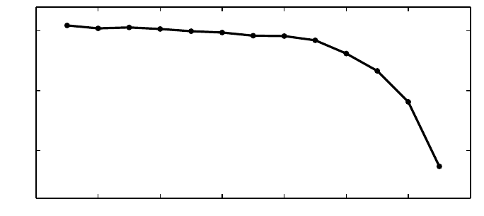
10. Nonlinear ODEs and Chebgui 13
0 2 4 6 8 10 12 14
10−10
10−5
100
Another way to get information about the Newton iteration with nonlinear backlash is by setting
cheboppref.setDefaults(’plotting’,’on’)
or
cheboppref.setDefaults(’display’,’iter’)
Type help cheboppref for details. Here we shall not pursue this option and thus return thesystem
to its factory state:
cheboppref.setDefaults(’plotting’,’off’)
cheboppref.setDefaults(’display’,’none’)
The heading of this section refers to the command solvebvp. When you apply backslash to a
nonlinear chebop, it invokes the overloaded MATLAB command mldivide; this in turn calls a
command solvebvp to do the actual work. By calling solvebvp directly, you can control the
computation in ways not accessible through backslash. This situation is just like the relationship in
standard MATLAB between \and linsolve. See the help documentation for details.
10.5 Graphical user interface: Chebgui
Chebfun includes a GUI (Graphical User Interface) for solving all kinds of ODE, time-dependent
PDE, and eigenvalue problems interactively. We will not describe it here, but we encourage the
reader to type chebgui and give it a try. Be sure to note the Demo menu, which contains dozens
of preloaded examples, both scalars and systems. Perhaps most important of all is the |Export to
m-file” button, which produces a Chebfun m-file corresponding to whatever problem is loaded into
the GUI. This feature enables one to get going quickly and interactively, then switch to a Chebfun
program to adjust the fine points.
chebgui

!

!
!
!
!
!
!
!
!
!
!
!
Part II
Functions of two variables
(Chebfun2)

!
11. Chebfun2: Getting Started
Alex Townsend, March 2013, latest revision June 2014
Contents
•11.1 What is a chebfun2?
•11.2 What is a chebfun2v?
•11.3 Constructing chebfun2 objects
•11.4 Basic operations
•11.5 Chebfun2 methods
•11.6 Object composition
•11.7 Analytic functions
•11.8 References
11.1 What is a chebfun2?
Chebfun2 is the part of Chebfun that deals with functions of two variables defined on a rectangle
[a, b]×[c, d]. Just like Chebfun in 1D, it is an extremely convenient tool for all kinds of computations
including algebraic manipulation, optimization, integration, and rootfinding. It also extends to
vector-valued functions of two variable, so that one can perform vector calculus.
A chebfun2, with a lower-case ”c”, is a MATLAB object, the 2D analogue of a chebfun. The syntax
for chebfun2 objects is similar to the syntax for matrices in MATLAB,andChebfun2objectshave
many MATLAB commands overloaded. For instance, trace(f) returns the sum of the diagonal
entries when fis a matrix and the integral of f(x, x)whenfis a chebfun2.
Chebfun2 builds on Chebfun’s univariate representations and algorithms. Algorithmic details are
given in [Townsend & Trefethen 2013b].
The implementation of Chebfun2 exploits the observation that many functions of two variables can
be well approximated by low rank approximants. A rank 1 function is oftheformu(y)v(x), and
arankkfunction can be written as the sum of krank 1 functions. Smooth functions tend to be
well approximated by functions of low rank. Chebfun2 determines low rank function approximations
automatically by means of an algorithm that can be viewed as an iterative application of Gaussian
elimination with complete pivoting [Townsend & Trefethen 2013]. The underlying function repre-
sentations are related to work by Carvajal, Chapman and Geddes [Carvajal, Chapman, & Geddes
2008] and others including Bebendorf [Bebendorf 2008], Hackbusch, Khoromskij, Oseledets, and
Tyrtyshnikov.
1
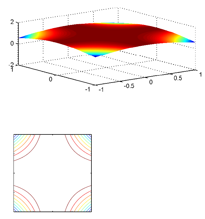
2Chebfun Guide
11.2 What is a chebfun2v?
Chebfun2 can represent scalar valued functions, such as exp(x+y), and vector valued functions, such
as [exp(x+y); cos(x−y)]. A vector valued function is called a chebfun2v, and chebfun2v objects
are useful for computations of vector calculus. For information about chebfun2v objects and vector
calculus, see Chapters 14 and 15 of this guide.
11.3 Constructing chebfun2 objects
A chebfun2 is constructed by supplying the Chebfun2 constructor with a function handle or string.
The default rectangular domain is [−1,1] ×[−1,1]. (An example showing how to specify a different
domain is given at the end of this chapter.) For example, here we construct and plot a chebfun2
representing cos(xy)on[−1,1] ×[−1,1].
f = chebfun2(@(x,y) cos(x.*y));
plot(f), zlim([-2 2])
There are several commands for plotting a chebfun2, including plot,contour,surf,andmesh.
Here is a contour plot of f:
contour(f), axis square
−1−0.5 0 0.5 1
−1
−0.5
0
0.5
1
One way to find the rank of the approximant used to represent fis like this:
11. Chebfun2: Getting Started 3
length(f)
ans =
7
Alternatively, more information can be given by displaying the chebfun2 object:
f
f=
chebfun2 object: (1 smooth surface)
domain rank corner values
[ -1, 1] x [ -1, 1] 7 [0.54 0.54 0.54 0.54]
vertical scale = 1
The corner values are the values of the chebfun2 at (−1,−1), (−1,1), (1,−1), and (1,1), in that
order. The vertical scale is used by operations to aim for close to machine precision relative to that
number.
11.4 Basic operations
Once we have a chebfun2, we can compute quantities such as its definite double integral:
sum2(f)
ans =
3.784332281468732
This matches well the exact answer obtained by calculus:
exact = 3.784332281468732
exact =
3.784332281468732
We can also evaluate a chebfun2 at a point (x, y), or along a line. When evaluating along a line a
chebfun is returned because the answer is a function of one variable.
Evaluation at a point:
x = 2*rand - 1; y = 2*rand - 1;
f(x,y)
ans =
0.989047610535538
Evaluation along the line y=π/6:
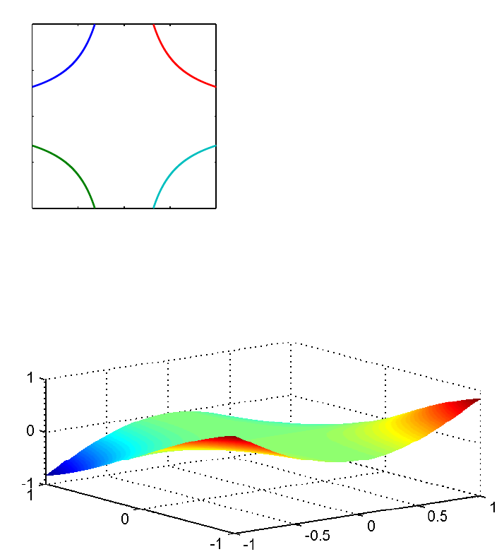
4Chebfun Guide
f(:,pi/6)
ans =
chebfun row (1 smooth piece)
interval length endpoint values
[ -1, 1] 11 0.87 0.87
Epslevel = 8.096942e-15. Vscale = 1.000000e+00.
There are plenty of other questions that may be of interest. For instance, what are the zero contours
of f(x, y)−.95?
r = roots(f-.95);
plot(r), axis square, title(’Zero contours of f-.95’)
−0.5 0 0.5
−1
−0.5
0
0.5
1
Zero contours of f−.95
What is the partial derivative ∂f/∂y?
fy = diff(f,1,1);
plot(fy)
The syntax for the diff command can cause confusion because we are following the matrix syntax
in MATLAB. Chebfun2 also offers diffx(f,k) and diffy(f,k), which differentiate f(x, y)ktimes
with respect to the first first and second variable, respectively.
11. Chebfun2: Getting Started 5
What is the mean value of f(x, y)on[−1,1] ×[−1,1]?
mean2(f)
ans =
0.946083070367183
11.5 Chebfun2 methods
There are over 100 methods that can be applied to chebfun2 objects. For a complete list type:
methods chebfun2
Methods for class chebfun2:
abs fevalm min2 size
cdr flipdim minandmax2 sph2cart
chebcoeffs2 fliplr minus sphere
chebfun2 flipud mldivide sqrt
chebpolyplot fred mrdivide squeeze
chebpolyval2 get mtimes std
chol grad norm std2
complex gradient pivotplot subsref
conj horzcat pivots sum
contour imag plot sum2
contourf integral plotcoeffs surf
cos integral2 plotcoeffs2 surface
cosh isempty plus surfacearea
ctranspose isequal pol2cart svd
cumprod isreal potential tan
cumsum iszero power tand
cumsum2 jacobian prod tanh
dblquad lap qr times
del2 laplacian quad2d trace
diag ldivide quiver transpose
diff length quiver3 uminus
diffx log rank uplus
diffy lu rdivide vertcat
discriminant max real volt
disp max2 restrict waterfall
display mean roots
ellipsoid mean2 simplify
exp median sin
feval min sinh
Static methods:
chebpts2 outerProduct vals2coeffs
coeffs2vals paduaVals2coeffs
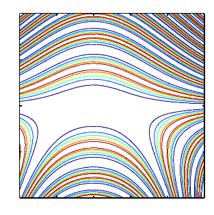
6Chebfun Guide
Most of these commands have been overloaded from MATLAB. More information about a Chebfun2
command can be found with help; for instance
help chebfun2/max2
MAX2 Global maximum of a CHEBFUN2.
Y = MAX2(F) returns the global maximum of F over its domain.
[Y, X] = MAX2(F) returns the global maximum in Y and its location X.
This command may be faster if the OPTIMIZATION TOOLBOX is installed.
See also MIN2, MINANDMAX2.
11.6 Object composition
So far, in this chapter, chebfun2 objects have been constructed explicitly via a command of the form
chebfun2(...). Another way to construct new chebfun2 objects is by composing them together
with operations such as +,-,.*,and.^. For instance,
x = chebfun2(@(x,y) x, [-2 3 -4 4]);
y = chebfun2(@(x,y) y, [-2 3 -4 4]);
f = 1./( 2 + cos(.25 + x.^2.*y + y.^2) );
contour(f), axis square
−2−1 0 1 2 3
−4
−2
0
2
4
11.7 Analytic functions
An analytic function f(z) can be thought of as a complex valued function of two real variables,
f(x, y)=f(x+iy). If the Chebfun2 constructor is given an anonymous function withoneargument,
it assumes that argument is a complex variable. For instance,
f = chebfun2(@(z) sin(z));
f(1+1i), sin(1+1i)
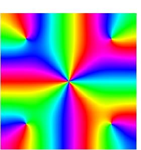
11. Chebfun2: Getting Started 7
ans =
1.298457581415977 + 0.634963914784736i
ans =
1.298457581415977 + 0.634963914784736i
These functions can be visualised by using a technique known as phase portrait plots. Given a
complex number z=reiθ,thephaseeiθcan be represented by a colour. We follow Wegert’s colour
recommendations [Wegert 2012], using red for a phase i, then yellow, green, blue, and violet as the
phase moves clockwise around the unit circle. For example,
f = chebfun2(@(z) sin(z)-sinh(z),2*pi*[-1 1 -1 1]);
plot(f)
Many properties of analytic functions can be visualised by these types of plots, such as the location
of zeros and their multiplicities. Can you work out the multiplicity of the root at z=0 from this
plot?
At present, since Chebfun2 only represents smooth functions, a trick is required to draw pictures
like these for functions with poles [Trefethen 2013]. For functions with branch points or essential
singularities, it is currently not possible in Chebfun2 to draw phase plots.
11.8 References
[Bebendorf 2008] M. Bebendorf, Hierarchical Matrices: A Means to Efficiently Solve Elliptic Bound-
ary Value Problems, Springer, 2008.
[Carvajal, Chapman, & Geddes 2008] O. A. Carvajal, F. W. Chapman and K. O. Geddes, Hy-
brid symbolic-numeric integration in multiple dimensions via tensor-product series, Proceedings of
ISSAC’05, M. Kauers, ed., ACM Press, 2005, pp.84-91.
[Townsend & Trefethen 2013] A. Townsend and L. N. Trefethen, Gaussian elimination as an iterative
algorithm, SIAM News, March 2013.
[Townsend & Trefethen 2013b] A. Townsend and L. N. Trefethen, An extension of Chebfun to two
dimensions, SIAM Journal on Scientific Computing, 35 (2013), C495-C518.
[Trefethen 2013] L. N. Trefethen, Phase Portraits for functions with poles,
http://www2.maths.ox.ac.uk/chebfun/examples/complex/html/PortraitsWithPoles.shtml
8Chebfun Guide
[Wegert 2012] E. Wegert, Visual Complex Functions: An Introduction with Phase Portraits,
Birkhauser/Springer, 2012.
12. Chebfun2: Integration and
Differentiation
Alex Townsend, March 2013, latest revision June 2014
Contents
•12.1 sum and sum2
•12.2 norm,mean,andmean2
•12.3 cumsum and cumsum2
•12.4 Complex encoding
•12.5 Integration along curves
•12.6 diff
•12.7 Integration in three variables
•12.8 References
12.1 sum and sum2
We have already seen the sum2 command, which returns the definite double integral of a chebfun2
over its domain of definition. The sum command is a little different and integrates with respect to
one variable at a time. For instance, the following commands integrateovertheyvariable:
f = chebfun2(@(x,y) sin(10*x.*y),[0 pi/4 0 3]);
sum(f)
ans =
chebfun row (1 smooth piece)
interval length endpoint values
[ 0, 0.79] 35 -1.8e-15 0.13
Epslevel = 8.354003e-15. Vscale = 2.172798e+00.
A chebfun is returned because the result depends on xand hence, is a function of one variable.
Similarly, we can integrate over the xvariable, and plot the result.
LW = ’linewidth’;
sum(f,2), plot(sum(f,2),LW,1.6)
1
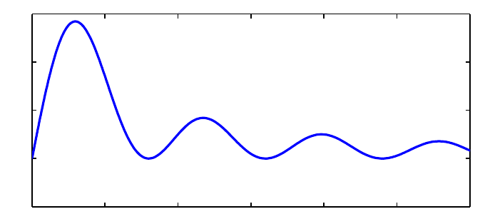
2Chebfun Guide
ans =
chebfun column (1 smooth piece)
interval length endpoint values
[ 0, 3] 35 -5.6e-16 0.033
Epslevel = 7.345480e-15. Vscale = 5.688372e-01.
0 0.5 1 1.5 2 2.5 3
−0.2
0
0.2
0.4
0.6
A closer look reveals that sum(f) returns a row chebfun while sum(f,2) returns a column chebfun.
This distinction is a reminder that sum(f) is a function of xwhile sum(f,2) is a function of y.If
we integrate over yand then xthe result is the double integral of f.
sum2(f)
sum(sum(f))
ans =
0.377914013520379
ans =
0.377914013520379
It is interesting to compare the execution times involved for computing the double integral by
different commands. Chebfun2 does very well for smooth functions. Here we see an example in
which it is faster than the MATLAB quad2d command.
F = @(x,y) exp(-(x.^2 + y.^2 + cos(4*x.*y)));
tol = 3e-14;
tic, I = quad2d(F,-1,1,-1,1,’AbsTol’,tol); t = toc;
fprintf(’QUAD2D: I = %17.15f time = %6.4f secs\n’,I,t)
tic, I = sum(sum(chebfun2(F))); t = toc;
fprintf(’CHEBFUN2/SUMSUM: I = %17.15f time = %6.4f secs\n’,I,t)
tic, I = sum2(chebfun2(F)); t = toc;
fprintf(’CHEBFUN2/SUM2: I = %17.15f time = %6.4f secs\n’,I,t)
QUAD2D: I = 1.399888131932670 time = 0.0851 secs
CHEBFUN2/SUMSUM: I = 1.399888131932670 time = 0.0229 secs
CHEBFUN2/SUM2: I = 1.399888131932670 time = 0.0178 secs
12. Chebfun2: Integration and Differentiation 3
Chebfun2 is not designed specifically for numerical quadrature (or more properly, ”cubature”), and
careful comparisons with existing software have not been carried out. Low rank function approx-
imations have been previously used for numerical quadrature by Carvajal, Chapman, and Geddes
[Carvajal, Chapman & Geddes 2005].
12.2 norm,mean,andmean2
The L2-norm of a function f(x, y) can be computed as the square root of the double integral of f2.
In Chebfun2 the command norm(f), without any additional arguments, computes this quantity. For
example,
f = chebfun2(’exp(-(x.^2 + y.^2 +4*x.*y))’);
norm(f), sqrt(sum2(f.^2))
ans =
2.819481057146934
ans =
2.819481057146935
Here is another example. This time we compute the norms of f(x, y), cos(f(x, y)), and f(x, y)5.
f = chebfun2(@(x,y) exp(-1./( sin(x.*y) + x ).^2));
norm(f), norm( cos(f) ), norm( f.^5 )
ans =
0.462652919760561
ans =
1.950850368197068
ans =
0.060896016071932
Just as sum2 performs double integration, mean2 computes the average value of f(x, y)overboth
variables:
help chebfun2/mean2
MEAN2 Mean of a CHEBFUN2
V = MEAN2(F) returns the mean of a CHEBFUN:
db
//
V = 1/(d-c)/(b-a) | | f(x,y) dx dy
//
ca
where the domain of F is [a,b] x [c,d].
See also MEAN, STD2.
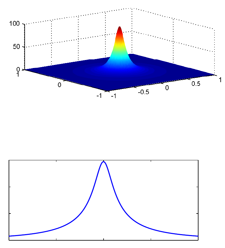
4Chebfun Guide
For example, here is the average value of a 2D Runge function.
runge = chebfun2( @(x,y) 1./( .01 + x.^2 + y.^2 )) ;
plot(runge)
mean2(runge)
ans =
3.796119578934829
The command mean computes the average along one variable. The output of mean(f) is a function
of one variable represented by a chebfun, and so we can plot it.
plot(mean(runge),LW,1.6)
title(’Mean value of 2D Runge function wrt y’)
−1−0.5 0 0.5 1
0
5
10
15
Mean value of 2D Runge function wrt y
If we average over the yvariable and then the xvariable, we obtain the mean value over the whole
domain.
mean(mean(runge)) % compare with mean2(runge)
ans =
3.796119578934826
12. Chebfun2: Integration and Differentiation 5
12.3 cumsum and cumsum2
The command cumsum2 computes the double indefinite integral, which is a function of two variables,
and returns a chebfun2.
help chebfun2/cumsum2
CUMSUM2 Double indefinite integral of a CHEBFUN2.
F = CUMSUM2(F) returns the double indefinite integral of a CHEBFUN2. That is
yx
//
CUMSUM2(F) = | | f(x,y) dx dy for (x,y) in [a,b] x [c,d],
//
ca
where [a,b] x [c,d] is the domain of f.
See also CUMSUM, SUM, SUM2.
On the other hand, cumsum(f) computes the indefinite integral with respect to just one variable,
also returning a chebfun2. Again, the indefinite integral in the yvariable and then the xvariable is
the same as the double indefinite integral, as we can check numerically.
f = chebfun2(@(x,y) exp(-(x.^2 + 3*x.*y+y.^2) ));
contour(cumsum2(f),’numpts’,400), axis equal
title(’Contours of cumsum2(f)’), axis([-1 1 -1 1])
norm( cumsum(cumsum(f),2) - cumsum2(f) )
ans =
0
Contours of cumsum2(f)
−1 0 1
−1
−0.5
0
0.5
1
12.4 Complex encoding
As is well known, a pair of real scalar functions fand gcan be encoded as a complex function f+ig.
This trick can be useful for simplifying many operations, but at the same time may be confusing.
6Chebfun Guide
For instance, instead of representing the unit circle with two real-valued functions, we can represent
it with one complex-valued function:
c1 = chebfun(@(t) cos(t),[0 2*pi]); % first real-valued function
c2 = chebfun(@(t) sin(t),[0 2*pi]); % second real-valued function
c = chebfun(@(t) cos(t)+1i*sin(t),[0 2*pi]); % one complex function
Here are two ways to make a plot of a circle.
subplot(1,2,1), plot(c1,c2,LW,1.6)
axis equal, title(’Two real-valued functions’)
subplot(1,2,2), plot(c,LW,1.6)
axis equal, title(’One complex-valued function’)
−1 0 1
−1
−0.5
0
0.5
1
Two real−valued functions
−1 0 1
−1
−0.5
0
0.5
1
One complex−valued function
This complex encoding trick is used in a number of places in Chebfun2. Specifically, it’s used to
encode the path of integration for a line integral (see section 12.5, below), to represent zero contours
of a chebfun2 (see Chapter 13), and to represent trajectories in vector fields (see Chapter 14).
We hope users become comfortable with using complex encodings, though they are not required for
the majority of Chebfun2 functionality.
12.5 Integration along curves
Chebfun2 can compute the integral of f(x, y) along a curve (x(t),y(t)). It uses the complex encoding
trick and encode the curve (x(t),y(t)) as a complex valued chebfun x(t)+iy(t). For instance, what
is the area under the following curve?
clf
f = chebfun2(@(x,y) cos(10*x.*y.^2) + exp(-x.^2)); % chebfun2 object
C = chebfun(@(t) t.*exp(10i*t),[0 1]); % spiral curve
plot(f), hold on
plot3(real(C),imag(C),f(C),’k’,’linewidth’,2)
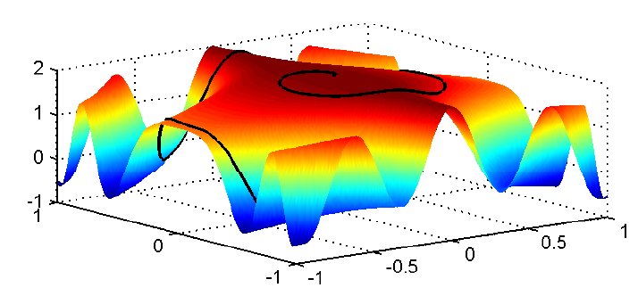
12. Chebfun2: Integration and Differentiation 7
We can compute this by restricting fto the curve and then integrating
sum(f(C))
ans =
1.613596461872283
12.6 diff
In MATLAB the diff command calculates finite differences of a matrix along its columns (by
default) or rows. For a chebfun2 the same syntax represents partial differentiation ∂f/∂y(by
default) or ∂f/∂x. This command has the following syntax:
help chebfun2/diff
DIFF Derivative of a CHEBFUN2s.
DIFF(F) is the derivative of F along the y direction.
DIFF(F, N) is the Nth derivative of F in the y direction.
DIFF(F, N, DIM) is the Nth derivative of F along the dimension DIM.
DIM = 1 (default) is the derivative in the y-direction.
DIM = 2 is the derivative in the x-direction.
DIFF(F, [NX NY]) is the partial derivative of NX of F in the first variable,
and NY of F in the second derivative. For example, DIFF(F,[1 2]) is
d^3F/dxd^2y.
See also GRADIENT, SUM, PROD.
Here we use diff to check that the Cauchy-Riemann equations hold for an analytic function.
8Chebfun Guide
f = chebfun2(@(x,y) sin(x+1i*y)); % a holomorphic function
u = real(f); v = imag(f); % real and imaginary parts
norm(diff(u) - (-diff(v,1,2)))
norm(diff(u,1,2) - diff(v)) % Do the Cauchy-Riemann eqns hold?
ans =
1.060890001425453e-14
ans =
2.569762378645554e-14
12.7 Integration in three variables
Chebfun2 also works pretty well for integration in three variables. The idea is to integrate over
two of the variables using Chebfun2 and the remaining variable using Chebfun. We have selected
a tolerance of 10−6for this example because the default tolerance in the MATLAB integral3
command is also 10−6.
r = @(x,y,z) sqrt(x.^2 + y.^2 + z.^2);
t = @(x,y,z) acos(z./r(x,y,z)); p = @(x,y,z) atan(y./x);
f = @(x,y,z) sin(5*(t(x,y,z) - r(x,y,z))) .* sin(p(x,y,z)).^2;
I = @(z) sum2(chebfun2(@(x,y) f(x,y,z),[-2 2 .5 2.5])); % integrate out x,y
tic, I = sum(chebfun(@(z) I(z),[1 2],’vectorize’)); t = toc;
fprintf(’ Chebfun2: I = %16.14f time = %5.3f secs\n’,I,t)
tic, I = integral3(f,-2,2,.5,2.5,1,2); t = toc; % compare with MATLAB
fprintf(’Integral3: I = %16.14f time = %5.3f secs\n’,I,t)
Chebfun2: I = -0.48056569408898 time = 1.272 secs
Integral3: I = -0.48056569417568 time = 0.286 secs
12.8 References
[Carvajal, Chapman & Geddes 2005] O. A. Carvajal, F. W. Chapman and K. O. Geddes, Hybrid
symbolic-numeric integration in multiple dimensions via tensor-product series, Proceedings of IS-
SAC’05, M. Kauers, ed., ACM Press, 2005, pp. 84–91.
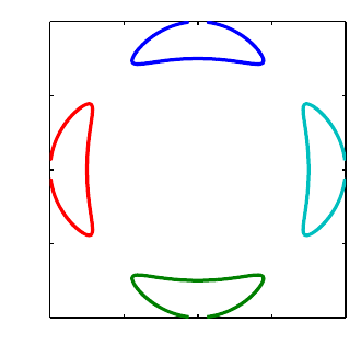
13. Chebfun2: Rootfinding and
Optimisation
Alex Townsend, March 2013, latest revision June 2014
Contents
•13.1 Zero contours
•13.2 roots
•13.3 Intersections of curves
•13.4 Global optimisation: max2,min2,andminandmax2
•13.5 Critical points
•13.6 Infinity norm
•13.7 References
13.1 Zero contours
Chebfun2 comes with the capability to compute the zero contours of a function of two variables.
For example, we can compute a representation of Trott’s curve, an example from algebraic geometry
[Trott 1997].
x = chebfun2(@(x,y) x); y = chebfun2(@(x,y) y);
trott = 144*(x.^4+y.^4)-225*(x.^2+y.^2) + 350*x.^2.*y.^2+81;
r = roots(trott);
LW = ’linewidth’; MS = ’markersize’;
plot(r,LW,1.6), axis([-1 1 -1 1]), axis square
−1−0.5 0 0.5 1
−1
−0.5
0
0.5
1
1
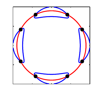
2Chebfun Guide
The zero curves are represented as complex valued chebfuns (see Chapter 5 of the guide). For
example,
r(:,1)
ans =
chebfun column (1 smooth piece)
interval length endpoint values
[ -1, 1] 576 complex values
Epslevel = 1.000000e-05. Vscale = 9.980190e-01.
The zero contours of a function are computed by Chebfun2 to plotting accuracy and they are typically
not accurate to machine precision.
13.2 roots
Chebfun2 also comes with the capability of finding zeros of bivariate systems, i.e., the solutions to
f(x, y)=g(x, y)=0. Iftheroots command is supplied with one chebfun2, it computes the zero
contours of that function, as in the last section. However, if it is supplied with two chebfun2 objects,
as in roots(f,g), then it computes the roots of the bivariate system. Generically, these are isolated
points.
What points on the Trott’s curve intersect with the circle of radius 0.9?
g = chebfun2(@(x,y) x.^2 + y.^2 - .9^2); % circle of radius 0.9
r = roots(trott,g);
plot(roots(trott),’b’,LW,1.6), hold on
plot(roots(g),’r’,LW,1.6)
plot(r(:,1),r(:,2),’.k’,LW,1.6,MS,20) % point intersections
axis([-1 1 -1 1]), axis square, hold off
−1−0.5 0 0.5 1
−1
−0.5
0
0.5
1
The solution to bivariate polynomial systems and intersections of curves, are typically computed to
full machine precision.
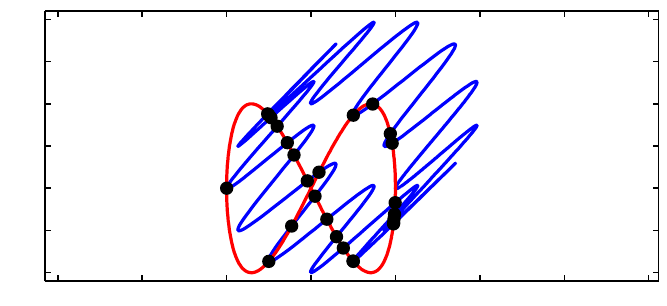
13. Chebfun2: Rootfinding and Optimisation 3
13.3 Intersections of curves
The problem of determining the intersections of real parameterised complex curves can be expressed
as a bivariate rootfinding problem. For instance, here are the intersections between the ’splat’ curve
[Guettel Example 2010] and a ’figure-of-eight’ curve.
t = chebfun(’t’,[0,2*pi]);
sp = exp(1i*t) + (1+1i)*sin(6*t).^2; % splat curve
figof8 = cos(t) + 1i*sin(2*t); % figure of eight curve
plot(sp,LW,1.6), hold on
plot(figof8,’r’,LW,1.6), axis equal
d = [0 2*pi 0 2*pi];
f = chebfun2(@(s,t) sp(t)-figof8(s),d); % rootfinding
r = roots(real(f),imag(f)); % calculate intersections
spr = sp(r(:,2));
plot(real(spr),imag(spr),’.k’,MS,20), ylim([-1.1 2.1])
hold off
−3−2−1 0 1 2 3 4
−1
−0.5
0
0.5
1
1.5
2
Chebfun2 rootfinding is based on an algorithm described in [Nakatsukasa, Noferini & Townsend
2013].
13.4 Global optimisation: max2,min2,andminandmax2
Chebfun2 also provides functionality for global optimisation. Here is a non-trivial example, where
we plot the computed minimum and maximum as black dots.
f = chebfun2(@(x,y) sin(30*x.*y) + sin(10*y.*x.^2) + exp(-x.^2-(y-.8).^2));
[mn mnloc] = min2(f);
[mx mxloc] = max2(f);
plot(f), hold on
plot3(mnloc(1),mnloc(2),mn,’.k’,MS,40)
plot3(mxloc(1),mxloc(2),mx,’.k’,MS,30)
zlim([-6 6]), hold off
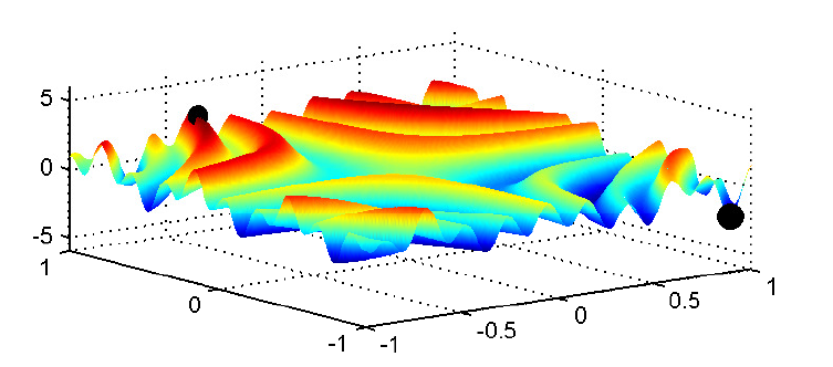
4Chebfun Guide
If both the global maximum and minimum are required, it is roughly twice as fast to compute them
at the same time by using the minandmax2 command. For instance,
tic; [mn mnloc] = min2(f); [mx mxloc] = max2(f); t=toc;
fprintf(’min2 and max2 separately = %5.3fs\n’,t)
tic; [Y X] = minandmax2(f); t=toc;
fprintf(’minandmax2 command = %5.3fs\n’,t)
min2 and max2 separately = 0.292s
minandmax2 command = 0.142s
The commands min2,max2,andminandmax2 run faster if the MATLAB Optimisation Toolbox is
available.
13.5 Critical points
The critical points of smooth function of two variables can be located by finding the zeros of ∂f/∂y=
∂f/∂x= 0. This is a rootfinding problem. For example,
f = chebfun2(@(x,y) (x.^2-y.^3+1/8).*sin(10*x.*y));
r = roots(gradient(f)); % critical points
plot(roots(diff(f,1,2)),’b’,LW,1.6), hold on % plot zero contours of f_x
plot(roots(diff(f)),’r’) % plot zero contours of f_y
plot(r(:,1),r(:,2),’k.’,’MarkerSize’,30) % plot extrema
axis([-1,1,-1,1]), axis square
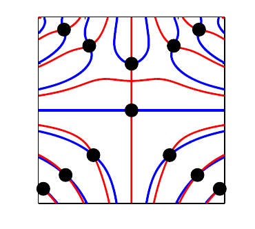
13. Chebfun2: Rootfinding and Optimisation 5
−1−0.5 0 0.5 1
−1
−0.5
0
0.5
1
There is a new command here called gradient that computes the gradient vector and represents
it as a chebfun2v object. The roots command then solves for the isolated roots of the bivariate
polynomial system represented in the chebfun2v representing the gradient. For more information
about the gradient command see Chapter 14 of this guide.
13.6 Infinity norm
The ∞-norm of a function is the maximum absolute value in its domain. It can becomputedby
passing an optional argument to the norm command.
f = chebfun2(@(x,y) sin(30*x.*y));
norm(f,inf)
ans =
0.999999999999995
13.7 References
[Guettel Example 2010] S. Guettel,
http://www2.maths.ox.ac.uk/chebfun/examples/geom/html/Area.shtml
[Nakatsukasa, Noferini & Townsend 2013] Y. Nakatsukasa, V. Noferini and A. Townsend, ”Comput-
ing the common zeros of two bivariate functions via Bezout resultants”, Numerische Mathematik,
to appear.
[Trott 2007] M. Trott, Applying Groebner Basis to Three Problems in Geometry, Mathematica in
Education and Research, 6 (1997), pp.15-28.

!
14. Chebfun2: Vector Calculus
Alex Townsend, March 2013, latest revision June 2014
Contents
•14.1 What is a chebfun2v?
•14.2 Algebraic operations
•14.3 Differential operators
•14.4 Line integrals
•14.5 Phase diagram
14.1 What is a chebfun2v?
Chebfun2 objects represent vector-valued functions. We use a lower case letter like ffor a chebfun2
and an upper case letter like Ffor a chebfun2v.
Chebfun2 represents a vector-valued function F(x, y)=(f(x, y); g(x, y)) by approximating each
component by a low rank approximant. There are two ways to form a chebfun2v: either by explicitly
calling the constructor, or by vertical concatenation of two chebfun2 objects. Here are these two
alternatives:
d=[0102];
F = chebfun2v(@(x,y) sin(x.*y), @(x,y) cos(y), d); % calling the constructor
f = chebfun2(@(x,y) sin(x.*y), d);
g = chebfun2(@(x,y) cos(y), d);
G = [f;g] % vertical concatenation
G=
chebfun2v object (Column vector) containing:
chebfun2 object: (1 smooth surface)
domain rank corner values
[ 0, 1] x [ 0, 2] 7 [3.3e-32 -1.5e-16 -1.8e-16 0.91]
vertical scale = 1
chebfun2 object: (1 smooth surface)
domain rank corner values
[0,1]x[0,2] 1 [1 1-0.42-0.42]
vertical scale = 1
Note that displaying a chebfun2v shows that it is a vector of two chebfun2 objects.
1
2Chebfun Guide
14.2 Algebraic operations
Chebfun2 objects are useful for performing 2D vector calculus. The basic algebraic operations are
scalar multiplication, vector addition, dot product and cross product.
Scalar multiplication is the product of a scalar function with a vector function:
f = chebfun2(@(x,y) exp(-(x.*y).^2/20), d);
f*F
ans =
chebfun2v object (Column vector) containing:
chebfun2 object: (1 smooth surface)
domain rank corner values
[ 0, 1] x [ 0, 2] 8 [7.3e-32 -2.1e-16 -2.7e-16 0.74]
vertical scale = 0.89
chebfun2 object: (1 smooth surface)
domain rank corner values
[0,1]x[0,2] 7 [1 1-0.42-0.34]
vertical scale = 1
Vector addition yields another chebfun2v and satisfies the parallelogram law:
plaw = abs((2*norm(F)^2 + 2*norm(G)^2) - (norm(F+G)^2 + norm(F-G)^2));
fprintf(’Parallelogram law holds with error = %10.5e\n’,plaw)
Parallelogram law holds with error = 0.00000e+00
The dot product combines two vector functions into a scalar function. If the dot product of two
chebfun2v objects takes the value zero at some (x,y), then the vector-valued functions are orthogonal
at (x,y). For example, the following code segment determines a curve along which two vector-valued
functions are orthogonal:
LW = ’linewidth’;
F = chebfun2v(@(x,y) sin(x.*y), @(x,y) cos(y),d);
G = chebfun2v(@(x,y) cos(4*x.*y), @(x,y) x + x.*y.^2,d);
plot(roots(dot(F,G)),LW,1.6), axis equal, axis(d)
0 0.5 1
0
0.5
1
1.5
2
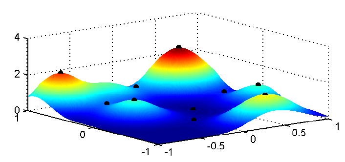
14. Chebfun2: Vector Calculus 3
The cross product for 2D vector fields works as follows.
help chebfun2v/cross
CROSS Vector cross product.
CROSS(F, G) returns the cross product of the CHEBFUN2V objects F and G. If F
and G both have two components, then it returns the CHEBFUN2 representing
CROSS(F,G) = F(1) * G(2) - F(2) * G(1)
where F = (F(1); F(2)) and G = (G(1); G(2)). If F and G have three
components then it returns the CHEBFUN2V representing the 3D cross
product.
14.3 Differential operators
Vector calculus also involves various differential operators defined on scalar- or vector-valued func-
tions such as gradient, curl, divergence, and Laplacian.
The gradient of a chebfun2 representing a scalar function f(x, y) is, geometrically, the direction and
magnitude of steepest ascent of f. If the gradient of fis 0 at (x, y), then fhas a critical point at
(x, y). Here are the critical points of a sum of Gaussian bumps:
f = chebfun2(0);
rng(’default’)
for k = 1:10
x0 = 2*rand-1; y0 = 2*rand-1;
f = f + chebfun2(@(x,y) exp(-10*((x-x0).^2 + (y-y0).^2)));
end
plot(f), hold on
r = roots(gradient(f));
plot3(r(:,1),r(:,2),f(r(:,1),r(:,2)),’k.’,’markersize’,20)
zlim([0 4]), hold off
The curl of 2D vector function is a scalar function defined as follows.
4Chebfun Guide
help chebfun2v/curl
CURL curl of a CHEBFUN2V
S = CURL(F) returns the CHEBFUN2 of the curl of F. If F is a CHEBFUN2V with
two components then it returns the CHEBFUN2 representing
CURL(F) = F(2)_x - F(1)_y,
where F = (F(1),F(2)). If F is a CHEBFUN2V with three components then it
returns the CHEBFUN2V representing the 3D curl operation.
If the chebfun2v Fdescribes a vector velocity field of fluid flow, for example, then curl(F) is the
scalar function equal to twice the angular speed of a particle in the flow at each point. A particle
moving in a gradient field has zero angular speed and hence, the curl of the gradient is zero. We
can check this numerically:
norm(curl(gradient(f)))
ans =
3.449144990253006e-15
The divergence of a chebfun2v is defined as follows.
help chebfun2v/divergence
DIVERGENCE Divergence of a CHEBFUN2V.
DIVERGENCE(F) returns the divergence of the CHEBFUN2V i.e.,
divergence(F) = F_x + F_y.
This measures a vector field’s distribution of sources or sinks. The Laplacian is closely related and
is the divergence of the gradient,
norm(laplacian(f) - divergence(gradient(f)))
ans =
0
14.4 Line integrals
Given a vector field F, we can compute the line integral along a curve with the command integral,
defined as follows.
help chebfun2v/integral
14. Chebfun2: Vector Calculus 5
INTEGRAL Line integration of a CHEBFUN2V.
INTEGRAL(F, C) computes the line integral of F along the curve C, i.e.,
/
INTEGRAL(F, C) = | < F(r), dr >
/
C
where the curve C is parameterised by the complex curve r(t).
The gradient theorem says that if Fis a gradient field, then the line integral along a smooth curve
only depends on the end points of that curve. We can check this numerically:
f = chebfun2(@(x,y) cos(10*x.*y.^2) + exp(-x.^2)); % chebfun2
F = gradient(f); % gradient (chebfun2v)
C = chebfun(@(t) t.*exp(10i*t),[0 1]); % spiral curve
v = integral(F,C);ends = f(cos(10),sin(10))-f(0,0); % line integral
abs(v-ends) % gradient theorem
ans =
1.332267629550188e-15
14.5 Phase diagram
A phase diagram is a graphical representation of a system of trajectories for a two variable au-
tonomous dynamical system. Chebfun2 plots phase diagrams with quiver command, which has
been overloaded to plot the vector field. Note that there is a potential terminological ambiguity in
that a ”phase portrait” can also refer to a portrait of a complex-valued function (see section 11.7 of
the guide).
In addition, Chebfun2 makes it easy to compute and plot individual trajectories of a vector field.
If Fis a chebfun2v, then ode45(F,tspan,y0) computes a trajectory of the autonomous system
dx/dt =f(x, y), dy/dt =g(x, y), where fand gare the first and second components of F. Given
a prescribed time interval and initial conditions, this command returns a complex-valued chebfun
representing the trajectory in the form x(t)+iy(t). For example:
d=0.04;a=1;b=-.75;
F = chebfun2v(@(x,y)y, @(x,y)-d*y - b*x - a*x.^3, [-2 2 -2 2]);
[t y] = ode45(F,[0 40],[0,.5]);
plot(y,’r’,LW,1.6), hold on,
quiver(F,’b’), axis equal
title(’The Duffing oscillator’,’FontSize’,14), hold off
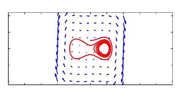
6Chebfun Guide
−4−3−2−1 0 1 2 3 4
−2
−1
0
1
2
The Duffing oscillator
15. Chebfun2: 2D Surfaces in 3D
Space
Alex Townsend, March 2013, latest revision June 2014
Contents
•15.1 Representing parametric surfaces
•15.2 Surface normals and the divergence theorem
•15.3 References
15.1 Representing parametric surfaces
In Chapter 14, we explored chebfun2v objects with two components, but Chebfun2 can also work
with functions with three components, i.e., functions from a rectangle in R2into R3. For example,
we can represent the unit sphere via spherical coordinates as follows:
th = chebfun2(@(th,phi) th, [0 pi 0 2*pi]);
phi = chebfun2(@(th,phi) phi, [0 pi 0 2*pi]);
x = sin(th).*cos(phi);
y = sin(th).*sin(phi);
z = cos(th);
F = [x;y;z];
surf(F), camlight, axis equal
1
2Chebfun Guide
Above, we have formed a chebfun2v with three components by vertical concatenation of chebfun2
objects. However, for familiar surfaces such as cylinders, spheres, and ellipsoids Chebfun2 has
overloads of the commands cylinder,sphere,andellipsoid to generate these surfaces more
easily. For example, a cylinder of radius 1 and height 5 can be constructed like this:
h=5;
r = chebfun(@(th) 1+0*th,[0 h]);
F = cylinder(r);
surf(F), camlight
An important class of parametric surfaces are surfaces of revolution, which are formed by revolving
a curve in the left half plane about the z-axis. The cylinder command can be used to generate
surfaces of revolution. For example:
f = chebfun(@(t) (sin(pi*t)+1.1).*t.*(t-10),[0 5]);
F = cylinder(f);
surf(F), camlight
15. Chebfun2: 2D Surfaces in 3D Space 3
Here as another example is a torus with a gap in it.
x = chebfun2(@(x,y) x); y = chebfun2(@(x,y) y);
theta = 0.9*pi*x; phi = pi*y;
F = [-(1+.3*cos(phi)).*sin(theta);
(1+.3*cos(phi)).*cos(theta);
.3*sin(phi)];
surf(F), axis equal, camlight
15.2 Surface normals and the divergence theorem
Given a chebfun2v representing a surface, the normal can be computed by the Chebfun2 normal
command. Here are the normal vectors of another torus:
r1 = 1; r2 = 1/3; % inner and outer radius
d = [0 2*pi 0 2*pi];
u = chebfun2(@(u,v) u,d);
v = chebfun2(@(u,v) v,d);
F = [-(r1+r2*cos(v)).*sin(u); (r1+r2*cos(v)).*cos(u); r2*sin(v)]; % torus
surf(F), camlight, hold on
4Chebfun Guide
quiver3(F(1),F(2),F(3),normal(F,’unit’),’numpts’,10)
axis equal, hold off
Once we have the surface normal vectors we can compute, for instance, the volume of the torus by
applying the divergence theorem:
!!
V!div(G)dV =!S!G·dS,
where div(G) = 1. Instead of integrating over the 3D volume, which is currently not possible in
Chebfun2, we integrate over the 2D surface:
G = F./3; % full 3D divergence of G is 1 because F = [x;y;z].
integral2(dot(G,normal(F)))
exact = 2*pi^2*r1*r2.^2
ans =
2.193245422464302
exact =
2.193245422464302
Chebfun2v objects with three components come with a warning. Chebfun2 works with functions of
two real variables and therefore, operations such as curl and divergence (in 2D) have little physical
meaning to the represented 3D surface. The reason we can compute the volume of the torus (above)
is because we are using the divergence theorem and circumventing the 3D divergence.
To finish this section we represent the Klein Bagel. The solid black line shows the parameterisation
seam and is displayed with the syntax surf(F,’-’). See [Platte 2013] for more on parameterised
surfaces.
u = chebfun2(@(u,v) u, [0 2*pi 0 2*pi]);
v = chebfun2(@(u,v) v, [0 2*pi 0 2*pi]);
x=(3+cos(u/2).*sin(v)-sin(u/2).*sin(2*v)).*cos(u);
y=(3+cos(u/2).*sin(v)-sin(u/2).*sin(2*v)).*sin(u);
z=sin(u/2).*sin(v)+cos(u/2).*sin(2*v);
15. Chebfun2: 2D Surfaces in 3D Space 5
surf([x;y;z],’-k’,’FaceAlpha’,.6), camlight left, colormap(hot)
axis tight equal off
15.3 References
[Platte 2013] R. Platte, Parameterizable surfaces, Chebfun2 Example:
http://www2.maths.ox.ac.uk/chebfun/examples/geom/html/ParametricSurfaces.shtml

!