Climada Manual
User Manual: Pdf
Open the PDF directly: View PDF ![]() .
.
Page Count: 72
- Instead of an Introduction: Preamble
- A visual primer
- A brief introduction to the concepts behind CLIMADA
- Getting started
- From tropical cyclone hazard generation to the adaptation cost curve
- Function reference
- CLIMADA modules
- Writing your own code
- Appendices

1
CLIMADA MANUAL 08 Feb 2018
Obtain the full package from https://github.com/davidnbresch/climada
David N. Bresch, david.bresch@gmail.com and dbresch@ethz.ch
Lea Mueller, muellele@gmail.com
CLIMADA is an open-source and -access global probabilistic risk modelling and
adaptation economics platform.
CLIMADA allows to assess risk, i.e. to estimate the expected economic impact of
weather and climate as a measure of risk today, the incremental increase from
economic growth and the further incremental increase due to climate change.
CLIMADA supports the appraisal of risk management options and adaptation
measures with the aim to strengthen weather and climate-resilient development.
The economics of climate adaptation methodology (ECA)
1
,
2
as implemented in
CLIMADA provides decision makers with a fact base to understand the impact of
weather and climate on their economies, including cost/benefit perspectives on
specific risk reduction measures.
Cite as
3
: Bresch, D. N., & Mueller, L., 2016: CLIMADA – the open-source and -access global
probabilistic risk modelling platform. https://github.com/davidnbresch/climada
The current version of climada does support the following hazards/perils:
Peril Coverage Resolution
4
Tropical cyclones and associated storm surge
5
global 10x10 and 1x1 km
European winter storms
6
all Europe 10x10 km
Wildfire and droughts
7
global 10x10 and 1x1 km
Earthquake and Volcano
8
global 10x10 and 1x1 km
Meteorites
9
global 10x10 and 1x1 km
River flood
10
(interface to existing hazard models) to be developed 1x1 km
Asset base
11
(kind of market portfolio) global 10x10 and 1x1 km
Population
12
global 10x10 and 1x1 km
Note on climate change: implemented by altering probabilistic hazard event sets (based on SREX
13
etc.), see pertinent sections in this manual.
Note on interoperability: CLIMADA hazard, exposure and vulnerability databases can be exported and
integrated into OASIS LMF ktools
14
. CLIMADA does support ktools as an alternative kernel.
1
See lecture course ETH Zurich: http://www.ied.ethz.ch/education/courses-offered/climrisk.html
2
For a list of case studies, see http://www.wcr.ethz.ch/research/casestudies.html
3
While climada is all lower-case in MATLAB, please use CLIMADA when referring to it in texts.
4
CLIMADA operates on a variable grid, i.e. any resolution is possible. The listed resolution is just
indicative of the resolution that is available by default.
5
Tropical cyclones are part of core climada, but see the section in additional modules, too.
6
See also climada module https://github.com/davidnbresch/climada_module_storm_europe
7
See also climada module https://github.com/davidnbresch/climada_module_drought_fire. Wildfire is
operational, drought is in early development stage.
8
See also climada module https://github.com/davidnbresch/climada_module_earthquake_volcano
9
See also climada module https://github.com/davidnbresch/climada_module_meteorite
10
See also climada module https://github.com/davidnbresch/climada_module_flood - still in early
development.
11
CLIMADA provides a default asset base for every country and default damage curves for every peril.
12
Based on satellite night-light intensity (open access). Interface to other sources (e.g. ssp2).
13
IPCC Special Report on Extremes, http://www.ipcc.ch/report/srex/
14
OASIS LMF and ktools, see http://www.oasislmf.org/the-toolkit

2
Instead of an Introduction: Preamble
Climate adaptation is an urgent priority for the custodians of national and local
economies, such as finance ministers and mayors. Such decision-makers ask:
• What is the potential climate-related damage to our economies and societies
over the coming decades?
• How much of that damage can we avert, with what measures?
• What investment will be required to fund those measures – and will the benefits
of that investment outweigh the costs?
The economics of climate adaptation methodology as implemented in climada
provides decision-makers with a fact base to answering these questions in a
systematic way. It enables them to understand the impact of climate on their
economies – and identify actions to minimize that impact at the lowest cost to
society. Hence it allows decision-makers to integrate adaptation with economic
development and sustainable growth. In essence, we provide a methodology to pro-
actively manage total climate risk. Using state-of-the-art probabilistic modelling, we
estimate the expected economic damage as a measure of risk today, the incremental
increase from economic growth and the further incremental increase due to climate
change. We then build a portfolio of adaptation measures, assessing the damage
aversion potential and cost-benefit ratio for each measure. The adaptation cost curve
illustrates that a balanced portfolio of prevention, intervention and insurance
measures allows to pro-actively managing total climate risk.
CLIMADA consists of the core module, providing the user with the key functionality to
perform an economics of climate adaptation assessment. Additional modules
implement global coverage (automatic asset generation), a series of hazards (tropical
cyclone, surge, rain, European winter storms, … and even earthquake, volcano and
meteorites) and further functionality, such as Google Earth access, animations…
CLIMADA runs on both MATLAB (version 7
15
and higher, all tested with version 9)
and GNU Octave (version 3.8.0
16
and higher). Some modules might not have been
thoroughly tested using Octave, but core CLIMADA works without limitations (in order
to read Excel, Octave’s IO package has to be installed, see section “Notes on
Octave” below). All CLIMADA is available on GitHub
17
.
15
see e.g. ch.mathworks.com/products/matlab and http://www.cse.cuhk.edu.hk/~cslui/CSCI1050/book.pdf
16
https://www.gnu.org/software/octave
17
Either use Clone to desktop in Git or install git first, then clone any repository by first creating an
empty folder (e.g. mkdir climada), then cd climada, then (note that the last . is part of the
command)
git clone https://github.com/davidnbresch/climada . See also climada_git_pull
3
Contents
Instead of an Introduction: Preamble ................................................................. 2
A visual primer..................................................................................................... 5
A brief introduction to the concepts behind CLIMADA ...................................... 6
Probabilistic damage model ............................................................................ 6
Adaptation cost curve ...................................................................................... 9
A note on decision-making ............................................................................ 11
Getting started ................................................................................................... 12
Local installation ............................................................................................ 12
Process on one page .................................................................................... 14
Excel interface to CLIMADA ......................................................................... 15
A note on Excel and Open Office file formats and their tolerance in
MATLAB and Octave ................................................................................. 18
Constructing your own entity ..................................................................... 18
From tropical cyclone hazard generation to the adaptation cost curve ........... 19
Hazard set ..................................................................................................... 19
Assets and damage functions ....................................................................... 26
Damage calculation ....................................................................................... 29
Dealing with uncertainty ................................................................................ 30
Adaptation cost curve .................................................................................... 31
A climada application example – tropical cyclone ensemble damage
forecasts ........................................................................................................ 35
Function reference ............................................................................................ 36
Basic entity functions..................................................................................... 36
Core calculations ........................................................................................... 36
Basic hazard functions .................................................................................. 37
Further display functions ............................................................................... 37
Tropical cyclone (TC) specific functions ....................................................... 38
Basic functions .............................................................................................. 38
Admin functions ............................................................................................. 38
Special functions (there are more) ................................................................ 39
CLIMADA modules............................................................................................ 39
advanced ....................................................................................................... 39
tropical_cyclone ............................................................................................. 40
storm_europe ................................................................................................ 40
country_risk ................................................................................................... 40
isimip .............................................................................................................. 40
4
earthquake_volcano ...................................................................................... 40
elevation_models .......................................................................................... 40
meteorite ........................................................................................................ 41
flood ............................................................................................................... 41
barisal_demo and salvador_demo ................................................................ 41
kml_toolbox.................................................................................................... 41
octave_io_fix .................................................................................................. 41
Some hints to useful data sources ................................................................ 41
Writing your own code ...................................................................................... 42
climada_init_vars ........................................................................................... 43
climada startup .............................................................................................. 45
Description of key climada structures ........................................................... 45
Notes on Octave (and OpenOffice) .............................................................. 50
Appendices ........................................................................................................ 51
climada, the inner workings .......................................................................... 51
Implementation .......................................................................................... 52
Insurance remarks ......................................................................................... 53
Insurability & forms of insurance ............................................................... 53
Insurance conditions .................................................................................. 56
climada implementation of insurance conditions ...................................... 57
Note on scenarios ......................................................................................... 58
climate impact scenarios – remarks on climada implementation ............. 59
Climate impact scenarios – sources ......................................................... 60
Tropical cyclones – technical remarks .......................................................... 61
Windfield calculation .................................................................................. 61
Single cyclone track evolution animation .................................................. 64
Economics of Climate Adaptation (ECA) – key routines .............................. 65
A remark on loss, damage and vulnerability ................................................ 69
Further sources of DRM/climate adaptation information/tools ..................... 70
MATLAB/Python – some possibly useful tools ............................................. 71
5
A visual primer
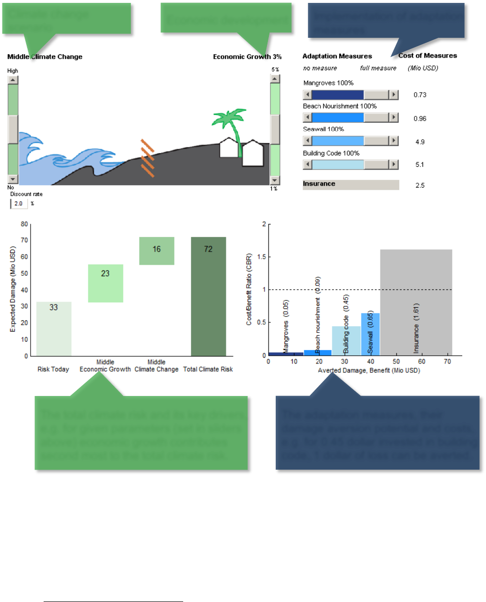
Figure: The demonstration code climada_demo
18
implements the concept of total
climate risk and cost-effective adaptation in an interactive way: The user can
experiment with key relevant factors (sliders, top) and instantly observe the effect –
both on risk (measured by expected damage, graph on the left) and the basket of
adaptation measures (shown as adaptation cost curve, graph on the right). The user
can also edit the underlying input data
19
and hence experiment further.
The simple call climada runs the core automatically and prompts for user input.
18
This GUI runs properly under MATLAB, see climada_demo_step_by_step for Octave for he time
being, as Octave does not yet support all GUI features.
19
Just edit the file ../climada/data/entities/demo_today.xls, then select Re-init from the GUI’s file menu.
Climate change
scenario
Implementation of adaptation
measures
The total climate risk and its key drivers,
e.g. for given parameters (set in sliders
above) economic growth contributes
second most to the total climate risk.
The adaptation measures, their
damage aversion potential and costs,
e.g. for 0.45 dollar invested in building
code, 1 dollar of loss can be averted.
Economic development

6
A brief introduction to the concepts behind CLIMADA
Instead of studying this now, the user might also jump to the step-by-step
introduction below and later come back.
Risk is the combination of the probability [or likelihood] of a consequence and its
magnitude, i.e. risk = probability x severity. Or, to be more specific:
risk = hazard x exposure x vulnerability
= (probability x intensity) x exposure x vulnerability
\…………………severity……………………../
where both the probability of occurrence and the (physical) intensity are part of the
hazard (sometimes named peril) and the ‘product’ of intensity, exposure and
vulnerability constitutes the severity. The product symbol ‘x’ does not stand for a
simple multiplication, but in fact a convolution of the respective distributions. Instead
of providing the general framework here, one can easily think of severity thus being
of the following form
severity = F(intensity,value,vulnerability)
where F is often of the form F = value * f(intensity),
where f(intensity) is the damage function which parametrizes vulnerability
Note that value is the asset value of the exposure, intensity the hazard intensity at
the exposure location and the * a simple multiplication. Note that assets do not
necessarily need to be monetary assets and value hence not necessarily a monetary
value, think about exposed people. In this simple form, vulnerability is given as a
function f of intensity (and asset class/type). See Appendix “climada, the inner
workings” below for details.
Any risk model hence attempts to quantify these elements in a way most appropriate
for the specific purpose. Depending on purpose, the level of detail in quantification of
any element will thus vary. For the geographical representation, think e.g. of a local
flood model at very high resolution of a few decameters compared to a global
earthquake model at e.g. 10 km resolution. For the vulnerability resolution, think e.g.
of a general description of building damage to an earthquake as a simple function of
modified Mercally intensity
20
compared to a detailed damage curve depending on
flood height in meters, building construction, number of floors, basements… and
usage (also called occupancy).
Probabilistic damage model
A model is nothing more than a simplified representation of reality. Natural hazard
models use the virtual world of computers in an attempt to simulate natural
catastrophe damage expected in reality. The quantification of natural catastrophe risk
depends on three basic elements (or sets of data), upon which the damage model
operates. They are:
• Hazard (sometimes also called peril): Where, how often and with what
intensity do events occur? A hazard (event) set is usually generated once and
stored for subsequent calls (resulting in massive speedup). A hazard event
20
Please note that a sophisticated earthquake model can indeed be built on MMI... see e.g.
https://github.com/davidnbresch/climada_module_earthquake_volcano
7
set comprises just many single events, i.e. one ‘footprint’ for each event.
Think of a single event footprint as for example a georeferenced distribution
(or simply a map) of windspeed.
• Assets (also referred to as value distribution or portfolio of exposed assets or
simply exposure): Where are the various types of potentially affected objects
located and what is their value? Think of the assets as for example a
georeferenced distribution (or simply a map) of houses, represented by their
replacement values – or of people, represented by their number at any given
location.
• Damage function (sometimes referred to as vulnerability or vulnerability
curve): What is the extent of damage at a given event intensity? A damage
function is just a simple function of the hazard intensity, but there can be
many damage functions for all kinds of assets (and obviously for different
hazards).
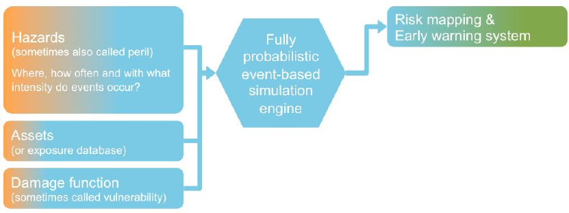
These three building blocks are combined in the process of estimating event damage
as follows:
Fig: The basic three building blocks (hazard, assets and damage function). Main result is risk
quantification (here subsumed as risk mapping), but the same system can also be (operationally) used
to provide early warnings in terms of impact quantities, if fed with a particular (forecasted) single hazard
event (such as a wind field of a storm or an shake map of an earthquake).
This approach may generally be applied to all forms of natural hazard, whether
storm, flood, earthquake … or any other type of peril.
The simplest way to assess the damage is to simulate an individual natural
catastrophe scenario. This is known as “deterministic” or “scenario-based” modeling.
Such models often refer back to major historical damage events, applying these to
the assets that exist now (“as-if analysis”). The disadvantage of this method is that,
whilst it allows a single, extreme, individual event damage to be assessed, it fails to
take account of all the other events that might occur. It is not possible to calculate an
expected annual damage for a portfolio of assets on the basis of single event
damage, and any prediction as to the occurrence frequency of the model scenario
will remain very uncertain.
Today, in an attempt to avoid these problems, so-called “probabilistic” models (i.e. a
fully probabilistic simulation engine) are being used to assess hazards such as
storms and floods. Rather than simply analyzing one event, the computer is
programmed to function as a sort of time-lapse film camera, simulating all the
possible events that could unfold within a sufficiently long period of time (thousands
or tens of thousands of years). This type of model produces a “representative” list of
event damages (i.e. a list that accurately reflects the risk). From this list it is possible
8
to understand the relationship between damage potential and occurrence frequency,
and hence the cost of average and extreme damage burdens.
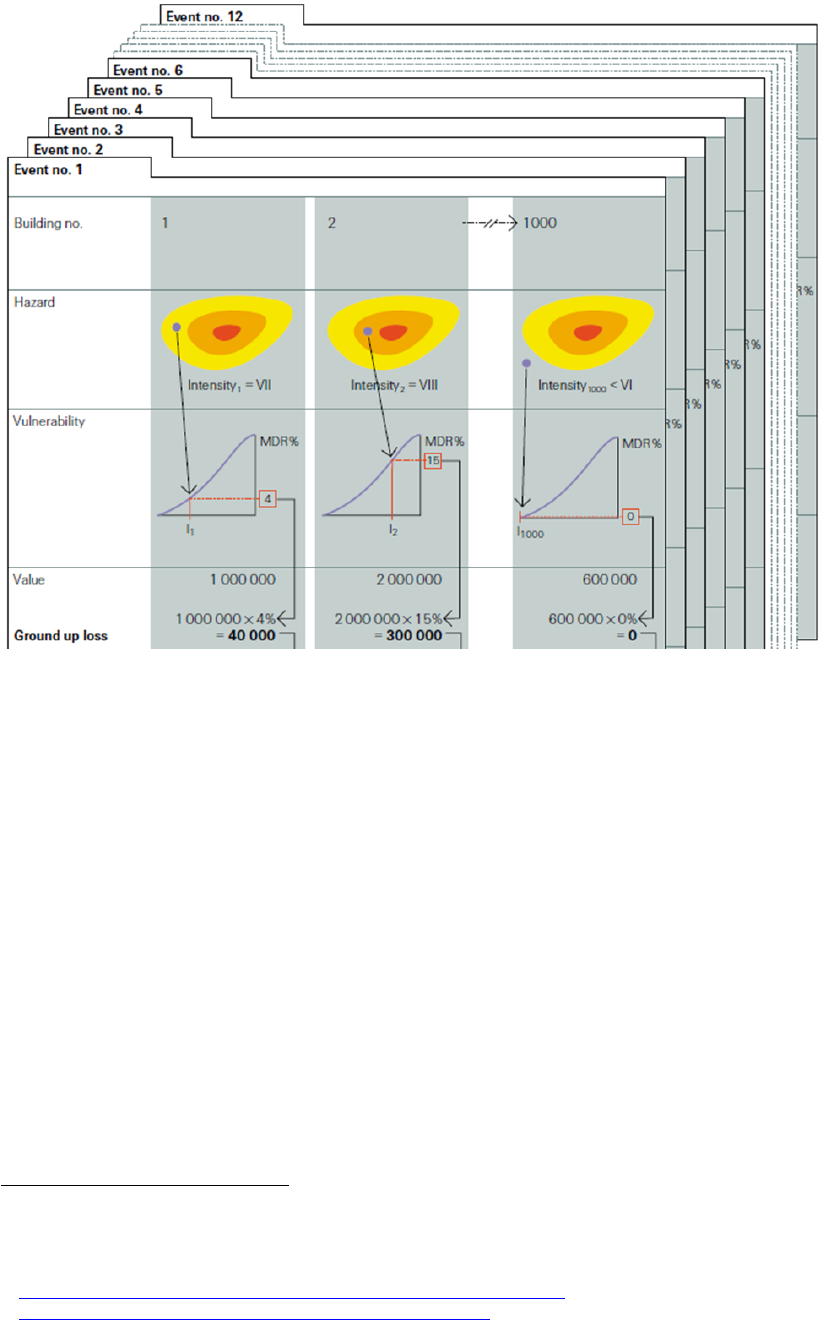
Figure (from Swiss Re publication "Natural catastrophes and reinsurance"): Using risk assessment
tools to calculate event damage. Let's assume a hypothetical portfolio containing 1000 assets
(buildings). For the sake of simplicity, let us assume that the risk assessment tool only contains 12
potential events over a projected period of 200 years. The following calculations would be performed:
• The hazard module generates the expected intensity (VII) for event no.1 at asset (building)
location no.1.
• The damage function (called vulnerability in the figure) corresponding to the asset provides us
with the mean damage ratio (MDR
21
) for given hazard intensity (4 stands for 4% of the asset's
value)
• The damage is calculated by multiplying the MDR and the value of the asset (1'000'000),
resulting in a (ground up) damage (called loss in the figure) of 40'000.
• Above steps are performed on all 1'000 assets in the portfolio. The sum of all damages
produces the total damage from event no.1, i.e. event damage no1.
• All above steps are then repeated for the other (11) events in the event set.
• Upon completion of all these stages in the modeling process, a list of all event damage is
produced, upon which damage statistics can be derived (average damage, max damage…).
See mentioned lecture course
22
or e.g. the Swiss Re publication
23
"Natural
catastrophes and reinsurance", which covers the methodology in detail.
21
Please note that climada uses MDR=MDD*PAA, where Mean damage degree (MDD) and percentage
of affected assets (PAA) allow to deal with local deductibles in a more appropriate form than a simple
Mean damage ration (MDR) model could do, since one does, due to the PAA, know how many assets
are affected, hence deductible application is more specific.
22
http://www.iac.ethz.ch/edu/courses/master/modules/climate-risk.html
23
http://media.swissre.com/documents/Nat_Cat_reins_en.pdf
9
Adaptation cost curve
While the assessment of cost and damage aversion potential of any adaptation
measure can be quite demanding, climada provides a consistent approach to do so.
The tool provides a common yet flexible framework to appraise a basket of
adaptation options (sometimes also referred to as resilience measures). Each option
can be specified to act on any component of the model (hazard, assets and damage
function) – or even a combination thereof.
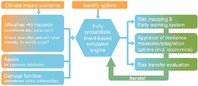
Fig: The climada model, including inputs such as different climate scenarios (which change the hazard
component, which itself can be understood as being built on weather events) as well as adaptation
options, plus additional outputs such as appraisal of resilience measures or adaptation options. Note the
emphasis on iterative approach in options appraisal (see main text, too).
The specific potential damage aversion comes with a certain degree of uncertainty,
even for measures for which extensive research exists – for example, for building
codes to fix roofs against hurricane winds. Hence, we strongly propose an iterative
approach, i.e. to re-run climada with a range of parameters in order to converge to a
consistent evaluation.
The assembled cost curve shows – from left to right – the range of measures from
most cost-efficient to least cost-efficient. The results should thus be used to start
discussions on the different measures and the opportunity to avert expected damage,
rather than be read as recommendations to implement certain measures.
10
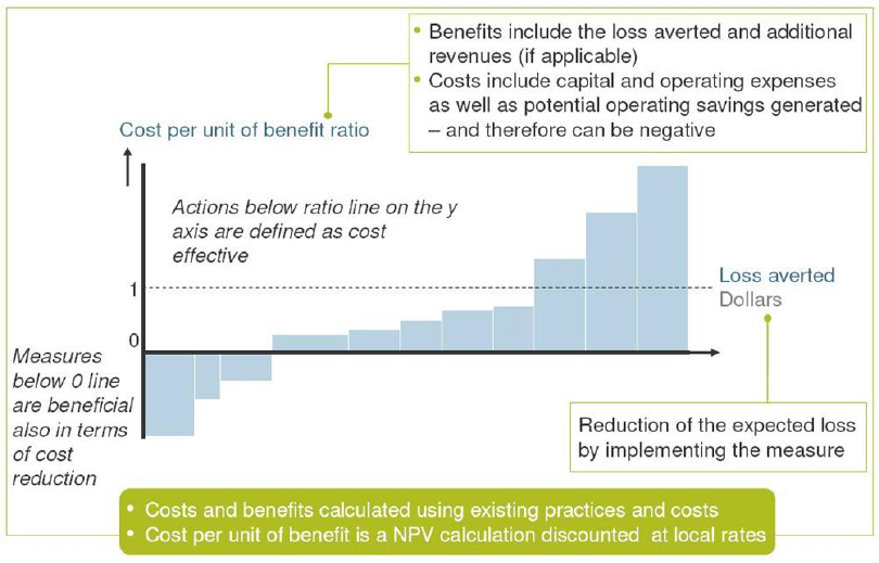
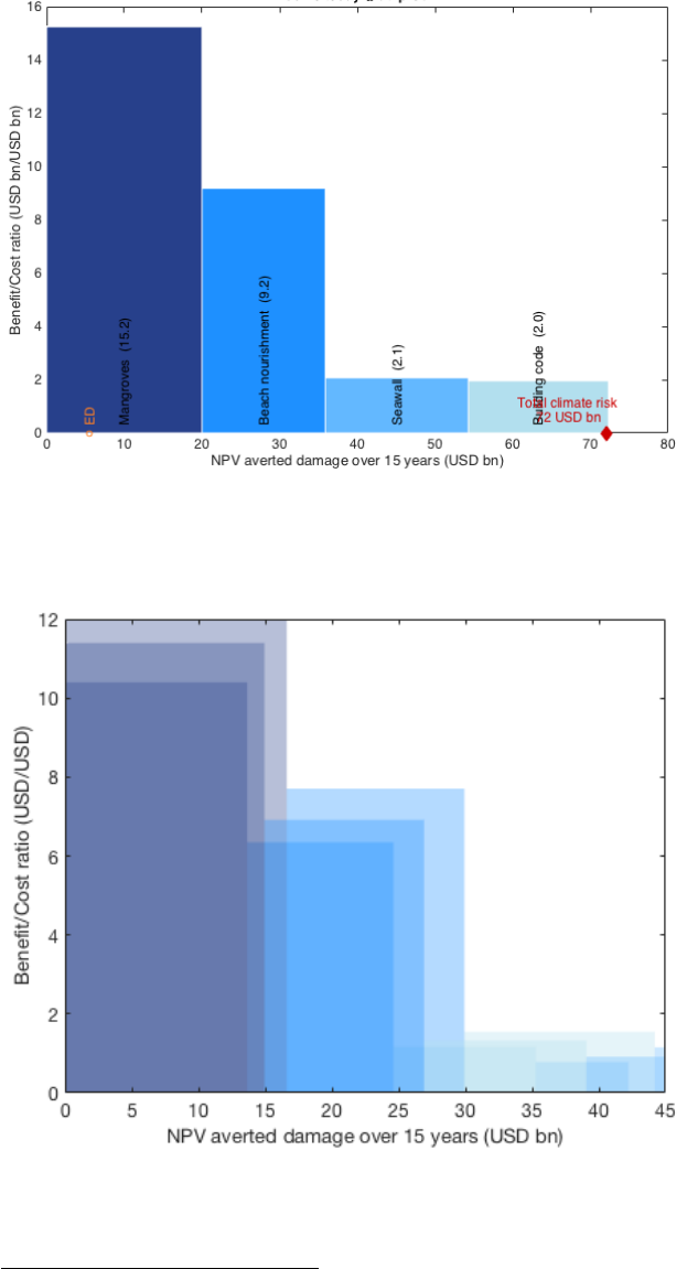
Figure: The width of each bar in a cost curve represents the cumulative potential of that measure to
reduce total expected damage up to 2030 for a given scenario. The height of each bar represents the
ratio between costs and benefits for that measure. Whether or not this ratio is attractive to a decision
maker depends on many factors, including risk appetite. After considering the other – including non-
economic – impacts and benefits related to implementing a measure, a risk-neutral decision maker
would select measures based on a sense of how much protection they offer and at what cost. The
advantage of calculating cost-benefit ratios for all measures is that doing so allows decision-makers to
compare measures using a single simple metric.
In a recipe form, the adaptation cost curve is constructed as follows (repeat for each
measure)
1. Calculate present value (PV) of costs of measure [e.g. Excel, outside of climada]
2. Risk today: import today's assets and damage functions (input via Excel) and
expose them to present hazard (part of climada)
2.1. climada calculates annual expected damage with no measures
2.2. climada calculates annual expected damage with measure applied
difference 2.1) minus 2.2) shows benefit of measure today
3. Future risk (e.g. year 2030): import future assets and damage functions (input via
Excel, damage functions likely to be unchanged) and expose them to future
hazard (part of climada)
3.1. climada calculates annual expected damage with no measures
3.2. climada calculates annual expected damage with measure applied
difference 3.1) minus 3.2) shows future benefit of measure
4. climada discounts benefits --> horizontal axis of adaptation cost curve
5. climada calculates the cost benefit ratio vertical axis of adaptation cost curve
11
A note on decision-making
While the climada tool does provide decision-makers with that a fact base, it does by
no means pre-empt any decision or constitute an adaptation strategy by itself. The
adaptation cost curve shall by no means be interpreted as a ‘recipe’ to be
implemented ‘from left to right’. Many more elements need to be considered in order
to take a decision, not least to contextualize model results.
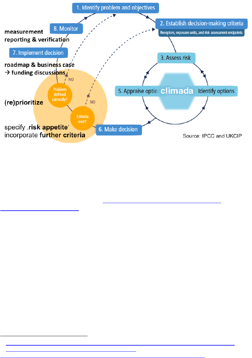
Fig: The decision-making context around climada. Note the necessary steps that precede any
application of climada – and even more so the steps that build on the modeling results.
Please refer to the descriptions of Economics of Climate Adaptation (ECA)
methodology
24
, which emphasizes mentioned context and provides a structured
approach to provide decision makers with a comprehensive fact base.
Please note that a comprehensive Economics of Climate Adaptation (ECA)
guidebook for practitioners
25
has recently been published. It describes the project
setup, the full planning cycle for an adaptation study and puts a lot of emphasis on
the stakeholder engagement. The ECA Guidebook is designed to accompany any
climate change adaptation assessment using the open-source ECA methodology and
its associated climada tool. The ECA Guidebook is particularly helpful in cases which
require an integrated approach towards the development, planning and financing of
specific adaptation measures.
24
http://media.swissre.com/documents/rethinking_shaping_climate_resilent_development_en.pdf
25
https://www.kfw-entwicklungsbank.de/PDF/Download-
Center/Materialien/2016_No6_Guidebook_Economics-of-Climate-Adaptation_EN.pdf
12
Getting started
Local installation
Get the climada core module from GitHub
26
, i.e. go to https://github.com/davidnbresch/climada
and either just click on the button or on .or just type
git clone https://github.com/davidnbresch/climada.git in a shell (if you
have git installed).
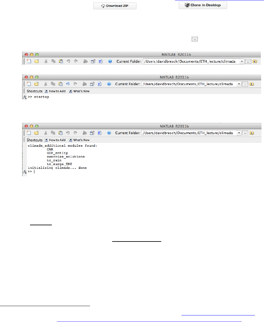
• Set the MATLAB
27
Current Folder to climada
28
(use the button to browse),
e.g.:
• Enter startup in the MATLAB Command Window:
and press Enter (or Return). This initializes climada, sets some variables (e.g.
the location of the data folder
29
) and detects any additional modules
30
.
After that, the Command Window looks something like:
It’s ok if there are no further modules shown, as long as ... done appears.
• Start by just invoking the climada demonstration by entering climada_demo
in the MATLAB Command Window
31
, which is also the best way to test
whether climada works properly – you should see something as shown above
as a visual primer (see above) and be able to play with the sliders.
In Octave, use climada_demo_step_by_step, instead, as Octave does
not support guide (the interactive climada GUI has been built with).
In case you run climada on a remote machine (e.g. a cluster, if no window
system), test it by entering the following three commands:
entity=climada_entity_load('USA_UnitedStates_Florida_entity');
hazard=climada_hazard_load('USA_UnitedStates_Florida_atl_TC');
EDS=climada_EDS_calc(entity,hazard)
EDS then contains the event damage set and the variable EDS.ED should
contain a value close to 2.3824e+09 (i.e. simulated annual expected tropical
cyclone damage to Florida amounts to USD 2.4 billion).
26
About GitHub, recommended reading (especially chapters 1, 2 and 3): http://git-scm.com/book/en/v2
and directly to the pdf: https://progit2.s3.amazonaws.com/en/2015-02-21-5277c/progit-en.346.pdf
27
Same procedure in Octave, see also „Notes on Octave“ below.
28
Usually the folder you downloaded or cloned to from GitHub.
29
The global variable climada_global (a struct) contains all these variables. See the code
climada_init_vars.m which sets all these variables. Make sure you never issue a clear all command,
as this would also delete climada_global and hence climada would not find it’s stuff anymore.
30
A climada_advanced module extends the functionality of climada and allows users to further develop
climada without risking to change the core code. See further below for some examples of modules. Just
run climada_git_clone to obtain and install most modules fully automatically.
31
From now on, just type any command in Courier in the MATAB Command Window, as we will not
state this each time again.

13
• Note that the command climada allows you to run the essentials in one go,
i.e. to import assets and hazard event sets, to show a few plots for checks, to
run all calculations and to produce the final adaptation cost curve
32
.
• Further note that climada('TEST_CLIMADA')tests the full climada (very
similar to climada_demo_step_by_step), that climada('DEMO')
invokes the demo GUI (same as climada_demo) and
• climada('TC') invokes the interactive GUI to calculate the ensemble-
prediction damage for a specific tropical cyclone (automatically accesses the
web to find latest tracks etc.).
While the standard climada setup contains the data folder within climada, it is highly
recommended to create a folder named climada_data parallel to climada to allow for
your local climada data NOT being synched (only the folder ../climada/data within
core climada gets synched). Just run climada_git_clone, which installs most
modules and sets up such a local climada_data folder. This way, any data used in
climada beyond the default files will not be synchronised. Your directory tree shall
then look like
{parent_dir}/climada % contains core climada, usually no edits in there
{parent_dir}/climada_data % contains your data
Make sure at the start, the folder {parent_dir}/climada_data (your local data folder)
does at least contain the contents of {parent_dir}/climada/data (the sub-folder within
core climada). If you run climada_git_clone, this has been taken care of.
In case you do not want to (or cannot, on some systems) run climada_git_clone,
install modules yourself (skip this, if you are new to climada and come back to thism
later). In order to grant core climada access to additional modules (see
https://github.com/davidnbresch?tab=repositories and the section on climada
modules further below), create a folder ‘climada_modules’ on the same level as the
core climada folder to store any additional modules. This way, climada sources all
modules' code upon startup. Your directory tree shall then look like
{parent_dir}/climada % contains core climada, usually no edits in there
{parent_dir}/climada_data % contains your data
{parent_dir}/climada_modules % contains additional modules
Again, see the code climada_git_clone to automatically clone all modules and
climada_git_pull to automatically update all installed modules
33
.
As for a start, you can generate the asset base (so-called entity) for any country with
entity=climada_entity_country and create all standard hazard sets with
hazard_info=climada_hazards(entity). If you do not have the relevant
modules installed
34
, climada prompts you, or you might consider to run
climada_git_clone, to get all modules installed.
32
On subsequent calls, the routine suggests last inputs - and if the first file selection is the same as on
previous call, even asks to re-run with previous call's inputs without asking for each file’s confirmation. It
further checks for the entity file to have been edited since last call. If not, it does not ask for plotting
assets and damagefunctions again.
33
Proper working of these two routines depend on your operating environment (it issues system
commands to your system’s git). On latest MATLAB version, it looks as if one could use its own git (not
implemented) and for Octave, it depends again on how it is set up (access to system commands).
34
Depending on the country (i.e. its exposure to different perils), not all modules might be needed.

14
Process on one page
To cut the whole story short, CLIMADA (inter alia) produces an adaptation cost
curve, as shown in the lower right part of the visual primer (and many more nice
things). The following steps are required in order to come up with a climate
adaptation cost curve
1. Generate a hazard event set
35
a. Generate a hazard event set for today’s climate
i. Obtain historical events
ii. Produce the probabilistic events
iii. Store intensities at centroids
b. Repeat above steps for future hazard
(climate change impact scenarios, e.g. for 2030)
2. Import a list of assets and corresponding damage functions
36
(the so-called entity)
a. Read the list of today’s assets
i. Encode to centroids (to the nearest point where hazard information is
available, up to a distance threshold
37
)
ii. Read the damage functions and make sure they correspond to
assets
b. Repeat above steps for future assets (e.g. 2030)
3. Import the list of adaptation measures
(also stored into the entity structure)
a. Read the list of measures
4. Calculate the damages and benefits of measures
a. Calculate the damages
38
for the list of today’s assets, today’s hazard event
set and the list of measures
39
b. Repeat the previous step for future assets but still today’s hazard and the list
of measures
c. Finally, repeat the first step (a.) again now for future assets, the climate
change scenarios and the list of measures. Note that for this step, you need
to create the hazard event set for the climate change scenarios (e.g. 2030)
5. Display the results – e.g. in the form of an adaptation cost curve.
35
Provided for basic tropical cyclones by core climada and climada module for other (and refined)
hazards (see further below).
36
Sometimes also referred to as ‚vulnerability curves’ of just ‚vulnerabilities’. See lecture material for
proper definitions.
37
For the threshold, see the parameter climada_global.max_encoding_distance_m in
climada_init_vars, the encoding distance in meters. One theoretically could interpolate between
points where the hazard intensity is defined (in fact, technically trivial), but in order for the code to be
general, the user shall in such a case provide a higher resolution hazard set, as the interpolation
depends on the kind of hazard – and the performance would drop substantially if the interpolation is
repeated each time a damage is calculated. Note that for the full use of climada (adaptation options
appraisal), the full damage calculations are easily run hundreds of times. Hence it is much faster to
provide the hazard at the appropriate resolution. climada does not make any assumption beyond what is
provided. As we otherwise would lure the user into providing suboptimal inputs and ‘hope’ for climada to
fix it ;-)
38
In essence, we calculate damagej,k=valuek * f(intensityj,k), where valuek ist he value of asset k and
intensityj,k the hazard intensity of event j at location of asset k. f denotes the damage function, i.e. the
relation between the hazard intensity and the resulting damage (as a fraction of the asset value). See
“climada, the inner workings” further below for some more details on the damage calculation
39
climada quantifies the damage reduction benefit of each measure by comparing the damage with the
measure in place tot he (default) run with no measures in place. This is obviously done on the full event
damage set (EDS), i.e. event by event.
15
Excel interface to CLIMADA
The hazard module is usually provided by climada developers or advanced users (it
will be described in the next section “From tropical cyclone hazard generation to the
adaptation cost curve”, see also the description of the climada modules further
below). It forms an integral part of climada and can be developed for almost any
hazard (wind, flood, surge, landslides...).
The assets, the damage functions as well as the list (and costs) of adaptation
measures are defined in an Excel file which is imported into climada (for advanced
users, it is possible to import this information from any source and to modify free
within MATLAB, of course). This Excel file is referred to as ‘entity’. climada provides
several outputs, among them the adaptation cost curve (as a graphic in almost any
format). Obviously, any number calculated by climada can be exported, too.
To start with, the key interface to climada is an Excel file
40
, with three main tabs,
named ‘assets’, ‘damagefunctions’ and ‘measures’. To familiarize, one might briefly
read this section, then inspect the template (../data/entities/entity_template.xlsx), and
(if familiar with MATLAB, otherwise proceed first to “From tropical cyclone hazard
generation to the adaptation cost curve”), run
entity=climada_entity_read('entity_template','TCNA_today_small');
and inspect the content of entity in MATLAB (each field is briefly described in the
header section of climada_entity_read, too).
But first now for the contents of the entity:
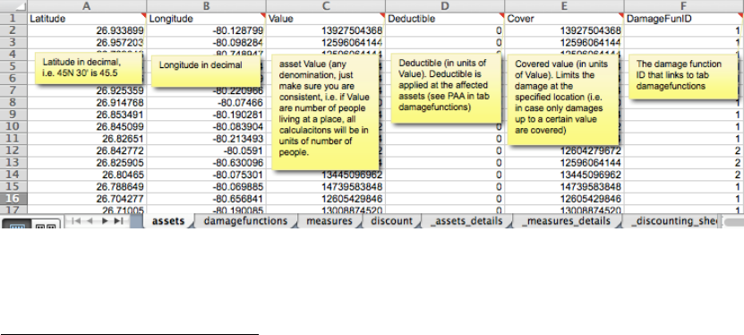
The tab 'assets' lists all exposed assets by location (Latitude/Longitude) and Value.
Please note that values do not necessarily need to be monetary values. E.g. in case
the number of exposed people is stated in the Value column, climada does calculate
the number of affected people (you will obviously use a damagefunction which
relates to people in this case). You can specify the unit of the Values in an additional
column labelled Value_unit, where you specify the unit for each Value entry, such as
‘USD’ or ‘people’ (best to start with only one value unit per Excel file, mixed use for
advanced users only). The column DamageFunID relates each asset to its
corresponding damage function (which is provided in tab damagefunctions).
Figure: the assets tab, see ../data/entities/entity_template.xls and display the comment for each field of
the header rows (only key columns showed here). Mandatory are only Latitude, Longitude, Value
and DamageFunID (if not provided, Deductible is set to zero and Cover is set to Value).
40
Since the content of the Excel file is imported (using climada_entity_read) into MATLAB, any
other source can be used to define the content of the entity structure of climada, too. In order to
understand the entity structure, it’s in fact easiest to import the file ../data/entities/entity_template.xls
using entity=climada_entity_read and to inspect the resulting entity structure.
16
Note for advanced users: In addition to the columns visible in above figure (the essential ones, so to
say), one can add a column labelled Category_ID which allows later to select results based on a single
or a group of categories (see climada_viewer
41
). The column does contain just integer values i.e. 1
for category one which might e.g. be ‘Residential House’ and 2 for category ‘Commercial Building’. Such
names can be defined in the tab names (see the Excel template). Further, there can be a column
Region_ID, which allows to group assets into regions (if one runs a large set of assets, for example,
same rules as for Category_ID apply).
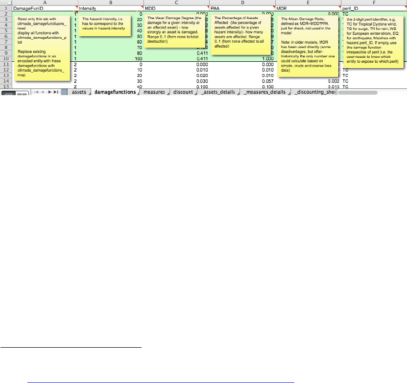
The tab 'damagefunctions' contains the relationship between the hazard intensity
(e.g. wind speed in m/s or storm surge height in meters) and the percentage of
affected assets (PAA) as well as the mean damage degree (MDD). What's called a
damage function in climada is elsewhere often also referred to as 'vulnerability
curve'. If for say a storm surge height of 1 meter, 50% of all assets are affected, and
the damage to these affected assets is 5% of their total value, the PAA is 0.5 and
MDD 0.05. In the case of value signifying exposed population, PAA is used to reflect
affected individuals, while MDD could be used to parameterize some sort of impact to
the affected individuals (e.g. using disability or quality adjusted life years,
DALY/QALY
42
). The DamageFunID is used to relate to the corresponding assets and
peril_ID to indicate for which peril/hazard the function shall apply. Please note that
there can be a damage function with DamageFunID equal to 1 for more than one
peril, say ‘TC’ and ‘EQ’. This way, one can run the same assets for more than one
hazard.
Figure: the damagefunctions tab, see ../data/entities/entity_template.xls. Mandatory fields are
DamageFunID, Intensity, MDD, PAA and peril_ID. MDR (=MDD*PAA) is ignored, just in the Excel
sheet for information.
Additional (optional) columns in the damagefunctions tab are Intensity_unit to specify
the unit of the intensity (for each entry, such as ‘m/s’) and name, a free name, eg.
'TC default'.
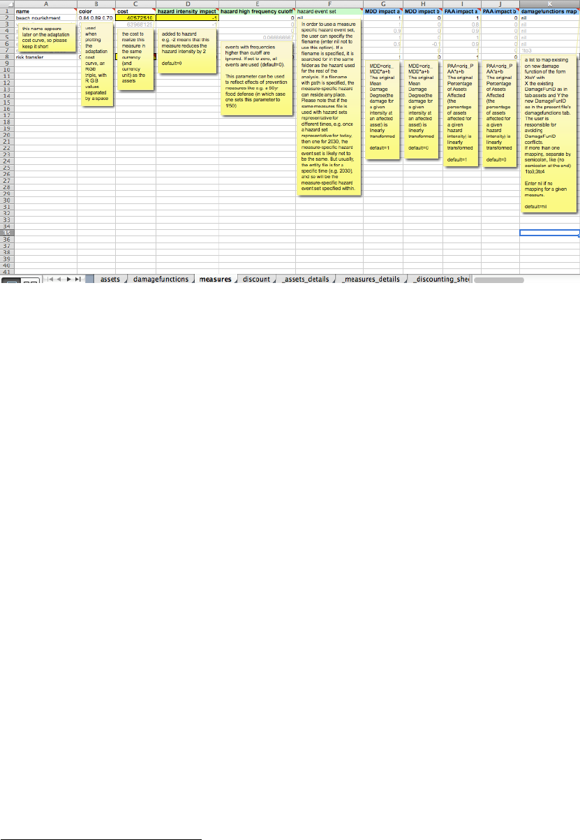
The tab 'measures' contains the list of climate adaptation measures
43
. It contains the
costs of the measures, i.e. the net present value of CAPEX and OPEX for each
measure. It also contains the parameterized impact of the measures on the hazard
and damage function. Imagine a coastal study region and say a mangrove forest.
Outside of climada, is has been calculated that the net present cost of this measure
amounts to 1'234'567 USD. Let's assume this mangrove forest slows down the wind
of a tropical cyclone by a certain amount, say 5 percent reduction in wind speed.
Both the cost as well as this 'parameterized' impact is hence entered in the
'measures' tab for this particular measure, cost goes into the cost column (obviously)
and the 5% windspeed reduction by putting 0.95 into the column
hazard_intensity_impact_a, since the resulting hazard intensity equals the original
hazard intensity times hazard_intensity_impact_a (plus hazard_intensity_impact_b,
41
But first make yourself familiar with climada as described on the following pages, as this result viewer
is rather for advanced use.
42
See http://www.iac.ethz.ch/edu/courses/master/modules/climate-risk.html (about lecture 9) for a
discussion of measures such as DALY and QALY.
43
note that for pure damage calculations (climada_EDS_calc), this information is not needed, i.e. one
can provide an entity Excel file with just the tabs assets and damagefunctions.
17
set to zero by default, or simply i=iorig*a+b). Note that climada can handle
parameterized impacts of higher complexity, too (please refer to the comments for
each column in the Excel template).
Figure: the measures tab, see ../data/entities/entity_template.xls. Mandatory fields are name, cost
and MDD_Impact_a and MDD_impact_b.
The (optional) tab ‘names’ contains
44
some speaking names for fields in other tabs
that are IDs, such as Category_ID and Region_ID. It just provides a name to be
shown e.g.in GUIs. There is a special use to communicate the reference year also
via this tab: If there is an entry reference_year in the Item column, a 0 in the ID
column and the reference year as a string in the name column, this value is stored
into the entity.assets.reference_year (otherwise, the default reference year
is used, see climada_init_vars). For ADVANCED users, the names tab also
allows to define global variables, such as the encoding distance, the default currency
or even folders such as hazards_dir etc., which are originally defined in
climada_init_vars (see section “Writing your own code” further below) but can
easily be redefined this way
45
.
Please note again that each column header in the Excel contains a detailed
explanation as a comment. The reference Excel sheet, called entity_template.xls can
be found in the entities sub-folder of the climada data folder
46
.
Note: If you use climada as an end-user (i.e. not developing anything, just to
‘process’ your Excel input and produce the waterfall and adaptation cost curve), the
simple call climada prompts the user to select the entity Excel file for today and in
the future as well as the hazard set for today and future, then runs all calculations
and shows the final adaptation cost curve. On subsequent calls, the routine suggests
last inputs - and if the first file selection is the same as on previous call, even asks to
re-run with previous call's inputs without asking for confirmation. This way, one can
edit the entity Excel file and then just call climada again.
44
See ../data/entities/entity_template.xlsx (there exists a .xls version for backward compatibility)
45
See See ../data/entities/entity_template_ADVANCED.xlsx, but please be aware of the impacts (as
one can re-define reference years etc. this way).
46
../data/entities/entity_template.xls

18
A note on coordinates: climada works best with standard geographical coordinates
47
(longitude -180..180, latitude -90..90). Please see climada_dateline_resolve to
resolve issues around the dateline (e.g. Fiji, where it is advisable to center the
coordinate system either somewhat left or right of the dateline in order to avoid
troubles with distance calculations).
A note on Excel and Open Office file formats and their tolerance in
MATLAB and Octave
Instead of .xls or .xlsx (use .xls 95 or 97 with MATLAB before R2015, and .xlsx with
latest MATLAB and Octave), climada also supports .ods (Open Office). If using .ods,
please avoid any cell comments, also see “Notes on Octave” further below. Please
do not use field format ‘Percentage’ in Open Office, but just ‘General’ or ‘Number’,
such that e.g. the discount_rate on tab discount is 0.02, not plain ‘2%’ in the .ods file
(2% works fine in .xls and .xlsx files). Please note further that starting Octave might
be easiest in a shell (terminal window), with path, e.g.
/Applications/Octave.app/Contents/Resources/usr/bin/octave
Constructing your own entity
A user might want to construct an entity from scratch, i.e. not import assets,
damagefunctions (and measures) from an Excel (or OpenOffice) file, but from any
other source (or define all in a MATLAB code file). In this case, it is advisable to first
familiarize with the Excel template (see above) to know the mandatory and optional
fields.
There are two options, once can either start from the entity template
48
, or really from
scratch:
▪ If one starts from the template, replace fields with your content, please make
sure all fields have the same final length (i.e. if you define 150 assets, i.e.
enter them in entity.assets.lon, entity.assets.lat,
entity.assets.Value, make sure all other fields in entity.assets are
of dimension 1x150).
▪ If one starts from scratch, populate the mandatory fields, see the comments in
the Excel template and the header section of climada_entity_read. Make
sure all fields in assets, damagefunction etc. have the same (corresponding)
length.
Once you defined your entity, please
▪ run climada_assets_complete, climada_damagefunctions_complete and
(if you define measures) climada_measures_complete to check entity
components for completeness.
▪ run entity.assets=climada_assets_encode(entity.assets) in
order to encode to a hazard.
▪ consider to run measures=climada_measures_encode(measures) in
order encode measures (i.e. convert some fields to machine-readable format
(i.e. if you populated entity.measures.damagefunctions_map, this fills
in entity.measures.damagefunctions_mapping
49
).
47
but one could use it on any other topology, as encoding does merely find nearest neighbours etc.
48
See ../data/entities/entity_template.xlsx (there exists a .xls version for backward compatibility)
49
This is the field used in climada_measures_impact (not entity.measures.damagefunctions_map)
19
Finally, test your entity by calling climada_EDS_calc and, if you defined measures,
also climada_measures_impact and carefully observe any warnings/errors
50
.
From tropical cyclone hazard generation to the adaptation
cost curve
51
In this section, we are going to illustrate the whole process step-by-step, using
tropical cyclone as the hazard and a few assets in South Florida for illustration
purposes. Note already here that climada provides global coverage for tropical
cyclone wind (often referred to as TC wind
52
) and storm surge (often referred to as
TC surge
53
) as well as other hazards, such as global earthquake
54
– see “climada
modules” section further below. For a comprehensive list of climada functions, please
refer to ../docs/code_overview.html
Instead of starting with a simple hazard set generation, the user might also jump to
the damage calculation right away, skip section “Hazard set” below and jump to the
second next section "Assets and damage functions". Please note that due to slower
processing speed of some explicit loops in Octave, the demo differs somewhat from
the MATLAB version as documented below (also with respect to certain graphics
features).
Hazard set
First, obtain the historic tracks
55
, i.e. define the name and location of the raw text file
with historical tropical cyclone tracks
56
global climada_global % to get access to climada_global
57
tc_track_file=[climada_global.data_dir filesep ...
'tc_tracks' filesep 'tracks.atl.txt'];
tc_track=climada_tc_read_unisys_database(tc_track_file,2);
% same as
58
tc_track=climada_tc_read_unisys_database('tracks.atl.txt',2);
Why 2 as last input? See help climada_tc_read_unisys_database and check the
description of the 2nd input parameter (it forces re-reading the database each time).
Let’s have a look at the output:
50
If you get really stuck, consider contacting the climada developers…
51
See the climada code climada_demo_step_by_step which performs all the steps and illustrates
the intermediate results by plots, just as shown here. Run climada_demo_step_by_step in debug
mode to follow (and understand ;-) each step.
52
Part of climada core module (i.e. the module this manual is part of)
53
Obtain it from https://github.com/davidnbresch/climada_module_tropical_cyclone and see the
manual(s) there.
54
See https://github.com/davidnbresch/climada_module_earthquake_volcano
55
See the function climada_tc_get_unisys_databases to automatically download all databases
from the internet (from weather.unisys.com/hurricane).
56
Note that the filename is defined using climada_global.data_dir in ordert to be machine and
file-system independent.
57
No need to look into this now, the structure climada_global just provides some machine and file-
system independent parameters. Later on, the advanced user might study the section about
climada_init_vars and climada_global further below.
58
Since most climada functions assume the default data (sub) folder if only the name (without path) is
passed.
20
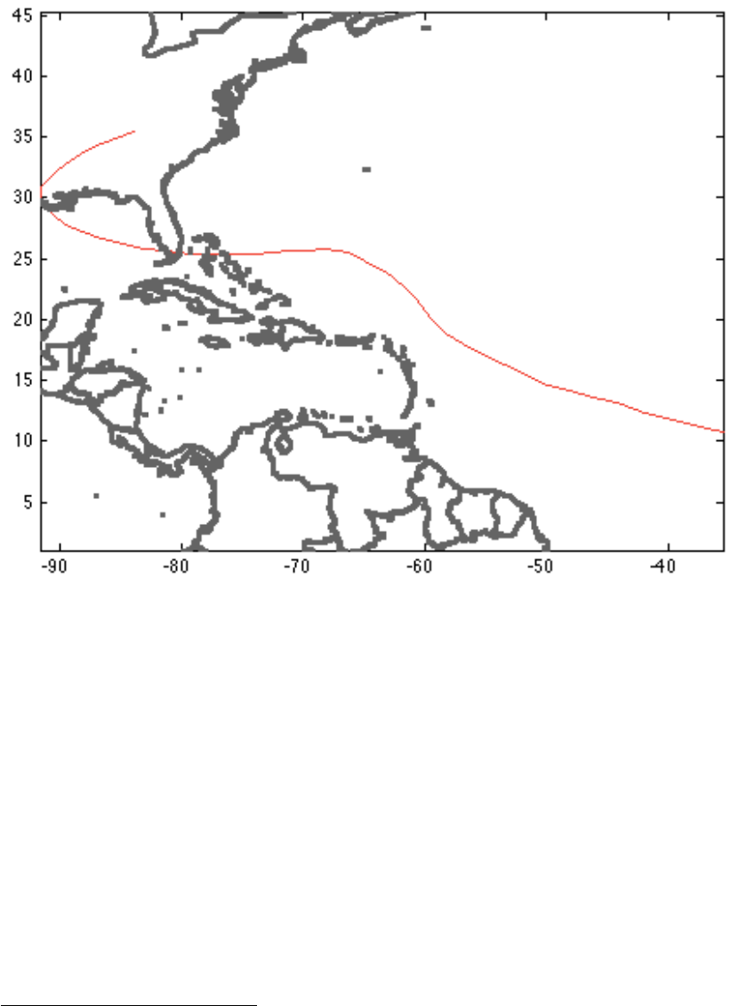
tc_track(i) contains position tc_track(i).lon(j) and
tc_track(i).lat(j) for each timestep j as well as the corresponding intensity
tc_track(i).MaxSustainedWind. E.g. track number 1170 is hurricane Andrew:
Figure: plot(tc_track(1170).lon,tc_track(1170).lat,'-r'); hold on;
set(gcf,'Color',[1 1 1]); axis equal
climada_plot_world_borders(2,'','',1) % plot world borders (for orientation)
In order to calculate the windfield of this particular single track, we first generate a
series of points on which to evaluate the windfield, we call these points centroids
59
:
centroids.lon=[];centroids.lat=[]; % init
next_centroid=1; % ugly code, but explicit for demonstration
for i=1:10
for j=1:10
centroids.lon(next_centroid)=i+(-85);
centroids.lat(next_centroid)=j+ 20;
next_centroid=next_centroid+1;
end % j
end % i
centroids.centroid_ID=1:length(centroids.lat);
Next, calculate the windfield
60
for a single track (Andrew again) as
59
Centroids are stored in a special folder ../data/centroids, see e.g. climada_centroids_read.
Please note that most routines requiring centroids are tolerant in the sense to also accept an entity
instead (where the assets with their coordinates are). See further below, just keep this in mind.
60
We implement a windfield according to Holland, G. J., 1980: An analytic model of the wind and
pressure profiles in hurricanes. Monthly Weather Review, 108, 1212-1218. In addition to the
axisymmetric vortex, we take forward speed into account. See also Holland, G. J., 2008: A Revised
Hurricane Pressure–Wind Model, Monthly Weather Review, 136, 3432-3445. A natural next step would
21
gust = climada_tc_windfield(climada_tc_equal_timestep(tc_track(1170)),centroids);
Figure: Gust wind field (in m/s) of Andrew, 1992:
climada_color_plot(gust,centroids.lon,centroids.lat)Note that without
climada_tc_equal_timestep in the call climada_tc_windfield above, we would not get a continuous
footprint due the fast forward speed of Andrew (try this by omitting climada_tc_equal_timestep in the
calculation of gust. Please consider some advice on appropriate colour schemes
61
.
We now generate the wind field not for one single hurricane, but for all events and
store them in an organized way, the so-called hazard event set:
hazard = climada_tc_hazard_set(tc_track,'atl_hist',centroids);
This hazard event set now contains the single Andrew wind field we generated
before in hazard.intensity(1170,:) and therefore we can reproduce the same
wind field with the following command (note the full(*), as we store a sparse matrix)
climada_color_plot(full(hazard.intensity(1170,:)),...
hazard.lon,hazard.lat,'none')
be the consideration of roughness (not implemented), see e.g. Vickery, P.J. et al., 2009: A Hurricane
Boundary Layer and Wind Field Model for Use in Engineering Applications. J. Appl. Meteor. Clim.
61
http://colorbrewer2.org and
http://www.personal.psu.edu/faculty/c/a/cab38/ColorBrewer/ColorBrewer_updates.html
22
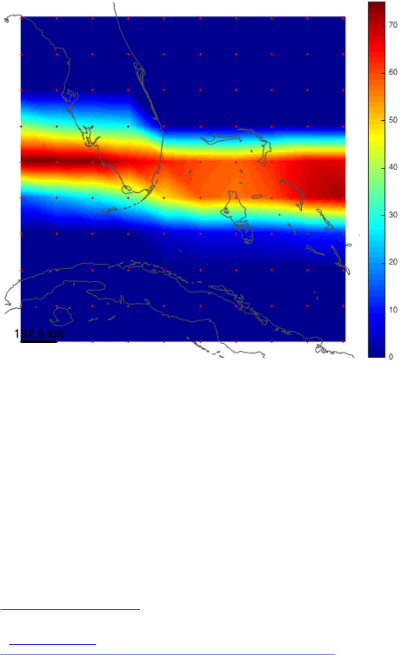
Or, instead, we can plot all hazard intensities at a given point (green circle
62
) like
Figure: figure; subplot(2,1,1) % only lower part shown here
climada_color_plot(full(hazard.intensity(1170,:)),...
hazard.lon,hazard.lat,'none'); hold on; plot(-81,26,'Og');
plot(centroids.lon(36),centroids.lat(36),'Og','MarkerSize',10);
subplot(2,1,2)
plot(full(hazard.intensity(:,36))); set(gcf,'Color',[1 1 1]);
xlabel(sprintf('storm number, years
%i..%i',tc_track(1).yyyy(1),tc_track(end).yyyy(end)))
ylabel('Intensity [m/s]')
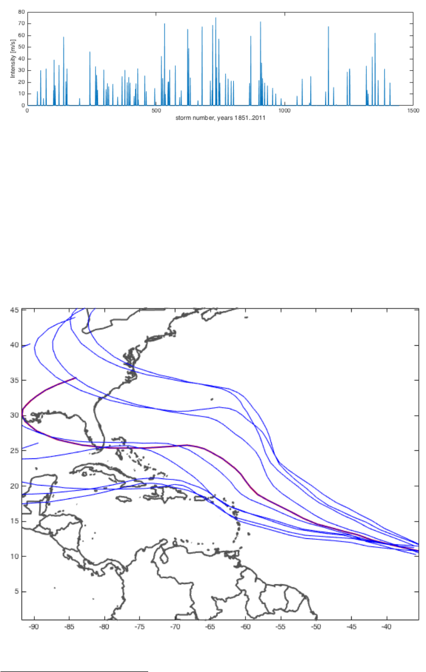
Instead of only historic tracks, we can generate artificial or probabilistic tracks, simply
by 'wiggling' the original tracks, e.g. for Andrew 1992 again:
tc_track_prob=climada_tc_random_walk(tc_track(1170));
Figure: plot(tc_track(1170).lon,tc_track(1170).lat,'-r','LineWidth',2);
hold on; set(gcf,'Color',[1 1 1]); axis equal
62
Not shown here in the figure, but in the upper part of the figure when created in MATLAB.
23
climada_plot_world_borders(2,'','',1)
for track_i=1:length(tc_track_prob)
plot(tc_track_prob(track_i).lon,tc_track_prob(track_i).lat,'-b');
end
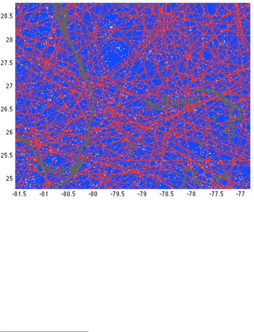
And repeated for all historic tracks, we obtain the full probabilistic track set
climada_global.waitbar=0; % switch waitbar off, speeds up
% hence the next line will take approx. 3 sec
tc_track_prob=climada_tc_random_walk(tc_track);
Figure (manually zoomed in, Southern tip of Florida):
for track_i=1:length(tc_track_prob)
plot(tc_track_prob(track_i).lon,tc_track_prob(track_i).lat,'-b');
hold on;end
for track_i=1:length(tc_track)
plot(tc_track(track_i).lon,tc_track(track_i).lat,'-r');end
climada_plot_world_borders(2,'','',1); set(gcf,'Color',[1 1 1]);
Note: Instead of this explicit code, consider climada_tc_info to print track information (name,
date....) to stdout and to show (nice) plots of historic (and probabilistic) tracks.
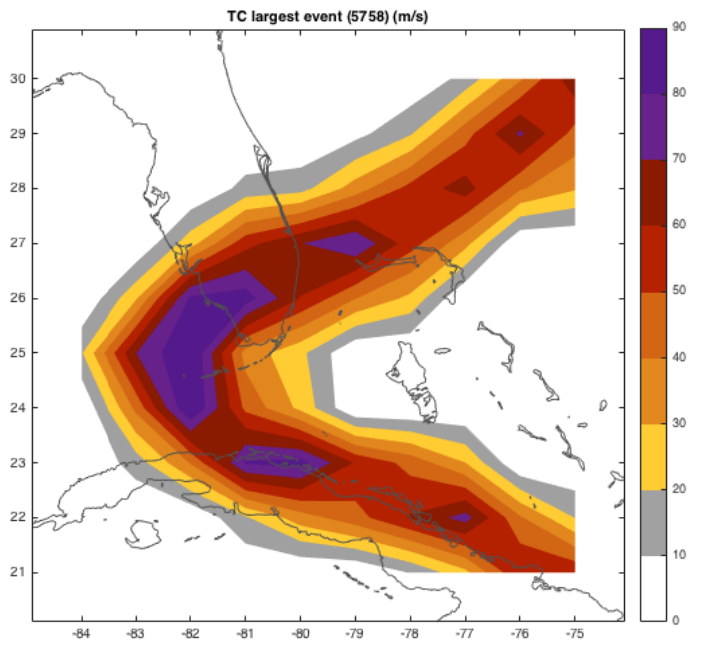
Next, we generate the wind fields for all 14’450 probabilistic tracks (takes a bit less
than 2 min on a MacBook Air
63
)
hazard=climada_tc_hazard_set(tc_track_prob,'atl_prob.mat',centroids);
63
Consider to set climada_global.parfor=1 before calling climada_tc_hazard_set . This invokes
parallel processing (parallel pool, using parfor).
24
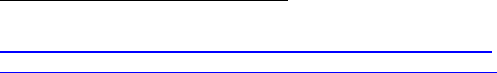
The hazard set now contains more than ten thousand (in fact 14’450) tropical cyclone
footprints, each stored at all centroids. We can for example plot the largest single
event with:
figure; climada_hazard_plot(hazard);
and generate the wind speed maps for several return periods:
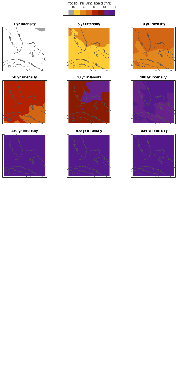
25
Figure: climada_hazard_stats(hazard);
Before we move on, let’s explain the key elements of the hazard structure:
hazard.lon(i) and hazard.lat(i) contain the coordinates of centroid i, hence
hazard.intensity(j,i) contains the hazard intensity of event j at centroid i.
Further hazard.frequency(j) contains the single event frequency of event j.
These are in fact the key elements of the hazard structure; note that
hazard.intensity is a sparse array (refer to e.g. help sparse in MATLAB
64
).
You might refer to functions such as the mentioned climada_tc_hazard_set or
climada_excel_hazard_set
65
to see how a hazard event set is generated.
64
In essence, a sparse array stores the non-zero elements of an array only. Since a single event hits
only a few centroids – especially true for a hazard set covering a larger geographical region – we save a
lot of memory and speed up the calculations substantially.
65
This function generates a hazard event set based on Excel input. The Excel sheet needs to contain all
the event footprints. An easy method to use climada with a finite (small) number of predefined events
(more hazard event scenarios then a full probabilistic set). See file ../data/hazards/ Excel_hazard.xls
which contains a small example (for Mozambique).
26
Assets and damage functions
So much for the hazard event set, let’s now import an asset base (the small
asset example as used in climada_demo, the demonstration GUI as shown
above
66
). Before we do so, we load the hazard set file as used in
climada_demo, in order to later reproduce the results:
hazard=climada_hazard_load('TCNA_today_small.mat')
and are now in a position to import the Excel file with all the asset
information
67
:
entity=climada_entity_read('demo_today.xls',hazard) % note
68
Such an entity structure contains the asset, damage function and adaptation
measures information, the tabs in Excel are named accordingly, and so are
the elements of the imported structure
69
. In the asset sub-structure, we find
70
entity.assets.lat(k) and entity.assets.lon(k), the geographical
position of asset k (does not need to be the same geographic location as
centroid i, since assets are encoded to the hazard
71
)
entity.assets.Value(k) contains the Value of asset k. Please note that
Value can be a value of any kind, not necessarily a monetary one, e.g. it could
be number of people living in a given place.
entity.assets.DamageFunID(k) contains a reference ID (integer) to link
the specific asset with the corresponding damage function (see Excel tab
damagefunctions and entity.damagefunctions). Before we move on the
the damagefunctions, note that entity.assets.centroid_index(k)
contains the centroid index onto which asset k is mapped in the hazard event
set
72
.
66
One can also generate assets (value distributions) in climada, see e.g. the climada module
https://github.com/davidnbresch/climada_module_GDP_entity or
https://github.com/davidnbresch/climada_module_country_risk . Please note that the two column names
Latitude and Longitude are shortened to lat and lon in climada’s entity.assets structure – not least to
ease typing on the command line, e.g. plot(entity.assets.lon,entity.assets.lat)
67
Please have a look at the Excel file, each column header is explained by a small comment (tiny yellow
triangel in the upper right corner of the cell). Please consider (later) to use e.g.
climada_entity_country to generate a basic entity for any country worldwide (at 10 km resolution).
68
Please note that climada_entity_read stores a .mat file of the imported entity structure to speed
up re-reading. But in case you edit the original (.xls or similar) file, climada re-reads from the latest
version (i.e. overwrites the .mat file). This check is performed by climada_check_matfile, which
might be useful to the advanced (programming) user.
69
Please note that we discuss the measures information further below
70
We focus on the key content here, please inspect the structure in MATLAB yourself.
71
See function climada_assets_encode. Encoding means: map asset positions to calculation
centroids of the hazard event set. This step is required to allow the user to freely specify asset locations,
rather than stick to the centroids the hazard set has been stored at. A beginner-level user should not
need to deal with such technical details, though. See also the remark about encoding in the section
“Process on one page” above.
72
As mentioned in a previous footnote, the beginner level user does not need worry too much about,
this simply speeds up damage calculation substantially. See code climada_assets_encode_check
to (visually) check the encoding.
27
figure;climada_entity_plot(entity,4);% The asset distribution as stored in entity (read from
Excel sheet)
The damagefunctions sub-structure contains all damage function information,
i.e. entity.damagefunctions.DamageFunID contains the IDs which
refers to the asset’s DamageFunID. This way, we can provide different
damage functions for different (groups or sets of) assets.
entity.damagefunctions.Intensity contains the hazard intensity,
entity.damagefunctions.MDD the mean damage degree and
entity.damagefunctions.PAA the percentage of affected assets. Last
but not least, entity.damagefunctions.peril_ID contains the peril ID
(2-digit character) which allows to identify specific damage functions with
perils. This way, we can in fact use DamageFunID 1 in the assets to link to
damage function one, which can exist several times, one for each peril. The
damagefunctions are stored in a bit a special format, since we get the first
damagefunction as
73
pos=find(entity.damagefunctions.DamageFunID==...
entity.damagefunctions.DamageFunID(1))
plot(entity.damagefunctions.Intensity(pos),...
entity.damagefunctions.MDD(pos)) % not shown, see next figure
73
In the case there is only one perilID, see further details in climada_damagefunctions_plot
28
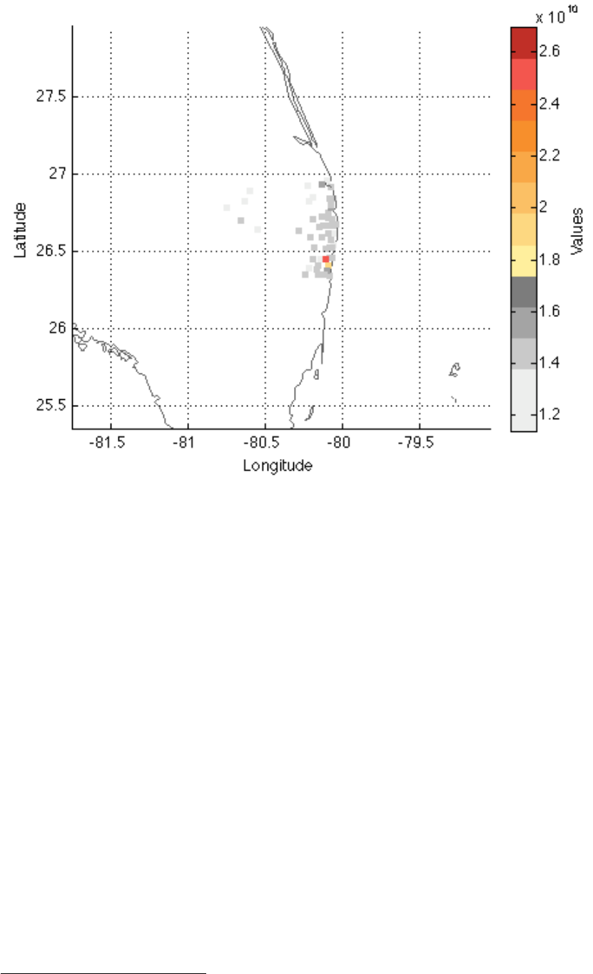
figure;climada_damagefunctions_plot(entity);% The three damage functions as defined in
the damagefunctions tab of the Excel file. TC is the peril ID and stands for tropical cyclone, while 001,
002 and 003 denote the DamageFunID. The horizontal axis denotes the hazard intensity (here tropical
cyclone windspeed, in m/s), the vertical axis is the same for MDD, PAA and MDR.
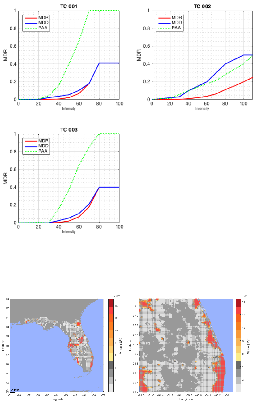
Note: Please consider using climada_nightlight_entity, which allows you to
generate an asset base on 10x10km or 1x1km resolution for any country of the
world.
Fig: 10x10km (left) and 1x1km (right, zoomed in) default asset distribution for Florida. Generated with
entity=climada_nightlight_entity(‘USA’,’Florida’); climada_entity_plot(entity)
29
Damage calculation
And with that, we’re ready for the damage calculation, simply as:
EDS=climada_EDS_calc(entity,hazard)
Where EDS contains the event damage set, it contains the annual expected damage
in EDS.ED, the event damage for event j in EDS.damage(j), the event frequency in
EDS.frequency(j) and the event ID in EDS.event_ID(j). In further fields it
stores the link to the original assets, the damagefunctions and hazard set used.
Instead of plotting the event damage set (here a vector with 14’450 elements), one
rather refers to the damage exceedance frequency curve (DFC)
74
:
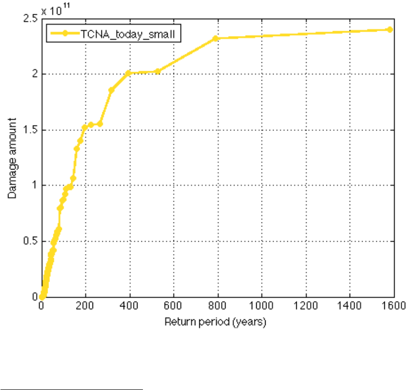
figure; climada_EDS_DFC(EDS); % show damage exceedance frequency (DEF) curve
The horizontal axis denotes the return period in years, the vertical axis the damage (in units the Values
were provided, here USD). The label of the curve denotes the hazard set used.
74
The damage (exceedance) frequency curve (DFC) is an annual per-occurrence damage exceedance
frequency curve, showing the return period of a certain damage level to be reached or exceeded for a
given return period. A DFC is constructed by sorting a per-occurrence damage event set (as shown for
historic events in Fig 2) by descending damage amount and assigning the corresponding return periods,
as given by the temporal extent of the damage event set. If the damage event set spans say 100 years
and contains for example only three damaging events of amounts a, b and c, with a>b>c, the largest
damage reached or exceed only once in these 100 years is a, while a damage level of b is reached or
exceeded twice in these 100 years, hence the return period for a damage level of b is 50 years, and c is
reached and/or exceeded three times, hence its return period is 33.3.. years.
Further, see e.g. McNeil, A.J., R. Frey, and P. Embrechts, Quantitative risk management: concepts,
techniques and tools. Vol. Revis. 2005, Princeton, N.J: Princeton Univ Press. and also Rice, J.A.,
Mathematical statistics and data analysis. Vol. 3rd. 2007, Belmont, CA: Thomson/Brooks/Cole.

30
While one would in a proper application of climada now calculate the damages of
future assets (to obtain the effect f economic growth) and then further repeat the
calculation with a future hazard set (to obtain the effect of climate change), we
illustrate the benefit of adaptation measures by simply using the assets and hazard
we have already used.
But before we do so, one remark about uncertainty – the first time reader shall either
skip or at least not spend time with the following short section. But since I’ve got so
many questions about dealing with uncertainty, I decided to cover the bare essentials
early on.
Dealing with uncertainty
In climada, we follow ‘measurement theory of probability’
75
and do not assume any
prior or suggest a possibly inappropriate approach
76
. The user is responsible for ANY
uncertainty calculation, as this way, he is in full control of the drivers (and
sensitivities). If user therefore might decide to quantify the effect of uncertainty
around damage functions, he would specify the distribution explicitly and just run his
own uncertainty assessment (from a simple trial to e.g. full Monte-Carlo approach).
Since all damage calculations a re easy to call functions, it is very easy to write a
small script that ‘samples’ e.g. several damage functions and runs the respective
statistics on the results, in the bare essence this could look something like:
Assume we have an entity with assets and damagefunctions and a hazard ready (as
at this stage the case), hence can just run the damage calculation with some
samples
77
around the original damage function:
sample_multiplier=[.7 .8 .9 1.1 1.2 1.3];
entity_orig=entity; % copy
EDS=climada_EDS_calc(entity,hazard); % the 'default' and to init EDS
for sample_i=1:length(sample_multiplier)
entity.damagefunctions.MDD= ...
entity_orig.damagefunctions.MDD*sample_multiplier(sample_i);
EDS(end+1)=climada_EDS_calc(entity,hazard);
end % sample_i
Since the annual expected damage (just to take one risk measure) is within each
EDS structure, to run some stats, we convert to an array (note that the first element
in ED is the default run, followed by the samples), e.g.
ED=[];for i=1:length(EDS),ED(end+1)=EDS(i).ED;end
And with that, one can run any statistics like mean(ED),std(ED)
Or, if one would like to run statistics on e.g. the 100 year return period damage,
simply convert the EDS into a DFC (that’s the elegance of it ;-):
75
See e.g. https://www.countbayesie.com/blog/2015/8/30/picture-guide-to-probability-spaces
76
e.g. one could (relatively easily) implement a beta-distribution on the damage uncertainty, but some
damage might be bound by an upper limit.
77
We use multipliers here to keep the code snippet simplest. But one could switch to another set of
damage functions or consider non-linear transformations, such as MDD=MDD.^2 or =MDD.^1/2 or …
(just in the e.g. MDD or PAA case make sure max(MDD) or max(PAA) do not exceed 1, e.g. use
MDD=min(MDD,1), unless you want that). One will very likely also ‘wiggle’ other parameters, such as
hazard intensity (start with simple tests such as e.g. hazard.intensity= hazard.intensity*.95).

31
DFC=climada_EDS2DFC(EDS,100); % calculate 100 year damage
damage_100=[];for i=1:length(EDS),damage_100(end+1)=DFC(i).damage;end
mean(damage_100),std(damage_100)
See also the visualization of uncertainty in the next section (climada_cost_curve)
Adaptation cost curve
As mentioned, the entity structure contains not only assets and damagefunctions, it
also holds the adaptation measures
78
. entity.measures.name{m} contains the
name of measure m, entity.measures.cost(m) the cost
79
. The following fields
allow the parameterization of the measure’s impact on both the hazard as well as the
damage function. entity.measures.hazard_intensity_impact(m) allows to
reduce the hazard intensity (e.g. -1 reduces tropical cyclone windspeed by 1 m/s) for
measure m. The hazard_high_frequency_cutoff
80
allows to specify a
frequency below which damages are suppressed due to the measures, e.g. the
construction/design level of a dam (hazard_high_frequency_cutoff=1/50
means the dam prevents damages up to the 50 year return period).
hazard_event_set allows to specify a measure-specific hazard event set, i.e. for
this particular measure, climada switches to the specified hazard event set instead of
the one used to assess the damages of the reference case. MDD_impact_a and
MDD_impact_b allow a linear transformation of the MDD (mean damage degree) of
the damage function, such that MDDeff = MDD_impact_a + MDD_impact_b * MDD.
Similarly, PAAeff = PAA_impact_a + PAA_impact_b * PAA.
damagefunctions_map allows to map to a new damage function to render the
effect of measure m, i.e. ‘1to3’ means instead of DamageFunID 1, DamageFunID 3
is used
81
. risk_transfer_attachement and risk_transfer_cover define the
attachement point and cover of a risk transfer layer
82
.
The simple call
measures_impact=climada_measures_impact(entity,hazard,'no');
does it all, e.g. it takes the entity and first calculates the EDSref using hazard in order
to create the baseline (situation with no measure applied). It then takes measure m
(m=1…), adjusts either hazard and/or damagefunctions according to the measure’s
specification and calculates a new EDSm. The difference to EDSref (i.e. EDSm-EDSref)
quantifies the benefit (averted damage) of measure m. By doing this on the event
damage set, a variety of measures can be compared, even account for measures
which for example only act on high frequency events (see
hazard_high_frequency_cutoff) or risk transfer layers (see
risk_transfer_attachement and risk_transfer_cover). This function
further handles all the measure impact discounting etc.
83
78
Please refer to the measures tab in the Excel file and the comments in each of the header fields.
79
entity.measures.color{m} contains the color (RGB) as shown in the adaptation cost curve of measure
m. colorRGB contains this converted into an RGB triple.
80
We do not repeat entity.measures.X(m) any more, just refer to X.
81
The filed entity.measures.damagefunctions_mapping contains the details, i.e. the mapping as used in
climada, a kind of ‘parsed’ version of e.g. ‘1to3’.
82
Please refer the tot he lecture, www.iac.ethz.ch/edu/courses/master/modules/climate_risk
83
See function climada_NPV
32
Since it would be quite cumbersome for the user to manually construct the adaptation
cost curve based on the detailed output provided by climada_measures_impact,
the following function
84
does it all:
climada_cost_curve(measures_impact)
Figure: the adaptation cost curve, see text for details.
the code does allow to show more than one result, to visualize uncertainties
85
:
Figure: the adaptation cost curve, for one set of measures under different assumptions (see dealing with
uncertainty above).
84
The legacy code is climada_adaptation_cost_curve, please use climada_cost_curve.
Difference being the ability of climada_cost_curve to plot n sets of measures, where
climada_adaptation_cost_curve could only handle two and has some other limitations.
85
The climada_cost_curve simply takes measures_impact as an array of structures, see its header.
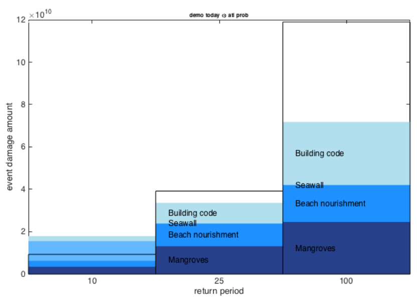
33
and finally, the effect of adaptation measures on different return periods:
climada_adaptation_event_view(measures_impact)
Figure: the effect of adaptation measures on return periods of 10, 25 and 100 years. Note that the 10-
year event can be fully mitigated by proposed measures, about 70% of the 50-year and about half of the
100-year event.
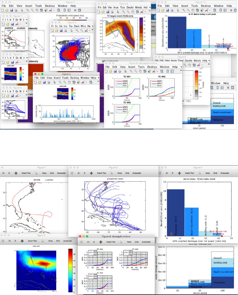
34
Figure: all output figures from climada_demo_step_by_step on one screen (resized) in order to
allow for an easy check whether your local installation of climada does produce the correct output.
Please note that exact figures and single numbers might be slightly different (say values differing +/-
10%) due to the use of a random number generator in the probabilistic track set and potentially later
versions of the historical tropical cyclone database – plus advancement of the climada engine itself.
Figure: as above, but for Octave in order to allow for an easy check whether your local installation of
climada does produce the correct output (numbers might change).
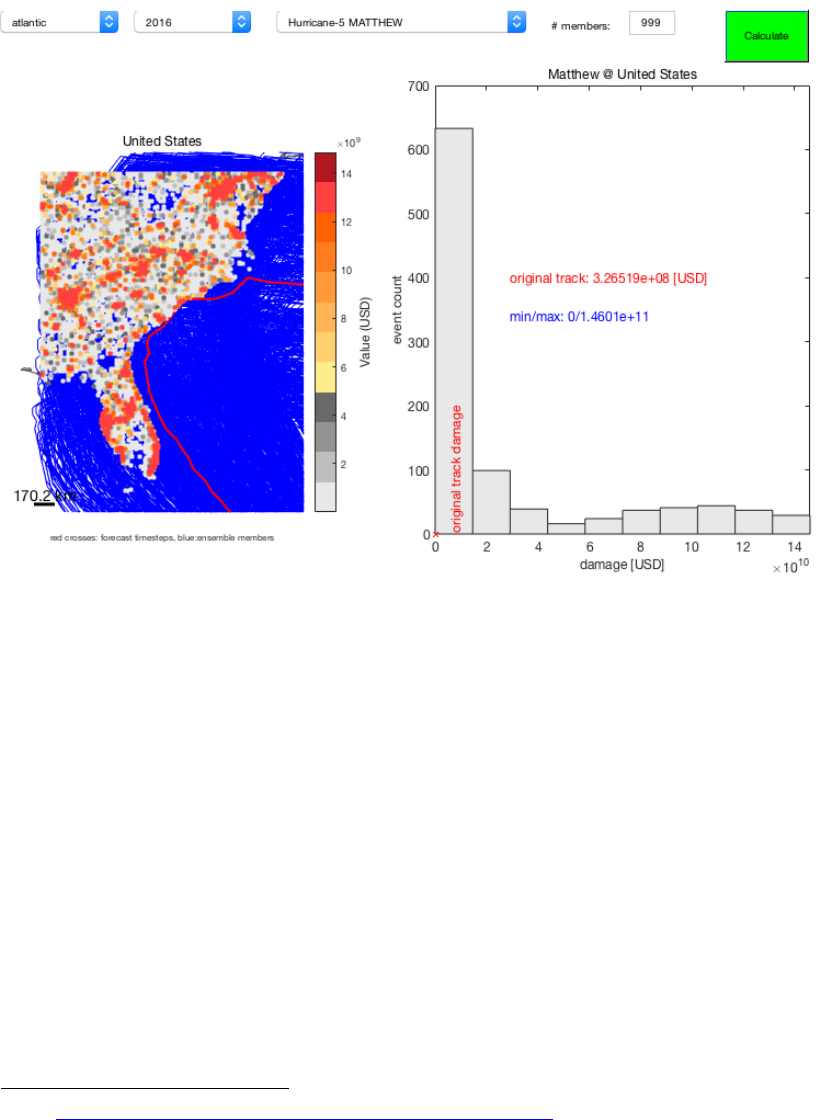
35
A climada application example – tropical cyclone ensemble
damage forecasts
At this stage, you might consider to look into a climada ‘application’, i.e. a GUI (or for
Octave, a command-line tool) which allows to calculate (forecast) damage for tropical
cyclones, both for the forecast track as well as for an ensemble of probabilistic
tracks, all around the globe (MATLAB GUI: climada_tc_guess, Octave and
MATLAB command line: climada_tc_event_damage_ens). Note that it does
require the country_risk module
86
.
Figure: The climada_tc_guess GUI, here shown for Matthew hitting the United States.
86
See https://github.com/davidnbresch/climada_module_country_risk

36
Function reference
This section makes reference to key climada functions in order to provide the user
with a starting point – the function are provided in a somewhat logical order, i.e. one
would usually use functions listed further down later in the process. Please refer to
each function’s detailed header (use help functionname in MATLAB). You might
also run compile_all_function_headers once in order to generate a .html file
with all function headers for fast reference
87
.
climada_demo: the demo GUI as documented above
climada_demo_step_by_step: the step-by-step demo as documented above
Basic entity functions
climada_entity_country: generate the entity (asset base) for any given country
climada_entity_read: read entity from Excel file
climada_entity_load: load a previously saved entity (climada_entity_read saves
a .mat file – which speeds up subsequent read, unless the original Excel file has been
changed, in which case it is re-read and the .mat file overwritten, see
climada_check_matfile)
climada_entity_save: save an entity (i.e. after modification in MATLAB)
climada_entity_country: generate a basic entity for any country worldwide
climada_damagefunctions_read: read damagefunctions tab only
climada_measures_read: read measures tab only
climada_measures_encode: encode measures, i.e. interpret them for use in
climada_measures_impact
climada_dateline_resolve: resolve issues around dateline
climada_{assets|damagefunctuons|measures}_complete: a handy function to
check for completeness of the respective sub-structure of an entity (e.g. if edited in
command line)
climada_entity_plot: plot assets distribution of an entity (entity.assets)
climada_entity_value_GDP_adjust: scale total asset value to GDP*blowup
climada_assets_encode: encode assets (i.e. to switch to another hazard event
set
88
)
climada_assets_encode_check: check encoding, plot asset locations and centroids
climada_damagefunctions_plot: plot damagefunctions
climada_damagefunctions_map: map damagefunctions (i.e. to another entity
89
)
climada_damagefunction_replace: replace a damage function
climada_damagefunction_generate: generate generically shaped damage
function, then use climada_damagefunction_replace.
Core calculations
climada_EDS_calc: calculate event damage set (EDS)
87
The file ../climada/docs/code_overview.html does contain the headers of all functions of all modules
(and the links to the source code); hence you might consult this file (e.g. use full text search within) and
might need to install the respective module in order to use the specific function.
88
climada_entity_read prompts for a hazard event set and hence encodes to the selected hazard’s
centroids already. For speedup, this is done prior to calling climada_EDS_calc, as mapping all asset
locations to the centroids oft he hazard event set usually does not need to be repeated each time (e.g.
only once for the series of calculations involved in assessment of adaptation measures). In case multiple
hazards (perils) are assessed, re-encoding is required indeed (that’s why climada measures impact
works for one hazard at a time only – this code does indeed checl for encoding).
89
This is especially useful if the user stores all damage functions in a kind of ‚reference’ file and
attaches the damage functions after reading any new entity, which might itself not contain (all) damage
functions (in this case, just disregard the warnings issues by climada_entity_read).

37
climada_EDS_stats: some statistics of an EDS
climada_EDS_save: save EDS
climada_EDS_load: load EDS
climada_EDS_DFC: plot damage frequency curve(s)
climada_damage_exceedence: the damage exceedance calculation
climada_EDS_DFC_report: write an Excel or .csv report of the DFC(s)
climada_EDS2DFC: just convert an EDS to a DFC as a structure, do not plot (for that,
see climada_EDS_DFC).
climada_waterfall_graph: plot the waterfall graph (with the elements risk today,
economic, climate)
climada_measures_impact: calculate the impact of adaptation measures
climada_NPV: net present value (NPV) calculation
climada_adaptation_cost_curve: show the adaptation cost curve
climada_adaptation_event_view: the event view on adaptation measures
climada_EDS2YDS: convert an event (per occurrence) damage set (EDS) into a
year damage set (YDS).
climada_EDS_combine: Combine two (or more) event damage sets (EDS), e.g.
add damages of TC and TS (same main peril) or EDS for global EQ across
several countries.
Basic hazard functions
climada_hazards: generate all standard hazard sets for any given entity
climada_hazard_plot: plot hazard events, max intensity etc.
climada_hazard_load: load hazard event set
climada_hazard_stats: plot hazard intensity return period maps
climada_hazard_check: show hazard intensity histogram, useful to compare two
hazard sets in general.
climada_excel_hazard_set: create a hazard set based on scenarios as
provided in an Excel file, see ../data/hazards/Excel_hazard.xls
climada_hazard_cleanup: cleanup a hazard event set (check for internal
consistency)
climada_hazard_clim_scen: create a climate scenario version of a hazard event
set
climada_IFC_plot: plot intensity/frequency relationship at centroid (needs
climada_hazard2IFC)
climada_asci2hazard: import hazard data from en external modeling tool
Further display functions
climada_plot_world_borders: plot world borders
90
climada_circle_plot: plot any values at coordinates as circles
climada_color_plot: plot any values at coordinates as colored area
climada_DFC_compare: compare a damage frequency curve (DFC) with other
model output
climada_event_damage_animation: create animation (a movie, such as .mp4)
of hazard and damage calculation. See also climada_event_damage_data_tc
climada_event_damage_data_tc: prepare tropical cyclone hazard, assets,
damage and cyclone track data to be rendered as an animation using
climada_event_damage_animation
90
Uses ../data/system/admin0.mat for the border shapes, see the file admin0.txt there and also
climada_shaperead('SYSTEM_ADMIN0'). The user can specify an other shape file, either as
parameter or in climada_global.map_border_file
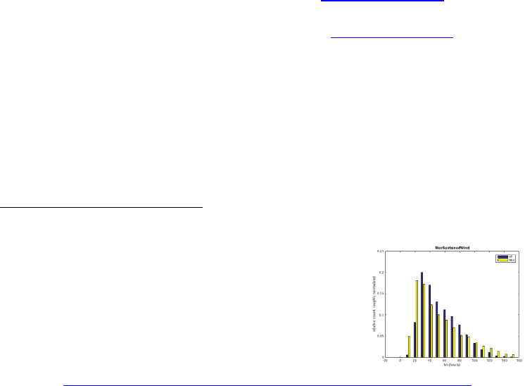
38
Tropical cyclone (TC) specific functions
91
climada_tc_get_unisys_databases: get all TC (besttrack) databases from
www. Please note that the windspeed measurement is not the same across the
globe, there are substantial differences e.g. between North Atlantic and West
Pacific
92
, such that the template damage function shall only be used with (utmost)
caution.
climada_tc_read_unisys_database: read (besttrack) data
climada_tc_random_walk: generate probabilistic tracks
climada_tc_windfield: generate the windfield for one TC event
climada_tc_hazard_set: generate a TC hazard event set (and yearset)
climada_tc_windfield_animation: animate a single TC track’s windfield
climada_plot_ACE: plot accumulated cyclone energy (ACE)
climada_tc_stormcategory: add Saffir-Simpson scale
93
climada_tc_read_unisys_track: read a single track (see also
climada_tc_read_unisys_database above)
Basic functions
climada_xlsread: read Excel file
climada_odsread: read .ods (Open Office) file, see also climada_init_vars to set
this as default
climada_shaperead: read shape file (does require MATLAB mapping toolbox)
climada_centroids_read and climada_centroids_load: read and load
centroids
climada_centroids_plot: plot centroids
climada_hazard2octave: deal with hazard saved with option –v7.3 in Octave
Admin functions
climada_git_pull: on a machine with GIT (https://github.com) installed, update
all local code and data (much faster than using GIT Desktop)
climada_git_clone: on a machine with GIT (https://github.com) installed, clone
most climada modules (much faster than using GIT Desktop)
climada_code_copy: (old, use climada_git_pull whenever possible!) copy all
code into a folder for easy transfer
climada_code_update: update local code based on the file provided by climada_code_copy
compile_all_function_headers: generate a html file with headers of all
functions (these headers explain all input and output of each function). You find
this file in ../docs/code_overview.html
climada_template: the function template to start new code from
91
Please note that we decided to use the TC hazard to illustrate core climada and some select features.
Please refer to the climada modules (next section)for other hazards with similar functionality.
92
A direct comparison of the historic storms’ windspeeds reveals:
93
See e.g. http://en.wikipedia.org/wiki/Saffir%E2%80%93Simpson_Hurricane_Scale
39
climada_country_name: get country name and admin0 ISO3 code, see also
../data/system/admin0.txt and admin.xls
climada_init_vars: init global varables (called upon startup
94
by startup)
climada_octave: called by climada_init_vars to init if operating on Octave
climada_init_folders: init folder structure (useful when creating a new module)
startup: the startup function, sets root folder and manages MATLAB path
95
climada_check_matfile: check whether the .mat (binary, fast access) version of
a file is older than the (Excel) file, used e.g. in climada_entity_read, which
reads the .mat file on second call, unless the Excel entity file has been edited.
Special functions (there are more)
climada_code_optimizer: remove some parts from core code (like
climada_EDS_calc) for speedup (only for expert use)
climada_distance_km: calculate distance between points in km
climada_nonspheric_distance_m: more precise distance in m
climada_collect_measures_impact: collect impact files for two hazards
created by climada_measures_impact (sometimes handy to process some
measures separately)
waitbar_toggle: toggle waitbars (on/off), see also climada_global.waitbar
climada_lonlat_cleanup: migrate entity.assets.Longitude to
entity.assets.lon …
climada_dateline_resolve: resolve issues around dateline
CLIMADA modules
While the core CLIMADA provides the user with the core probabilistic damage
calculation and climate adaptation measures assessment functionalities, it only
contains a simple tropical cyclone hazard. Therefore, there are climada extensions,
called modules, to add functionality. Since the core climada only contains a simple
tropical cyclone hazard, one of the first modules to be considered might be
tropical_cyclone, which improves the quality of the tropical cyclone hazard event set.
There exist modules for other perils (to generate or make use of other hazards, such
as storm_europe, flood and earthquake_volcano) and for other functionality, like
automatic generation of assets (country_risk). Each module contains (similar to core
climada) a code, data and docs folder, with a detailed documentation in the file
{module_name}.pdf in the docs folder. Therefore, one might first inspect these files
still on GitHub before downloading a specific module
96
. Please note that core climate
runs without restrictions under both MATLAB and Octave, but some modules might
not have been extensively tested in Octave – or might even require MATLAB libraries
(would be stated in the respective module’s manual).
advanced
https://github.com/davidnbresch/climada_advanced
This module provides advanced functionality, such as multi-hazard processing
and management of sets of measures. It does also contain the interface to ktools
97
,
94
Does also check for operating system being MATLAB or Octave (in the latter case also calling
climada_octave)
95
Adds paths to all climada modules
96
Please refer to the section ‚Getting started’ above about where to store the module(s). The process is
also described in each module’s readme file.
97
to run on a cluster (such as Euler at ETH) with tools installed, you need to set export
PATH=$PATH:/cluster/apps/climate/ktools/bin

40
the loss calculation engine of Oasis LMF (http://www.oasislmf.org/the-toolkit). See
module tropical_cyclone (below) for more realistic tropical cyclone wind fields (inland
decay) etc.
tropical_cyclone
https://github.com/davidnbresch/climada_module_tropical_cyclone
This module implements the tropical cyclone (TC) attenuation after landfall for
probabilistic events and allows to generate the precipitation fields accompanying a
tropical cyclone - the torrential rain (TR) hazard event set - as well as the associated
storm surge (TS) events. Make yourself familiar with the core climada tropical
cyclone hazard event set (and its generation) first. A good implementation of both the
basic, probabilistic and advanced tropical cyclone hazard generation (including TC,
TS, and TR) can be found in the climada module country_risk and there in the routine
centroids_generate_hazard_sets.
storm_europe
https://github.com/davidnbresch/climada_module_storm_europe
This climada module contains the basic European winter storm (WS) hazard event
sets
98
from 2010, an interface to the MeteoSwiss COSMO model output and further
code related to European winter storms.
country_risk
https://github.com/davidnbresch/climada_module_country_risk
This module runs all (available) perils for one country (or list of countries). It
generates country or admin1 (state/province) assets (consisting of centroids, used
later e.g. to generate a hazard event set of matching resolution and assets – if
requested scaled to the country GDP or proxy asset value for today and future), the
earthquake (EQ), tropical cyclone (TC), torrential rain (TR) and storm surge (TS)
hazard event sets, checks for European winter storm (WS) exposure and runs all risk
calculations for a given country. Note: this module contains also the former
GDP_entity module.
isimip
https://github.com/davidnbresch/climada_module_isimip
This module implements isimip-specific functionality (a community-driven climate-
impacts modelling initiative, see www.isimip.org, and the climada page within at:
www.isimip.org/impactmodels/details/243). It allows climada to connect to and work
from isimip datasets, e.g. assets, hazards and damage functions.
earthquake_volcano
https://github.com/davidnbresch/climada_module_earthquake_volcano
This module implements a raw global earthquake (EQ) and volcano (VQ) model.
Consider climada modules country_risk or GDP_entity to generate the centroids.
elevation_models
https://github.com/davidnbresch/climada_module_elevation_models
This module implements ETOPO, a global bathymetry (and topography) dataset. It’s
a separate module, since topographic (and bathymetry) information can be used in
various contexts – and since the dataset is quite large (ETOPO1 is 933 MB,
ETOPO2 still 233 MB).
98
Schwierz, C., P. Köllner-Heck, E. Zenklusen Mutter, D. N. Bresch, P.-L.Vidale, M. Wild, C., and
Schär, 2010: Modelling European winter wind storm losses in current and future climate. Climatic
Change (2010) 101:485?514, doi: 10.1007/s10584-009-9712-1.

41
meteorite
https://github.com/davidnbresch/climada_module_meteorite
This module implements a basic meteorite global hazard. Consider climada modules
country_risk or GDP_entity to generate the centroids.
flood
https://github.com/davidnbresch/climada_module_flood
Implements a first (simple) flood model (FL) and a landslide model. The flood model
is in early stage and very much still work in progress (contributions welcome!).
barisal_demo and salvador_demo
https://github.com/davidnbresch/climada_module_barisal_demo and
https://github.com/davidnbresch/climada_module_salvador_demo
Barisal, Bangladesh, and San Salvador demo module, all numbers and results are
for demonstration purposes only.
kml_toolbox
https://github.com/davidnbresch/climada_module_kml_toolbox
To write kml files, e.g. to visualize asset distribution and hazard/damage animations
in Google Earth.
octave_io_fix
https://github.com/davidnbresch/Octave_io_fix
Provides a crude fix for this issue by providing Octave io (e.g. read .xls, .xlsx and
.ods files) as a climada module instead of a proper Octave package. This climada
module contains the CRUDE work-around for cases where the Octave package io-
2.2.6.tar cannot be installed by using pkg. Tested on Mac Air, under OS X Yosemite,
Version 10.10.1 (computer in Octave returns x86_64-apple-darwin13.0.0) and
Octave version 3.8.0. Note that the issue did not occur on Mac Air with OS X version
10.9.5 and not any more with OS X (El Capitan) version 10.11.13 (computer in
Octave returns x86_64-apple-darwin13.0.0).
Programmer’s hint: in order to access data stored in other modules, you first need to
figure the actual path of that module. To use the etopo netCDF file directly, you
would find it at e.g.
etopo_data_file=[fileparts(fileparts(which('etopo_elevation_m'))) ...
filesep 'data' filesep 'ETOPO1.nc']
Some hints to useful data sources
We do mention key sources in the respective climada modules, but some data we
came across is worth mentioning in more general terms.
• http://www.naturalearthdata.com and directly
http://www.naturalearthdata.com/downloads: global shape files (see e.g.
climada_shaperead and the module country_risk). One will likely need the
MATLAB mapping toolbox to ease working with these files. Could be used to
either improve hazard sets (e.g. using location of reefs in surge model…) or
assets.
• http://download.geofabrik.de: highly detailed shape files for most countries
(e.g. more than 1.5 mio shapes of building’s outlines in Switzerland). Could
be used in conjunction with climada module country_risk to further refine the
42
asset base. See also http://www.openstreetmap.org/about,
https://mapzen.com and http://planet.openstreetmap.org
• Also www.diva-gis.org/gdata and www.diva-gis.org/Data for GIS data almost
any country
99
and also www.eea.europa.eu/data-and-maps/data/urban-atlas
• GIS data for Seychelles https://www.webgis.gov.sc/map_default.phtml
• SRTM elevation data (3-arc seconds resolution ~90m)
http://srtm.csi.cgiar.org/SELECTION/inputCoord.asp and generally
http://srtm.csi.cgiar.org
• Hydrosheds, based on SRTM, manipulated for river routing
http://hydrosheds.cr.usgs.gov/index.php
• http://www.geoportal.org/web/guest/geo_home_stp
• https://www.drought.gov/drought/content/products-current-drought-and-
monitoring-drought-indicators/palmer-drought-severity-index
• http://beta.sedac.ciesin.columbia.edu/data/collection/gpw-v4/sets/browse
population density, water bodies, admin center points with population
estimates (http://beta.sedac.ciesin.columbia.edu/data/set/gpw-v4-admin-unit-
center-points-population-estimates)
• https://search.earthdata.nasa.gov earth data search
• https://datahub.io/ open data sets of various kinds
• http://databank.worldbank.org/data/home.aspx macroeconomic data
• http://databank.worldbank.org/data/reports.aspx?source=subnational-
population sub-national population (admin1)
• http://www.trademap.org/Index.aspx trade statistics
• http://www.cger.nies.go.jp/gcp/population-and-gdp.html population and GDP
• http://data.footprintnetwork.org global country-level data on footprint etc.
• https://hazards.fema.gov/femaportal/wps/portal/NFHLWMSkmzdownload
FEMA, US
• http://www.nws.noaa.gov/gis/shapepage.htm NOAA shape files (mainly US)
• http://www.mapcruzin.com/free-netherlands-arcgis-maps-shapefiles.htm NLD
shape files, http://www.mapcruzin.com/do-it-yourself-gis-maps-shapefiles/
mainly US and http://www.mapcruzin.com/free-world-country-arcgis-maps-
shapefiles.htm global
• http://floodobservatory.colorado.edu floods
• https://freegisdata.rtwilson.com good global overview of free GIS data
• https://www.census.gov/geo/maps-data/data/cbf/cbf_msa.html US census
• https://data.oecd.org/gdp/real-gdp-forecast.htm OECD GDP past and future
• http://colorbrewer2.org good color scales to print well etc.
• http://www.reefbase.org global coral reef data, good preview via
http://www.reefbase.org/gis_maps/default.aspx
• http://datadryad.org/resource/doi:10.5061/dryad.dk1j0 Gridded global
datasets for GDP and Human Development Index over 1990-2015
Models
• http://www.hrc-lab.org Hydrologic Research Center, (local) flood model
Writing your own code
While climada does provide quite a range of functionality, the advanced user will
soon feel the need or even desire to start developing its own code. It is strongly
advised to start from the template
100
, since this code (fragment) does provide access
99
See also e.g. http://data.geocomm.com/catalog
100
../code/climada_template.m

43
to the climada global variables
101
and provides the standard function header
102
.
Please do take the time to keep the function header always up to date – upon first
use, this looks a bit like over-engineering, but as soon as one would like to share
code, it becomes a requirement. The template code further exemplifies the usual file
dialog and the standard use of waitbar in a for-loop (and the progress update to
stdout in case of waitbar suppressed
103
).
It is always a good idea to browse existing code as a place to start from – most likely
code such as climada_tc_hazard_set, climada_EDS_calc or
climada_EDS_DFC come to one’s mind, but also code in modules such as
country_risk_calc in moduel country_risk or tc_surge_hazard_create in
module tropical_cyclone.
Since climada is designed to provide utmost flexibility and (recursive) use of
functionality, please write any code such that all parameters have reasonable default
values (often defined either in the argument check or in the PARAMETERS section of
each function) and that every function can be run from command line, with any GUI
(like file dialog) only popping up in case not all function parameters are defined upon
call. Only exceptions are proper GUI’s, such as climada_demo.
Instead of adding code to climada core, it is highly recommended to start a new
module, as code development can much easier be managed this way. Just create a
new folder in the modules folder
104
and sub-folders code
105
, data and docs, as you
find it in all other modules. This way, your code folder gets automatically added to the
path upon next startup. This approach also eases later upload of your code as an
additional climada module in GitHub
106
.
climada_init_vars
Since the code climada_init_vars is sourced at startup and defines some core
global variables, it is worth briefly mentioning the most important ones, as the
programmer shall always make use of in order to keep the code machine and file-
system independent etc.
First, some paths are set
107
:
• climada_global.root_dir: the folder where all climada resides, there
should be no need for climada to access folders ‘above’ this level. This is
figured by startup.m
• climada_global.data_dir: the main data folder, either within climada
(../climada/data) or on the same level as climada (../climada_data, i.e.
{climada_global.root_dir}/ climada_data). The advanced user can set
101
See also climada_init_vars and the global variable climada_global
102
Use of the standard header is recommended, even required, as the code which generates he
overview of all climada functions (see compile_all_function_headers) does parse all headers of
all functions.
103
i.e. if climada_global.waitbar=0
104
Best to create a folder climada_modules parallel to the core climada folder (i.e. ion the same level -
in the same parent folder - as core climada). It is also possible to put it as ../climada/modules, but not
recommended.
105
Please note that a code folder can have ONE level of sub-folders to better organize your code.
startup does add these sub-folders tot he MATLAB path, too.
106
See https://help.github.com/articles/create-a-repo/
107
Please ONLY use filesep and never any explicit file separator, since ‚/’ or ‚\’ etc. depend on the file
system – and climada shall be independent of any file system.

44
this folder to any place for a specific project, i.e. to store one project’s entities
and hazards at a specific place
108
. Such a user might keep
climada_global.system_dir unchanged, as system files are very
unlikely to be project-specific.
• climada_global.system_dir: usually a sub-folder of
climada_global.data_dir with the key system files (such as
admin0.mat, coastline.mat…)
• climada_global.centroids_dir: usually a sub-folder of
climada_global.data_dir with the centroid files.
• climada_global.entities_dir: usually a sub-folder of
climada_global.data_dir with the entity files.
• climada_global.hazards_dir: usually a sub-folder of
climada_global.data_dir with the hazard files.
• climada_global.results_dir: usually a sub-folder of
climada_global.data_dir with the results.
Some key files are defined:
• climada_global.map_border_file: the map border file as used by
climada_plot_world_borders, see the short documentation in
{climada_global.system_dir}/admin0.txt and see also
109
climada_shaperead(‘SYSTEM_ADMIN0’)
• climada_global.coastline_file: the global coastline file, as used by
climada_distance2coast_km (see the short documentation in
{climada_global.system_dir}/coastline.txt) and see also
climada_shaperead(‘SYSTEM_COASTLINE’)
• climada_global.csv_delimiter: the country- and machine-specific .csv
delimiter (to read and convert to Excel properly)
• climada_global.spreadsheet_ext: the default spreadsheet type, either
'.xls' (default) or '.ods'. The user can always select from 'All Files', the default
is only used to compose the default filename.
Evaluation and NPV (net present value) specific parameters:
• climada_global.present_reference_year: the reference year for
‘today’
• climada_global.future_reference_year: the reference year for
‘future’
• climada_global.impact_time_dependence: time dependence of
impacts (1 for linear, default). >1 concave (e.g. 2: cubic), <1 for convex (e.g.
1/2: like square root). Concave means: damage increases slowly first (see
climada_measures_impact)
And further:
• climada_global.DFC_return_periods: Standard return periods for
DFC report
• climada_global.waitbar: whether we show waitbars for progress (e.g. in
climada_EDS_calc).
108
In case you do so, please make sure you call climada_init_vars(3), wich sets
climada_global.centroids_dir, climada_global.entities_dir,
climada_global.hazards_dir, climada_global.results_dir accordingly (i.e. relative to
(subfolders of) climada_global.data_dir). This call (with option 3) does NOT change
climada_global.system_dir and climada_global.tc_tracks.
109
Requires country_risk module https://github.com/davidnbresch/climada_module_country_risk

45
• climada_global.EDS_at_centroid: whether we store the damage (=1)
at each centroid for each event (an EDS for each centroid). Heavy memory,
see climada_EDS_calc; therefore: default=0. Please note that
EDS.ED_at_centroid is always calculated (only a vector length number of
centroids)
• climada_global.re_check_encoding: whether the code checks for
(possible) asset encoding issues and re-encodes in case of doubt (might take
time...). See climada_EDS_calc (and also its input parameter
force_re_encode).
climada startup
The file startup.m
110
is sourced at startup (see Getting started above) and mainly
defines the root folder (using pwd) and locates all installed climada modules and
adds their code folders
111
to the MATLAB path. In case the advanced user would like
to have other variables etc. defined at startup, one might write a separate
my_startup.m
112
which first calls startup. Editing startup.m is not
recommended, as this will fork compared to the climada repository.
Description of key climada structures
The detailed descriptions are of most use once the advanced user is familiar with
concepts and process as described in ‘From tropical cyclone hazard generation to
the adaptation cost curve’ above.
The entity structure contains assets, damage functions and measures, as described
in ‘Excel interface to climada’ above. Fields in the data structures have the exact
same name as the column headers
113
in the Excel interface – and entity contains a
sub-structure for each tab (i.e. assets, damagefunctions, measures and discount).
Therefore, we do not repeat the detailed description here, please inspect the
comment fields in the excel file. A few additional fields warrant some comments:
• entity.assets.DamageFunID(asset_i): links to the corresponding
damage function, see entity.damagefunctions.DamageFunID. Please
consider usage of climada_damagefunctions_map to map to another set
of damagefunctions, i.e. in the case you store your (reference) damage
functions in one Excel (using climada_damagefunctions_read, or even
just a MATLAB structure) and hence will call this mapping after import of the
assets into climada.
• entity.assets.distance2coast_km(asset_i): the distance to coast
in km, as added by climada_distance2coast_km, e.g. in case the entity
has been produced by climada_nightlight_entity
114
.
110
It resides at the root level, usually ../climada/startup.m
111
and two levels of sub-folders within each module’s code folder. This way, real ‘helper’ functions can
be put in a sub-folder to keep the main code folder(s) easier to inspect
112
Or any other name...
113
Only exception are Latitude and Longitude, which are named lat and lon in climada (i.e. get renamed
upon import from Excel). For backward compatibility, one column is still named „hazard intensity
impact“, but the MATLAB internal name is hazard_intensity_impact_b, since the hazard
transformation in measures is analog to MDD and PAA, i.e. intensity=intensityorig*a+b, wich b the value
from hazard_intensity_impact_b. Therefore, the user can also add a colunm named „hazard
intensity impact a“ which multiplies the hazard intensity.
114
See climada module country_risk, https://github.com/davidnbresch/climada_module_country_risk.

46
• entity.assets.elevation_m(asset_i): the elevation of asset_i, as
added by etopo_elevation_m
115
.
• entity.assets.centroid_index(asset_i): the centroid index of the
centroid nearest to asset_i in a hazard event set. See the function
climada_assets_encode to (re)encode to a (new) hazard event set. See
also climada_global.re_check_encoding (described above in ‘climada
startup’) to force (re)encoding. You can also simple delete this field to force
re-encoding, e.g. entity.assets=rmfield(entity.assets,
’centroid_index’).
• entity.assets.Values(year_i,asset_i): the asset value for year i.
entity.assets.Value does contain entity.assets.Values(1,:),
hence the user needs to ‘shuffle’ other times (usually years) into Value before
e.g. passing to climada_EDS_calc, see entity.assets.Values_yyyy.
• entity.assets.Values_yyyy(year_i): the year the assets are valid
for.
The hazard structure contains a hazard event set. While some key features have
been introduced in ‘From tropical cyclone hazard generation to the adaptation cost
curve’ above, we provide more details here (fields in italic are not mandatory, i.e. the
user shall make use of isfield to check before referencing, the few bold fields are
the core fields the damage calculation is essentially based upon):
• hazard.intensity(event_j,centroid_i): the hazard intensity for
event_j at centroid_i. A sparse matrix, hence use full in some instances
(e.g. when using fprintf).
• hazard.fraction(event_j,centroid_i): the fraction (range 0..1,
default=1) of centroid_i affected by the event_j. A sparse matrix, hence use
full in some instances (e.g. when using fprintf). Set
hazard.fraction=spones(hazard.intensity)as default, as it only
makes sense to define fraction for non-zero elements of intensity.
• hazard.frequency(event_j): the single event occurrence frequency of
event_j
• hazard.lon(centroid_i) and hazard.lat(centroid_i): the
coordinates of centroid_i.
• hazard.reference_year: the year the hazard is representative for. This
information is used in climada_measures_impact to discount (future)
benefits of measures accordingly, i.e. if hazard.reference_year=2030,
all benefits occurring in 2030 are discounted back to NPV as of the today
(and today is defined in climada_global.present_reference_year).
• hazard.centroid_ID(centroid_i): the ID of centroid_i, currently not
much used, but might be helpful to match centroids without comparing lat/lon.
• hazard.orig_years: the number of original years the hazard set is based
on.
• hazard.orig_event_count: the number of original events the hazard set
is based on
To add this field to an existing entity, use entity.assets.distance2coast_km=
climada_distance2coast_km(entity.assets.lon,entity.assets.lat). We do not add
this information by default (e.g. in climada_entity_read) as it might take some time to calculate –
especially in case of thousands o fasset locations.
115
See climada module etopo, https://github.com/davidnbresch/climada_module_etopo. To add this field
to an existing entity, use
entity.assets.elevation_m=etopo_elevation(entity.assets.lon,entity.assets.lat)

47
• hazard.event_count: the number of events (original and probabilistic
combind) in the hazard set.
• hazard.event_ID(event_j): a unique ID for event_j, currently not much
used.
• hazard.orig_event_flag(event_j): =1 if event_j is an original (e.g.
historic) event, =0 for probabilistic events.
• hazard.yyyy(event_j): the year (4 digits) of event_j, for probabilistic
events, the same as the original event the probabilistic one is based upon.
Not all original data might have event dates, hence this field is not mandatory
(and anyway not used in any damage calculation).
• hazard.mm(event_j), hazard.dd(event_j), hazard.hh(event_j):
month, day and hour of the original event.
• hazard.nodetime_mat(event_j): the MATLAB date/time number, just
yyyy,mm,dd and hh converted into one number, see datenum and datestr.
• hazard.name{event_j}: a free name, e.g. name of the TC event
• hazard.matrix_density: the density of the sparse matrix
hazard.intensity. Just for information, not used.
• hazard.peril_ID: the peril ID, such as TC, TS, TR, WS, EQ, FL…
• hazard.filename: the filename of the hazard event set, should be the
same as the name (without path) of the .mat file
• hazard.orig_yearset: the year set, grouping original events into years. A
structure with fields
• hazard.orig_yearset(year_i).yyyy: the original year (4 digit)
• hazard.orig_yearset(year_i).event_count: the number of
events in this year
• hazard.orig_yearset(year_i).event_jndex: the vector of
event indices for all the original events in year_i, such that
hazard.orig_yearset(year_i).event_jndex(1) is event_j of
the first event in year_i, i.e. you can reference e.g.
hazard.intensity(hazard.orig_yearset(year_i).event_j
ndex(1),centroid_i) which contains the intensity of the first
event in year_i at centroid_i.
See climada_tc_hazard_set about how the yearset is constructed and
climada_EDS2YDS to convert an event (per occurrence) damage event set
(EDS) into a year damage set (YDS). Please note that the grouping of
probabilistic events is currently assumed to be sequential to the original
events, such that if the original event is at event_j, the probabilistic derived
events (sometimes also called daughters) are to be found at
event_j+1..event_j+ens_size, where ens_size is the number of
probabilistic events per original event (as in climada_tc_random_walk).
See climada_EDS2YDS for a proper use of such a yearset
116
.
• hazard.comment: a free comment. There might (an can) be additional fields
in a hazard event set – the user is pretty free to build on.
The link between the geographical resolution of the assets and the hazard is
provided by centroids (whose coordinates are stored in hazard.lon and hazard.lat,
116
In case events are NOT sorted as recommended, i.e. in the case a hazard set would first comprise
all historic events, followed by all probabilistic ones, the user hast wo options: either to re-arrange
events in hazard to comply with the order as required by yearset (highly recommened), or to define a
yearset also for each probabilistic year, then to set hazard.orig_event_count=
hazard.event_count and to ignore the warning issued by climada_EDS2YDS with repsect to orig
event flag etc.

48
too). But there are centroids stored separately to ease some applications. The
centroids structure only needs to contain the fields (optional ones in italic):
• centroid.centroid_ID(centroid_i): a unique ID for centroid_i
• centroid.lon(i) and centroids.lat(i) the coordinates of
centroid_i
• centroid.distance2coast_km(centroid_i): distance to coast in km,
added by climada_distance2coast_km or
climada_centroids_distance_to_coast
• centroid.onLand(centroid_i): whether centroid_i is on land (=1) or
not (=0). Added by some TC routines.
The event damage set (EDS) structure has also been briefly introduced in ‘climada
demo step by step’ above, here follow the details (as quite some fields are just
copied from the hazard event set, see descriptions above).
• EDS.frequency(event_j): the single event occurrence frequency of
event_j (just a copy of hazard.frequency(event_j).
• EDS.damage(event_j): the single event damage for event_j in units as
units of assets.
• EDS.ED: the annual expected damage, simply
EDS.damage*EDS.frequency’.
• EDS.Value: the total value of assets used in the damage calculation. Useful
to express damage as percentage of asset value.
• EDS.reference_year: the year the hazard is representative for, a copy of
hazard. reference_year, see description above.
• EDS.event_ID: a copy of hazard.event_ID
• EDS.orig_event_flag: a copy of hazard.orig_event_flag
• EDS.ED_at_centroid(centroid_i): the annual expected damage at
centroid_i. See EDS.assets.lon(centroid_i),
EDS.assets.lat(centroid_i) and
EDS.assets.Value(centroid_i) for the corresponding coordinate and
total asset value at centroid_i (again useful to express ED_at_centroid as
percentage of local asset value).
• EDS.hazard.filename: the filename of the hazard set used to calculate
EDS.damage.
• EDS.damagefunctions: either just with the field
EDS.damagefunctions.filename to point to the filename the damage
functions came from or a full damagefunctions structure (see
entity.damagefunctions).
• EDS.annotation_name: the annotation as used e.g. in
climada_EDS_DFC, usually a short version of the hazard event set name.
• EDS.comment: a free comment
The year damage set (YDS) structure sums damages up over years, especially
useful for perils with (quite) likely more than one event per year – or series of events,
such as tropical cyclones and European winter storms. See climada_EDS2YDS and
the comments with respect to hazard.orig_yearset above, too. In essence, a
DYS contains the same information as an EDS, just YDS.frequency(year_i)
=1/length(YDS.damage) for all years
117
and YDS.damage(year_i) the sum of
117
This way, one can use climada_EDS_DFC(YDS) to plot the annual frequency curve (instead of the
per-occurrence frequency curve for EDS).
49
damages for year_i. Likewise, YDS.orig_year_flag=1 if the year_i is an original
year and =0 otherwise.
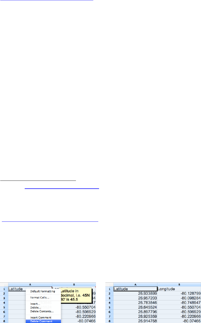
50
Notes on Octave (and OpenOffice)
climada has initially been developed in MATLAB and runs on both MATLAB (version
7
118
and higher) and GNU Octave (at least version 3.8.0, best 4.0.3 and higher, see
https://www.gnu.org/software/octave). Some modules might not have been
thoroughly tested using Octave, but core climada works without limitations
119
, except
for some figures being slow in creation and sometimes a bit limited in display
features. Core climada does not make use of any MATLAB toolboxes, but some
climada modules might do so (and this should be stated at the beginning of the
respective modules’ documentation) – hence note that Octave might not provide
similar toolboxes.
There is one distinct difference we observed during testing: While MATLAB on
machines without a full Excel COM environment (like a Mac with no Office installed)
works best with Excel 95 (or 97) .xls files, Octave seems to prefer .xlsx files.
Therefore, just open any Excel file which causes troubles upon import and save as
.xlsx to ease use with climada on Octave. Octave does not read all versions of .mat
files equally well. It looks as if there are some troubles with –v7.3 (hdf5), while
-v7 seems to work most of the time
120
.
Reading .ods (Open Office) spreadsheets works properly if you
• avoid cell comments
121
in tabs assets, damagefunctions, measures and
discount of the entity .ods file.
• Make sure the cell format for numbers is Number or General (but not e.g.
Percentage
122
) and that zeros show as ‘0’, not as ‘-‘.
We observed a few limitations with respect to plotting, complex plots like
climada_entity_plot (or usage of e.g. pcolor more generally) take very long
or even never complete. It looks as if Octave does not like the switch '-v7.3' in the
118
see e.g. ch.mathworks.com/products/matlab
119
In addition to core Octave, one needs the io package in order to import Excel files into climada.
Please install Octave’s io package directly from source forge with: pkg install -forge io -auto
In case this fails, get the io package first from Octave source forge and then install from the downloaded
package: pkg install {local_path}/io-2.2.5.tar –auto
In case this fails (e.g. troubles with pkg, consider the climada module fix Octave_io_fix
(https://github.com/davidnbresch/Octave_io_fix) which provides a crude fix for this issue by providing
Octave io as a climada module instead of a proper Octave package.
Note further that Octave (on Mac at least) properly reads .xlsx files, while MATLAB before version 9.x
preferred .xls (Excel 95 even). Therefore, if you mainly (or solely) use Octave, just open any non-.xlsx
file and save it as .xlsx in order to work properly in Octave.
120
There seems to be a size limit to save as –v7, hence MATLAB then switches to –v7.3 (with some
overhead). Therefore, you might have to split large .mat files (above about 250 MB, it seems). See the
variable climada_global.save_file_version, which is set to '–v7' for Octave, while '–v7.3'
for MATLAB. Hence, if you plan to read a .mat file generated by MATLAB, set
climada_global.save_file_version ='–v7' in MATLAB.
121
I.e. the comments that pop up if mouse over. To be on the safe side, select all cells and right-click on
cell A1, select Delete Comment:
122
Specifically, in the discount tab oft he entity file, use 0.02 and not 2%.

51
MATLAB save command
123
, hence use '-v7'. climada_EDS_calc checks for this
and throws an Error with the suggestion to save the hazard event set in MATLAB as
'–v7' again. On Mac computers, we observed that double-clikcing the Octave icon
might not work. In such cases use a shell and a command like
/Applications/Octave.app/Contents/Resources/usr/bin/octave & instead.
Appendices
The appendices contain detailed description of relevant aspects and shall provide the
advanced user with further information and especially serve those consider
expanding climada functionality.
climada, the inner workings
This section describes the core damage calculation. The damage is calculated for
each single asset at each location for each scenario or event, so basically
damage = asset value * damage function
where damage is summed up over assets and events, i.e. above line is at the core of
two loops, the outer one over assets, the inner one over events. More precisely:
damage = asset value * MDD * PAA, where
• MDD * PAA is the damage function
• damage is the damage ‘from ground up’, from the first dollar, so to speak
• asset value is the total value of the asset. Note again that value does not
need to a monetary value, it can also e.g. signify number of people at a given
location.
• MDD is the Mean Damage Degree (the damage for a given intensity at an
affected asset) - how strongly an asset is damaged. Range 0..1 (from none to
total destruction). In the case of asset value signifying number of people at a
given location, MDD represents the severity with which those people are
affected.
• PAA is the Percentage of Assets Affected (the percentage of assets affected
for a given hazard intensity) - how many assets are affected. Range 0..1
(from none affected to all affected). In the case of asset value signifying
number of people at a given location, PAA represents the percentage of
people affected. As the product MDD*PAA ultimately counts, the user shall
just make sure this product makes sense for the class of assets under
consideration.
So far, the hazard intensity did not show up in the calculation, did we miss
something? Well, the damage is a function of the hazard intensity, hence:
MDD = f(hazard intensity)
PAA = f(hazard intensity, hazard fraction)
where hazard intensity is the hazard's intensity at each asset for each event and
fraction the part of the centroid affected (i.e. if for one event fraction=.25, only a
123
Which saves a better compressed version and supports data items greater than or equal to 2GB on
64-bit systems.
52
quarter of the assets at the centroid are affected by this particular event). Since the
damage also depends on the asset type, we have in fact:
MDD = f(hazard intensity, asset type)
PAA = f(hazard intensity, asset type) * hazard fraction
While the hazard intensity is simply the entity.damagefunctions.Intensity,
the asset type is referred to by the DamageFunID, i.e. for a certain type of assets,
the user defines a specific DamageFunID in the assets tab and the corresponding
damage function (MDD and PAA as function of Intensity) in the damagefunctions
tab of the entity Excel file.
Implementation
The core calculation is done by climada_EDS_calc, where EDS stands for event
damage set, i.e. a vector with calculated damage for each event (or simply the vector
of event damages). The variables in the code have speaking names, but the inner
loop is vectorized, hence warrants some comments.
for asset_i=1:n_assets
temp_damage=entity.assets.Value(asset_i)*MDD.*PAA
end % asset_i
• temp_damage since it will be added in an ‘outer loop’ over asset_i
• entity.assets.Value(asset_i) is the Value of asset_i
entity is a structure which contains all asset and vulnerability data
• MDD is here a vector of MDDs, one element for each hazard event, PAA is the
vector or PAAs, also one element for each hazard event.
• .* is the element-wise (scalar) multiplication
So far, the hazard intensity did not show up in the calculation, did we miss
something? Well, the damage function is a function of the hazard intensity, hence:
MDD = f(hazard intensity) and PAA = f(hazard intensity)
where hazard intensity is the hazard intensity at asset_i for event_j, but event_j never
shows up in the code, since the code is vectorized along the event dimension for
performance reasons.
And now, it gets technical (no way around this, sorry, about line 170ff of
climada_EDS_calc) – how to get the vector of MDDs.
Remember: outer loop (explicit) over assets, inner loop (implicit) over events and
also remember that the hazard event set contains
• hazard.intensity(event_j,centroid_i): the hazard intensity (like
windspeed in m/s) at centroid_i for event_j
• hazard.fraction(event_j,centroid_i): the fraction (range 0..1,
defauklt=1) of centroid_i being affected for event_j
• hazard.frequency(event_j) contains the event-frequency for event_j
for asset_i=1:n_assets % approx line 270ff in climada_EDS_calc.m
% the index of the centroid for given asset in the hazard set
asset_hazard_pos=entity.assets.centroid_index(asset_i);

53
% find the vulnerability for the asset under consideration
asset_vuln_pos=find(entity.vulnerability.VulnCurveID == ...
entity.assets.VulnCurveID(asset_i));
% convert hazard intensity into MDD: we need a trick to apply
% interp1 to the SPARSE hazard matrix: we evaluate only at
% non-zero elements, therefore need a function handle (the
% @ below) to pass vulnerability to climada_sparse_interp:
interp_x_table=entity.vulnerability.Intensity(asset_vuln_pos);
interp_y_table=entity.vulnerability.MDD(asset_vuln_pos);
% apply to non-zero elements only
124
, note that for speedup reasons,
% intensity is a vector containing only the non-zero elements (position
% retuned in variable rows) of hazard.intensity at the given centroid
% and fraction the corresponding elements of hazard.fraction
[rows,~,intensity] = find(hazard.intensity(:,asset_hazard_pos));
fraction=hazard.fraction(rows,asset_hazard_pos); % get fraction
MDD=MDD_0; % get zero vector of full length
% we only deal with the non-zero elements, hence store only a row positions
MDD(rows)=interp1(interp_x_table,interp_y_table,...
intensity,'linear','extrap');
% similarly, convert hazard intensity into PAA. Note that we
% multiply the percentage of affected assets with the fraction of
% assets affected for the non-zero events
interp_y_table=entity.vulnerability.PAA(asset_vuln_pos);
PAA = PAA_0; % get zero vector of full length
PAA(rows)=interp1(interp_x_table,interp_y_table,...
intensity,'linear','extrap').*fraction;
% calculate the from ground up (fgu) damage
temp_damage=entity.assets.Value(asset_i)*MDD.*PAA;
% add to the resulting EDS (event damage set) structure:
EDS.damage=EDS.damage+temp_damage'; % add to the EDS
125
EDS.Value=EDS.Value+entity.assets.Value(asset_i); % add Value
end % asset_i
Next, you might consider “climada implementation of insurance conditions” further
below.
Insurance remarks
Insurability & forms of insurance
Insurance is the mutual cover of a fortuitous, assessable need of a large number of
similarly exposed business [Alfred Manes, 1877-1963].
• mutuality: numerous exposed parties must join together to form a risk
community, to share and diversify the risk large number
• fortuitous or randomness: time of occurrence must be unpredictable,
occurrence itself must be independent of the will of the insured
• assessability: damage probability and severity must be quantifiable
124
interp_x_table and interp_y_table are passed as global variables to
climada_sparse_interp for performance reasons
125
A note on ' : for historical reasons the EDS.damage vector is transposed
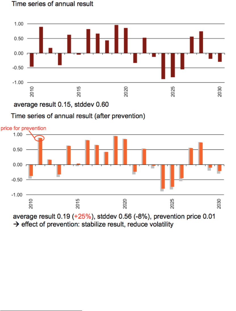
54
• similarly exposed business: a large number of similar risks
126
• plus: economic viability: private insurers must be able to obtain a risk-
adequate premium
The following figures show the effect of insurance, including the working (and benefit)
of risk reducing prevention measures. (Climate) adaptation measures work in a
similar fashion, hence do not only reduce risk, but render insurance more attractive
(i.e. affordable).
126
see Euler’s “law of large numbers”. Hence assessability also applies to large numbers, i.e. one needs
to be able to assess the average outcome over a large number of similarly exposed risks, not
necessarily the specific outcome at each single risk.
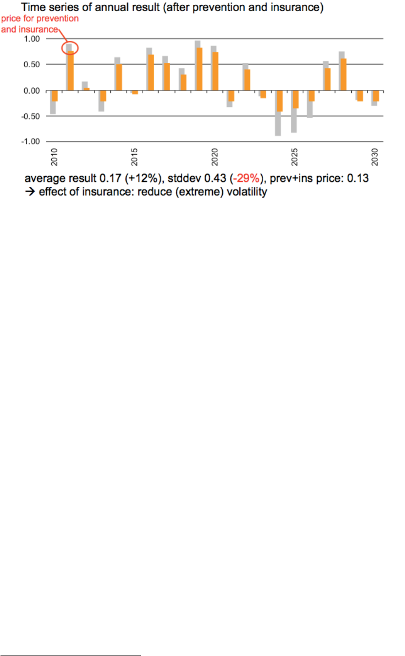
55
In summary, we therefore have:
Result stdev price
127
raw 0.15 0.60
+ prevention 0.19 (+25%) 0.56 (-8%) 0.01
cost-effective adaptation (net gain of 0.04 at cost of 0.01 )
+ insurance (and prevention) 0.17 (+12%) 0.43 (-29%) 0.01+0.12
substantial reduction of volatility, result increase even after deduction of
prevention cost and insurance premium affordable!
for comparison: insurance alone 0.12 (-17%) 0.45 (-25%) 0.153
prevention (strongly) incentivizes insurance
Key drivers for risk transfer demand to complement risk reduction measures are:
• Volatility of (remaining) damage
• Level and trend of expected damage (related to budget)
• Damage clusters (relative to budget and financing capacity)
• Budget constraints and opportunity costs (e.g. school investments)
• Availability of emergency relief capital
• Subjective risk appetite
The last point shall no means be underestimated, as it refers also strongly to risk
culture.
Risk transfer can be agreed upon based on different triggers:
• indemnity
128
, also called incurred or occurred damage: The incurred damage
is compensated for, i.e. the insured sends the bill for fixing the damage and
gets reimbursed. Pro: exact amount paid, Con: takes time, involves damage
assessment and may contain moral hazard (insurance fraud).
• parametric, also called index: A physical parameter exceeding a certain
threshold (e.g. wind speed above 35 m/s) triggers the payment of a pre-
agreed amount – or more generally an amount as a function of the
parameter(s). Pro: fast, unbureaucratic, pre-agreed. Con: the pre-agreed
127
Note that price is already taken into account in result
128
specific or market-share

56
value is paid, actual damage might differ (so called basis risk retained by the
insured
129
).
• modeled (well, a form of parametric): A model is run after an event, based on
the key properties of the event (e.g. a wind footprint as measured by a
meteorological office) and the resulting modeled damage amount is paid
and with different partners, such as:
• policyholders – from macro (e.g. large corporates in Texas) to micro (e.g.
smallholder farmers in Ethiopia) – and the usual single household
• insurers (reinsurers insure them)
• other reinsurers, called retrocession
• capital market, called insurance-linked security (ILS) or Cat Bond
130
• public sector (public-private partnership, PPP)
and can be based either on free choice (whether the take up insurance or not) or
mandatory
131
– or any shade in between. Please note the issue of adverse selection
(especially pertinent for perils such as flood), i.e. that only the most at risk seek
cover, rendering the scheme costly or even non-commercially viable – and hence the
justified consideration of compulsory or mandatory schemes.
Insurance conditions
There are basically two types of insurance conditions, proportional and non-
proportional. Proportional means the insured retains a proportional (linear) fraction of
the damage, non-proportional in essence means the insured is covered above a
certain threshold (called deductible) for a certain cover
132
.
proportional: damageafter=damagebefore * share
non-proportional: damageafter=min(max(damagebefore - deductible,0),cover)
Where share needs to be defined depending on who shall be liable for damage after,
i.e. if damageafter is the damage to be reimbursed by the insurer, share is the insurer’s
share of the total or ‘from ground up’ damage. Likewise, damageafter in above notation
in the non-proportional case is the damage the insurer is liable for, as the deductible
(and any damage exceeding the cover) remains with the insured.
129
That’s why one often finds hybrid solutions, but we refrain from getting into details.
130
Not this one:
131
See e.g. Source: Efficient Monopolies. The Limits of Competition in the European Property Insurance
Market, Thomas von Ungern-Sternberg, Oxford University press, 2004. ISBN 0-19-926881-9
132
There are unlimited covers, but this stretches the second principle of insurability, namely the ability to
assess the outcome.
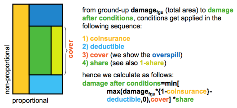
57
Figure: the elements of insurance conditions. The event based approach as followed in climada does
allow for the consideration of all these elements.
climada implementation of insurance conditions
Please read the above section “” carefully first. Remember that the outer (explicit)
loop is over assets, the inner (implicit) one over events.
for asset_i=1:n_assets % approx line 170 in climada_EDS_calc.m
[…]
% calculate the from ground up (fgu) damage
temp_loss=entity.assets.Value(asset_i)*MDD.*PAA;
if entity.assets.Deductible(asset_i)>0 || ...
entity.assets.Cover(asset_i) < entity.assets.Value(asset_i)
% apply Deductible and Cover
temp_damage=min(max(temp_damage-...
entity.assets.Deductible(asset_i)*PAA,0),...
entity.assets.Cover(asset_i));
end
% add to the resulting EDS (event damage set) structure:
EDS.damage=EDS.damage+temp_damage'; % add to the EDS
[…]
end % asset_i
Similarly, any conditions on the event damage set (EDS) can be evalaued, always of
the form min(max(loss-deductible,0 ),cover), i.e. a non-proportional per-event cover
(CatXL) can be evaluated on the EDS as:
EDS.damage = share * min(max(EDS.damage -deductible,0),cover)
For any index based risk transfer, the EDS can be computed starting from the hazard
event set and calculating the index value for each event. In the case of the simplest
index, just a wind speed threshold T at a given location, payout P of $10 per m/s
above threshold, this might look as simple as:
temp_hazard = hazard.intensity(*,hazard_pos);
nz_pos = find(temp_hazard);
EDS_index = min(temp_hazard(nz_pos)-T,0)*P
58
where hazard_pos contains the index of the centroid next to the station (determined
using climada_geo_distance). Note that due to the sparsity of
hazard.intensity, the min function is speeded up by using find first.
More specifically, and to ease the use of risk transfer measures, they can also be
specified in the measures tab of the entity Excel sheet
133
. In column ‘risk transfer
attachment’, one enters the attachment point (synonym for deductible) in the same
currency and currency unit as all other figures, and in column ‘risk transfer cover’ the
cover. In column ‘cost’, one only needs to enter the cost in addition to the pure
expected damage (which is calculated within climada, when the risk transfer gets
applied). Costs for risk transfer are – to keep it simple here – a fixed amount for
management expenses and capital costs that scale first order with the cover
134
. As
an approximation, one might use rules of thumb to determine a proxy for the sum of
management expenses and capital costs, like (GLM stands for geometric layer
mean):
1. determine sqrt(GLM), where GLM=sqrt(attachment_point*cover)
2. look up the probability of a damage of size sqrt(GLM) on the DFC (without
measures, to keep it simple)
3. proxy for sum of costs is max(sqrt(probability of
damage),0.01)*cover
Note on scenarios
Since climada makes use of scenarios in at least three instances, it might be
worthwhile providing a definition and some remarks.
climada uses scenarios e.g. in:
• hazard event set generation (generating artificial single hazard events or
scenarios, such as by ‘wiggling’ path and intensity of tropical cyclones)
Figure: historic (red) and probabilistic (blue) storms, see functions climada_tc_*
• charting out economic pathways (the economic development scenarios,
leading to future assets) and
• last but not least climada uses climate impact scenarios in the sense of
modified hazard event sets (one could also see them as events compatible
with future climate conditions).
133
See ../data/entities/entity_template.xls
134
this is a very crude assumption. As climada only adds the expected damage costs, one needs to be
careful here.
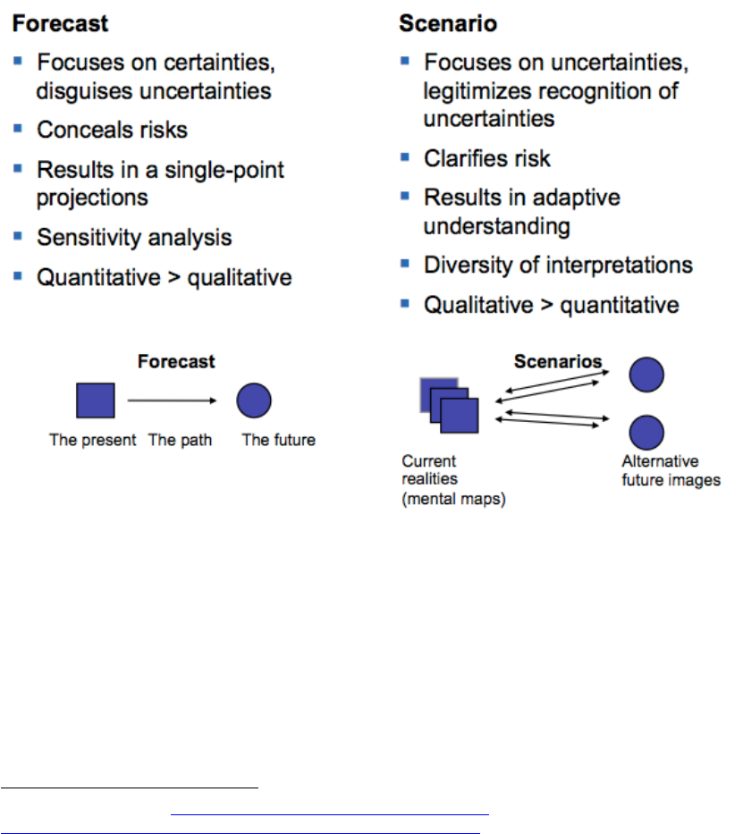
59
Definition: A scenario is a snapshot that describes a possible and plausible future.
Scenario analysis is a systematic approach to anticipate a broad range of plausible
future outcomes.
Scenario analysis is used in general …
• as a risk management tool to assess the potential impact of an event or
development to anticipate and understand risks (as e.g. in the climada hazard
event sets)
• as a tool to spot new business opportunities and to discover strategic
options
135
(e.g. as climada adaptation measures)
• as foresight in contexts of accelerated change, greater complexity and
interdependency
• for evaluation of highly uncertain events that could have a major impact (e.g.
climada climate change hazard event sets)
• to steer mitigation strategies, implementation and monitoring by reviewing
and tracking different possible developments (as in the whole economics of
climate adaptation assessment)
Figure: Some key properties of forecasts and scenarios in comparison.
climate impact scenarios – remarks on climada implementation
There are different ways to represent climate change scenarios in the model.
Representation is possible via
• Parameterized impact:
Estimate the climate change impact on key hazard parameters and represent
those changes in the probabilistic event set, either by
135
See e.g. the famous http://s03.static-shell.com/content/dam/shell-
new/local/corporate/Scenarios/New_Lens_Scenarios_Low_Res.pdf
60
o re-generating the probabilistic event set based on these parameters
(e.g. consider changing properties of tc_track prior to calling
climada_tc_hazard_set) or by
o reflecting those changes by modification of the ‘present climate’
hazard event set (e.g. multiply the hazard intensity by a factor), see
further below
• Downscaled event set:
Extract events from a downscaled GCM-driven model chain
136
Note that a changing climate might also have impacts on e.g. vulnerabilities
While there all degrees of freedom to implement climate change impact scenarios in
climada, the following few remarks might be of value:
Remember that hazard contains the hazard event set, hazard.intensity the
sparse array with intensities, hazard.frequency the vector of event (occurrence)
frequencies. Therefore, the following cases are very straightforward (we use wind
speed as example, works similarly for parameters such as flood height):
• Increase wind speed for all events by 5%:
hazard.intensity =hazard.intensity *1.05;
• Increase event frequencies by 5%:
hazard.frequency=hazard.frequency*1.05;
• Increase all wind speeds by 5 m/s (note that hazard.intensity is sparse, hence
we first need to identify the non-zero elements);
nz_pos=find(hazard.intensity) %non-zeros
hazard.intensity(nz_pos)=hazard.intensity(nz_pos)+5;
• Increase only wind speeds > 45 m/s by 5 m/s:
pos45=find(hazard.intensity>45);
hazard.intensity(pos45)=hazard.intensity(pos45)+5;
The code climada_hazard_clim_scen allows for such impact parameterizations.
Climate impact scenarios – sources
Since the advanced user will likely construct own climate change impact scenarios,
she might find relevant information at the following sources:
http://www.ipcc.ch/pdf/assessment-report/ar5/wg1/WG1AR5_AnnexI_FINAL.pdf and
http://www.ipcc.ch/report/ar5/wg1/docs/ar5_wg1_annexI_all.zip: IPCC Atlas of Global
and Regional Climate Projections
http://sealevel.climatecentral.org: domestic US coastal surge information until 2100
http://climate-adapt.eea.europa.eu: European adaptation site
http://www.meteoschweiz.admin.ch/home/klima/zukunft/klimaszenarien.html: Swiss
climate impact scenarios
and last but not least: http://newclimateeconomy.report
136
Please refer to the climada module ws_europe
(https://github.com/davidnbresch/climada_module_ws_europe) and see Schwierz, C., P. Köllner-Heck,
E. Zenklusen Mutter, D. N. Bresch, P.-L.Vidale, M. Wild, C., and Schär, 2010: Modelling European
winter wind storm losses in current and future climate. Climatic Change (2010) 101:485?514, doi:
10.1007/s10584-009-9712-1.
61
Tropical cyclones – technical remarks
Windfield calculation
To determine the impact of any given storm, function climada_tc_windfield
generates wind field resulting from single track of tropical cyclone. The function starts
from ther track center tc_track.MaxSustainedWind in knots and generates the
2D windfield in res.gust in m/s.
Normally wind footprint calculation is tested on a single tc_track prior to
generation of the hazard event set of all the entire historical and probabilistic track
set (as shown in the step-by-step approach at the beginning of the manual, see
climada_demo_step_by_step). The windfield calculations are speeded up by
only calculating for centroids within 750 km distance of min/max track lon/lat.
res = climada_tc_windfield(tc_track(1170),centroids);
For details, see the header of climada_tc_windfield
Method
Currently, the code implements the Holland windfield
137
.
S=max 0, M-abs T
( )
( )
×R
D
æ
è
çö
ø
÷
32×e1-R
D
æ
è
çö
ø
÷
32
æ
è
ç
ç
ö
ø
÷
÷+T
æ
è
ç
ç
ö
ø
÷
÷D<10×R from center to the outer core
0D>10×Rout of radius
In case one runs with pretty coarse centroids, where the ‘average’ distance between
centroids is much larger than the storms radius of maximum wind (R), the wind
speed (S) might better be parametrized by (see around line 290 in
climada_tc_windfield):
S=
min M,M+2×T×D
R
æ
è
çö
ø
÷D£Rin the inner core
max 0, M-abs T
( )
( )
×R
D
æ
è
çö
ø
÷
32×e1-R
D
æ
è
çö
ø
÷
32
æ
è
ç
ç
ö
ø
÷
÷+T
æ
è
ç
ç
ö
ø
÷
÷D<10×Rin the outer core
0D>10×Rout of radius
where M denotes the maximum sustained wind and T is the celerity (forward speed).
In case where D is still ten times smaller than R, you find yourself in the outer core of
137
Holland, G. J., 1980: An analytic model of the wind and pressure profiles in
hurricanes. Monthly Weather Review, 108, 1212-1218.
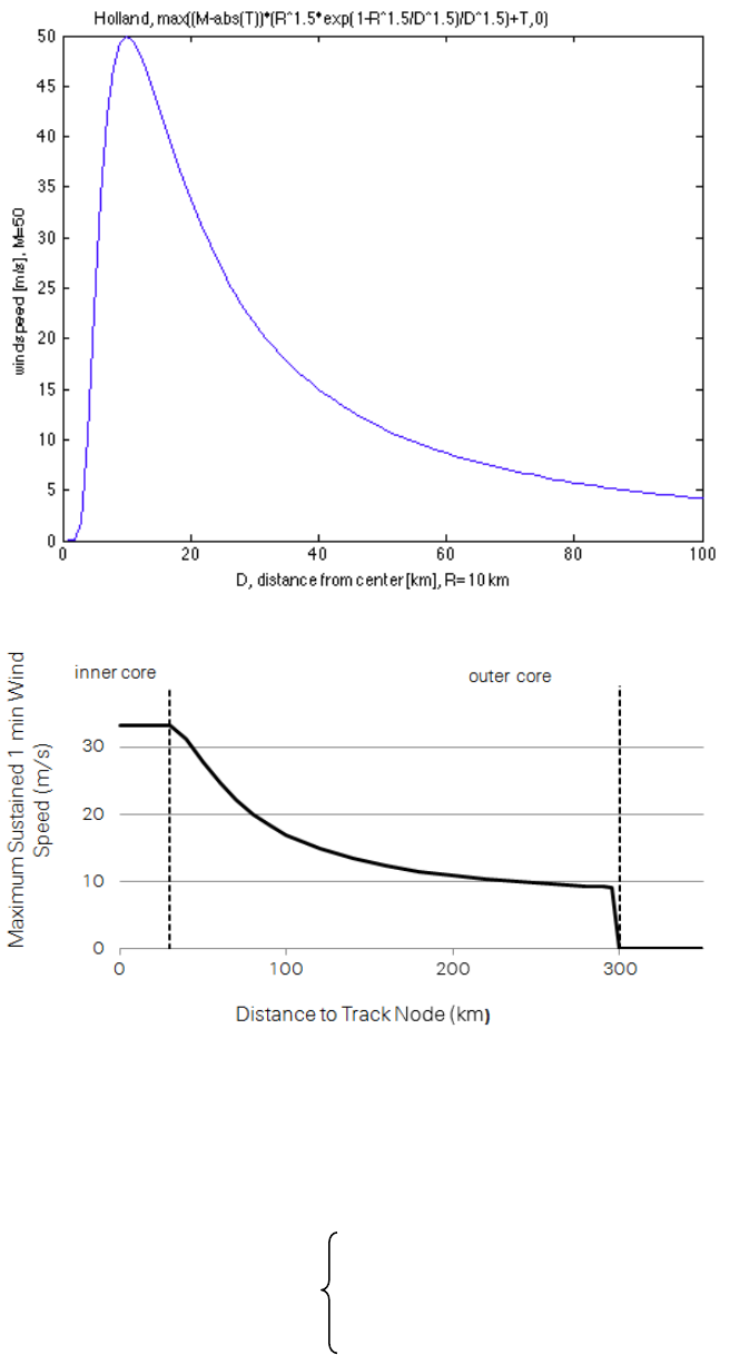
62
the storm where the wind speed takes the form of the second line in the equation
above. If none of these cases are true, the wind speed is set to zero.
Figure: Maximum sustained 1 min wind speed in relation to the distance to the
track node (top panel original Holland, lower panel for special case as described
above).
The radius of maximum wind (R, in km) depends on the latitude of the track node (L)
as follows:
4275
2424)abs(5.230
2430
L
LL
L
R
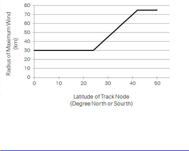
63
Figure: Radius of maximum wind in relation to latitude of track node.
Finally, the wind speed, S, describes the maximum sustained 1 min wind speed. To
derive wind gusts lasting just a few seconds (3-5 s), we note that wind peaks are
typically around 27% higher than a 1 min sustained wind in a hurricane environment.
http://www.prh.noaa.gov/cphc/pages/FAQ/Winds_and_Energy.php
Any other wind field parameterization can be implemented in a similar fashion (just
implement in a copy of climada_tc_windfield, e.g.
climada_tc_MY_windfield, see also the routine climada_tc_hazard_set to
change the caller when generating the probabilistic set).
In order to test the wind field calculation, the following might help:
Use the tc_track structure (should still be in memory), but start with only one track,
e.g. tc_track(84) for the 84th track. Investigate tc_track.name to find a particular
event. Use e.g. the following code to show a list of track number, year and name:
for i=1:length(tc_track)
fprintf('%i %i %s\n',i,tc_track(i).yyyy(1),char(tc_track(i).name));
end
Obtain centroids (points at which to evaluate the winfield) using
centroids = climada_centroids_read(‘’,1)
Note that this call with the 1 also plots the centroids (use the zoom function on the
map). See also the parameter check_plot in the PARAMETER section of the
climada_tc_windfield code or refer to the routine climada_color_plot.
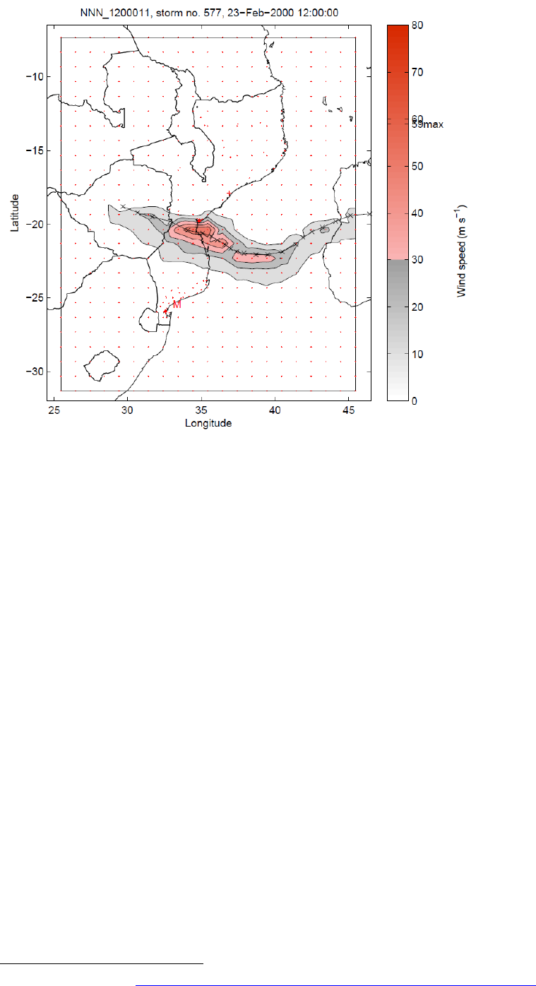
64
Figure: Wind field calculated based on track 577 of the South Indian Ocean. This
particular track results in the second highest wind speed in the city of Beira,
Mozambique.
Single cyclone track evolution animation
The function climada_tc_windfield_animation
138
refines tc_track to 1hour
resolution, calculates wind field for every time step of 1h. The function displays the
wind fields for selected aggregated time steps, e.g. 3h, 6h, 24h. Aggregation default
is 6h.
138
See climada module https://github.com/davidnbresch/climada_module_tc_hazard_advanced
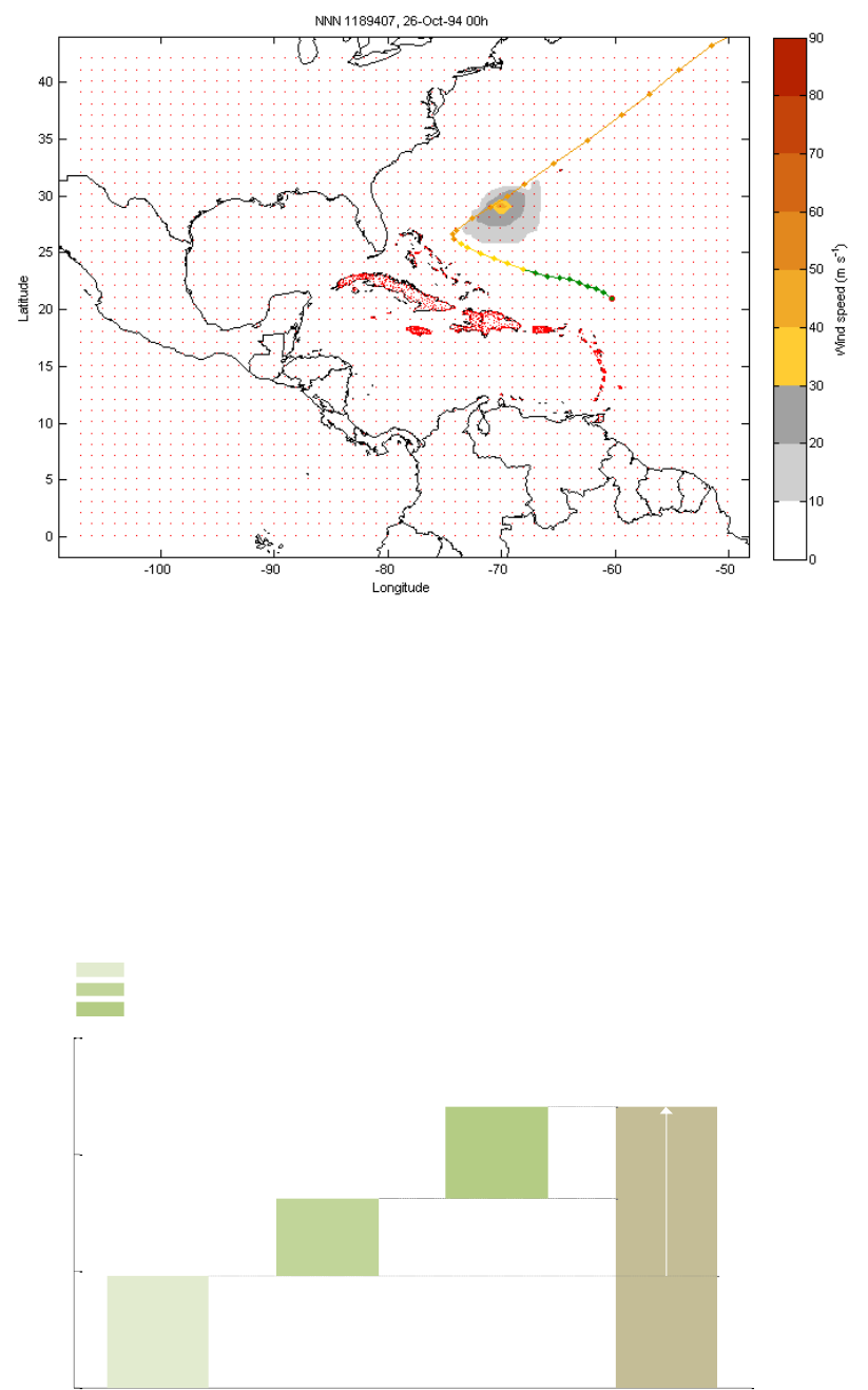
65
Figure: Snapshot from the animation, wind field calculated for every time step.
Economics of Climate Adaptation (ECA) – key routines
The function climada_waterfall_graph plots the waterfall figure for today’s
damage and future damage including economic growth and climate change for the
annual expected loss or any specific return period. Inputs are the three event
damage sets (e.g. EDS_today.mat, EDS_2030.mat, EDS_2030_clim.mat), prompted
for if not given. Any specific return period or annual expected damage can be
chosen.
Figure, see climada_waterfall_graph
0
5
10
15
5
3
4
12
Loss amount 109
+ 152%
Annual Expected Loss (AEL)
2012 today's
expected loss
Incremental increase
from economic
gow th; no climate
change
Incremental increase
from climate change
2030, total
expected loss
USFL MiamiDadeBrow ardPalmBeach2012 TCNA hazard event set 2012
USFL MiamiDadeBrow ardPalmBeach2030 TCNA hazard event set 2012
USFL MiamiDadeBrow ardPalmBeach2030 climate change scenario based on TCNA hazard event set 2012
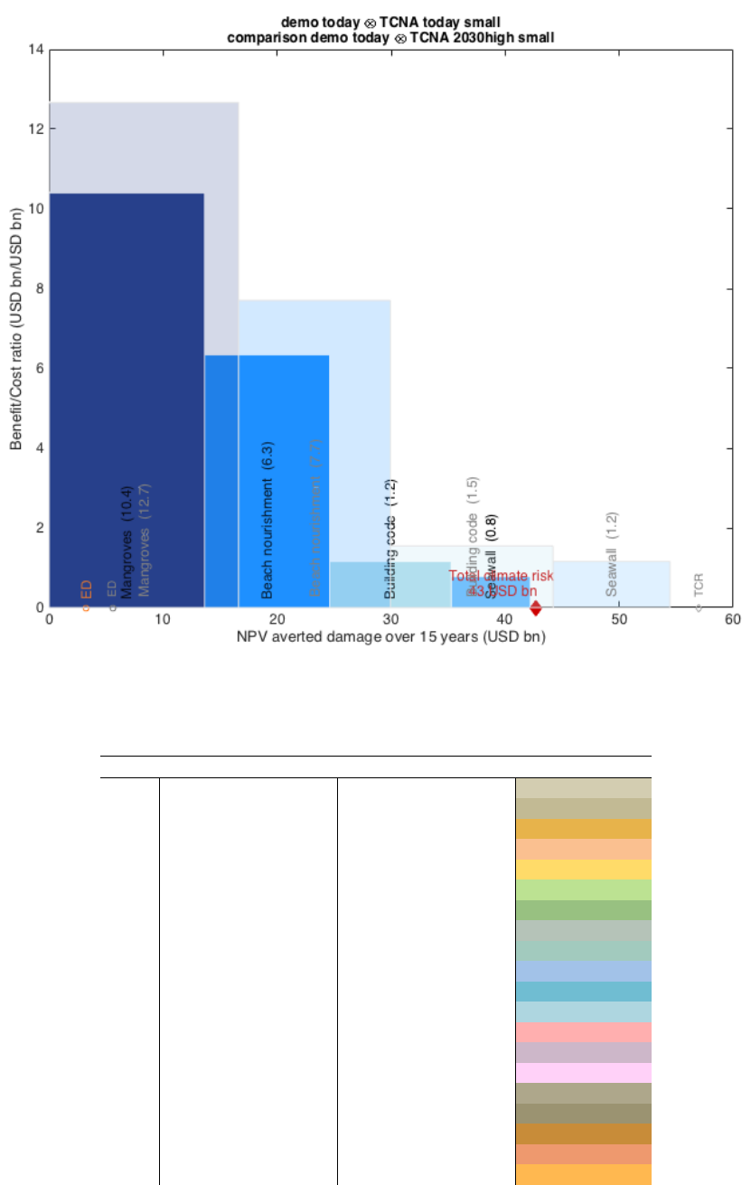
66
The function climada_adaptation_cost_curve plots the adaptation cost curve,
i.e. the cost/benefit (or benefit/cost) ratio for each measure on the vertical axis, the
benefit on the horizontal axis. Note that all values are NPV.
Figure, showing the option to plot two adaptation cost curves for direct comparison, see
climada_adaptation_cost_curve
Proposed colours to use for measures:
Color
red
green
blue
red
green
blue
for excel
1
211
205
177
0.82
0.80
0.69
0.82 0.8 0.69
2
194
186
148
0.76
0.73
0.58
0.76 0.73 0.58
3
231
179
75
0.90
0.70
0.29
0.9 0.7 0.29
4
250
192
144
0.98
0.75
0.56
0.98 0.75 0.56
5
255
219
105
1.00
0.86
0.41
1 0.86 0.41
6
188
226
146
0.73
0.88
0.57
0.73 0.88 0.57
7
152
193
129
0.59
0.75
0.50
0.59 0.75 0.5
8
181
195
184
0.71
0.76
0.72
0.71 0.76 0.72
9
162
202
190
0.63
0.79
0.74
0.63 0.79 0.74
10
162
194
232
0.63
0.76
0.91
0.63 0.76 0.91
11
112
189
210
0.44
0.74
0.82
0.44 0.74 0.82
12
174
214
224
0.68
0.84
0.88
0.68 0.84 0.88
13
255
175
175
1.00
0.68
0.68
1 0.68 0.68
14
205
183
201
0.80
0.71
0.79
0.8 0.71 0.79
15
255
209
248
1.00
0.82
0.97
1 0.82 0.97
16
174
167
139
0.68
0.65
0.54
0.68 0.65 0.54
17
155
147
113
0.61
0.57
0.44
0.61 0.57 0.44
18
200
140
57
0.78
0.55
0.22
0.78 0.55 0.22
19
238
153
110
0.93
0.60
0.43
0.93 0.6 0.43
20
255
184
80
1.00
0.72
0.31
1 0.72 0.31
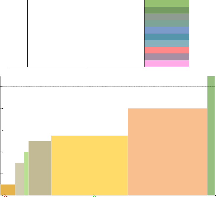
67
21
149
193
112
0.58
0.75
0.44
0.58 0.75 0.44
22
117
154
98
0.46
0.60
0.38
0.46 0.6 0.38
23
142
156
145
0.55
0.61
0.57
0.55 0.61 0.57
24
125
164
151
0.49
0.64
0.59
0.49 0.64 0.59
25
125
155
202
0.49
0.61
0.79
0.49 0.61 0.79
26
85
150
173
0.33
0.59
0.68
0.33 0.59 0.68
27
136
177
190
0.53
0.69
0.74
0.53 0.69 0.74
28
255
137
137
1.00
0.54
0.54
1 0.54 0.54
29
167
144
163
0.65
0.56
0.64
0.65 0.56 0.64
30
255
171
232
1.00
0.67
0.91
1 0.67 0.91
Figure: Example plot with proposed colours
See also climada_adaptation_event_view, which shows the effect of
measures for events of different return periods.
0 0.2 0.4 0.6 0.8 1 1.2 1.4 1.6 1.8 2
x 1011
0
0.2
0.4
0.6
0.8
1
PV of averted losses
cost/benefit ratio (CBR)
sandbags (0.1)
beach nourishment (0.3)
enforce building code (0.4)
vegetation management (0.5)
elevate existing buildings (0.55)
seawall (0.8)
risk transfer (1.1)
EL
TCR
m @ USFL MiamiDadeBrow ardPalmBeach2012 BATCHTEST TCXX hazard
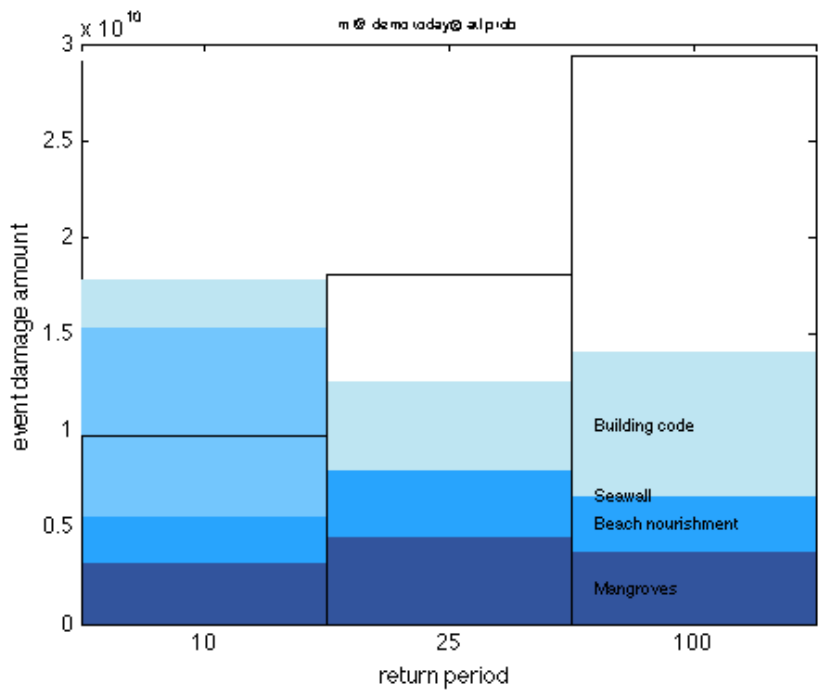
68
Figure: A sample plot of adaptation event view (see climada_adaptation_event_view). It shows
the effectiveness for measures for events of a given return period (here 10, 50 and 100 years, event
damage show as black rectangles, mitigating effect of measures in blue colors). Note that for the 10-
year event, all modeld damage can be averted by the proposed measures, for the 50-year event still
abut 70% and for the 100-year event, abput half of the damage. The plot shows has still one shortcoming: The
seawall (second lightest blue) shows up very effectively for the 10-year event, but the labeling (provided on the 100-year event only) is
hence difficult to read.
See also climada_EDS_DFC to visualize the effect of specific measures on the per
occurrence damage exceedance frequency curves (DFC).
Please be reminded that the function climada does prompt for today’s assets and
today’s hazard, future assets and hazard and perform all the calculations, resulting in
the adaptation cost curve as well as the adaptation event view.
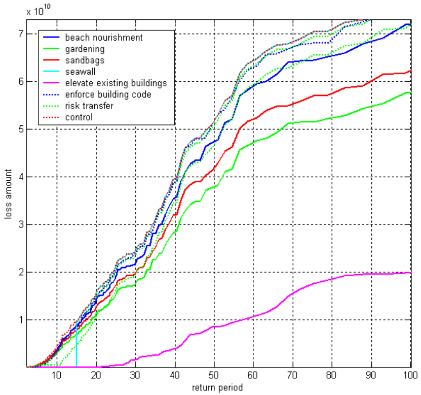
69
Figure: The per occurrence damage exceedance frequency curve (DFC) for today’s hazard. Note the
effect of the dam (cut-off at 15yr return period, light blue curve). Note further the prominent impact of
‘elevate existing buildings’, but this is entirely due to an optimistic modification of the underlying damage
function.
A remark on loss, damage and vulnerability
Loss: irrevocable loss [unersetzbarer Verlust], e.g. loss of glaciers (due to warmer
climate) or loss of coastal land (due to sea level rise) or loss of precipitation (due to
changed weather patterns). Losses can only be compensated for, not re-stated or re-
placed. A risk management approach to loss does strongly suggest avoiding such
losses due to their irrevocable nature. Risk management options such as intervention
or sharing of risk can only deal with some of the consequences of the loss, not the
loss itself. Irrevocable losses are uninsurable - still, some of their consequences can
be insured (e.g. glacier melt is not random, hence cannot be insured, but the risk of a
glacier lake bursting can be insured, since it's a random event. Likely: sea level rise
and the loss of coastal land cannot be insured, since it's not random - but storm
surge risk can be insured, since it's a random event).
Damage: replaceable damage [ersetzbarer Verlust], e.g. damage of property (can be
repaired/rebuilt), consequential damage, like business interruption (can be monetarily
compensated). Damage can be repaired or rebuilt at a cost. The full scale of risk
management options can be employed: avoidance, prevention, intervention and risk
transfer. Therefore, an economic analysis provides a suitable framework to assess

70
the damage and to determine the most effective combination of avoidance,
prevention, intervention and risk transfer measures to address damage.
→ Corollary: Any mechanisms to deal with loss & damage has to make this
differentiation - To propose a 'standard' risk management approach to replaceable
damage and a (e.g. compensation) mechanism to the irrevocable loss. Since most
adaptation measures as dealt with by climada a risk management ones, we refer to
'damage' wherever possible in the climada context.
Vulnerability (weadapt.org): The ordinary use of the word ‘vulnerability’ refers to the
capacity to be wounded, i.e., the degree to which a system is likely to experience
harm due to exposure to a hazard. The scientific use of ‘vulnerability’ has its roots in
geography and natural hazards research but this term is now a central concept in a
variety of research contexts such as natural hazards and disaster management,
ecology, public health, poverty and development, secure livelihoods and famine,
sustainability science, land change, and climate impacts and adaptation. In order to
make sense of the range of definitions, the different interpretations and definitions
can be seen to be rooted in three academic disciplines namely risk and hazard or
biophysical approaches, political economy and the concept of ecological resilience.
From a climate change perspective, according to the IPCC, vulnerability is “the
degree to which a system is susceptible to, or unable to cope with, adverse effects of
climate change, including climate variability and extremes”.
Damage function: functional relationship between the hazard intensity and the
resulting damage. The hazard intensity is measured (or modeled) at a given
spatiotemporal point (a location, a given event) of a hazard (e.g. a flood height at a
given latitude longitude at a given time). The damage is expressed as a percentage
of the exposed (and hence possibly affected) asset. One often differentiates between
the percentage of affected assets (PAA) as well as the mean damage degree (MDD).
What's called a damage function in climada is often also referred to as 'vulnerability
curve'.
If for say a storm surge height of 1 meter, 50% of all assets are affected, and the
damage to these affected assets is 5% of their total value, the PAA is 0.5 and MDD
0.05. If the total asset value is 100, the resulting damage is hence 100 x 0.5 x 0.05 =
2.50
In the case of value signifying exposed population, PAA is used to reflect affected
individuals; while MDD could be used to parameterize some sort of impact to the
affected individuals (e.g. using disability or quality adjusted life years, DALY/QALY).
→ Corollary: While many modelers use 'vulnerability' or 'vulnerability curve' as a
standard term to denote what is described as damage function above, we refer to
'damage function' wherever possible in the climada context.
Further sources of DRM/climate adaptation information/tools
Just for reference, with no aspiration for comprehensiveness, a small list of sites and
sources:
▪ www.climatesmartplanning.net/tools.html collection of tools
▪ www.preventionweb.net/english/professional tools, training material and much
more
71
▪ http://iri.columbia.edu/our-expertise/climate/tools collection of tools
▪ http://tilz.tearfund.org/en/themes/disasters/disaster_risk_reduction_drr/cost_b
enefit_analysis_of_drr cost-benefit analysis of DRR, also general interest:
http://tilz.tearfund.org/en/themes/disasters/
▪ http://policy-practice.oxfam.org.uk/publications/applying-cost-benefit-analysis-
at-a-community-level-a-review-of-its-use-for-com-303558 cost-benefit
analysis
▪ http://www.climate-service-center.de/036238/index_0036238.html.en
Sites featuring climada
▪ https://resilience-exchange.sphaera.world/solutions/economics-of-climate-
adaptation-assessment-model
▪ http://www.preventionweb.net/educational/view/42020
MATLAB/Python – some possibly useful tools
We plan to port climada to Python in 2018. For the time being, the MATLAB® Engine
API for Python® provides a Python package named matlab that enables you to call
MATLAB functions from Python
139
.
To run python from MATLAB, consider e.g. to set (assuming you installed Python 3.5
on a Mac
140
):
pyversion /Library/Frameworks/Python.framework/Versions/3.5/bin/python3.5
py.importlib.import_module('helper_advanced_windfield_global')
Just for reference, as one might consider converting code from Python to be used
with climada – or parts of climada to be used in Python…
code Python (not tested yet)
▪ Small Matlab to Python compiler: convert Matlab code to Python code, also
developed here: SMOP@chiselapp
▪ LiberMate: translate from Matlab to Python and SciPy. Github repo.
▪ OMPC: Matlab to Python (a bit outdated)
▪ Matlab to Python conversion: No download files available
There's also oct2py which can call .m files within python, see
https://pypi.python.org/pypi/oct2py. As climada runs in Octave, this is a viable
alternative to converting to Python (for the time being). It requires GNU Octave, see
right at the top of the manual.
Also, for those interested in an interface between the two languages and not
conversion:
▪ pymatlab: communicate from Python by sending data to the MATLAB
workspace, operating on them with scripts and pulling back the resulting data
▪ Python-Matlab wormholes: both directions of interaction supported
▪ Python-Matlab bridge: use Matlab from within Python, offers matlab_magic for
iPython, to execute normal matlab code from within ipython
▪ PyMat: Control Matlab session from Python
▪ pymat2: continuation of the appearingly abandoned PyMat.
▪ mlabwrap, mlabwrap-purepy: make Matlab look like Python library (based on
139
http://ch.mathworks.com/help/matlab/matlab_external/get-started-with-matlab-engine-for-python.html
140
See https://www.python.org/downloads or get Python including many libraries from
https://www.continuum.io/downloads#osx
72
PyMat)
▪ oct2py: run GNU Octave commands from within Python
▪ pymex: Embeds the Python Interpreter in Matlab, also on File Exchange
▪ matpy: Access MATLAB in various ways: create variables, access .mat files,
direct interface to MATLAB engine (requires MATLAB be installed).
▪ MatPy: Python package for numerical linear algebra and plotting with a
MatLab-like interface
