Dbsp Observing Manual
User Manual: Pdf
Open the PDF directly: View PDF ![]() .
.
Page Count: 8
DBSP Observing Manual
I. Arcavi, P. Bilgi, N.Blagorodnova, K.Burdge, A.Y.Q.Ho
May 7, 2018
Contents
1 Remote Computer Access 2
2 Setup 2
3 Wavelength coverage check 2
4 Instrument focus 3
5 Calibrations 3
5.1 Bias frames ........................................ 3
5.2 Arc-lamps ......................................... 4
5.3 Flat frames ........................................ 4
6 Getting started on science objects 4
7 Science objects 5
8 Data transfer 6
A Appendix - Spectral atlas plots 7
1

1 Remote Computer Access
•Find out what time sunrise and sunset is from your favorite ephemeris catalogs on the Internet.
Then add or subtract 48 minutes to find the times of 12 degree twilight. Alternatively, check
urlhttp://www.palomar.caltech.edu/calendar.tcl.
•If not observing remotely one should budget at least two hours to get to the Palomar obser-
vatory. The Dome is made dark by 4pm in the Summer and 3:30pm in the Winter.
•If observing remotely, login to the remote machine. Username and password can be found in
the handbook in the observing room (or you can ask the telescope operator).
Double click the shortcut to the DBSP VNC sessions which will give you to the GUI operating
DBSP on the instrument 7 machine (see the diagram in Figure 1).
•On the left of the three screens should be a shortcut named Instrument 7. This opens the
VNC session to the machine running the DBSP GUI. The password for access can be found
in the handbook in the observing room, or you can ask the telescope operator.
•The middle screen has DS9 and IRAF sessions running.
•The right screen shows a VNC session to the FacSum (facility summary) machine.
2 Setup
When submitting the online setup, use the following configuration.
Object Setting
# of slits Single
Dichroic D-55
Polarimeter None
Blue grating 600/4000
Blue angle 27◦17’
Red grating 316/7500
Red angle 24◦38.2’
Table 1: Usual ZTF setup.
3 Wavelength coverage check
Check if the spectral wavelength coverage is as expected and ensure overlap between the two cam-
eras. On the blue side, this will be from around 290nm to 590nm and on the red, 435nm to 1065nm.
The D-55 dichroic however will limit both sides to/from 550nm respectively.
IMPORTANT −clear both chips by doing a couple of test exposures before beginning the
run. Frequently, the TO will have already taken a few of these in the afternoon.
Change the turret setting (center grey window on left monitor) to lamps and turn on the internal
arc lamps. He+Ne+Ar works best for the red side and Fe+Ar for the blue (bear in mind that the
Fe+Ar lamp takes a minute to warm up). Perform the exposures listed below with the given slit
2
widths. Usually just the one set with 0.5 is fine, but it is ideal to use all three. Note that the blue
chip is vertical and the red chip is horizontal.
When checking exposures in the terminal, and subsequently removing test arcs, use ”del” instead
of ”rm.”
0.5 1 1.5
Red 0.4 sec 0.2 sec 0.1 sec
Blue 10 sec 5 sec 3 sec
Table 2: Recommended arc exposure times.
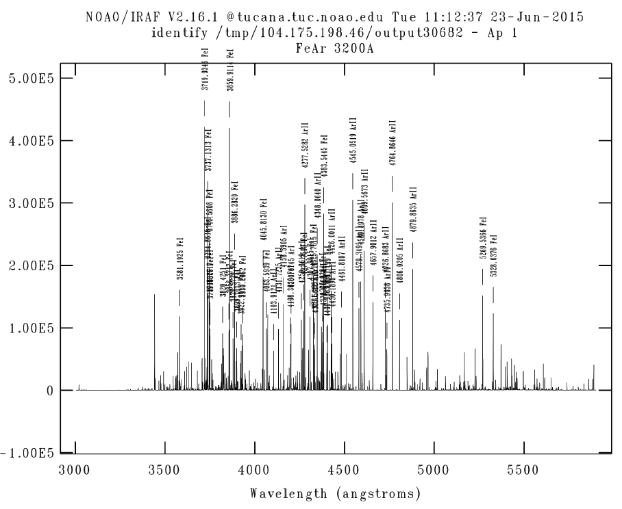
The resulting spectra can be cross-checked with the NOAO spectral atlas. The He+Ne+Ar and
Fe+Ar arc lamp spectra have been downloaded from the NOAO website. You can find the spectral
atlas plot in Figures 2and 3in the Appendix of this document.
•Open a local IRAF session on the observer1 machine or by clicking the ”IRAF Spectral Atlas”
icon on the desktop (middle monitor).
•Enter onedspec at the prompt to run the necessary package.
•Enter epar splot to edit the splot parameters. Change the xmin and xmax values to match
the blue side wavelength range.
•To adjust the plot dimensions, place the cursor over the desired bottom left corner and press
”e”, then place the cursor over the desired top right corner and press e again.
•Repeat the process for the red side using the henear.fits file. Find the wavelength solution
and ensure the coverage is as expected and that there is an overlap of around 20nm.
4 Instrument focus
Select the 0.5 slit and take the same arc-lamp exposures as before. It is desired to measure the
FWHM of four spectral lines in roughly four equally spaced locations along the direction of disper-
sion from end to end.
With the data FITS file open in DS9, run the IMEXAM utility from the IRAF terminal. To find
the FWHM place the cursor in the center of a spectral line and press j to acquire a profile in the
x-direction and k in the y-direction. Make a note of the focal setting and the FWHM measurements.
Ask the TO to go to the cage and change the focal setting (usually by 20 in either direction).
Repeat the measurements with the new focal setting for the same spectral lines. Find the focal
setting with the minimum overall FWHM and ask the TO to lock it there. For example, Table 3
shows a possible focus table for the red side.
5 Calibrations
5.1 Bias frames
Turn off the arc lamps (by pressing green circles next to them), switch the turret setting to “Closed”
and take a sequence of ten bias exposures. Set the exposure time to zero, adjust the image number
3

Focal setting
880 860 870 890
Pixel FWHM FWHM FWHM FWHM
980 3.39 3.01 3.11 3.33
1742 2.54 2.80 2.66 2.47
2051 2.55 3.12 2.82 2.37
3304 2.28 2.22 2.22 2.39
Table 3: The last column offers the overall best focus.
to 10 and edit the object name and type accordingly. Note that when typing values on the blue
and red side controls, it is important to hit enter to ensure the values register.
5.2 Arc-lamps
Put the lamps back on, switch the turret setting to “Lamps” and take two sets of the following
exposures: He+Ne+Ar lamp on the red side for 0.4 seconds and Fe+Ar lamp on the blue side for
60 seconds.
5.3 Flat frames
Switch the turret setting to “Aperture” and check with the TO that it is okay to remove the mirror
cover. Turn on the high lamps and then take flat frame exposures with the slit width(s) that will
most likely be used for the night based on the estimated seeing (ask the TO).
Typically 60 seconds on the red side and 90 seconds on the blue side generate dome flat frames
with an acceptable number of counts.
Note:
Red camera −4k ×2k CCD linear to 40000 DN, saturation at 45000 DN.
Blue camera −2k ×4k CCD linear to 62000 DN, saturation at 65000 DN.
6 Getting started on science objects
•Star-list: The star-list can be retrieved from the relevant page on the Marshall where targets
are assigned for a particular run. Use SCP to copy the star-list text file to the local com-
puter [user1@observer1.palomar.caltech.edu:/observer/observer/targets/username/]. Ask the
support astronomer for the password. Load it into the star-list program on the right screen.
Sort the targets by RA to aid in the scheduling process. The starlist is in the following sample
format to be parsed by the FacSum machine program:
14 g j t 00 18 39.64 +02 11 0 3 . 5 2000 . 0 ! c o m m e n t
•Sky focus: Once the dome is open, the TO will do a sky focus. Ask for the seeing and choose
the appropriate slit width for observations. Keep an eye on the seeing during the night and
change the slit width accordingly. This can be monitored at the Palomar maintenance page:
www.palomar.caltech.edu/maintenance/index.tcl.
4

•Standard star measurements: Change the turret setting to “Aperture”. At the onset of
12 degree twilight, take two one-minute exposures of one of the standard stars from Table 6.
Star RA Dec Epoch
G191B2B (blue) 05 05 30.6 +52 49 56.0 2000.0
Feige34 (red) 10 39 36.71 +43 06 10.1 2000.0
BD+28d4211 (blue) 21 51 11.07 +28 51 51.8 2000.0
Column 211 on the blue chip is a bad column so make sure that the trace is far enough away
from there. If switching slits during the night ensure that standard star measurements are
made with all slits used.
•Open the viewer to the slit viewing camera. On the computer to the right there will be a
shortcut that opens a VNC session to the computer that is running the slit viewing camera.
7 Science objects
•Ask the TO to use the parallactic angle for all measurements unless otherwise required. It
is best to cover targets in order of RA. Depending on the viewing conditions, the maximum
acceptable air-mass should be between 1.5 and 2.
•A target is communicated to the TO by highlighting it in the target list on the FacSum
machine and clicking Load to Telescope. Help the TO identify the target in the slit viewing
camera (which will most likely be FLI) so that it can be positioned on the slit.
•If the target is too faint to be detected on the slit viewing camera, it may be necessary to use
blind offsets. The two ways to do this are, 1) Go directly to an offset star by having it in the
target list and loading it to the telescope. Once positioned, read out the offset coordinates of
the target to the TO. 2) From the position of where the target is expected to be, read out the
offset coordinates of the offset-star from the target. Once the offset star is positioned in the
slit, ask the TO to reverse the offset coordinates to return to the target.
•Finding charts and offset coordinates can be found at any targets homepage at the ZTF tran-
sient or galactic marshal websites http://skipper.caltech.edu:8080/cgi-bin/growth/marshal.
cgi. Alternatively, you can use Nadia’s script1which uses the Pan-STARRS catalogue to find
the offset stars and plot the finder.
•Check the quality of the trace after each exposure. The minimum acceptable S/N for a given
target is usually 5. A good rule of thumb for deciding exposure time is the 20-20 rule. That is
to say that a 20th magnitude object requires a 20 minute exposure to achieve a decent S/N.
Note: There is software on the observer1 machine to get a quick look at reduced spectroscopic
data on the fly. This software does background subtraction and source extraction. Open a
terminal on observer1 and type in dbsp drp. This should open Jennifer Milburns quick look
software for which the manual is at www.astro.caltech.edu/palomar/observer/software/drp.
html.
1Download from here: https://github.com/nblago/utils/blob/master/finder chart ps1.py.
Use as: python finder chart ps1.py [RA] [Dec] [Name] [[rad]] [[telescope]]
5
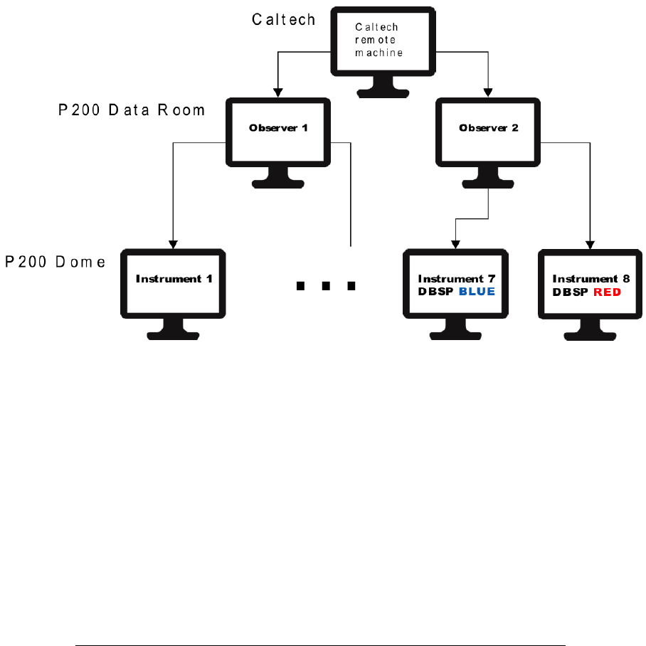
Figure 1: P200 instrument computer network
8 Data transfer
The various instrument computer directories are mounted on the observer1 machine also. Access
the DBSP data folder at: [/remote/instrument7/DBSP/date/]. Alternatively you may use rsync
to periodically transfer data throughout the night to your location of choice for on-the-fly data
reduction.
The remote machine at Caltech connects to either observer 1 or 2 at the P200 data room through
a VNC session. Both the observer 1 and 2 machines have three physical desktops at the ports shown
in Table 8:
Port number Observer 1 Observer 2
5900 FacSum display DBSP control screen
6900 LFC control desktop FacSum display
7900 LFC IRAF+DS9 sessions DBSP IRAF+DS9 sessions
The GUI for DBSP is loaded on the instrument 7 machine (the one for the blue camera). Each
instrument computer has three desktops of which the GUI is typically loaded onto that desktop
with an access port at 5916. Thus, the DBSP GUI is accessed from the observer computer by
initiating a VNC connection to, [instrument7.palomar.caltech.edu:16]. There is a shortcut for this
on the DBSP control screen on the observer machine.
6
A Appendix - Spectral atlas plots
Figure 2: Fe+Ar spectral atlas
7
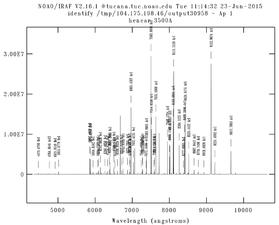
Figure 3: He+Ne+Ar spectral atlas
8
