Guide
User Manual: Pdf
Open the PDF directly: View PDF ![]() .
.
Page Count: 136 [warning: Documents this large are best viewed by clicking the View PDF Link!]
Acknowledgments
iii
Contents
Acknowledgments iii
Preface xiii
1 Fundamentals 1
1.1 InputandOutput ..................................... 1
1.2 Complexity ......................................... 2
1.3 FirstProblems ....................................... 3
1.3.1 Bessie’sCandles .................................. 3
1.3.2 Froyo ........................................ 3
1.4 Sorting............................................ 4
1.4.1 InsertionSort.................................... 4
1.4.2 MergeSort ..................................... 4
1.4.3 Quicksort ...................................... 5
1.4.4 Ms.Manana’sPuzzles............................... 5
2 Big Ideas 7
2.1 BruteForce......................................... 7
2.1.1 SquareRoot .................................... 7
2.1.2 CombinationLock ................................. 8
2.1.3 SkiCourseDesign ................................. 8
2.1.4 ContestPractice .................................. 9
2.2 Depth-FirstSearch(DFS)................................. 9
2.2.1 Permutations.................................... 10
2.2.2 Basketball...................................... 10
2.2.3 ProblemBreak ................................... 11
2.2.4 GeneralizingDFS.................................. 11
2.2.5 Dungeon....................................... 11
v

Hsiang, Wei, Liu Contents
2.2.6 nQueensPuzzle .................................. 11
2.3 GreedyAlgorithms..................................... 12
2.3.1 BessiethePolyglot................................. 12
2.3.2 MoreCowbell.................................... 12
2.3.3 FarmerJohnandBoxes .............................. 13
2.3.4 SnackTime..................................... 14
3 Standard Library Data Structures 15
3.1 Generics........................................... 15
3.2 List ............................................. 16
3.2.1 DynamicArray................................... 16
3.2.2 LinkedList ..................................... 17
3.3 Stack............................................. 19
3.4 Queue ............................................ 20
3.5 Heap............................................. 21
3.6 Set.............................................. 25
3.6.1 BinarySearchTree................................. 25
3.6.2 HashTable ..................................... 29
3.7 Map ............................................. 31
4 Graph Algorithms 35
4.1 ConnectedComponents .................................. 35
4.1.1 FloodFill...................................... 36
4.1.2 Union-Find (Disjoint Set Union) . . . . . . . . . . . . . . . . . . . . . . . . . 36
4.2 ShortestPath........................................ 38
4.2.1 Dijkstra....................................... 38
4.2.2 Floyd-Warshall................................... 41
4.2.3 Bellman-Ford.................................... 42
4.3 MinimumSpanningTree.................................. 42
4.3.1 Prim......................................... 43
4.3.2 Kruskal ....................................... 43
4.4 EulerianTour........................................ 44
vi

Hsiang, Wei, Liu Contents
5 Complex Ideas and Data Structures 45
5.1 Dynamic Programming over Subsets (n2nDP) ..................... 45
5.2 √nBucketing........................................ 46
5.3 SegmentTree........................................ 47
5.3.1 LazyPropagation ................................. 50
5.3.2 FenwickTree .................................... 55
5.4 QueuewithMinimumQuery ............................... 59
5.5 Balanced Binary Search Tree . . . . . . . . . . . . . . . . . . . . . . . . . . . . . . . 60
5.5.1 Treap ........................................ 60
5.5.2 TreeRotation.................................... 64
5.5.3 SplayTree...................................... 65
5.5.4 Red-BlackTree................................... 68
6 Computational Geometry 75
6.1 BasicTools ......................................... 76
6.2 Formulas .......................................... 76
6.2.1 Area......................................... 76
6.2.2 Distance....................................... 76
6.2.3 Configuration.................................... 76
6.2.4 Intersection..................................... 76
6.3 ConvexHull......................................... 76
6.4 SweepLine ......................................... 76
7 Tree Algorithms 79
7.1 DFSonTrees........................................ 79
7.2 JumpPointers ....................................... 80
7.3 EulerTourTechnique ................................... 82
7.3.1 EulerTourTree .................................. 82
7.4 Heavy-Light Decomposition . . . . . . . . . . . . . . . . . . . . . . . . . . . . . . . . 84
7.5 Link-CutTree........................................ 84
8 Strings 85
8.1 StringHashing ....................................... 85
8.2 Knuth-Morris-Pratt .................................... 85
8.3 Trie ............................................. 85
8.4 SuffixArray......................................... 86
vii

Hsiang, Wei, Liu Contents
8.5 Aho-Corasick ........................................ 88
8.6 Advanced Suffix Data Structures . . . . . . . . . . . . . . . . . . . . . . . . . . . . . 90
8.6.1 SuffixTree ..................................... 91
8.6.2 SuffixAutomaton.................................. 91
9 More Graph Algorithms 93
9.1 Strongly Connected Components . . . . . . . . . . . . . . . . . . . . . . . . . . . . . 93
9.2 NetworkFlow........................................ 96
9.2.1 Ford-Fulkerson ................................... 97
9.2.2 Max-Flow Min-Cut Theorem . . . . . . . . . . . . . . . . . . . . . . . . . . . 98
9.2.3 Refinements of Ford-Fulkerson . . . . . . . . . . . . . . . . . . . . . . . . . . 99
9.2.4 Push-Relabel ....................................100
9.2.5 Extensions .....................................104
9.2.6 BipartiteMatchings ................................104
10 Math 105
10.1NumberTheory.......................................105
10.1.1 Random Prime Numbers Bounds . . . . . . . . . . . . . . . . . . . . . . . . . 105
10.1.2 Prime Number Testing . . . . . . . . . . . . . . . . . . . . . . . . . . . . . . . 105
10.1.3 Sieve of Eratosthenes . . . . . . . . . . . . . . . . . . . . . . . . . . . . . . . 106
10.1.4 PrimeFactorization ................................106
10.1.5 GCD and the Euclidean Algorithm . . . . . . . . . . . . . . . . . . . . . . . . 106
10.1.6 Fermat’s Little Theorem . . . . . . . . . . . . . . . . . . . . . . . . . . . . . . 106
10.1.7 ModularInverses..................................106
10.2CombinatorialGames ...................................106
10.3Karatsuba..........................................107
10.4Matrices...........................................107
10.5FastFourierTransform...................................107
11 Nonsense 113
11.1SegmentTreeExtensions .................................113
11.1.1 Fractional Cascading . . . . . . . . . . . . . . . . . . . . . . . . . . . . . . . . 113
11.1.2 Persistence .....................................113
11.1.3 HigherDimensions.................................113
11.2DPOptimizations .....................................113
11.3TopTree...........................................113
11.4Link-CutCactus ......................................113
viii

Hsiang, Wei, Liu Contents
12 Problems 115
12.1Bronze............................................115
12.2Silver ............................................115
12.2.1 CompleteSearch ..................................115
12.2.2 Greedy .......................................115
12.2.3 Standard Dynamic Programming . . . . . . . . . . . . . . . . . . . . . . . . . 115
12.2.4 Standard Graph Theory . . . . . . . . . . . . . . . . . . . . . . . . . . . . . . 116
12.2.5 Easy Computational Geometry . . . . . . . . . . . . . . . . . . . . . . . . . . 119
12.3Gold.............................................119
12.3.1 More Dynamic Programming . . . . . . . . . . . . . . . . . . . . . . . . . . . 119
12.3.2 BinarySearch....................................119
12.3.3 SegmentTree....................................121
12.3.4 More Standard Graph Theory . . . . . . . . . . . . . . . . . . . . . . . . . . . 121
12.3.5 Standard Computational Geometry . . . . . . . . . . . . . . . . . . . . . . . . 122
12.3.6 Less Standard Problems . . . . . . . . . . . . . . . . . . . . . . . . . . . . . . 122
12.4Beyond ...........................................122
12.4.1 Data Structure Nonsense . . . . . . . . . . . . . . . . . . . . . . . . . . . . . 122
12.4.2 OtherNonsense...................................122
ix
List of Algorithms
1 Union-Find ......................................... 38
2 Dijkstra ........................................... 39
3 Floyd-Warshall ....................................... 42
4 Bellman-Ford........................................ 42
5 Prim............................................. 43
6 Kruskal ........................................... 44
7 EulerianTour........................................ 44
8 Jump Pointers, Level Ancestor and LCA . . . . . . . . . . . . . . . . . . . . . . . . . 81
9 Tarjan............................................ 95
10 Ford-Fulkerson ....................................... 97
11 Edmonds-Karp ....................................... 99
12 Push-Relabel(Generic) ..................................103
13 FastFourierTransform...................................108
xi

Preface
You might have heard of Evan Chen’s Napkin, a resource for olympiad math people that serves as a
jumping point into higher mathematics.
1
The Wikipedia articles on higher mathematics are just
so dense in vocabulary and deter many smart young students from learning them before they are
formally taught in a course in college. Evan’s Napkin aims to provide that background necessary to
leap right in.
I feel the same way about computer science. For most, the ease of the AP Computer Science
test means that the AP coursework is often inadequate in teaching the simplest data structures,
algorithms, and big ideas necessary to approach even silver USACO problems. On the other hand,
even the best reference books, like Sedgewick, are too dense and unapproachable for someone who
just wants to sit down and learn something interesting.
2
The road, for many, stalls here until college.
Everyone should be able to learn the simplest data structures in Java or C++ standard libraries,
and someone with problem-solving experience can easily jump right into understanding algorithms
and more advanced data structures.
A few important notes, before we begin.
•
I’m assuming some fluency in C-style syntax. If this is your first time seeing code, please look
somewhere else for now.
•
It is essential that you understand the motivations and the complexities behind everything
we cover. I feel that this is not stressed at all in AP Computer Science and lost under the
heavy details of rigorous published works. I’m avoiding what I call the heavy details because
they don’t focus on the math behind the computer science and lose the bigger picture. My
goal is for every mathematician or programmer, after working through this, to be able to code
short scripts to solve problems. Once you understand how things work, you can then move on
to those details which are necessary for building larger projects. The heavy details become
meaningless as languages develop or become phased out. The math and ideas behind the data
structures and algorithms will last a lifetime.
•
It is recommended actually code up each data structure with its most important functions or
algorithm as you learn them. I truly believe the only way to build a solid foundation is to
code. Do not become reliant on using the standard library (
java.util
, for instance) without
understanding how the tool you are using works.
1In fact, I’m using Evan’s template right now. Thanks Evan!
2Sedgewick, notably, is getting better. Check out his online companion to Algorithms, 4th Edition.
xiii

Chapter 1
Fundamentals
1.1 Input and Output
The first part of solving any programming contest problem is reading the input correctly. In this
section, we go over input and output in Java using
java.util.Scanner
and
java.io.PrintWriter
.
There are two scenarios that you should be familiar with:
stdin
/
stdout
and file I/O. You encounter
the former when you enter input and see output for a program run in the command line. You
encounter the latter when you have two files (for example
input.txt
and
output.txt
) that you
read from and write to.
When using
stdin
/
stdout
, we read input from
System.in
using a Scanner and output our
results using
System.out.println()
.
Scanner.nextInt()
and
Scanner.next()
read in integers
and strings, respectively.
System.out.println()
prints its argument and adds a newline at the
end. (If we don’t want the newline, we can use
System.out.print()
.) Here’s an example of a main
method that takes two integers and outputs their sum:
1public static void main(String args []) {
2// hint : you shoul d write " import java . util .*; " at the top of your code .
3Scanner sc =new Scanner(System.in ) ;
4int x=sc .nextInt() ;
5int y=sc .nextInt() ;
6System.out .println(x+y) ;
7}
File I/O is a touch more complicated. For our Scanner, we have to make a new File object and
use it in the constructor. We do the same for our PrintWriter. However, PrintWriter also comes
with a couple more usage notes. First, we should include
throws IOException
after our main
method, since Java requires that we acknowledge the possibility of an IOException. (We bravely
assume that our file open will succeed!) After we finish printing, we must also close the PrintWriter
to make sure that everything gets written. Here’s a snippet showing how Scanner and PrintWriter
work with files:
1

Hsiang, Wei, Liu Chapter 1. Fundamentals
1public static void main(String args []) throws IOException {
2// hint : for file I/O , you sh ould also have " import java . io .*;"
3Scanner sc =new Scanner(new File(" input . txt "));
4int x=sc .nextInt() ;
5int y=sc .nextInt() ;
6PrintWriter pw =new PrintWriter(new File(" outp ut . tx t "));
7pw .println(x+y) ;
8pw .close () ;
9}
Although more efficient methods of I/O exist, such as BufferedReader and BufferedWriter,
what’s covered here should be sufficient for now. (It’s possible to read in 10
5
integers with Scanner
in a fraction of a second.)
1.2 Complexity
Before we start computing contests, we should understand what the problems on these contests are
trying to test. One class of problems, called implementation problems, assesses your ability write
code quickly and accurately. These problems are only common in easier contests, since they usually
don’t involve too much thinking or creativity—you just have to implement what’s written in the
problem statement. Most competitive programming problems ask you to come up with a clever
algorithm instead, testing speed and memory efficiency.
To analyze the efficiency of algorithms, computer scientists use a concept called complexity.
Complexity is measured as a function of the input size; an algorithm could require 3
n
,
n4/
3or even
2
n
+
n2
steps to finish calculating for an input of size
n
. To express complexity, we use something
called “big-O notation.” Essentially, we write the number of steps it takes for an algorithm to finish
inside a pair of parentheses with an
O
in front, like this:
O
(
# of steps
). However, we drop any
constant factors and lower order terms from the expression.
1
I’ll explain why in a moment; let’s
look at some examples for now.
Suppose we have three programs that require 3
n
,
n4/
3and 2
n
+
n2
steps to finish, respectively.
The complexity of the first program is
O
(
n
)because we don’t care about the constant factor 3on
the 3
n
. The complexity of the second program is
O
(
n4
); again, we drop the constant. For the last
program, we write its complexity as O(2n)because n2is a lower order term.
As to why we drop the constants and the lower order terms, consider the first two programs
from above. When
n
= 300, the first program takes 900 steps, while the second program takes
2
,
700
,
000
,
000 steps. The second program is much slower, despite a smaller constant factor.
Meanwhile, if we had a third program that runs in 5
n
steps, it would still only take 1
,
500 steps to
finish. Constant factors become pretty much irrelevant when we’re comparing functions that grow
at different rates. The same can be said about lower order terms:
n2
gets dwarfed by 2
n
even when
n= 10.
Thus in programming contests, we usually want a program with the correct complexity, without
worrying about too much constant factors. Complexity will be the difference between whether a
program gets
accepted
or
time limit exceeded
. As a rule of thumb, a modern processor can do
1
Actually, this isn’t entirely accurate. Saying an algorithm is
O
(
f
(
n
)) really means it takes at most
c·f
(
n
)steps
to finish, for a sufficiently large constant c.
2

Hsiang, Wei, Liu Chapter 1. Fundamentals
around 10
8
computations each second. When you plug the maximum possible
n
into the complexity
of your algorithm, it should never be much more than that.
We’ve focused on time and haven’t talked much about memory so far, but memory does gets
tested. The amount of memory a program uses as a function of
n
is called its space complexity, as
opposed to the time complexity we discussed earlier. Space complexity however, shows up much less
frequently than time complexity—you usually run out of time before you can exceed the memory
limit.
1.3 First Problems
Now that you know the basics, let’s get started by solving a few problems. Try to figure out a
solution to each problem before reading our analysis. To test your code for the problems in this
chapter, you should create an account on Codeforces. After you login, there will be an “Introduction”
problem set available here that includes these problems and a few extras.
1.3.1 Bessie’s Candles
Bessie is a romantic cow; she spends her evenings writing code in the warm glow of
candlelight. In her barn, she currently has anew candles, each of which burns for
exactly one hour. Ever the efficient cow, Bessie can make a new candle from bburnt
out candles. Your task, given aand b(
2
≤a, b ≤
1000
), is to help her figure out the
maximum number of hours for which she can keep her barn illuminated. [Adapted from
Codeforces 379A.]
Bessie’s Candles
is a straightforward implementation problem. Since
a
and
b
are small, we
can simulate Bessie’s candle burning process. We track of the number of candles we have left, the
number of burnt out candles, and the number of hours that have passed. Whenever we have more
than
b
burnt out candles, we make a new candle. Once we run out of candles, we print our answer.
1.3.2 Froyo
Bessie has recently founded a froyo startup, offering froyo made from the best cows
in Wisconsin. She has kept track of her profits for the first ndays (
1
≤n≤
10
5)
and knows that she earned aidollars on the i-th day. Growth is always important in
startups, so Bessie wants to know the length of the longest non-decreasing subsegment
in her profits. Help her figure this out! (Here, a subsegment denotes a contiguous
block of numbers ai, ai+1,··· , aj(i<j).) [Adapted from Codeforces 580A.]
Our first thought upon reading this problem might be to check each subsegment of the sequence
ai
and see if that subsegment is non-decreasing. Unfortunately, this is too slow. There are
approximately
n2/
2pairs of endpoints that we could choose, far too many when
n
can be up to
10
5
. (Remember that rule of 10
8
?) Instead, we can solve this problem with around
n
steps by
performing a single sweep through the array. We maintain a counter representing Bessie’s currrent
“streak”—the number of days since her profit last decreased. If her profit decreases from day
i
to day
i
+ 1, then we reset the counter to zero. The answer we report is the longest streak that we ever see.
3

Hsiang, Wei, Liu Chapter 1. Fundamentals
Froyo
is a clear example of how getting the right complexity is essential. Our initial idea, which
could have been implemented in
O
(
n3
)or
O
(
n2
), was too slow. To make our program finish in time,
we had to work out a more efficient alrogithm that ran in O(n).
1.4 Sorting
To further explore the concept of complexity, we will use sorting algorithms as a case study. Sorting
is just as it sounds—we’re given a collection of objects, and we want to sort them into a predefined
order. For example, suppose we have a list of scores from a programming contest. In order to
generate the final standings, we’ll need to sort the contestants into ascending order by score. Below,
we present three classic sorting algorithms of varying complexity: insertion sort, merge sort and
quicksort.
Don’t worry too much about the details of these algorithms for now. You’ll rarely need to
implement them from scratch, since most modern programming languages come with built-in sorting
algorithms. In our last subsection, we discuss how to use these library functions in Java and C++
with a problem that involves sorting as a subtask.
To supplement our descriptions of the algorithms, you can check out the animations at
http:
//visualgo.net/sorting.html.
1.4.1 Insertion Sort
Insertion sort builds up a sorted list by inserting new elements one at a time. Inserting an element
into a sorted list takes time proportional to the length of the list, so the runtime of this algorithm
is 1+2+3+
···
+
n
= (
n2
+
n
)
/
2, which is
O
(
n2
). One way to think about this is to iterate
i
from 1to
n
, and let the first
i
elements be our sorted list. To insert the (
i
+ 1)-th element, we just
swap it with the largest, the second largest, and so on, until it’s greater than than the next largest
element. Then we have a sorted list in the first (
i
+ 1) entries of the array. Insertion sort, despite
being slower than merge sort and quicksort, is still useful because of its efficiency on small inputs.
Many implementations of merge sort and quicksort actually use insertion sort once the problem size
gets small.
Around how long is the longest list that you can sort with insertion sort in less than a second?
1.4.2 Merge Sort
The idea behind merge sort is the following observation: If we are given two sorted lists of length
n/
2, we only need
n
comparisons to merge them into one sorted list of length
n
. It is easy to find the
smallest element among the two lists, since this element has to be the smallest element in one of the
lists. To find the second-smallest element, we can delete the smallest and do the same comparison
again.
This method of merging lists allows us to divide and conquer. We cut the array in half, sort each
half recursively with merge sort, and then merge the two halves back together. Because our recursion
goes
log2n
levels deep and takes
O
(
n
)operations per level, this algorithm runs in
O
(
nlog n
). (In
fact, it is possible to prove that
O
(
nlog n
)comparisons is optimal for sorting algorithms, one of the
few problems in computer science that has a non-trivial lower bound.)
4

Hsiang, Wei, Liu Chapter 1. Fundamentals
Around how long is the longest list that you can sort with merge sort in less than a second?
1.4.3 Quicksort
Quicksort also uses a divide and conquer strategy to run in
O
(
nlog n
)on average. We first take
a random element from the array, called the pivot. We move anything less than the pivot to the
left of the pivot and anything greater than the pivot to the right of the pivot. Like merge sort, we
can then recursively quicksort the two “halves” that we just created. Since we choose the pivot
randomly, our problem size usually gets cut down by a constant factor, giving us
O
(
log n
)levels of
recursion with
O
(
n
)operations at each level. Thus quicksort runs in
O
(
nlog n
)on average. We say
“on average” because there are cases that can make quicksort run in
O
(
n2
). What would happen if
we chose the smallest element of the array as the pivot each time?
Quicksort was previously used by Java’s
Arrays.sort
and
Collections.sort
, but these func-
tions now use dual-pivot quicksort and timsort.
1.4.4 Ms. Manana’s Puzzles
The end of the school year is near and Ms. Manana will soon have to say goodbye
to a yet another class. As a farewell present, she decides to give each of her n
(
1
≤n≤
50
) students a jigsaw puzzle. The shop assistant tells Ms. Manana that
there are m(
1
≤m≤
50
) puzzles in the shop, but they differ in difficulty and
size. Specifically, the first jigsaw puzzle consists of f1pieces, the second one
consists of f2pieces, and so on. Ms. Manana doesn’t want to upset the children, so
she wants the difference between the numbers of pieces in her largest puzzle and her
smallest puzzle to be as small as possible. Can you help Ms. Manana find this minimum
difference? [Adapted from Codeforces 337A.]
We solve this problem by first sorting the sequence
fi
. After sorting, Ms. Manana will want to
buy puzzles from a contiguous block of the sequence. (If she doesn’t, then the difference between
the largest and smallest puzzles will be greater than necessary.) Thus we can iterate through the
sorted sequence to find the minimum difference between the endpoints of length nblocks.
Usually, when solving a sorting problem, we don’t need to implement our own sorting function.
If you’re using Java,
java.utils.Arrays
has a function
Arrays.sort
that does the magic for you.
In C++, you can add
#include <algorithm>
to your header and use
std::sort
. While coding
Ms. Manana’s Puzzles, try to use the builtin-in sort function in your language.
Here are code snippets for sorting an array arr of length nin Java and C++, respectively:
1// hint : you should have " import java . util .*;" at the top of your code .
2int[] arr =new int[n];
3// do something to fill up the array .
4Arrays.sort(arr ) ;
1// hint : you should have "# i n clude < algorithm >" at the top of your code .
2int arr[n];
3// do something to fill up the array .
4std:: sort(arr ,arr +n);
5

Chapter 2
Big Ideas
In this chapter, we’ll discuss some general problem solving ideas: brute force, depth-first search, and
the greedy algorithm. We can think of these as the building blocks to more complex methods—each
provides a very general approach to simplifying problems. In programming contests, they also
appear frequently by themselves as the core ideas to solutions. Since the concepts we cover are
independent of language, we will no longer present algorithms in concrete Java or C++ code, but
rather in more abstract pseudocode.
2.1 Brute Force
Sometimes, the best way to approach a problem is to try everything. This idea of exhaustively
searching all possibilities is called brute force. For example, if we want to unlock a friend’s iPhone,
we could try all of the 10
4
possible passcodes. As the name and this example suggest, brute force is
often crude and inefficient. Usually we want to make some clever observations to make the problem
more tractable. However, if the input size is small (check the number of operations against 10
8
) or
if we want to squeeze a few points out of a problem by solving only the small cases, brute force
could be the way to go. And if you’re stuck on a problem, thinking about a brute force is not a
bad way to start. Simpler, slower algorithms can often inspire faster ones. Through the following
problems, we’ll show you how to brutally apply the idea of brute force.
2.1.1 Square Root
Given an integer n,
1
≤n≤
10
12, find the greatest integer less than or equal to
√nwithout using any library functions. (This means you can’t call functions like
Math.sqrt or Math.log.)
At first, it’s not obvious how we can compute square roots. However, we can always go simple.
Set
i
= 1, and while (
i
+ 1)
2≤n
, increment
i
. That is, we increment
i
until increasing it further
will cause
i
to exceed
√n
. Since our answer
i
is at most
√n≤
10
6
, our program runs in time. This
is about the silliest approach we can use to calculate square roots, but hey, it works!
When implementing this algorithm, be careful about the size of
n
. The 32-bit
int
type in Java
and C++ only holds values up to 2
31 −
1 = 2
,
147
,
483
,
647, which is exceeded by the maximum
7

Hsiang, Wei, Liu Chapter 2. Big Ideas
possible value of
n
. Thus we need to use a 64-bit integer type for our calculations:
long
in Java
and long long in C++.
2.1.2 Combination Lock
Farmer John purchases a combination lock to stop his cows from escaping their pasture
and causing mischief! His lock has three circular dials, each with tick marks numbered
1
through N(
1
≤N≤
100
), with
1
and Nadjacent. There are two combinations that
open the lock: one combination set by Farmer John and one “master” combination set by
the locksmith. The lock has a small tolerance for error, however, so it will open if
the numbers on each of the dials are at most two positions away from that of a valid
combination. Given Farmer John’s combination and the master combination, determine
the number of distinct settings for the dials that will open the lock.
(For example, if Farmer John’s combination is
(1
,
2
,
3)
and the master combination is
(4
,
5
,
6)
, the lock will open if its dials are set to
(1
, N,
5)
(since this is close to Farmer
John’s combination) or to
(2
,
4
,
8)
(since this is close to the master combination).
Note that
(1
,
5
,
6)
would not open the lock, since it is not close enough to any single
combination. Furthermore, order matters, so
(1
,
2
,
3)
is distinct from
(3
,
2
,
1)
.) [Adapted
from USACO 2013, Combination Lock.]
Again, the simplest idea works. We can iterate over all possible settings of the lock, and for
each setting, check if it matches either Farmer John’s combination or the master combination. To
do this, we can use three nested
for
loops. The first loop goes through the values for the first dial,
the second loop through the values for the second dial, and the third loop through the values for
the third dial. Since there are three dials, the lock has at most
N3≤
10
6
possible settings. We can
check if each dial matches in O(1) time, hence our algorithm runs in less than a second.
In terms of implementation,
Combination Lock
is a great example of how a problem can
decompose into two easier components that we can think about separately. The first component is
to use nested loops to iterate through the possible settings, which we’ve described above. (Nested
for
loops like this show up often!) The second component is to check if a given setting is close to
either of the given combinations. If we implement a function
is_valid(a, b, c)
to do this, then
the code becomes quite clean.
2.1.3 Ski Course Design
Farmer John has Nhills on his farm (
1
≤N≤
1000
), each with an integer elevation
in the range
0
to
100
. In the winter, since there is abundant snow on these hills, he
routinely operates a ski training camp. In order to evade taxes, Farmer John wants
to add or subtract height from each of his hills so that the difference between the
heights of his shortest and tallest hills is at most 17 before this year’s camp.
Suppose it costs x2dollars for Farmer John to change the height of a hill by x
units. Given the current heights of his hills, what is the minimum amount that Farmer
John will need to pay? (Farmer John is only willing to change the height of each hill
by an integer amount.) [Adapted from USACO 2014, Ski Course Design.]
8

Hsiang, Wei, Liu Chapter 2. Big Ideas
For
Ski Course Design
, we need to be a bit clever about how to implement our brute force.
There are infinitely many ways we could change the heights of each hill, so it seems intractable to
iterate over the possible heights for each hill separately. Instead, we look at the final range of the ski
slope heights, which has length at most 17. This final range has to fall within the interval [0
,
100],
hence there are less than 100 possibilities. (The possible ranges are [0
,
17],[1
,
18],
···
,[83
,
100].)
Once we fix a range, we can calculate in
O
(
N
)the minimum cost to make the height of each hill
fall within that range. Thus if we let
M
be the number of possible ranges (
M <
100), we have an
O(MN)algorithm.
This problem shows that even when we brute force, we still have to think. Some approaches are
better than others. In particular, we don’t want to deal with cases that are irrelevant—for example,
when the heights are not within a range of width 17 or when Farmer John has not used the cheapest
set of changes. We also don’t want our possibilities to explode out of control, which would have
happened had we adjusted the height of each hill separately with nested
for
loops or recursion. By
iterating over a more restricted set of possibilities, we have created a brute force solution that runs
significantly faster.
2.1.4 Contest Practice
Here is a collection of problems solvable through brute force. Try working through them on your
own and applying the ideas you’ve seen so far. (May the brute force be with you.)
2.2 Depth-First Search (DFS)
Depth-first search is a recursive search technique that provides us with another way to brute force.
Instead of using nested loops to iterate through all possibilities, we can generate the possibilities
using recursion, checking all possible choices in each level. Here’s an example: All of your friends,
upon realizing that it only takes four nested
for
loops to iterate through all possible 4-digit iPhone
passcodes, have decided to make their passcodes
n
digits long. Since you don’t know
n
, nested
for
loops will no longer do the trick. Instead, we can use a DFS to recursively generate all
n
-digit
passcodes.
Depth-first search works as follows: We check all passcodes starting with “0”, then all passcodes
starting with “1”, then all passcodes starting with “2”, and so on. To check all passcodes starting
with “0”, we check all passcodes starting with “00”, then all passcodes starting with “01”, then all
passcodes starting with “02”, and so on. To check all passcodes starting with “00”, we have to check
all passcodes starting with “000”, then all passcodes starting with “001” and so on... (Think about
why DFS is depth-first.)
In this way, we recursively generate all possible passcodes by extending the prefix character by
character. We keep recursing until we have to check a passcode starting with a string of length
n
,
in which case that string is the passcode itself. Thus the first passcode we check is “00
···
0” and
the last passcode we check is “99
···
9”. We implement this algorithm by writing a function that
generates all passcodes given a prefix. Below is some pseudocode describing the algorithm. Make
sure you understand how the function calls itself!
9

Hsiang, Wei, Liu Chapter 2. Big Ideas
1: function generatePasscodes(depth,prefix)
2: if depth =nthen If we’ve reached maximum depth, then print and return.
3: print(prefix)
4: return
5: for cfrom ‘0’ to ‘9’ do Iterates over all possible next digits.
6: generatePasscodes(depth + 1,prefix +c)Recurses with a longer prefix.
2.2.1 Permutations
Given n(n≤
8
), print all permutations of the sequence {
1
,
2
,··· , n}in lexicographic
(alphabetical) order. (For n
= 3
, this would be
(1
,
2
,
3)
,
(1
,
3
,
2)
,
(2
,
1
,
3)
,
(2
,
3
,
1)
,
(3,1,2), and (3,2,1).)
Like the passcode problem, we use DFS instead of nested
for
loops, since we don’t know
n
.
However, we have to be careful with implementation—we can use each number only once. Along
with our current prefix, we have to keep track of the set of numbers that we’ve already used. This
is best done with a Boolean “used” array outside of the recursive function. Here’s the pseudocode:
1: used ← {false, false, ··· , false}Initialize used as an array of false values.
2: function generatePermutations(depth,pref ix)
3: if depth =nthen
4: print(prefix)
5: return
6: for i= 1 to ndo
7: if not used[i]then
8: used[i]←true
9: generatePermutations(depth + 1,pref ix +i)
10: used[i]←false We have to reset the used[i]variable once we’re done.
To understand the order in which we visit the permutations, we can visualize this algorithm as
traversing a tree-like structure. An animation of this algorithm for n= 5 is here.
2.2.2 Basketball
Two teams are competing in a game of basketball: the Exonians and the Smurfs. There
are nplayers on the Exonian team and mplayers on the Smurf team, with n
+
m≤
17
.
Each player has an integer skill level sbetween
1
and
10
8. Define the strength of a
set of players as the sum of their individual skill levels. In order to ensure a fair
game, the Exonians and Smurfs plan on choosing two equally strong starting lineups.
In how many ways can the two teams choose their lineups? (Two lineups are considered
different if there exists a player who starts in one game, but not in the other.)
We use a DFS to recursively generate all possible starting lineups. Each starting lineup can be
represented by a sequence of
n
+
m
0’s and 1’s, where a player starts if and only if he/she is assigned
a 1. We do this the same way we generate all passcodes of length
n
+
m
. Once we have a starting
lineup, it is straightforward to check for fairness. (Is it also possible to keep track of the strength of
each team as we DFS? Hint: Keep an extra variable similar to “used” in Permutations.)
10

Hsiang, Wei, Liu Chapter 2. Big Ideas
2.2.3 Problem Break
Before moving on, try to implement the DFS problems described above. You can test your code
on the problem set here. Try to do some complexity analysis too. How does the runtime of these
algorithms grow with respect to n?
2.2.4 Generalizing DFS
Thus far, all of the DFS solutions that we’ve seen have involved sequences. However, we can also
use DFS in a much more general setting. In the same spirit as brute force, if we want to enumerate
or construct something and we have a number of options at each step, we can recurse on each of
the possible options and thereby check all possibilities. The examples below show the flexibility of
depth-first search—a huge class of problems can be solved in a brute force manner like this.
2.2.5 Dungeon
Bessie is trying to escape from the dungeon of the meat packing plant! The dungeon is
represented by an n-by-ngrid (
2
≤n≤
6
) where each of the grid cells is trapped and
can only be stepped on once. Some cells of the grid also contain obstacles that block
her way. Bessie is currently located in the upper-left corner and wants to make her
way to the exit in the lower-right corner. How many paths can Bessie take to escape,
assuming that she avoids all obstacles and steps on no cell twice?
We write a function
DFS(x, y)
thats runs a DFS from cell (
x, y
)and counts the number of paths
to the lower-right corner given obstacles and previously visited squares. Upon arriving at (
x, y
), we
mark that cell as visited. If (
x, y
)is the destination, we increment our answer by one. Otherwise,
we try recursing in each direction—up, down, left, and right. Before recursing, we check that we
don’t go out of bounds and that we don’t step on an obstacle or previously visited square. Once
we’re done counting paths from (x, y), we have to remember to mark this cell as unvisited again.
In terms of implementation, it is easiest to store the obstacles and visited cells in Boolean arrays
outside of the recursive function. We can also define a function
ok(x, y)
to check if a cell (
x, y
)is
safe to step on—if
x
and
y
are in bounds, (
x, y
)is not an obstacle, and (
x, y
)is unvisited. Finally,
to avoid doing four cases, one for each direction, we can define two arrays
dx
and
dy
which contain
[1, 0, -1, 0]
and
[0, 1, 0, -1]
, respectively. Then
dx[i]
and
dy[i]
for 0
≤i <
4represent
the changes in x- and y-coordinates for each of Bessie’s possible moves.
2.2.6 nQueens Puzzle
Given n(
4
≤n≤
8
), find an arrangement of nqueens on an n-by-nchessboard so that
no two queens attack each other.
First, observe that each row must contain exactly one queen. Thus we can assume that the
i
-th
queen is placed in the
i
-th row. Like before, we try putting each queen on each possible square in
its row and recurse, keeping track of used columns and diagonals. When we add the
i
-th queen, we
mark its column and diagonals (both of them) as attacked. As usual, once we’re done checking all
possibilities for the
i
-th queen, we unmark its column and diagonals. We terminate when we find an
arrangement using all nqueens.
11

Hsiang, Wei, Liu Chapter 2. Big Ideas
2.3 Greedy Algorithms
A greedy algorithm is an algorithm that makes the (locally) most desirable choice at each step.
Instead of checking all possibilities as we do in a depth-first search, we choose the option that
“seems” best at the time. This usually results in a fast and easy to implement algorithm. While this
may not be a good way to live life—doing homework would always be relegated in favor of solving
programming contest problems—there exist many computer science problems where being greedy
produces optimal or almost optimal results. Keep in mind, however, that greedy algorithms usually
don’t work. Before coding any greedy solution, you should be able to convince yourself with a proof
of correctness. Let’s go through a few examples to get a better sense for what greedy algorithms are
like.
2.3.1 Bessie the Polyglot
Bessie would like to learn how to code! There are n(
1
≤n≤
100
) programming languages
suitable for cows and the i-th of them takes ai(
1
≤ai≤
100
) days to learn. Help Bessie
determine the maximum number of languages she could know after k(
1
≤k≤
10
4) days.
[Adapted from Codeforces 507A.]
It’s pretty easy to see that we want to learn programming languages in order of increasing
ai
,
starting from the smallest. Thus Bessie can obtain an optimal solution with a greedy approach. She
first learns the language that requires the fewest days to learn, then the language that takes the
next fewest days, and so on, until she can’t learn another language without exceeding
k
days. To
implement this, we sort
ai
and find the longest prefix whose sum is at most
k
. Due to sorting, the
complexity is O(nlog n).
With greedy algorithms, we usually want to have an ordering or heuristic by which we decide
what is the best choice at a given instance. In this case, our ordering was the most straightforward
possible, just choosing languages in order of increasing learning time. However, figuring out how
we want to greedily make decisions is not always obvious. Oftentimes, coming up with the correct
heuristic is what makes greedy algorithms hard to find.
2.3.2 More Cowbell
Kevin Sun wants to move his precious collection of n(
1
≤n≤
10
5) cowbells from
Naperthrill to Exeter, where there is actually grass instead of corn. Before moving,
he must pack his cowbells into kboxes of a fixed size. In order to keep his collection
safe during transportation, he will not place more than two cowbells into a single
box. Since Kevin wishes to minimize expenses, he is curious about the smallest size
box he can use to pack his entire collection.
Kevin is a meticulous cowbell collector and knows that the size of his i-th (
1
≤
i≤n) cowbell is an integer si. In fact, he keeps his cowbells sorted by size, so
si−1≤sifor any i >
1
. Also an expert packer, Kevin can fit one or two cowbells into
a box of size sif and only if the sum of their sizes does not exceed s. Given this
information, help Kevin determine the smallest sfor which it is possible to put all
of his cowbells into k(n≤
2
k≤
10
5) boxes of size s. [Adapted from Codeforces 604B.]
12

Hsiang, Wei, Liu Chapter 2. Big Ideas
Intuitively, we want to use as many boxes as we can and put the largest cowbells by themselves.
Then, we want to pair the leftover cowbells so that the largest sum of a pair is minimized. This
leads to the following greedy algorithm:
First, if
k≥n
, then each cowbell can go into its own box, so our answer is
max
(
s1, s2,··· , sn
).
Otherwise, we can have at most 2
k−n
boxes that contain one cowbell. Thus we put the 2
k−n
largest cowbells into their own boxes. For the remaining
n−
(2
k−n
) = 2(
n−k
)cowbells, we pair
the
i
th largest cowbell with the (2(
n−k
)
−i
+ 1)-th largest. In other words, we match the smallest
remaining cowbell with the largest, the second smallest with the second largest, and so on. Given
these pairings, we can loop through them to find the largest box we’ll need. The complexity of this
algorithm is O(n)since we need to iterate through all of the cowbells.
To prove that this greedy algorithm works, we first prove the case
n
= 2
k
, where each box must
contain exactly two cowbells. Consider any optimal pairing of cowbells. If
s2k
is not paired with
s1
,
then we can perform a swap so that they are paired without increasing the size of the largest box:
Suppose we initially have the pairs (
s1, si
)and (
s2k, sj
). If we rearrange them so that we have the
pairs (
s1, s2k
)and (
si, sj
), then
s1
+
s2k, si
+
sj≤s2k
+
sj
. After we’ve paired the largest cowbell
with the smallest, we can apply the same logic to the second largest, third largest, and so on until
we’re done. Therefore, our construction is optimal if
n
= 2
k
. For
n <
2
k
, we can imagine that we
have 2k−ncowbells of size 0and use the same argument.
This method of proving correctness for a greedy algorithm is rather common. We want to show
that our greedily constructed solution is as good as an arbitrarily chosen optimal solution, so we
compare where the optimal solution and our greedy solution differ. Once we find a difference, we
try to transform one to the other without changing the value we’re trying to optimize. In this case,
since transforming the optimal solution to our greedily constructed solution doesn’t make it worse,
our solution must be optimal as well.
2.3.3 Farmer John and Boxes
Farmer John has n(
1
≤n≤
100
) boxes in his barn. His boxes all have the same size
and weight but have varying strengths–-the i-th box is able to support at most xi
other boxes on top of it. If Farmer John wants to stack his boxes so that each box is
directly on top of at most one other box, what is the minimum number of stacks that
he’ll need? [Adapted from Codeforces 388A.]
We first observe that if a stronger box is on top of a weaker box, then we can swap the two
boxes and still have a valid stacking. Therefore, an optimal solution exists where no box is stronger
than any box below it. This allows us to sort the boxes in increasing order of strength and construct
an optimal solution by inserting stronger boxes below piles of weaker boxes.
Initially, we start with a single empty stack. We then add boxes one-by-one as follows: If we
can, we insert our new box below some stack that it can successfully support. Otherwise, if no such
stack exists, we create a new stack containing only the new box. It’s possible to check all existing
stacks in
O
(
n
); therefore this algorithm runs in
O
(
n2
). (In fact, binary searching allows us to do
the checking step in
O
(
log n
).) To prove correctness, we can again compare our construction to an
arbitrary optimal construction. Finishing the argument is left as an exercise for the reader.
The subtle part about this problem is the order in which we process the boxes. Processing
boxes from weakest to strongest offers an elegant greedy solution, while processing from strongest to
13

Hsiang, Wei, Liu Chapter 2. Big Ideas
weakest offers no simple approach. (At least I haven’t found one yet.) Again, we see that ordering
is important. Stepping back a bit, this problem also isn’t one that immediately suggests a greedy
approach. Since greedy solutions can often be unexpected, it’s always worthwhile to take a moment
to consider various orderings and “naïve” approaches to see if any work. Telltale hints of a greedy
approach are observations about order and monotonicity—for example “we can always have stronger
boxes below weaker ones.”
2.3.4 Snack Time
Here’s the link to the greedy problem set. Feast away!
14

Chapter 3
Standard Library Data Structures
The purpose of this chapter is to provide an overview on how the most basic and useful data
structures work. The implementations of most higher-level languages already coded these for us, but
it is important to know how each data structure works rather than blindly use the standard library.
More technical explanations of all of these can be found in a language’s API. For Java, this is
mostly under the package java.util, in the Java API.
I strongly believe that Java is better than C++ for beginning programmers. It forces people
into good coding habits, and though the lack of pointers initially frustrated me, it really does make
learning general concepts liked LinkedLists much easier, as the intricacies of the C++ pointer no
longer distract from the larger idea.
3.1 Generics
In general, a data structure can store any kind of data, ranging from integers to strings to other
data structures. We therefore want to implement data structures that can hold any and all kinds of
information. When we use a data structure, however, we might want our structure to store only one
kind of information: only strings, for example, or only integers. We use generics to specify to an
external structure that we only want it to store a particular kind of information.
1ArrayList <Integer >al =new ArrayList <Integer >() ;
This means that
al
is an ArrayList of Integers. We can only add Integers into the ArrayList,
and anything removed from the ArrayList is guaranteed to be an Integer. We can write
Integer i
= al.get(0) without any need to cast to an Integer.
I don’t think the beginning programmer needs to know how to necessarily code a class that
supports generics, since each language has its own complex set of rules governing generics. However,
we use the standard library extensively in any coding environment, so it is necessary to use a class
that does support generics. I think standard classes are relatively straightforward to use but can be
annoying to actually implement.
When examining Java API or explanations of implemented functions in this chapter, the
characters
E
,
V
, and
K
all can represent generics. For C++, generics are denoted by strings like
15
Hsiang, Wei, Liu Chapter 3. Standard Library Data Structures
value_type
. For example, in Java, when we set
al = new ArrayList<Integer>()
,
E
represents
Integer. Otherwise, Esimply means any object.
3.2 List
A list is a collection of objects with an ordering. The objects are ordered in the sense that each
element is associated with an index that represents its placement in the list. Users of a list have
control over where in the list each object is and can access a specific element by its index, like in an
array.
3.2.1 Dynamic Array
What is nice about an array? We can access or change any element we want in the array in
O
(1)
time. The problem is that an array has fixed length. It’s not easy to append an element to the end
of an array.
The fix to this is pretty simple. Why not just make a bigger array, and copy everything over to
the new array? Then there’s more room at the end to add a new element. If the backbone array
runs out of space, we create a new array with double the size and keep going as if nothing happened.
Therefore we now have an array of extendable size – a dynamic array.
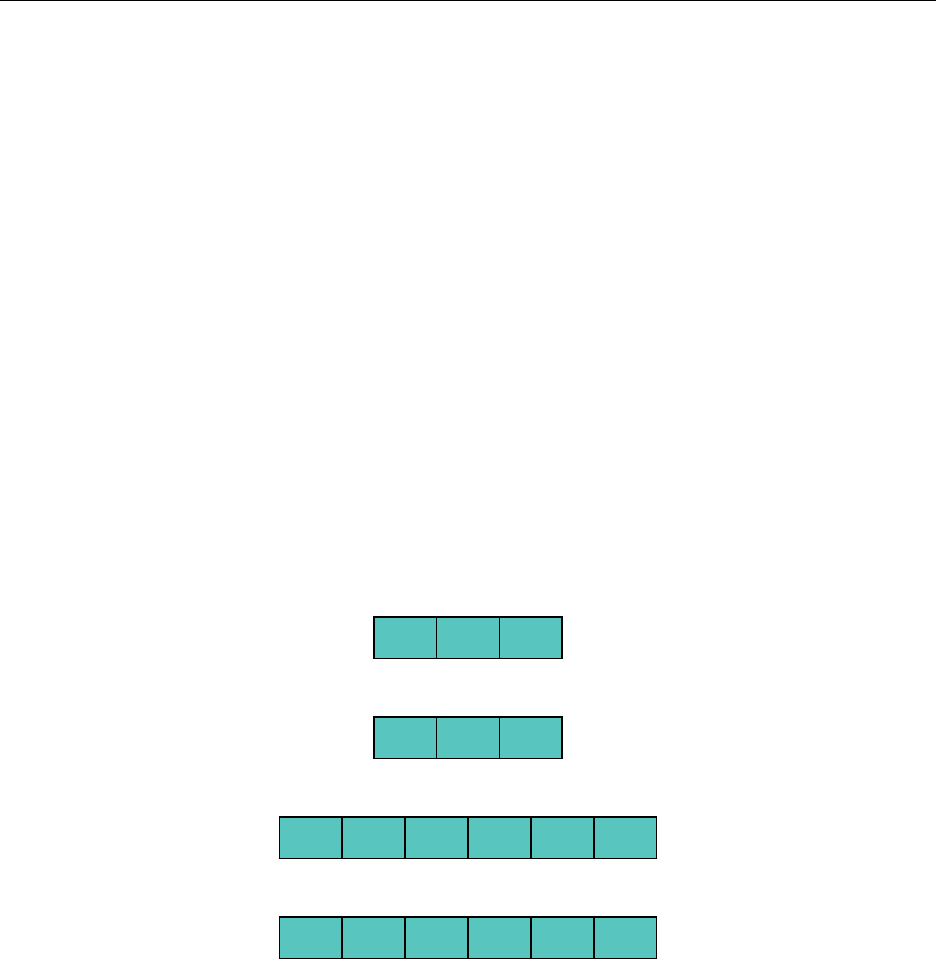
"a" "b" null
0 1 2
"a" "b" "c"
0 1 2
"a" "b" "c" null null null
0 1 2 3 4 5
"a" "b" "c" "d" null null
0 1 2 3 4 5
We see that there is still room in the array to add
"c"
, but to add more elements to the list, we
must use a new array with double the length.
It’s important to note that any given insertion to the structure is either
O
(
n
)or
O
(1), but there
is only one O(n)insertion for every O(n)O(1) insertions, so we still average out to constant time.
The Java implementation of a dynamic array is the
ArrayList
. The C++ implementation is
the vector.
For the following operations, think about how you would implement each and analyze its time
complexity.
16

Hsiang, Wei, Liu Chapter 3. Standard Library Data Structures
Function Java, ArrayList C++, vector
add an element to the end of
the list
boolean add(E e) void push_back(const
value_type& val)1
insert an element to a partic-
ular index in the list, shifting
all subsequent elements down
one index
void add(int index, E ele-
ment)
iterator insert(iterator
position, const
value_type& val)2
access the element stored at a
particular index
E get(int index) reference operator[]
(size_type n)3
update the value of the element
stored at a particular index to
a new element
E set(int index, E ele-
ment)
reference operator[]
(size_type n)
search whether the list con-
tains a particular element
boolean contains(Object
o)
iterator find (iterator
first, iterator last,
const value_type& val)4
remove the element at a par-
ticular index from the list
E remove(int index) iterator erase (iterator
position)
search for and remove a given
element from the list
boolean remove(Object o) use iterators
return the size of the list5int size() size_type size() const
Accessing and updating elements at particular indices are very nice. They are easy to code and run
in constant time. These are the bread and butter of any array. Adding at the end of the list is nice
as well. Checking whether some element is contained in the list is a pain, as it is
O
(
n
), and adding
to and removing from early in the list are more annoying.
3.2.2 Linked List
Arrays are nice for accessing, say, the seventh element in the list. We extend this to the dynamic
array to implement adding and removing elements to and from the end of the list nicely. Removing
elements from the beginning of the list, however, is cumbersome.
The linked list attempts to remedy this. It trades O(1) access to any element in the list for an
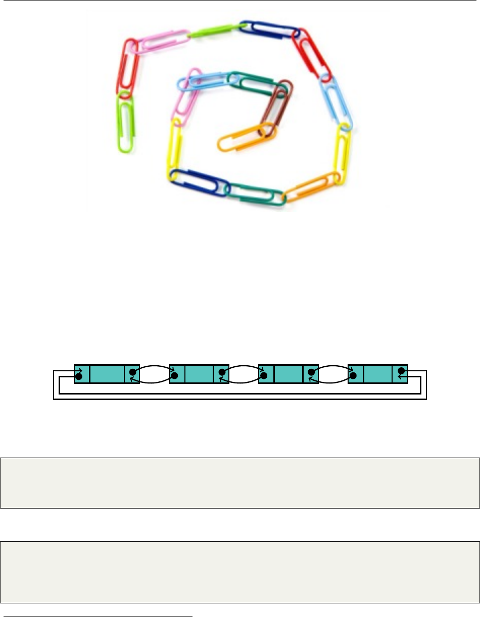
easier way to remove elements from either end of the list easily. Consider a chain of paper clips:
1& is a C++ reference
2
An iterator is like a pointer that allows for traversal of a data structure in a particular order. For example, we
can increment the iterator to access the next element in the list. An iterator is NOT merely an integer representing
the relative position in our list, as the in the Java implementation of add
3size_type
is, for our purposes,
unsigned int
, and
reference operator[]
makes this structure’s syntax more
like a normal array. In particular, to access the element at index
i
of a vector
v
, we simply use
v[i]
, and to update
an element, we use v[i] = val.
4This function is in <algorithm>.
5Note that the length of the list is not simply the size of the backing array.
17
Hsiang, Wei, Liu Chapter 3. Standard Library Data Structures
6
It’s easy to add or remove more paper clips from either end of the chain, and from any given
paper clip, it’s easy to access the paper clip directly previous or next to it in the chain. If we needed
the seventh paper clip in the chain, we’d need to manually count, an
O
(
n
)operation. However, if
we then needed to remove that paper clip from the chain, it wouldn’t be that hard, assuming we
kept a finger, or pointer, on the seventh paper clip.
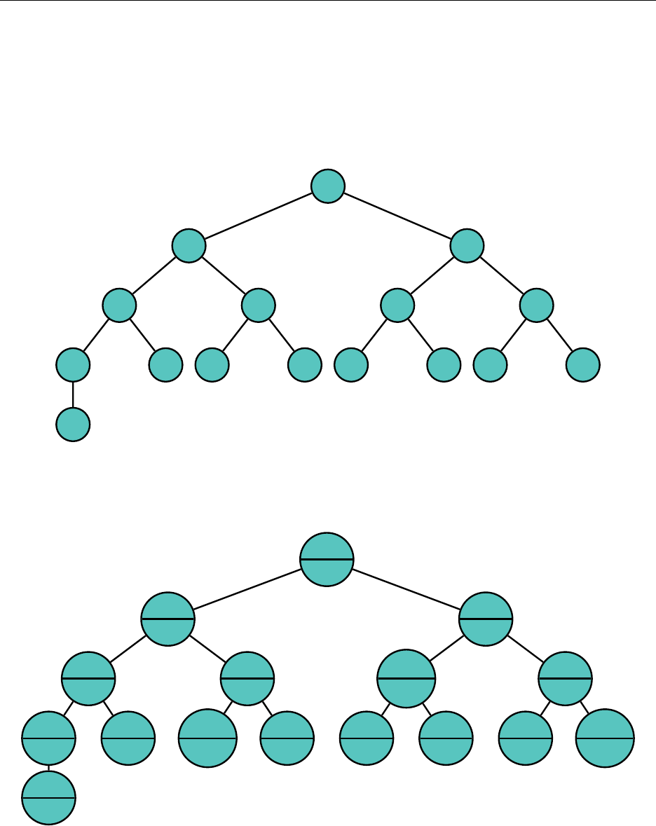
The best way to think about and implement a linked list is through a cyclical doubly-linked list,
with a dummy head. This means each element has its own node container, while the head of the list
is simply a node without an element. Such a data structure looks something like this:
null "a" "b" "c"
We see that each node maintains a pointer to its next neighbor and its previous neighbor, in
addition to containing the String it stores. We can store this data in a class like the following:
1class ListNode <E> {
2ListNode prev ,next;
3E s;
4}
If we were to insert an element after a ListNode a, it is necessary to update all pointers:
1ListNode <String >b=new ListNode <String >() ;
2b.prev =a;
3b.next =a.next;
4b.next.prev =b;
5a.next =b;
6http://img.thrfun.com/img/078/156/paper_clip_chain_s1.jpg
18

Hsiang, Wei, Liu Chapter 3. Standard Library Data Structures
Since the linked list is symmetric, inserting an element before a node is also easy. To add
something to the end of the list, simply add it before the dummy head. From here it should not be
too hard to implement all the important functions of a linked list.
The Java implementation of a linked list is
LinkedList
, and the C++ implementation is
list
.
A second C++ class that performs the same tasks but uses a backing array instead of a linked list
structure is the deque.
Function Java, LinkedList C++, list C++, deque
add an element to
the end
boolean add(E e) void push_back(const value_type& val)
insert7void add(int index, E
element)
iterator insert(iterator position, const
value_type& val)
access E get(int index) use iterators reference operator[]
(size_type n)
update E set(int index, E
element)
use iterators reference operator[]
(size_type n)
search boolean con-
tains(Object o)
iterator find (iterator first, iterator
last, const value_type& val)8
remove the ele-
ment at a partic-
ular index
E remove(int index) iterator erase (iterator position)
search for and re-
move a given ele-
ment
boolean re-
move(Object o)
void remove (const
value_type& val)
use iterators
size int size() size_type size() const
end operations addFirst
,
addLast
,
getFirst
,
getLast
,
removeFirst
,
remove-
Last
push_front,push_back,pop_front,pop_back
With a linked list implemented, two other data structures immediately follow.
3.3 Stack
Astack gets its name from being exactly that: a stack. If we have a stack of papers, we can push
things on the top and pop things off the top. Sometimes we peek at to access the element on top
7The index in a linked list is implicit.
8This function is in <algorithm>.
19

Hsiang, Wei, Liu Chapter 3. Standard Library Data Structures
but don’t actually remove anything. We never do anything with what’s on the bottom. This is
called LIFO: Last In, First Out.
Java implements the stack with Stack, C++ with stack.
Function Java, Stack C++, stack
push E push(E item) void push (const
value_type& val)
pop E poll() void pop()
top E peek() value_type& top()
size int size() size_type size() const
Java implements
Stack
using an array-like structure. This works just as well, and is faster in
practice, but I prefer the linked-list structure as a mathematical concept as it is more elegant in its
relationship with the queue and more easily customizable.
3.4 Queue
Aqueue is like a queue waiting in line for lunch. We push to the end and pop from the front.
Sometimes we peek at the front but don’t actually remove anything. The first person in line gets
served first. This is called FIFO: First In, First Out.
In Java, Queue is an interface, and in C++, the implementation of the queue is queue.
Function Java, Queue C++, queue
push boolean offer(E e) void push (const
value_type& val)
pop E poll() void pop()
top E peek() value_type& front()
size int size() size_type size() const
Since
Queue
is an interface in Java, we cannot instantiate a
Queue
, so the following statement is
illegal.
1Queue <String >q=new Queue <String >() ;
Instead, we must use LinkedList, so we do something like this:
1Queue <String >q=new LinkedList <String >() ;
This is legal because
LinkedList
implements
Queue
, making it the standard implementation of
the FIFO queue.
20
Hsiang, Wei, Liu Chapter 3. Standard Library Data Structures
3.5 Heap
Quite often a FIFO queue is not always desirable. For example, perhaps the string I want to remove
at every given point is the one that is lexicographically least.
A min heap is a tree such that every node is smaller than or equal to all of its children. A
max heap is a tree such that every node is larger than or equal to all of its children. Pictured is a
complete binary min heap, which will be of use to us.
"a"
"b"
"c"
"e"
"f"
"m"
"n"
"p" "o"
"d"
"g"
"i" "l"
"h"
"k" "j"
We see that the root of the tree will always be the smallest element. It is tempting to use a
container class with a pointer to its left and its right child. However, we have a much nicer way to
store complete binary trees with an array. Consider the following numbering of the nodes:
1
"a"
2
"b"
4
"c"
8
"e"
16
"f"
9
"m"
5
"n"
10
"p"
11
"o"
3
"d"
6
"g"
12
"i"
13
"l"
7
"h"
14
"k"
15
"j"
We see that every number from 1 to 16 is used, and for every node, if the index associated with
it is
i
, the left child is 2
i
, and the right child is 2
i
+ 1. This leads to a very natural implementation
of the tree in an array:
21
Hsiang, Wei, Liu Chapter 3. Standard Library Data Structures
null "a" "b" "d" "c" "n" "g" "h" "e" "m" "p" "o" "i" "l" "k" "j" "f"
0 1 2 3 4 5 6 7 8 9 10 11 12 13 14 15 16
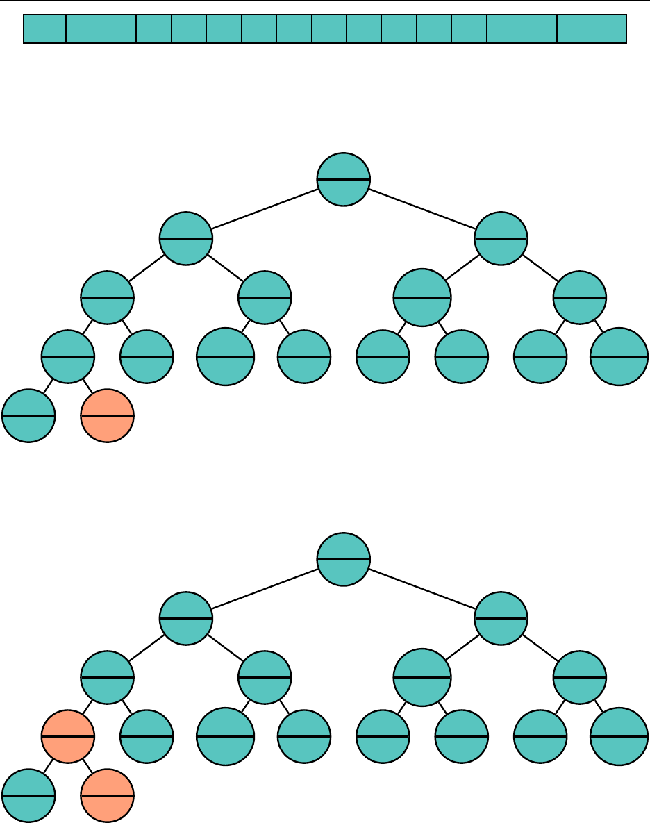
How do we add elements to our heap, while maintaining the heap qualities? Well, let’s just add
it to the very end and see what we get. Suppose we are to add "b" to the tree.
1
"a"
2
"b"
4
"c"
8
"e"
16
"f"
17
"b"
9
"m"
5
"n"
10
"p"
11
"o"
3
"d"
6
"g"
12
"i"
13
"l"
7
"h"
14
"k"
15
"j"
Well,
"b"
comes before
"e"
in the alphabet, so let’s swap the nodes. We are guaranteed that
"b" should come before the other child (in this case, "f") by the transitive property.
1
"a"
2
"b"
4
"c"
8
"b"
16
"f"
17
"e"
9
"m"
5
"n"
10
"p"
11
"o"
3
"d"
6
"g"
12
"i"
13
"l"
7
"h"
14
"k"
15
"j"
One more swap...
22
Hsiang, Wei, Liu Chapter 3. Standard Library Data Structures
1
"a"
2
"b"
4
"b"
8
"c"
16
"f"
17
"e"
9
"m"
5
"n"
10
"p"
11
"o"
3
"d"
6
"g"
12
"i"
13
"l"
7
"h"
14
"k"
15
"j"
And now we have the heap property restored. As the tree has depth at most
log n
, this process
is O(log n).
To remove the root from the heap, we replace the root with the last leaf:
1
"e"
2
"b"
4
"b"
8
"c"
16
"f"
9
"m"
5
"n"
10
"p"
11
"o"
3
"d"
6
"g"
12
"i"
13
"l"
7
"h"
14
"k"
15
"j"
17
"a"
We perform a series of swaps to restore the heap property. We always want to choose the smaller
child to swap until the heap property is satisfied.
23
Hsiang, Wei, Liu Chapter 3. Standard Library Data Structures
1
"b"
2
"e"
4
"b"
8
"c"
16
"f"
9
"m"
5
"n"
10
"p"
11
"o"
3
"d"
6
"g"
12
"i"
13
"l"
7
"h"
14
"k"
15
"j"
17
"a"
1
"b"
2
"b"
4
"e"
8
"c"
16
"f"
9
"m"
5
"n"
10
"p"
11
"o"
3
"d"
6
"g"
12
"i"
13
"l"
7
"h"
14
"k"
15
"j"
17
"a"
1
"b"
2
"b"
4
"c"
8
"e"
16
"f"
9
"m"
5
"n"
10
"p"
11
"o"
3
"d"
6
"g"
12
"i"
13
"l"
7
"h"
14
"k"
15
"j"
17
"a"
And we are done. Once again, this takes at most
log
(
N
)swaps. This idea can be extended to
removing or changing the value of any node we’d like from a tree – this is particularly useful for
Dijkstra later.
24
Hsiang, Wei, Liu Chapter 3. Standard Library Data Structures
Remember to implement your heap in an array-like structure!
Java implements a min heap with the
PriorityQueue
. This class, like
LinkedList
, also
implements
Queue
. C++ implements a max
9
heap with the
priority_queue
. The functions for
heaps in both languages are nearly identical to those for queues.
Function Java, PriorityQueue C++, priority_queue
push boolean offer(E e) void push (const
value_type& val)
pop E poll() void pop()
top E peek() value_type& top()
size int size() size_type size() const
3.6 Set
Aset is a collection of objects with no duplicate elements. Note that the data structures discussed
in this section can be extended to become multisets, but Java and C++ implementations of these
explicitly disallow multiplicity.
3.6.1 Binary Search Tree
Abinary search tree (BST) is a tree where every node is greater than every node in its left subtree
and less than every node in its right subtree. As with a heap, to use a BST, we need to impose
some kind of ordering on the elements stored.
"m"
"g"
"c"
"b"
"a"
"e"
"j"
"h" "k"
"t"
"r"
"s"
9Don’t forget that C++ implements a max heap, ever.
25
Hsiang, Wei, Liu Chapter 3. Standard Library Data Structures
The tree need not be complete, unlike the heap. Because it is not guaranteed to be complete,
there is no way to nicely bound the size of the array we would need if we were to use the same
storage method as with the heap. Thus, we are forced to use a
TreeNode
, with left and right
pointers. This is also problematic when determining guarantees on time complexities later, but the
ways to solve this problem are pretty complicated so we’ll ignore them for now.
Given the name of the tree, searching for an element within the tree is quite natural, and similar
to a binary search. Compare the element to be searched for with the current node. If they are
equal, we are done; otherwise, search the appropriate left or right subtree. As with most structures
and algorithms with a binary search structure, this operation lends itself nicely to recursion. If the
tree is reasonably nice, we expect to complete this in
O
(
log n
)time, but searching can be as bad as
linear if the tree looks like a linked list.
Adding an element is also natural. As our tree represents a set, it will not contain the same
element twice. We trace down until we hit a null pointer, and add the element in the appropriate
spot. Let’s add a "p" to the BST:
"m"
"g"
"c"
"b"
"a"
"e"
"j"
"h" "k"
"t"
"r"
"p" "s"
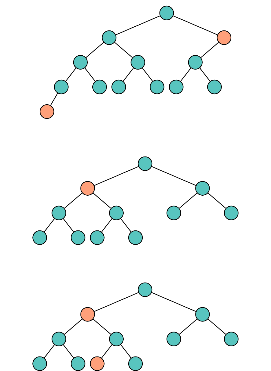
Deleting an element is the annoying part. Unfortunately, there’s not much we can do besides
casework.
Removing a leaf, like
"a"
, from the tree is very easy. Removing a node with only once child, like
"t", is also relatively straightforward.
26
Hsiang, Wei, Liu Chapter 3. Standard Library Data Structures
"m"
"g"
"c"
"b"
"a"
"e"
"j"
"h" "k"
"t"
"r"
"p" "s"
Now, removing an element with two children is tricky. We’ll try to remove
"g"
. Consider the
least element in the right subtree of
"g"
, which in this case is
"h"
. We find
"h"
by always choosing
the left child on the right subtree until we cannot go any further. This must be the least element.
"m"
"g"
"c"
"b" "e"
"j"
"h" "k"
"r"
"p" "s"
Note that
"h"
has either no children or only one child, and that nodes like these are easy to
remove. We then change the value of the node containing
"g"
to
"h"
, which is legal since
"h"
is the
least element, and remove "h" from the right subtree, and we are done.
"m"
"h"
"c"
"b" "e"
"j"
"h" "k"
"r"
"p" "s"
27
Hsiang, Wei, Liu Chapter 3. Standard Library Data Structures
"m"
"h"
"c"
"b" "e"
"j"
"k"
"r"
"p" "s"
Since a BST is ordered, iterating over it from left to right will pass over every element in sorted
order.
A standard BST has
O
(
log n
)operations if the tree is “nice,” or sufficiently randomized, but
each operation can be
O
(
n
)in the worst case. We need to find a way to automatically balance the
BST such that we avoid linear time complexities.
A red-black tree is a self-balancing BST that guarantees
O
(
log n
)operations by making sure
the height of the tree grows logarithmically. It is implemented in Java’s
TreeSet
and is usually
10
implemented in the C++ set, so while the simple BST I described above does not guarantee nice
time bounds, Java’s implementation does.
I don’t think learning exactly how a red-black tree works is particularly useful for the beginning
programmer or a competitive programmer. How exactly a red-black tree works, together with some
more balanced binary search trees which are useful on the competitive scene, are covered in a later
chapter.
Function Java, TreeSet C++, set
insert boolean add(E e) void insert (const
value_type& val)
search boolean contains(Object
o)
size_type count (const
value_type& val) const11
delete boolean remove(Object o) size_type erase (const
value_type& val)
,
void
erase (iterator position)
size int size() size_type size() const
other useful search functions first
,
last
,
ceiling
,
floor
,
higher,lower
begin
,
end
,
lower_bound12
,
upper_bound13,find
10Implementations of set must be some kind of balanced binary search tree, but need not be red-black.
111 if in the set, 0 otherwise.
12lower_bound is similar to Java’s ceiling
13upper_bound is similar to Java’s higher
28

Hsiang, Wei, Liu Chapter 3. Standard Library Data Structures
3.6.2 Hash Table
The fastest way to store values in a collection is through an array structure. Unfortunately, searching
an array for a specific value is very costly. The binary search tree provided a quick way to search
for a value by imposing constraints on its placement based on characteristics of the value. Similarly,
to find a specific value in an array, we need to impose constraints on what index the value is placed
in based on the value itself.
Suppose, for instance, I wanted to store some set of numbers from 0 to 999. I want to quickly
add a new number to our set, remove a number, or check if a number is in our set. The easiest way
to do this is to maintain a size-1000 array of boolean values. If a number
i
is in our set, we set the
ith index in our array to true. We then have O(1) updates and queries for our set.
To extend this to other values, we define the hash function. The hash function operates on the
object and returns something that characterizes that object. For example, for a string, a possible
hash could be the length of the string or the sum of the characters. We want to map an object with
an integer hash, so that we can store the values by their hashes in an array. The resulting structure
is a hash table.
What characterizes a good hash function?
1.
If two objects are considered equal, like the strings
"Hello"
and
"Hello"
, their hashes must
be equal.
2.
If two objects are not equal, like the strings
"Hello"
and
"Bye"
, their hashes are only equal
with very low probability. A collision is when two different objects have the same hash. We
want to minimize the probability of this happening. As a result, hashes like the length of the
string are not very good hashes.
3.
A good hash should be reasonably fast to compute. One main purpose of hashing is to make
equality checks between objects fast. A hash function that is hard to compute defeats the
purpose of this.
Every Java
Object
supports the
hashCode()
function. By default,
hashCode()
stores informa-
tion about the memory address of the
Object
. When we implement a new class, we can override
this function. For example, let us define the following polynomial hash for strings:
1public int ha s h C o d e () {
2int hash = 0;
3for (int k= 0; k<length() ; k++) {
4hash *= 31;
5hash += ( int ) ( charAt(k));
6}
7return hash;
8}
In Java,
a.equals(b)
should imply
a.hashCode() == b.hashCode()
. This function produces
the same result as the actual
hashCode()
function in the String class. However, this is not quite
what we want for our hash set implementation, because in the end we wish to be able to store the
objects in some kind of array. Since
hashCode()
can be any
int
, this hash not only returns integers
29
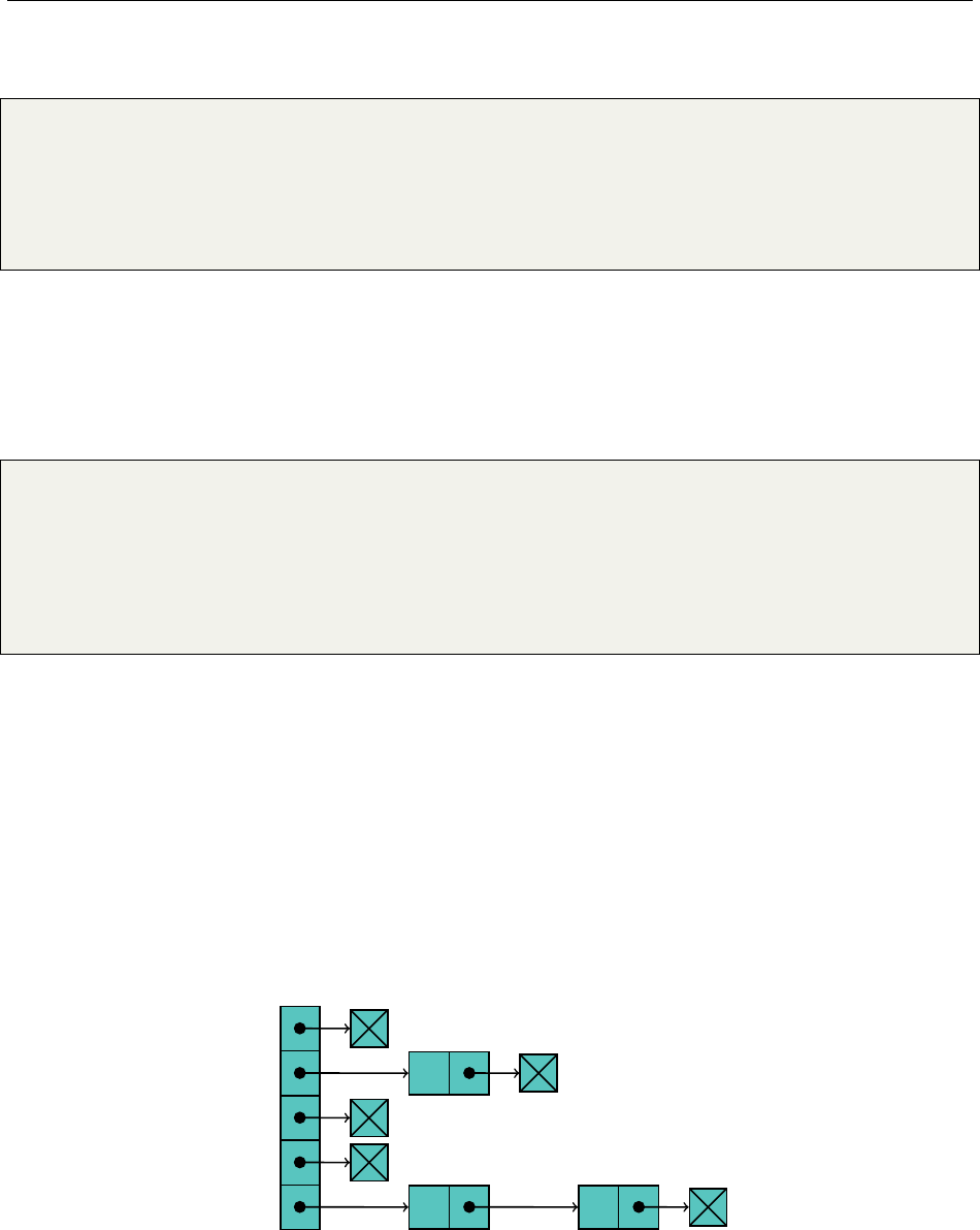
Hsiang, Wei, Liu Chapter 3. Standard Library Data Structures
that can be very large, they can also be negative, and thus are not suitable as array indices. The
natural way to fix this is to take the hash modulo the size of the array we want.
1String[] table =new String[10007];
2int inde x (E o) {
3int i=o.hashCode() % table .length;
4if (i>= 0)
5return i;
6return i+tabl e .length;
7}
The length of our array is somewhat arbitrary. We chose the number 100007 because it is a
prime number, and primes are generally nice since integers modulo a prime form a field. Remember
that a negative number
%
another number is not necessarily positive, so we need to be a little careful.
From here, adding an element to the table and checking if an element is contained both seem
straightforward:
1boolean add (E o ) {
2tabl e [index (o)]=o;
3return tru e ;
4}
5boolean contains (Object o) {
6int i=index (( E)o) ;
7return tabl e [i] != null && table [i]. equals(o) ;
8}
null is always annoying to deal with, and will always have to be handled separately.
However, a problem quickly arises in the (hopefully unlikely) instance of a collision. If two
strings have the same hash, we can’t add both to the table since there isn’t enough space in the
array. The easiest way to handle a collision is by chaining. We change the hash table to store a
linked list instead of a single element in the event of a collision. The hope is that not too many
objects map to a single index in the array, as searching a linked list for a particular element is
O
(
n
).
Java once implemented this method of resolving collisions, but recently changed it to a BST in Java
8.
Here’s an example of chaining on a small array of size 5 with the characters for “cow”. The
numbers below the letters represent their hashes. cand wcollide.
0
1
2
3
4
o
111
c
99
w
119
If we use a good hash function and a reasonable array size, collisions will almost always be
30
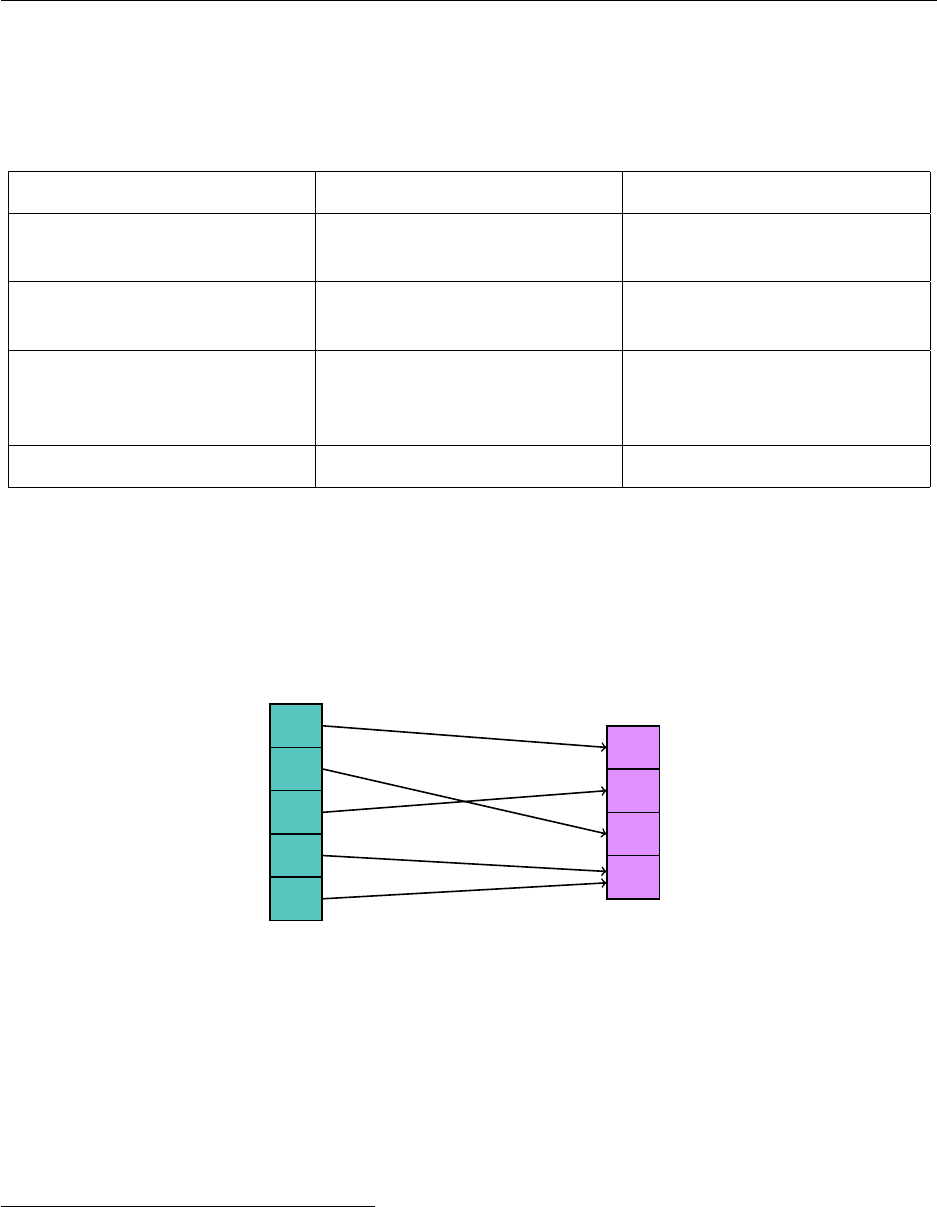
Hsiang, Wei, Liu Chapter 3. Standard Library Data Structures
pretty evenly spread across the array. Then, since we store everything using an array, the hash
table provides probabilistic O(1) time complexities for insertion, deletion, and search.
The Java set implementation of a hash table is the
HashSet
. The C++11
14
set implementation
of a hash table is the unordered_set.
Function Java, HashSet C++11, unordered_set
insert boolean add(E e) void insert (const
value_type& val)
search boolean contains(Object
o)
size_type count (const
value_type& val) const15
delete boolean remove(Object o) size_type erase (const
value_type& val)
,
void
erase (iterator position)
size int size() size_type size() const
3.7 Map
Amap is simply a function that takes a key to a value. As a map is a function, its domain, or the
keys of the map, form a set, though the values need not be unique. The most generic function looks
something like in the following diagram conceptually.
"a"
"c"
"d"
"f"
"g"
5
3
6
2
keys values
In implementation, a map is very similar to a set. Since the map represents a function from the
set of keys to the set of values, we want to support quick lookup and updates of the keys so we can
evaluate and change the function represented by our map. The best ways to store a set for quick
access and update are, as discussed in the previous section, the binary search tree and the hash
table, so all we need to store is the set of keys itself with extra information for the value associated
attached.
In a binary search tree map, the elements are sorted by the keys.
14added recently; not included in C++
151 if in the set, 0 otherwise.
31
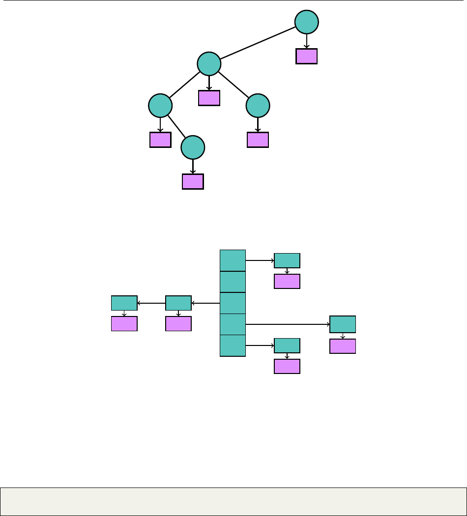
Hsiang, Wei, Liu Chapter 3. Standard Library Data Structures
"g"
"d"
"a"
"c"
"f"
5
6
3
2
2
Similarly, for the hash table map, we use the hashes of the keys.
0
1
2
3
4
"d"
100
3
"a"
97
5
"f"
102
2"g"
103
2
"c"
99
6
Map
is a Java interface. The
TreeMap
is the
Map
variant of the
TreeSet
; similarly, the
HashMap
is the
Map
variant of the
HashSet
.
map
is the C++ implementation of a balanced binary search tree
map, while unordered_map is the C++11 implementation of a hash table.
As a map involves two kinds of data, keys and values, generics for maps therefore have two
arguments, one for the key and one for the value. The following Java
Map
from
String
s to
Integer
s
demonstrates generics with multiple arguments.
1Map <String ,Integer >number =new TreeMap <String ,Integer >() ;
2emai l .put("Samuel Hsiang", 5) ;
32

Hsiang, Wei, Liu Chapter 3. Standard Library Data Structures
Function Java, TreeMap C++, map
insert and update value V put(K key, V value) mapped_type& operator[]
(const key_type& k)16
access V get(Object key) mapped_type& operator[]
(const key_type& k)
delete V remove(Object key) size_type erase (const
key_type& val)
,
void erase
(iterator position)
size int size() size_type size() const
set of keys Set<K> keySet() no implementation
other useful search functions just look in the API >.<
Function Java, HashMap C++11, unordered_map
insert and update value V put(K key, V value) mapped_type& operator[]
(const key_type& k)
access V get(Object key) mapped_type& operator[]
(const key_type& k)
delete V remove(Object key) size_type erase (const
key_type& val)
,
void erase
(iterator position)
size int size() size_type size() const
set of keys Set<K> keySet() no implementation
16Works like an array or vector.
33
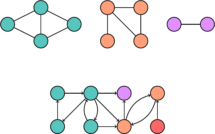
Chapter 4
Graph Algorithms
In this chapter we explore some of the most famous results in graph theory.
4.1 Connected Components
Aconnected component of an undirected graph is a subgraph such that, for any two vertices in
the component, there exists a path from one to the other. The diagram illustrates three connected
components of a graph, where each vertex is colored together with its associated component.
1
2
3
4
5
6 7
8
9 10
Astrongly connected component of a directed graph is a subgraph such that every vertex in the
component can be reached from any other vertex in the component.
5678
1234
Finding the connected components of an undirected graph is a straightforward problem, while
finding the strongly connected components of a directed graph is more complicated and won’t be
covered in this chapter.
35
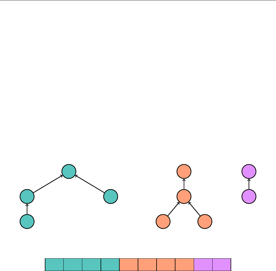
Hsiang, Wei, Liu Chapter 4. Graph Algorithms
4.1.1 Flood Fill
Really any kind of search method solves the undirected graph connected components problem. We
could use recursion with a depth-first search. To avoid using the run-time stack, we could use a
queue to perform a breadth-first search. Both of these run in
O
(
E
+
V
)time. I would recommend
in general to use the BFS.
4.1.2 Union-Find (Disjoint Set Union)
The union-find data structure is another way for us to solve the connected components problem.
Union-find is unique from the other search techniques in that it can process input as it is presented,
edge by edge. This also means it is possible to add more edges at the end, therefore changing the
graph, while still running quickly. An algorithm that works like this is an online algorithm, while
an algorithm that requires all the input data presented at the beginning is an offline algorithm.
A natural idea for solving the connected components problem is for each vertex to maintain a
pointer to another vertex it’s connected to, forming a forest, or collection of trees. To check whether
two elements are in the same component, simply trace the tree up to the root by jumping up each
pointer.
5
6
7 8
1
2
4
3
9
10
The idea of a pointer can easily be stored within an array.
-1 1 1 2 -1 5 6 6 -1 9
1 2 3 4 5 6 7 8 9 10
We want to support two operations:
find
(
v
), which returns the root of the tree containing
v
,
and
union
(
u, v
), which merges the components containing
u
and
v
. This second operation is easy
given the first; simply set the pointer of find(u)to be find(v).
union(4,6), unoptimized:
36
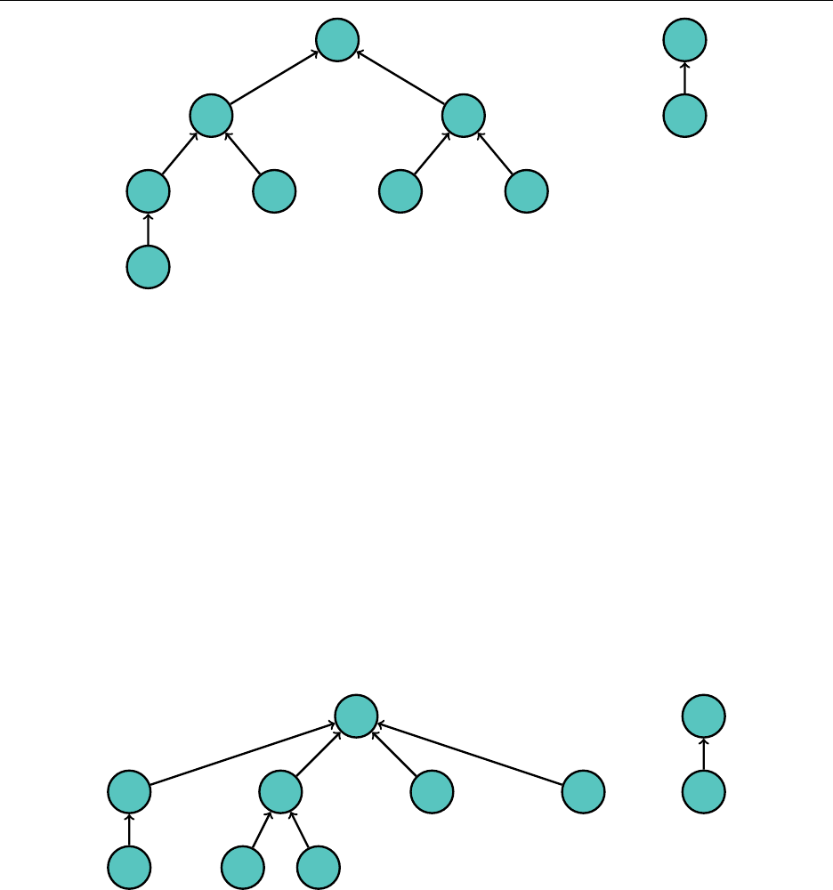
Hsiang, Wei, Liu Chapter 4. Graph Algorithms
5
1
2
4
3
6
7 8
9
10
A problem quickly arises – the
find
operation threatens to become linear. There are two simple
things we can do to optimize this.
The first is to always add the shorter tree to the taller tree, as we want to minimize the maximum
height. An easy heuristic for the height of the tree is simply the number of elements in that tree.
We can keep track of the size of the tree with a second array. This heuristic is obviously not perfect,
as a larger tree can be shorter than a smaller tree, but it turns out with our second optimization
that this problem doesn’t matter.
The second fix is to simply assign the pointer associated with
v
to be
find
(
v
)at the end of the
find
operation. We can design
find
(
v
)to recursively call
find
on the pointer associated with
v
, so
this fix sets pointers associated with nodes along the entire chain from
v
to
find
(
v
)to be
find
(
v
).
These two optimizations combined make the
union
and
find
operations
O
(
α
(
V
)), where
α
(
n
)is
the inverse Ackermann function, and for all practical values of n,α(n)<5.
find(4), optimized:
5
1
3
6
7 8
2 4
9
10
37

Hsiang, Wei, Liu Chapter 4. Graph Algorithms
Algorithm 1 Union-Find
function Find(v)
if vis the root then
return v
parent(v)←Find(parent(v))
return parent(v)
function Union(u,v)
uRoot ←Find(u)
vRoot ←Find(v)
if uRoot =vRoot then
return
if size(uRoot)< size(vRoot)then
parent(uRoot)←vRoot
size(vRoot)←size(uRoot) + size(vRoot)
else
parent(vRoot)←uRoot
size(uRoot)←size(uRoot) + size(vRoot)
4.2 Shortest Path
A classic. Assign nonnegative weights to each of the edges, where the weight of the edge (
u, v
)
represents the distance from uto v. This graph can be either directed or undirected.
4.2.1 Dijkstra
Dijkstra’s algorithm solves the single-source shortest path problem. From any vertex, we can
compute the shortest path to each of the remaining vertices in the graph. The two formulations of
Dijkstra’s algorithm run in
O
(
V2
)or
O
(
Elog V
)time, whichever one suits us better. Note that it
is possible to do better than
O
(
Elog V
)using a Fibonacci heap. The former works nicely on dense
graphs, as E≈V2, while the latter works better on sparse graphs, as E≈V.
For every vertex
v
in the graph, we keep track of the shortest known distance
dist
(
v
)from the
source to
v
, a boolean
visited
(
v
)to keep track of which nodes we “visited,” and a pointer to the
previous node in the shortest known path prev(v)so that we can trace the shortest path once the
algorithm finishes.
Dijkstra iteratively “visits” the next nearest vertex, updating the distances to that vertex’s
neighbors if necessary. Therefore, at any step, we have the first however-many nearest vertices to
the source, which we call “visited” and for which the shortest path is known. We also have the
shortest path to all the remaining vertices that stays within the “visited” vertices besides for the
very last edge, if such a path exists. We claim that the known distance to the closest vertex that
has not yet been visited is the shortest distance. We can then “visit” that vertex. It shouldn’t be
hard to prove that this algorithm indeed calculates the shortest path.
The O(V2)implementation immediately follows.
38
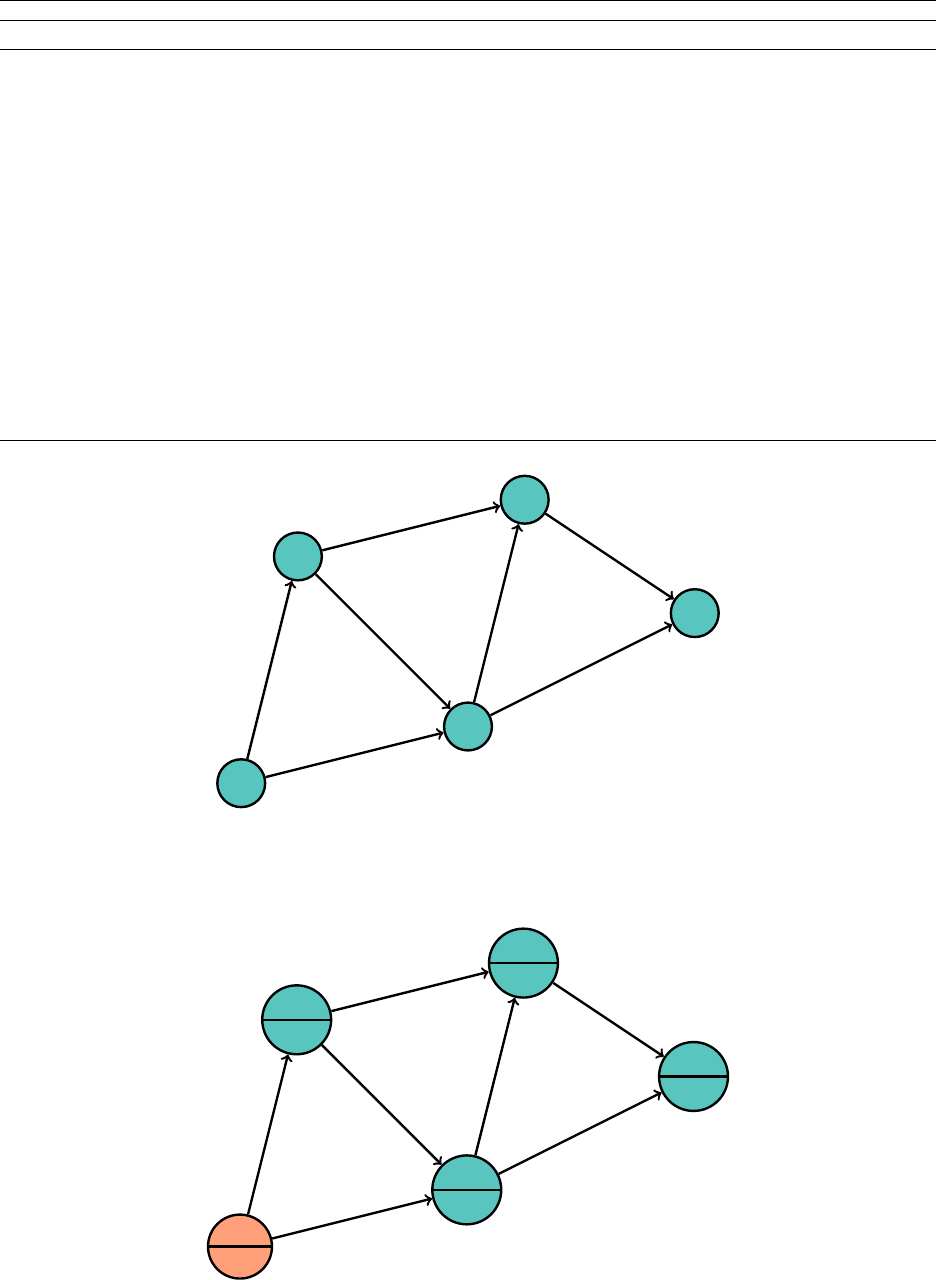
Hsiang, Wei, Liu Chapter 4. Graph Algorithms
Algorithm 2 Dijkstra
for all vertices vdo
dist(v)← ∞
visited(v)←0
prev(v)← −1
dist(src)←0
while ∃vs.t. visited(v)=0do
v≡vs.t. visited(v)=0with min dist(v)
visited(v)←1
for all neighbors uof vdo
if visited(u)=0then
alt ←dist(v) + weight(v, u)
if alt < dist(u)then
dist(u)←alt
prev(u)←v
1
2
3
4
5
4
2
7
6
3
5
4
Let’s run Dijkstra’s algorithm on the above graph with vertex 1 as the source. We first set all
the distances besides the source to be ∞.
1
0
2
∞
3
∞
4
∞
5
∞
4
2
7
6
3
5
4
39
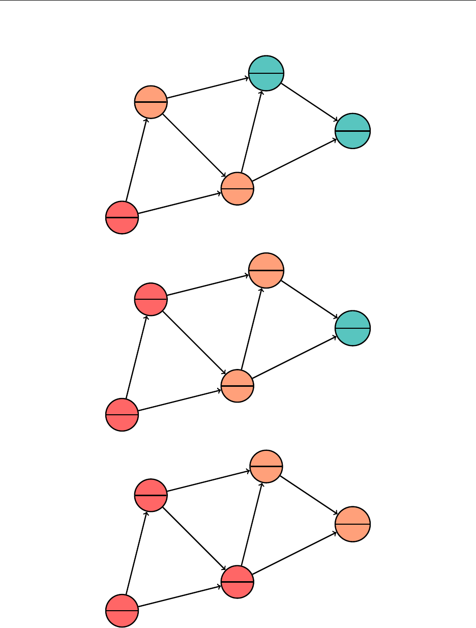
Hsiang, Wei, Liu Chapter 4. Graph Algorithms
Now, we continue choosing the closest unvisited node, mark it as visited, and and update its
neighbors.
1
0
2
4
3
7
4
∞
5
∞
4
2
7
6
3
5
4
1
0
2
4
3
6
4
10
5
∞
4
2
7
6
3
5
4
1
0
2
4
3
6
4
9
5
14
4
2
7
6
3
5
4
40
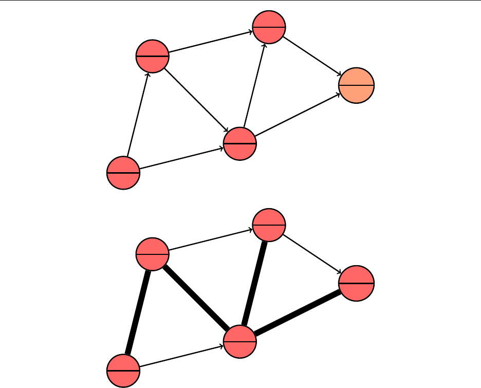
Hsiang, Wei, Liu Chapter 4. Graph Algorithms
1
0
2
4
3
6
4
9
5
14
4
2
7
6
3
5
4
1
0
2
4
3
6
4
9
5
14
4
2
7
6
3
5
4
The slow part of the
O
(
V2
)formulation is the linear search for the vertex
v
with the minimum
dist
(
v
). We happen to have a data structure that resolves this problem – a binary heap. The main
problem with using the standard library heap is having repeated vertices in the heap. We could just
ignore this problem and discard visited vertices as they come out of the heap. Alternatively, we
could choose never to have repeated vertices in the heap. To do this, we need to be able to change
the value of the distances once they are already in the heap, or decrease-key. This is a pretty simple
function to add, however, if you have a heap already coded. Either way, we achieve
O
(
Elog V
), as
we do E+Vupdates to our heap, each costing O(V).
4.2.2 Floyd-Warshall
Dijkstra is nice when we are dealing with edges with nonnegative weights and are looking for the
distances from one vertex to all the others. Floyd-Warshall solves the shortest path problem for all
pairs of vertices in
O
(
V3
)time, which is faster than
V
single-source Dijkstra runs on a dense graph.
Floyd-Warshall works even if some edge weights are negative but not if the graph has a negative
cycle.
41

Hsiang, Wei, Liu Chapter 4. Graph Algorithms
Algorithm 3 Floyd-Warshall
for all vertices vdo
dist(v, v)=0
for all edges (u, v)do
dist(u, v) = weight(u, v)
for all vertices kdo
for all vertices ido
for all vertices jdo
if dist(i, j)> dist(i, k) + dist(k, j)then
dist(i, j)←dist(i, k) + dist(k, j)
4.2.3 Bellman-Ford
Bellman-Ford is a single-source
O
(
V E
)shortest path algorithm that works when edge weights can
be negative. It is preferable to Floyd-Warshall when the graph is sparse and we only need the
answer for one source. Like Floyd-Warshall, the algorithm fails if the graph contains a negative
cycle, but the algorithm is still useful for detecting negative cycles.
The idea here is the shortest path, assuming no negative cycles, has length at most V−1.
Algorithm 4 Bellman-Ford
for all vertices vdo
dist(v)← ∞
prev(v) =← −1
dist(src)←0
for i≡1, V −1do
for all edges (u, v)do
if dist(u) + weight(u, v)< dist(v)then
dist(v)←dist(u) + weight(u, v)
prev(v)←u
for all edges (u, v)do check for negative cycles
if dist(u) + weight(u, v)< dist(v)then
negative cycle detected
4.3 Minimum Spanning Tree
Consider a connected, undirected graph. A spanning tree is a subgraph that is a tree and contains
every vertex in the original graph. A minimum spanning tree is a spanning tree such that the sum
of the edge weights of the tree is minimized. Finding the minimum spanning tree uses many of the
same ideas discussed earlier.
42
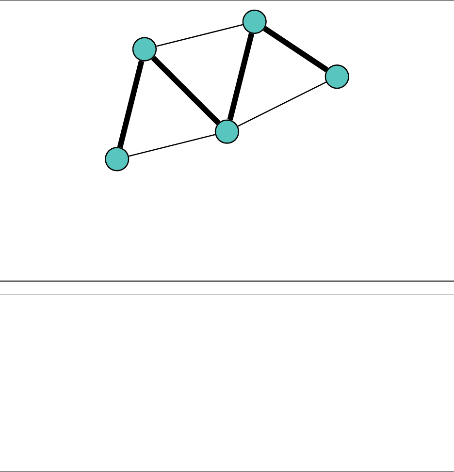
Hsiang, Wei, Liu Chapter 4. Graph Algorithms
1
2
3
4
5
4
2
7
6
3
5
4
4.3.1 Prim
Prim’s algorithm for finding the minimum spanning tree is very similar to Dijkstra’s algorithm
for finding the shortest path. Like Dijkstra, it iteratively adds a new vertex at a time to build a
tree. The only difference is
dist
(
v
)stores the shortest distance from any visited node instead of the
source.
Algorithm 5 Prim
for all vertices vdo
dist(v)← ∞
visited(v)←0
prev(v)← −1
dist(src)←0
while ∃vs.t. visited(v)=0do
v≡vs.t. visited(v)=0with min dist(v)
visited(v)←1
for all neighbors uof vdo
if visited(u)=0then
if weight(v, u)< dist(u)then
dist(u)←weight(v, u)
prev(u)←v
The proof of correctness is left as an exercise. The complexity of this algorithm depends on how
the minimum unvisited vertex is calculated. Using the same approaches as Dijkstra, we can achieve
O(V2)or O(Elog V).
4.3.2 Kruskal
While Prim greedily adds vertices to the tree, Kruskal’s algorithm greedily adds edges. It iterates
over all the edges, sorted by weight. We need to watch out for adding a cycle, breaking the tree
structure, which means we need to keep track of each vertex’s connected component. If an edge
43

Hsiang, Wei, Liu Chapter 4. Graph Algorithms
connects two vertices from the same connected component, we don’t want to add it to our tree.
However, we have a union-find algorithm that works perfectly for this.
Algorithm 6 Kruskal
for all edges (u, v)in sorted order do
if Find(u)6=Find(v)then
add (u, v)to spanning tree
Union(u, v)
This algorithm requires a sort of the edges and thus has complexity O(Elog E) = O(Elog V).
4.4 Eulerian Tour
An Eulerian tour of a graph is a path that traverses every edge exactly once. If the tour ends exactly
where it started, it is called an Eulerian circuit. A graph has an Eulerian circuit if it is connected
and every vertex has even degree. A graph has an Eulerian path if it is connected and all vertices
but exactly two have even degrees. The mathematical proofs for these graph properties hinge on
the idea that removing a cycle from the graph maintains the Eulerian property. We construct an
Eulerian tour by appealing to this idea.
Algorithm 7 Eulerian Tour
function FindTour(v)
while vhas a neighbor udo
delete edge (v, u)
FindTour(u)FindTour(u) must trace a circuit back to v
add vto tour
It is not preferable to use the run-time stack; we can use our own stack if necessary.
If the graph contains an Eulerian circuit, we call this function on any vertex we like. If it
contains an Eulerian path, we call this function on one of the vertices with odd degree.
44
Chapter 5
Complex Ideas and Data Structures
Here we build on previous material to introduce more complex ideas that are useful for solving
USACO Gold problems and beyond.
5.1 Dynamic Programming over Subsets (n2nDP)
We’ve already covered how dynamic programming can turn exponential solutions into polynomial
solutions, but it can also help turn factorial solutions into exponential. Problems where the bound
on
n
is 20, for example, signal that an exponential solution is the one required. Consider the
following problem:
(USACO December 2014, guard) Farmer John and his herd are playing frisbee. Bessie throws
the frisbee down the field, but it’s going straight to Mark the field hand on the other team! Mark
has height
H
(1
≤H≤
1
,
000
,
000
,
000), but there are
N
cows on Bessie’s team gathered around
Mark (2
≤N≤
20). They can only catch the frisbee if they can stack up to be at least as high
as Mark. Each of the
N
cows has a height, weight, and strength. A cow’s strength indicates the
maximum amount of total weight of the cows that can be stacked above her.
Given these constraints, Bessie wants to know if it is possible for her team to build a tall enough
stack to catch the frisbee, and if so, what is the maximum safety factor of such a stack. The safety
factor of a stack is the amount of weight that can be added to the top of the stack without exceeding
any cow’s strength.
We can try the
O
(
N
!) brute force, trying every permutation of cows possible. However, this is
far too slow.
N≤
20 hints at an exponential solution, so we think of trying every possible subset of
the cows. Given a subset
S
of cows, the height reached is the same, so perhaps we sort the subset by
strength, and put the strongest cow on the bottom. We see that this greedy approach fails: suppose
that the first cow has weight 1 and strength 3 and the second cow has weight 4 and strength 2.
Greedy would tell us to put the first cow on the bottom, but this fails, while putting the second cow
on the bottom succeeds.
When greedy fails, the next strategy we look at is dynamic programming. To decide whether
S
is stable, we have to find whether there exists a cow
j
in
S
that can support the weight of all the
other cows in
S
. But how do we know whether the set
S\ {j}
is stable? This is where dynamic
programming comes in.
45
Hsiang, Wei, Liu Chapter 5. Complex Ideas and Data Structures
This leads to a
O
(
N
2
N
)solution. This seems like a pain to code iteratively, but there is a nice
fact about subsets: there is a cute bijection from the subsets of {0,1,2, . . . , N −1}to the integers
from 0 to 2
N−
1. That is, the subset
{
0
,
2
,
5
,
7
}
maps to 2
0
+ 2
2
+ 2
5
+ 2
7
= 165 in the bijection. We
call this technique masking. We require all the subsets of
S
to be processed before
S
is processed,
but that property is also handled by our bijection, since subtracting a power of 2 from a number
decreases it. With a little knowledge of bit operators, this can be handled easily.
for i←0,2N−1do i represents the subset S
dp(i)← −1
for all j∈Sdo j ∈Ssatisfy i&(1«j)!=0
alt ←min(dp(i−2j), strength(j)−Pk∈S\{j}weight(k))
if dp(i)< alt then
dp(i)←alt
&is the bitwise and function, while «is the left shift operator.
5.2 √nBucketing
√n
bucketing is a relatively straightforward idea – given
n
elements
{xi}n
i=1
in a sequence, we group
them into
√n
equal-sized buckets. The motivation for arranging elements like this is to support an
operation called a range query.
Let’s take a concrete example. Suppose we want to support two operations:
•update(p, k)– increment the value of xpby k
•query(a, b)– return Pb
i=axi.
Suppose we simply stored the sequence in an array.
update
then becomes an
O
(1) operation,
but query is O(n).
2 4 7
−
53 6
−
31
−
2
−
4
−
62 8 6 0
−
7
1 2 3 4 5 6 7 8 9 10 11 12 13 14 15 16
Another natural approach would be to store in a separate array the sum of the first
i
terms in
the sequence for every index i, or store the prefix sums.
0 2 6 13 8 11 17 14 15 13 9 3 5 13 19 19 12
0 1 2 3 4 5 6 7 8 9 10 11 12 13 14 15 16
Now
query
becomes an
O
(1) operation, as we can simply subtract two elements in the array to
answer a query. Unfortunately,
update
becomes
O
(
n
), as changing the value of an element in the
beginning of the sequence forces us to change almost all the values in the prefix sum array.
We can still use this idea, though... what we are looking for is some way to group values into
sums such that we only need to change a small number of the sums to
update
and only require a
small number of them to query.
This leads us directly to a √nbucketing solution. Let’s group the 16 elements into 4 groups.
46
Hsiang, Wei, Liu Chapter 5. Complex Ideas and Data Structures
2 4 7
−
53 6
−
31
−
2
−
4
−
62 8 6 0
−
7
1 2 3 4 5 6 7 8 9 10 11 12 13 14 15 16
8 7
−
10 7
[1,4] [5,8] [9,12] [13,16]
We’ll keep track of the total sum of each group. Now, if we want to update a value, we need to
change only two values – the value of that element in the original array and the total sum of the
bucket it is in. When we query a range, we’ll take advantage of the sum of the bucket when we can.
Highlighted are the numbers we’ll need for query(7,15).
2 4 7
−
53 6
−
31
−
2
−
4
−
62 8 6 0
−
7
1 2 3 4 5 6 7 8 9 10 11 12 13 14 15 16
8 7
−
10 7
[1,4] [5,8] [9,12] [13,16]
Querying requires access to at most
√n
bucket sums and 2(
√n−
1) individual values. Therefore
we have
O
(
√n
)query and
O
(1) update. We are able to improve
O
(
√n
)update to
O
(1) because
of nice properties of the +operator. This is not always the case for range queries: suppose, for
instance, we needed to find the minimum element on a range.
It is often the case that
O
(
√n
)bounds can be improved to
O
(
log n
)using more complex data
structures like segment trees and more complex ideas like 2
n
jump pointers, both of which are
covered in this chapter. These are, however, more complicated to implement and as such are often
comparable in runtime in the contest environment. Steven Hao is notorious for using crude
√n
bucketing algorithms to solve problems that should have required tighter algorithm complexities.
√nbucketing is a crude yet powerful idea; always keep it in the back of your mind.
5.3 Segment Tree
For our range sum query problem, it turns out that we can do as well as
O
(
log n
)with a segment
tree, also known as a range tree or augmented static BBST. The essential idea is still the same—we
want to group elements in some way that allows us to update and query efficiently.
As the name “tree” suggests, we draw inspiration from a binary structure. Let’s build a tree on
top of the array, where each node keeps track of the sum of the numbers associated with its children.
Every node keeps track of the range it is associated with and the value of the sum of all elements
on that range. For example, the root of the tree is responsible for the sum of all elements in the
range [1
, n
], its left child is responsible for the range
h1,j1+n
2ki
and its right child is responsible for
hj1+n
2k+ 1, ni.
47
Hsiang, Wei, Liu Chapter 5. Complex Ideas and Data Structures
In general, for the vertex responsible for the range [
l, r
], its left child holds the sum for
hl, jl+r
2ki
and its right child
hjl+r
2k+ 1, ri
. As we go down to the tree, eventually we’ll have nodes with ranges
[
l, l
]that represent a single element in the original list. These, of course, will not have any children.
12
15
8
6
2 4
2
7−5
7
9
3 6
−2
−31
−3
−10
−6
−2−4
−4
−62
7
14
8 6
−7
0−7
2 4 7
−
53 6
−
31
−
2
−
4
−
62 8 6 0
−
7
1 2 3 4 5 6 7 8 9 10 11 12 13 14 15 16
Highlighted are the nodes we’ll need to access for
query
(7
,
15). Notice how the subtrees associated
with each of these nodes neatly covers the entire range [7,15].
12
15
8
6
2 4
2
7−5
7
9
3 6
−2
−31
−3
−10
−6
−2−4
−4
−62
7
14
8 6
−7
0−7
−
2represents the sum
x7
+
x8
,
−
10 the sum
x9
+
x10
+
x11
+
x12
,14 the sum
x13
+
x14
, and 0
represents the single element
x15
. It seems we always want to take the largest segments that stay
within the range [7,15]. But how do we know exactly which segments these are?
48
Hsiang, Wei, Liu Chapter 5. Complex Ideas and Data Structures
We handle queries using a recursive call, starting at the root of the tree. We then proceed as
follows: If the current node’s interval is completely disjoint from the queried interval, we return 0.
If the current node’s interval is completely contained within the queried interval, we return the sum
associated with that node. Otherwise, we pass the query on to the node’s two children. Note that
this process is O(log n)because each level in the tree can have at most two highlighted nodes.
function Query(range [l, r], range [a, b])at node [l, r], want Pb
i=axi
if r < a or b < l then [l, r]∩[a, b] = ∅
return 0
if a≤land r≤bthen [l, r]⊆[a, b]
return sum(l, r)
return Query(hl, jl+r
2ki,[a, b]) + Query(hjl+r
2k+ 1, ri,[a, b])
Segment trees also handle modifications well. If we want to change the third element to 2, then
we have to update the highlighted nodes in the following diagram. We can implement this the same
way we implement queries. Starting from the root, we update each modified node’s children before
recomputing the value stored at that node. The complexity is
O
(
log n
); we change the value of one
node in each level of the tree.
7
10
3
6
2 4
−3
2−5
7
9
3 6
−2
−31
−3
−10
−6
−2−4
−4
−62
7
14
8 6
−7
0−7
function Update(range [l, r],p,k) xp←xp+k
if r < p or p<lthen p 6∈ [l, r]
return
if l=rthen leaf node
sum(l, r)←k
return
Update(hl, jl+r
2ki,p,k)
Update(hjl+r
2k+ 1, ri,p,k)
sum(l, r)←sum(l, jl+r
2k) + sum(jl+r
2k+ 1, r)
I cheated with my example by using a nice power of two,
n
= 16, as the number of elements in
the sequence. Of course, the size is not always this nice. However, if we want a tree of size
n
, we
can always round up to the nearest power of 2, which is at most 2
n
. A perfectly balanced segment
49

Hsiang, Wei, Liu Chapter 5. Complex Ideas and Data Structures
tree of size
n
equaling a power of 2 requires 2
n−
1nodes representing our segments, so 4
n
bounds
the memory we’ll need.
Now all we need is a way for us to easily store the sum values associated with each node. We
can clearly use a structure with two child pointers, but we can also exploit the fact that the segment
tree structure is a balanced binary search tree. We can store the tree like we store a heap. The root
is labeled 1, and for each node with label
i
, the left child is labeled 2
i
and the right child 2
i
+ 1.
Here’s some sample code.
1final int SZ = 1 << 17; // some suffici e n tly large power of 2
2int[] sum =new int[2 * SZ ]; // sum [1] contains sum for [1 , SZ ], and so on
3int quer y (int i,int l,int r,int a,int b) {
4// i.e . query (1 , 1 , SZ , 7 , 15)
5if (r<a|| b<l)return 0;
6if (a<= l&& r<= b)return tree[i];
7int m= ( l+r) / 2;
8int ql =query (2 * i,l,m,a,b) ;
9int qr =query (2 * i+1,m+ 1 , r,a,b) ;
10 return ql +qr ;
11 }
12 void update(int i,int l,int r,int p,int k) {
13 // i.e . update (1, 1 , SZ , 3 , 2)
14 if (r<p|| p<l)return;
15 if (l== r){
16 sum[i]=k;
17 return;
18 }
19 int m= ( l+r) / 2;
20 update(2 * i,l,m,p,k);
21 update(2 * i+1,m+ 1 , r,p,k) ;
22 sum [i] = sum [2 * i] + sum[2 * i+ 1];
23 }
Mathematically, what allows the segment tree to work on the addition operation lies in the
fact that addition is an associative operation. This means that we can support a wide variety of
other kinds of range queries, so long as the operation is associative. For example, we can also
support range minimum queries and
gcd
and
lcm
queries. We can even combine different types of
information stored at a node. One situation that requires this is maintaining the maximum prefix
sum.
For our simple range sum query problem, we don’t need the nice, completely balanced structure
present when the number of elements is a nice power of two. However, it is necessary if we want to
force the array
sum
[] to have the same nice properties as an actual heap so we can perform nice
iterative operations on our tree, as previously, all tree operations were recursive. It is also necessary
if we need the numbers representing the indices in our tree to have special properties, as in the
Fenwick tree.
5.3.1 Lazy Propagation
It is often the case that in addition to performing range queries, we need to perform range updates.
(Before, we only had to implement point updates.) One extension of our sum problem would require
the following two functions:
50
Hsiang, Wei, Liu Chapter 5. Complex Ideas and Data Structures
•update(a, b, k)– increment the value of xiby kfor all i∈[a, b]
•query(a, b)– return Pb
i=axi.
Some Motivation: √nBlocking
Let’s go back to our
√n
blocking solution and see what changes we can make, and hopefully we
can extend this idea back to our segment tree. If we’re looking for an
O
(
√n
)implementation for
update
, we clearly can’t perform point updates for all values in the range. The way we sped up
query was by keeping track of an extra set of data, the sum of all the elements in a bucket, which
we used when the entire bucket was in the query range.
2 4 7
−
53 6
−
31
−
2
−
4
−
62 8 6 0
−
7
1 2 3 4 5 6 7 8 9 10 11 12 13 14 15 16
8 7
−
10 7
[1,4] [5,8] [9,12] [13,16]
Can we do something similar for
update
? The case we need to worry about is when an entire
bucket is included in the update range. Again, we don’t want to touch the original array
a
at all,
since that makes the operation linear. Instead, whenever we update an entire bucket, we track
the information about the update separately. Thus we store a value for each bucket indicating the
amount by which we’ve incremented that entire bucket.
With this in mind, highlighted are the elements we’ll need for update(4,14,3).
2 4 7
−
23 6
−
31
−
2
−
4
−
62 11 9 0
−
7
1 2 3 4 5 6 7 8 9 10 11 12 13 14 15 16
11 7
−
10 13
[1,4] [5,8] [9,12] [13,16]
0330
[1,4] [5,8] [9,12] [13,16]
To reiterate, we are not storing the actual values of the elements or buckets in the arrays, where
they were stored when we solved the original formulation of the problem. Despite this fact, we can
still calculate the value of any element or bucket.
ai
is equal to the sum of the
li
√nm
th value stored
in the third array and the
i
th value stored in the first array. The sum of any given bucket can be
calculated similarly. However, we must remember to adjust for bucket size. In the example, there
are four elements per bucket, so we have to add 4
·
3 = 12 to get the correct sum for an updated
bucket. Because of all this, we can query a range exactly like we did without range updates.
Highlighted are the values necessary for query(7,15).
51
Hsiang, Wei, Liu Chapter 5. Complex Ideas and Data Structures
2 4 7
−
23 6
−
31
−
2
−
4
−
62 11 9 0
−
7
1 2 3 4 5 6 7 8 9 10 11 12 13 14 15 16
11 7
−
10 13
[1,4] [5,8] [9,12] [13,16]
0330
[1,4] [5,8] [9,12] [13,16]
Thus we have achieved an O(√n)solution for both range updates and and range queries.
Lazy Propagation on a Segment Tree
Motivated by how we fixed our bucketing solution, let’s try adding a similar extra piece of information
to our segment tree to try to get an O(log n)solution. Call this extra value the “lazy” value.
12
0
15
0
8
0
6
0
2
0
4
0
2
0
7
0
−
5
0
7
0
9
0
3
0
6
0
−
2
0
−
3
0
1
0
−
3
0
−
10
0
−
6
0
−
2
0
−
4
0
−
4
0
−
6
0
2
0
7
0
14
0
8
0
6
0
−
7
0
0
0
−
7
0
Once again, if the entire range associated with a node is contained within the update interval,
we’ll just make a note of it on that particular node and not update that node or any of its children.
We’ll call such a node “lazy.”
Here’s the status of the tree after update(3,12,2).
52
Hsiang, Wei, Liu Chapter 5. Complex Ideas and Data Structures
32
0
27
0
12
0
6
0
2
0
4
0
2
2
7
0
−
5
0
7
2
9
0
3
0
6
0
−
2
0
−
3
0
1
0
5
0
−
10
2
−
6
0
−
2
0
−
4
0
−
4
0
−
6
0
2
0
7
0
14
0
8
0
6
0
−
7
0
0
0
−
7
0
When a node is lazy, it indicates that the sum numbers of every node in its subtree are no longer
accurate. In particular, if a node is lazy, the sum number it holds is not equal to the sum of the
values in its leaves. This means that whenever we need to access any node in the subtree of that
node, we’ll need to update some values.
Suppose we encounter a lazy node while traversing down the tree. In order to get accurate sum
values in that node’s subtree, we need to apply the changes indicated by its lazy value. Thus we
update the node’s sum value, incrementing by the lazy value once for each leaf in the node’s subtree.
In addition, we have to propagate the lazy value to the node’s children. We do this by incrementing
each child’s lazy value by our current node’s lazy value. And finally, we need to set the lazy value
to 0, to indicate that there’s nothing left to update. When we implement a segment tree, all of this
is usually encapsulated within a “push” function.
Let’s illustrate querying with an example:
query
(7
,
13). To answer this, we need to access the
nodes for the ranges [7
,
8],[9
,
12], and [13
,
13]. The node for [13
,
13] is up-to-date and stores the
correct sum. However, the other two nodes do not. (The node for [7
,
8] is in the subtree of the node
for [5
,
8], which is lazy.) Thus as we recurse, we push our lazy values whenever we encounter them.
Highlighted are the nodes we’ll need to update for the query. Notice how [5
,
8] and [9
,
12] simply
pass their lazy numbers to their children, where they’ll update themselves when necessary.
53
Hsiang, Wei, Liu Chapter 5. Complex Ideas and Data Structures
32
0
27
0
12
0
6
0
2
0
4
0
2
2
7
0
−
5
0
15
0
9
2
3
0
6
0
2
0
−
3
2
1
2
5
0
−
2
0
−
6
2
−
2
0
−
4
0
−
4
2
−
6
0
2
0
7
0
14
0
8
0
6
0
−
7
0
0
0
−
7
0
The complexity of querying remains the same, even when propagating lazy values. We have
to push at most once for each node we encounter, so our runtime is multiplied only by a constant
factor. Thus, like normal segment tree queries, lazy segment tree queries also run in O(log n).
While we’re thinking about complexity, we can also ask ourselves why it doesn’t take
O
(
n
)time
to update
O
(
n
)nodes. With lazy propagation, we take advantage of two things. The first is that on
each query, we access very few nodes, so as long as the nodes we access are up-to-date, we’re all set.
The second is that we can combine updates while they’re still being propagated, that the update
operation is associative. This allows us to update only when it’s absolutely necessary—the rest of
the time, we can be lazy. (The next time someone tells you you’re being lazy, you can say it’s a
good thing.)
Like normal segment trees, lazily propagating segment trees can handle a diverse set of range
updates and range queries. We can support an update, where instead of incrementing each element
on a range by a certain value, we set each element to that value. There is no difference between
the two as point updates, but they are very different operations when applied as range updates.
Sometimes, we can even have more than one range update on a single tree. When implementing this,
however, it is important to be careful when pushing lazy values—composing different operations
can become quite complicated.
Below is my implementation of a segment tree supporting range sum and range increment. Note
that it includes one detail that we left out in our development of lazy propagation above: how we
update a node whose range partially intersects the updated range. One way to do this is to calculate
the length of the intersection and update directly. However, this does not work well for queries that
are not as nice as incrementing, such as setting an entire range to a value. Instead, we first update
the children of this node. Then we push the lazy values off the children so their sum values are
accurate. This allows us to recalculate the sum value of the parent like we do for a non-lazy segtree.
I have this as my pull function below.
54

Hsiang, Wei, Liu Chapter 5. Complex Ideas and Data Structures
1final int SZ = 1 << 17;
2int[] sum =new int[2 * SZ ];
3int[] lazy =new int[2 * SZ ];
4
5void push(int i,int l,int r){
6if (lazy[i] != 0) {
7sum [i] += (r-l+ 1) * lazy[i];
8if (l<r) {
9lazy[2 * i] += lazy[i];
10 lazy[2 * i+ 1] += lazy[i];
11 }
12 lazy[i] = 0;
13 }
14 }
15
16 void pull(int i,int l,int r){
17 int m= ( l+r) / 2;
18 push(2 * i,l,m);
19 push(2 * i+1,m+1,r);
20 sum [i] = sum[2 * i] + sum[2 * i+ 1];
21 }
22
23 int quer y (int i,int l,int r,int a,int b) {
24 push(i,l,r);
25 if (r<a|| b<l)return 0;
26 if (a<= l&& r<= b){
27 return sum [i];
28 }
29 int m= ( l+r) / 2;
30 int ql =query (2 * i,l,m,a,b) ;
31 int qr =query (2 * i+1,m+ 1 , r,a,b) ;
32 return ql +qr ;
33 }
34
35 void update(int i,int l,int r,int a,int b,int k) {
36 // p us h (i , l , r ); // Necessary for non - c omm ut ati ve range u pd ate s .
37 if (r<a|| b<l)return;
38 if (a<= l&& r<= b){
39 lazy[i]+=k;
40 return;
41 }
42 int m= ( l+r) / 2;
43 update(2 * i,l,m,a,b,k);
44 update(2 * i+1,m+ 1 , r,a,b,k) ;
45 pull(i,l,r);
46 }
5.3.2 Fenwick Tree
AFenwick tree, or binary indexed tree (BIT), is simply a faster and easier to code segment tree
when the operator in question, in addition to being associative, has an inverse. Unfortunately, it’s
not at all intuitive, so bear with me at first and let the magic of the Fenwick tree reveal itself later.
1
1In fact, it is so magical that Richard Peng hates it because it is too gimmicky.
55
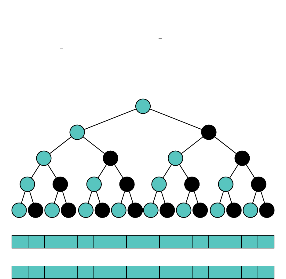
Hsiang, Wei, Liu Chapter 5. Complex Ideas and Data Structures
The key idea is to compress the data stored within a segment tree in a crazy way that ends up
having a really slick implementation using some bit operation tricks.
As discussed earlier, the +operator has an inverse,
−
. Therefore, there is an inherent redundancy,
for example, in keeping track of the sum of the first
n
2
elements, the sum of all
n
elements, and
the sum of the last
n
2
elements, as we do in the segment tree. If we are given only
Pn/2
k=1 ak
and
Pn
k=1 ak, we can find Pn
k=n/2+1 akeasily using subtraction.
With this in mind, let’s ignore every right child in the tree. We’ll mark them as black in the
diagram. After that, we’ll write out the tree nodes in postfix traversal order, without writing
anything whenever we encounter a black node.
12
15
8
6
24
2
7−5
7
9
36
−2
−31
−3
−10
−6
−2−4
−4
−62
7
14
86
−7
0−7
2 4 7
−
53 6
−
31
−
2
−
4
−
62 8 6 0
−
7
1 2 3 4 5 6 7 8 9 10 11 12 13 14 15 16
2 6 7 8 3 9
−
315
−
2
−
6
−
6
−
10
8 14 0 12
1 2 3 4 5 6 7 8 9 10 11 12 13 14 15 16
Our Fenwick tree is simply this last array. This should be quite confusing – it is not at all clear
why this array resembles a tree, and the numbers in the array make no sense whatsoever right now.
Notice that the final position of every unblackened node is just the rightmost black child in its
subtree. This leads to the fact that the ith element in the Fenwick tree array is the sum
yi=
i
X
k=i−2v2(i)+1
xk,
where 2
v2(i)
is simply the greatest power of 2 that divides
i
. Let’s look at a new diagram that
hopefully will better illustrate this key property of the random array we just came up with.
56
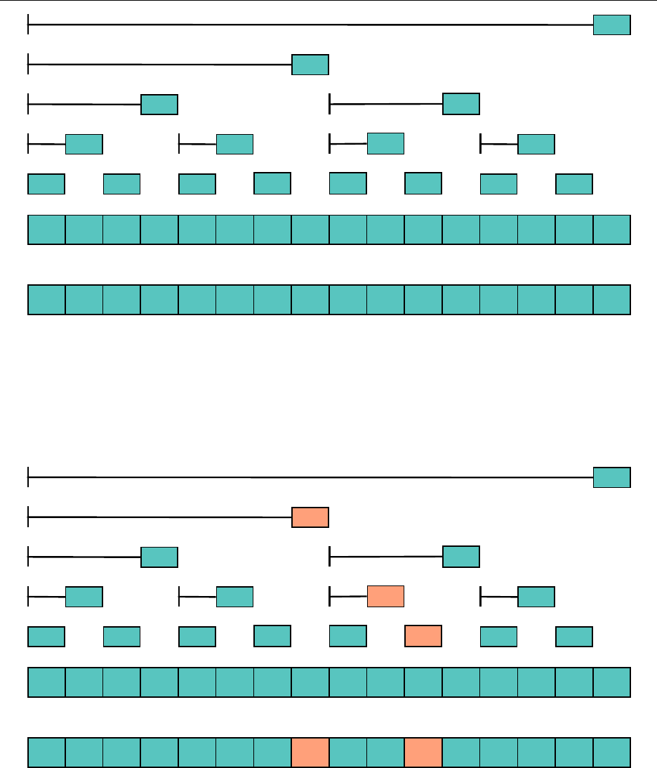
Hsiang, Wei, Liu Chapter 5. Complex Ideas and Data Structures
2 4 7
−
53 6
−
31
−
2
−
4
−
62 8 6 0
−
7
1 2 3 4 5 6 7 8 9 10 11 12 13 14 15 16
2
6
7
8
3
9
−
3
15
−
2
−
6
−
6
−
10
8
14
0
12
2 6 7 8 3 9
−
315
−
2
−
6
−
6
−
10
8 14 0 12
1 2 3 4 5 6 7 8 9 10 11 12 13 14 15 16
All the framework is now in place. Now we need to find out how to query and update the
Fenwick tree.
Suppose we wanted to find the sum
P11
k=1 xk
. Let’s take a look at the diagram to see which
elements we need.
2 4 7
−
53 6
−
31
−
2
−
4
−
62 8 6 0
−
7
1 2 3 4 5 6 7 8 9 10 11 12 13 14 15 16
2
6
7
8
3
9
−
3
15
−
2
−
6
−
6
−
10
8
14
0
12
2 6 7 8 3 9
−
315
−
2
−
6
−
6
−
10
8 14 0 12
1 2 3 4 5 6 7 8 9 10 11 12 13 14 15 16
We see that the sum
P11
k=1 xk
=
y8
+
y10
+
y11
. If we look at 11 in binary, we have 11 = 01011
2
.
Let’s see if we can find a pattern in these numbers in binary:
57
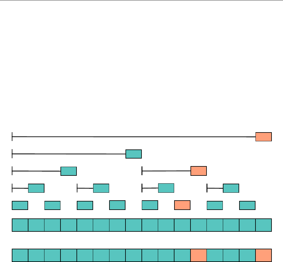
Hsiang, Wei, Liu Chapter 5. Complex Ideas and Data Structures
11 = 010112,
10 = 11 −2v2(11) = 010102,
8 = 10 −2v2(10) = 010002,
0=8−2v2(8) = 000002.
So, we can simply subtract 11
−
2
v2(11)
= 10 = 01010
2
, find the sum of the first 10 elements, and
add
b11
to that sum to get the sum of the first 11 elements. We see that repeating this process takes
off the last 1 in the binary representation of the number
i
, and since there are at most
log n
+ 1 1s
in the binary representation ∀i∈[1, n], the query operation is O(log n).
And now for the update operation. Suppose we want to change the value of
x11
from
−
6to
−
3.
Which numbers will we have to change?
2 4 7
−
53 6
−
31
−
2
−
4
−
32 8 6 0
−
7
1 2 3 4 5 6 7 8 9 10 11 12 13 14 15 16
2
6
7
8
3
9
−
3
15
−
2
−
6
−
3
−
7
8
14
0
15
2 6 7 8 3 9
−
315
−
2
−
6
−
3
−
78 14 0 15
1 2 3 4 5 6 7 8 9 10 11 12 13 14 15 16
We needed to increment the highlighted values,
y11
,
y12
, and
y16
, by 3. Once again we’ll look at
11, 12, and 16 in base 2.
11 = 010112,
12 = 011002= 11 + 2v2(11),
16 = 100002= 12 + 2v2(12).
It appears that instead of subtracting the largest dividing power of 2, we are adding. Once again
this is an O(log n)operation.
The real magic in the Fenwick tree is how quickly it can be coded. The only tricky part is
finding exactly what 2
v2(i)
is. It turns out, by the way bits are arranged in negative numbers, this is
58

Hsiang, Wei, Liu Chapter 5. Complex Ideas and Data Structures
just
i & -i
. With this in mind, here’s all the code that’s necessary to code a Fenwick tree. Note
that here, values in the array remain 1-indexed, which is different from how we code segment trees.
1int[] y=new int[MAXN]; // F e nwick tree stored as array
2void update(int i,int x) {
3for (;i<MAXN;i+= i& -i)
4y[i] += x;
5}
6int prefixSum (int i) {
7int sum = 0;
8for (;i> 0; i-= i& -i)
9sum += y[i];
10 return sum ;
11 }
12 int quer y (int i,int j) {
13 return prefixSum (j) - prefixSum (i- 1) ;
14 }
5.4 Queue with Minimum Query
Suppose we wanted a list data structure with the following three operations:
•add(x)– add xto the end of the list.
•remove() – remove the first element in the list.
•min() – return the minimum element in the list.
This is different from a heap since
remove
does not remove the minimum element. It’s pretty
easy to find a
O
(
log n
)solution using the data structures we already know. However, it is possible
to build a data structure that can do any of these operations with complexity O(1).
To solve this problem, we’ll first solve an easier problem. Suppose instead of removing the first
element of the list, we had remove the last element; in other words, we needed to build a stack with
minimum query instead of a queue. This is a simple task; we’ll just use a normal stack, but instead
of storing single numbers, we’ll store pairs. The pairs will each contain the number we’re adding
and the minimum element up to that point in the stack.
To build a queue given a stack with minimum query, we’ll just have two stacks. When we add
an element, we push it to the top of the first stack. When we remove an element, we take it off the
top of the second stack. The minimum element in the queue is the smaller element between the
minima of either stack.
This seems like it obviously doesn’t work – one of the stacks keeps growing, while the other can
only shrink. This is not a problem, however; when the second stack runs out of elements, we’ll just
pop off every element of the first stack and push each onto the second stack. This amounts to one
O(n)operation for every n O(1) operations, which averages out to constant time.
59
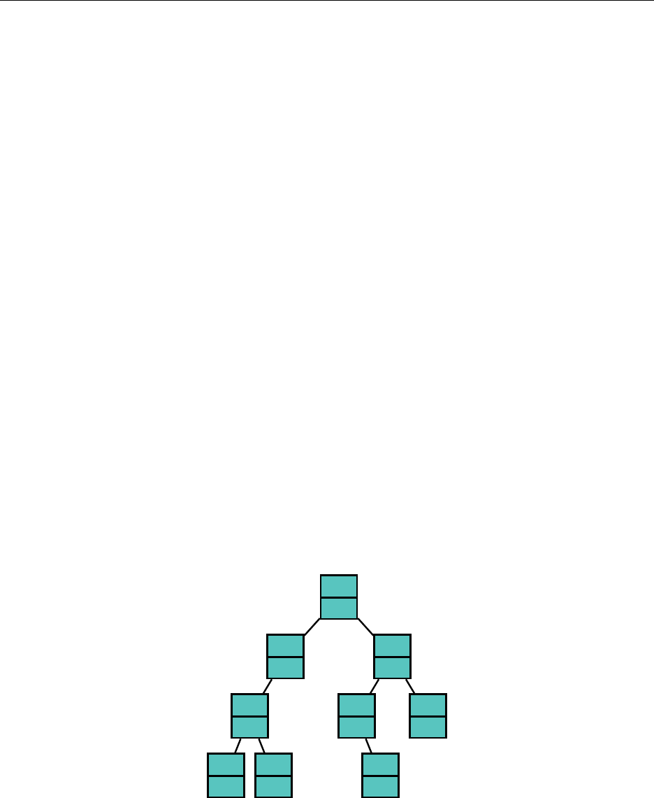
Hsiang, Wei, Liu Chapter 5. Complex Ideas and Data Structures
5.5 Balanced Binary Search Tree
Recall that a normal binary search tree is not guaranteed to be balanced. Many data structures
have been invented to self-balance the binary search tree.
The red-black tree was an early development that represents the “just do it” approach, using
casework to balance a tree. This results in a simple mathematical proof for the maximum depth of
the tree. Unfortunately, coding these up are quite nasty do to the casework involved, so doing so is
generally not preferred unless your name is Sreenath Are.
The splay tree is a data structure that guarantees amortized logarithmic performance; this means
that any single operation is not necessarily linear, but over any sequence of length
m
for
m≥n
, the
performance for all
m
operations is
O
(
mlog n
). Though the proof of the splay tree’s complexity is
necessarily more complicated than the red-black tree’s complexity, as it requires amortized analysis,
coding the splay tree is much easier than coding the red-black tree. In addition, the splay tree
grants us more flexibility than the red-black tree provides, allowing us to build more complicated
structures like link-cut trees using splay trees.
The treap is a probabilistic data structure that combines a binary search tree with a heap to
create a BBST. Just as quicksort is not guaranteed to run in
O
(
nlog n
), treaps are not guaranteed
to have logarithmic depth. In practice, however, they almost always have performance that is
O
(
log n
). Treaps are especially useful in programming contests because they are the easiest BBST
to implement.
5.5.1 Treap
A treap is a binary search tree smushed together with a heap. Each node is assigned, in addition to
its key, a random priority. The priorities in a treap always satisfy the heap property: for any node,
its priority is greater than the priority of either of its children. The diagram below illustrates a
treap. On each node, the letter is the node’s key and the number is the node’s priority.
E
9
D
6
B
4
A
1
C
2
H
8
F
5
G
3
I
7
The randomness in each node’s priority balances the treap. We can gain some intuition for why
this works by looking at how a treap is built. Consider an array containing pairs of key and priority,
sorted by key. To construct a treap from these values, we first take the element with the highest
priority and set it as the root. We can then recurse on the two halves of the array split by the root,
60

Hsiang, Wei, Liu Chapter 5. Complex Ideas and Data Structures
and construct the root’s left and right subtrees in a similar way. Because the priority of each node
is randomly chosen, we effectively choose a random element as the root each time we recurse.
Like quicksort, we can expect that the root doesn’t always split the tree too unevenly and obtain
a
O
(
log n
)bound on the expected depth of each node. Moreover, it is possible to show that the
entire tree has a depth of
O
(
log n
)with high probability. This analysis means that a treap is as
good complexity-wise as any other deterministic BBST for all practical purposes. (To do the first
part more rigorously, we can let
Ai,j
be an indicator random variable representing whether the
j
th
node is an ancestor of the ith node. What is the expected value of Pn
j=1 Ai,j?)
In the remainder of this section, we’ll go over the implementation of treaps. Our implementation
will be quite different from the rotation-based implementations of splay trees and red-black trees
described above. Instead of rotating, we will have two functions,
split
and
merge
, that will be
used to define all other treap operations. Here are their definitions:
split
takes a treap
T
and a key
k
and splits
T
into two treaps by
k
. Thus
split
outputs two
treaps,
L
and
R
, where all the elements of
L
are less than
k
and all the elements of
R
are at least
k
.
split has a complexity of O(log n).
merge
does the opposite of
split
. It takes two treaps
L
and
R
, where each key in
L
is at most
the smallest key in R, and turns them into one treap, T.merge also has a complexity of O(log n).
One way to think about these functions is to imagine treaps as a data structure that dynamically
maintains sorted arrays. Then splitting is cutting an array into two, and merging is appending one
array onto the end of another. With this perspective on
split
and
merge
, standard BST operations
are not difficult to write. For example, we can insert a key
k
into a treap
T
by splitting
T
into
L
and
R
by
k
. Then we can create a new node
n
with key
k
, and merge
L
,
n
and
R
back into
T
.
Other operations that we can implement are erase,union and intersect.
Writing
split
and
merge
is also relatively easy. With C++, we can use pointers and references
to simplify our work.
To
split
, we recurse on
T
, while maintaining references to
L
and
R
. The root of
T
becomes
the root of one of
L
and
R
, depending on its key. If the root of
T
becomes the root of
R
, we recurse
on the left subtree of
T
and
split
into
L
any nodes that have key less than
k
. The other case,
where the root of Tbecomes the root of L, works similarly.
To
merge
, we take the root of
L
and
R
with the higher priority, and set it as the root of
T
. If
the root of
L
has higher priority, we
merge R
and the right subtree of
L
. Otherwise, we
merge L
and the left subtree of
R
. Like
split
, we can recurse down the relevant subtrees until we are done.
Here’s a short C++ implementation of a treap with split,merge and insert:
61

Hsiang, Wei, Liu Chapter 5. Complex Ideas and Data Structures
1struct node {
2node *l, *r;
3int k,p;
4node(int k):l(0) , r(0) , k(k) , p(rand() ) { }
5};
6
7void spli t (node *t,node *&l,node *&r,int k) {
8// Splits t into l and r .
9if (t== NULL)l=r=NULL;
10 els e if (k<= t-> k)split (t-> l,l,t-> l,k) , r=t;
11 else spli t (t-> r,t-> r,r,k) , l=t;
12 }
13
14 void merg e (node *&t,node *l,node *r){
15 // Merges l and r into t .
16 if (l== NULL || r== NULL)t=l?l:r;
17 els e if (l-> p>r-> p)merge (l-> r,l-> r,r) , t=l;
18 else merg e (r-> l,l,r-> l) , t=r;
19 }
20
21 void insert(node *& t,int k) {
22 node *n=new node(k) , * a;
23 spli t (t,t,a,k);
24 merg e (t,t,n);
25 merg e (t,t,a);
26 }
We can also create an implicitly keyed treap, which functions as a dynamic array. Instead of
storing keys, each node stores the size of its subtree. We can then define the implicit key of a node
as its position in the in-order traversal of the treap, a value we can easily compute from subtree
sizes. Modifying
split
to operate based on the implicit key allows us to rearrange parts of the
array and insert new elements anywhere. Further augmentation allows us to perform range queries
as well. And if we add lazy propagation, we can also support operations that modify ranges.
Here’s an example of an implicitly keyed treap that supports reversal of subarrays. In
node
,
s
maintains the size of its subtree, and
f
is a flag that indicates reversal. We use
push
and
pull
to
propagate data down and up the treap, respectively. Note the difference in the implementation of
split.
62

Hsiang, Wei, Liu Chapter 5. Complex Ideas and Data Structures
1struct node {
2node *l, *r;
3int v,p,s,f;
4node(int v):l(0) , r(0) , v(v) , p(rand() ) , s(1) , f(0) {}
5};
6
7int size(node *t){
8return t?t-> s: 0;
9}
10
11 void push(node *t){
12 if (t== NULL)return;
13 if (t-> f) {
14 swap(t-> l,t-> r);
15 if (t-> l)t-> l-> f^= 1;
16 if (t-> r)t-> r-> f^= 1;
17 t-> f= 0;
18 }
19 }
20
21 void pull(node *t){
22 if (t== NULL)return;
23 t-> s=size(t-> l) + size(t-> r) + 1;
24 }
25
26 void spli t (node *t,node *&l,node *&r,int k) {
27 push(t);
28 if (t== NULL)l=r=NULL;
29 els e if (k<= size(t-> l)) split (t-> l,l,t-> l,k) , r=t;
30 else spli t (t-> r,t-> r,r,k-size(t-> l) - 1) , l=t;
31 pull(t);
32 }
33
34 void merg e (node *&t,node *l,node *r){
35 push(l) , push(r) ;
36 if (l== NULL || r== NULL)t=l?l:r;
37 els e if (l-> p>r-> p)merge (l-> r,l-> r,r) , t=l;
38 else merg e (r-> l,l,r-> l) , t=r;
39 pull(t);
40 }
41
42 void reverse(node *t,int l,int r){
43 // Reverse s t he r an ge [ l ,r ].
44 node *a, *b;
45 spli t (t,t,b,r+ 1) ;
46 spli t (t,t,a,l);
47 a-> f^= 1;
48 merg e (t,t,a);
49 merg e (t,t,b);
50 }
63
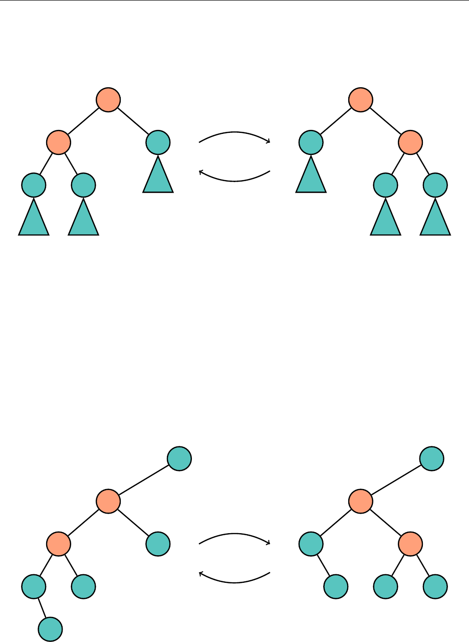
Hsiang, Wei, Liu Chapter 5. Complex Ideas and Data Structures
5.5.2 Tree Rotation
The key idea behind all of these data structures is the use of the tree rotation, which is used to
change the structure of the tree but will not change the order of the elements (inorder). Maintaining
the order of the elements is important, of course, if we wish our tree to remain a binary search tree.
Q
P
A B
C
P
AQ
B C
rotate right
rotate left
Here, the triangles represent subtrees, as
A
,
B
, and
C
could very well have children of our own,
but they are not shown in the diagram. Note that the inorder ordering of the nodes has not been
changed.
When we rotate right, we literally take the edge connecting
P
and
Q
and rotate it clockwise.
Then
P
becomes the parent of
Q
where before
P
was the child of
Q
. However, this definition of
rotation is somewhat cumbersome, as we have different terms for the highly symmetrical rotating
right and rotating left. The key characteristic a rotation is we move the lower node up one level.
Thus, I prefer to think of tree rotation as whatever tree rotation, either left or right, will rotate up a
node. In the diagram, rotating right is analogous to rotating
P
up, and rotating left is analogous to
rotating
Q
up. Rotating a node up will change the tree such that its former parent is now its child.
The other notable change in the tree structure is the subtree associated with
B
passes between
P
and
Q
upon tree rotation. Finally, tree rotation can happen at any place in the tree, not just at
the root. When we rotate Pup, we must update the parent of Qto change its child to P.
D
Q
P
A
E
B
C
D
P
A
E
Q
B C
rotate P
rotate Q
64
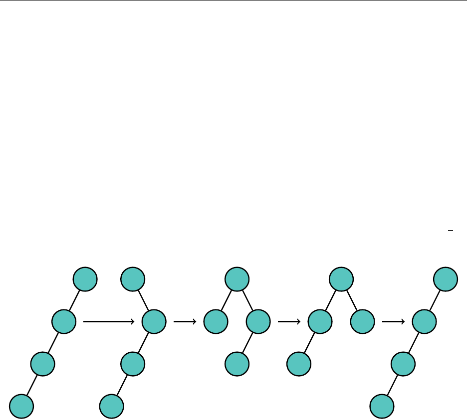
Hsiang, Wei, Liu Chapter 5. Complex Ideas and Data Structures
Note that in this example, rotating up
P
decreases the total height of the tree. We want to
somehow systematically rotate up nodes to accomplish this. The following data structures provide
such a system.
5.5.3 Splay Tree
Remember that rotating a node brings it one level closer to the root. The idea behind a splay tree
is to apply a sequence of rotations that rotate a node all the way up to the root. The intuition for
doing this is once we access a node, it is easy to perform other operations on it since it will simply
be the root of the tree.
It is not at all clear that rotating nodes to the root will somehow improve the average performance
of the tree. That’s because rotating the normal way doesn’t! To improve the performance of the
tree, we expect that our balancing procedure tends to decrease the height of the tree. Unfortunately,
simply repeatedly rotating a node up the tree doesn’t exactly do that task. Consider a tree that
looks liked a linked list, and rotating the nodes in the order
A
,
B
,
C
,
D
, as shown in the diagram.
The height of the tree remains linear in magnitude, as at its smallest stage the tree is around
n
2
in
height, so accessing elements remains O(n)on average.
D
C
B
A
A
D
C
B
B
A D
C
C
B
A
D
D
C
B
A
rot. Arot. Brot. Crot. D
As discussed earlier, simply repeatedly applying the standard rotation clearly is not guaranteed
to reduce the height of the tree on average. However, if we simply make one small change, magic
happens. The trick of the splay tree is to rotate a node to the root in such a way that the tree has a
tendency to decrease in height. We’ll use two compound rotations, and depending on the structure
of the tree, we’ll use a different one accordingly, to rotate a node to the root.
When a node is a left child and its parent is a left child, or the node is a right child and its
parent is a right child, we first rotate up the parent, and then rotate up the node. This sequence of
rotations is the only difference between splaying and rotating a node to the root using standard
rotation.
65
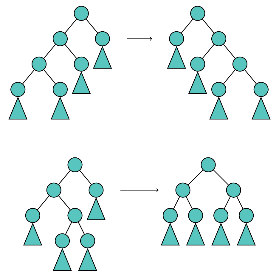
Hsiang, Wei, Liu Chapter 5. Complex Ideas and Data Structures
Z
Y
X
A B
C
D
X
A Y
B Z
C D
rotate Y, rotate X
When a node is a left child and its parent is a right child, or the node is a right child and its
parent is a left child, we rotate the node up twice, the normal way.
Z
Y
A X
B C
D
X
Y
A B
Z
C D
rotate X, rotate X
Finally, when a node’s parent is the root, so it has no grandparent, we simply rotate up the
normal way.
Rotating a node to the root in this way is called splaying the node. Thus, splaying a node brings
it to the root of the tree. Splaying seems too simple to lead to an amortized
O
(
log n
)solution. To
get a better idea of how splaying works, let’s see what it does to a tree that looks like a linked list.
66
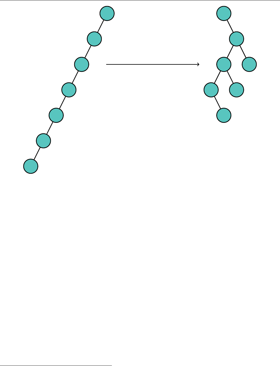
Hsiang, Wei, Liu Chapter 5. Complex Ideas and Data Structures
G
F
E
D
C
B
A
A
F
D
B
C
E
G
splay A
Splaying here cuts the height of the tree in half – a huge improvement. Splaying is not guaranteed
to decrease the height of the tree, and it is possible for a sequence of splays to even result in a
linked-list-like structure. However, given a number
m
at least equal to the maximum number of
nodes
n
ever in the tree, any sequence of
m
splays runs in
O
(
mlog n
). Splaying is then
O
(
log n
),
amortized.2
Then, whenever we access a node, even in insertion and deletion, we splay that node to the top.
This makes access, insert, and delete all O(log n)amortized.
Since splay trees need not satisfy a restrictive coloring, as red-black trees do, we have the freedom
to completely change the structure of the tree at a whim. Recall how tedious the casework was to
simply add or remove one node at a time in a red-black tree. Because the splay tree is simply a
normal binary search tree that rotates nodes up upon access, we can detach an entire subtree from
the tree and not worry about any properties of our tree no longer being satisfied.
For this reason, we define the split and join functions for splay trees.
Given two trees
S
and
T
, such that every element in
S
is less than every element in
T
, we join
S
and
T
into one tree by splaying the largest element in
S
, so that the root, which is now the largest
element, has no right child. Then, we set its right child to the root of
T
, resulting in a single tree
with elements from both Sand T.
Given a tree and a value
v
, we split the tree in two by splaying the greatest element not greater
than
v
to the root and detaching the right subtree from the rest. This results in two trees, one
containing all elements at most v, and the other containing all elements greater than v.
2
If you’re curious to see the proof of this, a rather in depth explanation can be found here:
http://www.cs.cmu.
edu/afs/cs/academic/class/15859-f05/www/documents/splay-trees.txt
67

Hsiang, Wei, Liu Chapter 5. Complex Ideas and Data Structures
Both of these operations are
O
(
log n
)amortized. It is possible to implement insert and delete
using split and join.
Since a binary search tree stores an ordered set, it is incredibly useful for storing a dynamic list
of elements where the length can change and elements need to be added or removed from any point
in the list, not just the beginning or the end. Splay trees are incredibly useful because of the split
and join operations, as they allow us to remove consecutive elements from the list represented by
our tree.
For example, to remove elements indexed in the range [
i, j
], we split at index
i
and split at index
j
+ 1 to get three splay trees, one representing [1
, i −
1], another [
i, j
], and the last [
j
+ 1
, n
]. We can
then merge the first and third trees together, to get two trees, one representing [
i, j
]and the other
representing the original list with [
i, j
]removed. A similar procedure can insert a list within another
list as as contiguous block. Both of these operations can be completed in
O
(
log n
)amortized using
a splay tree.
5.5.4 Red-Black Tree
Red-black trees are not very useful in the contest environment, but since nearly every implementation
of BBST in standard libraries uses them, it may be useful to be familiar with the idea behind them.
As stated earlier, the red-black tree represents the “just do it” approach. We want to somehow
bound the maximum length from the root to any leaf node by applying a constraint on the tree. In
this case, our constraint is a coloring of the nodes (red or black) such certain properties are satisfied.
For the red-black tree, the only nodes storing data are non-leaf nodes, and all leaf nodes store “null.”
The number of null nodes, then, is
n
+ 1, where
n
is the number of non-null nodes. We do this so
that any node storing useful information has two children.
We want our tree to satisfy the following properties:
1. The root is black.
2. All leaf nodes (null) are black.
3. Every red node has two black children. Consequently, a red node has a black parent.
4. Any path from the root to a null node contains the same number of black elements.
68
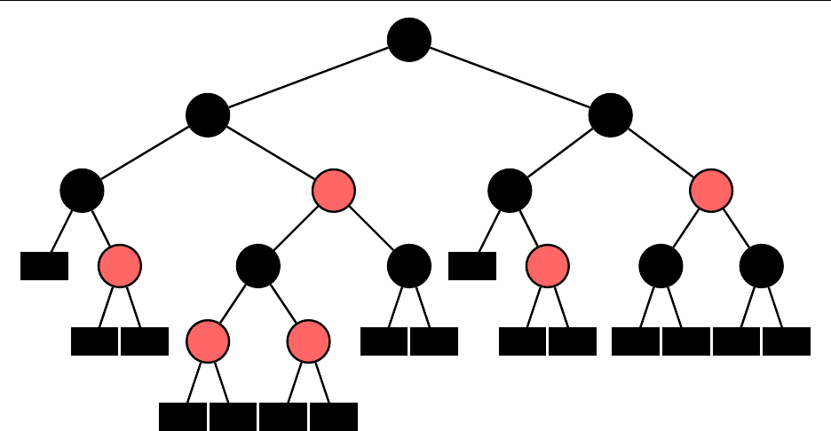
Hsiang, Wei, Liu Chapter 5. Complex Ideas and Data Structures
M
D
A
null
C
null null
K
G
E
null null
I
null null
L
null null
T
Q
null
R
null null
X
V
null null
Z
null null
Note that every path from the root to a null node contains four black nodes.
The proof of
O
(
log n
)search follows immediately. The shortest possible path contains only black
nodes, and the longest possible path contains black and red nodes alternating. Since the number of
black nodes in both must be the same, any path is at most twice as long as any other path. As the
number of nodes in the tree is 2
n
+ 1, the number of black nodes
m
in any path is then bounded
below by 2
2m−
1
≥
2
n
+ 1 and above by 2
m−
1
≤
2
n
+ 1. Thus the height of the tree is on the
order O(log n), and we are done.
Thus if our tree maintains its red-black coloring and satisfies the necessary properties, we can
guarantee that our tree is balanced. We then consider the two ways we change the state of the
tree, insertion and deletion. We can insert and delete in the normal way, but we might need to
make changes to the tree after that to restore the red-black properties. We do this through a small
number of color flips and tree rotations, which we can handle through casework.
Let’s handle insertion first. When we insert a node, it takes the place of a black null leaf node.
To maintain property 4, we must color the new node red, as it has two black null children. However,
we may have violated some of the other properties, specifically 1 and 3.
We’ll call the new node
N
, its parent
P
, its uncle (parent’s sibling)
U
, and its grandparent
G
, if
they exist.
We consider the following five cases.
1. Nis the root node. That is, Nis the first node added to the tree.
It is easy to just change the color of Nto red to restore property 1, and we are done.
2. Pis black.
Then property 3 is not violated, and we are done.
69
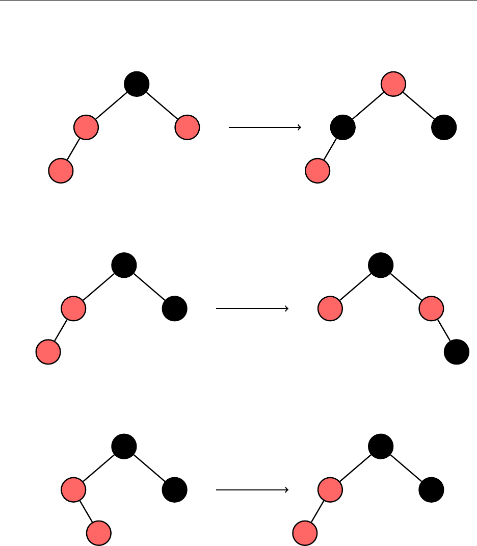
Hsiang, Wei, Liu Chapter 5. Complex Ideas and Data Structures
3. Pis red, and Uis red (Gand Uexist since Pcannot be the root, as the root is black).
As
P
and
U
are red,
G
is black. We simply color
P
and
U
black and
G
red to restore property
3.
G
P
N
U
G
P
N
U
4. Pis red, Uis black, and Nis on the same side of Pas Pis of G.
Gmust be black. We rotate up Pand color Pblack and Gred.
G
P
N
U
P
N G
U
5. Pis red, Uis black, and Nis on the opposite side of Pas Pis of G.
Gmust be black. We rotate up N, and this reduces to case 4.
G
P
N
U
G
N
P
U
Thus after we insert, we can always restructure the tree using a constant number of operations
to restore the necessary red-black tree properties.
Now we need to work on deletion. Recall how deletion works on a normal binary search tree. If
the node we need to replace has two children, we swap the node with the least element in its right
subtree, which does not have two children. We then are able to remove that node more easily.
70
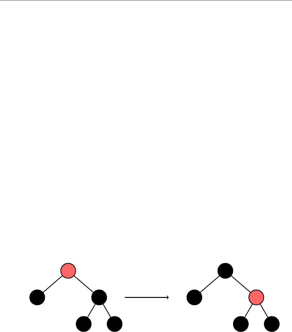
Hsiang, Wei, Liu Chapter 5. Complex Ideas and Data Structures
We can do the same thing with the red-black tree. If a node has two non-null children, we swap
its value with the least non-null node in its right subtree and remove that node. Thus we reduce
the deletion problem to the case where the node we need to remove has at least one null child.
Two cases are very easy.
1. The node we wish to remove is red.
Then the node must have two null leaf nodes as children. Then we remove the node by
replacing it and its children with a single null node.
2. The node is black and has a red child.
We replace the node with its child and paint its child red.
The remaining case is the node black with two black null children. We’ll first replace the node
with a null node
N
. Then, all paths passing through
N
are one black node short compared to all
other paths.
We denote the parent of
N
as
P
, its sibling
S
, and its sibling’s children
C
and
F
, such that
C
is
on the same side of
S
as
N
is of
P
, if they exist. That is,
C
is the “closer nephew” child, while
F
is
the farther. We now describe a six-case balancing procedure on the black node
N
that fixes our
problem.
1. Nis the root.
We are done, as every path possible must pass through N, so all paths are balanced.
2. Pis red and S,C, and Fare black.
Then we simply trade the colors of
P
and
S
. The number of black nodes for paths passing
through
S
stays the same, but the number of black nodes for paths passing through
N
increases, so we are done.
P
N S
C F
P
NS
C F
3. Sis black and Fis red.
Then we color
F
black and rotate up
S
, before swapping the colors of
P
and
S
. Then paths
passing through Ngain a black vertex, while paths passing through Cand Fstay the same.
71
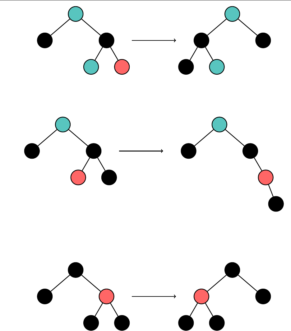
Hsiang, Wei, Liu Chapter 5. Complex Ideas and Data Structures
P
N S
C F
S
P
NC
F
4. Sis black, Fis black, and Cis red.
Then we rotate up Cand swap the colors of Sand C. Then this reduces to case 3.
P
N S
CF
P
N C
S
F
5. Sis red.
Then
P
,
C
, and
F
must be black. We rotate
S
up and swap the colors of
P
and
S
.
C
, the
new sibling of Nis black, so this then reduces to one of cases 2, 3, or 4.
P
NS
C F
S
P
N C
F
6. P,S,C, and Fare all black.
Then we recolor
S
red. Now, all paths through
P
have the same number of black nodes, but
each path through
P
has one less black node than each path not passing through
P
. Since
P
is black, and this procedure did not require that
N
be a leaf node, we can repeat this entire
balancing procedure on P.
72

Hsiang, Wei, Liu Chapter 5. Complex Ideas and Data Structures
P
N S
C F
P
NS
C F
Unlike the balancing for insertions, the balancing for deletions has the potential to call itself
on the parent node
P
. However, balancing following a deletion is still
O
(
log n
)worst case. It is
possible prove that it is
O
(1) amortized. Regardless, we now have a deletion algorithm that runs in
O(log n)time.
Thus the red-black tree supports standard binary search tree operations, all in O(log n).
73
Chapter 6
Computational Geometry
For actual geometry problems, and not graph theory problems hiding in the plane.
I’m too lazy to actually write this section right now so here are some useful links from the
USACO Training Pages.
https://www.dropbox.com/s/nqzk63bjby1iaq9/Computational%20Geometry.pdf?dl=0
https://www.dropbox.com/s/ykf65dk6sefb6zk/2-D%20Convex%20Hull.pdf?dl=0
These essentially cover anything I would want to say in this chapter anyway, so I’ll likely fill this
chapter out last.
75

Hsiang, Wei, Liu Chapter 6. Computational Geometry
6.1 Basic Tools
Cross Product
Dot Product
tan−1,atan2
6.2 Formulas
6.2.1 Area
6.2.2 Distance
6.2.3 Configuration
6.2.4 Intersection
6.3 Convex Hull
6.4 Sweep Line
Oftentimes when trying to solve geometry problems, or combinatorial problems that we give a
geometric interpretation, we have something that involves one or two dimensions. If this is difficult
to deal with directly, we can use a sweep line to reduce the dimension of the problem.
Sweep lines are best explained with an example. Suppose we’re given several intervals on the
number line, and we want to find the length of their union. If we wanted to, we could use a segment
tree with lazy propagation to insert the intervals and calculate the total length. However, a sweep
line gives us a much easier approach. Imagine a vertical beam of light sweeping from
−∞
to
∞
on the number line. At any given time, we keep track of the number of intervals that are hit by
this beam. This takes the problem from one dimension to zero dimensions. Our answer is then the
length over which our beam hit a positive number of intervals.
Our implementation of a sweep line simulates this process. If we sort the endpoints of our
intervals by their positions on the number line, we can simply increment our counter each time we
encounter a “start” endpoint and decrement our counter each time we encounter an “end” endpoint.
We can look at the regions between consecutive endpoints, and add to our result if our counter is
positive in that region.
76

Hsiang, Wei, Liu Chapter 6. Computational Geometry
One other way to interpret sweep lines is to consider time as the dimension we sweep along. For
the example above, this would mean that each interval appears and then disappears on our beam,
existing only when the time is between its endpoints. Although time may not seem useful for our
one dimensional problem, this type of thinking helps in higher dimensions.
Most sweep lines that you use won’t be as simple as this. Sweep line problems usually involve
reducing a two dimensional problem to a one dimensional problem and require maintaining data
structures such as BBSTs or segment trees along that dimension. This technique also generalizes to
higher dimensions—to solve a three dimensional problem, we can sweep along one dimension and
use two dimensional data structures to maintain the other two dimensions.
To finish, let’s go over another example, Cow Rectangles from USACO 2015 January:
The locations of Farmer John’s Ncows (
1
≤N≤
500
) are described by distinct
points in the 2D plane. The cows belong to two different breeds: Holsteins and
Guernseys. Farmer John wants to build a rectangular fence with sides parallel to the
coordinate axes enclosing only Holsteins, with no Guernseys (a cow counts as enclosed
even if it is on the boundary of the fence). Among all such fences, Farmer John
wants to build a fence enclosing the maximum number of Holsteins. And among all these
fences, Farmer John wants to build a fence of minimum possible area. Please determine
this area. A fence of zero width or height is allowable.
The first observation we should make is that we want a Holstein on every side of the fence.
Otherwise, we would be able to decrease the area of our fence without decreasing the number of
Holsteins. Even with our observation, this problem still seems hard to deal with. We can make it
easier by adding another constraint: Suppose we knew which Holstein was on the leftmost boundary
of our fence. Since we added the constraint to the
x
-dimension, we naturally want to figure out
where our rightmost Holstein is next. We can do this with a sweep line moving to the right.
The reason we want a sweep line here is because for any given rightmost cow, we want to know
information about the Guernseys and Holsteins in between. With a sweep line, we can collect and
maintain all this data by processing the cows from left to right. For example, whenever we see a
Guernsey, we have to limit the
y
-coordinates that our Holsteins can take. And whenever we see a
Holstein, we have to consider this Holstein as our rightmost cow and also store it in case we include
it in a fence later on.
What remains is to find an appropriate data structure to track all this. A set data structure (STL
set or Java TreeMap) turns out to be enough. We can insert the Holsteins, sorted by
y
-coordinate,
and delete one whenever any rectangle bounded by that Holstein, the leftmost Holstein, and our
77

Hsiang, Wei, Liu Chapter 6. Computational Geometry
sweep line includes a Guernsey. Thus we take
O
(
nlog n
)time to sweep, giving us an
O
(
n2log n
)
solution overall.
This type of analysis is pretty representative of sweep line problems. Whether you’re given
rectangles, line segments or even polygons, you want to think about how you can reduce the
dimension and obtain a tractable problem. Note that sweep lines don’t always have to move along
some axis. Radial sweep lines (sweeping by rotating) and sweeping at an angle (rotating the plane
by 45◦) also work.
78
Chapter 7
Tree Algorithms
Up until now, we have only looked at algorithms that deal with general graphs. However, there is
also much to be said about graphs with additional structure. In this section, we’ll explore some
problems and their solutions on trees. First, some definitions.
An undirected graph Gis a tree if one of the following equivalent conditions holds:
•Gis connected and has no cycles.
•Gis connected with nvertices and n−1edges.
•There exists exactly one simple path between any two vertices of G.
Arooted tree is a tree where one vertex has been designated as the root. This gives each edge a
natural direction – whether it leads towards or away from the root. In many problems, it is useful
to arbitrarily designate a root. For example, one interpretation of a DFS on a tree is that we start
from the root and traverse the tree downwards towards the leaves. (On trees, a leaf is a vertex with
degree 1.)
We’ll define a few more terms for rooted trees. An ancestor of a vertex
v
is another vertex
a
that
lies on the path between
v
and the root. The parent of a vertex is its closest ancestor. The depth of
a vertex is its distance from the root. We will use depth(v)to denote the depth of a vertex v.
7.1 DFS on Trees
DFS is a very useful technique for collecting information about the structure of a tree. For example,
we can compute in linear time the depth of each node, the size of each subtree or the diameter of the
entire tree. This can be done by recursively computing results for each subtree, and then combining
this data to obtain the final result. Sometimes, it takes more than one DFS to collect all the
necessary information. Calculating node depth and subtree size via DFS is relatively straightforward.
Below is a snippet of pseudocode computing these two sets of values.
79

Hsiang, Wei, Liu Chapter 7. Tree Algorithms
function DFS(v,p) v is the current vertex, pis its parent
sum(v)←1 sum(v)is size of the subtree rooted at vertex v
depth(v)←depth(p)+1 depth(v)is the depth of vertex v
for all vertices nadjacent to vdo
if n6=pthen
DFS(n,v)
sum(v)←sum(v) + sum(n)
Computing the diameter of a tree is a bit trickier. For a given tree, let
r
be its root, and let
a
be a vertex of maximum depth. It turns out that the diameter of the tree is the maximum distance
between
a
and any other vertex in the tree. (Try to prove this!) Thus we can run two DFSes to
compute the diameter, calculating the depth of each vertex with each pass.
Depth, subtree size and diameter are only a few of the values we can compute for trees. This
style of DFS shows up often in problems and is also fundamental to many more complex tree
algorithms.
7.2 Jump Pointers
Jump pointers are a technique for decomposing paths on rooted trees. The central idea is that we
can always take a path and break it into
O
(
log n
)chunks of size 2
i
. By augmenting these smaller
chunks with data, we can use jump pointers to quickly answer a variety of queries, including level
ancestor and lowest common ancestor.
Let’s start with an example. The most fundamental application of jump pointers is to level
ancestor queries—for any vertex
v
, we want to be able to find its
k
th ancestor in
O
(
log n
)time.To
solve this problem, we precompute for each vertex a pointer to its 2
i
th ancestor for all possible
values of
i
. These are the “jump pointers” for which this technique is named. If our tree has
n
vertices, then each vertex has at most
blog2nc
pointers leading out from it. Thus we have at most
O(nlog n)jump pointers in total. We can compute these with a DP in O(nlog n).
Using jump pointers, we can finish the level ancestor problem. Let 2
i
be the largest power of 2
that is at most
k
. We use our jump pointers to obtain
u
, the 2
i
th ancestor of
v
. If 2
i
is not equal to
k
, we can jump up again from
u
. Continuing recursively, we’ll finish in
O
(
log n
)iterations, since we
reduce kby at least a factor of 2 each time.
Now we’ll tackle lowest common ancestor queries. The lowest common ancestor (LCA),
l
, of
two vertices
u
and
v
is the deepest vertex that is an ancestor of both
u
and
v
. LCA queries are
especially useful because any path on a rooted tree can be broken into two shorter paths joined at
the LCA of its endpoints.
The solution of the LCA problem with jump pointers consists of two steps. The first step
involves bringing the two queried vertices to the same depth. If we are looking for the LCA of
u
and
v
, we can assume that
depth
(
u
)
> depth
(
v
)without loss of generality. Let
u0
be the ancestor of
u
satisfying
depth
(
u0
) =
depth
(
v
). We can compute
u0
with a single level ancestor query in
O
(
log n
)
time. If u0=v, then we are done.
Otherwise, if
u06
=
v
, we can find the LCA of
u0
and
v
by advancing them towards the root in
increments of 2
i
in a binary-search-like manner. If the 2
i
th ancestors of
u0
and
v
are distinct, then
the LCA of
u0
and
v
is equal to the LCA of the 2
i
th ancestors of
u0
and
v
. Thus, iterating down
80

Hsiang, Wei, Liu Chapter 7. Tree Algorithms
from the largest power of 2 less than
n
, we can move
u0
and
v
up the tree until they share a parent.
This common parent is the LCA of
u
and
v
. Since jump pointers allow us to access the 2
i
th ancestor
of a vertex in O(1), our algorithm runs in O(log n)time.
Algorithm 8 Jump Pointers, Level Ancestor and LCA
function BuildJumpPointers(V,par)Initially, par(0, v)holds the parent of vertex v.
par(i, v)denotes the 2ith ancestor of vertex v
for all i from 1 to blog2ncdo
for all vertices vdo
par(i, v)←par(i−1, par(i−1, v))
function LevelAncestor(u,k)
for all i from blog2ncto 0 do
if 2i≤kthen
u←par(i, u)
k←k−2i
return u
function LCA(u,v)
if depth(u)< depth(v)then
swap(u,v)
u←LevelAncestor(u, depth(v)−depth(u))
if u=vthen
return u
for all i from blog2ncto 0 do
if par(i, u)6=par(i, v)then
u←par(i, u)
v←par(i, v)
return par(0, u)
Level ancestor and LCA are the two basic tools to jump pointers. Applying these, we can
quickly answer queries about paths, such as the length of the path between two vertices
u
and
v
. If
we augment the jump pointers by storing additional information, we can also compute maximum
weight or distance queries on weighted trees. Another important observation that we can make is
that we can compute jump pointers on the fly, adding edges and answering queries online.
We now take some time to acknowledge a few limitations of jump pointers. Because each vertex
of the tree is covered by
O
(
n
)jump pointers on average (including the ones jumping over it), this
structure cannot handle updates efficiently. Thus we usually apply jump pointers only if we know
that the weights/values stored with the jump pointers will not change after being computed. For
example, if we want to both answer maximum weight queries for paths and update edge weights, we
should use heavy-light decomposition or link-cut trees to do so.
Overall, however, jump pointers are still a very flexible technique. With some creativity, these
ideas can be used to provide elegant and easy-to-code solutions for problems that would otherwise
require more complex data structures.
81
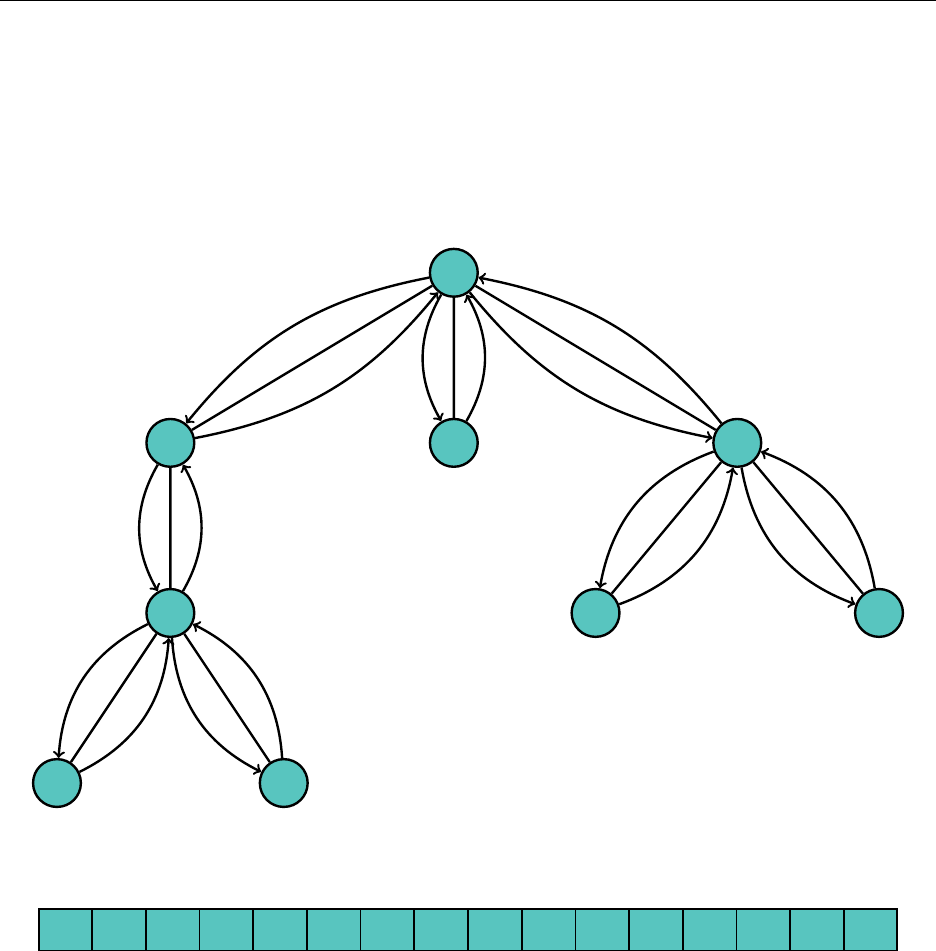
Hsiang, Wei, Liu Chapter 7. Tree Algorithms
7.3 Euler Tour Technique
The Euler tour technique is a method of representing a tree (not necessarily binary) as a list. The
idea is that a tree is uniquely determined by its DFS traversal order, going both down and up the
tree. We’ll keep track of the order in which we traverse the edges. Since each edge is traversed
twice, each edge will appear in our list twice. We’ll also name each edge by the child vertex in the
parent-child pair.
A
B
E
H
h
I
i
e
b
C
c
D
F
f
G
g
d
1
2
3
4 5
6
7
8
9 10
11
12
13 14
15
16
The edge traversal order is then described by the ordered list below.
b1e1h1h2i1i2e2b2c1c2d1f1f2g1g2d2
1 2 3 4 5 6 7 8 9 10 11 12 13 14 15 16
We see a pattern in this list – the subtree of a node is contained between the two edges
representing that node in the list, inclusive. For example, from the first
e
to the second
e
, the entire
subtree of Eis contained within the range [2,7].
7.3.1 Euler Tour Tree
The Euler tour tree uses this idea. Because we see the relationship between the list and the subtrees
of the tree, we’ll just have the list store the vertex names. To complete this pattern for the subtree
of A, which is the entire tree, we’ll simply add that letter to the beginning and end of the list.
82
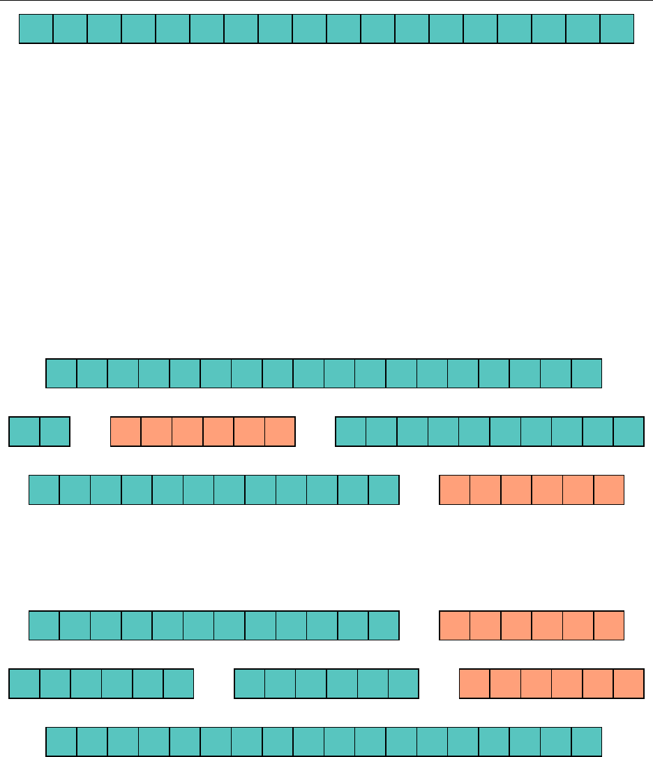
Hsiang, Wei, Liu Chapter 7. Tree Algorithms
A1B1E1H1H2I1I2E2B2C1C2D1F1F2G1G2D2A2
1 2 3 4 5 6 7 8 9 10 11 12 13 14 15 16 17 18
Now suppose we wanted to perform some operations on a forest, or collection of trees. The first
operation is to find the root of the tree containing a vertex
v
. The second is to link the trees of two
vertices
u
,
v
together by making
v
the parent of
u
. The third is to cut the subtree of
v
away from
the rest of the tree by deleting the edge from vto its parent.
Note that, without the cut operation, this is simply union-find. However, because of the cut
operation, we have to maintain the structure of the original forest, as otherwise we lose track of the
actual parent of any given node.
We see that all operations are not simply on a single vertex but on an entire subtree. However,
if we look at what each of the operations does to the Euler tour lists representing our forest, find
returns the first element in the list, link places one ordered list within another, and cut removes a
large contiguous section of one ordered list.
To cut Efrom the tree, we need to split the list in two:
A1B1E1H1H2I1I2E2B2C1C2D1F1F2G1G2D2A2
1 2 3 4 5 6 7 8 9 10 11 12 13 14 15 16 17 18
A1B1
1 2
E1H1H2I1I2E2
3 4 5 6 7 8
B2C1C2D1F1F2G1G2D2A2
9 10 11 12 13 14 15 16 17 18
A1B1B2C1C2D1F1F2G1G2D2A2
1 2 3 4 5 6 7 8 9 10 11 12
E1H1H2I1I2E2
1 2 3 4 5 6
Let’s see what happens when we link
E
to
D
. We need to split the first list immediately after
D1.
A1B1B2C1C2D1F1F2G1G2D2A2
1 2 3 4 5 6 7 8 9 10 11 12
E1H1H2I1I2E2
1 2 3 4 5 6
A1B1B2C1C2D1
1 2 3 4 5 6
F1F2G1G2D2A2E1H1H2I1I2E2
1 2 3 4 5 67 8 9 10 11 12
A1B1B2C1C2D1E1H1H2I1I2E2F1F2G1G2D2A2
1 2 3 4 5 6 7 8 9 10 11 12 13 14 15 16 17 18
We have a data structure that maintains a set of ordered elements that can split and merge
quickly. Splay trees can maintain an ordered list, and the split and join operations on splay trees
can easily implement link and cut. Each tree of our forest is then represented by a splay tree
maintaining that tree’s Euler tour list, and we can support each of the three necessary operations in
O(log n)amortized time.
83
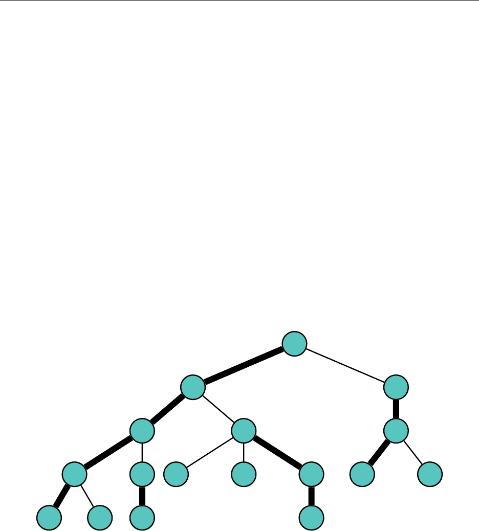
Hsiang, Wei, Liu Chapter 7. Tree Algorithms
7.4 Heavy-Light Decomposition
Brute-force algorithms on trees are often fast when the tree is nearly complete, or has small depth.
Unfortunately, brute force is far too slow when the tree becomes more and more unbalanced and
approximates a linked list.
Certain problems can be solved very nicely in a list with segment trees and similar data structures.
Heavy-light decomposition provides us with a way to exploit the fact that long “chains," which
are present in unbalanced trees, might be slow in brute force but can be sped up with other data
structures.
Heavy-light decomposition provides us a way to dynamically find the lowest common ancestor as
well as a way to prove time complexities about tree data structures, like link-cut trees.
Heavy-light decomposition is a coloring of all the edges in a binary tree either heavy or light.
For each vertex
v
, let
s
(
v
)denote the number of nodes in the subtree with
v
as its head. Then, if
u, w are the children of v,s(v) = s(u) + s(w)+1.
We see that the smaller child
u
or
w
must have less than half the subtree size as
v
, and so that
child exhibits qualities similar to those of a completely balanced tree. We color the edge connecting
vto its lesser child light. We color the other edge heavy.
We see that from any node, the number of light edges needed to reach the head of the tree is at
most
log n
, as each light edge doubles the subtree size. Then, the number of “heavy chains" along
the upwards path from any node is also of the order log n.
17
12
6
3
1 1
2
1
5
1 1 2
1
4
3
1 1
7.5 Link-Cut Tree
84
Chapter 8
Strings
8.1 String Hashing
String hashing is a probabilistic technique for dealing with strings. The most common hashing
algorithm used in programming contests is the polynomial hash, also known as the Rabin-Karp
hash. This method allows for the fast comparison of strings and their substrings—
O
(1) after linear
time precomputation. Thus we can often use conceptually simpler hashing to replace trickier string
algorithms, such as Knuth-Morris-Pratt and the Z-algorithm. In addition, adding binary search
allows for the computation of the longest common prefix in
log n
time, useful in constructing suffix
arrays.
Jonathan Paulson gives a great introduction to polynomial hashing:
https://www.reddit.com/
r/usaco/comments/39qrta/string_hashing/
8.2 Knuth-Morris-Pratt
Knuth-Morris-Pratt is an easy-to-code linear time string matching algorithm. Using the “needle
and haystack” analogy, for a given needle of length
n
and a haystack of length
m
, KMP takes
O
(
n
)to preprocess the needle and
O
(
m
)to search. Hariank and Corwin explain the algorithm well:
https://activities.tjhsst.edu/sct/lectures/1415/stringmatching_10_3_14.pdf
Beyond string matching, KMP is also useful for problems involving periodic strings. This is
because a string with an equal prefix and suffix of length
l
has a period of
n−l
, which is exactly
what KMP computes.
A similar (and equivalent) algorithm is the Z-algorithm, explained here:
http://codeforces.
com/blog/entry/3107
8.3 Trie
A trie (from retrieval) is a data structure for storing strings that supports insertion and look-up in
linear time. The trie maintains the strings in a rooted tree, where each vertex represents a prefix
and each edge is labeled with a character. The prefix of a node
n
is the string of characters on the
85
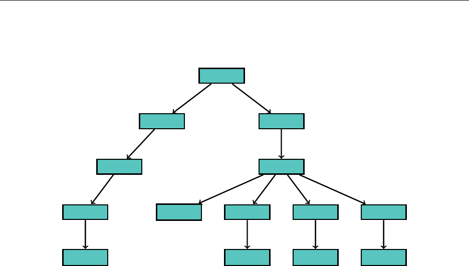
Hsiang, Wei, Liu Chapter 8. Strings
path from the root to
n
. (In particular, the prefix of the root is the empty string.) Every string
that is stored in the tree is represented by a path starting from the root. Below is a picture of a trie
storing “COW,” “MO,” “MOM,” “MOO,” and “MOP.”
C
CO
COW
COW$
$
W
O
C
M
MO
MO$
$
MOM
MOM$
$
M
MOO
MOO$
$
O
MOP
MOP$
$
P
O
M
Insertion into a trie is straightforward. We start at the root, and create edges and vertices as
necessary until a path representing the string is formed. If a vertex already has an edge of the
correct character leading out from it, we just travel down that edge. In order to identify the end of
a string, we can append a “$” to every string before we insert. Searching is the same as insertion,
except we terminate our search when we can’t go any further instead of adding a new edge.
What we’ve seen so far doesn’t make the trie seem particularly useful—string insertion and look
up can be easily done in linear time with Rabin-Karp and a hash table as well. The advantage of
the trie comes from its tree structure. Having common prefixes bundled together on the same path
means we can compute compute information relating to prefixes easily. This allows for tree DPs
that we wouldn’t be able to do with hashing. (However, hashing does handle certain forms of prefix
queries well, such as longest common prefix.)
Tries are also a building block for other string data structures, such as the Aho-Corasick
automaton and the suffix tree. (In fact, tries can be viewed as a very simple form of string
automaton.)
8.4 Suffix Array
For a string of length
n
, each index
i
(0
≤i<n
) can represent the suffix that starts at that index.
Asuffix array is a list of these indices, sorted in lexicographically increasing order by suffix. Thus
a suffix array is essentially a sorted list of the suffixes of a string. Below is the suffix array of
“mississippi$.”
86

Hsiang, Wei, Liu Chapter 8. Strings
Suffix Array Suffix
11 $
10 i$
7 ippi$
4 issippi$
1 ississippi$
0 mississippi$
9 pi$
8 ppi$
6 sippi$
3 sissippi$
5 ssippi$
2 ssissippi$
At first, it might seem surprising that such a structure is useful—why do we care about suffixes
at all? The crucial observation is that every substring of a string is a prefix of a suffix. Thus if
we have something that does well with prefixes, such as hashing or a trie, we use this to compute
information about substrings. A trie built from suffixes is known as a suffix tree, which we’ll cover
later. In this section, we’ll go over what we can do with hashing and a suffix array.
First, let’s figure out how we can construct a suffix array. The naive solution is to sort all
n
suffixes using
O
(
n
)string comparison. Since sorting itself takes
O
(
nlog n
)comparisons, we have an
O
(
n2log n
)algorithm. However, with hashing and binary search, we can lexicographically compare
two strings in
O
(
log n
)time. We do this by binary searching for the longest common prefix and then
comparing the next character. We can can compute the hash of any substring with a polynomial
hash, so it’s easy to compare if the prefixes of two suffixes (a.k.a two substrings) are equal. Now
that we have O(log n)comparison, our algorithm runs in O(nlog2n)overall.
Note that it is also possible to compute suffix arrays in
O
(
nlog n
)and even
O
(
n
), but these
algorithms are much more involved. For the purposes of contests, an
O
(
nlog2n
)suffix array
algorithm should almost always be enough.
With a suffix array, we can check if any queried “needle” string exists using a binary search
with hashing. We can even count the number of occurrences by binary searching for the first and
last match. This works in
O
(
m
+
log nlog m
), where
m
is the length of the needle, because we
need
O
(
log m
)operations for string comparison and
O
(
log n
)iterations of the binary search. Suffix
arrays differ from KMP because KMP preprocesses the “needle,” while suffix arrays preprocess the
“haystack.”
From the suffix array, we can also obtain another useful data structure called the LCP array.
This array stores the longest common prefix between adjacent suffixes in the suffix array. We can
use it to speed up pattern matching to
O
(
m
+
log n
). In addition, we can build a segment tree over
the LCP array to answer queries, such as the LCP between two arbitrary suffixes.
87

Hsiang, Wei, Liu Chapter 8. Strings
Suffix arrays can also be used to solve many string problems beyond matching. This data
structure does very well with most problems involving substrings. For example, suffix arrays/LCP
arrays can count the number of distinct substrings in a string or return the
k
th lexicographically
largest substring. The minimum string rotation problem can is another problem solvable with suffix
arrays, since each rotation of a string Sis a substring of S+S.
To handle multiple strings with suffix arrays, we can either concatenate them with separator
characters in between or separately compute their hashes.
Below is a short C++ code for computing suffix arrays. Look up lambda functions in C++ if
you’re not familiar with the syntax.
1typedef unsigned long long ull ;
2// We use A as the exponent and M as the mod for our hash .
3const ull M = 1000000007;
4const ull A = 127;
5
6void buil d (string S,int *sa ){
7// Builds a suffix array for a st ring S in array sa.
8S.push_back (’$’);
9int N=S.size() ;
10 ull P [N+ 1] , H[N+ 1];
11 P[0] = 1; // P stores the precompu t e d powers of A .
12 H[0] = 0; // H stores the prefix hashes of S.
13 for (int i= 0; i<N;i++) {
14 // P r e computing powers and hashes .
15 P[i+ 1] = A*P[i]%M;
16 H[i+ 1] = ( A*H[i]+S[i]) % M;
17 sa [i]=i;
18 }
19 auto f= [&](int a,int l) {
20 // Returns the hash of the substring s ta rting at index a with lengt h l.
21 return (H[a+l] - H[a]*P[l]%M+M)%M;
22 };
23 auto comp = [&](int a,int b) {
24 // C o mpares the suffixes starting at indices a and b.
25 int lo = 0, hi =min(N-a,N-b);
26 whil e (lo +1<hi ){
27 int m= ( lo +hi ) / 2;
28 (f(a,m) == f(b,m) ? lo :hi )=m;
29 }
30 return S[a+lo ] < S[b+lo ];
31 };
32 sort(sa ,sa +N,comp);
33 }
8.5 Aho-Corasick
One way to think about the Aho-Corasick algorithm is KMP/Z-algorithm on a trie. This algorithm
is used for matching multiple needles in a single haystack and runs in time linear in the length of
the haystack, with preprocessing linear in the total length of the needles. To do this, we first add
all strings to a trie that stores some extra information at its nodes. Upon inserting each string, we
mark the last node visited as a endpoint node. Each node, in addition to storing its children and its
88

Hsiang, Wei, Liu Chapter 8. Strings
status as an endpoint node, stores a suffix link. This link points to the longest proper suffix that is
also a node on the trie. If necessary, each node can also store a dictionary suffix link, which points
to the first endpoint node reachable by only following suffix links.
To build an Aho-Corasick automaton, we start with a trie of the needle strings. What we want to
do is compute the suffix links. We simplify this by using an
O
(
nk
)approach, where
k
is the alphabet
size. For each node n, we compute an additional failure function, with one value corresponding to
each letter of the alphabet. Suppose
p
is the prefix represented by
n
. Then the failure function of
n
for the letter αpoints to the node representing longest suffix of p+αin the trie.
We can compute all of this with a BFS. When we are at a node, we can find the suffix links of
its children using the failure function of its own suffix link. We also have to calculate the node’s
own failure function. For every letter that has a corresponding child, its failure function is equal
to that child. Otherwise, its failure function is equal to the corresponding failure function of the
node’s suffix link. Take a moment to think through why this works.
To query, we can iterate through our haystack string character by character and make the
corresponding moves in the automaton. We follow the failure function when no child exists. However,
note that there isn’t really a distinction between a normal trie edge and a failed edge anymore. To
check for matches, we can look at the values we store at each node and/or follow dictionary suffix
links. To find all matches with dictionary suffix links, we have to follow the pointers until we reach
a node that doesn’t have a suffix in the dictionary. Note that if we follow dictionary suffix links, the
complexity of our algorithm will also be linear in the number of matches. Here’s an implementation
of Aho-Corasick in C++ without dictionary suffix links:
89

Hsiang, Wei, Liu Chapter 8. Strings
1const int SIGMA = 26;
2const int MAXN = 100005;
3// Each node is assigned an index where its data is stored .
4// ch first stores the children of each node and later the failure function .
5// val counts the number of strings ending at a given node .
6// link stores suffix links .
7int ch [MAXN][ SIGMA ], val[MAXN] , link[MAXN], sz = 1;
8// Array q is a hand - imp l e mented queue .
9// h and t point to the head and tail , r e spectively .
10 int q[MAXN], h,t;
11
12 void add (string s){
13 // Adds a string to the trie .
14 int p= 0; // p tracks our curr e n t position and starts at 0, the root .
15 for (int i= 0; i<s.size() ; i+ +) {
16 int c=s[i] - ’A’;
17 // ch[ p ][c ] is 0 if null , so we have to allocate a new node / index .
18 if (! ch [p][ c]) ch [p][ c] = sz ++;
19 p=ch [p][ c];
20 }
21 val [p]++; // Updates endpoint marker .
22 }
23
24 void build () {
25 // C o mputes all suffix links with a BFS , starting from the root .
26 h=t= 0;
27 q[t++] = 0;
28 whil e (h<t){
29 int v=q[h++] , u=link[v];
30 val [v] += val[u]; // Propagates endpoint marker .
31 for (int c= 0; c<SIGMA ;c++) {
32 if (ch [v][ c]) {
33 // If chi ld exists , we cre at e a suff ix link .
34 // The node ’s failure function here is the child .
35 // Also , note that we have a special case if v is the root .
36 link[ch [v] [ c]] = v?ch [u][ c] : 0;
37 q[t++] = c h [v][ c];
38 }else {
39 // Otherwise , we need to figure out its failure function .
40 // We do this by using the failure function of the node ’s suffix link .
41 ch [v][ c] = ch [u][ c];
42 }
43 }
44 }
45 }
8.6 Advanced Suffix Data Structures
I’ve yet to see these used in a contest, but they do exist.
90

Hsiang, Wei, Liu Chapter 8. Strings
8.6.1 Suffix Tree
8.6.2 Suffix Automaton
91
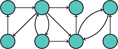
Chapter 9
More Graph Algorithms
With the renewal of strongly connected components and network flow in the IOI syllabus, we
overview some more graph algorithms that are standard but also noticeably more difficult than
other algorithms presented in earlier chapters.
9.1 Strongly Connected Components
This section covers Tarjan’s algorithm detects strongly connected components in a directed graph.
We begin with the DFS traversal of the graph, building a forest (collection of trees). In a DFS,
we only traverse each vertex once; this means when we encounter an edge to a vertex we already
visited, we move on without calling the DFS on that node. Once we obtain the forest, we can split
it into subgraphs that represent our strongly connected components.
Let’s work through how we can get the subgraphs representing the strongly connected components
from our DFS. Here’s the graph from the beginning of this section.
5678
1234
It doesn’t matter from which node we begin our DFS or the order in which we choose children;
in our example, we’ll simply choose the node with the minimum label to traverse first. This will
result in two trees in our forest, one rooted at 1 and the other rooted at 8.
93
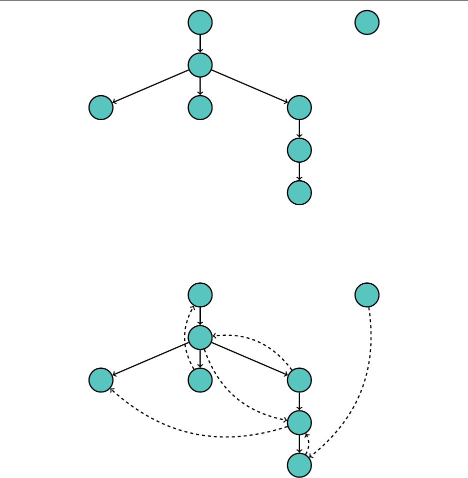
Hsiang, Wei, Liu Chapter 9. More Graph Algorithms
1
2
356
7
4
8
Now this by itself is not very useful, as in order to find strongly connected components, we’ll
need the edges in the directed graph that aren’t included in our tree. Here we add the other edges
as dashed pointers.
1
2
356
7
4
8
Note that strongly connected components are represented by subtrees in the graph. We call the
root of the subtree called the root of the strongly connected component.
One edge here is immediately useless. We already know that 2 can reach 7; 7 is in 2’s subtree.
The fact that there is an edge from 2 to 7 doesn’t change anything. Then we have a crucial
observation – the only possible useful extra edges are those that go up to a previous node in the
subtree, like the edge from 5 to 1, or those that go “left” to a previously-visited vertex, either to a
previous branch in the tree, like from 7 to 3, or to a previous subtree entirely, like from 8 to 4.
If a node
v
has an edge to a direct ancestor in the tree, that means we immediately have a cycle,
and therefore the node, its ancestor, and every vertex along the way must be in the same strongly
connected component.
94

Hsiang, Wei, Liu Chapter 9. More Graph Algorithms
Naturally, the “left” case is trickier. Suppose
v
has a left edge to a vertex
u
. We somehow need
a way to find out if
u
has a path back to
v
. We know that
u
cannot go down the tree to
v
as
v
is
not in the subtree of
u
by the way DFS constructed the tree. Therefore, we want to know whether
u
has a path back up to some common ancestor with
v
. However, again by the way DFS traverses
the graph, the entire subtree of
u
has already been searched before the DFS reaches
v
. We want to
exploit this fact with some kind of memoization.
If vertex
v
was the
n
th vertex visited in the DFS, we’ll mark
v
with the label
order
(
v
) =
n
.
We’ll also keep track of the “least” vertex
link
(
v
) =
u
that we know up to that point that
v
can
visit, or the vertex uwith the minimum order(u)that vcan reach so far.
As we’re using a DFS, we’ll use a stack
S
to keep track of nodes we’ve visited. In a normal DFS
on a tree, once we finish exploring a vertex
v
, we pop off
v
from the stack. This will not be the case
for us. A node remains on the stack iff it has a path to some node earlier in the stack.
This means as we explore the descendants of a vertex
v
, we’ll know if
v
has a path back to a
previous vertex. That is, if
link
(
v
)
< order
(
v
), it stays on the stack. If
link
(
v
) =
order
(
v
), we take
it off the stack.
Now we describe Tarjan’s algorithm. Here,
num
represents a global variable that indicates how
many vertices have been visited so far.
Algorithm 9 Tarjan
function StrongConnect(vertex u)
num ←num + 1 increment num
order(u)←num set order(u)to smallest unused number
link(u)←order(u)least order(v)accessible is uitself
push uon S
for all neighbors vof udo
if order(v)is undefined then v has not been visited
StrongConnect(v)
link(u)←min(link(u), link(v))
else if vis on stack Sthen v is in current component
link(u)←min(link(u), order(v))
if link(u) = order(u)then u is root of component, create SCC
create new strongly connected component
repeat
v←top of S
add vto strongly connected component
pop top from S
until u=v
function Tarjan(G(V, E))
num ←0
initialize new empty stack S
for all vertices v∈Vdo
if order(v)is undefined then v has not been visited
StrongConnect(v)
This algorithm runs in O(V+E).
95

Hsiang, Wei, Liu Chapter 9. More Graph Algorithms
9.2 Network Flow
We are given a directed graph with weighted edges, a source node, and a sink node. A flow is sent
from the source to the sink. Each edge weight represents the maximum capacity of that edge. For
every node besides the source and the sink node, total flow in is equal to total flow out. We can
think of a flow network as a series of pipes through which water travels from an entrance to an exit
in the network. The edge capacities represent pipe thickness. At any node, the total rate at which
water enters the node must equal the total rate at which it exits the node, and along any path, the
rate at which water flows is bottlenecked by the thinnest pipe.
More formally, for a graph
G
(
V, E
), where
c
(
u, v
)represents the capacity of the edge from
u
to
v, the flow f(u, v)from a source sto a sink tsatisfies
f(u, v)≤c(u, v)∀(u, v)∈E
f(u, v) = −f(v, u)∀(u, v)∈E
X
v∈V
f(u, v)=0 ∀u∈V\ {s, t}
X
v∈V
f(s, v) = X
v∈V
f(v, t) = |f|,
where |f|represents the total flow from the source to the sink.
Amaximum flow is one that maximizes the total flow
|f|
from
s
to
t
, or in our example,
maximizes the rate at which water can flow through our network.
We’ll also define the residual capacity
cf
(
u, v
) =
c
(
u, v
)
−f
(
u, v
). Note that
cf
(
u, v
)
≥
0by
the conditions imposed on
f
. The residual capacity of an edge represents how much capacity is
left after a certain amount of flow has already been sent. We therefore have the residual graph
Gf(V, Ef), where Efis the graph of residual edges, or all edges (u, v)∈V2satisfying cf(u, v)>0.
A natural approach to “solving” this problem would be to simply greedily add flow.
Find a path from the source to the sink in which all the edges have positive weight in the residual
graph. Send flow along this path; that is, find the max flow across this path, which is the minimum
weight of any edge on this particular path. Call this value
cap
. Then subtract
cap
from the residual
capacity of every edge in the path. We repeat, and this is guaranteed to terminate since on any
given move, we remove an edge from our residual graph.
What is wrong with our greedy approach? Consider the following graph:
1
2
3
4
2
2
2
1
1
The max flow from vertex 1 to vertex 4 is 3, but greedy gives only 2. This is because the best
possible single path from the source to the sink may not be included the best possible overall flow.
96

Hsiang, Wei, Liu Chapter 9. More Graph Algorithms
9.2.1 Ford-Fulkerson
We somehow need a way to fix the inclusion of any suboptimal paths in our greedy approach, or
to “send flow back” in case we sent it through a suboptimal path. We do this by introducing the
reverse edge to our residual graph.
Find a path from the source to the sink in which all the edges have positive weight in the
residual graph. Find the max flow across this path, which is the minimum weight of any edge on
this particular path. Call this value
cap
. Then subtract
cap
from the residual capacity of every edge
along the path and increment the residual capacity of the reverse edge (the edge connecting the
same two vertices but running in the opposite direction) by
cap
. We call this operation on the path
augmenting the path. We simply choose an augmenting path until no such paths exist.
Algorithm 10 Ford-Fulkerson
function AugmentPath(path p={vi}m
i=1, where (vi, vi+1)∈Ef,v1=s,vm=t)
cap ←minm−1
i=1 (cf(vi, vi+1))
for i≡1, m −1do
f(vi, vi+1)←f(vi, vi+1) + cap
cf(vi, vi+1)←cf(vi, vi+1) + cap
f(vi+1, vi)←f(vi+1, vi)−cap
cf(vi+1, vi)←cf(vi+1, vi) + cap incrementing reverse edge
function MaxFlow(G(V, E),s, t ∈V)
for all (u, v)∈V2do
f(u, v)←0
cf(u, v)←c(u, v)
|f| ← 0
while ∃p={vi}m
i=1, where (vi, vi+1)∈Ef,v1=s,vm=tdo
cap ←minm−1
i=1 (cf(vi, vi+1))
|f|←|f|+cap
AugmentPath(p)
return |f|
The difference between this algorithm and the greedy approach from earlier is that the paths
we now allow may run along a reverse path, essentially undoing any suboptimal flow from earlier.
These more general paths in our residual graph are called augmenting paths.
This algorithm is guaranteed to terminate for graphs with integral weights. Its performance
is bounded by
O
(
Ef
), where
f
is the maximum flow and
E
is the number of edges, as finding a
path from
s
to
t
takes
O
(
E
)and increments the total flow
f
by at least 1. The concept of removing
edges can’t be used to produce a stricter bound because while an edge in one direction may be
removed from the residual graph, doing so creates an edge in the other direction.
In its crudest form, Ford-Fulkerson does not specify on which path to push flow if multiple paths
exist. It simply states that as long as such a path exists, push flow onto it. In addition to being slow,
Ford-Fulkerson, as it is stated, is not guaranteed to terminate for graphs with non-integral capacities.
In fact, it might not even converge to the maximum flow for irrational capacities. However, these
problems can be fixed by simply specifying how the algorithm chooses the next path on which to
97

Hsiang, Wei, Liu Chapter 9. More Graph Algorithms
push flow. Nonetheless, the Ford-Fulkerson algorithm is formulated beautifully mathematically and
such is useful from a math perspective, as we will see with the Max-Flow Min-Cut Theorem.
9.2.2 Max-Flow Min-Cut Theorem
On a graph
G
(
V, E
), an s-t cut
C
= (
S, T
)splits the partitions
V
into
S
and
T
satisfying
s∈S
and
t∈T
. The cut-set of
C
is the set of edges
{
(
u, v
)
∈E
:
u∈S, v ∈T}
. The capacity of an s-t
cut is given by
c(S, T ) = X
(u,v)∈S×T
c(u, v).
Aminimum cut is an s-t cut that minimizes c(S, T ).
A cut represents a set of edges that, once removed, separates
s
from
t
. A minimum cut is
therefore a set of edges that does this but minimizes the total capacity of the edges necessary to
disconnect sfrom t.
The max-flow min-cut theorem states that the maximum value of any s-t flow is equal to the
minimum capacity of any s-t cut.
First, the capacity of any cut must be at least the total flow. This is true by contradiction. Any
path from
s
to
t
has an edge in the cut-set, so therefore any flow from
s
to
t
is upper bounded
by the capacity of the cut. Therefore, we need only construct one flow and one cut such that the
capacity of the cut is equal to the flow.
We consider the residual graph
Gf
produced at the completion of the Ford-Fulkerson augmenting
path algorithm.
1
Let the set
S
be all nodes reachable from
s
and
T
be
V\S
. We wish to show that
C
= (
S, T
)is a cut satisfying
|f|
=
c
(
S, T
) =
P(u,v)∈S×Tc
(
u, v
). This is true when the following is
satisfied:
1. All edges (u, v)∈S×Tare fully saturated by the flow. That is, cf(u, v)=0.
2. All reverse edges (v, u)∈T×Shave zero flow. That is, f(v, u)=0, or cf(v, u) = c(v, u).
The first condition is true by the way we constructed
S
and
T
, as if there existed a (
u, v
)where
cf(u, v)>0, then vis accessible to sand ought to have been in S.
The second condition is true by the way the Ford-Fulkerson algorithm constructed reverse edges.
If net flow was sent from
v
to
u
, then a reverse edge was constructed from
u
to
v
, so again,
v
is
accessible to s, which is a contradiction.
Therefore, we have the flow
|f|=X
(u,v)∈S×T
c(u, v)−X
(v,u)∈T×S
0 = c(S, T ),
so we constructed a flow and a cut such that the flow
|f|
is equal to the cut capacity
c
(
S, T
), and
we are done.
1
If you’re concerned that the Ford-Fulkerson algorithm will never terminate, there always exists a sequence of
paths chosen such that it will. Edmonds-Karp is one example that always terminates.
98

Hsiang, Wei, Liu Chapter 9. More Graph Algorithms
9.2.3 Refinements of Ford-Fulkerson
As stated earlier, Ford-Fulkerson is limited by not specifying on which path to push flow. There are
many algorithms that resolve this issue in different ways.
Edmonds-Karp
Edmonds-Karp fixes the problem by simply choosing the augmenting path of shortest unweighted
length. This can be done easily using a BFS.
Algorithm 11 Edmonds-Karp
function ChoosePath(Gf(V, Ef),s, t ∈V)BFS
visited(v)denotes vhas been added to queue
prev(v)denotes vertex preceding vin BFS
push son queue Q
visited(s)←1
while Qis not empty do
u←top of Q
for all neighbors vof uin Gfwhere visited(v)=0do
push von Q
visited(v)←1
prev(v)←u
pointer curr ←t
while curr 6=sdo
add curr to beginning of path p
curr ←prev(curr)
add sto beginning of p
return p
function MaxFlow(G(V, E),s, t ∈V)
for all (u, v)∈V2do
f(u, v)←0
cf(u, v)←c(u, v)
|f| ← 0
while tcan be reached from sdo
p←ChoosePath(Gf, s, t)
cap ←minm−1
i=1 (cf(vi, vi+1))
|f|←|f|+cap
AugmentPath(p)
return |f|
The BFS is clearly
O
(
E
). To complete our analysis, we must somehow bound the number of
times we need to perform the BFS. To do this, we’ll look at what pushing flow on a path does to our
residual graph; in particular, how it affects our BFS traversal tree. Note that each vertex is on some
level
i
in the BFS tree, characterized by the distance from the source
s
. For example,
L0
=
{s}
,
L1
contains all the neighbors of s,L2contains neighbors of neighbors not in L0or L1, and so on.
99

Hsiang, Wei, Liu Chapter 9. More Graph Algorithms
We first claim that the level of any vertex in the graph is nondecreasing following an augment on
a path
p
. If the augment saturates an edge, it may remove it from
Gf
, which cannot decrease the
distance of any vertex from
s
. If the augment creates an edge
e
= (
u, v
), that means we sent flow
from
v
to
u
on the path
p
. Therefore, if
v
was originally level
i
,
u
must have been level
i
+ 1. The
level of
u
does not change by adding (
u, v
), and the level of
v
can either be
i
or
i
+ 2, depending on
whether edge (
v, u
)was deleted in the process. Either way, the level of all vertices is nondecreasing.
Now consider the bottleneck edge
e
= (
u, v
)of an augmenting path
p
, where the level of
u
is
i
and the level of
v
is
i
+ 1. The push operation deletes the edge
e
, but the level of
v
must stay at
least
i
+ 1. Now for the edge
e
to reappear in the graph
Gf
, flow must have been sent on the reverse
edge
e0
= (
v, u
)on some augmenting path
p0
. But on path
p0
,
u
comes after
v
, which must be at
least level
i
+ 1. Therefore,
u
must be at least level
i
. But since the maximum level of a node that
is connected to sis V−1, an edge ecan only be chosen as the bottleneck edge V
2times, or O(V).
There are
E
edges, each of which can be the bottleneck edge for
O
(
V
)different augmenting paths,
each of which takes O(E)to process. Therefore, the Edmonds-Karp algorithm runs in O(V E2).
Dinic
Dinic’s algorithm is another refinement of Ford-Fulkerson. Dinic’s algorithm is similar to Edmonds-
Karp in that we make use of the length of the shortest path from
s
to each vertex
v
. We first define
the level graph GLof Gfas the graph containing edges (u, v)only if dist(v) = dist(u)+1.
We then define the blocking flow as a maximum flow
f
of a level graph
GL
. Dinic’s algorithm
constructs a level graph
GL
, augments the graph with a blocking flow, and repeats by finding another
level graph. This process can happen O(V)times, as with each blocking flow, dist(t)increases.
Each BFS to compute the level graph is
O
(
E
), and each blocking flow can be computed in
O(V E). Therefore, the run-time of Dinic’s algorithm is O(V2E).
Using a link-cut tree, the computation of a blocking flow can be improved to
O
(
Elog V
),
improving the overall run-time to O(V E log V).
In networks with unit capacities, each blocking flow can be computed in
O
(
E
), and the number
of total blocking flows is O(min √E, V 2/3), improving the overall run-time to O(min √E, V 2/3E).
9.2.4 Push-Relabel
Unfortunately, Dinic’s algorithm is considerably complex, and even the much-improved bounds of
the simpler
O
(
V E2
)Edmonds-Karp are admittedly bad. While the push-relabel method for solving
the max flow problem does not have the fastest theoretical bounds, two of its implementations have
complexities O(V3)and O(V2√E)and are among the fastest in practice.
Generic Push-Relabel
Ford-Fulkerson and its variants all deal with global augmentations of paths from
s
to
t
. Push-relabel
takes a different perspective, introducing the concept of a preflow and a height to make local
optimizations that ultimately result in the maximum flow.
100

Hsiang, Wei, Liu Chapter 9. More Graph Algorithms
A preflow maintains the same properties as a flow but modifies the conservation of flow condition.
Instead of total flow in equaling total flow out, flow in must be at least, and therefore can exceed,
flow out. We denote the difference between flow in and flow out as the excess e(v).
f(u, v)≤c(u, v)∀(u, v)∈E
f(u, v) = −f(v, u)∀(u, v)∈E
e(v) = X
u∈V
f(u, v)≥0∀v∈V\ {s}
e(s) = ∞.
The definitions of the residual capacity
cf
(
u, v
), edge set
Ef
, and graph
Gf
are the same as they
were defined before, except with a preflow finstead of a normal flow.
We call a vertex
v∈V\ {s, t}
active if
e
(
v
)
>
0. Therefore, a vertex besides the source or sink
is active if more flows into the vertex than flows out.
s
and
t
are never active. A preflow with no
active vertices is simply a flow, at which point the excess of the sink
e
(
t
)represents the value
|f|
of
the flow.
We can push flow from a node
u
to a node
v
by moving as much of the excess
e
(
u
)to
v
as the
capacity of the edge cf(u, v)will allow.
function Push(edge (u, v))
δ←min(e(u), cf(u, v)) cf(u, v) = c(u, v)−f(u, v)
f(u, v)←f(u, v) + δ
f(v, u)←f(v, y)−δ
e(u)←e(u)−δ
e(v)←e(v) + δ
The idea of the push-relabel algorithm is to first push as much preflow as possible through local
optimizations in the direction the sink. When a node can no longer push flow to the sink, it pushes
the excess back towards the source to turn the preflow into a flow.
However, the difficulty here lies in establishing this sense of “direction” from the source to the
sink. Remember that we simply push preflow along a single edge in the graph at a time, not along a
whole path. Moving flow from the source to the sink along a path that goes from the source to the
sink is easy; moving flow from the source to the sink through local pushes without the knowledge of
the graph structure as a whole is indeed a much harder problem.
To resolve this issue, we introduce a label to each of the nodes. The label
h
(
u
)represents the
“height” of
u
. In real life, water flows from higher to lower ground. We want
s
to represent that
high ground and
t
to represent the low ground. As we push preflow from
s
to
t
, vertices along the
way represent height values between those of
s
and
t
. However, eventually we have to push preflow
back to handle both excesses in flow and suboptimal previous pushes, à la Ford-Fulkerson, but this
contradicts the concept of height as we can’t flow both downhill and uphill. Therefore, we’ll need to
be able to relabel a node, changing the height
h
(
u
)to something that allows preflow to flow back
towards
s
. We will relabel
h
in a systematic way that allows us to direct the preflow through the
graph.
For this labeling to be useful for us, we’ll need to impose some more constraints that must be
satisfied no matter how we change the graph Gfor the height function h.
101

Hsiang, Wei, Liu Chapter 9. More Graph Algorithms
h(u)≤h(v)+1∀(u, v)∈Ef
h(s) = |V|
h(t)=0.
What does this mean? For our algorithm, we can push preflow along the edge from
u
to
v
only
if
cf
(
u, v
)
>
0and
h
(
u
)
> h
(
v
), so
h
(
u
) =
h
(
v
)+1. We call such an edge (
u, v
)
∈Ef
admissible.
Furthermore, for all vertices
v
that can reach
t
in
Ef
,
h
(
v
)represents the lower bound for the length
of any unweighted path from
v
to
t
in
Gf
, and for all vertices that cannot reach
t
, then
h
(
v
)
− |V|
is a lower bound for the unweighted distance from sto v.
t
will always represent the lowest node, so
h
(
t
) = 0 is a natural constraint. We’ll first set the
preflow values of all vertices
v
that can be immediately reached from
s
to
c
(
s, v
), saturating all the
out-edges of
s
. For any vertex
v
from which
t
can be reached,
h
(
v
)represents the lower bound of
the unweighted distance to tfrom vin the residual graph.
We want
h
(
s
)to be a number large enough that will indicate that
s
has been disconnected to
t
, as we have already sent as much preflow possible from
s
in the direction of
t
by saturating all
outgoing edges. Therefore, setting
h
(
s
) =
|V|
is also natural. Since
h
(
s
)represents the lower bound
of the distance from
s
to
t
in
Gf
, and there are no paths from
s
to
t
in the residual graph,
|V|
is a
natural choice, since the longest possible path is |V| − 1.
Furthermore, we don’t want any preflow sent back to
s
from a vertex
v
unless it is impossible to
send any more preflow from
v
to
t
. If preflow is pushed from
v
to
s
, then
h
(
v
) =
|V|
+ 1. If there
existed a path
v
to
t
such that every edge is admissible, the path must have
|V|
+ 2 vertices. This is
true because for any two consecutive vertices
vi, vi+1
in the path,
h
(
vi
) =
h
(
vi+1
) + 1, but no path
can have |V|+ 2 distinct vertices.
This leads to the fact that the only nodes that can possibly continue to contribute to the final
flow are active vertices
v
for which
h
(
v
)
<|V|
. A node with height at least
|V|
does not have a
valid path to t, and a node that is not active doesn’t have any excess flow to push.
Now that I’ve explained the general idea behind the labeling constraints, it’s time to actually
describe what our relabeling process is. At first, the labels of all vertices besides the source start at
0. We only relabel a node
v
if it is active (therefore, it has excess flow it needs to push;
e
(
u
)
>
0)
but has no admissible out-edges in
Gf
(so it has no adjacent vertex on which it can push that excess
flow). If a node has no admissible out-edges in
Gf
, every neighbor of
u
has a height label at least
equal to
h
(
u
). When we relabel a node, we always then increase the value of
h
(
u
)to the least value
where it can push flow onto another node.
function Relabel(vertex u)
h(u)←minv|(u,v)∈Ef(h(v)) + 1 (u, v)∈Ef⇐⇒ cf(u, v) = c(u, v)−f(u, v)>0
Since we take the minimum height of all neighbors in the graph, we first try adjusting the
height of
u
so that we can push flow from
u
to its neighbors that can possibly still reach
t
; that is,
neighbors
v
satisfying
h
(
v
)
<|V|
. Once we try all these neighbors, we then increase the height of
u
to begin to push flow back towards
s
. We can always find such an edge, as any preflow pushed onto
umust have also incremented the reverse edge from uback towards s.
Note that neither pushing on a admissible edge nor relabeling a vertex with no admissible
out-edges changes the fact that hremains a valid labeling function.
102

Hsiang, Wei, Liu Chapter 9. More Graph Algorithms
The generic push-relabel algorithm simply pushes and relabels vertices until there are no active
vertices and the preflow becomes a flow. This algorithm works because throughout the process,
h
remained a valid height function, and at the end, the preflow was converted into a flow. Since
h(s) = |V|and h(t)=0, there is no augmenting path from sto t, so our flow is maximal.
Algorithm 12 Push-Relabel (Generic)
function Push(edge (u, v))
if e(u)>0and h(u) = h(v)+1then push condition
δ←min(e(u), cf(u, v)) cf(u, v) = c(u, v)−f(u, v)
f(u, v)←f(u, v) + δ
f(v, u)←f(v, y)−δ
e(u)←e(u)−δ
e(v)←e(v) + δ
function Relabel(vertex u)
if u6=s, t and e(u)>0and h(u)≤h(v)∀v|(u, v)∈Efthen relabel condition
h(u)←minv|(u,v)∈Ef(h(v)) + 1 (u, v)∈Ef⇐⇒ cf(u, v) = c(u, v)−f(u, v)>0
function MaxFlow(G(V, E),s, t ∈V)
for all v∈V\ {s}do initialize excess
e(v)←0
e(s)← ∞
for all (u, v)∈V2do initialize preflow
f(u, v)←0
for all neighbors v6=sof sdo saturate edges to all neighbors of s
f(s, v)←c(s, v)
f(v, s)← −c(s, v)
e(v)←c(s, v)
for all v∈V\ {s}do preflow now has valid height function; initialize height
h(v)←0
h(s)← |V|
while we can still Push or Relabel do
Push or Relabel
return e(t) e(t) = |f|
We can argue that this algorithm runs in
O
(
V2E
), which is already an improvement from
Edmonds-Karp. However, just as Ford-Fulkerson could be sped up by specifying which augmenting
paths to choose, we can do the same with the push-relabel algorithm, speeding it up by specifying a
systematic method to choose an edge to push or a vertex to relabel.
Discharge
We first describe an auxiliary operation. For each vertex
u
, we’ll need a way to visit in- and
out-neighbors of
u
in a static cyclic order. This is easy with just a pointer; for vertex
u
, we’ll call
that pointer
curr
(
u
). When the pointer passes through every element in the list of neighbors, we’ll
just reset it back to the first element.
103

Hsiang, Wei, Liu Chapter 9. More Graph Algorithms
function Discharge(vertex u)
while e(u)>0do perform an operation as long as uis active
if curr(u)is at end of list of neighbors then
Relabel(u)
reset curr(u)
else
if (u, curr(u)) is an admissible edge then
Push((u, curr(u)))
else
move curr(u)to next neighbor of u
FIFO Selection
FIFO selection simply maintains a list of active vertices in a FIFO queue. We pop off the first
vertex in the queue and discharge it, adding any newly-activated vertices to the end of the queue.
This runs in O(V3).
Highest Label Selection
Highest label selection discharges the active vertex with the greatest height. This runs in
O
(
V2√E
).
Improvements with Heuristics
Heuristics are meant to help relabel vertices in a smarter way. Bad relabelings are the slowest part
of the algorithm, and improving the process can speed up max flow.
The gap heuristic takes advantage of “gaps” in the height function. Since a path of admissible
edges consists of vertices whose heights decrease by exactly 1, the presence of a gap in height
precludes the possibility of such a path. If there exists a value
h0
such that no vertex
v
exists such
that
h
(
v
) =
h0
, then for every vertex
v
satisfying
h0< h
(
v
)
<|V|
,
v
has been disconnected from
t
,
so we can immediately relabel h(v) = |V|+ 1.
The global relabeling heuristic performs a backwards BFS from
t
every now and then to compute
the heights of the vertices in the graph exactly.
Some dude on Codeforces
2
didn’t have much luck improving performance with the global
relabeling heuristic. I’d suggest sticking to the gap heuristic only.
9.2.5 Extensions
9.2.6 Bipartite Matchings
The bipartite matching problem is perhaps the most well-known problem solvable by flows.
2http://codeforces.com/blog/entry/14378
104

Chapter 10
Math
Algorithms here exhibit a different flavor than the graph theory, string, or geometry algorithms
from earlier. This chapter is placed towards the end because material here doesn’t really fit in any
other section or the USACO canon, not because this material is particularly difficult.
10.1 Number Theory
This section will contain much information about primes in many different ways. Indeed, prime
numbers are the building blocks of number theory!
10.1.1 Random Prime Numbers Bounds
The point of this section is mostly to make the complexity analysis of the later sections easier.
Therefore, I will list some useful theorems and bounds without proof. The proofs can be found in
any standard number theory textbook or online. They are extremely insignificant in the context of
the goals of this section.
Prime Number Theorem
: The number of prime numbers less than
n
is
O
(
n
log n
)for any
positive integer n.
Corollary: The n-th prime number, pn, is O(nlog n).
Prime Number Harmonic Sum:Pp≤n1
p=O(log log n).
10.1.2 Prime Number Testing
Let’s say if you want to test is a number
n
is prime. The most obvious way is to test all integers
from 2to
n−
1, and see if they divide
n
. This takes
O
(
n
)time. We can do better though! Note that
if
n
has a nontrivial factor, then it has one that is less than
√n.
Indeed, if
n
=
pq,
(as a nontrivial
factorization) if both
p, q > √n
, then
pq > √n2
=
n
, a contradiction. So we only need to check
whether
n
has factors between 2and
√n.
This takes
O
(
√n
)time. If you have precomputed a list of
prime numbers (up to say
√n
), ten you only need to check whether
n
has any prime factors in the
same 2to
√n.
This would give runtime
O
(
√n
log n
)from the Prime Number Theorem in section 10.1.1,
a small but nontrivial improvement.
105

Hsiang, Wei, Liu Chapter 10. Math
10.1.3 Sieve of Eratosthenes
If you want to compute all primes in the range 1to
n
. Runs in
O
(
nlog log n
). In other words, super
fast.
10.1.4 Prime Factorization
How can we prime factorize a number? That is, given a positive integer
n
, how can we write it in the
form
p1·p2·····pk
, where the
pi
are all primes? Form example, 30 = 2
·
3
·
5and 24 = 2
·
2
·
2
·
3. The
fact that every number can be uniquely factorized is called the Fundamental Theorem of Arithmetic.
Let’s now figure out how to prime factorize every number efficiently. Using our intuition from above,
we should expect that checking up to around
√n
suffices. This is indeed true. The code below
demonstrates:
10.1.5 GCD and the Euclidean Algorithm
I’ll start once again with a theorem in number theory: if positive integers
a, b
satisfy
gcd
(
a, b
)=1,
then there exist integers x, y such that ax +by = 1.This is called Bezout’s Lemma.
Similarly, if gcd(a, b) = g, then there are integers x, y such that ax +by =g.
10.1.6 Fermat’s Little Theorem
Fermat’s Little Theorem states that
ap≡a
(
mod p
)for any positive integer
a.
Equivalently, we can
say that ap−1≡1 (mod p).
10.1.7 Modular Inverses
If
p
is a prime, and
x
satisfies
gcd
(
x, p
) = 1, then there exists a positive integer
k
such that
kx ≡
1
(
mod p
)
. k
is called the modular inverse of
x
(
mod p
)
,
often just denoted as 1
/x
or
x−1.
Indeed,
1
/x ·x
=
x−1·x
= 1
,
so this notation is natural. The cool thing about modular inverses is that you
can see them as division modulo
p.
Since
x
is nonzero (
mod p
)
,
it makes sense that you should be
able to divide by
x.
This is the main application of modular inverses. But how to find one quickly?
There are two common algorithms, both of which run in
O
(
log p
)time. You can do this by running
the Euclidean Algorithm described above: find positive integers
j, k
such that
pj
+
kx
= 1
.
Then
obviously
kx ≡
1 (
mod p
)
.
The other way is to notice that
xp−1≡
1 (
mod p
)by Fermat’s Little
Theorem, so
xp−2≡x−1
(
mod p
)
.
Now compute the left hand side of the previous expression using
binary exponentiation.
Exercises related: Do
O
(
nlog p
)precomputation to compute any binomial coefficient of the form
m
k(mod p)where 0≤m, k ≤nin O(1) time.
10.2 Combinatorial Games
https://activities.tjhsst.edu/sct/lectures/1314/impartial_games_12_06_13.pdf
106

Hsiang, Wei, Liu Chapter 10. Math
10.3 Karatsuba
10.4 Matrices
10.5 Fast Fourier Transform
Introduction
The Fast Fourier Transform (FFT) is a technique used to multiply two polynomials of degree
n
in
O
(
n·log n
)time. At a high level, what this algorithm is doing is something called polynomial
interpolation. This refers to the fact that if we know the value of a polynomial
P
of degree
n
at
n
+ 1
points, then we can uniquely determine the polynomial
P.
The proof of this statement is simple, and
involves the Lagrange Interpolation Formula for one direction and a simple root counting argument
to prove uniqueness. I won’t go into detail here because the proof isn’t important, but it is useful to
know some motivation behind the algorithm.
Algorithm Outline
Let’s say we want to multiply 2 polynomials
A
(
x
)
, B
(
x
), both of degree
n
. Let
C
(
x
) =
A
(
x
)
B
(
x
)
.
The algorithm will proceed in 3 steps. Choose an integer
m >
2
n,
and choose
m
numbers
x0, x1, . . . , xm−1.
I’ll clarify what to choose
m
and the
xi
as later. Just keep in mind that we can
choose these values to be anything we want.
1. Evaluate A(x0), A(x1), . . . , A(xm−1).Similarly, evaluate B(x0), B(x1), . . . , B(xm−1).
2. Evaluate C(xi) = A(xi)B(xi)for 0≤i≤m−1.
3. Interpolate the coefficients of C(x)given the values C(x0), C(x1), . . . , C(xm−1).
The last step explains why we need
m >
2
n.
The degree of
C
(
x
)is 2
n
, so we need at least 2
n
+ 1
points to determine C(x)uniquely.
You should be skeptical that the above approach does any better than
O
(
n2
)
.
In particular, step
1 seems like it should take
O
(
n2
)
.
It turns out that if we choose the values
x0, x1, . . . , xm−1
properly,
then we can do much better. Let me now describe what to choose
m
to be, and what to choose
x0, x1, . . . , xm−1to be.
Roots of Unity
Before telling you precisely, here’s some food for thought. Let’s take then example polynomial
A
(
x
) = 1 + 2
x
+ 3
x2
+ 4
x3
+ 5
x4
+ 6
x5
+ 7
x6
+ 8
x7.
Let’s split this into 2 groups: the even
degree coefficients and odd degree coefficients. Let’s call these two groups
Aeven
and
Aodd.
Define
Aeven(x) = 1 + 3x+ 5x2+ 7x3, Aodd(x) = 2 + 4x+ 6x2+ 8x7.Then clearly
A(x) = Aeven(x2) + x·Aodd(x2)
107

Hsiang, Wei, Liu Chapter 10. Math
Notice that the
x2
in the formula makes it extremely easy to compute
A
(
−x
)given
A
(
x
)
.
It’s
only one sign flip off! Therefore, it would be cool if our
xi
above were symmetric with respect to
0, i.e. if we want to compute
x
, we also should want to compute
−x
. An example set like this
is
{
1
,
2
,
3
,
4
,−
1
,−
2
,−
3
,−
4
}.
So if we wanted to compute
A
(
x
)at these values, we would need to
compute the values of
Aeven, Aodd
at their squares, that is
{
1
,
4
,
9
,
16
}.
But this set is no longer
symmetric! So this is not what we want exactly, since that means that we can’t just recursively
compute
Aeven
and
Aodd.
So let’s say that the set we want to compute
Aeven, Aodd
on is something
like
{
1
,
4
,−
1
,−
4
}.
Then the values that we get for
A
(
x
)are
{
1
,−
1
,
2
,−
2
, i, −i,
2
i, −
2
i}.
Complex
numbers! This is closer to what we want, but still not precisely. The selection of the
xi
explained
below makes everything work out perfectly.
So what should we choose
m
and the
xi
to be? I’ll tell you now and then explain why this selection
works so well: choose
m
to be a power of 2that is larger than 2
n
, and choose
x0, x1, . . . , xm−1
to
be the
m
-th roots of unity. The
m
-th roots of unity are complex numbers that satisfy the equation
xm= 1.They are of the form cos 2kπi
m+i·sin 2kπi
mfor any integer kfrom 0to m−1.
Let
ω
be a primitive root of unity, i.e. the smallest
m0
such that
ωm0
= 1 is
m0
=
m.
We can
without loss of generality set ω= cos 2πi
m+i·sin 2πi
m.One can easily check the the remaining
roots of unity are
ω2, ω3, . . . , ωm.
From now on, let’s just set
xi
=
ωi
for all 0
≤i≤m−
1
.
Note
that x0= 1.Also set m= 2k>2n. Now I can proceed to describing why this algorithm works.
Algorithm Specifics: Step 1
In this section I’ll implement (using pseudocode) a function
vector<double> fft(vector<int>
A
, k,
ω
). This means that this will return a vector<double>
of length 2
k
containing the values
A
(
ω0
)
, A
(
ω1
)
, A
(
ω2
)
, . . . , A
(
ω2k−1
)
.
Remember that
ω2k
= 1
.
The
vector<int> Astores the coefficients of A(x). The xicoefficient of Awould be stored as A[i].
Here’s an implementation. The brackets {} will be shorthand for containing a vector.
Algorithm 13 Fast Fourier Transform
function FFT(vector<int> A, k, ω) ω2k= 1
A.resize(2k)
vector<double> f, feven, fodd
f.resize(2k)
if k= 0 then
return {A[0]}a vector of length 1
Aeven ={A[0], A[2], . . . , A[2k−2]}
Aodd ={A[1], A[3], . . . , A[2k−1]}
feven =FFT(Aeven, k −1, ω2)
fodd =FFT(Aodd, k −1, ω2)
for all i= 0, i < 2k−1, i + + do
f[i] = feven[i] + ωi·fodd[i]
f[i+ 2k−1] = feven[i]−ωi·fodd[i]
return f
108

Hsiang, Wei, Liu Chapter 10. Math
So why does this algorithm work? Note that the algorithm proceeds recursively, calling itself
twice (once for even, once for odd).
Aeven
(
x
)is the polynomial
A
[0] +
A
[2]
x
+
A
[4]
x2
+
···
+
A
[2
k−
2]
x2k−1−1.
Therefore, what the recursive call is doing is computing the values of
Aeven
at
the values
x
=
ω0, ω2, ω4, . . . , ω2k−2.
This is equivalent to computing the values of the polynomial
Beven
(
x
) =
A
[0] +
A
[2]
x2
+
A
[4]
x4
+
···
+
A
[2
k−
2]
x2k−2
at the values
x
=
ω0, ω1, ω2, . . . , ω2k−1−1.
The recursive call for
Aodd
(
x
) =
A
[1] +
A
[3]
x
+
A
[5]
x2
+
···
+
A
[2
k−
1]
x2k−1−1
behaves in a similar
way. Similarly, define Bodd(x) = A[1] + A[3]x2+A[5]x4+··· +A[2k−1]x2k−2.
The key is to note that
A
(
x
) =
Beven
(
x
)+
x·Bodd
(
x
)
.
Since we know the values of
Beven
(
x
)
, Bodd
(
x
)
for
x
=
ω0, ω1, . . . , ω2k−1−1,
we also can compute the values of
A
(
x
)for these values of
x
. But
what about the remaining values? This requires the observation that
ωi+2k−1
=
−ωi.
Since
Beven
(
x
)
, Bodd
(
x
)only have even powers,
Beven
(
ωi
) =
Beven
(
−ωi
) =
Beven
(
ωi+2k−1
)
.
The same
equality also holds for
Bodd
(
x
)
.
Using this observation along with the equation
A
(
x
) =
Beven
(
x
) +
x·Bodd
(
x
)
,
we can see now why the two equations in the for loop of the code above hold. And
that’s how we do Step 1!
Let’s analyze the runtime of this function FFT. Let
T
(2
k
)denote the time needed to run FFT
on an array of length 2
k.
Then
T
(2
k
) = 2
T
(2
k−1
) +
O
(2
k
) =
⇒T
(2
k
) =
k·
2
k,
by the Master
Theorem. Since 2kis O(n)by the above discussion, this steps runs in O(n·log n)time.
Algorithm Specifics: Step 2
I’ll give you a rest after a hard theoretical previous section. You do this step by looping through
the values
A
(
x0
)
, A
(
x1
)
, . . . , A
(
x2k−1
)
, B
(
x0
)
, B
(
x1
)
, . . . , B
(
x2k−1
)and directly multiplying
C
(
xi
) =
A(xi)B(xi).This step runs in O(n)time.
Algorithm Specifics: Step 3
This may seem like something completely new, but actually most of the work is already done. I’ll
explain. In fact I claim that writing the code
C
=
fft
(
C, k, ω−1
)
,
and then dividing all elements of
Cby 2kfinishes. Step 3 is very easy once you have Step 1!
To see this, let’s take a look at how step 1 works. We’ll consider the coefficients of
A
as a vector
(not a C++ vector, but an actual math vector – matrices!).
A(ω0)
A(ω1)
A(ω2)
A(ω3)
.
.
.
A(ω2k−2)
A(ω2k−1)
=
ω0ω0ω0ω0··· ω0ω0
ω0ω1ω2ω3··· ω2k−2ω2k−1
ω0ω2ω4ω6··· ω2(2k−2) ω2(2k−1)
ω0ω3ω6ω9··· ω3(2k−2) ω3(2k−1)
.
.
..
.
..
.
..
.
.....
.
..
.
.
ω0ω2k−2ω2(2k−2) ω3(2k−2) ··· ω(2k−2)(2k−2) ω(2k−1)(2k−2)
ω0ω2k−1ω2(2k−1) ω3(2k−1) ··· ω(2k−2)(2k−1) ω(2k−1)(2k−1)
A[0]
A[1]
A[2]
A[3]
.
.
.
A[2k−2]
A[2k−1]
109

Hsiang, Wei, Liu Chapter 10. Math
Now suppose we perform the FFT with
ω−1
. This is equivalent by multiplying by a similar
matrix.
110

Hsiang, Wei, Liu Chapter 10. Math
ω0ω0ω0ω0··· ω0ω0
ω0ω−1ω−2ω−3··· ω−(2k−2) ω−(2k−1)
ω0ω−2ω−4ω−6··· ω−2(2k−2) ω−2(2k−1)
ω0ω−3ω−6ω−9··· ω−3(2k−2) ω−3(2k−1)
.
.
..
.
..
.
..
.
.....
.
..
.
.
ω0ω−(2k−2) ω−2(2k−2) ω−3(2k−2) ··· ω−(2k−2)(2k−2) ω−(2k−1)(2k−2)
ω0ω−(2k−1) ω−2(2k−1) ω−3(2k−1) ··· ω−(2k−2)(2k−1) ω−(2k−1)(2k−1)
A(ω0)
A(ω1)
A(ω2)
A(ω3)
.
.
.
A(ω2k−2)
A(ω2k−1)
=
ω0ω0ω0ω0··· ω0ω0
ω0ω−1ω−2ω−3··· ω−(2k−2) ω−(2k−1)
ω0ω−2ω−4ω−6··· ω−2(2k−2) ω−2(2k−1)
ω0ω−3ω−6ω−9··· ω−3(2k−2) ω−3(2k−1)
.
.
..
.
..
.
..
.
.....
.
..
.
.
ω0ω−(2k−2) ω−2(2k−2) ω−3(2k−2) ··· ω−(2k−2)(2k−2) ω−(2k−1)(2k−2)
ω0ω−(2k−1) ω−2(2k−1) ω−3(2k−1) ··· ω−(2k−2)(2k−1) ω−(2k−1)(2k−1)
ω0ω0ω0ω0··· ω0ω0
ω0ω1ω2ω3··· ω2k−2ω2k−1
ω0ω2ω4ω6··· ω2(2k−2) ω2(2k−1)
ω0ω3ω6ω9··· ω3(2k−2) ω3(2k−1)
.
.
..
.
..
.
..
.
.....
.
..
.
.
ω0ω2k−2ω2(2k−2) ω3(2k−2) ··· ω(2k−2)(2k−2) ω(2k−1)(2k−2)
ω0ω2k−1ω2(2k−1) ω3(2k−1) ··· ω(2k−2)(2k−1) ω(2k−1)(2k−1)
A[0]
A[1]
A[2]
A[3]
.
.
.
A[2k−2]
A[2k−1]
=
2k0 0 0 ··· 0 0
0 2k0 0 ··· 0 0
0 0 2k0··· 0 0
0 0 0 2k··· 0 0
.
.
..
.
..
.
..
.
.....
.
..
.
.
0 0 0 0 ··· 2k0
0 0 0 0 ··· 0 2k
A[0]
A[1]
A[2]
A[3]
.
.
.
A[2k−2]
A[2k−1]
= 2k
A[0]
A[1]
A[2]
A[3]
.
.
.
A[2k−2]
A[2k−1]
.
111

Hsiang, Wei, Liu Chapter 10. Math
It follows that the inverse FFT is simply the same function, but run with
ω−1
instead of
ω
, and
dividing out m= 2k.
A Brief Note on Number Theory
There is a slight variation on FTT that avoids using complex numbers completely. Complex numbers
are often bad at precision and run slowly. There is a way to make FFT work over only the integers,
which is pretty cool. Here’s a brief description how.
We work (
mod p
)for a suitable prime
p
. The reason we need
p
to be prime is so that division
works as we want. As explained in the above section on number theory, every nonzero number
modulo
p
has a unique inverse, so division works as expected. There are also integers
g
such that
g0, g1, . . . , gp−2
run through all nonzero numbers (
mod p
)
.
These are called primitive roots. This
means that modulo
p
behaves a whole lot like the roots of unity that we want. More specifically, we
want an integer
ω
such that the smallest integer
m
that satisfies
ωm
= 1 is
m
= 2
k,
for some power
of 2
.
So when can we find such an
ω
?By the discussion of primitive roots, this can happen precisely
when 2
k|p−
1
.
Then all we do is find a primitive root
g
, and take
ω
=
gp−1
2k.
Finding primitive roots
is fast because math proves that there is always a small primitive root. So everything works just as
you expect! The same exact code works, just put a (
mod p
)at the end of every line and you’re set.
112
Chapter 11
Nonsense
Have fun.
11.1 Segment Tree Extensions
11.1.1 Fractional Cascading
11.1.2 Persistence
11.1.3 Higher Dimensions
11.2 DP Optimizations
11.3 Top Tree
Tree representation of a graph. Scary.
11.4 Link-Cut Cactus
Acactus is a graph such that any two distinct cycles in the graph share at most one vertex. Graphs
that are not trees are somehow hard to characterize; a cactus is a more general kind of graph that
still has some nice properties. In particular, certain tree algorithms still run in polynomial time
when modified on a cactus where no such generalization to all graphs exists.
Cacti are scary.
113
Chapter 12
Problems
Problems, to be worked through as you progress through the text.
12.1 Bronze
USACO bronze is quite ad hoc. Knowing basic data structures in the standard library helps.
12.2 Silver
USACO silver tends to have the most standard problems. Silver tests knowledge of basic algorithms
and coding ideas. Silver questions also sometimes require knowledge of the language, like familiarity
with standard library data structures.
12.2.1 Complete Search
12.2.2 Greedy
12.2.3 Standard Dynamic Programming
1.
(USACO Training) There is a long list of stalls, some of which need to be covered with boards.
You can use up to
N
(1
≤N≤
50) boards, each of which may cover any number of consecutive
stalls. Cover all the necessary stalls, while covering as few total stalls as possible.
2.
(IOI 1996) You are given a three-valued (1, 2, or 3) sequence of length up to 1000. Find a
minimum set of exchanges to put the sequence in sorted order.
3.
(Samir Khuller) We are given
N
jobs, each of which requires one unit of time to complete. The
i
th job opens at some time
ti
and must be completed by some deadline
di
, where
ti, di∈Z
.
Given that only one job can be completed at a time, determine if all
N
can be completed by
their deadlines.
115

Hsiang, Wei, Liu Chapter 12. Problems
12.2.4 Standard Graph Theory
Flood Fill
Shortest Path
1.
(USACO Training Pages, butter) Farmer John owns a collection of pastures with weighted
edges between some pairs of locations. Each pasture is inhabited by a cow, and the cows wish
to all congregate at one of the pastures. Find the pasture at which the cows should meet in
order to minimize combined travel distance.
2.
(USACO February 2012, relocate) FJ is moving! He is trying to find the best place to build a
new farm so as to minimize his daily travel time.
The region to which FJ plans to move has
N
towns (1
≤N≤
10
,
000). There are
M
bi-
directional roads (1
≤M≤
50
,
000) connecting certain pairs of towns. All towns are reachable
from each-other via some combination of roads. FJ needs your help selecting the best town as
the home for his new farm.
There are markets in
K
of the towns (1
≤K≤
5) that FJ wants to visit every day. In
particular, every day he plans to leave his new farm, visit the
K
towns with markets, and
then return to his farm. FJ can visit the markets in any order he wishes. When selecting a
town in which to build his new farm, FJ wants to choose only from the
N−K
towns that do
not have markets, since housing prices are lower in those towns.
Please help FJ compute the minimum distance he will need to travel during his daily schedule,
if he builds his farm in an optimal location and chooses his travel schedule to the markets as
smartly as possible.
3.
(USACO December 2012, mroute) Farmer John’s farm has an outdated network of
M
pipes
(1
≤M≤
500) for pumping milk from the barn to his milk storage tank. He wants to remove
and update most of these over the next year, but he wants to leave exactly one path worth of
pipes intact, so that he can still pump milk from the barn to the storage tank.
The pipe network is described by
N
junction points (1
≤N≤
500), each of which can serve
as the endpoint of a set of pipes. Junction point 1 is the barn, and junction point
N
is the
storage tank. Each of the
M
bi-directional pipes runs between a pair of junction points, and
has an associated latency (the amount of time it takes milk to reach one end of the pipe from
the other) and capacity (the amount of milk per unit time that can be pumped through the
pipe in steady state). Multiple pipes can connect between the same pair of junction points.
For a path of pipes connecting from the barn to the tank, the latency of the path is the sum
of the latencies of the pipes along the path, and the capacity of the path is the minimum
of the capacities of the pipes along the path (since this is the “bottleneck” constraining the
overall rate at which milk can be pumped through the path). If FJ wants to send a total of
X
units of milk through a path of pipes with latency
L
and capacity
C
, the time this takes is
therefore L+X
C.
Given the structure of FJ’s pipe network, please help him select a single path from the barn
to the storage tank that will allow him to pump
X
units of milk in a minimum amount of
total time.
116

Hsiang, Wei, Liu Chapter 12. Problems
4.
(IOI 1999, Traffic Lights) In the city of Dingilville the traffic is arranged in an unusual way.
There are junctions and roads connecting the junctions. There is at most one road between
any two different junctions. There is no road connecting a junction to itself. Travel time for a
road is the same for both directions. At every junction there is a single traffic light that is
either blue or purple at any moment. The color of each light alternates periodically: blue for
certain duration and then purple for another duration. Traffic is permitted to travel down the
road between any two junctions, if and only if the lights at both junctions are the same color
at the moment of departing from one junction for the other. If a vehicle arrives at a junction
just at the moment the lights switch it must consider the new colors of lights. Vehicles are
allowed to wait at the junctions. You are given the city map which shows
•the travel times for all roads (integers),
•the durations of the two colors at each junction (integers)
•
the initial color of the light and the remaining time (integer) for this color to change at
each junction.
Your task is to find a path which takes the minimum time from a given source junction to a
given destination junction for a vehicle when the traffic starts. In case more than one such
path exists you are required to report only one of them.
Minimal Spanning Tree
1.
(USACO March 2014, irrigation) Due to a lack of rain, Farmer John wants to build an
irrigation system to send water between his Nfields (1≤N≤2000).
Each field
i
is described by a distinct point (
xi, yi
)in the 2D plane, with 0 <= xi, yi <= 1000.
The cost of building a water pipe between two fields
i
and
j
is equal to the squared Euclidean
distance between them:
(xi−xj)2+ (yi−yj)2
FJ would like to build a minimum-cost system of pipes so that all of his fields are linked
together – so that water in any field can follow a sequence of pipes to reach any other field.
Unfortunately, the contractor who is helping FJ install his irrigation system refuses to install
any pipe unless its cost (squared Euclidean length) is at least C(1≤C≤1,000,000).
Please help FJ compute the minimum amount he will need pay to connect all his fields with a
network of pipes.
2.
(USACO February 2015, superbull) Bessie and her friends are playing hoofball in the annual
Superbull championship, and Farmer John is in charge of making the tournament as exciting
as possible. A total of
N
(1
≤N≤
2000) teams are playing in the Superbull. Each team is
assigned a distinct integer team ID in the range [1
,
2
30 −
1] to distinguish it from the other
teams. The Superbull is an elimination tournament – after every game, Farmer John chooses
which team to eliminate from the Superbull, and the eliminated team can no longer play in
any more games. The Superbull ends when only one team remains.
Farmer John notices a very unusual property about the scores in matches! In any game, the
combined score of the two teams always ends up being the bitwise exclusive OR (
XOR
) of
117

Hsiang, Wei, Liu Chapter 12. Problems
the two team IDs. For example, if teams 12 and 20 were to play, then 24 points would be
scored in that game, since 01100XOR10100 = 11000.
Farmer John believes that the more points are scored in a game, the more exciting the game
is. Because of this, he wants to choose a series of games to be played such that the total
number of points scored in the Superbull is maximized. Please help Farmer John organize the
matches.
3.
(SPOJ, INVENT) Given tree with
N
(1
≤N≤
15
,
000) vertices, find the minimum possible
weight of a complete graph (a graph where every pair of vertices is connected) such that the
given tree is its unique minimum spanning tree.
Union-Find
1.
(USACO February 2013, tractor) One of Farmer John’s fields is particularly hilly, and he
wants to purchase a new tractor to drive around on it. The field is described by an
N×N
grid of non-negative integer elevations (1
≤N≤
500). A tractor capable of moving from one
grid cell to an adjacent cell (one step north, east, south, or west) of height difference
D
costs
exactly Dunits of money.
FJ would like to pay enough for his tractor so that, starting from some grid cell in his field,
he can successfully drive the tractor around to visit at least half the grid cells in the field (if
the number of total cells in the field is odd, he wants to visit at least half the cells rounded
up). Please help him compute the minimum cost necessary for buying a tractor capable of
this task.
2.
(CF 266E) There are
n
(1
≤n≤
10
5
) employees working in company “X” (let’s number them
from 1 to
n
for convenience). Initially the employees didn’t have any relationships among each
other. On each of m(1≤m≤105) next days one of the following events took place:
•
either employee
y
became the boss of employee
x
(at that, employee
x
didn’t have a boss
before);
•
or employee
x
gets a packet of documents and signs them; then he gives the packet to
his boss. The boss signs the documents and gives them to his boss and so on (the last
person to sign the documents sends them to the archive);
•or comes a request of type “determine whether employee xsigns certain documents”.
Your task is to write a program that will, given the events, answer the queries of the described
type. At that, it is guaranteed that throughout the whole working time the company didn’t
have cyclic dependencies.
Euler Tour
1.
(USACO Training, Airplane Hopping) Given a collection of cities, along with the flights
between those cities, determine if there is a sequence of flights such that you take every flight
exactly once, and end up at the place you started. (In other words, find an Eulerian circuit
on a directed graph.)
118

Hsiang, Wei, Liu Chapter 12. Problems
2.
(USACO Training, Cows on Parade) Farmer John has two types of cows: black Angus and
white Jerseys. While marching 19 of their cows to market the other day, John’s wife Farmeress
Joanne, noticed that all 16 possibilities of four successive black and white cows (e.g.,
bbbb
,
bbbw
,
bbwb
,
bbww
, ...,
wwww
) were present. Of course, some of the combinations overlapped
others.
Given
N
(2
≤N≤
15), find the minimum length sequence of cows such that every combination
of Nsuccessive black and white cows occurs in that sequence.
(The answer is not hard to guess, but use Eulerian circuits to prove that it is correct.)
12.2.5 Easy Computational Geometry
12.3 Gold
USACO gold problems generally fall into two families; the first tests knowledge of more complex
data structures not in the standard library, and the second tests cleverness with more nonstandard
greedy or dynamic programming strategies.
12.3.1 More Dynamic Programming
12.3.2 Binary Search
1.
(USACO March 2014, sabotage) Farmer John’s arch-nemesis, Farmer Paul, has decided to
sabotage Farmer John’s milking equipment!
The milking equipment consists of a row of
N
(3
≤N≤
100
,
000) milking machines, where
the
i
th machine produces
Mi
units of milk (1
≤Mi≤
10
,
000). Farmer Paul plans to
disconnect a contiguous block of these machines – from the
i
th machine up to the
j
th machine
(2
≤i≤j≤N−
1); note that Farmer Paul does not want to disconnect either the first or
the last machine, since this will make his plot too easy to discover. Farmer Paul’s goal is
to minimize the average milk production of the remaining machines. Farmer Paul plans to
remove at least 1 cow, even if it would be better for him to avoid sabotage entirely.
Fortunately, Farmer John has learned of Farmer Paul’s evil plot, and he is wondering how bad
his milk production will suffer if the plot succeeds. Please help Farmer John figure out the
minimum average milk production of the remaining machines if Farmer Paul does succeed.
2.
(Matthew Savage) Ashley’s journey through Unova is just beginning, and she has just picked
her first Pokémon! Unfortunately, not knowing much about them, she picked a Snivy, and a
particularly stubborn and unfriendly one at that.
Being Ashley, she decides to try to win over the Snivy in the only way she knows how – baked
goods.
Ashley knows
r
(0
≤r≤
1000) recipes for Poképuffs. Each recipe
ri
has a deliciousness
rating
di
(0
≤di≤
1000) and requires some combination of the
I
(0
≤I≤
1000) available
ingredients. (More specifically, the recipe
ri
uses the quantity
Iij
(0
≤Iij ≤
1000) of
ingredient Ij.)
119

Hsiang, Wei, Liu Chapter 12. Problems
Ashley has some amount of each ingredient
Ij
on hand
Aj
(0
≤Aj≤
10
9
) and can buy
more from the nearby store for a price of
cj
(1
≤cj≤
10
9
) dollars per unit using the
M
(0≤M≤1012) dollars she currently has.
Of course, Ashley also has limited supplies and therefore can only produce Poképuffs from a
single recipe. However, she can make as many as she wants, in integer increments.
We define “total deliciousness” (
D
) to be the sum of the deliciousnesses of the individual
Poképuffs that Ashley has baked.
Ashley wants to have the best chance possible with Snivy, and therefore would like to know -
what is the maximum possible deliciousness (max(D)) that she can produce?
Note: there is a “just do it” solution that is faster than the binary search by a log factor.
It is also much more annoying to code; so annoying that I was unable to debug my “just
do it” solution in the actual contest environment. I included this problem as an exercise to
demonstrate how easy binary searching on the answer can be.
3.
(CF 287B) Vova, the Ultimate Thule new shaman, wants to build a pipeline. As there are
exactly
n
(1
≤n≤
10
18
) houses in Ultimate Thule, Vova wants the city to have exactly
n
pipes, each such pipe should be connected to the water supply. A pipe can be connected to the
water supply if there’s water flowing out of it. Initially Vova has only one pipe with flowing
water. Besides, Vova has several splitters.
A splitter is a construction that consists of one input (it can be connected to a water pipe)
and
x
output pipes. When a splitter is connected to a water pipe, water flows from each
output pipe. You can assume that the output pipes are ordinary pipes. For example, you can
connect water supply to such pipe if there’s water flowing out from it. At most one splitter
can be connected to any water pipe.
Vova has one splitter of each kind: with 2
,
3
,
4
, . . . , k
(2
≤k≤
10
9
) outputs. Help Vova use
the minimum number of splitters to build the required pipeline or otherwise state that it’s
impossible.
Vova needs the pipeline to have exactly n pipes with flowing out water. Note that some of
those pipes can be the output pipes of the splitters.
4.
(IOI 2009) Mecho the bear has found a little treasure - the bees’ secret honeypot, which is full
of honey! He was happily eating his newfound treasure until suddenly one bee saw him and
sounded the bee alarm. He knows that at this very moment hordes of bees will emerge from
their hives and start spreading around trying to catch him. He knows he has to leave the
honeypot and go home quickly, but the honey is so sweet that Mecho doesn’t want to leave
too soon. Help Mecho determine the latest possible moment when he can leave.
Mecho’s forest is represented by a square grid of
N
by
N
(1
≤N≤
800) unit cells, whose
sides are parallel to the north-south and east-west directions. Each cell is occupied by a tree,
by a patch of grass, by a hive or by Mecho’s home. Two cells are considered adjacent if one of
them is immediately to the north, south, east or west of the other (but not on a diagonal).
Mecho is a clumsy bear, so every time he makes a step, it has to be to an adjacent cell. Mecho
can only walk on grass and cannot go through trees or hives, and he can make at most
S
(1
≤S≤
1000) steps per minute. At the moment when the bee alarm is sounded, Mecho is in
the grassy cell containing the honeypot, and the bees are in every cell containing a hive (there
120

Hsiang, Wei, Liu Chapter 12. Problems
may be more than one hive in the forest). During each minute from this time onwards, the
following events happen in the following order:
•
If Mecho is still eating honey, he decides whether to keep eating or to leave. If he continues
eating, he does not move for the whole minute. Otherwise, he leaves immediately and
takes up to
S
steps through the forest as described above. Mecho cannot take any of the
honey with him, so once he has moved he cannot eat honey again.
•
After Mecho is done eating or moving for the whole minute, the bees spread one unit
further across the grid, moving only into the grassy cells. Specifically, the swarm of
bees spreads into every grassy cell that is adjacent to any cell already containing bees.
Furthermore, once a cell contains bees it will always contain bees (that is, the swarm
does not move, but it grows).
In other words, the bees spread as follows: When the bee alarm is sounded, the bees only
occupy the cells where the hives are located. At the end of the first minute, they occupy all
grassy cells adjacent to hives (and still the hives themselves). At the end of the second minute,
they additionally occupy all grassy cells adjacent to grassy cells adjacent to hives, and so on.
Given enough time, the bees will end up simultaneously occupying all grassy cells in the forest
that are within their reach.
Neither Mecho nor the bees can go outside the forest. Also, note that according to the rules
above, Mecho will always eat honey for an integer number of minutes.
The bees catch Mecho if at any point in time Mecho finds himself in a cell occupied by bees.
Write a program that, given a map of the forest, determines the largest number of minutes
that Mecho can continue eating honey at his initial location, while still being able to get to
his home before any of the bees catch him.
12.3.3 Segment Tree
1.
(SPOJ, CPAIR) Given a sequence
Ak
of
N
(1
≤N≤
100
,
000) non-negative integers
(
∀k, Ak<
1000), Answer
Q
(1
≤Q≤
100
,
000) queries, where each query consists of three
integers,
v
,
a
,
b
. The answer is the number of pairs of integers
i
and
j
such that 1
≤i≤j≤N
,
a≤j−i+ 1 ≤b, and Ak≥vfor every integer kbetween i, and j, inclusive.
12.3.4 More Standard Graph Theory
Maximum Flow and Variants
Strongly Connected Components
Other Graph Theory
1.
(USACO Open 2008, nabor) Farmer John has
N
(1
≤N≤
100
,
000) cows who group
themselves into “Cow Neighborhoods”. Each cow is at a unique rectilinear coordinate, on
a pasture whose
x
and
y
coordinates are in the range 1
. . .
1
,
000
,
000
,
000. Two cows are
neighbors if at least one of two criteria is met: (1) If the cows are no further than some
integer Manhattan distance
C
(1
≤C≤
1
,
000
,
000
,
000) apart. (2) If cow
A
and
B
are both
121

Hsiang, Wei, Liu Chapter 12. Problems
neighbors of cow
Z
, then cow
A
is a neighbor of cow
B
. Given the locations of the cows and
the distance
C
, determine the number of neighborhoods and the number of cows in the largest
neighborhood.
2. (CF 260C) Andrew plays a game called “Civilization”. Dima helps him.
The game has
n
(1
≤n≤
3
·
10
5
) cities and
m
(0
≤m<n
) bidirectional roads. The cities are
numbered from 1 to
n
. Between any pair of cities there either is a single (unique) path, or
there is no path at all. A path is such a sequence of distinct cities
v1, v2, . . . , vk
, that there is
a road between any contiguous cities
vi
and
vi+ 1
(1
≤i < k
). The length of the described
path equals to
k−
1. We assume that two cities lie in the same region if and only if, there is
a path connecting these two cities.
During the game events of two types take place:
•Andrew asks Dima about the length of the longest path in the region where city xlies.
•
Andrew asks Dima to merge the region where city
x
lies with the region where city
y
lies.
If the cities lie in the same region, then no merging is needed. Otherwise, you need to
merge the regions as follows: choose a city from the first region, a city from the second
region and connect them by a road so as to minimize the length of the longest path in
the resulting region. If there are multiple ways to do so, you are allowed to choose any of
them.
Dima finds it hard to execute Andrew’s
q
(1
≤q≤
3
·
10
5
) queries, so he asks you to help him.
Help Dima.
12.3.5 Standard Computational Geometry
12.3.6 Less Standard Problems
12.4 Beyond
12.4.1 Data Structure Nonsense
12.4.2 Other Nonsense
122