IMOD User Manual I MOD_User_Manual MOD
User Manual: Pdf iMOD_User_Manual
Open the PDF directly: View PDF ![]() .
.
Page Count: 832 [warning: Documents this large are best viewed by clicking the View PDF Link!]
- List of Figures
- List of Tables
- 1 Introduction
- 2 Getting Started
- 3 File Menu options
- 4 Edit Menu options
- 5 View Menu options
- 6 Map Menu options
- 6.1 Add Map
- 6.2 Quick Open
- 6.3 Map Info
- 6.4 Map Sort
- 6.5 Grouping IDF Files
- 6.6 Legends
- 6.7 IDF Options
- 6.8 IPF Options
- 6.9 IFF Options
- 6.10 ISG Options
- 6.10.1 ISG Configure
- 6.10.2 ISG Show
- 6.10.3 ISG Edit
- 6.10.3.1 ISG Edit window, Segments tab:
- 6.10.3.2 ISG Edit window, Polygons tab:
- 6.10.3.3 ISG Edit window, Attributes tab:
- 6.10.3.4 ISG Edit window, Calc. Points tab:
- 6.10.3.5 ISG Edit window, Structures tab:
- 6.10.3.6 ISG Edit window, Cross-Sections tab:
- 6.10.3.7 ISG Edit window, Q-Depth-Width tab:
- 6.10.3.8 Dropdown menu
- 6.10.3.9 ISG Attributes
- 6.10.3.10 ISG Colouring
- 6.10.3.11 ISG Search
- 6.10.3.12 ISG Profile
- 6.10.3.13 ISG Rasterize
- 6.11 GEN Options
- 7 Toolbox Menu Options
- 7.1 Cross-Section Tool
- 7.2 Timeseries Tool
- 7.3 3D Tool
- 7.3.1 Starting the 3D Tool
- 7.3.2 3D Tool: the Menu bar
- 7.3.3 3D Tool: the IDF-settings tab
- 7.3.4 3D Tool: the IPF-settings tab
- 7.3.5 3D Tool: the IFF-settings tab
- 7.3.6 3D Tool: the GEN-settings tab
- 7.3.7 3D Tool: the Fence Diagrams-tab
- 7.3.8 3D Tool: the Clipplanes-tab
- 7.3.9 3D Tool: the Miscellaneous-tab
- 7.3.10 3D Tool: the 3D Identify-tab
- 7.4 Solid Tool
- 7.5 Movie Tool
- 7.6 GeoConnect Tool
- 7.7 Plugin Tool
- 7.8 Import Tools
- 7.9 Start Model Simulation
- 7.10 Quick Scan Tool
- 7.11 Pumping Tool
- 7.12 RO-tool
- 7.13 Define Startpoints
- 7.14 Start Pathline Simulation
- 7.15 Interactive Pathline Simulator
- 7.16 Waterbalance
- 7.17 Compute Mean Groundwaterfluctuations (GxG)
- 7.18 Compute Mean Values
- 7.19 Compute Timeseries
- 8 iMOD Batch functions
- 9 iMOD Files
- 9.1 PRF-files
- 9.2 IMF-files
- 9.3 PRJ-files
- 9.4 TIM-files
- 9.5 IDF-files
- 9.6 MDF-files
- 9.7 IPF-files
- 9.8 IFF-files
- 9.9 ISG-files
- 9.10 GEN-files
- 9.11 DAT-files
- 9.12 CSV-files
- 9.13 ASC-files
- 9.14 ARR-files
- 9.15 LEG-files
- 9.16 CLR-files
- 9.17 DLF-files
- 9.18 CRD-files
- 9.19 ISD-files
- 9.20 SOL-files
- 9.21 SPF-files
- 9.22 SES-files
- 9.23 GEF-files
- 10 Runfile
- 10.1 Runfile Description
- 10.2 Data Set 1: Output Folder
- 10.3 Data Set 2: Configuration
- 10.4 Data Set 3: Timeseries (optional)
- 10.5 Data Set 4: Simulation mode
- 10.6 Data Set 5: Solver configuration
- 10.7 Data Set 5a: RCB load pointer grid (optional)
- 10.8 Data Set 6: Simulation window (optional)
- 10.9 Data Set 8: Active packages
- 10.10 Data Set 9: Boundary file
- 10.11 Data Set 10: Number of files
- 10.12 Data Set 11: Input file assignment
- 10.13 Data Set 12: Time discretisation
- 10.14 Data Set 14: Parameter Estimation – Main settings
- 10.15 Data Set 15: Parameter Estimation – Period Settings
- 10.16 Data Set 16: Parameter Estimation – Batch Settings
- 10.17 Data Set 17: Parameter Estimation - Parameters
- 10.18 Data Set 18: Parameter Estimation – Zones
- 10.19 Data Set 19: Parameter Estimation – Zone Definition
- 10.20 Runfile history
- 10.20.1 Upcoming additional runfile options
- 10.20.2 Updating from iMOD 4.2 to iMOD 4.2.1
- 10.20.3 Updating from iMOD 4.1.1 to iMOD 4.2
- 10.20.4 Updating from iMOD 4.1 to iMOD 4.1.1
- 10.20.5 Updating from iMOD 4.0 to iMOD 4.1
- 10.20.6 Updating from iMOD 3.6 to iMOD 4.0
- 10.20.7 Updating from iMOD 3.4 to iMOD 3.6
- 10.20.8 Updating from iMOD 3.3 to iMOD 3.4
- 10.20.9 Updating from iMOD 3.2.1 to iMOD 3.3
- 10.20.10 Updating from iMOD 3.2 to iMOD 3.2.1
- 10.20.11 Runfiles prior to iMOD 3.x
- 10.21 Starting a Model Simulation
- 10.22 Example Output file
- 10.23 Example Output Folders
- 11 iMOD tutorials
- 11.1 Tutorial 1: Map Display
- 11.2 Tutorial 2: Map Operations
- 11.3 Tutorial 3: Map Analyse
- 11.4 Tutorial 4: Create your First Groundwater Flow Model
- 11.5 Tutorial 5: Solid Tool
- 11.6 Tutorial 6: Model Simulation
- 11.7 Tutorial 7: Interactive Pathline Simulation
- 11.8 Tutorial 8: Surface Flow Routing (SFR) and Flow Head Boundary (FHB) Package
- 11.9 Tutorial 9: Lake Package
- 11.10 Tutorial 10: Multi-Node Well- and HFB Package
- 11.11 Tutorial 11: Unsaturated Zone Package
- 12 Theoretical background
- 12.1 CAP MetaSWAP Unsaturated zone module
- 12.2 BND Boundary conditions
- 12.3 SHD Starting Heads
- 12.4 KDW Transmissivity
- 12.5 VCW Vertical resistances
- 12.6 KHV Horizontal permeabilities
- 12.7 KVA Vertical anisotropy for aquifers
- 12.8 KVV Vertical permeabilities
- 12.9 STO Storage coefficients
- 12.10 SSC Specific storage coefficients
- 12.11 TOP Top of aquifers
- 12.12 BOT Bottom of aquifers
- 12.13 PWT Perched water table package
- 12.14 ANI Horizontal anisotropy module
- 12.15 HFB Horizontal flow barrier module
- 12.16 IBS Interbed Storage package
- 12.17 SFT Streamflow thickness package
- 12.18 WEL Well package
- 12.19 DRN Drainage package
- 12.20 RIV River package
- 12.21 EVT Evapotranspiration package
- 12.22 GHB General-head-boundary package
- 12.23 RCH Recharge package
- 12.24 OLF Overland flow package
- 12.25 CHD Constant-head package
- 12.26 FHB Flow and Head Boundary package
- 12.27 ISG iMOD Segment package
- 12.28 SFR Surface water Flow Routing Package
- 12.29 LAK Lake Package
- 12.30 MNW MultiNode Well Package
- 12.31 UZF Unsaturated Zone Package
- 12.32 PKS Parallel Krylov Solver Package
- 12.33 PST Parameter estimation
- 12.34 Serial runtimes
- 12.35 Timestep
- References
- Release Notes iMOD-GUI
- Release Notes iMODFLOW
- A About SIMGRO and MetaSWAP
- A.1 What are the models intended for?
- A.1.1 What is the scope of the model application?
- A.1.2 What are the used spatial and temporal scales of the model?
- A.1.3 What are the necessary input data?
- A.1.4 What output data can the model produce
- A.1.5 How does the model communicate with the user, in what language?
- A.1.6 On what platform does the model operate?
- A.1.7 What does the model cost?
- A.1.8 How are the model and its documentation made available?
- A.1.9 Who are the contact persons?
- A.1 What are the models intended for?
iMOD
User Manual
DRAFT
DRAFT
DRAFT
iMOD
User Manual
4.3
P.T.M. Vermeulen
L.M.T. Burgering
F.J. Roelofsen
B. Minnema
J. Verkaik
Version: 4.3
SVN Revision: 56254
June 21, 2018
DRAFT
iMOD, User Manual
Published and printed by:
Deltares
Boussinesqweg 1
2629 HV Delft
P.O. 177
2600 MH Delft
The Netherlands
telephone: +31 88 335 82 73
fax: +31 88 335 85 82
e-mail: info@deltares.nl
www: https://www.deltares.nl
For sales contact:
telephone: +31 88 335 81 88
fax: +31 88 335 81 11
e-mail: sales@deltares.nl
www: http://oss.deltares.nl
For support contact:
telephone: +31 88 335 81 00
fax: +31 88 335 81 11
e-mail: imod.support@deltares.nl
www: http://oss.deltares.nl
Copyright © 2018 Deltares
All rights reserved. No part of this document may be reproduced in any form by print, photo
print, photo copy, microfilm or any other means, without written permission from the publisher:
Deltares.

DRAFT
Contents
Contents
List of Figures xi
List of Tables xvii
1 Introduction 1
1.1 Motivation ................................... 1
1.2 The iMOD approach ............................. 1
1.3 Main functionalities .............................. 3
1.4 Minimal System Requirements ........................ 3
1.5 Getting Help ................................. 4
1.6 Deltares ................................... 4
1.7 Acknowledgements .............................. 4
2 Getting Started 7
2.1 Get the Deltares-software executables of iMOD . . . . . . . . . . . . . . . . 8
2.2 Installation of iMOD .............................. 10
2.3 Installation of MPI software . . . . . . . . . . . . . . . . . . . . . . . . . . 13
2.3.1 Limitations .............................. 13
2.3.2 Installation steps for the MPI software . . . . . . . . . . . . . . . . . 13
2.3.3 Checking your MPI-installation . . . . . . . . . . . . . . . . . . . . 13
2.3.4 Info on how to use the PKS-package . . . . . . . . . . . . . . . . . 14
2.4 A 3D-appetizer... ............................... 15
2.5 Starting iMOD ................................ 18
2.6 Main Window ................................. 19
2.6.1 Menu Bar ............................... 21
2.6.2 Icon Bar ............................... 21
2.6.3 Popup Menu ............................. 23
2.6.4 Window Status Bar . . . . . . . . . . . . . . . . . . . . . . . . . . 25
2.6.5 Title Panel .............................. 25
2.7 Preferences .................................. 26
2.8 Colour Picking ................................ 28
2.9 Tips and Tricks ................................ 30
2.9.1 Keyboard shortcuts . . . . . . . . . . . . . . . . . . . . . . . . . . 30
2.9.2 Exporting Figures ........................... 30
2.9.3 Saving iMOD Projects . . . . . . . . . . . . . . . . . . . . . . . . 30
2.9.4 Copying part of a Table . . . . . . . . . . . . . . . . . . . . . . . . 30
3 File Menu options 31
4 Edit Menu options 35
4.1 Create an IDF-file ............................... 35
4.2 Create a GEN-file ............................... 47
4.3 Create an IPF-file ............................... 50
4.4 Create an ISG-file ............................... 51
4.5 Drawing Polygons ............................... 52
4.6 Create an iMOD Batch file . . . . . . . . . . . . . . . . . . . . . . . . . . 54
5 View Menu options 57
5.1 Overview of View Menu options . . . . . . . . . . . . . . . . . . . . . . . . 57
5.2 Goto XY ................................... 60
5.3 Add Background Image . . . . . . . . . . . . . . . . . . . . . . . . . . . . 61
5.4 iMOD Manager ................................ 63
5.4.1 iMOD Manager Properties . . . . . . . . . . . . . . . . . . . . . . 69
Deltares iii

DRAFT
iMOD, User Manual
5.4.2 iMOD Manager Find Files ....................... 70
5.5 iMOD Project Manager . . . . . . . . . . . . . . . . . . . . . . . . . . . . 71
5.5.1 Define Characteristics . . . . . . . . . . . . . . . . . . . . . . . . 76
5.5.2 Define Characteristics Automatically . . . . . . . . . . . . . . . . . 79
5.5.2.1 Define Source for Topics . . . . . . . . . . . . . . . . . . 79
5.5.2.2 Modify List of Topics . . . . . . . . . . . . . . . . . . . . 81
5.5.3 Define Periods . . . . . . . . . . . . . . . . . . . . . . . . . . . . 82
5.5.4 Define Simulation ........................... 83
5.5.5 Parameter Estimation ......................... 88
5.6 Subsurface Explorer ............................. 93
5.7 Lines and Symbols .............................. 98
6 Map Menu options 99
6.1 Add Map ................................... 99
6.2 Quick Open ..................................102
6.3 Map Info . . . . . . . . . . . . . . . . . . . . . . . . . . . . . . . . . . . 103
6.4 Map Sort . . . . . . . . . . . . . . . . . . . . . . . . . . . . . . . . . . . 107
6.5 Grouping IDF Files ..............................108
6.6 Legends . . . . . . . . . . . . . . . . . . . . . . . . . . . . . . . . . . . 110
6.6.1 Adjust Legends . . . . . . . . . . . . . . . . . . . . . . . . . . . . 110
6.6.2 Generation of Legends . . . . . . . . . . . . . . . . . . . . . . . . 115
6.6.3 Synchronize Legends . . . . . . . . . . . . . . . . . . . . . . . . . 116
6.6.4 Plot Legends . . . . . . . . . . . . . . . . . . . . . . . . . . . . . 117
6.7 IDF Options ..................................118
6.7.1 IDF Value . . . . . . . . . . . . . . . . . . . . . . . . . . . . . . . 118
6.7.2 IDF Export ..............................121
6.7.3 IDF Calculator . . . . . . . . . . . . . . . . . . . . . . . . . . . . 122
6.7.4 IDF Edit . . . . . . . . . . . . . . . . . . . . . . . . . . . . . . . 127
6.7.4.1 IDF Edit Select . . . . . . . . . . . . . . . . . . . . . . . 133
6.7.4.2 IDF Edit Draw . . . . . . . . . . . . . . . . . . . . . . . 135
6.7.4.3 IDF Edit Calculate . . . . . . . . . . . . . . . . . . . . . 136
6.8 IPF Options ..................................140
6.8.1 IPF Configure . . . . . . . . . . . . . . . . . . . . . . . . . . . . . 140
6.8.2 IPF Labels ..............................143
6.8.3 IPF Analyse . . . . . . . . . . . . . . . . . . . . . . . . . . . . . 145
6.8.3.1 Drop down menu . . . . . . . . . . . . . . . . . . . . . . 150
6.8.3.2 IPF Analyse Figure . . . . . . . . . . . . . . . . . . . . . 151
6.8.4 IPF Extract ..............................156
6.8.5 IPF Find . . . . . . . . . . . . . . . . . . . . . . . . . . . . . . . 157
6.9 IFF Options ..................................159
6.9.1 IFF Configure . . . . . . . . . . . . . . . . . . . . . . . . . . . . . 159
6.10 ISG Options . . . . . . . . . . . . . . . . . . . . . . . . . . . . . . . . . 161
6.10.1 ISG Configure . . . . . . . . . . . . . . . . . . . . . . . . . . . . 161
6.10.2 ISG Show ..............................162
6.10.3 ISG Edit . . . . . . . . . . . . . . . . . . . . . . . . . . . . . . . 164
6.10.3.1 ISG Edit window, Segments tab: . . . . . . . . . . . . . . 166
6.10.3.2 ISG Edit window, Polygons tab: . . . . . . . . . . . . . . . 169
6.10.3.3 ISG Edit window, Attributes tab: . . . . . . . . . . . . . . 170
6.10.3.4 ISG Edit window, Calc. Points tab: . . . . . . . . . . . . . 172
6.10.3.5 ISG Edit window, Structures tab: . . . . . . . . . . . . . . 174
6.10.3.6 ISG Edit window, Cross-Sections tab: . . . . . . . . . . . 176
6.10.3.7 ISG Edit window, Q-Depth-Width tab: . . . . . . . . . . . . 178
6.10.3.8 Dropdown menu . . . . . . . . . . . . . . . . . . . . . . 179
6.10.3.9 ISG Attributes . . . . . . . . . . . . . . . . . . . . . . . 182
iv Deltares

DRAFT
Contents
6.10.3.10 ISG Colouring . . . . . . . . . . . . . . . . . . . . . . . 193
6.10.3.11 ISG Search . . . . . . . . . . . . . . . . . . . . . . . . . 195
6.10.3.12 ISG Profile . . . . . . . . . . . . . . . . . . . . . . . . . 196
6.10.3.13 ISG Rasterize . . . . . . . . . . . . . . . . . . . . . . . 197
6.11 GEN Options . . . . . . . . . . . . . . . . . . . . . . . . . . . . . . . . . 200
6.11.1 GEN Info . . . . . . . . . . . . . . . . . . . . . . . . . . . . . . . 200
6.11.2 GEN Configure . . . . . . . . . . . . . . . . . . . . . . . . . . . . 201
7 Toolbox Menu Options 205
7.1 Cross-Section Tool ..............................206
7.1.1 Properties ..............................211
7.1.2 Profile Legend . . . . . . . . . . . . . . . . . . . . . . . . . . . . 226
7.1.3 Movie . . . . . . . . . . . . . . . . . . . . . . . . . . . . . . . . . 226
7.1.4 Cross-Section Inspector . . . . . . . . . . . . . . . . . . . . . . . 227
7.1.5 Export ................................228
7.1.6 Background Bitmaps . . . . . . . . . . . . . . . . . . . . . . . . . 228
7.2 Timeseries Tool ................................230
7.2.1 Draw Timeseries . . . . . . . . . . . . . . . . . . . . . . . . . . . 232
7.2.2 Legends . . . . . . . . . . . . . . . . . . . . . . . . . . . . . . . 237
7.2.3 TimeSeries Export . . . . . . . . . . . . . . . . . . . . . . . . . . 237
7.3 3D Tool ....................................239
7.3.1 Starting the 3D Tool . . . . . . . . . . . . . . . . . . . . . . . . . 240
7.3.2 3D Tool: the Menu bar . . . . . . . . . . . . . . . . . . . . . . . . 247
7.3.3 3D Tool: the IDF-settings tab . . . . . . . . . . . . . . . . . . . . . 250
7.3.4 3D Tool: the IPF-settings tab . . . . . . . . . . . . . . . . . . . . . 257
7.3.5 3D Tool: the IFF-settings tab . . . . . . . . . . . . . . . . . . . . . 265
7.3.6 3D Tool: the GEN-settings tab . . . . . . . . . . . . . . . . . . . . 267
7.3.7 3D Tool: the Fence Diagrams-tab . . . . . . . . . . . . . . . . . . . 272
7.3.8 3D Tool: the Clipplanes-tab . . . . . . . . . . . . . . . . . . . . . . 279
7.3.9 3D Tool: the Miscellaneous-tab . . . . . . . . . . . . . . . . . . . . 281
7.3.10 3D Tool: the 3D Identify-tab . . . . . . . . . . . . . . . . . . . . . . 287
7.4 Solid Tool . . . . . . . . . . . . . . . . . . . . . . . . . . . . . . . . . . . 289
7.4.1 Create a Solid . . . . . . . . . . . . . . . . . . . . . . . . . . . . 293
7.4.2 Solid Editing using Cross-Sections . . . . . . . . . . . . . . . . . . 296
7.4.3 Solid Analysing using the 3D Tool . . . . . . . . . . . . . . . . . . . 299
7.4.4 Compute Interfaces . . . . . . . . . . . . . . . . . . . . . . . . . . 300
7.5 Movie Tool ..................................303
7.5.1 Create a New Movie . . . . . . . . . . . . . . . . . . . . . . . . . 303
7.5.2 Play an Existing Movie . . . . . . . . . . . . . . . . . . . . . . . . 308
7.6 GeoConnect Tool . . . . . . . . . . . . . . . . . . . . . . . . . . . . . . . 310
7.7 Plugin Tool ..................................318
7.7.1 Plugin file description . . . . . . . . . . . . . . . . . . . . . . . . . 319
7.7.1.1 Plugin MENU file . . . . . . . . . . . . . . . . . . . . . . 319
7.7.1.2 Plugin IN file . . . . . . . . . . . . . . . . . . . . . . . . 320
7.7.1.3 Plugin OUT file . . . . . . . . . . . . . . . . . . . . . . . 321
7.7.2 Using the Plugin . . . . . . . . . . . . . . . . . . . . . . . . . . . 321
7.8 Import Tools . . . . . . . . . . . . . . . . . . . . . . . . . . . . . . . . . 324
7.8.1 Import SOBEK Models . . . . . . . . . . . . . . . . . . . . . . . . 324
7.8.2 Import Modflow Models . . . . . . . . . . . . . . . . . . . . . . . . 325
7.9 Start Model Simulation . . . . . . . . . . . . . . . . . . . . . . . . . . . . 327
7.10 Quick Scan Tool . . . . . . . . . . . . . . . . . . . . . . . . . . . . . . . 336
7.10.1 Initial Settings . . . . . . . . . . . . . . . . . . . . . . . . . . . . 336
7.10.2 Start Quick Scan Tool . . . . . . . . . . . . . . . . . . . . . . . . . 336
7.11 Pumping Tool . . . . . . . . . . . . . . . . . . . . . . . . . . . . . . . . . 345
Deltares v

DRAFT
iMOD, User Manual
7.11.1 Initial Settings . . . . . . . . . . . . . . . . . . . . . . . . . . . . 345
7.11.2 Start Pumping Tool . . . . . . . . . . . . . . . . . . . . . . . . . . 346
7.11.3 Well Systems . . . . . . . . . . . . . . . . . . . . . . . . . . . . . 352
7.11.4 Observation Wells . . . . . . . . . . . . . . . . . . . . . . . . . . 356
7.11.5 Results ................................359
7.12 RO-tool ....................................362
7.12.1 RO-tool window . . . . . . . . . . . . . . . . . . . . . . . . . . . . 363
7.12.2 Preprocessing . . . . . . . . . . . . . . . . . . . . . . . . . . . . 367
7.12.3 Operational setup . . . . . . . . . . . . . . . . . . . . . . . . . . . 368
7.12.4 Output ................................369
7.13 Define Startpoints . . . . . . . . . . . . . . . . . . . . . . . . . . . . . . . 370
7.14 Start Pathline Simulation . . . . . . . . . . . . . . . . . . . . . . . . . . . 374
7.14.1 Input Properties . . . . . . . . . . . . . . . . . . . . . . . . . . . 382
7.15 Interactive Pathline Simulator . . . . . . . . . . . . . . . . . . . . . . . . . 383
7.16 Waterbalance . . . . . . . . . . . . . . . . . . . . . . . . . . . . . . . . . 391
7.16.1 Compute Waterbalance . . . . . . . . . . . . . . . . . . . . . . . . 392
7.16.2 Analyse Waterbalance . . . . . . . . . . . . . . . . . . . . . . . . 397
7.17 Compute Mean Groundwaterfluctuations (GxG) . . . . . . . . . . . . . . . . 405
7.18 Compute Mean Values . . . . . . . . . . . . . . . . . . . . . . . . . . . . 407
7.19 Compute Timeseries . . . . . . . . . . . . . . . . . . . . . . . . . . . . . 408
8 iMOD Batch functions 409
8.1 General introduction . . . . . . . . . . . . . . . . . . . . . . . . . . . . . 409
8.1.1 What is an iMOD Batch Function? . . . . . . . . . . . . . . . . . . 409
8.1.2 How to run an iMOD Batch Function? . . . . . . . . . . . . . . . . . 410
8.1.3 Using DOS scripting (*.BAT file) to organize iMOD Batch Functions . . 410
8.1.4 Examples of advanced DOS scripting options . . . . . . . . . . . . . 410
8.2 IDF-FUNCTIONS . . . . . . . . . . . . . . . . . . . . . . . . . . . . . . . 414
8.2.1 IDFCALC-Function . . . . . . . . . . . . . . . . . . . . . . . . . . 414
8.2.2 IDFSCALE-Function . . . . . . . . . . . . . . . . . . . . . . . . . 416
8.2.3 IDFMEAN-Function . . . . . . . . . . . . . . . . . . . . . . . . . . 419
8.2.4 IDFCONSISTENCY-Function . . . . . . . . . . . . . . . . . . . . . 421
8.2.5 IDFSTAT-Function . . . . . . . . . . . . . . . . . . . . . . . . . . 422
8.2.6 IDFMERGE-Function . . . . . . . . . . . . . . . . . . . . . . . . . 423
8.2.7 IDFTRACE-Function . . . . . . . . . . . . . . . . . . . . . . . . . 424
8.2.8 CREATEIDF-Function . . . . . . . . . . . . . . . . . . . . . . . . 425
8.2.9 CREATEASC-Function . . . . . . . . . . . . . . . . . . . . . . . . 426
8.2.10 XYZTOIDF-Function . . . . . . . . . . . . . . . . . . . . . . . . . 427
8.3 ISG-FUNCTIONS . . . . . . . . . . . . . . . . . . . . . . . . . . . . . . . 434
8.3.1 GEN2ISG-Function . . . . . . . . . . . . . . . . . . . . . . . . . . 434
8.3.2 ISGGRID-Function . . . . . . . . . . . . . . . . . . . . . . . . . . 436
8.3.3 ISGADDCROSSSECTION-Function . . . . . . . . . . . . . . . . . 438
8.3.4 ISGSIMPLIFY-Function . . . . . . . . . . . . . . . . . . . . . . . . 440
8.3.5 ISGADJUST-Function . . . . . . . . . . . . . . . . . . . . . . . . . 441
8.3.6 ISGADDSTRUCTURES-Function . . . . . . . . . . . . . . . . . . . 442
8.3.7 ISGADDSTAGES-Function . . . . . . . . . . . . . . . . . . . . . . 443
8.3.8 SFRTOISG-Function . . . . . . . . . . . . . . . . . . . . . . . . . 444
8.3.9 IPFTOISG-Function . . . . . . . . . . . . . . . . . . . . . . . . . . 445
8.4 GEN-FUNCTIONS ..............................447
8.4.1 GENSNAPTOGRID-Function . . . . . . . . . . . . . . . . . . . . . 447
8.4.2 GEN2GEN3D-Function . . . . . . . . . . . . . . . . . . . . . . . . 449
8.5 IPF-FUNCTIONS . . . . . . . . . . . . . . . . . . . . . . . . . . . . . . . 450
8.5.1 IPFSTAT-Function . . . . . . . . . . . . . . . . . . . . . . . . . . . 450
8.5.2 IPFSPOTIFY-Function . . . . . . . . . . . . . . . . . . . . . . . . 452
vi Deltares

DRAFT
Contents
8.5.3 IPFSAMPLE-Function . . . . . . . . . . . . . . . . . . . . . . . . 454
8.6 MODEL-FUNCTIONS . . . . . . . . . . . . . . . . . . . . . . . . . . . . . 455
8.6.1 IMPORTMODFLOW-Function . . . . . . . . . . . . . . . . . . . . 455
8.6.2 IMPORTSOBEK-Function . . . . . . . . . . . . . . . . . . . . . . 456
8.6.3 MODELCOPY-Function . . . . . . . . . . . . . . . . . . . . . . . . 457
8.6.4 CREATESUBMODEL-Function . . . . . . . . . . . . . . . . . . . . 458
8.6.5 RUNFILE-Function . . . . . . . . . . . . . . . . . . . . . . . . . . 459
8.6.6 IMODPATH-Function . . . . . . . . . . . . . . . . . . . . . . . . . 464
8.7 GEO-FUNCTIONS ..............................468
8.7.1 DINO2IPF-Function . . . . . . . . . . . . . . . . . . . . . . . . . . 468
8.7.2 GEOTOP-Function . . . . . . . . . . . . . . . . . . . . . . . . . . 469
8.7.3 GEF2IPF-Function . . . . . . . . . . . . . . . . . . . . . . . . . . 470
8.7.4 CUS-Function . . . . . . . . . . . . . . . . . . . . . . . . . . . . 471
8.7.5 SOLID-Function . . . . . . . . . . . . . . . . . . . . . . . . . . . 474
8.7.6 FLUMY-Function . . . . . . . . . . . . . . . . . . . . . . . . . . . 479
8.7.7 GEOCONNECT-function . . . . . . . . . . . . . . . . . . . . . . . 480
8.7.8 CREATEIZONE-Function . . . . . . . . . . . . . . . . . . . . . . . 483
8.8 PREPROCESSING-FUNCTIONS . . . . . . . . . . . . . . . . . . . . . . . 484
8.8.1 CREATEIBOUND-Function . . . . . . . . . . . . . . . . . . . . . . 484
8.8.2 AHNFILTER-Function . . . . . . . . . . . . . . . . . . . . . . . . . 485
8.8.3 CREATESOF-Function . . . . . . . . . . . . . . . . . . . . . . . . 487
8.8.4 DRNSURF-Function . . . . . . . . . . . . . . . . . . . . . . . . . 493
8.9 POSTPROCESSING-FUNCTIONS . . . . . . . . . . . . . . . . . . . . . . 495
8.9.1 GXG-Function . . . . . . . . . . . . . . . . . . . . . . . . . . . . 495
8.9.2 WBALANCE-Function . . . . . . . . . . . . . . . . . . . . . . . . 497
8.9.3 PWTCOUNT-Function . . . . . . . . . . . . . . . . . . . . . . . . 501
8.9.4 IDFTIMESERIE-Function . . . . . . . . . . . . . . . . . . . . . . . 502
8.9.5 IPFRESIDUAL-Function . . . . . . . . . . . . . . . . . . . . . . . 503
8.9.6 PLOTRESIDUAL-Function . . . . . . . . . . . . . . . . . . . . . . 504
8.10 WELL-FUNCTIONS ..............................506
8.10.1 DEVWELLTOIPF-Function . . . . . . . . . . . . . . . . . . . . . . 506
8.10.2 ASSIGNWELL-Function . . . . . . . . . . . . . . . . . . . . . . . 508
8.10.3 MKWELLIPF-Function . . . . . . . . . . . . . . . . . . . . . . . . 509
8.11 BMPTILING-Function . . . . . . . . . . . . . . . . . . . . . . . . . . . . . 512
8.12 PLOT-Function ................................513
9 iMOD Files 521
9.1 PRF-files . . . . . . . . . . . . . . . . . . . . . . . . . . . . . . . . . . . 524
9.2 IMF-files . . . . . . . . . . . . . . . . . . . . . . . . . . . . . . . . . . . 527
9.3 PRJ-files . . . . . . . . . . . . . . . . . . . . . . . . . . . . . . . . . . . 528
9.4 TIM-files . . . . . . . . . . . . . . . . . . . . . . . . . . . . . . . . . . . 529
9.5 IDF-files . . . . . . . . . . . . . . . . . . . . . . . . . . . . . . . . . . . 530
9.6 MDF-files . . . . . . . . . . . . . . . . . . . . . . . . . . . . . . . . . . . 531
9.7 IPF-files . . . . . . . . . . . . . . . . . . . . . . . . . . . . . . . . . . . 532
9.7.1 Associated Files with Timevariant Information . . . . . . . . . . . . . 533
9.7.2 Associated File with 1D Borehole Information . . . . . . . . . . . . . 533
9.7.3 Associated File with Cone Penetration Test Information . . . . . . . . 534
9.7.4 Associated File with 3D Borehole Information . . . . . . . . . . . . . 534
9.8 IFF-files ....................................536
9.9 ISG-files . . . . . . . . . . . . . . . . . . . . . . . . . . . . . . . . . . . 538
9.9.1 ISP fileformat . . . . . . . . . . . . . . . . . . . . . . . . . . . . . 539
9.9.2 ISD1 and ISD2 fileformat . . . . . . . . . . . . . . . . . . . . . . . 540
9.9.3 ISC1 and ISC2 fileformat . . . . . . . . . . . . . . . . . . . . . . . 543
9.9.4 IST1 and IST2 fileformat . . . . . . . . . . . . . . . . . . . . . . . 545
Deltares vii

DRAFT
iMOD, User Manual
9.9.5 ISQ1 and ISQ2 fileformat . . . . . . . . . . . . . . . . . . . . . . . 545
9.10 GEN-files . . . . . . . . . . . . . . . . . . . . . . . . . . . . . . . . . . . 547
9.10.1 Standard GEN-files . . . . . . . . . . . . . . . . . . . . . . . . . . 547
9.10.2 iMOD GEN-files . . . . . . . . . . . . . . . . . . . . . . . . . . . 548
9.11 DAT-files . . . . . . . . . . . . . . . . . . . . . . . . . . . . . . . . . . . 550
9.12 CSV-files . . . . . . . . . . . . . . . . . . . . . . . . . . . . . . . . . . . 551
9.13 ASC-files . . . . . . . . . . . . . . . . . . . . . . . . . . . . . . . . . . . 552
9.14 ARR-files . . . . . . . . . . . . . . . . . . . . . . . . . . . . . . . . . . . 553
9.15 LEG-files . . . . . . . . . . . . . . . . . . . . . . . . . . . . . . . . . . . 554
9.16 CLR-files . . . . . . . . . . . . . . . . . . . . . . . . . . . . . . . . . . . 555
9.17 DLF-files . . . . . . . . . . . . . . . . . . . . . . . . . . . . . . . . . . . 556
9.18 CRD-files . . . . . . . . . . . . . . . . . . . . . . . . . . . . . . . . . . . 557
9.19 ISD-files . . . . . . . . . . . . . . . . . . . . . . . . . . . . . . . . . . . 558
9.20 SOL-files . . . . . . . . . . . . . . . . . . . . . . . . . . . . . . . . . . . 560
9.21 SPF-files . . . . . . . . . . . . . . . . . . . . . . . . . . . . . . . . . . . 561
9.22 SES-files . . . . . . . . . . . . . . . . . . . . . . . . . . . . . . . . . . . 562
9.23 GEF-files . . . . . . . . . . . . . . . . . . . . . . . . . . . . . . . . . . . 562
9.23.1 CPT GEF-file . . . . . . . . . . . . . . . . . . . . . . . . . . . . . 562
9.23.2 Borehole GEF-file . . . . . . . . . . . . . . . . . . . . . . . . . . 563
10 Runfile 565
10.1 Runfile Description ..............................566
10.2 Data Set 1: Output Folder . . . . . . . . . . . . . . . . . . . . . . . . . . . 566
10.3 Data Set 2: Configuration . . . . . . . . . . . . . . . . . . . . . . . . . . . 566
10.4 Data Set 3: Timeseries (optional) . . . . . . . . . . . . . . . . . . . . . . . 568
10.5 Data Set 4: Simulation mode . . . . . . . . . . . . . . . . . . . . . . . . . 569
10.6 Data Set 5: Solver configuration . . . . . . . . . . . . . . . . . . . . . . . 569
10.7 Data Set 5a: RCB load pointer grid (optional) . . . . . . . . . . . . . . . . . 570
10.8 Data Set 6: Simulation window (optional) . . . . . . . . . . . . . . . . . . . 570
10.9 Data Set 8: Active packages . . . . . . . . . . . . . . . . . . . . . . . . . 571
10.10 Data Set 9: Boundary file . . . . . . . . . . . . . . . . . . . . . . . . . . . 573
10.11 Data Set 10: Number of files . . . . . . . . . . . . . . . . . . . . . . . . . 573
10.12 Data Set 11: Input file assignment . . . . . . . . . . . . . . . . . . . . . . 578
10.13 Data Set 12: Time discretisation . . . . . . . . . . . . . . . . . . . . . . . 578
10.14 Data Set 14: Parameter Estimation – Main settings . . . . . . . . . . . . . . 579
10.15 Data Set 15: Parameter Estimation – Period Settings . . . . . . . . . . . . . 580
10.16 Data Set 16: Parameter Estimation – Batch Settings . . . . . . . . . . . . . 580
10.17 Data Set 17: Parameter Estimation - Parameters . . . . . . . . . . . . . . . 580
10.18 Data Set 18: Parameter Estimation – Zones . . . . . . . . . . . . . . . . . . 581
10.19 Data Set 19: Parameter Estimation – Zone Definition . . . . . . . . . . . . . 581
10.20 Runfile history ................................582
10.20.1 Upcoming additional runfile options . . . . . . . . . . . . . . . . . . 582
10.20.2 Updating from iMOD 4.2 to iMOD 4.2.1 . . . . . . . . . . . . . . . . 582
10.20.3 Updating from iMOD 4.1.1 to iMOD 4.2 . . . . . . . . . . . . . . . . 582
10.20.4 Updating from iMOD 4.1 to iMOD 4.1.1 . . . . . . . . . . . . . . . . 582
10.20.5 Updating from iMOD 4.0 to iMOD 4.1 . . . . . . . . . . . . . . . . . 582
10.20.6 Updating from iMOD 3.6 to iMOD 4.0 . . . . . . . . . . . . . . . . . 582
10.20.7 Updating from iMOD 3.4 to iMOD 3.6 . . . . . . . . . . . . . . . . . 583
10.20.8 Updating from iMOD 3.3 to iMOD 3.4 . . . . . . . . . . . . . . . . . 583
10.20.9 Updating from iMOD 3.2.1 to iMOD 3.3 . . . . . . . . . . . . . . . . 583
10.20.10Updating from iMOD 3.2 to iMOD 3.2.1 . . . . . . . . . . . . . . . . 583
10.20.11Runfiles prior to iMOD 3.x . . . . . . . . . . . . . . . . . . . . . . 583
10.21 Starting a Model Simulation . . . . . . . . . . . . . . . . . . . . . . . . . . 583
10.22 Example Output file ..............................585
viii Deltares

DRAFT
Contents
10.23 Example Output Folders . . . . . . . . . . . . . . . . . . . . . . . . . . . 591
11 iMOD tutorials 593
11.1 Tutorial 1: Map Display . . . . . . . . . . . . . . . . . . . . . . . . . . . . 595
11.2 Tutorial 2: Map Operations . . . . . . . . . . . . . . . . . . . . . . . . . . 609
11.3 Tutorial 3: Map Analyse . . . . . . . . . . . . . . . . . . . . . . . . . . . . 616
11.4 Tutorial 4: Create your First Groundwater Flow Model . . . . . . . . . . . . . 625
11.5 Tutorial 5: Solid Tool . . . . . . . . . . . . . . . . . . . . . . . . . . . . . 649
11.6 Tutorial 6: Model Simulation . . . . . . . . . . . . . . . . . . . . . . . . . . 668
11.7 Tutorial 7: Interactive Pathline Simulation . . . . . . . . . . . . . . . . . . . 686
11.8 Tutorial 8: Surface Flow Routing (SFR) and Flow Head Boundary (FHB) Package693
11.9 Tutorial 9: Lake Package . . . . . . . . . . . . . . . . . . . . . . . . . . . 712
11.10 Tutorial 10: Multi-Node Well- and HFB Package . . . . . . . . . . . . . . . . 725
11.11 Tutorial 11: Unsaturated Zone Package . . . . . . . . . . . . . . . . . . . . 738
12 Theoretical background 753
12.1 CAP MetaSWAP Unsaturated zone module . . . . . . . . . . . . . . . . . . 753
12.2 BND Boundary conditions . . . . . . . . . . . . . . . . . . . . . . . . . . . 754
12.2.1 Scaling ................................755
12.3 SHD Starting Heads . . . . . . . . . . . . . . . . . . . . . . . . . . . . . 755
12.3.1 Scaling ................................755
12.4 KDW Transmissivity ..............................756
12.5 VCW Vertical resistances . . . . . . . . . . . . . . . . . . . . . . . . . . . 756
12.6 KHV Horizontal permeabilities . . . . . . . . . . . . . . . . . . . . . . . . 756
12.7 KVA Vertical anisotropy for aquifers . . . . . . . . . . . . . . . . . . . . . . 756
12.8 KVV Vertical permeabilities . . . . . . . . . . . . . . . . . . . . . . . . . . 756
12.9 STO Storage coefficients . . . . . . . . . . . . . . . . . . . . . . . . . . . 757
12.10 SSC Specific storage coefficients . . . . . . . . . . . . . . . . . . . . . . . 757
12.11 TOP Top of aquifers ..............................757
12.12 BOT Bottom of aquifers . . . . . . . . . . . . . . . . . . . . . . . . . . . 757
12.13 PWT Perched water table package . . . . . . . . . . . . . . . . . . . . . . 757
12.14 ANI Horizontal anisotropy module . . . . . . . . . . . . . . . . . . . . . . . 761
12.14.1 Introduction ..............................761
12.14.2 Parameterisation . . . . . . . . . . . . . . . . . . . . . . . . . . . 762
12.15 HFB Horizontal flow barrier module . . . . . . . . . . . . . . . . . . . . . . 764
12.16 IBS Interbed Storage package . . . . . . . . . . . . . . . . . . . . . . . . 766
12.17 SFT Streamflow thickness package . . . . . . . . . . . . . . . . . . . . . . 766
12.18 WEL Well package ..............................766
12.19 DRN Drainage package . . . . . . . . . . . . . . . . . . . . . . . . . . . 767
12.20 RIV River package ..............................767
12.21 EVT Evapotranspiration package . . . . . . . . . . . . . . . . . . . . . . . 767
12.22 GHB General-head-boundary package . . . . . . . . . . . . . . . . . . . . 767
12.23 RCH Recharge package . . . . . . . . . . . . . . . . . . . . . . . . . . . 768
12.24 OLF Overland flow package . . . . . . . . . . . . . . . . . . . . . . . . . 768
12.25 CHD Constant-head package . . . . . . . . . . . . . . . . . . . . . . . . . 768
12.26 FHB Flow and Head Boundary package . . . . . . . . . . . . . . . . . . . . 768
12.27 ISG iMOD Segment package . . . . . . . . . . . . . . . . . . . . . . . . . 769
12.28 SFR Surface water Flow Routing Package . . . . . . . . . . . . . . . . . . 772
12.29 LAK Lake Package ..............................773
12.30 MNW MultiNode Well Package . . . . . . . . . . . . . . . . . . . . . . . . 774
12.31 UZF Unsaturated Zone Package . . . . . . . . . . . . . . . . . . . . . . . 775
12.32 PKS Parallel Krylov Solver Package . . . . . . . . . . . . . . . . . . . . . . 776
12.32.1 Introduction ..............................776
12.32.2 Mathematical model . . . . . . . . . . . . . . . . . . . . . . . . . 776
Deltares ix

DRAFT
iMOD, User Manual
12.32.3 Implementation and some practical considerations . . . . . . . . . . 777
12.33 PST Parameter estimation . . . . . . . . . . . . . . . . . . . . . . . . . . 778
12.33.1 Introduction ..............................778
12.33.2 Methodology . . . . . . . . . . . . . . . . . . . . . . . . . . . . . 778
12.33.3 Eigenvalue Decomposition . . . . . . . . . . . . . . . . . . . . . . 780
12.33.4 Pilot Points and Regularisation . . . . . . . . . . . . . . . . . . . . 781
12.33.4.1 Kriging . . . . . . . . . . . . . . . . . . . . . . . . . . . 781
12.33.5 First-Order Second Moment Method (FOSM) . . . . . . . . . . . . . 783
12.33.6 Scaling ................................784
12.33.7 Sensitivity ..............................784
12.33.8 Example . . . . . . . . . . . . . . . . . . . . . . . . . . . . . . . 786
12.33.9 Remarks . . . . . . . . . . . . . . . . . . . . . . . . . . . . . . . 787
12.34 Serial runtimes ................................787
12.35 Timestep . . . . . . . . . . . . . . . . . . . . . . . . . . . . . . . . . . . 788
References 791
Release Notes iMOD-GUI 793
Release Notes iMODFLOW 803
A About SIMGRO and MetaSWAP 807
A.1 What are the models intended for? . . . . . . . . . . . . . . . . . . . . . . 807
A.1.1 What is the scope of the model application? . . . . . . . . . . . . . 808
A.1.2 What are the used spatial and temporal scales of the model? . . . . . 808
A.1.3 What are the necessary input data? . . . . . . . . . . . . . . . . . 808
A.1.4 What output data can the model produce . . . . . . . . . . . . . . . 808
A.1.5 How does the model communicate with the user, in what language? . 808
A.1.6 On what platform does the model operate? . . . . . . . . . . . . . . 809
A.1.7 What does the model cost? . . . . . . . . . . . . . . . . . . . . . . 809
A.1.8 How are the model and its documentation made available? . . . . . . 809
A.1.9 Who are the contact persons? . . . . . . . . . . . . . . . . . . . . 809
x Deltares

DRAFT
List of Figures
List of Figures
8.1 Example of command in DOS box to run an iMOD Batch script. . . . . . . . . 410
11.1 Example of a 2D IDF-view. . . . . . . . . . . . . . . . . . . . . . . . . . . . 596
11.2 Example of a two-coloured legend. . . . . . . . . . . . . . . . . . . . . . . . 597
11.3 Example of the ’Synchronize legend by:’ window. . . . . . . . . . . . . . . . . 599
11.4 Example of plotted labels using the ’Labels’ button of the IPF Configure window. 601
11.5 Example of a 3D-display of boreholes. . . . . . . . . . . . . . . . . . . . . . 602
11.6 Example of using different thickness’s when displaying lithology of boreholes in
3D. .......................................603
11.7 Example of 3D image of a set of planes and boreholes; display depends on
options chosen in the 3D IDF Settings-window. . . . . . . . . . . . . . . . . . 604
11.8 Example of a 3D IDF Settings window for displaying pairs of IDF’s as solids. . . 605
11.9 Example of 3D-image of displaying pairs of IDF’s as solids. . . . . . . . . . . . 605
11.10 Pop-up window with ’Select For’ option when right-clicking on canvas when IPF
Analyse window is active. . . . . . . . . . . . . . . . . . . . . . . . . . . . 606
11.11 Example of plotted timeseries next to selected points using the option ’Simple’
from the Graph dropdown menu in the Setting tab of IPF Analyse. . . . . . . . 607
11.12 Example of showing a topographical map (full extent, red dots represent the
observation.ipf). ................................608
11.13 Example of displaying the selected grid cells using the ’Show Selection’ button
in the ’IDF Edit Select’ window. . . . . . . . . . . . . . . . . . . . . . . . . . 612
11.14 Example of displaying selected cells using the Trace option. . . . . . . . . . . 613
11.15 Contour map of the original THICKNESS3.IDF-file (cell size 100x100 meter). . . 614
11.16 Contour map of the upscaled THICKNESS3_SCALED.IDF-file (cell size 1000x1000
meter). .....................................615
11.17 Example of interactively generating a vertical cross-section of a 3D subsurface
including boreholes. ..............................619
11.18 3D Tool view of the subsurface and borehole data used in the previous 2D
cross-section exercise. . . . . . . . . . . . . . . . . . . . . . . . . . . . . . 620
11.19 3D Tool view of the subsurface and borehole data after drawing a fence diagram
interactively. ..................................621
11.20 3D Tool view of the subsurface and borehole data after drawing a fence diagram
interactively. ..................................622
11.21 Screen shot of the ’Draw Timeseries’- and ’Timeseries Tool’-windows while hov-
ering with the mouse over a map of a series of IDF-files. . . . . . . . . . . . . 623
11.22 Example of a content of an iMOD_INIT.PRF file. . . . . . . . . . . . . . . . . 625
11.23 Example of showing a topographical map using the main menu ’View’, ’Show
Background Image(s)’ option. . . . . . . . . . . . . . . . . . . . . . . . . . 626
11.24 Example of the polygon that you might have created. . . . . . . . . . . . . . . 628
11.25 Example of the ’Content of file:’ window. . . . . . . . . . . . . . . . . . . . . 628
11.26 Example of the ’Input’ window to add an attribute. . . . . . . . . . . . . . . . 629
11.27 Example of the ’Content of file:’ window. . . . . . . . . . . . . . . . . . . . . 629
11.28 Example of a final result sketching the surface level for the island. . . . . . . . 630
11.29 Example of a resulting topography of the island. . . . . . . . . . . . . . . . . 631
11.30 Example of a 3D image of your created island. . . . . . . . . . . . . . . . . . 631
11.31 Example of the selection of cells with values greater or equal to zero. . . . . . . 632
11.32 Example of assigned active and fixed head cells. . . . . . . . . . . . . . . . . 633
11.33 Example of a screen layout at the current step. . . . . . . . . . . . . . . . . . 634
11.34 Sketch of a estimated flow pattern that might occur in our island model. . . . . 634
11.35 Example of the ’Define Characteristics for:’ window, filled in for Recharge (RCH). 636
Deltares xi

DRAFT
iMOD, User Manual
11.36 Example of selecting a parameter in the ’Project Definition’ window: in this ex-
ample firsts ’(BOT) Bottom Elevation’ is selected to expand the tree view by
clicking the ’+’-sign. ..............................636
11.37 In this example the exisiting (BOT) parameter set of layer 1 is selected. Click on
the ’Properties’ button to open the ’Define Characteristics for:’ window to edit
the Bottom Elevation parameters. . . . . . . . . . . . . . . . . . . . . . . . 637
11.38 Schematic representation of the model. . . . . . . . . . . . . . . . . . . . . 637
11.39 Example of Project Manager window after filling in a model configuration. . . . . 638
11.40 The Define Simulation Configuration window after entering the value ’3’ for the
’Number of layers’. . . . . . . . . . . . . . . . . . . . . . . . . . . . . . . . 639
11.41 Example of the ’Start Model Simulation’ window. . . . . . . . . . . . . . . . . 640
11.42 Example of the ’Result Folder’ tab in the ’Start Model Simulation’ window. . . . 640
11.43 Example of the volumetric water balance as printed by MODFLOW in the iMODFLOW.list-
file. .......................................641
11.44 Isolines of the computed hydraulic heads of the island. . . . . . . . . . . . . . 642
11.45 The ’Start Points Definition’ window. . . . . . . . . . . . . . . . . . . . . . . 643
11.46 The ’Pathline Simulation’ window. . . . . . . . . . . . . . . . . . . . . . . . 644
11.47 The ’Input Properties’ window for the Boundary Conditions. . . . . . . . . . . . 645
11.48 The ’Input Properties’ window for the Top- and bottom Files. . . . . . . . . . . 645
11.49 Example of a two-dimensional image of pathlines. . . . . . . . . . . . . . . . 647
11.50 Example of a three-dimensional image of pathlines near the well. . . . . . . . . 647
11.51 Sketch of a flow pattern that might occur in our island model. . . . . . . . . . . 650
11.52 Example of a 3D-image of boreholes of the hypothetical island. . . . . . . . . . 651
11.53 The ’Create New Solid’ window. . . . . . . . . . . . . . . . . . . . . . . . . 652
11.54 Example of the initial Solid. . . . . . . . . . . . . . . . . . . . . . . . . . . . 653
11.55 The ’Fit Interfaces’ window. . . . . . . . . . . . . . . . . . . . . . . . . . . . 654
11.56 Result of the initial guess for the cross-section based on the values entered in
the previous ’Fit Interfaces’ window. . . . . . . . . . . . . . . . . . . . . . . 654
11.57 Result of adjusting the nodes on each line such that the line crosses each bore-
hole at the right position using the ’Fit’ button. . . . . . . . . . . . . . . . . . 655
11.58 Example of the outline of the cross-sections. . . . . . . . . . . . . . . . . . . 656
11.59 Example of a 3D image of the outline of the cross-sections. . . . . . . . . . . 656
11.60 3D image of the individual cross-section [CROSSB7B1B5B3]. . . . . . . . . . 657
11.61 Example of the ’Compute Interfaces’ window. . . . . . . . . . . . . . . . . . . 658
11.62 Example of the used Kriging Settings. . . . . . . . . . . . . . . . . . . . . . 658
11.63 Example of the cross-section CROSSB7B1B5B3 after interpolation. . . . . . . 659
11.64 Editing the interfaces of cross-section CROSSB7B1B3B5. . . . . . . . . . . . 659
11.65 Editing the interfaces of cross-section CROSSB6B1B2. . . . . . . . . . . . . . 660
11.66 The cross-section CROSSB6B1B2 after manual modification. . . . . . . . . . 660
11.67 3D image of the computed elevations of cross-section CROSSB6B1B2 and one
of the intersecting cross-sections. . . . . . . . . . . . . . . . . . . . . . . . 661
11.68 Same cross-sections as previous figure, but now seen from below using trans-
parency view settings. . . . . . . . . . . . . . . . . . . . . . . . . . . . . . 661
11.69 Example of the estimated standard deviation of the estimated interface. . . . . 662
11.70 Example of the computed heads using the adjusted subsurface geometry. . . . 664
11.71 The ’Start Point Definition’ window. . . . . . . . . . . . . . . . . . . . . . . . 665
11.72 The ’Input Properties’ window that appears when choosing ’Start Pathline Sim-
ulation...’ from the main menu, followed by selecting the ’Input’ tab, and clicking
the ’Properties’ button at the right of ’Top- and Bottom files’ field of the ’Pathline
Simulation’ window. ..............................666
11.73 The final pathlines representing the capture zone of the well; capture zone is
here defined as that part of the groundwater flow system that contributes water
to the pumped well. ..............................667
11.74 Difference between starting heads of model layers 1 and 2. . . . . . . . . . . . 670
xii Deltares

DRAFT
List of Figures
11.75 Stages of the rivers of the first system. . . . . . . . . . . . . . . . . . . . . . 670
11.76 Cross-section of heads of the 25x25 meter model (dark blue) and the corre-
sponding 100x100 meter model (red). . . . . . . . . . . . . . . . . . . . . . 672
11.77 Example of interactively specifying a part of the total model domain (smallest
rectangle with hatching-pattern) for a model simulation. Also the size of the
surrounding buffer zone can be specified here. . . . . . . . . . . . . . . . . . 673
11.78 Example of a water balance TXT-file. . . . . . . . . . . . . . . . . . . . . . . 674
11.79 Example of a water balance displayed from a CSV-file. . . . . . . . . . . . . . 675
11.80 Example of a water balance displayed from a CSV-file. . . . . . . . . . . . . . 676
11.81 Example of a water balance aggregated on a monthly base from a CSV-file. . . 677
11.82 The ’IDF Edit’ window in front of the area of interest. . . . . . . . . . . . . . . 678
11.83 Contour levels of the computed effect of a raised water level. . . . . . . . . . . 680
11.84 Cross-section of the computed effect of raised water level. . . . . . . . . . . . 680
11.85 The ’Solver Settings’ tab of the ’Model Simulation’ window. In this example the
user has assigned more than one CPU; as a result the PKS solver is activated. . 681
11.86 The values of the LOAD.IDF grid used to specify the weights to be used in the
Recursive Coordinate Bisection partitioning method; in this example approxi-
mately 20% of the model cells were assigned weight values that are two times
larger than the rest 80% of the model cells. . . . . . . . . . . . . . . . . . . 682
11.87 The non-merged head-IDF’s of the two sub-domains using the RCB partitioning
method. The partitioning is visible when choosing ’View’, ’Show IDF features’,
’IDF Extent’. ..................................683
11.88 Drain pipe ending in a surface water channel. . . . . . . . . . . . . . . . . . 684
11.89 The ’IDF Settings’ window allows specifying starting positions of particles using
an existing IDF (e.g. calculated groundwater heads) as a reference. . . . . . . 687
11.90 Randomly generated particles (in red). . . . . . . . . . . . . . . . . . . . . . 687
11.91 The ’Particle Settings’ window that appears after clicking the ’Configure Parti-
cles...’ button in the ’Pathlines’ tab of the 3D Tool. . . . . . . . . . . . . . . . . 688
11.92 Screen shot of a particle simulation in the ’Pathline’ tab of the 3D Tool. . . . . . 689
11.93 The ’Sink settings’ window appears after selecting the ’Sink’ option and clicking
the ’Properties’ button in the ’Start Point Definition’ part of the ’Pathlines’ tab in
the 3D Tool. ..................................690
11.94 Setting the direction of a group of particles to ’Backward’. . . . . . . . . . . . 691
11.95 Simultaneous pathlines simulation for two groups of particles, each having its
own colour. . . . . . . . . . . . . . . . . . . . . . . . . . . . . . . . . . . . 691
11.96 Image after selecting all cells of the most left column of the model. . . . . . . . 694
11.97 Image of the 3 added ISG segments after turning on the labels Nodes,C.Section,
Seg.Nodes,Clc.Pnts. and Direction.. . . . . . . . . . . . . . . . . . . . . . 698
11.98 The ’Waterlevels’-tab in the ’ISG Attributes’ window for the Calculation point
’FROM’ for segment 1. . . . . . . . . . . . . . . . . . . . . . . . . . . . . . 699
11.99 The ’ISG Attributes’ window after entering the Manning’s Resistance Coefficient
in the ’Crosssection’-tab for segment 1. . . . . . . . . . . . . . . . . . . . . . 700
11.100 The ISG Profile window facilitates inspecting ISG-variables of selected segments.701
11.101 Showing the connection (light grey arrow) to Segment 2 from Segment 1 (cyan
line) by selecting the ’Connection’-option in the ’Show’-part of the ’ISG Edit’-
window. ....................................702
11.102 The Project Manager after loading the project file MODEL.PRJ. . . . . . . . . 703
11.103 Image after selecting all Segment 1 and 2 streams of SFR.ISG in the ISG Edit
window. ....................................705
11.104 Stream levels in the ISG Profile window. . . . . . . . . . . . . . . . . . . . . 705
11.105 Stream discharges along segments 1 to 3. . . . . . . . . . . . . . . . . . . . 706
11.106 Stream width and stream depth along segments 1 to 3. . . . . . . . . . . . . . 707
11.107 Stream levels visualised when using a colour legend. . . . . . . . . . . . . . . 708
11.108 Visualising the computed fluxes between surface water and groundwater. . . . 709
Deltares xiii

DRAFT
iMOD, User Manual
11.109 The ’Read CSV file’ window. . . . . . . . . . . . . . . . . . . . . . . . . . . 710
11.110 The cross-section as read from the CSV file (black dots) and the 8-points simpli-
fied cross-section (blue dots) after selecting ’Simplified’ in the ’ISG Attributes’-
window, including the corresponding areas of the original and simplified cross-
section. ....................................710
11.111 34 cells selected after clicking the ’Get selection’ button. . . . . . . . . . . . . 714
11.112 The Solver Settings window. . . . . . . . . . . . . . . . . . . . . . . . . . . 715
11.113 The interpolated surface level. . . . . . . . . . . . . . . . . . . . . . . . . . 715
11.114 Lake Identification. . . . . . . . . . . . . . . . . . . . . . . . . . . . . . . . 716
11.115 Lake Bathymetry. ................................717
11.116 Example of the ’Define Characteristisc for: (LAK) Lake Package’ window; the
part ’Define Specific Characteristics’ contains a pull-down Parameter list which
should be parameterized according to the values given in Table Table 11.7. . . . 718
11.117 Example of the iMOD Define Simulation Configuration window. . . . . . . . . . 719
11.118 Time Series of lake levels. . . . . . . . . . . . . . . . . . . . . . . . . . . . 720
11.119 Computed spatial Lake fluxes. . . . . . . . . . . . . . . . . . . . . . . . . . 721
11.120 Current layout of the SFR and LAK maps. . . . . . . . . . . . . . . . . . . . 722
11.121 Current result of the groundwater levels for 31st of December 2037. . . . . . . 723
11.122 Example of the Special Open window. . . . . . . . . . . . . . . . . . . . . . 726
11.123 3-D image of our model. . . . . . . . . . . . . . . . . . . . . . . . . . . . . 727
11.124 Example of the Layer Types window: assigning layer type ’Convertible (HNEW-
BOT)’ to all layers. . . . . . . . . . . . . . . . . . . . . . . . . . . . . . . . 728
11.125 Example of the iMOD Define Simulation Configuration window. . . . . . . . . . 729
11.126 Time Series of computed hydraulic heads and abstraction rates at the location of
the well using the WEL package: heads in layer 1 (blue line), layer 2 (turquoise
line) and layer 3 (cyan line), abstraction rates [m3/day] in layer 1 (red line), layer
2 (green line) and layer 3 (yellow line). . . . . . . . . . . . . . . . . . . . . . 730
11.127 Attribute values for the MNW-well. . . . . . . . . . . . . . . . . . . . . . . . 731
11.128 Time Series of computed extraction rates using the MNW package in layer 1
(red), layer 2 (orange) and layer 3 (violet); total time series (above) and zoomed
in from 2040 onwards (below). . . . . . . . . . . . . . . . . . . . . . . . . . 733
11.129 Time Series of computed hydraulic heads at the location of the abstraction well:
in layer 1 using the WEL package (red line), and heads in layers 1 to 3 using
the MNW package (blue, turquoise and cyan lines respectively). . . . . . . . . 734
11.130 Outline of our sheet pile. . . . . . . . . . . . . . . . . . . . . . . . . . . . . 735
11.131 Example of the iMOD Project Manager window. . . . . . . . . . . . . . . . . 736
11.132 Display of the possible outcome of our HFB model. . . . . . . . . . . . . . . . 737
11.133 Example of the Define Characteristics Automatically window. . . . . . . . . . . 739
11.134 Example of the Automatic Package Allocation window. . . . . . . . . . . . . . 739
11.135 Example of the Layer Types window: assigning layer type ’Convertible (HNEW-
BOT)’ to layer 1. ................................742
11.136 Example of the iMOD Define Simulation Configuration window. . . . . . . . . . 743
11.137 Example of the iMOD Time Discretization Manager for Simulation window. . . . 744
11.138 Time Series of computed groundwater levels and precipitation. . . . . . . . . . 745
11.139 Example of the Define Characteristics Automatically window. . . . . . . . . . . 746
11.140 Example of the Define Characteristics Automatically window. . . . . . . . . . . 747
11.141 Time Series of computed groundwater levels with the RCH and EVT and the
UZF package. . . . . . . . . . . . . . . . . . . . . . . . . . . . . . . . . . 748
11.142 Empirical relation between water content (θ) and hydraulic conductivity K(θ)
for different values for the Brooks-Corey Exponent (). . . . . . . . . . . . . . 749
11.143 Time Series of computed groundwater levels for the combination RCH-EVT and
the two variants with the UZF package. . . . . . . . . . . . . . . . . . . . . . 750
xiv Deltares

DRAFT
List of Figures
12.1 Unsaturated zone with Pn= nett precipitation, Ps= irrigation, E = evapotran-
spiration, V = soil moisture, Veq = soil moistureat equilibrium and Qc= rising
flux. ......................................754
12.2 Example of the boundary conditions for a single layer (source McDonald and
Harbaugh, 1988) ................................755
12.3 Hydraulic layer parameters used in iMODFLOW . . . . . . . . . . . . . . . . 756
12.4 Conceptual schematization of a perched water table. . . . . . . . . . . . . . . 757
12.5 Conceptual schematization of a perched water table in a groundwater model. . . 758
12.6 Example of groundwater flow [q] for (a) isotropic and (b) anisotropic flow condi-
tions. ......................................761
12.7 Anisotropy expressed by angle ϕand anisotropic factor f. . . . . . . . . . . 762
12.8 Example of (a) anisotropy aligned to the model network and (b) anisotropy non-
aligned to the model network. . . . . . . . . . . . . . . . . . . . . . . . . . 763
12.9 Example of (a) flow terms in isotropic flow conditions and (b) flow terms in
anisotropic flow conditions. . . . . . . . . . . . . . . . . . . . . . . . . . . . 763
12.10 Example of a horizontal flow barrier parameterization in case of a uniform model
network consisting of model cells of 25 x 25 m. Based on the location of an
irregular shaped fault line (white line) the cell faces (thick black lines) are iden-
tified where the conductance between the cells is adjusted using the parameter
values of the fault line. The computed hydraulic heads (thin black contour lines)
illustrate the local effects of the barriers on groundwater flow. . . . . . . . . . . 765
12.11 The same example as above, but now for a uniform model network consisting
of model cells of 100 x 100 m. . . . . . . . . . . . . . . . . . . . . . . . . . 765
12.12 Principle of the RIV package (adapted from Harbaugh, 2005) . . . . . . . . . . 767
12.13 Principle of the General Head Boundary package (Harbaugh, 2005) . . . . . . 768
12.14 Example of the conductance (m2/d) of a segment (red line) in an ISG file gridded
on a model network. ..............................770
12.15 Example of the brush method; (left) showing the fractions for the first location
of the brush; (right) showing the updated and new fractions when the brush is
moved one row down. . . . . . . . . . . . . . . . . . . . . . . . . . . . . . 771
12.16 Example of different conductances for a segment in an ISG file gridded on differ-
ent model network with and without local sub grid refinements and for different
type of cross-sections. . . . . . . . . . . . . . . . . . . . . . . . . . . . . . 772
12.17 Scheme of the implementation of the LAK package in iMOD. . . . . . . . . . . 773
12.18 Two partitioning methods for the Netherlands Hydrological Model based on
weights as specified by the boundary grid. Left: uniform partitioning; right:
recursive coordinate bisection partitioning. . . . . . . . . . . . . . . . . . . . 777
12.19 Example of the different behaviours in a common Φm(p)surface for different
trust hyper spheres, purple=1000, green=100, red=10 and blue=2. Solid lines
are Levenberg and dashed lines are Marquardt. . . . . . . . . . . . . . . . . 780
12.20 Sensitivity ratio of different parameters during the parameter estimation process. 785
12.21 Parameter adjustments in relation to the reduction of the objective function value.785
12.22 Computed run times for a single time step, for several different amount of nodes.
The results are based on the simulation of the IBRAHYM model for 5843 time
steps, and cell sizes varying in between 25m2and 1000m2.. . . . . . . . . . 788
12.23 Estimated critical time step (y-axis) for a porosity of S= 0.15 and different
values for transmissivity (x-axis) and cell sizes (coloured lines) . . . . . . . . . 789
A.1 Overview of the processes modelled in SIMGRO. MetaSWAP (Van Walsum and
Groenendijk, 2008) is used for the SVAT (Soil Vegetation Atmosphere Transfer)
processes that are modelled within vertical columns. These column models
are integrated with the groundwater model (MODFLOW) and a surface water
model; for the latter there are several options, including a simplified metamodel
that can be linked to form a basin network. . . . . . . . . . . . . . . . . . . . 807
Deltares xv

DRAFT
iMOD, User Manual
xvi Deltares

DRAFT
List of Tables
List of Tables
11.1 Elevation of the island elements . . . . . . . . . . . . . . . . . . . . . . . . 629
11.2 Model requirements for a confined, steady-state three layered model. . . . . . 635
11.3 Adjust the following 2 parameters . . . . . . . . . . . . . . . . . . . . . . . . 646
11.4 Model requirements for a confined, steady-state three layered model. . . . . . 662
11.5 Manning’s Resistance Coefficients n(source: http://www.engineeringtoolbox.
com/mannings-roughness-d_799.html). . . . . . . . . . . . . . . 699
11.6 Parameters per Stream Segment. . . . . . . . . . . . . . . . . . . . . . . . 700
11.7 Modeling Parameters for the Lake Package. . . . . . . . . . . . . . . . . . . 718
11.8 Summary of Lake Water balance. . . . . . . . . . . . . . . . . . . . . . . . 724
11.9 Summary of water balance for the different model configurations for the unsat-
urated zone (uz) and saturated zone (sz). . . . . . . . . . . . . . . . . . . . 750
Deltares xvii

DRAFT
iMOD, User Manual
xviii Deltares

DRAFT
1 Introduction
Welcome to iMOD. This chapter gives a brief introduction to:
section 1.1: our motivation to develop iMOD,
section 1.2: the iMOD approach of building groundwater models,
section 1.3: iMOD’s main functionalities,
section 1.4: the minimal system requirements,
section 1.5: info on where to get help.
section 1.6: some general info on Deltares.
1.1 Motivation
Stakeholders (e.g. water companies, water boards, industrial users) and decision makers
(e.g. municipalities, provincial governments) are increasingly participating in jointly developing
numerical groundwater flow models that cover land areas of common interest. The reason for
this is twofold:
1 minimize the undesired high costs of repeatedly developing individual - partly overlapping
- models, and
2 facilitate stakeholder engagement participation in the model building process.
In an effort to facilitate this the concepts of MODFLOW were used by Deltares to develop
iMOD (interactive MODeling) to;
1 provide the necessary functionalities to manage very large groundwater flow models, in-
cluding interactive generation of sub-models with a user-defined (higher or lower) resolu-
tion embedded in- and consistent with the underlying set of model data, and
2 facilitate stakeholder participation during the process of model building.
A major difference, compared to other conventional modeling packages, is the generic geo-
referenced data structure that for spatial data may contain files with unequal resolutions
and can be used to generate sub-models at different scales and resolutions applying up-
and down-scaling concepts. This is done internally without creating sub-sets of the origi-
nal model data. For modelers and stakeholders, this offers high performance, flexibility and
transparency.
1.2 The iMOD approach
High resolution groundwater flow modeling, necessary to evaluate effects on a local scale, has
traditionally been restricted to small regions given the computational limitations of the CPU
memory to handle large numerical MODFLOW-grids. Although CPU-memory size doubles
every two years (‘Moore’s law’) the restriction still holds from a hardware point of view. This
restriction has traditionally forced a model builder to always choose between (1) building a
model for a large area with a coarse grid resolution or (2) building a model for a small area with
a fine grid resolution. For some time it appeared that finite element models could fill the gap by
refining the grid only where hydrological gradients were anticipated. However, unanticipated
stress may also occur in parts of the model area where the grid is not yet refined resulting in a
possible undesired underestimation of these effects. Theoretically the modeler could choose
to design a finite element network with a high resolution everywhere, but then it becomes more
economic to use finite differences. This is why Deltares has based its innovative modeling
techniques on MODFLOW considering it is largely seen world-wide as the standard finite
difference source code. Still, modelers ideally need an approach that allows: (1) flexibility to
generate high resolution model grids everywhere when needed, (2) flexibility to use or start
Deltares 1 of 812
DRAFT
iMOD, User Manual
with a coarser model grid, (3) reasonable runtimes / high performance computing and (4)
conceptual consistency over time for any part of the area within their administrative boundary.
Deltares has invested in understanding all of these requirements and has developed the iMOD
software package to advance the methods and approach used by modelers and regulators.
The development of the iMOD approach took off in The Netherlands in 2005 when Deltares
and a group of 17 stakeholders decided to jointly build a numerical groundwater model for
their common area of interest (Berendrecht et al., 2007, Vermeulen, 2013). The groundwater
model encompasses the entire north of the Netherlands at a resolution of 25 x 25 m2and was
constructed together via an internet accessible user-interface. This makes it possible for the
modelers to easily access the model data, intermediate results and participate in the model
construction. The iMOD approach allows gathering the available input data to be stored at
its finest available resolution; these data don’t have to be clipped to any pre-defined area of
interest or pre-processed to any model grid resolution.
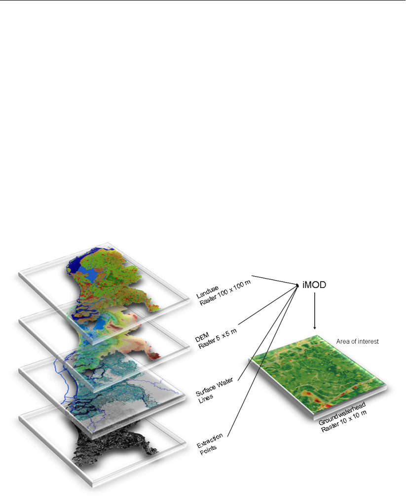
The iMOD approach: one input data set:
Resolutions of parameters can differ and the distribution of the resolution of one parameter
can also be heterogeneous. In addition, the spatial extents of the input parameters don’t have
to be the same. iMOD will perform up- and down scaling (Vermeulen, 2006) whenever the
resolution of the simulation is lower or higher than that of the available data. This approach
allows the modeler to interactively generate models of any sub-domain within the area covered
by the data set. When priorities change in time (e.g. due to changing political agenda’s) the
modeler can simply move to that new area of interest and apply any desired grid resolution.
In addition the modeler can edit the existing data set and / or add new data types to the data
set. Utilizing the internal up- and down-scaling techniques ensures that sub-domain models
remain consistent with the bigger regional model or that the regional model can locally be
updated with the details added in the sub-domain model.
Suppose the modeler needs to simulate groundwater flow for the total area covered by the
2 of 812 Deltares

DRAFT
Introduction
data set, but the theoretical size of the model is far too big to fit in any CPU-memory. iMOD
facilitates generating sub models for parts of the whole area of interest with a user-defined
resolution depending on how large the available CPU-memory is and how long the modeler
permits her/himself to wait for the model calculations to last. To generate a high resolution
result for the whole model domain a number of partly overlapping but adjacent sub models are
invoked and the result of the non-overlapping parts of the models are assembled to generate
the whole picture. The modeler should of course be cautious that the overlap is large enough
to avoid edge effects, but this overlap is easily adjustable in iMOD. A big advantage of this
approach is that running a number of small models instead of running one large model (if it
would fit in memory, which it often will not) takes much less computation time; computation
time (T) depends on the number of model cells (n) exponentially: T = f(n1,5−2,0). The approach
also allows the utilization of parallel computing, but this is not obligatory. Using this approach
means that the modeling workflow is very flexible and not limited anymore by hardware when
utilizing iMOD.
1.3 Main functionalities
The capability of iMOD to rapidly view and edit model inputs is essential to build effective
models in reasonable timeframes. The rapid and integrated views of the geologic / hydros-
tratigraphic models as well as dynamic model output is critical for the public, stakeholders
and regulators to understand and trust the model as a valid decision support tool. iMOD is
fast even when working from very large data files because it uses a random accessible data
format for 2D grids which facilitates instant visualization or editing subsets of such a large
grid file. Also iMOD contains very economic zoom-extent-dependent visualization techniques
that allow subsets of grids being visualized instantaneously both in 2D and 3D. Another fea-
ture is that iMOD generates MODFLOW input direct in memory, skipping the time-consuming
production of standard MODFLOW input files (generating standard MODFLOW input files in
ASCII format for large transient models may take hours to a full working day); this efficiency
is especially useful during the model building phase when checking newly processed or im-
ported data.
iMOD includes the MetaSWAP-module developed by Wageningen Environmental Research
(Alterra); for references to the separate MetaSWAP-documentation see section A.1.8.
1.4 Minimal System Requirements
iMOD works on IBM-compatible personal computers equipped with at least:
a Pentium or compatible processor;
512 MB internal memory (2,045MB recommended);
100 MB available on the hard disk (10GB is recommended in case large model simulations
need to be carried out);
A graphics adapter with 32 MB video memory and screen resolution of 800-600 (256MB
video memory and a screen resolution of 1024x768 is recommended). Moreover, a graph-
ical card that supports OpenGL (OpenGL is a trademark of Silicon Graphics Inc.), such as
an ATI Radeon HD or NVIDIA graphical card is necessary to use the 3D rendering.
Please note: it is permitted to install the Model System on a different Hardware Platform as
long as it is a computer with similar minimum features as listed above. The transfer of the
Model System to a dissimilar computer may endanger the working of the Model System and
require adjustments in the Configuration.
iMOD can run on 64-bits systems, but iMOD itself is 32-bits. iMOD supports 32- and 64-bit
machines working under the following platforms: Windows XP / Server 2003 / Vista Business
Deltares 3 of 812
DRAFT
iMOD, User Manual
/ Vista Ultimate / Server 2008 / 7 .
1.5 Getting Help
Take a look at http://oss.deltares.nl/web/imod. Any questions? Contact the
help-desk imod.support@deltares.nl.
1.6 Deltares
Since January 1st 2008, GeoDelft together with parts of Rijkswaterstaat-DWW, -RIKZ and -
RIZA, WL | Delft Hydraulics and a part of TNO Built Environment and Geosciences are forming
the Deltares Institute, a new and independent institute for applied research and specialist
advice. For more information on Deltares, visit the Deltares website: www.deltares.nl.
1.7 Acknowledgements
The development and enhancement of iMOD functionality is project-based. This section lists
these project-based developments and specifies its funding and organisations Deltares has
collaborated with during the implementation.
Functionality Funding Implementation
iMOD Maintenance & Support & iMOD-Helpdesk
In 2013 a group of five iMOD-consortia started the
project "iMOD Beheer en Onderhoud, Helpdesk en
Website" initiating and (co-)financing a coordinated fur-
ther development of iMOD and enhanced maintenance
and support. The current iMOD-consortia are AMIGO,
AZURE, IBRAHYM, MIPWA and MORIA; info on the
members of each iMOD-consortium can be found here.
iMOD-CGO
consortia
MetaSWAP
iMOD includes the unsaturated zone MetaSWAP-
module which covers the plant-atmosphere interactions
and soil water. MetaSWAP is based on a quasi steady-
state solution of the Richards equation. MetaSWAP is
developed by Wageningen Environmental Research (Al-
terra) and was (among others) financed by The Nether-
lands Hydrological Instrument. For references to the
MetaSWAP-documentation see section A.1.8.
.
MODFLOW-MetaSWAP coupling
The coupling of MODFLOW and MetaSWAP was cre-
ated in a collaboration between Deltares and Wagenin-
gen Environmental Research (Alterra) and was (among
others) financed by The Netherlands Hydrological In-
strument.
4 of 812 Deltares
DRAFT
Introduction
Functionality Funding Implementation
Quick Scan Tool
The MIPWA consortium initiated and funded the
QuickScan Tool which is an instrument to efficiently
compute effects on groundwater levels and seepage
fluxes to- and from drainage systems using a so-called
Impulse-Response Database. This database stores
pre-computed effects of several measures which can be
combined in the QuickScan Tool using the principles of
superposition.
MIPWA
consortium
Perched Water Table package
The MIPWA consortium initiated and funded the de-
velopment of the Purged Water Table (PWT) Package.
With this package purged water table conditions can be
simulated occurring on shallow (clayey) aquitards with a
significant vertical resistance. The initial concept was
developed in collaboration with Wageningen Environ-
mental Research (Alterra).
MIPWA
consortium
3D Tool
Waternet funded the development of the first version
of the 3D Tool allowing an interactive 3D visualiza-
tion of the subsurface in combination with the (litho-
stratigraphy) of boreholes.
GeoConnect Tool
The GeoConnect Tool allows the modeller to define and
utilize permanent links between 1) the (unassembled)
geologic layers (incl. its properties) and 2) the aggre-
gated model layers. With the GeoConnect Tool you can
re-calculate the hydraulic conductivities of a model layer
after adapting the individual weights of each contributing
geological layer. The development of was funded by the
IBRAHYM concortium (Waterschap Limburg,Provincie
Limburg,Waterleiding Maatschappij Limburg).
IBRAHYM
consortium
ISG
The IBRAHYM consortium initiated the development of
the concept of line elements (vector format) as a basis
to discretize streams as an alternative for grid based pa-
rameterization. This yielded considerable data handling
efficiency and much more flexibility when parameteri-
zation for different model grids sizes. It also facilitated
more user-friendliness regarding inspecting and editing
the stream data.
IBRAHYM
consortium
Runfile Editor & Plug-In Tool
The project manager was extended to support editing
of a runfile and project files. Also the iMOD-GUI was
extended with Plug-In functionality allowing to invoke
external programs in the iMOD-GUI using iMOD files.
These functionalities were funded by the iMOD-CGO
group.
iMOD-CGO
consortia
Deltares 5 of 812
DRAFT
iMOD, User Manual
Functionality Funding Implementation
Parallel Krylov Solver Package
Deltares,USGS and Wageningen Environmental Re-
search (Alterra) together with Utrecht University and
Technical University Delft have developed the new par-
allel solver package for iMOD called PKS (Parallel
Krylov Solver). It is based on overlapping domain de-
composition combining both the techniques of MPI and
OpenMP.
3D-assignment of fault-lines
Extension and improvement of the 3D-parameterization
of faults in the Horizontal Flow Barrier package. This
extension was funded by the IBRAHYM-consortium led
by the Province of Limburg.
IBRAHYM
consortium
Extension of the water balance tool
The extension of the water balance tool (released in
iMOD 4.2) was created in a collaboration between
Deltares and Tauw and financed by the Dutch iMOD-
CGO group; it allows visualization (interactive stack-
bars time series plots and schematic vertical cross-
sectional overviews) of water balances for sub-regions
and contains several time-aggregation possibilities (e.g.
averages per year, month and season).
iMOD-CGO
consortia
Fence diagrams & Deviated wells
The 3D Tool was extended with an option to interac-
tively create so-called fence-diagrams by using clipping
planes along the major Euclidian axes. The 3D Tool
was also extended with the option to visualize deviated
wells. These developments were funded by the Alberta
Energy Regulator | Alberta Geological Survey and came
available starting from the iMOD 4.2 release.
6 of 812 Deltares

DRAFT
2 Getting Started
This chapter describes:
section 2.1: How to obtain the Deltares-software executables of iMOD.
section 2.2: How to install iMOD.
section 2.3: How to get and install third-party MPI software.
iMOD 4.3 includes the new Parallel Krylov Solver (PKS) Package. This package facili-
tates running (large) iMOD models on Windows-based multi-core computers potentially
resulting in a drastic reduction of runtimes. The PKS-package is a new alternative next
to the current single-core PCG-solver. The modeller of course is not required to apply
the new PKS-package, however, in iMOD 4.3 it is easy to switch between the single- and
multi-core solver.
In iMOD 4.3 the LAK-, MNW-, PST-, SFR- and UZF-packages are not supported by the
PKS-package; when an iMOD-model contains one or more of these package the single-
core PCG-solver package has to be used.
The PKS-package can be used on Windows-based 64-bits systems only.
Please note that the PKS package can be used for iMOD models that contain the MetaSWAP-
concept. This potentially gives another boost to the speed of model simulations containing
an iterative state-of-the-art coupling between the saturated and unsaturated zone.
The PKS package uses Message Passing Interface (MPI) software. Hence, prior to using
the PKS-package MPI-software should be installed on your computer too; section 2.3 de-
scribes how to get and install the MPI-software. However, if you are not going to use the
PKS-package you are not required installing the MPI software and you can skip section 2.3
all together.
The other sections focus on how to operate iMOD and how new users can familiarize them-
selves with iMOD:
section 2.4: a 3D-appetizer.
section 2.5: how to start iMOD after installation.
section 2.6: the Main Menu options.
section 2.7: how to specify your preferences.
section 2.8: how to specify your colours.
section 2.9: some Tips and Tricks.
Additionally, the Tutorials in chapter 11 provide a selection of iMOD case studies to intro-
duce the program’s functions. New iMOD users are advised to use the Tutorials to familiarize
themselves with iMOD.
Deltares 7 of 812

DRAFT
iMOD, User Manual
2.1 Get the Deltares-software executables of iMOD
To get the latest release of the Deltares-software executables of iMOD, please submit the form
’Request form for the Deltares-software executables of iMOD’, see
http://oss.deltares.nl/web/imod/get-started.
By submitting this form you are requesting for the use of the Deltares-software executables
of iMOD. iMOD is Deltares-software; the source code of iMOD is also available as free open
source software at oss.deltares.nl. You may use the Deltares-software executables of iMOD
without any remuneration to be paid to Deltares if you accept the iMOD Software License
Agreement (iMOD License) which is offered to you as a PDF-file, see
http://oss.deltares.nl/web/iMOD/iMOD_Software_License_Agreement.
Please go to the PDF-file of the iMOD License, read it and decide whether you want or do not
want to accept the iMOD License. Without your acceptance of the iMOD License the use of
the Deltares-executables of the iMOD-software is prohibited and illegal.
The iMOD software is distributed in the hope that it will be useful, but WITHOUT ANY GUAR-
ANTEE OR (IMPLIED) WARRANTY. Any use of the Deltares-executables of the iMOD-software
is for your own risk. See the iMOD License for more details.
For more info, please contact: Stichting Deltares, P.O. Box 177, 2600 MH Delft, The Nether-
lands. Email: imod.support@deltares.nl.
After your submitted request (section 2.1) was processed successfully you received an email
with details on how to download the Deltares-executables of iMOD; this email contains the
required download-password.
Please perform the following steps:
1 Browse to https://download.deltares.nl.
2 Click the iMOD-icon.
3 Download the file ‘iMOD 4.3 Installation Instructions.pdf‘: enter the download-password
sent to you in the above mentioned email and click the ’Download’-button.
4 Download the file ‘iMOD 4.3.zip‘: enter the download-password sent to you in the above
mentioned email and click the ’Download’-button.
5 Unzip the file ‘iMOD 4.3.zip‘.
After unzipping the file ‘iMOD 4.3.zip you will have the following 3 files:
1iMOD 4.3 Installation Instructions.pdf: the iMOD installation instructions.
2iMOD_setup_V4_3.exe: an installation program that:
determines whether you are installing iMOD on a 32-bit or on a 64-bit system (by
processing the output of the DOS-command ’systeminfo’)
determines your default PDF-viewer, if available.
calls the self-extracting archive iMOD_zipped_V4_3.000,
creates an initial IMOD_INIT.PRF preference file,
installs the Tutorial Data Set.
3iMOD_zipped_V4_3.000: a self-extracting archive containing the following files and di-
rectory:
iMOD_V4_3_X32R.exe: the iMOD-GUI for 32-bit systems.
iMOD_V4_3_X64R.exe: the iMOD-GUI for 64-bit systems.
iMODFLOW_V4_3_X32R.exe: iMODFLOW excl. MetaSWAP, for 32-bit systems.
iMODFLOW_V4_3_METASWAP_SVN1233_X64R.exe:
iMODFLOW including MetaSWAP for 64-bit systems. The MetaSWAP-module is de-
8 of 812 Deltares

DRAFT
Getting Started
veloped by Wageningen Environmental Research (Alterra); for references to the sep-
arate MetaSWAP-documentation see section A.1.8.
netcdf.dll: a NetCDF-library.
fmpich2.dll, mpich2mpi.dll and mpich2nemesis.dll: MPICH 1.4.1p1 libraries necessary
for PKS.
run_test_mpi_installation.bat, test_mpi_installation.exe: a test to check a MPI-installation.
USGS Software User Rights Notice.txt: a copy of the USGS Software User Rights
Notice.
iMOD_User_Manual_V4_3.pdf: the iMOD User Manual, in PDF-format.
iMOD_Software_License_Agreement_V4_3.pdf: the PDF-file of the iMOD License.
the files and folders of the iMOD Tutorial Data Set.
Deltares 9 of 812
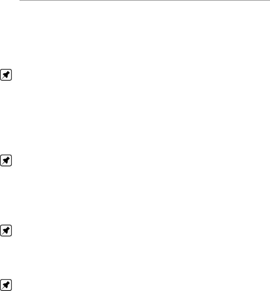
DRAFT
iMOD, User Manual
2.2 Installation of iMOD
To install iMOD please perform the following steps:
1 Make sure you have read-, write and execute rights in the directory you want to install
iMOD in. You also need read- and write rights to create sub-directories and to create,
read and write files.
Note: Starting from iMOD version 3.2 you only need execute-rights for {installfolder}
after iMOD has been installed and the iMOD-GUI has been invoked once allowing iMOD
to generate the file ’I_accepted_V4_3.txt’ in {installfolder}; the file ’I_accepted_V4_3.txt’ is
generated when the user selects the option ’I Accept’ during first time use in the iMOD-
GUI.
Until iMOD version 3.01 the iMODFLOW-executable was always copied to the actual modelrun-
folder and the iMOD-GUI invoked the iMODFLOW-executable copied to that modelrun-folder; start-
ing from version iMOD 3.2 the iMODFLOW-executable is still copied to the modelrun-folder for
archiving purposes, however, the iMOD-GUI invokes the iMODFLOW-executable as defined by the
keyword ’MODFLOW’ in the preference file.
Note: Administrators who wish to assign execute-rights only to {installfolder}, please
invoke the iMOD-GUI once and follow the ’I Accept’-procedure to allow iMOD to write the
file ’I_accepted_V4_3.txt’ in {installfolder}; once the file ’I_accepted_V4_3.txt’ is present in
{installfolder} iMOD only needs execute-rights for {installfolder}.
During installation no additional access rights are required for other directories; after in-
stallation when you start using iMOD you of course need access rights for your to be
created iMOD project-files and -directories.
Note: The installation of iMOD does NOT require write access to the Windows Reg-
istry, in other words, the installation of iMOD does not make any changes in the Windows
Registry.
2 Create and go to a new (sub-)directory or go to an existing EMPTY directory where you
want to install iMOD.
Note: In this user manual {installfolder} refers to the full path of the directory you in-
stalled iMOD in (e.g. D:\iMOD).
3 Move the files ’iMOD_setup_V4_3.exe’ and ’iMOD_zipped_V4_3.000’ to {installfolder},
e.g. to D:\iMOD.
4 In {installfolder} double-click the file ’iMOD_setup_V4_3.exe’ from the Windows Explorer,
or start a ’Windows Command Processor’-box in {installfolder},
type ’iMOD_setup_V4_3’ and press Enter.
If the archive ’iMOD_zipped_V4_3.000’ is not present, the setup will stop.
5 The setup will first determine 1) whether you are installing iMOD on a 32-bit or 64-bit sys-
tem (using the DOS-command ’systeminfo’) and 2) which default pdf-viewer is available,
if any. After that, the Windows Command Processor box looks similar as below (and a
pop-up window appears, see step 6):
10 of 812 Deltares
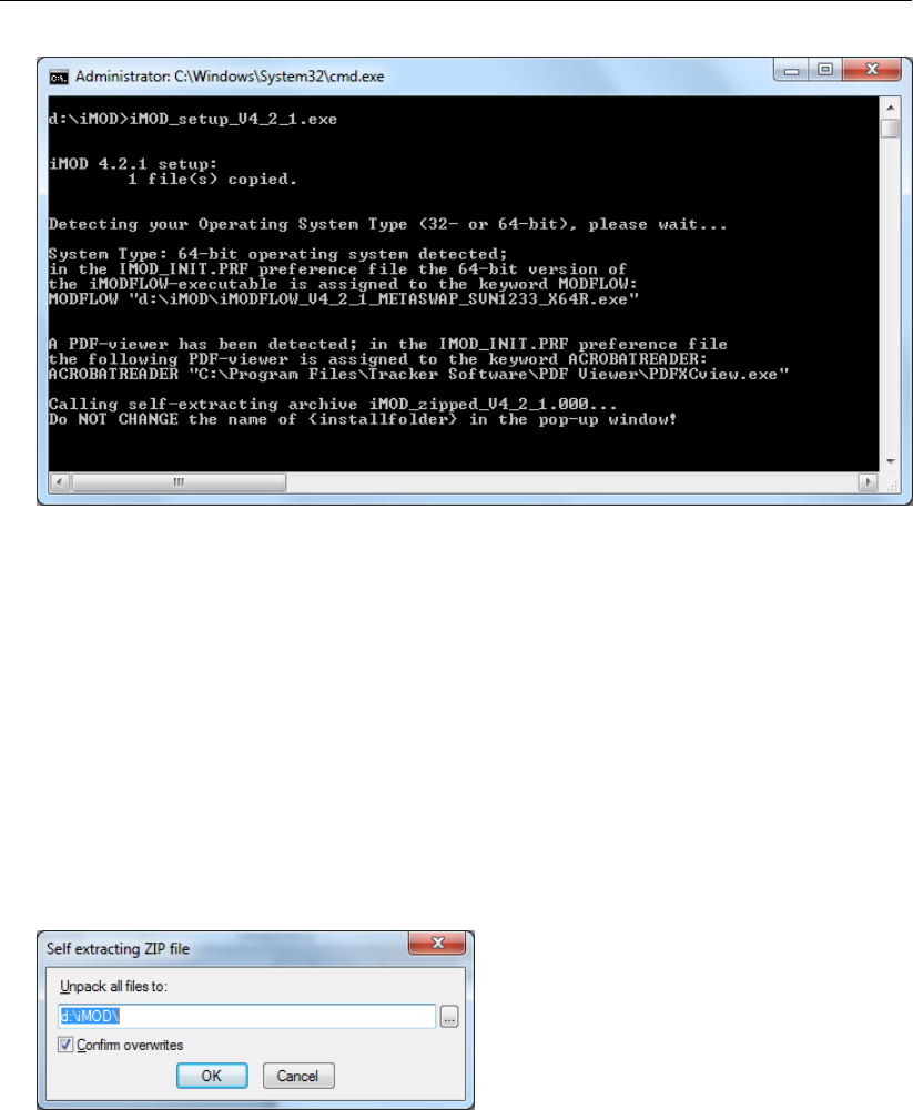
DRAFT
Getting Started
In the preference file IMOD_INIT.PRF (see step 7 below) the keyword ’MODFLOW’ will
be assigned the 64-bit or the 32-bit version of the iMODFLOW-executable respectively
(64-bit versions of Windows became available starting from Windows XP).
If during setup your Windows Operating System Type could not be determined the setup
uses 64-bit as a default.
If during setup no default PDF-viewer is detected the keyword ACROBATREADER can
be specified in the file IMOD_INIT.PRF manually, see step 7 below.
6 In this step the self-extracting the archive ’iMOD_zipped_V4_3.000’ is invoked and the
following window appears; do NOT CHANGE the name of the {installfolder} and click the
’OK’-button; the archive will unzip.
After the archive ’iMOD_zipped_V4_3.000’ has finished self-extracting (it may take a
while to extract more than 3300 files...) also a new sub-folder TUTORIALS has been
created in {installfolder}, containing a sub-folder for each individual tutorial:
.\TUT_Map_Display
.\TUT_Data_Map_Oper
.\TUT_Map_Analyse
.\TUT_Initial_Modeling
.\TUT_Solid_Building
.\TUT_Model_Simulation
.\TUT_IPS
.\TUT_SFR
.\TUT_LAK
.\TUT_MNW
.\TUT_UZF
Deltares 11 of 812
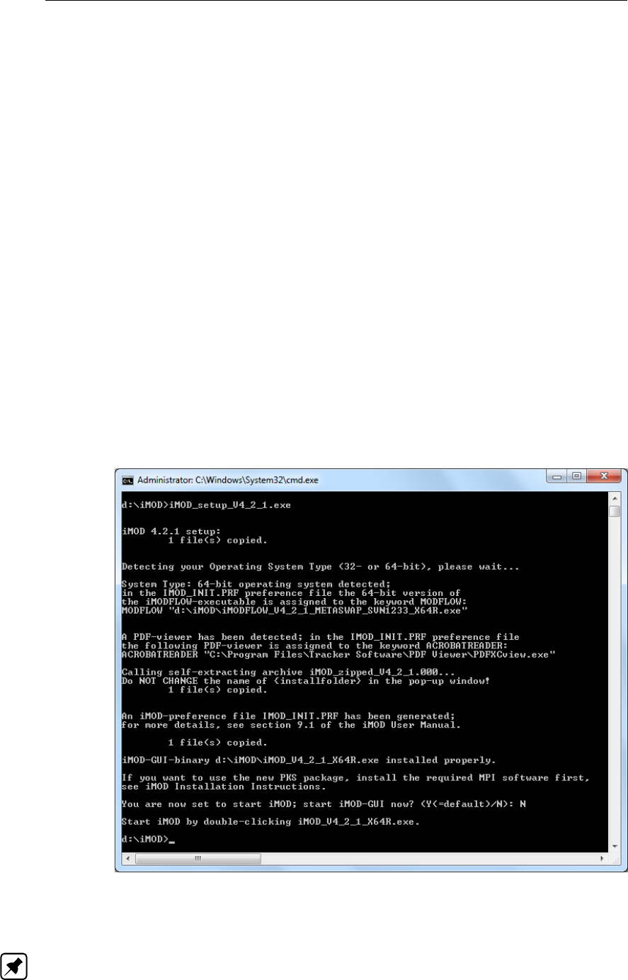
DRAFT
iMOD, User Manual
7 An initial iMOD preference file IMOD_INIT.PRF has been generated, including the key-
words ’USER’, ’HELPFILE’, ’ACROBATREADER’, ’MODFLOW’ and ’DBASE’. For more
keywords please have a look in Section 9.1.
For the examples used above the content of the IMOD_INIT.PRF-file looks like this:
USER "d:\iMOD\IMOD_USER"
HELPFILE "d:\iMOD\iMOD_User_Manual_V4_3.pdf"
ACROBATREADER "c:\Program Files (x86)\Adobe\Reader 11.0\
Reader\AcroRd32.exe"
MODFLOW "d:\iMOD\iMODFLOW_V4_3_MetaSWAP_SVN1233_X64R.exe"
DBASE "d:\iMOD"
8 You have now completed the installation of iMOD:
When you press Enter, the iMOD-GUI will start.
Or when you type ’N’ and press Enter:
and if in step 2 you invoked the setup by a double-click, the Windows Command
Processor-box will now be closed.
or
and if in step 2 you invoked the setup by typing ’iMOD_setup_V4_3’ from a manu-
ally opened ’Windows Command Processor-box’, after pressing Enter the box will
look similar (depending on your {installfolder}) to this:
The installation of the iMOD software is now completed.
Note: To be able to use the Parallel Krylov Solver (PKS) package additional third party
MPI software needs to be installed first, see the next section.
12 of 812 Deltares

DRAFT
Getting Started
2.3 Installation of MPI software
iMOD 4.3 includes the Parallel Krylov Solver (PKS) package. The Parallel Krylov Solver (PKS)
package facilitates running (large) iMOD models on Windows-based multi-core computers
potentially resulting in a drastic reduction of runtimes. This package uses Message Passing
Interface (MPI) software. Hence, prior to using the PKS-package MPI-software should be
installed on your computer too.
2.3.1 Limitations
The PKS package was implemented for the 64-bit version of iMODFLOW (see Step 5), so
the PKS package can be used on Windows-based multi-core 64-bit computer systems, for
example on Windows-based laptops and desktops containing Intel CORE i5 or i7 processors
or on Windows-based multi-core 64-bit supercomputers.
In iMOD 4.3 the LAK-, MNW-, PST-, SFR- and UZF-packages are not supported by the PKS-
package; when an iMOD-model contains one or more of these package the single-core PCG-
solver has to be used. So, the PKS-package can be used in combination with the remaining
MODFLOW-packages implemented in iMOD; please note that the PKS package can also be
used for iMOD models containing the MetaSWAP-concept; this potentially gives another boost
to the speed of model simulations containing an iterative state-of-the-art coupling between the
saturated and unsaturated zone.
2.3.2 Installation steps for the MPI software
The 64-bit iMODFLOW-executable uses the 64-bit MPICH (1.4.1p1) implementation for MPI,
hence the following MPI software http://www.mpich.org/static/downloads/1.
4.1p1/mpich2-1.4.1p1-win-x86-64.msi should be installed prior to using the PKS
package.
Note: In order to install the MPI software correctly, you should do this as Administrator:
Download the appropriate MPI software.
Open the Command Prompt as administrator by: Start →(Search programs and files)
cmd →right mouse click →Run as administrator
In the MS-DOS-box named Administrator: Command Prompt:
msiexec /i mpich2-1.4.1p1-win-x86-64.msi
Follow the instructions of the MPI-installer.
2.3.3 Checking your MPI-installation
We included a general test-program that allows you to check whether the installation of the
MPI-software was successful. To perform this check please do the following:
Go to your {installfolder}, e.g. to D:\iMOD.
Open the batch-file ’Run_test_mpi_installation.bat’ in an ascii-editor.
In line 2, adjust the reference to the folder and name of the installed MPI-executable, e.g.
set mpi "C:\Program Files\MPICH2\bin\mpiexec.exe"
Save the batch-file and close the ascii-editor.
Open a ’Windows Command Processor’-box.
Type ’Run_test_mpi_installation.bat’ and press Enter.
Deltares 13 of 812
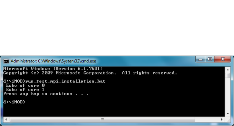
DRAFT
iMOD, User Manual
A test is performed using 2 cores; when the test is successful the following message appears:
echo of core 0
echo of core 1
and the ’Window Command Processer’-box should look similar to this:
Please contact your system administrator for help on installing MPI.
2.3.4 Info on how to use the PKS-package
It is very easy to adapt existing (pre-iMOD 4.0)-runfiles (*.RUN) for the use of the PKS-
package; for more info, see section ’Updating a runfile from iMOD 3.6 to iMOD 4.0’ in sec-
tion 10.20.6 of the iMOD User Manual.
The PKS-package can be configured in the ’Solver Settings’-tab of the ’Start Model Simulation’-
window of the main menu option ’Tools’; for more info see the iMOD User Manual, section 7.9.
Once the PKS-package has been configured, there are two ways to start a multi-core model
simulation:
1 Inside the iMOD-GUI: see section 7.9 (’Model Simulation’) of the iMOD User Manual.
2 Outside the iMOD-GUI by typing the appropriate command at the DOS-prompt in a ’Win-
dows Command Processor’-box; here’s an example of how to start a multi-core model
simulation from outside the iMOD-GUI by entering the following command in a ’Windows
Command Processer’-box:
mpiexec.exe -localonly 2 iMODFLOW.exe iMODFLOW.run
In this example MPI launches two processes of iMODFLOW.exe instances on two compu-
tational cores, meaning that the model runs using two subdomains. The -localonly
option ensures that you should not necessarily have to be connected to your network for
running with MPI.
For more detailed info, see section 10.21 (’Start Model Simulation’) of the iMOD User
Manual.
Tutorial 6 (section 11.6) contains an excercise on how to run your model using the PKS
package.
You are now set to start iMOD; after completing this chapter new iMOD-users are encouraged
to proceed with the tutorials (chapter 11 of the iMOD User Manual). As a 3D-appetizer con-
sider trying to run and visualize one of the pre-defined tutorial models: follow the steps as
described in the next section.
14 of 812 Deltares
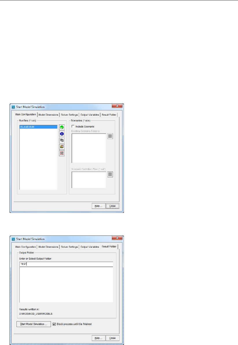
DRAFT
Getting Started
2.4 A 3D-appetizer...
As an appetizer let’s try to run and visualize one of the pre-defined tutorial models in 3-D right
away by performing the following steps:
1 If you chose ’N’ in the previous step, start iMOD as described in section 2.5.
2 Read and decide whether or not you accept the term and conditions of the iMOD License
Agreement.
3 Assuming you accept, click ’Yes, I Accept’ and click ’OK’
4 When the ’iMOD Start’ window appears, click the ’Start’ button.
5 In the main menu click ’Toolbox’, and click ’Start Model Simulation ...’, the following window
appears, displaying the presence of the runfile ’ISLAND.RUN’:
6 Select the tab ’Result Folder’ and type a to be created output folder name, e.g. ’TEST’:
7 Click the button ’Start Model Simulation’ and click ’Yes’ in the confirmation pop-up window
to start the MODFLOW run; a Windows Command Processor box appears echoing the
MODFLOW in- and output process:
Deltares 15 of 812
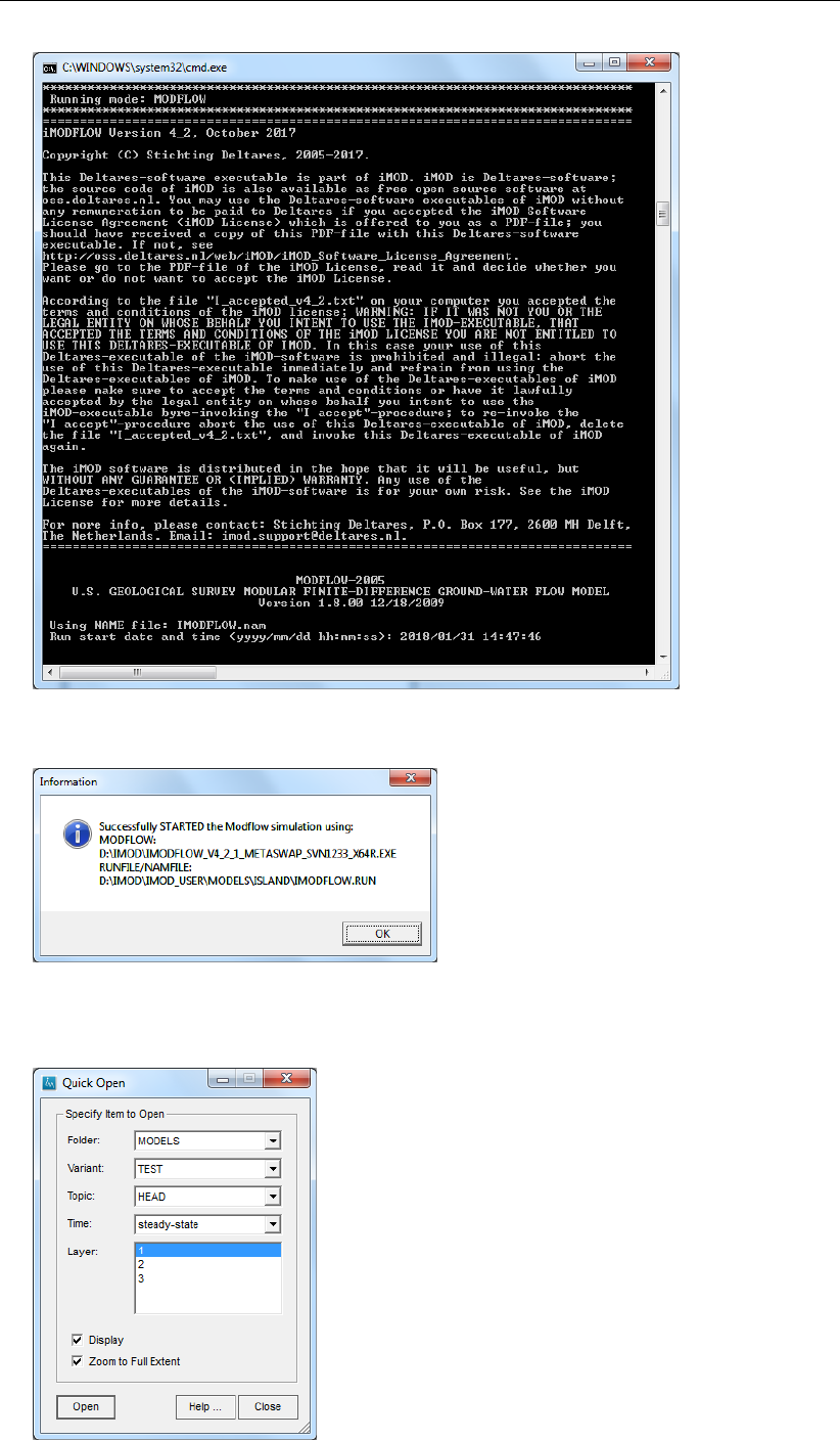
DRAFT
iMOD, User Manual
followed by an information window:
8 Click ’Ok’ in this information window, and ’Close’ in the ’Start Simulation Model’-window.
9 To visualize the calculated groundwater head in 2D, in the main menu click ’Map’ and
’Quick Open ...’; the following window appears:
16 of 812 Deltares
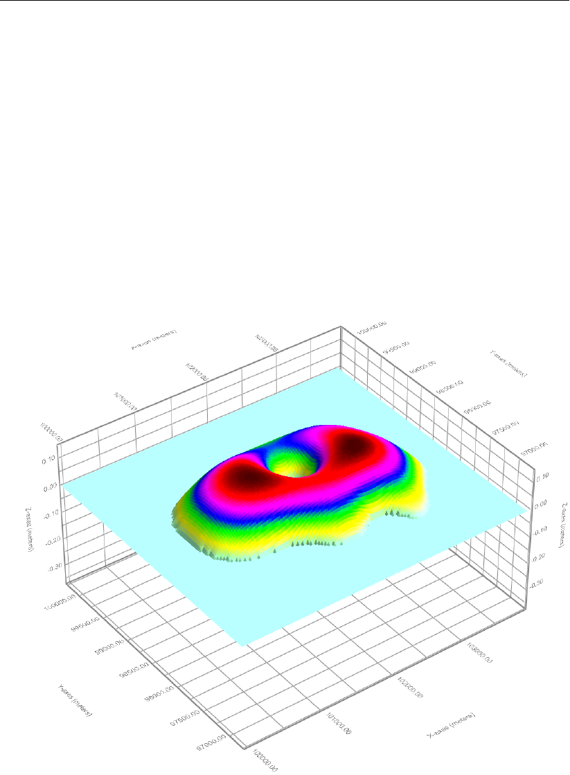
DRAFT
Getting Started
10 In the ’Topic’-list, choose ’HEAD’.
11 In the ’Layer’-window, click at least one layer, e.g. layer 1.
12 Select ’Zoom to full extent’.
13 Click the ’Open’-button to visualize the calculated heads of layer 1 of tutorial 4; click the
’Close’ button.
14 Optionally, you can redraw the map using different colours by choosing ’Map’ in the main
menu, followed by selecting ’Entire extent’ and clicking on ’percentiles’.
15 To visualize these groundwater levels in 3D right away, select ’Toolbox’ in the main menu
and choose ’3D Tool ...’; click ’Apply’ to use the default settings.
16 In the ’3D Plot Settings’-window, in the ’Colouring’ sub-window choose the ’Use Colouring
defined in Legend for:’-option to re-use the legend-colours of the 2D-map.
17 Change the 3D-view by dragging over the 3D-map while you keep pressing the left-,
middle- or right mouse button. The 3D-map could look something like this:
18 Optionally, in the 3D Tool change the Horizontal / Vertical ratio by selecting in the 3D Tool
menu bar the option ’View’ and select ’Horizontal / Vertical Ratio’ followed by the choosing
your preferred ratio.
19 Congratulations, you just visualized your first iMOD-model! You are now set to continue
exploring iMOD; after completing this chapter new iMOD-users are encouraged to proceed
with the tutorials (chapter 11).
Deltares 17 of 812
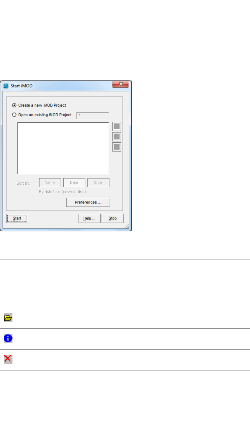
DRAFT
iMOD, User Manual
2.5 Starting iMOD
To start iMOD, click Start on the Windows menu bar and fill in the location and name of the
executable: {installfolder}\iMOD_V4_3_X64R.EXE, e.g. D:\iMOD\iMOD_V4_3_X64R.EXE or
C:\program files\iMOD_V4_3_X64R.EXE, or double-click on the executable from the Windows
Explorer. The Start iMOD window will appear.
Start iMOD window:
Create a New
iMOD Project
Select this option to refresh the iMOD session and release all memory and
maps from previous sessions and start iMOD with an empty drawing list.
Open an existing
iMOD Project
Select this option to start iMOD with an iMOD configuration saved by a previ-
ous iMOD session. Those configurations are stored in *.IMF files and those
listed are found in the folder {USER}\IMFILES. Use the wildcard to select a
part of existing *.IMF files in the menu field. Use wildcards as ”*“ (any sign)
and ”?¿‘ (any two characters) for specific selections, e.g. *A_??*. The search
will be case insensitive and the extension IMF will be added to it automatically.
Leaving out any wildcard will act as ”*.IMF“.
Open an IMF-file
Select and search an *.IMF-file from a different location than those presented
in the menu.
Information of an IMF-file
Click this button to open the selected *.IMF-file in a regular text-editor
(Notepad) for inspection or adjustments.
Delete an IMF-file
Click this button to delete the selected *.IMF file from disk. After that, no
recovery is possible.
Sort by: Select one of the following to sort the list of IMF files:
Name Select this to sort the IMF file by Name (case insensitive);
Date Select this to sort the IMF file by Date/Time, youngest will be ap-
pearing on top of the list;
Size Select this to sort the IMF file by Size (largest first).
Preferences . . . Click this button to open the Preferences Window.
Start Click this button to start iMOD with the selected *.IMF file or with an empty
drawing list.
18 of 812 Deltares
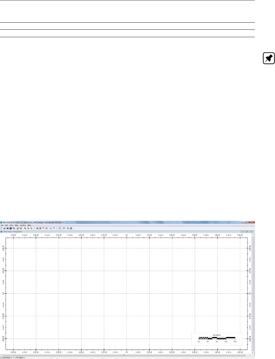
DRAFT
Getting Started
Stop Click this button to stop iMOD
Help. . . Click this button to start the iMOD Help Functionality.
Note: iMOD can be started in different ways, alternatively:
{installfolder}\iMOD_V4_3_X64R.exe
will start a regular iMOD session
{installfolder}\iMOD_V4_3_X64R.exe *.IMF
will start an iMOD session and read the supplied *.IMF directly;
{installfolder}\iMOD_V4_3_X64R.exe *.IDF
will start an iMOD session and read the supplied *.IDF-file directly. This works for *.MDF,
*.ASC, *.GEN, *.IFF, *.IPF, and *.ISG-files;
{installfolder}\iMOD_V4_3_X64R.exe *.INI
will read the supplied *.INI file. These *.INI files contain specific functionalities of iMOD
that can be executed without starting the graphical interface, see chapter 8 for a list and
description of all these available functionalities.
In the examples above the iMOD executable iMOD_V4_3_X64R.exe was used; alternatively
the 32-bit version of the iMOD executable can invoked, see section 2.2.
2.6 Main Window
When iMOD is started, the iMOD Main window is displayed:
Important to notice that the graphical canvas can be modified, the location of the axes can
be changed, as well as the position and size of the scale bar. Whenever the position of the
mouse is near the current axes, the axes highlights in red and the cursor changes. At that
moment, selecting the left-mouse button, it is possible to drag the axes. This is similar to the
resizing and positioning of the scale bar.
Deltares 19 of 812
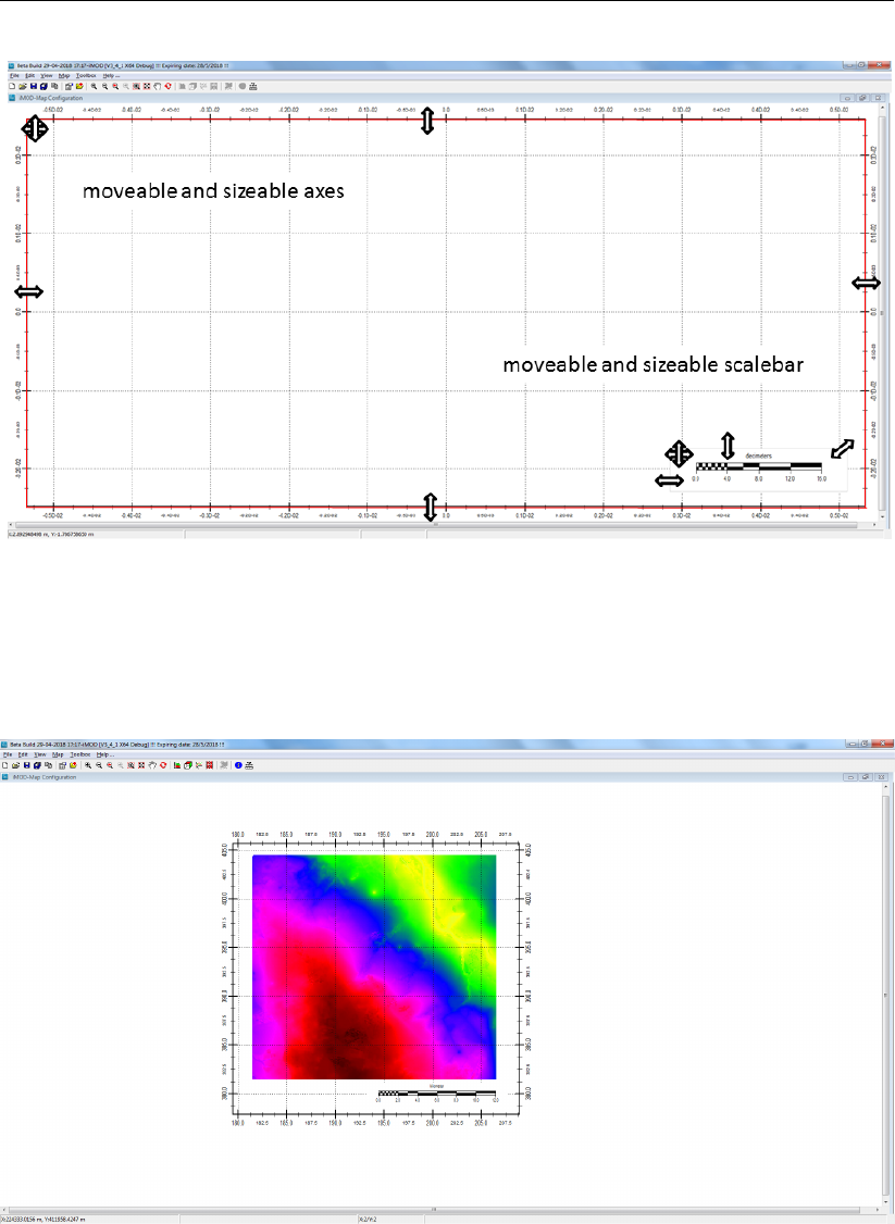
DRAFT
iMOD, User Manual
The settings of the modified axes and scale bar are saved in the IMF file. Reopening an IMF
file will show the modified axes and scale bar. The advantage of repositioning the axes is the
ability to closely match the size of the current visible map, sush as a square IDF file.
Furthermore, this window contains a menu bar, an icon bar and information displayed on the
window status bar.
20 of 812 Deltares
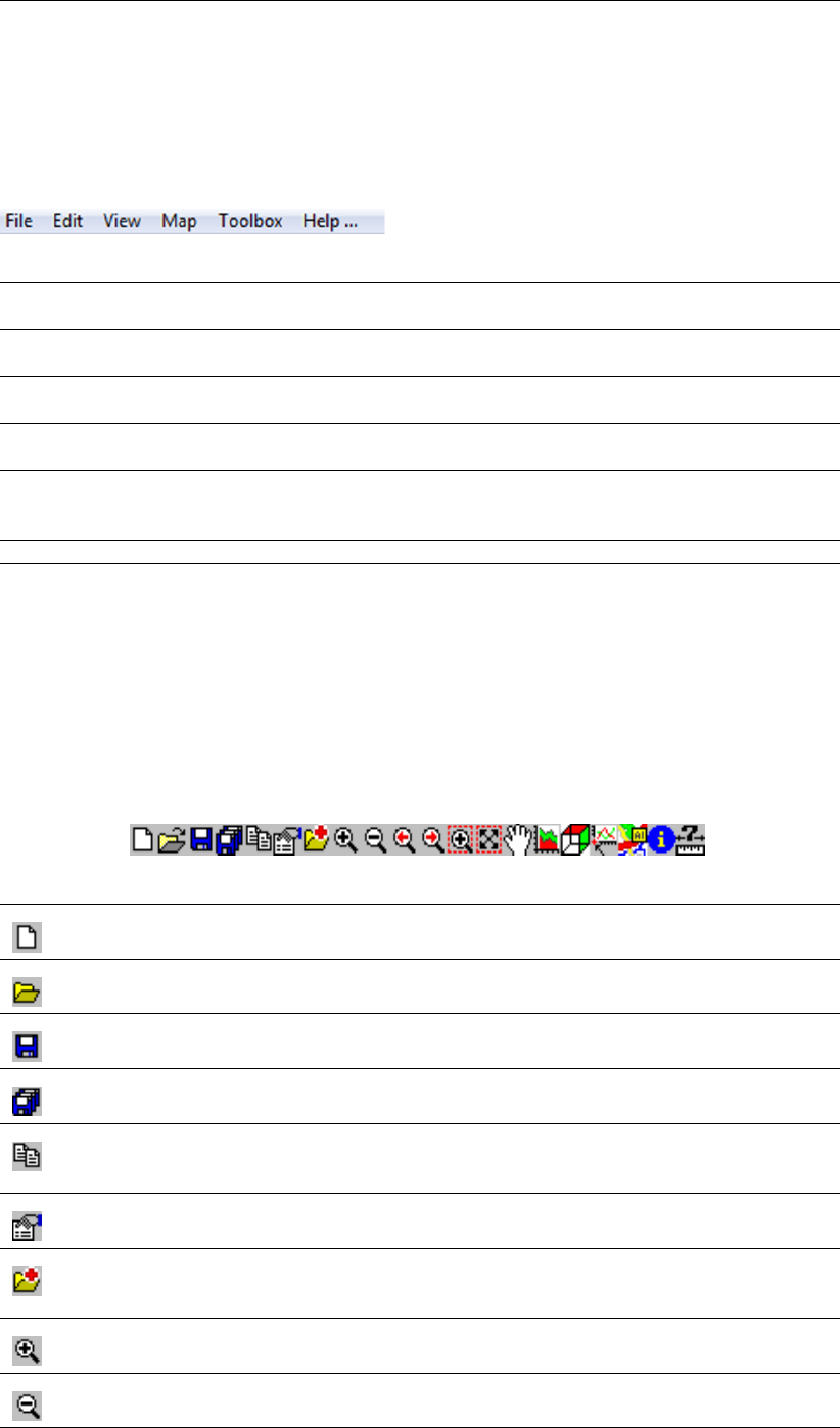
DRAFT
Getting Started
2.6.1 Menu Bar
To access the iMOD menus, click the menu names on the menu bar, or alternatively use
Alt+<first letter of the menu name>.
Menu bar:
File Standard Windows options for saving and opening iMOD MetaFile (*.IMF), export the
content of the graphical area.
Edit This contains a limited set of features to create iMOD Files, such as IDFs out of IPF’s,
IFF’s and GEN-files.
View This contains functionalities to copy the content of the graphical area onto the Clip-
board of Windows and a variety of manners to display data.
Map This menu option offers the ability to open iMOD maps and configure their appear-
ance.
Toolbox A variety of tools are available, e.g. Cross-Section Tool,WaterbalancingTool,Model-
ingTool, and more, but also an ImportTool for MODFLOW and SOBEK model config-
urations.
Help . . . Starts the Help-file (if available in the selected *.PRF file).
Detailed descriptions of these menu options can be found in the Reference section.
2.6.2 Icon Bar
Use the buttons on the iMOD Icon bar to quickly access frequently used functions.
Icon Bar:
New:
Start a new iMOD Project (*.IMF-file)
Open
Open an existing iMOD Project (*.IMF-file)
Save
Save the current configurations (maps) in the last saved *.IMF file
SaveAs
Save the current configurations (maps) in a new *.IMF file
Copy
Click this icon to copy the entire content of the graphical area onto the Clipboard of
Windows.
iMOD-Manager
Click this icon (checkbox) to start or hide (if shown) the iMOD-Manager window.
OpenMap
Click this icon to open an existing iMOD Map, such as *.IDF, *.IPF, *.ISG, *.IFF, *.GEN,
*.NC, *.MAP
ZoomIn
Click this icon to zoom IN on the centre of the current graphical dimensions.
ZoomOut
Click this icon to zoom OUT on the centre of the current graphical dimensions.
Deltares 21 of 812
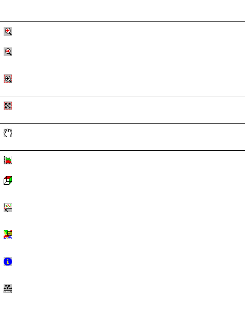
DRAFT
iMOD, User Manual
Go Back to Previous Extent
Click this icon and the map will return to the previous map extent and view. This view
becomes the last view automatically whenever any other zoom button will be used.
Go to Next Extent
Click this icon and the map will go to the next extent viewed after the current view.
This option becomes available whenever the Zoom to Previous Extent button has
been selected priorly.
ZoomRectangle
Click this icon to zoom in for a rectangle to be drawn. Use your left-mouse button to
determine the lower-left corner of the rectangle, click again for the upper-right corner
(or vice-versa).
ZoomFull
Click this icon to zoom in on the entire extent of the selected maps on the tab Maps
on the iMOD Manager or on the selected overlay Maps in the tab Overlay on the
iMOD Manager.
Move
Click this icon to move the current display. Click the left-mouse button on that loca-
tion where you want to move from, repeat this after the display has been refreshed
(automatically). Use the right mouse button to stop the moving process.
Cross-Section Tool
Click this icon to start the Cross-Section Tool for all the maps selected on the tab
Maps from the iMOD Manager Window.
3DTool
Click this icon to start the 3DTool for all the maps selected on the tab Maps from
the iMOD Manager Window and those selected on the tab Overlays from the iMOD
Manager.
TimeSerie Tool
Click this icon to start the TimeSerie Tool for all the IDFs (timevariant) and IPFs (with
associated files assigned to them) selected on the tab Maps from the iMOD Manager
Window.
Topographical Overlay
Click this icon to display the default topographical overlay as defined by the KeyWord
TOP25 in the selected *.PRF-file or display the overlays (*.BMP, *.png) as defined by
the menu option Add Background Image.
MapInfo
Click this icon to start the MapInfo window to analyse the dimensions of IDFs, IPFs,
IFFs, and GENs. For IDFs additional statistics and meta-information can be viewed
too.
DistanceTool
Click this icon to start the distance tool where you can specify the location where to
measure from, by clicking your left-mouse button. Intermediate points can be added
by clicking your left-mouse button repeatedly. To stop the process, click your right-
mouse button.
Detailed descriptions of these menu options can be found in the Reference section.
22 of 812 Deltares
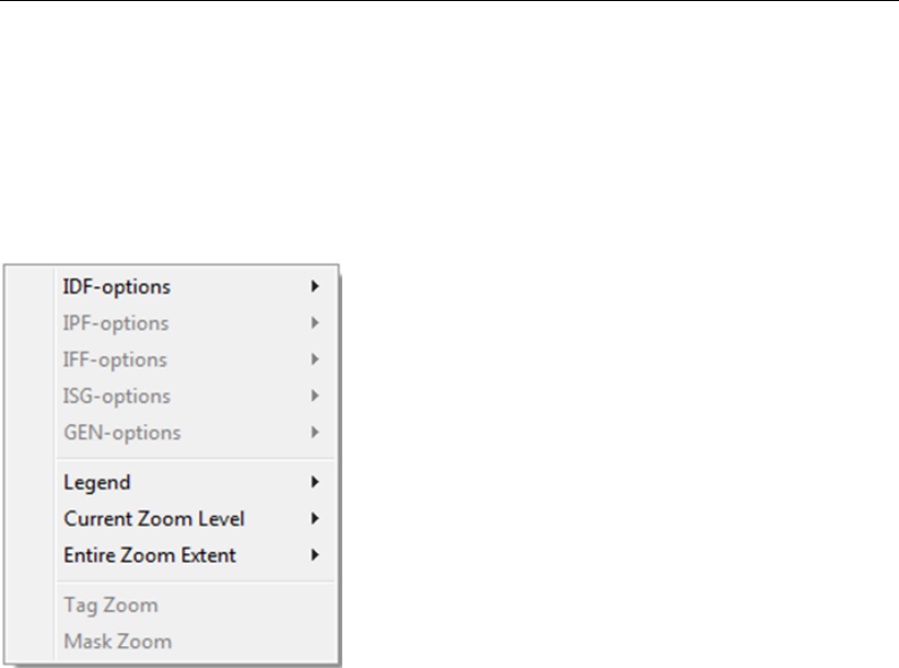
DRAFT
Getting Started
2.6.3 Popup Menu
Right-click anywhere in the canvas of the graphical window to open the popup menu. This
menu presents several options. The options might be unavailable because no correct file(s)
are selected in the iMOD Manager.
Popup menu:
IDF-options
IDF Analyse, Click this option to get an overview of the analyse options (see sec-
tion 6.7.1).
◦Analyse . . . , Click this option to start Map Value.
◦Plot No Locations, Check this item whenever no rastercells of the selected IDF-file
need to be displayed.
◦Plot All locations, Check this item whenever the rastercells of all selected IDF-
files need to be displayed. Bear in mind that the performance will slow down
whenever many IDF-files are included, and if IDF-files with non-equidistant rasters
are included. Whenever this option is checked, all values in Map Value will be
coloured differently.
◦Plot First Location Only, Check this item whenever the raster cells of the first IDF-
file listed in the Map Value table, need to be displayed. This is the default.
◦Points, Check this item whenever the values for the current location of the mouse
need to be listed. This is the default.
◦Rectangle, Check this item whenever the values need to be summed within a
rectangle that you can draw. Use the left mouse button to locate the first position
of the rectangle and the left/right mouse button to stop and close the Map Value
window.
◦Polygon, Check this item whenever the values need to be summed within a polygon
that you can draw. Use the left mouse button to locate the first position of the
polygon and continue to add more points (as desired) to complete the polygon.
Use the right mouse button to stop and close the Map Value window.
◦Circle (not available in current release), Check this item whenever the values need
to be summed within a circle that you can draw. Use the left mouse button to
locate the first position of the circle and expand the size of the circle while moving
the mouse pointer away from the first position (center of the circle). Click again on
your left mouse button to stop and close the Map Value window.
IDF Calculate, Click this option to start the Map Calculator (see section 6.7.3).
IDF Edit, Click this option to start Map Edit (see section 6.7.4).
Deltares 23 of 812

DRAFT
iMOD, User Manual
IDF Group, Click this option to group selected IDF-files (see section 6.5).
IDF Ungroup, Click this option to ungroup selected MDF-file (see section 6.5).
IDF Export, Click this option to export the selected IDF-files (see section 6.7.2) to:
◦ESRII ASCII Format
◦NetCDF Format
IPF-options
IPF Analyse, Click this option to startIPF Analyse (see section 6.8.3).
IPF Extract, Click this option to start IPF Extract (see section 6.8.4).
IPF Configure, Click this option to start IPF Configure (see section 6.8.1).
IFF-options
IFF Configure, Click this option to start IFF Configure (see section 6.9.1).
ISG-options
ISG Configure, Click this option to start ISG Configure (see section 6.10.1).
ISG Edit, Click this option to startISG Edit (see section 6.10.3).
ISG Show, Click this option to define the shown attributes (see section 6.10.2):
◦Nodes, Click this option to display nodes of ISG-segments;
◦Segments Nodes, Click this option to display begin- and end-nodes of the ISG-
segments;
◦Cross-sections, Click this option to display the position of cross-sections on ISG-
segments;
◦Calculation nodes, Click this option to display the location of calculation nodes of
ISG-segments;
◦Structures, Click this option to display the location of structures of ISG-segments;
◦QH-relationships, Click this option to display the location of QH-relations on ISG-
segments.
GEN-options
GEN Configure, Click this option to start GEN Configure (see section 6.11.2).
GEN Extract, Click this option to start GEN Extract (function not implemented).
Legend
Plot Legend on Map, Click this option to display the legend on the graphical window
(see section 6.6.4)
Legend Columns
1 Click this option to display the legend in a single column;
2 Click this option to display the legend in two columns;
3 Click this option to display the legend in three columns;
4 Click this option to display the legend in four columns;
5 Click this option to display the legend in five columns;
Adjust Legend, Click this option to open a window to adjust the legend (see sec-
tion 6.6.1)
Synchronize Legend, Click this option to synchronize legends, see section 6.6.3.
Current Zoom Level
Click this option to create a legend based on the values for the current zoom level (see
section 6.6.2):
Percentiles, Click this option to create a legend with non-linear values,
Linear, Click this option to create a legend with linear values,
Unique Values, Click this option to create a legend with unique values,
24 of 812 Deltares
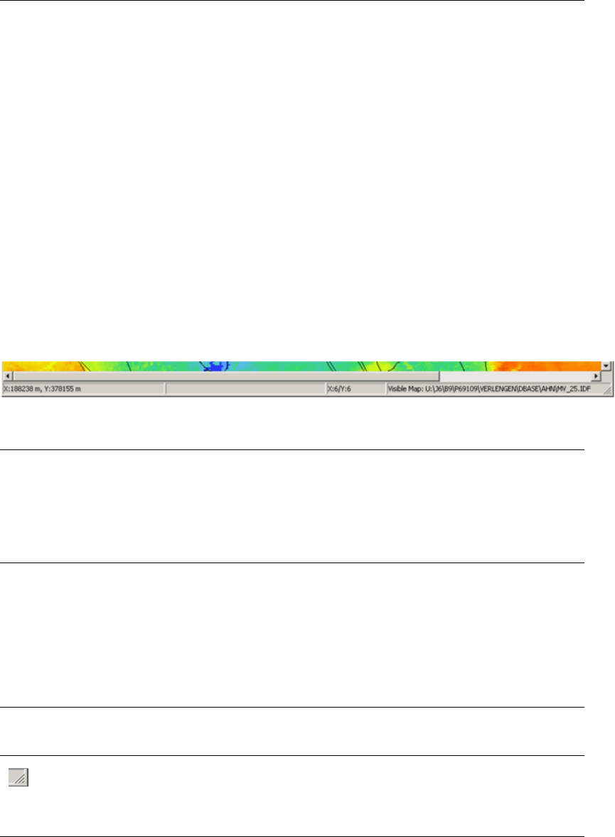
DRAFT
Getting Started
Entire Zoom Extent
Click this option to create a legend based on the values of the current zoom level (see
section 6.6.2):
Percentiles, Click this option to create a legend with non-linear values,
Linear, Click this option to create a legend with linear values,
Unique Values, Click this option to create a legend with unique values,
Tag Zoom
Click this option to zoom to the selected Tags (Comments)
Mask Zoom
Click this option to zoom onto the last *.MSK file loaded.
2.6.4 Window Status Bar
The status bar of the iMOD main window contains several elements to be considered.
Window Status bar:
X: . . . . m
Y: . . . .. m
Current Mouse Coordinates
The coordinates of cursor in the map are displayed in the lower left of the win-
dow. The units for the values on the X and Y axis are given in the coordinates
of the system in which one is currently working. In the case of Dutch data, this
is the National Triangulation System. In principle it is possible to read files in
another system (if the system is projected, such as the National Triangulation
System, for flat surfaces).
X:6/Y:6 RasterDisplayResolution
This element on the status bar shows the accuracy of the displayed IDF-file.
Since these IDF-files can be enormous in size, iMOD will decline the number
of data read as the zoom level is increased. In such a manner, iMOD can
display these enormous IDFs raster files quickly. For IDF-files that have non-
equidistant cellsizes, iMOD needs to read all data. Consequently, these type
of IDFs will be slower in presentation than the equidistant ones. The accu-
racy can be altered by selecting the menu option View and then the option
Accuracy.
mv_25.IDF Current IDF
This element on the status bar shows the current IDF at the current mouse
position.
WindowExtent
Click on your left-mouse button whenever it is positioned on this lower-
right corner of the iMOD main window. By dragging your mouse (while the
left-mouse button is pressed), the size of the iMOD main window can in-
crease/decrease.
2.6.5 Title Panel
This panel situated at the top of the main window displays the iMOD version and the type of
iMOD license. The top of the graphical window displays the name of the *.IMF used last to
save the iMOD Project.
Deltares 25 of 812
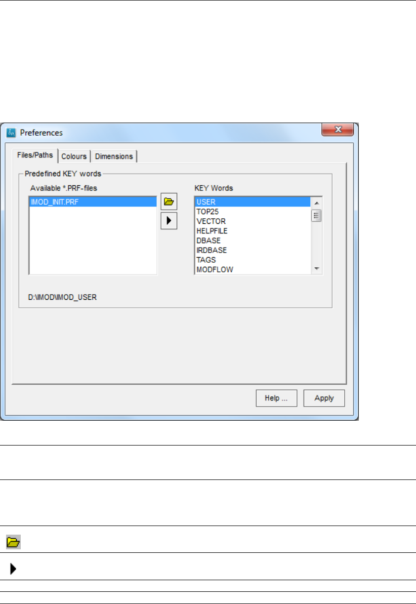
DRAFT
iMOD, User Manual
2.7 Preferences
Several settings can be initiated to configure the current iMOD session. These can be defined
in a *.PRF file (see section 9.1 for more information). On the menu bar, click the option File
and then choose Prefences to open the corresponding Preferences Window.
Preferences window, Files/Paths tab:
Available *.PRF
files
Display of all available *.PRF files in the folder in which iMOD was executed.
Select one of them to load an iMOD configuration. Different *.PRF file can be
stored to switch between different iMOD configurations quickly.
Keywords Select one of the keywords to inspect the value assigned to it under-
neath the tab. In this example above the keyword {user} has the value
c:\users\peter\work\imodproject\user. To change any keyword, you should
open the *.PRF in any third-party software, e.g. Notepad.
Open *.PRF-file
Click this button to search for a *.PRF-file on disk.
Use the selected *.PRF-file
Click this button to read the selected *.PRF-file and use its settings.
Close Click this button to close the Preferences Window.
Help... Click this button to start the iMOD Help Functionality.
26 of 812 Deltares
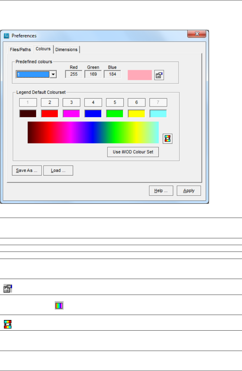
DRAFT
Getting Started
Preferences window, Colours tab:
Predefined
Colours
The dropdown menu presents the current colour number. iMOD supports 50
predefined colours to be used as default in a variety of iMOD functionalities,
e.g. plotting of Cross-Sections,TimeSeries.
Red Value of the red-component of the current default colour (0-255)
Green Value of the green-component of the current default colour (0-255)
Blue Value of the blue-component of the current default colour (0-255)
Legend Default
Colourset
Change and save the preferred default colour-settings for the 7 basic legend
colours in the *.CLR-file. Changing the colours works as similar as described
in section 6.6.1.
Colour Selection
Click this button to open a default Colour window from Windows
Use iMOD Colour
Set
Use the iMOD default legend colours, rainbow colouring:
.
Flip Colours. Click this option to “flip” the colour sequence, e.g. red becomes
blue and blue becomes red.
Save As . . .
Save a *.CLR-file
Click this option to save the current default (legend) colours in a given *.CLR
file.
Load . . .
Open *.CLR-file
Click this button to search for a *.CLR-file on disk. This type of file defines the
default (legend) colours used by iMOD.
Deltares 27 of 812
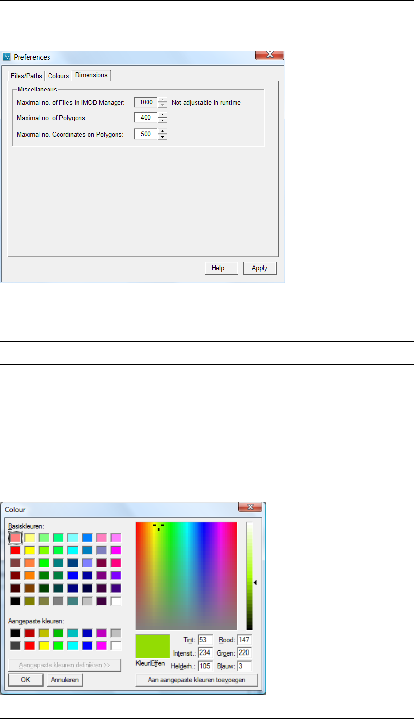
DRAFT
iMOD, User Manual
Preferences window, Dimensions tab:
Maximal no. Files
in the iMOD Man-
ager:
Maximum number of maps to be loaded in the iMOD Manager. This value can
not be altered, a change can be applied in the source-code.
Maximal no. of
Polygons:
Maximum number of polygons in a single *.SHP and/or *.GEN file.
Maximal no. of
Coordinates on
Polygons:
Maximum number of coordinates upon each polygon within a *.SHP and/or
*.GEN file.
2.8 Colour Picking
On various dialogs in iMOD, you can specify a colour. In all these cases the default Colour
window is used, as shown below.
Colour window:
28 of 812 Deltares

DRAFT
Getting Started
OK Select this button to accept the selected/created colour. The Colour window
will close.
Cancel Select this button to cancel any change in colour. The Colour window will
close.
Deltares 29 of 812
DRAFT
iMOD, User Manual
2.9 Tips and Tricks
2.9.1 Keyboard shortcuts
Use the keyboard shortcuts to directly open a window without selecting the option from the
menu bar.
Navigation
Centre mouse button Move Map (Pan).
Shift-right mouse button Zoom Out.
Shift-left mouse button Zoom In.
iMOD Manager
Ctrl-M Open iMOD Manager Window.
Ctrl-N New iMOD Project.
Ctrl-O Open iMOD Project.
Ctrl-S Save iMOD Project.
Ctrl-P Open iMOD Project Manager Window.
Ctrl-C Copy current presentation to Windows Clipboard.
F1 Open iMOD Help-file (if available in the selected *.PRF file).
F2 Add Map to the iMOD Manager.
F3 Set map information (point, polygon, rectangle).
2.9.2 Exporting Figures
The content of the graphical window can be exported in PostScript (*.PS), Bitmap (*.BMP),
ZSoft PC Paintbrush (*.PCX) , Portable Network Graphic Image (*.png) and WMF (Windows
Meta Files) format. In the File menu, select the option Export and select the appropriate
export type finally. These files can be later imported in a Word document, for example or
added as annex in a report. The option Copy to Clipboard from the View menu can also be
used to copy directly the display in a Word document.
2.9.3 Saving iMOD Projects
The content of the iMOD Manager can be save into a *.IMF file. Select the option Save or
Save As from the File menu. On default, iMOD will save the content of the iMOD Manager
each minute whenever the option Autosave On (1 minute) from the File menu is checked. This
file will be called AUTOSAVE-IMOD.IMF and will be located in the directory {USER}\imffiles,
where {USER} will be the directory assigned to the keyword USER in the used *.PRF file.
2.9.4 Copying part of a Table
It is possible to copy part of a table in another document, an Excel sheet for example.
If the cursor is placed on a cell of the table, select a specific area by using the dragging the
mouse while the left-mouse button is pressed. Then, using the shortcut Ctrl+C, this area can
be copied and pasted into any other (commercial) Windows oriented software.
30 of 812 Deltares

DRAFT
3 File Menu options
This chapter contains a detailed description of the menu options for iMOD for general use.
The examples in the tutorial section provide a convenient starting point for familiarization with
the program.
Besides the familiar Windows options for opening and saving files, the File menu contains a
number of options specific to iMOD:
Autosave On (1 minute)
On default, iMOD saves the current content of the iMOD Manager each minute. It yields
an AUTOSAVE-IMOD.IMF that will be overwritten each time. The file is located in the
directory {USER}\IMFILES, where the variable {USER} directs to the value of the keyword
USER in the selected *.PRF file.
Print . . .
Prints the current content of the graphical window to an installed external printer. iMOD
uses the default Windows Print Manager.
Export
The content of the graphical window can be exported to
PostScript (*.PS);
Bitmap (*.BMP);
ZSoft PC Paintbrush (*.PCX);
Portable Network Graphic Image (*.PNG);
JPEG/JFIF image (*.JPG; *.JPEG).
In the File menu, select the option Export and select the appropriate export type finally.
These files can be later imported in a Word document, for example or added as annex in
a report.
Deltares 31 of 812
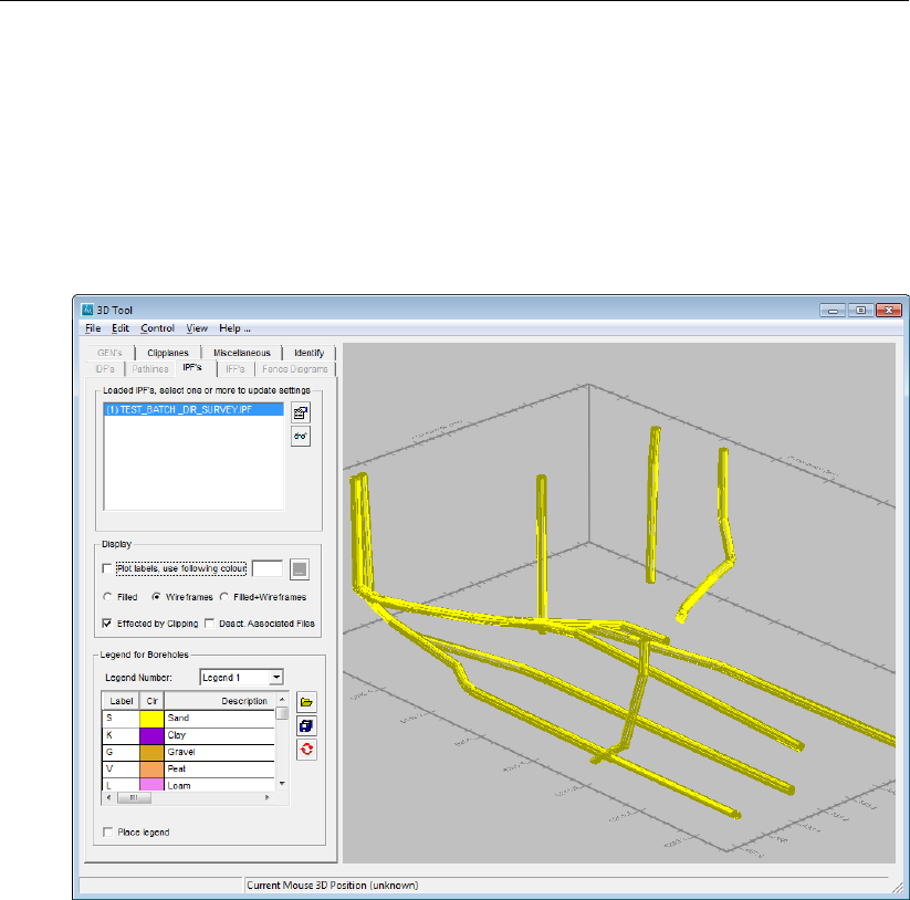
DRAFT
iMOD, User Manual
Import . . .
iMOD offers the limited ability to import a few formats from third-party software packages.
Import Deviated Wells
Select this option to import deviated wells into an IPF format (see section section 9.7.
Example of a yielding deviated well in the 3D of iMOD:
After selecting this item, a CSV file need to be selected from which the appropriate
columns within the CSV need to be assigned, or alternatively a constant value can be
entered. The following parameters are obliged:
◦Name
Select a column that represents the name of the well;
◦X Coordinate
Select a column from the drop down menu that represents x-coordinate of the well;
◦Y Coordinate
Select a column from the drop down menu that represents y-coordinate of the well;
◦Z Coordinate
Select a column from the drop down menu that represents z-coordinate of the well;
◦Depth
Select a column from the drop down menu that represents the depth of the well.
This is the depth measured as net distance (meter) through the borehole;
◦Inclination
Select a column from the drop down menu that represents inclination of the well.
The inclination is defined as the angle from the surface (xy-plane) downwards by
a positive angle whereby 90.0 degrees is perpendicular downwards;
◦Azimuth
Select a column from the drop down menu that represents the azimuth of the well.
The azimuth is defined as the angle with the z-axes measured clockwise with a
zero angle pointing to the north and 90.0 degrees to the east;
32 of 812 Deltares
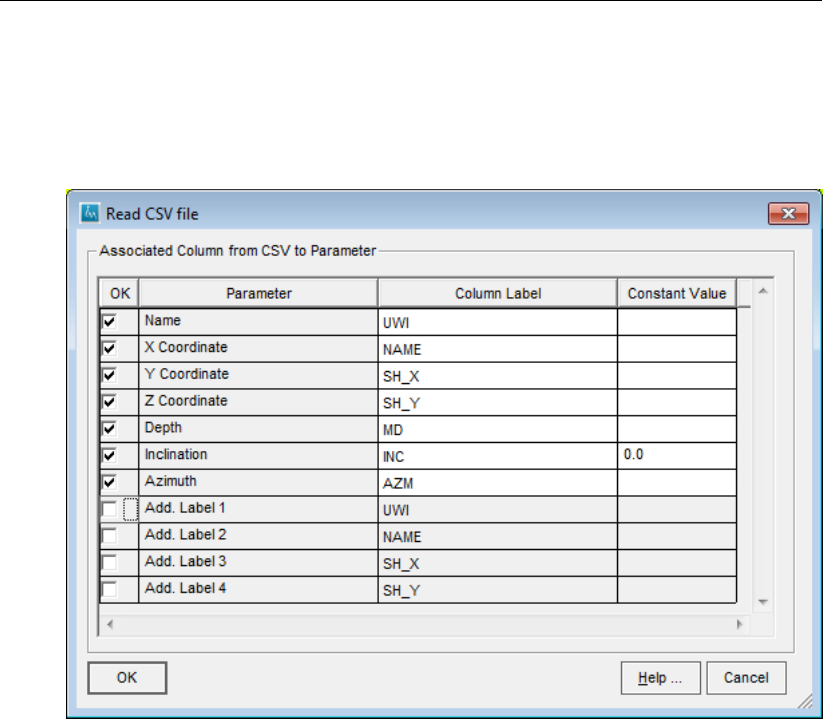
DRAFT
File Menu options
◦Add. Label 1,2,3,4
Select a column from the drop down menu that represents an additional label of
the well. Up to four additional labels can be assigned.
Example of the Read CSV File window:
There is also an iMOD Batch function DEVWELLTOIPF available, see section sec-
tion 8.10.1.
Deltares 33 of 812
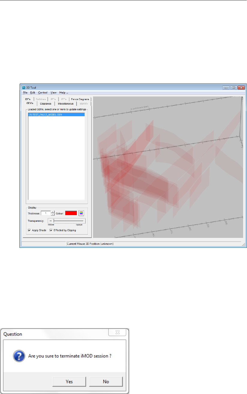
DRAFT
iMOD, User Manual
Import Keypillars Petrel ASCII format
Use this option to import a Keypillars Petrel ASCII format file. This file is exported
from Petrel. It assumes a version 4 file format describing the x,y and z-coordinates of
so-called Keypillars of faults. After selecting an ASC file, iMOD convert this to a 3D
GEN (see section section 9.10). It can then be inspected and visualized in 2D and 3D.
Example of a converted Keypillars Petrel ACII file into a 3D GEN and visualized in
the 3D Tool of iMOD:
Preferences . . .
Click this option to open the Preferences Window.
Quit . . .
Click this option to quit iMOD. Before leaving iMOD you will be asked whether you are sure
to leave iMOD, in that case you’ll be offered to opportunity to save your work first before
leaving iMOD.
Question window:
34 of 812 Deltares

DRAFT
4 Edit Menu options
The Edit menu contains the following options for the creation of:
section 4.1: creating new IDF files.
section 4.2: creating new IPF files.
section 4.3: creating new GEN files.
section 4.4: creating new ISG-files.
section 4.5: creating new Polylines.
section 4.6: creating new iMOD Batch files.
4.1 Create an IDF-file
IDF-files can be created from scratch or by conversion from different formats. The available
options are:
Scratch
Click this item to create a new IDF.
Points (*.ipf)
Click this item to create an IDF from point data stored in an IPF-file.
Polygons/Lines (*.gen; *.shp)
Click this item to create an IDF out of a (set of) polygon(s).
Flowlines (*.iff)
Click this item to create an IDF from line data stored in an IFF-file.
To create a new IDF select the main option Edit, choose Create Feature, then IDFs from and
then one of the options shown above.
When creating a new IDF from scratch then the IDF is created with NoData values. When
creating an IDF from the other formats then the IDF cells are assigned values derived from
these files.
Deltares 35 of 812
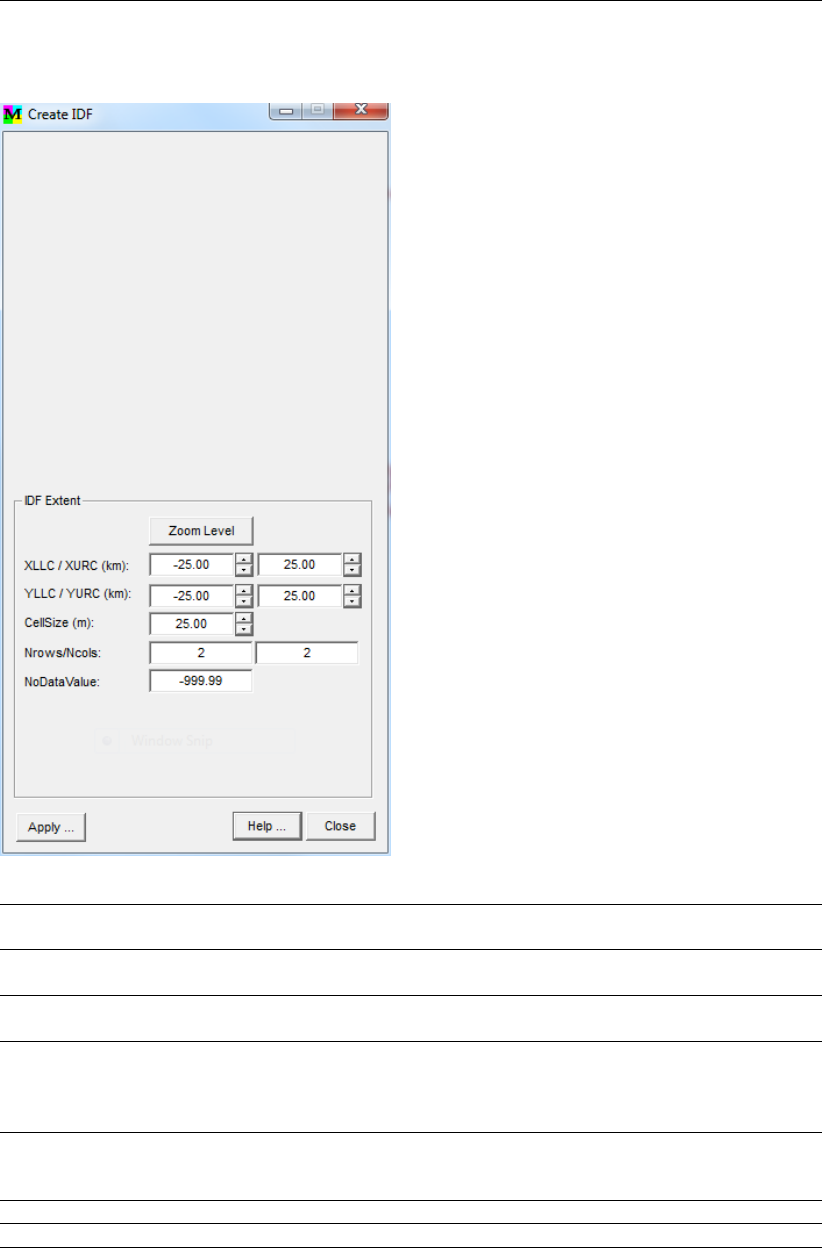
DRAFT
iMOD, User Manual
Option Scratch, Create IDF window:
Zoom Level Click this button to adjust the IDF extent to the current zoom level in
the graphical display.
XLLC / XURC (m) : Enter the X coordinate for the lower-left-corner (XLLC) and upper-right-
corner (XURC) of the IDF extent.
YLLC / YURC (m) : Enter the Y coordinate for the lower-left-corner (YLLC) and upper-right-
corner (YURC) of the IDF extent.
CellSize (m) : Enter the cellsize of the IDF in meters.
NOTE: The values for XLLC, YLLC, XURC and YURC will be
trimmed automatically to the CellSize value.
Nrows/Ncols: Displays the number of rows and the number of columns for the current
IDF extent. These values are computed automatically and can not be
changed directly.
NoDataValue: Enter the NoDataValue for the IDF
Apply Click this button to start the creation of the IDF
Close Close the Create IDF window. The new IDF is added to the iMOD
Manager window.
36 of 812 Deltares
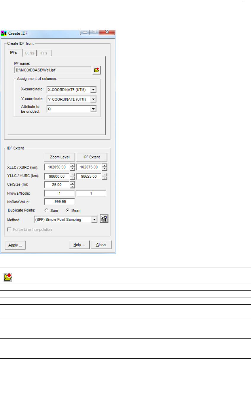
DRAFT
Edit Menu options
Create IDF window, IPFs tab:
Open Map
Click this button to open an IPF-file.
IPF-name: Displays the name of the IPF-file.
X-coordinate: Specify a column in the IPF-file that represents the X coordinate
Y-coordinate: Specify a column in the IPF-file that represents the Y coordinate
Attribute to be gridded: Specify a column in the IPF-file that represents the values to be grid-
ded. Only numeric values can be gridded.
Zoom Level Zoom Level
Click this button to adjust the IDF extent to the current zoom level in
the graphical display.
IPF Extent IPF Extent
Click this button to adjust the IDF extent to the entire extent of the
selected IPF-file.
XLLC / XURC (m) : Enter the X coordinate for the lower-left-corner (XLLC) and upper-right-
corner (XURC) of the IDF extent.
YLLC / YURC (m) : Enter the Y coordinate for the lower-left-corner (YLLC) and upper-right-
corner (YURC) of the IDF extent.
CellSize (m) : Enter the cellsize of the IDF in meters.
NOTE: The values for XLLC, YLLC, XURC and YURC will be
trimmed automatically to the CellSize value.
Deltares 37 of 812
DRAFT
iMOD, User Manual
Nrows/Ncols: Displays the number of rows and the number of columns for the current
IDF extent. These values are computed automatically and can not be
changed directly.
NoDataValue: Enter the NoDataValue for the IDF.
Duplicate Points Select one of the options for points with identical coordinates:
Sum: use the sum of the values to be gridded
Mean: use the mean of the values to be gridded.
Method: Select one of the interpolation methods (see for batch creation of IDF’s
section 8.2.10):
(SPP) Simple Point Sampling:
Click this option to determine grid values on those points that are
inside the current grid cell only. As a result, it might be that many grid
cells getNoDataValues.
(BI) Bivariate Interpolation:
Click this option to determine grid values from a smooth interpolation
function Z(x,y), which agrees with the given data (Hiroshi Akima,
A Method of Bivariate Interpolation and Smooth Surface Fitting for
Values Given at Irregularly Distributed Points, ACM Transactions on
Mathematical Software, Volume 4, Number 2, June 1978).
PCG (Preconditioned Conjugate Gradient):
Click this option to apply the Preconditioned Conjugate Gradient
method (this is the same as the solver used in MODFLOW)
VG (Variogram):
Click this option to create a semivariogram; this yields no interpolation
of the data, it generates a table filled in with a variogram. The results
will be written in the VARIOGRAM.TXT file.
(SKI) Simple Kriging Interpolation:
Click this option to apply a Kriging interpolation assuming a constant
mean over the entire domain.
(OKI) Ordinary Kriging Interpolation:
Click this option to apply a Kriging interpolation assuming a constant
mean in the neighborhood of each estimation point.
Open settings window
This function is active for the interpolation methods PCG, SKI and OKI.
38 of 812 Deltares
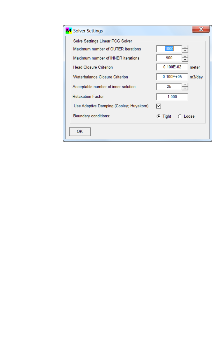
DRAFT
Edit Menu options
Solver Settings window for PCG interpolation:
Outer
Iterations
Specify the maximum number of outer iterations used by
the PCG solver;
Inner
Iterations
Specify the maximum number of inner iterations used by
the PCG solver. The more inner iterations used for a lin-
ear problem, the faster a PCG solution will be achieved;
Head Closure
Criterion
Specify the closure criterion (e.g. Heads) for the problem
to be solved. This value related to the units of the prob-
lem to be solved, choose a value at least two order of
magnitude less than the desired accuracy;
Waterbalance
Closure
Criterion
Specify the closure criterion for the water balance for the
problem to be solved, e.g. the lumped error of accuracy
in the head. This value related to the units of the problem
to be solved, choose a high value whenever the usage
of the Head Closure Criterion is sufficient;
No. Inner
Solutions
Specify an acceptable value, e.g. 25, whenever the prob-
lem to be solved shows high non-linearities that avoid
any convergence of the solver. Solving a Solid might in-
troduce these non-linearities that can be tackled in this
manner;
Relaxation
Factor
This factor damps the subsequent solutions of the solver.
Use a high value (1.0) for linear problems and a lower
value for non-linear problems. Use the Use Adaptive
Damping option for non-linear problems instead;
Adaptive
Damping
Apply this for non-linear problems as it will adapt the
Relaxation Factor during the iteration process to yield
a more robust solution;
Boundary
Conditions
Select the Tight option to fixate the known location dur-
ing the solution, use Loose instead to use a different
approach in which the known areas are simulated by
a boundary condition that allows more change on the
known areas;
OK Select this button to agree with the entered values.
The PCG solver is available in an iMOD Batch functionality as well, see
for more information section 8.2.10.NOTE: Consult scientific literature
regarding PCG solver settings as described above.
Deltares 39 of 812
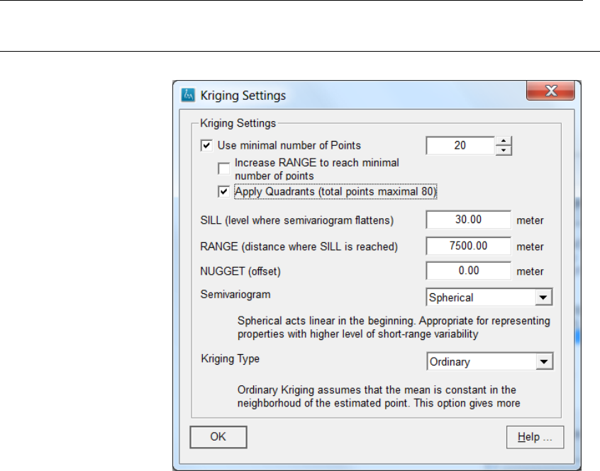
DRAFT
iMOD, User Manual
Kriging Settings window for Simple and Ordinary Kriging interpolation:
Use minimal
number of
Points
Specify the minimum number of points (per quadrant).
Increase
Range to
reach minimal
number of
Points
Select this option to allow the search increase the Range
whenever the number of points is less than the entered
minimal number of points.
Apply Quad-
rant
Select this option to devide the number of points in quad-
rant to met the minimal number of points individually.
SILL Specify the SILL value. The value that the semivari-
ogram model attains at the range (the value on the y-
axis) is called the sill. The partial sill is the SILL minus
the NUGGET.
RANGE Specify the RANGE value. When you look at the model
of a semivariogram, you’ll notice that at a certain dis-
tance, the model levels out. The distance where the
model first flattens out is known as the range. Sample lo-
cations separated by distances closer than the range are
spatially autocorrelated, whereas locations farther apart
than the range are not.
NUGGET Specify the NUGGET value. The nugget effect can be
attributed to measurement errors or spatial sources of
variation at distances smaller than the sampling inter-
val or both. Measurement error occurs because of the
error inherent in measuring devices. Natural phenom-
ena can vary spatially over a range of scales. Variation
at microscales smaller than the sampling distances will
appear as part of the nugget effect. Before collecting
data, it is important to gain some understanding of the
scales of spatial variation. Increased smoothness is ap-
plied whenever the NUGGET value is increased.
40 of 812 Deltares
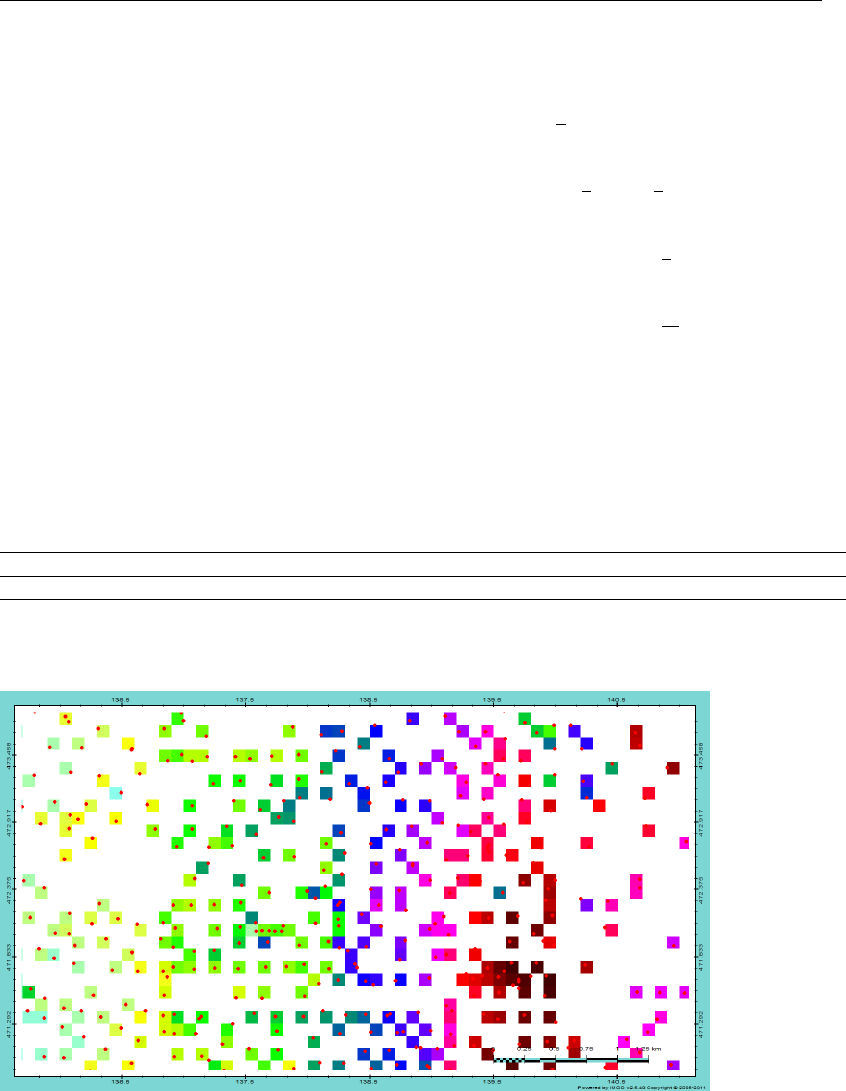
DRAFT
Edit Menu options
Semivariogram Specify the type of Semivariogram, select from:
Linear Model:
g(h) = c0+c1∗h
a
Spherical Model:
g(h) = c0+c1∗1.5h
a−0.5(h
a)3
Exponential Model:
g(h) = c0+c1∗(1 −exp(−3h
a))
Gaussian Model:
g(h) = c0+c1∗(1 −exp(−3h2
a2))
Power Model:
g(h) = c0+c1∗h0.5
hrepresents the lag distance, c0+c1is the SILL value,
c0is the NUGGET value and ais the range.
Kriging is also available in an iMOD Batch functionality, see for more in-
formation section 8.2.10.NOTE: Consult scientific literature regarding
Kriging Settings as described above.
Force Line Interpolation Not active for IPFs.
Apply Click this button to start the creation of the IDF.
Example of a Simple Point Sampling interpolation:
Deltares 41 of 812
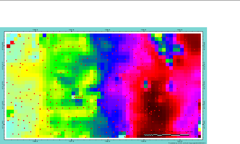
DRAFT
iMOD, User Manual
Example of a Bivariate interpolation:
42 of 812 Deltares
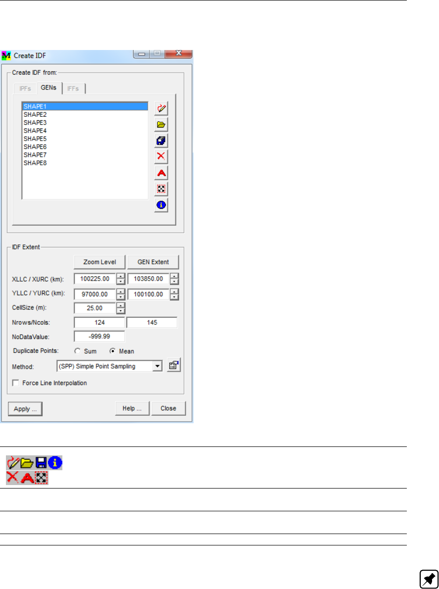
DRAFT
Edit Menu options
Create IDF window, GENs tab:
Click these buttons to draw, open, save, delete or rename a shape. More
detailed information can be found in Table 4.1.
IDF Extent Specify the extent and dimensions of the IDF and the interpolation method.
See the description for the IPFs tab for an explanation.
Force Line
Interpolation
Create interpolated raster cells only along the lines as specified in the GEN
Apply Click this button to start the creation of the IDF
Note: The value for a raster cell will be determined by the polygon number. The value
of raster cells that are part of overlapping polygons will be equal to the mean value of the
polygon numbers. NoDataValues are assigned to raster cells outside any polygon.
Deltares 43 of 812
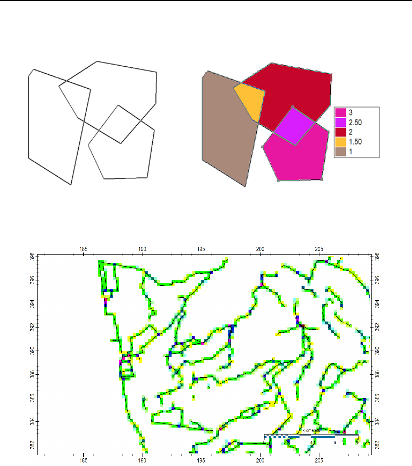
DRAFT
iMOD, User Manual
Example of a polygon GEN translated into an IDF-file:
Example of a line GEN translated into an IDF-file:
The above example shows the rasterizing of lines into an IDF-file. The result is an IDF-file
with the number of the different lines and another IDF showing the length of the line in each
rastercell crossed by it.
44 of 812 Deltares
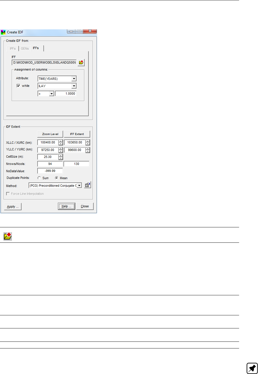
DRAFT
Edit Menu options
Create IDF window, IFFs tab:
Open Map
Click this button to open an IFF-file.
Attribute Select one of the options to grid:
PARTICLE_NUMBER – number of the particle
ILAY – modellayer number
XCRD – x coordinate
YCRD – y coordinate
ZCRD – z coordinate
TIME(YEARS) – elapsed time in years
VELOCITY – velocity (m/day)
while Click this checkbox to use an extra logical expression. Choose one
of the options (see under Attribute) and specify a logical operator
(“=”;”<>”;”<”;”<=”,”>”;”>=”) and numeric value.
IDF Extent Specify the extent and dimensions of the IDF and the interpolation method.
See the description for the IPFs tab for an explanation.
Force Line
Interpolation
Not active for IFFs
Apply Click this button to start the creation of the IDF
Note: The value for a raster cell will be determined by the particle that passes through.
Whenever more particles pass through the same rastercell, a mean value for the chosen
attribute will be computed.
Deltares 45 of 812
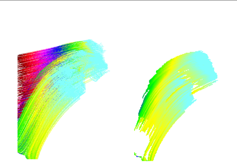
DRAFT
iMOD, User Manual
Example of a result of a particle simulation (left) gridded into a single IDF-file (right) for those
parts that are within modellayer 3 only:
46 of 812 Deltares
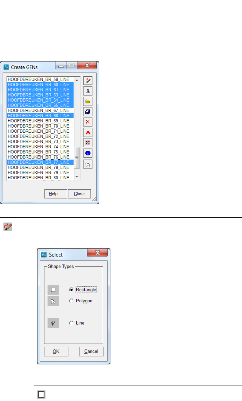
DRAFT
Edit Menu options
4.2 Create a GEN-file
Select the main option Edit and then choose the option Create Feature and then the option
GENs to display the Create GENs window.
Create GENs window:
Draw Polygon
Click this button to start drawing a polygon on the canvas, see section 4.4 for more
details on drawing polygons. First you need to select the type of shape you want to
draw from the Select window:
This window shows the available type of topology to supported by the GEN
file format.
Rectangle
Click this option to define a rectangle.
Deltares 47 of 812
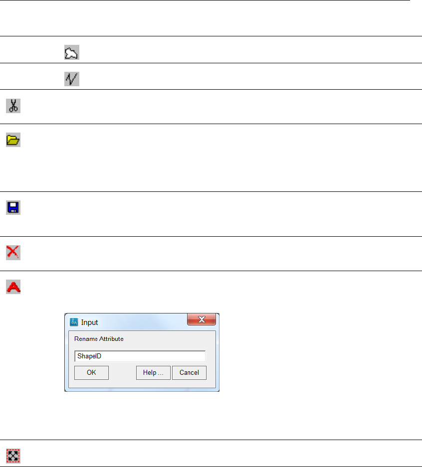
DRAFT
iMOD, User Manual
Polygon
Click this option to define a polygon.
Line
Click this option to define a line.
Cut
Click this button to start drawing a line that intersects current lines/ polygons or rect-
angles to split the intersected segments accordingly into separate lines.
Open File
Click this button to open a *.GEN or *.SHP file. iMOD will create a name for each
shape (polygon, line, point) inside the *.GEN and/or *.SHP file. If no name is
specified for a shape (next to the ID identification), iMOD will create a name as
follows: {name_of_the_gen}_{shapenumber}_{shapetype}, e.g. AREA_1_POLYGON
or AERA_9_POINT.
Save File
Click this button to save the polygons to a *.GEN-file (see section 9.9). iMOD will save
the names for the individual features in the *.GEN too. Those will be read whenever
those files are read in iMOD again whenever the button Open File is selected.
Delete Polygon
Click this button to delete the selected polygons from the list. This action can not be
undone, however, you will be asked first whether you are sure to delete the polygons.
Rename Shape
Click this button to rename the shape (line, polygon, rectangle), the Input window
will appear:
You can enter a different name for the current selected polygon. Click the but-
ton OK to accept your entry, or click Cancel to leave the name unchanged. In both
cases you will return to the Create GENs window again.
ZoomSelect
Click this button to adjust the zoomlevel to the selected shapes.
48 of 812 Deltares
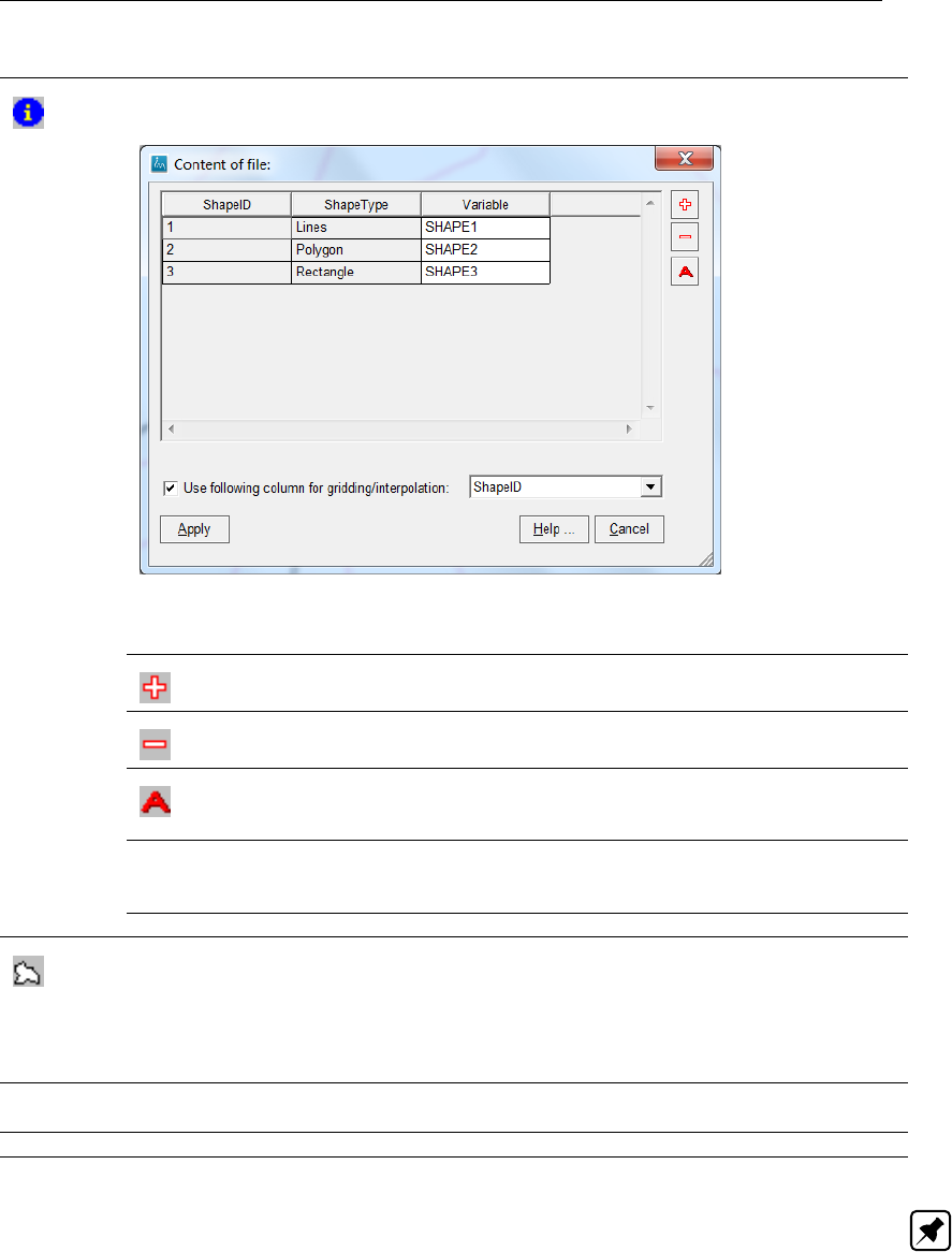
DRAFT
Edit Menu options
Information
Click this button to open theContent of file window:
This window shows the properties of the shapes which are used to create the
GEN-file.
Insert attribute
Add an attribute to the shapes.
Remove attribute
Remove the selected attribute.
Rename
Change the name of the selected attribute, see the Rename
Shape item previously described here.
Use following
column for gridding
/interpolation:
Check the box and select the attribute name from the pull down
list in case interpolation is to be done for an attribute different
from the SHAPEID.
Apply Make the changes in the shapes.
Select in Polygon
Click this button to create a polygon for which all polygons, lines and/or poins will be
selected that are within the polygon. Start drawing the polygon by clicking your left
mouse button at the first point of the polygon, click left for each additional polygon
point and stop drawing by clicking your right mouse button. After that iMOD will select
all topologies within the polygon.
Help ... Click this button to start the iMOD Help Functionality (if available in the selected
*.PRF file).
Close ... Close the Create GENs window, you will be asked to save your shapes first.
Note: The functionalities mentioned above appear throughout iMOD in different windows.
The behavior for each of those is similar as explained above.
Deltares 49 of 812
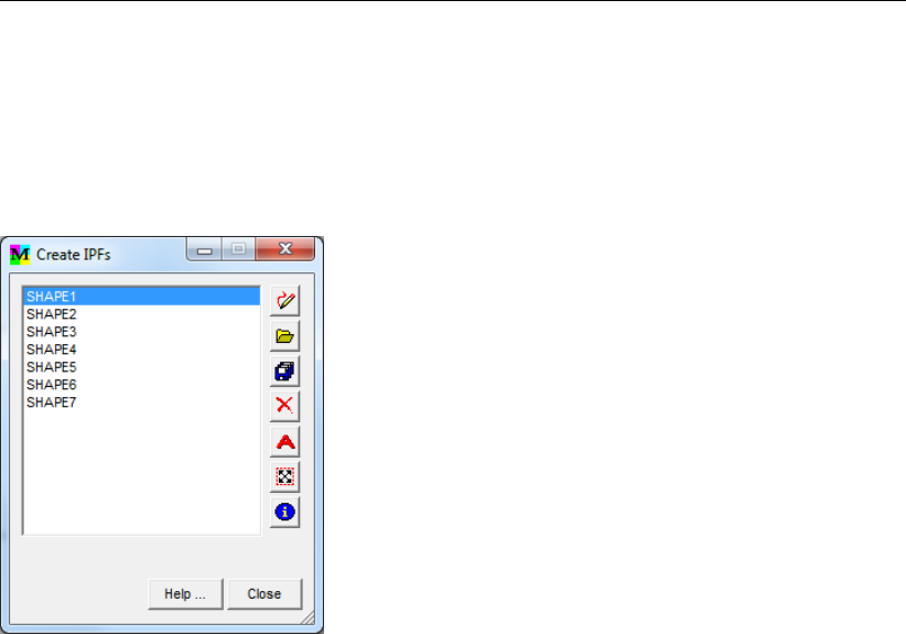
DRAFT
iMOD, User Manual
4.3 Create an IPF-file
Select the main option Edit and then choose the option Create and then the option IPFs to
display the Create IPFs window.
Create IPFs window:
The options in this window are similar to the options described in the previous section on
Create GENs window.
50 of 812 Deltares

DRAFT
Edit Menu options
4.4 Create an ISG-file
Select the main option Edit and then choose the option Create Feature and then the option
ISGs and then the option RIV Applicable... or SFR Applicable.... Thereafter you need to enter
a name for the ISG to be created. Once a valid file name has been entered, iMOD will create
the necessary files that relate to an ISG file, see section 9.9. After that, the ISG Edit window
will start in which it is possible to add and/or modify the outline of the content of the ISG file,
see section 6.10.3.
Note: The content of the files depends on the chosen applicability of the ISG-file. The SFR
type of ISG has more attributes in the ISG than the RIV type of ISG file. The latter is used for
the conventional RIV/DRN package, as the SFR type of ISG file is specially development to
support the SFR package. Moreover, this SFR type of ISG file cannot be used in conjunction
with a runfile
Deltares 51 of 812
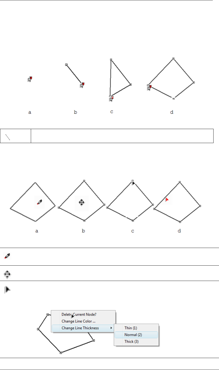
DRAFT
iMOD, User Manual
4.5 Drawing Polygons
For several functionalities in iMOD you need to specify or draw polygons. For each of those,
the methodology is similar and will be described here. After you click the Draw Polygon button
you can add points of the polygon on the graphical window by clicking your left-mouse button
sequentially.
Click the left mouse button to place another point of the polygon. Click your right
mouse button to stop
After the polygon has been drawn, the following options are available whenever you move the
mouse in or near the polygon.
This icon appears whenever you move the mouse inside a polygon. Then click
the left mouse button to select the polygon. Once a polygon is selected the
other options become available.
Click the left mouse whenever this icon appears and drag the mouse over the
graphical window to move the selected polygon.
This icon appears whenever the mouse position is on one of the nodes of the
polygon.
Click the LEFT mouse button to move the selected node.
Click the RIGHT mouse button to display the following menu options:
Delete Current
Node?
click this option to delete the current node. You can not undo
this action.
52 of 812 Deltares
DRAFT
Edit Menu options
Change Line
Color . . .
click this option to change the colour of the polygon with the
Colour window.
Change Line
Thickness
click this option to change the thickness of the line into Thin (1),
Normal (2) or Thick (3).
This icon appears whenever the mouse position is on a segment of the polygon.
Click the left mouse and you can ADD a new node.
Deltares 53 of 812
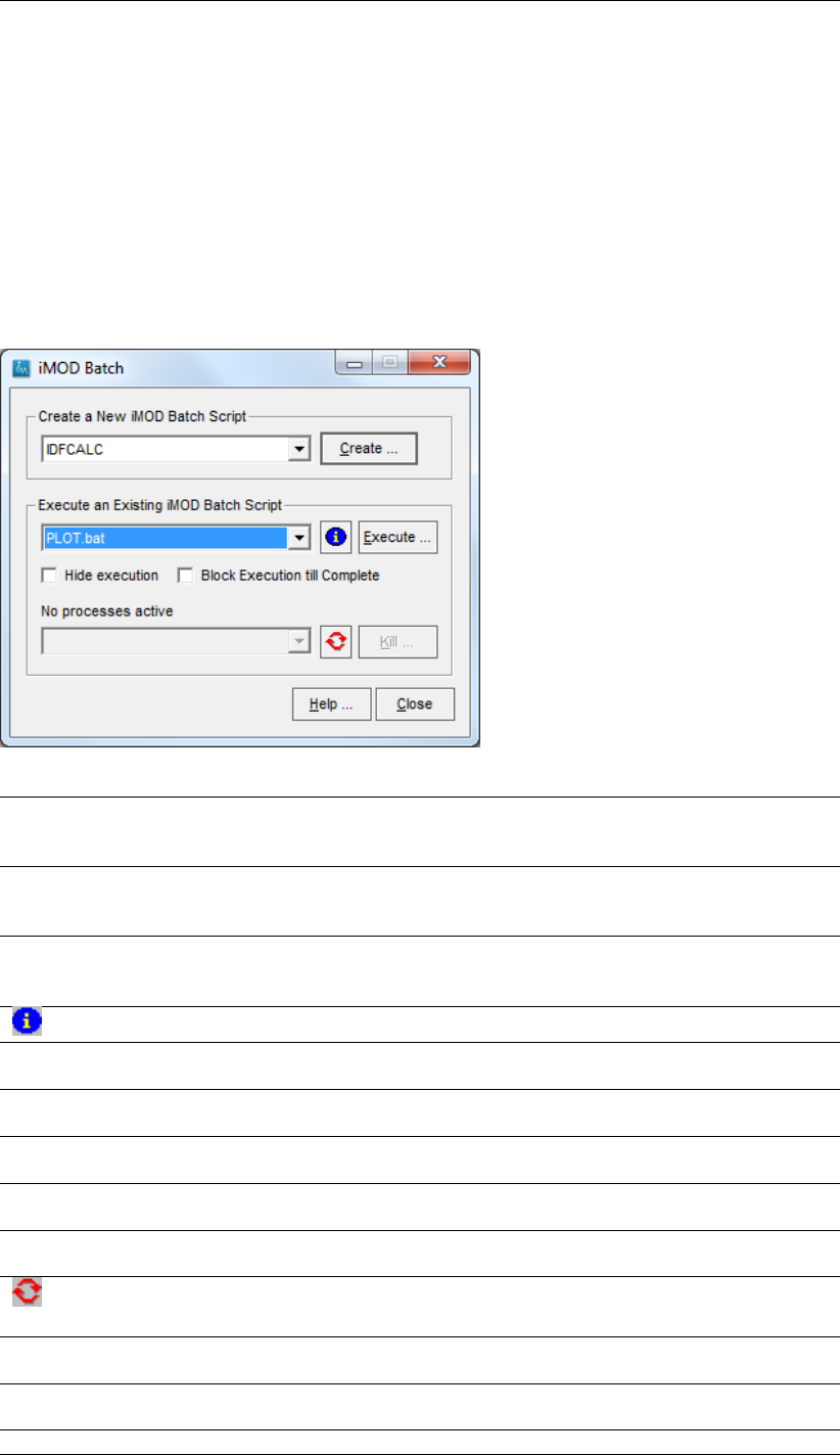
DRAFT
iMOD, User Manual
4.6 Create an iMOD Batch file
The iMOD Batch functions include a variety of tools that can be used to execute iMOD data
processes fast and repetitively. The Batch functions are described in detail in chapter 8. The
Batch functions can be executed in command mode without starting iMOD. But these functions
can be used also interactively from the iMOD main menu.
Select the main option Edit and then choose the option iMOD Batch to display the iMOD
Batch window.
iMOD Batch window:
Create a New
iMOD Batch
Script
Select a Batch function from the dropdown menu.
Create Click this button to create and save a batch file in the .\USER\IMODBATCH
directory. The file automatically gets an extension .bat. The file will open in a
text editor after it is saved. See below for an explanation of the file contents.
Execute an Exist-
ing iMOD Batch
Script
Select a Batch file from the dropdown menu.
Open a text editor with the Batch file contents.
Help ... Click this button to start the iMOD Help Functionality (if available in the se-
lected *.PRF file).
Execute Click this button to start the execution of the Batch function selected in the
dropdown menu.
Hide execution Check this option whenever it is needed to start an iMOD Batch file in a hidden
command window.
Block Execution till
Complete
Check this option to block the execution of iMOD until the executed iMOD
Batch file has terminated.
No processes ac-
tive
This drop down menu lists the processes that are currently running.
Refresh
Select this button to refresh the drop down list of active processes.
Kill Select this button to terminate the selected process from the drop down menu
left.
Help ... Click this button to start the iMOD Help Functionality (if available in the se-
lected *.PRF file).
Close ... Close the iMOD Batch window.
54 of 812 Deltares
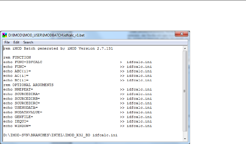
DRAFT
Edit Menu options
Example of an iMOD Batch file in a text editor window:
The file contains all keywords used for the specific batch function. The keyword contents can
be added to complete the batch function. The command line to execute the batch file is at the
bottom of the file.
Deltares 55 of 812

DRAFT
iMOD, User Manual
56 of 812 Deltares

DRAFT
5 View Menu options
This chapter describes the View Menu options, starting with on overview (section 5.1).
The following View Menu options are described in more detail:
section 5.2: Goto XY.
section 5.3: Add Background Image.
section 5.4: iMOD Manager.
section 5.4.1: iMOD Manager Properties.
section 5.5: iMOD Project Manager.
section 5.6: Subsurface Explorer.
section 5.7: Lines and Symbols.
5.1 Overview of View Menu options
The View menu contains the following options:
Copy to Clipboard
Click this item to copy the content of the current graphical window to the Windows Clip-
board. You can use the shortcut Ctrl-C instead.
Show Transparent IDFs
Check this item to draw IDF-files in a transparent mode. The used transparency is 50%
and can not be altered.
Show Opaque IDF’s
Check this item to draw all selected IDFs in opaque mode onto each other. This is helpful
to plot IDFs with different dimensions onto each other, e.g. a smaller IDF on top of a larger
one.
Apply NODATA Transparency
Check this item to draw those parts of IDF-files transparently that contain “missing” data
(cell value is equal to the NoDataValue of the particular IDF).
Show IDF Features
IDF Raster Lines
Check this item to draw the line around each of the cells within an IDF.
IDF Extent
Check this item to draw a single line around the boundaries of the IDF.
iMOD Manager . . .
Check this item to show the iMOD Manager window (section 5.4), this window will hold all
active/loaded maps.
Project Manager
Check this item to display the iMOD Project Manager window; this window is able to read
in a runfile and display its content in a tree view. From here the content can be ported to
the iMOD Manager to quickly display model information.
Zoom Map
In
Click this item to zoom IN on the centre of the current graphical dimensions.
Out
Click this item to zoom OUT on the centre of the current graphical dimensions.
Rectangle
Click this item to zoom in for a rectangle to be drawn. Use the left-mouse button to
determine the lower-left corner of the rectangle, click again for the upper-right corner
(or vice-versa).
Full Map
Deltares 57 of 812

DRAFT
iMOD, User Manual
Click this item to zoom in on the entire extent of the selected maps on the tab Maps on
the iMOD Manager or on the selected overlay Maps in the tab Overlay on the iMOD
Manager.
Mask Zoom: *.msk
Click this item to zoom to the zoom level in the last used or saved mask file.
Tag Zoom
This option is not available in the most recent iMOD version
Mask
Save Mask . . .
Click this item to save the current zoom level to a *.MSK-file
Load Mask . . .
Click this item to load a *.MSK-file and zoom to the zoom level in that file.
Goto XY . . .
Click this item to display the Goto XY window (see section 5.2) in which you can specify
a location in coordinates or cell indices to zoom on to.
Graph
This is used internally by iMOD and can not be manipulated.
Show Background Image
Click this icon to display the default topographical overlay as defined by the KeyWord
TOP25 in the selected *.PRF-file or display the overlays (*.BMP; *.png) as defined by the
menu option Add Background Image.
Add Background Image . . .
Click this item to specify bitmaps (*.BMP; *.png) to be used as background whenever the
Show Background Image is selected, see section 5.3.
Transparent Background Image
Click this item to display bitmaps that are used for background plotting in a transparent
way.
Show Location in Google Earth
Click this item to show the current zoom window within Google Earth. iMOD assumes that
UTM-coordinates are used.
Accuracy
This item computes the number of cells out of an IDF-file that are used to display a
coloured image of the values within the IDF. The more cells are read, the more accu-
rate the image will be displayed, however, the more time this will cost. iMOD computes
the number of screen pixels necessary to display the image with the highest detail (i.e. the
optimal detail). Thereafter, it depends on the choice of the user, how much of the optimal
detail will remain:
Low
Check this item to display IDF at a 10th of the optimal detail.
Medium
Check this item to display IDF at a 5th of the optimal detail.
High
Check this item to display IDF at a 3rd of the optimal detail (default).
Excellent
Check this item to display IDF at full detail.
Layout
Show Scalebar
Click this item to show a scalebar in the lower-right corner of the graphical window. The
size and parts of the scalebar are determined automatically and will update whenever
the zoomlevel changes. The location and size of the scale bar can be changed inter-
actively via the mouse.
58 of 812 Deltares
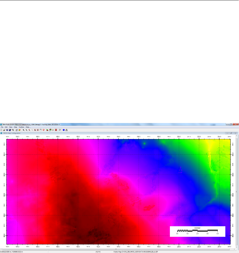
DRAFT
View Menu options
Show Axes
Check this option to show axes around the graphical window. The coordinates are
trimmed to most logic values. The textsize, font and ticsizes can not be changed,
though the location of the axes can be changed interactively via the mouse.
Show Rasterlines
Check this option to show raster lines around the graphical window from the major tic
marks.
Show NorthArrow
Check this option to show a north arrow (or other image) that has been assigned to
the keyword NORTHARROW in the selected *.PRF-file.
Example of usage of the options Show Axes and Show ScaleBar and pasted into this manual
by the option Copy to Clipboard:
Deltares 59 of 812
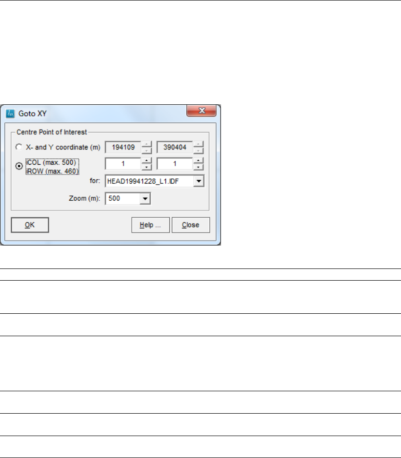
DRAFT
iMOD, User Manual
5.2 Goto XY
This functionality will offer the possibility to zoom on a centre point of interest. On the menubar
click View and then choose the option Goto XY to open the corresponding window.
Goto XY window:
X- and Y coordinate (m) Check this option to enter coordinates (X and Y) to zoom on.
iCOL (max. 5,800)
iROW (max. 6,680)
Check this option to enter column and row indices to zoom for. In this
case the limits for the column and row indices are 5,800 and 6,680,
respectively. Those are based on the dimensions of the selected IDF.
for: Select an IDF in the dropdown menu. You can select out of those listed
in the iMOD Manager.
Zoom (m) Select a range for the zoom level out of the dropdown menu. The
final zoom level will be at the maximum amount of cells fitting in the
y-direction in the map-window, e.g. Zoom level = 100 m, cell size = 25
m; at this zoom level a box of 4x4 cells will be completely shown in the
middle of the map-window.
OK Adjust the zoom level, closes the Goto XY Window and redraws the
canvas
Help Click this button to start the iMOD Help Functionality (if available in the
selected *.PRF file).
Close Leave the current zoom level unchanged and close the Goto XY Win-
dow.
60 of 812 Deltares
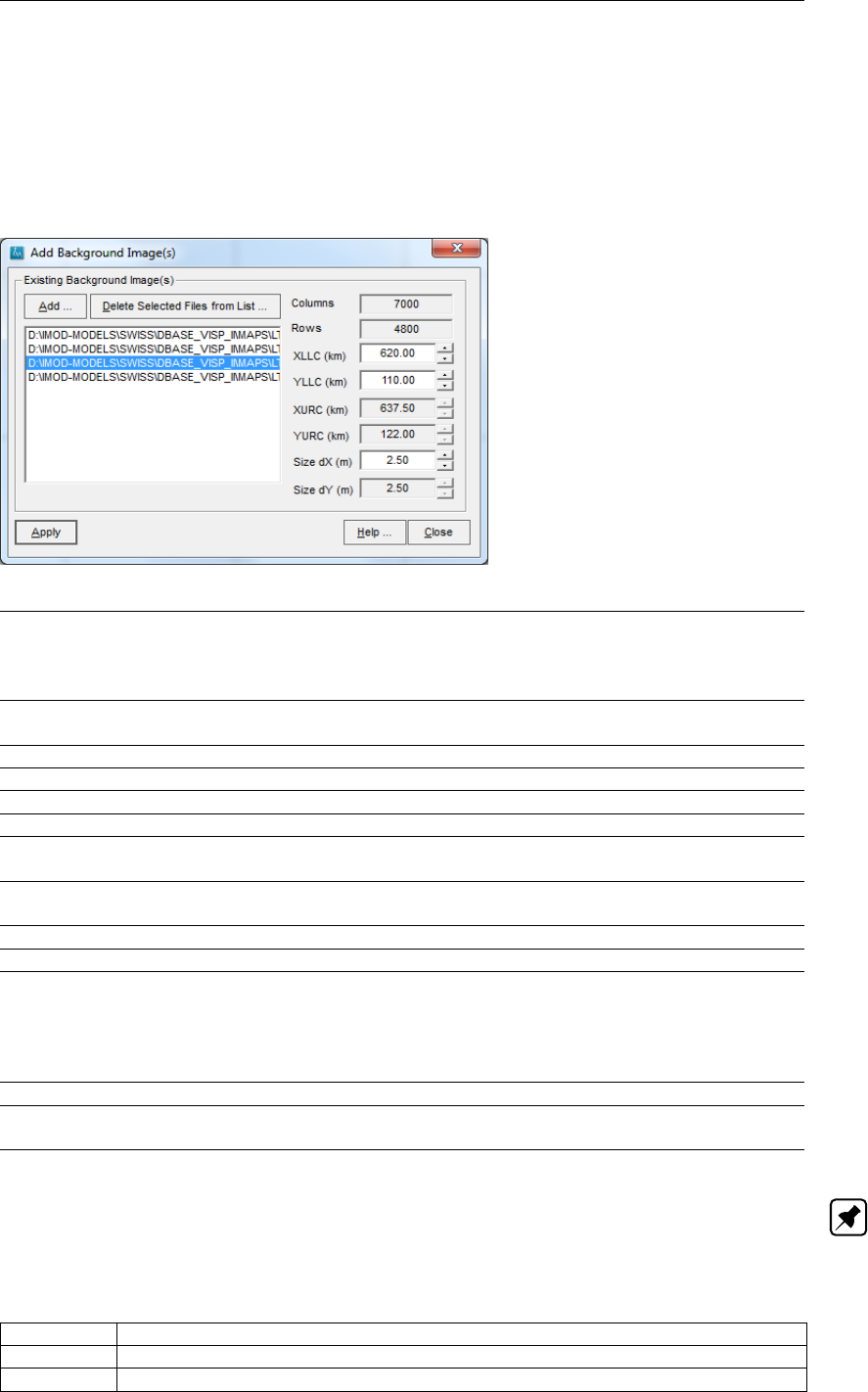
DRAFT
View Menu options
5.3 Add Background Image
This functionality will offer the possibility to use your own background images instead of the
one defined by the keyword TOP25 in the selected *.PRF-file. On the menubar click View and
then choose the option Add Background Image to open the corresponding window.
Add Background Image window:
Add ... Click this button to add a *.BMP or *.png file to the menu list of Existing BMPs.
You are able to load all kinds of images, e.g. aerial photograph, satellite im-
ages (obtained by Google Earth). The PNG format is preferable to BMPs
since it is significant smaller in size.
Delete Selected
Files from List ...
Click this button to delete the selected file from the menu list of Existing BMPs.
Columns Number of columns in the image
Rows Number of row in the image
XLLC (km) Enter the x-coordinate of the lower-left-corner (south-west) of the image.
YLLC (km) Enter the y-coordinate of the lower-left-corner (south-west) of the image.
XURC (km) Displays the x-coordinate of the upper-right-corner (north-east) of the image
that will be computed from the XLLC and the bitmap width.
YURC (km) Displays the y-coordinate of the upper-right-corner (north-east) of the image
that will be computed from the YLLC and the bitmap height.
Size dX (m) Bitmap width.
Size dY (m) Bitmap height which will be equal to Size dX, automatically.
Apply Click this button to show the background map. It also closes the Add Back-
ground Image window. The images (can be more than one) in the list of
Existing BMPs will be shown when the menu option Show Background Image
from the View menu is checked or when the corresponding icon from the tool
bar is checked.
Close Click this button to close the Add Background Image window.
Help . . . Click this button to start the iMOD Help Functionality (if available in the se-
lected *.PRF file).
Note: To reference the image topographically you can either enter the position of the image
or add a so called worldfile in the same directory as the loaded image. iMOD will search for
{ext}W files, e.g. BMPW or PNGW to read the information. The following information is listed
in a worldfile.
Dx Rastersize (m) x-direction (west-east).
RotX Value of rotation along the y-axis, RotX=0 for correct usage in iMOD.
RotY Value of rotation along the x-axis, RotY=0 for correct usage in iMOD.
Deltares 61 of 812
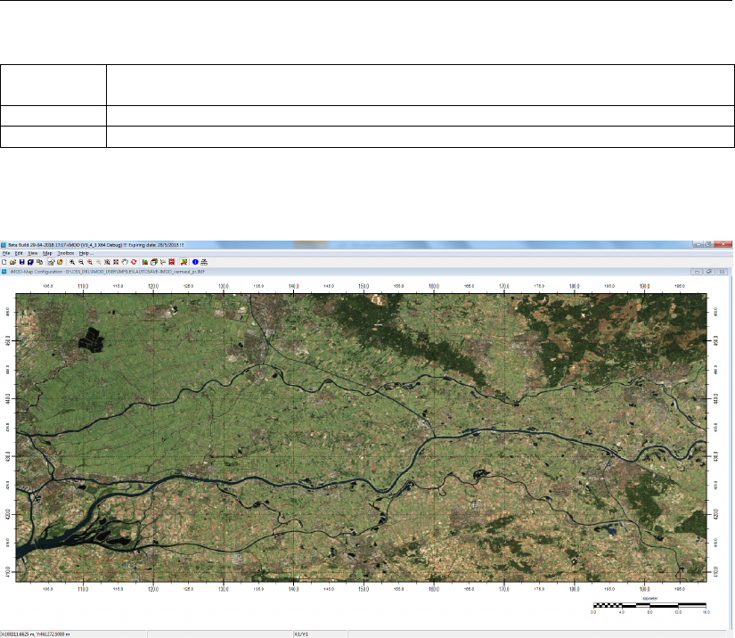
DRAFT
iMOD, User Manual
Dy Rastersize (m) in the y-direction, it should be a negative number, since it is measured
from north to south. For correct usage in iMOD Dx=-Dy.
XULC X-coordinate (m) for the center of the upper-left-corner (north-west).
YULC Y-coordinate (m) for the center of the upper-left-corner (north-west).
Example of usage of a bitmap loaded via the option Add Background Image:
62 of 812 Deltares
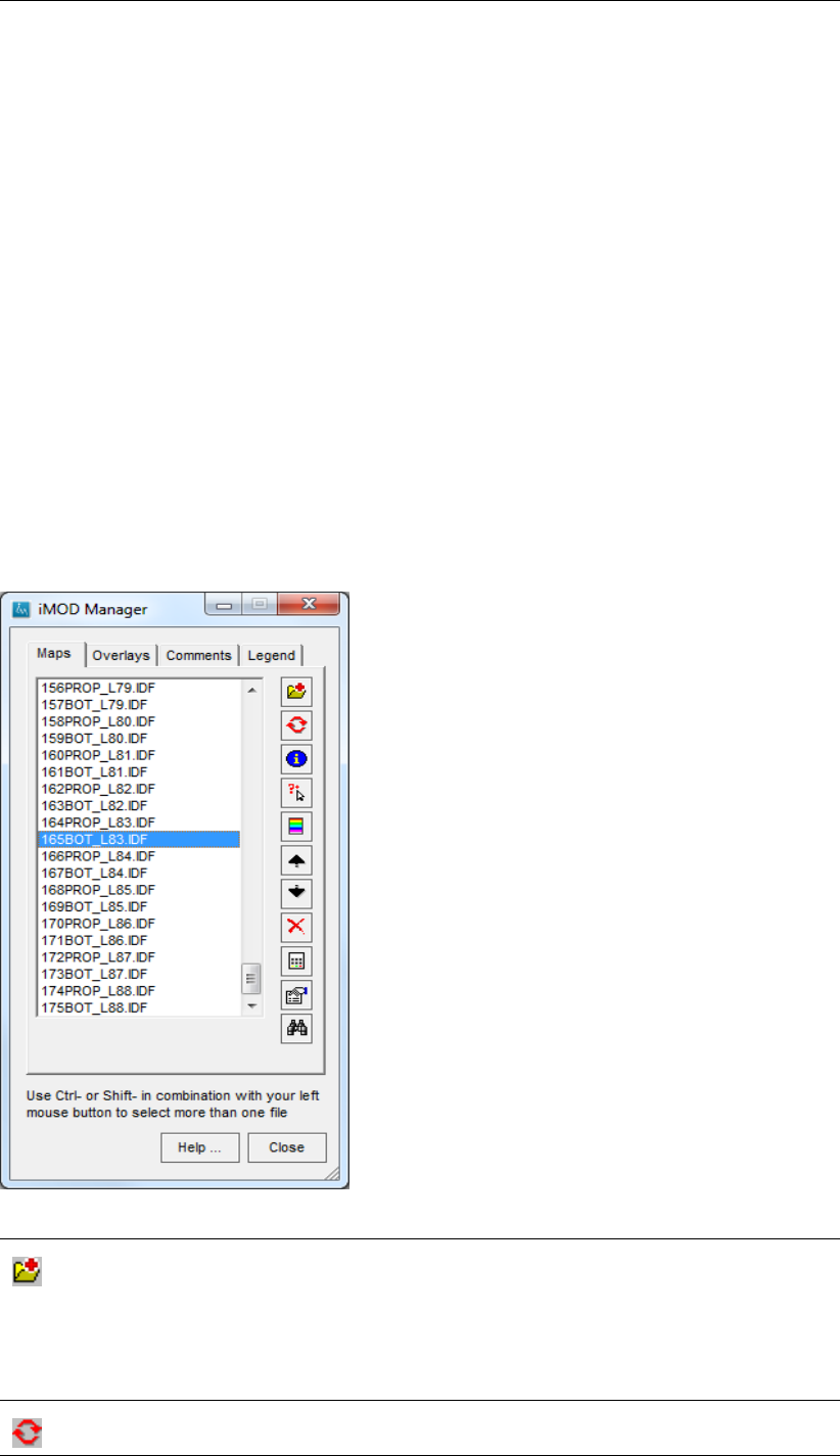
DRAFT
View Menu options
5.4 iMOD Manager
All active maps and overlays are managed by the iMOD Manager. On the menubar click View
and then choose the option iMOD Manager to open the corresponding window.
The window has four tabs:
1Maps:
This tab lists all maps loaded in iMOD. A large variety of maps can be loaded in the iMOD
Manager, up to 500 files;
2Overlays:
This tab lists all maps used as background only, these can be *.GEN and *.IPF files. Any
*.SHP that will be read in this tab will be converted to a *.GEN file format;
3Comments:
This tab lists comments that are attached to the selected map on the Maps tab;
4Legend:
This tab displays the legend of the selected map which was drawn lastly from the selected
list of maps on the Maps tab.
iMOD Manager window, Maps Tab:
Open Map
Click this button to open a map. iMOD can read a variety of maps with known file
types: *.IDF, *.IPF, *.IFF, *.ISG, *.ASC, *.SHP (will be converted internally to a GEN
of IPF file), *.GEN, *.GEF (will be converted internally to a IPF file), *.NC (will be
converted internally to a IDF file) and *.MAP (will be converted internally to a IDF
file). Alternatively the shortcut F2 can be used, or select the menu option Map and
then choose Add Map.
(re)Draw a Map
Click this button to redraw all selected maps.
Deltares 63 of 812
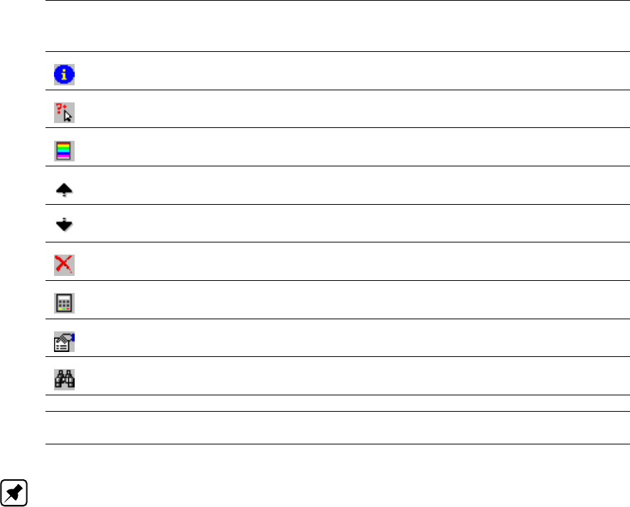
DRAFT
iMOD, User Manual
MapInfo
Click this button to open the MapInfo window.
Map Value inspection
Click this button to open the Map Value window.
Legend
Click this button to open the Legend window.
Up
Click this button to move the selected files one position up in the list.
Down
Click this button to move the selected files one position down in the list.
Delete
Click this button to remove the selected files from the iMOD Manager.
Calculate
Click this button to open the IDF Calculator window.
Properties
Click this button to open theProperties window.
Find Files
Click this button to open theFind Files window, see section section 5.4.2.
Help Click this button to start the iMOD Help Functionality.
Close Hides the iMOD Manager. The iMOD Manager can be displayed again by choosing
the menu option View and then choose the option iMOD Manager.
Note: To select more than one of the files in the tab Maps of the iMOD Manager, use the
mouse-keyboard combination Ctrl- or Shift- combination. For many functionalities in iMOD it
is necessary to select the desired files in the iMOD Manager, first. Bear in mind that several
options are not available if these files are not selected.
64 of 812 Deltares
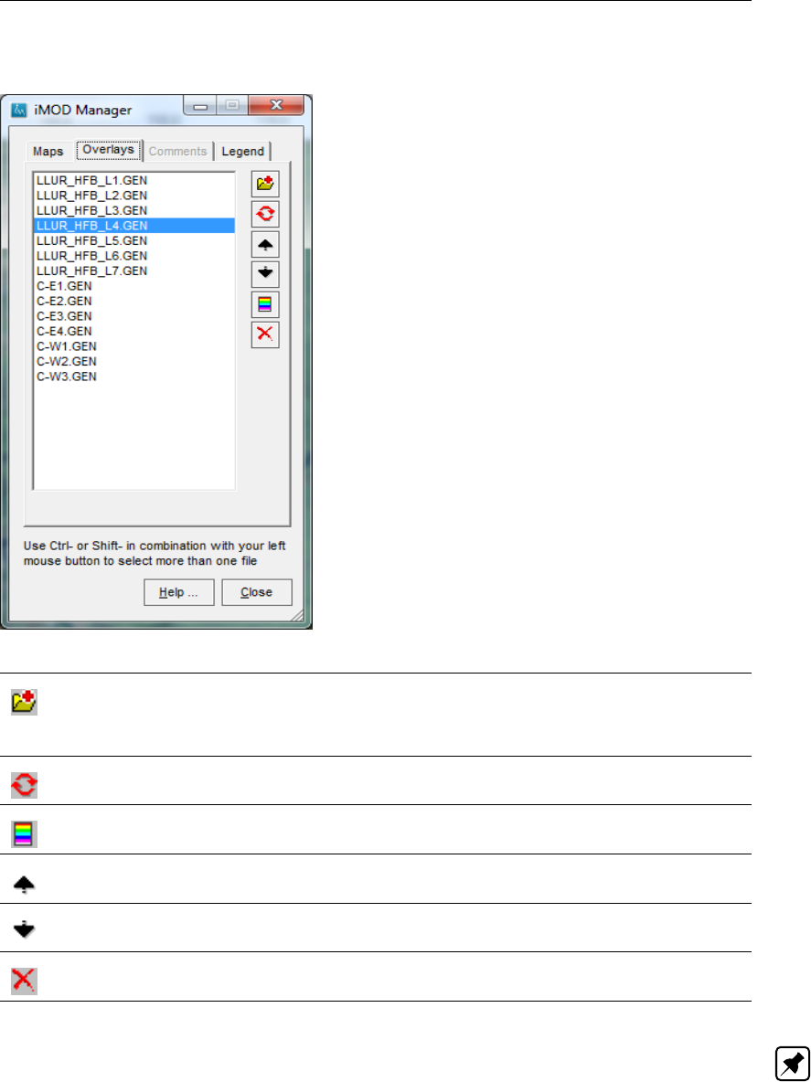
DRAFT
View Menu options
iMOD Manager window, Overlays Tab:
Open Overlay
Click this button to open an overlay map. iMOD can read a variety of overlays with
known file types: *.GEN, *.SHP (will be converted internally to a GEN of IPF file), and
*.IPF.
(re)Draw an Overlay
Click this button to redraw all selected maps.
Legend
Click this button to open the Lines and Symbols window, see section 5.7.
Up
Click this button to move the selected files one position up in the list.
Down
Click this button to move the selected files one position down in the list.
Delete
Click this button to remove the selected files from the iMOD Manager.
Note: Whenever the tab Overlays is selected in combination with the menu option ZoomMap
and then ZoomFull (or the ZoomFull icon from the icon bar), iMOD will use the selected
overlays to adjust the zoom level such that those files will be displayed fully.
Deltares 65 of 812
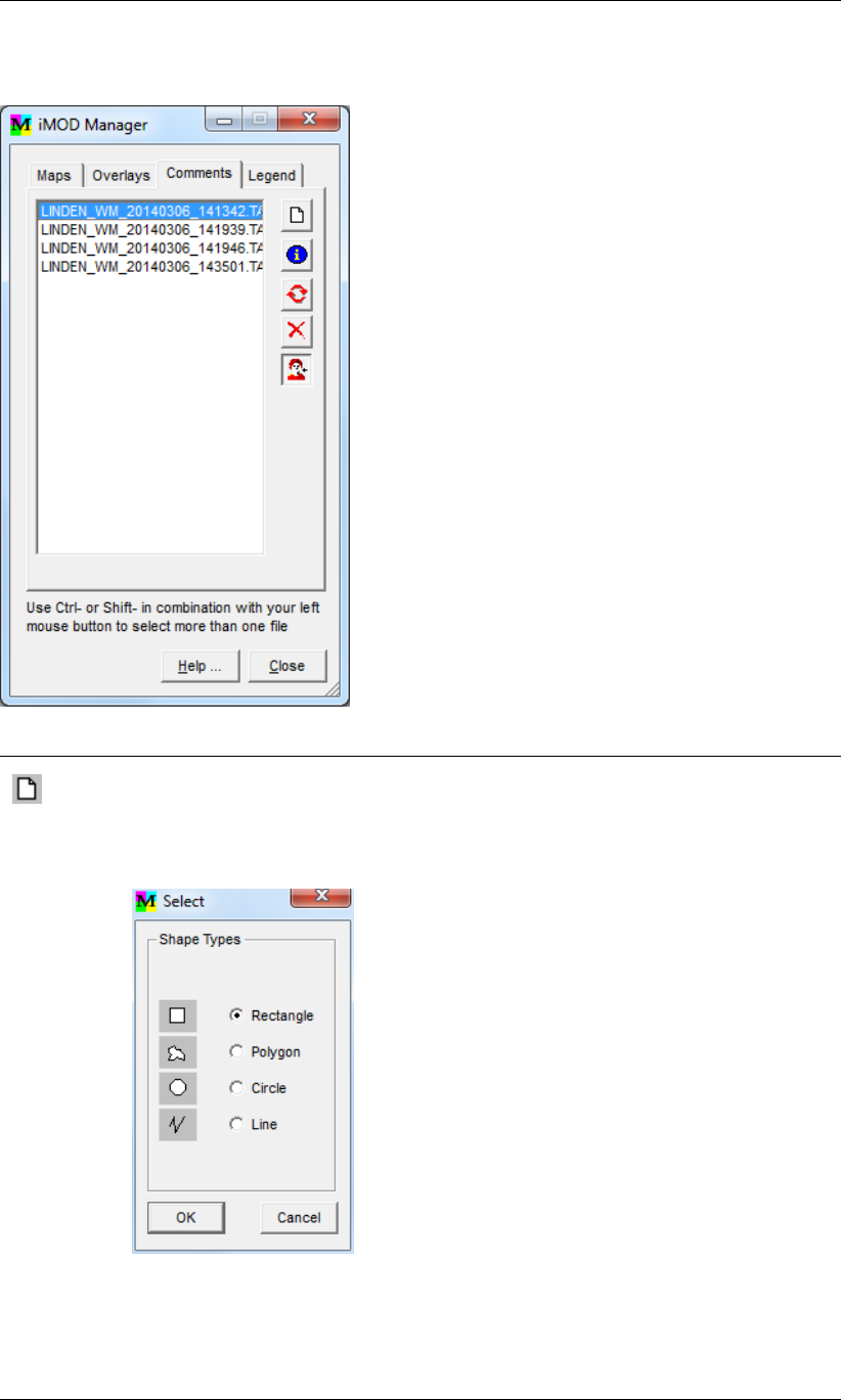
DRAFT
iMOD, User Manual
iMOD Manager window, Comments Tab:
Create tag
Click this button to create a tag. The tags are connected to the selected map (only
one map may be selected). The tags may be defined as rectangle, polygon, circle or
line. Select the shape type, click the OK button on the Select window and draw the
shape on the graphical window (see section 4.4 for instructions).
A text file editor will open in which the coordinates of the drawn shape are
shown and in which a comment can be added which will be tagged to the map. The
comment is to be added at the location of the text: <enter comment>
66 of 812 Deltares
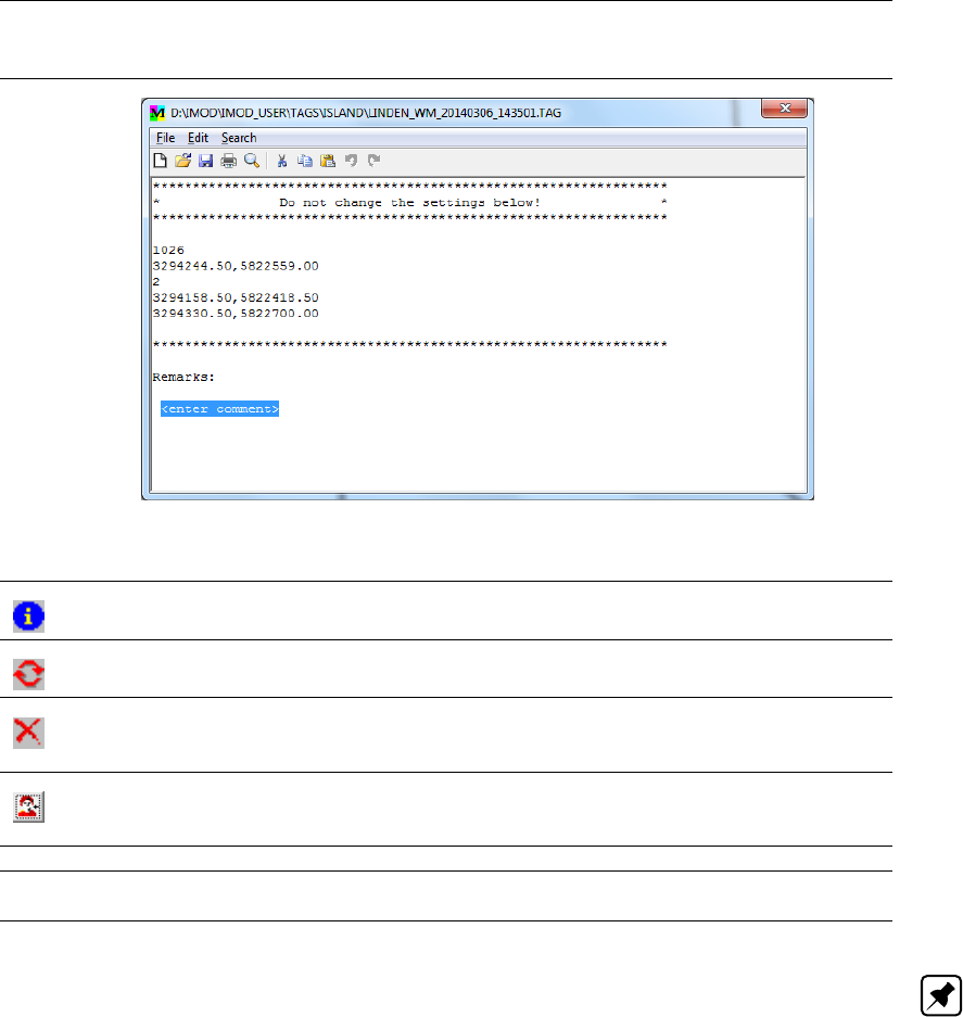
DRAFT
View Menu options
Save the comment and close the text editor window to proceed.
Info
Click this button to open a text editor window to view the comment.
(re)Draw a Map
Click this button to draw the tag and the comment id.
Delete
Click this button to remove the selected tag from the iMOD Manager. The button is
active when the user button is activated
User
Click this button to allow the user to delete tags. Each user can delete his/her own
tags only.
Help Click this button to start the iMOD Help Functionality.
Close Hides the iMOD Manager. The iMOD Manager can be displayed again by choosing
the menu option View and then choose the option iMOD Manager.
Note: The Comments tab on the iMOD Manager window is active when the TAGS variable is
defined in the iMOD_INIT.PRF file, see section 9.1.
Deltares 67 of 812
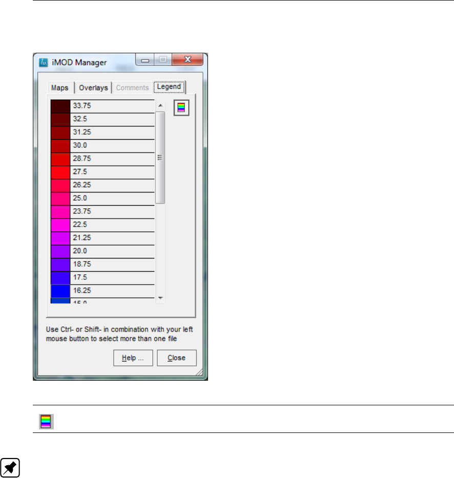
DRAFT
iMOD, User Manual
iMOD Manager window, Legend Tab:
Legend
Click this button to open the Legend window (section 6.6).
Note: The legend will be shown for the file (map) that has been drawn last, i.e. the lowest
selected file in the Map list on the Maps tab. There are different ways to plot the legend on
the canvas.
68 of 812 Deltares
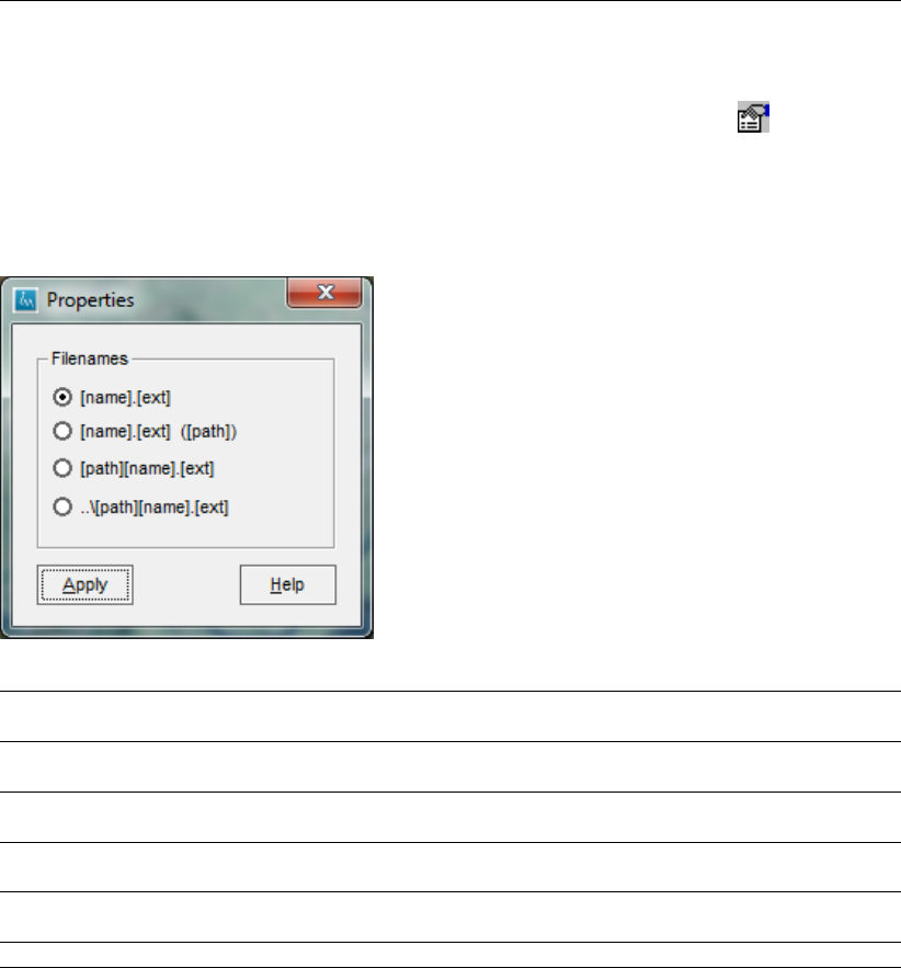
DRAFT
View Menu options
5.4.1 iMOD Manager Properties
In the Maps tab of the iMOD Manager window, click the Properties button ( ) to open the
Properties window. iMOD will use the selected file name properties to display the names of
the files in all the tabs of the iMOD Manager.
Properties Window:
[name].[ext] Click this option to display the names and their extent only, e.g. SUR-
FACE.IDF.
[name].[ext] ([path)] Click this option to display the names and their extent together with the
entire path, e.g. SURFACE.IDF (C:\IMOD).
[path][name].[ext] Click this option to display full pathnames, e.g.
C:\IMOD\SURFACE.IDF.
..\[path][name].[ext] Click this option to display the relative pathnames, such that all files in
the iMOD Manager can be still distinguished, e.g. ..\SURFACE.IDF.
Apply Click this button to close the Properties window and apply the selected
syntax.
Help . . . Click this button to start the iMOD Help Functionality.
Deltares 69 of 812
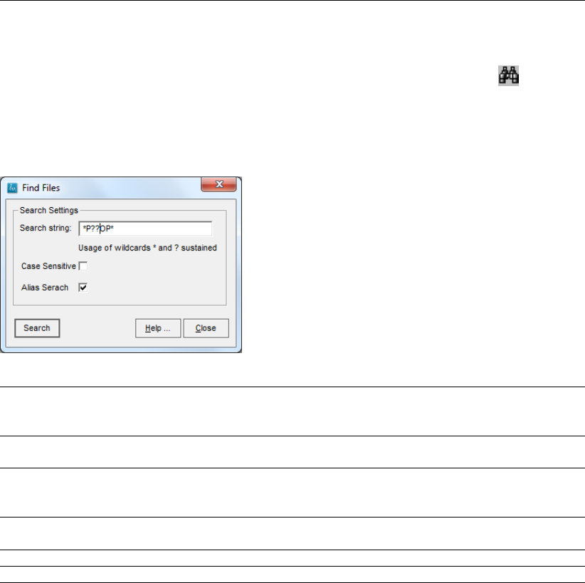
DRAFT
iMOD, User Manual
5.4.2 iMOD Manager Find Files
In the Maps tab of the iMOD Manager window, click the Find Files button ( ) to open
the Find Files window. iMOD will select files in the iMOD Manager to the selection criteria
specified in this window.
Find Files Window:
Search String Specify the search string for which filenames need to be selected. Use
the wildcards ”*“ (all characters and unknown amount) and ”¿‘ (all char-
acter but amount is equal to number of ”¿‘-symbols).
Case Sensitive Select this option to select filenames which are case-sensitive equal to
the search string, in this case ”E“ 6=”e“.
Alias Search Select this option to allow the search on the alias given to each file-
name in the iMOD Manager. If unselected, the search string is applied
to the filename and the complete foldername.
Search Click this button to select the filenames in the iMOD Manager for the
given entries in this window. After that it closes this Find Files window.
Help . . . Click this button to start the iMOD Help Functionality.
Close Click this button to close the iMOD Find Files window.
70 of 812 Deltares
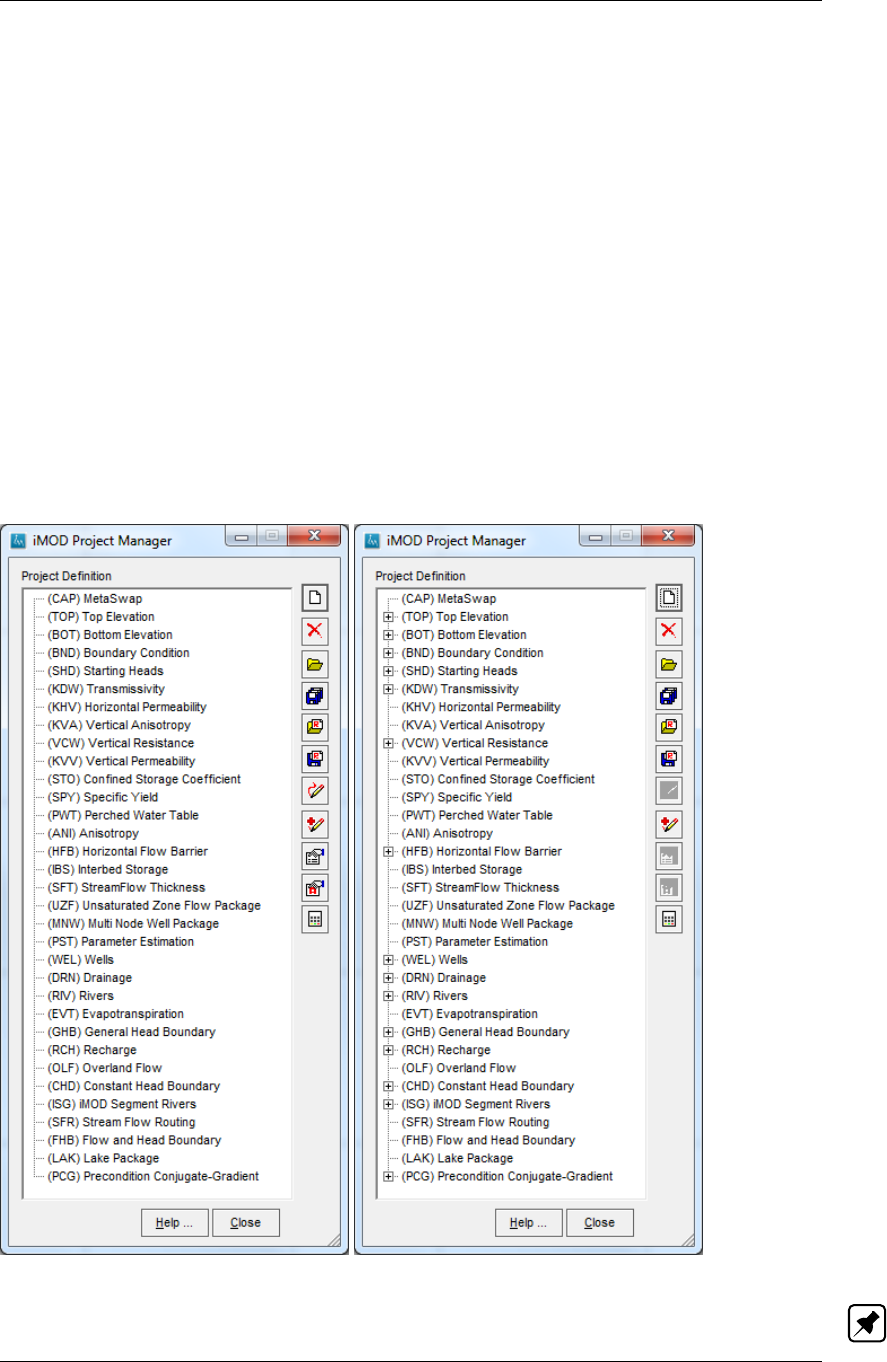
DRAFT
View Menu options
5.5 iMOD Project Manager
The files needed in a model simulation are defined in the iMOD Project Manager. On the
menubar click View and then choose the option iMOD Project Manager to open the corre-
sponding window.
The iMOD Project Manager window shows a list of all possible model input topics. iMOD
saves the characteristics in a project file, a so called *.PRJ file. From a project file a runfile
(*.RUN) can be generated that will be used in the model simulation, see section 7.9 or a stan-
dard MF2005 configuration can be save (*.NAM), see section 5.5.4. Moreover, a runfile can
be read and used to write a *.PRJ file. During the creation of a model configuration (*.RUN
or *.NAM), it is possible to change the number of model layers and/or the time characteris-
tics of the simulation, e.g. the begin and end time and/or sizes in stress-periods and/or the
configuration of packages.
iMOD Project Manager window:
Initially: After reading a project (*.PRJ) file:
Note: The Project Manager does not yet support the PKS package.
Deltares 71 of 812
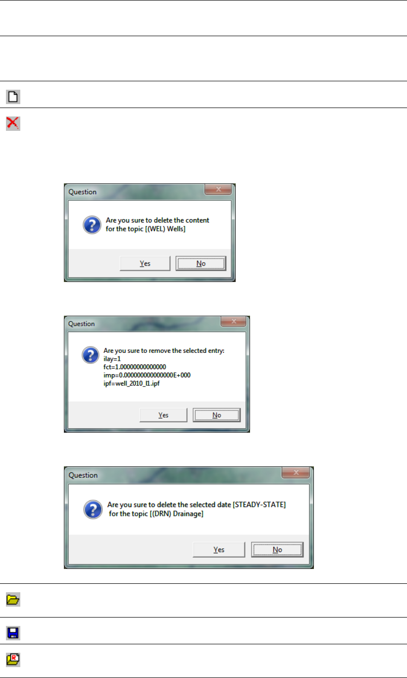
DRAFT
iMOD, User Manual
Project
Definition
All acronyms bracketed are described in more detail in chapter 10. Once a project file
*.PRJ (or a runfile *.RUN) has been read, the topics that contain model information
(recognized by the small “plus” signs) can be expanded to access the underlying
files/information.
Refresh
Click this button to refresh the Project Definition table. All definitions will be removed.
Delete
Click this button to delete the selected entry. If the main category is selected, the
entire category will be deleted. If a single entry is selected, the corresponding
package entry will be deleted.
Question to confirm the desired removal of a category.
Question to confirm the desired removal of a single entry.
Question to confirm the desired removal of all entries for a selected date.
Open Project file (*.prj)
Click this button to select a project file (*.PRJ). iMOD will read the project file and fills
the treeview in the Project Definition table.
Save Project file (*.prj)
Click this button to save the project file (*.PRJ) on disk.
Open Runfile (*.run)
Click this button to select a runfile (*.RUN). iMOD will read the entire runfile and fills
the treeview accordingly in the Project Definition table.
72 of 812 Deltares
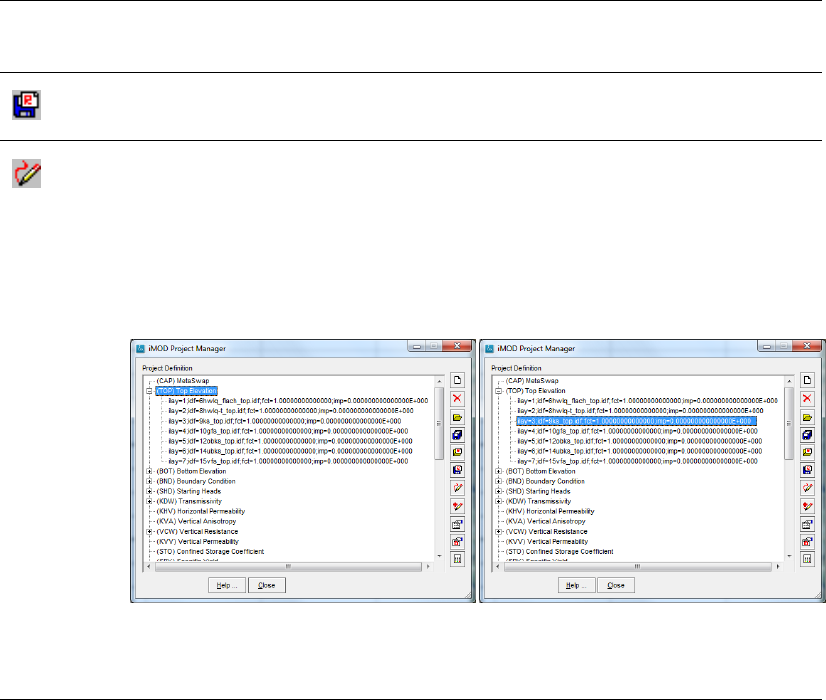
DRAFT
View Menu options
Save Runfile (*.run / *.nam)
Click this button to create a runfile (*.RUN) or MF2005 configuration (*.NAM) file. It
starts the Define Simulation Configuration window, see section 5.5.4.
Draw
Click this button to port the files within the selected topic to the iMOD Manager and
to display the files. The action of the Draw button depends on the selection in the
tree view. It will port all files underneath the selected branch. Whenever a branch
is expanded individual files can be selected that need to be ported to the iMOD
Manager.
Draw all files in the expanded branch: Draw the selected file only:
Packages that are defined by constant values instead of spatial datasets, such
as IDF, IPF, ISG and/or GEN-files (e.g. lay=3;fct=1.0;imp=0.0;constant=15.0) will not
be ported to the iMOD Manager.
Deltares 73 of 812
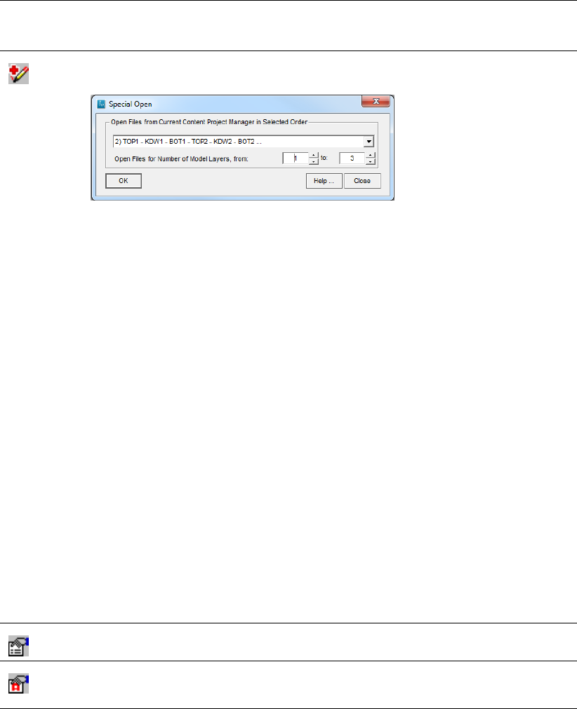
DRAFT
iMOD, User Manual
Special Open:
In this case, the files that are assigned to the 3layers will be opened in the
order top elevation, transmissivity and bottom elevation for each model layer, up to
the 3rd model layer. More options are:
TOP1 - BOT1 - TOP2 - ...
Ports the IDF files for the top and bottom elevations to the iMOD Manager;
TOP1 - KDW1 - BOT1 - TOP2 - KDW2 - BOT2 ...
Ports the IDF files for the top, transmissivity and bottom elevations to the iMOD
Manager;
TOP1 - KDW1 - BOT1 - VCW1 - TOP2 - BOT2 - VCW2 - TOP3 ...
Ports the IDF files for the top, transmissivity, bottom elevations and vertical resis-
tance to the iMOD Manager;
TOP1 - BOT1 - VCW1 - TOP2 - BOT2 - VCW2 - TOP3 ...
Ports the IDF files for the top, bottom elevation and vertical resistance to the
iMOD Manager;
TOP1 - SHD1 - BOT1 - TOP2 - SHD2 - BOT2 ...
Ports the IDF files for the top, starting head and bottom elevations to the iMOD
Manager;
TOP1 - KHV1 - BOT1 - TOP2 - KHV2 - BOT2 ...
Ports the IDF files for the top, horizontal permeability and bottom elevations to
the iMOD Manager;
TOP1 - BOT1 - KVV1 - TOP2 - BOT2 - KVV2 - TOP3 ...
Ports the IDF files for the top, bottom elevations and vertical permeability of the
interbed to the iMOD Manager;
Define Characteristics:
Click this button to open the Define Characteristics window, see section 5.5.1.
Define Characteristics Automatically:
Click this button to open the Define Characteristics Automatically window, see sec-
tion 5.5.2.2.
74 of 812 Deltares
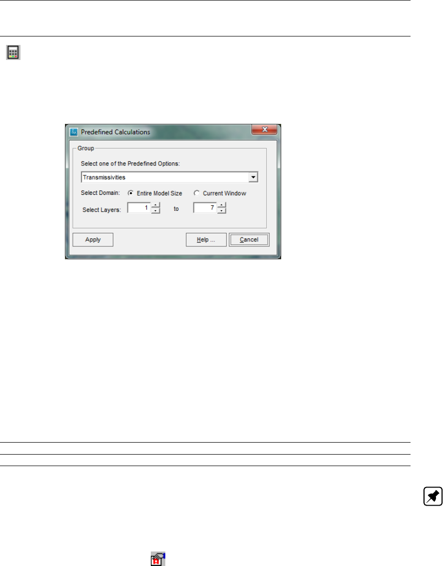
DRAFT
View Menu options
Calculator
Click this button to start the Predefined Calculations window in which it is possible
to complete standard calculations on model parameters, such as computed vertical
resistances between model layers based upon permeability values and top- and
bottom of model interfaces.
Predefined Calculations:
The following predefined calculations are implemented:
Transmissivities
Based upon the horizontal permeability (m/d) values per modellayer and the top-
and bottom of model layers, the transmissivity (m2/d) is computed;
Vertical Resistances Aquitards
Based upon the vertical permeability (m/d) in between model layers, the vertical
resistance (d) of the intermediate model layer (aquitard) is computed;
Total Vertical Resistances
Based upon the horizontal permeability (m/d), the top- and bottom, the verti-
cal anisotropy (-) per model layer and the vertical permeability (m/d) in between
model layers, the total vertical resistance (d) between model layers is computed.
The computation can be carried out for the total modeling domain or for the current
zoom window of the graphical canvas. Also, it can be done for a selected (sub)set of
model layers.
Help ... Click this button to start the iMOD Help Functionality.
Close Click this button to close the iMOD Project Manager.
Note: For transient (time variant) topics, individual stressperiods (specific dates and/or peri-
ods) can be assigned to packages as a whole. They become accessible in the iMOD Project
Manager. Those (and time invariant topics) may contain more than one levels (subtopics)
of necessary input, such as ANISOTROPY that consists of FACTORS and ANGLES and
DRAINAGE that consists of CONDUCTANCE and DRAINAGELEVEL. Use the Define Char-
acteristics Automatically button ( ) option to efficiently configure the time variant model
input and/or multi-layered input.
Anisotropy with more subtopics: Drainage/Constant Head with time variant informa-
tion:
Deltares 75 of 812
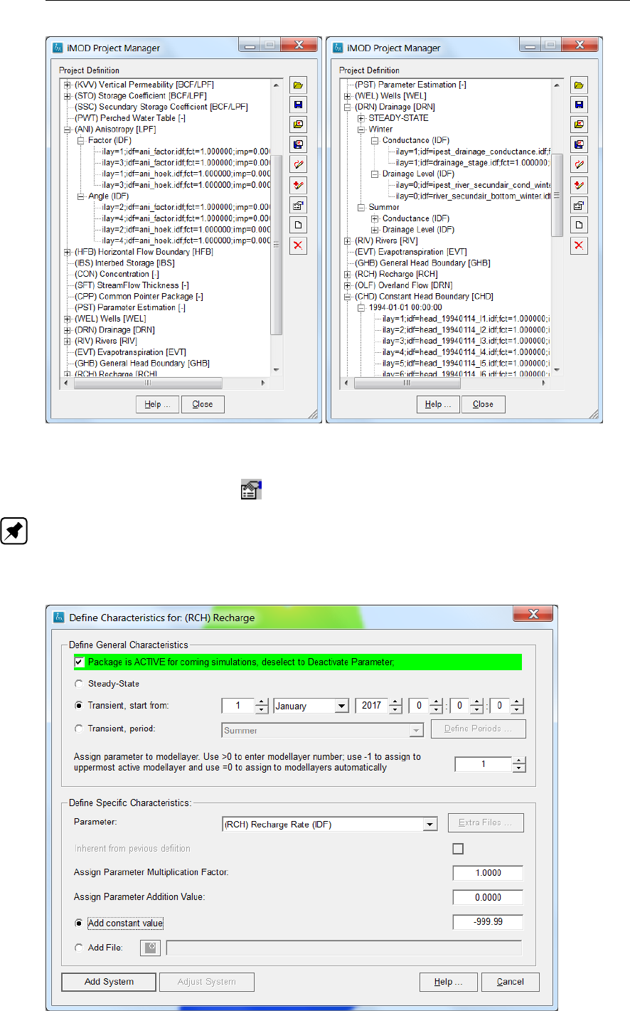
DRAFT
iMOD, User Manual
5.5.1 Define Characteristics
The Define Characteristics ( ) option of the iMOD Project Manager window opens a
window which enables to define the characteristics of the model input topics as described
below. Note: Whenever the PST package is selected a dedicated window is displayed (see
section 5.5.5).
Define Characteristics window:
76 of 812 Deltares

DRAFT
View Menu options
Package is ACTIVE for
coming simulations, de-
select to Deactivate Pa-
rameter
Check this option to exclude, in case it is ACTIVE, or include, in case it
is DEACTIVE (red bar), this model topic when saving a runfile (*.RUN).
Steady-state Check this button to define a steady state model input for the selected
topic.
Transient, start from Check this button to define input for use in a transient model. Enter the
start date for the input in the input fields to the right. Besides defining
the date there is also the option of defining the time [hh]:[mm]:[ss].
E.g. entering 10th of June 2014 08 00 00 means that the input files as
specified under Define Specific Characteristics: are starting at the 10th
of June 2014 at 08:00:00 am forward. The packages end, whenever
another input is defined ahead of time.
Transient period: Select a predefined period to indicate the start period for the current
topic. This period will be endless in time, unless another input is de-
fined ahead in time.
Define Periods... Click this button to open the window in which it is possible to add and/or
alter period definitions, see section 5.5.3.
Assign parameter to
model layer . . .
Enter the model layer number to which the input is assigned in the
model. Three options are possible:
Layer = 0 (for time variant input)
A zero-value will assign the characteristics automatically to the
model layers intersected by the depth of the model topic (e.g. the
depth of the screen for wells or the depth of stage to bottom level
for rivers);
Layer < 0 (for time variant input)
A negative value will assign the characteristics to the upper most
active model layer as defined in the Boundary Condition. When-
ever the RCH and/or EVT packages are selected, the appropriate
flags in the corresponding MF2005 packages will be set to 3 to
indicate this automatic layer assignment;
Layer > 0
A positive value will assign the characteristics to the corresponding
model layer.
Parameter: Choose the parameter for which the specific characteristics will be de-
fined. Depending on the model input topic the number of parameters
is 1 (e.g. for WEL), 2 (e.g. for ANI), 3 (e.g. for EVT) or 4 (e.g. for RIV).
See chapter 10 for detailed information about these different input per
topic.
Deltares 77 of 812
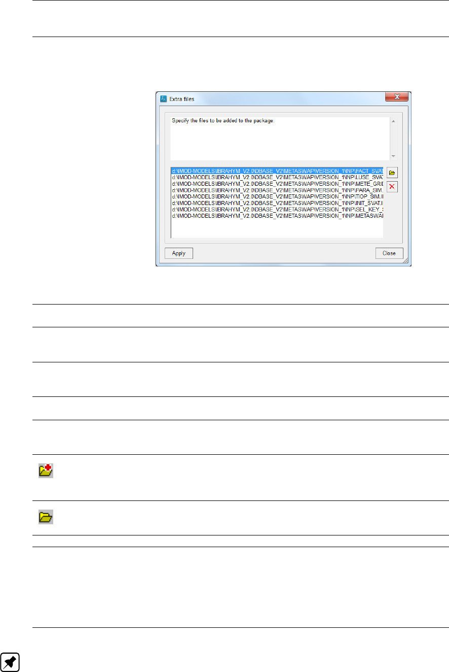
DRAFT
iMOD, User Manual
Extra files: Click this option to add extra files to the topic. This option is only
available whenever the MSW (Unsaturated Zone) package is selected.
Extra Files:
In this case, the files are listed to be copied in a simulation with
MetaSWAP.
Inherent from previous
definition:
Select this option to inherent the input for the selected topic from the
previous (in time) definition for this topic.
Assign Parameter
Multiplication Factor:
Change the multiplication factor from the default value 1.0 in case the
model input needs to be multiplied. Multiplication goes before the ad-
ditional value.
Assign Parameter
Addition Value:
Change the addition factor from the default value 0.0 in case the model
input needs to be increased (added) with a constant value. Multiplica-
tion goes before the additional value.
Add constant value Check this button and enter a constant value for the parameter for the
whole model area.
Add file: Check this option and enter a file name to be used for the parameter.
It depends on the package whether an IDF, IPF, ISG or GEN file need
to be entered.
Open File
Click this button to open the a Windows Explorer to locate the file name
for the parameter, this can be an IDF, IPF, ISG or GEN file that depends
on the topic considered.
Open
Click this button to select a folder, remember to add a wild-card to the
folder name in order to select appropriate file names by iMOD.
Help ... Click this button to start the iMOD Help Functionality.
Add System
Adjust System
Check this button to save the entered input for the selected topic and
return to the Project Manager window. This can mean that the param-
eter for an existing topic are adjusted, or a new system is added to
a topic. The tree-view in this window will collapse all topics and ex-
pand the selected and modified topic. For large project configurations
with many time-definitions it can take several minutes to (re)fill in the
tree-view field.
Note: Packages are assigned to a particular date and time at which they start. They will
never end, but can be overruled by another packages that is defined ahead of them. In the
following figure it is explained what this means whenever more packages become available
and interact whenever periods are defined.
78 of 812 Deltares
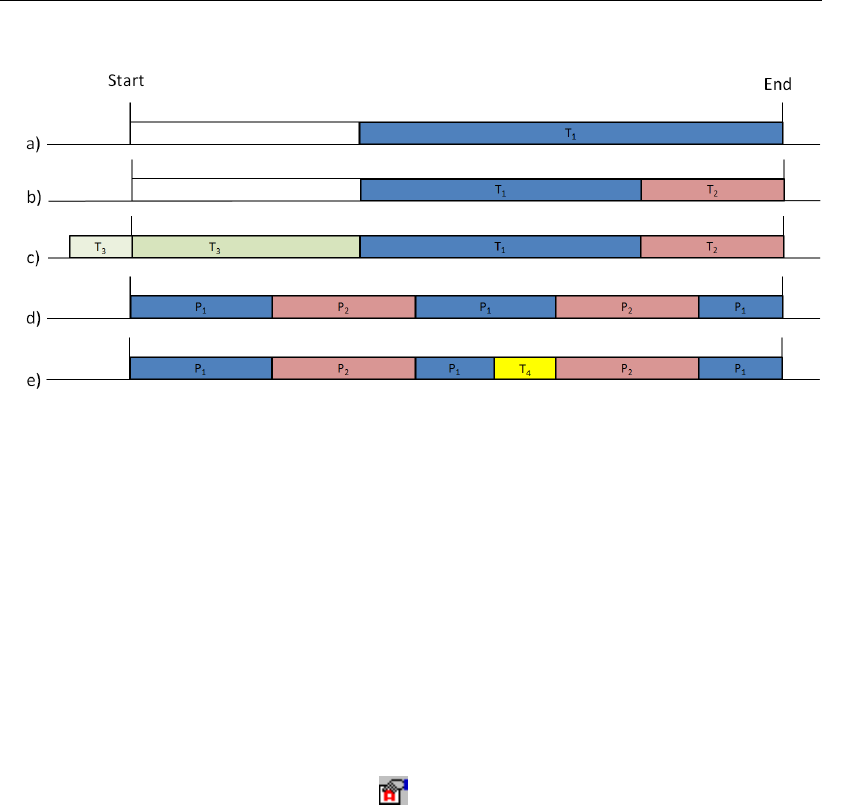
DRAFT
View Menu options
In the figure shown above, a) describes the situation in which only a single package T1is
defined half-way a simulation between Start and End. In b), another package T2is defined
and overrules T1at the start of T2. In c), a third package T3is defined before T1and even
before the start of the simulation. Consequently, the package T3becomes active, directly at
the start of the simulation. In d), a period P1and P2are defined at a certain moment within
a single year, they will be repeated for each year, automatically. Finally, in e) a package T4is
defined besides the period definitions P1and P2. As a consequence, the package T4will split
period P1halfway, up to the moment period P2is defined again.
5.5.2 Define Characteristics Automatically
The Define Characteristics Automatically ( ) option on the iMOD Project Manager window
opens a window which enables to define the characteristics of the model input topics in a
more advanced way than the default Define Characteristics window (see section 5.5.1). The
process consists out of two steps. In the first step you define the characteristic of the source
for each topic, in the second step iMOD will list the found sources and it is possible to modify
this list manually before adding them to the Project Manager window.
5.5.2.1 Define Source for Topics
The first step is to define the type of sources for each topic.
Deltares 79 of 812
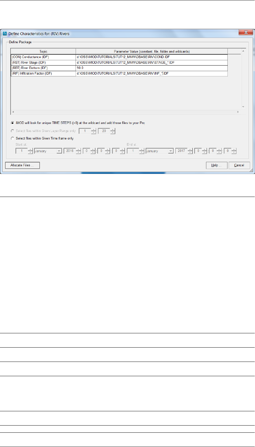
DRAFT
iMOD, User Manual
Define Characteristics for: window
Define Package This table show how each of the topics for the package (here the topics
CON, RST, RBT and RIF for the RIV package) need to be specified.
Three options are available
Constant Value
Specify a constant value for the topic to be used for all stress-
periods or model layers, e.g. a value of 90.0 means that this topics
is 90.0 for all stress-periods or model layers;
File Name
Specify a file name for the topic to be used for all stress-periods or
model layers, e.g. a file name as D:\MODEL\DBASE\BOTTOM.IDF
applies that this file is used for all stress-periods or model layers;
Wild card
Specify a file name with a wild card ( * ) to specify that all
files that are part of this will be added. It depends whether
a module or package is associated, for modules layers can
be added this way, for packages multiple stress periods, e.g.
D:\MODEL\DBASE\STAGE_*_.IDF will add all files that belong to
this group.
iMOD will look for unique
TIMESTEPS
Select this option to select unique timesteps and add the related files
to your project.
iMOD will look for unique
LAYERS
Select this option to only select unique layers and add the related files
to your project.
Select files within given
layer range
Select this option to be able to only select the files of the given layer
range of your project.
Select files within given
time frame only
Select this option to define the start- and end date for the input. Be-
sides defining the date there is also the option of defining the time
[hh]:[mm]:[ss]. E.g. entering 10th of June 2014 08 00 00 means that
the input files as selected at the 10th of June 2014 at 08:00:00 am up
to the specified end date.
Allocate Files ... Click this button to apply the given sources for topics and pop-up a list
of constant values and/or file namer per model layer or stress period.
Help ... Click this button to start the iMOD Help Functionality.
Cancel ... Click this button to close the Define Characteristics Automatically win-
dow and return to the Project Manager window.
80 of 812 Deltares
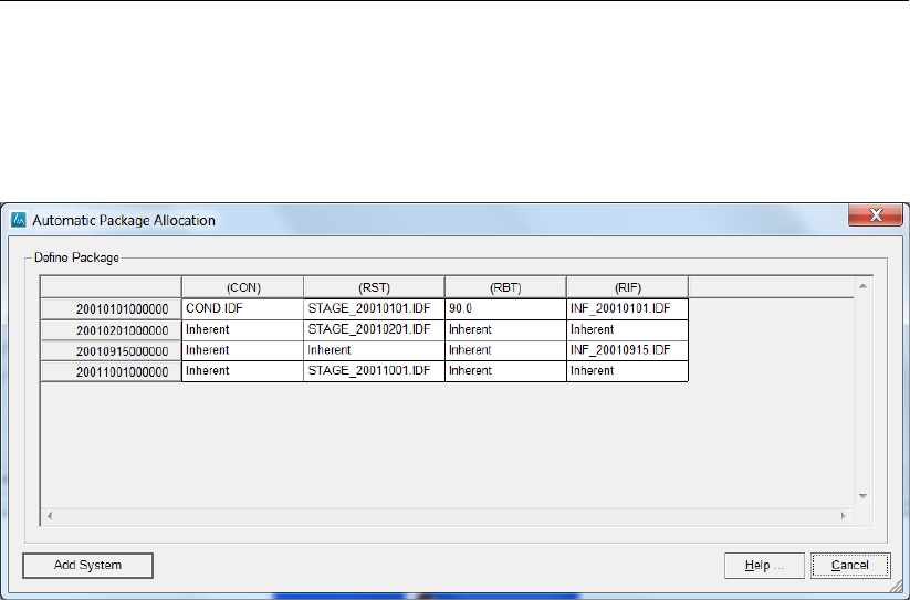
DRAFT
View Menu options
5.5.2.2 Modify List of Topics
The second step is to inspect the list of found files based on the given sources for each topic.
Define Characteristics for window:
example time and layers
Deltares 81 of 812
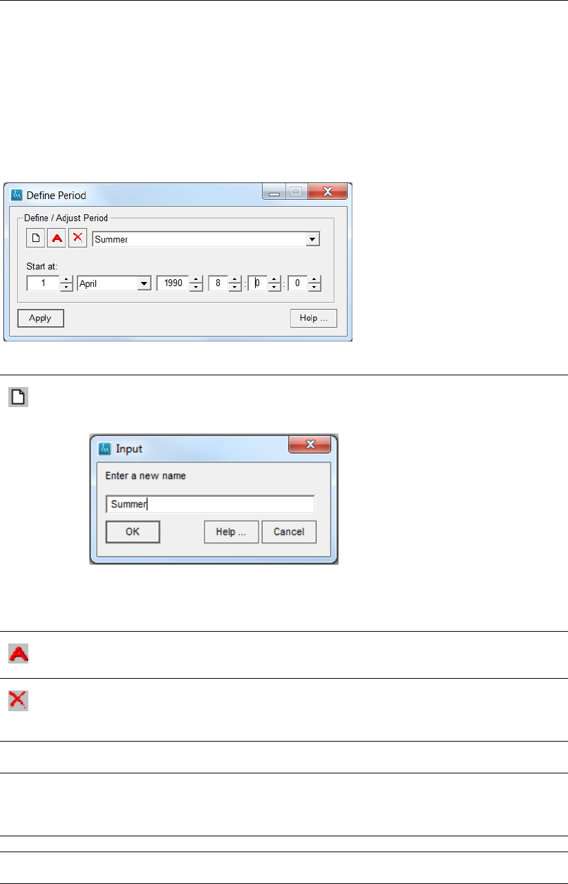
DRAFT
iMOD, User Manual
5.5.3 Define Periods
A period is defined by a starting date and time for which a package, assigned to that period,
will be repeatedly included in the runfile. A period start at a particular moment in time, but it
will never end repeating itself. The only way of ending a package defined by a period, is by
defining another package after or equal to the starting date of the period.
Define Periods window:
New
Click this button to define a new period. In the following window it is possible to enter
a name for the period.
Use the OK button to agree with the entered period name, click the Cancel
button to cancel the creation of a new period. Click Help to open the iMOD help
functionality.
Rename
Click this button to rename an existing period name. Usage of the window as de-
scribed by New will be used.
Delete
Click this button to delete the selected period. Whenever the last period is delete,
iMOD will ask to enter a period name as described by New and if this cancelled, the
Define Period window will be closed.
Summer Select one of the predefined period from the dropdown list. If none available, create
one first by means of the New button.
From Modify the starting date and time for the selected predefined period. In this example
the period Summer is a period starting from 1990 and thereafter each year at the 1st
of April at 08:00:00 am. Any modification will effect any systems for topics that are
assigned to that period definition.
Help ... Click this button to start the iMOD Help Functionality.
Apply Click this button to close this window, any modification to a period definition will be
stored.
82 of 812 Deltares
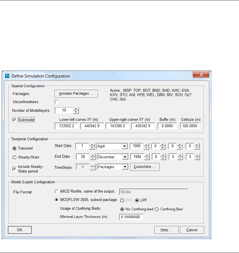
DRAFT
View Menu options
5.5.4 Define Simulation
Define Simulation window:
Within the Define Simulation window it is possible to configure the runfile and/or standard
Modflow2005 configuration files. Several options are available, such as defining the location
and size of clip models, time-discretisations and active packages.
Deltares 83 of 812
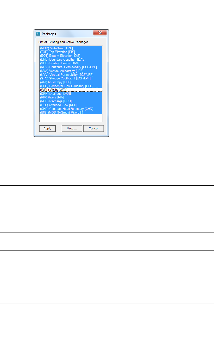
DRAFT
iMOD, User Manual
Packages: Click this button to select the packages that need to be active in de model.
By default all packages are selected, those are listed on the uppermost right
corner on the Define Simulation window as well. Use the CTRL-left-mouse button to
selected and deselect packages. It is not recommended to deselect packages that
are essential for a correct simulation of the model, such as the BND, SHD packages.
Click the Apply button to accept your choice, click the Cancel to leave the Packages
window without any changes in the selected package and click the Help button to
start the Help-functionality.
Unconfined-
ness
Select this checkbox whenever a model configuration need to be prepared to simu-
late unconfined conditions whereby the transmissivity is a function of the computed
hydraulic head. This option becomes selectable whenever the packages TOP, BOT,
KHV and KVV are available.
Number of
Modellayers
Enter a number of modellayers for which the model configuration need be built. iMOD
will fill in the maximum number of modellayers based on the modellayers that have
been filled in for the most important packages, BND, SHD (TOP and BOT), KDW or
KHV and VCW or KVV.
Submodel Check this option to define the lower- and upper-right-corner, buffersize and cellsize
of a submodel or clipmodel to be included in the runfile or used to generate the
Modflow2005 configuration files.
Transient Check this option to generate a transient runfile (*.RUN) or Modflow2005 configu-
ration files. iMOD will collect all packages that are within the specified Start Date
and End Date. Besides defining the date there is also the option of defining the time
[hh]:[mm]:[ss]. On default the start- and end time is set to 00:00:00.
Start Date Enter a start date and time for the transient simulation, this date will be start of the
first stress-period. iMOD will fill in this Start Date initially with the earliest defined
date in the packages. Whenever the Start Date is decreased, before the initial value,
the model will include packages that remain inactive until the first dat at which they
are defined.
End Date Enter an end date and time for the transient simulation, this date will be the end of
last stress-period. iMOD will fill in this End Date initially with the latest defined date
in the packages. The End Date is the date at which the simulate will terminate, so it
is the end of the last stress period. It is allowed to increase the End Date beyond the
initial value to enforce the latest stress period to be include in the model.
Steady-
State
Check this option to generate a runfile (*.RUN) for a steady-simulation, the option
becomes available only whenever at least one package is defined for a steady-state
period. iMOD will collect all packages that are connected to a steady-state definition
as specified in the Define Characteristics window.
84 of 812 Deltares

DRAFT
View Menu options
Include
Steady
State
period
Select this option to include an initial steady-state period, prior to the start of the
transient simulation. This option becomes available whenever at least one package
is defined for a steady-state period, see section section 5.5.1.
TimeSteps Select one of the option from the drop down menu:
Hourly
Select this option to generate hourly stress-periods;
Daily
Select this option to generate daily stress-periods;
Weekly
Select this option to generate weekly stress-periods;
14/28
Select this option to generate stress-periods on the 14th and 28th day of each
month;
Monthly
Select this option to generate monthly stress-periods;
Yearly
Select this option to generate yearly stress-periods;
Decade
Select this option to generate stress-periods per decade;
Packages
Select this option to generate stress-periods that are determined by the input
data as specified by the available packages in the Define Characteristics window.
It can yield a non-constant time sequence for stress periods, but will be most
optimally to the amount of stress-periods;
Custom
Select this option to refine or inspect time configuration priorly defined. This op-
tion is selected automatically after the first time the option Customize is selected.
Deltares 85 of 812
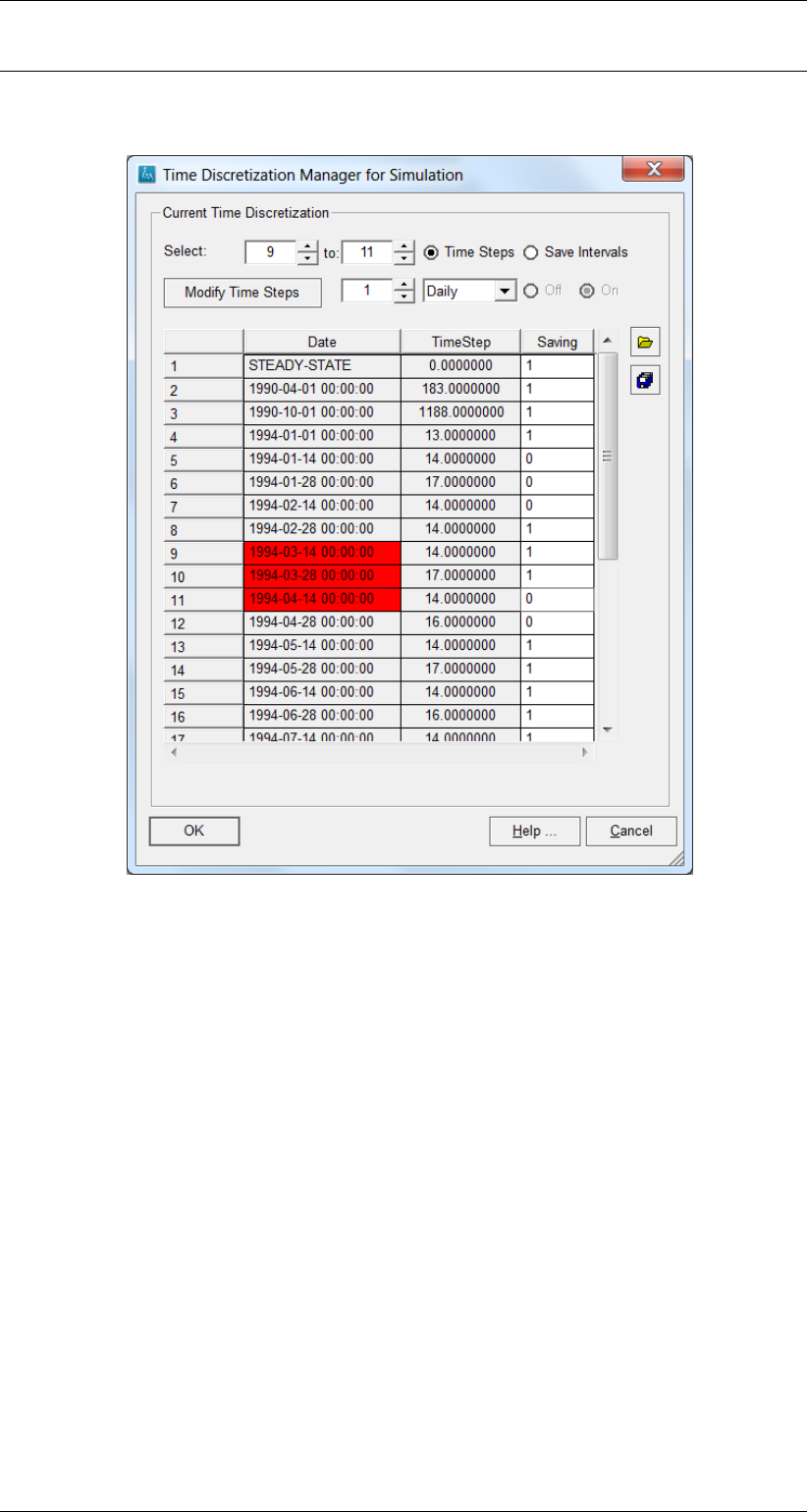
DRAFT
iMOD, User Manual
Customize... Click this button open the Time Discretization Manager for Simulation window to
customize the time steps of the simulation to be included in the runfile and/or
Modflow2005 configuration.
Select
Enter the row number within the table to be modified, e.g. 9ad 11, those will be
displayed by a red box to indicate the selected rows;
Time Steps
Select this option to modify time steps in the table;
Save Intervals
Select this option to modify the save intervals in the table;
Modify Time Steps / Modify Save Intervals
Click the button to adjust the selected rows according to the selected settings in
the fields right of this button and explained below;
1
Enter a number to enter time steps sizes for the selected value from the drop
down menu, next to it to the right, e.g. 1means in this case 1day.
Daily
Select from the drop down menu the appropriate time step size to be used for
the selected rows. E.g. Daily will include time steps on a daily base for the
selected rows. Other choices are Hourly, Weekly, Monthly, Decade, 14 / 28,
Yearly, Packages
Off / On
Select on of the options to turn the Save interval for the selected rows on or off;
Save As
Click this button to save the current time step configuration to a *.TIM file, see
section 9.4;
Open
Click this button to load the current time step configuration from a *.TIM file, see
section 9.4;
86 of 812 Deltares
DRAFT
View Menu options
File
Format:
The file format of the model configuration can be defined with this option. There are
two possibilities:
1. iMOD Runfile and/or standard MODFLOW2005 files.
iMOD
Runfile,
name of
the output:
Select this option if the iMOD Runfile format is preferred. Give the name of re-
sult folder to be created by the runfile, e.g. the result folder is finally located in the
{USER}\MODELS \MODEL. After selecting the OK button, it is necessary to enter
the name of the runfile to be created.
MODFLOW
2005
Select this option if the MODFLOW 2005 format is preferred. After selecting the OK
button, it is necessary to enter the name of the namfile to be created.
BCF / LPF Select on of the configuration options to denote the subsoil characteristics in the
Modflow2005 files. The availability of the options depend on the active packages.
Usage of
confining
beds
Select the No Confining bed whenever the model configuration is 3-D, that is there
are no confined beds, the bottom of each model layer is equal to the top of the
underlying model layer. Select the Confining Bed whenever the bottom of each or at
least a single model layer is not equal to the top of the underlying model layer.
Minimal
Layer
Thickness
(m)
Enter a minimal thickness for model layers. For Modflow2005 it is important that
the thickness of model layers is not zero. Whenever a minimal thickness of 0.01 is
entered, the top- and bottom elevations will be adapted such that there is a minimal
thickness of 0.01 meter. Moreover, the hydraulic properties will be adjusted for those
areas to reflect the corresponding layer, that will be part of the model layers that
increase in thickness.
OK Click this button to select an existing or non-existing runfile (iMODFLOW) and/or
namfile (Modflow2005), by default iMOD will save the runfile and/or namfile in the
{USER}\RUNFILES folder. It is convenient to do that as well, however not obliged, but
it will allows iMOD to start the runfile from the Model Simulation tool, see section 7.9.
Help ... Click this button to start the iMOD Help Functionality.
Cancel Click this button to close this window.
Deltares 87 of 812
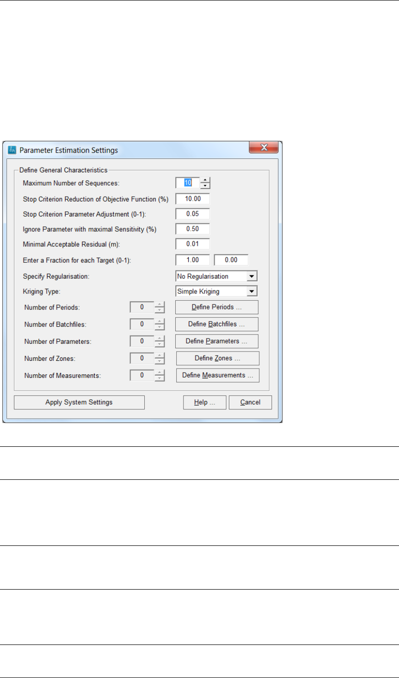
DRAFT
iMOD, User Manual
5.5.5 Parameter Estimation
Parameter Estimation Settings window:
Within the Parameter Estimation Settings window it is possible to configure the settings for
a parameter estimation. Several options are available, such as defining the main settings,
the number and characteristics of parameters, the zones and measurements, see section
section 12.33 for more detailed information on parameter estimation. Most of the parameters
are described in more detail in section section 10.14 as well.
Maximum
Number of
Sequences
Enter the number of sequences (iteration) of the parameter estimation routine. Enter
a zero will start a sensitivity analysis only.
Stop Cri-
terion
Reduc-
tion of
Objective
Function
Enter a percentage for which the objective function needs to be reduced between
adjacent iteration in order to terminate the parameter estimation process. The per-
centage is computed as the ratio between the previous and current objective function
value.
Stop Crite-
rion Param-
eter Adjust-
ment
Enter a value for this stop criterion between 0.0 and 1.0 to terminate the parameter
estimation whenever it becomes less than the specified value. The stop criterion is
computed as
Ignore
parame-
ter with
maximal
Sensitivity
Enter a percentage of the sensitivity of a parameter which will be excluded from the
current parameter estimation cycle, whenever its sensitivity is less than the specified
value.
Minimal
Acceptable
Residual
Enter a value to skip measurements in the formulation of the objectie function when-
ever the absolute residual is less than the specified value.
88 of 812 Deltares

DRAFT
View Menu options
Enter a
fraction
for each
Target
Enter a weight value for two targets of the objective function; the first target is the
sum of the square root residuals, the second the sum of the square root residual of
the dynamic in a measurement (see section 12.33.2). Its is not necessary to scale
them to a sum of 1.0, internally the entered fraction will be scaled to a total sum of
1.0, this includes any Batchfiles included (see NUmber of Batchfiles further below).
Specify
Regulari-
sation
Regularisation is a process in which parameters can be grouped mathematically
of excluded/ignored in the parameter optimization. This can be done manually
(using the parameter sensitivity) or automatically by means of some mathematically
expressions. Select of the following options to use a regularisation:
No Regularisation
No use of regularisation, that is no Scaling and/or Eigenvalue Decomposition;
Scaling
Use Scaling as a regularisation, use this option whenever the amplitude of differ-
ent residuals differ significantly, such as measurements of groundwater level and
discharge;
Scaling and Eigenvalues
Use Scaling and Eigenvalue Decomposition whenever it is very difficult to exclude
parameters on their sensitivity or relevant contribution to the reduction of the
objective function;
Eigenvalues
Use Eigenvalue Decomposition whenever the parameter sensitivity alone, is not
enough the estimate the relevance of a parameter to the parameter optimization.
Kriging
Type
Specify the type of Kriging (section 12.33.4.1) whenever the Pilot Point concept is
used (section 12.33.4). Whether Pilot Points are used is steered by the fact that an
IPF file will be entered by the zones (see Number of Zones) instead of IDF files. The
following options are available:
Simple Kriging (section 12.33.4.1)
Simple Kriging assumes stationarity of the mean, all variables have the same
mean over the entire domain;
Ordinary Kriging (section 12.33.4.1)
In Ordinary Kriging a unknown mean is assumed only over the search neighbor-
hood, so the mean is recomputed for the values in the search neighborhood.
Deltares 89 of 812
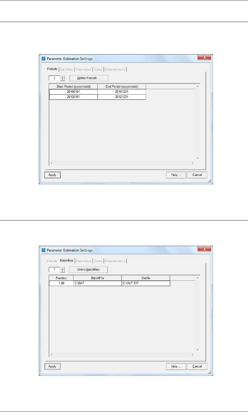
DRAFT
iMOD, User Manual
Define Pe-
riods ...
Click this button to define periods (see section 10.15) for which measurement need
to be included in the computation of the objective function, e.g. 1st of January 2010
to the 31st of December 2010 and the 1st of January 2012 to the 31st of December
2012.
Click the Define Periods to increase or decrease the number of available rows
(entry fields) in the table, e.g. 2. There is a maximum of 10 rows. Click the Apply
button to accept your entry, click the Cancel to ignore any changes, click the Help
button to start the Help-functionality.
Define
Batchfiles
...
Click this button to define batchfiles (see section section 10.16) for which extra or
additional measurement need to be included in the computation of the objective
function.
Click the Define Batchfiles to increase or decrease the number of available
rows (entry fields) in the table, e.g. 1. There is a maximum of 10 rows. Click the
Apply button to accept your entry, click the Cancel to ignore any changes, click the
Help button to start the Help-functionality.
90 of 812 Deltares
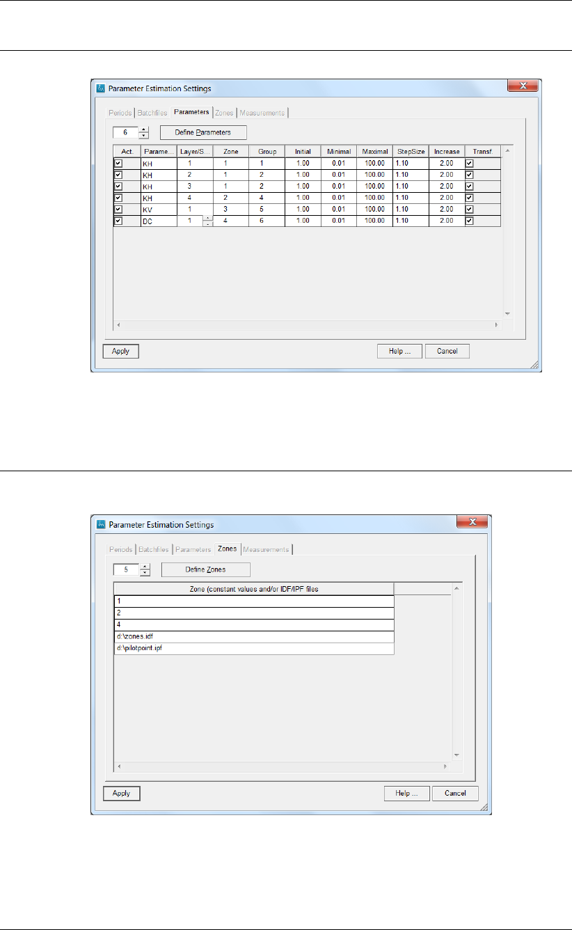
DRAFT
View Menu options
Define Pa-
rameters ...
Click this button to define parameter to be optimized.
Click the Define Parameters to increase or decrease the number of available
rows (entry fields) in the table, e.g. 2. There is a maximum of 1000 parameters, see
section section 10.17 for the explanation of the variables. Click the Apply button to
accept your entry, click the Cancel to ignore any changes, click the Help button to
start the Help-functionality.
Define
Zones ...
Click this button to define zones (see section section 10.19) for which parameters
need to be adjusted.
Click the Define Zones to increase or decrease the number of available rows
(entry fields) in the table, e.g. 5. There is a maximum of 1000 zones, constant values
can be entered to denote a zone fore the entire model area, multiply zones can be
combined in a single IDF file and/or IPF files can be entered for usage of Pilot Points
(section 12.33.4). Click the Apply button to accept your entry, click the Cancel to
ignore any changes, click the Help button to start the Help-functionality.
Deltares 91 of 812
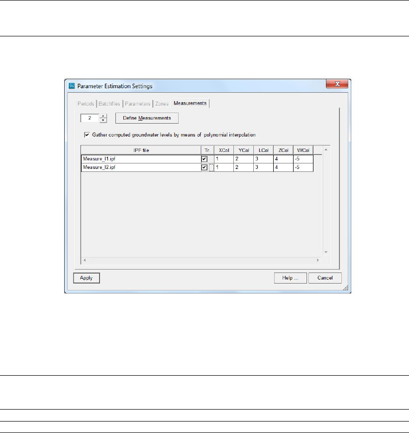
DRAFT
iMOD, User Manual
Define
Measure-
ments
...
Click this button to define measurements (see section section 10.4) which are
needed to compute the objective function. It is also possible to exclusively use
Batchfiles instead.
Click the Define Measurements to increase or decrease the number of avail-
able rows (entry fields) in the table, e.g. 2. There is a maximum of 50 zones,
constant values can be entered to denote a zone fore the entire model area, multiply
zones can be combined in a single IDF file and/or IPF files can be entered for usage
of Pilot Points (section 12.33.4). Click the Apply button to accept your entry, click the
Cancel to ignore any changes, click the Help button to start the Help-functionality.
Apply
System
Settings
Click this button to leave the Parameter Estimation Settings window and store the
adjustments.
Cancel Click this button to close the Parameter Estimation Settings window
Help ... Click this button to start the Help-functionality
92 of 812 Deltares
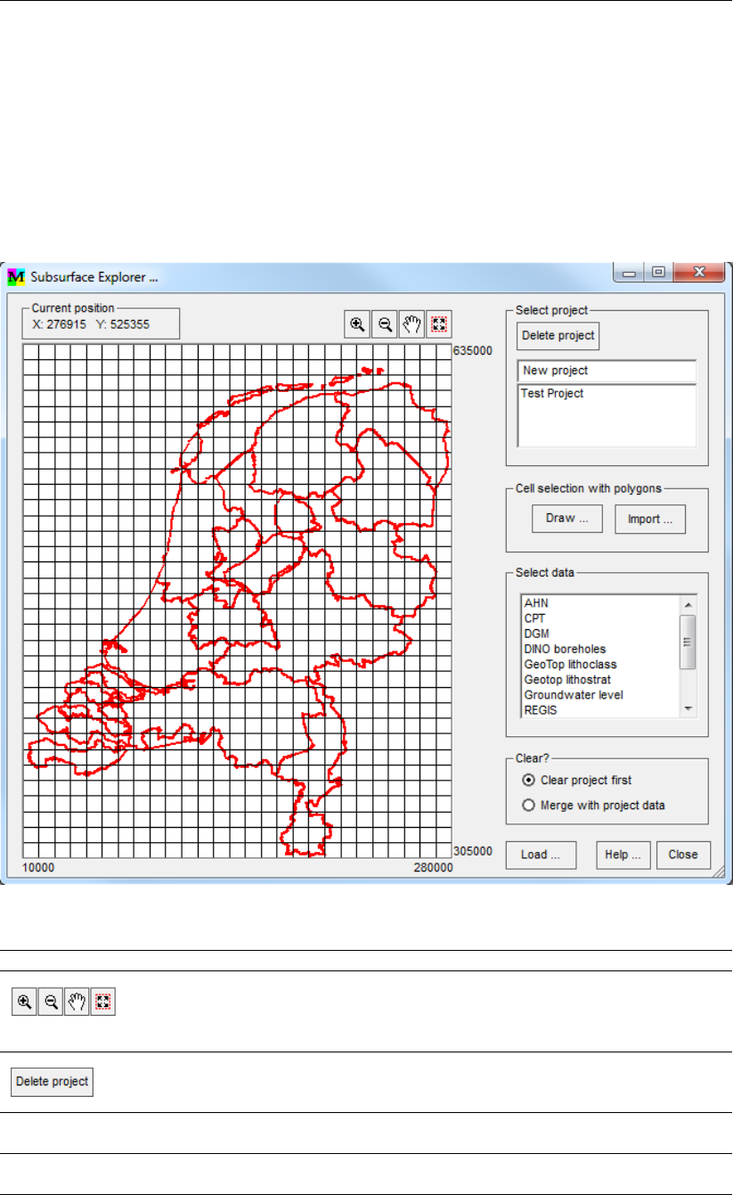
DRAFT
View Menu options
5.6 Subsurface Explorer
The Subsurface Explorer tool can be used to import prepared subsurface data of the Nether-
lands into iMOD. The data that can be loaded are stored in a database, of which the path has
to be specified in the IMOD_INIT.PRF file using the keyword SUBSURFEXDBASE. Further-
more, the path to the 7-zip executable on the users computer also has to be specified in this
file using the keyword 7ZIP, see section 9.1 for more information.
Subsurface Explorer window:
Current Position Shows the current mouse position on the map in RD coordinates.
Navigation buttons for the map
Use these buttons to adjust the view of the map. The buttons can be used to
zoom in, to zoom out, to move the map by dragging and to reset the map to
the original view, respectively.
Delete a project
Select an existing project in the Select project listbox and click this button to
delete the project.
Create a new
project
To create a new project enter a new name in the Select project listbox.
Use an existing
project
To continue using an existing project select it by clicking the name once in the
Select project listbox.
Deltares 93 of 812
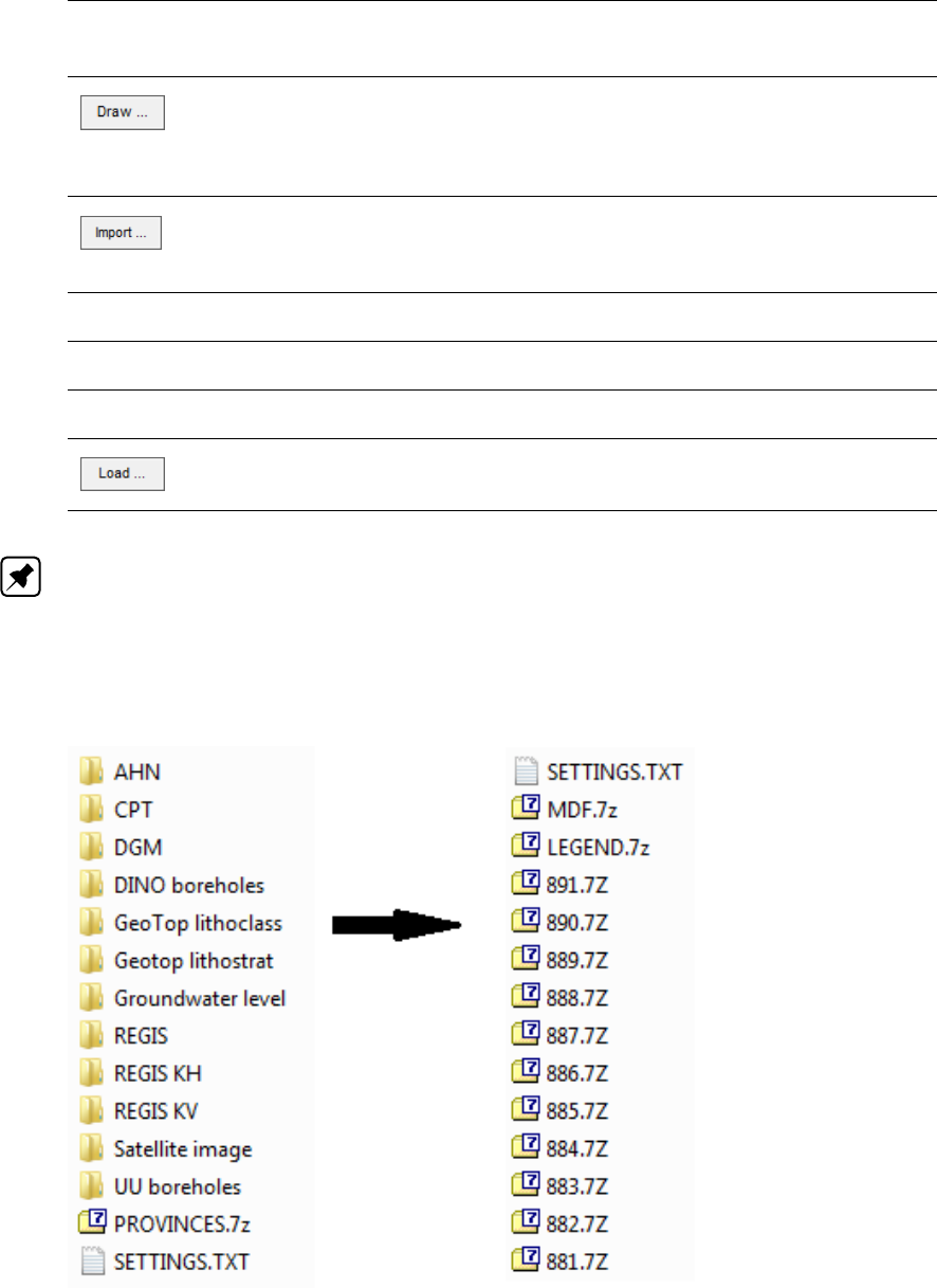
DRAFT
iMOD, User Manual
Draw a polygon
Click this button to be able to draw one or more polygons on the map. To draw
a polygon, click the left mouse button to place points and click the right mouse
button to stop drawing. When the polygon is finished the tool will select the
cells corresponding to the polygon.
Import a polygon from file
Click this button to open a *.GEN file containing one or more polygons. The
polygons will be drawn on the map and the corresponding cells will be se-
lected.
Select data This list shows the available data. Select one or more data types from this list
you would like to load.
Clear project first Select this option to first clear the data in an existing project before loading
the selected data.
Merge with project
data
Select this option to merge the selected data with the data already present in
an existing project folder.
Load the data
Click this button to load the current selection. The tool will check whether all
required information is present.
Note: The window can be resized by dragging the edges in order to adjust the size of the
map. When using polygons to select cells, the data will not be clipped to the polygon, it is
only used to select the cells. A *.SHP file can easily be converted to a *.GEN file in order
to be able to use it in the Subsurface Explorer. Simply open the file in iMOD as an overlay
(iMOD Manager) and the *.SHP file will automatically be converted to a *.GEN file, which will
be placed in the same directory.
The database that contains the data that is imported using the Subsurface Explorer tool
should be structured as the above figure shows:
The data type folders, SETTINGS.TXT and PROVINCES.7Z are stored in the folder to
which the IMOD_INIT.PRF file should refer (see section 9.1).
The SETTINGS.TXT file contains the minimal X, minimal Y, maximum X, maximum Y and
the grid size of the map that is visible on the tool. In this case the map of the Netherlands
94 of 812 Deltares

DRAFT
View Menu options
is divided into cells using a grid with a cell size of 10 km2, resulting in a total of 891 cells.
An example of this SETTINGS.TXT is:
10000.0
305000.0
280000.0
635000.0
10000.0
The map of the Netherlands is drawn using a GEN file stored in PROVINCES.7Z. The
data type folders contain a zip file for each cell, containing only the data of that data type
for that cell.
Furthermore, when applicable, the data type folder can contain a legend in LEGEND.7Z
archive, containing an iMOD format legend which will then be used when plotting the data
(see section 9.15).
For data types that consist of many raster files, e.g. REGIS, an MDF file stored in the
database in MDF.7Z, is used to be able to handle these files more conveniently (see
section 6.5).
Finally each data type folder also contains a SETTINGS.TXT file, in which the extension
(e.g. IPF), whether a legend is present (1 for yes, 0 for no) and (only when the data type
has the IPF extension) a header which should be used for the IPFs of that data type are
given.
By using the SETTINGS.TXT files the tool can also be used for other datasets in other
geographical regions and new data types can be added easily without editing the source
code.
The names of the files in the archives containing the data of cells are only the cell number
followed by the extension of the file. For example the DINO borehole data of cell 55 are
stored in 55.IPF (and corresponding text files). Only raster files have an extended name
which also contains one string with information about the layer the file describes, this
information can for example be which geological formation the layer describes or at which
depth the layer is situated. For example the geotop layer at a depth of 50 centimeters
below the surface in cell 55 is named -50_55.IDF. The string on the left of the underscore
can contain any character supported by the operating system, except for an underscore,
because this character is used to be able to separate the additional information about the
layer from the cell number.
The grid cells are numbered in the following way:
Deltares 95 of 812
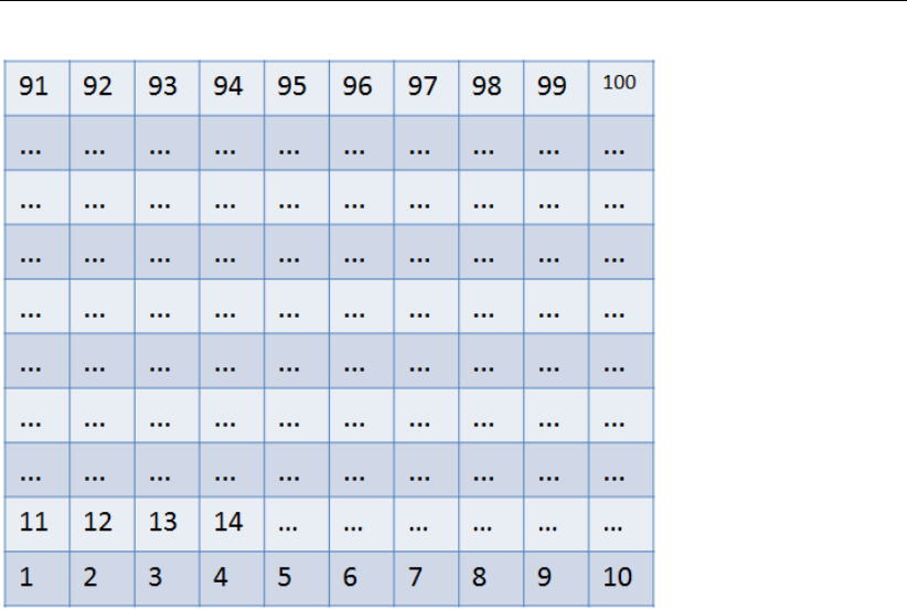
DRAFT
iMOD, User Manual
The data that are loaded are downloaded from the database to the user´
s computer and
are stored in a folder with the name of the project specified using the tool in the
IMOD_USER\SUBSURFACE_EXPLORER\directory.
The data that are loaded into iMOD using the Subsurface Explorer are plotted and shown
in the iMOD manager, after which all iMOD functionalities can be used to analyse and edit
the data.
Examples of dataset settings-files
Example AHN
IDF
0
This means that the AHN-dataset contains files of the filetype *.IDF and no predefined legend-
file (*.DLF) is provided.
Satellite image
PNG
0
In this example satellite images are stored as *.png files and will be available via the iMOD
TOPO-tool.
Example DINO boreholes - header file
IPF
1
5
"X-COORDINATE, M"
"Y-COORDINATE, M"
"IDENTIFICATIE"
"MAAIVELD, M+NAP"
"EINDDIEPTE, M+NAP"
3,TXT
96 of 812 Deltares

DRAFT
View Menu options
iMOD will merge all IPF-files to one large IPF-file and putting these header lines on top of
the final IDF-file. In this example the header lines stand for: 1. filetype, 2. legend provided
(1=yes, 0=no), 3. amount of IPF-files to be merged, 4.-8. column names, 9. IPF attribute file
types with the needed information given in column 3.
Deltares 97 of 812
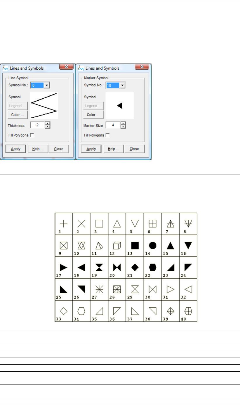
DRAFT
iMOD, User Manual
5.7 Lines and Symbols
In the Overlays tab of the iMOD Manager window, click the Legend button to open the Lines
and Symbols window, left for lines (GENs, IFFs, ISGs), right for points (IPFs).
Lines and Symbols window:
Symbol No.: Select one of the symbol numbers out of the dropdown menu. For lines
(GENs and SHPs) these types vary from solids, to dashed and stippled
pattern (1-7). For point data (IPFs) these types vary from between circles,
triangles, rectangles and other shape forms (1-40).
Available markerset:
Symbol This field will display the symbol chosen from the dropdown menu Symbol
No.:.
Color Click this button to open the default Colour Selection window.
Thickness Enter the value of the thickness of the line (GENs and SHPs).
Markersize Enter the value of the size for the symbol (IPFs).
Fill Polygons Select this checkbox to fill in the polygons (GENs and SHPs).
Close Click this button to close the Lines and Symbols window without applying any
changes.
Apply Click this button to apply the configuration and close the Lines and Symbols
window.
Help Click this button to start the iMOD Help Functionality.
98 of 812 Deltares
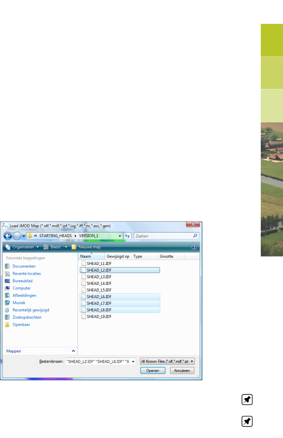
DRAFT
6 Map Menu options
This chapter describes the Map Menu options:
section 6.1: Add Map.
section 6.2: Quick Open.
section 6.3: Map Info.
section 6.4: Map Sort.
section 6.5: Grouping IDF Files.
section 6.6: Legends.
section 6.7: IDF Options.
section 6.8: IPF Options.
section 6.9: IFF Options.
section 6.10: ISG Options.
section 6.11: GEN Options.
6.1 Add Map
Click the option Add Map from the Map menu to open an IDF-, MDF-, IPF-, IFF-, ISG-, GEN-
or ASC-file. Alternatively click on the Add Map button on the iMOD Manager, click on the icon
Open Map on the toolbar, or use the shortcut F2 on the keyboard to open the Load iMOD
Map window.
Load iMOD Map window:
Note: To select multiple files, use the combination Shift-left mouse to select adjacent files or
use the Ctrl-left mouse button to select files in any order.
Note: Whenever an ASC-file is opened (see section 9.13 for the syntax of an ASC-file), iMOD
will convert these file into IDF format and write them in the same folder. Whenever such a file
Deltares 99 of 812
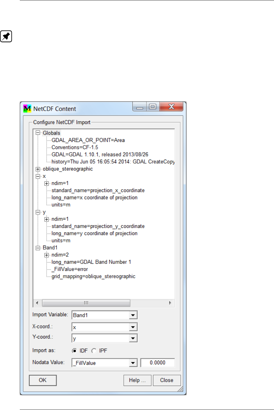
DRAFT
iMOD, User Manual
exists, you will be asked to overwrite it.
Note: Whenever NC-file (NetCDF) is opened, iMOD will convert these file into IDF format and
write them in the same folder. Since, a NetCDF file is general file format iMOD can not convert
this type of a file without the interference of the user. Here for, iMOD will display the following
window in which the user can specify the correct attributes for the x- and y-coordinate and the
actual data block to be converted. This function is only available in the X32-bits version
of iMOD.
NetCDF Content window:
100 of 812 Deltares

DRAFT
Map Menu options
Configure NetCDF
Import
This treeview lists the content of the selected NetCDF file. iMOD needs an
attribute for the x- and y-coordinates and an actual data block. In the example
presented above, these are the attributes x,yand Band1. The x- and y-
coordinates (actual the mids of the gridcells) need to be stored in an one
dimensional array (ndim=1) and the data block in a two dimensional array
(ndim=2). iMOD will compute the cell size that is needed for the formulation
of an IDF file, which can be equidistant en non-equidistant.
Import Variable Select an available variable that is stored by a two dimensional array in the
NetCDF, e.g. Band1.
X-Coord.: Select an available variable that is stored by an one dimensional array in the
NetCDF for the representation of the x-coordinate, e.g. x.
Y-Coord.: Select an available variable that is stored by an one dimensional array in the
NetCDF for the representation of the y-coordinate, e.g. y.
Import As: Select one of the following options to store the converted NetCDF file:
IDF
Select this option to generate an IDF file;
IPF
Select this option to generate an IPF file, each point in the IPF file repre-
sents the location as described by the selected x- and y-variable;
NoData Value Select an available variable to represent the NodataValue of the data block.
iMOD will fill in the corresponding value in the input field to the right.
Close Click this button to close the NetCDF Content window without converting the
NetCDF file into an IDF.
OK Click this button to convert the NetCDF into an IDF file and close the NetCDF
Content window.
Help Click this button to start the iMOD Help functionality.
Deltares 101 of 812
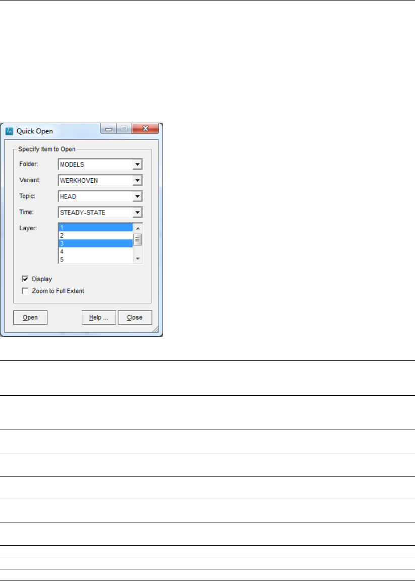
DRAFT
iMOD, User Manual
6.2 Quick Open
This functionality offers the ability to search specific iMOD folders for particular IDF-files more
quickly than by means of the default windows Explorer. Select the menu option Map and then
choose Quick Open to open the Quick Open window.
Quick Open window:
Folder Select one of the existing foldernames from the dropdown menu. The folder-
names MODELS, SCENARIOS and SCENTOOL refer to the corresponding
folders below {USER}.
Variant Displays the existing subfolders below Folder. In the situation that the option
SCENTOOL is chosen from the Folder dropdown menu, it will display the
scenario variants of the active scenario opened by the Pumping Tool.
Topic Displays the existing subfolder below Variant. These will be the particular
result folders.
Time Displays all unique IDF-files in the Folder\Variant\Topic folder. iMOD will
search in this folder for IDF-files that agree with Topic_*_L*.IDF.
Layer Displays all existing layers in the Folder \Variant\Topic folder. iMOD will search
in this folder for IDF-files that agree with Topic_Time_L*.IDF.
Display Select this option to display the IDF-file(s). Unselect this option to add the
IDF-file(s) to the drawing list in the iMOD Manager only.
Zoom to Full
Extent
Select this option to adjust the zoom level to the maximum extent of the last
selected IDF-file.
Open Click this button to add the selected IDF-file(s) to the iMOD Manager.
Help . . . Click this button to start the Help functionality.
Close Click this button to close the Quick Open window.
102 of 812 Deltares
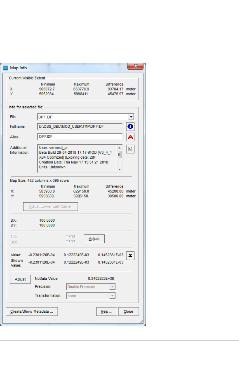
DRAFT
Map Menu options
6.3 Map Info
The functionality Map Info will display information about the selected map. Select the menu
option Map and then choose Info Map to open the corresponding window.
Map Info window:
Current visible
extent
This group displays the current extent of the graphical window. It shows the min-
imum and maximum x- and y coordinates and the delta-x and delta-y values (all
in meters).
File: This dropdown menu shows all the files that are opened in the iMOD Manager.
Click this menu to select the file for which the information should be displayed.
Fullname: This string field shows the full pathname of the selected map.
Deltares 103 of 812
DRAFT
iMOD, User Manual
Map Information
The functionality depends on the selected type of map (IDF, MDF and GEN) and
is as follows:
IDF
Select this option to open the IDF Edit Table window, see section sec-
tion 6.7.4.3;
MDF
Select this option to open the MDF Files Sorter window, see section sec-
tion 6.5;
GEN
Select this option to open the Content of Associated Datafile window, see
section section 6.11.1.
Alias: This string field shows the alias of the selected map. This name will be used in
the iMOD Manager as well and offers the possibility to clarify identical file names.
Any modification will be saved only whenever the Rename button will be clicked.
Rename
Click this button to rename the entered Alias.
Additional Infor-
mation
This field shows any additional information that is attached to the selected IDF.
For other file types, this field will be showing the string: “No additional information
found”.
Edit
Click this button to edit the additional information in a regular text editor, e.g.
Notepad. Whenever any modifications are saved from Notepad, iMOD will write
the renewed additional information in the IDF file, automatically.
Map Size This string will show the number of rows and columns in an IDF or IPF-file.
X:
Y:
This field shows for the whole map the minimum and maximum values for the x-
and y coordinates and their total delta-x and total delta-y values (all in meters).
Adjust Lower
Left Corner
Click this button to allow editing of the lower left corner of the IDF file. Click this
button (rename to Save Adjustments) again to save the modification in the IDF
file, iMOD will adjust the upper right corner accordingly.
DX:
DY:
For equidistant IDF-files, it shows the width and height of the rows and columns,
respectively. For non-equidistant IDF-files, it shows the minimum and maximum
dimensions in both directions (all in meters).
TOP:
BOT:
These will show the internal TOP and BOT values for IDF-files for so called voxel-
IDF file. These are used to present the IDF as a horizontal layer in the Profile
Tool and/or 33D Tool using the TOP and BOT values for the upper- and lower
interface. If the values are greyed out, these values are not present in the current
selected IDF file.
Adjust Click this button to edit the TOP and BOT values. Once those values differ
(TOP>BOT), the IDF-file will be treated as a voxel in the 3D Tool and the Profile
Tool.
Adjusting TOP and BOT values:
Store Click this button to save the adjustments for TOP and BOT.
Value: Displays the minimum and maximum data values of the IDF or IPF-file and the
difference between them
Shown Value: The minimum, maximum and difference between them of the current values plot-
ted on the graphical canvas. This values represents the current statistics of data
presented.
104 of 812 Deltares
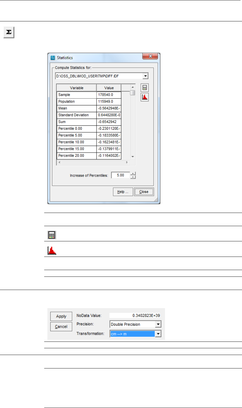
DRAFT
Map Menu options
Statistics
Click this button to get the statistics of the selected IDF-file.
Statistics window:
Compute
Statistics for:
Select one of the files from the dropdown menu to compute
statistics for.
Compute
Click this button to (re)compute the statistics of the IDF-file.
Graph
Click this button to get a graph of the percentiles of the IDF-file.
Increase of
Percentiles Enter a value for the increment of the computed percentiles.
Help ... Click this button to start the Help functionality.
Close Click this button to close the Statistics window.
Adjust Click this button the adjust the NoDataValue, type of Precision or internal
Transformation.
Apply Click this button to store the adjustments into the IDF.
Cancel Click this button to cancel any adjustments.
NoData
Value:
This field shows the NoDataValue of the IDF-file.
Precision: Select a type of precision for IDF files. By default IDF files are
saved in single precision (4 bytes per real/integer number). To
maintain a level of accuracy in the representation of number, it
could be desirable to change the single- to double precision (8
bytes per real/integer number). Bear in mind that the entire IDF
file becomes double in size if switched to double precision.
Deltares 105 of 812

DRAFT
iMOD, User Manual
Transfor-
mation
Select a type of transformation for the values in the IDF. The
data will be transformed internally. The available options are:
m→cm: transforms meters into centimeters;
cm →m: transforms centimeters into meter;
m→mm: transforms meters into millimeters;
mm →m: transforms millimeters into meters;
m3/day →mm/day: transforms cubic meter per day into
millimeters per day;
mm/day →m3/day: transforms millimeters per day into cu-
bic meters per day
Create/Show
Metadata . . .
Click this button to display the metadata (.MET) file that might be associ-
ated to the selected map. For the example, iMOD will try to open the file
HEAD_20050501_L1.MET. If the file does not exist, iMOD will create the file. This
function is strongly discouraged for IDF files, use the Edit button to add additional
info to an IDF file instead.
Help . . . Click this button to start the iMOD Help Functionality.
Close Hides the iMOD Manager. The iMOD Manager can be displayed again by choos-
ing the menu option View and then choose the option iMOD Manager.
106 of 812 Deltares
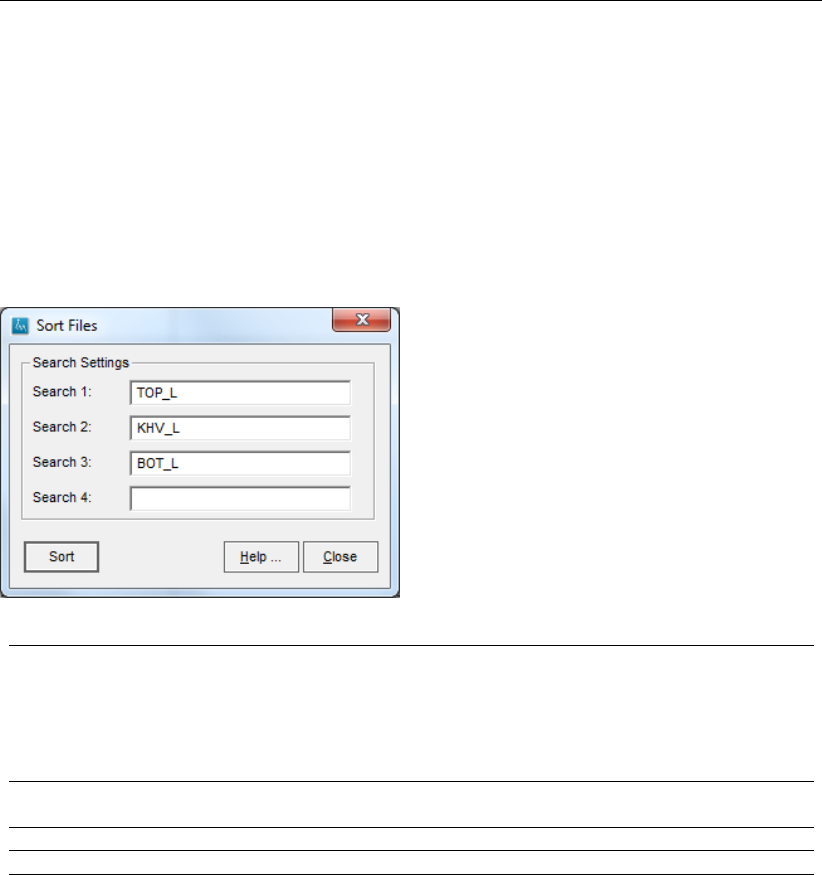
DRAFT
Map Menu options
6.4 Map Sort
The functionality Sort Selected Maps will offer the possibility to sort/re-arrange selected (IDF)
files in the iMOD Manager accordingly to a selected type of order. Select the menu option
Map and then choose Sort Selected Maps to expand the following options:
Sort Using Keywords
Select this option to sort the selected IDF file in a order that is defined by their individual
internal values. E.g., use this option to re-arrange IDF files that describe top- and bottom
elevations of interfaces;
Search 1:
Search 2:
Search 3:
Search 4:
Enter a keyword that need to be used to sort the selected IDF files in the iMOD
Manager. The entered example of three keywords will sort all files that match
the following: TOP_L1.IDF, KHV_L1.IDF, BOT_L1.IDF, TOP_L2.IDF, KHV_L2.IDF,
BOT_L2.IDF. The number of layers is determined automatically from the selected
IDF files in the iMOD Manager, these files need to have a number after the char-
acter sequence of ”_L”.
.
Sort Click this button to sort the selected IDF files in the iMOD Manager according to
the entered search strings.
Help . . . Click this button to start the iMOD Help Functionality.
Close Closes the Sort Files window.
Sort Alphabetic Ascending Order (A-Z)
Select this option to sort any the selected files upon their filename in an alphabetic as-
cending order, that is from A up to Z;
Sort Alphabetic Descending Order (Z-A)
Select this option to sort any the selected files upon their filename in an alphabetic de-
scending order, that is from Z up to A;
Deltares 107 of 812
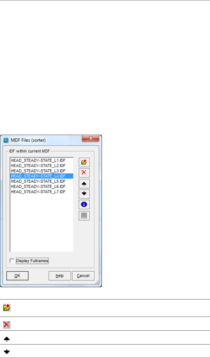
DRAFT
iMOD, User Manual
6.5 Grouping IDF Files
Different files in the iMOD Manager may be identified, analysed and/or displayed at the same
time. For example, you want to analyse the differences between two model simulations and/or
combine these with geohydrological cross-sections. To control the number of files in the iMOD
Manager, it can be helpful to minimize (grouping) the number of files in the iMOD Manager in
to a so-called MDF (Multi-Data-File). Use the following steps to create an MDF file:
1 Select the IDF-files that you want to Group in the menu list of the iMOD Manager;
2 Select the menu option IDF Options from the Map menu and choose the option IDF Group
and enter an MDF file name in the File Selector window that pops-up.
After you entered a file name, iMOD will create an MDF-file. An MDF-file lists all the selected
IDF-files in one single file. iMOD will remove all files from the iMOD Manager and reads in
the created MDF file instead. The content of that file can be displayed via the option Info on
the Map Info window. The following window will be displayed.
MDF Files (sorter) window:
Open IDF
Click this button to open an IDF-file, it will be added to the MDF-file whenever you
click the Ok button.
Delete
Click this button to remove the selected files from the MDF-file.
Up
Click this button to move the selected files one position up in the list.
Down
Click this button to move the selected files one position down in the list.
108 of 812 Deltares
DRAFT
Map Menu options
Information
Click this button to display the description of the MDF-file.
Legend
Click this button to adjust the legend of the selected IDF-file
Display
Fullnames
Click this option to display the entire pathnames for the IDF-files.
OK Click this button to save the adjustments to the MDF-file. After that it will close the
MDF Files (sorter) window.
Help . . . Click this button to start the iMOD Help Functionality.
Cancel Click this button to close the MDF Files (sorter) window without any changes.
To ungroup a MDF-file, select the menu option Map and choose the option IDF Options and
then the option IDF Ungroup MDF.
Note: The IDF-file that is selected in the MDF-file will be used to plot on the graphical canvas.
If multiple files are selected, only the first will be plotted though. The properties of the IDFs are
known as all attributes (legend, cross-section types, colours, aliases) of the IDFs are copied
into the MDF-file too.
Note: The order in which the IDF-files are listed is the same order as which they appear
in the Map Value,Cross-Section Tool and 3DTool. Moreover, MDF-files will be displayed in
graphs separate from the files that are not in the MDF-file(s), see section 6.8.3.2.
Deltares 109 of 812
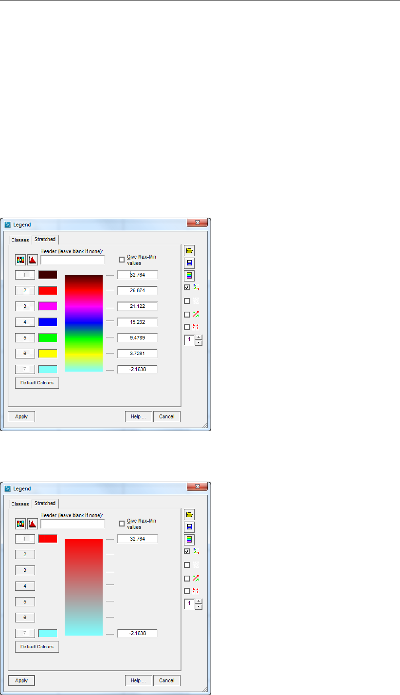
DRAFT
iMOD, User Manual
6.6 Legends
This section describes the usage of legends.
6.6.1 Adjust Legends
A legend is assigned to a map (*.IDF, *.IPF, *.IFF, *.GEN, *.MAP). Make sure you select one
of them in the iMOD Manager to activate the Legend button on the Maps tab of the iMOD
Manager. Alternatively you can click the right mouse button anywhere on the canvas and
select the option Legend from the pop-up menu and then choose the option Adjust Legend.
In both cases, the Legend window will appear, two examples of the Stretched tab on the
Legend window, left using all color gradients (7 gradients), right using the first and last only
(one gradient).
Legend window, Stretched Tab using all color gradients:
Legend window, Stretched Tab using two color gradients:
110 of 812 Deltares
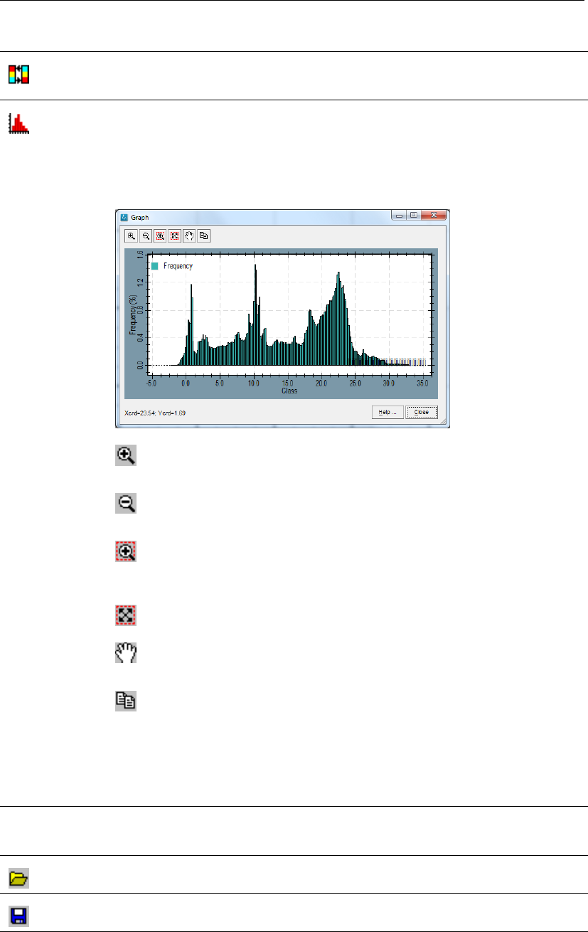
DRAFT
Map Menu options
Flip Colours
Click this option to “flip” the colour sequence, e.g. red becomes blue and blue
becomes red.
Histogram
Click this button to display a frequency distribution of the current legend classes.
Move your mouse in the graph to show the value (X-crd) and the frequency in %
(Y-crd).
Graph Window (with a Frequency Distribution for 250 stretched legend classes):
Zoom In
Click this button to zoom in at the position of the mouse cursor, repeat-
edly. Right click the mouse to stop.
Zoom Out
Click this button to zoom out at the position of the mouse cursor, re-
peatedly. Right click the mouse to stop.
Zoom Window
Click this button to zoom into a drawn rectangle. Left click the mouse to
define the first corner of the rectangle. Left click again for the second
corner. Right click to cancel the zoom operation.
Zoom Full
Click this button to adjust the zoom level to the full extent of the graph.
Move
Click this button to move the graph. Keep the left mouse button pressed
and drag the mouse cursor to move the graph.
Copy to Clipboard
Click this button to copy the graph onto the clipboard of Windows.
Paste the image into e.g. Word by the Ctrl-V key combination
Xcrd=
Ycrd=
Display of the coordinates of the current mouse position.
Help... Select this button to start the Help functionality.
Close Select this button to close the Graph window.
Header Enter a descriptive text for the corresponding legend. The text will be plotted on
top of the legend whenever the legend is plotted on the graphical canvas. Leave
the input field empty to ignore any legend header.
Open Legend File
Click this option to open an existing *.LEG-file for the syntax.
Save Legend File
Click this option to save the current legend in a *.LEG-file.
Deltares 111 of 812
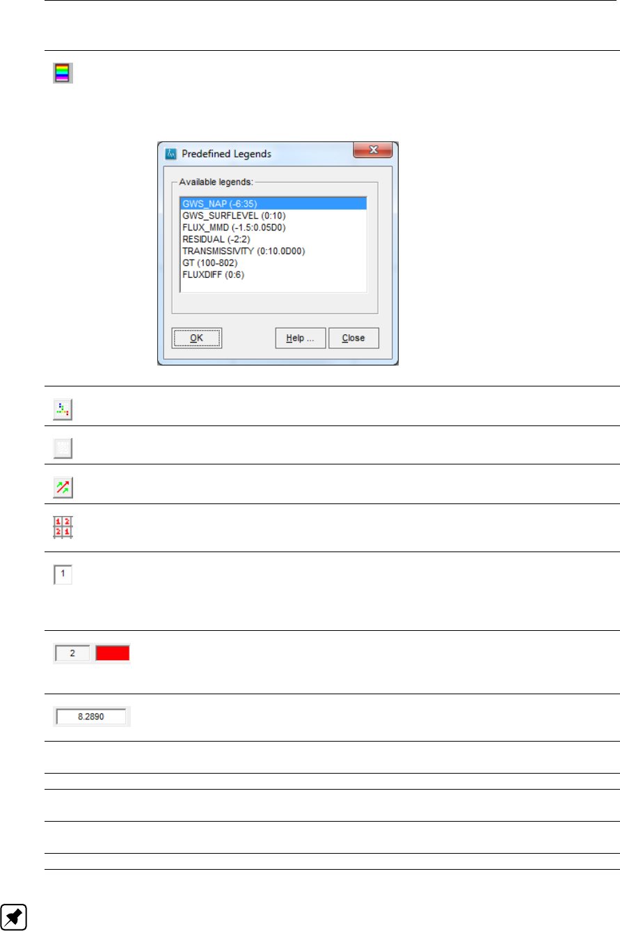
DRAFT
iMOD, User Manual
Predefined Legends
Click this option to select a predefined legend. Select one of the available leg-
ends and click the OK button to read the selected legend into the Legend window.
Predefined Legends:
GridCells
Click this option to display the IDF-file with filled gridcells.
ContourLines
Click this option to display the IDF as contourlines.
Flow direction
Click this option to display arrows indicating the direction of flow.
Data Numbers
Click this option to display the actual data on the mids of the selected IDF file.
The size of the text is given by the entered Line thickness.
Line thickness
Click this option to set the line thickness of the contours and the direction of flow
arrows. If you specify a line thickness of <0, no labels will be plotted and the
line thickness becomes the absolute given thickness, e.g. a line thickness of -2
means a line thickness of 2, without any label plotted.
ColorMark
Select the checkbox (2-6) to turn on/off the corresponding colour in the legend
colour ramp. Clicking on the coloured field (red in this case) will show the default
Colour window wherein you can specify another colour.
Class
Enter a class that corresponds to the colour, in this case the value 8.2890 corre-
sponds to the red colour in checkbox 2.
Give Min-Max
values
Select this checkbox to enter a minimum and maximum value. As a result only
the top and bottom input fields will be available to enter values.
Default Colours Click this option to reset the current colours for the default colours.
Apply Click this button to apply the legend setting to the current selected map file (IDF,
IPF, IFF or GEN).
Cancel Click this button to close the Legend window without applying any changes to the
current legend settings.
Help Click this button to start the iMOD Help Functionality.
Note: A stretched legend contains always 255 colours and classes. Whenever a legend
contains 50 classes or less, the Classes tab will appear instead.
112 of 812 Deltares
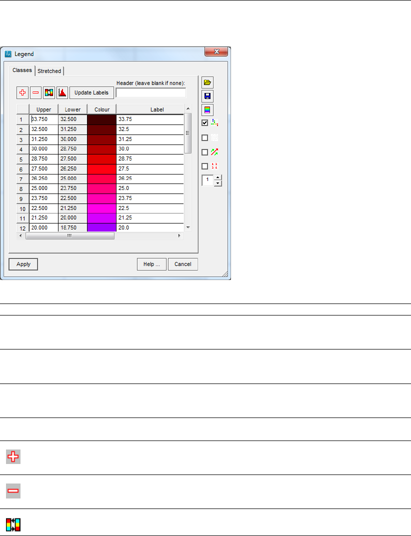
DRAFT
Map Menu options
Legend window, Classes tab:
Upper The first column shows the Upper limit for each class, enter different values if desired.
Lower The second column shows the Lower limit for each class. It will be filled in automati-
cally based on the filled in values for the Upper limit. The Lower limit should be filled
in for the last record only.
Color The third column displays the colour for the class. You can click on the colour to
display the Colour window. The colour will be used to colour the values less than the
Upper class and greater or equal to the Lower class.
Label The fourth column shows the label that can be displayed in the Legend tab on the
iMOD Manager window and/or plotted on the canvas. The label can be entered with
a maximum of 50 characters.
Freq. (%) The fifth column shows the frequency of occurrence of values within each class. It is
only applicable to IDF-files.
Insert a Row
Click this button to insert a row in the table. It will be inserted one row above the row
you select.
Delete a Row
Click this button to delete the selected row.
Flip Colours
Click this option to “flip” the colour sequence.
Deltares 113 of 812
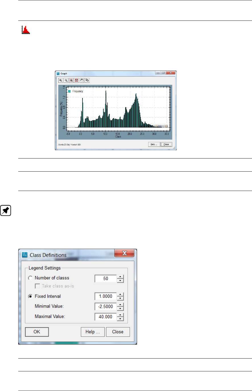
DRAFT
iMOD, User Manual
Histogram
Click this button to compute the frequencies of IDF values within each class of the
current legend, a histogram is plotted, see above for an explanation). The computed
values are temporary written in the fifth column. Once the Legend window has been
closed, the values are removed.
Graph window:
Update
Labels
Click this button to update the labels in the Label column. These values will be used
whenever the legend is plotted on the graphical canvas.
Header Enter a descriptive text for the corresponding legend. The text will be plotted on top
of the legend whenever the legend is plotted on the graphical canvas. Leave the input
field empty to ignore any legend header.
Note: The maximum number of classes in a Classed Legend is 50. However, less is often
desired. You are requested to specify beforehand the number of classes you want. When
switching from the Stretched tab to the Classes tab, the following window will appear.
Class Definitions window:
Number of classes
(1-50)
Enter the number of classes for which the stretched legend will be trans-
formed.
Take class
as-is
Select this option to sample from the classes as specified in Streched legend.
If deselected, iMOD will try to round the class-interval to nice numbers that
might - however - yield less classes.
114 of 812 Deltares
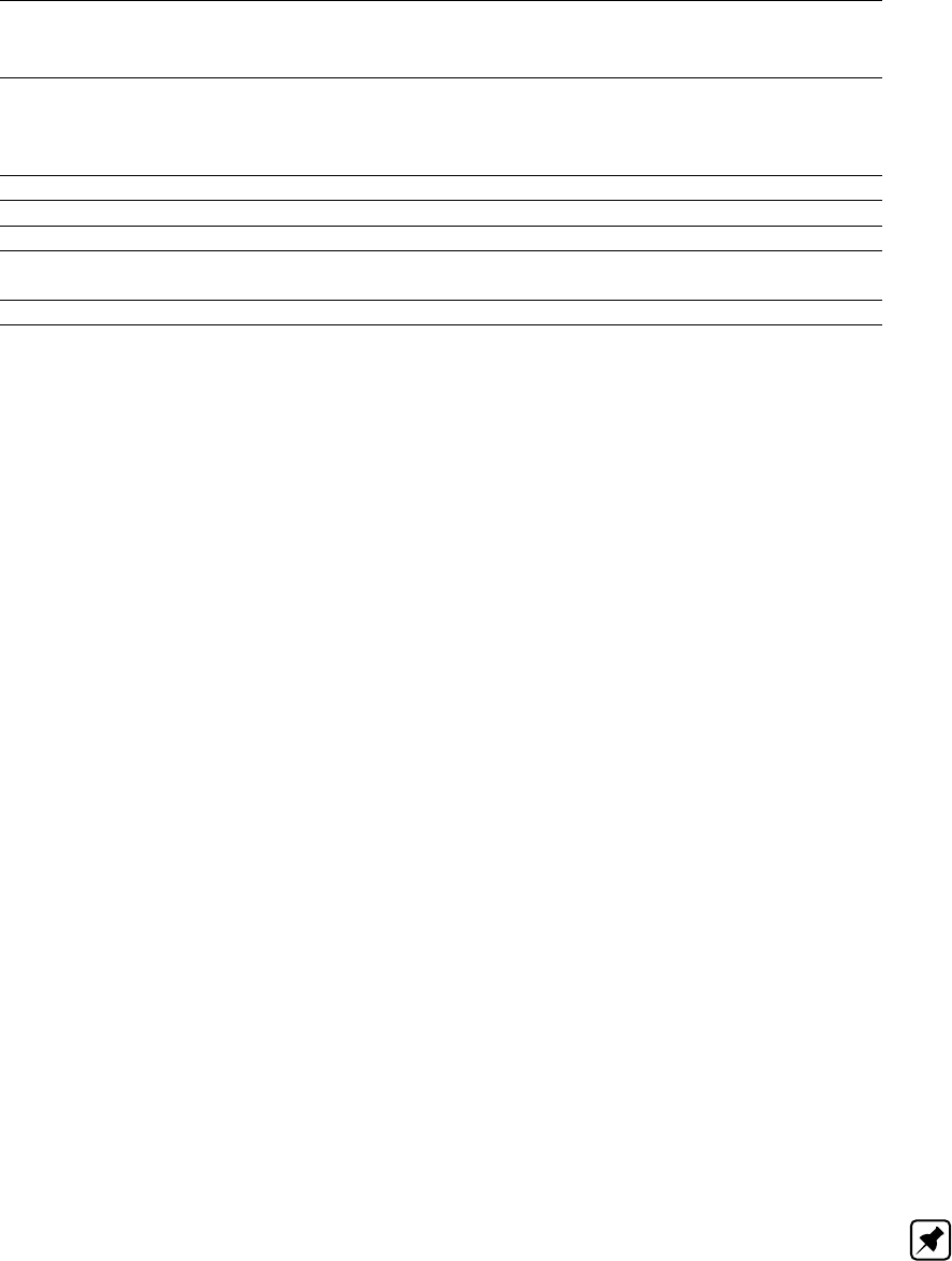
DRAFT
Map Menu options
Fixed Interval Select this option to generate a legend with a fixed interval, e.g. 1.0 in between
the specified Minimal Value and Maximal Value. iMOD starts at the minimal
value and add another class with the specified interval to a maximum number
of 50 classes or less if the maximal values is reached prior to that.
Minimal Value: Enter a minimal value for the legend, e.g. -2.5.
Maximal Value: Enter a minimal value for the legend, e.g. 40.0.
Ok Click this button to continue to the Classes tab of the Legend window.
Close Click this button to close this Class Definition window and return to the
Stretched tab of the Legend window..
Help Click this button to start the iMOD Help Functionality.
6.6.2 Generation of Legends
All active maps are accompanied by a legend. IDF-files are drawn standard by a legend,
as well as IPFs, IFFs, ISGs and GENs. How to specify a legend is explained in sections
3.4.5, 4.2.1, 4.3.1, 4.4.1 and 4.5.2, respectively. However you can let iMOD assign classes
and colours also. In that case you should select the respective *-options under Map, or alter-
natively you can press the right mouse button anywhere on the canvas to see the following
options:
Current Zoom Level
Percentiles
Click this option to build a non-linear legend based on the distribution of values in the
selected IDF’s for the current zoom level of these files (max. 2000 points).
Linear
Click this option to build a linear legend based on the minimum and maximum values
in the selected IDF’s for the current zoom level of these files.
Unique Values
Click this option to build a legend with unique values that appear in the selected IDF’s
for the current zoom level of these files (should be less or equal to 50).
Entire Zoom Extent
Percentiles
Click this option to build a non-linear legend based on the distribution of values in the
selected IDF’s for the entire zoom extent of these files (max. 2000 points).
Linear
Click this option to build a linear legend based on the minimum and maximum values
in the selected IDF’s for the entire zoom extent of these files.
Unique Values
Click this option to build a legend with unique values that appear in the selected IDF’s
for the entire zoom extent of these files (should be less or equal to 50).
Note: Whenever the number of unique classes exceeds the maximum of 50, iMOD will
distribute the original number of classes to fit the maximum of 50. It will take the frequency of
the original classes into account, such that the frequencies of the renewed classes are evenly
distributed.
Deltares 115 of 812
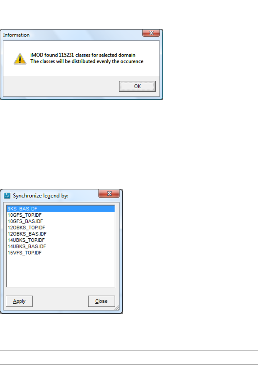
DRAFT
iMOD, User Manual
Information window:
6.6.3 Synchronize Legends
Whenever more than one map is selected in the iMOD Manager then the option Synchronize
Legends becomes available to display the Synchronize Legends window. You can open this
window by selecting the menu option Map and the option Legend or alternatively the same
menu options from the popup menu whenever you click your right mouse button anywhere on
the canvas.
Synchronize Legend by window:
List menu The menu list displays all the selected IDF-files from the iMOD Manager. The legend
from the one that is selected (in this case the PWTHEAD_19890114_L1.IDF) will be
used to be copied to the others.
Apply Click this button to synchronize the listed IDF-files to the selected IDF and close the
Synchronize Legend window.
Close Click this button to close this Synchronize Legend window without changing any
legend.
116 of 812 Deltares
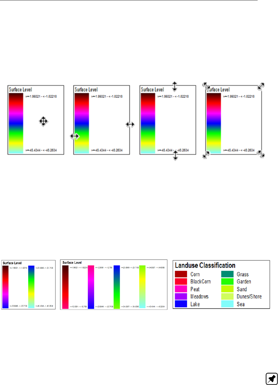
DRAFT
Map Menu options
6.6.4 Plot Legends
Right-click your mouse button anywhere on the canvas to select the menu option Legend and
then choose the option Plot Legend on Map to plot the legend of the last drawn Map on the
canvas.
How to move the legend:
The first picture shows that you can move the legend whenever the mouse symbol changes
in a cross. The 2nd, 3rd and 4th show that you can increase and decrease the size of the
legend whenever the arrows appear (near the legend boundaries).
Whenever you right click the mouse button, you can specify the number of columns (1-5)
that are used to display the legend, by selecting those in the popup menu Legend Columns.
Whenever the legend contains less or equal 50 classes, the legend will be plotted such, that
you can distinguish all the classes.
The left two pictures show a legend for two and four columns (both 255 classes) and the right
picture shows a legend with 10 classes.
To remove the legend from the map, deselect the Plot Legend on Map option again.
Note: The size of the text will increase and decrease whenever the size of the legend area
is changed. So, to increase the textsize, you should increase the area for the legend.
The following sections contains detailed descriptions of the Map options for different files that
iMOD supports.
Deltares 117 of 812
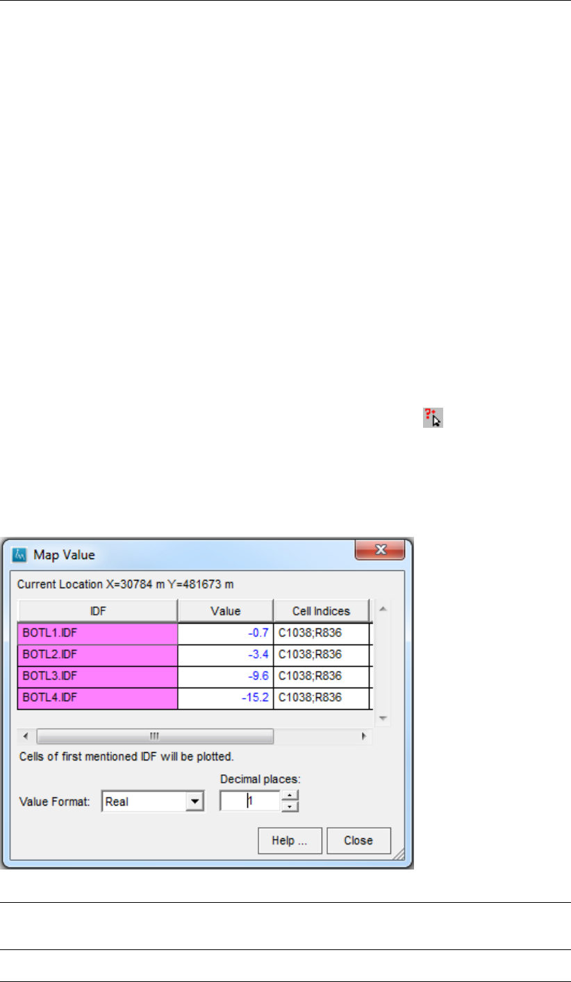
DRAFT
iMOD, User Manual
6.7 IDF Options
iMOD supports several basic functionalities that manipulate IDF-files:
IDF Value,
IDF Export,
IDF Calculator, use this tool to apply simple algebra, rescale the IDF and/or merge sev-
eral IDF-file into a single one.
IDF Edit, use this tool to select areas for which computations are carried out. These can
be simple algebraic computations and/or smoothing and/or interpolation.
6.7.1 IDF Value
WHY?
IDF-files are raster files with (non)-equidistant rastersizes. Interactive inspection of the raster
with the IDF Value option is a quick and easy way to check the raster values.
WHAT?
IDF Value allows you to view particular rastercell values for a single IDF-file, or multiple IDF-
files. iMOD will read the IDF values underneath the current mouse position.
HOW?
In the Map tab of the iMOD Manager window, click the Map Value ( ) button to open the
Map Value window. Otherwise, use the shortcut F3 or right-click anywhere on the canvas to
open the popup menu. Select the option IDF Options and then choose IDF Analyse. Or alter-
natively, select the menu option Map, choose the option IDF Options and then IDF Analyse.
Map Value Window:
Current Lo-
cation
This field shows the current location of the mouse on the canvas. Press the LEFT
mouse button to freeze the current location. Restart inspection over the canvas by
pressing the LEFT mouse button again.
IDF This column in the table shows the IDF selected in the iMOD Manager and part of
the inspection with MapValue.
118 of 812 Deltares
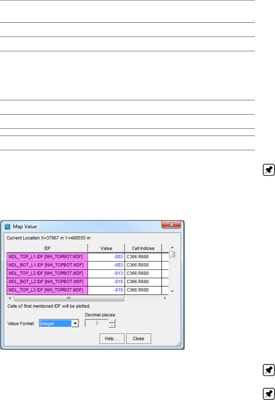
DRAFT
Map Menu options
Values This column shows the value of the IDF (column 1) for the current location. Values
that are greater than zero will be coloured red, less than zero become blue.
Transf. This column shows the transformation that could take place, see for more information
about this the syntax of the IDF-file and how to apply a transformation.
Cell
Indices
This column shows the column and row number of the selected IDF-files, e.g. Cell
Indices=C32;R12 to represent column 32 and row 12 respectively. There is no need
that the inspected IDF-files have identical dimension and/or raster discretization.
Whenever the mouse is positioned outside the limits of the IDF, Cell Indices=Outside.
In case the inspector works with a rectangle/polygon, the Cell Indices will show the
minimum and maximum values for the column and row numbers that are within the
rectangle/polygon, e.g. Cell Indices=C40-32;R32-54.
Value For-
mat:
Choose the preferred value format from the dropdown menu. You can choose from:
Real (e.g. 2.345), Integer (e.g. 002) and Scientific notation (0.2345E+01).
Decimal
places:
Change this value to set the total amount of decimal values (values behind the point),
the possible range is 0-15.
Help . . . Click this button to start the iMOD Help Functionality.
Close Click this button to close the MapValue window. Alternatively the MapValue window
can be closed by clicking the RIGHT mouse button anywhere on the canvas.
Note: All selected files in the iMOD Manager will be listed in the Map Value window, however,
IPFs, IFFs, GENs and ISGs will be left out automatically. There is no need to deselect them
before clicking the Map Value button. Whenever a MDF-file is selected, all IDF-files within the
MDF-file will be displayed and also the MDF-filename.
Map Value window filled with items from a MDF-file:
Note: The menu options Move, Zoom In, Zoom Out, Zoom Full and Zoom Rectangle are
available during the Map Value exercise.
Note: Click the left mouse button to stop hovering over the graphical display. It will freeze the
values in the Map Value window. Start hovering again by clicking the left mouse button again,
terminate the entire functionality by clicking the right mouse button.
On default, the Map Value window will operate as a point inspector, in other words, the value
will be read for the current position of the mouse. Click the menu option Map, the option IDF
Deltares 119 of 812
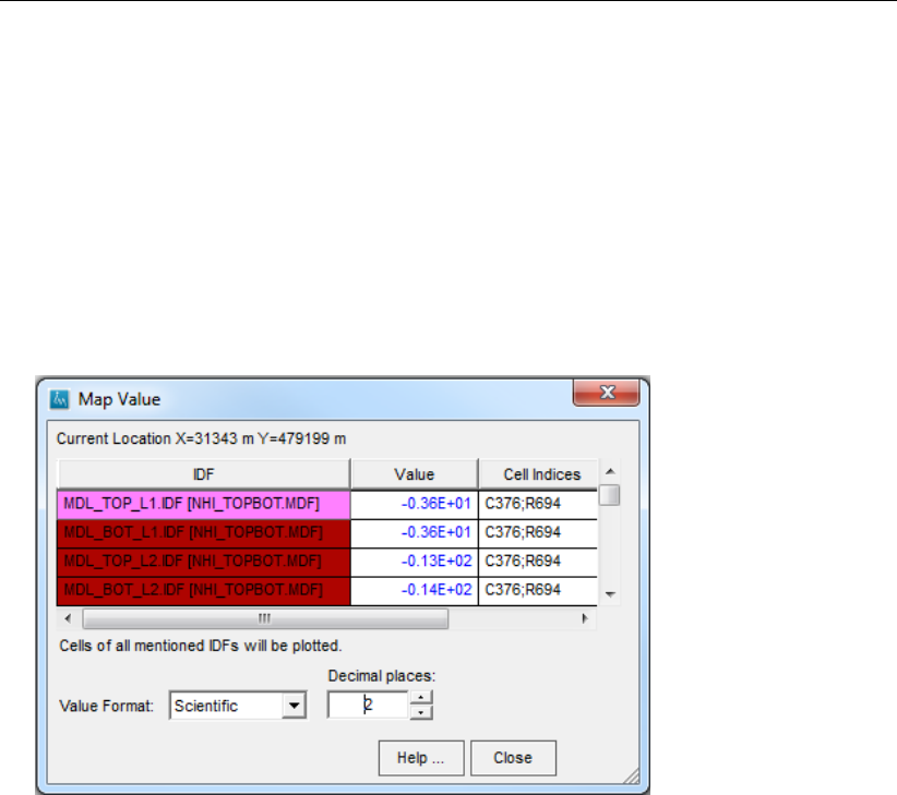
DRAFT
iMOD, User Manual
Options and then the option IDF Analyse to display the following options to alter this:
Plot No Location
Check this item whenever no rastercells of the selected IDF-file need to be displayed.
Plot All Locations
Check this item whenever the rastercells of all selected IDF-files need to be displayed.
Bear in mind that the performance will slow down whenever many IDF-files are included,
and if IDF-files with non-equidistant rasters are included. Whenever this option is checked,
all values in Map Value will be coloured differently.
Map Value window in Plot All Locations mode:
Plot First Location Only
Check this item whenever the rastercells of the first IDF-file listed in the Map Value table,
need to be displayed. This is the default.
Points
Check this item whenever the values for the current location of the mouse need to be
listed. This is the default.
Rectangle
Check this item whenever the values need to be summed within a rectangle that you can
draw. Use the left mouse button to locate the first position of the rectangle and the left/right
mouse button to stop and close the Map Value window.
Polygon
Check this item whenever the values need to be summed within a polygon that you can
draw. Use the left mouse button to locate the first position of the polygon and continue to
add more points (as desired) to complete the polygon. Use the right mouse button to stop
and close the Map Value window.
Circle
Check this item whenever the values need to be summed within a circle that you can draw.
Use the left mouse button to locate the first position of the circle and expand the size of
the circle while moving the mouse pointer away from the first position (centre of the circle).
Click again on your left mouse button to stop and close the Map Value window.
120 of 812 Deltares

DRAFT
Map Menu options
6.7.2 IDF Export
WHY?
IDF-files have a specific format. The export to a format readable in other software applications
makes it possible to use the IDF-files outside iMOD.
WHAT?
The IDF-files can be exported in several formats.
HOW?
Choose the option Map from the main menu, choose IDF Options and then IDF Export to
display the following menu options:
ESRI ASC Format
Check this option to export the IDF into an ESRI ASCII format. Bear in mind that this
ESRI ASCII format does not support non-equidistant cell sizes. Therefore, the export will
result always in an equidistant ASCII file, see section section 9.13 for the exact syntax of
an ESRI-ASCII file. Any ASCII file can be read in again in iMOD to convert is back to an
IDF file, see section section 6.1.
NetCDF Format
Check this option to export the IDF into the NetCDF3 format. Any NetCDF file can be read
in again in iMOD to convert is back to an IDF file, see section section 6.1.This function
is only available in the X32-bits version of iMOD.
For both export formats the following options are available:
Export Total Extent
Click this option to export the current IDF for its total extent.
Export Current Extent
Click this option to export the current IDF for the current extent of the graphical window.
Export Given Extent
Click this option to export the current IDF for an extent to be entered.
Deltares 121 of 812
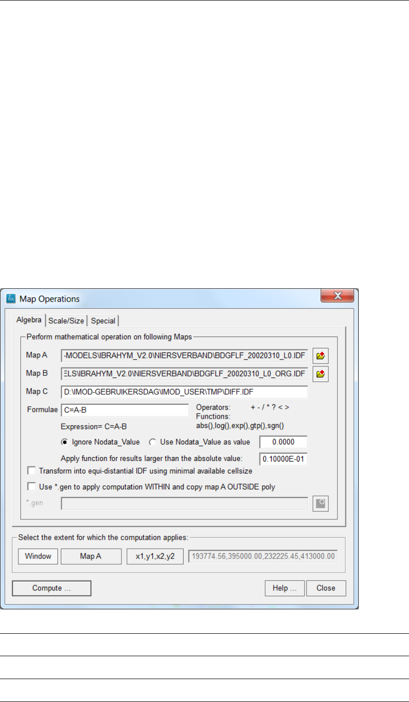
DRAFT
iMOD, User Manual
6.7.3 IDF Calculator
WHY?
Arithmetic operations enable the creation of new IDF-files.
WHAT?
The IDF Calculator works with IDF-files as input and enables to:
calculate a new IDF-file using an arithmetic expression on one or two IDF-files (the Algebra
tab)
change the rastersize of an IDF-file by upscaling or downscaling (the Scale/Size tab)
merge a selected number of IDF-files into one IDF-files (the Special tab).
HOW?
The IDF Calculator can be displayed at any time from the iMOD Manager, click the Calculator
button and/or use the Map option from the main menu (or the popup menu that displays
whenever you click your right mouse button on the graphical window), choose IDF Options
and then the option IDF Calculate. The following Map Operations window will be displayed.
Map Operation window, Algebra tab:
Map A Displays the first IDF. On default it will display the first selected IDF from the
iMOD Manager, click the button Open IDF to open a different one.
Map B Displays the second IDF. On default it will display the second selected IDF
from the iMOD Manager, click the button Open IDF to open a different one.
Map C Enter the name of the resulting IDF. On default it will use the name DIFF.IDF
that will be saved in the TMP-folder of the USER-folder.
122 of 812 Deltares
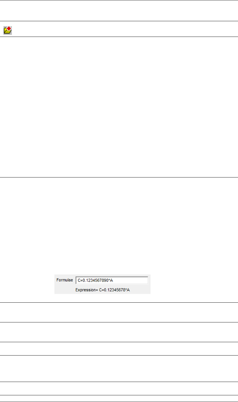
DRAFT
Map Menu options
Open IDF
Click this button to select an IDF-file from a folder
Formulae Enter the formulae to be used. The syntax of the formulae is that the IDF-
names entered as Map A,Map B and Map C are represented by the charac-
ters A,Band C, respectively. The example C=A-B means that the values of
Map A will be subtracted by the values in Map B.
The following operators are available in the formulae:
“+” : adds values
“-“ : subtract values
“/” : divides values
“*” : multiplies values
“?” : takes the first NoDataValue found in Map A then Map B
“<”: takes the smallest from both values between Map A and Map B
“>”: takes the largest from both values between Map A and Map B
The following functions are available in the formulae:
ABS() : takes the absolute value of the expression between brackets;
LOG() : takes the logarithmic value of the expression between brackets;
EXP() : takes the exponent of the expression between brackets;
GTP() : computes the groundwaterclass (‘grondwatertrap’). Enter a mean
highest groundwaterlevel for Map A and the mean lowest groundwater
level for Map B.
Expression The Formulae entered is translated into an Expression which will be used,
eventually. The expression can be used to check whether the formulae has
been filled in correctly.
Note: It is possible to include constant values in the Formulae, e.g.
[C=1.5*A] which means that all values in Map A will be multiplied with a
factor of 1.5. Be aware that the number should come before Map A as in the
formulae [C=A*1.5] the constant value is ignored. This can be extended to
another factor to be used for Map B, e.g. [C=1.5*A-0.5/B].
It should be noticed that these constant value are rounded to a single
precision real (8 digit number), so the entered value 0.1234567890 becomes
0.12345678 in the Expression.
Example of the Formulae:
Ignore
NoData_ Value
Check this option to ignore the NoDataValues in the IDF-files.
On default cells equal to the NoDataValue of the IDF will be excluded in the
computation.
Use
NoData_ Value as
value
Check this option to use the NoDataValues in the computation.
Specify the value to replace the NoDataValue of the IDFs.
On default the value 0.0 is used.
Apply function for
...
After the calculation, this option gives values smaller than given/entered ab-
solute value a nodata value, e.g. C=A-B if C<0.1 C=nodata.
Transform into . . . Check this option to force that the resulting IDF (Map C) will have equidistant
cellsizes. Whenever any of the selected IDF-files (Map A and/or Map B) is an
IDF-file with non-equidistant cellsizes, the smallest cellsize in one of these will
be used to determine the cellsize of Map C.
Use *.gen Check this option to force that the results of Map C will be computed inside
the polygons that are defined in the entered *.GEN-file (*.gen).
*.gen Enter the *.GEN-file with polygons
Deltares 123 of 812
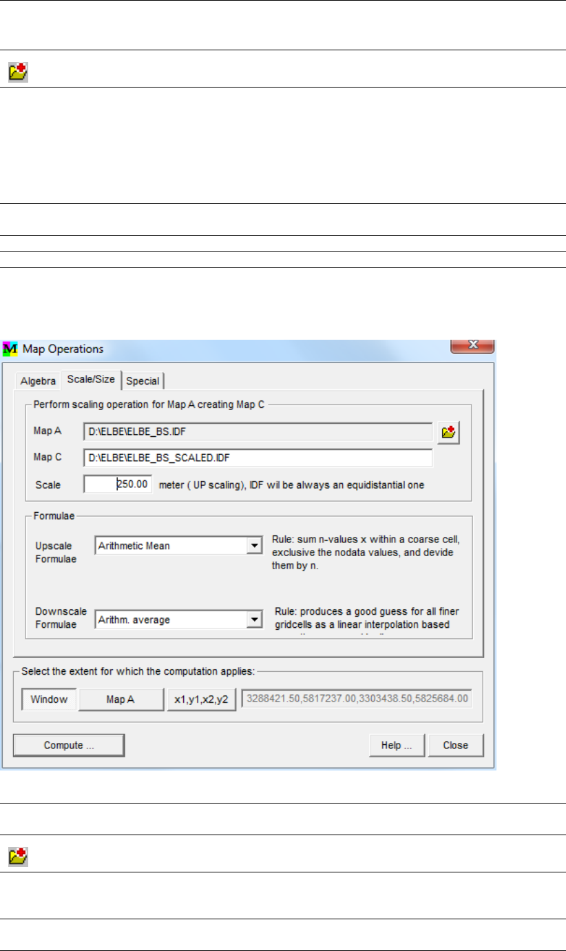
DRAFT
iMOD, User Manual
Open File
Click this button to select a *.GEN file
Select the extent
for which the
computation
apllies:
Click one of the following options:
Window, to force that the results of Map C will be computed for the current
ZoomLevel only;
Map A, to force that the results of Map C will be computed for the extent
of Map A.
x1,y1,x2,y2, to enter the coordinates of a specific window
Compute... Click this button to start the computation, it closes the Map Operations window
afterwards.
Help ... Click this button to start the iMOD Help Functionality.
Close Click this button to close the Map Operations window.
Map Operation window, Scale/Size tab:
Map A Displays the IDF to be scaled. On default it will display the selected IDF in the
iMOD Manager, click the Open IDF button to open a different one.
Open IDF
Click this button to select an IDF-file from a folder.
Map C Enter the name of the resulting IDF. On default it will use the IDF-file from Map
A and add the postfix SCALED to it, so the IDF-name will change from *.IDF
into *_SCALED.IDF.
Scale Enter the new cell size of the IDF. The resulting IDF will be an equidistant IDF
with this cellsize.
124 of 812 Deltares
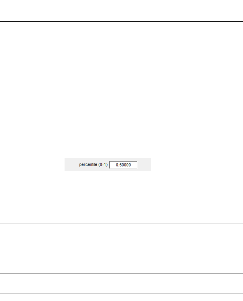
DRAFT
Map Menu options
Formulae
Upscale Formulae
Select a Formulae to be used in the
Upscaling (increased cell size):
Boundary : minus values above positive values above zero values;
Arithmetic Mean :sum cell values, excluding the NoDataValues, and divide
them by the number of cells;
Geometric Mean : take log()-function for cell values, excluding the No-
DataValues and zero values, sum cell log-values, divide them by the num-
ber of cells and take the exp()-function;
Sum : sum cell values, excluding the NoDataValues;
Sum Conductance : sum cell values, multiplied with the ratio of . . . ., ex-
cluding the NoDataValues;
Inverse : take the inverse (1/x) of cellvalues, excluding the NoDataValues
and zero values, and divide them by the number of cells;
Most.Freq.Occur. : take the cell value that occurs most frequently within a
coarse cell, excluding the NoDataValues;
Sum Inverse: take the sum of the inverse (x−1) of the cell values, exclud-
ing NoDataValues and zero values;
Percentile : take the cell value that occurs for a given percentile (0-1)
within a coarse cell, excluding the NoDataValues;
Block value : the value of the centre cell.
Downscale
Formulae
Downscaling (decreased cell size):
Arithm. Average: produces a good guess for all finer gridcells as a linear
interpolation based on the coarse gridcells.
BlockValue: assign the value of the coarse gridcell to all finer gridcells.
Select the extent
for which the
computation
apllies:
Click one of the following options:
Window, to force that the results of Map C will be computed for the current
ZoomLevel only;
Map A, to force that the results of Map C will be computed for the extent
of Map A.
x1,y1,x2,y2, to enter the coordinates of a specific window
Compute... Click this button to start the computation, it closes the Map Operations window
afterwards.
Help . . . Click this button to start the iMOD Help Functionality.
Close Click this button to close the Map Operations window.
Deltares 125 of 812
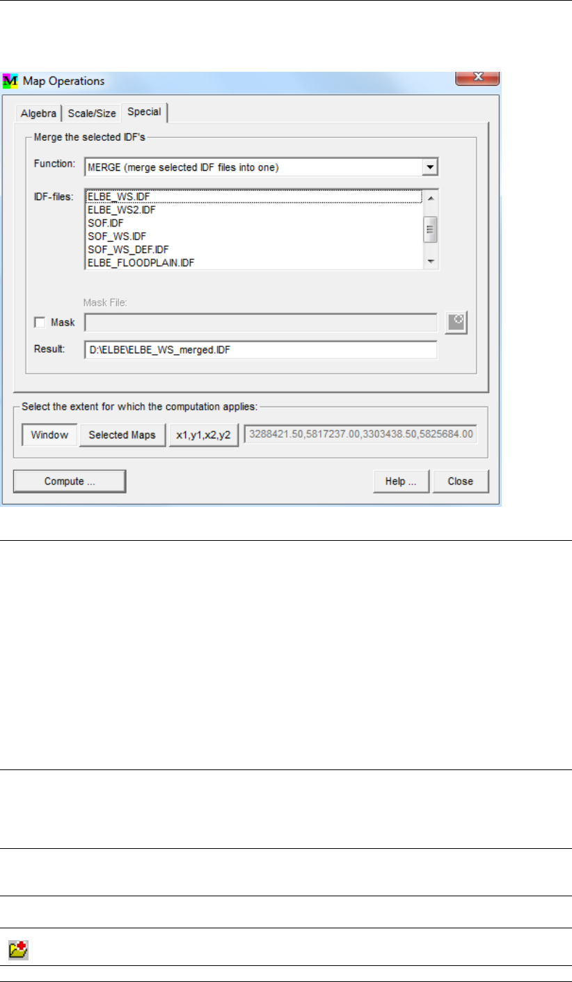
DRAFT
iMOD, User Manual
Map Operation window, Special tab:
Function Select one of the following functions:
MERGE
use this option to merge the selected IDF-files into a single one;
SUM
use this option to sum all values for the selected IDF-files into a single one.
MEAN
use this option to compute the mean for all values for the selected IDF-files;
MIN
use this option to compute the minimum value for all values for the selected IDF-
files;
MAX
use this option to compute the maximum value for all values for the selected
IDF-files.
IDF-files: Select more than one IDF-file to be merged. iMOD will calculate values for the over-
lapping areas based on the inverse distance to the extent border of the IDF-files.
The weigh-factor for an IDF-file, increases whenever the point considered, lies fur-
ther away from the extent border of the IDF-file. Exact in the middle between two
IDF-files, the weigh-factors for both will become 0.5.
Mask Select this option to include a mask that determines the area to be merged, e.g.
a boundary of catchment area. This option is only available whenever Func-
tion=MERGE.
Mask File: Enter the IDF-file of the mask. All data in the IDF, not equal to the NoDataValue will
be used to identify the size of the mask.
Open IDF-file
Click this button to open an IDF-file as MaskFile.
Result: Enter the name of the IDF-file to be created.
126 of 812 Deltares
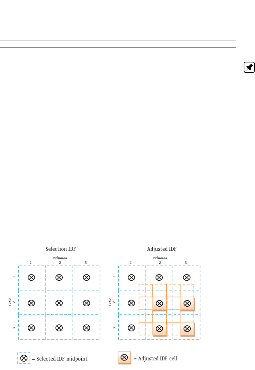
DRAFT
Map Menu options
Compute... Click this button to start the computation, it closes the Map Operations window after-
wards.
Help ... Click this button to start the iMOD Help Functionality.
Close Click this button to close the Map Operations window.
Note: It is allowed only to merge equidistant IDF-files (IEQ=0, see section 9.5).
6.7.4 IDF Edit
WHY?
IDF-files are raster files with (non)-equidistant rastersizes. Normal GIS systems can not ma-
nipulate raster files in an easy way, moreover, it is difficult to edit individual rastercells.
WHAT?
The values of individual rastercells can be easily altered by selecting the rastercells and as-
signing a new value using the Calculate option. Also cellsizes of existing IDFs can be altered
easily by grid refinement using upscaling and downscaling techniques.
IDF Edit allows you to select particular rastercells inside an IDF-file based on a maximum of
two logical expressions that optionally operate inside a polygon. Logical expressions can be
carried out sequentially. Once a selection has been made, different values can be assigned
to them directly, or an interpolation and/or smoothing algorithm can be applied. A selection is
carried out for mid points of rastercells for a particular IDF (Selection IDF). Those midpoints
will be used also to perturb corresponding rastercells for IDF-files with different rastersizes
and/or position. For these cases, it should be known that not all of the rastercells are affected
by the alteration due to intermediate cells that are in-between midpoints of the Selection IDF.
Methodology of selecting and calculating with IDF Edit:
HOW?
To start IDF Edit select Map from the main menu, choose IDF Options and then IDF Edit.
Alternatively, you can select the menu item from the popup menu that appears when you
right-click your mouse in the graphical window. In both cases, you should select at least one
Deltares 127 of 812
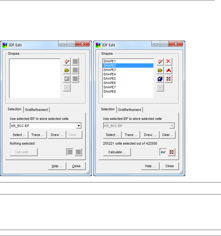
DRAFT
iMOD, User Manual
IDF from the iMOD Manager, the IDF Edit window will appear.
IDF Edit window, Selection tab, (left) initial window, (right) after selection:
Shapes This groupbox contains several functionalities that are needed to draw and
open polygons. The functionalities are explained in detail.
Use selected IDF
to store selected
cells
Select one of the IDF-files listed in the dropdown menu. The content of the
list is based on the list of IDF-files in the iMOD Manager. The dimensions of
the file that you select will be used to display the selection. This file will be the
Selection IDF. If you select a Selection IDF with CellSizes of 25x25 meter, the
selection will be displayed on that dimension. It is only possible to change the
Selection IDF if the current selection is cleared and/or is empty.
Select . . . Click this button to start the IDF Edit Select window.
128 of 812 Deltares
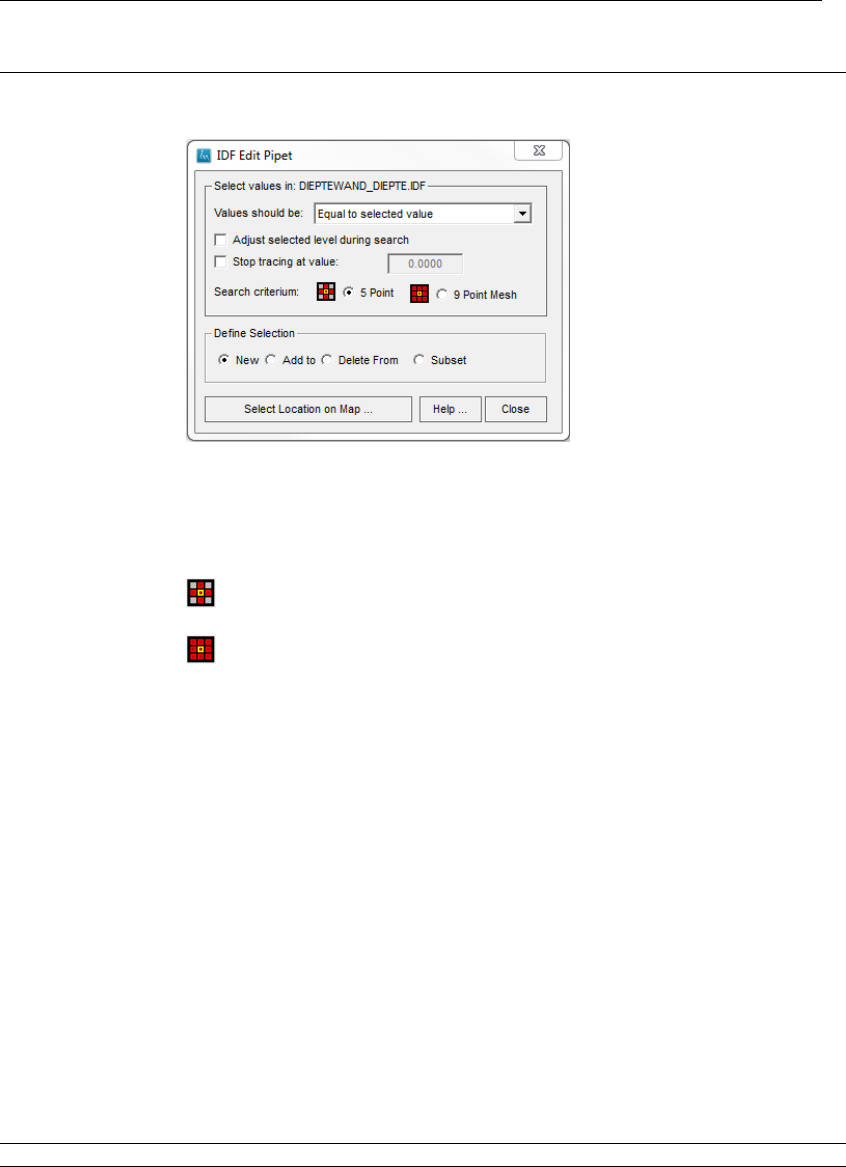
DRAFT
Map Menu options
Trace . . . Click this button to start the IDF Edit Pipet window.
IDF Edit Pipet window:
The trace selection will select cells in the IDF on the basis of their value and
their connection to the identified cell.
Values should be: choose the selection condition from the pull down list.
Search criterium: check one of the buttons:
5 point: iMOD will search directly connecting cells on a five-point
pattern
9 point: iMOD will search connecting cells on a nine-point pattern
Select
Location
on Map . . . :
click this button to start the selection. The cursor will change
in a pipette. Left click your mouse to select the cell from where
you want to find the connecting cells which fulfill the selection
condition. The IDF Edit Pipet window will close and the number
of selected cells is indicated in the IDF Edit window. Click this
button again if you like to start a new selection with new criteria
and cell value (shown in the message bar at the bottom of your
window IDF-value:{value}).
Define Selection:
New Select this option to start a new selection.
Important Note: After a selection is made a new (clean) selec-
tion can only be started by clicking on the Select Location on
Map . . . button. The selected cells will only than be deselected
and a new selection can be made.
Add to Select this option to add the results of the evaluation to the
current selection set.
Delete From Select this option to delete the results of the evaluation from the
current selection set.
Subset Select this option to take the result of the evaluation from the
selection that is already in the selection set.
Draw . . . Click this button to start the IDF Edit Draw window (see section 6.7.4.2).
Deltares 129 of 812
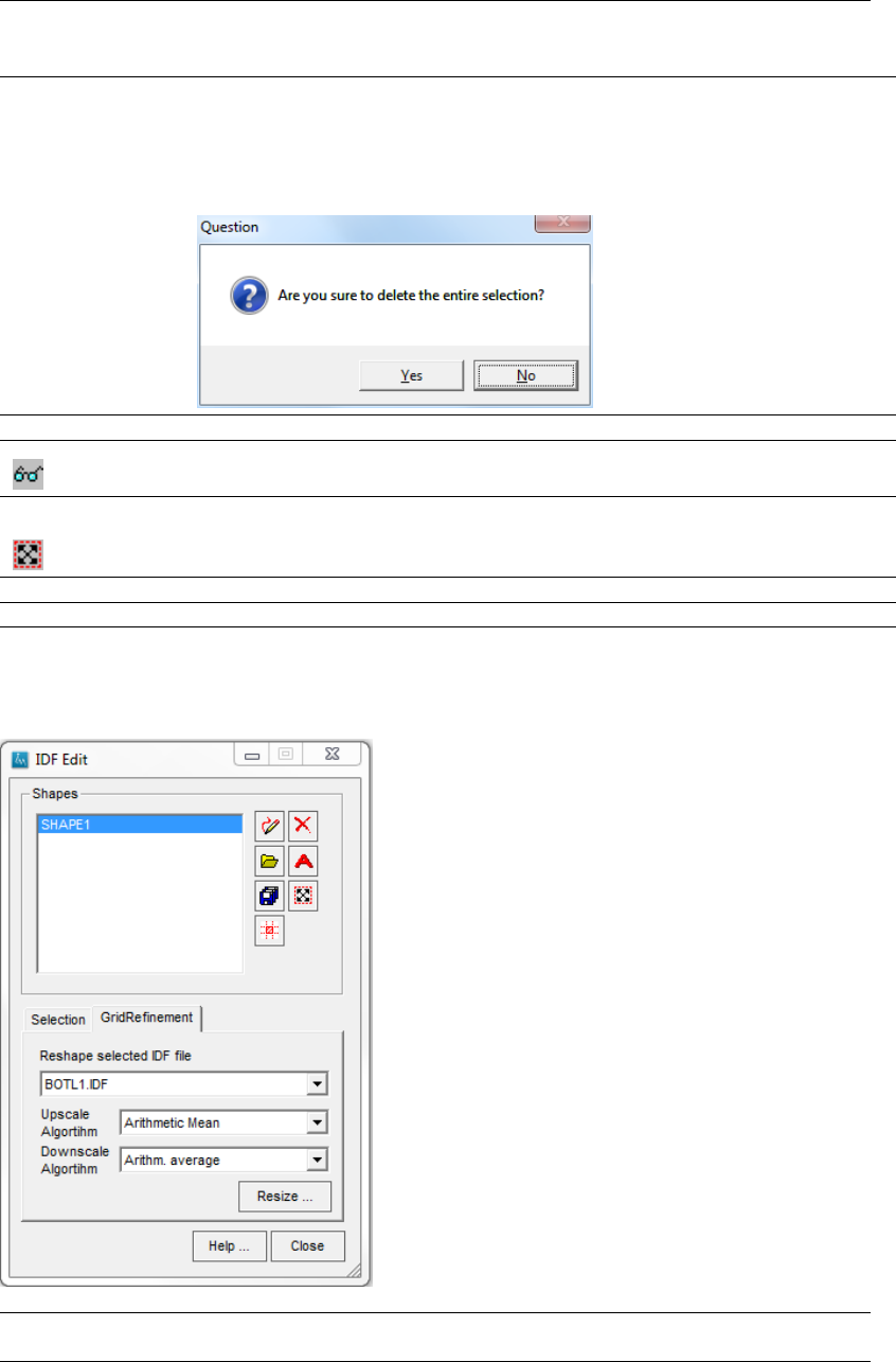
DRAFT
iMOD, User Manual
Clear Click this button to clear the entire selection for the Selection IDF. This button
is only available whenever cells are selected. You will be asked whether you
are sure to continue.
Question window:
Calculate . . . Click this button to start the IDF Edit Calculation window (see section 6.7.4.3).
Show Selection
Click this checkbox to display the selection.
Zoom Selection
Click this button to adjust the zoomlevel to the selected cells.
Help . . . Click this button to start the iMOD Help Functionality.
Close Click this button to close the IDF Edit window.
IDF Edit window, GridRefinement tab:
Reshape selected
IDF file
Select the IDF file from the dropdown menu.
130 of 812 Deltares
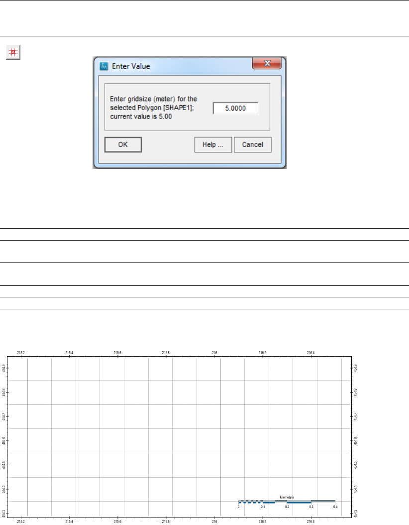
DRAFT
Map Menu options
Click this button to assign a new grid size. The Enter Value window will open.
Enter the new gridsize. This gridsize will be used within the selected
polygon. It will be used for the entire extent of the IDF in case no polygon is
selected. The new values of the gridcells are calculated by applying the up-
or downscaling methodology selected in the dropdown menus.
Resize . . . Click this button to resize and save the IDF-file.
Upscale algorithm Select the upscaling methodology from the dropdown menu; more detail about
the available methodologies is given in section 6.7.3
Downscale
algorithm
Select the downscaling methodology from the dropdown menu; more detail
about the available methodologies is given in section 6.7.3
Help . . . Click this button to start the iMOD Help Functionality.
Close Click this button to close the IDF Edit window.
Example of grid refinement:
Before refinement: grid with 100 m cell size
Deltares 131 of 812
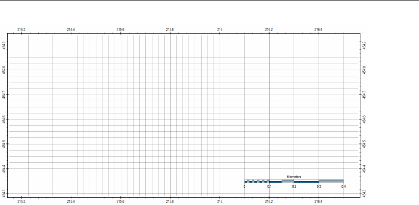
DRAFT
iMOD, User Manual
After refinement: grid with 100 m cell size and refined 25 m cell size; note that the cells on the
right side are shifted.
132 of 812 Deltares
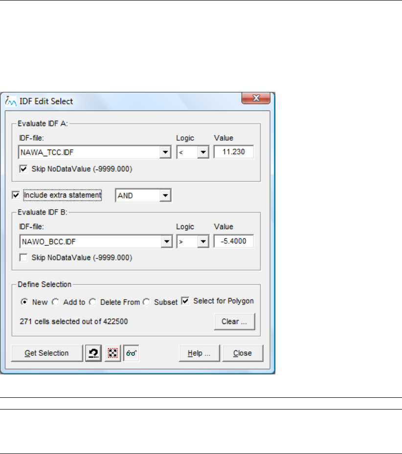
DRAFT
Map Menu options
6.7.4.1 IDF Edit Select
Click the option Select on the IDF Edit window, to display the IDF Edit Select window.
IDF Edit Select window:
IDF-file: Select one of the IDF-files listed in the dropdown menu.
Skip NoDataValue
value (. . . .)
Select this checkbox to “skip” the NoDataValues in the selection. On default
this will be turned on, so cells with NoDataValues will not be selected, dis-
carding their values. For the selected IDF-file, the current NoDataValue will
be displayed between brackets.
Deltares 133 of 812
DRAFT
iMOD, User Manual
Logic Select one of the logic variables out of the dropdown menu:
“=” : Equal to Value
“<>” : Not equal to Value
“<” : Less than Value
“<=” : Less than or equal to Value
“>” : greater than Value
“>=” : Greater than or equal to Value
“BND“ : Selects the cells at the boundary of an area with cells equal to Value
“SPIKE(4)“: selects spikes with difference byValue relative to surrounding
cells in four directions
“SPIKE(3)“: Selects spikes with difference byValue relative to surrounding
cells in at least three directions
“SPIKE(2)“: Selects spikes with difference byValue relative to surrounding
cells in at least two directions
“ALL“: Selects all cells
“NaN“: Select values equal to a so-called NaN-value in the IDF, these
numbers contains value that are beyond the range of a single precision real
“Inf“: Select values equal to an infinite value. E.g. infinity is caused by dividing
by zero
“NodataValue“: Select values equal to the NodataValue of an IDF-file
Note: The selection of SPIKE(i) may be used to smooth outliers in the
IDF-file using the smooth option in the IDF Edit Calculation window.
Value Enter the value to be evaluated, e.g. 11.230 or -5.400
Include extra
statement
Select this checkbox to add an extra IDF to be evaluated for the selection. You
can choose the keywords:
AND, click this option to make the selection set fulfill both the settings in Eval-
uate IDF A and Evaluate IDF B;
OR, click this to make the selection set fulfill at least one of the settings in
Evaluate IDF A or Evaluate IDF B.
New Select this option to start a new selection.
Add to Select this option to add the results of the evaluation to the current selection
set.
Delete from Select this option to delete the results of the evaluation from the current se-
lection set.
Subset Select this option to take the result of the evaluation from the selection that is
already in the selection set.
Select for Polygon Select this checkbox to apply the evaluation inside the current polygon(s) only.
This option is active whenever a shape is selected in the IDF Edit window.
271 cells selected
out of 422500
This shows the current number of selected cells (271) in the Selection IDF
that consists of 422500 cells.
Clear . . . Click this button to clear the entire selection for the Selection IDF. This button
is only available whenever cells are selected. You will be asked whether you
are sure to continue.
Get Selection Select this button to get the selection. Each selection will be saved in the file:
{USER}\tmp\{username}tmpselected{i}.dat.
Undo
Click this button to restore the previous selection.
Question window:
134 of 812 Deltares
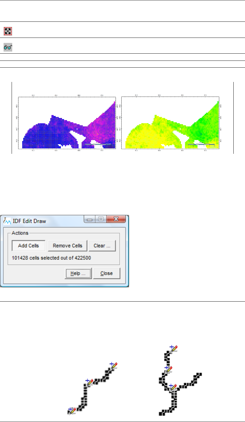
DRAFT
Map Menu options
Zoom to Selection
Click this button to adjust the zoomlevel to the selected cells.
Show Selection
Click this checkbox to display the selection (see below).
Help ... Click this button to start the iMOD Help Functionality.
Close Click this button to close the IDF Edit window.
Example showing (left) and deshowing (right) the selected cells:
6.7.4.2 IDF Edit Draw
Click the option Draw on the IDF Edit window, to display the IDF Edit Draw window. Cells
from the selected IDF can be selected or deselected interactively in the graphical window.
IDF Edit Draw window:
Add Cells Click this button to add cells to the selection. Use the left mouse button and
drag the cells you want to select on the graphical window. Release the left
mouse button to stop drawing and click the left mouse again to add more
cells to the selection.
Draw a selection in the Selection IDF:
Deltares 135 of 812
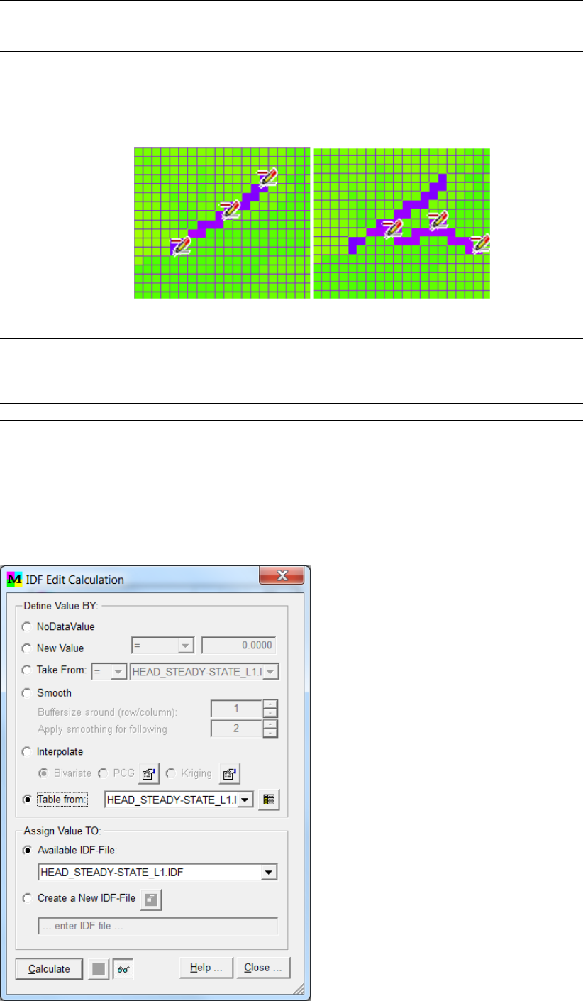
DRAFT
iMOD, User Manual
Remove Cells Click this button to remove current cells from the selection. Use the left
mouse button to deselect cells from the current selection. Release the left
mouse button to stop deselecting cells and click the right mouse button again
to deselect more.
Deselect cells for the Selection IDF:
Clear . . . Click this button to clear the entire selection for the Selection IDF. You will be
asked whether you are sure to continue.
101428 cells
selected out of
422500
This shows the current number of selected cells (101428) in the SelectionIDF
that consists of 422500 cells.
Help . . . Click this button to start the iMOD Help Functionality.
Close Click this button to close the IDF Edit Draw window.
6.7.4.3 IDF Edit Calculate
Click the option Calculate on the IDF Edit window, to display the IDF Edit Calculate window.
This option is not active whenever nothing is selected.
IDF Edit Calculation window:
136 of 812 Deltares
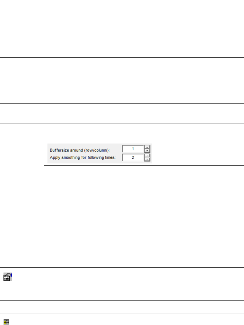
DRAFT
Map Menu options
The calculation method is defined in the upper part of the window: Define Value BY:.
The IDF on which the calculation is applied is selected in the lower part of the window: Assign
Value TO:.
NoDataValue Select this option to apply NoDataValues
New Value Select this option to enter a new value. Choose one of the following options from
the dropdown menu:
“=” : equal
“+” : add a value
“-“ : subtract
“*” : multiply
“/” : divide
Copy Values
From:
Select this option to copy the values from the selected IDF-file in the dropdown
menu. The IDF-files are those that are available in the menu on theiMOD Man-
ager.
Smooth Select this option to smooth the values within the selection only.
Smooth options:
Buffersize
around
(row/column):
Enter the number of rows/columns that need to be taken into
account in the smoothing. The value 1means that around a cell
that needs to be smoothed, one row/column will be used.
Apply
smoothing
for following
times:
Enter the number of smooth operations. The more times
smoothing is done the more smoother the result will be.
Interpolate Select one of the following options to interpolate:
BIVARIATE
apply a bivariate method;
PCG
apply a preconditioned conjugate gradient method;
KRIGING
apply a normal Kriging procedure.
Properties
Click this button to display a properties window for the selected interpolation op-
tion. Whenever the PCG is selected the PCG Settings window will be displayed
(section Table 4.1), in case a Kriging method is selected, the Kriging Settings
window is displayed (Table 4.1.
Table from: Click this option to open a table that shows the cell values in the selected cells for
the IDF-file selected in the dropdown menu (right).
Click this button to display an overview of the cell values in a table. The IDF Edit
Table window opens.
Deltares 137 of 812
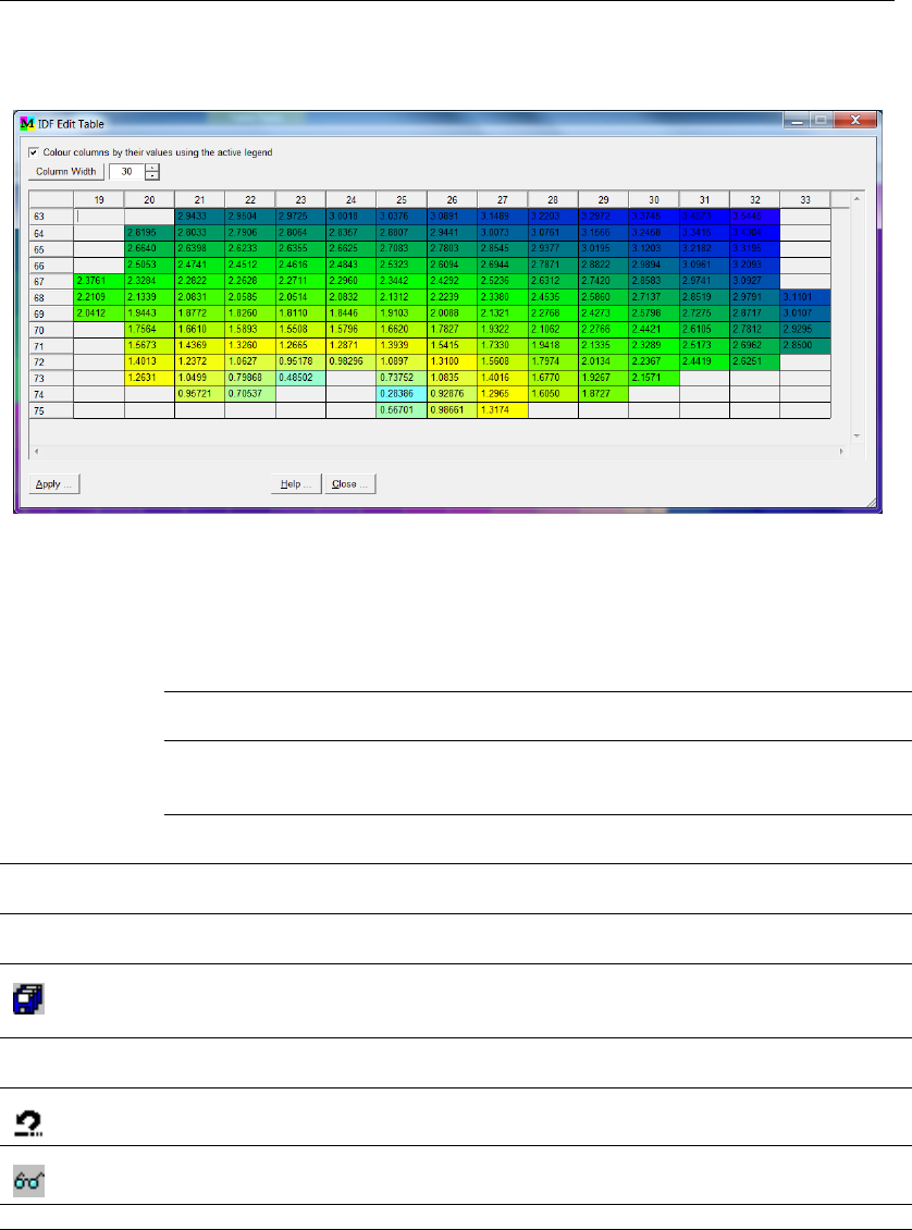
DRAFT
iMOD, User Manual
Example of IDF Edit Table:
The values shown in the table can be edited.
Colour
columns
...
Select this checkbox to colour the table cells by their corre-
sponding values. Deselect this checkbox to display the table
uniformly white. Each time a table value is changed, the colour-
ing will be adjusted accordingly.
Column
Width
Click this button to uniformly change the table column width by
the entered column width
Apply . . . Click this button to confirm to copy the values. Be aware that
you need to click the Calculate button to actually copy those
values into the IDF-file selected in Assign Value TO.
Close . . . Select this button to discard any entered values and to close the
IDF Edit Table window
Available
IDF-file:
Select the IDF-file that need to be adjusted from the dropdown list.
Create a New
IDF-file
Select this option to enter a different IDF file (not yet loaded in the iMOD Manager
and/or to be created
.
Save As
Click on the button and enter a name for the new IDF. The name of the new IDF
is displayed.
Calculate Select this button to execute the calculation and to adjust the values in the se-
lected IDF-file.
UndoClick this button to undo the last calculation. Each calculation will be saved
in the file: {USER}\TMP\{USERNAME}TMPCOMPUTED{i}.DAT.
Show Selection
Click this checkbox to display the selection of the graphical window.
Help . . . Click this button to start the iMOD Help Functionality.
138 of 812 Deltares
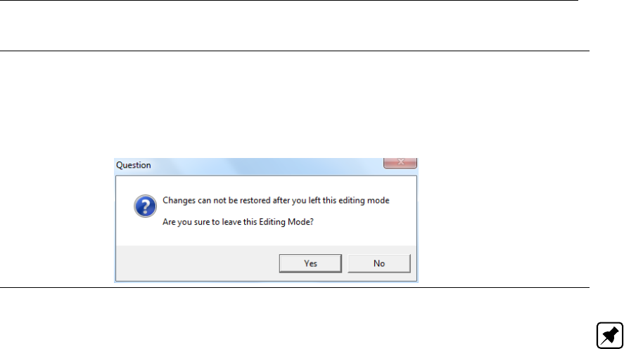
DRAFT
Map Menu options
Close . . . Click this button to close the IDF Edit Calculation window. If you have adjusted
one/more files, you will be asked whether you are sure to leave the IDF Edit
Calculation window. Changes can not be restored once you have agreed upon
closing the IDF Edit Calculation window.
Question window to leave the IDF Edit Calculation window:
Note: Whenever you click the Calculation button, the IDF-file will be adjusted and the new
results will be saved directly in the IDF-file. You can use the Map Value option, to inspect the
adjusted results, without leaving the IDF Edit Calculation window.
Deltares 139 of 812
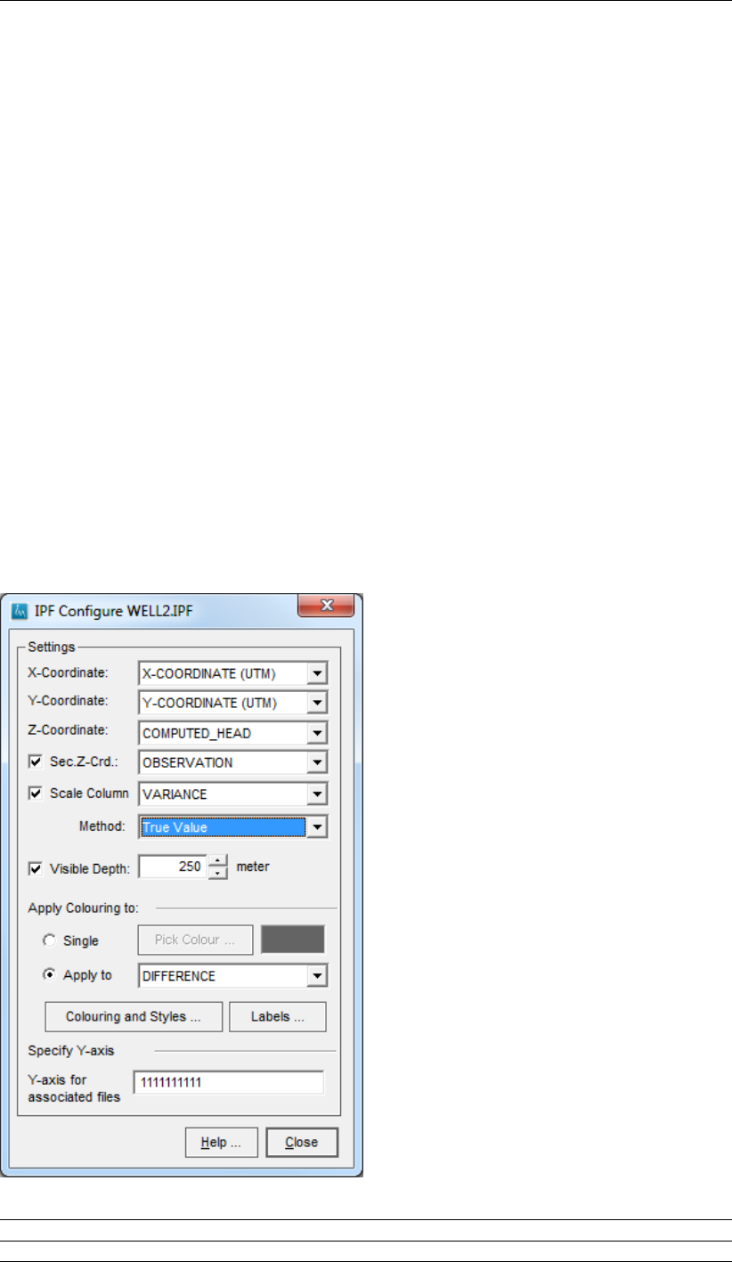
DRAFT
iMOD, User Manual
6.8 IPF Options
iMOD supports several basic functionalities that manipulate IPF-files:
IPF Configure,
IPF Analyse, use this tool to analyse the content of the IPF-files (including the associated
files, if available).
IPF Extract, use this tool to extract points out of an IPF-file to be saved independently.
6.8.1 IPF Configure
WHY?
IPF-files in iMOD represent point data that can be displayed in different ways.
WHAT?
IPF Configure is used to define the settings for display and assigns a symbol, colour or label
to the point data.
HOW?
Select the menu option IPF Configure from the IPF-options menu in the Map menu to display
the IPF Configure window. Or, use right-click anywhere on the canvas to open the popup
menu. Select the option IPF-options and then choose IPF Configure.
IPF Configure window:
X-Coordinate: Select the column in the IPF that represents the X coordinate.
Y-Coordinate: Select the column in the IPF that represents the Y coordinate.
140 of 812 Deltares
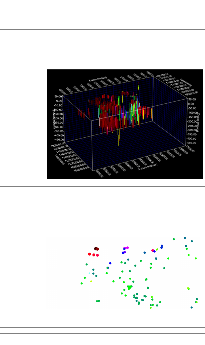
DRAFT
Map Menu options
Z-Coordinate: Select the column in the IPF that represents the Z coordinate. This data col-
umn will be used in the Cross-Section Tool and/or 3D Tool.
Sec.Z-Crd.: Select the column in the IPF that represents the secondary Z coordinate.
This data column will be used in the Cross-Section Tool and/or 3D Tool in
combination with the Z-Coordinate. In these cases, iMOD will draw a line
between the Z-Coordinate and Sec.Z-Crd.. You can use this for the top and
the bottom of the screen-depth of a well.
Example:
Scale Column: Select the column in the IPF to scale the symbol size. This option scales
points that have larger values than others, those will be displayed as an
increased marker symbol. iMOD will scale the values linearly from large up
to small and displays them accordingly, such that small values will be plotted
upon large values. As NO legend is specified, the internal values of the
appropriate column will be used, otherwise the minimal and maximal values
of the specified legend will be used to scale the symbols.
Example:
Method Select a method.
Visible Depth Select and specify an interval in meters, over which points are visible.
Single Select this option to display all points with the same colour.
Pick Colour . . . Select this button to display the default Colour window in which a colour can
be specified. The current colour is displayed to the right of this button.
Deltares 141 of 812
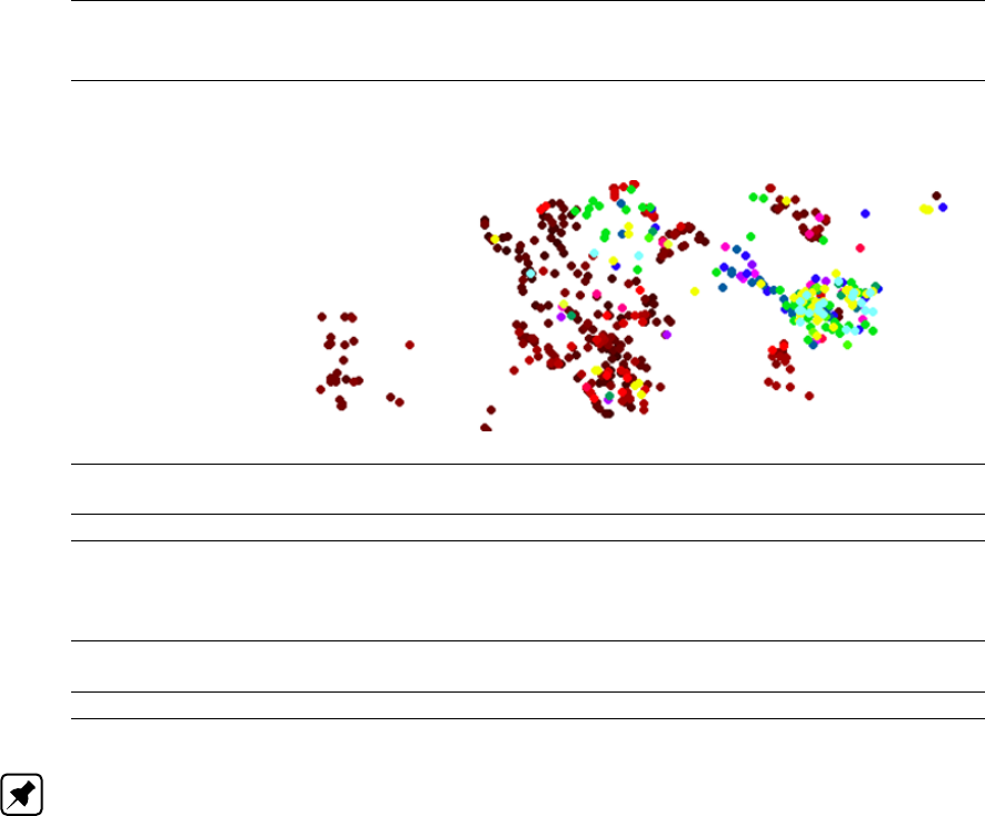
DRAFT
iMOD, User Manual
Apply to Select this option to colour the points according to the selected attribute that
is chosen in the dropdown menu at the right.
Example:
Colouring and
Styles. . .
Select this option to display the Lines and Symbols window, section 5.7.
Labels. . . Select this button to display the Select Label to be Printed window.
Y-axes for
associated files
Insert an indication which vertical axis to use for maximal 10 attributes that are
available in associated files. The value 1, means that the attribute is plotted
against the first y-axis, 2 means that the attribute is plotted against the second
y- axis (on the right of the final graph).
Help. . . Click this button to start the iMOD Help Functionality (if available in the se-
lected *.PRF file).
Close Select this button to apply the settings and close the IPF Configure window.
Note: On default, the classes for a legend will be computed linearly between the minimum
and maximum values for the selected attribute. Use the options described to adjust this legend
in order to plot proper colours.
142 of 812 Deltares
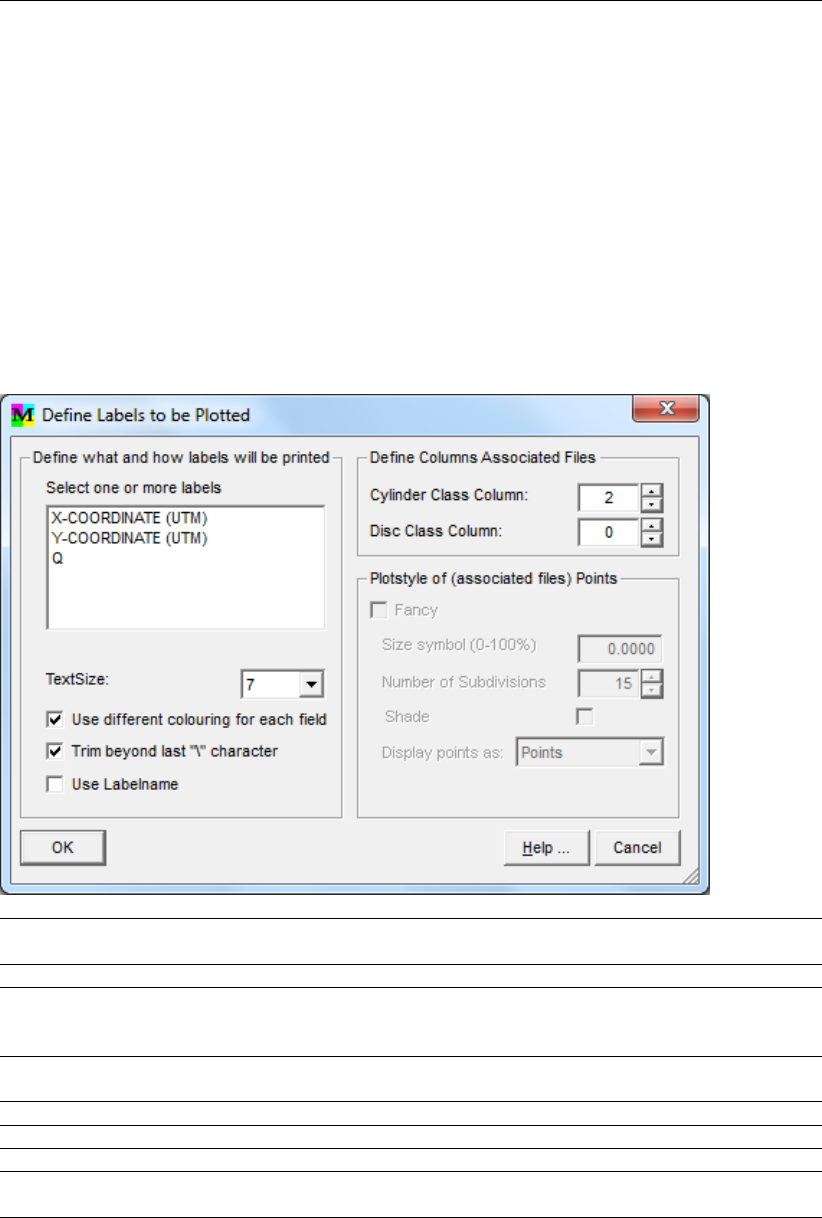
DRAFT
Map Menu options
6.8.2 IPF Labels
WHY?
The attributes of point data are displayed as labels.
WHAT?
At the location of each point one or more labels can be displayed.
HOW?
Choose the option Define Labels to be Plotted from the IPF Configure window to display the
following window.
Define Labels to be Plotted window:
Select one or
more labels
Select one of more labels from the menu to display near the point of the IPF
file.
TextSize Select one of the available textsizes from the dropdown menu.
Use different
colouring for each
field
Select this option to use different colour for each attribute value. Uncheck this
option to use a white fill for each label.
Trim beyond last
“\”character
Select this option to trim the attribute value beyond the last “\”character, so
the attribute value boreholes\east\NH45 will be displayed as NH45.
Use Labelname Select this option to display the label name and the label value.
OK Click this button to close the Define Labels to be Plotted window.
Help. . . Click this button to start the iMOD Help Functionality.
Cancel Click this button to cancel the chosen definition and to close the Define Labels
to be Plotted window.
Deltares 143 of 812
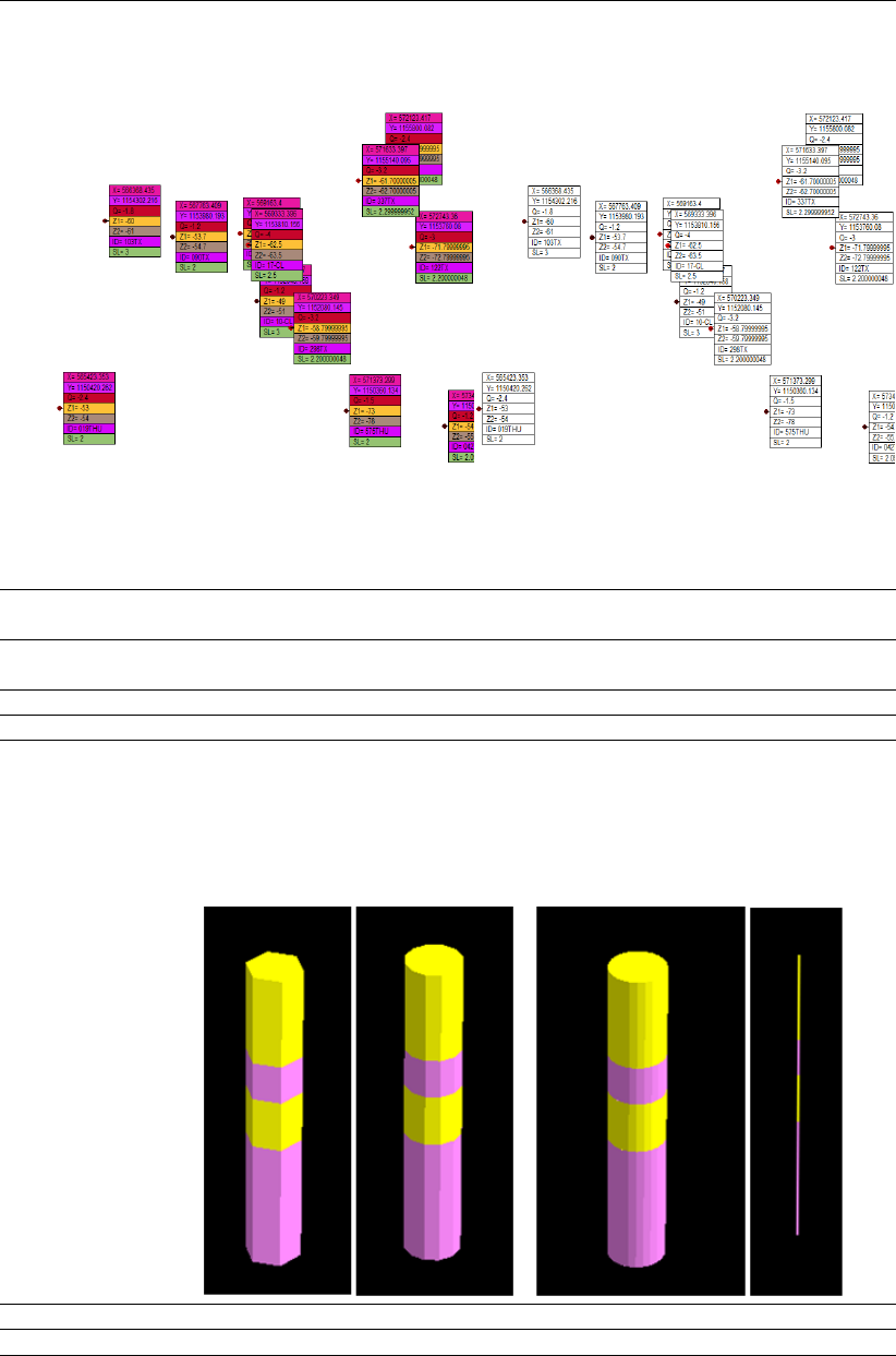
DRAFT
iMOD, User Manual
Example of the usage of different colouring for attribute fields:
The following options are available from the 3D Tool only:
Cylinder Class
Column
Enter the number of the column in the associated files that need to be used
for the size of the cylinders plotted for the boreholes.
Disc Class
Columns
Enter the number of the column in the associated files that need to be used
for the vertical location of a disc around a borehole
Fancy Check this item to improve the display of a borehole.
Size Symbol Enter a value to increase the size of the borehole
Number of subdi-
visions
Enter a number of subdivisions to be used to display a borehole. A large
number of
subdivisions will improve the appearance.
Examples of a fancy (first three on the left) display with different num-
ber of subdivisions and a non-fancy appearance (utmost right):
Shade Check this item to apply a shade on the boreholes.
Display points as: Choose one of the options: Points, lines, silhouette, fill
144 of 812 Deltares
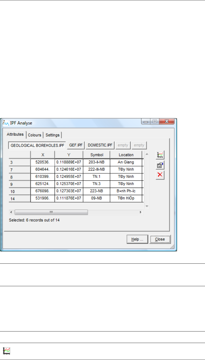
DRAFT
Map Menu options
6.8.3 IPF Analyse
WHY?
The attribute and time series data of selected point data are displayed interactively.
WHAT?
The IPF Analyse function is used primarily to display the timeserie data of selected point
locations in a graph on the map or separately.
HOW?
To display the IPF Analyse window, click the Map option from the main menu, then the option
IPF-options and then the option IPF Analyse (this is similar from the popup menu that displays
whenever you click your right mouse button on the graphical window). The selected IPF-file(s)
from the iMOD Manager will be used in the IPF Analyse window.
IPF Analyse window, Attributes tab:
Geological-
boreholes.ipf,
Gef.ipf,
Domestic.ipf
These buttons show the IPF-files that are currently available in IPF Analyse.
It is possible to select maximal 5 IPF-files before entering the IPF Analyse
window. iMOD will switch to the correct tab if points are selected from other
IPF-file(s).
Table The table shows all attributes for the IPF-file, in this case 5 attributes are avail-
able (X, Y, Symbol, Location, FinalDepth). To add a point to the selection,
left-click the mouse button at the location of the desired point in the graphical
window. The cursor of the mouse will show a “plus”- or “minus”-sign to indi-
cate whether you add or delete the current location to/from the selection. All
selected points will appear on the graphical window as a small red cross. The
first column in the table shows the record number, i.e. the row number in the
data field of the IPF-file.
Selected 6 records
out of 95
This shows the current number of selected point in the table.
IPF Figure
Click this button to display the content of the associated files for the selected
point in the IPF Analyse Plot window.
Deltares 145 of 812
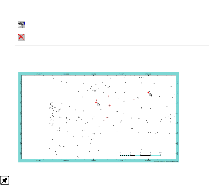
DRAFT
iMOD, User Manual
Properties
Click this button to display theIPF Configure window.
Delete
Click this button to remove the selected row from the selection displayed in
the table.
Help. . . Click this button to start the iMOD Help Functionality.
Close Click this button to close the IPF Analyse window.
Example of selected points in IPF Analyse:
Note: Only 50 records can be displayed in each table. However, more records can be
selected, but they will not appear in the table.
146 of 812 Deltares
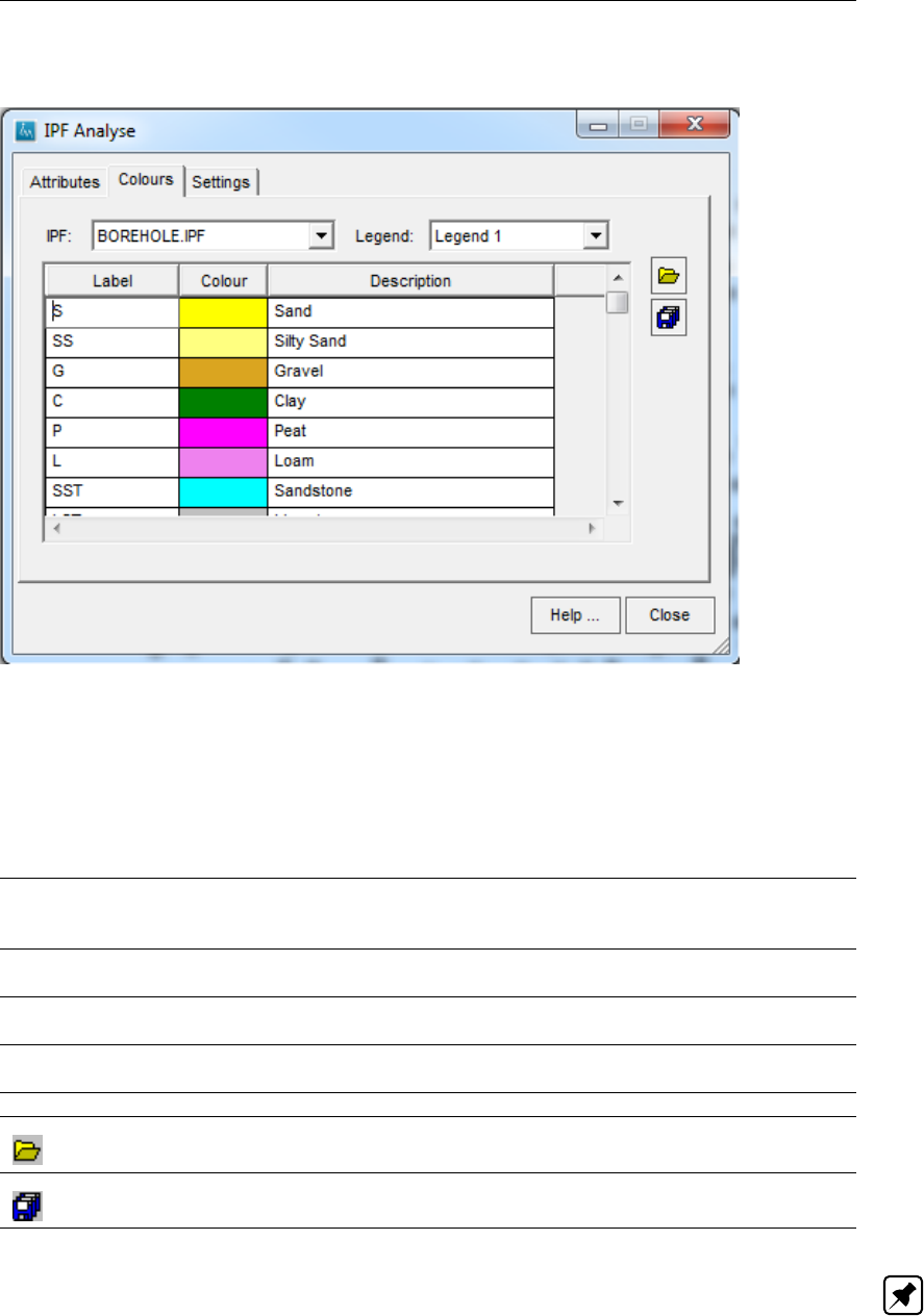
DRAFT
Map Menu options
IPF Analyse window, Colours tab:
The Colours tab is only used when IPF-file(s) are selected that contain associated files that
describe borehole information. The settings from the Colours tab will be used to colour the
individual zones in the boreholes. The chosen and/or defined legend(s) will be saved in the
IMF-file for later use. The next time you enter the IPF Analyse window the same legends will
appear.
IPF: This dropdown menu shows the IPF-files that are currently available in the IPF Anal-
yse. For each IPF-file a different legend can be defined by making use of the Legend:
dropdown menu.
Legend: This dropdown menu allows you to select and/or define a different legend per avail-
able IPF-file.
Label Enter the label that matches the second field (column) in the associated file that
contain borehole information.
Color Displays the colour of the field. You can specify a different colour by selecting the
Color column for the appropriate row. The default Colour window will appear.
Description Enter a descriptive string that will be used in the display of the legend.
Open
Click this button to open a *.DLF file that describes the colouring info.
SaveAs
Click this button to save the current colouring information to a *.DLF-file.
Note: On default the file {USER}\SETTINGS\DRILL.DLF will be used.
Deltares 147 of 812
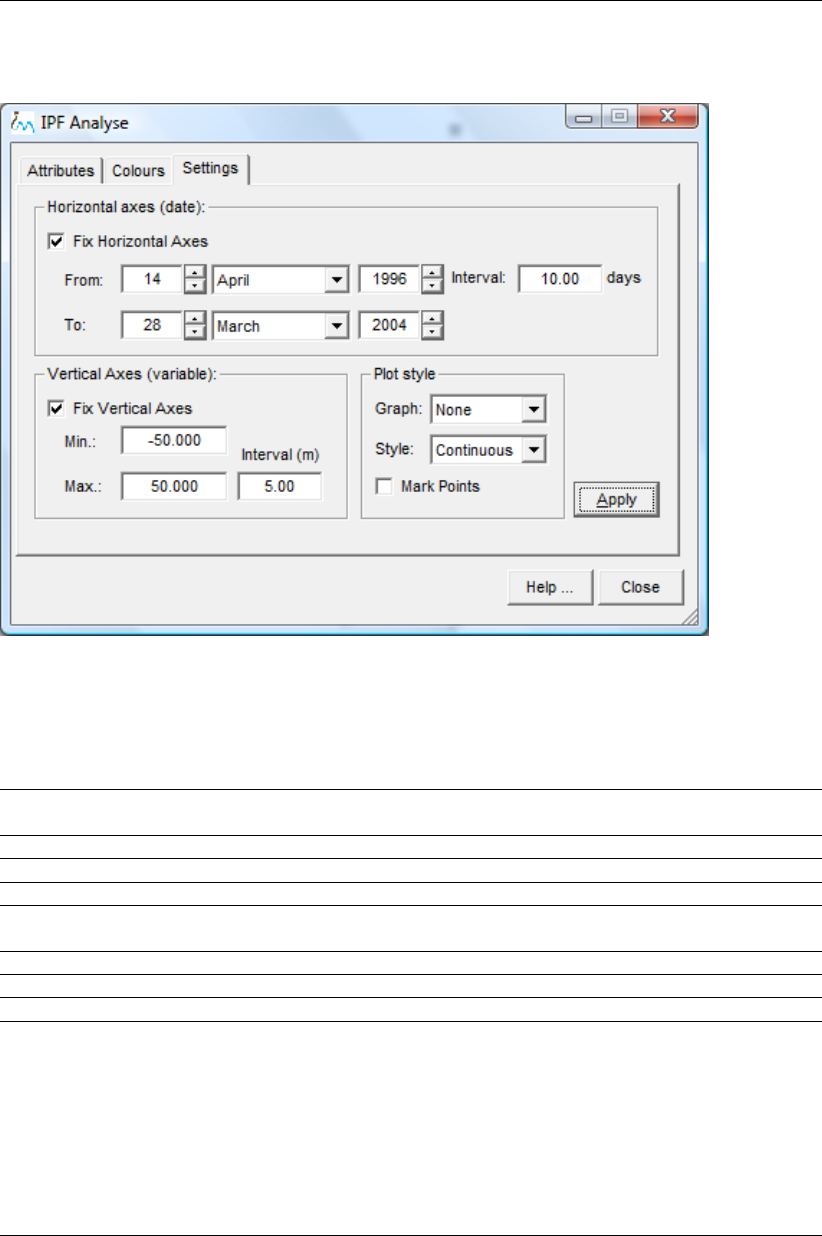
DRAFT
iMOD, User Manual
IPF Analyse window, Settings tab:
The Settings tab is only used when IPF-file(s) are selected that contain associated files that
describe timeseries information. The settings from the Settings tab will be used to plot the
individual timeseries that are associated with the selected points.
Fix Horizontal Axis Select this checkbox to specify the dimensions of the X-axis. Whenever uns-
elected, iMOD will determine the dimensions of the X-axis automatically.
From: Enter the start date for the X-axis.
Interval: Enter the interval of the X-axis in days.
To: Enter the end date for the X-axis.
Fix Vertical Axes Select this checkbox to specify the dimensions of the Y-axis. Whenever unse-
lected, iMOD will determine the dimensions of the Y-axis automatically.
Min.: Enter the minimum value for the Y-axis.
Max.: Enter the maximum value for the Y-axis.
Interval (m): Enter the interval of the Y-axis in meters.
Graph: Select one of the following options:
None:
No timeserie will be plotted at the selected points;
Simple:
A simple timeserie-graph will be plotted at the selected points, without any
axes;
Extended:
A timeserie-graph will be plotted at the selected points with x- and y-axes.
148 of 812 Deltares
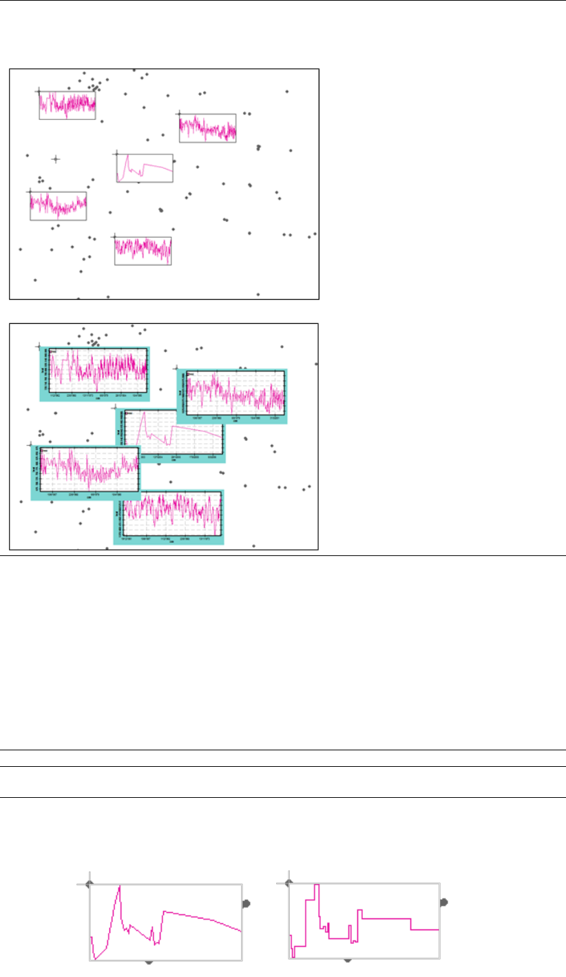
DRAFT
Map Menu options
Example of the plotstyle Simple (top) and Extended (bottom)
Style: Select one of the following options:
Continuous:
The individual data points in the timeseries will be connected directly from
one point to the other. This assumes that the intermediate unknown data
points will be on a straight line between the two known data points. e.g.
use this option to display timeseries of groundwaterhead;
Blocked:
The individual data points in the timeseries will be connected as horizontal
line. This assumes that the intermediate unknown data points will have
the same value as the previous known data point. e.g. use this option to
display timeseries of extraction rates.
Mark Points Select this checkbox to place markers (cross) at the location of data points.
Apply Select this button to apply the settings to the data points selected in the table
on the Attributes tab.
Example of Continuous (left) and Blocked (right) lines:
Deltares 149 of 812
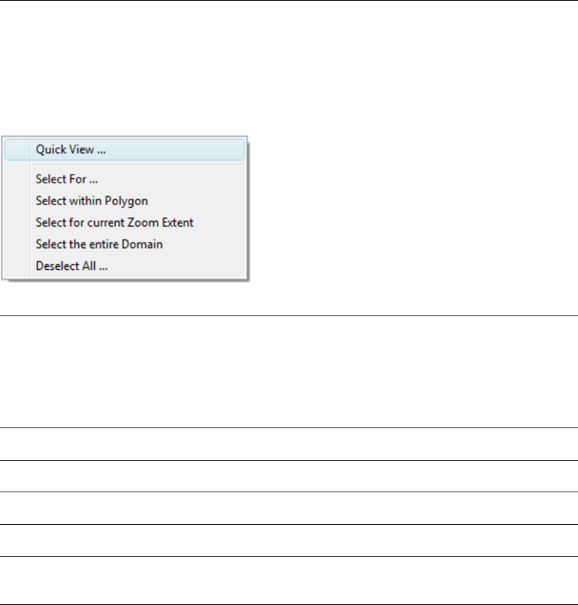
DRAFT
iMOD, User Manual
6.8.3.1 Drop down menu
Click the right mouse button on the graphical display to show the following option.
Drop down menu IPF Analyse:
Quick View . . . Select this option to display the IPF Analyse Figure window. The content of
the IPF Analyse Figure window will change whenever you select a different
data point with the mouse. Whenever you click the left-mouse button, the
current location remains unchanged and you can use the IPF Analyse Figure
window. If you click the left-mouse button again on the graphical display, the
current location changes again according your mouse position. Use the right
mouse button to stop Quick View.
Select For . . . Select this option to display the Select For window to select data points that
meet a specific criteria.
Select within
Polygon
Select this option to draw a polygon on the graphical display, to select all data
points that are inside that polygon.
Select for current
Zoom Extent
Select this option to select all data points present in the current zoom extent.
Select the entire
Domain
Select this option to select all data points from the current IPF.
Deselect All . . . Select this option to delete all selected data points from the table in the At-
tributes tab on the IPF Analyse window. You will be asked to confirm this
operation beforehand.
150 of 812 Deltares
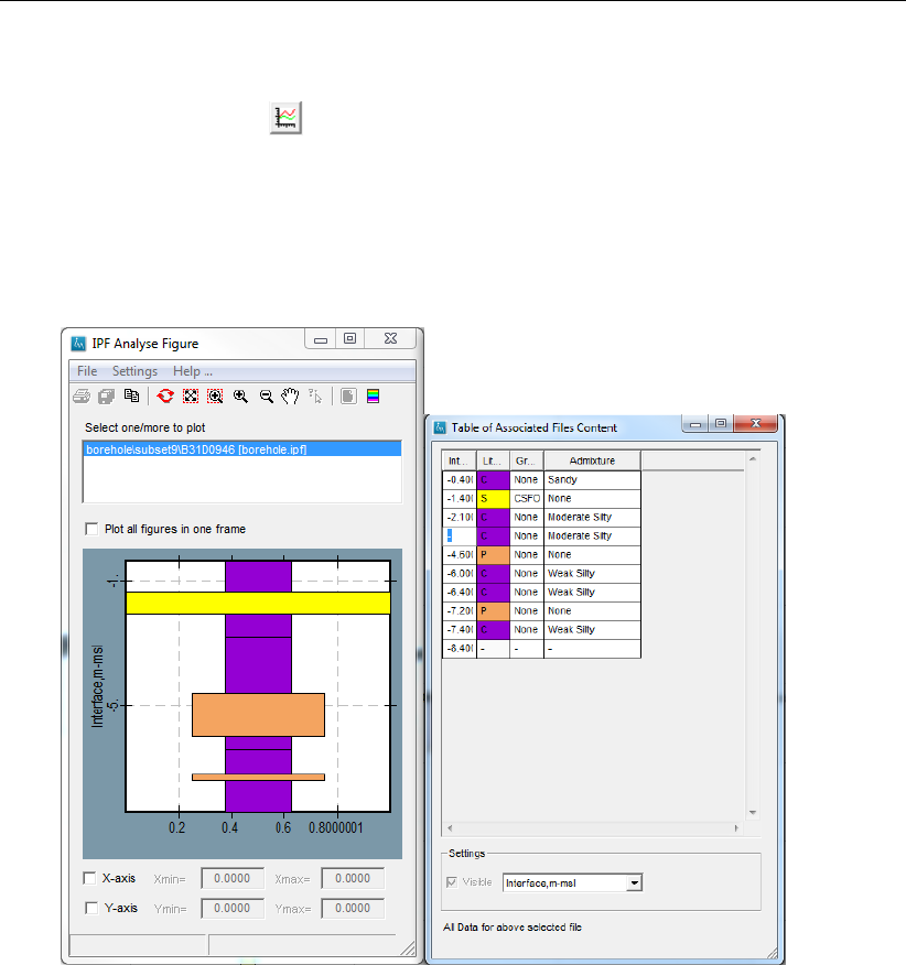
DRAFT
Map Menu options
6.8.3.2 IPF Analyse Figure
Click the option IPF Figure from the IPF Analyse window to start the IPF Analyse Figure
window. By moving with your cursor over the boreholes you are able to navigate through the
characteristics of the boreholes. Depending on the position of the cursor on the borehole, the
specific layer will be highligthed in the Table of Associated Files Content (see figures below).
Example 1: Borehole (IPF option=2) representation
IPF Analyse Figure window: Table of Associated File Content
Deltares 151 of 812
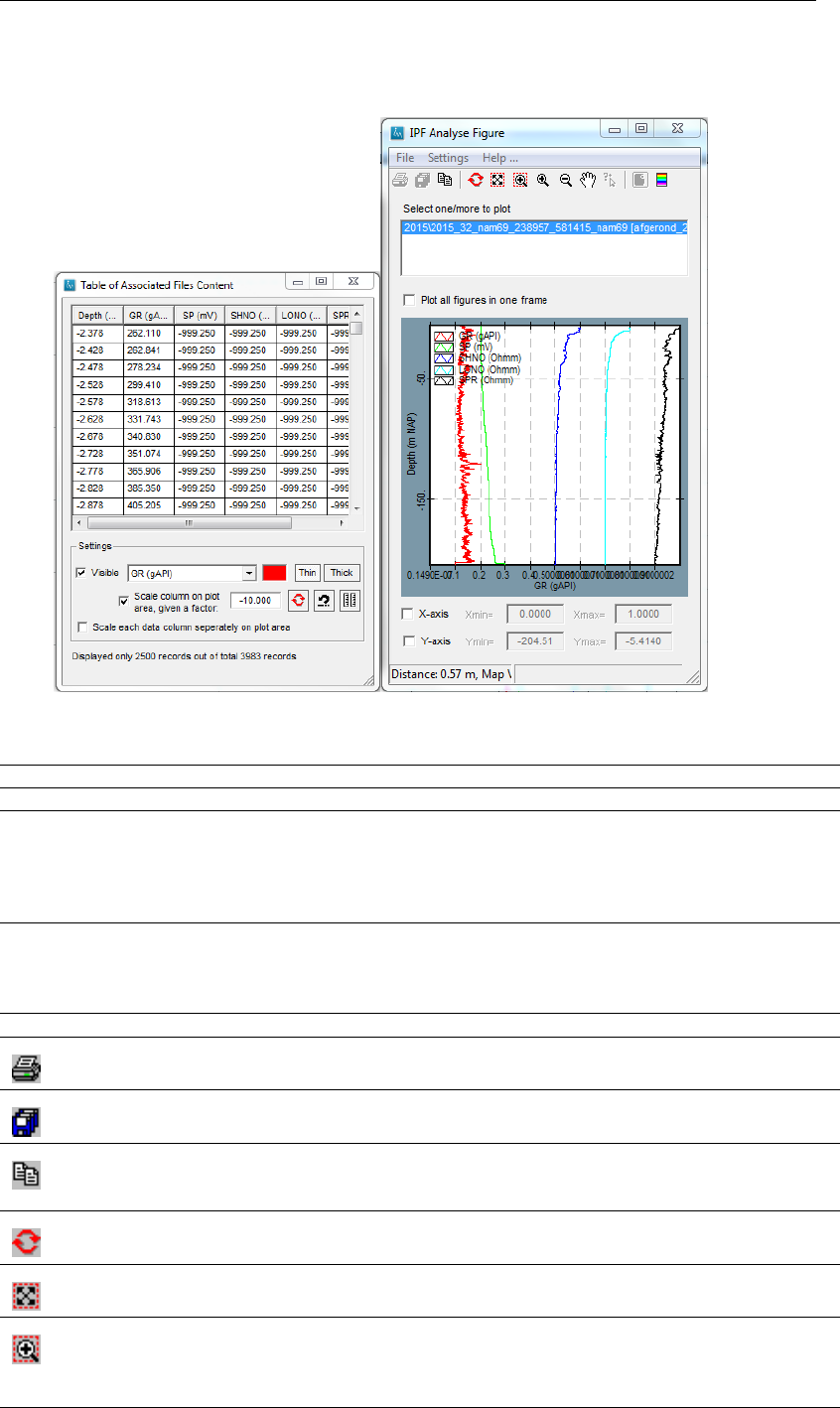
DRAFT
iMOD, User Manual
Example 2: Well locs (IPF option=3) representation
IPF Analyse Figure window: Table of Associated File Content
File – Print Print the selected figure to the default Windows external Printer.
File – Quit Click this option to close the IPF Analyse Figure window.
Settings –
Continuous Lines
Click this option to display timeseries as continuous lines. The individual data
points in the timeseries will be connected directly from one point to the other.
This assumes that the intermediate unknown data points will be on a straight
line between the two known data points. e.g. use this option to display time-
series of groundwaterhead.
Settings –
Block Lines
Click this option to display timeseries as block lines. The individual data points
in the timeseries will be connected as horizontal line. This assumes that the
intermediate unknown data points will have the same value as the previous
known data point. e.g. use this option to display timeseries of extraction rates.
Help . . . Click this button to start the iMOD Help Functionality.
Print
Click this icon to print the current Graph(s) to a printer.
Export
Click this icon to export the current Graph(s) to an ASCII-file (*.csv).
Copy to Clipboard
Click this icon to copy the current Graph(s) to the windows Clipboard. Use the
shortcut Ctrl-C , alternatively
Redraw
Click this button to redraw to the graphical content.
Zoom Full
Click this button to zoom to the entire extent of the Graph(s).
Zoom Rectangle
Click this button to zoom in for a rectangle. Use the left-mouse button to
determine the lower-left corner of the rectangle, click again for the upper-right
corner (or vice-versa). All graphs will be adjusted accordingly.
152 of 812 Deltares
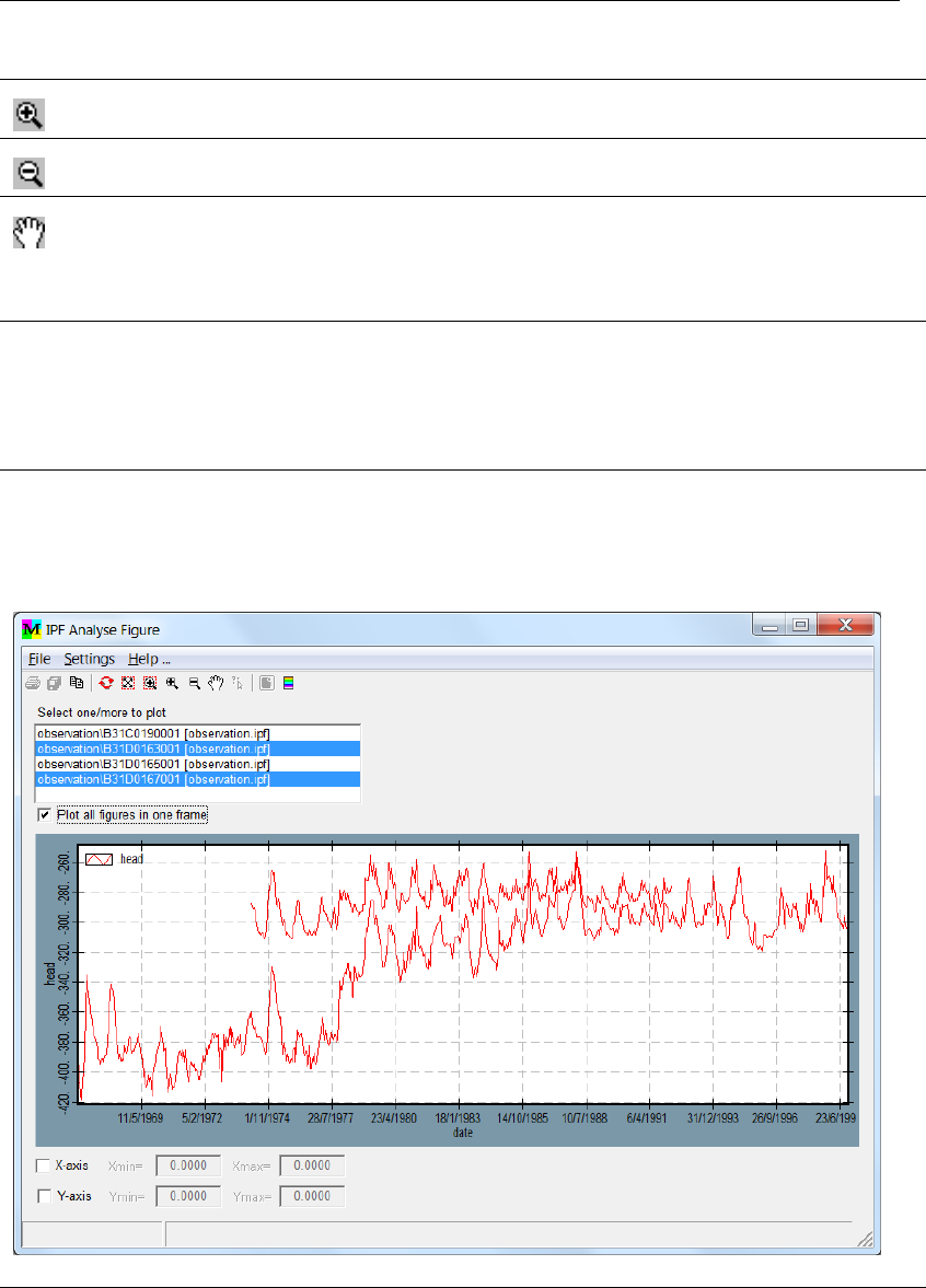
DRAFT
Map Menu options
Zoom In
Click this button to zoom IN on the centre of the current Graph(s).
Zoom Out
Click this button to zoom OUT on the centre of the current Graph(s).
Move
Click this button to move the current Graph(s). Click the left-mouse button
on that location where you want to move from, repeat this after the display
has been refreshed (automatically). Use the right mouse button to stop the
moving process.
All data for above
selected file
The maximal number of records that can be displayed in the table is 500.
Whenever, more data is found in the associated file, iMOD will display this
warning (e.g. displayed only
500 out of total
812 record) and will not present data that exceeds the number of 500 records.
However, they will be presented in the graph.
Select one/more
to plot
Select one or more of the listed files to plot. For each file that is selected, a
new graph will be displayed.
Example of two timeseries displayed:
Plot all figures in
one frame
This option is available whenever more than one file is active in the IPF Anal-
yse Figure window. It allows you to combine the selected files in a single
graph.
Deltares 153 of 812
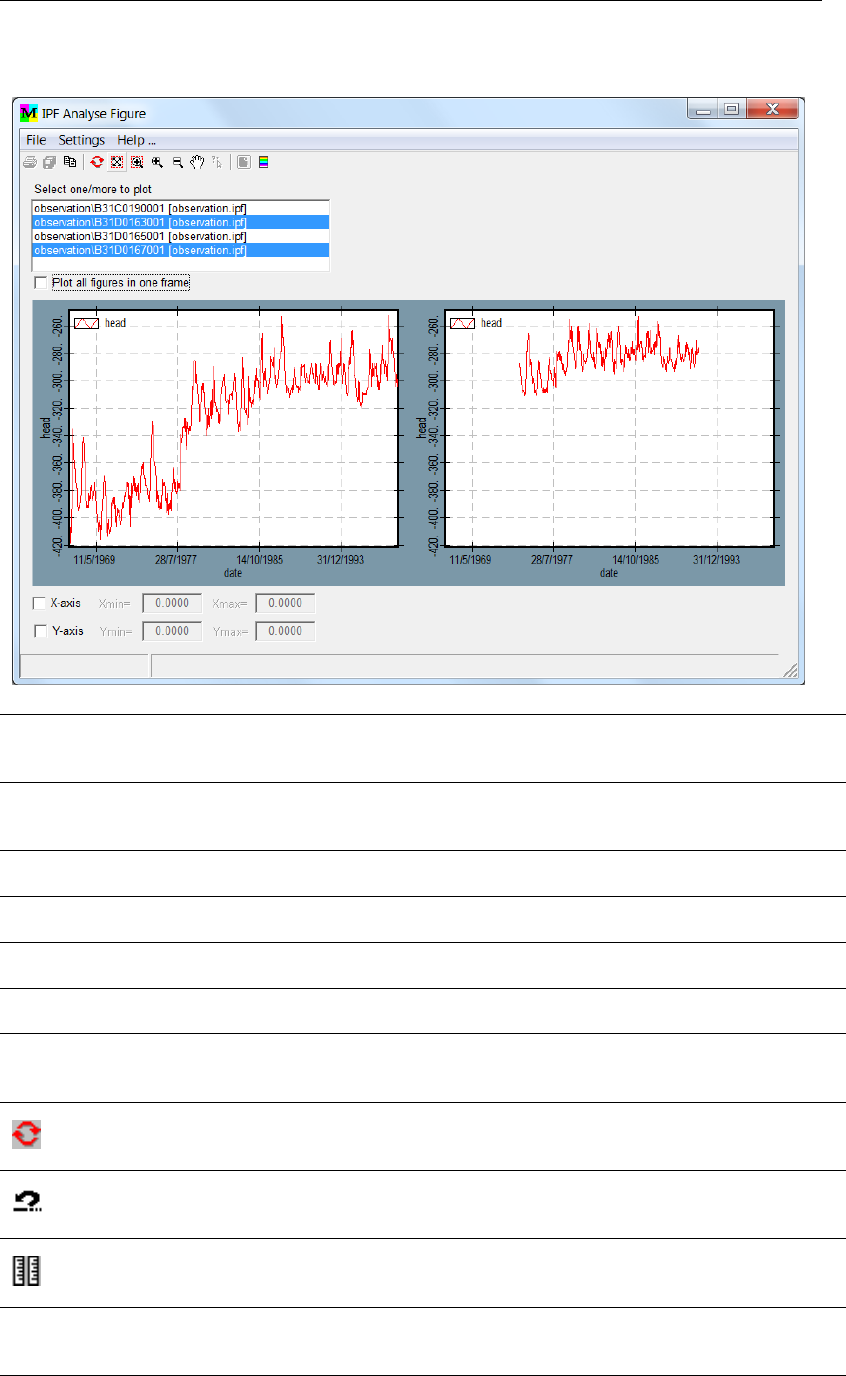
DRAFT
iMOD, User Manual
Example combining different files together in a single frame:
X-axis Select this option to specify the minimum and maximum values for the x-axis.
These values remain active for graphs that are plotted on the graphical canvas
as well as specified on the Settings tab on the IPF Analyse window.
Y-axis Select this option to specify the minimum and maximum values for the y-
axis.These values remain active for graphs that are plotted on the graphical
canvas as well as specified on the Settings tab on the IPF Analyse window.
Visible Select a attribute from the dropdown menu to adjust the plotting setting asso-
ciated with it.
Red colour
box
Click in this field to open a Window Colour Window in which a colour can be
depicted to be used for the selected field from the dropdown menu.
Thin Select this option at the Table of Associated Files Content window to apply a
thin line thickness.
Thick Select this option at the Table of Associated Files Content window to apply a
thick line thickness.
Scale column on
plot area, given a
factor:
Select this option to define the multiplication factor per data column selected
in the dropdown menu.
Update
Click on this button to update the IPF Analyse Figure plot window with the
defined factor(s).
Reset
Click on this button to reset all the defined factors (for all columns) to 1.0 and
refresh the IPF Analyse Figure plot window to the initial values.
Scale All
Click on this button to apply the defined factor to all columns at once and
refresh the IPF Analyse Figure plot window with the defined factor(s).
Scale each data
column seperately
on plot area
Select this option to plot each data column on a different x-axis next to the
previous data column. This can make it easier to analyze each data column
seperately. This option only works in case of cone penetration or well log data.
154 of 812 Deltares
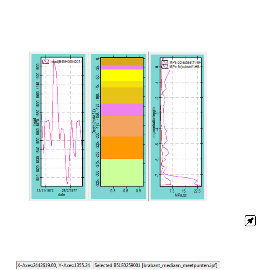
DRAFT
Map Menu options
It depends on the type of the selected associated files what kind of figure will be displayed.
Example of (left) timeseries, (middle) boreholes and (right) borelogs in an IPF Analyse Figure
window:
Note: Whenever you move the mouse in the graphical area, the coordinates of the current
graph will be displayed underneath. If more than one file is selected, the current selected
graph will be displayed too.
Example of display of the current position in the graph that shows the timeseries of B15E0259001:
Deltares 155 of 812
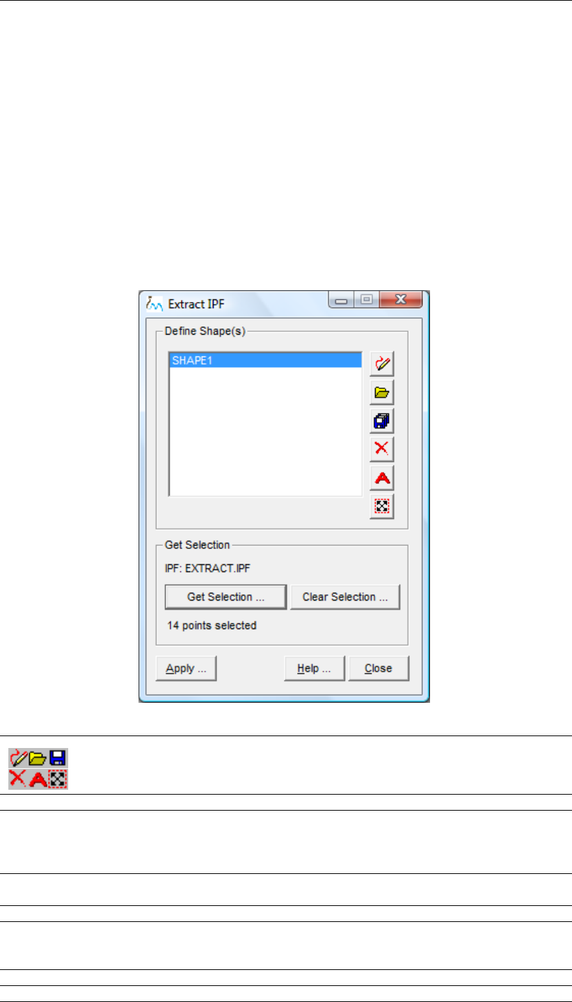
DRAFT
iMOD, User Manual
6.8.4 IPF Extract
WHY?
An IPF-file containing a subset of point data is extracted from an IPF-file.
WHAT?
A new IPF-file is created by selecting point locations from an existing IPF-file.
HOW?
Select a single IPF file in the iMOD Manager for which points need to be extracted and saved
in a new file. Select the option Map from the main menu, choose the option IPF-options and
then the option IPF Extract to display the IPF Extract window.
IPF Extract window:
Click these buttons to draw, open, save, delete or rename a shape. More
detailed information can be found in section 4.2
IPF: Displays the IPF filename selected in the iMOD Manager.
Get Selection ... Click this button to start the IPF Find window (section 6.8.5). Whenever you
have specified a polygon, bear in mind that only those points will remain that
are inside the selected polygons. All selected points will be marked by a red
cross.
Clear Selection ... Click this button to remove the current selection. You will be asked to confirm
this action.
14 points selected Shows the number of selected points.
Apply . . . Click this button to select a new IPF file to save the selected IPF points. If this
action is successfully, the IPF Extract window will close and the new created
IPF will be added to the iMOD Manager.
Help . . . Click this button to start the Help functionality.
Close Click this button to close the IPF Extract window.
156 of 812 Deltares
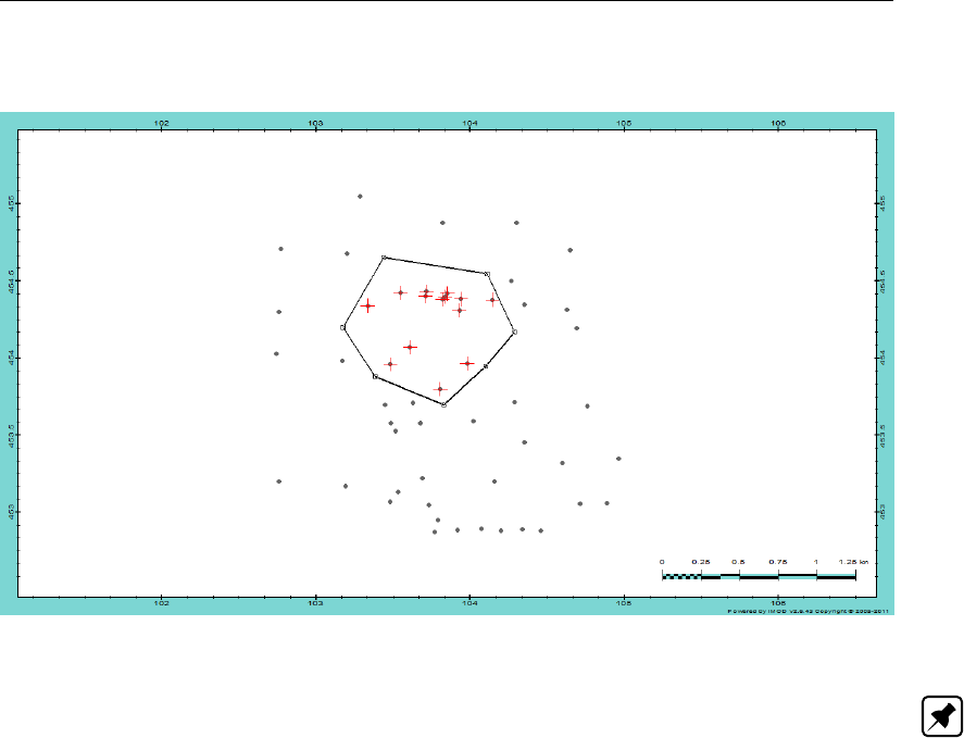
DRAFT
Map Menu options
Example of selected IPF Points:
Note: Associated files will be copied too. If the original IPF relates to a relative folder, e.g.
“asfiles\”, the new IPF will copy those associated files to a relative folder “asfiles\” below the
folder of the new IPF file.
6.8.5 IPF Find
WHY?
To create a new IPF-file by extracting points from an existing IPF-file.
WHAT?
The selection of point data is made inside an interactively defined rectangle or polygon using
a logical expression for numerical data or using a character expression for alphanumeric data.
HOW?
Select the option IPF Find from the Extract IPF window to start the IPF Find window.
Deltares 157 of 812
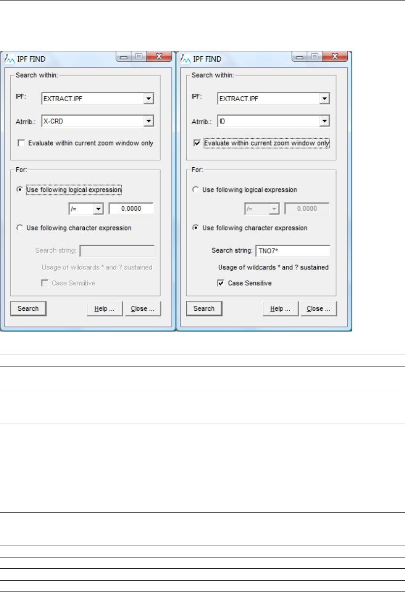
DRAFT
iMOD, User Manual
IPF Find window, (left) using a logical expression and (right) using a character expression:
IPF: Displays the active IPF file.
Attrib.: Select one of the attributes within the IPF file to be used for the selection of
points.
Evaluate within
current zoom
window only
Select this checkbox to force a search of points within the current zoom level
only.
Use following logi-
cal expression
Select this option to specify a logical operator and enter a numeric value to be
evaluated. Select one of the following expression (only for numeric values!):
<:Less than
<=: Less or equal to
=: Equal to
>:Greater than
>=: Greater or equal to
\=: Not equal to
Use following
character
expressions
Select this option to specify a search string, e.g. TNO7*. Use the character “*”
to identify that any character is valid and the “?” to denote that any character
is valid but for that number of positions equal to the number of “?”-marks.
Case sensitive Select this item to apply a case sensitive search on characters.
Search Click this button to start the search process.
Help . . . Click this button to start the Help functionality
Close Click this button to close the IPF Find window.
158 of 812 Deltares
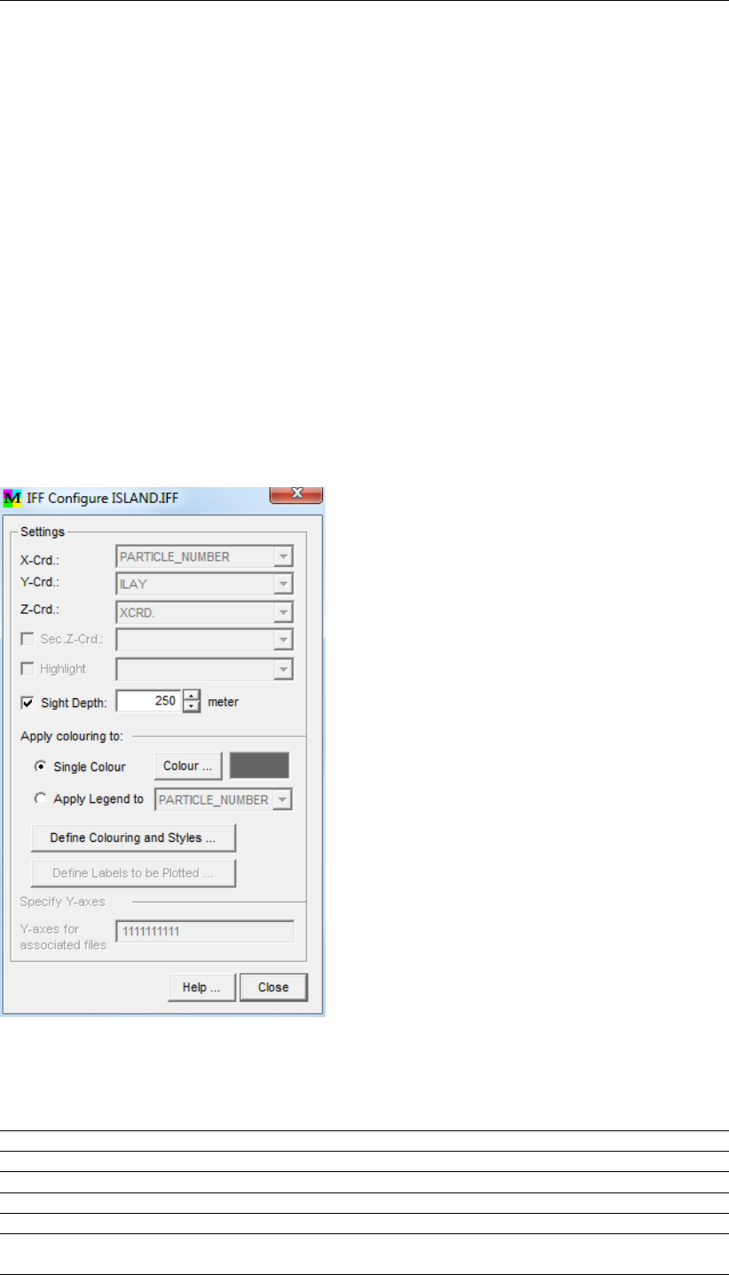
DRAFT
Map Menu options
6.9 IFF Options
6.9.1 IFF Configure
WHY?
IFF-files (iMOD Flowpath Files) in iMOD represent line data generated by the Pathline Simu-
lation function (see section 7.14). This function uses IMODPATH to compute flowlines based
on the budget terms that result from an iMODFLOW computation.
WHAT?
IFF Configure is used to define the settings for display and assigns a symbol, colour or label
to the flowlines. The options are similar to the IPF Configure function (see section 6.8.1).
HOW?
Select the menu option IFF Configure from the IFF-options menu in the Map menu to display
the IFF Configure window. Or, use right-click anywhere on the canvas to open the popup
menu. Select the option IFF-options and then choose IFF Configure.
IFF Configure window:
The IFF-configure window is comparable to the IPF-configure window (see section 6.8.1)
except that some functions are not active.
X-Crd.: Not active
Y-Crd.: Not active
Z-Crd.: Not active
Sec. Z-Crd.: Not active
Highlight Not active
Sight Depth Select and specify an interval in meters, over which points need to be dis-
played.
Deltares 159 of 812
DRAFT
iMOD, User Manual
Single Colour Select this option to display all points with the same colour.
Colour . . . Select this button to display the default Colour window in which a colour can
be specified. The current colour is displayed to the right of this button.
Apply Legend to Select this option to colour the lines according to the selected attribute that is
chosen in the dropdown menu at the right.
Define Colouring
and Styles. . .
Select this option to display the Lines and Symbols window, section 5.7.
Define Labels to
be Plotted
Not active
Y-axes for
associated files
Not active
Help. . . Click this button to start the iMOD Help Functionality (if available in the se-
lected *.PRF file).
Close Select this button to apply the settings and close the IPF Configure window.
160 of 812 Deltares
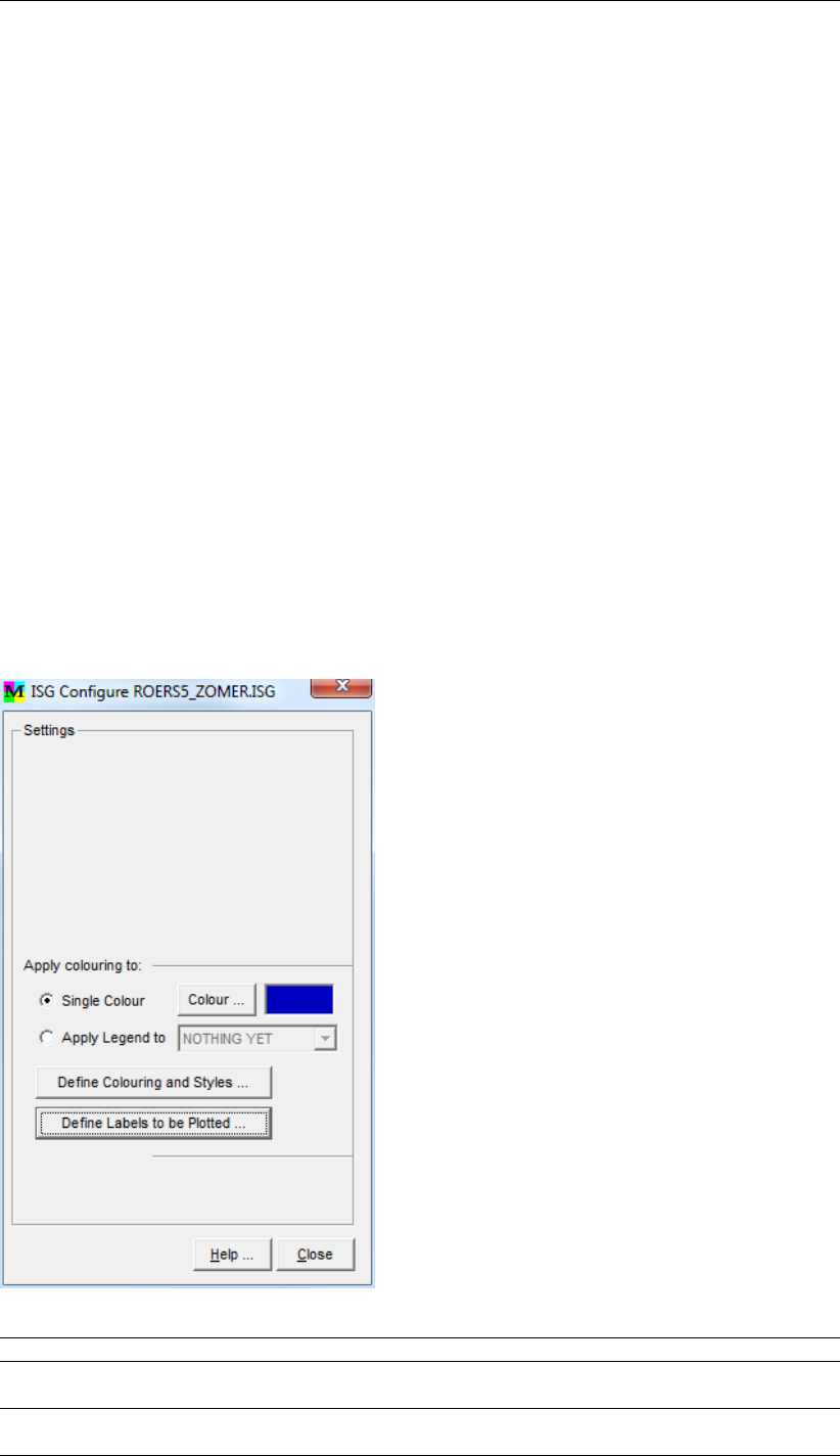
DRAFT
Map Menu options
6.10 ISG Options
ISG-files contain all necessary information to simulate a river segment, such as: location,
time dependent waterlevels, cross-sections, structures. iMOD supports functionalities that
manipulate these ISG-files:
ISG Configure,
ISG Edit, use this tool to analyse and/or adjust the content of the ISG-file.
ISG Show, specify what attribute need to be plotted.
6.10.1 ISG Configure
WHY?
ISG-files are used in iMOD to simulate the location of the surface water system.
WHAT?
ISG-files in iMOD represent line and point data that can be displayed in different ways.
HOW?
Select the menu option ISG Configure from the ISG-options menu in the Map menu to display
the ISG Configure window. Or, use right-click anywhere on the canvas to open the popup
menu. Select the option ISG-options and then choose ISG Configure.
ISG Configure window:
Settings Not yet implemented
Apply colouring to: The lines can be presented in a single colour or in different colours according
a defined legend
Single colour Select this option to display all lines with the same colour. The colour can be
changed by clicking the Colour . . . button.
Deltares 161 of 812

DRAFT
iMOD, User Manual
Apply legend to Not yet implemented
Define Colouring
and Styles. . .
Select this option to display the Define Colouring and Styles window
Define Labels to
be plotted
Select this button to display the Select Label to be Printed window.
Not yet implemented.
Help. . . Click this button to start the iMOD Help Functionality (if available in the se-
lected *.PRF file).
Close Select this button to apply the settings and close the IPF Configure window.
6.10.2 ISG Show
WHY?
To show the location of point data of ISG-files.
WHAT?
ISG-files contain six types of point data which are connected to the river segments: nodes,
segment nodes, cross-sections, calculation nodes, structures and QH-relationships.
HOW?
Select at least one ISG-file in the iMOD Manager and use the option Map from the main menu
(or right click your mouse on the graphical canvas), choose the option ISG-options, and then
ISG Show to list the following categories (see also next page)
Nodes
Check this item to display the FromNode (FN) and ToNode (TN) of the river segment
(symbol = rectangle) and their labels;
Segment Nodes
Check this item to display the nodes (symbol = solid circle) that define the river segment;
Calculation Nodes
Check this item to display the calculation nodes (symbol = square with a crossline) that
contain information on waterlevels, bottom levels, infiltration resistance and infiltration fac-
tors, all time dependent.
Cross-Sections
Check this item to display the cross-sections (symbol = polygon shape of cross-section)
that are available on the river segment containing information on the shape of the river
bed;
Structures
Check this item to display the locations (symbol = triangle) that contain information on
waterlevels before and after weirs/structures, both time dependent;
QHW-relationships
Check this item to display the nodes (symbol = square with two colours) with a discharge-
head relationship;
Flow Direction
Check this item to display the flow direction (symbol = arrow in the direction of the flow).
The flow direction is the order in which the coordinates for the segment are entered.
This can be changed by the Rotate-button on the Coordinates -tab on the ISG Attributes-
window.
Note: Colouring of all above mentioned attributes can be defined in the ISG Edit window.
162 of 812 Deltares
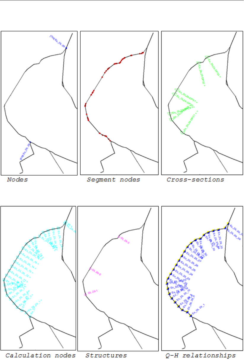
DRAFT
Map Menu options
Examples of the symbols used for all categories available in ISG-files:
Deltares 163 of 812
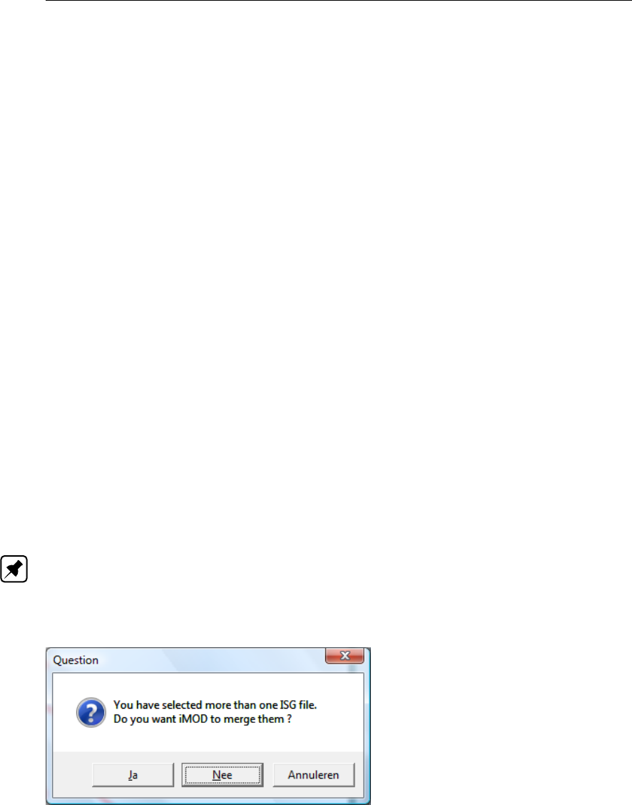
DRAFT
iMOD, User Manual
6.10.3 ISG Edit
WHY?
To add, delete or adjust interactively the line and point (attribute) data stored in an ISG-file.
WHAT?
The ISG Edit window has seven tabs:
Segments: to select one or more segments from the list; actions on the segments can be
executed, such as viewing in a profile or conversion to a raster;
Polygons: to define or load a polygon to use in the selection;
Attributes: to remove or adjust one or more of the attributes;
Calc. Points: to define the value to be adjusted of the attribute Calculation points; calcula-
tion points are the points on a segment where a water level is calculated;
Structures: to define the value to be adjusted of the attribute Structures; Structures are
the weirs on a segment where a (fixed) water level is maintained;
Cross-sections: to define the value to be adjusted of the attribute Cross-sections; Cross-
sections are the points on a segment where a cross-section is defined;
QWD relationships: to define the value to be adjusted of the attribute Q-Width-Depth
relationships; Q-Width-Depth relationships are the points on a segment where the relation
between the discharge and the width and depth of the water level is defined.
The bottom part of the ISG Edit window shows the display settings of the segment attributes.
HOW?
Select at least one ISG-file in the iMOD Manager and use the option Map from the main menu
(or right click your mouse on the graphical canvas), choose the option ISG-options, and then
ISG Edit to display the ISG Edit window.
Note: In case, more ISG-files are selected in the iMOD Manager, prior to starting the ISG
Edit option, iMOD will offer the possibility to merge all selected ISG-files into a single ISG-file.
Question window:
The example below shows how two different ISG-files would be merged into a single one.
164 of 812 Deltares
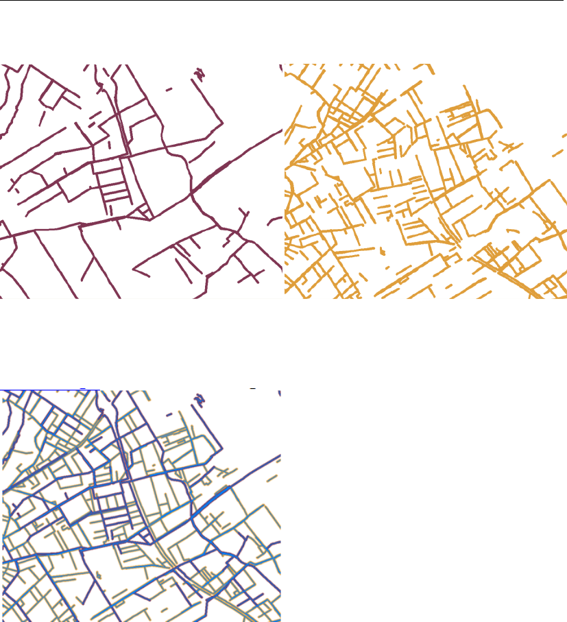
DRAFT
Map Menu options
Example of ISG’s of a primary and secondary surface water system
Example of an ISG capturing the combined primary and secondary surface water systems
Deltares 165 of 812
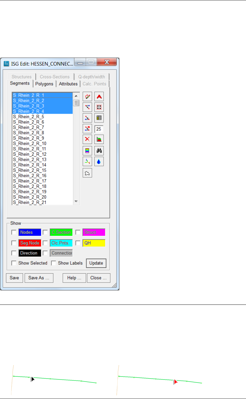
DRAFT
iMOD, User Manual
6.10.3.1 ISG Edit window, Segments tab:
Use this window to select segment for modification, create new segments, delete existing
segments and or start a variety of analyse functionalities, such as visuals of length-profiles,
colouring of attributes on segments, rasterize parameters and so on.
Segment
List
This list shows all the available river segments in the current opened ISG-file, e.g.
17.ISG. Select at least one river segment from the list to activate the Delete, Profile
and ZoomSelect options. Moreover, a segment can be selected on the graphical
canvas whenever the mouse is left-clicked near a Segment Node. A segment that is
selected will be presented as a green line and can be edited moving your mouse on
the line. Several options are available using the right-mouse button.
Example of a selected segment,
(left) moving an existing node, (right) adding a new node:
166 of 812 Deltares
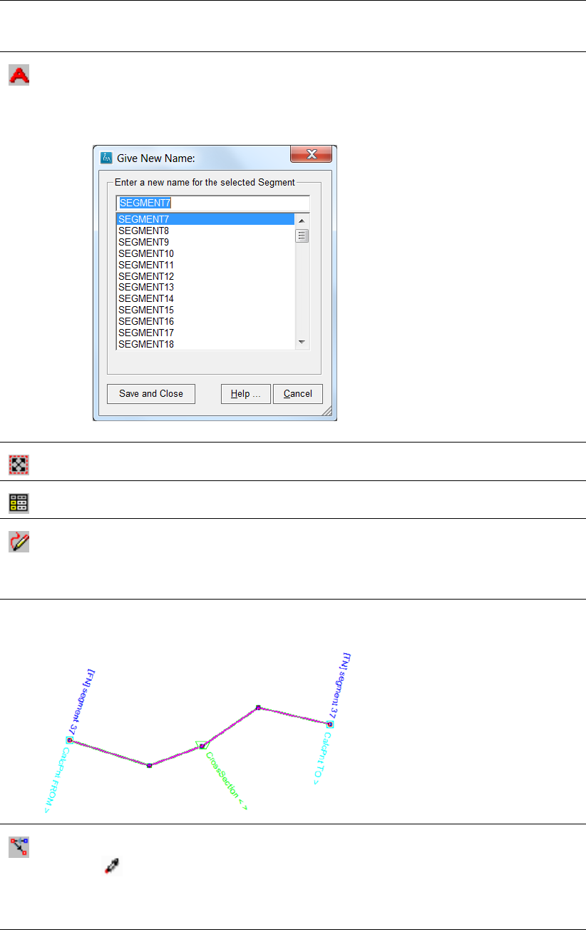
DRAFT
Map Menu options
Rename
Click this button the rename the selected segment point. The Give New Name:
window will appear.
Give New Name window:
ZoomSelect
Click this button to adjust the zoom level to fit the selected segments.
Attributes
Click this button to start the ISG Attributes window, see section 6.10.3.9.
DrawSegment
Click this button to start drawing a new segment. On default, the name of the segment
will be Segment{number}, it has two calculation nodes (one at the beginning and one
at the end, that are both compulsory) and a single cross-section in the middle (one
cross-section is compulsory for each segment).
Drawing a new segment:
Connect Upstream
Click this button to select the upstream segment interactively, a Pipet cursors appears
( ) and any segment that is near your mouse position will be highlighted. Use
your left mouse button to select the segment that need to be used from the upstream
segment. Remove an entered upstream by clicking next to any of the segments.
Terminate the selection process by the clicking the right or middle mouse button.
Deltares 167 of 812
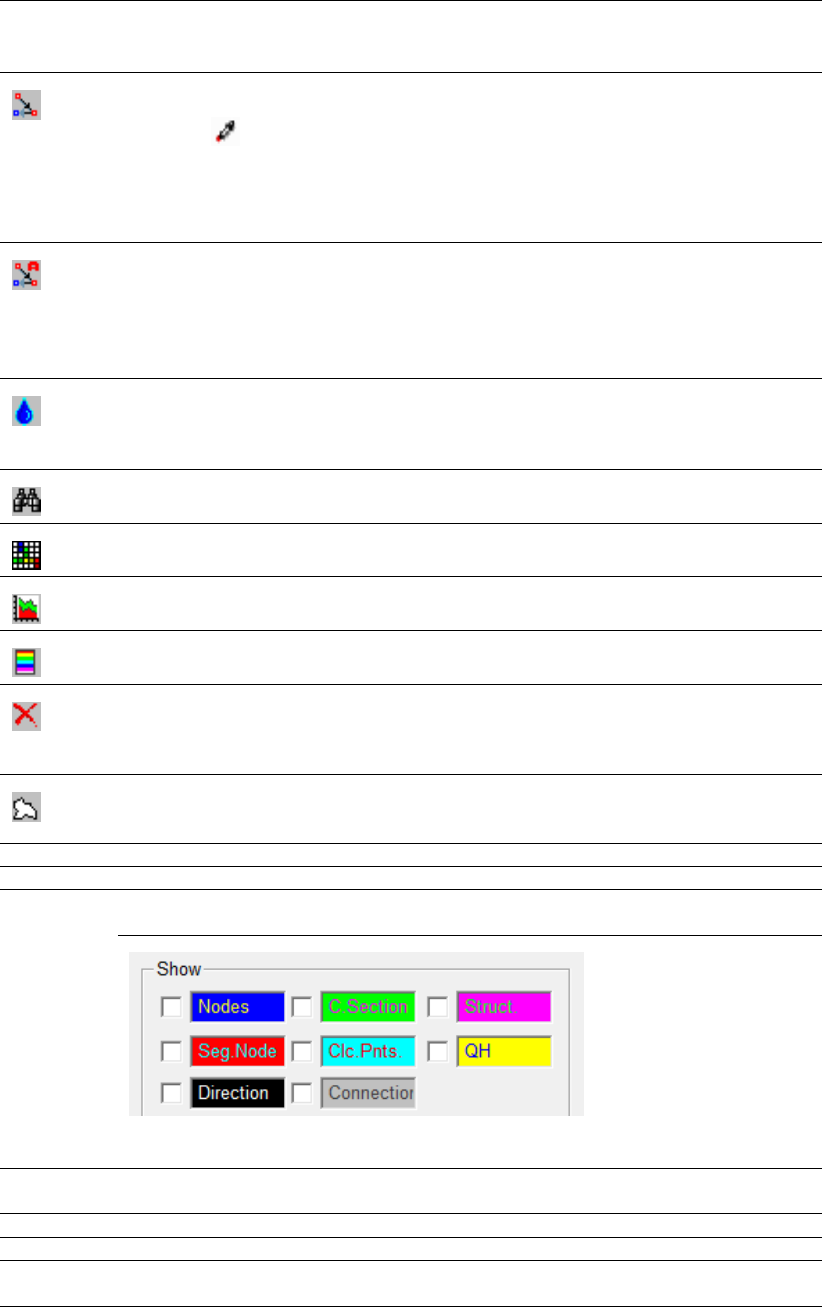
DRAFT
iMOD, User Manual
Connect Downstream
Click this button to select the downstream segment interactively, a Pipet cursors
appears ( ) and any segment that is near your mouse position will be highlighted.
Use your left mouse button to select the segment that need to be used from the
downstream segment. Remove an entered upstream by clicking next to any of the
segments. Terminate the selection process by the clicking the right or middle mouse
button.
AutoConnect Downstream
Click this button select the downstream segments, automatically. iMOD avoids any
recursive connections, so whenever the first point of a nearby segment is within the
selected distance (Snap Distance) but it connects (in)direct to the selected segment,
it is not used as a downstream segment. Eventually iMOD picks the nearest of all
suitable segment within the Snap Distance.
Drip
Click this button to select all connected, downstream segments from the selected
isg segments, automatically. iMOD select all connected segments from the initial
selected segment.
ISG Search
Click this button to start the ISG Search window, see section 6.10.3.11.
ISG-Rasterize
Click this button to start the ISG Rasterize window, see section 6.10.3.13.
Profile
Click this button to start the ISG Profile window, see section 6.10.3.12.
Legend
Click this button to start the ISG Legend window, see section 6.10.3.10.
Delete
Click this button to remove the selected river segment(s) from the current list of seg-
ments. You need to confirm this action. Unless the Save option is applied, the
segment is removed from memory only.
Select in Polygon
Click this button to draw a polygon and select all segment inside the polygon. If at
least one point of the segment falls within the polygon, the segment is selected.
Save Click this button to save the loaded ISG to disc, using the original ISG-filename.
SaveAs ... Click this button to save the loaded ISG by another filename.
Show
Labels
Click the checkboxes for the attributes to be plotted.
Click on the input field (Nodes, Seg.Nodes, C.Sections, Clc.Pnts, Struct, QH or Di-
rection) to start the default Colour window in which the colour can be changed.
Show
Selected
Check this checkbox to display the attributes as defined by Show for the selected
segment(s) only.
Update Click this button to redraw the ISG.
Help ... Click this button to start the Help functionality.
Close ... Click this button to close the ISG Edit window. Whether you‘ve changed the ISG or
not, you’ll be asked to confirm this.
168 of 812 Deltares
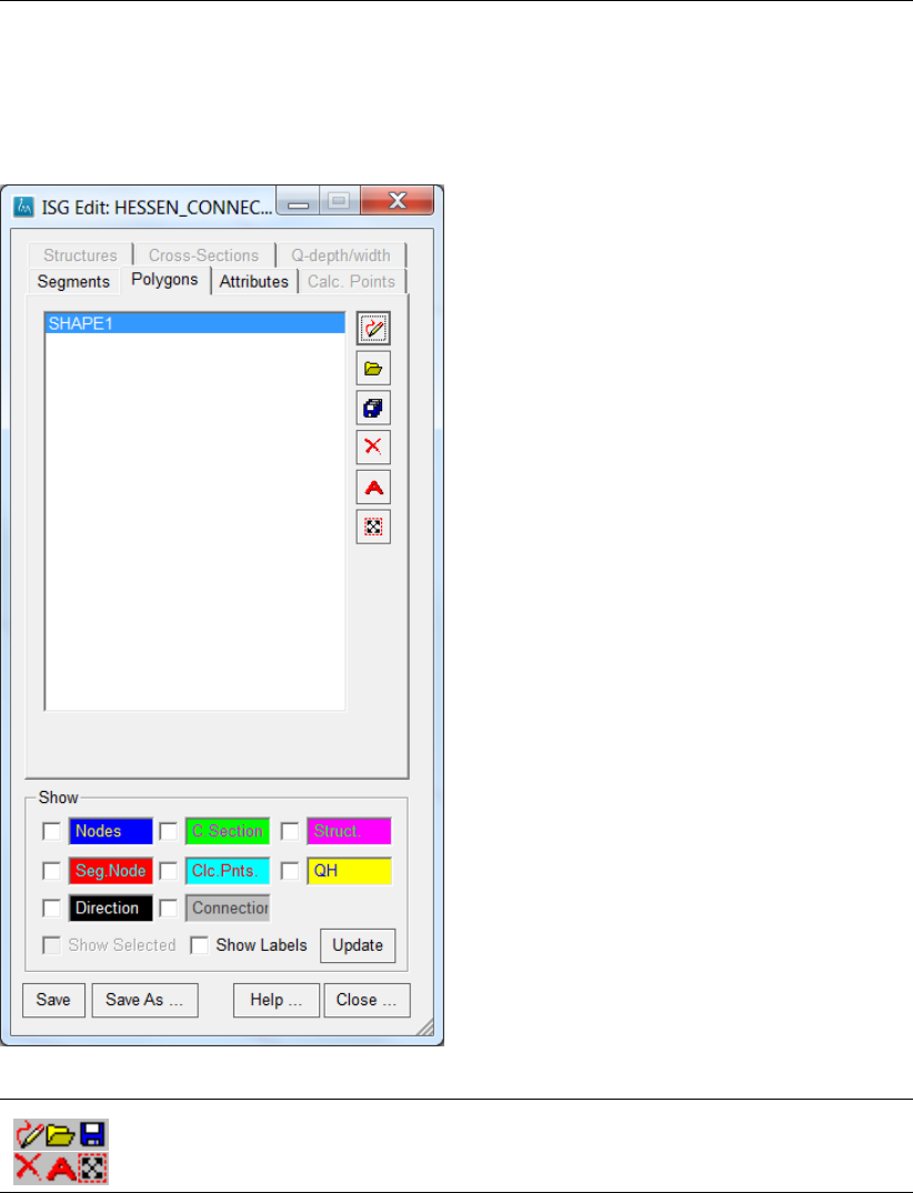
DRAFT
Map Menu options
6.10.3.2 ISG Edit window, Polygons tab:
Use this window to enter polygon(s) for which selection and modifications need to be carried
out for a variety of attributes of the ISG file.
Click one of these buttons to draw, open, save, delete, rename a shape and/or
zoom into the selected shape(s). More detailed information can be found in
section 4.2.
Deltares 169 of 812
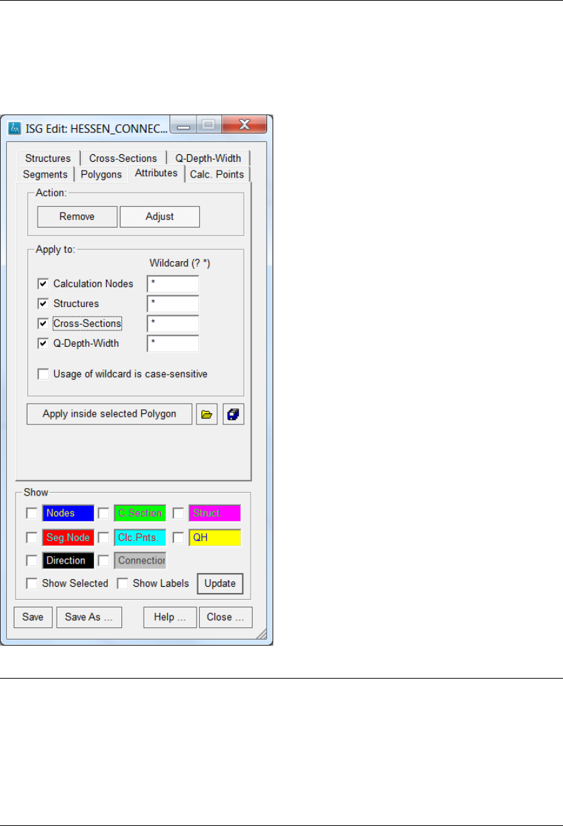
DRAFT
iMOD, User Manual
6.10.3.3 ISG Edit window, Attributes tab:
Use this window, to specify what attributes of the ISG file need to be modified and whether
this need to be done for selected segments or within the entered polygons.
Action Select the following options:
Remove:
Click this option to remove all selected attributes that match the given
search string;
Adjust:
Click this option to adjust all selected attributes to match the given search
string.
170 of 812 Deltares
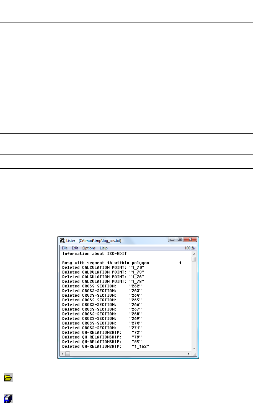
DRAFT
Map Menu options
Apply to Select the following options:
Calculation nodes:
Select this option to apply modification on attributes for calculation nodes,
such water levels, inflow, stream widths;
Structures:
Click this option to apply modification on attributes for structures, such as
up- and downstream water levels;
Cross-Sections:
Click this option to apply modification on attributes for cross-sections, such
as widths, depth, Manning’s coefficients;
Q-Depth-Width:
Click this option to apply modification on attributes for discharge-depth-
width relation ships, such as discharge, width and depth values.
The appropriate tabs (more than one if needed) become available depending
on the choice of your selection.
Wildcard (?*) Enter a search string; e.g. Test* selects all labels that start with Test and end
with anything; ??Test selects all labels that start with two characters followed
by Test only.
Usage of wildcard
is case-sensitive
Select this checkbox to evaluate the search string as case sensitive.
Apply inside
selected polygon
Select this button to apply the removal or adjustment to the loaded ISG-file.
Whenever at least one polygon is selected on the Polygons tab, the operation
will affect attributes inside those selected polygons. If no polygons are
selected, the operation will affect the selected segment on the Segments tab
only. Bear in mind that all these adjustments are stored in the loaded
ISG. A log file (LOG_SES.TXT) will be created and stored in the {user}\tmp
folder. This file shows all adjustments to the ISG-file.
An example of the LOG_SES.TXT file:
Open SES-file
Click this button to open a Segment Edit Settings *.SES file for a more detailed
description of this type of file see section 9.22.
Save SES-file
Click this button to save the current settings on the Attributes tab to a Segment
Edit Settings *.SES file. Whenever such a files has been saved, it can be used
via the iMOD Batch function ISGADJUST (see section 8.3.5).
Deltares 171 of 812
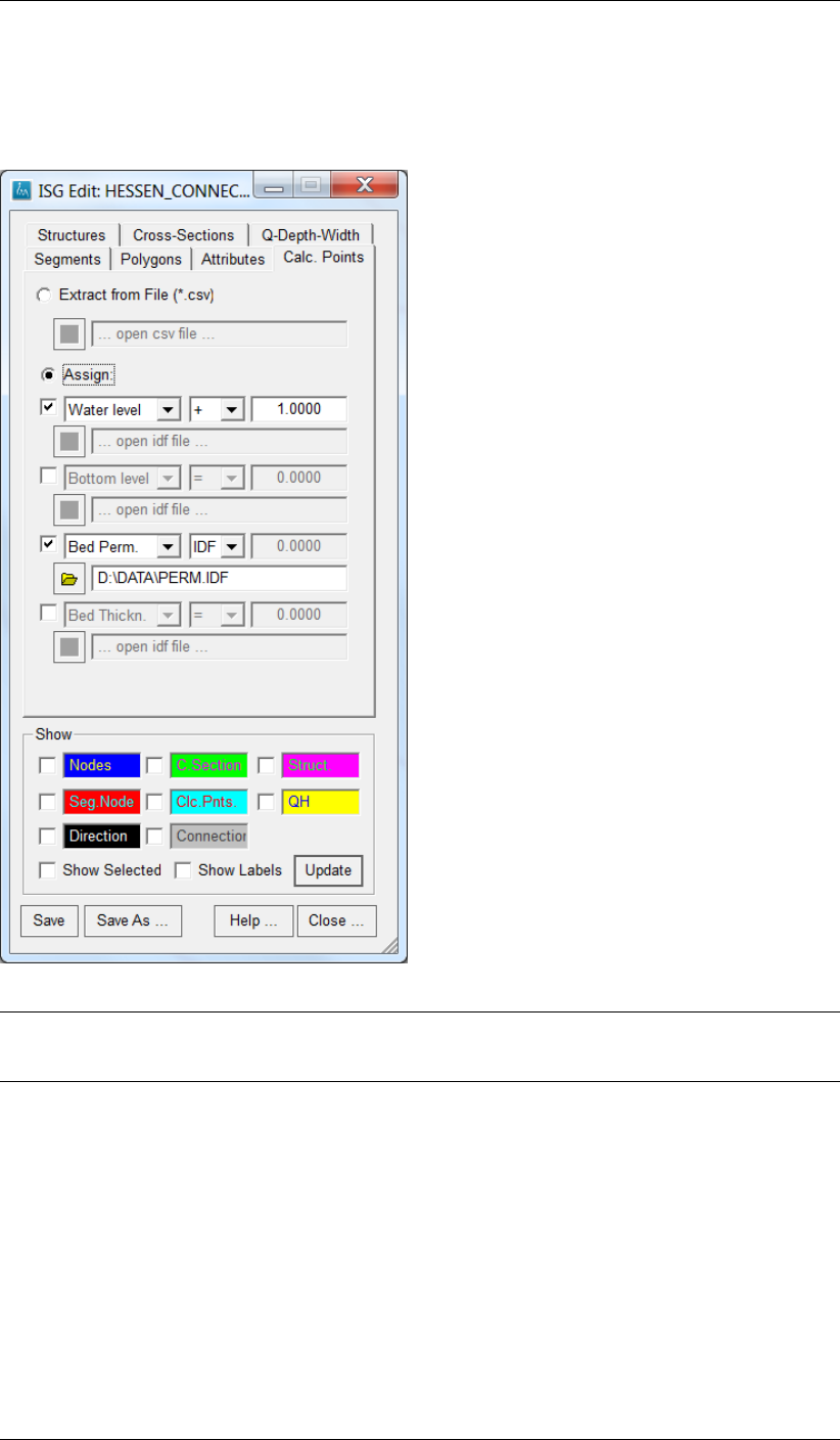
DRAFT
iMOD, User Manual
6.10.3.4 ISG Edit window, Calc. Points tab:
Use this window to specify what parameters need to be modified and how that need to be
carried out. A maximum of four multiply (duplicate) parameters can be applied.
Extract from File
(*.CSV)
Select this option to read adjustments for all variables from a CSV File (see
section 9.12). The list of parameters depends on the type of ISG (see sec-
tion 9.9.2)
Assign Select this option to specify adjustments for all variables separately.
Select the checkbox to activate a specific parameter. There is a maximum
of four (duplicate) attributes to be modified at the same time. The list of
parameters depends on the type of ISG (see section 9.9.2).
Specify the kind of adjustment that manipulates the selected variable. Choose
an operator from the dropdown menu:
Select “=” to use the entered value;
Select “+” to add the entered value;
Select “-” to subtract the entered value;
Select “/” to divide by the entered value;
Select “*” to multiply by the entered value;
Select “IDF” to sample a value out of the entered IDF-file at the location of
the calculation point.
172 of 812 Deltares
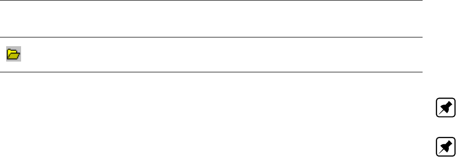
DRAFT
Map Menu options
Open IDF
Click this button to open an IDF-file. This becomes available whenever the
option “IDF” is selected from the dropdown menu for the type of operator.
Note: Adjustments to the number of calculation points can be made by the iMOD Batch
function ISGSIMPLIFY (see section 8.3.4).
Note: Adjustment to calculation points can be carried out by the iMOD Batch Function IS-
GADDSTAGES (see section 8.3.7). This function is suitable of modifying water levels in the
ISG via IPF files.
Deltares 173 of 812
DRAFT
iMOD, User Manual
6.10.3.5 ISG Edit window, Structures tab:
Use this tab to specify any adjustment for the up- and downstream water levels at structure,
these are simple weirs.
Extract from File
(*.CSV)
Select this option to read adjustments for all variables from a CSV File (see
section 9.12). The list of parameters is described in section 9.9.4.
Assign Select this option to specify adjustments for all variables separately.
Select the checkbox to activate a specific parameter (“Up Waterlevel” and
“Down Waterlevel”). There is a maximum of two (duplicate) attributes to be
modified at the same time.
Specify the kind of adjustment that manipulates the selected variable. Choose
an operator from the dropdown menu:
Select “=” to use the entered value;
Select “+” to add the entered value;
Select “-” to subtract the entered value;
Select “/” to divide by the entered value;
Select “*” to multiply by the entered value;
Select “IDF” to sample a value out of the entered IDF-file at the location of
the calculation point.
174 of 812 Deltares
DRAFT
Map Menu options
Open IDF
Click this button to open an IDF-file. This becomes available whenever the
option “IDF” is selected from the dropdown menu for the type of operator.
Deltares 175 of 812
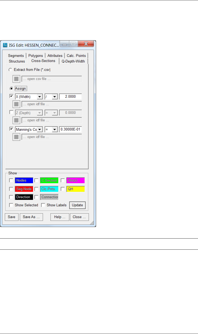
DRAFT
iMOD, User Manual
6.10.3.6 ISG Edit window, Cross-Sections tab:
Use this tab to specify the modification on parameters for cross-section, such as Width, Depth
and/or Manning’s coefficient (MRC).
Extract from File
(*.CSV)
Select this option to read adjustments for all variables from a CSV File (see
section 9.12). The list of parameters is described in section 9.9.3.
Assign Select this option to specify adjustments for all variables separately.
Select the checkbox to activate a specific parameter (“X (Width)” and “Z
(Depth)” and “Manning’s Coefficient”). There is a maximum of three (dupli-
cate) attributes to be modified at the same time.
Specify the kind of adjustment that manipulates the selected variable. Choose
an operator from the dropdown menu:
Select “=” to use the entered value;
Select “+” to add the entered value;
Select “-” to subtract the entered value;
Select “/” to divide by the entered value;
Select “*” to multiply by the entered value;
Select “IDF” to sample a value out of the entered IDF-file at the location of
the calculation point.
176 of 812 Deltares
DRAFT
Map Menu options
Open IDF
Click this button to open an IDF-file. This becomes available whenever the
option “IDF” is selected from the dropdown menu for the type of operator.
Note: Cross-sections can be added also by the iMOD Batch function ISGADDCROSSSEC-
TION (see section 8.3.3).
Deltares 177 of 812
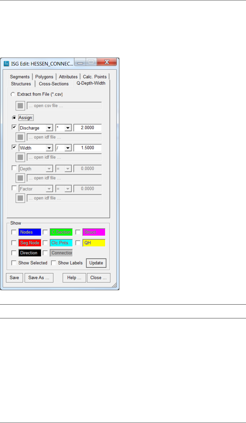
DRAFT
iMOD, User Manual
6.10.3.7 ISG Edit window, Q-Depth-Width tab:
Use this tab to specify the modification on parameters for the discharge (Q), -width (W) and
-depth (D) relation ships. These can be used for ISG files that are compliant to the SFR
packages, see section 9.9.
Extract from File
(*.CSV)
Select this option to read adjustments for all variables from a CSV File (see
section 9.12). The list of parameters is described in section 9.9.5.
Assign Select this option to specify adjustments for all variables separately.
Select the checkbox to activate a specific parameter (“Discharge”, “Width ”,
“Depth” and “Factor”. There is a maximum of four (duplicate) attributes to be
modified at the same time.
Specify the kind of adjustment that manipulates the selected variable. Choose
an operator from the dropdown menu:
Select “=” to use the entered value;
Select “+” to add the entered value;
Select “-” to subtract the entered value;
Select “/” to divide by the entered value;
Select “*” to multiply by the entered value;
Select “IDF” to sample a value out of the entered IDF-file at the location of
the calculation point.
178 of 812 Deltares
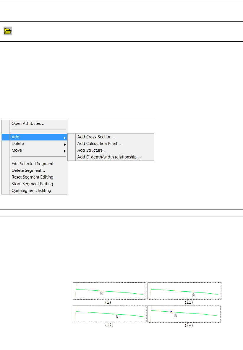
DRAFT
Map Menu options
Open IDF
Click this button to open an IDF-file. This becomes available whenever the
option “IDF” is selected from the dropdown menu for the type of operator.
6.10.3.8 Dropdown menu
Once you have selected a segment by either picking it in the menulist in the Segments tab on
the ISG Edit window, or alternatively by clicking your left mouse button at any segment node
on the graphical canvas, the following options will be available whenever you press the right
mouse button anywhere on the graphical canvas.
Dropdown menu:
Open Attributes . . . Click this button to start the ISG Attributes window.
Add Cross-Section
Add Calculation Point
Add Structure
Add Q-Depth-Width Rela-
tionship
Click this button to add a Cross-section, Calculation point, Structure
and/or Q-Depth-Width relationship to the selected segment. Click your
left mouse button to add the attribute along the selected segment;
depending on the type a icon will move along the segment. Click your
right mouse button to cancel the operation.
Example of adding different attributes to a segment, (i) cross-
section, (ii) calculation nodes, (iii) structure and (iv) Q-Depth-Width
relationship:
Bear in mind that you cannot add additional calculation point,
cross-sections whenever the ISG is compliant to SFR.
Deltares 179 of 812
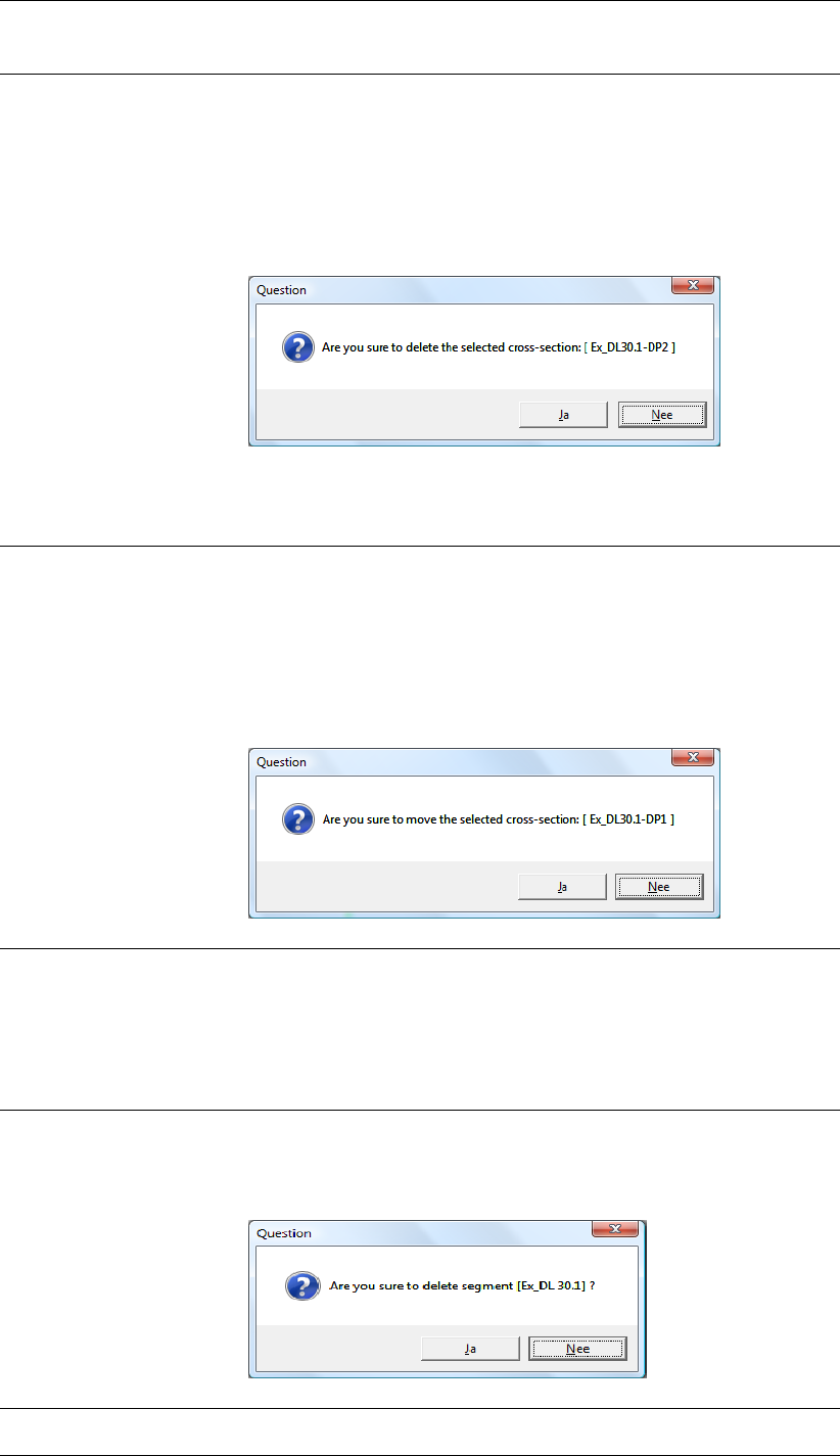
DRAFT
iMOD, User Manual
Delete Cross-Section
Delete Calculation Point
Delete Structure
Delete Q-Depth-Width
Relationship
Click this button to delete a Cross-section, Calculation point, Structure
and/or Q-Depth-Width relationship from the selected segment. Select
the feature by moving your mouse in the neighbourhood of the feature
and press the left mouse button. iMOD will select the feature that is
nearest to the current location of the mouse. You need to confirm any
delete action via a Question window:
Question window:
Bear in mind that the begin- and end calculation node may never
be deleted and a single cross-section is at least obligatory for each
segment.
Move Cross-Section
Move Calculation Point
Move Structure
Move Q-Depth-Width Re-
lationship
Click this button to move a Cross-section, Calculation point, Structure
and/or Q-Depth-Width relationship from the selected segment. Select
the feature by moving your mouse in the neighbourhood of the feature
and press the left mouse button. iMOD will select the feature that is
nearest to the current location of the mouse. You need to confirm any
move action.
Question window:
Start Segment Editing Click this item to start editing the layout of the segment. Whenever
in this mode, you can alter the location of each individual node of the
segment. The method is similar as used for altering nodes for poly-
gons, see section 4.5. Until you select the option Save ISG Editing all
modifications to the selected segment are not stored. You need to ac-
tively click the Save button on the ISG Edit window to save the modified
segment on disc.
Delete Segment . . . Click this item to delete the selected segment. You will be asked to
confirm this delete operation.
Question window:
Reset Segment Editing Click this item to restore the layout of the segment to that one prior to
the moment that the option Start ISG Editing was selected.
180 of 812 Deltares

DRAFT
Map Menu options
Store Segment Editing Click this item to store the current layout of the segment. Bear in mind
that as long as the ISG has not been saved on disk using the option
Save and/or SaveAs on the ISG Edit window, all changes are stored in
memory only.
Quit Segment Editing Click this item to quit the segment editing. Bear in mind that as long
as the ISG has not been saved on disk using the option Save and/or
SaveAs on the ISG Edit window, all changes are stored in memory
only.
Deltares 181 of 812
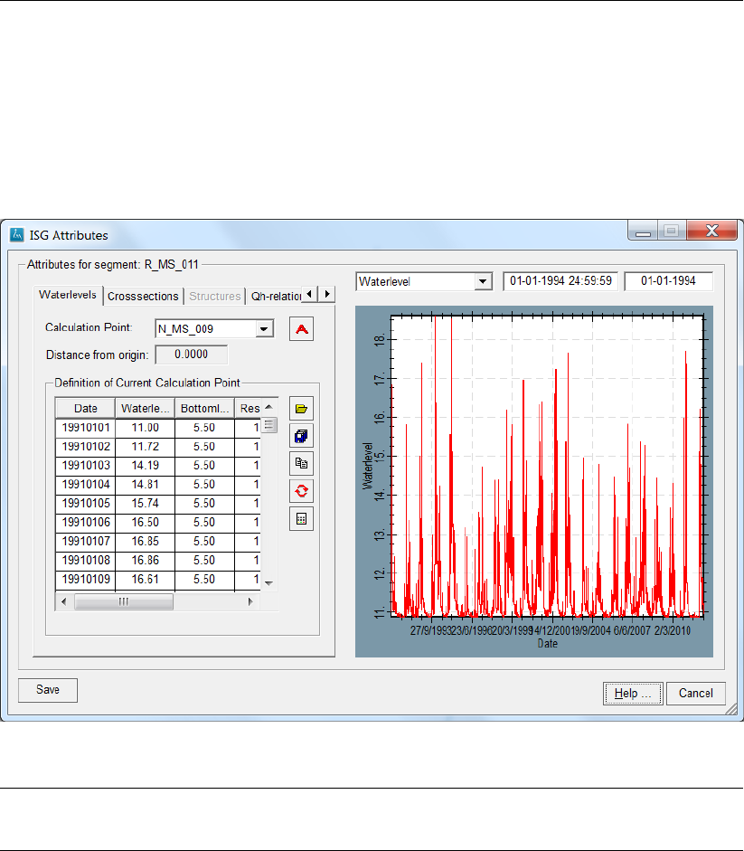
DRAFT
iMOD, User Manual
6.10.3.9 ISG Attributes
All attributes that appear on segments, can be analysed and adjusted in the ISG Attributes
window. Click the ISG Attributes button on the Segments tab on the ISG Edit window to open
the ISG Attributes window.
6.10.3.9.1 ISG Attributes window, Waterlevels tab:
Calculation Point: Select one of the listed calculation points from the dropdown menu. Any
change in this dropdown menu will change the content of the underlying table
and update the figure if possible.
182 of 812 Deltares
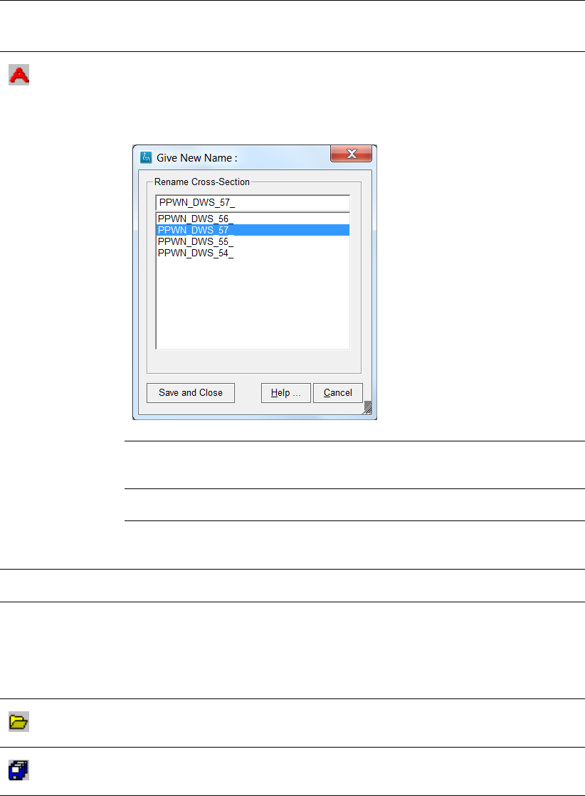
DRAFT
Map Menu options
Rename
Click this button the rename the selected calculation point via the Give New
Name: window:
Give New Name window:
Save and Close
Click this button to store the changed name for the selected segment, the Give
New Name: window will be closed.
Help
Click this button to start the Help functionality.
Cancel
Click this button to leave the name of the selected segment unchanged and
close the Give New Name: window
Distance from
origin
This field displays the distance of the selected calculation point from the origin
of the segment (FromNode) in meters.
Definition of
current
Calculation Point
This table shows the current values for the current selected calculation point.
Use the slide bars to manoeuvre through the table and enter new values for
any gridcell if desired. A new record can be entered by filling in all columns.
They will be sorted by date automatically after you select the Redraw option.
It depends on the type of ISG what attributes need to be available, see sec-
tion 9.9.2 for the exact content and meaning of variables.
Open CSV-file
Click this button to open a CSV-file, see section 9.12 for more detailed infor-
mation about CSV-files.
SaveAs CSV-file
Click this button to save to a CSV-file, see section 9.12 for more detailed
information about CSV-files.
Deltares 183 of 812
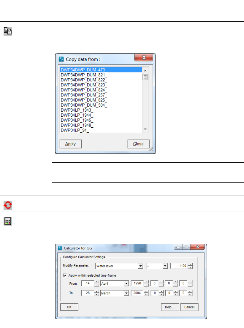
DRAFT
iMOD, User Manual
Copy
Click this button to open the Copy Data from window.
Copy data from window:
Apply
Click this button to copy the data from the selected calculation point onto the
current calculation point and close the Copy data from window.
Close
Click this button to close the Copy data from window.
Redraw
Click this button to redraw the graphical display.
Calculator
Click this button to start the attribute calculator.
Attribute Calculator window:
184 of 812 Deltares

DRAFT
Map Menu options
Modify Parameter
Select one of the available parameters from the dropdown list. The con-
tent of the dropdown menu depends from which tab the Attribute Calculator
is started. Select the appropriate modifier from the second dropdown list,
choose from:
+
Select this to add a value to all existing values;
-
Select this to subtract a value to all existing values;
*
Select this to multiply a value to all existing values;
/
Select this to divide a value to all existing values;
=
Select this to set a constant value to all existing values.
Enter a value in the right most entry field.
Apply within selected time-frame
Click this option to ensure that the modification will be applied within the en-
tered time-frame that can be specified in the underlying entry fields.
From
Specify the date from which any modification will take place.
To
Specify the date to which any modification will take place.
OK
Click this button to modify the parameter as configured and close the Attribute
Calculator window.
Help
Click this button to start the Help functionality.
Cancel
Click this button to close the Copy data from window.
Segment Name: This field shows the name of the current selected segment.
Current value: Select one of the attributes (WLevel, Bottom, Resistance, Inf.Factor) from the
dropdown menu to be shown in the graph.
Current {}-value: This field shows the current value in the graph at the position of the mouse
cursor.
Save Click this button to store any modifications and close the ISG Attribute window.
Help ... Click this button to start the Help functionality.
Cancel Click this button to close the ISG Attribute window. You will not be asked to
confirm to take any adjustments made.
Deltares 185 of 812
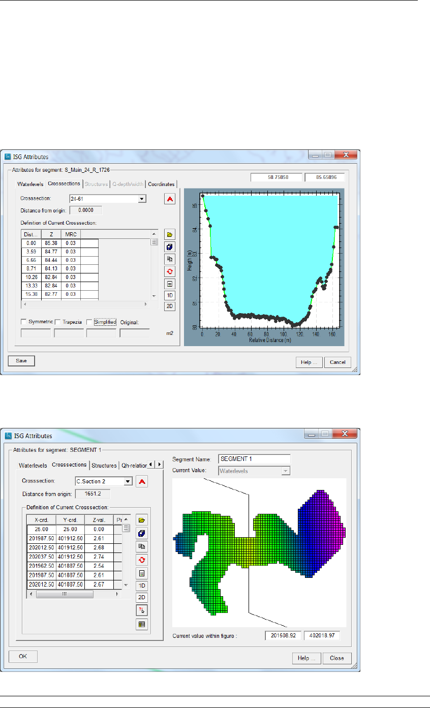
DRAFT
iMOD, User Manual
6.10.3.9.2 ISG Attributes window, Crosssections tab:
The ISG Attributes window, Crosssections tab can have two differences appearances. It de-
pends on the usage of 1-D and 2-D cross-sections. A 1-D cross-section describes the bathy-
metry of a stream as a representation of a cross-section perpendicular to the direction ot the
stream. A 2-D cross-section describes the bathymetry of a stream as a 2-D representation, a
grid.
1D-representation
2D-representation
Crosssection: Select one of the listed cross-sections from the dropdown menu.
186 of 812 Deltares
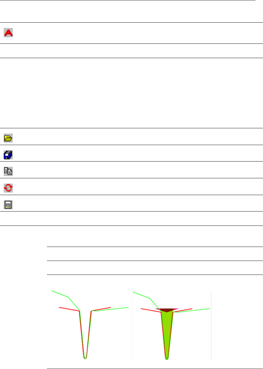
DRAFT
Map Menu options
Rename
Click this button the rename the selected cross-section. The Give New Name:
window will appear (see previous page).
Distance from
origin
This field displays the distance of the selected cross-section from the origin of the
segment (FromNode) in meters.
Definition of
current
Crosssection
This table shows the current values for the current selected cross-section point.
Use the slidebars to manoeuvre through the table and enter new values for any
gridcell if desired. A new record can be entered by filling in all columns. They will
be sorted by date automatically after you select the Redraw option.
Column names within the table:
- DIST: Distance of the cross-section measured from the centre of the riverbed
(minus to the left en positive to the right).
- Z: Relative level of the riverbed (meter), whereby zero will be assigned to the
lowest riverbed level
- MRC: Manning’s roughness coefficient (-).
Open CSV-file
Click this button to open a CSV -file, see section 9.12.
SaveAs CSV-file
Click this button to save to a CSV -file, see section 9.12.
Copy
Click this button to open the CopyAttribute window.
Redraw
Click this button to redraw the graphical display.
Calculator
Click this button to start the attribute calculator.
1D 1D representation
Click this button to view the 1D cross-section coupled to the cross-section point.
The following 3 options are only available in combination with the 1D cross-section representation:
Symmetric Click this checkbox to determine a symmetric cross-section and compute the area
that belongs to it.
Trapezia Click this checkbox to determine a double multiply trapezia that represents the
area computed by the symmetric cross-section most optimally.
Example of a symmetric cross-section, green is the original cross-section, red the
symmetric one:
Deltares 187 of 812
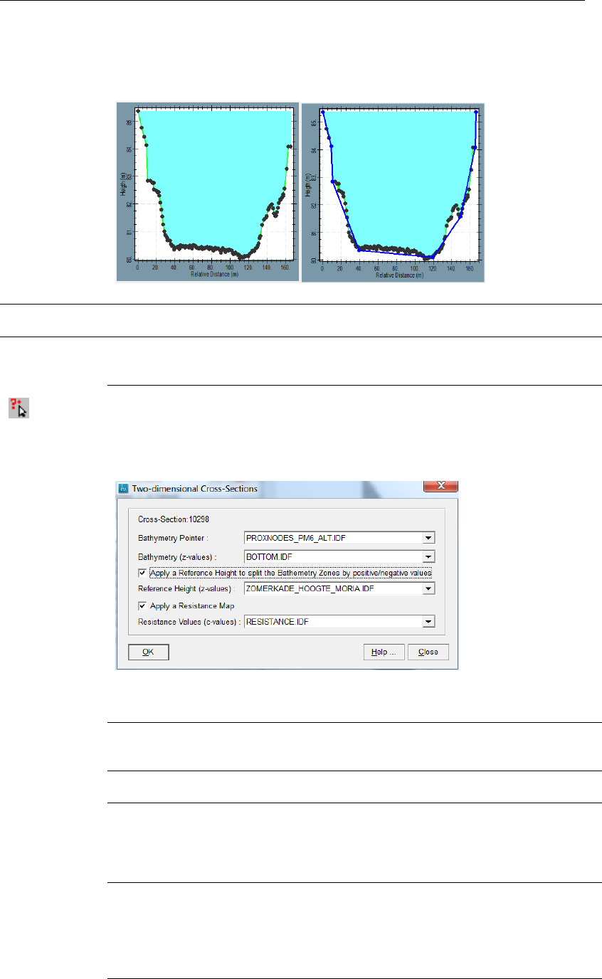
DRAFT
iMOD, User Manual
Simplified Click this checkbox to determine an eight-point cross-section. This option is
used for an SFR compliant ISG file during the creation of the SFR package, see
section 12.28.
2D 2D representation
Click this button to view the 2D cross-section coupled to the cross-section point.
The following options are only available in combination with the 2D cross-section representation:
Add/adjust Cross-section point
Click this button to add or adjust a specific cross-section point. The following
window will be opened:
Two-Dimensional Cross-section window:
Cross-Section: This value shows the number of the
cross-section point.
Bathymetry
Pointer:
Enter the name of an IDF-file de-
scribes the spatial distribution of two-
dimensional cross-sections.
Bathymetry
(z-values):
Select the name of an IDF-file that de-
scribes the bathymetry for the riverbed.
Apply a
reference
height. . .
Select this option in case both negative
and positive values in the bathymetry
pointer IDF-file needs to be taken into
account at a certain reference level in
assigning cross-sections.
Referenceheight
(z-values)
Select the name of an IDF-file that de-
scribes the reference height for which
positive and negative pointer values
given at Bathymetry Pointer need to be
applied. A single value is obtained per
2-D cross-section.
188 of 812 Deltares
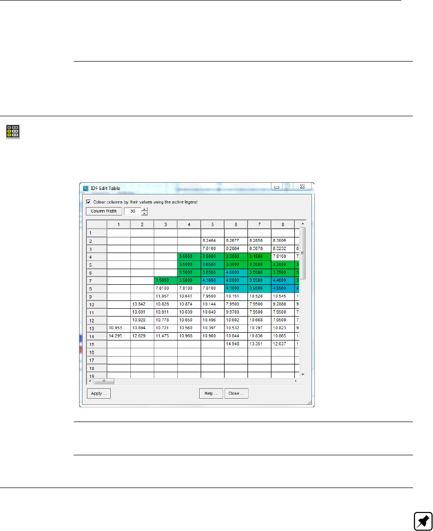
DRAFT
Map Menu options
Apply a
Resistance
map
Select this option to insert a spatial
variable resistance value for the bathy-
metry of the 2-D cross-section.
Resistance Values
(c-values)
Select the name of an IDF-file that de-
scribes the resistance value for the 2-D
cross-section. This is an integer multi-
plication factor with a maximal value of
256.
Edit Cross-Section grid
Click this button to view and edit the cross-section grid related to the selected
cross-section point. This option will open the following window:
IDF Edit Table window:
Colour columns. . . Select this option when coloring the
grid cells by the given legend is pre-
ferred.
Column width Click on this button to refresh the col-
umn width with the value given in de
box to the right of this button.
Note: Cross-sections can be applicable for different sections on a segment. It depends
whether it is a one-dimensional cross-section or a two-dimensional one.
Deltares 189 of 812
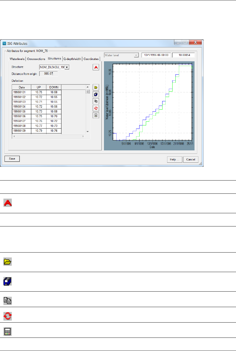
DRAFT
iMOD, User Manual
6.10.3.9.3 ISG Attributes window, Structures tab:
Use this tab to enter information on structures.
Structure: Select one of the listed structures on the current segment from the dropdown
menu.
Rename
Click this button the rename the selected structure point. The Give New
Name: window will appear.
Distance from ori-
gin
This field displays the distance of the selected structure point from the origin
of the segment (FromNode) in meters.
Definition Struc-
tures
This table shows the current values for the current selected structure point.
Use the slidebars to manoeuvre through the table and enter new values for
any grid cell if desired. A new record can be entered by filling in all columns!
They will be sorted by date automatically after you select the Redraw option.
Open CSV-file
Click this button to open a CSV-file, see section 9.12 for more detailed infor-
mation about CSV-files.
SaveAs CSV-file
Click this button to save to a CSV-file, see section 9.12 for more detailed
information about CSV-files.
Copy
Click this button to open the Copy Data from window.
Redraw
Click this button to redraw the graphical display.
Calculator
Click this button to start the attribute calculator.
Value boxes on
the top-right
These fields shows the current value in the graph at the position of the mouse
cursor.
190 of 812 Deltares
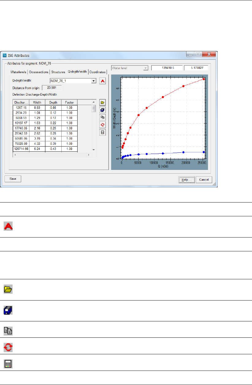
DRAFT
Map Menu options
6.10.3.9.4 ISG Attributes window, Q-Depth-Width tab:
Use this tab to enter information on Q-Depth-Width relationships. This information is used for
SFR compliant ISG files.
Q-Depth-Width: Select one of the listed Q-Depth-Width relation points from the dropdown
menu.
Rename
Click this button the rename the selected Q-Depth-Width relation point. The
Give New Name: window will appear.
Distance from ori-
gin
This field displays the distance of the selected Q-Depth-Width relation point
from the origin of the segment (FromNode) in meters.
Definition Q-
Depth-Width
Relationships
This table shows the current values for the current selected Q-Depth-Width
Relationships point. Use the slidebars to manoeuvre through the table and
enter new values for any grid cell if desired. A new record can be entered by
filling in all columns!
Open CSV-file
Click this button to open a CSV-file, see section 9.12 for more detailed infor-
mation about CSV-files.
SaveAs CSV-file
Click this button to save to a CSV-file, see section 9.12 for more detailed
information about CSV-files.
Copy
Click this button to open the Copy Data from window.
Redraw
Click this button to redraw the graphical display.
Calculator
Click this button to start the attribute calculator.
Value boxes on
the top-right
These fields shows the current value in the graph at the position of the mouse
cursor.
Deltares 191 of 812
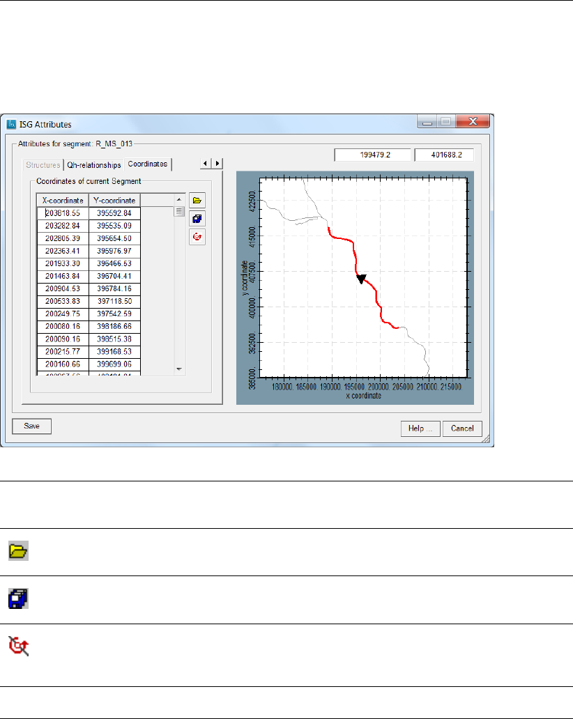
DRAFT
iMOD, User Manual
6.10.3.9.5 ISG Attributes window, Coordinates tab:
Use this tab to display the coordinates of the selected segment, read in a different set of
coordinates and/or switch the order in which the coordinates are entered.
Coordinates of
current
Segment
This table shows the current coordinates of the reaches in the current selected
segment. Use the slidebars to manoeuvre through the table and enter new
values. A new record can be entered by filling in all columns!
Open GEN-file
Click this button to open a GEN-file, see section 9.10 for more detailed infor-
mation about GEN-files.
SaveAs GEN-file
Click this button to save to a GEN-file, see section 9.10 for more detailed
information about GEN-files.
Rotate
Click this button to rotate the coordinates. The order of the coordinate de-
termines the flow direction whenever this type of ISG is used for the SFR
package, see section 12.28.
Value boxes on
the top-right
These fields shows the current value in the graph at the position of the mouse
cursor.
192 of 812 Deltares
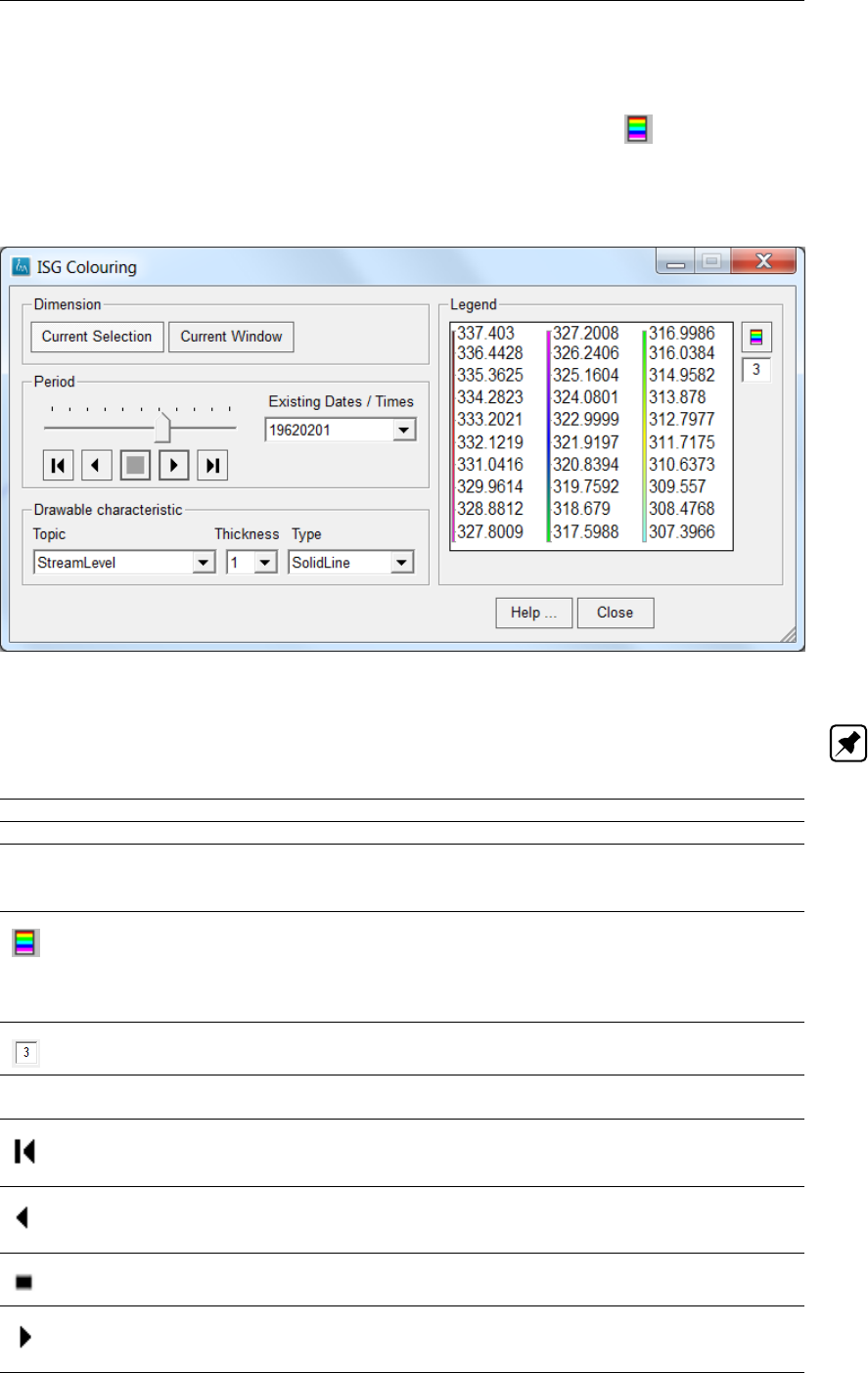
DRAFT
Map Menu options
6.10.3.10 ISG Colouring
Use this functionality to visualize the parameters on the ISG file as lines, so colouring the
individual lines according a specified legend. Click the Legend option ( ) on the ISG Edit
window to display the ISG Colouring window.
ISG Colouring window:
Note: At the start of the ISG Colouring window the legend for all parameters are initialised
based on their minimal and maximal values.
Current Selection Select this option to colour segment from the current selection only.
Current Window Select this option to colour all segments disregard whether they are selected.
Period Use this trackbar to select a different period that is available in the dropdown
menu with Existing Dates/Times. This option is disabled whenever a single
date/time step is available.
Legend
Click this button to start the Adjust Legend window in which the legend for
the current Topic can be modified. Those modified legends will be stored as
long as the ISG Colouring window remains active. Whenever the window is
restarted, all legend will be initialised again.
Number of Columns
Enter the number of columns to represent the legend.
Existing
Dates/Times
Select one of the existing dates/times from the dropdown menu. This option
is disabled whenever a single date/time step is available.
Complete Backward
Click this button to go the first existing date and move the trackbar to the
utmost left.
Backwards
Click this button to step a single date step against time, repeatedly. The track-
bar moves accordingly.
Stop
Click this button to stop the actions Backwards or Forwards.
Forwards
Click this button to step a single date step in time, repeatedly. The trackbar
moves accordingly.
Deltares 193 of 812
DRAFT
iMOD, User Manual
Complete Forward
Click this button to go the utmost existing date and move the trackbar to the
utmost right.
Topic Select one of the existing topic from the dropdown menu to display. The
amount of topics depend on the type of ISG (see section 9.9.2).
Thickness Select one of the existing line thicknesses to display the lines.
Type Select one of the existing line types. The following line types are available:
SolidLine;
Dotted;
Dashed;
DotDash;
DotDotDash;
LongShort;
ShortDash;
LongShortShort.
Help ... Click this button to start the Help functionality.
Close Click this button to close the ISG Colouring window.
Note: All other functionalities of ISG Edit remain active whenever the ISG Colouring window
is active.
194 of 812 Deltares
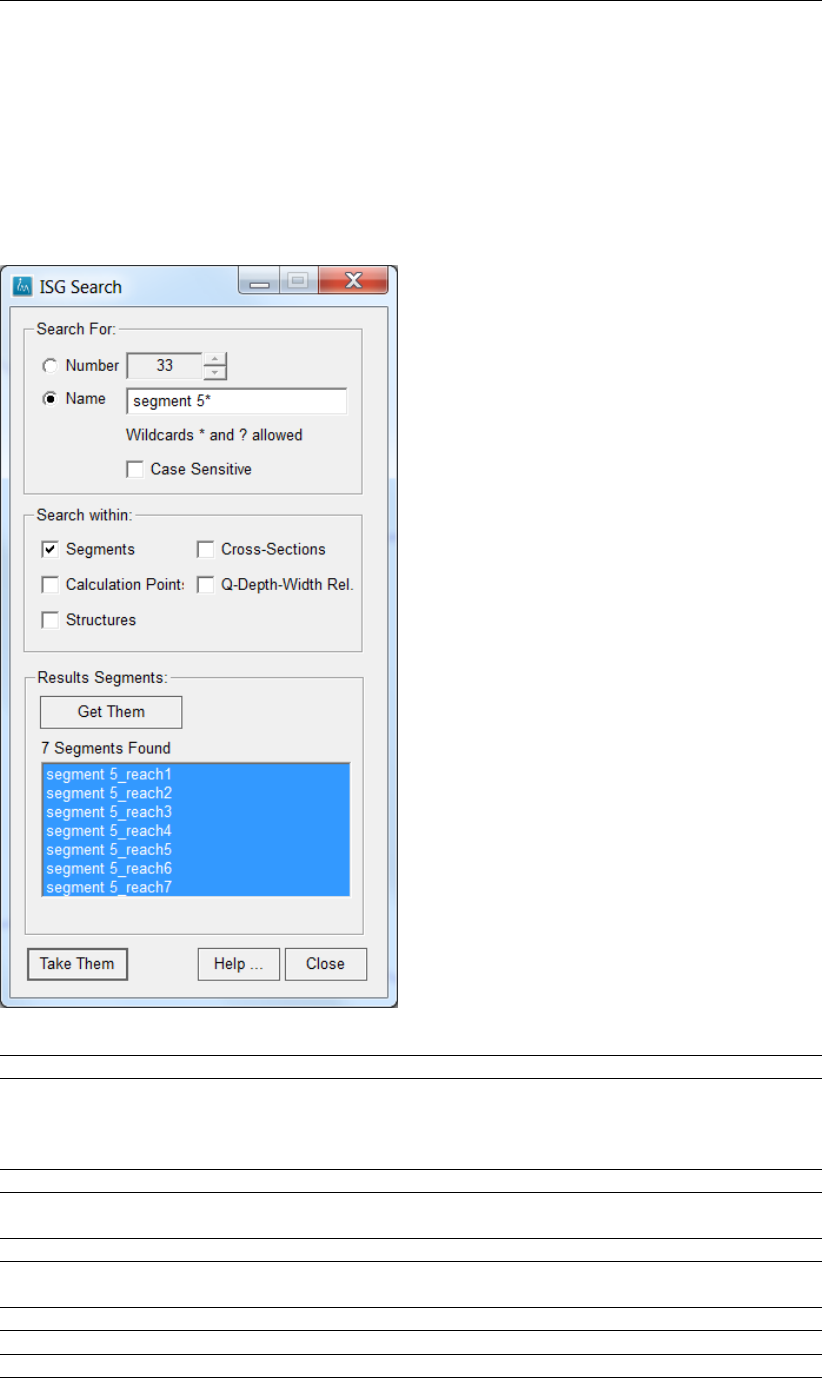
DRAFT
Map Menu options
6.10.3.11 ISG Search
Each segment and their attributes (Cross-sections, Calculation nodes, Structures and Q-
Depth-Width Relationships) have labels. WithISG Search it is possible to search segments
for specific labels in their segment and attributes. Click the ISG Search option from the ISG
Edit window to start the ISG Search window.
ISG Search window:
Number: Select this option to enter a segment number to search for explicitly.
Name: Select this option to enter a search string. Use the asterix (‘*’) as wildcard and
the questionmark (‘?’) to define the number of positions. e.g. Ex_* means,
select all that match the Ex_ at the start and a search string of ??Ex_* means
that all are selected that start with two characters prior to Ex_.
Case Sensitive Click this checkbox to make the search string case sensitive.
Search within: Select those variables for which the search string will be applied to in order to
find those segments that yield a match.
Get Them Click this button to apply the search string for the selected variables.
Results
Segments:
The menulist displays all segments that meet the entered search string.
Take Them Click this button to take the selection to the mainISG Edit window.
Help . . . Click this button to start the Help functionality.
Close Click this button to close the ISG Search window.
Deltares 195 of 812
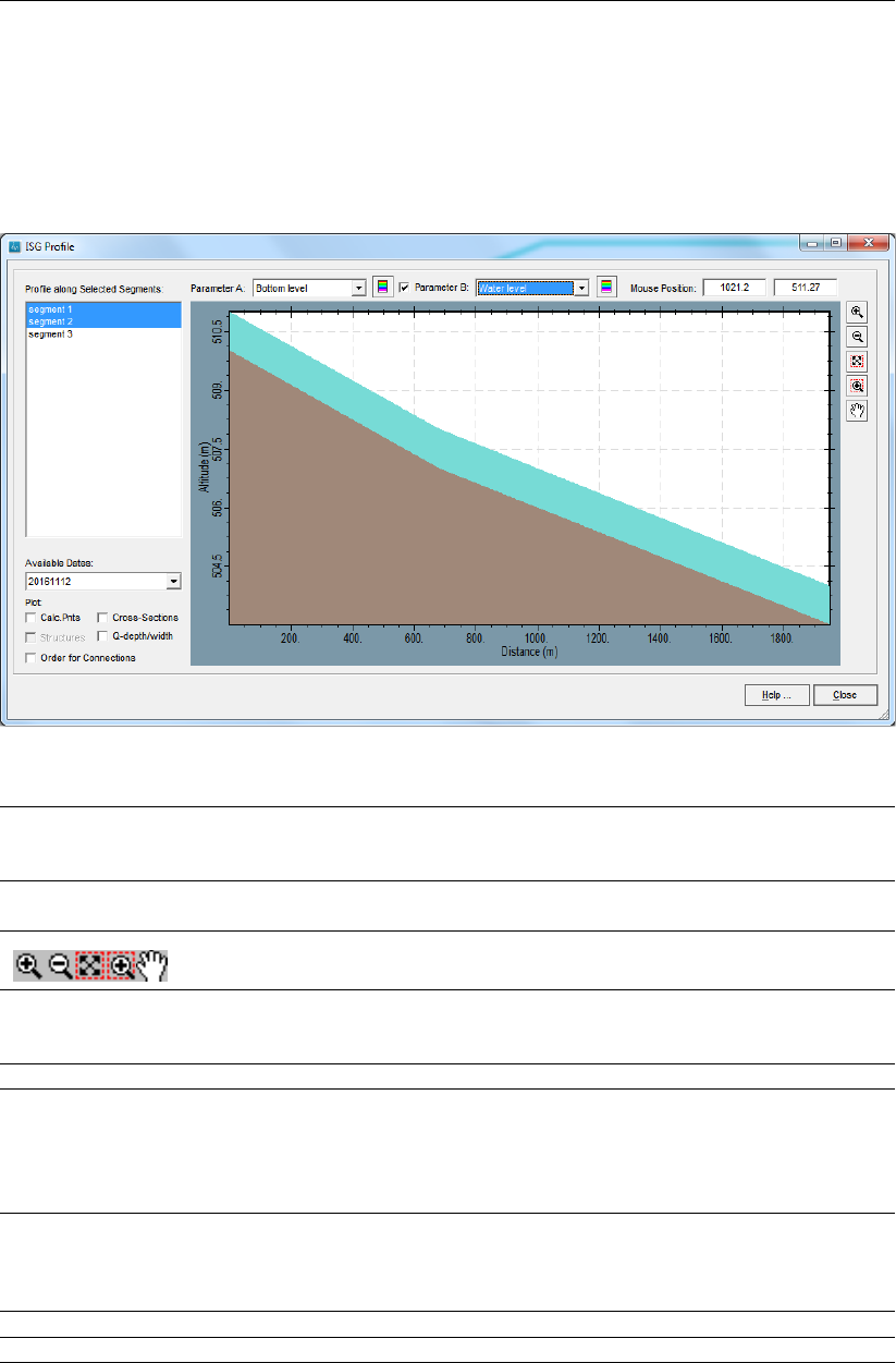
DRAFT
iMOD, User Manual
6.10.3.12 ISG Profile
Click the menu option Profile from the ISG Edit window to display the ISG Profile window. A
length-cross section is presented for the selected ISG segment.
ISG Profile window:
Profile along
Selected
Segments:
Select one or more segments from the menu list to visualize their length pro-
file. Use your mouse wheel to switch quickly between segments.
Existing Dates: Select an available date from the dropdown menu to visualize any of the se-
lected items at Polygon A: and Polygon B: for the selected date.
Zoom functions: see section 2.6.2 for an explanation
Graphical
display
In the graphical display the profile along the selected segment is presented.
In cyan, any parameters at Polygon B: is presented, in brown the parameter
from Polygon A:.
Mouse Position Displays the current position of the mouse in units of the display.
Plot:
Calc. Pnts
Cross-Sections
Structures
Q-Depth-Width
Click one of the checkbox next to those keywords to display the position of
these in the graph.
Order for Connec-
tions
Click this keyword to sort the individual segment based on their connections.
Segments can be randomly sorted in the segment list and can distort the
graphical presentation whenever the graph of the individual segments is not
in the correct order. This option sorts them before plotting.
Help . . . Click this button to start the Help functionality.
Close Click this button to close the ISG Profile window.
196 of 812 Deltares
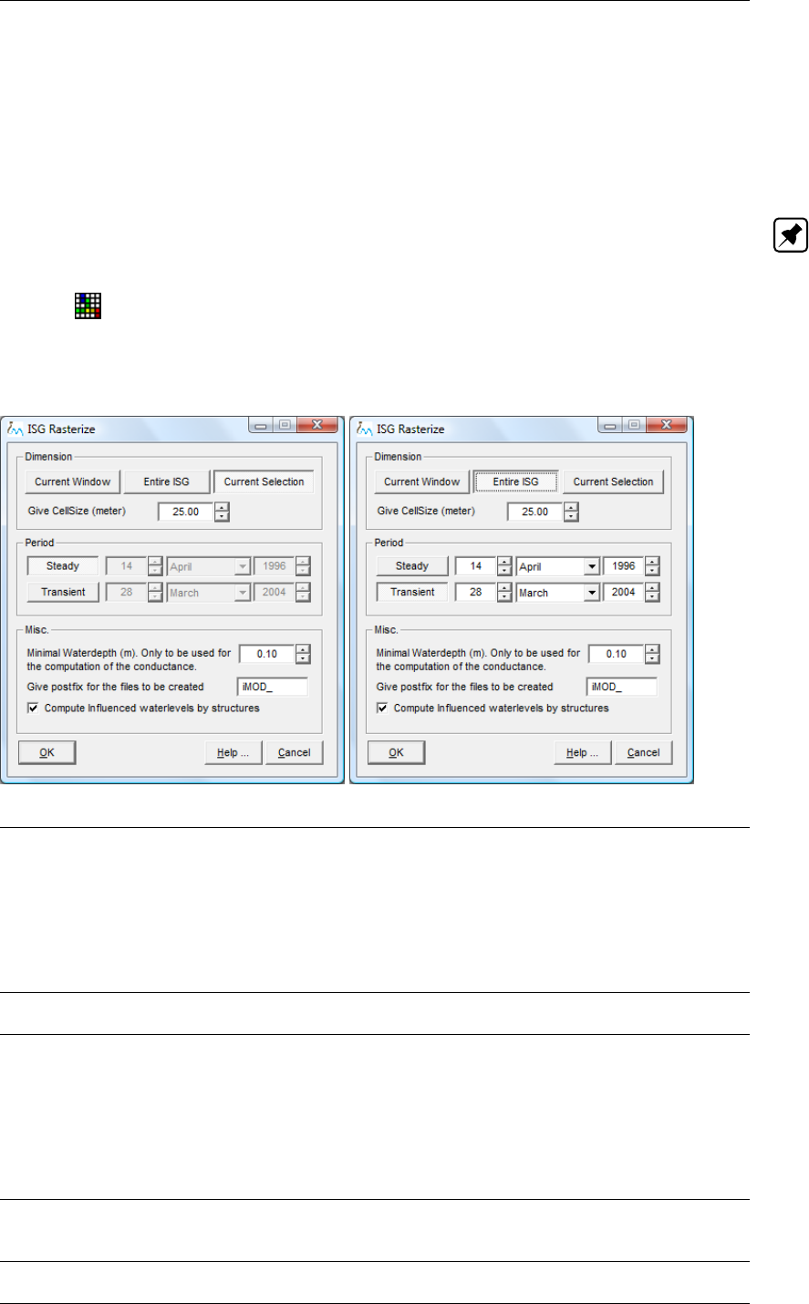
DRAFT
Map Menu options
6.10.3.13 ISG Rasterize
For reasons of visual inspection (are all waterlevels correct?) as well as usage in a runfile
(see runfile description), iMOD can perform a rasterization of the ISG-file in total or for individ-
ual river segments within the ISG-file. It yields several IDF-files (STAGE.IDF, BOTTOM.IDF,
INFFCT.IDF and COND.IDF) that can be used and analysed using the standard iMOD func-
tionalities.
Note: IMPORTANT to note is that a minimal resistance is applied of 0.001 days to avoid
extraordinary conductance (COND) values.
Click the ISG Rasterize button in the ISG Edit window to start the ISG Rasterize window.
ISG Rasterize window, (top) for a Steady State configuration for the Current Selection and
(bottom) for a Transient configuration for the Entire ISG:
Dimension Select one of the following options:
Current window:
Click this option to rasterize all river segments within the current graphical
zoom level.
Entire ISG:
Click this option to rasterize all river segments in the entire ISG.
Current Selection:
Click this option to rasterize the selected river segment(s) only.
Give CellSize
(meter)
Enter the cellsize of the resulting IDF after the rasterization.
Period Select one of the following options:
Steady:
Click this option to rasterize all timevariant input variables (e.g. waterlevels,
bottom levels, infiltration factors, riverbed resistances, weirlevels) as mean
values over all input.
Transient:
Click this option to rasterize all timevariant input variables as mean values
over the selected period that can be entered in the input fields at the right.
Minimal
waterdepth . . .
Enter a minimal waterdepth to be used when computing conductances, which
in principal depend on waterdepth. By entering a minimal waterdepth >0.0,
the conductance will not become zero.
Give postfix . . . Enter the postfix to be added to the default names after the rasterization, e.g.
iMOD_ yields the IDF-filename iMOD_STAGE.IDF
Deltares 197 of 812
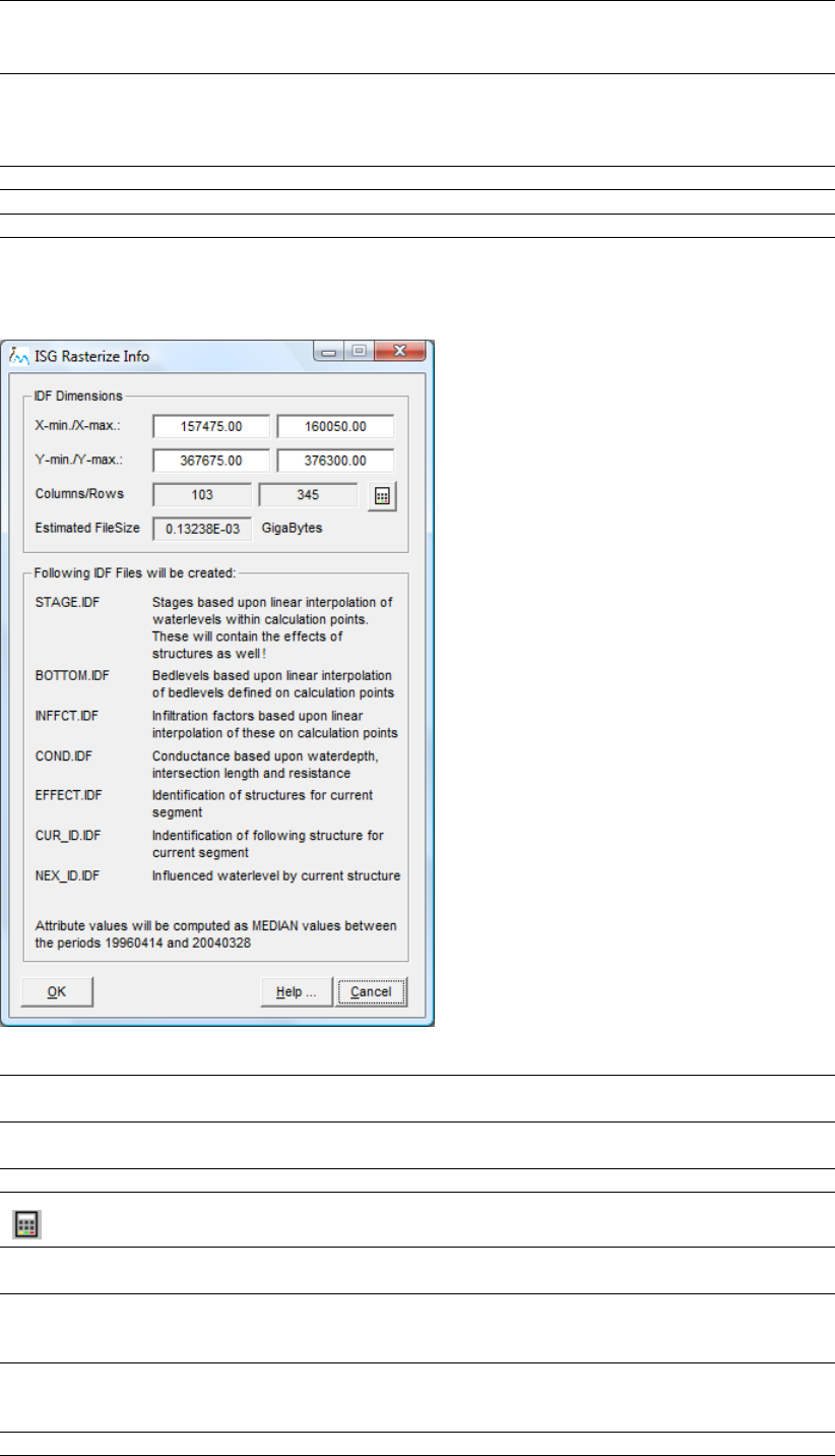
DRAFT
iMOD, User Manual
Compute
influenced
waterlevels
by structures
Check this item to compute the waterlevel as it is influenced by a weir struc-
ture. Upstream from each weir the waterlevel is horizontal until it reaches
the level of the river plus waterdepth. From there the waterlevel follows the
gradient of the river segment.
OK . . . Click this button to open the ISG Rasterize Info window.
Help . . . Click this button to start the Help functionality.
Cancel Click this button to close the ISG Rasterize window.
ISG Rasterize Info window:
X-min/X-max Enter the minimum and maximum X coordinates. On default these are filled
in depending on the chosen Dimension on the ISG Rasterize window.
Y-min/Y-max Enter the minimum and maximum Y coordinates. On default these are filled
in depending on the chosen Dimension on the ISG Rasterize window.
Columns/Rows Computed number of columns and rows that the yielding IDF-files receive.
Calculator
Click this button to recompute the number of columns and rows.
Estimated
FileSize
Display of the filesize in Gbytes.
Following IDF
Files will be
created
This shows a list of all IDF-files that will be created by the rasterization, to-
gether with a brief description. The list depends on the choices made on the
ISG Rasterize window.
OK Click this button to start the rasterization. After successful rasterization, both
theISG Rasterize and ISG Rasterize Info window will be closed. All resulting
IDF-files will be added to the iMOD Manager.
Help ... Click this button to start the Help functionality.
198 of 812 Deltares

DRAFT
Map Menu options
Cancel Click this button to close the ISG Rasterize Info window and to return to the
ISG Rasterize window.
Deltares 199 of 812
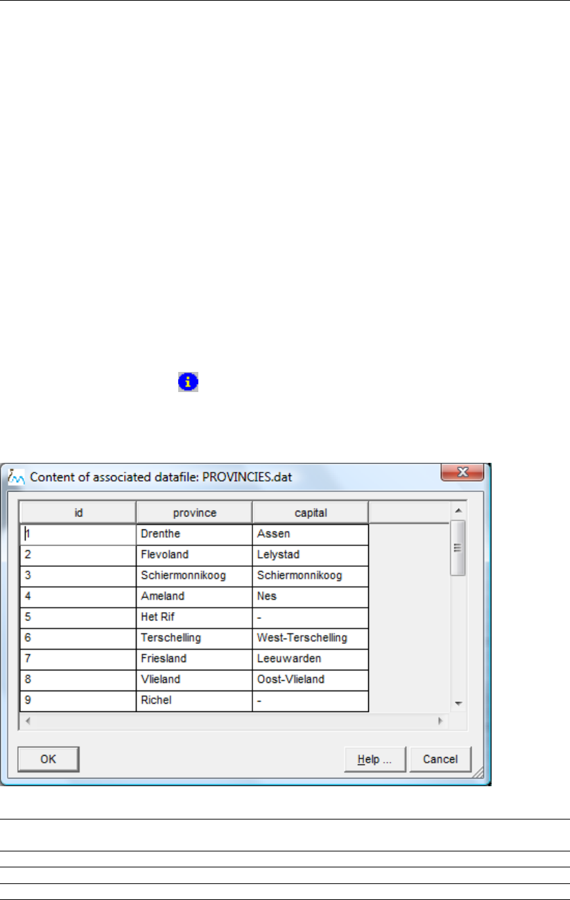
DRAFT
iMOD, User Manual
6.11 GEN Options
iMOD supports several basic functionalities to display GEN-files. These GEN-files should be
loaded in the Map tab on the iMOD Manager (see section 5.4) instead of the Overlays tab.
Whenever a GEN-file is selected the following options can be used:
GEN Info, use this tool to analyse the content of the associated DAT file, if available.
GEN Configure,
GEN Extract, not supported yet!
6.11.1 GEN Info
WHY?
To display the information from a datafile associated to the GEN-file.
WHAT?
The attribute data is stored in a DAT-file which has the same name as the GEN-file. The
attribute data is linked by the ID of the features (see section 9.11).
HOW?
Click the Map Additional Info button from the Map Info window (see section 6.3) to display
the Content of associated datafile window.
Content of associated datafile window:
Table Displays the content of the {name}.dat associated to {name}.gen. The first column is
compulsory to enter values to relate to the ID of the lines or polygons.
OK Click this button to close the Content of Associated Datafile window.
Help ... Click this button to start the Help functionality.
Cancel Click this button to close the Content of Associated Datafile window.
200 of 812 Deltares
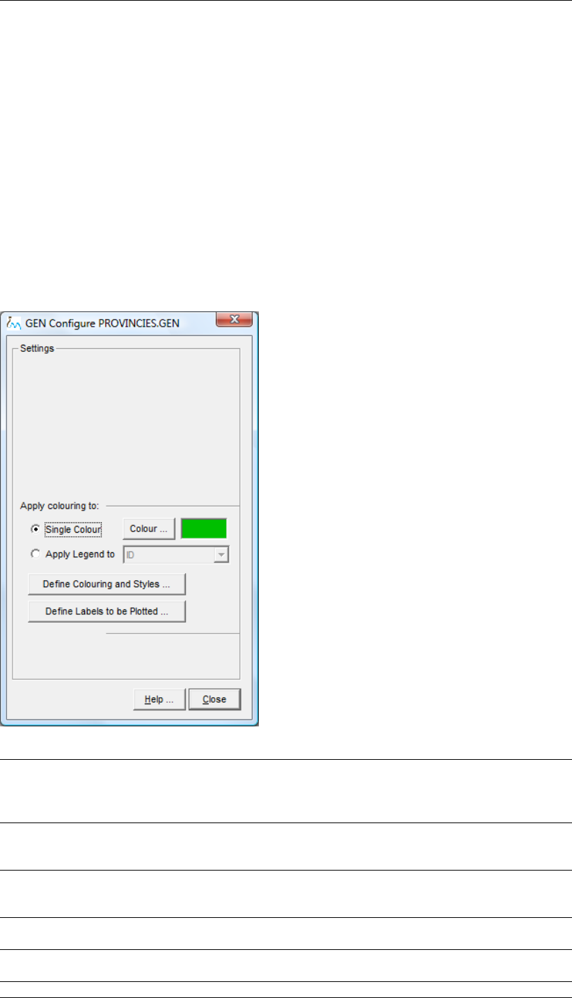
DRAFT
Map Menu options
6.11.2 GEN Configure
WHY?
To display the GEN-file.
WHAT?
GEN Configure is used to define the settings for display and assigns a symbol, colour or label.
The options are similar to the IPF Configure function (see section 6.8.1).
HOW?
GEN-files in iMOD represent polygon or line data that can be displayed in different ways.
Select the menu option GEN Configure from the GEN Options menu in the Map menu to
display the GEN Configure window.
GEN Configure window:
Single Colour Select this option to display all polygon(s) or lines with the same colour.
Depending whether you’ve selected the Fill Polygons option on the Define
Colouring and Styles window, see section 5.7, the polygon will be filled in or
the polygon will be outlined.
Colour . . . Select this button to display the default Colour window in which a colour can
be specified. The current colour is displayed to the right of this button, green
is used in the example above.
Apply Legend to Select this option to colour the polygons according to the selected attribute
that is chosen in the dropdown menu at the right. A legend can be assigned
identical to other iMOD files, e.g. IDF, IPF.
Define Colouring
and Styles. . .
Select this option to display the Lines and Symbols window
Define Labels
to be plotted
Select this button to display the Define Labels to be Plotted window.
Help. . . Click this button to start the iMOD Help Functionality.
Deltares 201 of 812
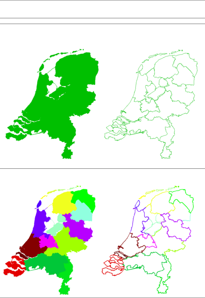
DRAFT
iMOD, User Manual
Close Select this button to apply the settings and close the GEN Configure window.
Example of uniform colouring of a GEN-file, using the Fill Polygons option (left) or outline option
(right):
Example of legend colouring of a GEN-file, using the filled in option (left) or outline option (right):
202 of 812 Deltares
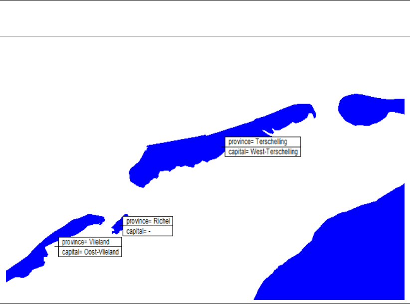
DRAFT
Map Menu options
Example of labeling polygons of a GEN-file:
Deltares 203 of 812

DRAFT
iMOD, User Manual
204 of 812 Deltares

DRAFT
7 Toolbox Menu Options
This chapter contains a detailed description of a variety of Tools that are available in IMOD:
section 7.1: Cross-Section Tool.
section 7.2: Timeseries Tool.
section 7.3: 3D Tool.
section 7.4: Solid Tool.
section 7.5: Movie Tool.
section 7.6: GeoConnect Tool.
section 7.7: Plugin Tool.
section 7.8: Import Tools.
section 7.9: Model Simulation.
section 7.10: Quick Scan Tool.
section 7.11: Pumping Tool.
section 7.12: RO-tool.
section 7.13: Define Startpoints.
section 7.14: Start Pathline Simulation.
section 7.15: Interactive Pathline Simulator.
section 7.16: Waterbalance Tool.
section 7.17: Compute Mean Groundwaterfluctuations (GxG).
section 7.18: Compute Mean Values.
section 7.19: Compute Timeseries.
??: Compute Time-variant Statistics.
Deltares 205 of 812
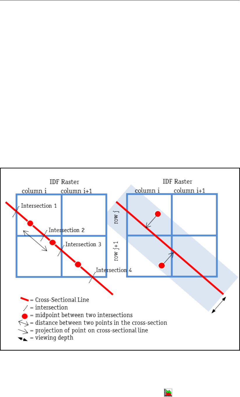
DRAFT
iMOD, User Manual
7.1 Cross-Section Tool
WHY?
The Cross-Section Tool can be used to display cross-sections over a variety of data types,
such as IDF’s, IPF’s with associated files (e.g. boreholes, timeseries) and IFF’s (flowlines).
WHAT?
The Cross-Section Tool allows you to draw any line (Cross-Sectional Line) that will intersect
the rastercells of any of the selected IDF-files. The IDF cell value in-between two raster cell
intersections will be assigned to the cross-section points (the midpoints). Consequently, the
distances between different points of a cross-section can vary, especially in case the Cross-
Sectional Line is chosen to be diagonally.
IPF points and/or IFF lines, can be projected perpendicular on the Cross-Sectional Line within
a chosen viewing depth. Bear in mind that breakpoints will cause points and/or lines to be
projected twice (in the inside) or not at all (in the outside). For points, the nearest line will
be used to be projected upon. Moreover, points that are too close to each other will become
narrower, this can be overruled.
Methodology used by the Cross-Section Tool:
HOW?
To start the Cross-Section Tool select Toolbox from the main menu, choose Cross-Section
Tool. Alternatively you can select the Cross-Section Tool icon from the main toolbar. In
both cases, all the selected files in the iMOD Manager will be activated in the Cross-Section
Tool. The order in which these files are arranged, might affect the way they are displayed.
206 of 812 Deltares

DRAFT
Toolbox Menu Options
The Cross-Section Tool consists of two windows: Draw Cross-Section window and the iMOD
Cross-Section CHILD window.
Deltares 207 of 812
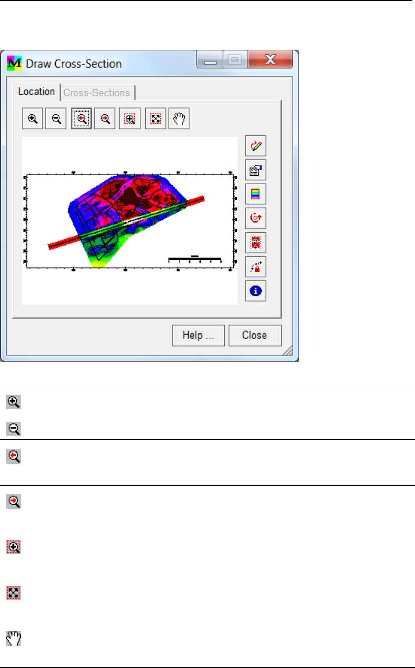
DRAFT
iMOD, User Manual
Draw Cross-Section window:
Zoom In
Click this button to zoom IN on the centre of the current graphical dimensions.
Zoom Out
Click this button to zoom OUT on the centre of the current graphical dimensions.
Go Back to Previous Extent
Click this icon and the map will return to the previous map extent and view. This
view becomes the last view automatically whenever any other zoom button will be
used.
Go to Next Extent
Click this icon and the map will go to the next extent viewed after the current view.
This option becomes available whenever the Zoom to Previous Extent button has
been selected priorly.
Zoom Rectangle
Click this button to zoom in for a rectangle to be drawn. Use you the left-mouse
button to determine the lower-left corner of the rectangle, click again for the upper-
right corner (or vice-versa).
Zoom Full
Click this button to zoom in on the entire extent of the selected maps on the tab
Maps on the iMOD Manager or on the selected overlay Maps in the tab Overlay
on the iMOD Manager.
Move
Click this button to move the current display. Click the left-mouse button on that
location where you want to move from, repeat this after the display has been
refreshed (automatically). Use the right mouse button to stop the moving process.
208 of 812 Deltares
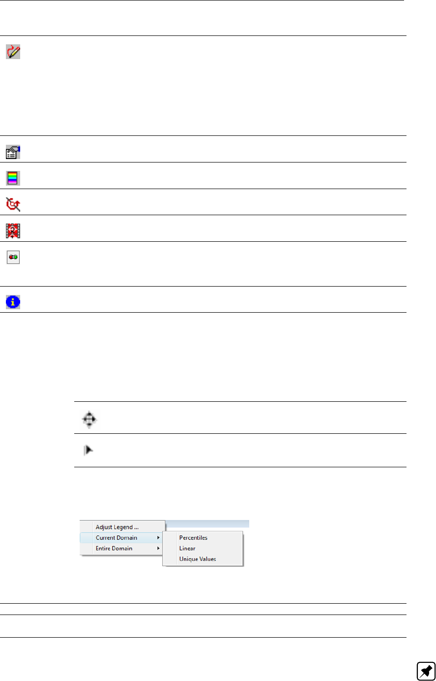
DRAFT
Toolbox Menu Options
Draw Line of the Cross-Section
Click this button to draw the line of the cross-section on the Graphical Area on the
Draw Cross-Section window. Click the left-mouse button to define the first point
of the line and click this left-mouse button to insert intermediate points, if desired.
Click the right-mouse button to stop the line drawing. If you’ve defined one point
only, the last location will be added to the line, in other cases this last point will
not be used! The used coordinates can be displayed on the cross-sectional view
and/or within the Cross-Section Properties window. The line of the cross-section
may consist of 250 points, maximally.
Cross-Section Properties
Click this button to open the Properties window (see section 7.1.1).
Cross-Section Legend
Click this button to open the Adjust Legend window (see section 6.6.1).
Flip Cross-Section
Click this button to “flip” the current Cross-Section
Cross-Section Movie
Click this button to open the Movies window.
Snap Coordinates
Click this button to “snap” the coordinates of the Cross-Section to the coordinates
in the selected IPF-file. This functionality is therefore only available whenever an
IPF is selected.
IPF-info
Click this button to open the IPF-Info window.
Graphical
Display
This presents the display from the Main iMOD window. Anything that has been
drawn before entering the Cross-Section Tool will display here. In this area
you can specify the location of the Cross-Section. The location will appear as
a black line. When you move the mouse in this Graphical Area your current
coordinates will be displayed in the lower-left corner of the Cross-Section window.
Moreover, the following symbols might occur whenever you move the mouse
near the Cross-Section line:
Click your left mouse button and hold it, to move the entire Cross-
Section line. Stop this by releasing the mouse button.
Click your left mouse button and hold it, to move an individual node of
the Cross-Section line. Stop this by releasing the mouse button. iMOD
will update your cross-section immediately.
Click your right-mouse button anywhere on the Graphical Display to popup the
following dropdown menu.
Popup menu:
The functionalities are described in section 2.6.3. The popup menu becomes
available only when IDF-files are selected in the iMOD Manager.
Help ... Click this button to start the iMOD Help Functionality.
Close Click this button to close the Cross-Section Tool; the Draw Cross-Section and
iMOD Cross-Section windows will also close.
Note: All adjustments in the zoomlevel on the Graphical Area will be used whenever you
leave the Cross-Section Tool again.
Deltares 209 of 812
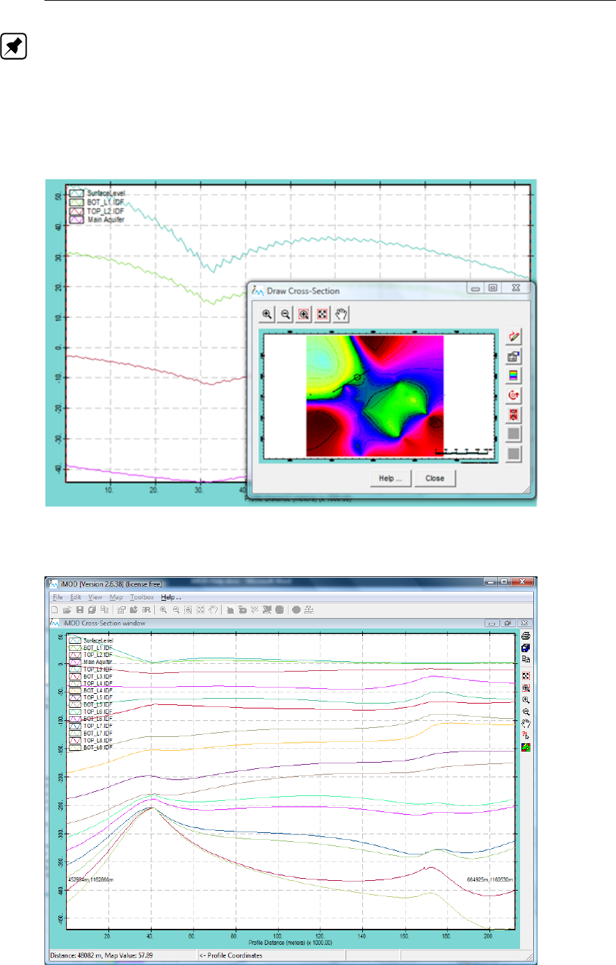
DRAFT
iMOD, User Manual
Note: iMOD will intersect the cross-section line with the raster cellvalues of the IDF-files.
Since different IDF-files may be used (constant- and variable rastersizes), each cross-section
can have different results at the intersections. After the intersection, iMOD determines the
IDF values for the midpoints that are in the centre between two intersection points. Due to
this, diagonal lines may display cross-sections with jagged lines.
Example of cross-sections that are jagged:
iMOD Cross-Section window:
210 of 812 Deltares
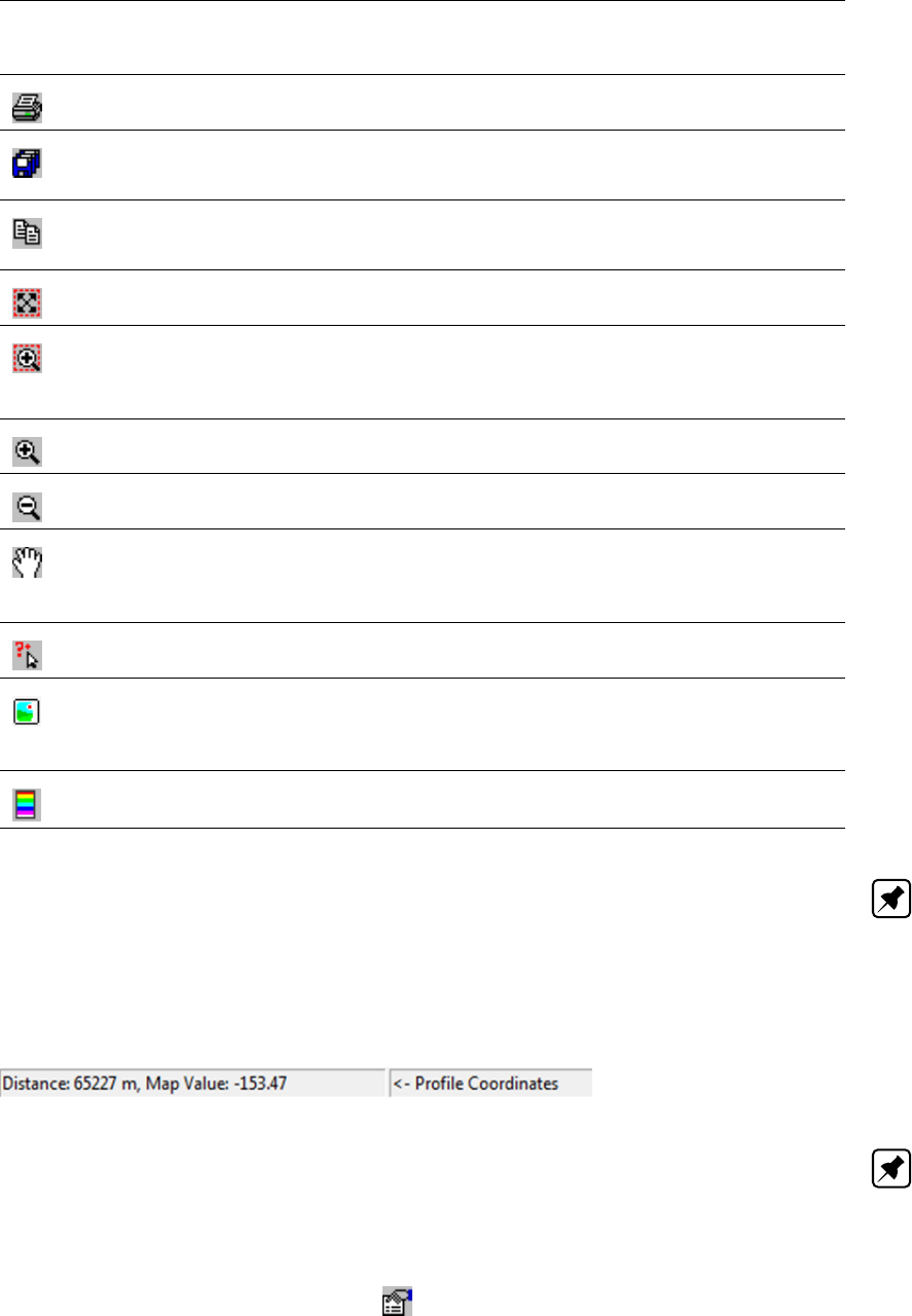
DRAFT
Toolbox Menu Options
Print
Click this icon to print the current Cross-Section on a printer.
Export or Save As Demo . . .
Click this icon to export the current Cross-Section to an ASCII-file (*.csv) or to save
the current Cross-Section as an iMOD-demo in a new IMF-file.
Copy to Clipboard
Click this icon to copy the current Cross-Section to the windows Clipboard. Use the
shortcut Ctrl-C , alternatively
Zoom Full
Click this button to zoom in on the entire extent of the Cross-Section.
Zoom Rectangle
Click this button to zoom in for a rectangle. Use the left-mouse button to determine
the lower-left corner of the rectangle, click again for the upper-right corner (or vice-
versa).
Zoom In
Click this button to zoom IN on the centre of the current Cross-Section.
Zoom Out
Click this button to zoom OUT on the centre of the current Cross-Section.
Move
Click this button to move the current Cross-Section. Click the left-mouse button on
that location where you want to move from, repeat this after the display has been
refreshed (automatically). Use the right mouse button to stop the moving process.
Cross-Section Inspector
Click this icon to use the Cross-Section Inspector.
Add a bitmap as background
Click this icon to select a BMP-file to be shown as background map. Whenever the
Profile Tool is started via the Solid Tool (see section section 7.4, the position and
background bitmap will be saved in the SPF file, see section section 9.21.
Legend
Click this icon to display the legend, see section section 7.1.2.
Note: Whenever you move the cursor over the Draw Cross-Section window, the coordinates
are displayed in the lower-left corner of the iMOD Cross-Section window. Moreover, your
position in the cross-section will be displayed in the Draw Cross-Section window as a small
circle on the line for the cross-section.
Example of cursor location in the Cross-Section:
Note: Each point that determines the line for the cross-section is displayed as a red, vertical
dashed line in the graph.
7.1.1 Properties
Click the option Cross-Section Properties on the Draw Cross-Section window to open the
Cross-Section Properties window. The properties are grouped for each filetype in the Cross-
Section (IDF’s, IPF’s and/or IFF’s) and their corresponding tabs become available when the
filetype is present in the Cross-Section.
Deltares 211 of 812
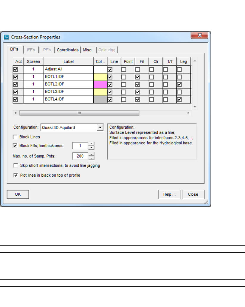
DRAFT
iMOD, User Manual
Cross-Section Properties window, IDF’s tab:
The display mode of the IDFs is defined in the table. Several quick display configurations are
available for layer models.
Act Select the checkbox in this column to include the IDF in the cross-section.
Screen Number of Graphical Windows (screens 1-50) for display; e.g. you can specify a
separate Graphical Window (screen) for each IDF.
All screens are synchronized, which means that all zoom and/or pan actions will be
carried out for all screens simultaneously.
Label Insert a text for a label.
Col. . .
(Colour)
Displays the colour used to display the Cross-Section for each IDF. Select the column
to open the Colour window to change the colour.
212 of 812 Deltares
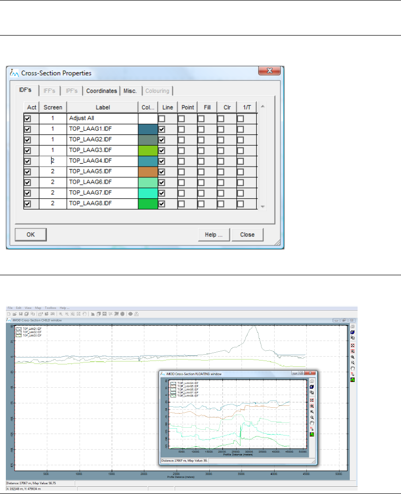
DRAFT
Toolbox Menu Options
Cross-Section Properties window, IDFs tab for multiple Graphical Windows:
This is also possible for the loaded IPFs by adjusting the number in the Screen column, e.g. 1
means plot on first (=main) screen, 2 means plot on a second screen.
Example of using multi-screens to display the cross-section:
Deltares 213 of 812
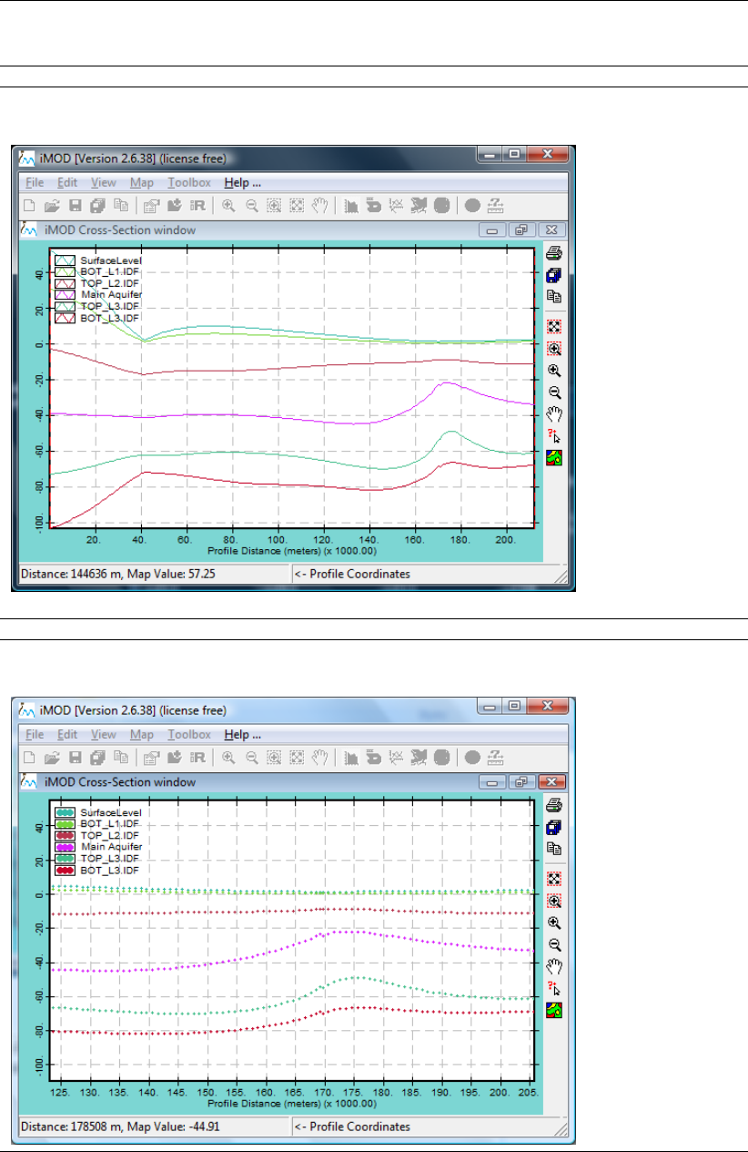
DRAFT
iMOD, User Manual
Line Select the checkbox in this column to present the cross-section as solid lines.
Example of cross-section using the Line option:
Point Select the checkbox in this column to present the cross-section as individual points.
Example of a cross-section using the Point option:
214 of 812 Deltares
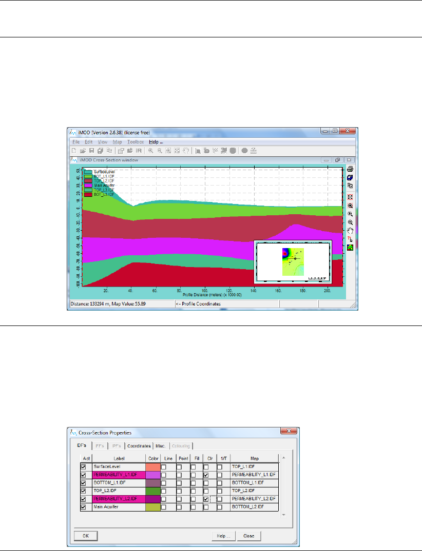
DRAFT
Toolbox Menu Options
Fill Select the checkbox in this column to present the cross-section as a filled area. The
cross-section is bounded by the surfacelevel at the top, and the minimum z-value
of the cross-section at the bottom. It is important to know that IDFs with lower
z-values will be “painted” over by IDFs with higher z-values, whenever the IDFs
with higher z-values appear below the IDFs with lower z-values in the iMOD Manager.
Example of a cross-section using the Fill option:
Clr Select the checkbox in this column to present the cross-section as filled surfaces
coloured by the values of the IDF-file. It uses the previous- and next IDF to determine
the top- and bottom boundaries of the filled area. Whenever you choose this option,
the Act option is selected for the previous and next IDF, automatically. E.g., use
this option to display different information such as heads, transmissivities between
boundaries of aquifers/aquitards.
Example of using the Clr-option:
Deltares 215 of 812
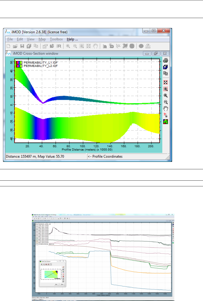
DRAFT
iMOD, User Manual
Example of a cross-section using the Clr option:
1/T Select the checkbox in this column in combination with the option Clr, to divide the
value of the IDF by the thickness.
Map Displays the IDF-filename. You can not adjust this field.
Configuration Select an option from the drop down list to display the layers in a predefined display
mode.
Interfaces
Select this option to display each IDF separately as a line interface.
216 of 812 Deltares
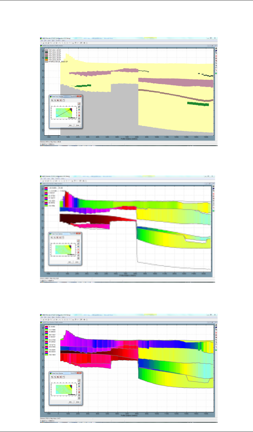
DRAFT
Toolbox Menu Options
Quasi 3D model
Select this option to display the aquifers in yellow and the aquitards in a contrasting
colour.
Coloured Quasi 3D Model
Select this option to display the aquifers coloured by the values of the IDF-file as
defined in the legend.
Coloured 3D Model
Select this option to display the aquitards coloured by the values of the IDF-file as
defined in the legend.
Deltares 217 of 812
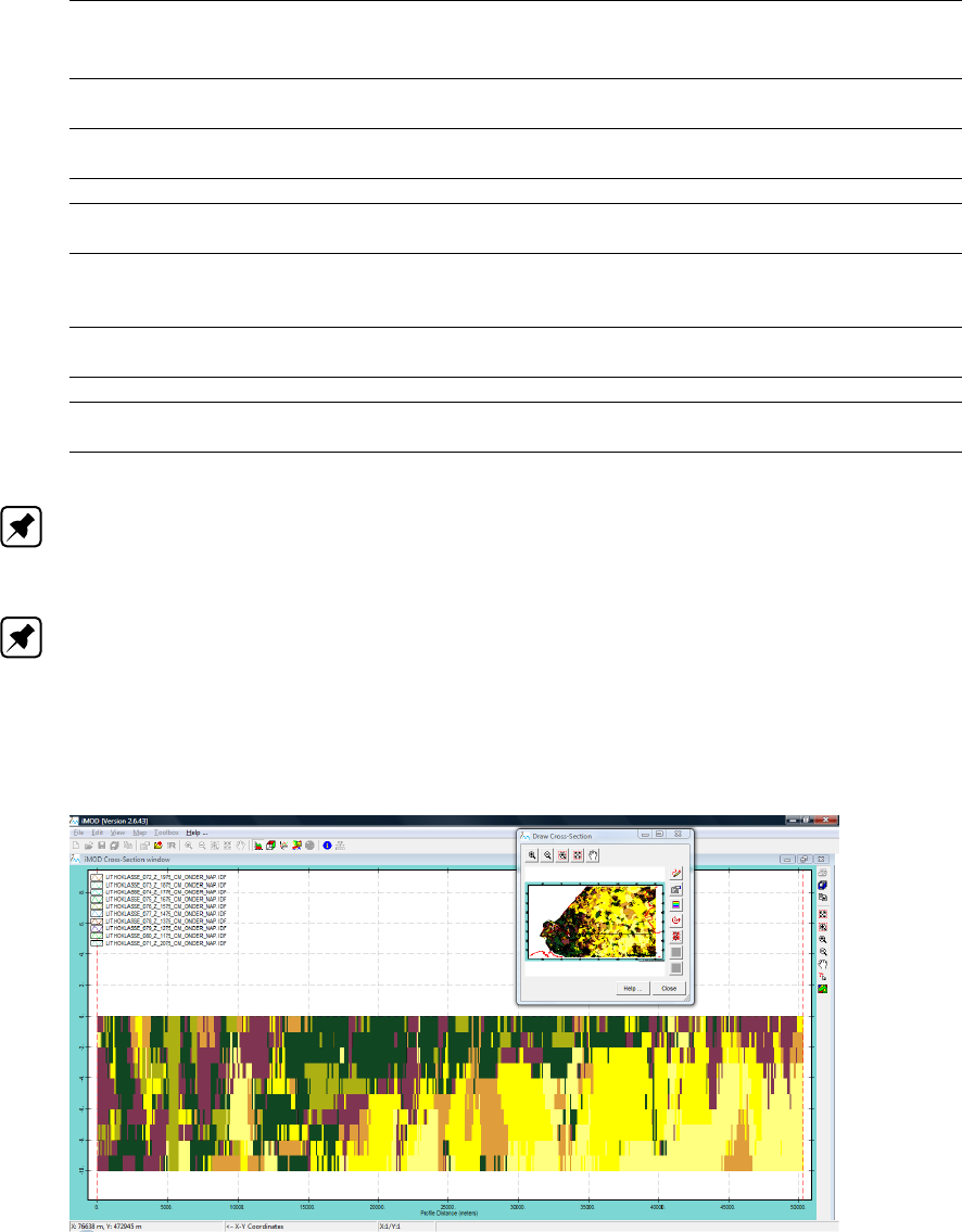
DRAFT
iMOD, User Manual
Block lines Check the box to display the cross-section with lines that connect the individual data
points with horizontal lines.
Block Fills Check the box to display the cross-section with lines that connect the individual data
points directly.
Linethickness Choose the linethickness to display the layer interfaces
Plot lines
in black. . .
Check the box to plot the lines in black on top of the drawn profile, e.g. to be able to
distinguish multiple aquifers when no in between aquitards are available.
Max. no
of Samp.
Pnts.
Maximum number of sampling points used to construct the cross-section.
OK Click this button to accept any changes; the Cross-Section Properties window is
closed.
Help. . . Click this button to start the iMOD Help Functionality.
Close Click this button to close the Cross-Section Properties window, without any changes
to the properties of the cross-section.
Note: The checkbox in the first row of the table is used to adjust all rows simultaneously.
So, whenever you select the option Fill on the first row, all rows will inherit this setting. It also
applies to the Colour option.
Note: Alternative to the Clr option, IDF-files can have top- and bottom information stored
internally (see IDF syntax). If those IDF-files (voxels) are plotted in the Cross-Section Tool the
actual IDF value (e.g. permeability) will be coloured (using the associated legend as with the
Clr option) between the stored top and bottom elevation inside the IDF.
Example of a coloured plot of IDF with internal top and bottom elevations:
218 of 812 Deltares
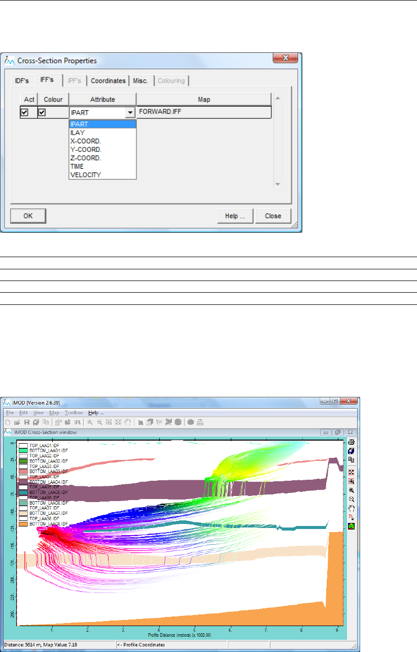
DRAFT
Toolbox Menu Options
Cross-Section Properties window, IFF’s tab:
Act Select the checkbox in this column to include the IFF in the cross-section.
Colour Select this checkbox to colour the lines according to the selected Attribute item.
Attribute Select an item from the dropdown menu to be used to colour the lines.
Map Displays the IFF filename. You can not adjust this field.
The example below shows a cross-section presenting an IFF-file (flowpath) in combination
with IDF-files that represent the top and bottom of aquitards.
Example of a Cross-Section showing flowlines from an IFF file:
Deltares 219 of 812
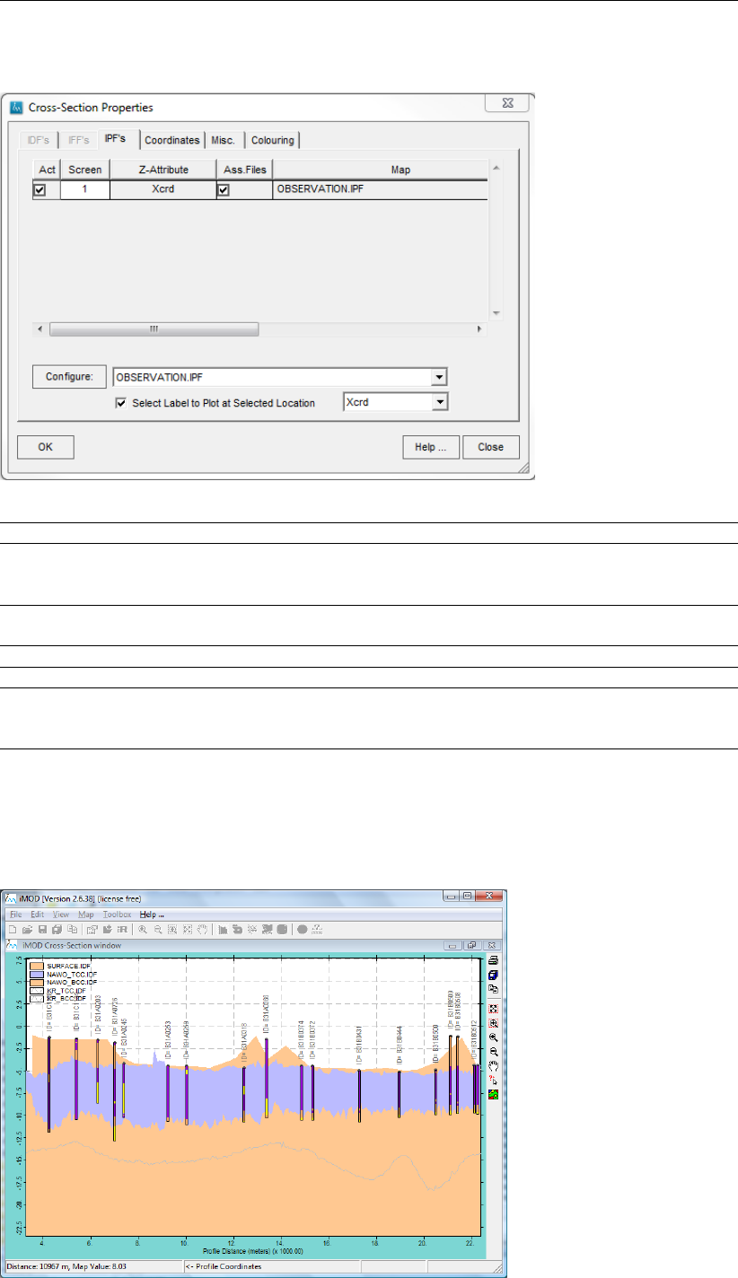
DRAFT
iMOD, User Manual
Cross-Section Properties window, IPF’s tab:
Act Select the checkbox in this column to include the IPF in the cross-section.
Z-Attribute This is the attribute in the IPF-file that will be used to position any label. In
case timeseries are presented, this attribute value is used too. For others
(boreholes, borelogs) this value is irrelevant.
Ass-Files Select this checkbox to use the associated file of the IPF. These can be time-
series, boreholes and/or borelogs.
Map Displays the IPF-filename. You can not adjust this field.
Configure: Select this button to set the configuration for the IPF-file (see 129).
Select label to Plot
at Selected Loca-
tion
This dropdown menu allows you to set the location of the labels of the bore-
holes.
Below an example is given of IPF-files displayed in combination with the Fill option.
Example of a cross-section with boreholes associated to an IPF-file:
220 of 812 Deltares
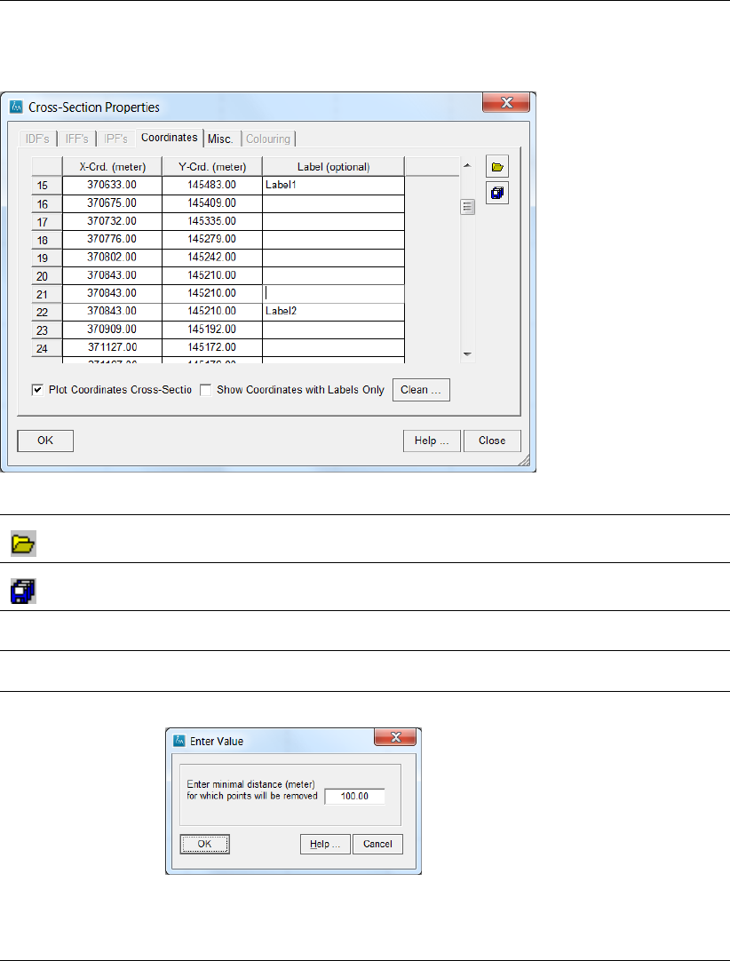
DRAFT
Toolbox Menu Options
Cross-Section Properties window, Coordinates tab:
Open
Click this button to use the coordinates from an existing GEN-file.
Save As
Click this button to save the current coordinates into a GEN-file format.
Plot Coordinates
Cross-Section
Select this option to display the coordinate of the line of the cross-section
within the graph of the cross-section.
Show Coordinates
with Labels Only
Select this option to only display the coordinates with a label within the graph
of the cross-section.
Clean... Starts a new window Enter Value:
In this window a value can be filled in for the minimal distance that needs to
be between coordinate points. The points in a profile will be depleted; points
that are closer to each other than the given distance will be removed.
Deltares 221 of 812
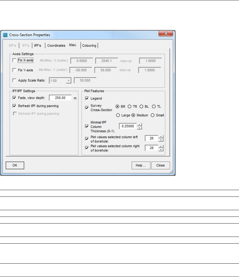
DRAFT
iMOD, User Manual
Cross-Section Properties window, Misc. tab:
Fix X-axis Select this checkbox to specify the dimensions of the X-axis.
Minimal/maximal
X:
Enter the minimal and maximal values for the X-axis.
Interval: Enter the interval of the X-axis.
Fix Y-axis Select this checkbox to specify the dimensions of the Y-axis.
Minimal/maximal
Y:
Enter the minimal and maximal values for the Y-axis.
Interval: Enter the interval of the Y-axis.
Apply Scale Ratio: Chose the preferred x,z-scale ratio from the drop down-menu or enter a ratio-
value in the given field. The ratio is shown on the graph. See figure below for
an example of the cross-section window with adjusted ratio.
Fade Select this option to fade-out the colouring for IPF (points) and/or IFF (lines)
whenever they appear at more distant from the line of the cross-section.
222 of 812 Deltares
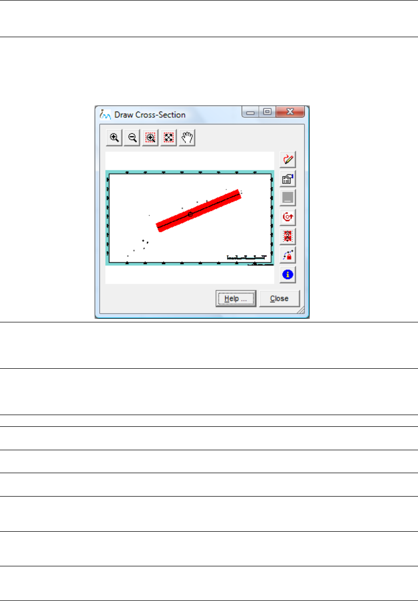
DRAFT
Toolbox Menu Options
Fade, view depth Enter the distance perpendicular on the line for the cross-section for which
points (IPF) and/or lines (IFF) are projected perpendicular on the line of the
cross-section. This “area” is displayed as a red rectangle around the drawn
line for the cross-section.
Example of the Viewing Depth:
Refresh IPF dur-
ing panning:
Select this option if you have a small borehole IPF dataset. This option forces
iMOD to refresh the cross-section view when you move your window extent
(=panning). Deselect it whenever the data set is large since this will delay the
drawing significantly.
Refresh IFF dur-
ing panning:
Select this option if you have a small pathline IFF file. This option forces iMOD
to refresh the pathline view when you move your window extent (=panning).
Deselect it whenever the data set is large since this will delay the drawing
significantly.
Legend Select this option to display a legend on the graph
Survey
Cross-section
Select this option to display a 2D map of the location of the cross-section.
BR, TR, BL, TL Select on of the following to specify the location of the survey, BR is Bottom-
Right, TR is TopRight, BL is BottomLeft and TL is TopLeft.
Large, Medium,
Small
Select on of the following to specify the size of the location of the survey.
Minimal IPF Col-
umn Thickness (0-
1):
Select this option to set a minimal Column thickness of the boreholes. This
prevent iMOD from hiding a certain borehole when it is at the same location
as another borehole in the display window.
Plot values se-
lected column left
of borehole:
Select this option to plot the values of the defined column (e.g 26) in the IPF
associated file at the left side of the borehole in the Cross-section plotting
window.
Plot values se-
lected column
right of borehole:
Select this option to plot the values of the defined column (e.g 28) in the IPF
associated file at the right side of the borehole in the Cross-section plotting
window.
Deltares 223 of 812
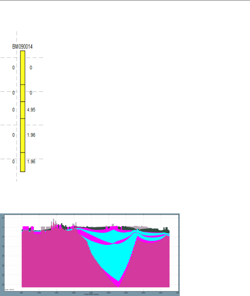
DRAFT
iMOD, User Manual
Example of the plotting window with the values of the defined columns (from the associated
text file) plotted next to the borehole:
Example of the cross-section window with adjusted ratio:
Cross-Section Properties window, Colouring tab:
The table on this tab is used to display the boreholes that might be associated with the se-
lected IPF-files. On default the file: {user}\settings\DRILL.DLF will be read.
224 of 812 Deltares
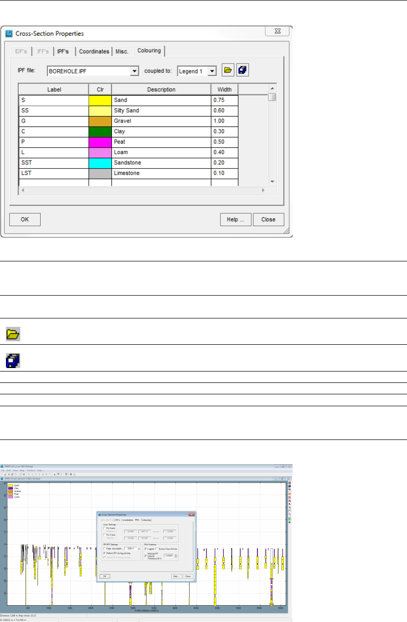
DRAFT
Toolbox Menu Options
IPF file: This dropdown menu shows the IPF-files that are currently available in the IPF Anal-
yse. For each IPF-file a different legend can be defined by making use of the Legend:
dropdown menu.
Legend: This dropdown menu allows you to select and/or define a different legend per avail-
able IPF-file.
Open
Click this button to open a *.DLF-file
Save As
Click this button to save the current legend into a DLF file format
Label Associated label to the specific Legend attribute.
Clr Associated colour to the specific Legend attribute.
Description Associated description to the specific Legend attribute.
Width Adjustable width of the borehole unit related to the specific legend attribute. If differ-
ences in width are defined between the layers this is visible in the cross-section of
the boreholes (see figure below).
Deltares 225 of 812
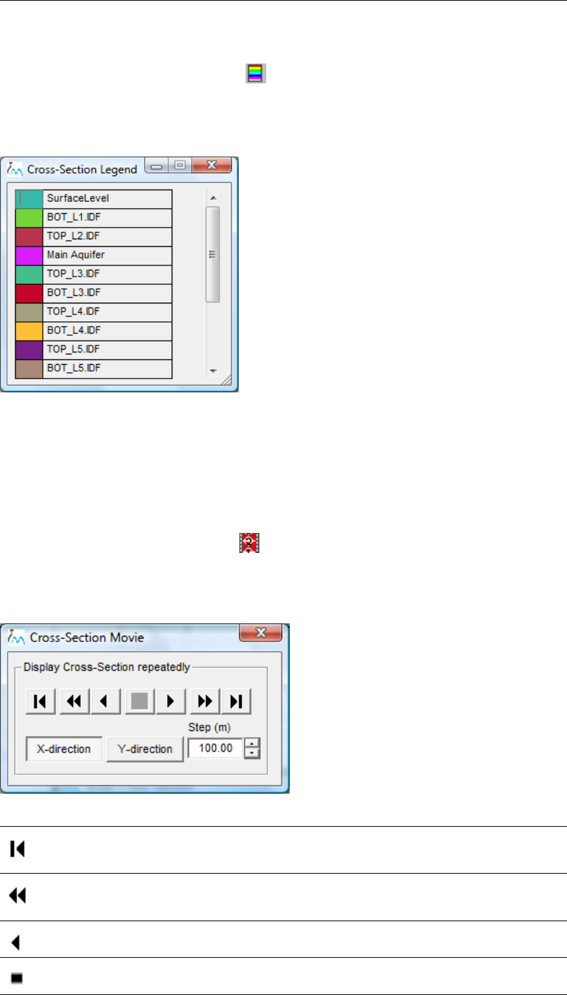
DRAFT
iMOD, User Manual
7.1.2 Profile Legend
Click the option Cross-Section Legend on the Draw Cross-Section window to open the
Profile Legend window.
Cross-Section Legend window:
The Cross-Section Legend window displays the filenames of the IDF’s, however, these can
be adjusted in the Cross-Section Properties window. Moreover, a legend for each of the items
in the Cross-Section are displayed on the iMOD Cross-Section window too.
7.1.3 Movie
Click the option Cross-Section Movie on the Draw Cross-Section window to open the
Cross-Section Movie window.
Cross-Section Movie window:
Complete Backward
Click this button to move the Cross-Section line to the utmost left (X direction) or
utmost top (Y-direction) coordinate of the current extent of the graphical window.
Fast Backward
Click this button to move the Cross-Section line against the X- or Y-direction, repeat-
edly with the chosen Step.
Single Backward
Click this button to move the Cross-Section a single step against the X- or Y-direction.
Stop
Click this button to stop the actions Fast Backwards or Fast Forwards.
226 of 812 Deltares
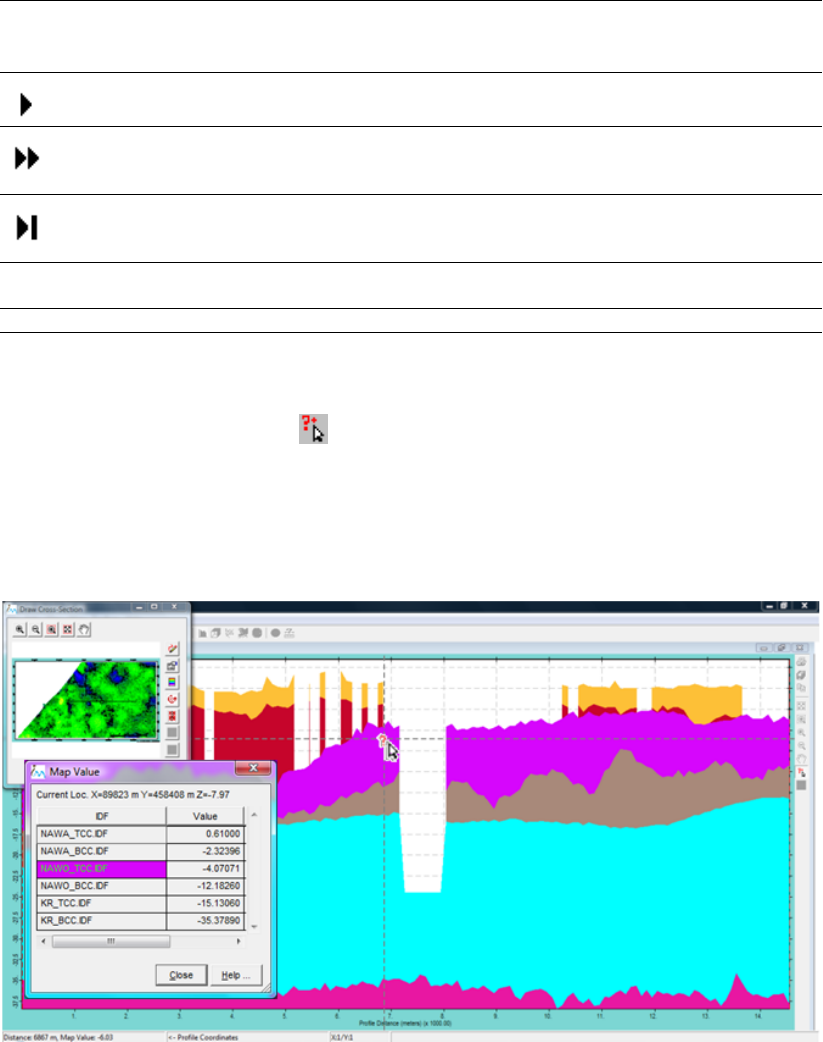
DRAFT
Toolbox Menu Options
Single Forward
Click this button to move the Cross-Section a single step along the X- or Y-direction.
Fast Forward
Click this button to move the Cross-Section line along the X- or Y-direction, repeatedly
with the chosen Step
Complete Forward
Click this button to move the Cross-Section line to the utmost right (X direction) or
utmost bottom (Y-direction) of the current extent of the graphical window.
X-direction
Y-direction
Choose one of the directions in which the line of the cross-section moves.
Step (m) Insert the interval for which the line of the cross-section moves repeatedly.
7.1.4 Cross-Section Inspector
Click the Cross-Section Inspector on the iMOD Cross-Section window to identify the values
for each IDF at the selected position in the cross-section. You can move the mouse-cursor
over the cross-section and the IDF values for each selected IDF will be displayed in the Map
Value window.
Example of the Cross-Section Inspector option:
The position of the mouse will be displayed on top of the Map Value window (e.g. Current Loc.
X=89823 m Y=458408 m Z=-7.97 ). iMOD will colour the name of the IDF in the Map Value
window nearest to the mouse cursor. If there is any inconsistency in the IDF values (that is,
whenever the IDF are not arranged such that they represent values that increase from the first
IDF to the last IDF), iMOD will not colour any field, but will present the message Inconsistency
in top/bottom at current location on the bottom of the Map Value window. The Cross-Section
Inspector can be closed by clicking the left-mouse button or select the Close button on the
Map Value window.
Deltares 227 of 812
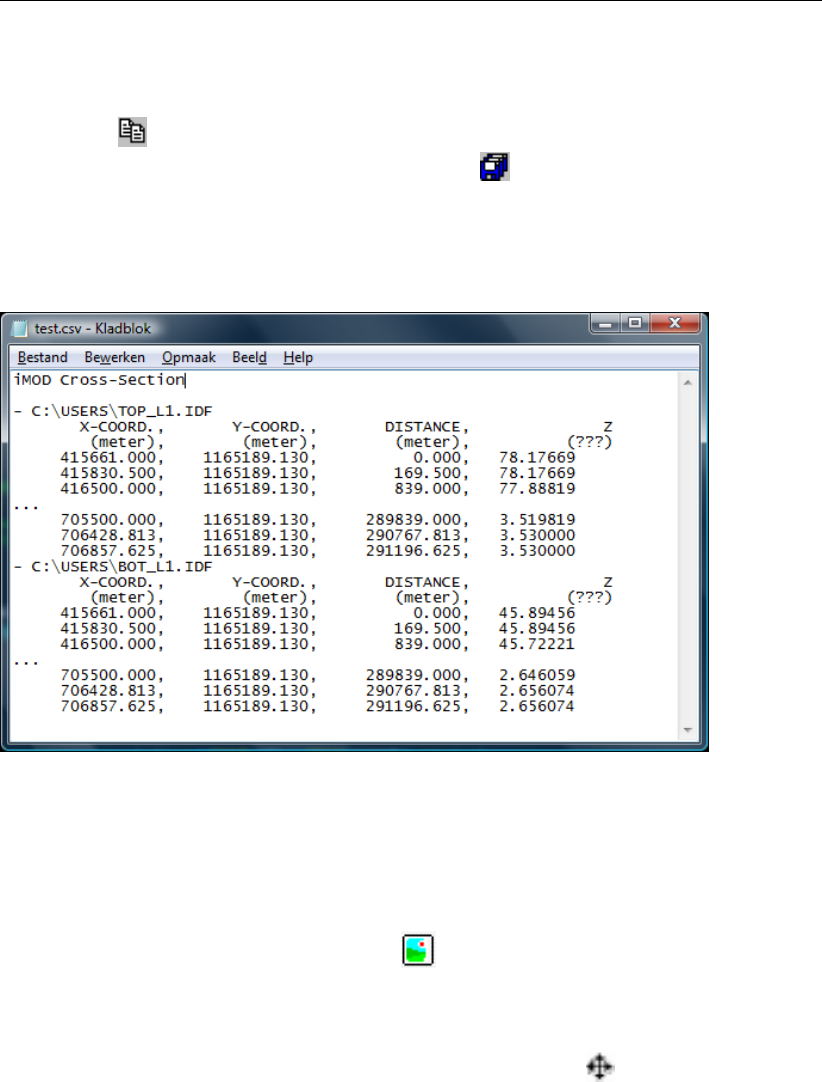
DRAFT
iMOD, User Manual
7.1.5 Export
There are two ways to export a cross-section: (1) as an image (BMP): use the Copy to Clip-
board option from the iMOD Cross-Section window and paste it into a third party software
application, (2) as data (*.csv): use the Export option from the iMOD Cross-Section win-
dow. For the latter, an example is given of the file format. A new data-block starts for each
IDF, since, the points of intersection might differ.
Example of an export of a cross-section:
7.1.6 Background Bitmaps
A graphical *.JPG, *.BMP- or *.png-file can be added to the iMOD Cross-Section window to be
displayed as background. This could be a profile prepared outside iMOD with other graphical
tools.
Click the Add a bitmap as background button on the iMOD Cross-Section window to open
the file manager to select a bitmap. The bitmap will be added to the cross-section. Next the
position and size will have to be set in the cross-section using the mouse.
Move your cursor on to the bitmap and you will see it change in: . Click your left mouse
button and move the bitmap. Move your mouse to the edge of the bitmap, you will see it
change and move the edge. Repeat this until your bitmap fits the iMOD cross-section. The
position of those bitmaps will be save in a SPF file (section 9.21) that is used by the Solid Tool
(section 7.4).
228 of 812 Deltares
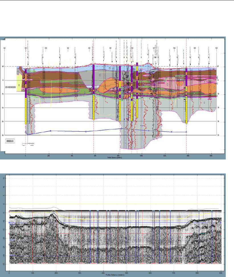
DRAFT
Toolbox Menu Options
Examples of an iMOD Cross-Section with borehole information showing sub-surface layers
added as background:
Deltares 229 of 812
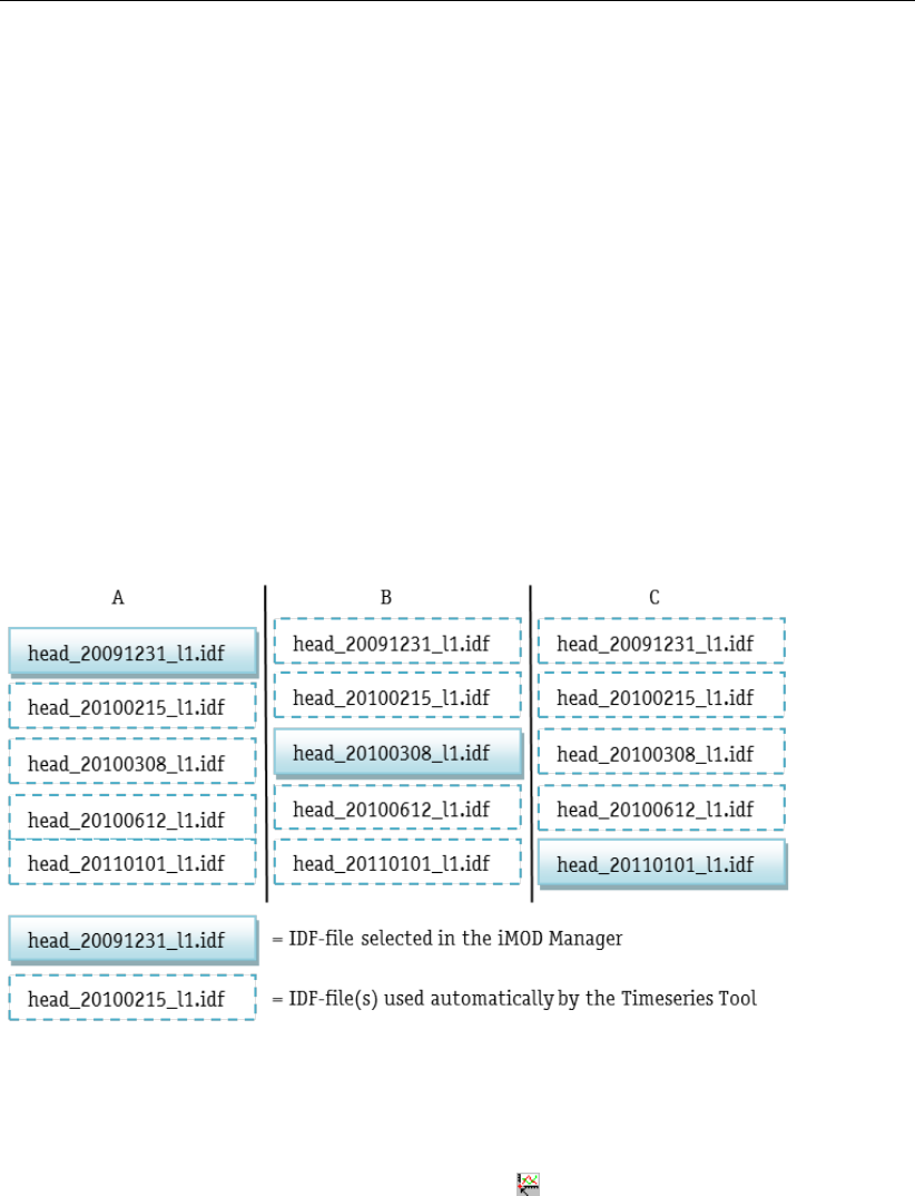
DRAFT
iMOD, User Manual
7.2 Timeseries Tool
WHY?
The Timeseries Tool can be used to view timeseries directly for data stored in different IDF-
files. These can be combined with timeseries that are associated to IPF-files.
WHAT?
The Timeseries Tool allows you to point at a particular location inside the full extent of an
IDF-file with time-dependent data. iMOD will construct a timeseries for that particular location
by collecting all data from the other related time-dependent IDF-files. Related time-dependent
IDF-files have identical names but have a different date string. A date string is an eight digit
continuous number, e.g. 20091231 meaning the 31th of December 2009. It is not necessary
to load all related time-dependent IDF-files in the iMOD Manager. At least one is sufficient to
view the entire timeseries.
Example of IDF-files (A,B and/or C) available in the iMOD Manager prior to the start of the
Timeseries Tool:
HOW?
To start the Timeseries Tool select Toolbox from the main menu, choose Timeseries Tool.
Alternatively, you can click the Timeseries button ( ) at the main toolbar. In both cases,
you should select at least one IDF-file in the iMOD Manager that has a date notation in its
name. This is a continuous number with eight-digits (yyyymmdd), e.g. 20110115. In this case,
it represents the 15th of January, 2011. If iMOD can not find such a date notation somewhere
in the filename (in at least one of the selected IDF-files), the following window will appear and
the Timeseries Tool will not start.
Warning window:
230 of 812 Deltares
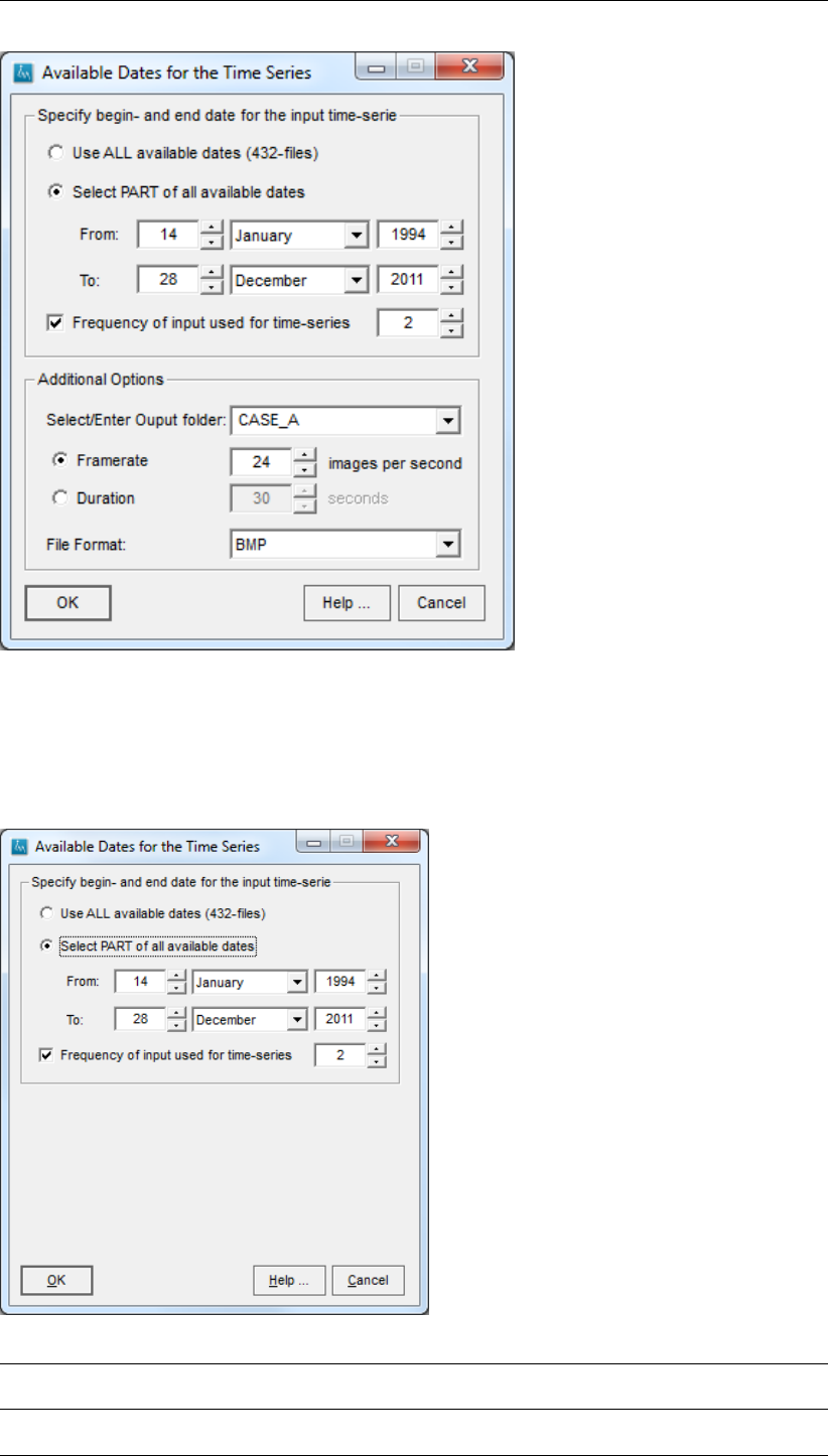
DRAFT
Toolbox Menu Options
If a proper IDF-file(s) has been selected in theiMOD Manager, the following window will ap-
pear.
Available Dates window:
Use ALL available
dates (297-files)
Select this option whenever you want to display timeseries for the entire time
window that iMOD found.
Select PART of all
available dates
Select this option to specify a different time window. This may gain processing
time as less files need to be opened.
Deltares 231 of 812
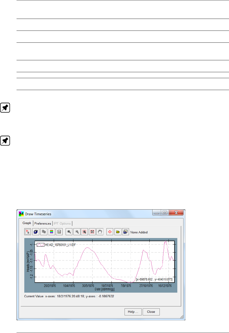
DRAFT
iMOD, User Manual
From: Enter the start date of the time window. On default it displays the earliest date
of the data.
To: Enter the end data of the time window. On default it displays the latest date of
the data.
Frequency of in-
put used for time-
series
Select this option to decrease the number of dates used, e.g. by entering the
value 2 iMOD will skip each second available date of the time series.
OK Click this button to start the Timeseries Tool for the selected time window. The
Available Dates window will close.
Help . . . Click this button to start the iMOD Help Functionality.
Cancel Click this button to close the Available Dates window; the Timeseries Tool will
not start.
Note: You should select at least one IDF with date information in its filename, other IDF-files
that are selected without a date information, will be displayed as time-constant. In this way you
can easily make a combination with time-variant information (e.g. heads) and time-invariant
information (e.g. surfacelevel).
Note: When you select an IPF with associated timeseries, these timeseries will be displayed
simultaneously with those obtained from the IDF-file(s). In case you specify one IDF and one
IPF, the option to compute differences between them becomes available.
7.2.1 Draw Timeseries
The Draw Timeseries window consists of three tabs. The IPF Options tab is only available
when IPF-files are loaded.
Draw Timeseries window, Graph tab:
232 of 812 Deltares
DRAFT
Toolbox Menu Options
Timeserie Hovering
Click this button to start the hovering of timeseries. Move your mouse over the main
graphical window to compute the timeseries. The current location will be highlighted
on the map and the corresponding timeserie(s) will be displayed immediately. iMOD
will try to read and process the entire timeseries (could be more than one) within
one second. If this fails, the progress bar shows the amount of data that could be
processed within this time limit.
Progress bar in Graph tab:
To complete the timeseries, you need to press the left mouse button in the
main graphical window. If the progress bar is absent, the timeseries are displayed
completely. To stop the Timeserie Hovering you need to press the right mouse
button.
Save As
Click this button to save the current graph to a comma-separated-values file (*.CSV).
More detailed information.
Copy
Click this button to copy the graph to windows Clipboard.
Legend
Click this button to open theIndividual Colouring window.
Statistics
Click this button to open the Time-statistics window (. . . ).
Zoom In
Click this button to zoom in at the location of the mouse. Stop by clicking the right
mouse button.
Zoom Out
Click this button to zoom out at the location of the mouse. Stop by clicking the right
mouse button.
Zoom Box
Click this button to draw a zoom window in the graph to adjust the zoom level to.
Click your left mouse button for the first point and click your left mouse button for the
second point.
Zoom Full
Click this button to adjust the zoom level to the initial value.
Move
Click this button to move the graph. Use your left mouse button to start moving and
click your right mouse button to stop moving. The displayed differences, (Compute
Residuals from the Preferences tab), are not affected by any vertical moving.
Add Point
Click this button to store the current location internally.
Open IPF-file
Click this button to open an IPF-file for which all locations are stored internally, as if
you were clicking the Add Point button for each location.
Save IPF
Click this button to compute and save the timeseries for all locations that are stored
internally (Add Point and/or Open IPF File). This yields an IPF-file that you can name,
with associated timeseries.
Added 2
points
Displays the number of points that are added by clicking the Add Point button.
Help . . . Click this button to start the iMOD Help Functionality.
Close Click this button to close the Timeseries Tool window.
Note: Whenever you move the mouse over the Timeseries graphical window, the current
coordinates are displayed below the graph. It shows the current date (x-axis) and the corre-
Deltares 233 of 812

DRAFT
iMOD, User Manual
sponding value on the y-axis. It shows Current Value: x-axis 14/2/1997; y-axis: -1.154.
Note: Whenever you include an IPF-file with associated timeseries, iMOD will display the
timeserie(s) of the point of the IPF that nearest to the current location of the mouse. You can
fixate a particular point on the IPF-options tab.
Note: When using theTimeseries Tool you will be able to use the functions ZoomIn, ZoomOut,
ZoomBox, ZoomFull, Move and DistanceTool of the main graphical window.
234 of 812 Deltares
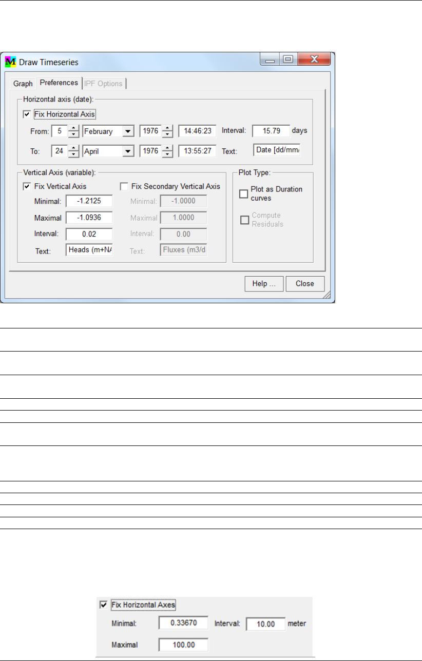
DRAFT
Toolbox Menu Options
Draw timeseries window, Preferences tab:
Fix Horizontal Axis
(date)
Click this option to specify the horizontal axis manually.
From: Enter the start date of the horizontal axis, you can specify start time as
hh:mm:ss.
To: Enter the end date of the horizontal axis, you can specify end time as
hh:mm:ss.
Interval (days) Enter the interval of the horizontal axis in days.
Text: Enter the text to be displayed at the horizontal axis
Fix Vertical Axes
(variable)
Click this option to specify the vertical axes manually.
Fix Secondary
Vertical Axes
Click this option to specify the second vertical axes manually (appears on
the right of the graph). This option becomes available whenever the option
Compute Residuals is selected.
Minimal Enter the minimum value for the vertical axes.
Maximal Enter the maximum value for the vertical axes.
Interval Enter the interval for the vertical axes.
Text: Enter the text to be displayed at the vertical axis
Plot as duration
curve
Click this option to plot all figures as duration curve (Cumulative Distribution
Function). The entry for the option Fix Horizontal Axis changes whenever this
checkbox is selected.
Fix Horizontal Axis for Duration curves:
Deltares 235 of 812
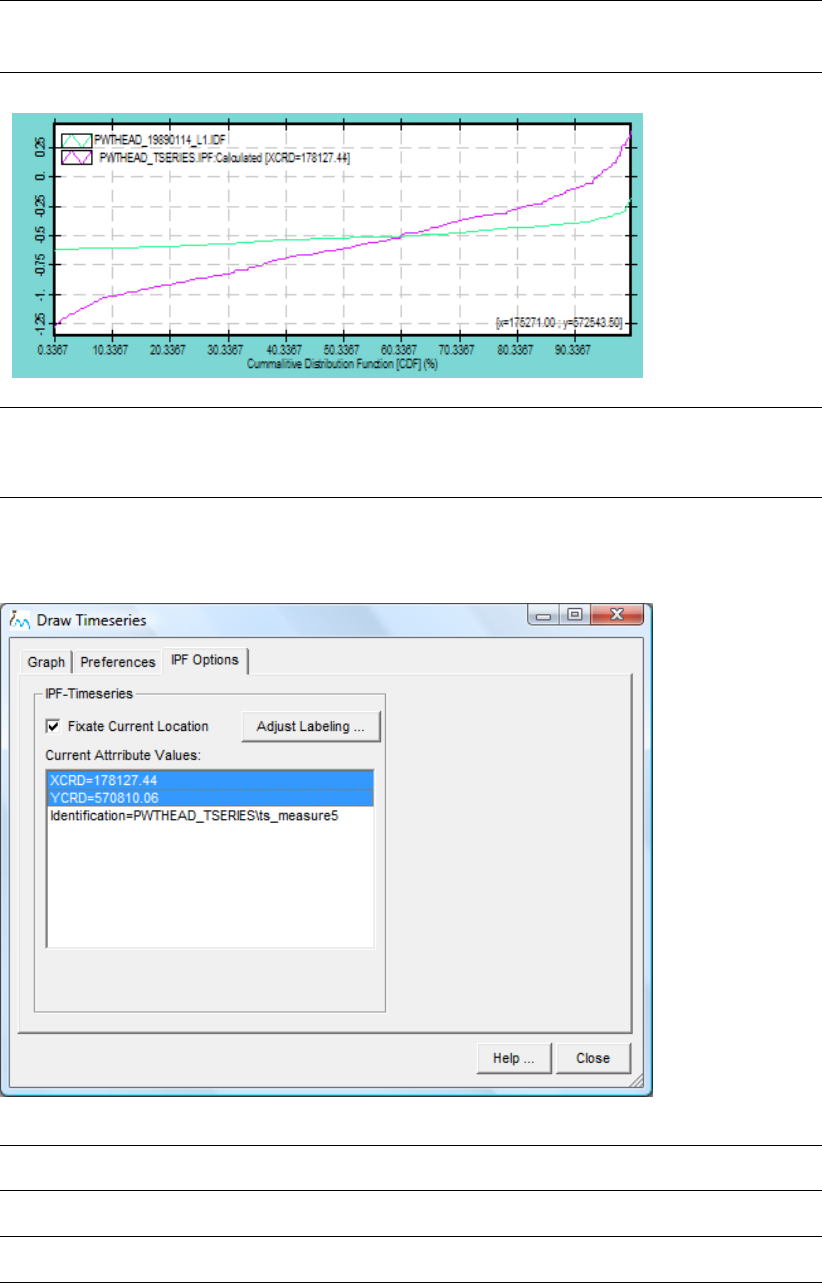
DRAFT
iMOD, User Manual
Example of duration curves:
Compute Residu-
als
Click this option to compute and display differences between the first and
second file. That could be the difference between two IDFs or the difference
between an IDF and the associated timeserie of a point in an IPF.
Draw timeseries window, IPF Options tab:
Fixate Current
Location
Check this option to fix the current location of the point in the IPF that is used
to display the timeserie.
Adjust Labeling Select this button to display labels for the points in the IPF on the main graph-
ical window.
Current Attribute
Values
Select the attributes from the list that will be displayed in the legend section
on the graph.
236 of 812 Deltares
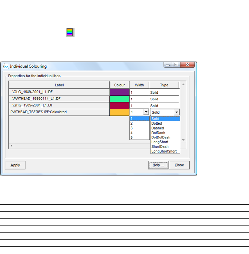
DRAFT
Toolbox Menu Options
7.2.2 Legends
Click the option Legend on the Graph tab to open the Individual Colouring window.
Individual Colouring window:
Label The label of the loaded file (IDFs and/or IPFs)
Colour The current colour of the line in the graph. Click this field to open the Colour window.
Width Click this field to open a dropdown menu with the width of the lines (1-5)
Type Click this field to open a dropdown menu with the different linetypes.
LineStyle Click this field to open a dropdown menu to choose between Continuous or Blocklines
Axes Click this field to open a dropdown menu to choose the axis
Apply Click this button to accept the adjustments and close the Individual Colouring window.
Help . . . Click this button to start the iMOD Help Functionality.
Close Click this button to close the Individual Colouring window without any adjustments.
7.2.3 TimeSeries Export
There are two ways to export the timeseries data from the Timeseries Tool to ASCII-files, as
comma-separated-file-values (*.CSV) to be read by Excel, or/and as an IPF-file with associ-
ated timeseries for direct use in iMOD. When the option Compute Residuals on the Prefer-
ences tab is selected, an extra column will be added with the computed differences. Moreover,
whenever the option Plot as duration curve on the Preferences tab is selected, the export will
describe the duration curves instead. Time-invariant IDF–file(s) will be exported with their
time constant values.
Comma-Separated-Values File
To export the current timeserie(s), click the Save As option from the Graph tab to select a file.
The export file will be a comma-separated-values file (*.CSV) and can be read directly into
Excel. The first column of the export file prints the data (yyyymmdd), the second, third and so
on (as many columns as files active in the Timeserie Tool) print the timeserie(s).
Deltares 237 of 812
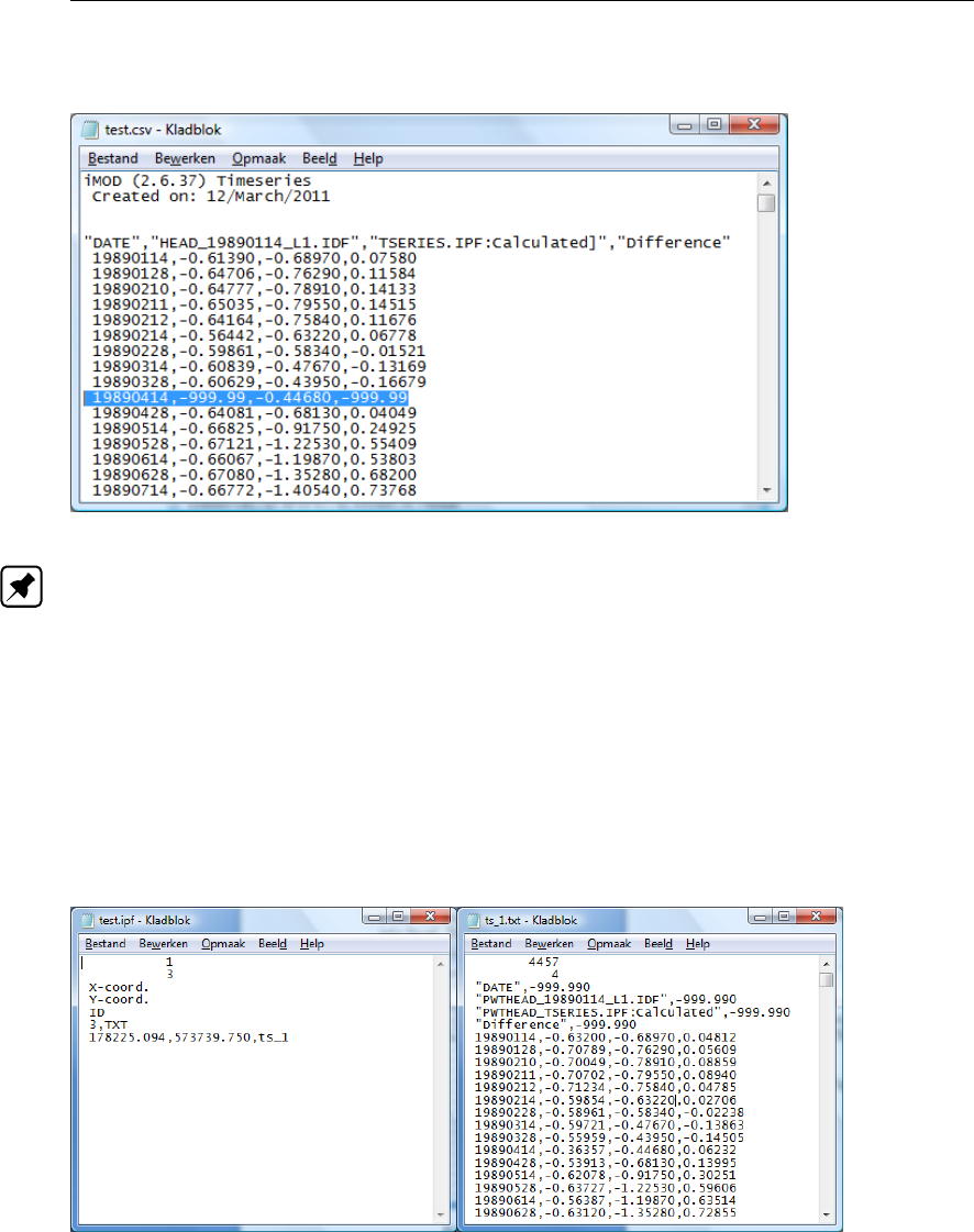
DRAFT
iMOD, User Manual
Example of a comma-separated-values file by the Timeserie Tool:
Note: The number of records in the export file depends on the dates that contain data for each
column. In case column2 has no data (NoDataValue=-999.99) than the computed difference
is nodata too. Since, column three has data, the 14th of April, 1989 is exported whatsoever.
IPF-file
To export the current timeserie(s), click the Save IPF option from the Graph tab to select a
file. The export file will be an *.IPF file with an associated timeserie TXT-file. The latter can
be read into Excel directly.
Example of an IPF-file (left) and the associated text file (right) exported by the Timeserie Tool:
238 of 812 Deltares
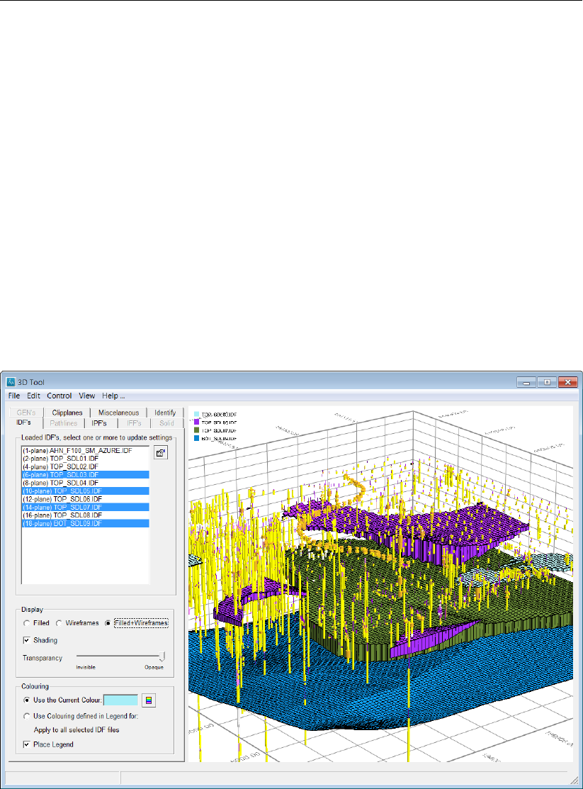
DRAFT
Toolbox Menu Options
7.3 3D Tool
WHY?
The 3D Tool can be used to visualize raster data (IDF), point data (IPF, with/without bore-
holes), polygon data (GEN), flowline data (IFF) in a 3D viewing environment.
WHAT?
iMOD is equipped with an OpenGL library (Open Graphics Library) that is a standard spec-
ification for writing applications that produce 2D and 3D computer graphics. OpenGL was
developed by Silicon Graphics Inc. (SGI) in 1992 and is widely used in CAD, virtual reality,
scientific visualization, information visualization, flight simulation, and video games.
HOW?
To use the OpenGL functionalities in iMOD, simply select the map(s)(IDF, IPF, IFF, GEN, MDF)
from the iMOD Manager and select the option Toolbox from the main menu and then choose
the option 3D Tool to start the 3D Tool.
Example of the 3D tool:
Deltares 239 of 812
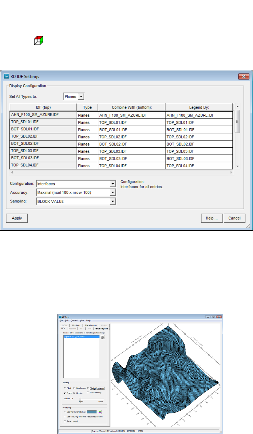
DRAFT
iMOD, User Manual
7.3.1 Starting the 3D Tool
The 3D Tool starts by selecting the 3D Tool option from the main menu option Toolbox. Alter-
natively, the -button can be selected from the main window. In the situation IDF files are
selected in the iMOD Manager window, the 3D IDF Settings window pops up. In this window
each IDF can be configured how it is presented in 3D.
Set all Types to Select the type for all IDF files, any individual modification can be done in the
table. Select one of the following:
Planes
Select this option to compute the 3D image as quadrilateral between the cell
mid of four adjacent cells.
Example of a planes representation.
240 of 812 Deltares
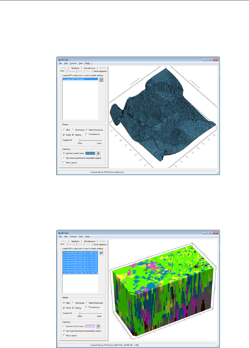
DRAFT
Toolbox Menu Options
Cubes
Select this option to present the IDF using the individual grid cells values as
constant for each individual cell.
Example of a cubic representation.
Voxels
This option is selected automatically whenever the IDF-file represents a voxel
(see section 9.5 for the syntax of an IDF file and how to switch to a voxel
representation for an IDF file).
Example of a voxel representation.
Deltares 241 of 812
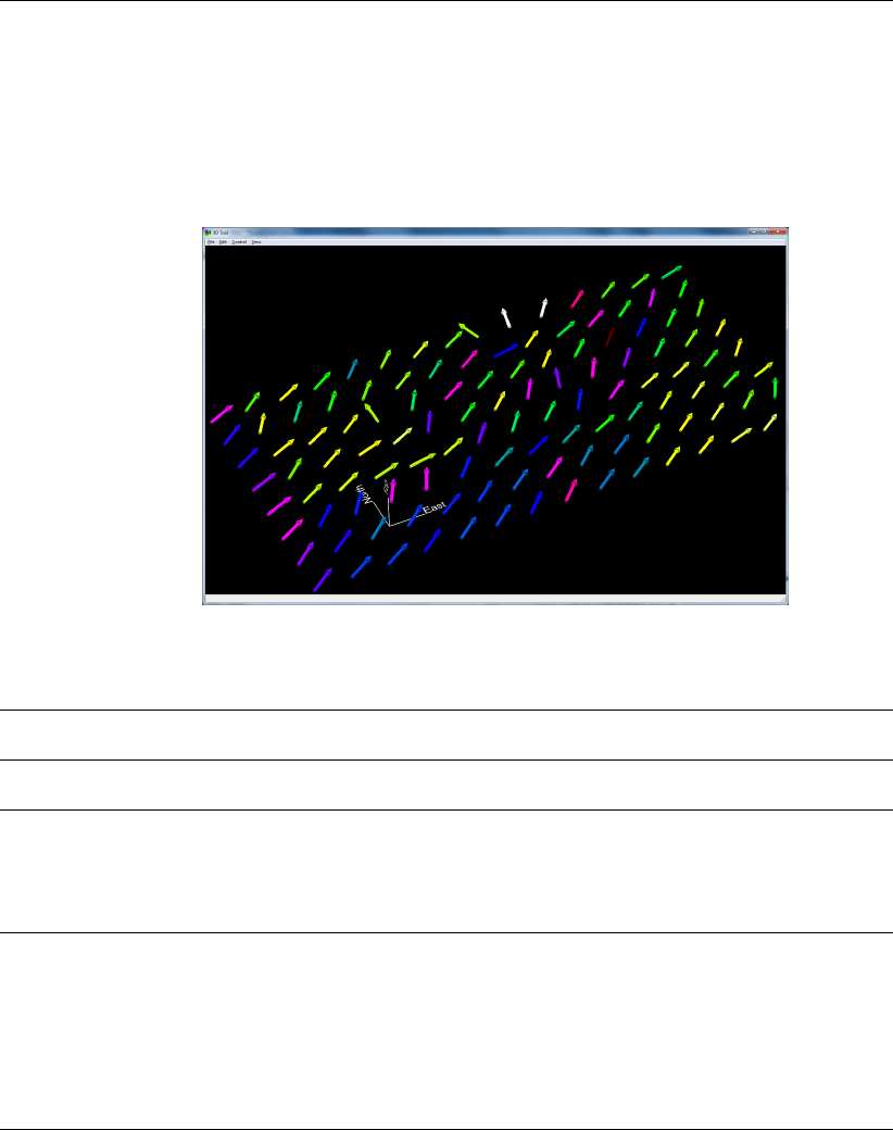
DRAFT
iMOD, User Manual
Vectors
This option is selected automatically whenever the IDF represents a vector
field. See section 9.5 for more information about vectors. Use the iMOD-
Batch function CREATEIVF to create vector IDF’s.
Example of a vector representation.
Off
Select this option to turn the IDF off temporarily.
Table: IDF (top) Displays the current name of the IDF-file, combined with another IDF this
would be the top. It is not possible to change the entry.
Table: Type A type can be selected per individual IDF. For the available types see the ’Set
All Types to’-description above.
Table: Combine
With
(bottom):
Select the IDF-file from the drop-down menu that needs to be combined with
the IDF-file specified in the first column (IDF (top)) of this table. In this way the
first IDF will be used to identify the top of the solid, the ’Combine With
(bottom)’ IDF will be the bottom. It gives a solid representation of these two
IDF’s.
Table: Legend By: Select the IDF-file from the drop-down menu for which the associated legend
needs to be used to colour the 3D representation of the IDF (top) in combina-
tion with the entered IDF at Combine With (bottom). Several possibilities arise,
you may want to colour an IDF using an associated legend of another IDF
and/or whenever two IDF-files are combined as a solid, it could be coloured
by an associated legend of an IDF that represent the permeability of the solid.
Use the different options at Configuration to modify the setting in the table
automatically.
242 of 812 Deltares
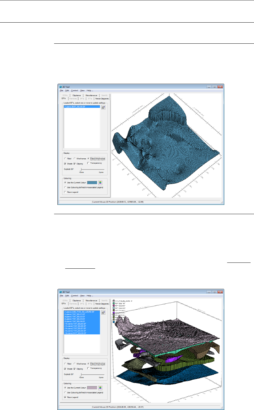
DRAFT
Toolbox Menu Options
Configuration Select an option from the drop down list Configuration to display a layer model
using a predefined display mode.
Interfaces
Use this option to represent each IDF separately as an interface.
Example of an Interface visualisation.
Quasi 3D model (aquitard)
Select this configuration to arrange the Table such that the first IDF will be the
top surface level and presented as a white fishnet. Further downwards, IDF
number 2 will be combined with number 3, number 4 with number 5 and so
on. The last IDF will be presented as a normal plane. This option is especially
handy whenever a Quasi-3D model needs to be presented showing aquitards
as solid bodies.
Example of a Quasi 3D visualisation of aquitards.
Deltares 243 of 812
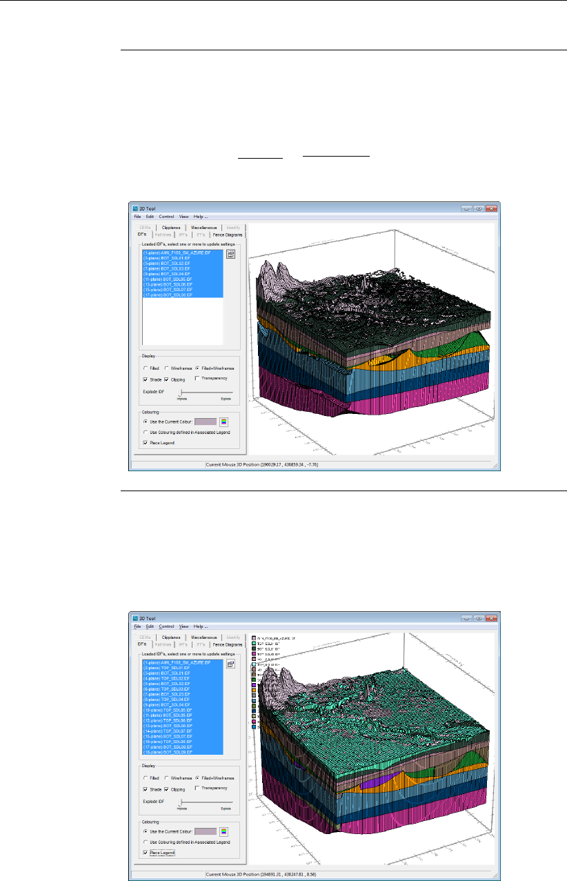
DRAFT
iMOD, User Manual
Quasi 3D model (aquifer)
Select this configuration to arrange the Table such that the first IDF will be
the top aquifer and combined with the second surface; further downwards,
IDF number 3 will be combined with number 4, number 5 with number 6 and
so on. This option is especially handy when a Quasi-3D model needs to be
presented showing aquifers as solid bodies.
Example of a Quasi 3D visualisation of aquifers.
3D Model
Use this configuration to combine each IDF with the following IDF, so IDF
number 1 will be combined with IDF number 2 and that will be combined with
IDF number 3.
Example of a 3D Model visualisation.
244 of 812 Deltares
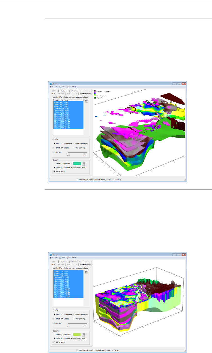
DRAFT
Toolbox Menu Options
Coloured Quasi 3D Model (aquitard)
Use this configuration to present and colour aquitards by sets of 3 IDF’s per
aquitard using the associated legend of each second IDF of that set of 3 IDF’s
to colour the aquitard. The first IDF will be draped as a white fishnet. Then it
will combine the second with the fourth IDF to form a solid and colour it by
the associated legend of the third IDF. Then it will combine the fifth with the
seventh to form a solid and colour it using the legend of the sixth, and so on.
Example of a coloured Quasi 3D (aquitard) visualisation.
Coloured Quasi 3D Model (aquifer)
Use this configuration to present and colour aquifers by sets of 3 IDF’s per
aquifer using the associated legend of each second IDF of that set of 3 IDF’s
to colour the aquifer. It will combine the first with the third IDF to form a solid
and colour it by the associated legend of the second IDF. Then it will combine
the fourth with the sixth and colour it by using the associated legend of the
fifth, and so on.
Example of a coloured Quasi 3D (aquifer) visualisation.
Deltares 245 of 812
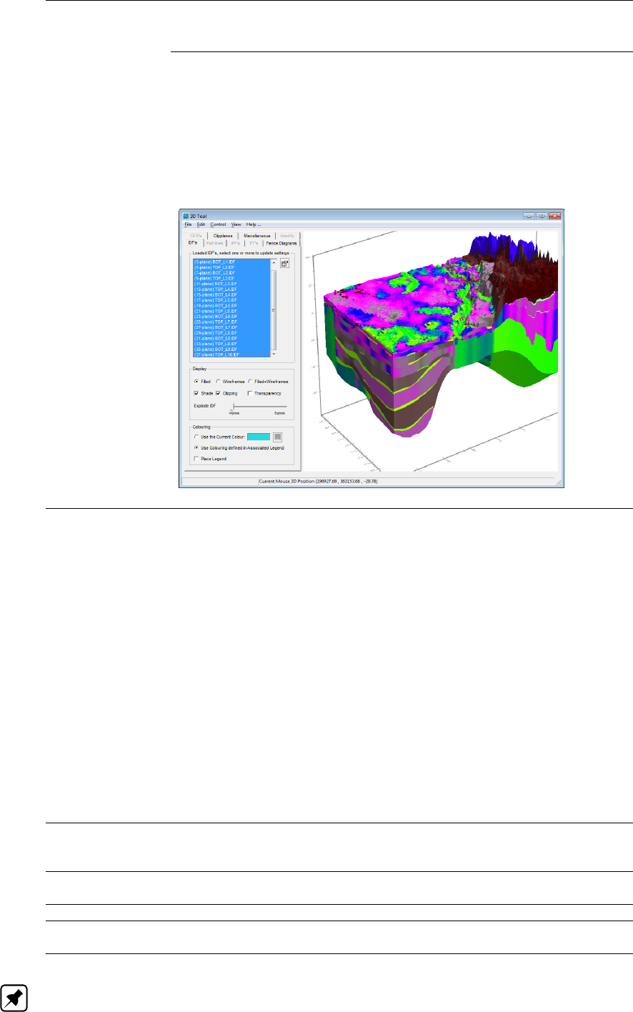
DRAFT
iMOD, User Manual
Coloured 3D Model
Use this configuration to present a complete 3D model with the first IDF
combined with the third to create a solid and colour it according to the
associated legend of the second IDF. Then it will create a solid with the third
and fifth IDF and colour it using the associated legend of the fourth IDF and
so on.
Example of a coloured 3D Model visualisation.
Accuracy Select the accuracy of the representation of the loaded IDF-files. To increase
the performance select a lower resolution, to increase the accuracy of the
representation select a higher resolution. Bear in mind that a high resolution
will need more resources from the graphical card. If this fails, then iMOD will
crash. Choose from:
Minimal (100 x 100):
IDF-file will be represented by a maximum 100 x 100 cells;
Low (max 250 x 250):
IDF-file will be represented by maximum 250 x 250 cells;
Normal (max 500 x 500):
IDF-file will be represented by maximum 500 x 500 cells;
High (max 750 x 750):
IDF-file will be represented by maximum 750 x 750 cells;
Very High (max 1000 x 1000):
IDF-file will be represented by max 1000 x 1000 cells;
Maximal (max ncol x nrow):
IDF-file will be represented by maximal the size of the IDF, e.g ncol x nrow
cells.
Sampling Select the method of upscaling whenever the chosen Accuracy is lower than
the dimensions of the original IDF-file. Select from the dropdown list, for more
detail about these type of upscaling, go to section 6.7.3.
Apply Click this button to to close the 3D Plot Settings window and apply the chosen
display configurations and start the 3D Tool window.
Help . . . Click this button to start the Help functionality.
Cancel Click this button to close the 3D Plot Settings window, the 3D Tool window will
not start.
Note: Bear in mind that iMOD will blank out all elements of an IDF that have a white colour.
In this way it is easy to blank out a specific area, such as high permeable areas by giving them
246 of 812 Deltares

DRAFT
Toolbox Menu Options
a white colour.
Note: It is possible to select the configuration of the table and paste it into e.g. Excel. From
there may it might be easier to detail your configuration and copy and paste it from Excel to
the iMOD your configuration-table of the 3D Tool Settings window.
7.3.2 3D Tool: the Menu bar
The 3D Tool graphics window has the following pull down menus:
File Print ...
Select this item to print the current view via the Windows Print Manager
onto the external printer.
Save As ...
Select this item to save a bitmap (*.BMP; *.PNG; *.JPG) of the 3D
image.
Save As Demo ...
Save 3D Tool settings as an iMOD-demo in a new IMF-file.
Quit 3D Tool ...
Select this item to close the 3D Tool.
Edit Copy to Clipboard
Click this item to copy the current image to the Windows Clipboard.
Control Walk Mode
The image can be moved with the left mouse button as if walking
through the 3D display.
Mouse Left Button;
Mouse Wheel;
Mouse Right Button;
Keyboard Cursor Keys
Select these to modify the behaviour of mouse buttons, mouse wheel
and keyboard cursor keys. For all choices the following operations can
be assigned:
Rotate:
Assign this item to rotate the image;
Pan:
Assign this item to pan/move the image;
Zoom:
Assign this item to zoom in/out the image;
Scale X:
Assign this item to scale the horizontal x axes;
Scale Z:
Assign this item to scale the vertical z axes;
Scale Y:
Assign this item to scale the horizontal y axes;
Scale XY:
Assign this item to scale both horizontal axes simultaneously.
View All Solids
Select this item to transform all IDF-files to solids.
All Wireframes
Select this item to transform all IDF-files to wireframes.
All Solids+Wireframes
Select this item to transform all IDF-files to solids and wireframes.
All Shades
Select this item to switch a shade on/off for all IDF-files (only for option
All Solids).
Show IDF Legends
Select this item to display all legends for selected IDF files.
All Single Colour
Select this item to apply a single colour to the IDF-files.
Deltares 247 of 812
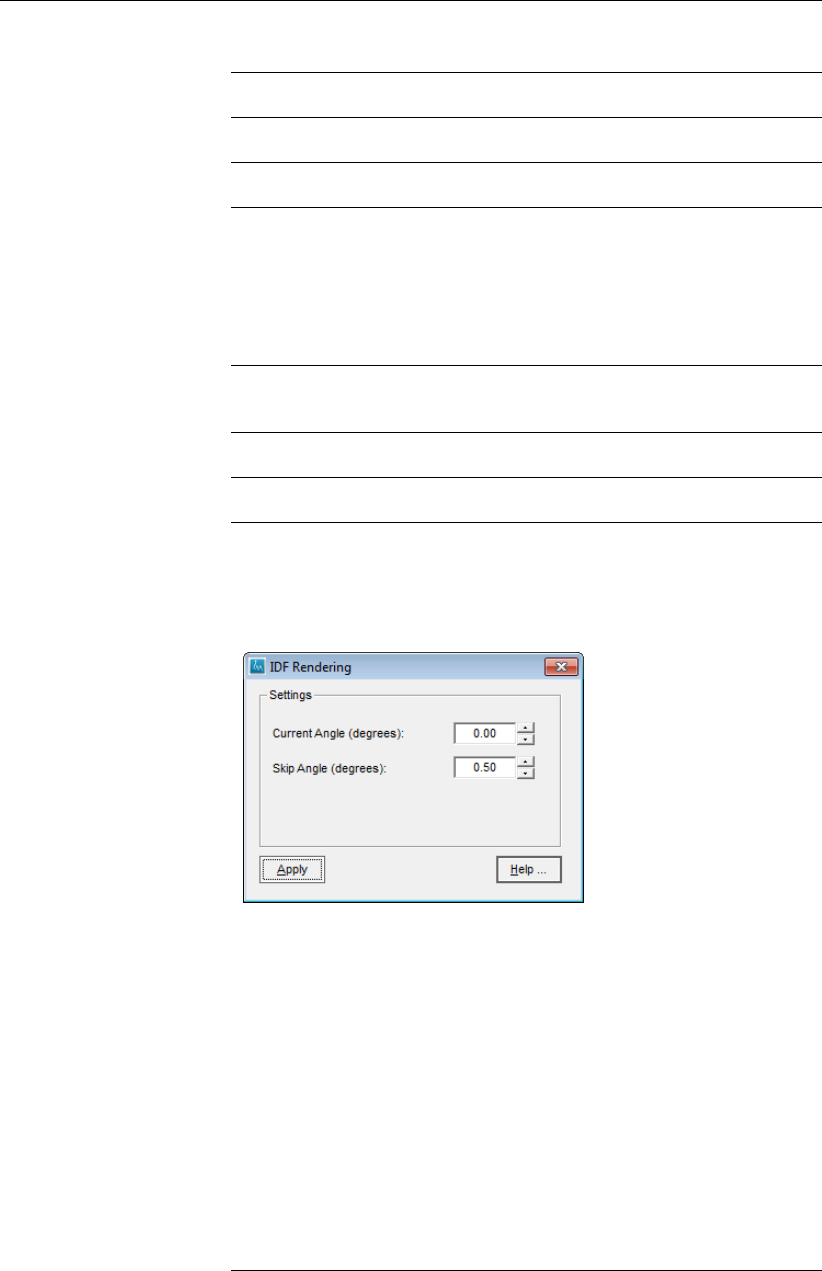
DRAFT
iMOD, User Manual
All Legend Colour
Select this item to apply colours with the associated legend.
Show Axes
Select this item to display axes.
Show Orientation
Select this item to display an orientation box.
Show 3D Coordinates
Select this item to display the position of the mouse in 3D coordinates
at the status bar (always showing this) of the 3D Tool window as well as
a graphical display of the location via a straight red line. The position
of the mouse can only be determined when the mouse is positioned on
a visible IDF/IPF/IFF file. Here the use of a transparency-option does
hamper to yield a correct mouse position.
Anaglyph
Switch to an anaglyph representation of the 3D image. Use this option
to gain a 3D experience using a cyan-red coloured glasses.
Orthographic Projection
Switch to an orthographic projection without perspective.
Reset View Angle
Select this item to reset the viewing angle to the initial view.
Scenic Path . . .
Select this item to specify the dimensions of a circle around the current
viewpoint. The following window pops up:
Scenic Path window.
Current Angle (degrees)
Enter the angle ...
Skip Angle (degrees)
Enter the angle to be skipped in sequential rotations, e.g. a value of 5
will skip 5 degrees during a sequential rotation.
Apply
Select this button to apply the modified entries.
Help . . .
Select this button to start the Help functionality.
Whenever the spacebar is invoked, iMOD will render the image follow-
ing the scenic path automatically and repeatedly.
Horizontal / Vertical Ratio
Select one of the following 5 predefined ratios Scale 1:{x}from the hor-
izontal and vertical dimensions. iMOD computes these automatically
whereby the maximal scale generates a 3D box, that has the same
height as the maximum between the size in x- or y-direction. In linear
steps this is decreased, e.g. Scale 1:25;Scale 1:20 Scale 1:15 Scale
1:10 Scale 1:5.
248 of 812 Deltares
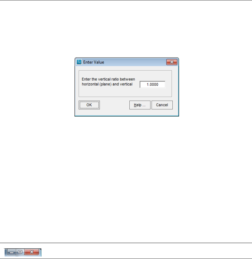
DRAFT
Toolbox Menu Options
Specify . . .
Select this option to enter a user-specified ratio via the following
window that pops up.
Enter Value window
Enter the vertical ratio between horizontal (plane) and vertical
Enter a value to express the ratio between the horizontal plane and
the vertical, e.g. 2.0 means that the vertical is exaggerated twice com-
pared to the horizontal.
OK
Select this button to apply the entered vertical scale ratio. After this the
Enter Value window will be closed and the entered vertical scale ratio
is added to the list of available ratio in the pop up menu at the option
Horizontal / Vertical Ratio.
Help . . .
Select this button to start the Help functionality.
Cancel
Select this button to close the Enter Value window without modifying
the current vertical scale ratio.
Click one of these buttons to minimize, maximize and/or close the 3D
Tool.
The 3D Tool window has separate tabs to configure the display for different types of data, e.g.
there is a tab to configure IDF files and a tab to configure IPF files. There is a tab for general
settings as well. In the following sections, those tabs will be explained in detail.
Deltares 249 of 812
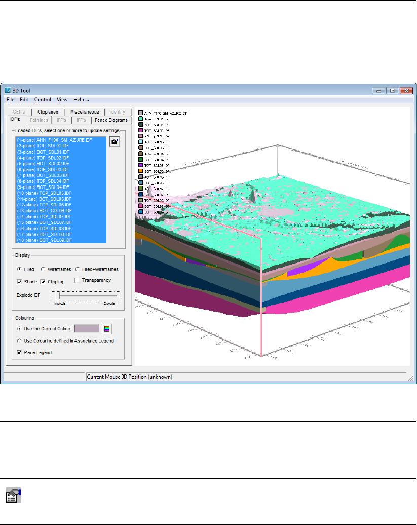
DRAFT
iMOD, User Manual
7.3.3 3D Tool: the IDF-settings tab
Here, the configuration can be applied for the display of IDF files. This is done on the IDFs
tab on the 3D Plot window.
Loaded IDF’s, se-
lect one or more to
update settings
Select one or more IDF-files from the list to activate them in the 3D visual-
ization. The 3D display will update each time an IDF is (de)selected. Click
the option Recompute vertical axes instantaneously in the tab Miscellaneous
to recompute the vertical axes instantaneously each time a different (set of)
IDF-files is selected.
Properties
Click this button to change the appearance of IDF-files. The 3D IDF Settings
window will appear. This is the same window which appears when starting
the 3D tool, see section section 7.3.1.
250 of 812 Deltares
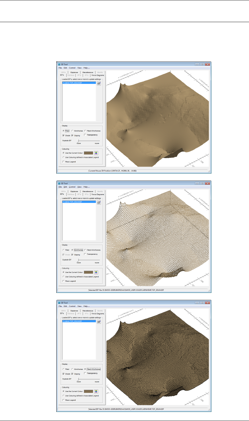
DRAFT
Toolbox Menu Options
Filled;
Wireframes;
Filled+Wireframes
The following options configure the appearance of the IDF files. Choose one
of these to display the selected IDF-files.
Examples when selecting ’Filled’ (top figure), ’Wireframes’ (middle figure) and
’Filled+Wireframes’ (lower figure) in the IDF-Display sub-window:
Deltares 251 of 812
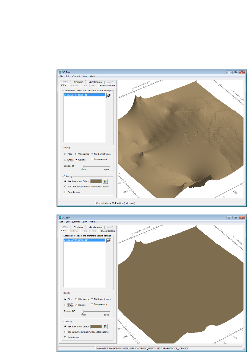
DRAFT
iMOD, User Manual
Shade Select this checkbox to apply shades directly to the selected IDF-files. If no
shade is applied, the surfaces appear flat. This can be specified per IDF file
separately or as a group.
Examples when turning Display-option ’Shade’ on (upper figure) and off
(lower figure):
252 of 812 Deltares
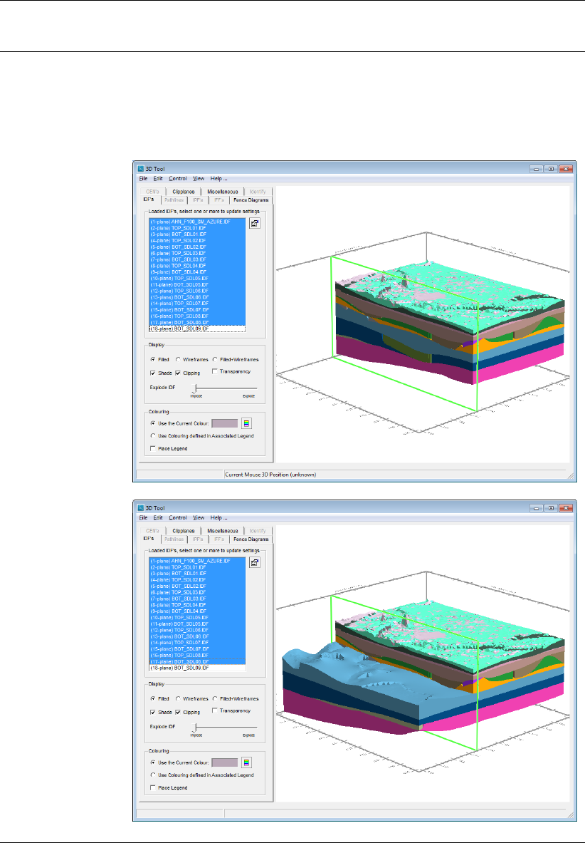
DRAFT
Toolbox Menu Options
Clipping Select this checkbox to clip a selected set of IDF file. By default all IDF files
are clipped, but it is possible to set the clipping per IDF or for a group of IDF
files. The actual clipping is done via the Clipping tab in the 3D Tool window.
Example of clipping for all IDF files (upper figure) and clipping a selected set
of IDF files (lower figure):
Deltares 253 of 812
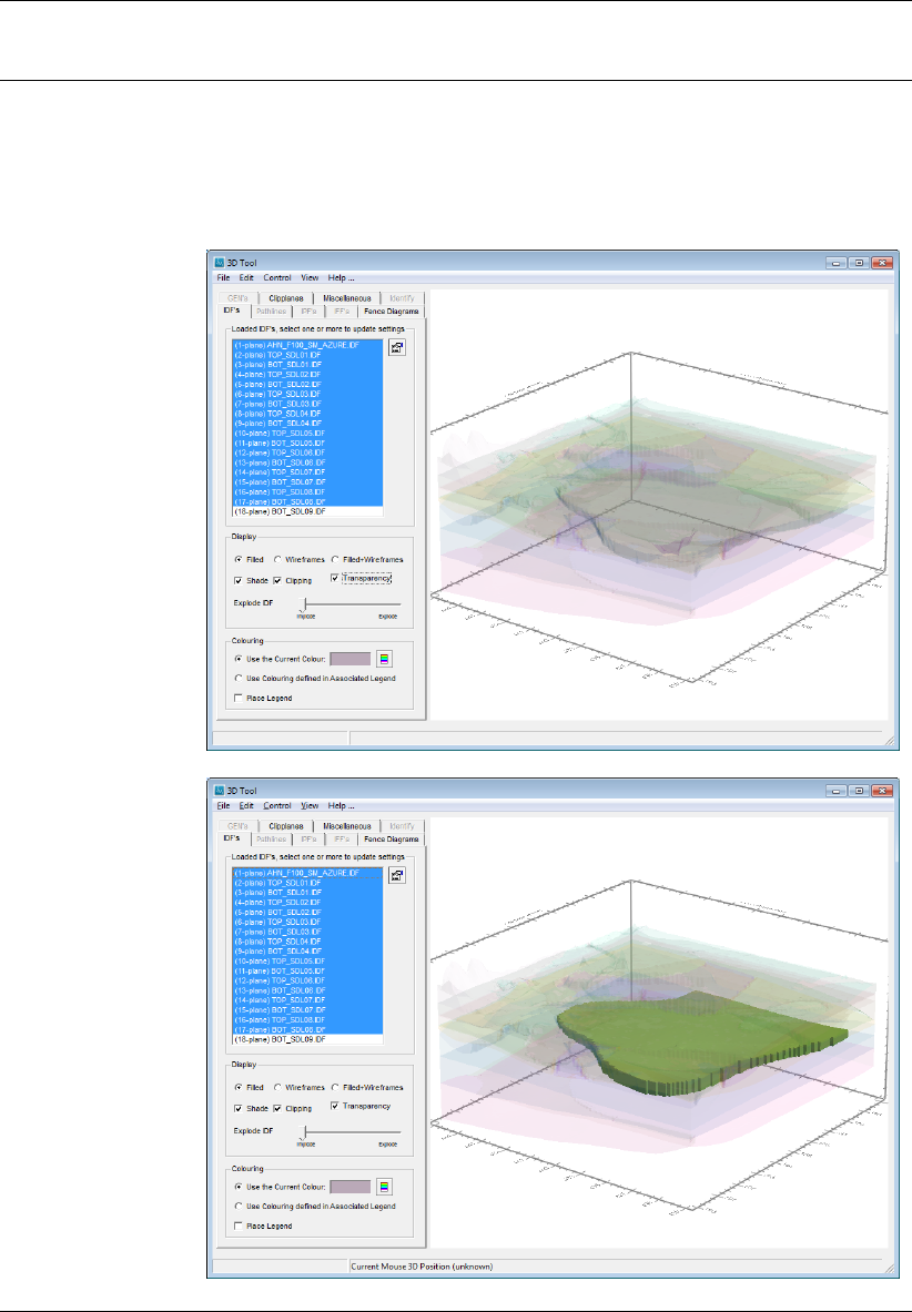
DRAFT
iMOD, User Manual
Transparency Select this checkbox to apply transparency to the selected IDF files. Each
selected IDF is assigned the same amount of transparency. It is also possible
to specify transparency per IDF file.
Example of transparency for all IDF files (upper figure) and excluding a single
IDF file from being displayed transparent (lower figure):
254 of 812 Deltares
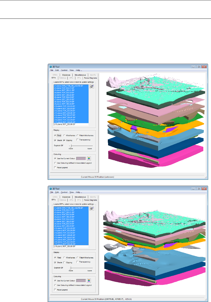
DRAFT
Toolbox Menu Options
Explode IDF Use the ’Explode IDF’-slider to increase (explode) or decrease (implode) ad-
ditional vertical distance between the selected individual IDF’s. Each IDF file
can be configured to explode with its own offset, simple set the slide for the
selected IDF files separately.
Example of exploding all IDF files equally (top figure) or explode some IDF
files more than others (bottom figure).
Deltares 255 of 812
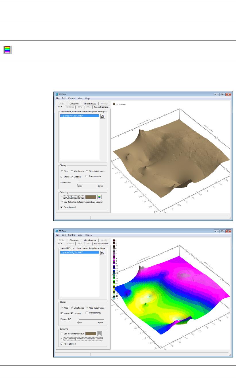
DRAFT
iMOD, User Manual
Use the current
colour
Select this option to display the selected IDF-file(s) by a single colour as dis-
played to the right of this option.
Legend
Click this button to start the default Colour window to select a colour for the
first of the selected IDF-file(s).
Use colouring de-
fined in Associ-
ated Legend
Select this option to colour all selected IDF-files by their associated legend
definitions, i.e. the colour legend they have.
Example of single colouring (upper figure) and legend colouring (lower figure)
Place Legend Check the box to show the legend. This can be set for each IDF file individu-
ally.
256 of 812 Deltares
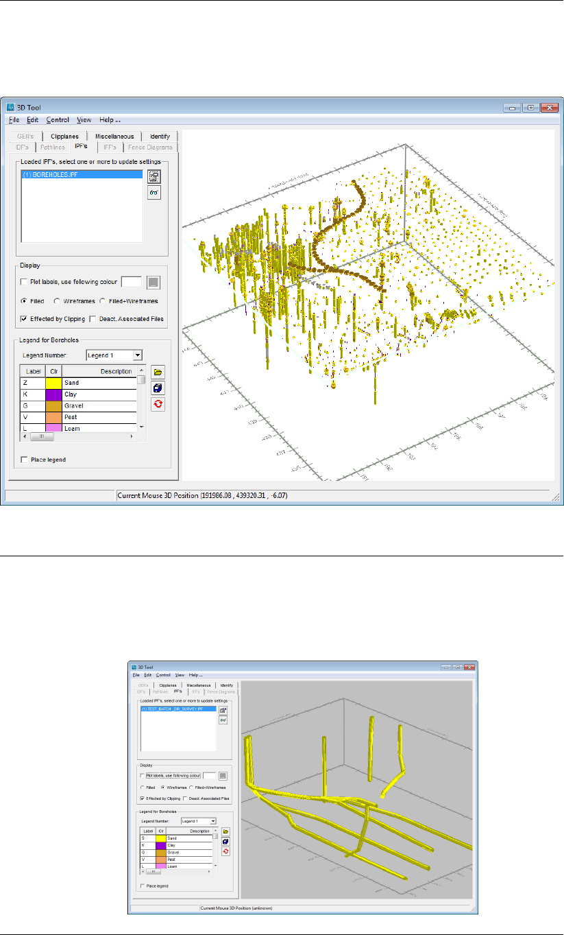
DRAFT
Toolbox Menu Options
7.3.4 3D Tool: the IPF-settings tab
The IPF’s tab of the 3D Plot window allows configuring the display of IPF files.
Loaded IPF’s, se-
lect one of more to
update settings
Select one or more IPF files from the list to activate them in the 3D visualiza-
tion. The 3D display will update each time an IPF is (de)selected. It depends
on the configuration of the IPF(s), how the points (and associated files) will
be displayed.
Example of an IPF file showing deviated wells.
Deltares 257 of 812
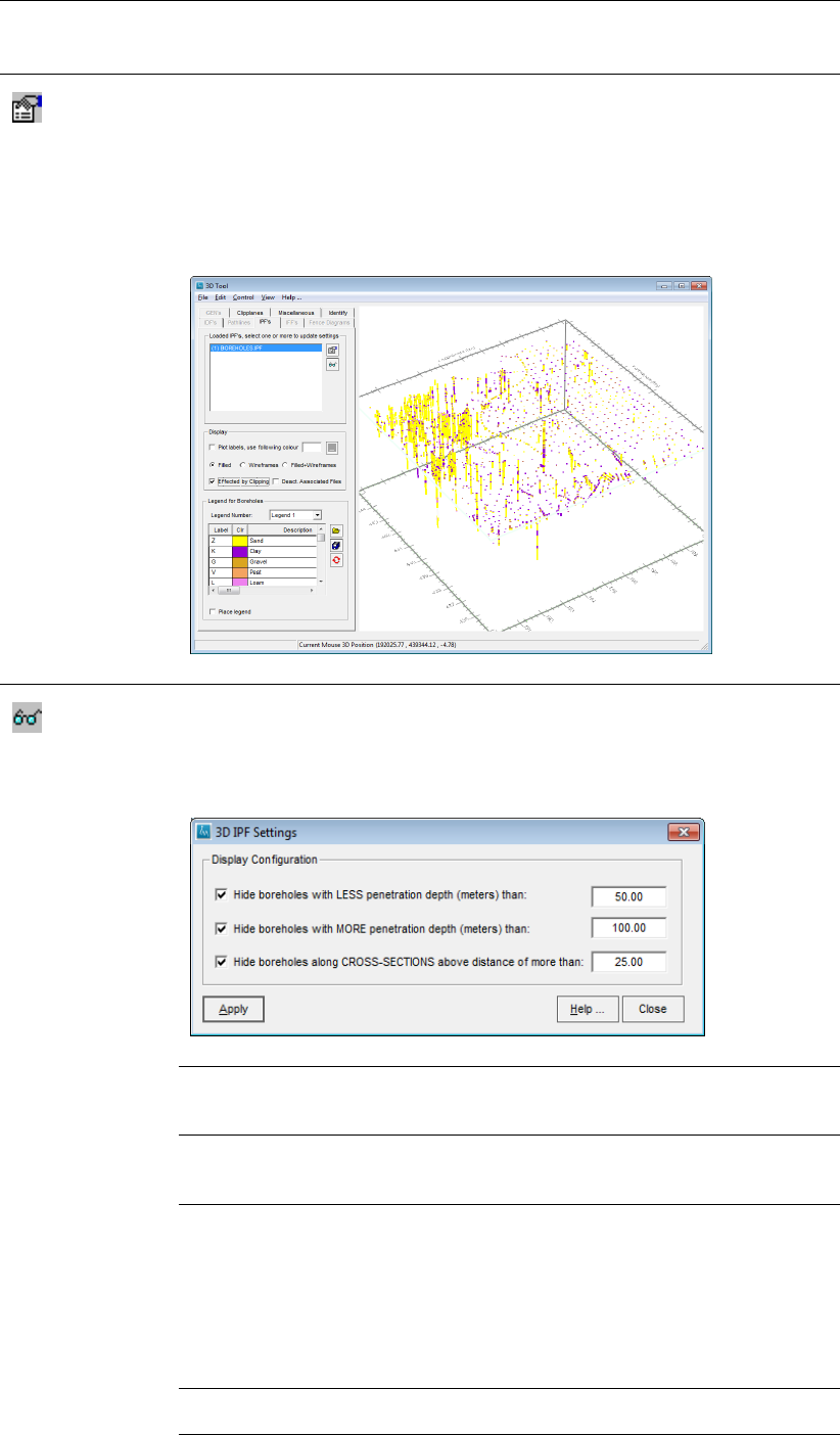
DRAFT
iMOD, User Manual
Properties
Click this button to define labels to be plotted. The presentation of boreholes
can configured in this window, see section section 6.8.2 for more details.
When less than 1000 points are read iMOD will display boreholes by fancy
tubes, when more are loaded the boreholes are represented as single
(vertical) lines instead.
Example of a simple boreholes representation:
Select
Click this button to change the selection of boreholes using their length or
distance to a cross-section, it will open the 3D IPF Settings window:
3D IPF Settings window:
Hide boreholes with LESS penetration depth (meters) than:
Enter the maximal depth for which boreholes will be hidden, e.g. a value of 50
will hide all boreholes with less than 50 meter depth.
Hide boreholes with MORE penetration depth (meters) than:
Enter the minimal depth for which boreholes will be hidden, e.g. a value of
100 will hide all boreholes with more than 100 meter depth.
Hide boreholes with larger distance to CROSS-SECTIONS than:
Enter the distance perpendicular to any selected cross-sections/fence dia-
gram (see ’Fade, view depth’ in the ’Misc.’ tab of the ’Cross-Section Prop-
erties’ window in section section 7.1.1) for boreholes to be hidden, e.g. a
value of 25 will hide boreholes on both sides of a selected cross-section/fence
diagram with more than 25 meter distance.
Apply
Select this button to apply the entered display configuration.
Help . . .
Select this button to start the Help functionality.
258 of 812 Deltares
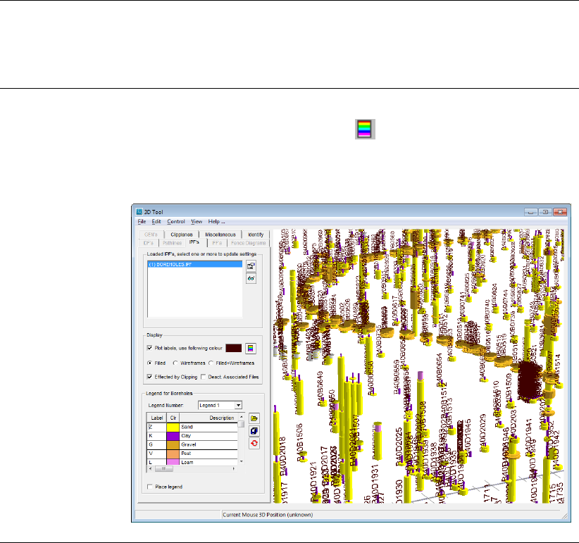
DRAFT
Toolbox Menu Options
Close
Select this button to close the 3D IPF Settings window without modifying ex-
isting entries.
Plot labels, use
following colour
Check this option to display labels as defined by the options entered via
Properties. After the option is selected it is possible to enter a different label
colour (default is white) via the button . This will start the default Colour
window in which a colour can be picked for the selected IPF file(s).
Example of labelling a borehole
Deltares 259 of 812

DRAFT
iMOD, User Manual
Filled, Wireframe,
Filled+Wireframe
Select of the options to display the boreholes of the selected IPF files.
Example of Filled (top figure), Wireframes (middle figure) and
Filled+Wireframe (lower figure) configurations:
260 of 812 Deltares
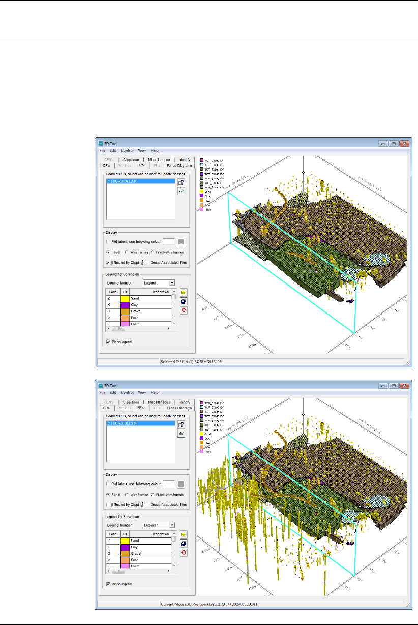
DRAFT
Toolbox Menu Options
Effected by clip-
ping
Select this option to activate clipping for each of the IPF file(s) separately,
by default all IPF files are effected by clipping. If all IPF files are selected,
any modification of this checkbox effect all, but it is possible to (de)select this
option per IPF. This option is handy whenever a surface model needs to be
clipped away and the boreholes should not.
Example of clipping a surface model (top figure) and deactivate clipping
(lower figure) for boreholes
Deltares 261 of 812
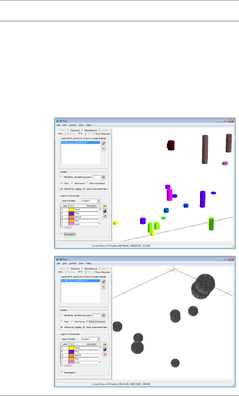
DRAFT
iMOD, User Manual
Deact. Associated
Files
Click this checkbox to ignore the associated files that are attached to the
selected IPF file. This checkbox will be greyed out whenever no associated
files are available and/or automatically deselected for associated files that
represent time series as they can not be displayed in a 3D environment.
For IPF files with boreholes this checkbox will deselected by default. When
this option is selected, iMOD will use the columns from the IPF file that are
assigned to the Z-coordinate and if applicable the Sec. Z-Crd., see section
section 6.8.1. In this way iMOD will create spheres (only Z-coordinate is as-
signed) or vertical tubes when both attributes are assigned. It is also possible
to colour the tubes/spheres according to the attribute Apply Colouring To that
is assigned for colouring.
Example of a tube (top figure) and sphere (bottom figure) representa-
tion of an IPF file with deactivated/no associated txt files.
262 of 812 Deltares

DRAFT
Toolbox Menu Options
Legend Number: Select one of the ten predefined legends from the drop down menu. Each
time another item is selected, the current legend from the table below will be
saved in that predefined legend number. In this way a multiply set of legends
can be managed efficiently.
Legend for bore-
holes
Table of the legend used for colouring the boreholes associated to the selected
IPF file(s).
Label
The first column will be used to represent the label that need to be matched
(case insensitive) with a particular column in the associated files (Cylinder
Class Column, see section section 6.8.2). This is the number of the column in
the associated files that need to be used for the size of the cylinders plotted
for the boreholes.
Clr
The second column will be used to represent the colour that will be used for
those items that match the entered label in the column Label.
Description
The third column is for descriptive purposes only. This will be the actual text
that will be plotted in the legend on the 3D window.
Deltares 263 of 812
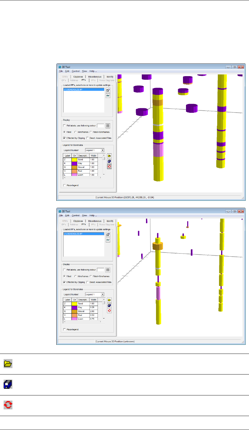
DRAFT
iMOD, User Manual
Width:
The fourth column can be used to specify a particular width to the individual
parts of the borehole.
Example of Borehole with constant width (top figure) and variable width
(bottom figure)
Open DLF-file
Select this button to open a DLF file (see section section 9.17) that will be
used to colour the boreholes associated to the IPF file.
Save As DLF-file
Select this button to save the current legend to a DLF file (see section sec-
tion 9.17).
Redraw
Select this button to redraw the IPF file with the adjusted legend specified in
the table. Any adjustment in legend colour and/or width will be applied.
Place legend Select the check box to show the legend on the graphical canvas. This will
affect the selected IPF files only.
264 of 812 Deltares
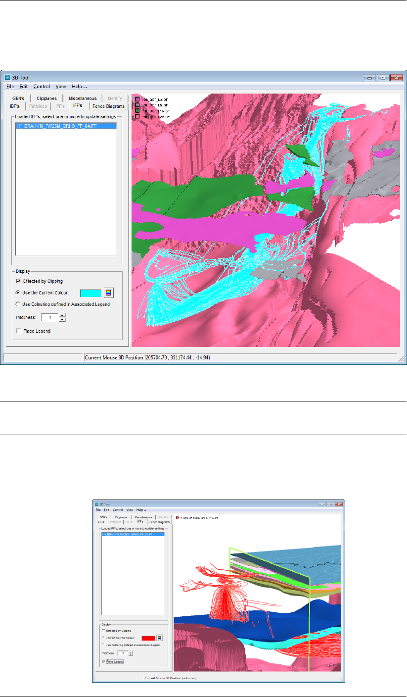
DRAFT
Toolbox Menu Options
7.3.5 3D Tool: the IFF-settings tab
The IFF’s tab of the 3D Plot window allows configuring the display of IFF files.
Loaded IFF’s, se-
lect one or more to
update settings
Select one or more IFF files from the list to activate them in the 3D visualiza-
tion. The 3D display will update each time an IFF is (de)selected.
Effected by Clip-
ping
Select this option to effect the IFF file for clipping, this is the default. It can
be illustrative to ignore clipping for an IFF in combination with a subsurface
model that will be clipped.
Example of a subsurface clip and non clipping an IFF file.
Deltares 265 of 812
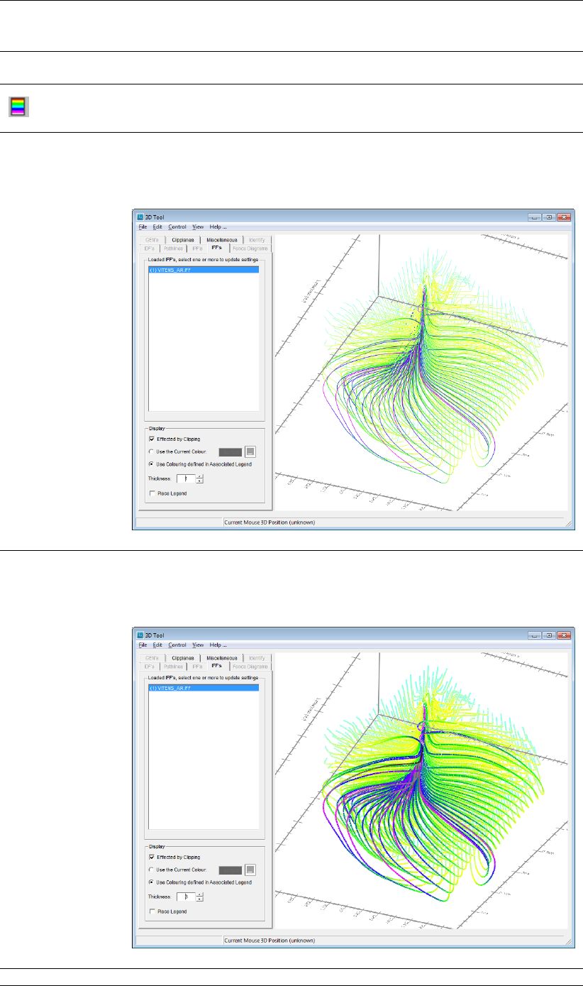
DRAFT
iMOD, User Manual
Use the current
colour
Click this option to display the selected IFF file by a single colour as displayed
to the right of the option.
Legend
Click this button to start the default Colour window to select a colour for the
first of the selected IFF file(s).
Use Colouring de-
fined in Associ-
ated Legend
Select this option to present the all selected IFF files by their associated
legend definition.
Example of an IFF file coloured by age.
Thickness Enter the thickness of the lines used to display the flowlines. The higher the
number, the thicker the line appears on the graphical display.
Example of an IFF file coloured by age with a line thickness of 3.
Place legend Check the box to show the legend.
266 of 812 Deltares
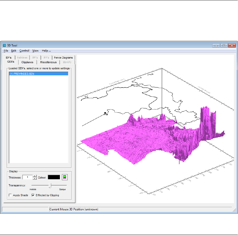
DRAFT
Toolbox Menu Options
7.3.6 3D Tool: the GEN-settings tab
Use the GEN Settings tab to configure the display of GEN files.
Loaded GENs, se-
lect one of more to
update settings
Select one or more GEN-files from the list to activate them in the 3D visualiza-
tion. The 3D display will update each time a GEN is (de)selected. GEN-files
can be loaded in the Maps tab or the Overlays tab in the iMOD Manager;
the behaviour is different and illustrated below.
Overlay tab
This is the most common way to load GEN files into iMOD. Each selected file
from the Map tab on the iMOD Manager will be presented as a separate entry
for which all setting described below can be set. There are two options for a
GEN file (see section section 9.10 for more detailed information):
Deltares 267 of 812
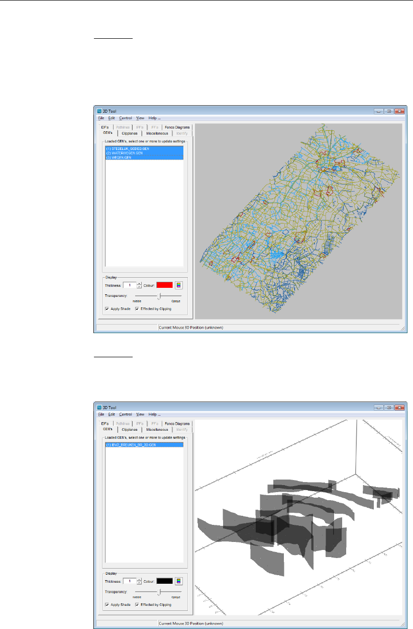
DRAFT
iMOD, User Manual
2D GENs
These are the most common files and used for topographical information,
such as e.g. road and borders.
Example of a display of 2D GEN showing, rivers (blue), urban area
(red) and roads (green).
3D GENs
These can be used to display 3D spatial information, such as faults in 3D.
Example of a display of 3D GEN showing a fault outline.
268 of 812 Deltares
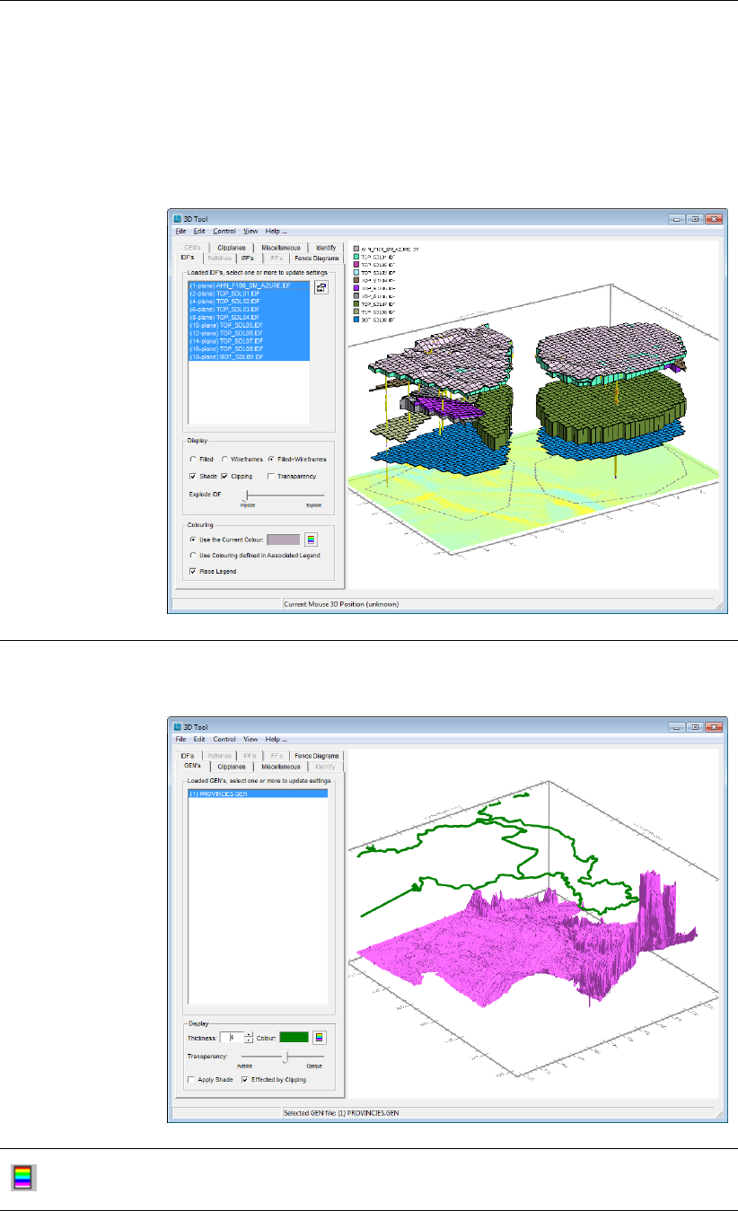
DRAFT
Toolbox Menu Options
Map tab
Whenever a GEN file is selected in the Map tab on the iMOD Manager
window, the GEN files acts as a cookie-cutter. In this way it is possible to
cut-out e.g. solids using irregular shaped polygons and display these in 3D.
Example of an irregular shaped GEN file acting as a cookie-cutter in
the 3D.
Thickness Enter the thickness of the lines used to display the GEN-files.
Example showing the effect of a thick green line for a GEN file.
Legend
Click this button to start the default Colour window to select a colour for the
selected GEN-file(s).
Deltares 269 of 812
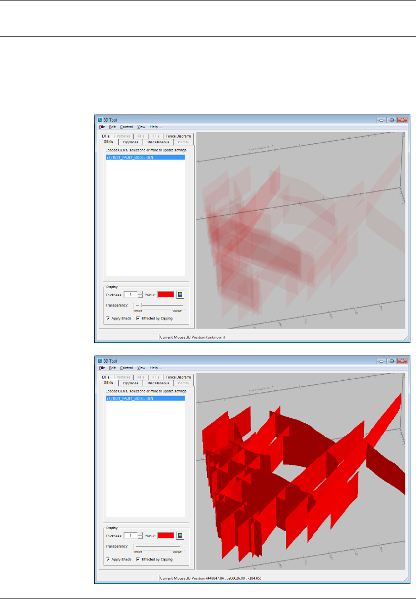
DRAFT
iMOD, User Manual
Transparency Move the ’Transparency-slider’ to change the transparency within the range
’Opaque’ (not transparent) and ’Invisible’ (full transparent). This is especially
nice for 3D GEN file, see section section 9.10.
Example of a transparent 3D GEN (top figure) and an opaque display
(lower figure).
270 of 812 Deltares
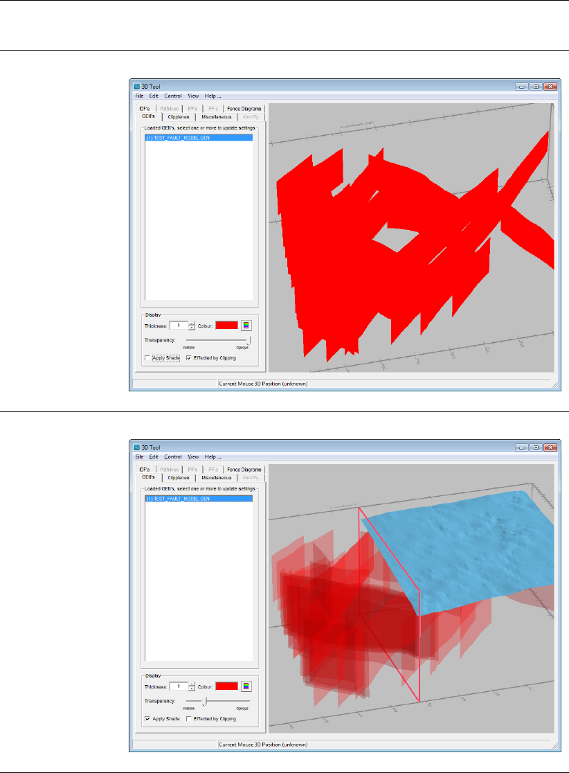
DRAFT
Toolbox Menu Options
Apply Shade Example of showing a 3D GEN without shade.
Effected by Clip-
ping
Deltares 271 of 812
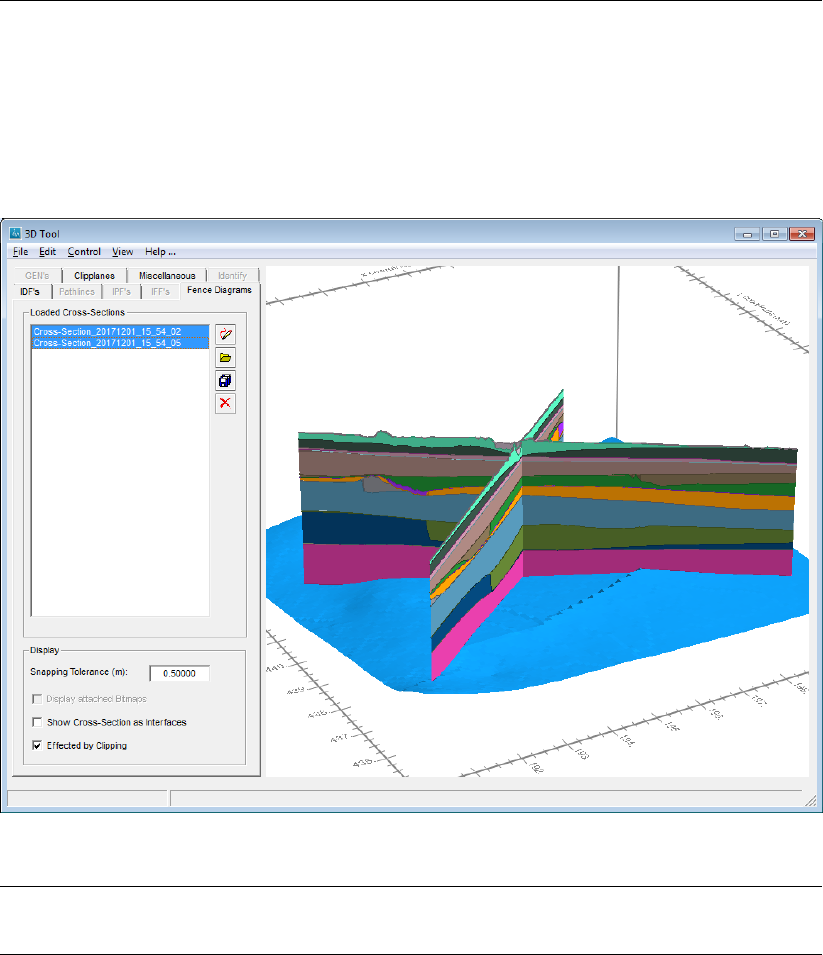
DRAFT
iMOD, User Manual
7.3.7 3D Tool: the Fence Diagrams-tab
The functionality of this tab Fence Diagram is twofold. It will be used to display cross-sections
as fence diagrams from the SOLID Tool (see section section 7.4.3 and secondly whenever the
regular 3D Tool is started, this tab allows to interactively draw the location of a fence-diagram,
iMOD will convert this to a fence diagram and display it on the graphical display.
Loaded Cross-
Sections
Select one or more cross-section files from the list to activate them in the
3D visualization. The 3D display will update each time a cross-section is
(de)selected.
272 of 812 Deltares
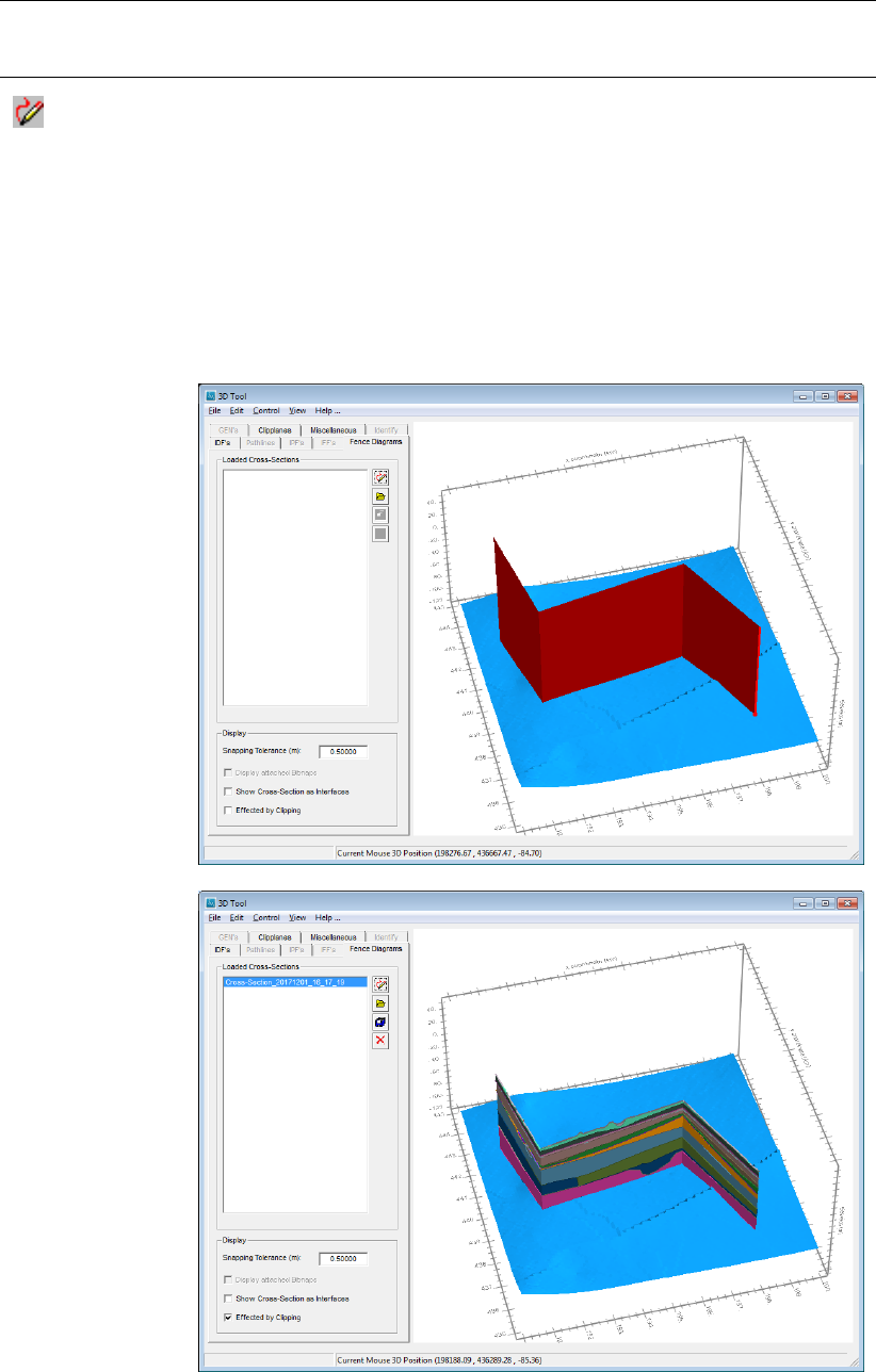
DRAFT
Toolbox Menu Options
Draw
Select this button to start drawing a cross-section in the 3D graphical canvas.
The line is started by clicking the left-mouse button and terminated with the
right mouse button. After that, iMOD generates a fence-diagram and adds
it as a separate entry in the menu list; the naming convention is {Cross-
Section_yyyymmdd_hh_mm_ss}. Subsequent left-mouse clicking will insert
additional nodes to the same cross-sections. Be aware that it is necessary to
select at least one IDF file, as it is only possible to draw a cross-section over
an IDF that is visible; do not use transparency!
Example of a cross-sections drawn on lower most IDF file (top figure)
and the yielding fence diagram (bottom figure).
Note: It is important to note that the appearance of the fence-diagram
depends on the configuration of the individual interfaces. So whenever you
pick the Quasi 3D Model (aquitard) configuration, the fence-diagram appears
as filling the aquitard only. Moreover, if you select the Coloured Quasi 3D
Model (aquitard) configuration, the fence-diagram is filled in with the property
that is selected.
Deltares 273 of 812
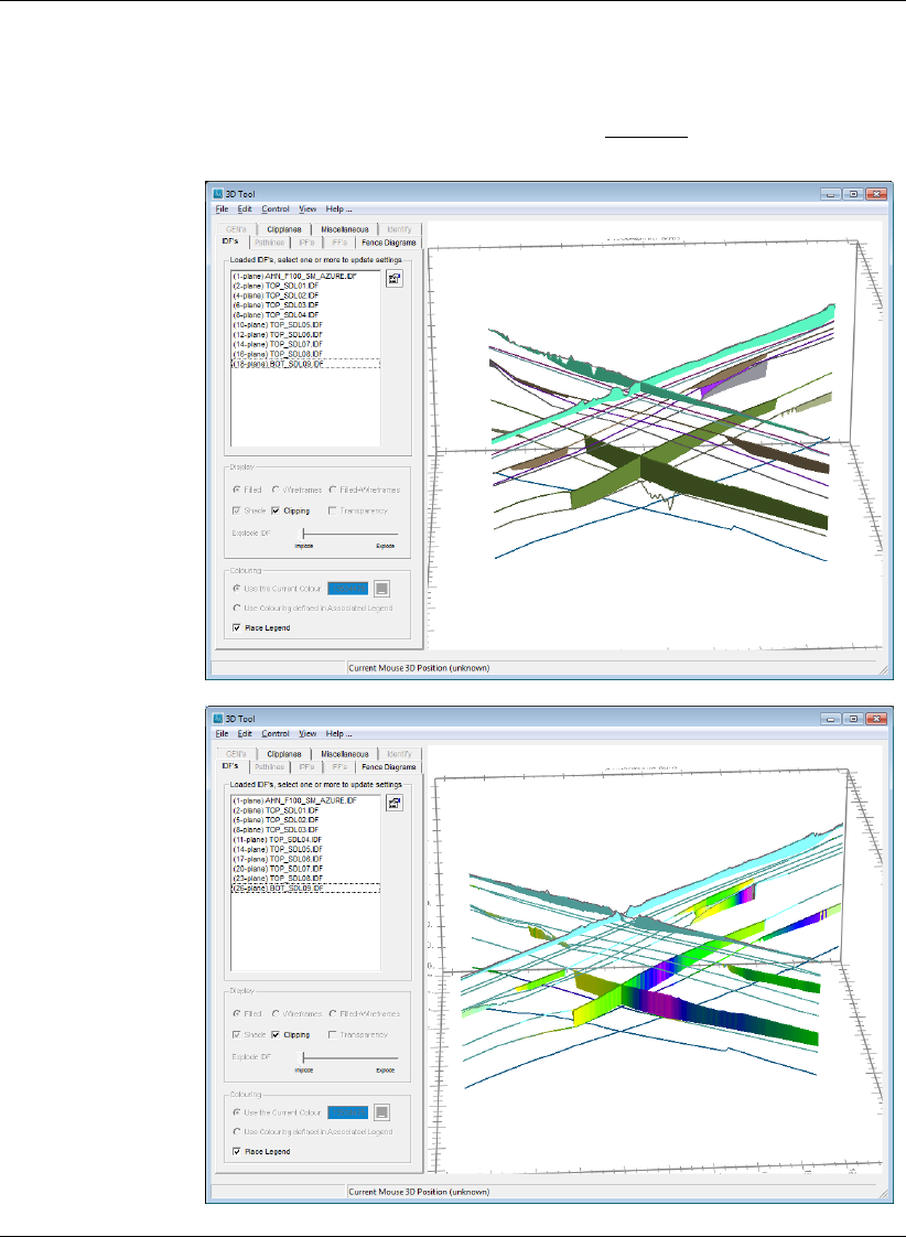
DRAFT
iMOD, User Manual
Example of a cross-sections drawn for aquitards only (top figure) or
filled in by the selected property (bottom figure).
274 of 812 Deltares
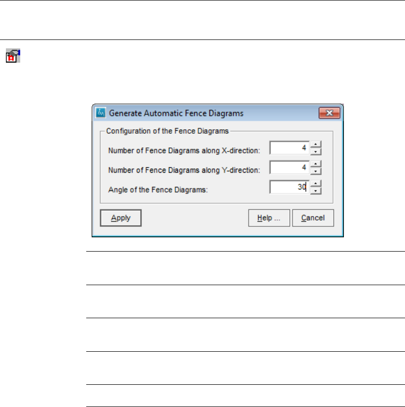
DRAFT
Toolbox Menu Options
Automatic Fence Diagrams
Click this button to open the Generate Automatic Fence Diagrams window.
With this window it is possible to generate a regular pattern of fence diagrams.
Generate Automatic Fence Diagrams window.
Number of Fence Diagrams along X-direction
Enter the number of fence diagrams along the X-direction; when specifying 0
no fence diagrams will be generated in the X-direction.
Number of Fence Diagrams along Y-direction
Enter the number of fence diagrams along the Y-direction, when specifying 0
no fence diagrams will be generated in the Y-direction.
Angle of the Fence Diagrams
Enter the angle for which all fence diagram need to be rotated, specify 0.0 to
avoid any rotation.
Apply
Click this button to generate the fence diagrams and close the Generate Au-
tomatic Fence Diagrams window.
Help . . .
Click this button to start the HELP functionality.
Cancel
Click this button to close the Generate Automatic Fence Diagrams window
without adding any fence diagrams.
Deltares 275 of 812
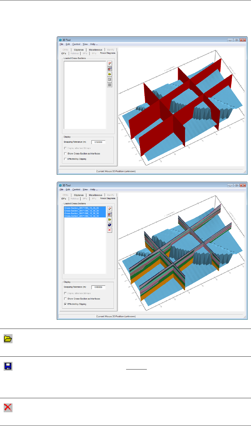
DRAFT
iMOD, User Manual
Example of configuring 2 x 2 fence diagram rotated 10 degrees (top figure)
and the yielding fence diagrams (bottom figure).
Open SPF File
Click this button to open an *.SPF file (see section 9.21). This file described
the entire cross-sections per interface and can be used in the SOLID Tool (see
section 7.4).
Save As SPF File
Click this button to save the selected cross-sections to an *.SPF-file (see sec-
tion 9.21). This type of file can be used in the SOLID Tool (see section 7.4).
The SPF file is saved with the name of the cross-sections in the iMOD TMP
folder at the user folder associated to the PRF-keyword USER (see section
section 9.1), e.g. IMOD_USER \TMP \*.SPF.
Delete
Click this button to delete the selected cross-section(s) from the list. This
action can not be undone, however, you will be asked first whether you are
sure to delete the cross-section(s).
276 of 812 Deltares
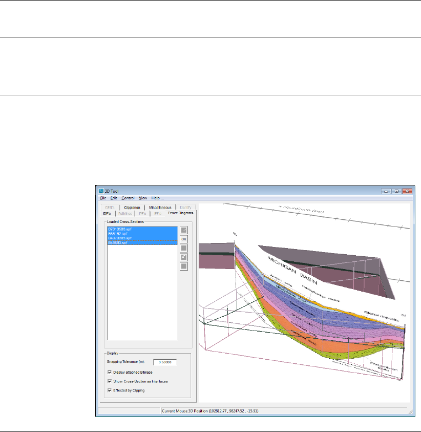
DRAFT
Toolbox Menu Options
Snapping Toler-
ance
Enter a value for the snapping tolerance, the smaller the more accurate the
computed fence-diagram becomes. This value denotes that acceptable error
between the estimated fence-diagram and the true IDF value at that location.
The higher the snapping tolerance, the more this is allowed to differ but, gen-
erates a fence-diagram with less points.
Display Attached
Bitmaps
Check this box to display the attached bitmap on the cross-section. Those
bitmaps need to be added to the cross-section by the Profile Tool (section 7.1)
that has been started by the Solid Tool (section 7.4) and need to be available
in the SPF file (section 9.21).
Example showing an image of a geological profile attached on the cross-
section.
Deltares 277 of 812
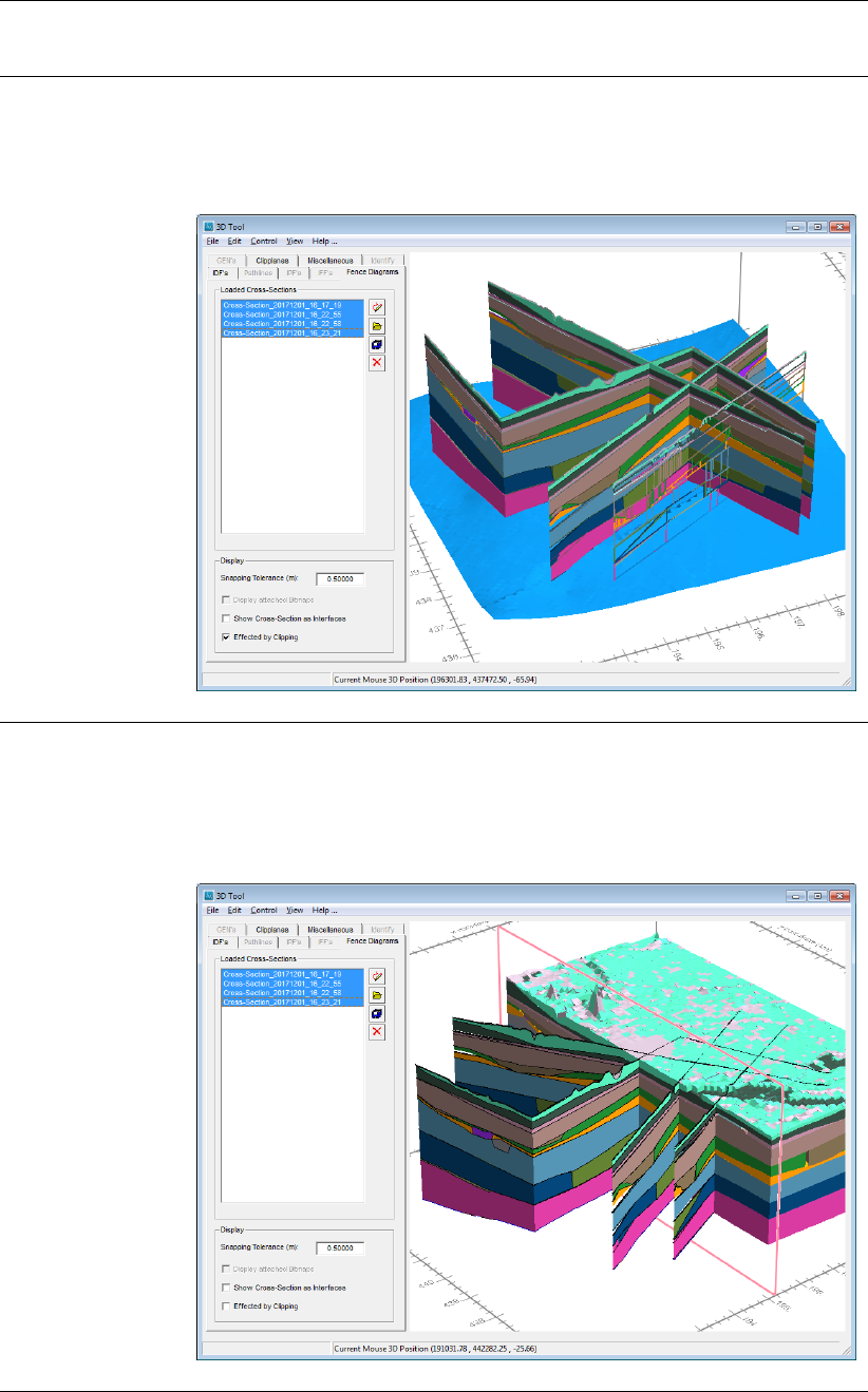
DRAFT
iMOD, User Manual
Show Cross-
Section as Inter-
faces
Select this checkbox to show the cross-sections a interfaces only, so the
individual polygons will not be filled in.
Example of multiple cross-sections for which some of them are drawn
as an interface.
Effected by Clip-
ping
Select this checkbox to effect clipping of the cross-sections. You might select
different choices per cross-section, which allows to clip some cross-sections,
and leave others unclipped.
Example of multiple cross-sections which are not clipped in combina-
tion with a subsurface model that is clipped.
278 of 812 Deltares
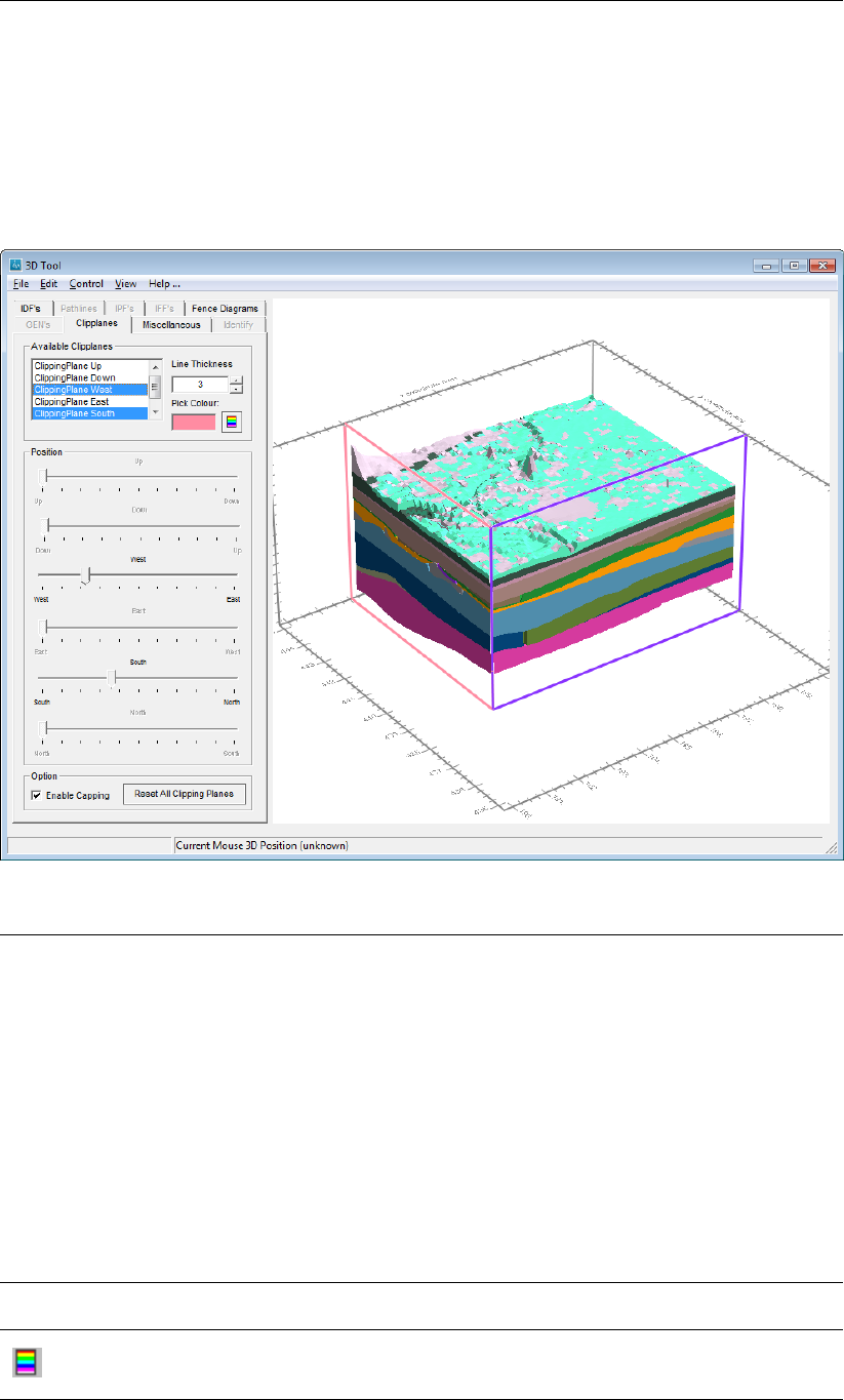
DRAFT
Toolbox Menu Options
7.3.8 3D Tool: the Clipplanes-tab
The ’Clipplanes-tab’ of the 3D Tool allows configuring the clipping planes. With clipping planes
it is possible to clip part of a 3D image and observe what is behind the clipping plane. In the
IDF -tab (see section section 7.3.3), the IPF -tab (see section section 7.3.4), and the IFF -tab
(see section section 7.3.5) it is possible to activate the clipping planes. It is possible to e.g.
clip IDF files but leave IPF files intact.
Available
clipplanes
Select one or more clip planes to activate:
ClippingPlane Up
Defines a clip plane from the top of the image and moves downwards;
ClippingPlane Down
Defines a clip plane from the bottom of the image and moves upwards;
ClippingPlane West
Defines a clip plane from the west of the image and moves to the east;
ClippingPlane East
Defines a clip plane from the east of the image and moves to the west;
ClippingPlane South
Defines a clip plane from the south of the image and moves to the north;
ClippingPlane North
Defines a clip plane from the north of the image and moves to the south.
By selecting a particular clip plane, the corresponding slider becomes active.
Line Thick-
ness
Enter a value to specify the thickness of the outline of the selected clip plane. Enter
a value of zero to hide the outline.
Pick Colour
Use this button to start the default Colour Picking window to assign a particular colour
to the outline of the selected clip plane(s).
Deltares 279 of 812
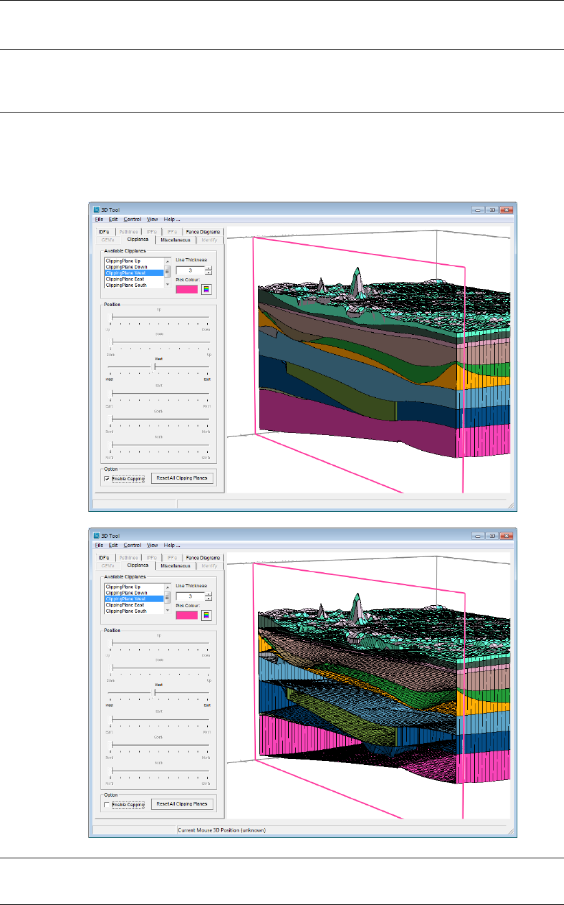
DRAFT
iMOD, User Manual
Position For each selected clip plane its corresponding slider becomes active. For example
when the clip planes ClippingPlane West and ClippingPlane South are selected both
the corresponding sliders are available and can be dragged to move the correspond-
ing clipping plane.
Enable
Capping
Capping is a technique of putting a solid colour on the interface of a 3D image that
has been clipped away.
Example of cross-sections drawn with capping (top figure) and without capping
(bottom figure).
Reset All
Clipping
Planes
Click this button to reset all clipping planes to their default values. iMOD will ask the
user to confirm before resetting all clipping planes.
280 of 812 Deltares
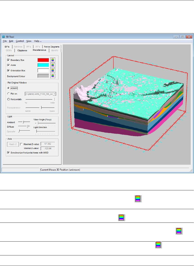
DRAFT
Toolbox Menu Options
7.3.9 3D Tool: the Miscellaneous-tab
The Miscellaneous tab provides several layout functions.
Boundary Box Click this checkbox to turn the boundary box on or off. The colour of the
Boundary Box can be changed by clicking the button (see section sec-
tion 2.6.4 for use of this Colour Picking window.).
Axes Select this checkbox to turn on axes around the 3D image. The colour of the
axes can be modified by selecting the button.
Orientation Box Click this option to plot a simple orientation box with directions to North, East
and West. The colour of this orientation box can be modified via the but-
ton.
Background
Colour
The background colour can be modified by selecting the button. Some-
times, it gives an improved image if the background colour is not white.
Absent Select this option to remove the image as currently displayed in the 2D graph-
ical canvas.
Deltares 281 of 812
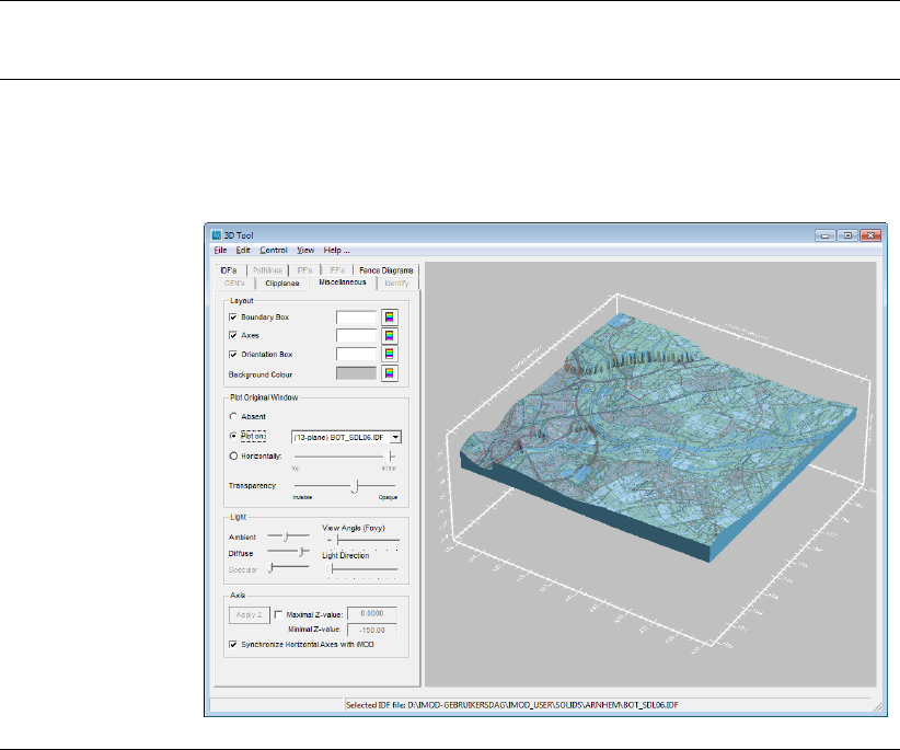
DRAFT
iMOD, User Manual
Plot on Select this option to drape the currently displayed image of the 2D graphical
canvas on the selected IDF file from the drop-down menu.
Example of draping the active image of the 2D graphical canvas on a
selected IDF file.
282 of 812 Deltares
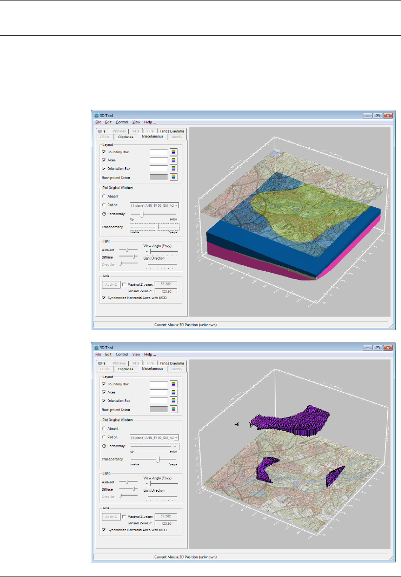
DRAFT
Toolbox Menu Options
Horizontally Select this option to display the active image of the 2D graphical canvas as
a horizontal plane; use the slider (Top up to Bottom) to position the plane
vertically between the top and bottom of the 3D image.
Example of a horizontal plot of the active image of the 2D graphical
canvas.
Deltares 283 of 812
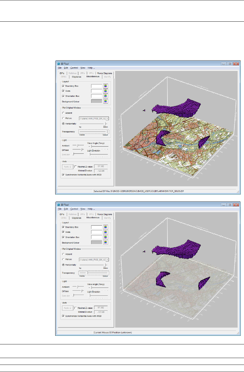
DRAFT
iMOD, User Manual
Transparency Drag the slider between fully transparent (Invisible on the left) and fully
opaque (Opaque to the right).
Example of using transparency: fully opaque (top figure) and almost in-
visible (bottom figure).
Ambient Use the slider to increase the ambient light component (directional light com-
ponent, generated shades).
Diffuse Use the slider to increase the diffuse light component (background light).
Specular Use the slider to increase the diffuse light component (shininess).
284 of 812 Deltares
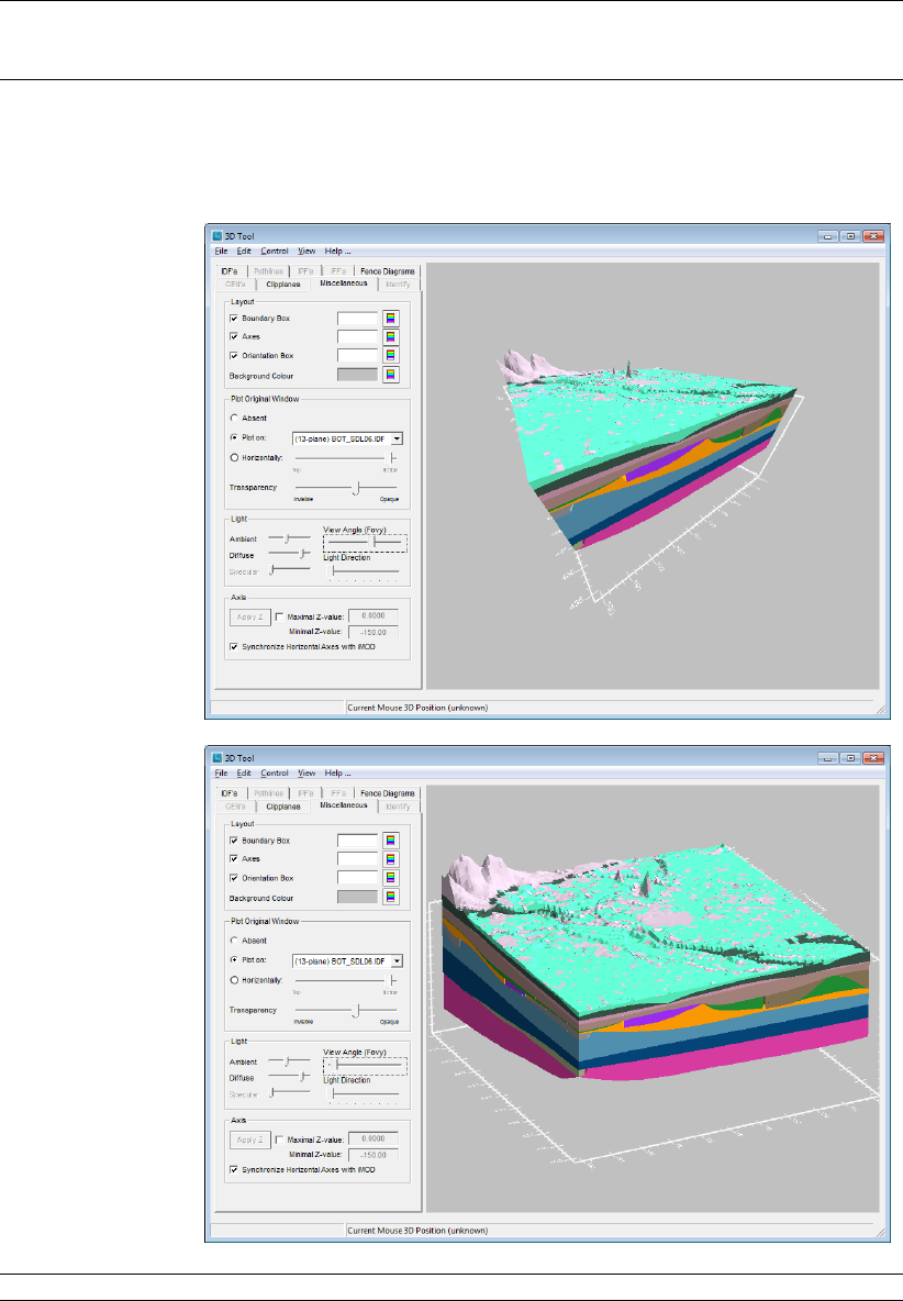
DRAFT
Toolbox Menu Options
View Angle (Fovy) Use the slider to change the view angle from a fish-eye (180 degrees) to 1
degrees (very narrow). A normal view-angle is 10% as a wider view angle
gives a more flattened view, e.g. 60%.
Example of a Fisheye view and a normal view.
Light direction Use the slider to change the light direction and shading.
Deltares 285 of 812
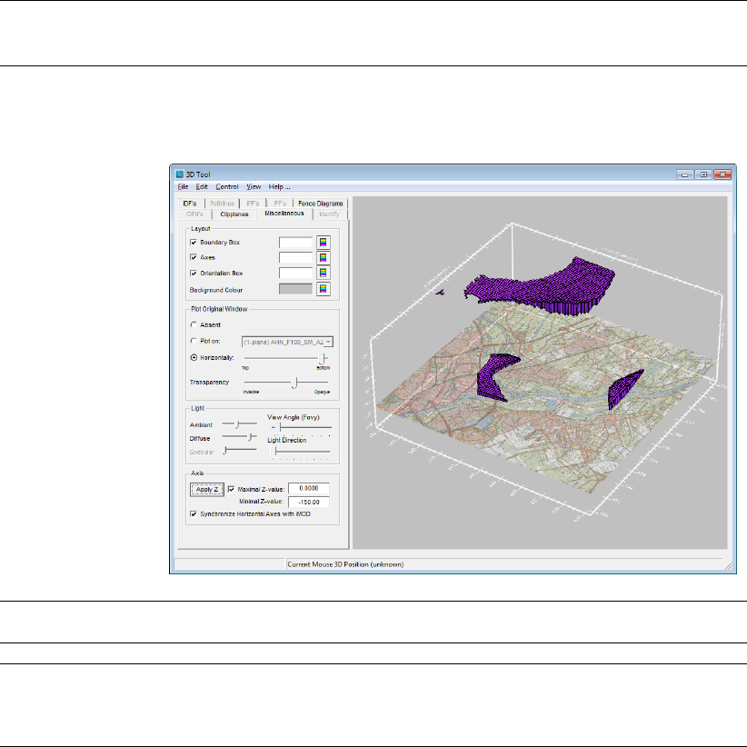
DRAFT
iMOD, User Manual
Apply Z: Click this button to reset the 3D image with the entered values for minimum
and maximum values on the Z-scale.
Example of a different entry for the maximal- and minimal Z-values.
Maximal Z-value Select this option to enter a different value for the maximum Z-value in the 3D
image. The option Minimal Z-value becomes available as well.
Minimal Z-value Enter a different value for the minimum Z-value in the 3D image.
Synchronize Hori-
zontal Axes with
iMOD
This option is checked to allow the 3D Tool to be synchronized with the ex-
tent of the 2D view of iMOD. Whenever this extent is changed (zoomed or
panned) the 3D view will be adjusted accordingly. Uncheck this option to al-
low to change the extent in the 2-D window, without updating the 3-D view.
286 of 812 Deltares
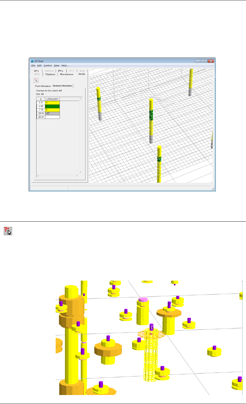
DRAFT
Toolbox Menu Options
7.3.10 3D Tool: the 3D Identify-tab
Use the 3D Tool Identity functionality to identify individual boreholes for inspection purposes.
Select the Identify tab from the 3D Tool window, this tab becomes available in case IPF’s are
selected for display.
The options of the Identity tab are described below:
Select
Click this button to (re)start selecting a borehole on the graphical canvas by
hoovering the mouse pointer over a borehole. Clicking the left or right mouse
button once on a borehole will stop the hoovering. Once a borehole has been
selected its appearance will change to a wireframe representation and the
table will be filled with the values of the IPF file of the selected borehole.
Example of a selected borehole with a wireframe appearance:
Deltares 287 of 812
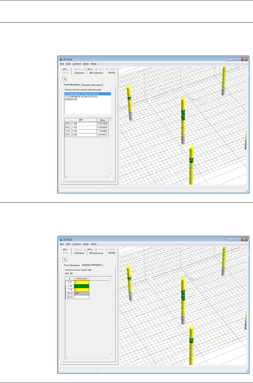
DRAFT
iMOD, User Manual
Point Information
tab
This table shows the content of IPF file for the selected borehole and all
values for the IDF files at the location of the particular point.
Point Information table
Borehole Informa-
tion tab
This table shows the content of the associated file for the selected borehole;
information on the actual borehole.
Borehole Information table
288 of 812 Deltares
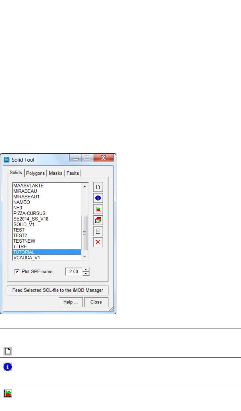
DRAFT
Toolbox Menu Options
7.4 Solid Tool
WHY?
The Solid Tool is an instrument that can be used to create a 3D representation of the subsur-
face in which modellayers with different composition can be distinguished.
WHAT?
A solid is a collection of IDF-files that describes the different geohydrological modellayers of
the subsurface. Each modellayer is represented by a top and bottom elevation and these are
stored as IDF-files (TOP_L{i}.IDF and BOT_L{i}.IDF) in the folder {USER}\SOLIDS. The IDF-
files are created or updated with the Solid Tool by interpolation of interface depths derived
from cross-sections that describe the elevation of all modellayer interfaces.
HOW?
Select the option Toolbox from the main menu and then choose the option Solid Tool to start
the Solid Tool window.
Solid Tool window, Solids tab:
List The Solid Tool window shows the solids saved in the folder {USER}\{SOLIDS}. Select
a solid from the list by clicking on the name.
New
Click this button to create a new solid (see section 7.4.1).
Info
Click this button to open the SOL file for the selected solid. Borehole logs can be
included in the cross-section by a definition added to the solid file (*.SOL), see section
section 9.20 for more detailed information about a SOL file.
Cross-Section Tool
Click this button to start the Cross-Section Tool (see section 7.1) in combination with
the selected Solid to create and/or edit Solid Cross-Section Files (SPF) for more
detailed information about SPF files.
Deltares 289 of 812
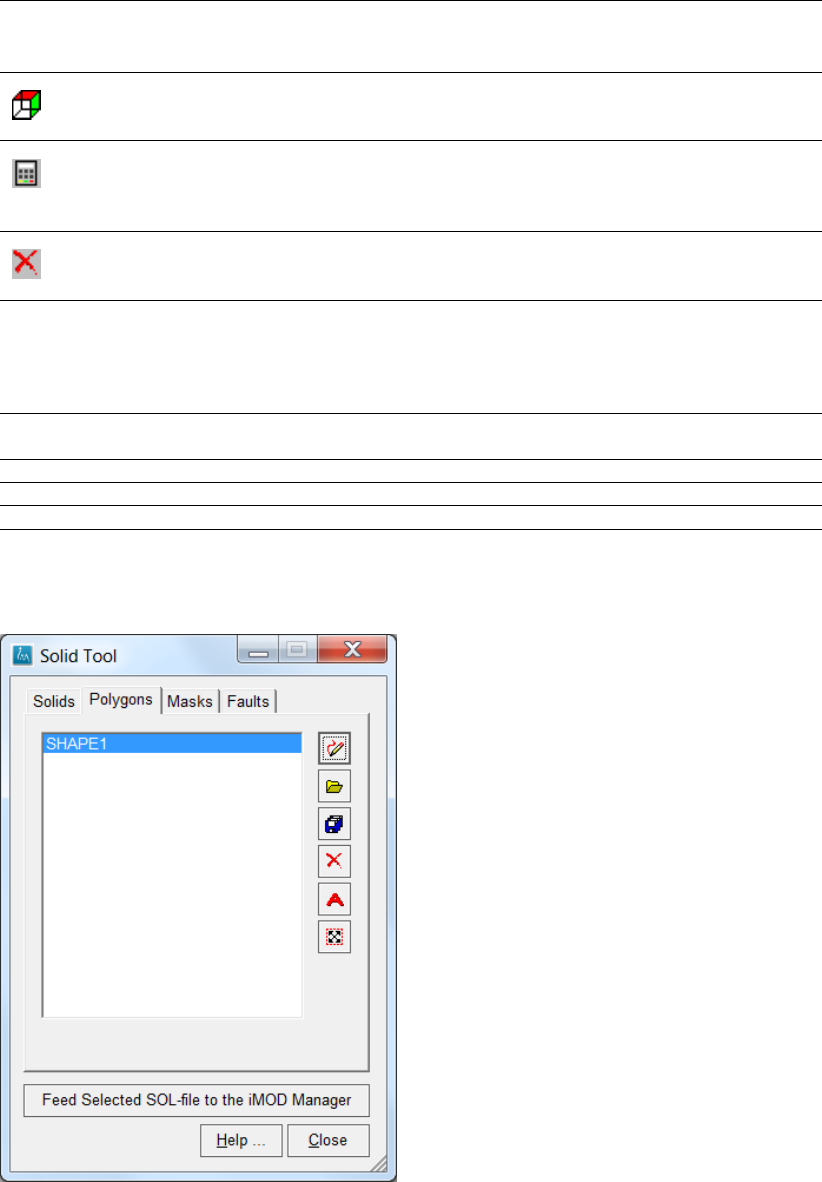
DRAFT
iMOD, User Manual
3D Tool
Click this button to start the 3D Tool (see section 7.3) in combination with the selected
Solid.
Compute
Click this button to compute the elevation of all modellayers in the selected solid
based on the cross-sections described in the SPF files (see section section 9.21)
and mentioned in the SOL file. See section section 7.4.4 for more information.
Delete
Click this button to delete the selected solid, iMOD will remove the folder
{USER}\{SOLIDS} and its content.
Feed Se-
lected
SOL-file to
the iMOD
Manager
Click this item to let iMOD read automatically the solid properties and to add the solid
IDF-files to the iMOD Manager when clicking the name of the solid in the list.
Plot SPF
name
Select this option to display the name of each SPF in the 2-D plot.
2.00 Enter the letter size at which the SPF names are plotted.
Help ... Click this button to start the Help functionality.
Close Click this button to close the Solid Tool window.
Solid Tool window, Polygons tab:
The interpolation of the interfaces of the solid may be executed within the limits of one or
more defined polygons solely. In this manner it is possible to adjust any geological model
locally. Each polygon will act similar for to modellayers. If different areas need to be applied
for different model layers, the use of the Masks window (see AquitardsMasks tab on the Solid
Tool is more appropriate. The polygons are defined in the Solid Tool window, Polygons tab
and the functions of those buttons are described in detail in section section 4.2.
290 of 812 Deltares
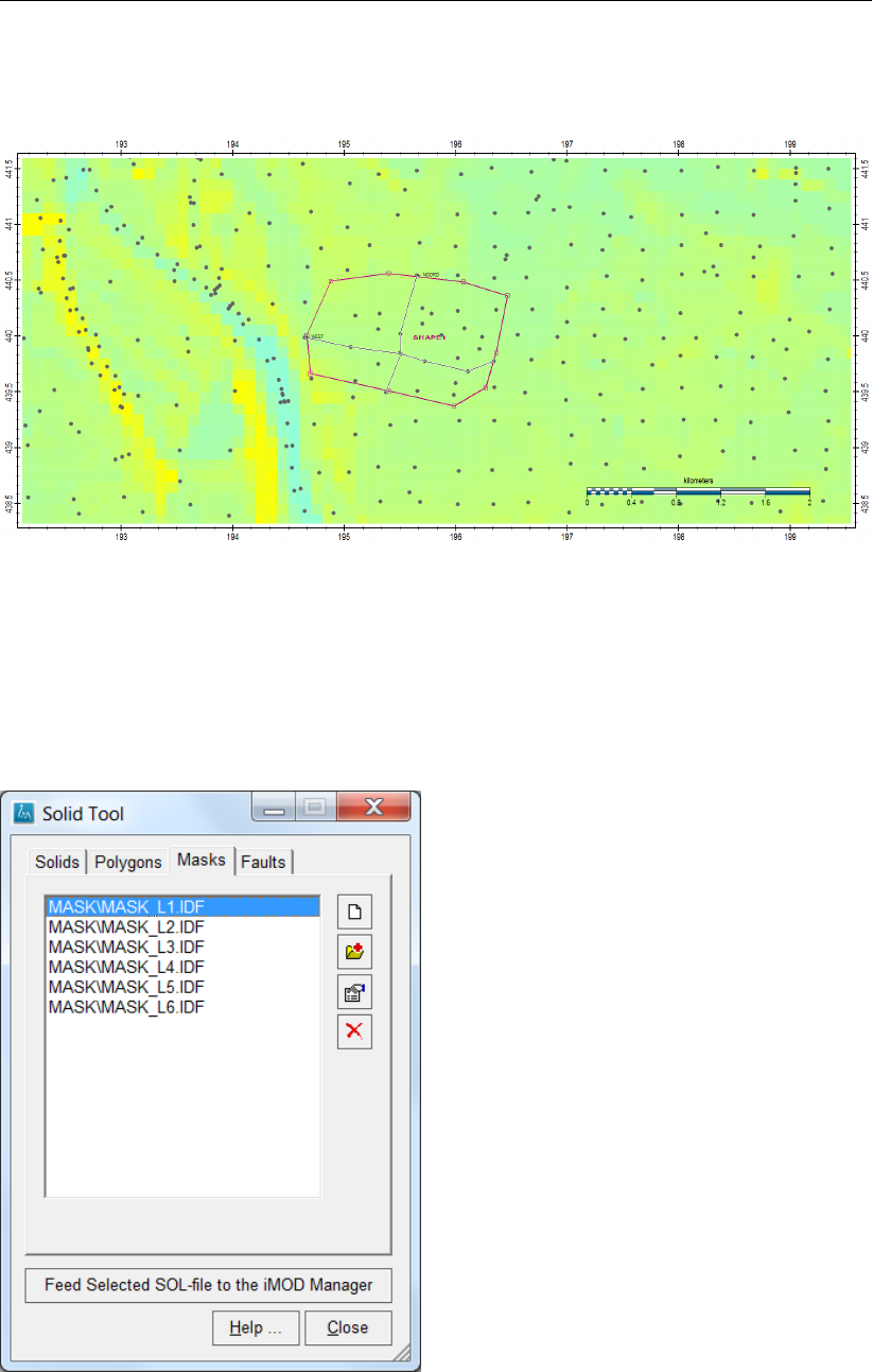
DRAFT
Toolbox Menu Options
Example of a polygon (SHAPE1) that defines the area for which interfaces of the solid will be
adjusted by the two drawn cross-sections.
The defined polygon is saved to the solid when tabbing towards to the Solids tab of the Solid
Tool window. The defined polygon is not saved to the solid when clicking the Close button on
the Solid Tool window.
Solid Tool window, AquitardsMasks tab:
The extent of the aquitards located between the bottom and top interfaces of subsequent
layers can be defined using masks. In this manner the extent can be formed by values in
the mask files. Those mask files are IDF files that can be created using the New button (see
Deltares 291 of 812
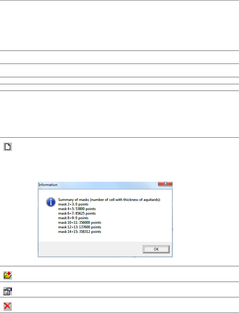
DRAFT
iMOD, User Manual
below) and/or created differently as long as the dimensions of the Mask-IDF is identical to the
IDF files listed in the SOL-file. Eventually, any Mask IDF file will be saved in the selected SOL
file whenever the tab Solids on the Solid Tool window is selected. The values in the Mask IDF
behave as follows:
−2iMOD applies a value of −2internally to fixate locations that are effected by cross-
sections.
−1Use this value to specify areas that do not need to be computed. iMOD will use the
original values instead.
0Use this value to specify areas that are excluded.
1Use this value to specify areas that need to be compute.
2Use this value to specify areas that need to be equal to the values of the upper layer.
It will act as if its value is −1but uses the results from the upper layer as fixated value.
The value 2 is recommended to extent aquitards, specify a value of +2 outside the
extent of an existing aquitard or equivalent in order to define the boundaries of these
aquitard.
New
Click this button to create new masks for all aquitards. iMOD will compute a Mask
Value of 1for the bottom elevation of modellayer iwhere there is a positive difference
with the underlying top of modellayer i+ 1. Outside those area, the Mask Value is
1and for the top of the underlying modellayer 2. An information window appears
specifying the created masks.
Open Map
Click this button to open an IDF-file to be used as mask file.
Properties
Click this button to open the properties of the mask.
Delete
Click this button to remove the mask file from the list.
Solid Tool window, Faults tab:
292 of 812 Deltares
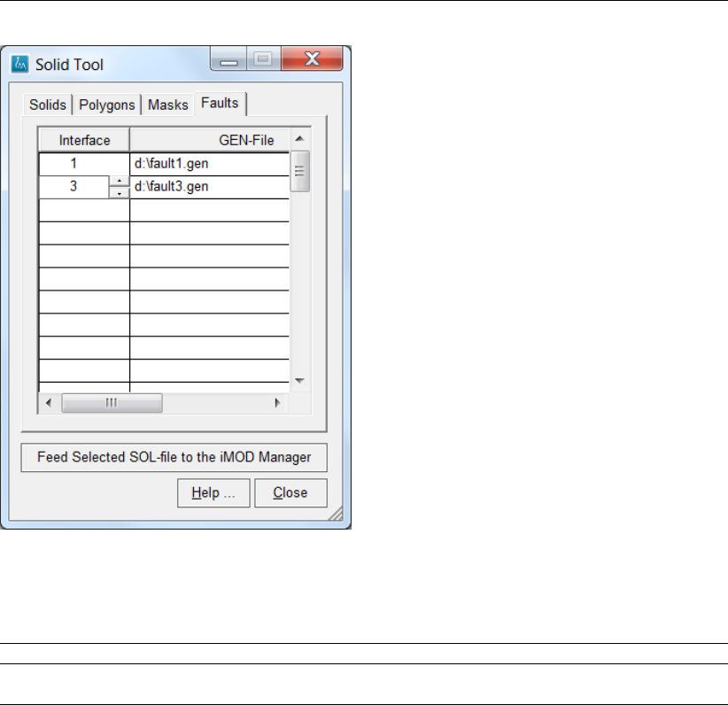
DRAFT
Toolbox Menu Options
The interpolation can be obstructed by the shape of faults, or breaklines. Those need to be
entered as GEN-files (see section section 9.10).
Interface Enter the number of the interface for which the faults or breaklines need to be applied.
GEN-file Enter the name of the GEN file which contains the breaklines. More than one break-
line may be present in each GEN file.
7.4.1 Create a Solid
A solid is a collection of IDF-files that describe the top and bottom elevations of geohydrolog-
ical interfaces in the subsurface. The solid is created by selecting the relevant IDF-files in the
iMOD Manager and by clicking the New button on the Solid Tool window to start the Create
New Solid window.
Deltares 293 of 812
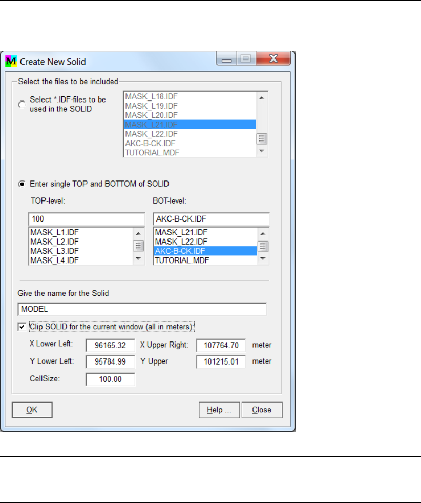
DRAFT
iMOD, User Manual
Create New Solid window:
Select *.IDF files
to be used in the
SOLID
Select this option to specify IDF files from the list that need to be used as
individual interfaces in the SOLID. iMOD will copy or clip the selected IDF
files and save them in the specified folder in which all SOLIDS are saved (i.e.
{USER}\{SOLIDS}\*.IDF.
294 of 812 Deltares
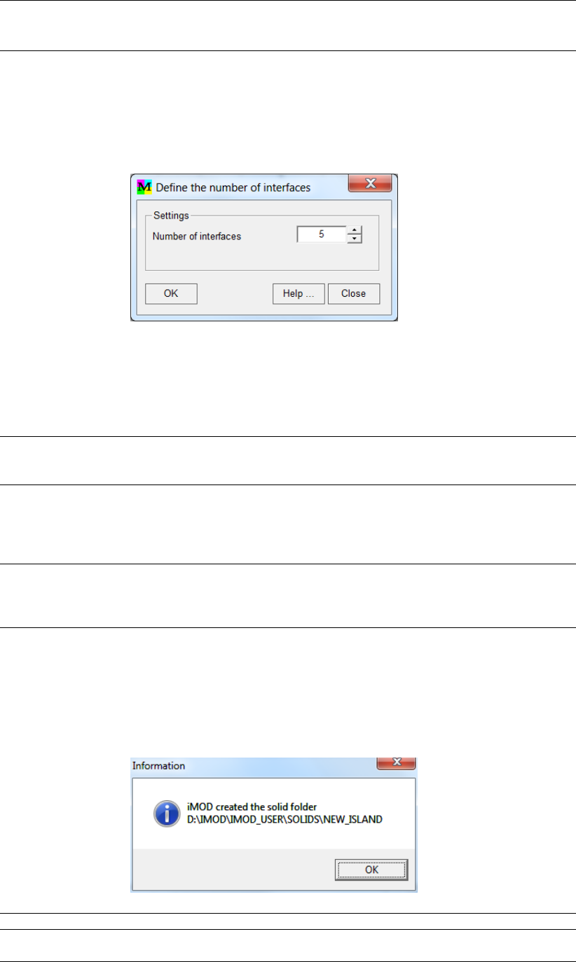
DRAFT
Toolbox Menu Options
Enter single TOP
and BOTTOM of
SOLID
Select this option to specify a constant value and/or IDF file for the definition
of a TOP- and BOTTOM level of the SOLID. iMOD will copy or create these
files (in case of constant values) to the SOLID folder and rename them to
INT_L{i}.IDF and INT_L{n}.IDF, identical to the order of the selected files. The
actual number of interfaces can be entered in the following appearing menu
Define the number of interfaceswindow:
Number of interfaces
Select the number of interfaces a separate IDF file is generated.
iMOD will divide the distance between the entered TOP and BOTTOM
values into equally distances. All these files are located in the SOLIDS
subdirectory.
Give the name for
the Solid
Enter the name of the solid, e.g. ISLAND. iMOD will create a folder called
{user}\solids\ISLAND and saves the SOL file: ISLAND.SOL for more detailed
information about SOL files.
CellSize: Enter the cell size of the IDF files for the interfaces. Bear in mind that those
cell sizes can be modified easily in the Compute Interfaces window. This item
is compulsory whenever no IDF files are entered whenever the option Enter
single TOP and BOTTOM of SOLID is selected, otherwise the IDF dimensions
are use of the specified IDF files.
Clip SOLID for the
current window (all
in meters)
Check the checkbox in case you want to enter an extent different from the area
of the selected IDFs. Enter the coordinates for the lower left and upper right
corner of the solid. Make sure that these coordinates are within the extent of
the selected IDFs.
OK Click this button to create:
A solid folder in {USER}\{SOLIDS}\{SOLIDNAME};
A solid file (*.SOL) inside the SOLIDS folder;
A collection of INT_L{i}.IDF and INT_L{n}.IDF-files inside the SOLIDS
folder where n represents the number of interfaces.
Information window after a successful completion of the creation process.
Help . . . Click this button to start the Help functionality.
Close Click this button to close the Create New Solid window and return to the Solid
Tool window.
Deltares 295 of 812
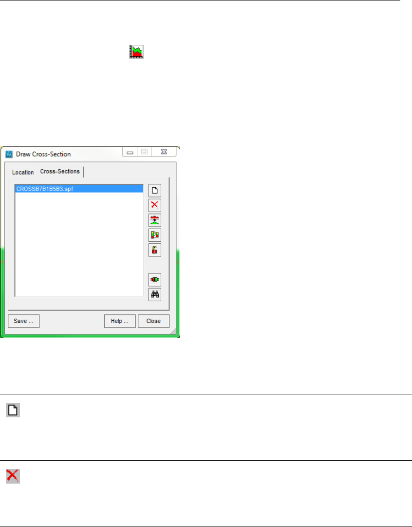
DRAFT
iMOD, User Manual
7.4.2 Solid Editing using Cross-Sections
Click the Cross-Section Tool button on the Solid Tool window to start the Draw Cross-
Section window and the Cross-Sections window. The Draw Cross-Section window has the
same functions as described for the Cross-Section Tool in section 7.1. The cross-section will
be displayed in the iMOD Cross-Section CHILD window. The interfaces of the model layers in
the solid can be edited manually using the Cross-Sections window.
Cross-Sections window:
List of
Available
Cross-sections
The cross-sections defined for the selected solid are shown here.
New
Click this button to create a new cross-section. Make sure that you draw a new
cross-section first using the Draw button on the Draw Cross-Section window.
If not, a copy will be made of the selected cross-section in the list. The Fit
Interfaces window will be started to define the name of the cross-section and
enter initial settings to fit the interfaces.
Delete
Click this button to delete the selected cross-section. The cross-section will
be deleted from the list in the Cross-Section window. The cross-section will be
deleted from the solid once you close the Cross-Section window and confirms
the Question to save the (adjusted/added) cross-sections. However the cross-
section SPF-file is not removed and remains available for later use.
296 of 812 Deltares
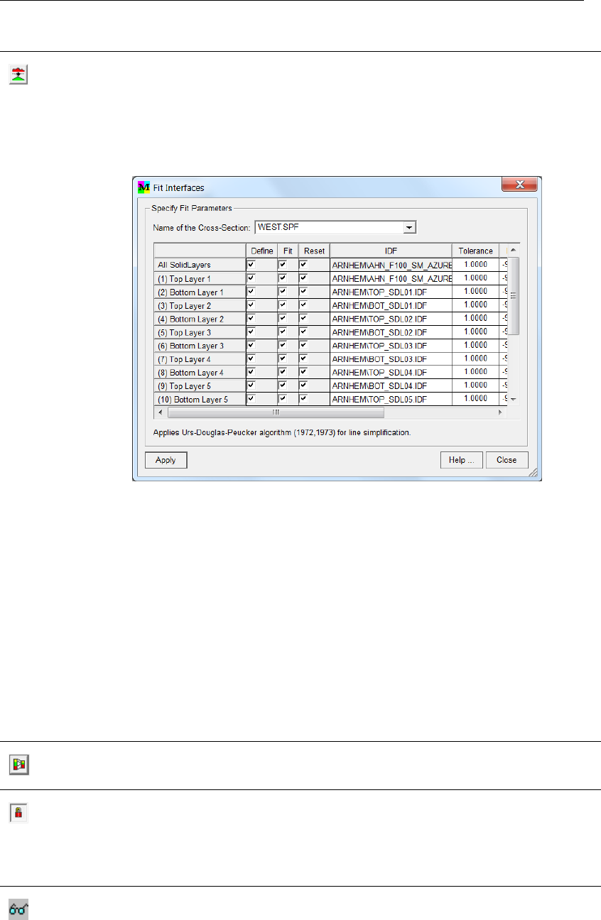
DRAFT
Toolbox Menu Options
Fit Interfaces
Click this button to open the Fit Interfaces window. This window offers the
possibility to start an initial guess for the interfaces in the cross-section by
fitting the interfaces along the cross-section on the values read from the
corresponding IDFs as mentioned and assigned to in the selected SOL-file.
Example of the Fit Interfaces window:
Name of
the Cross-
Section:
Specify the name of the selected cross-section; the name can
not be modified once cross-sections have been defined.
Define Check the box to define an interface line that can be modified.
Fit Check the box to allow fitting of the interface of the IDF.
Reset Check the box to initialize an interface line; the result will be a
horizontal interface.
IDF Select the IDF for each interface from the dropdown list.
Tolerance Enter the accuracy in meters for which an interface is fitted.
Exclude Enter the value of the IDF not used in the fitting; this is usually
(by default) the NoDataValue of the IDF files.
Apply Click this button to start to fit each interface line to the corre-
sponding IDF-files.
Help ... Click this button to start the Help functionality.
Close Click this button to close the Fit Cross-Section window and re-
turn to the Solid Tool window.
Create interfaces from borehole logs
Click this button to create interfaces based on the interfaces defined in the
borehole logs which are part of the solid definition.
Lock
Click this button to lock the behaviour of each interfaces in between upper-
and lower interfaces. Whenever they might cross due to a movement, they
will be locked in order to avoid that they cross. Whenever two nodes are
exactly on each other (which is allowed), this can prevent a movement of the
node. Uncheck this button in that case to allow full editing of the interfaces.
View Editable Area
Click this button to view the editable area based on the extent of the entered
polygons as specified on the Solid Tool window, Polygons tab. Though, inter-
faces can be changed outside the editable areas (grey areas), they will not be
used in the interpolation of new interfaces.
Deltares 297 of 812
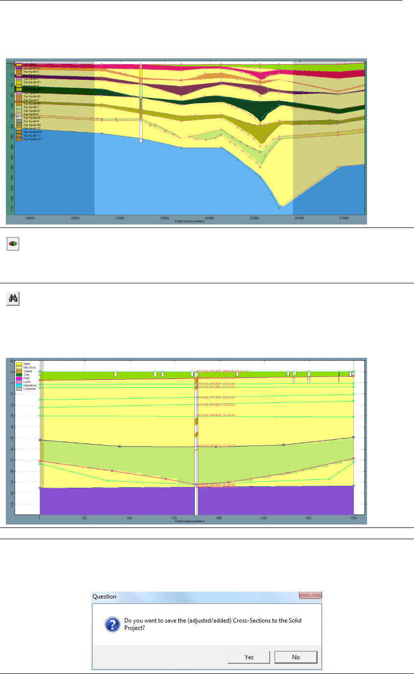
DRAFT
iMOD, User Manual
Example of a cross-section showing the editable area and non-editable areas (grey)
Snap
Select this option to snap the selected node on the interface ito the nearest
interface i−1and i+ 1. Whenever the snap does not work, it is probably
caused by the fact that the interface to be snapped at, is not directly above- of
beneath the interface considered.
View
Click this button to show the name of the cross-section and the name of the in-
terfaces that crosses the current cross-section as shown on the Cross-Section
CHILD window.
Example of a cross-section showing the interfaces of a crossing cross-section.
Help . . . Click this button to start the Help functionality.
Close Click this button to close the Solid Tool window (and therefore the Cross-
Section Tool window) and to return to the Solid Tool window. The cross-
section(s) will be saved into separate SPF-files to the solid folder when
confirming the Question to save the (adjusted/added) cross-sections.
298 of 812 Deltares
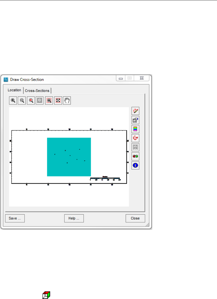
DRAFT
Toolbox Menu Options
The iMOD Cross-Section CHILD window provides the opportunity to edit the interfaces man-
ually. When you move the cursor in the neighborhood of a (red, blue or green) line it changes
in a red arrow and you can click the left mouse button and drag the line to another position.
When the cursor becomes a black arrow you can modify the existing node of the line. This
editing mode is similar to modifying polygons, see section 4.4. Be aware that there is no
possibility to undo move actions.
Example of iMOD Cross-Section CHILD window:
The iMOD Cross-Section CHILD window shows the interfaces of the model layers in three
colors: red, blue and green. The red colour is used for the top interface of a modellayer, the
blue colour is used for the bottom interface of a modellayer. The green colour is used when
bottom and top interfaces of subsequent model layers overlap.
7.4.3 Solid Analysing using the 3D Tool
Click the 3D Tool button on the Solid Tool window to start the3D Tool graphical window.
The 3D IDF Settings window will appear first whenever IDFs are selected in the iMOD Man-
ager window. This window has the same functions as described for the 3D Tool in section 7.3.
After that, all cross-sections are listed in the tab Fence Diagrams on the 3D-Tool window, see
section section 7.3.7 for further explanation.
Example of a 3D image of the possible outline of cross-sections of a solid.
Deltares 299 of 812
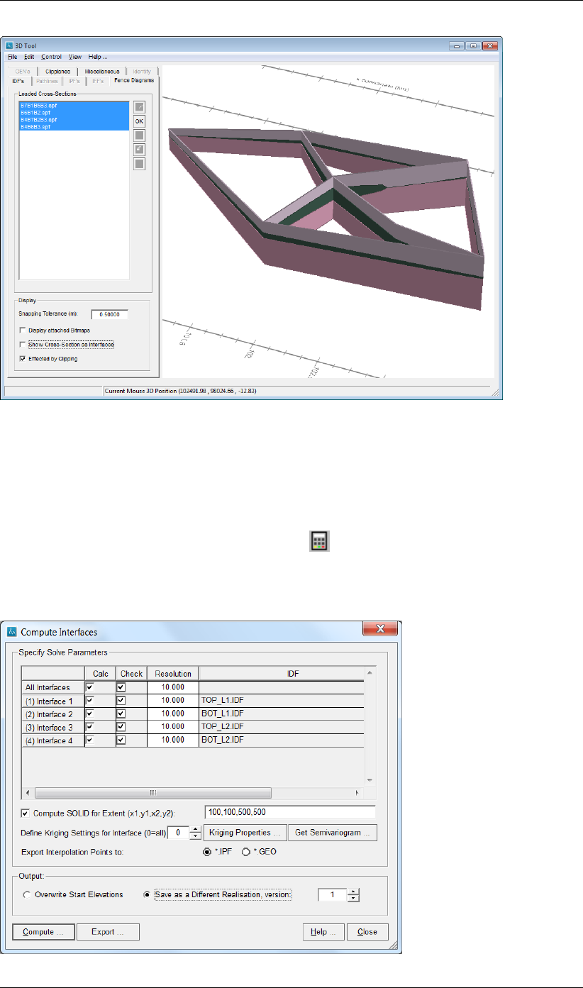
DRAFT
iMOD, User Manual
7.4.4 Compute Interfaces
iMOD facilitates two methodologies to convert the cross-section into a 3D representation of
the subsoil, named a SOLID. Basically, iMOD uses (a) a linear interpolation of the entire
interface in each cross-section yielding an accurate representation of the interfaces or (b)
performs a Kriging interpolation using only the knick points in the interfaces, yielding a more
smooth interpolation. Select the option Compute from the Solid Tool window top start the
Compute Interfaces window.
Compute Interfaces window
300 of 812 Deltares
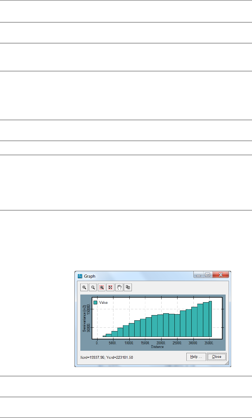
DRAFT
Toolbox Menu Options
Calc: Check this option to select the interfaces to be recomputed, if not se-
lected, those will remain unchanged, unless the option Check is acti-
vated.
Check: Check this option to perform a consistency check upon the interfaces,
this applied whether it will be computed or not. iMOD uses the rule that
interface imust be <=interface i−1, if not interface ibecomes equal
to the value of interface i−1.
Resolution: Enter a resolution of the IDF to be interpolated for the individual inter-
faces. It has the advantage to start at a coarse scale (e.g. 100m) to
have a quick results of the interpolation and whenever the SOLID im-
proves, the final interpolation can be carried out on a finer scale. Bear
in mind, that the resolution should be at least as fine as the detail of
the cross-sections. At the end, the specified cell size in the runfile will
smoothen the interpolated interfaces furthermore if desired.
IDF : List of the used and written IDF file names for the interfaces. The
SOLID tool always uses those IDF files at the root of the SOLID folder,
results can be written in different version folder, see Output settings.
Compute SOLID for Ex-
tent (x1,y1,x2,y2):
Enter the extent or which the SOLID need to be computed. In this
manner the existing SOLID files can be enlarged or reduced.
Kriging Proporties ... Click this button to show the settings of the Kriging interpolation, see
Table 4.1 for more detailed information. Whenever 0 is given in the
integer field to the left, the Kriging settings apply for all interfaces. Al-
ternatively, whenever a value of e.g. 4 is entered, the specific Kriging
settings apply for interface 4 solely. Bear in mind, that the most impor-
tant parameter for Kriging is the range over which the semivariogram
extends. Changing that parameter does probably have the largest im-
pact on the results of the interpolation.
Get Semivariogram ... Click this button to compute the semivariogram for the selected layers
at Calc in the table. For each of the interfaces the semivariogram will
be displayed in a graph. By clicking the Cancel button the next inter-
face will be computed. Before the semivariogram will be computed, it
is necessary to confirm this action since, it might can take some while
to compute.
Example of a computed Semivariogram
Export Interpolation
Points to
Select the option *.IPF or *.GEO to export the knickpoints on each in-
terface to an IPF or GEO file. A separate IPF or GEO file will be created
and stored in {USER}\SOLIDS\{SOLIDNAME}\{VERSION}\EXPORT.
Overwrite Start
Elevations:
Overwrite the original interfaces in the folder
{USER}\SOLIDS\{SOLIDNAME}. However, it is not recommend-
able to do this.
Deltares 301 of 812

DRAFT
iMOD, User Manual
Save as a different
Realisation, version:
Save the result of the interpolation as a new version with the speci-
fied version number e.g. {USER}\SOLIDS\{SOLIDNAME}\{VERSION}.
This is the default option.
Compute: Start the interpolation for each interface.
Export: Start the export of the knickpoints for each interface.
Help: Click this button to start the Help functionality
Close: Click this button to close the Compute Interfaces window and return to
the Solid Tool window.
302 of 812 Deltares
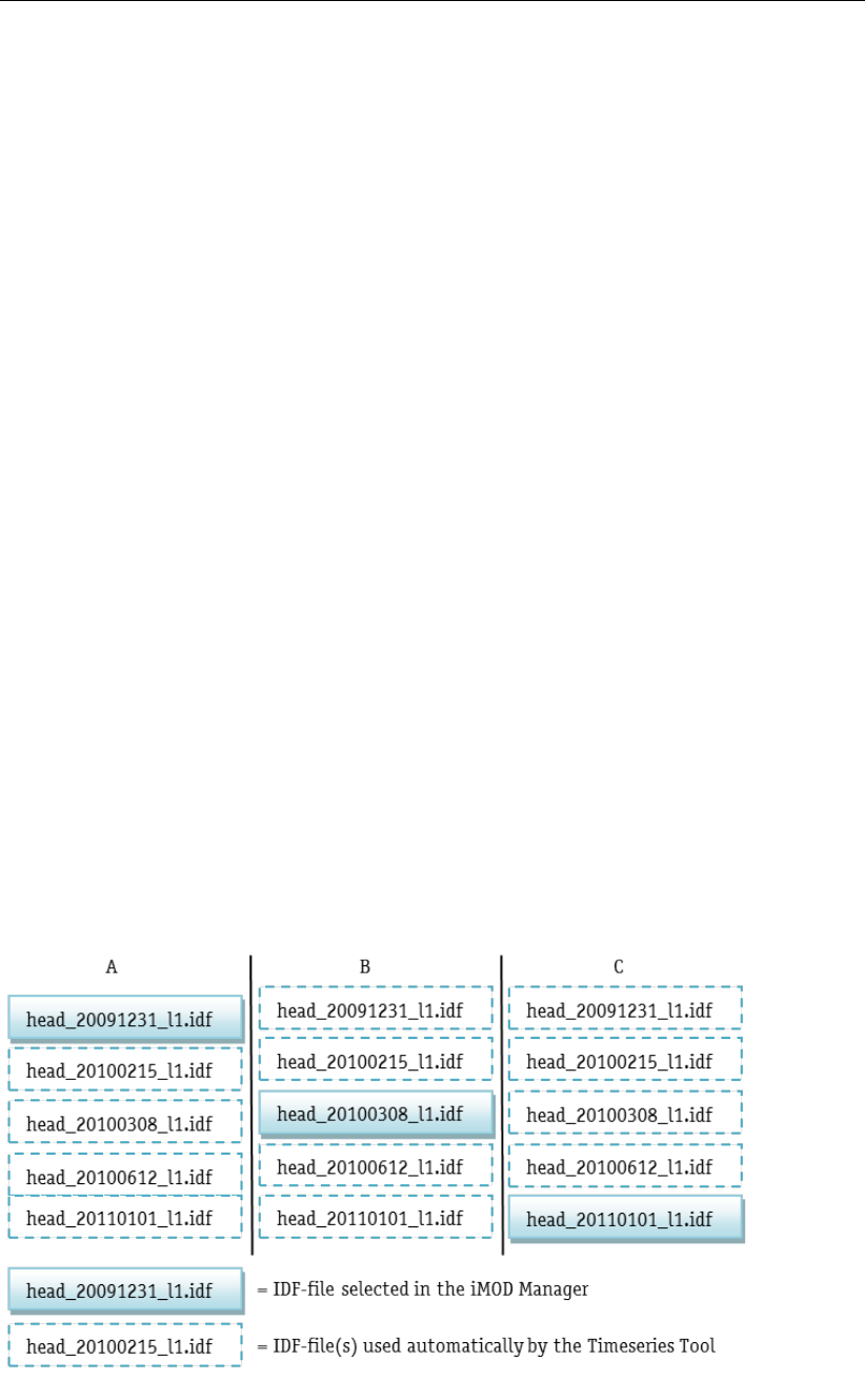
DRAFT
Toolbox Menu Options
7.5 Movie Tool
WHY?
The Movie Tool is an instrument that can be used to create an playable movie out of a se-
quence of images created from 2D plot, e.g. contour maps of draw downs in time can be
collected into a single *.AVI file to be displayed in a movie player. These movies can illustrate
in a dynamical way how groundwater responds to measures.
WHAT?
Any combination of images, such as contour lines, grid and overlay can be used to create a
movie file. These movie files are *.AVI and can be played with an existing and installed movie
player.
HOW?
Select the option Toolbox from the main menu and then choose the option Movie Tool, from
there a option exists to create a movie via the option Create a New Movie . . . and to display
and start the movie via the option Play an Existing Movie . . . .
7.5.1 Create a New Movie
The Create a New Movie Tool allows you to create an AVI from a selected set of plots with
time independent and time dependent IDF files. iMOD will construct these files by collecting
all data from the other related time-dependent IDF-files. Related time-dependent IDF-files
have identical names but have a different date string. A date string is an eight digit continuous
number, e.g. 20091231 meaning the 31th of December 2009. It is not necessary to load all
related time-dependent IDF-files in the iMOD Manager. At least one is sufficient to construct
the entire time series. If a multiply set of IDF files is selected, each of them is used to load
all time-dependent files. In the end all unique time steps will be used to generate images and
IDF files will be re-used whenever they do not coincide with the current time step.
Example of IDF-files (A,B and/or C) available in the iMOD Manager prior to the start of the
Create a New Movie Tool:
To start the Create a New Movie window, select the option Toolbox from the main menu,
choose Movie Tool and then choose Create a New Movie . . . . Alternatively, you can click the
Deltares 303 of 812
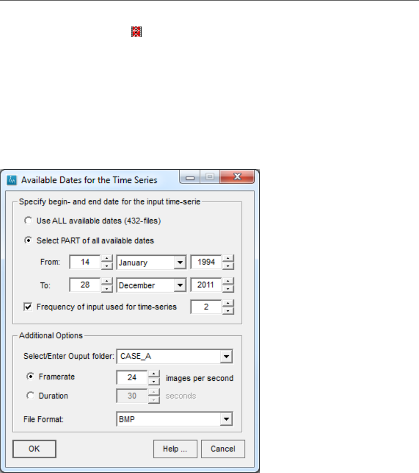
DRAFT
iMOD, User Manual
Create a New Movie button ( ) at the main toolbar. In both cases, you should select at least
one IDF-file in the iMOD Manager that has a date notation in its name. This is a continuous
number with eight-digits (yyyymmdd), e.g. 19940114 or fourteen-digits (yyyymmddhhmmss),
e.g. 20121228123010. In the first case, it represents the 14th of January, 1994, for the second
case is represents the 28th of December 2012 at 12 hours, 30 minutes and 10 seconds. If
iMOD can not find such a date notation somewhere in the filename (in at least one of the
selected IDF-files), the following window will appear and the Create a New Movie Tool will not
start.
Warning window:
If a proper IDF-file(s) has been selected in theiMOD Manager, the following window will ap-
pear.
Available Dates window:
304 of 812 Deltares
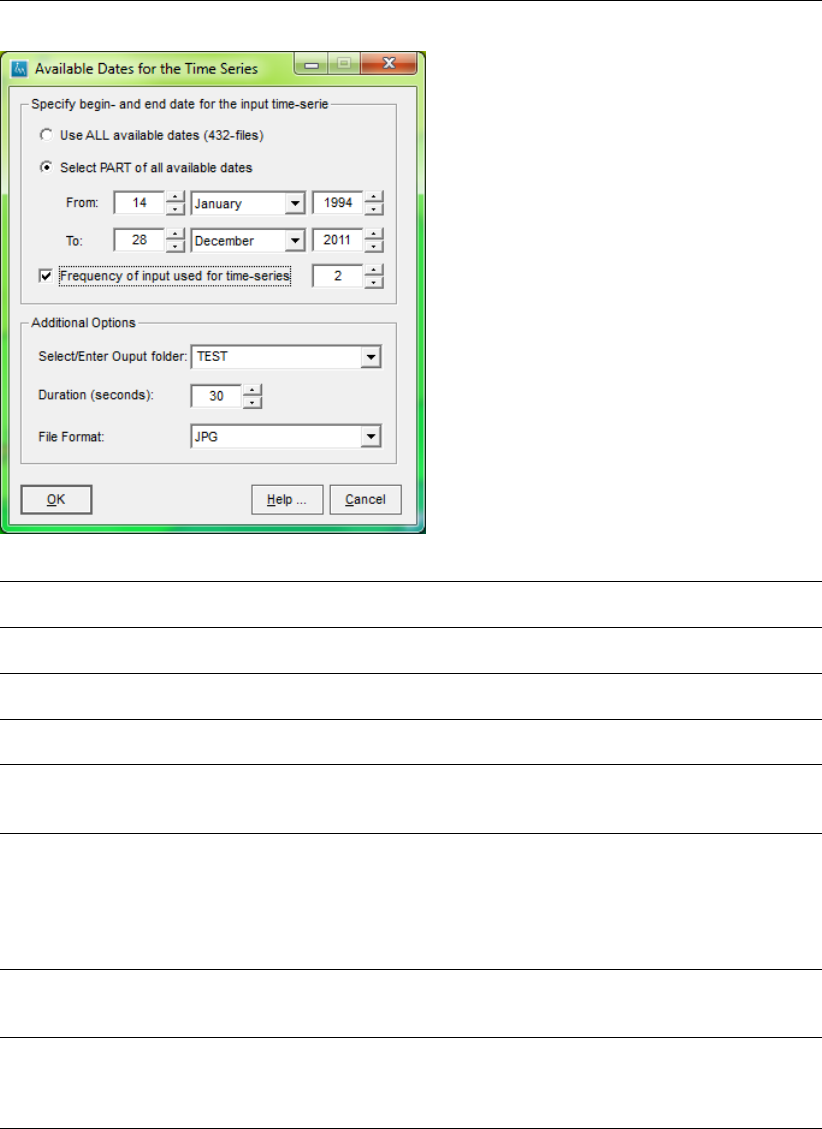
DRAFT
Toolbox Menu Options
Use ALL available
dates (432-files)
Select this option whenever you want to create an movie file for the entire time
window that iMOD found.
Select PART of all
available dates
Select this option to specify a different time window. This may gain processing
time as less files need to be opened.
From: Enter the start date of the time window. On default it displays the earliest date
of the data.
To: Enter the end data of the time window. On default it displays the latest date of
the data.
Frequency of input
used for time se-
ries
Select this option to decrease the number of dates used, e.g. by entering the
value 2 iMOD will skip each second available date of the time series.
Select/Enter Out-
put folder:
Select an existing output folder in which the individual images will be saved
that are used to create a movie file (AVI) out of it. iMOD lists all the avail-
able folders in the user folder {IMOD_USER \MOVIE}. If an existing folder is
selected, iMOD will ask for confirmation to delete its entire content before pro-
ceeding. It is also possible to enter a non-existing folder by typing in the name
of the new folder.
Framerate Enter the framerate of the movie in frames per seconds. Suppose iMOD gen-
erates a movie for 48 images (frames) and the framerate of the movie is 24
frame per seconds, the Duration of the movie will be 2 seconds.
Duration Enter the duration of the movie in seconds. Suppose iMOD generates a movie
for 48 images (frames) and the duration of the movie need to be 4 seconds,
the framerate will be 12 frames per seconds. The higher the framerate the
faster the consecutive images will appear.
Deltares 305 of 812
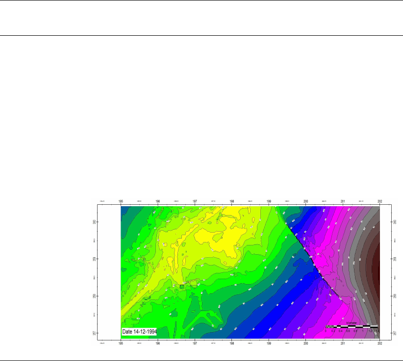
DRAFT
iMOD, User Manual
File Format Choose one of the following file formats:
Bitmap (*.BMP);
Portable Network Graphics (*.PNG);
ZSoft PC Paintbrush (*.PCX);
JPEG image (*.JPG).
Be aware that the BMP file format is not compressed and gives a more
detailed quality, it consumes more disc-space per image, approximately
7.0Mb. Instead, PCX or even better JPG file formats can be used that
consume significantly less disc-space per image, approximately 0.1Mb. For
each image, a separate file is create in the selected Output Folder, e.g.
IMAGE001.JPG. Each file has a time stamp as well.
Example of one of the consecutive images
306 of 812 Deltares
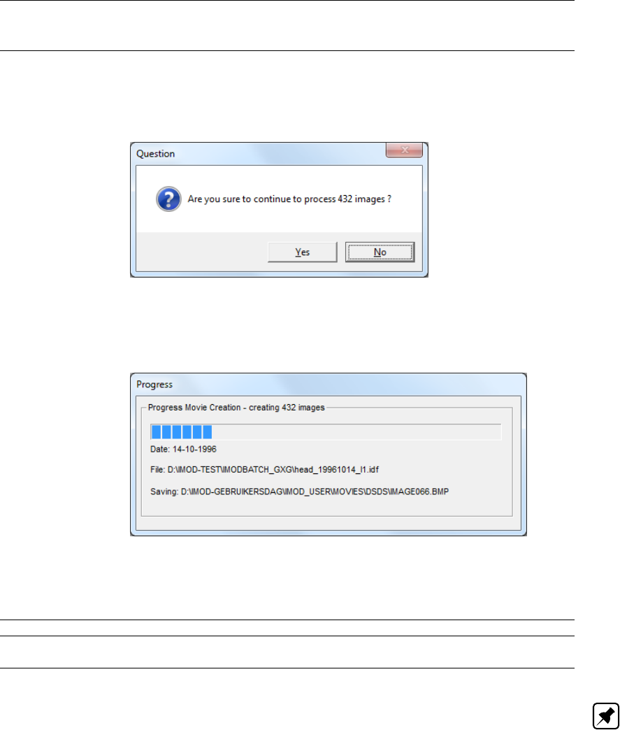
DRAFT
Toolbox Menu Options
OK Click this button to start the Create a New Movie Tool for the selected
time window. The Available Dates window will close. iMOD will generate a
question first to confirm the generation of the consecutive images.
Question for confirmation of the generation of consecutive images
Enduring the process of generating these consecutive images, the progress
is displayed in the following window.
Progress window in the process of generating consecutive images
The process cannot be stopped, but will if there might be an error while
saving an image to disc, e.g. whenever the disc-space runs out. After the
process, iMOD asks to start the Play an Existing Movie Tool to display the
images, see section 7.5.2.
Help . . . Click this button to start the iMOD Help Functionality.
Cancel Click this button to close the Available Dates window; the Timeseries Tool will
not start.
Note: You should select at least one IDF with date information in its filename, other IDF-
files that are selected without a date information, will be displayed as time-constant. In this
way you can easily make a combination with time-variant information (e.g. drawdown) and
time-invariant information (e.g. landuse).
Deltares 307 of 812
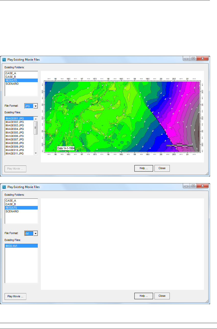
DRAFT
iMOD, User Manual
7.5.2 Play an Existing Movie
Start the Play Existing Movie Files window by selecting the option Toolbox from the main
menu, choose Movie Tool and then choose Play Existing Movie Files . . . .
Play Existing Movie Files window:
Existing Folders: Select one of the existing folders in the {IMOD_USER \MOVIE} folder.
308 of 812 Deltares
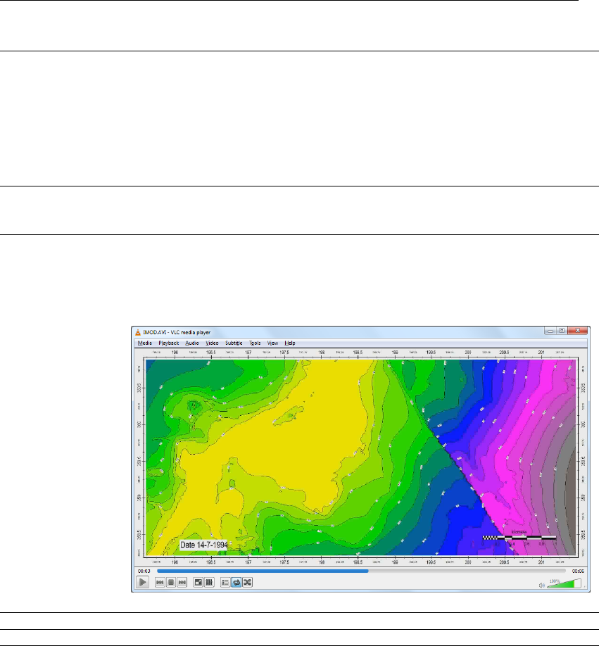
DRAFT
Toolbox Menu Options
File Format: Select one of the existing file formats for display purposes. Choose one of the
following file formats:
Bitmap (*.BMP);
Portable Network Graphics (*.PNG);
ZSoft PC Paintbrush (*.PCX);
JPEG image (*.JPG);
AVI Audio Video Interleave (*.AVI).
Existing Files: Select one of the existing files to display them in the graphical frame on the right.
This is operational as long as one of the following file formates are selected: BMP,
PNG, PCX, JPG are selected.
Play Movie . . . Click this button to start a movie player, such as FFMPLAY or VLCPLAYER. This
option is available whenever one of this players are referred to in the PRF-file,
see section 9.1 and whenever the AVI file format is selected.
Example of the VLCPLAYER
Help. . . Click this button to start the HELP functionality
Close Click this button to close the Play Existing Movie Files window
Deltares 309 of 812

DRAFT
iMOD, User Manual
7.6 GeoConnect Tool
WHY?
The GeoConnect Tool is an instrument that can be used to aggregate geological formations
to model layers and vice versa.
WHAT?
With the GeoConnect Tool it is possible to aggregate geological formations to a dataset with
different model layers containing combined formation information. It is now possible to go from
model results with multiple geological formations per layer to a geological formations dataset.
Besides, with this tool it is possible to use geological formations to come up with a new model
parameterization. This functionality is also available as a batch-function (see section 8.7.7).
HOW?
Before starting the GeoConnect Tool, the user needs to create a textfile with the general
settings to be used in the tool. This file needs to be placed in the "IMOD_USER\SETTINGS\"
subfolder with the name "GeoConnect.txt".
The textfile with general settings needs to contain the following keywords:
ACTLAYERS=
(optional)
Enter a string of values to include or exclude a specific model layer from
the computation; 0=inactive, 1=active, on default all layers are used in de
computation (similar to e.g.: ACTLAYERS=1111111111). E.g. in case of
the amount of model layers is 10 and it is preferred to only take the first 6
layers into account: ACTLAYERS=1111110000.
REGISFOLDER= Give the directory and name of the folder where all REGIS-files are stored.
Note: subdirectories are not allowed and the filenames need to be of
the following format: abbreviation formation name-t/b/ks/kv-ck/sk.idf (’t’
and ’b’ need to be combined with ’ck’, and ’ks’ and ’kv’ with ’sk’), e.g.
d:\Model\REGIS\bez1-b-ck.idf.
TOPFOLDER= Give the directory and name of the folder of the model TOP-files, e.g.
d:\Model\TOP\TOP.
BOTFOLDER= Give the directory and name of the folder of the model BOT-files, e.g.
d:\Model\BOT\BOT.
NLAY= Enter the amount of model layers, e.g. NLAY=10.
These settings are automatically placed on the Settings tab on the GeoConnect window when-
ever the tool is started. The aggregation process is described in the example below.
Example 1
ACTLAYERS=1111110000000000000
REGISFOLDER=d:\Model_Ibrahym\REGIS\
TOPFOLDER=d:\Model_Ibrahym\TOP\VERSION_1\
BOTFOLDER=d:\Model_Ibrahym\BOT\VERSION_1\
NLAY=19
Geostratigraphy textfile
The geostratigraphy.txt file contains the order of the formations (from surface layer to base)
and needs to be located in the Settings-folder in the iMOD user environment (in case of
using the GUI), contains all formation abbrevations as used in the geological dataset and
corresponding factors. This file can be loaded into the Postprocessing-tab on the GeoConnect
window in the iMOD-GUI.
Example of the first 11 and last 4 lines of a geostratigraphy.txt:
HLC
310 of 812 Deltares
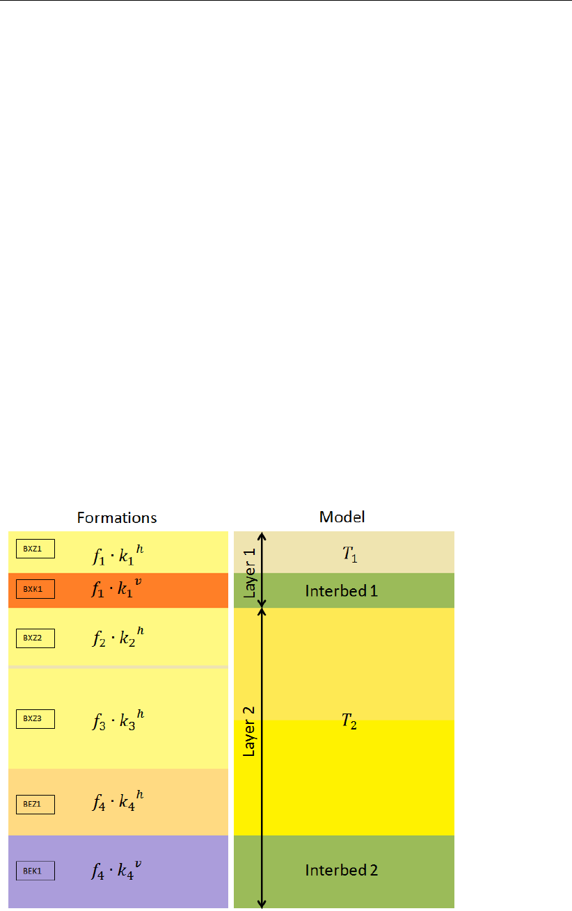
DRAFT
Toolbox Menu Options
BXSCK1
BXZ1
BXLMK1
BXK1
BXZ2
BXK2
BXZ3
BEROK1
BEZ1
BEK1
...
MTQ
GUQ
VAC
AKC
Calculation/Aggregation of formations:
This example shows the mathematical theory behind the aggregation of formation charac-
teristics within one model layer. The formulas in the table are used to calculate the new
transmissivity, groundwater head vertical resistance and flux. The choice of the formula de-
pends on the variable that needs to be aggregated. In case, it is preferred to calculate the
transmissivity (see figure) of the first and second model layer based on the formations given
in the formation dataset, the first formula in the table is used to achieve this. In example:
T1=(df
1×kh
1×f1)
T2=(df
2×kh
2×f2)+(df
3×kh
3×f3)+(df
4×kh
4×f4)
Deltares 311 of 812
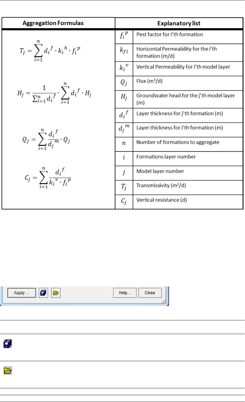
DRAFT
iMOD, User Manual
Start the Tool
To start the GeoConnect Tool select Toolbox from the main menu, choose GeoConnect Tool.
This tool allows the user to continue working in the same iMOD session and using the Geo-
Connect tool at the same time. Included are a preprocessing, a postprocessing and an identify
functionality. The tool opens with the Settings tab up front. The general settings on the tool-
window are:
Apply. . . Click this button to start the preprocessing or postprocessing compu-
tation.
Save as. . .
Click this button to save the settings in a GeoConnect.txt file in case
of Settings tab, or alternatively in an iMODBATCH *.ini file in case the
Preprocessing tab or Postprocessing tab is selected.
Open
Click this button to get the settings from a GeoConnect.txt file in case
of Settings tab, or alternatively from an iMODBATCH *.ini file in case
the Preprocessing tab or Postprocessing tab is selected.
Help. . . Click this button to start the Help functionality.
Close Click this button to close the window.
312 of 812 Deltares
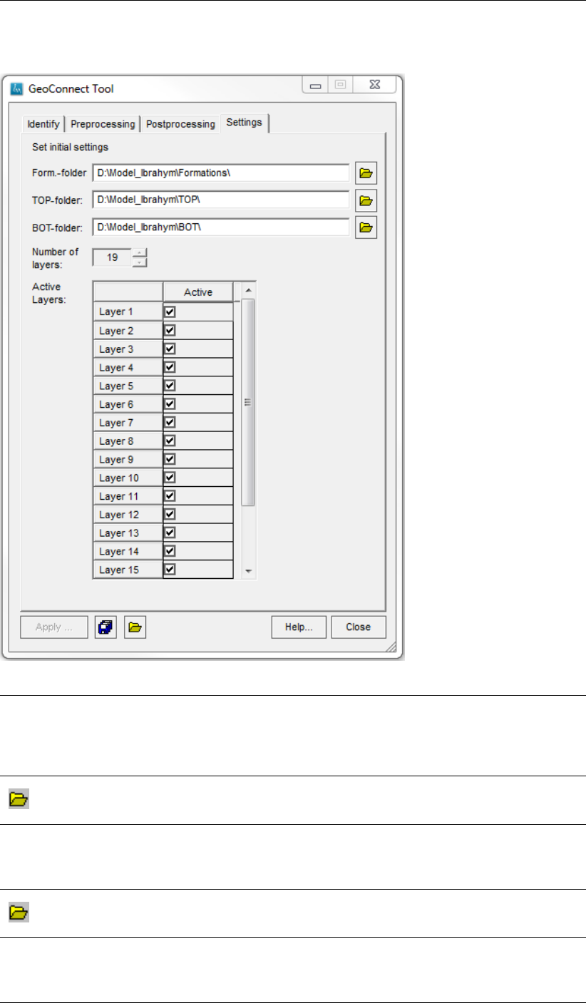
DRAFT
Toolbox Menu Options
Example of the GeoConnect window; Settings tab
Form.-
folder:
Give the name of the folder where all geological formation files are
stored. Note: subdirectories are not allowed and the filenames need
to be of the following format: abbreviation formation name-t/b/ks/kv-
ck/sk.idf (’t’ and ’b’ need to be combined with ’ck’, and ’ks’ and ’kv’ with
’sk’), e.g. d:\MODEL_Ibrahym\Formations\bez1-b-ck.idf.
Open
Click on this button to search for the name of the folder containing
geological formation data.
Top-folder: Give the name of the folder of the model TOP-files;
e.g. d:\MODEL_Ibrahym\TOP. The tool searches for
"d:\MODEL_Ibrahym\TOP\TOP_L1.IDF" in the given folder. This
is repeated for each layer.
Open
Click on this button to search for the name of the folder containing the
Top elevation of the model.
Bot-folder: Give the name of the folder of the model BOT-files,
e.g. d:\MODEL_Ibrahym\BOT. The tool searches for
"d:\MODEL_Ibrahym\BOT\BOT_L1.IDF" in the given folder. This
is repeated for each layer.
Deltares 313 of 812
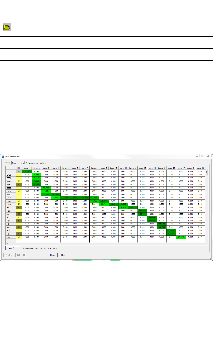
DRAFT
iMOD, User Manual
Open
Click on this button to search for the name of the folder containing the
Bottom elevation of the model.
Number
of layers
Represents the amount of model layers as defined in settings file that
you can read into the GUI on the Postprocessing-tab, e.g. NLAY=10.
Active
layers
Check a checkbox for a particular layer to include a specific model layer
in the Identify routine (see Identify-tab).
Identify
The Identify option can be found on the first tab of the GeoConnect window. With this option
it is possible to analyze, "on-the-fly", the model composition per individual location by making
use of the Identify button. The functionality shows the content of the geological formations
in the model at mouse position. Aquitard layers (e.g. clayey formations) are identified as
connected to the Aquifer layers (sandy formations), the clayey layers are so called "interbed"
layers. When a model layer contains a clayey layer the fraction shown in the Identify table is
always 100%. See for example Layer 2 in the figure below (Identify-tab). This layer consists
for 0.211% of BXZ3, 26.538% of BEZ1, 73.140% of BEZ2 and for 100% of BEK2.
Example of the GeoConnect window; Identify tab
Identify. . . Click this button to be able to hover over the map in the main iMOD window.
Table description Lith.: Lithology class of the specific formation shown in the first col-
umn of the table.
Layer}{i}: i’th model layer
"100.0": Fraction of specific geological formation in given model layer,
e.g. Layer 2, row 3: "26.538" means that layer 2 consists of
26.538% BEZ1 formation. The darker the color green the higher
the fraction.
Current location
(...m,...m)
Gives the current location (in meters) of the model composition at the mouse
position.
Preprocessing
The preprocessing functionality in the GeoConnect tool can be used to compute a renewed
model parameterization out of the geological formation related top-, bot- and k-values.
314 of 812 Deltares
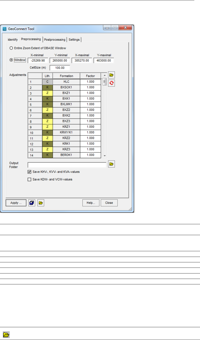
DRAFT
Toolbox Menu Options
Example of the GeoConnect window; preprocessing tab
Entire Zoom
Extent. . .
Select this option to use the complete model extent as described by the IDF-
files in the TOP-folder (as defined on the Settings tab).
Window Select this option to compute only for the given window extent. Click on "Win-
dow" to refresh the extent accordingly to the current extent in the main iMOD
window.
X-minimal Give a minimum X-coordinate value in meters.
Y-minimal Give a minimum Y-coordinate value in meters.
X-maximal Give a maximum X-coordinate value in meters.
Y-maximal Give a maximum Y-coordinate value in meters.
CellSize (m) Give the cell size in meters of the new model to be computed.
Adjustments Adjustable grid with factors sorted per formation.
Table description: Lith.: In this column the lithology class is shown related to a specific
geological formation, e.g. "K" means Clay, "Z" means Sand. The
cells are colored accordingly to the individual lithology class.
Formation: In this column the geological formations are displayed.
Factor: In this column the factors per formation are given and can be
adjusted, either by loading in an file with factors (on default fac-
tors.txt is read from the IMOD_USER\SETTINGS folder, see for
an example section 8.7.7) or by changing the factors manually.
Open
Click this button to read a file with factors into the Adjustments grid.
Deltares 315 of 812
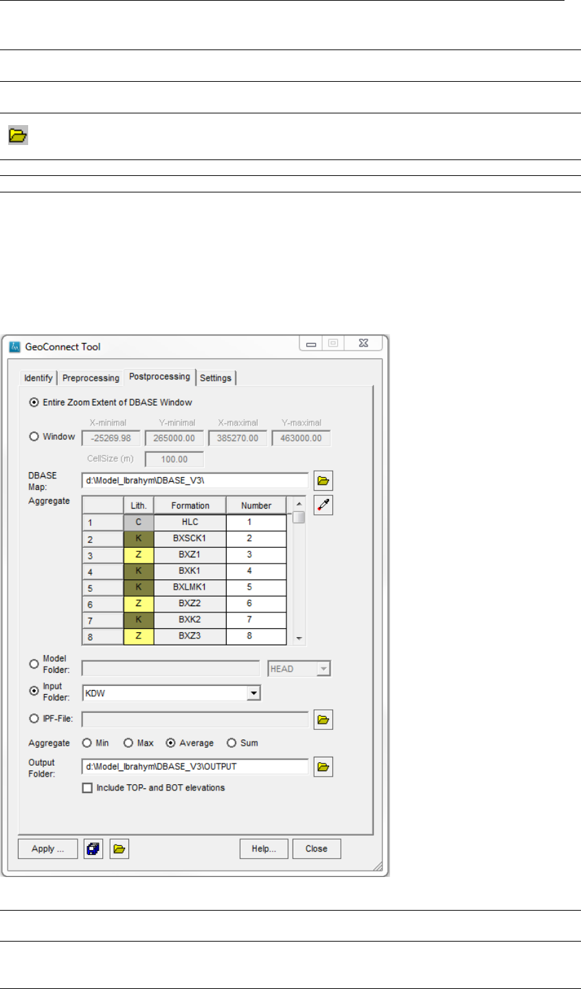
DRAFT
iMOD, User Manual
Refresh Click this button to refresh the factors in the grid to 1.0.
Output Folder Give the directory and name of the folder to store the results of the prepro-
cessing computation.
Open
Click on this button to search for the name of the folder to store the results of
the preprocessing computation.
Save KHV-,. . . Check this option to calculate new parameter files for KHV, KVV and KVA.
Save KDW-,. . . Check this option to calculate new parameter files for KDW and VCW.
Postprocessing
The postprocessing functionality in the GeoConnect tool can be used to perform model layer
aggregation for variables to be chosen based on the formation settings.
Example of the GeoConnect window; postprocessing tab
Current Zoom
Extent. . .
Select this option to use the complete model extent as described by the IDF-
files in the TOP-folder (as defined on the Settings tab).
Window Select this option to compute only for the given window extent. Click on "Win-
dow" to refresh the extent accordingly to the current extent in the main iMOD
window.
316 of 812 Deltares
DRAFT
Toolbox Menu Options
DBASE map: Give the directory and name of the folder containing DBASE model informa-
tion.
Open
Click this button to search for the specific DBASE model folder.
Pipet
Click this button to fill the aggregated grid with all available geological forma-
tions at the current window extent.
Aggregate Grid with geological formations, arranged by the order given in GEOSTRATIG-
RAPHY.TXT (see section 8.7.7). Changing the numbers in the 4th column
makes aggregation of geological layers possible, e.g. to aggregate all the BX*
formations give them all the same number for example 2 or 5.
Table description: Lith.: In this column the lithology class is shown related to the specific
geological formation, e.g. "K" means Clay, "Z" means Sand. The
cells are colored accordingly to the individual lithology class.
Formation: In this column the geological formations are displayed.
Number: In this column each unique number represents one geological
formation. To combine different geological formations change
the number, e.g. if you want to consider the Boxtel Sands/Clays
(BX*) as one model layer, enter the same number (e.g. 2) for
each Boxtel formation related geological layer in this column.
Model Folder: Give the directory and name of the folder containing the preferred model out-
put information. Choose the favored variable in the related dropdown menu
to apply the aggregation to. Options in dropdown menu are: "HEAD", "BDG-
WEL", "BDGRIV", "BDGDRN".
Input Folder: Choose the preferred variable from the dropdown menu to apply the aggrega-
tion to. Options are: "KDW", "VCW", "KHV", "KVV".
IPF-File: Give the name of the IPF-file to select points in the IPF that coincides with the
aggregated formations.
Open
Click on this button to search for the directory and name of the IPF-file to apply
the aggregation to.
Aggregate Select the aggregation method to be used. The aggregation can be based on
the values minimum (=Min), maximum (=Max), Average or Sum.
Output Folder: Enter the name of the folder to store the results of the postprocess-
ing computation, e.g. (OUTPUTFOLDER)\BEZ1_BEZ2_BEZ_KDW.IDF,
(OUTPUTFOLDER)\BEZ1_BEZ2_BEZ_TOP.IDF, (OUTPUT-
FOLDER)\BEZ1_BEZ2_BEZ_THK.IDF.
Open
Click on this button to search for the name of the folder to store the results of
the postprocessing computation.
Include TOP-,. . . Select this option to include TOP- and BOT elevation and thickness IDF-files
in the aggregation and save these files in the given Output folder.
Deltares 317 of 812

DRAFT
iMOD, User Manual
7.7 Plugin Tool
WHY?
The Plugin Tool is an instrument that can be used to run external executables (from compli-
cated to simple) or batchfiles within iMOD.
WHAT?
The Plugin tool makes it possible to include advanced plugins that come close to fully software
integration as well as plugins that simply run an executable file. This allows you to start a
specific program within an iMOD-session without stop working in this session. A number
of pre-settings and couplings are necessary before you can launch a plugin. iMOD needs
information about the plugin and vice versa.
HOW?
Before starting the iMOD Plugin Tool, you need to walk through a couple of preprocessing
steps before a plugin can be used within the iMOD gui.
1 Predefine PLUGIN1= and/or PLUGIN2= in the iMOD preference file (IMOD_INIT.PRF).
With these two keywords you can set the specific file-directory where iMOD can find the plugin(s).
You are able to use two different plugin-directories inside iMOD. The iMOD preference file might
look like this (See section 9.1 for a more extended description of the preference file):
PLUGIN1 "C:\PLUGIN1"
PLUGIN2 "E:\PLUGIN2"
2 Create a subfolder with the plugin-name in which you can store all the needed "coupling"-files,
including the executable file itself. Note: this subfolder should be located in de PLUGIN1 or
PLUGIN2 folder.
3 An initialization file called PLUG-IN.INI, needs to be created that should be placed within the
plugin-subfolder. This file can contain the following keywords:
Keyword Description
TXT= This keyword is linked to the filename of the text file that contains a short descrip-
tion of the plugin.
CMD= With this keyword the specific plugin-executable or batch-file is called. You
have to make an additional choice whether you prefer to run the plugin in
"WAIT" modus or in the background ("NOWAIT") of other iMOD-processes, e.g.
CMD=DEMO.EXE NOWAIT
MENU= This keyword is optional. MENU refers to a file that describes an optional menu to
be displayed, before the actual plugin will start, e.g. MENU=D:\PLUGIN1\PLUG-
IN.MENU. The file contains the visual-settings of the specific plugin window. See
description in section section 7.7.1 for the PLUG-IN.MENU setup.
HELP= This keyword is optional and refers to the helpfile related to the plugin itself (PDF
or HTML). In case the helpfile is in PDF-format, the keyword ACROBATREADER
is needed to be defined in the preference file to be able to read the PDF-file.
BACK= With this keyword you specify a filename that iMOD will check repeatedly (minute
time interval), e.g. BACK=PLUG-IN.OUT, see section section 7.7.1 for more de-
tailed information about the content of this file.
Example1
TXT= WATERBALANCE.TXT
CMD= WATERBALANCE.EXE WAIT
Example2
TXT= RASTERCONVERSION.TXT
MENU= RASTERCONVERSION.MENU
HELP= RASTERCONVERSION_MANUAL.PDF
CMD= RASTERCONVERSION.EXE NOWAIT
BACK= RASTERCONVERSION.OUT
318 of 812 Deltares
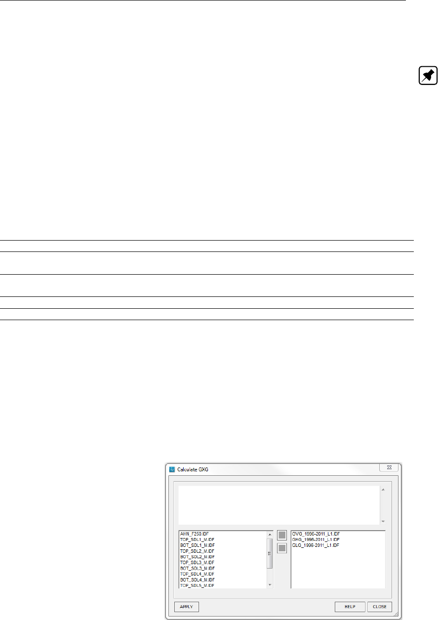
DRAFT
Toolbox Menu Options
The files related to the keywords are described in section section 7.7.1.
4 Now the Plugin Tool can be used. For the steps to be taken see section 7.7.2
Note: You are able to save the activated plugins for later use within the IMF-file. You can
do this by saving the current iMOD project session via the Save-button or via File->Save as...
in the main-menu. Also the chosen time interval (see TMO.PITools.execution how to set this
interval) on which iMOD tests whether a plugin is running or not, is saved in the IMF-file.
7.7.1 Plugin file description
In the PLUG-IN.INI different initialization files are listed behind the above explained keywords. Some
of these files also contain a list of keywords. We will explain them here.
7.7.1.1 Plugin MENU file
All keywords are optional.
Keyword Description
TITLE= Optional keyword that sets the title of the menu window, e.g. TITLE="This plugin
computes residuals".
BUTTON1= Optional keyword that sets the text on the Close-button, e.g. BUT-
TON1=Afbreken.
BUTTON2= Optional keyword that sets the text on the Help-button, e.g. BUTTON=Hilfe.
BUTTON3= Optional keyword that sets the text on the Apply -button, e.g. BUTTON3=Go-for-it
LIST= Optional keyword that loads all available files from a certain place or directory. If
not defined, iMOD shows a diaolog in which you need to select files yourself. The
following options are available:
IMODMANAGER Whenever LIST=IMODMANAGER, iMOD will display the
selected files from the iMOD Manager in a separate win-
dow.
Be aware that iMOD places a ’+’-sign in front of the direc-
tory name in case the related file is selected in the iMOD
Manager and a ’-’-sign in case the file is not selected! To be
able to read the file properly the plugin needs to handle this.
Example
Use the buttons left and right to move the selected
items from left to right or the other way around
.
Deltares 319 of 812
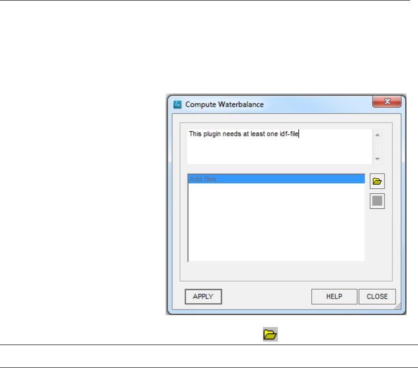
DRAFT
iMOD, User Manual
*.IDF / *.* Whenever LIST=*.IDF iMOD will display a dialog in which
files can be selected, e.g. IDF-files. Any combination of
wildcards can be uses, e.g. LIST=*.*, LIST=*.RUN, or
whatsoever the plugin need as an input.
Example
Use the "open"-button ( ) to add files to the dialog.
TEXT= Refers to an addition text file with explanatory text with requirements for using the
chosen plugin, e.g. TEXT=EXPLAINATION.TXT.
The list of files defined with keyword LIST or by making use of the plugin menu-dialog, is stored in a
file called "PLUG-IN.IN" (see section 7.7.1.2).
Example1
TITLE= Compute Waterbalance
BUTTON1= Quit
BUTTON2= Info
BUTTON3= Run
LIST= IMODMANAGER
TEXT= EXPLAIN.TXT
Example2
TITLE= Convert Raster settings
LIST= *.IDF
TEXT= EXPLAIN.TXT
7.7.1.2 Plugin IN file
The list of files that is used by the plugin is saved in this file "PLUG-IN.IN", and can serve as a checkup
for the user of the plugin. In case LIST="IMODMANAGER" is given in the MENU-file, iMOD puts a
’+’- or a ’-’-sign in front of each individual file listed in PLUG-IN.IN. The ’+’-sign is written when a file is
selected in the iMOD manager, else a ’-’-sign appears.
320 of 812 Deltares
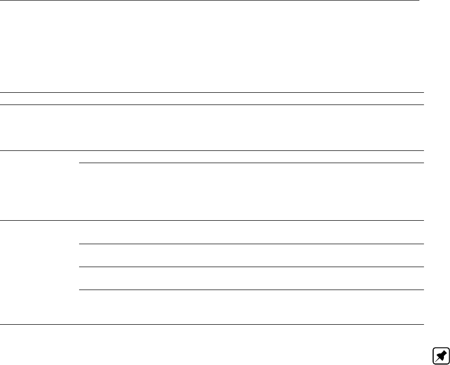
DRAFT
Toolbox Menu Options
7.7.1.3 Plugin OUT file
This file needs to be written by the plugin executable after or during its execution. It needs to be
prepared within the code of the plugin. To allow iMOD to interact with the plugin, it is required to
include at least one of the following keywords in the OUT file.
Keyword Description
WINDOW= With this keyword the plotting window extent (decimal coordinates) in iMOD can
be set. Once this is read, iMOD will adapt the current window extent to the extent
mentioned by WINDOW. Use the format: XMIN,YMIN,XMAX,YMAX, e.g. WIN-
DOW=10000.0,250000.0,150000.0,300000.0.
NFILE= Number of files to be read into the iMOD Manager.
FILE{i}= The ith file to be read into iMOD Manager, e.g.
FILE1=FLUX.IDF. Given file needs to be available in
the specific plugin-(sub)folder. Only name of the (sub-
folder+)file+extension are needed to be given. As men-
tioned the use of subfolders is allowed.
MESSAGE_{...}= Contains some text lines to be given at a certain moment in de executable pro-
cess.
{INFO} Contains general information to be given in a popup window
at a certain moment during de executable process.
{ERROR} Contains error-information to be given in a popup window at
a certain moment during de executable process.
{PROGRESS} Contains progress-information to be given at a certain mo-
ment during de executable process. This will be visible in
the information-bar at the bottom of the iMOD main-window.
Note: It is the responsibility of the plugin owner to process the message(s) of the plugin in the right
way and at the right moment. After reading the OUT-file, iMOD will delete the file from disc to avoid
any double interpretation of the file.
Example1
WINDOW= 140000.0,445000.0,150000.0,452000.0
NFILE= 2
FILE1 = WBAL_2014_SUMMER.IDF
FILE2 = WBAL_2014_WINTER.IDF
MESSAGE_INFO= "The waterbalance is succesfully calculated."
Example2
MESSAGE_PROGRESS= "Plugin is still busy ..."
7.7.2 Using the Plugin
To start the Plugin Tool from the main menu, choose Plug-in. A sub-menu will appear. If you did define
PLUGIN1 and/or PLUGIN2 in the iMOD preference file, you can choose Manage Plug-in 1 ... and/or
Manage Plug-in 2 .... To start the Plugin Manager window, click on either of the two.
Deltares 321 of 812
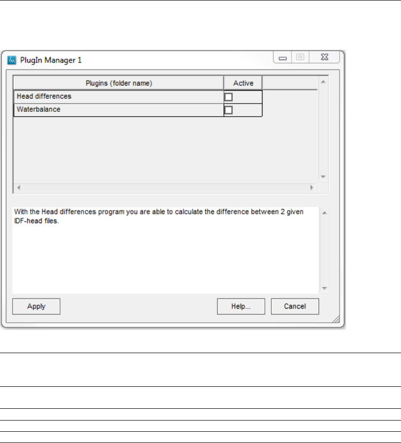
DRAFT
iMOD, User Manual
Example of Plugin Manager window
Plugins
(folder
name)
The list displays all sub-folders in the {PLUGIN1}\folder. Click on the sub-folder. If a
{PLUGIN}.txt is available in the sub-folder an explanatory text of the plugin will appear
in the sub-window below.
Active Select the check box to (de)activate a specific plugin. When you activate a plugin,
the plugin appears in the main sub-menu Tools and Plugin.
Apply Click this button to apply your plugin-settings and to close the window.
Cancel Click this button to close the window and not applying your modified plugin-settings.
Help. . . Click this button to start the Help functionality.
After clicking on Apply button, the activated plugins are added to the Plugin menu. At maximum, 10
plugins can be activated at once into this menu list. The Plugin-menu might look like this:
322 of 812 Deltares
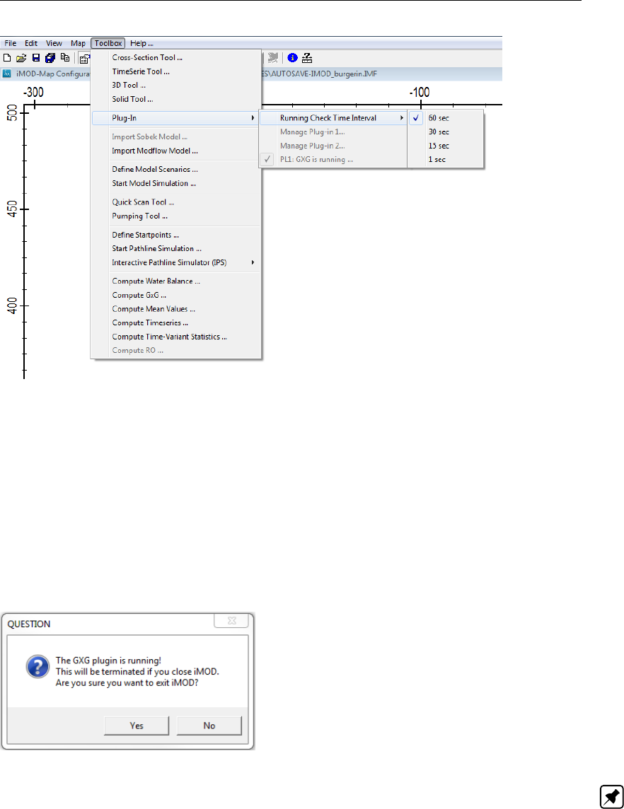
DRAFT
Toolbox Menu Options
It depends on the configuration of the Plugin what will happen whenever the plugin is selected from
the menu. During the whole running process iMOD checks at predefined fixed moments (intervals of
60, 30, 15 or 1 seconds) if there are plugins running. The running check time interval can be changed
by selecting the similar called option in the Plug-In menu (see figure below). On default this interval is
set on 60 seconds. As long as a single plugin or multiply plugins are running, the plugin manager(s)
cannot be reached (Menu options are grayed-out) for making changes. Though you are able to use
already selected plugins from the plugin-menu.
As shown in the example above, only the plugins that are running are grayed-out. If there are still
plugins running when trying to close iMOD, iMOD asks the following question for every plugin that is
running:
Note: When using a batch file as a plugin to call an executable, this plugin cannot be terminated by
iMOD. The plugin continues running after iMOD is closed.
Deltares 323 of 812
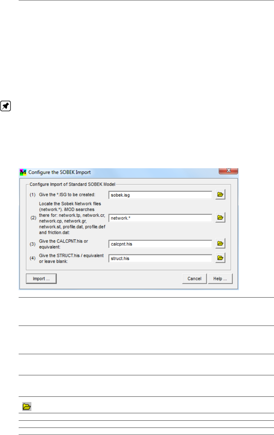
DRAFT
iMOD, User Manual
7.8 Import Tools
7.8.1 Import SOBEK Models
WHY?
SOBEK models are surface water models made with the SOBEK suite software available from Deltares.
SOBEK models may be imported in iMOD to be used with iMODFLOW.
WHAT?
The available SOBEK files are converted to iMOD format and saved as ISG-file. All SOBEK Network,
Profile and His-files are converted
Note: This function is only available in the X32-bits version of iMOD, in the X64-bits version of iMOD
this functionality is greyed-out. This functionality is supported also by iMOD Batch.
HOW?
Select the option Toolbox from the main menu and then choose the option Import Sobek Model to start
the Configure the SOBEK Import window.
Example of Configure the SOBEK Import window:
(1) Give the *.ISG to be created
Enter the name of the ISG-file to be created. All information from the SOBEK files
will be saved in one ISG-file. The location of the ISG-file can be chosen with the save
button.
(2) Locate the Sobek Network files
iMOD searches for network.tp, network.cr, network.cp, network.gr, network.st, pro-
file.dat, profile.def and friction.dat. Select the name of the network file and iMOD will
search all other files in the same folder.
(3) Give the CALCPNT.his or equivalent
Select the HIS file that contains the computed waterlevels at the SOBEK calculation
points.
(4) Give the STRUCT.his / equivalent or leave blank
Select the HIS file that contains the computed waterlevels at the SOBEK structures
points. Leave this blank when not required or available.
Open
Click this button to select the required file.
Import Click this button to import the SOBEK configuration into the ISG-file.
Cancel Click this button to close the window
Help. . . Click this button to start the Help functionality.
324 of 812 Deltares
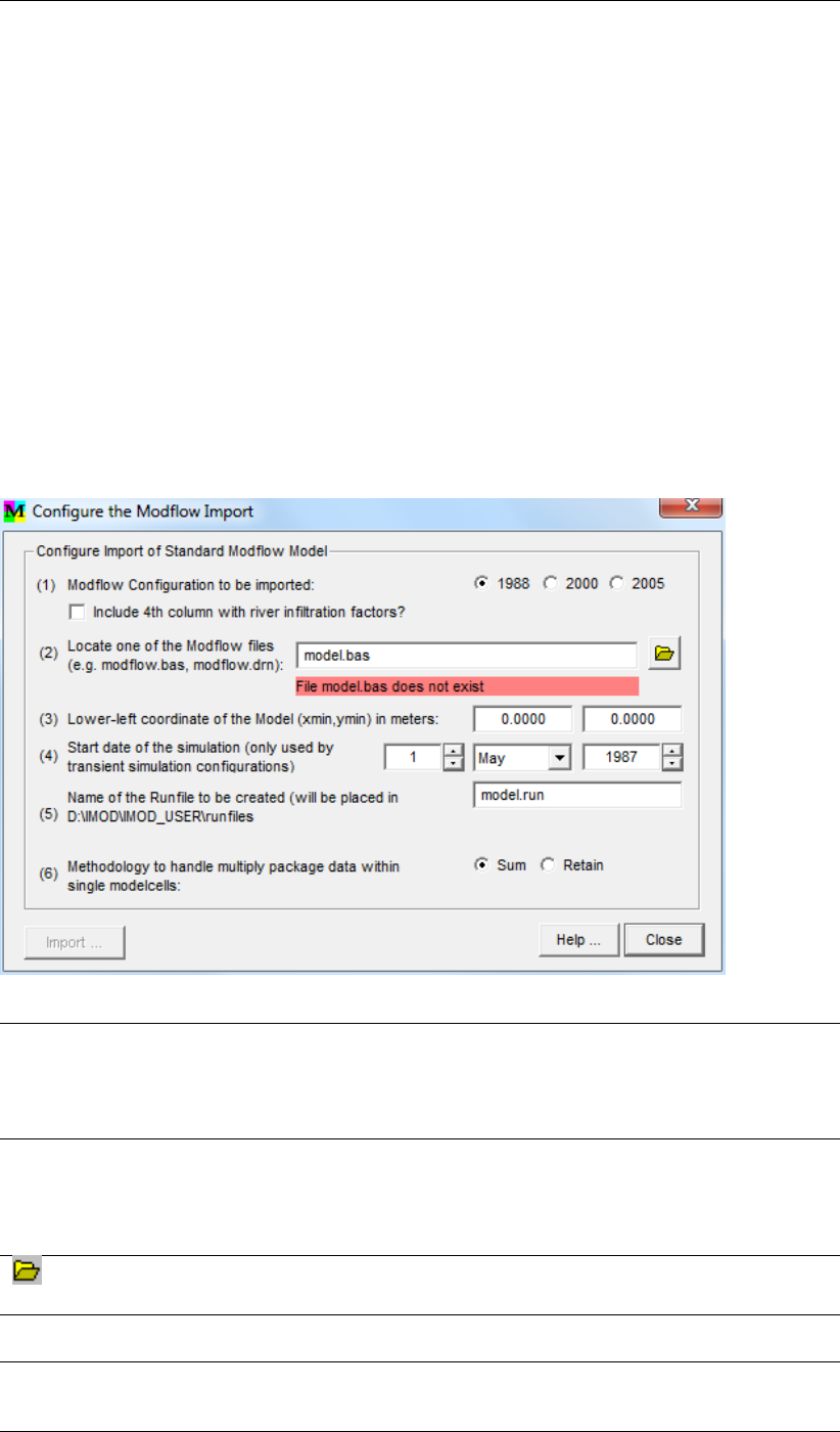
DRAFT
Toolbox Menu Options
7.8.2 Import Modflow Models
WHY?
MODFLOW models made outside iMOD may be imported in iMOD to be used with iMODFLOW.
WHAT?
An existing standard MODFLOW configuration is converted into iMOD files (e.g. IDFs, IPFs and GENs).
The conversion works for three MODFLOW versions: 1988, 2000 and 2005. iMOD will convert the
MODFLOW packages once the location of one of the packages is defined. The conversion will stop in
case no BAS-file (1988 version) or NAM-file (2000 and 2005 version) is found.
This functionality is supported also by iMOD Batch.
HOW?
Select the option Toolbox from the main menu and then choose the option Import Modflow Model to
start the Configure the Modflow Import window.
Configure the Modflow Import window:
(1) Modflow configuration to be imported
Select the year of the Modflow version (1988, 2000, 2005)
Check the box at Include 4th column with river infiltration factors in case the RIV-
package has a 4th column defining the ratio in conductance between infiltration and
drainage
(2) Locate one of the Modflow files (e.g. modflow.bas, modflow.drn)
Select the name of one of the Modflow input files and iMOD will search all other files
in the same folder. iMOD will look for a BAS-file for the 1988 version and will look for
a NAM-file for the 2000 and 2005 versions.
A remark is shown in case the BAS-package or NAM-package input file is not found.
Open
Click this button to select the required file as defined in option (1).
(3) Lower-left coordinate of the Model (xmin, ymin) in meters:
Enter the X- and Y-coordinate of the lower left corner of the model.
(4) Start date of the simulation (only used by transient simulation configurations)
Enter the date of the first time step by selecting the appropriate day, month and year.
This is required for transient models only.
Deltares 325 of 812

DRAFT
iMOD, User Manual
(5) Name of the runfile to be created (will be placed in . . . \runfiles)
Enter a name for the runfile to be created in the RUNFILES folder of the iMOD_USER
folder). For more information on the runfile see section 7.9.
(6) Methodology to handle multiple package data within single modelcells:
Select the appropriate option:
Sum: all existing package information is summed into a single modelcell. This
is the default. Whenever more elements occur in a single modelcell, they will be
lumped together to form one value.
Retain: all existing package information in a single modelcell is extracted and
stored in individual iMOD files.
Import Import the MODFLOW configuration into iMOD
The iMOD model files will be stored in the iMOD_USER\MODELS folder.
Close Click this button to close the window.
Help. . . Click this button to start the Help functionality.
326 of 812 Deltares
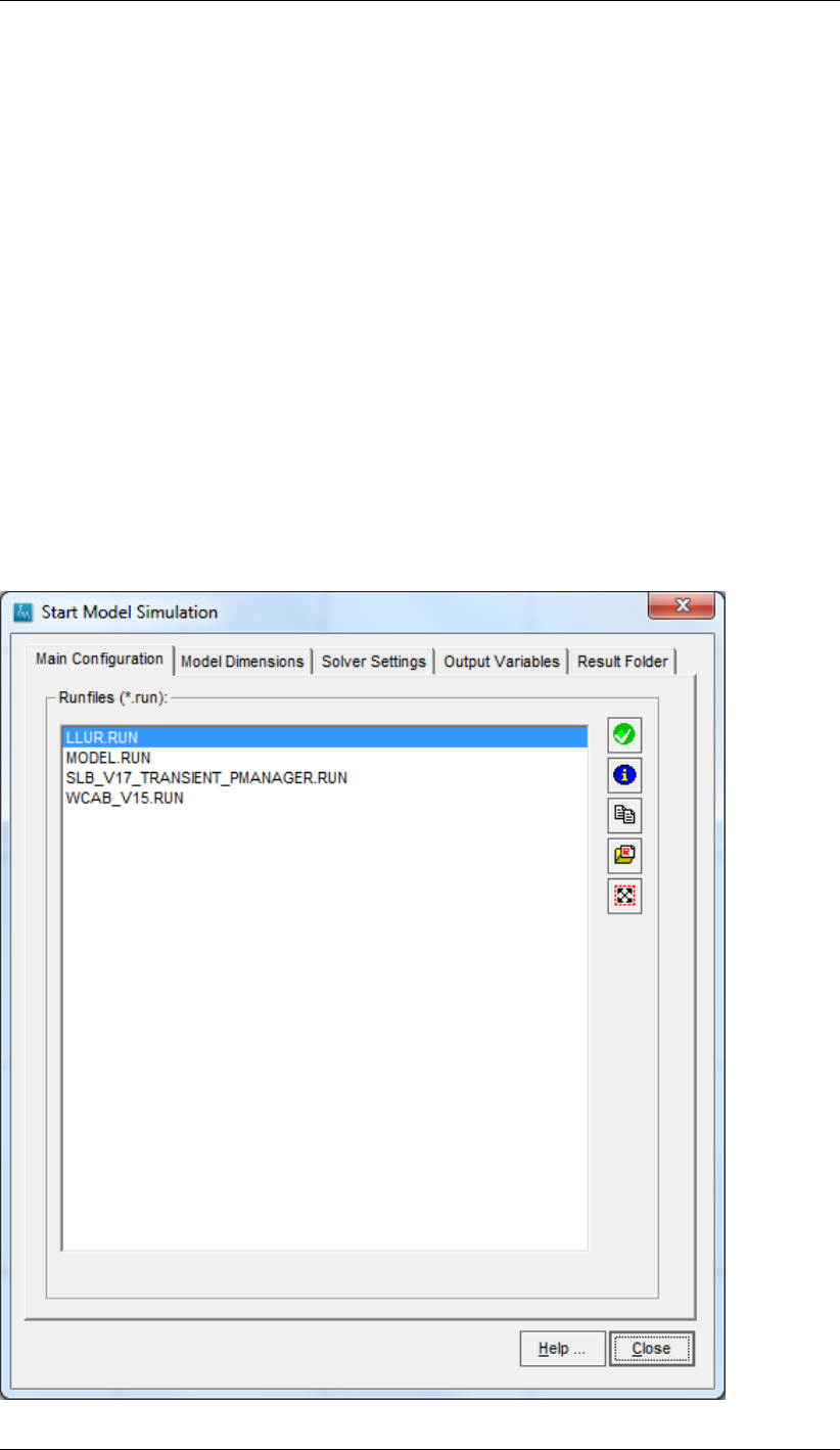
DRAFT
Toolbox Menu Options
7.9 Start Model Simulation
WHY?
A runfile is required for a groundwater flow model that is configured with the iMOD concept. Such a
runfile (see chapter 10) consists of a header with general information about the location, horizontal
resolution, number of modellayers and solver settings. This type of information can be easily modified
in the Start Model Simulation Tool described in this section. A runfile can be constructed using the
Project Manager, see section 5.5. Alternatively, a simulation can be initiated using the Project Manager
and/or using the iMOD Batch Function RUNFILE, see section 8.6.5.
WHAT?
It takes two requirements to start a model simulation within iMOD:
Include the keyword MODFLOW in the preference file (section 9.1) and add the appropriate iMOD-
FLOW executable;
Include at least one runfile in the {user}\runfiles folder.
HOW?
Select the option Toolbox from the main menu and then choose the option Start Model Simulation to
display the Start Model Simulation window.
Start Model Simulation window, Main Configuration tab:
Deltares 327 of 812
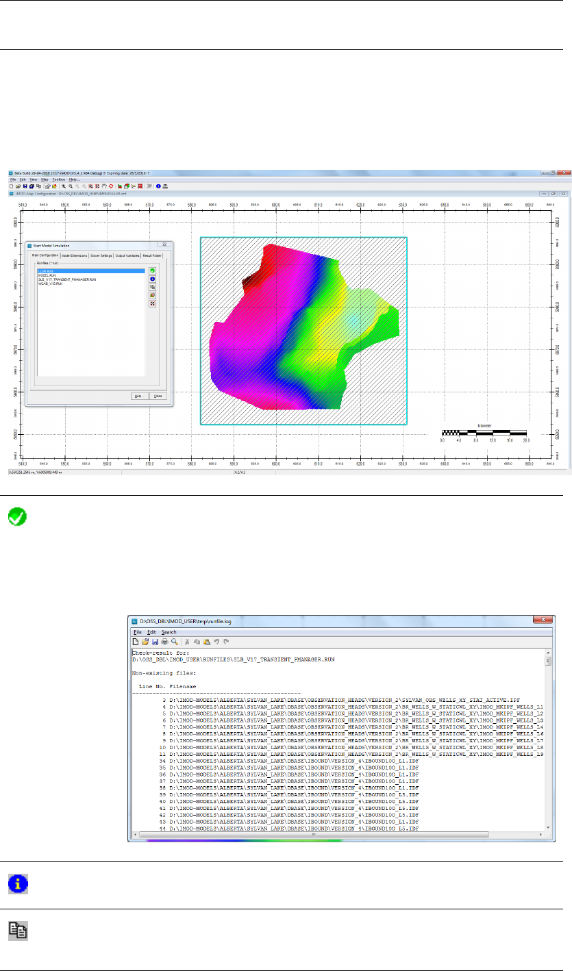
DRAFT
iMOD, User Manual
Runfiles (*.run) This list displays the existing runfiles (*.run) in the folder {user}\runfiles (see
for more detailed information about runfiles Vermeulen, 2011). Whenever a
runfile is selected, iMOD will try to read the header information and if no errors
are found, the extent of the model (as described by the BNDFILE in the runfile)
will be displayed on the graphical display (hatched area).
Example of the graphical display:
CheckRun
Click this button to check the existence of all files in the selected runfile.
iMOD will check files with the extensions *.IDF, *.IPF, *.ISG and *.GEN as
these are valid to be used in a runfile. A list of all missing files are recorded
in a file: {user}\tmp\runfile.log.
Example of a runfile.log:
Info
Click this button to display the content of the selected runfile (*.RUN) in a
texteditor.
RunfileCopy
Click this button to make a complete copy of the content of the selected runfile
for the current window. All IDF and IPF files that can be found in the runfile
will be clipped to this window.
328 of 812 Deltares
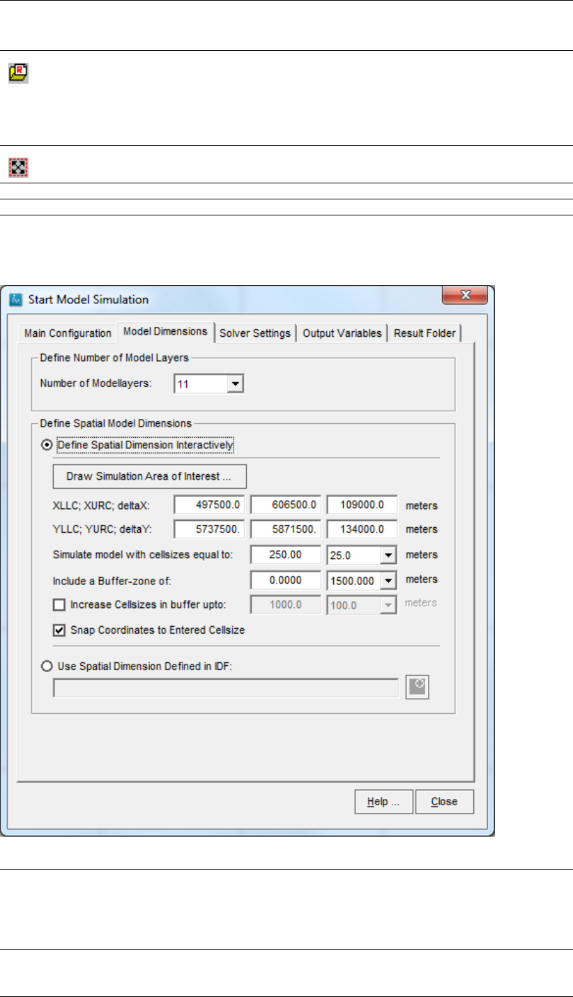
DRAFT
Toolbox Menu Options
Project Manager
Click this button to display the Project Manager (section 5.5) and read in the
selected runfile. This might be handy as different runfiles can be generated
from the Project Manager as well as steering a runfile from the iMOD Batch
Function RUNFILE (section 8.6.5) is more efficient for simulations that need
to be carried repeatedly.
ZoomFull
Click this icon to zoom to the entire extent of the model.
Help . . . Click this button to start the HELP functionality.
Close Click this button to close the Start Model Simulation window.
Start Model Simulation window, Model Dimensions tab:
Number of Model-
layers
Select the number of modellayers to be used in the current model simulation.
Whenever the Number of Modellayers is less than the MXNLAY variable in the
run-file, iMOD will display a message at the right of the dropdown menu, indi-
cating that the boundary condition of the lowest modellayer will be a Constant
Head boundary condition.
Define Spatial Di-
mensions Interac-
tively
Select this option to determine the dimension and size of the rastercells (com-
putational nodes) interactively.
Deltares 329 of 812
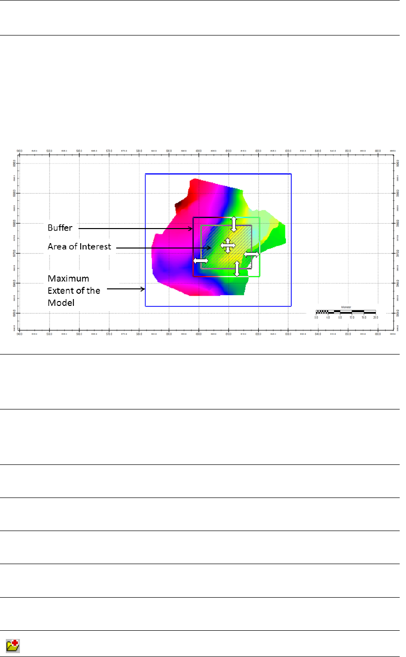
DRAFT
iMOD, User Manual
Draw Simulation
Area of Interest
Click this button to start drawing a rectangle on the graphical display to indi-
cate the location of the simulation area (hatched area). Use your left-mouse
button to position the first points of the rectangle, use the left/right-mouse
button to identify the opposite border. Whenever you move the mouse cur-
sor inside the hatched area, a cross-arrow appears indicating that the entire
hatched area can be moved while clicking the left-mouse button. Similar the
borders can be moved whenever the horizontal/vertical arrows appear.
Example of a model extent after drawn interactively on the graphical display:
XULC,XURC,
DeltaX
Enter the X-coordinate for the lower-left-corner (XULC) and the upper-right-
corner (XURC). The difference between them will be computed automatically
(DeltaX). All variables need to be entered in meters, moreover, they will be
filled in automatically whenever the simulation area is adjusted interactively
on the graphical display.
YULC,YURC,
DeltaY
Enter the Y-coordinate for the lower-left-corner (YULC) and the upper-right-
corner (YURC). The difference between them will be computed automatically
(DeltaY). All variables need to be entered in meters, moreover, they will be
filled in automatically whenever the simulation area is adjusted interactively
on the graphical display.
Simulate model
with cellsizes
equal to
Select one of the cellsize from the dropdown menu or enter a value in the
input field next to it.
Include a Buffer-
zone of:
Select one of the buffersizes from the dropdown menu or enter a value in the
input field next to it. The Buffer-zone is an extra “ring” of modelcells around
the chosen simulation area and indicated by a green rectangle.
Increase Cellsize
in buffer upto:
Select this option to increase the cellsizes in the Buffer-zone upto a cellsize
that can be selected from the dropdown menu or entered in the input field next
to it.
Snap Coordinates
to Entered Cell-
size
Select this option to snap the coordinates of the model domain to the entered
cellsizes. In this manner, the coordinates of the model will have ”nice-and-
round” coordinates.
Use Spatial
Dimensions
Defined in IDF:
Select this option whenever an (ir)regular network needs to be used that is
described in the header information of an IDF that can be entered in the cor-
responding input field.
Open IDF
Select this button to select an IDF-file from the system.
330 of 812 Deltares
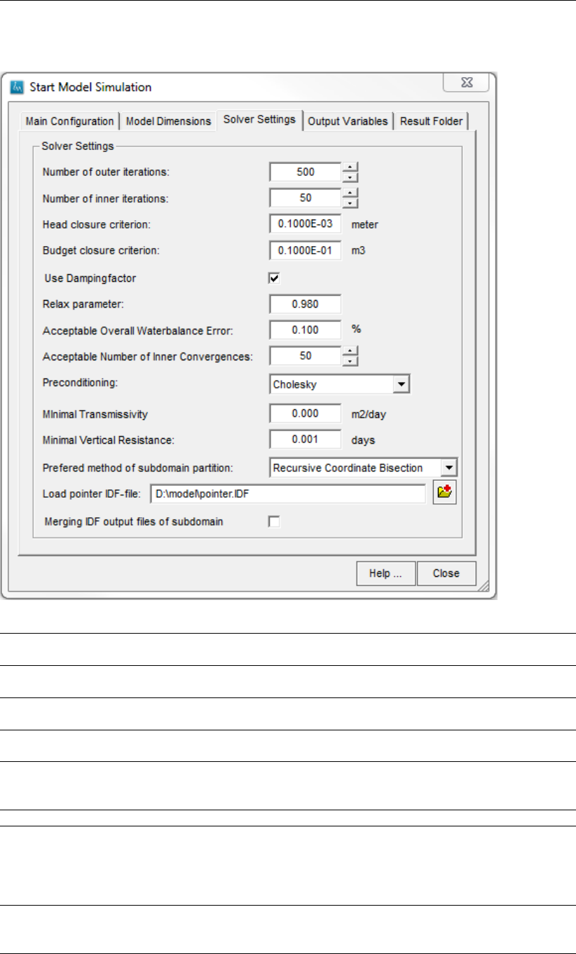
DRAFT
Toolbox Menu Options
Start Model Simulation window, Solver Settings tab:
Number of outer
iterations:
Enter the maximum number of outer iterations.
Number of inner
iterations:
Enter the maximum number of inner iterations.
Head closure
criterion:
Enter the maximum head residual in meters.
Budget closure
criterion:
Enter the maximum budget residual in cubic meters.
Use
Dampingfactor
Check this option to include adaptive damping. The relaxation factor (RELAX)
will be adjusted according to Cooley’s method with Huyakorn’s modification.
This will increase convergence for a nonlinear model.
Relax parameter: Enter the relaxation parameter (0.0 <relax <1.0)
Acceptable
Overall
Waterbalance
Error
Enter the overall acceptable waterbalance error in percentage of the water-
balance error (Qin-Qout) divided by the mean of the absolute total of both:
0.5*(Qin+Qout). Whenever the simulation can not find a solution within the
number of outer *inner iterations, it can still continue whenever it meets the
Acceptable Overall Waterbalance Error.
Acceptable
Number of Inner
Convergences
Enter the number of sequential inner convergences that forces the solver to
stop further iteration. The simulation will continue whenever the result passes
the Acceptable Overall Waterbalance Error too.
Deltares 331 of 812
DRAFT
iMOD, User Manual
Preconditioning: Choose the preferred pre-conditioning method (only possible when using the
PCG-solver):
1. Modified Incomplete Cholesky (for use on scalar computers),
2. Polynomial matrix conditioning method (for use on vector computers or to
conserve computer memory).
If the Preconditioning Method is set to Cholesky, the Relaxation parameter
can be set. Although the default is 1, in some cases a value of 0.97-0.99 may
reduce the number of iterations required for convergence.
Minimal
Transmissivity:
Enter a value for the minimal transmissivity that may occur in the model. In
case a grid value is found below this threshold this will be corrected before the
modelsimulation is started.
Minimal Vertical
Resistance:
Enter a value for the minimal vertical resisitance that may occur in the model.
In case a grid value is found below this threshold this will be corrected before
the modelsimulation is started
Preferred method
of subdomain
partition:
Choose the preferred subdomain partition option. There are two methods
supported:
1. Uniform subdomain partitioning (default) for uniform partitioning in lateral x
and y-direction,
2. Recursive Coordinate Bisection (RCB) subdomain partitioning that com-
putes the subdomain dimensions according to be specified pointer IDF grid
(selecting a pointer IDF-file is required with this option).
By selecting None the PKS package will not be used during the simulation.
Note: Each subdomain always includes all model layers.
Load pointer
IDF-file:
In case hte RCB option is chosen, the filename of the needed pointer IDF grid
needs to be filled in here.
Open
Click this button to find and select an IDF-file with the needed PKS pointer
information.
Merging IDF
output files
of subdomain
Check this option if merging of parallel subdomain IDF output files is needed
(see for more information section 10.6). Note: Enabling this option could slow
down overall parallel computations.
Note: Consult scientific literature regarding the Solver Settings as described above in order to avoid
any unwise input.
332 of 812 Deltares
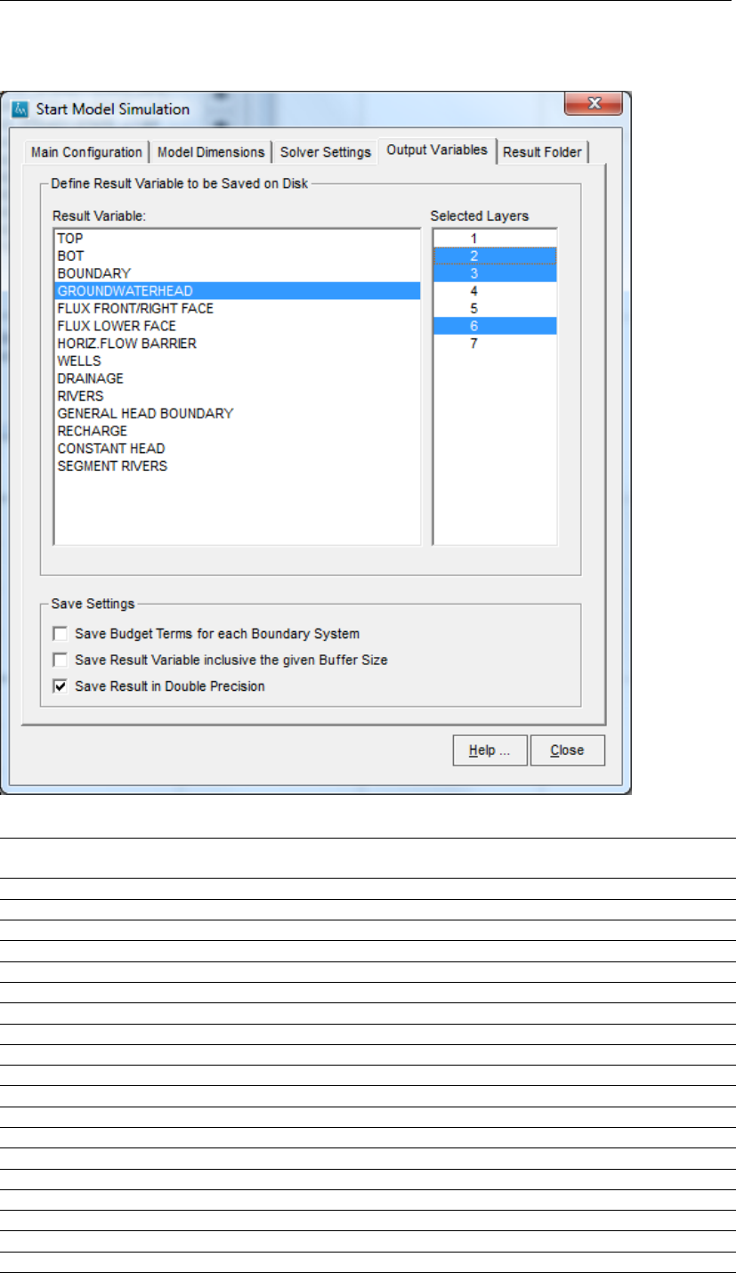
DRAFT
Toolbox Menu Options
Start Model Simulation window, Output Variables tab:
Result Variable This list will display the available output variables that are within the selected
runfile from the Main Configuration tab. Select one of the following:
File (*.idf) Variable Description
SIMGRO Flux in/out Simgro elements
bdgbnd BOUNDARY Flux in/out constant head boundaries
head GROUNDWATERHEAD Groundwater head
bdgfff/bdgfrf FLUX FRONT/RIGHT FACE Flux in/out front/right cell faces
bdgflf FLUX LOWER FACE Flux in/out bottom cell face
bdgsto STORAGE Flux in/out storage
PURGED WATER TABLE Absent
ANISOTROPY Absent
HORIZ.FLOW BARRIER Absent
TOP Absent
BOT Absent
CONCENTRATION Absent
HORIZ.K VALUE Absent
VERT.K VALUE Absent
bdgwel WELLS Flux in/out well systems
bdgdrn DRAINAGE Flux out drainage systems
bdgriv RIVERS Flux in/out river systems
bdgevt EVAPOTRANSPIRATION Flux out evapotranspiration
Deltares 333 of 812
DRAFT
iMOD, User Manual
bdgghb GENERAL HEAD BOUND-
ARY
Flux in/out general head boundaries
bdgrch RECHARGE Flux in recharge
bdgolf OVERLAND FLOW Flux out overland flow
bdgbnd CONSTANT HEAD Flux in/out constant head boundaries (identical to
BOUNDARY)
bdgisg SEGMENT RIVERS Flux in/out river systems
bdgibs INTERBED STORAGE Flux in/out interbeds
Selected
Layers
Select the modellayers for which the current selected variable need to be saved.
The number of modellayers to choose from is determined by the Number of
Modellayers selected in the Model Dimensions tab.
SaveBudget
Terms for each
Boundary
System
Select this item to save budget terms for each of the defined sub-systems
in the selected runfile. Each subsystem will be added to the filename, e.g.
bdgriv_steady-state_l1_sys1.idf.
Saved Result
Variable inclu-
sive the given
Buffer Size
Select this item to save the results within the specified buffer size entered in the
Include a Buffer-zone of field on the Model Dimensions tab.
Save Results
in Double
Precision
Select this option to save all results in double precision accuracy instead of single
precision (which is the default). Bear in mind that all files will be doubled in size
as well as the option for double precision is selected. Also, result files saved in
double precision cannot be read in iMOD version older than v3.4.
334 of 812 Deltares
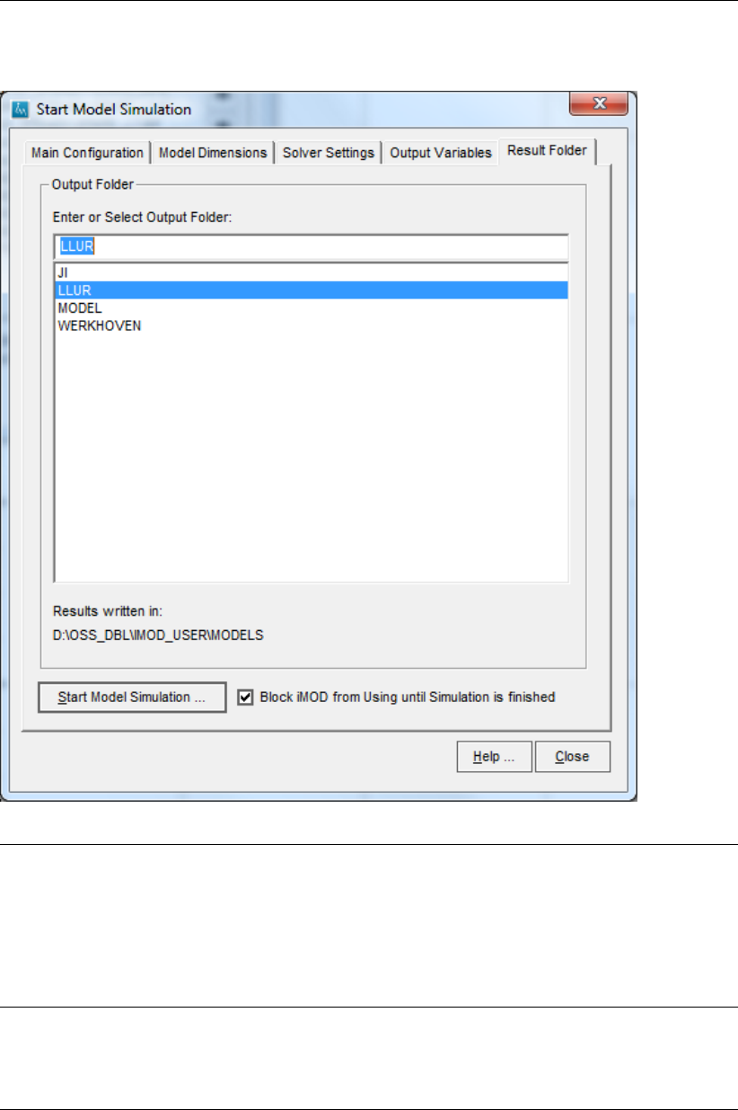
DRAFT
Toolbox Menu Options
Start Model Simulation window, Result Folder tab:
Enter or Select
Output Folder
The selected variables, as specified in the Output Variables tab, will be saved
in the folder entered/selected here. Each variable will be saved within a sep-
arate folder, e.g. {outputfolder}\bdgrch\bdgrch_steady-state_l1.idf. Whenever
NO scenario is included on the Main Configuration tab, the results will be
saved in the {user}\models folder. Otherwise, in case a scenario is included,
the results will be saved in {user}\scenarios\{scenarioname}. In this latter
case, the output folder is determined by the selected scenario and can not
be changed.
Start Model
Simulation . . .
Click this button to start a model simulation. iMOD will ask you to confirm,
before the actual simulation starts. Whenever the model dimensions (number
of rows * columns * modellayers) is more than 30.000.000 nodes, this button
will be inactivated, since a normal 32-bits operating system can not carry out
simulations with higher dimensions.
Deltares 335 of 812

DRAFT
iMOD, User Manual
7.10 Quick Scan Tool
WHY?
The effects of changes in hydrogeological conditions in an area can be visualized once a groundwater
model has been created. This can be done by changing the model input (as described in section 7.9)
or by using scenarios (currently not available!). However much run time may be needed in case of
complicated large groundwater models while many variations of the model input are required to select
the desired changes in the model input. The Quick Scan Tool is designed to reduce significantly this
run time. The Quick Scan Tool will provide an approximated result indicating the effect of the model
variation and enabling to choose the desired model input. After selecting the model input a single final
model run is needed to obtain the detailed model output.
WHAT?
The Quick Scan Tool works with a database (the Quick Scan database or QS-database, in previous
iMOD versions called the Impulse-Response database or IR-database) which contains the model out-
put of many model runs made by varying combinations of model input. The result of a change in model
input can be presented very quickly just by querying this QS-database.
7.10.1 Initial Settings
The Quick Scan Tool needs an input file (*.INI) with initial settings. The input file is defined in the *.PRF
file using the keyword QSTOOL (not yet implemented) or IRDBASE.
The Quick Scan Tool input file (*.INI) needs to contain the following parameters:
NIDF Number of IDF-files used as reference file.
IDFNAME# Name used in the QS Tool for IDF number #
IDFFILE# Name of the IDF file used as IDF number #
RESDIR Name of the folder with the results of the QS Tool
NIR Number of QS databases used in the QS Tool
DIRIR# Name of the folder with QS database number #
NAMEIR# Name used in the QS Tool for QS database number #
IMPIR# Name of the Impulse used in the QS database
MINIR# Minimal impulse value
MAXIR# Maximal impulse value
IDFIR# IDF with the link to the REFIR#
REFIR# Name of the file linking the IDFIR# value with the Response data
7.10.2 Start Quick Scan Tool
HOW?
Select the Toolbox option from the main menu and then choose Quick Scan Tool to start the Quick
Scan Tool window.
336 of 812 Deltares
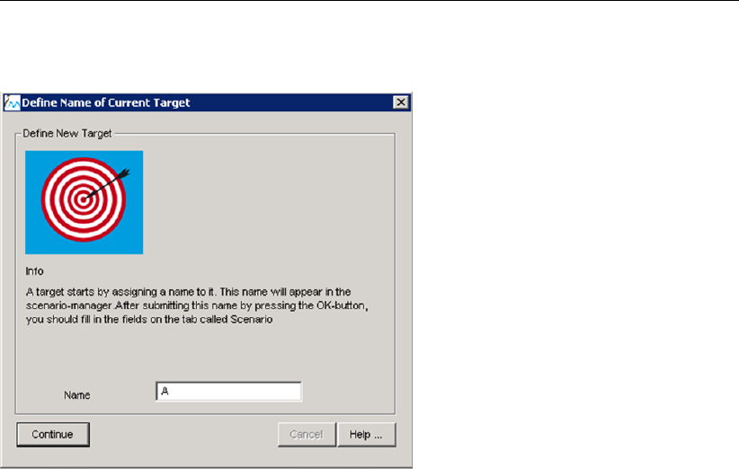
DRAFT
Toolbox Menu Options
Define Name of Current Target window:
Enter a name for the target and click the Continue button. The Quick Scan Tool window will appear
with the name of the target in the Project Overview list.
The Project Overview list contains all defined Targets (T),Measures (M) and Results (R).
The Active Polygons list contains all defined polygons. The targets and measures are defined in the
tabs in the bottom half of the window by defining the area and the target or measure values.
Deltares 337 of 812
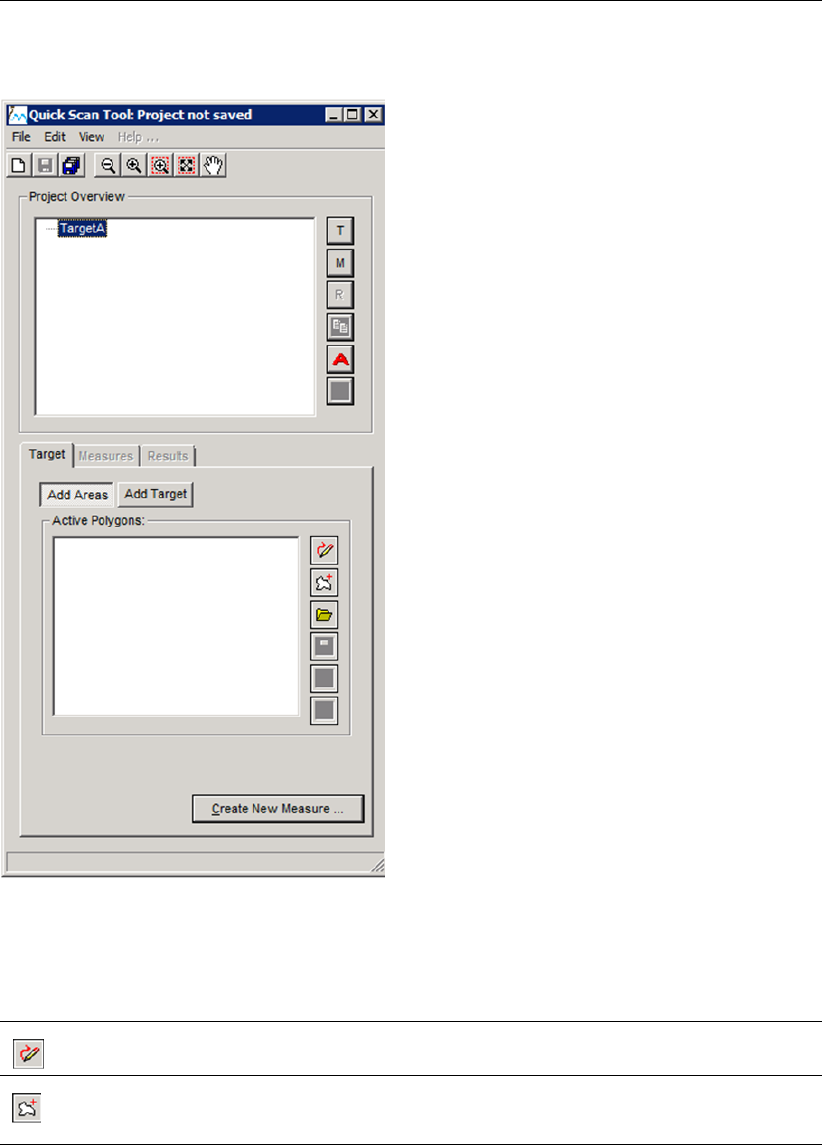
DRAFT
iMOD, User Manual
Quick Scan Tool window:
A target (Target tab) and a measure (Measure tab) is defined by:
Click on the Add Areas button:
Draw
Draw a polygon to define the area where the target/measure is valid.
Select
Select a surface water level area from the map with surface water level areas. This map is
shown in the background.
Click on the Add Target orAdd Measure button: a target/measure is linked to the area defined. Infor-
mation on the targets/measures linked to a polygon is shown in the bottom half of the Quick Scan Tool
window when selecting the polygon on the map.
338 of 812 Deltares
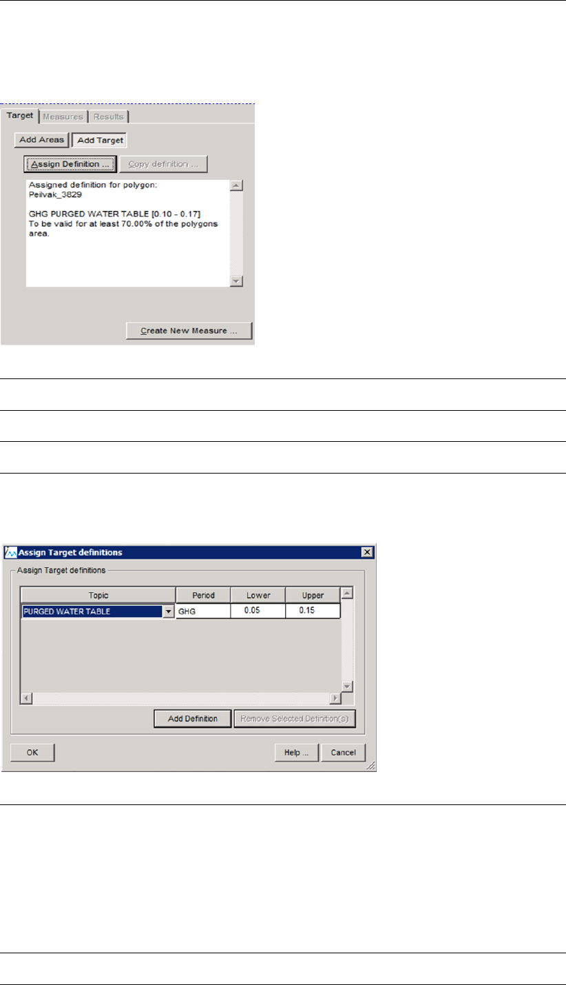
DRAFT
Toolbox Menu Options
Quick Scan Tool window, bottom half for selected polygon:
for Targets tab:
Assign Definition Click on the Assign Definition button to add the target definition. The Assign
Target Definition window appears.
Copy Definition Click on the Copy Definition button to copy target definitions from one polygon
to other polygons.
Create New
Measure
Click on the Create New Measure button to make a new measure definition
linked to the target.
Assign Target Definition window:
Topic List of variables for which a target may be defined:
Purged water table: level of the purged groundwater above the confining
layer;
Groundwater table: level of the groundwater under the confining layer;
Seepage fluxes: seepage-/infiltration flux from modellayer 1 to modellayer
2;
River fluxes: recharge/discharge of surface water;
Drainage fluxes: discharge by drainage tubes and ditches.
Period Period or condition for which the target is valid: GHG (average highest ground-
water level) or GLG (average lowest groundwater level)
Deltares 339 of 812
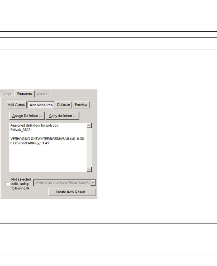
DRAFT
iMOD, User Manual
Lower Lower limit of the target
Upper Upper limit of the target
Add Definition Add target definition to the list of targets
Remove Selected
Definition(s)
Remove the selected target definitions from the list of targets
Quick Scan Tool window, bottom half for selected polygon:
for Measures tab, Add Measures button:
Assign Definition Click on the Assign Definition button to add the measure definition. The As-
sign Measure Definition window appears.
Copy Definition Click on the Copy Definition button to copy measure definitions from one poly-
gon to other polygons.
Plot selected cells,
using following IR
Check the box to show the QS(=IR) units (model cell clusters) for which the
effects of measures are calculated. The measure should be selected in the
listbox because each measure may be linked to different units.
Create New
Result
Click on the Create New Result button to save the set of measures to a result.
340 of 812 Deltares
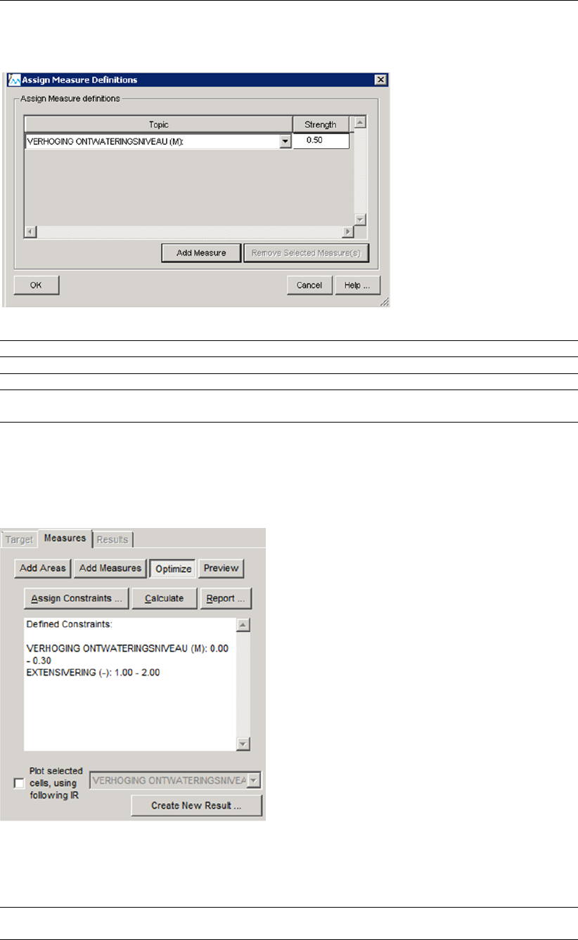
DRAFT
Toolbox Menu Options
Assign Measure Definition window:
Topic Name of the measure
Strength Strength of the measure
Add Measure Add measure definition to the list of measures
Remove Selected
Measure(s)
Remove the selected measure definitions from the list of measure
Quick Scan Tool window, bottom half for selected polygon:
for Measures tab, Optimize button:
The Optimize function gives the opportunity to search in the QS-database for the optimal set of mea-
sures. These are the measures which give the desired result with the minimum number of measures.
Assign
Constraints
Click on the Assign Constraints button to open the Assign Constraints window.
Deltares 341 of 812
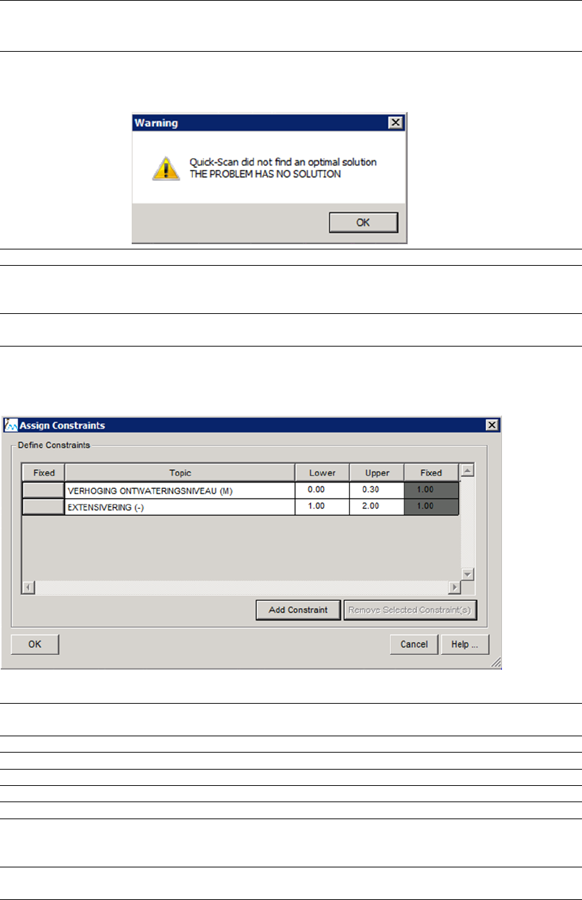
DRAFT
iMOD, User Manual
Calculate Click on the Calculate button to search for the optimal set of measures using
the assigned constraints. A report (see below) is generated in case the QS-
database finds a solution. A warning is shown in case the QS-database is not
able to find a solution.
Report Show the report generated by the Calculate function
Plot selected cells,
using following IR
Check the box to show the QS(=IR) units (model cell clusters) for which the
effects of measures are calculated. The measure should be selected in the
listbox because each measure may be linked to different units.
Create New
Result
Click on theCreate New Result buttonto save the set of measures to a result.
Assign Constraints window:
Fixed Click on the button to set a fixed constraint. The value of the measure is fixed
and can not be changed.
Topic Name of the measure
Lower Lower limit of the constraint
Upper Upper limit of the constraint
Fixed Fixed value of the constraint (usable when button on first column is clicked)
Add Constraint Click on the Add Constraint button to add a constraint to the list of measures.
Remove
Selected
Constraint(s)
Remove the selected constraints from the list of constraints
OK The constraint values are checked to be within the limits of the QS-database
and the window closes.
342 of 812 Deltares
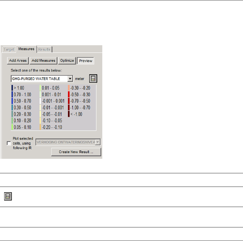
DRAFT
Toolbox Menu Options
Quick Scan Tool window, bottom half for selected polygon:
for Measures tab, Preview button:
Select one of the
results below:
Select the result from the list box. The effect of the measure is shown for the
area selected under Add Areas.
Show the result
Click on the button to show the result on the map.
The legend is shown below the list box.
Plot selected cells,
using following IR
Check the box to show the QS(=IR) units (model cell clusters) for which the
effects of measures are calculated. The measure should be selected in the
listbox because each measure may be linked to different units.
Create New
Result
Click on theCreate New Result buttonto save the set of measures to a result.
Deltares 343 of 812
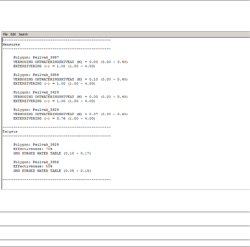
DRAFT
iMOD, User Manual
Example of report generated by Calculate on the Measures tab, Optimize button:
Measures The proposed measures are listed by polygon. The constraints are shown
between brackets.
Targets The desired targets are listed by polygon. The upper and lower limits of the
target are shown between brackets.
Exit The report can be closed with the Window Close button or by [File / Exit].
344 of 812 Deltares
DRAFT
Toolbox Menu Options
7.11 Pumping Tool
Note: The update of this functionality is still in progress.
WHY?
iMOD offers the possibility to manipulate existing model features, such as well strength, waterlevels,
etc., by means of the functionalities offered by the scenario definitions. However, the scenario defini-
tions are limited to existing features and new elements can not be added easily without changing the
runfile manually. The Pumping Tool can be applied to configure new elements to an existing model
configuration (runfile) and simulate and analyse the results easily. The Pumping Tool is developed
specifically to simulate the effect of pumping, Aquifer-Storage-Recovery systems and/or Thermal-Heat-
Storage systems.
WHAT?
Any pumping system can be outlined by defining its location, vertical screen depths and corresponding
well abstraction rates. The Pumping Tool includes these properties to any existing model configuration
(runfile) prior to the simulation. The Pumping Tool allocates the well strength to the appropriate model-
layer(s) and extends the model simulation time to include the given well regime. After the simulation
the Pumping Tool offers a quick tool to analyse the results.
7.11.1 Initial Settings
The Pumping Tool needs an input file (*.INI) with initial settings. These settings are needed by
the Pumping Tool to incorporate and allocate the well systems to the runfile(s). In the preference
file the keyword SCENTOOL needs to be included that directs to that file, e.g. SCENTOOL {install-
folder}\SCENTOOL.INI. The file SCENTOOL.INI needs to contain the following parameters:
NSCNCONF Number of Scenario Configurations. This will indicate the number of runfiles
that will be used to incorporate the well systems, e.g. NSCNCONF=2
RUNFNAME{i} For each of the NSCNCONF runfiles specify the full filename of the runfile,
e.g. RUNFNAME1=c:\scentool\scen_summer.run
RUNNAME{i} For each of the NSCNCONF runfiles specify an alias for the runfile as de-
scribed by RUNFNAME{i}, e.g. RUNNAME1=’Mean Summer Situation’. This
alias will be displayed in the Pumping Tool.
NLAY Specify the number of modellayers of the model configurations specified by
RUNFNAME{i}, e.g. NLAY=8.
TOP{i} Specify an IDF-file that represents the top elevation of the ith modellayer, e.g.
TOP1=c:\scentool\idf\top1.idf.
BOT{i} Specify an IDF-file that represents the bottom elevation of the ith modellayer,
e.g. BOT1=c:\scentool\idf\bot1.idf.
KD{i} Specify an IDF-file that represents the transmissivity (kD) of the ith modellayer,
e.g. KD1=c:\scentool\idf\kd1.idf.
MAXNWEL* Specify the maximum number of Well Systems in one configuration, e.g.
MAXNWEL=20 (default value=10).
MAXNCUT* Specify the maximum number of Cut-Out Areas in one configuration, e.g.
MAXNCUT=20 (default value=10).
MAXNOBS* Specify the maximum number of Observation Wells in one configuration, e.g.
MAXNOBS=20 (default value=10).
MAXNMON* Specify the maximum number of Monitoring Wells in one configuration, e.g.
MAXNMON=20 (default value=10).
MAXNRES* Specify the maximum number of results in one configuration, e.g. MAXN-
RES=20 (default value=10).
* optional
Example of Pumping Tool SCENTOOL.INI file:
Deltares 345 of 812
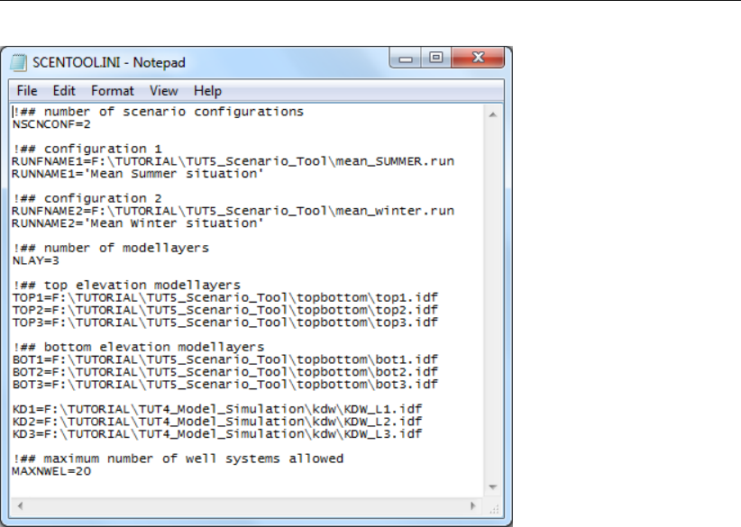
DRAFT
iMOD, User Manual
7.11.2 Start Pumping Tool
HOW?
Select the Toolbox option from the main menu and then choose Pumping Tool to start the Pumping
Tool window.
The Pumping Tool window manages the scenario configuration which is saved in the iMOD Scenario
File (*.ISF).
The Pumping Tool window has five tabs:
Well Systems: to define the locations of the wells and the extraction rates
Cut-Out Areas: to define the location of the cut-out or excavation areas
Observation Wells: to define the locations of observation screens and the observed groundwater
heads
Monitoring Wells: to define the location of existing monitoring wells with groundwater head time-
series
Results: to define the model simulation configuration and to start the model calculation
346 of 812 Deltares
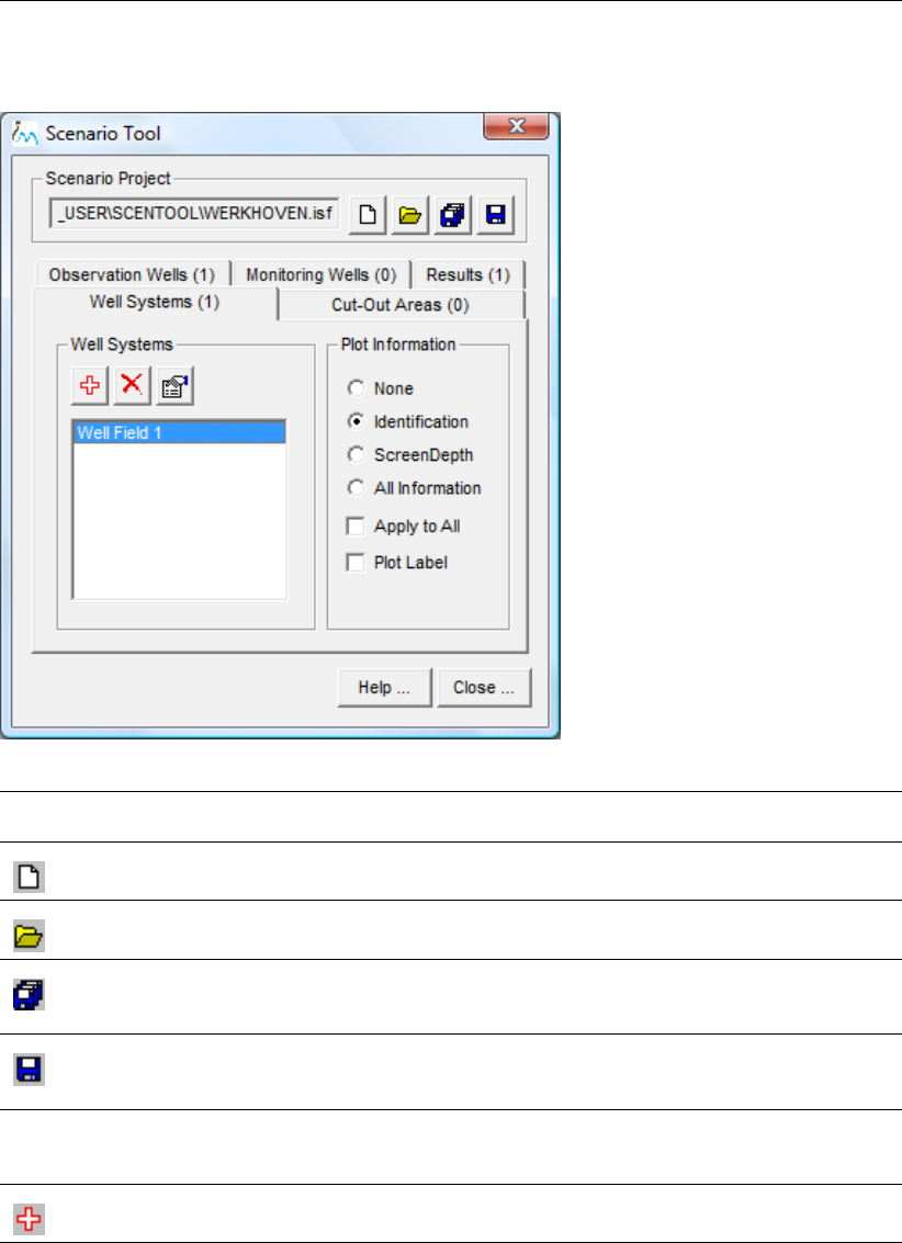
DRAFT
Toolbox Menu Options
Pumping Tool window, Well Systems (..) tab:
Scenario Project This displays the iMOD Scenario File (*.ISF) under which the current configu-
ration is saved.
New
Click this button to start a new/empty scenario configuration.
Open
Click this button to open an existing iMOD Scenario File (*.ISF).
Save As
Click this button to save the current scenario configuration to a new iMOD
Scenario File (*.ISF).
Save
Click this button to save the current scenario configuration to the current iMOD
Scenario File (*.ISF).
Well Systems Click one of the well systems in the list to activate the Delete and Proper-
ties buttons. The Plot Information setting will be applied to the selected well
system too.
Add
Click this button to add a new well system.
Deltares 347 of 812
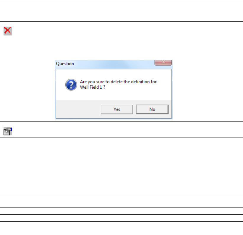
DRAFT
iMOD, User Manual
Delete
Click this button to remove the selected well system from the scenario
configuration.
Question window:
Properties
Click this button to adjust the parameters for the selected well system.
Plot Information Select one of the following options to specify the method to display information
for the individual pumping locations for the selected well system (see below).
None only the specified symbol will be drawn. The symbol can be changed
in the Display tab of the Well Systems window, see section 7.11.3.
Identification: displays the identifications;
Screendepth: displays all screen depths;
All Information: displays all information available.
Apply to All Select this option to apply the display settings to all available well systems at
once.
Plot Label Select this option to add the labels to the different parameters.
Help ... Click this button to start the Help functionality.
Close ... Click this button to stop the Pumping Tool. You will be asked to save your work
before the Pumping Tool need to be closed.
348 of 812 Deltares
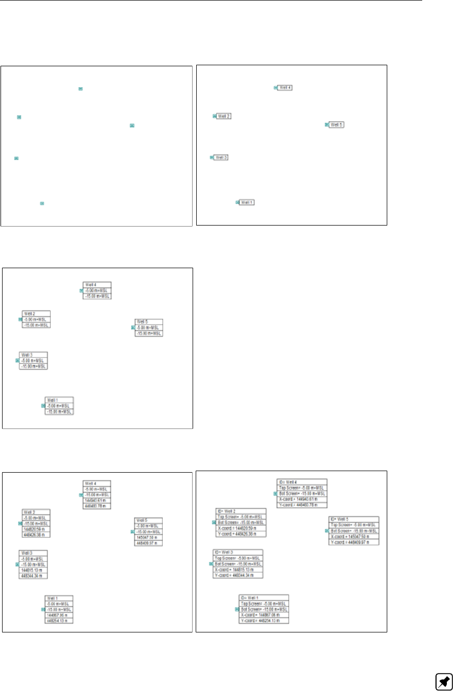
DRAFT
Toolbox Menu Options
Example of the Plot Information: (1) None, (2) Identification, (3) ScreenDepth, (4) All Information
without and (5) with labels
(1) (2)
(3)
(4) (5)
Note: All other iMOD functionalities remain active whenever the Pumping Tool is loaded. This means
that map operations can be carried out, legends can be changed, but the Profile Tool (see section 7.1)
and/or 3D Tool can not be used without leaving the Pumping Tool.
Deltares 349 of 812
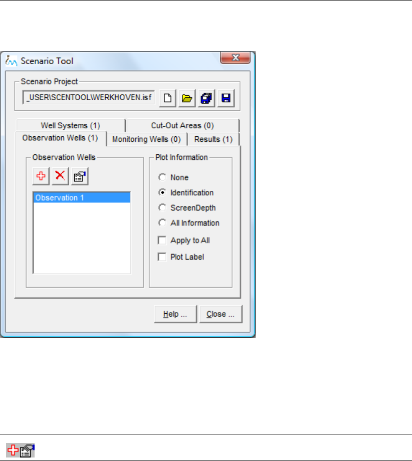
DRAFT
iMOD, User Manual
Pumping Tool window, Observation Wells (..) tab:
The observation wells are used to define screens where the calculated groundwater head can be
compared with the observed groundwater head.
All functionalities of the Observation Wells tab behave similar to those described for the Wells Systems
tab and for the Wells Systems window.
Add/Adjust
Click these buttons to add/adjust a new/existing observation well, see section 7.11.4.
350 of 812 Deltares
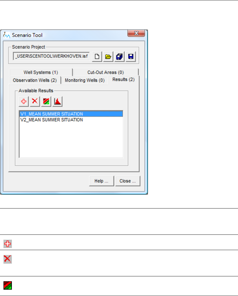
DRAFT
Toolbox Menu Options
Pumping Tool window, Results (..) tab:
Available
Results
Display of all available result folders in the scenario project
folder, e.g. folder C:\..\USER\SCENTOOL\WERKHOVEN\* for the
C:\..\USER\SCENTOOL\WERKHOVEN.ISF file. The list will be refreshed whenever
the tab is toggled with other tabs on the Pumping Tool window.
Add
Click this button to start a new simulation.
Delete
Click this button to delete the selected result in the Available Results list. You will be
asked to confirm this action, since all files for the selected result will be deleted from
disk.
Contour
Click this button to start the Quick Open window and specify the results that need to
be displayed.
Deltares 351 of 812
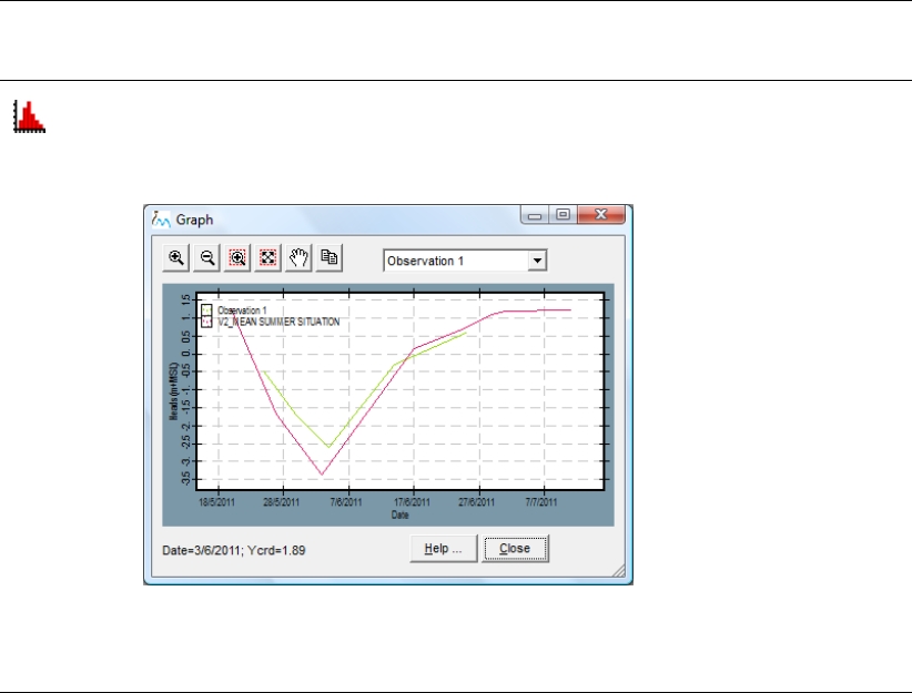
DRAFT
iMOD, User Manual
Graph
Click this button to display the selected result in combination with observation wells.
Therefore, this button is only available whenever Observation Wells are defined.
Graph window:
See section 6.6.1 for more information on the use of the available functions of
this window. In this graph window a drop-down menu is added. The graph is updated
whenever another item (Observation Well) is selected from the dropdown menu.
7.11.3 Well Systems
Select the Add or Properties button on the Well Systems tab on the Pumping Tool window, to display
the Well Systems window.
352 of 812 Deltares
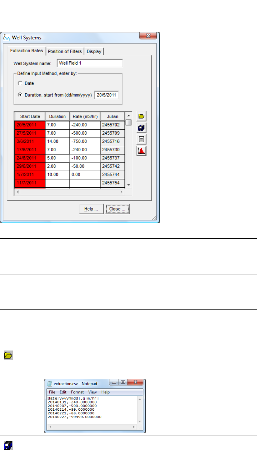
DRAFT
Toolbox Menu Options
Wells Systems window, Extraction Rates tab:
Well System
name
Enter the name of the well system, maximum 24 characters.
Date Select this option to enter the extraction rates by their (start)date, the Start Date
column in the table will become enabled to enter values. The values within the
Duration column will be computed, automatically.
Duration,
start from
(dd/mm/yyyy)
Select this option to enter the extraction rates by specifying an initial date, e.g.
20/5/2011. The column Duration becomes enabled to enter the duration for each
extraction rate, e.g. 7.0, 7.0, 14.0 and 7.0 days. The date within the Start Date
column will be computed automatically whenever the Calculate button is clicked or
when closing the window.
Table Each row in the table expresses an extraction rate for the entire well system. The
red coloured column can not be edited and is computed whenever the Calculate
button is clicked. Enter the extraction rates (strength) in the third column in m3/hr
(during the actual modeling, those values will be translated on the background into
m3/day). The last column (Julian) is not editable and is use by iMOD internally.
Open
Click this button to open a plain text file that contains date and extraction rates.
Example of a text file with extraction data
Save As
Click this button to save a plain text file that contains date and extraction rates.
Deltares 353 of 812
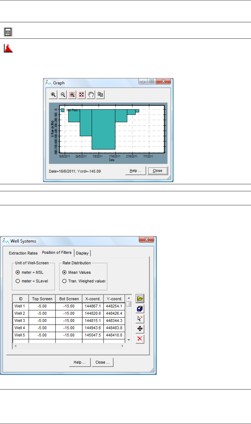
DRAFT
iMOD, User Manual
Calculate
Click this button to compute the Start Date or Duration column in the table.
Graph
Click this button to display a bar diagram of the extraction rates (see section 6.6.1
for more information on the use of the available functions of this window).
Graph window:
Help . . . Click this button to start the Help functionality.
Close . . . Click this button to close the Well Systems window. You will be asked to save any
adjustments or you can cancel closure.
Well Systems window, Position of Filters tab:
Unit of
Well-
Screen
Select one the following options to determine the treatment of well screens:
Meter+MSL: enter the screen depths in meter+Mean-Sea-Level (MSL)
Meter+SLevel: enter the screen depths in meter+Surface Level (SLevel). The surface
level will be extracted from the {TOP1}.idf as defined in the initialization file (SCEN-
TOOL.INI).
354 of 812 Deltares
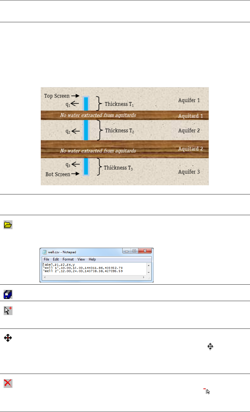
DRAFT
Toolbox Menu Options
Rate Distri-
bution
Select one of the following options to determine the distribution of extraction rates
among all individual well screens.
Mean Values: distribute the extraction rate evenly among all filter screens using the
thickness of each screen in penetrating aquifers, e.g. q1=T1/(T1+T2+T3)*Q
Tran. Weighed values: distribute the extraction rate weighed by their thicknesses of
each screen penetrating aquifers and their corresponding transmissivity values, e.g.
q1=T1*Tran1/(T1*Tran1+T2*Tran2+T3*Tran3)*Q
Extraction well (Q) and rate allocation to the different screens (q1+q2+q3):
Table Each row in the tables represents a well location and corresponding well screen
depths. It is allowed to edit the table directly (screen depths). It is recommended to
change lateral positions (the coordinates) by means of the Move option, however.
Open
Click this button to open a plain text file that contains date and extraction rates.
Example of a text file with well location and screen depth
Save As
Click this button to save a text file that contains date and extraction rates.
Add
Click this button to add a new extraction well by clicking your left mouse button at
the location of the well. Each time you click the left mouse button a new well will be
added. Click your right mouse button to stop.
Move
Click this button to move an existing well. Move your mouse cursor in the neigh-
bourhood of a well and observe that the mouse cursor changes to and the cor-
responding row in the table changes to red. Hold your left mouse button down and
move the well by moving the mouse cursor. Release the left mouse button to start
moving another well. Click your right mouse button to stop.
Delete
Click this button to delete an existing well. Move your mouse cursor in the neigh-
bourhood of a well and observe that the mouse cursor changes to and the corre-
sponding row in the table changes to red. Click your left mouse button to delete the
well. Click another well to delete it, or click your right mouse button to stop.
Deltares 355 of 812
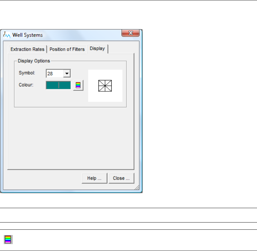
DRAFT
iMOD, User Manual
Well Systems window, Display tab:
Symbol Select a symbol number (see section 5.7 for available symbols). The current
symbol is displayed on the right.
Colour Displays the current symbol colour (dark green in this example).
Colour
Click this button to change the colour by means of the default Windows Colour
window.
7.11.4 Observation Wells
Select the Add or Properties button on the Observation Wells tab on the Pumping Tool window, to
display the Observation Wells window.
356 of 812 Deltares
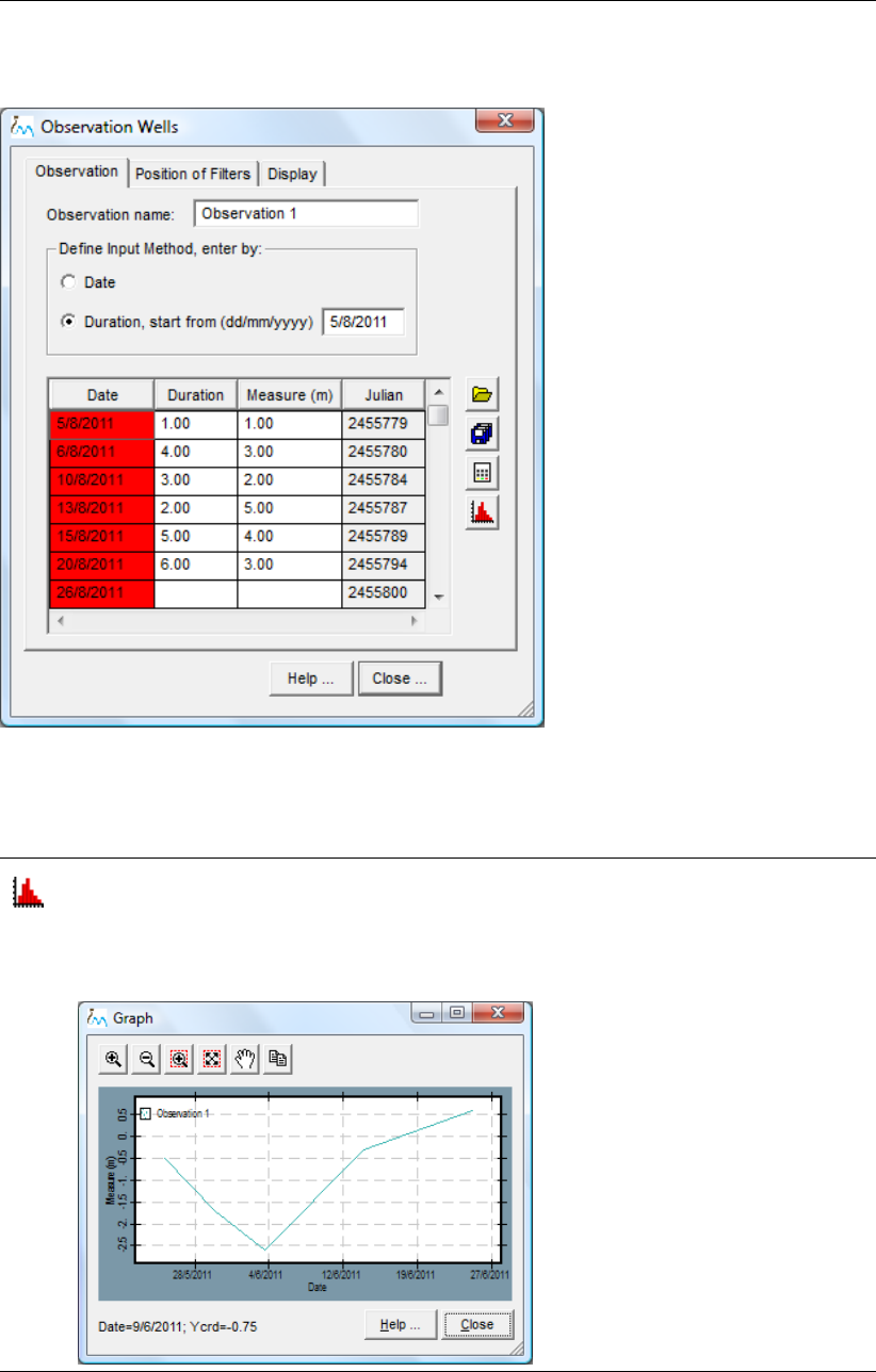
DRAFT
Toolbox Menu Options
Observation Well window, Observation tab:
All functionalities of the Observation tab behave similar to those described for the Extraction Rates tab
on the Wells Systemswindow, however, a few remarks are needed.
Graph
Click these buttons to display a graph for the observations. The graph will represent the
observations by plotting straight lines between the given dates, ignoring the last (final) date
without any given observation (26/8/2011).
Graph window:
Deltares 357 of 812
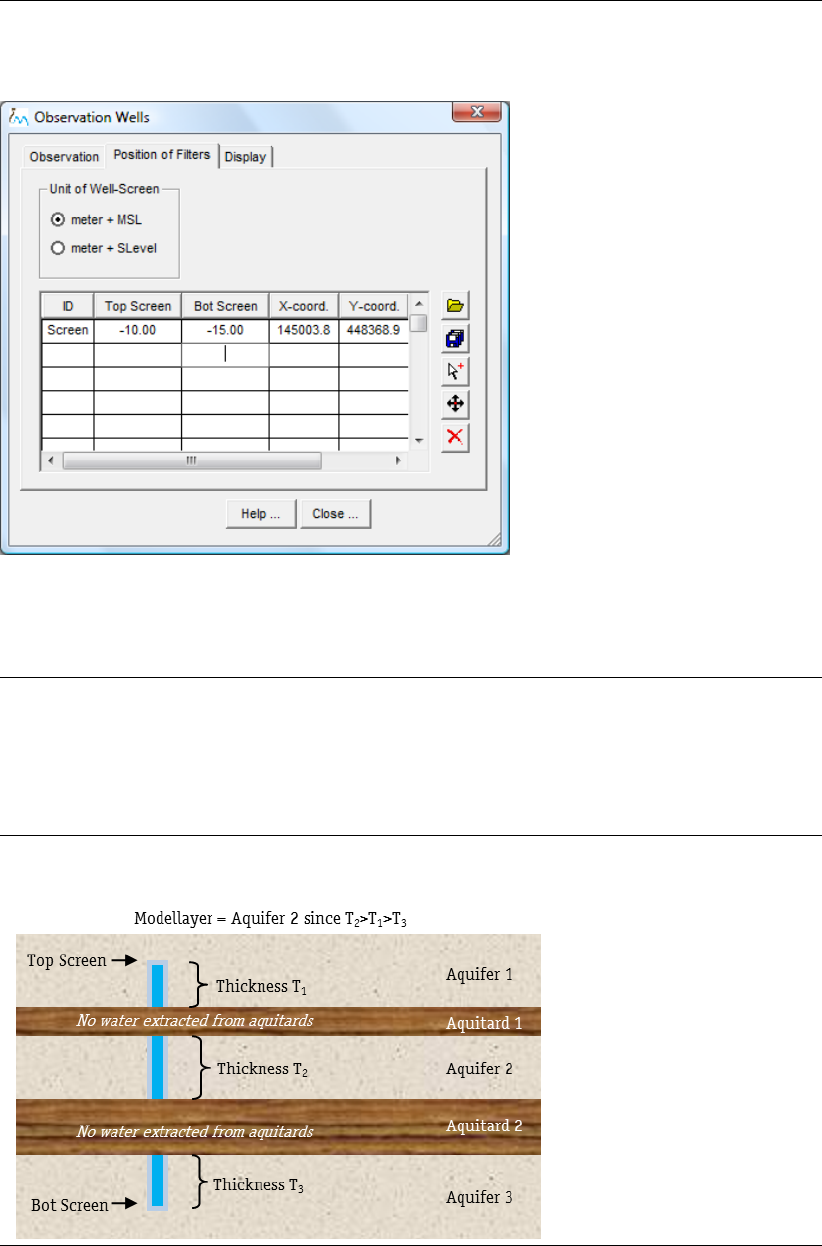
DRAFT
iMOD, User Manual
Observation Wells window, Position of Filters tab:
All functionalities of the Position of Filters tab behave similar to those described for the same tab on
the Wells Systems window, however, a few remarks are needed.
Table Each row in the table represents a single observation and corresponding well screen
depth. Only one location is sustained for each observation. It is allowed to edit
the table directly (screen depths). It is recommended to change lateral positions by
means of the Move option, however. Observed heads will be used to compare with
model results and the modellayer that will correspond to each observation depends
on the screen depths. iMOD will assign a modellayer that is occupied by the largest
part of the entire screen.
Allocation of screens of observation wells to modellayers:
Observation window, Display tab:
This window behaves and is identical to the window described before for the Wells Systems tab.
358 of 812 Deltares
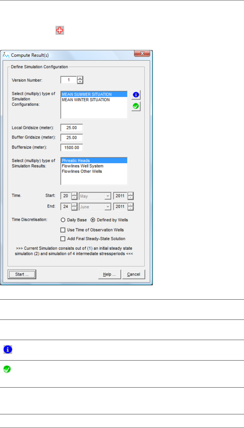
DRAFT
Toolbox Menu Options
7.11.5 Results
Select the Add button on the Results tab on the Pumping Tool window, to display the Compute
Result(s) window.
Version Number Enter a version number. The version number will be added to the re-
sult folder that is formed by the name of the model configuration, e.g.
V1_{modelconfiguration}.
Select (multiple)
type of Simulation
Configurations
Select one or more model configurations from the list. The list is reflecting the
content of the parameter RUNNAME{i} in the initialization file for the Pumping
Tool. It is an alias for the runfile described by the keyword RUNFNAME{i].
Info
Click this button to edit the ith selected runfile (RUNFNAME{i}) that is associ-
ated to the alias (RUNNAME{i}) from the list.
CheckRun
Click this button to check the content of the ith selected runfile (RUNF-
NAME{i}) that is associated to the alias (RUNNAME{i}) from the list. More
information about this kind of runfile check.
Local GridSize (m) Enter the gridsize inside the area of interest, e.g. 25.0 meter. The area of
interest will be computed automatically based on the layout of the scenario,
i.e. the lateral position of the extraction wells, cut-out areas and observation
wells.
Buffer GridSize
(m)
Enter the gridsize to be used inside the buffer defined by the Buffersize (m),
e.g. 100.0 meter.
Deltares 359 of 812
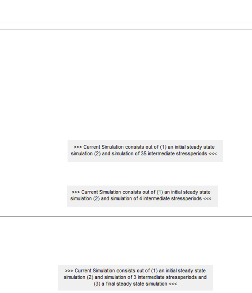
DRAFT
iMOD, User Manual
Buffersize (m) Enter the size of the buffer in meters, e.g. 1500 meter.
Select (multiple)
type of Simulation
Results
Select one or more of the supplied result options.
Phreatic Heads – choose this option to compute Phreatic Heads (and
piezometric heads as well).
Drawdown
Flowlines Well Systems
Not yet implemented
Flowlines All Wells
Not yet implemented
Time Display of the Start and End dates (not editable). These are determined auto-
matically by the entered extraction rates. The simulation duration is primarily
determined by the sequence of extraction.
Time
Discretisation
Choose out of the following:
Daily base – choose this option to simulate between the Start and End
date on a daily base. A summary is given below:
Defined by wells – choose this option to simulate between the Start and
End with stressperiod lengths that depend on the entered moment of ex-
traction. A summary is given below:
Use Time of
Observation wells
Select this option to include (extra) intermediate stressperiods to take the mo-
ment of observations into account. This ensures that any comparison be-
tween observations and computed heads are measured/computed at identi-
cal moments. Bear in mind that computational times are linearly related to the
number of stressperiods.
Add Final Steady-
state solution
Select this option to add a final stress-period that simulates a steady-state of
the last entered model input (i.e. extraction rates). A summary is given below:
360 of 812 Deltares
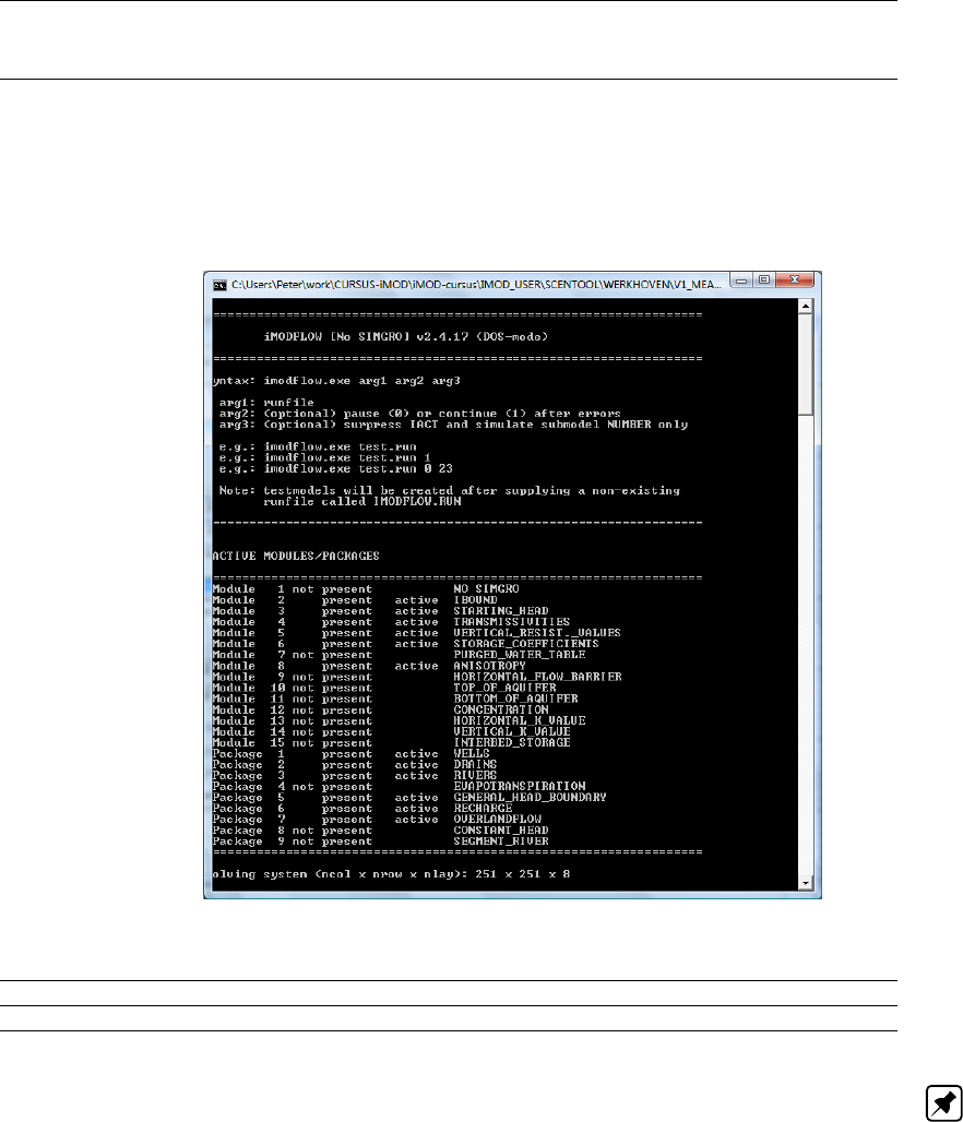
DRAFT
Toolbox Menu Options
Start . . . Click this button to start the simulation(s). You will be asked to confirm
this. iMOD will add the appropriate information regarding extraction wells
to the selected runfile(s) and start iMODFLOW as defined by the keyword
MODFLOW in the active preference file. iMODFLOW will start in a separate
commandtool window.
Scenario Simulation Command window:
After a successful simulation, both the Scenario Simulation Command
window and the Compute Results window will be closed.
Help . . . Click this button to start the Help functionality.
Cancel Click this button to cancel and close the Compute Results window.
Note: A simulation will block any use of iMOD. A simulation can be terminated by pressing the (red in
Windows Vista) closing window button on the upper-right corner of the Scenario Simulation Command
window.
Deltares 361 of 812

DRAFT
iMOD, User Manual
7.12 RO-tool
WHY?
The iMOD RO-tool is based on the ArcGIS WaterNOOD-application (“WaterNOOD”approach: “Water-
systeemgericht NOrmeren, Ontwerpen en Dimensioneren”) by Stichting Toegepast Onderzoek Water-
beheer ( STOWA).
The WaterNOOD-application provides water managers with information on hydrological requirements
of farm crops and vegetation types, and helps them to predict the effects of water management mea-
sures on crop-yields and vegetation. The application is used in the water management of nature
conservation areas and surrounding agricultural or urban areas.
The iMOD RO-tool (like the ArcGIS WaterNOOD-application) incorporates two knowledge/database/
model-based tools, that are widely used in the Netherlands to determine productivity of farm-crops and
potential for development of groundwater dependent vegetation types under various abiotic conditions
(soil type and soil-hydrology):
“HELP2005-tabellen”for calculating farm crop productivity. (see also: http://help200x.alterra.
nl/HELP2005.pdf and http://help200x.alterra.nl/)
“WATERNOOD - Hydrologische randvoorwaarden natuur”for calculating potential for development
of groundwater dependent vegetation types.(see also: http://www.synbiosys.alterra.
nl/waternood/ and
http://waterwijzer.stowa.nl/upload/publicatie2014/STOWA%202015%2022_
Webversie%20LR.pdf)
Note: Because this is a Dutch spatial planning tool, based on a Dutch policy-makers’approach for
optimizing groundwater regimes for agriculture and nature restoration, Dutch remarks are included.
WHAT?
Abiotic conditions determine productivity of farm-crops and potential for development of groundwa-
ter dependent vegetation types. The tool calculates productivity of farm-crops and potential for de-
velopment of groundwater dependent vegetation types, as a function of abiotic conditions (soil type,
seasonal groundwatertables).
Agriculture: actual crop-yield, compared to crop-yield under optimal conditions. The RO-tool
calculates the actual crop-yield (relative to crop-yield under optimal abiotic conditions) and decrease of
crop-yield due to moisture-stress (“natschade landbouw”) or respiration-stress (“droogteschade land-
bouw”), given the actual, site specific abiotic conditions (soil type, seasonal groundwatertables). De-
crease of crop-yield is calculated in % and/or Euros. doelrealisaties (= 1 –[opbrengstreductiepercent-
age t.o.v. optimale condities]/100)
Natural vegetation: potential for development of groundwater dependent vegetation types. The
RO-tool calculates the potential for development of pre-defined groundwater dependent vegetation
types. The potential is expressed as a percentage, relative to the potential for development under
optimal abiotic conditions. doelrealisaties (= 1 –[actuele ontwikkeling vegetatie/ontwikkeling vegetaties
onder optimale condities]
Urban area: suitability for urban development, as a function of groundwatertable-depth. The
RO-tool calculates the suitability for urban development, based on a range of drainage-level, defined
in a lookup-table. Groundwatertable above the upper range results in a 0% suitability for building,
groundwatertable between upper and lower range results in a 50% suitability for building, and ground-
watertable below the lower range results in a 100% suitability for building.
HOW?
The RO-tool is a post-processing scenario-tool. The user can use pre-defined maps of soil types,
landuse (crop types) and vegetation types and pre-defined tables of hydrological requirements for
vegetation and/or habitat types. All these maps and tables can also be modified by the user, to meet
special interests. Input for the hydrological conditions are the Dutch groundwater-table-depth statistics
maps (“GHG, GLG, GVG”). They are the result of a groundwate rmodel simulation. The user can run
the RO-tool for different groundwater model scenarios.
362 of 812 Deltares

DRAFT
Toolbox Menu Options
Explanation of the Dutch groundwatertable-depth statistics (“GHG, GLG, GVG”): The groundwater-
table-depth statistics (Mean Highest, Mean Lowest or Mean Spring Watertable depth). The Mean
Highest Watertable (MHW or GHG) is defined as the mean value of the three shallowest groundwa-
ter depths measured in one year (in meter beneath soil surface), averaged over a period of 8 years
with bi-weekly measurements or simulation-results. The Mean Lowest Watertable (MLW or GLG) is
defined likewise, with the deepest groundwater depths. The groundwater depths measured at three
dates nearest to April 1, are used for calculation of the Mean Spring Watertable (MSW or GVG). The
period to calculate MHW is defined between October 1st and April 1st.
Important Note: Despite the fact that the iMOD RO-tool is based on version 2 of the “Water-
NOOD”application, it is possible to implement tables with hydrological requirements for user defined
vegetation/habitat-types, created with “WaterNOOD”version 3. The tables can be created with and
exported from the “WaterNOOD”application, version 3. To download “WaterNOOD”version 3 go to:
http://www.synbiosys.alterra.nl/waternood/ and follow the instructions in the man-
ual to export the user created tables for later use in iMOD RO-tool.
Before starting the RO-tool, the desired settings need to be defined in the Preference file (see sec-
tion 9.1). The preference tab at the RO-tool window is filled with these settings. The keywords in the
preference file are linked to the required input files of the RO-tool. section 7.12.2 contains a list and
description of these files. In section 7.12.3 the operational setup of the RO-tool is explained and in
section 7.12.4 a list of output files and a short explanation can be found. To start the RO-tool win-
dow, select the Toolbox option from the main menu and then choose RO-tool from the bottom of the
menu-list.
7.12.1 RO-tool window
In this section an explanation is given about each tab on the RO-tool window. General settings on the
RO-tool window are:
Compute... Click on this button to start the scenario based map calculation with the given
settings.
Help. . . Click on this button to search for relevant information in the iMOD-manual if
the directory of the file is defined in the PRF-file (see section 9.1).
Cancel Click on this button to Quit the RO tool without saving or computing anything.
After all settings are selected the user can click on the Compute... button to start the scenario computa-
tion. Directly after starting the calculation iMOD checks continuously which input files and lookup-tables
are needed. The computation is performed per selected subtype. In case one scenario is chosen in
combination with a reference situation, iMOD creates, additionally to the reference/scenario related
result maps, a map with the difference between reference results and scenario results. Result-files are
immediately loaded in the iMOD Manager.
Deltares 363 of 812
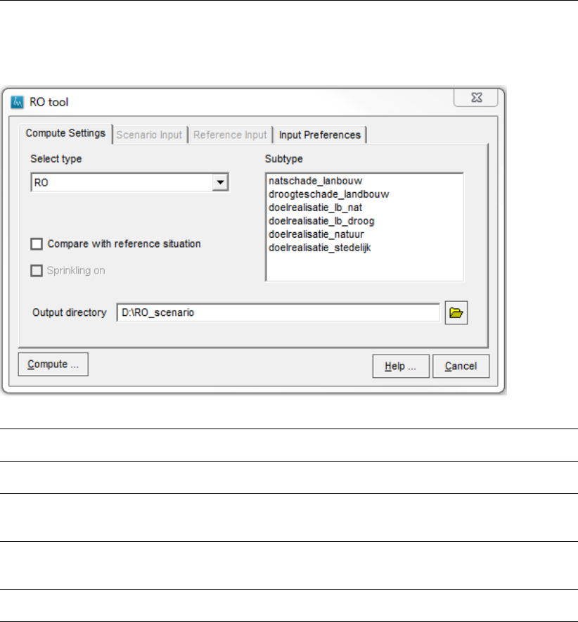
DRAFT
iMOD, User Manual
Compute Settings tab:
Select type Choose the preferred group of investigation questions. (Note: at this moment
only the RO (flood related) type is available.)
Subtype Depending on the selected type a list of scenario related subtypes appears.
Selecting 1 or more subtypes enables the Scenario Input tab.
Compare with ref-
erence situation
Check this option if it is preferred to compare the selected scenario with a
reference (or other) situation. Checking this option enables the Reference
Input tab.
Sprinkling on This option is only available in drought related scenarios. Check this
option if re-wetting through sprinkling during a period of drought is wished. By
applying this option, respiration-stress of farm crops is eliminated.
Output directory Enter the name of the output directory where iMOD stores the scenario re-
sults. Default: TMP-folder in the USER directory.
364 of 812 Deltares
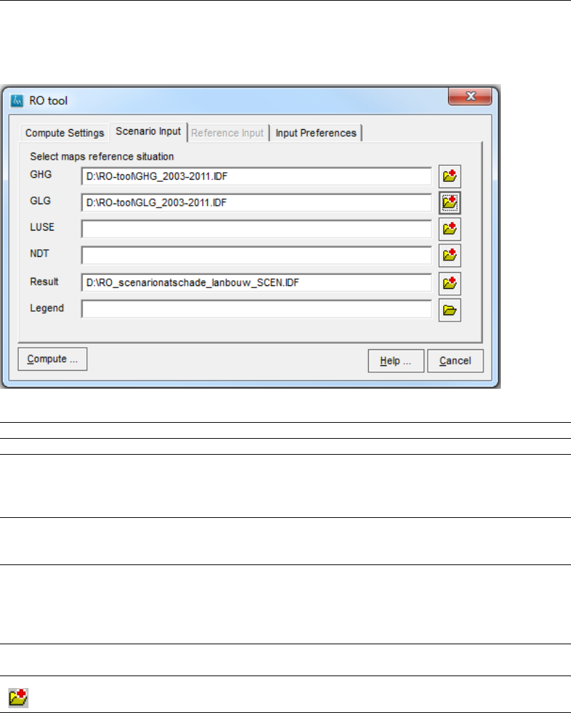
DRAFT
Toolbox Menu Options
Scenario Input tab:
GHG Enter the directory and name of the GHG-file to be used in the scenario.
GLG Enter the directory and name of the GLG-file to be used in the scenario.
LUSE (Optional) Enter the directory and name of the landuse type related file to be used in
the scenario (Note: only available if at least an Agriculture-subtype is chosen,
or a combination of Agriculture- and Nature-subtypes; not available if only a
Nature-subtype is chosen).
NDT (Optional) Enter the directory and name of the file with the vegetation
type(s),"natuurdoeltype kaart" (Note: only available if a Nature-subtype is
chosen, or in a combination with a Nature-subtype and Agriculture-subtype).
Result Enter the directory and name of the result file (Note: not available if
more than 1 subtype is selected). On default the Output Folder is se-
lected and the name of the results file equals the chosen subtype de-
scription *.idf, e.g. subtype="natschade_landbouw" the name of the file is
"natschade_landbouw_SCEN.IDF".
Legend Enter the directory and name of the legend file (Note: not available if more
than 1 subtype is selected).
Click on this button to search for the needed file.
Deltares 365 of 812
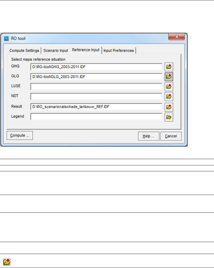
DRAFT
iMOD, User Manual
Reference Input tab:
Only available if option Compare with reference situation on tab Compute Settings is checked.
GHG Enter the directory and name of the GHG-file to be used in the scenario.
GLG Enter the directory and name of the GLG-file to be used in the scenario.
LUSE (Optional) Enter the directory and name of the landuse type related map to be used in
the scenario (Note: only available if at least an Agriculture-subtype is chosen,
or a combination of Agriculture- and Nature-subtypes; not available if only a
Nature-subtype is chosen).
NDT (Optional) Enter the directory and name of the file with the vegetation type(s), "natuur-
doeltype kaart" (Note: only available if a Nature-subtype is chosen, or in a
combination with a Nature-subtype and Agriculture-subtype).
Result Enter the directory and name of the result file (Note: not available if
more than 1 subtype is selected). On default the Output Folder is se-
lected and the name of the results file equals the chosen subtype de-
scription *.idf, e.g. subtype="natschade_landbouw" the name of the file is
"natschade_landbouw_SCEN.IDF".
Legend Enter the directory and name of the legend file (Note: not available if more
than 1 subtype is selected).
Click on this button to search for the needed file.
On the Scenario Input tab and Reference Input tab, it is not necessary to fill in the fields for LUSE
("landgebruik") and NDT ("natuurdoeltype"). When empty, iMOD uses the defined file as given in the
Preference file; defined with keyword LANDUSE in case of LUSE and keyword NDT in case of NDT. As
mentioned, it is not possible to fill in the fields for Result and Legend whenever more than 1 scenario
objective is chosen.
Input Preferences tab:
This tab contains all information as defined in the Preference file (section 9.1), including cross reference
tables, lookup tables and basic files. Files may be placed in any directory and/or different directories
on user’s harddisk(s).
366 of 812 Deltares
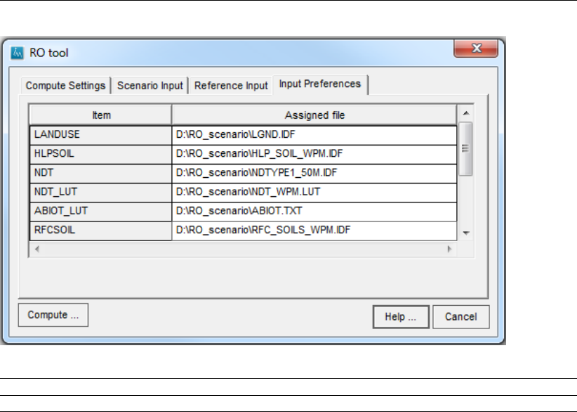
DRAFT
Toolbox Menu Options
Item List of the preference keywords.
Assigned file Name and directory of a file referring to Item.
7.12.2 Preprocessing
The needed input files to be prepared:
Two IDF-files, one containing the GHG and one with GLG information in meters relative to surface
level (positive values = below surface level). A minimum of 1 set is required for the scenario
situation.
A landuse map (IDF-format) according to the LGN5 encoding.
A soil map (IDF-format) with HELP soil units and RFC soil units (explained later in more detail).
This conversion from the 1:50.000 soil map to HELP soils and to RFC soils is done by Deltares,
using a conversion table.
A map of vegetation types (NDT, natuurdoeltypenkaart), with encoding matching the lookup-tables
NDT_LUT and ABIOT_LUT.
So called “HELP”-tables, with HELP2005-database, containing relations between crop - soiltype -
GHG/GLG -respiration/moisture-stress.
As mentioned in section 7.12 “WHY?”, actual crop-yield, decrease of crop-yield and potential for de-
velopment of selected vegetation types are determined by use of the two knowledge/database/ model-
based tools:
“HELP2005-tabellen”for calculating farm crop productivity.
“WATERNOOD - Hydrologische randvoorwaarden natuur”for calculating potential for develop-
ment of groundwater dependent vegetation types.
The RO-tool requires maps, tables and binary files that represent the above mentioned knowledge/database/
model-based tools.
To calculate Agriculture-subtypes, these files from “HELP2005-tabellen”are required:
HLP_DRY.DAT HELP2005-database: crop|soiltype|GHG/GLG|respiration-stress.
HLP_WET.DAT HELP2005-database: crop|soiltype|GHG/GLG|moisture-stress.
HLP_SOIL.IDF Raster file: 1:50.000 soil map reclassified for HELP2005 (using bod2hlp.lut).
LUSE\LGN5.IDF Raster file with land use types in LGN5-codes.
CROP_COSTS.LUT Lookup table with crops (in LGN5-codes) and crop-yields (Euro/ha/year).
Deltares 367 of 812

DRAFT
iMOD, User Manual
To calculate Nature-subtypes, these files from “WATERNOOD - Hydrologische randvoorwaarden
natuur”are required:
RFC_SOIL.IDF Raster file: 1:50.000 soil map reclassified to RFC-soils (using bod2rep.lut).
RFC_LUT.LUT Lookup table with RFC(reprofunction)-characteristics.
NDT.IDF Raster file with vegetation types to calculate potential development for.
NDT_LUT.LUT Lookup table with option to aggregate vegetation types.
ABIOT_LUT.LUT Lookup table: hydrologic requirements for vegetation types (NDT’s).
To calculate Urban area:
URBAN_RANGE.LUT Lookup table with range of drainage-level (upper- and lower value in meter
below surface)
Realization of the RFC soil map
A soil map containing 1:50000 soil codes is needed for this realization as well as a field with an assimi-
lation of the fields "VOOR", "LETTER", "CIJFER", and "KALK". In case a new field needs to be added,
ArcView3.x can be used by fill in the following line in the Field calculator:
[VOOR]+[LETTER]+[CIJFER].ASSTRING+[KALK]. The associations are not included in the conver-
sion table and therefore the value of the field "EERSTE_BOD" can be used as a replacement. In
the soil map, the codes related to excavated soils starting with a "|"-character are represented in the
conversion table with the first two characters of the soil code (RFC-value = 99). All codes starting
with a "|"-character can be selected by making use of a query function (in ArcView3.x), e.g. ([field-
name]).contains("|"). Via the calculator the specific field can be filled with the first 2 characters by
making use of [CODE].LEFT(2). Similar functions are available in ArcGis. A final step in the prepara-
tion of a RFC soil map is joining the soil map with the table RFCCODES.DBF.
Realization of the HELP soil map
The same soil map (1:50000 soil codes) as was used for the realization of the RFC soil map, is needed
for realization of the HELP soil map. Only now an additional field is needed, containing the groundwater
tables. Accordingly, a compilation of the following fields is included in the map: "VOOR", "LETTER",
"CIJFER", "KALK", and "GWT". This field is available in most of the soil maps labeled as "CODE".
Next, the "BOD50_2_HLP.DBF" table needs to be joined to the "GWT"-field and converted to a raster
format on field "HELPID".
7.12.3 Operational setup
To start the computation of the RO-tool, it is necessary to define at least a GHG- and/or a GLG-file (de-
pending on chosen subtype) on the scenario tab. If iMOD cannot find all needed files, an explanatory
error is raised. In case a scenario has to be compared with a reference situation, computation is only
possible if all required files are defined in the Scenario Input and Reference Input tabs. At the moment
everything is correctly defined, clicking on Compute... executes the computation.
In case of comparing a scenario with a reference situation, the output contains:
1 For both scenario and reference:
1.1 For Agriculture-subtypes: an IDF and table with actual crop-yield (relative to crop-yield
under optimal abiotic conditions), and/or an IDF and table with decrease of crop-yield due to
moisture-stress (“natschade landbouw”) or respiration-stress (“droogteschade landbouw”).
1.2 For Nature-subtypes: an IDF and table with the potential for development of chosen veg-
etation types, expressed as a percentage, relative to the potential for development under
optimal abiotic conditions.
1.3 An IDF and table with the difference between the scenario results and the reference situation
results for chosen Agriculture and Nature subtypes (difference = reference - scenario).
In case the computation is limited to 1 situation (either scenario, or reference), the output only contains
one IDF and table with either actual crop-yield, decrease of crop-yield, or potential for development of
chosen vegetation types, depending on the chosen subtype(s).
368 of 812 Deltares

DRAFT
Toolbox Menu Options
Calculation of subtype “Urban Area” returns an IDF and table with suitability for urban development
(values 0, 50 and 100). A range for drainage-level is defined in a lookup-table. Groundwatertable
above the upper range results in a 0% suitability for building, groundwatertable between upper and
lower range results in a 50% suitability for building, and groundwatertable below the lower range results
in a 100% suitability for building.
7.12.4 Output
The output of the computation contains:
1 IDF-files (raster files) containing:
Agriculture: decrease of crop-yield due to moisture-stress and respiration-stress (“natschade
landbouw”, “droogteschade landbouw”).
Agriculture: actual crop-yield, relative to crop-yield under optimal abiotic conditions (“doelreal-
isatie landbouw”).
Nature: potential for development of pre-defined groundwater dependent vegetation types,
expressed as a percentage, relative to the potential for development under optimal abiotic
conditions (“doelrealisatie natuur”).
Urban Area: suitability for urban development (“doelrealisatie stedelijk”).
2 A table with:
Total crop-yield for all crops in scenario and reference situation (if applicable).
Total yield per area.
Average decrease in crop-yield, for both decrease of crop-yield due to moisture-stress and
respiration-stress.
Computed area of total extent with pro-/regression per subtype (crop-yield, vegetation type,
urban class).
The output per subtype is managed over the surface area for which the computation was performed.
Cells within the area but lacking any information (nodata values), are not taken into account and there-
fore these cells are not visible in the output totals.
Deltares 369 of 812
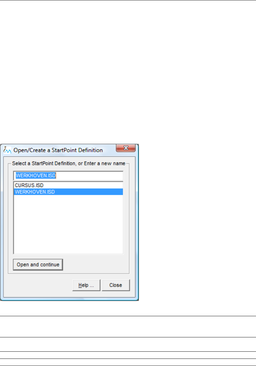
DRAFT
iMOD, User Manual
7.13 Define Startpoints
WHY?
iMOD offers the possibility to trace particles throughout the model extent. For these simulations it is
necessary to define the starting locations (startpoints) for these particles (pathlines).
WHAT?
The starting location for particles is defined inside polygons, along lines and/or on the edge of circles
around specified points. All these are specified in normal 3D-coordinates (x,y,z) and will be translated
to the model at trace time. In this manner, a startpoint definition, can be easily (re) used to other model
resolutions and/or model extinctions.
HOW?
Select the Toolbox option from the main menu and then choose Define Startpoints to start the Open/Create
a Startpoint Definition window.
Open/Create a Startpoint Definition window:
Select a StartPoint
Definition, etc . . .
Enter or select an existing *.ISD file from the list. Those *.ISD files are found
in the {user}\startpoints folder, see SrefiF.ISD for more detailed information on
*.ISD files.
Open and
continue
Click this button to open the selected *.ISD file and start the StartPoint Defini-
tion window.
Help . . . Click this button to start the Help functionality
Close Click this button to close the Open
370 of 812 Deltares
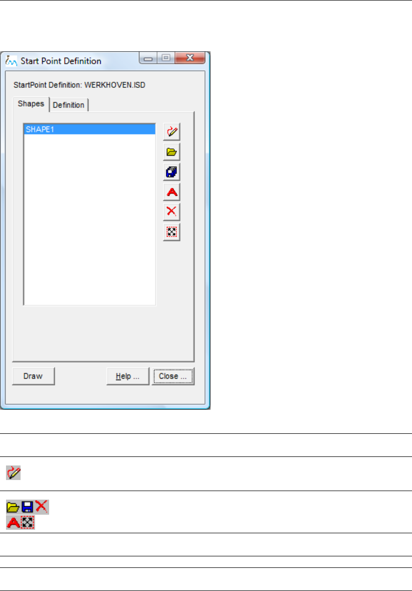
DRAFT
Toolbox Menu Options
Start Point Definition window, Shapes tab:
Startpoint
Definition
Displays the name of the current opened *.ISD file from the folder
{user}\startpoints.
Draw
Click this button to start the Select window in which you select the shape that
defines the lateral position of the startpoints (see next page).
Click these buttons to draw, open, save, delete or rename a shape. More
detailed information can be found in section 2.6.2
Draw Click this button to draw the spatial location of the startpoints of the selected
shapes.
Help ... Click this button to start the Help functionality.
Close ... Click this button to close the StartPoint Definition window. You will be asked
to save the adjustments to the opened *.ISD file.
Deltares 371 of 812
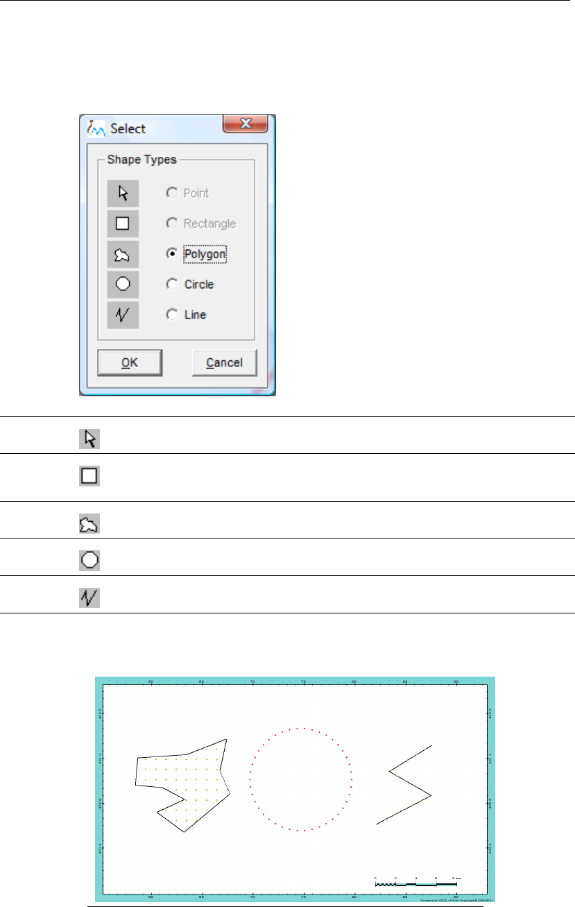
DRAFT
iMOD, User Manual
The Select window in which you select the shape that defines the lateral position of the
startpoints.
Select window:
Point
Click this option to define startpoints for a single point
Rectangle
Click this option to define startpoints within a rectangle
(NOT YET IMPLEMENTED)
Polygon
Click this option to define startpoints within a polygon
Circle
Click this option to define startpoints on a circle
Line
Click this option to define startpoints on a line
Example of startpoint created by (left) polygons, (middle) circles
and (right) lines:
372 of 812 Deltares
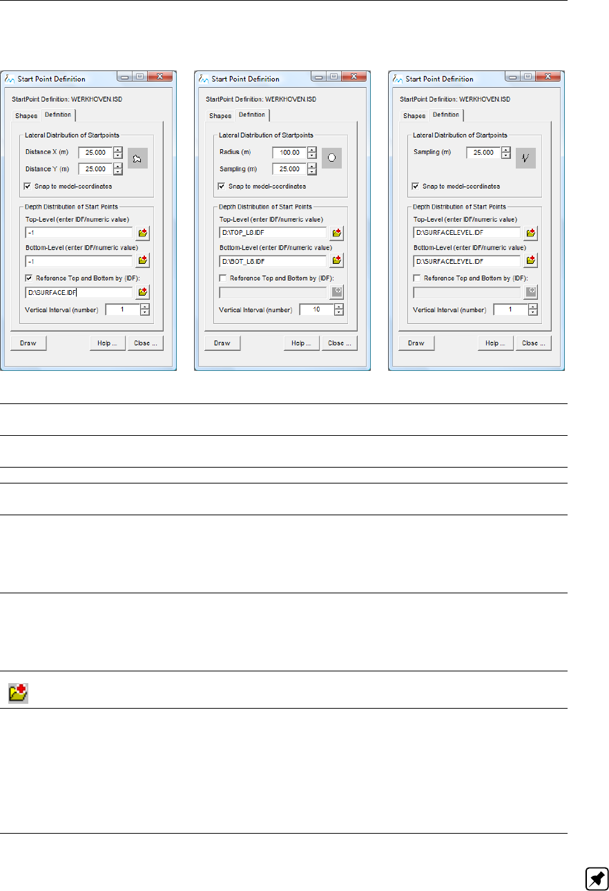
DRAFT
Toolbox Menu Options
StartPoint Definition window, Definition tab, (1) for polygons (2) on circles and (3) along lines:
Distance X,
Distance Y
Enter the lateral distances in X and Y direction for those startpoints
inside the selected Polygon shape.
Snap to model
coordinates
Click this item to snap the startpoints location to the nearest model
centroid (NOT YET IMPLEMENTED)
Radius Enter the radius of the circle.
Sampling Enter the distance between the startpoint on the radius of the circle
(Circle shape) or on the line (Line shape).
Top-Level (enter
IDF/numeric value)
Bottom-Level (enter
IDF/numeric value)
Enter a IDF that represents the top and/or bottom elevation of the start-
points, e.g. D:\TOP_L8.IDF and D:\BOT_L8.IDF. For each lateral po-
sition of a startpoint, the values will be read from the entered IDF-files.
Moreover, you can enter a constant value (e.g., -1) to indicate that all
values are constant.
Reference Top and Bot-
tom by (IDF)
Check this item to enter an IDF-file as reference level. The values from
this IDF will be used to add or subtract the values from the Top-level
and Bottom-level. In the example in Figure 5-9d-i, the final values for
the Top elevation will be those values in the D:\SURFACE.IDF minus 1
(the entered numeric value).
Open IDF
Select this button to select an IDF-file from the file selector.
Vertical Interval (number) Enter the number of vertical intervals between the values from the top
and bottom elevation. By entering the number:
1: iMOD will position one startpoint in-between the values for the top
and bottom elevation;
2: will yield a startpoint equal to the top and a startpoint equal to the
bottom elevation;
>2: yields startpoints equally distributed between the top and bottom
elevation.
Note: iMOD will not check, at this time, for the non-existence of any entered IDF-file. These files will
be checked at runtime for the particle tracking.
Deltares 373 of 812
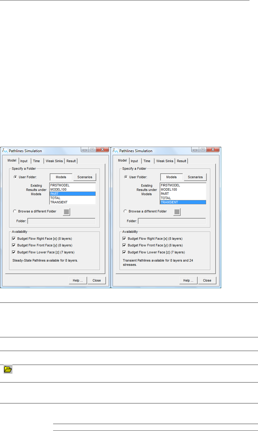
DRAFT
iMOD, User Manual
7.14 Start Pathline Simulation
WHY?
Particle tracking analyses are particularly useful for delineating capture zones or areas of influence for
wells.
WHAT?
iMOD is equipped with iMODPATH that is a modified version of MODPATH version 3 (Pollock, 1994).
iMODPATH is a particle tracking code that is used in conjunction with iMODFLOW. After running a
iMODFLOW simulation, the user can designate the location of a set of particles. The particles are
then tracked through time assuming they are transported by advection using the flow field computed
by iMODFLOW. Particles can be tracked either forward in time or backward in time.
HOW?
Select the option Toolbox from the main menu and then choose the option Start Pathline Simulation to
open the Pathlines Simulation window.
Pathlines Simulation window, Model tab (i) for a steady-state model (ii) for a transient model:
User Folder: Select this radio button to select one of the following options:
Models:
Click this radio button to list all existing models in the folder {user}\models
Scenarios:
Click this radio button to list all existing models in the folder {user}\scenarios
Existing results
under Models
Select one of the folders that appear in this listbox.
Browse for a differ-
ent folder
Select this radio button to specify a result folder from a different location, other
that the {user}\models and/or {user}\scenarios folder.
Open File
Click this button to search for a folder on disk
Folder: Enter the name of the folder, otherwise the name of the folder will be displayed
after accepting the folder from the Open File button. The Availability status will
update each time an alteration is noticed in the folder name.
Availability iMOD will check those results that are available and includes the number of
modellayers.
Alias Subfolder
374 of 812 Deltares
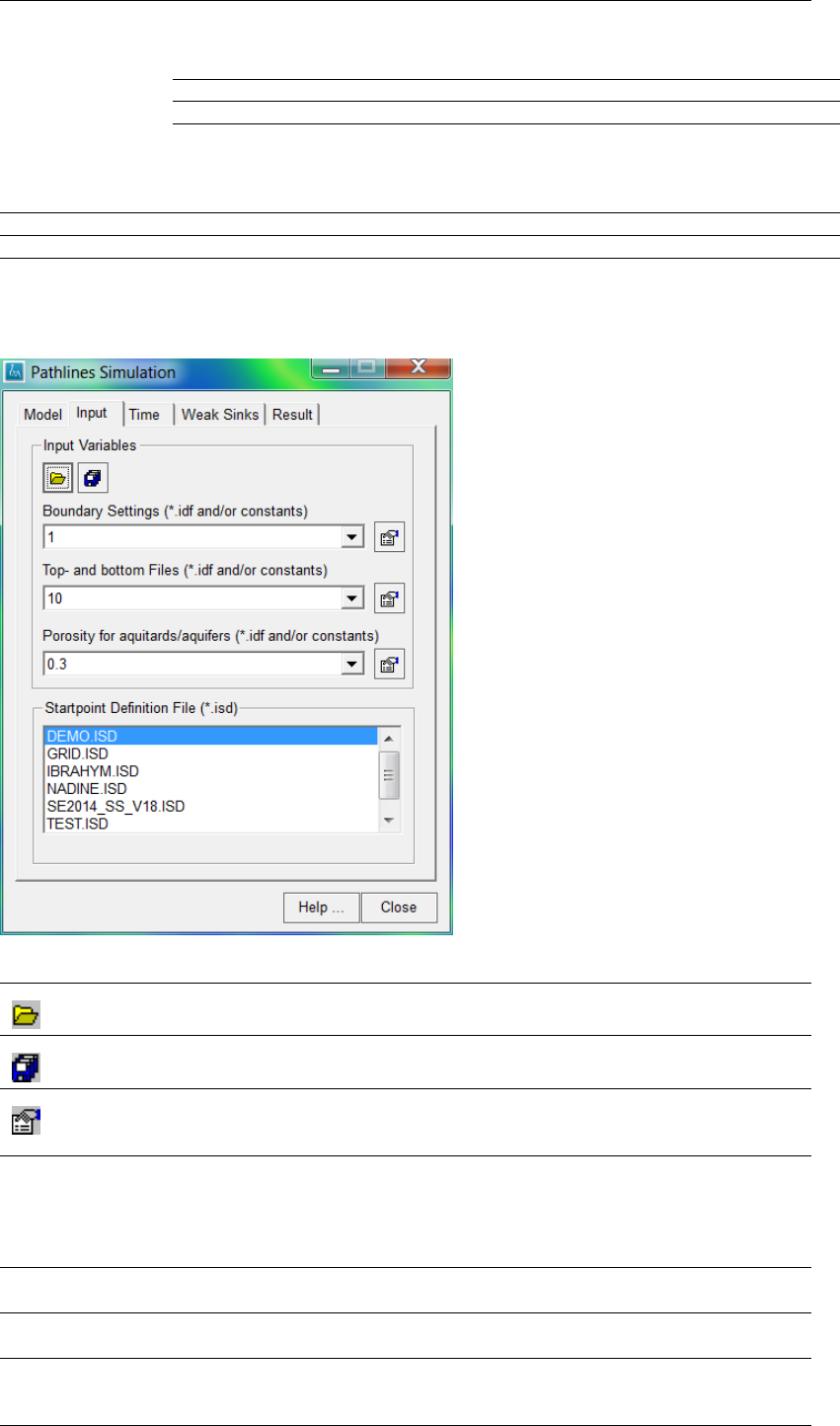
DRAFT
Toolbox Menu Options
Budget Flow Lower Face [z] (.) BDGFLF\BDGFLF_L*.IDF
Budget Flow Right Face [x] (.) BDGFRF\BDGFRF_L*.IDF
Budget Flow Front Face [y] (.) BDGFFF\BDGFFF_L*.IDF
Displays the status of the selected model. Whenever data is missing the other
tabs are greyed out.
Help. . . Click this button to start the HELP functionality.
Close Click this button to close the Pathlines Simulation window.
Pathlines Simulation window, Input tab:
Open
Click this button to open an *.IPS (iMOD Pathlines Settings) file.
SaveAs
Click this button to save the current input settings to an *.IPS file.
Properties
Click this button to open the Input Properties window (see
SrefTMO.SPS.InputProp).
Boundary Settings Click the dropdown menu to view the current files and/or values to be used
as boundary settings. Any value greater than zero determines the active flow
extent in which particle tracking is allowed. As a default the boundary of the
flow simulation can be used (see section 7.9), however, it is not obligatory to
use that particular file.
Top- and bottom Click the dropdown menu to view the current files and/or values to be used as
top- and bottom elevations of the model layers.
Porosity Click the dropdown menu to view the current files and/or values to be used as
porosity.
Startpoint
Definition File
Select one of the existing *.ISD files from the list menu to use as startingpoints
for the particle simulation. Those *.ISD can be created by the Startpoint Tool
(page 297) and are located in the {user}\STARTPOINTS folder.
Deltares 375 of 812
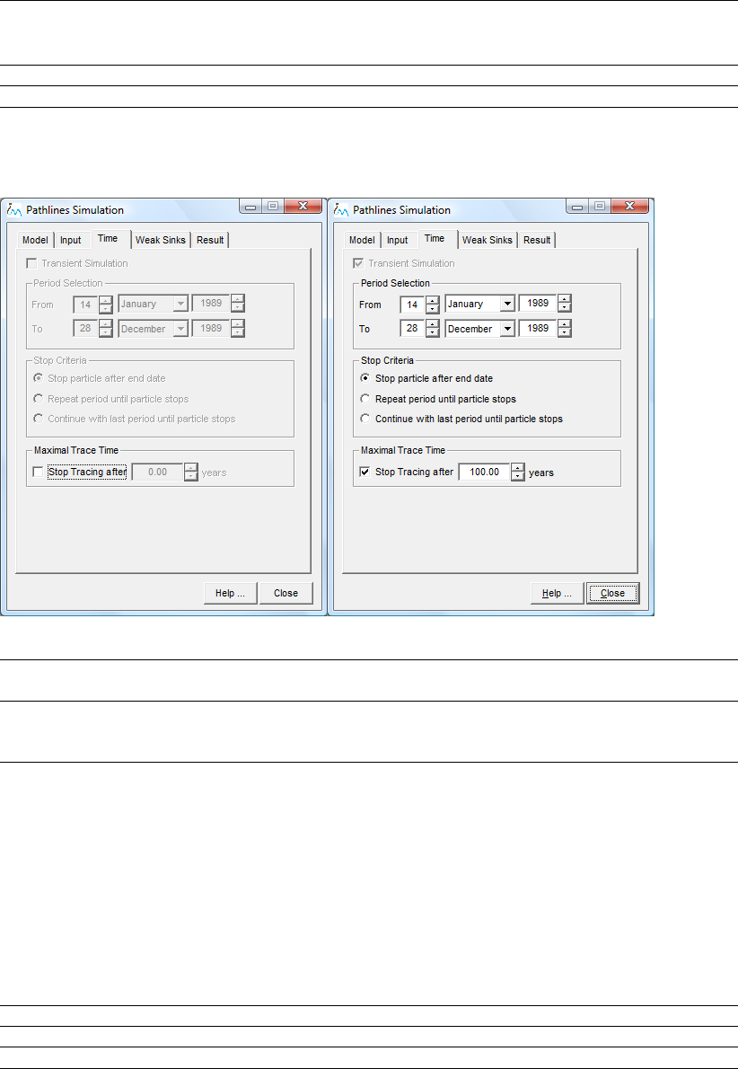
DRAFT
iMOD, User Manual
Help. . . Click this button to start the HELP functionality.
Close Click this button to close the Pathlines Simulation window.
Pathlines Simulation window, Time tab:
Transient
Simulation
This checkbox is selected automatically for transient solutions and deselected
for steady-state solutions.
From, to Specify the start- and end period whenever a transient solution is used. The
input fields are filled in automatically and defined by the content of the selected
result folder on the Model tab.
Stop criteria Select one out of three options to specify how particles are to be treated when-
ever they are not captured before the end of the existing solution files (only for
transient simulations).
Stop Particle after end date:
Stop the particle simulation whenever the elapsed time of the particle exceeds
the given To date.
Repeat period until particle stops:
Repeat the period selection (From-To) until the elapsed time of the particle
exceeds the increased To date.
Continue with last period until particle stops:
Use the last solution within the From-To period, to simulate all particles until
they are captured.
Stop tracing after Enter the number of years for which particles need to be traced.
Help. . . Click this button to start the HELP functionality.
Close Click this button to close the Pathlines Simulation window.
376 of 812 Deltares
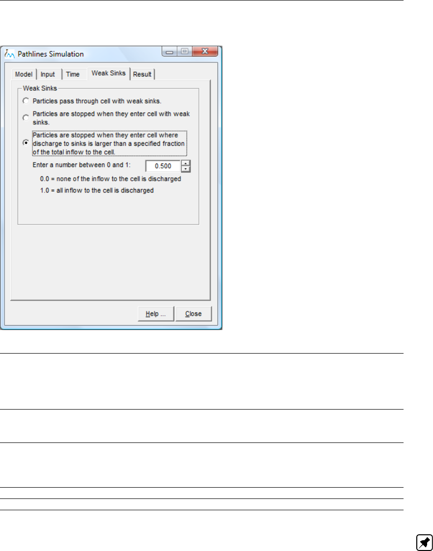
DRAFT
Toolbox Menu Options
Pathlines Simulation window, Weak Sinks tab:
Particles pass . . . Select this option to let particles pass any cell with a weak sink, no matter how
“weak” they are. Be aware of the consequences of this option, since particles
tend to trace over long distances until they are captured by a strong sink. This
option could be wise to use whenever Forward Tracing option is selected on
the Result tab.
Particles are
stopped . . .
Select this option to stop particles at any cell with a weak sink, no matter how
“weak” they are. Use this option whenever Backward Tracing is selected on
the Result tab.
Particles are
stopped when
they enter . . .
Select this option to let particles stop whenever they enter a cell where the dis-
charge is larger than a fraction of the total inflow. Whenever the fraction=1.0,
particles stop at a strong sink only, as fraction=0.0, they will always stop, no
matter the size of the total outflow.
Help. . . Click this button to start the HELP functionality.
Close Click this button to close the Pathlines Simulation window.
Note: The final representation of flowpaths and/or endpoints of particles is influenced significantly by
the treatment of weak sinks. A strong sink is defined as a model cell in which all flowterms are directed
into the model cell. Weak sinks are those that have at least one flow component that directs outside
the model cell.
Deltares 377 of 812
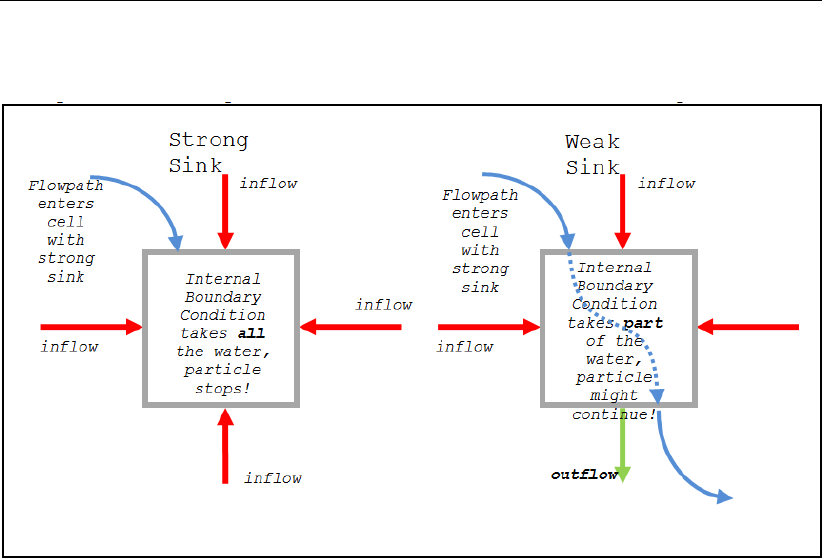
DRAFT
iMOD, User Manual
Example of Strong sink (left) and a Weak sink (right):
There is no way that the particle tracking algorithm itself can decide correctly whether a particle should
stop or not. Moreover, it is an essential scale issue, since strong or weak sinks do not exist in reality.
As the scale size (rastersize) increases, the occurrences of weak sinks in the model, will increase.
This is simply caused by the phenomenon that a single coarse modelcell should represent more than
one internal boundary condition and represents a larger area than the area taken by the boundary
condition. So, the flowterms of these coarse cells represent an average flowfield that represent on
average particles that should stop and particles that should continue. Unfortunately, that particular
particles can not be simulated with the coarse model, so one should decide whether the particles
should stop, continue of stop/continue depending on the ratio between the total inflow and the outflow
component. These three options can be chosen in iMOD
378 of 812 Deltares
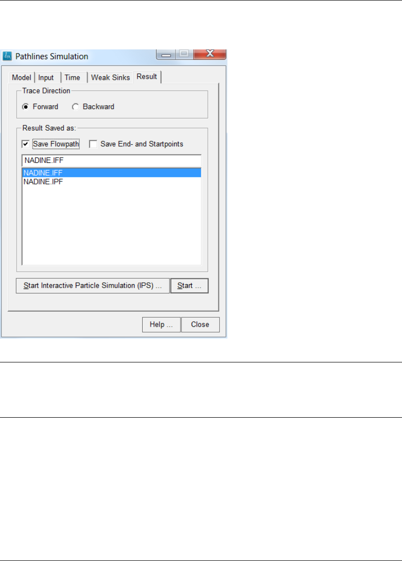
DRAFT
Toolbox Menu Options
Pathlines Simulation window, Result tab:
Trace Direction Select one of the following options:
Forward:
This option will compute pathlines in the direction of flow
Backward:
This option will compute pathlines against the direction of flow
Result Save as: Select on the following options:
Save Entire Flowpath (*.iff):
Select this option to save the entire flowpath in an *.IFF file (see section 9.8
for more details). The IFF has the following attributes:
PARTICLE_NUMBER – number of the released particle;
ILAY – modellayer of the current particle position;
XCRD. – X coordinate of the current particle position;
YCRD. – Y coordinate of the current particle position;
ZCRD. – Z coordinate of the current particle position;
TIME(YEARS) – elapsed time on the current particle since moment of release;
VELOCITY(M/DAY) – current velocity of the particle;
IROW – row index of current location;
ICOL – column index of current location.
Deltares 379 of 812
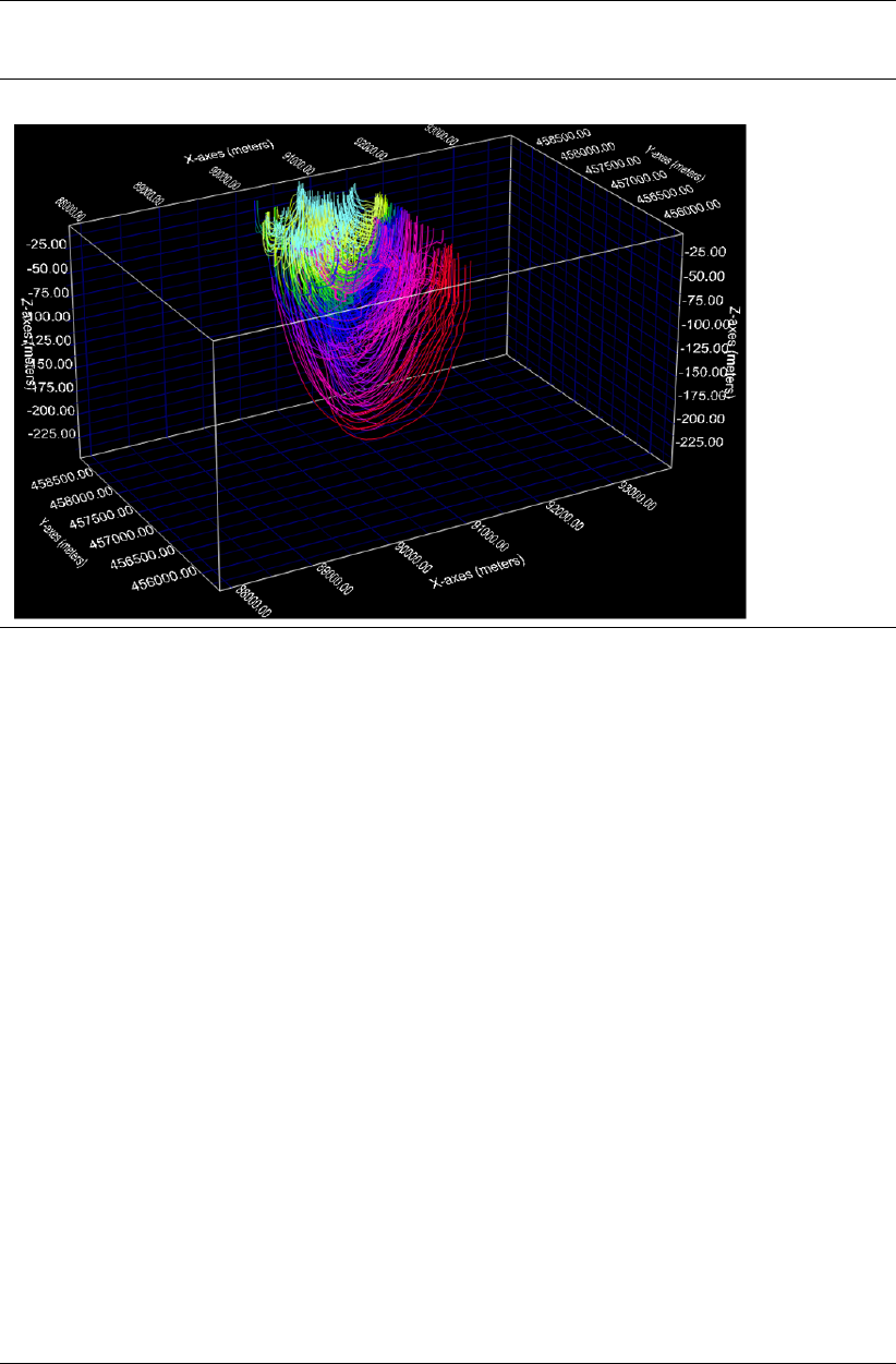
DRAFT
iMOD, User Manual
Example of flowpaths (IFF) plotted by the 3D Tool.
Save End- and Startpoints (*ipf):
Select this option to save the entire flowpath in an *.IPF file (see section 9.7).
The IPF has the following attributes:
SP_XCRD – X coordinate of starting location of particle;
SP_YCRD – Y coordinate of starting location of particle;
SP_ZCRD – Z coordinate of starting location of particle;
SP_ILAY – modellayer of starting location of particle;
SP_IROW – row index of starting location;
SP_ICOL – column index of starting location;
EP_XCRD – X coordinate of end location of particle;
EP_YCRD – Y coordinate of end location of particle;
EP_ZCRD – Z coordinate of end location of particle;
EP_ILAY – modellayer of end location of particle;
EP_IROW – row index of end location;
EP_ICOL – column index of end location;
TIME(YEARS) – elapsed time of particle at end location;
MAXLAYER – deepest model layer that a particles passed;
DISTANCE – traveled distance of particle from begin to end location;
IDENT.NO. – number of particle;
CAPTURED_BY – code identification of capture:
-1 – error occurred
0 – initial value
1 – inactive cell
2 – velocity is zero
3 – strong sink (no outflow)
4 – weak sink (regardless of flow)
5 – weak sink outflow greater than fraction
6 – modelboundary reached
7 – elapsed time greater that maximum time allowed.
380 of 812 Deltares
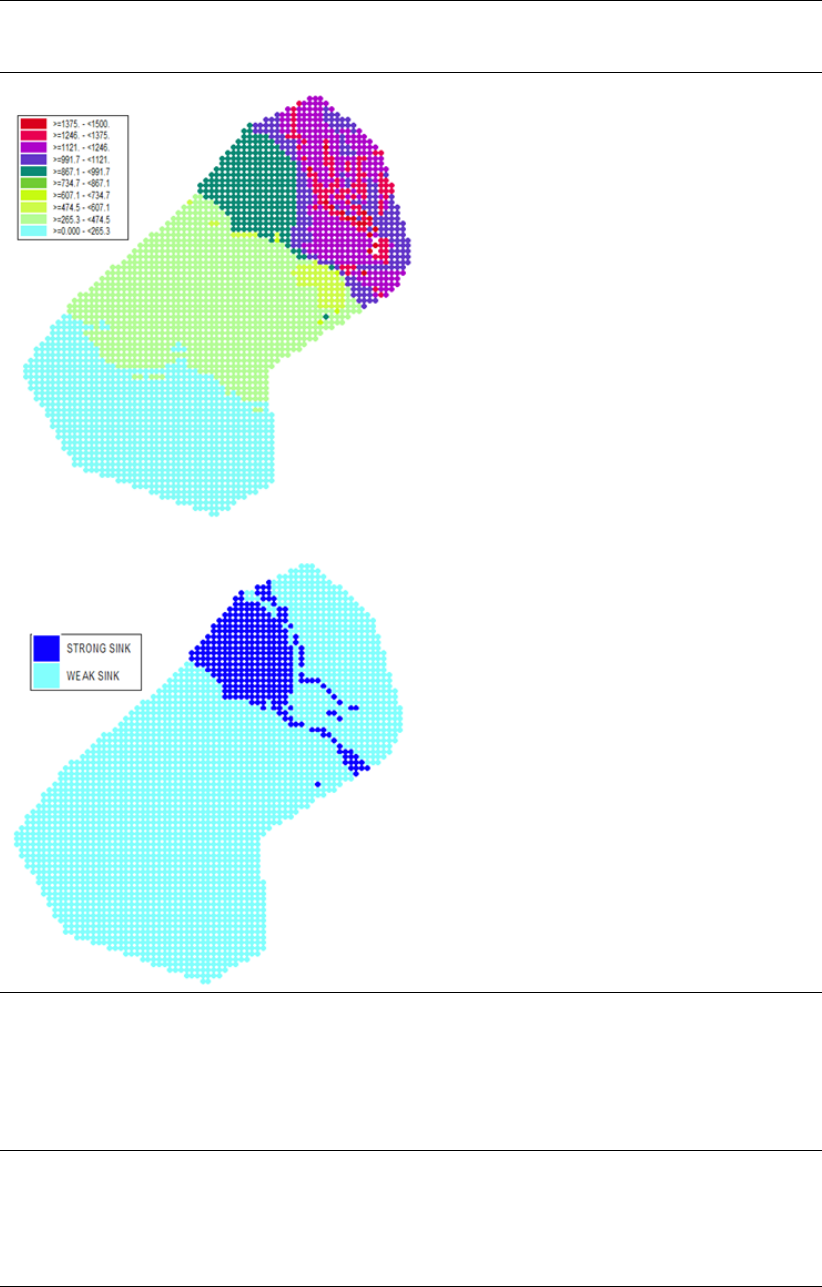
DRAFT
Toolbox Menu Options
Example of startpoints plotted by their age (upper figure) and their captured_by code (lower figure):
Start IPS . . . Click this button to start the Interactive Pathline Simulation (IPS), see 7.15.
iMOD will start the 3-D Tool directly and opens the IPS tab in the 3-D Tool in
which pathlines might be computed interactively. The output of those simula-
tion go straight into OpenGL and will be rendered, no results will be saved to
disc, use the Start . . . option for that instead. Any selected SDF file will be
neglected whenever the IPS is started as the starting points for the pathlines
will be defined in the IPS-Tool.
Start . . . Click this button to start the pathline simulation. iMOD will start directly, or
asks for confirmation in the situation that the output file exists already. The
iMODPATH runfile will be saved in the Model folder as given on tab Model.
This runfile can be re-used easily by the iMODBatch function IMODPATH (see
8.6.6). A log-file will be saved there as well, that given information about the
used files.
Deltares 381 of 812
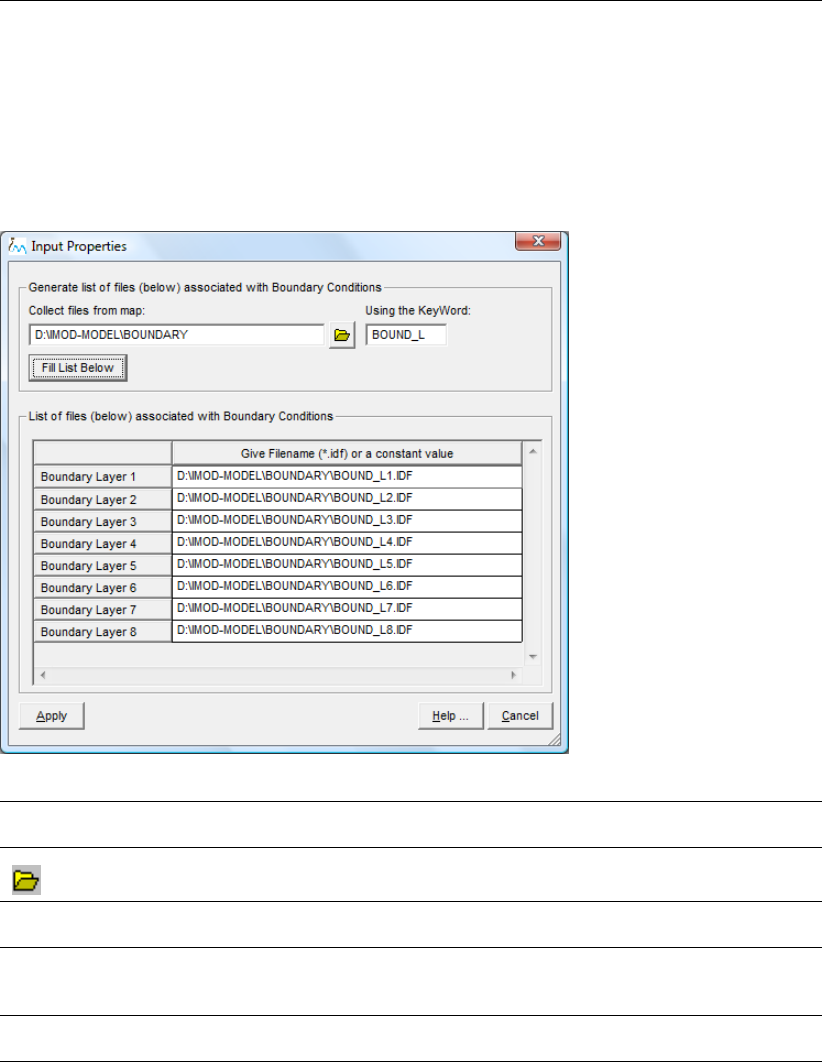
DRAFT
iMOD, User Manual
7.14.1 Input Properties
A pathline simulation needs particular files that can be easily defined (and stored in an *.IPS file) with
the Input Properties function. Select the Input Properties button on the Input tab of the Pathlines
Simulation window to start the Input Properties window.
Input Properties:
Collect files from
Folder:
Enter the folder name to be used to construct filenames, e.g. d:\imod-
model\boundary
Open
Click this button to select a folder from the file selector.
Using the
keyword:
Enter the keyword that need to be added to the foldername, e.g. boundary_l
Fill List Below: Click this button to construct filenames for all modellayers. The above men-
tioned example yield the filenames d:\imod-model\boundary\boundary_l1.idf
upto modellayer 8.
List of files . . . Display the filenames and/or constant values to be used in the pathline simu-
lation.
382 of 812 Deltares
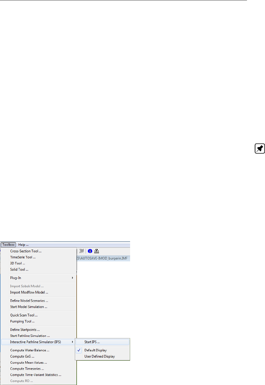
DRAFT
Toolbox Menu Options
7.15 Interactive Pathline Simulator
(Extension of this functionality is in progress; we expect it will be completed and part of a Deltares-
release of the iMOD-executables in February 2016.)
WHY?
Interactive Particle tracking analyses can be essential in understanding how a geohydrological system
works. For reasons of system analyses this tool might be having a great additional value. The main
purpose of this tool is to gain insight in geohydrological processes by using animated groundwater
flows and the ability to interactively change your point of view in a 3D-environment.
WHAT?
iMOD is equipped with iMODPATH that is a modified version of MODPATH version 3 (Pollock, 1994).
iMODPATH is a particle tracking code that is used in conjunction with iMODFLOW. After running a
iMODFLOW simulation, the user can use the runfile of iMODPATH (see section section 8.6.6) to enter
the 3-D tool of iMOD (see section section 7.3). In this 3-D environment, the user is able to interactively
analyze the flow path of groundwater particles, e.g. pause the flow at arbitrary moments. Particles can
be tracked either forward in time or backward in time.
Note: The IPS runs only for a Steady State flow situation. In case a transient iMODPATH run file is
uploaded, only the first stress period is read and used for particle tracking.
HOW?
Select the option Toolbox from the main menu, click on the submenu option Interactive Pathline Simu-
lator and then on Start IPS. . . to select an appropriated runfile for iMODPATH. The 3-D tool will start
and all the necessary files (top, bottom and fluxes) will be allocated for the current zoom extent. It is
easily to start the tool for limited areas of interest, especially to be more efficient. On default iMOD
starts the IPS with default display settings (checked in IPS-submenu), this means that all the files avail-
able in the runfile are loaded into the 3D-tool. Another option is to choose User Defined Display and
iMOD only loads the files selected in the iMOD manager.
IPS-submenu:
Deltares 383 of 812
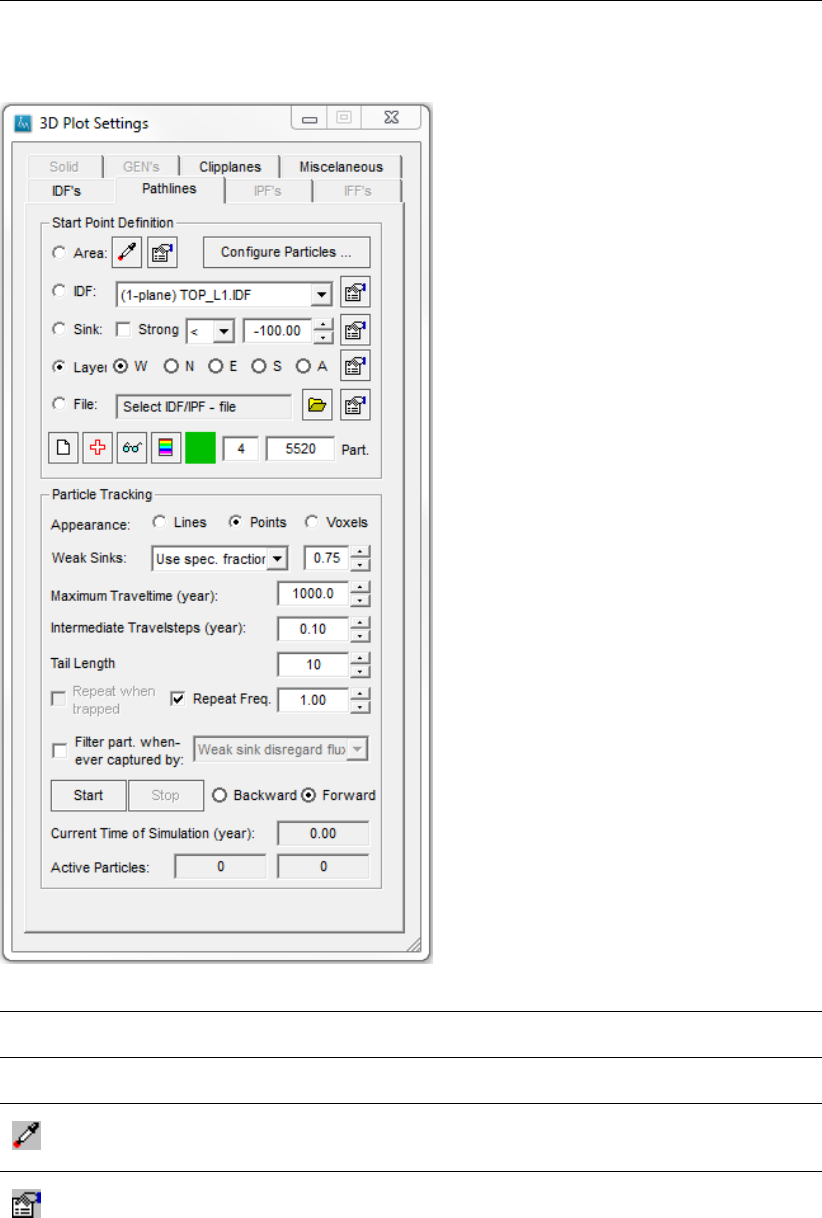
DRAFT
iMOD, User Manual
3D Plot Settings window, Pathlines Folder tab:
Start Point
Definition
With the following options the starting point of the particles can be defined.
Area: Select this option to define a rectangular area with starting points somewhere in
the modeled area.
Select
Click on this button to drag a rectangle (NOT AVAILABLE IN CURRENT VER-
SION!).
Attributes
Click on this button to open the
Location Settings window:
384 of 812 Deltares
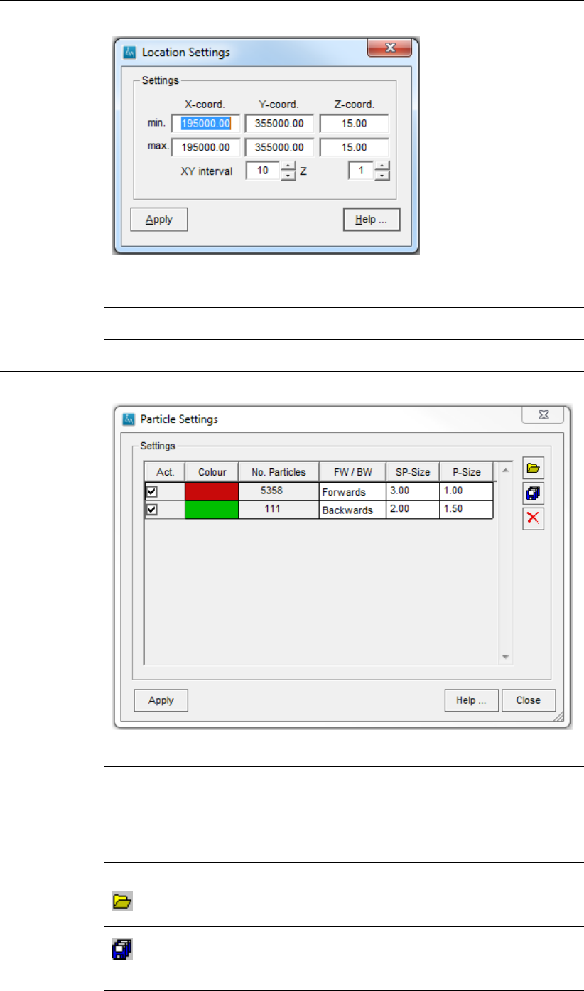
DRAFT
Toolbox Menu Options
Enter the minimum and maximum x, y and z-coordinates to define the extent of
the box in which the starting points needs to be placed.
XY interval Enter a value for the amount of staring points in x- and
y-direction.
ZEnter a value for the amount of starting points in the z-
direction.
Configure
Particles. . .
Click on this option to open the Particle Settings window:
Act. Check this option to activate a particle group.
Colour Click on this field to change the colour of the particles
and starting points.
No. Particles Total amount of particles in a group.
BW/FW Click on this field to change the tracking option in "For-
ward" or "Backward".
SP-Size Click on this field to change the size of the starting point.
P-Size Click on this field to change the size of the particle.
Open PTF
Opens an PTF(Particle Tracking File)-file containing the
particle settings per group.
Save As
Saves the particle group settings in a IPF-file, if points
needs to be analyzed in iMOD separately from the IPS-
tool, or in a PTF-file for later use in IPS.
Deltares 385 of 812
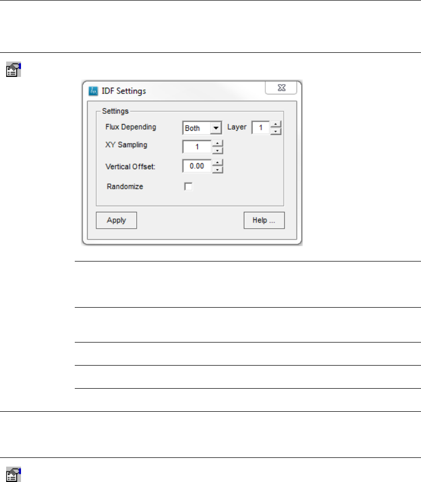
DRAFT
iMOD, User Manual
IDF: Select this option to define the starting points based on the in a loaded IDF-file
available points. Make use of the dropdown menu to select the preferred IDF-file.
Attributes
Click on this button to open the window IDF Settings:
Flux Depending Select from the dropdown menu the preferred vertical
direction of the flux in a particle related cell: Up (only
positive fluxes are drawn), Down (only negative fluxes
are drawn) or both (all fluxes are taken into account).
Layer iMOD uses the fluxes from the layer defined with this
option, e.g. if Layer=1, iMOD uses the fluxes from model
layer 1.
XY Sampling Give the horizontal distance in meters between the start-
ing points.
Vertical Offset Give the vertical distance in meters between the top of
the layer and the particle start position.
Randomize Check this option to randomly place the starting points
with the given settings.
Sink: Select this option to locate the starting points on the location of the in the model
area available sinks. Check Strong to apply the given condition, defined with the
dropdown menu and the value box, only to strong sinks. The background theory
about strong and weak sinks can be found in section 7.14 under Weak Sinks tab.
Attributes
Click on this button to open the window Sink Settings:
386 of 812 Deltares
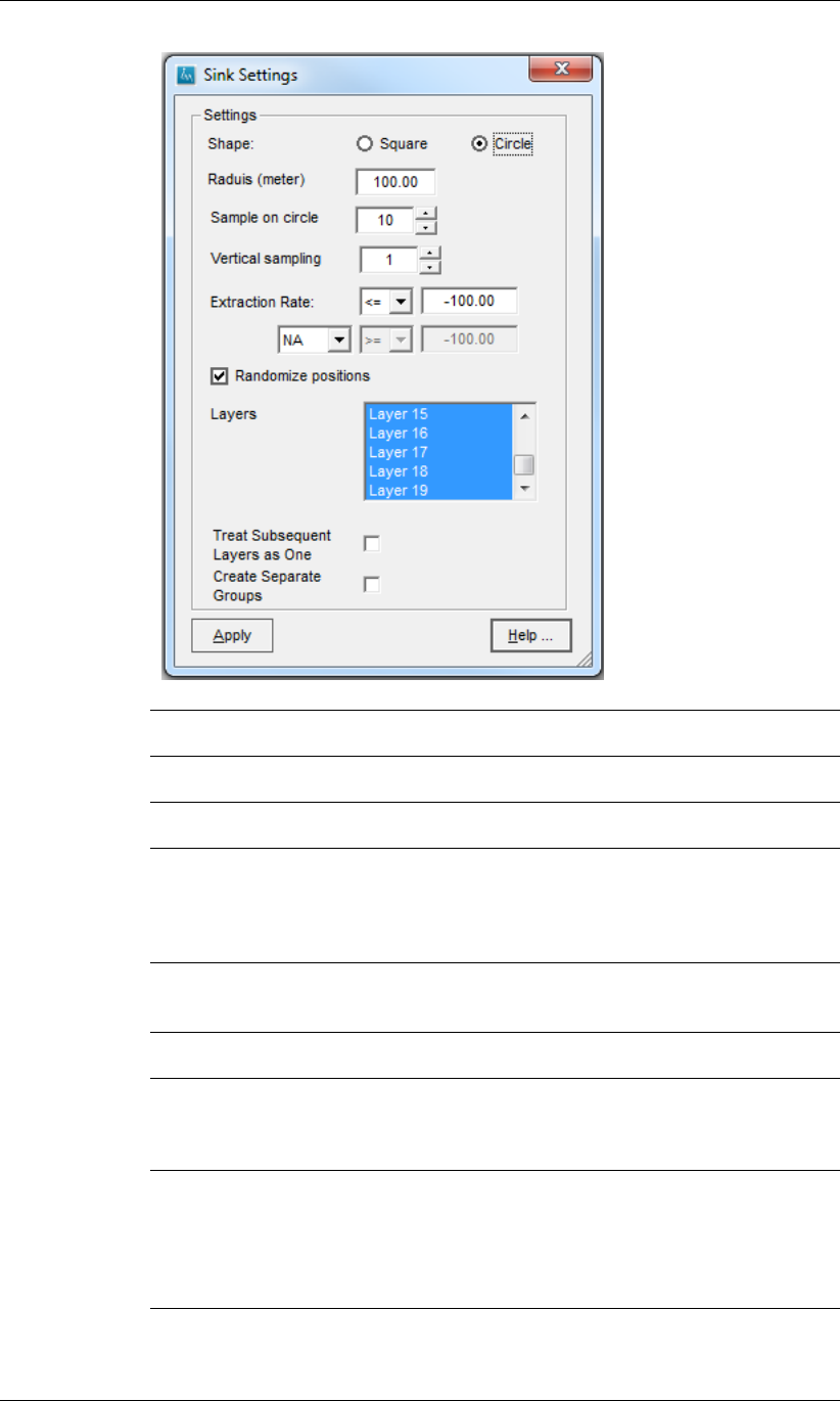
DRAFT
Toolbox Menu Options
Shape: Choose the shape of the points on the sink locations;
Square or Circle.
Radius (meter) Enter the size of the radius in meters of the sinks related
points.
Sample on
circle
Enter a value for the horizontal influence area around the
sink (in meters) to be shown in the simulation.
Vertical
sampling
Enter the amount of starting points per layer in the ver-
tical direction at the sink location, e.g. if 5 layers are se-
lected and a vertical sampling amount of 10 is chosen,
there will be in total 5x10=50 starting points in the verti-
cal direction.
Extraction
rate:
Define the range of the sink extraction rate. Only sinks
with discharges within the given range are labeled as
sinks.
Randomize
positions
Check this option to randomly place the starting points
with the given settings.
Layers Select the layers to be taken into account in the PTS
at the well locations (e.g. selecting 5 layers results into
5 groups with each the total amount of defined starting
points).
Treat subsequent
Layers as One
Check this option to evaluate all selected layers as one
layer (be aware: only successive layers are consolidated
to one layer), e.g. 5 selected layers with 10 vertical sam-
ples results in 50 starting points, with this option checked
on there is only 1 group with 5 layers and 10 starting
points in total.
Create
Separate Groups
Check this option if it is preferred to treat each selected
layer as an separate subgroup within 1 group, e.g. 1
group is made with the 5 selected layers, each contain-
ing 10 starting points (50 starting points in total).
Deltares 387 of 812
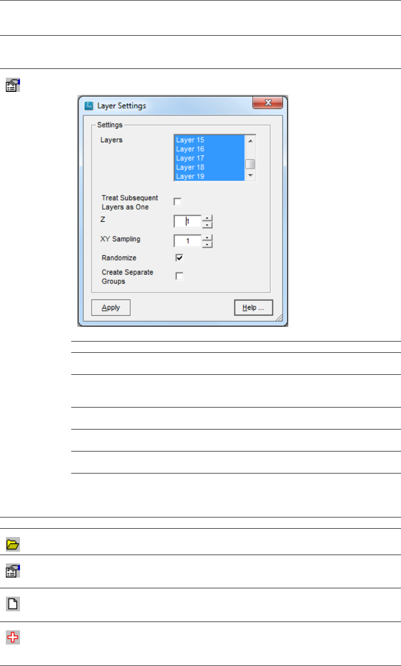
DRAFT
iMOD, User Manual
Layer: Select this option to locate the particles at one of the displayed model boundaries.
W=West boundary, N=North boundary, E=East boundary, S=South boundary and
A=all boundaries.
Attributes
Click on this button to open the window Layer Settings:
In this window it is possible to i.e. select the layers to place the starting points in.
Layers Select the layers to be taken into account in the PTS at
the border location(s).
Treat Subsequent
Layers as One
Check this option to evaluate all selected layers as one
layer (be aware: only successive layers are consolidated
to one layer).
ZEnter the amount of starting points per layer in the verti-
cal direction.
XY Sampling Give the horizontal distance in meters between the start-
ing points.
Randomize Check this option to randomly place the starting points
with the given settings.
Create
Separate Groups
Check this option if it is preferred to treat each selected
layer as an separate subgroup within 1 group, e.g. 1
group is made with the 5 selected layers, each contain-
ing 10 starting points (50 starting points in total).
File: Select this option to choose an IDF- or IPF-file for the start point definition.
Open
Use this button to search for and open the preferred file.
Attributes
Click on this button to open the window IDF Settings which is similar to the IDF-
option settings window.
New
Click on this button to reset the Particle settings, the Part. value boxes are set on
0.
Add
Click on this button to add a new PSP (Particle Start Point) definition group to the
simulation. Every time this button is used a new group is added to the particle
simulation and the value in the first Part. value box is increased with 1.
388 of 812 Deltares
DRAFT
Toolbox Menu Options
Show Selection
Click on this button to analyze the location of the defined particles in advance of
or during the particle simulation.
Color
Click on this button the change the color of the just defined point-group.
Part. The first value box counts the amount of PSP definition groups specified by the
user. Every time the ( )-button is used, this value is increased with 1 (total
value = amount of defined particle groups). In this case 4 start point definitions
are specified. The second value box is the sum of all the defined starting points (in
this case 5520). By clicking on Configure Particles. . . the total amount of particles
per start point definition can be distinguished.
Particle
Tracking
With the below mentioned options it is possible to set the graphic settings of the
particle tracking. A change in some of the options is directly visible on screen.
Appearance: Choose the representation of the simulated path line points; Lines, Points or Vox-
els (Not Available yet).
Weak Sinks: Make a choice between "Use spec. fraction", "Particles stop. . . " and "Particles
pass. . . ". Selecting "Use spec. fraction" allows the user to enter a fraction number
in between 0 and 1 (See page 377 at Particles are stopped when they enter. . .
for a more extended description). The other two menu items use a fixed factor
value in their selection (see page 377 for an extended explanation about these
other two Weak Sinks options).
Maximum
Travel time
(year):
Give the maximum time a particle can travel through the model area during the
simulation before the particle disappears from the screen or restarts from its start-
ing point, e.g. a value of 1000 years gives the user the opportunity to follow a
particle for 1000 years of simulation time.
Intermediate
Travel steps
(year):
Give the time step size in between two shown particles. Examples: 1. an inter-
mediate travel step of 0.10 year and a maximum travel time of 10 years results
into 100 time steps, 2. An intermediate travel step of 1 year, on the other hand,
and the same maximum travel time (10 years) results in 10 time steps. The actual
time of the simulation is longer in the first example compared to the second ex-
ample, because the actual simulation time is based on the amount of time steps
(more=longer).
Tail Length Enter a value to define the length of the particle "shadow". The shadow shows a
part (the length of the tail) of the particles pathline, in real life comparable to the
contrails of aircrafts in the sky.
Repeat
when trapped
Check this option to restart a particle at its starting point after the particle disap-
peared, e.g. it was trapped in a sink or it flews outside the model domain (only
available when Repeat Freq. is not checked).
Repeat Freq. Check this option to restart a particle after the entered time step value, e.g. at a
frequency of 1.00 iMOD starts a new particle simulation every year of simulation
time (only available when Repeat
when trapped is not checked).
Filter part.
whenever cap-
tured by:
Check this option to be able to apply a particle filter to the whole simulated particle
cloud. In this refinement there are the following options:
1. Inactive cell: restart only the particles in the simulation that are captured by an
inactive cell.
2. Zero velocity: restart only particles that have no velocity at the moment they
are trapped.
3. Strong sink: restart only the particles that are captured by strong sink(s).
4. Weak sink disregard flux: restart only the particles that are trapped by weak
sinks with a negligible flux compared to the total inflow.
5. Weak sink flux gt frac: restart only the particles that are stopped by weak sinks
with a flux larger than the fraction of the total inflow.
6. Boundary grid reached: restart only the particles that reached the boundary of
the presented model grid.
7. T greather than max T: Restart all particles when the current simulation time
is greater than the maximum Travel time.
Deltares 389 of 812

DRAFT
iMOD, User Manual
Start Click on this button to start the simulation.
Stop Click on this button to stop the simulation.
Backward Select this option to track the particles backward.
Forward Select this option to track the particles forward.
Current Time
of Simulation
(year):
Counter for displaying the current time of simulation. It counts from 0 until the
set Maximum Traveltime (years) with a time step given by textitIntermediate Trav-
elsteps (year). The counter starts over again, when the maximum travel time is
reached and a repeat-option is selected.
Active
Particles:
Counters for the total amount of particles at the beginning of the simulation (left
value box) and the amount of active particles during the simulation (right value
box).
390 of 812 Deltares
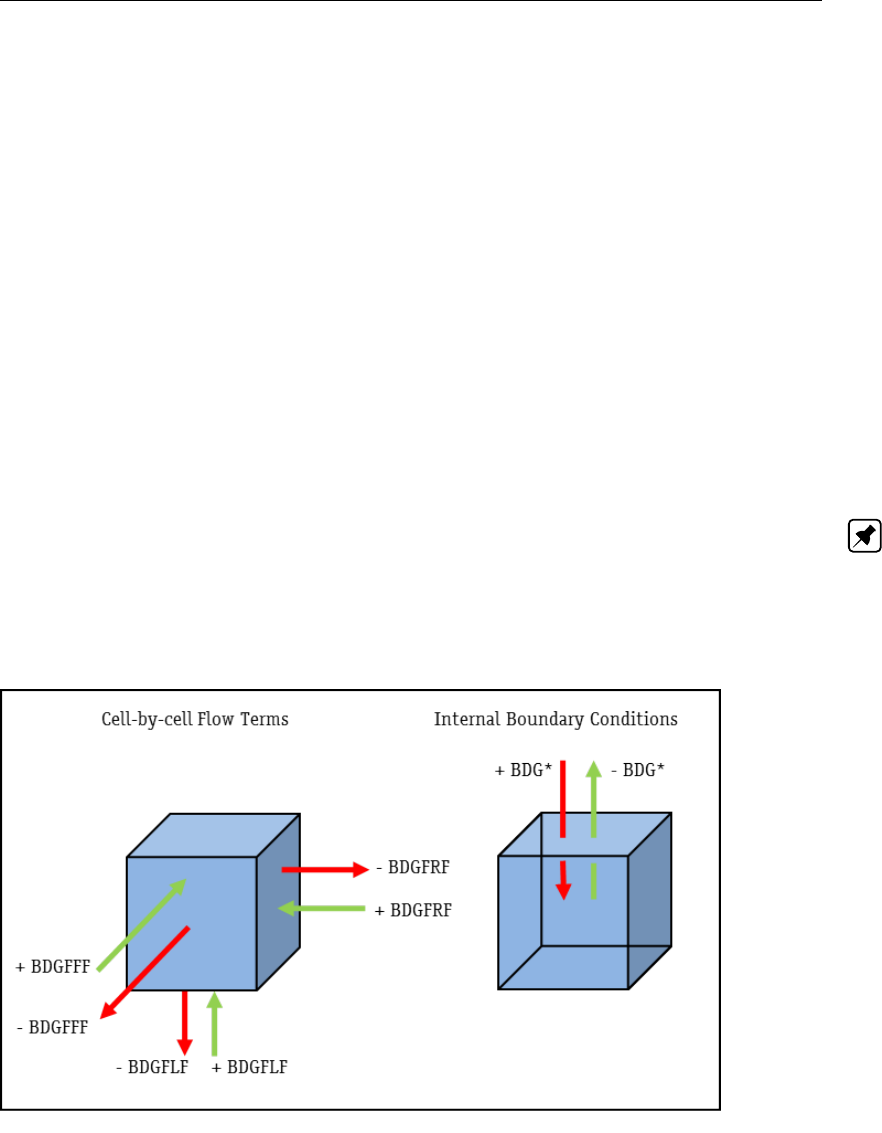
DRAFT
Toolbox Menu Options
7.16 Waterbalance
WHY?
The Waterbalance Tool can be used to calculate the sum of budget quantities for different components
for specified regions within the model extent and/or the entire model extent. Several budget items can
be selected, as well as particular mode layers and/or model output periods, see section 7.16.1. The
output can be analysed in the iMOD Water balance Analyser, see section 7.16.2.
WHAT?
The Waterbalance Tool uses specific results from iMODFLOW that start with BDG*.IDF and/or MetaSwap
output file starting with MSW*.IDF. Those files are stored in folders with identical names, such as BG-
GFLF\BDGFLF*.IDF. All these files store the flow quantity in m3/day (cubic meters a day). As a rule of
thumb the flow quantity is negative whenever it leaves the cell and positive whenever it enters the cell.
Flow that leaves the cell from the Right Face (BDGFRF), the Front Face (BDGFFF) and/or the Lower
Face (BDGFLF) is negative. However, for flow terms that enter the cell from the Left Face, Back Face
and/or Top Face of a model cell, the appropriate flow terms from the adjacent cells need to be multi-
plied with minus 1, to be consequent. For Internal Boundary Conditions (e.g. rivers, drainage systems,
recharge, wells) a similar approach is valid: water that enters the cell is positive, withdrawal of water is
negative. Water that flow from a specified water balance region to another region is noted netagive as
it leave the corresponding water balance region.
Note: The waterbalance assumes that the dimensions for data that is included are in m3/day. Bear
in mind that fluxes that are produced by MetaSWAP are in m3/m2and represent cumulative values as
specified in the TIME_SIM.INP. Those may NOT overlap with the output file from iMODFLOW.
Example of budget terms inside and outside a computational cell for (left) cell-by-cell flow terms and
(right) internal boundary conditions:
The Waterbalance Tool will just add all flow terms within (defined) areas and list them within a summary
text files (*.TXT and *.CSV) to be opened with e.g. NotePad, TextPad and/or Excell. Alternatively, it is
possible to read in a generated *.CSV file into the waterbalance analyser.
HOW?
To compute a water balance, select the option Toolbox from the main menu, choose Water Balance
and then choose Compute Waterbalance to open the Waterbalance window. To analyse the results of
a water balance computation, select the option Toolbox from the main menu, choose Water Balance
and then choose Analyse Waterbalance to open the Analyse Waterbalance window
Deltares 391 of 812
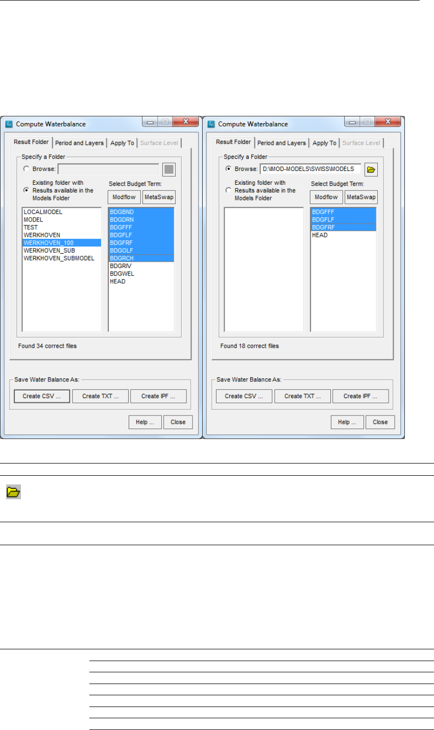
DRAFT
iMOD, User Manual
7.16.1 Compute Waterbalance
Start the Compute Water Balance window by selecting the option Toolbox from the main menu, choose
Water Balance and then choose Compute Waterbalance.
Compute Waterbalance window, Result Folder tab; left for results from the Models folders and right
from a different folder:
Browse: Select this radio button to specify a result folder from a different location.
Select Folder
Click this button to search for a folder on disk and use that folder to list the existing
budget terms. Alternatively, it is possible to enter a folder name into the string
field.
Existing folder
with Results ...
Select one of the folders that appear in this list box. These are the folders in the
{IMOD_USER} \MODELS folder.
Select Budget
Term
iMOD will list all sub folders under the current selected or entered folder. If none
are selected the other tabs in this window are unavailable. Also, whenever in-
correct folders (folders that doesn’t contain the correct files) are selected this
happens. Each time a single, or multiply budget terms are selected, iMOD starts
searching for corresponding files. For large models, this can take a while, so it
is often better to select the items in one click using Ctrl-Left- Mouse-Button of
Shift-Left-Mouse-Button. The name convention is that the folder should start with
BDG and/or MSW:
Subfolder Alias
BDGBND\bdgbnd* CONSTANT HEAD
BDGFLF\bdgflf* FLUX LOWER FACE
BDGFRF\bdgfrf* FLUX RIGHT FACE
BDGFFF\bdgfff* FLUX FRONT FACE
BDGSTO\bdgsto* STORAGE
BDGWEL\bdgwel* WELLS
392 of 812 Deltares

DRAFT
Toolbox Menu Options
BDGDRN\bdgdrn* DRAINAGE
BDGRIV\bdgriv* RIVERS
BDGEVT\bdgevt* EVAPOTRANSPIRATION
BDGGHB\bdgghb* GENERAL HEAD BOUNDARY
BDGOLF\bdgolf* OVERLAND FLOW
BDGRCH\bdgrch* RECHARGE
BDGISG\bdgisg* SEGMENT RIVERS
BDGIBS\bdgibs* INTERBED STORAGE
BDGCAP\bdgcap* CAPSIM
BDGDS\bdgds* DECREASE WATER ST. ROOTZONE
BDGPM\bdgpm* MEASURED PRECIPITATION
BDGPS\bdgps* SPRINKLING PRECIPITATION
BDGEVA\bdgeva* NET EVAPORATION WATER
BDGQRU\bdgqru* RUNOFF
Modflow Select this option to select budget terms that are specific for Modflow, automati-
cally.
MetaSwap Select this option to select budget terms that are specific for MetaSwap, automat-
ically.
Found 34 correct
files
Displays the number of files (34) that are correct (i.e. they fulfil the naming con-
vention as described above and contain model layer information (_L*) and a date
string (YYYYMMDD and/or YYYYMMDDHHMMSS) or STEADY-STATE keyword,
e.g. BDGFLF_STEADY-STATE_L1.IDF or BDGFLF_20111231_L8.IDF or BDG-
WEL_20120414123015_L3.IDF.
Create CSV . . .
Create TXT . . .
Create IPF . . .
Click this button to save the water balance computation into a CSV, TXT or IPF
file, respectively. Use the extent *.TXT to define a “table” layout of the water
balance in which all components are listed together. Use the extension *.CSV
to define a “time series” layout of the water balance in which all component are
listed as time series. This file can be read by the Analyse Water Balance Tool,
see section 7.16.2. All default settings from the other tabs (Period and layers and
Apply to) will be used. Check these before clicking this button!
Help. . . Click this button to start the HELP functionality
Close Click this button to close the Compute Waterbalance window
Deltares 393 of 812
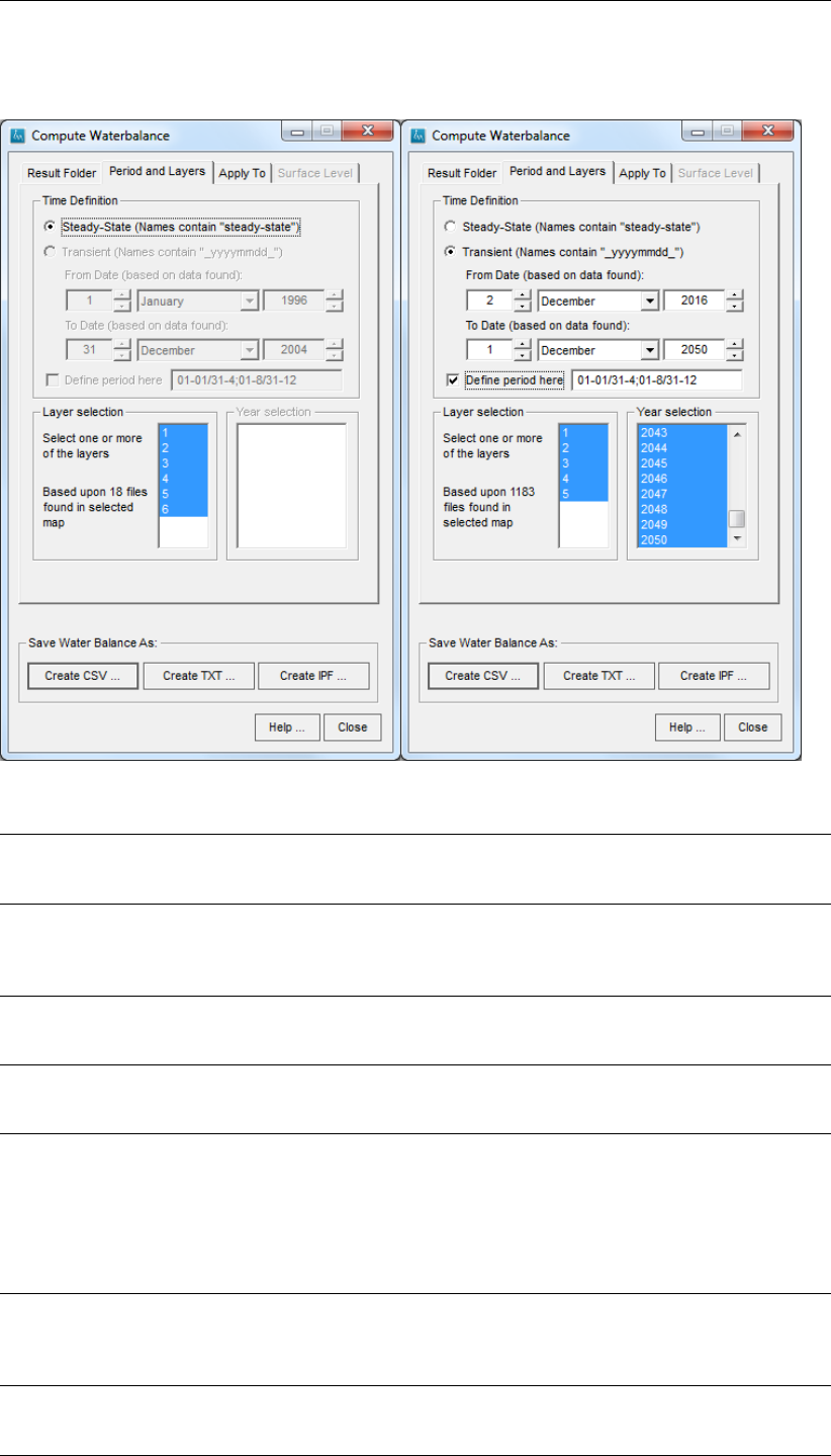
DRAFT
iMOD, User Manual
Compute Water Balance window, Period and Layers tab (left) for a steady-state configuration
and (right) for a transient configuration:
Steady-State Click this radio button to use files only that contain the keyword steady-state,
e.g. BDGFLF_STEADY-STATE_L1.IDF. This option is only available whenever
these files can be found in the result folder selected on the Result Folder tab.
Transient Click this radio button to use files only that contain date information (YYYYM-
MDD), e.g. BDGFLF_20111231_L1.IDF. This option is only available when-
ever these files can be found in the result folder selected on the Result Folder
tab.
From Date: Specify the start date (day, month and year) from which the water balance
needs to be computed. It has been on default filled in with the earliest result
file that could be found in the result folder selected in the Result Folder tab.
To Date: Specify the end date (day, month and year) to which the water balance need
to be computed. It has been on default filled in with the earliest result file that
could be found in the result folder selected in the Result Folder tab.
Define Period
here:
Enter the periods for which the water balance need to be computed solely.
Each period consist of two dates delimited by a slash, e.g. dd-mm/dd-mm.
In-between periods, use the “;” as a delimited. The convention is as follows:
01-01/31-4:
Periods starts on the first of January and ends after the 31stof April
01-8/31-12:
Periods starts on the first of August and ends after the 31stof December
Select one or
more of the layers
Select one or more of the listed model layers. This content of the list box is
based on the BDG*-files that are found in the selected result folder on the
Result folder tab. Use the Ctrl-left mouse button to exclude or add individual
layers, otherwise drag the mouse cursor to select layers.
Year selection Select one or more of the listed years. The content of the list box is based on
the bdg*-files that are found in the selected result folder on the Result folder
tab.
394 of 812 Deltares
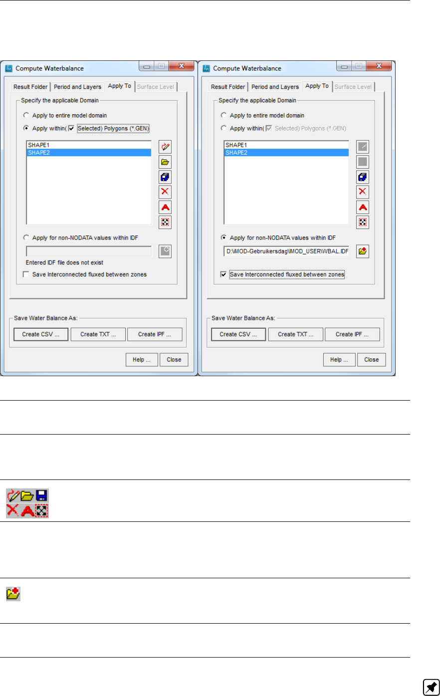
DRAFT
Toolbox Menu Options
Compute Waterbalance window, Apply To tab for (left) applied to selected shapes only or (right) for all
non-NoDataValues within a selected IDF-file:
Apply to entire
model domain
Select this option to compute all budget terms for the entire model extent. In
fact this will be that area and dimension as described by the first BDG*.IDF to
be read.
Apply within
(Selected) Poly-
gons (*.GEN)
Select this option to specify regions of interests by polygons. By default all
polygons will be used for the water balance, however, if the option Selected is
selected, only those polygons will be used that are currently selected, in the
example above, this is polygon SHAPE2.
Click these buttons to draw, open, save, delete or rename a shape. More
detailed information can be found in section 4.2 (Create a GEN-file).
Apply for non-
NODATA values
within IDF
Select this option to use an IDF-file that describes the area of interest by its
non-NoDataValue. For those locations of the first BDG*.IDF or MSW*.IDF
read, the value within this IDF-file will be read and evaluated. A non existing
IDF file name will outgrey the Create CSV . . . ,Create TXT . . . and Create
IPF . . . button.
Open IDF-file
Click this button to open an IDF-file. The selected file will be displayed, how-
ever, an IDF-file can be entered in the string field alternatively. If the IDF-file
does not exists, the Apply button will grey out.
Save Intercon-
nected fluxed
between zones
Select this option to generate interconnected flux between the zones. This
option is only valid whenever the flux terms BDGFRF and BDGFFF are active.
Note: After a computation for a water balance, iMOD will save an IDF-file at the location where you’ve
saved the output file via Create CSV ;Create TXT ;Create IPF. This IDF files contains the location
of the raster cells for each zone. Inspection of this file can lead to adjustment of the polygons used,
Deltares 395 of 812
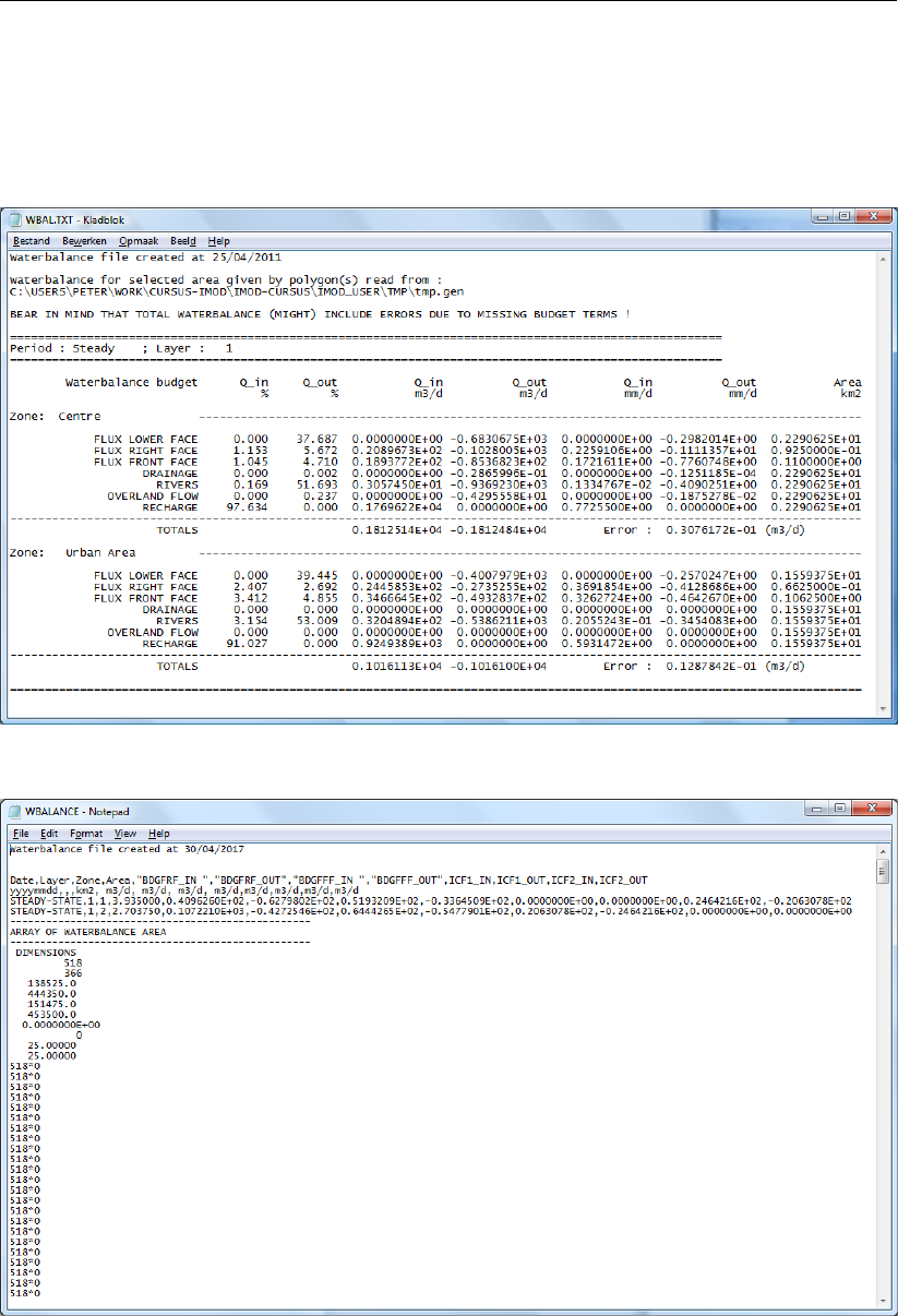
DRAFT
iMOD, User Manual
and/or reuse this particular IDF file for different model scenarios. Remember that in case of overlap in
polygons, the value of the zone in the IDF-file becomes negative, so zone 1 might appear as -1. This
doesn’t affect the computation of the water balance volumes but has a purpose for finding overlap only.
Example of “table” layout of the water balance:
Example of a “time serie” layout of the water balance:
396 of 812 Deltares
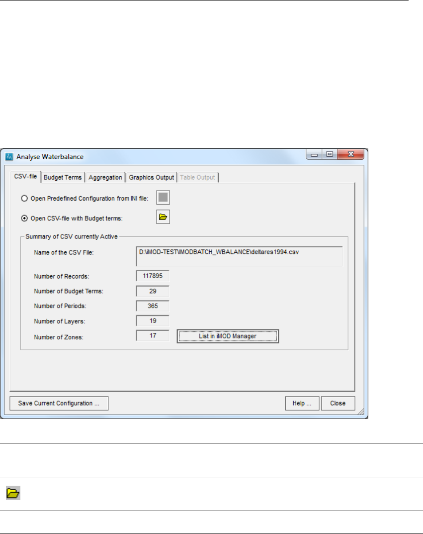
DRAFT
Toolbox Menu Options
7.16.2 Analyse Waterbalance
To analyse the results of a water balance computation, select the option Toolbox from the main menu,
choose Water Balance and then choose Analyse Waterbalance to open the Analyse Waterbalance
window. The key thought is that a CSV file is read in first and after that several selection can be
made by the different tab on the window. Finally an output can be defined, this can be a schematic
representation of the water balance, a time series, a table and/or spatial patterns of water balance
term saved in IDF files.
Analyse Waterbalance window, CSV-file tab:
Open Predefined
Configuration
from INI file:
Select this radio button to select an INI file that contains a particular set of config-
uration parameters.
Select INI file
Click this button to select an INI file from a folder. iMOD will read the configuration
and read the CSV file defined in te INI file.
Open CSV-file
with Budget terms:
Select this radio button to select a CSV that contains the budget terms for a
particular set, default configuration parameters will be applied.
Deltares 397 of 812
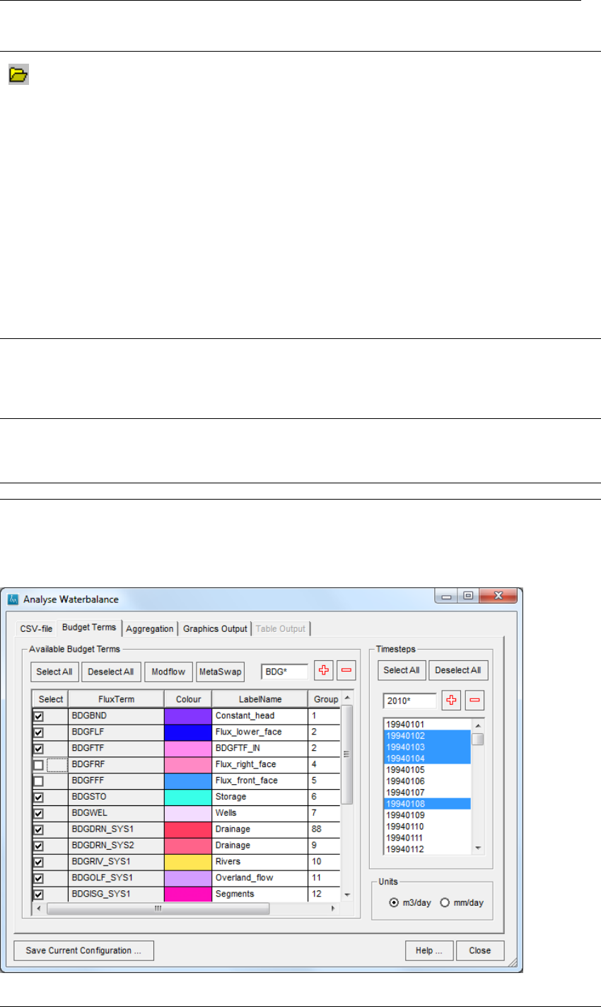
DRAFT
iMOD, User Manual
Select CSV file
Click this button to select a CSV-file from a folder on disk. iMOD will read the CSV
completely and stores the content in memory to perform adequate and efficient
selection as defined by the other tabs. The content of the CSV file will be listed
as:
Name of the CSV file: This is the name of the read CSV file;
Number of records: This is the number of entry records, it is a multiplication
of the number of periods, zones and layers;
Number of Budget Terms: This is the number of budget terms, this can include
the interconnected flow as separate entries;
Number of Periods: This the number of periods, time series can be con-
structed whenever this is large than 1;
Number of Layers: This is the number of model layers that exists in the CSV
file;
Number of Zones: This is the number of zones
All the above mentioned separate quantities can be selected, aggregated and
displayed by setting the appropriate selection criteria in the following tabs.
List in iMOD Man-
ager
Click this button to export the zones as defined in the CSV file into an IDF file
({IMOD_USER} \TMP \WATERBALANCE.IDF) and listed in the iMOD Manager
for viewing options, this is the only way to get the zones stored in the CSV out to
re-use them and/or select the appropriate zones once the original GEN- or IDF
file has been deleted.
Save Current Con-
figuration:
Click this button to save the current configuration (the name of the CSV and the
corresponding selection and settings, including changed colours to a INI file. This
INI file can be loaded by the Open Predefined Configuration from INI file: and/or
used in the iMOD Batch function WBALANCE, see section 8.9.2.
Help. . . Click this button to start the HELP functionality
Close Click this button to close the Analyse Waterbalance window
Analyse Waterbalance window, Budget Terms tab:
398 of 812 Deltares
DRAFT
Toolbox Menu Options
Select All Click this button to select all budget items in the table (first column) and/or select
all the available periods in the list of Timesteps.
Deselect All Click this button to deselect all budget items in the table (first column) and/or
deselect all the available periods in the list of Timesteps.
Modflow Click this button to select all specific iMODFLOW budget terms.
MetaSwap Click this button to select all specific MetaSwap budget terms.
BDG*
2010*
Enter a search string to select or deselect budget terms (second column in the
table FluxTerm) and/or select Timesteps. The search string is case sensitive
and contain wildcards such as * and question marks to notate a fixed number of
character, such as 2010??01.
Increase Selection
Click this button to increase the current selection for budget terms in the table
with Available Budget Terms and/or periods in the list of available Timesteps.
Decrease Selection
Click this button to decrease the current selection for budget terms in the table
with Available Budget Terms and/or periods in the list of available Timesteps.
Units Select one of the options to define the units in the water balance. If the option
m3day is selected no conversion is applied, whenever the option mmday is cho-
sen, the budget volumes will be divided by the area of the corresponding zone
and multiplied with 1000.
Available Budget
Terms
The table gives all existing budget terms in the current read CSV file. The follow-
ing columns are defined:
Select: This column activates and deactivates a individual budget to more
included or excluded in the presentation of a water balance;
FluxTerm: This is a non-editable column with predefined labels for the budget
terms. This is used by iMOD to be able to assign the appropriate budget
terms to specific entries for the graphical representation that can be chosen
on tab4;
Colour: The colour for each row in the table is used to colour the bar in the
time series graph. To change the colour, select the appropriate cell and the
standard colour picking window appears in which it is possible to select a
colour, see section 2.8;
LabelName: Enter a name for each budget term that will be used in the output
of the waterbalance, it will be used as a legend name in the time series and
as a name in the graphical representation of the water balance. iMOD fills in
a default for each distinguished budget term;
Group: This column is filled in with a group number. By default the groups
are unique numbers starting from 1 to the number of budget terms in the CSV
file. The use of this group number is twofold:
The group number is used to group budget terms into a single entry for
the time series. So whenever two budget term receive an similar, unique
group number that appear as a single budget term in the output. The
name for the legend of that group will be formed by the first entry of a
budget term that belongs to that group. Any number can be entered as
a group number, zero is sustained as a group number as well. In the
example on the figure above, the budget terms BDGFLF and BDGFTF
are grouped together as group number 2;
The value of the group number defines the order in which budget terms
are plotted in the time series. The appearance of the time series might
change significantly by changing the group numbers. In the example on
the figure above the budget term BDGDRN_SYS1 is plotted at last since
its group number is 88 and the highest value compared to the others.
Deltares 399 of 812
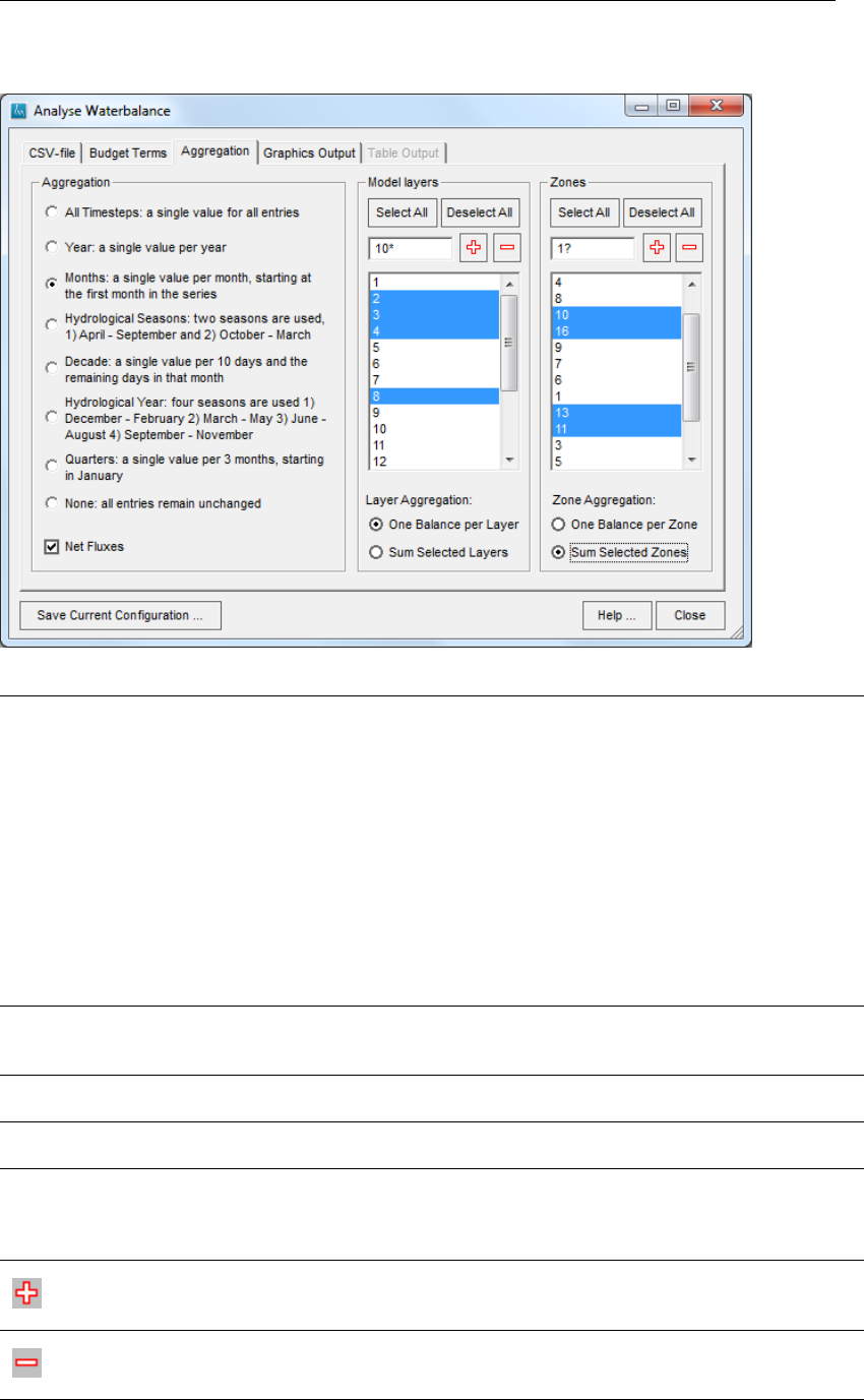
DRAFT
iMOD, User Manual
Analyse Waterbalance window, Aggregation tab:
Aggregation Select one of the following options to aggrate the water balance for the period as
selected on tab 2:
All Time steps: a single value for all entries
Year: a single value per year
Months: a single value per month, starting at the first month in the series
Hydrological Seasons: two seasons are used, 1) April - September and 2)
October - March
Decade: a single value per 10 days and the remaining days in that month
Hydrological Year: four seasons are used 1) December - February 2) March
- May 3) June - August 4) September - November
Quarters: a single value per 3 months, starting in January
None: all entries remain unchanged.
Net fluxes Select this option to compute net fluxes. In that case iMOD will compute a total
net flux for all selected budget terms, each budget terms receives in that particular
case a single net (sum of the in- and outflow) entry in the water balance
Select All Click this button to select all model layers in the list of available Model layers
and/or select all the available zones in the list of Zones.
Deselect All Click this button to deselect all model layers in the list of available Model layers
and/or select all the available zones in the list of Zones.
10*
1?
Enter a search string to select or deselect budget terms (second column in the
table FluxTerm) and/or select Timesteps. The search string is case sensitive
and contain wildcards such as * and question marks to notate a fixed number of
character, such as 1?.
Increase Selection
Click this button to increase the current selection for model layers in the list of
available Model Layers and/or zones in the list of available Zones.
Decrease Selection
Click this button to deecrease the current selection for model layers in the list of
available Model Layers and/or zones in the list of available Zones.
400 of 812 Deltares
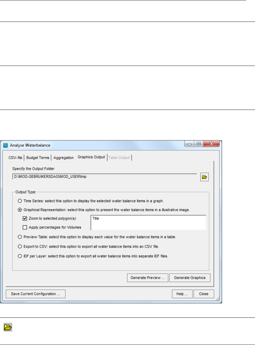
DRAFT
Toolbox Menu Options
Layer aggregation Select one of the following options:
One Balance per Layer: Select this option to treat budget terms as separate
items in the selected form for output;
Sum Selected Layers: Select this option to aggregate budget terms for se-
lected model layers.
Zone aggregation Select one of the following options:
One Balance per Zone: Select this option to treat budget terms as separate
items in the selected form for output;
Sum Selected Zones: Select this option to aggregate budget terms for se-
lected zones.
Analyse Waterbalance window, Graphics Output tab:
Select Folder
Click this button to select a folder that iMOD will uses to save images if needed.
It depends on the choice of the Output Type whether this is applicable. By default
iMOD will save the images in the TMP folder of the {IMOD_USER} folder.
Deltares 401 of 812
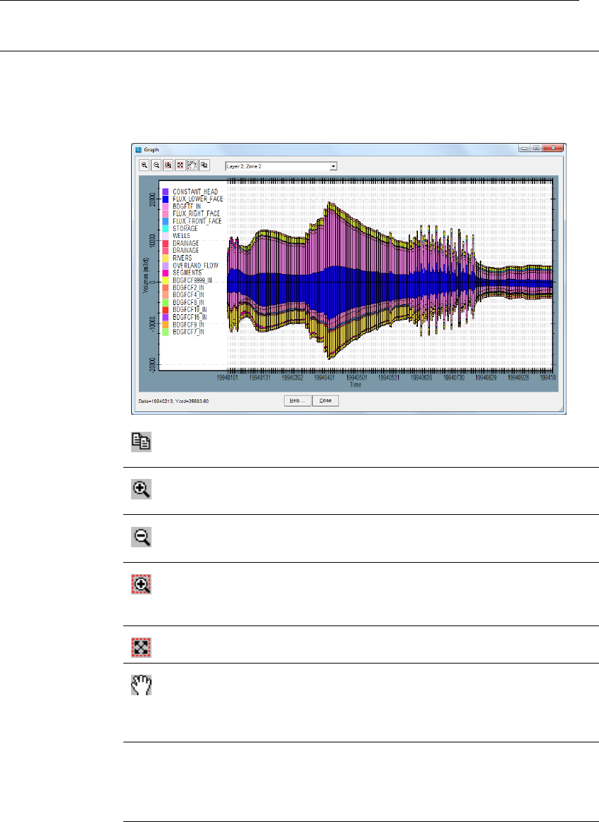
DRAFT
iMOD, User Manual
Output Type Select one of the following output options:
Time Series: Select this option to display the selected water balance items in
a graph. Below is an example of the time series.
Example of the water balance time series
Copy
Click this icon to copy the entire content of the graphical area onto the
Clipboard of Windows.
ZoomIn
Click this icon to zoom IN on the centre of the current graphical dimen-
sions.
ZoomOut
Click this icon to zoom OUT on the centre of the current graphical di-
mensions.
ZoomRectangle
Click this icon to zoom in for a rectangle to be drawn. Use your left-
mouse button to determine the lower-left corner of the rectangle, click
again for the upper-right corner (or vice-versa).
ZoomFull
Click this icon to zoom in on the entire extent of the time series.
Move
Click this icon to move the current display. Click the left-mouse button
on that location where you want to move from, repeat this after the
display has been refreshed (automatically). Use the right mouse button
to stop the moving process.
Layer
2;
Zone
2
This dropdown menu displays all possible combination in between se-
lected model layers and selected zone, in case no aggregation is se-
lected for both of those entries. If a single model layer and a single
zone is selected, or they are both aggregated, the dropdown menu will
not appear.
402 of 812 Deltares
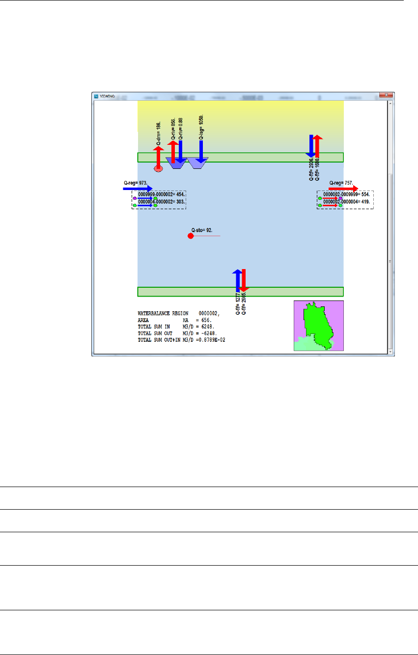
DRAFT
Toolbox Menu Options
Graphical Representation: Select this option to present the water balance
items in a illustrative image. Below is an example of the time series.
Example of the water balance as an illustrative image
Preview Table: Select this option to display each value for the water balance
items in a table, see the explanation given at the following section;
Export to CSV: select this option to export all water balance items into an
CSV file;
IDF per Layer: Select this option to export all water balance items into sepa-
rate IDF files. This yields a single IDF per budget term, per model layer and
per period as selected. Any aggregation will decrease the number of output
combinations. The name of each IDF file is constructed automatically and
includes the budget term, the period, model layer.
Zoom to Selected
Polygon(s)
Select this option to create an overview image on the graphical representation
graph whereby the area is zoomed in on the selected polygon(s).
Apply percent-
ages for Volumes
Select this option to compute percentages for each waterbalance entry in the
graphical representation graph.
Title Specify the title of the graphical representation graph. The title will automatically
wrap over two line of the number of characters excceds the number for a single
line. The maximum of characters is 256.
Generate Preview
Generate Table
Click this button to generate a preview of the selected Output Type. Not all of the
output types support a preview, this button will be out greyed for those situations.
Whenever the Generate Table is active, the tab Table Output becomes accessible
and display a table form of the results of the water balance.
Generate Graph-
ics
Export CSV File
Export IDF File
Click this button to generate an image to be saved on disc. In this case the output
folder as specified by Output Folder is applied. Not all of the output types support
a preview, this button will be out greyed for those situations.
Deltares 403 of 812
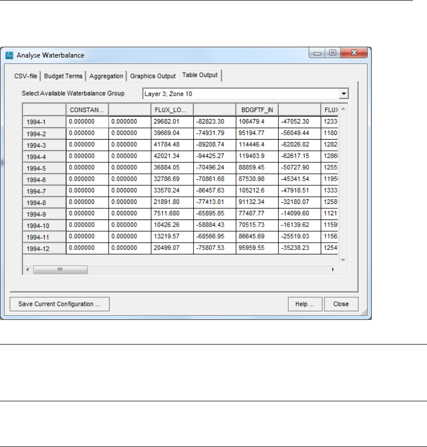
DRAFT
iMOD, User Manual
Analyse Waterbalance window, Table Output tab:
Select Available
Waterbalance
Group
Select from the dropdown the appropriate combination of selected model layers
and/or zones. This dropdown menu displays all possible combination in between
selected model layers and selected zone, in case no aggregation is selected for
both of those entries. If a single model layer and a single zone is selected, or they
are both aggregated, the drop down menu will not appear.
Table The entries in the table are the results of any configuration settings applied in
the previous tabs. Each row is a period and depend on the Aggregation type
as selected on tab3. It is possible to copy the content of the entire table to the
clipboard by the using the option Crtl-C.
404 of 812 Deltares

DRAFT
Toolbox Menu Options
7.17 Compute Mean Groundwaterfluctuations (GxG)
WHY?
Groundwater fluctuations are indicative for the seasonal dry or wet status of an area. The so-called
GxG’s are indicative of the high and low phreatic groundwater levels occurring in a period of at least 8
years. The GxG’s are used frequently in the Netherlands when defining the geohydrological conditions
of an area.
WHAT?
The GxG’s consist of:
1 GHG (‘gemiddeld hoogste grondwaterstand’ / average highest groundwater level) is calculated as
the average of the three highest groundwater levels (measured or simulated around every two
weeks) per hydrological year (1 April – 31 March) averaged over at least eight consecutive years.
2 GLG (‘gemiddeld laagste grondwaterstand’ / average lowest groundwater level) is calculated as the
average of the three lowest groundwater levels (measured or simulated around every two weeks)
per hydrological year (1 April – 31 March) averaged over at least eight consecutive years.
3 GVG (‘gemiddelde voorjaars grondwaterstand’ / average spring groundwater level) is calculated as
the average groundwater level of the 14th of March, the 28th of March and the 14th of April and
again averaged over at least eight consecutive years.
In general GXG’s are expressed as groundwater depths below the land surface.
HOW?
Select the option Toolbox from the main menu and then choose Compute GxG to open the Compute
GxG’s window.
This function is not described separately. The functionalities of the Compute GXG’s window are very
similar to the Compute Waterbalance window (see section 7.16.1). The GXG’s are calculated based
on the output of a transient groundwater model.
Deltares 405 of 812
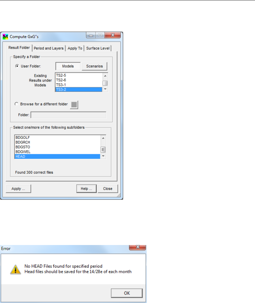
DRAFT
iMOD, User Manual
Compute GxG’s window, Result Folder tab:
The computation of the GxG’s will be executed using model results from the 14th and 28th of each
month. The system will generate an error when there are no files found for these dates. The filenames
will have to be head_yyyymm14.IDF or head_yyyymm28.IDF.
406 of 812 Deltares

DRAFT
Toolbox Menu Options
7.18 Compute Mean Values
WHY?
The Mean Values of budgets or heads are calculated based on the output of a transient groundwater
model.
WHAT?
A new IDF is created containing the mean values.
HOW?
Select the option Toolbox from the main menu and then choose Compute Mean Values to open the
Compute Mean Values window.
This function is not described separately. The functionalities of the Compute Mean Values window are
very similar to the Compute Waterbalance window (see section 7.16.1).
Deltares 407 of 812
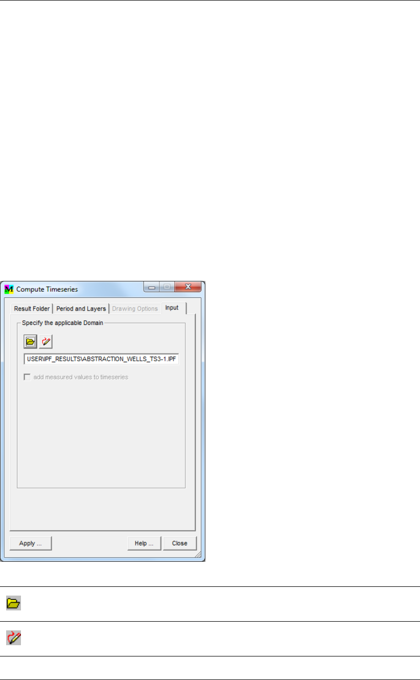
DRAFT
iMOD, User Manual
7.19 Compute Timeseries
WHY?
The time-dependent results of a transient model are converted to timeseries for specified locations,
e.g. at boreholes. The variation in time of the head (and of the budget-terms if desired) can be viewed
in a graph and is available for processing outside iMOD.
WHAT?
The Compute Timeseries option checks the available model output of the selected model and reads
the IDF-files at locations read from an IPF-file or defined interactively on the map. The result is stored
in an IPF-file which can be viewed in iMOD.
The functionalities of the Compute Timeseries window are very similar to the Compute Waterbalance
window (see section 7.16.1). Only the specific functions in the Input tab of theCompute Timeseries
window are described here.
HOW?
Select the option Toolbox from the main menu and then choose Compute Timeseries to open the
Compute Timeseries window.
Compute Timeseries window, Input tab:
Open
Click this button to open an IPF-file, see section 9.7 for more details. The IPF-file
contains the locations where the time-series are generated.
Draw
Click this button to start drawing the point locations on the map by clicking the left
mouse button. Stop using the right mouse button and save the points in an IPF-file.
Apply Click this button to start the computation of the time series. You should enter a name
for the resulting IPF-file.
408 of 812 Deltares

DRAFT
8 iMOD Batch functions
8.1 General introduction
This chapter contains a detailed description of a library of tools or functions that is available in iMOD-
Batch mode.
8.1.1 What is an iMOD Batch Function?
An iMOD Function in general is a procedure to perform a specific task in iMOD or on iMOD files
returning a new file or a series of files. Functions can be found on many places in the menu structure
of the iMOD Graphical User Interface (GUI). For instance functions to:
create, edit or analyse files (IDF, IPF ect).
run processes like iMODFLOW and iMODPATH.
post process modelresults (waterbalance, timeseries or plots).
An iMOD Batch Function can be used outside the iMOD GUI and its operation is controlled by param-
eters in an *.INI file, the initialization file.
Below you find an example of the content of a PLOT.INI file. It describes the keywords and parameters
for the Function PLOT, for plotting IDF or IPF files to a PNG file.
FUNCTION=PLOT
IDFFILE=D:\DATA\AHN.IDF
GENFILE=D:\DATA\PROV.GEN
OUTFILE=D:\DATA\PLOT.PNG
In general an *.INI file contains keywords some of which are compulsory (e.g. the Function name),
others are optional. iMOD searches for the keywords in the entire file so there is no fixed order of
keywords allowing you to insert white lines and remarks. Examples of the set up of such an *.INI file
for all available iMOD Batch function is given in the following paragraphs.
The advantage of using the iMOD Batch mode instead of the iMOD Graphical User Interface (GUI) is
manifold:
it saves time when iMOD functions must be performed on many files or many times.
the total set of *.INI files in a project can be seen as a logbook of your pre- and post-processing
activities.
minor changes to a function are easily applied by editing the *.INI file.
*.INI files are easily shared with colleagues or clients.
over time the *.INI files form a library, easy to re-use.
you don’t need to click around in the GUI and repeatedly type file names.
The number of functions in iMOD Batch mode is expected to grow gradually. Not all functions in the
iMOD GUI are (yet) available in iMOD Batch mode (e.g. create IDF from scratch). On the other hand,
some functions are available in iMOD Batch mode but not in the GUI (e.g. Modelcopy).
Deltares 409 of 812
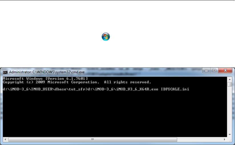
DRAFT
iMOD, User Manual
8.1.2 How to run an iMOD Batch Function?
To start an iMOD Batch procedure first open a Dos command window. How? Search for ’CMD’ in ’All
Programs’ under the Windows start button ). In that DOS window, simply enter the name of the
iMOD executable followed by the name of the *.INI file, e.g. "iMOD_V4_3_X64R.exe IDFSCALE.INI",
(see Figure 8.1) and press Enter. The program will stop after the function, described by the *.INI file,
is executed.
Figure 8.1: Example of command in DOS box to run an iMOD Batch script.
An iMOD batch function can also be started from the maim menu. See section 4.6 for an explanation.
8.1.3 Using DOS scripting (*.BAT file) to organize iMOD Batch Functions
The iMOD Batch functions can be used as described above, however, to introduce more options these
functions can also be controlled in a DOS Batch file (*.BAT) using DOS scripting. Of course you can
use your favourite scripting languages (e.g. Python or Matlab) to create and execute any iMOD Batch
*.INI file.
This is an example of a *.BAT file creating (line 1-4) and executing (line 5) the PLOT.INI file:
ECHO FUNCTION=PLOT >PLOT.INI
ECHO IDFFILE=D:\DATA\AHN.IDF >> PLOT.INI
ECHO GENFILE=D:\DATA\PROV.GEN >> PLOT.INI
ECHO OUTFILE=D:\DATA\PLOT.PNG >> PLOT.INI
iMOD_V4_3_X64R.exe PLOT.INI
A *.BAT file is recognized in Windows as a Dos script and starts running by double clicking the *.BAT
file.
8.1.4 Examples of advanced DOS scripting options
Advanced DOS scripting options enables you to make more complex use of iMOD Batch functions.
This paragraph gives you some examples of advances options. On the internet there are plenty sites
available giving basic or advanced DOS scripting tips and tricks in more detail (e.g. http://www.
robvanderwoude.com/batchcommands.php).
With the installation of iMOD an example of a *.BAT file is copied to the Tutorial folder. Search for
..\TUTORIALS \TUT_Map_Analyse \SubsoilSystem \iMOD-Batch-example-IDFCALC.BAT. Open the
file, read some tips and tricks, double click and experience that this iMOD Batch function calculates
the thickness of a series of 6 aquifers.
Below we describe some examples of advanced DOS scripting options.
A (nested) loop over a list of Text elements
Not more than 6 lines in the next example are necessary to create and run the iMOD Batch Func-
tion PLOT producing 12 PNG files showing the HEAD for the first 4 month of 3 successive years.
410 of 812 Deltares

DRAFT
iMOD Batch functions
FOR %%A IN (1994,1995,1996) DO (
FOR %%B IN (01,02,03,04) DO (
ECHO FUNCTION=PLOT >PLOT.INI
ECHO IDFFILE=D:\MODEL\HEAD\HEAD_%%A%%B01_L1.IDF >> PLOT.INI
ECHO OUTFILE=D:\MODEL\HEAD\HEAD_%%A%%B01_L1.PNG >> PLOT.INI
iMOD_V4_3_X64R.exe PLOT.INI))
A loop over a series of Numbers
The next example of a FOR loop (including Command Extension /L) gives you the variable %%A
between 1 upto 18 with steps of 2.
FOR /L %%A IN (1,2,18) DO (
ECHO %%A)
)
Using specific files from a folder
The next DOS script gives you the variable %%A for all IDF-files found in the folder D:\IMOD-
MODEL\DBASE. Usage of ˜n gives you the filenames only without extension.
SET DIR=D:\IMOD-MODEL\DBASE
FOR %%A IN (%DIR%\*.IDF) DO (
ECHO %DIR%\%%˜nA.IDF
ECHO %%A
)
Introduce an arithmetic operator within a loop
Adding a looping parameter %%b might be interesting whenever computing the thickness of aquitards
since each time you need to subtract the bottom of modellayer 1 minus the top of modellayer 2.
SETLOCAL ENABLEDELAYEDEXPANSION
SET /A B=1
FOR /L %%C IN (1,1,18) DO (
SET /A B=B+1
ECHO FUNCTION=IDFCALC >IDFCALC.INI
ECHO FUNC=C=A-B >> IDFCALC.INI
ECHO NREPEAT=1 >> IDFCALC.INI
ECHO ABC1=BOT%%C.IDF TOP!B!.IDF TAQT%%C.IDF >> IDFCALC.INI
iMOD_V4_3_X64R.exe IDFCALC.INI
)
Notice that the variable B is used by bracketing it by “!” and the variable C is used by adding “%%”
in front. The statement SETLOCAL ENABLEDELAYEDEXPANSION is necessary to delay the in-
terpretation of the variable B.
include IF-THEN-ELSE statements
It is often handy to include and if-then-else statement inside the batch structure, for example when-
ever you might want the generate a runfile for iMODPATH (see section 8.6.6). Unfortunately, the
MS-DOS IF statement does not support logical operators (AND and OR) so we have to find other
ways.
In the example below we only write a budget term whenever it is not equal to the BDGFLF (flow-
lower-face) and the layer number is not equal to the lowest one (5).
SETLOCAL ENABLEDELAYEDEXPANSION
FOR /L %%A IN (1,1,5) DO (
FOR %%B IN (FFF,FRF,FLF) DO (
SET /A Flag=0
IF %%B==FLF SET /A Flag=Flag + 1
IF %%A==5 SET /A Flag=Flag + 1
IF !Flag! NEQ 2 (
ECHO ..\BDG%%B\BDG%%B_STEADY-STATE_L%%A.IDF >> IMODPATH.INI)
Deltares 411 of 812

DRAFT
iMOD, User Manual
))
If an OR-statement need to be applied, do as follows:
SETLOCAL ENABLEDELAYEDEXPANSION
FOR /L %%A IN (1,1,5) DO (
FOR %%B IN (FFF,FRF,FLF) DO (
SET res=F
IF %%B==FLF SET res=T
IF %%B==FRF SET res=T
IF !res!==T (
ECHO ..\BDG%%B\BDG%%B_STEADY-STATE_L%%A.IDF >> IMODPATH.INI)
))
Compare operators in DOS
Use the following compare operators:
EQU - equal
NEQ - not equal
LSS - less than
LEQ - less than or equal
GTR - greater than
GEQ - greater than or equal
The following syntax is than valid:
FOR /L %%A IN (1,1,10) DO (
IF %%A LSS 6 (ECHO value %%A is less than 6
) ELSE IF %%A GTR 6 (ECHO value %%A is greater than 6
) ELSE (ECHO value %%A is equal to 6
))
Start execute process within a DOS script
Finally the iMOD executable can be started in different ways with different behavior. Any *.INI can
be started with:
FOR %%A IN (1,2) DO (
iMOD_V4_3_X64R.exe {}.INI
)
however this will block the batch (*.BAT) structure that starts it until the process is ended. Below
an example is given that starts iMOD and continues the batch and starts another iMOD session in
another command-window.
FOR %%A IN (1,2) DO (
START iMOD_V4_3_X64R.exe {}.INI)
Batch array definition
In addition to the described batch looping commands, it is also possible to define arrays within the
batch environment. This might be helpful in case e.g. there are multiple files with different filenames
that can be divided into a number of subgroups and that need to be processed in a similar way. For
example:
setlocal EnableDelayedExpansion
set n=0
for %%a in (KHV, KVV) do (
set var[!n!]=%%a
set /A n+=1
) for /L %%i in (0,1,1) do (
for /L %%j in (1,1,12) do (
echo FUNCTION=IDFCALC > calc_idf.ini
echo FUNC= "C=A*B" » calc_idf.ini
echo NREPEAT=1 » calc_idf.ini
412 of 812 Deltares

DRAFT
iMOD Batch functions
echo ABC1= "d:\MODEL\Factor.IDF" "d:\MODEL\DATA\!var[%%i]!_L%%j.idf"
"d:\MODEL\DATA\!var[%%i]!_L%%j_factor.idf" » calc_idf.ini
d:\iMOD_versies\iMOD_v3.3\iMOD_V4_3_X64R.exe calc_idf.ini
))
In this example two type of files can be distinguished, files with 1. "KHV" and 2. "KVV" information.
Each file category contains 12 files; one for each layer. All files need to be multiplied by specific factor
grid, saved in Factor.idf. With the outer loop the file category is controlled and with the second loop
the layers per category. Array definition can be applied to multiple cases and serve as a helpful tool to
shorten your batch-scripts.
The iMOD Batch function are categorized into several topics related to IDF, IPF, ISG and GEN files and
described on the following pages.
Deltares 413 of 812

DRAFT
iMOD, User Manual
8.2 IDF-FUNCTIONS
8.2.1 IDFCALC-Function
The IDFCALC function can be used to carry out simple arithmetical operations on maximal two different
IDF-files to create a new IDF-file. See for more information section 6.7.3.
FUNCTION= IDFCALC
FUNC= Enter the function, e.g. C=A-B or C=ABS(A-3.0*B), or C=A, see section 6.7.3
for more information. Whenever the symbol “/” is used, apply quotes, thus
“C=A/B”.
ABC{i}= Enter the ith out of NREPEAT IDF-filenames that corresponds with “A”, “B”
and “C” in the function FUNC.
AC{i}= Enter the ith out of NREPEAT IDF-filename that corresponds with “A” and “C”
in the function FUNC.
BC{i}= Enter the ith out of NREPEAT IDF-filename that corresponds with “B” and “C”
in the function FUNC.
NREPEAT= Specify the number of times the function FUNC need to be carried out.
SOURCEDIRA= Enter a folder that contains all the IDF-files associated to the “A” in FUNC.
Apply this keyword whenever NREPEAT is absent.
SOURCEDIRB= Enter a folder that contains all the IDF-files associated to the “B” in FUNC.
Apply this keyword whenever NREPEAT is absent.
SOURCEDIRC= Enter a folder that contains all the IDF-files associated to the “C” in FUNC.
Apply this keyword whenever NREPEAT is absent.
USENODATA= Enter USENODATA=1 to use cells that have NoDataValues. By default,
USENODATA=0, so those cells that have NoDataValue will be ignored.
NODATAVALUE Enter the value for the NoDataValue to be used in the computation, e.g. NO-
DATAVALUE=0.0. This keyword is compulsory whenever USENODATA=1.
GENFILE= Enter the name of a GEN-file, e.g. GENFILE=D:\DATA\AREA.GEN. Any com-
putation will be carried out inside the polygons of the GENFILE. On default,
GENFILE=’ ’, which means that no genfile will be used.
IEQUI= Enter IEQUI=0 to construct (if needed) a non-equidistant IDF-file that counts
for all raster dimensions of the entered IDF-files, this is the default. Enter
IEQUI=1 to force that the resulting IDF-files are produced with equidistant
cellspaces, based on the smallest cell size occurring in the IDF-files “A” and/or
“B”.
WINDOW= Enter the coordinates of the window that need to be computed, solely. Enter
coordinates of the lower-left corner first and then the coordinates of the upper-
right corner, e.g. WINDOW=100000.0, 400000.0, 200000.0, 425000.0. When
WINDOW=is absent, the entire dimensions of the first mentioned IDF-file will
be used.
TRIM_VALUE= Enter a value to be able to ignore all result values smaller than this spe-
cific absolute value after the calculation. This option gives values smaller
than given/entered absolute value a NodataValue, e.g. C=A-B if C<0.1
C=NodataValue.
Example 1
FUNCTION=IDFCALC
FUNC= “C=A/B”
NREPEAT=2
ABC1=D:\KD_L1.IDF D:\THICKNESS_L1.IDF D:\K_L1.IDF
ABC2=D:\KD_L4.IDF D:\THICKNESS_L4.IDF D:\K_L4.IDF
The above mentioned example will compute the permeability (k) by dividing the transmissivity (KD) by
the thickness (THICKNESS) for modellayer 1 and modellayer 4, subsequently.
414 of 812 Deltares

DRAFT
iMOD Batch functions
Example 2
FUNCTION=IDFCALC
FUNC= C=A-B
USENODATA=1
NODATAVALUE=0.0
IEQUI=1
GENFILE=D:\AREA.GEN
WINDOW=100000.0,350000.0,150000.0,450000.0
SOURCEDIRA=D:\MODEL\HEAD_*_L1.IDF
SOURCEDIRB=D:\SCENARIO\HEAD_*_L1.IDF
SOURCEDIRC=D:\EFFECT\DIFF_*_L1.IDF
The above mentioned example will compute the differences within the polygon(s) described by the
AREA.GEN and within the given WINDOW. If any NoDataValues are found in the IDF-files, they will be
treated as if they were NODATAVALUE=0.0. Any file that agrees with the filename HEAD_*_L1.IDF in
two different folders, D:\MODEL and D:\SCENARIO will be subtracted and the results will be saved, as
an equidistant IDF, in the folder D:\EFFECT. Suppose HEAD_20101231_L1.IDF is found in D:\MODEL
(SOURCEDIRA), an identical filename is searched for in D:\SCENARIO (SOURCEDIRB). The yielding
IDF will be DIFF_20101231_L1.IDF and will be written in D:\EFFECT.
Example 3: batch-array definition
setlocal EnableDelayedExpansion
set n=0
for %%a in (1.30 0.80 0.70 0.75 0.85 1.25 0.75 0.75 0.85 1.10 1.15 ) do (
set RCH_factor[!n!]=%%a
set /A n+=1
)
setlocal EnableDelayedExpansion
set n=0
for %%a in (1990 1991 1992 1993 1994 1995 1996 1997 1998 1999 2000 2001) do (
set year[!n!]=%%a
set /A n+=1
)
for /L %%i in (0,1,11) do (
echo FUNCTION=IDFCALC > calc_idf.ini
echo !RCH[%%i]!
echo FUNC= "C=!RCH_factor[%%i]!*A" » calc_idf.ini
echo SOURCEDIRA=d:\RCH_grids\RCH_averaged_1990-2001.idf » calc_idf.ini
echo SOURCEDIRC=d:\RCH_grids\RCH_!year[%%i]!.idf » calc_idf.ini
This example uses multiple arrays to end up with one recharge grid per year based on a given recharge
factor.
Deltares 415 of 812

DRAFT
iMOD, User Manual
8.2.2 IDFSCALE-Function
With this function it is possible to (re)scale IDF-files according to different methodologies, see sec-
tion 6.7.3.
FUNCTION= IDFSCALE
SCALESIZE= Enter the cell size of the upscaled or downscaled IDF-file(s), e.g. SCALE-
SIZE=100.0 meaning that the cellsize of the resulting IDF-file(s) will be
100 square meter uniformly.
The keyword SCLTYPE_UP and SCLTYPE_DOWN may be specified both because it is possi-
ble to execute upscaling and downscaling in one action on IDF’s containing different scales. In
case SCLTYPE _UP and/or SCLTYPE_DOWN are not specified than default values are used, for
SCLTYPE _UP: 2 and for SCLTYPE_DOWN: 1.
SCLTYPE_UP Enter the scale type. Choose from the following:
1: boundary scaling (rule: minus values above positive values xabove
zero values);
2: arithmetic scaling (rule: sum n-values xwithin coarse cell, excluding
the NoDataValues, and divide them by n);
3: geometric scaling (rule: take log()-function for n-values xwithin a
coarse cell, excluding NoDataValues and zero values, sum them, divide
them by nand take the exp() function);
4: sum (rule: sum n-values x, excluding NoDataValues);
5: sum conductance (rule: sum n-values times ratio values to calculate
the average conductance over cells for upscaled cell.)
6: inverse (rule: take the inverse (x−1) of n-values xwithin a coarse cell,
excluding NoDataValues and zero values and divide them by n.
7: most frequent occurrence (rule: take that value xthat occurs mostly
within a coarse cell, excluding NoDataValues);
8: sum inverse (rule: take the inverse (x−1) of n-values xwithin a coarse
cell, excluding NoDataValues and zero values);
9: percentile (rule: take the value xthat occurs for a given percentage
within a coarse cell, excluding NoDataValues);
10: block value (rule: takes the center value of the cells that needs to be
upscaled.)
11: Darcian method (rule: take the value xthat occurs after a Darcian sim-
ulation of fine mesh with extent of the coarse cell, excluding NoDataVal-
ues);
12: homogenization (rule: take the value xthat occurs after a Darcian
simulation with periodic boundaries of fine mesh with extent of the coarse
cell, excluding NoDataValues);
13: global-local method (rule: take the value xthat occurs after a Darcian
simulation with realistic boundary conditions of fine mesh with extent of
the coarse cell, excluding NoDataValues);
14: 3d simulations (rule: Calculates with help of a numerical model the
needed initial values of the upscaled model per cell;
15: zonation (rule: Calculates an upscaled value as the most frequent
value for the integer values within the coarse grid cell, and the fraction
as the averaged fraction, while ignoring those cells that do not coin-
cide with the upscaled integer value (e.g. x1=1.5; x2=2.25 and x3=1.4,
means that the most frequent integer is 1, and the average fraction for 1 is
(0.5+0.4+0.0)/3=0.3, so the final value is 1.3).
SCLTYPE_DOWN= Enter the scale type. Choose from the following:
1: interpolation (rule: produces a good guess for al finer gridcells by a lin-
ear interpolation based on the coarse gridcells, excluding the NoDataVal-
ues);
2: gridvalues (rule: assign the value of the coarse gridcell to all finer grid-
cells).
SOURCEIDF Enter the name of the IDF-file to be upscaled or downscaled, e.g. SOUR-
CEIDF=D:\DATA\TRANSMISSIVITY.IDF.
OUTFILE Enter the name of the upscaled or downscaled IDF-files, e.g. OUT-
FILE=D:\DATA\SCALED_TRANSMISSIVITY.IDF.
416 of 812 Deltares

DRAFT
iMOD Batch functions
PERCENTILE= Enter a percentile, e.g. PERCENTILE=0.5 (0.0<PERCENTILE<1.0). This
keyword is obliged whenever SCLTYPE=9.
KMIN= Enter a value that represents the minimal K-value. This value accounts for
the upper- and lower-boundaries of the clay-layer within the voxels.
ILGROUP= Enter a value for the amount of layers that will be taken into account to find
the representative K-value at which a clay-layer begins.
WEIGHFACTOR= Enter a weight factor, e.g. WEIGHFACTOR=0.5. This keyword is op-
tional in case SCLTYPE in {1,3,4,5,6,9}, the default value is WEIGHFAC-
TOR=1.0.
BLOCK= Enter the size of the interpolation block, e.g. BLOCK=16. This keyword is
optional whenever SCLTYPE=-1, meaning that a matrix of 4x4 will be used
for the interpolation of each point. The default value is BLOCK=4 and other
possible values are BLOCK in {4,16,36,64,100). In most situation good
results are obtained with BLOCK=4.
WINDOW=
(optional)
Enter the coordinates of the window that need to be computed, solely.
Enter coordinates of the lower-left corner first and then the coordinates
of the upper-right corner, e.g. WINDOW=100000.0, 400000.0, 200000.0,
425000.0. When WINDOW=is absent, the entire dimensions of the first
mentioned IDF-file will be used.
The following are keywords that are optional in case SCLTYPE=14, solely.
SOURCEDIR= Enter the name of the folder that contains IDF-files that need to be used
for a 3D simulation, e.g. SOURCEDIR=D:\DATA\K*.IDF.
BUFFER= Enter the size of the buffer to be used for the Darcian simulation,
BUFFER=5 (SCLTYPE in {9,10,11,12}). The default value is BUFFER=0.
ANI_X=
ANI_Z=
Enter the horizontal (ANI_X) or vertical (ANI_Z) anisotropy, e.g.
ANI_Z=0.3. This means that the permeability will be 3 time less per-
meable in vertical direction than in horizontal direction. Default value is
ANI_X=ANI_Z=1.0.
DH_X=
DH_Y=
DH_Z=
Enter the pressure for the x, y and z direction to be imposed on the system,
e.g. DH_X=1.0. This means that the hydraulic pressure difference along
the x direction is equal to meter. By default DH_X=DH_Y=DH_Z=0.0.
QRATE= Enter the strength of a extraction well positioned in the lower most model-
layer, e.g. QRATE=-100 m3/day. By default QRATE=0.0, however, in those
case where QRATE<>0.0, DH_X, DH_Y and DH_Z will be ignored.
Enter the permeability to be substituted for those cells that contain No-
DataValues.
AQFR_KD=
Example 1
FUNCTION=IDFSCALE
SCLTYPE_UP=1
SCALESIZE=250.0
SOURCEIDF=D:\DATA\BOUNDARY_L1.IDF
OUTFILE=D:\DATA\BOUNDARY_L1_250.IDF
This example shows how to upscale an IDF-file with boundary conditions.
Example 2
FUNCTION=IDFSCALE
SCLTYPE_DOWN=1
SCALESIZE=5.0
SOURCEIDF=D:\DATA\HEAD_STEADY-STATE_L1.IDF
OUTFILE=D:\DATA\HEAD_STEADY-STATE_L1_5X5.IDF
This example shows how to downscale an IDF-file with computed heads.
Deltares 417 of 812

DRAFT
iMOD, User Manual
Example 3
FUNCTION=IDFSCALE
SCLTYPE_UP=3
SCALESIZE=500.0
WINDOW=100000.0,425000.0,150000.0,500000.0
SOURCEIDF=D:\DATA\HEAD_STEADY-STATE_L1.IDF
OUTFILE=D:\DATA\HEAD_STEADY-STATE_L1_500.IDF
This example shows how to upscale transmissivity for a specific window.
Example 4
FUNCTION=IDFSCALE
SCLTYPE_UP=12
SCALESIZE=100.0
SOURCEDIR=D:\GEOTOP\SEL*.IDF
OUTFILE=D:\GEOTOP\VERTICAL_C.IDF
BUFFER=5
ANI_X=3.0
DHZ=1.0
DHX=0.0
DHY=0.0
This examples show an example how to upscale permeability with a 3D Darcian simulation. The result
will be vertical resistances.
418 of 812 Deltares
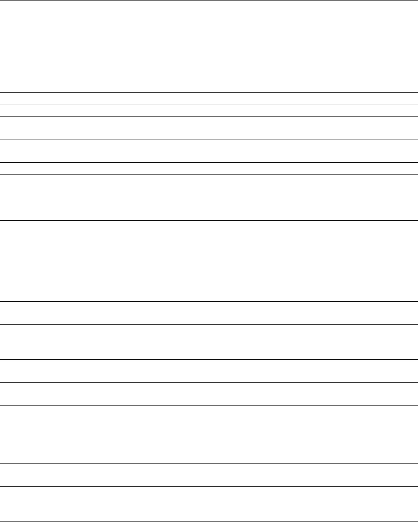
DRAFT
iMOD Batch functions
8.2.3 IDFMEAN-Function
The IDFMEAN function can be used to compute a new IDF-file with the mean value (or minimum,
maximum value) of different IDF-files. It is not necessary to have exactly similar IDF-files (see sec-
tion 6.7.3).
FUNCTION= IDFMEAN
ILAYER= Enter the layer numbers for the IDF-files to be averaged, e.g. ILAYER=1,3.
SDATE= Enter the starting date (yyyymmdd) for which IDF-files are used, e.g.
SDATE=19980201.
EDATE= Enter the ending date (yyyymmdd) for which IDF-files are used, e.g.
EDATE=20111231.
NDIR= Enter the number of folders to be processed repeatedly, e.g. NDIR=10.
SOURCEDIR{i}= Enter the folder and wildcard for all files that need to be used, e.g.
SOURCEDIR1=C:\DATA\HEAD\HEAD*.IDF. Repeat SOURCEDIR{i} for
NDIR times. Do not include year, month or day before or after the wild-
card *.
CFUNC= Specify the name of the function to be applied. Choose out of:
MEAN, to compute mean values (equal weighed);
MIN to compute the minimum values;
MAX to compute the maximum values.
SUM to compute the sum of the values per grid cell;
PERC to compute the median value (50 percentile).
The default is CFUNC=MEAN.
PERCVALUE= Specify a percentile whenever CFUNC=PERC, e.g. PERCVALUE=50.0 for
median values.
IYEAR= Specify particular year (within SDATE and EDATE) to be used exclusively,
e.g. 2001,2003,2005. IYEAR is filled in for all years in-between SYEAR
and EYEAR.
NPERIOD= Enter a number of periods to be defined to use IDF-file within these periods
solely, e.g. NPERIOD=2. NPERIOD=0 by default.
PERIOD{i}= Enter a period i (ddmm-ddmm), e.g. PERIOD1=1503-3110 to express the
period 15th of March until the 31th of October.
ISEL= Enter a code for the area to be processed:
ISEL=1 will compute the entire region
ISEL=2 will compute within given polygons;
ISEL=3 will compute for those cells in the given IDF-file that are not equal
to the NoDataValue of that IDF-file.
GENFNAME= Enter a GEN-filename for polygon(s) for which mean values need to be
computed. This keyword is obliged whenever ISEL=2.
IDFNAME= Enter an IDF-file for which mean values will be computed for those cell in
the IDF-file that are not equal to the NoDataValue of that IDF-file. This
keyword is compulsory whenever ISEL=3
Example 1
FUNCTION=IDFMEAN
ILAYER=6
SDATE=19980714
EDATE=20110728
NDIR=1
SOURCEDIR1=D:\DATA\BDGFLF*.IDF
This example shows the mimimum configuration of this function and yield the mean values for all
BDGFLF*.IDF-files in the folder D:\DATA that are assigned to layer 6 (function searches for L6.IDF),
and are within the periode 14th of July 1998 and 28th of July 2011.
The output file will be:
1 D:\DATA\BDGFLF_MEAN_1998-07-14_to_2011-07-28_L6.IDF;
Deltares 419 of 812

DRAFT
iMOD, User Manual
2 D:\DATA\BDGFLF_COUNT_1998-07-14_to_2011-07-28_L6.IDF.
The latter shows the number of occurrences for each raster cell.
Example 2
FUNCTION=IDFMEAN
ILAYER=1,3
SDATE=19980101
EDATE=20000101
IYEAR=1999
NPERIOD=1
PERIOD1=1503-3110
ISEL=2
CFUNC=MAX
GENFILE=D:\DATA\AREA.GEN
NDIR=1
SOURCEDIR1=D:\DATA\HEAD*.IDF
This example shows a more extended configuration and will yield maximum values for all IDF-files
inside the folder D:\DATA that meet the requirement HEAD*.IDF. Furthermore, they contain the key
combination L1.IDF where “1” is defined by ILAY=1. The date expression should be within the time
domain of the 1th of Januari 1998 (SDATE) and 31th of December 2000 (EDATE), within the year 1999
(IYEAR) and within the period between the 15th of March and the 31th of October (PERIOD1). Finally
the mean values is computed within the polygon(s) described by the polygon AREA.GEN, solely. The
output file will be:
1 D:\DATA\HEAD_MAX_19980101-20000101_L1.IDF;
2 D:\DATA\HEAD_DATEMAX_19980101-20000101_L1.IDF.
The latter shows the date (yyyymmdd) on which raster cell maximal values appeared.
420 of 812 Deltares

DRAFT
iMOD Batch functions
8.2.4 IDFCONSISTENCY-Function
Use this function to make IDF-files consistent, meaning that the first IDF is always higher or equal
to the second, which is higher or equal to the top of the IDF underneath, and so on. IDF files can
represent anything, however, this tool is especially handy for consistencies applied on top- and bottom
elevation of model layers.
FUNCTION= IDFCONSISTENCY
NLAY= Enter the number of model layers, e.g. NLAY=6.
TOP_L{i}= Enter the IDF for the ith modellayer that represents the top of modellayer
i, e.g. TOP_L1=D:\INPUT\TOP_L1.IDF. Constant value may be entered as
well, e.g. TOP_L1=10.0.
BOT_L{i}= Enter the IDF for the ith modellayer that represents the bottom of model-
layer i, e.g. BOT_L1=D:\INPUT\BOT_L1.IDF. Constant value may be en-
tered as well, e.g. BOT_L2=-43.12.
OUTPUTFOLDER= Enter the foldername in which the adjusted IDF-files will be saved, e.g.
OUTPUTFOLDER=D:\RESULT. Whenever a file is entered by a constant
value, e.g. TOP_L1=23.32, a file will be created called TOP_L1.IDF that
represents the (corrected) value.
ICLEAN= Enter an option for the cleaning of the IDF files. Whenever ICLEAN=1 the
procedure removes all data in all files whenever at least a single nodata
value is found among them at that specific location, whenever ICLEAN=2,
Removes all data whenever at least a nodata value is found for the first
and second idf file at that specific location. By default ICLEAN=0 which
mean that only consistency corrections are applied for cells not equal to
their nodata values.
WINDOW= Enter the coordinates of the window that needs to be computed. En-
ter coordinates of the lower-left corner first and then the coordinates of
the upper-right corner, e.g. WINDOW=100000.0, 400000.0, 200000.0,
425000.0. When WINDOW=is absent, the entered IDF-files by TOP_L{i}
and BOT_L{i} need to be equally in their dimensions. Otherwise they will
be upscaled (mean) or downscaled (interpolation) to the entered CELL-
SIZE.
CELLSIZE= Enter the cell size (meter) for the IDF-files that will be created, e.g.
CELL_SIZE=25.0.
MINLAY_THICKNESS= Enter the minimum layer thickness to be applied for the permeable layers
in the model. Only the layers between the TOP and BOT of the same layer
are taken into account, e.g. MINLAY_THICKNESS=0.10; in case the layer
thickness of the second modellayer (THICKNESS_L2=TOP_L2-BOT_L2)
is smaller then 0.10 m the TOP_L2 will be corrected, so the thickness of
layer 2 becomes 0.10 m.
MINLTZERO_OPT Enter this option when it is preferred to apply the given minimal layer
thickness (defined with “MINLAY_THICKNESS”) also to layers that have
a thickness of 0.0 m. By default this option is set to 0, which means that
layers with a layer thickness equal to zero will not be corrected.
Example
FUNCTION= IDFCONSISTENCY
NLAY=2
WINDOW=120000.0,298000.0,240000.0,430000.0
CELLSIZE=100.0
TOP_L1=D:\MODEL\TOP_L1.IDF
TOP_L2=D:\MODEL\TOP_L2.IDF
BOT_L1=D:\MODEL\BOT_L1.IDF
BOT_L2=D:\MODEL\BOT_L2.IDF
OUTPUTFOLDER=D:\OUTPUT
This example corrects the top and bottom IDF-files specified by the TOP_L{i} and BOT_L{i} keywords
in a top-bottom consistent manner and scales the IDF-files to the specified WINDOW and CELL_SIZE.
Deltares 421 of 812

DRAFT
iMOD, User Manual
8.2.5 IDFSTAT-Function
The IDFSTAT function can be used to perform some elementary statistical analyses on the content of
IDF-files. You can use the IDF Info functionality in iMOD, alternatively (see section 6.3).
FUNCTION= IDFSTAT
SOURCEDIR= Enter the name of a folder that contains a specific set of IDF-file(s), e.g.
{installfolder}:\DATA\RESULTS\HEAD*.IDF. All IDF-files that agree, will be
included in the analysis.
IFORMAT
(optional)
Select the type of output desired, e.g. IFORMAT=1. Default value is IFOR-
MAT=0. See for the differences in output format at the description of OUT-
FILE.
OUTFILE= Specify a filename for the resulting statistical analysis, e.g. {install-
folder}\DATA\RESULTS\RESULT.CSV. A result of this can look as
(IFORMAT=0):
1,AHN.IDF
2,AHN_FILTERED.IDF
3,AHN_SCALED.IDF
File, Population, Mean, Variance, P( 0), . . . , P(100)
1, 585917, 9.2359428, 0.0248852, -6.8000002, . . . , 4.0799999
2, 40000, 1.9279687, 0.0015057, -0.1490000, . . . , 2.9757273
3, 147912, 9.2729473, 0.0498930, -6.7449999, . . . , 335.730011
All percentiles will be computed between 0 and 100 by steps of
5.
The output format can also look as (IFORMAT=1):
File, Population, Mean, Variance, Min, Max, Median
AHN_1 , 585917, 9.2359428, 0.0248852, -6.8000002, 4.0799999, -
0.324343
AHN_2, 40000, 1.9279687, 0.0015057, -0.1490000, 2.9757273, 1.35984
AHN_3, 147912, 9.2729473, 0.0498930, -6.7449999, 335.730011,
87.32234
Example 1
FUNCTION=IDFSTAT
SOURCEDIR=D:\DATA\AHN*.IDF
OUTFILE=D:\DATA\STAT.CSV
This examples illustrated how to get the statistics of all IDF-files inside the folder D:\DATA that agree
with the wildcard AHN*.IDF; results will be written in the file D:\DATA\STAT.CSV.
422 of 812 Deltares
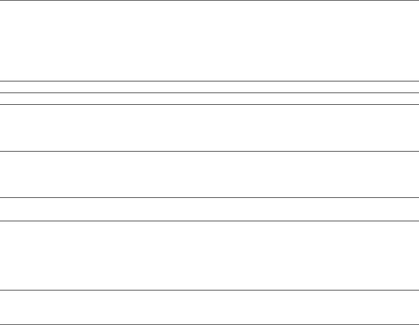
DRAFT
iMOD Batch functions
8.2.6 IDFMERGE-Function
The MERGE function can be used to merge different IDF-files into a new IDF-file. If these IDF-files
might overlap, an interpolation between the overlapping IDF-files will be carried out.
FUNCTION= IDFMERGE
NMERGE= Enter the number of IDF-files that need to be merged, e.g. NMERGE=6.
SOURCEIDF{i}= Enter the ith IDF-file, e.g. SOURCEIDF1=D:\SUBMODEL1\HEAD_L1.IDF,
SOURCEIDF2= D:\SUBMODEL2\HEAD_L1.IDF. Repeat this keyword
NMERGE-times. Whenever NMERGE is absent, the keyword
SOURCEDIR will be used.
SOURCEDIR= Enter the source folder and part of the filename that need to be merged,
e.g. D:\DATA\HEAD*L1.IDF to merge all files that corresponds to this wild-
card. This keyword SOURCEDIR is used whenever the keyword NMERGE
is absent.
TARGETIDF= Specify a filename for the resulting IDF-file, e.g.
{installfolder}\TOTAL\HEAD_L1.IDF.
WINDOW= Specify a window in which the entered IDF-files (SOURCEIDF{i},
SOURCEDIR) will be merged only. Enter coordinates of the lower-left
corner first and then the coordinates of the upper-right corner, e.g. WIN-
DOW=100000.0, 400000.0, 200000.0, 425000.0. When WINDOW=is ab-
sent, the total dimension of all selected IDF-files in the SOURCEDIR will
be used.
MASKIDF= Enter an IDF-file that needs to be mask areas (those with values
equal to the NoDataValue in the MASKIDF) in the merged results, e.g.
D:\MASK\AREA.IDF.
Example 1
FUNCTION=IDFMERGE
NMERGE=2
SOURCEIDF1=D:\MODEL1\HEAD_L1.IDF
SOURCEIDF2=D:\MODEL2\HEAD_L1.IDF
TARGETIDF=D:\RESULT\HEAD_L1.IDF
This example merges two IDF-files, HEAD_L1.IDF and HEAD_L1.IDF from two different folders, into a
single one D:\RESULTS\HEAD_L1.IDF.
Example 2
FUNCTION=IDFMERGE
MASKIDF=D:\MASK\AREA.IDF
WINDOW=120000.0,425000.0,165000.0,465000.0
SOURCEDIR=D:\DATA\HEAD*_L1.IDF
TARGETIDF=D:\DATA\HEAD_MERGED_L1.IDF
This example merges all IDF-files in the folder D:\DATA that agree with the filename HEAD*_L1.IDF,
such as HEAD_A1_L1.IDF, HEAD_A2_L1.IDF. The merged results will be “clipped” for the given extent
by WINDOW and will be “masked” out by the given NoDataValues in the MASKIDF. Finally the results
will be saved in HEAD_MERGED_L1.IDF.
Deltares 423 of 812

DRAFT
iMOD, User Manual
8.2.7 IDFTRACE-Function
Use this function to make a spatial IDF file with unique zone numbers of non-connecting areas of a
given IDF file.
FUNCTION= IDFTRACE
IDF_IN= You can enter the IDF file with the areas, e.g.
IDF_IN=D:\DATA\LAKES.IDF. All values greates than 0.0 will be pro-
cessed.
IDF_OUT= You can enter the output IDF file with areas numbered uniquely, e.g.
IDF_OUT=D:\DATA\LAKES_ID.IDF.
MINT=
(optional)
Enter the minimal size of the aggregated areas to be numbered, e.g.
MINT=10. By default MINT=0 and all locations with values greater than
0.0 will be used to create a numbered zone, if you enter MINT=10, only
areas that are aggregated to be more than 10 locations will be numbered.
Example
FUNCTION=IDFTRACE
IDF_IN=D:\DATA\LAKE.IDF
IDF_OUT=D:\DATA\LAKE_ID.IDF
MINT=10
This example creates an IDF file that can be used by the Lake package for the identification of indivual
lakes, larger than 10 gridcells from the entered IDF file at IDF_IN.
424 of 812 Deltares

DRAFT
iMOD Batch functions
8.2.8 CREATEIDF-Function
The CREATEIDF function can be used to create IDF-files out of ESRI ASC File Formats, see sec-
tion 9.13. Be aware of the fact that you can open more of these ASC files in the iMOD Manager,
alternatively (see section 5.4).
FUNCTION= CREATEIDF
SOURCEDIR= Enter the name of a folder that contains a specific set of ASC file(s), e.g.
{installfolder}\DATA\RESULTS\HEAD*_L*.ASC. All ASC files that agree
will be converted to IDF-files.
TOPWC= Enter the wildcard that specifies the part of the filename that represents
the top elevation of the data, e.g. SEL_*.ASC. In this case, iMOD will
search for the absolute top elevation to be defined at the location of the
asterix, e.g. SEL_0.45.ASC will yield the value 0.45.
BOTEL= Enter the relative bottom of the elevation to be added to the top elevation,
e.g. BOTEL=-0.5 will yield an absolute bottom elevation of 0.45-0.5=-0.10.
ADD= Enter a value to add to the top and the bottom elevation (TOP and BOT),
e.g. ADD=3, TOP=TOP+3.
MULT= Enter a value to multiply with the top and the bottom elevation (TOP and
BOT), e.g ADD=3, TOP=TOP*3.
Example 1
FUNCTION=CREATEIDF
SOURCEDIR=D:\DATA\TOP*.ASC
The above mentioned example transforms all ESRI ASCII gridfiles that agree with the wildcard TOP*.ASC
into the IDF format. The yielding files will have identical names with the extension .IDF, and will be
placed in the same folder as their ASCII files, so TOP1.ASC becomes TOP1.IDF.
Files will be overwritten without questioning!
Example 2
FUNCTION=CREATEIDF
SOURCEDIR=D:\DATA\SEL*.ASC
TOPWC=SEL_*.ASC
BOTEL=-0.5
The following example translates all ESRI ASCII gridfiles that agree with the wildcard SEL*.ASC. into
SEL*.IDF-files. Moreover, a top elevation (TOPWC) will be extracted from the filename at the position
of the wildcard, so the function tries to read a real value at the position of the asterix, suppose the
filename is SEL_0.25.ASC, the value finally read is 0.25. It will be used to enter the TOP elevation
inside the IDF (see section 9.5 for the syntax of IDF-files). The bottom elevation will be equal to the top
elevation (0.25 in this example) plus the given value BOTEL, in this case -0.5, thus bottom elevation is
0.25+-0.5=-0.25.
Deltares 425 of 812

DRAFT
iMOD, User Manual
8.2.9 CREATEASC-Function
The CREATEASC function can be used to create ESRI ASC files out of IDF File, see section 9.13.
This function will always replace ’****" with a NODATA value.
FUNCTION= CREATEASC
SOURCEDIR= Enter the name of a folder that contains a specific set of IDF file(s), e.g.
{installfolder}\DATA\RESULTS\HEAD*_L*.IDF. All IDF files that agree will
be converted to ASC-files.
Example 1
FUNCTION=CREATEASC
SOURCEDIR=D:\DATA\TOP*.IDF
The above mentioned example transforms all IDF gridfiles that agree with the wildcard TOP*.IDF into
the ESRI ASCII format. The yielding files will have identical names with the extension .ASC, and will
be placed in the same folder as their IDF files, so TOP1.IDF becomes TOP1.ASC.
Files will be overwritten without questioning!
426 of 812 Deltares

DRAFT
iMOD Batch functions
8.2.10 XYZTOIDF-Function
Use this function to create an IDF from a plain data file(s) or IPF file(s) that contain x,y,z data at least.
The column (“z”) can contain any type of (real) data. Also use this function to generate a 3D model of
the subsoil via indicator-interpolation of various thressholds (lithology and permeability).
FUNCTION= XYZTOIDF
XYZFILE= Enter the name of a plain text file that contains x,y,z data, e.g. XYZ-
FILE=D:\DATA\XYZ.TXT. The format of the file should be: 1st line: header;
next lines: x, y, z-data.
IPFFILE= Enter the name of an IPF file that contains x,y,z data, e.g. IPF-
FILE=D:\DATA\POINTS.IPF.
IXCOL=
(optional)
Enter the column number of the IPF that contains the x-
coordinates, e.g. IXCOL=1 (default value).
IYCOL=
(optional)
Enter the column number of the IPF that contains the y-
coordinates, e.g. IYCOL=2 (default value).
IZCOL=
(optional)
Enter the column number of the IPF that contains the z-
coordinates, e.g. IZCOL=3 (default value).
ASSF_
COLUMN=
(optional)
Enter the column number of the associated file of the given
column IZCOL in the IPF, e.g. ASSF_COLUMN=2. In this
manner, the gridding will take the values from associated
files instead of those from the IPF file. This is only applied
whenever the IZCOL is equal to the column in which asso-
ciated files are listed in the IPF file.
ASSF_
IDEPTH=
(optional)
Enter ASSF_IDEPTH=0 to enter a the starting date from
which values are picked from the associated files, e.g.
ASSF_STARTDATE=20121231. Enter ASSF_IDEPTH=0 to
enter an initial depth and interval to interpolate intermediate
interfaces e.g. ASSF_TOP.
Enter the following items whenever ASSF_IDEPTH=0
ASSF_
STARTDATE=
Enter the starting date from which values are picked from
the associated files, e.g. ASSF_STARTDATE=20121231.
ASSF_
ENDDATE=
Enter the end date to which values are picked from the as-
sociated files, e.g. ASSF_ENDDATE=20160515.
ASSF_DDATE= Enter the time interval for which subsequent gridding
is carried out, e.g. ASSF_DDATE=14 which mean that
each 14 days between the given ASSF_STARTDATE and
ASSF_ENDDATE will be processed. Alternatively the key-
words ’D’,’W’,’M’,’Y’ can be applied to denote ’daily’, ’weekly’,
’monthly’ and ’yearly’.
Enter the following items whenever ASSF_IDEPTH=1
ASSF_
TOP=
Enter the uppermost elevation of the first interface, e.g.
ASSF_TOP=4.0.
ASSF_
BOT=
Enter the lowermost elevation of the last interface, e.g.
ASSF_BOT=-40.0.
ASSF_
DZ(.)=
Enter the thickness of all interfaces, e.g. ASSF_DZ=5.0.
This can be a list of values as well, e.g.
ASSF_DZ=5.0,2.5,10.0. In this case the first interface
has a thickness of 5.0 m, the second 2.5 m and the third
10.0 m, all the other remaining interfaces will have 10.0 m
as well.
ASSF_
ZPLUS=
Enter the vertical offset to be applied to look beyond the
current interface, e.g. ASSF_ZPLUS=0.5. In this case, the
boreholes will be read for a length of DZ(i)±ASSF_ZPLUS.
Enter the following items whenever ASSF_IDEPTH=2
NLAY= Enter the number of interfaces, e.g. NLAY=10. The interpo-
lation of information will take place in between the interface
iand i+ 1.
Deltares 427 of 812
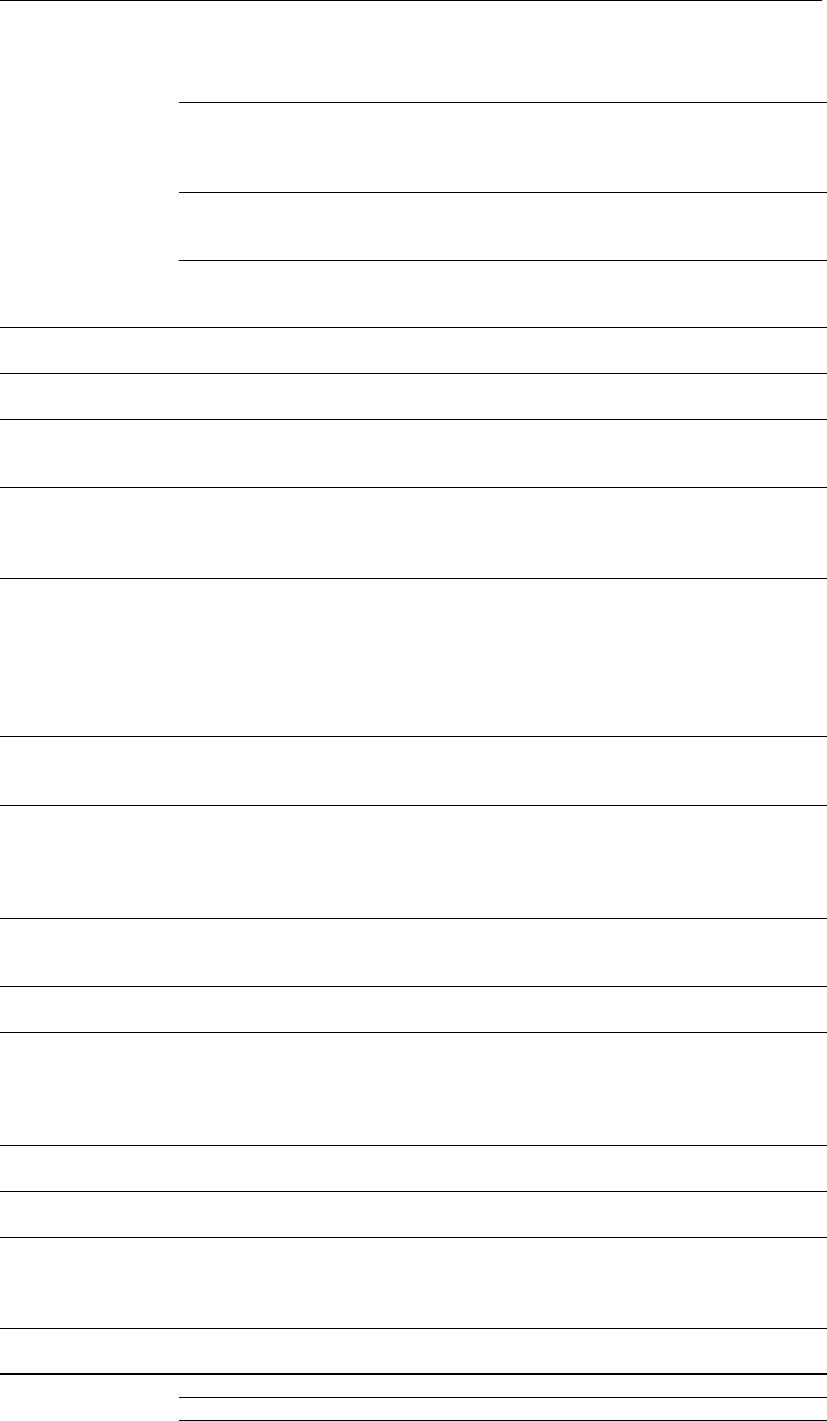
DRAFT
iMOD, User Manual
INT_L{i}= Enter the IDF file for each interface iup to NLAY, e.g.
INT_L1=D:\DATA\INTERFACE_L1.IDF.
KSUM=
(optional)
Enter KSUM=1 to generate permeability value as a weighted
sum of all individual permeability value within each vertical
interval. By default KSUM=0 and the permeability is that
permeability associated with the most common lithology.
TRIMTOP_IDF=
(optional)
Enter the name of an IDF file to be used to trim
the interpolated values at the top, e.g. TRIM-
TOP_IDF=D:\DATA\DEM.IDF.
TRIMBOT_IDF=
(optional)
Enter the name of an IDF file to be used to trim
the interpolated values at the bottom, e.g. TRIM-
BOT_IDF=D:\DATA\BEDROCK.IDF.
GENFILE=
(optional)
Enter the name of a Gen-file that contains the data x,y,z data, e.g. GEN-
FILE=D:\DATA\DATA.GEN.
NBLNFILE=
(optional)
Specify the number of GEN-files that need to be taken into account in the
grid-interpolation.
BLNFILE_{i}= Give the name of a specific GEN-file containing x,y-data of
the faults that need to be taken into account in the grid-
interpolation. Repeat this keyword for NBLNFILE times.
FCTBLNFILE_{i}=
(optional)
Enter the mutiplication factor for each BLNFILE for which the
points will be moved further away if they are on both sides
of a fault cq. line in the GEN file. Repeat this keyword for
NBLNFILE times.
IBLNTYPE=
(optional)
Specify the type of BLNFILE, e.g. IBLNTYPE=0 (default) which denotes that
iMOD will use the BLNFILE or any blanked out area via a) outside the entered
trim IDF files at TRIMTOP_IDF and/or TRIMBOT_IDF or b) outside the active
area specified by IDFFILE_POINTER as a breakline in the interpolation (only
point that can be ”seen“ without obstructed by the line will be used). Whenever
IBLNTYPE=1, the BLNFILE and/or the other options a) and b), will be used
as a ”polygon“ (only points within the same polygon will be used).
SOURCEDIR=
(optional)
Enter the folder and wildcard that corresponds to the XYZFILEs, e.g.
D:\DATA\REGION*.XYZ. The keyword XYZFILE and IPFFILE should be ab-
sent, otherwise XYZFILE or IPFFILE will be used!
TARGETDIR=
(optional)
Enter the folder to which the IDFFILEs will be saved that correspond
to the XYZFILEs or IPFFILEs found in the SOURCEDIR, e.g. TARGET-
DIR=D:\DATA\IDFS, the results will be called D:\DATA\IDFS\REGION*.IDF
whenever SOURCEDIR=D:\DATA\REGION*.XYZ. This keyword is compul-
sory whenever the optional keyword SOURCEDIR is applied.
NODATA=
(optional)
Enter a NoDataValue for those data points that need to be excluded from the
gridding, e.g. NODATA=0.0 to exclude data points equal to zero. By default,
NODATA=-999.99.
ILOG=
(optional)
Enter ILOG=1 to perform a log transformation for the data points that need to
be grided. By default, ILOG=0.
WINDOW=
(optional)
Enter the coordinates of the window that needs to be computed. Enter co-
ordinates of the lower-left corner first and then the coordinates of the upper-
right corner, e.g. WINDOW=100000.0, 400000.0, 200000.0, 425000.0. When
WINDOW=is absent, the entire XYZFILE or IPFFILE will be gridded for its
maximum extent.
CS= Enter the cellsize of the IDFFILE to be created, e.g. CS=100.0. This keyword
is not necessary whenever IDFFILE is specified.
IDFFILE_IN=
(optional)
Enter the name of an IDF-file for which data points that are equal to its No-
DataValue will be interpolated.
IDFFILE_
POINTER=
(optional)
Enter an IDF-file that will be needed to specify what locations will be interpo-
lated. It temporarily blanks out the IDF-file given by IDFFILE_IN before the
interpolation and resets the original value in the blanked-out area after the
interpolation.
IDFFILE Enter the name of an IDF-file that need to be created, e.g. IDF-
FILE=D:\DATA\XYZ.IDF.
GRIDFUNC= Enter the grid function to be used:
MIN minimum of all data points inside a gridcell;
428 of 812 Deltares

DRAFT
iMOD Batch functions
MAX maximum of all data points inside a gridcell;
MEAN mean of all data points inside a gridcell;
PERC percentile of all data points inside a gridcell.
PERCENTILE= Enter the percentile (>=0 PERCENTILE <=100.0) when-
ever GRIDFUNC=PERC, e.g. PERCENTILE=25.0. A per-
centile value will be interpolated linearly, whenever the
entered PERCENTILE falls in-between two values. En-
tering PERCENTILE=0.0 or PERCENTILE=100.0 will yield
the same results as with GRIDFUNC=MIN and GRID-
FUNC=MAX, respectively, however, the latter functions are
faster than the function GRIDFUNC=PERC. Entered values
beyond 0.0 and above 100.0, will be trimmed to 0.0 and
100.0, automatically.
BIVAR: takes a bivariate interpolation
SKRIGING:
OKRIGING:
takes a Kriging interpolation, SKRIGING stands for Simple
Kriging (assuming a constant mean over the entire domain);
OKRIGING stands for Ordinary Kriging (assuming a con-
stant mean in the neighborhood of each estimation point).
Choose one of both at one time.
PNTSEARCH=
(optional)
Specify PNTSEARCH=1 to allow to search for points within
the distance specified by RANGE the minimum number of
points used for the interpolation. Default MINP=10 (or less
whenever the dataset contains less points).
MINP=
(optional)
Enter the minimal number of points needed for the interpo-
lation, e.g. whenever MINP=50, iMOD will take the 50 near-
est point in the Kriging interpolation. Whenever the keyword
IQUADRANT=1, the entered MINP value is valid for each
quadrant, so whenever MINP=10 and IQUADRANT=1, the
total number of points will be 10 ×4 = 40. Default MINP=10
(or less whenever the dataset contains less points). This
keyword can be entered only whenever PNTSEARCH=1.
IQUADRANT=
(optional)
Select IQUADRANT=1 to force an equal distribution of
point from the four quadrants around an point to be es-
timated. This keyword can be entered only whenever
PNTSEARCH=1. By default IQUADRANT=0.
RANGE= Enter the range that defines a neighbourhood within which
all data points are related to one another, e.g. RANGE=1000
meter. It is possible to specify multiply values for RANGE
whenever ASSF_IDEPTH=2 for each interface. If the num-
ber of entered values for RANGE is less than the number
of interfaces to be computed, the last entered values for
RANGE will be re-used for the remaining interfaces. The
semivariance will become approximately equal to the vari-
ance of the whole surface itself (SILL).
SILL= Enter the distance at which the semivariance approaches a
flat region. SILL is referred as the range or span of the re-
gionalized variable, e.g. SILL=2500. This parameter resem-
blances a variance. The magnitude of the semivariance be-
tween points depends on the distance between the points. A
smaller distance yields a smaller semivariance and a larger
distance results in a larger semivariance.
NUGGET= Enter the offset of the semivariogram, e.g. NUGGET= 10.0.
Deltares 429 of 812

DRAFT
iMOD, User Manual
KTYPE= Enter the type of the Kriging model to be used to compute
the value at Xi, choose from:
1 Linear Model:
Xi=DISTi*(SILL-NUGGET)/RANGE
2 Spherical Model:
DISTi<=RANGE:
Xi=SILL*(1.5*(DISTi/RANGE))-(0.5*(DIST3/RANGE3))
DISTi>RANGE:
Xi=SILL
3 Exponential Model:
Xi=SILL*(1.0-EXP(-DIST3i/RANGE))
STDEVIDF= Enter the name for the standard deviation computed, e.g.
STDEVIDF=D:\VAR.IDF.
VARIOGRAM: create a semivariogram, this yields no interpolation of the
data, it generates a table filled in with a variogram. When-
ever the WINDOW keyword is specified, a variogram will be
computed for those data points that are within the bounds of
the given WINDOW. The results will be written in the VARI-
OGRAM.TXT file, see coming pages for an example.
LAG-
INTERVAL=
Enter the number of distances over which the VARIOGRAM
will be computed, e.g. LAGINTERVAL=50 will yield fifty in-
tervals equally distributed between zero and the maximum
distance between point.
LAG-
DISTANCE=
Specify the lag distance, e.g. LAGDISTANCE=50.0 to over-
rule the lag distance as computed by LAGINTERVAL.
ELLIPS_LEN=
(optional)
Specify the ellipsoids maximum diameter (∆x), e.g. EL-
LIPS_LEN=5000.0 meter. Specify this parameter only
whenever IQUADRANT=0. By default ELLIPS_LEN is equal
to the length specifief at RANGE.
ELLIPS_ANI=
(optional)
Specify the ellipsoids anisotropy, e.g. ELLIPS_ANI=45.0 to
denote a 45 degrees shift from the north clock-wise. Spec-
ify this parameter only whenever IQUADRANT=0 and . By
default ELLIPS_ANI=0.0.
ELLIPS_RAT=
(optional)
Specify the ellipsoids ratio between the semi-major axis
(∆x) and the semi-minor axes (∆y), e.g. ELLIPS_RAT=0.5
denotes a flattened ellipsoid whereby the ∆yis half the
size of ∆x. Specify this parameter only whenever IQUAD-
RANT=0. By default ELLIPS_RAT=1.0.
PCG: takes a Preconditioned Conjugate Gradient interpolation
HCLOSE=
(optional)
Enter a closure criterion for the PCG solver to terminate the
interpolation, e.g. HCLOSE=0.001 (this is the default).
RCLOSE=
(optional)
Enter a closure criterion for the PCG solver to terminate the
interpolation, e.g. RCLOSE=1000.0 (this is the default).
NINNER=
(optional)
Enter the number of inner iteration for the PCG solver, e.g.
NINNER=50 (this is the default). Use large values for NIN-
NER to speed up the interpolation since the problem to be
solved is linear.
INDICATOR
(optional)
Enter INDICATOR=1 (by default INDICATOR=0) to use an indicator interpola-
tion. Whenever this function is used, a value is assigned to a point whenever
it meets a given thresshold (see NTHRESHOLD). In that case it gets score
of 1.0, this is corrected for the penetration length of this in the current inter-
val. After interpolation it yields a probability of occurrence, a fraction between
0.0 and 1.0. Use INDICATOR=-1 to skip the interpolation and recompute the
probability of occurence and permeability from the existing files, in case INDI-
CATOR=1 is applied first.
NTHRESHOLD Enter the number of thresholds to be used in the indicator
interpolation, e.g. NTHRESHOLD=2.
430 of 812 Deltares

DRAFT
iMOD Batch functions
THRESHOLD{i} Enter for each threshold the appropriate name, e.g.
THRESHOLD1=SAND. Use quotation marks for thresholds
with spaces, e.g. THRESHOLD{i}=“SILTY SAND”. Enter
NTHRESHOLD number of thresholds. iMOD will generate a
probability map for each threshold for each interval. It also
generates a map per intergface of the most-common thresh-
old per grid cell.
KH_THRES-
HOLD{i}
Enter for each threshold the horizontal permeability, e.g.
KH_THRESHOLD1=35.0. Enter NTHRESHOLD number of
horizontal permeability values. iMOD will generate a hori-
zontal permeability map for each threshold for each inter-
val. It also generates a total, averaged horizontal perme-
ability map per interface as the weighted sum of all individual
thresholds.
KV_THRES-
HOLD{i}
Enter for each threshold the vertical permeability, e.g.
KV_THRESHOLD1=10.0. Enter NTHRESHOLD number of
vertical permeability values. iMOD will generate a vertical
permeability map for each threshold for each interval. It also
generates a total, averaged vertical permeability map per
interface as the weighted sum of all individual thresholds.
Example 1
FUNCTION=XYZTOIDF
XYZFILE=D:\DATA\28BN.XYZ
IDFFILE=D:\DATA\28BN.IDF
CS=5.0
GRIDFUNC=MEAN
Above an example is given how to rasterize, for a 5x5 resolution (CS=5.0), the content of an XYZ file
by means of its mean values (GRIDFUNC=MEAN) inside the individual rastercells. The default No-
DataValue of -999.99 will be assigned to those rastercells that doesn’t have any points inside, more-
over, data points that have this particular value will be left out.
Example 2
FUNCTION=XYZTOIDF
SOURCEDIR=D:\DATA\*.XYZ
TARGETDIR=D:\DATA\IDF
IDFFILE=D:\DATA\28BN.IDF
CS=25.0
GRIDFUNC=PERC
PERCENTILE=5.0
NODATA=0.0
Example above shows how to rasterize, for a 25x25 resolution (CS=25.0), the content of all *.XYZ files
in the folder D:\DATA, by means of its 5.0 percentile values (PERCENTILE=5.0; GRIDFUNC=PERC)
inside the individual rastercells. A NoDataValue of 0.0 will be assigned to those rastercells that doesn’t
have any points inside, moreover, data points that have this particular value will be left out.
Deltares 431 of 812
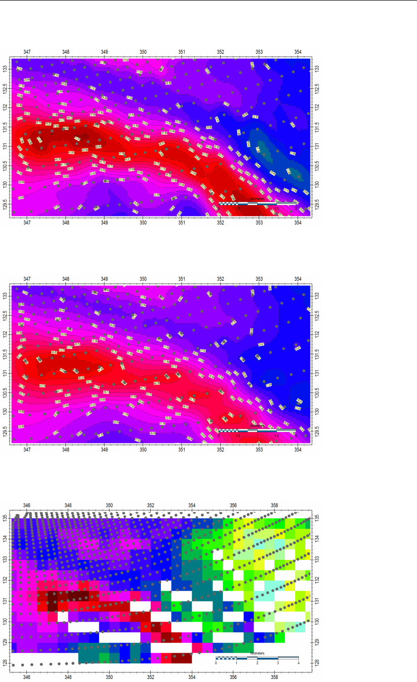
DRAFT
iMOD, User Manual
Example of Bivariant interpolation:
Example of PCG interpolation:
Example of MEAN sampling:
432 of 812 Deltares
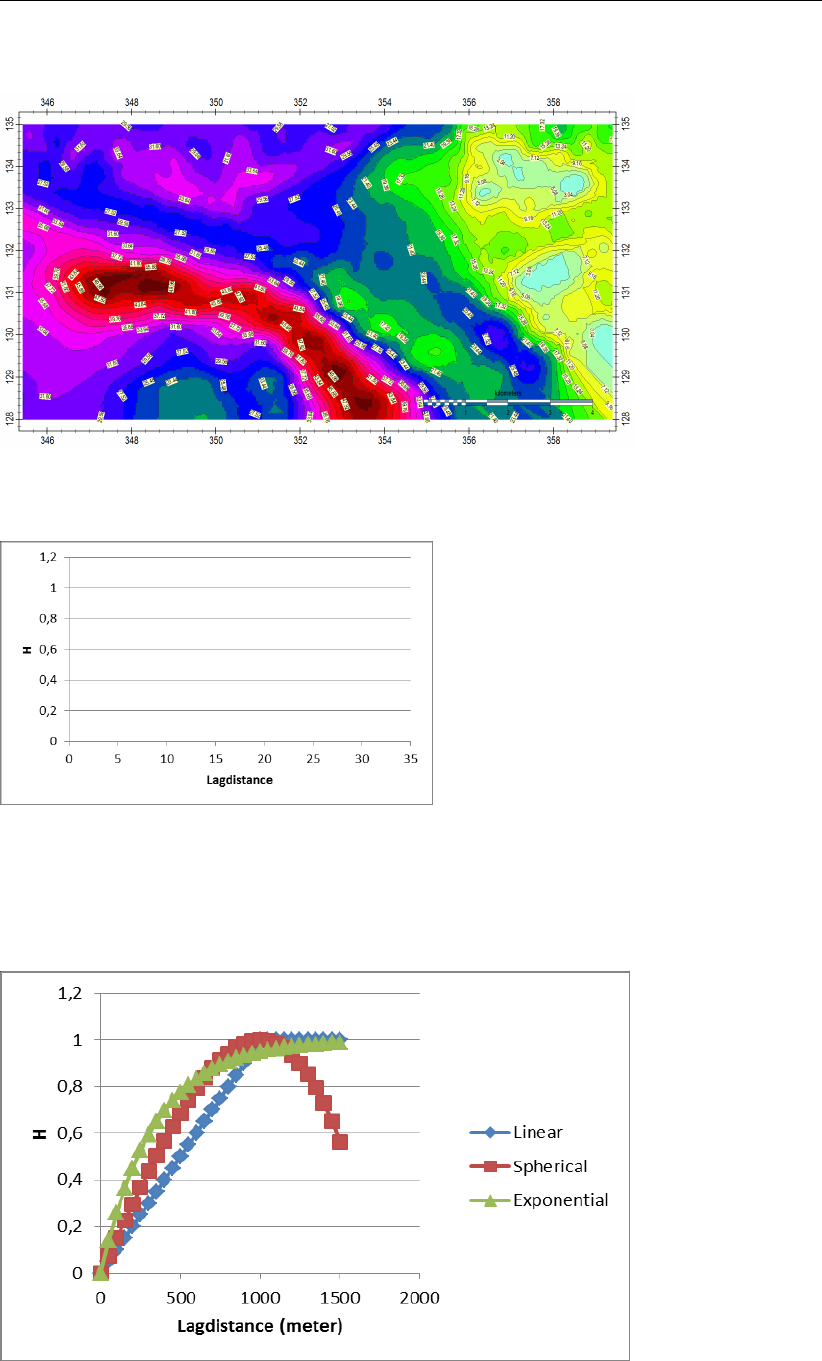
DRAFT
iMOD Batch functions
Example of Kriging interpolation (linear model):
Example of a Variogram:
From the above presented variogram, the SILL would be 30 and the corresponding RANGE approxi-
mately 1000m, at that distance the SILL value flattens. The NUGGET is zero in this example.
Example of the different models to be used in the Kriging interpolation:
Deltares 433 of 812

DRAFT
iMOD, User Manual
8.3 ISG-FUNCTIONS
8.3.1 GEN2ISG-Function
The GEN2ISG function reads a GEN file and creates a ISG file. There are two ways to use this function;
IUSEDAT=1 and IUSDAT=0. These will be explained below.
Use IUSEDAT=1 to force using the *.DAT file (with GEN file information).
FUNCTION= GEN2ISG
GENFNAME= Give a GEN file containing x and y coordinates of GEN segments.
IUSEDAT=1 Enter the column number in the DAT file that represents:
STAGE1_COLUMN= Stage on Startpoint of the Segment, e.g. STAGE1_COLUMN=1
STAGE2_COLUMN= Stage on Endpoint of the Segment, e.g. STAGE2_COLUMN=2
BOTL1_COLUMN= Bottom on Startpoint of the Segment, e.g. BOTL1_COLUMN=3
BOTL2_COLUMN= Bottom on Endpoint of then Segment, e.g. BOTL2_COLUMN=4
shape of the Crosssection of the Segment:
SLOPE_L_COLUMN= Left slope, e.g. SLOPE_L_COLUMN=5
SLOPE_R_COLUMN= Right slope, e.g. SLOPE_R_COLUMN=6
BWIDTH_COLUMN= Bottom width, e.g. BWIDTH_COLUMN=7
Use IUSEDAT=0 if you do not have a *.DAT file (with GEN file information).
FUNCTION= GEN2ISG
GENFAME= Give a GEN file containing x and y coordinates of GEN segments.
IUSEDAT=0 the following keywords must be given:
IDFSTAGE= Enter the column number in the DAT file that represents the y coor-
dinate, e.g. STAGE1_COLUMN=1.
IDFSUMMER= Enter the filename of the IDF-file containing summer heads.
IDFSUMMER_BACKUP= Enter the filename of the IDF-file containing summer heads. This
file is created as backup-file in case no values are found in IDF-
SUMMER or by using the SAMPLE_SEARCH function.
IDFWINTER= Enter the filename of the IDF-file containing winter heads.
IDFWINTER_BACKUP= Enter the filename of the IDF-file containing winter heads. This file
is created as backup-file in case no values are found in IDFWINTER
or by using the SAMPLE_SEARCH function.
SUMMERPERIOD=
(optional)
Enter the day and month at which the summer period starts (e.g.
default value is SUMMERPERIOD=0104 in case summer starts at
the 1st of April each year).
WINTERPERIOD=
(optional)
Enter the day and month at which the winter period starts (e.g.
default value is WINTERPERIOD=0110 in case summer starts at
the 1st of October each year)
START_YEAR= Enter the starting year of the calculation period, e.g
START_YEAR=2014.
END_YEAR= Enter the end year of the calculation period, e.g.
END_YEAR=2020.
IDFBOTTOM= Enter the name of the IDF-file containing all bottom values of the
area.
BOTTOMVALUE= If there’s no IDFBOTTOM-file available give a constant value for the
bottom height, e.g. BOTTOMVALUE=12.32.
SAMPLE_DISTANCE
(optional)=
Enter a value (in meters) that accounts for the distance iMOD
needs to sample the IDF-file on, e.g. 100 m. On default SAM-
PLE_DISTANCE=250 m.
CCFFNAME= Enter the name of a CCF-file that describes the cross-section that
will be used to insert cross-section for all segments.
SEARCH_DISTANCE=
(optional)
Enter a value (in meters) that accounts for the distance iMOD
needs to resample the IDF-file on, e.g. 50 m. On default
SEARCH_DISTANCE=250 m. This value will only be used if there
were no values found by making use of the SAMPLE_DISTANCE.
434 of 812 Deltares

DRAFT
iMOD Batch functions
IPUZZLE= Enter a 0.0 or 1.0. If a value of 1.0 is given, iMOD tries to find
all possible places where segments can be joined and join them if
needed.
IDFRESISTANCE= Enter the name of IDF-file that contains resistance values of the
area.
RESISTANCE= Enter a resistance value that will be applied to the whole area. Can
only be used if IDFRESISTANCE is not available.
IDFINFILTRATIONFACTOR= Enter the name of IDF-file that contains infiltration factors for the
area.
INFILTRATIONFACTOR= Enter an infiltration factor that will be applied to the whole area. Can
only be used if IDFINFILTRATIONFACTOR is not available.
OUTFILE= Enter the name of the ISG output-file, e.g. NEWFILE.ISG.
Example 1
FUNCTION=GEN2ISG
FUNCTION=GEN2ISG
GENFNAME=d:\Model\Data\Shape_data\river_lines.gen
IUSEDAT=0
IDFSUMMER=d:\Model\Basic_data\SUMMER_LEVEL_RIVER.IDF
IDFWINTER=d:\Model\Data\Basic_data\WINTER_LEVEL_RIVER.IDF
IDFBOTTOM=d:\Model\Data\Basic_data\BODEMHOOGTE_RIVER.IDF
SAMPLE_DISTANCE=25.0
CCFFNAME=d:\Model\Data\Basic_data\CROSS-SECTION.CCF
IDFRESISTANCE=d:\Model\Data\Basic_data\RIV_RESISTANCE.idf
IDFINFILTRATIONFACTOR=d:\Model\Data\Basic_data\INFFACTOR_RIVER.IDF
OUTFILE=d:\Model\Data\ISG_data\River.isg
Above an example is given how to use the GEN2ISG. This example will generate and ISG file based
on river levels, bottom elevation, resistance, infiltration factor and the location of the river segments.
The ISG will contain the following information: as many as cross-sections per river segment as there
are unique ID-numbers in CCFFNAME related file, calculation nodes on each segment intersection
and segment nodes as much as there are coordinate points defined in the GEN file.
Deltares 435 of 812

DRAFT
iMOD, User Manual
8.3.2 ISGGRID-Function
Use this function to rasterize the selected ISG-files into IDF-files that can be used by iMODFLOW in a
runfile.
FUNCTION= ISGGRID
ISGFILE_IN= Enter an ISG-file that need to be simplified, e.g. ISGFILE_IN=D:\PO.ISG.
CELL_SIZE= Enter the cell size (meter) for the IDF-files that will be created from the ISG-file
mentioned by ISGFILE_IN, e.g. CELL_SIZE=25.0.
MINDEPTH=
(optional)
Enter the minimum water depth (meter) used for the calculation of the con-
ductance of the stream bed, e.g. MINDEPTH=1.0. The default value is MIN-
DEPTH=0.1.
MAXWIDTH=
(optional)
Enter the maximal width of a stream (meter) used for the calculation of the
conductance of the stream bed. Introducing this parameter limits any stream
width larger than MAXWIDTH, e.g. MAXWIDTH=1000. The default value is
MAXWIDTH=250.
OUTPUT
FOLDER=
Enter a foldername to save all rasters into, e.g.
OUTPUTFOLDER=D:\OUTPUT. The following rasters will be saved:
1 COND The computed stream bed conductance (m2/day)
2 STAGE The interpolated riverlevel (m+MSL)
3 BOTTOM The interpolated riverbed height (m+MSL)
4 INFFCT The interpolated river infiltration factor (-)
5 TOTAL_LENGTH Total length if existing river segments in a single
rastercell (meter)
6 MEAN_
WPERIMETER
Mean wetted perimeter within a river segment
7 MEAN_WIDTH Mean stream bed width
8 RESISTANCE Interpolated river resistance (days). IMPORTANT
to note is that a minimal resistance is applied of
0.001 days to avoid extraordinary conductance
(COND) values.
9 EROSION Erosion matrix to be used to extent the riverbed
existence over more rastercells
The following will be created only whenever ICDIST=1
10 EFFECT The computed water level that are influenced by
the weirs.
11 CUR_ID Identification of structures for current segment.
12 NEX_ID Identification of following structure for current
segment.
POSTFIX=
(optional)
Enter a postfix to be used to add to the end of the IDF-file names men-
tioned above, e.g. POSTFIX=_SUMMER yields STAGE_SUMMER.IDF instead
of STAGE.IDF.
NODATA= Enter a NodataValue for which water levels will be skipped in determining the
waterlevels along profiles, e.g. NODATA=-999.
WINDOW=
(optional)
Enter the coordinates of the window that needs to be computed. Enter coor-
dinates of the lower-left corner first and then the coordinates of the upper-right
corner, e.g. WINDOW=100000.0, 400000.0, 200000.0, 425000.0. When WIN-
DOW=is absent, the entire ISG will be gridded for its maximum extent.
ISAVE= Enter the numbers to be saved solely, e.g. ISAVE=1,1,1,0,0,0,0,0,0,0,0,0 to iden-
tify that the IDF-files COND, STAGE and BOTTOM need to be saved.
IPERIOD=
(optional)
Specify whether the waterlevels need to be calculated for a specific period, by
default IPERIOD=1 which means that waterlevels will be computed as the mean
over the entire existing periods within the ISG-file (which can be different among
the segments). Specify IPERIOD=2 to enter a date over which the waterlevels
will be averaged.
SDATE= Enter a starting date to compute averaged waterlevels for, e.g.
SDATE=19910101 to represent the 1st of January 1991.
EDATE= Enter a starting date to compute averaged waterlevels for, e.g.
EDATE=19911231 to represent the 31st of December 1991.
436 of 812 Deltares
DRAFT
iMOD Batch functions
DDATE= Enter a date-difference to be used to compute more rasters for differ-
ent periods, e.g. DDATE=14 means that a sequence between SDATE
and EDATE will be computed with length of 14 days. By default
DDATE=0 which will ignore any timesteps in-between the SDATE and
EDATE variables. The names of the IDF-file will be extended to include
a date notification, e.g. STAGE{POSTFIX}_19910101.IDF
ICDIST=
(optional)
Set this value to 1to compute the effects of weir as stored in the ISG file. By
default ICDIST=0. See keyword OUTPUTFOLDER to get the names of the extra
IDF files that will be created.
ISIMGRO=
(optional)
Set this value to 1 to export the gridded values for the ISG into a MetaSWAP file
svat_swnr_drng.inp.
SVAT2SWNR_DRNG= Enter the name for the svatswnr_drng.inp file.
SEGMENTCSVFNAME= Enter the CSV that contains the list of ...
THIESSENFNAME= Enter an IDF file that represents the SVAT-id for
MetaSWAP.
AHNFNAME= Enter an IDF file with the surface level.
SYSID= Enter a single value for the system identification.
WDEPTH= Enter a water depth that will be used to define the
appropriate trapezia for MetaSWAP.
IAVERAGE=
(optional)
Enter IAVERAGE=1 to apply an arithmetic mean for stages, bottomlevels, resis-
tances and infiltrationfactor over time. Enter IAVERAGE=2 to apply the median
value for those parameters. The default value is IAVERAGE=1.
IEXPORT=
(optional)
Set this value to 1 to export the gridded ISG into a MODFLOW river file, impor-
tant to notice is that it yield a single value for each gridded cell. The export river
file will be called OUTPUTFOLDER \modflow.riv. By default IEXPORT=0 and
IDF files will be created.
NLAY= Enter the number of model layers for which the gridded ISG file need to
be assigned vertically, e.g. NLAY=3. This option is only valid whenever
IEXPORT=1.
TOP_Li= Enter an IDF file that represents the TOP elevation of the ithlayer, e.g.
TOP_L1=D:\TOP_L1.IDF.
BOT_Li= Enter an IDF file that represents the BOT elevation of the ithlayer, e.g.
BOT_L2=D:\BOT_L2.IDF.
KHV_Li= Enter an IDF file that represents the horizontal permeability of the ith
layer, e.g. KHV_L2=D:\KHV_L2.IDF.
BND_Li= Enter an IDF file that represents the boundary condition of the ith
layer, e.g. BND_L4=D:\BND_L4.IDF.
Example:
FUNCTION=ISGGRID
ISGFILE_IN=D:\PO.ISG
CELL_SIZE=100.0
NODATA=-999.99
ISAVE=1,1,1,1,0,0,0,0,0,0,0,0
IPERIOD=1
SDATE=19980101
EDATE=19980131
OUTPUTFOLDER=D:\PO_GRIDS
The example above will rasterize the entire ISG for the period of the 1th of January up to the 31th of
January 1998 on a 100x100 meter grid.
Deltares 437 of 812
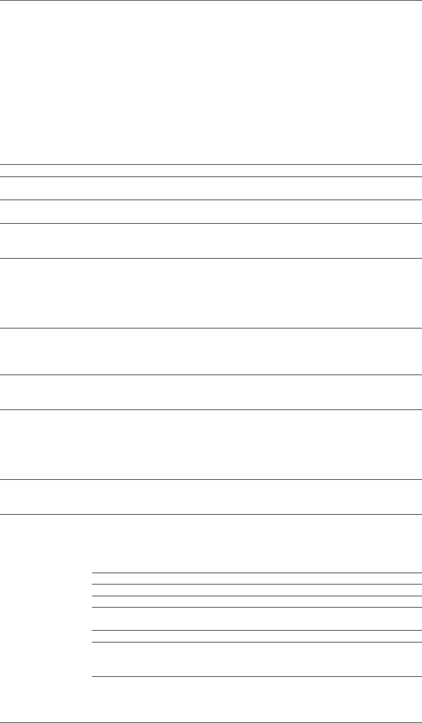
DRAFT
iMOD, User Manual
8.3.3 ISGADDCROSSSECTION-Function
Use this function to add cross-sections to an existing ISG-file (see section 9.9.3 for more information
about the content of an ISG-file and storage of cross-sections). The methodology is twofold:
1One-dimensional cross-sections:
Reading cross-sectional information from a text file for one-dimensional cross-sections.
2Two-dimension cross-sections:
Reading two-dimensional bathymetry from an IDF-file for areas that are defined by a pointer IDF.
All existing cross-section will be used to assign two-dimensional cross-sections. The dimension of
the bathymetry will be overruling the dimensions of the pointer IDF.
FUNCTION= ISGADDCROSSSECTION
ISGFILE_IN Enter an ISG-file for which cross-sections need to be added, e.g. ISG-
FILE_IN=D:\DATA\MAAS.ISG.
ISGFILE_OUT= Enter an ISG-file to save the renewed ISG for, e.g.
ISGFILE_OUT=D:\DATA\MAAS_NEWCROSSSECTIONS.IDF.
2-D Cross-sections
CROSS_PNTR= Enter the name of an IDF-file describes the spatial distribution of two-
dimensional cross-sections, e.g. CROSS_PNTR=D:\DATA\PNTR.IDF. This
pointer file is used to denote areas with equal values as the pointer value at
the location of the cross-section on the segmenet. The bathymetry for those
areas will be read from CROSS_BATH and applied as a 2-D cross-section on
the segment.
CROSS_BATH= Enter the name of an IDF-file that describes the bathymetry for the
riverbed at the locations where the values for CROSS_PNTR are 6=to
the pointer value at the corresponding cross-section at the segment, e.g.
CROSS_BATH=D:\DATA\RIVERBED.IDF.
CROSS_ZCHK
(optional)=
Enter the name of an IDF-file that describes the Reference Height to be
used to distinguish between areas with positive and negative values for
CROSS_PNTR, e.g. CROSS_ZCHK=D:\DATA\REFHEIGHT.IDF.
CROSS_CVAL
(optional)=
Enter the name of an IDF-file that describes the Resistance values
to be used to distinguish different resistance in inundation areas, e.g.
CROSS_CVAL=D:\DATA\RESISTANCE.IDF. The values in this IDF act as a
multiplication factor to the given resistance (attribute RESIS in the ISD2-file,
see 9.9.2) at the nearest calculation point. Bear in mind that the multiplication
factor will be saved in the ISG as an integer with a maximal value of 256.
1-D Cross-sections
CROSSSEC-
TION_IN=
Enter the filename that stores the renewed cross-sections, e.g. CROSSSEC-
TION_IN=D:\DATA\CROSS.TXT. The syntax of the CROSSSECTION_IN file
is a free-formatted, comma-separated-values file with for which each row is
defined as follows (be aware that you do not include a header in the text-file):
XC,YC,LABEL,N,X1,X2,..,XN,Z1,Z2,..,ZN
XC X-coordinate (meter) for the cross-section;
YC Y-coordinate (meter) for the cross-section
LABEL Label for the cross-section, maximum length is 32 charac-
ters.
N Number of cross-sections points.
XiSpecify as many distances as needed to define the bathy-
metry of the riverbed. The amount of definitions Nshould
be >3.
ZiSpecify as many elevations as needed to define the bathy-
metry of the riverbed. The amount of definitions Nwould be
equal the number of definitions used for Xi.
438 of 812 Deltares

DRAFT
iMOD Batch functions
ICLEAN=
(optional)
Enter ICLEAN=1 to clean ALL cross-sections before adding new ones, apply
ICLEAN=2 to remove existing cross-section only for those segments where
an update of the cross-section will be applied. By default ICLEAN=1.
WIDTH_IDF=
(optional)
Specify an IDF that represents the width of default cross-sections to be
placed on all segments and a default water depth of 5 meter where no
cross-section will be placed based on the entered data by the following key-
words, e.g. WIDTH_IDF=D:\DIST.IDF. This keyword is necessary only when-
ever ICLEAN=1.
MAXDIST=
(optional)
Specify a distance (meter) over which the cross-section will be snapped to
the segment, e.g. MAXDIST=5.0. By default MAXDIST=0.0 meter.
Example 1 (one-dimensional cross-sections):
FUNCTION=ISGADDCROSSSECTION
ISGFILE_IN=D:\iMOD-DATA\MAAS.ISG
CROSSSECTION_IN=D:\DATA\CROSS.TXT
WIDTH_IDF=D:\DATA\WIDTH.IDF
MAXDIST=2.5
ISGFILE_OUT=D:\iMOD-DATA\MAAS_RENEWEDCROSSSECTIONS.ISG
The example above will add cross-sections based on the entered CROSS.TXT file that specifies a
cross-section for “New Cross” as follows:
12000.0,45300.0,”New Cross”,-10.0,-5.0,-2.5,2.5,7.5,12.0,5.0,3.0,2.0,1.0,2.5,5.0
the results will be saved in MAAS_RENEWEDCROSSSECTION.ISG.
Example 2 (two-dimensional cross-sections):
FUNCTION=ISGADDCROSSSECTION
CROSS_PNTR=D:\DATA\PNTR.IDF
CROSS_BATH=D:\DATA\BATHEMETRY.IDF
ISGFILE_OUT=D:\iMOD-DATA\MAAS_RENEWEDCROSSSECTIONS.ISG
The example above will transform the existing cross sections with two-dimensional definitions based
on the pointerfile read in CROSS_PNTR and the corresponding bathymetry read in BATHEMETRY.IDF.
Deltares 439 of 812

DRAFT
iMOD, User Manual
8.3.4 ISGSIMPLIFY-Function
Use this function to reduce the amount of calculation points in a ISD file (part of the ISG-files, see
section 9.9.2). iMOD will eliminate calculation points that do not add significant information to the
declination of waterlevels, in other words, whenever the gradient of the waterlevel can be described by
less calculation points, iMOD will locate those calculation points that are able to represent the original
waterlevel most optimally. iMOD will use the mean waterlevels for all calculation nodes to determine
a mean descent of waterlevels along a segment. Simplification will be carried out for segments as a
whole. Whenever segments will be very short, this function will have a minor effect.
FUNCTION= ISGSIMPLIFY
ISGFILE_IN= Enter an ISG-file that need to be simplified, e.g. ISG-
FILE_IN=D:\DATA\MAAS.ISG.
ZTOLERANCE= Specify a distance (meter) for which the simplified waterlevel along a pro-
file may differ from the original one, e.g. ZTOLERANCE=0.10.
NODATA= Enter a NoDataValue for which waterlevels will be skipped in determining
the waterlevels along profiles, e.g. NODATA=-999.
ISGFILE_OUT= Enter an ISG-file to save the simplified ISG for, e.g. ISG-
FILE_OUT=D:\DATA\MAAS_SIMPLIFIED.IDF.
Example:
FUNCTION=ISGSIMPLIFY
ISGFILE_IN=D:\iMOD-DATA\MAAS.ISG
ZTOLERANCE=0.10
NODATA=-999.99
ISGFILE_OUT=D:\iMOD-DATA\MAAS_SIMPLIFIED.ISG
The example above will reduce the amount of calculation points such that the simplified waterlevel will
be differ more than 0.10 from the original one, the results will be saved in MAAS_SIMPLIFIED.ISG.
440 of 812 Deltares

DRAFT
iMOD Batch functions
8.3.5 ISGADJUST-Function
Use this function to perform changes to an existing ISG.
FUNCTION= ISGADJUST
SESFILE= Enter the name of the SES file,
e.g. D:\iMOD-DATA\ISGEDIT\ISG-change-stage.SES.
LOGFILE= Enter a name for the logfile showing all changes by listing both old and
new parameter values , e.g. D:\iMOD-DATA\ISGEDIT\ISG-LOG.TXT
default = .\log_ses.txt
OUTNAME= Foldername for new location to save all ISG related files (*.isg, *.isp, *.isd
etc),
e.g. OUTNAME=D:\RIV\ISG_new
Example:
FUNCTION=ISGADJUST
SESFILE=D:\iMOD-DATA\ISGEDIT\ISG-change-stage.SES
LOGFILE=D:\iMOD-DATA\ISGEDIT\ISG-LOG.TXT
OUTNAME=D:\iMOD-DATA\RIV\ISG_new
The example above will preduce new ISG files based on new data in the SES file.
Deltares 441 of 812
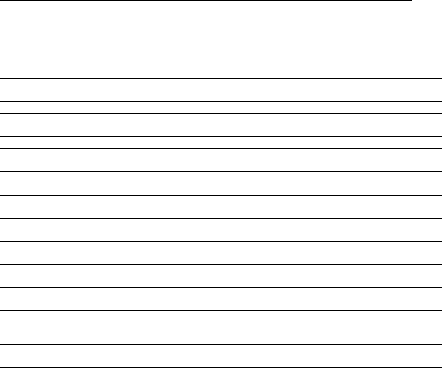
DRAFT
iMOD, User Manual
8.3.6 ISGADDSTRUCTURES-Function
Use this function will add weirs to an ISG.
FUNCTION= ISGADDSTRUCTURES
ISGFILE_IN= Enter the name of the ISG file.
IPFFILE_IN= Enter the name of the IPF file containing weir data
Specify the column number in the IPFFILE_IN that defines:
IXCOL= .. the X coordinates, by default IXCOL=1.
IYCOL= .. the Y coordinates, by default IYCOL=2.
IDCOL= .. the ..., by default IDCOL=3.
IOCOL= .. the ..., by default IOCOL=4.
ISCOL= .. the ..., by default ISCOL=5.
IWCOL= .. the ..., by default IWCOL=6.
MAXDIST= Specify the maximum distance ...., by default MAXDIST=1000.
SYEAR= Specify the start year, by default SYEAR=1980.
EYEAR= Specify the end year, by default EYEAR=2012.
START_PERIOD_
SUMMER=
Specify the start date of summer, by default START_PERIOD_SUMMER=’01-04’.
END_PERIOD_
SUMMER=
Specify the end date of summer, by default END_PERIOD_SUMMER=’30-09’.
START_PERIOD_
WINTER=
Specify the start date of winter, by default START_PERIOD_WINTER=’01-10’.
END_PERIOD_
WINTER=
Specify the end date of winter, by default END_PERIO_WINTER=’31-03’.
DATE_WLEVEL= Date of measure to be used to compute undisturbed waterlevel. Give 0-0-0
to compute the mean of all values or 28-02-1994 for a fixed date, by default
DATE_WLEVEL=0-0-0.
IPFLOGFILE= Enter a name for the log file, by default IPFLOGFILE=log.ipf.
ISGFILE_OUT= Enter the name of the ISG output file.
Example:
FUNCTION=ISGADDSTRUCTURES
ISGFILE_IN=D:\RIV-DATA\LEGGER.ISG
IPFFILE_IN=D:\RIV-DATA\WEIR.IPF
ISGFILE_OUT=D:\RIV-DATA\LEGGER_V2.ISG
The example above will produce new ISG files based on new data in WEIR.IPF.
442 of 812 Deltares
DRAFT
iMOD Batch functions
8.3.7 ISGADDSTAGES-Function
Use this function will add water levels to an ISG. Existing water levels wil be overwritten if the entered
IPF with water levels has water levels for identical dates as already mentioned in the ISG file.
FUNCTION= ISGADDSTAGES
ISGFILE_IN= Enter the name of the ISG file.
IPFFILE= Enter the name of the IPF file containing water level data via associated TXT-files.
The construction of the IPFFILE_IN file must be:
Column 1 X coordinate.
Column 2 Y coordinate.
Column irefers to the IEXT variable in the IPF-file to indicate the column
with the associated TXT-files, see section 9.7 for more detailed
description of the IPF-files.
ISGFILE_OUT= Enter the name of the ISG output file.
STAGETYPE=
(optional)
Specify STAGETYPE=1 to enter river stages in the IPFFILE in depth values. By
default STAGETYPE=0 and stages are entered in absolute values (m+MSL).
ICLEAN=
(optional)
Specify ICLEAN=1 to remove all existing entries for stages in the ISG file prior to
adding new entries. By default ICLEAN=0 and existing entries are retained.
Example:
FUNCTION=ISGADDSTAGES
ISGFILE_IN=D:\RIV-DATA\LEGGER.ISG
IPFFILE=D:\RIV-DATA\WATERLEVEL.IPF
ISGFILE_OUT=D:\RIV-DATA\LEGGER_V2.ISG
The example above will produce new ISG files based on new data in WATERLEVEL.IPF.
Deltares 443 of 812
DRAFT
iMOD, User Manual
8.3.8 SFRTOISG-Function
This function can be used to convert the output of the SFR package onto an ISG file. In this way the
existing functionalities of ISG Edit can be used to inspect and analyse the output of the SFR package.
FUNCTION= SFRTOISG
ISGFILE_IN= Enter the name of the ISG file, e.g. SFRFILE_IN=D\MODEL\SFR.ISG.
ISGFILE_OUT= Enter the name of the ISG file that need to be created, e.g. SFR-
FILE_OUT=D\MODEL\SFR_RESULT.ISG.
SFRFILE_IN= Enter the name of the output file of the SFR package, e.g. SFR-
FILE_IN=D\MODEL\TUT_FSFR.TXT. The file need to contain exactly the amount
of calculation points as the ISG files given at ISGFILE_IN. You should always use
the ISG files that iMOD created during the export of your model to MF2005 files.
This file contains per reach and per time step the following columns:
Column 1: Layer number.
Column 2: Row number.
Column 3: Column number.
Column 4: Stream number.
Column 5: Segment number.
Column 6: Flow into Stream Reach, a positive number means flow in the
stream, a negative number would not be feasible.
Column 7: Flow to Aquifer, negative means that groundwater migrates to
surface water (stream acts as a drain), a positive value denotes
that surface water infiltrates.
Column 8: Flow out of Stream Reach, a positive number means flow out of
the stream, a negative number would not be feasible.
Column 9: Overland Runoff.
Column 10: Precipitation.
Column 11: Evaporation.
Column 12: Stream Head, the stage in the river.
Column 13: Stream Depth, the depth of the river.
Column 14: Stream Width, the width of the river.
Column 15: Conductance, the area of contact between the surface water
and the groundwater, divided by the resistance of the riverbed.
Column 16: Gradient, the hydraulic gradient across the stream bed, nega-
tive gradient means that the stream acts as a drain. Large hy-
draulic gradients might indicate some conceptual errors. There
is a difference in how the SFR package deals with unsaturated
flow underneath the stream bed. As the conventional RIV pack-
age applies a hydraulic gradient as the difference between the
surface water level and the river bed level, the SFR package
takes the thickness of the river bed material instead.
Not all of the above mentioned columns are converted to the ISG file, the average stream discharge
(half of the sum of the Flow into Stream Reach plus the Flow out of Stream Reach) is converted from
m3/d to m3/s. Also the stream head, depth and width are transferred to the ISG file. Those four
attributes are considered to be most valuable.
Example:
FUNCTION=SFRTOISG
SFRFILE_IN=D\MODEL\SFR.ISG.
SFRFILE_OUT=D\MODEL\SFR_RESULT.ISG.
SFRFILE_IN=D\MODEL\TUT_FSFR.TXT.
The example above will produce a new ISG files based on the results of the SFR package.
444 of 812 Deltares
DRAFT
iMOD Batch functions
8.3.9 IPFTOISG-Function
This function can be used to convert an IPF file with appropriate columns into an ISG suitable for the
SFR package. Two following pairs of coordinates will form a single segment in the ISG file. Also,
only one calculation point and cross-section will appear on each segment. The cross-section will be
rectangular (4 points) based on the given stream width (see below).
FUNCTION= IPFTOISG
IPFFILE= Enter the name of the IPF file, e.g. IPFFILE=D\DATA\STREAM.IPF.
IXCOL=
(optional)
Enter the column number in the IPF file that represents the X-coordinate (m), e.g.
IXCOL=2, by default IXCOL=1.
IYCOL=
(optional)
Enter the column number in the IPF file that represents the Y-coordinate (m), e.g.
IYCOL=3, by default IYCOL=2.
ILABELCOL=
(optional)
Enter the column number in the IPF file that represents the stream label, e.g.
ILABELCOL=5, by default ILABELCOL=3. This will be used to label the stream
in the ISG file. If the label appeared to be empty (not available), the stream
segment identification will be used as given by the keyword ISEGMCOL. In the
end the segment name in the ISG file becomes “S_{stream label}_R_{i}” where i
is the sequential order number.
ISEGMCOL=
(optional)
Enter the column number in the IPF file that represents the stream segment iden-
tification, e.g. ISEGMCOL=5, by default ISEGMCOL=4. If two following pairs of
coordinates in the IPF have similar stream segment identification, they become a
segment in the ISG file.
IWIDTHCOL=
(optional)
Enter the column number in the IPF file that represents the stream total width (m),
e.g. IWIDTHCOL=6, by default IWIDTHCOL=5.
IBOTTOMCOL=
(optional)
Enter the column number in the IPF file that represents the stream bottom height
(m+MSL), e.g. IBOTTOMCOL=8, by default IBOTTOMCOL=6.
ISTAGECOL=
(optional)
Enter the column number in the IPF file that represents the stream stage
(m+MSL), e.g. ISTAGECOL=12, by default ISTAGECOL=7.
IPERMCOL=
(optional)
Enter the column number in the IPF file that represents the stream bed perme-
ability (m/d), e.g. IPERMCOL=2, by default IPERMCOL=8.
SDATE=
(optional)
Enter the date for which the data will be recorde in the ISG file, e.g.
SDATE=20101231123030 to represent the 31st of December 2010 at 12:30:30,
by default SDATE=20000101000000.
ISGFILE= Enter the name of the ISG file that need to be created, e.g. SFR-
FILE=D\MODEL\SFR_RESULT.ISG.
Example:
FUNCTION=IPFTOISG
IPFFILE=D\DATA\STREAM.IPF.
ISGFILE=D\MODEL\SFR.ISG.
ILABELCOL=4
ISEGM=3
The example above will produce a new ISG files compatible with the SFR package, for more clar-
ification an example is given for the IPF file as well. This file will create 2 ISG segment called
S_2391526_R_1 and S_2391526_R_2.
3
8
X
Y
SECTION
NAME
WIDTH
WATERLEVEL
BOTTOMLEVEL
Deltares 445 of 812

DRAFT
iMOD, User Manual
PERM
0,TXT
459420.449184,5495001.214598,252-2391526,"2391526",4.000000,90.72400,89.724000,100.000000
459327.814399,5495038.775708,252-2391526,"2391526",4.000000,90.27100,89.271000,100.000000
459235.179516,5495076.336717,252-2391526,"2391526",2.000000,89.14100,88.141000,100.000000
446 of 812 Deltares
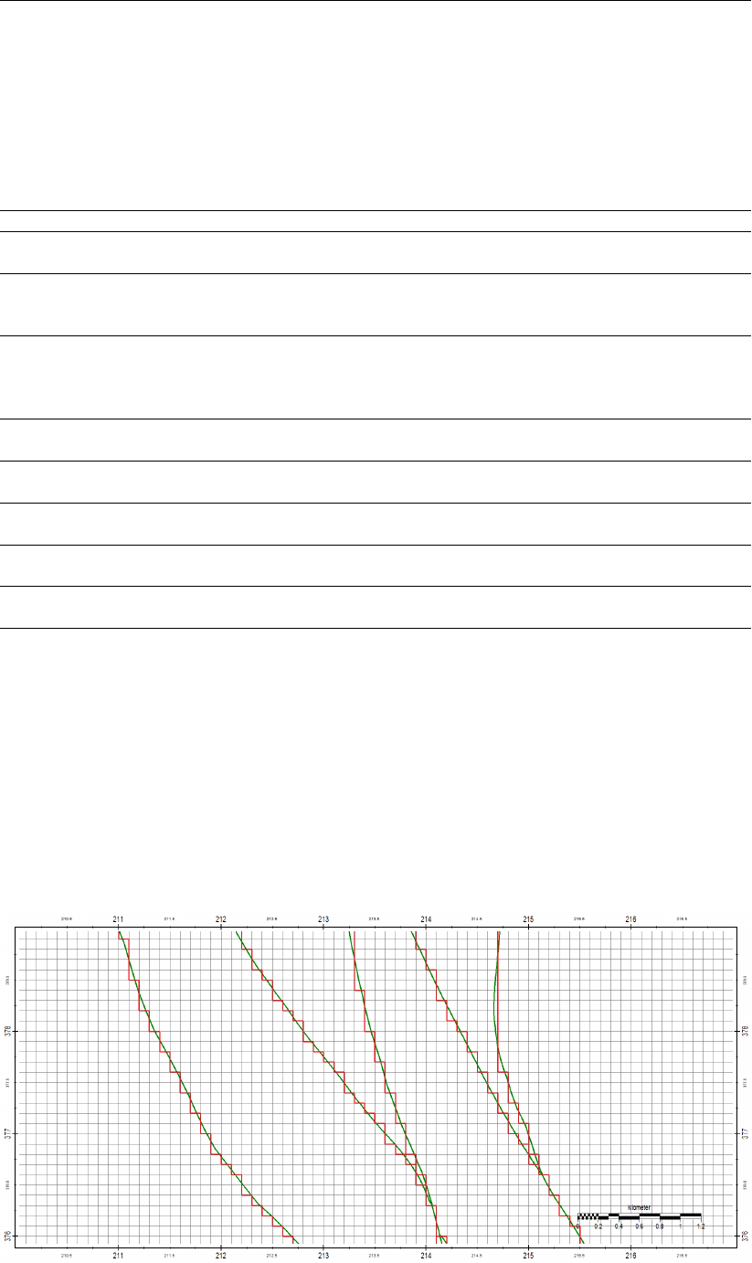
DRAFT
iMOD Batch functions
8.4 GEN-FUNCTIONS
8.4.1 GENSNAPTOGRID-Function
The GENSNAPTOGRID function can be used to rasterize a GEN file for a given raster. This gives
more grip on the way these GEN files will be applied in a model for particular cell sizes. This GEN file
can be transformed into a 3D GEN file as well.
FUNCTION= GENSNAPTOGRID
IDFFILE=
(optional)
Enter an IDF file for which the dimensions will be used to rasterize the speci-
fied GENFILE, e.g. IDFFILE=D:\BND\BND.IDF.
GENFILE= Enter the name of a GEN-file, e.g. GENFILE=D:\DATA\AREA.GEN. These ver-
tices in the GENFILE will be rasterized on the specified network via IDFFILE
or an entered window and cell size.
WINDOW=
(optional)
Enter the coordinates of the window that need to be computed, solely. Enter
coordinates of the lower-left corner first and then the coordinates of the upper-
right corner, e.g. WINDOW=100000.0, 400000.0, 200000.0, 425000.0. When
WINDOW=is absent, the dimensions of the specified IDFFILE will be used.
CELL_SIZE=
(optional)
Enter the cellsize of the grid that need to be used to rasterize the GEN file,
e.g. CELL_SIZE=100.0.
GENFILE_OUT= Enter the name of a GEN-file to be created, e.g. GEN-
FILE_OUT=D:\DATA\AREA_RASTER.GEN.
I3D=
(optional)
Specify I3D=1 whenever the GEN file need to be transformed into a 3D GEN
file. By default I3D=0 and a regular, 2D GEN is created.
IDF_TOP= Give an IDF file that represents the uppermost values of the GEN file, e.g.
IDF_TOP=D:\FAULTS\BR-T-CK.IDF. Specify this keyword whenever I3D=1.
IDF_BOT= Give an IDF file that represents the lowermost values of the GEN file, e.g.
IDF_TOP=D:\FAULTS\BR-B-CK.IDF. Specify this keyword whenever I3D=1.
Example 1
FUNCTION=GENSNAPTOGRID
IDFFILE= D:\BND\BND.IDF
GENFILE=D:\DATA\AREA.GEN
GENFILE_OUT=D:\DATA\AREA_RASTER.GEN
The above mentioned example will rasterize the AREA.GEN on the dimensions of the specified BND.IDF,
see the results on the next figure.
Deltares 447 of 812

DRAFT
iMOD, User Manual
Example 2
FUNCTION=GENSNAPTOGRID
IDFFILE= D:\BND\BND.IDF
GENFILE=D:\DATA\AREA.GEN
GENFILE_OUT=D:\DATA\AREA_RASTER.GEN
I3D=1
IDF_TOP= D:\GEOLOGY\TOP_KI.IDF
IDF_BOT= D:\GEOLOGY\BOT_KI.IDF
The above mentioned example will rasterize the AREA.GEN on the dimensions of the specified BND.IDF
and generates a 3D GEN using the values of the specified TOP- and BOT IDF files, see the results on
the next figure.
448 of 812 Deltares

DRAFT
iMOD Batch functions
8.4.2 GEN2GEN3D-Function
The GEN2GEN3D function reads a GEN file and creates a 3-D GEN file (see section 9.10) to be
displayed in the 3-D tool or used in the runfile of iMODFLOW.
FUNCTION= GEN2ISG
GENFILE_IN= Give a GEN file containing x and y coordinates of GEN segments,
e.g. GENFILE_IN=D:\FAULTS\FAULT.GEN.
IDF_TOP= Give an IDF file that represents the uppermost values of the GEN
file, e.g. IDF_TOP=D:\FAULTS\BR-T-CK.IDF.
IDF_BOT= Give an IDF file that represents the lowermost values of the GEN
file, e.g. IDF_TOP=D:\FAULTS\BR-B-CK.IDF.
GENFILE_OUT= Specify the yielding GEN file, e.g. GEN-
FILE_OUT=D:\FAULTS\FAULT_BR.GEN.
XSAMPLING=
(optional)
Specify the sampling distance to add z-coordinates to the GEN file,
e.g. XSAMPLING=100.0 will add a point each 100 meter. If this
keyword is absent, XSAMPLING will be equal to the cell size of the
IDF file entered at IDF_TOP.
Example 1
FUNCTION=GEN2GEN3D
GENFILE_IN=D:\MODEL\FAULTS\FAULT.GEN
IDF_TOP=D:\GEOLOGY\TOP_BREDA.IDF
IDF_BOT=D:\GEOLOGY\BOT_BREDA.IDF
XSAMPLING=250.0
GENFILE_OUT=D:\MODEL\FAULTS_BREDA.GEN
Above an example is given how to use the GEN2GEN3D. This example will generate and 3-D GEN file
based on top- and bottome elevations of the geological formation BREDA; the result GEN is written in
D:\MODEL\FAULTS_BREDA.GEN.
Deltares 449 of 812

DRAFT
iMOD, User Manual
8.5 IPF-FUNCTIONS
8.5.1 IPFSTAT-Function
The IPFSTAT function can be used to perform statistical analyses on timeseries that are defined in IPF
files as associated files.
FUNCTION= IPFSTAT
IPF1= Enter the name of an *.IPF file for which the associated timeseries need
to be analysed, e.g. {installfolder}\MEASURE.IPF.
OUTFILE= Specify a filename for the resulting IPF (or GEN whenever a GENFILE is
specified), e.g. {installfolder}\RESULT.IPF.
VARIABLES= Specify the number of variables to be computed.
Only IPF1 specified:
1. Auto-Correlation
-Correlation
-MeanLag
-NumberPoints
2. P50 over entire data period
3. (n)GxG starts at DMY1 and end at DMY2
-GHG
-GLG
-n(GxG)
Both IPF1 and IPF2 specified:
1. Cross-Correlation
-Correlation
-MeanLag
-NumberPoints
2. P50 IPF1 over overlapping data period IPF1 and IPF2
3. P50 IPF2 over overlapping data period IPF1 and IPF2
4. (n)GxG IPF1 starts at DMY1 and end at DMY2
-GHG
-GLG
-n(GxG)
5. (n)GxG IPF2 starts at DMY1 and end at DMY2
-GHG
-GLG
-n(GxG)
Enter the variables by their subsequent numbers, e.g. VARIABLES=0, 1,
0 in case IPF1 is specified solely, it will compute the P50 only. Or VARI-
ABLES=0, 0, 0, 1, 1 in case IPF1 and IPF2 are both specified, in this case
for both the (n)GxG will be computed.
ICOLDATE1 Enter the column number that contains the date expression in the txt files
associated to the first IPF file, on default ICOLDATE1=1.
ICOLVARS1 Enter the column number that contains the data, e.g. the measure-
ment/computed head in the txt files associated to the first IPF file, on de-
fault ICOLDATE2=2.
IPF2= Enter the name of a second *.IPF file for which the associated time-
series need to be analysed and compared to those in IPF1, e.g. {in-
stallfolder}:\COMPUTED.IPF. Be aware that the number of VARIABLES
change whenever IPF2 is absent.
ICOLDATE2 Enter the column number that contains the date expression in the txt files
associated to the second IPF file, on default ICOLDATE2=1.
ICOLVARS2 Enter the column number that contains the data, e.g. the measure-
ment/computed head in the txt files associated to the second IPF file, on
default ICOLDATE2=2.
GENFILE= Enter the name of a *.GEN-file that needs to be used to aggregate value
upon its individual polygons. This option is valid in combination with
IPF2 only.
450 of 812 Deltares

DRAFT
iMOD Batch functions
PERCENTILES= Enter the percentiles to be computed for each individual polygon in the
given GENFILE, e.g. 0.10, 0.90. If absent, PERCENTILES=0.10, 0.25,
0.50, 0.75, 0.90. This option is valid in combination with GENFILE
only.
IINVERSE= Enter IINVERSE=0 to use PERCENTILES as defined, however, enter IIN-
VERSE=1 to find the percentiles that belong to the values entered by
PERCENTILES. This option is valid in combination with GENFILE
only.
RELATECOLIPF1=
RELATECOLIPF2=
Enter the column number in IPF1 and IPF2 that need to be used to relate
between the data in IPF1 and IPF2. This option is valid in combination
with IPF2 only.
XLAG= Specify the lagwidth to be used to compute the auto/cross correlation, e.g.
XLAG=30 means that the auto/cross correlation will be computed over 30
(days). If absent XLAG=0.0 an auto/cross correlation will be computed
between measurements on similar dates.
DLAG= Specify the lag distance to be used to extent the search area, e.g. DLAG=7
means that 7 (days) before and 7 (days) after the given date+XLAG will be
used to search for data. If absent DLAG=7.0 (days).
DMY1=
DMY2=
Specify a starting and end date, both notated by yyyymmdd, e.g.
20110131 to express 31th January 2011. If absent these values are
DMY1=19000101 and DMY2=21001231, respectively. Both will be used
for VARIABLES that compute (n)GxG values.
SURFACELEVEL= Enter the name of an IDF-file that represent the surfacelevel, e.g. SUR-
FACELEVEL=D:\DATA\AHN.IDF. This will be used to express the GxG
value according to this surfacelevel.
Example 1
FUNCTION=IPFSTAT
IPF1=D:\TESTS\TEST.IPF
OUTFILE=D:\TESTS\OUT.IPF
VARIABLES=0,1,0
The example above computes the median groundwaterlevels (or equivalent) that are associated with
the IPF file TEST.IPF. The result is stored in OUT.IPF.
Example 2
FUNCTION=IPFSTAT
IPF1=D:\TESTS\MEASURE.IPF
IPF2=D:\TESTS\MODEL.IPF
OUTFILE=D:\TESTS\RESIDUAL.IPF
VARIABLES=1,0,0,0,0
RELATECOLIPF1=4
RELATECOLIPF2=3
ICOLDATE2=1
ICOLVARS2=2
The example above, computes the cross-correlation between the measurements associated with the
MEASURE.IPF and the computed values associates with the MODEL.IPF. The relation-columns are 4
and 3 for the MEASURE.IPF and MODEL.IPF, respectively.
Deltares 451 of 812

DRAFT
iMOD, User Manual
8.5.2 IPFSPOTIFY-Function
The IPFSPOTIFY function can be used to spotify geological formations in existing model discretisa-
tions. It gives per modellayer the fraction that a geological formation exists.
FUNCTION= IPFSPOTIFY
IPFFILE_IN
(optional)=
Enter the name of an *.IPF file for which the locations need to be spotified in the
selected op geological formations, e.g IPFFILE_IN=D:\WELLS.IPF.
IPFFILE_OUT= Specify an IPF file for which the fraction per geological formation
will be saved, e.g. D:\RESULT.IPF.
IXCOL= Specify the column number in the IPFFILE_IN that defines the
X coordinates, by default IXCOL=1.
IYCOL= Specify the column number in the IPFFILE_IN that defines the
Y coordinates, by default IYCOL=2.
IFCOL= Specify the column number in the IPFFILE_IN that defines the
attribute for which the fraction need to be computed, by default
IFCOL=3.
IZ1COL= Specify the column number in the IPFFILE_IN that defines the
top elevation to spotify underneath, by default IZ1COL=4.
IZ2COL= Specify the column number in the IPFFILE_IN that defines the
bottom elevation to spotify above, by default IZ2COL=5.
ILCOL= Specify the column number in the IPFFILE_IN that defines the
modellayer, by default ILCOL=6.
OUTPUT
FOLDER
(optional)=
Specify the output folder in which all IDF files will be saved with the in-
dividual fractions per geological formation per model layer, e.g OUTPUT-
FOLDER=D:\AQUIFER
NLAY= Specify the number of model layers to be spotified, e.g NLAY=10
TOP_{i}= Specify the top elevation for the ith model layer, e.g
TOP_L2=D:\MODEL\TOP_L2.IDF.
BOT_{i}= Specify the bottom elevation for the ith model layer, e.g
BOT_L2=D:\MODEL\BOT_L2.IDF.
FORMTOP= Specify the folder that stores the TOP elevation of geological formations, e.g.
FORMTOP=D:\GEOLOGY\*-T-CK.IDF. All files will be used that fit this wildcard
definition.
FORMBOT= Specify the folder that stores the BOT elevation of geological formations, e.g.
FORMBOT=D:\GEOLOGY\*-B-CK.IDF. All files will be used that fit this wildcard
definition.
Example 1
FUNCTION=IPFSPOTIFY
IPFFILE_IN=D:\WELLS\TEST.IPF
IPFFILE_OUT=D:\SPOTIFIED\OUT.IPF
NLAY=2
TOP_L1=D:\MODEL\TOP_L1.IDF
BOT_L1=D:\MODEL\BOT_L1.IDF
TOP_L2=D:\MODEL\TOP_L2.IDF
BOT_L2=D:\MODEL\BOT_L2.IDF
REGISTOP=D:\REGIS\*-T-CK.IDF
REGISBOT=D:\REGIS\*-B-CK.IDF
The example above computes the fractions for each location in the IPFFILE_IN of all geological forma-
tions in REGISTOP and REGISBOT for each model layer.
452 of 812 Deltares

DRAFT
iMOD Batch functions
Example 2
FUNCTION=IPFSPOTIFY
OUTPUTFOLDER=D:\FRACTIONS\AQUIFER
NLAY=2
TOP_L1=D:\MODEL\TOP_L1.IDF
BOT_L1=D:\MODEL\BOT_L1.IDF
TOP_L2=D:\MODEL\TOP_L2.IDF
BOT_L2=D:\MODEL\BOT_L2.IDF
REGISTOP=D:\REGIS\*-T-CK.IDF
REGISBOT=D:\REGIS\*-B-CK.IDF
The example above, computes the fractions for each cell in the model layers for each geological for-
mation defined by the REGISTOP and REGISBOT keywords, the results are stored in the AQUIFER
folder. To spotify aquitards in it is neccessary to switch the top and bottom elevations, e.g.
FUNCTION=IPFSPOTIFY
OUTPUTFOLDER=D:\FRACTIONS\AQUITARD
NLAY=1
TOP_L1=D:\MODEL\BOT_L1.IDF
BOT_L1=D:\MODEL\TOP_L2.IDF
REGISTOP=D:\REGIS\*-T-CK.IDF
REGISBOT=D:\REGIS\*-B-CK.IDF
Deltares 453 of 812

DRAFT
iMOD, User Manual
8.5.3 IPFSAMPLE-Function
The function IPFSAMPLE samples IDF-files to add values to the points defined in an IPF file.
FUNCTION= IPFSAMPLE
IPFFILE_IN= Enter the name of an IPF file with minimal 2 columns that represents x-
and y coordinates, e.g. D:\DATA\MEASURE.IPF.
IPFFILE_OUT= Enter the name of an IPF file that need to be written with the results of the
IDF values from the specified IDFFILE, e.g. D:\DATA\CHECK.IPF. Results
read from the IDF-files in SOURCEDIR, will be stored as an extra column
in IPFFILE_IN, the label will be identical to the name of the IDF-files.
SOURCEDIR= Enter the name of an IDF-file that needs to be read by the points specified
in the IPF file IPFFILE_IN, e.g. D:\DATA\RESULTS\HEAD.IDF.
IXCOL Enter the column number in the IPF file IPFFILE_IN that represents the
X-coordinate, e.g. IXCOL=4. By default IXCOL=1.
IYCOL Enter the column number in the IPF file IPFFILE_IN that represents the
Y-coordinate, e.g. IYCOL=6. By default IYCOL=2.
IACOL Enter the column number to enter the sampled data from the IDF files, e.g.
IACOL=3 which means that the entered starts at columns 3. By default
IACOL=0 which means that the sampled data will be added at the end of
the IPF file.
Example 1
FUNCTION=IPFSAMPLE
IPFFILE_IN=D:\WELLS.IPF
IPFFILE_OUT=D:\WELLS_KD.IPF
SOURCEDIR=D:\DATA\KD*.IDF
This example, adds values (columns) to all points in the IPF file WELLS.IPF, with the corresponding
values from the KD*.IDF-files in the folder D:\DATA.
Example 2
FUNCTION=IPFSAMPLE
IPFFILE_IN=D:\WELLS.IPF
IPFFILE_OUT=D:\WELLS.IPF
SOURCEDIR=D:\DATA\KD*.IDF
IXCOL=4
IYCOL=3
This example, adds values (columns) to all points in the IPF file WELLS.IPF, with the corresponding
values from the KD*.IDF-files in the folder D:\DATA. The x- and y coordinates in the IPF file WELLS.IPF,
will be read from the fourth and third column, respectively.
454 of 812 Deltares

DRAFT
iMOD Batch functions
8.6 MODEL-FUNCTIONS
8.6.1 IMPORTMODFLOW-Function
Use this function to import an existing MODFLOW configuration into iMOD files (e.g. IDFs, IPFs and
GENs), see for more information section 9.7.
FUNCTION= IMPORTMODFLOW
MVERSION= Enter the version number of the MODFLOW configuration files, e.g.
MVERSION=1988. There are four available versions supported: 1988,
1996, 2000 and 2005.
BASFILE= Enter the location of the, so called, BAS file (use this keyword whenever
MVERSION=1988), e.g. BASFILE=D:\MODEL\MODEL.BAS.
NAMFILE= Enter the location of the, so called, NAM file (use this key-
word whenever MVERSION=1988, 1996, 2000 or 2005), e.g. NAM-
FILE=D:\MODEL\MODEL.NAM.
OUTDIR= Enter the folder in which all iMOD files will be saved, e.g. OUTDIR
=D:\IMPORT. Subfolders will be created automatically to save the indi-
vidual files, e.g. D:\IMPORT\BND\VERSION_1\BND_L1.IDF . By default
OUTDIR =’.’ which means that the files will be saved directly at the current
location of the iMOD executable.
LLCORNER= Enter the coordinates of the lower-left corner of your model,
e.g. XMIN=200000.0,YMIN=400000.0 (all in meters). By default
XMIN=YMIN=0.0.
SDATE= Enter the starting date of your simulation, e.g. SDATE=20111027 which
means 27th of October 2011. By default SDATE=20110101.
PACKAGESUM= Enter PACKAGESUM=1 to sum all existing package information into a sin-
gle modelcell, this is the default. Whenever more elements occur in a
single modelcell, they will be lumped together to form one value. Enter
PACKAGESUM=0 to extract all elements in a single modelcell to store
them, if necessary, in individual iMOD files.
RIV5TH= Enter RIV5TH=1 to include a 5th column in the river files that expresses
the infiltration resistance. On default RIV5TH=0.
Example 1
FUNCTION=IMPORTMODFLOW
MVERSION=1988
BASFILE=D:\IMOD-MODEL\VELUWE\MS1L5.BAS
This is the shortest version to import the MODFLOW model MS1L5.
Example 2
FUNCTION=IMPORTMODFLOW
MVERSION=2005
NAMFILE=D:\MODEL\GWR54\MODFLOW.NAM
LLCORNER=125000.0,432000.0
SDATE=20050101
PACKAGESUM=0
RIV5TH=1
This example shows how to import a (transient) MODFLOW2005 configuration.
Deltares 455 of 812
DRAFT
iMOD, User Manual
8.6.2 IMPORTSOBEK-Function
Use this function to import a SOBEK configuration into ISG-files for iMOD for more information.
Note: This function is only available in the X32-bits version of iMOD.
FUNCTION= IMPORTSOBEK
ISGNAME= Enter the name of the ISG-file to be created, e.g. ISG-
NAME=D:\IMPORT\SOBEK.ISG.
SOBEKDIR= Enter the name (location) of the SOBEK files, e.g. SOBEKDIR=D:\DATA.
iMOD will search for all other files that it need in the folder D:\DATA, these
files are:
{SOBEKDIR}\NETWORK.TP
{SOBEKDIR}\NETWORK.CR
{SOBEKDIR}\NETWORK.CP
{SOBEKDIR}\NETWORK.GR
{SOBEKDIR}\NETWORK.ST
{SOBEKDIR}\PROFILE.DAT
{SOBEKDIR}\PROFILE.DEF
{SOBEKDIR}\PROFILE.DEF
{SOBEKDIR}\FRICTION.DAT
CALCHIS= Enter the name of the HIS file that contains the computed waterlevels at
the calculation points, e.g. CALCHIS=D:\SOBEK\CALC.HIS.
STRUCHIS= Enter the name of the HIS file that contains the computed waterlevels at
the structures, e.g. STRUCHIS =D:\SOBEK\STRUCT.HIS.
Example 1
FUNCTION=IMPORTSOBEK
ISGNAME=D:\IMPORT\HCMC0611.ISG
SOBEKDIR=D:\SOBEK\HCMC0611
CALCHIS=D:\SOBEK\HCMC0611\CALCPNT.HIS
STRUCHIS=D:\SOBEK\HCMC0611\STRUC.HIS
The above mentioned examples imports the SOBEK model (files) in the folder D:\SOBEK\HCM0611\*
and combines this with the computed results from the two entered HIS files (CALCPNT.HIS and
STRUC.HIS) and saves it in HCMC0611.ISG.
456 of 812 Deltares

DRAFT
iMOD Batch functions
8.6.3 MODELCOPY-Function
The function MODELCOPY can be used to extract a separate data set for a sub model from a large
model. It can also be applied to copy the entire dataset as specified by the entered runfile into a
separate folder. In this process, all IDF and IPF files that can be identified in a given runfile, will be
clipped to the given window. Other files that are mentioned in the runfile will be copied. As a result a
complete copy of a part of the original model will be saved and can be simulated separately.
Note: Other files that might be referred to from files other than the specified runfile, will not be copied.
FUNCTION= MODELCOPY
RUNFILE= Enter the name of a runfile that contains a specific set of IDF-file(s), e.g. RUN-
FILE=D:\RUNFILES\MODEL.RUN.
TARGETDIR= Enter the name of a folder in which the resulting files will be copied, e.g. TARGET-
DIR=D:\SUBMODEL.
WINDOW=
(optional)
Specify a window (X1,Y1,X2,Y2) for which the entered RUNFILE will be clipped,
WINDOW=125100.0,345000.0,135000.0,355000.0. By absence of this keyword,
the extent of the model will be read from the runfile, including the corresponding
cell size.
CELL_SIZE= Specify a cellsize whenever the keyword WINDOW is specified,
e.g. CELL_SIZE=250.0.
CLIPDIR=
(optional)
Enter a foldername for which all filenames will be
trimmed, e.g. CLIPDIR=D:\MODEL. If the original file-
names are D:\MODEL\DRN\SYS1\DRN_EL_L1.IDF and
D:\MODEL\DRN\SYS2\DRN_EL_L1.IDF, they will be saved
in {TARGETDIR}\DRN\SYS1\DRN_EL_L1.IDF and {TARGET-
DIR}\DRN\SYS2\DRN_EL_L1.IDF, respectively. By omitting CLIPDIR, both
files will be stored in {TARGETDIR}\DRN\DRN_EL_L1.IDF instead.
Example 1
FUNCTION=MODELCOPY
RUNFILE=D:\RUNFILES\MODEL.RUN
TARGETDIR=D:\MODEL\SUBMODEL
The above mentioned example copies all IDF and IPF files from the runfile D:\RUNFILES\MODEL.RUN
and the result is saved in D:\MODEL\SUBMODEL. A new runfile is created that will be saved in
D:\MODEL\SUBMODEL\MODEL.RUN. Use this configuration to create a cleaned up folder structure
of the model.
Example 2
FUNCTION=MODELCOPY
RUNFILE=D:\RUNFILES\MODEL.RUN
TARGETDIR=D:\MODEL\SUBMODEL
WINDOW=147000.0 448000.0 155000.0 452000.0
CLIPDIR=D:\MODEL
The above mentioned example is equal to example 1 except that it clips all IDF and IPF files from
the runfile D:\RUNFILES\MODEL.RUN to the window 147000.0 448000.0 155000.0 452000.0 and the
files remain their original filename under D:\MODEL. In this way complex structured in filename will be
preserved.
Deltares 457 of 812
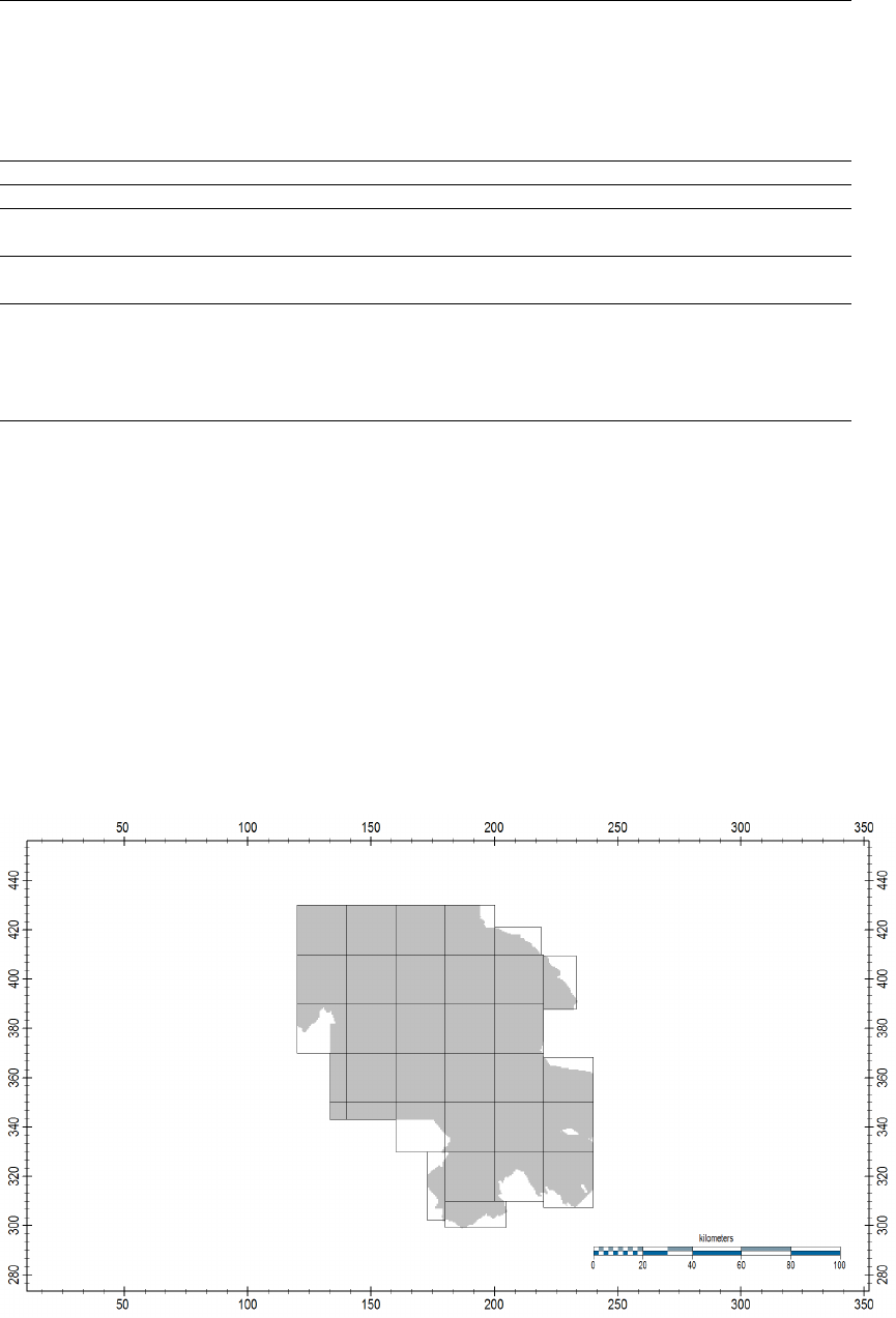
DRAFT
iMOD, User Manual
8.6.4 CREATESUBMODEL-Function
Use this function to create submodels for iMODFLOW based on a pointer IDF that determines the
active area to be simulated.
FUNCTION= CREATESUBMODEL
DSIZE= Enter the maximum size of a submodel in meters, e.g. DSIZE=10000.0.
CSIZE= Enter the cellsize to be used in the submodels, this will be used to fill in
the appropriate column in the runfile, e.g. CSIZE=25.
IBOUND= Enter the IDF-file that describes the location of active area to be simulated,
e.g. IBOUND=D:\IBOUND_L1.IDF.
SUBMODELFILE= Enter the name of the text file that will be created that stores the
header of a runfile that describes the submodels, e.g. SUBMOD-
ELFILE=D:\SUBMODELS. iMOD will create a SUBMODELFILE.RUN to
be used in a runfile and a SUBMODELFILE.GEN of the submodels to be
displayed in iMOD.
Example 1
FUNCTION=CREATESUBMODEL
DSIZE=10000.0
CSIZE=25.0
IBOUND=D:\DBASE\IBOUND_L1.IDF
SUBMODELFILE=D:\RUNFILE\SUBMODEL
The example above will create submodels with a maximum extent of 10000m (10km) and will write a
runfile header with cellsizes of 25m. The IDF-file IBOUND.IDF will be used to determine the active
areas of the model. iMOD creates boxes with 10x10km first and then decreases submodels whenever
this is possible, moreover, whenever submodels become too small (25% of 10km), they will be joined
together.
458 of 812 Deltares

DRAFT
iMOD Batch functions
8.6.5 RUNFILE-Function
The function RUNFILE can be used to create a runfile (*.RUN) from a projectfile (*.PRJ), or create a
projectfile from a runfile.
FUNCTION= RUNFILE
RUNFILE_IN=
(optional)
Enter the name of a runfile that contains a specific set of IDF-file(s), e.g. RUN-
FILE=D:\RUNFILES\MODEL.RUN.
PRJFILE_OUT=
(optional)
Enter the name of a projectfile that need to be created based
on the content of the runfile specified by RUNFILE_IN, e.g. PRJ-
FILE_OUT=D:\PRJFILES\MODEL.PRJ."
PRJFILE_IN=
(optional)
Enter the name of a projectfile that need to be used to create a runfile specified
by RUNFILE_OUT, e.g. PRJFILE_IN=D:\PRJFILES\MODEL.PRJ.
RUNFILE_OUT=
(optional)
Enter the name of a runfile that will be created, e.g. RUN-
FILE_OUT=D:\RUNFILES\MODEL.RUN.
NAMFILE_OUT=
(optional)
Enter the name of a namfile that will be created, e.g. NAM-
FILE_OUT=D:\NAMFILES\MODEL.NAM.
OUTPUT_
FOLDER=
(optional)
Enter the name of an output folder that will be created to save the results of
the model simulation, e.g. OUTPUT_FOLDER=D:\MODEL\OUTPUT. In the situ-
ation that RUNFILE_OUT is entered, this keyword will add the output folder at
the first line of the runfile, in the situation that NAMFILE_OUT is entered, the
OUTPUT_FOLDER will be written in the *.MET file.
IDEBUG=
(optional)
Enter IDEBUG=0 to generate a MF2005 compatible model, all
arrays are listed in *.ARR files if needed. Use IDEBUG=1 or
IDEBUG=2 to export all model input to ASC or IDF, respectively.
ISS=
(optional)
Specify the type of time configuration to be added to the RUNFILE or NAMFILE;
for transient enter ISS=1 and for steady state enter ISS=0. By default ISS=0.
Specify following keywords for transient configurations (ISS=1)
TIMFNAME=
(optional)
Specify the name of the *.TIM file that contains the
time discretisation of the model to be created, TIMF-
NAME=D:\RUNFILES\MODEL.TIM. For more information on
the content of a *.TIM file see section 9.4.
SDATE=
(optional)
Specify a starting date of the simulation in yyyymmddhhmmss
format, e.g. SDATE=20120101080000 to denote the 1st of Jan-
uary 2012 at 08:00:00 am. This keyword is only compulsory
whenever TIMFNAME is absent.
EDATE=
(optional)
Specify a starting date of the simulation in yyyymmddhhmmss
format, e.g. EDATE=20121231153030 to denote the 31st of De-
cember 2012 at 15:30:30. This keyword is only compulsory
whenever TIMFNAME is absent.
Deltares 459 of 812

DRAFT
iMOD, User Manual
ITT=
(optional)
Specify a time interval category, e.g. ITT=2 to denote days.
The other are:
1 Hourly
Select this option to generate hourly stress-periods;
2 Daily
Select this option to generate daily stress-periods;
3 Weekly
Select this option to generate weekly stress-periods;
4 Decade
Select this option to generate stress-periods per decade;
5 14/28
Select this option to generate stress-periods on the 14th
and 28th day of each month;
6 Monthly
Select this option to generate monthly stress-periods;
7 Yearly
Select this option to generate yearly stress-periods;
8 Packages
Select this option to generate stress-periods that are deter-
mined by the input data
This keyword is only compulsory whenever TIMFNAME is ab-
sent.
IDT=
(optional)
Specify a time interval of the time steps corresponding to the
chosen time interval category ITT, e.g. IDT=7 to denote the 7
days whenever ITT=2. This keyword is only compulsory when-
ever TIMFNAME is absent.
ISTEADY=
(optional)
Specify ISTEADY=1 to include an initial steady-state time step
to the model. This will add packages with the time stamp
STEADY-STATE to the first stress-period of your model. By de-
fault ISTEADY=0.
NSTEP=
(optional)
Specify the number time step within each stress period, e.g.
NSTEP=10. Whenever a model suffers some convergence is-
sues, increase the number of time steps might help. Also,
steady-state convergence problems can be overcome by cre-
ating a transient model with enough time step. By default
NSTEP=1.
NMULT=
(optional)
Specify the multiplication factor in which the step size of each
subsequent time step will increase, e.g. NMULT=1.2. The factor
need to ≥1.0. The higher the number to more explosive the
size will increase in subsequent time steps according to:
∆ti= ∆TjNMULT −1
NMULTNSTP −1(8.1)
wherein ∆iis the current length of the time step i,∆Tjis the to-
tal length of the current stress period j. By default NMULT=1.0.
SSYSTEM=
(optional)
Specify SSYSTEM=1 to save each system for a package by a separate file. By
default SSYSTEM=0.
ISAVEEND
DATE=
(optional)
Specify ISAVEENDDATE=1 to save each file with a time stamp equal to the end
of the corresponding stress period (and/or time step). By default ISAVEEND-
DATE=0 and the time stamp will be equal to the start date of each stress period
(and/or time step). This option is applicable whenever NAMFILE_OUT is speci-
fied, whenever RUNFILE_OUT is specified, this keyword doesn’t have any effect.
460 of 812 Deltares
DRAFT
iMOD Batch functions
IPKS=
(optional)
Specify IPKS=1 to apply the PKS package instead of the PCG package. The
PKS seems to be more robust than the PCG solver, so you might want to use
this PKLS solver in case of non-convergency due to huge contrasts in conductiv-
ities and/or using the multi-core applications. This option is applicable whenever
NAMFILE_OUT is specified, whenever RUNFILE_OUT is specified, this keyword
doesn’t have any effect.
ICHKCHD=
(optional)
Specify ICHKCHD=1 to convert constant head cells (from the read starting heads)
that are not belonging to the layer to which they are assigned. If a value exceeds
the top of a model layer to which it is assigned, the boundary value is turned
into 99 and is converted to an active node. This option is applicable whenever
NAMFILE_OUT is specified, whenever RUNFILE_OUT is specified, this keyword
doesn’t have any effect.
ICONCHK=
(optional)
Use this keyword to correct the drainage levels automatically during a simulation.
Whenever ICONCHK=1 the drainage level will be higher or equal to existing level
from the RIV and/or ISG package. This prevents undesired circulation of ground-
water between drainage system underlying an infiltrating river system. By default
ICONCHK=0 and no corrections are performed.
IDOUBLE=
(optional)
Use this keyword to save all results from the simulation in double precision.
Whenever IDOUBLE=0 (default) a single precision value is saves, whenever
IDOUBLE=1 a double precision is saved. Be ware that all files will be affected
by this and therefore the total space that will be occupied by the results will be
doubled.
IFVDL=
(optional)
Use this keyword to use the Formulae of ”Van de Lange“ for the correction of
river conductances. This keyword can be used whenever the PRJ file contains
TOP and BOT definitions as well as KHV. The SFT package might be used to
include permeabilities and thickness used by the formulae, otherwise, if this SFT
package is absent, de values from the model will be used. By default IFVDL=0
and no corrections are performed.
MINKD=
(optional)
Use this keyword to assign a minimal horizontal conductance KD (m2/d) to
maximize the computed conductances, internally, e.g. MINKD=0.01, by default
MINKD=0.0.
MINC=
(optional)
Use this keyword to assign a minimal vertical resistance C (d) to maximize the
computed vertical resistances, internally, e.g. MINC=1.0, by default MINC=0.0.
UNCONFINED=
(optional)
Use this keyword to include unconfined conditions for model layers, e.g. UN-
CONFINED=1,1,1,0,0,0 by default UNCONFINED=0 and model layers are
confined. So, if NLAY=10 and UNCONFINED=1,1,1 this means that the first
three model layers are unconfined, the remaining layers are confined. The values
for UNCONFINED are:
0
The model layer is confined, the saturated thickness is defined by the top-
and bottom elevation per model layer;
1
The model layer is unconfined, the saturated thickness is defined by the com-
pute hydraulic head and the bottom elevation per model layer;
2
The model layer is confined by the saturated thickness is defined by the start-
ing heads and the bottom elevation per model layer.
It is obligatory to include the modules STO and SPY whenever unconfined con-
ditioned are simulated for a transient model. iMOD will add and configure the
WETDRY option automatically.
IPEST=
(optional)
Use this keyword to include the parameter optimisation package PST, e.g.
IPEST=1, by default IPEST=0 and the model is simulated conventionally.
Deltares 461 of 812
DRAFT
iMOD, User Manual
SAVESHD=
SAVEWEL=
SAVEDRN=
SAVERIV=
SAVEGHB=
SAVERCH=
SAVEEVT=
SAVEMNW=
SAVELAK=
SAVESFR=
SAVEUZF=
SAVEFHB=
(all optional)
Use these keywords to save the hydraulic head per layer or/and results for the
WEL, DRN, RIV, GHB, RCH, EVT, LAK, MNW, SFR, FHB and UZF package, e.g.
SAVESHD=3,4,10 to note that model layers 3, 4 and 10 will be saved only, by
default all keyword are 0, meaning no layers will be saved. Specify SAVESHD=-
1 to denote that ALL layers will be saved, this is similar for the other packages,
except for the SFR and UZF package, specifying more layers does not have any
effect.
SAVEFLX=
(optional)
Use this keyword to include layers to be saved for the spatial fluxes in x,y and
z direction, e.g. SAVEFLX=3,4,10 to note that model layers 3, 4 and 10 will be
saved only, by default SAVEFLX=0, meaning no layers will be saved. Specify
SAVEFLX=-1 to denote that ALL layers will be saved. Part of this, the BDGFFF,
BDGFRF, BDGFLF and BDGBND will be saved.
NETWORKIDF=
(optional)
Specify an IDF file that represents the network for the simulation, e.g. NET-
WORKIDF=D:\MODEL \NETWORK.IDF. This keyword is optional, whenever this
keyword is absent the network is defined by the first IDF file in the entered PRJ
file or specified by the keyword WINDOW.
WINDOW=
(optional)
Specify a window (X1,Y1,X2,Y2) for which the constructed RUNFILE will be
clipped, e.g. WINDOW=125100.0,345000.0,135000.0,355000.0.
CELLSIZE= Specify a cell size to be used, e.g. CELLSIZE=25.0. This key-
word is necessary and read whenever the WINDOW keyword is
entered.
BUFFER=
(optional)
Specify a buffer to be added to the specified window (WIN-
DOW), e.g. BUFFER=1500.0. This keyword is optional and the
default value is BUFFER=0.0.
BUFFERCS=
(optional)
Specify a maximal cell size in the buffer, e.g.
BUFFERCS=100.0. This keyword is optional and read
whenever BUFFER is specified and greater than 0.0 meter.
ISOLVE=
(optional)
Enter ISOLVE=1 to start a simulation after generating a RUNFILE or NAMFILE,
by default ISOLVE=0.
MODFLOW= Whenever ISOLVE=1, enter the simulator, e.g. MOD-
FLOW=D:\PROGRAMS\IMODFLOW.EXE.
Example 1
FUNCTION=RUNFILE
RUNFILE_IN=D:\RUNFILES\MODEL.RUN
PRJFILE_OUT=D:\PRJFILES\MODEL.PRJ
The above mentioned example creates a projectfile D:\PRJFILES\MODEL.PRJ file out of the runfile
D:\RUNFILES\MODEL.RUN.
Example 2
FUNCTION=RUNFILE
PRJFILE_IN=D:\PRJFILES\MODEL.PRJ
RUNFILE_OUT=D:\RUNFILES\MODEL.RUN
WINDOW=147000.0 448000.0 155000.0 452000.0
CELLSIZE=25.0
BUFFER=1500.0
SDATE=19940101120000
EDATE=20121231235959
ITT=3
462 of 812 Deltares

DRAFT
iMOD Batch functions
IDT=2
The above mentioned example creates runfile D:\RUNFILES\MODEL.RUN, based on the content of
the projectfile D:\PRJFILES\MODEL.PRJ for a specified window. The model starts at the 1st of January
1994 at 12:00:00 am and ends at the 31st of December 2012 at 23:59:59 am at uses two-weekly time
steps.
Example 3
FUNCTION=RUNFILE
PRJFILE_IN=D:\PRJFILES\MODEL.PRJ
NAMFILE_OUT=D:\NAMFILES\MODEL.NAM
TIMFILE_OUT=D:\TIMFILES\MODEL.TIM
ISOLVE=1
MODFLOW=D:\PROGRAM\IMODFLOW.EXE
The above mentioned example creates a Modflow2005 configuration NAMFILE D:\NAMFILES\MODEL.NAM,
based on the content of the projectfile D:\PRJFILES\MODEL.PRJ for a times discretisation speci-
fied in the *.TIM file D:\TIMFILES\MODEL.TIM. After that, it starts the simulation using the simulator
D:\PROGRAM\IMODFLOW.EXE.
Deltares 463 of 812

DRAFT
iMOD, User Manual
8.6.6 IMODPATH-Function
The function IMODPATH computes flowlines based on the budget terms that result from the iMOD-
FLOW computation. The IMODPATH function uses a very simple runfile. For more information see
section 7.14.
FUNCTION= IMODPATH
IRUN=
(optional)
Specify IRUN=1 to start a particle simulation, apply IRUN=0 to skip the parti-
cle simulation and perform a post processing solely, if IPOSTP=1. By default
IRUN=1.
RUNFILE=
(optional)
Enter the name of the runfile that describes the files needed for the iMOD-
PATH simulation, e.g. RUNFILE=D:\MODEL\SIM.RUN. This keyword is compul-
sory whenever IRUN=1. The content of such a runfile is as follows:
NLAY Enter the number of model layers, e.g. NLAY=8
NPER,ISTO Enter the number of stress periods, .e.g. NPER=1 and whether
fluxes from storage need to be read in, in case a transient sim-
ulation is carried out. The storage flux will correct the total wa-
ter balance and influence whether an unbalance will denote a
weak/strong sink. Whenever the absolute unbalance is larger
than 0.01 m3/d, iMODPATH will treat the location as a potential
weak/strong sink. The parameter ISTO is optional and when-
ever it is absent the flow from storage is as assumed to be zero.
NSDF
(optional)
Enter the number of SDF files to be computed, sequentially. En-
ter a value for this only whenever NSDF≥2. Leave this keyword
out, whenever a single ISDFILE and OUTFILE is entered.
ISDFILE /
IPFFILE
Enter the name of the startpoint file, see section 7.13 for more
information about this type of file (see section 9.19 for the actual
syntax). Repeat this, together with OUTFILE for NSDF-times
whenever NSDF is specified and NSDF≥2. Alternatively an IPF
file can be specified. It is compulsory to specify at least three
columns whereby the first three columns are reseverd for the x-,
y- and z-coordinate.
OUTFILE Enter the name of the result file. The extent will be added or
replaced to the appropriate output format (IFF and/or IPF), e.g.
D:\d:\RESULT. Repeat this, together with ISDFILE for NSDF-
times whenever NSDF is specified and NSDF≥2.
IMODE Enter the mode of the results to be achieved, use IMODE=1,0
for flowlines and IMODE=0,1 for endpoints only. For example
IMODE=1,1 will save both particles in the IFF and IPF format.
IFWBW Enter the direction of the tracing, use IFWBW=0 for a forward
tracing and IFWBW=1 for a backward tracing.
ISNK Specification on how to handle “weak”-sinks. Particles will con-
tinue at weak sinks for ISNK=1 as they stop at weak sinks for
ISNK=2. The latter can be specified as a fraction for ISNK=3,
see keyword FRACTION.
FRACTION Specify the fraction of the total outflow to be a measure to deter-
mine whether particles should stop or continue in a model with
a “weak”-sink. FRACTION=1.0 to let particles stop at a strong
sink only, as FRACTION=0.0 act as particles will always stop,
no matter the size of the total outflow (ISNK=1).
STOPCRIT Enter the stop criteria. Specify STOPCRIT=1 to stop the parti-
cle as its age becomes equal to MAXT; specify STOPCRIT=2
to repeat the transient period in the time window as specified
by the keywords SWINDOW and EWINDOW until the particles
meets the MAXT criterion or stops in a weak/strong sink. Or,
alternatively set STOPCRIT=3 to continue with the last results
at the end of the time window until the particle terminates. This
keyword STOPCRIT is only applicable whenever NPER>1.
MAXT Enter the maximum tracing time (days).
464 of 812 Deltares

DRAFT
iMOD Batch functions
STARTDATE Enter the startdate for the particle tracing, e.g. 19960414 to ex-
press the 14th of April 1994. This keyword is used only when-
ever NPER >1, but you need to specify an artificial START-
DATE for NPER=1.
SWINDOW Enter the start date for the time window in which the particle
tracing will operate, e.g. 19960414 to express the 1st of April
1994. Only used whenever NPER >1, but you need to specify
an artificial SWINDOW for NPER=1.
EWINDOW Enter the end date for the time window in which the particle
tracing will operate, e.g. 20040328 to express the 28th of March
2004. Only necessary whenever NPER >1, but you need to
specify an artificial EWINDOW for NPER=1.
Repeat the following NLAY-times
IBOUND Enter the boundary condition (IDF). Particle tracing will pass
through boundary values >0 only.
TOP Enter the top elevation (IDF or constant value) of a modellayer
(m+MSL).
BOT Enter the bottom elevation (IDF or constant value) of a model-
layer (m+MSL).
PORAQF Enter the porosity (IDF or constant value) of the aquifer (-).
PORAQT Enter the porosity (IDF or constant value) of the aquitard (-).
Specify this keyword for model layers < NLAY.
Repeat the following NLAY times and NPER times
BDGFRF Enter the IDF file that represents the water budget (m3/day)
along the x axes (columns) at the eastern border of each cell;
positive flow is westwards, negative is eastwards.
BDGFFF Enter the IDF file that represents the water budget (m3/day)
along the y axes (rows) at the southern border of each cell;
positive flow is northwards, negative flow is southwards.
BDGFLF Enter the IDF file that represents the water budget (m3/day)
along the z axes (layers) at the lower border of each cell; pos-
itive flow is upwards, negative flow is downwards. Specify this
keyword for model layers 1 up to NLAY-1.
BDGSTO
(optional)
Enter the IDF file that represents the water budget (m3/day) that
goes into storage; positive flow is going out of the storage, nega-
tive flow is going into the storage. This parameter is only needed
whenever ISTO=1.
WINDOW=
(optional)
Specify a window (X1,Y1,X2,Y2) for which the constructed model will be sim-
ulated, e.g. WINDOW=125100.0,345000.0,135000.0,355000.0. This might in-
crease the efficiency as only a part of the model need to be allocated and read
in.
ICONVERTGEN=
(optional)
Specify ICONVERTGEN=1 to convert the results of the pathline simulation as
well into a GEN (see 9.10) and DAT file (see 9.11). Bij default ICONVERTGEN=0
and no conversion will occur.
IPOSTP=
(optional)
Use IPOSTP=1 to include a post processing direct after the pathline simulation.
This post processing will separate the IFF and/or IPF files to a given selection
criterion. By default IPOSTP=0.
The following keyword are applicable only whenever IPOSTP=1
IFFFLOW=
(optional)
Enter the name of the IFF file (generated by the pathline simulation) to be pro-
cessed, e.g. IPFFLOW=D:\RESULT\PATHLINES.IFF. By default no IFF file will be
processed.
IPFFLOW=
(optional)
Enter the name of the IPF file (generated by the pathline simulation) to be pro-
cesses, e.g. IPFFLOW=D:\RESULT\PATHLINES.IPF. By default no IPF file will be
processed.
Deltares 465 of 812

DRAFT
iMOD, User Manual
IPFFNAME=
(optional)
Enter the IPF file to be used to separate the content of the IFFFLOW and or
IPFFLOW file names to the labels (ILABELCOL) as specified in the IPFFNAME,
e.g. D:\INPUT\WELLS.IPF
IDFFLOW= Specify an IDF file that will be used to map the points from the
IPF file given at IPFFNAME on a network in order to match them
with the results in the IPF and/or IFF file given at IPFFLOW and
IFFFLOW, respectively, most common is to use a random IDF
from the result map of the simulation results, used for the par-
ticle simulation, e.g. IDFFLOW=D:\RESULT\HEAD_STEADY-
STATE_L1.IDF.
IXCOL= Enter the column number in the given IPF file IPFFNAME that
represents the X-coordinate, e.g. IXCOL=1.
IYCOL= Enter the column number in the given IPF file IPFFNAME that
represents the Y-coordinate, e.g. IYCOL=2.
ILABELCOL= Enter the column number in the given IPF file IPFFNAME that
represents the label, e.g. ILABELCOL=3. For each unique la-
bel, a separate IPF and/or IFF will be constructed.
ILAYCOL= Enter the column number in the given IPF file IPFFNAME that
represents the model layer, e.g. ILAYCOL=4.
TOPFNAME=
(optional)
Enter the IDF file to be used to identify the top of an interface that need to
be used to separate IPF and/or IFF file that are underneath the interface, e.g.
D:\INPUT\TOP_L1.IDF, by default no top is given and in that case all is valid. Any
NodataValue in the IDF file will be used to exclude any particle.
BOTFNAME=
(optional)
Enter the IDF file to be used to identify the bot of an interface that need
to be used to separate IPF and/or IFF file that are above the interface, e.g.
D:\INPUT\BOT_L7.IDF, by default no bottom is given and in that case all is valid.
Any NodataValue in the IDF file will be used to exclude any particle.
IEXTRACT=
(optional)
Enter the extract option for the particles, choose from the following:
IEXTRACT=1
Choose this option to extract the entire particle that satisfies the top- and/or
bottom criterion, if only a single segment of the particle meets the criterion
the entire particle is exported;
IEXTRACT=2
Choose this option to extract the particle until it satisfies the top- and/or bot-
tom criterion, if only a single segment meets the criterion, the particle up to
that location is extracted, the particle is not examined after that anymore, so
a multiply agreement to the selection criterion does not hold;
IEXTRACT=3
Choose this option to extract the entire particle onwards after it satisfies the
top- and/or bottom criterion lastly at first agreement, so whenever a particle
hits the selection criterion the extraction will start after the last segment that
met this selection criterion;
IEXTRACT=4
Choose this option to extract the entire particle that ends within any of the
locations that satisfies the top- and/or bottom criterion.
By default IEXTRACT=4. This option is also only valid for IPF files that are en-
tered at IPFFLOW.
Example 1
FUNCTION=IMODPATH
RUNFILE=D:\IMOD\IMODPATH.RUN
466 of 812 Deltares

DRAFT
iMOD Batch functions
and the content of the IMODPATH.RUN file: 2, !## NLAY
1, !## NPER
2
D:\STARTPOINTS\LAYER2.ISD
D:\MODEL\CAPTURE_LAYER2.IFF
D:\STARTPOINTS\LAYER3.ISD
D:\MODEL\CAPTURE_LAYER3.IFF
1,1 !## IMODE
0, !## IFWBW
2, !## ISNK
0.50, !## FRACTION
1, !## ISTOP
0.1000E+31, !## MAXT
19960414, !## SDATE
19960401, !## SWINDOW
20040328, !## EWINDOW
D:\IMOD-MODEL\IBOUND1.IDF, !## IBOUND
D:\IMOD-MODEL\TOP1.IDF, !## TOP
D:\IMOD-MODEL\BOT1.IDF, !## BOT
0.3, !## PORAQF
0.1, !## PORAQT
D:\IMOD-MODEL\IBOUND2.IDF, !##
D:\IMOD-MODEL\TOP2.IDF, !##
D:\IMOD-MODEL\BOT2.IDF, !##
0.3, !## PORAQF
D:\MODEL\BDGFRF\BDGFRF_STEADY-STATE_L1.IDF, !## BDGFRF
D:\MODEL\BDGFFF\BDGFFF_STEADY-STATE_L1.IDF, !## BDGFFF
D:\MODEL\BDGFLF\BDGFLF_STEADY-STATE_L1.IDF, !## BDGFLF
D:\MODEL\BDGFRF\BDGFRF_STEADY-STATE_L2.IDF, !## BDGFRF
D:\MODEL\BDGFFF\BDGFFF_STEADY-STATE_L2.IDF, !## BDGFFF
The above mentioned example will do a particle simulation.
Example 2
FUNCTION=IMODPATH
IRUN=0
IPOSTP=1
IFFFLOW=D:\RESULT\PATHLINES.IFF
IPFFLOW=D:\RESULT\PATHLINES.IPF
IDFFLOW=D:\RESULT\HEAD_STEADY-STATE_L1.IDF
IPFFNAME=D:\INPUT\WELLS.IPF
IXCOL=1
IYCOL=2
ILAYCOL=3
ILABELCOL=4
The above mentioned example will NOT do a particle simulation (IRUN=0), but performs a post pro-
cessing solely.
Deltares 467 of 812
DRAFT
iMOD, User Manual
8.7 GEO-FUNCTIONS
8.7.1 DINO2IPF-Function
This function will extract from a CSV file exported from DINO (TNO) appropriate data to generate an
IPF file with borehole information attached to it. The content of the CSV file is prescribed on the next
page.
FUNCTION= DINO2IPF
CSVFILE= Enter a CSV file that contains the necessary information from the DINO
database, e.g. CSVFILE=D:\DATA\DINO.CSV. The output file (IPF file)
will be named after the CSVFILE. Moreover, you can specify a wild-
card to transform more CSV files into a single IPF file, e.g. CSV-
FILE=D:\DATA\*.CSV. In this case you need to specify an IPF filename
with the keyword IPFFILE=.
WINDOW= Specify a window (X1,Y1,X2,Y2) for which the entered RUNFILE will be
clipped, WINDOW=125100.0,345000.0,135000.0,355000.0.
GENFILE= Enter a name for a GEN-file that contains a polygon that determines the
area for which the CSV files need to be converted into the IPF files.
IPFFILE= Enter the name of the IPF file to be created, e.g. IPFFILE=D:\DINO.IPF.
This keyword is obliged only whenever the CSVFILE contains a wildcard
“*”.
Example 1:
FUNCTION=DINO2IPF
CSVFILE=D:\iMOD-DATA\DINO\*.csv
IPFFILE=D:\iMOD-DATA\DINO\AREA.IPF
WINDOW=130000.0,450000.0,141000.0,461000.0
This example imports all CSVFILES (*.csv) into the IPF file AREA.IPF for a particular window.
Example 2:
FUNCTION=DINO2IPF
CSVFILE=D:\iMOD-DATA\DINO\BOX12.CSV
GENFILE=D:\IMOD-DATA\AREA.GEN
WINDOW=130000.0,450000.0,141000.0,461000.0
The example above imports the boreholes from the BOX12.CSV for the area within the specified poly-
gon(s) in AREA.GEN.
468 of 812 Deltares
DRAFT
iMOD Batch functions
8.7.2 GEOTOP-Function
This function will replace the top of a groundwatermodel with a GEOTOP schematization.
FUNCTION= GEOTOP
RESULTFOLDER= Enter the name of the folder that will store the merged model
NLAYG= Enter the number of GEOTOP model layers.
KVG_L{i}= Enter the IDF for the ith modellayer of GEOTOP that represents the KV i, e.g.
TOP_L1=D:\GEOTOP\KVG_L1.IDF.
KHG_L{i}= Enter the IDF for the ith modellayer of GEOTOP that represents the KH i, e.g.
TOP_L1=D:\GEOTOP\KHG_L1.IDF.
NLAYM= Enter the number of model layers in the groundwatermodel
Enter the IDF for the jth model layer of the model that represents: ...
IBM_L{j}= ... the iBOUND for layer j, e.g. IBM_L1=D:\UTRECHT\iBOUND_L1.IDF
SHM_L{j}= ... the starting head for layer j, e.g. SHM_L1=D:\UTRECHT\SHEAD_L1.ID
TPM_L{j}= ... the top of layer j, e.g. TPM_L1=D:\UTRECHT\TOP_L1.IDF
BTM_L{j}= ... the bot of layer j, e.g. BTM_L1=D:\UTRECHT\BOT_L1.IDF
KHM_L{j}= ... the KH for layer j, e.g. KHM_L1=D:\UTRECHT\KH_L1.IDF
KAM_L{j}= ... the KA for layer j, e.g. KAM_L1=D:\UTRECHT\KA_L1.IDF
KVM_L{j}= ... the KV for layer j, e.g. KVM_L1=D:\UTRECHT\KV_L1.IDF
WINDOW= Specify a window (X1,Y1,X2,Y2) for which the entered RUNFILE will be
clipped, e.g. WINDOW=125100,345000,135000,355000
CELLSIZE= Enter the cell size (meter) for the IDF-files that will be cre-
ated, e.g. CELLSIZE=25
Example 1:
FUNCTION=GEOTOP
RESULTFOLDER=D:\MODEL
NLAYG=95
WINDOW=130000,450000,141000,461000
kvg_l1 =D:\MODEL\kv1.idf
khg_l1 =D:\MODEL\kh1.idf
..........
kvg_l95=D:\MODEL\kv95.idf
khg_l95=D:\MODEL\kh95.idf
NLAYM=9
tpm_l1=d:\modelutrecht\GEOHYDROLOGY\VERSION1\TOP_l1.IDF
btm_l1=d:\modelutrecht\GEOHYDROLOGY\VERSION1\BOTTOM_l1.IDF
kdm_l1=d:\modelutrecht\TRANSMISSIVITY\VERSION1\TRANSMISSIVITY_l1.IDF
vcm_l1=d:\modelutrecht\VERTICALRESISTANCE\VERSION1\VERTICALRESISTANCE_l1.IDF
ibm_l1=d:\modelutrecht\IBOUND\VERSION1\IBOUND_l1.IDF
shm_l1=d:\modelutrecht\STARTINGHEADS\VERSION1\SHEAD_l1.IDF
....
tpm_l9=d:\modelutrecht\GEOHYDROLOGY\VERSION1\TOP_l9.IDF
btm_l9=d:\modelutrecht\GEOHYDROLOGY\VERSION1\BOTTOM_l9.IDF
kdm_l9=d:\modelutrecht\TRANSMISSIVITY\VERSION1\TRANSMISSIVITY_l9.IDF
vcm_l9=d:\modelutrecht\VERTICALRESISTANCE\VERSION1\VERTICALRESISTANCE_l9.IDF
ibm_l9=d:\modelutrecht\IBOUND\VERSION1\IBOUND_l9.IDF
shm_l9=d:\modelutrecht\STARTINGHEADS\VERSION1\SHEAD_l9.IDF
Deltares 469 of 812

DRAFT
iMOD, User Manual
8.7.3 GEF2IPF-Function
This function will combine information from a series of GEF files to generate an IPF file with borehole
or cone penetration test (CPT) information attached to it. The content of the GEF file is prescribed in
section 9.23.1.
FUNCTION= GEF2IPF
GEFDIR= Enter a DIR name that contains the GEF files, e.g. GEFDIR=D:\DATA\.
IPFFILE= Enter the name of the IPF file to be created, e.g. IPFFILE=D:\DINO.IPF.
GEFTYPE= Enter a number for the type of file you prefer to read in. 1=CPT, 2=Bore-
hole.
WINDOW= Specify a window (X1,Y1,X2,Y2) for which the GEF files will be selected,
WINDOW=125100.0,345000.0,135000.0,355000.0.
GENFILE= Enter a name for a GEN-file that contains a polygon that determines the
area for which GEF files will be selected for conversion.
Example 1:
FUNCTION=GEF2IPF
GEFDIR=D:\iMOD-DATA\DINO\
IPFFILE=D:\iMOD-DATA\DINO\AREA.IPF
GEFTYPE=1
This example imports all GEFFILES (*.GEF) into the IPF file AREA.IPF.
Example 2:
FUNCTION=GEF2IPF
GEFDIR=D:\iMOD-DATA\DINO\*DELFT*.GEF
GENFILE=D:\IMOD-DATA\AREA.GEN
GEFTYPE=1
The example above imports the GEFFILES for the area within the specified polygon(s) in AREA.GEN.
Note: Before the calculation is started, iMOD asks you what type of GEF-file you want to convert to
IPF; one that contains CPT (Cone Penetration Test) information or one that contain Borehole informa-
tion. Below you can find a brief description of both GEF-file types.
470 of 812 Deltares
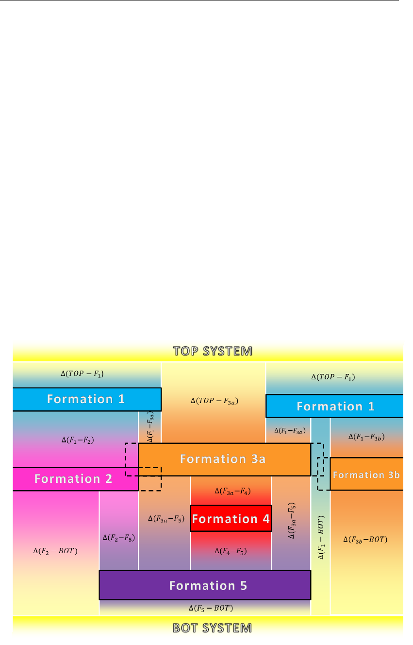
DRAFT
iMOD Batch functions
8.7.4 CUS-Function
Use this function to determine a minimal number of model layers (aquifers) based on layers that de-
scribe geological formations (mainly aquitards). The concept idea is that the vertical distribution of
aquitards (or other distinguishing layers), determine the minimal number of model layers to represent
the aquifers.
The methodology computes the interrelation ship of all the individual parts within a geological formation
and those from other geological formations. This interrelation ship is used to compute the minimal
number of model layers to capture all of them without any loss of information. In fact is depends mainly
on the lateral distribution of the geological formation whether the number of model layers becomes less
than the number of geological formations. The more spread in the distribution, probably less model
layers are necessary. In figure an overview is given of the methodology as it shows all the interrelation
ships that are computed, e.g. ∆F1−F5represents the distance between a individual element on the
the first and fifth geological formation, and moreover, the vertical position of both elements as the first
element should always be in a higher model layer than the fifth element. All these interrelation ships
are fed into a linear-programming algorithm than find a model layer for each of them such that the total
number of model layers is minimized.
The CUS function is fully automatic, which means that a) the vertical order of given geological for-
mations is irrelevant, b) overlapping geological formations may be clipped and c) interrelation ships in
vertical and horizontal direction are computed automatically that yield a minimal set of model layers.
With some variables it is possible to set the threshold at what distance of interrelation ship geological
formation may join together, in this way aquitards can be combined whenever they are separated less
than a given distance.
Schematic overview working of CUS
Deltares 471 of 812
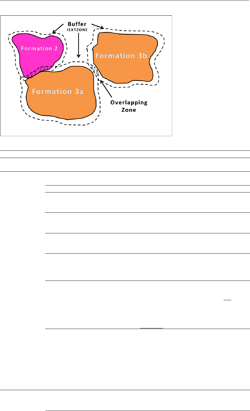
DRAFT
iMOD, User Manual
FUNCTION= CUS
ICPOINTERS= Enter a value whether or not use a given CUS pointer IDF (0 or 1).
ICPOINTERS=1
FDISTANCES= file containing predefined vertical distances that is cre-
ated in a former CUS-action.
or
CRIT_THICKNESS= maximum vertical step size (e.g.
CRIT_THICKNESS=25.0 m) to combine elements
laterally.
MIN_THICKNESS= minimal thickness of the element to be included in the
final model, e.g. MIN_THICKNESS=0.5 will include ele-
ments thicker than 0.5 meter only.
ZCRIT= Critical vertical distance. Layers will be connected verti-
cally whenever a percentage of their vertical distance is
less than ZCRIT, e.g. ZCRIT=0.5 m.
PERCENTAGE= Give the percentile for which ZCRIT needs to be taken
into account, e.g. if a percentage of 90 is given, lay-
ers will be connected if 90% of the distance is less than
ZCRIT.
ICLIP= Enter the name of an IDF file (at least at the dimension of
the given IDF files are FORMTOP_Li or FORMTOP key-
word) that denote the zone for which an entry is not need
to be blanked out. E.g. ICLIP=D:\CUS\ZONES.IDF.
Whenever a value of 1 is found in the IDF file, all geolog-
ical formations that refer to this zone 1, will be blanked
out for areas not equal to 1.
IEXPZONE= Enter a number of additional cells around each individual
element in each formation (IEXPZONE>1 to have any ef-
fect), to be used to include any element laterally to deter-
mine the most optimal model layer, e.g. IEXPZONE=2.
Adding a value of IEXPZONE will have the effect that
elements that are horizontally nearby (less than 2 cells
in this case), will be tried to vertically positioned in the
same model layer.
ICPOINTERS=0
NLAY= Enter the fixed number of model layers to be con-
structed based on the IDf file with pointer values given
at PNT_L{i}.
NFORM= Enter number of geological formations, e.g. NFORM=19.
FORMTOP_L{i}= Enter an optional zone number after the file name whenever the keyword ICLIP
is used, e.g. FORMTOP_L1=D:\INPUT\BEK1_CK.IDF,1.
472 of 812 Deltares
DRAFT
iMOD Batch functions
FORMBOT_L{i}= Enter an optional zone number after the file name whenever the keyword ICLIP
is used, e.g. FORMBOT_L1=D:\INPUT\BEK1_CK.IDF,1.
ICPOINTERS=0
PNT_L{i}= Enter an IDF for the ith formation that gives a
pointer values that refers to a modellayer i, e.g.
PNT_L1=D:\INPUT\PNT_L1.IDF. This file contains for
example the values 1-5. These values serve as a label
of a specific aquitard layer (1-5).
or
FORMTOP= Enter a path and wildcard to specify for a collection of IDF files containing infor-
mation about the TOP of the geological formations to be included, e.g. FORM-
TOP_L1=D:\FORMATIONS\*_TOP.IDF.
FORMBOT= Enter a path and wildcard to specify for a collection of IDF files containing infor-
mation about the BOT of the geological formations to be included, e.g. FORM-
BOT_L1=D:\FORMATIONS\*_BOT.IDF.
OUTPUTFOLDER=Enter the foldername in which the results will be saved, e.g. OUTPUT-
FOLDER=D:\RESULT.
WINDOW= Enter the coordinates of the window that needs to be computed. Enter coor-
dinates of the lower-left corner first and then the coordinates of the upper-right
corner, e.g. WINDOW=100000, 400000, 200000, 425000. When WINDOW=is
absent iMOD will take the WINDOW-extent of the input IDF’s.
CELLSIZE= Enter the cell size (meter) for the IDF-files that will be created, e.g.
CELL_SIZE=25.0.
TOPSYSTEM= Enter the name of the IDF-file containing the AHN for the specific model area.
BOTSYSTEM= Enter the name of the IDF-file containing the bottom-depth of the lowest bottom
layer of the model.
Example
FUNCTION= CUS
NLAY=2
WINDOW=120000.0,298000.0,240000.0,430000.0
CELLSIZE=100.0
FORMTOP_L1=D:\MODEL\BEK1_T.IDF
FORMTOP_L2=D:\MODEL\BEK2_T.IDF
FORMBOT_L1=D:\MODEL\BEK1_B.IDF
FORMBOT_L2=D:\MODEL\BEK2_B.IDF
OUTPUTFOLDER=D:\OUTPUT
TOPSYSTEM=D:\MODEL\AHN250.IDF
BOTSYSTEM=D:\MODEL\BEDROCK_TOP.IDF
This example corrects the top and bottom IDF-files specified by the FORMTOP_L{i} and FORM-
BOT_L{i} keywords in a top-bottom consistent manner and scales the IDF-files to the specified WIN-
DOW and CELLSIZE.
Deltares 473 of 812

DRAFT
iMOD, User Manual
8.7.5 SOLID-Function
Use this function to generate hypothetical interfaces (i.e. line in between model layers that represent an
artificial interface since any resistance layer (e.g. clay). This function computes the transmissivities and
vertical resistance between model layers as well. It uses the PCG solver algorithm for the interpolation
of the hypothetical interfaces and uses the existence of permeability field and the top- and bottom
elevation to compute the nett transmissivity for each a modellayer and vertical resistance between
those model layers. By means of masks it is possible to define those areas for which hypothethical
interfaces need to be computed.
FUNCTION= SOLID
NLAY= Enter the number of modellayers, e.g. NLAY=6.
OUTPUT-
FOLDER=
Enter the foldername in which the results IDF-files will be saved, e.g. OUTPUT-
FOLDER=D:\RESULT. The following results will be saved:
\MASK If IMASK=1, for each interface a mask IDF will be cre-
ated and saved in this folder. Those may be adjusted
afterwards, but set IMASK=0 to avoid that those modi-
fied mask files will be overwritten
if ICKDC=1
\FFRAC For each model layer, the fraction of each geological for-
mation will be saved. It represents the fraction (0.0−1.0)
of the geological that is present in the model layer.
\CFRAC For each in between model layer (aquitard), the fraction
of each geological formation will be saved. It represents
the fraction (0.0−1.0) of the geological that is present in
the aquitard.
MDL_TOP_{i} The TOP elevation for each model layer;
MDL_BOT_{i} The BOT elevation for each model layer;
MDL_KD_{i} The total transmissivity for each model layer, it becomes
zero when the thickness of the aquifer (model layer) is
zero;
MDL_VC_{i} The vertical resistance over aquitards in between each
model layer, excluding the resistance due to the vertical
resistance in the above- and beneath lying aquifers. Its
value becomes zero if the aquitard is absent;
MDL_KHV_{i} The horizontal permeability for each model layer, it can
be zero for layer thicknesses of zero;
MDL_KVA_{i} The vertical anisotropy for each model layer, it will always
have a value larger than 0 and smaller equal to 1. For
non existing model layers (aquifers) this parameter will
be one;
MDL_KVV_{i} The vertical permeability for each aquitard in between
each model layer, it becomes zero when the aquitard
does not exists;
MDL_KDFRAC_{i} The total fraction of the model layers that has been
parameterised by the permeabilities found by the
REGISKHV and/or REGISKVV files, whenever the frac-
tion is 1.0 is means that the entire model layer has been
filled in correctly, lower values indicate that areas in the
model layers have not been filled in properly.
MDL_CFRAC_{i} The total fraction of the aquitards in between the model
layers that has been parameterised by the permeabilities
found by the REGISKHV and/or REGISKVV files. So
more comment above;
TOP_L{i}= Enter the IDF for the ith modellayer that represents the top of modellayer i, e.g.
TOP_L1=D:\INPUT\TOP_L1.IDF.
ICLC_TL{i}= Enter the option 0 or 1 to define whether this TOP modellayer needs to be inter-
polated, e.g. ICLC_TL1=1. This is optional, the default is 1.
BOT_L{i}= Enter the IDF for the ith modellayer that represents the bottom of modellayer i,
e.g. BOT_L1=D:\INPUT\BOT_L1.IDF.
474 of 812 Deltares

DRAFT
iMOD Batch functions
ICLC_BL{i}= Enter the option 0 or 1 to define whether this BOTTOM modellayer needs to be
interpolated, e.g. ICLC_BL1=1. This is optional, the default is 1.
IMASK= Specify IMASK=1 to (re)compute masks. Those are IDF files that contain a
pointer value that indicates how the interfaces need to be computed. A mask
value can have the following values:
0 means that this particular location will be excluded, those
locations are initially formed by non-existence of the
upper- and lowermost interface;
-1 means that for that particular area no interface will be
computed, the original value will be used;
+1 means that the interface will be computed for this loca-
tions.
Each mask IDF file will be saved in the MASK folder under the given OUTPUT-
FOLDER. Whenever IMASK=0, iMOD will look in this particular folder to read the
mask IDF files, make sure that those files are in that folder.
if IMASK=1
ZOFFSET= Specify a vertical offset (meters) for which mask val-
ues need to be set af -1. In other words, whenever
the difference between the TOP_L{i} and BOT_L{i+1} is
larger than ZOFFSET the mask will be put on -1. Small
aquitards can be removed in this manner. By default
ZOFFSET=0.0 meter.
IHYPO= Specify IHYPO=1 to compute the hypothetical interfaces, for mask values of 1.
As the values for TOP_L|[i} and BOT_L{i+1} need to be identical for mask values
of +1, only the interface for TOP_L|[i} will be computed and BOT_L{i+1} will be
set equal to that value.
if IHYPO=1
DZ(.)=
(optional)
Specify for each model layer the minimal thickness (me-
ter), e.g. DZ(1)=1.0 means that the minimal thickness will
be 1.0 meter. In this way it is possible to have continu-
ous thicknesses for model layers. This minimal thickness
requirement can not be met whenever the distance be-
tween two aquitards is less than this DZ. In that case a
smaller thickness is forced. By default DZ=0.0 for each
model layer.
IMIDELEV=
(optional)
Specify IMIDELEV > 0.0 to force te PCG solver to po-
sition the hypothetical interface more-or-less such that
model layers have uniform thicknesses. By default
IMIDELEV=1.0, however, IMIDELEV=0.0 will deactivate
this feature. The higher the value for IMIDELEV the more
the hypothetical interface is a true average for all appro-
priate interfaces, the lower the value, the more smooth
is the hypothetical interface will be probably, but the con-
straint of even distributed interfaces is more violated.
IINT_IDF=
(optional)
This keyword can be defined as IINT_IDF=1 (Default) to
use upper and lower situated clay layers by the investi-
gation of the hypothetical interfaces.
IBNDCHK=
(optional)
Specify IBNDCHK=1 to check internally for isolated cells
that are NOT connected to constant value cells. By de-
fault IBNDCHK=0.
HCLOSE=
(optional)
Specify the closure criterion of the PCG solver, e.g.
HCLOSE=0.1 m. By default HCLOSE=0.001 meter.
MICNVG=
(optional)
Specify the number of subsequent inner convergences
of the PCG solver, e.g. MICNVG=25. Use this whenever
the PCG solver does not find a unique solution. By de-
fault MICVNG=5.
ICKDC= Specify ICKDC=1 to compute transmissivities for model layers and vertical resis-
tances for in between model layers.
if ICKDC=1
Deltares 475 of 812

DRAFT
iMOD, User Manual
FNLAY=
(optional)
Number of formation to be specified separately, e.g. FNLAY=10.
if FNLAY speci-
fied
FTOP_L{i}= Specify the IDF file for the ith TOP el-
evation of a geological formations, e.g.
FTOP_L1=D:\FORMATION\BEK1_TOP.IDF.
FBOT_L{i}= Specify the IDF file for the ith BOT el-
evation of a geological formations, e.g.
FBOT_L1=D:\FORMATION\BEK1_BOT.IDF.
FKHV_L{i}= Specify the IDF file for the ith horizontal per-
meability of a geological formations, e.g.
FKHV_L1=D:\FORMATION\BEK1_KHV.IDF. If no
file is defined, this permeability will be assumed to be
3.0 the given vertical permeability at FKVV_L{i}.
FKVV_L{i}= Specify the IDF file for the ith vertical per-
meability of a geological formations, e.g.
FKVV_L1=D:\FORMATION\BEK1_KVV.IDF. If no
file is defined, this permeability will be assumed to be
0.3 the horizontal permeability at FKHV_L{i}.
if FNLAY is not
specified
FOLDERTOP= Specify the folder that stores the TOP elevation of ge-
ological formations, e.g. FOLDERTOP=D:\REGIS\*-T-
CK.IDF. All files will be used that fit this wildcard defi-
nition.
FOLDERBOT= Specify the folder that stores the BOT elevation of ge-
ological formations, e.g. FOLDERBOT=D:\REGIS\*-B-
CK.IDF. All files will be used that fit this wildcard defi-
nition.
FOLDERKHV= Specify the folder that stores the horizon-
tal permeability of geological formations, e.g.
FOLDERKHV=D:\REGIS\*-KH-SK.IDF. All files will
be used that fit this wildcard definition. If no file is found
for the horizontal permeability for a particular geological
formation, this permeability will be assumed to be 3.0
the vertical permeability.
FOLDERKVV= Specify the folder that stores the vertical permeability of
geological formations, e.g. FOLDERKVV=D:\REGIS\*-
KV-SK.IDF. All files will be used that fit this wildcard defi-
nition. If no file is found for the vertical permeability for a
particular geological formation, this permeability will be
assumed to be 0.3 the horizontal permeability.
WINDOW=
(optional)
Enter the coordinates of the window that needs to be computed. Enter coordi-
nates of the lower-left corner first and then the coordinates of the upper-right cor-
ner, e.g. WINDOW=100000.0, 400000.0, 200000.0, 425000.0. When WINDOW=
is absent, the entered IDF-files by TOP_L{i} and BOT_L{i} need to be equally in
their dimensions. Otherwise they will be upscaled (mean) or downscaled (inter-
polation) to the entered CELLSIZE.
CELLSIZE= Enter the cell size (meter) for the IDF-files that will be
created, e.g. CELLSIZE=25.0.
NGEN=
(optional)
Enter a value of the amount of GEN-files containing fault information to be taken
into account in the interpolation.
if NGEN ≥1
GEN_i= Related to NGEN with this keyword all the GEN-files are
included in the interpolation. Enter first a value for the
interface number, followed by the name of the GEN-file.
Example: GEN_1=3,faults_l3.GEN.
476 of 812 Deltares
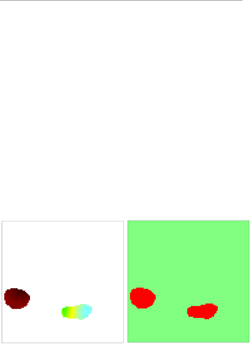
DRAFT
iMOD Batch functions
Example
FUNCTION=SOLID
NLAY=4
TOP_L1=D:\MODEL\TOP_L1.IDF
TOP_L2=D:\MODEL\TOP_L2.IDF
TOP_L3=D:\MODEL\TOP_L3.IDF
TOP_L4=D:\MODEL\TOP_L4.IDF
BOT_L1=D:\MODEL\BOT_L1.IDF
BOT_L2=D:\MODEL\BOT_L2.IDF
BOT_L3=D:\MODEL\BOT_L3.IDF
BOT_L4=D:\MODEL\BOT_L4.IDF
IMASK=1
IHYPO=1
ICKDC=1
FOLDERTOP=D:\REGIS\*-T-CK.IDF.
FOLDERBOT=D:\REGIS\*-B-CK.IDF.
FOLDERKHV=D:\REGIS\*-KH-SK.IDF.
FOLDERKVV=D:\REGIS\*-KV-SK.IDF.
OUTPUTFOLDER=D:\OUTPUT
This example creates a mask files based on the specified top and bottom IDF-files specified by the
TOP_L{i} and BOT_L{i} keywords. For those areas that does not contain an aquitard, the hypothetical
interfaces will be computed. After that the transmissivities and vertical resistances will be computed
and the other output as specified at the ketword OUTPUTFOLDER.
Example of (left) the computed thickness of an aquitard; (right) the corresponding values
for the mask IDF (green is +1 and red = -1). The green area will be filled in by hypothetical
interfaces.
Deltares 477 of 812
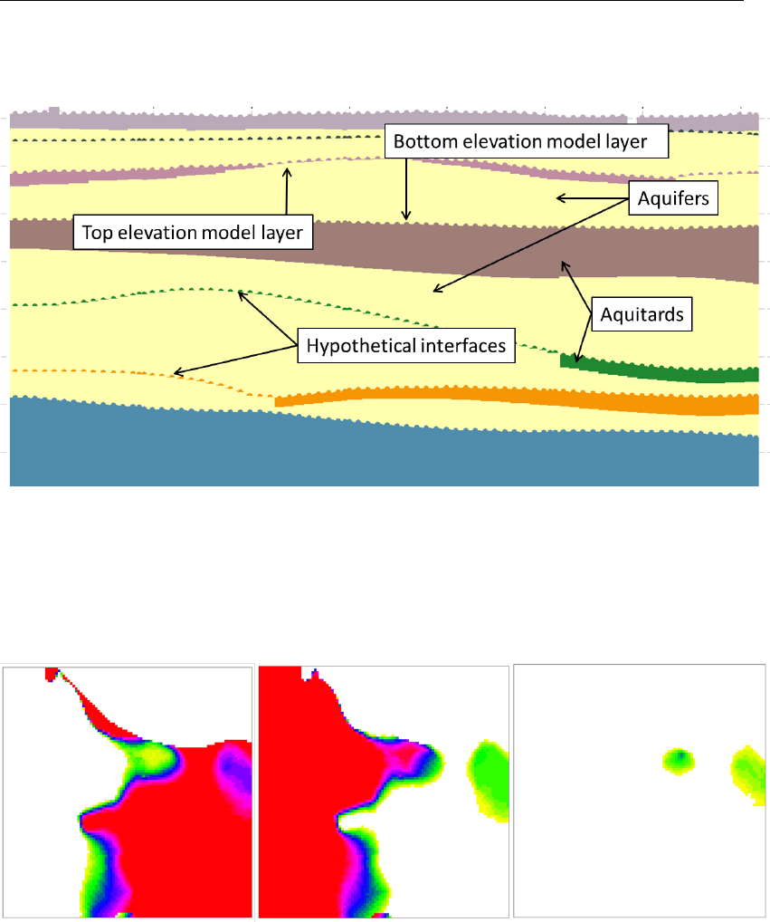
DRAFT
iMOD, User Manual
Example of computed hypothetical interfaces as TOP and BOTTOM elevation for the model
layers.
Example of computed fractions of a geological formation in three different model layers. The
formation has been part of three model layers and the total transmissivity of each model
layers depends on the given fraction of the geological formation. Red represents a higher
fraction than yellow.
478 of 812 Deltares
DRAFT
iMOD Batch functions
8.7.6 FLUMY-Function
Use this function to create Flumy textfiles with borehole information out of IPF-file related textfiles.
Flumy textfiles contain information about the fluvial deposits in (former) riverbeds (Flumy is a Geovari-
ances software program).
FUNCTION= FLUMY
IPFFILE= Enter the name of the IPF-file that contains the borehole information to be
converted to a Flumy readable format.
OFFSET= Optional variable. Enter a value to elevate the depth of the borehole, e.g.
current depth of borehole is -50 m, on OFFSET=50 results in a borehole
reference depth of 0 m.
NPARAM= Enter the number of parameters {i} that needs to be distinguished in the
Flumy-textfile(s).
GRAIN{i}= Enter the name of each grain type as given in IPF related textfile, e.g.
GRAIN1=SILT or GRAIN2=’Sandy Clay’
FACIESL{i}= Enter the verb for the location in the fluvial area where the ith Grain type
will be located, e.g. FACIESL1=OB, in case "SILT" needs to be located in
the Overbanks.
FACIESN{i}= Enter the number related to the facies layer as defined with FACIESL, e.g.
FACIESL1=OB, FACIESN1=8.
The created Flumy textfile(s) are(is) stored in the working directory of the FLUMY-batchfile within a
new generated folder “FLUMY”.
Example 1
FUNCTION=FLUMY
IPFFILE=’D:\flumy\Boreholes\Borelogs.ipf’
NPARAM=2
GRAIN1=SILT
FACIESL1=OB
FACIESN1=8
GRAIN2=’SANDY Clay’
FACIESL2=PB
FACIESN2=2
Note: Be aware that quotes are obligatory around a “GRAIN”-description containing more than one
word, e.g. ’SANDY CLAY’. Otherwise iMOD is not able to read this parameter properly.
Deltares 479 of 812

DRAFT
iMOD, User Manual
8.7.7 GEOCONNECT-function
Use this function to:
1 Compute (new) KHV, KVV and KVA grids, and/or KDW and VCW grids based on a given factor
(iPEST) per formation, or
2 Aggregate model output based on given REGIS formations.This functionality is also available as a
GUI-function (see section 7.6).
3 Identify fraction grids based on REGIS formations at a chosen model location and for the selected
model layers (not available yet, only in the iMOD GUI).
General Settings
These are the general settings needed in each *.ini file using the GEOCONNECT-Batch function:
FUNCTION= GEOCONNECT
NLAY= Enter the amount of model layers, e.g. NLAY=10.
ACTLAYERS=
(optional)
Enter a string of values to include or exclude a specific model layer from
the computation; 0=inactive, 1=active, on default all layers are used in de
computation (similar to e.g.: ACTLAYERS=1111111111). E.g. in case of
the amount of model layers is 10 and it is preferred to only take the first 6
layers into account: ACTLAYERS=1111110000.
REGISFOLDER= Give the directory and name of the folder where all REGIS-files are stored.
Note: subdirectories are not allowed and the filenames need to be of
the following format: abbreviation formation name-t/b/ks/kv-ck/sk.idf (’t’
and ’b’ need to be combined with ’ck’, and ’ks’ and ’kv’ with ’sk’), e.g.
d:\Model\REGIS\bez1-b-ck.idf.
TOPFOLDER= Give the directory and name of the folder of the model TOP-files, e.g.
d:\Model\TOP\TOP.
BOTFOLDER= Give the directory and name of the folder of the model BOT-files, e.g.
d:\Model\BOT\BOT.
WINDOW= Enter the coordinates of the window that needs to be computed. En-
ter coordinates of the lower-left corner first and then the coordinates of
the upper-right corner, e.g. WINDOW=100000, 400000, 200000, 425000.
When WINDOW= is absent iMOD will take the WINDOW-extent of the in-
put IDF’s.
CELLSIZE= Enter the cell size (meter) for the IDF-files that will be created, e.g.
CELL_SIZE=25.0.
NFORM= Enter a value for the total amount of formation factors to be read from this
*.ini file, e.g. NFORM=127.
FORM{i}= Give the name of the i’th formation and the corresponding factor, e.g.
FORM1=HLC,1.000. The largest i-number needs to correspond with the
total amount of factors as defined with NFORM.
OUTPUTFOLDER= Give the directory and name of the folder to store the results of the prepro-
cessing computation.
IFLAG= Enter a value for the specific GeoConnect function to be used: 1=Prepro-
cessing, 2=Postprocessing. E.g. IFLAG=1.
Options
In case of IFLAG=1 (Preprocessing option), the *.ini file with specific options needs to contain:
ISAVEK=
(optional)
Use this keyword to save KHV, KVV and KVA values in IDF-format;
1=saved and 0=not saved, on default ISAVEK=1.
ISAVEC=
(optional)
Use this keyword to save KDW and VCW values in IDF-format; 1=saved
and 0=not saved, on default ISAVEC=0.
In case of IFLAG=2 (Postprocessing option), the *.ini file with specific options needs to contain:
480 of 812 Deltares

DRAFT
iMOD Batch functions
DBASEFOLDER= Give the directory and name of the folder containing DBASE model infor-
mation, e.g. p:\1221301-ibrahym-dld\DBASE_V1
IAGGR= Give the value related to the aggregation option to be used, IAGGR=1:
apply to model output, IAGGR=2: apply to model input, IAGGR=3: apply
to ipf-file
if IAGGR=1. . .
MODELFOLDER= Give the directory and name of the folder containing the preferred model
output information.
MODELTYPE= Choose the favored variable to apply the aggregation to, e.g. MODEL-
TYPE=2. Options are: 1="HEAD", 2="BDGWEL", 3="BDGRIV", 4="BDG-
DRN".
if IAGGR=2. . .
INPUTTYPE= Choose the preferred variable to apply the aggregation to, e.g. INPUT-
TYPE=3. Options are: 1="KDW", 2="VCW", 3="KHV", 4="KVV".
if IAGGR=3. . .
IPFFILE= Give the directory and name of the IPF-file to apply the aggregation to.
IDUPLICATES= Give the type of aggregation. When IDUPLICATES=1 the maximum value
per grid cell is taken from the files to be aggregated, IDUPLICATES=2:
maximum value, IDUPLICATES=3: average value, and IDUPLICATES=4
the sum of the value per grid cell for all files is taken as new value in the
aggregated grid cell in the file.
ISAVETB=
(Optional)
Use this option to include TOP- and BOT elevation IDF-files in the aggre-
gation and save these files in the given Output folder. In case ISAVETB=1,
TOP and BOT elevation are saved, otherwhise when ISAVETB=0 these
files are not saved in the Output folder.
OUTPUTFOLDER= Give the directory and name of the folder to store the results of the prepro-
cessing computation.
Be sure that the geostratigraphy.txt file is placed in the defined DBASEFOLDER!
Example 1
FUNCTION=GEOCONNECT
NLAY=19
ACTLAYERS=1111111100011100000
REGISFOLDER=d:\Model_Ibrahym2\REGIS21
TOPFOLDER=d:\Model_Ibrahym2\DBASE_V2\TOP\VERSION_1
BOTFOLDER=d:\Model_Ibrahym2\DBASE_V2\BOT\VERSION_1
IFLAG=1
NFORM=8
FORM1=HLC,1.000
FORM2=BXSCK1,1.300
FORM3=BXZ1,1.000
FORM4=BXK1,1.000
FORM5=BXLMK1,2.500
FORM6=BXZ2,1.000
FORM7=BXK2,1.000
FORM8=BXZ3,0.910
OUTPUTFOLDER=d:\Model_Ibrahym2\Results\
ISAVEK=1
ISAVEC=0
With this example the KHV, KVV and KVA grids are (re)calculated (preprocessing) based on a given
factor per formation (FORM{i}) for the first 8 formation seen from the top of the Ibrahym model.
Deltares 481 of 812

DRAFT
iMOD, User Manual
Example 2
FUNCTION=GEOCONNECT
NLAY=19
ACTLAYERS=1111111100011100000
REGISFOLDER=d:\Model_Ibrahym2\REGIS21
TOPFOLDER=d:\Model_Ibrahym2\DBASE_V2\TOP\VERSION_1
BOTFOLDER=d:\Model_Ibrahym2\DBASE_V2\BOT\VERSION_1
IFLAG=2
DBASEFOLDER=d:\Model_Ibrahym2\DBASE_V2
NFORM=8
FORM1=HLC,1
FORM2=BXSCK1,4
FORM3=BXZ1,4
FORM4=BXK1,4
FORM5=BXLMK1,4
FORM6=BXZ2,4
FORM7=BXK2,4
FORM8=BXZ3,4
IAGGR=2
INPUTTYPE=3
IDUPLICATES=3
ISAVETB=0
OUTPUTFOLDER=d:\Model_Ibrahym2\DBASE_V4\
In this example the (postprocessing) aggregation is applied to the input model variable "KHV" for which
all BX-formations are taken together as one formation. An average value is calculated per grid cell for
all BX-formations. Top and Bot elevations are not saved.
482 of 812 Deltares

DRAFT
iMOD Batch functions
8.7.8 CREATEIZONE-Function
Use this function to calculate zones and corresponding fractions per model layer based on geologic
formations, these IDF files can be used during an iPEST optimization.
FUNCTION= CREATEIZONE
OFOLDER= Give an output folder name to store all the fractions per model layer.
PFOLDER= Give a folder name that contains the fraction per model layers per geolog-
ical formations. This is the results
NLAY= Enter the number of modellayers, e.g. NLAY=6
MINF= Minimum fraction to assign .... to a zone....
IZONEOFFSET= Enter the number of zones .....
IGROUPOFFSET= Enter the number of zones .....
NFORMATIONS= Enter the number of formations.
FORMATION{i}= Enter the ... for the ith formation.
TPARAMETER= Enter the name of the ...
Example
FUNCTION=CREATEIZONE
OFOLDER=D:\MODEL
PFOLDER=D:\RESULTS
NLAY=2
MINF=...
IZONEOFFSET=...
IGROUPOFFSET=...
NFORMATIONS=2
FORMATION1=...
FORMATION2=...
TPARAMETER=5
The example above will ......
Deltares 483 of 812

DRAFT
iMOD, User Manual
8.8 PREPROCESSING-FUNCTIONS
8.8.1 CREATEIBOUND-Function
Use this function to create an IBOUND IDF-file that takes into account non existing cells on the bottom
of a layer system. The IBOUND value in a cell is set to 0 whenever this cell and all underlying cells do
not exist (thickness = 0.). Otherwise the IBOUND value is set to 1.
FUNCTION= CREATEIBOUND
NLAY= Enter the number of model layers, e.g. NLAY=6.
TOP_L{i}= Enter the IDF for the ith modellayer that represents the top of modellayer
i, e.g. TOP_L1=D:\MODEL\TOP_L1.IDF.
BOT_L{i}= Enter the IDF for the ith modellayer that represents the bottom of model-
layer i, e.g. BOT_L1=D:\MODEL\BOT_L1.IDF.
RESULTDIR= Enter the foldername in which the adjusted IDF-files will be saved, e.g.
RESULTDIR=D:\RESULT.
Example
FUNCTION= CREATEIBOUND
NLAY=3
TOP_L1=D:\MODEL\TOP_L1.IDF
TOP_L2=D:\MODEL\TOP_L2.IDF
TOP_L3=D:\MODEL\TOP_L3.IDF
BOT_L1=D:\MODEL\BOT_L1.IDF
BOT_L2=D:\MODEL\BOT_L2.IDF
BOT_L3=D:\MODEL\BOT_L3.IDF
RESULTDIR=D:\RESULT
This example checks for a 3 layer system whether there are non existing cell on the bottom of the
system. These cells get an IBOUND value of 0.
The result of this function is an IBOUND file for each layer D:\RESULT\IBOUND_L{i}.IDF.
484 of 812 Deltares
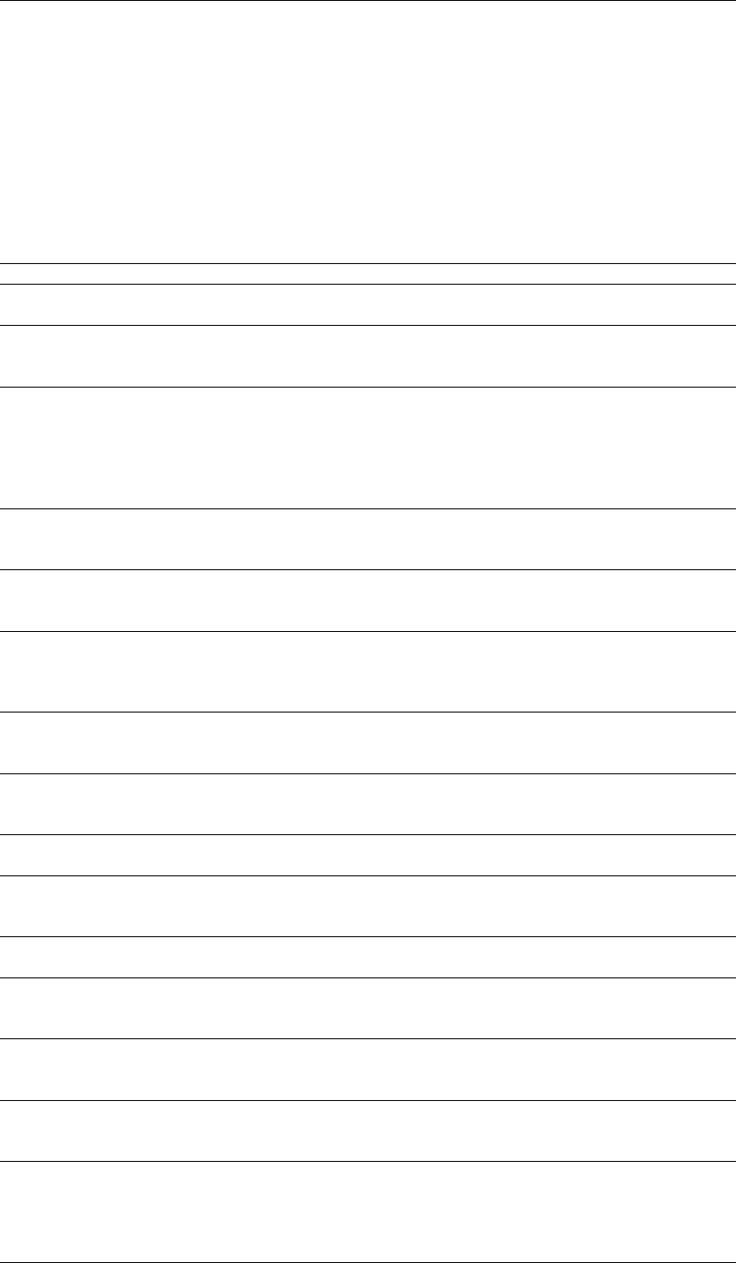
DRAFT
iMOD Batch functions
8.8.2 AHNFILTER-Function
This function filters artificial elements out of a digital terrain model (or equivalent). The method
searches for areas that are connected by small vertical thresholds and denote them as true surface
whenever the extent is significant. The remaining areas with less extent are marked as potential sur-
face and will become true surface whenever they differ minorly with the interpolated surface at those
locations. Moreover, the algorithm searches for local upconing (trees, buildings) and depressions
(streams) and removes them from the surface. The function yields two output files: the filtered original
file and a pointer file. The pointer file indicates the type of change by the filtering to the original file.
The values in the pointer file indicate: 2: no change; <2: filtered cell.
FUNCTION= AHNFILTER
NAHN= Enter the number of the IDF-files to be used during the AHN filtering, e.g.
NAHN=2.
IDFFILE{i}= Enter the name of the ith IDF-file. The IDF-files should contain
data points that represent some kind of elevation data, e.g. IDF-
FILE2=D:\DATA\AHN_REGION2.IDF.
XCRIT= Enter the vertical offset between adjacent cells that are allowed to group
together, e.g. XCRIT=0.5 (default value). In this case all adjacent cells
that have an offset of less or equal 0.25 (unit of IDFFILE{i}). Increasing
XCRIT will group more cells together, decreasing XCRIT will group them
more difficult. The size of the group will determine whether the group is
assigned a surfacelevel directly, or not. The default value is XCRIT=0.5.
NSCRIT= Enter the number of cells that behave like a threshold whether the current
group of cells can be denoted as surface level, e.g. NSCRIT=1500 (default
value).
DPW= Enter the size of the window that will be used to determine local upconing
and depressions in the area, e.g. DPW=5 (default value). In this case a
squared 5x5 window will be applied .
LOCCRIT= Enter the max difference of those values (not equal to the NoDataValue)
in the DPW window, e.g. LOCCRIT=2.0 (default value). Whenever this
difference exceeds LOCCRIT, no local upconing and depression will be
computed.
DP1= Enter the percentile for which all data points in the DPW window that are
less or equal to DP1 will be assigned to local depression, e.g. DP1=30.0
(default value).
DP2= Enter the percentile for which all data points in the DPW window that are
greater or equal to DP2 will be assigned to local upconing, e.g. DP2=30.0
(default value).
INTXCRIT= Enter the maximum residual change in the interpolation of the intermediate
surface level, INTXCRIT=0.05 (default value).
CORXCRIT= Enter the difference between the original surface level, as read by the
IDFFILE{i}-files, and the intermediate surface level, e.g. CORXCRIT=0.10
(default value).
NCORXCRIT= Enter the minimum number of changes by CORXCRIT, e.g. NCORX-
CRIT=50 (default value).
IGNORENODATA= Enter IGNORENODATA=1 (default value) to ignore all data points equal
to the NoDataValue of the IDFFILES{i}. Enter IGNORENODATA =0 to
interpolate all data points equal to the NoDataValue.
NWINDOW= Enter the number of windows to filter, e.g. NWINDOW=5. By default the
entire dimensions of the IDFFILES{i} will be processed. The default value
is NWINDOW=0.
WINDOW{i}= Enter the coordinates of the lower-left corner first and then the coordinates
of the upper-right corner, e.g. WINDOW5=100000.0, 400000.0, 200000.0,
425000.0. This keyword is compulsory whenever NWINDOW>0.
OUTFILE=
OUTFILE{i}=
Enter the name of the IDF-file that contains the filtered surface level,
e.g. OUTFILE=D:\DATA\AHN.IDF. In case NWINDOW>0, it is obliged to
specify the OUTFILE for all windows, e.g. OUTFILE5=D:\DATA\AHN5.IDF.
In the latter case, you can use the FUNCTION=IDFMERGE (see sec-
tion 8.2.4) to merge all outcomes.
Deltares 485 of 812

DRAFT
iMOD, User Manual
BUFFER= Enter a buffersize to overlap the different WINDOW{i}’s, e.g.
BUFFER=1500.0 (default value).
IAGGREGATEY= Enter IAGGREGATEY=1 to join adjacent intermediate surface levels to
form larger ones, with a change that they become greater than NSCRIT
and become surfacelevel. Default value is IAGGREGATEY=0.
Example 1
FUNCTION=AHNFILTER
NAHN =1
IDFFILE1=D:\DATA\AHN_ORG.IDF
OUTFILE=D:\DATA\AHN_FILTERED.IDF
The above mentioned example is the most simple one, it filters the AHN_ORG.IDF with all default
setting values and saves the result in AHN_FILTERED.IDF.
Example 2
FUNCTION=AHNFILTER
NAHN =2
IDFFILE1=D:\DATA\AHN_ORG1.IDF
IDFFILE2=D:\DATA\AHN_ORG2.IDF
NWINDOW=2
WINDOW1=125000.0 426000.0 130000.0 430000.0
WINDOW2=130000.0 426000.0 135000.0 430000.0
OUTFILE1=D:\DATA\AHN_FILTERED1.IDF
OUTFILE2=D:\DATA\AHN_FILTERED2.IDF
BUFFER=2500
IGNORENODATA=0
NSCRIT=1250
LOCCRIT=200.0
XCRIT=100.0
DPW=5
DP1=30.0
DP2=90.0
CORXCRIT=10
CORCRIT =75
INTXCRIT=5
The above mentioned example filters two windows and uses two different IDF-files (AHN_ORG1.IDF
and AHN_ORG2.IDF). The main reason for using most of the setting variables is that the dimension of
the original IDF-files (IDFFILE1 and IDFFILE2) is centimeter instead of meter.
486 of 812 Deltares
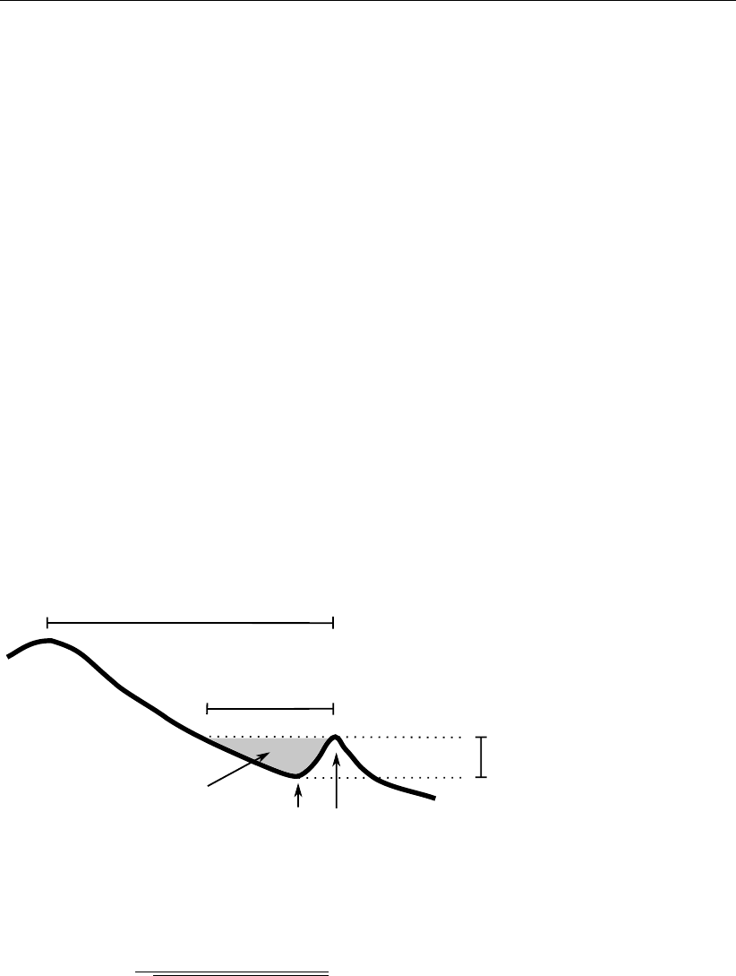
DRAFT
iMOD Batch functions
8.8.3 CREATESOF-Function
The iMOD-Batch function SOF (Surface Overland Flow) is able to compute “spill” levels (surface over-
landflow levels) for large regions with or without supplied outflow or outlet locations. First of all, the
“pit”-locations are identified, these are defined as those locations that are surrounded by higher values
all around in a 3×3matrix of grid cells. There is no other escape possible other than the lowest
neighbouring level, the so called “spill”-level. All these identified “pitts” are sorted from the lowest to
the highest “pitt” and processed in that order. Given a “pitt” location, the surrounding grid cells will be
stored in a boundary list. From the boundary list the lowest “spill”-level will be found and stored in a
boundary list. Whenever this “spill”-level is lower than the current “spill”-level, the process stops, be-
cause than probably the water can flow outside the current “core-volume”. If not, the lowest level on the
boundary becomes the new “spill”level and the node will be remove from the boundary list and added
to the “pitt”-list. The process repeats itself. All grid cells that are mentioned in the pitt-list will belong
to the same “core-volume” and receive the final “spill”-level. At the end of this section, an example is
given. As the “core-area” will be flat, the discharge occurs on that area as follows: it first follows the
steepest gradient along the digital elevation model into the pit location and from there it follows the
shortest way up towards the outflow cell. As the “core-area” will be flat, it cannot be used for a SFR
package (see section 12.28). To avoid flat-surfaces, the SOF function can be generate a slight adapted
surface level for flat areas as a gradient from where the flat area is entered to the elevation next to the
exitpoint. Those corrected flat areas (that can be a stretch along a stream) can be used for the SFR
discretisation, at the same time the original slope of the flat area (0.0) is adjusted as saved. This slope
is used as well for the SFR to define the stream slopes.
In the following figure the mentioned variables are explained.
Example of the concepts for the “spill”-level procedure.
core area
overflow level
pit level
pit
cell
outflow
cell
pit catchment
outflow
depth
core volume
The steepest gradient of the digital terrain model is computed for a 3×3neighbourhood, so the slope
sand aspect aare at one point estimated from elevations of it and surrounding 8points i, thus:
si= tan−1zi−z0
p(xi−x0)2+ (yi−y0)2
ai= arctan−1(xi−x0, yi−y0)
where the slope siis in radians as well as the aspect ai, and z0,x0and y0are the elevation, x-
coordinate and y-coordinate at the current node respectively, for which the gradient and aspect need
to be computed. For reasons of conveniences, the aspect ais taken by the arctangent function with two
arguments. The purpose of using two arguments instead of one is to gather information on the signs
of the inputs in order to return the appropriate quadrant of the computed angle, which is not possible
for the single-argument arctangent function. The final value for the aspect ais −π < a < π, meaning
that πis pointing to the east, 0.5×πpoints to the south, 0.0×πpoints to the west and −0.5×π
points to the north. For perfect flat areas, a south direction is chosen arbitrarily. Also NodataValues
are threated as “pitts”.
The CREATESOF function continues to follow a drop of water to its down slope neighbour, we call this
a trace and all cells that are passed are stored in a thread. This method uses the steepest descent
Deltares 487 of 812

DRAFT
iMOD, User Manual
direction from a particular location and moves to the next ceel along that direction, so the new x-location
xiis found from the previous x-location xi−1by:
xi=xi−1+ ∆x·cos(ai−1) ; yi=yi−1∆y·sin(ai−1)
where ∆xand ∆yare the cellsizes of the digital elevation model.
FUNCTION= CREATESOF
IFLOW= Enter a code to specify the way the CREATESOF function need to work. Below
the options are described
IFLOW=0 Apply IFLOW=0 to compute the “spill”-levels, slopes and aspect angles.
The following files will be saved:
*_COPY.IDF used digital elevation data after clipping and/or up- or down-
scaling, this file is only save whenever the keyword WINDOW is
given;
*_PITT.IDF describes the location of the individual “pitts”-cells (value 1 for a
“pitts”-cell; 0 for all non-“pitts”-cells);
*_SLOPE.IDF gradient ( ∆x
∆z) of the steepest slope of each grid cell (only when-
ever IGRAD=1);
*_ASPECT.IDF steepest flow angle (azimuth) in radians, north=−1
2π; west=0;
south= 1
2π; east=π; (only whenever IGRAD=1).
LEVELIDF= Enter the surface level (Digital Terrain Model DTM) IDF-file that
need to be processed, e.g. LEVELIDF=D:\DATA\DTM.IDF.
PITTSIZE=
(optional)
Enter the minimal size of a pit to become a natural outlet. If the
size of the pit exceeds the number given for e.g. PITTSIZE=100,
this area becomes a natural outlet and all streams will terminate
at that location.
OUTLETIDF=
(optional)
Enter an IDF file that describes the outlet locations, e.g. OUT-
LETIDF=D:\MODEL\RIVERS.IDF. Each location not equal to
the NodataValue in the given OUTLETIDF will be used to ter-
minate the further search for a “spill”-level.
WINDOW=
(optional)
Specify a window for which the entered LEVELIDF will
be clipped and resized whenever the entered CELLSIZE
/ne the cellsize of the given IDF file at LEVELIDF.
Enter the coordinates of the lower-left corner first and
then the coordinates of the upper-right corner, e.g. WIN-
DOW=100000,400000,200000,425000. When WINDOW is ab-
sent, the internal dimensions of LEVELIDF will be used.
CELLSIZE= Specify a cell size for the WINDOW to be clipped out or resized,
e.g. CELLSIZE=100.0.
IGRAD=
(optional)
Enter the IGRAD=0 to ignore the computation of the aspects of
the DTM as these computations can take significant amount of
time, especially the flat areas and the elevation on the core vol-
umes. Choose IGRAD=1 to include the aspect computations.
The default value is IGRAD=0 whenever this keyword is absent.
SOFIDF= Enter the SOFIDF to save the computed Surface Overland Flow
level; this elevation describes the elevation at which surface wa-
ter will discharge water. For “pitts” this is the overflow level, for
all others it is the original DTM-level. By subtracting the original
DTM- and SOF-level the size and depth (“pitts”-volume) of the
can be computed.
IFLOW=1 Specify IFLOW=1 to compute the entire “flow path” of the particle flowing over the
surface.
The following files will be saved:
*.GEN describes the entire flow path only if IWRITE=1;
*_ZONE.IDF describes the number of discharge zone as specified by the IPF
file given by the optional keyword DISZONEIPF.
LEVELIDF= Enter the surface level (Digital Terrain Model DTM) IDF-
file that need to be corrected for flat surfaces, it is log-
ical to use the SOFIDF from a IFLOW=0 run; e.g. LEV-
ELIDF=D:\DATA\SOF.IDF.
488 of 812 Deltares

DRAFT
iMOD Batch functions
SLOPEIDF= Enter the slope IDF file that need to be processed, it is
logical to use the slope IDF from a IFLOW=0 run; e.g.
SLOPEIDF=D:\DATA\SLOPE.IDF.
LEVEL_
OUTIDF=
Enter the IDF file for the corrected surface level
(Digital Terrain Model DTM) for flat areas, e.g.
LEVEL_OUTIDF=D:\DATA\SOF_FLAT.IDF.
SLOPE_
OUTIDF=
Enter the slope IDF file corrected for flat areas, e.g.
SLOPE_OUTIDF=D:\DATA\SLOPE_FLAT.IDF.
COUNTIDF Enter the IDF file for which the total number of flow
paths (friction) that passes each grid cell, e.g. COUN-
TIDF=D:\DATA\FRICTION.IDF;
ASPECTIDF= Enter the name of the IDF file that contains the aspects for
each grid cell, e.g. ASPECTIDF=D:\RESULTS\ASPECT.IDF.
Normally, this is the result of the simulation with IFLOW=0
(*_ASPECT.IDF).
DISZONEIPF=
(optional)
Enter the name of the IPF file that describes the lo-
cation of discharge measurement station, e.g. DIS-
ZONEIPF=D:\INPUT\DIS.IPF. The minimal requirement of
the data in the IPF file is that the first three columns need to
describe the x,yand station number (integer). The resulting
{SOFIDF}_ZONE.IDF will present the areas that discharge to
the given station numbers. This DISZONEIPF is optional.
IWRITE=
(optional)
Enter IWRITE=1 to write a GEN file of all “flow paths” of par-
ticles flowing over the DTM. This will yield the file {ASPEC-
TIDF}.GEN. Writing this file will reduce the performance and
it often will yield an enormous file. The default option is
IWRITE=0.
IFLOW=2 Specify IFLOW=2 to compute cumulative volumes for catchments for each loca-
tion and for given percentiles.
COUNTIDF Enter the IDF file with the total number of flow paths that passes
each grid cell this is equal to the output file *_COUNT.IDF when-
ever IFLOW=1;
ITQP Enter ITQP=0 to compute the percentiles and ITQP=1 to use
the percentiles. Suppose, ITQP=0, the IDF files given at
TQPIDF{i} will be created, and whenever ITQP=1, those files
at TQPIDF{i} will be used.
MINQ Enter a minimal discharge volume to be taken into account in
the comutation of percentiles, e.g. MINQ=1000 m3/day will ex-
clude those with total discharges less than this amount.
TTQP Enter TTQP=0 to compute a total percentile, or enter ITQP=1 to
compute monthly percentiles.
NTQP Enter the number of percentiles of discharges to be computed,
e.g. NTQP=5 means that you need to enter 5 percentiles at
PTQP{i}..
PTQP{i} Enter the percentile value (0.0 ≥PTQP{i} ≤100.0) for the ith
percentile out of NTQP, e.g. PTQP2=50.0.
RESULTIDF Enter a folder of the results IDF files to be used
for the total volume computation, e.g., RESUL-
TIDF=D:\RESULTS\BDGRIV\BDGRIV_*_L1.IDF. This means
that all files will be used to compute a percentile, it depends on
the amount of files that meet this wildcard. Whenever TTQP=0
a single percentile will be computed for all files, whenever
TTQP=1, a monthly percentile will be computed, this means
that a monthly output will be created at OUTPUTFOLDER.
Deltares 489 of 812

DRAFT
iMOD, User Manual
OUTPUT-
FOLDER
Enter a directory to store all results, e.g. OUTPUT-
FOLDER=D:\RESULTS\VOLUMES. Here, for each in-
putfile (RESULTIDF) a percentile will be computed of
the current discharge compared to the total (TTQP=0)
or monthly (TTQP=1) percentile. The files are called
TQ_PERCENT_{yyyymmdd}.IDF. This files gives a unique
value of the class at which the current discharge belong.
Whenever the value is 3, this means a percentile value that
belongs in between the 3rd and 4th class. A value of 0 means
that the current percentile undercounts the given percentiles in
the TQPIDF{i} files, a value above NTQP, means that it exceeds
the given percentiles.
TQPIDF{i} Enter the name of the IDF to save the percentiles,
e.g. TQPIDF2=D:\RESULTS\VOLUMES\TQP_50.IDF.
Whenever TTQP=1, these names will be enhanced by
a month identification, e.g. the final name becomes
D:\RESULTS\VOLUMES\TQP_50_AUG.IDF to denote the
50th percentile for the month August.
IFLOW=3 Specify IFLOW=2 to compute cumulative volumes for catchments for each loca-
tion and for given percentiles.
LEVELIDF= Enter the surface level (Digital Terrain Model DTM) IDF-file, it
is logical to use the SOFIDF from a IFLOW=1 run; e.g. LEV-
ELIDF=D:\DATA\SOF_FLAT.IDF.
SLOPEIDF= Enter the slope IDF file that need to be processed, it is
logical to use the slope IDF from a IFLOW=1 run; e.g.
SLOPEIDF=D:\DATA\SLOPE_FLAT.IDF.
COUNTIDF Enter the IDF file for which the total number of flow
paths (friction) that passes each grid cell, e.g. COUN-
TIDF=D:\DATA\FRICTION.IDF;
ASPECTIDF= Enter the name of the IDF file that contains the aspects for
each grid cell, e.g. ASPECTIDF=D:\RESULTS\ASPECT.IDF.
Normally, this is the result of the simulation with IFLOW=0
(*_ASPECT.IDF).
IFORMAT= Enter the format of the output file structure. Apply IFOR-
MAT=1 whenever a conventional RIVER package need to be
constructed with river conductances, -stage, -bottomlevels and
infiltration factors. Apply IFORMAT=2 to construct a ISG file for
the SFR package.
RCND_IDF= Enter the IDF file that represented to river conductance; e.g.
RCND_IDF=D:\DATA\RCOND.IDF.
RSTG_IDF= Enter the IDF file that represented to river stage; e.g.
RSTG_IDF=D:\DATA\RSTAGE.IDF.
RBOT_IDF= Enter the IDF file that represented to river bottom; e.g.
RBOT_IDF=D:\DATA\RBOTTOM.IDF.
RINF_IDF= Enter the IDF file that represented to river stage; e.g.
RINF_IDF=D:\DATA\RINF.IDF.
RAIN=
(optional)
Enter the size of the rainfall used to compute the dimension of
the stream, e.g. RAIN=1.0 means an constant rain event of 1
mm/day. By default RAIN=1.0 mm/day.
MINFRICTION=
(optional)
Enter the size of the minimal value for the friction (number of
passes in the COUNTIDF file) to be used to generate a stream,
e.g. MINFRICTION=5.0 means all grid sizes with a friction value
of less than 5.0 will not be processed to a IDF-files (see above)
or an ISG file. By default MINFRICTION=0.0.
490 of 812 Deltares
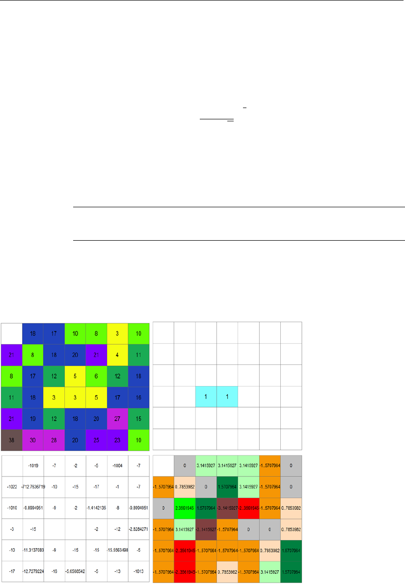
DRAFT
iMOD Batch functions
NQDW=
(optional)
Enter the number of discharge-depth-width relations, e.g.
NQDW=3. iMOD will interpolate between three given relations
between discharge, depth and width to determine the dimen-
sions at each gridcell based on the friction in the COUNTIDF.
By default NQDW=0 and iMOD uses the Manning equation to
determine the dimensions at each gridcell.
d=Q×n
w×√S
3
5
(8.2)
where dis the depth, Qthe discharge, nMannings roughness
coefficient (n=0.03), wis the width (w=1.0) and Sis the slope
between two gridcells. It is advisable to use the QDP-relations
as that will results in a more reliable conductance than the Man-
ning Equation since the latter is very sensitive to local gradients
in the DTM (slopes).
QDW_{i}(.)= Enter for each relation the discharge (m3/day), depth (m)
and width (m), e.g. QDW_3=100.0,1.5,20.0. Start with
QDW_1=0.0,0.0,0.0.
Below an example is given for the output variables for IFLOW=0 and IFLOW=1 for an artificial DTM.
Example of (upperleft) a DTM (upperright) the PITTs (lowerleft) the SLOPE and (lowerright) the AS-
PECT.
Example of (upperleft) a SOF (upperright) the number of passes and (lowerleft) the flowpaths GEN).
Deltares 491 of 812
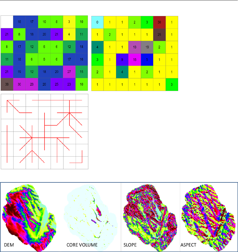
DRAFT
iMOD, User Manual
Example 1
FUNCTION=CREATESOF
IFLOW=0
LEVELIDF=D:\DATA\DTM.IDF
SOFIDF=D:\OUTPUT\SOF.IDF
Example 2
FUNCTION=CREATESOF
IFLOW=1
ASPECTIDF=D:\OUTPUT\DTM_ASPECT.IDF
IFLOW=1
Example 3
FUNCTION=CREATESOF
IFLOW=2
492 of 812 Deltares
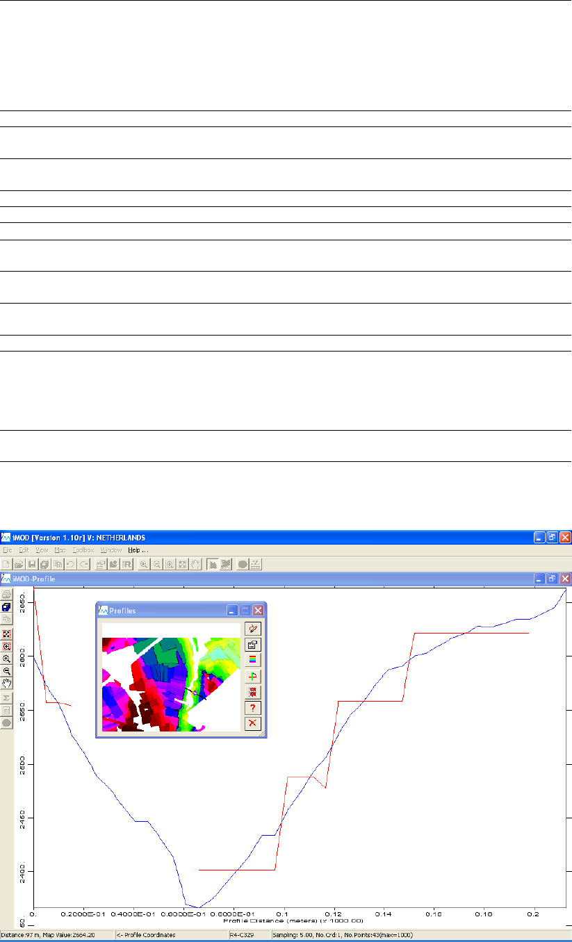
DRAFT
iMOD Batch functions
8.8.4 DRNSURF-Function
The DRNSURF function is used to calculate the drainage level for surface runoff based on info about
landuse, DEM and a pointer IDF with info on buildings.
FUNCTION= DRNSURF
SURFIDF= Enter the surface level IDF-files that need to be processed, e.g. SUR-
FIDF=D:\DATA\DEM.IDF.
PNTRIDF= Enter the pointer IDF with built area = 1, e.g. PN-
TRIDF=D:\DATA\KDSTR.IDF.
LUSEIDF= Enter the Landuse IDF file, e.g. LUSEIDF=D:\DATA\LGN6.IDF.
NLUSE= Number of landuse zones to be distinguished.
ILUSE{i}= Enter the ith landuse code, e.g. ILUSE1 = 3
TDRAINAGE= Give the percentage of maximum change in drainage level in the area.
Used as a treshold.
TSURFLEVEL= Give the percentage that accounts for the maximum change in surface
level. This percentage will be used to define zones.
PERCENTILE= Give a percentile value (0-100, 50=median) that accounts for the agricul-
tural area that needs to contain drainage within the zones.
OUTIDF= Enter the name of the output IDF file.
WINDOW= Enter the coordinates of the window that need to be computed, solely.
Enter coordinates of the lower-left corner first and then the coordinates of
the upper-right corner, e.g. WINDOW=100000, 400000, 200000, 425000.
When WINDOW= is absent, the entire dimensions of the IDF-window will
be used.
CELL_SIZE= Enter the cell size (meter) for the IDF-files that will be created, e.g.
CELL_SIZE=25.0.
This figure shows the differences in surface level relative to the defined drainage levels.
Deltares 493 of 812

DRAFT
iMOD, User Manual
Example 1
FUNCTION=DRNSURF
SURFIDF=D:\DATABASE\AHN2.IDF
PNTRIDF=d:\DATABASE\KDSTR_2012.IDF
LUSEIDF=d:\DATABASE\LGN6.IDF
NLUSE=3
ILUSE1=1
ILUSE2=2
ILUSE3=3
TDRAINAGE=50.0
TSURFLEVEL=50.0
PERCENTILE=50.0
OUTIDF=d:\MODEL\DRN\DRN_SL.idf
This example creates an IDF with the drainage elevation for the surface level.
494 of 812 Deltares
DRAFT
iMOD Batch functions
8.9 POSTPROCESSING-FUNCTIONS
8.9.1 GXG-Function
The GXG function calculates the maximum and minimum groundwaterhead during the hydrological
year (from 1st April) based on the mean of the three highest, c.q. lowest observed groundwaterheads.
The GXG is an indicator used in the Netherlands to indicate the seasonal variation of the groundwa-
terhead.
FUNCTION= GXG
ILAYER= Enter the layer numbers to be used in the GxG computation,
subsequently; e.g. ILAYER=1,3,6.
NDIR= Enter the number of folders to be processed repeatedly, e.g. NDIR=10.
SOURCEDIR{i}= Enter the folder and first part of the filename for all files that need to be
used, e.g. SOURCEDIR1=C:\DATA\HEAD. This mean that the GXG func-
tion will search for IDF-files that meet the name syntax requirement of
C:\DATA\HEAD_{yyyymmdd}_L{ILAY}.IDF.
SURFACEIDF= Enter a name for the surface, e.g. SURFACEIDF=C:\DATA\AHN.IDF. By
default a surface elevation of 0.0m+MSL will be considered.
SYEAR= Enter the start year (yyyy) for which IDF-files are used, e.g. SYEAR=1998.
EYEAR= Enter the end year (yyyy) for which IDF-files are used, e.g. EYEAR=2011.
This keyword will be read whenever SYEAR is included.
IYEAR= Specify particular years to be used, e.g. IYEAR=2001,2003,2004. This
keyword will be read whenever the keyword SYEAR is absent.
STARTMONTH= Enter the start month from the which the hydrological year starts. Default
STARTMONTH=4.
IPERIOD= Enter two integers (0 or 1) for each month to express the in-
clusion of the 14th and 28th of that particular month, e.g.
IPERIOD=010101010101010101010101, which mean to use the 14th of
each month solely. On default IPERIOD=111111111111111111111111.
ISEL= Enter a code for the area to be processed:
ISEL=1 will compute the entire region
ISEL=2 will compute within given polygons;
ISEL=3 will compute for those cells in the given IDF-file that are not equal
to the NoDataValue of that IDF-file.
GENFNAME= Enter a GEN-filename for polygon(s) for which mean values need to be
computed. This keyword is obliged whenever ISEL=2.
IDFNAME= Enter an IDF-file for which mean values will be computed for those cell in
the IDF-file that are not equal to the NoDataValue of that IDF-file. This
keyword is compulsory whenever ISEL=3
HGLG3= Indicates whether or not the HG3 and LG3 needs to be computed output
per year. HG3(LG3)=the groundwater stage maps of the 3 days with the
highest(lowest) stages per year. Note: Only the first layer indicated by
keyword ILAYER, will be taken into account. Its not possible to get the
HG3 and LG3 for more layers within one GXG-calculation. Note 2: in case
of SYEAR=2011, EYEAR=2013 and startmonth=4, the HG3 and LG3 are
computed for year 2011 (=04-2011 till 03-2012) and 2012 (=04-2012 till
03-2013).
Example 1
FUNCTION=GXG
ILAYER=1
NDIR=1
SOURCEDIR1=D:\MODEL\HEAD
SYEAR=1991
EYEAR=2000
This illustrates a simple example of a GxG computation over the years 1991 (actually starts at 14th of
Deltares 495 of 812

DRAFT
iMOD, User Manual
April 1991) until 2000 (actually 28th of March 2000), for all the HEAD* files that are within the folder
D:\MODEL. Since the keyword SURFACEIDF is absent, the GxG will be expressed according to 0.0
instead of a true surface level, moreover, ILAY is absent too, but ILAY=1 will be used as default.
Example 2
FUNCTION=GXG
ILAYER=1,2
SURFACEIDF=D:\DATA\AHN.IDF
IYEAR=1994,1995,2000,2001
IPERIOD=000000001111111100000000
ISEL=3
IDFNAME=D:\DATA\ZONE.IDF
NDIR=1
SOURCEDIR1=D:\MODEL\HEAD
This example computes the GxG for the years 1994, 1995, 2000 and 2001 only. This means two
hydrological years, namely 14-4-1994-upto 28-3-1995 and 14-4-2000 upto 28-3-2001. In this period
the summer months May, June, July, August are included as expressed by the IPERIOD keyword.
496 of 812 Deltares

DRAFT
iMOD Batch functions
8.9.2 WBALANCE-Function
The WBALANCE function calculates the water balance based on the model output for the steady state
condition or for a specific period and area. Alternatively, this function can create images, IDF files
and/or CVS files from aggregation on existing CSV files.
FUNCTION= WBALANCE
CSVFNAME=
(optional)
Enter the name of the CSV file that contains a water bal-
ance created previously by this function, e.g. CSVF-
NAME=D:\MODELRESULTS\WBAL.CSV.
Use the following keywords whenever CSVFNAME is entered
DIR= Enter the name of the output folder that will be used to save the resulting
pictures, e.g. DIR=D:\MODELRESULTS\FIGURES.
BDGIACT=
(optional)
Enter BDGIACT=1 to denote that the budget is present in the output file
(IDF, CSV and/or time series/graphical representation image). By default
BDGIACT=1 for all budget terms.
BDGIGRP=
(optional)
Enter the group numbers for the individual budget terms, e.g. BDGI-
GRP=1,2,5,5. By default BDGIGRP is a sequence of the numbers 1,2,3
etc.
BDGICLR=
(optional)
Enter the colour number (combination of the individual colour red,green en
blue - each ranging between 0-255) of the particular budget term, BDGI-
CLR=2443254.
IAVG=
(optional)
Enter the method for averaging:
1 = All Time steps: a single value for all entries;
2 = Year: a single value per year;
3 = Months: a single value per month, starting at the first month in the
series;
4 = Hydrological Seasons: two seasons are used, 1) April - September
and 2) October - March;
5 = Decade: a single value per 10 days and the remaining days in that
month;
6 = Hydrological Year: four seasons are used 1) December - February
2) March - May 3) June - August 4) September - November;
7 = Quarters: a single value per 3 months, starting in January;
8 = None: all entries remain unchanged, this is the default.
NETFLUX=
(optional)
Enter NETFLUX=1 to apply net fluxes in the output, by default NET-
FLUX=0.
IUNIT=
(optional)
Enter INUIT=1 to apply net fluxes in the output, by default IUNIT=0.
LSUM=
(optional)
Enter LSUM=1 to aggregate all selected model layers into a single water
balance, by default LSUM=0.
ZSUM=
(optional)
Enter ZSUM=1 to aggregate all selected zones into a single water balance,
by default ZSUM=0.
LAYERS=
(optional)
Enter the number of layer(s) to be used for the water balance, e.g. LAY-
ERS=1,2,5. By default ALL layers are selected.
ZONES=
(optional)
Enter the number of zones(s) to be used for the water balance, e.g.
ZONES=10,23. By default ALL zones are selected.
DATES=
(optional)
Enter the number of dates(s) to be used for the water balance, e.g.
DATES=20100114,20100128. By default ALL dates are selected.
Deltares 497 of 812
DRAFT
iMOD, User Manual
IOPT=
(optional)
Enter the output option:
1 = Time Series: select this option to display the selected water bal-
ance items in a graph, this is the default;
2 = Graphical Representation: select this option to present the water
balance items in a illustrative image;
3 = Preview Table: select this option to display each value for the water
balance items in a table;
4 = Export to CSV: select this option to export all water balance items
into an CSV file;
5 = IDF per Layer: select this option to export all water balance items
into separate IDF files.
OUTPUTFNAME=
(optional)
Enter the name of the CSV file to be created whenever IOPT=4, e.g. OUT-
PUTFNAME=D:\OUTPUT\SUMMARY.CSV.
Use the following keywords whenever CSVFNAME is NOT entered
NDIR= Enter the number of folders to be processed repeatedly, e.g. NDIR=10.
SOURCEDIR{i}= Enter the main source folder for which underlying files need to be used;
e.g. SOURCEDIR1=C:\DATA\MODEL. It depends on the following key-
words: BAL{i}, BAL{i}ISYS, ILAYERS and SDATE/EDATE, what specific
files the WBALANCE function will obtain.
ILAYER= Enter the layer numbers to be included in the waterbalance,
e.g. ILAYER=1,3,6. It is also possible to specify the layers as LAY-
ERS=4:45 to indicate that these layers 4 up to 45 need to used.
SDATE=
(optional)
Enter the starting date (yyyymmdd or yyyymmddhhmmss) for which IDF-
files are used, e.g. SDATE=19980201 or SDATE=20141231123015 (the
latter expresses the 31th of December 2014 at 12 hours, 30 minutes and
15 seconds.
EDATE=
(optional)
Enter the ending date (yyyymmdd or yyyymmddhhmmss) for which IDF-
files are used, e.g. EDATE=20111231 or EDATE=20180715084500 (the
latter expresses the 15th of July 2018 at 08 hours, 45 minutes and 00
seconds. In case SDATE is specified, EDATE is compulsory as well.
IYEAR=
(optional)
Specify a particular year (within SDATE and EDATE) to be used exclu-
sively, e.g. IYEAR=2001,2003,2005. IYEAR is filled in for all years in-
between SYEAR and EYEAR.
NPERIOD=
(optional)
Enter a number of periods to be defined to use IDF-file within these periods
solely, e.g. NPERIOD=2. NPERIOD=0 by default.
PERIOD{i}=
(optional)
Enter a period i (ddmm-ddmm), e.g. PERIOD1=1503-3110 to express the
period 15th of March until the 31th of October.
NBAL= Enter the number of water balance topics, e.g. NBAL=2.
BAL{i}= Enter for each of NBAL topics one of the folder name, e.g.
BDGBND, BDGSFR. iMOD will look for files that are in the
folder SOURCEDIR{i}\BAL{i}\BAL{i}_{time}_{layer}.IDF. whenever
SDATE/EDATE is absent, {time} is the keyword STEADY_STATE.
Repeat BAL{i} for NBAL times. E.g., whenever BAL1=BDGWEL
and the simulation is steady state, the following file is appropri-
ate: SOURCEDIR{i}\BDGWEL\BDGWEL_STEADY-STATE_L1.IDF.
For transient simulations, the iMOD Batch function will search
for SOURCEDIR{i}\BDGWEL\BDGWEL_????????_L1.IDF and
SOURCEDIR{i}\BDGWEL\BDGWEL_??????????????_L1.IDF files.
After that, the selected set of files will be matched against the given
SDATE and EDATE keywords, and if necessary against NPERIOD.
498 of 812 Deltares

DRAFT
iMOD Batch functions
BAL{i}ISYS=
(optional)
Enter the number of systems to be included in the water balance, e.g.
BAL1ISYS=1,2,3. This mean to add the systems 1,2 and 3 for the first
entered water balance item, specified by BAL1. E.g. iMOD will look for
files as BDGDRN_STEADY-STATE_SYS1_L1.IDF. By default, no systems
will be distinguished and iMOD will look for files as BDGDRN_STEADY-
STATE_L1.IDF.
OUTPUTNAME{i}= Enter the output filename (*.TXT, *.CSV or *.IPF), e.g. OUTPUT-
NAME1=C:\DATA\HEAD\WBAL_MIPWA.CSV
ISEL=
(optional)
Enter a code for the area to be processed:
ISEL=1 will compute the entire region
ISEL=2 will compute within given polygons;
ISEL=3 will compute for those cells in the given IDF-file that are not equal
to the NoDataValue of that IDF-file. By default ISEL=1.
GENFILE=
(optional)
Enter a GEN-filename for polygon(s) for which mean values need to be
computed. This keyword is obliged whenever ISEL=2.
IDFNAME=
(optional)
Enter an IDF-file for which mean values will be computed for those cell in
the IDF-file that are not equal to the NoDataValue of that IDF-file. This
keyword is compulsory whenever ISEL=3
WBEX=
optional)
Enter WBEX=1 to generate interconnected flux between the zones. This
option is only valid whenever the flux terms BDGFRF and BDGFFF are
active. By default WBEX=0 and none of the interconnected fluxes is com-
puted.
Example 1
FUNCTION=WBALANCE
NBAL=3
BAL1=BDGFRF
BAL2=BDGFFF
BAL3=BDGFLF
ILAYER=3
NDIR=1
ISEL=2
GENFILE=D:\MODEL\zone.gen
SOURCEDIR1=D:\MODEL
OUTPUTNAME1=D:\MODEL\WBAL.TXT
The above mentioned simple example will give a waterbalance for the BDGFRF, BDGFFF and BDGFLF,
respectively, for modellayer 3.
The IDF-files will be D:\MODEL\BDGFRF\BDGFRF_STEADY-STATE_L3.IDF;
D:\MODEL\BDGFFF\BDGFFF_STEADY-STATE_L3.IDF; and
D:\MODEL\BDGFLF\BDGFLF_STEADY-STATE_L3.IDF.
The result is written in D:\MODEL\WBAL.TXT.
Example 2
FUNCTION=WBALANCE
NBAL=2
BAL1=BDGRIV
BAL1SYS=1,2
BAL2=BDGDRN
ILAYER=1,2
SDATE=19900101
EDATE=20001231
IYEAR=1990,1995,1997,2000
NPERIOD=1
PERIOD1=0104-3107
ISEL=2
Deltares 499 of 812

DRAFT
iMOD, User Manual
GENFNAME=D:\DATA\ZONES.GEN
NDIR=2
SOURCEDIR1=D:\MODEL
SOURCEDIR2=D:\SCENARIO
OUTPUTNAME1=D:\OUTPUT\WBAL_MODEL.CSV
OUTPUTNAME2=D:\OUTPUT\WBAL_SCENARIO.CSV
The example above will compute a waterbalance for two modellayers (1,2) for the budgetfiles BD-
GRIV*SYS1 and BDGRIV*SYS2 and BDGDRN in the period from 1th of April until the 31th of July for
the years 1990,1995,1997,2000. The waterbalance will be summed for the zones that are described
by the polygon(s) inside the file ZONES.GEN. Finally, the computation will be executed twice, for those
results in D:\MODEL and those in D:\SCENARIO. Results are stored in the folder D:\OUTPUT.
500 of 812 Deltares

DRAFT
iMOD Batch functions
8.9.3 PWTCOUNT-Function
Use this iMODFLOW post-processing function to count the number of moments where a PWT situation
occurs.
FUNCTION= PWTCOUNT
SDLIDF= Enter the name of the IDF file containing the layer number of the first
Aquitard.
ILAYIDF= Enter the name of the IDF file containing the deepest modellayers to be
processed.
SDATE= Enter the starting date (yyyymmdd) for which IDF-files are used.
EDATE= Enter the ending date (yyyymmdd) for which IDF-files are used.
SOURCEDIR{i}= Enter the folder and wildcard for all files that need to be used.
OUTPUTIDF= Enter the name of the IDF file that contains calculated sum of moments
where PWT situations occur.
Example 1
FUNCTION=PWTCOUNT
SDLIDF=C:\RESULTS2\PWT\SDL_LAYER.IDF
ILAYIDF=C:\RESULTS2\PWT\PWT_LAYER.IDF
SDATE=19980201
EDATE=20111231
SOURCEDIR=C:\RESULTS\PWT\PWT*.IDF
OUTPUTIDF=D:\RESULTS\PWT_COUNT.IDF
The above mentioned examples creates the IDF file PWT_COUNT.IDF based on a timeseries of PWT
result files in directory C:\DATA\
Deltares 501 of 812

DRAFT
iMOD, User Manual
8.9.4 IDFTIMESERIE-Function
Use this function to generate timeseries out of IDF-files that have the notation {item}_yyyymmdd_l{ilay}.idf.
These are IDF-files that yield from a normal iMODFLOW simulation.
FUNCTION= IDFTIMESERIE
IPF1= Enter the name of an IPF file that contains the locations of the measure-
ments, e.g. IPF1=D:\DATA\MEASURE.IPF.
IPF2= Enter the name of an IPF file that will be used to store the computed time
series, e.g. IPF2=D:\IMOD\MODEL.IPF.
ILAY= Enter the modellayer, e.g. ILAY=2.
SOURCEDIR= Enter the directory name of the folder that contains the spe-
cific files + the first (similar) part of the name of the files, e.g.
SOURCEDIR=D:\MODEL\HEAD\HEAD. This will yield IDF-files that be-
long to D:\MODEL\HEAD\HEAD_{yyyymmdd}_L{ilay}.IDF .
SDATE=
(optional)
Enter the start date of the time series to be computed, e.g.
SDATE=19700803000000 to express the 3rd of August 1970. By default
SDATE=0 and will not be used, the series starts at the earliest file that
confirms the SOURCEDIR.
EDATE=
(optional)
Enter the end date of the time series to be computed, e.g.
SDATE=20120601133015 to express the 1st of June 2012 at 13 hours,
30 minutes and 15 seconds. By default EDATE=0 and will not be used,
the series ends at the latest file that confirms the SOURCEDIR.
LABELCOL=
(optional)
Enter the column to be used for labelling the associated text files. Default
LABELCOL=0 and will not be used.
Example 1
FUNCTION=IDFTIMESERIE
IPF1=D:\MODEL\HEAD_TSERIES.IPF
IPF2=D:\MODEL\HEAD_TSERIES_IMODBATCH.IPF
ILAY=1
SDATE=19500101000000
EDATE=20120101123005
SOURCEDIR=D:\RESULT\HEAD\HEAD
The example above will yield time series from the results in D:\RESULT\HEAD_*.IDF for the period
between the 1st of January 1950 and the 1st of January 2012 at 12 hours, 30 minutes and 5 seconds.
Example 2
FUNCTION=IDFTIMESERIE
IPF1=D:\MODEL\HEAD_TSERIES.IPF
IPF2=D:\MODEL\HEAD_TSERIES_IMODBATCH.IPF
ILAY=1
SDATE=19500101000000
EDATE=20120101000000
SOURCEDIR=D:\RESULT\HEAD\HEAD
LABELCOL=3
The example above differs for LABELCOL only. The 3rd column will be used to generate the name of
the text file that stores the time series.
502 of 812 Deltares
DRAFT
iMOD Batch functions
8.9.5 IPFRESIDUAL-Function
Use this function to calculate residuals based on IPF files containing statistics.
FUNCTION= IPFRESIDUAL
NIPF= Enter the number of IPF files to be handled.
IPFFILE{i}= Enter the name of the ith IPF file containing measurement and computed values, or
refer to associated TXT files with time series of measurements and computed values.
OUTNAME= Enter the name of the output filename, the statistics will be written in this file.
Also, per IZONE and per LAYER, a separate IPF file will be created called
residual_ILAY{i}_IZONE{j}
.
ILCOL{i}=
(optional)
Enter the column number in the IPF{i} that represents the model layer, by default
ILCOL{i}=3.
IMCOL{i}=
(optional)
Enter the column number in the IPF{i} that represents the measurement. In the case
that the measurement is given by associated TXT files, it is not necessary to enter
this keyword, in the other case the default value is IMCOL{i}=3.
IHCOL{i}=
(optional)
Enter the column number in the IPF{i} that represents the computed head. In the
case that the computed head is given by associated TXT files, it is not necessary to
enter this keyword, in the other case the default value is IHCOL{i}=3.
W_TYPE{i}=
(optional)
Give whether the load is entered as variance (W_TYPE1=1) or weights
(W_TYPE1=2). Whenever variances are entered, a weight is computed internally
as: w=1
√vin which wis the weight and vis the variance. By absent of the key-
word, so NO weight are expected in that case (in fact the weight will be 1.0 for all
locations).
IWCOL{i}=
(optional)
Enter the column number in the IPF{i} that represents the variance or weight, by
default IWCOL{i}=3 and is only read whenever W_TYPE{I} 6=0.0.
SDATE=
(optional)
Enter the starting date for which statistics need to be gathered, e.g.
SDATE=20020726 to express the 26th of July 2002. By default SDATE=-1010.
EDATE=
(optional)
Enter the starting date for which statistics need to be gathered, e.g.
EDATE=20041226 to express the 26th of December 2004. By default EDATE=1010.
POINTERIDF=
(optional)
Enter the name of an IDF file containing zones, those zones will be used to distinguish
in different statistics per zone.
NZONE= Enter the number of zones in the IDF file to be used, e.g.
NZONE=3 will use three zone form the IDF files mentioned at
POINTERIDF.
IZONE{i}= Enter the value in the IDF file for the ith zone, e.g. IZONE1=10
denotes that the first zone will be number 10 from the POINT-
ERIDF.
ICOLLECT=
(optional)
Specify ICOLLECT=1 to add the associated TXT files to the created IPF files, by
default ICOLLECT=0.
HNODATA=
(optional)
NodataValue of the computed head, by default HNODATA=-999.99. This value will
be only used for IPF files with W_TYPE{i}=0
.
Example
FUNCTION=IPFRESIDUAL
NIPF=2
POINTERIDF=D:\MODEL\POINTER.IDF
IPF1=D:\MODEL\HEAD_TSERIES_1.IPF
IPF2=D:\MODEL\HEAD_TSERIES_2.IPF
W_TYPE2=1
NZONE=2
IZONE1=5
IZONE2=6
OUTNAME=D:\RESULTS\STATISTICS.TXT
The example above will give a file containing all the residual values per given IPF-file based on the
predefined conditions.
Deltares 503 of 812
DRAFT
iMOD, User Manual
8.9.6 PLOTRESIDUAL-Function
Use this function to make a scatter plot or histogram plot of the observations and calculated heads and
residuals (calculated-observed) from the iPEST-output data file(s).
FUNCTION= PLOTRESIDUAL
INPUTFILE= You can either enter the iPEST output text file name or an IPF file with
appropriate information, such as x, y, measurement, computed head and
weight values. For IPF files with associated text files, you need to specify
ITRANSIENT=1 .
IXCOL=
(optional)
Enter the column number in the IPF file for the X-coordinates, by default
this IXCOL=1.
IYCOL=
(optional)
Enter the column number in the IPF file for the Y-coordinates, by default
this IYCOL=2.
IMCOL=
(optional)
Enter the column number in the IPF file for the measurement, for TRAN-
SIENT=1, it means the column in the associated text file, by default this
IMCOL=2.
IHCOL=
(optional)
Enter the column number in the IPF file for the computed head, for TRAN-
SIENT=1, it means the column in the associated text file, by default this
IHCOL=3.
IWCOL=
(optional)
Enter the column number in the IPF file for the weight values, by default
this IWCOL=0 and the weight values are assumed to be all equal to 1.0.
ILCOL=
(optional)
Enter the column number in the IPF file for the layer values, by default this
ILCOL=0 and the layer is assumed to be all equal to 1.
IPLOT= Choose the preferred plot type (see for examples further this function de-
scription):
1=Scatter plot;
2=Histogram plot;
3=IPF file.
BMPNAME=
(IPLOT=1,2)
Give the name of the output plot file (*.BMP. *.PNG, *.JPG or *.PCX), e.g.
d:\SCATTERPLOT_LAYER2.BMP.
IPFNAME=
(IPLOT=3)
Give the name of the output IPF file (*.IPF), e.g. d:\RESIDUAL.IPF.
ITRANSIENT=
(optional)
Choose the type of input file you use:
0=Steady-state input (this is the default value ITRANSIENT=0);
1=Transient input.
A transient input file contains date values in the first column whenever
the INPUTFILE is an iPEST output file, in the case the INPUTFILE is an
IPF-file, the measurement and computed heads are expected to be in as-
sociated text files.
ILAYER=
(optional)
Choose the layers you prefer to plot, e.g. ILAYER=1,4,8 plots data points
related to layer 1, 4 and 8. On default all layers are plotted.
IIPF=
(optional)
Choose the IPF-file(s) for which the data needs to be plotted, e.g. IIPF=1,3
plots the data points for the first and 3rd given IPF-file from the input file.
This keyword is not used in case the INPUTFILE is an IPF file.
WC1=
(optional)
Specify the lower limit of a weight value to be included in the selection
for the statistics, e.g. WC1=1000.0 means that only points with weight
value larger than 1000 will be included in the statistics. By default WC1 is
absent, so all will be included.
WC2=
(optional)
Specify the upper limit of a weight value to be included in the selection
for the statistics, e.g. WC2=5000.0 means that only points with weight
value smaller than 5000 will be included in the statistics. By default WC2
is absent, so all will be included.
504 of 812 Deltares
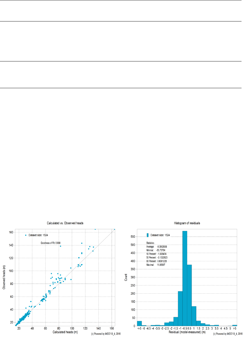
DRAFT
iMOD Batch functions
HCLASSES=
(optional)
Specify the classes for the histogram, by default this keyword is
absent and the following classes are used: -10.0E10,-5.0,-4.5,-
4.0,. . . ,4.0,4.5,5.0,10.0E10. However, it is possible to specify a user de-
fined class via e.g. HCLASSES=-10.0,-1.0,-0.5,0.5,1.0,10. In this case
the first class is for >−10.0and ≤ −1.0, the second for >−1.0- and
≤ −0.5and so on.
IWEIGHT=
(optional)
Choose whether you will include the weight factors in the calculation or
not. IWEIGHT=0 the weight factor is not included, IWEIGHT=1 the weight
factor is included. In case the weight factor equals 0 the related data point
will not be plotted.
Example
FUNCTION=PLOTRESIDUAL
INPUTFILE=D:\LOG_PEST_RESIDUAL_10V2.6.66.TXT
IPLOT=1
BMPNAME=d:\SCATTERPLOT.BMP
ITRANSIENT=1
ILAYER=16
IIPF=1
IWEIGHT=1
This example makes a scatter plot with the name SCATTERPLOT.BMP of the transient data available
in the LOG_PEST_RESIDUAL_10V2.6.66.TXT file for a selection of layer 16 and the first IPF-file. The
plotted values are multiplied with the given weight factor.
Result of PLOTRESIDUAL, left a scatter plot (IPLOT=1) , right a histogram (IPLOT=2)
Deltares 505 of 812
DRAFT
iMOD, User Manual
8.10 WELL-FUNCTIONS
8.10.1 DEVWELLTOIPF-Function
The function DEVWELLTOIPF converts Deviated Wells, described in CSV format, to an IPF file.
FUNCTION= DEVWELLTOIPF
CSVFNAME= Enter the name of an CSV file with minimal 6 columns that rep-
resents x- and y coordinates, azimuth and inclination, e.g. CSVF-
NAME=D:\DATA\AGS.CSV.
IPFFNAME= Enter the name of an IPF file that need to be created for the data in the
CSVFNAME„ e.g. IPFFNAME=D:\DATA\AGS.IPF. For each unique bore-
hole in the CSV file, another point will be created in the IPF. The associ-
ated TXT files for the boreholes will be stored in the same folder as the
IPFFNAME.
NCOL
(optional)
Enter the column number in the CSV file that represents the unique NAME
of the borehole, e.g. NCOL=4. By default NCOL=1. The NAME of the
borehole will be used to create the file name for the associated TXT files.
Therefore, the character set ‘: /’ will be replaced by a ‘_’ (a space is part of
the replacement as well, denoted as the second character in the set).
XCOL
(optional)
Enter the column number in the CSV file that represents the x-coordinate,
e.g. XCOL=4. By default XCOL=2.
YCOL
(optional)
Enter the column number in the CSV file that represents the y-coordinate,
e.g. YCOL=6. By default YCOL=3.
ZCOL
(optional)
Enter the column number in the CSV file that represents the z-coordinate,
e.g. ZCOL=6. By default ZCOL=0 that means that the z-coordinate will be
0.0 m+MSL.
DCOL
(optional)
Enter the column number in the CSV file that represents the depth, e.g.
DCOL=6. By default DCOL=5. Remember that the DEPTH is measured
as the net distance (meter) through the borehole.
ACOL
(optional)
Enter the column number in the CSV file that represents the azimuth, e.g.
ACOL=8. By default ACOL=6. The azimuth is defined as the angle with
the z-axes measured clockwise with a zero angle pointing to the north and
90 to the east.
ICOL
(optional)
Enter the column number in the CSV file that represents the inclination,
e.g. ICOL=12. By default ICOL=7. The inclination is defined as the angle
from the surface (xy-plane) downwards by a positive angle whereby 90.0
degrees is perpendicular downwards.
NLCOL
(optional)
Enter the number of labels to be additional added to the TXT files of the
boreholes, e.g. NLCOL=2. By default NLCOL=1 and a default label column
is added (see LCOL{i}).
LCOL{i}
(optional)
Enter the column number in the CSV file that represents the label, e.g.
LCOL1=4. By default LCOL1=0 and a default label is used. The label can
be used to colour particular trajectories along a borehole differently. If this
keyword is absent, iMOD will add a default label ‘S’.
Example 1
FUNCTION=DEVWELLTOIPF
CSVFNAME=D:\AGS.CSV
IPFFNAME=D:\IPF.IPF
This example, converts the columns in the CSV file via the default columns setting to an IPF file, the
outcome in 3D could look like the following image.
506 of 812 Deltares
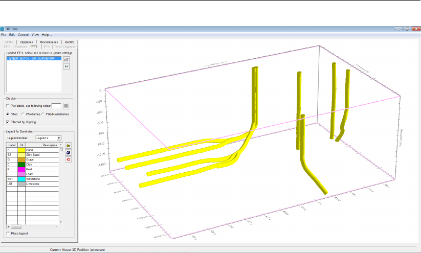
DRAFT
iMOD Batch functions
Deltares 507 of 812
DRAFT
iMOD, User Manual
8.10.2 ASSIGNWELL-Function
The ASSIGNWELL function reads a geological model (TOP/BOT) in order to assign well screens to
the right formation layer.
FUNCTION= ASSIGNWELL
IPFFILE_IN= Give IPF file containing WELL or MEASUREMENT information.
IPFFILE_out= Give IPF file outputfile.
IXCOL= Enter the column number in the IPF file IPF{i} that represents the x coor-
dinate, e.g. IXCOL=4. By default IXCOL=1.
IYCOL= Enter the column number in the IPF file IPF{i} that represents the y coor-
dinate, e.g. IYCOL=6. By default IYCOL=2.
IDCOL= Enter the column number in the IPF file IPF{i} that represents the extraction
rate of the well, e.g. IQCOL=12. By default IQCOL=3.
IZ1COL= Enter the column number in the IPF file IPF{i} that represents the top of
the well screen, e.g. ITCOL=4. By default ITCOL=4.
IZ2COL= Enter the column number in the IPF file IPF{i} that represents the bottom
of the well screen, e.g. IBCOL=6. By default IBCOL=5.
NFORMATIONS= Enter the number of formations
FORMATION{i}= Enter the number of the column in the IPF for the ..... of the ith formation
TOP_L{i}= Enter the IDF for the ith modellayer that represents the top of modellayer
i, e.g. TOP_L1=D:\INPUT\TOP_L1.IDF.
BOT_L{i}= Enter the IDF for the ith modellayer that represents the bottom of model-
layer i, e.g. BOT_L1=D:\INPUT\BOT_L1.IDF.
Example 1
FUNCTION=ASSIGNWELL
IPFFILE_IN=D:\DATA\WELL.IPF
IPFFILE_OUT=D:\DATA\WELL_ASSIGNED.IPF
NFORMATIONS=2
FORMATION1=1
FORMATION2=2
TOP_L1=D:\GEOHYDROLOGY\TOP1.IDF
BOT_L1=D:\GEOHYDROLOGY\BOT1.IDF
TOP_L2=D:\GEOHYDROLOGY\TOP2.IDF
BOT_L2=D:\GEOHYDROLOGY\BOT2.IDF
Above an example is given how to divide well filters in the file WELL.IPF over 2 model layers resulting
in the file WELL_ASSIGNED.IPF.
508 of 812 Deltares
DRAFT
iMOD Batch functions
8.10.3 MKWELLIPF-Function
The MKWELLIPF function computes the extraction strength for each well based on a weighed value
according to their length and permeability of the penetrated model layer. At the end of the procedure
iMOD echoes a summary of the total and average extraction per model layer.
FUNCTION= MKWELLIPF
NLAY=
(optional)
Enter the number of layers from which well may be organized, e.g.
NLAY=7, by default NLAY=0 which means that only extraction rates are
computed from the associated TXT files.
Following keywords are needed/optional whenever NLAY greater than zero
TOPIDF{i}= Enter the name of an IDF-file that represents the top elevation of the ith
modellayer, e.g. TOPIDF1=D:\MODEL\TOP1.IDF.
BOTIDF{i}= Enter the name of an IDF-file that represents the bottom elevation of the
ith modellayer, e.g. BOTIDF3=D:\MODEL\BOT_LAYER3.IDF.
KDIDF{i}=
(optional)
Enter the name of an IDF-file that represents the transmissivity of a partic-
ular ith modellayer, e.g. KDIDF2=D:\MODEL\TRAN_L2.IDF.
CIDF{i}=
(optional)
Enter the name of an IDF-file that represents the vertical re-
sistance between two adjacent modellayers i and i+1, e.g.
CIDF1=D:\MODEL\C_L1.IDF.
ITCOL=
(optional)
Enter the column number in the IPF file IPF{i} that represents the top of
the well screen, e.g. ITCOL=4. By default ITCOL=4.
IBCOL=
(optional)
Enter the column number in the IPF file IPF{i} that represents the bottom
of the well screen, e.g. IBCOL=6. By default IBCOL=5.
MINKHT=
(optional)
Specify the minimum horizontal transmissivity (m2/d) that will receive a
well. By default MINKHT=0.0 m2/day. This parameters is used only when-
ever values are entered for KDIDF{i}.
MINKD=
(optional)
Specify the horizontal transmissivity that is used te define the model layer
of the well. The first model layer with a transmissivity of more than the
specified MINKD, will receive the complete well. By default MINKD=0.0
m2/day. This parameters is used only whenever values are entered for
KDIDF{i} and will be active for those wells that cannot be assigned due to
missing values for ITCOL and IBCOL.
IMIDF=
(optional)
Whenever IMIDF=0, the mid of a well screen is computed by the top and
bottom screen heights if both available (not equal to the parameter FNO-
DATA). Whenever IMODF=1, the mid of the screen is equal to the top of
the screen whenever the bottom height might be absent, and equal to the
bottom whenever the top is absent. It both are available, the computation
of the mid of the well screen is equal to the method described by IMIDF=0.
By default IMIDF=0.
ICLAY=
(optional)
Whenever wells might fall completely in an aquitard (in between two model
layers), specify ICLAY=1 to shift the well vertically to that model layer that
is most nearby (above- or beneath), this is the default value. Specify
ICLAY=0 and the well will be removed whenever completely in an aquitard.
FNODATA=
(optional)
Specify the NoDataValue for the top and bottom of the well screen, de-
noted by ITCOL and IBCOL. By default FNODATA=-99999.0, values equal
to this will be discarded.
Rest of keywords are applicable for all values of NLAY.
NIPF Enter the number of IPF files to be organized, e.g. NIPF=3.
IPF{i}= Enter the name for the ith IPF file, e.g. D:\DATA\WELL.IPF.
The resulting IPF files will be save in the folder
D:\DATA\WELL\IMOD_MKIPF_WELLS_L*.IPF for each model layer
that has extraction rate <> 0.0.
IXCOL=
(optional)
Enter the column number in the IPF file IPF{i} that represents the x coor-
dinate, e.g. IXCOL=4. By default IXCOL=1.
IYCOL=
(optional)
Enter the column number in the IPF file IPF{i} that represents the y coor-
dinate, e.g. IYCOL=6. By default IYCOL=2.
Deltares 509 of 812
DRAFT
iMOD, User Manual
IQCOL=
(optional whenever
ISS=0)
Enter the column number in the IPF file IPF{i} that represents the extraction
rate of the well, e.g. IQCOL=12. By default IQCOL=3.
ISS=
(optional)
This flags determines whether an time average extraction volume need to
be computed for a specified period of time, for that case ISS need to be 1.
By default ISS=0 and an average value is computed for the time series as
a whole.
SDATE=
(if ISS=1)
Specify a starting date (YYYYMMDD) from which the determination of a
well strength/head will be computed. This keyword is compulsory when-
ever ISS=1.
EDATE=
(if ISS=1)
Specify an end date (YYYYMMDD) from which the determination of a well
strength/head will be computed. This keyword is compulsory whenever
ISS=1.
HNODATA=
(optional)
Specify the NoDataValue for the extraction rate, values equal to this will
be discarded. By default HNODATA=0.0.
The IPF file IMOD_MKIPF_WELLS_ALL.IPF contains all rows from the original IPF. This file is easier
to analyse whether the well screen assigned have been computer properly. There is an attribute
ERROR_CODE in the IPF that denotes the way the well has been assigned. The following codes
are applicable; "@" means that the well is assigned to a nearby model layer; "#" means that the well
could not be assigned; and "-" means that the well has been assigned appropriately. The IPF file
IMOD_MKIPF_WELLS_UNASSIGNED.IPF contains all rows from the original IPF that could not be
assigned to model layer.
Methodology
The following steps are carried out for each individual record in the IPF file (IPF{i}):
1 Compute the individual length of the well screen between the ITCOL and IBCOL into well screen
segments, that penetrate any model layer. Well screen segments that are above the surface ele-
vation (TOPIDF1) or below the lowest bottom elevation (BOTIDF{NLAY}) will be clipped off;
2 Compute the horizontal permeability (k-value) for all model layers that are penetrated by the re-
maining well screen segments. Assign a ratio to all well screen segments based on their individual
length multiplied by the k-values of the corresponding model layer divided by their total summed
value;
3 Correct any ratio for a mismatch between the centre of the penetrating model layer zcand the
vertical midpoint of the well screen segment fc, by:
f= 1.0−|zc−fc|
0.5∆z,
where ∆zis the thickness of the corresponding aquifer.
4 Remove ratio that are smaller than 5%.
5 If in aquitard, move it to the nearest aquifer above or below the aquitard, only whenever ICLAY=1;
6 If nothing in model, whenever system on top of model, put them in first model layer with thickness
and permeability larger than MINKH.
510 of 812 Deltares

DRAFT
iMOD Batch functions
Example 1
FUNCTION=MKWELLIPF
NLAY=3
TOPIDF1=D:\DATA\TOP1.IDF
TOPIDF2= D:\DATA\TOP2.IDF
TOPIDF3= D:\DATA\TOP3.IDF
BOTIDF1= D:\DATA\BOT1.IDF
BOTIDF2= D:\DATA\BOT2.IDF
BOTIDF3= D:\DATA\BOT3.IDF
KDIDF1= D:\DATA\KD1.IDF
KDIDF2= D:\DATA\KD2.IDF
KDIDF3= D:\DATA\KD3.IDF
CIDF1=D:\DATA\C1.IDF
CIDF2=D:\DATA\C2.IDF
NIPF=1
IPF1=D:\DATA\WELL.IPF
The example above, will classify each location in the IPF file D:\DATA\WELL.IPF according their length
and associated transmissivity, within any penetrating modellayer.
Example 2
FUNCTION=MKWELLIPF
NLAY=3
TOPIDF1=D:\DATA\TOP1.IDF
TOPIDF2= D:\DATA\TOP2.IDF
TOPIDF3= D:\DATA\TOP3.IDF
BOTIDF1= D:\DATA\BOT1.IDF
BOTIDF2= D:\DATA\BOT2.IDF
BOTIDF3= D:\DATA\BOT3.IDF
KDIDF1= D:\DATA\KD1.IDF
KDIDF2= D:\DATA\KD2.IDF
KDIDF3= D:\DATA\KD3.IDF
CIDF1=D:\DATA\C1.IDF
CIDF2=D:\DATA\C2.IDF
IXCOL=1
IYCOL=2
ITCOL=3
IBCOL=4
IQCOL=8
NIPF=3
IPF1=D:\DATA\INDUSTRY.IPF
IPF2= D:\DATA\DRINKINGCOOPERATION.IPF
IPF3= D:\DATA\AGRICULTURE.IPF
The example above, will classify each location in three IPF files according their length and associated
transmissivity, within any penetrating model layer. The content of the IPF files is different than the
default IXCOL, IYCOL, ITCOL, IBCOL and IQCOL column identifications, and therefore added here.
Deltares 511 of 812
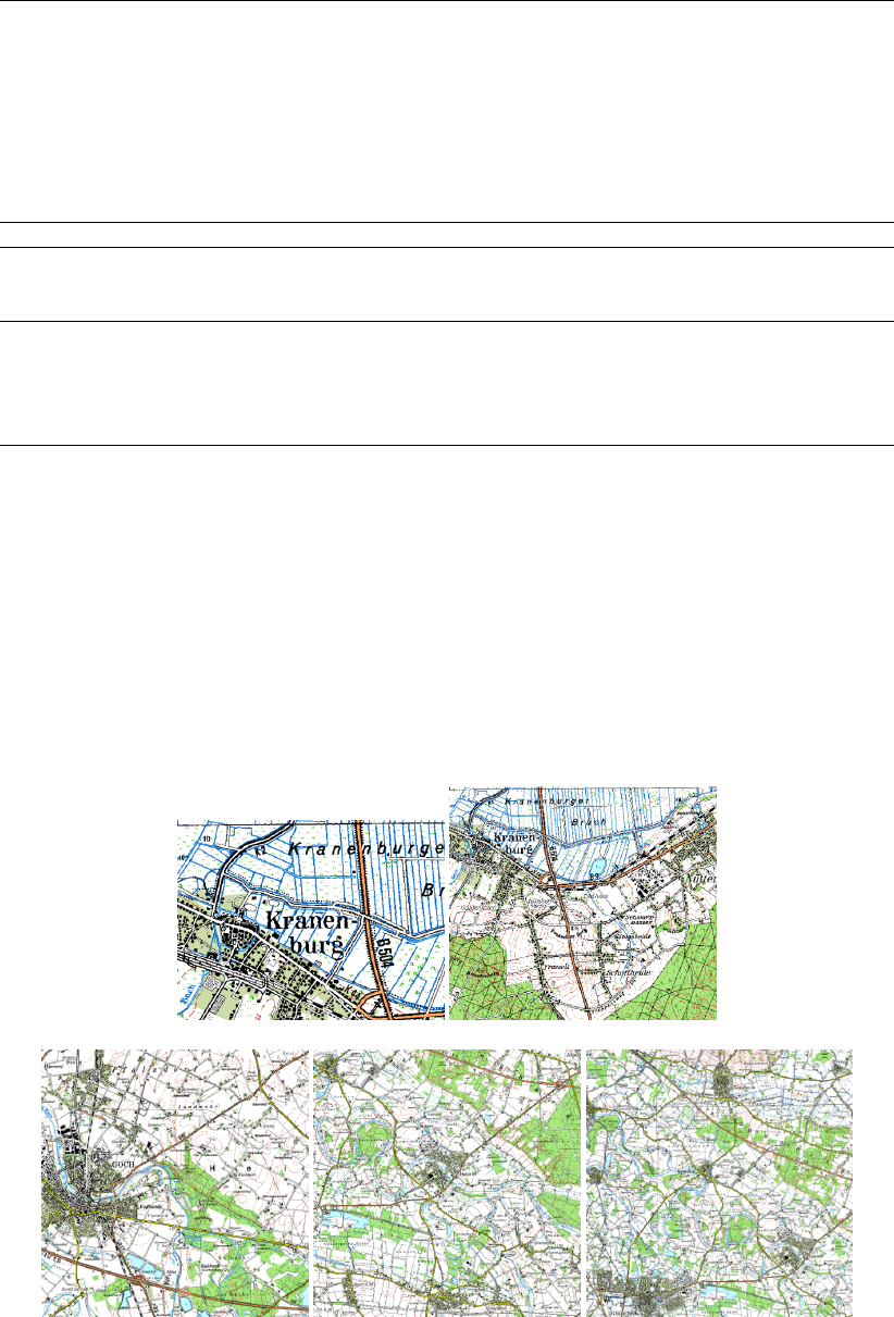
DRAFT
iMOD, User Manual
8.11 BMPTILING-Function
Use this function to create a set of topographical bitmaps out of a single one, to be used as back-
ground topology. The function assumes that one single bitmap needs to be split in small “tiles” for
different resolutions. Those different resolutions can be used at different zoom levels to maintain a
high performance while plotting these bitmaps on the graphical canvas.
FUNCTION= BMPTILING
BMPFILE= Enter the name of a BMP file, e.g. D:\DATA\AIRPHOTO.BMP.The function
assumes that a worldfile (*.BMPW) is accompanied by the bitmap for the
syntax of a worldfile.
OUTPUTFOLDER= Enter the name of the folder that will store all the generated bitmaps (tiles)
at different resolutions (5), e.g. D:\DATA\BMP. The function will generate a
*.CRD file too and associated TXT files. Referring to the *.CRD file from
the iMOD preference file will ensure that the bitmaps can be used directly
in iMOD.
Example
FUNCTION=BMPTILING
BMPFILE=D:\DATA\AIRPHOTO.BMP
OUTPUTFOLDER=D:\DATA\BMP
The example above generates different tiles from the bitmap AIRPHOTO.BMP in the folder D:\DATA\BMP.
In this folder the file BMP.CRD will be stored that can be used to direct with a keyword TOP25 in the
iMOD preference file.
Tile 1 Tile2
Tile 3 Tile 4 Tile 5
512 of 812 Deltares

DRAFT
iMOD Batch functions
8.12 PLOT-Function
The Plot function can be used to construct figures that are normally displayed on the graphical display
of iMOD.
FUNCTION= PLOT
OUTFILE= Enter the name of the output filename. The format of the image depends on the
extension of the filename:
*.BMP : Windows Bitmap;
*.PCX : ZSoft PC Paintbrush;
*.PNG : Portable Network Graphic image;
*.JPG : JPEG/JFIF image.
IDFFILE=
(optional)
Enter the name of an *.IDF-file that needs to be plotted, for example IDF-
FILE=D:\AHN.IDF.
IDFLEGFILE=
(optional)
Enter the name of a *.LEG file that needs to be used for
colouring the *.IDF-file. If no IDFLEGFILE is given, iMOD
will apply a default iMOD Legend based on a linear distribu-
tion of IDF values.
IDFLEGTXT
(optional)
Enter the text to be added to the legend, e.g. ID-
FLEGTXT=”Transmissivity (m2/day)”. By default no legend
text will be displayed.
IDFSTYLE=
(optional)
Specify whether the IDF need to be displayed as gridval-
ues, contourlines, vectors or all three combined. For ex-
ample IDFSTYLE=111 will plot the IDF-file by all styles, de-
fault IDFSTYLE=100. Use the following syntax to specify the
style to be used, any combination is possible:
100 IDF will be displayed as filled rectangles.
010 IDF will be contoured.
001 IDF will be displayed as arrows based on
the gradient in the IDF file.
IPFFILE=
(optional)
Enter the name of an IPF file to be plotted, for example IPFFILE=D:\DATA.IPF.
iMOD will use the first and second column in the IPF for the x- and y coordinate
and displays the point in red circles. Use the other keywords to change these
settings.
IPFXCOL=
(optional)
Specify the column to be used for the x-coordinate, by de-
fault IPFXCOL=1
IPFYCOL=
(optional)
Specify the column to be used for the y-coordinate, by de-
fault IPFYCOL=2
IPFHCOL=
(optional)
Specify the column to scale the dots that have larger values
than others, those will be displayed as an increased marker
symbol. iMOD will scale the values based on the entries at
the keyword IPHCOL_M. By default IPFHCOL=0.
IPFHCOL_M=
(optional)
Specify the methodology to scale the symbol, by default
IPFHCOL=0 and no scaling applies. iMOD displays them,
such that small symbol sizes will be plotted upon large sym-
bols, choose a method from the following:
1 iMOD scales the values for IPFHCOL lin-
early from large up to small using 4 sizes
(sizes 1,2,3 and 4).
2 iMOD scales the values for IPFHCOL lin-
early from large up to small using 4 sizes
(sizes 1,2,3 and 4) within the range of the
entered legend.
3 iMOD scales the absolute values for IPFH-
COL linearly from large up to small using
4 sizes (sizes 1,2,3 and 4).
4 iMOD scales the symbols using the direct
value for IPFHCOL, sizes need to be pos-
itive, negative entries will be as treated as
positive sizes.
Deltares 513 of 812

DRAFT
iMOD, User Manual
IPFASSFILES=
(optional)
Specify whether to plot the graph (e.g. timeseries, bore-
holes) described in the associated TXT files linked by the
IPFFILE. Specify IPFASSFILES=1 to plot a simple graph
(without axes) and IPFASSFILES=2 to plot a advanced
graph with axes. By default IPFASSFILES=0 and no associ-
ated text files are displayed.
IPFASSFILES_
ALL=
(optional)
Specify whether to plot the content of all associated TXT
files in a single image (IPFASSFILES_ALL=1) or alterna-
tively, plot each TXT file in a separate image (IPFASS-
FILES_ALL=2). In that case the OUTFILE will be created
automatically by the name of the individual points given by
the column denoted by the IEXT, see section 9.7 for more
information on IPF files.
IPFSTYLE=
(optional)
Specify the style to be used to plot the points. Use the fol-
lowing options:
0 Use this style to display the points as solid
circles.
1 Use this style to colour the points by the
labels in the column IPFLCOL in combina-
tion with the specified legend in LEGFILE.
Specify the following whenever IPFSTYLE=1
IPFLEGFILE=
(optional)
Enter the appropriate legend
file to be used, e.g. IPFLEG-
FILE=D:\RESIDUAL.LEG
IPFLCOL= Specify the column in the IPF file for
the colouring of points, needed whenever
IPFLEGFILE is specified.
IPFLEGTXT=
(optional)
Enter the text to be added to the legend,
e.g. IPFLEGTXT=”Residual (m)”. By de-
fault, whenever the keyword is absent, no
legend text will be displayed.
NLABELS=
(optional)
Specify the total number of labels to be
plotted, e.g. NLABELS=3. By default NLA-
BELS=0 and no labels (i.e. columns in the
IPF file) will be plotted.
ILABELS= Specify the number of individual labels
(i.e. the columns in the IPF file) to
be plotted, e.g. ILABELS=3,5,7 and NLA-
BELS=3.
IFFFILE=
(optional)
Enter the name of an IFF file to be plotted, for example IFF-
FILE=D:\MODEL\FLOW.IFF. iMOD will plot the lines in coloured by the sixth
column in the IFF file (normally that is the attribute CUMTT).
IFFLEGFILE=
(optional)
Enter the appropriate legend file to be used, e.g. IFFLEG-
FILE=D:\CUMTT.LEG. By default no legend is used.
IFFLEGTEXT=
(optional)
Enter the text to be added to the legend, e.g. ID-
FLEGTXT=”Cumulative Time (years)”. By default no legend
text will be displayed.
LEGTSIZE=
(optional)
Enter the size for the legend text, enter the size in fraction of the plotting box, e.g.
LEGTSIZE=0.05.
NGEN=
(optional)
Enter the number of GEN files to be included, e.g. NGEN=3.
GENFILE{i}= Enter the name of a *.GEN-file that needs to be plotted on
the background. On default the line, points and/or polygons
in the GENFILE, will be drawn as black features, e.g. GEN-
FILE1=D:\GENS\TOPOGRAPHY.GEN. This keyword need
to be repeated for NGEN-times.
514 of 812 Deltares
DRAFT
iMOD Batch functions
GENCOLOUR{i}=
(optional)
Enter a colour number to be used colouring the ith GEN
file specified by GENFILE{i}. By default a black line will
be plotted. Specify a colour by red,green and blue
components, e.g. GENCOLOUR1=255,0,0 to express full
red. Use GENCOLOUR1=0,0,0 to specify black and GEN-
COLOUR1=255,255,255 to set white.
GENTHICK
NESS{i}=
(optional)
Enter a line thickness to be used for the ith GEN file speci-
fied by GENFILE{i}. By default GENTHICKNESS1=1 and a
line thickness of 1 will be applied, e.g. GENTHICKNESS1=5
to express a line thickness of 5.
TOP25=
(optional)
Enter the location of the CRD-file (see section 9.18 for the syntax of
such a file), used by iMOD to display ... background images, e.g.
TOP25=d:\TOP25\BMPCRD.CRD.
WINDOW=
(optional)
Enter the coordinates of the window that needs to be displayed. Enter coordi-
nates of the lower-left corner first and then the coordinates of the upper-right
corner, e.g. WINDOW=100000.0, 400000.0, 200000.0, 425000.0. When the key-
word is absent, the figure will be displayed at the maximum extent of the entered
filenames at the keywords IDFFILE, IPFFILE and/or IFFFILE.
The following keywords need to be all defined in order to generate more sophisticated display,
including legend boxes and figure labels.
TITLE= Enter a name for the main title of the figure, e.g. TITLE=”Effect of an Increased
Well Capacity on Groundwater Levels”. Use quotes for titles that contain spaces.
SUBTITLE= Enter a string for a subtitle, e.g. SUBTITLE=”Financed by European Union”. Use
quotes for titles that contain spaces.
FIGTXT= Enter a figure identification, e.g. FIGTXT=”Figure 1-a”. Use quotes for titles that
contain spaces.
PRJTXT= Enter a description of the project, e.g. PRJTXT=”iMOD Groundwater Flow Model”.
Use quotes for titles that contain spaces.
YFRAC-
LEGEND=
(optional)
Enter the percentage (0-100%) of the legend occupation in the legend area, e.g.
YFRACLEGEND=50.0 means that the legend will be placed in 50% of the total
legend area. On default YFRACLEGEND=100.0, so the entire legend area will
be used.
RESOLUTION=
(optional)
Enter the resolution of the bitmap, i.e. the number of pixels. On default RESOLU-
TION=3200. Higher resolutions will yield more accurate images.
Deltares 515 of 812
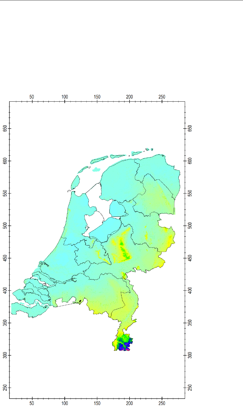
DRAFT
iMOD, User Manual
Example 1
FUNCTION=PLOT
IDFFILE=D:\TUTORIAL\iMODBATCH\AHN.IDF
IDFSTYLE=100
NGEN=1
GENFILE1=D:\TUTORIAL\iMODBATCH\PROVINCES.GEN
OUTFILE=D:\TUTORIAL\iMODBATCH\AHN.png
As a result of the above described content the following figure will be created:
516 of 812 Deltares
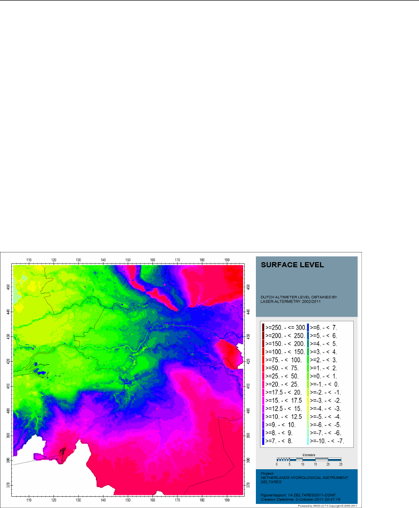
DRAFT
iMOD Batch functions
Example 2
FUNCTION=PLOT
IDFFILE=D:\TUTORIAL\iMODBATCH\AHN.IDF
IDFSTYLE=100
IDFLEGFILE=TUTORIAL\AHN.LEG
GENFILE1=D:\TUTORIAL\iMODBATCH\PROVINCES.GEN
OUTFILE=D:\TUTORIAL\iMODBATCH\AHN.png
RESOLUTION=3200
WINDOW=100000.0,400000.0,200000.0,425000.0
TITLE=”Surface Level”
SUBTITLE=”Dutch Altimeter Level obtained by Laser-Altimetry 2002/2011”
FIGTXT=”1A DELTARES2011-Conf. ”
PRJTXT=”Netherlands Hydrological Instrument, Deltares”
As a result of the above described content the following figure will be created.
Advanced example of a resulting bitmap:
Deltares 517 of 812
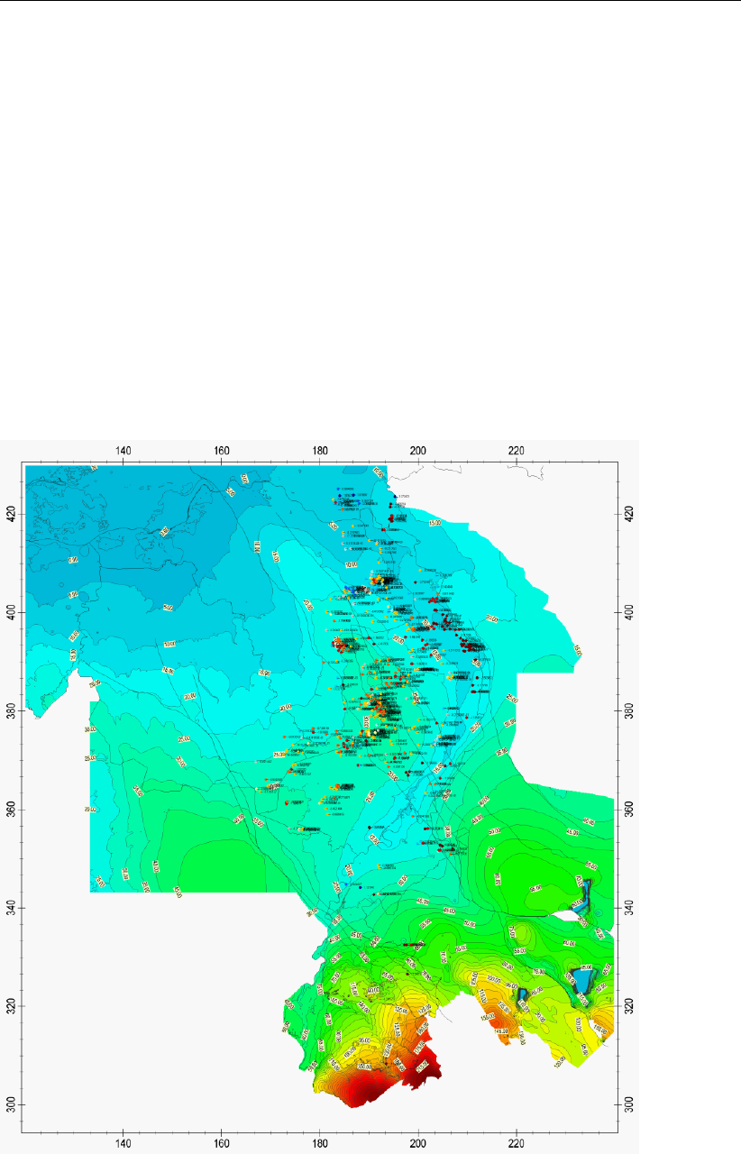
DRAFT
iMOD, User Manual
Example 3
FUNCTION=PLOT
IDFFILE=D:\IMOD-TEST\PLOT\BATHEMETRY.IDF
IDFLEGFILE=D:\iMOD-TEST\PLOT\LEGEND.LEG
IDFSTYLE=010
IPFFILE=D:\iMOD-TEST\PLOT\BATHYMETRY.IPF
IPFXCOL=2
IPFYCOL=1
IPFLCOL=3
IPFSTYLE=1
IPFLEGFILE=D:\iMOD-TEST\PLOT\LEGEND.LEG
NLABELS=1
ILABELS=3
NGEN=2
GENFILE1=D:\PROVINCES.GEN
GENFILE2=D:\FAULTS.GEN
OUTFILE=D:\IMOD-TEST\PLOT\BATHEMETRY.png
518 of 812 Deltares
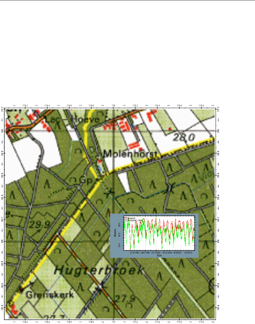
DRAFT
iMOD Batch functions
Example 4
FUNCTION=PLOT
IPFFILE=D:\TUTORIAL\iMODBATCH\MEASURE.IPF
IPFASSFILES=2
IPFASSFILES_ALL=1
TOP25=D:\TUTORIAL\iMODBATCH\BMP.CRD
OUTFILE=D:\TUTORIAL\iMODBATCH\TIMESERIES.png
As a result of the above described content the following figure will be created.
Deltares 519 of 812

DRAFT
iMOD, User Manual
520 of 812 Deltares
DRAFT
9 iMOD Files
This chapter describes the types of files used by iMOD.
Below a summarizing table of all file types used by iMOD is given; per file type it includes a short
description of it’s purpose. iMOD uses both generally known file types (e.g. bitmap BMP-files, ESRI-
shape files, NetCDF-files) and iMOD-specific file types; the latter group of files is described in detail
in section 9.1 -section 9.4. The table includes links to the related sections in this chapter or other
sections in this user manual, or links to external sources.
Extent Associated
Extension(s)
Reference in
this manual
Description
*.prf section 9.1 iMOD Preference File (ASCII):
File containing the initial settings for iMOD.
*.imf section 9.2 iMOD-MetaFile (ASCII):
File containing information to display selected
maps including legend and topographical over-
lays.
*.idf section 9.5 iMOD Data-File (BINARY):
Raster file, containing information on a raster
with evenly or non-evenly distributed rows and
columns. Format is specific for iMOD and devel-
oped to handle large sized data sets in a time-
efficient way. Besides geographical information,
IDF-files can handle meta-data as well (such as
descriptive information).
*.mdf section 9.6 iMOD Multi-Data-File (ASCII):
This file contains several references to IDF-files.
Whenever IDF will be grouped they will be col-
lected into a MDF-file.
*.ipf *.txt
*.dat
section 9.7 iMOD Point-File (ASCII):
File containing the information on points. An IPF-
file can direct to several *.TXT files that contain
timevariant information (such as timeseries) or
vertical descriptions (such as drilling logs or cone
penetration test logs).
*.iff section 9.8 iMOD Flow-File (ASCII):
File containing the information that result after
computing flow-lines within iMOD. It describes
mainly lines in 3D-coordinates with their age and
velocity.
*.isg *.isp (BINARY)
*.isd1 (BINARY)
*.isd2 (BINARY)
*.isc2 (BINARY)
*.ist2 (BINARY)
section 9.9 iMOD Segment-File (ASCII):
File containing the information to describe a
line/segment for river modeling. An ISG-file di-
rects to an ISP-file (containing the actual coor-
dinates of the segment), an ISD#-file (contain-
ing timevariant information on e.g. waterlevels),
an ISC#-file (containing information on the cross-
section of the segments) and *.IST# (contain-
ing timevariant information on e.g. waterlevels at
weirs and/or water structures)
*.gen *.dat section 9.10 (both ASCII):
ESRI Generate File that described line elements,
e.g. lines, polygons (closed lines). For polygons,
*.DAT can be included that contain information for
polygons.
Deltares 521 of 812
DRAFT
iMOD, User Manual
Extent Associated
Extension(s)
Reference in
this manual
Description
*.csv section 9.12 Comma Seperated Values file. It stores tabular
data (numbers and text) in plain text. Each line
of the file is a data record. Each record con-
sists of one or more fields, separated by commas.
The use of the comma as a field separator is the
source of the name for this file format.
*.asc section 9.13 An ASCII format based ESRI grid, also known
as an ARC/INFO ASCII GRID. (A binary format
is widely used within Esri programs, such as Ar-
cGIS.) The ASCII format is used as an exchange,
or export format, due to the simple and portable
ASCII file structure.
*.leg section 9.15 iMOD Legend File (ASCII):
File containing information on classes and
colours used by iMOD to display an IDF, IPF, IFF
and/or GEN.
*.clr section 9.16 iMOD Colour File (ASCII):
File containing the initial colour used by iMOD
*.dlf section 9.17 File containing color information to display bore-
holes
*.crd *.* section 9.18 iMOD Coordinate File (ASCII):
File that directs to other files depending on the
zoom levels.
*.isd section 9.19 An ISD-file contains information about the loca-
tion of startpoints used in the calculation of path-
lines from model output.
*.sol section 9.20 iMOD SOLid project file (ASCII):
File containing the layer definitions of a solid
*.spf section 9.21 A SPF-file describes the variation in the top and
bottom elevation along a cross-sectional line.
*.ses section 9.22 File describing the operations that need to be car-
ried out by ISG Edit.
*.tim section 9.4 A time step configuration file.
*.prj section 5.5 iMOD Project File (ASCII):
File containing the characteristics of files used in
a model simulation.
*.run chapter 10 iMOD Runfile (ASCII):
File used to run a model simulation with iMOD-
FLOW. An iMOD Runfile may be generated from
an iMOD Project File
*.ini section 7.10.1,
section 7.11.1
iMOD Initialization File (ASCII):
File containing specific information for particular
parts of iMOD, such as the ScenarioTool and the
QuickScanTool. The syntax is comparable to the
*.INI-files of Windows.
*.msk section 5.1 iMOD Mask-File (BINARY):
File contains coordinates of a rectangular area
that can be loaded into iMOD to zoom to that par-
ticular area.
*.isd section 7.13 iMOD Startpoint Definition File (ASCII):
*.bmp *.png
*.pcx
*.ps
Window Bitmap (BMP), Portable Network
Graphics Image (*.png), ZSoft PC Paintbrush,
PostScript (*.ps) (all BINARY):
Export file containing the image of the current
window.
*.nc NetCDF File (BINARY). More info: www.
unidata.ucar.edu/software/netcdf.
522 of 812 Deltares

DRAFT
iMOD Files
Extent Associated
Extension(s)
Reference in
this manual
Description
*.map Map file (BINARY):
A Map file is a binary data text file, which
is mainly used as in-/output file of PCRaster.
For more information about PCRaster go to:
http://pcraster.geo.uu.nl/.
*.arr section 9.14 Array file (ASCII):
An array file is a text file, which is used as input
file for iMODFLOW. It is generated by iMOD once
the input is created for iMODFLOW. You can read
in such a file directly in iMOD.
*.shp ESRI Shape File (BINARY). File containing topo-
logical information on lines, points, polygons.
Deltares 523 of 812

DRAFT
iMOD, User Manual
9.1 PRF-files
During the start-up of iMOD the iMOD preference file is read to instruct iMOD to operate with the
correct settings. These settings are placed in the IMOD_INIT.PRF file, or in a *.PRF file saved by the
user.
Example of a PRF-file:
USER "D:\IMOD\IMOD_USER"
DBASE "D:\IMOD\DBASE"
MODFLOW "D:\OSSDELTARES\IMOD_X64_R.EXE"
TOP25 "D:\TOP25 \BMPCRD.CRD"
SUBSURFEXDBASE "N:\Units\\DBASE"
7ZIP "C:\PROGRAM FILES\7-ZIP\7Z.EXE"
PLUGIN1 "D:\IMOD\PLUGINS
FFMPEG "D:\THIRD_PARTY_SOFTWARE\FFMPEG.EXE"
FFMPLAY "D:\THIRD_PARTY_SOFTWARE\FFMPLAY.EXE"
VLCPLAYER "C:\PROGRAM FILES (X86)\VIDEOLAN \VLC.EXE"
The following keywords can be included in the *.PRF file:
KeyWord Folder/
File
Description
USER (compul-
sory)
Folder User Map.
TOP25 File Name of the *.CRD file to be able to position topographical bitmaps
at the right coordinates.
VECTOR Folder Map to direct to the map that stores topographical vector informa-
tion (GEN, IPF, SHP files).
HELPFILE File iMOD Help file (*.PDF) that can be used by the Help ... button
throughout the application.
DBASE Folder Map that directs to the location of the model data. This map is used
to replace the string $DBASE$ in a runfile.
IRDBASE File Map that directs to the location of the Quick Scan Tool command
(see section 7.10). Used for obtaining an approximate result from
a database filled with model results.
TAGS File Map to store all the Tags (Comments), make sure this location is
accessible by all relevant iMOD users.
MODFLOW File Name of the iMODFLOW executable.
SCENTOOL File Initialization file (*.INI) for usage of the ScenarioTool.
PLUGIN1 Folder First folder that directs to the location of plugin subfolders. Such a
subfolder at least contains the executable-file to be used in iMOD.
PLUGIN2 Folder Second folder that directs to another location of plugin subfolders.
Such a subfolder at least contains the executable-file to be used in
iMOD.
NORTH-
ARROW
File Bitmap (BMP, PNG) that represents a North arrow that can be
placed on the graphical window.
ACROBAT-
READER
Exe Executable for the Acrobat Reader to be used to read the iMOD
Help file as specified by the Keyword HELPFILE.
IR_COSTS File Give the name of the map file containing action related cost to be
used in the IR-database.
7ZIP Exe Executable that will be used to unzip the files used by the Subsur-
face Explorer, see section 5.6.
SUBSURF-
EXDBASE
Folder Folder in which the corresponding files are organized for the Sub-
surface Explorer, see section 5.6.
SOLIDTOOL File Initialization file (*.INI) for usage of the SolidTool.
HELPFILE File iMOD Help file (*.PDF) that can be used by the Help ... button
throughout the application.
524 of 812 Deltares

DRAFT
iMOD Files
KeyWord Folder/
File
Description
FFMPEG Exe Give the name of the FFMPEG executable, this program is nec-
essary to compute playable movie files from bitmaps. This func-
tionality is supported via the Movie Tool, see section 7.5. You can
download the program for free at: https://ffmpeg.org.
FFMPLAY Exe Give the name of the FFMPLAY executable, this program is nec-
essary to play movie files, such as *.AVI and/or *.MPG. This func-
tionality is supported via the Movie Tool, see section 7.5. You can
download the program for free at: https://ffmpeg.org.
VLCPLAYER Exe Give the name of the VLC-player, this program is necessary to play
movie files, see section 7.5.2. You can download the program for
free at: http://www.videolan.org/vlc/index.nl.html.
To calculate Agriculture-subtypes, these files from “HELP2005-tabellen”are required:
HLP_DRY File Give the name of the map file (HLP_DRY.dat) containing help dry
values. HELP2005-database: crop|soiltype|GHG/GLG|respiration-
stress.
HLP_WET File Give the name of the map file (HLP_WET.dat) containing help wet
values.
HLPSOIL File Give the name of the Raster file (HLP_SOIL.IDF); 1:50.000 soil
map reclassified for HELP2005 (using bod2hlp.lut).
LANDUSE File Give the name of the Landuse Raster file (*.INP) containing lan-
duse types in LGN5-codes, to be able to read in the landuse distri-
bution over the area.
CROP_COSTS File Give the name of the map file containing lookup table with crops (in
LGN5-codes) and crop-yields (Euro/ha/year).
To calculate Nature-subtypes, these files from “WATERNOOD - Hydrologische randvoor-
waarden natuur”are required:
RFC_SOIL File Give the name of the Raster file:1:50.000 soil map reclassified to
RFC-soils (using bod2rep.lut).
RFC_LUT File Give the name of the file containing lookup table with
RFC(reprofunction)-characteristics.
NDT File Give the name of the Raster file with vegetation types to calculate
potential development for.
NDT_LUT File Give the name of the file (*.LUT) containing lookup table with option
to aggregate vegetation types.
ABIOT_LUT File Give the name of the file containing a lookup table with hydrologic
requirements for vegetation types (NDT’s).
To calculate Urban-subtypes, these files from “WATERNOOD - Hydrologische randvoorwaar-
den stedelijk”are required:
URBAN_RANGE File In case of urban area, give name of map file to be able to read
ranges of groundwater level. Values are in meters below surface.
Note: iMOD will search for the IMOD_INIT.PRF file in the same folder from where iMOD is started.
If such a file can not be found, iMOD will ask to create its own, with the minimal required keyword:
USER. In the USER folder the following subdirectories are created when you start working in iMOD:
{USER}\imffiles – storage of iMOD MetaFiles (*.IMF)
{USER}\tmp – storage of temporary files;
{USER}\legend – storage of legend files (*.LEG);
{USER}\masks – storage of maskfiles (*.MSK);
{USER}\runfiles – storage of runfiles (*.RUN);
{USER}\scenarios – storage of scenario folders with scenario files (*.SCN;*.SDF);
{USER}\solids – storage of SOLID-folders (*.SOL and *.SPF);
{USER}\qsresults – storage of results of the QuickScanTool;
{USER}\scentool – storage of results of the ScenTool;
{USER}\settings – storage of setting-files (*.*);
Deltares 525 of 812

DRAFT
iMOD, User Manual
{USER}\shapes – storage of shape-file (*.GEN; *.SHP);
{USER}\startpoints – storage of startingpoint (*.ISP).
526 of 812 Deltares

DRAFT
iMOD Files
9.2 IMF-files
All information of an iMOD project as shown in the iMOD Manager is saved in an iMOD Meta File
(IMF). The file enables to save the project contents for later use. The IMF-file contains information to
display the selected maps including legend and topographical overlays.
The IMF-file is saved in ASCII-format and it has a logical structure. However it is not advised to change
this file outside iMOD due to the long list of map properties.
On default, iMOD saves the content of the iMOD Manager each minute whenever the option Autosave
On (1 minute) from the File menu is checked. This file is called AUTOSAVE-IMOD.IMF and is located
in the folder {USER}\imffiles.
Deltares 527 of 812

DRAFT
iMOD, User Manual
9.3 PRJ-files
A PRJ file describes the configuration of a model, it is a list of files that are associated to model layers
and/or time steps. From a PRJ a MF2005 or Runfile can be configured for a specified number of
model layers and/or transient periods. The PRJ file is the base file from which numerical simulations
can be carried out. The syntax of the PRJ is simple and straightforward as all individual modules and
packages are listed uniformly.
528 of 812 Deltares
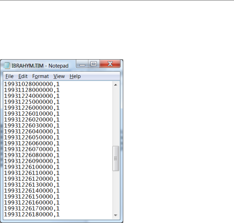

DRAFT
iMOD, User Manual
9.5 IDF-files
The file syntax of IDF-files (iMOD Data Files) is based on a file structure without any line feeds. This
means that all data is written direct after each other. It is not written on a different line, but in a different
record. An advantage of such a file structure is the possibility to access data randomly throughout the
file (known as direct-access). The fileformat is unformatted and can therefore not be read in a normal
TextEditor. It is based on the little-endian data format, as we read the file with records of 4 bytes (or 1
word). Since iMOD 5.0, the IDF file can be written in double-precision as well. In that case, the format
of the real values are double precision (float 8) instead of single precision (float 4).
Cond. Record Format (bytes) Variable Description
1 Integer 4 1271
2296
Lahey Record Length Iden-
tification; 1271 is a single
precision IDF, 2296 a double
precision.
2 Integer 4 NCOL Number of columns
3 Integer 4 NROW Number of rows
4 Float 4/8 XMIN X lower-left-coordinate
5 Float 4/8 XMAX X upper-right-coordinate
6 Float 4/8 YMIN Y lower-left-coordinate
7 Float 4/8 YMAX Y upper-right-coordinate
8 Float 4/8 DMIN Minimal data value
9 Float 4/8 DMAX Maximal data value
10 Float 4/8 NODATA NoData value
11 Integer 1 IEQ 0: equidistant IDF
1: nonequidistant IDF
Integer 1 ITB 0: no usage of TOP and
BOT Values
1: usage of TOP and BOT
Values
Integer 1 — Not used
Integer 1 — Not used
IEQ=0 12 Float 4/8 DX Column width.
13 Float 4/8 DY Row height.
ITB=1 12+ABS(IEQ-
1)*2
Float 4/8 TOP Top value if ITB=1
13+ABS(IEQ-
1)*2
Float 4/8 BOT Bot value if ITB=1
IEQ=1 12+ITB*2 Float 4/8 DX(NCOL) Column width for each col-
umn, ranging from west to
east
13+ITB*2+NCOL Float 4/8 DY(NROW) Row height for each row,
ranging from north to south
IREC=10 + ABS(IEQ-1)*2 + IEQ*(NROW+NCOL) + ITB*2 + 1
IREC Float 4/8 X(:,:) Value for each cell
IREC
+(NROW*NCOL)
Integer 1 IADIT Binary number to store op-
tional arguments:
IP1=1: Comments added
IP?=?:
IP1=1 IREC
+(NROW*NCOL)+1
Integer 1 NLINE Number of lines that contain
comments
Char. 4 COMM(NLINE) Comment for NLINE
530 of 812 Deltares

DRAFT
iMOD Files
9.6 MDF-files
iMOD map files can be grouped into a Multi Data File (MDF) which contains the references to all
grouped IDF-files. The MDF-file helps to control the number of files in the iMOD Manager.
The MDF-file is saved in ASCII-format and it has a logical structure. However it is not advised to
change this file outside iMOD.
The content of the MDF-file can be displayed by the option Info on the Map Info window
Deltares 531 of 812
DRAFT
iMOD, User Manual
9.7 IPF-files
The file syntax for IPF-files (iMOD Point File) is very straightforward and stored in ASCII-format. In
this way this type of file can be easily edited and/or created outside iMOD with any other type of
(commercial) software package. The syntax of the file is twofold and depends on whether the IPF file
need to be associated with additional files (see next subsections).
1 IPF file that is configured such that is cannot be used with additional, associated, files;
2 IPF file that is configured such that it can be used with additional, associated, files.
The first type of IPF file is very easy and simple. The syntax is equal to any regular comma-separated
file.
Variable Description
NLABELS Specify for each column the label names.
DATABLOCK For NLABELS, specify individual entries per column. Entries with
empty spaces need to be bracketed by single quotes.
An example of such an IPF file as a comma-separated file is given below:
X,Y,Z,"City of Holland"
100.0,435.0,-32.3,Amsterdam
553.0,143.0,-7.3,"Den Bosch"
For such an IPF file it is not necessary to define the number of columns or row to be read in, iMOD will
distinguish these itself. Another IPF format, for which it more desired to explicitly define the number of
attributes and entries is given below, as an advantage it allows to attach additional data to the IPF file:
Variable Description
NRECORDS Number of records
NFIELDS Number of fields
FIELDNAMEiName of the field number i, data is stored in column number iin the
DATABLOCK. Repeat this item for NFIELDS on a separate line.
INDEXCOLUMN,EXTENT Number of the index column, to be used for assess an extra file. Use
INDEXCOLUMN=0, to indicate that there are no extra files associated.
If INDEXCOLUMN >0, the EXTENT (e.g. TXT), will be added to the
names in the INDEXCOLUMN to form the actual filename to be read.
The maximum length for the EXTENT is 10 characters. It is not nec-
essary to choose the extension *.TXT for these type of files, moreover,
any extension can be chosen as long as the right EXTENT is given in
the IPF-file that should call these additional files.
DATABLOCK For NRECORDS each record (line) will contain data for each field. It
is not sustained to leave data out, whenever no data is known for that
particular field. For each data entry the maximum is 50 characters!
Example of an IPF-file without a reference to an additional file associated to it (INDEXCOLUMN=0,EXTENT=TXT):
2
4
X
Y
Z
"City of Holland"
0,TXT
100.0,435.0,-32.3,Amsterdam
553.0,143.0,-7.3,"Den Bosch"
The different data for each field should be delimited by a single (or more) space(s), or a comma. Do
532 of 812 Deltares
DRAFT
iMOD Files
not use tabs as delimiters! Entries that contain spaces should be encapsulated by quotes, e.g. City of
Holland should be entered as ‘City of Holland’.
Associated Files
Associated files can contain different types of data that are processed differently by iMOD. The syntax
of each of those type of files is similar each time and described as follows:
Variable Description
NRECORDS Number of records
NFIELDS,ITYPE Number of fields and the type of this file.
1 Timevariant information such as timeseries of measurements, extraction
rates and so on (ITYPE=1);
2 1D Borehole information that are oriented downwards perpendicularly by
a z value (ITYPE=2);
3 Cone Penetration Test Information that are oriented downwards perpen-
dicularly (ITYPE=3);
4 3D Borehole information that is truly 3D as each interval is expressed by
x,y and z coordinates (ITYPE=4).
FIELDNAMEi,
NODATAi
Name of the field number i, data is stored in column number iin the DAT-
ABLOCK. Missing data per field is determined by their corresponding No-
DataValue. Repeat this item for NFIELDS.
DATABLOCK For NRECORDS each record (line) will contain data for each field. It is not
sustained to leave data out, whenever no data is known for that particular field
use the corresponding Field NoDataValue.
In the next subsections each of those type of files will explained in more detail.
9.7.1 Associated Files with Timevariant Information
Timevariant information of timeseries can be stored in *.TXT files and their location and other spatial
attributes (e.g. depth of the screen, surfacelevel) or non-dimensional information (e.g. id, name) can
be stored in the IPF-file. The syntax of the *.TXT file is as follows:
4
3,1
DATE,-9999.0
MEASUREMENT,-9999.0
PREDICTION,-9999.0
19940114 5.70 5.70
19940128 5.73 5.71
19940214 4.95 5.10
19940228 5.01 5.15
Note: It is compulsory to use the first column to enter the date, expressed by a [yyyymmdd] notation
or alternatively [yyyymmddhhmmss].
9.7.2 Associated File with 1D Borehole Information
Boreholes can be stored in *.TXT files and their location and other spatial attributes (e.g. surfacelevel)
or non-dimensional information (e.g. id, name) can be stored in the IPF-file. The syntax of these *.TXT
files is equal to the syntax of the TimeVariant information, however, ITYPE=2.
It is compulsory to use the first column to enter the vertical coordinate, expressed by meter+MSL
(mean-sea-level). Use comma’s and/or space(s) as delimiters. Moreover, any other column can be
used for colouring the interval i and i+1. In the example below, the Lithology=S will be used to colour
Deltares 533 of 812

DRAFT
iMOD, User Manual
the interval between 3.90 and -3.10 m+MSL. The colours that will be used are defined in iMOD or can
be read by iMOD from a *.DLF-file.
6
4,2
"Z-COORDINATE,M+MSL",-9999.99
"LITHOLOGY",-9999.99
"SANDCLASS NEN5104",-9999.99
"DISTORTION",-9999.99
3.90,S,NONE,NONE
-3.10,S,NONE,SPARSE
-11.10,S,ZFC,NONE
-23.10,C,NONE,NONE
-26.10,S,ZFC,NONE
-38.10,-,-,-
9.7.3 Associated File with Cone Penetration Test Information
Cone Penetration Test(or borelog) information can be stored in *.TXT files and their location and other
spatial attributes (e.g. surfacelevel) or non-dimensional information (e.g. id, name) can be stored in
the IPF-file. The syntax of these *.TXT files is equal to the syntax of the TimeVariant information,
however, ITYPE=3. It is compulsory to use the first column to enter the vertical coordinate, expressed
by meter+MSL (mean-sea-level). Use comma’s and/or space(s) as delimiters.
6
8,3
"M,LENGTH",-9999.99
"MPA,CONUSRESISTANCE",-9999.99
"MPA,RESISTANCE",-9999.99
0.32,0.721,-9999.99
0.30,0.760,-9999.99
0.28,0.783,0.048
0.26,0.828,0.061
0.24,0.865,0.066
0.22,0.893,0.073
0.20,0.838,0.073
0.16,0.930,0.070
In the example above, the fields that contain values equal to the Field NoDataValue will not be drawn
and are excluded in the graph.
9.7.4 Associated File with 3D Borehole Information
3D Boreholes information (dx,dy,z) can be stored in *.TXT files and their origin location and other
spatial attributes (e.g. surfacelevel) or non-dimensional information (e.g. id, name) can be stored in
the IPF-file. It is compulsory to use the first three columns to enter the offset in x and y direction
and the vertical coordinate, expressed by meter+MSL. Use comma’s and/or space(s) as delimiters.
Moreover, any other column can be used for colouring the interval i and i+1. In the example below, the
Lithology=S will be used to colour the interval between (x,y,z) 5.0,5.0,-1.0 and (x,y,z) 7.5,5.0,-2.5. The
colours that will be used are defined in iMOD or can be read by iMOD from a *.DLF-file.
9
4,4
"OFFSET X",-9999.99
"OFFSET Y",-9999.99
"Z-COORDINATE,M+MSL",-9999.99
"PERF_TREATMENT_TYPE",-9999.99
0.0,0.0,0.0,CEMENT
534 of 812 Deltares

DRAFT
iMOD Files
5.0,5.0,-1.0,CEMENT_PLUG
7.5,5.0,-2.5,PERFORATION
12.1,6.0,-4.5,PERFORATION
3.1,2.0,-12.3,"ACID TREATMENT"
-2.1,-3.1,-32.3,"MULTI-STAGE FRACTURE"
-21.1,-43.1,-12.3,"PACKING DEVICE"
-2.1,-5.6,-4.3,"PACKING DEVICE"
-5.1,3.6,-7.3,-
Note: It is possible with this type of boreholes to change azimuth and angle throughout the borehole,
in this manner the borehole can move in any direction through the subsoil and even move up- and
downwards.
Deltares 535 of 812

DRAFT
iMOD, User Manual
9.8 IFF-files
The File syntax for IFF-files (iMOD Flowpath File) is very simple and stored in ASCII-format. In this way
these type of files can be easily edited and/or created outside iMOD with other (commercial) software.
The formal syntax is as follows and prescribed:
NFIELDS Number of fields; NFIELDS=9.
PARTICLENUMBER Number of the particle in the particle tracking.
ILAY Modellayer number of the current position of the particle.
XCRD. X-coordinate of the current position of the particle.
YCRD. Y-coordinate of the current position of the particle.
ZCRD. Z-coordinate of the current position of the particle.
TIME(YEARS) Age at the current position of the particle.
VELOCITY(M/D) Velocity at the current position of the particle.
IROW Row number at the current position of the particle.
ICOL Column number at the current position of the particle.
DATABLOCK Each record (line) will contain data for each field.
iMOD will draw the flowpath using the XCRD, YCRD and ZCRD (the latter is used within the Cross-
Section Tool and the 3DTool). Whenever the PARTICLENUMBER changes, iMOD will start drawing
another line until the end of the IFF-file is reached.
9
PARTICLE_NUMBER
ILAY
XCRD.
YCRD.
ZCRD.
TIME(YEARS)
VELOCITY(M/DAY)
IROW
ICOL
1 1 0.5000000E-01 0.5000000E-01 -0.9999871E-05 0.0000000E+00 0.0000000E+00
1 1
1 1 0.5000000E-01 0.5000000E-01 -0.1000000E-01 0.5673637E-01 0.3333346E-05
1 1
1 2 0.5000000E-01 0.5000000E-01 -0.2000000E-01 0.6494979E-01 0.3333346E-05
1 1
1 2 0.1024045E-01 0.5000000E-01 -0.5000000E-01 0.7477629E-01 0.2234009E-01
1 1
1 3 0.1024045E-01 0.5000000E-01 -0.6000000E-01 0.7639593E-01 0.2234009E-01
1 1
1 3 0.3189280E-02 0.5000000E-01 -0.1000000E+00 0.8600117E-01 0.1724361E-01
1 1
1 4 0.3189280E-02 0.5000000E-01 -0.1100000E+00 0.8977942E-01 0.1724361E-01
1 1
1 4 0.5000000E+00 0.5000000E+00 -0.1300000E+00 0.8977942E-01 0.0000000E+00
1 1
2 1 0.1050000E+01 0.5000000E-01 -0.9999871E-05 0.0000000E+00 0.0000000E+00
1 2
2 1 0.1050000E+01 0.5000000E-01 -0.1000000E-01 0.5673701E-01 0.3333308E-05
1 2
2 2 0.1050000E+01 0.5000000E-01 -0.2000000E-01 0.6495053E-01 0.3333308E-05
1 2
2 2 0.1000000E+01 0.5000000E-01 -0.2037707E-01 0.6526318E-01 0.4339061E+00
1 1
2 2 0.2150384E+00 0.5000000E-01 -0.5000000E-01 0.7478765E-01 0.4418139E+00
1 1
2 3 0.2150384E+00 0.5000000E-01 -0.6000000E-01 0.7640729E-01 0.4418139E+00
1 1
536 of 812 Deltares

DRAFT
iMOD Files
2 3 0.6697147E-01 0.5000000E-01 -0.1000000E+00 0.8601253E-01 0.7347348E-01
1 1
2 4 0.6697147E-01 0.5000000E-01 -0.1100000E+00 0.8979079E-01 0.7347348E-01
1 1
2 4 0.5000000E+00 0.5000000E+00 -0.1300000E+00 0.8979079E-01 0.0000000E+00
1 1
3 1 0.2050000E+01 0.5000000E-01 -0.9999871E-05 0.0000000E+00 0.0000000E+00
1 3
3 1 0.2050000E+01 0.5000000E-01 -0.1000000E-01 0.5673680E-01 0.3333321E-05
1 3
3 2 0.2050000E+01 0.5000000E-01 -0.2000000E-01 0.6495028E-01 0.3333321E-05
1 3
3 2 0.2000000E+01 0.5000000E-01 -0.2058719E-01 0.6543636E-01 0.2796153E+00
1 2
3 2 0.1000000E+01 0.5000000E-01 -0.2783243E-01 0.7310726E-01 0.2836847E+00
1 1
3 2 0.4154203E+00 0.5000000E-01 -0.5000000E-01 0.7855114E-01 0.4418535E+00
1 1
3 3 0.4154203E+00 0.5000000E-01 -0.6000000E-01 0.8017078E-01 0.4418535E+00
1 1
3 3 0.1293783E+00 0.5000000E-01 -0.1000000E+00 0.8977602E-01 0.1391620E+00
1 1
3 4 0.1293783E+00 0.5000000E-01 -0.1100000E+00 0.9355428E-01 0.1391620E+00
1 1
3 4 0.5000000E+00 0.5000000E+00 -0.1300000E+00 0.9355428E-01 0.0000000E+00
1 1
Deltares 537 of 812

DRAFT
iMOD, User Manual
9.9 ISG-files
The ISG-file format is developed to capture all relevant information used by surface water elements
in direct relation with groundwater. It stores stages, bottom heights, infiltration factors, resistances,
and moreover, the actual outline of the surface water element. To store all these different types of
information the ISG-file format consists of associated files that are connected by the ISG-file. This ISG-
file is the one that will be actually read by iMOD, the other files will be opened by iMOD automatically.
The syntax of the ISG-file format, and its associated files is as follows:
Attribute Description
First line add the following columns
NSEG Number of segments.
ASFR Usage of surface-flow routing (SFR) ability from the associated file *.ISD*. If
ASFR=0, a default ISG file is used, if ASFR=1, a SFR compliant version of the
ISG is used.
LABEL Enter the name of the labels that are present in the ISD file, whenever ASFR=0
the following labels are present:
Date
The date of the entry;
Water level
The Waterlevel at the calculation node
Bottom level
The Bottom level at the calculation node;
Resistance
The Resistance at the calculation node;
Inf.factor
The Infiltration factor at the calculation node.
whenever ASFR=1 the following labels are present:
Date
The date of the entry;
For each segment add the following columns
LABEL Name of the segment, use quotes to distinguish names with empty spaces. Max-
imum size of each label is 52 characters.
ISEG Record number that defines the first coordinate (node) in the associated ISP-file.
NSEG Number of records in the ISP-file that describes the segment by coordinates.
ICLC Record number that defines the first calculation points on the segment ISEG
within the associated ISD1-file.
NCLC Number of calculation points on segment ISEG.
ICRS Record number that defines the first cross-section on the segment ISEG within
the associated ISC1-file.
NCRS Number of cross-sections on segment ISEG.
ISTW Record number that defines the first weir/structure on the segment ISEG within
the associated IST1-file.
NSTW Number of weirs/structures on segment ISEG.
IQHR Number of discharge-water level relationships.
NQHR Record number that defines the first discharge-water level relationships on the
segment ISEG within the associated ISQ1-file.
538 of 812 Deltares
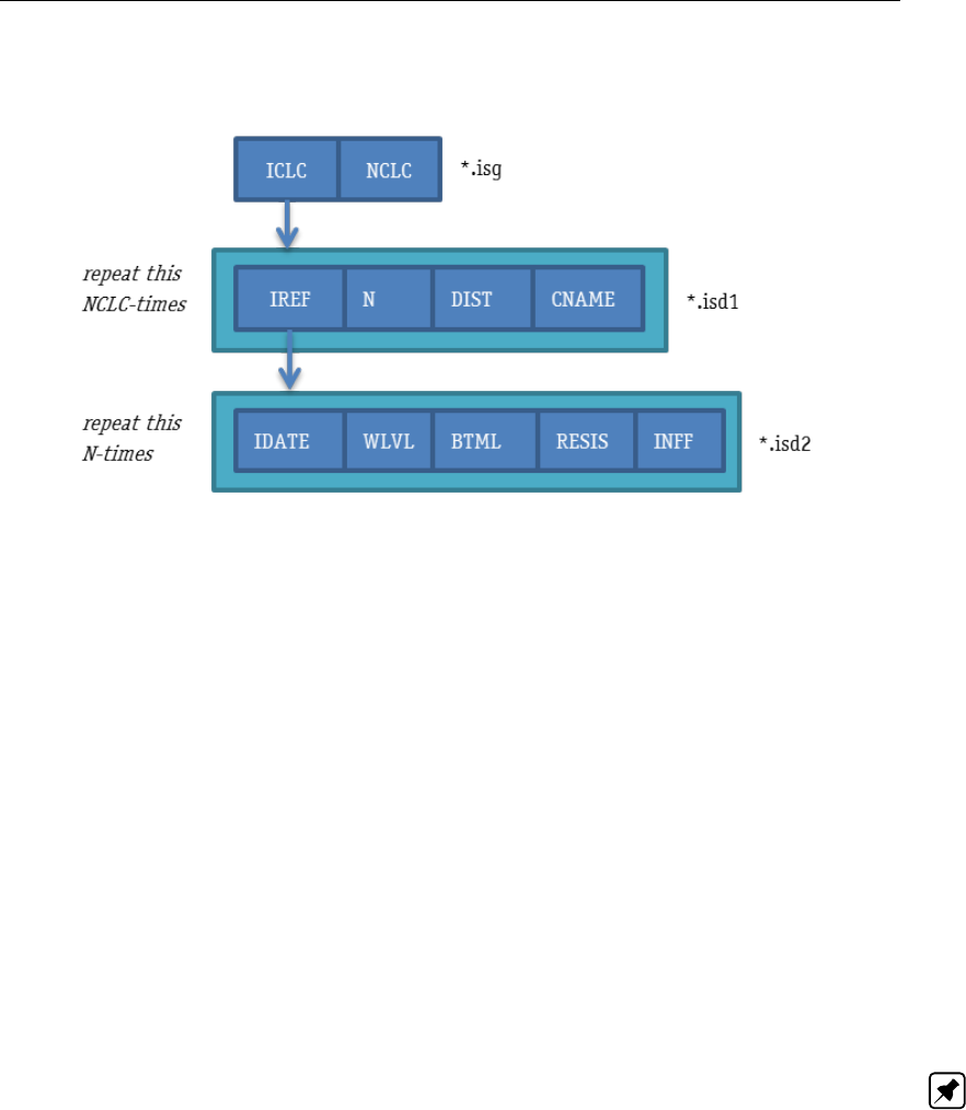
DRAFT
iMOD Files
The structure of the ISG-file can be illustrated by the following figure:
Example of an ISG-file:
16,0,"Date","Water level","Bottom level","Resistance","Inf.factor"
"NOM_1",1,120,1,15,1,8,1,2,1,16
"NOM_2",121,18,16,7,9,3,3,2,17,8
"NOM_3",139,7,23,13,12,3,5,9,25,21
"NOM_4",146,6,36,4,15,1,14,2,46,5
"NOM_5",152,44,40,15,16,4,16,2,51,16
"NOM_6",196,16,55,8,20,3,18,2,67,9
"NOM_7",212,27,63,9,23,3,20,0,76,9
"NOM_8",239,31,72,12,26,4,20,4,85,16
"NOM_9",270,88,84,13,30,4,24,1,101,13
"NOM_10",358,10,97,6,34,1,25,1,114,6
"NOM_11",368,71,103,15,35,5,26,4,120,18
"NOM_12",439,11,118,32,40,10,30,0,138,31
"NOM_13",450,12,150,4,50,2,30,2,169,5
"NOM_14",462,30,154,6,52,2,32,1,174,6
"NOM_15",492,4,160,2,54,1,33,0,180,1
"NOM_16",496,15,162,5,55,2,33,1,181,5
Note: Warning: To maintain consistency do not edit a ISG-file outside iMOD.
For nodes, calculations points, cross-section, structures a similar setup is used. A first reference is
made from the *.ISG file to the record in the *.ISD1 file. From there another reference is made to the
*ISD2 file that contains the specific configuration parameters.
The files associated from the ISG-file (ISP-, ISD-, ISC-, IST- and ISQ-files) are all binary and indexed
files and cannot be edited in regular text editors. In the following sections these file-types will be
described in detail.
9.9.1 ISP fileformat
The ISP-file is built with a record length of 8 bytes/2 words. The first record of the ISP is reserved
to store the record length (2295). The ISEG variable in the ISG points to the record number that
determines the first coordinate of the segment. Since the first record is reserved already, iMOD actually
reads the ISEG+1 record instead. From each record two reals will be read that represent the x and y
coordinate of the current node on the segment, see table below:
Attributes for each record in an ISP-file:
Deltares 539 of 812
DRAFT
iMOD, User Manual
Attribute Width (bytes) Description
X4 (real) X-coordinate of node (meter)
Y4 (real) Y-coordinate of node (meter)
9.9.2 ISD1 and ISD2 fileformat
The ISD1-file is built with a record length of 44 bytes/11 words. The first record is solely reserved to
store the record length (11511). The ICLC variable in the ISG-file points to the record number that
determines the first calculation point on the segment. Since the first record is reserved already, iMOD
actually reads the ICLC+1 record instead. Each record contains the following attributes:
Attributes for each record in an ISD1-file:
Attribute Width (bytes) Description
N4 (int) Number of data records in the ISD2-file that describes
the timeserie of the calculation point.
IREF 4 (int) Record number within the ISD2-file for the first data
record that describes the timeserie for the calculation
point.
DIST 4 (real) Distance (meters) measured from the beginning of the
segment (node 1) that located the calculation point.
CNAME 32 (char) Name of the calculation point.
Note: For the SFR-option, only two calculation points are allowed, one at the beginning of a segment
and one at the end.
It depends on the ASFR whether this file contains information for the RIV package (ASFR=0) or alter-
natively for the SFR package (ASFR=1). The ISD2-file is built with a record length of 20 bytes/5 words
for ASFR=0. For ASFR=1, the record length is 44 bytes/13 words of 4 bytes each. The first record is
solely reserved to store the record length (ASFR=0: 5367 and ASFR=1: 12535). The IREF variable
in the ISD1-file points to the record number that determines the data for the calculation point on the
segment. Since the first record is reserved already, iMOD actually reads the IREF+1 record instead.
Each record contains the following attributes:
Attributes for each record in an ISD2-file (ASFR=0):
Attribute Width
(bytes)
Description
IDATE 4 (int) Date representation as yyyymmdd.
WLVL 4 (int) Waterlevel of the river (m+MSL)
BTML 4 (real) Bottom level of the riverbed (m+MSL).
RESIS 4 (real) Resistance of the riverbed (days).
INFF 4 (real) Infiltration factor (-)
Attributes for each record in an ISD2-file (ASFR=1):
Attribute Width
(bytes)
Description
IDATE 4 (int) Date representation as yyyymmdd.
CTIME 8 (char) Time representation as hh:mm:ss.
BOTTOM-
LEVEL
4 (real) Bottom level of the riverbed (m+MSL).
THICK-
NESS
4 (real) Thickness of the river bed (m).
HCFACT 4 (real) Conductivity of the river bed (md−1).
540 of 812 Deltares

DRAFT
iMOD Files
IDOWN-
SEG
4 (int) An integer value of the downstream stream segment (-) that receives
tributary inflow from the last downstream reach of this segment.
IDOWNSEG >0If this segment feeds (or discharges into) an-
other downstream (tributary) segment, then enter the number of
that stream;
IDOWNSEG = 0 If this segment does not feed (or discharge into)
another downstream (tributary) segment, then enter a value of 0
for this variable. If the segment ends within the modeled grid and
IDOWNSEG = 0, outflow from the segment is not routed anywhere
and is no longer part of the stream network. One may wish to use
this if all flow in the stream gets diverted into a lined canal or into a
pipe;
IDOWNSEG <0If the flow out of this segment discharges into a
lake, IDOWNSEG will be equal to the negative value of the lake
identification number; where the minus sign is used as a flag to
tell the model that flow enters a lake rather than a tributary stream
segment.
IUPSEG 4 (int) An integer value of the upstream segment (-) from which water is
diverted (or withdrawn) to supply inflow to this stream segment if this
segment originates as a diversion from an upstream segment.
IUPSEG >0If this stream segment receives inflow as a diversion
from an upstream segment, enter the stream number;
IUPSEG <0If the source of a stream segment is discharge from
a lake, set IUPSEG equal to the negative value of the lake iden-
tification number; where the minus sign is used as a flag to tell
the model that streamflow into this segment is derived from a lake
rather than a stream segment;
IUPSEG = 0 If this stream segment does not receive inflow as a
diversion from an upstream segment, then set IUPSEG = 0.
CALCOPT 4 (int) Method determines how stream depth and width are calculated for
each reach in a segment (-).
CALCOPT=1 Stream depth in each reach is specified at the begin-
ning of a stress period and remains unchanged unless flow at the
midpoint of a reach is zero, then depth is set to zero in that reach;
CALCOPT=2 Stream depth is calculated and updated each itera-
tion of the solver within a time step and is calculated from Man-
ning’s equation assuming a wide rectangular channel;
CALCOPT=3 Stream depth and width is calculated and updated
each iteration of the solver within a time step and are calculated
from Manning’s equation using an eight-point cross section;
CALCOPT=4 Stream depth and width is calculated and updated
each iteration of the solver within a time step and are calculated
from a power function;
CALCOPT=5 Stream depth and width is calculated and updated
each iteration of the solver within a time step and are calculated
from a table of values as entered in the Q-DEPTH/WIDTH relation
ships.
Deltares 541 of 812
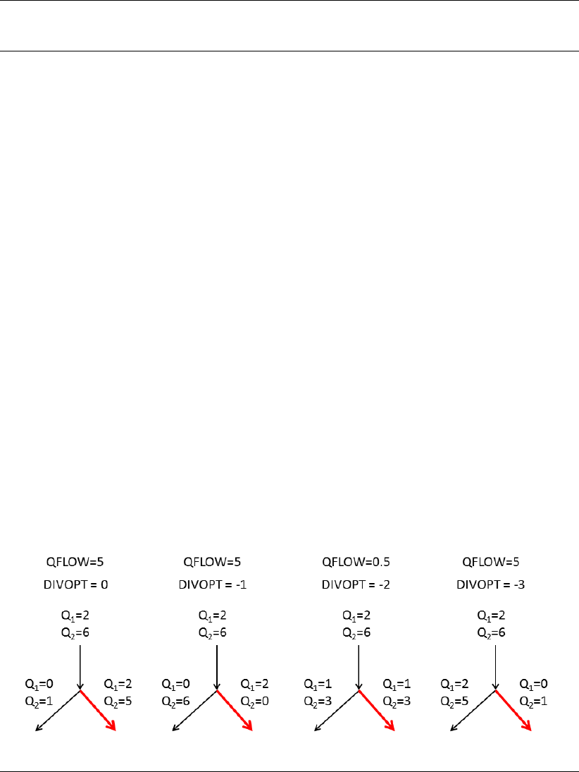
DRAFT
iMOD, User Manual
DIVOPT 4 (int) An integer value that only is specified if IUPSEG > 0 (do not specify a
value in this field if IUPSEG = 0 or IUPSEG <0). DIVOPT defines the
prioritization system for diversion, such as when insufficient water is
available to meet all diversion stipulations, and is used in conjunction
with the value of QFLOW (specified below) (-).
DIVOPT=1 then if the specified diversion flow (QFLOW) is greater
than the flow available in the stream segment from which the di-
version is made, the diversion is reduced to the amount available,
which will leave no flow available for tributary flow into a down-
stream tributary of segment IUPSEG;
DIVOPT=2 then if the specified diversion flow (QFLOW) is greater
than the flow available in the stream segment from which the diver-
sion is made, no water is diverted from the stream. This approach
assumes that once flow in the stream is sufficiently low, diversions
from the stream cease, and is the ”priority“ algorithm that originally
was programmed into the STR1 Package (Prudic, 1989);
DIVOPT=3 then the amount of the diversion is computed as a frac-
tion of the available flow in segment IUPSEG; in this case, 0.0<
QFLOW <1.0;
DIVOPT=4 then a diversion is made only if the streamflow leav-
ing segment IUPSEG exceeds the value of QFLOW. If this occurs,
then the quantity of water diverted is the excess flow and the quan-
tity that flows from the last reach of segment IUPSEG into its down-
stream tributary (IDOWNSEG) is equal to QFLOW. This represents
a flood-control type of diversion, as described by Danskin and Han-
son (2002).
Illustration of the diversion rates per DIVOPT category that is assigned to the red segment in the
figure.
542 of 812 Deltares

DRAFT
iMOD Files
QFLOW 4 (real) Streamflow entering or leaving the upstream end of a stream segment
(i.e. the first reach) (m3s−1). iMOD will check whether you have
entered a value larger than 100000.0, as this might indicate that the
entered volume is m3d−1instead of m3s−1. Be aware of the fact that
the meaning of QFLOW depends on the fact whether the stream is a
If the stream is a headwater stream (IUPSEG = 0) which is the
first stream of a segment without any segment upstreams, QFLOW
defines the total inflow to the first reach of the segment. The value
can be any number ≥0.0;
If the stream is a tributary stream (IUPSEG = 0) with an upstream
dewatering stream, QFLOW defines additional specified inflow to
or withdrawal from the first reach of the segment (that is, in addi-
tion to the discharge from the upstream segment of which this is a
tributary). This additional flow does not interact with the groundwa-
ter system. For example, a positive number might be used to rep-
resent direct outflow into a stream from a sewage treatment plant,
whereas a negative number might be used to represent pumpage
directly from a stream into an intake pipe for a municipal water
treatment plant;
If the stream is a diversionary stream (IUPSEG 6=0), and the diver-
sion is from another stream segment, QFLOW defines the stream-
flow diverted from the last reach of stream segment IUPSEG into
the first reach of this segment. The diversion is computed or ad-
justed according to the value of DIVOPT;
If the stream is a diversionary stream (IUPSEG 6=0), and the di-
version is from a lake, QFLOW defines a fixed rate of discharge
diverted from the lake into the first reach of this stream segment
(unless the lake goes dry) and flow from the lake is not dependent
on the value of ICALC. However, if QFLOW = 0, then the lake out-
flow into the first reach of this segment will be calculated on the
basis of lake stage relative to the top of the streambed for the first
reach using one of the methods defined by ICALC.
QRUNOFF 4 (real) volumetric rate (m3s−1) of the diffuse overland flow runoff that enters
the stream segment, the rate is apportioned to each reach of the seg-
ment.
PPTSW 4 (real) precipitation (mmd−1) that is the volumetric rate per unit area of water
added by precipitation directly on the stream channel (in units of length
(millimeter) per time (day)).
ETSW 4 (real) evaporation (mmd−1) that is the volumetric rate per unit area of wa-
ter removed by evapotranspiration directly from the stream channel (in
units of length (millimeter) per time (day)). ETSW is always defined as
a positive value.
9.9.3 ISC1 and ISC2 fileformat
The ISC1-file is built with a record length of 44 bytes/11 words. The first record is solely reserved to
store the record length (11511). The ICRS variable in the ISG-file points to the record number that
determines the first calculation point on the segment. Since the first record is reserved already, iMOD
actually reads the ICRS+1 record instead. Each record contains the following attributes:
Attributes for each record in an ISC1-file:
Attribute Width (bytes) Description
N4 (int) The meaning of this attribute is twofold:
>0 Number of data records in the ISC2-file that describes the
actual cross-section.
Deltares 543 of 812
DRAFT
iMOD, User Manual
<0 The absolute number of data records in the ISC2-file that
describes the riverbed as a collection of x,y,z points includ-
ing an extra record to describe the dimensions (DX,DY ) of
the network that captured the x,y,z points.
IREF 4 (int) Record number within the ISC2-file for the first data record
that describes the cross-section.
DIST 4 (real) Distance (meters) measured from the beginning of the seg-
ment (node 1) that locates the cross-section.
CNAME 32 (char) Name of the cross-section.
The ISC2-file is built with a record length of 12 bytes/3 words. The first record is solely reserved
to store the record length (3319). The IREF variable in the ISC1-file points to the record number
that determines the data for the calculation point on the segment. Since the first record is reserved
already, iMOD actually reads the IREF+1 record instead. Each record contains the following attributes
whenever N>0:
Attributes for each record in an ISC2-file:
Attribute Width (bytes) Description
DISTANCE 4 (real) Distance of the cross-section measured from the centre of
the riverbed (minus to the left en positive to the right).
BOTTOM 4 (real) Bottom level of the riverbed (meter), whereby zero will be
assigned to the lowest riverbed level.
MRC 4 (real) Manning’s roughness coefficient (-).
Alternatively, the record can have a different meaning whenever N<0:
Attribute Width (bytes) Description
First record at IREF+1
DX 4 (real) Absolute width kDX kin meters of the rectangular raster that
follows.
DY 4 (real) Absolute height kDY kin meters of the rectangular raster
that follows.
HREF 4 bytes Reference Height in meters. Whenever specified (DX < 0.0
and DY < 0.0), the attribute Z (specified below) is organized
differently.
Following records starting at IREF+2
X4 (real) X coordinate (meter) for a riverbed “pixel”, these coordinates
need to be on a rectangular network with spatial distance of
kDX kmeasured at the centre of the “pixel”.
Y4 (real) Y coordinate (meter) for a riverbed “pixel” , these coordi-
nates need to be on a rectangular network with spatial dis-
tance of kDY kmeasured at the centre of the “pixel”.
Following record is valid whenever DX > 0.0 and DY > 0.0
Z4 (real) Bottom level of the riverbed (meter).
Following record is valid whenever DX < 0.0 and DY < 0.0
Zm2 (integer) Integer value of bottom level of the riverbed (integer of me-
ters), e.g. bottom level is -23.43, Zm=-23.
Zc1 (integer) Integer value of remaining digits of bottom level of the
riverbed (remaining centimeter), e.g. bottom level is -23.43,
Zc=43 centimeters.
544 of 812 Deltares
DRAFT
iMOD Files
Zp1 (integer) Integer value of area affected by HREF, e.g. areas with Zp<
0will be inundated only whenever the current river stage
is higher than the Reference Height (HREF) and the river
stage is higher than the corresponding riverbed. Areas with
Zp>0, will be inundated whenever the river stage is higher
than the current riverbed. The absolute value of Zpis used
as a multiplication factor for the river bed resistances for the
attribute RESIS in the ISD2-file (see 9.9.2).
9.9.4 IST1 and IST2 fileformat
The IST1-file is built with a record length of 44 bytes/11 words. The first record is solely reserved to
store the record length (11511). The ISTW variable in the ISG-file points to the record number that
determines the first calculation point on the segment. Since the first record is reserved already, iMOD
actually reads the ISTW+1 record instead. Each record contains the following attributes:
Attributes for each record in an IST1-file:
Attribute Width (bytes) Description
N4 (int) Number of data records in the IST2-file that describes the
actual timeserie for the weir/structure.
IREF 4 (int) Record number within the IST2-file for the first data record
that describes the weirs/structure.
DIST 4 (real) Distance (meters) measured from the beginning of the seg-
ment (node 1) that locates the weir/structure.
CNAME 32 (char) Name of the weir/structure.
The IST2-file is built with a record length of 12 bytes/3 words. The first record is solely reserved to
store the record length (3319). The IREF variable in the IST1-file points to the record number that
determines the data for the calculation point on the segment. Since the first record is reserved already,
iMOD actually reads the IREF+1 record instead. Each record contains the following attributes:
Attributes for each record in an IST2-file:
Attribute Width (bytes) Description
IDATE 4 (int) Date representation as yyyymmdd.
WLVL_UP 4 (real) Water level for the upstream side of the weir/structure
(m+MSL).
WLVL_DWN 4 (real) Water level for the downstream side of the weir/structure
(m+MSL).
9.9.5 ISQ1 and ISQ2 fileformat
The ISQ1-file is built with a record length of 44 bytes/11 words. The first record is solely reserved to
store the record length (11511). The IQHR variable in the ISG-file points to the record number that
determines the first calculation point on the segment. Since the first record is reserved already, iMOD
actually reads the IQHR+1 record instead. Each record contains the following attributes:
Attributes for each record in an ISQ1-file:
Attribute Width (bytes) Description
N4 (int) Number of data records in the ISQ2-file that describes the
actual timeserie for the q-width/depth relation ship.
IREF 4 (int) Record number within the ISQ2-file for the first data record
that describes the q-width/depth relation ship.
DIST 4 (real) Distance (meters) measured from the beginning of the seg-
ment (node 1) that locates the q-width/depth relation ship.
Deltares 545 of 812
DRAFT
iMOD, User Manual
CNAME 32 (char) Name of the q-width/depth relation ship.
The ISQ2-file is built with a record length of 12 bytes/3 words. The first record is solely reserved to
store the record length (3319). The IREF variable in the ISQ1-file points to the record number that
determines the data for the calculation point on the segment. Since the first record is reserved already,
iMOD actually reads the IREF+1 record instead. Each record contains the following attributes:
Attributes for each record in an ISQ2-file:
Attribute Width (bytes) Description
Q4 (int) Discharge in m3d−1.
WIDTH 4 (real) Width of the stream at the given discharge Q (m).
DEPTH 4 (real) Depth of the stream at the given discharge Q (m).
FACTOR 4 (real) obsolete factor at the given discharge Q (-).
546 of 812 Deltares

DRAFT
iMOD Files
9.10 GEN-files
In iMOD two types of GEN files are distinguished a) the standard GEN file format as developed by
ESRI, maker of ArcINFO, ARCGIS, ArcView and b) the GEN file developed for iMOD to generate
images from large GEN-files most efficiently.
9.10.1 Standard GEN-files
Creating a GEN-file can be done in ArcView3.x by means of the sample script shp2gen.ave
(installdirectory \ESRI\AV_GIS30\ARCVIEW\Samples\scripts\shp2gen.ave). Within ArcGIS this can
be performed only by a conversion of the ArcGIS shapefile to a ArcINFO coverage and finally using
the command UNGENERATE to create a GEN-file. The syntax of a GEN-file should be as follows:
Points
ID1, X1, Y1
ID2, X2, Y2
..
IDn, Xn, Yn
END
Lines
ID1
X1,Y1
X2,Y2
X3,Y3
...
Xn,Yn
END
ID2
X1,Y1
X2,Y2
X3,Y3
...
Xn,Yn
END
END
Polygons
ID1
X1,Y1
X2,Y2
X3,Y3
...
X1,Y1
END
ID2
X1,Y1
X2,Y2
X3,Y3
...
X1,Y1
END
END
Deltares 547 of 812
DRAFT
iMOD, User Manual
or 3-D representatives as
3-D Polygons
ID1
X1,Y1,Z1
X2,Y2,Z2
X3,Y3,Z3
...
X1,Y1,Z1
END
ID2
X1,Y1,Z1
X2,Y2,Z2
X3,Y3,Z3
...
X1,Y1,Z1
END
END
Note: iMOD will display 3-D Polygons as filled surfaces in the 3-D tool.
3-D Lines
ID1
X1,Y1,Z1
X2,Y2,Z2
X3,Y3,Z3
...
Xn,Yn,Zn
END
ID2
X1,Y1,Z1
X2,Y2,Z2
X3,Y3,Z3
...
Xn,Yn,Zn
END
END
Note: The ID field is read by iMOD as a character-type, thus ID can be an integer, real or character,
e.g. ID=1, or ID=3.22 or ID=Area1. Make sure that quotes are use for ID field with spaces or commas;
such as ID=“Area 1”.
9.10.2 iMOD GEN-files
The GEN file format for iMOD is optimized for usage in iMOD and to represent large GEN-files ef-
ficiently. The file format is a binary format and consists out of coordinates as well as attributes for
existing labels.
XMIN(real*8),YMIN(real*8),XMAX(real*8),YMAX(real*8)
MAXPOL(integer*4),MAXCOL(integer*4)
add following in case MAXCOL > 0
COLWIDTH(integer*4)[dimension MAXCOL]
LABELS(character*11)[dimension MAXCOL]
repeat following for MAXPOL
NPOINTS(integer*4)
548 of 812 Deltares

DRAFT
iMOD Files
add following in case MAXCOL > 0
LABELS(character*COLWIDTH[dimension MAXCOL])[dimension MAXCOL]
add these representing the point,polygon,lines
XMIN(real*8),YMIN(real*8),XMAX(real*8),YMAX(real*8)
X(real*8),Y(real*8))[dimension NPOINTS]
The above mentioned format is slightly different whenever labels are absent, some of the entries can
be skipped for those cases. The size of the labels for the attributes is limited to 11 characters, this
is similar are present in the DBF-files from ESRI-ArcGIS. Whenever NPOINTS=1, iMOD will display a
points, whenever the first and last coordinates are similar a polygon will be plotted, in others cases a
line.
Deltares 549 of 812
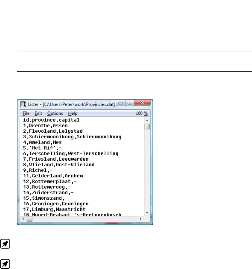
DRAFT
iMOD, User Manual
9.11 DAT-files
DAT-files can be used to associate information to GEN-files (see section section 9.10.1). The DAT-file
should have the same name as the GEN-file. The IDinumber(s) for the polygons is used to relate to
the proper ID in the DAT-file. The syntax of a DAT-file is simple.
Header Header label for each column. The first column is reserved for the ID number to
relate to the ID number of the associated GEN-file.
Values Enter a value for each column for each unique ID value in the associated GEN-file.
Example of a DAT-file:
Note: It is possible, however, to relate more polygons with identical ID numbers, to the same ID in the
DAT-file.
Note: The different data for each field should be delimited by a single (or more) space(s), or a comma.
Do not use tabs as delimiters! Entries that contain spaces should be encapsulated by quotes, e.g. Het
Rif should be entered as ‘Het Rif’.
550 of 812 Deltares
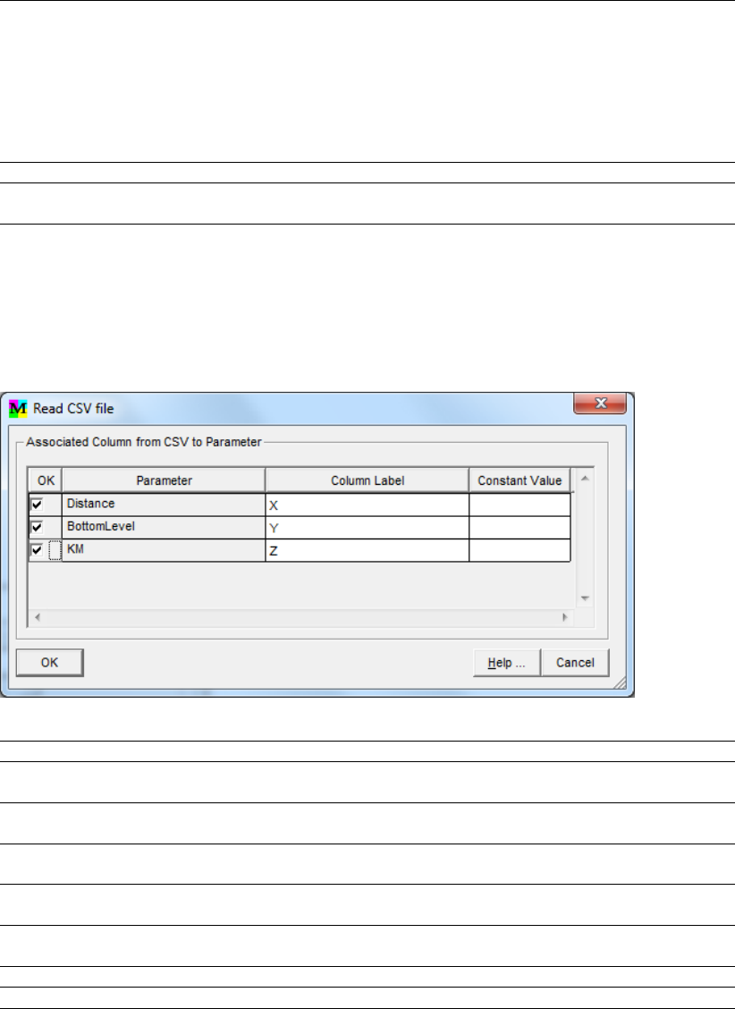
DRAFT
iMOD Files
9.12 CSV-files
Throughout the iMOD application it is possible to import or export data for and into a CSV-file format
(comma-separated-values file). The syntax for those files is simple and straightforward and equal to a
DAT-file format (see section 9.11).
Header Header label for each column.
Values Enter a value for each column, use quote for entry fields that contain spaces,
comma’s, e.g. Klompen Plein should be noted as “Klompen Plein”.
Whenever a CSV is imported in iMOD the Read CSV-file window is shown. For each parameter that
needs to be assigned (depending on the calling interface, see section 6.10.3.9), this window links the
parameter read from the CSV-file to the column in the CSV-file.
Read CSV-file:
Field in the Table:
OK Click this checkbox to use the associated column for the corresponding column, e.g.
the Distance parameter will be read from the column with the label X.
Parameter The rows for this column will be filled in automatically based on the parameters
needed from the calling interface.
Column La-
bel
Select the appropriate column in the CSV-file to be assigned to the parameter listed
in the Parameter column.
Constant
Value
Enter a value to be used as a constant value for all rows in the CSV-file.
OK Click this button to import the data from the CSV-file and use the read value for the
appropriate Parameters.
Help . . .
Cancel Click this button the cancel the import from the selected CSV-file.
Deltares 551 of 812
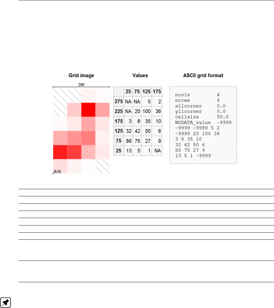
DRAFT
iMOD, User Manual
9.13 ASC-files
The format is relatively straight-forward: the first six lines indicate the reference of the grid, followed by
the values listed in the order they would naturally appear (left-right, top-down). For example, consider
a grid, shown to the left. This could be encoded into an ASCII grid file that would look like:
ESRI ASCII Format:
Variable Format Description
# - Comments
Ncols Integer Numbers of columns
Nrows Integer Numbers of rows
Xllcorner Real The western (left) x-coordinate
Yllcorner Real The southern (bottom) y-coordinate
Cellsize Real The length of one side of a square cell
NODATA_
value
Real The value that is regarded as “missing” or “not applicable”; this
line is optional, but highly recommended as iMOD will expect
this line to be declared
DataBlock Integer
Real
Listing of the raster values for each cell, starting at the upper-
left corner (north-west). These number are delimited using a
single (or more) space(s) character(s).
Note: These ESRI ASCII rasters will be converted into IDF-files whenever they are read into iMOD.
However, iMOD can export IDF-files into ESRI ASCII files again.
552 of 812 Deltares

DRAFT
iMOD Files
9.14 ARR-files
The format is relatively straight-forward: it is a free-formatted file format generate by iMOD to create
the input per package for iMODFLOW. For example, consider a grid with boundary conditions:
-1,1,1,1,1,1,-1
0,0,0,1,1,1,-1
0,0,0,1,1,1,-1
0,0,0,1,1,1,-1
0,0,0,0,0,1,-1
This could be encoded into an ARR grid file that would look like:
-1
5*1
-1
3*0
3*1
-1
3*0
3*1
-1
3*0
3*1
-1
5*0,
1
-1
At the end of the file, there is a list of the dimensions of the file with:
DIMENSIONS
120
132
120000.0
298000.0
240000.0
430000.0
3.4028235E+38
0
1000.000
1000.000
Variable Format Description
# - Comments
Ncols Integer Numbers of columns
Nrows Integer Numbers of rows
Xllcorner Real The western (left) x-coordinate
Yllcorner Real The southern (bottom) y-coordinate
Xurcorner Real The eastern (right) x-coordinate
Yurcorner Real The northern (top) y-coordinate
NODATA_
value
Real The value that is regarded as “missing” or “not applicable”; this line is
optional, but highly recommended as iMOD will expect this line to be
declared
IEQ Integer Identifier to specify a uniform grid (IEQ=0) or a nonuniform grid (IEQ=1)
Cellsize_X Real The length of the x-side of a square cell
Cellsize_Y Real The length of the y-side of a square cell
Deltares 553 of 812
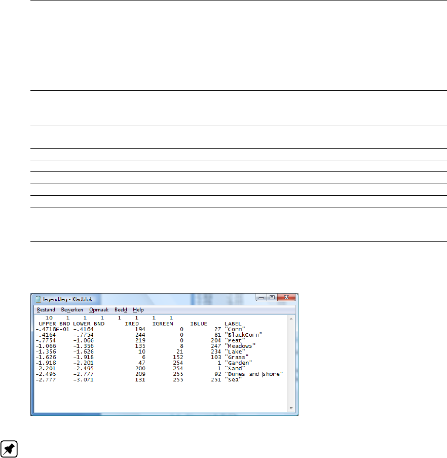
DRAFT
iMOD, User Manual
9.15 LEG-files
Each map file in iMOD (IDFs, IPFs, ISGs, GENs and IFFs) can be displayed by classes that are defined
in a legend. The legend is stored internally, but can be saved to, and loaded from disk. The syntax of
a *.LEG-file is as follows:
NClass Number of classes. Bear in mind that legends that have NClass<=50, behave
differently than legends that have 50<NClass<=255, see for more information
0.
ColourMarks In the Legend window (see 3.3.4), these ColourMarks (0-1) define whether
the ColourMark is turned on or off in the colour ramp.
Upper BND Upper Boundary of the class
Lower BND Lower Boundary of the class
IRED Red component in RGB-colour model (0-255)
IGREEN Green component in RGB-colour model (0-255)
IBLUE Blue component in RGB-colour model (0-255)
Label Label, make sure the length of the label is less or equal to 50 characters.
For Labels that contain more than one word, such as Dunes and Shore, they
should be bracketed by quotes, i.e. “Dunes and Shore”.
Example of a LEG-file:
Note: Use comma’s and/or space delimiters within LEG-files.
554 of 812 Deltares
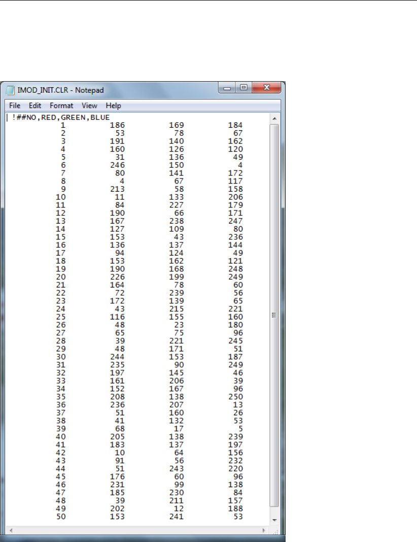
DRAFT
iMOD Files
9.16 CLR-files
iMOD supports 50 predefined colours to be used as default in a variety of iMOD functionalities. The
colour definitions are stored in the IMOD_INIT.CLR file which is stored in the USER directory.
Deltares 555 of 812
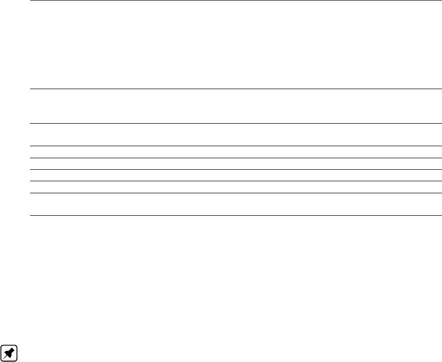
DRAFT
iMOD, User Manual
9.17 DLF-files
The colour information for boreholes will be read from a DLF-file. On default, iMOD tries to read the
file: {user}\settings\DRILL.DLF. If this fails, iMOD will use its internal default values. The syntax of a
DLF-file is as follows:
LABELS Use the first line of the file to identify the columns. These are however unchangeable!
Repeat the following attributes (CLASS, IRED, IGREEN, IBLUE, LEGEND) for each
line.
CLASS Use the first column to specify the search-string that should match the first column of
the associated *.TXT file as described.
IRED Red saturation (0-255)
IGREEN Green saturation (0-255)
IBLUE Blue saturation (0-255)
LEGEND Label used in the legend.
WIDTH
(optional)
Enter the width category (1-10) used in 2D and 3D plotting. This is an optional value
and is assigned the value 1 by default.
Example of a DLF-file:
CLASS,IRED,IGREEN,IBLUE,LEGEND
FS,255,255,0,"Fine Sand",1.00
C,148,0,211,Clay,0.25
G,218,165,32,Gravel,2.00
"P H",244,164,96,"Peat Holland",0.50
L,238,130,238,Loam,0.75
Note: The maximum string length of the Class-column is 20 characters. The maximum string length
for the LEGEND column is 50 characters. The maximum number of classes is 250 (lines, excluding
the header).
556 of 812 Deltares
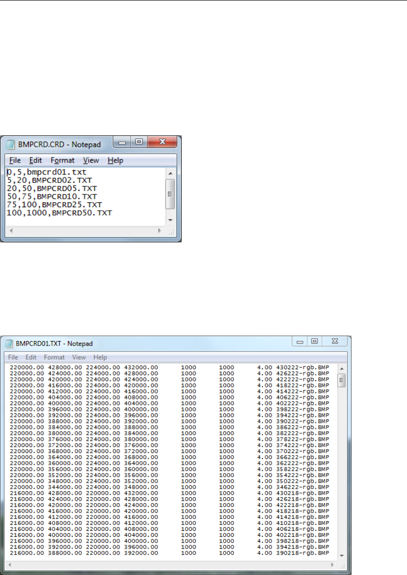
DRAFT
iMOD Files
9.18 CRD-files
The display of tiled background maps is directed by the iMOD coordinate CRD-file. The CRD-file is
defined with the keyword TOP25 in the iMOD preference file.
The CRD-file links BMP-files as background maps by specifying the scale (at unit 1000) at which the
BMP-files will be displayed and the name of the TXT-files in which the BMP-files are defined.
Example of a CRD-file:
The TXT-files referred to in the CRD-file define the BMP-files used as background maps. For each
BMP-file is specified: coordinates LL-corner, coordinates UR-corner, number of pixels in X-direction,
number of pixels in Y-direction, cellsize (m), name of the BMP-file.
Example of a TXT-file linked to a CRD-file:
Deltares 557 of 812

DRAFT
iMOD, User Manual
9.19 ISD-files
An ISD-file contains information about the location of startpoints used in the calculation of pathlines
from model output. An ISD-file can be created by IMOD using the Define Startpoints option from the
Toolbox option on the main menu. The syntax of an ISD-file is as follows:
Delimiter line
ShapeName Name of the shape, use quotes for a name containing more than one word
Delimiter line
Number, Shape-
type
Number of the shape type, type of shape
1027,POINT
1026,RECTANGLE
1025,POLYGON
1024,CIRCLE
1028,LINE
1139,GRID
Number, Number Depending on the shape type:
POINT: radius of the circle around the point, distance between points on the
circle
POLYGON: distance X, distance Y between points within the polygon
CIRCLE: radius of the circle, distance between points on the circle
LINE: distance between points along the line (second number not necessary)
GRID: vertical offset of point, apply zero to put the points on the values of the
grid (top-level file) (second number not necessary)
Top-level file /
Numeric value
IDF-file defining the top level at which startpoints are defined or
Numeric value defining the top level at a fixed elevation
Bottom-level file /
Numeric value
IDF-file defining the bottom level at which startpoints are defined or
Numeric value defining the bottom level at a fixed elevation
Number Number indicating whether a reference level is used
0 = reference level is not used; 1 = reference level is used
Reference level Reference level used to position the startpoints ;
Vertical interval
number
The number of points to be used between the specified top-level and bottom-
level
Delimiter line
No. Points Shape Number of points defined laterally as startpoints
Xcrd,Ycrd X- and Y-coordinates of the startpoints
Delimiter line
558 of 812 Deltares
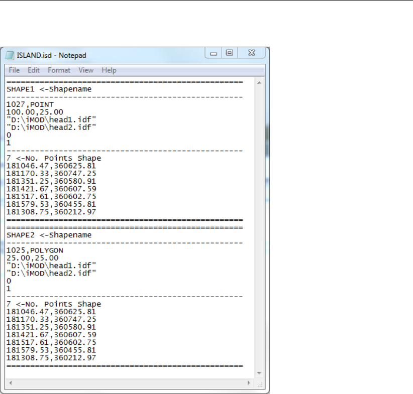
DRAFT
iMOD Files
Example of an ISD-file:
Deltares 559 of 812
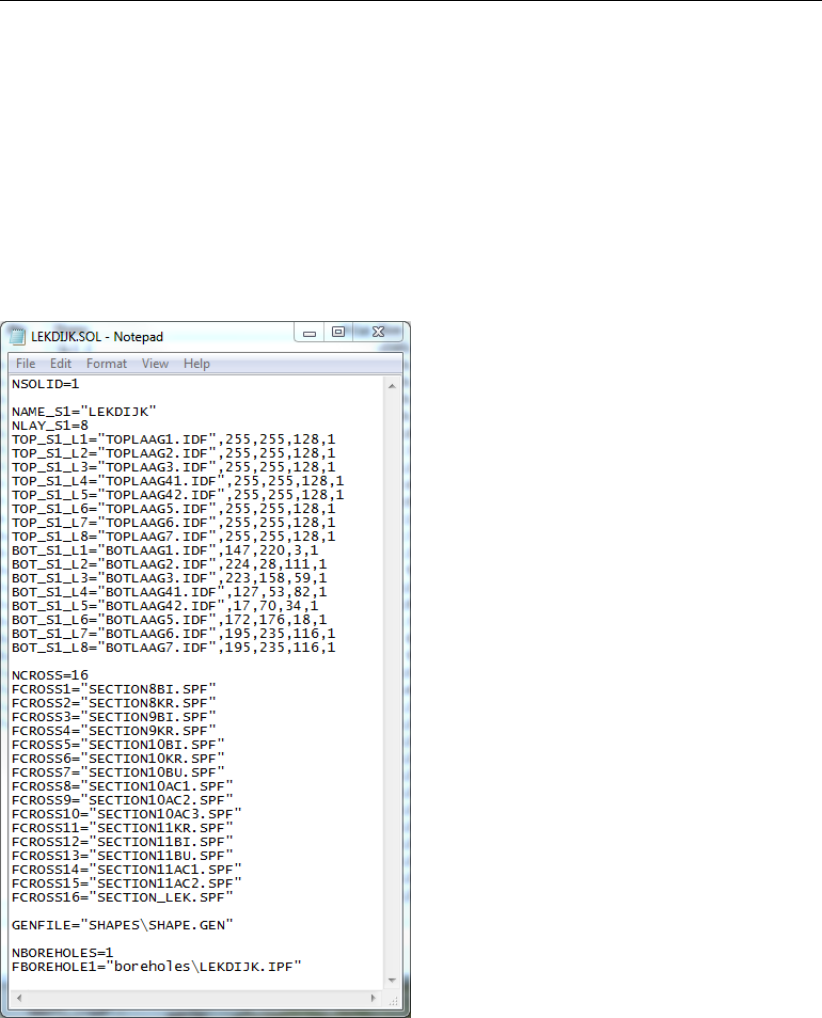
DRAFT
iMOD, User Manual
9.20 SOL-files
A SOL-file describes the number of modellayers that are within a Solid. A solid contains several IDF-
files that describe the top and bottom elevation of modellayers. Those files are listed in a SOL-file
too. Each modellayer is described by two IDFs, one that stores the top elevation and one for the
bottom elevation. Thereafter, a SOL-file includes a number of references to SPF-files that describe
how the elevation of those top and bottom elevations vary along a cross-sectional line. A SOL-file will
be created and updated by iMOD, however, it can be edited outside iMOD easily. The syntax of a
SOL-file is shown below:
Example of a SOL-file with reference to 8 modellayers and 16 cross-sections:
560 of 812 Deltares
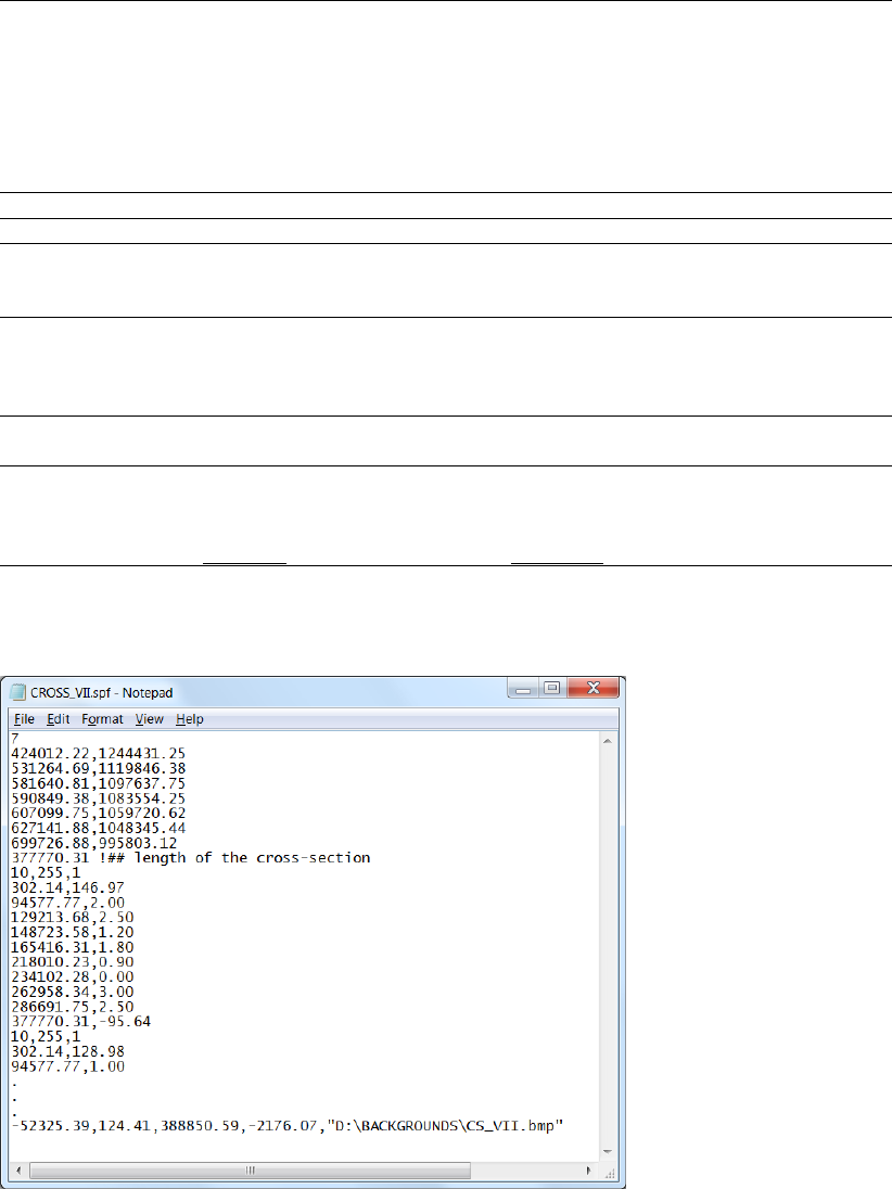
DRAFT
iMOD Files
9.21 SPF-files
A SPF-file describes the variation in the top and bottom elevation along a cross-sectional line. Each
SPF-file can be alternated individually within iMOD or within regular text editors, such as NotePad. The
latter is not recommended however.
NCRD Number of coordinates that describe the cross-sectional line.
X{i},Y{i} Enter NCRD number of coordinates Xand Y.
TotLength Total length of the cross-section. This is used (and updated whenever the
coordinates Xand Yare adjusted inside and/or outside iMOD) to avoid any
adjustments of the elevations outside the outer limit of the cross-sectional line.
NP{i},Clr{i},Lt{i} Number of alternations of the top (i=uneven) or bottom (i=even) elevations.
Clr{i} and Lt{i} are the linecolour (colour number for a colourdisplay of 16 mil-
lion colours; 255=red) and linethickness (between 1 and 10) of the ith top or
bottom IDF as mentioned in the SOL-file that directs to this SPF-file.
x{i},z{i} The distance from the first coordinate (X1,Y1) of the cross-sectional line, fol-
lowed by the vertical position of the elevation (top or bottom).
x1,y1,x2,y2,bitmap On the last line of the SPF file it is possible to add a bitmap (*.jpg, *.bmp or
*.png) that need to be attached to the cross-section. Specify the position of
the bitmap by the x1,y1,x2,y2variables. Note: Be aware that iMOD uses the
upper-left corner as x1, y1and the lower-right corner as x2, y2.
Example:
Deltares 561 of 812
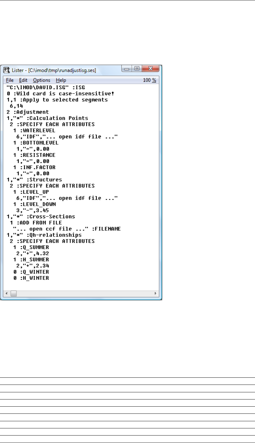
DRAFT
iMOD, User Manual
9.22 SES-files
A SES-file describes the operations that need to be carried out by ISG Edit. The file can be loaded
into ISG Edit in order to recompute identical operations sequentially.
Example of a SES-file:
9.23 GEF-files
9.23.1 CPT GEF-file
A CPT GEF-file usually contains information about the penetration length, measure cone resistance,
friction resistance, pore pressure, friction number, inclination, corrected depth, time, corrected cone
resistance, net cone resistance, pore ratio, cone resistance number, weight per unit volume, in-situ
initial pore pressure, total vertical soil pressure and effective vertical soil pressure.
Keyword Content
#GEFID= 1,0,0
#PROCEDURECODE= GEF-CPT-Report, 1,1,0, -
#COMPANYID= CPT bv, Sondeerburg, 31
#PROJECTID= CT, 380730
#FILEDATE= 1998,02,18
#TESTID= C2-265
#FILEOWNER= W.A. van Buuren
#COLUMN= 2
562 of 812 Deltares

DRAFT
iMOD Files
#LASTSCAN= 1251
#COLUMNINFO= 1, m, penetration length, 1
#COLUMNINFO= 2, MPa, Cone, 2
#MEASUREMENTTEXT= 9, ground level, horizontal reference level
#ZID= 31000, -2.41
#EOH=
0.12;0.205
0.14;0.199
0.16;0.219
0.18;0.252
......
......
25.04 20.261
25.06 21.368
25.08 23.121
See for a more extensive description the TNO manual "GEF-CPT-Report.pdf".
9.23.2 Borehole GEF-file
A Borehole GEF-file usually contains information about the layer depth, the numerical sand fraction
("zandmediaan" in Dutch) and the numerical gravel fraction ("grindmediaan" in Dutch). In addition
information can be given on the clay percentage, silt percentage, sand percentage, gravel percentage,
organic matter percentage, main soil type (sand, clay, etc.), color intensity, soil color and Carbon
carbonate fraction.
Once the IPF-file has been created, this file can be loaded into iMOD and analyzed by making use of
e.g. the cross-section visualization tool. Within iMOD you are able to choose the column you prefer to
link to the *.DLF file legend in the 2D- and 3D-tool (see iMOD configuration in section 6.8.1).
Note: Before loading the IPF-file into iMOD check the coordinate system (projection) of the data in
the IPF-file. This might be different from the default coordinate system of iMOD; WSG84, EPSG:28992
Amersfoort RDnew. A reprojection of your GEF or IPF file might be preferred.
See for a more extensive description the TNO manual "GEF-BORE-Report.pdf".
Deltares 563 of 812

DRAFT
iMOD, User Manual
564 of 812 Deltares

DRAFT
10 Runfile
To initiate a groundwater flow model simulation using iMODFLOW a Runfile is required. This file
describes:
the location of the (sub)model;
the simulation time (number of stress periods);
the current distribution of computational nodes (grid size);
the current number of model layers to be used;
the collection of files that describe the model parameters;
the desired output variables to be saved.
ARunfile gives an overview of the entire model configuration and is therefore easy to transfer and
reproduce. A major difference between the input files necessary for other conventional simulators
(e.g. standard Modflow) is that a Runfile does not contain any model data, unless a constant value is
assigned to a model parameter. It consists mainly of references to other files (IDFs, IPFs, ISGs, GENs)
that contain the actual model data.
The philosophy of using iMODFLOW and the concept of a Runfile is that all the referred files are
constructed for a REGION of interest rather than for an AREA of interest. A REGION of interest can
be extremely large (provinces, countries); an AREA of interest is often smaller (watersheds, water
management areas). The central idea is that model data is collected for large regional areas at the
finest scale available for that type of model data, e.g. land use observations at a resolution of 100 x
100 meter and precipitation distribution at a scale of 1000 x 1000 meter. These files are referred to
in the Runfile and iMOD combines the different data to the desired AREA of interest and resolution at
the moment a simulation will start. Simulations for different AREA‘s of interest can be performed using
identical model data that need to be maintained at a single location.
This chapter covers the Runfile-related topics:
section 10.1: the general structure of a Runfile.
section 10.2 -section 10.19: a one-by-one description of Data Sets 1 to 19.
section 10.20:Runfile-history: any differences between Runfile-structures per iMOD release.
section 10.21: all options of how a Runfile can be used to start a MODFLOW simulation.
section 10.22: an example of printed MODFLOW output.
section 10.23: a table containing the names and content of the output folders.
Deltares 565 of 812
DRAFT
iMOD, User Manual
10.1 Runfile Description
ARunfile lists the configuration necessary to start a simulation. It consists of several Data Sets that
are briefly commented in the following table.
Repeat Data
Set
Description
1Result folder
2e.g. number of model layers, stress periods, type of simulation,
spatial network methodology
3File to monitor time-series during a simulation
4e.g. flags that specify number of sub models, computation mode
(simulation, debug, export modes), well positioning and usage of
scenarios
5Solver configuration (e.g. closure criterion)
6Location of the (sub)model and the chosen raster size
7Not supported in iMOD 4.x releases.
8Activated modules(9)/packages(9) and their corresponding output
9File that describes maximal extension of model domain
MODULES FOR EACH LAYER
Each package (9) 10 Number of files
11 Actual file and association to particular model layer
PACKAGES FOR EACH LAYER AND STRESS PERIOD
Each stress period 12 Length of current stress period, name convention assigned to re-
sult files and whether results should be saved
Each package (9) 10 Number of files
11 Actual file and association to particular model layer
In the following sections each of these Data Sets are described in more detail. Bear in mind that all
input variables are free format!
10.2 Data Set 1: Output Folder
Data Set 1 OUTPUT-FOLDER
OUTPUT-
FOLDER
Notification of the folder name in which the model results will emerge. Within this
folder an output file will be created that summarizes the model simulation, such a file
is called: log_[version-tag].txt. A non-existing folder will be created automatically. It
is compulsory to fill in a complete path, e.g.: c:\model\test rather than a relative path,
and not a relative path, e.g.: ..\..\test1
10.3 Data Set 2: Configuration
Data Set 2 NLAY,MXNLAY,NPER,SDATE,NSCL,IFTEST,ICONCHK,IIPF,
IUNCONF,IFVDL,IARMWP
NLAY The number of model layers that the current simulation will take into account.
There is no need to adjust the Runfile as long as NLAY will be smaller or equally
to MXNLAY. Whenever NLAY becomes less than MXNLAY all active model cells,
within model layer NLAY, operate as a Dirichlet boundary condition and simulate
a vertical flux over the edge stressed by the starting head condition (SHD, see
Data Set 8) or last given heads from the constant head package (CHD, see Data
Set 8) for that particular model layer.
MXNLAY This runfile-option is scheduled for a next iMOD release; currently MXNLAY al-
ways equals NLAY.
MXNLAY is used to determine whether the lowest model layer NLAY should be
modeled as an open model boundary, which is the case whenever NLAY <MXN-
LAY.
566 of 812 Deltares
DRAFT
Runfile
NPER The number of time periods (conform the stress periods within standard MOD-
FLOW) to be simulated. For each time period it is compulsory to define at least
appropriate model input. iMODFLOW does not support the concept of time steps
within time periods as standard MODFLOW does.
SDATE This option has become obsolete as it is now steered via the keyword
ISAVEENDDATE in the iMODBatch function RUNFILE, see section section 8.6.5.
For the sake of backward compatibility with earlier runfiles SDATE is still a key-
word in the runfile, but acts as a dummy.
NSCL Flag that determines the methodology of constructing the modeling network:
0The modeling network will be identical to the network that is described
in the IDF file (or entered xy coordinates) given by de keyword BND-
FILE, see Data Set 9. In this manner, it is possible to compute with
networks that distorted spatially on different locations.
1The modeling network will be defined by Data Set 6. The buffer around
the area of interest will be equal to the chosen grid sizes within that
area of interest.
2The modeling network will be defined by Data Set 6 whereby the grid
sizes within the buffer around the area of interest will increase up to a
given maximum size.
IFTEST Flag to indicate the mode in which iMODFLOW will perform the simulation:
0
(default)
Start the simulation without testing the existence of files. Any none
existing file will terminate the simulation and after recovering such file
the simulation need to be restarted from the beginning.
1This option 1 is scheduled for a next iMOD release.
Test the entire Runfile on the existence of files and correct content of
IPF files. The model will not be computed and at the end of the evalu-
ation a summary is written in a file called: imodflow_[version-tag].log.
ICONCHK Within a model configuration it can occur that within identical model cells, the
drainage level from the Drainage package (DRN, see Data Set 8) and/or the
drainage level from the Overlandflow package (OLF, see Data Set 8), or even
other elements from a River package (RIV, see Data Set 8) are positioned below
a specified water level of the River package (RIV) itself. To avoid such undesired
situation, e.g. within flooded areas, these drainage systems (DRN, OLF and RIV)
can be inactivated for this situation, automatically.
0No adjustments of the DRN and OLF packages
1The DRN, OLF and/or RIV systems are turned off whenever their
drainage levels are below existing river water levels (RIV-package) in
corresponding model cells.
IIPF This flag indicates whether time series need to be computed during the simula-
tion.
0No time series included
nInclude n-number of IPF files with location of time series to be com-
puted for each stress period throughout the simulation, See Data Set
3.
-n Apply an interpolation of computed heads toward the location of the
measurement.
IUNCONF
(optional)
This flag indicates the usage of unconfinedness for aquifers.
0All aquifers are confined, unconfinedness is supported via the NAM-file
export mode only, see section section 5.5 and section 8.6.5.
IFVDL
(optional)
This flag indicates the methodology to be used computing the conductance for
streams given in the ISG package. The default value is IFVDL=0.
0River conductance is a function of river length (m), wetted perimeter
(m) and river resistance (d), solely.
1River conductance is a function of river length (m), wetted perime-
ter (m), river resistance (d), permeability and thickness of appropriate
aquifer, resistance of first aquitard.
Whenever IFVDL=1, it is obliged to have the keywords TOP and BOT activated
or the package SFT should be active
Deltares 567 of 812

DRAFT
iMOD, User Manual
IARMWP Use this to specify artificial recharge to be read from an IPF file
10.4 Data Set 3: Timeseries (optional)
Data Set 3 Apply only whenever IIPF<>0 from Data Set 2
IPF_TS,IPFTYPE,IXCOL,IYCOL,ILCOL,IMCOL,IVCOL (all compulsory)
IPF_TS Notification of an IPF filename that stores the location of measures to be moni-
tored as time series throughout the simulation.
IPFTYPE Type of the IPF file
1For a steady-state simulation the 5 attributes within the given IPF
should be (in this order):
Xx coordinate
Yy coordinate
ILAY Model layer identification
OBS Observed value (OBS=0.0 if no observation is available)
VAR variance of the measurement σ2= Var(X)
(VAR=1.0 if no observation is available)
After the simulation the given IPF is copied to the folder [OUTPUT-
FOLDER]\[ipfname] and contains the additional records:
COMP Computed values
DIFF Difference (COMP-OBS)
DIFFW Weighed difference (COMP-OBS)*√σ2−1
2For the transient simulation the attributes within the given IPF should
be (in this order):
Xx coordinate
Yy coordinate
ILAY Model layer identification
After the simulation the given IPF is copied to the folder [OUTPUT-
FOLDER]\[ipfname] and contains the additional record:
ID Reference ID to the individual time series
which are stored within the file [OUTPUT-
FOLDER]\timeseries\location_[i].txt.
Whenever the IPF_TS consists of time series initially, those will be included in
the final time series. Time series within the buffer zone (see Data Set 6) will be
left out.
IXCOL Specify the column number in the IPF file (IPF_TS) that is representative for the
X-coordinate of the measurement.
IYCOL Specify the column number in the IPF file (IPF_TS) that is representative for the
Y-coordinate of the measurement.
ILCOL Specify the column number in the IPF file (IPF_TS) that is representative for the
layer identification of the measurement.
IMCOL Specify the column number in the IPF file (IPF_TS) that is representative for the
measurement value. Whenever the number of columns in the IPF file be less
than 4, IMCOL=0 and no observations will be used.
IVCOL Whenever the number of columns in the IPF file be less than 5, IMCOL=0 and
no observations will be used.
>0Specify the column number in the IPF file (IPF_TS) that is repre-
sentative for the variance of the measurement Var(X). The vari-
ance of a random variable Xis its second central moment, the ex-
pected value of the squared deviation from the mean µ=E[X], thus:
Var(X) = E (X−µ)2. This definition encompasses random vari-
ables that are discrete, continuous, neither, or mixed. The variance
(σ2) can also be thought of as the covariance of a random variable
with itself: Var(X) = Cov(X, X) = σ2.
<0Whenever IVCOL is negative (e.g. IVCOL=-5), it means that instead
of variances (σ2), weight values ware entered. Weight values are
computed as w=√σ2−1
.
568 of 812 Deltares
DRAFT
Runfile
10.5 Data Set 4: Simulation mode
Data Set 4 NMULT,IDEBUG,IDOUBLE,IPOSWEL,ISCEN,IBDG,MINKD,MINC
NMULT The number of areas to be computed sequentially. The areas need to be defined
in Data Set 6. NMULT need to be 0 in case NSCL=0.
IDEBUG A flag indicating the output frequency during a simulation:
0Default configuration whereby a solution of the simulation is saved on
disk after convergence, or whenever the number of iteration exceeds
MXITER (see Data Set 5) and the simulation terminates thereafter.
1Debug configuration whereby both input for the activated packages and
intermediate solutions during the iteration process are saved on disk.
IDOUBLE This option replaces the previous IEXPORT option which became obsolete since
v3-series. By default IDOUBLE=0, which means that the results of the simu-
lation will be single precision values. If IDOUBLE=1, the results will be double
precision, keep in mind that in that case, all files will be doubles in size as well.
IPOSWEL Flag indicating the assignment of well onto the model network:
0Assignment of the well onto the single model grid cell is based on the
x and y coordinates of the well.
1Not supported in iMOD 4.x releases.
ISCEN Flag indicating the usage of scenario definitions:
0No usage of scenarios
1Not supported in iMOD 4.x releases.
IBDG
(optional)
Flag indicating the definition of budget computation for packages:
0Not supported in iMOD 4.x releases.
1
(default)
Fluxes from packages (except CHD) within one single model cell are
saved separately. As a result the output file name convention (see
ILSAVE in Data Set 8) will include a system number, e.g. _sys1_;
_sys12_.
MINKD
(optional)
Minimal value for transmissivity (m2/day). Use MINKD >0for reasons of stability
in combination with horizontal anisotropy.
MINC
(optional)
Minimal value for the vertical resistance (days). Use MINC >1for reasons of sta-
bility and to avoid large contrasts between horizontal en vertical conductances.
Especially whenever the cell size (CELLSIZE) increases, it could be advisable to
specify MINC >1.
10.6 Data Set 5: Solver configuration
Data Set 5
(optional PCG)
(optional PKS)
OUTER,INNER,HCLOSE,QCLOSE,RELAX
,NPCOND,MAXWBALERROR
,PARTOPT,IDFMERGE
OUTER Maximal number of “outer” iteration loops. The iterative procedure used in MOD-
FLOW for solving nonlinear problems is commonly referred to as Picard iteration.
It splits the solving process into an outer iteration loop, the equation that needs
to be solved in the “inner” is (re)formulated.
If OUTER < 0, the Parallel Krylov Solver (PKS) is activated instead of PCG, and
for this solver OUTER = -OUTER is taken as the number of outer iterations. For
PKS, the supported preconditioning is Incomplete LU-factorization only, which is
automatically being set. Hence, you are not allowed to set NPCOND when PKS
is activated.
INNER Maximal number of “inner” iteration loops. Within each inner iteration loop, the
equation that was formulated in the outer iteration loop is (partly) solved. In
common, it is more expensive to have much inner iteration though each iteration
loop represents a temporary formulation of the equation. True linear systems
can speed up drastically by increasing the number of inner iterations and RELAX
= 1, however, most groundwater models are a mixture of linear and non-linear
elements and therefore a fair trade-off between robustness and speed seems to
be NITER = 20.
Deltares 569 of 812
DRAFT
iMOD, User Manual
HCLOSE m Closure criterion for the hydraulic head (state variable). Commonly
it is practice to choose HCLOSE to be 2 orders of magnitude smaller
than the desired accuracy to be obtained.
QCLOSE m3Closure criterion for the mass balance. This criterion depends on the
grid size, since large grid cells produce larger errors in mass balances
than smaller ones does.
RELAX Relaxation factor that quantifies the amount of confidence for each solution ob-
tained after an inner iteration loop, default value is 0.98. It influences the robust-
ness and efficiency of convergence. For purely linear systems it can/must be
1.0, though non-linear system prefers lower values (e.g. 0.50-0.97). It is difficult
to know the optimal value for RELAX beforehand. Use the adaptive damping
(IDAMPING) instead.
NPCOND
(optional, PCG
only)
Pre-conditioning method. If the Preconditioning Method is set to Cholesky, the
Relaxation parameter can be set. Although the default is 1, in some cases a value
of 0.97-0.99 may reduce the number of iterations required for convergence.
1Modified Incomplete Cholesky (for use on scalar computers)
2Polynomial matrix conditioning method (for use on vector computers or
to conserve computer memory)
MAXW-
BALERROR
(optional, PCG
only)
Maximal overall acceptable error for the water balance in percentage (the default
value = 0.0% and the solver stops whenever the criterion of QCLOSE cannot
be met). Whenever the external-iteration does not converge (due to numerical
instability), the simulation will continue whenever the overall error in de the water
balance is less than the given MAXWBALERROR criterion.
PARTOPT
(optional, PKS
only)
Subdomain partition option. There are two methods supported: PARTOPT = 0
(default) for uniform partitioning in lateral x and y-direction; PARTOPT = 1 that
enables the Recursive Coordinate Bisection partitioning method computes the
subdomain dimensions according to a load pointer IDF grid. Note that each
subdomain always includes all model layers.
0Uniform subdomain partitioning (default)
1Recursive Coordinate Bisection (RCB) subdomain partitioning
IDFMERGE
(optional, PKS
only)
Flag for merging parallel subdomain IDF output files. The default is IDFMERGE
= 0, corresponding to no merging. In this case, each subdomain writes its out-
put IDF files like "<IDFNAME>_p<MPIRANK >.idf", where "<IDFNAME>" is the
iMOD output variable name, e.g. "head_steady-state_l1" and "<MPIRANK >" the
three-digit subdomain MPI rank identifier. Note that enabling this option could
slow down overall parallel computations.
0No merging of subdomain IDF output files (default)
1Merging of subdomain IDF output files
10.7 Data Set 5a: RCB load pointer grid (optional)
Data Set 5a LOADFILE
LOADFILE IDF file that represents with weights to be used when PKS is enabled (Data Set
5: OUTER <0) and the RCB subdomain partitioning option is enabled (Data Set
5: PARTOPT = 1). Only the absolute weights are being used for the subdomain
partitioning.
10.8 Data Set 6: Simulation window (optional)
Data Set 6 Apply whenever NMULT=1 and NSCL=1
XMIN,YMIN,XMAX,YMAX,CSIZE,BUFFER
Apply whenever NMULT>1 and NSCL=1
IACT,XMIN,YMIN,XMAX,YMAX,CSIZE,BUFFER,CSUB
Apply whenever NMULT=1 and NSCL=2
XMIN,YMIN,XMAX,YMAX,CSIZE,MAXCSIZE,BUFFER,CSUB
Apply whenever NMULT>1 and NSCL=2
IACT,XMIN,YMIN,XMAX,YMAX,CSIZE,MAXCSIZE,BUFFER,CSUB
IACT Flag that determines the whether a sub model need to be computed:
570 of 812 Deltares

DRAFT
Runfile
-1 Sub model will be computed only whenever the result folder does not
exist
0Sub model will not be computed
1Sub model will be computed and overwrite existing results if available
XMIN m Lower left X-coordinate of the area of interest
YMIN m Lower left Y-coordinate of the area of interest
XMAX m Upper right X-coordinate of the area of interest
YMAX m Upper right Y-left coordinate of the area of interest
CSIZE m Grid cell size within the area of interest and within the buffer.
MAXCSIZE m This is the maximum grid cell size within the buffer. Within the buffer the
entered grid cell size CSIZE, will increase gradually up to MAXCSIZE.
Apply whenever NMULT>1 and NSCL=2.
BUFFER m This represents the size of the buffer around the area of inter-
est. The total simulation model will have a total width of (XMAX-
XMIN)+2*BUFFER and a total height of (YMAX-YMIN)+2*BUFFER.
CSUB
(optional)
This is the name of the result folder for the current sub model, yielding [OUTPUT-
FOLDER]\[CSUB]\as result folder. Whenever no name is given, the default folder
name will be submodel[i], where i represents the ith sub model within NMULT.
10.9 Data Set 8: Active packages
Data Set 8 IPM,NLSAVE,ILSAVE(NLSAVE),KEY
IPM This represents whether a specific time independent module (mod) / time de-
pendent package (pck) is active in the current simulation. The following package
are supported:
Key Act Description
(mod) CAP 0/1 Usage of the unsaturated zone package
(mod) BND 0/1 (compulsory) Usage of boundary condi-
tions
(mod) SHD 0/1 (compulsory) Usage of starting heads
(mod) KDW 0/1 Usage of hydraulic conductance
(mod) VCW 0/1 Usage of vertical resistances
(mod) KHV 0/1 Usage of horizontal permeabilities
(mod) KVA 0/1 Usage of vertical anisotropy for aquifers
(mod) KVV 0/1 Usage of vertical permeabilities
(mod) STO 0/1 Usage of storage coefficients
(mod) TOP 0/1 Usage of top of aquifers
(mod) BOT 0/1 Usage of bottom of aquifers
(mod) PST 0/1 Usage of parameter estimation
(mod) PWT 0/1 Usage of the purge-water table package
(mod) ANI 0/1 Usage of the horizontal anisotropy pack-
age
(mod) HFB 0/1 Usage of the horizontal flow barrier pack-
age
(mod) IBS 0/1 Usage of interbed storage/subsidence
(mod) SFT 0/1 Usage of streamflow thickness
(pck) WEL 0/1 Usage of the well package
(pck) DRN 0/1 Usage of the drainage package
(pck) RIV 0/1 Usage of the river package
(pck) EVT 0/1 Usage of the evapotranspiration package
(pck) GHB 0/1 Usage of the general-head-bound. Pack-
age
(pck) RCH 0/1 Usage of the recharge package
(pck) OLF 0/1 Usage of the overland flow package
(pck) CHD 0/1 Usage of the constant-head package
(pck) ISG 0/1 Usage of the segment package
Deltares 571 of 812

DRAFT
iMOD, User Manual
It is easy to turn an IPM on or off by assigning 0 (off) or 1 (on). There is no need
to adjust the Runfile for these adjustments. It is not necessary to include all the
packages and/or packages in a runfile and the order you specify is irrelevant.
Of course, the packages BND, SHD, (KDW or KHV), (VCW or KVV) are obliged
for any (multi-layered) model!
NLSAVE Determines the number of model layers for which output need to be saved on
disk. NLSAVE may be larger than NLAY, however all layers that exceed the cur-
rent simulation will be neglected.
Important Note: the NLSAVE settings for BND/bdgbnd or STO/bdgsto deter-
mine the layers to be saved for all fluxes (bdgbnd, bdgsto, bdgflf, bdgfrf and
bdgfff). This means that settings for only KHV or only KVV are always neglected
and will be overruled by the settings given for BND or STO.
Important Note 2: the NLSAVE settings for ISG/bdgisg determine the layers to
be saved for the river fluxes (bdgriv). The NLSAVE settings for the RIV-package
are overruled by the settings given for ISG.
ILSAVE This parameter stores the model layers for each IPM keyword for ILSAVE model
layers. The model layers may be given in any order, e.g. 4, 5, 1. Any layer that
exceeds the current NLAY is neglected.
Important Note: the ILSAVE settings for BND/bdgbnd or STO/bdgsto deter-
mine the layers to be saved for all fluxes (bdgbnd, bdgsto, bdgflf, bdgfrf and
bdgfff). This means that settings for only KHV or only KVV are always neglected
and will be overruled by the settings given for BND or STO.
Important Note 2: the ILSAVE settings for ISG/bdgisg determine the layers to
be saved for the river fluxes (bdgriv). In case ILSAVE settings are defined for
RIV, these are overruled by the settings given for ISG.
=0 Identifies all modellayers
>0Modellayer identification
The following result will be saved:
Key NAME Unit Description
PST - - No output available
CAP BDGCAP m3/day Flux between the unsaturated zone and
the saturated zone
BND BDGBND m3/day Flux for constant head boundaries
SHD HEAD m Hydraulic head
KDW BDGFRF m3/day Flux over the eastern model faces
BDGFFF m3/day Flux over the southern model faces
VCW BDGFLF m3/day Flux over the lower model faces
KHV BDGFRF m3/day Flux over the eastern model faces
BDGFFF m3/day Flux over the southern model faces
KVV BDGFLF m3/day Flux over the lower model faces
STO BDGSTO m3/day Fluxes for storage
TOP - - No output available
BOT - - No output available
PST \PEST
folder
- No output available, other than *.txt and
*.ipf files that write performance and resid-
uals of optimalisation
KVA - - No output available
PWT - - No output available
ANI BDGANI m3/day Fluxes caused by anisotropy
HFB - - No output available
IBS BDGIBS m3/day Fluxes for interbed storage
SFT - - No output available
WEL BDGWEL m3/day Fluxes for wells
DRN BDGDRN m3/day Fluxes out drainage
RIV BDGRIV m3/day Fluxes for rivers
EVT BDGEVT m3/day Fluxes out evapotranspiration
GHB BDGGHB m3/day Fluxes for general head boundaries
RCH BDGRCH m3/day Fluxes for recharge
OLF BDGDRN m3/day Fluxes out overland flow.
CHD BDGBND m3/day Flux over constant head boundaries
572 of 812 Deltares

DRAFT
Runfile
ISG BDGISG m3/day Fluxes for rivers (fast SOBEK )
All fluxes that extract water from a specific model cell are negative. There-
fore, seepage water values are negative, within the file BDGFLF. Identical ele-
ments within one single model cell are lumped together in the output file, e.g.
fluxes from different drainage systems in a single model cell add together. The
naming convention for all files is:
DELT=0 [NAME]_[SNAME]_l[ILAY].idf; e.g. head_steady-
state_l1.idf or bdgflf_quarter_l10.idf
DELT>0[NAME]_[yyyymmdd]_l[ILAY].idf; e.g.
head_20101231_l1.idf or bdgdrn_20110814_l1.idf
Whenever the option IBDG=1 (see Data Set 4), the naming convention will be in-
cluding the system number of the package, e.g.: bdgriv_20110814_l1_sys1.idf
The number of system(s) is defined by the NFILES parameter in Data Set 10.
KEY Packages should be specified between brackets: “(“and “)” so iMODFLOW can
recognize the keyword. It will be used to compare this with the variable KEY in
Data Set 10.
10.10 Data Set 9: Boundary file
Data Set 9 BNDFILE or XMIN,YMIN,XMAX,YMAX
XMIN,YMIN,
XMAX,YMAX
Enter the coordinates of the entire model at maximum extension (area of regional
interest). Beyond these limits the model will give an error and below these limits
constant head boundary conditions will be applied, automatically whenever the
area of interest is smaller.
BNDFILE IDF file that represents the entire model at maximum extension (area of regional
interest). This file will be used differently for the following flag values for NSCL
(see Data Set 2):
NSCL=0 This file will be used to determine whether it extends the given
area of local interest defined in Data Set 6. If so the area of lo-
cal interest will be trimmed to fit the area of regional interest. On
the other hand, whenever the area of local interest is smaller (in
many cases), the boundary nodes along the cutting edges are
transformed into “open”-boundaries. The starting heads (SHD) or
constant-head (CHD) values fixate these boundaries.
NSCL>0 The network as described in the given IDF file is used for the mod-
eling simulation. Any network schematization is accepted as long
as it will not exceed the maximum extension of the area of regional
interest.
10.11 Data Set 10: Number of files
Data Set 10 NFILES,KEY
NFILES This expresses the number of entries that will follow, zero entries can be defined
by NFILES=0. It is possible the reuse the entries obtained in the previous stress
period by assigning the value NFILES=-1. For several package a single entry
consist of multiple files (parts). Moreover: each individual part of a package
should be repeated NFILES times before entering the next part of a package;
whenever a single nodata value is read for one of the individual parts of a package
for a particular location, the package on that particular location will be turned off!;
See table below for the individual parts (No.) of each package (they should be
entered in this order!):
Key No. Unit
PST 1 - Number of parameters to be estimated, see Data
Set 14, 15, 16 and 17 for more specific input in-
formation.
CAP n Number of input files (this is needed to determine
the number of files to be copied, which equals this
number – the 22 (or 21 whenever IARMWP=1)
compulsory IDF/IPF files)
Deltares 573 of 812

DRAFT
iMOD, User Manual
1 - BND Boundary setting, used to specify ac-
tive MetaSWAP elements
2 - LGN Landuse code, should be referred to
by the file luse_svat.inp
3 cm RTZ Rootzone thickness (min. value is 10
centimeter).
4 - SFU Soil Physical Unit should be referred
to by fact_svat.inp.
5 - MET Meteo Station number should be re-
ferred to by mete_svat.inp.
6 m+MSL SEV Surface Elevation.
7a - ART (if IARMWP=0) Artificial Recharge
(= Irrigation) Type, 0=no occurrence,
ART>0 means present at current lo-
cation whereby ART=1: from ground-
water, ART=2: from surface water ex-
traction
7b - ART (if IARMWP=1) Location of the actual
Artificial Recharge, the value of each
location refers to the attribute ID in the
IPF-file (see dataset 8b)
8a - ARL (if IARMWP=0) Artificial Recharge (=
Irrigation) Location, number of model
layer from which water is extracted.
8b - ARL (if IARMWP=1) IPF with locations
(X,Y) for Artificial Recharge (= Irriga-
tion), the number of model layer (ILAY)
from which water is extracted, the
identification (ID) of the area on which
the recharge is applied and the capac-
ity (CAP) in mm/day. All of those as
separate columns in the IPF file, thus
the following fields: X,Y,ILAY,ID,CAP.
Here, the source of the artificial
recharge is always groundwater.
9 mm/d ARC (if IARMWP=0) Artificial Recharge (=
Irrigation) Capacity. The capacity of
the irrigation installation. The applied
capacity depends on the duration of
the irrigation (part of a day) as spec-
ified in the file luse_svat.inp
10 m2 WTA Wetted Area specifies the total area
occupied by surface water elements.
Value will be truncated by maximum
cellsize.
11 m2 UBA Urban Area, specifies the total area
occupied by urban area. Value will be
truncated by maximum cellsize.
12 m PDU Ponding Depth Urban Area, specifying
the acceptable depth of the ponding of
water on the surface in the urban area
before surface runoff occurs
13 m PDR Ponding Depth Rural Area. Same as
above but for rural area.
14 day OFU Runoff Resistance Urban Area, spec-
ifying the resistance surface flow en-
counters in the urban area. The mini-
mum value is equal to the model time
period.
15 day OFR Runoff Resistance Rural Area. Same
as above but for rural area.
574 of 812 Deltares

DRAFT
Runfile
16 day ONU Runon Resistance Urban Area, spec-
ifying the resistance surface flow en-
counters to a model cell from an adja-
cent cell in the urban area. The mini-
mum value is equal to the model time
period.
17 day ONR Runon Resistance Rural Area. Same
as above but for rural area.
18 m/d QIU QINFBASIC Urban Area, specifying
the infiltration capacity of the soil sur-
face in the urban area. The range is
0-1000 m/d. The NoDataValue -9999
indicates unlimited infiltration is possi-
ble.
19 m/d QIR QINFBASIC Rural Area. Same as
above but for rural area.
20 m+MSL PWT Level of the Perched Water Table
level. When groundwater falls below
this level then the capillary rise be-
comes zero.
21 - SFC Soil Moisture Factor to adjust the soil
moisture coefficient. This factor may
be used during calibration. Default
value is 1.0.
22 - CFC Conductivity Factor to adjust the ver-
tical conductivity. This factor may be
used during calibration. Default value
is 1.0.
..n Remaining files will be copied to the simulation
folder as set by OUTPUTNAME (Data Set 1)
BND 1 - IDF with boundary settings; 0 = inactive, >0 = ac-
tive, <0 = fixed for each model layer
SHD 1 m+MSL IDF with starting heads for each model layer. In-
active cells will be transformed to nodata value -
999.99
KDW 1 m2/day Transmissivity for each model layer (trimmed in-
ternally to be minimal 0 m2/day)
VCW 1 days Vertical Resistance between model layers
(trimmed internally for minimal 0.001 days). For
reasons of scaling, it is important to assign the
nodata value for VCW to be zero!
KHV 1 m/day Horizontal Permeability for each model layer.
KVV 1 m/day Vertical Permeability for each aquitard (in be-
tween modellayers!). KVV is assumed to be
1/3*KHV for the modellayers!
STO 1 - Storage coefficient for each model layer, i.e. the
specific storage coefficient multiplied with the
thickness of the model layer, for the first uncon-
fined model layer, enter the specific storage coef-
ficient instead, e.g. 0.15.
TOP 1 m+MSL Top of the aquifer.
BOT 1 m+MSL Bottom of the aquifer.
KVA 1 - Vertical anisotropy for aquifers
PWT 6 - Layer identification of the PWT unit; elements with
values <= 0 will be removed.
- Storage coefficient of the phreatic part under-
neath the PWT layer
m+MSL Top of the PWT layer
m Thickness of the PWT layer
Deltares 575 of 812

DRAFT
iMOD, User Manual
m Thickness of layer of the aquifer above the PWT
layer in which the transmissivity will be adjusted.
day Vertical resistance of the clay underlying the PWT
unit. This should be larger or equal to the given C
value of the PWT layer, otherwise the C value will
be used given by the module VCW.
ANI 2 - The anisotropic factor perpendicular to the main
principal axis (axis of highest permeability). Fac-
tor between 0.0 (full anisotropic) and 1.0 (full
isotropic). Do not use a nodata value of 0.0
since
this will deactivate the package!
degrees The angle along the main principal axis (highest
permeability) measured in degrees from north (0),
east (90), south (180) and west (270). Do not use
a nodata value of 0.0 since
this will deactivate the package!
HFB 1 - GEN file (*.gen) defining the location and FCT val-
ues of faults/horizontal barriers. When GEN files
are assigned to layer number 0, iMOD will assign
the fault to the appropriate model layers automat-
ically; in that case the GEN file needs to be a 3D
GEN (see section 9.10). When the TOP and BOT
of the aquifer are defined in the runfile, the FCT
value is assigned to a resistance r; otherwise FCT
is assigned to a factor fthat is used to multiply the
conductances between cells. When FCT (so fac-
tor for the resistance r) is zero the barrier is im-
permeable! See section 12.15 for details on how
the conductance between cells is calculated.
IBS 4 m+MSL Preconsolidation head or preconsolidation stress
in terms of head in the aquifer. Preconsolidation
head is the previous minimum head value in the
aquifer. For any model cells in which specified HC
is greater than the corresponding value of starting
head, value of HC will be set to that of starting
head.
- The dimensionless elastic storage factor for in-
terbeds present in model layer. The storage factor
may be estimated as the sum of the products of
elastic skeletal specific storage and thickness of
all interbeds in a model layer.
- The dimensionless inelastic storage factor for in-
terbeds present in model layer. The storage factor
may be estimated as the sum of the products of
inelastic skeletal specific storage and thickness of
all interbeds in a model layer.
m The starting compaction in each layer with in-
terbed storage. Compaction values computed by
the package are added to values in this array
so that printed or stored values of compaction
and land subsidence may include previous com-
ponents. Values in this array do not affect calcula-
tions of storage changes or resulting compaction.
For simulations in which output values are to re-
flect compaction and subsidence since the start of
the simulation, enter zero values for all elements
of this array.
SFT 2 m+MSL Stream Flow Thickness
m/d Permeability
WEL 1 m3/day An IPF file with:
576 of 812 Deltares

DRAFT
Runfile
1Three columns representing the
x,y coordinate and the rate, e.g.:
x,y,q,{z1,z2}
2Two columns representing the x,y co-
ordinate and a third column referring
to associated files with time-variant
rates, e.g. x,y,[id],{z1,z2}
The parameters z1 and z2 express the screen of
the well and are optional. Use these parameters
in combination with ILAY=0 (see Data Set 11)
DRN 2 m2/day Conductance of the drainage system within a sin-
gle model cell; elements with values <= 0 will be
removed.
m+MSL Elevation of the drainage system.
RIV 4 m2/day Conductance of the drainage system within a sin-
gle model cell; values need to be ≥0.
m+MSL Elevation of the water level.
m+MSL Elevation of the bottom level. Whenever the eleva-
tion of the bottom level is higher than the entered
elevation of the water level, iMODFLOW will ad-
just internally the elevation of the bottom level to
be equal to the elevation of the water level. Any
corrections made are listed by a negative system
number in the *.LST file whenever the IDEBUG
flag is set on 1.
- Infiltration factor:
=0 No infiltration is allowed
>0Infiltration is allowed whenever the
head is below the stage up to a max-
imum (stage minus bottom pressure)
whenever the head is less than the
bottom. Infiltration conductance is cal-
culated as: river conductance * infiltra-
tion factor.
EVT 3 mm/day This option can only be used in combination with
ILAY=1
Evapotranspiration strength.
m+MSL Top elevation for maximal evapotranspi-ration
strength.
m Thickness in which evapotranspiration strength
reduced to zero.
GHB 2 m2/day Conductance of the general head system within a
single model cell; elements with values <= 0 will
be removed.
m+MSL Elevation at the general head boundary.
RCH 1 mm/day This option can only be used in combination with
ILAY=1
Recharge strength.
OLF 1 m+MSL Surface elevation where above overland flow
takes place; elements with values equal to the no-
data value will be removed.
CHD 1 m+MSL Elevation of constant heads at the location where
BND <0 only.
ISG 1 - Specific segment file for the simulation of water
systems directly from vectors.
KEY Text string that identifies the Key of the module/package listed by Data Set
10.
Deltares 577 of 812

DRAFT
iMOD, User Manual
10.12 Data Set 11: Input file assignment
Data Set 11 ILAY,FCT,IMP,FNAME
ILAY This represents the model layer to which the input data assigns to. For the pack-
age: BND, SHD, KDW, VCW, STO, TOP, BOT and ANI, it is not sustained to assign
more input data to identical model layers. However, multiple assignments to iden-
tical model layers are sustained for the other packages: PWT, HFB, WEL, DRN,
RIV, EVT, GHB, RCH, OLF, CHD and ISG. ILAY can be used as follows:
>0Expresses the model layer number to which the module and/or package
is assigned to
=0 Automatic allocation of model layers to packages. It is compulsory to
have included the TOP and BOT package (see Data Set 8). Only the
following packages are affected by ILAY=0:
HFB The given elevation in a 3-D GEN file (see section 9.10) will be
used to determine the actual model layer, use the iMODBatch
function GEN2GEN3D to construct those 3-D GEN files (see
section 8.4.2)
WEL Given IPF should contain the records, X,Y,Q,Z1,Z2. Z1 and
Z2 will be used to assign well strength to the appropriate
model layer(s)
DRN The given elevation will be used to determine the actual
model layer
RIV Both, the given stage and bottom elevation will be used to
determine the appropriate model layer(s)
GHB The given elevation will be used to determine the model layer.
OLF The given elevation will be used to determine the model layer.
ISG Both, the given stage and bottom elevation will be used to de-
termine the appropriate model layer(s). Moreover, the speci-
fied wetted perimeter will be used to adjust conductances.
<0Assign package to the highest active model cell with a BND-value >0
(see Data Set 10, Key=BND). Every package (except the CHD package)
can be affected by ILAY<0; package however, are not supported.
FCT The multiplication factor for the input data (nodata values excluded). It is pos-
sible to use the FCT parameter to assign mean values, e.g. apply FCT=0.5 for
conductance’s for rivers in summer and winter periods. Moreover, it is possible
to compute a weighed mean of two periods within the package assigned to the
identical model layer.
IMP Addition for the input data (nodata values excluded). Mathematical order is that
multiplication (FCT) comes before the addition (IMP).
FNAME The name of the input file, although it is sustained, it is preferable to note the
FNAME with an absolute path (e.g. c:\fname) rather than a relative path (..\fname).
The following format of these files are assigned to the existing package:
Format Module/package
IDF CAP,BND,SHD,KDW,VCW,KHV,KVV,STO,PWT,ANI,CHD,
DRN,RIV,EVT,GHB,RCH,OLF,IBS,TOP,BOT,KVA
IPF WEL
GEN HFB
ISG ISG
In case the input parameters are constant over the entire modeling domain, a con-
stant value can be given. An exception to this is made for the packages WEL,HFB
and ISG packages
10.13 Data Set 12: Time discretisation
Data Set 12 KPER,DELT,SNAME,ISAVE,ISUMSAVE
KPER The number of the stress period. It will be used solely to verify whether the
current stress period matches the stress period read. If not a warning appears in
the log file.
DELT day The length of the current stress period.
SNAME The date or name for the current stress period.
578 of 812 Deltares

DRAFT
Runfile
DELT=0 For steady-state simulations, it should state “steady-state”, mainly
for reasons of compatibility with iMOD.
DELT>0For transient simulations it should state the date notated as: yyyym-
mdd; e.g. 20101231 to express the 31th of December 2010. Us-
age of these format is recommended strongly for compatibility with
iMOD (e.g. time-series plotting).
As a consequence, all result files will show the given date/name in their names,
e.g. head_[yyyymmdd]_l1.idf or bdgflf_steady-state_l8.idf.
ISAVE This parameter defines whether output (as defined by Data Set 8) is generated
for the current stress period.
-1 Result will be saved with the buffer excluded
0No results will be saved
1Results will be save with the buffer included
In case NMULT>1 (see Data Set 4), ISAVE will become abs(ISAVE) because
the proper merging procedure will use the results in the buffer area.
ISUMSAVE
(optional)
This optional parameter allows to sum all fluxes for each package per model
layer. If more package entries are defined per model layers, those will be lumped
into a single budget quantity.
0Explicitly save all budget per package entry as a separate results
file.
1Sum all individual fluxes per model layer for the package entries.
10.14 Data Set 14: Parameter Estimation – Main settings
Data Set 14 PE_MXITER,PE_STOP,PE_SENS,PE_NPERIOD,PE_NBATCH,
PE_TARGET(.),PE_SCALING,PE_PADJ,PE_DRES,PE_KTYPE
PE_MXITER MXITER can have different meanings:
<0iMODFLOW will be run a single run and adjust all parameters ac-
cordingly and than stop.
=0 If PE_MXITER is equal to zero, a sensitivity matrix will
be computed yielding Jacobian values (finite difference be-
tween the change in head and the parameter update) for
the entire zones. Those values will be written to disk in
.\head\head_{date}_l{i}_sens_{param}_ils{ils}.idf. Those values
can be helpful to estimate the adjustment to a parameter to yield a
desired improvement of the head and/or flux (assuming the model
act linearly). The process will stop whenever all parameters are
perturbed.
>0Maximum number of iterations.
PE_STOP Stop criterion whenever decrease of objective function J becomes less or equal
to the ratio Ji/Ji−1. Entering a value of 0.1 means than the optimization stops
whenever the objective function value Jifor the current optimization step i, is
reduced less than 10% of the last objective function value Ji−1.
PE_SENS Enter the acceptable sensitivity for parameters to be included in the parameter
upgrade vector, e.g. PE_SENS=0.5 mean that parameters that have less than
0.5% sensitivity will be left out until they achieve a higher sensitivity.
PE_NPERIOD Enter the number of periods. If PE_NPERIOD >0, than repeat Data Set 15 for
each period.
PE_NBATCH Enter the number of batch files to be included during the parameter estimation.
Each batch file can have its own fraction that determines the weigh for the total
objective function value.
PE_TARGET(.) Enter a fraction for each target:
(1) The difference for each stress period between an available mea-
surement and its corresponding observation
(2) The difference between the measurement dynamics and the obser-
vational dynamics
Deltares 579 of 812
DRAFT
iMOD, User Manual
The entered fraction should be entered relative to each other since iMODFLOW
will recomputed the normalized values for the fraction. e.g. entering 1.0 and
2.0 will yield the fraction values 0.33 and 0.66, they will be summed equal to one.
Whenever PE_NBATCH>0(see Data Set 16), the entered weigh values for each
batch file will be included in the final normalization of the fractions.
PE_SCALING
(optional)
Enter a scaling option:
0No use of scaling/Eigenvalue decomposition (SVD)
1Only use of scaling
2Use of scaling and Eigenvalue decomposition (SVD)
3Only use of Eigenvalue decomposition (SVD)
In case a SVD decomposition is used (PE_SCALING=2 and PE_SCALING=3),
eigenvalues that explain at least 99% of variance are included.
PE_PADJ
(optional)
Enter the stopping criteria for Parameter ADJustment, e.g. PE_PADJ=0.05
means than whenever the parameter adjustment vector is less than 0.05, the
optimization will stop. By default PE_PADJ=0.0 which means that the optimiza-
tion will stop only whenever to parameters adjustment is applied.
PE_DRES
(optional)
Enter the minimal acceptable absolute residual used for the objective function.
Absolute residuals smaller that PE_DRES will not be included in the objec-
tive function and therefore not influence any parameter adjustment. By default
PE_DRES=0.0 which means that all residuals will be included.
PE_KTYPE
(optional)
Enter the type of Kriging to be used (whenever the PilotPoint concept is used).
By default Simple Kriging is applied (PE_KTYPE=1), select PE_KTYPE=2 for
Ordinary Kriging. The latter is used whenever a trend exists in the PilotPoints.
10.15 Data Set 15: Parameter Estimation – Period Settings
Data Set 15 Apply PE_NPERIOD times (see Date Set 14) S_PERIOD,E_PERIOD
S_PERIOD
[yyyymmdd]
Enter the start date for the period for which observations from the entered IPF
file (IPF_TS IN Data Set 3), need to be included, e.g. S_PERIOD=19890101 to
express the 1th of January 1989.
E_PERIOD
[yyyymmdd]
Enter the end date for the period for which observations from the entered IPF
file (IPF_TS IN Data Set 3), need to be included, e.g. S_PERIOD=20120321 to
express the 21th of March 2012.
10.16 Data Set 16: Parameter Estimation – Batch Settings
Data Set 16 Apply PE_NBATCH times (see Date Set 14)
B_FRACTION,B_BATCHFILE,B_OUTFILE
B_FRACTION Enter the fraction for the results from the current batch files. The entered fraction
will be normalized together with the entered fraction for PE_TARGET(.) (see
Data Set 14).
B_BATCHFILE Enter the name of the batch file to be executed after each simulation, e.g.
C:\BATCHFILES\FLOWLINES.BAT
B_OUTFILE Enter the name of the output file from the batch file (B_BATCHFILE), e.g.
C:\BATCHFILES\OUTPUT\FLOWLINES.OUT. The syntax of the file should be
as follows:
NEnter the number of records, e.g. N=2.
Z,V,H Enter for each record ito N the measurement (Z), variance (V) and
computed value (H). They can be entered in “free”-format. These
values will be added to the total objective function value and in-
cluded in the determination of the gradient.
10.17 Data Set 17: Parameter Estimation - Parameters
Data Set
17
PACT,PPARAM,PILS,PIZONE,PINI,PDELTA,PMIN,PMAX,PINCREASE,
PIGROUP,PLOG
PACT Activation of the current parameter.
0Parameter is not adjusted, initial parameter value PINI remains un-
changed during the estimation
580 of 812 Deltares
DRAFT
Runfile
1Parameter is part of the estimation process
PPARAM Parameter type, choose from:
Type Transf.
KD LOG Transmissivity, equal to KDW
KH LOG Horizontal permeability, equal to KHV
KV LOG Vertical permeability, equal to KVV
VC LOG Vertical resistance, equal to VCW
SC LOG Storage coefficient equal to STO
RC LOG River conductance as mentioned in RIV
RI LOG River infiltration factor as mentioned in RIV
DC LOG Drainage conductance as mentioned in DRN
IC LOG River conductance as mentioned in ISG file
II LOG River infiltration factor as mentioned in ISG file
AH - Angle of Anisotropy
AF LOG Factor of Anisotropy
VA LOG Vertical Anisotropy
HF LOG Horizontal Barrier Factor
MS LOG MetaSWAP storage coefficient (Theta)
MC LOG MetaSWAP conductance (k)
RE - Recharge
EX LOG External parameter, specify on the next line the batch file that
need to be executed to modify any parameter.
EP LOG Corey-Epsilon parameter for the UZF package.
PILS Enter the layer number or system number for the parameter PPARAM. In case
KD,KH,KV,C,S,AH,AF,VA,EP are used apply a model layer number, for the other
parameters apply the system number.
PIZONE Enter the zone number (integer value) for which the parameter PPARAM need to
be adjusted. For the parameter type HF this is irrelevant since all lines from the
HF module will be optimized together, not differentiation can be made along the
line within the same system. You should enter a value but it will not be used!
PINI Enter the initial multiplication factor for the parameter PPARAM.
PDELTA Enter the step size to be used for the sensitivity computation. PDELTA should be
larger than 1.0
PMIN Enter the minimum multiplication factor for the parameter PPARAM that might be
applied during the optimization.
PMAX Enter the maximum multiplication factor for the parameter PPARAM that might be
applied during the optimization.
PINCREASE Enter the maximum increase of the parameter factor.
PIGROUP
(optional)
Enter the group number to which the parameters belongs, parameters within the
same group will be estimated simultaneously.
PLOG
(optional)
Enter whether the parameter need to be log transformed, e.g. set PLOG=1 to
log transform the parameter, set PLOG=0 to use a linear relation. By default the
settings will be applied as described by the PPARAM keyword.
10.18 Data Set 18: Parameter Estimation – Zones
Data Set 18 NZONES
NZONES Enter the number of zones to be used.
10.19 Data Set 19: Parameter Estimation – Zone Definition
Data Set 19 IDF,IPF or CONSTANT
IDF Enter for NZONES an IDF file that contains the position of zones. The zone
numbering should be equal to the value PIZONE from Data Set 16. You can
specify PIZONE to be specified in more than one IDF.
IPF Enter an IPF file that contains the location of a pilot point. The content of the IPF
should be x,yand zone. Within a single IPF more zones per point or more points
per zone can be defined.
Deltares 581 of 812

DRAFT
iMOD, User Manual
CONSTANT Enter a constant value to specify one PIZONE for the entire model area, e.g.
CONSTANT=2
A fraction can be added to specify a fraction that that parameter will be used for the parameter
optimization, e.g. the value within the IDF will be 2.34, meaning that the parameter belong to zone
number 2 and taken for 34% part of the optimization of that parameter.
10.20 Runfile history
10.20.1 Upcoming additional runfile options
We are implementing additional runfile-options scheduled for a next iMOD release;
in section 10.2 to section 10.18 these additional options are denoted as
"This runfile-option is scheduled for a next iMOD release".
10.20.2 Updating from iMOD 4.2 to iMOD 4.2.1
You can re-use your existing iMOD 4.2-runfile in iMOD 4.2.1 without any changes.
10.20.3 Updating from iMOD 4.1.1 to iMOD 4.2
You can re-use your existing iMOD 4.1.1-runfile in iMOD 4.2 without any changes.
10.20.4 Updating from iMOD 4.1 to iMOD 4.1.1
You can re-use your existing iMOD 4.1-runfile in iMOD 4.1.1 without any changes.
10.20.5 Updating from iMOD 4.0 to iMOD 4.1
You can re-use your existing iMOD 4.0-runfile in iMOD 4.1 without any changes, except for the following
issues:
ISG definitions now must include FCT and IMP parameter specifications.
The RCH and EVT package cannot be defined for ILAY=0 anymore.
Note: The processing of FCT and IMP has been corrected, possibly yielding different results.
Note: The use of the SFR-, LAK-, UZF- and MNW-packages in a runfile is not supported; these
packages have to be configured in a so-called project (*.PRJ) file.
10.20.6 Updating from iMOD 3.6 to iMOD 4.0
You can re-use your existing iMOD 3.6-runfile in iMOD 4.0 without any changes using the default PCG
solver. iMOD 4.0 contains the Parallel Krylov Solver package too, however, it is recommended always
trying to run your model with the default PCG solver first.
To run your model using the PKS-package - after installing the third party MPI-software (see iMOD
installation instructions, section 2.3) - change the Solver Settings in Data Set 5 accordingly; see sec-
tion 10.6 for details. An example of a runfile including PKS-solver settings is given in the figure below.
582 of 812 Deltares
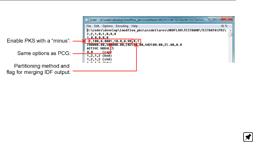
DRAFT
Runfile
To define or change the PKS-solver settings via the iMOD-GUI see section 7.9. For instructions on
how to run a model including the PKS-package, see section 10.21.
10.20.7 Updating from iMOD 3.4 to iMOD 3.6
You can re-use your existing iMOD 3.4-runfile in iMOD 3.6 without any changes.
Note: The use of the SFR-, LAK-, UZF- and MNW-packages in a runfile is not supported; these
packages have to be configured in a so-called project (*.PRJ) file.
10.20.8 Updating from iMOD 3.3 to iMOD 3.4
You can re-use your existing iMOD 3.3-runfile in iMOD 3.4 without any changes.
10.20.9 Updating from iMOD 3.2.1 to iMOD 3.3
You can re-use your existing iMOD 3.2.1-runfile in iMOD 3.3 without any changes.
10.20.10 Updating from iMOD 3.2 to iMOD 3.2.1
The only difference between iMOD 3.2 and iMOD 3.2.1 is that in iMOD 3.2.1 it is possible to use
folder- and filenames including spaces. As a consequence, to be able to re-use your iMOD 3.2-runfile
in iMOD 3.2.1 utilizing spaces in folder- and/or filenames, the folder- and/or filenames have to be
between double quotes.
10.20.11 Runfiles prior to iMOD 3.x
iMOD became open source mid 2014 resulting in the release of iMOD 3.0. Compared to iMOD 2.x
some runfile options are not supported in iMOD 3.x releases; in the tables of section 10.2 to sec-
tion 10.18) these options are denoted as: "Not supported in iMOD 3.x releases".
10.21 Starting a Model Simulation
There are 2 ways to start a model simulation:
1 Inside the iMOD-GUI:
In section 7.9 detailed instructions are given on how to interactively configure the model location,
model grid size and model output, including a description of how to specify necessary settings for
either the PCG-solver or the Parallel Krylov Solver in the ’Solver settings’-tab of the ’Start Model
Simulation’ window.
2 Outside the iMOD-GUI:
By entering the appropriate command manually at the DOS-prompt in a ’Window Command
Processor’-box; an example of such a command is:
d:\iMOD\iMODFLOW_V4_3_METASWAP_SVN1233_X64R.exe model.run
Deltares 583 of 812

DRAFT
iMOD, User Manual
By specifying and storing such a command in a batch-file, e.g. run.bat, and double-clicking
this run.bat file or typing run.bat at the DOS-prompt and pressing Enter.
The content of such a batch file should have the following structure:
On line one: [name of iMODFLOW-executable] [name of the model runfile]
On line two: pause
The Pause-statement causes the command tool to remain visible after the simulation has fin-
ished; this is handy for reasons of inspection in cases you invoke the run.bat file by double-
clicking it; omitting the ’Pause’-statement causes the ’Windows Commander Processor’-box to
close immediately as soon as the model simulation has finished.
When using the PKS-package:
Prior to using the PKS-package MPI software has to be installed, see section 2.3. Here’s
an example of how to start a multi-core model simulation from outside the iMOD-GUI by enter-
ing the following command in a ’Windows Command Processer’-box:
"C:\Program Files\MPICH2\bin\mpiexec.exe" -localonly 2 iMODFLOW.exe iMODFLOW.run
In this example MPI launches two processes of iMODFLOW.exe instances on two com-
putational cores, meaning that the model runs using two subdomains. The -localonly
option ensures that you should not necessarily have to be connected to your network
for running with MPI.
584 of 812 Deltares
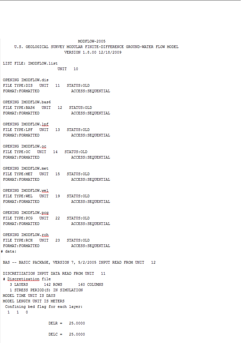
DRAFT
Runfile
10.22 Example Output file
Example output written by iMODFLOW in the iMODFLOW.list-file:
Deltares 585 of 812
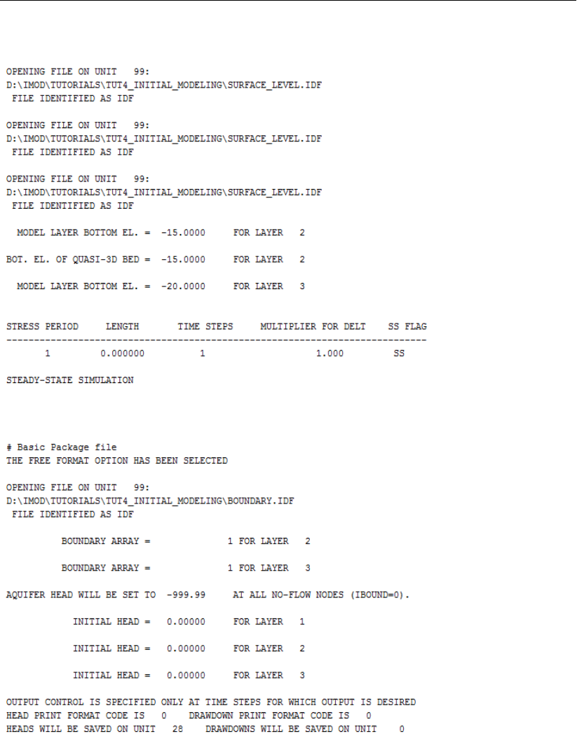
DRAFT
iMOD, User Manual
Example output written by iMODFLOW in the iMODFLOW.list-file (continued):
586 of 812 Deltares
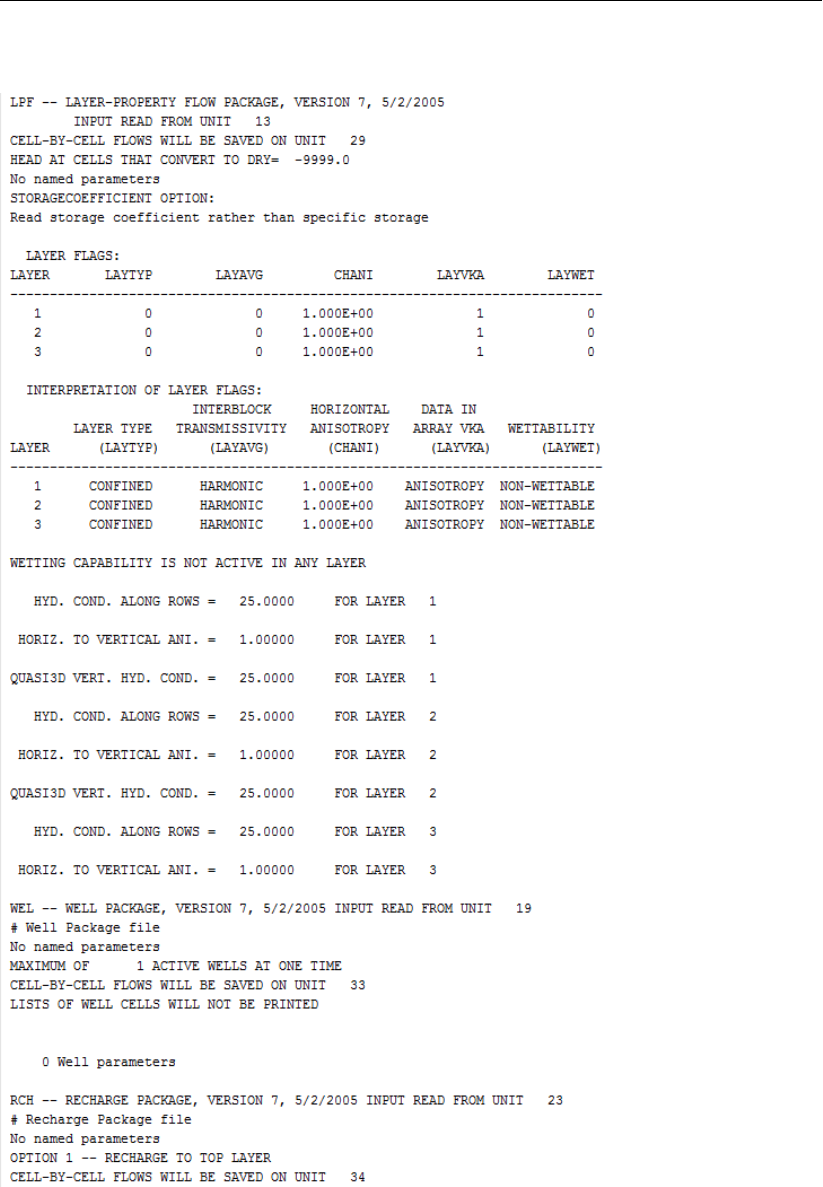
DRAFT
Runfile
Example output written by iMODFLOW in the iMODFLOW.list-file (continued):
Deltares 587 of 812
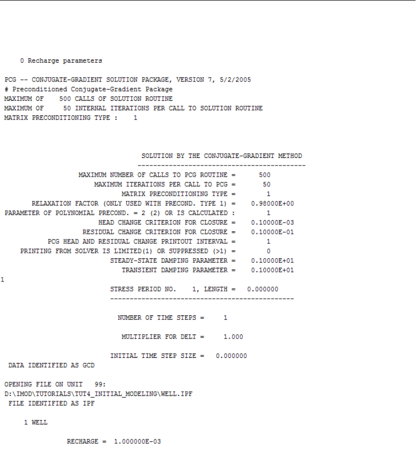
DRAFT
iMOD, User Manual
Example output written by iMODFLOW in the iMODFLOW.list-file (continued):
588 of 812 Deltares
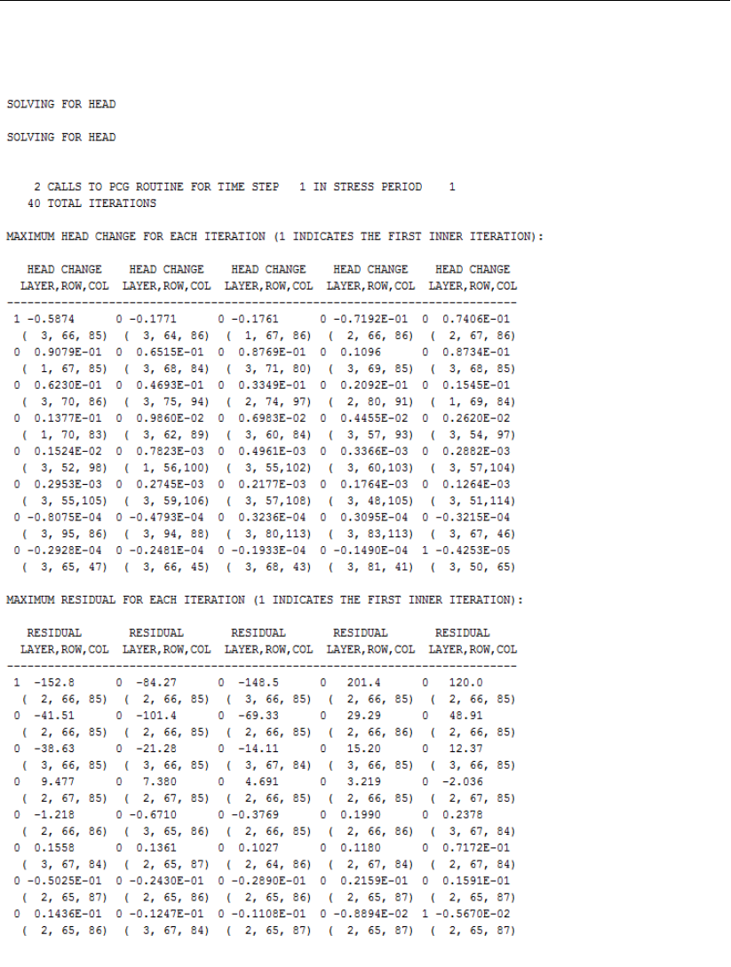
DRAFT
Runfile
Example output written by iMODFLOW in the iMODFLOW.list-file (continued):
Deltares 589 of 812
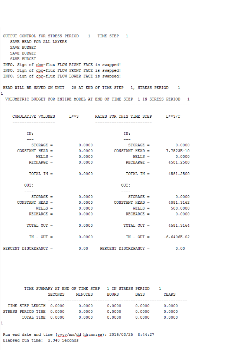
DRAFT
iMOD, User Manual
Example output written by iMODFLOW in the iMODFLOW.list-file (continued):
590 of 812 Deltares
DRAFT
Runfile
10.23 Example Output Folders
The output folder (Data Set 1) is created during a model simulation and all selected results (Data Set
8) are stored in subfolders:
Folder Subfolder* File Content
OUTPUT-
FOLDER
imodflow.list Log file of the entire
model simulation
HEAD head_steady-state_l[ilay].idf Steady-state Head
head_[yyyymmdd]_l[ilay].idf Transient Head
BDGFLF bdg_steady-state_[ilay].idf Steady-state flux
bdg_[yyyymmdd]_[ilay].idf Transient flux
bdg_sys[i]_[yyyymmdd]_[ilay].idf
BDG[pck] [pck]_steady-state_[ilay].idf Steady state
[pck]-information
[pck]_[yyyymmdd]_[ilay].idf Transient
[pck]-information
* see for further details Data Set 8
Deltares 591 of 812

DRAFT
iMOD, User Manual
592 of 812 Deltares

DRAFT
11 iMOD tutorials
This chapter contains the following tutorials:
1 Tutorial 1: Map Display (section 11.1) with exercises on:
Displaying an IDF-file and manipulate its associated legend;
Displaying an IPF file and configure its presentation;
Using the 3-D Tool;
Saving your display configuration.
2 Tutorial 2: Map Operations (section 11.2) with exercises on:
Calculate differences between two IDF-files;
Assign values to an IDF-file, conditionally;
Perform an up- and or downscaling of the cellsize for an IDF-file.
3 Tutorial 3: Map Analyse (section 11.3) with exercises on:
Creating cross-sections over several IDF-files (combined with an IPF file) and manipulate the
configuration;
Computing timeseries out of IDF-files (combined with an IPF file);
Using the 3-D Tool.
4 Tutorial 4: Create your First Groundwater Flow Model (section 11.4) with exercises on:
Creating the basic input files for a simple groundwater flow model;
Enhancing the model with an extraction well to compute the drawdown caused by the well;
Simulating flowlines that describe the catchment area of the well;
Experiment with extraction rates to compute the maximum sustainable yield without extracting
water from the sea.
5 Tutorial 5: Solid Tool (section 11.5) with exercises on:
Visualizing the boreholes in 3D;
Enhancing the subsoil characteristics based on the boreholes using the Solid Tool;
Simulating the updated model to observe the consequences of an aquitard in-between two
aquifers;
Simulating flow of particles.
6 Tutorial 6: Model Simulation (section 11.6) with exercises on:
Understanding the content of a model configuration file, i.e. a runfile;
Simulating a groundwater flow model for different cell sizes and areas of interest;
Understanding the resulting folder structure with results;
Defining a simple model scenario and include such a configuration to an original model config-
uration.
7 Tutorial 7: Interactive Pathline Simulation (IPS) (section 11.7) with exercises on:
Define the starting points interactively;
Change the appearance of the particles;
Start (and stop) the pathline simulation;
Practice the interactive functionalities.
8 Tutorial 8: Surface Flow Routing (SFR) (section 11.8) with exercises on:
Define the model and head- and flux boundaries using the FHB package;
Define the outline of the stream network;
Set the characteristics of each stream and define the connections within the stream network;
Start the SFR simulation and examine the outcome.
9 Tutorial 9: Lake Package (LAK) (section 11.9) with exercises on:
Interpolate a gradually declining interface for the first model layer;
Define a simple, five layered, transient model and constant head boundaries along the model;
Define the input for the LAK package;
Start the model simulation and examine the outcome;
Combine the LAK package with the SFR package.
Deltares 593 of 812
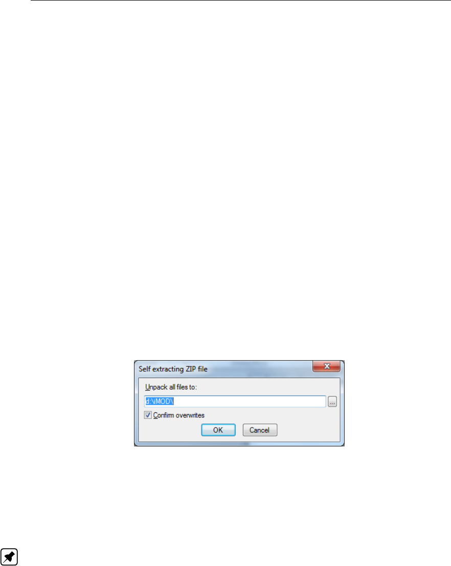
DRAFT
iMOD, User Manual
10 Tutorial 10: Multi-Node Well- (MNW) and Horizontal Barrier Flow (HFB) Package (section 11.10)
with exercises on:
Load an existing modelling project and display the model in 3-D;
Construct a quick and simple modelling project with the WEL package;
Define the model as an unconfined model and simulate the model;
Modify the modelling project with the MNW package and simulate the model;
Inspect both results;
Change some parameters in the MNW package to simulate well losses.
Include the horizontal barrier flow package (HFB) and simulate the results for that configuration.
11 Tutorial 11: Unsaturated Zone Package (UZF) (section 11.11) with exercises on:
Create a transient PRJ file with TOP, BOT, KHV, RCH and EVT package;
Simulate the RCH and EVT package for an unconfined model and examine the results;
Modify the PRJ file with the UZF package;
Simulate the UZF package and examine the results and compare it with the conventional RCH
and EVT model;
Modify the parameters of the UZF package to see the impact of parameters;
The tutorials come with a Tutorial Data Set located in {installfolder} \tutorials; in this manual {in-
stallfolder } \tutorials refers to the full path of the sub-folder . \tutorials, see section 2.2. If the Tu-
torial Data Set subfolder . \tutorials is not present (anymore) on your computer, download it from
oss.deltares.nl. and perform the following steps:
1 Locate the self-extracting archive iMOD_Tutorial_Data_Set_V4_3.exe on your system. If not
available, please download it from http://oss.deltares.nl/web/imod/tutorials.
2 Double-click the archive iMOD_Tutorial_Data_Set_V4_3.exe, the following pop-up window ap-
pears:
3 In the pop-up window choose the destination-folder where you want to unzip the Tutorial Data
Set: you can accept the default {path of installfolder} (e.g. D: \iMOD) by clicking the OK-button, or
choose another location first; after clicking the OK-button the archive will be unzipped.
After the archive has finished self-extracting (it may take a while to extract more than 6600 files...) a
new sub-folder tutorials has been created in the above chosen destination-folder.
Note: In this user manual {installfolder } \tutorials refers to the full path of the newly created tutorials-
sub-folder, e.g. to D: \iMOD \tutorials.
The folder {installfolder} \tutorials contains a sub-folder for each individual tutorial:
. \TUT_Map_Display;
. \TUT_Data_Map_Oper;
. \TUT_Map_Analyse;
. \TUT_Initial_Modeling;
. \TUT_Solid_Building;
. \TUT_Model_Simulation;
. \TUT_IPS;
. \TUT_SFR;
. \TUT_LAK;
. \TUT_MNW;
. \TUT_UZF.
594 of 812 Deltares

DRAFT
iMOD tutorials
11.1 Tutorial 1: Map Display
This tutorial gives a brief introduction to several display options for IDF (rasters) and IPF (points) files.
See for more detailed references chapter 6 and subsections.
Outline
This is what you will do:
Displaying an IDF-file and manipulate its associated legend;
Displaying an IPF file and configure its presentation;
Using the 3D Tool;
Saving your display configuration.
Required Data
For this tutorial you need the following iMOD Data Files (IDF), iMOD Point Files (IPF) and TXT-files to
which the IPF-files are directing:
KR_TCC.IDF;
KR_BCC.IDF;
NAWO_TCC.IDF;
NAWO_BCC.IDF;
BOREHOLE.IPF;
OBSERVATION.IPF;
Folder BOREHOLE that contains seven folders called SUBSET{i} containing files called B{i}.TXT
that represents borehole-logs;
Folder OBSERVATIONS chat contains files called B{i}.TXT that contains values of the timeseries.
All these files are located in the folder: {path of installfolder} \TUTORIALS \TUT_MAP_DISPLAY.
Getting Started
1 If iMOD is not yet installed, please follow the instructions as described in section 2.2.
2 Launch iMOD by double click on the {path of installfolder} \iMOD__V4_3_X64R.exe or
{path of installfolder} \iMOD__V4_3_X32R.exe in the Windows Explorer.
The IMOD_INIT.PRF is the only file that iMOD needs at the initial startup. If it does not exist, iMOD will
create one. The file contains several keywords that are needed by a variety of functionalities in iMOD,
however, the keyword USER is the only one that is obligatory. In the coming up tutorial you’ll notice
that the content of the IMOD_INIT.PRF file will change. Let us examine the current content.
3 Click on the Preferences button.
This displays the Preferences window. On default the keyword [USER] is selected and the path that
is assigned to that keyword is displayed underneath the list box. Probably it shows the folder {path
of installfolder} \IMOD_USER. Several folders will be created in the USER folder. Those folders might
be used by iMOD for different purposes, moreover, during your iMOD sessions new folders could be
created. However, the most important thing you need to remember about the USER folder is that it
stores data created by iMOD, e.g. temporary files, model results and drawings. In this case you might
interpret a USER folder as a project folder as well, e.g. USER D: \IMOD \PROJECT_X.
Okay, let us continue with iMOD.
4 Click on the Apply button.
5 Select the option Create a new iMOD Project from the Start iMOD window and click the Start
button.
An empty graphical window will appear surrounded by a default axes and a scale bar. The initial
Deltares 595 of 812
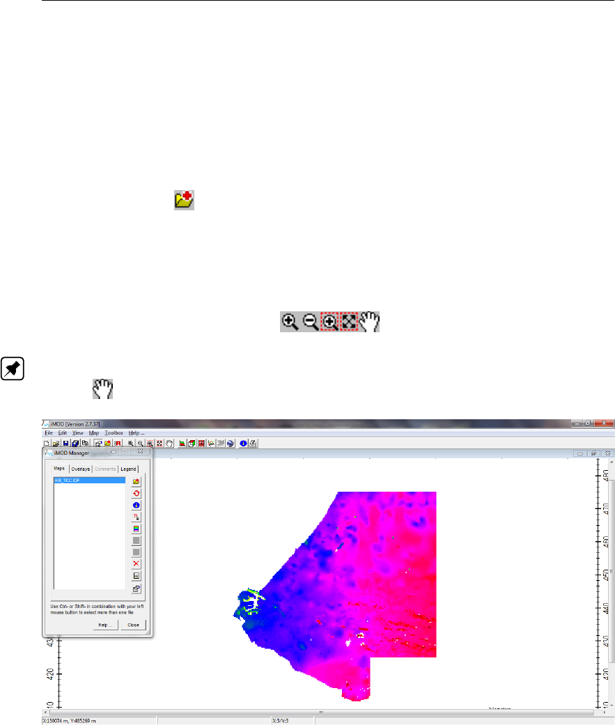
DRAFT
iMOD, User Manual
position of the graphical window is (-1,-1) by (1,1). It is possible to turn off the axes and scale bar, so:
6 Go to View and then choose the option Layout and turn the options Show Scalebar and/or Show
Axes on and off and observe what is happening.
Display of an IDF-file
An IDF-file stores rasterized data, let us open an IDF-file:
7 Go to View in the menu bar and select the iMOD Manager (or use the shortcut Ctrl+M). Select the
Open Map button ( ) and select the IDF-file KR_TCC.IDF and click the button Open. If the file
is not showing up, you might need to change the folder to the appropriate tutorial folder, {path of
installfolder} \tutorials \TUT_MAP_DISPLAY.
Observe that the loaded IDF-file emerges in the iMOD Manager. iMOD will adjust the zoomlevel
automatically to display the entire IDF.
8 Use the zoom buttons on the toolbar ( ) to familiarize with their behaviour.
Note: Please remember that a right-click of the mouse button is necessary to stop moving the map
around ( ).
Figure 11.1: Example of a 2D IDF-view.
Adjust the legend
Each IDF-file that has been loaded into the iMOD Manager will be displayed by a legend with values
that decline linearly between the maximum and minimum values of the IDF-file. A legend is connected
to the IDF internally and can be changed easily.
9 Select the Map option from the main menu, choose the option Current Zoom Level and then choose
the option Percentiles.
By selecting the percentile option, iMOD will compute classes for a legend based on the distribution
of the IDF values, like a duration curve. Since the option Current Zoom Level has been chosen, the
legend will be computed for those values that are inside the current zoom level only.
10 Adjust the legend for the other options (Linear,Percentile and Unique Values) and observe their
596 of 812 Deltares
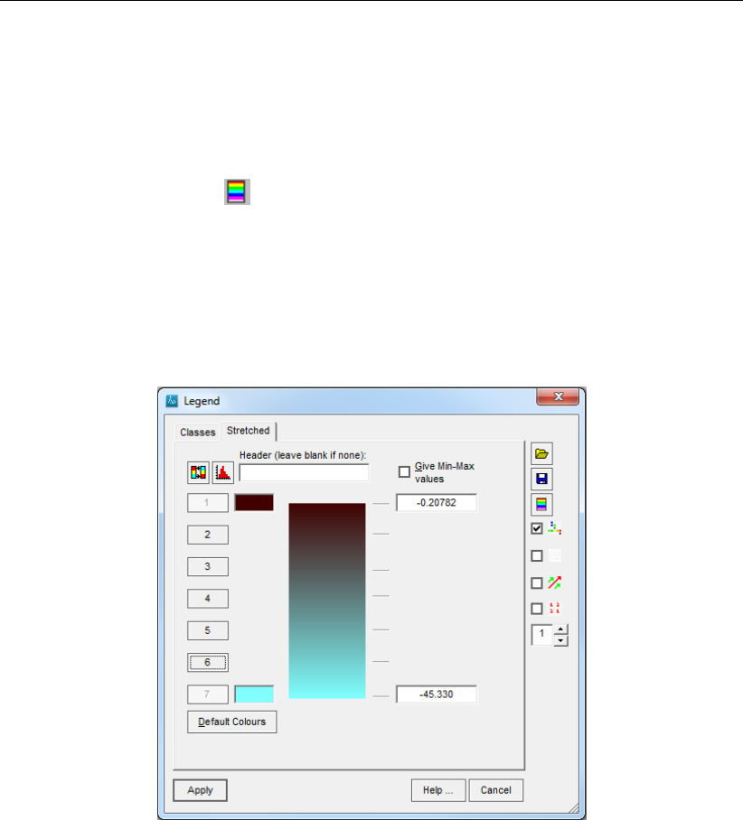
DRAFT
iMOD tutorials
differences in combination with the options Current Zoom Level and Entire Zoom Extent.
11 Click the Legend tab on the iMOD Manager to display the current legend colours and values.
Adjusting a legend like this automatically, is extremely useful whenever the content of an IDF-file needs
to be explored. However, legends can be constructed manually and/or loaded from disk.
12 Click the Legend button ( ) on the Legend tab of the iMOD Manager to display the Legend
window (see section 6.6.1). Make sure you’ve selected the IDF on the Map tab to gain access to
this particular Legend tab.
13 Deselect the numbered buttons on the left that indicate 2,3,4,5and6to turn off their appearance
in the colours used by the legend. Click the Apply button and observe the renewed legend ranging
linearly from dark brown to cyan (light-blue).
In this way it is easy to change the colour range of the legend.
Figure 11.2: Example of a two-coloured legend.
Let’s use more colours in the legend.
14 Reopen the Legend window (step 12) and change the dark brown colour into a red one by clicking
on the coloured field. Include more colours in the legend by selecting the buttons that indicate a
2,3,4,5and/or 6. See the effects for different legends by clicking the Apply button.
iMOD distinguishes two types of legends:
Stretched: a legend that consists of 255 colours and classes that can be specified for 7 levels only;
Classes: a legend that consists of maximal 50 classes and colours that can be specified individu-
ally.
Reopen the Legend window (step 12) again and let us create a legend with 10 classes:
15 Click the Classes tab on the Legend window and give in [10] classes in the Class Definition window
that appears. Check the optionTake classes as-is and click the Ok button.
16 Each row in the table represents a class. Change the values in the first column (Upper) for each
row into [0.0; -5.0; -10.0; -15.0; -20.0; -25.0; -30.0; -35.0; -40.0; -45.0]. Observe that the second
column (Lower) will be adjusted automatically, except for row 10. Change the second column for
Deltares 597 of 812
DRAFT
iMOD, User Manual
row 10 into [–50.0] to specify the lowermost limit of the legend.
17 The column Label will not be updated automatically, this is the text that will be printed next to the
legend. Click the Update Labels button to reflect the entered legend value correctly.
Let’s look at another way of adjusting the legend, more convenient actually.
18 Click the Stretched tab to return to the 255 classes legend and then return back to the Classes
tab. Given in [10] classes and deselect the option Take classes as-isand click the Ok button.
iMOD will try to adjust the number of classes such that a legend is created with nicely legend classes,
automatically. Select the Take classes as-is option whenever you do not want iMOD to create nice,
round classes. Or, alternatively when you do want to have more control on the legends, select the
option Fixed Interval and specify the interval, minimal and maximal values for the legend classes.
19 Click the Save button ( ) to save this legend on disk. Use the Open button ( ) to reload the
legend (this is not necessary of course).
20 Click the OK button to observe the display of the IDF-file with this adjusted legend.
Let us plot a legend on the map
21 Click the Map option from the main menu, choose the Legend option and then choose Plot Legend
on Map.
22 Click the left mouse button inside the legend to change the mouse cursor into a – symbol. Now
the legend can be moved to the desired position.
Select the canvas window with your left-mouse button and observe how the cursor changes when the
mouse is moved to the boundary of the legend.
23 Drag around the legend and reshape its size.
The text size of the legend will be adjusted automatically to fit the boundary box of the legend. Change
the width or height of the legend box in case the label text is not readable.
24 Remove the legend by deselecting the Plot Legend on Map option.
Let us open some more IDF-files.
25 Open the IDF-files: KR_BCC.IDF, NAWO_TCC.IDF, NAWO_BCC.IDF.
26 Select all IDF-files in the Maps tab of the iMOD Manager by dragging the mouse over all files. Or
use the combination Ctrl-left mouse button to select the different IDF-files.
Whenever more than one IDF-file is selected in the iMOD Manager the Legend button will become
inactive. However, the following method can be used to adjust all legends simultaneously.
27 Click the Map option from the main menu, choose the option Legend and then choose the op-
tion Synchronize Legends to display the Synchronize Legends by: window. Select the first IDF
(KR_TCC.IDF) and click the Apply button.
598 of 812 Deltares
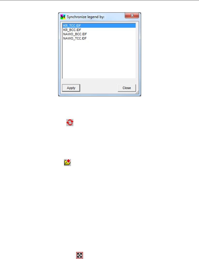
DRAFT
iMOD tutorials
Figure 11.3: Example of the ’Synchronize legend by:’ window.
28 Observe that all IDF-files have identical legends. Select in the iMOD Manager each file sequentially
and click the Redraw button ( ).
Display of an IPF file
An IPF file stores pointwise information, such as boreholes and/or observation wells. Let us open such
a file.
29 Click the Open Map button ( ) and select the file BOREHOLE.IPF.
An IPF file is an iMOD-Point-File and see section 9.7 for more detailed information about the content
of these IPF files. The IPF file that we’ve just opened in iMOD does contain the following information:
X-CRD: X coordinate value of borehole in UTM coordinates;
Y-CRD: Y coordinate value of borehole in UTM coordinates;
ID: Identification name for borehole;
SURFACELEVEL: Altitude of surfacelevel at borehole in m+MSL;
Z_END: End depth of borehole in m+MSL;
I_USED: Attribute specifying whether this particular borehole has been used in building the geo-
logical model.
Be aware of the fact that all of these attributes do not have any direct meaning in iMOD or whatsoever.
In the next steps we will show how these attributes can be used in iMOD.
30 Click the Zoom Full Extent button ( ) on the tool bar to adjust the zoom level such that all points
are displayed.
All points will be plotted as grey dots initially, however, it is easy to change that.
31 Click the Map option from the main menu, choose IPF-options and then choose IPF Configure to
display the IPF Configure window.
iMOD will use the first column of the IPF file (label is X-CRD) for the X coordinate (X-Crd.:) and the
second column (label is Y-CRD) for the Y coordinate (Y-Crd.:). On default, the Z coordinate will be
assigned to the first column, too, which is incorrect.
32 Select the label [SURFACELEVEL] from the dropdown menu at the menu field Z-Crd.:.
iMOD is able to position points in 3D and/or in cross-sections when this Z-Crd.: is assigned properly.
Deltares 599 of 812

DRAFT
iMOD, User Manual
33 Select the option Highlight and select the label [I_USED] in the dropdown menu to the right.
iMOD will increase the symbol and applies a different colour to highlight each point that has values for
the chosen label [I_USED] not equal to zero. This feature can be useful to emphasize specific points
on a map.
34 Click the Pick Colour button to open the standard Windows Colour window.
35 Select the colour cyan (light-blue) from the Custom Colors field.
36 Click the Ok button.
All points will be coloured as cyan (light-blue) in this manner, however, a legend can be used to colour
the points as well, so:
37 Select the option Apply to and choose the label [Z_END] in the dropdown menu.
iMOD will create a legend initially, based on the minimum and maximum values of the label [Z_END].
The legend functionalities as described by step 12-18 can be applied to IPF files too.
38 Click the Colouring and Styles to change the Symbol No. to [21] and the Thickness to [2].
39 Click the Apply button to apply the entered configuration.
40 Click the Close button to close the configuration window.
iMOD will colour all points by their values for the label [Z_END] and highlight those that have values
for [I_USED] that are not equal zero. iMOD will use an inversed colour (i.e. black becomes white, red
becomes light-blue) of the colour used to emphasize the point by a disc around the original point.
Let us adjust the zoomlevel such that we enter coordinates that are the centre of the current zoomlevel.
41 Zoom in onto a particular area by selecting the View option from the main menu and then choose
the option Goto XY. Enter the coordinates [111000.0] and [456000.0] for the X- and Y coordinate,
respectively.
As we used Zoom (m) as [500.0], the zoomlevel will have a minimum width and/or height of about 2 x
500 meter. Let us measure that.
42 Click the Measurement tool ( ) from the tool bar to measure the distances of the current display.
The measured distance can be found at the bottom of the screen in the grey-coloured bar. Break-
off with your right mouse button.
The Measurement tool can be used to identify distances between objects on the map, use the left
mouse button to include more points during the measuring of the distance.
Since we’ve zoomed in, let us place some labels to the points to see the actual values for [Z_END].
43 Click the Labels button on the IPF Configure window (see step 31) to open the Define Label to be
Plotted window. Select the label [Z_END] in the list and turn off the option Use different colouring
for each field. Select a Textsize of 6 and select the option Use Labelname.
Notice that some labels will overlap other labels. iMOD does not support (yet) any advanced labeling
to avoid overlapping. Use the zoom functionalities to avoid overlapping.
44 Try to add more labels, remember that it could be handy, in that case, to display the column names
too, select therefore the option Use Labelname.
600 of 812 Deltares
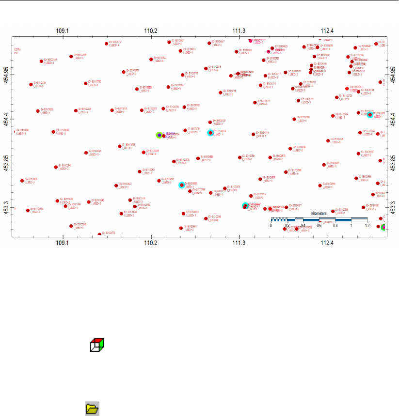
DRAFT
iMOD tutorials
Figure 11.4: Example of plotted labels using the ’Labels’ button of the IPF Configure win-
dow.
45 Turn off all labeling. Use the combination Ctrl-left mouse button to deselect the labels from the
Define Label to be Plotted window (see step 43). You should select the BOREHOLE.IPF in the
iMOD Manager solely to outgrey the IPF Configure option. (Note: before going to step 46 turn on
all labeling again. This is needed for step 51.)
46 Click the 3D Tool ( ) from the tool bar to enter the 3D environment to observe the boreholes.
By default the coloring used to display the boreholes is different than used in this dataset, so we will
load the proper legend file used for displaying the lithology of the boreholes.
47 Click the Load ( ) button on the IPF’s tab on the 3D IDF Settings window and select the
[BOREHOLES.DLF] from the . \TUT_Map_Display folder. iMOD will reload the IPF file and displays
the boreholes according to the legend read from the DLF file. See section 9.17 for more detailed
information about a DLF file.
48 Use your left mouse button to rotate the image and your right mouse button to zoom.
The 3D Tool is simulated by OpenGL libraries and is very powerful; however, the display of borehole
data can take a while to load since all boreholes are stored in individual text files that need to be
processed sequentially. The associated IO consumes most of the time.
49 Check the options Boundary Box and Axes from the Miscellaneous tab in the 3D Plot Settings
window to display the axes and a boundary box.
Deltares 601 of 812
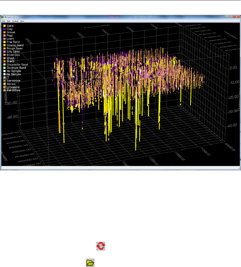
DRAFT
iMOD, User Manual
Figure 11.5: Example of a 3D-display of boreholes.
Let us reshape the representation of the boreholes. As you can notice each borehole represents a
lithology as displayed in the Legend for Boreholes table. This legend can be created inside and/or
outside iMOD; however, the last column expresses the width that will be used to present the corre-
sponding lithology. So, [Clay] is displayed by a smaller width (with=0.25) than [Sand] that has a width
of 1.0.
50 Change the width for different lithologies and even change colours by clicking in the appropriate
column(s). Click the redraw button ( ) to update the 3D image for your inserted changes. For
example you might increase the width for Sand to 2.0 to distinguish the difference between clay
and sand more. Use the Load ( ) button to restore the legend setting to the original values by
selecting the . \TUT_Map_Display folder \boreholes.dlf file.
602 of 812 Deltares
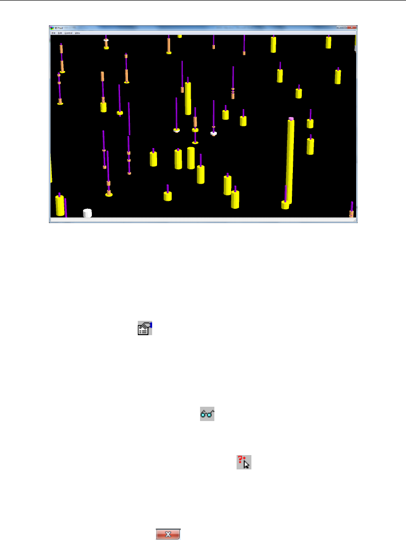
DRAFT
iMOD tutorials
Figure 11.6: Example of using different thickness’s when displaying lithology of boreholes
in 3D.
Alternatively we can change the 3D representation of the borehole.
51 Click the option Plot labels, use following colour to add to the boreholes the label selected in
theDefine Labels to be plotted window.
52 Select the properties button ( ) to enter the Define Labels to be plotted window, turn off the
checkbox Fancy and click the OK button. Observe what has happened. Check the option Fancy
again and see the effects of the options Size,Number of Subdivisions and the option Shade.
Often the number of boreholes is large and therefore we would like to concentrate on those with a
particular bore depth. Let us select only those with a penetration depth of more than 100 meter.
53 In ‘3D Plot Settings‘ in the IPF‘s-tab click the ( ) icon to start the 3D IPF settings dialog. Check
the option Hide boreholes with less penetration depth and enter the value of [100]. Click the Apply
button and observe what happened.
Extra:
54 Select the Identify tab and select the Map Value button ( ) and click on the borehole of interest in
the 3D tool window. The Point Information tab gives an overview of the basic point characteristics of
the selected borehole. The Borehole Information tab displays the specific drill information (including
Lithology and sand-fraction) for each individual layer. Repeat this procedure for different boreholes
by selecting the Map Value button again.
55 Close the 3D Tool by clicking the File option from the main menu and then choose Quit 3D Tool, or
alternatively use the close button ( ).
Let us combine in 3D the boreholes with the top and bottom IDF’s we’ve loaded into iMOD previously.
56 Select in the iMOD Manager all IDF-files together with the BOREHOLES.IPF and enter the 3D
Tool.
You’ll notice that prior to the 3D tool the 3D IDF Settings dialog appears. In this dialog the appearance
of the IDF-files can be configured. For example, an IDF can be represented by planes (quads between
mids of gridcells giving a smooth surface) and/or cubes (representing the gridcells as flat surfaces, like
Lego-blocks). However, any adjustments in this dialog can be made while in the 3D environment as
well, so let us accept the dialog as it is.
57 Click the Apply button.
Deltares 603 of 812
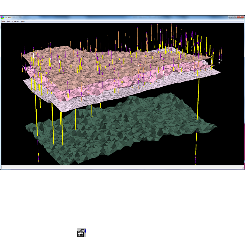
DRAFT
iMOD, User Manual
Figure 11.7: Example of 3D image of a set of planes and boreholes; display depends on
options chosen in the 3D IDF Settings-window.
You’ll see the graphical representation of the surface for the different IDF’s. Another way to do that is
by means of a cross-section (section 11.3). Since the IDF-files represent a clay-body, it is nice to draw
them as solids.
58 Click the properties button ( ) to change the settings used to display the IDF-files.
Each row defines how that particular IDF will be displayed. To make a solid of two IDF-files you should
combine an IDF with another one. The next image shows how the settings should be configured. For
example we combined the IDF-file KR_TCC.IDF (top of the KR-formation) with KR_BCC.IDF (bottom
of the KR-formation) by selecting that file from the dropbox in the third column. Also we changed to
Off the Type in the second column of the KR_BCC.IDF-file. Similarly we adjusted this for the NAWO
formation.
604 of 812 Deltares
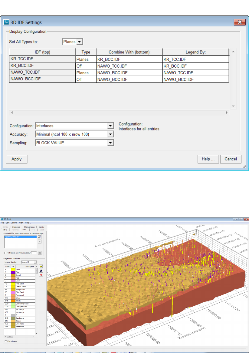
DRAFT
iMOD tutorials
Figure 11.8: Example of a 3D IDF Settings window for displaying pairs of IDF’s as solids.
59 Adjust the 3D IDF Settings window as above, keep in mind that your order of files might be different
yielding a slightly different configuration. Click the Apply button.
Figure 11.9: Example of 3D-image of displaying pairs of IDF’s as solids.
60 Activate and deactivate files from the IDF’s tab on the 3D Plot Settings window. Experiment with
the options Filled,Wireframes and Filled+Wireframes to see the effects and finally place a legend
by checking the Legend checkbox.
61 Experiment with the functionalities on the 3D Plot Settings window. See what you could do with
the Plot Original Window options from the Miscellaneous tab.
62 Close the 3D Tool window (see step 55)
Let us open another IPF file.
Deltares 605 of 812
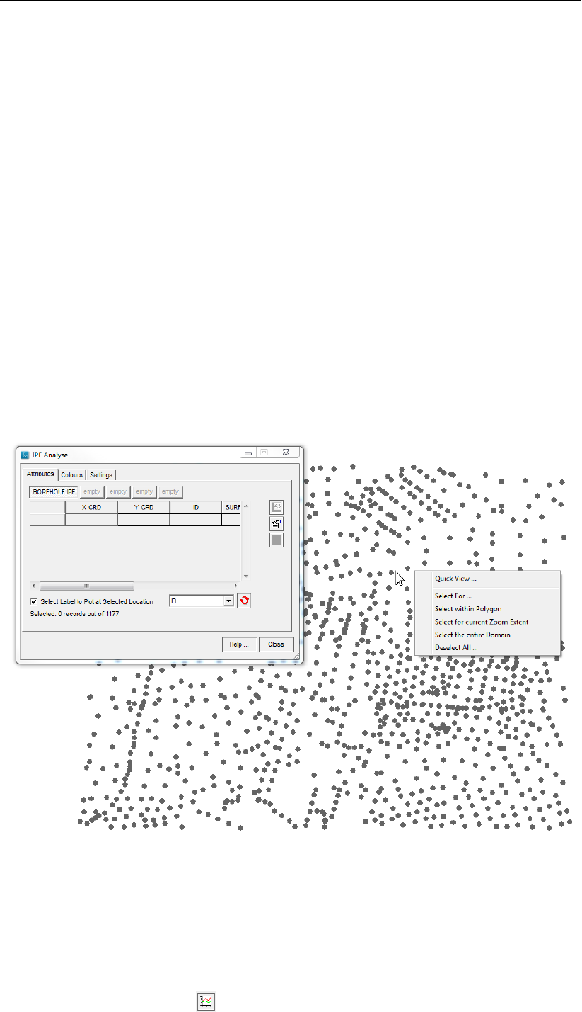
DRAFT
iMOD, User Manual
63 Open the IPF file [OBSERVATION.IPF] and adjust the zoom level to display all points.
All observation points are displayed by a grey circular dot, however, these points have timeseries
associated. Let us look at these associated timeseries.
64 Select the Map option from the main menu, choose IPF-options and then IPF Configure to start
the IPF Configure window.
65 Select the option Labels to start the Define Labels to be plotted window.
66 Place a label named ID at each point (see step 43) by selecting the attribute [ID] from the Select
one or more labels from the menu field and select a Textsize of 6.
By default any “ \” string will be deleted from the ID field, so the ID-string will shorten whenever it will
be displayed on the graphical canvas.
67 Click the OK button to close the Define Labels to be plotted window and click the Close button to
close the IPF Configure window. Observe the results. You might want to change the number of
labels by repeating steps 64 to 66 again.
68 Select the Map option from the main menu, choose IPF-options and then choose the IPF Analyse
option to display the IPF Analyse window.
69 Click the option Select For in the dropdown menu when you right click your mouse button on
the graphical window (see figure below). In the IPF Find window, select the label [ID] next to the
menu field Attrib.:, check theUse following character expression button and enter the Search String:
[*B31D011*].
Figure 11.10: Pop-up window with ’Select For’ option when right-clicking on canvas when
IPF Analyse window is active.
iMOD will find any point that satisfies this search string. Notice that the wildcard is necessary at the
first portion of the search string, since all label IDs start with “observation \”. As a result 2 points will
be selected and displayed in the table on the IPF Analyse window. Both points represent two different
observation screens. Let us display the associated time series.
70 Click the IPF Figure button ( ) in the IPF Analyse window to open the IPF Analyse Figure
606 of 812 Deltares
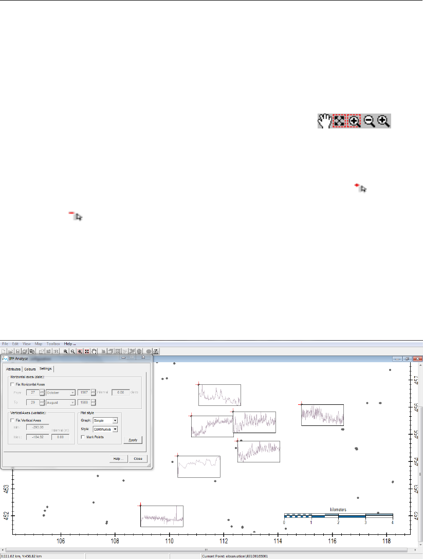
DRAFT
iMOD tutorials
window (see section 6.8 for more information).
Two figures are displayed. Whenever one figure is selected in the Select one/more to plot list, a table
is presented with the actual values for the time series.
71 Select one of the items in the list Select one/more to plot and analyse the content of the table.
72 Select the checkbox Plot all figures in one frame and select both items in the listSelect one/more
to plot. Use the zoom functionalities to analyse the figure in more detail ( ).
73 Quit the IPF Analyse Figure window by selecting the option File and then choose Quit.
Let us look at another way of adding/deleting points from the selection table.
74 Move the mouse over the points and observe that the mouse symbol changes to . It indicates
that when clicking the mouse the particular point will be added to the selection. If the mouse symbol
changes to , it indicates that the particular point will be deleted from the selection.
75 Explore the dropdown menu at your right mouse button to experiment with more options to (de)select
points.
Additionally to the display options of timeseries in the IPF Analyse Figure window, let us plot timeseries
on the map.
76 Select the Settings tab on the IPF Analyse window and select the option [Simple] from the Graph
dropdown menu and click the Apply button.
Figure 11.11: Example of plotted timeseries next to selected points using the option ’Sim-
ple’ from the Graph dropdown menu in the Setting tab of IPF Analyse.
For those points in the selection table on the Attributes tab, their associated timeseries will be plotted
on the map. Each time another point is added or deleted the display is updated.
77 Use your left mouse button on the map to add and/or delete points from the selection table.
Whenever a small crossed-out rectangle is displayed, it means that the associated timeseries for that
point is missing.
78 Click the Close button to stop the IPF Analyse window.
Deltares 607 of 812
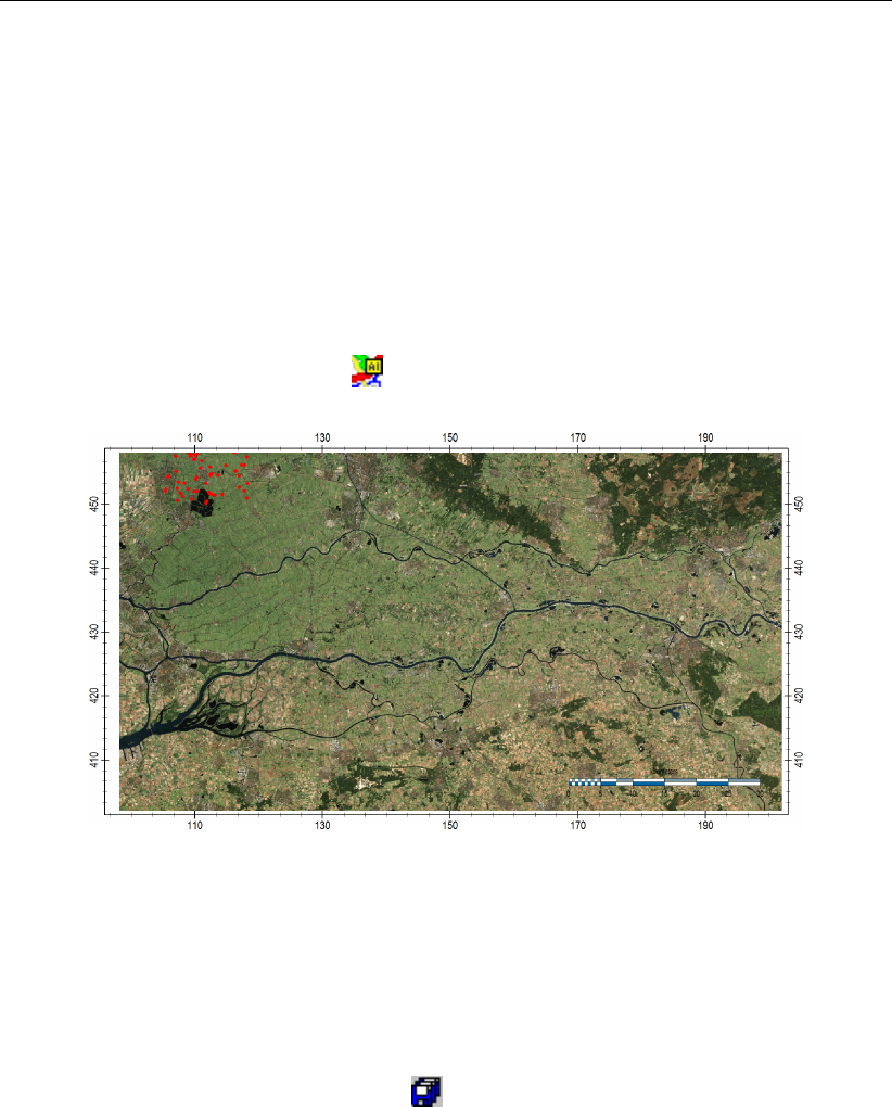
DRAFT
iMOD, User Manual
Whenever the IPF Analyse window is closed, timeseries cannot be plotted on the map anymore.
Show a background image
One of the first things one would like to display is an image of the underlying topography. Let’s do that.
79 Select the option View from the main menu and then select Add Background Image .. from the
dropdown menu. This will start the Add Background Image dialog.
80 Select the option Add from the dialog and select the file
{path of installfolder} \tutorials \TUT_Map_Display \wsrl.bmp from the Windows Explorer, see sec-
tion 5.3 for more information about this dialog.
81 Select the Apply button that closes the dialog.
82 Click the Show Background Image ( ) on the main menu whenever the image does not appear.
Figure 11.12: Example of showing a topographical map (full extent, red dots represent
the observation.ipf).
Save /Open a Display Configuration
The entire configuration of legends and settings for the files that are loaded in the iMOD Manager
can be saved on disk. Whenever iMOD will be restarted, this file can be loaded to recover the iMOD
session again.
83 Click the Save As Current Project button ( ) on the tool bar and enter a name for the file, e.g.
TUTORIAL1.IMF.
The filename entered will be saved in the {USER} \IMFILES folder on default, however, another location
can be entered too. For reasons of efficiency and transferability, it is advisable to store these IMF files
in that particular folder.
Let us quit iMOD now.
84 Click the File option from the main menu and choose the option Quit and confirm this action.
Let us restart iMOD.
85 Repeat step 2in the beginning of this tutorial to launch iMOD.
86 Select TUTORIAL1 from the display list and select the Start button from the Start iMOD window.
As expected, the original iMOD session has been restored.
608 of 812 Deltares

DRAFT
iMOD tutorials
11.2 Tutorial 2: Map Operations
This tutorial gives an introduction to several map operations using IDF-files. See for more detailed
references section 6.7.
Outline
This is what you will do:
Calculate differences between two IDF-files;
Assign values to an IDF-file, conditionally;
Perform an up- and or downscaling of the cellsize for an IDF-file.
Required Data
For this tutorial you need the following iMOD Data Files (IDF):
TOP_LAYER3.IDF;
BOTTOM_LAYER3.IDF;
KD-VALUE_LAYER3.IDF.
All these files are located in the folder:{path of installfolder} \tutorials \TUT_DATA_MAP_OPER.
Getting Started
1 Launch iMOD by double clicking the iMOD executable in the Windows Explorer, and start with
Create a new iMOD Project.
2 Go to View in the menu bar and select the iMOD Manager (or use the shortcut Ctrl+M).
Calculate Layer Thickness
Quite often it is necessary to compute the difference between two maps. In this example we compute
the thickness of a particular model layer. We start by opening the files: TOP_LAYER3.IDF, BOT-
TOM_LAYER3.IDF from disk.
3 Click the Open IDF button ( ) from the Maps tabs on the iMOD Manager. Select the above
mentioned files in the Open File window and click the Open button. Go to the folder where the
tutorial material has been installed.
After the files have been opened, those files will be added to the list of opened iMOD files in the
iMOD Manager. iMOD will draw the first IDF from the list and will zoom to the full extent of that IDF
automatically. The latter will occur only whenever no maps were available in the iMOD Manager.
Let us compute the thickness of model layer 3.
4 Click on the maps TOP_LAYER3.IDF and BOT_LAYER3.IDF as they appear in the iMOD Manager,
while pressing the Ctrl button.
Alternatively, you can select those files by left click your mouse and drag your mouse position over
the files. If necessary, deselect those files that are undesired by clicking your left mouse button in
combination with the Ctrl button.
5 Click on the iMOD Calculator button ( ) on the Maps tab of the iMOD Manager to enter the
Map Operations window.
The selected IDF-files (inputfiles) will be filled in, as well as the outputfile. On default the output
file will be saved in the folder: {USER} \TMP \DIFF.IDF. The default equation (Formulae is [C=A-B])
subtracts the first IDF minus the second IDF, in the order in which those IDF-files will appear in the
Deltares 609 of 812
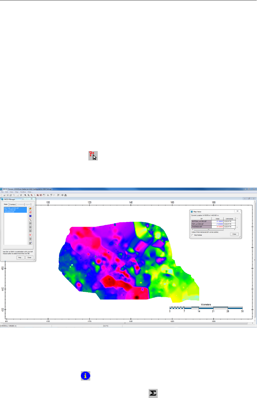
DRAFT
iMOD, User Manual
iMOD Manager. Whenever your BOT_LAYER3.IDF is mentioned before the TOP_LAYER3.IDF in the
iMOD Manager, you have to change the Formulae into [C=B-A].
6 Change the output file DIFF.IDF into THICKNESS3.IDF, so enter this name in the field specified
behind Map C.
7 Select the option Map A. This allows the size of the THICKNESS3.IDF to be exactly the size of the
first mentioned IDF. Whenever you need results for the current zoom extent only, click the option
Window instead, this will speed up the calculation since only a part of the selected maps (Map A
and Map B) will be subtracted.
8 Click the Compute button.
The computed difference between the files TOP_LAYER3.IDF and BOT_LAYER3.IDF will be saved in
the TMP folder of your USER environment by the name THICKNESS3.IDF. iMOD has added that file
to the iMOD Manager, automatically.
Let us check the result.
9 Select the maps TOP_LAYER3.IDF, BOTTOM_LAYER3.IDF and THICKNESS3.IDF from the iMOD
Manager.
10 Select the Map Value button ( ) on the Map tabs on the iMOD Manager window to start the
Map Value window. Check the results by moving your mouse around the graphical display. Stop
this inspection by rightclicking your mouse somewhere on the graphical display.
Example of the use of the ’Map Value’ button when moving the mouse over the canvas.
Since this kind of visual inspection is rather easy to use, it is recommended to use it frequently to check
any computations.
11 Select the Map Info button ( ) to inspect some simple statistics for THICKNESS3.IDF. Observe
that the history of the THICKNESS3.IDF is saved and that the content is shown in the Additional
Information box. Moreover click the Statistical button ( ) to get some statistical characteristics
of the data.
610 of 812 Deltares
DRAFT
iMOD tutorials
Calculating Permeability
Each resulting IDF can be used subsequently for other map operations.
12 Open the T-VALUE_LAYER3.IDF (or KD-VALUE_LAYER3.IDF in older Tutorial sets) by clicking the
Open IDF button ( ) and select this file from the {path of installfolder}\tutorials \TUT_DATA_MAP_OPER.
13 Select the maps T-VALUE_LAYER3.IDF (or KD-VALUE_LAYER3.IDF in older Tutorial sets) and the
THICKNESS3.IDF from the iMOD Manager.
14 Select the IDF Calculator ( ) and change for Map C the IDF-file DIFF.IDF into K-VALUE_LAYER3.IDF.
15 Enter the formula: [C=A/B].
All values in Map A (will be KD-VALUE_LAYER3.IDF) will be divided by the values of Map B (THICK-
NESS3.IDF). If map A and map B are reversed, the equation can be entered as [C=B/A] without
interchanging the IDF name next to the field Map A and Map B.
16 Select the option Window and click the Compute button; in this manner we will compute the per-
meability only for the current zoom extent.
To decrease computational times, map operations can be computed for the current zoomlevel on the
graphical display only. The resulting IDF will have dimensions equal to the zoom level, however, cell-
sizes will be copied from the first mentioned IDF in the equation.
17 Check the result again with Map Value ( ).
Bear in mind that the computed legend classes are initially based on the minimum and maximum
values of the IDF-file(s). Whenever you do not see much detail on the map, those minimum and
maximum values might be far apart from each other. Use the Percentile legend (by clicking on: in
the Stretched tab) for more detail on the values of the data. Looking at this graph can provide you with
more insight in the color distribution of your legend.
Conditioned Map Operation
IDF Edit is a tool in which map operations can be applied for a particular selection of cells. In this
tutorial a simple example is demonstrated. Suppose a map is required that shows all areas of the third
model layer that have a thickness of more than 25 meter.
First we make an empty copy of THICKNESS3.IDF and name it THICKNESS3_25.IDF.
18 Enter the Map Calculator with THICKNESS3.IDF, enter the equation [C=0.0*A] and enter a file-
name for Map C to be THICKNESS3_25.IDF.
By means of the Map Calculator it is easier to make copies of IDF-files, rather than using the Windows
Explorer, since the content can be blanked out and/or the resulting IDF can be resized (use the option
Window or the optionx1,y1,x2,y2 where you can specify specific coordinates yourself).
Next step is to enter IDF Edit.
19 Select the option IDF Edit from the IDF Options menu from the Map menu.
It is not relevant what IDF is (de)selected in the iMOD Manager, since all IDF-files that are inside the
iMOD Manager can be manipulated in IDF Edit.
Important is to specify an IDF that operates as a template. All mids of raster cells inside that particular
IDF will be used to store any selection. Please be aware of the fact that a coarse IDF used as a
template, will not make adjustments to a finer IDF.
Deltares 611 of 812
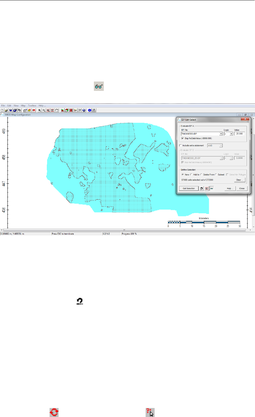
DRAFT
iMOD, User Manual
20 Select THICKNESS3_25.IDF from the dropdown menu Use selected IDF to store selected cells.
21 Click the Select button to open the IDF Edit Select window.
22 Select the IDF-file THICKNESS3.IDF from the dropdown menu by Evaluate IDF A: and specify the
Logic operator to be [>] and enter a Value to be [25].
23 Click the Get Selection button and observe that 97088 cells are selected.
The current selection will be displayed as filled rectangles. Especially whenever a large selection need
to be displayed it can take a while.
24 Click the option Show Selection ( ) to turn the selection on or off.
Figure 11.13: Example of displaying the selected grid cells using the ’Show Selection’
button in the ’IDF Edit Select’ window.
A selection is stored on disk in the {USER} \tmp folder. For iMOD-user a specific filename will be used,
{USERNAME}_selected{i}.dat. These files will store the current (i) and previous selections (i-?). As
long as these files exist, iMOD can undo a selection.
25 Click the Undo Selection ( ) button to reset the selection. Repeat step 20 to 22 again to restore
the selection.
26 Close the IDF Edit Select window and click the Calculate button in the IDF Edit window to open
theIDF Edit Calculation window.
This window offers several functions to adjust values in IDF-files of the current selection.
27 Select the option Take From and select THICKNESS3.IDF from the dropdown menu.
28 Select the THICKNESS3_25.IDF from the dropdown menu at the menu field Assign Value TO.
29 Click the Calculate button.
The iMOD Manager can be used whenever the IDF Edit Calculate window is active. Let us check
whether the computation has been carried out correctly.
30 Select the maps THICKNESS3.IDF and THICKNESS3_25.IDF in the iMOD Manager, click the
redraw button ( ) and click the Map Value button ( ). Inspect the values.
As long as the IDF Edit Calculation window is active, any computation to any IDF can be undone.
612 of 812 Deltares
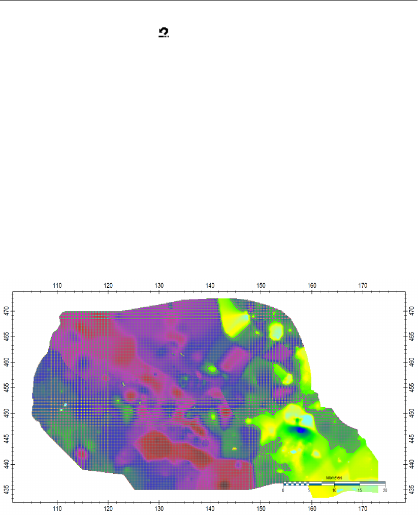
DRAFT
iMOD tutorials
31 Click the Undo Calculation button ( ) in the IDF Edit Calculation window to undo the computation.
Repeat step 29 to compute the values again.
32 Click the Close button and confirm the next window.
Let us see what other method can be used to make a selection and/or calculation.
33 Clear the current selection by clicking the Clear button in the IDF Edit window. Accept the following
window stating whether you’re sure to delete the selection.
34 Click the Trace button and select the option [Greater than selected value] in the Values should
be option. Leave the option Search Criterium selected for [5 Point] which means that iMOD will
search connecting cells that are connected on a five-point stencil. Use the option [9 Points] to use
diagonal connected cells too.
This option allows you to make a selection that is determined by the location that you will select on
the graphical window for all cells that have values greater than the value at the selected point. The
selection should be connected to each other which makes it quite different from the previous selection
method. Let us do that.
35 Select a cell from which a selection should be made that have greater values. Click your left mouse
button. Please note that it may take a while to get the selection.
Figure 11.14: Example of displaying selected cells using the Trace option.
Finally we can adjust the current selection by means of a drawing functionality that allows you to
interactively draw regions to add to the selection and/or remove from the current selection.
36 Select the Draw option in the IDF Edit window and choose option Remove Cells from the IDF Edit
Draw window. Move over the cells you want to remove by holding down your left mouse button.
Observe what is happening, try to add cells to the selection too.
37 Click the Close button and finally close the IDF Edit window by clicking its Close button too.
Map Scaling
One of the great options of iMOD is its ability to rescale data files. A variety of up- and downscaling
algorithms have been implemented. In this example we will rescale the top elevation of a model layer
from a cell size of 100 x 100 meter into a cell size of 1000 x 1000 meter.
38 Select the map TOP_LAYER3.IDF from the iMOD Manager.
Deltares 613 of 812
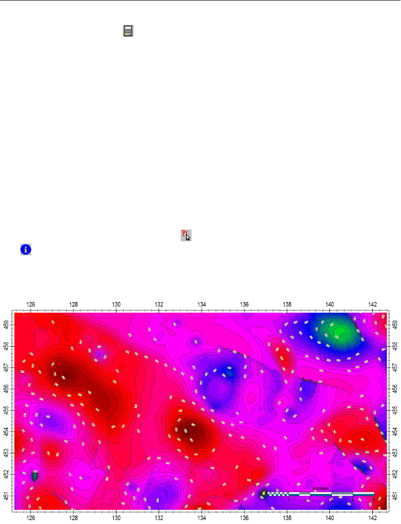
DRAFT
iMOD, User Manual
39 Enter the Map Calculator ( ) and select the Scale/Size tab.
On this particular tab, a variety of up- and downscaling options are available by the menu fields Upscale
Formulae and Downscale Formulae.
40 The resulting IDF will be saved in the same folder as the TOP_LAYER3.IDF and will be called
TOP_LAYER3_SCALED.IDF. We accept this default output name.
41 Enter a gridsize of 1000 meter in the Scale field.
As a consequence, all resulting IDF-files from up- or downscaling will become IDF-files with equidistant
cellsizes.
42 Select the option Arithmetic Mean from the Upscale Formulae menu. Click the Compute... button.
This formula takes the arithmetic mean for all values that lie inside a coarsened raster of the resulting
IDF-file.
43 Observe the values of the TOP_LAYER3.IDF in relation to the scaled version TOP_
LAYER3_SCALED.IDF. Use Map Value ( ) and inspect the Additional Information in Map Info
( ).
Experiment with different Formulae for up- and downscaling.
Figure 11.15: Contour map of the original THICKNESS3.IDF-file (cell size 100x100 me-
ter).
614 of 812 Deltares
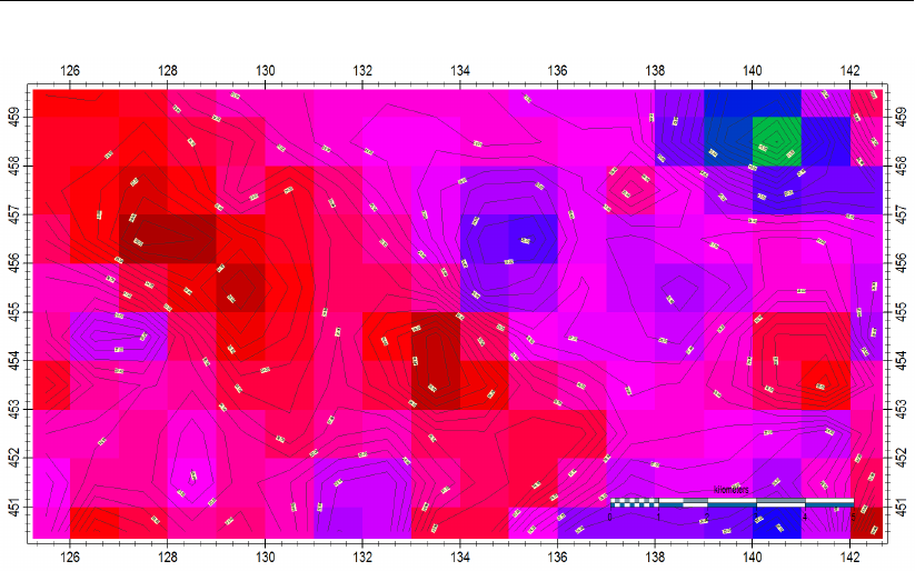
DRAFT
iMOD tutorials
Figure 11.16: Contour map of the upscaled THICKNESS3_SCALED.IDF-file (cell size
1000x1000 meter).
Deltares 615 of 812

DRAFT
iMOD, User Manual
11.3 Tutorial 3: Map Analyse
This tutorial gives a brief introduction to several options to visualize and analyse the content of IDF
(raster) files. See for more detailed references section 7.1 (Cross-Section Tool), section 7.2 (Time-
series Tool) and section 7.3 (3D Tool).
Outline
This is what you will do:
Creating cross-sections over several IDF-files (combined with an IPF file) and manipulate the con-
figuration;
Computing timeseries out of IDF-files (combined with an IPF file);
Using the 3D Tool.
Required Data
For this tutorial you need the following iMOD Data Files (IDF):
Folder HEAD that contains HEAD_*_L1.IDF-files that represent transient model results;
Folder SUBSOILSYSTEM that contains SURFACE_LEVEL.IDF and HYDROLOGICAL_
BASE.IDF that represent the top and bottom elevation of the modeled hydrological system. In-
between there are 6 aquitards distinguished that are described by their top and bottom elevations,
called TOP_SDL{i} and BOT_SDL{i}, respectively for each of the 6 aquitards. Moreover, a subfolder
called BOREHOLES containing borehole information stored in the file BOREHOLES.IPF
Folder OBSERVATION that contains the file OBSERVATION.IPF representing several synthetic
measurements.
All these files are located in the folder: {path of installfolder} \tutorials \TUT_MAP_ANALYSE.
Getting Started
1 Launch iMOD by double click on the iMOD executable in the Windows Explorer, and start with
Create a new iMOD Project.
2 Go to View in the menu bar and select the iMOD Manager (or use the shortcut Ctrl+M).
Cross-Section
Let us start by creating a cross-section that visualizes the subsoil system as described by the data
stored in the folder SUBSOILSYSTEM.
3 Open all IDF-files that are located in the SUBSOILSYSTEM subfolder of the folder {path of install-
folder} \tutorials \TUT_Map_Analyse. Click the Open IDF button ( ) from the Maps tabs on the
iMOD Manager. Select the IDF-files in the Open File window and click the Open button.
All files will appear in the iMOD Manager, they will be ordered similar to the order in which they
appeared in the Windows Open File window. Whenever the Cross-Section Tool is used to visualize
the subsoil system it is important that IDF-files are arranged such that internal values are higher for
IDF-files that appear higher in the list. Let us change the order of the files in the iMOD Manager.
4 Select the file HYDROLOGICALBASE.IDF from the iMOD Manager and click the button ( )
sequentially until the file is at the bottom of the list. Select the file SURFACE_LEVEL.IDF and click
the button ( ) sequentially to put the file on top of the list.
Now we should arrange the TOP_SLD{i} and BOT_SLD{i} properly.
5 Select all TOP_SLD{i} files simultaneously in the iMOD Manager and press the button ( ) to
move them all together direct below the SURFACE_LEVEL.IDF. Now deselect the file TOP_SLD1.IDF
616 of 812 Deltares
DRAFT
iMOD tutorials
by clicking the Ctrl-key and your left mouse button simultaneously. Now press the button ( ) to
move all files directly below the file BOT_SLD1.IDF.
It is important to place the IDF-files in the right order and to put together the top and bottom of each
layer. Also, you can arrange files simultaneously by selecting them. It is faster to select multiple files
and move them downwards to move the file underneath upwards.
6 Use the Map Value ( ) to inspect whether all files are arranged in the proper sequence.
Let us now make a cross section of the subsoil.
7 Select all IDF-files from the iMOD Manager and select the option Toolbox and select the option
Cross-Section Tool, or, click alternatively, the Cross-Section Tool button ( ) from the main tool-
bar.
iMOD will display an empty graphical canvas, called the iMOD Cross-Section CHILD window, since no
cross-section has defined yet. Let’s start drawing the location of the cross-section.
8 Click the Draw Line of the Cross-Section button ( ) and left click your mouse button somewhere
in the Draw Cross-Section window. Now move your mouse and you’ll notice that the cross section
will be built up automatically and will be refreshed each time you move your mouse. Right click
somewhere else on the Draw Cross-Section window to store the line.
Whenever you move your mouse in the iMOD Cross-Section CHILD window, you’ll notice a circle on the
line of the cross-section that directs to the current location in the cross-section. Once a cross-section
has been drawn, you can adjust/manipulate it, let’s do that.
9 Move your mouse in the neighbourhood of the cross-section line in the Draw Cross-Section window.
Click your left mouse button whenever the mouse symbol changes to . You can drag the current
location of the cross-section.
10 Release the left mouse button and move towards one of the ends of the cross-sectional line. Press
the left mouse button as soon as the symbol changes to . Move the mouse and watch that
you can change the start- and/or end-location of the line.
Let’s change the configuration of the cross-section, so our aquitards will be filled by different colours
and our aquifers will become yellow.
11 Click the Cross-Section Properties button ( ) on the Draw Cross-Section window to display the
Cross-Section Properties window for a more detailed description of its functionalities.
12 Click the option Block Lines to display the cross-section with lines that represent the true values
and extent of the grid cells, rather than connecting grid cell mids. Click the OK button to observe
the effects.
13 Re-open the Cross-Section Properties window.
14 Click the checkbox of the fifth column (Line) in the first row (Label is Adjust all) twice. Once to
select it and then to deselect it. All rows underneath will become unchecked.
15 Click the checkbox of the seventh column (Fill) in the first row to check all rows underneath.
16 Click the first inputfield of the fourth column (Colour ) and select a yellow colour from the default
Colour window. All rows become yellow in this way.
17 Click the inputfield for the fourth column (Colour) for the third row (Label=TOP_SLD1.IDF) and
change the colour into, let’s say, green. Repeat this for TOP_SLD2.IDF, TOP_SLD3.IDF, TOP_SLD4.IDF,
TOP_SLD5.IDF and TOP_SLD6.IDF. Give a grey colour to the HYDROLOGICALBASE.IDF. Click
the OK button and observe the result.
Since this can be quite laborious, iMOD facilitates several display configurations that configure the
table assuming the IDF-files are ordered in a particular manner (see section 7.3.1). For this set of IDF
files you might use the one below.
Deltares 617 of 812
DRAFT
iMOD, User Manual
18 Choose the configuration Quasi 3D model (aquitard) from the dropdown menu. Turn off the Block
Fills to have a smoother surface. Check the differences with or without this feature.
19 Click the OK button to close the Properties window.
As you might observe, the cross-section gives a clear image of the subsurface. Moreover, the settings
we just applied in the steps 11 until 19 are stored internally. Whenever you leave the Cross-Section Tool
and re-enter it, these settings remain intact, except for the coordinates of the cross-section. Whenever
you would like to re-use the same coordinates save them in the Miscellaneous tab on the Cross-Section
Properties window, or alternatively save the last drawn cross-sections as a Demo-IMF (see section 7.1
for more information on this).
Let us try it.
20 Leave the Cross-Section Tool by clicking the Close button on the Draw Cross-Section window, or
press the symbol ( ) on the top-right of theiMOD Cross-Section CHILD window.
Let’s us include some boreholes in the cross-section of the subsoil.
21 Open the file BOREHOLES.IPF from the folder {path of installfolder} \tutorials \TUT_MAP_
ANALYSE \SUBSOILSYSTEMS \BOREHOLES
22 Select this file together with all other files before entering the Cross-Section Tool (step 7).
23 Draw a cross-section (step 8) and insert some extra points by clicking your left mouse button, while
drawing the cross-sectional line. Observe that all settings are still intact and a vertical dashed line
is drawn at the intermediate points. Moreover, all boreholes that are within a close range to the
cross-sectional line, are projected perpendicular on the cross-section.
We need to tell iMOD to use a different colour legend for plotting the boreholes, just like we did in 11.1.
24 Click the Properties button ( ) on the Draw Cross-Section window.
25 Select the tab Colouring on the Cross-Section Properties window and click the Open DLF button
( ). Select the [BOREHOLES.DLF] from the . \TUT_MAP_ANALYSE folder and click the Open
button.
iMOD will redraw the cross-section using this renewed legend and will use this legend during your
iMOD session.
618 of 812 Deltares
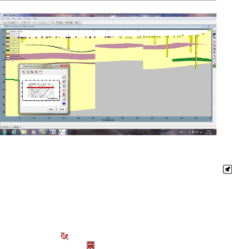
DRAFT
iMOD tutorials
Figure 11.17: Example of interactively generating a vertical cross-section of a 3D subsur-
face including boreholes.
Note: Boreholes within a user-specified horizontal distance from the cross-section are projected on
the vertical cross-section; this specified distance is visualised by the thickness of the trajectory of
the cross-section (red line) in the ’Draw Cross-section’ window. While drawing the trajectory of the
cross-section in the ’Draw Cross-section’ window, the vertical cross-section through the subsurface is
updated in the ’Cross-Section CHILD’ window simultaneously; when dragging an existing trajectory,
the cross-section is updated as soon as the left mouse button is released.
26 Try to apply the zoom functionalities on the right of the iMOD Cross-Section CHILD window, and
those located on the Draw Cross-Section window.
27 Close the Cross-Section Tool (see step 20).
You can use the flip button ( ) to rotate your cross-section clock-wise. Another option is to analyse
the cross-section with the Movie button ( ). This option might be helpful if you would like to analyse
e.g. the spatial variability of your vertical cross-section.
3D Tool
The next step is to analyse these data in the 3D tool.
28 Click the 3D Tool icon in the menu bar.
29 Now you’re in the 3D IDF Settings dialog. Select the same display configuration from the configu-
ration dropdown menu as you did in the Cross-Section tool (see step 18).
30 Observe the contents of the Display Configuration and try to understand what happened. Click the
Apply button. You should see an image similar to the figure below. You can, of course, change all
settings in the 3D IDF Settings window.
Deltares 619 of 812
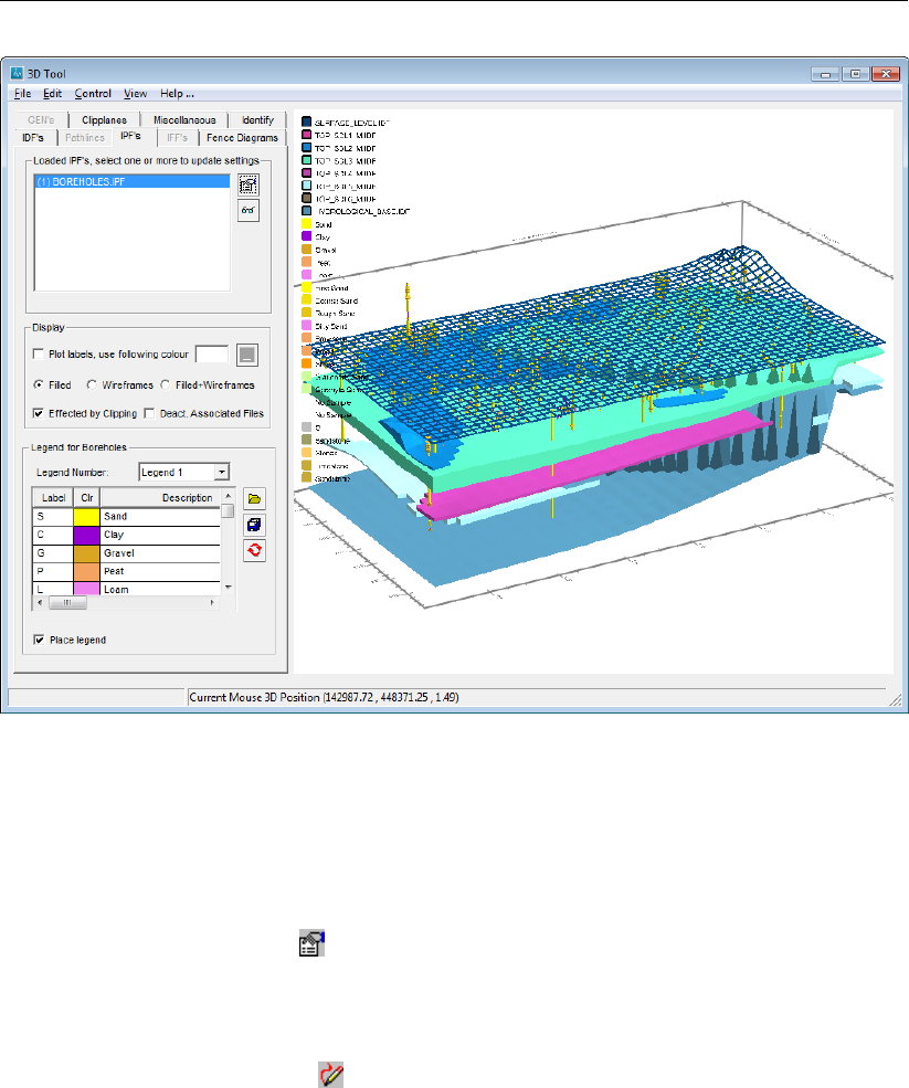
DRAFT
iMOD, User Manual
Figure 11.18: 3D Tool view of the subsurface and borehole data used in the previous 2D
cross-section exercise.
Let’s experiment with the fence-diagrams and clipping planes functionalities. First we switch to a 3D
solid model.
31 Select the IDF’s tab from the 3D Tool window.
32 Select the properties button ( ) to open the 3D IDF Settings window.
33 Select the option [3D Model] from the dropdown menu at the field Configuration.
34 Click the button to close the 3D IDF Settings window.
35 Select the lower most IDF file called HYDROLOGICALBASE.IDF.
36 Select the Fence Diagram tab from the 3D Tool window.
37 Select the option Draw button ( ).
In this mode, you’re able to actually draw a line on the 3D graphical canvas. If you move your mouse
into that area, a red vertical line appear and a red dot. The red dot is the actual position of your
mouse on the 3D image (actually the HYDROLOGICALBASE.IDF) and the x-,y- and z-coordinates are
presented in the window status bar.
38 Click your left mouse button somewhere left, in the deeper part of the HYDROLOGICALBASE.IDF.
39 Now move your mouse button to the right and observe that a red rectangle will be drawn showing
the actual position of the fence diagram.
40 Click your left mouse button to insert an additional knick-point somewhere half-way the left- and
right utmost boundaries of the image.
41 Click your left mouse button somewhere in the right.
42 Click your right mouse button to stop drawing, the fence diagram will be computed as displayed
directly.
Well, that’s no too bad. Try to add another fence-diagram, the following figure shows what the result
might be.
620 of 812 Deltares
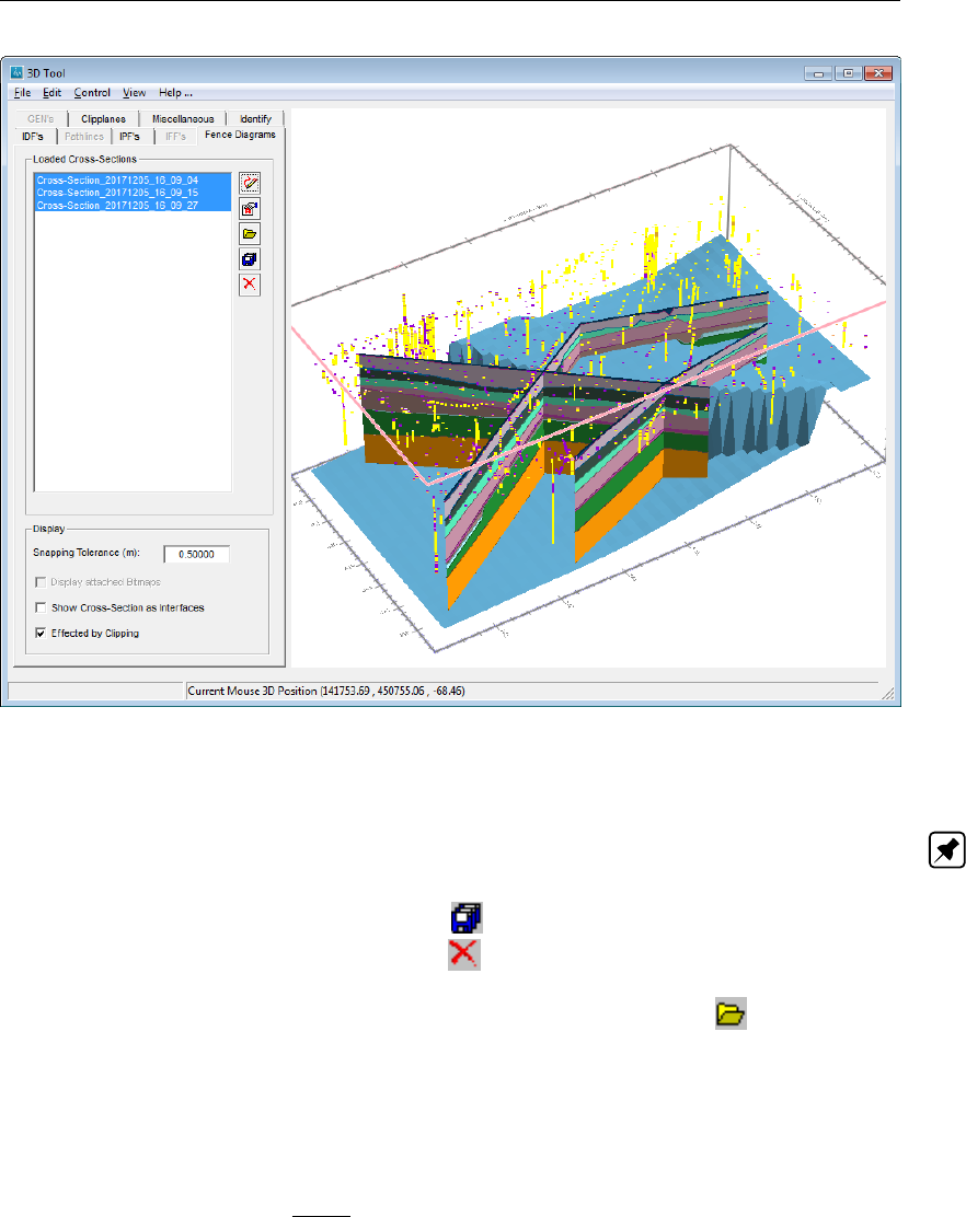
DRAFT
iMOD tutorials
Figure 11.19: 3D Tool view of the subsurface and borehole data after drawing a fence
diagram interactively.
Note: The colours in the fence diagram are the colours assigned to the individual IDF files; you can
each of them individually via the IDF’s tab.
43 Save all cross-section via the option Save As ( )
44 Delete all cross-section via the option Delete ( )
45 Click Yes to confirm to remove the cross-sections.
46 Load in again some of the cross-sections via the open Open Cross-section ( ).
Remember that these cross-section file can be (re) used by the Solid Tool (see Tutorial 5, section 11.5).
Let’s apply some clipping planes.
47 Deselect the option Effected by Clipping on the Fence Diagram tab from the 3D Tool window.
48 Select the IDF’s tab again from the 3D Tool window.
49 Select all the listed IDF files, except the last one called HYDROLOGICALBASE.IDF.
50 Select the option Filled+Wireframes to emphasize the top of the IDF files.
51 Select the Clipplanes tab from the 3D Tool window.
52 Select the entry [ClippingPlane West] from the Available Clipplanes field.
53 Use the slider at the entry field West to move the clipping plane from the western border to the
eastern boundary.
Observe that once the clipping is active the subsurface model is torn open and it is possible to look
into it. To avoid that it is possible to fill those openings with a solid colour. This is called capping.
54 Select the option Capping from the Clipplanes tab.
For each entry in the 3D Tool, it is possible to exclude clipping. Let us do that.
Deltares 621 of 812
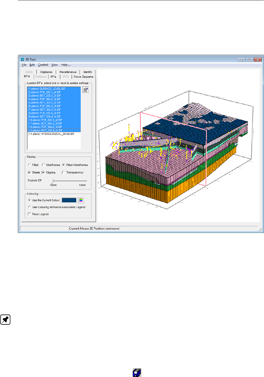
DRAFT
iMOD, User Manual
55 Select the IDF’s tab one more time from the 3D Tool window.
56 Select the IDF files 7 up to 13.
57 Deselect the Clipping checkbox.
58 Select all entries again (except the last one).
Figure 11.20: 3D Tool view of the subsurface and borehole data after drawing a fence
diagram interactively.
That’s pretty fancy, so we can exclude the boreholes from the clipping as well.
59 Select the IPF’s tab from the 3D Tool window.
60 Deselect the Effected by Clipping checkbox.
61 Select the Clipplanes tab from the 3D Tool window.
62 Move the West slider to see what happens.
Note: iMOD uses a technique to count how many time pixels are drawn in order to decide whether
that position need to be capped. If the number of IDF files is uneven, this might cause some undesired
interferences. Also if you activate more than one clipping plane in combination with capping. Try that
to see what happens.
Okay, that is enough in 3D, let’s go back.
63 Close the 3D Tool by selecting File from the main menu and then Close 3D Tool.
64 Click the Save As Current Project button ( ) on the Map Menu bar and enter a name for the
file, e.g. TUTORIAL3.IMF. All settings for the cross-section will be saved into the TUTORIAL3.IMF
for later use.
Timeseries
Let’s draw some timeseries interactively. In iMOD you need to open just one IDF-file that contains
specific information about a date in its name notation, such as *_20101231_* to express the 31th of
622 of 812 Deltares
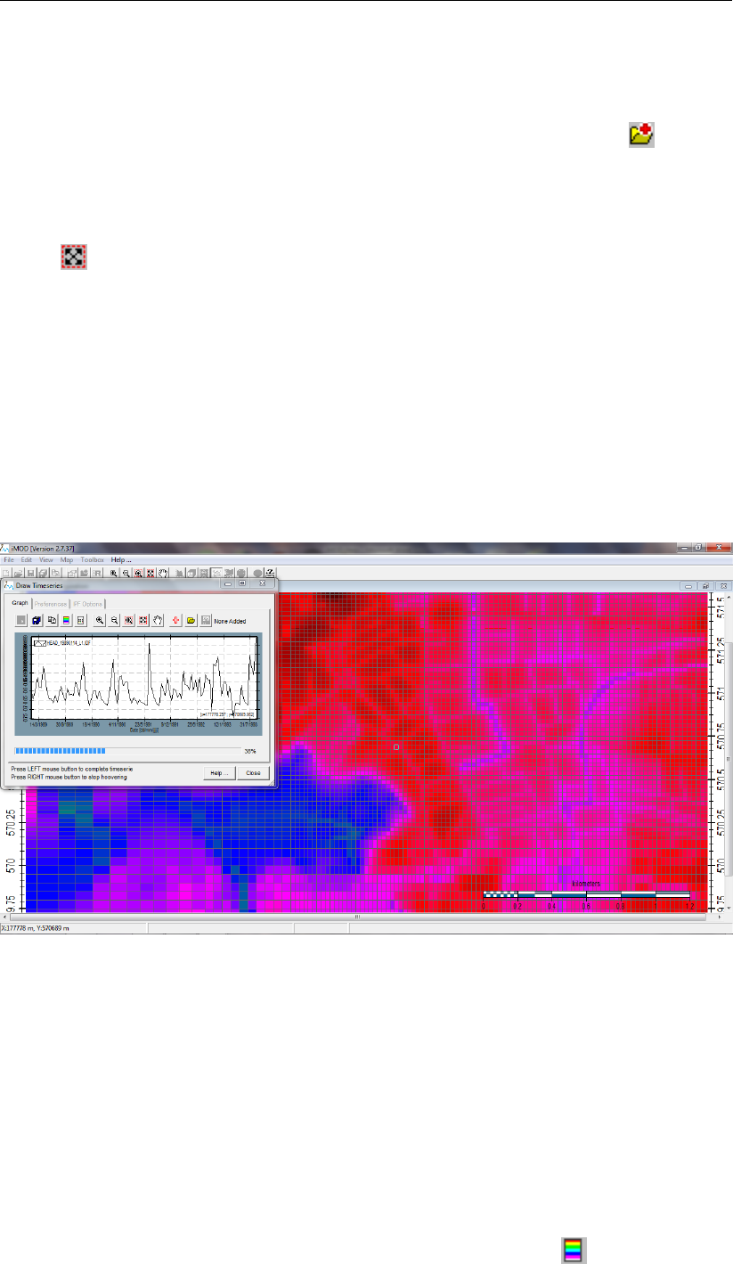
DRAFT
iMOD tutorials
December 2010. Without having to open other files for other dates, iMOD searches for equivalent files,
instead. Just as easy!
65 Open a single IDF-file located in the HEAD subfolder of the folder
{path of installfolder} \tutorials \TUT_MAP_ANALYSE. Click the Open IDF button( ) from the
Maps tabs on the iMOD Manager.
66 Click the option View from the main menu, choose Show IDF Features and select IDF Raster
Lines.
Choose to see the selected IDF. Observe that the current IDF has a non-equidistant network.
67 Zoom in on a particular area in the highly detailed area to observe the network layout even better.
68 Click the option Toolbox from the main menu and the option Timeserie Tool to start drawing time-
series, interactively. Accept the Available Dates window for now. You could have specified a
selection of the available IDF-files.
iMOD will read/open all available IDF-files from the same folder as the IDF-files that you’ve opened in
step 65. This could take several seconds, watch the progress in the status bar. Once this has finished
the Draw Timeseries window will be displayed.
69 Move your mouse over the screen and watch how the timeseries will be updated for the adjusted
location.
Figure 11.21: Screen shot of the ’Draw Timeseries’- and ’Timeseries Tool’-windows while
hovering with the mouse over a map of a series of IDF-files.
Since iMOD will draw a timeserie that can be computed within one second only, you’ll notice that not
the entire timeserie will be plotted. This can be seen in the progress bar on the bottom of the Draw
Timeseries window.
70 Click your right mouse button to compute the entire timeserie and stop the hoover mode.
As soon as the hovering has stopped you can examine the entire drawn timeserie.
71 Use the regular zoom buttons to navigate on the timeserie.
72 Explore the tab Preferences, to see what you can do and how it works.
73 Change the appearance of the timeserie by clicking the Legend button ( ) on the Graph tab.
Deltares 623 of 812

DRAFT
iMOD, User Manual
Experiment with the options that are available in the Individual Colouring window.
624 of 812 Deltares
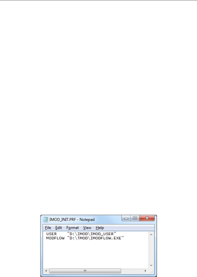
DRAFT
iMOD tutorials
11.4 Tutorial 4: Create your First Groundwater Flow Model
This tutorial gives a short introduction in creating a groundwater flow model from scratch. It yields a
preliminary model that will be enhanced even more in section 11.5.
All steps in this tutorial were demonstrated during the first live iMOD webinar, recorded on May
2016. You can watch the recordings via the webinar page on the iMOD website (http://oss.
deltares.nl/web/imod/webinars). (Be aware that some parts of the tutorial might be im-
proved or edited in the mean time)
Outline
This is what you will do:
Create the basic input files that are necessary to simulate a simple groundwater flow model;
Enhance the model with an extraction well to compute the drawdown caused by the well;
Simulate flowlines that describe the catchment area of the well;
Experiment with extraction rates to compute the maximum sustainable yield without extracting
water from the sea.
Required Data
For this tutorial you need the following iMOD Data Folders:
island.png/island.pngw: this image sketches the outlines of the island
This file is located in/below the folder: {path of installfolder} \tutorials \TUT_INITIAL_MODELING.
Beside this data you will need the iMODFLOW executable to make the final model computations.
Getting Started
1 Place the iMODFLOW executable somewhere on your disk (for instance next to the iMOD-GUI
executable) and define the keyword MODFLOW in the IMOD_INIT.PRF.
Figure 11.22: Example of a content of an iMOD_INIT.PRF file.
See section 11.1 and chapter 9 for more information about the folder structure in iMOD and a descrip-
tion of IMOD_INIT.PRF (see section 9.1 for more information about this PRF file). Please restart iMOD
after changing the IMOD_INIT.PRF file.
2 Launch iMOD by double clicking the iMOD executable in the Windows Explorer, and start by se-
lecting the option Create a new iMOD Project. Click the Start button.
Deltares 625 of 812
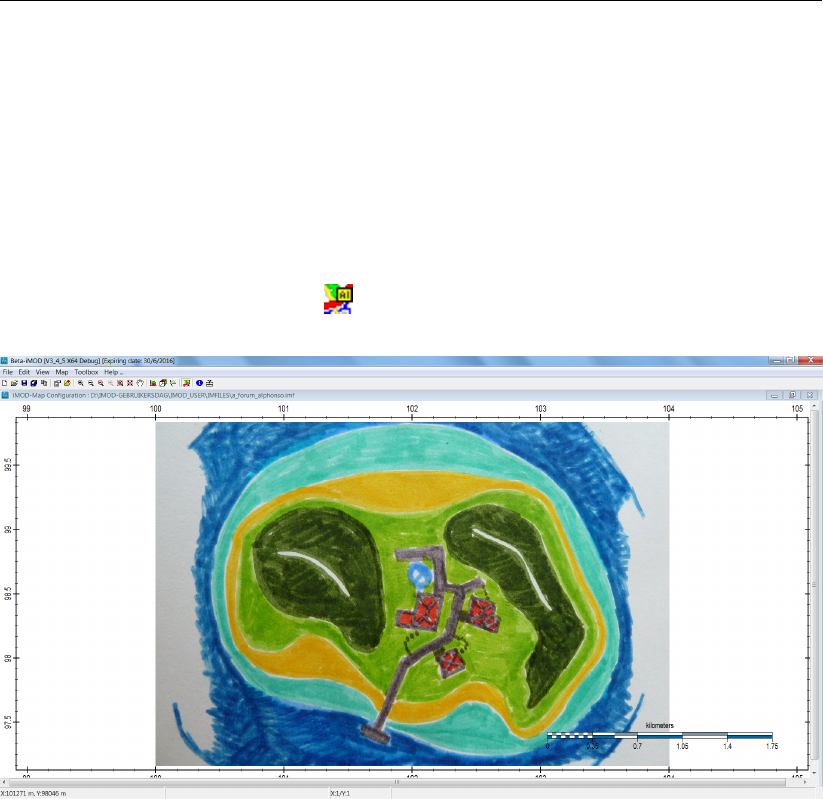
DRAFT
iMOD, User Manual
Background Image
One of the first things one would like to display is an image of the outline of our island that we’re going
to model. Let’s do that.
3 Select the option View from the main menu and then select Add Background Image ... from the
dropdown menu. This will start the Add Background Image dialog.
4 Select the option Add from the dialog and select the file
{path of installfolder} \tutorials \TUT_INITIAL_MODELING \island.png from the Windows
Explorer, see section 5.3 for more information about this window.
5 Select the Apply button that closes the window.
6 Click the Show Background Image ( ) on the main menu whenever the image does not appear.
Figure 11.23: Example of showing a topographical map using the main menu ’View’,
’Show Background Image(s)’ option.
This island represents a small tropical island (3 x 3 km) somewhere in the Pacific. It is surrounded by
shallow waters with crystal clear water (light blue), white beaches all around (yellow) and meadows
(light green) with some bush areas (dark green). In the centre of the island there exists a small
settlement with a few houses that use groundwater for watering their fields and cattle and use it as
primary source for drinking water. They extract groundwater at the centre of the island (blue circle).
Many people have discovered the beauty of this island and plans arise to build a resort on the island.
This will increase the pressure on the natural water resource and the question to be answered is: “How
much water can be sustainably extracted from the subsoil, without attracting seawater in the near future
to the pumps?”.
With this very simple example we will use iMOD to build a hypothetical model of this island. By means
of this example we will illustrate the methodology in iMOD to create a groundwater flow model. At
this stage we will ignore any effects of density-driven components caused by salt water. The following
steps will be undertaken:
build an IDF-file for the surface level of the island which will be our uppermost boundary of the
system modeled;
create an IDF-file that defines the boundary conditions of the model, for which part the groundwater
head needs to be computed and for which part this is known beforehand;
create an IPF file that describes the location and rate of the pumping well;
create a runfile that describes the necessary files and values for the simulation;
simulate the model using the runfile;
626 of 812 Deltares
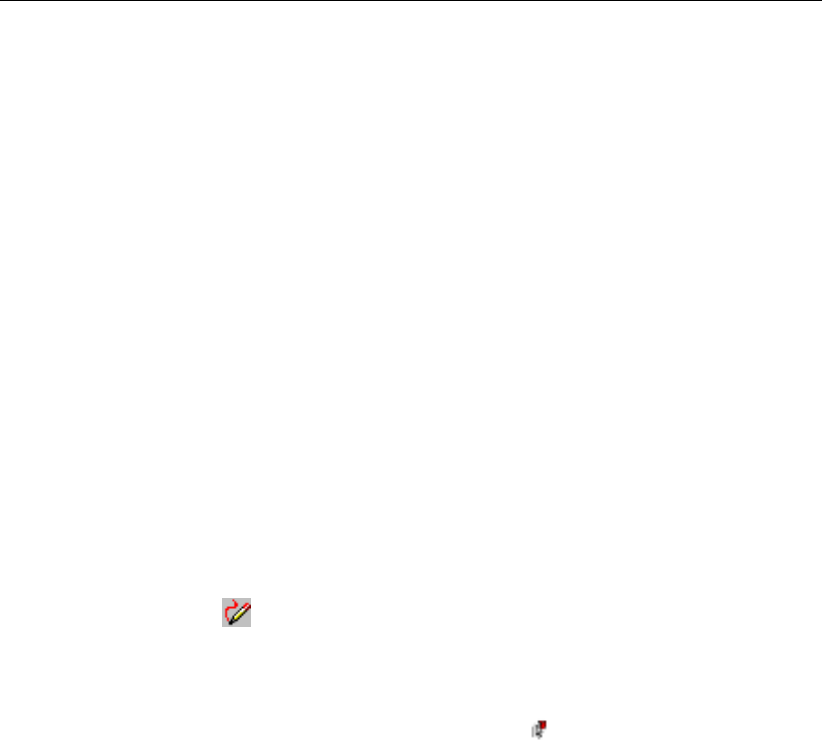
DRAFT
iMOD tutorials
create startpoints for the particle tracking simulation and carry out this simulation;
modify the extraction rate in order to search for the maximum sustainable yield.
Okay, a lot of work needs to be done, so let’s go!
Creating the topography
Our model will describe the groundwater flow between the surface level and the bedrock in the subsoil.
Our first task is to get a digital representation of the surface elevation. Often this is available in the form
of a Digital Elevation Model (DEM), unfortunately, we’re lacking this DEM for our island, so we have to
sketch it ourselves.
7 Select the option Edit,Create Feature from the main menu, then select the option IDF’s from... and
finally the option Polygons/Lines [GEN] to start the Create IDF window.
With this functionality in iMOD we’re able to create simple features in the format that iMOD needs to
perform a model simulation. In this case we would like to create the outline of the surface level and
therefore we need to draw the contours of the surface level and assign appropriate levels to it. After
that we can tell iMOD to interpolate from the contours. Okay, let’s start this by digitizing the shore of
the island (i.e. 0.0 m+MSL contour).
8 Make sure you’ve shown the topographical image of the island (repeat step 3upto 6whenever you
don’t see the image);
9 Click the Draw button ( ), this will start the Select window;
10 Select the option Polygon from the Shape types;
11 Click the Ok button.
Your cursor has been changed into the following cursor symbol which means that you can start
drawing a polygon.
12 Click your left mouse button on the graphical canvas at the location of the first point of the polygon
to be drawn. Repeat clicking your left mouse button to insert more point of the polygon. Whenever
you are satisfied click your right mouse button to stop this process. Note: if you are a left-handed
person and you converted your mouse button settings, ’left mouse button’ should be ’right mouse
button’ and vice versa in these tutorials.
See section 4.5 for more details how to modify the polygon once you’ve created it.
Deltares 627 of 812
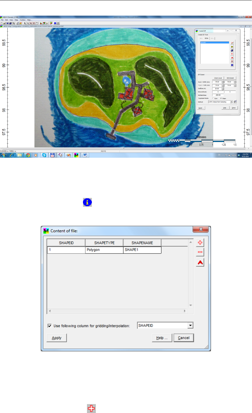
DRAFT
iMOD, User Manual
Figure 11.24: Example of the polygon that you might have created.
Now we have to assign a surface level of 0.0 m+MSL to the drawn polygon.
13 Click the Information button ( ) to start the Content of File window. Click the Yes button when-
ever iMOD asks “Do you want to add additional data to the shapes?”.
Figure 11.25: Example of the ’Content of file:’ window.
With this Content of file window we can observe/change the attributes that can be added to the shapes
(polygons, lines). We have to add a new attribute to the data to store the contour values of the surface
level. Let’s do that.
14 Click the Add Attribute button ( ) and enter the label [Level] in the Input window that arises.
628 of 812 Deltares
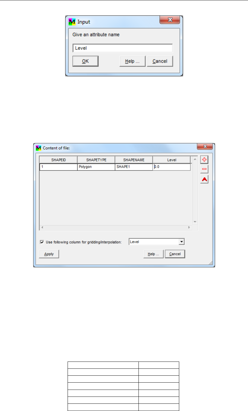
DRAFT
iMOD tutorials
Figure 11.26: Example of the ’Input’ window to add an attribute.
15 Click the OK button to return to the Content of file window. Observe that an extra column has been
added to the table.
16 Enter the value [0.0] to the input field Level.
17 Select the option Use following column for gridding/interpolation and select the attribute [Level]
from the dropdown menu. iMOD will use the values from this column during the interpolation.
Figure 11.27: Example of the ’Content of file:’ window.
18 Click the Apply button.
Similarly repeat steps 12 to 18 to sketch the other polygons and lines of the surface elevation of the
island. Choose the corresponding elevation values from the table below. Please note that it is not
necessary to add the attribute column named [Level] for each shape since this will be applicable for
all shapes that are entered. Also use a [Line] feature to express the watershed on the more elevated
parts of the island.
Table 11.1: Elevation of the island elements
Island level description elevation [m]
Hills ridge (west and east) 15
Hills feet (west and east) 5
Border green area 2
Island Boundary 0
Shallow water -1
Deep water -5
Deltares 629 of 812
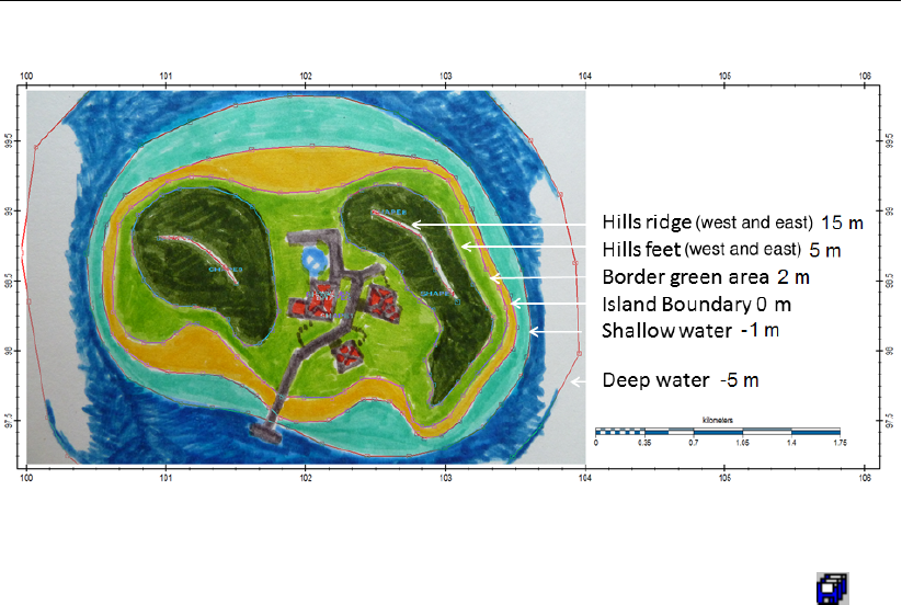
DRAFT
iMOD, User Manual
Figure 11.28: Example of a final result sketching the surface level for the island.
19 To save the set of shapes listed in the ’GENs-tab’ window click on the Save As button ( ) and
save as ISLAND.GEN in the folder iMOD_USER \SHAPES. Please note that it does not matter
whether only some of the shapes were selected, all shapes listed in the ’GENs’-tab will be saved
as one set of shapes.
The associated labels are saved to the file ISLAND.DAT at the same location. Both files (ISLAND.GEN
and ISLAND.DAT) may be modified outside iMOD using a text-editor. Please note that the first column
in the DAT file will be used to reference between the GEN and DAT file. Make sure that this connection
remains intact!
Once we’ve outlined the surface level, we will interpolate the contours to a grid (IDF) with rastersize of
10 meter. This will be accurate enough for our simulation. However, gridsizes at this stage will not be
determined for the final simulation scale. See section 11.6 for more information on scaling issues for
model simulations.
20 Click the button GEN-Extent to adjust the coordinate settings for the IDF to be created such that
the entire GEN will be included in the gridding.
21 In the boxes for the Lower Left and Upper Right coordinates of the extent (XLLC, XURC etc), please
remove the centimeter values and round down or up to meters.
22 Enter a cell size of 10 meter in the field Cellsize (m).
23 Select the option [PCG (Preconditioned Conjugate Gradient)] from the Method dropdown menu.
This interpolation method will follow the given contours accurately giving a smooth representation of
the entered contours.
24 Click the Apply button and save the gridded IDF-file in the folder iMOD_USER \DBASE as SUR-
FACE_LEVEL.IDF. Probably you need to create this folder first!
630 of 812 Deltares
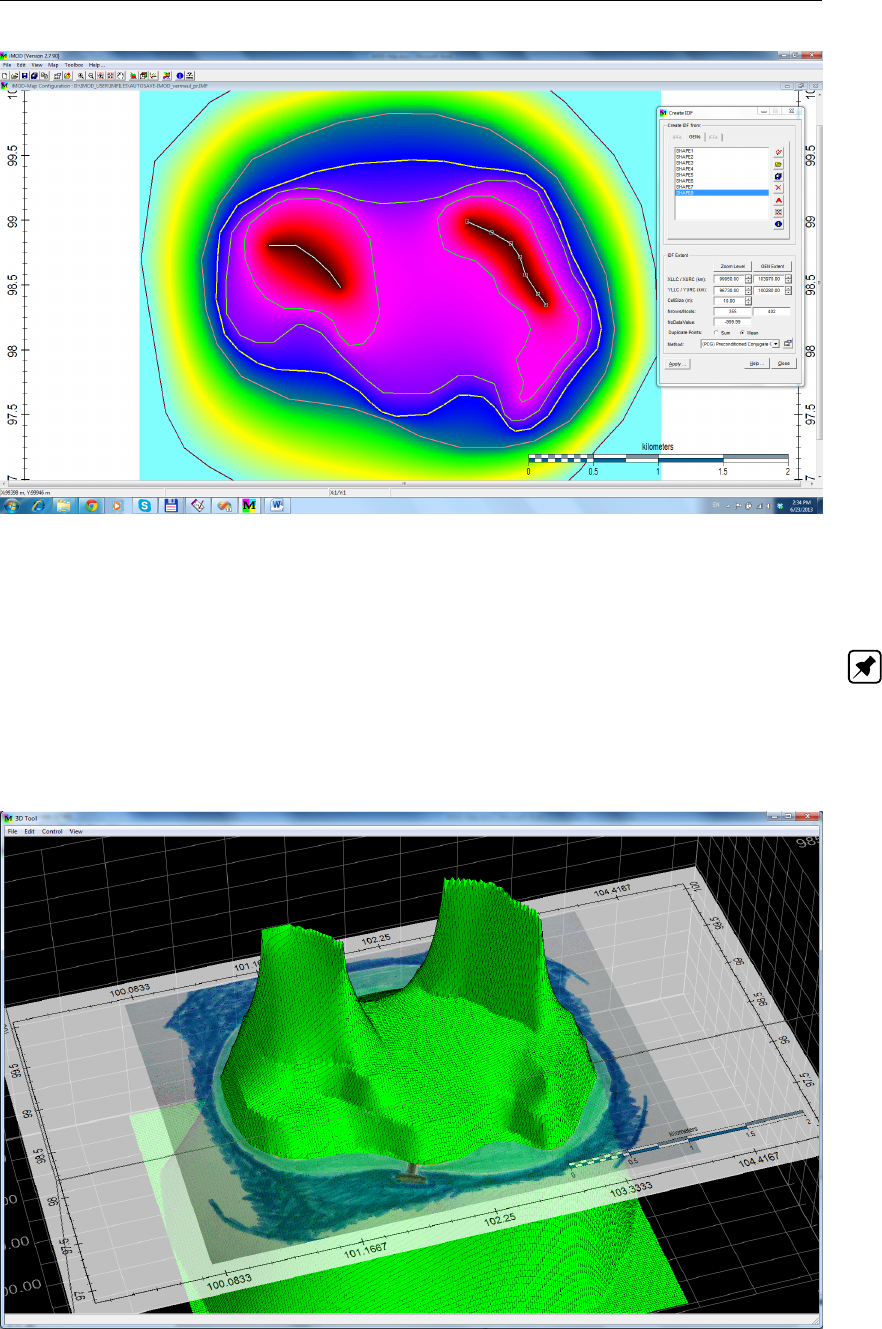
DRAFT
iMOD tutorials
Figure 11.29: Example of a resulting topography of the island.
It is completely irrelevant where files are saved actually; however, in order to keep your project or-
ganized well, it is advisable to create a clear structure in which you save all files that are related to
the model. Note: Commonly, we use the foldername DBASE to store all model files. So whenever
we refer to the folder DBASE in the coming parts of this tutorial we actually denote the IMOD_USER
\DBASE folder.
25 Use your experience from the Tutorials 1, 2 and 3 to create a 3D image of the topography we just
created.
Figure 11.30: Example of a 3D image of your created island.
Deltares 631 of 812
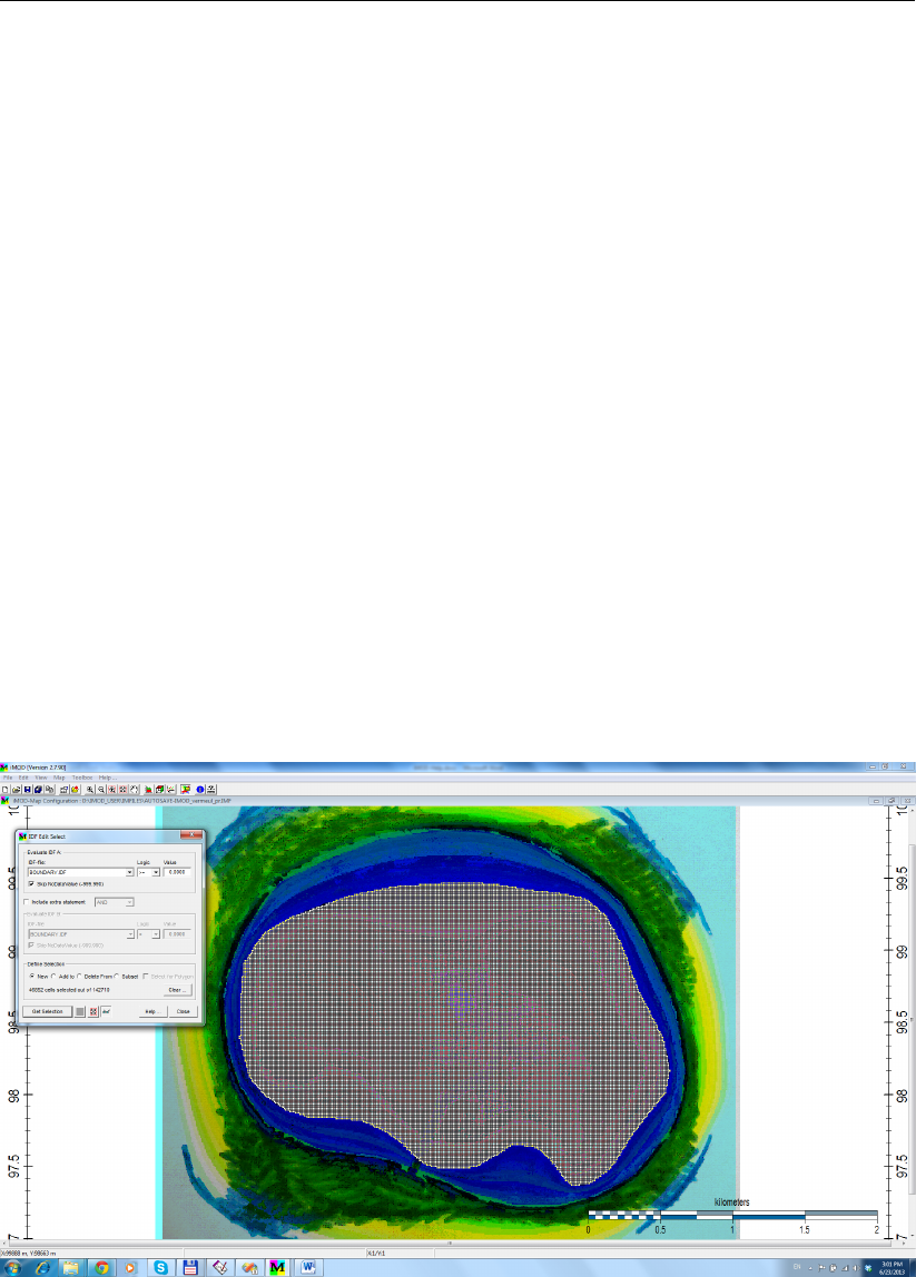
DRAFT
iMOD, User Manual
Creating the boundary conditions
Okay, now we’ve outlined the uppermost boundary of our model, we will specify those areas that are
part of the model simulation (active areas) and areas that have fixed values (fixed or non-active areas)
for the hydraulic heads. We will use IDF-Calc and IDF-Edit that you both have used in section 11.2 (we
assume you finished section 11.2 before you moved on to section 11.4). Okay, we need to copy the
SURFACE_LEVEL.IDF to an IDF that we can use for the definition of boundary conditions.
26 Select the [SURFACE_LEVEL.IDF] from the iMOD Manager and Click the IDF Calculator button.
27 Enter the IDF-file [. \DBASE \BOUNDARY.IDF] in the Map C field on the Algebra tab on the Map
Operations window. Make sure you use the same folder name as the one used for . \DBASE
\SURFACE_LEVEL.IDF.
28 Make sure the entered formulae is [C=A].
29 Select the option Map A to create an IDF that has the same dimensions as the IDF-file mentioned
by Map A (i.e. SURFACE_LEVEL.IDF).
30 Click the Compute button.
Please note that when we created the BOUNDARY.IDF and it is drawn and listed in the iMOD Manager,
it is a copy of the SURFACE_LEVEL.IDF. Now we are going to determine the active areas of the
simulation by selecting the area with surface level values above zero. Areas with values less than zero
will be fixed areas. So let’s continue with that.
31 Select the [BOUNDARY.IDF] from the iMOD Manager and click the Map option from the main
menu, select IDF Options and then IDF Edit option to start the IDF Edit window.
32 Click the Select button to start the IDF Edit Select window.
33 Select the option [>=] from the dropdown menu Logic in the groupbox Evaluate IDF A.
34 Click the Get Selection button to get a selection of all cells that have values greater and equal zero.
Figure 11.31: Example of the selection of cells with values greater or equal to zero.
35 Click the option Close to return to the IDF Edit window again.
36 Click the Calculate option from the IDF Edit window to start the IDF Edit Calculation window.
37 Select the option New Value in the group Define Values by and enter the value [1] so it says New
Value [=] [1.0].
38 Click the Calculate button.
39 Click the Close button and click Yes on the appearing window asking you to be sure to leave this
Edit environment.
Repeat steps 32 upto 39 to adjust all values that have values less than zero and calculate those values
632 of 812 Deltares
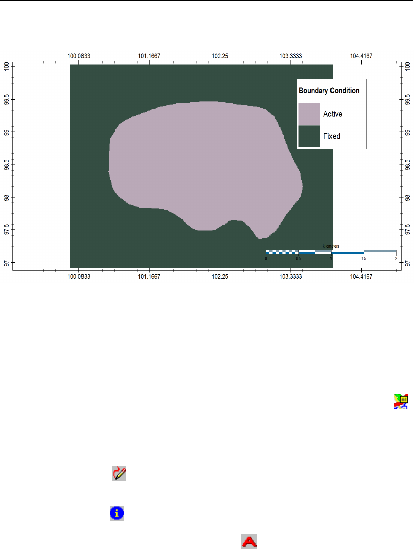
DRAFT
iMOD tutorials
to become -1.0.
Figure 11.32: Example of assigned active and fixed head cells.
Last thing we need to do is to create an IPF file (iMOD Point File) to represent the well in our model.
We have a single well situated in the centre of the island, in the following steps we will create this
simple file inside iMOD; however, it can be easily modified/created outside iMOD. For large datasets it
is often more convenient to process these types of data in another program.
40 Deselect the BOUNDARY.IDF in the iMOD Manager.
41 Make sure you’ve switched the background image on, if not press Show Background Image ( )
again.
42 Select the option Show Transparent IDFs from the View menu, to be able to either see the back-
ground image and the IDF files to be analysed.
43 Select the option Edit from the main menu, then select the option Create Feature and then IPF’s
to start the Create IPF’s window.
44 Click the Draw button ( ) and click your left mouse button when the cursor is on the location of
the well.
45 Click your right mouse button to return to the Create IPF’s window.
46 Click the Information ( ) button and click the Yes button on the question “Do you want to add
additional data to the shapes?”.
47 Select the third column and press the Rename button ( ).
48 Enter the name [Q] in the field Rename Attribute and click the OK button.
49 Enter a value of [-500.0] for the extraction rate in the first row, third column. Rates are entered in
m3/day and you cannot perturb the first two columns since these are used by iMOD for internal
processes.
Deltares 633 of 812
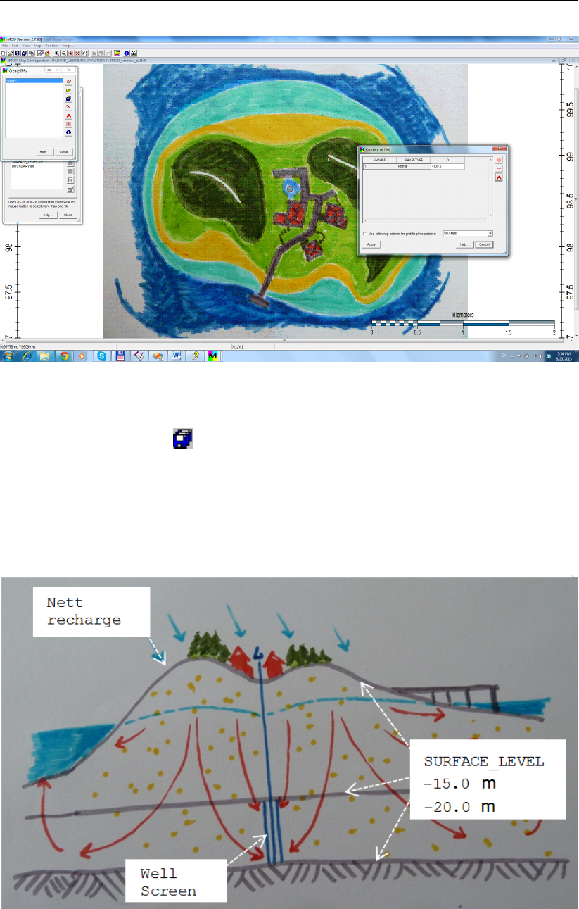
DRAFT
iMOD, User Manual
Figure 11.33: Example of a screen layout at the current step.
50 Click the Apply button to close this window and return to the Create IPFs window.
51 Click the Save As button ( ) to save this file in . \DBASE \WELL.IPF.
For this hypothetical model, these three IDF-files (. \DBASE \SURFACE_LEVEL.IDF, . \
DBASE \BOUNDARY.IDF and . \DBASE \WELL.IPF) are the only spatial varying data sources. The
other model input are constant values throughout the model domain and we will assign those values
by creating a modeling project in the following section. In the next figure we’ve given a sketch of the
subsoil and flow patterns that might occur.
Figure 11.34: Sketch of a estimated flow pattern that might occur in our island model.
634 of 812 Deltares

DRAFT
iMOD tutorials
Creating a Modeling Project and defining a runfile
iMOD arranges a model project by a project file, a so called PRJ file. This file stores all files that are
assigned to particular phenomena in the model. From a project file (*.PRJ) you can generate a runfile
(*.RUN) that will be used eventually to simulate groundwater heads for a specific configuration. We can
imagine that you’ll need to simulate different scenarios (e.g. steady-state simulation versus transient
simulations) that can be initiated by the Project-Manager. Well, probably it is better just to start with it.
52 Select the option View from the main menu and select the option Project Manager to start the
Project Manager window.
This window shows all available packages that are supported by iMOD. Still many will come in future
though. Okay, we have to fill in this project manager with our model configuration. In the table, shown
below, we have outlined the requirements for this particular three-layered model. Note: the "Porosity
Aquifer" and "Porosity Aquitard" values are only needed for the pathlines simulation from step 95
onwards.
Table 11.2: Model requirements for a confined, steady-state three layered model.
Parameter model layer IDF/Constant Value
BND Boundary 1 . \DBASE \BOUNDARY.IDF
2,3 1
SHD Starting Heads 1,2,3 0.0 m+MSL
TOP Top Elevation 1 . \DBASE \SURFACE_LEVEL.IDF
2 . \DBASE \SURFACE_LEVEL.IDF - 1.0 m
3 -15.0 m+MSL
BOT Bottom Elevation 1 . \DBASE \SURFACE_LEVEL.IDF - 1.0 m
2 -15.0 m+MSL
3 -20.0 m+MSL
KHV Horizontal Permeability 1,2,3 25.0 m/day
KVA Vertical Anisotropy 1,2,3 1.0
KVV Vertical Permeability 1,2 25.0 m/day
WEL Wells 3 . \DBASE \WELL.IPF
RCH Net Recharge 1 1.0 mm/day
Okay let us fill in the boundary conditions in the Project Manager.
53 Select the option [(BND) Boundary Conditions] in the Project Definition list.
54 Click the Properties button ( ) to start the Define Characteristics for window.
In the current window you can specify how the package (in this case the Boundary Condition) needs
to be configured. Let us fill this dialog for the boundary condition for model layer 1.
55 Enter the value [1] in the Assign Parameter to model layer . . . field, if this is not the case by default.
56 Specify a Parameter Multiplication Factor of [1.0], if that is not the case by default. Any parameter
can be multiplied with the associated factor during runtime. You can use this factor to easily perform
some sensitivity analyses on parameters and their effect on the distribution of the groundwater
head.
57 Specify a Parameter Addition Value of [0.0], if that is not the case by default. Any value can be
added to or subtracted from a parameter.
58 Select the option Add File and click the Open File button. Select the file
. \DBASE \BOUNDARY.IDF from the appropriate folder. This file we’ve created in step 39, remem-
ber?
Deltares 635 of 812
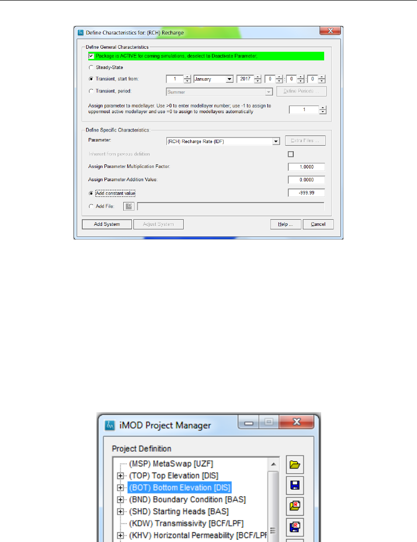
DRAFT
iMOD, User Manual
Figure 11.35: Example of the ’Define Characteristics for:’ window, filled in for Recharge
(RCH).
59 Click the Add New System button and this will return you to the Project Manager window. You’ll
notice that the option [(BND) Boundary Conditions] has been altered. You can select the “plus”
sign to expand the tree view. You’ll notice the entered fields in the presented string.
Now let us fill in the remaining parameters from the table given.
60 Repeat the steps 53 upto 59 for the remaining parameters. Take care to select the parameter name
in the Project Definition list each time you want to open the Define Characteristics for window to
enter NEW parameters.
Figure 11.36: Example of selecting a parameter in the ’Project Definition’ window: in this
example firsts ’(BOT) Bottom Elevation’ is selected to expand the tree view
by clicking the ’+’-sign.
Whenever you select the expression under an expanded branch in the treeview in the Project Definition
list, you’ll be able to edit an existing entered parameter; see the example below.
636 of 812 Deltares
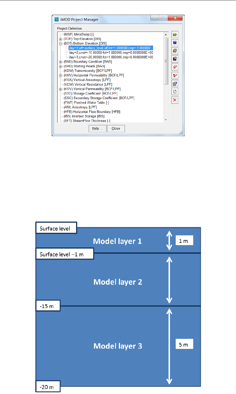
DRAFT
iMOD tutorials
Figure 11.37: In this example the exisiting (BOT) parameter set of layer 1 is selected.
Click on the ’Properties’ button to open the ’Define Characteristics for:’ win-
dow to edit the Bottom Elevation parameters.
As you may have noticed, we simulate this model with three model layers. The first model layer has a
thickness of 1.0 meter (almost no horizontal flow in that model layer) to intercept the recharge. From
there water will migrate to the deeper layers 2 and 3. The third model layer is the actual aquifer from
which water is extracted via the well screen.
Schematic, the model can be represented by the following figure:
Figure 11.38: Schematic representation of the model.
Deltares 637 of 812
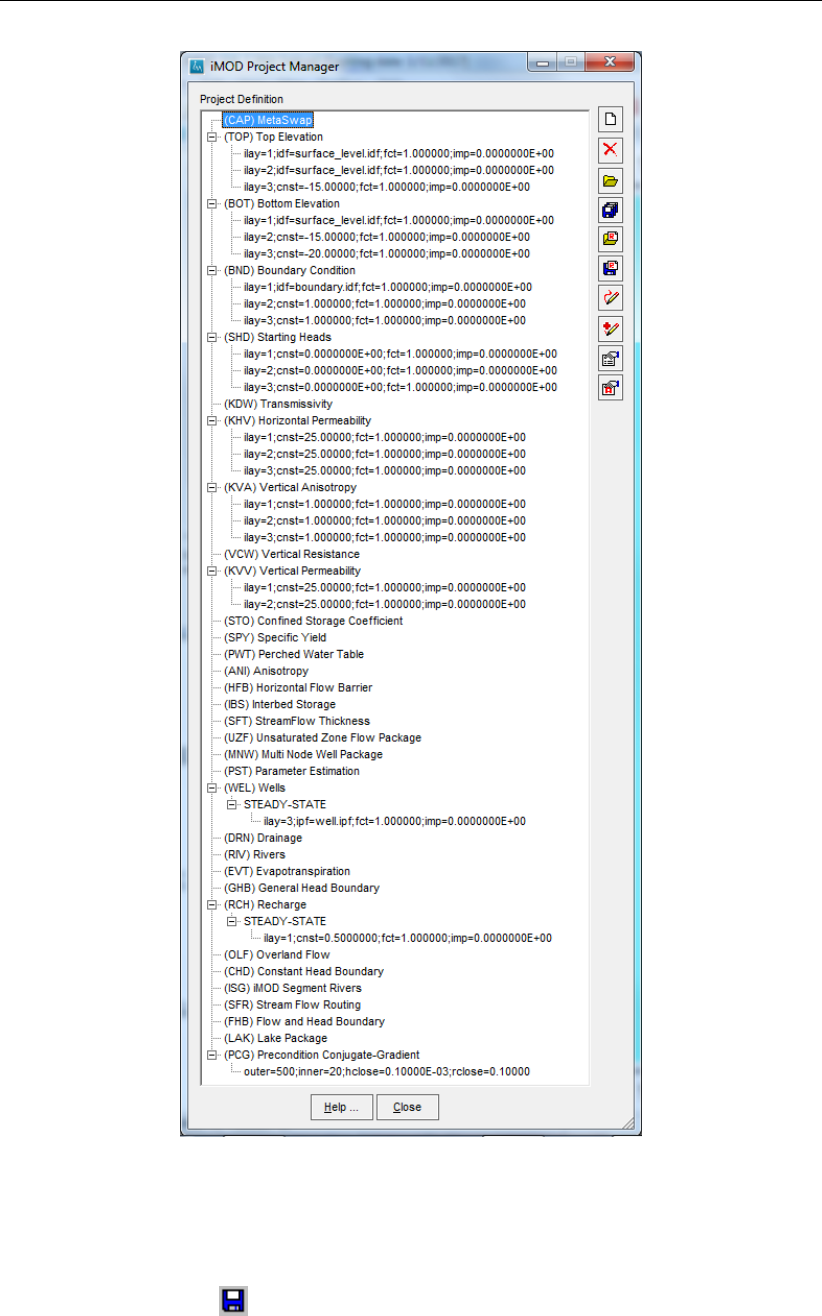
DRAFT
iMOD, User Manual
Figure 11.39: Example of Project Manager window after filling in a model configuration.
For the meaning and explanation of the available buttons on the Project Manager window go to section
section 5.5.
61 Click the Save button ( ) to save this model configuration in a PRJ file. This file may be loaded
again whenever we need to modify this project.
The next step will be to create a runfile than can be used for a model simulation.
638 of 812 Deltares
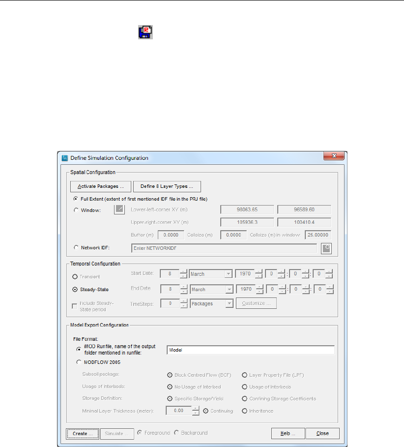
DRAFT
iMOD tutorials
62 Click the Save Runfile button ( ) to start the Define Simulation Configuration window.
iMOD will fill this dialog depending on the definitions in the Project Manager. We are not able to create
a transient runfile since we do not have any transient data. We will generate a runfile for a three-layered
model.
63 Click on Activate Packages... to select all packages in de pop-up window if this is not already the
case.
64 Click the Apply button to accept the selection and close the Packages window.
Figure 11.40: The Define Simulation Configuration window after entering the value ’3’ for
the ’Number of layers’.
65 Click the Create ... button and save the runfile in the folder . \IMOD_USER \RUNFILES and call it
ISLAND.RUN.
iMOD will create a runfile for a steady-state simulation taking into account all active packages in the
Project Manager. This runfile can be used to start the model simulation.
66 Click the OK button that says that the runfile has been written successfully. This will return you
to the Project Manager. Click the Close button to close the Project Manager window. It remains
active in the background and can be re-opened by selecting the option Project Manager from the
View menu at the main menu.
Deltares 639 of 812
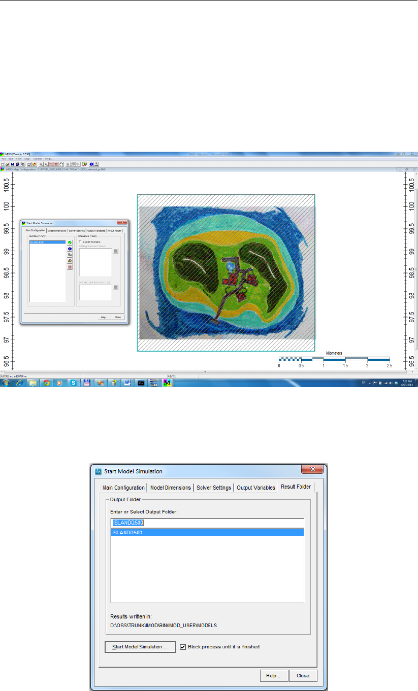
DRAFT
iMOD, User Manual
Running the Model
67 Select the option Toolbox from the main menu and then the option Start Model Simulation to start
the Model Simulation window.
68 Select the [ISLAND.RUN] from the Runfiles (*.run) list.
iMOD will draw a hatched rectangle showing the maximum extent of the model described in the runfile.
In section 11.6 we will demonstrate more functionalities in scaling and creating a submodel using the
Model Simulation Tool. For now we will just skip most of the functionalities on this window and start
running the model.
Figure 11.41: Example of the ’Start Model Simulation’ window.
69 Select the Result Folder tab and enter the name [ISLANDQ500] in the Enter or Select Output
Folder field.
Figure 11.42: Example of the ’Result Folder’ tab in the ’Start Model Simulation’ window.
640 of 812 Deltares
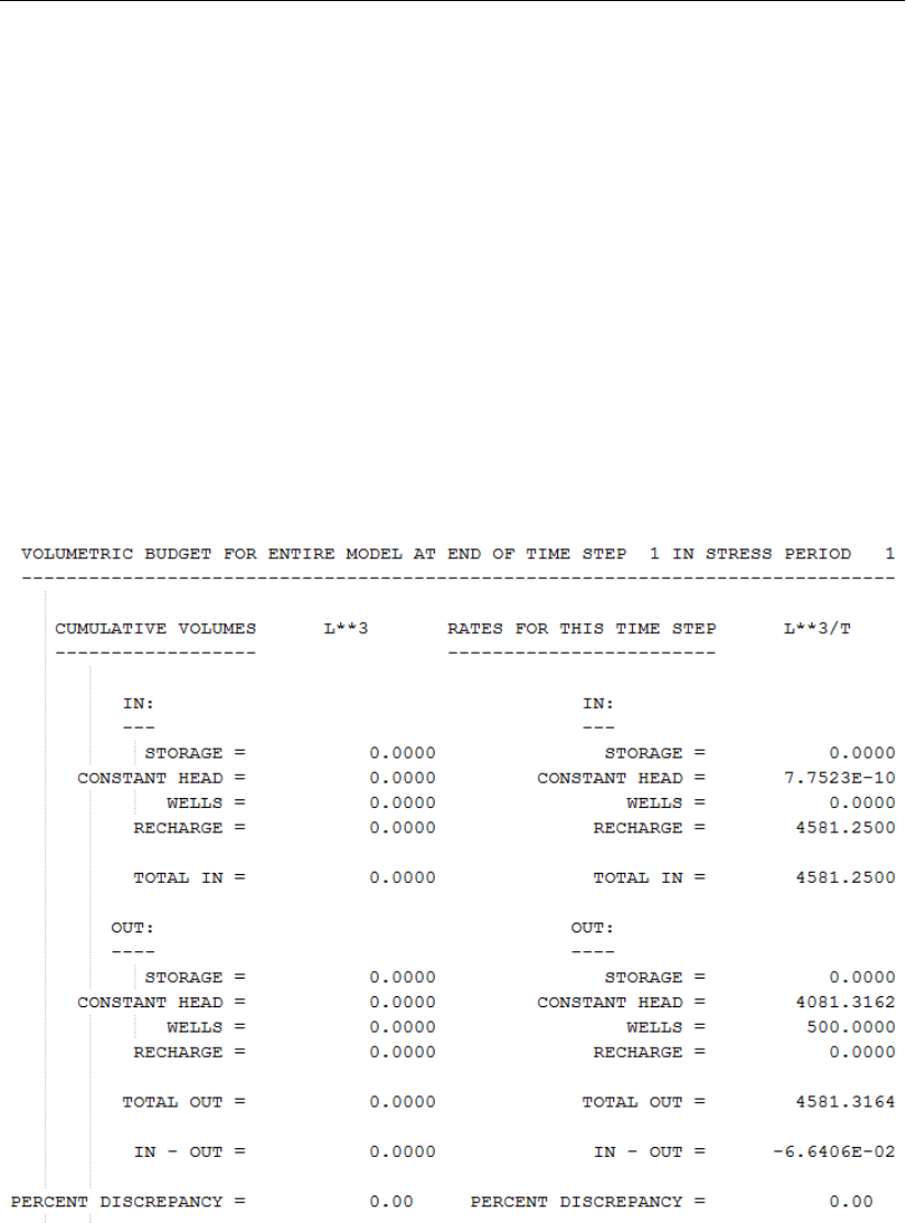
DRAFT
iMOD tutorials
70 Click the Start Model Simulation button to start the model simulation.
The actual simulation will be carried out by the iMODFLOW executable and will run in the DOS box
attached to iMOD. Please check whether you can find this window and examine the results, it will look
more or like as follows:
iMOD will create folder \IMOD_USER \MODELS \ISLANDQ500 in which the results of the model sim-
ulation will be saved. Moreover, a complete copy of the runfile, the used executable for the simulator
(e.g. iMOD__V4_3_X64R.exe) and a batch script will be saved too. Double clicking this batch script
(RUN.BAT) from Windows Explorer or Total Commander will re-run this model outside iMOD. This can
be very convenient whenever some trial-and-error computations have to be carried out. For now, we
will work purely within iMOD.
iMODFLOW produces standard output in the file iMODFLOW.list (always in the subfolder mf2005_tmp
of the Result Folder you specified (in this example . \IMOD_USER \MODELS \ISLANDQ500 \mf2005_tmp);
at the end of this file the overall volumetric budget is printed and can be checked for the resulting water
balance error (IN - OUT):
Figure 11.43: Example of the volumetric water balance as printed by MODFLOW in the
iMODFLOW.list-file.
So, in short, the iMODFLOW standard output file iMODFLOW.list contains info on:
the model discretization
the model time and length units
the processed input packages
the solver used and how the iteration process progressed
the volumetric budget for the entire model, including the percent discrepancy
elapsed run time
Deltares 641 of 812
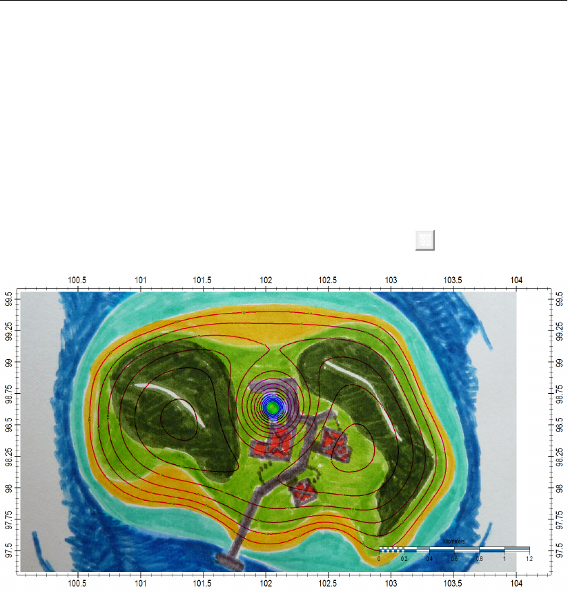
DRAFT
iMOD, User Manual
Let’s have a look at some more results.
71 Close the Model Simulation window by selecting the Close button.
72 Select the option Map and then the option Quick Open to start the Quick Open window, see sec-
tion 6.2. With this window it is easy to open and view results from a model simulation.
73 Select the option [HEAD] from the Topic dropdown menu.
74 Select the options [1], [2] and [3] from the Layer dropdown menu.
75 Click the Open button.
iMOD will load the selected results files (HEAD for model layers 1, 2 and 3) into the iMOD Manager and
displays the result on the graphical canvas. Use your experience learned from the previous Tutorials
to display the computed heads as shown in the example on the next page. To show the IDF by
contourlines, open the Legend window and click the Contourlines button ( ).
Figure 11.44: Isolines of the computed hydraulic heads of the island.
As we can see by the computed hydraulic head, the gradient towards the well in the centre of the island
tends to be such that no water is extracted from the ocean. To illustrate this even more we can compute
pathlines that show the actual path through the subsoil that groundwater follows from the location of
infiltration towards the location of extraction. We call that particle tracking.
642 of 812 Deltares
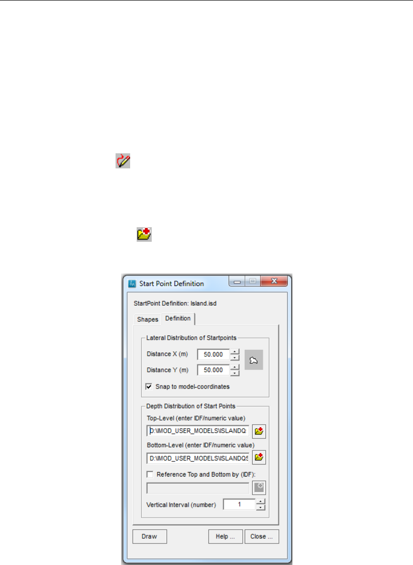
DRAFT
iMOD tutorials
Create Startpoints for a Pathline Simulation
76 Select the option Toolbox from the main menu and then the option Define Startpoints to open the
Open/Create a Startpoint Definition window, see section 7.13 for more detailed information.
77 Enter the name [ISLAND] in the input field.
78 Click the Open and Continue button to open the Start Point Definition window.
iMOD offers the possibility to define startpoints for any particle tracking independently of a model,
modelsize and or cellsize. Startpoints will be defined by means of a polygon a line and/or points and
startpoints are distributed within the limits of that/those polygon(s)/lines. So, let us define startpoints
on the island.
79 Click the Draw button ( ) and start drawing a polygon. We’ve done this before (see step 8)
so you’ll manage to get this done. Make a polygon wide around the island, so we can observe
whether seawater is flowing to the well too.
80 Select the right mouse button to stop drawing a polygon.
81 Select the Definition tab and enter a cellsize of [50] meter for the Distance X (m) and Distance Y
(m), so each 50 meter we will have a particle starting.
82 Select the Open IDF button ( ) to select the computed hydraulic head of layer 1 to be used as
Top Level, use the same IDF for the Bottom Level.
Figure 11.45: The ’Start Points Definition’ window.
83 Click the Draw button to get an idea of the density of the particles to be started.
84 Click the Close button to close this Start Point Definition window. Whenever iMOD asks to overwrite
the current [ISLAND.ISD], do so.
So now we’re finished creating startpoints, let’s use them in the pathline simulator.
Deltares 643 of 812
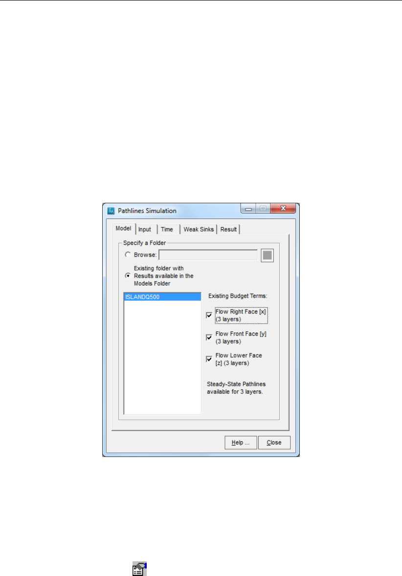
DRAFT
iMOD, User Manual
Running the Pathline Simulator
85 Select the option Toolbox from the main menu and then the option Start Pathline Simulation. This
will start the Pathlines Simulation window; see section 7.14 for more detailed information.
86 Select the model [ISLANDQ500] in the list at Existing Results under Models.
iMOD will search in the appropriate folders to see whether all necessary files are available. For a
particle tracking you need at least the budget terms in the x, y and z direction, these files are stored
in the . \BDGFRF, . \BDGFFF and . \BDGFLF, respectively. iMOD will display the availability of those
files whenever you select a model result.
The example shown here will only highlight the most important steps to perform the particle simulation;
however, it is difficult to explain the results whenever one cannot fully understand the technique behind
it. So please, read some documentation on particle tracking, done by D.W. Pollock (USGS OpenFile
Report 94-464).
Figure 11.46: The ’Pathline Simulation’ window.
87 Click the Input tab on the Pathlines Simulation window.
On this tab we need to tell iMOD the specific information that is needed for the particle simulation.
Most important are the top- and bottom interfaces for the two model layers, see section 7.14 for more
detailed information on this topic. Let’s fill it in quickly.
88 Click the Properties button ( ) next to the Boundary Settings to display the Input Properties
window.
89 Enter the [. \DBASE \BOUNDARY.IDF] in the first row and enter [1] for the second and third row.
The particle tracking algorithm will use this information to exclude areas where the values in the
IDF-files are less or equal to zero.
644 of 812 Deltares
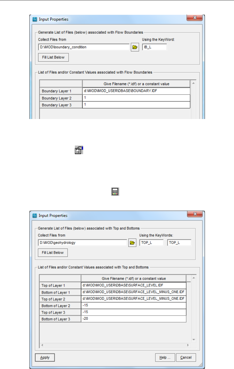
DRAFT
iMOD tutorials
Figure 11.47: The ’Input Properties’ window for the Boundary Conditions.
90 Click the Apply button to use the entered values as input.
91 Click the Properties button ( ) next to the Top- and bottom Files to display the Input Properties
window.
92 Specify the tops and bottoms according to the table on page 635; the specification for the top-
and bottom files could look similar to the figure below. Please note that for the bottom of layer
1 (and the top of layer 2) we use an IDF which has an elevation 1 meter below the surface level
IDF; you can create such an IDF e.g. by selecting the DBASE\SURFACE_LEVEL.IDF in the iMOD
manager, and click on the IDF Calculator ( ) button, type the Formulae ’C=-1+A’ and assign
e.g. the name DBASE\SURFACE_LEVEL_MINUS_ONE.IDF to Map C.
Figure 11.48: The ’Input Properties’ window for the Top- and bottom Files.
93 Click the Apply button to use the entered values; iMOD will check the existence of the specified
files.
Deltares 645 of 812
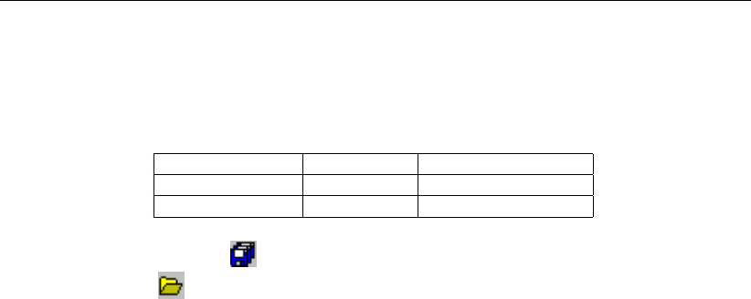
DRAFT
iMOD, User Manual
94 Select the Properties button for the other input fields and fill in the Input Properties appropriately.
Use the configuration as mentioned in the table on page 635 and adjust the following 2 parameters.
Table 11.3: Adjust the following 2 parameters
Parameter model layer IDF/Constant Value
Porosity Aquifer 1,2,3 0.3
Porosity Aquitard 1,2,3 0.1
95 Click the Save As button ( ) to save the input properties to an IPS file. Next time you can use
the Load button ( ) to read the input properties from disk. Whenever you save the settings as [.
\IMOD_USER \SETTINGS \IMODPATH.IPS], iMOD will read this file automatically each time you
start the Particle Simulation window.
For now we will skip most of the configuration setting in the other tabs, but feel free to have a look in
more detail at section 7.14.
96 Click the Result tab and make sure the Trace Direction is [Forward]. We compute the particles
from the groundwater elevation upto the discharge location (a well and/or the ocean).
97 Select the option Save Entire Flowpath (*.IFF) so we will get a file that describes the entire flowpath
of each particle.
98 Enter a name for the yielding flowfile, e.g. [ISLAND.IFF].
99 Click the Start button. This can take a while, especially whenever you have a lot of particles.
Bear in mind that whenever you have a lot of particles to examine, but you’re not actually interested in
their paths but only in their age at interception, consider the IPF files as alternative to flowlines. Those
files are much-much smaller and can be examined quicker.
100 Click the OK button on the Information summary that will be displayed after the particle tracking is
completed.
iMOD will load the computed IFF file and presents it like black lines. So let’s color it by their age, which
makes more sense.
101 Click the Map option from the main menu, select the option IFF Options and then the option IFF
Configure to display the IFF Configure window. See section 6.9.1 for more detailed information
about the functionalities on this window.
102 Select the option Apply Legend to and select the [TIME (YEARS)] from the dropdown menu.
One of the other items to be plotted is the velocity, that is computed as the flux (m3/day) divided by
the porosity (-) divided by the area (m2; width*model layer thickness). A change in porosity will change
the velocity linearly and therefore the age of the flowline, but will, however, not affect the shape of the
pathline.
103 Click the Close button to redraw the IFF with the assigned adjustments.
646 of 812 Deltares
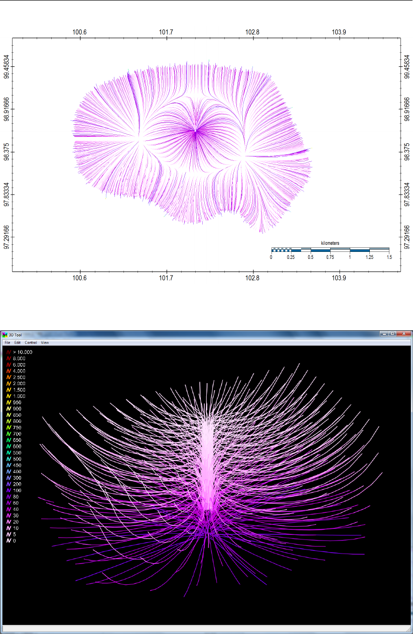
DRAFT
iMOD tutorials
Figure 11.49: Example of a two-dimensional image of pathlines.
Figure 11.50: Example of a three-dimensional image of pathlines near the well.
Please note that the vertical scale is always very much exaggerated! From the 3D image above, it is
clear that most of the water penetrates vertically to the deeper subsoil and then flows to the well. Given
that the material is highly permeable (25m/day) and homogeneous. In the next section 11.5 we will
Deltares 647 of 812

DRAFT
iMOD, User Manual
enhance this model to include more resistance in the subsoil which will affect the pathline behaviour.
Finally, our major question is still unanswered.
Sensitivities and sustainable yield
So, now we know that an extraction of 500m3/day will be sustainable, we’re still wondering what the
maximum will be. It will be your task as hydraulic engineer to give an answer to that question by
simulating a variety of model simulations for different extraction rates for the well. Use the next figure
to monitor the behavior of the system for different rates. Moreover, you could vary the permeability
too, since this parameter is often uncertain. It will be interesting to illustrate the accuracy of your
sustainable yield estimation with a bandwidth that expresses the inaccuracy of the permeability too.
As stated above, after each model simulation you should check the total water balance of the model
in the iMODFLOW.list file located in the model directory . \MODELS \ISLANDQ500 \mf2005_tmp), it
shows the total summary of the model simulation. If you scroll down, you’ll see the total water balance
for the model.
In the example above shows the quantity of water flowing in from the sea is close to zero while the
amount of water flowing out to the sea is 4081m3/day. You could use these as evaluation criteria as
well!
648 of 812 Deltares

DRAFT
iMOD tutorials
11.5 Tutorial 5: Solid Tool
This tutorial gives a short introduction in enhancing the groundwater flow model from section 11.4 with
an aquitard that has been characterized by several boreholes. See for a more detailed description of
the Solid Tool section 7.4.
Outline
This is what you will do:
Visualizing the boreholes in 3D;
Enhancing the subsoil characteristics based on the boreholes using the Solid Tool;
Simulate the updated model to observe the consequences of an aquitard in-between two aquifers;
Simulate flow of particles.
Required Data
For this tutorial you need the following iMOD Data Folders:
SURFACE_LEVEL.IDF: describes the surface level of the model area;
BOUNDARY.IDF: describes the boundary conditions;
WELL.IPF: ipf file that describes the location and rate of the wells;
ISLAND.PRJ: project file that describes the model configuration;
BOREHOLES.IPF: ipf file that describes the location and actual borehole data.
BEDROCK.IDF: idf file that describes the elevation of the bedrock layer.
All these files are located in/below the folder: {path of installfolder} \tutorials \TUT_ SOLID_BUILDING.
Beside this data you will need the iMODFLOW executable to make the model computations, see step
1in section 11.4.
Getting Started
1 Launch iMOD by double click on the iMOD executable in the Windows Explorer, and start by se-
lecting the option Create a new iMOD Project.
2 Open the SURFACE_LEVEL.IDF from by clicking the Open IDF ( ) from the main menu. The
file is located in . \TUT_SOLID_BUILDING \.
This file shows the surface level of a small island that we’ve been modeling in section 11.4. If you want
you can add a sketch of the outline of the island by following the steps 3upto 6from section 11.4.
Now we have an IDF of the uppermost interface of our model (the actual surface-level), we need to
have an IDF for our lowermost interface as well (to start with; this can be modified later). So, we will
copy the SURFACE_LEVEL.IDF and assign a default value of 20m-MSL and call it BEDROCK.IDF. We
have done that for you, so please open this file in iMOD.
3 Open the BEDROCK.IDF from by clicking the Open IDF ( ) from the main menu. The file is
located in . \TUT_SOLID_BUILDING \.
These two files describe the vertical and horizontal limits of our model. In-between there exists an
aquitard that has been identified by several boreholes, when they we’re installing the well.
Deltares 649 of 812
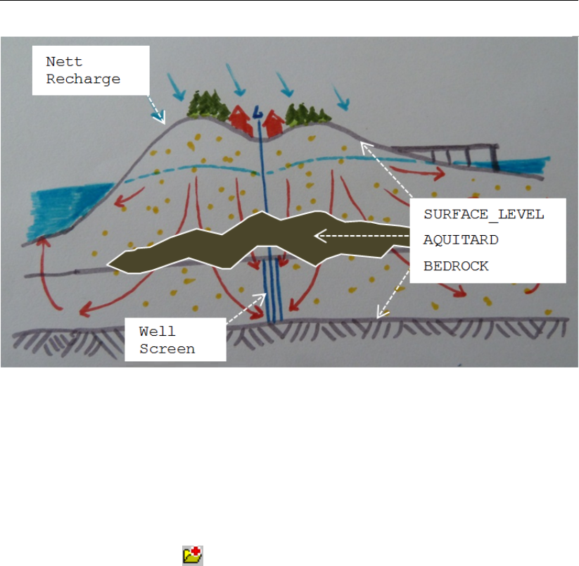
DRAFT
iMOD, User Manual
Figure 11.51: Sketch of a flow pattern that might occur in our island model.
Boreholes
When they drilled the well in the early 80’s, the borehole company found some clays with low permeable
material (less than 0.0001 m/day). Probably these are some ancient deposits, but they can interfere
with the flowpath to the well screen and therefore might decrease the level of sustainability of the
well. To this end, they decided to collect more information about the extent of this clay layer by drilling
additional boreholes. A total of 5 boreholes were drilled, let’s start by loading these in iMOD.
4 Click the Open IDF button ( ) and select the file BOREHOLES.IPF from the . \TUT_
SOLID_BUILDING folder.
The syntax of the file BOREHOLES.IPF is as described in more detail in section 9.7. For now, each lo-
cation of the boreholes has an x- and y coordinate and a reference to an attached textfile that describes
the actual borelog. Let’s see how the subsoil should look like whenever we include the boreholes.
5 Use your experience from the previous tutorials to produce the following figure, see steps 46 and
further from the first tutorial whenever you need some assistance in this. Note: If not all labels are
visible directly, go to the Clipplanes tab and select one direction a time until all labels are visible.
650 of 812 Deltares
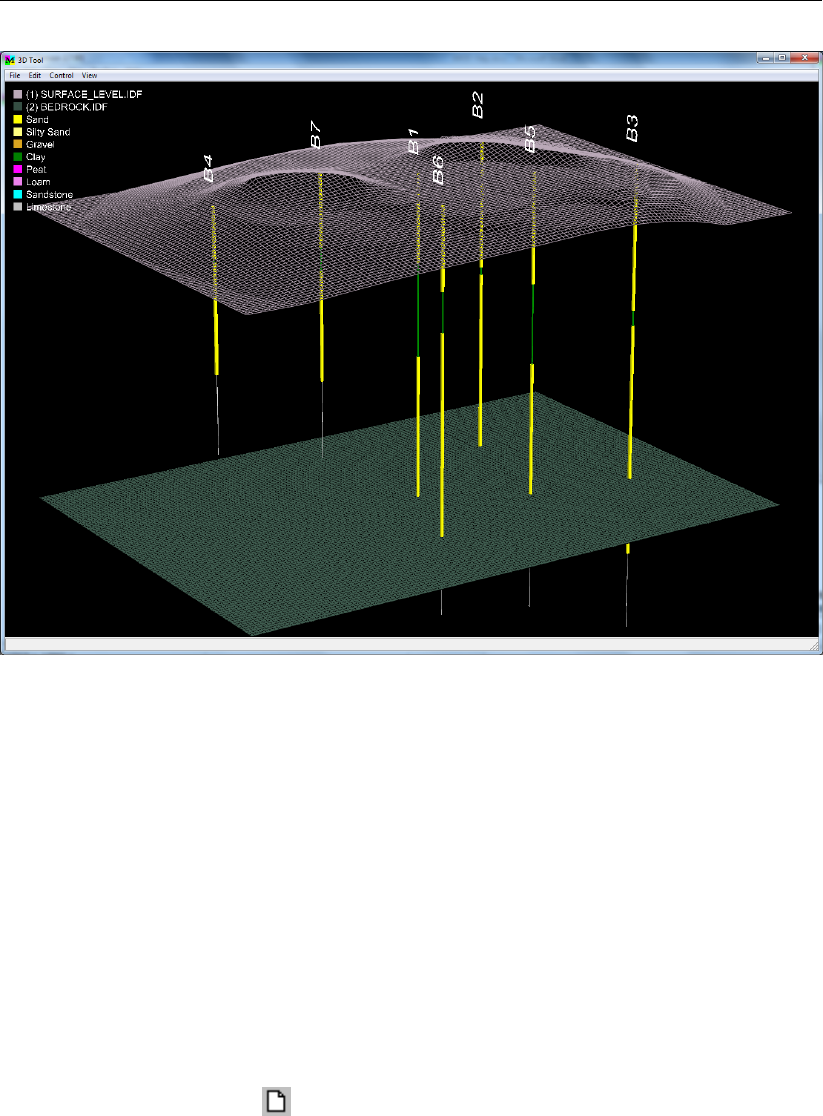
DRAFT
iMOD tutorials
Figure 11.52: Example of a 3D-image of boreholes of the hypothetical island.
From the above given figure, it seems that our estimation of the bedrock depth is not accurate as the
boreholes show an increasing bedrock depth from the west to the east. Moreover, we can clearly
observe a clay layer (green) in-between the aquifer (yellow). This clay layer has its greatest thickness
in the centre of the island (off course) and thins out to the side of the island. Probably eroded by some
ancient seas. We are going to use the Solid Tool to construct the interfaces that describe the top- and
bottom elevation of the aquitard, as well as adapting the bedrock level of the limestone.
Create a Solid
A solid is a representation of the subsoil divided into separate interfaces, such as clay and other lower-
or higher permeabilities. It contains a set of continuous interfaces that exist throughout the model
domain and can be used in a groundwater flow model.
6 Click the Toolbox option from the main menu and then select the Solid Tool to start the Solid Tool
window.
7 Click the New Solid button ( ) to start the Create New Solid window.
8 Select Enter single TOP and BOTTOM of SOLID.
9 Select the IDF-file [SURFACE_LEVEL.IDF] from the list mentioned by TOP-level and the IDF-file
[BEDROCK.IDF] from the list mentioned by BOT-level.
10 Enter [ISLAND] in the Give the name for the Solid input field.
Deltares 651 of 812
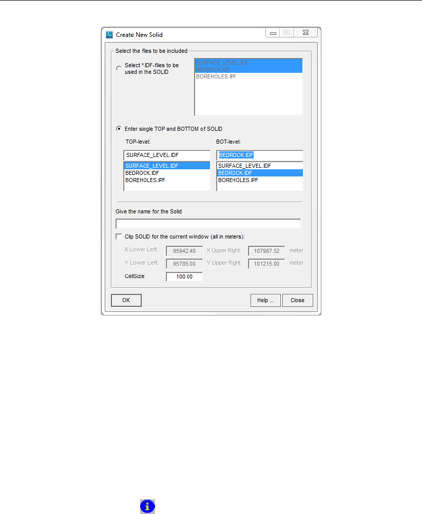
DRAFT
iMOD, User Manual
Figure 11.53: The ’Create New Solid’ window.
iMOD will use the selected IDF-files (SURFACE_LEVEL.IDF and BEDROCK.IDF) as the uppermost
and lowermost interfaces of our model. It is important that the files are selected in the right sequence
(from the top to the bottom). iMOD can add extra interfaces whenever you specify that, so based on
the two selected IDF-files iMOD can create extra interfaces in-between. In our modeling project, we
need at least two model layers, one to describe the groundwater head above the aquitard, and one to
describe the situation underneath.
11 Click the OK button
12 Enter [4] for the Number of interfaces .
13 Click the OK button
14 Click the OK button on the Information window that mentions that the solid has been created
successfully. This returns you to the Solid Tool window again.
15 Click the Information button ( ) to display the content of the *.SOL file. This file describes the
files to be used for the solid.
As you can see, the names for the top and bottom interfaces are changed into INT_L1.IDF and
INT_L4.IDF. These are copied from the SURFACE_LEVEL.IDF and BEDROCK.IDF, respectively. The
other interfaces INT_L2.IDF and INT_L3.IDF are interfaces that iMOD created and are by default the
mids in-between the surface (L1) and the bedrock level (L4). All these files are located in the folder .
\IMOD_USER \SOLIDS \ISLAND.
16 Close the Texteditor as this will return you to the Solid Tool window.
17 Select the [ISLAND] in the list on the Solid Tool window, if this is not selected yet. Click on Feed
Selected SOL-file to the iMOD Manager.
18 Open the iMOD Manager and observe that there is a file called [ISLAND.MDF]. An MDF-file is a
collection of IDF-files into a single file, see section 6.5 for more information about these MDF-files,
how to create them and how to dissolve them again.
19 Select the BOREHOLES.IPF and the ISLAND.MDF in the iMOD Manager.
20 Click the 3D Tool button (on the Solid Tool window!) to start the 3D Tool (see for more information
section 7.3 and step 46 in section 11.1).
652 of 812 Deltares
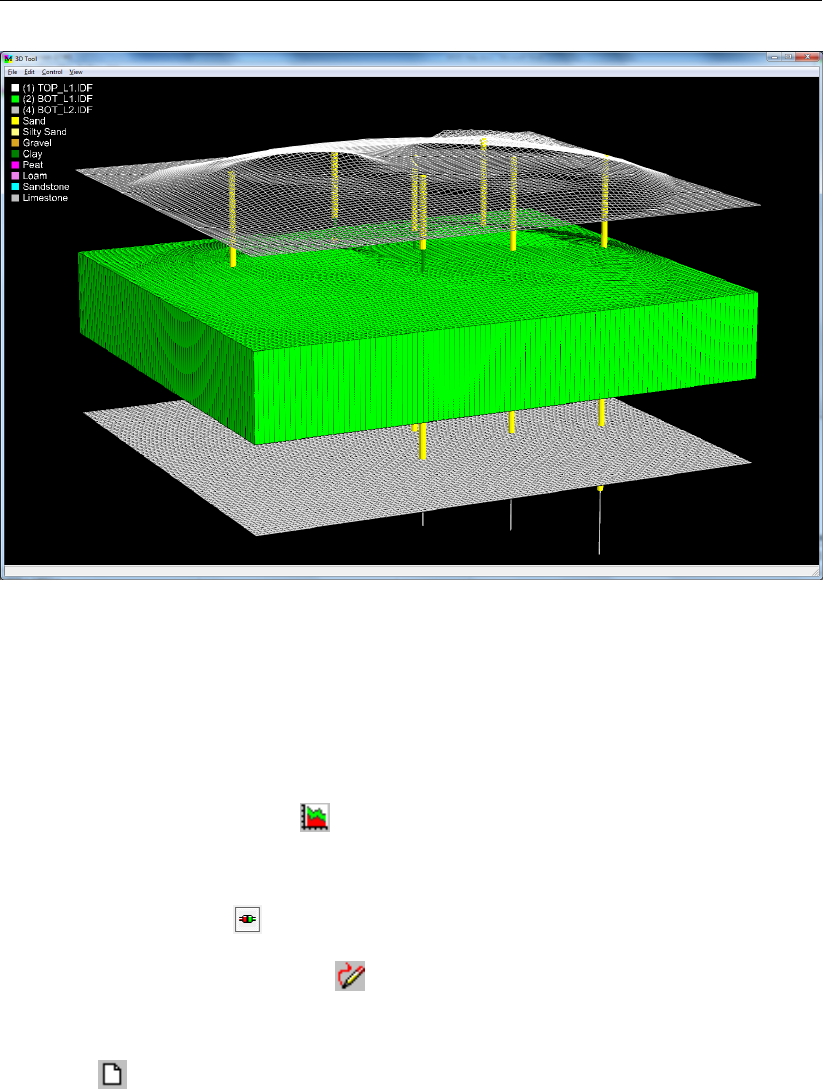
DRAFT
iMOD tutorials
Figure 11.54: Example of the initial Solid.
You can see how the current solid looks like, it contains a single aquifer on top of the (green) aquitard,
and another aquifer beneath it. It is not very accurate though, compared to the boreholes. We are
going to manipulate the green aquitard such that is resembles the boreholes more realistic.
21 Choose the option File from the main menu on the 3D Tool window and then select the Quit 3D
Tool option, this returns you to the main screen again.
22 Click the Cross-Section button ( ) on the Solid Tool window (again not the one on the main
menu!). This will start the Cross-Section Tool as you experienced in section 11.3, step 7. Read
section 7.1 for more information about this tool.
23 Enlarge the Draw Cross-Section window such that you can see the boreholes more clearly.
24 Select the Snap option ( ) on the Draw Cross-Section window at the Location tab (caution: do
not select the same option on the Cross-Sections tab!).
25 Click the Draw Cross-section button ( ) on the Draw Cross-Section window and start drawing a
cross-section in the Draw Cross-Section window, start from the left borehole B7 via B1, B5 to B3.
Click your right mouse button to stop this drawing.
26 Select the tab Cross-Sections on the Draw Cross-Section window and click the New Cross-section
button ( ) on the Cross-Section window to start the Fit Interfaces window.
Here, you can enter a name for the cross-section. We suggest that you enter the name [CROSSB7B1B5B3],
so it will be clear, in future, what cross-section this is.
Furthermore, this window offers the possibility to start your initial guess for the cross-section using the
current values for those interfaces.
Deltares 653 of 812
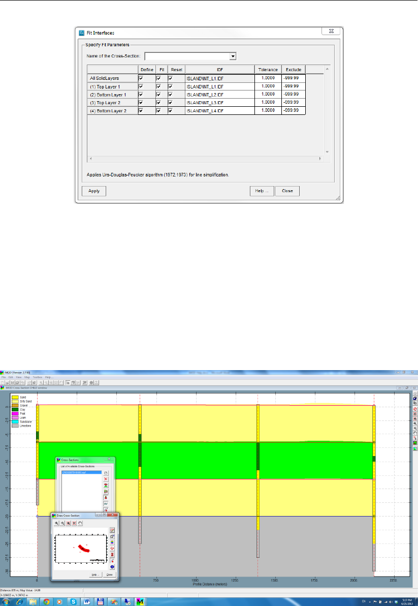
DRAFT
iMOD, User Manual
Figure 11.55: The ’Fit Interfaces’ window.
iMOD will fit the interface along the cross-section on the values read from the appropriate IDF, so in this
case iMOD will create a line for the [Top Layer 2] (third row in the table) on the content of the ISLAND
\INT_L3.IDF. The accuracy of this fit is determined by the Tolerance, which is set to [1.0] meter, which
is rather high for this case; however, it is fine for now. Feel free to change the tolerance values to see
the impact.
27 Click the Apply button.
iMOD will fit each line to the corresponding IDF-files, the result is presented below.
Figure 11.56: Result of the initial guess for the cross-section based on the values entered
in the previous ’Fit Interfaces’ window.
Now we can do two things:
We can manually edit the line such that it will fit the boreholes. You can easily move your cursor in
the neighborhood of the (red) line. Whenever it changes in a red arrow you can click the left mouse
button and drag the line to another position. Whenever it becomes a black arrow you can modify
the existing node of the line. This behavior is similar to modifying polygons, see section 4.4 for an
example.
654 of 812 Deltares
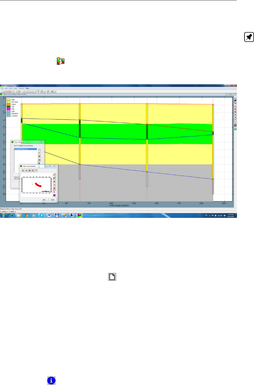
DRAFT
iMOD tutorials
We can tell iMOD to connect the lines through the boreholes. We will start with this.
Note: iMOD will connect the interfaces through all boreholes in the cross-section. Bear in mind that
boreholes might be projected on the cross-section over an undesired distance. To avoid that, decrease
the Fade, view depth on the Misc. tab on Cross-Section Properties window.
28 Click the Fit button ( ) to adjust the nodes on each line such that the line crosses each borehole
at the right position.
Figure 11.57: Result of adjusting the nodes on each line such that the line crosses each
borehole at the right position using the ’Fit’ button.
For now we will accept this cross-section.
Okay, let us define the other cross-sections. Follow the steps 22 upto 26 for the different cross-sections.
Simply press the New Cross-Section button ( ) again to start another cross-section. We suggest
you draw the following cross-sections (you’re free to draw other combinations as well):
[CROSSB7B1B5B3]: B7-B1-B5-B3 (you just did this one!)
[CROSSB6B1B2]: B6-B1-B2
[CROSSB4B7B2B3]: B4-B7-B2-B3
[CROSSB4B6B3]: B4-B6-B3
29 Click the Close button on the Draw Cross-Section window. You’ll be asked to save the current
cross-sections, click Yes.
iMOD will save the current cross-sections into separate files, e.g. called CROSSB7B1B5B3.SPF in the
. \IMOD_USER \SOLIDS \ISLAND folder. Also the ISLAND.SOL will be adjusted such that it includes
a reference to this CROSSB7B1B5B3.SPF. Please have a look in the ISLAND.SOL by pressing the
Information button ( ).
Deltares 655 of 812
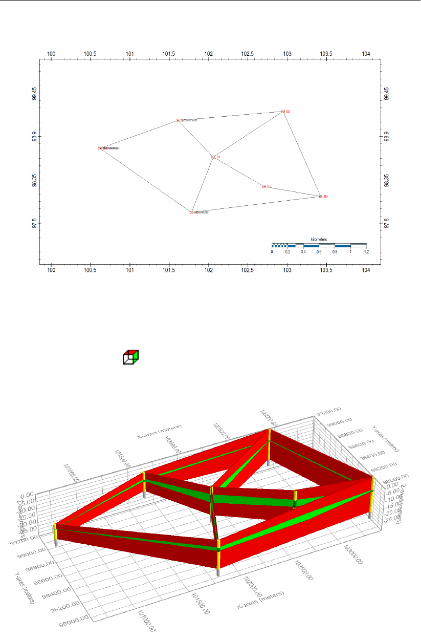
DRAFT
iMOD, User Manual
Your result might look like the following example.
Figure 11.58: Example of the outline of the cross-sections.
Bear in mind that the area outside the cross-sections will be extrapolated from the cross-sections.
You’re allowed to define other cross-sections in those areas too, to direct the interpolation more.
30 Select the [BOREHOLE.IPF] in the iMOD Manager solely.
31 Click the 3D Tool button ( ) on the Solid Tool window.
Figure 11.59: Example of a 3D image of the outline of the cross-sections.
There is a Solid tab active now. On that tab you’ll find a list of all the cross-sections, you can select
them all or select them individually.
32 Select the cross-section CROSSB7B1B5B3 from the list on the Solid tab in the 3D Plot Settings
656 of 812 Deltares
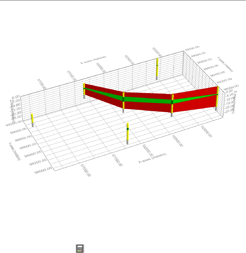
DRAFT
iMOD tutorials
window.
Figure 11.60: 3D image of the individual cross-section [CROSSB7B1B5B3].
33 Click the File option from the 3D Tool menu and then select the optionQuit 3D Tool to return to the
Solid Tool window.
Our next step is to create a fully 3D interpretation of the interfaces by numerical interpolation. The
interpolation is based on the cross-sections.
34 Click the Calculate button ( ) on the Solid Tool window to start the Compute Interfaces window.
In this window you’ll be allowed to determine what elevations/interfaces need to be computed. Since
the top elevation for our first model layer is the SURFACE_LEVEL.IDF (see step 2) we will not recom-
pute that interface, so we turn it off.
35 Deselect the Calc option for [(1) Interface 1].
We will overwrite our initial elevations/interfaces since that will increase the performance of our next
interpolations. Moreover, we will be able to see any update of our interfaces more easily.
Deltares 657 of 812
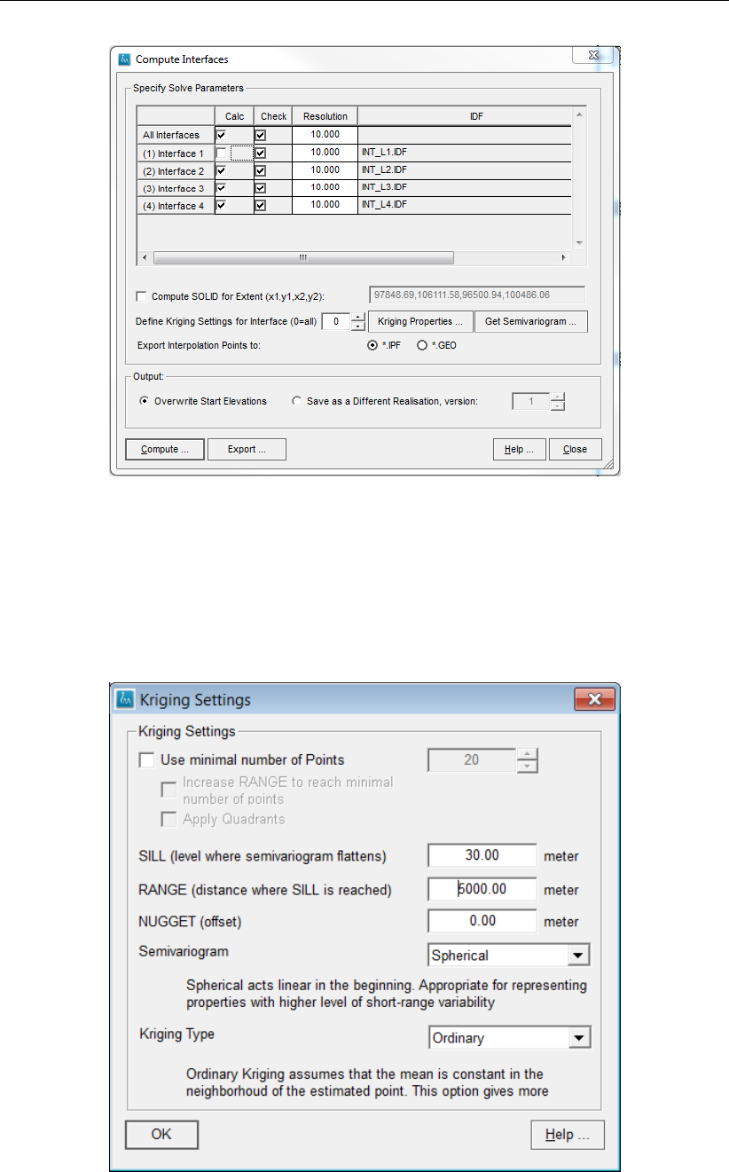
DRAFT
iMOD, User Manual
Figure 11.61: Example of the ’Compute Interfaces’ window.
iMOD uses as default Kriging interpolation. This is far-out the best suitable interpolation method for
these interfaces.
36 Click the Kriging Properties button to display the settings for the Kriging interpolation, see for more
details on the properties on this window Section ...
Figure 11.62: Example of the used Kriging Settings.
37 Click the OK button to accept the default settings of the Kriging parameters.
38 Click the Compute button to start the interpolation process.
658 of 812 Deltares
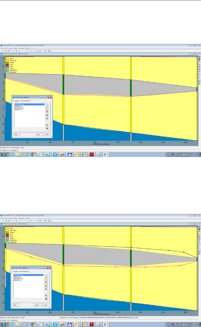
DRAFT
iMOD tutorials
39 Click the OK button whenever the interpolation has been finished.
40 Select ISLAND in the Solid Tool and click the Cross-Section Tool button on the Solid Tool window
and select the cross-section [CROSSB7B1B5B3.SPF] from theList of Available Cross-sections on
the Cross-Sections window.
Figure 11.63: Example of the cross-section CROSSB7B1B5B3 after interpolation.
Pretty cool, but also a bit unrealistic. We can modify each cross-section easily to become more smooth.
41 Use your mouse cursor to move in the neighbourhood of the a line to be modified and whenever
it becomes red, just press your left mouse button and drag the line. Try to create some detail, or
even try to create a hole inside the aquitard.
Figure 11.64: Editing the interfaces of cross-section CROSSB7B1B3B5.
Deltares 659 of 812
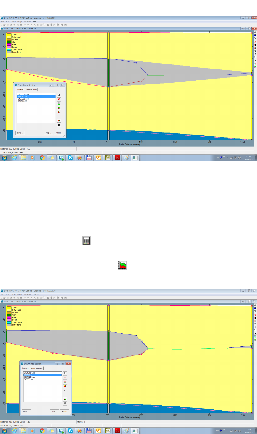
DRAFT
iMOD, User Manual
Figure 11.65: Editing the interfaces of cross-section CROSSB6B1B2.
Be aware of the fact that whenever you move a node into the neighbourhood of another node from
another line, iMOD will try to snap it. Whenever the line turns green, lines will be overlapping each
other perfectly, which means that there will be no thickness left for an aquitard. In this way, you can
create a hole in the aquitard.
42 Click the Close button on the Cross-Sections window to close the Cross-Section Tool, click the Yes
button whenever you are asked to save your adjustments.
43 Click the Calculate button ( ) and deselect the Calc option for [(1) Interface 1] and click the
Compute button to start a new interpolation.
44 Click the OK button whenever the interpolation has finished and re-enter the Cross-Section Tool
by clicking the Cross-Section Tool button ( ) again and select the cross-section
[CROSSB6B1B2.SPF] from the list.
Figure 11.66: The cross-section CROSSB6B1B2 after manual modification.
660 of 812 Deltares
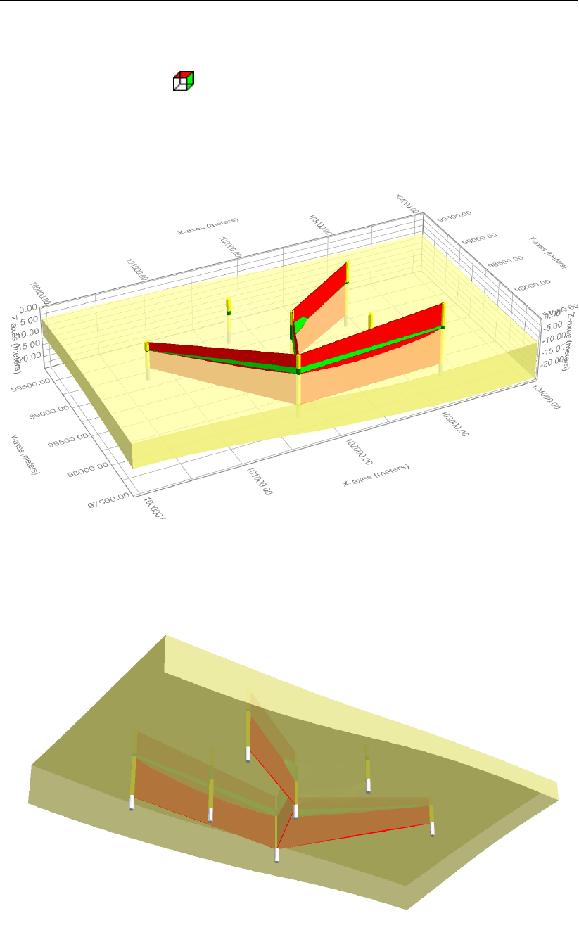
DRAFT
iMOD tutorials
45 Click the Close button on the Cross-Section window to leave the Cross-Section Tool, click No for
the question whether you want to save the adjustments (well we did not adjust anything, did we?)
46 Click the 3D Tool button ( ) and select the Quasi 3D Model (aquitard) configuration. This will
organize the table for the Display Configuration such that iMOD will create a solid representation
of aquitards.
47 Click the Apply button.
Figure 11.67: 3D image of the computed elevations of cross-section CROSSB6B1B2 and
one of the intersecting cross-sections.
Figure 11.68: Same cross-sections as previous figure, but now seen from below using
transparency view settings.
Deltares 661 of 812
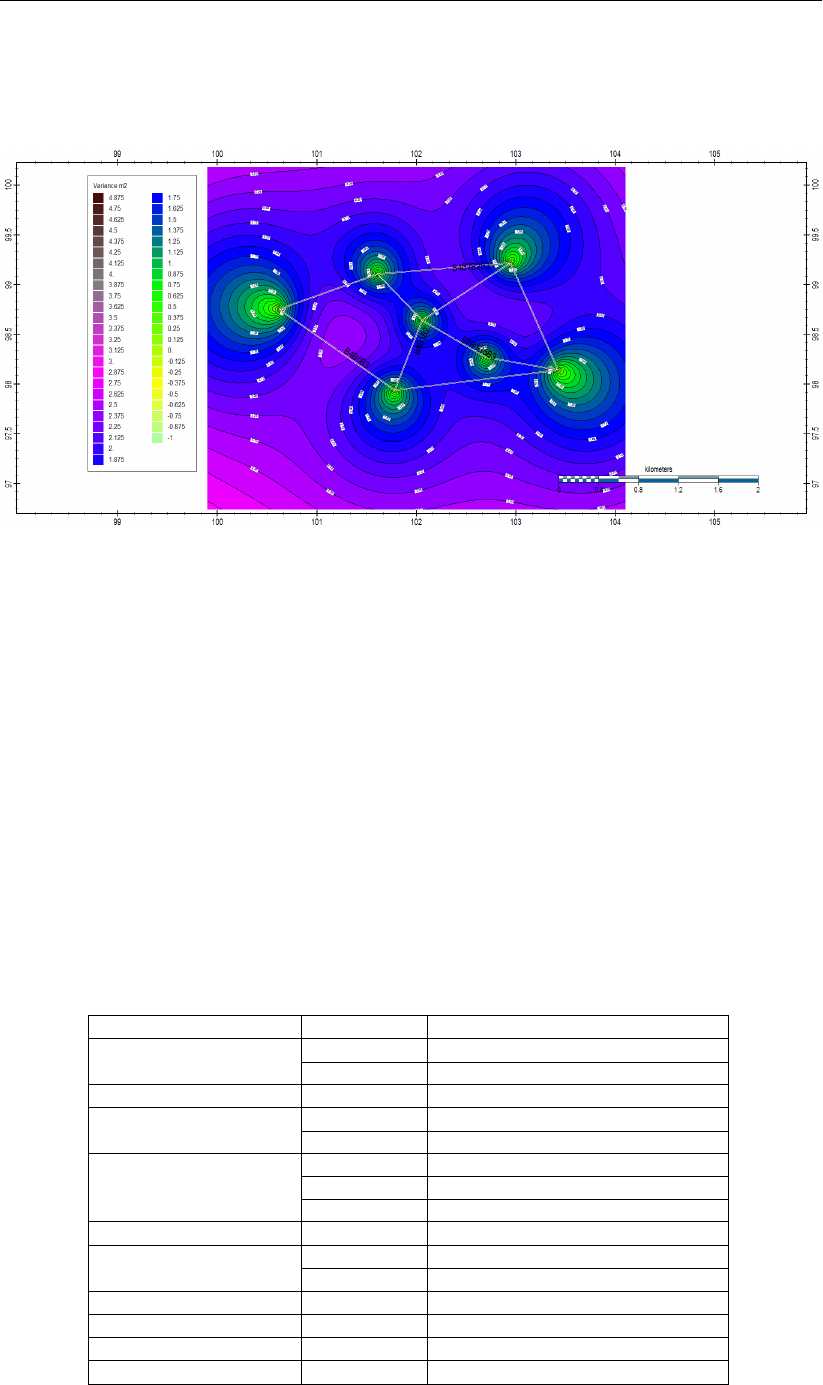
DRAFT
iMOD, User Manual
The Kriging algorithm generates the uncertainty of the estimate as a standard deviation (m). These
files can be visualised per interface, they are save in the same folder as the computed interfaces and
included the name _STDEV in the IDF file names.
Figure 11.69: Example of the estimated standard deviation of the estimated interface.
Okay, for now this looks quite nice, we’re done with our solid.
48 Click the option File from the 3D Tool main menu and then select the option Quit 3D Tool.
49 Click the Close button on the Solid Tool window.
We will examine what the consequences are for the flow paths towards the well. In section 11.4 we’ve
constructed a model from scratch and we will anticipate on your knowledge to do that again. We start
with the requirements for this particular three-layered model.
50 Select the option View from the main menu and then select the option Project Manager to start the
Project Manager window.
We have used this Project Manager in section 11.4 in detail. Please refer to that section for more
information. Here, we will create the necessary model configuration as outlined in Table 11.4.
Table 11.4: Model requirements for a confined, steady-state three layered model.
Parameter model layer IDF/Constant Value
Boundary 1 . \DBASE \BOUNDARY.IDF
2,3 1
Starting Heads 1,2,3 0.0 m+MSL
Top Elevation 1,2 . \DBASE \SURFACE_LEVEL.IDF
3 . \SOLIDS \ISLAND \INT_L3.IDF
Bottom Elevation 1 . \DBASE \SURFACE_LEVEL.IDF
2 . \SOLIDS \ISLAND \INT_L2.IDF
3 . \SOLIDS \ISLAND \INT_L4.IDF
Horizontal Permeability 1,2,3 25.0 m/day
Vertical Permeability 1 25.0 m/day
2 0.0001 m/day (1000 days/m)
Wells 3 . \DBASE \WELL.IPF
Net Recharge 1 0.5 mm/day
Porosity Aquifer 1,2,3 0.3
Porosity Aquitard 1,2,3 0.1
662 of 812 Deltares

DRAFT
iMOD tutorials
So, the only difference with our previous model in section 11.4 is that we use different values for our
Top- and Bottom elevations. Let’s start with the Project file we saved in section 11.4.
51 Click the Open PRJ button ( ) and select the PRJ file you’ve saved at step 61 of section 11.4.
52 Adjust the Top for model layer 3 and the Bottom elevations for model layer 2 and 3 by clicking
the Properties button ( ) and change the parameter in the window accordingly. Don’t forget to
change the constant value for the Vertical Permeability for model layer 2!
53 Click the Save As Runfile button ( ) when you are finished and save the file as [ISLAND_SOLID.RUN]
in the . \IMOD_USER \RUNFILES folder.
54 Click the Close button to hide the Project Manager window.
55 Select the option Toolbox from the main menu and then the option Start Model Simulation to start
the Start Model Simulation window.
56 Select the [ISLAND_SOLID.RUN] from the list of available runfile.
57 Select the tab Results on the Model Simulation window and enter the name
[ISLAND_SOLID] as the result name.
58 Click the Start Model Simulation button.
59 Close the Model Simulation window by selecting the Close button.
60 Use the Quick Open window to display the computed heads for the first model layer, see step 74
in section 11.4.
Deltares 663 of 812
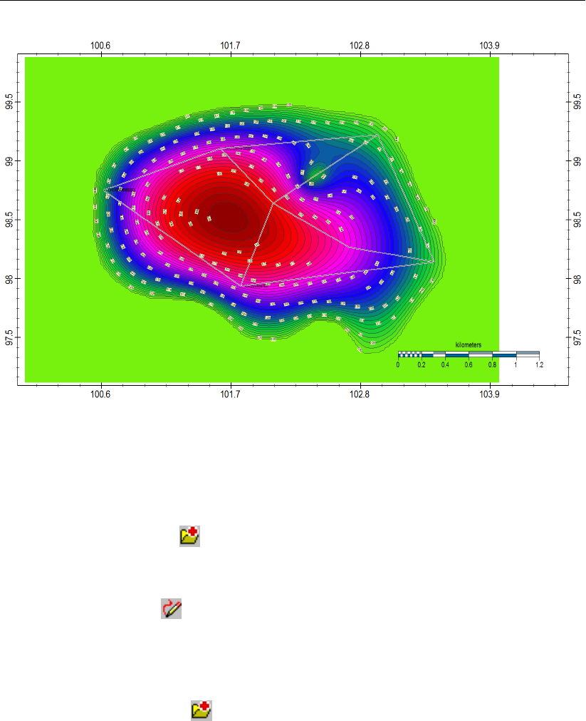
DRAFT
iMOD, User Manual
Figure 11.70: Example of the computed heads using the adjusted subsurface geometry.
You can see what the effects are from the hole in the aquitard (denoted by the white arrow). So, let’s
compute the flowlines towards the well. Instead of computing a forward tracing, we will compute a
backward trace from the well back to its infiltration areas.
61 Click the Add Map button ( ) on the main menu and select the [WELL.IPF] which is situated in
the . \TUTORIAL5_SOLID_BUILDING folder. So now we know where the well is actually.
62 Select the option Toolbox from the main menu and then choose the option Define Startpoints.
63 Enter [ISLAND_SOLID] in the input field and click the Open and Continue button.
64 Click the Draw button ( ), select the option Circle from the Select window and click OK. Now
locate the well with your mouse cursor and left click your mouse on the well. Press the right mouse
button to stop.
65 Select the Definition tab on the Start Point Definition window.
66 Enter [25] for the Radius and [5] for the Sampling. We will create startpoints every 5 meter on a
circle which has a radius of 25 meter.
67 Click the Open IDF button ( ) to select the Top elevation of the second aquifer (actually the
third model layer in which the well is located) as Top Level, so select the INT_L3.IDF from the .
\IMOD_USER \SOLIDS \ISLAND folder. Repeat this for the Bottom Level and select the bottom
elevation of the second aquifer (INT_L4.IDF).
68 Enter [10] for the Vertical Interval. We will have 10 particles starting in-between the top- and bottom
elevation of the second aquifer (third model layer).
69 Click the Draw button to see the actual location of the start points.
664 of 812 Deltares
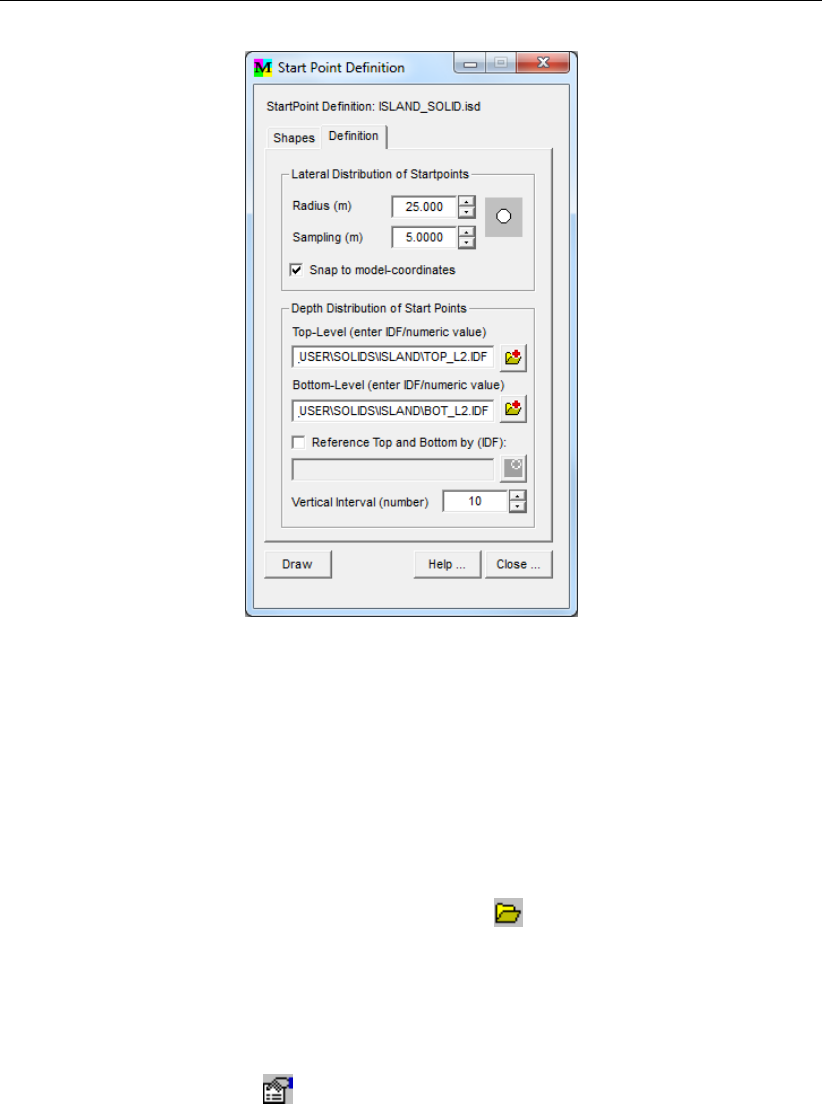
DRAFT
iMOD tutorials
Figure 11.71: The ’Start Point Definition’ window.
70 Click the Close button to save and close the window. Click Yes if you will be asked to save the file
to [ISLAND_SOLID.ISD].
71 Select the option Toolbox from the main menu and the select the option Start Pathline Simulation...
to start the Pathlines Simulation window.
We’ve have used this functionality before (see section 11.4, steps 85 onwards), so we will be brief this
time.
72 Select the model result [ISLAND_SOLID] from the list of Existing Results.
73 Select the Input tab and click the Open IPS File button ( ) and search for the IPF file that you
have saved in section 11.4.
If you did not save any IPF file, follow the steps 85 onwards mentioned in section 11.4, to fill in this
window. Though we need to do a slight modification too. Since we’ve changed the interfaces of our
model we should change the Pathline settings accordingly. So, . . .
74 Click the Properties button ( ) behind the Top- and Bottom files (second dropdown menu) and
change the filenames in the list as shown in the next figure (SURFACE_LEVEL.IDF may be used
instead of INT_L1.IDF).
Deltares 665 of 812
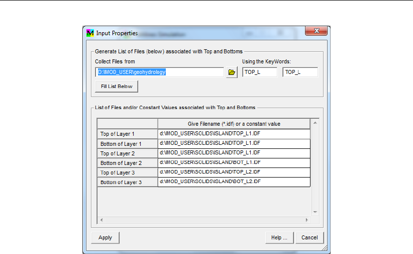
DRAFT
iMOD, User Manual
Figure 11.72: The ’Input Properties’ window that appears when choosing ’Start Pathline
Simulation...’ from the main menu, followed by selecting the ’Input’ tab, and
clicking the ’Properties’ button at the right of ’Top- and Bottom files’ field of
the ’Pathline Simulation’ window.
75 Click the Apply button to return to the Pathline Simulation window.
76 Select the [ISLAND_SOLID.ISD] from the list withStart Point Definition files.
77 Select the Results tab of the Pathline Simulation window.
78 Select the Backward option from the Trace Direction.
79 Select the option Save Entire Flowpath.
80 Enter [ISLAND_SOLID.IFF] as the name to save the results to.
81 Click the Start button.
82 Click the OK button in the Information window that appears after the simulation finished.
83 Click the Close button to quit the Pathline Simulation window.
iMOD will display the results directly on screen.
84 Use step 101 upto 102 from section 11.4 to change the visualization such that the total travel times
will be displayed.
85 Use the 3D Tool to visualize the flowlines in combination with the created solid in a single view.
You should be able to figure this out by yourself.
666 of 812 Deltares
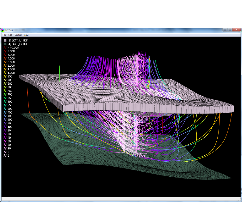
DRAFT
iMOD tutorials
Finally, we complete this Tutorial with the results of our well capture zone in a 3D environment.
Figure 11.73: The final pathlines representing the capture zone of the well; capture zone
is here defined as that part of the groundwater flow system that contributes
water to the pumped well.
Deltares 667 of 812

DRAFT
iMOD, User Manual
11.6 Tutorial 6: Model Simulation
This tutorial gives a short introduction in starting a groundwater flow model simulation. See for more
detailed references Model Scenarios and Model Simulation.
Outline
This is what you will do:
Understand the content of a model configuration file, i.e. a runfile;
Simulating a groundwater flow model for different cell sizes and areas of interest;
Understand the resulting folder structure with results;
Computing and visualizing a waterbalance of the model;
Defining a simple model scenario and include such a configuration to an original model configura-
tion.
Applying the new PKS-solver to simulated the model parallel.
Required Data
For this tutorial you need the following iMOD Data Folders:
BND: IDF-files that describe the boundary conditions;
DRN: IDF-files that describe drainage conditions;
KDW: IDF-files that describe the horizontal transmissivity;
OLF: IDF-files that describe the overland flow conditions;
RCH: IDF-files that describe the natural recharge;
RIV: IDF-files that describe the river conditions;
SHD: IDF-files that describe the starting head conditions;
VCW: IDF-files that describe the vertical resistance;
WEL: IPF-files that describe the wells;
TUT_MODEL.RUN: file that describes the model configuration and refers to the above mentioned
folders;
SCENARIO.GEN: file that describes the area that needs to be manipulated.
All these files are located in/below the folder: {path of installfolder} \tutorials \TUT_Model_Simulation.
Beside this data you will need the iMODFLOW executable to make the model computations.
Getting Started
1 Copy the TUT_MODEL.RUN into the . \IMOD_USER \RUNFILES folder.
2 Launch iMOD by double click on the iMOD executable in the Windows Explorer, and start by se-
lecting the option Create a new iMOD Project.
3 Open the TUT_MODEL.RUN in a text editor (e.g. Notepad++) and observe the $DBASE$ key-
words; as soon iMOD uses this runfile to perform a simulation this keyword will be replaced by the
string as defined in the IMOD_INIT.PRF file which is in {installfolder}. Go to File–>Preferences...
and click on to read the contents of the PRF-file; when you change and save the contents of
the IMOD_INIT.PRF file in a text editor, click on to re-read the keyword settings for the current
iMOD session. For more info on Preferences see section 2.7, for more info on available keywords
see section 9.1. For information on the iMOD folder structure ee section 11.1 and chapter 9.
4 Go to View in the menu bar and select the iMOD Manager (or use the short-key Ctrl+M).
668 of 812 Deltares
DRAFT
iMOD tutorials
Model Parameters
Let us first observe some model parameters and understand what this model might be up to. We use
the Project Manager for that, so let start that one.
5 Click the option Project Manager from the View menu.
iMOD simulates a groundwater flow model by means of a runfile. A runfile gives a full description of
the use of all files needed for the simulation. The Project Manager is able to read the entire runfile and
present the content in a treeview field.
6 Click the Open Runfile button ( ) and select the TUT_MODEL.RUN file from the {IMOD_
USER} \RUNFILE folder.
iMOD presents the content of the runfile in a treeview. Each branch represents a model parameter,
and whenever a branch contains more information we can expand the branch to analyse its contents.
Let us visualize the starting conditions for this particular model.
7 Make sure the iMOD Manager is also active (if not, press CTRL+M).
8 In the Project Manager expand the branch called (SHD) Starting Heads from the treeview field.
Select this branch (not an individual IDF) and click the draw button ( ). If no image appears you
may have to click the Zoom Full Extent button ( ).
As a result iMOD will open all the files of the selected branch and adds them to the iMOD Manager.
In this manner it is easy to explore the available model parameters for the model. In this model the
starting condition of a model simulation is equal to a result of a previous simulation. Since IDF-files
are geo-referenced, they can be easily (re)used for different modules and/or packages in a model
configuration.
9 Analyse the starting condition by creating several cross-sections (see section 11.3) and compute
the difference between the starting condition for model layer 1 and the one for model layer 2 (see
section 11.2). This gives you insight in downward and upward fluxes.
10 Click the branch (RIV) Rivers (Cauchy conditions) and observe that this model has two river sys-
tems. One is connected to model layer 1 and the other one is connected to model layer 2. Further-
more each river system consists of 4 input grids, CONDUCTANCE, RIVER LEVEL, RIVERBOT-
TOM LEVEL and INFILTRATION FACTOR. Examine the content of these files.
11 Explore the content of the Project Manager, e.g. plot the elevation of the existing Rivers in the first
system.
Deltares 669 of 812
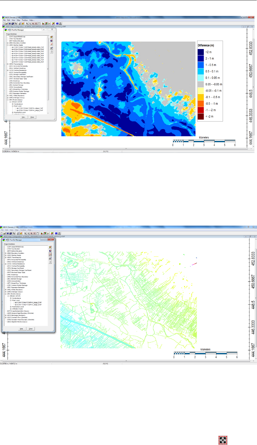
DRAFT
iMOD, User Manual
Figure 11.74: Difference between starting heads of model layers 1 and 2.
In this particular model a river is discretized for two different model layers , i.e. model layer 1 and model
layer 2. The number of river elements is unlimited, however, a single IDF can store one river for each
cell, so you should define more IDF files in those cases you want to specify more river elements at the
same location. In this particular case we specified river elements for model layer 2 that penetrate the
first aquitard and connect to the first aquifer (i.e. the second model layer).
Figure 11.75: Stages of the rivers of the first system.
Model Simulation
Let’s start the model simulation.
12 Select the option Start Model Simulation from the Toolbox option on the main menu. Whenever the
Start Model Simulation window does not appear, check the keyword MODFLOW in the PRF file.
13 Select the TUT_MODEL.RUN from the Runfiles list. You should see a hatched area of the maxi-
mum extent of the model. If you do not see that, click the Zoom to Extent button ( ). Click the
670 of 812 Deltares
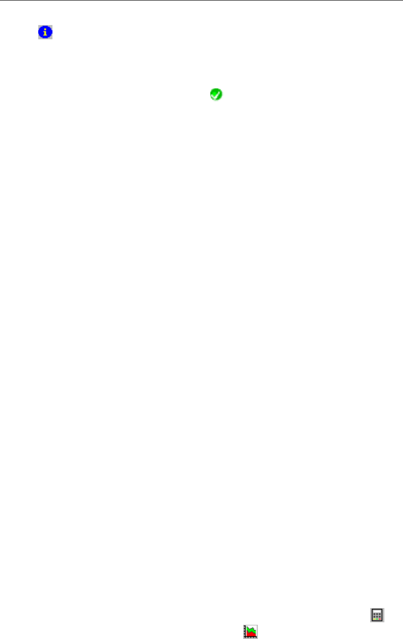
DRAFT
iMOD tutorials
Info ( ) to display the runfile in a texteditor.
The first 15 lines of the runfile can be manipulated by the Start Model Simulation window. The rest
refers to existing model input data, let’s check whether all these data is available.
14 Close the editor and click the CheckRun button ( ).
iMOD will popup a summary file ({USER} \TMP \RUNFILE.LOG) of all files that cannot be found. Use
step 6to open a runfile to change pathnames if needed. If no files are listed, all files can be found and
we can proceed.
15 Select the Result Folder tab and enter a name for the model results, e.g. MODEL25 and click the
Start Model Simulation button.
iMOD will copy the selected runfile [TUT_MODEL.RUN] to the {IMOD_USER} \MODELS \
MODEL25 folder and renames it into IMODFLOW.RUN. Thereafter it will copy the simulation exe-
cutable (e.g. iMODFLOW_V4_3_METASWAP_SVN1233_X64R.exe) to the same folder for archiving
purposes, and it will start the simulation by the statement
’{installfolder}\iMODFLOW_V4_3_METASWAP_SVN1233_X64R.exe IMODFLOW.RUN’
in this example in the {installfolder}\IMOD_USER\MODEL25 folder. A DOS-command tool will open in
which the simulation runs. You can proceed with iMOD or wait until the simulation finishes; it will take
a very short time since the starting conditions are similar to the results.
The model simulation is always logged in the file IMODFLOW.list located in the subfolder mf2005_tmp,
so in this example located in the folder {IMOD_USER} \MODELS \MODEL25 \mf2005_tmp. You should
check this file IMODFLOW.list first whenever there is a problem with the simulation; as mentioned
above it contains info on:
the model discretization
the model time and length units
the processed input packages
the solver used and how the iteration process progressed
the volumetric budget for the entire model, including the percent discrepancy
elapsed run time
16 When the simulation has finished, choose Quick Open from the main menu option Map.
17 Select the Folder [MODELS], then the variant [MODEL25], then choose the Topic [HEAD], and
choose Layer [1] and then click the Open button. Make sure the option Display is selected! If
everything went well the only option to be selected is [STEADY-STATE] in the dropbox Time. For
transient simulations, you might be able to select a specific date.
18 Compare the results to the starting conditions. Use tools experienced in section 11.1, 2 and 3 if
desired.
Let us simulate this model at a different resolution.
19 Start the Start Model Simulation (step 12) again and select the Model Dimensions tab and change
the cellsize in Simulate model with cellsizes equal to = [100]. You can select a cellsize from the
dropdown menu and/or enter a different cellsize in the input field to the right of the dropdown menu.
20 Go to the Result Folder tab and enter an output foldername [MODEL100] and click the Start Model
Simulation button.
21 Open the resulting phreatic heads (model layer 1) with Quick Open (see step 74) and subtract the
head calculated for MODEL100 from the head of MODEL25 using the Map Calculator ( ) on
the iMOD Manager and/or use the Cross-Section Tool ( ) on the main toolbar to explore the
differences caused by the different simulation cellsizes.
When using the Cross-Section Tool with the Block Line option (see section 11.3 step 12), you may
expect the width of 4 blocks of the MODEL25 line equal to the width of 1 block of the MODEL100 line.
Deltares 671 of 812
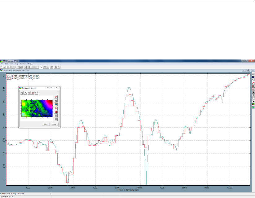
DRAFT
iMOD, User Manual
But this is probably not what you observe in step 22 and 25 of this tutorial, because iMOD standard
reduces the number of sampling points to speed up the calculations. To get the widths as expect, you
have to increase the value of Maximum number of sampling points in the Cross-Section Properties
window (see section 11.3 step 11 or section 7.1 to open this window), e.g. set Maximum number of
sampling points to [1000].
Figure 11.76: Cross-section of heads of the 25x25 meter model (dark blue) and the cor-
responding 100x100 meter model (red).
Let us simulate just a part of the model.
22 Start the Start Model Simulation (step 12) again and select the Model Dimensions tab and click
the Draw Simulation Area of Interest button. You can interactively draw the area of interest within
the hatched area. Click your left mouse button to set the first corner and give a second left mouse
click to specify the opposite corner. You may drag the area of interest interactively by dragging
the mouse while your inside the graphical display. Reset the cellsize to 25 meter and include a
buffer-zone of 1500 meter.
672 of 812 Deltares
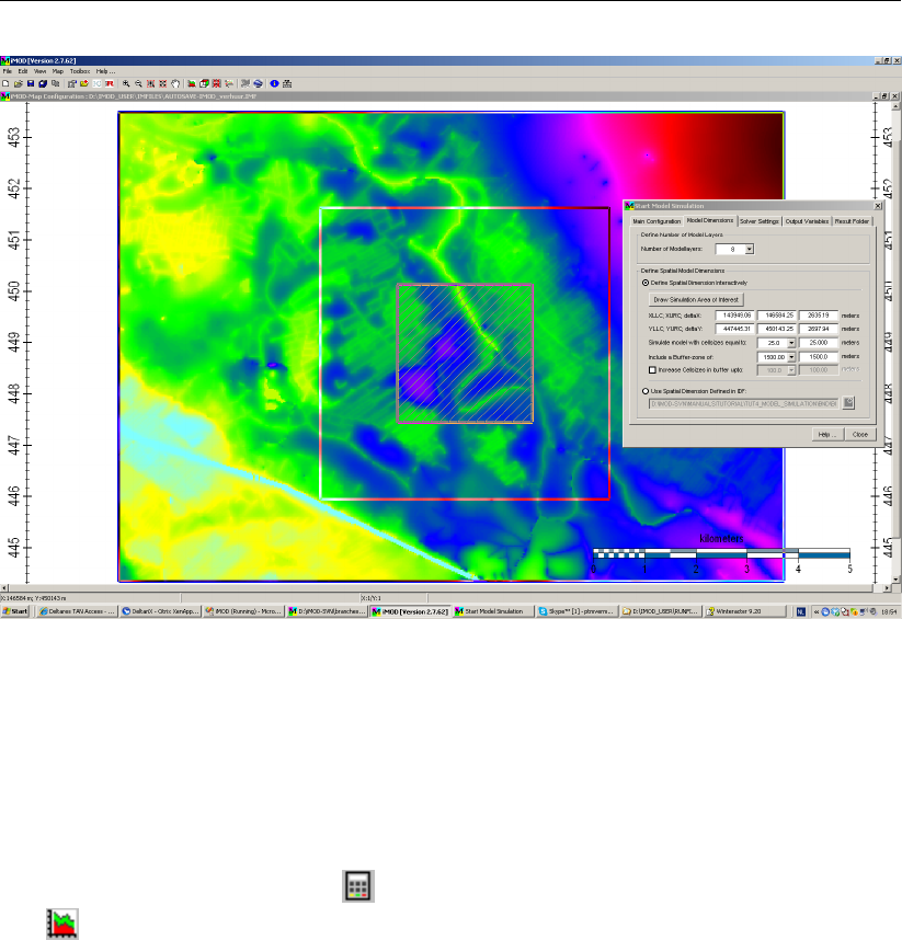
DRAFT
iMOD tutorials
Figure 11.77: Example of interactively specifying a part of the total model domain (small-
est rectangle with hatching-pattern) for a model simulation. Also the size of
the surrounding buffer zone can be specified here.
23 Go to the Output Variables tab and select the option Save Result Variable including the given Buffer
Size.
24 Go to the Result Folder tab and enter an output foldername [MODEL25PART] and click the Start
Model Simulation button.
25 Open the resulting phreatic heads (model layer 1) with Quick Open (see step 74) and subtract the
results using the Map Calculator ( ) on the iMOD Manager and/or use the Cross-Section Tool
( ) on the main toolbar to explore any differences.
Water Balances
An important aspect of groundwater flow modeling is the ability to compute water balances. In iMOD
you can compute these too. It is important that you specify the appropriate output variables prior to your
simulation, see tab Output Variables in the Start Model Simulation window. In this case the defaults for
the output variables were used.
26 Select the option Water Balance and then Compute Water Balance from the Toolbox menu.
27 Select the model [MODEL25] from the list at Existing folder with Results available in the Models
Folder.
28 Click the Modflow button to select all water balance term that are relevant to Modflow (saturated
groundwater), automatically. The iMOD convention is that all flux related output files start with
BDG*. The content of these files is always in m3/day.
29 Select the Period and Layers tab from the Compute Waterbalance window.
Here you can specify for what layers, and periods (in case of a transient model) need to be included in
the water balance. For now we select all layers (which are selected by default), so we leave it like it is.
30 Click the Create TXT . . . button and save the water balance as WBAL.TXT.
31 iMOD will present the content of the WBAL.TXT file. Inspect the terminology and its content; more
is explained below.
Deltares 673 of 812
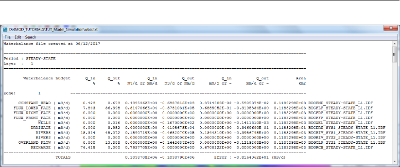
DRAFT
iMOD, User Manual
Figure 11.78: Example of a water balance TXT-file.
In the above given example a water balance is presented for the entire model and for all model layers
sequentially. In this case the water balance is given for a steady-state simulation and summed for the
entire model area. There is only one zone used and the following terms are organized row wise:
CONSTANT HEAD
flux in or out across the boundary according the boundary condition specified around the model.
FLUX LOWER FACE
flux over the interface between model layer 1 and 2, along the z-direction downwards.
FLUX RIGHT FACE
flux over the interface between column interfaces between cells in model layer 1. along the x-
direction eastwards.
FLUX FRONT FACE
flux over the interface between adjacent row interfaces in model layer 1, against the y-direction
southwards.
WELLS
flux in the wells.
DRAINAGE
flux out the drainage systems.
RIVERS
flux in or out the river systems. There are two river systems presents, so therefore two lines are
presented, though the second system is not active in the current model domain.
OVERLAND FLOW
flux in the overland flow drainage system.
RECHARGE
flux from the recharge.
Especially the (Q_in and Q_out) percentages are interesting and can be used to observe the rela-
tionship between the different water balance terms. In the above example >45% of the groundwater
is discharged to the surface water.
32 Close the water balance text file in order to continue. The file can be inspected any time by a
regular text editor.
There is another, more interactive manner, to examine water balances, let’s try that.
33 Select the Create CSV . . . button and save the water balance as WBAL.CSV.
34 iMOD asks to start the Waterbalance Analyser after finishing the creation of the WBAL.CSV, click
Yes to start the Analyse Waterbalance window.
Now you can see that iMOD read 8 records, 11 budget terms, 1 period, 8 layers and 1 zone. The
Waterbalance Analyser can be used to aggregate budget terms and display them graphically.
35 Select the Budget Terms tab, here all available budget terms are listed from the WBAL.CSV.
674 of 812 Deltares
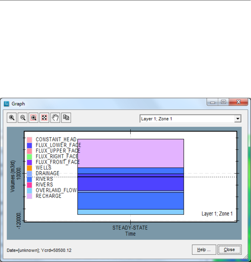
DRAFT
iMOD tutorials
36 Select the option [STEADY-STATE] form the Timesteps list.
37 Select the Aggregation tab, here all type of aggregation can be performed.
38 Select the Select All button from the Model Layers list.
39 Select the Select All button from the Zones list.
40 Select the Graphics Output tab, here all types of output can be selected, we leave it for now like it
is.
41 Select the Generate Preview button to display the current configuration (as set in the previous tabs)
in a graphical display.
The following image might appear.
Figure 11.79: Example of a water balance displayed from a CSV-file.
From here you can zoom in or zoom out in the image, as well as select a different combination of model
layer and zone number. If you have multiply zones nz and multiply layers nl, the list in the drop down
menu is as long as nz ×nl. Let us display another graphical presentation of the water balance.
42 Click the Close button to close the Graph window.
43 Select the option Graphical Representation.
The water balance is presented as follows:
Deltares 675 of 812
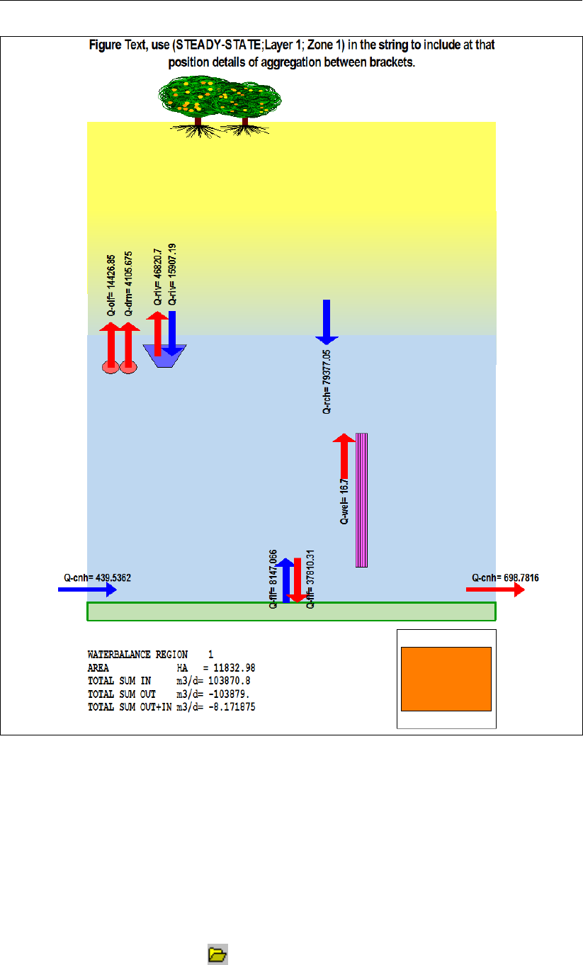
DRAFT
iMOD, User Manual
Figure 11.80: Example of a water balance displayed from a CSV-file.
There will be a sequence of 8 figures passing by, since we have selected 8 model layers, so repeat the
following step 8 times to close all the repeating windows.
44 Click the Close button to close the graphical image window.
Let’s try a more complicated CSV file in this tool.
45 Click the Close button to close the Graph window.
46 Select the CSV-File tab from the Analyse Waterbalance window.
47 Click the Open CSV-File button ( ) and select the file {path of installfolder} \tutorials \TUT_Model_Simulation
\DELTARES1994.CSV. It’s a pretty big water balance file and holds the results of a daily model sim-
ulation (365 periods) for 29 budget terms, 19 layers and 17 zones.
48 Select the Budget Terms tab.
676 of 812 Deltares
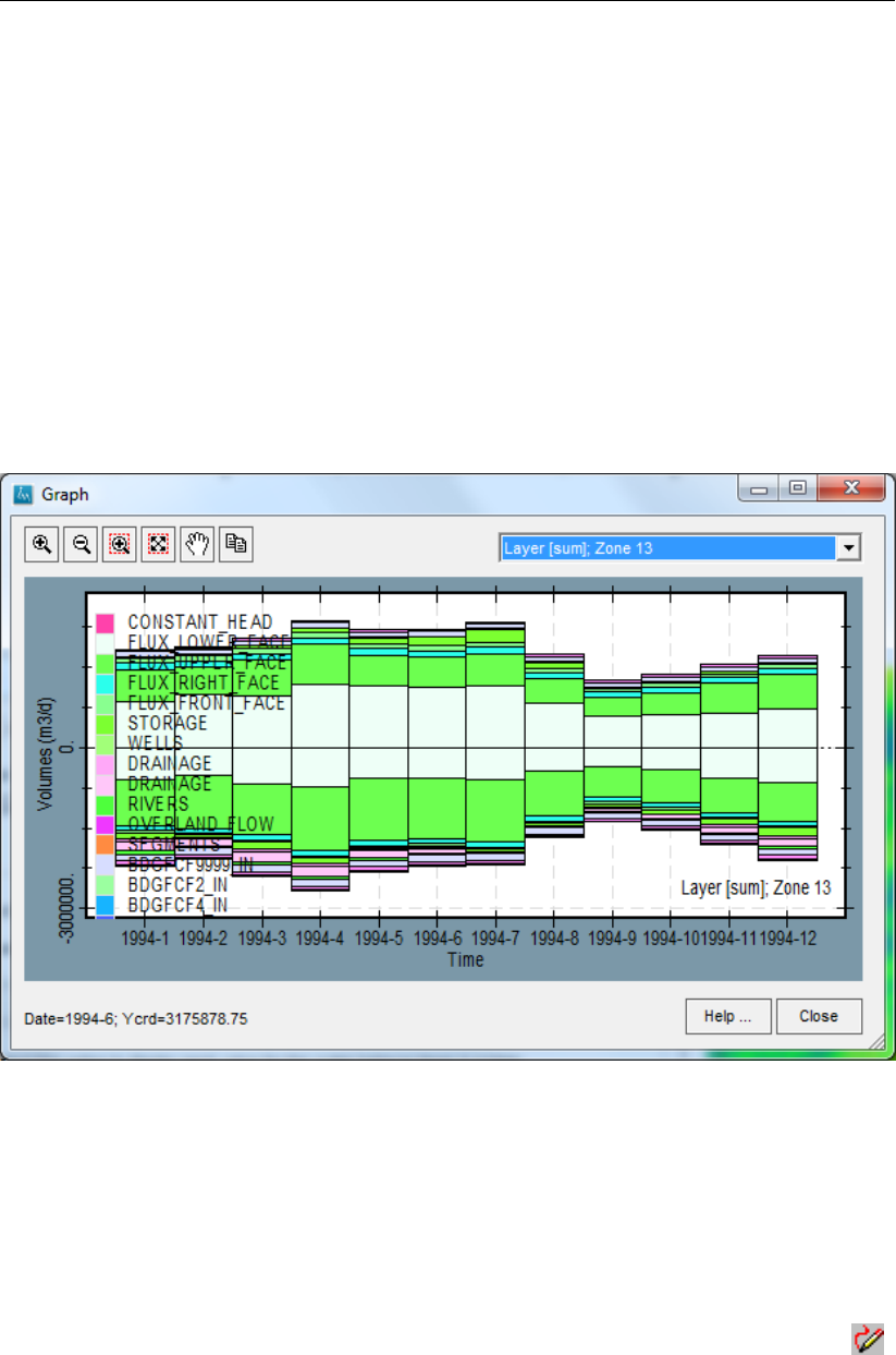
DRAFT
iMOD tutorials
49 Click the Select All button from the Timesteps list.
50 Select the Aggregation tab.
51 Select the option Months, a single value per month, starting at the first month of the series. Al-
though the original data is for a daily base, the Waterbalance Analyser can aggregate the budget
terms on a monthly base automatically.
52 Click the Select All button from the Model layers list.
53 Select the option Sum Selected Layers from the Layer Aggregation input field. In this way, all fluxes
as summed over the selected layers.
54 Click the zones 8, 9 and 13 from the Zones list. Use the Ctrl-Left mouse button to make that
selection.
55 Select the Graphics Output tab.
56 Click the Generate Preview, make sure the option Time Series is still selected.
57 Select the option Layer [sum]; Zone 13 from the drop down list in the Graph window.
The following image appears.
Figure 11.81: Example of a water balance aggregated on a monthly base from a CSV-file.
There is a lot to try in this tool, all kind of different settings can be combined, see section section 7.16.2
for more detailed information. Feel free to experiment a bit more with all the possibilities. If you’re
done, we would like to compute a water balance for a specific region.
58 Click the Close button on the Analyse Waterbalance window to close it.
59 If the Compute Waterbalance window is removed, restart it again by following the steps 26 up to
29.
60 Go to the Apply To tab and select the option Apply within shapes (*.gen). Select the pencil ( )
and start drawing a polygon on the graphical canvas (see section 4.5 for more information about
the specific functionalities that you can use while drawing a polygon).
61 Click the Create TXT button and enter the name WBAL_PART.TXT and inspect the resulting water
balance file.
In the iMOD Manager you will notice the hNAME OF water balancei.IDF. This file reflects the position
of the given polygon. You can reuse this file (e.g. after editing) in another water balance computation
Deltares 677 of 812
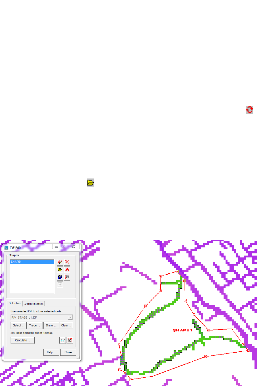
DRAFT
iMOD, User Manual
(Apply for NoDataValues in given IDF-file).
62 Close the water balance text file in order to continue. The file can be inspected any time by a
regular text editor.
Scenario Simulation
Let’s build a scenario in which we will increase a river stage from the current model configuration.
We can do that in two manners. One manner is to adjust the appropriate IDF-files that discretize the
river system, e.g. RIV \RIV_STAGE_L1.IDF and RIV \RIV_STAGE_L2.IDF by means of IDF Edit (see
section 6.7.4).
63 Click the Close button on the Model Simulation window, if needed.
64 Select the file RIV \RIV_STAGE_L1.IDF in the iMOD Manager and click the Redraw button ( )
to (re)draw it.
65 Make a copy of RIV_STAGE_L1.IDF and RIV_STAGE_L2.IDF by using the Map Operation option.
Fill in on tab Algebra in field Map C the directory+RIV_STAGE_L1_0.5.IDF, fill in ‘C=1.0*A’in the
field Formulae and select Map A and click on Compute.... Now a copy of the selected file is made.
66 Repeat the previous step for RIV_STAGE_L2_0.5.IDF
67 Zoom in for the desired river segment at the coordinates [x=145000.0] and [y=448100]. You can
use the option GotoXY from the View menu (see section 5.2) and use Zoom(m)=[1500m].
68 Select RIV_STAGE_L1_0.5.IDF in the iMOD Manager and select the option IDF Edit from the Edit
menu or with the right mouse click on the map.
69 Click the Open GEN button ( ) and open the file SCENARIO.GEN that is located at {path of
installfolder} \tutorials \TUT_MODELSIMULATION.
We’ve created a shape (polygon) to specify the area in which we will change the river stage. Let’s
assign the measure to be attached to the polygon.
70 Select [SHAPE1] from the list (see figure below).
Figure 11.82: The ’IDF Edit’ window in front of the area of interest.
71 Click on Select. . . at the selection tab of the IDF Edit window.
72 The IDF Edit Select window will be opened. Notice that the option Select for Polygon is checked!
73 Select ‘All’in the Logic dropdown menu and click on Get Selection at the bottom of the window.
Now all river cells in the polygon ‘Shape 1’are selected.
74 Click on Close to close the IDF Edit Select window.
678 of 812 Deltares
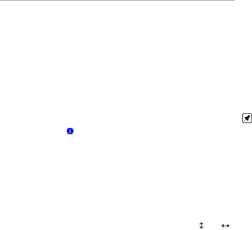
DRAFT
iMOD tutorials
75 Click on Calculate. . . on the IDF Edit window.
76 Select the option New Value on the IDF Edit Calculation window and choose ‘+’from the dropdown
menu.
77 Fill in ‘0.5’in the field behind the dropdown menu and click on Calculate.
78 Click on Close and repeat step 68-77 for RIV_STAGE_L2_0.5.IDF.
So, we’ve created a scenario definition that raises by 0.50m the stage of all river systems that penetrate
model layer 1 and 2 inside the current polygon (SHAPE1), by making. use of the iMOD Edit option.
Okay, let’s use this scenario definition in a model simulation.
79 Create a new folder in your IMOD_USER_MODELS folder outside of iMOD (in the Windows Ex-
plorer), e.g. "C: \_iMOD_IMOD_USER_MODELS_RIVER_STAGE". This folder is needed later to
store the results of the scenario simulation (step 89).
80 Select the option Start Model Simulation from the Toolbox option on the main menu. Select the
TUT_MODEL.RUN from the Runfiles list. (Note: if TUT_Model.run is not available in the list copy
the runfile from the Tutorial folder to your IMOD_USER/RUNFILE folder.)
81 Click on the Info button ( ) to open the runfile in the inbuild texteditor.
82 Find the lines with the filenames of the river stages, ]
e.g. ‘1,1.0,0.0,D: \iMOD \tutorials \TUT_MODEL_SIMULATION \RIV \RIV_STAGE_L1.IDF and
2,1.0,0.0,D: \iMOD \tutorials \TUT_MODEL_SIMULATION \RIV \RIV_STAGE_L2.IDF.
83 Change the filenames into RIV_STAGE_L1_0.5.IDF and RIV_STAGE_L2_0.5.IDF.
84 Click on the save button and close the text editor window.
As you might observe, the area of interest (within the shape) is smaller than the total extent of our
model. Let’s decrease the size of our model (in order to speed up our simulation).
85 Select the Model Dimensions tab and click the Draw Simulation Area of Interest button.
86 Left click your mouse approximately 1,000m west of the south west corner of the polygon (SHAPE1)
and left click on approximately 1,000m east of the north east corner of the polygon. This will be
our area of interest. You can increase or decrease it by moving your mouse in the neighbourhood
of the boundaries and drag your mouse as soon as the mouse cursor changes in and .
87 Select or enter a buffersize (Include a Buffer-zone of ) of [1500m].
88 Select the Output Variables tab and select the option Save Result Variable inclusive the given
Buffer Size.
A buffer zone prevents that model results are affected by boundary conditions on the lateral model
boundary. It depends on the scenario configuration, model configuration itself and the geohydrological
subsoil what this buffersize should be. It is hard to determine beforehand, so it is wise to analyse the
effects near the model boundaries to decide whether your simulation is affected by the lateral boundary
conditions too.
89 Go back to iMOD and select the Result Folder tab on the Start Model Simulation window.
90 Select the folder you created and click the Start Model Simulation button to confirm the operation.
Results of scenario computations will be stored in the folder you created yourself.
91 After the simulation ended, open the phreatic heads (HEAD_STEADY-STATE_L1.IDF) with Quick
Open (see step 74).
92 Compute the differences in phreatic heads between the . \MODELS \MODEL25 and this scenario
. \MODELS \RIVER_STAGE. Use step 14 and forward from section 11.2.
93 Analyse the differences in head for all model layers to observe whether the chosen buffersize was
sufficient. Use Quick Open to load all files in the iMOD Manager.
Deltares 679 of 812
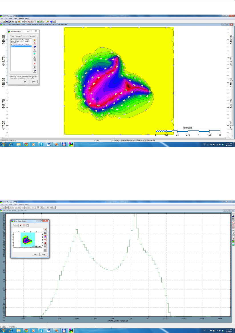
DRAFT
iMOD, User Manual
Figure 11.83: Contour levels of the computed effect of a raised water level.
In the example above it is clear that the boundaries of our submodel have been chosen appropriately
since the change in head is not affected by the model boundary. You can also make a cross-section of
the computed effect to judge whether the boundary has been chosen right.
Figure 11.84: Cross-section of the computed effect of raised water level.
94 Finally try to answer the question: “Why are the head differences more than 0.50m at some loca-
tions (0.55 meter), although river stages are increased by 0.50 meter only?”
Model simulation with the Parallel Krylov Solver (PKS) package
So far we only used the single core PCG solver, now let’s switch to the multi core Parallel Krylov Solver.
This requires that you have correctly installed the MPI software, see the iMOD Installation Instructions
(section 2.3).
680 of 812 Deltares
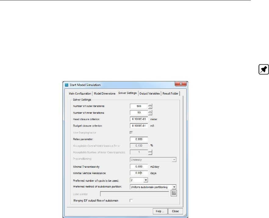
DRAFT
iMOD tutorials
The PKS package solver settings can be configured in two ways:
1 In the iMOD-GUI: in the ’Solver Settings’ tab of the ’Model Simulation’ window of the ’Tools’ main
menu option (see the figure below); we will practise this in a minute.
2 Manually: by editing Data Set 5 of a runfile according the specifications given in section 10.6; an
example is given in section 10.20.6.
Note: The PKS package is not yet available in the Project Manager.
Figure 11.85: The ’Solver Settings’ tab of the ’Model Simulation’ window. In this example
the user has assigned more than one CPU; as a result the PKS solver is
activated.
When using the PKS package, the model domain is divided in sub-domains automatically; the number
of sub-domains is always equal to the number of computational cores the user assigns in the ’Solver
Settings’ window.
The overall computational model performance depends among others on how long it takes to solve
each individual sub-domain; an iteration for the whole model domain can only be completed when all
individual sub-domains have been solved. This means that load balancing is very important for the
overall parallel performance. Ideally the actual work/load should be distributed as equally as possi-
ble over the multiple computational cores. PKS now supports two methods sub-domain partitioning
methods:
1 Uniform sub-domain partitioning in x,y-direction; when e.g. using four CPU’s the model domain will
be divided into four equally sized sub-domains.
2 The Recursive Coordinate Bisection (RCB) method. The RCB method incrementally partitions the
model domain step by step and alternates the partitioning in the x- and y-direction until the number
of sub-domains is equal to the number of assigned CPU’s. Simultaneously the sub-domains are
automatically being re-sized such that ultimately the load of each sub-domain is the same. The
load of a sub-domain is the summation of the user-defined weights (or load) of the model cells
within the boundaries of that particular sub-domain.
Figure 12.18 in section 12.32.3 shows an example of both methods for the Netherlands Hydrological
Model (De Lange et al. (2014)) and 128 sub-domains.
When assigning two CPU’s and selecting the uniform partitioning method, the model domain will be
divided into two equal sub-domains.
Deltares 681 of 812
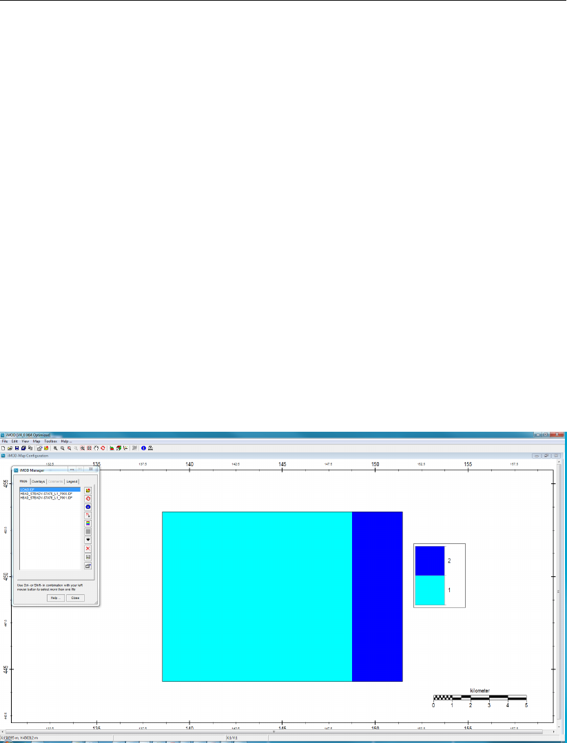
DRAFT
iMOD, User Manual
When using the RCB method, the user has to specify per model cell a weight representing an es-
timate of how much each cell contributes to the computational effort to be made to solve the set of
equations. There is no partitioning in the z-direction, so ideally the specified weights should also take
variations of the total number of active cells per x,y-location (a particular vertical column) into account.
One should be aware of the fact that even with the RCB and irregular boundaries, finding an optimal
weight distribution can be difficult and subject to trial-and-error. The spatial weight distribution depends
on for example differences in the complexity of boundary conditions (stresses) and coupling concepts.
In this tutorial we will exercise the use of the RCB method: you will run the groundwater flow model
using two CPU’s applying a load balancing grid. This can be done by the following steps.
95 Select the option Toolbox from the main menu and then the option Start Model Simulation to start
the Start Model Simulation window.
96 Select the TUT_MODEL.RUN from the Runfiles list.
97 Select the Solver Settings tab.
98 Within this tab, select 2for Preferred number of cpu’s to be used.
99 For Preferred method of subdomain partition select Recursive Coordinate Bisection.
100 For Load pointer select {installfolder}\TUTORIALS\TUT_MODEL_SIMULATION \PKS \LOAD.IDF.
The following figure shows the specified loads of the LOAD.IDF grid: in the left part of the grid all cells
have the value 1and in the right part all cells have a value 2. So in this example we assign twice as
much weight to approximately 20% of the model cells (note that this grid is just illustrative since for this
model a uniform load of 1for each computational cell would be most optimal).
Figure 11.86: The values of the LOAD.IDF grid used to specify the weights to be used
in the Recursive Coordinate Bisection partitioning method; in this example
approximately 20% of the model cells were assigned weight values that are
two times larger than the rest 80% of the model cells.
101 Turn on the checkbox for Merge IDF output files of subdomain.
102 Select the Result Folder tab and enter a name for the model results, e.g. MODEL25_PKS and
click the Start Model Simulation button; the model will be run using two computational cores.
Similar to a serial computations you can view the head results with Quick Open from the main menu
option Map. We turned on the checkbox Merge IDF output files of subdomain: after the model-run the
sub-domain-IDF’s will be merged to IDF’s covering the total model domain and the sub-domain-IDF’s
are deleted. Of course we are also curious about how the total model domain was partitioned in two
sub-domains automatically using our weight distribution grid. To see the partitioning-result of RCB
682 of 812 Deltares
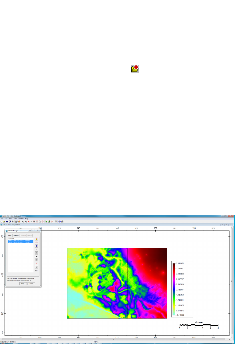
DRAFT
iMOD tutorials
method we will re-run the model in parallel mode, however, now without turning on the Merge IDF
output files of subdomain-option:
103 Select the Solver Settings tab.
104 Within this tab, turn off the checkbox for Merge IDF output files of subdomain.
105 Select the Result Folder tab and enter a name for the model results, e.g. MODEL25_PKS2 and
click the Start Model Simulation button.
106 When the simulation is done, go to View in the menu bar and select the iMOD Manager (or use
the shortcut Ctrl+M). Select the Open Map button ( ) and click the button Open. Navigate to
\IMOD_USER \MODELS \MODEL25_PKS2 \head and select the files head_steady-state_l1_p000.idf
and head_steady-state_l1_p001.idf for the computed heads for the first model layer. Click the but-
ton Open.
107 Select the Map option from the main menu, choose the option Current Zoom Level and then choose
the option Percentiles.
108 Select the View option from the main menu, choose the option Show IDF Features and then choose
the option IDF Extent.
These steps result into the following figure, where the left sub-domain is clearly larger than the right
sub-domain due to the specified weights. As you may have noticed the partitioning is not equal to
the weight distribution of the LOAD.IDF grid, in other words, by specifying this pointer grid, you are
not enforcing a particular partitioning of the model domain. This is caused by the RCB method which
results in two sub-domains that each have an equal computational load (based on your estimated
weight distribution); as mentioned above, the load of each sub-domain is calculated as the sum of
the user-assigned weights of all cells lying within the boundaries of that sub-domain. Suppose we
would have taken the LOAD.IDF grid as a basis for partitioning, this would have resulted in a relative
load for the left part of ’80’ and for the right part ’2 x 20 = 40’. The RCB automatically shifts the
boundary between the sub-domains such that the two resulting sub-domains each have a fifty-fifty
(50-50) computational burden; that’s why the right sub-domain also contains part of the model domain
having cells with weight values equal to 1.
Figure 11.87: The non-merged head-IDF’s of the two sub-domains using the RCB parti-
tioning method. The partitioning is visible when choosing ’View’, ’Show IDF
features’, ’IDF Extent’.
For your own model, experiment with different weight distributions for finding optimal load balancing.
Provided your machine has more than two CPU’s available experiment with using (almost) all of them
and compare overall performance.
Deltares 683 of 812
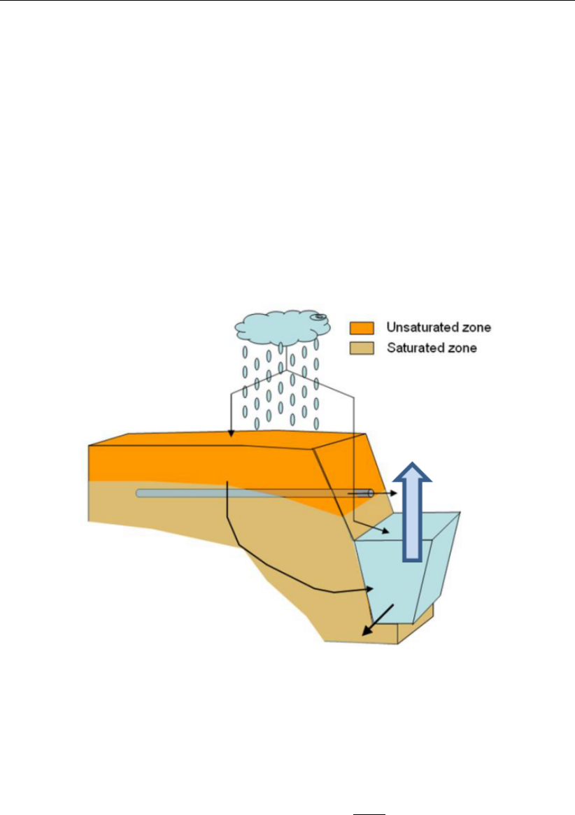
DRAFT
iMOD, User Manual
Additional background questions
The following questions are meant for extra training and get more insight in the concept of groundwater
modeling.
1 Make a second scenario: increase the stationary groundwater recharge (RCH_L1.IDF) in the entire
model area by a factor 1.2 (Note: be sure that you use the equation C=1.2*A in the iMOD calcula-
tor), thus simulating a possible future climatic change. Follow the procedure analog to increasing
the rivers stages. Again, compare computed groundwater levels with those in the default situation
(’MODEL25’).
2 Explain the spatial pattern of the increase in groundwater levels. In which areas is it more and in
which areas less? Examine this by exploring other IDFs e.g. RIV, DRN.
3 Why is a converged model not necessarily a correct model?
4 Consider a drain pipe, ending in a surface water channel. Will the drain pipe keep draining ground-
water into the channel if the surface water stage rises above the drain pipe elevation?
Figure 11.88: Drain pipe ending in a surface water channel.
5 In MODFLOW, each package treats an inflow or outflow, resulting from a boundary condition, as
an external source or sink (Q_ext). It does not consider possible interactions with other packages
/ boundary conditions. Knowing this, what will happen in MODFLOW if the surface water stage
(RIV) rises above the drain pipe elevation (DRN)?
6 How should DRN_LEVEL_L1.IDF be adjusted to prevent this?
7 OLF_L1.IDF represents the surface elevation, referenced to sea level. Using this OLF file and the
simulated heads, calculate the (steady state) groundwater depth in the MODEL25 situation.
8 Subtract the drainage elevation from the surface elevation, and compare the resulting drainage
depth map to e.g. Google Maps for the area South East of the city of Utrecht. What is the drainage
depth that occurs most often in built-up areas?
9 Compare the drainage elevation in the built-up areas in the north east of the model to the ground-
water head. What is the general picture?
10 Compare the drainage elevation in the built-up areas in the (south)west of the model to the ground-
water head. What is the general picture?
11 With which of the statements below do you agree most? Motivate.
This model is suitable to determine which model cells in built up areas have too high ground-
water levels.
This model is suitable to determine which towns and villages are dependent on drainage sys-
684 of 812 Deltares

DRAFT
iMOD tutorials
tems to prevent too high groundwater levels.
Deltares 685 of 812

DRAFT
iMOD, User Manual
11.7 Tutorial 7: Interactive Pathline Simulation
This tutorial gives a brief overview of the capabilities of the Interactive Pathline Simulation Tool (IPS).
It allows the user to demonstrate and examine the flow behaviour of the groundwater system in an
interactive manner. It is advised to get familiar with description of the IPS first, see section 7.15 that
handles all the functionalities, for which a few are outlined in this tutorial.
Outline
This is what you will do:
Load an existing model simulation into the IPS tool;
Define starting points;
Start a pathline simulation and represent them in different ways;
Filter pathlines depending on their type of capture;
Required Data
For this tutorial you need the following iMOD Data Files/folders:
The entire folder (and subfolders) in {path of tutorialfolder} \TUT_IPS, containing:
BOUNDARY.IDF – model boundary;
SURFACE_LEVEL.IDF – uppermost elevation of the model;
AQUITARD_TOP.IDF – top of the intermediate aquitard;
AQUITARD_BOT.IDF – bottom of the intermediate aquitard;
BEDROCK.IDF – bottom of the underlying aquifer;
. \RESULTS \IMODPATH.RUN – imodpath runfile (see section 8.6.6) referring to all result files
that are needed for the particle tracking simulation.
Getting Started
1 Open from {installfolder } \tutorials \TUT_IPS \RESULTS \head the file head_steady-state_l1.idf and
display heads.
2 Select Interactive Pathline Simulation and Start IPS.
3 Select from {installfolder} \tutorials \TUT_IPS \RESULTS \the file IMODPATH.RUN.
iMOD is reading the content of the RUN file and starts the 3-D tool.
Define the Starting Points
Position your Starting Points on the level of the calculated groundwater:
4 Select the option File.
5 Click the Open button and select from {installfolder } \tutorials \TUT_IPS \RESULTS \head \the file
head_steady-state_l1.idf and click the OK button.
686 of 812 Deltares
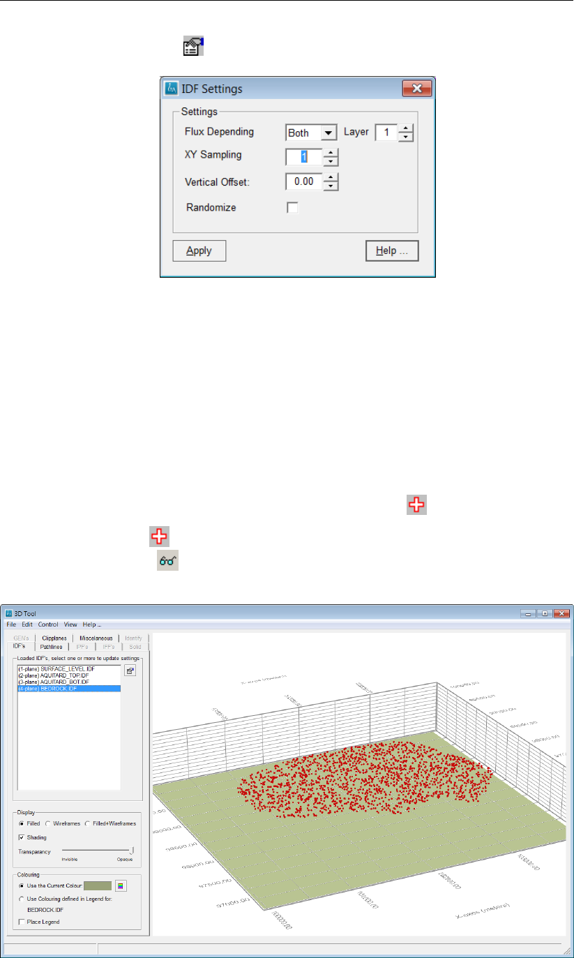
DRAFT
iMOD tutorials
6 Click the Properties button ( ) next the input field it displays:
Figure 11.89: The ’IDF Settings’ window allows specifying starting positions of par-
ticles using an existing IDF (e.g. calculated groundwater heads) as a
reference.
Flux depending is incorrect here, but means that you can use the positive or negative values on
the IDF to start particles. Leave it like this.
7 Enter for the XY-Sampling 5 to decrease the number of particles (every 5 cells there will be a
starting point).
8 Leave the option Vertical Offset that can be used to position particles a bit higher or lower than the
selected values in the IDF file.
9 The option Randomize places the particles at random locations, activate that option.
10 Click Apply.
To add this selection of particles to the simulation click the Plus button ( ), so:
11 Click the Plus button ( ), you’ll notice that 1813 particles are added.
12 Click the Glass button ( ) to display the particles in red.
13 Go to the tab IDF’s and select the BEDROCK IDF only than you’ll see the particles.
Figure 11.90: Randomly generated particles (in red).
Deltares 687 of 812
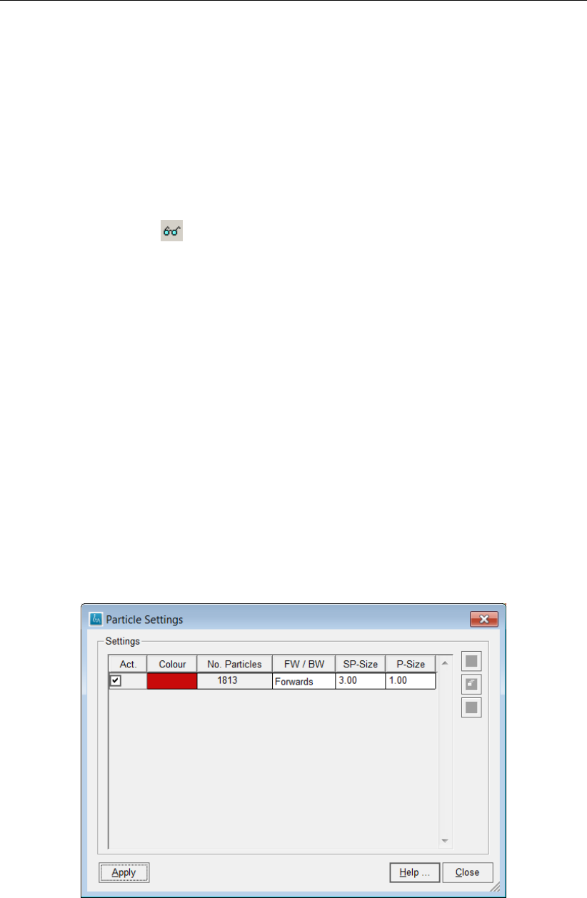
DRAFT
iMOD, User Manual
Starting the Particle Tracking
To start the particles simulation follow the next steps:
14 Select the tab Pathlines.
15 Select the option “Repeat when trapped” , in this way particles are restarted automatically when-
ever they might be captured by a weak or strong sink.
16 Click the Start button.
Pretty nice, isn’t it? You can turn the particle start location on and off by clicking the Glass button
17 Click the Glass button ( ) on and off.
18 You can rotate, zoom and pan during the simulation by the regular mouse functionalities for the 3-D
tool, try it!
You can pause the simulation by pressing the Pause button and restart it by clicking the Continue
button, so:
19 Click the Pause button, notice that you can change all other settings in the 3-D tool as well, just
experiment with that.
20 Click the Continue button to restart the particle simulation.
Enhance the Appearance
The appearance of the particle is given by lines or point, standard points are selected, these are the
most efficient, but lines give a more realistic view, so:
21 Click the Lines option.
We can configure the appearance and settings of the current particle set, so:
22 Click the Configure Particles. . . button.
Figure 11.91: The ’Particle Settings’ window that appears after clicking the ’Configure
Particles...’ button in the ’Pathlines’ tab of the 3D Tool.
You are now in the Configure Particles settings window. We alter some settings such as activation,
colour, size and direction of the particles. In fact it is possible to have different groups of particles that
688 of 812 Deltares
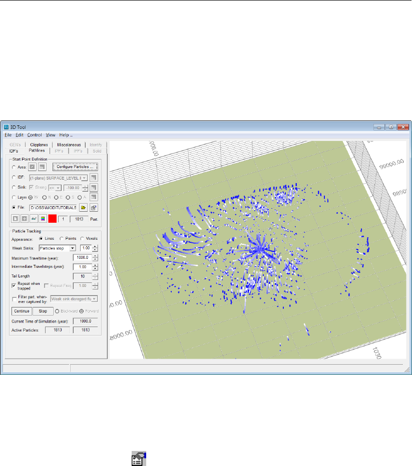
DRAFT
iMOD tutorials
go forward and backward.
23 Click the Colour (red) field and change the colour into blue and click OK.
24 Increase the size of the line by specifying a 3.0 in P-Size.
25 Click Apply.
The appearance of the particles is updated immediately.
Figure 11.92: Screen shot of a particle simulation in the ’Pathline’ tab of the 3D Tool.
Let us add another group of particles.
26 Select from the Start Point Definition the option Sink.
27 Click the Properties button ( ) associated with this Sink option.
Deltares 689 of 812
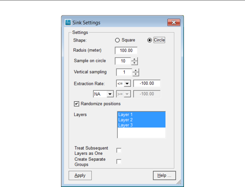
DRAFT
iMOD, User Manual
Figure 11.93: The ’Sink settings’ window appears after selecting the ’Sink’ option and
clicking the ’Properties’ button in the ’Start Point Definition’ part of the ’Path-
lines’ tab in the 3D Tool.
Starting Points around Sinks
Here you can specify how the particles need to be positioned in combination with sinks (a sink is a
source that takes water out of the model, can also be a river, drain of well). There is a single well in
layer 3 that extract 500 m3/d, so we would like to put particles around that well, so:
28 Enter a value of 5 for Radius, the cell size is 10 meter and we want to have the particles all in the
strong sink.
29 Enter 10 for Vertical Sampling, so we have 10 intervals in the vertical and 10 per interval on a
circle, so in total 10x10=100 particles.
30 Click the Apply button.
If the Plus button has been greyed out, that means that there is a simulation active that need to be
stopped first, so:
31 Click the Stop button.
32 Click the Plus button and notice that 2 groups of particles are now available and in total we have
1913 particles.
33 Click the Glass button to examine the particles.
690 of 812 Deltares
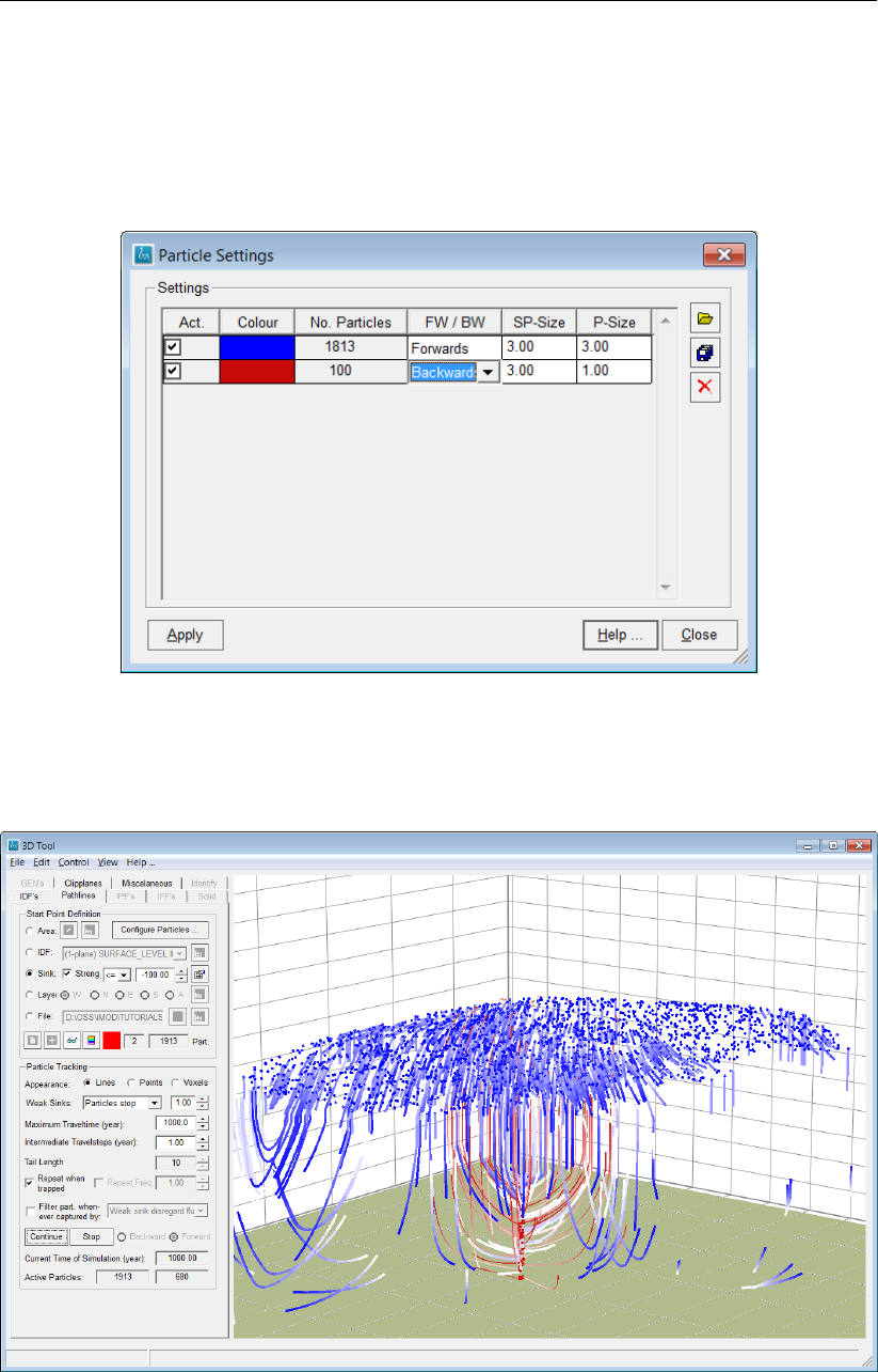
DRAFT
iMOD tutorials
Change of Particle Tracking Directions
The particle from the well should migrate backwards, so let us change that:
34 Click the Configure Particles...
35 Select the option Backward for the last group.
Figure 11.94: Setting the direction of a group of particles to ’Backward’.
36 Click the Apply button.
37 Click the Start button.
Figure 11.95: Simultaneous pathlines simulation for two groups of particles, each having
its own colour.
The blue particles can be turned off temporarily:
Deltares 691 of 812

DRAFT
iMOD, User Manual
38 Click the Configure Particles. . . button.
39 Deactivate the first particles group. Note: The particles settings can be saved from this window
using the Save As button, allowing complex particles settings to be re-used, also in a different
extent.
40 Click the Apply button.
41 Click the Stop button to stop the current simulation.
42 Click the Start button to start with only the particles from the well.
We can increase the density of the simulation by release more particles after each other, before they
actually terminate, so:
43 Click the Stop button to stop the current simulation.
44 Deselect the option “Repeat when trapped”
45 Select the option “Repeat Freq.”
46 Click the Start button.
You see that after a full length of a particle (in this case 10, namely the “tail length” ), another set of
particles is released. You can try to see the effect of changing the “Release Freq.”
47 Click the Spinner ( ) next to the “Release Freq.” input field to see the effect of this. Bigger
values will allow more time in between the next particles, as smaller values will release another
particle quicker.
Filtering of Particles
The final thing we do it to filter out particles during a simulation.
48 Click the Configure Particles. . . button.
49 Deselect the second particles group.
50 Select the first set of particles again.
51 Click the Apply button.
52 Deselect the option “Release Freq.”.
53 Select the “Repeat when trapped” again.
54 Click the “Filter part. whenever captured by” option and select the option “Strong Sink”.
55 Click the Start button to start the simulation.
Now, only the particles that are captured by a strong sink will be repeated. In this way a sense of a
capture zone if created. Okay. That it for today, so close the IPS by:
56 Selecting the option “File” from the main menu and than “Close 3-D Tool.”.
692 of 812 Deltares
DRAFT
iMOD tutorials
11.8 Tutorial 8: Surface Flow Routing (SFR) and Flow Head Boundary (FHB) Package
This tutorial gives an introduction to a steady-state, surface water routing package (see section 12.28,
and Prudic et al. (2004)). See for more detailed references regarding ISG-Edit (see section 6.10.3)
and the ISG-file format regarding the SFR package (section 9.9). The tutorial also outlines the use of
the FHB package (section 12.26) which facilitates a combination of constant head- and constant flux
boundaries.
Outline
This is what you will do:
Define a simple, single-layer, steady-state model and head- and flux boundaries using the FHB
package;
Define the outline of the stream network;
Set the characteristics of each stream and define the connections within the stream network;
Start the SFR simulation and examine the outcome.
Required Data
For this tutorial you need the following iMOD Data Files/folders:
The entire folder (and subfolders) in {path of tutorialfolder}\TUT_SFR, containing:
.\DBASE\TOP.IDF – the uppermost elevation of the model;
.\DBASE\BND.IDF – boundary conditions of the model (to be created in tutorial);
.\DBASE\FHB.IDF – constant head and constant flow boundary of the model (to be created in
tutorial);
.\DBASE\SFR.ISG – ISG with surface flow routing information (to be created in tutorial);
.\DBASE\CROSSSECTION.CSV – CSV file with a complex cross-section;
.\MODEL.PRJ – model project file;
Getting Started
1 Start iMOD.
2 Select the option Create a New iMOD Project.
3 Click the Start button.
4 Go to View in the menu bar and select the iMOD Manager (or use the shortcut Ctrl+M), or click
the iMOD Manager button ( ) from the main window to start the iMOD Manager window.
5 Click the Open IDF button ( ) from the Maps tabs on the iMOD Manager and open {path of
tutorialfolder}\TUT_SFR\DBASE\TOP.IDF.
This IDF describes the upper most elevation of the model, the top of our single layered aquifer that
declines from 512 m+MSL in the west towards 505 m+MSL in the east. We use this IDF to create the
boundary IDF.
Creating the Boundary File BND.IDF
6 Click the Calculator ( ) on the iMOD Manager in the iMOD Manager window to start the Map
Operations window.
7 Enter the output name “{path of installfolder}\IMOD_USER\DBASE\TUT_SFR\BND.IDF” at Map C.
8 Make sure the Formulae is “C=0*A”.
9 Select the option Map A at the section Select the extent for which the computation applies.
10 Click the Compute ... button.
We will use this BND.IDF file to specify how the boundary conditions need to be. On the west we apply
an open boundary condition with constant heads (511 m+MSL, that is 1 meter below the surface level
Deltares 693 of 812
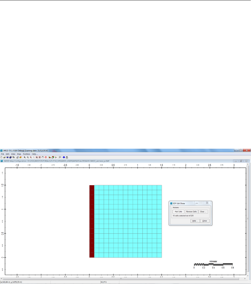
DRAFT
iMOD, User Manual
TOP.IDF). On the east we apply an open boundary condition with a constant outflow flux boundary
(-950 m3/d; a negative number will be used to take water out of the groundwater system, use a positive
number to insert water to the groundwater system instead). We will modify the BND.IDF via IDF-Edit,
which has been part of Tutorial 2, make sure you have applied this tutorial already.
11 Click the menu option View,Show IDF features and then IDF Raster Lines to display the gridlines
of the IDF files.
12 Click the right mouse button and the select from the dropfown menu, the option IDF Options and
then the option IDF Edit ... to start the IDF-Edit window.
13 In the ’Selection’-tab click the Draw ...-button to start the IDF Edit Draw window.
14 Move your mouse in the graphical canvas (note that the cursor symbol changes) and drag, while
holding your left-mouse button, all model cells in the left column of our model.
You can release the left mouse button to position the mouse on a different location without selecting
the underlying cells. To continue selecting cells, you need to press the left mouse button again. If you
need to remove some of the selected cells, click the Remove Cells from the IDF Edit Draw window.
Restart selecting cells, click the Add Cells again from the IDF Edit Draw window. Below is an image of
the final selected cells.
Figure 11.96: Image after selecting all cells of the most left column of the model.
Now we are going to change the values for those cells.
15 Click the Close button on the IDF Edit Draw window to leave the mode to select cells.
16 Click the Calculate option from the IDF Edit window to start the IDF Edit Calculation window.
17 Selection the option New Value and enter the value “-2” in the input field next the the “=” sign.
18 Click the Calculate button to assign those values to the BND.IDF file.
19 Click the Close button.
20 Click Yes to leave the editing mode.
A constant head boundary is specified by a negative number, so all values less than zero are ap-
propriate. However, whenever the FHB package is used and a constant head boundary needs to be
combined with a constant flux boundary, it is necessary to specify a -2 for constant head cells. For
constant flux boundaries we need to specify a +2. Let’s do that for the right boundary.
21 Click the Clear button and agree to the question whether you are sure to delete the current selec-
tion.
22 Click the option Draw to start the IDF Edit Draw window.
23 Move your mouse in the graphical canvas and drag, while holding your left-mouse button, all
694 of 812 Deltares
DRAFT
iMOD tutorials
model cells in the right column of our model.
24 Click the Close button on the IDF Edit Draw window to leave the mode to select cells.
25 Click the Calculate option from the IDF Edit window to start the IDF Edit Calculation window.
26 Selection the option New Value and enter the value “2” in the input field next the the “=” sign.
27 Click the Calculate button to assign those values to the BND.IDF file.
28 Click the Close button.
29 Click Yes to leave the editing mode.
We’re almost done, we only need to change all the zero values in the BND.IDF to be 1.
30 Click the Clear button and agree to the question whether you are sure to delete the current selec-
tion.
31 Click the option Select to start the IDF Edit Select window.
32 Select “BND.IDF” at IDF-File:; select “=” at Logic: and select “0.0” at Value:.
33 Click the Get Selection button and notice all rows are selected for column 2 up 14.
34 Click the Close button.
35 Click the Calculate option from the IDF Edit window to start the IDF Edit Calculation window.
36 Selection the option New Value and enter the value “1.0” in the input field next the the “=” sign.
37 Click the Calculate button to assign those values to the BND.IDF file.
38 Click the Close button to leave the IDF Edit Calculation window..
39 Click Yes to leave the editing mode.
40 Click the Close button to leave the IDF Edit window.
We’re finished !
Specify the characteristic of the boundary
We need two other files that specify the actual constant head values and the constant flux rates. For
this we need to copy the BND.IDF into a file called FHB_H.IDF, give the values that are -2 (in BND.IDF
that represent a constant head boundary) the value 511 m+MSL.
Note: To estimate the flux over the edge of model, apply Darcy’s Law. In our case we have a head
gradient of ∆h=7 m over distance d=1500 m, a permeability of k=60 m/d and an average
thickness of T=34 m, so the horizontal conductance c=k×T=2040 m2/d. Filling these in in
Darcy’s Law we come up with:
q=k×T∆h
d
= 60 ×34 ×7
1500
= 9.52m2/d
(11.1)
The cell width is 100 m, so the total volume of water is Q= 952 m3/d.
Secondly, we need to copy the BND.IDF to a file called FHB_Q.IDF and give the values that are +2 (in
BND.IDF that represent a constant flux boundary) a value of -950 m3/d (constant flux boundary). It is
more-or-less a repetition of the previous steps, but let’s dot that together.
41 Click the Calculator ( ) on the iMOD Managerin the iMOD Manager window to start the Map
Operations window. Make sure you have selected the BND.IDF in the iMOD Manager.
42 Enter the output name “{path of installfolder}\IMOD_USER\DBASE\TUT_SFR\FHB_H.IDF” at Map
C.
43 Make sure the Formulae is “C=A”.
44 Select the option Map A at the section Select the extent for which the computation applies.
45 Click the Compute ... button.
Let’s create the IDF file for the constant flux boundary as well.
Deltares 695 of 812

DRAFT
iMOD, User Manual
46 Click the Calculator ( ) on the iMOD Manager in the iMOD Manager window to start the Map
Operations window. Make sure you have selected the BND.IDF in the iMOD Manager.
47 Enter the output name “{path of installfolder}\IMOD_USER\DBASE\TUT_SFR\FHB_Q.IDF” at Map
C.
48 Make sure the Formulae is “C=A”.
49 Select the option Map A at the section Select the extent for which the computation applies.
50 Click the Compute ... button.
Enter the IDF Edit to change the values.
51 Click the right mouse button and the select from the dropfown menu, the option IDF Options and
then the option IDF Edit ... to start the IDF-Edit window.
52 Click the option Select to start the IDF Edit Select window.
53 Select “BND.IDF” at IDF-File:; select “=” at Logic: and select “-2.0” at Value:.
54 Click the Get Selection button and notice all rows are selected for column 1.
55 Click the Close button.
56 Click the Calculate option from the IDF Edit window to start the IDF Edit Calculation window.
57 Selection the option New Value and enter the value “511.0” in the input field next the the “=” sign.
58 Make sure the FHB_H.IDF is selected in the Available IDF Files at the Assign Value to section.
59 Click the Calculate button to assign those values to the FHB_H.IDF file.
60 Click Yes to leave the editing mode.
61 Click the Close button to leave the IDF Edit Calculation window.
Now for the constant flux boundary on the right.
62 Click the option Select to start the IDF Edit Select window.
63 Select “BND.IDF” at IDF-File:; select “=” at Logic: and select “2.0” at Value:.
64 Click the Get Selection button and notice all rows are selected for column 15.
65 Click the Close button.
66 Click the Calculate option from the IDF Edit window to start the IDF Edit Calculation window.
67 Selection the option New Value and enter the value “-950.0” in the input field next the the “=” sign.
68 Make sure the FHB_Q.IDF is selected in the Available IDF Files at the Assign Value to section.
69 Click the Calculate button to assign those values to the FHB_Q.IDF file.
70 Click the Close button to leave the IDF Edit Calculation window.
71 Click Yes to leave the editing mode.
72 Click the Close button to leave the IDF Edit window.
Done regarding the boundary definition. We need to add this to the model via the iMOD Project
Manager. For the Tutorial we have done already a small amount of work to fill in an iMOD Model
Project file (*.PRJ). We need to add the BND.IDF, FHB_H.IDF and FHB_Q.IDF to the current PRJ file.
We will do this after we have created the input for the SFR package.
Creating the SFR Package
In our model a stream flows from the west towards the east and splits halfway into two separate
streams (see Figure 11.97). We will model this stream in iMOD. First we need to create an ISG file that
is capable of generating the SFR input.
73 Select from the main window, the option Edit,Create Feature,ISGs and then SFR Applicable ....
74 Enter the ISG file name “{path of installfolder}\IMOD_USER\DBASE\TUT_SFR\SFR.ISG” in the
Save window.
The entered ISG file will be added to your iMOD Manager, but since it will be completely empty, you’ll
not see anything appearing on the screen. So, let us create the stream network and the corresponding
characteristics.
75 In the iMOD Manager select and draw ( ) the file FHB_H.IDF.
696 of 812 Deltares
DRAFT
iMOD tutorials
76 Select the Legend button ( ) from the iMOD Manager to start the Legend window.
77 Deselect the option ( ) to ignore the colouring of the FHB_H.IDF file.
78 Click the Apply button to leave the Legend window.
79 Select from the main window the option View,Show IDF Features and then the option IDF In-
dices to display the cell indices (row-column numbers) of the IDF file FHB_H.IDF. This is handy to
produce the ISG file in the next steps.
80 Add the created SFR.ISG file in the iMOD Manager to the current selection of files: use the key
“Ctrl” and click your left mouse button on the SFR.ISG file to this file to the selection. So both
SFR.ISG and FHB_H.IDF should be selected now.
81 Select from the main window, the option Map,ISG options and then ISG Edit ... to start the ISG
Edit window.
So because we cannot visualize the file SFR.IDF yet (it is still completely empty) we also selected the
FHB_H.IDF in the iMOD Manager to use it as a guide to draw the stream network in the next steps.
Drawing the Stream Network
We are ready now to start drawing our stream network.
82 Select the Draw option ( ) from the ISG Edit window.
83 Start drawing the first stream from west to east, we start by clicking the left mouse button at the
cell (8-1) (row are numbered from top to bottom); and then make a straight line and click the left
mouse button at cell (8-7).
84 Right mouse click to stop drawing.
You’ll notice that a stream has been created in the menu field on the ISG Edit window called “Seg-
ment_1”. This was our first stream, let’s create another one.
85 Select the Draw option ( ) from the ISG Edit window.
86 Start drawing the second stream by clicking your left mouse button at cell (8-7), towards the north
and click the left mouse button at cell (4-7), further up north-east click at cell (3-10) and finally
towards the east, mouse click at cell (3-15).
87 Right mouse click to stop drawing.
and the final one:
88 Select the Draw option ( ) from the ISG Edit window.
89 Start drawing the second stream from cell and click the left mouse button at cell (8-7), towards the
south and click at cell (12-7 , further down south-east click at cell (13-10) and finally towards the
east click at cell (13-15).
90 Right mouse click to stop drawing.
91 Select all stream from the menu field, i.e. “Segment_1”; “Segment_2” and “Segment_3”.
92 Check the options Nodes;C.Section;Seg.Nodes;Clc.Pnts. and Direction in the Show section at
the bottom of the ISG edit window.
93 Click the Update button.
Deltares 697 of 812
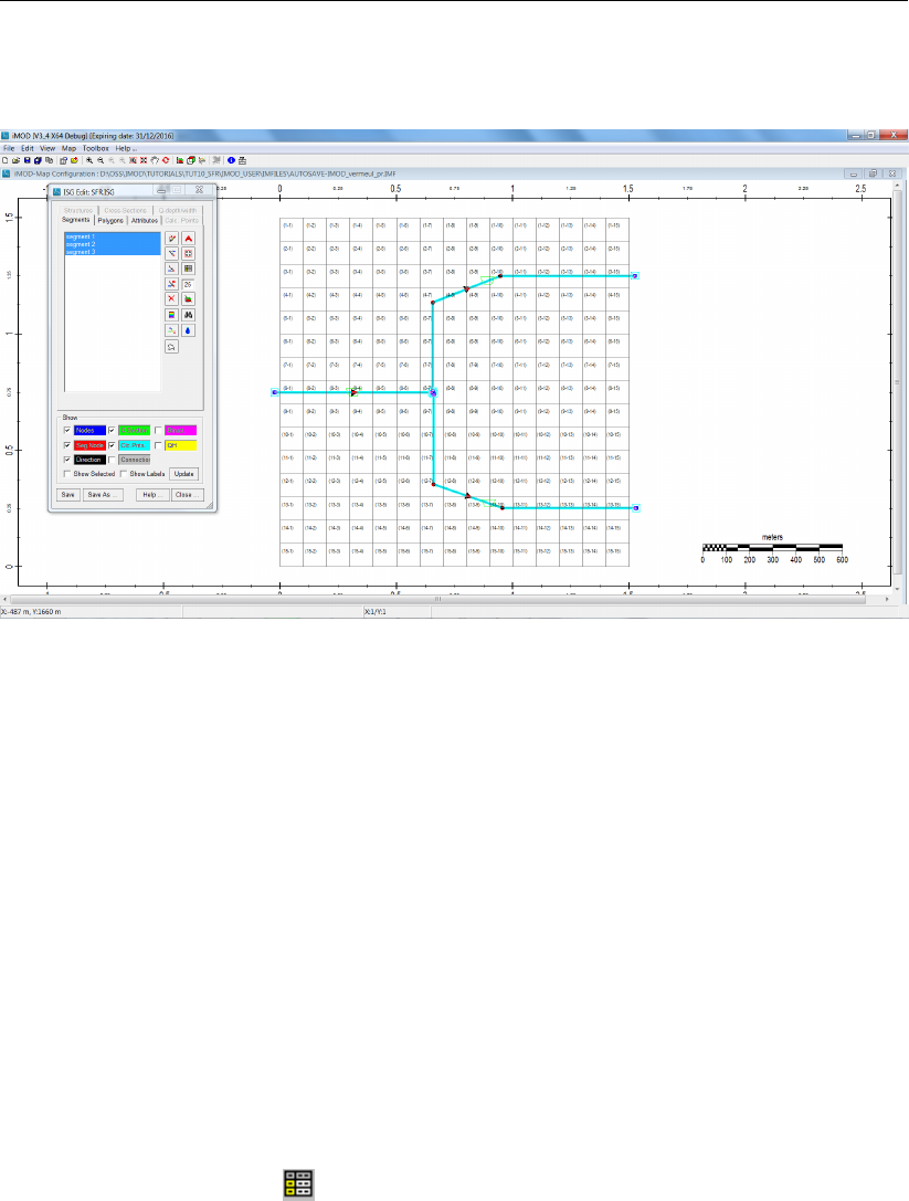
DRAFT
iMOD, User Manual
When you did it right (I’m sure you did), the following stream network should be displayed on your
graphical canvas.
Figure 11.97: Image of the 3 added ISG segments after turning on the labels Nodes,
C.Section, Seg.Nodes, Clc.Pnts. and Direction.
So, what do we see?
First of all, each stream consists of segment nodes (red dots, Seg.Nodes). Each stream contains a
single cross-section (green polygons, C.Section), and a calculation point at the beginning and end of
a stream (blue rectangle with a cross, Clc.Pnts. and the start and end of a stream (blue dot, Nodes).
Furthermore, as we draw the stream, the order in which the coordinates of each stream are entered
by clicking the left mouse button, determines the direction of the flow (black arrow, Direction). In our
case, the order of the coordinates is such that water is flowing from the west to the east and splits at
the bifurcation in a north- and south branch. Finally, all segments are selected and therefore those are
highlighted in cyan.
Characterizing the Stream Network
The next thing to do is to characterise the stream with appropriate water levels, bottom height, cross-
sections and so on.
94 Select “Segment_1” in the ’Segment’-TAB of the ’ISG EDit: SFR.ISG’ window.
95 Click the Attributes button ( ) to open the ISG Attributes window, stretch the window a bit such
that the entire table is visible.
We will enter some data in the table. First of all, we will apply this SFR to a steady-state model, so the
date and time are irrelevant in this case. We will leave it as it is.
96 Enter “511” for the Water Level (column 3).
97 Enter “510” for the Bottom level (column 4).
98 Enter “20” for the Stream width (column 5).
99 Enter “1” for the Bed thickness (column 6).
100 Enter “1” for the Bed Permeability (column 7).
101 We will define a rectangular cross-section: select “1” from the drop down menu for Calc Opt.
(column 10).
102 Enter “13.9” for the Q flow (column 12). There is a flow rate entering from the west into the stream
of 13.9 m3/s, that is 1.2 million m3/day.
698 of 812 Deltares
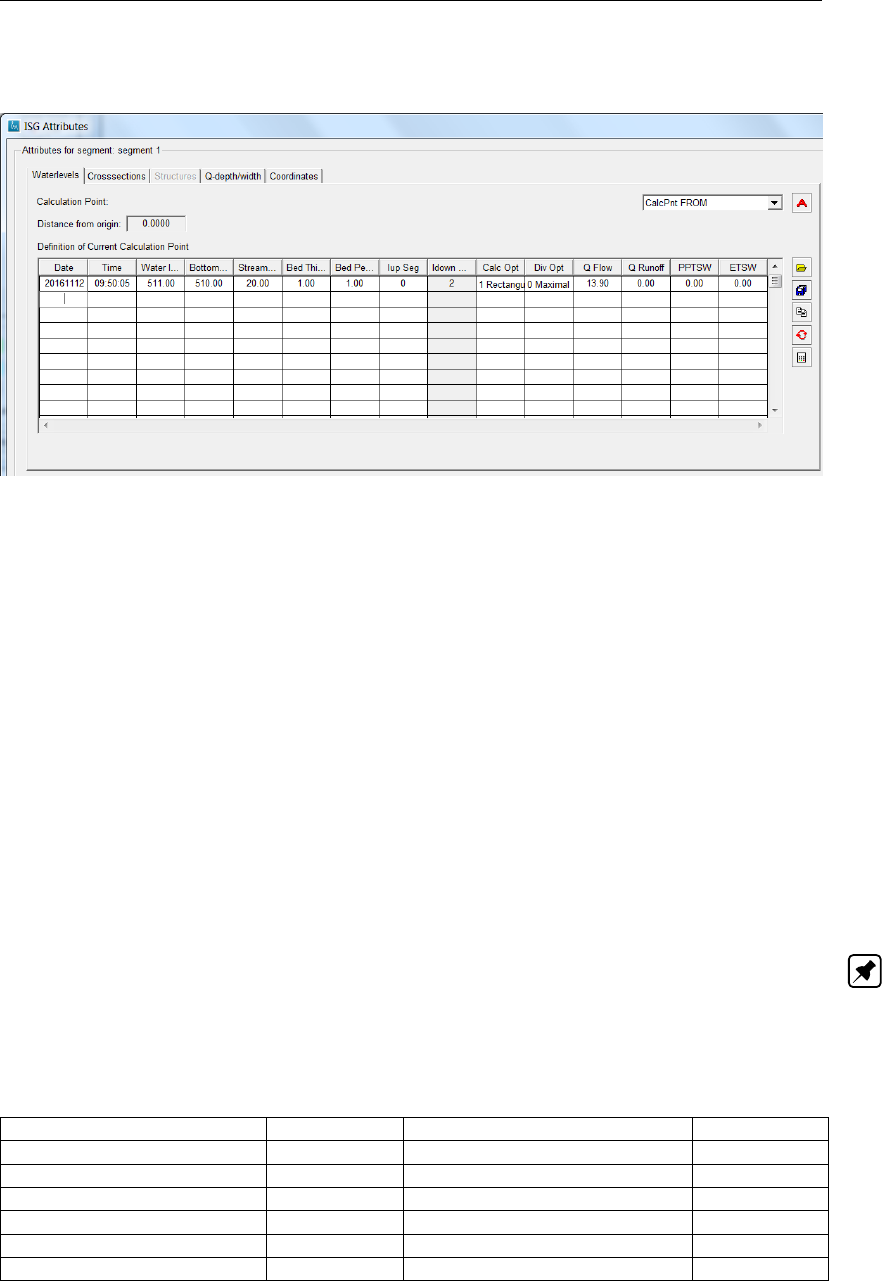
DRAFT
iMOD tutorials
We accept the default values for the remaining columns; the table should look similar to the figure
below.
Figure 11.98: The ’Waterlevels’-tab in the ’ISG Attributes’ window for the Calculation point
’FROM’ for segment 1.
The next thing is to enter data for the downstream node.
103 Select the “CalcPnt TO” from the drop down menu Calculation Point:.
104 Enter “508” for the Water Level (column 3).
105 Enter “507” for the Bottom level (column 4).
106 Enter “20” for the Stream width (column 5).
107 Enter “1” for the Bed thickness (column 6).
108 Enter “1” for the Bed Permeability (column 7).
We accept the default values for the remaining columns.
Even though we specified the width and depth of the stream already on the tab Waterlevels, we need
to specify the Manning’s Resistance Coefficient MRC for the cross-section. In case you need to use
a more sophisticated cross-section, you can specify that in the table on the tab Crosssections. We
modify the table such that it will align with our entered width (w=20 m) and maximal depth (d=2 m),
and assign a Manning’s Resistance Coefficient n=0.03.
Note: Manning’s Resistance Coefficients nrange roughly from n=0.01-0.06; some important values
are given in table Table 11.5.
Table 11.5: Manning’s Resistance Coefficients n(source: http://www.
engineeringtoolbox.com/mannings-roughness-d_799.
html)
Surface Material Coefficient nSurface Material Coefficient n
Asphalt 0.016 Brick 0.015
Clay tile 0.014 Concrete (Cement) 0.012
Earth - clean 0.022 Earth channel - weedy 0.030
Floodplains - pasture 0.035 Floodplains - heavy brush 0.075
Metal - corrugated 0.022 Natural streams - clean / straight 0.030
Natural streams - major rivers 0.035 Natural channels, poor condition 0.060
109 Select the tab Crosssections from the ISG Attributes window.
110 Enter “-20” in column=1 and row=1 and 2 (Distance).
111 Enter “+20” in column=1 and row=3 and 4 (Distance).
112 Enter “2.0” in column=2 and row=1 and 4 (Z).
113 Enter “0.0” in column=2 and row=2 and 3 (Z).
Deltares 699 of 812
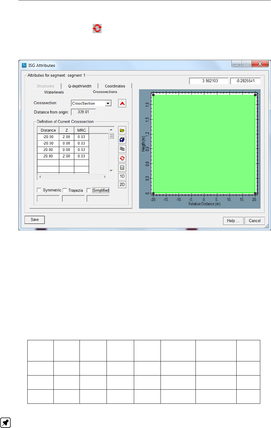
DRAFT
iMOD, User Manual
114 Enter “0.03” in column=3 for all rows (MRC).
115 Click the Redraw button ( ) to update the display with your modified cross-section.
After you did it correctly, the ISG Attributes window should look like the figure below.
Figure 11.99: The ’ISG Attributes’ window after entering the Manning’s Resistance Coef-
ficient in the ’Crosssection’-tab for segment 1.
Bear in mind that iMOD stores all modifications in memory. To actually save your modification on disk,
you need to save your data explicitly, let’s do that.
116 Click the Save button to store our adjusted stream data and return to the ISG Edit window.
117 Click the Save button on the ISG Edit window to save your adjusted SFR.ISG to disk.
118 Click the Yes button to accept overwriting the existing SFR.ISG file.
Okay, one third done! You need to apply the modifications to the other segments by applying the
previous steps (76 to 91) using the data from Table 11.6.
Table 11.6: Parameters per Stream Segment.
Up Down Water Bottom Stream Bed Bed Q
stream stream Level Level Width Thickness Permeability Inflow
- - m+MSL m+MSL m m m/d m3/s
1 511.0 510.0 20 1.0 1.0 13.9
1 508.0 507.0 20 1.0 1.0 0.0
2 508.0 507.0 15 1.0 1.0 0.0
2 504.0 503.0 15 1.0 1.0 0.0
3 508.0 507.0 5 1.0 1.0 0.0
3 504.0 503.0 5 1.0 1.0 0.0
Note: To compute the total steady-state influx of 13.9 m3/s, we apply the simplified Manning’s Equation
for a rectangular stream. The gradient of Segment_1 is S= ∆h=7 m over d= 1500 m; its width
is w=20 m, its depth is d=1 m and its roughness is n=0.03. Filling these in in the simplified
700 of 812 Deltares
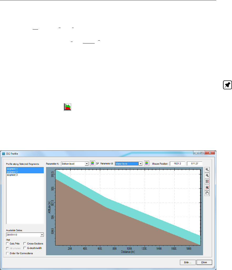
DRAFT
iMOD tutorials
Mannings’ Equation:
Q=1.0
n×w×y5
3×S1
2
= 45.5×20.0×1.05
3×7.0
1500.0
1
2
= 1239393 m3/d
= 13.9 m3/s
(11.2)
Note: A nice functionality to check whether you didn’t make any typo’s entering the data is the profile
option; this functionality is also very handy when you need to inspect the result of the simulation (more
on that later). Let’s do that.
119 Click the Profile button ( ) on the ISG Edit window (not the same icon on the main iMOD
window) to start the ISG Profile window.
120 Select “Segment_1” and “Segment_2” from the menu field at Profile Along Selected Segments.
121 Select “Bottom Level” from the drop down menu Parameter A: window.
122 Check the checkbox at Parameter B: and select “Water Level” from the drop down menu Parameter
B: window.
Figure 11.100: The ISG Profile window facilitates inspecting ISG-variables of selected
segments.
123 Click the Close button to return to the ISG Edit window.
124 Click the Save button in the ISG Edit window to save your adjusted stream data to disk.
125 Click the Yes button to accept overwriting the existing SFR.ISG file.
Connecting the Stream Network
Now that we have given all streams their appropriate characteristics, the streams need to be connected.
This can be done manually or automatically. When many streams are to be connected, this automatic
option is very handy, it connects streams within a certain distance automatically. To give an idea of
how easy streams can be connected manually, we will practice that right now.
126 Select the stream “Segment_1” on the graphical canvas by clicking your left mouse button near a
node or in between two nodes. If the stream is selected it turns into a cyan-coloured line.
Deltares 701 of 812
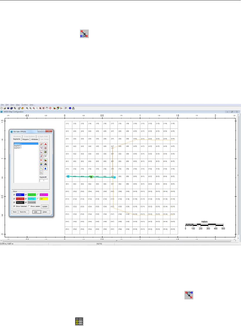
DRAFT
iMOD, User Manual
127 Click the option Show Selected to draw features on the selected stream only, just for reasons of
simplification of the image on the graphical canvas.
128 Click the Connect To button ( ) and move your mouse toward “Segment_2” until it becomes a
red line.
129 Click the left mouse button to indicate that this stream “Segment_1” will be connected to “Seg-
ment_2”. If you click next to a line (so no segment is selected), the connection will be removed.
130 Click the right mouse button to stop this selection process and return to the ISG Edit window.
131 Click the option Connections on the ISG Edit window to display the connection as a grey arrow.
132 Click the Update button to refresh the graphical canvas.
When you did it right (I’m sure you did), the your display should look similar to the figure below.
Figure 11.101: Showing the connection (light grey arrow) to Segment 2 from Segment 1
(cyan line) by selecting the ’Connection’-option in the ’Show’-part of the
’ISG Edit’-window.
So, “Segment_1” flow into “Segment_2” , but in fact it also flows towards “Segment_3”. We call this a
diversion. In order to achieve this, we need to define for “Segment_3” that its inflow is diverted from
“Segment_1”. We can do that interactively using the Connect From button ( ), or specifying this
explicitly in ISG Attributed window.
133 Select “Segment_3” from the menu field on the ISG Edit window.
134 Click the Attributes button ( ) to start the ISG Attribute window.
135 Make sure the “ClcPnt FROM” from the menu field Attributes for:.
136 Enter the stream number “1” in column Iup Seg. This specifies the model to divert from segment
Segment_1 (first in the segment list).
137 Select the option “-2” in column Div. Opt. This specifies the model to divert from Segment_1 as a
fraction of the total inflow.
138 Enter the value “0.30” in column Q Flow. This specifies that the fraction of diversion is 0.30 of the
outflow of Segment_1.
139 Click the Save button to store your modification in memory and return to the ISG Edit window.
It is not necessary to specify a diversion for Segment_2 as it automatically receives 100-30=70% of
the outflow of Segment_1.
I think we’re done with this ISG, let’s quit the ISG Edit window.
702 of 812 Deltares
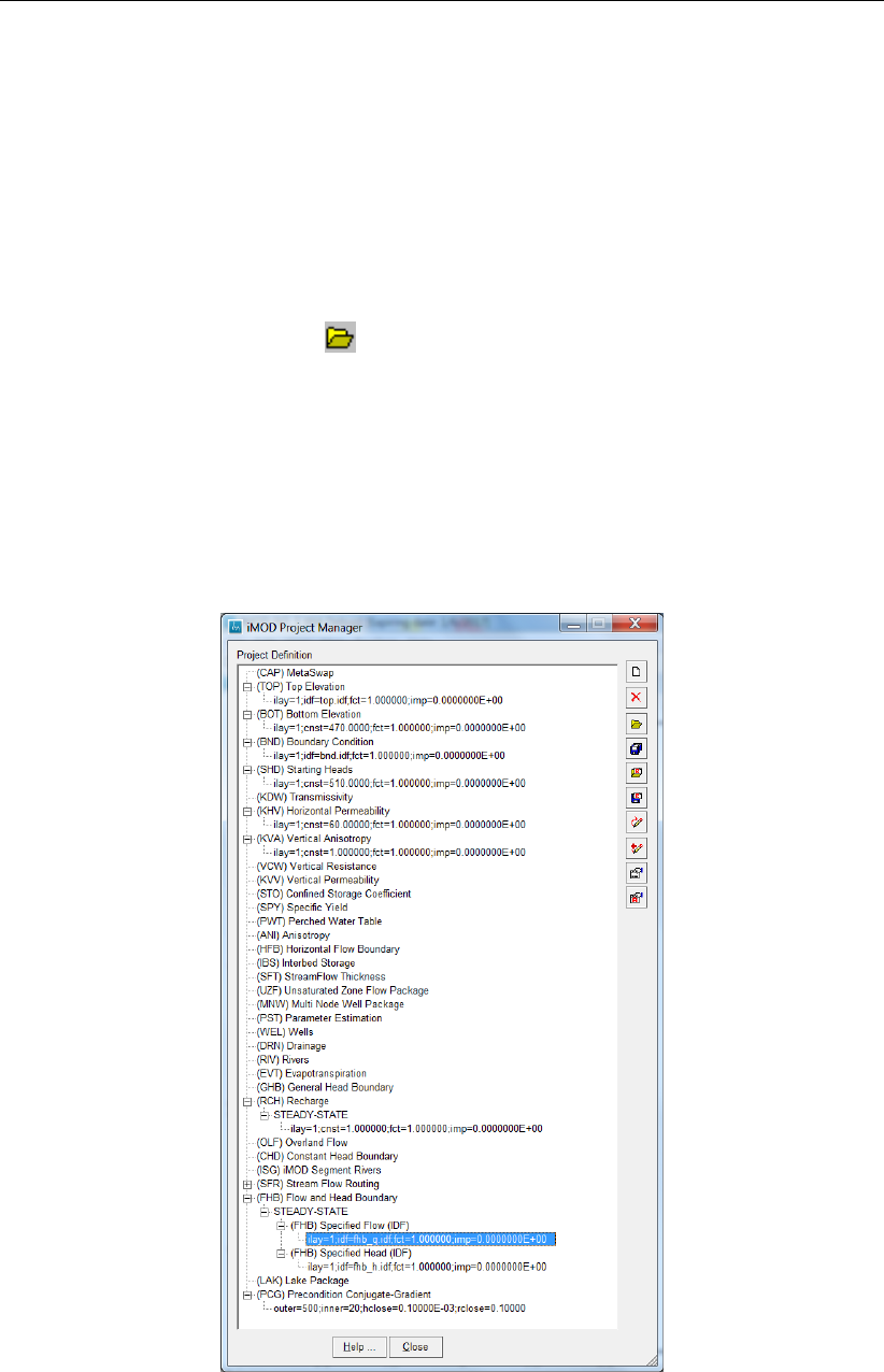
DRAFT
iMOD tutorials
140 Click the Save button in the ISG Edit window to save your adjusted stream data to disk.
141 Click the Yes button to accept overwriting the existing SFR.ISG file.
Defining the Model Project
Now that we have created all necessary packages for our model, let’s get them together in a Model
Project.
142 Select from the main menu the option View and then Project Manager to start the Project Manager
window.
143 Click the Open Projectfile button ( ) and select the file {path of tutorialfolder} \TUT_SFR\MODEL.PRJ.
144 Click OK.
For a detailed exercise on how to create a Project-file from scratch, see Tutorial 4: Create your First
Groundwater Flow Model, we will not exercise that here. The opened project file MODEL.PRJ contains
all necessary parameter definitions.
The Project Manager will look as follows:
Figure 11.102: The Project Manager after loading the project file MODEL.PRJ.
We have a permeability of KHV=60 m/d, a bottom height of our aquifer of BOT=470 m+MSL, a uniform
starting head of SHD=510 m+MSL, a uniform recharge of RCH=1 mm/d. Notice that we filled in the
FHB- and SFR package for you.
Deltares 703 of 812

DRAFT
iMOD, User Manual
Running the Model
Let’s run this model.
145 Click the Save As Run button ( ) to start the Define Simulation Configuration window.
146 Select the option MODFLOW2005.
147 Click the Simulate button and enter the following *.NAM file “{path of installfolder}\IMOD_USER\MODELS
\TUT_SFR\TUT_SFR.NAM to export the model to Modflow2005 files and start the simulation.
Note, that you need to create the folder TUT_SFR yourself first.
Note: There is an option to start a model simulation in the background so that you can continue
working with iMOD once the model has been started. As this model is very, very small, we will run the
model in the foreground and we have to wait until it has finished before we can continue working with
iMOD - probably, reading this sentence was enough time for the model to be finished.
Once iMOD converts your model to MF2005 files, it creates a conventional ISG-file that can be used
to transfer the results of the SFR package into iMOD. In this way we can use the existing functional-
ities in ISG-Edit (such as displaying time series, profiles) for the output of the model. Four items are
converted to iMOD after the simulation has finished using the iMOD Batch function SFRTOISG (see
section 8.3.8). This iMOD Batch function is part of the run-script (. \TUT_SFR \run.bat) and has been
carried out already, so let’s see some results.
148 Click the OK button once the simulation has been finished.
149 Click the Close button on the iMOD Project Manager window to close it.
150 Select from the main menu the option Map,Add Map ... and select the ISG file {path of installfolder}
\MOD_USER \MODELS \TUT_SFR \BDGSFR \ISG \SFR.ISG.
151 Select from the main menu the option Map,ISG Options and than ISG Edit ... to start the ISG Edit
window.
You probably notice that instead of three segments, we have now 35 segments.
152 Check Seg. Nodes whenever it has not been checked yet.
153 Click on the Update button.
The names of the individual segments still contain the original segment name, so it is easy to select all
streams that belong to the same original stream.
154 In the ’ISG Edit’ window select all items from the menu field that belong to the original Segment_1
and Segment_2.
704 of 812 Deltares
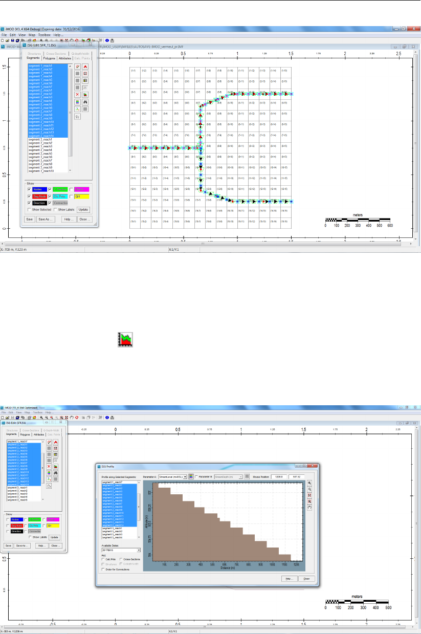
DRAFT
iMOD tutorials
Figure 11.103: Image after selecting all Segment 1 and 2 streams of SFR.ISG in the ISG
Edit window.
Now we want to see the decline of the water level, or change in discharge per segment.
155 Click the Profile button ( ) to start the Profile window.
In this picture we observe that the computed surface water level is declining from west to east. We can
see how the discharge distribution aligns with our predefined diversion fractions.
Figure 11.104: Stream levels in the ISG Profile window.
156 Select the option “Stream Discharge“ from the drop down menu Parameter A:.
157 In the ’ISG Profile’ window (not the ’ISG Edit’ window) select all segments from the menu field.
158 Try the other options from the drop down menu Parameter A:.
Deltares 705 of 812
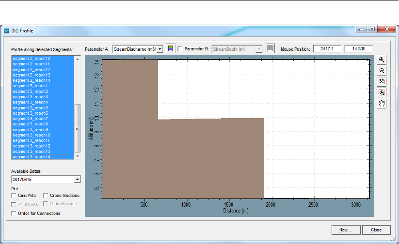
DRAFT
iMOD, User Manual
Figure 11.105: Stream discharges along segments 1 to 3.
In the graph we see that the inflow volume in “Segment_1” is 14 m3/s, and the volumes for the “Seg-
ment_2” and “Segment_3” are 10 m3/s (≈70%) and 4.25 m3/s (≈30%), respectively.
706 of 812 Deltares
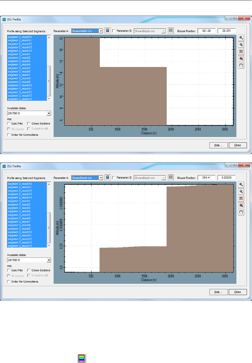
DRAFT
iMOD tutorials
Figure 11.106: Stream width and stream depth along segments 1 to 3.
Another (fancy) way to look at your results is to use a legend to colour the lines for a selected output
item, such as water levels, discharges.
159 Click the Close button to return to the ISG Edit window.
160 Select the Legend button ( ) to start the ISG Colouring window.
161 Select the option Current window to colour all segments within the current graphical window.
162 Increase the line-thickness to 5.
Deltares 707 of 812
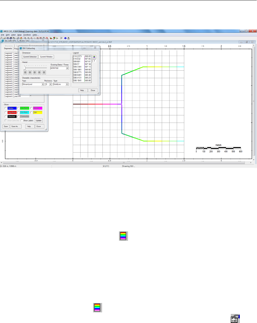
DRAFT
iMOD, User Manual
In this visual we observe that the surface water is indeed declining from west to east.
Figure 11.107: Stream levels visualised when using a colour legend.
It is easy to visualize the other model outcomes as well:
163 Select “StreamDepth” ,“StreamWidth” and “StreamDischarge” as well.
The legend is computed automatically based on the data of the ISG file. Each stream characteristic
in the ISG file has its own legend. This can be modified by using the default Legend window that
starts whenever you select the option Legend ( ) from the ISG Colouring window. For any transient
simulation you might do in future, you can drag the slider in the ’Period’ part of the of the ’ISG colouring’-
window to visualise stream characteristics for different periods.
Now it’s time to visualise the total exchange flux between the surface water and groundwater.
164 Click the Close button on the ISG Edit window to close the ISG Edit window and ISG Colouring
window, accept the question upon closing.
165 Select from the main menu the option Map,Add Map ... and select the ISG file {path of installfolder}
\IMOD_USER \MODELS \TUT_SFR \BDGSFR \BDGSFR_STEADY-STATE_L1.IDF.
166 Click the Adjust Legend button ( ) from the iMOD Manager to start the Legend window. If the
iMOD Manager is not visible, display it again by selecting the iMOD Manager button ( ) from
the main iMOD window.
167 Use your skills to create the legend as displayed in the next figure. If you find difficulties reproducing
this legend, have a look again at Tutorial 1: Map Display.
708 of 812 Deltares
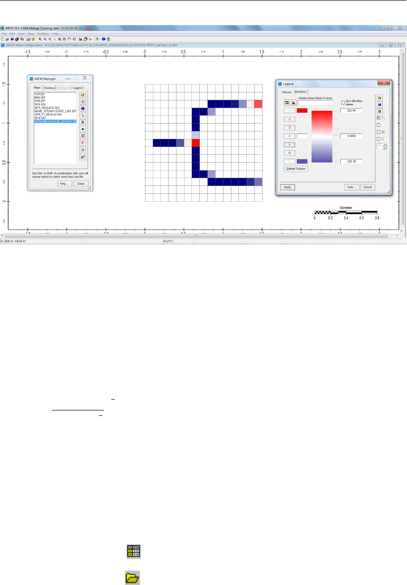
DRAFT
iMOD tutorials
Figure 11.108: Visualising the computed fluxes between surface water and groundwater.
Regarding practising the visualisation of ISG’s it’s OK for now.
168 Click the Close button to stop ISG Edit window.
It would be nice if you try experimenting with different parameters of the SFR package, such as stream
width, Manning’s Resistant Coefficients and/or implement an extraction in the model to see whether
that effects the surface water level. To estimate the extraction rate, such that the surface water level
might change with 0.10 m, use the following equation of the re-organised Manning’s Equation:
y=Q×n
C×w×S1
2
3
5
(11.3)
If you apply this for stream “Segment_2” , the extraction need to be at least 3.3 m3/s=285,000 m3/d.
Enhance the model by an Eight Point Cross-Section
In the coming few steps we will enhance the model a bit more, adding a more complex cross-section
and apply a q-width/depth relationship for a segment.
169 Select the option ISG Options and then ISG Edit to start the ISG Edit window.
170 Select “Segment_1” from the menu list of segment names.
171 Click the Attributes button ( ) to start the ISG Attributes window.
172 Select the tab Cross-sections from the ISG Attributes window.
173 Select the Open button ( ) and select the file {path of tutorialfolder} \TUT_SFR \DBASE
\CROSSSECTION.CSV.
174 Click OK to read the selected file.
iMOD will open the Read CSV file window. Here you can specify what column from the CSV-file you
want to use for each of the columns of the cross-section, such as “Distance” , “BottomLevel” and
“MRC”. We leave the default values as shown below.
Deltares 709 of 812
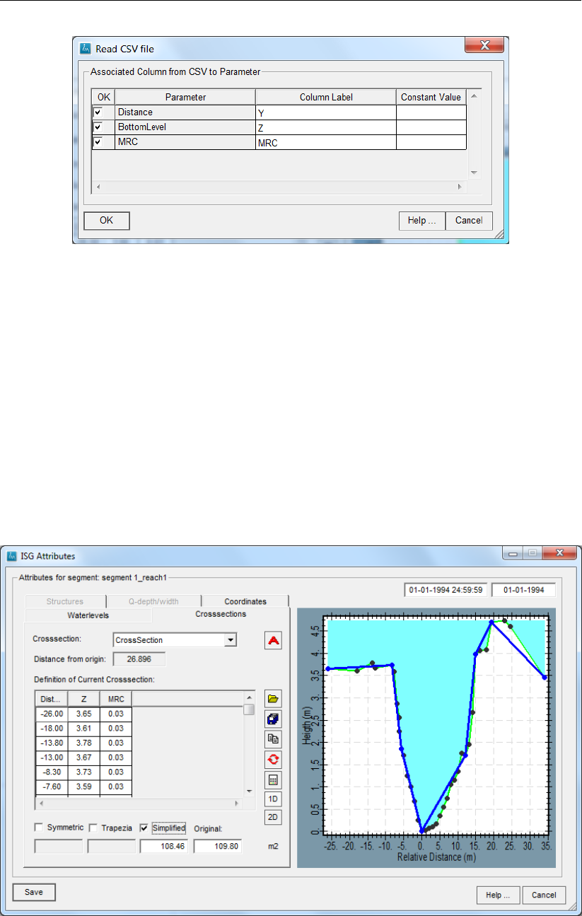
DRAFT
iMOD, User Manual
Figure 11.109: The ’Read CSV file’ window.
175 Click Ok to accept the column definitions and return to tab Cross-sections on the ISG Attributes
window.
176 Click the checkbox Simplified to observe a simplified cross-section.
The SFR Package has the limitation that only eight-point cross section geometries can be assumed.
Eight values each for the horizontal and vertical distances are specified for the segment. Vertical walls
are assumed at the end of each cross section. Stream depth, width, and wetted perimeter (hydraulic
radius) are computed from the cross section for a given flow using Manning’s equation and by dividing
the cross section into three parts, one part for the points 1-2-3, a second part for the points 3-4-5-6 and
a third part for the points 6-7-8. All those together form the total wetted perimeter and the area. As this
can be rather complex, the SFR package uses an iterative procedure to estimate the total discharge
(sum of the three parts) until the computed flow is more-or-less equal to the stream flow. This method
may not solve for all geometries, especially wide, flat bottom geometries might cause problems, in
those case an other option is advised to be used for computing the stream depth.
Figure 11.110: The cross-section as read from the CSV file (black dots) and the 8-points
simplified cross-section (blue dots) after selecting ’Simplified’ in the ’ISG
Attributes’-window, including the corresponding areas of the original and
simplified cross-section.
710 of 812 Deltares

DRAFT
iMOD tutorials
From the figure above, it seems that the simplified cross-section has a more-or-less similar wetted area
(108.46 m2) compared to the original one (109.80 m2). Actually, this simplification is done once the
model is exported to the SFR package of MODFLOW2005, automatically.
Next thing is to modify the ISG file a little bit more such that it knowns to use this eight-point cross-
section.
177 Select the tab Water Levels on the ISG Attributes window.
178 Select the option “2 Eight Point” from column 10 with label Calc Opt..
179 Click the Save button to save the modification in memory and return to the ISG Edit window.
180 Click the Save As button to save the modification on disk in another name, enter the file name
{path of installfolder} \IMOD_USER\DBASE\TUT_SFR\SFR2.ISG.
181 Click the Close button to leave to the ISG Edit window.
182 Accept the question by clicking the Yes button.
Deltares 711 of 812

DRAFT
iMOD, User Manual
11.9 Tutorial 9: Lake Package
This tutorial gives an introduction to a transient implementation of the Lake package (LAK), see sec-
tion 12.29.
Outline
This is what you will do:
Define a simple, five layered, transient model and constant head boundaries along the model;
Define the input for the LAK package;
Start the model simulation and examine the outcome;
Combine the LAK package with the SFR package.
Required Data
For this tutorial you need the following iMOD Data Files/folders:
The entire folder (and subfolders) in {path of tutorialfolder} \TUT_LAK \DBASE, containing:
BND.IDF – boundary conditions of the model (to be created);
TOP.IDF – uppermost interface of the model (to be created);
LAK_ID.IDF – lake identification number (to be created);
LAK_BATHYMETRY.IDF – lake bathymetry number (to be created);
MODEL.PRJ – initial model project file;
MODEL_LAK.PRJ – model project file with the LAK package (to be created);
Getting Started
1 Start iMOD.
2 Select the option Create a New iMOD Project.
3 Click the Start button.
Create the boundary conditions
We start to create our first IDF file.
4 Select the main menu option Edit Create Feature,IDFs from ... and then Scratch ... to start the
Create IDF window;
5 Enter the following values:
XLLC / XURC (ft) : “0.00” and “8500.0”;
YLLC / YURC (ft) : “0.00” and “8500.0”;
CellSize (ft) : “250.0”.
6 Activate the iMOD Manager (Ctrl+M) (if not active already); the map BND should be selected now.
7 Select the option Apply ... and enter the file name
{path of installfolder}\IMOD_USER\DBASE\TUT_LAK\BND.IDF.
8 Select the menu option View,Show IDF Features and then IDF Raster Lines to display the raster-
lines of the IDF just created.
Now we copy the geometry of this BND file to a to be created TOP file.
9 Select the main menu option Map,IDF Option and then IDF Calculate ... to start the Map Opera-
tions window;
10 Enter at Map C the output file {path of installfolder}\IMOD_USER\DBASE\TUT_LAK\TOP.IDF;
11 Select the option Map A to determine the extent for which the computation applies;
12 Click the Compute ... button.
712 of 812 Deltares

DRAFT
iMOD tutorials
We will assign the IBOUND value ’-1’ (fixed heads) to all cells of columns and rows 1 and 34. There
are a number of possibilities to select the appropriate cells; we will now select them by dragging
the mouse of the cells, similar to step 14 of Tutorial 8: Surface Flow Routing (SFR) and Flow Head
Boundary (FHB) Package:
13 Select the main menu option Map,IDF Option and then IDF Edit ... to start the IDF Edit window;
14 Click the option Draw to start the IDF Edit Draw window.
15 Move your mouse in the graphical canvas and drag, while holding your left-mouse button, all
model cells in the first row, the right column, the last row and the first column of our model; it should
result in 132 selected cells.
16 Click the Close button on the IDF Edit Draw window to leave the mode to select cells.
17 Click the Calculate ... button to start the IDF Edit Calculation window;
18 Select the option New Value and enter the value “-1” at the utter most right input field;
19 Select the IDF file “BND.IDF” from the dropdown menu at Available IDF-file;
20 Click the Calculate button to adjust the selected cells in the IDF file.
21 Click the Close button to close this window;
22 Click the Yes button to confirm the question whether you want to leave this window.
Now we need to define the active area in the boundary conditions.
23 Click the Select ... button to start the IDF Edit Select window;
24 Select the option “BND.IDF” from the IDF-file: dropdown menu;
25 Select the option “NodataValue” from the Logic dropdown menu;
26 Click the Get Selection button, 1024 cells are selected;
27 Click the Close button to leave the IDF Edit Select window;
28 Click the Calculate ... button to start the IDF Edit Calculation window;
29 Select the option New Value and enter the value “1” at the utter most right input field;
30 Select the IDF file “BND.IDF” from the dropdown menu at Available IDF-file;
31 Click the Calculate button to adjust the selected cells in the IDF file.
32 Click the Close button to close this window and return to the IDF Edit window;
33 Click the Yes button to confirm the question whether you want to leave this window. .
Now, we will create the surface level. The surface level declines gradually from west to east, starting
at 160 m and ending at 140 m.
34 Select the Draw Polygon ( ) and draw a polygon around all cells of the first column. iMOD will
select IDF cells that are in a polygon with their midpoint;
35 Click the Select ... button to start the IDF Edit Select window;
36 Select the IDF file “TOP.IDF” from the IDF-file dropdown menu;
37 Select the option “All” from the Logic dropdown menu;
38 Click the Get Selection button and 34 cells are selected;
Deltares 713 of 812
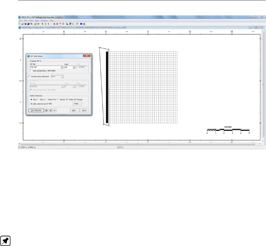
DRAFT
iMOD, User Manual
Figure 11.111: 34 cells selected after clicking the ’Get selection’ button.
39 Click the Close button to leave the IDF Edit Select window;
40 Click the Calculate button to start the IDF Edit Calculation window;
41 Enter a value of “160” in the input field right of the option New Value;
42 Click the Calculate button to adjust the selected cells in the IDF file.
43 Click the Close button to close this window and return to the IDF Edit window;
44 Click the Yes button to confirm the question whether you want to leave this window. .
Now we compute the right in a similar manner and give the east side of the model the value 140.0.
Note: It is easy to just move the drawn polygon to the right and than follow the steps 25-30 again.
Let’s interpolate the surface level.
45 Click the Select ... button to start the IDF Edit Select window;
46 Select the IDF file “TOP.IDF” from the IDF-file dropdown menu;
47 Select the option “NodataValue” from the Logic dropdown menu;
48 Uncheck the option Select for Polygon;
49 Click the Get Selection button and 1088 cells are selected in between column 1 and column 34;
50 Click the Calculate button to start the IDF Edit Calculation window;
51 Select the option Interpolate;
52 Select the option PCG to use a linear interpolation;
53 Click the Calculate button to adjust the selected cells in the IDF file.
iMOD will start the Solver Settings window in which you can specify the accuracy of the interpola-
tion. We will accept all the default settings.
714 of 812 Deltares
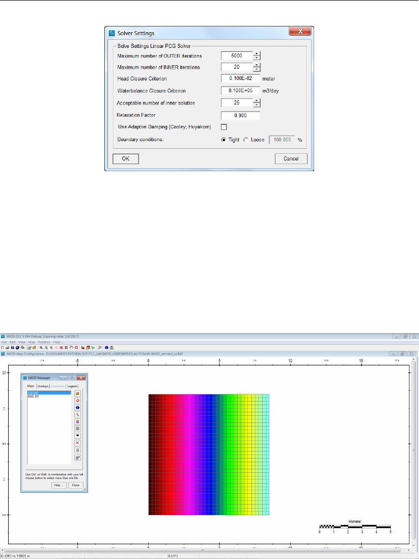
DRAFT
iMOD tutorials
Figure 11.112: The Solver Settings window.
54 Click the OK button to close the Solver Settings window and start the interpolation;
55 Click the Close button to close the IDF Edit Calculation window and return to the IDF Edit window;
56 Click the Yes button to confirm the question whether you want to leave this window.
57 Click the Close button to close the IDF Edit window.
Let’s see how the interpolation looks like.
58 Right mouse click on the graphical canvas and select the option Current Zoom Level and then
Linear to display the top of our system than gradually declines from west to east.
Figure 11.113: The interpolated surface level.
Create the Lake
We would like to introduce a lake in the middle of our model. We need an IDF file that describes the
maximal extent of the lake, and another IDF file that describes the bathymetry of the lake.
59 Create the following two IDF files; apply the Formulae “C=0.0*A”in Map Operations when copying
the geometry of the map BND:
{path of installfolder}\IMOD_USER\DBASE\TUT_LAK\LAK_ID.IDF - this file will store the loca-
tion of the Lake;
{path of installfolder}\IMOD_USER\DBASE\TUT_LAK\LAK_BATHYMETRY.IDF - this file will
Deltares 715 of 812
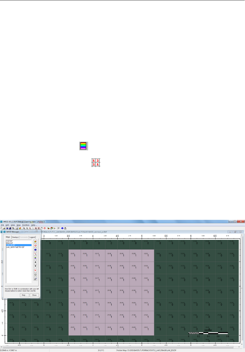
DRAFT
iMOD, User Manual
store the depth (bathymetry) of the lake.
I’m sure you know by now how IDF Edit works, so:
60 Start IDF Edit and modify the files as follows:
fill in the LAK_ID.IDF file such that it contains a value of “1” for the rectangle given by the cell
indices (row=12,column=15) and (row=18,column=21);
fill in the LAK_BATHYMETRY.IDF file such that it contains a value of “107” for the rectangle
given by the cell indices (row=12,column=15) and (row=18,column=21), and a value of “97” for
the rectangle given by the cell indices (row=14,column=17) and (row=16,column=19).
61 Turn on the cell-indices via View,Show IDF Features and than Cell Indices. We have done this
before in step 79 in section 11.8.
You can configure your IDF files to display the actual IDF values as follows:
62 Select the file LAK_BATHYMETRY.IDF in the iMOD Manager (if not visible select from the main
window, the menu option View and than iMOD Manager or click Ctrl+M alternatively);
63 Select the Legend button ( ) from the iMOD Manager window to start the Adjust Legend
window;
64 Select the option Data Numbers ( ) to display the IDF values;
65 Increase the textsize by entering a “3” underneath the Data Numbers option;
66 Click the Apply button to close the Adjust Legend window and redraw the graphical canvas.
67 Select the option Map,Entire Extent and than Unique Values to display the content of the IDF files
with a colouring legend for unique values only.
You should have the following IDF files created:
Figure 11.114: Lake Identification.
716 of 812 Deltares
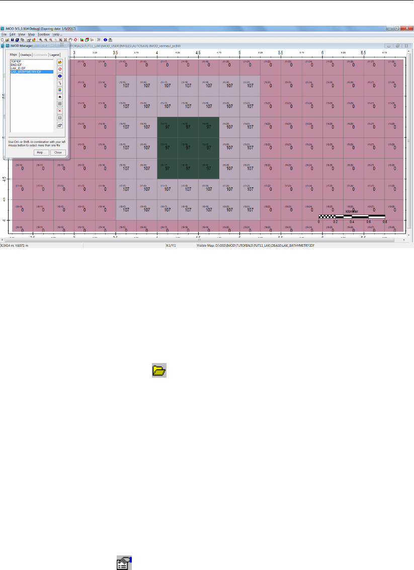
DRAFT
iMOD tutorials
Figure 11.115: Lake Bathymetry.
Add the Lake to the Modelling Project
Now, we will add the parameters for the Lake Package in our modelling project.
68 Select the option View and then select Project Manager to start the iMOD Project Manager win-
dow;
69 Click the Open Projectfile button ( ) and select the file {path of tutorialfolder}\TUT_LAK\MODEL.PRJ;
70 Click the Open button.
The entire model has been filled in already. Notice that this MODEL.PRJ file refers to the prepared
IDF files given with the iMOD install in the folder {path of tutorialfolder}\TUT_LAK\DBASE instead of the
files you created yourself and saved in the folder {path of installfolder}\IMOD_USER\DBASE\TUT_LAK.
With the Define Characteristics button on the Project Manager window you can change the file refer-
ence if you like (see also section 5.5.1).
You may inspect the model for a while and you will notice that it is a model with 5 model layers. The
BND.IDF and TOP.IDF are filled in as well. The BND.IDF is used to define the boundary types for all
model layers and the TOP.IDF is used at the module (TOP) for the first model layer. That file is also
used for the Surface Elevation used by the (EVT) module. We will now enter the parameters for the
(LAK) module.
71 Select the option (LAK) in the tree view Project Definition;
72 Click Properties button ( ) to start the Define Characteristics for window.
73 Select the option Transient, start from and enter the date “1 December 2016” in the date entry
fields. All the other packages (RCH and EVT) start at that period as well;
Deltares 717 of 812
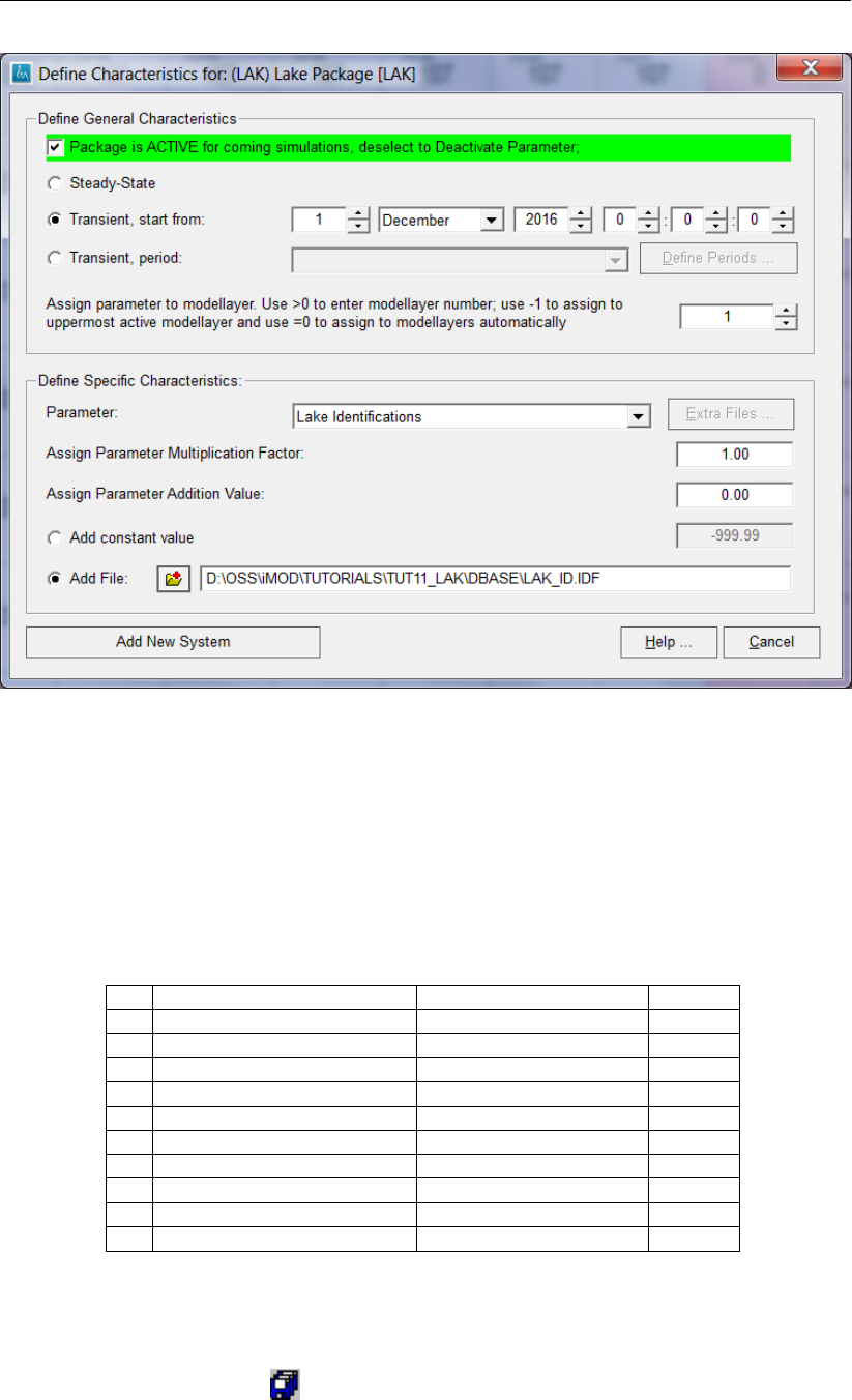
DRAFT
iMOD, User Manual
Figure 11.116: Example of the ’Define Characteristisc for: (LAK) Lake Package’ window;
the part ’Define Specific Characteristics’ contains a pull-down Parameter
list which should be parameterized according to the values given in Table
Table 11.7.
74 We will enter the following values for the different input parameters by selecting the appropriate
parameter from the Parameter dropdown list sequentially, see Table 11.7.
75 Click the Add New System button to add the parameter to the modeling project.
Table 11.7: Modeling Parameters for the Lake Package.
-Parameter Entry Units
1 Lake Identifications LAK_ID.IDF -
2 Lake Bathymetry LAK_BATHYMETRY.IDF m+MSL
3 Initial Lake Levels 110.0 m+MSl
4 Minimal Lake Levels 97.0 m+MSl
5 Maximal Lake Levels 145.0 m+MSL
6 Lakebed Resistance 10.0 days
7 Precipitation at surface Lake 0.0116 m/d
8 Evaporation at surface Lake 0.0103 m/d
9 Total Overland runoff 0.0 m3/d
10 Total Lake Withdrawall 0.0 m3/d
So, let’s first save our configuration in a new project file.
76 Close the Define Characteristics for window by selecting the Add System button.
77 Click the Save As button ( ) and save a new modeling project file at {path of installfolder}
\IMOD_USER \RUNFILE \MODEL_LAK.PRJ.
718 of 812 Deltares
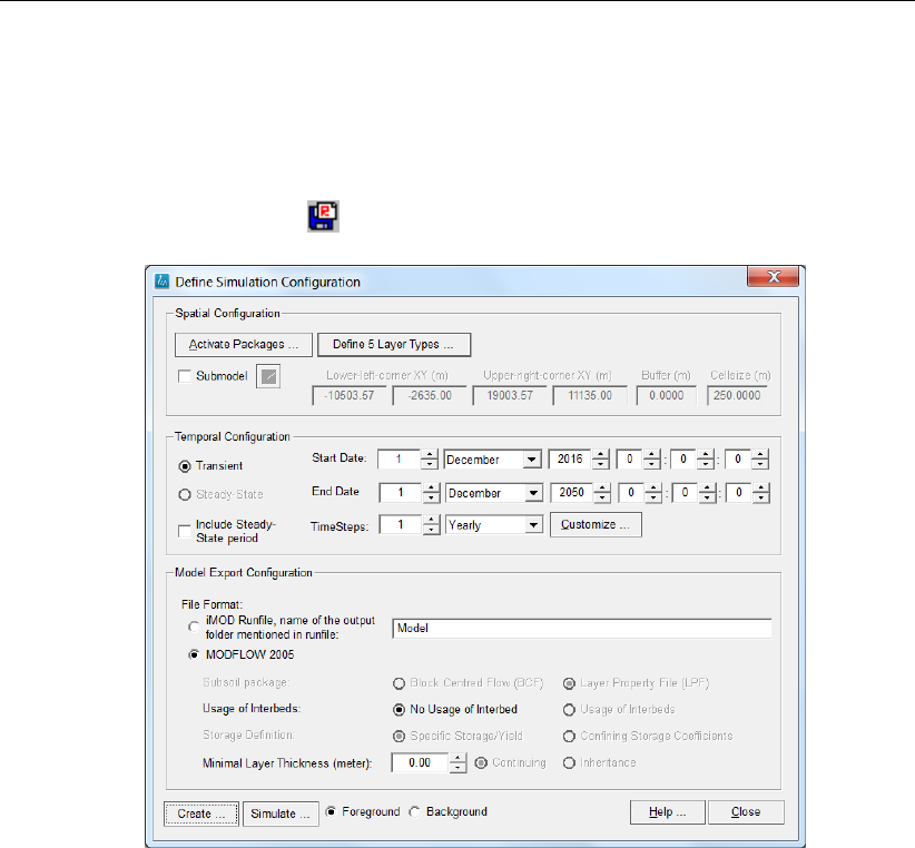
DRAFT
iMOD tutorials
Start the model simulation
With this project file we can generate a Runfile and/or a standard MODFLOW2005 model. As we use
the LAK-package and this is not supported by a Runfile we need to create standard MODFLOW2005
files, let’s do that.
78 Click the Save Model button ( ) to start the Define Simulation Configuration window.
Figure 11.117: Example of the iMOD Define Simulation Configuration window.
79 Enter “2050” at the End Date input field.
80 Select the option “Yearly” from the TimeSteps: dropdown menu field.
81 Select the option “MODFLOW2005” at the File Format: radio button.
So, we will create a model that is transient, starts at the 1st of December 2016 00:00:00 and ends at
the 1st of December 2050 00:00:00. The model will generate output after each year.
82 Click the Simulate button and enter the following *.NAM file {path of installfolder} \IMOD_USER
\MODELS \TUT_LAK \TUT_LAK.NAM to export the model to MODFLOW2005 files and start the
simulation. Note, that you need to create the folder TUT_LAK yourself first, use the option New
Folder in your current Save window.
83 Click the Save button.
iMOD will now first create the necessary MODFLOW2005 file; as the model is tiny, this will be finished
rapidly, then the simulation will start immediately. You’ll see that the model start in a separate DOS-
command window and it will echo the simulation progress. As it is a transient simulation with 34 stress
periods, it will consume probably 30 seconds to accomplish.
Deltares 719 of 812
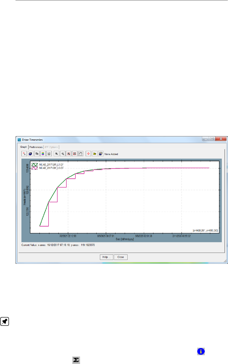
DRAFT
iMOD, User Manual
Inspect the result of lake simulation
The lake levels will be part of the saved hydraulic heads, so we only have to open, e.g. the hydraulic
of the first stress-period to generate time series. The lake exchange with groundwater will be saved in
a separate budget file, we will open that as well.
84 Select the option Map and then the option Quick Open to start the Quick Open window, see sec-
tion 6.2. With this window it is easy to open and view results from a model simulation.
85 Select the option “HEAD” from the Topic dropdown menu.
86 Select the option “20171201” from the Time: dropdown menu.
87 Select the options “1 2 3 4 5” from the Layer dropdown menu. Tip: drag your mouse to select all
layers.
88 Click the Open button.
89 Repeat the above mentioned steps to open the results for BDGLAK as well, do this for model layers
1,2 and 3.
iMOD will load all selected results files into the iMOD Manager and displays the result on the graphical
canvas. Use your experience learned from the previous Tutorials to display the computed heads as
time series as shown in the following figure.
Figure 11.118: Time Series of lake levels.
The lake package simulates the exchange of groundwater and surface water such that the water bal-
ance of the lake equals (more-or-less). So, in the end it finds a water level of 133.47 m+MSL. At this
lake level there is an equilibrium between the nett recharge of the lake (precipitation minus evaporation)
and the drainage to the lake.
Note: The total volumes can be found, per stress-period, in the list file after the simulation. You
can find the file here: {path of installfolder} \IMOD_USER \MODELS \TUT_LAK \TUT_LAK.LIST. To
get this water balance, search for a part of the string “HYDROLOGIC BUDGET SUMMARIES FOR
SIMULATED LAKES”. For the first year, the total inflow to the lake is 2.7264E+07 m3/year (we have
time step lengths of one year). This is equal to 74695 m3/d, that is the sum of all fluxes from the
BDGLAK-files. You can find the total fluxes per BDGLAK-file via the Map Info option ( ) and then
select the Statistic button ( ) you can read the Sum of the individual flux file.
720 of 812 Deltares
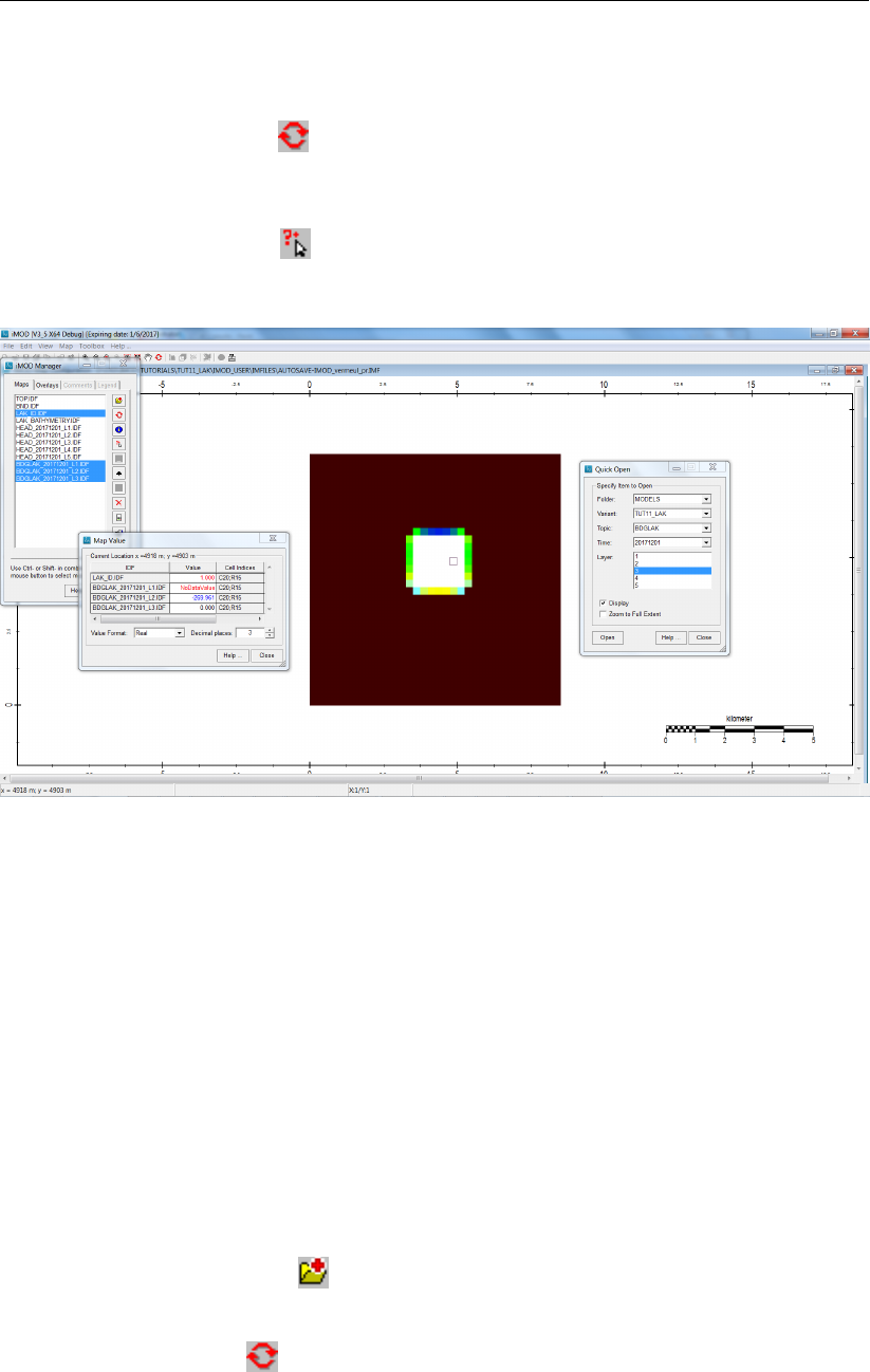
DRAFT
iMOD tutorials
Let’s look at the lake spatial exchange volumes.
90 Select the file “BDGLAK_20171201_L1.IDF” from the iMOD Manager and redraw the canvas by
clicking the Redraw button ( ).
91 Add to the selection of files in the iMOD Manager, the files “LAK_ID.IDF”,
“BDGLAK_20171201_L2.IDF” and “BDGLAK_20171201_L3.IDF”. Use your Ctrl-Left mouse button
to select multiply files.
92 Click the Map Value button ( ) to start the Map Value window.
93 Mouse your mouse over the image and observe the values of the selected maps.
Figure 11.119: Computed spatial Lake fluxes.
The fluxes to- and from the lake are given by the BDGLAK-files. These fluxes are stored within the
first model cell next to the lake. So whenever you hoover your mouse, you’ll notice that the fluxes are
all zero at the location of the lake for the first model layer. As the lake connects for only a part to the
second model layer, you’ll notice that lake fluxes appear in the second layer only underneath the lake
and even for model layer 3, the bottom of the lake. Try to understand the pattern of the fluxes. Having a
look at the head differences between layer 1 and 5 in a cross-section (utilizing the Cross-Section Tool)
may also shed some extra light on how the flux pattern looks like.
Connect the Lake with the SFR package
In this final step, we will connect the lake with the surface water model as described by the SFR
package. The implementation of this package is explained in section 11.8. We have created the SFR
layout and stored the file in {path of tutorialfolder} \TUT_LAK \DBASE \SFR.ISG. Let us open the file.
94 Select the Map Open button ( ) and select the file {path of tutorialfolder} \TUT_LAK \DBASE
\SFR.ISG.
95 Select the file “LAK_ID.IDF” from the iMOD Manager.
96 Click the redraw button ( ) to refresh the graphical canvas.
97 Select from the main menu the option Map,ISG Options and then ISG Edit ... to start the ISG Edit
window.
98 Select “Segment 1” from the list of segments.
Deltares 721 of 812
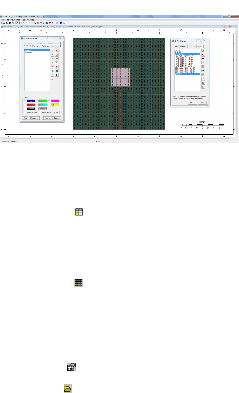
DRAFT
iMOD, User Manual
Figure 11.120: Current layout of the SFR and LAK maps.
In the figure you can see that the streams are connected to the lake on the south and north sides.
From the south, the stream feeds the lake, from the north, it drains the lake.
To connect the lake (LAK) to the stream (SFR), we need to specify a negative lake number in the
SFR.ISG, let’s do that.
99 Click the Attributes button ( ) to open the ISG Attributes window for ’Segment 2’ (’Segment 2’
should be selected in the previous step).
100 Select the “CalPnt TO” from the Calculation Point: dropdown menu.
101 Enter the Lake number at “-1” Idown Seg. (column 9). Use a minus to indicate that the connection
is a lake number and not a stream number.
102 Click the Save button to store the modification in memory.
Now we need to connect the upstream segment 2, such that it can receive water from the lake.
103 Select “Segment 2” from the list of segments.
104 Click the Attributes button ( ) to open the ISG Attributes window.
105 Enter the Lake number at “-1” Iup Seg. (column 8). Use a minus-sign to indicate that the connection
is a lake number and not a stream number.
106 Click the Save button to store the modification in memory.
That’s all, we need to add this ISG file to our project.
107 Click the Save button to save the modification in your model database as file {path of installfolder}
\IMOD_USER \DBASE \TUT_LAK\SFR.ISG.
108 Select the option View and then select Project Manager to pop-up the iMOD Project Manager
window;
109 Select the option (SFR) in the tree view Project Definition.
110 Click Properties button ( ) to start the Define Characteristics for window.
111 Select the option Transient, start from and enter the date “1 December 2016” in the date entry
fields.
112 Click the Open button ( ) and select the file you just created {path of installfolder} \IMOD_USER
\DBASE \TUT_LAK \SFR.ISG.
113 Click the Add New System button to add the parameter to the modeling project and close the
Define Characteristics for window.
722 of 812 Deltares
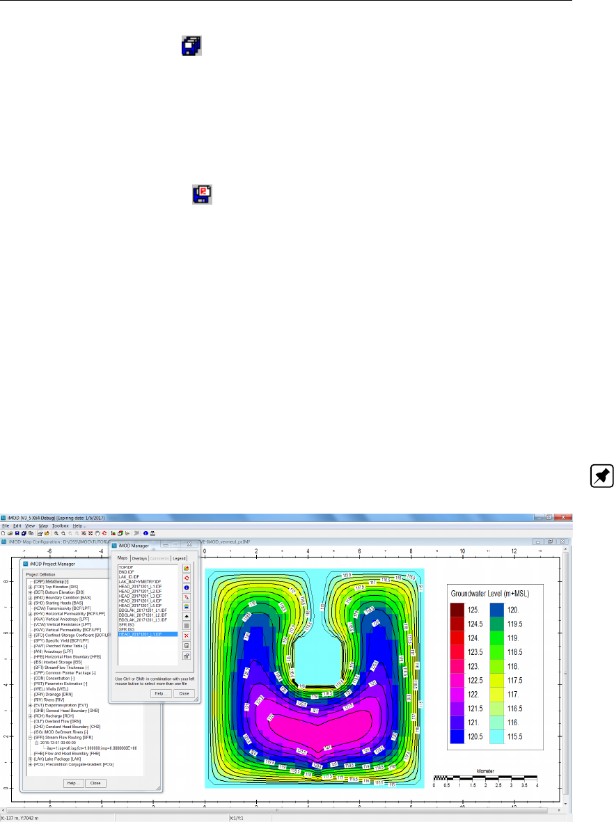
DRAFT
iMOD tutorials
114 Click the Save As button ( ) and save a new modeling project file at {path of installfolder}
\IMOD_USER \RUNFILE \MODEL_LAK_SFR.PRJ.
Simulate the enhanced model
As we use the LAK-package in combination with the SFR we need to create standard MODFLOW2005
files, let’s do that.
115 Click the Save Model button ( ) to start the Define Simulation Configuration window.
116 Enter “2036” at the End Date input field.
117 Select the option “Yearly” from the TimeSteps: dropdown menu field.
118 Select the option “MODFLOW2005” at the File Format: radio button.
119 Click the Simulate button and enter the following *.NAM file {path of installfolder} \IMOD_USER
\MODELS \TUT_LAK_SFR \TUT_LAK.NAM to export the model to MODFLOW2005 files and start
the simulation. Note, that you need to create the folder TUT_LAK_SFR yourself first, use the option
New Folder in your current Save window.
120 Click the Save button.
Inspect the result of the enhanced model simulation
Use the steps from 84 to open the result files from the the folder {path of installfolder} \IMOD_USER
\MODELS \TUT_LAK_SFR. Use yor skills to observe that the steady-state lake level becomes 112.10
m+MSL and the stream stage up- and downstream of the lake are 118.63 and 111.57, respectively.
Note: Use ISG Edit to explore the results of the results of the SFR package, see section 11.8, step
148 onwards.
Figure 11.121: Current result of the groundwater levels for 31st of December 2037.
Use the {path of installfolder} \IMOD_USER \MODELS \TUT_LAK \TUT_LAK.LIST to explore the water
balance for the lake at the last stress period.
Deltares 723 of 812
DRAFT
iMOD, User Manual
It follows that:
Table 11.8: Summary of Lake Water balance.
Parameter Value Unit
Lake Stage 112.09 m+MSL
Lake Volume 2.121050E+07 m3
Precipitation 1.300215E+07 m3/year
Evaporation 1.154501E+07 m3/year
Groundwater Inflow 5.7897E+07 m3/year
Groundwater Outflow 0.0000E+00 m3/year
Surface Water Inflow 2.5738E+08 m3/year
Surface Water Outflow 3.1528E+08 m3/year
Okay, please feel free to experiment more with several parameters for the LAK package.
724 of 812 Deltares

DRAFT
iMOD tutorials
11.10 Tutorial 10: Multi-Node Well- and HFB Package
This tutorial gives an introduction to the Multi-Node Well Package (MNW, see section 12.30) by using it
in an unconfined quasi 3-D transient model. It also compares the MNW package with the conventional
WEL package. We also add the HFB package to block the horizontal flow from a particular direction.
Outline
This is what you will do:
Load an existing model project and display the model in 3-D;
Construct a quick and simple model project with the WEL package;
Define the model as an unconfined model and simulate the model;
Modify the model project with the MNW package and simulate the model;
Inspect both results;
Change some parameters in the MNW package to simulate well losses;
Include the horizontal barrier flow package (HFB) and simulate the results for that configuration.
Required Data
For this tutorial you need the following iMOD Data Files/folders:
The entire folder (and subfolders) in {path of tutorialfolder} \TUT_MNW \DBASE, containing:
BND \BND.IDF – boundary conditions of the model;
TOP \TOP.IDF – top elevation of each model layer;
BOT \BOT.IDF – bottom elevation of each model layer;
HFB \SHEET_PILE.GEN – location of the sheet piling (to be created);
WEL \WEL.IPF – location of the extraction well;
WEL \WEL.TXT – time series of the extraction rate of the well;
MNW \WEL_THIEM.IPF – location of the extraction well configured for a well loss based on
Thiem equation;
MNW \WEL.TXT – time series of the extraction rate of the well;
MODEL_WEL.PRJ – initial model project file;
MODEL_MNW.PRJ – model project file with the MNW package (to be created);
MODEL_HFB.PRJ – model project file with the HFB package (to be created);
Getting Started
1 Start iMOD.
2 Select the option Create a New iMOD Project.
3 Click the Start button;
4 Activate the iMOD Manager (short-cut is Ctrl+M)
Load the Modelling Project in 3-D
We will load the modelling project and generate a 3-D image of our model.
5 Select the option View and then select Project Manager to start the iMOD Project Manager win-
dow;
6 Click the Open Projectfile button ( ) and select the file {path of tutorialfolder} \TUT_MNW
\MODEL_WEL.PRJ;
7 Click the Open button;
8 Select the option (WEL) in the tree view Project Definition;
9 Click the Draw button ( ) to add the well file to the iMOD Manager;
10 Click the Zoom All button ( ) to view the location of the well.
Deltares 725 of 812
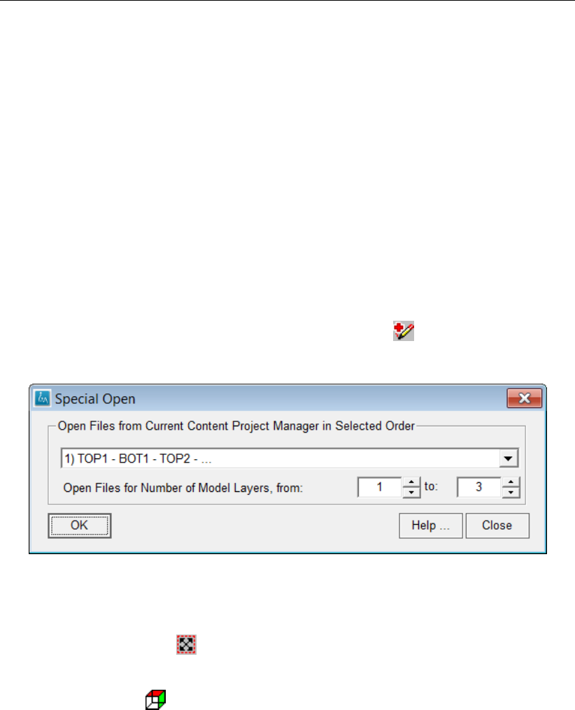
DRAFT
iMOD, User Manual
We want to display the well in 3-D together with the modellayers, so we need to configure the Z-settings
of the well via IPF Configure, let’s do that.
11 Right click your mouse button and select the option IPF Options and than IPF Configure to start
the IPF Configure window;
12 Select “Z1” at the dropdown menu at Z-coordinate. (top elevation of the screen);
13 Check the option Sec.Z-Crd to define the secondary Z-coordinate. (botom elevation of the screen);
14 Select “Z2” at the dropdown menu at Sec.Z-Crd;
15 Click the button Pick Colour ;
16 Select a red colour from the Colour window;
17 Click the Ok button to leave the Colour window;
18 Click the Close button to leave the IPF Configure window.
We will now load the upper- and lower elevations per model layer, we use the Special Open option
from the Project Manager. This option allows you to quickly read a selection of IDF files in a particular
order from the current model project to the iMOD Manager. In that way, it is easy to port the files in the
right order to the Profile Tool and/or 3-D Tool.
19 In the Project Manager window click the Special Open button ( ) to start the Special Open
window.
Figure 11.122: Example of the Special Open window.
20 Click the OK button to load the selected files to the Project Manger and leave the Special Open
window;
21 Click the Zoom All button ( ) to set the graphical display to the extent of the IDF files loaded in
the iMOD Manager;
22 Select in the iMOD Manager all IDF-files together with the WEL.IPF;
23 Click the 3-D button ( ) from the iMOD Main window;
You’ll notice that prior to the 3D tool the 3D IDF Settings dialog appears. In this dialog the appearance
of the IDF-files can be configured. For example, an IDF can be represented by planes (quads between
mids of gridcells giving a smooth surface) and/or cubes (representing the grid cells as flat surfaces,
like Lego-blocks). To visualize aquitards as solids we will combine each bottom of an aquifer with the
top of the aquifer lying underneath it.
24 Select the option “Quasi 3D Model (aquitard)” from the Configuration dropdown menu;
25 Click the Apply button.
To show the well we need to instruct iMOD to ignore the associated txt file temporarily and use the Z
and Sec.Z-Crd as set previously. Therefore do the following:
26 Select the tab IPF’s from the 3-D Tool window;
27 Select the option Deact. Associated Files.
Now we see our well.
726 of 812 Deltares
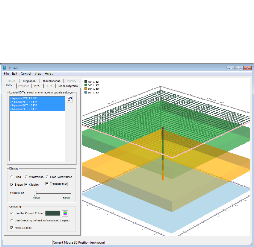
DRAFT
iMOD tutorials
28 Select the tab IDFs from the 3-D Tool window;
29 Select the option Transparancy to create translucent blocks in order to see the well clearly;
30 Rotate the image with your left mouse button.
The image might look like this:
Figure 11.123: 3-D image of our model.
The 3D-image allows you to observe that the well is penetrating all model layers; in fact the well screen
is for a length of 1.0 meter in model layer 1, model layer 2 is fully penetrated and layer 3 contains 5
meters (half of the thickness of that aquifer) of the well screen. The well extracts from all three model
layers, proportional to the respective length of the well screen in each layer; this will be computed by
iMOD when the model definition is translated to the MF2005 WEL package. The total strength of the
well is 10,000.0 m3/d from December 1st 2016 up to December 1st 2040. Starting from December 1st
2040 the well is turned off (0.0 m3/d). This is specified in the WEL.TXT file associated to the WEL.IPF.
Below is the content of that file.
2
2
DATE , -9999.0
Q , -9999.0
20161201,-10000.0
20401201, 0.0
31 Quit the 3-D Tool window by clicking the option File and then Quit 3-D Tool;
Deltares 727 of 812
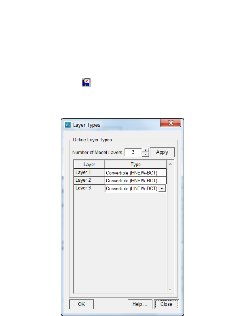
DRAFT
iMOD, User Manual
Run the Model
Because we want to be able to simulate layers falling dry we apply a model with unconfined model
layers. In that way the areas that fall dry are no part of the simulation until these model cells are re-
wetted again. When unconfined model layers are applied in iMOD, iMOD includes the wetting option
of MF2005 automatically.
32 Whenever the Project Manager may have disappeared, pop-it-up by selecting the menu option
View and than Project Manager;
33 Click the Save Model button ( ) to start the Define Simulation Configuration window;
34 Click on the button Define 3 Layer Types to start the Layer Types window.
Figure 11.124: Example of the Layer Types window: assigning layer type ’Convertible
(HNEW-BOT)’ to all layers.
35 Select the option Convertible (HNEW-BOT) for model layer 1, 2 and 3. In this way all model layers
will be unconfined and the transmissivity is a function of the computed head (HNEW) minus the
bottom of each model layer (BOT).
It is important to know that MF2005 includes the option to simulate model cells becoming dry when
the hydraulic head of that cell drops below the bottom of that model cell. To ensure that dry cells can
become part of the simulation again, iMOD includes the wetdry-option in the LPF-package automati-
cally: it is not needed to specify extra input for this option. iMOD defines the wetdry-option to all active
model cells that are part of an unconfined model layer. Whenever the head underneath the dry cell
(hn) is higher than 0.1 meter above the bottom of the model layer (BOT), it becomes wet again. Using
this option, is more stable than using all four adjacent model cells as well. In the iteration, the head at
728 of 812 Deltares
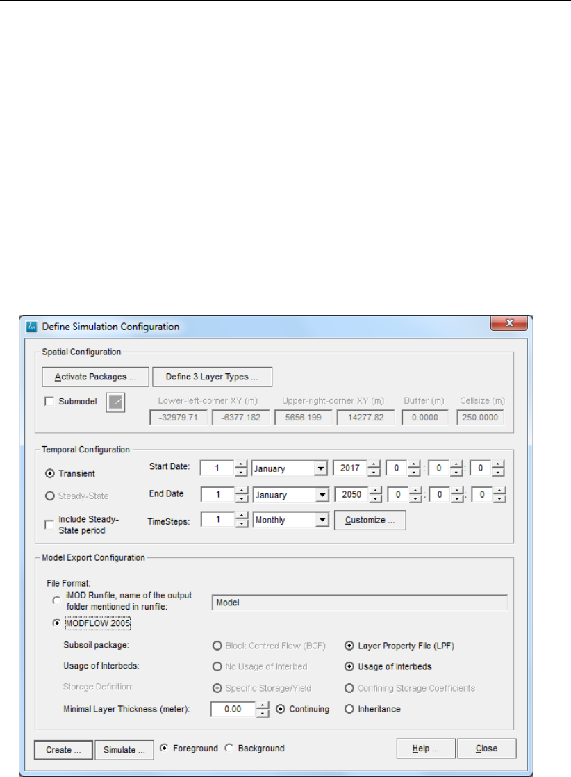
DRAFT
iMOD tutorials
that cell is than initially set to by following equation:
h= BOT + WETFCT (hn−BOT) ,(11.4)
whereby WETFCT=0.1. These are programmed internally in iMOD as they give the most robust ap-
proach. However, whenever it is still needed to modify this, the (advanced) model user can modify the
exported MF2005-files outside iMOD themselves.
36 Click the OK button;
From the PRJ-file iMOD has read the transient characteristics of your model; it starts at 1st of Decem-
ber 2017 00:00:00 and ends at the same date. More input was not yet given to the model, but we can
extent the simulation period of the model by simply defining another end date, let’s do that.
37 Enter the year “2050” at the Enddate;
38 Enter “Monthly” at the TimeSteps;
39 Select the option “MODFLOW 2005” at the File Format: radio button.
Figure 11.125: Example of the iMOD Define Simulation Configuration window.
After step 39 the Define Simulation Configuration window should look like in Figure 11.125.
The model will generate results on a monthly time step which is based on the definition of the input
data, we can inspect this.
40 Click the Simulate button and enter the following *.NAM file {path of installfolder} \IMOD_USER
\MODELS \TUT_WEL \TUT_WEL.NAM to export the model to MODFLOW2005 files and start the
simulation immediately. Note, that you need to create the folder TUT_WEL yourself first, use the
option New Folder in your current Save window.
Deltares 729 of 812
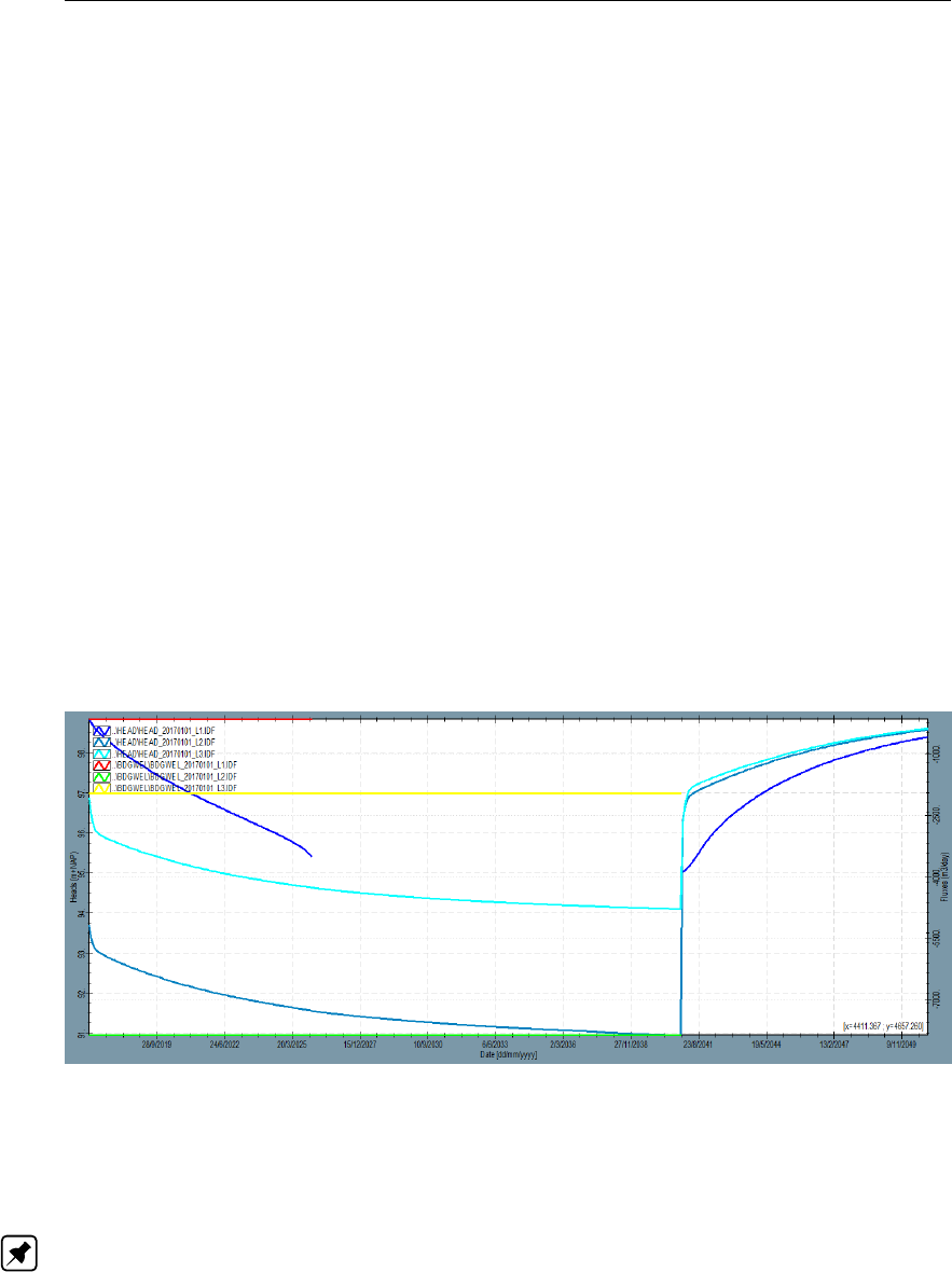
DRAFT
iMOD, User Manual
iMOD will now first create the necessary MODFLOW2005 files; as the model is tiny this will be will
finished quickly. Immediately thereafter the simulation starts. You’ll see that the model starts in a
separate DOS-command window and it will echo the simulation progress. It is a transient simulation of
408 stress periods, it probably will take something like 20 seconds of runtime (e.g. on a computer with
a 2.6 GHz processor).
Inspect the result of simulation
Let’s inspect the hydraulic head of the first model layer and the well rates and generate time series.
41 Select the option Map and then the option Quick Open to start the Quick Open window, see sec-
tion 6.2. With this window it is easy to open and view results from a model simulation.
42 Select the option “HEAD” from the Topic dropdown menu.
43 Select the option “20171201” from the Time: dropdown menu.
44 Select the options “1”, “2” and “3” from the Layer dropdown menu. Tip: drag your mouse to select
multiply entries of the menu field.
45 Click the Open button; the specified head maps are added to the iMOD Manager;
46 Repeat the above mentioned steps to open the results for BDGWEL as well;
47 Click the Close button to leave the Quick Open window.
iMOD will load all selected result files into the iMOD Manager and displays the result on the graphi-
cal canvas. Use your experience learned from the previous Tutorials to display the computed heads
(HEAD) and the extraction rate (BDGWEL) as time series as shown in the following figure. Be aware
that it can take a few seconds, as iMOD needs to open 1224 files.
Figure 11.126: Time Series of computed hydraulic heads and abstraction rates at the
location of the well using the WEL package: heads in layer 1 (blue line),
layer 2 (turquoise line) and layer 3 (cyan line), abstraction rates [m3/day]
in layer 1 (red line), layer 2 (green line) and layer 3 (yellow line).
Note: The extraction in model layer 1 is inactive as soon as the layer becomes dry. Also observe that
the layer is re-wetted and the extraction of layer 1 is re-activated again as a result of deactivation of the
extractions in the other model layers.
The total extraction for the entire duration of the model is less than was assigned to the model. So,
instead of taking out 87.8E6m3/d, the amount of extracted water was 86.8E6m3/d. One of the advan-
tages of the MNW package is that the total extracted amount remains intact once a model layer falls
dry. Another improvement is that the extraction rate declines gradually as a model layers tends to dry,
instead of abrupt as with the WEL package. The other layers will get an increased extraction for those
case. Let’s observe that in the coming part of this tutorial.
730 of 812 Deltares
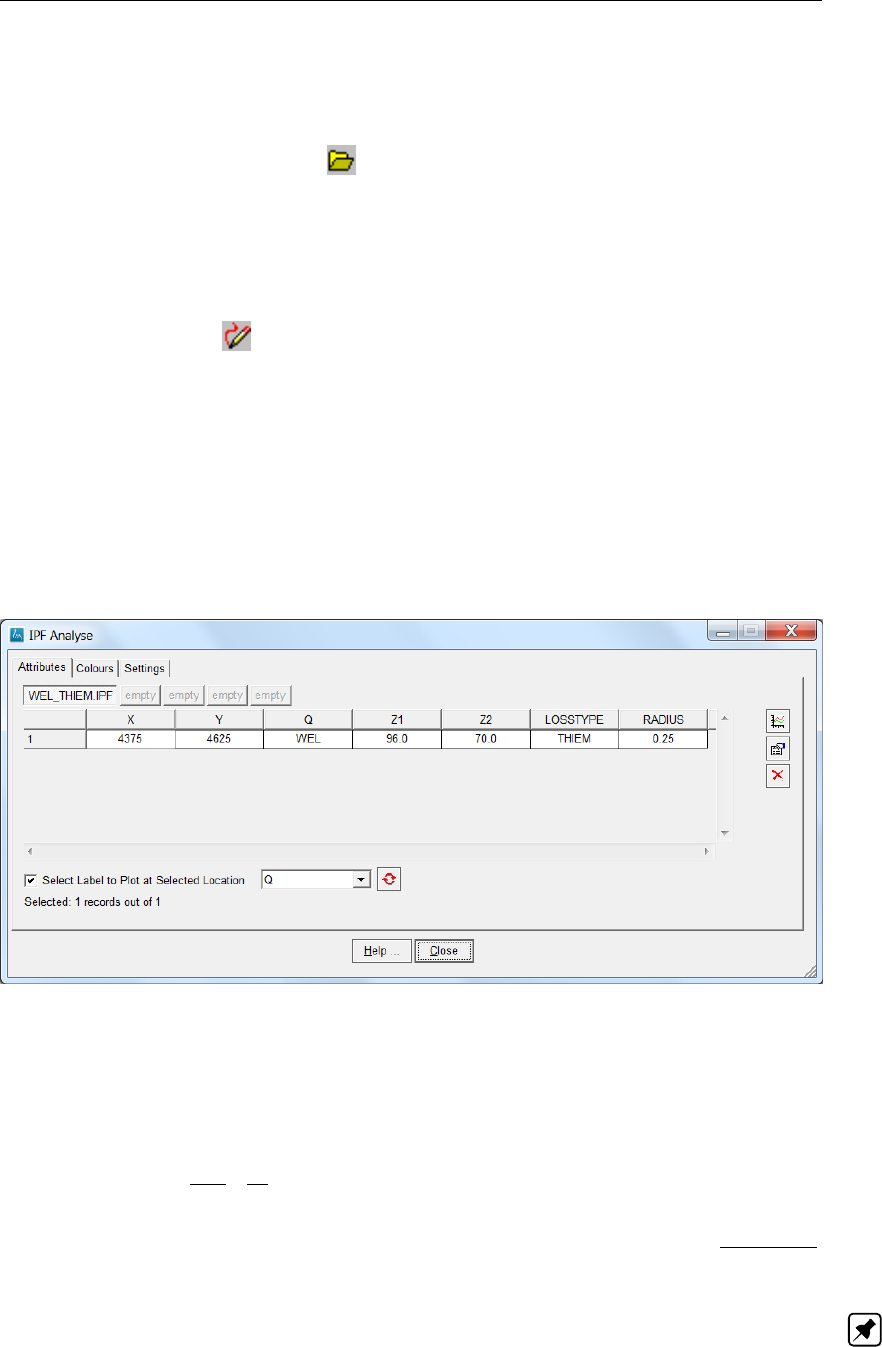
DRAFT
iMOD tutorials
Creating the Multi-Node Well (MNW) input
48 Select the option View and then select Project Manager to start the iMOD Project Manager win-
dow;
49 Click the Open Projectfile button ( ) and select the file {path of tutorialfolder} \TUT_MNW
\IMOD_USER \RUNFILE \MODEL_MNW.PRJ;
50 Click the Open button;
This will clean the entire Project Manager first before loading in the selected PRJ file.
51 Select the option (MNW) in the tree view Project Definition;
52 Click the Draw button ( ) to add the well file to the iMOD Manager;
53 Select the option Map,IPF Options and than IPF Analyse ... to start the IPF Analyse window.
54 Click your right mouse button on the graphical canvas and select the option Select the Entire
Domain.
Now we have selected our MNW-well and the values for the different attributes are presented in the
table. We can see that that screens of the well starts at 96.0 m+MSL and ends at 70.0 m+MSL. This
is similar to our previous well modelled by the conventional WEL package. You can also see that the
methodology of computing well loss is given by the keyword THIEM and the appropriate parameter
relevant to that is the RADUIS (rw= 0.25 m), see section section 12.30 for more detailed information
about the MNW package.
Figure 11.127: Attribute values for the MNW-well.
MNW computes a hydraulic head in the cell hnsuch that it equals the computed hydraulic head at the
well minus a head loss term (e.g. the Thiem equation, see Konikow et al. (2009)). Here we neglect
head loss due to skin and local turbulence effects for that particular cell, so:
hWELL −hn=Qn
2πT ln r0
rw
,(11.5)
where Qnis the well rate (m3/d), Tis transmissivity of the aquifer (m2/d) at the well, r0is the effective
radius of a finite-difference cell (m), this is assumed for isotropic conditions as r0= 0.14p∆x2+ ∆y2;
and rwis the actual radius of the well.
Note: Because r0is typically much larger than rw, the head in a pumping well will be lower than the
model-computed head. The head in the pumping well is not equal to the hydraulic head saved by the
model.
Okay, let’s run the model with the MNW package.
Deltares 731 of 812

DRAFT
iMOD, User Manual
55 Apply steps 32 and further;
56 Click the Simulate button and enter the following *.NAM file {path of installfolder} \IMOD_USER
\MODELS \TUT_MNW \TUT_MNW.NAM to export the model to MODFLOW2005 files and start
the simulation. Note, that you need to create the folder TUT_MNW yourself first, use the option
New Folder in your current Save window.
Again, iMOD will first create the necessary MODFLOW2005 files and start the simulation immediately.
Similar to the model using the WEL package, this model including the MNW package will also probably
take no more than something like 20 seconds to run.
Compare the result of WEL and MNW simulation
Let’s inspect the hydraulic head of the first model layer and the computed distribution of extraction rates
and generate time series.
57 Select the option Map and then the option Quick Open to start the Quick Open window, see sec-
tion 6.2. With this window it is easy to open and view results from a model simulation.
58 Select the option “TUT_MNW” from the Variant dropdown menu.
59 Select the option “HEAD” from the Topic dropdown menu.
60 Select the option “20171201” from the Time: dropdown menu.
61 Select the options “1”, “2” and “3” from the Layer dropdown menu. Tip: drag your mouse to select
multiply entries of the menu field.
62 Click the Open button;
63 Repeat the above mentioned steps to open the results for BDGMNW as well;
64 Click the Close button to leave the Quick Open window.
iMOD will load all selected result files into the iMOD Manager and displays the result on the graphical
canvas.
65 Use your experience learned from the previous Tutorials to display the extraction rate (BDGMNW)
as time series as shown in the following figure. Be aware that it can take a few seconds, as iMOD
needs to open 1224 files.
732 of 812 Deltares
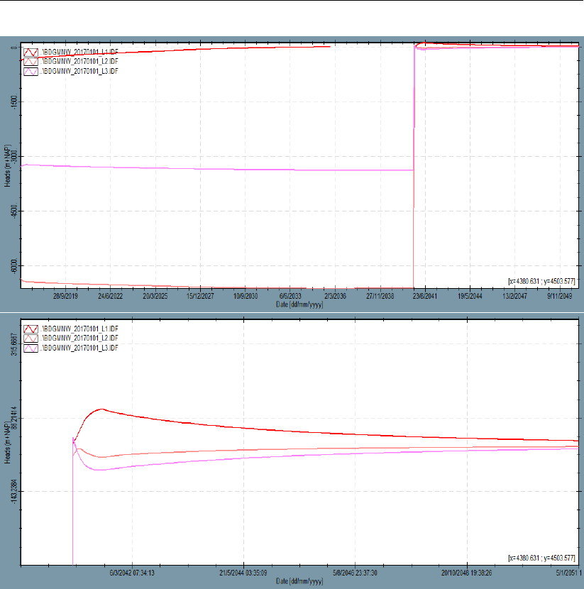
DRAFT
iMOD tutorials
Figure 11.128: Time Series of computed extraction rates using the MNW package in layer
1 (red), layer 2 (orange) and layer 3 (violet); total time series (above) and
zoomed in from 2040 onwards (below).
As expected, you might observe that the total extraction rate varies and that the extraction rate for
the first model layer slowly decrease to zero. At the same time the extraction of the deeper aquifers,
increases to sum up to 10,000 m3/d. If we look at the zoomed in image (bottom) for the period after
2040, where we turned off the well, we observe that the well rates vary although there is no external
rate specified.
So, what is happening?
Well, one of the features of the MNW package is the capability of simulating intra borehole flow, actually
water can move from one aquifer - through the borehole - to another aquifer. Due to the stopping of
the pumping, the deeper aquifers recover quicker from the computed draw down than the unconfined
aquifer, mainly due to the low storage coefficient. This causes an overpressure from the deep aquifers
to the shallow one and generates a groundwater flow that migrates directly through the borehole into
the first aquifer.
66 Use your experience learned from the previous Tutorials to display the hydraulic head (HEAD) for
our model with the WEL- and MNW package as time series as shown in the following figure. Be
aware that it can take a few seconds, as iMOD need to open 1632 files.
Deltares 733 of 812
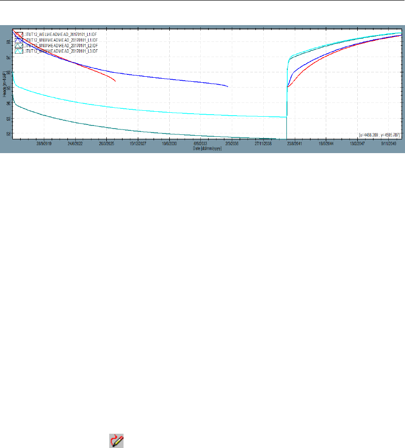
DRAFT
iMOD, User Manual
Figure 11.129: Time Series of computed hydraulic heads at the location of the abstraction
well: in layer 1 using the WEL package (red line), and heads in layers 1 to
3 using the MNW package (blue, turquoise and cyan lines respectively).
The figure of timeseries of computer hydraulic heads at the location of the well clearly shows that
there is an overpressure that causes this intra borehole flow. Moreover, when comparing the hydraulic
heads in layer 1 cells at the well location, in the model with the MNW package the cell remains wet for
a longer period of time compared to the model with the WEL package. This is caused by the MNW
package decreasing the extraction amount gradually and therefore decreases the draw down rate of
the ground water head. Due to the early mentioned intra borehole flow, the heads in the model with an
MNW package recover more quickly than in the model with the WEL package.
So the MNW package can really add some extra features concerning the behaviour of a well in your
model. Speaking of more detail, it seems that there is a horizontal barrier (sheet pile wall) blocking the
flow to our well. Let’s see how to incorporate this with iMOD into our model.
Enhancing the model with a Horizontal Flow Barrier (HFB) input
Let’s create our sheet pile wall.
67 Select from the main menu the option Edit,Create Features and then GENs ... to start the Create
GENs window.
68 Click the Draw button ( ), this will start the Select window;
69 Select the option Line from the Shape types;
70 Click the Ok button.
71 Start drawing a line at the west side of the well. Click your left mouse button to position the first
point of the line. Each left mouse click will insert another point.
72 Click your right mouse button to finish the drawing.
734 of 812 Deltares
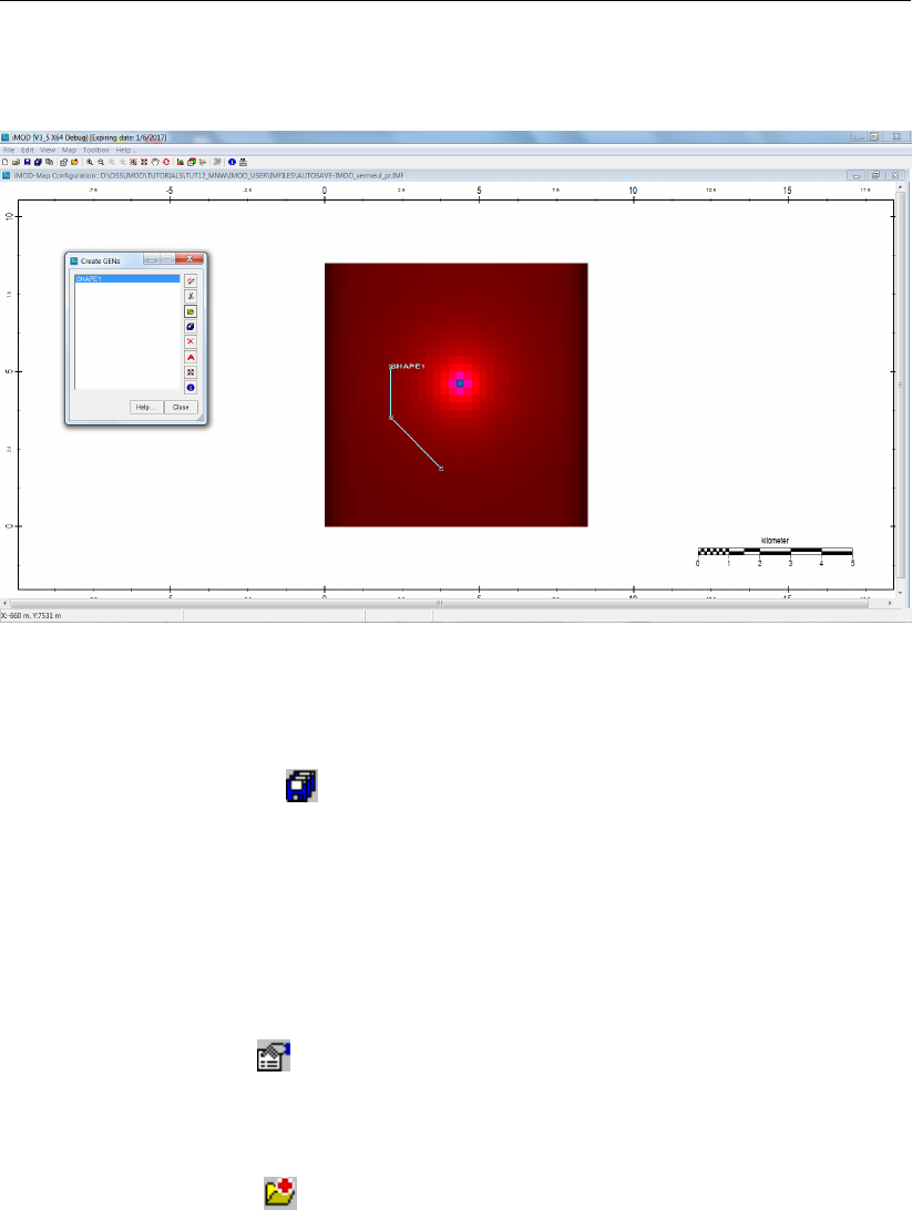
DRAFT
iMOD tutorials
The following line could be on your screen.
Figure 11.130: Outline of our sheet pile.
Let’s save the sheet pile wall.
73 Click the Save As button ( ) and save the sheet pile at {path of installfolder} \IMOD_USER
\DBASE \TUT_MNW \SHEET_PILE.GEN.
74 Click the Save button.
75 Click the Close button to close the Create GENs window.
Now we have to add this sheet pile to our modelling project.
76 Select the option View and then select Project Manager to start the iMOD Project Manager win-
dow;
77 Select the option (HFB) in the tree view Project Definition;
78 Click Properties button ( ) to start the Define Characteristics for window.
79 Enter a value of “2”at the Assign Parameter to model layer ..., our pile sheet wall will act as barrier
for the second model layer only;
80 Enter a value of “1000.0”at the Assign Parameter Addition Value, our pile sheet wall will have a
resistance of 1000.0 days;
81 Click the Add File button ( ) and select the file we just created: {path of installfolder} \IMOD_USER
\DBASE \TUT_MNW \SHEET_PILE.GEN.
Deltares 735 of 812
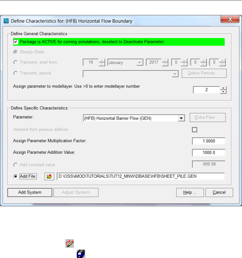
DRAFT
iMOD, User Manual
Figure 11.131: Example of the iMOD Project Manager window.
82 Click the Add New System button to add the parameter to the modeling project; the Define Char-
acteristics for window will be closed.
83 Click the Draw button ( ) to open the sheet pile to the iMOD Manager ;
84 Click the Save As button ( ) and save a new modeling project file at {path of installfolder}
\IMOD_USER \RUNFILES \MODEL_HFB.PRJ.
So, we’re ready to run this model.
85 Apply steps 32 and further;
86 Click the Simulate button and enter the following *.NAM file {path of installfolder} \IMOD_USER
\MODELS \TUT_HFB\TUT_HFB.NAM to export the model to MODFLOW2005 files and start the
simulation. Note, that you need to create the folder TUT_HFB yourself first, use the option New
Folder in your current Save window.
Also here again iMOD will first create the necessary MODFLOW2005 files and starts the simulation.
Similar to the previous 2 models, this model including the MNW + HFB package will also probably take
no more than something like 20 seconds to run.
Compare the results of the MNW and HFB simulation
Let’s inspect the hydraulic head of the first model layer and generate time series.
87 Click the Close button to leave the Define Simulation Configuration window;
88 Select the option Map and then the option Quick Open to start the Quick Open window, see sec-
tion 6.2. With this window it is easy to open and view results from a model simulation.
89 Select the option “TUT_HFB” from the Variant dropdown menu.
736 of 812 Deltares
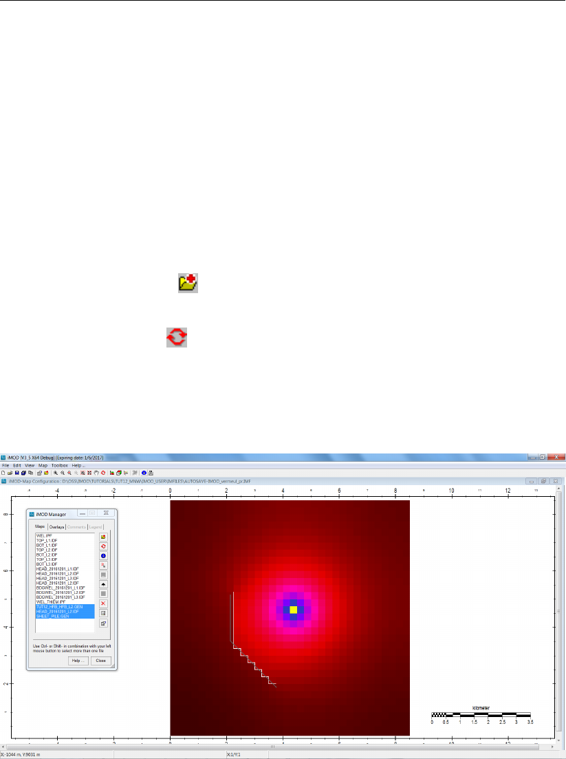
DRAFT
iMOD tutorials
90 Select the option “HEAD” from the Topic dropdown menu.
91 Select the option “20171201” from the Time: dropdown menu.
92 Select the options “2” from the Layer dropdown menu.
93 Click the Open button;
94 Click the Close button to leave the Quick Open window.
iMOD will load all selected result files into the iMOD Manager and displays the result on the graphical
canvas.
During the simulation iMOD translates the manually drawn sheet pile wall - which we saved earlier
as SHEET_PILE.GEN - to a continuous (kinked) line coinciding exactly with the lateral cell faces it
intersects; when utilizing the HFB package the specified resistance is assigned to these cell faces. It is
always a good idea to examine the result of such a translation, e.g. to check whether the discretization
has resulted in a sheet pile wall that is fully continuous and thus behaving like a true barrier. Let’s open
that file.
95 Click the Add File button ( ) from the main toolbar and select the file {path of installfolder}
\IMOD_USER \MODELS \TUT_HFB\MODELINPPUT \TUT_HFB_L2.GEN.
96 Select the file SHEET_PILE.GEN and HEAD_20171201_L2.IDF from the iMOD Manager window.
97 Click the Redraw button ( ).
98 Use your experience to change the colour of the lines.
You should see, more-or-less, the following image. In white is the actual position of the sheet pile in
the model. Due to the chosen grid size, it is a little bit shifted and crenelated due to the rectangular
simulation network.
Figure 11.132: Display of the possible outcome of our HFB model.
You could try to experiment with more complex shapes for the HFB and/or modify the resistance of the
sheet pile.
Deltares 737 of 812

DRAFT
iMOD, User Manual
11.11 Tutorial 11: Unsaturated Zone Package
This tutorial gives an introduction to a transient implementation of the Unsaturated Zone package
(UZF), see section 12.31.
Outline
This is what you will do:
Create a transient PRJ file with TOP, BOT, KHV, RCH and EVT package;
Simulate the RCH and EVT package for an unconfined model and examine the results;
Modify the PRJ file with the UZF package;
Simulate the UZF package and examine the results and compare it with the conventional RCH and
EVT model;
Modify the parameters of the UZF package to see the impact of parameters;
Required Data
For this tutorial you need the following iMOD Data Files/folders:
The entire folder (and subfolders) in {path of tutorialfolder} \TUT_UZF \DBASE, containing:
. \TOP \TOP_L*.IDF – IDF files with top of model layers (3);
. \BOT \BOT_l*.IDF – IDF files with bottom of model layers (3);
. \PREC \PREC_*.IDF – IDF files with precipitation on a daily base;
MODEL_RCH_EVT.PRJ – model project file with RCH and EVT package (to be created);
MODEL_UZF.PRJ – model project file with UZF package (to be created);
Getting Started
1 Start iMOD.
2 Select the option Create a New iMOD Project.
3 Click the Start button;
Create a PRJ file
We will quickly generate a PRJ file using the auto fill option of the Project Manager.
4 Select the option View and then select Project Manager to start the iMOD Project Manager win-
dow;
5 Select the option (TOP) in the tree view Project Definition;
6 Click Define Characteristics Automatically button ( ) to start the Define Characteristics for
window.
7 Add the following string to the second column in the table “{path of tutorialfolder} \TUT_UZF
\DBASE \TOP \TOP_L*.IDF”;
8 Select the option Select files within Given Layer Range and enter “1” and“3” in the input fields to
the right.
738 of 812 Deltares
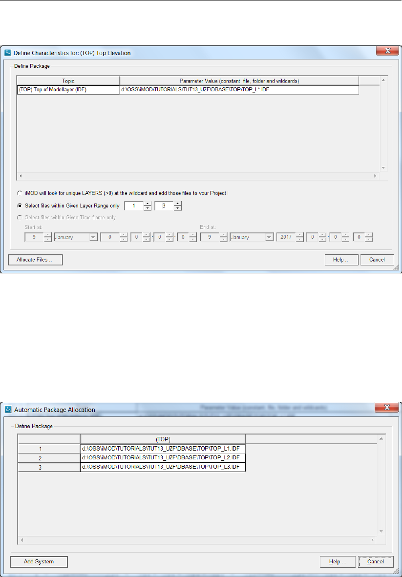
DRAFT
iMOD tutorials
Your window should look as follows:
Figure 11.133: Example of the Define Characteristics Automatically window.
In this manner we tell iMOD to add the given files for model layer 1,2 and 3 automatically. Let’s see
how that works.
9 Click the Allocate Files ... button.
iMOD will pop-up a window with the files found in the Automatic Package Allocation window.
Figure 11.134: Example of the Automatic Package Allocation window.
Here we can inspect the results, or even modify this. We leave it like this as it is correct and continue.
10 Click the Add System button, this will add the files to our modelling project and closes the Automatic
Package Allocation window.
11 Repeat the steps 5 up to 10 for the bottom of the model layers (keyword is BOT), these are stored
in “{path of tutorialfolder} \TUT_UZF \DBASE \BOT \BOT_L*.IDF”.
Deltares 739 of 812
DRAFT
iMOD, User Manual
Also constant values for a package or modules can be inserted in this manner, as the boundary condi-
tions of our three-layered model are all equal one, we insert this information as follows:
12 Select the option (BND) in the tree view Project Definition;
13 Click Define Characteristics Automatically button ( ) to start the Define Characteristics for
window.
14 Add the following string to the second column in the table “1”;
15 Select the option Select files within Given Layer Range and enter “1” and“3” in the input fields to
the right.
16 Click the Allocate Files ... button.
17 Click the Add System button, this will add the files to our modelling project and closes the Automatic
Package Allocation window.
That’s convenient, right? Let’s add the constant information for the other packages repeating the steps
12 up to 17.
18 Add a constant starting head of “95.0” m+MSL for the SHD package (starting heads) for the model
layers 1,2 and 3;
19 Add a constant starting head of “10.0” m/d for the KHV package (horizontal permeability) for the
model layers 1,2 and 3;
20 Add a constant starting head of “1.0” for the KVA package (vertical anisotropy) for the model layers
1,2 and 3;
21 Add a constant starting head of “0.3” for the SPY package (specific yield) for the model layers 1,2
and 3.
Next thing is to add the confined storage coefficients (STO).
22 Select the option (STO) in the tree view Project Definition;
23 Click Define Characteristics Automatically button ( ) to start the Define Characteristics for
window.
24 Add the following string to the second column in the table “0.2E-03”;
25 Select the option Select files within Given Layer Range and enter “1” and“3” in the input fields to
the right.
26 Click the Allocate Files ... button.
27 Modify the value “0.2E-03” for model layer 1 into “1.0”;
28 Click the Add System button, this will add the files to our modelling project and closes the Automatic
Package Allocation window.
Almost done, we will add the Evaporation package (EVT) on the conventional way as it will be defined
for our first stress period only.
29 Select the option (EVT) in the tree view Project Definition;
30 Click Properties button ( ) to start the Define Characteristics for window.
31 Select the option Transient, start from and enter the date “6 October 2013” in the date entry fields;
32 Select the option Add constant value;
33 We will enter the following values for the different input parameters by selecting the appropriate
parameter from the Parameter dropdown list sequentially:
(EVA) Evapotranspiration Rate (IDF) = “10.0” mm/day;
(SUR) Surface Level (IDF) = “100.0” m+MSL;
(EXD) Extinction Depth (IDF) = “8.0” m.
34 Click the Add New System button to add the parameter to the modelling project and close the
Define Characteristics for window.
Note: By defining a surface level (SUR) of 100.0 m+MSL and an extinction depth (EXD) of 8.0, there
will be a linear reduction of evaporation with depth. At a depth of 8 m+MSL (2 meter above the bottom
of model layer 1), the evaporation is 0.0.
740 of 812 Deltares
DRAFT
iMOD tutorials
Precipitation is the input parameter that varies per stress period. We will add that parameter with the
automatic package allocation.
35 Select the option (RCH) in the tree view Project Definition;
36 Click Define Characteristics Automatically button ( ) to start the Define Characteristics for
window.
37 Add the following string to the second column in the table “{path of tutorialfolder} \TUT_UZF
\DBASE \PREC \PREC_*.IDF”.;
38 Select the option iMOD will look for unique TIME STEPS ...;
39 Click the Allocate Files ... button.
40 Click the Add System button, this will add the files to our modelling project and closes the Automatic
Package Allocation window.
We have add now 459 definitions for precipitation in a single mouse click, that’s awesome isn’t it. Final
thing to do is to add the configuration for the PCG solver.
41 Select the option (PCG) in the tree view Project Definition;
42 Click Properties button ( ) to start the PCG settings window.
43 Click the Apply button to add the parameter to the modelling project and close the PCG settings
window.
Okay, we’re done, let’s save the modelling project.
44 Click the Save As button ( ) and save a new modeling project file at {path of installfolder}
\IMOD_USER \RUNFILE \MODEL_RCH_EVT.PRJ.
Simulate the model
With this project file we generate a standard MODFLOW2005 model, let’s do that.
45 Click the Save Model button ( ) to start the Define Simulation Configuration window;
46 Click on the button Define 3 Layer Types to start the Layer Types window.
Deltares 741 of 812
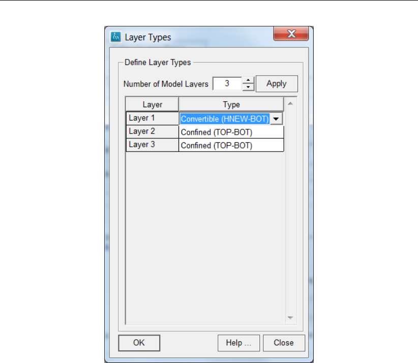
DRAFT
iMOD, User Manual
Figure 11.135: Example of the Layer Types window: assigning layer type ’Convertible
(HNEW-BOT)’ to layer 1.
47 Select the option Convertible (HNEW-BOT) for model layer 1 by clicking on the cell of the second
column. In this way the first model layer will be unconfined and the transmissivity is a function of
the computed head (HNEW) minus the bottom of the model layer (BOT);
48 Click the OK button;
49 Select the option “MODFLOW 2005” at the File Format: radio button.
iMOD has found out what the transient content of your model is, it starts at 6st of October 2013
00:00:00 and ends at the 7st of January 2015 00:00:00. based on the entered precipitation (RCH) and
evaporation (EVT) data.
742 of 812 Deltares
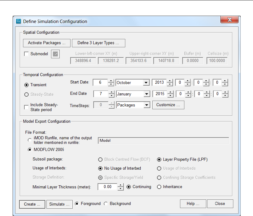
DRAFT
iMOD tutorials
Figure 11.136: Example of the iMOD Define Simulation Configuration window.
The model will generate results on a daily time step which is based on the occurrence of the input data,
we can inspect this.
50 Click the option Customize ... (on the Define Simulation Configuration window at the Temporal
Configuration settings) to start the Time Discretization Manager for Simulation window.
Deltares 743 of 812
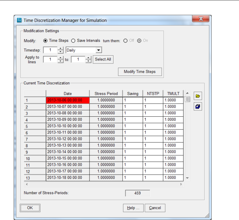
DRAFT
iMOD, User Manual
Figure 11.137: Example of the iMOD Time Discretization Manager for Simulation window.
We will leave the definition of the stress-periods for now.
51 Click the OK button to close the Time Discretization Manager for Simulation window.
52 Click the Simulate button and enter the following *.NAM file {path of installfolder} \IMOD_USER
\MODELS \TUT_RCH_EVT \TUT_RCH_EVT.NAM to export the model to MODFLOW2005 files
and start the simulation. Note, that you need to create the folder TUT_RCH_EVT yourself first, use
the option New Folder in your current Save window.
53 Click the Save button.
iMOD will now create the necessary MODFLOW2005 file and runs the model, as the model is tiny, this
will be finished rapidly. It will start the simulation directly thereafter. You’ll see that the model start in a
separate DOS-command window and it will echo the simulation progress. As it is a transient simulation
with 458 stress periods, it will consume probably 10 seconds to accomplish.
Inspect the result of simulation
Let’s inspect the hydraulic head of the first model layer and the computed recharge (equal to the input
in fact) and generate time series.
54 Select the option Map and then the option Quick Open to start the Quick Open window, see sec-
tion 6.2. With this window it is easy to open and view results from a model simulation.
55 Select the option “HEAD” from the Topic dropdown menu.
56 Select the option “20131006” from the Time: dropdown menu.
744 of 812 Deltares
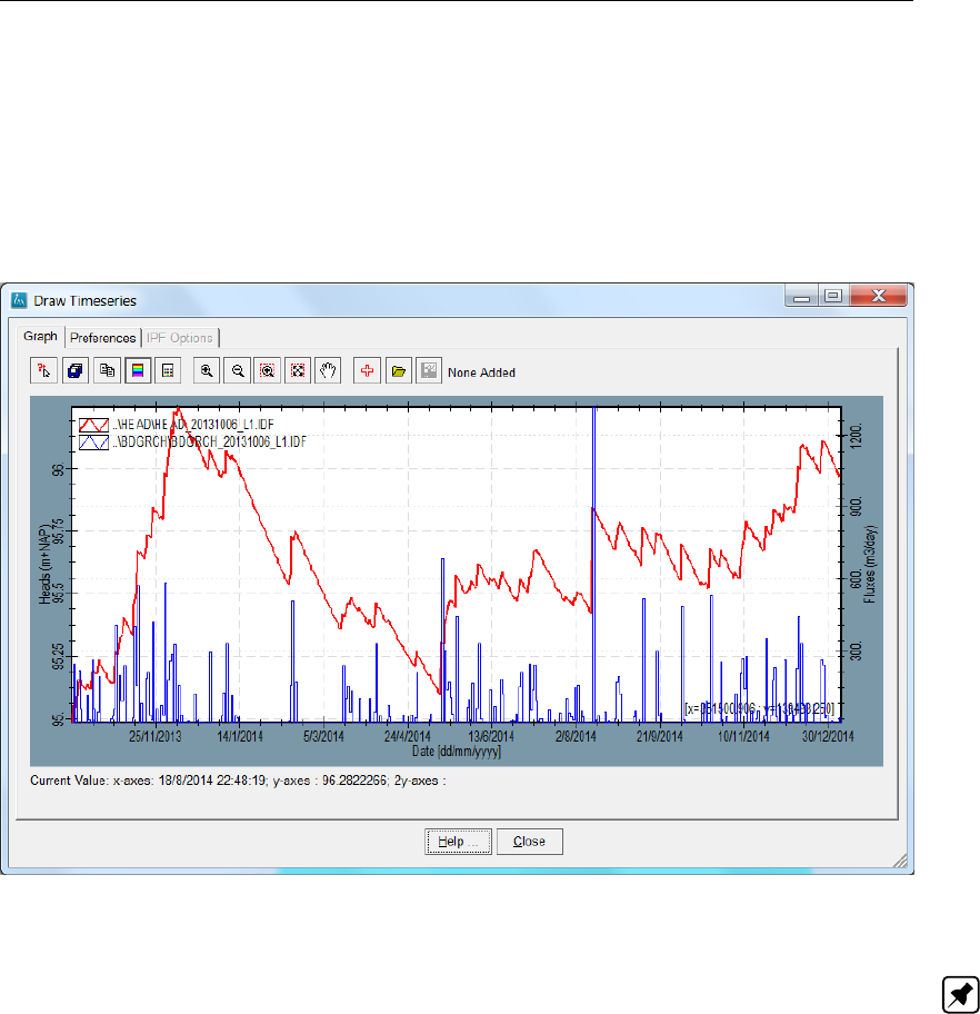
DRAFT
iMOD tutorials
57 Select the option “1” from the Layer menu.
58 Click the Open button.
59 Repeat the above mentioned steps to open the results for BDGRCH as well.
iMOD will load all selected results files into the iMOD Manager and displays the result on the graphical
canvas. Use your experience learned from the previous Tutorials to display the computed heads as
time series as shown in the following figure.
Figure 11.138: Time Series of computed groundwater levels and precipitation.
Note: Modify the settings of the time series to assign the recharge from the BDGRCH on the second
y-axes and use “BlockLines” as LineStyle.
As you may have noticed, the groundwater levels respond directly to the net-recharge. This is often,
especially by these deep groundwater levels (> 2 meter depth) unrealistic. A delay of recharge through
the unsaturated zone is a process that is taken care of by the UZF package.
Creating the UZF input
So, this tutorial is called UZF Package, but up to now we didn’t do anything with that. Well, most of the
preparation we have done and running the model with the RCH and EVT packages, gives us a nice
comparison of two different commonly used concepts. First we will delete the RCH and EVT packages.
60 Select the option (RCH) in the tree view Project Definition;
61 Click the Delete option and confirm that you really want to remove the package content;
62 Select the option (EVT) in the tree view Project Definition;
63 Click the Delete option and confirm that you really want to remove the package content;
Now we will add the input for the UZF package which is more-or-less a combination of the RCH and
EVT package input.
64 Select the option (UZF) in the tree view Project Definition;
Deltares 745 of 812
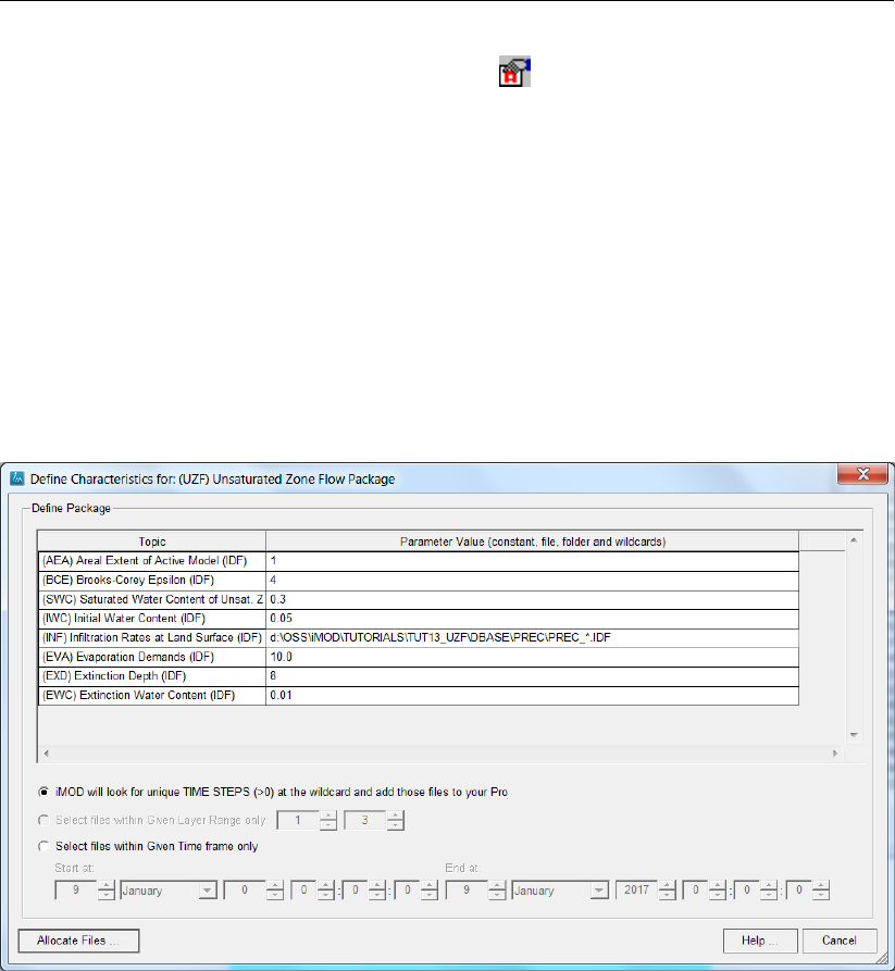
DRAFT
iMOD, User Manual
65 Click Define Characteristics Automatically button ( ) to start the Define Characteristics for
window.
66 Add the following strings to the second column in the table:
(AEA) Areal Extent of Active Model (IDF) = “1”;
(BCE) Brooks-Corey Epsilon (IDF) = “4”;
(SWC) Saturated Water Content of Unsat. Zone (IDF) = “0.3”;
(IWC) Initial Water Content (IDF) = “0.05”;
(INF) Infiltration Rates at Land Surface (IDF) = “{path of tutorialfolder} \TUT_UZF \DBASE
\PREC \PREC_*.IDF”;
(EVA) Evaporation Demands (IDF) = “10.0”;
(EXD) Extinction Depth (IDF) = “8”
(EWC) Extinction Water Content (IDF) = “0.01”;
Below is an example of your current window.
Figure 11.139: Example of the Define Characteristics Automatically window.
Let’s gather the appropriate files.
67 Select the option iMOD will look for unique TIME STEPS ...;
68 Click the Allocate Files ... button.
iMOD will combine the constant given values with the wild cards. At those location where the “inher-
ent” is mentioned, iMOD will use the previous mentioned value/file.
746 of 812 Deltares
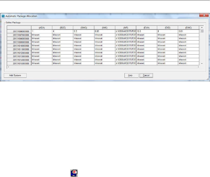
DRAFT
iMOD tutorials
Figure 11.140: Example of the Define Characteristics Automatically window.
We will leave it like it is.
69 Click the Add System button, this will add the files to our modelling project and closes the Automatic
Package Allocation window.
It can take a little bit longer to refill the Project Manager. But once it is finished, we’re ready to start the
model.
Model Simulation
70 Click the Save Model button ( ) to start the Define Simulation Configuration window;
71 Select the option “MODFLOW 2005” at the File Format: radio button.
72 Click the Simulate button and enter the following *.NAM file {path of installfolder} \IMOD_USER
\MODELS \TUT_UZF \TUT_UZF.NAM to export the model to MODFLOW2005 files and start the
simulation. Note, that you need to create the folder TUT_UZF yourself first, use the option New
Folder in your current Save window.
73 Click the Save button.
iMOD will now create the necessary MODFLOW2005 file and runs the model, it will consume probably
a little bit longer than our previous model to accomplish.
Inspect the result of simulation
Let’s inspect the hydraulic head of the first model layer, the computed groundwater recharge, the
precipitation and evaporation and generate time series.
74 Select the option Map and then the option Quick Open to start the Quick Open window, see sec-
tion 6.2. With this window it is easy to open and view results from a model simulation.
75 Select the option “TUT_UZF” from the Varient dropdown menu.
76 Select the option “HEAD” from the Topic dropdown menu.
77 Select the option “20131006” from the Time: dropdown menu.
78 Select the options “1” from the Layer menu.
79 Click the Open button.
80 Repeat the above mentioned steps up to to open the results for:
BDGGET = the amount of computed evapotranspiration (m3/d);
BDGGRC = the amount of computed groundwater recharge (m3/d);
UZFET = the amount of computed evapotranspiration in the unsaturated zone (m3/d);
UZFINF = the amount of precipitation (infiltration) in the unsaturated zone (m3/d).
iMOD will load all selected results files into the iMOD Manager and displays the result on the graphical
Deltares 747 of 812
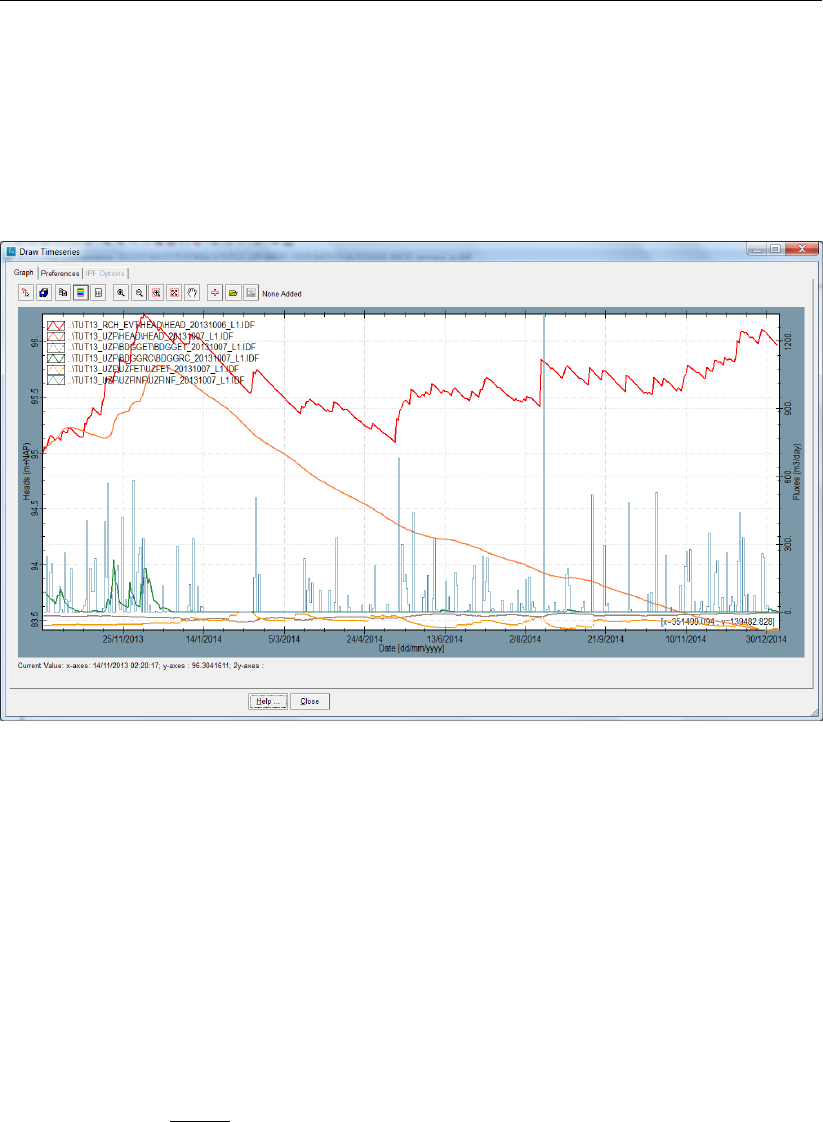
DRAFT
iMOD, User Manual
canvas.
81 Select the files HEAD_20131006_L1.IDF for both the model TUT_RCH_EVT and TUT_UZF from
the iMOD Manager window;
82 Add to the current selection of files the files BDGGET, BDGGRC, UZFINF and UZFET;
83 Use your experience learned from the previous Tutorials to display the selected files as time series
as shown in the following figure.
Figure 11.141: Time Series of computed groundwater levels with the RCH and EVT and
the UZF package.
Modify the parameters of the UZF package
As you may have noticed, the UZF package generates some ground water recharge whenever multiply
rainfall events appear on a short notice (dark green line). Short, heavy rainfall events, may not even
feed the groundwater due to the strong evaporation or instant surface runoff. The evaporation has been
modelled with an extinction depth of 8 meter, this may be a bit unrealistic and deplete the groundwater
more than it should; let us change some parameters to see the effect of this.
First we should know what the Brooks-Corey Exponent () represents. The Brooks-Corey Exponent is
used to compute the unsaturated hydraulic conductivity K(θ)as a function of the moisture content θ.
K(θ) = Ksθ−θr
θs−θr
,(11.6)
whereby Ksis the saturated hydraulic conductivity; θris the residual water content; θsis the saturated
water content; and is the Brooks-Corey exponent. This function describes how the hydraulic con-
ductivity approaches the saturated conductivity as the water content θincreases. This can be a linear
relation ship (= 1.0), or a non-linear whereby the hydraulic conductivity increases more slow than
the water content increases ( > 1.0) or faster than the water content increases ( < 1.0). The next
figure shows the relation ship for different values of and the effect on the hydraulic conductivity K().
748 of 812 Deltares
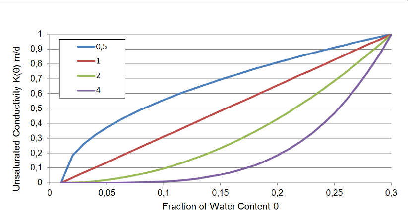
DRAFT
iMOD tutorials
Figure 11.142: Empirical relation between water content (θ) and hydraulic conductivity
K(θ)for different values for the Brooks-Corey Exponent ().
In our case, it seems that our model has too less amount of recharge. In order to increase the recharge
we need to decrease the Brooks-Corey Exponent (). The hydraulic conductivity will increase more
rapid for a slight increase of the water content, allowing precipitation seeps through the subsoil more
quicker.
The easiest way to modify the parameters for the UZF package is to re-read the input, let’s do that:
84 Repeat the steps 60 up to 66, but use the value 2.0 for the Brooks-Corey Exponent;
85 Repeat the steps 70 up to 73 to run the adjusted model, save the results in the folder {path of
installfolder}\IMOD_USER \MODELS \TUT_UZF2;
86 Repeat the steps starting from 74 to load the results into iMOD and generate time series;
Deltares 749 of 812
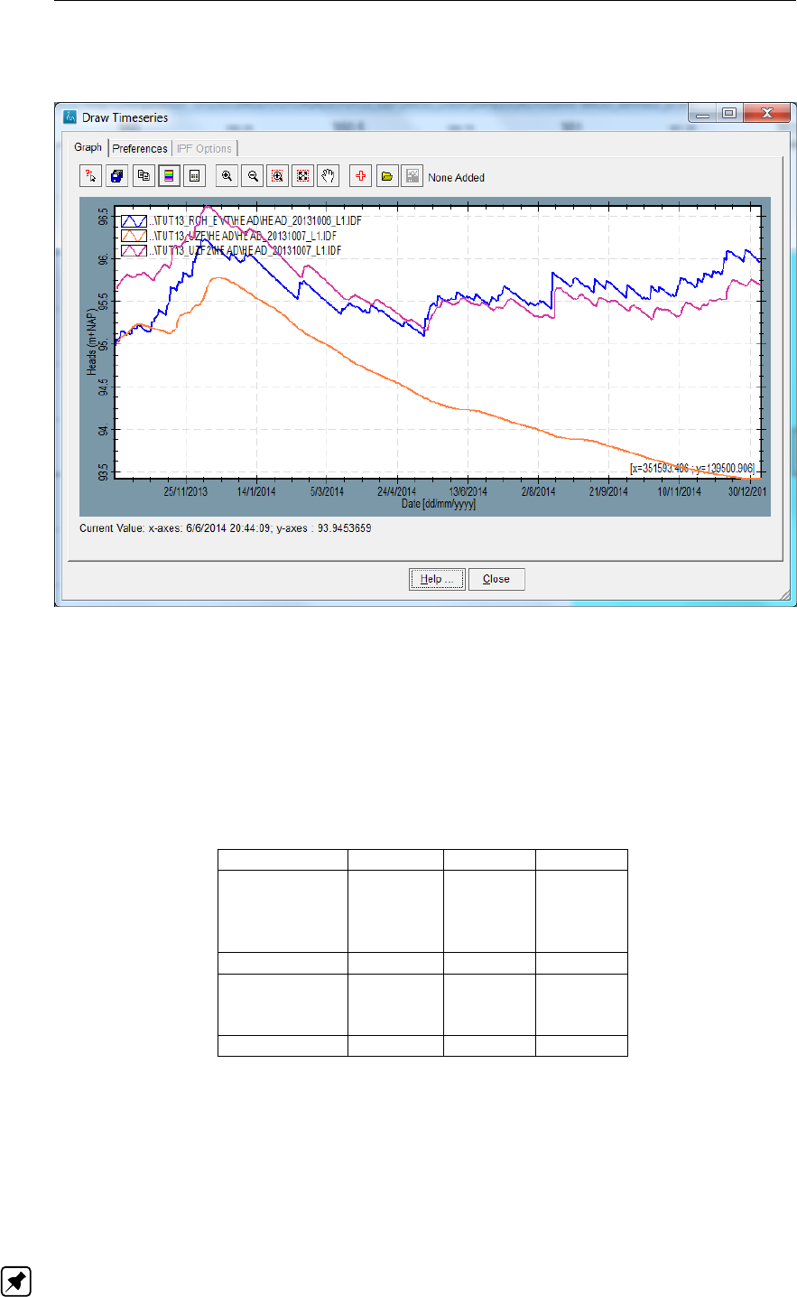
DRAFT
iMOD, User Manual
If you have successfully carried out the above mentioned steps, the time series should like the figure
below.
Figure 11.143: Time Series of computed groundwater levels for the combination RCH-
EVT and the two variants with the UZF package.
With a Brooks-Corey (=2.0) the computed hydraulic head is significantly different and almost align
(though more smooth) with the RCH-EVT combination. If you examine the water balance in the output
files (*.LST-files), the following tables can be derived to clearly show the influence of the UZF package
on the net recharge of the aquifer.
Table 11.9: Summary of water balance for the different model configurations for the un-
saturated zone (uz) and saturated zone (sz).
Parameter RCH-EVT UZF(=4) UZF(=2)
Precipitationuz - 2365470 2365470
Evaporationuz - -2053611 -285329
Seepageuz - -403764 -2311417
Net Storageuz - -86867 201259
Totaluz - -5038 -954
Rechargesz 2365470 403764 2311417
Evaporationsz 2075648 -878899 -2107888
Net Storagesz 290137 475197 203549
Totalsz -315 62 -20
The UZF package is able to reduce the net recharge significantly, the Brooks-Corey Exponent ()
is very sensitive in the amount of ground water recharge that seeps through the unsaturated zone
and influences the behaviour of the groundwater level. Feel free to experiment more with the UZF
parameters and observe how the influence the model outcomes. If you decrease the (SWC) Saturated
Water Content of Unsat. Zone (IDF), the yielding hydraulic heads will be almost similar to the RCH-
EVT combination. It is also interesting to start with a very wet subsoil (IWC) Initial Water Content (IDF),
and see how the model responds on that.
Note: It is possible to examine per cell the moisture content in more detail, especially during the
750 of 812 Deltares

DRAFT
iMOD tutorials
model building phase this could be desirable. This functionality is not steered via iMOD, but can be
easily added to the MF2005 file directly, please visit the website of the USGS for this adjustments.
Note: It is possible to examine per cell the moisture content in more detail, especially during the
model building phase this could be desirable. This functionality is not steered via iMOD, but can be
easily added to the MF2005 file directly, please visit the website of the USGS for this adjustments.
Deltares 751 of 812

DRAFT
iMOD, User Manual
752 of 812 Deltares
DRAFT
12 Theoretical background
In this chapter the iMOD-packages are described in detail. In the table below these iMOD-packages
are listed by their acronyms including their MODFLOW-equivalent (if available). Also any differences
between an iMOD-package and its MODFLOW-equivalent is described.
iMOD
Key
Req. Description section nr Equivalent
MODFLOW
package
CAP Unsaturated zone package section 12.1 n.a.
BND x Boundary conditions (compulsory) section 12.2 BAS
SHD x Starting heads (compulsory) section 12.3 BAS
KDW Transmissivity section 12.4 LPF/BCF
VCW Vertical resistances section 12.5 LPF/BCF
KHV Horizontal permeabilities section 12.6 LPF/BCF
KVA Vertical anisotropy for aquifers section 12.7 LPF/BCF
KVV Vertical permeabilities section 12.8 LPF/BCF
STO Storage coefficients section 12.9 LPF/BCF
SSC Specific storage coefficients section 12.10 LPF/BCF
TOP Top of aquifers section 12.11 DIS
BOT Bottom of aquifers section 12.12 DIS
PWT Perched-water table package section 12.13 n.a.
ANI Horizontal anisotropy package section 12.14 LPF
HFB Horizontal flow barrier package section 12.15 HFB
IBS Interbed Storage package section 12.16 IBS
SFT Streamflow thickness package section 12.17 n.a.
WEL Well package section 12.18 WEL
DRN Drainage package section 12.19 DRN
RIV River package section 12.20 RIV
EVT Evapotranspiration package section 12.21 EVT
GHB General-head-boundary package section 12.22 GHB
RCH Recharge package section 12.23 RCH
OLF Overland flow package section 12.24 n.a.
CHD Constant-head package section 12.25 CHD/BAS
FHB Flow Head Boundary package section 12.26 FHB
ISG Segment package section 12.27 RIV/DRN
SFR Surface water Flow Routing package section 12.28 SFR
LAK Lake package section 12.29 LAK
PST Parameter estimation package section 12.33 n.a.
MNW Multi-Node Well package section 12.30 MNW
UZF Unsaturated Zone package section 12.31 UZF
PKS Parallel Krylov Solver section 12.32 n.a.
12.1 CAP MetaSWAP Unsaturated zone module
The process of groundwater recharge and discharge through the unsaturated zone is simulated in
iMODFLOW with the MetaSWAP concept (see Annex 1). MetaSWAP is developed by Alterra, Wa-
geningen as part of the SIMGRO model code (Van Walsum,2017b), (Van Walsum,2017a). The SIM-
GRO framework is intended for regions with an undulating topography and unconsolidated sediments
in the (shallow) subsoil. Both shallow and deep groundwater levels can be modelled by MetaSWAP.
This model is based on a simplification of ‘straight Richards’, meaning that no special processes like
hysteresis, preferential flow and bypass flow are modelled. Snow is not modelled, and neither the influ-
ence of frost on the soil water conductivity. A perched watertable can be present in the SVAT column
model, but interflow is not modelled. There are plans for including the mentioned special processes in
MetaSWAP Inundation water can be modelled as belonging to both groundwater and surface water at
the same time. Processes that are typical for steep slopes are not included. The code contains several
parameterized water management schemes, including irrigation and water level management.
The input data required for MetaSWAP are (Van Walsum et al.,2016):
Deltares 753 of 812
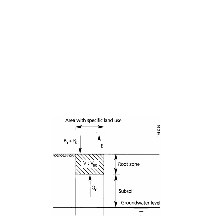
DRAFT
iMOD, User Manual
BND: Boundary setting, used to specify active MetaSWAP elements
LGN: Landuse code, should be referred to by the file luse_mswp.inp
RTZ: Rootzone thickness in cm (min. value is 10 centimeter).
SFU: Soil Fysical Unit should be referred to by fact_mswp.inp.
MET: Meteo Station number, should be referred to by mete_mswp.inp.
SEV: Surface Elevation (m+MSL).
ART: Artificial Recharge Type, 0=no occurrence, ART>0 means present at current location whereby
ART=1: from groundwater, ART=2: from surface water extraction
ARL: Artificial Recharge Location, number of modellayer from which water is extracted.
ARC: Artificial Recharge Capacity (mm/d).
WA: Wetted Area (m2) specifies the total area occupied by surface water elements. Value will be
truncated by maximum cellsize.
UA: Urban Area (m2) specifies the total area occupied by urban area. Value will be truncated by
maximum cellsize.
PD: Ponding Depth (m)
PWT: Depth of the perched water table level (m-SL)
Figure 12.1: Unsaturated zone with Pn= nett precipitation, Ps= irrigation, E = evapotran-
spiration, V = soil moisture, Veq = soil moistureat equilibrium and Qc= rising
flux.
12.2 BND Boundary conditions
The boundary conditions (-) consist of one IDF (or a constant value) for each modellayer specifying for
each cell whether
Boundary value <0
Those values denote areas that fixated head. The model will not change these values and they act
as a fix boundary condition;
Boundary value = 0
Those values denote areas that are excluded for the simulation. No groundwater flow will go
through those areas;
Boundary value >0
Those values denote areas that take part of the simulation, groundwater flow goes through them
and the head are computed. An important constraint to those locations is that need to be connected
to at least a single fixed boundary condition, e.g. a boundary condition <0or one of the other
packages that are head-dependent, such as the RIV, GHB, DRN package. The latter could be
risky since that boundary condition might be removed whenever the head is below the drainage
base.
The cell values correspond with the IBOUND values specified in the MODFLOW BAS package.
754 of 812 Deltares
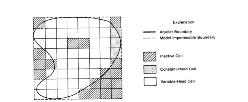
DRAFT
Theoretical background
Figure 12.2: Example of the boundary conditions for a single layer (source McDonald and
Harbaugh, 1988)
12.2.1 Scaling
For different grid resolutions the boundary is scaled internally via iMOD or iMODFLOW. For downscal-
ing (e.g. from an input of 100 x 100 meter to a finer resolution of 10 x 10 meter) all finer grid cells
obtain the identical value of the original cell. No interpolation of boundary conditions is performed.
That means that the image looks identical to the original dataset but then at a finer resolution. For up-
scaling on the other hand, a different approach is used, which can be described best by the following
rules that lists the steps to come from local values (the original values of the fine grid) to the global
value (the upscaled courser grid):
1 If the local value is equal to its NodataValue it is set to zero, it becomes inactivated;
2 If the (corrected) local value is less than 0.0 (fix boundary condition) the global value becomes
equal to the local value;
3 If the global value is equal to zero and the local value is greater than zero, the global value becomes
equal to the local value.
To summarize the above, fix boundary conditions goes before variable locations, which go before
inactive locations. As a consequence, an up-scaled model is always equal or larger in size than its
finer representation, as well as the total size of fix boundary conditions. To compare an up-scaled
model with its finer representation might yield differences in fluxes from boundary conditions as well
as differences in RCH, EVT, UZF packages.
12.3 SHD Starting Heads
The starting head (L) consists of one IDF (or a constant value) for each modellayer specifying for each
cell the initial head to start the model simulation. The starting heads correspond with the initial heads
specified in the MODFLOW BAS package.
12.3.1 Scaling
For different grid resolutions the starting head is scaled internally via iMOD or iMODFLOW. For down-
scaling (e.g. from an input of 100 x 100 meter to a finer resolution of 10 x 10 meter) all finer grid cells
obtain an interpolated value of the original cell. A four-point polynomial interpolation is used for this,
which gives a smooth interpolation based upon the direct neighbouring grid cell centres that are not
equal to the NodataValue. If none is found, the up-scaled value remains equal to the NodataValue. It
might be advisable to store starting head conditions on a coarse scale, as they will be smoothed any-
how, prior to the simulation. For up-scaling, a simple approach is applied by computing the average
value of all finer grid cells inside the coarse cell. Values that are equal to the NodataValue are excluded
and if they all appear to be equal to the NodataValue, the up-scaled value becomes NodataValue as
well. Bear in mind that iMOD does not take into account whether grid cells are partially overlapping
cells. It simply uses grid cells that are inside a coarse grid cell based upon their grid centres.
Deltares 755 of 812
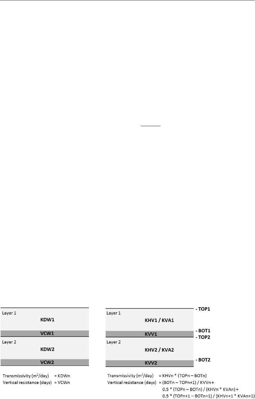
DRAFT
iMOD, User Manual
12.4 KDW Transmissivity
The transmissivity (L2/T) of each modellayer is defined by one IDF (or a constant value). Alterna-
tively the transmissivity of a modellayer may be defined by the product of the horizontal permeability
defined in the KHV package and the layer thickness derived from the TOP and BOT package (see
Figure 12.3). The KDW transmissivity corresponds with the TRAN variable specified in the MODFLOW
BCF package.
12.5 VCW Vertical resistances
The vertical resistance (T) of each modellayer is defined by one IDF (or a constant value). Alternatively
the vertical resistance of a model layer may be defined indirectly by the layer thicknesses derived
from the TOP and BOT package, the vertical permeability defined in the KVV package, the horizontal
permeability defined in the KHV package and the vertical anisotropy defined in the KVA package (see
Figure 12.3). The VCW vertical resistance corresponds with the reciprocal of the VCONT variable
specified in the MODFLOW BCF package, so V CW =1
V CON T .
12.6 KHV Horizontal permeabilities
The horizontal permeability (L/T) of each modellayer is defined by one IDF (or a constant value). The
horizontal permeability is used in combination with the layer thickness to calculate the transmissivity
of a modellayer (see Figure 12.3). The KHV horizontal permeability corresponds with the HY vari-
able specified in the MODFLOW BCF package and the HK variable specified in the MODFLOW LPF
package.
12.7 KVA Vertical anisotropy for aquifers
The vertical anisotropy (-) of each modellayer is defined by one IDF (or a constant value). The vertical
anisotropy is multiplied with the horizontal permeability to calculate the vertical permeability in the
permeable part of a modellayer (see Figure 12.3). The KVA vertical anisotropy corresponds with the
VKA variable specified in the MODFLOW LPF package.
12.8 KVV Vertical permeabilities
The vertical permeability (L/T) of the resistance layer between two modellayers is defined by one
IDF (or a constant value). The vertical permeability is used in combination with the thickness of the
resistance layer to calculate the vertical resistance between two modellayers (see Figure 12.3). The
KVV vertical permeability corresponds with the HY variable specified in the MODFLOW BCF package
and the VKCB variable specified in the MODFLOW LPF package.
Figure 12.3: Hydraulic layer parameters used in iMODFLOW
756 of 812 Deltares
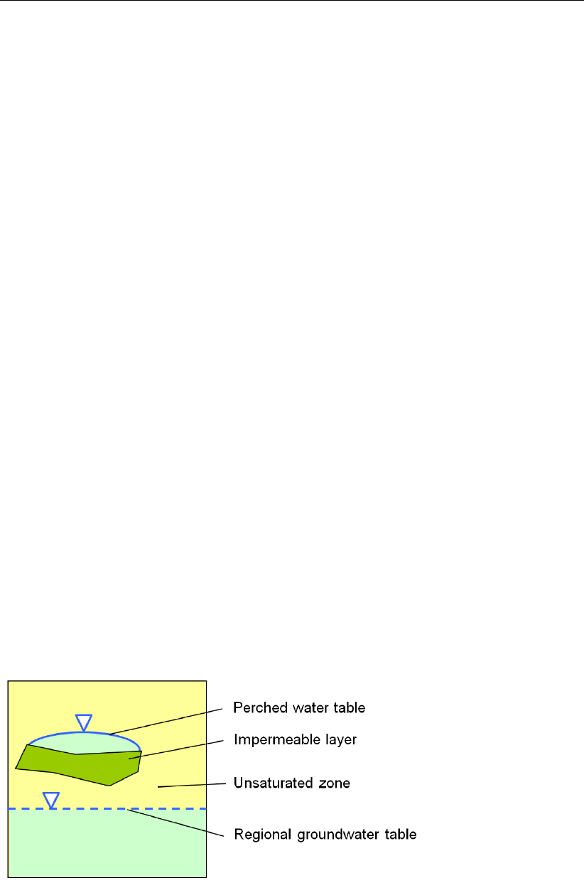
DRAFT
Theoretical background
12.9 STO Storage coefficients
The storage coefficient (for confined conditions) or specific yield (for unconfined conditions) of each
modellayer is defined by one IDF (or a constant value). The value depends on the lithology of the
modellayer. The storage coefficient in confined aquifers varies between 1x10⁻⁵to 1x10⁻³. The
specific yield ranges between 0.02 for clay to 0.25 for gravel. The STO storage coefficient corresponds
with the SF1 variable specified in the MODFLOW BCF package and the SS and SY variable specified
in the MODFLOW LPF package.
12.10 SSC Specific storage coefficients
The storage coefficient for modellayers which can change from confined to unconfined conditions is
defined by two IDFs (or constant values) for each modellayer. The SSC storage coefficient corresponds
with the SF2 variable specified in the MODFLOW BCF package and the SS and SY variable specified
in the MODFLOW LPF package.
porosity is sum of void spaces as specific yield is drainable volume (always les then porosity as some
pores are undrainable due to capillary suction forces)
12.11 TOP Top of aquifers
The top level of the permeable part of each modellayer (see Figure 12.3) is defined by one IDF (or a
constant value). The TOP level corresponds with the TOP variable specified in the MODFLOW DIS
package.
12.12 BOT Bottom of aquifers
The bottom level of the permeable part of each modellayer (see Figure 12.3) is defined by one IDF (or
a constant value). The BOT level corresponds with the BOTM variable specified in the MODFLOW DIS
package.
12.13 PWT Perched water table package
A perched water table (or perched aquifer) is a (temporary) water table that occurs above the regional
groundwater table in the unsaturated zone. This occurs when there is a (relatively) impermeable layer
above the regional groundwater table in the unsaturated zone. With the PWT-package a perched water
table can be schematized in iMOD, the perched water table concept is given in Figure 12.4.
Figure 12.4: Conceptual schematization of a perched water table.
In the following pages the concept of the perched water table package is described and illustrated by
several hydrologic situations. Hereby, the following figure (Figure 12.5) is used which that represents
the perched water table in terms of model parameters. Important to understand is that there can be
only a single perched water table in each vertical column. Once a perched water table exists, both the
Deltares 757 of 812
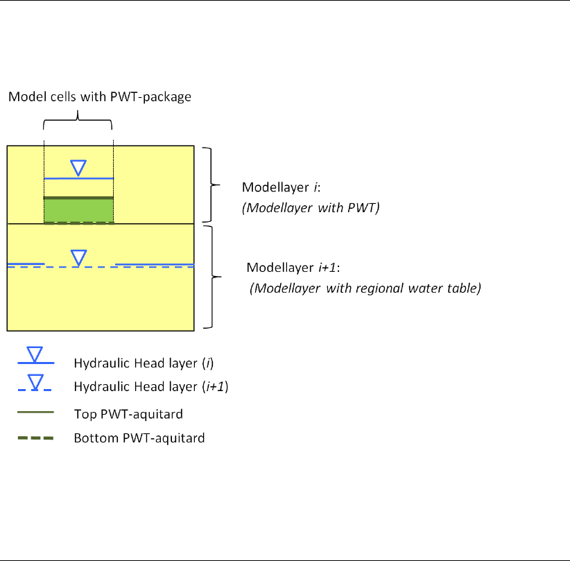
DRAFT
iMOD, User Manual
horizontal and vertical flow component will be reduced up to zero when the pressure head above the
perched water table drops below the top of the aquitard that creates the perched water table.
Figure 12.5: Conceptual schematization of a perched water table in a groundwater model.
The PWT package is applied using the following assumptions, these are described in the following
table in more detail.
758 of 812 Deltares
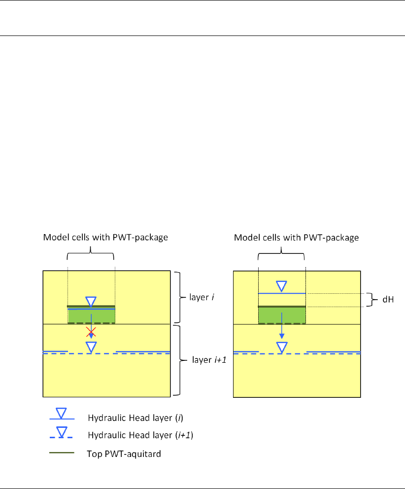
DRAFT
Theoretical background
I. There is no storage in the PWT aquitard and the driving force for vertical flow equals
the pressure head of layer x minus the top of the PWT-aquitard.
There are two situations to distinguish
No Perched Water table
This situation is depicted on the left figure, the perched water table is below the top of
the aquitard yielding a zero flux through the aquitard
Thickness of a perched water table
This situation is show on the right figure, in this particular case the vertical flux through
the aquitard is computed as:
dH/(Hi−Hi+1)whereby
dH=Hi−T: thickness of the perched water table
T:top of the aquitard
Hi:pressure head of modellayer i
(12.1)
Schematization of vertical fluxes using the PWT-Package
Deltares 759 of 812
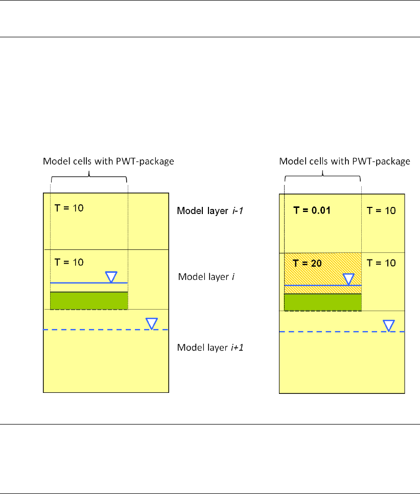
DRAFT
iMOD, User Manual
II. The model cells with the PWT-package are considered to be the top most layer with
saturated groundwater.
If the PWT cells are not within the first model layer the transmissivity above the PWT
cells is recalculated. On the figure left, the transmissivities are 10 and 10 for the first two
modellayer above the PWT. Since the PWT package will compute the transmissivity only for
the first modellayer above the PWT layer, iMODFLOW will redistribute the transmissivities
such that they all are lumped in the first modellayer above the PWT layer. This is shown in
the figure right. Now, the transmissivitiy of the first modellayer is 0.01 (actually this is equal
to the parameter MINKD in the runfile) and the first modellayer above the PWT layer has 20.
Schematization of transmissivity when the PWT-Package is used in second model layer
III. The model cells with the PWT-package are considered to be unconfined and thus
also have a phreatic storage coefficient.
In order to compute the effective transmissivity Te, the permeability is computed ini-
tially by k=T/(T OPaquifer −T OPaquitard). This permeability is used to compute the
transmissivity Teas function of the pressure head as Te(h) = k(h−T OPaquitard).
760 of 812 Deltares
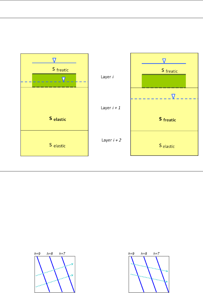
DRAFT
Theoretical background
IV. The model cells in layer i+ 1 have a phreatic storage coefficient, unless the pressure
Head of layer i+ 1 is greater than the bottom of the PWT aquitard. In this case an
elastic storage coefficient is used.
In case the underlying aquifer becomes unconfined, and therefore the
elastic storage coefficient is used, this is illustrated in the figures below.
Schematization of transmissivity when the PWT-Package is used in second model layer
The numerical implementation is such that the horizontal conductances and the vertical resistances
are calculated on the heads of timestep t−1. This is in order to avoid numeric instability.
12.14 ANI Horizontal anisotropy module
12.14.1 Introduction
Anisotropy is a phenomenon for which the permeability kis not equal along the x- and y Cartesian axis,
kxx and ky y , respectively. It can be notated that for isotropic conditions kxx =ky y (see Figure 12.6a),
and for anisotropic conditions kxx 6=ky y (see Figure 12.6b).
(a) Isotropic conditions, flow [q] perpendicular
to piezometric head [h]
(b) Anisotropic conditions, flow [q] non per-
pendicular to piezometric head [h]
Figure 12.6: Example of groundwater flow [q] for (a) isotropic and (b) anisotropic flow
conditions.
To express the amount of flow along the x- and y-axes of a Cartesian coordinate system, the following
equations are valid to compute the flow along these direction; qxand qy, respectively (Strack ODL
Deltares 761 of 812
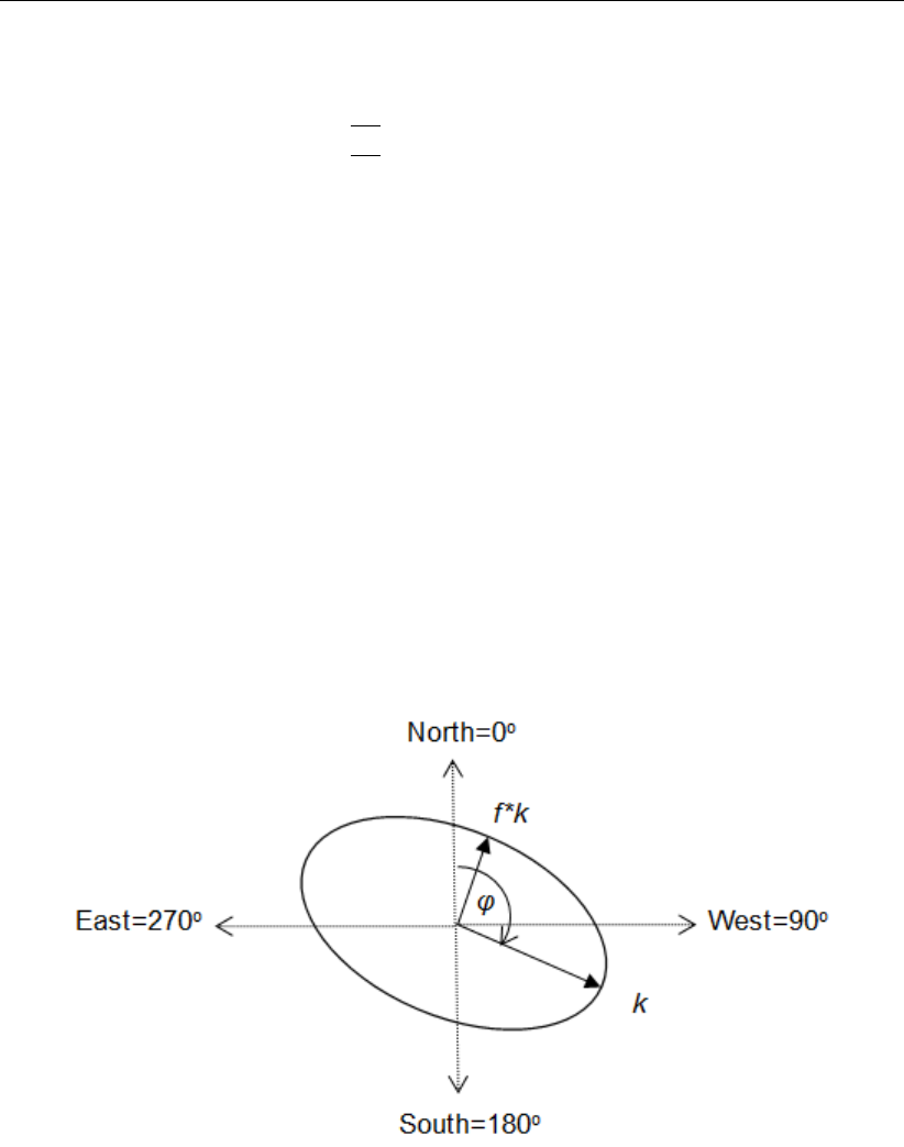
DRAFT
iMOD, User Manual
(1989), Groundwater Mechanics, Princeton Hall, Inc., Englewood Cliffs, New-Jersey):
qx
qy=−kxx −kxy
−kyx −kyy "∂hx
∂x
∂hy
∂y #(12.2)
From equation (12.2), it can be seen that in anisotropic conditions (kxx 6=ky y ), flow along the x-
direction is not influenced solely by the hydraulic gradient along this x-axis, but also by a hydraulic
gradient along the y-axis. The permeability’s kxy and kxy are equal to each other and depend on the
angle ϕof the principal axis to the x-axis:
kxx =f×T×cos(ϕ)2+T×sin(ϕ)2
kxy =kyx = ((f×T)−T)×cos(ϕ)×sin(ϕ)
kyy =f×T×sin(ϕ)2+T×cos(ϕ)2
(12.3)
For values ϕ=0.0; ϕ=90.0; ϕ=180.0; ϕ=270.0, kxy and kxy become 0.0.
12.14.2 Parameterisation
Anisotropy is expressed by an angle ϕand anisotropic factor f. The angle ϕdenotes the angle along
the main principal axis (highest permeability k) measured in degrees from north (0◦), east (90◦), south
(180◦) and west (270◦). The anisotropic factor fis perpendicular to the main principal axis. The factor
is between 0.0 (full anisotropic) and 1.0 (full isotropic), see Figure 12.7.
Figure 12.7: Anisotropy expressed by angle ϕand anisotropic factor f
Most optimally, the model discretisation should follow the configuration of the anisotropy, see Fig-
ure 12.8a. However, anisotropy could be folded in many different directions (principal directions),
which probably yield for anisotropy in many angles throughout the modeling domain. With the cho-
sen mathematical method (finite-differences) in iMODFLOW, it is impossible to fold the model network
according to the anisotropy, see Figure 12.8b.
762 of 812 Deltares
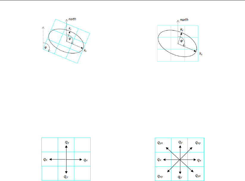
DRAFT
Theoretical background
(a) Kx< Ky;ϕ= 120.0◦(b) Kx< Ky;ϕ= 120.0◦
Figure 12.8: Example of (a) anisotropy aligned to the model network and (b) anisotropy
non-aligned to the model network.
Since the principal direction of the permeability is not aligned to the axes of the modeling network, it
is necessary to add extra flow terms to the finite difference equation to take into account the diagonal
flow, caused by the anisotropy, see Figure 12.9.
(a) Isotropic conditions (b) Anisotropic conditions
Figure 12.9: Example of (a) flow terms in isotropic flow conditions and (b) flow terms in
anisotropic flow conditions.
For more detailed explanation on the computation of these extra flow terms, see Vermeulen PTM
(2006) et al. Limitation to Upscaling of Groundwater Flow Models dominated by Surface Water Inter-
action, Water Resources Research 42, W10406, doi:10.1029/2005WR004620.
For each cell in the model network, anisotropic angles ϕand factors fcan be specified. For those
situations where a single model cell contains more than one of these anisotropic parameters, they will
be up-scaled to the model cell. For the anisotropic angle, the most frequent occurrence will be used,
as for the anisotropic factor, a mean value will be computed. This seems to be the most robust and fair
trade-off between a coarsened model network and loss in detail.
The ANI horizontal anisotropy corresponds with the TRPY variable specified in the MODFLOW BCF
package and the HANI variable specified in the MODFLOW LPF package.
Deltares 763 of 812

DRAFT
iMOD, User Manual
12.15 HFB Horizontal flow barrier module
Horizontal barriers obstructing flow such as semi- or impermeable fault zone or a sheet pile wall are
defined for each model layer by a *.GEN line file. The behaviour of this is twofold:
Factor f
This is used automatically whenever the packages TOP and BOT are omitted in the runfile. By
lines that obstruct groundwater with a particular reduction factor ffor the hydraulic conductance
or permeability, see Figure 12.9a, resulting in variable resistances along the line. The factor fis
applied to the computed harmonic conductances in between cells i(icol index) and j(irow index).
CRi,j =f2T2T1DYj
(T1DXi+T2DXi−1)
CCi,j =f2T2T1DXi
(T1DYj+T2DXj−1)
(12.4)
Resistance rThis is used automatically whenever the packages TOP and BOT are included in the
runfile. By lines that obstruct groundwater flow with a variable resistance rin days for that line, see
Figure 12.9b, resulting in variable resistances C0along that line. This combined resistance C0(as
a sum of the original resistance and the additional fault resistance) is computed internally as:
CRi,j =2T2T1DYj
(T1DXi+T2DXi−1)
DZi,j =1
2(T OPi,j −BOTi,j ) + 1
2(T OPi+1,j −BOTi+1,j )
Ci,j =1
2DXiDXi+1 CRi,j
DZi,j
C0
i,j =r+Ci,j
CRi,j =C0
i,j
2T2T1DYj
(T1DXi+T2DXi−1)
(12.5)
Whenever ris negative, the resulting resistance C0is equal to abs(r). In that way the resistance
between cells can become less than the resistance that is based on the permeability of the geo-
logical material.
Note: AFactor for Resistance rof 0.0, means that the fault is completely impermeable.
764 of 812 Deltares
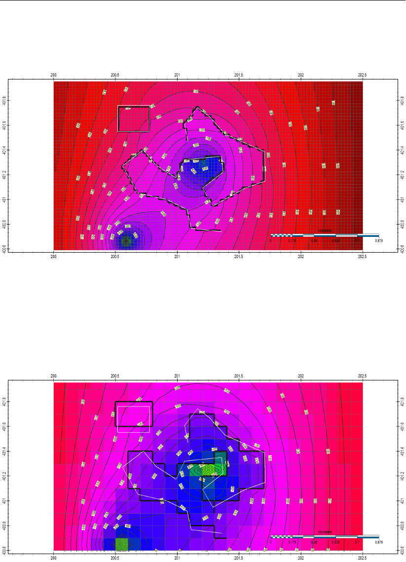
DRAFT
Theoretical background
In iMOD faults can be simulated by entering GEN files in the runfile directly. iMOD will define auto-
matically at which cell faces the permeabilities need to be adjusted based on the specifications of the
fault.
Figure 12.10: Example of a horizontal flow barrier parameterization in case of a uniform
model network consisting of model cells of 25 x 25 m. Based on the location
of an irregular shaped fault line (white line) the cell faces (thick black lines)
are identified where the conductance between the cells is adjusted using
the parameter values of the fault line. The computed hydraulic heads (thin
black contour lines) illustrate the local effects of the barriers on groundwater
flow.
Figure 12.11: The same example as above, but now for a uniform model network consist-
ing of model cells of 100 x 100 m.
The line *.GEN file defines the location of the barrier. The multiplication factor is used to create the
obstruction by reducing the conductance between model cells. The HFB module corresponds with the
MODFLOW HFB package.
Deltares 765 of 812

DRAFT
iMOD, User Manual
Whenever GEN files are assigned to layer number 0, iMOD will assign the fault to the appropriate
model layers automatically. In that case the GEN file needs to be a 3D GEN (see section 9.10). Based
on the elevation in the 3D GEN file and the TOP and BOT elevations of each model layer, the fault and
the nett resistance will be assigned according the following method:
Whenever the thickness of the model layer is <0.5meter:
Compute the nett resistance ror factor fof the fault as a weighted arithmetic mean for the
thickness of each individual fault along that particular cell.
Whenever the thickness of the model layer is >0.5meter:
Each grid cell interface will be filled in until no space is available that can be occupied by a fault
line;
Each contribution of an individual fault is harmonic (c−1);
The system number as used in the model, is equal to the fault that contributed mostly to the
nett resistance;
The final nett resistance is the harmonic mean between:
1 the summed resistance weighted to the level of occupation index (i= 0.0−1.0), and
2 a resistance of 1 day for the remaining part of the model layer (1.0−i).
Be aware that whenever the occupation index is 90 %, the resistance will be already significantly
less. An example is demonstrating what the nett resistance are for different settings.
Total Thickness Resistance Weighted Nett Confined
thickness harmonic Resistance Resistance
m m d md−1c c
2.5 100 0.025
2.5 1,000 0.0025
5.0 5.0 0.0275 181.82 181.82
2.0 100 0.02
2.0 1,000 0.002
5.0 4.0 0.022 227.27 4.89
(12.6)
12.16 IBS Interbed Storage package
The compaction of modellayers by a reduction in water pressure is calculated using four IDFs (or
constant values): preconsolidation head or preconsolidation stress in terms of head in the aquifer (L);
dimensionless elastic storage factor for interbeds present in the modellayer; dimensionless inelastic
storage factor for interbeds present in the modellayer; starting compaction in each layer with interbed
storage (m). The IBS package is comparable to the IBS package of MODFLOW.
12.17 SFT Streamflow thickness package
The streamflow thickness is defined by two IDFs (or constant values): the streamflow thickness (L) and
the permeability (L/T).
12.18 WEL Well package
The well package defines the groundwater abstractions for each modellayer from wells by IPF-files.
The IPF-files contain the coordinates of the well locations and may contain an average abstraction
rate (L3/T) or a link to a text-file with abstraction time series (L3/T). The screen depth may be added
to assign automatically the modellayer from which the abstraction takes place. The WEL package is
comparable to the WEL package of MODFLOW.
766 of 812 Deltares
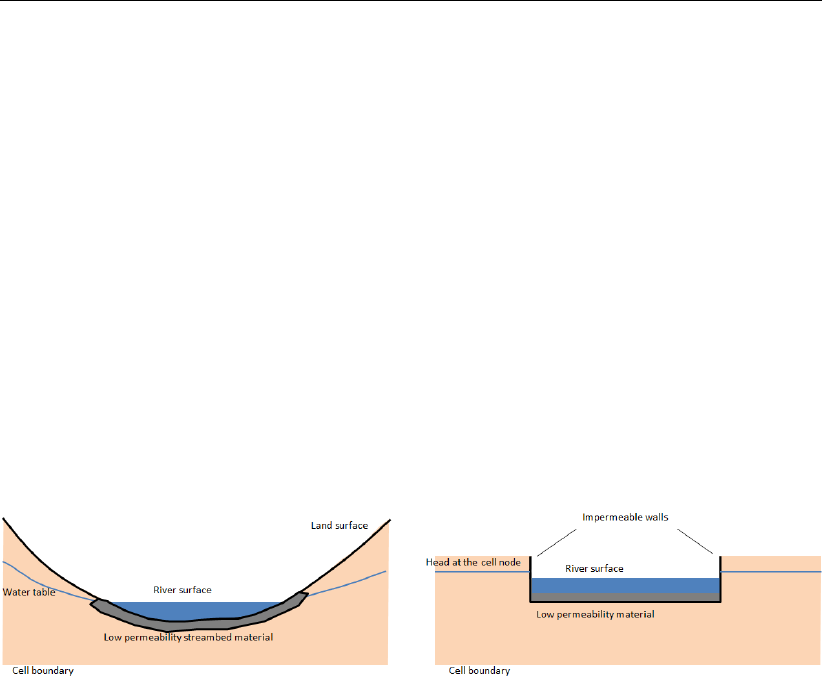
DRAFT
Theoretical background
12.19 DRN Drainage package
The drainage package defines the location, the elevation (L) and the conductance (L2/T) of the drainage
system by two IDFs. The drainage system represents drainage pipes and drainage ditches by which
water is removed from the model when the calculated head in a modellayer exceeds the elevation of
the drainage system. The drainage package is usually connected to the first modellayer only. The DRN
package is comparable to the DRN package of MODFLOW.
Drainage simulated in cells with surface water becomes inactive when the drainage elevation is below
the water level in the same cell as defined in the RIV package. Herefor it is necessary to set the
parameter ICONCHK=1 in the runfile.
12.20 RIV River package
The river package defines the location, the water level (L), the bottom level (L), the conductance (L2/T)
and the infiltration factor (-) by four IDFs. The river package represents the presence of permanent
water from which water may infiltrate or to which water may discharge. The source of water in the river
package is unlimited which means that rivers never dry out. The RIV package is comparable to the
RIV package of MODFLOW, except for the infiltration factor which is added in iMODFLOW.
Figure 12.12: Principle of the RIV package (adapted from Harbaugh, 2005)
The RIV package may be replaced by the ISG package which defines the surface water in segments.
12.21 EVT Evapotranspiration package
The evapotranspiration package defines the evapotranspiration by plant transpiration or directly from
the saturated groundwater by three IDFs: evapotranspiration rate (0.001L/T), top elevation (L) for maxi-
mal evapotranspiration rate and thickness (L) over which the evapotranspiration rate is reduced to zero.
The EVT package is comparable to the EVT package of MODFLOW. Remember that the units for the
evapotranspiration rate are mm/d for iMODFLOW.
The EVT package may be replaced by the CAP module which makes a more sophisticated simulation
of the processes in the unsaturated zone.
12.22 GHB General-head-boundary package
The general head boundary package simulates flow to or from a model cell from an external source
by two IDFs: the elevation (L) and the conductance (L2/T) of the general head boundary. The GHB
package assumes an unlimited source of water and is often used to model large water bodies which
border the area of interest.
Deltares 767 of 812
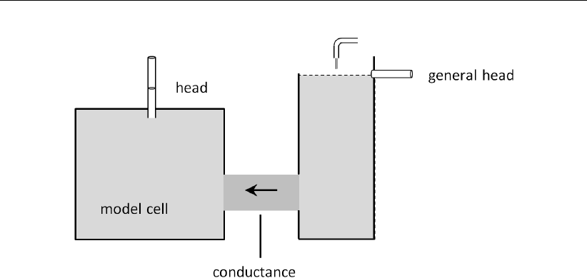
DRAFT
iMOD, User Manual
Figure 12.13: Principle of the General Head Boundary package (Harbaugh, 2005)
12.23 RCH Recharge package
The recharge package defines the quantity of water (0.001L/T) from precipitation that percolates to the
groundwater by one IDF (or a constant value). The RCH package is comparable to the RCH package
of MODFLOW. Remember that the units are mm/d for iMODFLOW.
The RCH package may be replaced by the CAP module which makes a more sophisticated simulation
of the recharge process through the unsaturated zone.
12.24 OLF Overland flow package
The overland flow package defines the elevation (L) above which outflow of groundwater will occur
when exceeded by the groundwater head. The package simulates the effect of outflow of water across
the land surface. The water is discharged out of the model and does not return to the groundwa-
ter. The OLF elevation may be determined at a few centimetres above ground elevation to represent
shallow ponding caused by small obstructions against outflow. The flow rate of the OLF package is
calculated assuming a fixed resistance against outflow of 1 day. The OLF package is not available in
MODFLOW, however, the OLF-concept can also be applied by using the conventional DRN package,
see section 12.19. The modeller might prefer to use the OLF package because 1) the assigned resis-
tance value is cell size independent and 2) in the model output the resulting volumetric budget are kept
seperate from e.g. the DRN volumetric budgets.
12.25 CHD Constant-head package
The constant head package defines the elevation (L) of groundwater heads at cells where the BND
value <0by one IDF (or a constant value). The CHD package is comparable to the definition of the
CHD in the BAS package of MODFLOW.
12.26 FHB Flow and Head Boundary package
The existing Flow and Head Boundary package of MODFLOW2005 (Leake (1997)) was implemented
in iMOD. With this package it is possible to combine constant head- and constant flux boundaries for all
model layers independently. For each model cell it is possible to define whether it becomes a constant
head or constant flux boundary condition.
768 of 812 Deltares

DRAFT
Theoretical background
12.27 ISG iMOD Segment package
The iMOD Segment package defines the surface water system with an ISG-file which contains all
relevant information used by surface water elements which are in direct relation with groundwater. The
ISG-file stores:
the actual outline of the surface water element;
(time-dependent) stages, bottom heights, infiltration factors and the resistance of the riverbed;
the cross-sections 2D and/or 3D;
(time-dependent) up- and downstream stages at weirs;
discharge/width/depth relation ships.
To store all these different types of information the ISG-file format consists of associated files that are
connected by the ISG-file. The ISG package as is, is not available in MODFLOW, but it generates the
input for the conventional RIV package. For the SFR package (see section section 12.28), this type of
an ISG file is expanded with more data, see section section 9.9 for a detailed description of both types
of ISG files.
The ISG package file format is based on vectors and time series and therefore has a much more
efficient disk use than the RIV package. iMOD and iMODFLOW both, can handle those ISG files to
generate model input. Within ISG Edit (see section section 6.10.3) it is possible to compute IDF files
from the ISG file for the different model parameters such as conductance, stage, bottom heights and
infiltration resistances. Or, more efficient, it is possible to use the ISG directly in the RUN- and/or PRJ
file and let iMOD/iMODFLOW grid the ISG file internally to a conventional/modified RIV-file, see section
section 10.11.
The way iMOD/iMODFLOW grids the vector based ISG file onto the simulation raster is as follows.
Each segment, containing at least two nodes, is treated separately from the other segments and
intersected with the model network;
All intersected model cells are given the linear interpolated values for stage s, bottom heights b,
infiltration factor fand resistances cin between all existing calculation nodes along the segment;
For each location along the stream the appropriate cross-section is assigned. If a single cross-
section is specified, that cross-section is valid for the entire stream. If more cross-sections are
specified, the application of each cross-section is the stretch along the stream between the location
of that cross-section up to the next specified cross-section - along the direction of the FROM- and
TO-node. As a exception, the first specified cross-section is applied as well for the stretch between
the FROM-node up to the first specified cross-section;
The conductance is a function of the interpolated stage sand bottom height b. The water depth
d(difference between the stage and bottom height; d=s−b) is used to compute the wetted
perimeter wp at each location along the segment with the appropriate cross-section. The con-
ductance (m2/d) is the product of the wetted perimeter wp times the length of the intersection in
the particular model cell l, divided by the resistance, so cond =wp×l
c. The infiltration factor f
is used as a package entry and corrects the conductance iteratively whenever the stage is higher
than the computed groundwater level h, in that case the conductance becomes cond =wp×l
f×c. The
conductance has a lower values for short intersections than for longer ones, this is clearly seen in
the following figure.
Deltares 769 of 812
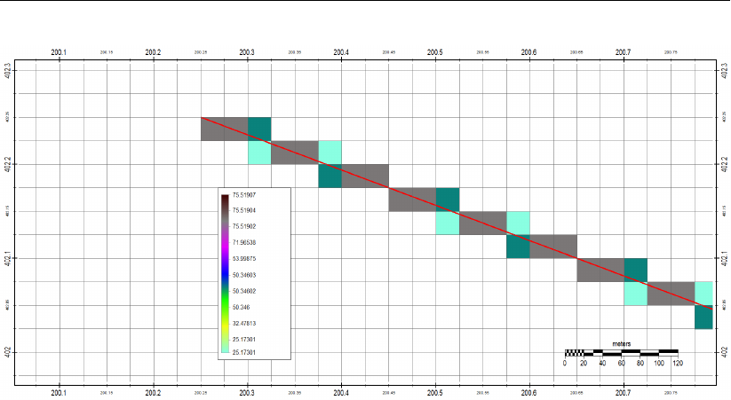
DRAFT
iMOD, User Manual
Figure 12.14: Example of the conductance (m2/d) of a segment (red line) in an ISG file
gridded on a model network.
The cross-sections in a ISG can yield different appearances of the conductance and therefore the
outline of the segment in the model network. The following configurations might occur:
The cross-section is a 2D cross-section perpendicular to the stream and describes the bathymetry
as a function of distance xand height z. The distance xis at all times less than the width of current
location in the model network;
The cross-section is a 2D cross-section perpendicular to the stream and describes the bathymetry
as a function of distance xand height z. The distance xcan be more than 1.5 times the width of
current location in the model network. In this particular case, the influence of the segment will be
distributed over more than the single intersected model cell. A ”brush“ (circle with a radius equal
to the half the width at the current location along the segment) is used to compute the fraction in
which each model cell is influenced by the segment. The fraction is computed as the number of
points in a grid cell that occupied by a circle, a grid cell which is completely covered by a circle is
given a fraction of 1.0, other location with less covering receive a fraction <1.0, see the following
figure.
770 of 812 Deltares
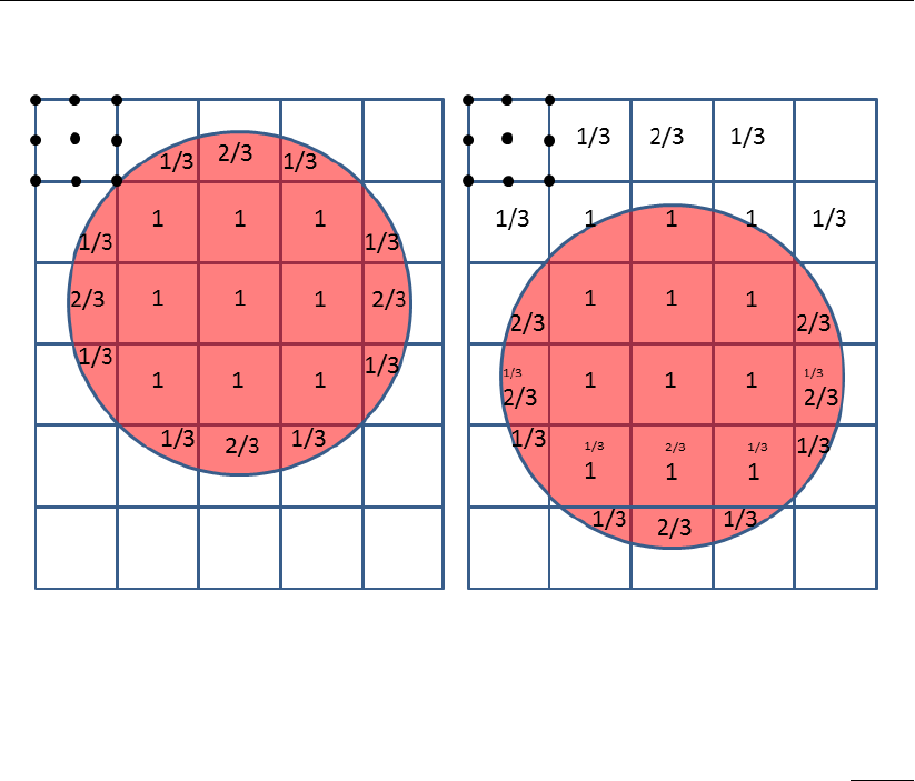
DRAFT
Theoretical background
Figure 12.15: Example of the brush method; (left) showing the fractions for the first loca-
tion of the brush; (right) showing the updated and new fractions when the
brush is moved one row down.
The cross-section is a 3D cross-section which describes the bathymetry on a local and regular
x, y, z raster. The local regular raster is projected in the (ir)regular model network. The conduc-
tance is the sum of the overlying areas of the local regular bathymetry raster divided by the entered
resistance. Whenever an indicator iis present in the ISG file - to denote inundation which depend
on a reference height href - the final resistance is multiplied with the value of the indicator i. This
is only done whenever the stage sis higher than the river bathymetry bat that particular location.
Each of the above mentioned configuration yield a different assignment of conductances to the under-
lying model network, as shown in the following figure.
Deltares 771 of 812
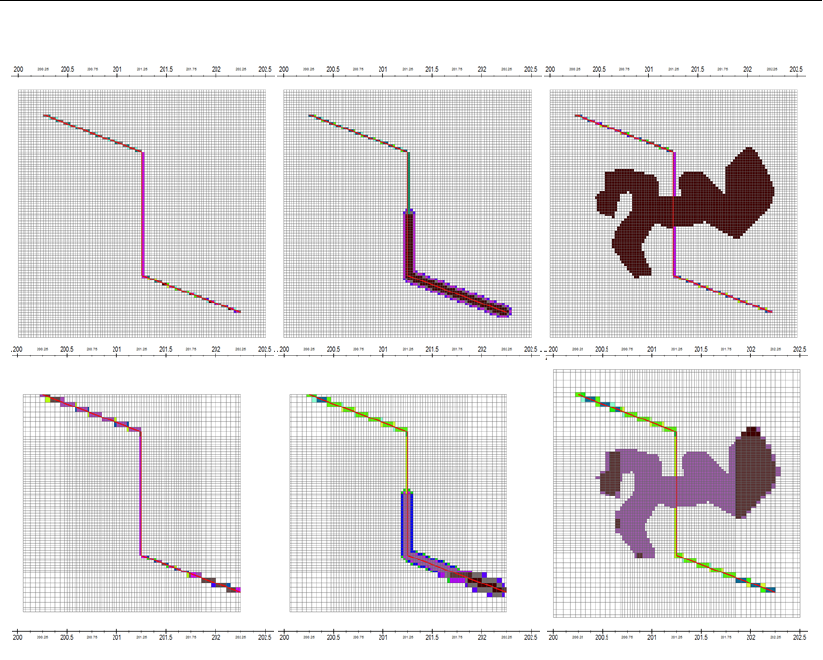
DRAFT
iMOD, User Manual
Figure 12.16: Example of different conductances for a segment in an ISG file gridded on
different model network with and without local sub grid refinements and for
different type of cross-sections.
The ISG file format also makes it more easy to convert a surface water model data from SOBEK into
iMOD using the SOBEK import tool.
12.28 SFR Surface water Flow Routing Package
The existing Surface Flow Routing package of MODFLOW2005 (Prudic et al. (2004)) has been imple-
mented in iMOD. With this package it is possible to route surface water through a network of segments.
These segments are stored in an additional type of ISG file that contains more records than the con-
ventional ISG. These additional records are specific for the SFR package and describe the connection
and diversion between individual segments and how the water depth in the segments needs to be
computed. The water depth is a function of precipitation, evaporation, external discharges and the
computed hydraulic head. The cross-section of each segment can be specified by a rectangle, an
eight-point cross-section and/or a relationship between discharge, width and depth. The SFR can dis-
charge surface water in and from a lake as described by the LAK Package. The SFR is therefore a
significant improvement in the interaction between surface- and groundwater.
There are a few limitations to the SFR package due to the iMOD implementation:
the input units for discharge are m3/s;
it is not allowed to define the water depth by an empirical equation;
a connection to a lake (up- and/or downstream) needs to be specified by the negative lake identifi-
cation, it is not necessary that the stream segment truly enters the lake, in fact any connection can
be made to any lake, even if the lake isn’t in the neighbourhood of the segment;
by default the output of each segment is written in an output file that is converted to an ISG file
after the simulation is finished. For large networks, this file may become very large. The interaction
between the SFR and the groundwater is saved in the BDGSFR file and is a per cell lumped
quantity;
inspect the *.LST-file for more detailed information on total water balances per lake and in- and/or
772 of 812 Deltares
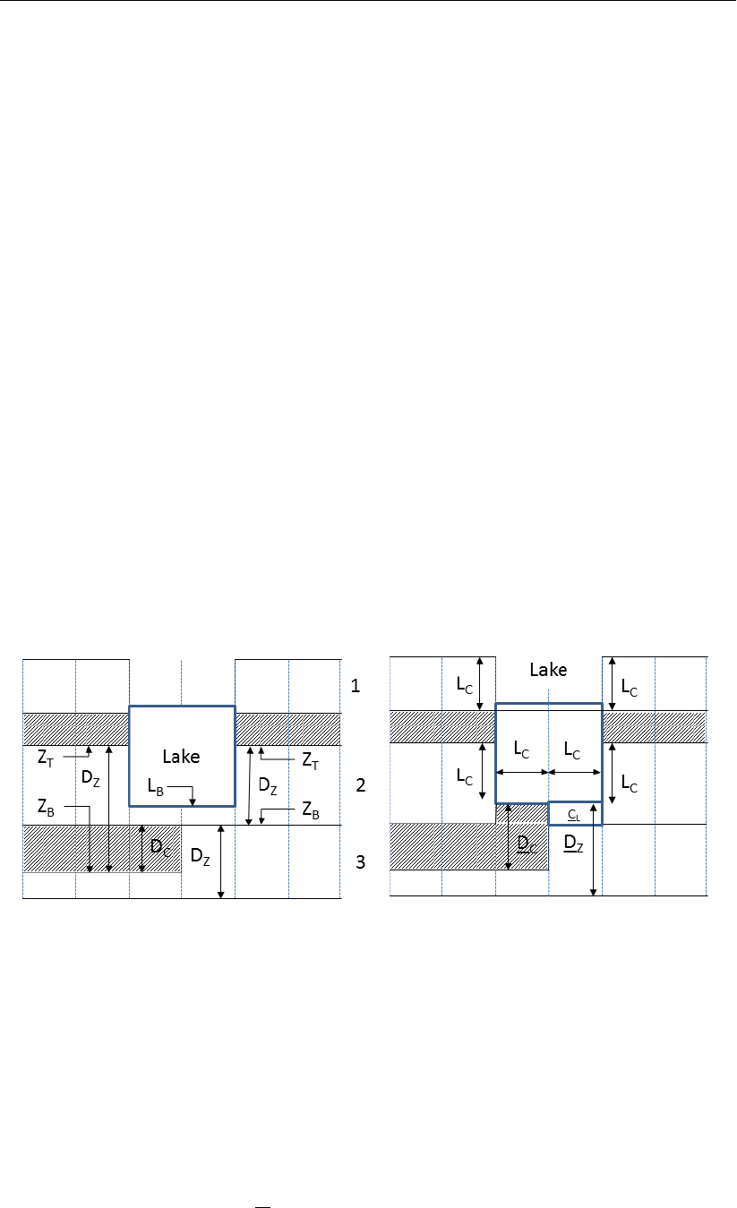
DRAFT
Theoretical background
outflow to streams that are connected;
the SFR may be subject to convergence problems; an increase of the riverbed resistance may
avoid these problems.
the value used to set the tolerance level of stream depth used in computing leakage between each
stream reach and active model cell is set to 0.0001;
no solute transport is supported;
a unsaturated zone underneath the segments is not supported.
12.29 LAK Lake Package
The existing Lake package of MODFLOW2005 (Merritt and Konikow (2000)) has been implemented
in iMOD. With this package it is possible to compute lake stages in relation to the groundwater head.
Given a bathymetry of the lake, iMOD will assign the lake to the appropriate model layers and assign
the correct conductances to the lake. The SFR can be connected to locations where a lake is defined
to route water in- and from a lake.
The implementation of the LAK package in iMOD is straightforward as several IDF files (and or con-
stant values) need to be specified. iMOD computes the Lake Identifications and Lake conductances
underneath and along the sides of the Lakes. In that same process, iMOD can adjust some of the
geohydrologic parameters, such as top- and bottom elevation of model layers as well as permeability
values. It is assumed that the position and spatial extent of the lake volume is defined by the specifi-
cation of a volume of inactive cells within a three dimensional model grid. Because the model grid is
used to define the lake volume, the lateral and vertical grid dimensions must be appropriately chosen
so that the spatial extent and bathymetry of the lake are defined with the necessary accuracy. In some
cases this may require a finer horizontal discretization in the vicinity of the lake and a finer vertical
discretization than would be necessary to simulate heads in the aquifer. iMOD will modify the vertical
discretization internally, this is explained the following figure.
Figure 12.17: Scheme of the implementation of the LAK package in iMOD.
Suppose a Lake is considered that intersects two model layers, the user enters the bathymetry of the
lake (LB). Whenever the lake bathymetry is lower than the top of a model layer (ZT) and higher than
the bottom of that model layer (ZB) the bottom of the lake is supposed to be in that particular model
layer. The bottom of a model layer contains an existing interbed with thickness DCas well. For the
Lake package it is essential that the elevation of the model layers describe the bathymetry of the Lake
as these are used to compute the table with depth, area, and volume relations. iMOD will adjust the
bottom of a model layer to reflect the bathymetry and corrects for the removed aquifer and/or increased
thickness of the interbed. In case there is an interbed underneath the Lake, iMOD will increase the
permeability of that interbed such that the vertical resistance of that interbed remains identical though
its thickness has been increased (DC> DC). In case the lake bathymetry intersects the interbed
itself, nothing is changed.
In case there is no interbed, the permeability that existed underneath the Lake bathymetry and in
Deltares 773 of 812

DRAFT
iMOD, User Manual
the same model layer, will be added to the layer below such that the transmissivity for (DZ)remains
identical to the sum of the original two model layers. The permeability of the model layer underneath will
be increased or decreased which depends on the permeability fraction between the two model layers.
Furthermore, the vertical resistance of the removed aquifer (CL), is added to the Lake resistance.
The side conductances (LC) are the sum of resistances of a) the lake itself and b) the resistance
through the subsoil.
There are some build-in limitations and assumptions:
The RCH and EVT packages need to be assigned to model layer 0, which means they will be
assigned to the upper active model layer. This is necessary in case a lake or part of lake dries up
and blocks any recharge to the underlying aquifer;
iMOD does not support the usage of sub lakes;
the numbering of the lakes needs to be unique but it is not necessary to number them continuously.
The lake number can have the format of a real number (e.g. 1.2 or 1.43) instead of an integer.
Usage of integers is preferred as any connection to the SFR needs to be specified in the SFR
package by an integer. iMOD will reassign a unique lake number internally, but the original lake
number will be displayed in the LAK-package (*.lak);
theta is the time weighting factor for computing lake stages during transient time steps. A theta of
0.5 represents the average lake stage during a time step. In iMOD the lake package is configured
with a theta of -1.0 that represents the lake stage at the end of the time step; Moreover, a negative
THETA applies for a SURFDEPTH that decreases the lakebed conductance for vertical flow across
a horizontal lakebed caused both by a groundwater head that is between the lakebed and the
lakebed plus SURFDEPTH and a lake stage that is also between the lakebed and the lakebed
plus SURFDEPTH. This method provides a smooth transition from a condition of no groundwater
discharge to a lake, when groundwater head is below the lakebed, to a condition of increasing
groundwater discharge to a lake as groundwater head becomes greater than the elevation of the
dry lakebed. The method also allows for the transition of seepage from a lake to groundwater when
the lake stage decreases to the lakebed elevation. Values of SURFDEPTH ranging from 0.01 to
0.5 have been used successfully in test simulations. SURFDEP is configured by default to a value
of 0.25.
the interaction between the lake and groundwater is saved in the BDGLAK and is a per cell lumped
volume.
inspect the *.LST-file for more detailed information on total water balances per lake and in- and/or
outflow to streams that are connected;
the LAK package is very sensitive to non-convergence, a quasi steady-state approach and/or a
transient implementation with small time steps is recommended.
no solute transport is supported.
12.30 MNW MultiNode Well Package
The existing Multi Node Well package of MODFLOW2005 (Halford and Hanson (2002), Konikow et al.
(2009)) was implemented in iMOD. The Multi-Node Well package is used to simulate “long” wells that
are connected to more than one model layer; the abstraction rate is vertically distributed proportional
to the transmissivity adjacent to the well screen; e.g. when a hydraulic head gradually drops below the
top of a well screen the yield of this shallow part of the well will also gradually drop.
MODFLOW computes the head at a block-centered node of a finite-difference grid on the basis of a
fluid mass balance for fluxes into and out of the volume of the cell of interest, including flow in or out of a
well located within the surface area (and volume) of that cell. However, because of differences between
the volume of a cell and the volume of a well-bore, as well as differences between the average hydraulic
properties of a cell and those immediately adjacent to a well, it is not expected that the computed head
for the node of a finite-difference cell will accurately reproduce or predict the actual head or water level
in a well at that location. Furthermore, if the length of the open interval or screen of a vertical well
is greater than the thickness of the cell, then the head in the well would be related to the head in the
ground-water system at multiple levels (and at multiple locations for a non-vertical well). Thus, if the
user needs to estimate the head or water level in a well, rather than just the head at the nearest node,
then additional calculations are needed to correct for the several factors contributing to the difference
between the two.
774 of 812 Deltares

DRAFT
Theoretical background
As denoted by the name of the package, the advantage of the MNW package benefits mostly whenever
wells are considered that discharge from a multi-aquifer system. Since the MNW package can deal
with intra borehole flow and computes a realistic head loss at the well, this makes the package mostly
applicable for multi-layered unconfined systems. In the case that the well falls dry, this is more realistic
simulated with the MNW package, more-over, the total strength of a multi-layered extraction system
remains intact as-much-as possible during a simulation. This example also demonstrates that the well
discharge is not simply proportional to the transmissivities of the multiple aquifers screened by the well.
For single penetrating, confined system the MNW is similar to the WEL package.
MNW computes a hydraulic head in the cell hnsuch that it equals the computed hydraulic head at the
well minus a head loss term (e.g. the Thiem equation, we neglect in this tutorial head loss due to skin
and local turbulence effects) for that particular cell, so:
hWELL −hn=Qn
2πT ln r0
rw
CWCn=ln r0
rw
2πT
Qn= (hWELL −hn) CWCn
hWELL =CWCnhn+Qn
CWCn
(12.7)
where CWCnis the cell-to-well conductance m2/d; Qnis the well rate (m3/d), Tis transmissivity of
the aquifer (m2/d) at the well, r0is the effective radius of a finite-difference cell (m), this is assumed
for isotropic conditions as r0= 0.14p∆x2+ ∆y2;rwis the actual radius of the well. Because r0
is typically much greater than rw, the head in a pumping well will be lower than the model-computed
head.
The problem is solved by MODFLOW via estimations of hWELL and Qnthat lag an iteration behind
estimated of hnbecause the above mentioned equation are solved explicitly. This causes slow con-
vergence of the solver if the MNW cells are incorporated in MODFLOW as a general-head boundary
(subtract CWCnfrom HCOF and subtract CWCn×hWELL from RHS). Convergence is accelerated
by alternately incorporating the MNW cells as specified rates in odd iterations (subtract Qnfrom RHS)
and as general-head boundaries in even iterations.
Note: Multi-node wells with cell-to-well conductances that are “too great” tend to make MODFLOW nu-
merically unstable. Cell-to-well conductances increase as cell size is decreased, which also decreases
the effective external radius (r0). Cell-to-well conductances become greater as r0approaches rw and
are undefined if r0is less than or equal to rw. For these small cells, a pumped well should be simulated
as a high-conductivity zone as cell area approaches the cross-sectional area of a well.
12.31 UZF Unsaturated Zone Package
The existing Unsaturated Zone Flow package of MODFLOW2005 (Niswonger et al. (2006)) has been
implemented in iMOD. Percolation of precipitation through unsaturated zones is important for recharge
of ground water. Rain and snow melt at land surface are partitioned into different pathways including
runoff, infiltration, evapotranspiration, unsaturated-zone storage, and recharge. The package was de-
veloped to simulate water flow and storage in the unsaturated zone and to partition flow into evapotran-
spiration and recharge. A kinematic wave approximation to Richards’ equation is solved by the method
of characteristics to simulate vertical unsaturated flow. The approach assumes that unsaturated flow
occurs in response to gravity potential gradients only and ignores negative potential gradients (upward
capillary flow); the approach further assumes uniform hydraulic properties in the unsaturated zone for
each vertical column of model cells.
The iMOD implementation of the UZF package has the following limitation and/or assumptions:
the UZF can be added to the model in a spatially distributed way and therefore for user-specified
areas. The pointer value for this needs to be negative to ignore any UZF at that particular location,
the absolute value in this IDF file is the model layer for which the upper elevation will be used to
specify the surface level;
Deltares 775 of 812

DRAFT
iMOD, User Manual
the RCH- and or EVT packages can be used with the UZF package simultaneously, it is a user
responsibility not to overlap these concepts with the UZF;
whenever the UZF package is active, iMOD will include the WETDRY option automatically for each
model layer;
the computed net recharge is saved in the BDGUZF file.
the package also accounts for land surface runoff to streams and lakes, however this is not sup-
ported by iMOD.
by default iMOD uses the permeability as specified for model layer 1, to be equal to the saturated
permeability used by the UZF package.
12.32 PKS Parallel Krylov Solver Package
12.32.1 Introduction
The Parallel Krylov Solver (PKS) for speeding-up computations is a new package that is being de-
veloped in cooperation with the USGS, Utrecht University, Alterra and Delft University of Technology
(Verkaik et al. (2016)). PKS is basically a linear solver that is largely based on the PCGU-solver in
MODFLOW-USG for unstructured grids (Panday et al. (2003)) and is used in iMODFLOW for structured
grids. PKS is suitable for coarse-grained problems, where the computational time for each subdomain
is much larger than the actual communication overhead.
12.32.2 Mathematical model
Subject for PKS is solving the linear system of equations, resulting from the finite-volume discretization
of the groundwater flow equation (Harbaugh (2005)), to be denoted by:
Ah=b,(12.8)
where Ais a square, symmetric, positive-definite coefficient matrix [L2/T] that includes cell-by-cell
conductances, calculated using cell dimensions and hydraulic conductivities at cell interfaces, and
unknown components of sink/source and storage terms; his the vector of unknown heads at time t;
and bis a known vector of source/sink and storage terms.
It can be shown mathematically that convergence of iterative methods is strongly related to the spectral
properties (eigenvalues) of the coefficient matrix. Instead of solving the system (12.8), it is more
efficient to solve the (left-)preconditioned equivalent
M−1Ah=M−1b,(12.9)
where Mis called the preconditioner. Choosing Mis usually done such that Mis a good approxi-
mation of A, the eigenvalues of M−1Aare clustered around 1, and the system involving Mis much
easier to solve than the original system.
The PKS solver is a so-called Schwarz domain decomposition solver (Dolean et al. (2015)) and uses
a parallel Additive Schwarz (AS) preconditioner1:
M−1
jac =X
i
A−1
i,(12.10)
where Aicorresponds to the (local) interior coefficients of the (global) coefficient matrix Afor sub-
domain i. Basically, this corresponds to the block-Jacobi (block-diagonal) preconditioner, after num-
bering the unknowns over the sub-domains.
PKS solves the preconditioned sytem (12.9) with the AS-preconditioner (12.10) using the Conjugate
Gradient (CG) Krylov subspace method, resulting in the so-called CG-Schwarz method. Within CG,
application of M−1
jac can be fully done in parallel. The corresponding sub-domain solutions are obtained
inaccurately by ILU(0) (zero fill-in incomplete LU-factorization) preconditioning of Aionly. PKS only
supports Dirichlet interface transmission conditions and does not (yet) support coarse-space correction
like deflation.
1To be more precise, an overlapping Restricted Additive Schwarz preconditioner is implemented, but for iMOD,
only a fixed overlap of 1 is being used, corresponding to the non-overlapping case.
776 of 812 Deltares
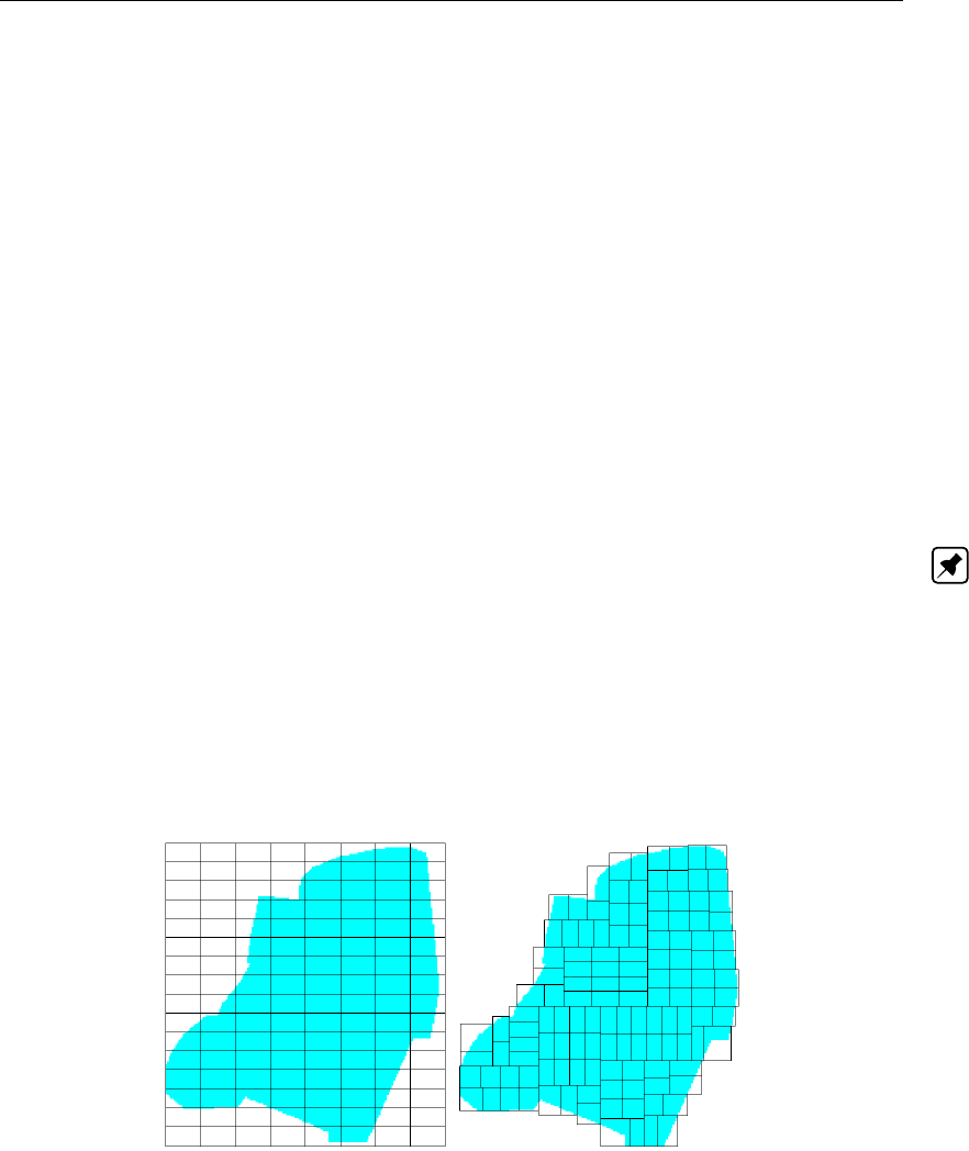
DRAFT
Theoretical background
12.32.3 Implementation and some practical considerations
Inter-subdomain communication
PKS follows a so-called distributed memory parallellization approach, where each subdomain is uniquely
assigned to one computational core (process), using local memory (RAM) only. In this way PKS is
scalable regarding problem size and hardware. Exchanging data between subdomains is done by the
Message Passing Interface, and typically involves communication for each CG inner (Schwarz) itera-
tion, ensuring a tight coupling: local (point-to-point) communication for the vector update and global
(all-reduce) communications for computing interior products and evaluating stopping criteria. Since this
is done for each inner iteration the expected speed-up in computational time with PKS largely depends
on MPI (latency and bandwidth).
Typically, PKS is suitable through MPI on fast networks, like Infiniband/Myrinet on Linux clusters, or
MPI through memory such as multi-core CPUs on desktop/laptop machines or shared-memory ma-
chines like SGI-clusters. For the current generation of multi-core CPUs, e.g. Intel Haswell E5-2698v3
16-core CPU, one should keep in mind that for large, memory-driven, groundwater models the actual
bandwidth between processor and memory limits the parallel performance. In practice, this means it
may be sometimes more beneficial to use less than the maximum number of cores.
Note: On desktops/laptops with multi-core CPUs it may be beneficial not to use all cores.
Load balance
Besides MPI communication, load balance is also very important for parallel performance. This means
that the actual work/load should be distributed as equally as possible over the multiple computational
cores. PKS now supports two methods: uniform in x,y-direction, and the Recursive Coordinate Bi-
section (RCB) method. The RCB method, recursively, weight the user-defined load, by alternating in
horizontal and vertical direction. Figure 12.18 shows an example of both methods for the Netherlands
Hydrological Model (De Lange et al. (2014)) and 128 subdomains.
Figure 12.18: Two partitioning methods for the Netherlands Hydrological Model based on
weights as specified by the boundary grid. Left: uniform partitioning; right:
recursive coordinate bisection partitioning.
For this example the uniform partitioning method (left) results in some subdomains containing zero
cells, since in this case the model boundary (IBOUND) is irregular, while the RCB method (right)
results in a more optimal partitioning. Although RCB results in optimal load, it does not result in an
optimal communication scheme regarding MPI. One should notice that even with the RCB and irregular
boundaries, finding the optimal weight can be hard and subject for trial-and-error. For each MODFLOW
cell, the weight can varying due to for example boundary conditions (stresses) and coupling concepts.
Deltares 777 of 812

DRAFT
iMOD, User Manual
Input/output
Another parallel performance aspect that is important is input/output (I/O). PKS supports parallel bi-
nary (clipping) reading of model IDF input files and parallel writing of IDF output files, that can be
merged by the master MPI process afterwards. However, the actual I/O performance depends on the
given hardware (e.g. type of hard drive) and file system configuration. When too many MPI processes
simultaneously try to access one hard drive it can slow down I/O. This is typically the case for common
off-the-shelf desktops or laptops. On the other hand, super computers use parallel file-systems - e.g.
Lustre file systems - to tackle this problem by accessing multiple hard drives simultaneously.
Note: In general, it is always recommended to try to minimize model output.
12.33 PST Parameter estimation
12.33.1 Introduction
In mathematics and computing, the Levenberg-Marquardt algorithm (LMA) provides a numerical so-
lution to the problem of minimizing a function, generally nonlinear, over a space of parameters of the
function. These minimization problems arise especially in least squares curve fitting and nonlinear
programming. The LMA interpolates between the Gauss–Newton algorithm (GNA) and the method of
gradient descent. The LMA is more robust than the GNA, which means that in many cases it finds
a solution even if it starts very far off the final minimum. For well-behaved functions and reasonable
starting parameters, the LMA tends to be a bit slower than the GNA. LMA can also be viewed as
Gauss–Newton using a trust region approach. The LMA is a very popular curve-fitting algorithm used
in many software applications for solving generic curve-fitting problems. However, the LMA finds only
a local minimum, not a global minimum.
The used algorithm is known as the Levenberg-Marquardt algorithm (LMA) that goes back to 1943 as
Kenneth Levenberg presented his work to the Mathematical Society at their annual meeting (Leven-
berg, K. The Quarterly of Applied Mathematics 2, 164 (1944)). Marquardt on the other hand popular-
ized the method by distributing his FORTRAN code for free. In the following section a brief overview is
given of the Levenberg-Marquardt algorithm and its implementation in iMODFLOW.
Most of the following LMA implementation has been based on the paper of Olsthoorn (1995), Effective
Parameter Optimization for Ground-Water Model Calibration, Groundwater, Vol. 33, no.1) and the
paper of Knorr BM (2011), The Levenberg-Marquardt Algorithm, Seminar in Modern Physics, Summer
2011 and the PEST Manual of Doherty (2010).
12.33.2 Methodology
The core of parameter estimation is the minimization of some error criterion, cost or objective function
Φm(p), that depends on a parameter vector pwith elements pi→i= 1, Npwhere Npdenotes the
number of unknowns to be optimized (i.e. the amount of parameters). In general the objective function
Φm(p)is the sum of squares sum of the individual errors notated as:
Φm(p)=(y−φ(p))TQ1(y−φ(p))
where yare the measurements with elements yi→i= 1, Nh; where Nhdenotes the number of
observations; φ(p)are the computed head for the parameters defined in pand Qis the weight matrix
assigned to the observations defined as:
Qi,i =1
pσ2
i
where Qi,i is the weight for the ith observation. The variance σ2
iis the squared standard deviation
σithat measures the amount of variation from the average. A low σiindicates that an particular
observation yishould be able to the meet the corresponding computed head φimore closely that
observations with higher values of variations σ. It is possible to specify weight values Qi,i or variances
σ2
iin iPEST.
778 of 812 Deltares

DRAFT
Theoretical background
The Levenberg-Marquardt algorithm is applied to minimize the objective function value by adjusting
the individual values for the parameter vector with αipiwhere αiis the optimal multiplication factor for
the ith parameter that yields a minimal objective function value. In order to arrive at a valid minimal
objective function value, it is advisable to let Nhsubstantially larger than the number of parameters Np
(Yeh and Yoon (1981), Aquifer parameter identification with optimum dimension in parameterization,
Wat.Res.Res, v17, no. 3, pp. 664-672) or apply regularisation as done by the Pilot Point concept
(Doherty, 2003), see subsection 12.33.4.
The Gradient Descent Method (the simplest method) approaches the minimum of the objective function
Φm(p)by adjusting each parameter according to:
pi+1 =pi−ζi∇Φm(pi),
where the subscript idenotes the sequential parameter iteration (parameter update cycle) and ζiis
a weighting factor for the ith cycle. It says that for each cycle i, the individual parameter sensitivities
(∇Φm(p)) to the residual surface (i.e. the multi dimensional representation of the objective function),
multiplied with a weighting factor ζwill contribute to a reduction on the objective function. In this
way steps are taken towards the minimum according to the gradient ∇of the residual surface. The
problem is that the Gradient Descent Method takes large steps in those areas of the residual surface
that have small gradients and it takes small steps for those areas with large gradients. It normally
leads to zigzagging in long narrow valleys on the Φm(p)residual surface. The Gauss-Newton method
replaces the scaling factor ζby the inverse of the curvature (second derivative∇2Φm(p)often called
the Hessian) of the Φm(p)surface and interchanges the undesired behaviour of the Gradient Descent
Method. It therefore converges faster, so:
pi+1 =pi−∇2Φm(pi)−1∇Φm(pi).
The gradient ∇Φm(p)is denoted as the Jacobian Jand each column in that matrix Jis defined by:
J=∂φ
∂pi
=φ(pi)−φ(p0)
∆αi
,
where Jis a Jacobian matrix Nh×Np(number of observations row wise and number of parameters
column wise) and represents the sensitivity of the residual for each observation point according to a
small perturbation ∆αiin the ith parameter compared to the original parameter value p0. Since the
algorithm assumes linearity over the interval ∆αi, the second derivative ∇2Φm(p)is approximated by
JTQJ in the neighbourhood of p0. This yields the following Gauss-Newton parameter update formula:
pi+1 =pi+ ∆pi
∆pi=−2JTQJ−1JTQ(y−φ(p))
where Qis the diagonal weight matrix with individual weight values qiin the diagonal, where the
product −2JTQ(y−φ(p)) represents the steepest gradient on the residual surface. If parameters
are far from their optimum, which they are probably initially, this JTQJ is only a crude approximation
of the true Hessian matrix. As a result the parameter update vector ∆pmight be quite wrong which
can result in a failure to converge. The great insight of Levenberg was to simply combine the Gradient
Descent and the Gauss-Newton Methods to include a damping factor λwhich determines how much
of the Gradient Descent or Gauss-Newton Method to include, so:
∆p=−2JTQJ −ψI−1JTQ(y−φ(p))
where Iis the identity matrix. Whenever ψis large, the parameter update will be determined more by
the Gradient Descent Methods and whenever ψis small, the Gauss-Newton Method will be included
significantly. The great insight of Marquardt is to replace the identity matrix Iby the diagonal of the
matrix JTQJ, so:
∆p=−2JTQJ −ψdiag(JTQJ)−1JTQ(y−φ(p))
Olsthoorn (1994) suggested to adjust ψsuch that the yielding parameter update vector ∆pis within
a certain trust hyper sphere (with a radius around the current parameter vector which is determines
Deltares 779 of 812
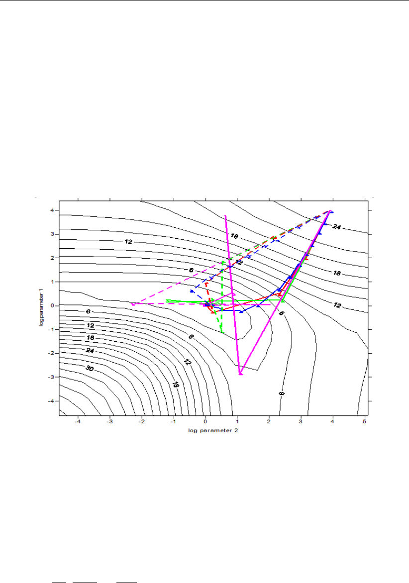
DRAFT
iMOD, User Manual
by their minimal en maximal values and a maximal ∆pcompared to the previous iteration). So, by
starting at a small value for ψ(full confidence in the contribution of Gauss-Newton), it will increase
until all parameter vectors are within their trust hyper sphere. It should be noticed that parameters that
exceed their upper and or lower bounds, within their trust hyper sphere, will influence the parameter
update for the other parameters and coming iterations. This is circumvented by temporarily remove
the Jacobian vector Jifor that particular parameter iand hold the parameter at their upper- or lower
bounds (i.e. a frozen parameter). On later iterations, the parameter will be included whenever the
parameters vector will be calculated that moves parameters from their bounds back into the allowed
parameter domain.
In the figure below it is demonstrated how the trusted hyper sphere affects the behaviour of conver-
gence to the minimum of the Φm(p)surface. In practice, small trust hyper spheres will yield more
iterations than large trust hyper spheres; however, the latter can zigzag from one side of the valley
onto the other side. In table the following behavior has to be expected for the different settings.
Figure 12.19: Example of the different behaviours in a common Φm(p)surface for dif-
ferent trust hyper spheres, purple=1000, green=100, red=10 and blue=2.
Solid lines are Levenberg and dashed lines are Marquardt.
12.33.3 Eigenvalue Decomposition
Identifiability of the parameters to be optimized is a prerequisite of model calibration. This means
that a unique set of parameters values pyields a unique head φfield. In fact, all information for
identifiability of the parameters is contained in the Jacobian matrix of the model at the optimum values
of the parameters.
J=∂φ
∂pi
,∂φ
∂pi+1
, ..., ∂φ
∂pnp
The Jacobian reveal the observability of the parameters by virtue of its rows and columns. Each row
expresses the sensitivity of a single observation with respect the set of parameters. Each column
expresses the sensitivity of all observations with respect to a single parameter. Some fundamental
studies have been carried out which shed light of the inverse problem with respect to the identifiability
parameters (Dietrich, 1990, Speed and Ahlfeld, 1996). These are based on the singular value decom-
position of the sensitivity matrix, they even define the dimensions of the inverse problem, given the
model and the data. Their conclusions should be valid if they are based on the optimum parameters
and if the model is no too non-linear near its optimum.
JTQJv= Λv
780 of 812 Deltares

DRAFT
Theoretical background
where Λcontains the ordered eigenvalues (singular values are Λ1
2) and vare the eigenvectors. The
eigenvectors are representing the axis of the residual surface, the eigenvalues √λirepresent the
length of axis i. The ratio between the first and last eigenvalues is the condition number κ=λ1/λn.
As a general rule of thumb, if the condition number κ(A) = 10k=⇒k= log(κ), then you may
lose up to kdigits of accuracy on top of what would be lost to the numerical method due to loss of
precision from arithmetic methods. However, the condition number does not give the exact value of
the maximum inaccuracy that may occur in the algorithm. It generally just bounds it with an estimate
(whose computed value depends on the choice of the norm to measure the inaccuracy). An informal
rule of thumb is that if the condition number κ= 15, multicollinearity is a concern (multicollinearity or
collinearity is a statistical phenomenon in which two or more variables in a multiple regression model
are highly correlated); if it is greater than κ > 30 multicollinearity is a very serious concern. But
again, these are just informal rules of thumb. The size of the condition number determines the shape
of the minimum in the residual surface. Whenever the condition number is small, the parameters
are identifiable, they all contribute significantly and unique to the residual surface. Whenever the
eigenvalues decomposition leads to eigenvalues of zero, it means that the matrix JTQJ is singular; in
that case the determinant is zero. Whenever this occurs, it means that the current rank of the Jacobian
matrix is less than the actual dimensions of the Jacobian matrix, in other words, there is a redundancy
in the data, as a consequent it is impossible to generate a unique solution. There is a true linear
dependency in the data. More often, the smallest eigenvalue might be very small that blow up small
errors in the observations and cause large error in (some of) the estimated parameters. It is important
to compute those eigenvalues from the covariance matrix stored in double precision.
12.33.4 Pilot Points and Regularisation
12.33.4.1 Kriging
Kriging is a stochastic interpolation method used to estimate the value of an attribute at an unknown
location. The beauty of Kriging is that coincides that the unknown values, that need to be interpo-
lated, meet the statistics of the measurement points. Hence the predicted location obtains the lowest
statistical probability of not yielding the desired result. Kriging uses prior knowledge about the spa-
tial distribution of an event such as permeability’s: this prior knowledge encapsulates how permeability
varies over a given region. Then, given a series of measurements of permeability’s, Kriging can predict
permeability’s at unobserved points x∗. The predicted value ˆzat location x∗is defined by:
ˆz(x∗) = w1, w2,··· wn·
z1
z2
.
.
.
zn
where wiare the weighting variables for each of the measurements zi. It is different than Inverse
Distance Weighting (IDW) which also ignores the spatial location of the sample points and assign
weight variables based on the distances between measuring points and unknown points. In Kriging,
however, statistics is used to assign values to the weighting variable, such that all locations are related
but nearby locations are more related than more distant locations. Moreover, for locations that are
strongly correlated, those with less correlation with the estimation location, are effectively ignored. The
covariances (interrelationship) and thus the Kriging weights, are determined entirely by the data. The
measure that determines the interrelationship between all locations is given by the semivariance. It
describes the variance of variables γwhen the corresponding pair of points xiand xjare at some
distance (d=|xi−xj|) apart, such that:
γ(d) = 1
2N(d)
N(d)
X
i=1
(z(xi)−z(xi+d))2
where ziis the value of the measurement at location i,zjat location jwithin the distance dand N(d)
represents the number of data points that belong to d, normally drepresents a certain tolerance of
distance. The correlation between the variables solely depends on the spatial distance that separates
them and is independent of its true location (i.e. stationarity of the second moment). The key here is
to take as many samples within the study region as possible to insure the statistical accuracy of the
semivariance at each distinct distance dand be able to calculate an average semivariance (from all
Deltares 781 of 812

DRAFT
iMOD, User Manual
sample points). Those semivariances combined, defines a semivariogram. Intersecting the semivari-
ogram in three places provides the nugget (the height of the jump of the semivariogram at the origin),
the sill (highest level of semivariance) and the range (where the line of best fit for the semivariance has
slope of zero). This means that beyond the range no relationship exists between corresponding pair
of points. The nugget effect can be attributed to measurement errors or spatial sources of variation
at distances smaller than the sampling interval or both. Measurement error occurs because of the
error inherent in measuring devices. Natural phenomena can vary spatially over a range of scales.
Variation at microscales smaller than the sampling distances will appear as part of the nugget effect.
Before collecting data, it is important to gain some understanding of the scales of spatial variation. It
often happens that the semivariogram is a good match for spherical functions, however, linear and/or
exponential functions (acts as a kind of IDW) can be applicable as well. The following expressions are
used for those relationships:
γ(d) = c0+c1∗d
range linear
γ(d) = c0+c1∗1.5d
range −0.5( d
range)3spherical
γ(d) = c0+c1∗1.0−exp(−3.0d
range) exponential
γ(d) = c0+c1∗1.0−exp(−3.0d2
range2) gaussian
γ(d) = c0+c1∗d0.5power
where dis the true distance between two locations. With those semivariances the weights are com-
puted to be used in estimating values of the attribute value in unknown locations. Using the semivari-
ances predicted from the semivariogram the results from the linear equations are the weights producing
an interpolation minimizing the error in the predicted values. In these, two approaches are described
and implemented in iPEST.
Simple Kriging
Simple Kriging assumes stationarity of the first moment (all variables have the same mean ¯z) over the
entire domain. Eventually the following system is solved for each location x∗to obtain the weights W:
W=K−1
SkS=
γ(x1, x1)··· γ(x1, xn)
.
.
.....
.
.
γ(xn, x1)··· γ(xn, xn)
−1
γ(x1, x∗)
.
.
.
γ(xn, x∗)
The assumption that you will know the exact mean ¯zis often unrealistic. However, sometimes it makes
sense to assume that a physically based model gives a known trend. Then you can take the difference
between that model and the observations, called residuals, and use Simple Kriging on the residuals,
assuming the trend in the residuals is known to be zero. This is done in Simple Kriging.
Ordinary Kriging
In Ordinary Kriging a constant unknown mean ¯zis assumed only over the search neighborhood of x∗.
So, instead of subtracting the global mean for each random variable, the mean is computed for the
values in the search neighborhood of each individual location x∗.
W
µ=K−1
OkO=
γ(x1, x1)··· γ(x1, xn) 1.0
.
.
.....
.
..
.
.
γ(xn, x1)··· γ(xn, xn) 1.0
1.0··· 1.0 0.0
−1
γ(x1, x∗)
.
.
.
γ(xn, x∗)
1.0
782 of 812 Deltares

DRAFT
Theoretical background
where µis the Lagrange multiplier used in the minimization of the Kriging error σ2
k(x)to honor the
unbiasedness condition. In other words, this µforces the sum of the Kriging weights to become 1.0.
Ordinary Kriging can be used for data that seems to have a trend.
Kriging Variance
By Kriging it is possible to compute the variance σ2of the estimated points as well. Therefore, the
computed Kriging weights wneed to be multiplied with the matrix k, so:
σ2
O=wTkO=w1,··· wn, µ
γ(x1, x∗)
.
.
.
γ(xn, x∗)
1.0
The standard deviation of the estimate becomes pσ2
O. The variance estimate depends entirely on the
data configuration and the covariance function, not on the data values themselves.
12.33.5 First-Order Second Moment Method (FOSM)
Uncertainty in groundwater may be divided into two classes; intrinsic uncertainty and information un-
certainty. The first class derives from the variability of certain natural properties or processes and is an
irreducible uncertainty inherent to the system. The second class is the result of ”noisy“ or incomplete
information about the system and may be reduced by various strategies, notable further measure-
ments and analyses (Dettinger and Wilson,1981). The spatial and temporal variation of parameters,
such as the recharge rate, and spatial variability of properties such as hydraulic conductivity are ex-
tremely complicated. The first idea for the First-Order Second Moment Method (FOSM) was applied to
groundwater by Dettinger and Wilson (1981). The first moment of the heads is assumed to first-order
accuracy by the mean heads obtained as the solution of the model using the optimized values for the
model parameters. The variance of the head is denoted as the Second-Order moment. The FOSM
method is a approximation method and one of the most widely applied in engineering design. One
of the advantages of the method is that it allows the estimation of uncertainty in the output variables
without knowing the shapes of pdfs of input variables in detail.
How the uncertainty of the parameters propagates into the head uncertainty is given by the parameter
covariance matrix Cp. Here for we can compute the parameter covariance matrix as the total objective
function value Φmdivided by the degrees of freedom, so:
Cp=Φm
Nh−NpJTQJ−1
ep
i=qCp
i,i
the entries of the diagonal elements of this parameter covariance matrix are the squared standard
deviations of the uncertainties of the zonal values; the confident limits (standard error ep
i) of the pa-
rameters. So, the true parameter value pimight be in between:
pi−ep
i≤pi≥pi+ep
i
This standard parameter error epis a measure of how unexplained variability in the data propagates
to variability in the parameters, and is essentially an error measure for the parameters. The variance
indicates the range over which a parameter value could extend without affecting model fit too adversely.
Moreover, from this parameter covariance matrix the correlation coefficients can be computed as:
Rp
i,j =Cp
i,j
qCp
i,i ·Cp
j,j
The correlation matrix shows those parameters that are highly correlated whenever they have correla-
tion factors of >0.90 or <−0.90. This means that whenever it appears that parameter A would be
Deltares 783 of 812

DRAFT
iMOD, User Manual
larger in reality, this also will be the case for parameter B. In other words, one can be linearly predicted
from the others with a non-trivial degree of accuracy.
The Jacobian expresses the sensitivity in φto variations or uncertainties in the parameters. In this case
the Jacobian is computed for all nodes in the model, and not only for the location where measurements
are available, as done by the Levenberg-Marquardt Algorithm (LMA), so in this case Jfosm is a NM×
NPmatrix as the Jacobian Jfor the LMA is NH×NP, where NMis the total number of model nodes.
var(φ) = diag(JfosmCpJT
fosm)
Finally the standard head error σφdue to the standard parameter error σpbecomes pvar(φ). Owing
to its simplicity the First-Order Second Moment Method (FOSM) is one of the most widely used tech-
nique. Its problem, though, is it linearisation of the model-output function about the mean values of the
input variables assuming to represent the statistical properties of the model output over the complete
range of input values.
12.33.6 Scaling
For several problems, especially those involving different types of observations and parameters whose
magnitudes may differ greatly, the elements of J can be vastly different in magnitude. This can lead
to roundoff errors. Fortunately, this can be circumvented to some extent through the use of a scaling
matrix S. Let Sbe a square, n×nmatrix with diagonal elements only, the ith diagonal element of S
being given by:
12.33.7 Sensitivity
The possibility that a parameter estimation problem runs smoothly decreases with the number of pa-
rameters. In highly parameterized problems some parameters are likely to be more sensitive in com-
parison with others. As a result, the Levenberg-Marquardt algorithm may decide that large adjustments
are required for their values if they are to make any significant contribution to reducing the objective
function F(p). However, limits are set on parameter changes, such that the magnitude (but not the di-
rection) of the parameter update vector is reduced. If a parameter is particularly insensitive compared
to others, it may denominate the parameter update vector, yielding a large update vector. This need
to be trimmed to fit the limits of the parameter update and as a result the update for other parameters
might not change much at all, with a result that the objective function might be not reduced significantly
at all. The result is that the convergence takes place intolerable slowly (or not at all), with a huge
wastage of model runs. The relative sensitivity for a parameter is computed by:
si=
m−1m
P
j=1
wjjij
Psi·100%,
where siis the sensitivity of the ith parameter and is the product of the observational weigh times
the Jacobian value for that particular observation jin relation to the parameter I, divided by the total
observation m. In the figure below an example is given of the relative sensitivity of different parameter
during parameter estimation.
784 of 812 Deltares
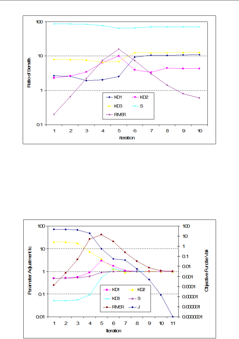
DRAFT
Theoretical background
Figure 12.20: Sensitivity ratio of different parameters during the parameter estimation
process.
The most sensitive parameter is the storage (S) in Figure 12.20, however, the parameter adjustment
is adjusting the storage the least since the least sensitive parameter, the RIVER, determines the final
parameter update vector. As can see in the decrease of the objective function, it is not the best thing
to do. Whenever the sensitivity of the Rivers increase, the storage becomes more important in the
gradient and the objection function declines more significantly.
Figure 12.21: Parameter adjustments in relation to the reduction of the objective function
value.
In order to avoid the disturbance, and therefore slower convergence, due to insensitive parameters,
iMODFLOW temporary holds those parameter(s). Whether a parameter is insensitive or not is deter-
mined by the ratio of their sivalue compared to the total sensitive value, see Figure 4.8.
Deltares 785 of 812

DRAFT
iMOD, User Manual
12.33.8 Example
In this section a simple example is given for a single optimalisation step using the Levenberg-Marquardt
algorithm as outlines in the previous sections. Suppose two parameters p1=p2= 1.0need to be
optimized that describe two different zones for permeability in a single modellayer. Two measurements
are available, one measurement in each zone. The first simulation is to run the model with p1=p2=
1.0, thereafter with p1= ∆pand p2= 1.0and finally with p1= 1.0and p2= ∆pwith ∆p= 1.1. For
each measurement location the measurements zjis subtracted from the computed head φi
jfor the ith
simulation and stored in the matrix D[m], thus:
D=φ0
1−z1φ1
1−z1φ2
1−z1
φ0
2−z2φ1
2−z2φ2
2−z2⇒D=−1.484 −1.391 −1.406
−1.686 −1.645 −1.513
From Dit is obvious that both parameters decline the objective function by a multiplication of ∆p. An
adjustment in p1does reduce the measurement z1mostly and p2reduces the second measurement
z2. However, both parameters influence both measurements and therefore both parameters cannot be
estimated separately as they are correlated to eachother. This is more clear in the Jacobian J[m/∆p],
defined as:
J=(d2
1−d1
1)/∆p1(d3
1−d1
1)/∆p1
(d2
2−d1
2)/∆p2(d3
1−d1
1)/∆p2⇒J=0.976 0.818
0.430 1.815
where di
jrepresent the ith column and jth row from the Dmatrix. As it is common to apply a log
transformation whenever permeabilities are calibrated, the value for ∆p= log(1.1) = 0.0953. Based
on the Jacobian, the Hessian H[∆p2/m2] is computed as:
H= (JTQJ +ψI)−1=1.137 1.585
1.585 3.977−1
=1.979 −0.789
−0.789 0.566
where Qis an identity matrix with diagonal values of 1.0, so every measurement has equal weights.
The Hessian is proportional to the curvature of the plane of the objective function Φ, it implies a large
step in the direction with low curvature (i.e., an almost flat terrain) and a small step in the direction with
high curvature (i.e, a steep incline). From the Hessian the parameter covariance Cp[∆p2] is estimated
as:
Cp=Φm
max(1.0, Nh−Np)H=4.266
11.979 −0.789
−0.789 0.566 =8.442 −3.365
−3.365 2.414
where the total objective function Φ=4.266 m2and the number of measurements Nh= 2 and the
number of parameter Np= 2. From these parameter covariance matrix the parameter standard error
ep[∆p] can be computed as:
ep=pdiag(Cp) = 2.905
1.554
In other words, the twice the parameter standard error represents 95% of the confident limits of the
parameter. In this case the current parameter value is highly uncertain as it ∆p1±2.905 and ∆p2±
1.554. Since the parameter is log transformed, the confident limits of the parameters are currently:
exp(∆p1= 0.0±2.905) −→ 0.0033 >∆p1<297.32
exp(∆p2= 0.0±1.554) −→ 0.0476 >∆p2<21.02
As the optimization of the parameters continues, this parameter standard error should decline as the
objective function value Φdeclines and the Jacobian will be become more flattened in the minimum
of the plane of Φ. As a result the confident limits decreases as well. Another useful parameter is the
correlation matrix Rpthat can be computed from the covariance matrix Cpeasily.
Rp=1.0−0.745
−0.745 1.0
786 of 812 Deltares

DRAFT
Theoretical background
From this correlation matrix is can be observed that both parameters are not correlated significantly and
can be determined in combination. Another method of determining the uniqueness of the covariance
matrix is the computation of its eigenvalues and eigenvectors, so:
(JTQJ)v= Λv=1.137 1.585
1.585 3.9770.408 0.913
0.913 −0.408=91.611
8.389 1.137 1.585
1.585 3.977
where Λcontains the ordered eigenvalues (singular values are Λ1
2) and vare the eigenvectors. The
eigenvectors are representing the axis of the residual surface, the eigenvalues √λirepresent the
length of axis i. The ratio between the first and last eigenvalues is the condition number κ, thus
κ= 91.611/8.389 = 10.920. This condition number κis relatively small and therefore the problem
is well-conditioned; the parameters are identifiable, they all contribute significantly and unique to the
residual surface.
The Gradient Descent gradient ∆p∗of the parameter adjustment becomes:
∆p∗=−JTQd1=−0.976 0.818
0.430 1.8151.0 1.0
0.0 0.0−1.484
−1.686=2.177
4.280
The parameter update becomes the exp() of the computed Gradient Descent gradient, so ∆p1= 8.82
and ∆p2= 72.24, which is rather huge that can be reduced within the limits of a trust hypersphere.
Whenever the Hessian His included (at this stage the ψis assumed to be 0.0 meaning that the full
Gauss-Newton algorithm is applied, this ψnormally increases during the optimisation such that in
the final stage the parameter update will be more equal to the Gradient Descent method) the final
parameter update vector ∆pbecomes:
∆p=−HJTQd1=−1.979 −0.789
−0.789 −0.566−2.177
−4.280=0.931
0.705
The elements for the final parameter update ∆pbecomes ∆p1= exp(0.0+0.931) = 2.537 and
∆p2= exp(0.0+0.705) = 2.024. After this the sequence starts again.
12.33.9 Remarks
Notes:
Do not use parameter adjustments that are too large, whenever many parameters are concerned
use a step size of 2, whenever you have less parameters you can increase this to a maximum of
10;
Experiment with different starting values for a parameter to see whether you end up with the same
optimal values;
12.34 Serial runtimes
The time that a simulation will consume depends on many things, e.g. the type of machine that you’re
using (hardware), and the configuration of your model. So, the consumption of the ANI package is
more than whenever the HFB package is used to simulate any type of horizontal anisotropy.
Deltares 787 of 812
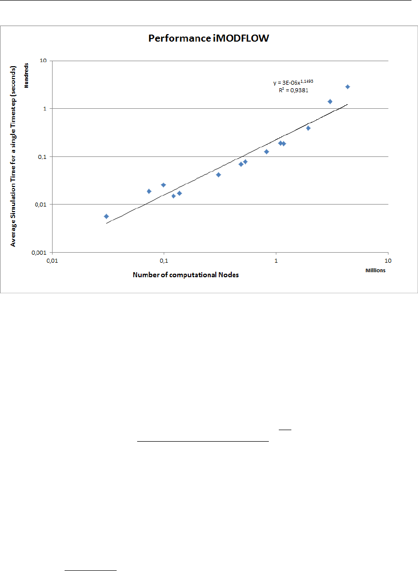
DRAFT
iMOD, User Manual
Figure 12.22: Computed run times for a single time step, for several different amount of
nodes. The results are based on the simulation of the IBRAHYM model for
5843 time steps, and cell sizes varying in between 25m2and 1000m2.
On average is seems that the simulation time is related to the number of nodes as follows:
Time (seconds)=3.0−6×Nodes1.15 ×Number of Time steps
Nodes =Time (seconds)
3.0−6×Number of Time steps
1
1.15
12.35 Timestep
Just a small nodal spacing is desirable, one would like to use small time steps to obtain an accurate
solution as well. A good order-of-magnitude is to estimate the critical time step ∆tcwith a formulae
given by de Marsily (1986). For a homogeneous and isotropic aquifer ∆tccan be estimated by:
∆tc=S(∆x×∆y)2
4T
whereby ∆xand ∆yare the cell sizes of the model (m), S(-) is the porosity values and Tis the
transmissivity value (m2/day). The result of the equation is given in the following figure:
788 of 812 Deltares
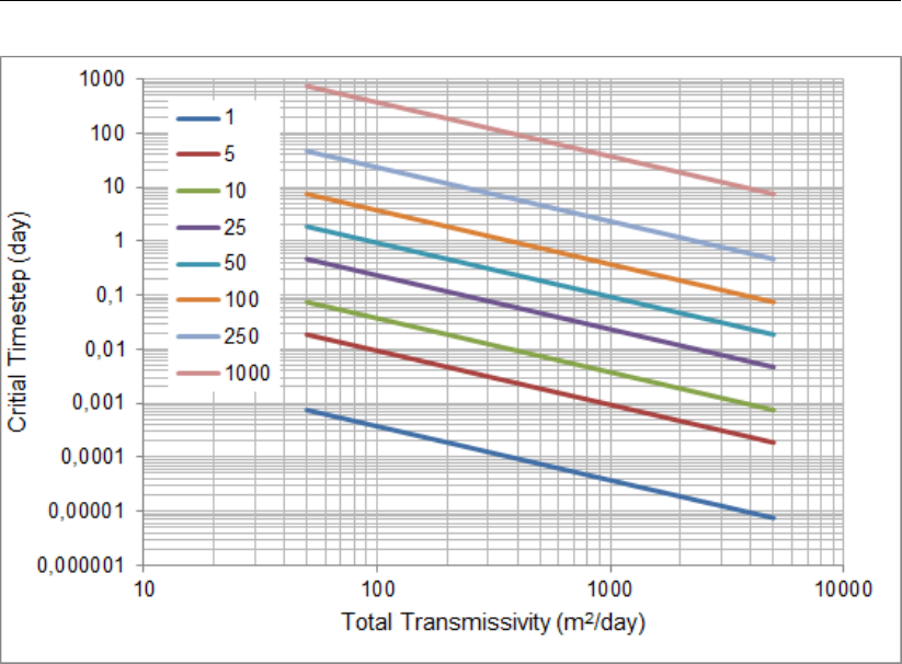
DRAFT
Theoretical background
Figure 12.23: Estimated critical time step (y-axis) for a porosity of S= 0.15 and different
values for transmissivity (x-axis) and cell sizes (coloured lines)
Deltares 789 of 812

DRAFT
iMOD, User Manual
790 of 812 Deltares

DRAFT
References
Ang, A.-S. and W. Tang, 1975. First-Order-Second-Moment (FOSM) analyse, Probability Concepts in
Engineering Planning and Design,, vol. I Basic Principles. John Wiley & Sons, Inc., New York, USA.
Berendrecht and Others, 2007. “A Methodology for Interactive Planning for Water Management.” In
Oxley, L. and Kulasiri, D. (eds) MODSIM 2007 International Congress on Modelling and Simulation
Modelling and Simulation Society of Australia and New Zealand, pages 74-80.
De Lange, W. J., G. F. Prinsen, J. C. Hoogewoud, A. A. Veldhuizen, J. Verkaik, G. H. P. Oude-Essink,
P. E. V. van Walsum, J. R. D. J. C. Hunink, H. T. L. Massop and T. Kroon, 2014. “An operational, multi-
scale, multi-model system for consensus-based, integrated water management and policy analysis:
The Netherlands Hydrological Instrument.” Environmental Modelling & Software 59: 98-108.
Dettinger, M. and J. Wilson, 1981. “First Order Analysis of Uncertainty in Numerical Models of Ground-
water Flow.” Water Resources Research 17 (1): 149-161. Part 1. Mathematical Development.
Doherty, J. E., 2003. “Ground water model calibration using pilot points and regularization.” Ground-
water 41 (2): 170-177.
Doherty, J. E., 2010. Approaches to highly parameterized inversion - A guide to using PEST for
groundwater-model calibration. Tech. Rep. 2010-5169, U.S. Geological Survey Scientific Investiga-
tions, Reston, Va. U.S. Dept. of the Interior, U.S. Geological Survey.
Dolean, V., P. Jolivet and F. Nataf, 2015. An introduction to domain decomposition meth-
ods. Society for Industrial and Applied Mathematics (SIAM), Philadelphia, PA. Algorithms,
theory, and parallel implementation, PDF: https://www.ljll.math.upmc.fr/nataf/
OT144DoleanJolivetNataf_full.pdf.
Glasgow, H., M. Fortney, J. Lee, A. Graettinger and H. Reeves, 2003. “MODFLOW 2000 head uncer-
tainty, a first-order second moment method.” Groundwater 41 (3): 342-50.
Halford, K. and R. Hanson, 2002. User Guide for the Drawdown-Limited, Multi-Node Well (MNW)
Package for the U.S. Geological Survey’s Modular Three-Dimensional Finite-Difference Ground-
Water Flow Model, Versions MODFLOW-96 and MODFLOW-2000. Tech. Rep. Open-File Report
02-293, 33 p., U.S. Geological Survey.
Harbaugh, A., 2005. MODFLOW-2005, The U.S. Geological Survey Modular Ground-Water Model—
the Ground-Water Flow Process. Tech. rep., USGS.
Konikow, L. F., G. Z. Hornberger, K. J. Halford, R. T. Hanson and A. W. Harbaugh, 2009. Revised
Multi-Node Well (MNW2) Package for MODFLOW Ground-Water Flow Model. Tech. rep., USGS.
Kunstmann H., K. W. and S. T., 2002. “Conditional first-order second-moment method and its appli-
cation to the quantification of uncertainty in groundwater modelling.” Water Resources Research
38 (4).
Leake, D., S.A. Prudic, 1991. Documentation of a computer program to simulate aquifer-system com-
paction using the modular finite-difference ground-water flow model. Tech. rep., U.S. Geological
Survey, Techniques of Water-Resources Investigations, Book 6, Chapter A2.
Leake, M. R., Stanley A. Lilly, 1997. Documentation of computer program (FHB1) for assignment of
transient specified-flow and specified-head boundaries in applications of the modular finite-diference
ground-water flow model (MODFLOW). Tech. rep., U.S. Geological Survey. Open-File Report 97-
571.
Maskey, S. and G. V., 2012. “Improved first-order second moment method for uncertainty estimation
of flood forecasting.” Hydrological Sciences Journal .
McDonald, M. and A. Harbaugh, 1988. A modular three-dimensional finite-difference ground-water
flow model: Techniques of Water-Resources Investigations of the United States Geological Survey.
Tech. rep., USGS.
Deltares 791 of 812

DRAFT
iMOD, User Manual
Merritt, M. L. and L. F. Konikow, 2000. Documentation of a Computer Program to Simulate Lake-Aquifer
Interaction Using the MODFLOW Ground-Water Flow Model and the MOC3D Solute-Transport
Model. Tech. Rep. Water-Resources Investigations Report 00-4167, U.S. Geological Survey.
Minnema, B. e. a., 2013. “Utilization of Interactive MODeling (iMOD) to Facilitate Stakeholder En-
gagement in Model Development Using a Sustainable Approach with Fast, Flexible and Consistent
Sub-Domain Modeling Techniques.” In MODFLOW AND MORE 2013: TRANSLATING SCIENCE
INTO PRACTICE. Colorado, The United States of America.
Niswonger, R., D. Prudic and R. Regan, 2006. Documentation of the Unsaturated-Zone Flow
(UZF1) Package for modeling unsaturated flow between the land surface and the water table with
MODFLOW-2005. Tech. Rep. Techniques and Methods Book 6, Chapter A19, 62 p., U.S. Geological
Survey.
Panday, S., C. D. Langevin, R. G. Niswonger, M. Ibaraki and J. D. Hughes, 2003. An unstructured grid
version of MODFLOW for simulating groundwater flow and tightly coupled processes using a control
volume finite-difference formulation. Tech. Rep. book 6, chap. A45, 66 p., U.S. Geological Survey.
Open-File Report.
Pollock, D., 1994. User’s Guide for MODPATH/MODPATH-PLOT, Version 3: A particle tracking post-
processing package for MODFLOW, the U.S. Geological Survey finite-difference ground-water flow
model. Tech. Rep. 94-464 6 ch., U.S. Geological Survey. Open-File Report.
Prudic, D. E., L. F. Konikow and E. R. Banta, 2004. A New Streamflow-Routing (SFR1) Package to
Simulate Stream-Aquifer Interaction with MODFLOW-2000. Tech. rep., U.S. GEOLOGICAL SUR-
VEY.
Van Walsum, P. E. V., 2017a. SIMGRO V7.3.3.2, Input and Output reference manual. Tech. Rep.
Alterra-Report 913.3, Alterra, Wageningen. 98 pp.
Van Walsum, P. E. V., 2017b. SIMGRO V7.3.3.2, Users Guide. Tech. Rep. Alterra-Report 913.2,
Alterra, Wageningen. 111 pp.
Van Walsum, P. E. V. and P. Groenendijk, 2008. “Quasi Steady-State Simulation on of the Unsaturated
Zone in Groundwater Modeling of Lowland Regions.” Vadose Zone Journal 7: 769-778.
Van Walsum, P. E. V., A. A. Veldhuizen and P. Groenendijk, 2016. SIMGRO V7.2.27, Theory and model
implementation. Tech. Rep. Alterra-Report 913.1, Alterra, Wageningen. 93 pp 491.
Verkaik, J., J. D. Hughes, E. H. Sutanudjaja and P. E. V. van Walsum, 2016. “First Applications of
the New Parallel Krylov Solver for MODFLOW on a National and Global Scale.” In 2016 AGU Fall
Meeting. San Francisco, California, USA.
Vermeulen, P., 2006. Model-Reduced Inverse Modeling. Ph.D. thesis, Delft, University of Technology.
With summary in Dutch. ISBN-10: 90- 9020536-5. ISBN-13: 978-90-9020536-6.
Vermeulen, P., B. Becker and T. Heinz, 2014. Coupling iMOD-SOBEK. Coupling of a surface water-
and groundwater flow model to compute bank storage effects in wetlands along the Elbe River on
different grid resolutions. Tech. rep., Bundesanstalt für Gewässerkunde. Koblenz, Germany.
Vermeulen, P. and Others, 2013. “Groundwater modeling for the Mekong delta using iMOD.” In 20th
International Congress on Modelling and Simulation (MODSIM2013).
792 of 812 Deltares

DRAFT
Release Notes iMOD-GUI
Version 3.01.00 iMOD_V3_01_00_X32R.exe (for 32-bit systems)
iMOD_V3_01_00_X64R.exe (for 64-bit systems)
Date 18-9-2015
Based On 3.00.00
Changed
Functionality
SVN 32 - Displays Bitmaps in the SOLID TOOL, in cross-sections and 3D
displays.
SVN 33 - MODFLOW2000 does not have the capability as MODFLOW2005
does, to use LENUNI and ITMUNI; when importing a MOD-
FLOW2000 model LENUNI and ITMUNI are set separately.
SVN 46 - Keywords MONTHLY and YEARLY added to the functionality of
the iMODBATCH function XYZ2IDF. In combination with a transient
IPF (including a TXT file), it is possible to grid the IPF for mean
values for selected years or months.
SVN 46 - Changed ACCURACY from EPSILON(1.0) to 0.0 in the IMOD-
PATH. This influences the minimal velocity that determines whether
a particles does not move anymore, by changing it into 0.0 m/day,
particles will continue until they truly stop. The value EPSILON(1.0)
yielded the value 1.1920929E-07 m/day.
SVN 48 - Changed the method to write the borehole information in TXT
file for IPF files created by the iMODBATCH function DINO2IPF, in
situation whereby no values are read, the value becomes "None".
SVN 70 - The iMODBatch function IMPORTMODFLOW has been modified
such that it can read external files with a MODFLOW-88 format.
- The iMODBatch function ISGGRID has been extended to export
the gridded data to a MODFLOW river file (SCD format).
SVN 79 - The keywords for the SOLIDTOOL are changed from TOP and
BOT into INT to make it possible to construct subsoils with an un-
even number of interfaces.
- The Darcian upscaling method reviewed and updated.
SVN 91 - The iMODBATCH function ISGGRID extended to support the ex-
port to svatswnr_drng.inp used by MetaSWAP.
- Problems with rendering on a Remote Desktop Server(s) related
to Winteracter 10. Included an iMOD version based on Winteracter
8 that does not have these problems. In this Winteracter 8 - Re-
mote Desktop Server-version some (minor) functionalities of iMOD
are not supported on the RDP-server(s).
SVN 165 - SOLIDTOOL corrects layers that crosses the lowest layer.
SVN 166 - IMODBATCH the function IPFSAMPLE includes the parameter
IACOL to specify the column to start inserting the sampled data.
SVN 299 - Enlarged fields (20/50) to (52) in *.dlf files.
New Function-
ality
SVN 39 - Added the iMODBATCH functionality UTM2LATLONG to trans-
form IDF UTM coordinates to a Lat-Long IPF with data, e.g. to be
gridded by the IMODBATCH functionality XYZ2IDF.
SVN 43 - Added functionality to the WATERBALANCE TOOL to use hours,
minutes and seconds as time scales, so IDF files with date and time
identifications become processed, e.g. HEAD_20141231063000
as the head on the 31stof December 2014 at 6hours, 30 minutes
and 0 seconds.
- Added functionality to the TIMESERIES TOOL to plot time series
using hours, minutes and seconds as time scale.
SVN 48 - Increase the size for the grid fields automatically in IPFANALYSE
whenever borelogs/time series are identified.
SVN 51 - Reading IPF files with associated TXT files with long dates
(yyyymmddhhmmss).
SVN 70 - Added the iMOD Batch functionality ISGADDSTAGE to add and/or
modify existing waterlevels in an ISG file from a given IPF file with
timeseries.
Deltares 793 of 812

DRAFT
iMOD, User Manual
SVN 71 - Added the functionalities Go Back to Previous Extent and Go to
Next Extent on the main icon bar and the Cross-Section window.
SVN 163 - Export possible from the SOLID tool to the GEO format as used
by GeoSoftware of Deltares.
- The SOLID tool supports the dynamic use of different cell size for
each interface.
- In IMPORTMODFLOW function the Modflow scheme 1996 is sup-
ported.
- Size of the profile tool increased and gave it a red colour.
SVN 236 - Reading of *.MAP files from PCRaster.
SVN 269 - Context-sensitive HELP-functionality: adding section-bookmarks
to the iMOD User Manual and synchronize the list of bookmarks in
iMOD.
SVN 283 - The IDF-function for exportation of IDF-files to ascii-files is ex-
tended with the "Export given extent"-functionality.
SVN 290 Reading of GEF files, as addition to iMODBATch function GEF2IPF.
Fixed Bugs SVN 34 - Bug in IPFSAMPLING in combination with CSV-file format.
SVN 46 - SAVE button didn’t work for steady-state configuration, also the
selection of a different model layer didn’t responded accordingly.
SVN 47 - Bug in iMODPATH using NCON=0 should be NCON=1.
SVN 51 - Bug in IDFCALC whenever the function MIN,MAX,MEAN or SUM
is selected; the variable LEX was not initiated.
- Bug in X64 versions only: in displaying the license agreement, the
variable IU was not initiated.
SVN 60 - Bug in WATERBALANCE as a result of implementation of SVN
43, dates with 8 digits didn’t work anymore.
SVN 70 - Bug in default legends that could not be saved temporarily when-
ever a relative pathname was specified by the USER keyword in
the preference file.
SVN 72 - Bug on the Add Topography window as the coordinates could not
be manipulated appropriately.
SVN 76 - Bug in memory allocation for the Quick-Response Tool.
- Bug in reading IPF files as CSV using the double quotes.
SVN 77 - Bug in display of IFF lines in the 3D Tool that are vertically.
SVN 88 - Export format for the output files for iMODPATH (IFF and IPF) syn-
chronized.
- Identical algorithm used in the postprocessing of pathlines in the
iMODBATCH function iMODPATH, to determine appropriate cell in-
dices for points as used in iMODFLOW. This means that points that
are exactly on the boundary of model cell will be assigned to the
i+1 cell instead of i.
SVN 163 - Bug in creation of legend where the difference exceeds the range
of a single precision real, namely >10.0+e37. For those cases the
legend will be inaccurate but iMOD will not hang.
- The display of the NodataValue of an IDF is displayed correctly in
MapInfo and IDF Edit displays.
SVN 213 - Bug in Compute Mean Values..., after measuring the mean the
specific dialog window cannot be closed neither it is possible to
proceed with the iMOD session.
SVN 216 - Bug in positioning of labels in 3D-tool. Labels did disappeared
when turning the 3D-schematisation under certain angles.
SVN 218 - Update of keywords vor iMOD Batch in code.
SVN 226 - Fix coordinates in CreateIDF whenever changes are made in the
dialog.
SVN 240 - Correct reading of run-files in the ModelTool without bounding co-
ordinates in submodels.
SVN 254 - iMOD Batch reading of keuword with an extra space after the "="-
signs raised a problem. This has been fixed, as it was noticed by
the GxG-function in iMOD Batch using the keyword IPERIOD=.
794 of 812 Deltares

DRAFT
Release Notes iMOD-GUI
SVN 267 - Changed the keyword CROSS-SECTION_IN to CROSSSEC-
TION_IN
SVN 287 - Fixed bug in reading *prf having a last empty line.
SVN 298 - No capitalizing input from *.ini file.
SVN 299 - Colouring of the correct field using DLF legends.
Version 3.2.00 iMOD_V3_2_X32R.exe (for 32-bit systems)
iMOD_V3_2_X64R.exe (for 64-bit systems)
Date 11-11-2015
Based On 3.01.00
Changed
Functionality
SVN 305 - Reading/assignment of DLF files (maximal 10) for usage within
Profile Tool, 3D Tool and IPF Analyse.
SVN 309 - Usage of the DLF field colourwidth to display boreholes with
variable widths.
- include the keyword STOPERROR in BAS file for convergence
issues in Modflow2005.
SVN 312 - Labeling of IPF files in the 3D tool can be specific selected for
each IPF separately.
SVN 320 - ISGGRID create nodatavalues (-9999.00) for cells not inter-
sected by lines.
SVN 325 - IMPORTSOBEK stopped whenever actual length weren’t
equal to the lengths based on the nodes of the segment. The
import now is not stopped but a warning is issued to the file im-
portsobek.log and the process continues.
- Enlarged fields (20/50) to (52) in *.dlf files.
New Function-
ality
SVN 305 - Add screen number for IPF and IFF in the profile tool.
- Use different legends for IPF files (*DLF).
SVN 309 - Save DLF legends in IMF-files.
- Manually activate display of IPF/IFF files during mov-
ing/drawing the cross-section.
- Mousemove coupled to location in identification window in IPF
Analyse via Profile Tool.
SVN 320 - Saving of solid files during editing without leaving the cross-
section tool.
- Extended the IMODBatch functionality ISGEXPORT with key-
word IEXPORT to denote export of calculation points or cross-
sections.
SVN 326 - Remove and/or modify more nodes in SOLIDTOOL simultane-
ously
SVN 341 - Added Inf and NaN in IDF Edit to search on those values in
the IDF files.
SVN 343 - Added an active/deactive code per line in the SolidTool. Now
per line it can be specified whether or not it need to be included
in the solid.
SVN 351 - Added functionality in the 3D Tool to zoom to predefined zoom
scales.
- Display the lines in the cross-sections as true splines or
straight lines.
SVN 364 - Change timesteps in the projectmanager.
- Save cross-sections and 3D Tool configurations in a iMOD
Demo-mode.
SVN 370 - Include the option sign() as a function in IDF Calc, subtract
only whenever the sign of the two are equal and use pointer
values to note the type of difference.
- the iMODFLOW-executable present in the {installfolder} will be
invoked instead of the iMODFLOW-executable copied to {install-
folder}\MODELS\{Result Folder}.
SVN 375 - Usage of preference colours for the default legend.
- Apply a value in IDFCalc to "trim" outcome of calculation when-
ever the outcome is less than a specified absolute value
Deltares 795 of 812

DRAFT
iMOD, User Manual
SVN 401 - Export to Modflow2005, give explicitly if the model is 3D or
Quasi 3D.
Fixed Bugs SVN 306 - iMODBatch ISGSIMPLIFY removal of first and last calculation
point in case stage were completely flat.
- iMODBatch CREATESOF correct usage of given OUTLET
points to stop tracing the drainage level.
SVN 309 - Screen number were outgreyed in Profile Tool.
- Export of BND to Modflow2005 created constant head along
submodel as it was filled with nodata from IDF.
SVN 312 - Display of bitmaps in 3D Tool in combination with bitmaps at-
tached to solid cross-sections.
SVN 343 - Total length of line in SolidTool didn’t match true length, only
visible in cross-sections with many points.
SVN 351 - Delete of spf will not shift attached bitmaps appropriately.
SVN 376 - Use of small-caps for FUNC in IDFCALC gave errors.
SVN 378 - Bug in smoothing the IDF files whenever the file to be used
for the smoothing exceeds the size of the IDF to be smoothed
upon.
Version 3.2.1 iMOD_V3_2_1_X32R.exe (for 32-bit systems)
iMOD_V3_2_1_X64R.exe (for 64-bit systems)
Date 24-11-2015
Based On 3.2
New Function-
ality
SVN 440 iMOD-GUI can now invoke iMODFLOW using foldernames con-
taining spaces.
Changed
Functionality
Fixed Bugs
Version 3.3 iMOD_V3_3_X32R.exe (for 32-bit systems)
iMOD_V3_3_X64R.exe (for 64-bit systems)
Date 25-03-2016
Based On 3.2.1
New Function-
ality
SVN 439 - Specify the option to reduce sizes of boreholes if they do not
fit next to each other and thus may overlap.
SVN 466 - Added iMODBatch function RUNFILE, to create *.PRF from
*.RUN files and/or create *.RUN files out of *.PRJ files.
SVN 471 - Project Manager supports now the creation of RUNFILES.
- PlugIn Tool is added as an additional tool to support external
programs or scripts to be invoked by iMOD and exchange input
and output.
- Added an extra MetaSWAP output component to the waterbal-
ance tool (BDGPSSW).
SVN 471 - The Interactive Pathline Simulator tool for animating ground-
water flow.
SVN 487 - Added units to waterbalance items.
SVN 502 - Added an option to change the transparancy of individual IDF
files in the 3D Tool.
SVN 512 - The IPS functionality can now be started from the Pathline
Tool.
SVN 520 - The usage of breaklines in the SOLID Tool is made available
in the GUI.
- Coordinates in the Profile Tool can be decreased in number by
specifying a minimal distance between coordinates.
- Compute differences in IDFTIMESERIES can handle IDF files
with hours, minutes and seconds.
796 of 812 Deltares

DRAFT
Release Notes iMOD-GUI
SVN 528 - Automatic spinner in 3-D.
- Entry of scale ratio in the Profile Tool.
- Display label and size on the cross-section for the SOLID Tool
on 2D
SVN 541 - Kriging settings can be defined per interface.
SVN 544 - Automatic rendering of the image in a circular movement in 3D
by pressing the spacebar.
SVN 546 - Bitmap in the background of cross-sections in the SOLID Tool
can be temporarily hidden and fixed so that it cannot be moved
while adjusting the lines of the cross-section.
Changed
Functionality
SVN 422 - Solid Tool; Compute Interfaces window. Export to *.geo is with
the "version" name attached to the keyword VERSION.
SVN 439 - Spline mode in Solid Tool is "off" by default, for export to IPF
or GEO.
SVN 489 - The IPS module can create a temporary submodel for parti-
cle tracking purposes. - The reading module or the imodpath
entries has been made similar to other scaling modules.
SVN 504 - PNG, PCX and JPG file can now by used as background im-
ages, and can be resized and flipped horizontally and vertically.
- iMODBatch function CREATEIDF will NOT ask to overwrite ex-
isting IDF-files while importing ASC-files, GUI still does.
- Read in GEN file in Profile Tool are corrected for duplicated
points.
SVN 507 - Previous foldernames are saved to be re-used in next search
in folders.
SVN 512 - Pathline Tool creates its runfile in the RUNFILE folder instead
of the TMP folder, it also creates a stamp of the chosen model
result folder in the filename.
- Adjustment of the NODATA value in the IDF file, causes that
the content of the IDF file itself will be changed accordingly.
So values that are equal to the previous NODATA value, will
become adapted to the new NODATA value.
- Bitmaps that can be positioned behind the cross section in the
solid tool, can be stretched and moved interactively whenever
the corresponding bitmap is selected from the Add Background
Image dialog.
- Background Images may be BMP, PNG, PCX and JPG files.
SVN 516 - IFF attributes can be plotted all, also whenever the number of
columns are enlarged above 7.
SVN 581 - In the waterbalance tool: extra comment line that explains the
possible causes for disclosure of the balance, e.g. differences
in used units (m3/day or mm/day) for specific fluxes.
Fixed Bugs SVN 418 - Translate x,y coordinates from shape files into GEN files using
the double-precision format.
- Non-existing background files are turned off and properly re-
set.
SVN 427 - Bug in reading the CLR files and display them in the preference
tab.
SVN 429 - Bug in collecting correct dates in the waterbalance tool.
SVN 432 - When defining a new function using iMODBatch, now the cor-
rect function is presented (instead of the next function from the
list of available functions).
SVN 443 - Whenever IPF files are not active in profile tool setting the
snapping option was not available.
SVN 466 - Bug in ISG grid in combination with 2d and 1d cross-sections.
SVN 467 - iMODBATCH function MKWELLIPF ignored ICLAY variable.
SVN 471 - Bugfix in Compute GXG. Selecting correct surface level.
SVN 472 - Bigfux in iMODBatch PLOT function - usage of IPF files for
timeseries plotting.
Deltares 797 of 812

DRAFT
iMOD, User Manual
SVN 482 - Usage of particles pass through all weak sinks gave problems
whenever the weak sinks approaches a strong cell as an inter-
nal value 0f FRAC=0.99 was used to denote a strong cell, FRAC
is now 1.0 and maximized to be 1.0 numerically.
- Applying a fraction for iMODPATH (ISNK=3) didn’t work from
iMODBatch.
SVN 486 - Computation of SUMC in IDFSCALE option 14, went wrong.
- Applying lower-left coordinates in IDFSCALE went wrong.
SVN 489 - Default colouring of IDF files was maximized to 50, following
files got colour number 1, now the colour numbering continues.
SVN 502 - Bug reading GEN files for overlays.
- Intersect for non-equidistantial cell went wrong, created a
killing bug for the profile-tool.
- 3D tool with non-equidistantial IDF gave bug.
- In profiletool, whenever a knickpoint was positioned outside
the selected IDF, the profile length
didn’t take into account the extra space of the cross-section out-
side the IDf file.
SVN 509 - Import of Modflow2005 the LENUNI variabel didn’t applied cor-
rectly to EVT package and the elevation in the DIS whenever
LAYCON=0.
SVN 515 - Bug in timeseries export.
SVN 528 - Load SHP file in CreateIDF from Polygons/lines.
SVN 544 - Rasterizing ISG didn’t take into account stages with nodata
values for transient mean values.
SVN 616 - Bug in Solid Tool by using the "pan" function in Zoom-in
modus.
Version 3.4 iMOD_V3_4_X32R.exe (for 32-bit systems)
iMOD_V3_4_X64R.exe (for 64-bit systems)
Date 30-06-2016
Based On 3.3
Changed
Functionality
SVN 647 - 3D TOOL: 3D Tool is organized differently whereby the dialog
is attached to the graphical screen and the tool operates inde-
pendently of the existing 2-D screen.
SVN 666 - IMODBATCH: EXPORTASC Write results per row instead of
free-formatted
SVN 660 - IMODBATCH CUS: Usage of IEXPZONE to include an addi-
tional buffer around each isolated formation to ensure a more
logical connection within parts of the formation laterally;
- Usage of ICLIP to include a clipping IDF for each formation to
be internally blanked out to ensure usage of overlapping maps
for formations
SVN 635 - XYZTOIDF: Interpolation of interfaces from IPF files, median
values are not supported anymore
SVN 707 - WATERBALANCE: Always using files with/without *sys* in
their given names
SVN 709 - STARTPOINTS: Tried to read from the non-existing SDF-file
the first time an SDF-file is created
SVN 713 - GENERAL: The numeric format of plotting IDF values is now
depending on the accuracy of the IDF values
SVN 738 - CONTOURING: Improved contouring algorithm, especially to
include delineation of flat areas
SVN 756 - CONTOURING: Legend label on contours uses appropriate
number of decimals
- LEGEND: Legend plotting now plots a grey rectangle around
classes
- 3DTOOL: The menu option ’Select’ is now part of the main
dialog and removed from the main menu
798 of 812 Deltares

DRAFT
Release Notes iMOD-GUI
SVN 762 - LEGEND: Enhanced legend plotting for 255 and 50 classes
categories
SVN 781 - IMODBATCH: Testbank does not subtract results if one-of-the-
two is equal to its Nodatavalue
SVN 787 - IMODPATH: Restored functionality to save deepest model
layer during particle tracking (MAXLAY)
New Function-
ality
SVN 635 - SOLID TOOL: Usage of separate IPF files to include (addi-
tional) interpolation points, or use those points solely for the
interpolation, with- and without associated txt files that describe
the elevations of the individual interfaces. Without associated
txt files, each IPF describes the z-elevation at the third column
SVN 642 - GENERAL: Relative path can be read from IMF-files, those are
relative to the name of the current - IMF-file and are converted
to global paths
SVN 734 - LEGEND: Legend can be adjusted with chosen intervals
SVN 778 - GENERAL: Added debug reporting level
SVN 784 - GENERAL: Reading of Point Shapefiles will be converted to
IPF-files, also Shapefiles can be read from the MAP-tab on the
iMOD Manager
SVN 849 - GEOCONNECT TOOL: Geoconnect tool is usable to deter-
mine the geologic origin of 3D models (what geologic formation
is within what model layer) and (re)create the parameterisations
of a 3D model (compute the correct k-values for each model
layer based on the fractions of geologic formations in that model
layer)
Fixed Bugs SVN 625 - TIMESERIES TOOL: Series can be plotted while new files are
added to the selected folder in the background as a model is
still running
SVN 630 - IMPORT MODFLOW: Time units to adjust PERLEN to days,
usage of TSMULT included to generate additional stress-
periods
- ISS flag does not to be read from the BCF pcakage in 2000
and 2005 configurations
- Conversion of time units to days was wrong for the WEL, DRN,
RIV packages
- GENERAL: Out greying of the iMOD Info button on the menu-
bar didn’t synchronize with the rest
SVN 634 - PROFILE TOOL: Cross-section did not work whenever DX is
not equal to DY
SVN 636 - ISG EDIT TOOL: Gridding of transient data gave error, in com-
bination of computing the mean and entered start and end date
SVN 640 - GEOCONNECT: Factors in preprocessing were not used;
iMODBatch in preprocessing array already allocated; Added co-
ordinates on tab 1; include the identify button on tab 3 to inspect
the current existing formations on the current window.
- DEMO-MODE: 3D DEMO functionality was not working prop-
erly
SVN 695 - MF2005 EXPORT: HFB was not assigned to the utmost row
and column, e.g. irow=1, irow=nrow, icol=1 and icol=ncol
- MODELTOOL: Applied quotes for file names
SVN 698 - PATHLINES: Writing of column/row numbers at start- and end
location in IPF files was switched
SVN 706 - WATERBALANCE: Could not find the *sys* files from iMOD-
FLOW V3.0 and younger
SVN 709 - GENERAL: Usage of MAXSHAPES is supported from the
preference menu
- IPS: Usage of constant values from a iMODPATH runfile for
TOP and BOT parameters
SVN 727 - IMODBATCH: Whenever an argument is missing after the "="
of an optional argument an error message appeared
Deltares 799 of 812

DRAFT
iMOD, User Manual
SVN 732 - MODELTOOL: Including the PST parameter while converting
to a imodflow.run file
- GENERAL: Didn’t position a contour line in between a class of
0.0
SVN 744 - PROJECTMANAGER: Saving of number of timeseries in run-
file on right position PST was not mentioned in the header of
packages
- ISGEDIT: Gridding of ISG file did not overrule grid-dimensions
entered on the last window
SVN 750 - KRIGING: Improved algorithm, NUGGET effect was not cor-
rectly processed
SVN 762 - LEGEND: Bug in class-legend gave a crash whenever a neg-
ative value from the legend was selected in the table
SVN 776 - PROFILETOOL: Loading of BMP causes the 21st filename
(IDF, IPF of IFF) to be closed by the Winteracter routine IGR-
FILEINFO.
SVN 781 - PROJECTMANAGER: Removal of PST didn’t work properly
- GEOCONNECTTOOL: Small issues resolved, crash by re-
peatedly starting the post-processing
800 of 812 Deltares

DRAFT
Release Notes iMOD-GUI
Version 3.6 iMOD_V3_6_X32R.exe (for 32-bit systems)
iMOD_V3_6_X64R.exe (for 64-bit systems)
Date 10-05-2016
Based On 3.4
Starting from iMOD 3.6 we summarize all new, changed, extended and fixed functionalities on the
iMOD-website: http://oss.deltares.nl/web/imod/release-notes. Per release these
release notes are also distributed per email to all iMOD-community members,
Deltares 801 of 812

DRAFT
iMOD, User Manual
802 of 812 Deltares

DRAFT
Release Notes iMODFLOW
Version 3.00.01 iMODFLOW_V3_00_01_METASWAP_SVN1004_X32R.exe
(for X32-bit systems)
iMODFLOW_V3_00_01_METASWAP_SVN1004_X64R.exe
(for X64-bit systems)
Date 15-10-2014
Based On 3.00.00
New Function-
ality
Changed
Functionality
linked with MetaSWAP SubVersion number 1004 from repository
https://repos.deltares.nl/repos/GWSobek/trunk/src/modmsw/
Fixed Bugs SVN 49 When a GEN-file coincides exactly with cell face no HFB-cell face
was assigned resulting in a barrier with a hole. This bug has par-
tially been fixed; with the real world test model NHI the bug fix
works, however, the standard USGS HFB-test still fails because
the test contains a barrier partly at a cell face. Version 3.00.01 was
released because the bug manifests only in exceptional cases; a
subsequent bugfix is planned to also fix these exceptional cases.
Version 3.00.02 iMODFLOW_V3_00_02_METASWAP_SVN1004_X32R.exe
(for X32-bit systems)
iMODFLOW_V3_00_02_METASWAP_SVN1004_X64R.exe
(for X63-bit systems)
Date 20-11-2014
Based On 3.00.01
New Function-
ality
Changed
Functionality
Fixed Bugs SVN 80 IMOD-319: default value added for KVA-module (1.0).
SVN 81 IMOD-327: bug fixed upscaling anisotropy factor (most frequent
occurrence).
SVN 82 Bug fixed applying factor for recharge.
Version 3.01.00 iMODFLOW_V3_01_00_METASWAP_SVN1031_X64R.exe
(for 64-systems)
iMODFLOW_V3_01_00_X32R.exe (for 32-bit systems)
iMODFLOW_V3_01_00_X64R.exe (for 64-bit systems)
Date 17-07-2015
Based On 3.00.02
New Function-
ality
SVN 194 In Perched Water Table PWT-package: new conceptual enhance-
ments implemented for how groundwater flows at the edges of a
Perched Water Tables to avoid some numerical instabilities.
Changed
Functionality
linked with MetaSWAP SubVersion number 1032 from repository
https://repos.deltares.nl/repos/GWSobek/trunk/src/modmsw/
SVN 188 Update for VS2008 (EXTERNAL statements removed) - Update for
interface MODFLOW-TRANSOL.
SVN 194 HFB-package update (based on an earlier implementation in iMOD-
FLOW 2.6.) improving the discretization of curved lines to the
model grid.
SVN 202 PEST package update based on iMODFLOW 2.6.
SVN 221 Update for TRANSOL interface.
SVN 242 Update interface with TRANSOL to previous version.
SVN 259 Some minor iPEST-messages and I/O adjustments.
SVN 260 Removed ’modflow’ subdirectory from output results directory.
Deltares 803 of 812
DRAFT
iMOD, User Manual
SVN 214,
215, 228-
230, 234,
246
Update of iMOD license text.
Fixed Bugs SVN 105 In SGWF2BCF7C: adding uninitialized variable CR to variables list.
SVN 191 Initialization of constant CNSTNT added for u1drel and u2dint.
SVN 212 In HFB package: minor error-correction for case that lines are out-
side model domain.
SVN 238 In Grid2MetaSWAP: reading ascii files standard with xllcorner and
yllcorner which also could be xllcenter and yllcenter.
SVN 257 In coupling Modflow-MetaSWAP with Mozart: change of general
missing parameter value.
SVN 258 In HFB package: minor error-correction for case that lines are out-
side model domain.
SVN 261 In ISG package: a small change in the ISG calculation routine was
made.
SVN 261 Automated scaling factor: the computation of the simulation window
was sometimes incorrect in case the extent of the entered model
was not exactly divisible by the cell size of the model.
Version 3.2 iMODFLOW_V3_2_METASWAP_SVN1044_X64R.exe
(for 64-systems)
iMODFLOW_V3_2_X32R.exe (for 32-bit systems)
Date 10-09-2015
Based On 3.01.00
New Function-
ality
Changed
Functionality
linked with MetaSWAP SubVersion nr. 1044 from repository
https://repos.deltares.nl/repos/GWSobek/trunk/src/modmsw/
Fixed Bugs SVN 317 Bug fix uninitialized arrays when using the ANI package. This
problem may result in a floating point error at some machines.
SVN 318 Bug fix automatic assigning ISG to layer: a floating point error
(division by zero) might occur are specific machines.
SVN 344 Bug fixes CHD-package: 1. input start/end head was swapped;
2. iMOD usage of factors (e.g. h = 0.5h1 + 0.5h2) was incorrect.
SVN 352 Bug fix ISG 2-D cross sections.
Version 3.2.1 iMODFLOW_V3_2_1_METASWAP_SVN1044_X64R.exe
(for 64-systems)
iMODFLOW_V3_2_1_X32R.exe (for 32-bit systems)
Date 20-11-2015
Based On 3.2
New Function-
ality
SVN 438 iMODFLOW can now work with foldernames containing spaces.
Changed
Functionality
Fixed Bugs
Version 3.3 iMODFLOW_V3_3_METASWAP_SVN1047_X64R.exe
(for 64-systems)
iMODFLOW_V3_3_X32R.exe (for 32-bit systems)
Date 25-03-2016
Based On 3.2.1
New Function-
ality
Changed
Functionality
linked with MetaSWAP SubVersion nr. 1047 from repository
https://repos.deltares.nl/repos/GWSobek/trunk/src/modmsw/
804 of 812 Deltares

DRAFT
Release Notes iMODFLOW
Fixed Bugs SVN 561 Restoring the gridding functionality of flow-width in ISG.
SVN 618 Bug fix Metadata package (MET) timestep management in
MODFLOW, causing a delayed read of transient well data. This
bug was relevant when defining stress period lengths that were
larger than the available time discretisation present in the ipf-
and txt-files used as the source of the abstraction data.
SVN 621 Adjusted scaling of well extraction from median value to mean
values weighted to time - usage of nodata values in txt files.
Version 3.4 iMODFLOW_V3_4_METASWAP_SVN1047_X64R.exe
(for 64-systems)
iMODFLOW_V3_4_X32R.exe (for 32-bit systems)
Date 20-06-2016
Based On 3.3
New Function-
ality
Changed
Functionality
Fixed Bugs SVN 660 DRN: Memory reallocation of the drain package will be per-
formed whenever the number of drains exceeds the previous
allocated memory.
SVN 662 TIMESERIES: A limited number of unit numbers were available
(10-99) for time series, now it is set to (10-999).
COMMON: An inactive package in the runfile was seen as
"reuse" package instead of a new package definition without
any entries.
SVN 680 PCG: The cleaning of the matrix coefficients was not done cor-
rectly.
SVN 671 IPF: Reading screen depths only needed whenever ilay.eq.0.
SVN 719 ANI: The incorrect nodata values were assigned to the inactive
corner cells at the computational area.
SVN 720 HFB: The issue with the out of array boundary horizontal flow
barrier package is solved.
SVN 732 COMMON: The initialization problem is solved for iMOD license
agreement file.
SVN 786 COMMON: A non-converging steady-state MODFLOW simula-
tion was not finalized correctly.
SVN 792 BALANCE: Computing the waterbalans, the ANI-terms were not
included in the constant-head boundary flux, also they were not
applied as a correction on the BDFFFF and BDGFRF fluxes for
the LPF-configuration.
SVN 799 PWT: The floating point exception for inactive cells should be
skipped in the perched water table package.
SVN 806 CHD: For zero-thickess cells at a subdomain boundary a con-
stant head cell could be activated incorrectly resulting in an error
message "no-flow cells cannot be converted to constant head
cells".
Deltares 805 of 812

DRAFT
iMOD, User Manual
Version 3.6 iMODFLOW_V3_6_METASWAP_SVN1196_X64R.exe
(for 64-systems)
iMODFLOW_V3_6_X32R.exe (for 32-bit systems)
Date 30-05-2017
Based On 3.5
Starting from iMOD 3.6 we summarize all new, changed, extended and fixed functionalities on the
iMOD-website: http://oss.deltares.nl/web/imod/release-notes. Per release these
release notes are also distributed per email to all iMOD-community members,
806 of 812 Deltares
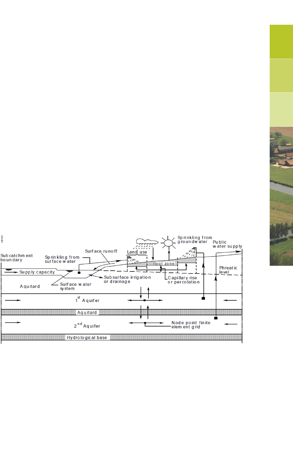
DRAFT
A About SIMGRO and MetaSWAP
A.1 What are the models intended for?
Most regional model codes cover only part of the processes within a region. For coming to grips with
many issues of integrated water management it is necessary to have a model that covers the whole
(regional) system, including plant-atmosphere interactions, soil water, groundwater and surface water.
SIMGRO (a dated acronym of SIMulation of GROundwater) was developed for that purpose.
The name ‘SIMGRO’ was formerly used for referring to an integrated model code, including submodels
for the compartments and processes as shown in Fig. 1. Now it is used in the meaning of a modelling
framework. This framework has been connected to a number of ‘inhouse’ components, but also has
possibilities for coupling to other codes. The in-house components are:
1 an SVAT-model that is commonly referred to as ‘MetaSWAP’, covering the plantatmosphere inter-
actions and soil water;
2 a simplified surface water metamodel;
3 a drainage package, for simulating groundwater drainage with fast feedback from surface water.
The current possibilities for coupling to other codes are:
1 MODFLOW for groundwater (operational);
2 SOBEK-CF for surface water (under development).
The used schematisation assumes that the separate SVAT columns only interact with each other via
their connections to groundwater and surface water.
Figure A.1: Overview of the processes modelled in SIMGRO. MetaSWAP (Van Walsum
and Groenendijk,2008) is used for the SVAT ( Soil Vegetation Atmosphere
Transfer) processes that are modelled within vertical columns. These col-
umn models are integrated with the groundwater model (MODFLOW) and
a surface water model; for the latter there are several options, including a
simplified metamodel that can be linked to form a basin network.
Deltares 807 of 812

DRAFT
iMOD, User Manual
A.1.1 What is the scope of the model application?
The SIMGRO framework is intended for regions with an undulating topography and unconsolidated
sediments in the (shallow) subsoil. Both shallow and deep groundwater levels can be modelled by
MetaSWAP. This model is based on a simplification of ‘straight Richards’, meaning that no special
processes like hysteresis, preferential flow and bypass flow are modelled. Snow is not modelled, and
neither the influence of frost on the soil water conductivity. A perched watertable can be present in
the SVAT column model, but interflow is not modelled. There are plans for including the mentioned
special processes in MetaSWAP Inundation water can be modelled as belonging to both groundwater
and surface water at the same time. Processes that are typical for steep slopes are not included.
The code contains several parameterized water management schemes, including irrigation and water
level management.
A.1.2 What are the used spatial and temporal scales of the model?
The spatial scale of the model is typically for a unit of 1 km2and less. Model applications have involved
up to 500 000 units (National Hydrological Instrument for the Netherlands). A prototype model of a
small basin involved 800 000 cells of 5x5 m. A resolution finer than 5x5 m is considered to be beyond
the scope of the model, because then the one-dimensional flow schematization is not adequate.
It is possible to couple several MetaSWAP columns to a single ground water cell. In that way it is
possible to use ‘tiles’ for representing fractions of the soil surface, for e.g. the vegetated part and the
built-up part.
The model uses two nested time scales:
1 a fast cycle for the plant-atmosphere interactions and the interactions with surface water;
2 a slow cycle for the unsaturated zone and the coupling to the groundwater model.
Typically an interval of 1 hour is used for the fast processes, and 0.5 or 1 day for the slow processes.
The time step of the slow processes and that of the groundwater model should be equal.
A.1.3 What are the necessary input data?
The required input data are described in Alterra Report 913.2. The main categories of input data are:
1 temporal scales;
2 schematization and coupling to other models;
3 soil elevation and soil physical data;
4 land and water use parameters, including irrigation demand;
5 irrigation water supply capacities;
6 meteorological data, including the option of grid files;
7 output control parameters
A.1.4 What output data can the model produce
The main categories of output data are:
1 databases involving up to 129 (optional) data simulated items per SVAT unit, at the time scale the
groundwater model, and also for user-defined output periods;
2 files in csv-format that are accessible while the model is still running (‘monitoring files’)
A.1.5 How does the model communicate with the user, in what language?
The model is run from a DOS-prompt and communicates with the user via files, both binary and ASCII
ones. By using the facility of the csv-files, the user can follow a simulation as it progresses.
808 of 812 Deltares

DRAFT
About SIMGRO and MetaSWAP
A.1.6 On what platform does the model operate?
The model available for Windows platforms. The used language (Intel Fortran) makes it possible to
migrate to a Linux platform, however, this is not supported by Alterra. The model has been coded
with ‘dynamic’ memory allocation, meaning that the amount of used RAM memory is exactly tuned
to the needs of the application. Large models will require a 64-bit environment due to RAM memory
requirements.
A.1.7 What does the model cost?
The model is freely available, including the source code.
A.1.8 How are the model and its documentation made available?
The model and documentation is available at the SIMGRO ftp-site
ftp://ftp.wur.nl/simgro/ and contains the following folders:
doc: documentation;
unsa: available soil physical databases and automated procedure;
tests: test sets used for the Status A certification;
exe: executable of MainSIMGRO.
The doc folder contains (among others) the following documents:
SIMGRO Release notes
SIMGRO Theory and model implementation
SIMGRO User’s guide
SIMGRO Input and output reference manual
A.1.9 Who are the contact persons?
More information about the model can be obtained from:
Paul van Walsum, paul.vanwalsum@wur.nl.
Ab Veldhuizen, ab.veldhuizen@wur.nl.
Deltares 809 of 812

DRAFT
iMOD, User Manual
810 of 812 Deltares
DRAFT
PO Box 85467
3508 AL Utrecht
Princetonlaan 6-8
3584 CBUtrecht
The Netherlands
+31 (0)88 335 81 00
imod.support@deltares.nl
www.deltares.nl
DRAFT
