Ibic Make Manual
User Manual: Pdf
Open the PDF directly: View PDF ![]() .
.
Page Count: 157 [warning: Documents this large are best viewed by clicking the View PDF Link!]
- Contents
- List of Figures
- Manual
- Introduction to make
- Running make in Context
- Running make in Parallel
- Recipes
- Practicals
- Examples
- Downloading Data From XNAT
- Running FreeSurfer
- DTI Distortion Correction with Conditionals
- Quantifying Arterial Spin Labeling Data
- Processing Scan Data for a Single Test Subject
- Preprocessing Resting State Data
- Generating A Methods Section
- Seed-based Functional Connectivity Analysis I
- Seed-based Functional Connectivity Analysis II
- Group Level Makefile - tapping/Makefile
- Subject Level Makefile - tapping/lib/resting/subject.mk
- Preprocessing - tapping/lib/resting/Preprocess.mk
- Generation of Nuisance Regressors - tapping/lib/resting/Regressors.mk
- ROI Timeseries Extraction - lib/resting/timeseries.mk
- First Level Analysis - lib/resting/fsl.mk
- Quality Assurance Reports - lib/resting/qa.mk
- Using ANTs Registration with FEAT
- Creating Result Tables Automatically Using Make
- Plotting Group FEAT Results Against Behavioral Measures

Using GNU Make for
Neuroimaging Workflow
University of Washington

Using GNU make for Neuroimaging Workflow
Mary K. Askren∗, Trevor K. M. Day, Natalie Koh, Zoé Mestre, Jennifer N.
Dines, Benjamin A. Korman, Susan J. Melhorn, Daniel J. Peterson, Matthew
Peverill, Swati D. Rane, Melissa A. Reilly, Maya A. Reiter, Kelly A.
Sambrook, Karl A. Woelfer, Xiaoyan Qin, Thomas J. Grabowski, and Tara
M. Madhyastha†
University of Washington, Seattle
August 18, 2017
∗askren@uw.edu
†madhyt@uw.edu
i
Contents
Contents ii
List of Figures vi
I Manual 1
1 Introduction to make 2
Conventions Used in This Manual ...................... 3
Quick Start Example .............................. 3
A More Realistic Example ........................... 5
What is the Difference Between a Makefile and a Shell Script? ...... 7
Make Built-In Functions ............................ 8
The shell and wildcard Functions .................. 8
Text and Filename Manipulation .................... 8
Logging Messages from make ...................... 10
Additional Resources For Learning About make ............... 11
2 Running make in Context 13
File Naming Conventions ........................... 13
Subject Identifiers ............................ 13
Filenames ................................. 15
Directory Structure ............................... 16
Setting up an Analysis Directory ....................... 18
Defining the basic directory structure ................. 18
Creating the session-level makefiles ................... 19
Creating the common subject-level makefile for each session ..... 20
Creating links to the session-level makefile ............... 21
Creating links to subject-level makefile ................. 21
Running analyses ............................. 21
Setting Important Variables .......................... 22
ii

Contents
Variables that control make’s Behavior ................. 22
Other important variables ........................ 24
Variable overrides ............................. 25
Suggested targets ............................. 25
3 Running make in Parallel 28
Guidelines for Writing Parallelizable Makefiles ............... 28
Each line in a recipe is, by default, executed in its own shell . . . . . 28
Filenames must be unique ........................ 29
Separate time-consuming tasks ..................... 30
Executing in Parallel .............................. 31
Using multiple cores ........................... 31
Using the grid engine .............................. 31
Setting FSLPARALLEL for FSL jobs ................... 32
Using qmake ................................ 32
How long will everything take? ..................... 33
Consideration of memory ........................ 33
Troubleshooting make ............................. 34
Find out what make is trying to do ................... 34
Use the trace option in make 4.1 .................... 34
Check for line continuation ....................... 35
No rule to make target! ......................... 35
Suspicious continuation in line #.................... 36
make keeps rebuilding targets ...................... 36
make doesn’t rebuild things that it should ............... 36
Using Make Functions to Save Time ..................... 37
Using Functions on Recipes ....................... 37
Using Functions to Create Dependency Lists ............. 39
4 Recipes 40
Obtaining a List of Subjects .......................... 40
Setting a variable that contains the subject id ............ 41
Using Conditional Statements ......................... 41
Setting a conditional flag ........................ 41
Using a conditional flag ......................... 42
Conditional execution based on the environment ........... 42
Conditional execution based on the Linux version ........... 43
iii

Contents
II Practicals 45
1 Overview of make 47
Lecture: The Conceptual Example of Making Breakfast .......... 47
Practical Example: Skull-stripping ...................... 49
Manipulating a single subject ...................... 49
Pattern rules and multiple subjects ................... 51
Phony targets ............................... 52
Secondary targets ............................. 53
make clean ................................ 54
2make in Context 56
Lecture: Organizing Subject Directories ................... 56
Practical Example: A More Realistic Longitudinal Directory Structure . . 57
Organizing Longitudinal Data ...................... 57
Recursive make .............................. 59
Running make over multiple subject directories ............ 60
Running FreeSurfer ............................ 61
3 Getting Down and Dirty with make 62
Practical Example: Running QMON ..................... 62
Practical Example: A Test Subject ...................... 63
Estimated total intracranial volume .................. 65
Hippocampal volumes .......................... 67
Implementing a Resting State Pipeline: Converting a Shell Script into a
Makefile .................................. 68
4 Advanced Topics & Quality Assurance with R Markdown 72
Creating a make help system ......................... 72
Makefile Directory Structure ......................... 73
The clean target ................................ 74
Creating New Makefile Rules On The Fly .................. 75
Incorporating R Markdown into make .................... 75
III Examples 81
1 Downloading Data From XNAT 83
2 Running FreeSurfer 86
3 DTI Distortion Correction with Conditionals 89
iv

Contents
4 Quantifying Arterial Spin Labeling Data 94
5 Processing Scan Data for a Single Test Subject 99
Testsubject Main Makefile ........................... 99
Testsubject FreeSurfer ............................. 103
Testsubject Transformations .......................... 105
Testsubject QA Makefile ............................ 107
6 Preprocessing Resting State Data 112
7 Generating A Methods Section 118
8 Seed-based Functional Connectivity Analysis I 121
9 Seed-based Functional Connectivity Analysis II 123
Group Level Makefile - tapping/Makefile ................. 123
Subject Level Makefile - tapping/lib/resting/subject.mk ....... 124
Preprocessing - tapping/lib/resting/Preprocess.mk .......... 125
Generation of Nuisance Regressors - tapping/lib/resting/Regressors.mk127
ROI Timeseries Extraction - lib/resting/timeseries.mk ........ 129
First Level Analysis - lib/resting/fsl.mk ................. 130
Quality Assurance Reports - lib/resting/qa.mk .............. 130
10 Using ANTs Registration with FEAT 132
Group Level Makefile .............................. 132
Subject Level Makefile ............................. 133
Preparatory Registrations - Prep.mk ..................... 134
Running Feat and Applying ANTs Registrations - Feat.mk ........ 135
11 Creating Result Tables Automatically Using Make 139
Simple Result Tables .............................. 139
Multiple Group Analyses ........................... 140
12 Plotting Group FEAT Results Against Behavioral Measures 141
Other Resources ................................ 149
v
List of Figures
1.1 Basic make syntax. ............................. 4
1.2 A very basic make recipe. .......................... 4
1.3 Automatic make variables .......................... 5
1.4 A more realistic example ........................... 5
1.5 An expansion of Figure 1.4 ......................... 6
1.6 A makefile expressed in bash ........................ 7
1.7 make filename manipulation functions ................... 9
1.8 How to use subst .............................. 9
1.9 How to use word ............................... 10
1.10 Using strip .................................. 10
1.11 make filename manipulation functions ................... 11
1.12 Extra-special variables ............................ 11
2.1 Example of good file naming conventions ................. 15
2.2 An example of a project directory. ..................... 17
2.3 A longitudinal analysis directory. ...................... 19
2.4 Session-level Makefile ............................ 20
2.5 Subject-level makefile ............................ 20
2.6 Creating symbolic links to the session-level makefile ........... 21
2.7 Making test ................................. 21
2.8 Output of recursive make .......................... 22
2.9 Setting $(SHELL) ............................... 22
2.10 Running DTIPrep in make ......................... 24
2.11 Controlling software version ......................... 24
2.12 Specifying BET flags in make ........................ 25
3.1 A non-functional multi-line recipe ..................... 29
3.2 A now-functional multi-line recipe ..................... 29
3.3 A multi-line recipe using “&&\”....................... 29
3.4 How not to name files ............................ 29
vi

List of Figures
3.5 The wrong way to run two long tasks ................... 30
3.6 The right way to run two long tasks .................... 30
3.7 Pattern-matching error handling ...................... 36
3.8 Two very similar make recipes ........................ 37
3.9 How to use the eval function ........................ 38
3.10 Using def ................................... 39
3.11 Looping over make function ......................... 39
4.1 Obtaining a list of subjects from a file. ................... 40
4.2 Obtaining a list of subjects using a wildcard. ............... 41
4.3 Determining the subject name from the current working directory and a
pattern. .................................... 41
4.4 Setting a variable to determine whether a FLAIR image has been acquired. 42
4.5 Setting a variable to indicate the study site. ................ 42
4.6 Testing the site variable to determine the name of the T1 image. . . . . 43
4.7 Testing to see whether an environment variable is undefined ....... 43
4.8 /etc/os-release .............................. 44
4.9 Testing the Linux version to determine whether to proceed ....... 44
1.1 Creating a waffwich ............................. 48
1.2 How to make a waffwich ........................... 49
1.3 Pattern-matching as a sieve ......................... 52
2.1 Script to create symbolic links within a longitudinal directory structure 58
3.1 resting-script file ............................. 70
4.1 make’s Help System ............................. 73
4.2 Example of a R Markdown File ....................... 78
4.3 QA report in R Markdown ......................... 80
1.1 XNAT access directory structure. ...................... 84
3.1 Flowchart of the Toy Makefile ........................ 91
4.1 Installing MATLAB Runtime Libraries and surround subtraction appli-
cation ..................................... 94
4.2 Entering location of installation folder for Surround Subtraction stan-
dalone MATLAB application. ........................ 95
7.1 Methods generation in R Markdown .................... 120
12.1 Report plotting group FEAT results against behavioral measures. . . . . 148
vii

Part I
Manual
1
Chapter 1
A Conceptual Introduction to
make for Neuroimaging Workflow
This guide is intended for scientists working with neuroimaging data (especially a
lot of it) who would like to spend less time on workflow and more time on science.
The principles of automation and parallelization, taken from computer science, can
easily be applied to neuroimaging to make certain parts of the analysis go quickly
so that the computer can do what it’s best at. This kind of automation supports
reproducible science (or at the very least, allows you to rerun your analysis extremely
quickly with a variant of the processing stream, or on a new dataset).
Over the last few years we have developed neuroimaging workflows using make,
a program from the 1970s that was originally used to describe how to compile and
link complicated software packages. It is an amazing program that is still in use
today. It is fairly easily repurposed to describe neuroimaging workflows, where you
specify how you “make” one file, which can depend on several other files, using
some set of commands. Once you have expressed these “rules” or “recipes” in a file
(a Makefile), you actually have a fully parallelizable program, which allows you to
run the Makefile over as many cores as you have (or on a Sun Grid Engine). This
has been done before: FreeSurfer incorporates make into their pipeline “behind the
scenes.” We have developed many examples of neuroimaging pipelines in multiple
domains that are written using make.
Modern tools for neuroimaging workflow (nipype, LONIPipeline) incorporate
data provenance (e.g., information about how and when the results were generated),
wrappers for arguments so that you do not need to worry about all the different
calling conventions of programs, and generation of flow graphs. However, make al-
lows expression of neuroimaging workflow with only the programming concepts of
parallelism and variables. Being able to incorporate programs from many different
packages without wrapping them saves time and effort. T. M. M. has taught sev-
2

Conventions Used in This Manual
eral undergraduates, graduates, and staff to use it to develop, debug, and execute
pipelines. These students have contributed examples to this manual. It is sim-
ple enough that the basic concepts can be understood by non-programmers. This
results in more time teaching and doing neuroimaging than teaching (and doing)
programming.
Conventions Used in This Manual
By convention, actual commands or filenames will be typeset in fixed-width (monospaced)
font (for example, ls,make, FSL’s bet, and flirt.) Makefile examples will also be
typeset in monospaced font.
Commands to be executed in a shell (we assume bash throughout this manual)
are written on a line beginning with a dollar sign ($) and displayed between two !You do not
type the $ to
execute bash
commands; it
stands for the
prompt.
horizontal lines, as follows:
$ echo Hello World!
Examples of commands from Makefiles are shown in an outlined box with no
special prompt character:
This is a make command.
Additionally, recipes are easily identified by their opening syntax, where the
recipe target is usually rendered in blue (see Figure 1.1 or Figure 1.2).
Data for the lab practicals and examples documented in this manual are available
from NITRC. We will assume that you have downloaded them into some location on
your own machines (e.g. makepipelines) and will refer to these files directly. To
run the example makefiles, you must set an environment variable, MAKEPIPELINES
to the location of this directory (see Examples). If you are at IBIC you may find
these examples on /project_space/makepipelines.
Throughout this manual we assume a UNIX style environment (e.g., Linux or
MacOS) with common neuroimaging packages installed. All examples have been
tested on Debian Wheezy using GNU Make 3.81. Please let us know of problems or
typos, as this manual is a work in progress.
Quick Start Example
!Recipes in
make need to be-
gin with a TAB
character. Not
eight spaces,
not nine, but
exactly one TAB
character.
A makefile is a text file created in your favorite text editor (e.g., txtedit,emacs,vi,
gedit –not Office or OpenOffice). By convention, it is typically called “Makefile”
or “foo.mk” (i.e., it has a .mk extension). It is like a little program that is run by the
3

Quick Start Example
program make, in the same way that a shell script is program run by the program
/bin/bash.
A makefile contains commands that describe how to create files from other files
(for example, a skull-stripped image is created from the raw T1 image, or a T1 to
standard space registration matrix is created from a standard space skull-stripped
brain and a T1 skull-stripped brain).
These commands take the form of “rules” that look like those in Figure 1.1.
target: dependencies
-4em-4emShell commands to create target from dependencies (a recipe),
beginning with a [TAB] character.
Figure 1.1: Basic make syntax.
This may be best understood by example. Figure 1.2 is a simple makefile that
executes FSL’s bet command to skull-strip a T1 NIfTI file.
s001_T1_skstrip.nii.gz: s001_T1.nii.gz
bet s001_T1.nii.gz s001_T1_skstrip.nii.gz -R
Figure 1.2: A very basic make recipe.
In Figure 1.2 the target file is s001_T1_skstrip.nii.gz, which “depends” on
s001_T1.nii.gz. More specifically, to “depend on” something means that a) it
cannot be created unless the dependency exits, and b) it must be recreated if the
dependency exists, but is newer than the target.
The “recipe” is the bet command that creates the skull-stripped image from the
T1 image. This executes in a shell, just as if you were typing it in the terminal.
If this rule is saved inside a file called Makefile in the same directory as s001_-
T1.nii.gz, then you can create the target as follows:
$ make s001_T1_skstrip.nii.gz
Alternatively, in this instance, you could call:
$ make
If you specify a target as an argument to make, it will create that target. If you
do not, make will build the first target in the file. In this case, they are the same.
4

A More Realistic Example
A More Realistic Example
In the example above, we specified exactly what file to create and what file it de-
pended upon. However, in neuroimaging analyses we normally have many subjects
and want to do the same things for all of them. It would be a royal pain to type in
every rule to create every file explicitly, although it would work. Instead we can use
the concepts of variables and patterns to help us. A variable is a name that is used
to store other things. You can set a variable to something and then refer to it later.
Figure Figure 1.3 lists the syntax for common make variables. A pattern is a sub-
string of text that can appear in different names, and is denoted using %. Suppose
we have a directory that contains the T1 images from 100 subjects with identifiers
s001 through s100. The T1 images are named s001_T1.nii.gz,s002_T1.nii.gz
and so on. This makefile will allow you to skull strip all of them (and on as many
processors as you can get a hold of (see Running make in Parallel) but I’m getting
ahead of myself here).
$@ is the target.
$< is the first dependency.
$(VAR) is a make variable.
Figure 1.3: Automatic make variables
The first two lines in Figure 1.4 set variables for Make. Yes, the syntax is icky
but it is well explained in the GNU make manual. We will summarize here. The first
variable is assigned to the result of a “wildcard” operation that expands to all files
with the pattern s???_T1.nii.gz. If you are not familiar with wildcards, if you do
a directory listing of that same pattern, it will match all files that begin with an “s,”
are followed by exactly three characters, and then “_T1.nii.gz.” In other words, the
T1files variable is set to be all T1 files belonging to those subjects in the current
directory.
T1files=$(wildcard s???_T1.nii.gz)
T1skullstrip=$(T1files:%_T1.nii.gz=%_T1_skstrip.nii.gz)
all: $(T1skullstrip)
%_T1_skstrip.nii.gz: %_T1.nii.gz
bet $< $@ -R
Figure 1.4: A more realistic example
The second variable is set using pattern substitution on the list of T1 files, sub-
stituting the file ending (_T1.nii.gz) for a new file ending (_T1_skstrip.nii.gz)
5

A More Realistic Example
to create the list of target files. Note that the percent sign (%) matches the subject
identifier. It is necessary to use the percent sign to match only the subject identifier
(and not the subject identifier plus the following underscore, or some other extension)
when matching parts of file names in this way.
We have now introduced a new type of rule (make all) which has no recipe.
Make will look for a file called all and this file will not exist. It will then try to
create all the things that all depends on (and those files, the skull stripped images,
don’t exist either). So it will then take names of each skull stripped file, one by
one, and look for a rule to make it. When it has done that, it will execute the
(nonexistent) recipe to make target all and be finished. Because the file all still
does not exist (by intention), trying to make the target will always result in trying
to make all the skull stripped files.
This brings us to the final rule. The percent sign in the target matches the same
text in the dependency. This target matches the name of each of the skull stripped
files desired by target all. So one by one, they will be created. In the recipe for
the final rule, we have used a shorthand of make to refer to both the dependency
that triggered the rule ($<) and the target ($@). We do this because since the rule
is generic, we do not know exactly what target we are making. However, we could
also write out the variables (as seen in Figure 1.5).
%_T1_skstrip.nii.gz: %_T1.nii.gz
bet $*_T1.nii.gz $*_T1_skstrip.nii.gz -R
Figure 1.5: An expansion of Figure 1.4
In this version of the rule, we use the notation $* to refer to what was matched
in the target/dependency by %. If the previous version looked to you like a sneeze,
this may be more readable.
Now you can run this makefile in many ways. As before, to create a specific file,
you can type:
$ make s001_T1_skstrip.nii.gz
To do everything, you can type: make all or just make.
Suppose you do this and later find that the T1 for subject 036 was not properly
cropped and reoriented. You regenerate this T1 image from the dicoms and put it
in this directory. Now if you type make again, it will regenerate the file s036_T1_-
skstrip.nii.gz, because the skull strip is now older than the original T1 image.
Suppose you acquire four more subjects. If you dump their T1 images into this
directory following the same naming convention and type make, off you go.
6

What is the Difference Between a Makefile and a Shell Script?
This probably seems like an enormous amount of effort to go to for some skull
stripping. However, the benefit becomes clearer as the complexity of the pipelines
increases.
What is the Difference Between a Makefile and a Shell
Script?
This is a really good question. A makefile is basically a specialized program that
is good at expressing how X depends upon Y and how to create it. The recipes in
a makefile are indeed little shell scripts, adding to the confusion. By making these
dependencies explicit, you enable the computer to execute as many of the recipes as
it can at once, finishing the work as quickly as possible. It allows the computer to
pick right back up if there is a crash or error that causes the job to die somewhere in
the middle. It allows you, the scientist, to decide that you want to change some step
three-quarters of the way down and redo everything that depends upon that step.
However, make will do no more work than it has to. It will not rebuild anything that
does not depend on anything you have changed, however indirectly. And magically,
once you have made dependencies explicit, you never need to remember what needs
to be updated following a change. The computer will do it for you.
Shell scripts are more general programs that can do all sorts of things, but
inherently do them one at a time. For example, the shell script that is the equivalent
to Figure 1.4 could be written something like Figure 1.6.
#!/bin/bash
for i in s???_T1.nii.gz
do
name=`basename $i .nii.gz`
bet $i $name_skstrip.nii.gz -R
done
Figure 1.6: A makefile expressed in bash
There is nothing in this script to explicitly tell the computer that each individual
T1 image can be processed independently of the others; the order does not matter.
So if you are on a multicore computer that can execute many processes at once, you
could not exploit this parallelism with this shell script. Furthermore, you can see
that to add a few subjects or redo a few subjects, you will need to edit the script to
avoid rerunning everyone.
7

Make Built-In Functions
If you have ever found yourself writing a shell script to do a large batch job,
and then commenting out some of the subject identifiers to redo the few that need
redoing, then commenting out some other parts and adding new lines to the program,
and so forth, you are dealing with the problems that make can help with. If you are
not convinced, see Overview of make for a more detailed explanation of how make
works.
Make Built-In Functions
make contains a number of built in functions that take the general form:
$(cmd ...)
These functions can be read about in section 8 of the GNU Make Manual, but
we will detail some of the more convenient functions here as well.
The shell and wildcard Functions
The shell and wildcard functions allows acces to the shell outside of make, they
can be thought of as performing command expansion outside of the makefile (e.g.
with the ‘cat foo‘ or $(cat foo) syntaxes). We often use the shell function to
identify subject names, for example:
$(shell cat subjects.txt)
wildcard can be used in a similar manner. It performs wildcard expansion much
in the same way as the bash shell. If all your subjects had a six-digit identifier of the
form that started with 12-, the wildcard function could be used in the following
manner to identify your subjects:
$(wildcard $(PROJECT_DIR)/subjects/12????)
In most cases, using 12* would be synonymous, but would include any file begin-
ning with 12-, for example, 129999.backup. For this reason, we recommend being
most explicit and using question marks over an asterisk.
Text and Filename Manipulation
There are several functions designed for manipulating filenames, whose name, argu-
ments, and description are given in Figure 1.7.
8

Make Built-In Functions
dir name(s) Equivalent to $ dirname name.
notdir name(s) Removes everything up to, and including, the fi-
nal /.
suffix name(s) Extracts the suffix (including the period).
basename names(s) Equivalent to $ basename name
addsuffix suffix,name(s) Appends suffix to all name(s).
addprefix prefix,name(s) Appends prefix to all name(s).
join list1,list2 Joins elements from lists pairwise.
realpath name(s) For each file, returns the absolute canonical
name. Returns empty string on failure.
abspath name(s) For reach file, return canonical name. Does not
resolve symlinks, and accepts non-extant files.
Figure 1.7: make filename manipulation functions
Additionally, make provides functionality for manipulating strings in other ways.
One function that is handy for manipulating files with the same basename but
different extensions is subst (for “substitute”). For example, if one script outputs a
.png file and your recipe calls for a .gif file1, you can refer to the .png intermediary
by calling $(subst gif,png,$@).
For example, if we take take-picture to output picture01.png to a given
directory, we could use subst in a makefile like so:
QA/images/picture01.gif: mprage/T1.nii.gz
$(BIN)/take-picture mprage/T1.nii.gz QA/images ;
convert $(subst gif,png,$@) $@
rm $(subst gif,png,$@)
Figure 1.8: How to use subst
convert is an ImageMagick function that, among its many powers, can convert
filetypes. We rm the .png file at the end, because the whole point of this filetype-
conversion exercise was to save disk space.
There also exists the patsubst function, whose functionality is mostly better
executed by using substitution references instead. See subsection 8.2 of the GNU
Make Manual for more information.
Avery handy function is word, which selects the nth word from a whitespace-
delimited string. Because dependency lists are whitespace-separated, this allows us
to select the nth dependency. For example, $(word 2,foo bar baz) would return
1.gif files are smaller.
9

Make Built-In Functions
bar. The list of dependencies can be accessed as $ˆ, in the following example, it is
mprage/T2.nii.gz that would be skull-stripped, not mprage/T1.nii.gz.
mprage/T2_brain.nii.gz: mprage/T1.nii.gz mprage/T2.nii.gz
bet $(word 2,$^) $@
Figure 1.9: How to use word
One can also use firstword but $(word 1,$ˆ
)has the advantage of being more
consistent. There is also words, which returns the number of words, and lastword,
whose functionalities seem limited in context. But perhaps there is a use for them.
The third most useful text-manipulation function is strip, which removes lead-
ing and trailing whitespace from its argument, and replaces internal whitespace
sequences with a single space.
strip’s functionality is highlighted in logic statements (read more about con-
ditionals in chapter 3), where whitespace can be introduced through things like
$(shell cat foo). Stripping knotty strings like that allows make’s limited logic to
compare all variables.
If each subject had a small text file flag in their directory that indicated their
status, say group, its contents could be read and acted up on.
GROUP=$(shell cat group)
ifeq ($(GROUP),TD)
Preprocess: Preprocess-TD QA-TD
else
Preprocess: Preprocess-ASD QA-ASD
endif
Figure 1.10: Using strip
In Figure 1.10, only the TD pipeline will be called, depending on the tag.
There are other string manipulation functions we have not found a use for, that
are documented here nonetheless for your reference.
Furthermore, there are special variables that can access the directory and file
path from the target and prerequisites.
Logging Messages from make
Further, there are three make control functions that will report a message to the
terminal, as well as additional behaviors, depending on the function.
•error generates a fatal error and exists make.
10

Additional Resources For Learning About make
findstring find,in Returns “find” if find is found in in, otherwise,
the empty string.
filter pattern,text Returns all words in text that match pattern
filter-out pattern,text Returns the inverse of filter.
sort list Sorts the list and removes duplicates.
Figure 1.11: make filename manipulation functions
$(@D) The directory part of the target, without the trailing slash.
$(@F) The file part of the target.
$(<D) The directory part of the first prerequisite.
$(<F) The file part of the first prerequisite.
$(ˆ
D) The directory parts of all prerequisites.
$(ˆ
F) The file parts of all prerequisites.
Figure 1.12: Extra-special variables
•warning prints a message to the screen with the name of the makefile and the
line number, but doesn’t stop execution.
•info prints a message, but does not print the name of the makefile or the line
number.
All these functions are called with the same syntax as the other functions,
$(func) "message...").
Additional Resources For Learning About make
The focus of this manual is on structuring neuroimaging projects using make. These
additional books and manuals will be extremely helpful for learning about make more
generally.
“GNU Make Manual,” Free Software Foundation. Last updated Oct 5, 2014.
Link to manual. Although this manual is for version 4.1, which is a somewhat newer
version than we use in our examples, most of the information here is the same. This
is an excellent reference for the syntax of make and its functionality.
“Managing Projects with GNU Make,” Third Edition by Robert Mecklenburg.
Nov 2004. Link to open book content. This O’Reilly book covers a lot of basics but
in a readable form for someone trying to manage a large scale project. Information
about directory structures is probably less relevant for neuroimaging applications.
11

Additional Resources For Learning About make
“The GNU Make Book” by John Graham-Cumming. April 2015. Link to pur-
chase. This book has an enormous amount of useful advanced information, including
details describing differences between different versions of make, many approaches
to debugging, and the help system that we use in our examples.
12

Chapter 2
Running make in Context
In the previous chapter we presented some toy examples. However, in real neu-
roimaging life one deals with hundreds of subjects with multiple types of scans and
many planned analyses. To keep this straight requires some conventions, whether
you use make or not. Here we describe some conventions that are useful for managing
realistic projects.
File Naming Conventions
File naming conventions are critical for scripting in general, and for Makefiles in par-
ticular. make is specifically designed to turn files with one extension (the extension
is the last several characters of the filename) into files with another extension. For
example, in Figure 1.2 we turned a file with an extension “T1.nii.gz” into a file with
the extension “T1_skstrip.nii.gz.” !“Extension”
often refers to
the file suffix,
e.g., “.csv,”but
there is no
reason it must
be limited to a
fixed number of
characters after
a period.
So we can use naming conventions within a project, and across projects consis-
tently to reuse rules that we write for common operations. In fact, make has many
built-in rules for compiling programs that are absolutely useless to us. But we can
write our own rules.
Thus, it is important to decide upon naming conventions.
Subject Identifiers
The first element of naming conventions is the subject identifier. This is usually the
first part of any file name that we might end up using outside of its directory. For
example, we might include the subject identifier in the final preprocessed resting
state data, allowing us to dump all those files into a new directory for subsequent
analysis with another program, without having to rename them or risk overwriting
other subject files. Some features (by no means exhaustive) that may be useful for
13

File Naming Conventions
subject identifiers are:
1. They should contain some indicator of which project the subjects
belong to.
This is particularly important if you work on multiple projects, or if you may
be pooling data from multiple studies. Typically choose a multi-letter code
that is the prefix to the subject ID.
2. If applicable, they should contain some indicator of treatment group
that the subject belongs to.
It is helpful to indicate in the subject ID (usually with another letter or digit
code) whether the subject is part of a treatment group or a control.
3. They should be short.
Short names are easier to type and to remember, and make it easier to work
with lists of directories that are named according to the subject id.
4. They should be the same length.
This is not necessary but helpful for pattern matching using wildcards in a
variety of contexts within make and without.
5. They should sort reasonably in UNIX.
Many utilities ultimately require a list of filenames, which is easy to generate
using wildcards and the treatment group code if the subject ID sort order is
reasonable. The classic problem is to name subjects S1 . . . S10, S11 – the
subjects will not be in numeric order without zero-padding to the subject
numbers.
6. They should be easy to type.
bash has many tricks to help you avoid typing, but when you have to type,
the farther you have to move the longer it takes. Do you really need capital
letters?
7. They should be easy to remember for short periods of time.
My attention span is very short when doing repetitive tasks; subject IDs that
are nine-digit random numbers are harder to remember than subject IDs that
are four letter random sequences.
8. They should be easy to divide into groups using patterns.
My favorite set of subject IDs were randomly generated four letter sequences
that sounded like fake English words, making it easy to divide the subjects
into groups of just about any size using the first letters and wildcards. This
makes it very easy to test something on a subset of subjects.
9. They should be consistently used in all data sets within the project.
If the subject identifier is “RC4101” in a directory, it should not be “RC4-101”
14

File Naming Conventions
in the corresponding REDCap database1and “101” in the neuropsychological
data. It is easier if everyone can decide upon one form of name.
Filenames
File naming conventions begin with converted raw data (NIfTI files derived from the
original DICOMs, for example), and continue on for each level of processing. We
find it helpful to give these files specific names and then to perform subject-specific
processing within the subject/session directory. The filenames for a recent active
project are shown in Figure 2.1, where the subject ID is “RTI001.”
Filename Description
RTI001_T1_brain.nii.gz Skull stripped T1 MPRAGE image
RTI001_T1.nii.gz T1 MPRAGE image
RTI001_read.nii.gz Reading task scan
RTI001_read_rest.nii.gz Resting state scan for reading ses-
sion
RTI001_read_fMRIB0_phase.nii.gz B0Field map phase image for read-
ing session
RTI001_read_fMRIB0_mag.nii.gz B0Field map magnitude image for
reading session
RTI001_read_fMRIB0_mag_brain.nii.gz Skull stripped B0magnitude image
RTI001_write.nii.gz Writing task scan
RTI001_write_rest.nii.gz Resting state scan for writing ses-
sion
RTI001_write_fMRIB0_phase.nii.gz B0Field map phase image for writ-
ing session
RTI001_write_fMRIB0_mag.nii.gz B0Field map magnitude image for
writing session
RTI001_write_fMRIB0_mag_brain.nii.gz Skull stripped B0magnitude image
RTI001_DTI.nii.gz DTI image
bvecs.txt b-vectors for DTI processing
bvals.txt b-values for DTI processing
Figure 2.1: Example of good file naming conventions
1REDCap is the Research Electronic Data Capture web application that we use for storing
subject-specific information.
15

Directory Structure
The specific file names chosen are not as important as consistency in the use
of extensions and names, and documentation of what these files are and how they
were processed. The more you can keep things the same between projects, the more
Makefiles you will be able to reuse from one study to another with minimal changes.
Directory Structure
Typically, we create a directory for each project. Within that project directory is
storage for scripts, masks, data files from other sources (e.g., cognitive or neuropsy-
chological data) and subject neuroimaging data. Subjects may have different time-
points or occasions of imaging data, as well as physiological data and task-related
behavioral data. An example hierarchy (for project Udall) is shown in Figure 2.2.
We have recreated this directory structure in $MAKEPIPELINES/Udall, without any
actual MRI data, so that you can follow the structure. You can also look at chapter 2
for a description of how to set up a similar directory structure for an actual data
set.
This directory is typically protected so that only members of the project who
are permitted by the Institutional Review Board to access the data may cd into the
directory, using a specific group related to the project. The setgid bit is set on the ?The setgid
bit on a direc-
tory ensures
that files cre-
ated here
assume the
group to which
the directory
belongs, and
not the group
to which the
person creating
them belongs.
project directory and the file permissions are set by default to permit group read,
write, and execute permission for each individual so that files people create within
the directory substructure are accessible by others in the project.
The structure is set up for a longitudinal project, where each subject is imaged
at separate time points (sessions). All subject data is stored under the directory
subjects (under subdirectories corresponding to each session). However, because
often it is convenient to conduct analyses on a single time point, we create a con-
venience directory at the top level (e.g., session3) which has symbolic links to all
of the subjects’ session 3 data. This can make it easier to perform subject-specific
processing.
Notice that in the project directory, we keep scripts that we write to process the
data in the bin directory. Although bin historically is where “binary” executable files
are kept, the distinction between executable bash scripts and compiled executables
is not terribly important. In this example we separate tcl scripts and Rscripts to
make things neater.
Other data files and miscellaneous support files for workflow are stored in the
lib/ subdirectory. Again, your naming conventions may differ and there may be
more categories than we have, but it is important to decide upon some structure
that everyone agrees upon for the project. This makes it much easier to find things.
16

Directory Structure
/project_space/Udall
bin.............................Holds bash scripts written for this project
R......................................................Holds R scripts
tcl...................................................Holds tcl scripts
data.................................Other sources of data for all subjects
lib ............... Holds things that are used by many scripts and analyses
makefiles ................................... Makefiles for this project
networkROIs.....................A set of ROI masks for fMRI analysis
tractographyMasks............A set of masks for tractography analysis
freesurfer............................ Freesurfer (cortical thickness) runs
tbss ................... Group-level Tract-Based Spatial Statistics analyses
subjects ............... All subject data collected in neuroimaging sessions
SUBJECT.............................................A specific subject
session1 ................................ Difference subject sessions
session2
session3
behavioral .................. Subject behavioral (e.g., task) data
Dicoms..........................................Original dicoms
Parrecs........PAR/REC files, the native Philips scanner format
physio ....................................... Physiological data
xfm_dir ....................................... Registration files
session3/SUBJECT ..... Symbolic link to the subject/session3 directories
incoming .................. Zip files with subject data from the scanner.
Figure 2.2: An example of a project directory.
We find it useful to locate the results of some subject-specific processing (e.g. co-
registration of files, subject-level DTI processing, subject-level task fMRI processing)
in the subject/session directories. However, other types of single-subject (and group)
analyses are more conveniently performed in directories (e.g. freesurfer/,tbss/)
that are stored at the top level of the project.
Data files that are collected from non-neuroimaging sources are usually kept in
text (tab or comma-separated) form in the data/ directory so that scripts can find
and use them (e.g., to use the subject age or some cognitive variable as a regressor
in an analysis). We have found it very useful to document, manage, and merge this
data very carefully, including the important QA variables that describe whether or
not a subject’s scan should be included in analyses.
Finally, note that we have a directory labeled incoming. This is a scratch direc-
tory (it could be a symbolic link to a scratch drive) for placing zip files that come from
the scanner, that contain the dicoms for the scan, the Philips-specific PAR/REC files,
17

Setting up an Analysis Directory
the physiological data logged (used to correct functional MRI data for heart rate and
respiration-related signal) and data from scanner tasks (e.g., EPRIME files).
Setting up an Analysis Directory
Up until this point we have only seen little examples of makefiles that process subjects
within a single directory. However, real studies include many subjects and many
analyses; each analysis often produces hundreds of files per subject. Often, several
researchers are trying to conduct different analyses on the same data set at the same
time.
For these reasons, we use a collection of makefiles to manage a project. This
section describes this basic recipe (which is a little complicated). You can also see
this recipe implemented in Udall. Typically the steps involving creating subject
directories and links are done by a script or an “incoming” makefile at the time that
the subject data appears from the scanner. Better, if you use an archival system
that you can write programs to access (for example, XNAT) a script can create all
the links and name files nicely for you (see Downloading Data From XNAT).
This recipe relies on the concept of a “symbolic link.” This is a file that points
to another file or directory. A symbolic link allows you to access a file or directory
using a different pathname. If you remove the link, you will not remove the thing
that it points to. However, if you remove the target of the link, the link won’t work
any more.
To create a symbolic link, use the ln command.
$ ln -s target linkname
target is the path of the file you’re linking to, and linkname is the name of the
new symbolic link.
Target paths can either be absolute or relative, but they must be relative to their
new location (in linkname). For example, using the directory structure in Figure 2.2,
the command to create the link session1/RC4101 would look like this (run from
Udall/session1:
$ ln -s ../subjects/RC4101/session1 RC4101
Defining the basic directory structure
Let us assume the project home (PROJHOME) is called $MAKEPIPELINES/Udall/.
There are three scans per individual. Let us also assume there are two subjects:
18

Setting up an Analysis Directory
/project_space/Udall
subjects ............... All subject data collected in neuroimaging sessions
RC4101
session1.....................Subject-level processing happens here.
session2
session3
RC4103
session1
session2
session3
session1/RC4103..............Symbolic link to subjects/RC4103/session1.
session2/RC4101..............Symbolic link to subjects/RC4101/session2.
session2/RC4103..............................................and so on.
session3/RC4101
session3/RC4103
Figure 2.3: A longitudinal analysis directory.
RC4101 and RC4103. These are the directories that need to be in place. Note we
organize the actual files by subject ID and scan session. However, to make process-
ing at each cross-sectional point easier, we create directories with symbolic links to
the correct subject/session directories. This flexibility helps in many ways to make
cross-sectional and longitudinal analyses easier.
All simple subject-specific processing is well-organized within the subject/session
directories (for example, skull-stripping, possibly first level FEAT, DTI analysis, co-
registrations). We normally run FreeSurfer in a separate directory, because it likes
to put directories in a single place. Analyses that combine data across subjects or
timepoints (e.g. TBSS) best go in separate directories.
Figure 2.3 shows an example directory for a longitudinal study.
Creating the session-level makefiles
We will do all the subject-level processing from the PROJHOME/sessionN/ directories.
You will need to create a Makefile in PROJHOME/session1,PROJHOME/session2,
and PROJHOME/session3 whose only purpose is to run make within all the subject-
level directories beneath it. Figure 2.4 shows the example session-level makefile
(Udall/subjects/makefile_session.mk). ?#: the make
comment char-
acter.
This Makefile obtains the list of subjects using a wildcard (so it expects to be in
a directory where each subject has its own subdirectory). We will create symbolic
19

Setting up an Analysis Directory
# Top level makefile
# make all will recursively make specified targets in each subject
directory.
SUBJECTS=$(wildcard RC4???)
.PHONY: all $(SUBJECTS)
all: $(SUBJECTS)
$(SUBJECTS):
$(MAKE) –directory=$@ $(TARGET)
Figure 2.4: Session-level Makefile
links to this Makefile later.
The name of the subject directory is declared to be a phony target, so even if it
exists, make will try to rebuild it. The recipe to do this is the very last line, which
calls make recursively within each subject directory. It also passes along a TARGET
variable. If unspecified, this would be the first target in the subject specific makefile.
Creating the common subject-level makefile for each session
As we described, the session-level makefile only exists to call make within all the sub-
directories (symbolic links) in each session. So, we need to create a makefile within
each subdirectory. However, we expect that the only thing that is different about
each session is session-specific processing, which can be controlled by a SESSION vari-
able. We can create a single subject-specific makefile and set up symbolic links to it
just like we intend to do with the session-level makefile. Figure 2.5 is an example of a
subject-level makefile that can be seen at Udall/subjects/makefile_subject.mk.
SESSION=$(shell pwd|egrep -o ’session[0-9]’|egrep -o ’[0-9]’)
subject=$(shell pwd|egrep -o ’RC4[0-9][0-9][0-9]’)
test:
@echo Testing that we are making $(subject) from session
$(SESSION)
Figure 2.5: Subject-level makefile
The subject-level makefile defines critical variables, such as the SESSION, which
it obtains from the directory path, and the subject variable, which it also obtains
from the directory path and a regular expression that matches the expected subject
name. To set these variables we use the program egrep, which allows us to extract
a specific pattern from the current working directory.
20

Setting up an Analysis Directory
The only rule is a little dummy rule (because we have no actual data in this test
directory) that ensures we have set these variables directly.
Creating links to the session-level makefile
Recall that the session-level makefile needs to be located within the directories
Udall/session1,Udall/session2 and Udall/session3. We could just copy it
there, but then if we modified it in one place we would have to remember to change
it everywhere. This would probably cause inconsistencies at some point.
Instead, we create a symbolic link to makefile_session.mk from each session
directory as follows:
cd $PROJHOME/Udall/session1
ln -s ../subjects/makefile_session.mk Makefile
Figure 2.6: Creating symbolic links to the session-level makefile
Creating links to subject-level makefile
The last step now is to create a symbolic link within each subject directory to the ap-
propriate subject-level makefile. For example, within the directory subjects/RC4101/session1/,
we can type
$ ln -s ../../makefile_subject.mk Makefile
Running analyses
Once these steps are completed, you can conduct single-subject processing for each
session by changing directory to the correct location and issuing the specific make
command. Here, we illustrate how to make the “test” target for all subjects within
session2/.
cd $PROJHOME/Udall/session2
make TARGET=test
Figure 2.7: Making test
This should generate output similar to that shown in Figure 2.8, showing that
21

Setting Important Variables
make goes in to each of the subject directories and creates the test target.
Figure 2.8: Output of recursive make
Setting Important Variables
make uses variables to control a lot of aspects of its own behavior. We describe only
a few here; see the GNU Make manual for the full list. However, it also allows you to
set variables so that you can avoid unnecessary changes to makefiles when you move
them to different projects. This is very important, because after going through the
hassle of writing a makefile for an analysis once, we would like to reuse as much of
it as possible for subsequent studies. It is reasonable to change the recipes to reflect
the most appropriate scientific methods or new versions of software, but it’s not fun
to have to play with naming conventions, etc. We discuss some of the best practices
we have found for using variables to improve portability.
Variables that control make’s Behavior
SHELL
By default the shell used by make recipes is /bin/sh. This shell is one of many that
you can use interactively in Linux or MacOS, but it probably is not what you are
using interactively (because it lacks nice editing capabilities and is less usable than
other shells). Here, we set the default shell to /bin/bash, the same as what we use
interactively, so that we can be sure when we test something at the command line
that it will work similarly in a Makefile.
# Set the default shell
SHELL=/bin/bash
export SHELL
Figure 2.9: Setting $(SHELL)
22

Setting Important Variables
Note that a make variable is accessed within make by prefixing it with a $ sign
and surrounding it with parentheses. Therefore, SHELL is accessed within make as
$(SHELL).
TARGET
In the strategy that we outline for organizing makefiles and conducting subject-
level analyses, we run make recursively (i.e., within the subject directories) from the
session-level directory. To do this very generally, we call make from the session-level
by specifying the TARGET, or what it should “make” within the subject directory.
You do not need to do this within the subject directory itself. For example:
(in subjects/session1)
$ make TARGET=convert_dicoms
(in subjects/session1/s001)
$ make convert_dicoms
SUBJECTS
We think it makes life easier to set this variable to the list of subjects in the study
(or subjects for whom data has been collected). For example, given our directory
structure, when in the top level for a session, the subject identifiers can easily be
found with a wildcard on the directory names. The following statement sets the
variable SUBJECTS to be all the six-digit files in the current directory (i.e., all the
subject directories.)
SUBJECTS=$(wildcard [0-9][0-9][0-9][0-9][0-9][0-9])
subject
Often makefiles are intended to process a single subject. In this case, it is useful to
set a subject variable to be the subject identifier.
SESSION
When subject data is collected at multiple time points, it is useful to set a SESSION
variable that can be used to locate the correct subject files.
23

Setting Important Variables
Other important variables
Ultimately, when it comes time to publish, it is important to state what version of
the different software packages you have used. This means that you need to make
it difficult to accidentally run a job with a different version of the software. For
example, consider this rule to run DTIPrep, a program for eddy correction, motion
correction, and removal of noise from DTI images.
dtiprep/$(subject)_dwi_QCReport.txt: dtiprep$(subject)_dwi.nhdr
DTIPrep --DWINrrdFile $< -p dtiprep/default.xml --default
--check --outputFolder dtiprep/
Figure 2.10: Running DTIPrep in make
Unless you take preventative measures, the version of DTIPrep that is used de-
pends entirely on the caller’s path. So if the version of DTIPrep on one machine is
newer than that on another, results may differ. Alternatively, if my graduate student
runs this makefile, and happens to have the newest version of DTIPrep installed in
their own bin/ directory, that is the version that will be used. This is a big problem
for reproducibility.
A practical way to control for this is to specify the location of the program (if
that conveys version information) as in Figure 2.11.
DTIPREPHOME=/usr/local/DTIPrep_1.1.1_linux64/DTIPrep
dtiprep/$(subject)_dwi_QCReport.txt: dtiprep$(subject)_dwi.nhdr
$(DTIPREPHOME)/DTIPrep --DWINrrdFile $< -p
dtiprep/default.xml --default --check --outputFolder dtiprep/
Figure 2.11: Controlling software version
What about when the programs are installed in some default location, e.g. /usr/local/bin/,
with no version information? In our installation, this occurs frequently when using
other workflow scripts that express pipelines more complicated than what might
reasonably be put into a makefile.
In the case of simple scripts or statically linked programs, it is fairly easy to copy
them into a project-specific bin directory, giving them names that indicate their
versions. If you cannot do this, you need to check the version (if the program is kind
enough to provide an option that will provide the version) or to check the date that
the program was installed, to alert yourself to potential errors. It is useful to set
variables for things like reference brains, templates, and so forth.
24

Setting Important Variables
Variable overrides
It is probably a good idea not to edit a makefile too much once it works. But
sometimes, it is useful to reissue a command with different parameters. Target-
specific variables may be specified in the makefile and overridden on the command
line. In the example below, the default flags for FSL bet are specified as -f .4 -B
.
BETFLAGS = -f .4 -B
%skstrip.nii.gz: %flair.nii.gz
bet $< $@ $(BETFLAGS)
Figure 2.12: Specifying BET flags in make
However, these can be overriden from the command line as follows:
make BETFLAGS=’-f .4 -R’
Suggested targets
These suggestions come from experience building pipelines. Having conventions, so
that similarly named targets do similar kinds of things across different neuroimaging
workflows, is rather helpful and comforting, especially when you spend a lot of time
going between modalities and tools.
We propose splitting functions into multiple makefiles that can then be called
from a common makefile. It is helpful to avoid overruling target names for common
targets. See Processing Scan Data for a Single Test Subject for an example of how
this is done in practice.
all
This is the default, the first target in the file. Nothing in this target should
require human intervention.
help
We use a help system described by John Graham-Cumming, described in Ad-
vanced Topics & Quality Assurance with R Markdown, to document makefiles. You
can approach any makefile by typing make and get a list of documented targets and
their line numbers. From the programmer’s perspective, it is easy to add documen-
tation to a target, because the call to print help and the target are located right
next to each other.
25

Setting Important Variables
clean
Typically this target is used to remove all generated files (e.g., .o, dependency
lists) and clean up the directory to its original state so that one can type "make"
again and regenerate. So the idea is that “make clean” will clear the decks to allow
you to restart the pipeline from scratch. This is particularly useful if you have acci-
dentally altered some files and would like to make sure that you know exactly what
processing has occurred.
mostlyclean (or archive)
This is the same as clean, but does not remove things that are a pain to recreate
(e.g., involve hand checking, or time-consuming analysis) or are critical results for
publication. We use this because we are perpetually short of disk space, and this
helps to clean up.
.PHONY
.PHONY (the period in front is necessary) is a special target used to tell make which
targets are not real files. For example, common targets are all (to make everything)
and clean (to remove everything). If you create a file named “all” or “clean” in the
directory with the makefile, suddenly make will see that the target file “all” exists,
and will not do anything if it is newer than its dependencies.
To stop this rather unexpected behavior, list targets that are not real files as
.PHONY:
.PHONY: all clean anything_else_that_is_not_a_file
.SECONDARY
This target is used to define files that are created as intermediate products by implicit
rules, but that you don’t want deleted. This is critically important - perhaps a good
philosophy is to define here all the files that are a pain to recreate. See Overview of
make for a lesson on secondary targets.
.INTERMEDIATE
This target allows you to specify files that can be automatically deleted after the final
targets are created. For example, during resting state preprocessing (Preprocessing
Resting State Data) you create many intermediate files during the process (e.g., the
output of motion correction, despiking). These are useful to check for QA purposes
26

Setting Important Variables
but in the end you may not want to keep them. Specifying them as intermediate
targets will delete them after completion of the pipeline.
If you specify targets as intermediate, but you leave .SECONDARY blank, interme-
diates are treated as secondary and are not deleted automatically. However, if you
delete them (e.g., in a clean target), they will not be recreated when you run make
again so long as the targets depending on them already exist.
27
Chapter 3
Running make in Parallel
Although it is very powerful to be able to use makefiles to launch jobs in parallel,
some care needs to be taken when writing the makefile, as with any parallel program,
to ensure that simultaneously running jobs do not conflict with each other. In
general, it is good form to follow these rules for all makefiles, because it seems
highly likely that if you ignore them, there will come a deadline, and you will think
to yourself “I have eight cores and only a few days” and you will run make in parallel,
and all of your results will be subtly corrupted due to your lack of forethought,
something you won’t discover until you only have a few hours left. This is the way
of computers.
Guidelines for Writing Parallelizable Makefiles
There are a few key things to remember when setting running make in parallel.
Each line in a recipe is, by default, executed in its own shell
This means that any variables you set in one line won’t be “remembered” by the
next line, and so on. The best thing to do is to put all lines of a recipe on the same
line, by ending each of them with a semicolon and a backslash (;\). Similarly, when
debugging a recipe in a parallel makefile gone wrong, look first for a situation where
you have forgotten to put all lines of a recipe on the same line. For example, the
recipe shown in Figure 3.1 will not work as intended, not matter what, because the
first line of this recipe is not remembered by the second, and brain.volume.txt
will be empty.
Instead, write the script as shown in Figure 3.2. Note the ;\ in red connects the
two lines.
28

Guidelines for Writing Parallelizable Makefiles
set foo=`fslmaths brain.nii.gz -V | awk ’print $$2’`
cat $$foo > brain.volume.txt
Figure 3.1: A non-functional multi-line recipe
set foo=`fslmaths brain.nii.gz -V | awk ’print $$2’` ;\
cat $$foo > brain.volume.txt
Figure 3.2: A now-functional multi-line recipe
You can also use &&, a bash operator that executes the next command only if
the previous command was successful1. For example:
set foo=`fslmaths brain.nii.gz -V | awk ’print $$2’` &&\
cat $$foo > brain.volume.txt
Figure 3.3: A multi-line recipe using “&&\”
In this instance, bash will not attempt to cat the file if fslmaths or awk failed.
Filenames must be unique
It is very tempting to do something like the following, or the previous example, as
you would while interactively using a shell script.
some_program > foo.out ;\
do something --now --with foo.out
Figure 3.4: How not to name files
This will work great sequentially; first foo.out is created and then it is used.
You have attended to rule #1 and the commands will be executed together in one
shell. But consider what happens when four processors run this recipe independently,
in the same directory. Whichever recipe completes first will overwrite foo.out. This
could happen at any time, so it is entirely possible that process A writes foo.out
just in time for process B to use it. Meanwhile, process C can come along and rewrite
it again. You see the point. The best way to avoid this problem, no matter how
1In other words, has exited with an exit status ($?) of “0.”
29

Guidelines for Writing Parallelizable Makefiles
the makefile is used, is to always create temporary files (like foo.out) that include
a unique identifier. Alternately, you could use a subject identifier to form the name.
For longitudinal analysis we play it safe and often use a timepoint identifier as well.
Thus, whether you conduct your analysis using one subdirectory per subject or in
a single directory for the entire analysis, you can take the recipe you have written
and use it without modification. Another approach is to create unique temporary
names using the mktemp program and delete them when you are finished.
Many neuroimaging software packages use the convention that files within a
subject-specific directory that contains a subject identifier can have the same names.
In that case, just go with it: They have done that in part to avoid this confusion
while running the software in parallel on a shared filesystem.
Separate time-consuming tasks
Try to separate expensive tasks into seperate recipes. Suppose you have two time-
consuming steps: run_a and run_b.run_a takes half an hour to generate a.out and
run_b takes an hour to generate b.out. Additionally, run_a must complete before
the other can begin. Examine the rule in Figure 3.5.
a.out b.out: b.in
run_a ;\
run_b
Figure 3.5: The wrong way to run two long tasks
This sort of works, but suppose another task only needs a.out, and doesn’t
depend at all on b.out. You would spend a lot of extra time generating b.out,
especially if this was a batch job. A worse problem is that you have specified two
targets, a.out and b.out. This is like reproducing this rule twice. If you run in
parallel this rule will fire twice, once to create a.out and once to createb.out, and
you will spend twice as much effort as you need to (but in parallel). So it is better
for many reasons to write the rule in two separate lines, as in Figure 3.6.
a.out: b.in
run a
b.out: a.out
run_b
Figure 3.6: The right way to run two long tasks
30

Executing in Parallel
Executing in Parallel
Using multiple cores
Most modern computers have multiple processing elements (cores). You can use
these to execute multiple jobs simultaneously by passing the -j option to make. You
can either specify the number of jobs after -j or you can omit the argument and let
it use the maximum number of cores available.
It is good to know the number of cores on your machine. The command nproc
might work, or you can ask your system administrator.
You have to be careful not to start a lot more jobs than you have cores, other
wise the performance of all the jobs will suffer. Let us assume there are four cores
available. Pass the number of jobs to make.
$ make -j 4
Now you will execute the four cores simultaneously. This will work well if no one
else is using your machine to run jobs. For this reason, you may want to specify that
make should use fewer cores than available so that you can still get good response
time on the machine.
Recall that make will die when it encounters an error. When running jobs in
parallel, make can encounter an error that much faster. If one job dies, all the rest
will be stopped. This is rarely the behavior you want, because typically each job is
independent of the others. To tell make not to give up when the going gets tough,
use the -k (keep going!) flag.
$ make -j 4 -k
Using the grid engine
Four cores (or even eight or 12 or 24) is nice, but a cluster is even nicer. A cluster
gangs together several multi-core machines to act like one. At IBIC, our cluster
environment is the Sun Grid Engine (SGE) which is a batch queuing system. This
software layer allows you to submit jobs, queue them up, and farm them out to one
of the many machines in the cluster. Different sites may be configured differently,
so check with your system administrator. !In IBIC, you
can submit jobs
from any ma-
chine in a grid
engine. In IBIC,
pole and pons
are easy to type.
31

Using the grid engine
Setting FSLPARALLEL for FSL jobs
There are two ways to use make to run jobs in parallel on the SGE. The first is to
use the scripts for parallelism that are built in to FSL. In our configuration, all you
need to do is set the environment variable FSLPARALLEL from your shell as follows:
$ export FSLPARALLEL=true
This must be done before running make! Then, you run your makefile as you
would on a single machine, on a machine that is allowed to submit jobs to the SGE
(check with your system administrator to find out what this is). What will happen
is that the FSL tools will see that this flag is set, and use the script fsl_sub to
break up the jobs and submit them to the SGE. You do not need to set the -j flag
as above, because FSL will control its own job submission and scheduling.
Note that this trick will only work if you are using primarily FSL tools that are
written to be parallel. What happens if you want to use something like bet on 900
brains (which is not parallelized), or other tools that are not from FSL?
Using qmake
By using qmake, a program that interacts with the SGE, you can automatically
parallelize jobs that are started by a makefile. This is a useful way to structure
your workflows, because you can run the same neuroimaging code on a single core,
a multicore, and the SGE simply by changing your command line. You may need
to discuss specifics of environment variables that need to be set to run qmake with
your system administrator. If you are using make in parallel, you also will probably
want to turn off FSLPARALLEL if you have enabled it by default.
There are two ways that you can execute qmake, giving you a lot of flexibility.
The first is by submitting jobs dynamically, so that each one goes into the job queue
just like a mini shell script. To do this, type
$ qmake -cwd -V -- -j 20 all
The flags that appear before the “--” are flags to qmake,and control grid
engine parameters. The -cwd flag means to start grid engine jobs from the current
directory (useful!) and -V tells it to pass all your environment variables along. If
you forget the -V, we promise you that very bad things will happen. For example,
FSL will crash because it can’t find its shared libraries. Many programs will “not
be found” because your path is not set correctly. Your jobs will crash, and that
earthquake will kill all of us.
32

Using the grid engine
On the opposite side of the “--” are flags to make.By default, just like
normal make, this will start exactly one job at a time. This is not very useful! You
probably want to specify how much parallelism you want by using the -j flag to
make (how many jobs to start at any one time). The above example runs 20 jobs
simultaneously. The last argument, all, is a target for make that is dependent upon
the particular makefile used.
One drawback of executing jobs dynamically is that make might never get enough
computer resources to finish. For this reason, there is also a parallel environment
for make that reserves some number of processors for the make process and then
manages those itself. You can specify your needs for this environment by typing
$ qmake -cwd -V -pe make 1-10 -- freesurfer
This command uses the -pe to specify the parallel environment called make and
reserves 10 nodes in this environment. The argument to make is freesurfer in this
example. Note that we do not use this environment in IBIC.
How long will everything take?
A good thing to do is to estimate how long your entire job will take by running make
on a single subject and measuring the “wall clock” time, or the time that it takes
between when you start running it and when it finishes. If you will be going home
for the night, add a command to print the system date (date) as the last line in
the recipe, or look at the timestamp of the last file created. Suppose one subject
takes 12 hours. Probably other subjects will take, on average, the same amount of
time. So you multiply the number of subjects by 12 hours, and divide by 24 to get
days. For 100 subjects, this job would take 50 days. This calculation tells you that
it would be a long time to wait for your results on your four-core workstation (and
in the meantime, it would be hard to do much else).
Suppose you have a cluster of 75 processors, and 100 subjects. If you can use
the entire cluster, you can divide the number of subjects by processors and round
up. This gives you two. If you multiply this by your average job time, you find that
you can complete this job on the cluster in one day. If you think about this, you see
that if you had 100 processors, you could finish in half the time (12 hours) because
you would not have to wait for the last 25 jobs to finish.
Consideration of memory
Processing power is not the only resource to consider when running jobs in paral-
lel. Some programs (for example, bbregister in our environment) require a lot of
memory. This means that attempts to start more jobs than the available memory
33

Troubleshooting make
can support will cause the jobs to fail. A good thing to do is to look at the system
monitor while you are running a single job, and determine what percentage of the
memory is used by the program (find a computer that only you are using, start the
monitor before you begin the job, and look at how much additional memory is used,
at a maximum, while it runs). If you multiply this percentage by the number of cores
and find that you will run out of memory, do not submit the maximum number of
jobs. Submit only as many as your available resources will support.
Troubleshooting make
One flaw of make (and indeed, many UNIX and neuroimaging programs and just life
in general) is that when things do not go as expected, it is difficult to find out why.
These are some hints and tricks to help you to troubleshoot when things go wrong.
Find out what make is trying to do
Start from scratch, remove the files you are trying to create, then execute make with
the -n flag.
$ make -n all
You can also place the flag at the end of the command. This way, it is easy to
hit ↑and delete -n without having to muck about arrowing over to the flag placed
at the beginning of the command. By doing this you could save seconds a day!
$ make all -n
The -n flag shows what commands will be executed without executing them.
This is very handy for debugging problems, as it tells you what make is actually
programmed to do. Remember, computers do exactly what you tell them.
Use the trace option in make 4.1
Debugging is such an issue that the latest version of GNU make, version 4.1, has
tracing functionality to show you what is going on. Even if your system does not
have this installed, you can download it and run it with the –trace option. Note that
there are some subtle differences between make versions. For a thorough desciption
of version differences and more debugging options, see (?).
34

Troubleshooting make
Check for line continuation
Ensure that you have connected subsequent lines of a recipe with a semicolon and
a backslash (;\). If you don’t do this, each line will be run in a separate shell, and
variables from one will not be readable in the other.
No rule to make target!
Suppose you write a makefile and include in it what you think should be a rule to
create a specific file (say, data_FA.nii.gz). However, when you type make, you get
the following message:
make: *** No rule to make target `data_FA.nii.gz’, needed by `all’
This can be rather frustrating. There are multiple ways this error message could
be generated. We recommend the following steps to diagnose your makefile.
1. Read the error message.
Seriously. It is tempting to try to read a program’s mind, but inevitably this
fails. Mostly because they don’t have minds. In the error above, the key
aspects of the error above are as follows:
(a) The error comes from make, as you can see by the fact that the line starts
with make:. It is also possible that your Makefile fails because a program
that you called within it fails (and you either did not specify the -k flag
to keep going, or there is nothing left to do).
(b) make claims that there is “no rule” to make the target “data_FA.nii.gz.”
This tells you that make could not find a target: dependency combination
to create this particular target.
(c) make is trying to create this target to satisfy the target all. This tells you
that it was trying to make data_FA.nii.gz because this is a dependency
of the target all.
2. If your error is indeed coming from make, then try to pinpoint the rule that is
failing. Look at your makefile and check that the rule looks correct. Do all the
dependencies of the rule (the things to the left of the colon) exist? Are they
where they should be? Can you read them?
3. If everything looks ok, you are missing something. Rules that expand patterns
and that use variables can be tricky to interpret (the same way that you gen-
erally like a debugger to look at code). To see what make is really doing with
your rules, use the -p flag to print the database and examine the rules. We
suggest doing this in conjunction with -n so that you do not actually execute
anything.
4. Pattern matching has an odd behavior where, if there is no rule to create a
dependency, it will tell you there is no rule to create the target.
35

Troubleshooting make
For example, Figure 3.7 will fail with
... No rule to make target `<subj>_T1_brain.nii.gz’ ...
not
... No rule to make target `foo’ ...
%_T1_brain.nii.gz: %_T1.nii.gz foo
bet $< $@
Figure 3.7: Pattern-matching error handling
Suspicious continuation in line #
If you get this error while trying to save a makefile (using emacs, which is smart
enough to help you ensure the syntax of your makefile is correct), it means that you
probably have a space after the trailing ;\ at the end of the line. No, you can’t have
indiscriminate whitespace in a makefile!
make keeps rebuilding targets
A more subtle problem occurs when your makefile works the first time, but it also
“works” the second time . . . and the third . . . and so on. In other words, it keeps
rebuilding targets even when they do not “need” to be rebuilt. This means that
make examines the dependencies of the target, decides that they are newer than the
target (or that the target does not exist) and executes the recipe.
This cycle never stops if, somewhere, a target is specified that is never actually
created (and that is not marked as phony). This is easy to do, for example, when
trying to execute more complex neuroimaging pipelines (such as those provided by
FSL) that create entire directories of files with specific naming conventions. Check
that the commands that keep re-executing really create the targets that would in-
dicate that the command has completed. For example, when running feat with a
configuration file, the name of the output directory is specified in the configuration
file. This must be the same as the target in the makefile, or it will never be satisfied.
make doesn’t rebuild things that it should
This type of error usually indicates a logical problem in the tree of targets that
begins with what you have told make to do. Recall that by default, make builds
the first target that appears in the makefile. If you have included makefiles at the
beginning of your file, it might happen that the default target is not actually what
you think it is.
36

Using Make Functions to Save Time
Using Make Functions to Save Time
One might notice that very often strings or entire recipes are duplicated in a makefile.
We can use make’s built-in functions to save time and shrink a makefile.
Using Functions on Recipes
Recipes in a single makefile often appear very similar to one another, but different
enough that either pattern matching is insufficient or technically impossible (because
you are limited to one “%” in a target specification).
For example, take the two very similar recipes in Figure 3.8 that extract and con-
vert rest_on,rest_off,axcpt_on, and axcpt_off, but are limited by the fact that
only one pattern can be matched at a time (e.g. either the rest/axcpt alternation
can be subsumed by pattern matching, or on/off can be, but not both.)
rest_%/rest_%_e001.nii.gz: parrec/rest_%.zip
mkdir -p rest_$*;
unzip $< -d rest_$*/ ;
$(PIPELINES)/bin/run_ConvertR2A.sh $(MATLABCompiler)
$(SubjDIR)/rest_$*/ ;
rm -f rest_$*/*.{PAR,REC,XML} ;
for i in ‘seq 1 3‘; do mv rest_$*/*RS*-e00$${i}*.nii
rest_$*/rest_$*_e00$${i}.nii; done ;
gzip rest_$*/rest_$*_*.nii
axcpt_%/axcpt_%_e001.nii.gz: parrec/axcpt_%.zip
mkdir -p axcpt_$* ;
unzip $< -d axcpt_$*/ ;
$(PIPELINES)/bin/run_ConvertR2A.sh $(MATLABCompiler)
$(SubjDIR)/axcpt_$*/ ;
rm -f rest_$*/*.{PAR,REC,XML} ;
for i in ‘seq 1 3‘; do
mv axcpt_$*/*Task*-e00$${i}*.nii
axcpt_$*/axcpt_$*_e00$${i}.nii; done ;
gzip axcpt_$*/axcpt_$*_*.nii
Figure 3.8: Two very similar make recipes
These two recipes can be simplified by using make’s eval function, discussed on-
line (in a different context) in the GNU make manual’s “The eval function” chapter.
The eval function takes arguments passed to it and evaluates and expands them, as
37

Using Make Functions to Save Time
if they written out in the makefile as normal.
The eval function is used as follows, where “function” is the predefined function,
the definition of which we’ll arrive to in a second:
$(eval $(call function,param1,param2,...))
Figure 3.9: How to use the eval function
Functions can have any number of parameters, although at least one is required
for the use of a function to make any sense. These are passed as comma-separated
arguments to call. Within the function, the numbered arguments are accessed
much like a bash command-line argument: $(1),$(2), etc.
Using the eval function to create recipes for neuroimaging proceeds as below:
1. Define a function that expands to a useful recipe.
2. Create a list of the parameters to be passed to that function (i.e. the different
ways transform).
3. Evaluate the function.
4. Add the newly created targets to a phony target (if required).
The definition of the function is quite simple, wrap the recipe in the lines def
<name> = and endef (Figure 3.10), note that parameters are referred to with regular
make variable syntax — $(n) — and that some extreme levels of escaping are required
for shell variables. Because the function is expanded an extra time before being
evaluated, shell variables (like the iterator in the for loop), need to be doubly escaped,
leading to an obnoxious string of four $.
In this case, the make variables $(PIPELINES),$(MATLABCompiler), and $(SubjDir)
are expanded on the first go-round, which is fine because they’re defined properly
outside of the function. A variable whose expansion must wait until execution, for
example, if it’s set in the recipe itself, would have to be escaped as well, but with
only two $.
Note that in this definition, $(1) encompasses the entire (rest|axcpt)_(on|off)
sequence. Hence we must now build up a list of strings representing the permuta-
tions. Although four permutations are relatively easy to type, Figure 3.11 is an
example of a programmatic way to create such a list.
Here, because there are two lists to combine, we simply loop over both lists (note:
defined without quotes), and make the argument to convert the concatenation of
both scan and status. If the function required the two to be separated at some point,
they could be passed as two arguments and concatenated within the script.
This has the result of essentially adding four new recipes, one for each scan type
to the makefile before it is interpreted for execution.
38

Using Make Functions to Save Time
define convert =
$(1)/$(1)_e001.nii.gz: parrec/$(1).zip
mkdir -p $(1) ;
if [ ! -f $(1)/*.PAR ] && [ ! -f $(1)/*.REC ] ; then
unzip parrec/$(1).zip -d $(1) ;
fi ;
$(PIPELINES)/bin/run_ConvertR2A.sh $(MATLABCompiler)
$(SubjDIR)/$(1)/ ;
rm -f $(1)/*.{PAR,REC,XML,LOG} ;
for i in ‘seq 3‘ ; do
mv $(1)/*ME*-e00$$$${i}*.nii $(1)/$(1)_e00$$$${i}.nii ;
gzip $(1)/$(1)_e00$$$${i}.nii ;
done
endef
Figure 3.10: Using def
scans = rest axcpt
status = on off
$(foreach i,$(scans), $(foreach j,$(status), $(eval $(call
convert,$(i)_$(j)))))
Figure 3.11: Looping over make function
Using Functions to Create Dependency Lists
Another place one might find long, repetitive strings is in the definition of long
dependency list for phony targets. As a brief example: pcasl-patient: pcasl_-
on/PCASLrs.nii.gz pcasl_off/PCASLrs.nii.gz
This string can be shortened too, with the $(foreach ) function described above.
For example, the above recipe could be replaced with pcasl-patient: $(foreach
s,$(status), pcasl_$(s)/PCASLrs.nii.gz. This allows the $(s) to be reused in
multiple places (unlike the pattern substitution function, $(patsubst ), which can
only replace one occurrence of a %.
39

Chapter 4
Recipes
This section contains recipes for different kinds of small tasks you may wish to
accomplish with make. Some of these recipes can be seen “in action” in real makefiles
in the example data supplement to this manual. These real example makefiles are
documented in Examples. When we refer to these files, we will assume that the path
is relative to where you have unpacked these examples in your environment.
Obtaining a List of Subjects
A common thing you may want to do in a Makefile is to set a variable that includes
the names of all subjects that you will be processing. Here are some examples of
code to set the SUBJECTS variable. This first approach (Figure 4.1) keeps a list of
subjects in a file called subject-list.txt. This is extremely handy for analyses
that use only a subset of the subjects: for example, only a treatment group, or a
selected subset of subjects from the entire study. For an example of this approach
in use, see Downloading Data From XNAT.
SUBJECTS=$(shell cat subject-list.txt)
Figure 4.1: Obtaining a list of subjects from a file.
This second approach (Figure 4.2) simply uses the project directory as reference,
finding all the subject directories it can, and then assumes if a subject directory
exists, so does the data to run this analysis. For an example of this approach in use,
see oasis-longitudinal-sample-small/visit1/Makefile, described in Practical
2.
Both approaches are appropriate for different circumstances. For example, we
have used the first approach for a pilot study where several subjects in the pilot
40

Using Conditional Statements
SUBJECTS = $(wildcard OAS2_????)
Figure 4.2: Obtaining a list of subjects using a wildcard.
had some technical problems with their ASL scans. They were perfectly usable for
other purposes but not for the ASL analysis. We have used the second approach
for keeping up with FreeSurfer analyses of cortical thickness, running FreeSurfer on
new subjects as soon as their dicoms are converted to nifti files and their T1 image
is placed in their subject directories.
Setting a variable that contains the subject id
It is useful to set a variable that contains the subject identifier, to be used when
naming or accessing files that incorporate the subject identifier. We assume that this
is in the context of subject-specific processing within a directory. One way to do this
robustly (so that it works whether or not you are accessing the subject directory via a
symbolic link or from the directory itself) is as shown in Figure 4.3. For an example of
this approach in use, see oasis-longitudinal-sample-small/visit1/Makefile.subdir,
described in Practical 2.
subject=$(shell pwd | egrep -o `OAS2_[0-9]*’)
Figure 4.3: Determining the subject name from the current working directory and a pattern.
By using the command grep and a pattern to identify the subject identifier from
the current working directory, this method will work no matter where in the path
the subject identifier is located.
Using Conditional Statements
Setting a conditional flag
Sometimes we wish to process data only if we have the correct file (or files). By
design or by accident, it may be that a certain scan was not acquired or is not of
sufficient quality to process. Here, we have created a file 00_NOFLAIR for each subject
data directory that is missing a Fluid Attenuated Inversion Recovery (FLAIR) scan
sequence. We set a variable called HAVEFLAIR that we can later use to “comment
out” commands that would fail miserably if the basis files do not exist (Figure 4.4).
To see this in use, see testsubject/test001/Makefile, described in Practical 3.
41

Using Conditional Statements
HAVEFLAIR = $(shell if [ -f 00_NOFLAIR ] ; then echo false; else
echo true; fi)
Figure 4.4: Setting a variable to determine whether a FLAIR image has been acquired.
We could also just look for the FLAIR image and decide that if it isn’t there,
we shouldn’t try to process it (not throwing an error). With hundreds of subjects,
however, it takes a lot of time to cross reference the master spreadsheet to check
whether the file is missing by design or whether it did not get copied correctly.
Making little marker files such as 00_NOFLAIR (which can contain missing data codes
and reasons for the missing data) helps a lot to avoid re-checking.
Another example is a multisite study that occurs at several sites, each with
different scanners. We may want to set a site variable that we can use to perform
conditional processing (for example, adjusting for different sequence flags). Here, we
create a site file called 00_XX, where the XX is a two letter code for the specific site.
The site variable is then set to 00_XX (Figure 4.5).
SITE = $(shell echo 00_??)
Figure 4.5: Setting a variable to indicate the study site.
Finally, DTI Distortion Correction with Conditionals illustrates how to perform
conditional processing based on the existence of specific files. In that example, the
presence of certain files triggers different streams of diffusion tensor imaging (DTI)
processing. This is a useful strategy for programming a makefile to be portable
across different common acquisitions.
Using a conditional flag
Once set, it is possible to test a conditional flag and perform different processing.
Having set a conditional flag, it can be used to select rules in your makefile. Here,
for example, we use the SITE variable to reorient and rename the correct T1 image
(which has a different name depending on the different sequence/scanner used at
each site).
Conditional execution based on the environment
By default, environment variables set in the shell are passed to make. These variables
may be overridden within a makefile. In this example (Figure 4.7), used in many of
the example data makefiles, we check whether users have set an environment variable
42

Using Conditional Statements
ifeq ($(SITE),00_BN)
$(subject)_T1.nii.gz: $(wildcard *SCALP.nii.gz)
fslreorient2std $< $@
endif
ifeq ($(SITE),00_MR)
$(subject)_T1.nii.gz: $(wildcard *t1_fl3d_SAG.nii.gz)
fslreorient2std $< $@
endif
Figure 4.6: Testing the site variable to determine the name of the T1 image.
MAKEPIPELINES. This is used to refer to files within the example directories. If it is
undefined it is set to the default IBIC location (so that IBIC users can try out the
makefiles without worrying about setting the variable).
ifeq “$(origin MAKEPIPELINES)” “undefined”
MAKEPIPELINES=/project_space/makepipelines
endif
Figure 4.7: Testing to see whether an environment variable is undefined
Conditional execution based on the Linux version
In our environment we strive to run the exact same image of the Linux operating
system, with all the same software packages installed, on all computers. However,
we often migrate workstations to the latest version of the operating system over a
period of several months. Different groups time their upgrades to minimally disturb
image processing. In one case, there was a particular AFNI program necessary for
our resting state analysis that was only installed in the latest OS. So, we check the
version of the OS in order to conditionally set the targets that the makefile will build
(Figure 4.9).
On IBIC workstations, operating system information is recorded in /etc/os-release.
(See Figure 4.8.) !Not all sys-
tems use this
file. Ask your
system adminis-
trator what pro-
gram or file to
use if you can-
not find it.
source this file in order to save the strings to the given variables, which can then
be read easily in make. For example, one could test if the newest version of Debian
– 7 (wheezy) – is installed on the current workstation.
43

Using Conditional Statements
PRETTY_NAME="Debian GNU/Linux 7 (wheezy)"
NAME="Debian GNU/Linux"
VERSION_ID="7"
VERSION="7 (wheezy)"
ID=debian
ANSI_COLOR="1;31"
HOME_URL="http://www.debian.org/"
SUPPORT_URL="http://www.debian.org/support/"
BUG_REPORT_URL="http://bugs.debian.org/"
Figure 4.8: /etc/os-release
SHELL=/bin/bash
RELEASE=$(shell source /etc/os-release && echo $$VERSION_ID)
ifeq ($(RELEASE),7)
all: processedrest_medn.nii.gz
else
all:
@echo “The software to run this pipeline is only installed
on the newest version of the OS, 7 (wheezy)”
endif
Figure 4.9: Testing the Linux version to determine whether to proceed
44

Part II
Practicals
45
Part II will guide you through four make classes, using data available on the
IBIC system and on NITRC. Each class is structured as a brief lecture followed
by a practical designed to be completed as you read the chapter. Note that in
Practicals and in Examples, Makefiles are printed with a yellow background
so that they can easily be identified.

Practical 1
Overview of make
Learning objectives: Obtain a conceptual understanding of make, understand the
basic syntax of makefiles and pattern rules.
Lecture: The Conceptual Example of Making Breakfast
make is a tool for implementing a workflow, or a sequence of steps that you need to
execute. Probably the way that most of you have been implementing workflows up
until this point is with some kind of program, possibly a shell script. The goal of
this lecture and practicum is to motivate the reasons why you might want to move
from a shell script to some language for better specifying workflow.
A few elements of good workflow systems are:
•Reproducibility, which a shell script can provide.
•Parallelism, which a shell script cannot provide.
•Fault tolerance, which a shell script can absolutely not deal with. If there is
a problem in subject nine of your 100-subject loop, subjects 10-100 will not
even begin, even if nothing is wrong with them.
We will start with a conceptual example of the difference between shell scripts
and make.make organizes code into blocks called “recipes,” so for our conceptual
example, we will create a “waffwich”, a delicious1breakfast food that one can eat
with one hand on the way to the bus stop. We can create a pseudocode example of ! Pseudocode
does not fol-
low any real
programming
syntax
how to make a waffwich (Figure 1.1).
This “script” tells you very neatly what to do. However it enforces a linear order-
ing on the steps that is unnecessary. If you had lots of sandwich-making resources
you could use, you would not know from this description that the sandwiches do
not have to be made sequentially. You could, for example, toast all the waffles for
1So I’m told.
47

Lecture: The Conceptual Example of Making Breakfast
for person in a b c
do
toast waffle
spread peanut_buttter --on waffle
arrange berries --on waffle --in squares --half
cut waffle
fold waffle
done
Figure 1.1: Creating a waffwich
each person before spreading the peanut butter on them. You could make person
c’s waffwich before person a’s, but the script does not specify this flexibility.
You also would have no way of knowing what ingredients the waffwich depends
on. If you execute the steps, and realize you don’t have any berries, your script will
fail. If you go out to the store and get berries, you would have to rewrite your script
to selectively not retoast and spread peanut butter on the first person’s waffle, or
you would just have to do everything again.
This is a conceptual example, but in practice, having this information in place
saves a whole lot of time. In neuroimaging, because we often process many subjects
simultaneously, exploiting parallelism is essential. Similarly, there are often failures
of processing steps (e.g., registrations that need to be hand-tuned, tracts that need
to be adjusted). With higher-resolution acquisition, jobs run longer and longer, so
the chance of computer failure (or a disk filling up, or something) during the time
that you run a job is more likely. But all this information cannot be automatically
determined from a shell script.
There has been a lot of work done on automatically inferring this information
from languages such as C and MATLAB, but because shell scripts call other pro-
grams that do the real work, there is no way to know what inputs they need and
what outputs they are going to create.
The information in Figure 1.1 can alternatively be represented as a directed
acyclic graph (Figure 1.2).
Note that there are no circular references in this graph! (Hence, it is called an
“acyclic” graph.) Also note that every arrow points in one direction (to what it
depends upon). This is what makes this graph “directed”. A graph like this is a
very good way of describing a partially ordered sequence of steps. However, drawing
a graph is a really nasty way of writing a program, so we need a better syntax for
making dependencies. The make recipe for a waffwich would look something like the
example below.
48
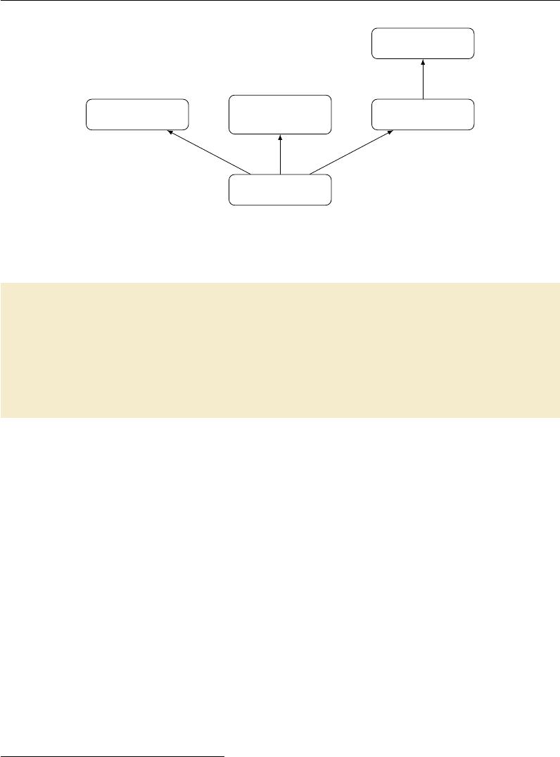
Practical Example: Skull-stripping
waffwich
peanut
butter
berries toasted waffle
waffle
Figure 1.2: How to make a waffwich
waffwich : to as ted wa ffl es berries BP
spread PB -- on waffle
ar ran ge be rri es -- on wa ffl e -- in squa res -- h al f
cut waffle
fold waffle
to as te dwaffle : waffle
toast waffle
We must note: makefiles are not linear, unlike shell scripts. toastedwaffle2
needs to be created before waffwich, but does not need to appear before it in the
script. make will search for the targets that it needs to create in whatever order it
needs to find them.
However, we’ve reached the point where we have to leave this conceptual example
because make is aware of whether something exists or not, and whether it has to
make it. It does this by assuming that the target and dependencies are files, and by
checking the dates on those files. There are many exceptions to this; but let’s accept
this simplification for the moment, and move on to a real example with files.
Practical Example: Skull-stripping
Manipulating a single subject
Follow along with this example. Copy directory
$MAKEPIPELINES/oasis-multisubject-sample/ to your home directory. You can
do this with the following command:
2Indeed, two instances of a toastedwaffle
49

Practical Example: Skull-stripping
$ cp -r $MAKEPIPELINES/oasis-multisubject-sample ~
This is a tiny sample of subjects from the OASIS data set (http://www.oasis-brains.org).
Your task is to skull strip all of these brains. However, note that first you need to
reorient each image (try looking at it in fslview). So there are two commands you
need to execute:
$ fslreorient <subject>_raw.nii.gz <subject>_T1.nii.gz
and
$ bet <subject>_T1.nii.gz <subject>_T1.skstrip.nii.gz
The first command reorients the image and the second performs the skull strip-
ping. By default, make reads files called “Makefile.” According to the manual, GNU
looks for GNUmakefile,makefile, and Makefile (in that order) but if you stick to
just one convention, you are unlikely to get confused.
Open the makefile (Makefile)that came with the directory with an editor. You
should see the following:
OA S2 _0 001_ T1_s kstr ip . nii . gz : O AS2_0001_T1 . nii . gz
bet OA S2 _00 01_T 1 . nii . gz O AS 2_00 01_T 1_sk stri p . nii . gz
OA S2 _00 01_T1 . nii . gz : O AS2_0001 _ra w . nii . gz
fs lr eorien t2s td OA S2 _00 01 _ra w . nii . gz O AS2_ 000 1_T1 . nii .
gz
Play around with this. What happens when you execute make from the command
line? What is it really doing?
Change the order of the rules. What happens? Note that by default, make starts
by looking at the first target (the first thing with a colon after it). That is why,
when you change the order of the rules, you get different outcomes, but not because
it is reading them one by one. It’s creating a directed acyclic graph, but it has to
start somewhere.
You can also tell it where to start. Delete any files that you may have created.
Leave the makefile with the rules reordered (so that the fslreorient2std rule is
first). Now type:
$ make OAS2_0001_skstrip.nii.gz
50

Practical Example: Skull-stripping
Now make starts with this target and goes on from there, working backward to
figure out what it needs to do.
Pattern rules and multiple subjects
This is great, but so far we have only processed one subject. You can create rules for
each subject by cutting and pasting the two rules you have and editing them. But
that sounds like a huge chore. And what if you get more subjects? Yuck.
You can specify in rules that you want to match patterns. Every file begins with
the subject identifier so you can use the %symbol to replace the subject in both the
target and the dependencies. However, what do you do in the recipe when you don’t !Patterns can
be matched
anywhere in
the filename,
not just at the
beginning.
know the actual names of the file you’re presently working with? The %won’t work
there. However, the symbol $* does, as you can see in the next example.
% _ T1_ sk str ip . nii . gz : % _T1 . nii . gz
bet $ * _T1 . nii . gz $* _ T1_ sks tr ip . nii . gz
% _T1 . nii . gz : % _raw . nii . gz
fs lr eorien t2s td $ * _raw . nii . gz $* _T1 . nii . gz
Using the $* to stand in for patterns can get visually ugly. One common short-
cut is to use the automatic variable $@ to replace the target, and $< for the first
dependency.
Using these new variables, our code can now be written as in this example.
% _ T1_ sk str ip . nii . gz : % _T1 . nii . gz
bet $ < $@
% _T1 . nii . gz : % _raw . nii . gz
f slr eo ri en t2 st d $ < $@
But try executing make now, with just those rules. (If you are completely lost
now, look at the file Makefile.1 to see what your makefile should look like). You
should get an error that there are no targets. Note that %does not work as a wildcard
as in the bash shell. If you are used to that behavior, you might expect make will
sense that you have a lot of files with subject identifiers, and it should automatically
expand the %to match them all. It will not do that, so you have to be explicit about
what you want to create.
For example, try typing:
$ make OAS2_0001_T1_skstrip.nii.gz
Now make has a concrete target in hand, and it can go forth and figure out if
there are any rules that match this target (and there are!) and execute them.
51
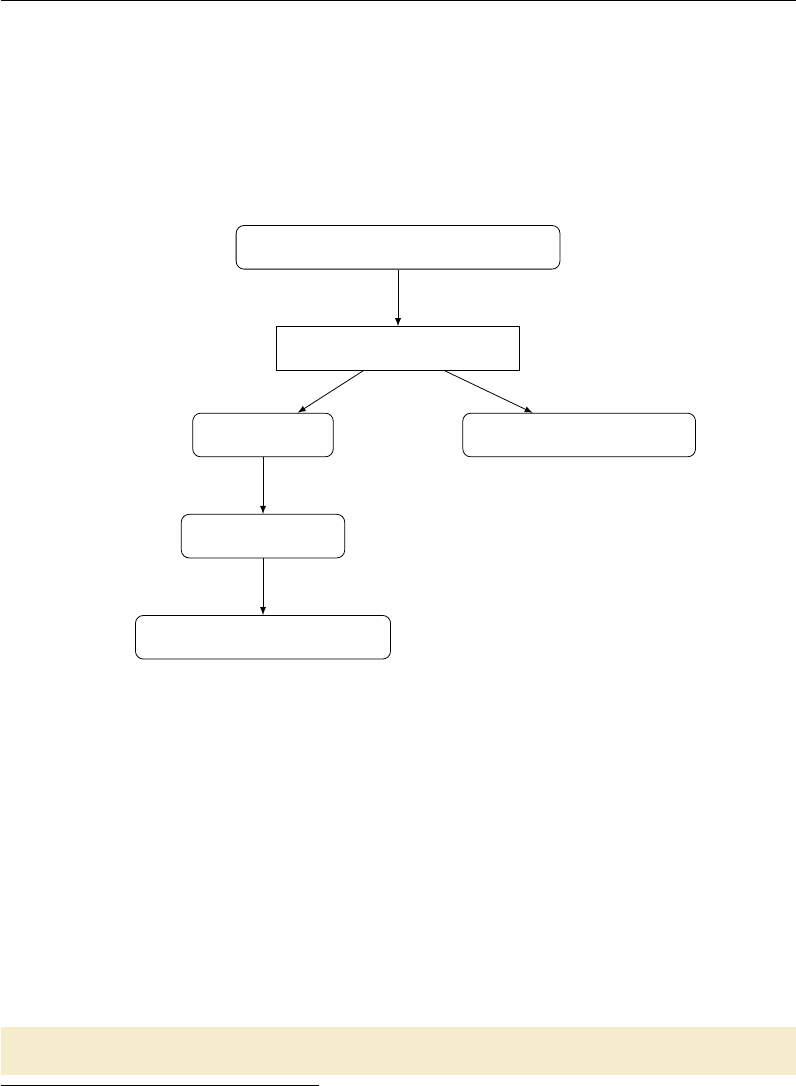
Practical Example: Skull-stripping
make will first look for targets that match exactly, and then fall through to
pattern matching.3
It can be helpful to visualize pattern matching as a sieve that catches and “knocks
off” the part that it matched, leaving only the stem. It will additionally strip any
directory information when present. For example, foo/%_T1.nii.gz: %.nii.gz
will work just as you would like.
OAS2_0001_T1_skstrip.nii.gz
%_T1_skstrip.nii.gz:
OAS2_0001 _T1_skstrip.nii.gz
%_T1.nii.gz
OAS2_0001_T1.nii.gz
Figure 1.3: Pattern-matching as a sieve
Figure 1.3 shows how make identifies a pattern from an input and applies it
to match the dependencies. Here, you can see that it is important to not include
trailing (or leading!) underscores or other characters in your expected pattern.
Phony targets
Great, but how do you specify that you want to build all of these subjects? You
can create a phony target (best placed at the top) that specifies all of the targets
you really want to make. It is called a phony target because it does not refer to an
actual file.
skstrip: OAS2_0001_T1_skstrip.nii.gz OAS2_0002_T1_skstrip.nii.
gz
3It will use more specific rules before more generic ones: see the GNU make manual for more
information on this behavior.
52

Practical Example: Skull-stripping
Add as many subjects as you’re patient enough to type and execute
$ make skstrip
Of course, typing out all the subjects (especially with ugly names like OAS2_-
0001_T1_skstrip.nii.gz) is almost as time-consuming as copying the rule multiple
times. Thankfully, there are a lot of ways to create lists of variables, shell commands,
wildcards, and most other things you might think of. Conveniently, there is a file
called subjects in this directory. We can get a list of subjects by using the following
make command.
SUBJECTS =$( shell cat subject s )
Now we can write a target for skull-stripping.
sk strip : $( SU BJE CTS := _ T1_ skstrip . nii . gz )
You must tell make that skstrip is not a real file.4Do this by using the following
statement:
. PHONY : skstrip
The pattern substitution for changing subjects to files comes from Section 8.2 of
the GNU make manual. You can look up the other options, but the basic function
of this command is to add the affix _T1_skstrip.nii.gz to each item in SUBJECTS.
The command uses the more general syntax, which can be used to remove parts
of names before adding your new affix.
$( var : su ffix = r eplacem en t )
As an esoteric example, this command could be used to replace all the final 5s
with the string “five.”
$( SUBJE CTS :5= five )
make should now fail and tell you that there is no rule to make the target OAS2_-
00five_T1.nii.gz.
Secondary targets
Now if you type make here it is going to go through and do everything, if there’s
anything to do. But it’s easier to see the point of secondary targets if you use the
-n flag for make, which asks make to tell you what it’s going to do, without actually
4Otherwise, if someone were to create a file named skstrip in this the directory, the makefile
would stop working as expected.
53

Practical Example: Skull-stripping
doing it.5It’s puzzling, isn’t it, that all the T1 files are deleted? What’s wrong
here?
Because we explicitly asked for the skull-stripped brains, make figured out it
needed to make the T1 brains. This is an implicit call. make, once it has finished
running, goes back and erases anything that was implicitly created. This is a good
thing, or a weird thing, depending on how you look at it. You can specify to make
to keep those intermediary targets by adding it to the .SECONDARY target, like so:
. S EC ON DAR Y : $ ( SU BJ ECT S := T1 . nii . gz )
An alternative method is explicitly add targets you want to keep to the phony
target.
sk strip : $( SU BJE CTS := _ T1_ skstrip . nii . gz ) $ ( SU BJECTS = _T 1_s kstrip
. nii . gz )
This is a little easier to interpret, as well. It also provides the advantage of
allowing make to realize when an intermediary target needs to be remade. For
example, if you erased only a T1 image (perhaps to rerun bet), and told it to make
skstrip, it would look and see that all the T1_brain images are newer than the
raw images, and therefore, no change needs to be made. While this problem could
be solved by also removing the T1_brain image, that’s more work and we want to
do as little of that as possible.
make clean
What if you want to clean up your work? You’ve been deleting files by hand, but with
phony targets, you don’t have to. A common approach is to create a target called
clean, which removes everything that the makefile created to bring the directory to
its original state.
clean :
rm -f * _T1 . nii . gz * _T 1_s ks tri p . nii . gz
Note that in the recipe, it’s totally fine to use wildcards. Depending on how far
along you got with your processing before you decide to clean and restart, not every
file might have been created. For this reason we typically use the -f flag for rm.
This flag hides error messages from attempting to erase nonexistent files.
The convention of putting a target for clean is just a convention; you need to
muster the discipline to add every new file that you create in a makefile to the clean
target. More dangerous is that sometimes to get a neuroimaging subject to a certain
state, you need to do some handwork that would be expensive to recreate. For
example, no one wants to blow away FreeSurfer directories after doing hand editing.
5Trevor likes to use make <cmd> -n, which makes it easier to hit ↑and remove the flag without
any annoying arrowing around.
54

Practical Example: Skull-stripping
For these reasons, we like the looser convention of mostlyclean or archive
which means to remove things that can easily be regenerated, but to leave important
partial products (e.g., your images converted from dicoms, FreeSurfer directories,
final masks, and other things).
Do not forget to add clean,mostlyclean and any other phony targets that you
find useful to your list of phony targets:
. PHONY : skstrip clean
Compare your final makefile to the finished version in Makefile.2 and you are
done with the first practical.
55
Practical 2
make in Context
Learning objectives: Organize a subject directory, run make in parallel.
Lecture: Organizing Subject Directories
In practice, a project will involve multiple subjects, each with several types of scans.
One could imagine a universal standard where every NIfTI file contained information
about where it came from and what information it contained, and all neuroimaging
programs understood how to read and interpret this information. We could dump
all of our files into a database and extract exactly what we wanted. We wouldn’t
need to use something as archaic as make because we could specify dependencies
based on the products of certain processing steps, no matter what they were called.
If you can’t imagine this, that’s totally fine, because it’s a very long way off and
won’t look like that when it’s here. Right now, we need to work with UNIX file
naming conventions to do our processing.
Therefore, selecting good naming conventions for files and for directories is key.
make specifically depends upon naming conventions so that people can keep track of
what programs and steps were used to generate what projects. See Running make in
Context for examples of good file naming conventions and typical project directory
structures.
Many of our studies are longitudinal. Even if they don’t start out that way,
if you are trying to study a developmental or degenerative disease, and you scan
subjects once, it is often beneficial to scan them again to answer new questions
about longitudinal progression. However, this aspect of study design poses some
challenges for naming conventions.
Different sites organize data in different ways. For example, the Waisman Brain
Imaging Lab has a detailed description of their preferred data organization. Because
our directory structure evolved from a large longitudinal study with cross-sectional
56

Practical Example: A More Realistic Longitudinal Directory Structure
and longitudinal analyses, we organize multiple visits for each subject as subdirecto-
ries under that subject’s main data directory. However, this organization is highly
inconvenient for processing with make.
These basic issues and the goal of minimizing complexity drive the directory
structure described in this practical.
Practical Example: A More Realistic Longitudinal
Directory Structure
Organizing Longitudinal Data
Follow along with this example. Copy directory
$MAKEPIPELINES/oasis-longitudinal-sample-small/
to your home directory using the following command:
$ cp -r $MAKEPIPELINES/oasis-longitudinal-sample-small/
This is a very small subset of the OASIS data set (http://www.oasis-brains.org),
which consists of a longitudinal sample of structural images. There are several T1
images taken at each scan session, and several visits that occurred a year or more
apart. I have reduced the size of this directory by taking only one of the T1 images
for each person, for each visit, and only of a small sample of subjects.
Look at the directory structure of subjects/. A useful command to do this is
called find. For example, if you are in the subjects directory you can type:
$ find .
You can see that as we have discussed, each subject has one to five separate
sessions. The data for each session (here, only a single MPRAGE) is stored under
each session directory. I realize that creating a directory to store what is right now a
single scan seems a bit like overkill, but in a real study there would be several types
of scans in each session directory. Here, to focus on the directory organization and
how to call make recursively, we are only looking at one type of scan.
Normally there are two types of processing that are performed for a study. The
first are subject-level analyses — in short, analyses that are completely independent
of all the other subjects. The second are group-level analyses, or analyses that
involve all the subjects data, or a subset of the subjects. In general, a good rule of
thumb is that the results of subject-level analyses are best placed within the subject
directories.
57

Practical Example: A More Realistic Longitudinal Directory Structure
Group-level analyses seem to be best found elsewhere in the project directory,
either as a subdirectory within a specific timepoint or organized at the top level.
Change into the directory visit1/ within your copy of oasis-longitudinal-sample-small:
$ cd visit1
What we want to do is create the symbolic links for each subject’s first visit here.
You can do one link by hand:
$ ln -s ../subjects/OAS2_0001/visit1 OAS2_0001
This command creates a symbolic link called OAS2_0001 to the original directory
../subjects/OAS2_0001/visit1. Now, if you enter ls -l into the command line !Your ls com-
mand may be
aliased to some-
thing pleasing,
in which case
you might see
slightly differ-
ent behavior
than described
here.
while remaining in the visit1 directory, you will notice that the subdirectory OAS2_-
0001 is symbolically linked, as indicated by an arrow, to the original target directory.
You can also check whether a file or directory is linked by using the ls -F shorthand
command, which indicates symbolic links with an symbol. The command ls -L
dereferences the symbolic links so that you can view information for the original
target file or directory itself.
You can also create symbolic links in bulk. To do so, remove the link that you
have just created and use the program in the visit1 directory (makelinks) to create
all the subject links for visit1.
!The current
directory won’t
be in your PATH,
so make sure
to call it with
./makelinks.
Take a look at the makelinks script in Figure 2.1. This script loops through
all of the subject directories that have a first visit (visit1). It extracts the subject
identifier from the directory name ($i) by using the egrep command to find the bit
of the name that matches the subject identifier pattern (OAS2_[0-9]). With this
information, it can link the subject name to the directory.
#!/bin/bash
for i in ../subjects/*/visit1
do
subject=‘echo $i| egrep -o ’OAS2_[0-9]*’‘
ln -s $i $subject
done
Figure 2.1: Script to create symbolic links within a longitudinal directory structure
58

Practical Example: A More Realistic Longitudinal Directory Structure
Recursive make
Now let’s look at the Makefile (visit1/Makefile). This is just a top-level “driver”
makefile for each of the subjects. All it does is create a symbolic link, if necessary, to
the subject-level makefile, and then it goes in and calls make in every subdirectory.
Do you know why the subject target is a phony target? The reason is that we
want make to be triggered within the subject directory every time we call it.
Create the symbolic links to the subject-level makefile as follows:
$ make Makefile
Do you know why we use the $PWD variable to create the link? If we used a relative
path to the target file, what would happen when we go to the subject directory?
Let us see how this works. Look at the subject-level makefile (Makefile.subdir).
Go into a subject directory and run make.
By now, you might be getting really tired of seeing the same fslreorient2std
and bet commands. make, by default, will echo the commands that it executes to
the terminal. If you would like it to stop doing that, you can tell it not to do that
by prepending the @character to each line.
% _ T1_ sk str ip . nii . gz : % _T1 . nii . gz
@be t $ < $@
Now go find the same subject via the subject subtree:
$ cd /oasis-longitudinal-sample-small/subjects/visit1/OAS2_0001/visit1
Type make and see that it works. Part of this magic is that we set the subject
variable correctly, even though where it appears in a directory path is different in
each place.
There is a useful little rule defined in the GNU Make Book (Chapter 2, p. 44)
that may be useful for checking that you have set variables correctly. Add the
following lines to the subject-level makefile.
print - %:
@echo $* = $( $ *)
Now if you type:
$ make print-subject
You can see the value that the variable subject is set to. Note that even if you
place this new rule at the very top of the makefile, it will not execute this rule by
59

Practical Example: A More Realistic Longitudinal Directory Structure
default. It will fall through to the next non-pattern rule. This is one of the ways in
which pattern rules (implicit rules) differ subtly from explicit rules.
Running make over multiple subject directories
Now that we have verified that the individual makefile works, we can go to the
visit1 directory and process all the subjects. First, go back and edit the subject-
level makefile to remove the @characters in front of the commands so that they are
printed.
From within the visit1/ directory, type:
$ make -n TARGET=skstrip
Note that what this is doing is (recursively) going into each subject directory
and calling make. It will do this whether or not there is anything to do within the
subject directory, because each subject directory has no dependencies. However,
because we have specified the -n flag, it prints out what commands it will perform
without actually executing them.
We can do this work in parallel. Bring up a system monitor (gkrellm is installed
on the IBIC systems). See how many processing units you have and how busy they
are. Note these numbers and get familiar with the configuration of the computers
that you have in the lab. In general, each job will require a certain amount of
memory and can use at maximum one CPU. A safe calculation for most things is
that you can normally run as many jobs at one time on a computer as you have
CPUs. This is a huge oversimplification but it will suffice for now.
You can specify to make how many CPUs to use. For example, if we specify the
-j flag with an argument of 2 (processors), we can parallelize execution of make over
two CPUs.
$ make -j 2 TARGET=skstrip
If you specify make -j without any options, it will use as many CPUS as you
have on your machine. This is great if all the work you have “fits” into the computing
resources that are available. However, if it does not, you can use a computing cluster.
In our environment, we use the Sun Grid Engine (SGE) to distribute jobs across
machines that are “clustered” together. To run on a cluster, you need to be logged
on one of the machines that is allowed to submit to the grid engine.1Once there,
you can use the command:
1In IBIC, they are: broca,dentate,homunculus,pole,pons,precuneus, and triangularis.
60

Practical Example: A More Realistic Longitudinal Directory Structure
$ qmake -cwd -V – -j 20 TARGET=skstrip
Here, we use qmake instead of make to interact with the grid engine. The -cwd
flag says to run from the current working directory, and -V says to pass along all
your environment variables. You will normally want to specify both of these flags.
The –specifies to qmake that we are done specifying qmake flags and are now giving
normal flags to make. For example, in this command we specify 20 jobs.
As an optional exercise, here you might want to set up the same directory struc-
ture for visit2/ and build everything from scratch in parallel.
Running FreeSurfer
Now let us look at an example of a subject-level analysis that we typically don’t run
within the subject directories. FreeSurfer (see ???) is a program that we use for
cortical and subcortical parcellation. It itself is a complicated neuroimaging pipeline
that can use make to drive it. It likes to put all subject directories for an analysis in
one directory, which makes it difficult to enforce the subject-level structure described.
But in general, it is much wiser to work around what the programs want to do than
to reorganize their output in ways that might break when the software is updated!
This is our approach.
The FreeSurfer example is documented in Testsubject FreeSurfer.
61

Practical 3
Getting Down and Dirty with
make
Learning objectives: Understand how to write a simple makefile for a single
subject pipeline.
Practical Example: Running QMON
As we mentioned in the previous practical, we can determine how many processing
units we have on our computer by running the system monitor. To do so, type
gkrellm into the command line. As you will see, this software also allows us to !You may
have a different
system monitor
installed at
your site. Ask
your system
administrator.
monitor the status of CPUs, memory usage, and disk space.
If the number of jobs that you need to run exceeds the number of cores that you
have, submitting jobs to the grid engine (explained in Chapter 2) might be a good
idea. But how do we check whether the machines in the cluster we are interested in
are available for batch processing? The qmon monitor is a graphical user interface
that comes with the Sun Grid Engine software. It gives us the ability to track the
status of machines in a cluster (and more besides, but you do not have to worry
about that for now).
!A list of the
clusters and ma-
chines available
for use at IBIC
can be found on
the wiki.
To run qmon, you need to be logged in to one of the cluster workstations. This
can be done by initiating a secure shell session, as follows:
$ ssh -X <username>@broca.ibic.washington.edu
If you do not specify the -X flag, you will be able to log in to the remote machine,
but graphical output (such as from fslview and emacs) will not show up on your
graphical display. The -X flag forwards this output to the computer that is managing
your graphical display.
62

Practical Example: A Test Subject
Once you have entered your password at the prompt, type qmon into the com-
mand line. Of interest to us is the first button in the panel: “Job Control.” When
you click on this, you will be able to see the number of jobs running on the cluster
and the number of jobs in the queue, along with the username of the person who
submitted those jobs. Ideally, you want to submit your jobs to the cluster when the
cluster is free.
However, this scenario does not necessarily always present itself. If you use qmake,
you will get an error by default if the grid engine is busy. You can get around this by
using the -now no options to qmake, which will cause it to wait until the grid engine
is free. For more information on how to use the grid engine to run a parallel make
workflow, refer to the manual, or Practical 2 where we covered the use of qmake.
If you are primarily employing FSL tools with make, you can use FSLPARALLEL
to submit jobs for parallel processing. Before running make, set up the following
environment variable in your shell:
$ export FSLPARALLEL=true
Once you have done this, you may go ahead and use make without parallelization
to submit jobs to the grid engine. This calls a script called fsl_sub that FSL uses to
schedule and submit jobs in parallel in the way that some of its cluster aware tools,
such as MELODIC, are capable of doing. Jobs parallelized using FSLPARALLEL will
automatically be queued under “Pending Jobs” if the cluster workstations are busy
processing other jobs.
Practical Example: A Test Subject
If you have not already, copy testsubject to your home directory as follows:
$ cp -r $MAKEPIPELINES/testsubject ~
This copy will take a few minutes, depending on what kind of file systems you
are copying from and to, because this directory is fairly large.
Go into this directory and look at its contents.
$ cd testsubject; ls
You will see four subdirectories: bin/,lib/,test001/ and freesurfer. As I
am sure you have noticed, this is a much simplified structure as compared to the
longitudinal directory structure that we looked at in the previous practical. For this
63

Practical Example: A Test Subject
example, I have eliminated the individual subject subdirectories (because there is
only one) and the symbolic links (because there is only one timepoint). This will
allow us to focus on the makefile structure for multiple types of analyses.
While there is no strict convention dictating the manner in which you should
organize your project directory, it is good practice to set up a directory tree structure
that clearly separates the various parts of your projects from one another. In most
cases, a bin/ directory stores executables and scripts that have been written for the
project. The lib/ directory, on the other hand, typically holds makefiles used for
the project (although in some IBIC project directories, a templates/ directory is
used for this purpose instead). The testsubject/ directory in this example stores
a single subject’s processed data.
Now, cd into the test001/ directory and have a look at the top-level makefile.
In the first section of the makefile (prior to the listing of the various targets and
dependencies), I have set two conditionals to check whether we have a FLAIR and
T1 image. While this may not useful when we are dealing with a single subject, you
will find that it makes processing a large number of subjects much easier. What the
two conditionals are doing is that they are asking shell to go into a subject directory
and look for files called ‘00_NOFLAIR’ and ‘00_NOT1’. For this to work, you will need
to create these files beforehand in the subject directories of subjects whom you know
do not have these images. This is relatively easy to do and makes processing less of
a pain. It will also help you to debug make, which is likely to break when it finds
that it is missing dependencies that do not exist.
If a file ‘00_NOT1’ is found, a FALSE boolean is returned, and make will not
make targets that require a T1 image as a dependency. This is specified in the next
conditional:
1ife q ( $( HA VET 1 ) , tr ue )
all : $ ( cal l print - help , all , Do s kull st ripp ing , etiv , HC v olum e
ca lc ul at ion ) T 1_s ks tr ip . nii . gz fi rst eti v
2else
all : $ ( cal l print - help , all , Do s kull s trip pi ng , etiv , HC vo lum e
calculation)
@echo " Subject ␣ is ␣ missing ␣ T1 ␣ -␣ not hing ␣ to ␣do␣ here ."
endif
1If the variable HAVET1 returns TRUE, make will make the targets listed in
all.
2If the variable HAVE1 returns FALSE, make will echo to your screen that the
subject is missing a T1 image.
Test out this conditional by making a 00_NOT1 file in the testsubject directory
like so:
$ touch 00_NOT1; make -n
64

Practical Example: A Test Subject
You will find that make will tell you that the subject is missing a T1 image and
that there is nothing to do.
Remove 00_NOT1 and try running make again. You can see that make is now
running our edited version of the first script, to conform to the Enigma protocol (see
?). The protocol may be viewed online.
Because running FIRST will take a little time, start it now and place it in the
background:
$ make first &
Estimated total intracranial volume
Let’s now turn our attention to the calculation of estimated total intracranial volume
(etiv). This can be estimated by running FreeSurfer, but FreeSurfer takes a long time
to run and had some difficulties with automatic processing of many of the subjects
in the study that this makefile was modified from.
One technique for estimating the total intracranial volume is simply to linearly
register the brain to standard space (see http://enigma.ini.usc.edu). The transforma-
tion matrix describes the scaling that is necessary to align the brain to the standard
brain. The inverse of the determinant of this transformation matrix is a scaling
factor that can be multiplied by the size of the template (e.g., the volume of the
standard space brain) to obtain an actual volume.
If you type make -n etiv, the first command that will be executed is to skull-
strip the brain. This uses the -B flag, which does bias field correction and is rather
slow. However, you can see that the T1_skstrip file is actually sitting in that
directory. So why does it want to recreate it?
Look at the dates at which the files in your testsubject/ directory were last
modified. Now look at the dates in the master directory project_space. Copying,
using cp -r, did not preserve the dates! Everything got the new date that it was
created. Up until now, we have created everything in the directories in which we are
working, from scratch.
You can avoid this by copying the files in some way that preserves the dates. For
example, you can type:
$ cp -r –preserve=time-stamps
Alternatively, you can use tar to create an archive, copy the archive, and unar-
chive it. For example, to tar up a directory called mydirectory into an archive
65

Practical Example: A Test Subject
called archive.tar in your home directory, type:
$ tar cvf ~/archive.tar mydirectory
To untar this archive that you have just created, type:
$ tar xvf ~/archive.tar
How can we “trick” make into not recreating this skull-stripped file? An easy
way is simply to touch the skull-stripped file, like so:
$ touch T1_skstrip.nii.gz
Once you have done this, go ahead and make etiv:
$ make etiv
This time, make will not try to recreate the skull-stripped file, because touching it
makes it newer than the image from which it is created. Instead, it will run FLIRT
on the T1 skull-stripped image. FLIRT is a FSL tool for linear registration, and
is used to align a brain to standard space by transforming the skull-stripped brain
image using an affine matrix. Following this, make will extract the intracranial volme
from the output matrix generated by FLIRT and print this to a comma-separated
value (csv) file.
To look at the contents of the file eTIV.csv, type:
$ cat eTIV.csv
Often, there are statistics that need to be collected for each subject. One way
to go about this is to write a program that gathers the correct statistics for each
individual, and then decide whether or not you want to call the program from within
make. I find, however, that often I want to know what those numbers are while I am
examining the output for a single individual, such as now. Thus, I normally create
a little comma separated value (csv) file that contains the subject ID and whatever
statistics I am interested in looking at. This way, I do not need to remember the
commands to obtain the statistics I want (e.g. what NIfTI file should I be looking
at? What command do I need to use to extract the right value?). This will also
allow me to go to the “top level” directory that contains all the subjects within it
and use cat to gather all the files into a single file for data analysis later on.
66

Practical Example: A Test Subject
As it is, I happen to know that this subject has a big head. And yet, the etiv file
tells us that the scaling factor is approximately 0.6. This is, of course, a contrived
example. But have a look at the skull-stripped image to see what went wrong. You
will see that too much of the brain was removed, which may have occured because
there is a lot of neck in the T1 image. As such, you will need to correct the skull-strip.
One way to do this is by specifying the center of the brain:
$ bet T1.nii.gz T1_skstrip.nii.gz -c 79,120,156
This improves the situation but it is still not great. Moreover, in a large study
(suppose you are looking at 1,000 brains), even a modest 10% failure in running a
skull-stripping program like FSL’s BET would mean having to handle 100 brains by
hand.
Look back at the makefile. You can see that there are two alternative rules for
obtaining the skull-stripped brain. My favorite way is to obtain a brain mask from
FreeSurfer. It takes many hours to run, but if you have run it, why not just use it?
But for now, consider the program robex. This is a robust skull stripping pro-
gram (?) that we can run.
$ make robex
Now check to see that the skull-stripping is better. Use whatever skull-strip you
think best represents the brain volume (so that the scaling will be improved, at least
– even if it is not perfect) and type:
$ make etiv
You should see that the scaling factor is higher than it was. Note that it is still
less than one. This is because the MNI template has “drifted” and is larger than
most actual brains.
Hippocampal volumes
By now, you should have a file called hippo.csv that contains the hippocampal
volumes from the Enigma protocol. However, we have not done the quality checking
step that is recommended by the protocol. In this example, we will add the step to
create a webpage that displays the registrations to the makefile.
This command is as follows:
67

Implementing a Resting State Pipeline: Converting a Shell Script into a Makefile
$ ${FSLDIR}/bin/slicesdir -p ${FSLDIR}/data/standard/MNI152_T1_1mm.nii.gz
*_to_std_sub.nii.gz
Run it and you can see the output. Then, delete the directory, slicesdir, that
you just created. Now, as an optional exercise, create a rule called firstqa that will
execute this command and make sure that it is part of the target to make first.
Implementing a Resting State Pipeline: Converting a
Shell Script into a Makefile
In the testsubject/test001 directory, you will find a bash script called resting-script.
The goal for this part of the practical is to convert that shell script into a makefile.
A few things that are worth taking note of:
1. Note that the shell script assumes it will never be re-run again and simply calls
mkdir xfm_dir. If this directory already exists, however, you will get an error.
To avoid this, add a -p flag to the command mkdir. This allows it to create
the specified directory if it does not exist, but to not give an error otherwise.
This is especially useful in makefiles that create deep directory structures.
2. Many FSL commands (and other neuroimaging commands) automatically add
file extensions such as .nii.gz to the input files if you do not append them.
However, a makefile will not do this. Therefore, when converting commands
from a script, you need to make sure that you don’t take such shortcuts in a
makefile. A good rule of thumb is to specify all extensions in your targets.
3. The decision whether to make something a multi-line recipe, a shell script of
its own, or a short recipe is a little arbitrary. If I think that I want to do
something often on a command line, I make it into a short shell script and call
it from a makefile. In this example, despiking with AFNI is short enough that
it can fit into a recipe.
4. However, anything complicated that constitutes a pipeline in itself is better
coded from the beginning as a makefile. Not only does this allow parallelism
and fault tolerance at a fine granularity, but you can see that it is easy to
ask someone for commands to do registrations or obtain a skull-strip from
FreeSurfer. Makefile commands can easily be shared, updated, and replaced
with the latest methods. Instead of using FSL FLIRT for registration, try
editing your makefile such that registration is done with epi_reg.
5. Note that 3dDespike is an AFNI program that has been compiled to use all
the cores in a machine. You will want to turn that off because you will do the
68

Implementing a Resting State Pipeline: Converting a Shell Script into a Makefile
parallelization yourself; this can be achieved by entering the following line in
a makefile: export OMP_NUM_THREADS=1 !To create
a makefile in
emacs, you
need to ensure
that you are in
“make”mode.
Type esc x
makefile_-
gmake_mod into
the emacs con-
sole to change
the mode you
are operating
in.
To go about translating this script into a makefile, it may help to do things one
step at a time. I recommend that you write and test one rule at a time for each
step in the workflow in the command line. This will help with debugging. Create
a rule, test it with the -n flag (which echoes to your shell what make intends to do
to make the target), then run make without the flag to create your specific target.
Then delete all the things that you have created and add the next rule. This will
allow you to see if things chain together. One of the worst things you can do (if you
are not very comfortable with make) is to write your entire makefile and then try to
figure out why it does not work as expected.
For the purposes of this exercise, create a makefile named Makefile.rest in
order to distinguish it from the top-level makefile that already exists.
To ensure that you are calling the right makefile in the command line, you should
do the following:
$ make -f Makefile.rest nameoftarget
The -f flag lets you specify the name of your makefile where the rule to creating
your target of interest exists. Recall that by default make will look for commands
in files called Makefile or makefile. Because Makefile.rest has a different name,
you need to tell make about it.
Now, let us have a look at the first part of resting-script.
If you need help with identifying your target and dependency from the shell
commands alone, you should look at the usage of the command in your terminal
window. E.g. for FLIRT, simply type flirt. You will be able to understand what
the flags mean, and from there find out what your input and output is.
The script from Figure 3.1 would look like the rules below in a makefile:
1PR OJ EC T_ HO ME =/ mnt / home / username / testsubject / tests ub je ct
2SHELL =/ bin / bash
1When creating your makefile, you must specify your project home.
2Be sure to tell make to use bash by setting the default shell.
3. PHONY = all clean
4all : xfm_dir / T1_to_MNI . mat rest_mc
5xf m_dir / T1 _to _MN I . mat : T1_sks trip . nii . gz
mkdir -p xfm_dir ;\
69

Implementing a Resting State Pipeline: Converting a Shell Script into a Makefile
#!/bin/bash
mkdir xfm_dir
#Create transformation matrices
#Making the 2mm MNI –> ANAT matrix
echo "Registering the T1 brain to MNI"
flirt -in T1_skstrip.nii.gz -ref /usr/share/fsl/data/standard/MNI152_-
T1_2mm_brain.nii.gz -omat xfm_dir/T1_to_MNI.mat
echo "Preprocessing RESTING scans..."
### MOTION CORRECTION
echo "Begin motion correction for rest.nii.gz"
mcflirt -plots rest_mc.par -in rest.nii.gz -out rest_mc -rmsrel
-rmsabs
Figure 3.1: resting-script file
fli rt - in T1 _sk str ip . nii . gz - ref / usr / share / fsl / data /
standard / MNI152_ T1_ 2mm_brai n .nii .gz - omat xfm_dir /
T1 _to _MN I . mat
6re st_ mc . nii . gz : res t . nii . gz
mc flirt - plots rest _mc . par - in rest . nii . gz - out re st_mc
-rmsrel -rmsabs
3Define your phony variable which is a special target used to tell make which
targets are not real files. clean is a common rule to remove unnecessary files, while
all is a common rule to make all your other targets.
4Define all to include all your targets.
5Format your commands to take the form of "rules" to include a target and
dependency. Every command following your [target:dependency] definition should
be entered on a new line beginning with a TAB character. The target is your
output and the dependency is your input (you can, however, have several targets
and dependencies listed under a single rule). Remember to also use ;\ at the end
of each line to tell make to read each line separately, as in the example for creating
transformation matrices. Here, we are using FSL FLIRT to create an output matrix
called T1_to_MNI.mat.
6For motion correction, our expected output (i.e. target) is rest_mc.nii.gz,
70

Implementing a Resting State Pipeline: Converting a Shell Script into a Makefile
and our input (i.e. dependency) is rest.nii.gz. The last line tells make to run FSL
mcflirt on rest.nii.gz.
71

Practical 4
Advanced Topics & Quality
Assurance with R Markdown
Learning objectives: Understand how to write self-documenting makefiles in an
organized directory structure, use macros, and write quality assurance reports using
R markdown.
Creating a make help system
It is sometimes useful to know what a makefile does without having to look through
the entire makefile itself. One way of getting that information at a glance is to create
amake help system that prints out the targets and a short summary explaining what
each target does.
To go about creating this help system, you need to create a separate “help”
makefile that tells make what to do when you call for help. Before we expand on
that, however, let us take a look at the main makefile in the testsubject directory
copied over from /project_space/.
$ cd /testsubject/test001
Let the variable $(PROJECT_HOME) represent the pathway to your testsubject
directory. You can set this variable in top-level makefile.
PR OJ EC T_ HO ME =/ you rh omedire ct ory / testsubject
Open up Makefile in an editor. You will notice that one of first few lines at the
top of the file asks make to include a makefile called help_system.mk; this is the
“help” makefile that we alluded to earlier. The include directive tells make to read
other makefiles before continuing with the execution of other things in the current
72

Makefile Directory Structure
makefile.
As you scroll down, you will see that some of the targets are followed by a call
command before their dependencies. For instance, look at the line:
robex : $( call print - help ,robex , Alte rnate skull st ripping with
ROB EX ) T1 . nii . gz
This tells make to return the target robex along with its description when
print-help is called (print-help is defined in help_system.mk, as we will see later).
Other targets such as freesurferskstrip and etiv also make calls to print-help.
Now, have a look at $(PROJECT_HOME)/lib/makefiles/help_system.mk.
hel p : ; @e cho $ ( if $ ( need - h el p ) ,, T ype ‘ $( MAKE)$( dash -f) help ‘
to get help )
This line tells make to echo the fellowing when you type make into the command
line.
$ make
Type ‘make help’ to get help
Figure 4.1: make’s Help System
The variable need-help is set such that make will filter for the word help in
your command line entry to decide whether or not you need help. If so, the function
print-help will be called, and this will result in make printing the name of your
targets and their descriptions to your shell. Depending on whether or not this will
be helpful for you, you may want to copy help_system.mk to your own project
directory and include it in your top-level Makefile.
We will not reproduce the details of how help_system.mk works in this practical.
For an excellent description of this simple but useful system, please refer to page 181
of John Graham-Cumming’s GNU Make Book, or to his blog posting.
Makefile Directory Structure
Often several people collaborate to work on analyzing different types of data from a
project and this calls for several makefiles. Or, you may wish to split up a processing
pipeline into various parts as we have in our Makefile example. In the main makefile
Makefile from the $(PROJECT_HOME)/test001 directory – and this was mentioned
earlier – you should have noticed that several other makefiles were included.
include $ ( PR OJ EC T_ HO ME ) /lib / makefile s / help_system .mk \\
in clude $( PR OJ ECT _HOME ) / lib / make fil es / re sti ng . mk \\
73

The clean target
in clude $( PR OJ ECT _HOME ) / lib / make fil es / xfm . mk \\
in clude $( PR OJ ECT _HOME ) / lib / make fil es / f cco nn ect iv ity . mk \\
in clu de $ ( P RO JE CT _HO ME ) / lib / ma ke fil es / QA . mk
Here, we see that there are makefiles for:
1. defining the make help system.
2. processing resting-state data called resting.mk (this is documented in detail
in Preprocessing Resting State Data).
3. obtaining transformation matrices for registrations called xfm.mk (see Testsub-
ject Transformations for documentation).
4. running seed-based connectivity analysis called fcconnectivity.mk (see Seed-
based Functional Connectivity Analysis I for documentation).
5. creating QA reports called QA.mk (see Testsubject QA Makefile for documen-
tation).
For a full description of the makefiles (excluding help_system.mk), we encourage
you to refer to their full documentation.
Note that makefiles should be stored in the lib directory as we did in this ex-
ample. This is good practice and helps keep your directories organized and less
cluttered. The importance of creating a tidy directory tree structure has been con-
tinually emphasized throughout this course. Refer to Practical 3 or Chapter 2 of the
manual for a more thorough discussion of the directory structure common to most
IBIC projects.
The clean target
In make, the clean target normally delete all unnecessary files that were created in
the process of running make. Remember that storage is limited on IBIC systems!
Cleaning up your project directory will make space for future projects that you will
be working on. The target itself is usually specified last in a typical make recipe,
and must be included in your list of .PHONY targets if you choose to define it.
Now, go to your $(PROJECT_HOME)/test001/ directory and open Makefile in
an editor. Scroll all the way down. You will see both an archive and clean target.
archive is a target intended to clean up the directory for archiving after a paper has
been accepted. The purpose of this target is to retain important results but remove
the partial products. Obviously, what you define as “important results” depend
upon the kind of analysis that you are doing and the amount of risk you are willing
to assume.
The clean target in this makefile includes clean_qa and clean_rest which are
themselves targets in other makefiles in the lib/ directory. Typically, files that are
“easy” to make and are no longer necessary can be removed. Other files, such as those
74

Creating New Makefile Rules On The Fly
generated by FreeSurfer’s recon-all, require more compute resources and are not
as easily remade. Other examples of files that you may not want to remove include
hand-edited files, and end stage products of quantitative processing pipelines. You
should therefore think carefully about what you want to remove and what you want
to keep.
Creating New Makefile Rules On The Fly
One of the drawbacks of implicit rules in make is that they can only substitute one
pattern at a time. For example, we may give multiple fMRI task blocks (which could
be matched by one pattern) but then wish to process each contrast of parameter
estimates (COPE) using an implicit rule. Thankfully, there is a way to “create new
makefile rules on the fly” using functions built in to make. We will work through an
example that overrides default Feat registration and does just this (see Using ANTs
Registration with FEAT).
Incorporating R Markdown into make
Quality assurance (QA) is an important step in a neuroimaging analyses pipeline.
At IBIC, data is typically preprocessed and checked for quality before proceeding
with further analyses. This can be done both qualitatively and quantitatively. Some
of the common aspects of data that are looked at include motion outliers, quality
of brain registration/normalization to a subjects-specific or standard template, and
whether brain segmentation has been performed correctly.
While neuroimaging packages usually include QA tools of their own (such as
FSL’s FEAT report), built-in QA tools have limited application when you are using
more than one neuroimaging package to process your data or if you want to view
your data in a non-traditional way.
Know that you may certainly create QA measures for each subject in your project
and inspect these one-by-one or examine NIfTI images created at various stages with
a previewer, but this may be inconvenient and time-consuming. Because there usu-
ally are several things that have to be inspected during a quality assurance procedure,
it is incredibly helpful to have images and data parameters or statistics displayed on
a single page for each subject in a project. Alternatively, you may choose to look at
a single aspect of your data and would like to concatenate a QA measure from all
of your subjects into one report. This is where R Markdown comes in.
R Markdown is an authoring format that allows us to generate reports using a
simple markup language (http://rmarkdown.rstudio.com). It is extremely versa-
tile in that it can incorporate code from multiple languages (including HTML, bash,
python and R) to generate HTML and PDF documents, or even interactive web
75

Incorporating R Markdown into make
applications.
Although QA reports be viewed using PDF documents or HTML pages, at IBIC
we prefer to use the HTML format for a couple of reasons. For one, a HTML report
gives us the ability to look at moving GIF images, which are useful when we want to
view the collected brain scans as a time series. In addition, it circumvents the issue
of pagination and allows us scroll seamlessly through all our images and statistics
in a single page. PDFs, tend to be more cumbersome to use as images may be
awkwardly split between pages and cause page breaks if they are not properly sized.
Go to the directory $(PROJECT_HOME)/freesurfer/QA and open up QA_check.html
with your internet browser.
$ iceweasel QA_check.html
Clicking on the link testsubject will redirect you to a page that holds the
images generated by FreeSurfer. Here, you can see the segmented and parcellated
brain of the subject, along with images showing the surface curvature of the brain.
This page is automatically created by FreeSurfer’s recon-all.
We can also create our own QA images to, say, check whether a T1 brain has
been properly registered to a brain in standard space. These images can be specified
as targets in your makefile as follows.
QA / images / T1_to _m ni_defo rmed . png : xfm_dir / T1_to _m ni_defo rmed .
nii . gz $( FS Lpa th ) / data / st and ard / M NI 15 2_T 1_ 2m m_br ain . nii . gz
mk di r -p QA / ima ges ;\
$ ( FS Lpa th )/ bin / s lic er $ ( w or d 1 ,$ ^) $ ( wo rd 2 ,$ ^) -s 2 -x
0.35 sla . png -y 0.35 slb . png -z 0.35 slc . png ;\
pn gap pen d sla . png + slb . png + slc . png QA / ima ges /
in term edi ate1 . png ;\
$ ( FS Lpa th )/ bin / s lic er $ ( w or d 2 ,$ ^) $ ( wo rd 1 ,$ ^) -s 2 -x
0.35 sld . png -y 0.35 sle . png -z 0.35 slf . png ;\
pn gap pen d sld . png + sle . png + slf . png QA / ima ges /
in term edi ate2 . png ;\
pngappend QA / images / i nte rme dia te1 . png - QA / images /
in term edi ate2 . png $@ ;\
rm -f sl ?. png QA / images / intermediate ?. png
Here, FSL slicer is used to create 2D images from 3D images. To get a better
understanding of how slicer is used, simply type slicer into the command line. This
FSL page also provides a brief description of what slicer does.
In the context of the above example, slicer first overlays the T1_to_mni_-
deformed image on top of the MNI152 brain. Subsequently, it creates several 2D
images named sl?.png that come from sagittal, coronal or axial slices. This is
indicated by the -x/y/z flags used followed by the name of the image generated.
76

Incorporating R Markdown into make
Note that these files are temporary! Once pngappend has been used to paste these
images next to each other to generate a single image, the temporary files are removed.
If you are using FSL slicer for more than one instance in a makefile, the temporary
files created may cause make to crash if they are given the same names and are put
into the same directory when make is run in parallel. Make sure that the names of
your outputs from FSL slicer do not overlap each other.
Given that the code used to generate QA images can be very messy and ugly, you
may want to create a bash script to create those images and call that from your QA
makefile instead. This also avoids potential problems that may arise when many sim-
ilarly named temporary files are generated that may cause make to continually over-
write these files when using a tool like FSL slicer in parallel. A wonderful example
of such a script can be found at $MAKEPIPELINES/tapping/bin/sliceappend.sh
(credit goes to Matt Peverill!).
Once we have created all the QA images we want to include in our HTML report,
we need to create a .Rmd file that tells R Markdown where to find these images.
Now let us have a look at a subsection of a .Rmd file on the next page. The file
is $(PROJECT_HOME)/lib/Rmd/fMRI.Rmd.
A.Rmd file should always begin with a demarcated section listing the title of the
report and the type of file to be created. We see that the output here is a HTML
document. toc refers to table of contents.
In R Markdown, the size of headers depend on the number of #(hash) symbols
used before the name of a header. This is akin to how the titles of major sections of a
text are rendered in the largest text size, and subsections along with sub-subsections
are printed in smaller-size text. A double hash symbol before a title will mean that
the title will be treated as a “sub-section” and be printed in smaller size than the
main headers. As the number of hash symbols used before a title increases, the text
becomes smaller.
Notice that HTML syntax is used to insert images into the report. Heights and
widths of images can be specified as well.
Assuming we want to print out some information about the subject into the
report, we can use bash within a R Markdown file to grep for the stuff we need or
cat a value from a file. In the example above, we open the bash script portion of
the file with three backticks and a curly bracket telling R that the following text
is written in bash code. Here, we are asking bash to cat the values from two text
files that gives us the mean absolute and mean relative displacement in mm (see cat
help if you are not familiar with its usage). These will then be printed out into our
HTML report.
Once we have a .Rmd file ready, we want to tell make to create the HTML report
for us. By doing so, we can parallelize the generation of QA reports. We do this
by inserting a target such as the following into our QA makefile (which is fully
documented in Testsubject QA Makefile):
77

Incorporating R Markdown into make
–-
title: Quality Assurance of Preprocessing for TASK for ID SUBJECT
output:
html_document:
keep_md: no
toc: yes
force_captions: TRUE
–-
#T1 Skull-Strip
<img src=“/project_space/makepipelines/testsubject/test001/QA/images/T1_-
skstrip.gif” width=“500px” />
#Parameters
##Time Series Difference Analysis
<img src=“/project_space/makepipelines/testsubject/test001/QA/images/TASK_-
tsdiffana.gif” width=“750px” />
# MOTION
##Motion Statistics
```{r engine=’bash’, echo=FALSE}
val=`cat /project_space/makepipelines/testsubject/test001/rest_-
dir/TASK_mean_abs_disp.txt`
echo “Mean Absolute Displacement : $val mm”
val=`cat /project_space/makepipelines/testsubject/test001/rest_-
dir/TASK_mean_rel_disp.txt`
echo “Mean Relative Displacement : $val mm”
```
Figure 4.2: Example of a R Markdown File
QA / res t_Pr epro ces si ng . html : ( PR OJ ECT _HOME ) / lib / R/ fMRI . Rmd TSNR
MotionGraphs SkullstripQA
sed -e ‘s/ SUBJECT /$ ( subject )/g ’ -e ‘s/ TASK / rest /g ’ $(
78

Incorporating R Markdown into make
word 1,$ ^) > QA/ re st _Prepro cessing . Rmd ;\
R -e ‘ library ( ‘‘ rmarkdown ’’) ; rmarkdo wn :: render (‘ ‘ QA /
r es t_ P re pr o ce ss i ng . Rmd ’ ’) ’
The target is your HTML file, and the dependencies are your .Rmd file and
your images or whatever else you decide to include in your report. The output is
dependent on the .Rmd file to trigger to regenerate when the source has been changed.
We then use sed to replace instances of the string “SUBJECT” in the R Markdown
file with the actual subject ID. The subject ID variable $subject should have been
set at the initial portion of your makefile.
make will then call R to load the package “rmarkdown” so that it can read R
Markdown, and proceed to generate/render your report, which will look something
like Figure 4.3.
Holy Bad Skullstripping! This is one of the many reasons why we do QA. The
full report can be viewed in your favorite Internet browser and can be found at
$(PROJECT_HOME)/test001/QA/rest_Preprocessing_example.html.
And that’s it!
79
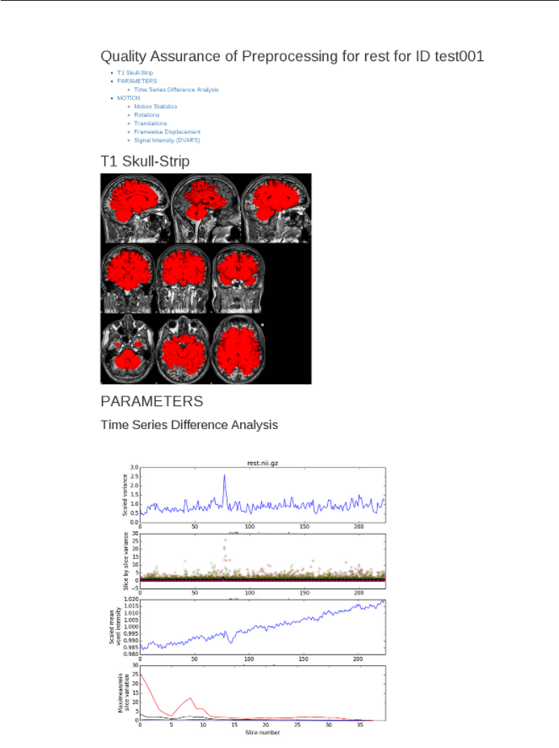
Incorporating R Markdown into make
Figure 4.3: QA report in R Markdown
80

Part III
Examples
81

This part includes examples of Makefiles included in the practical data. We
assume that you have unzipped the practical data into a directory somewhere
in your local environment. Once you have done that, you should set an environ-
ment variable called MAKEPIPELINES to refer to this directory. In the command
below we assume you have placed it in your home directory:
$ export MAKEPIPELINES=~/makepipelines
The examples included below will reference this environment variable as
necessary to find the correct files.
Please contact the example’s author with questions, or Katie Askren or
Tara Madhyastha where no specific author is listed.

Example 1
Downloading Data From XNAT
Karl Woelfer1
This is an example of how to use a Makefile to create and populate a project directory with images from an open
dataset stored in an XNAT (eXtensible Neuroimaging Archive Toolkit) database, in this case from the NITRC
(Neuroimaging Informatics Tools and Resources Clearinghouse) 1000 Functional Connectomes project image
repository at http://www.nitrc.org/ir. The code for this example is located at fcon_1000/Makefile.
To run this pipeline you will need to have first created an individual user account on NITRC, at http:
//www.nitrc.org/account/register.php, and obtained access to the 1000 Functional Connectome project.
To simplify this example, we download only a subset of the subjects in the repository. A file with the
names of these subjects is used to determine what files to download.
In our example, we selected 23 Baltimore subjects, saved in the file Subjects_Baltimore. To recreate
this file you can do the following. From the NITRC Image Repository home page “Search,” choose Projects
→1000 Functional Connectomes. At the 1000 Functional Connectomes project home page, select Options →
Spreadsheet to download a CSV file of the 1288 subjects AnnArbor_sub00306 ...Taipei_sub91183. Select
a subset, or all, of the subjects from the first column of the downloaded spreadsheet, and save to a text file.
The directory hierarchy that this Makefile creates under your project home, from which make is run, is
shown in Figure 1.1. Note that this Makefile assumes that the directory visit1 already exists.
# Site hosting XNAT
1NITRC = http :// www . nitrc . org / ir
2SHELL =/ bin / bash
# Obtain the list of subjects to retriev e from NITRC
3SUBJECTS = $( shell cat Sub jects_Ba ltimore )
4. PHONY : clean all allT1 a llT 1_brain allrest a lls ymlinks
This portion of the Makefile defines key variables and targets.
1We set the “base name” of the XNAT web site in a variable NITRC. This can be changed when using
another XNAT repository, and the variable can be named accordingly.
2By default, make uses /bin/sh to interpret recipes. Sometimes this can cause confusion, because sh
has only a subset of the functionality of bash. We set the make variable SHELL explicitly.
3The SUBJECTS variable will contain a list of the subject data we wish to download. The individual
subject names will be used to create directory names.
4We define six targets that do not correspond to files, so these are denoted as phony targets.
5all : sess ion id allT1 a llT 1_brain allre st alls ymlinks
6allT1 : $( SUBJEC TS :%= s ubjects /%/ visit1 /T1 . nii .gz )
1kwoelfer@uw.edu
83
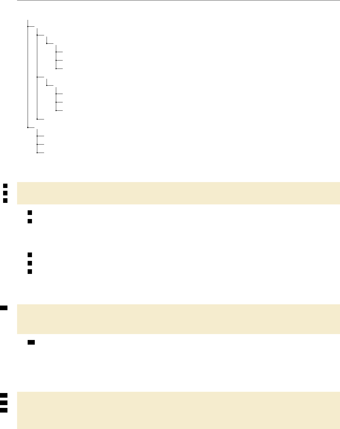
fcon_1000/
subjects/
Baltimore_sub17017/
visit1/
rest.nii.gz
T1_brain.nii.gz
T1.nii.gz
Baltimore_sub19738/
visit1/
rest.nii.gz
T1_brain.nii.gz
T1.nii.gz
...
visit1/
Baltimore_sub17017/ ...................... A symlink to ../subjects/Baltimore_sub17017/visit1
Baltimore_sub19738/
...
Figure 1.1: XNAT access directory structure.
7al lT1_brain : $( S UBJECTS :%= subjects /%/ visit1 / T1 _brain .nii . gz )
8allrest : $( S UBJECTS :%= s ubjects /%/ visit1 /rest . nii . gz )
9al lsymlinks : $( S UBJECTS :%= visit1 /%)
5all is the default target, and simply defines the five dependencies.
6We need to derive the names of all the files that we intend to create from the list of subjects. We do
this using pattern substitution to define several targets. Here, we use pattern matching to generate a list of
the T1 image names that we need to create. Each of the subject names, e.g. Baltimore_sub17017, is used to
create the corresponding T1 image (e.g. subjects/Baltimore_sub17017/visit1/T1.nii.gz).
7As above, we form the names of the skull stripped T1 images.
8And the resting state images.
9The last thing the Makefile does is create a visit1/ directory after the subjects/ directory has been
populated. Here we use pattern matching, as above, to generate the list of symbolic links that need to be
created. Each visit1/SUBJECT directory will be a symbolic link to the actual subjects/SUBJECTS/visit1/
directory.
10 sessionid :
@echo -n " Username : " ;\
read u sername ;\
curl -- user $$usernam e $( NITRC )/ REST / JSES SION > $@
10 Here we use the client URL Request Library (cURL) to create a session with the XNAT server. The
first line prompts for the user’s name on the XNAT server, the second line reads and stores that in the
variable username. With one single REST transaction, the cURL call on the following line, we authenticate
with the XNAT server, entering a password only once, and saving the return value SESSIONID in a file named
sessionid. This single session will persist for an hour. Obtaining a session identifier is important to reduce
load on the remote XNAT server.
11 su bj ect s /%/ v isit 1 / T1 . nii . gz : | s ess io nid
12 mkdir -p `dirname $@ `; \
13 curl -- c ooki e J SESSI ONID = `cat sessionid `$( NITRC )/ data / project s / fcon_ 1000 /
subjects /$*/ ex periments / $*/ scans / ALL / r esources / NIfTI / files /
sc an _m pr age_ anon ymiz ed . nii . gz > $@
84
11 This recipe downloads all of the T1 images required by target allT1 (6). It has an order-only
dependency upon the file sessionid because we assume that if these files exist, it does not matter if they are
older than the sessionid file. They will only be recreated if they do not exist.
12 This command creates the directory subjects/SUBJECT/visit1 if it does not exist (where SUBJECT
is the actual subject identifier).
13 This curl command uses the SESSIONID which was stored in the sessionid file. The URL defined
here is specific to the location where scan data of interest is stored on the NITRC instance of XNAT. Note
that $* is used in two places to refer to the subject identifer, denoted by %in the target. The XNAT file
scan_mprage_anonymized.nii.gz is downloaded and saved under the local name T1.nii.gz.
$s ub jec ts / %/ vi sit 1 / T 1_ bra in . nii . gz : | s es si oni d
mkdir -p `dirname $@ `; \
curl -- c ooki e J SESSI ONID = `cat sessionid `( NITRC )/ data / projects / fc on_1000 /
subjects /$*/ ex periments / $*/ scans / ALL / resource s / NIfTI / files /
scan_mprage_skullstripped.nii.gz > $@
This recipe is analogous to the previous one, except that it creates the skull stripped T1 images needed
by target allT1_brain.
su bj ect s /%/ v isit 1 / r est . nii . gz : | s es si oni d
mkdir -p `dirname $@ `; \
curl -- c ooki e J SESSI ONID = `cat sessionid `$( NITRC )/ data / project s / fcon_ 1000 /
subjects /$*/ ex periments / $*/ scans / ALL / resource s / NIfTI / files / sc an_rest .
nii . gz > $@
Similarly, this recipe creates the resting state images needed by allrest.
visit1/%:
ln - s ../ s ubj ec ts / $ */ vi sit1 $@
This recipe populates the project top-level visit1/ directory with symbolic links, pointers to the actual
locations of the subjects’ visit1 data downloaded above. This enables an alternate way to access the subject
data.
clean :
rm - rf subj ects ; \
rm - rf visit1 /*; \
rm -f sessio nid
This clean recipe will delete everything in subjects/, links in the visit1/ directory, and the sessionid
file.
85

Example 2
Running FreeSurfer
This is an example of how to use a makefile to execute FreeSurfer’s longitudinal pipeline. Note that FreeSurfer
itself is a large pipeline built using make. However, we do not need to know that if we treat the program
recon-all as a single executable and show how to use make to call it. Here, the Makefile functions more as a
way to permit parallel execution of recon-all rather than a way to track dependencies.
The code for this example is in oasis-longitudinal-example-small/freesurfer/Makefile.
PR OJH OME = $$ MA KE PIP EL IN ES / oasis - l ong itud ina l - samp le - s mall
1SU BJ EC TS _D IR =$( PROJHOME ) / frees ur fer
QA_TOOLS =/ usr / local / fre es urfer / QAtools_v 1 .1
FR EESURFER _SE TUP = / usr / local / fr ees urfer / st able5_3 / SetUpFree Sur fer . sh
RE CON _AL L = / usr / local / f ree sur fer / s tab le5 _3 / bin / recon - all $ ( RECON_FLAG S )
2RE CON_FLAGS = - use - mritotal - nuin tensitycor -3 T - qcache - all -notal - check
3SHELL =/ bin / bash
1FreeSurfer normally likes to work with all subjects in a single directory. We set the make variable
PROJHOME for convenience, and the SUBJECTS_DIR because it is required by FreeSurfer.
2Because we have multiple versions of FreeSurfer installed, and because it is possible to run FreeSurfer
with different flags, we set several variables that describe what version of FreeSurfer and what options we are
using in the Makefile. Note that the definition for RECON_ALL refers to RECON_FLAGS seemingly before it is set.
Recall that make dereferences variables when it uses them, so the order that these variables are set does not
matter. This is not like bash!
3By default, make uses /bin/sh to interpret recipes. Sometimes this can cause confusion, because sh has
only a subset of the functionality of bash. We can avoid such confusion by setting the make variable SHELL
explicitly.
4SUBJECTS =$( notdir $ ( wildca rd $ ( PROJHOME ) / subject s /*) )
4We need to obtain a list of subject identifiers to process. Here, we form this list by using a wildcard
to obtain all the subject directories in PROJHOME and then stripping away all the directory prefixes using the
notdir call.
SESSION=1
5inputdirs =$( SUBJECTS :%=%. t$ ( SESSIO N ))
6. PHONY : qa setup f ree surfer
7setup : $ ( inputdirs )
8%. t$ ( SESSION ) : $ ( PROJHOME )/ subjects /%/ visit$ ( SESSION )/mpr -1. nifti .nii .gz
mkdir -p $@ / mri / o rig ; \
86

cp $^ $@ / mri / orig ; \
cd $@ / mri / orig ; \
mr i_conve rt mpr -1. n ifti . nii . gz 001. mgz
5This Makefile is intended to handle a longitudinal acquisition. Normally, one indicates the timepoint
(here, the SESSION variable indicates the timepoint) by appending some suffix to the subject identifier. Here,
we append the suffix .t1 to each subject identifier to indicate that we are processing the first session. To run
the makefile on the second timepoint, one could either edit it, or set this variable when calling make as follows:
$ make SESSION=2
6We define three targets that do not correspond to files, so these are denoted as phony targets.
7The phony target setup depends upon the input directories we defined in 6.
8This recipe creates the input directories by transforming the first MPRAGE image from the subject
directory into mgz format. More complicated recipes may include conditionally choosing one of multiple
MPRAGE images, using two images if available, and so forth.
fr ees urfer : $ ( i npu tdi rs :%=%/ mri / aparc + aseg . mgz )
9%. t$ ( SE SSION ) / mri / aparc + a se g . mgz : $ ( PR OJH OME )/ su bje cts /%/ visit $ ( SE SSION ) /mpr -1.
nif ti . nii . gz
rm -rf `dirname $@ `/ IsRunni ng .*
source $( FR EE SURFER_SE TU P ) ;\
export SUBJECTS_DIR=$(SUBJECTS_DIR) ;\
$( RECON _ALL ) - subjid $ *. t$ ( SESSION ) - all
9FreeSurfer creates many output files when it runs. Here, we select one of the critical files that should exist
upon successful completion, mri/aparc+aseg.mgz to be the target of this rule. It depends upon the directory
having been created so that we can call recon-all by specifying the subject directory. You might think that
it would be wise to specify multiple FreeSurfer output files as targets. In this case, if the multiple targets are
specified using a pattern rule, the recipe would be executed only once to create the targets. However, if we did
not use a pattern rule, the recipe could be executed once per target. This is clearly not the intended behavior.
To avoid confusion, we usually pick a single late-stage output file to be the target.
10 qa : $ ( inputdir s :%= QA /%)
11 QA /%: %
source $( FR EE SURFER_SE TU P ) ;\
$( QA_ TOOLS )/ recon _c he ck er -s $*
10 We can create a number of quality assurance (QA) images from the FreeSurfer directories using the
recon_checker program. The qa target depends upon directories within the QA subdirectory. These are
created by recon_checker in 12 .
12 Makefile . lo ng it ud in al :
$(PROJHOME)/bin/genctlongitudinalmakefile > $@
11 After all the cross-sectional runs have been completed, we can run the longitudinal pipeline. The first
step in this pipeline is to create an unbiased template from all timepoints for each subject. The second step
is to longitudinally process each timepoint with respect to the template.
Here, we have a bit of a problem specifying these commands to make because each subject may have a
different number of timepoints and subjects may be missing a timepoint that is not the first or last. The
syntax of the recon-all command to create an unbiased template does not lend itself well to using wildcards
to resolve these issues:
$ recon-all -base <templateid> -tp <tp1id> -tp <tp2id> ... -all
87

We solve these problems by writing a shell script that generates a correct Makefile (Makefile.longitudinal).
This is an example of taking a “brute force” approach rather than trying to use pattern rules or something
more sophisticated. It gets the job done.
The new makefile defines a target longitudinal, and can be called as follows, adding additional flags for
parallelism.
$ make -f Makefile.longitudinal longitudinal
88

Example 3
DTI Distortion Correction with
Conditionals
Daniel J. Peterson1
In this example, we will use a Makefile to apply the appropriate distortion correction procedure automatically,
using conditionals. The code for this example may be found in dti_suceptibility_correction/subjects,
in Makefiles in the directories fugue_DTI,topup_DTI, and toy_test as described below.
First, a bit of background: The most common way to acquire a series of MRI images as quickly as possible
is to use what is called an “echo-planar imaging readout,” or “EPI.” A drawback that comes with this rapid
acquisition is that EPI images are prone to distortions due to an uneven magnetic field. Sometimes these
distortions are called “susceptibility-induced distortions,” because it is the differing magnetic susceptibility of
tissue, bone, and air that causes the magnetic field to be uneven. Fortunately, because these distortions are
constant and predictable within an imaging session, they can be undone.
We will consider two ways of undoing these distortions, each requiring at least one extra image to be
acquired. The first method is to acquire an image of the uneven magnetic field, called a “fieldmap.” This
image contains a map of the deviation from the main magnetic field, in radians/sec (the resonance frequency
of the water protons is directly proportional to the strength of the magnetic field as per the Larmor equation:
ω=γB0). To do this we will use a tool called fugue, which is distributed as part of FSL. fugue will convert
this fieldmap into a nonlinear warp, and then we can apply that warp to undo the susceptibility-induced
distortions. The other method is to acquire an additional image with the EPI readout going in the other
direction, meaning that the direction of the susceptibility-induced distortion will be reversed. We can then
use a tool called topup (also from FSL), that will warp two images with opposite distortions towards each
other, until they meet in the middle. We can then apply this computed warp to the rest of our data.
These are two different procedures that require different sets of files (an acquisition parameters file for
topup and a fieldmap for fugue), but can be part of an otherwise similar pipeline. We can use make to sense
which procedure to use based on what files are present, and assemble the appropriate prerequisites.
To help understand the behavior of make, we have created an example of a “toy” makefile, which does not
call any real programs, and can operate on empty “dummy” files. When debugging and developing makefiles
it can be useful to write such simplified makefiles, and run them with make -n. The code for this Makefile is
in dti_suceptibility_correction/subjects/toy_test/Makefile.
1SDC_METHOD = $( shell if [ -f fiel dmap ] ; then echo FUGUE ; \
elif [ -f acqpar ams ] ; then echo TOPUP ; \
els e ech o FA LSE ; fi )
motio n_ corre cted_ datas et : r aw _diff us ion_d ataset
to y_ edd y . sh r a w_ di ff us io n_ da ta se t
1djpeters@uw.edu
89

to pu p_ re su lt : ra w_dif fu sion_ dataset acqp arams
to y_ top up . sh r aw _d if f us io n_ da ta se t a cqp ar ams
2ifeq ( $( SDC_M ET HOD ) , TOPUP )
fully _co rr ect ed_di ffu sion_ datas et : r aw_di ff usion _data se t t op up _r es ul t
to y_ edd y . sh r a w_ di ff us io n_ da ta se t t op up _re su lt
else ifeq ( $( SDC_M ET HOD ) , FUGUE )
fully _co rr ect ed_di ffu sion_ datas et : m otion _corr ected _data se t f ieldmap
to y_ fug ue . sh m ot i on _c or re ct ed _d a ta se t fi eld ma p
else
3$( error ERROR : ne ither fi eldmap for FUGUE \
nor ac qui sit ion parameter file for TOPUP were found )
endif
tensor: fully_corrected_diffusion_dataset
toy_solve_tensor.sh fully_corrected_diffusion_dataset
1If there is a file called fieldmap in the working directory we want to use fugue, and if acqparams exists
instead, we want to use topup.
2When make runs, it will insert a different recipe into the set of rules depending on the value of SDC_-
METHOD. The conditional block extends until endif. The else ifeq statement in the middle is part of the
same conditional block (i.e. you only need one endif).
3It’s always a good idea to halt and raise an error if none of the expected conditions are met.
If we run this makefile to build the tensor target (using the -n flag) in a directory that contains both
raw_diffusion_dataset and fieldmap, the result looks like this:
$ make -n tensor
toy_eddy.sh raw_diffusion_dataset
toy_fugue.sh motion_corrected_dataset fieldmap
toy_solve_tensor.sh fully_corrected_diffusion_dataset
However, if both raw_diffusion_dataset and acqparams (and not fieldmap) are in the directory, we
see:
$ make -n tensor
toy_topup.sh raw_diffusion_dataset acqparams
toy_eddy.sh raw_diffusion_dataset topup_result
toy_solve_tensory.sh fully_corrected_diffusion_dataset
Figure 3.1 is a flowchart of the toy makefile.
If we were to implement this process in a bash script, the earlier “upstream” processes would need to be
part of the conditional block. An advantage of using make for workflows is that only the part that causes
the “split” in the branching logic needs to be surrounded by the if-then-else-end logic. Also note that if we
were using topup with a fieldmap, but for some reason we wanted to do just the motion correction (like for
QC, or for debugging purposes), that unused “branch” of the makefile would be available with a simple make
90
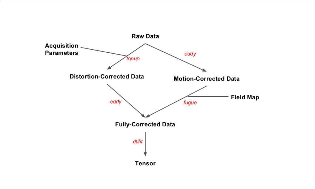
Figure 3.1: Flowchart of the Toy Makefile
motion_corrected_dataset command.
91

Here’s the full Makefile, located in dti_suceptibility_correction/subjects/fugue_DTI and dti_-
suceptibility_correction/subjects/topup_DTI. You can see each of these files is in fact a symbolic link
to the same file, located in dti_suceptibility_correction/lib/diffusion.Makefile.
ifeq " $( origin M AK EPIPELINES )" " un defined "
MA KE PI PELINES =/ pr oj ec t_ sp ac e / makepipelines
endif
PR OJECT_DIR =$ ( MAK EP IP EL INES )/ d ti_su cepti bilit y_cor rec ti on
SDC_METHOD = $( shell if [ -f fiel dmap . nii .gz ] ; then echo FUGUE ; \
elif [ -f acqpar ams . txt ] ; then echo TOPUP ; \
els e ech o FA LSE ; fi )
1NU M_ DI FFU SI ON _VOL S = $( s hell fslval r aw_ di ffu sion . nii . gz d im 4 | tr -d
'\040\011\012\015')
2ED DY_ITERATIO NS = 1
TO PUP _MO DE = fast
ECHO_SPACING =.00072
UNWARP_DIRECTION=y-
. PHONY : clean tensor
3me c_ dif fu sio n . nii . gz : r aw_d iff us ion . nii . gz bva l bvec br ain _mask . nii . gz
echo " 0 1 0 0.072 " > temp_acqp ar am s . txt ;\
for i in `seq 1 $( NU M_ DIFFU SI ON_VOLS ) `; do echo 1 >> temp_index . txt ; done
;\
eddy -- i main = r aw_ di ffu si on . nii . gz -- ma sk = b rai n_m ask . nii . gz \
-- index = temp_i nde x .txt --acqp = temp_acqparam s . txt -- bvecs = bvec \
-- bvals = bval -- out = me c_d iffusion -- niter = $( E DDY _ITERATION S ) \
--verbose ;\
rm t emp_ac qpa ra ms . txt t emp _in dex . txt
4to pu p_ resu lts_ movp ar . txt : raw_dif fus io n . nii . gz acqp arams . txt
fslroi ra w_diff usi on . nii . gz S 0_i mag es . nii . gz 0 2 ;\
topup -- imain = S0_im ages -- datain = acqpa rams . txt \
-- co nfig =$ ( P ROJ ECT_DIR ) / lib / b0 2b0_$ ( TO PUP_M ODE ) . cnf \
-- out = top up_ re su lts -- fou t = f iel d_e st -- i ou t = u nw ar pe d_ S0 _i mag es \
--verbose
ifeq ( $( SDC_M ET HOD ) , TOPUP )
sd c_ mec_ diff usi on . nii . gz : r aw_d iff us ion . nii . gz t op up _res ults _mov par . txt index . txt
eddy -- i main = r aw_ di ffu si on . nii . gz -- ma sk = b rai n_m ask -- acqp = a cqpar ams . txt \
-- index = index . txt -- bvecs = bvec --bvals = bval \
-- to pu p = t opu p_ res ul ts \
-- out = sd c_ mec_di ffus ion . nii . gz -- n it er = $( ED DY _IT ER ATIONS ) \
--verbose
else ifeq ( $( SDC_M ET HOD ) , FUGUE )
sd c_ mec_ diff usi on . nii . gz : m ec_d iff us ion . nii . gz f iel dma p . nii . gz
fugue -- loadfmap = fieldmap . nii . gz -- dwell =$ ( ECHO_SPACING ) \
-i m ec_diffusi on . nii . gz -u s dc _mec _di ff us ion . nii . gz \
-- unwarpd ir = $( UNWARP _D IRECTION ) -v
92

else
$( error ERROR : neithe r fieldmap for FUGUE nor acqu is it io n p arameter file for TOPUP
were found )
endif
tensor : sdc _me c_ di ffu si on . nii . gz brain_ mask . nii . gz bv ec bval
dtifit -k s dc _me c_ di ffu si on . nii . gz -r bvec -b bva l -m b rain_ mask -o dti
clean :
rm -f dti_ * s dc_ mec_ dif fusi on .* m ec_diffusion .* S0 _images * \
fi eld _es t . nii . gz t opup_resul ts * u nw ar ped _S 0_ ima ge s . nii . gz
1fslval returns a trailing space as part of its output, which we pipe to tr for deletion.
2The settings here are for a quick test run for demonstration purposes. For more accurate (but slower)
processing, TOPUP_MODE can be changed to ’accurate’, and EDDY_ITERATIONS can be increased to 5. Placing
the settings clearly in the Makefile makes it easy to extract them for quality assurance reports.
3In addition to running eddy, this recipe creates a simple acquisition parameters file and a simple index
file (eddy requires that you supply one). This tells eddy that all the images were acquired with the phase
encoding along the same direction. These files are deleted afterwards.
4The first two images are assumed to be the two non-diffusion weighted images (i.e. the S0images), with
the phase encoding along different directions.
There are a few more files and commands here than in the toy example, but the basic structure is the
same. It’s still missing some elements of a full-featured DTI preprocessing pipeline (for example, unwarping
the brain mask, coregistration of the fieldmap with the diffusion data, and rotation of the b-vectors), but this
example illustrates how using conditional statements in makefiles can make them more robust and versatile.
More information about the options and the formats of the files supplied to eddy,topup, and fugue is
available on the FSL website.
93

Example 4
Quantifying Arterial Spin Labeling Data
Swati D. Rane1
This is an example of how to use a makefile to quantify cerebral blood flow (CBF) from pseudo-continuous
arterial spin labeling (pCASL) data.
The code for this example is in $MAKEPIPELINES/ASLTestsubject/S001/Makefile. S001 is the name
of the subject and the folder name. In this example we assume we have one folder per subject. The folder
name reflects the subject name and contains the SUBJECTNAME_ASL.nii.gz and SUBJECTNAME_M0.nii.gz files.
The ASL file contains alternating volumes from the control and label acquisitions, where the odd volumes are
control volumes and the even volumes are the label volumes. The M0 file is a single 3D volume of the reference
proton density weighted image.
A unique feature of this example is that we have performed surround subtraction in MATLAB to improve
the signal-to-noise ratio of the ASL data. We have included a standalone MATLAB application that can be
installed with the necessary runtime binaries and libraries to complete this step. Note that this approach does
not require you to have MATLAB installed on your computer. Similarly, if you have a limited number of
floating licenses available, deploying a standalone MATLAB application does not require a floating license.
If you are not at IBIC, before running this example you must install the MATLAB runtime libraries and
surround subtraction application as follows:
Change directory to ASLTestsubject/bin and run the program SSInstaller_mcr.install as shown in
Figure 4.1.
cd $MAKEPIPELINES/ASLTestsubject/S001/Makefile
./SSInstaller_mcr.install
Figure 4.1: Installing MATLAB Runtime Libraries and surround subtraction application
The installer will, perhaps after some delay, open a splash screen with an opportunity to change connection
settings. Just click next. The next screens will prompt for a location for the installation folder (see Figure 4.2).
Enter the location of $MAKEPIPELINES/ASLTestsubject/bin whenever asked. Note that here, the value of
MAKEPIPELINES is set to /project_space/makepipelines. In your environment this will be different.
1srleven@uw.edu
94
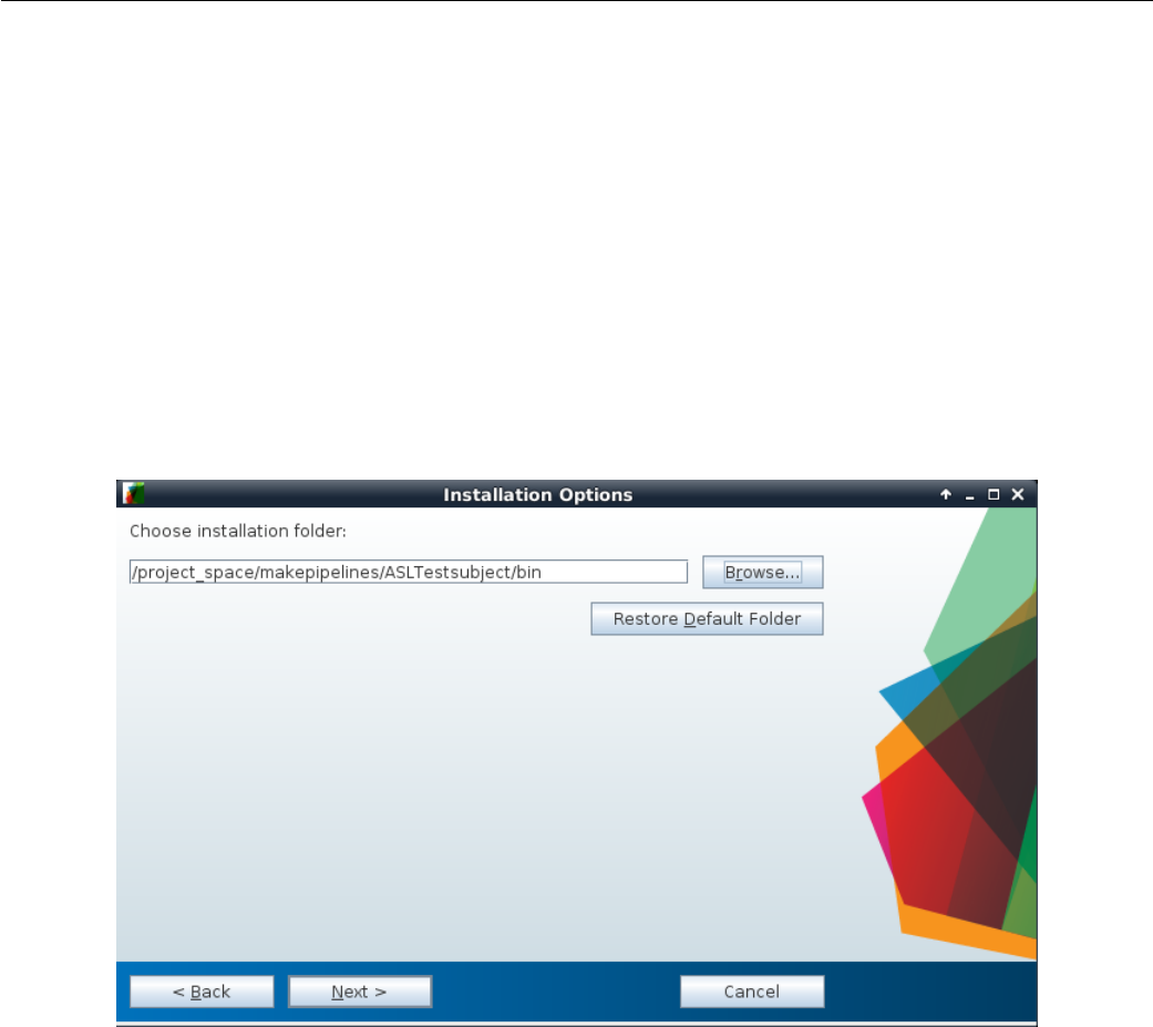
Figure 4.2: Entering location of installation folder for Surround Subtraction standalone MATLAB application.
95
SHELL =/ bin / bash
1tau = 1.5
pld = 1.525
label_eff = 0.85
T1b = 1.627
lambda =0.9
ifeq " $( origin M AK EPIPELINES )" " un defined "
MA KE PI PELINES =/ pr oj ec t_ sp ac e / makepipelines
endif
PR OJ EC T_ HO ME = $ ( MA KEPIPELINES ) / AS LT es tsubject / S001
2# FSLDIR =/ usr / share / fsl /5.0
FSL_PATH = ${ FSLDIR }/ bin
3MA TLAB_PATH = $( MAKE PI PE LI NE S )/ ASLTests ub je ct / bin
ST D_ BRA IN2mm = ${ FSLDIR }/ data / st and ard / M NI 15 2_T1 _2m m_ br ain . nii . gz
ST D_ BRAI N2mm _MA SK = $ { FSL DIR }/ d ata / stan dar d / M NI 15 2_T1 _2mm _b rain _mas k . nii . gz
ST D_BRAIN2mm_ GM = $ { FSLDIR }/ data / standard / tissuepriors / avg1 52 T1 _g ra y . img
SUBJECT = $( shell b asenam e ${ PR OJE CT_ HOM E })
1CBF quantification requires specific sequence parameters such as label duration (tau), post labeling
delay (pld), longitudinal relaxation, T1 of blood (T1b). label_eff and lambda are constants defining the
labeling efficiency for pCASL and the tissue-blood partition coefficient respectively. For convenience, we have
predefined the paths for subject directory PROJECT_HOME as well as standard template brains and masks under
STD_BRAIN2mm,STD_BRAIN2mm_MASK, and STD_BRAIN2mm_GM.
2Because we have multiple versions of FSL installed, we set variables to describe what version of FSL we
are using in the Makefile.
3The MALTAB app is a .mcr file. Double clicking will open an installation window to copy the codes
to a user-specified location. In this project, we have copied these files and folders in the bin directory under
ASLTestSubject. This can serve as the common directory for all subjects. The surround_subtraction.sh
is the shell file that calls run_Surround_Subtraction.sh generated by the MATLAB app.
. PHONY = all clean
all : ${ S UBJ ECT } _CBF _MN I . nii . gz QA / ASL . gif
${ SU BJECT } _mc_A SL . nii . gz : $ { SU BJE CT } _ASL . nii . gz ${ SU BJE CT } _M0 . nii . gz
$ { F SL_ PAT H }/ m cf lir t - in $ < - re ffi le $ ( wor d 2 ,$ ^) - out $@ ;
In this segment of code, we motion correct the ASL data using MCFLIRT in FSL. Because the ASL and
M0 data are acquired as separate scans, all ASL volumes are registered to the M0 volume. This is unlike the
motion correction typically performed in BOLD fMRI where the central dynamic is considered as the reference
volume. All remaining volumes are registered to this central volume.
# Imp lement surrou nd su bt ra ction for ca lc ul ating differences in MATLAB
4${ SUBJECT } _DeltaM . nii . gz : $ { SUBJECT } _mc_ASL . nii .gz
${ MATLAB_PA TH }/ sur round _s ubtra ct ion . sh $ < ${ MATLAB_ PA TH }
5${ SU BJECT } _CBF . nii . gz :$ { SU BJE CT } _ Del taM . nii . gz $ { SU BJECT } _M0 . nii . gz ;
$ { F SL_ PAT H }/ f sl mat hs $ < - div $ ( w or d 2 ,$ ^) t em p ;\
${ FSL _PATH }/ fslm aths temp -mul \
$( shell echo " scale =5; 6000* ${ lambda }; " | bc -l) temp ;\
96

${ FSL _PATH }/ fslm aths temp -mul \
$ ( sh ell echo " sca le =5; e ( ${ p ld }/ $ { T1b }) ; " | bc - l) tem p ;\
${ FSL _PATH }/ fslm aths temp -div \
$ ( sh ell echo " sca le =5; 2* $ { l abe l_ eff }* $ { T1b }*(1 - e (- $ { tau }/ $ { T1b }) ) ;" \
| bc -l ) $@ ;\
rm temp . nii . gz
In this section, we compute absolute values of CBF. 4The surround_subtraction.sh script evaluates
the dimensions of the ASL data (rows, columns, slices) and calls the MATLAB script via run_Surround_-
Subtraction.sh.5CBF is computed in ml/100gm/min, from the ASL white paper (?).
${ SU BJECT } _C BF_ MNI . nii . gz : $ { SUB JEC T } _M0 . nii . gz $ { SUB JEC T } _CBF . nii . gz
${ FSL_PATH }/ flirt - in $< -ref ${ STD_BRAIN2mm } -out temp . nii . gz \
- oma t c bf _t o_ MN I . m at - b ins 2 56 - c ost co rr at io - s ea rc hrx -90 90 \
- searchry -90 90 - searchrz -90 90 - dof 12 - interp t rilinear ;\
${ FSL_PATH }/ flirt - in $ ( word 2 , $ ^) -ref $ { STD_BRAIN2mm } \
- out temp . nii . gz - appl yxf m - init cb f_t o_M NI . mat ;\
${ FS L_P ATH }/ f slmath s te mp . nii . gz - mul $ { STD _BRAIN 2mm_ MAS K } $@ ;\
rm temp . nii . gz
This portion of the Makefile registers the CBF map to MNI space and removes background. We did not
have a corresponding T1 image for this ASL data. Hence we regististered the M0 image directly to the the
standard 2mm MNI template available in FSL. We then applied the subsequent transformation matrix to the
CBF map.
Ideally, if a T1 image were available, this step would be different. We would register the M0 image to the
subject’s native T1 image. The T1 image would be registered to the MNI template, and we would combine
the two transformation matrices to register the CBF map to MNI space.
QA / ASL . png :$ { SUBJ ECT } _C BF_ MNI . nii . gz
mkdir -p ${ PROJECT_HOME }/ QA ;\
${ FS L_P ATH }/ sl icer $ < - i 0 150 - a QA / ASL . png ;\
${ FSL_PATH }/ fslmat hs $ { ST D_BRAIN2m m_ GM } -thr 130 temp ;\
$ { F SL_ PAT H }/ f sl mat hs $ < - mas tem p t emp ;\
gm_cbf=`${ FSL_PATH }/ fslstats -t temp -M ';\
echo $ $gm_cbf ;\
echo " ---" > QA / ASL_QA . Rmd ;\
echo " output : html_document " >> QA / ASL_QA . Rmd ;\
echo " ---" >> QA / ASL_QA . Rmd ;\
ech o " # ASL QA " >> QA / A SL_ QA . Rmd ;\
echo `< img src = " ../ QA / ASL . png " width =900 px ; />'>> QA / ASL _QA . Rmd ;\
ech o >> QA / A SL_ QA . Rm d ;\
6echo `T ypical GM CBF = 49(2) ml /100 gm /min '> > QA / ASL _QA . Rmd ;\
ech o >> QA / A SL_ QA . Rm d ;\
echo `This subject , GM CBF = '$ $g m_c bf >> QA / A SL_ QA . Rmd ;\
7R -e `l ibr ary ( " kn itr " ) ; kn itr :: kn it 2h tml ( " QA / AS L_QA . Rmd " ," QA / A SL_ QA . html ") '
In the last section, we make a QA report for the ASL quantification process. 6Typical CBF values in the
gray matter in healthy adults is 49 ±2 ml/100gm/min and is provided as reference. This value is lower than
the standard 55 ml/100gm/min, because we did not correct for partial volume effects. In this piece of code,
we evaluate CBF in the gray matter. Because no native T1 images are available for this subject, we used the
the standard 2mm resolution gray matter mask available in FSL. As part of the QA, we generate an image of
CBF maps along the mid-sections in all three planes.
7The image for QA and the CBF values (typical and measured) are embedded in a R markdown file
which is then knit to obtain an HTML report for every subject.
clean :
97

rm -f $( wildca rd [A-Z ][0 -9][0 -9][0 -9] _CBF *. nii . gz ) \
$( wildcard [A -Z ][0 -9][0 -9][0 -9] _Del *. nii . gz ) dimen . txt ;\
rm - f $ ( w ild car d [ A -Z ] [0 -9][ 0 -9][ 0 - 9] _mc_ *. nii . gz ) t emp . n ii . gz \
cb f_ to _MN I . mat A SL_ QA . md ;\
rm -r QA
The final target clean removes intermediary NIFTI files and matrix or text files using wildcards. Prepro-
cessed images generated for QA reports can also be cleaned up this way.
98

Example 5
Processing Scan Data for a Single Test
Subject
Testsubject Main Makefile
This is an example of a subject-specific makefile that includes pipelines (written using make) that have been de-
veloped by several people to process different types of subject-level MRI data. Because there is only one subject
in this example, this subject specific makefile is not a symbolic link, as it is in the oasis-longitudinal-sample-small
directory.
The code for this example is in $MAKEPIPELINES/testsubject/test001/Makefile.
1. PHONY = etiv fast flex robex freesur ferskul lstrip
2FSL_DIR =/ usr / share / fsl /5.0
ST D_B RAI N = $( F SL_DIR ) / da ta / stan dar d / M NI152_T1 _2m m . nii . gz
ifeq " $( origin M AK EPIPELINES )" " un defined "
MA KE PI PELINES =/ pr oj ec t_ sp ac e / makepipelines
endif
3t1subj := $( shell pwd )
subject := $( notdir $( t1subj ))
PR OJ EC T_ HO ME = $( MAKEPIPELINES ) / te stsubject /
4include $ ( PR OJ EC T_ HO ME ) /lib / makefile s / help_system .mk
include $ ( PR OJ EC T_ HO ME ) /lib / mak efiles / re sting . mk
in clude $( PR OJ ECT _HOME ) / lib / make fil es / xfm . mk
include $ ( PR OJ EC T_ HO ME ) /lib / mak efiles / fccon ne ct iv ity . mk
in clu de $ ( P RO JE CT _HO ME ) / lib / ma ke fil es / QA . mk
include $ ( PR OJ EC T_ HO ME ) /lib / mak efiles / met ho dsgenerat or . mk
5export OM P_ NUM_THREADS =1
SHELL =/ bin / bash
6FLEXPATH =$ ( PROJECT_HOME )/ bin / wmpr ogram /sb / cr oss_platform / scripts
1We begin by specifying our phony targets. These will be defined later. 2This line that sets FSL_DIR
will be commented out in your makefile, but you should find out where your version of FSL is installed and
make sure that it is correct. If we do not specify the version of the programs that we run in a makefile, make
99
Testsubject Main Makefile
will use the individual’s PATH variable to find them. Because different people may have different PATH variables,
this will result in unpredictable results (the opposite of reproducibility!) Recall that make inherits variables
from your environment, and you can override them by setting them.
3It is useful to have a variable to refer to the subject. Here, we simply obtain the subject from the last
part of the directory name. This won’t work for more complicated linking structures as described in make in
Context.
4We include lots of other makefiles that we need. This keeps this makefile short and readable.
5Certain programs do their own parallelization on computers with multiple processing elements (cores).
To turn this off, we override the environment variable OMP_NUM_THREADS. This allows us to use the -j flag to
make to parallelize execution of the entire makefile.
6FLEX is a program for white matter hyperintensity quantification that we use for this project. This
variable simply specifies its location. If you do not have it installed you just won’t be able to run that part of
the processing. It is not mandatory.
7FLAIR = $( shell if [ -f 00 _NOF LAIR ] ; then echo false ; else echo true ; fi )
HAVET1 = $( shell if [ -f 00 _NOT1 ] ; then echo false ; else echo true ; fi)
8ife q ( $( HA VET 1 ) , tr ue )
9all : $ ( call print - help , all , Do s kul l st ri ppin g , etiv , HC v olu me ca lc ul at ion )
T1 _s ks tri p . nii . gz f ir st etiv
else
all : $ ( call print - help , all , Do s kull st ripp in g , etiv , HC v olu me c alc ul at io n )
@echo " Subject is missi ng T1 - nothing to do here . "
endif
7In large and complicated studies, a certain type of image may be missing, but this does not stop us
from processing all the data that we have. Here, we test for a FLAIR acquisition by looking for a marker file
in the directory called 00_NOFLAIR (and similarly for the T1).
8Here we modify the target all depending on whether or not the subject has a T1 image. We also use
the help system described in Advanced Topics & Quality Assurance with R Markdown to document what this
target does.
T1 _s ks tri p . nii . gz : T1 . nii . gz
bet $ < $@ -B
ro be x : $( call print - help , robex , Al te rna te s ku ll s tri pp ing w it h RO BEX ) T1 . nii . gz
$( PROJECT_HOME ) / bin / ROB EX / r unROBE X . sh T1 . nii . gz T 1_s kst rip . nii . gz
f re es ur fe rs ks tr ip : $ ( c al l p rint - help , fr ee su rfe rs ku lls tr ip , A lt ern at e s kull
stripping with FreeSu rf er ) $( PROJECT_HOME ) / fr eesurfer /$( subject )/ mri / brain .mgz
subj = $( su bject ) ;\
mr i_vol2vol -- mov $( PROJECT_HOME ) / fr ee surfer / $$ { subj }/ mri / brain .mgz \
-- targ $( PROJECT_HOME ) / freesurfer / $$ { subj }/ mri / rawavg . mgz \
-- r egh ead er --o brain - in - rawavg . mgz ;\
mr i_conve rt brain - in - ra wavg . mgz brain - in - rawavg . nii . gz ;\
fs lr eorien t2s td brain - in - rawavg . nii . gz T 1_skstr ip . nii . gz ;\
We have rules in this makefile for three methods of skull stripping. The default is simply to call bet with
the bias correction option (which worked well on the data for the study this makefile was modeled after).
However, when this method did not work well, we tried alternative methods using ROBEX and FreeSurfer.
Note that because the targets robex and freesurferskstrip are phony, they can be created at any time and
will always overwrite T1_skstrip.nii.gz.
etiv : $ ( call print - help , etiv , Esti mat ion of ICV using en igma proto col ) eTIV . csv
100

Testsubject Main Makefile
br ai n_t o_std . mat brain_to_std . nii . gz : T 1_s kstri p . nii . gz
flirt - in $ < -ref $ ( STD_BRAIN ) - omat $@ - out b rain_to_std . nii . gz
eTIV . csv : b rai n_to_std . mat
10 etiv = `$( P ROJ ECT_HOME ) / bin / m at2det br ai n_t o_std . mat \
| awk '{ print $$2 }' ` ;\
ech o $ ( su bje ct )" , " $$ eti v > $@
We estimate intracranial volume (ICV) using the ENIGMA protocol (as described in Getting Down and
Dirty with make). This approach calculates the inverse determinant of the linear transformation of the T1
image to standard space. This is a scaling factor that we can multiply the volume of the standard space brain
by to obtain an estimated ICV volume.
9Note that when calling the mat2det script and echoing the results to a file, we need two dollar signs
($$) for every one that we intend to pass to the shell.
fir st : f irst _all _f ast_ firs ts eg . nii . gz T1 . nii . gz hip po . csv
f ir st _a ll _f as t_ fi r st se g . n ii . gz : T1 . nii . gz
$( PROJECT_HOME ) / bin / r un_f irs t_ al l_ed it - s " L_Hipp , R _Hip p " -d -i T1 . nii . gz
-o first
hip po . csv : f ir st_a ll _fas t_fi rsts eg . nii . gz
rh = `fslstats $ < -u 54 -l 52 -V | awk `{ pri nt $$2 } ' ' ;\
lh = `fslstats $ < -u 18 -l 16 -V | awk `{ pri nt $$2 } ' ' ;\
echo $$lh $$rh > hippo . csv
We run FSL FIRST to calculate hippocampal volumes. We put these into a comma separated value file
to make it easy to remember how to extract these numbers from the first_all_fast_firstseg.nii.gz and
check them (or include them in a QA report) although there is no reason you could not write a separate
program to gather them all.
ifeq ($( FLAIR ) , true )
fle x : $ ( ca ll print - help , flex , Run fle x fo r w hit e m atte r hy pe ri nt en si ty
qu an tif ic ati on ) f lair . nii . gz fl ai r_s ks tri p . hdr f la ir _sks tr ip_f lw mt _les io ns . hdr
wm hst ats . csv
fl ai r_r es tor e . nii . gz : fl air . nii . gz
fas t - B - o fl air - t 2 $ <
fl ai r_s ks tri p . nii . gz : f lair _re stor e . nii . gz
bet $ < $@ -R
fl ai r_s ks tri p . hdr : f lair_skstr ip . nii . gz
fs lc hf il et yp e A NA LYZ E $ < $@
fla ir_s ks trip _f lwmt _les io ns . hdr : flair_sks tri p . hdr
@e ch o " F lex pr oc es sin g " $ <
$( FLE XPATH )/ sb_flex -fl $ <
fl ai r_ sk str ip _r en amed . nii . gz : f lai r_ sks tr ip . nii . gz
cp $ < $@
fl ai r_w mh _mask . nii . gz : f la ir _s ks trip _f lwmt _l esio ns . hdr
fs lm at hs $ < - ut hr 1 $@
else
flex:
101

Testsubject Main Makefile
@echo No FLAIR , nothing to do
endif
wm hst ats . csv : f la ir_s ks tr ip_f lw mt_l es ions . hdr f lair _s kst ri p_ re nam ed . nii . gz
@ec ho Writi ng wm hst ats . csv
tot = `fsl sta ts f la ir _s kst ri p_ re name d . nii . gz -V | awk `{ print $$2 } ' ' ; \
wmh = `fslstats flair _skst rip_f lwmt_ lesio ns . hdr -u 2 -V \
| awk `{ p rint $$2 } ' ' ; \
per = `echo $$wmh $$tot | awk `{ pr in t ( $$1 / $$2 ) *100} ' ' ; \
ech o $ ( su bje ct )" , " $$ wmh " , " $$ per >> $@
These are rules to run FLEX, a program for white matter hyperintensity quantification from FLAIR images.
This example comes from a multi-site study where not all subjects obtained a viable FLAIR scan. If they
do have a FLAIR scan, we bias correct, skull strip, and process the data using the program sb_flex. The
volume of white matter hyperintensities (absolute volume and percent of skull stripped brain) are written to
wmhstats.csv. If we don’t have a FLAIR scan, there is nothing to do. You may not have FLEX installed on
your system in which case you can disregard this part of the makefile.
archive:
rm - rf flair_ bc_ *
rm - rf f la ir_sk st rip_a xc or * f la ir_skst ri p_flf _ * flair_s ks trip_WM T *
rm -rf *~ \# * br ai n_t o_std . nii . gz f lair_s kst rip . hdr f lai r_ sks tr ip . img
clean : $( call print - help , clean , Clean up ev ery thing from all makefile s )
cl ean_rest clean_qa clean_ tr an sform cle an _fcco nn ectiv ity clean_p ro venance
rm - rf flair _s ks tr ip * f lair_pve * flair_restore * *~ wmhstats . csv eTIV . csv \
br ain_to_std * fl ai r_mixe lty pe . nii . gz T 1_ sks tr ip_mas k . nii . gz \
first - L_Hipp * first - R_Hipp * T1_to_std_sub * \
T1 _sk strip . nii . gz hippo . csv first *
Finally, we define two targets to help us clean up. The first target, archive, is intended to remove files
that we don’t need when we intend to "tidy up". What we remove here is very subjective and dependent upon
the needs of the researchers.
The second target, clean is intended to remove everything from all makefiles to clean up everything. Note
that clean depends upon targets such as clean_transform and clean_rest that are defined in the makefiles
we have included at the beginning.
102

Testsubject FreeSurfer
Testsubject FreeSurfer
This is an example of how to use a makefile to execute FreeSurfer in a cross-sectional context (in contrast to
Testsubject FreeSurfer), which describes a longitudinal pipeline. In addition, here we use FreeSurfer to create
a brain mask for skull stripping.
The code for this example is in $MAKEPIPELINES/testsubject/freesurfer/Makefile.
ifeq " $( origin M AK EPIPELINES )" " un defined "
MA KE PI PELINES =/ pr oj ec t_ sp ac e / makepipelines
endif
PROJHOME =$ ( MAK EP IP EL INES )/ testsubject
This first section of the code looks to see if the environment variable MAKEPIPELINES is set. This allows
people who are not at IBIC to override the default location of these files.
1include $ ( PROJH OME )/ lib / makefil es / h el p_ system . mk
2SUBJECTS = test001
export SUBJECTS_DIR = $( PROJ HOME ) / fr eesurfer
export FR EESURFER_S ETUP = / usr / local / freesurfer / s table5_3 / S etU pFreeSurfe r .sh
export RE CON _AL L = / usr / lo ca l / free surfer / st able5 _3 / bin / recon - all
export T KME DIT = / usr / lo cal / fr ees urfer / st abl e5_ 3 / bin / t kmedit
QA_TOOLS =/ usr / local / fre es urfer / QAtools_v 1 .1
export SHELL=/ bin / bash
3ou tputsta ts =$( SU BJE CTS :%=%/ mri / apa rc + aseg . mgz ) $ ( SUBJ ECT S :%=%/ mri / br ain mas k . mgz )
$( SU BJE CTS :%=%/ mri / brai nma sk . nii . gz )
4inputdirs = $( SUBJECTS :%=%)
. PHONY : all clean qa freesu rfe r
. SECONDARY : $( inputdi rs ) $( outputstats )
This portion of the Makefile defines key variables and targets. 1We make use of the help system described
in Advanced Topics & Quality Assurance with R Markdown.2There is only one subject here, so for clarity we
simply write it out. However, in real life you would have many subjects, and obtain them through a wildcard
or from a file (see Obtaining a List of Subjects). 3We use pattern substitution to specify all of the output
targets we wish to create. These are the aparc+aseg.mgz file, the brainmask.mgz file, and the brainmask
converted to NIfTI format (brainmask.nii.gz). Note that all of these files are designated as SECONDARY
targets so that they are not deleted at the end! 4We also use pattern substitution to set up the input
directories.
all : $ ( call print - help , all , Set up dir ect orie s , Run Fr eesu rfer , and Run QA ) se tup
fr eesurfer qa
freesurfer : $( call print - help , freesurfer , Run FreeSu rfer ) $( outputstats )
The all and freesurfer targets here are documented using the help system.
%/ mri / br ain mas k . mgz : %
subj = $* ;\
export FREESURFER_SETUP=$(FREESURFER_SETUP) ;\
export WATERSHED_PREFLOOD_HEIGHTS='05 15 25 35 ';\
rm -rf $$ { subj }/ scripts / IsR unning .* ;\
103

Testsubject FreeSurfer
source $$FRE ES URFER_S ET UP ;\
export SUBJECTS_DIR=$(SUBJECTS_DIR) ;\
recon - all - sub jid $$ { subj } - mu ltist rip - au torecon 1 ;\
height=`cat $$ { subj }/ mri / op ti ma l_p re fl oo d_h ei gh t ';\
if [[ $$hei ght == 05 ]]; then max =$$ (( $$height + 5 )); \
WATERSHED_PREFLOOD_HEIGHTS=`echo $$heigh t $$max '; \
else min =$$ (( $$height - 5 )); max =$$ (( $$height + 5 )); \
WATERSHED_PREFLOOD_HEIGHTS=`echo $$min $$ height $$max '; fi ;\
export WATERSHED_PREFLOOD_HEIGHTS ;\
recon - al l -s $$ { subj } - mu lt is tri p - clean - bm - g cu t
This rule creates the brain mask (in .mgz format). We use the -multistrip flag to recon-all which allows
us to try multiple preflood heights, trying different thresholds automatically. Then recon-all is continued
using the optimal height. Note that this approach will begin a separate process for each preflood height (e.g.,
four processes). This makes it a bit hard to run this pipeline on many brains in parallel. Normally, we use
this approach when we are processing subjects one at a time after they have been scanned.
%/ mri / bra inmask . nii .gz : %/ mri / bra inmask . mgz
export FREESURFER_SETUP=$(FREESURFER_SETUP) ;\
source $$FRE ES URFER_S ET UP ;\
mri_convert $< $@
This rule converts the brain mask from mgz format to NIfTI format.
%/ mri / a parc + aseg . mgz : %/ mri / brai nma sk . mgz
subj = $* ;\
export FREESURFER_SETUP=$(FREESURFER_SETUP) ;\
source $$FRE ES URFER_S ET UP ;\
export SUBJECTS_DIR=$(SUBJECTS_DIR) ;\
recon - all - s $$ { sub j } - a utore con2 - a utore con3
This rule finishes the remaining stages of recon-all. It depends upon the brain mask being generated
(the result of the previous rule).
setup : $( call print - help , setup , Setup subject direct ori es ) $( inpu tdirs )
%: $( PROJ HOM E ) /%/ T1 . nii . gz
mkdir -p $@ / mri / orig ; \
cp $^ $@ / mri / orig ; \
cd $@ / mri / orig ; \
mr i_conve rt * nii . gz 001. mgz
The setup target depends upon the T1 image in the subject directory (here, in $PROJHOME). It creates a
FreeSurfer style subject directory, copies the file there, and converts it to NIfTI format.
qa : $( call print - help ,qa , Run QA - do this i nt er ac tively with screen sa ve r \
shut off ) $ ( inputdi rs :%= QA /%)
QA /%: %
source $( FR EE SURFER_SE TU P ) ;\
$( QA_ TOOLS )/ recon _c he ck er -s $*
We run the FreeSurfer QA tools to generate images that we can put into our own reports. One problem
with QA is that the images cannot be generated in parallel in batch. We include a warning in the help system
that they should be generated interactively without a screensaver.
echo rm - rf $( inp utdirs )
Finally, we define a clean target to remove all processing results.
104
Testsubject Transformations
Testsubject Transformations
This is an example of using a makefile to create a set of transformation matrices using different registration
methods available in FSL.
The code for this example is in $MAKEPIPELINES/testsubject/lib/makefiles/xfm.mk. It is included by
$MAKEPIPELINES/testsubject/test001/Makefile. Therefore, certain variables that this example uses are
defined there. This approach helps to organize multiple makefiles and reuse rules across projects.
. PHONY = cle an_ transform transf orm s
tr an sf orm s : $ ( cal l print - help , xfm , Cre ate r es tin g s tate to M NI t ra ns fo rm at io ns )
xfm_dir xfm_ dir / MNI _t o_ re st . mat
The first line defines two phony targets (clean_transform and transforms). The .PHONY target can be
set as many times as you need to, and note that each makefile included by testsubject/test001/Makefile
defines phony targets.
The second target, xfm, uses the print-help call introduced in Advanced Topics & Quality Assurance
with R Markdown to document this main function, to create an MNI to resting state transformation.
xfm_dir:
1mkdir -p xfm_dir
2xf m_dir / T1 _to _MN I . mat : xf m_d ir T1 _skst rip . nii . gz
fli rt - in T1 _sk str ip . nii . gz - ref $ ( STD_ BRA IN ) - omat $@
1We define a target to create a directory, xfm_dir, to hold all of our transformations. This is handy
because it allows us to reuse transformations for other analyses. We know that the registrations saved here
will be checked.
2This is just a simple rule to call flirt to perform linear registration of the skull stripped T1 image to
the standard brain. Note that the definition for STD_BRAIN comes from the including makefile, as do the rules
to create the file T1_skstrip.nii.gz.
re st_ dir / r est _m c_v ol0 . nii . gz : r est _dir / r est_mc . nii . gz
fs lro i $ < $@ 0 1
xf m_dir / re st_ to_T1 . mat : re st_ dir / r es t_m c_vol0 . nii . gz T1 _sk strip . nii . gz
mkdir -p xfm_dir ;\
3ep i_re g -- epi = re st_ dir / r est_mc _vo l0 . nii . gz --t1 = T1 . nii . gz \
-- t1br ain = T1_sks trip . nii . gz --out = xf m_dir / re st_ to_T1
These rules use FSL’s epi_reg program to register the resting state data to the subject’s structural data.
We noticed that epi_reg used a lot of memory when running, limiting the number of processors that we could
use in parallel to preprocess resting state data. 3This requirement can be circumvented by using only the
first volume of the resting state data, obtained in the first rule.
xfm_dir / T1_to_ re st . mat : xfm_dir / res t_to_T1 . mat
c onv er t_ xf m - om at $@ - in ver se $ <
xfm_dir / MNI_ to_T1 . mat : xfm_dir / T1_t o_MNI . mat
c onv er t_ xf m - om at $@ - in ver se $ <
xf m_dir / MN I_to_re st . mat : xfm _dir / T 1_t o_r est . mat xf m_dir / MN I_t o_T 1 . mat
co nvert_xfm - omat xfm_dir / MNI_to_rest . mat \
- con cat x fm_d ir / T1 _to_r est . mat x fm_d ir / MN I_t o_T 1 . mat
We obtain the T1 to resting matrix by inverting the resting to T1 matrix, and similarly for the MNI to T1
matrix. Finally, these matrices are concatenated to create the final target, MNI_to_rest.mat. Notice that
everything else we needed was automatically created as necessary to make this final target.
105

Testsubject Transformations
cl ean_transfo rm :
rm -rf xfm_dir
Finally, we define a target to remove what we have created and clean up. Notice that we call it clean_-
transform, rather than simply clean, so that it does not override any other targets for cleaning up that are
included by the including Makefile.
106
Testsubject QA Makefile
Testsubject QA Makefile
This is an example of using a makefile to create quality assurance (QA) images, and then generate a final QA
report in HTML using R Markdown.
The code for this example is in testsubject/lib/makefiles/QA.mk, and it is included by
testsubject/test001/Makefile.
1NIPYPATH =/ usr / local / a nacond a /bin
FSL_DIR =/ usr / share / fsl /5.0
2. PHONY : TNSR MotionGraphs Sk ull str ipQ A Q ARepor t
3qa : $( call print - help , qa , Create QA report ) TSNR Mo tionGraphs SkullstripQA
QAreport
1As is customary in a makefile, we first define paths to locations that we want to refer to later on.
2Here, our phony targets are targets that are not actual files.
3This line tells the make help system what to do when you are unsure of what this makefile does. Here, it
will print out what the qa target does (i.e., create a QA report). See Advanced Topics & Quality Assurance
with R Markdown for more information about the help system.
4TSN R : QA / im age s / re st _t sd if fa na . gif
QA / images /% _ tsd iff ana . gif : res t . nii .gz
5mk di r -p QA / ima ges ;\
6pngout = `echo $@ | sed `s/ gif / png /g '` ;\
7$( NIP YPATH )/ nip y_ ts dif fa na -- out - file $$pngout $ < ;\
convert $$pngo ut $@ ;\
rm -f $$pn gout
4Our first target creates TSNR images for the QA. In this example, the phony target TSNR only wants
make to create a single gif image.
5This line creates a directory called QA/images if it does not already exist. The -p flag tells mkdir not to
throw an error if that directory exists, but create it if it does not. 6The variable pngout is defined to take
the filename of your target and substitute gif with png.
7Subsequently, the code calls the script nipy_tsdiffana which is located in the directory $(NIPYPATH) you
defined earlier.
The python script will generate a png image comprised of 4 graphs showing the scaled variance, slice-by-slice
variance, scaled mean voxel intensity and the max/mean/min slice variation of your resting-state time series,
as seen in the image below.
107
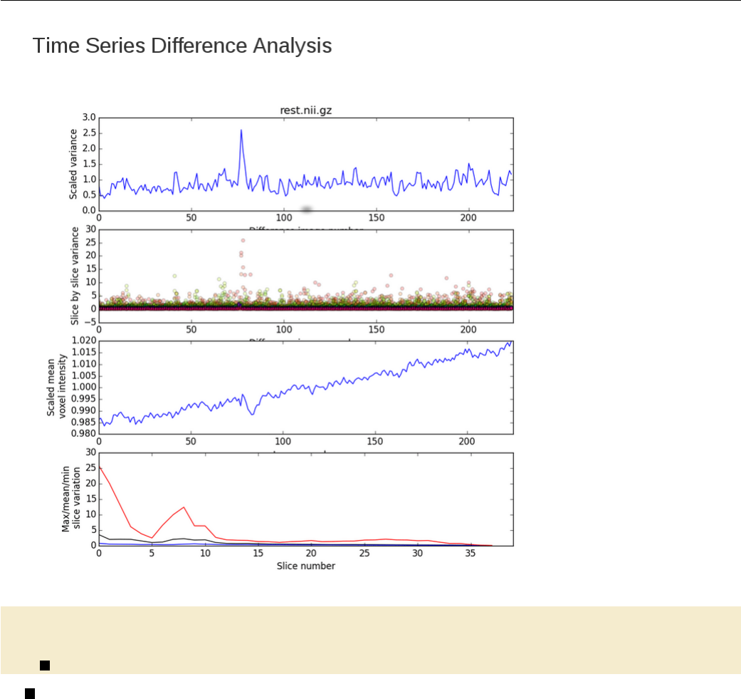
Testsubject QA Makefile
Mo ti on Gr ap hs : QA / i mag es / r es t_ Mo ti on G ra ph Ro ta ti on s . gif
QA / images / r es t_ Moti on Grap hR otat io ns . gif : r est _di r / rest _mc . nii . gz
8$( PROJECT_HOME )/ bin /R/ M ak in gG ra ph s . Rscript QA / images rest
8MakingGraphs.Rscript is a R script that will generate 4 separate graphs for you:
1. A motion rotations graph showing rotations along the x/y/z planes.
2. A motion translations graph showing translations along the x/y/z planes.
3. A framewise displacement (FD) graph to show displacement in mm across acquired volumes.
4. A signal intensity (DVARS) graph to show signal intensity across acquired volumes.
To understand the usage of an R script, it is usually necessary to look at the code itself. In this line, the R
script called with the output directory QA/images as the first argument, followed by the prefix rest to be
used for naming the output images.
108
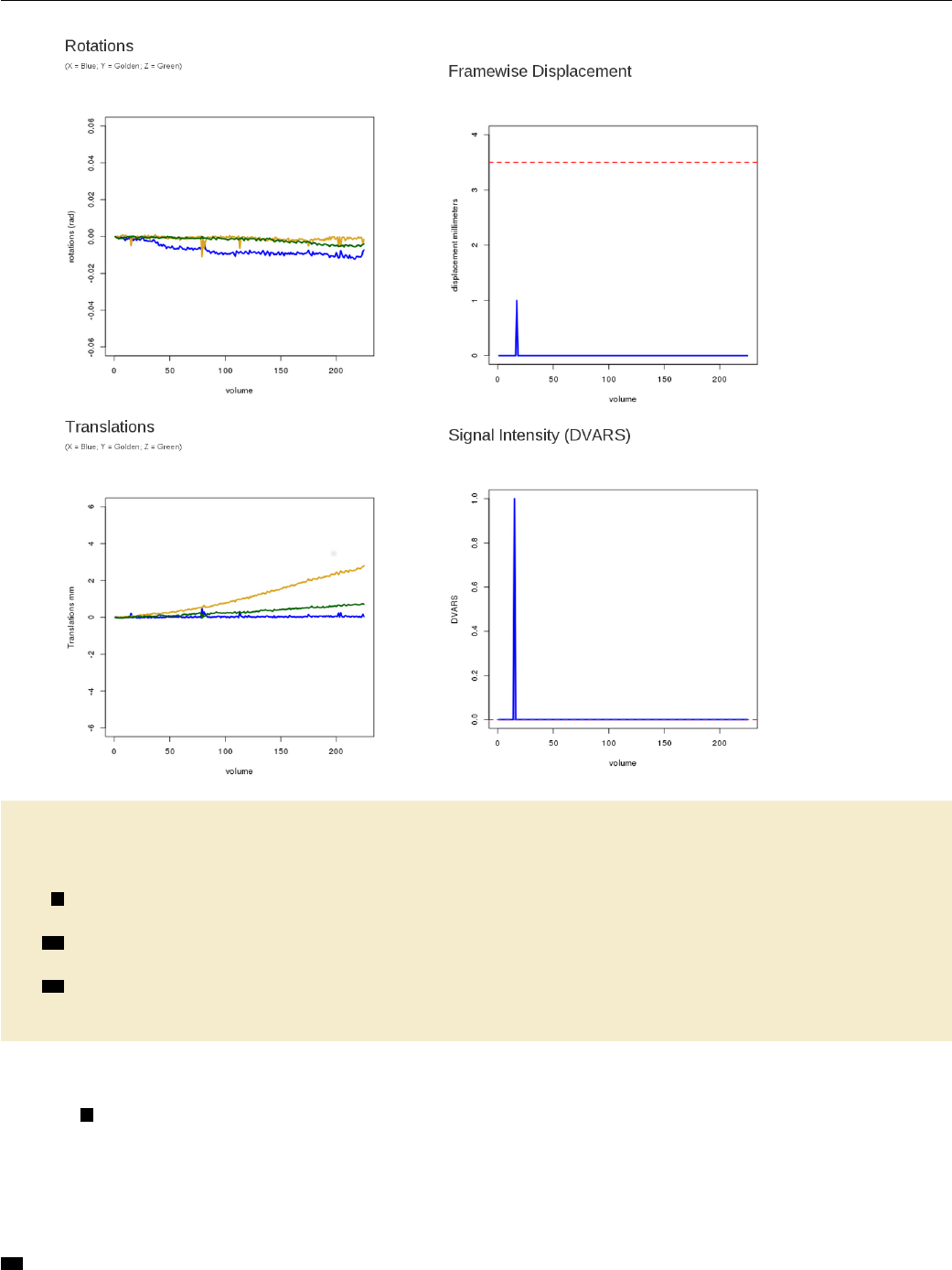
Testsubject QA Makefile
Sk ul ls tr ip QA : QA / images / T1_skstrip .gif
QA / images / T 1_s kst rip . gif : T1 . nii . gz T 1_sk str ip _mask . nii . gz
mk di r -p QA / ima ges ;\
9$( FSL_DIR )/ bin / overlay 1 1 $ < -a $( word 2 ,$ ^) 1 10 \
rendered_T1_brain.nii.gz ;\
10 $( PROJECT_HOME ) / bin / slice s r en dered_ T1_b rai n . nii . gz \
-o `dirname $@`/` basename $@ . gif`. png ;\
11 convert `dirname $@`/`basename $@ . gif`. png - re siz e 500 $@ ;\
rm r en der ed _T 1_b ra in . nii . gz ;\
rm `dirname $@`/`b asename $@ . gif`. png
To ensure that our skull-strip does not remove too much of the brain or too little of the skull, we can
create an image to overlay the skull-stripped mask generated from resting.mk on top of the T1 brain.
9FSL overlay is a tool that is used to overlay a 3D images over another. It is capable of overlaying
a maximum of 2 images on top of a reference image. Type overlay into your command line to understand how
it is used. In this line, we call overlay. The 1s that are provided as arguments specify the color and output
type of your overlay. The next argument is the background image, which in this case is the first dependency
we have listed, i.e. T1.nii.gz. The $^ refers to this file. The final output image is called rendered_T1_-
brain.nii.gz. Again, to understand the flags, you must look at overlay’s usage.
10 FSL slices is a script that calls the FSL tool slicer to create an image consisting of 3 axial, 3 sagittal
109
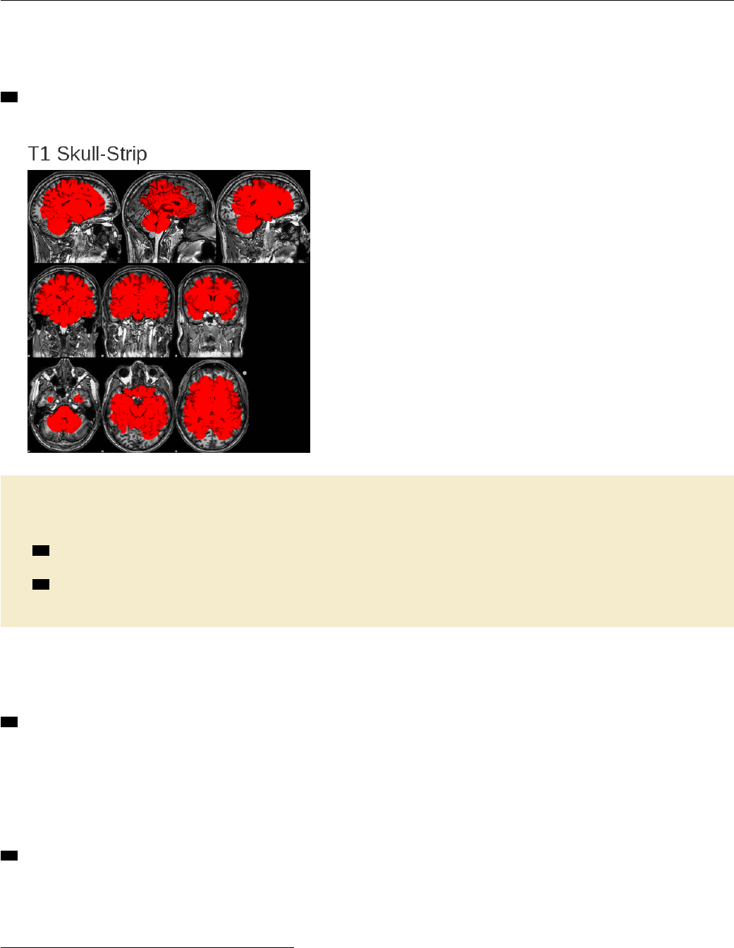
Testsubject QA Makefile
and 3 coronal slices. Here, we feed it the rendered_T1_brain.nii.gz file that we want FSL slices to use.
The output will be a file called QA/images/T1_skstrip.png. Instead of typing out the full name of the file,
however, we simply provide the directory name and basename of our target and replace .gif with .png.
11 Following this, we convert our PNG image into a GIF image, using ImageMagick’s convert that performs
the conversion and resizes the image.1
QAreport : QA / re st _Prepro ce ssing . html
QA / res t_Pr epro ces si ng . html : $ ( PROJECT_HOME ) / lib / Rmd / fMRI . Rmd TSNR MotionGraphs
SkullstripQA
12 sed -e `s / SUBJECT /$ ( subjec t )/g '-e `s / TASK / rest /g '$ ( word 1 ,$ ^) > \
QA / re st_Prep ro cessing . Rmd ;\
13 R -e `library (" rmar kdown ") ; \
rm ark dow n :: render ( " QA / r es t_Pr epr oc es sing . Rmd " )';\
rm -f QA / rest _P reproce ssing . Rmd QA / re st_Prep ro cessi ng . md
Finally, to generate our QA HTML report, we use R Markdown. We do this by writing a file called
fMRI.Rmd, which is the first dependency listed here. The fMRI.Rmd file reads the QA images that were gen-
erated in the previous portions of this makefile to create a HTML page (see Advanced Topics & Quality
Assurance with R Markdown for a brief explanation of what goes into a Rmd file and how to write one).
12 In this line, we substitute pattern strings in the fMRI.Rmd file with variables that have been defined in
the makefiles by using sed.SUBJECT, for instance, will be replaced with the $(subject) variable defined in
the main makefile $(PROJECT_HOME)/test001/Makefile.TASK will be replaced with rest, because we are
only interested in looking at the QA report for resting-state functional scans for now. We can define another
variable called task if we have several types of runs that we want to generate QA reports for (e.g., task runs or
multiple resting state runs). Once the pattern strings have been substituted, the fMRI.Rmd file will be copied
over to the QA directory and be renamed as rest_Preprocessing.Rmd.
13 This line tells R to load the ‘rmarkdown’ library so that it can read the R Markdown file. R will then
render QA/rest_Preprocessing.Rmd to create your HTML report!
To view the full report, you can open the file testsubject/test001/QA/rest_Preprocessing_example.html
in a browser.
1This step was necessary in earlier versions of R Markdown that had trouble including PNG images, but may not be necessary
for you.
110

Testsubject QA Makefile
clean_qa:
rm -rf QA
Finally, with other makefiles, we define a clean target specifically for QA. Because quality assurance is
an intermediate step in the neuroimaging processing pipeline, we do not necessarily need to retain the QA
images and reports once they have been checked.
111

Example 6
Preprocessing Resting State Data
Benjamin A. Korman1
This is an example of how to use a makefile to preprocess functional resting state data. The pipeline incorpo-
rates typical preprocessing steps taken when preparing resting state data for analysis. This example includes
motion and slice time acquisition correction, brain extraction, signal despiking, spatial smoothing and the
calculation and removal of nuisance variables.
The code for this example is in testsubject/lib/makefiles/resting.mk.
1cwd = $( shell pwd )
SUBJECTS_DIR=$(PROJECT_HOME)/freesurfer
SC RIP Tpath =$( PR OJ ECT _HOME ) / bin
FR EESURFER_H OME =/ usr / local / freesurf er / stable 5_3
2HWHM =3
TR =2
SLICEORDER =`ascending '
NPC =5
PCTVAR=0
er os io nfactor =1
1In any script or makefile, it is a good idea to set working directory variables early on to ease the script
writing process and to avoid later confusion. In this pipeline we have set a path variable for our subject
subdirectory cwd as well as for the subdirectory that is home to the FreeSurfer pipeline’s output SUBJECTS_-
DIR. In addition, we have set the variable SCRIPTpath to the subdirectory home of additional scripts that
will be called during various preprocessing steps. 2Besides directory variables, it is helpful for us to set
processing-relevant variables which can be used throughout the pipeline. Included here are variables for
the half-width-half-maximum (HWHM) kernel size needed for spatially smoothing the resting state data, the
time of repetition (TR) needed for slice time correction, as well as the number of principal components (NPC)
and percent variance (PCTVAR) needed when using principal component analysis to calculate regressors for
nuisance variables. Including these variables in the Makefile also makes it easy to extract them for inclusion
in a generated QA report.
3. PHONY : rest F reesurfer_ tes t regressors R un_ aCo mpC or postr egr ess ion cl ean_rest
. SECONDARY :
3The targets listed in the .PHONY section are targets that do not correspond to actual files. Some of
these targets (ex. regressors,postregression) are intended to be used to process the resting state data in
grouped steps whereas other .PHONY targets are related to cleanup or testing. One such target is clean_rest
1bkorman@uw.edu
112

which may be called on to eliminate all of the pipeline’s generated output when testing and debugging the
pipeline.
The .PHONY target rest is used here to easily invoke all preprocessing steps of the pipeline. This is the
target we would use to completely preprocess a subject. It is documented using the help system (see Example 4)
and depends upon all preprocessing targets, described below.
4re st _di r / r est . nii . gz : r es t . nii . gz
5echo " Setting up resting - state specif ic dire ctory "
mkdir -p rest_dir ;\
if [ ! - h re st_ dir / rest . nii . gz ];\
then \
ln -s $ ( cwd ) / rest . nii . gz re st_ dir / rest . nii . gz ;\
fi ;\
if [ ! - h re st_ dir / rest . nii . gz ];\
then \
ln -s $ ( cwd ) / T1 . nii . gz r est _di r / T1 . nii . gz ;\
fi
4This target creates resting state specific subdirectory to keep our project directory clean and organized.
We first create rest_dir and then create symbolic links within this directory to the files needed for prepro-
cessing. The required files for resting state preprocessing in this pipeline include the subject’s resting state
NIfTI image and its corresponding T1 anatomical image. 5Before we do this, we echo (i.e., print to the
screen) an informative message to provide progress information while the pipeline runs. Similar informational
messages are distributed throughout the remainder of the makefile.
re st_ dir / rest _mc . nii . gz : re st_ dir / rest . nii . gz
echo " Pr ep roc es sin g RE STING scans ... " ;\
echo " Beginn ing motion correction for rest . nii . gz using 4 dRegister " ;\
6$ ( S CR IPT pa th ) /4 d Re gi ste r . py - - inp uts $ ^ -- tr $ ( TR ) \
-- slice_order $ ( SLICEORDER ) -- ti me _i nt erp True
Our first preprocessing step once a resting state-specific subdirectory has been created is to correct the
resting state data for signal changes caused by motion and slice time acquisition. To do this we require the
unprocessed resting state data, which is the sole dependency in this recipe. 6We will use 4dRegister.py,
a script provided by the Neuroimaging in Python (NIPY) community, to apply 4D motion and slice time
correction simultaneously. The dependency rest_dir/rest.nii.gz, our input, is referred to as $ˆ for short
in the recipe. The resulting output will renamed with the _mc extension to indicate that it has been motion
corrected.
7re st_ dir / rest _be t . nii . gz : rest _di r / re st_ mc . nii . gz
echo " Skull s tripping r esti ng data with FSL 's BET " ;\
bet $ < $@ -F
7Following motion and slice time correction, we invoke FSL’s BET with the -F flag to skullstrip the 4D
resting state data. The output, referred to as $@ for short in the recipe, will be renamed _bet to indicate that
it has undergone brain extraction (aka skull stripping).
rest_dir / re st _d es pi ke . nii . gz : rest _dir / rest_bet . nii .gz
echo " De spiking the fu nct ion al data with AFNI " ;\
83 d De spi ke - s save sp ik ine ss -q $^ ;\
3 dAFNItoNIFTI despike + orig . BRIK ;\
3 dAFNItoNIFTI sp iki ness + orig . BRIK ;\
echo " Renaming output , zipping it and de leting unnecessary despike files "
;\
9mv desp ike . nii r est _di r / rest_de spi ke . nii ;\
mv s pik ine ss . nii r est_di r / r es t_s pi kin es s . nii ;\
rm - rf re st_ dir / r est_despik e . nii . gz rest _di r / r est_spik ine ss . nii . gz ;\
113

gzip r est_dir / rest_ de sp ik e . nii ;\
gzip r est _di r / r est_ spi ki nes s . nii ;\
rm -f de spike + orig * ;\
rm -f spik ine ss + orig *
8After skullstripping the brain, we perform voxel-wise despiking with AFNI to reduce noise caused by
framewise displacement. 9In addition to our despiked resting state output, a list of "spikiness" values is
produced. These are renamed to rest_despike.nii.gz and rest_spikiness.nii.gz respectively. These
output files are then compressed to save space while the original output files are removed.
10 re st_ dir / r est _s smo oth . nii . gz : r est _dir / r est_despike . nii . gz
echo " Smooth ing resting date with FSL 's SUSAN " ;\
susan $^ -1.0 $ ( HWHM ) 3 1 0 $@
10 Once the resting state data has been despiked it is ready to be spatially smoothed. To do this we use
FSL’s SUSAN with a 3D smoothing kernel 3mm in size. We rename our output with the _ssmooth extension
to indicate that it has been spatially smoothed.
11 Fr ee surfer _te st : $( SUBJECTS_DIR ) /$ ( subje ct ) / mri / brai nma sk . mgz
$( SU BJ ECT S_DIR )/$ ( su bject ) / mri / apa rc + aseg . mgz
12 xf m_dir / res t_to _fr ee su rfe r . mat : r est _di r / r est _despike . nii . gz
$( SUBJEC TS _DI R )/$ ( su bject ) / mri / apa rc + aseg . mgz
mkdir -p xfm_dir ;\
source / usr / local / fr ees urf er / stab le5_3 / Se tU pFr ee Surfer . sh ;\
export SUBJECTS_DIR=$(SUBJECTS_DIR) ;\
fslroi r est _di r / r est _d esp ike . nii . gz r est_di r / r es t_de spi ke _v ol0 0 1 ;\
bb reg ister -- s $ ( su bjec t ) -- mov r est _dir / r es t_de spi ke _v ol0 . nii . gz \
-- reg xfm_d ir / re st _t o_fr ees ur fe r . dat --init - fsl -- bold \
--o xfm_ dir / r est_ to_f ree su rf er . nii . gz \
-- fslmat xfm_dir / rest_t o_ freesur fer . mat
13 xfm_dir / freesur fer_to_ re st . mat : xf m_dir / res t_ to_fr ee surfer . mat
c onv er t_ xf m - o ma t $@ - i nve rse $ <
11 To proceed with the calculation and removal of nuisance regressors from our spatially smoothed resting
state data we first need to check whether the necessary FreeSurfer output files are available. This is because
our estimation of background noise in the data will require white matter and cerebrospinal fluid masks which
are created from the output of FreeSurfer’s recon-all segmentation process. We normally run FreeSurfer
separately, because it takes a lot longer to run than the resting state preprocessing. This target depends upon
the FreeSurfer results brainmask.mgz and aparc+aseg.mgz. If these do not exist, no processing that depends
upon this target can occur. Because the target Freesurfer_test is not an existing file (and will not at any
point be created) it is included in the .PHONY section located above.
12 Once we are certain that the necessary files exist in our FreeSurfer directory, we create a directory
(xfm_dir) in which to keep all of our data transformations. Then, using fslroi, we select the first volume of
our despiked resting state data (rest_despike_vol0) as input for FreeSurfer’s bbregister. BBregister is used
to perform within-subject, cross-modal rigid registration. 13 After registering the despiked data in FreeSurfer
space we must transform this registration back into resting state space. This is because FreeSurfer space is
unique and the pipeline will encounter problems if attempting to directly register images from FreeSurfer space
to standard (i.e. MNI) space.
14 re gre ssors : re st_ dir / f s_w Mma sk . nii . gz r est _di r / f s_c sf_mask . nii . gz
rest_dir / rest_wm . nii .gz rest_dir / re st_csf . nii .gz
15 re st_ dir / f s_w m_m ask . nii . gz : $ ( SU BJ ECT S_DIR ) /$ ( subje ct ) / mri / aparc + a seg . mgz
source / usr / local / fr ees urf er / stab le5_3 / Se tU pFr ee Surfer . sh ;\
114

export SUBJECTS_DIR=$(SUBJECTS_DIR) ;\
mr i_ bi na ri ze --i $^ -- o $@ -- e ro de 1 -- wm
re st_ dir / f s_c sf_mask . nii . gz : $ ( PR OJH OME )/ f ree sur fer / $( subje ct ) / mri / aparc + aseg . mgz
source / usr / local / fr ees urf er / stab le5_3 / Se tU pFr ee Surfer . sh ;\
export SUBJECTS_DIR=$(SUBJECTS_DIR) ;\
mr i_ bi na ri ze --i $^ -- o $@ -- e ro de 1 -- v en tri cle s
16 re st_ dir / rest _wm . nii . gz : re st_ dir / f s_w m_m ask . nii . gz r est_di r / r est_despike . nii . gz
xfm_dir / freesur fer_to_ re st . mat
fl ir t - ref $ ( wor d 2 ,$ ^) - in $ ( wor d 1 ,$ ^) - out $@ - ap ply xfm \
- init $( word 3 ,$^) ;\
fslmaths $@ -thr .5 -bin $@
re st_ dir / rest _cs f . nii . gz : rest _di r / f s_c sf_mask . nii . gz r est _di r / r est _despike . nii . gz
xfm_dir / freesur fer_to_ re st . mat
fl ir t - ref $ ( wor d 2 ,$ ^) - in $ ( wor d 1 ,$ ^) - out $@ - ap ply xfm \
- init $( word 3 ,$^) ;\
fslmaths $@ -thr .3 -bin $@
14 The target regressors is included here for ease of use if one wanted to specifically create or recreate
binarized masks from FreeSurfer’s white matter and ventricle segmentations. 15 We binarize and extract
white matter and ventricle masks. 16 We register the despiked resting state data to the white matter and
CSF masks using FSL’s FLIRT. Note that in the recipe the $(word #, $ˆ) refers to a dependency in the
dependency list. The first dependency may be referenced in the recipe as $(word 1, $ˆ), the second $(word
2, $ˆ), and so forth.
17 Ru n_ aC om pC or : rest_dir / rest_wm . txt rest_di r / rest_csf . txt
re st_ dir / rest _wm . txt : r est _di r / r est _d esp ike . nii . gz r est _dir / rest _wm . nii . gz
fs lma ths r est _di r / r est _d esp ike . nii . gz - mas re st_ dir / rest _wm . nii . gz
rest_dir / rest_wm_t s . nii . gz ;\
18 Rs crip t $ ( SC RIPTp ath )/ aC omp Cor .R r est_di r / r est _wm_t s . nii . gz $( NPC ) $ (
PCTVAR) ;\
convert rest_d ir / res t_wm_ ts_Va rianc eExpl ained . png \
rest_dir / rest _wm _t s_V arian ceExp laine d . gif ;\
rm rest_dir / re st_ wm_ts _Vari anceE xplai ned . png ;\
mv rest_dir / re st_wm_ts_pc . txt $@
rest_dir / rest_ csf . txt : re st_dir / rest_despike . nii .gz rest_dir / rest_csf . nii . gz
fs lma ths r est _di r / r est _d esp ike . nii . gz - mas re st_ dir / r est_cs f . nii . gz
re st _di r / re st _cs f_ ts . nii . gz ;\
Rs crip t $ ( SC RIPTp ath )/ aC omp Cor .R r est_di r / r est _csf_ts . nii . gz $( NPC ) \
$( PCTVAR ) ;\
convert rest_d ir / res t_csf _ts_V arian ceE xp lai ned . png \
rest_dir / re st _cs f_ts_ Varia nceEx plain ed . gif ;\
rm rest_dir / re st_ csf_t s_Var iance Exp la ine d . png ;\
mv rest _di r / r est_cs f_t s_ pc . txt $@
19 re st_ dir / r est _a bs_ pc1 . txt : rest _di r / rest _mc . nii . gz
ech o " C re ati ng lis t of m oti on r egr es so rs us in g M ot io nR eg re ss or G en er at or . py
" ;\
$( SCRIP Tp ath )/ M ot ionReg resso rG enerat or .py -i rest _dir / rest . par \
-o rest _dir / rest
20 rest_dir / rest_ nuisa nce_r eg ressor s . txt : rest _dir / rest_csf . txt r est_dir / rest_wm . txt
115

rest_dir / rest_abs_pc1 . txt
echo " Co mbine lists of motion regresso rs into one text file " ;\
pas te $ ( word 1,$ ^) $( word 2,$ ^) $( word 3 ,$ ^) rest _dir / rest_rel_pc1 . txt \
>$@
Once we have registered the despiked resting state data to the white matter and CSF masks, we need to
compute nuisance regressors. 17 The target Run_aCompCor depends upon these regressors and is a convenience
target. 18 The R script aCompCor calculate nuisance regressors from the masked resting state data. This script
can extract a set number of principal components NPC or by setting a specific percent of variance PCTVAR that
should be explained by the principal components included in the analysis. In this example we use 5 principal
components. 19 A python script named MotionRegressorGenerator, located in the bin directory, is also
called in this pipeline to calculate nuisance regressors from motion parameters. 20 The nuisance regressors
generated during this step are then combined with the nuisance regressors calculated by aCompCor into a single
text file.
21 po st reg re ssion : re st_ dir / r es t_de sig nr ange . txt re st_ dir / r es t_po stre gres sion . nii . gz
echo " Regr essing motion artifacts out of resting - state data "
22 re st_ dir / r es t_d es ignr ang e . txt : r est _di r / r es t_nu is ance _r egre ssor s . txt
Rscript $( SCRIPTpath )/ rangeArra y .R $ < $@
23 re st_ dir / r es t_po stre gres sion . nii . gz : rest _di r / r est _ssmoo th . nii . gz r est _di r /
re st _n ui sanc e_ regr es sors . txt re st_ dir / r es t_desi gnr an ge . txt
npc=`awk `{ pr int NF } '$( word 2, $ ^) | sort - nu | tail -n 1` ;\
npts =`wc -l $( word 2 , $ ^)` ;\
echo " / NumWave s $$npc " > rest_dir / rest_ re gr ess ors . feat . mat ;\
echo " / NumPoints $$npts " >> rest_d ir / rest_re gr essors . feat .mat ;\
echo " / PPheigh ts " `cat $( word 3, $ ^)` >> \
rest_dir / rest_r eg ressors . feat . mat ;\
echo " / Matrix " >> rest_di r / rest _r egressors . feat . mat ;\
cat $ ( word 2, $ ^) >> rest_di r / rest_regr ess ors . feat . mat ;\
fs l_regfi lt -i rest_ dir / r es t_s smooth . nii . gz \
-d rest _dir / r est _regre sso rs . feat . mat \
-f `seq -s , 1 1 $$npc` -o $@
24 re st_ dir / r es t_ outl ie rs_d va rs_v als . txt : r est _dir / r est_ mc . nii . gz
$( PROJECT_HOME ) / bin / m oti on _outli ers -i $ ^ \
-o rest_dir / rest_ou tl iers_ dv ars . txt \
-s r es t_ ou tl ie rs_d va rs _val s . txt -- dv ars -- no moco
re st_ dir / r es t_ outl iers _fd_ vals . txt : r est . nii . gz
$( PROJECT_HOME ) / bin / m oti on _outli ers -i $ ^ \
-o rest_dir / rest_outl ie rs_fd . txt \
-s rest_outliers_fd_vals.txt --fd
Once the nuisance regressors have been calculated and combined into a single file, the next step is to
remove them from the data. 21 This portion of the pipeline may be called specifically using the target
postregression.22 To regress out nuisance variables, we create a little FEAT design matrix and run
fsl_regfilt. We calculate the range of the included nuisance regressors using the R script rangeArray.R.
23 Finally, we denoise the data by regressing out the nuisance regressors using simple ordinary least squares
regression with FSL. 24 It may also be helpful to create text files listing motion outlier volumes based on
dvars (RMS intensity differences in images between timepoints) or framewise displacement (fd).
clean_rest :
echo " Removing all output files except for f reesurfer tr ansforms " ;\
rm -rf rest_dir
116

Lastly, we create a target to remove all files created by the pipeline. This is particularly useful when
testing and debugging the pipeline. When called, this target will simply remove the rest_dir directory and
all files located within it; in other words, everything that we have created with this Makefile.
117

Example 7
Generating A Methods Section
Benjamin A. Korman1
This is an example of how to use a makefile to automatically generate a methods section. Using a makefile to
generate methods sections saves time and limits human error when reporting MRI acquisition and preprocess-
ing parameters by obtaining the necessary values directly from the image source data, the computer system,
and the processing pipelines themselves. This is an example of how we handle provenance — we generate a
human-readable description of the pipelines while saving information about the versions of the programs used
to generate them.
We do this in two steps. First, important parameters are written to a comma-separated value (CSV) file.
These are extracted from wherever appropriate for the study using a bash shell script. For example, versions
of tools such as FSL and AFNI can be obtained from the system. Imaging acquisition parameters can be
obtained from the PAR file (a Philips human-readable parameter file), or the DICOMs, or any other exported
parameter specification file appropriate to your study. Parameters that are used in the processing pipelines
themselves can be obtained from those makefiles. After the CSV file is complete, we render an R Markdown
file that loads those values and generates an HTML report. We include PubMed links to references in the R
Markdown file so that, if necessary, the links can be used to import bibliographic records into bibliographic
software databases.
The code for this example is in testsubject/lib/makefiles/methodsgenerator.mk. This example
builds upon the other processing pipelines in place for testsubject,dti_susceptibility_correction, and
ASLTestsubject. It describes the resting state processing pipeline in Preprocessing Resting State Data, the
DTI susceptibility-correction pipeline in DTI Distortion Correction with Conditionals, and the ASL processing
pipeline in Quantifying Arterial Spin Labeling Data.
1rs _p ar so ur ce = $( wildcard parrecs /* REST *. PAR )
t1 _p ar so ur ce = $( wild card parrecs /* MPRAGE *. PAR )
dt i_ pa rsource =$( wildca rd parrecs /* DTI *. PAR )
as l_ pa rsource =$( wildca rd parrecs /* ASL *. PAR )
This makefile begins by 1searching for and selecting the PAR source files from which the makefile will
acquire the majority of the generated methods section’s parameter values. Because the naming conventions
for the PAR files do not often follow a specific pattern, we use a wildcard to search for a string we are sure
will be in the file name.
2rs_framewisedisplacement="\#"
rs_accelerationfactor="\#"
t 1_ sh oti nt er va l = " \# "
d ti _a cc el er at i on fa ct or = " \# "
asl_invertpulse1="\#"
1bkorman@uw.edu
118

asl_invertpulse2="\#"
asl_labelduration="\#"
a sl _p os tl ab el de la y = " \# "
asl_M0_repetitiontime="\#"
2Not all of the necessary parameter values are available in PAR files, so there are few parameters that
must be set (by replacing the #’s specified for these values). Here we wish to report framewise displacement
and acceleration factor used during resting-state data acquisition as well as the shot interval during the T1
anatomical scan acquisition along with parameters important for diffusion tensor imaging (DTI) and arterial
spin labeling (ASL) processing. This makefile currently reports parameters important to resting-state, DTI,
and ASL data and preprocessing but may be expanded to include other MRI techniques as well (e.g. voxel-
based morphometry and susceptibility-weighted imaging).
3. PHONY : prov enance clean _pr ovenance
. SECONDARY :
4pr ov en anc e : $ ( cal l print - help , p rove nanc e , " Au to ma ti ca ll y g en era te a m eth ods s ect io n
") prove na nc ed ir proven an ce / p ar ame te r_table . csv pr ovenance / Met ho ds_ Generat or .
html
3The targets listed in the .PHONY section are targets that do not correspond to actual files. The target 4
provenance may be called to undertake all necessary steps towards creating an automated methods section
while the target clean_provenance may be invoked to eliminate all of the makefile’s generated output, useful
for testing and debugging purposes.
5pr ov en ancedir :
echo " Creating p rovenance directory " ;\
mkdir -p pro ve nance
6provenance / paramet er _t able . csv : p ro ve nancedir $ ( rs_parsource ) $( t1_parsource ) $(
dt i_ pa rsource ) $( a sl _p arsource )
echo " Creati ng pa rameter table " ;\
bash $ ( PROJECT_HOME ) / bin / M etho ds_ Ge ne rat or . sh $( r s_p arsource ) $ (
t1 _p ar so ur ce ) $( dti_pars ou rc e ) $ ( asl _p arsource ) $(
rs _fr am ewise displ aceme nt ) $( rs _a ccele rationf actor ) $( t1_shoti nt er val ) $
( dti_a cc elera tionf ac tor ) $( asl_in ve rt pulse1 ) $ ( asl_inver tp ulse2 ) $(
as l_label du ration ) $ ( asl_pos tlabeld el ay ) $( as l_M0_ re petit iontime ) > $@
5This target creates a data provenance subdirectory to keep our project directory clean and organized.
The files generated by this makefile will be stored in this folder. 6Once a methods specific subdirectory has
been created it is time to extract the parameter values we wish to include in our methods section from their
respective PAR files and tabulate them appropriately. This is done by 7calling a bash script which generates
a table including the parameters’ name (both an abbreviated form as well as a long form), value, and unit of
measurement if applicable.
provenance / Methods _G enerato r . html : provenance / parameter_t ab le .csv
echo " C reating methods secti on html file " ;\
cd provenance ;\
cp $( PR OJ ECT _HOME ) / lib / Rmd / Met hods _Ge ne rato r . Rmd . ;\
Rscript -e `li brary ( " rmarkdow n "); \
rm ark dow n :: render ( " Met hod s_ Ge ner at or . Rmd " )'
Using the parameter_table.csv file created in the previous step, an R script is called to incorporate the
necessary parameter values into a model methods section R Markdown (.Rmd) file. One thing that is a little
frustrating about R Markdown is that it will look for files in the directory in which it is located. This is why
we first copy it to the provenance subdirectory. The R Markdown file then looks for the CSV file in the
current working directory, with no need to pass paths back and forth between programs.
119
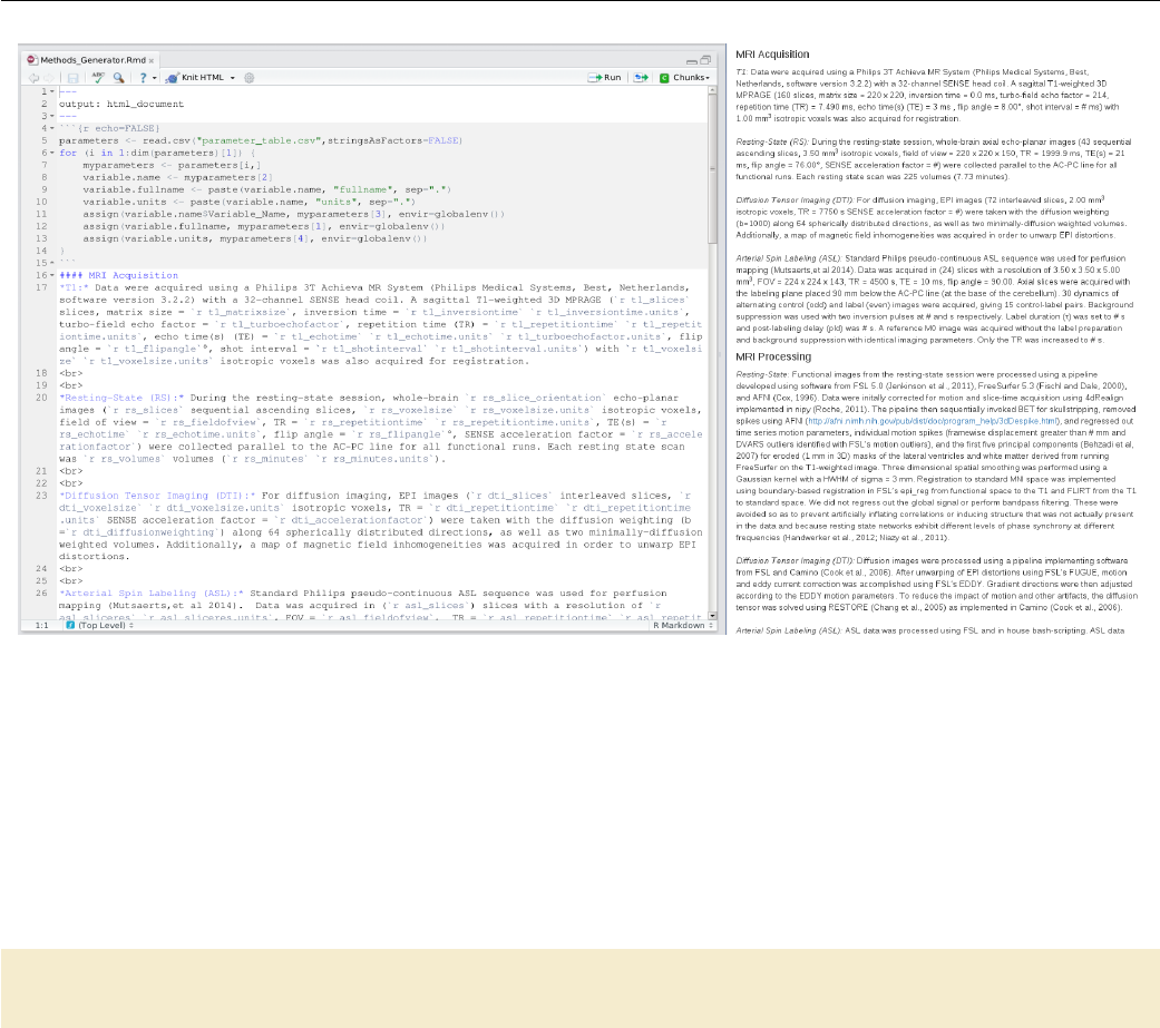
Figure 7.1: Methods generation in R Markdown
The outputted methods section HTML file can be viewed in any web browser. Figure 7.1 shows the R
Markdown code that is processed (on the left) to generate the HTML report (on the right). The R Markdown
code is very simple. The first “chunk” of code reads in the CSV file and uses the short variable names to
construct a variety of variables for the value of the parameter, its full name, and the units. These are accessed
in the text description of the protocol with the syntax ‘r variablename’. For more information about how
to write reports with R Markdown, see their excellent documentation.
clean_provenance:
echo " Removing p rovenance directory " ;\
rm -r provenance
Lastly, we create a target to remove all files created by this makefile. When called, this target will simply
remove the provenance directory and all files located within it.
120

Example 8
Seed-based Functional Connectivity
Analysis I
Susan J. Melhorn1
This is an example of how to use a makefile to execute a single-subject seed-based functional connectivity
analysis. Here, the network of interest is the salience network with a 4mm sphere in the right insula as the
seed region (seedrins4.nii.gz). Note the seed region mask has already been created based on the literature
(??).
We conduct a seed-based analysis by (1) extracting the time course of interest, and (2) using this time
course as a regressor in a GLM, including all nuisance variables. Here, this analysis is implemented using
FSL’s FEAT (feat) program.
The code for this example is in testsubject/lib/makefiles/fcconnectivity.mk. Note that the vari-
ables PROJECT_HOME, FSL_DIR, STD_BRAIN, and subject are all set elsewhere, but are needed. This exam-
ple builds upon the other processing pipelines in place for testsubject.
. PHONY : Connectivity clean _fccon nec tivi ty
Co nne cti vit y : $ (call print - help , Connectivity , " Perform subject - level seed - based
co nn ec ti vi ty an alysis ") \
fc co nn ect iv it y_di r / R ins _i n_f unc . nii . gz f cc onne ctiv ity _d ir / Rins _ts . txt \
fc co nn ect iv it y_di r /$( subje ct ) . feat / sta ts / zstat1 . nii . gz \
fc co nn ect iv it y_di r /$( subje ct ) . feat / sta ts / FZT1 . nii . gz
1fc co nn ect iv it y_di r / R ins _i n_f unc . nii . gz : $ ( PROJECT_HOME ) / lib / fcc onn ec tiv it y /
se edr ins 4 . nii . gz xfm_ dir / M NI_ to_ re st . mat r est_di r / r est_ssmooth . nii . gz
mkdir -p f cconnec ti vity_ di r ;\
fli rt - in $ ( PR OJ ECT _HOME ) / lib / f cco nn ect iv ity / s eed rin s4 . nii . gz \
- ref r est _di r / r est _ssmooth . nii . gz - a ppl yxfm \
- init xfm_dir / M NI_to_rest . mat - out $@ ;\
fslmaths $@ -bin $@
2fc co nn ect iv it y_di r / Rins _ts . txt : fc co nn ect iv it y_d ir / Ri ns_in_func . nii . gz
re st _di r / re st _s smo ot h . nii . gz
mkdir -p `dirname $@ ` ;\
fs lme ant s -i r est _dir / r est_ssmooth . nii . gz -o $@ \
-m f cc onne cti vi ty _di r / Ri ns _in _func . nii . gz
1This target puts the seed mask in functional space from standard space. Note the dependencies here are
created in the resting state preprocessing makefile. Normally we would threshold the mask at .5 to preserve
1smelhorn@uw.edu
121
its volume, but this particular seed is so small that we only binarize it using fslmaths 2We use fslmeants
to extract the timeseries from the masked functional connectivity data.
3fc co nn ect iv it y_di r / f cconne cti vi ty . fsf : $ ( PR OJ ECT _HOME ) / lib / fcc onn ec tiv it y /
fc co nn ec tivi tyTE MPLA TE . fsf
pipelines =`echo $( MAKEPIPE LI NE S )| sed `s/\//\\\\\//g'`;\
sed -e `s / SUBJECT /$ ( subjec t )/g '\
-e `s / MA KE PI PE LI NES /'$$pipelines '/g '$ < > $@
This step relies on a template .fsf file created using the Feat graphical user interface. We set this up for the
first subject, and use the text file for the seed time course as an explanatory variable. The input data is the
resting state data that has been processed up until nuisance regressors are removed. We use no convolution
(the seed time course is already convolved by the brain) and turn off temporal derivative and temporal filtering.
We include all nuisance regressors in the model.
The .fsf file created in this way has hardcoded paths that include the directory of the specific subject and
the path to all of the pipeline examples. To make it work for other subjects (at other sites) we parameterize
the file created by Feat to substitute the path to the subject with the text MAKEPIPELINES, and the subject
identifier with the text SUBJECT. You can see this file at lib/fcconnectivity/fcconnectivityTEMPLATE.fsf.
We use the sed command to replace these placeholder strings with their actual values, thus generating a
customized .fsf file for each subject. We set the pipelines variable just to escape the slashes (/) in the
MAKEPIPELINES variable for sed. If you like, after you run this step, you can open up the newly created
.fsf file to see the settings that are described above.
fc co nn ect iv it y_di r /$( subje ct ) . feat / sta ts / zstat1 . nii . gz :
re st_ dir / r est _s smo oth . nii . gz r est _dir / r es t_ nu isan ce _reg ress or s . txt \
fc co nn ect iv it y_di r / Rins _ts . txt f cc on nect ivi ty _d ir / f cco nn ect iv ity . fsf
feat fcc onn ec ti vit y_ di r / f ccon nec ti vit y . fsf
Run feat. Note that there are several dependencies in this rule that don’t appear anywhere else in the
recipe. However, they are needed by the .fsf file used to run feat.
fc co nn ect iv it y_di r /$( subje ct ) . feat / sta ts / FZT1 . nii . gz :
fc co nn ect iv it y_di r /$( subje ct ) . feat / sta ts / zstat1 . nii . gz \
re st_ dir / r est _s smo oth . nii . gz r est _dir / r es t_ nu isan ce _reg ress or s . txt
NBVOLS=`fsl val rest _di r / r est _s smo oth . nii . gz dim4 ';\
NB NUISANCE =`awk `{ p rint NF } 'rest_d ir / res t_nui sa nce_r egres sors . txt \
| head -1` ;\
SD =`echo " sqrt ( $$NBVOLS - $$NBNUISANCE -3) " | bc -l` ;\
echo $$SD ;\
fs lma ths fc co nn ectivi ty_d ir / $( subje ct ) . feat / sta ts / zstat1 . nii . gz \
- div $$SD fc co nn ect iv it y_d ir / $( s ubj ect ) . fea t / stats / FZT1 . nii . gz
After running feat, we need to convert the zstat to Fisher’s Z transformed partial correlation. This math
is implemented using fslmaths and is based on Jeanette Mumford’s recommendation.
clean_fcconnectivity:
rm -rf fccon nectivi ty _dir
Finally, we define a target to remove all the files we have created.
122

Example 9
Seed-based Functional Connectivity
Analysis II
Matthew Peverill1
This is an example of how to use make to preprocess and analyze resting state fMRI data and conduct a
group-level seed-based functional connectivity analysis. The fMRI data is motion corrected using Nipype (?)
and then skull stripped and smoothed using FSL (?) standard utilities. FreeSurfer is used to structurally
define a region of interest (ROI - for the purpose of this example, the right superior frontal gyrus) specific to
each subject which is then registered to the functional image.2fslmeants is used to extract a timeseries of
activity in this ROI which is entered as a regressor in FSL along with nuisance regressors corresponding to
motion outliers, rigid body movement, and white matter and CSF fluctuations to correct for noise. A simple
quality assurance (QA) report is generated for registration and ROI extraction using an HTML template.
The code for this example is in $MAKEPIPELINES/tapping, in multiple files described below.
Group Level Makefile - tapping/Makefile
1SUBJECTS = $( wildc ard Ta ppingSubj ?)
. PHONY : ma kefiles all $ ( SUBJECTS ) resting - gfeat
all : makefile s $( SUBJECTS ) resting - gfeat
$( SUB JECTS ):
2$( MAKE) - - di rec to ry = $@ subject - resting
3makefiles : $( S UBJECTS :%=%/ Makefile )
$( SUB JECTS :%=%/ Makefi le ) : lib / resting / subject . mk
4ln -s $$PWD /$ < $@
resting - gfeat : re stin g . gfeat / cope1 . feat / stats / cope1 . nii . gz
5resting . gfeat / cope1 . feat / stats / cope1 . nii . gz : lib / resting / T apping_S econdL eve l . fsf
$( SUB JECTS )
rm - rf / project_space / m ake pi pel in es / tapping / resting . gfeat ;\
fea t $ <
The group level Makefile in the project parent allows for recursive make of all subjects in the project.
1mrpev@uw.edu
2This is a very large seed! However, this is just an example.
123

Subject Level Makefile - tapping/lib/resting/subject.mk
1The variable SUBJECTS is set to a wildcard which captures all folders named TappingSubj followed by a
single character (this would need to be modified for more than nine subjects - likely by expanding all subject
numbers to two digit format and adding a second ?).
2This recipe provides the definition that make (subject) should execute make subject-resting within
each subject’s folder after a subject-level Makefile has been generated.
3The makefiles phony target uses make’s substitution reference syntax to expand the list of subjects to
a list of subject level makefiles.
4Another recipe provides rules to generate the makefiles enumerated in 3.
5The final recipe executes group-level feat according to the template lib/resting/Tapping_SecondLevel.fsf,
generating the final results of the analysis. For convenience, this recipe can be run by typing make resting-gfeat.
Subject Level Makefile - tapping/lib/resting/subject.mk
The subject-level Makefile is stored in lib/resting/, but a symbolic link pointing to it is generated in every
subject directory. This makefile sets up necessary environment variables and then imports all component
makefiles. The code executes exactly as if everything were in one makefile, but separating the code by
procedure makes the code more readable.
. PHONY : prept1 clean printall
. SECONDARY :
ifeq " $( origin M AK EPIPELINES )" " un defined "
MA KE PI PELINES =/ pr oj ec t_ sp ac e / makepipelines
endif
SHELL = / bin / bash
6subject = $( shell pwd | egrep -o `TappingSubj [0 -9]* ')
projdir = $( MAKEPIPELI NE S )/ tapping /
7SU BJ EC TS _D IR =$( projdir )/ frees urfer
SC RIP Tpath =$( pr ojdi r )/ bin
8FSL_DIR =/ usr / share / fsl /5.0/ bin
AF NIp ath =/ usr / lib / af ni / bin
TR =2.5
When we run make within a subject directory, the program reads Makefile first. Because of this, we can set
environment variables once in this file and they will carry over to all included files. This section should be
carefully reviewed when moving the code to a new environment.
6Here, the subject variable is set to the subject directory name.
7FreeSurfer’s SUBJECTS_DIR variable should be set for the users environment.
8Paths to the local installation of FSL and AFNI are set here. Later references to programs provided by
these packages use these variables to provide a path so that the pipeline can be flexibly executed with different
package versions.
9include $ ( projdir ) / lib / resting / Preprocess . mk
include $ ( projdir ) / lib / resting / Regressors . mk
include $ ( projdir ) / lib / resting / timeseries . mk
include $ ( projdir ) / lib / resting / feat .mk
in clu de $ ( p roj dir ) / lib / res ti ng / qa . mk
10 subje ct - re stin g : p rept 1 p rep fun c r egres sors t ime serie s feat qa - all
11 clean - resting :
124
Preprocessing - tapping/lib/resting/Preprocess.mk
rm -rf resti ng m emprage ;\
rm -f QA - r eport . html
12 tidy - resting :
rm -fv resti ng /* ;\
rm -fv memprage /* ;\
rm - rf resting / timese ri es
13 print -%:
@echo $* = $( $ *)
9Here we import child makefiles which contain all of the code necessary to execute the analysis.
10 The phony target subject-resting depends on all components of the analysis, providing one target
to execute the entire workflow for this subject. This is the target referenced in the group-level makefile.
11 The clean-resting target removes all files created by the pipeline, returning the subject folder to a
pre-run state.
12 The tidy-resting target allows for the removal of working files only and retains feat output.
13 The print-% target is provided for debugging purposes, eg. make print-subject will return the value
of the subject environment variable.
Preprocessing - tapping/lib/resting/Preprocess.mk
. P HONY = p rep t1 p rep t1 - qa p re pfu nc pr ep func - qa
prept1 : memprage / T1 _brain . nii .gz
14 me mp rag e / T1 . nii . gz : M PR AG E_S 2 . n ii . gz
15 mkdir -p memprage && \
$( FS L_DIR ) / bin / f slre ori en t2s td $ < $@
16 me mp rag e / T1 _br ai n . nii . gz : m em pra ge / T1 . nii . gz
$( FS L_DIR ) / bin / bet $ < $@
17 memprage / T1 _b rai n_ ma sk . nii .gz : memprage / T1_br ain . nii . gz
$( FS L_DIR ) / bin / fslm ath s $ < - bin $@
This code provides basic preprocessing of the T1 structural image. In preprocessing, each image is generated
from the prior image, so the makefile reads much as a bash script would with each line proceeding from the
last, save that dependency and target shortcuts are substituted for filenames.
14 T1.nii.gz is generated by orienting the scanner output image to FSL’s preferred orientation using
fslreorient2std.
15 The ‘&& \’ syntax at line ends causes bash to stop and make to return a failure for the recipe if the
preceding command fails (otherwise all commands are executed and only the success or failure of the last
executed command is considered when make reports whether the recipe ran successfully). This saves time
by skipping programs that cannot succeed and makes the cause of a failure more clear, since the last error
message presented to the user will be from the command that first failed instead of from a program that failed
as a consequence.
16 Skull stripping is accomplished with bet.
17 A mask of the skull stripped brain is generated with fslmaths.
pr epf unc : x fm_ dir / T 1_t o_ Res ti ng . mat r esting / R es tin g_ ssmoot h . nii . gz
xfm_dir / fs_to_Resting . mat
re sting / Re st ing_or ien t . nii . gz : R esting . nii . gz
125
Preprocessing - tapping/lib/resting/Preprocess.mk
mkdir -p resting && \
$( FS L_DIR ) / bin / f slre ori en t2s td $ < $@
18 re sting / Re sti ng_mc . nii . gz : rest ing / R est in g_o ri ent . nii . gz
py tho n $ ( S CR IPT pa th ) /4 d Re gi ste r . py - - inp uts $ < -- tr $ ( TR ) \
--slice_order `ascending '&& \
mv resting / Res ti ng_orie nt _mc . nii . gz $@
19 re sting / Resti ng . par : r esti ng / Re sti ng_mc . nii . gz
mv rest ing / R est in g_o ri ent . par $@
20 re sting / Re st ing _b rai n . nii . gz : r esting / R est ing _mc . nii . gz
$( FSL_DIR )/ bin / fslroi $ ^ resting / R es ting_vo l0 0 1 && \
$( FSL_DIR )/ bin / bet resting / Resting_vol0 resting / Resting_vol0 -f 0.3 && \
$( FSL_DIR )/ bin / fslma ths resting / Resting_v ol 0 - bin rest ing / Resting_vol0 &&
\
$( FSL_DIR )/ bin / fslma ths $ ^ - mas resting / Resting_vol0 $@ && \
rm rest ing / R est ing_vol0 . nii . gz
21 re sting / Resti ng_ ss mooth . nii . gz : r esting / R esting_b rai n . nii . gz
$( FSL_DIR )/ bin / susan $^ -1.0 3 3 1 0 $@
This code provides basic preprocessing of the functional resting state image.
18 A python script, 4dRegister.py, is called which outputs both the motion corrected image and a .par
file containing 6 motion regressors.
19 Although the par file is created by 4dRegister.py, a separate recipe allows us to rename the file and,
importantly, allows for the execution of later recipes which depend on the .par file.
20 fslroi is used to extract the first volume (time point) of the four dimensional functional image. bet
Is used to skull-strip the image and a binarized mask is generated and applied using fslmaths.
21 Smoothing is applied with susan to produce the final preprocessed image.
22 xf m_dir / Re st ing _t o_T 1 . mat : rest ing / R est in g_b ra in . nii .gz me mpr age / T1 . nii . gz
memprage / T1_br ain . nii . gz
mkdir -p xfm_dir && \
$( FSL_DIR )/ bin / fslroi $ < resting / r es ting_vo l0 0 1 && \
$( FSL_DIR )/ bin / epi_reg -- epi = restin g / re sti ng _v ol 0 -- t1 =$ (word 2 ,$^) \
-- t1brain = $( word 3 ,$^) -- out= xfm_dir /`basename $@ .mat '
23 xfm_dir / Resting_to_T1 . nii .gz : xfm_dir / Res ting_to_T1 . mat
xfm_dir / T1_to_Resting . mat : xf m_dir / Resting _t o_ T1 . mat
$( FS L_DIR ) / bin / c onv ert_x fm - omat $@ - i nve rse $ ^
24 $( SUBJECTS_DIR ) /$ ( subje ct ) / mri / aparc + aseg . mgz : | me mpr age / T1 . nii . gz
source / usr / local / fr ees urf er / stab le5_3 / Se tU pFr ee Surfer . sh && \
export SUBJECTS_DIR=$(SUBJECTS_DIR) && \
/ usr / local / f ree surfe r / s tab le5 _3 / bin / recon - all -i $ < - s ubji d $( su bject ) \
-all && \
touch $( SUBJECTS_DIR ) /$( subject )
25 xf m_dir / fs _to _T1 . mat : $( SUBJECTS_DIR ) /$ ( subje ct ) / mri / aparc + aseg . mgz
me mp rag e / T1 . nii . gz
mkdir -p xfm_dir && \
source / usr / local / fr ees urf er / stab le5_3 / Se tU pFr ee Surfer . sh && \
export SUBJECTS_DIR=$(SUBJECTS_DIR) && \
tk registe r2 -- mov $ ( SU BJECTS_DIR ) /$( subje ct ) / mri / orig . mgz \
126
Generation of Nuisance Regressors - tapping/lib/resting/Regressors.mk
-- targ $( word 2, $ ^) --noedit -- re gheader \
-- reg xfm_dir / fs_to_T1 . dat \
-- fslrego ut xfm_dir / fs_to_T1_init . mat && \
mr i_conve rt $ ( SUBJECTS_DIR ) /$ ( subje ct ) / mri / orig . mgz \
$( SUBJECTS_DIR ) /$ ( subje ct ) / mri / orig . nii . gz && \
$( FS L_DIR ) / bin / flirt - ref $ ( word 2,$ ^) \
-in $ ( S UBJ ECTS_DIR )/$ ( su bject ) / mri / orig . nii . gz \
- init xfm_dir / f s_ to _T 1_ init .mat - omat $@
26 xfm_dir / fs_to_Resting . mat : xf m_dir / fs_t o_T1 . mat xfm_dir / T1_to _R es ti ng . mat
$( FS L_DIR ) / bin / c onv ert_x fm - con cat $ ( word 2 , $ ^) - omat $@ $ <
This code creates registrations between functional, structural, and standard space as well as brain segmen-
tation using FreeSurfer.
22 Registration is created from functional to structural space.
23 Although the recipe above creates both .mat and .nii.gz files created by epi_reg, later recipes
depending on Resting_to_T1.nii.gz will fail unless we add this empty recipe referring back to the rule
for the .mat file. Although it is possible to simply make these later recipes depend on the .mat file despite
using the .nii.gz file, the workflow is both more readable and easier to debug if we indicate the relationship
between the two files here and reference either file as called for later.
24 Here FreeSurfer is called to segment the brain, with the recipe targeting a label file which is generated
at the end of recon-all. The ’|’ (pipe) symbol here indicates that T1.nii.gz is an ’order only’ dependency,
which means that recon-all will not be re-run if T1.nii.gz is newer than aparc+aseg.mgz. The purpose
here being that FreeSurfer is often run separately from individual analyses, and it may be undesirable for the
pipeline to re-run recon-all each time the code generating T1.nii.gz is changed. Other applications may
be better served with a normal dependency, in which case the pipe can be omitted.
25 Here the FreeSurfer image is registered on to the T1 structural image. tkregister2 is used to generate
an initial affine registration matrix. The final registration is generated by flirt, using tkregister2’s matrix
as a starting point so as to avoid local minima.
26 Registration from FreeSurfer to functional space is generated by concatenating fs_to_T1.mat with
T1_to_Resting.mat using convert_xfm.
Generation of Nuisance Regressors - tapping/lib/resting/Regressors.mk
. PHONY : regr essors
re gre ssors : r est ing / wm . txt re sti ng / csf . txt r esting / n ui sanc e_re gres sors . txt
27 re sting / dvars _regre sso rs : re sting / Resting_b rai n . nii . gz
$( SCRIP Tp ath )/ motio n_ outliers -i $^ -o $@ -- dvars -s resting / dvars _v als \
-- no moco && \
rm resting / d va rs_vals && \
touch $@
28 resting / fd_regressors : resting / R es ti ng _b rain . nii .gz resting / Resting . par
$( SCRIP Tp ath )/ motio n_ outliers -i $^ -o $@ -- fd -s resting / fd_vals \
-c rest ing / Re sting . par -- nomoco -- th resh =3 && \
rm resting/fd_vals && \
touch $@
29 resting / all_outliers . txt : resting / d var s_r egr ess ors resting / fd_regressors
cat resting / dvars _s pike_vols | $( SCRIPTpath )/ trans pose \
> resting / allou tliers_ns or t . txt && \
cat resting / fd_spike_vols | $( SCRIPTpath )/ trans pose \
>> r est ing / a llou tli er s_ nso rt . txt && \
127

Generation of Nuisance Regressors - tapping/lib/resting/Regressors.mk
sort -nu resting / alloutl iers_nsor t . txt > $@ && \
rm resting / all ou tliers_ ns ort . txt
30 re sting / out lier _re gr es sor s . txt : r esting / R es tin g_ ori en t . nii . gz
re sting / al l_ out liers . txt
vols = `fsl val $ < dim4 '&& \
echo " vols is $$vols " && \
python ${ SC RIPTpath }/ S in glePo in tGene ra tor . py -i $( word 2,$ ^) -v $$vols \
-o $@ -p resting / restin g_ per ce nt_ou tlier s . txt
This code generates motion outlier regressors in feat compatible syntax.
27 -28 FSL’s motion_outliers script is called to generate lists of motion outliers using two separate
metrics (RMS intensity difference of volume N to volume N+1 and frame displacement, respectively - see (?)).
A separate regressor is generated for each outlier.
29 The resulting two regressor files are transposed (rotated) and sorted numerically, effectively sorting the
outlier volumes by time (duplicates from the two sources will appear next to each other).
30 The python script SinglePointGenerator.py then extracts unique outliers and returns them in stan-
dard column format.
31 fs _wm _mask . nii . gz : $ ( SU BJECTS_DIR )/$ ( su bject ) / mri / aparc + a seg . mgz
source / usr / local / fr ees urf er / stab le5_3 / Se tU pFr ee Surfer . sh && \
export SUBJECTS_DIR=$(SUBJECTS_DIR) && \
mr i_ bi na ri ze -- i $ < -- o $@ -- e rode 1 -- wm
32 re sting / wm . txt : fs _wm _mask . nii . gz re sti ng / Re sti ng_ mc . nii . gz
xfm_dir / T1_to_Resting . mat
$( FS L_DIR ) / bin / flirt - ref $ ( word 2,$ ^) - in $ < - out wm . nii . gz - app lyx fm \
- init $( word 3 ,$^) && \
$( FS L_DIR ) / bin / fslm ath s wm . nii . gz - thr .5 wm . nii . gz && \
$( FS L_DIR ) / bin / fslm eants -i $ ( word 2,$ ^) - o $@ -m wm . nii . gz
33 fs _v en tri cl es _mas k . nii . gz : $ ( SU BJECTS_DIR ) /$( subje ct ) / mri / aparc + aseg . mgz
source / usr / local / fr ees urf er / stab le5_3 / Se tU pFr ee Surfer . sh && \
export SUBJECTS_DIR=$(SUBJECTS_DIR) && \
mr i_ bi na ri ze -- i $ < -- o $@ -- e rode 1 -- v entri cl es
34 re sting / csf . txt : f s_ vent ric le s_ mas k . nii . gz r est ing / Restin g_mc . nii . gz
xfm_dir / T1_to_Resting . mat
$ ( FS L_D IR )/ bin / f lirt - ref $ ( w or d 2 ,$ ^) - in $ ( wo rd 1 ,$ ^) \
-out `dirn ame $@`/`basename $@ . txt`. n ii . gz \
- applyxfm - init $( word 3, $ ^) && \
$( FS L_DIR ) / bin / fslm ath s ` dirnam e $@`/`basename $@ . txt`. nii . gz \
-thr .5 `dirname $@`/`basename $@ . txt`. nii . gz && \
$( FS L_DIR ) / bin / fslm eants -i $ ( word 2,$ ^) - o $@ \
-m `dirname $@`/` basename $@ . txt`. nii . gz
35 re sting / nui sanc e_re gre ss or s . txt : re sti ng / csf . txt rest ing / wm . txt
re sting / Resti ng . par rest ing / o utli er_r egr es so rs . txt r esting / R esting_b rai n . nii . gz
pas te $ ( word 1,$ ^) $( word 2,$ ^) $( word 3 ,$ ^) $( word 4,$ ^) > $@
Here we generate noise correction regressors from signal in white matter and CSF regions.
31 A binarized mask of FreeSurfer’s white matter volume is generated in the first recipe.
32 The mask from 31 is then put in to functional space using flirt and binarized again to remove any gray
areas generated during registration. Finally, fslmeants is used to generate a timeseries containing outliers in
WM activity.
33 -34 The same procedure used above is repeated with FreeSurfer’s CSF volume.
128

ROI Timeseries Extraction - lib/resting/timeseries.mk
35 To generate the final nuisance regressors file to be input to feat,paste is used to combine the three
outlier regressor files with the rigid body motion regressors generated in preprocessing.
ROI Timeseries Extraction - lib/resting/timeseries.mk
. PHONY : time series
timeseries : resting / timeseries / ctx - rh - su per io rfrontal . txt
re sti ng / t im ese ri es /r - sfg - m as k . nii . gz
re sting / ti mes eries / ctx - rh - s uper ior fr ontal . txt : rest ing / R esting _ss mo oth . nii . gz
re sti ng / t im ese ri es /r - sfg - m as k . nii . gz
36 fslmeants -i $ < -m $ ( word 2, $^) -o $@
37 resting / timese ri es /r-sfg - mask .nii .gz : resting / t imeseries /ctx - rh - super io rf rontal .
nii re sting / Re st ing_ ssm oo th . nii . gz x fm_ dir / f s_t o_ Res ti ng . mat
flirt - in $ < - applyxfm - init $ ( word 3 , $ ^) \
- out r esting / t ime serie s / rsfg - fu ncs pace . nii . gz - pa dd ing siz e 0.0 \
- in ter p t ri lin ea r - ref $ ( wor d 2 , $ ^) && \
fs lma ths r est ing / time series / rsfg - f unc spa ce . nii . gz - bin $@ && \
rm rest ing / timese ries / rsfg - f unc spa ce . nii . gz
38 $( SUBJECTS_DIR ) /$ ( subje ct ) / re gister . dat : $( SU BJ ECT S_ DIR ) /$ ( subje ct ) / mri / aparc + aseg
. mgz
tk registe r2 -- mov $ ( SU BJECTS_DIR ) /$( subje ct ) / mri / T1 . mgz -- noe dit \
--s $( subject ) -- regheader -- reg $@
39 $( SUBJECTS_DIR ) /$ ( subje ct ) / label s2 / aparc + aseg - in - ra wavg . mgz : $ ( S UBJ EC TS_ DIR ) /$ (
subject ) / register . dat
mkdir -p $( SU BJ EC TS_DIR )/$ ( subject )/ labels2 / ;\
mr i_ lab el 2vo l -- seg $ ( SU BJECTS_DIR ) /$( subje ct ) / mri / apa rc + ase g . mgz \
-- reg $( SUBJECTS_DIR ) /$( subject )/ regis ter . dat --o $@ \
-- temp $ ( SU BJE CT S_D IR )/$ ( su bject ) / mri / aparc + a seg . mgz
40 resting / timeseries /ctx - rh - sup er ior fro nta l .nii : $ ( SUBJECTS_DIR )/ $( subject ) / labels 2 /
ap ar c + aseg - in - r awav g . mgz
mkdir -p resting / timese ries && \
mr i_ bi na ri ze --i $( SUBJECTS_DIR )/$ ( subject ) / labels2 / aparc + aseg - in - rawavg .
mgz \
-- match 2028 --o resting / timeseries / ctx - rh - su per io rfr on tal . nii
Here a mask of the ROI (Right SFG) is generated from FreeSurfer and registered to functional space; a time-
series of activity in the ROI is then generated using FSL. The recipes are written roughly in the reverse order
they are run, starting with the desired endpoint and working backwards through all required dependencies.
make will execute them in the desired order according to the dependency structure.
36 The fslmeants command generates a timeseries of average activation from the preprocessed resting
image within the area defined by the specified mask file.
37 The registered mask file is generated by applying the registration matrix transforming FreeSurfer to
functional space generated in 26 to the mask of the ROI generated with FreeSurfer. The mask must be
binarized using fslmaths, as registration will generate non-binary values around the edges of the mask. The
non-binarized mask is then removed.
38 An image indexed by FreeSurfer’s aseg and aparc atlases is generated using mri_label2vol.
39 The (unregistered) FreeSurfer mask for the ROI is generated from the labeled volume by using mri_-
binarize to isolate image voxels whose value matches the relevant FreeSurfer label (the index value for the
129
First Level Analysis - lib/resting/fsl.mk
ctx-rh-superiorfrontal area is 2028 - see FreeSurferColorLUT.txt in your FreeSurfer install directory for
a list of volume labels).
First Level Analysis - lib/resting/fsl.mk
. PHONY : feat
. SECONDARY :
41 feat : resting / Resting . feat / stats / cope1 . nii .gz
42 resting / Resting . feat / stats / cope1 . nii . gz: resting / Resting . fsf resting /
Re st ing_ss moo th . nii . gz
re sting / nui sanc e_re gre ss or s . txt $ ( FS L_D IR ) / data / st and ard / M NI 15 2_T 1_ 2m m_br ain . nii .
gz
resting / ti meseries / ctx -rh - super io rf rontal . txt
rm - rf resting / R esting . feat && \
$( FSL_DIR )/ bin / feat resting / Resting . fsf
43 resting / Resting . fsf : $( proj dir )/ lib / resting / Tap pi ng_First Le vel . fsf
re sti ng / R es ti ng _s sm oo th . nii . gz
sed -e `s / SUBJECT /$ ( subjec t )/g '$ < > $@
Here a template .fsf file is copied from the lib directory and feat is run. Because there is only one functional
run per subject, only the subject number need be substituted when copying the template. 41 feat Creates
many files, but as the first cope is the one we are most interested in (and will only generate if the program
runs successfully), it is listed as the recipe target. Therefor the phony target amounts to an alias, as there is
only one dependency.
42 First, any previous runs of fsl are removed - otherwise fsl will continually create new directories
when feat is rerun, leading to inconsistent file structures between subjects and breaking the make dependency
structure. To execute the analysis, feat is simply called on the fsf file.
43 The fsf file is generated per subject in this recipe by using sed to copy a template while substituting
the subject number for the text SUBJECT in the original. If further by-subject customization is needed, the -e
flag can be provided to perform additional substitutions.
Quality Assurance Reports - lib/resting/qa.mk
. P HONY = qa - all pr ept 1 - qa prep func - qa t imes erie s - qa
qa - al l : prept1 - qa pr ep func - qa t ime se rie s - qa QA - r epor t . h tml
QA - report . html : ../ lib / rest ing / sub jec t_QA _repor t . html
44 sed -e `s / SUB JE CT NU MB ER /$ ( subject )/g '$ < > $@
prept1 - qa : memprage / QA / images / T1_bra in . png
45 me mp rag e / QA / i ma ges / r en de re d_ T1 _b ra in . n ii . gz : m em pra ge / T1 . nii . gz
memprage / T1_brain _m as k . nii . gz
mkdir -p `dirname $@` && \
$( FSL_DIR )/ bin / overlay 1 1 $ ( word 1,$ ^) -a $( word 2,$ ^) 1 10 $@
46 me mp rag e / QA / i ma ges / T 1_b ra in . png : me mp rag e / QA / ima ges / re nd er ed _T 1_ br ai n . nii . gz
$ ( S CRI PT pa th ) / s lic es m emp rag e / QA / i mag es / r en de re d_ T1 _b ra in . nii . gz -o $@
pre pf unc - qa : r es tin g / QA / i mag es / R es t in g_ ss mo o th _m id _ an im at io n . gif re sti ng / QA / im age s
/ r esting_to_ T1 . png
130

Quality Assurance Reports - lib/resting/qa.mk
47 re sting / QA / im ages / R es ti ng _s sm ooth _m id_a ni ma tion . gif :
re sti ng / R es ti ng _s sm oo th . nii . gz
mkdir -p `dirname $@` && \
$( SCRIP Tp ath )/ fun ct ional_m ov ies . sh $ < `dirname $@`
48 resting / QA / images / re st in g_ to _T1 . png : xfm_dir / Resting_to_T1 . nii .gz
memprage / T1_br ain . nii . gz
mkdir -p `dirname $@` && \
$ ( S CRI PT pa th ) / sl ic eap pe nd . sh -1 $ ( wo rd 1 ,$ ^) -2 $ ( wor d 1 ,$ ^) -o $@ -s
ti me ser ies - qa : r est ing / QA / i mag es / ren dere d_r - sfg - m ask . p ng
49 re sting / QA / im ages / re ndered_r -sfg - mask . nii . gz : r esting / R esti ng_ br ain . nii . gz
re sti ng / t im ese ri es /r - sfg - m as k . nii . gz
mkdir -p `dirname $@` && \
$( FSL_DIR )/ bin / overlay 1 1 $ ( word 1,$ ^) -a $( word 2,$ ^) 1 10 $@
50 re sting / QA / im ages / re ndered_r -sfg - mask . png :
re sti ng / QA / im age s / r ende red _r - sfg - m ask . nii . gz
$( SCRIP Tp ath )/ slices $ < -o $@
A simple quality assurance (QA) report is generated per subject from an .html template.
44 The template is copied from the lib directory using sed to substitute the appropriate subject number.
Because filenames are preserved within subjects and relative paths are used in the html code to indicate paths
to qa images, no other substitutions are necessary.
45 The FSL utility overlay is used to generate an image of the skull-stripped structural image in red
overlaying the original T1, allowing for visual inspection of the quality of the skull strip.
46 The slices script generates an image of several slices of the above overlay volume for easy visual
inspection. As elsewhere, these steps could be written in a single recipe, but separating it to smaller recipes
allows for cleaner code and easier debugging.
47 The functional_movies.sh script creates an animated .gif file displaying slices of the functional
volume animated over time. This allows for visual inspection of gross movement and other imaging artifacts.
48 The sliceappend.sh script allows for the inspection of registration by presenting an outline of one
image on top of a second image to which it has been registered on one row of slices and the reverse on the
next.
49-50 The same method as was used for the inspection of skull stripping is used to inspect the quality of
the ROI extraction.
131

Example 10
Using ANTs Registration with FEAT
Kelly A. Sambrook1
This is an example of using Advanced Normalization Tools (ANTs)(?) registration with FSL Feat. ANTs
provides a superior nonlinear registration from the T1 to MNI brain compared to FSL’s fnirt command, so
we use it here in conjunction with FSL’s epi-reg to replace the functional to standard space registrations
created by FEAT with those created by ANTs.
The code for this example is in $MAKEPIPELINES/ANTsreg/ in specific makefiles described below. It is
assumed that the fMRI data here have been pre-processed (including motion correction) before running this
pipeline.
Note that to run this example, and indeed, to use ANTs with FSL, you must have ANTs and ITK-SNAP
Convert3D tools installed. We assume that Convert3D tools (specifically, c3d_affine_tool) are installed in
your bin directory and is available in your path. You can type:
$ which c3d_affine_tool
to determine where it is located if it is in your path. ANTs, however, is another story; you may have
a different version than we do and it may be installed in a different location. So please note that you will
probably need to edit this example to specify your location for ANTs.
Group Level Makefile
SUBJECTS = TS001 TS002
. PHONY : all $( SUBJECTS )
all : $( SU BJE CTS )
$( SUB JECTS ):
$( MAKE) - - di rec to ry = $@ $(TARGET)
The code for this makefile can be found at $MAKEPIPELINES/ANTsreg/Makefile. There are two subjects
in this directory that require the same subject-level processing. Of course, in a real study there would be many
more. This group level makefile is a driver that will recursively call targets defined the subject-level makefiles.
See Setting up an Analysis Directory for more information on this type of directory structure.
1kelly89@uw.edu
132

Subject Level Makefile
Subject Level Makefile
The subject-level makefile is in ANTsreg/Makefile.subject. Each subject directory has a symbolic link to
this file that is named Makefile. In this way, we can change it in the top-level directory but all subjects will
immediately see the changes.
cwd = $ ( shel l pwd )
su bject = $( notdir $ ( cwd ) )
We use the directory name here to set a variable that contains the name of the subject. This is handy when
full pathnames must be specified to programs.
1export OM P_ NUM_THREADS =1
SHELL =/ bin / bash
ifeq " $( origin M AK EPIPELINES )" " un defined "
MA KE PI PELINES =/ pr oj ec t_ sp ac e / makepipelines
endif
PR OJECT_DIR =$ ( MAK EP IP EL INES )/ AN Tsreg
ST AN DA RD _D IR =$( PROJECT _DIR )/ Standard
SU BJECT_DIR =$ ( PRO JECT_DIR ) /$( subject )
2AN TSp ath =/ usr / local / ANTs -2.1.0 - rc3 / bin /
3BLOCKS = Tap pi ng Blo ck 1 T app ing Bl ock 2
4FSLDIR =/ usr / share / fsl /5.0/
ST D_B RAI N = $( F SLDI R )/ d ata / stan dar d / M NI 152_ T1_ 2m m_ brai n . nii . gz
STD = $( F SLDI R )/ data / s tandar d / M NI15 2_T 1_2m m . nii . gz
Here we define a number of variables that are used by other makefiles.
1ANTs exploits multiple cores to speed up execution. However, if we are running this pipeline across many
subjects using make, we disable this parallelism by setting the variable OMP_NUM_THREADS to be one.
2This is where ANTs is located on our systems. It is unlikely that ANTs is in the same directory on your
system, so you will have to edit this line.
3Similarly, the location of FSL may be different on your system. Check the location of FSLDIR on your
system and uncomment it as shown in this example. Note that if FSL is in a different location on your system,
you will have to edit the Feat template files, located in ANTsreg/templates.
4We set a variable called BLOCKS to the names of the fMRI tapping task runs. This saves some typing later.
antsreg : PrepSubject Feat
include ../ lib / make files / Prep .mk
include ../ lib / make files / Feat .mk
clean : clean_prep c lean_feat
The main target here, antsreg, creates some basic registrations (defined by the PrepSubject target in the
Prep.mk makefile) and then runs FEAT, creating ANTs registrations in the FEAT directories (target Feat
defined in the Feat.mk makefile). These makefiles are stored in the lib directory and are included by the
subject-level makefile.
Finally, we define a clean target that depends upon the clean_prep and clean_feat targets, defined in
their respective makefiles.
133

Preparatory Registrations - Prep.mk
Preparatory Registrations - Prep.mk
For convenience we have separated the main work of performing registrations with ANTs from the task of
running Feat and applying the ANTs registrations to the Feat output. The registrations are defined in the
Makefile ANTsreg/lib/makefiles/Prep.mk, described in this section.
. PHONY : PrepSubj ect bet s tru ct_r egi strati ons epi_r egi strati ons clean_ pre p
Pr epSubject : bet str uc t_r egi str ati ons e pi _registra tions
5Drop1Sfx = $ ( bas ename $ (1) )
We define phony targets as usual, and the main target is the PrepSubject target. 5We also define a helpful
little function, Drop1Sfx that drops the suffix of its argument. This is accomplished by using the make defined
function basename.
6bet : MP RAGE / T 1_b rain . nii . gz $( pa tsu bst % , Ta pping /% _ brain . nii . gz , $ ( BL OCKS ) )
MP RAG E / T 1_ bra in . nii . gz : M PRAG E / T1 . nii . gz
bet $ ^ $@ -R
7Ta ppi ng /% _b rai n . nii . gz : T app in g / %. ni i . gz
bet $ < $@ -F
We define a phony target, bet, to perform skull stripping of the MPRAGE and functional images. 6We
use pattern substitution on the BLOCKS variable to form the names of the skull-stripped functional images. 7
An implicit rule is used to create the skull-stripped functional images. This simplifies the Makefile when there
are multiple functional runs that all need to be processed in the same way.
st ru ct _reg istr atio ns : x fm_dir / T 1_ to_ mn i_W ar p . nii . gz
xf m_dir / T1 _t o_mni_ War p . nii . gz : MPRAGE / T1 _brain . nii . gz
mkdir -p xfm_dir ;\
export A NTSPATH = $( ANTSpath ) ;\
$( ANT Spath )/ a nt sIntroduc ti on .sh -d 3 -i MPRAGE / T1_brai n . nii . gz \
-m 30 x90x20 -o $ ( SUB JECT_DIR )/ xfm_di r / T1 _t o_mni_ \
-s CC -r $( STD_B RAIN ) -t GR
The structural registration of the MPRAGE to the standard brain is performed using ANTs, using the script
antsIntroduction.sh. The target file T1_to_mni_Warp.nii.gz will be created by this script because we
have specified the output prefix using the -o flag.
ep i_regist ra tio ns : $( pat subst % , xfm_dir /% _to_T1 . mat , $( BLOCKS ) )
$( pa tsu bst % , xf m_dir /% _to _mni _epi reg_ ant s . nii . gz , $( B LOCK S ))
8Ta pping /% _b rain_vo l0 . nii . gz : Ta ppi ng /% _ brai n . nii . gz
fs lro i $ < $@ 0 1
xf m_dir /% _ to_T1 . mat : T appi ng /% _b rain_vol0 . nii . gz M PRAG E / T1 . nii . gz
MP RAG E / T 1_ bra in . nii . gz
mkdir -p xfm_dir ;\
9ep i_r eg -- epi = T app ing / $* _ bra in _v ol 0 \
-- t1 = M PRAG E / T1 . nii . gz -- t 1br ain = MP RAGE / T 1_b rain . nii . gz \
-- out = $ ( ca ll D ro p1Sfx , $@ )
We use the target epi_registrations to perform the registrations involving the functional data. Our first step
is to use epi_reg from FSL to perform boundary-based registration of the functional image to the MPRAGE.
8We take the first volume of each skull-stripped functional run to use as the input volume for epi_reg. This
neat trick (thanks Katie Askren!) allows epi_reg to run faster and use a lot less memory. 9Note that we
get to use the Drop1Sfx function that we defined earlier on the target to specify the output path to epi_reg.
134
Running Feat and Applying ANTs Registrations - Feat.mk
10 xf m_dir /% _t o_T 1_ras . txt : MPRAGE / T1 _brain . nii . gz T apping /% _ bra in_vol0 . nii . gz
xf m_dir /% _ to_T1 . mat
c3 d_ affine _to ol - ref MPRA GE / T 1_b rain . nii . gz \
- src T ap pi ng / $ * _ br ai n_ vo l0 x fm _di r / $ * _ to_ T1 . mat - fs l2r as - o it k $@
11 xf m_dir /% _to _mni _ep ir eg _ant s . nii . gz : Ta ppi ng /% _b rai n_vol0 . nii . gz $ ( ST D_B RAI N )
MPRAGE / T1_b rai n . nii . gz xf m_dir /% _t o_T 1_ras . txt xfm_ dir / T 1_t o_ mni _W arp . nii . gz
export A NTSPATH = $( ANTSpath ) ;\
$( ANT Spath )/ W arpIm ag eMulti Trans fo rm 3 Ta pping / $* _brain_vol0 . nii .gz $@ \
-R $( ST D_B RAI N ) xf m_dir / T1 _t o_m ni _Warp . nii . gz \
xf m_di r / T 1_ to_mni _Af fi ne . txt xfm_d ir / $* _t o_T 1_ras . txt
Now comes the moment where we combine the T1 to standard space registration that we made with ANTs with
the functional to T1 registration that we did with epi_reg. To do this you need to use WarpImageMultiTransform
from the ANTs package. 10 We first convert the FSL style transformation matrices to ITK format using c3d_-
affine_tool.11 Then we use WarpImageMultiTransform to combine this matrix with the T1 to standard
space warp and affine matrix. Voila! We have achieved registration.
clean_prep :
rm - rf */* _ brai n *. nii .gz */* vo l0 . nii . gz xf m_d ir
Finally, we define a target clean_prep to remove all files created by this makefile.
Running Feat and Applying ANTs Registrations - Feat.mk
The next step is to run first level Feats, apply the ANTs registrations to the resulting output files, and
then run a second level Feat for each individual. This is done by the Makefile described here, located in
ANTsreg/lib/makefiles/Feat.mk.
TEMPLATES = $( PROJECT_DIR )/ templat es
Ta pping_ FE AT1_TEMP LATE =$( PROJECT_DIR )/ templat es / Tapping_FL .fsf
Ta pping_ FE AT2_TEMP LATE =$( PROJECT_DIR )/ templat es / Tapping_HL .fsf
We run Feat on multiple blocks with multiple subjects by defining Feat templates. We create these by
setting up Feat runs for a single subject using the graphical user interface and saving the configuration file.
Then we edit that file, replacing things like subject ID and the run name with capitalized text strings that we
can find and replace in a makefile with their real values. Here we define variables for these templates (first
level and higher level).
. PHONY : Feat FirstLe vel Feats FirstLevelReg SecondLev elF eats
. SECONDARY : $( al lu pd at er eg )
12 allcopes =$( w ildcar d Tapping /*. feat / stats / cope *. nii . gz )
al lvarcopes = $( w ildcar d Tapping /*. feat / stats / varcope *. nii . gz )
13 al lu pd at er eg =$( subst stats , reg_standard / stats ,$( allcopes ) )
$( subst stats , reg_standard / stats ,$( a ll va rc op es ) )
al lup dat etdof = $ ( subst stats / cope , reg_standard / stats / FEtdof_t , $( allcop es ))
Feat : FirstLevelF ea ts FirstLevelReg Seco nd LevelFeat s
We define our phony targets as usual.
Our goal is to transform the copes and varcopes into standard space using the ANTs registration. 12
However, because there may be an arbitrary number of copes, we use a wildcard here to obtain their names.
13 We use pattern substitution on the names that we obtained from wildcards to define the filenames for the
updated registrations that we need to create. Similarly, we also define the DOF (degrees of freedom) files that
would normally be created by Feat.
135

Running Feat and Applying ANTs Registrations - Feat.mk
Fi rstLevelFe ats : $( patsubst %, Tapping /%. feat / stats / cope4 . nii .gz , $( BLOCKS ))
Tapping /%. feat / stats / cope4 . nii . gz : $ ( patsubst % , Tapping /% _brain . nii .gz ,
Ta pp in gBlock1 T appingBlock2 )
rm -rf `echo $@ | awk -F " / " `{ print $$1 " /" $$2 } ' ' ;\
NBVOLS=`fsl val $ ( wor d 1 ,$ ^) dim4 ';\
RUN = $* ;\
RUN_NUM = `ech o $$ { RUN } | s ed - e `s/TappingBlock//g' ' ;\
sed -e `s | SUBDIR |$( SUBJECT_DIR )|g'-e "s / NB / $$ { NB VOL S }/ g " \
-e "s/ RUN / $${ RUN_NUM }/ g" -e "s/ S UBJECT /$ ( subjec t )/g " \
$( Tapp ing_F EA T1_TE MPLATE ) > Tapping / $ *. fsf ;\
fea t T app ing / $ *. fsf ;\
This block of code runs Feat for the two fMRI blocks. We use the last cope (cope 4) as the target file to
indicate that the recipe has completed correctly. We set variables for the number of volumes, the run name,
and the run number, and use these (in addition to the subject and subject directory) to modify the Feat
template before running Feat.
14 Fi rs tL evelReg : Firs tL evelFeats $ ( allupdatereg )
$( pa tsu bst % , Ta pping /%. feat / r eg _st anda rd / mask . nii . gz , $ ( BL OCKS ) )
$( pa tsu bst % , Ta pping /%. feat / r eg _st anda rd / me an_ fun c . nii . gz , $ ( BLO CKS ) )
$( patsubst % , Tapping /%. feat / reg_standard / example_func . nii .gz , $( BLOCKS ))
$( allupda tet do f ) $ ( pa tsu bst % , Ta ppi ng /%. feat / reg / s tan dar d . nii .gz ,
$( BLOCKS )) $ ( patsu bst % , Ta ppi ng /%. feat / reg / ex am pl e_fu nc2s ta nda rd . mat , $ ( BLO CKS ) )
15 define make - cope
Tapping /%. feat / reg_standard / stats /$( notdir $ (1) ): Ta pping /%. feat / stats /$( notdir $
(1) ) xf m_d ir / T 1_ to_mni _Wa rp . nii . gz
xf m_dir / T1_to _mni_A ffi ne . txt xf m_d ir /% _ to_T1 _ras . txt
mkdir -p `dirname $$@` ;\
export A NTSPATH = $( ANTSpath ) ;\
$( ANT Spath )/ W arpIm ag eMulti Trans fo rm 3 $$ ( word 1 , $$ ^) $$@ -R $( S TD_BRAIN ) \
$$ ( wo rd 2 , $$ ^) $$ ( w ord 3 , $$ ^) $$ ( wo rd 4 , $$ ^)
endef
16 $ ( f ore ach c , $ ( a ll up da ter eg ) ,$ ( ev al $ ( ca ll make - cope , $c ) ))
After running Feat, we need to create all the standard space files that Feat normally would create, using ANTs
registration instead of FEAT to do so. 14 This target defines all the files that need to be created for Feat
using ANTs registration matrices. We make liberal use of pattern substitution here to form these names. 15
Because we have multiple fMRI runs (TappingBlock1 and TappingBlock2) and a lot of copes that we wish to
register to standard space, we cannot simply use implicit rules to describe how to transform them. It would
be nice if you could use one character to substitute for the tapping block name, and another character for the
cope number, but make doesn’t work that way. So you could use a pattern to substitute for the tapping block
name and explicitly write out rules for each of the files to register.
Instead, we use a combination of canned recipes, the call function, and the eval function to create the
registration rules for the copes and varcopes "on the fly" in make. The first step here is to define the canned
recipe make-cope, which uses the filename of its first argument to create the snippet of recipe that registers
the cope or varcope file in the stats directory to standard space. Note that there are two dollar signs for every
one in the recipe. This is necessary because of how this recipe will be evaluated. 16 This line does the magic
of creating new makefile rules out of our make-cope variable. The foreach function goes through the list of
files in the allupdatereg variable that we defined earlier, calling each of them c. For each file, it then evalutes
(using eval) the output of calling make-cope on each of the files. The call function creates a make recipe for
each file, and then eval causes make to actually evaluate these new rules, as if they had been written out in
the Makefile from the beginning. The argument to eval is expanded twice: first by eval and then by make,
136

Running Feat and Applying ANTs Registrations - Feat.mk
which is why there are extra $characters.
This is long and a little tricky but it does the job.
Ta pping /%. fe at / r eg_ st and ard / e xa mpl e_func . nii . gz : Tapp ing /%. f eat / e xam ple_func . nii .
gz xfm_ dir / T 1_t o_ mni _W arp . nii . gz xfm_ dir / T 1_to _mn i_ Affine . txt xf m_di r /%
_t o_T 1_ras . txt
mkdir -p `dirname $@`;
$ ( A NTS pat h ) / W a rp Im ag eM ul ti Tr an s fo rm 3 T app ing / $ *. fea t / e xa mp le _fu nc . nii . gz
$@ -R $( S TD_BRAIN ) xfm_dir / T1_to _m ni _W arp . nii . gz xfm_dir /
T1 _t o_mni_ Aff in e . txt xf m_di r /$* _t o_T 1_ras . txt
Ta pping /%. fe at / r eg_ st and ard / m ean _fu nc . nii . gz : T app ing /%. fe at / m ean _fu nc . nii . gz
xf m_dir / T1 _t o_mni_ War p . nii . gz x fm_d ir / T1_ to_ mn i_Af fin e . txt xfm_ dir /% _to_T1 _ras .
txt
mkdir -p `dirname $@`;
$ ( A NTS pat h ) / W a rp Im ag eM ul ti Tr an s fo rm 3 T app ing / $ *. fea t / m ea n_f un c . nii . gz \
$@ -R $( ST D_BRA IN ) x fm_dir / T 1_ to_ mn i_W ar p . nii . gz \
xf m_di r / T 1_ to_mni _Af fi ne . txt xfm_d ir / $* _t o_T 1_ras . txt
Tappi ng /%. feat / reg_standard / mask . nii . gz : Ta pping /%. feat / mask . nii . gz xfm_ dir /
T1 _t o_m ni _Warp . nii . gz xfm_ dir / T 1_to _mn i_ Affi ne . txt x fm_dir /% _ to_ T1_ ras . txt
mkdir -p `dirname $@`;
$ ( A NTS pat h ) / W a rp Im ag eM ul ti Tr an s fo rm 3 T app ing / $ *. fea t / mas k . nii . gz \
$@ -R $( ST D_BRA IN ) x fm_dir / T 1_ to_ mn i_W ar p . nii . gz \
xf m_di r / T 1_ to_mni _Af fi ne . txt xfm_d ir / $* _t o_T 1_ras . txt
Ta pping /%. fe at / reg / s tan dar d . nii . gz : xfm_ dir / T 1_t o_ mni_Wa rp . nii . gz
mkdir -p `dirname $@`;
cp $ < $@
Ta pping /%. fe at / reg / ex am pl e_fu nc2s tand ard . mat : $( TE MPL ATE S ) / sel fre g . mat
mkdir -p `dirname $@`;
cp $ < $@
There are a variety of files that need to be registered using ANTs that can easily be specified using implicit
rules parameterized by the block name. We do not need to use eval to create these rules; we can just write
them.
define make - tdof
Ta pping /%. fe at / r eg_ st and ard / stats /$( n otdir $ (1) ) :
Tapping /%. feat / stats / cope1 . nii . gz Tapping /%. feat / stats / dof
mkdir -p Tapping / $$ *. feat / reg_standard / stats ;\
fslmaths Tapping / $$ *. feat / stats / cope1 . nii .gz - mul 0 \
-add `cat Tapping / $$ *. feat / stats / dof` $$@
endef
$ ( f ore ach c , $ ( a ll up da te tdo f ) ,$ ( eval $ ( ca ll make - tdof , $c ) ))
Just like the copes, the degrees of freedom files (dof) can be created by defining a canned parameterized recipe
to create them. These files are just NIfTI files of the same dimensions as the cope with the degrees of freedom
of the analysis in all voxels. The parameterized recipe takes the dof filename as an argument, uses the call
function create a make recipe for each dof file, and then use eval to have make evaluate these new rules!
Se condLeve lFe ats : Tapping / Tapping_F ixe dFX . gfeat / cope4 . feat / stats / zstat4 . nii . gz
Tapping / Tapping_F ixe dFX . gfeat / cope4 . feat / stats / zstat4 . nii . gz :
$( T appi ng_F EAT2 _T EMPL ATE ) $( pa tsu bst % , T apping /%. fea t / mask . nii .gz , $( BLOCKS ))
Fi rs tL evelReg
137

Running Feat and Applying ANTs Registrations - Feat.mk
rm -rf `echo $@ | awk -F " / " '{ print $$1 " /" $$2 } ' ` ;\
featName=`echo $@ | awk -F " /" '{ print $$2 } '| \
awk -F ". gfeat " '{ print $$1 } ' ` ;\
sed -e 's | SUBDIR |$( SUBJECT_DIR )|g'$ ( word 1 ,$ ^) \
> T app ing / $$ { f eat Na me }. f sf ;\
fea t T app ing / $$ { f ea tNa me }. f sf
After all the ANTs registrations have been applied we can run the second level Feats. We use the last zstat file
as a marker that indicates Feat has completed successfully. As in the first level Feat, we modify a template
to specify the subject and the block.
clean_feat :
rm - rf Tapping /*.* feat Tapping /*. fsf
Finally, we define a target to clean up all files that we have created!
The next step in processing, not covered in this example, would be to perform group level analysis across
all subjects.
138

Example 11
Creating Result Tables Automatically
Using Make
Maya Reiter1
Creating result tables illustrating the results of fMRI group analysis takes a LOT of time and effort, especially
because FSL does not provide anatomical labels for each significant cluster. It is possible to identify anatomical
regions of significant clusters using FSL atlasquery by hand, for each cluster, and copy-paste these labels
into a spreadsheet. This takes (or, I speculate that it takes — as I decided that there must be a better way
before even trying) hours on end! Moreover, if anything changes in your model, you will have to do this all
over again! Rest assured, there is a better way.
In this example, I will introduce a program that I wrote (in bash and Python), that creates result tables
out of group analysis directories (truth be told, it also works on individual first level .feat directories). The
product of this program is an almost-ready version of a table that you would publish in a journal article
(Yay!). I have also found the result tables generated by this program a useful tool to display results as I am
interpreting them. It’s a nice way to "see it all at once".
This is also an example of how make can help you parallelize your favorite scripts, if you do not wish to
re-write them in make. In this case, I had spent a full week creating this software using bash and Python, and
was pleased with the way it was working. Nevertheless, using make, I was able to parallelize this code using
the -j flag. This allowed me to create result tables for different group analyses in parallel, and saved me a lot
of computer time (my program takes a long time to run if there are many significant clusters).
To run this example, you will need the example group analysis directory (GROUP_2BACK.gfeat), the Make-
file, and all of the scripts in the bin directory. You will also need to have Python and FSL installed. Group
Feat (.gfeat) directory names may not exceed 20 characters because spreadsheet tab names cannot exceed
20 characters.
The code for this example is in $MAKEPIPELINES/Gen_Result_Tables/Makefile.
Simple Result Tables
SHELL =/ bin / bash
all : results1 . txt results2 . xlsx
1re sul ts1 . txt : GROUP_2B AC K . gfeat
bin / m Sc ri pt _G et _f e at _s ta ts $ < ;\
1mayar15@uw.edu
139

Multiple Group Analyses
mv GROUP_2BACK . gfeat _Feat_R es ults $@
2results2 . xlsx : results 1 . txt
bin/mScript_make_result_tables -o $@ -f $ ( word 1 ,$ ^)
There are only two targets in this makefile: results1.txt and results2.1results1.txt is a preliminary
result table that has separate cells for the anatomical label as defined by each of the three atlases I chose
to implement ("Harvard-Oxford Cortical Structural Atlas", "Harvard-Oxford Subcortical Structural Atlas",
"Cerebellar Atlas in MNI152 space after normalization with FLIRT"). It also includes all atlas-defined regions
encompassed by the clusters, no matter how low the probability that they belong to the region according to
the atlas (0.07% probability frontal pole gets included in this table). Indeed this table is useful for checking
the probability that each cluster or peak of the cluster belongs to the anatomical region/structure defined by
the atlas.
Other than that, this table is a pain to look at. Each atlas is incomplete in terms of providing anatomical
labels for the whole brain. Thus, looking up a cerebellum cluster in the Harvard-Oxford Subcortical Structural
Atlas will leave you with a blank cell in this table. (As a side note, this program does not implement all
atlases, and as such, does not provide specific anatomical labels for the brainstem or various nuclei, etc. This
functionality can be added but I haven’t done it yet).
2results2.xlsx is a far cleaner result table than results1.txt. The peak region is looked up in the
three atlases, and the other regions that the cluster encompases are listed by order of probability (NOT peak/z-
score). Only labels that have a probability of more than 5% of belonging to that cluster are listed. Labels in
this result table do not include white matter. Also, the program figures out which of the three atlases to use.
Multiple Group Analyses
The other cool thing about the program mScript_make_result_tables is that it can assemble multiple group
analyses (for each of which you would create a "results1-like" table first) in different worksheets within the
spreadsheet. You can thus create one file (let’s call it ResultsForPaperX) with multiple "tabs" or worksheets,
one for each group analyses. For example, the first tab of this filecould be group differences and the second
could be correlations with a behavioral measure. Here is an example of how you would make a Makefile to do
that (this is not available in the examples directory).
SHELL =/ bin / bash
export SHELL
. PHONY :
all: GroupDifferences Correlations ResultsForPaperX
Gr ou pDif fer en ces . txt : g ro up Di ffer ence sA naly sis . g fe at
bin / m Sc ri pt _G et _f e at _s ta ts $ < ;\
mv g roupD if fer en cesAn alysi s . gfeat_F ea t_Resul ts $@
Co rr ela tions . txt : c or rela tion sAna lysi s . gf ea t
bin / m Sc ri pt _G et _f e at _s ta ts $ < ;\
mv correlationsAnalysis.gfeat_Feat_Results $@
3Re su ltsF orP ap erX . xlsx : Gro upD if fere nces . txt Co rrelat ion s . txt
bin/mScript_make_result_tables -o $@ -f $ ( word 1 ,$ ^) ,$ ( wor d 2 ,$ ^)
Here, we create tables from two group Feat directories (groupDifferencesAnalysis.gfeat
and correlationsAnalysis.gfeat). Because these tables are independent of each other (they only depend on
the gfeat directory), you can use the -j flag so that they are made in parallel (this is also the time consuming
step!). 3The file ResultsForPaperX.xlsx will be created from the tables GroupDifferences.txt and
Correlations.txt. Because this target depends on both these tables, make will wait patiently until both are
generated before it runs mScript_make_result_tables. Give it a try with your own group Feats!
140

Example 12
Plotting Group FEAT Results Against
Behavioral Measures
Melissa A. Reilly1
In neuroimaging research it is often beneficial to examine your results in conjunction with behavioral data to
gain a more complete understanding of your effect. For example, it is certainly informative enough to look
at group activation maps from subjects completing a memory task within the scanner; however, taking it a
step further and incorporating the subjects’ accuracy scores on the task arguably paints a richer picture. The
example provided here does exactly this using a subset of a dataset from OpenFMRI.org (https://openfmri.
org/dataset/ds000115); these study subjects completed a memory task (the n-back) within the scanner and
their accuracy scores were tracked. In this example, we will visualize each significant cluster, identify it, and
plot its activation against the accuracy scores, all in the hopes of providing a clearer interpretation of the
data.
The code for this example is in $MAKEPIPELINES/WorkingMemory. From within that directory, call the
PrepareExample script to download the data and organize the directory - please note, this may take upwards
of 30 minutes depending on your machine.
$ bash PrepareExample
Once the download is complete, you can use the "prepare" target to run the lower-level FEATs.
$ make -f makefiles/Makefile -k -j TARGET=prepare
When the lower-level FEATs have completed, you can run the higher-level group analysis. A design file is
already prepared for this:
$ Feat lib/GROUP_2BACK.fsf
If you open the file with Feat, you will note that the accuracy scores are already included (these scores were
obtained from data/demographics.txt). You should check that the paths to the input files and standard
brain are correct on your system. Once you have, click "Go" to run the analysis.
This example uses a makefile in several smaller chunks to create the final product. The first part is to
read the results from the .gfeat directory to generate masks for each significant cluster, and this utilizes
makefiles/Makefile.gfeat. The second part is to use an FSL tool (featquery) to warp each mask into
the subject’s space and extract from it the mean z-score. We then use the makefile to create a spreadsheet
1mreilly@uw.edu
141

within the .gfeat directory containing all the featquery z-scores, and finally, plot all those values against
n-back performance and create an HTML report containing the plots as well as visualization of the clusters.
Let’s begin:
SHELL =/ bin / bash
export SHELL
FSL_DIR =/ usr / share / fsl /5.0
ifeq " $( origin M AK EPIPELINES )" " un defined "
MA KE PI PELINES =/ pr oj ec t_ sp ac e / makepipelines
endif
1group1 : . readyforfq
group2: FQresults_DATA
group3 : F Qrepor t . html
. PHONY : group1 featqueries group2 group3 clean . gfeat
clean . gfeat :
rm - rf . read yforfq FQ * de sig n2 . mat sed * P LOTS MA SKS CL UST ERS AQUERY .
legend
MY LOCA T =$( s hell pwd )
SCRIPTDIR =/ project_space / mak ep ip el in es / Wor ki ngMemor yI BIC / lib
GF = $( ba sen ame $ ( s hell b as ena me `pwd `) )
ALLCOPES =$ ( wildc ard cope *. feat )
NUMMASKS=`ls MASKS | wc -l `
As you’ve seen before, we define our SHELL and FSL_DIR variables for consistency. We also include a
"clean.gfeat" target to remove any of the outputs generated from this makefile. 1Makefile.gfeat is run
in several small chunks, so the makefile is divided into four phony targets to make this easier to run from
the command line (three of the four are defined above, the forth is soon to come). Here we prepare some
variables to help make complete the "group1" target, which creates the masks we need before we move into
the subject directories. MYLOCAT is a variable to save our current location, and GF pulls the name of the .gfeat
out of that. We define SCRIPTDIR to make a note of where we will be keeping some scripts we’ll need later.
The ALLCOPES variable complies a list of all the cope*.feat subdirectories within the .gfeat. The NUMMASKS
variable will list all the masks in our soon-to-be-created MASKS/ subdirectory. The "group1" target has only
one prerequisite - .readyforfq.
. re adyforfq :
mkdir -p MASKS ;\
mkdir -p CLUSTERS ;\
2for COPE in $ ( ALLCOPES ); do \
3Zs = `ls $$ { COPE } | grep ^ clu ster_ma sk _zstat | wc -l `;\
WHICHZ=`seq 1 1 $$ { Zs } `;\
for CM in $$ { WHICHZ }; do \
4CNUM=`fs lst at s $$ { COPE }/ c lu st er _m as k_ zs ta t $$ { CM }. n ii . gz - R | awk
'{ print $$2 }' ` ;\
for VAL in `seq -w 01 01 $$ { CNUM %%.*} `; do \
$( FSL_DI R )/ bin / fslmaths $$ {COPE }/
cl us te r_ma sk_z stat $$ { CM }. nii . gz - thr $$ { VAL } -
uth r $$ { VAL } - bi n MA SK S / $$ { CO PE %.*} _z$ $ { CM } _m$$
{ VAL }. n ii . gz ;\
$( FSL_DI R )/ bin / fslmaths $$ {COPE }/ thres h_ zs tat $$ { CM
}. n ii . gz - mas MAS KS / $$ { C OPE %% .*} _ z$ $ { CM } _m $$ {
142

VAL }. nii . gz CL US TER S / $$ { C OP E %.*} _ z$ $ { CM } _m $$ {
VAL }. nii . gz ;\
done ;\
done ;\
done ;\
ech o " $( NU MMA SKS ) m ask s fo und for $ ( GF ) ! " ;\
touch . readyforfq
We begin by creating MASKS/ and CLUSTERS/ subdirectories to house the files we are about to create. We
have already defined our ALLCOPES variable to be anything in the directory that fits the cope*.feat wildcard.
In this example we have five copes, which are defined in GROUP_2BACK/design.fsf, but a given analysis could
have any number, so a wildcard allows the program to be accommodating to both simpler and more complex
designs. We want make to go into each of these copes ( 2), find out how many cluster_mask_zstat*.nii.gz
images are in each ( 3), and then how many unique clusters are in each of those ( 4). Though not ideal
as far aesthetics are concerned, some shell variables and looping is the simplest way to do this. (It is worth
pointing out that the double $$ is intentional – when referring to shell variables make requires that you escape
the $with another $.) For each unique cluster, fslmaths will create a binary mask to be placed in the MASKS/
directory, and will then use that mask to create a thresholded image in the CLUSTERS/ directory. The images
are identical, except that the MASKS/ one is binarized, and both are named according to the same convention
(cope(#)z(#)m(#).nii.gz). To put all this into practice, move into GROUP_2BACK.gfeat and run the "group1"
target (NOTE: the "group1" target should NOT be parallelized):
$ make -f ../makefiles/Makefile.gfeat -k group1
As the "group1" target completes, it will print the number of masks created to the terminal. If there are no
masks, there is nothing left to do; this analysis has 13 masks, which you can confirm by looking in the MASKS/
subdirectory. The next step is to pass these masks to Featquery to run in the individual subject directories.
INTYPE=`cat d esig n . fsf | grep " set fmr i ( in put typ e )" | awk '{ print $$$$3 } ' `
INPUTS =$ ( shell cat `pwd `/ d esig n . fsf | g rep " set feat _file s " | awk '{ p ri nt $$3 } '|
sed -e 's / " // g '| sed -e 's /\. feat .*/\. f ea t / ')
MASKLIST =$( b asenam e $( basen ame $ ( shell ls MASKS )))
5define query
$ (1) / fq_$ ( GF ) _$ (2) / re port . txt : . r ead yfo rfq M AS KS / $ (2) . nii .gz
if [ $( INTYPE ) -eq 1 ]; then COPENUM =`e cho $ (2) | cut -c 5 -5 `; else
COPENUM =1; fi ;\
if [ -d $ (1) / fq_$ ( GF ) _$ (2) ]; then rm - rf $ (1) / fq_$ ( GF ) _$ (2) *; fi ;\
$( FS L_DIR ) / bin / feat query 1 $ (1) 1 s ta ts / z sta t$$ $$ { CO PENUM } fq_ $ (GF ) _$ (2) $
( MYLO CAT ) / MASKS / $ (2) . nii . gz ;\
ech o " `cat $ (1) / f q_ $ (GF ) _$ (2) / report . txt | awk '{ print $$$$6 } ' ` "
endef
6fe at qu er ies : $ ( fo rea ch mask , $( M ASK LIS T ) , $ ( I NPU TS : %=%/ fq_ $ ( GF ) _$ ( mask ) / re por t . txt
))
7$ ( f ore ach input , $ ( IN PUT S ) ,$ ( f ore ach mask , $( MA SKL IS T ) ,$ ( e va l $ ( cal l query , $( inp ut ) ,
$( mask ) )) ))
clean . featqueries :
rm - rfv $ ( for ea ch mask , $ ( M ASK LI ST ) , $ ( I NPU TS : %=%/ fq_ $ ( GF ) _$ ( mask )) )
143

We will first define a few more variables to help us in running the featqueries target. The INTYPE
variable reads the .gfeat design file to determine the input type: lower-level FEATs or cope images. We have
already discussed that using shell variables requires an extra $, but this gets even more complicated within a
function. Additional escapes are necessary, hence the four $in the awk command. The INPUTS variable reads
the subject inputs from the design file, and uses some sed commands to remove some extensions and quotation
marks. The MASKLIST variable is, of course, a list of all the masks contained in the MASKS/ directory. Since a
given group FEAT can have any number of masks, it is imperative that our program is flexible enough to deal
with an unspecified number. We need to write a smarter recipe, where make will know to take each mask, run
featquery, and create the output file – and all this without us specifying how many masks or how they are
named. 5To do this, we define a function called query. The recipe defined within it is written like any other,
but makes use of arguments, which appear as $(1) and $(2). The intent is for every subject input ($(1))
and for every mask we have generated ($(2)), to run Featquery. Breaking down the recipe itself, the first
line reads the INTYPE variable to determine how to define the COPENUM variable, as this is slightly different
when using lower-level FEATs as inputs vs. cope images. The second line will check if a Featquery directory
already exists for this subject and mask combination, and will delete it if it does. The third line actually runs
the Featquery command.
6The phony "featqueries" target is defined using pattern substitution to be all the report.txt files that
result from each featquery that is to be run. 7We use a combination of make’s foreach,eval, and call to
read all the masks contained in MASKLIST and all the subject inputs and submit each of those as arguments
to query. We also define a "clean.featqueries" target to clean up all the Featquery outputs in the subject
directories, which you may find useful for clutter-control after the spreadsheet has been generated. Run the
"featqueries" target (and this time, parallelizing is encouraged!).
$ make -f ../makefiles/Makefile.gfeat -k -j featqueries
When all the featqueries have completed, we are ready for the "group2" target:
RESULTS = $( MASKLIST :%= FQ results_ %)
INPUTNUM=`cat d esig n . fsf | g re p " set fe at_ fil es ( " | wc -l `
There are only a few additional variables we need for completing the "group2" target, which compiles the
spreadsheet (FQresults_DATA) containing the subject list, explanatory variables (EVs) and the mean values
for each mask. INPUTNUM is a count of our subject inputs, which we are reading from the design.fsf file.
RESULTS will hold the names of the files that will contain each column of the Featquery data in the spreadsheet.
FQ res ult s_ DAT A : . readyf or fq FQresul ts _allSUBS FQresults_EVs $ ( RESULTS )
pa st e -d ','FQ re sul ts_allSUBS FQresults_EVs $ ( RESULTS ) > FQresul ts _D ATA
FQresults_DATA will be a comma-separated spreadsheet that contains a column of the subject IDs, the
names of the EVs and their values for each subject, and the names of the masks and the mean z-scores
extracted from each of them for each subject. This file is created by pasting together several smaller files
which are created below.
FQ results _a llSUBS : . readyforfq
echo $ ( INPUTNU M ) _SUBJECTS >> FQres ul ts_ allSUBS ;\
echo $ ( INPUTS ) >> FQresults _al lSUBS ;\
sed -i 's / /\ n /g 'FQresults_allSUBS ;\
rm -f sed *
FQresults_allSUBS is a text file containing each subject input. This file will be the first column of the
FQresults_DATA spreadsheet. We simply print "$(INPUTNUM)_SUBJECTS" to the file to serve as the column
header. We echo the subject inputs (the contents of $(INPUTS)) after that, and use sed to replace spaces
with linebreaks.
FQ re su lts_EVs : . readyforfq
144

NUMEV =`cat d esig n . mat | awk '/ NumWav es / { print $$2 }' ` ;\
8for EV in `seq 1 1 $$ { N UMEV } `; do \
ech o - ne " `cat design .fsf | grep " set fmri ( evtitle$$ {EV }) " | awk
'{ pr in t $$3 } ' ` ," >> FQresul ts _E Vs ;\
done ;\
echo >> F Qr esults_EVs ;\
sed -i 's / " // g 'FQ re su lts_EVs ;\
cat design . mat | tail - n $ ( INPUT NUM ) >> desig n2 . mat ;\
NUMEV =`cat d esig n . mat | awk '/ NumWav es / { print $$2 }' ` ;\
sed -i 's /\ t / ,/ g 'design 2 . mat ;\
cat de sign2 . mat >> FQres ult s_EV s ;\
sed -i 's / , $$ // g 'FQresults_EVs ;\
sed -i 's /\ "/ / g 'FQresults_EVs ;\
rm -f sed *
FQresults_EVs is another text file that will make up the column(s) immediately to the right of the subject
inputs in FQresults_DATA, with the number of columns being determined by how many EVs were included
in your .gfeat model (in our case, two). This recipe reads the .gfeat’s design.mat and design.fsf files,
which contain all the information we need. Our end goal is to have a column for each EV where the EV name
is printed in the first row and the value for each subject is printed on the subsequent lines, with each column
being separated from the next with a comma. The NUMEV variable will read the header of the design.mat file
to determine the number of EVs. 8We will then use a simple for loop to read the names of the EVs one
through $(NUMEV) from design.fsf, and print all those names to the first row of FQresults_EVs. To obtain
the values for these EVs, we essentially want the information contained in design.mat (but not all of it, and not
in that format). We will copy the lines of design.mat that pertain to the individual subjects to design2.mat
by using the tail command in conjunction with our INPUTNUM variable. A series of sed commands at the
end of the recipe cleans up the data: the first exchanges tabs for commas, the second removes commas at the
end of a line, and the last removes quotes that FEAT puts around the values. FQresults_EVs is now ready
to be pasted next to FQresults_allSUBs in the creation of FQresults_DATA; we need only the columns that
correspond to the individual clusters:
define get values
FQ resul ts_$ (1) : . r eadyf orfq
echo " $ (1) " > te mp_$ (1) ;\
for i in $ ( INPUTS ); do echo `cat $$$ $ { i }/ fq_ $ ( GF ) _$ (1) / r epor t . tx t | awk '{
print $$$$6 }' ` >> te mp_$ (1) ; d on e ;\
mv temp_$ (1) FQresults_$ (1)
endef
9$( foreach mask , $( MASKLI ST ) ,$( eval $ ( call getvalues , $( mask ))) )
As you well know by now, a function is our best bet for dealing with the unpredictable nature of the number
of masks in our analysis. The getvalues function will create a text file for each mask called "FQresults_-
MaskName", which will have the name of the mask in the first row and the values for each subject in subsequent
rows. 9As we did with the query function, we submit each mask name as an argument. For each mask, the
recipe looks into each subjects corresponding featquery results page, grabs the mean value, and prints it to
the FQresults file for that mask.
Despite the lengthy explanation, this all runs very quickly. Run the "group2" target; you should not include
a-j flag.
$ make -f ../makefiles/Makefile.gfeat group2 -k
145

Completion of the "group2" target yields a comma-separated spreadsheet that you can import to statistical
or graphing software, but make still has a few more tricks up its sleeve. The "group3" target is by far the most
impressive part of this example, so let’s jump right in:
INTYPE2=`cat design . fsf | grep " set fmri ( inputtype )" | awk '{ pri nt $$3 } ' `
WHICHX = $( shell head -n 1 FQresults_EV s | awk -F ',' ' { p rint $$ NF } ')
PAGES =$( MASKLI ST :%= AQUERY /%)
ST AND ARD =/ usr / sh are / fsl /5. 0/ data / s tandar d / M NI 15 2_T 1_ 2m m_br ain . nii . gz
We define just a few new variables to complete the "group3" target. The INTYPE2 variable is similar to
the INTYPE variable we defined earlier, different only in the number of escapes in the awk command, because
we won’t be using it within a function this time. When we call R to read FQresults_DATA and create the
scatterplots, we need to specify which variable goes on the x-axis. For simplicity, it is assumed that the last
EV entered is intended to be the x-axis variable, and thus WHICHX is defined to be the last item in the first
row of FQresults_EVs.PAGES represents the names of the small chunks of HTML we will put together for
each cluster we intend to display in our final report, which will be saved in a subdirectory called AQUERY/.
STANDARD contains the full path to our standard brain, which should be modified to match your system.
Rplots: FQresults_DATA
mkdir -p PLOTS ;\
Rscript $( SCRIPTDIR ) / AUTOPLOT . R $( WHICHX ) FQr es ul ts_ DA TA $( shell pwd ) ;\
define ssclust
PLO TS / $ (1) _ brain . png : . r ead yforfq
echo $ (1) ;\
mkdir -p PLOTS ;\
/ bin / bash $ ( SC RIP TDI R ) / ss clu ste r $ (1) $ ( FSL_ DIR ) $ ( ST AND ARD )
endef
$( foreach cluster , $( MASKLIST ) ,$( eval $ ( call ssclust , $( cluster )) ))
The phony "Rplots" target will create a directory to house some of the images we’re about to create,
and will call the R script (located in the lib/ directory) to create the scatterplots. Each plot will be saved
according to the mask name. Within the ssclust function we will call an external script to create a screenshot
of each cluster to view alongside the corresponding scatterplot, saved as PLOTS/MaskName_brain.png. These
screenshots will overlay the cluster on the specified standard brain, and will capture ten images in each plane
to create a visual representation of each cluster.
define atlas qu ery
AQUERY /$ (1) : . re adyfo rfq $ ( MA SKL IST :%= PL OT S /% _brain . png ) Rp lots . leg end
mkdir -p AQUERY ;\
HTML = AQUERY / $ (1) ;\
echo " < img src = " PLO TS /$ (1) . png " alt = "$ (1) . png " >" >> $$$$ { HTML } ;\
echo " < img src = " PLO TS /$ (1) _ brai n . png " alt = "$ (1) _b rain . png " width = " 60% " >"
>> $$$$ { HTML } ;\
echo " <br > <br > < table width =" 100% " ><tr > " >> $$$$ { HTML } ;\
HOCORT=`$( FS L_DIR ) / bin / a tla squ ery -a " Harvard - O xfor d C ort ical St ruc tural
Atl as ( La ter alized ) " -m CLUS TER S /$ (1) `;\
ech o " < td v ali gn = " to p " >< p al ign = " l ef t " > Harva rd - Ox for d C or tic al S tr uct ur al
Atl as : <br > < small > `echo $$$$ { HOCOR T } | sed -e 's /[0 -9] / <br >/g ' ` </small
> </ p > </ td > " > > $ $$ $ { HTM L } ;\
HOSUBCORT = `$( F SL_ DIR ) / bin / a tlasq uery - a " Harv ard - Ox ford Su bcortic al
St ruc tural Atl as " -m C LUSTER S /$ (1) `;\
146

ech o " < td v ali gn = " to p " >< p al ign = " l ef t " > Harva rd - Ox for d S ub co rt ica l
St ructu ra l Atlas : <br > < small > `echo $$$$ { HO SUBCORT } | sed -e 's /[0 -9] / <
br >/g ' ` </ small > </p > </ td > " >> $ $$$ { H TM L } ;\
CEREBELL=`$( FSL_DIR )/ bin / atl asquery -a " Cere be llar Atlas in MNI152 space
aft er no rm ali za tio n with FLI RT " -m C LUSTER S /$ (1) `;\
echo " < td v align = " top " ><p al ign = " left " > C ere bel lar A tlas af ter
no rm alizat ion w it h FL IRT : <br >< small > `echo $$$$ { CERE BELL } | sed -e 's
/[0 -9] / <br >/ g ' ` </ small > </p > </ td > " >> $ $$ $ { HTM L } ;\
JUEL = `$( FS L_D IR ) / bin / atlasq uery - a " J uelich Hi stological Atlas " -m
CL UST ERS / $ (1) `;\
ech o " < td v ali gn = " to p " >< p al ign = " l ef t " > J uel ich H is to lo gi ca l A tlas : <br > <
small >`echo $$$$ { JUEL } | sed -e 's /[0 -9] / <br >/ g ' ` </ small > </ p > </ td >" >>
$$$$ { HTML } ;\
echo " </ tr > </ table > " >> $$$$ { HTML } ;\
echo " <p > - - - - - - - - - - - - - - - - - - - - - </p>" >> $$$$ { HTML }
endef
$( foreach cluster , $( MASKLIST ) ,$( eval $ ( call atlasquery ,$( cluster )) ))
The final FQreport.html file is built from a number of smaller pieces, and the atlasquery function
will create most of these pieces. We first create a AQUERY/ subdirectory to put all these pieces in, where
"AQUERY" is short for atlasquery, an FSL tool that gives the average probability of a mask being a member
of the different labeled regions of a given atlas. The small pieces of HTML we are compiling here will, for all of
our masks, place the scatterplot next to the corresponding cluster screenshot, and below that, will provide the
atlasquery outputs for four different atlases: the Juelich Histological Atlas, Cerebellar Atlas in MNI152 space
after normalization with FLIRT, and the Harvard-Oxford Cortical and Subcortical Structural Atlases. These
individual pieces can be viewed on their own, but we will pull them all together to create the FQreport.html
file:
FQreport . html : $( MASKLI ST :%= AQUERY /%)
REPORT = FQreport . html ;\
echo " <! DOCTYPE html > < html >" > $$ { REPORT } ;\
ech o " < head > " >> $$ { R EPO RT } ;\
ech o " < title > $( GF ) . gfeat </ title > " >> $$ { R EPO RT } ;\
ech o " </ head > " >> $$ { R EPO RT } ;\
ech o " < bod y b gc olo r = " #000000" > < font face =" Arial " color ="# ffffff ">" >> $$ {
REPORT} ;\
ech o " < center > " > > $$ { REP ORT } ;\
ech o " <p > S cat ter p lot s d epi ct in g the r el at ion sh ip b et wee n b rain a ct ivi ty
and behavi oral measures are provide d for descriptiv e purpos es only </p>"
>> $$ { R EPO RT } ;\
10 for p age in $ ( PA GES ); do e cho " < BR > <BR > " >> $$ { REP ORT }; cat $$ { page } >> $$ {
REPORT }; done ;\
echo " </ center > </ body > </ html > " >> $$ { R EPO RT }
The last bit of code here serves as a template for the HTML report. It contains code pertaining to basic
styling and formatting of the HTML document, and 10 then looks to $(PAGES) to get the names of the
HTML pieces contained in the AQUERY/ subdirectory, and embeds those into this report. To run this final bit,
you should feel free to parallelize:
$ make -f ../makefiles/Makefile.gfeat group3 -k -j
An example of the final report is shown below (for a clearer view, a pre-generated copy is saved at
lib/pregenREPORT.html; it provides a clear description of the data, and together with the FQresults_DATA
147
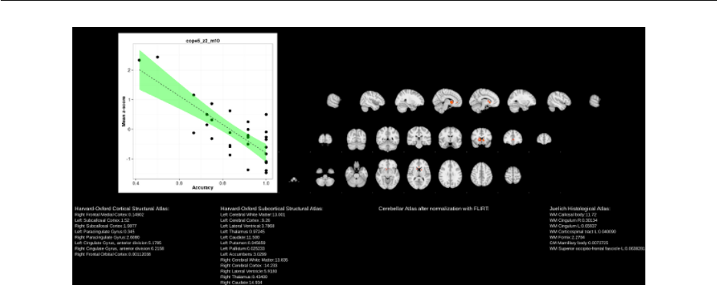
Figure 12.1: Report plotting group FEAT results against behavioral measures.
file, provides an excellent stepping stone for further analysis.
148

