Manual
manual
User Manual: Pdf
Open the PDF directly: View PDF ![]() .
.
Page Count: 109 [warning: Documents this large are best viewed by clicking the View PDF Link!]
- Introduction
- Getting Started
- Modeling
- Power Flow
- Optimal Power Flow
- Extending the OPF
- Unit De-commitment Algorithm
- Acknowledgments
- Appendix MIPS – Matlab Interior Point Solver
- Appendix Data File Format
- Appendix Matpower Options
- Appendix Matpower Files and Functions
- Appendix Extras Directory
- Appendix ``Smart Market'' Code
- Appendix Optional Packages
- References
Matpower 4.0
User’s Manual
Ray D. Zimmerman Carlos E. Murillo-S´anchez
February 7, 2011
©2010, 2011 Power Systems Engineering Research Center (Pserc)
All Rights Reserved
Contents
1 Introduction 7
1.1 Background ................................ 7
1.2 License and Terms of Use ........................ 7
1.3 Citing Matpower ............................ 8
2 Getting Started 9
2.1 System Requirements ........................... 9
2.2 Installation ................................ 9
2.3 Running a Simulation ........................... 10
2.3.1 Preparing Case Input Data .................... 11
2.3.2 Solving the Case ......................... 11
2.3.3 Accessing the Results ....................... 12
2.3.4 Setting Options .......................... 13
2.4 Documentation .............................. 13
3 Modeling 16
3.1 Data Formats ............................... 16
3.2 Branches .................................. 16
3.3 Generators ................................. 18
3.4 Loads ................................... 18
3.5 Shunt Elements .............................. 18
3.6 Network Equations ............................ 19
3.7 DC Modeling ............................... 19
4 Power Flow 23
4.1 AC Power Flow .............................. 23
4.2 DC Power Flow .............................. 25
4.3 runpf ................................... 25
4.4 Linear Shift Factors ............................ 27
5 Optimal Power Flow 29
5.1 Standard AC OPF ............................ 29
5.2 Standard DC OPF ............................ 30
5.3 Extended OPF Formulation ....................... 31
5.3.1 User-defined Costs ........................ 31
5.3.2 User-defined Constraints ..................... 33
5.3.3 User-defined Variables ...................... 33
2
5.4 Standard Extensions ........................... 34
5.4.1 Piecewise Linear Costs ...................... 34
5.4.2 Dispatchable Loads ........................ 35
5.4.3 Generator Capability Curves ................... 37
5.4.4 Branch Angle Difference Limits ................. 38
5.5 Solvers ................................... 38
5.6 runopf ................................... 39
6 Extending the OPF 44
6.1 Direct Specification ............................ 44
6.2 Callback Functions ............................ 45
6.2.1 ext2int Callback ......................... 46
6.2.2 formulation Callback ...................... 48
6.2.3 int2ext Callback ......................... 50
6.2.4 printpf Callback ......................... 52
6.2.5 savecase Callback ........................ 55
6.3 Registering the Callbacks ......................... 57
6.4 Summary ................................. 58
7 Unit De-commitment Algorithm 59
8 Acknowledgments 60
Appendix A MIPS – Matlab Interior Point Solver 61
A.1 Example 1 ................................. 64
A.2 Example 2 ................................. 65
A.3 Quadratic Programming Solver ..................... 67
A.4 Primal-Dual Interior Point Algorithm .................. 68
A.4.1 Notation .............................. 68
A.4.2 Problem Formulation and Lagrangian .............. 69
A.4.3 First Order Optimality Conditions ............... 70
A.4.4 Newton Step ........................... 70
Appendix B Data File Format 73
Appendix C Matpower Options 78
3

Appendix D Matpower Files and Functions 86
D.1 Documentation Files ........................... 86
D.2 Matpower Functions .......................... 86
D.3 Example Matpower Cases ....................... 92
D.4 Automated Test Suite .......................... 93
Appendix E Extras Directory 96
Appendix F “Smart Market” Code 97
F.1 Handling Supply Shortfall ........................ 99
F.2 Example .................................. 99
F.3 Smartmarket Files and Functions .................... 103
Appendix G Optional Packages 104
G.1 BPMPD MEX – MEX interface for BPMPD .............. 104
G.2 MINOPF – AC OPF Solver Based on MINOS ............. 104
G.3 TSPOPF – Three AC OPF Solvers by H. Wang ............ 105
G.4 CPLEX – High-performance LP and QP Solvers ............ 105
G.5 Ipopt – Interior Point Optimizer .................... 106
G.6 MOSEK – High-performance LP and QP Solvers ........... 106
References 108
4
List of Figures
3-1 Branch Model ............................... 17
5-1 Relationship of wito rifor di= 1 (linear option) ............ 32
5-2 Relationship of wito rifor di= 2 (quadratic option) ......... 33
5-3 Constrained Cost Variable ........................ 34
5-4 Marginal Benefit or Bid Function .................... 36
5-5 Total Cost Function for Negative Injection ............... 36
5-6 Generator P-QCapability Curve .................... 37
6-1 Adding Constraints Across Subsets of Variables ............ 49
List of Tables
4-1 Power Flow Results ............................ 26
4-2 Power Flow Options ........................... 26
4-3 Power Flow Output Options ....................... 27
5-1 Optimal Power Flow Results ....................... 40
5-2 Optimal Power Flow Options ...................... 42
5-3 OPF Output Options ........................... 43
6-1 Names Used by Implementation of OPF with Reserves ........ 47
6-2 Results for User-Defined Variables, Constraints and Costs ....... 51
6-3 Callback Functions ............................ 58
A-1 Input Arguments for mips ........................ 62
A-2 Output Arguments for mips ....................... 63
B-1 Bus Data (mpc.bus)............................ 74
B-2 Generator Data (mpc.gen)........................ 75
B-3 Branch Data (mpc.branch)........................ 76
B-4 Generator Cost Data (mpc.gencost)................... 77
C-1 Power Flow Options ........................... 79
C-2 General OPF Options .......................... 80
C-3 Power Flow and OPF Output Options ................. 81
C-4 OPF Options for MIPS and TSPOPF .................. 82
C-5 OPF Options for fmincon,constr and successive LP Solvers ..... 82
C-6 OPF Options for CPLEX ........................ 83
C-7 OPF Options for MOSEK ........................ 84
C-8 OPF Options for Ipopt ......................... 84
C-9 OPF Options for MINOPF ........................ 85
D-1 Matpower Documentation Files .................... 86
5
D-2 Top-Level Simulation Functions ..................... 86
D-3 Input/Output Functions ......................... 87
D-4 Data Conversion Functions ........................ 87
D-5 Power Flow Functions .......................... 87
D-6 OPF and Wrapper Functions ...................... 87
D-7 OPF Model Object ............................ 88
D-8 OPF Solver Functions .......................... 88
D-9 Other OPF Functions ........................... 89
D-10 OPF User Callback Functions ...................... 89
D-11 Power Flow Derivative Functions .................... 90
D-12 NLP, LP & QP Solver Functions .................... 90
D-13 Matrix Building Functions ........................ 91
D-14 Utility Functions ............................. 91
D-15 Example Cases .............................. 92
D-16 Automated Test Utility Functions .................... 93
D-17 Test Data ................................. 93
D-18 Miscellaneous Matpower Tests ..................... 94
D-19 Matpower OPF Tests ......................... 95
F-1 Auction Types .............................. 98
F-2 Generator Offers ............................. 100
F-3 Load Bids ................................. 100
F-4 Generator Sales .............................. 103
F-5 Load Purchases .............................. 103
F-6 Smartmarket Files and Functions .................... 103
6

1 Introduction
1.1 Background
Matpower is a package of Matlab®M-files for solving power flow and optimal
power flow problems. It is intended as a simulation tool for researchers and educators
that is easy to use and modify. Matpower is designed to give the best performance
possible while keeping the code simple to understand and modify. The Matpower
home page can be found at:
http://www.pserc.cornell.edu/matpower/
Matpower was initially developed by Ray D. Zimmerman, Carlos E. Murillo-
S´anchez and Deqiang Gan of PSERC1at Cornell University under the direction of
Robert J. Thomas. The initial need for Matlab-based power flow and optimal power
flow code was born out of the computational requirements of the PowerWeb project2.
Many others have contributed to Matpower over the years and it continues to be
developed and maintained under the direction of Ray Zimmerman.
1.2 License and Terms of Use
Beginning with version 4, the code in Matpower is distributed under the GNU
General Public License (GPL) [1] with an exception added to clarify our intention
to allow Matpower to interface with Matlab as well as any other Matlab code
or MEX-files a user may have installed, regardless of their licensing terms. The full
text of the GPL can be found in the COPYING file at the top level of the distribution
or at http://www.gnu.org/licenses/gpl-3.0.txt.
The text of the license notice that appears with the copyright in each of the code
files reads:
1http://www.pserc.cornell.edu/
2http://www.pserc.cornell.edu/powerweb/
7

MATPOWER is free software: you can redistribute it and/or modify
it under the terms of the GNU General Public License as published
by the Free Software Foundation, either version 3 of the License,
or (at your option) any later version.
MATPOWER is distributed in the hope that it will be useful,
but WITHOUT ANY WARRANTY; without even the implied warranty of
MERCHANTABILITY or FITNESS FOR A PARTICULAR PURPOSE. See the
GNU General Public License for more details.
You should have received a copy of the GNU General Public License
along with MATPOWER. If not, see <http://www.gnu.org/licenses/>.
Additional permission under GNU GPL version 3 section 7
If you modify MATPOWER, or any covered work, to interface with
other modules (such as MATLAB code and MEX-files) available in a
MATLAB(R) or comparable environment containing parts covered
under other licensing terms, the licensors of MATPOWER grant
you additional permission to convey the resulting work.
Please note that the Matpower case files distributed with Matpower are not
covered by the GPL. In most cases, the data has either been included with permission
or has been converted from data available from a public source.
1.3 Citing Matpower
While not required by the terms of the license, we do request that publications derived
from the use of Matpower explicitly acknowledge that fact by citing reference [2].
R. D. Zimmerman, C. E. Murillo-S´anchez, and R. J. Thomas, “Matpower: Steady-
State Operations, Planning and Analysis Tools for Power Systems Research and Ed-
ucation,” Power Systems, IEEE Transactions on, vol. 26, no. 1, pp. 12–19, Feb. 2011.
8

2 Getting Started
2.1 System Requirements
To use Matpower 4.0 you will need:
•Matlab®version 6.5 or later3, or
•GNU Octave version 3.2 or later4
For the hardware requirements, please refer to the system requirements for the
version of Matlab5or Octave that you are using. If the Matlab Optimization
Toolbox is installed as well, Matpower enables an option to use it to solve optimal
power flow problems, though this option is not recommended for most applications.
In this manual, references to Matlab usually apply to Octave as well. However,
due to lack of extensive testing, support for Octave should be considered experimen-
tal. At the time of writing, none of the optional MEX-based Matpower packages
have been built for Octave.
2.2 Installation
Installation and use of Matpower requires familiarity with the basic operation of
Matlab, including setting up your Matlab path.
Step 1: Follow the download instructions on the Matpower home page6. You
should end up with a file named matpowerXXX.zip, where XXX depends on
the version of Matpower.
Step 2: Unzip the downloaded file. Move the resulting matpowerXXX directory to the
location of your choice. These files should not need to be modified, so it is
recommended that they be kept separate from your own code. We will use
$MATPOWER to denote the path to this directory.
3Matlab is available from The MathWorks, Inc. (http://www.mathworks.com/). Though
some Matpower functionality may work in earlier versions of Matlab 6, it is not supported.
Matpower 3.2 required Matlab 6, Matpower 3.0 required Matlab 5 and Matpower 2.0 and
earlier required only Matlab 4. Matlab is a registered trademark of The MathWorks, Inc.
4GNU Octave is free software, available online at http://www.gnu.org/software/octave/.
Matpower 4.0 may work on earlier versions of Octave, but has not been tested on versions prior
to 3.2.3.
5http://www.mathworks.com/support/sysreq/previous_releases.html
6http://www.pserc.cornell.edu/matpower/
9

Step 3: Add the following directories to your Matlab path:
•$MATPOWER – core Matpower functions
•$MATPOWER/t – test scripts for Matpower
•(optional) sub-directories of $MATPOWER/extras – additional function-
ality and contributed code (see Appendix Efor details).
Step 4: At the Matlab prompt, type test matpower to run the test suite and verify
that Matpower is properly installed and functioning. The result should
resemble the following, possibly including extra tests, depending on the
availablility of optional packages, solvers and extras.
>> test_matpower
t_loadcase..........ok
t_ext2int2ext.......ok
t_jacobian..........ok
t_hessian...........ok
t_totcost...........ok
t_modcost...........ok
t_hasPQcap..........ok
t_mips..............ok
t_qps_matpower......ok (144 of 252 skipped)
t_pf................ok
t_opf_fmincon.......ok
t_opf_mips..........ok
t_opf_mips_sc.......ok
t_opf_dc_mips.......ok
t_opf_dc_mips_sc....ok
t_opf_dc_ot.........ok
t_opf_userfcns......ok
t_runopf_w_res......ok
t_makePTDF..........ok
t_makeLODF..........ok
t_total_load........ok
t_scale_load........ok
All tests successful (1530 passed, 144 skipped of 1674)
Elapsed time 5.36 seconds.
2.3 Running a Simulation
The primary functionality of Matpower is to solve power flow and optimal power
flow (OPF) problems. This involves (1) preparing the input data defining the all of
10

the relevant power system parameters, (2) invoking the function to run the simulation
and (3) viewing and accessing the results that are printed to the screen and/or saved
in output data structures or files.
2.3.1 Preparing Case Input Data
The input data for the case to be simulated are specified in a set of data matrices
packaged as the fields of a Matlab struct, referred to as a “Matpower case” struct
and conventionally denoted by the variable mpc. This struct is typically defined in
a case file, either a function M-file whose return value is the mpc struct or a MAT-
file that defines a variable named mpc when loaded7. The main simulation routines,
whose names begin with run (e.g. runpf,runopf), accept either a file name or a
Matpower case struct as an input.
Use loadcase to load the data from a case file into a struct if you want to make
modifications to the data before passing it to the simulation.
>> mpc = loadcase(casefilename);
See also savecase for writing a Matpower case struct to a case file.
The structure of the Matpower case data is described a bit further in Section 3.1
and the full details are documented in Appendix Band can be accessed at any time
via the command help caseformat. The Matpower distribution also includes many
example case files listed in Table D-15.
2.3.2 Solving the Case
The solver is invoked by calling one of the main simulation functions, such as runpf
or runopf, passing in a case file name or a case struct as the first argument. For
example, to run a simple Newton power flow with default options on the 9-bus system
defined in case9.m, at the Matlab prompt, type:
>> runpf('case9');
If, on the other hand, you wanted to load the 30-bus system data from case30.m,
increase its real power demand at bus 2 to 30 MW, then run an AC optimal power
flow with default options, this could be accomplished as follows:
7This describes version 2 of the Matpower case format, which is used internally and is the
default. The version 1 format, now deprecated, but still accessible via the loadcase and savecase
functions, defines the data matrices as individual variables rather than fields of a struct, and some
do not include all of the columns defined in version 2.
11

>> define_constants;
>> mpc = loadcase('case30');
>> mpc.bus(2, PD) = 30;
>> runopf(mpc);
The define constants in the first line is simply a convenience script that defines a
number of variables to serve as named column indices for the data matrices. In this
example, it allows us to access the “real power demand” column of the bus matrix
using the name PD without having to remember that it is the 3rd column.
Other top-level simulation functions are available for running DC versions of
power flow and OPF, for running an OPF with the option for Matpower to shut
down (decommit) expensive generators, etc. These functions are listed in Table D-2
in Appendix D.
2.3.3 Accessing the Results
By default, the results of the simulation are pretty-printed to the screen, displaying
a system summary, bus data, branch data and, for the OPF, binding constraint
information. The bus data includes the voltage, angle and total generation and load
at each bus. It also includes nodal prices in the case of the OPF. The branch data
shows the flows and losses in each branch. These pretty-printed results can be saved
to a file by providing a filename as the optional 3rd argument to the simulation
function.
The solution is also stored in a results struct available as an optional return value
from the simulation functions. This results struct is a superset of the Matpower
case struct mpc, with additional columns added to some of the existing data fields
and additional fields. The following example shows how simple it is, after running a
DC OPF on the 118-bus system in case118.m, to access the final objective function
value, the real power output of generator 6 and the power flow in branch 51.
>> define_constants;
>> results = rundcopf('case118');
>> final_objective = results.f;
>> gen6_output = results.gen(6, PG);
>> branch51_flow = results.branch(51, PF);
Full documentation for the content of the results struct can be found in Sec-
tions 4.3 and 5.6.
12

2.3.4 Setting Options
Matpower has many options for selecting among the available solution algorithms,
controlling the behavior of the algorithms and determining the details of the pretty-
printed output. These options are passed to the simulation routines as a Matpower
options vector. The elements of the vector have names that can be used to set the
corresponding value via the mpoption function. Calling mpoption with no arguments
returns the default options vector, the vector used if none is explicitly supplied.
Calling it with a set of name and value pairs modifies the default vector.
For example, the following code runs a power flow on the 300-bus example in
case300.m using the fast-decoupled (XB version) algorithm, with verbose printing of
the algorithm progress, but suppressing all of the pretty-printed output.
>> mpopt = mpoption('PF_ALG', 2, 'VERBOSE', 2, 'OUT_ALL', 0);
>> results = runpf('case300', mpopt);
To modify an existing options vector, for example, to turn the verbose option off
and re-run with the remaining options unchanged, simply pass the existing options
as the first argument to mpoption.
>> mpopt = mpoption(mpopt, 'VERBOSE', 0);
>> results = runpf('case300', mpopt);
See Appendix Cor type:
>> help mpoption
for more information on Matpower’s options.
2.4 Documentation
There are two primary sources of documentation for Matpower. The first is this
manual, which gives an overview of Matpower’s capabilities and structure and
describes the modeling and formulations behind the code. It can be found in your
Matpower distribution at $MATPOWER/docs/manual.pdf.
The second is the built-in help command. As with Matlab’s built-in functions
and toolbox routines, you can type help followed by the name of a command or
M-file to get help on that particular function. Nearly all of Matpower’s M-files
have such documentation and this should be considered the main reference for the
13

>> help runopf
RUNOPF Runs an optimal power flow.
[RESULTS, SUCCESS] = RUNOPF(CASEDATA, MPOPT, FNAME, SOLVEDCASE)
Runs an optimal power flow (AC OPF by default), optionally returning
a RESULTS struct and SUCCESS flag.
Inputs (all are optional):
CASEDATA : either a MATPOWER case struct or a string containing
the name of the file with the case data (default is 'case9')
(see also CASEFORMAT and LOADCASE)
MPOPT : MATPOWER options vector to override default options
can be used to specify the solution algorithm, output options
termination tolerances, and more (see also MPOPTION).
FNAME : name of a file to which the pretty-printed output will
be appended
SOLVEDCASE : name of file to which the solved case will be saved
in MATPOWER case format (M-file will be assumed unless the
specified name ends with '.mat')
Outputs (all are optional):
RESULTS : results struct, with the following fields:
(all fields from the input MATPOWER case, i.e. bus, branch,
gen, etc., but with solved voltages, power flows, etc.)
order - info used in external <-> internal data conversion
et - elapsed time in seconds
success - success flag, 1 = succeeded, 0 = failed
(additional OPF fields, see OPF for details)
SUCCESS : the success flag can additionally be returned as
a second output argument
Calling syntax options:
results = runopf;
results = runopf(casedata);
results = runopf(casedata, mpopt);
results = runopf(casedata, mpopt, fname);
results = runopf(casedata, mpopt, fname, solvedcase);
[results, success] = runopf(...);
Alternatively, for compatibility with previous versions of MATPOWER,
some of the results can be returned as individual output arguments:
[baseMVA, bus, gen, gencost, branch, f, success, et] = runopf(...);
Example:
results = runopf('case30');
See also RUNDCOPF, RUNUOPF. 15
3 Modeling
Matpower employs all of the standard steady-state models typically used for power
flow analysis. The AC models are described first, then the simplified DC models. In-
ternally, the magnitudes of all values are expressed in per unit and angles of complex
quantities are expressed in radians. Internally, all off-line generators and branches
are removed before forming the models used to solve the power flow or optimal power
flow problem. All buses are numbered consecutively, beginning at 1, and generators
are reordered by bus number. Conversions to and from this internal indexing is done
by the functions ext2int and int2ext. The notation in this section, as well as Sec-
tions 4and 5, is based on this internal numbering, with all generators and branches
assumed to be in-service. Due to the strengths of the Matlab programming lan-
guage in handling matrices and vectors, the models and equations are presented here
in matrix and vector form.
3.1 Data Formats
The data files used by Matpower are Matlab M-files or MAT-files which define
and return a single Matlab struct. The M-file format is plain text that can be edited
using any standard text editor. The fields of the struct are baseMVA,bus,branch,gen
and optionally gencost, where baseMVA is a scalar and the rest are matrices. In the
matrices, each row corresponds to a single bus, branch, or generator. The columns
are similar to the columns in the standard IEEE CDF and PTI formats. The number
of rows in bus,branch and gen are nb,nland ng, respectively. If present, gencost
has either ngor 2ngrows, depending on whether it includes costs for reactive power
or just real power. Full details of the Matpower case format are documented
in Appendix Band can be accessed from the Matlab command line by typing
help caseformat.
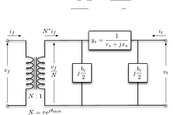
3.2 Branches
All transmission lines, transformers and phase shifters are modeled with a com-
mon branch model, consisting of a standard πtransmission line model, with series
impedance zs=rs+jxsand total charging capacitance bc, in series with an ideal
phase shifting transformer. The transformer, whose tap ratio has magnitude τand
phase shift angle θshift, is located at the from end of the branch, as shown in Fig-
ure 3-1. The parameters rs,xs,bc,τand θshift are specified directly in columns 3, 4,
5, 9 and 10, respectively, of the corresponding row of the branch matrix.
16
The complex current injections ifand itat the from and to ends of the branch,
respectively, can be expressed in terms of the 2 ×2 branch admittance matrix Ybr
and the respective terminal voltages vfand vt
if
it=Ybr vf
vt.(3.1)
With the series admittance element in the πmodel denoted by ys= 1/zs, the branch
admittance matrix can be written
Ybr =ys+jbc
21
τ2−ys1
τe−jθshift
−ys1
τejθshift ys+jbc
2.(3.2)
Figure 3-1: Branch Model
If the four elements of this matrix for branch iare labeled as follows:
Yi
br =yi
ff yi
ft
yi
tf yi
tt (3.3)
then four nl×1 vectors Yff ,Yft,Ytf and Ytt can be constructed, where the i-th element
of each comes from the corresponding element of Yi
br. Furthermore, the nl×nbsparse
connection matrices Cfand Ctused in building the system admittance matrices can
be defined as follows. The (i, j)th element of Cfand the (i, k)th element of Ctare
equal to 1 for each branch i, where branch iconnects from bus jto bus k. All other
elements of Cfand Ctare zero.
17
3.3 Generators
A generator is modeled as a complex power injection at a specific bus. For generator i,
the injection is
si
g=pi
g+jqi
g.(3.4)
Let Sg=Pg+jQgbe the ng×1 vector of these generator injections. The MW and
MVAr equivalents (before conversion to p.u.) of pi
gand qi
gare specified in columns 2
and 3, respectively of row iof the gen matrix. A sparse nb×nggenerator connection
matrix Cgcan be defined such that its (i, j)th element is 1 if generator jis located
at bus iand 0 otherwise. The nb×1 vector of all bus injections from generators can
then be expressed as
Sg,bus =Cg·Sg.(3.5)
3.4 Loads
Constant power loads are modeled as a specified quantity of real and reactive power
consumed at a bus. For bus i, the load is
si
d=pi
d+jqi
d(3.6)
and Sd=Pd+jQddenotes the nb×1 vector of complex loads at all buses. The
MW and MVAr equivalents (before conversion to p.u.) of pi
dand qi
dare specified in
columns 3 and 4, respectively of row iof the bus matrix.
Constant impedance and constant current loads are not implemented directly,
but the constant impedance portions can be modeled as a shunt element described
below. Dispatchable loads are modeled as negative generators and appear as negative
values in Sg.
3.5 Shunt Elements
A shunt connected element such as a capacitor or inductor is modeled as a fixed
impedance to ground at a bus. The admittance of the shunt element at bus iis given
as
yi
sh =gi
sh +jbi
sh (3.7)
and Ysh =Gsh +jBsh denotes the nb×1 vector of shunt admittances at all buses.
The parameters gi
sh and bi
sh are specified in columns 5 and 6, respectively, of row i
of the bus matrix as equivalent MW (consumed) and MVAr (injected) at a nominal
voltage magnitude of 1.0 p.u and angle of zero.
18
3.6 Network Equations
For a network with nbbuses, all constant impedance elements of the model are
incorporated into a complex nb×nbbus admittance matrix Ybus that relates the
complex nodal current injections Ibus to the complex node voltages V:
Ibus =YbusV. (3.8)
Similarly, for a network with nlbranches, the nl×nbsystem branch admittance
matrices Yfand Ytrelate the bus voltages to the nl×1 vectors Ifand Itof branch
currents at the from and to ends of all branches, respectively:
If=YfV(3.9)
It=YtV. (3.10)
If [ ·] is used to denote an operator that takes an n×1 vector and creates the
corresponding n×ndiagonal matrix with the vector elements on the diagonal, these
system admittance matrices can be formed as follows:
Yf= [Yff ]Cf+ [Yf t]Ct(3.11)
Yt= [Ytf ]Cf+ [Ytt]Ct(3.12)
Ybus =Cf
TYf+Ct
TYt+ [Ysh].(3.13)
The current injections of (3.8)–(3.10) can be used to compute the corresponding
complex power injections as functions of the complex bus voltages V:
Sbus(V)=[V]I∗
bus = [V]Y∗
busV∗(3.14)
Sf(V) = [CfV]I∗
f= [CfV]Y∗
fV∗(3.15)
St(V) = [CtV]I∗
t= [CtV]Y∗
tV∗.(3.16)
The nodal bus injections are then matched to the injections from loads and generators
to form the AC nodal power balance equations, expressed as a function of the complex
bus voltages and generator injections in complex matrix form as
gS(V, Sg) = Sbus(V) + Sd−CgSg= 0.(3.17)
3.7 DC Modeling
The DC formulation [8] is based on the same parameters, but with the following
three additional simplifying assumptions.
19

•Branches can be considered lossless. In particular, branch resistances rsand
charging capacitances bcare negligible:
ys=1
rs+jxs
≈1
jxs
, bc≈0.(3.18)
•All bus voltage magnitudes are close to 1 p.u.
vi≈ejθi.(3.19)
•Voltage angle differences across branches are small enough that
sin(θf−θt−θshift)≈θf−θt−θshift.(3.20)
Substituting the first set of assumptions regarding branch parameters from (3.18),
the branch admittance matrix in (3.2) approximates to
Ybr ≈1
jxs1
τ2−1
τe−jθshift
−1
τejθshift 1.(3.21)
Combining this and the second assumption with (3.1) yields the following approxi-
mation for if:
if≈1
jxs
(1
τ2ejθf−1
τe−jθshift ejθt)
=1
jxsτ(1
τejθf−ej(θt+θshift)).(3.22)
The approximate real power flow is then derived as follows, first applying (3.19) and
(3.22), then extracting the real part and applying (3.20).
pf=< {sf}
=<vf·i∗
f
≈ < ejθf·j
xsτ(1
τe−jθf−e−j(θt+θshift))
=<j
xsτ1
τ−ej(θf−θt−θshift)
=<1
xsτsin(θf−θt−θshift) + j1
τ−cos(θf−θt−θshift)
≈1
xsτ(θf−θt−θshift) (3.23)
20

As expected, given the lossless assumption, a similar derivation for the power injec-
tion at the to end of the line leads to leads to pt=−pf.
The relationship between the real power flows and voltage angles for an individual
branch ican then be summarized as
pf
pt=Bi
br θf
θt+Pi
shift (3.24)
where
Bi
br =bi1−1
−1 1 ,
Pi
shift =θi
shiftbi−1
1
and biis defined in terms of the series reactance xi
sand tap ratio τifor branch ias
bi=1
xi
sτi.
For a shunt element at bus i, the amount of complex power consumed is
si
sh =vi(yi
shvi)∗
≈ejθi(gi
sh −jbi
sh)e−jθi
=gi
sh −jbi
sh.(3.25)
So the vector of real power consumed by shunt elements at all buses can be approx-
imated by
Psh ≈Gsh.(3.26)
With a DC model, the linear network equations relate real power to bus voltage
angles, versus complex currents to complex bus voltages in the AC case. Let the
nl×1 vector Bff be constructed similar to Yff , where the i-th element is biand let
Pf,shift be the nl×1 vector whose i-th element is equal to −θi
shiftbi. Then the nodal
real power injections can be expressed as a linear function of Θ, the nb×1 vector of
bus voltage angles
Pbus(Θ) = BbusΘ + Pbus,shift (3.27)
where
Pbus,shift = (Cf−Ct)TPf,shift.(3.28)
21
Similarly, the branch flows at the from ends of each branch are linear functions of
the bus voltage angles
Pf(Θ) = BfΘ + Pf,shift (3.29)
and, due to the lossless assumption, the flows at the to ends are given by Pt=−Pf.
The construction of the system Bmatrices is analogous to the system Ymatrices
for the AC model:
Bf= [Bff ] (Cf−Ct) (3.30)
Bbus = (Cf−Ct)TBf.(3.31)
The DC nodal power balance equations for the system can be expressed in matrix
form as
gP(Θ, Pg) = BbusΘ + Pbus,shift +Pd+Gsh −CgPg= 0 (3.32)
22
4 Power Flow
The standard power flow or loadflow problem involves solving for the set of voltages
and flows in a network corresponding to a specified pattern of load and generation.
Matpower includes solvers for both AC and DC power flow problems, both of
which involve solving a set of equations of the form
g(x) = 0,(4.1)
constructed by expressing a subset of the nodal power balance equations as functions
of unknown voltage quantities.
All of Matpower’s solvers exploit the sparsity of the problem and, except for
Gauss-Seidel, scale well to very large systems. Currently, none of them include any
automatic updating of transformer taps or other techniques to attempt to satisfy
typical optimal power flow constraints, such as generator, voltage or branch flow
limits.
4.1 AC Power Flow
In Matpower, by convention, a single generator bus is typically chosen as a refer-
ence bus to serve the roles of both a voltage angle reference and a real power slack.
The voltage angle at the reference bus has a known value, but the real power gen-
eration at the slack bus is taken as unknown to avoid overspecifying the problem.
The remaining generator buses are classified as PV buses, with the values of voltage
magnitude and generator real power injection given. Since the loads Pdand Qdare
also given, all non-generator buses are PQ buses, with real and reactive injections
fully specified. Let Iref ,IPV and IPQ denote the sets of bus indices of the reference
bus, PV buses and PQ buses, respectively.
In the traditional formulation of the AC power flow problem, the power balance
equation in (3.17) is split into its real and reactive components, expressed as functions
of the voltage angles Θ and magnitudes Vmand generator injections Pgand Qg, where
the load injections are assumed constant and given:
gP(Θ, Vm, Pg) = Pbus(Θ, Vm) + Pd−CgPg= 0 (4.2)
gQ(Θ, Vm, Qg) = Qbus(Θ, Vm) + Qd−CgQg= 0.(4.3)
For the AC power flow problem, the function g(x) from (4.1) is formed by taking
the left-hand side of the real power balance equations (4.2) for all non-slack buses
23

and the reactive power balance equations (4.3) for all PQ buses and plugging in the
reference angle, the loads and the known generator injections and voltage magnitudes:
g(x) = "g{i}
P(Θ, Vm, Pg)
g{j}
Q(Θ, Vm, Qg)#∀i∈ IPV ∪ IPQ
∀j∈ IPQ.(4.4)
The vector xconsists of the remaining unknown voltage quantities, namely the volt-
age angles at all non-reference buses and the voltage magnitudes at PQ buses:
x=θ{i}
v{j}
m∀i /∈ Iref
∀j∈ IPQ.(4.5)
This yields a system of nonlinear equations with npv + 2npq equations and un-
knowns, where npv and npq are the number of PV and PQ buses, respectively. After
solving for x, the remaining real power balance equation can be used to compute
the generator real power injection at the slack bus. Similarly, the remaining npv + 1
reactive power balance equations yield the generator reactive power injections.
Matpower includes four different algorithms for solving the AC power flow
problem. The default solver is based on a standard Newton’s method [4] using a
polar form and a full Jacobian updated at each iteration. Each Newton step involves
computing the mismatch g(x), forming the Jacobian based on the sensitivities of
these mismatches to changes in xand solving for an updated value of xby factorizing
this Jacobian. This method is described in detail in many textbooks.
Also included are solvers based on variations of the fast-decoupled method [5],
specifically, the XB and BX methods described in [6]. These solvers greatly reduce
the amount of computation per iteration, by updating the voltage magnitudes and
angles separately based on constant approximate Jacobians which are factored only
once at the beginning of the solution process. These per-iteration savings, however,
come at the cost of more iterations.
The fourth algorithm is the standard Gauss-Seidel method from Glimm and
Stagg [7]. It has numerous disadvantages relative to the Newton method and is
included primarily for academic interest.
By default, the AC power flow solvers simply solve the problem described above,
ignoring any generator limits, branch flow limits, voltage magnitude limits, etc. How-
ever, there is an option (ENFORCE Q LIMS) that allows for the generator reactive power
limits to be respected at the expense of the voltage setpoint. This is done in a rather
brute force fashion by adding an outer loop around the AC power flow solution. If
any generator has a violated reactive power limit, its reactive injection is fixed at
the limit, the corresponding bus is converted to a PQ bus and the power flow is
24

solved again. This procedure is repeated until there are no more violations. Note
that this option is based solely on the QMIN and QMAX parameters for the generator
and does not take into account the trapezoidal generator capability curves described
in Section 5.4.3.
4.2 DC Power Flow
For the DC power flow problem [8], the vector xconsists of the set of voltage angles
at non-reference buses
x=θ{i},∀i /∈ Iref (4.6)
and (4.1) takes the form
Bdcx−Pdc = 0 (4.7)
where Bdc is the (nb−1) ×(nb−1) matrix obtained by simply eliminating from Bbus
the row and column corresponding to the slack bus and reference angle, respectively.
Given that the generator injections Pgare specified at all but the slack bus, Pdc can
be formed directly from the non-slack rows of the last four terms of (3.32).
The voltage angles in xare computed by a direct solution of the set of linear
equations. The branch flows and slack bus generator injection are then calculated
directly from the bus voltage angles via (3.29) and the appropriate row in (3.32),
respectively.
4.3 runpf
In Matpower, a power flow is executed by calling runpf with a case struct or case
file name as the first argument (casedata). In addition to printing output to the
screen, which it does by default, runpf optionally returns the solution in a results
struct.
>> results = runpf(casedata);
The results struct is a superset of the input Matpower case struct mpc, with some
additional fields as well as additional columns in some of the existing data fields.
The solution values are stored as shown in Table 4-1.
Additional optional input arguments can be used to set options (mpopt) and
provide file names for saving the pretty printed output (fname) or the solved case
data (solvedcase).
>> results = runpf(casedata, mpopt, fname, solvedcase);
25

Table 4-1: Power Flow Results
name description
results.success success flag, 1 = succeeded, 0 = failed
results.et computation time required for solution
results.order see ext2int help for details on this field
results.bus(:, VM)†bus voltage magnitudes
results.bus(:, VA) bus voltage angles
results.gen(:, PG) generator real power injections
results.gen(:, QG)†generator reactive power injections
results.branch(:, PF) real power injected into “from” end of branch
results.branch(:, PT) real power injected into “to” end of branch
results.branch(:, QF)†reactive power injected into “from” end of branch
results.branch(:, QT)†reactive power injected into “to” end of branch
†AC power flow only.
The options that control the power flow simulation are listed in Table 4-2 and those
controlling the output printed to the screen in Table 4-3.
By default, runpf solves an AC power flow problem using a standard Newton’s
method solver. To run a DC power flow, the PF DC option must be set to 1. For
convenience, Matpower provides a function rundcpf which is simply a wrapper
that sets PF DC before calling runpf.
Table 4-2: Power Flow Options
idx name default description
1PF ALG 1 AC power flow algorithm:
1 – Newtons’s method
2 – Fast-Decoupled (XB version)
3 – Fast-Decouple (BX version)
4 – Gauss-Seidel
2PF TOL 10−8termination tolerance on per unit P and Q dispatch
3PF MAX IT 10 maximum number of iterations for Newton’s method
4PF MAX IT FD 30 maximum number of iterations for fast decoupled method
5PF MAX IT GS 1000 maximum number of iterations for Gauss-Seidel method
6ENFORCE Q LIMS 0 enforce gen reactive power limits at expense of |Vm|
0 – do not enforce limits
1 – enforce limits, simultaneous bus type conversion
2 – enforce limits, one-at-a-time bus type conversion
10 PF DC 0 DC modeling for power flow and OPF formulation
0 – use AC formulation and corresponding alg options
1 – use DC formulation and corresponding alg options
26
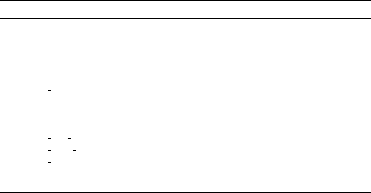
Table 4-3: Power Flow Output Options
idx name default description
31 VERBOSE 1 amount of progress info to be printed
0 – print no progress info
1 – print a little progress info
2 – print a lot progress info
3 – print all progress info
32 OUT ALL -1 controls pretty-printing of results
-1 – individual flags control what is printed
0 – do not print anything†
1 – print everything†
33 OUT SYS SUM 1 print system summary (0 or 1)
34 OUT AREA SUM 0 print area summaries (0 or 1)
35 OUT BUS 1 print bus detail, includes per bus gen info (0 or 1)
36 OUT BRANCH 1 print branch detail (0 or 1)
37 OUT GEN 0 print generator detail (0 or 1)
†Overrides individual flags.
Internally, the runpf function does a number of conversions to the problem data
before calling the appropriate solver routine for the selected power flow algorithm.
This external-to-internal format conversion is performed by the ext2int function,
described in more detail in Section 6.2.1, and includes the elimination of out-of-service
equipment, the consecutive renumbering of buses and the reordering of generators
by increasing bus number. All computations are done using this internal indexing.
When the simulation has completed, the data is converted back to external format
by int2ext before the results are printed and returned.
4.4 Linear Shift Factors
The DC power flow model can also be used to compute the sensitivities of branch
flows to changes in nodal real power injections, sometimes called injection shift factors
(ISF) or generation shift factors [8]. These nl×nbsensitivity matrices, also called
power transfer distribution factors or PTDFs, carry an implicit assumption about
the slack distribution. If His used to denote a PTDF matrix, then the element in
row iand column j,hij , represents the change in the real power flow in branch i
given a unit increase in the power injected at bus j,with the assumption that the
additional unit of power is extracted according to some specified slack distribution:
∆Pf=H∆Pbus.(4.8)
This slack distribution can be expressed as an nb×1 vector wof non-negative
27

weights whose elements sum to 1. Each element specifies the proportion of the slack
taken up at each bus. For the special case of a single slack bus k,wis equal to the
vector ek. The corresponding PTDF matrix Hkcan be constructed by first creating
the nl×(nb−1) matrix
e
Hk=e
Bf·B−1
dc (4.9)
then inserting a column of zeros at column k. Here e
Bfand Bdc are obtained from Bf
and Bbus, respectively, by eliminating their reference bus columns and, in the case
of Bdc, removing row kcorresponding to the slack bus.
The PTDF matrix Hw, corresponding to a general slack distribution w, can be
obtained from any other PTDF, such as Hk, by subtracting wfrom each column,
equivalent to the following simple matrix multiplication:
Hw=Hk(I−w·1T).(4.10)
These same linear shift factors may also be used to compute sensitivities of branch
flows to branch outages, known as line outage distribution factors or LODFs [9].
Given a PTDF matrix Hw, the corresponding nl×nlLODF matrix Lcan be con-
structed as follows, where lij is the element in row iand column j, representing the
change in flow in branch i(as a fraction of its initial flow) for an outage of branch j.
First, let Hrepresent the matrix of sensitivities of branch flows to branch flows,
found by multplying the PTDF matrix by the node-branch incidence matrix:
H=Hw(Cf−Ct)T.(4.11)
If hij is the sensitivity of flow in branch iwith respect to flow in branch j, then lij
can be expressed as
lij =
hij
1−hjj
i6=j
−1i=j.
(4.12)
Matpower includes functions for computing both the DC PTDF matrix and
the corresponding LODF matrix for either a single slack bus kor a general slack
distribution vector w. See the help for makePTDF and makeLODF for details.
28
5 Optimal Power Flow
Matpower includes code to solve both AC and DC versions of the optimal power
flow problem. The standard version of each takes the following form:
min
xf(x) (5.1)
subject to
g(x) = 0 (5.2)
h(x)≤0 (5.3)
xmin ≤x≤xmax .(5.4)
5.1 Standard AC OPF
The optimization vector xfor the standard AC OPF problem consists of the nb×1
vectors of voltage angles Θ and magnitudes Vmand the ng×1 vectors of generator
real and reactive power injections Pgand Qg.
x=
Θ
Vm
Pg
Qg
(5.5)
The objective function (5.1) is simply a summation of individual polynomial cost
functions fi
Pand fi
Qof real and reactive power injections, respectively, for each
generator:
min
Θ,Vm,Pg,Qg
ng
X
i=1
fi
P(pi
g) + fi
Q(qi
g).(5.6)
The equality constraints in (5.2) are simply the full set of 2 ·nbnonlinear real and
reactive power balance equations from (4.2) and (4.3). The inequality constraints
(5.3) consist of two sets of nlbranch flow limits as nonlinear functions of the bus
voltage angles and magnitudes, one for the from end and one for the to end of each
branch:
hf(Θ, Vm) = |Ff(Θ, Vm)| − Fmax ≤0 (5.7)
ht(Θ, Vm) = |Ft(Θ, Vm)| − Fmax ≤0.(5.8)
29
The flows are typically apparent power flows expressed in MVA, but can be real power
or current flows, yielding the following three possible forms for the flow constraints:
Ff(Θ, Vm) =
Sf(Θ, Vm),apparent power
Pf(Θ, Vm),real power
If(Θ, Vm),current
(5.9)
where Ifis defined in (3.9), Sfin (3.15), Pf=<{Sf}and the vector of flow limits
Fmax has the appropriate units for the type of constraint. It is likewise for Ft(Θ, Vm).
The variable limits (5.4) include an equality constraint on any reference bus angle
and upper and lower limits on all bus voltage magnitudes and real and reactive
generator injections:
θref
i≤θi≤θref
i, i ∈ Iref (5.10)
vi,min
m≤vi
m≤vi,max
m, i = 1 . . . nb(5.11)
pi,min
g≤pi
g≤pi,max
g, i = 1 . . . ng(5.12)
qi,min
g≤qi
g≤qi,max
g, i = 1 . . . ng.(5.13)
5.2 Standard DC OPF
When using DC network modeling assumptions and limiting polynomial costs to
second order, the standard OPF problem above can be simplified to a quadratic
program, with linear constraints and a quadratic cost function. In this case, the
voltage magnitudes and reactive powers are eliminated from the problem completely
and real power flows are modeled as linear functions of the voltage angles. The
optimization variable is
x=Θ
Pg(5.14)
and the overall problem reduces to the following form.
min
Θ,Pg
ng
X
i=1
fi
P(pi
g) (5.15)
subject to
gP(Θ, Pg) = BbusΘ + Pbus,shift +Pd+Gsh −CgPg= 0 (5.16)
hf(Θ) = BfΘ + Pf,shift −Fmax ≤0 (5.17)
ht(Θ) = −BfΘ−Pf,shift −Fmax ≤0 (5.18)
30

θref
i≤θi≤θref
i, i ∈ Iref (5.19)
pi,min
g≤pi
g≤pi,max
g, i = 1 . . . ng(5.20)
5.3 Extended OPF Formulation
Matpower employs an extensible OPF structure [10] to allow the user to modify
or augment the problem formulation without rewriting the portions that are shared
with the standard OPF formulation. This is done through optional input parame-
ters, preserving the ability to use pre-compiled solvers. The standard formulation is
modified by introducing additional optional user-defined costs fu, constraints, and
variables zand can be written in the following form:
min
x,z f(x) + fu(x, z) (5.21)
subject to
g(x) = 0 (5.22)
h(x)≤0 (5.23)
xmin ≤x≤xmax (5.24)
l≤Ax
z≤u(5.25)
zmin ≤z≤zmax.(5.26)
Section 6describes the mechanisms available to the user for taking advantage of
the extensible formulation described here.
5.3.1 User-defined Costs
The user-defined cost function fuis specified in terms of parameters H,C,N, ˆr,k,
dand m. All of the parameters are nw×1 vectors except the symmetric nw×nw
matrix Hand the nw×(nx+nz) matrix N. The cost takes the form
fu(x, z) = 1
2wTHw +CTw(5.27)
where wis defined in several steps as follows. First, a new vector uis created by
applying a linear transformation Nand shift ˆrto the full set of optimization variables
r=Nx
z,(5.28)
31
u=r−ˆr, (5.29)
then a scaled function with a “dead zone” is applied to each element of uto produce
the corresponding element of w.
wi=
mifdi(ui+ki), ui<−ki
0,−ki≤ui≤ki
mifdi(ui−ki), ui> ki
(5.30)
Here kispecifies the size of the “dead zone”, miis a simple scale factor and fdiis
a pre-defined scalar function selected by the value of di. Currently, Matpower
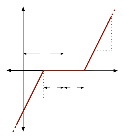
implements only linear and quadratic options:
fdi(α) = α, if di= 1
α2,if di= 2 (5.31)
as illustrated in Figure 5-1 and Figure 5-2, respectively.
wi
mi
ri
ˆri
ki
ki
Figure 5-1: Relationship of wito rifor di= 1 (linear option)
This form for fuprovides the flexibility to handle a wide range of costs, from
simple linear functions of the optimization variables to scaled quadratic penalties
on quantities, such as voltages, lying outside a desired range, to functions of linear
32
wi
ri
ˆri
ki
ki
Figure 5-2: Relationship of wito rifor di= 2 (quadratic option)
combinations of variables, inspired by the requirements of price coordination terms
found in the decomposition of large loosely coupled problems encountered in our own
research.
Some limitations are imposed on the parameters in the case of the DC OPF since
Matpower uses a generic quadratic programming (QP) solver for the optimization.
In particular, ki= 0 and di= 1 for all i, so the “dead zone” is not considered and
only the linear option is available for fdi. As a result, for the DC case (5.30) simplifies
to wi=miui.
5.3.2 User-defined Constraints
The user-defined constraints (5.25) are general linear restrictions involving all of the
optimization variables and are specified via matrix Aand lower and upper bound
vectors land u. These parameters can be used to create equality constraints (li=ui)
or inequality constraints that are bounded below (ui=∞), bounded above (li=∞)
or bounded on both sides.
5.3.3 User-defined Variables
The creation of additional user-defined zvariables is done implicitly based on the
difference between the number of columns in Aand the dimension of x. The op-
tional vectors zmin and zmax are available to impose lower and upper bounds on z,
respectively.
33
5.4 Standard Extensions
In addition to making this extensible OPF structure available to end users, Mat-
power also takes advantage of it internally to implement several additional capa-
bilities.
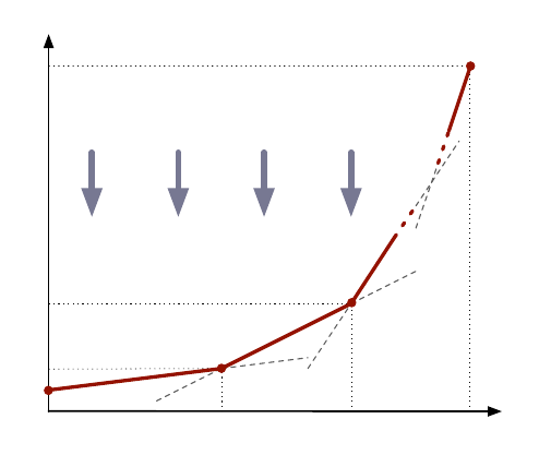
5.4.1 Piecewise Linear Costs
The standard OPF formulation in (5.1)–(5.4) does not directly handle the non-
smooth piecewise linear cost functions that typically arise from discrete bids and
offers in electricity markets. When such cost functions are convex, however, they
can be modeled using a constrained cost variable (CCV) method. The piecewise lin-
ear cost function c(x) is replaced by a helper variable yand a set of linear constraints
that form a convex “basin” requiring the cost variable yto lie in the epigraph of the
function c(x).
Figure 5-3 illustrates a convex n-segment piecewise linear cost function
c(x) =
m1(x−x1) + c1, x ≤x1
m2(x−x2) + c2, x1< x ≤x2
.
.
..
.
.
mn(x−xn) + cn, xn−1< x
(5.32)
x
x0
x1
x2
c
c0
c1
c2
y
cn
xn
Figure 5-3: Constrained Cost Variable
34

defined by a sequence of points (xj, cj), j= 0 . . . n, where mjdenotes the slope of
the j-th segment
mj=cj−cj−1
xj−xj−1
, j = 1 . . . n (5.33)
and x0< x1<· · · < xnand m1≤m2≤ · · · < mn.
The “basin” corresponding to this cost function is formed by the following n
constraints on the helper cost variable y:
y≥mj(x−xj) + cj, j = 1 . . . n. (5.34)
The cost term added to the objective function in place of c(x) is simply the variable y.
Matpower uses this CCV approach internally to automatically generate the
appropriate helper variable, cost term and corresponding set of constraints for any
piecewise linear costs on real or reactive generation. All of Matpower’s OPF
solvers, for both AC and DC OPF problems, use the CCV approach with the ex-
ception of two that are part of the optional TSPOPF package [11], namely the
step-controlled primal/dual interior point method (SCPDIPM) and the trust region
based augmented Lagrangian method (TRALM), both of which use a cost smoothing
technique instead [12].
5.4.2 Dispatchable Loads
A simple approach to dispatchable or price-sensitive loads is to model them as nega-
tive real power injections with associated negative costs. This is done by specifying
a generator with a negative output, ranging from a minimum injection equal to the
negative of the largest possible load to a maximum injection of zero.
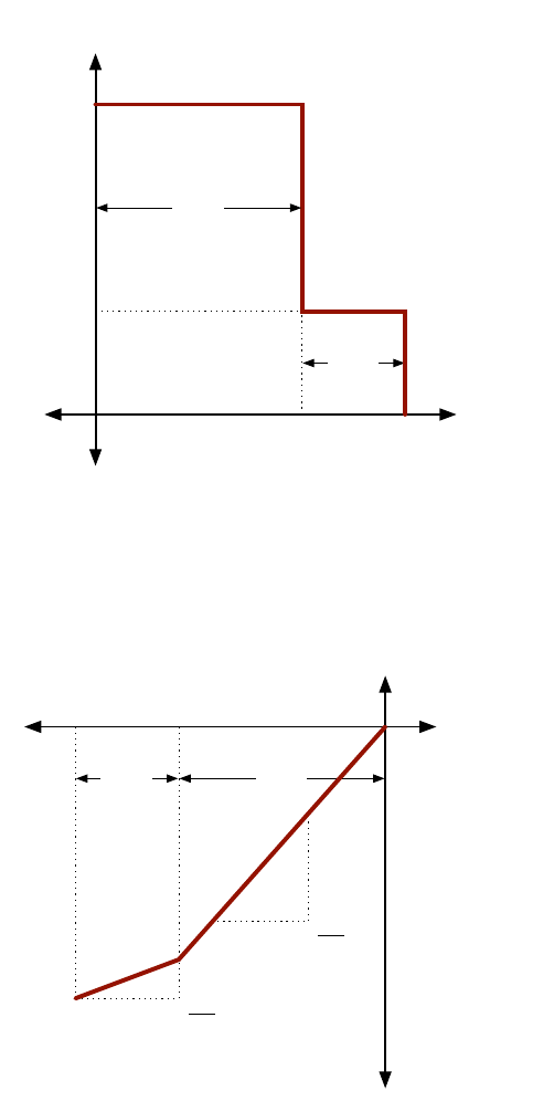
Consider the example of a price-sensitive load whose marginal benefit function is
shown in Figure 5-4. The demand pdof this load will be zero for prices above λ1,p1
for prices between λ1and λ2, and p1+p2for prices below λ2.
This corresponds to a negative generator with the piecewise linear cost curve
shown in Figure 5-5. Note that this approach assumes that the demand blocks can
be partially dispatched or “split”. Requiring blocks to be accepted or rejected in
their entirety would pose a mixed-integer problem that is beyond the scope of the
current Matpower implementation.
With an AC network model, there is also the question of reactive dispatch for
such loads. Typically the reactive injection for a generator is allowed to take on any
value within its defined limits. Since this is not normal load behavior, the model used
in Matpower assumes that dispatchable loads maintain a constant power factor.
When formulating the AC OPF problem, Matpower will automatically generate
35
λ(marginal benefit)
$/MW
MW
λ1
λ2
p1
p2
p(load)
Figure 5-4: Marginal Benefit or Bid Function
MW
λ2
p2
λ1
p1
p1
p2
$
p(injection)
c(total cost)
Figure 5-5: Total Cost Function for Negative Injection
36
an additional equality constraint to enforce a constant power factor for any “negative
generator” being used to model a dispatchable load.
It should be noted that, with this definition of dispatchable loads as negative
generators, if the negative cost corresponds to a benefit for consumption, minimizing
the cost f(x) of generation is equivalent to maximizing social welfare.
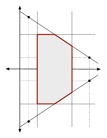
5.4.3 Generator Capability Curves
The typical AC OPF formulation includes box constraints on a generator’s real and
reactive injections, specified as simple lower and upper bounds on p(pmin and pmax)
and q(qmin and qmax). On the other hand, the true P-Qcapability curves of phys-
ical generators usually involve some tradeoff between real and reactive capability,
so that it is not possible to produce the maximum real output and the maximum
(or minimum) reactive output simultaneously. To approximate this tradeoff, Mat-
power includes the ability to add an upper and lower sloped portion to the standard
box constraints as illustrated in Figure 5-6, where the shaded portion represents the
qmax
1
qmax
2
qmin
2
qmin
1
qmin
qmax
pmax
pmin
p1
p2
q
p
Figure 5-6: Generator P-QCapability Curve
37

feasible operating region for the unit.
The two sloped portions are constructed from the lines passing through the two
pairs of points defined by the six parameters p1,qmin
1,qmax
1,p2,qmin
2, and qmax
2. If
these six parameters are specified for a given generator, Matpower automatically
constructs the corresponding additional linear inequality constraints on pand qfor
that unit.
If one of the sloped portions of the capability constraints is binding for genera-
tor k, the corresponding shadow price is decomposed into the corresponding µPmax
and µQmin or µQmax components and added to the respective column (MU PMAX,MU QMIN
or MU QMAX) in the kth row of gen.
5.4.4 Branch Angle Difference Limits
The difference between the bus voltage angle θfat the from end of a branch and
the angle θtat the to end can be bounded above and below to act as a proxy for
a transient stability limit, for example. If these limits are provided, Matpower
creates the corresponding constraints on the voltage angle variables.
5.5 Solvers
Early versions of Matpower relied on Matlab’s Optimization Toolbox [13] to
provide the NLP and QP solvers needed to solve the AC and DC OPF problems,
respectively. While they worked reasonably well for very small systems, they did not
scale well to larger networks. Eventually, optional packages with additional solvers
were added to improve performance, typically relying on Matlab extension (MEX)
files implemented in Fortran or C and pre-compiled for each machine architecture.
Some of these MEX files are distributed as optional packages due to differences in
terms of use. For DC optimal power flow, there is a MEX build [14] of the high
performance interior point BPMPD solver [15] for LP/QP problems. For the AC
OPF problem, the MINOPF [16] and TSPOPF [11] packages provide solvers suitable
for much larger systems. The former is based on MINOS [17] and the latter includes
the primal-dual interior point and trust region based augmented Lagrangian methods
described in [12]. Matpower version 4 and later also includes the option to use the
open-source Ipopt solver8for solving both AC and DC OPFs, based on the Matlab
MEX interface to Ipopt9. It also includes the option to use CPLEX10 or MOSEK11
8Available from https://projects.coin-or.org/Ipopt/.
9See https://projects.coin-or.org/Ipopt/wiki/MatlabInterface.
10See http://www.ibm.com/software/integration/optimization/cplex-optimizer/.
11See http://www.mosek.com/.
38

for DC OPFs. See Appendix Gfor more details on these optional packages.
Beginnning with version 4, Matpower also includes its own primal-dual interior
point method implemented in pure-Matlab code, derived from the MEX imple-
mentation of the algorithms described in [12]. This solver is called MIPS (Matlab
Interior Point Solver) and is described in more detail in Appendix A. If no optional
packages are installed, MIPS will be used by default for both the AC OPF and as the
QP solver used by the DC OPF. The AC OPF solver also employs a unique technique
for efficiently forming the required Hessians via a few simple matrix operations [18].
This solver has application to general nonlinear optimization problems outside of
Matpower and can be called directly as mips. There is also a convenience wrapper
function called qps mips making it trivial to set up and solve LP and QP problems,
with an interface similar to quadprog from the Matlab Optimization Toolbox.
5.6 runopf
In Matpower, an optimal power flow is executed by calling runopf with a case
struct or case file name as the first argument (casedata). In addition to printing
output to the screen, which it does by default, runpf optionally returns the solution
in a results struct.
>> results = runopf(casedata);
The results struct is a superset of the input Matpower case struct mpc, with
some additional fields as well as additional columns in some of the existing data
fields. In addition to the solution values included in the results for a simple power
flow, shown in Table 4-1 in Section 4.3, the following additional optimal power flow
solution values are stored as shown in Table 5-1.
Additional optional input arguments can be used to set options (mpopt) and
provide file names for saving the pretty printed output (fname) or the solved case
data (solvedcase).
>> results = runopf(casedata, mpopt, fname, solvedcase);
Some of the main options that control the optimal power flow simulation are listed in
Table 5-2. There are many other options that can be used to control the termination
criteria and other behavior of the individual solvers. See Appendix Cor the mpoption
help for details. As with runpf the output printed to the screen can be controlled
by the options in Table 4-3, but there are additional output options for the OPF,
related to the display of binding constraints that are listed Table 5-3, along with
39

Table 5-1: Optimal Power Flow Results
name description
results.f final objective function value
results.x final value of optimization variables (internal order)
results.om OPF model object†
results.bus(:, LAM P) Lagrange multiplier on real power mismatch
results.bus(:, LAM Q) Lagrange multiplier on reactive power mismatch
results.bus(:, MU VMAX) Kuhn-Tucker multiplier on upper voltage limit
results.bus(:, MU VMIN) Kuhn-Tucker multiplier on lower voltage limit
results.gen(:, MU PMAX) Kuhn-Tucker multiplier on upper Pglimit
results.gen(:, MU PMIN) Kuhn-Tucker multiplier on lower Pglimit
results.gen(:, MU QMAX) Kuhn-Tucker multiplier on upper Qglimit
results.gen(:, MU QMIN) Kuhn-Tucker multiplier on lower Qglimit
results.branch(:, MU SF) Kuhn-Tucker multiplier on flow limit at “from” bus
results.branch(:, MU ST) Kuhn-Tucker multiplier on flow limit at “to” bus
results.mu shadow prices of constraints‡
results.g (optional) constraint values
results.dg (optional) constraint 1st derivatives
results.raw raw solver output in form returned by MINOS, and more‡
results.var.val final value of optimization variables, by named subset‡
results.var.mu shadow prices on variable bounds, by named subset‡
results.nln shadow prices on nonlinear constraints, by named subset‡
results.lin shadow prices on linear constraints, by named subset‡
results.cost final value of user-defined costs, by named subset‡
†See help for opf model for more details.
‡See help for opf for more details.
an option that can be used to force the AC OPF to return information about the
constraint values and Jacobian and the objective function gradient and Hessian.
By default, runopf solves an AC optimal power flow problem using a primal dual
interior point method. To run a DC OPF, the PF DC option must be set to 1. For
convenience, Matpower provides a function rundcopf which is simply a wrapper
that sets PF DC before calling runopf.
Internally, the runopf function does a number of conversions to the problem
data before calling the appropriate solver routine for the selected OPF algorithm.
This external-to-internal format conversion is performed by the ext2int function,
described in more detail in Section 6.2.1, and includes the elimination of out-of-service
equipment, the consecutive renumbering of buses and the reordering of generators
by increasing bus number. All computations are done using this internal indexing.
When the simulation has completed, the data is converted back to external format
by int2ext before the results are printed and returned. In addition, both ext2int
40
and int2ext can be customized via user-supplied callback routines to convert data
needed by user-supplied variables, constraints or costs into internal indexing.
41

Table 5-2: Optimal Power Flow Options
idx name default description
11 OPF ALG 0 AC optimal power flow algorithm:
0 – choose default solver based on availability in
the following order: 540, 560
300 – constr,Matlab Opt Toolbox 1.x and 2.x
320 – dense successive LP
340 – sparse successive LP (relaxed)
360 – sparse successive LP (full)
500 – MINOPF, MINOS-based solver†
520 – fmincon,Matlab Opt Toolbox ≥2.x
540 – PDIPM, primal/dual interior point method‡
545 – SC-PDIPM, step-controlled variant of
PDIPM‡
550 – TRALM, trust region based augmented Lan-
grangian method‡
560 – MIPS, Matlab Interior Point Solver, pri-
mal/dual interior point method
565 – MIPS-sc, step-controlled variant of MIPS
16 OPF VIOLATION 5×10⁻⁶constraint violation tolerance
24 OPF FLOW LIM 0 quantity to limit for branch flow constraints
0 – apparent power flow (limit in MVA)
1 – active power flow (limit in MW)
2 – current magnitude (limit in MVA at 1 p.u.
voltage)
25 OPF IGNORE ANG LIM 0 ignore angle difference limits for branches
0 – include angle difference limits, if specified
1 – ignore angle difference limits even if specified
26 OPF ALG DC 0 DC optimal power flow algorithm:
0 – choose default solver based on availability in
the following order: 540, 560
100 – BPMPD§
200 – MIPS, Matlab Interior Point Solver, pri-
mal/dual interior point method
250 – MIPS-sc, step-controlled variant of MIPS
300 – Matlab Opt Toolbox, quadprog,linprog
400 – Ipopt¶
500 – CPLEX♦
600 – MOSEK4
†Requires optional MEX-based MINOPF package, available from http://www.pserc.cornell.edu/minopf/.
‡Requires optional MEX-based TSPOPF package, available from http://www.pserc.cornell.edu/tspopf/.
§Requires optional MEX-based BPMPD MEX package, available from http://www.pserc.cornell.edu/bpmpd/.
¶Requires MEX interface to Ipopt solver, available from https://projects.coin-or.org/Ipopt/.
♦Requires optional Matlab interface to CPLEX, available from http://www.ibm.com/software/integration/
optimization/cplex-optimizer/.
4Requires optional Matlab interface to MOSEK, available from http://www.mosek.com/.
42

Table 5-3: OPF Output Options
idx name default description
38 OUT ALL LIM -1 controls constraint info output
-1 – individual flags control what is printed
0 – do not print any constraint info†
1 – print only binding constraint info†
2 – print all constraint info†
39 OUT V LIM 1 control output of voltage limit info
0 – do not print
1 – print binding constraints only
2 – print all constraints
40 OUT LINE LIM 1 control output of line flow limit info‡
41 OUT PG LIM 1 control output of gen active power limit info‡
42 OUT QG LIM 1 control output of gen reactive power limit info‡
52 RETURN RAW DER 0 for AC OPF, return constraint and derivative info in
results.raw (in fields g,dg,df,d2f)
†Overrides individual flags.
‡Takes values of 0, 1 or 2 as for OUT V LIM.
43

6 Extending the OPF
The extended OPF formulation described in Section 5.3 allows the user to modify the
standard OPF formulation to include additional variables, costs and/or constraints.
There are two primary mechanisms available for the user to accomplish this. The first
is by directly constructing the full parameters for the addional costs or constraints
and supplying them either as fields in the case struct or directly as arguments to
the opf function. The second, and more powerful, method is via a set of callback
functions that customize the OPF at various stages of the execution. Matpower
includes two examples of using the latter method, one to add a fixed zonal reserve
requirement and another to implement interface flow limits.
6.1 Direct Specification
To add costs directly, the parameters H,C,N, ˆr,k,dand mof (5.27)–(5.31)
described in Section 5.3.1 are specified as fields or arguments H,Cw,Nand fparm,
repectively, where fparm is the nw×4 matrix
fparm =dˆr k m .(6.1)
When specifying additional costs, Nand Cw are required, while Hand fparm are
optional. The default value for His a zero matrix, and the default for fparm is such
that dand mare all ones and ˆrand kare all zeros, resulting in simple linear cost,
with no shift or “dead-zone”. Nand Hshould be specified as sparse matrices.
For additional constraints, the A,land uparameters of (5.25) are specified as
fields or arguments of the same names, A,land u, respectively, where Ais sparse.
Additional variables are created implicitly based on the difference between the
number of columns in Aand the number nxof standard OPF variables. If Ahas
more columns than xhas elements, the extra columns are assumed to correspond to
a new zvariable. The initial value and lower and upper bounds for zcan also be
specified in the optional fields or arguments, z0,zl and zu, respectively.
For a simple formulation extension to be used for a small number of OPF cases,
this method has the advantage of being direct and straightforward. While Mat-
power does include code to eliminate the columns of Aand Ncorresponding to Vm
and Qgwhen running a DC OPF12, as well as code to reorder and eliminate columns
appropriately when converting from external to internal data formats, this mecha-
nism still requires the user to take special care in preparing the Aand Nmatrices
12Only if they contain all zeros.
44

to ensure that the columns match the ordering of the elements of the opimization
vectors xand z. All extra constraints and variables must be incorporated into a
single set of parameters that are constructed before calling the OPF. The bookkeep-
ing needed to access the resulting variables and shadow prices on constraints and
variable bounds must be handled manually by the user outside of the OPF, along
with any processing of additional input data and processing, printing or saving of
the additional result data. Making further modifications to a formulation that al-
ready includes user-supplied costs, constraints or variables, requires that both sets
be incorporated into a new single consistent set of parameters.
6.2 Callback Functions
The second method, based on defining a set of callback functions, offers several
distinct advantages, especially for more complex scenarios or for adding a feature
for others to use, such as the zonal reserve requirement or the interface flow limits
mentioned previously. This approach makes it possible to:
•define and access variable/constraint sets as individual named blocks
•define constraints, costs only in terms of variables directly involved
•pre-process input data and/or post-process result data
•print and save new result data
•simultaneously use multiple, independently developed extensions (e.g. zonal
reserve requirements and interface flow limits)
Matpower defines five stages in the execution of a simulation where custom
code can be inserted to alter the behavior or data before proceeding to the next
stage. This custom code is defined as a set of “callback” functions that are regis-
tered via add userfcn for Matpower to call automatically at one of the five stages.
Each stage has a name and, by convention, the name of a user-defined callback func-
tion ends with the name of the corresponding stage. For example, a callback for
the formulation stage that modifies the OPF problem formulation to add reserve
requirements could be registered with the following line of code.
mpc = add_userfcn(mpc, 'formulation', @userfcn_reserves_formulation);
45

The sections below will describe each stage and the input and output arguments
for the corresponding callback function, which vary depending on the stage. An
example that employs additional variables, constraints and costs will be used for
illustration.
Consider the problem of jointly optimizing the allocation of both energy and
reserves, where the reserve requirements are defined as a set of nrz fixed zonal MW
quantities. Let Zkbe the set of generators in zone kand Rkbe the MW reserve
requirement for zone k. A new set of variables rare introduced representing the
reserves provided by each generator. The value ri, for generator i, must be non-
negative and is limited above by a user-provided upper bound rmax
i(e.g. a reserve
offer quantity) as well as the physical ramp rate ∆i.
0≤ri≤min(rmax
i,∆i), i = 1 . . . ng(6.2)
If the vector ccontains the marginal cost of reserves for each generator, the user
defined cost term from (5.21) is simply
fu(x, z) = cTr. (6.3)
There are two additional sets of constraints needed. The first ensures that, for
each generator, the total amount of energy plus reserve provided does not exceed the
capacity of the unit.
pi
g+ri≤pi,max
g, i = 1 . . . ng(6.4)
The second requires that the sum of the reserve allocated within each zone kmeets
the stated requirements.
X
i∈Zk
ri≥Rk, k = 1 . . . nrz (6.5)
Table 6-1 describes some of the variables and names that are used in the example
callback function listings in the sections below.
6.2.1 ext2int Callback
Before doing any simulation of a case, Matpower performs some data conversion
on the case struct in order to achieve a consistent internal structure, by calling the
following.
mpc = ext2int(mpc);
46

Table 6-1: Names Used by Implementation of OPF with Reserves
name description
mpc Matpower case struct
reserves additional field in mpc containing input parameters for zonal reserves in
the following sub-fields:
cost ng×1 vector of reserve costs, cfrom (6.3)
qty ng×1 vector of reserve quantity upper bounds, ith element is rmax
i
zones nrz ×ngmatrix of reserve zone definitions
zones(k,j) =1 if gen jbelongs to reserve zone k(j∈Zk)
0 otherwise (j /∈Zk)
req nrz ×1 vector of zonal reserve requirements, kth element is Rkfrom (6.5)
om OPF model object, already includes standard OPF setup
results OPF results struct, superset of mpc with additional fields for output data
ng ng, number of generators
Rname for new reserve variable block, ith element is ri
Pg plus R name for new capacity limit constraint set (6.4)
Rreq name for new reserve requirement constraint set (6.5)
All isolated buses, out-of-service generators and branches are removed, along with
any generators or branches connected to isolated buses. The buses are renumbered
consecutively, beginning at 1, and the in-service generators are sorted by increasing
bus number. All of the related indexing information and the original data matrices
are stored in an order field in the case struct to be used later by int2ext to perform
the reverse conversions when the simulation is complete.
The first stage callback is invoked from within the ext2int function immediately
after the case data has been converted. Inputs are a Matpower case struct (mpc),
freshly converted to internal indexing and any (optional) args value supplied when
the callback was registered via add userfcn. Output is the (presumably updated)
mpc. This is typically used to reorder any input arguments that may be needed in
internal ordering by the formulation stage. The example shows how ext2int can also
be used, with a case struct that has already been converted to internal indexing, to
convert other data structures by passing in 2 or 3 extra parameters in addition to
the case struct. In this case, it automatically converts the input data in the qty,
cost and zones fields of mpc.reserves to be consistent with the internal generator
ordering, where off-line generators have been eliminated and the on-line generators
are sorted in order of increasing bus number. Notice that it is the second dimension
(columns) of mpc.reserves.zones that is being re-ordered. See the on-line help for
ext2int for more details on what all it can do.
47

function mpc = userfcn_reserves_ext2int(mpc, args)
mpc = ext2int(mpc, {'reserves','qty'}, 'gen');
mpc = ext2int(mpc, {'reserves','cost'}, 'gen');
mpc = ext2int(mpc, {'reserves','zones'}, 'gen', 2);
This stage is also a good place to check the consistency of any additional input
data required by the extension and throw an error if something is missing or not as
expected.
6.2.2 formulation Callback
This stage is called from opf after the OPF Model (om) object has been initialized
with the standard OPF formulation, but before calling the solver. This is the ideal
place for modifying the problem formulation with additional variables, constraints
and costs, using the add vars,add constraints and add costs methods of the OPF
Model object. Inputs are the om object and any (optional) args supplied when the
callback was registered via add userfcn. Output is the updated om object.
The om object contains both the original Matpower case data as well as all of the
indexing data for the variables and constraints of the standard OPF formulation.13
See the on-line help for opf model for more details on the OPF model object and the
methods available for manipulating and accessing it.
In the example code, a new variable block named Rwith ngelements and the
limits from (6.2) is added to the model via the add vars method. Similarly, two
linear constraint blocks named Pg plus R and Rreq, implementing (6.4) and (6.5),
respectively, are added via the add constraints method. And finally, the add costs
method is used to add to the model a user-defined cost block corresponding to (6.3).
Notice that the last argument to add constraints and add costs allows the con-
straints and costs to be defined only in terms of the relevant parts of the optimiza-
tion variable x. For example, the Amatrix for the Pg plus R constraint contains only
columns corresponding to real power generation (Pg) and reserves (R) and need not
bother with voltages, reactive power injections, etc. As illustrated in Figure 6-1,
this allows the same code to be used with both the AC OPF, where xincludes Vm
and Qg, and the DC OPF where it does not. This code is also independent of any
13It is perfectly legitimate to register more than one callback per stage, such as when enabling
multiple independent OPF extensions. In this case, the callbacks are executed in the order they
were registered with add userfcn. E.g. when the second and subsequent formulation callbacks
are invoked, the om object will reflect any modifications performed by earlier formulation callbacks.
48
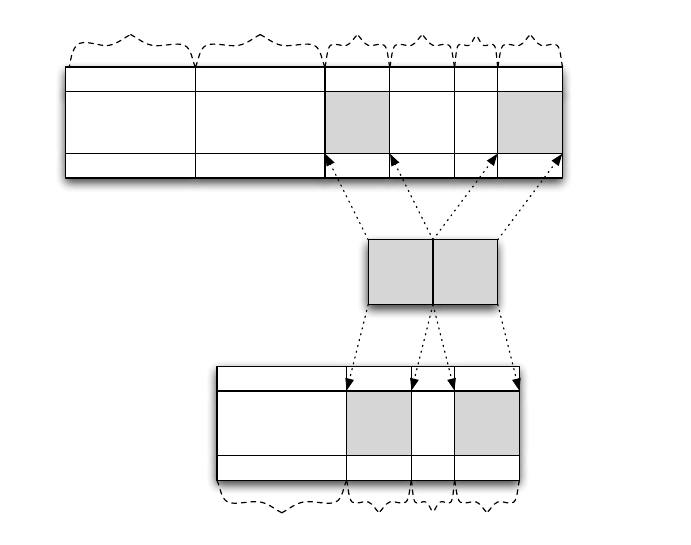
additional variables that may have been added by Matpower (e.g. yvariables from
Matpower’s CCV handling of piece-wise linear costs) or by the user via previous
formulation callbacks. Matpower will place the constraint matrix blocks in the
appropriate place when it constructs the overall Amatrix at run-time. This is an im-
portant feature that enables independently developed Matpower OPF extensions
to work together.
Va
A = 0A10 00 A2
A = 0A1 0A2
Ar = A1 A2
Va PgVm yQg R
Pg y R
AC OPF
DC OPF
Figure 6-1: Adding Constraints Across Subsets of Variables
49

function om = userfcn_reserves_formulation(om, args)
%% initialize some things
define_constants;
mpc = get_mpc(om);
r = mpc.reserves;
ng = size(mpc.gen, 1); %% number of on-line gens
%% variable bounds
Rmin = zeros(ng, 1); %% bound below by 0
Rmax = r.qty; %% bound above by stated max reserve qty ...
k = find(mpc.gen(:, RAMP_10) > 0 & mpc.gen(:, RAMP_10) < Rmax);
Rmax(k) = mpc.gen(k, RAMP_10); %% ... and ramp rate
Rmax = Rmax / mpc.baseMVA;
%% constraints
I = speye(ng); %% identity matrix
Ar = [I I];
Pmax = mpc.gen(:, PMAX) / mpc.baseMVA;
lreq = r.req / mpc.baseMVA;
%% cost
Cw = r.cost * mpc.baseMVA; %% per unit cost coefficients
%% add them to the model
om = add_vars(om, 'R', ng, [], Rmin, Rmax);
om = add_constraints(om, 'Pg_plus_R', Ar, [], Pmax, {'Pg','R'});
om = add_constraints(om, 'Rreq', r.zones, lreq, [], {'R'});
om = add_costs(om, 'Rcost', struct('N', I, 'Cw', Cw), {'R'});
6.2.3 int2ext Callback
After the simulation is complete and before the results are printed or saved, Mat-
power converts the case data in the results struct back to external indexing by
calling the following.
results = int2ext(results);
This conversion essentially undoes everything that was done by ext2int. Generators
are restored to their original ordering, buses to their original numbering and all
out-of-service or isolated generators, branches and buses are restored.
This callback is invoked from int2ext immediately before the resulting case is
converted from internal back to external indexing. At this point, the simulation
50

has been completed and the results struct, a superset of the original Matpower
case struct passed to the OPF, contains all of the results. This results struct is
passed to the callback, along with any (optional) args supplied when the callback
was registered via add userfcn. The output of the callback is the updated results
struct. This is typically used to convert any results to external indexing and populate
any corresponding fields in the results struct.
The results struct contains, in addition to the standard OPF results, solution in-
formation related to all of the user-defined variables, constraints and costs. Table 6-2
summarizes where the various data is found. Each of the fields listed in the table
is actually a struct whose fields correspond to the named sets created by add vars,
add constraints and add costs.
Table 6-2: Results for User-Defined Variables, Constraints and Costs
name description
results.var.val final value of user-defined variables
results.var.mu.l shadow price on lower limit of user-defined variables
results.var.mu.u shadow price on upper limit of user-defined variables
results.lin.mu.l shadow price on lower (left-hand) limit of linear constraints
results.lin.mu.u shadow price on upper (right-hand) limit of linear constraints
results.cost final value of user-defined costs
In the example code below, the callback function begins by converting the reserves
input data in the resulting case (qty,cost and zones fields of results.reserves)
back to external indexing via calls to int2ext with extra arguments. See the help
for int2ext for more details on how it can be used.
Then the reserves results of interest are extracted from the appropriate sub-fields
of results.var,results.lin and results.cost, converted from per unit to per MW
where necessary, and stored with external indexing for the end user in the chosen
fields of the results struct.
51

function results = userfcn_reserves_int2ext(results, args)
%%----- convert stuff back to external indexing -----
%% convert all reserve parameters (zones, costs, qty, rgens)
results = int2ext(results, {'reserves','qty'}, 'gen');
results = int2ext(results, {'reserves','cost'}, 'gen');
results = int2ext(results, {'reserves','zones'}, 'gen', 2);
r = results.reserves;
ng = size(results.gen, 1); %% number of on-line gens (internal)
ng0 = size(results.order.ext.gen, 1); %% number of gens (external)
%%----- results post-processing -----
%% get the results (per gen reserves, multipliers) with internal gen indexing
%% and convert from p.u. to per MW units
[R0, Rl, Ru] = getv(results.om, 'R');
R = results.var.val.R * results.baseMVA;
Rmin = Rl * results.baseMVA;
Rmax = Ru * results.baseMVA;
mu_l = results.var.mu.l.R / results.baseMVA;
mu_u = results.var.mu.u.R / results.baseMVA;
mu_Pmax = results.lin.mu.u.Pg_plus_R / results.baseMVA;
%% store in results in results struct
z = zeros(ng0, 1);
results.reserves.R = int2ext(results, R, z, 'gen');
results.reserves.Rmin = int2ext(results, Rmin, z, 'gen');
results.reserves.Rmax = int2ext(results, Rmax, z, 'gen');
results.reserves.mu.l = int2ext(results, mu_l, z, 'gen');
results.reserves.mu.u = int2ext(results, mu_u, z, 'gen');
results.reserves.mu.Pmax = int2ext(results, mu_Pmax, z, 'gen');
results.reserves.prc = z;
for k = 1:ng0
iz = find(r.zones(:, k));
results.reserves.prc(k) = max(results.lin.mu.l.Rreq(iz)) / results.baseMVA;
end
results.reserves.totalcost = results.cost.Rcost;
6.2.4 printpf Callback
The pretty-printing of the standard OPF output is done via a call to printpf after
the case has been converted back to external indexing. This callback is invoked from
within printpf after the pretty-printing of the standard OPF output. Inputs are
52

the results struct, the file descriptor to write to, a Matpower options vector, and
any (optional) args supplied via add userfcn. Output is the results struct. This is
typically used for any additional pretty-printing of results.
In this example, the OUT ALL flag in the options vector is checked before printing
anything. If it is non-zero, the reserve quantities and prices for each unit are printed
first, followed by the per-zone summaries. An additional table with reserve limit
shadow prices might also be included.
53

function results = userfcn_reserves_printpf(results, fd, mpopt, args)
%% define named indices into data matrices
[GEN_BUS, PG, QG, QMAX, QMIN, VG, MBASE, GEN_STATUS, PMAX, PMIN, ...
MU_PMAX, MU_PMIN, MU_QMAX, MU_QMIN, PC1, PC2, QC1MIN, QC1MAX, ...
QC2MIN, QC2MAX, RAMP_AGC, RAMP_10, RAMP_30, RAMP_Q, APF] = idx_gen;
%%----- print results -----
r = results.reserves;
ng = length(r.R);
nrz = size(r.req, 1);
OUT_ALL = mpopt(32);
if OUT_ALL ~= 0
fprintf(fd, '\n=======================================================');
fprintf(fd, '\n| Reserves |');
fprintf(fd, '\n=======================================================');
fprintf(fd, '\n Gen Bus Status Reserves Price');
fprintf(fd, '\n # # (MW) ($/MW)');
fprintf(fd, '\n---- ----- ------ -------- --------');
for k = 1:ng
fprintf(fd, '\n%3d %6d %2d ', k, results.gen(k, GEN_BUS), ...
results.gen(k, GEN_STATUS));
if results.gen(k, GEN_STATUS) > 0 && abs(results.reserves.R(k)) > 1e-6
fprintf(fd, '%10.2f', results.reserves.R(k));
else
fprintf(fd, '-');
end
fprintf(fd, '%10.2f ', results.reserves.prc(k));
end
fprintf(fd, '\n --------');
fprintf(fd, '\n Total:%10.2f Total Cost: $%.2f', ...
sum(results.reserves.R(r.igr)), results.reserves.totalcost);
fprintf(fd, '\n');
fprintf(fd, '\nZone Reserves Price ');
fprintf(fd, '\n # (MW) ($/MW) ');
fprintf(fd, '\n---- -------- --------');
for k = 1:nrz
iz = find(r.zones(k, :)); %% gens in zone k
fprintf(fd, '\n%3d%10.2f%10.2f', k, sum(results.reserves.R(iz)), ...
results.lin.mu.l.Rreq(k) / results.baseMVA);
end
fprintf(fd, '\n');
%% print binding reserve limit multipliers ...
end
54

6.2.5 savecase Callback
The savecase is used to save a Matpower case struct to an M-file, for example,
to save the results of an OPF run. The savecase callback is invoked from savecase
after printing all of the other data to the file. Inputs are the case struct, the file
descriptor to write to, the variable prefix (typically 'mpc.') and any (optional) args
supplied via add userfcn. Output is the case struct. The purpose of this callback is
to write any non-standard case struct fields to the case file.
In this example, the zones,req,cost and qty fields of mpc.reserves are written
to the M-file. This ensures that a case with reserve data, if it is loaded via loadcase,
possibly run, then saved via savecase, will not lose the data in the reserves field.
This callback could also include the saving of the output fields if present. The
contributed serialize function14 can be very useful for this purpose.
14http://www.mathworks.com/matlabcentral/fileexchange/1206
55

function mpc = userfcn_reserves_savecase(mpc, fd, prefix, args)
%
% mpc = userfcn_reserves_savecase(mpc, fd, mpopt, args)
%
% This is the 'savecase'stage userfcn callback that prints the M-file
% code to save the 'reserves'field in the case file. It expects a
% MATPOWER case struct (mpc), a file descriptor and variable prefix
% (usually 'mpc.'). The optional args are not currently used.
r = mpc.reserves;
fprintf(fd, '\n%%%%----- Reserve Data -----%%%%\n');
fprintf(fd, '%%%% reserve zones, element i, j is 1 iff gen j is in zone i\n');
fprintf(fd, '%sreserves.zones = [\n', prefix);
template = '';
for i = 1:size(r.zones, 2)
template = [template, '\t%d'];
end
template = [template, ';\n'];
fprintf(fd, template, r.zones.');
fprintf(fd, '];\n');
fprintf(fd, '\n%%%% reserve requirements for each zone in MW\n');
fprintf(fd, '%sreserves.req = [\t%g', prefix, r.req(1));
if length(r.req) > 1
fprintf(fd, ';\t%g', r.req(2:end));
end
fprintf(fd, '\t];\n');
fprintf(fd, '\n%%%% reserve costs in $/MW for each gen\n');
fprintf(fd, '%sreserves.cost = [\t%g', prefix, r.cost(1));
if length(r.cost) > 1
fprintf(fd, ';\t%g', r.cost(2:end));
end
fprintf(fd, '\t];\n');
if isfield(r, 'qty')
fprintf(fd, '\n%%%% max reserve quantities for each gen\n');
fprintf(fd, '%sreserves.qty = [\t%g', prefix, r.qty(1));
if length(r.qty) > 1
fprintf(fd, ';\t%g', r.qty(2:end));
end
fprintf(fd, '\t];\n');
end
%% save output fields for solved case ...
56

6.3 Registering the Callbacks
As seen in the fixed zonal reserve example, adding a single extension to the standard
OPF formulation is often best accomplished by a set of callback functions. A typical
use case might be to run a given case with and without the reserve requirements
active, so a simple method for enabling and disabling the whole set of callbacks as a
single unit is needed.
The recommended method is to define all of the callbacks in a single file containing
a “toggle” function that registers or removes all of the callbacks depending on whether
the value of the second argument is 'on'or 'off'. The state of the registration of any
callbacks is stored directly in the mpc struct. In our example, the toggle reserves.m
file contains the toggle reserves function as well as the five callback functions.
function mpc = toggle_reserves(mpc, on_off)
%TOGGLE_RESERVES Enable or disable fixed reserve requirements.
% mpc = toggle_reserves(mpc, 'on')
% mpc = toggle_reserves(mpc, 'off')
if strcmp(on_off, 'on')
% <code to check for required 'reserves'fields in mpc>
%% add callback functions
mpc = add_userfcn(mpc, 'ext2int', @userfcn_reserves_ext2int);
mpc = add_userfcn(mpc, 'formulation', @userfcn_reserves_formulation);
mpc = add_userfcn(mpc, 'int2ext', @userfcn_reserves_int2ext);
mpc = add_userfcn(mpc, 'printpf', @userfcn_reserves_printpf);
mpc = add_userfcn(mpc, 'savecase', @userfcn_reserves_savecase);
elseif strcmp(on_off, 'off')
mpc = remove_userfcn(mpc, 'savecase', @userfcn_reserves_savecase);
mpc = remove_userfcn(mpc, 'printpf', @userfcn_reserves_printpf);
mpc = remove_userfcn(mpc, 'int2ext', @userfcn_reserves_int2ext);
mpc = remove_userfcn(mpc, 'formulation', @userfcn_reserves_formulation);
mpc = remove_userfcn(mpc, 'ext2int', @userfcn_reserves_ext2int);
else
error('toggle_reserves: 2nd argument must be either ''on'' or ''off''');
end
To run case that includes the fixed reserves requirements, is as simple as loading
the case, turning on reserves and running it.
mpc = loadcase('t_case30_userfcns');
mpc = toggle_reserves(mpc, 'on');
results = runopf(mpc);
57

6.4 Summary
The five callback stages currently defined by Matpower are summarized in Ta-
ble 6-3.
Table 6-3: Callback Functions
name invoked . . . typical use
ext2int . . . from ext2int immediately after
case data is converted from external
to internal indexing.
Check consistency of input data, con-
vert to internal indexing.
formulation . . . from opf after OPF Model (om)
object is initialized with standard
OPF formulation.
Modify OPF formulation, by adding
user-defined variables, constraints,
costs.
int2ext . . . from int2ext immediately before
case data is converted from internal
back to external indexing.
Convert data back to external index-
ing, populate any additional fields in
the results struct.
printpf . . . from printpf after pretty-printing
the standard OPF output.
Pretty-print any results not included
in standard OPF.
savecase . . . from savecase after printing all of
the other case data to the file.
Write non-standard case struct fields
to the case file.
Matpower includes two OPF extensions implemented via callbacks. One is a
more complete version of the example of fixed zonal reserve requirements use for illus-
tration above. The code can be found in toggle reserves. A wrapper around runopf
that turns on this extension before running the OPF is provided in runopf w res.
A second extension that imposes interface flow limits using DC model based
flows is implemented in toggle iflims. Examples of using these extensions and a
case file defining the necessary input data for both can be found in t opf userfcns
and t case30 userfcns, respectively. Additional tests for runopf w res are included
in t runopf w res.
58

7 Unit De-commitment Algorithm
The standard OPF formulation described in the previous section has no mechanism
for completely shutting down generators which are very expensive to operate. Instead
they are simply dispatched at their minimum generation limits. Matpower includes
the capability to run an optimal power flow combined with a unit de-commitment
for a single time period, which allows it to shut down these expensive units and find
a least cost commitment and dispatch. To run this for case30, for example, type:
>> runuopf('case30')
By default, runuopf is based on the AC optimal power flow problem. To run a DC
OPF, the PF DC option must be set to 1. For convenience, Matpower provides a
function runduopf which is simply a wrapper that sets PF DC before calling runuopf.
Matpower uses an algorithm similar to dynamic programming to handle the
de-commitment. It proceeds through a sequence of stages, where stage Nhas N
generators shut down, starting with N= 0, as follows:
Step 1: Begin at stage zero (N= 0), assuming all generators are on-line with all
limits in place.
Step 2: Solve a normal OPF. Save the solution as the current best.
Step 3: Go to the next stage, N=N+1. Using the best solution from the previous
stage as the base case for this stage, form a candidate list of generators
with minimum generation limits binding. If there are no candidates, skip
to Step 5.
Step 4: For each generator on the candidate list, solve an OPF to find the total
system cost with this generator shut down. Replace the current best solu-
tion with this one if it has a lower cost. If any of the candidate solutions
produced an improvement, return to Step 3.
Step 5: Return the current best solution as the final solution.
It should be noted that the method employed here is simply a heuristic. It does
not guarantee that the least cost commitment of generators will be found. It is also
rather computationally expensive for larger systems and was implemented as a simple
way to allow an OPF-based “smart-market”, such as described in Appendix F, the
option to reject expensive offers while respecting the minimum generation limits on
generators.
59
8 Acknowledgments
The authors would like to acknowledge contributions from others who have helped
make Matpower what it is today. First we would like to acknowledge the input
and support of Bob Thomas throughout the development of Matpower. Thanks to
Chris DeMarco, one of our PSERC associates at the University of Wisconsin, for the
technique for building the Jacobian matrix. Our appreciation to Bruce Wollenberg
for all of his suggestions for improvements to version 1. The enhanced output func-
tionality in version 2.0 is primarily due to his input. Thanks also to Andrew Ward
for code which helped us verify and test the ability of the OPF to optimize reactive
power costs. Thanks to Alberto Borghetti for contributing code for the Gauss-Seidel
power flow solver and to Mu Lin for contributions related to power flow reactive
power limits. Real power line limits were suggested by Pan Wei. Thanks to Roman
Korab for data for the Polish system. Some state estimation code was contributed
by James S. Thorp and Rui Bo contributed additional code for state estimation and
continuation power flow. Matpower was improved in various ways in response to
Doug Mitarotonda’s contributions and suggestions.
Thanks also to many others who have contributed code, testing time, bug reports
and suggestions over the years. And, last but not least, thanks to all of the many
users who, by using Matpower in their own work, have helped to extend the
contribution of Matpower to the field of power systems far beyond what we could
do on our own.
60

Appendix A MIPS – Matlab Interior Point Solver
Beginning with version 4, Matpower includes a new primal-dual interior point
solver called MIPS, for Matlab Interior Point Solver. It is implemented in pure-
Matlab code, derived from the MEX implementation of the algorithms described
in [12,19].
This solver has application outside of Matpower to general nonlinear optimiza-
tion problems of the following form:
min
xf(x) (A.1)
subject to
g(x) = 0 (A.2)
h(x)≤0 (A.3)
l≤Ax ≤u(A.4)
xmin ≤x≤xmax (A.5)
where f:Rn→R,g:Rn→Rmand h:Rn→Rp.
The solver is implemented by the mips function15, which can be called as follows,
[x, f, exitflag, output, lambda] = ...
mips(f_fcn, x0, A, l, u, xmin, xmax, gh_fcn, hess_fcn, opt);
where the input and output arguments are described in Tables A-1 and A-2, respec-
tively. Alternatively, the input arguments can be packaged as fields in a problem
struct and passed in as a single argument, where all fields except f fcn and x0 are
optional.
[x, f, exitflag, output, lambda] = mips(problem);
The calling syntax is nearly identical to that used by fmincon from Matlab’s
Optimization Toolbox. The primary difference is that the linear constraints are
specified in terms of a single doubly-bounded linear function (l≤Ax ≤u) as opposed
to separate equality constrained (Aeqx=beq ) and upper bounded (Ax ≤b) functions.
Internally, equality constraints are handled explicitly and determined at run-time
based on the values of land u.
15For Matlab 6.x use mips6.
61

Table A-1: Input Arguments for mips†
name description
f fcn Handle to a function that evaluates the objective function, its gradients and Hessian‡
for a given value of x. Calling syntax for this function:
[f, df, d2f] = f fcn(x)
x0 Starting value of optimization vector x.
A,l,uDefine the optional linear constraints l≤Ax ≤u. Default values for the elements of
land uare -Inf and Inf, respectively.
xmin,xmax Optional lower and upper bounds on the xvariables, defaults are -Inf and Inf,
respectively.
gh fcn Handle to function that evaluates the optional nonlinear constraints and their gra-
dients for a given value of x. Calling syntax for this function is:
[h, g, dh, dg] = gh fcn(x)
hess fcn Handle to function that computes the Hessian‡of the Lagrangian for given values
of x,λand µ, where λand µare the multipliers on the equality and inequality
constraints, gand h, respectively. The calling syntax for this function is:
Lxx = hess fcn(x, lam, cost mult),
where λ=lam.eqnonlin,µ=lam.ineqnonlin and cost mult is a parameter used
to scale the objective function
opt Optional options structure with the following fields, all of which are also optional
(default values shown in parentheses).
verbose (0) controls level of progress output displayed
0 – print no progress info
1 – print a little progress info
2 – print a lot progress info
3 – print all progress info
feastol (1e-6) termination tolerance for feasibility condition
gradtol (1e-6) termination tolerance for gradient condition
comptol (1e-6) termination tolerance for complementarity condition
costtol (1e-6) termination tolerance for cost condition
max it (150) maximum number of iterations
step control (0) set to 1 to enable step-size control
max red (20) max number of step-size reductions if step-control is on
cost mult (1) cost multiplier used to scale the objective function for im-
proved conditioning. Note: This value is also passed as the
3rd argument to the Hessian evaluation function so that it
can appropriately scale the objective function term in the
Hessian of the Lagrangian.
problem Alternative, single argument input struct with fields corresponding to arguments
above.
†All inputs are optional except f fcn and x0.
‡If gh fcn is provided then hess fcn is also required. Specifically, if there are nonlinear constraints, the Hessian
information must provided by the hess fcn function and it need not be computed in f fcn.
62

Table A-2: Output Arguments for mips
name description
xsolution vector
ffinal objective function value
exitflag exit flag
1 – first order optimality conditions satisfied
0 – maximum number of iterations reached
-1 – numerically failed
output output struct with fields
iterations number of iterations performed
hist struct array with trajectories of the following: feascond,
gradcond,compcond,costcond,gamma,stepsize,obj,alphap,
alphad
message exit message
lambda struct containing the Langrange and Kuhn-Tucker multipliers on the con-
straints, with fields:
eqnonlin nonlinear equality constraints
ineqnonlin nonlinear inequality constraints
mu l lower (left-hand) limit on linear constraints
mu u upper (right-hand) limit on linear constraints
lower lower bound on optimization variables
upper upper bound on optimization variables
The user-defined functions for evaluating the objective function, constraints and
Hessian are identical to those required by fmincon, with one exception described
below for the Hessian evaluation function. Specifically, f fcn should return fas the
scalar objective function value f(x), df as an n×1 vector equal to ∇fand, unless
gh fcn is provided and the Hessian is computed by hess fcn,d2f as an n×nmatrix
equal to the Hessian ∂2f
∂x2. Similarly, the constraint evaluation function gh fcn must
return the m×1 vector of nonlinear equality constraint violations g(x), the p×1
vector of nonlinear inequality constraint violations h(x) along with their gradients
in dg and dh. Here dg is an n×mmatrix whose jth column is ∇gjand dh is n×p,
with jth column equal to ∇hj. Finally, for cases with nonlinear constraints, hess fcn
returns the n×nHessian ∂2L
∂x2of the Lagrangian function
L(x, λ, µ, σ) = σf(x) + λTg(x) + µTh(x) (A.6)
for given values of the multipliers λand µ, where σis the cost mult scale factor for
the objective function. Unlike fmincon,mips passes this scale factor to the Hessian
evaluation function in the 3rd argument.
The use of nargout in f fcn and gh fcn is recommended so that the gradients
63

and Hessian are only computed when required.
A.1 Example 1
The following code shows a simple example of using mips to solve a 2-dimensional
unconstrained optimization of Rosenbrock’s “banana” function16
f(x) = 100(x2−x2
1)2+ (1 −x1)2.(A.7)
First, create a Matlab function that will evaluate the objective function, its
gradients and Hessian, for a given value of x. In this case, the coefficient of the first
term is defined as a paramter a.
function [f, df, d2f] = banana(x, a)
f = a*(x(2)-x(1)^2)^2+(1-x(1))^2;
if nargout > 1 %% gradient is required
df = [ 4*a*(x(1)^3 - x(1)*x(2)) + 2*x(1)-2;
2*a*(x(2) - x(1)^2) ];
if nargout > 2 %% Hessian is required
d2f = 4*a*[ 3*x(1)^2 - x(2) + 1/(2*a), -x(1);
-x(1) 1/2 ];
end
end
Then, create a handle to the function, defining the value of the paramter ato be
100, set up the starting value of x, and call the mips function to solve it.
>> f_fcn = @(x)banana(x, 100);
>> x0 = [-1.9; 2];
>> [x, f] = mips(f_fcn, x0)
x =
1
1
f =
0
16http://en.wikipedia.org/wiki/Rosenbrock_function
64

A.2 Example 2
The second example17 solves the following 3-dimensional constrained optimization,
printing the details of the solver’s progress:
min
xf(x) = −x1x2−x2x3(A.8)
subject to
x2
1−x2
2+x2
3−2≤0 (A.9)
x2
1+x2
2+x2
3−10 ≤0.(A.10)
First, create a Matlab function to evaluate the objective function and its gra-
dients,18
function [f, df, d2f] = f2(x)
f = -x(1)*x(2) - x(2)*x(3);
if nargout > 1 %% gradient is required
df = -[x(2); x(1)+x(3); x(2)];
if nargout > 2 %% Hessian is required
d2f = -[0 1 0; 1 0 1; 0 1 0]; %% actually not used since
end %% 'hess_fcn'is provided
end
one to evaluate the constraints, in this case inequalities only, and their gradients,
function [h, g, dh, dg] = gh2(x)
h = [ 1 -1 1; 1 1 1] * x.^2 + [-2; -10];
dh = 2 * [x(1) x(1); -x(2) x(2); x(3) x(3)];
g = []; dg = [];
and another to evaluate the Hessian of the Lagrangian.
function Lxx = hess2(x, lam, cost_mult)
if nargin < 3, cost_mult = 1; end %% allows to be used with 'fmincon'
mu = lam.ineqnonlin;
Lxx = cost_mult * [0 -1 0; -1 0 -1; 0 -1 0] + ...
[2*[1 1]*mu 0 0; 0 2*[-1 1]*mu 0; 0 0 2*[1 1]*mu];
17From http://en.wikipedia.org/wiki/Nonlinear_programming#3-dimensional_example.
18Since the problem has nonlinear constraints and the Hessian is provided by hess fcn, this
function will never be called with three output arguments, so the code to compute d2f is actually
not necessary.
65

Then create a problem struct with handles to these functions, a starting value for x
and an option to print the solver’s progress. Finally, pass this struct to mips to solve
the problem and print some of the return values to get the output below.
function example2
problem = struct( ...
'f_fcn', @(x)f2(x), ...
'gh_fcn', @(x)gh2(x), ...
'hess_fcn', @(x, lam, cost_mult)hess2(x, lam, cost_mult), ...
'x0', [1; 1; 0], ...
'opt', struct('verbose', 2) ...
);
[x, f, exitflag, output, lambda] = mips(problem);
fprintf('\nf = %g exitflag = %d\n', f, exitflag);
fprintf('\nx = \n');
fprintf('%g\n', x);
fprintf('\nlambda.ineqnonlin =\n');
fprintf('%g\n', lambda.ineqnonlin);
>> example2
MATLAB Interior Point Solver -- MIPS, Version 1.0, 07-Feb-2011
it objective step size feascond gradcond compcond costcond
---- ------------ --------- ------------ ------------ ------------ ------------
0 -1 0 1.5 5 0
1 -5.3250167 1.6875 0 0.894235 0.850653 2.16251
2 -7.4708991 0.97413 0.129183 0.00936418 0.117278 0.339269
3 -7.0553031 0.10406 0 0.00174933 0.0196518 0.0490616
4 -7.0686267 0.034574 0 0.00041301 0.0030084 0.00165402
5 -7.0706104 0.0065191 0 1.53531e-05 0.000337971 0.000245844
6 -7.0710134 0.00062152 0 1.22094e-07 3.41308e-05 4.99387e-05
7 -7.0710623 5.7217e-05 0 9.84878e-10 3.41587e-06 6.05875e-06
8 -7.0710673 5.6761e-06 0 9.73397e-12 3.41615e-07 6.15483e-07
Converged!
f = -7.07107 exitflag = 1
x =
1.58114
2.23607
1.58114
lambda.ineqnonlin =
0
0.707107
More example problems for mips can be found in t mips.m.
66

A.3 Quadratic Programming Solver
A convenience wrapper function called qps mips19 is provided to make it trivial to set
up and solve linear programming (LP) and quadratic programming (QP) problems
of the following form:
min
x
1
2xTHx +cTx(A.11)
subject to
l≤Ax ≤u(A.12)
xmin ≤x≤xmax.(A.13)
Instead of a function handle, the objective function is specified in terms of the
paramters Hand cof quadratic cost coefficients. Internally, qps mips passes mips
the handle of a function that uses these paramters to evaluate the objective function,
gradients and Hessian.
The calling syntax for qps mips is similar to that used by quadprog from the
Matlab Optimization Toolbox.
[x, f, exitflag, output, lambda] = qps_mips(H, c, A, l, u, xmin, xmax, x0, opt);
Alternatively, the input arguments can be packaged as fields in a problem struct and
passed in as a single argument, where all fields except H,c,Aand lare optional.
[x, f, exitflag, output, lambda] = qps_mips(problem);
Aside from Hand c, all input and output arguments correspond exactly to the same
arguments for mips as described in Tables A-1 and A-2.
As with mips and fmincon, the primary difference between the calling syntax
for qps mips and quadprog is that the linear constraints are specified in terms of a
single doubly-bounded linear function (l≤Ax ≤u) as opposed to separate equality
constrained (Aeqx=beq) and upper bounded (Ax ≤b) functions.
Matpower also includes another wrapper function qps matpower that provides
a consistent interface for all of the QP and LP solvers it has available. This interface
is identical to that used by qps mips with the exception of the structure of the opt
input argument. The solver is chosen according to the value of opt.alg. See the help
for qps matpower for details.
Several examples of using qps matpower to solve LP and QP problems can be
found in t qps matpower.m.
19For Matlab 6.x use qps mips6.
67

A.4 Primal-Dual Interior Point Algorithm
This section provides some details on the primal-dual interior point algorithm used
by MIPS and described in [12,19].
A.4.1 Notation
For a scalar function f:Rn→Rof a real vector X=x1x2· · · xnT, we use
the following notation for the first derivatives (transpose of the gradient):
fX=∂f
∂X =h∂f
∂x1
∂f
∂x2· · · ∂f
∂xni.(A.14)
The matrix of second partial derivatives, the Hessian of f, is:
fXX =∂2f
∂X2=∂
∂X ∂f
∂X T
=
∂2f
∂x2
1· · · ∂2f
∂x1∂xn
.
.
.....
.
.
∂2f
∂xn∂x1· · · ∂2f
∂x2
n
.(A.15)
For a vector function F:Rn→Rmof a vector X, where
F(X) = f1(X)f2(X)· · · fm(X)T(A.16)
the first derivatives form the Jacobian matrix, where row iis the transpose of the
gradient of fi
FX=∂F
∂X =
∂f1
∂x1· · · ∂f1
∂xn
.
.
.....
.
.
∂fm
∂x1· · · ∂fm
∂xn
.(A.17)
In these derivations, the full 3-dimensional set of second partial derivatives of Fwill
not be computed. Instead a matrix of partial derivatives will be formed by computing
the Jacobian of the vector function obtained by multiplying the transpose of the
Jacobian of Fby a vector λ, using the following notation
FXX (λ) = ∂
∂X FX
Tλ.(A.18)
Please note also that [A] is used to denote a diagonal matrix with vector Aon
the diagonal and eis a vector of all ones.
68
A.4.2 Problem Formulation and Lagrangian
The primal-dual interior point method used by MIPS solves a problem of the form:
min
Xf(X) (A.19)
subject to
G(X) = 0 (A.20)
H(X)≤0 (A.21)
where the linear constraints and variable bounds from (A.4) and (A.5) have been
incorporated into G(X) and H(X). The approach taken involves converting the ni
inequality constraints into equality constraints using a barrier function and vector of
positive slack variables Z.
min
X"f(X)−γ
ni
X
m=1
ln(Zm)#(A.22)
subject to
G(X) = 0 (A.23)
H(X) + Z= 0 (A.24)
Z > 0 (A.25)
As the parameter of perturbation γapproaches zero, this solution to this problem
approaches that of the original problem.
For a given value of γ, the Lagrangian for this equality constrained problem is
Lγ(X, Z, λ, µ) = f(X) + λTG(X) + µT(H(X) + Z)−γ
ni
X
m=1
ln(Zm).(A.26)
Taking the partial derivatives with respect to each of the variables yields:
Lγ
X(X, Z, λ, µ) = fX+GX
Tλ+HX
Tµ(A.27)
Lγ
Z(X, Z, λ, µ) = µT−γeT[Z]−1(A.28)
Lγ
λ(X, Z, λ, µ) = GT(X) (A.29)
Lγ
µ(X, Z, λ, µ) = HT(X) + ZT.(A.30)
And the Hessian of the Lagrangian with respect to Xis given by
Lγ
XX (X, Z, λ, µ) = fXX +GXX (λ) + HXX (µ).(A.31)
69
A.4.3 First Order Optimality Conditions
The first order optimality (Karush-Kuhn-Tucker) conditions for this problem are
satisfied when the partial derivatives of the Lagrangian above are all set to zero:
F(X, Z, λ, µ) = 0 (A.32)
Z > 0 (A.33)
µ > 0 (A.34)
where
F(X, Z, λ, µ) =
Lγ
X
T
[µ]Z−γe
G(X)
H(X) + Z
=
fX
T+λTGX+µTHX
[µ]Z−γe
G(X)
H(X) + Z
.(A.35)
A.4.4 Newton Step
The first order optimality conditions are solved using Newton’s method. The Newton
update step can be written as follows:
FXFZFλFµ
∆X
∆Z
∆λ
∆µ
=−F(X, Z, λ, µ) (A.36)
Lγ
XX 0GX
THX
T
0 [µ] 0 [Z]
GX0 0 0
HXI0 0
∆X
∆Z
∆λ
∆µ
=−
Lγ
X
T
[µ]Z−γe
G(X)
H(X) + Z
.(A.37)
This set of equations can be simplified and reduced to a smaller set of equations
by solving explicitly for ∆µin terms of ∆Zand for ∆Zin terms of ∆X. Taking the
2nd row of (A.37) and solving for ∆µwe get
[µ] ∆Z+ [Z] ∆µ=−[µ]Z+γe
[Z] ∆µ=−[Z]µ+γe −[µ] ∆Z
∆µ=−µ+ [Z]−1(γe −[µ] ∆Z).(A.38)
Solving the 4th row of (A.37) for ∆Zyields
HX∆X+ ∆Z=−H(X)−Z
∆Z=−H(X)−Z−HX∆X. (A.39)
70
Then, substituting (A.38) and (A.39) into the 1st row of (A.37) results in
Lγ
XX ∆X+GX
T∆λ+HX
T∆µ=−Lγ
X
T
Lγ
XX ∆X+GX
T∆λ+HX
T(−µ+ [Z]−1(γe −[µ] ∆Z)) = −Lγ
X
T
Lγ
XX ∆X+GX
T∆λ
+HX
T(−µ+ [Z]−1(γe −[µ] (−H(X)−Z−HX∆X))) = −Lγ
X
T
Lγ
XX ∆X+GX
T∆λ−HX
Tµ+HX
T[Z]−1γe
+HX
T[Z]−1[µ]H(X) + HX
T[Z]−1[Z]µ+HX
T[Z]−1[µ]HX∆X=−Lγ
X
T
(Lγ
XX +HX
T[Z]−1[µ]HX)∆X+GX
T∆λ
+HX
T[Z]−1(γe + [µ]H(X)) = −Lγ
X
T
M∆X+GX
T∆λ=−N(A.40)
where
M≡ Lγ
XX +HX
T[Z]−1[µ]HX(A.41)
=fXX +GXX (λ) + HXX (µ) + HX
T[Z]−1[µ]HX(A.42)
and
N≡ Lγ
X
T+HX
T[Z]−1(γe + [µ]H(X)) (A.43)
=fX
T+λTGX+µTHX+HX
T[Z]−1(γe + [µ]H(X)).(A.44)
Combining (A.40) and the 3rd row of (A.37) results in a system of equations of
reduced size: M GX
T
GX0∆X
∆λ=−N
−G(X).(A.45)
The Newton update can then be computed in the following 3 steps:
1. Compute ∆Xand ∆λfrom (A.45).
2. Compute ∆Zfrom (A.39).
3. Compute ∆µfrom (A.38).
In order to maintain strict feasibility of the trial solution, the algorithm truncates
the Newton step by scaling the primal and dual variables by αpand αd, respectively,
71

where these scale factors are computed as follows:
αp= min ξmin
∆Zm<0−Zm
∆Zm,1(A.46)
αd= min ξmin
∆µm<0−µm
∆µm,1(A.47)
resulting in the variable updates below.
X←X+αp∆X(A.48)
Z←Z+αp∆Z(A.49)
λ←λ+αd∆λ(A.50)
µ←µ+αd∆µ(A.51)
The parameter ξis a constant scalar with a value slightly less than one. In MIPS,
ξis set to 0.99995.
In this method, during the Newton-like iterations, the perturbation parameter γ
must converge to zero in order to satisfy the first order optimality conditions of the
original problem. MIPS uses the following rule to update γat each iteration, after
updating Zand µ:
γ←σZTµ
ni
(A.52)
where σis a scalar constant between 0 and 1. In MIPS, σis set to 0.1.
72

Appendix B Data File Format
There are two versions of the Matpower case file format. Matpower versions 3.0.0
and earlier used the version 1 format internally. Subsequent versions of Matpower
have used the version 2 format described below, though version 1 files are still han-
dled, and converted automatically, by the loadcase and savecase functions.
In the version 2 format, the input data for Matpower are specified in a set of
data matrices packaged as the fields of a Matlab struct, referred to as a “Mat-
power case” struct and conventionally denoted by the variable mpc. This struct is
typically defined in a case file, either a function M-file whose return value is the mpc
struct or a MAT-file that defines a variable named mpc when loaded. The fields of
this struct are baseMVA,bus,branch,gen and, optionally, gencost. The baseMVA field
is a scalar and the rest are matrices. Each row in the data matrices corresponds to
a single bus, branch, or generator and the columns are similar to the columns in the
standard IEEE and PTI formats. The mpc struct also has a version field whose value
is a string set to the current Matpower case version, currently '2'by default. The
version 1 case format defines the data matrices as individual variables rather than
fields of a struct, and some do not include all of the columns defined in version 2.
Numerous examples can be found in the case files listed in Table D-15 in Ap-
pendix D. The case files created by savecase use a tab-delimited format for the data
matrices to make it simple to transfer data seamlessly back and forth between a text
editor and a spreadsheet via simple copy and paste.
The details of the Matpower case format are given in the tables below and
can also be accessed by typing help caseformat at the Matlab prompt. First,
the baseMVA field is a simple scalar value specifying the system MVA base used
for converting power into per unit quantities. For convenience and code portability,
idx bus defines a set of constants to be used as named indices into the columns of the
bus matrix. Similarly, idx brch,idx gen and idx cost define names for the columns
of branch,gen and gencost, respectively. The script define constants provides a
simple way to define all the usual constants at one shot. These are the names that
appear in the first column of the tables below.
73

The Matpower case format also allows for additional fields to be included in the
structure. The OPF is designed to recognize fields named A,l,u,H,Cw,N,fparm,z0,
zl and zu as parameters used to directly extend the OPF formulation as described
in Section 6.1. Other user-defined fields may also be included, such as the reserves
field used in the example code throughout Section 6.2. The loadcase function will
automatically load any extra fields from a case file and, if the appropriate 'savecase'
callback function (see Section 6.2.5) is added via add userfcn,savecase will also save
them back to a case file.
Table B-1: Bus Data (mpc.bus)
name column description
BUS I 1 bus number (positive integer)
BUS TYPE 2 bus type (1 = PQ, 2 = PV, 3 = ref, 4 = isolated)
PD 3 real power demand (MW)
QD 4 reactive power demand (MVAr)
GS 5 shunt conductance (MW demanded at V= 1.0 p.u.)
BS 6 shunt susceptance (MVAr injected at V= 1.0 p.u.)
BUS AREA 7 area number (positive integer)
VM 8 voltage magnitude (p.u.)
VA 9 voltage angle (degrees)
BASE KV 10 base voltage (kV)
ZONE 11 loss zone (positive integer)
VMAX 12 maximum voltage magnitude (p.u.)
VMIN 13 minimum voltage magnitude (p.u.)
LAM P†14 Lagrange multiplier on real power mismatch (u/MW)
LAM Q†15 Lagrange multiplier on reactive power mismatch (u/MVAr)
MU VMAX†16 Kuhn-Tucker multiplier on upper voltage limit (u/p.u.)
MU VMIN†17 Kuhn-Tucker multiplier on lower voltage limit (u/p.u.)
†Included in OPF output, typically not included (or ignored) in input matrix. Here we assume
the objective function has units u.
74

Table B-2: Generator Data (mpc.gen)
name column description
GEN BUS 1 bus number
PG 2 real power output (MW)
QG 3 reactive power output (MVAr)
QMAX 4 maximum reactive power output (MVAr)
QMIN 5 minimum reactive power output (MVAr)
VG 6 voltage magnitude setpoint (p.u.)
MBASE 7 total MVA base of machine, defaults to baseMVA
GEN STATUS 8 machine status, >0 = machine in-service
≤0 = machine out-of-service
PMAX 9 maximum real power output (MW)
PMIN 10 minimum real power output (MW)
PC1*11 lower real power output of PQ capability curve (MW)
PC2*12 upper real power output of PQ capability curve (MW)
QC1MIN*13 minimum reactive power output at PC1 (MVAr)
QC1MAX*14 maximum reactive power output at PC1 (MVAr)
QC2MIN*15 minimum reactive power output at PC2 (MVAr)
QC2MAX*16 maximum reactive power output at PC2 (MVAr)
RAMP AGC*17 ramp rate for load following/AGC (MW/min)
RAMP 10*18 ramp rate for 10 minute reserves (MW)
RAMP 30*19 ramp rate for 30 minute reserves (MW)
RAMP Q*20 ramp rate for reactive power (2 sec timescale) (MVAr/min)
APF*21 area participation factor
MU PMAX†22 Kuhn-Tucker multiplier on upper Pglimit (u/MW)
MU PMIN†23 Kuhn-Tucker multiplier on lower Pglimit (u/MW)
MU QMAX†24 Kuhn-Tucker multiplier on upper Qglimit (u/MVAr)
MU QMIN†25 Kuhn-Tucker multiplier on lower Qglimit (u/MVAr)
*Not included in version 1 case format.
†Included in OPF output, typically not included (or ignored) in input matrix. Here we assume the
objective function has units u.
75

Table B-3: Branch Data (mpc.branch)
name column description
F BUS 1 “from” bus number
T BUS 2 “to” bus number
BR R 3 resistance (p.u.)
BR X 4 reactance (p.u.)
BR B 5 total line charging susceptance (p.u.)
RATE A 6 MVA rating A (long term rating)
RATE B 7 MVA rating B (short term rating)
RATE C 8 MVA rating C (emergency rating)
TAP 9 transformer off nominal turns ratio, (taps at “from” bus,
impedance at “to” bus, i.e. if r=x= 0, tap =|Vf|
|Vt|)
SHIFT 10 transformer phase shift angle (degrees), positive ⇒delay
BR STATUS 11 initial branch status, 1 = in-service, 0 = out-of-service
ANGMIN*12 minimum angle difference, θf−θt(degrees)
ANGMAX*13 maximum angle difference, θf−θt(degrees)
PF†14 real power injected at “from” bus end (MW)
QF†15 reactive power injected at “from” bus end (MVAr)
PT†16 real power injected at “to” bus end (MW)
QT†17 reactive power injected at “to” bus end (MVAr)
MU SF‡18 Kuhn-Tucker multiplier on MVA limit at “from” bus (u/MVA)
MU ST‡19 Kuhn-Tucker multiplier on MVA limit at “to” bus (u/MVA)
MU ANGMIN‡20 Kuhn-Tucker multiplier lower angle difference limit (u/degree)
MU ANGMAX‡21 Kuhn-Tucker multiplier upper angle difference limit (u/degree)
*Not included in version 1 case format.
†Included in power flow and OPF output, ignored on input.
‡Included in OPF output, typically not included (or ignored) in input matrix. Here we assume the
objective function has units u.
76

Table B-4: Generator Cost Data†(mpc.gencost)
name column description
MODEL 1 cost model, 1 = piecewise linear, 2 = polynomial
STARTUP 2 startup cost in US dollars*
SHUTDOWN 3 shutdown cost in US dollars*
NCOST 4 number of cost coefficients for polynomial cost function,
or number of data points for piecewise linear
COST 5 parameters defining total cost function f(p) begin in this column,
units of fand pare $/hr and MW (or MVAr), respectively
(MODEL = 1) ⇒p0, f0, p1, f1, . . . , pn, fn
where p0< p1<· · · < pnand the cost f(p) is defined by
the coordinates (p0, f0), (p1, f1), . . . , (pn, fn)
of the end/break-points of the piecewise linear cost
(MODEL = 2) ⇒cn, . . . , c1, c0
n+ 1 coefficients of n-th order polynomial cost, starting with
highest order, where cost is f(p) = cnpn+· · · +c1p+c0
†If gen has ngrows, then the first ngrows of gencost contain the costs for active power produced by the
corresponding generators. If gencost has 2ngrows, then rows ng+ 1 through 2ngcontain the reactive
power costs in the same format.
*Not currently used by any Matpower functions.
77

Appendix C Matpower Options
Matpower uses an options vector to control the many options available. It is
similar to the options vector produced by the foptions function in early versions
of Matlab’s Optimization Toolbox. The primary difference is that modifications
can be made by option name, as opposed to having to remember the index of each
option. The Matpower options vector controls the following:
•power flow algorithm
•power flow termination criterion
•power flow options (e.g. enforcing of reactive power generation limits)
•OPF algorithm
•OPF termination criterion
•OPF options (e.g. active vs. apparent power vs. current for line limits)
•verbose level
•printing of results
The default Matpower options vector is obtained by calling mpoption with no
arguments.
>> opt = mpoption;
Calling it with a set of name/value pairs as arguments returns an options vector
with the named options set to the specified values and all others set to their default
values. For example, the following runs a fast-decoupled power flow of case30 with
very verbose progress output:
>> opt = mpoption('PF_ALG', 2, 'VERBOSE', 3);
>> runpf('case30', opt);
To make changes to an existing options vector, simply include it as the first argument.
For example, to modify the previous run to enforce reactive power limts, suppress
the pretty-printing of the output and save the results to a struct instead:
78

>> opt = mpoption(opt, 'ENFORCE_Q_LIMS', 1, 'OUT_ALL', 0);
>> results = runpf('case30', opt);
The available options and their default values are summarized in the following
tables and can also be accessed via the command help mpoption. Some of the options
require separately installed optional packages available from the Matpower website.
Table C-1: Power Flow Options
idx name default description
1PF ALG 1 AC power flow algorithm:
1 – Newtons’s method
2 – Fast-Decoupled (XB version)
3 – Fast-Decouple (BX version)
4 – Gauss-Seidel
2PF TOL 10−8termination tolerance on per unit P and Q dispatch
3PF MAX IT 10 maximum number of iterations for Newton’s method
4PF MAX IT FD 30 maximum number of iterations for fast decoupled method
5PF MAX IT GS 1000 maximum number of iterations for Gauss-Seidel method
6ENFORCE Q LIMS 0 enforce gen reactive power limits at expense of |Vm|
0 – do not enforce limits
1 – enforce limits, simultaneous bus type conversion
2 – enforce limits, one-at-a-time bus type conversion
10 PF DC 0 DC modeling for power flow and OPF formulation
0 – use AC formulation and corresponding alg options
1 – use DC formulation and corresponding alg options
79

Table C-2: General OPF Options
idx name default description
11 OPF ALG 0 AC optimal power flow algorithm:
0 – choose default solver based on availability in
the following order: 540, 560
300 – constr,Matlab Opt Toolbox 1.x and 2.x
320 – dense successive LP
340 – sparse successive LP (relaxed)
360 – sparse successive LP (full)
500 – MINOPF, MINOS-based solver†
520 – fmincon,Matlab Opt Toolbox ≥2.x
540 – PDIPM, primal/dual interior point method‡
545 – SC-PDIPM, step-controlled variant of
PDIPM‡
550 – TRALM, trust region based augmented Lan-
grangian method‡
560 – MIPS, Matlab Interior Point Solver, pri-
mal/dual interior point method
565 – MIPS-sc, step-controlled variant of MIPS
580 – Ipopt¶
16 OPF VIOLATION 5×10⁻⁶constraint violation tolerance
24 OPF FLOW LIM 0 quantity to limit for branch flow constraints
0 – apparent power flow (limit in MVA)
1 – active power flow (limit in MW)
2 – current magnitude (limit in MVA at 1 p.u.
voltage)
25 OPF IGNORE ANG LIM 0 ignore angle difference limits for branches
0 – include angle difference limits, if specified
1 – ignore angle difference limits even if specified
26 OPF ALG DC 0 DC optimal power flow algorithm:
0 – choose default solver based on availability in
the following order: 540, 560
100 – BPMPD§
200 – MIPS, Matlab Interior Point Solver, pri-
mal/dual interior point method
250 – MIPS-sc, step-controlled variant of MIPS
300 – Matlab Opt Toolbox, quadprog,linprog
400 – Ipopt¶
500 – CPLEX♦
600 – MOSEK4
†Requires optional MEX-based MINOPF package, available from http://www.pserc.cornell.edu/minopf/.
‡Requires optional MEX-based TSPOPF package, available from http://www.pserc.cornell.edu/tspopf/.
¶Requires MEX interface to Ipopt solver, available from https://projects.coin-or.org/Ipopt/.
§Requires optional MEX-based BPMPD MEX package, available from http://www.pserc.cornell.edu/bpmpd/.
♦Requires optional Matlab interface to CPLEX, available from http://www.ibm.com/software/integration/
optimization/cplex-optimizer/.
4Requires optional Matlab interface to MOSEK, available from http://www.mosek.com/.
80
Table C-3: Power Flow and OPF Output Options
idx name default description
31 VERBOSE 1 amount of progress info to be printed
0 – print no progress info
1 – print a little progress info
2 – print a lot progress info
3 – print all progress info
32 OUT ALL -1 controls pretty-printing of results
-1 – individual flags control what is printed
0 – do not print anything†
1 – print everything†
33 OUT SYS SUM 1 print system summary (0 or 1)
34 OUT AREA SUM 0 print area summaries (0 or 1)
35 OUT BUS 1 print bus detail, includes per bus gen info (0 or 1)
36 OUT BRANCH 1 print branch detail (0 or 1)
37 OUT GEN 0 print generator detail (0 or 1)
38 OUT ALL LIM -1 controls constraint info output
-1 – individual flags control what is printed
0 – do not print any constraint info†
1 – print only binding constraint info†
2 – print all constraint info†
39 OUT V LIM 1 control output of voltage limit info
0 – do not print
1 – print binding constraints only
2 – print all constraints
40 OUT LINE LIM 1 control output of line flow limit info‡
41 OUT PG LIM 1 control output of gen active power limit info‡
42 OUT QG LIM 1 control output of gen reactive power limit info‡
52 RETURN RAW DER 0 for AC OPF, return constraint and derivative info in
results.raw (in fields g,dg,df,d2f)
†Overrides individual flags.
‡Takes values of 0, 1 or 2 as for OUT V LIM.
81

Table C-4: OPF Options for MIPS and TSPOPF
idx name default description
81 PDIPM FEASTOL†0 feasibiliy (equality) tolerance
set to value of OPF VIOLATION by default
82 PDIPM GRADTOL†10−6gradient tolerance
83 PDIPM COMPTOL†10−6complementarity condition (inequality) tolerance
84 PDIPM COSTTOL†10−6optimality tolerance
85 PDIPM MAX IT†150 maximum number of iterations
86 SCPDIPM RED IT‡20 maximum number of step size reductions per iteration
87 TRALM FEASTOL*0 feasibiliy tolerance
set to value of OPF VIOLATION by default
88 TRALM PRIMETOL*5×10⁻⁴primal variable tolerance
89 TRALM DUALTOL*5×10⁻⁴dual variable tolerance
90 TRALM COSTTOL*10−5optimality tolerance
91 TRALM MAJOR IT*40 maximum number of major iterations
92 TRALM MINOR IT*100 maximum number of minor iterations
93 SMOOTHING RATIO§0.04 piecewise linear curve smoothing ratio
†For OPF ALG option set to 540, 545, 560 or 565 and OPF ALG DC option set to 200 or 250 (MIPS, PDIPM and
SC-PDIPM solvers) only.
‡For OPF ALG option set to 545 or 565 and OPF ALG DC option set to 250 (step-controlled solvers MIPS-sc or
SC-PDIPM) only.
*For OPF ALG option set to 550 (TRALM solver) only.
§For OPF ALG option set to 545 or 550 (SC-PDIPM or TRALM solvers) only.
Table C-5: OPF Options for fmincon,constr and successive LP Solvers
idx name default description
17 CONSTR TOL X†10−4termination tolerance on x
18 CONSTR TOL F†10−4termination tolerance on f
19 CONSTR MAX IT†0 maximum number of iterations
0⇒2nb+ 150, where nbis number of buses
20 LPC TOL GRAD‡3×10⁻³termination tolerance on gradient
21 LPC TOL X‡10−4termination tolerance on x(min step size)
22 LPC MAX IT‡400 maximum number of iterations
23 LPC MAX RESTART‡5 maximum number of restarts
55 FMC ALG§1 algorithm used by fmincon in Matlab Opt Toolbox ≥4
1 – active-set
2 – interior-point, default “bfgs” Hessian approximation
3 – interior-point, “lbfgs” Hessian approximation
4 – interior-point, exact user-supplied Hessian
5 – interior-point, Hessian via finite-differences
†For OPF ALG option set to 300 or 520 (fmincon and constr solvers) only.
‡For OPF ALG option set to 320, 340 or 360 (successive LP-based solvers) only.
§For OPF ALG option set to 520 (fmincon solver) only.
82

Table C-6: OPF Options for CPLEX†
idx name default description
95 CPLEX LPMETHOD 0 algorithm used by CPLEX for LP problems
0 – automatic; let CPLEX choose
1 – primal simplex
2 – dual simplex
3 – network simplex
4 – barrier
5 – sifting
6 – concurrent (dual, barrier, and primal)
96 CPLEX QPMETHOD 0 algorithm used by CPLEX for QP problems
0 – automatic; let CPLEX choose
1 – primal simplex
2 – dual simplex
3 – network simplex
4 – barrier
97 CPLEX OPT 0 if non-zero, appended to cplex user options to form the name
of a user-supplied function called to modify the default options
struct for CPLEX‡
†Requires optional Matlab interface to CPLEX, available from http://www.ibm.com/software/integration/
optimization/cplex-optimizer/.
‡See help cplex options for details.
83

Table C-7: OPF Options for MOSEK†
idx name default‡description
111 MOSEK LP ALG 0 solution algorithm used by MOSEK for continuous LP problems
0 – automatic; let MOSEK choose
1 – interior point
4 – primal simplex
5 – dual simplex
6 – primal dual simplex
7 – automatic simplex (MOSEK chooses which simplex)
10 – concurrent
112 MOSEK MAX IT 0 (400) MSK IPAR INTPNT MAX ITERATIONS, interior point max-
imum iterations
113 MOSEK GAP TOL 0 (1e-8) MSK DPAR INTPNT TOL REL GAP, interior point relative
gap tolerance
114 MOSEK MAX TIME 0 (-1) MSK DPAR OPTIMIZER MAX TIME, maximum time allowed
for solver (negative means Inf)
115 MOSEK NUM THREADS 0 (1) MSK IPAR INTPNT NUM THREADS, maximum number of
threads to use
116 MOSEK OPT 0 if non-zero, appended to mosek user options to form the name
of a user-supplied function called to modify the default options
struct for MOSEK§
†Requires optional Matlab interface to MOSEK, available from http://www.mosek.com/.
‡Default values in parenthesis refer to defaults assigned by MOSEK if called with option equal to 0.
§See help mosek options for details.
Table C-8: OPF Options for Ipopt†
idx name default description
60 IPOPT OPT 0 if non-zero, appended to ipopt user options to form the name
of a user-supplied function called to modify the default options
struct for Ipopt‡
†Requires MEX interface to Ipopt solver, available from https://projects.coin-or.org/Ipopt/.
‡See help ipopt options for details.
84

Table C-9: OPF Options for MINOPF†
idx name default‡description
61 MNS FEASTOL 0 (10−3) primal feasibility tolerance
set to value of OPF VIOLATION by default
62 MNS ROWTOL 0 (10−3) row tolerance
set to value of OPF VIOLATION by default
63 MNS XTOL 0 (10−3)xtolerance
set to value of CONSTR TOL X by default
64 MNS MAJDAMP 0 (0.5) major damping parameter
65 MNS MINDAMP 0 (2.0) minor damping parameter
66 MNS PENALTY PARM 0 (1.0) penalty parameter
67 MNS MAJOR IT 0 (200) major iterations
68 MNS MINOR IT 0 (2500) minor iterations
69 MNS MAX IT 0 (2500) iteration limit
70 MNS VERBOSITY -1 amount of progress output printed by MEX file
-1 – controlled by VERBOSE option
0 – do not print anything
1 – print only only termination status message
2 – print termination status & screen progress
3 – print screen progress, report file (usually fort.9)
71 MNS CORE 0 memory allocation
defaults to 1200nb+ 2(nb+ng)2
72 MNS SUPBASIC LIM 0 superbasics limit, defaults to 2nb+ 2ng
73 MNS MULTI PRICE 0 (30) multiple price
†For OPF ALG option set to 500 (MINOPF) only.
‡Default values in parenthesis refer to defaults assigned in MEX file if called with option equal to 0.
85

Appendix D Matpower Files and Functions
This appendix lists all of the files and functions that Matpower provides, with
the exception of those in the extras directory (see Appendix E). In most cases, the
function is found in a Matlab M-file of the same name in the top-level of the distri-
bution, where the .m extension is omitted from this listing. For more information on
each, at the Matlab prompt, simply type help followed by the name of the function.
For documentation and data files, the filename extensions are included.
D.1 Documentation Files
Table D-1: Matpower Documentation Files
name description
README,README.txt†basic introduction to Matpower
docs/
CHANGES,CHANGES.txt†Matpower change history
manual.pdf Matpower 4.0 User’s Manual
TN1-OPF-Auctions.pdf Tech Note 1 Uniform Price Auctions and Optimal Power Flow
TN2-OPF-Derivatives.pdf Tech Note 2 AC Power Flows, Generalized OPF Costs and
their Derivatives using Complex Matrix Notation
†For Windows users, text file with Windows-style line endings.
D.2 Matpower Functions
Table D-2: Top-Level Simulation Functions
name description
runpf power flow†
runopf optimal power flow†
runuopf optimal power flow with unit-decommitment†
rundcpf DC power flow‡
rundcopf DC optimal power flow‡
runduopf DC optimal power flow with unit-decommitment‡
runopf w res optimal power flow with fixed reserve requirements†
†Uses AC model by default.
‡Simple wrapper function to set option to use DC model before calling the cor-
responding general function above.
86

Table D-3: Input/Output Functions
name description
cdf2matp converts data from IEEE Common Data Format to Matpower format
loadcase loads data from a Matpower case file or struct into data matrices or a
case struct
mpoption sets and retrieves Matpower options
printpf pretty prints power flow and OPF results
savecase saves case data to a Matpower case file
Table D-4: Data Conversion Functions
name description
ext2int converts data from external to internal indexing
int2ext converts data from internal to external indexing
get reorder returns Awith one of its dimensions indexed
set reorder assigns Bto Awith one of the dimensions of Aindexed
Table D-5: Power Flow Functions
name description
dcpf implementation of DC power flow solver
fdpf implementation of fast-decoupled power flow solver
gausspf implementation of Gauss-Seidel power flow solver
newtonpf implementation of Newton-method power flow solver
pfsoln computes branch flows, generator reactive power (and real power for slack
bus), updates bus,gen,branch matrices with solved values
Table D-6: OPF and Wrapper Functions
name description
opf†the main OPF function, called by runopf
dcopf ‡calls opf with options set to solve DC OPF
fmincopf ‡calls opf with options set to use fmincon to solve AC OPF
mopf ‡calls opf with options set to use MINOPF to solve AC OPF§
uopf‡implements unit-decommitment heuristic, called by runuopf
†Can also be used as a top-level function, run directly from the command line. It provides more calling
options than runopf, primarly for backward compatibility with previous versions of mopf from MINOPF,
but does not offer the option to save the output or the solved case.
‡Wrapper with same calling conventions as opf.
§Requires optional MEX-based MINOPF package, available from http://www.pserc.cornell.edu/minopf/.
87

Table D-7: OPF Model Object
name description
@opf model/ OPF model object used to encapsulate the OPF problem formulation
add constraints adds a named subset of constraints to the model
add costs adds a named subset of user-defined costs to the model
add vars adds a named subset of optimization variables to the model
build cost params builds and stores the full generalized cost parameters in the model
compute cost computes a user-defined cost†
display called to display object when statement not terminated by semicolon
get cost params returns the cost parameter struct created by build cost params†
get idx returns the idx struct for vars, lin/nln constraints, costs
get lin N*returns the number of linear constraints†
get mpc returns the Matpower case struct
get nln N*returns the number of nonlinear constraints†
get var N*returns the number of variables†
getN returns the number of variables, constraints or cost rows†
get returns the value of a field of the object
getv returns the initial values and bounds for optimimization vector†
linear constraints builds and returns the full set of linear constraints (A, l, u)
opf model constructor for the opf model class
userdata saves or returns values of user data stored in the model
*Deprecated. Will be removed in a subsequent version.
†For all, or alternatively, only for a named subset.
Table D-8: OPF Solver Functions
name description
copf solver*sets up and solves OPF problem using constr,Matlab Opt Tbx 1.x & 2.x
dcopf solver sets up and solves DC OPF problem
fmincopf solver sets up and solves OPF problem using fmincon,Matlab Opt Toolbox
fmincopf6 solver*sets up and solves OPF problem using fmincon,Matlab Opt Toolbox¶
ipoptopf solver sets up and solves OPF problem using Ipopt†
lpopf solver*sets up and solves OPF problem using successive LP-based method
mipsopf solver sets up and solves OPF problem using MIPS
mips6opf solver*sets up and solves OPF problem using MIPS¶
mopf solver sets up and solves OPF problem using MINOPF‡
tspopf solver sets up and solves OPF problem using PDIPM, SC-PDIPM or TRALM§
*Deprecated. Will be removed in a subsequent version.
¶For Matlab 6.x, avoids using handles to anonymous functions.
†Requires MEX interface to Ipopt solver, available from https://projects.coin-or.org/Ipopt/.
‡Requires optional MEX-based MINOPF package, available from http://www.pserc.cornell.edu/minopf/.
§Requires optional MEX-based TSPOPF package, available from http://www.pserc.cornell.edu/tspopf/.
88

Table D-9: Other OPF Functions
name description
fun copf*†evaluates AC OPF objective function and nonlinear constraints
grad copf*†evaluates gradients of AC OPF objective function and nonlinear constraints
LPconstr*successive LP-based optimizer, calling conventions similar to constr
LPeqslvr*runs Newton power flow, used by lpopf solver
LPrelax*solves LP problem with constraint relaxation, used by lpopf solver
LPsetup*solves LP problem using specified method, used by lpopf solver
makeAang forms linear constraints for branch angle difference limits
makeApq forms linear constraints for generator PQ capability curves
makeAvl forms linear constraints for dispatchable load constant power factor
makeAy forms linear constraints for piecewise linear generator costs (CCV)
opf args input argument handling for opf
opf setup constructs an OPF model object from a Matpower case
opf execute executes the OPF specified by an OPF model object
opf consfcn‡evaluates function and gradients for AC OPF nonlinear constraints
opf costfcn‡evaluates function, gradients and Hessian for AC OPF objective function
opf hessfcn‡evaluates the Hessian of the Lagrangian for AC OPF
totcost computes the total cost of generation as a function of generator output
update mupq updates generator limit prices based on the shadow prices on capability
curve constraints
*Deprecated. Will be removed in a subsequent version.
†Used by constr and LPconstr for AC OPF.
‡Used by fmincon, MIPS and Ipopt for AC OPF.
Table D-10: OPF User Callback Functions
name description
add userfcn appends a userfcn to the list of those to be called for a given case
remove userfcn appends a userfcn from the list
run userfcn executes the userfcn callbacks for a given stage
toggle iflims enable/disable the callbacks implementing interface flow limits
toggle reserves enable/disable the callbacks implementing fixed reserve requirements
89

Table D-11: Power Flow Derivative Functions
name description†
dIbr dV evaluates the partial derivatives of If|tevaluates the V
dSbr dV evaluates the partial derivatives of Sf|tevaluates the V
dSbus dV evaluates the partial derivatives of Sbus evaluates the V
dAbr dV evaluates the partial derivatives of |Ff|t|2with respect to V
d2Ibr dV2 evaluates the 2nd derivatives of If|tevaluates the V
d2Sbr dV2 evaluates the 2nd derivatives of Sf|tevaluates the V
d2AIbr dV2 evaluates the 2nd derivatives of |If|t|2evaluates the V
d2ASbr dV2 evaluates the 2nd derivatives of |Sf|t|2evaluates the V
d2Sbus dV2 evaluates the 2nd derivatives of Sbus evaluates the V
†Vrepresents complex bus voltages, If|tcomplex branch current injections, Sf|tcomplex branch power injec-
tions, Ibus complex bus current injections, Sbus complex bus power injections and Ff|trefers to branch flows,
either If|tor Sf|t, depending on the inputs. The second derivatives are all actually partial derivatives of the
product of a first derivative matrix and a vector λ.
Table D-12: NLP, LP & QP Solver Functions
name description
cplex options default options for CPLEX solver†
ipopt options default options for Ipopt solver‡
mips Matlab Interior Point Solver – primal/dual interior point solver for NLP
mips6*Matlab Interior Point Solver – primal/dual interior point solver for NLP¶
mipsver prints version information for MIPS
mosek options default options for MOSEK solver4
mp lp*old wrapper function for Matpower’s LP solvers
mp qp*old wrapper function for Matpower’s QP solvers
qps matpower Quadratic Program Solver for Matpower, wrapper function
provides a common QP solver interface for various QP/LP solvers
qps cplex common QP solver interface to CPLEX (cplexlp and cplexqp)†
qps bpmpd common QP solver interface to BPMPD MEX§
qps ipopt common QP solver interface to Ipopt-based solver‡
qps mips common QP solver interface to MIPS-based solver
qps mips6*common QP solver interface to MIPS-based solver¶
qps mosek common QP solver interface to MOSEK (mosekopt)4
qps ot common QP solver interface to Matlab Opt Toolbox’s quadprog,linprog
*Deprecated. Will be removed in a subsequent version.
¶For Matlab 6.x, avoids using handles to anonymous functions.
†Requires optional Matlab interface to CPLEX, available from http://www.ibm.com/software/integration/
optimization/cplex-optimizer/.
‡Requires MEX interface to Ipopt solver, available from https://projects.coin-or.org/Ipopt/.
§Requires optional MEX-based BPMPD MEX package, available from http://www.pserc.cornell.edu/bpmpd/.
4Requires optional Matlab interface to MOSEK, available from http://www.mosek.com/.
90

Table D-13: Matrix Building Functions
name description
makeB forms the fast-decoupled power flow matrices, B0and B00
makeBdc forms the system matrices Bbus and Bfand vectors Pf,shift and Pbus,shift
for the DC power flow model
makeJac forms the power flow Jacobian matrix
makeLODF forms the line outage distribution factor matrix
makePTDF forms the DC PTDF matrix for a given choice of slack
makeSbus forms the vector of complex bus power injections
makeYbus forms the complex bus and branch admittance matrices Ybus,Yfand Yt
Table D-14: Utility Functions
name description
bustypes creates vectors of bus indices for reference bus, PV buses, PQ buses
compare case prints summary of differences between two Matpower cases
define constants convenience script defines constants for named column indices to data
matrices (calls idx bus,idx brch,idx gen and idx cost)
fairmax same as Matlab’s max function, except it breaks ties randomly
hasPQcap checks for generator P-Q capability curve constraints
have fcn checks for availability of optional functionality
idx area*named column index definitions for areas matrix
idx brch named column index definitions for branch matrix
idx bus named column index definitions for bus matrix
idx cost named column index definitions for gencost matrix
idx gen named column index definitions for gen matrix
isload checks if generators are actually dispatchable loads
load2disp converts fixed loads to dispatchable loads
mpver prints version information for Matpower and optional packages
modcost modifies gencost by horizontal or vertical scaling or shifting
poly2pwl creates piecewise linear approximation to polynomial cost function
polycost evaluates polynomial generator cost and its derivatives
pqcost splits gencost into real and reactive power costs
scale load scales fixed and/or dispatchable loads by load zone
total load returns vector of total load in each load zone
*Deprecated. Will be removed in a subsequent version.
91

D.3 Example Matpower Cases
Table D-15: Example Cases
name description
caseformat help file documenting Matpower case format
case ieee30 IEEE 30-bus case
case24 ieee rts IEEE RTS 24-bus case
case4gs 4-bus example case from Grainger & Stevenson
case6ww 6-bus example case from Wood & Wollenberg
case9 9-bus example case from Chow
case9Q case9 with reactive power costs
case14 IEEE 14-bus case
case30 30-bus case, based on IEEE 30-bus case
case30pwl case30 with piecewise linear costs
case30Q case30 with reactive power costs
case39 39-bus New England case
case57 IEEE 57-bus case
case118 IEEE 118-bus case
case300 IEEE 300-bus case
case2383wp Polish system - winter 1999-2000 peak
case2736sp Polish system - summer 2004 peak
case2737sop Polish system - summer 2004 off-peak
case2746wop Polish system - winter 2003-04 off-peak
case2746wp Polish system - winter 2003-04 evening peak
92

D.4 Automated Test Suite
Table D-16: Automated Test Utility Functions
name description
t/
t begin begin running tests
t end finish running tests and print statistics
t is tests if two matrices are identical to with a specified tolerance
t ok tests if a condition is true
t run tests run a series of tests
t skip skips a number of tests, with explanatory message
Table D-17: Test Data
name description
t/
soln9 dcopf.mat solution data, DC OPF of t case9 opf
soln9 dcpf.mat solution data, DC power flow of t case9 pf
soln9 opf ang.mat solution data, AC OPF of t case9 opfv2 w/only branch angle
difference limits (gen PQ capability constraints removed)
soln9 opf extras1.mat solution data, AC OPF of t case9 opf w/extra cost/constraints
soln9 opf Plim.mat solution data, AC OPF of t case9 opf w/OPF FLOW LIM = 1
soln9 opf PQcap.mat solution data, AC OPF of t case9 opfv2 w/only gen PQ capabil-
ity constraints (branch angle diff limits removed)
soln9 opf.mat solution data, AC OPF of t case9 opf
soln9 pf.mat solution data, AC power flow of t case9 pf
t auction case.m case data used to test auction code
t case ext.m case data used to test ext2int and int2ext, external indexing
t case int.m case data used to test ext2int and int2ext, internal indexing
t case9 opf.m sample case file with OPF data, version 1 format
t case9 opfv2.m sample case file with OPF data, version 2 format, inludes addi-
tional branch angle diff limits & gen PQ capability constraints
t case9 pf.m sample case file with only power flow data, version 1 format
t case9 pfv2.m sample case file with only power flow data, version 2 format
t case30 userfcns.m sample case file with OPF, reserves and interface flow limit data
93

Table D-18: Miscellaneous Matpower Tests
name description
t/
test matpower runs all Matpower tests
t auction minopf runs tests for auction using MINOPF†
t auction mips runs tests for auction using MIPS
t auction tspopf pdipm runs tests for auction using PDIPM‡
t ext2int2ext runs tests for ext2int and int2ext
t hasPQcap runs tests for hasPQcap
t hessian runs tests for 2nd derivative code
t jacobian runs test for partial derivative code
t loadcase runs tests for loadcase
t makeLODF runs tests for makeLODF
t makePTDF runs tests for makePTDF
t mips runs tests for MIPS NLP solver
t mips6*runs tests for MIPS NLP solver¶
tmodcost runs tests for modcost
t off2case runs tests for off2case
t qps matpower runs tests for qps matpower
t pf runs tests for AC and DC power flow
t runmarket runs tests for runmarket
t scale load runs tests for scale load
t total load runs tests for total load
t totcost runs tests for totcost
*Deprecated. Will be removed in a subsequent version.
†Requires optional MEX-based MINOPF package, available from http://www.pserc.cornell.edu/minopf/.
‡Requires optional MEX-based TSPOPF package, available from http://www.pserc.cornell.edu/tspopf/.
¶For Matlab 6.x, avoids using handles to anonymous functions.
94
Table D-19: Matpower OPF Tests
name description
t/
t opf constr*runs tests for AC OPF solver using constr
t opf dc bpmpd runs tests for DC OPF solver using BPMPD MEX§
t opf dc cplex runs tests for DC OPF solver using CPLEX♦
t opf dc ipopt runs tests for DC OPF solver using Ipopt¶
t opf dc mosek runs tests for DC OPF solver using MOSEK4
t opf dc ot runs tests for DC OPF solver using Matlab Opt Toolbox
t opf dc mips runs tests for DC OPF solver using MIPS
t opf dc mips sc runs tests for DC OPF solver using MIPS-sc
t opf fmincon runs tests for AC OPF solver using fmincon
t opf ipopt runs tests for AC OPF solver using Ipopt¶
t opf lp den*runs tests for AC OPF solver using dense successive LP
t opf lp spf*runs tests for AC OPF solver using sparse successive LP (full)
t opf lp spr*runs tests for AC OPF solver using sparse successive LP (sparse)
t opf minopf runs tests for AC OPF solver using MINOPF†
t opf mips runs tests for AC OPF solver using MIPS
t opf mips sc runs tests for AC OPF solver using MIPS-sc
t opf tspopf pdipm runs tests for AC OPF solver using PDIPM‡
t opf tspopf scpdipm runs tests for AC OPF solver using SC-PDIPM‡
t opf tspopf tralm runs tests for AC OPF solver using TRALM‡
t opf userfcns runs tests for AC OPF with userfcn callbacks for reserves and
interface flow limits
t runopf w res runs tests for AC OPF with fixed reserve requirements
*Deprecated. Will be removed in a subsequent version.
†Requires optional MEX-based MINOPF package, available from http://www.pserc.cornell.edu/minopf/.
‡Requires optional MEX-based TSPOPF package, available from http://www.pserc.cornell.edu/tspopf/.
§Requires optional MEX-based BPMPD MEX package, available from http://www.pserc.cornell.edu/bpmpd/.
¶Requires MEX interface to Ipopt solver, available from https://projects.coin-or.org/Ipopt/.
♦Requires optional Matlab interface to CPLEX, available from http://www.ibm.com/software/integration/
optimization/cplex-optimizer/.
4Requires optional Matlab interface to MOSEK, available from http://www.mosek.com/.
95

Appendix E Extras Directory
For a Matpower installation in $MATPOWER, the contents of $MATPOWER/extras con-
tains additional Matpower related code, some contributed by others. Some of
these could be moved into the main Matpower distribution in the future with a
bit of polishing and additional documentation. Please contact the developers if you
are interested in helping make this happen.
cpf Continuation power flow code contributed by Rui Bo. Type
test cpf to run an example. See cpf intro.pdf for a brief in-
troduction to this code.
psse2matpower Perl script for converting PSS/E data files into Matpower
case file format. Derived from a psse2psat script in the PSAT
distribution. Usage:
psse2matpower <options> inputfile <outputfile>
se State-estimation code contributed by Rui Bo. Type test se,
test se 14bus or test se 14bus err to run some examples. See
se intro.pdf for a brief introduction to this code.
smartmarket Code that implements a “smart market” auction clearing mech-
anism based on Matpower’s optimal power flow solver. See
Appendix Ffor details.
state estimator Older state estimation example, based on code by James S. Thorp.
96

Appendix F “Smart Market” Code
Matpower 3 and later includes in the extras/smartmarket directory code that
implements a “smart market” auction clearing mechanism. The purpose of this code
is to take a set of offers to sell and bids to buy and use Matpower’s optimal
power flow to compute the corresponding allocations and prices. It has been used
extensively by the authors with the optional MINOPF package [16] in the context of
PowerWeb20 but has not been widely tested in other contexts.
The smart market algorithm consists of the following basic steps:
1. Convert block offers and bids into corresponding generator capacities and costs.
2. Run an optimal power flow with decommitment option (uopf) to find generator
allocations and nodal prices (λP).
3. Convert generator allocations and nodal prices into set of cleared offers and
bids.
4. Print results.
For step 1, the offers and bids are supplied as two structs, offers and bids,
each with fields Pfor real power and Qfor reactive power (optional). Each of these
is also a struct with matrix fields qty and prc, where the element in the i-th row
and j-th column of qty and prc are the quantity and price, respectively of the j-th
block of capacity being offered/bid by the i-th generator. These block offers/bids are
converted to the equivalent piecewise linear generator costs and generator capacity
limits by the off2case function. See help off2case for more information.
Offer blocks must be in non-decreasing order of price and the offer must cor-
respond to a generator with 0 ≤PMIN <PMAX. A set of price limits can be speci-
fied via the lim struct, e.g. and offer price cap on real energy would be stored in
lim.P.max offer. Capacity offered above this price is considered to be withheld from
the auction and is not included in the cost function produced. Bids must be in non-
increasing order of price and correspond to a generator with PMIN <PMAX ≤0 (see
Section 5.4.2 on page 35). A lower limit can be set for bids in lim.P.min bid. See
help pricelimits for more information.
The data specified by a Matpower case file, with the gen and gencost matrices
modified according to step 1, are then used to run an OPF. A decommitment mech-
anism is used to shut down generators if doing so results in a smaller overall system
cost (see Section 7).
20See http://www.pserc.cornell.edu/powerweb/.
97

In step 3 the OPF solution is used to determine for each offer/bid block, how
much was cleared and at what price. These values are returned in co and cb, which
have the same structure as offers and bids. The mkt parameter is a struct used to
specify a number of things about the market, including the type of auction to use,
type of OPF (AC or DC) to use and the price limits.
There are two basic types of pricing options available through mkt.auction type,
discriminative pricing and uniform pricing. The various uniform pricing options are
best explained in the context of an unconstrained lossless network. In this context,
the allocation is identical to what one would get by creating bid and offer stacks
and finding the intersection point. The nodal prices (λP) computed by the OPF
and returned in bus(:,LAM P) are all equal to the price of the marginal block. This
is either the last accepted offer (LAO) or the last accepted bid (LAB), depending
which is the marginal block (i.e. the one that is split by intersection of the offer and
bid stacks). There is often a gap between the last accepted bid and the last accepted
offer. Since any price within this range is acceptable to all buyers and sellers, we end
up with a number of options for how to set the price, as listed in Table F-1.
Table F-1: Auction Types
auction type name description
0 discriminative price of each cleared offer (bid) is equal to the offered (bid)
price
1 LAO uniform price equal to the last accepted offer
2 FRO uniform price equal to the first rejected offer
3 LAB uniform price equal to the last accepted bid
4 FRB uniform price equal to the first rejected bid
5 first price uniform price equal to the offer/bid price of the marginal
unit
6 second price uniform price equal to min(FRO, LAB) if the marginal unit
is an offer, or max(FRB, LAO) if it is a bid
7 split-the-difference uniform price equal to the average of the LAO and LAB
8 dual LAOB uniform price for sellers equal to LAO, for buyers equal to
LAB
Generalizing to a network with possible losses and congestion results in nodal
prices λPwhich vary according to location. These λPvalues can be used to normalize
all bids and offers to a reference location by multiplying by a locational scale factor.
For bids and offers at bus i, this scale factor is λref
P/λi
P, where λref
Pis the nodal
price at the reference bus. The desired uniform pricing rule can then be applied to
the adjusted offers and bids to get the appropriate uniform price at the reference
bus. This uniform price is then adjusted for location by dividing by the locational
98

scale factor. The appropriate locationally adjusted uniform price is then used for all
cleared bids and offers.21 The relationships between the OPF results and the pricing
rules of the various uniform price auctions are described in detail in [20].
There are certain circumstances under which the price of a cleared offer deter-
mined by the above procedures can be less than the original offer price, such as
when a generator is dispatched at its minimum generation limit, or greater than
the price cap lim.P.max cleared offer. For this reason, all cleared offer prices are
clipped to be greater than or equal to the offer price but less than or equal to
lim.P.max cleared offer. Likewise, cleared bid prices are less than or equal to the
bid price but greater than or equal to lim.P.min cleared bid.
F.1 Handling Supply Shortfall
In single sided markets, in order to handle situations where the offered capacity is
insufficient to meet the demand under all of the other constraints, resulting in an
infeasible OPF, we introduce the concept of emergency imports. We model an import
as a fixed injection together with an equally sized dispatchable load which is bid in
at a high price. Under normal circumstances, the two cancel each other and have
no effect on the solution. Under supply shortage situations, the dispatchable load is
not fully dispatched, resulting in a net injection at the bus, mimicking an import.
When used in conjunction with the LAO pricing rule, the marginal load bid will not
set the price if all offered capacity can be used.
F.2 Example
The case file t/t auction case.m, used for this example, is a modified version of
the 30-bus system that has 9 generators, where the last three have negative PMIN to
model the dispatchable loads.
•Six generators with three blocks of capacity each, offering as shown in Ta-
ble F-2.
•Fixed load totaling 151.64 MW.
•Three dispatchable loads, bidding three blocks each as shown in Table F-3.
21In versions of Matpower prior to 4.0, the smart market code incorrectly shifted prices instead
of scaling them, resulting in prices that, while falling within the offer/bid “gap” and therefore
acceptable to all participants, did not necessarily correspond to the OPF solution.
99

Table F-2: Generator Offers
Generator Block 1 Block 2 Block 3
MW @ $/MWh MW @ $/MWh MW @ $/MWh
1 12 @ $20 24 @ $50 24 @ $60
2 12 @ $20 24 @ $40 24 @ $70
3 12 @ $20 24 @ $42 24 @ $80
4 12 @ $20 24 @ $44 24 @ $90
5 12 @ $20 24 @ $46 24 @ $75
6 12 @ $20 24 @ $48 24 @ $60
Table F-3: Load Bids
Load Block 1 Block 2 Block 3
MW @ $/MWh MW @ $/MWh MW @ $/MWh
1 10 @ $100 10 @ $70 10 @ $60
2 10 @ $100 10 @ $50 10 @ $20
3 10 @ $100 10 @ $60 10 @ $50
To solve this case using an AC optimal power flow and a last accepted offer (LAO)
pricing rule, we use:
mkt.OPF = 'AC';
mkt.auction_type = 1;
100

and set up the problem as follows:
offers.P.qty = [ ...
12 24 24;
12 24 24;
12 24 24;
12 24 24;
12 24 24;
12 24 24 ];
offers.P.prc = [ ...
20 50 60;
20 40 70;
20 42 80;
20 44 90;
20 46 75;
20 48 60 ];
bids.P.qty = [ ...
10 10 10;
10 10 10;
10 10 10 ];
bids.P.prc = [ ...
100 70 60;
100 50 20;
100 60 50 ];
[mpc_out, co, cb, f, dispatch, success, et] = runmarket(mpc, offers, bids, mkt);
101

The resulting cleared offers and bids are:
>> co.P.qty
ans =
12.0000 23.3156 0
12.0000 24.0000 0
12.0000 24.0000 0
12.0000 24.0000 0
12.0000 24.0000 0
12.0000 24.0000 0
>> co.P.prc
ans =
50.0000 50.0000 50.0000
50.2406 50.2406 50.2406
50.3368 50.3368 50.3368
51.0242 51.0242 51.0242
52.1697 52.1697 52.1697
52.9832 52.9832 52.9832
>> cb.P.qty
ans =
10.0000 10.0000 10.0000
10.0000 0 0
10.0000 10.0000 0
>> cb.P.prc
ans =
51.8207 51.8207 51.8207
54.0312 54.0312 54.0312
55.6208 55.6208 55.6208
102

In other words, the sales by generators and purchases by loads are as shown
summarized in Tables F-4 and Tables F-5, respectively.
Table F-4: Generator Sales
Generator Quantity Sold Selling Price
MW $/MWh
1 35.3 $50.00
2 36.0 $50.24
3 36.0 $50.34
4 36.0 $51.02
5 36.0 $52.17
6 36.0 $52.98
Table F-5: Load Purchases
Load Quantity Bought Purchase Price
MW $/MWh
1 30.0 $51.82
2 10.0 $54.03
3 20.0 $55.62
F.3 Smartmarket Files and Functions
Table F-6: Smartmarket Files and Functions
name description
extras/smartmarket/
auction clears set of bids and offers based on pricing rules and OPF results
case2off generates quantity/price offers and bids from gen and gencost
idx disp named column index definitions for dispatch matrix
off2case updates gen and gencost based on quantity/price offers and bids
pricelimits fills in a struct with default values for offer and bid limits
printmkt prints the market output
runmarket top-level simulation function, runs the OPF-based smart market
runmkt*top-level simulation function, runs the OPF-based smart market
smartmkt implements the smart market solver
SM CHANGES change history for the smart market software
*Deprecated. Will be removed in a subsequent version.
103

Appendix G Optional Packages
There are a number of optional packages, not included in the Matpower distribu-
tion, that Matpower can utilize if they are install in you Matlab path. Each of
them is based on one or more MEX files, pre-compiled for various platforms.
G.1 BPMPD MEX – MEX interface for BPMPD
BPMPD MEX [14,15] is a Matlab MEX interface to BPMPD, an interior point
solver for quadratic programming developed by Csaba M´esz´aros at the MTA SZ-
TAKI, Computer and Automation Research Institute, Hungarian Academy of Sci-
ences, Budapest, Hungary. It can be used by Matpower’s DC and LP-based OPF
solvers and it improves the robustness of MINOPF. It is also useful outside of Mat-
power as a general-purpose QP/LP solver.
This MEX interface for BPMPD was coded by Carlos E. Murillo-S´anchez, while
he was at Cornell University. It does not provide all of the functionality of BPMPD,
however. In particular, the stand-alone BPMPD program is designed to read and
write results and data from MPS and QPS format files, but this MEX version does
not implement reading data from these files into Matlab.
The current version of the MEX interface is based on version 2.21 of the BPMPD
solver, implemented in Fortran.
Builds are available for Linux (32-bit), Mac OS X (PPC, Intel 32-bit) and Win-
dows (32-bit) at http://www.pserc.cornell.edu/bpmpd/.
G.2 MINOPF – AC OPF Solver Based on MINOS
MINOPF [16] is a MINOS-based optimal power flow solver for use with Matpower.
It is for educational and research use only. MINOS [17] is a legacy Fortran-based
software package, developed at the Systems Optimization Laboratory at Stanford
University, for solving large-scale optimization problems.
While MINOPF is often Matpower’s fastest AC OPF solver on small problems,
as of Matpower 4, it no longer becomes the default AC OPF solver when it is
installed. It can be selected manually by setting the OPF ALG option to 500 (see help
mpoption for details).
Builds are available for Linux (32-bit), Mac OS X (PPC, Intel 32-bit) and Win-
dows (32-bit) at http://www.pserc.cornell.edu/minopf/.
104

G.3 TSPOPF – Three AC OPF Solvers by H. Wang
TSPOPF [11] is a collection of three high performance AC optimal power flow solvers
for use with Matpower. The three solvers are:
•PDIPM – primal/dual interior point method
•SCPDIPM – step-controlled primal/dual interior point method
•TRALM – trust region based augmented Lagrangian method
The algorithms are described in [12,19]. The first two are essentially C-language
implementations of the algorithms used by MIPS (see Appendix A), with the ex-
ception that the step-controlled version in TSPOPF also includes a cost smoothing
technique in place of the constrained-cost variable (CCV) approach for handling
piece-wise linear costs.
The PDIPM in particular is significantly faster for large systems than any previ-
ous Matpower AC OPF solver, including MINOPF. When TSPOPF is installed,
the PDIPM solver becomes the default optimal power flow solver for Matpower.
Additional options for TSPOPF can be set using mpoption (see help mpoption for
details).
Builds are available for Linux (32-bit, 64-bit), Mac OS X (PPC, Intel 32-bit, Intel
64-bit) and Windows (32-bit, 64-bit) at http://www.pserc.cornell.edu/tspopf/.
G.4 CPLEX – High-performance LP and QP Solvers
The IBM ILOG CPLEX Optimizer, or simply CPLEX, is a collection of optimiza-
tion tools that includes high-performance solvers for large-scale linear programming
(LP) and quadratic programming (QP) problems, among others. More informa-
tion is available at http://www.ibm.com/software/integration/optimization/
cplex-optimizer/.
Although CPLEX is a commercial package, at the time of this writing the full
version is available to academics at no charge through the IBM Academic Initia-
tive program for teaching and non-commercial research. See http://www.ibm.com/
support/docview.wss?uid=swg21419058 for more details.
When the Matlab interface to CPLEX is installed, the CPLEX LP and QP
solvers, cplexlp and cplexqp, can be used to solve DC OPF problems by setting the
OPF ALG DC option equal to 500. The solution algorithms can be controlled by Mat-
power’s CPLEX LPMETHOD and CPLEX QPMETHOD options. A “CPLEX user options”
105

function can also be used to override the defaults for any of the many CPLEX pa-
rameters. See help cplex options and the “Parameters Reference Manual” section
of the CPLEX documentation at http://publib.boulder.ibm.com/infocenter/
cosinfoc/v12r2/ for details.
G.5 Ipopt – Interior Point Optimizer
Ipopt [21] (Interior Point OPTimizer, pronounced I-P-Opt) is a software package
for large-scale nonlinear optimization. It is is written in C++ and is released as
open source code under the Common Public License (CPL). It is available from
the COIN-OR initiative at https://projects.coin-or.org/Ipopt/. The code has
been written by Carl Laird and Andreas W¨achter, who is the COIN project leader
for Ipopt.
Matpower requires the Matlab MEX interface to Ipopt, which is included in
the Ipopt source distribution, but must be built separately. Additional information
on the MEX interface is available at https://projects.coin-or.org/Ipopt/wiki/
MatlabInterface. Please consult the Ipopt documentation, web-site and mailing
lists for help in building and installing Ipopt Matlab interface. This interface uses
callbacks to Matlab functions to evaluate the objective function and its gradient,
the constraint values and Jacobian, and the Hessian of the Lagrangian.
When installed, Ipopt can be used by Matpower to solve both AC and DC
OPF problems. The many algorithm options can be set by creating an “Ipopt
user options” function to override the defaults set by ipopt options. See help
ipopt options and the options reference section of the Ipopt documentation at
http://www.coin-or.org/Ipopt/documentation/ for details.
G.6 MOSEK – High-performance LP and QP Solvers
MOSEK is a collection of optimization tools that includes high-performance solvers
for large-scale linear programming (LP) and quadratic programming (QP) problems,
among others. More information is available at http://www.mosek.com/.
Although MOSEK is a commercial package, at the time of this writing there is a
free academic license available. See http://www.mosek.com/index.php?id=99 for
more details.
When the Matlab interface to MOSEK is installed, the MOSEK LP and QP
solvers can be used to solve DC OPF problems by setting the OPF ALG DC option equal
to 600. The solution algorithm for LP problems can be controlled by Matpower’s
MOSEK LP ALG option. See Table C-7 for other MOSEK-related Matpower options.
106

References
[1] GNU General Public License. [Online]. Available: http://www.gnu.org/
licenses/.1.2
[2] R. D. Zimmerman, C. E. Murillo-S´anchez, and R. J. Thomas, “Matpower:
Steady-State Operations, Planning and Analysis Tools for Power Systems Re-
search and Education,” Power Systems, IEEE Transactions on, vol. 26, no. 1,
pp. 12–19, Feb. 2011. 1.3
[3] F. Milano, “An Open Source Power System Analysis Toolbox,” Power Systems,
IEEE Transactions on, vol. 20, no. 3, pp. 1199–1206, Aug. 2005.
[4] W. F. Tinney and C. E. Hart, “Power Flow Solution by Newton’s Method,”
IEEE Transactions on Power Apparatus and Systems, vol. PAS-86, no. 11, pp.
1449–1460, November 1967. 4.1
[5] B. Stott and O. Alsa¸c, “Fast Decoupled Load Flow,” IEEE Transactions on
Power Apparatus and Systems, vol. PAS-93, no. 3, pp. 859–869, May 1974. 4.1
[6] R. A. M. van Amerongen, “A General-Purpose Version of the Fast Decoupled
Load Flow,” Power Systems, IEEE Transactions on, vol. 4, no. 2, pp. 760–770,
May 1989. 4.1
[7] A. F. Glimm and G. W. Stagg, “Automatic Calculation of Load Flows,” AIEE
Transactions (Power Apparatus and Systems), vol. 76, pp. 817–828, October
1957. 4.1
[8] A. J. Wood and B. F. Wollenberg, Power Generation, Operation, and Control,
2nd ed. New York: J. Wiley & Sons, 1996. 3.7,4.2,4.4
[9] T. Guler, G. Gross, and M. Liu, “Generalized Line Outage Distribution Fac-
tors,” Power Systems, IEEE Transactions on, vol. 22, no. 2, pp. 879–881, May
2007. 4.4
[10] R. D. Zimmerman, C. E. Murillo-S´anchez, and R. J. Thomas, “Matpower’s
Extensible Optimal Power Flow Architecture,” Power and Energy Society Gen-
eral Meeting, 2009 IEEE, pp. 1–7, July 26–30 2009. 5.3
[11] TSPOPF. [Online]. Available: http://www.pserc.cornell.edu/tspopf/.
5.4.1,5.5,G.3
108

[12] H. Wang, C. E. Murillo-S´anchez, R. D. Zimmerman, and R. J. Thomas, “On
Computational Issues of Market-Based Optimal Power Flow,” Power Systems,
IEEE Transactions on, vol. 22, no. 3, pp. 1185–1193, August 2007. 5.4.1,5.5,
A,A.4,G.3
[13] Optimization Toolbox 4 Users’s Guide, The MathWorks, Inc., 2008. [On-
line]. Available: http://www.mathworks.com/access/helpdesk/help/pdf_
doc/optim/optim_tb.pdf.5.5
[14] BPMPD MEX. [Online]. Available: http://www.pserc.cornell.edu/bpmpd/.
5.5,G.1
[15] C. M´esz´aros, The Efficient Implementation of Interior Point Methods for Linear
Programming and their Applications, Ph.D. thesis, E¨otv¨os Lor´and University of
Sciences, Budapest, Hungary, 1996. 5.5,G.1
[16] MINOPF. [Online]. Available: http://www.pserc.cornell.edu/minopf/.5.5,
F,G.2
[17] B. A. Murtagh and M. A. Saunders, MINOS 5.5 User’s Guide, Stanford Uni-
versity Systems Optimization Laboratory Technical Report SOL83-20R. 5.5,
G.2
[18] R. D. Zimmerman, AC Power Flows, Generalized OPF Costs and their Deriva-
tives using Complex Matrix Notation,Matpower Technical Note 2, Febru-
ary 2010. [Online]. Available: http://www.pserc.cornell.edu/matpower/
TN2-OPF-Derivatives.pdf 5.5
[19] H. Wang, On the Computation and Application of Multi-period Security-
constrained Optimal Power Flow for Real-time Electricity Market Operations,
Ph.D. thesis, Electrical and Computer Engineering, Cornell University, May
2007. A,A.4,G.3
[20] R. D. Zimmerman, Uniform Price Auctions and Optimal Power Flow,Mat-
power Technical Note 1, February 2010. [Online]. Available: http://www.
pserc.cornell.edu/matpower/TN1-OPF-Auctions.pdf F
[21] A. W¨achter and L. T. Biegler, “On the implementation of a primal-dual inte-
rior point filter line search algorithm for large-scale nonlinear programming,”
Mathematical Programming, 106(1):2557, 2006. G.5
109
