Manual
User Manual: Pdf
Open the PDF directly: View PDF ![]() .
.
Page Count: 65
GITM User Manual
Version 2.1
A.J. Ridley, A.G. Burrell
March 9, 2014

2
Contents
1 Introduction to GITM 5
1.1 SourceTerms ............................................... 5
1.2 GhostCells ................................................ 5
1.3 CodeOutline ............................................... 6
2 Getting Started 15
2.1 Extracting the code from a tar file . . . . . . . . . . . . . . . . . . . . . . . . . . . . . . . . . . . . 15
2.2 CheckingoutthecodewithCVS..................................... 15
2.3 ConfiguringandMakingGITM...................................... 16
2.4 RunningtheCode............................................. 16
2.5 PostProcessing .............................................. 17
2.6 TheCodeWon’tCompile!!........................................ 18
3 Inputs 21
3.1 PrincipleInput .............................................. 21
3.1.1 RequiredInputs.......................................... 21
3.1.2 TemporalBoundaries....................................... 22
3.1.3 DefiningOutputs......................................... 23
3.1.4 RestartInput ........................................... 25
3.1.5 NumericalOptions........................................ 25
3.1.6 DataAssimilation ........................................ 26
3.1.7 Solar and Geomagnetic Indices . . . . . . . . . . . . . . . . . . . . . . . . . . . . . . . . . 27
3.1.8 PhysicalProcesses ........................................ 29
3.1.9 GeographicBoundaries...................................... 35
3.2 SettingtheGrid.............................................. 36
3.2.1 Running 3D Over the Whole Globe . . . . . . . . . . . . . . . . . . . . . . . . . . . . . . . 37
3.2.2 Running 3D Over the Part of the Globe . . . . . . . . . . . . . . . . . . . . . . . . . . . . . 38
3.2.3 Runningin1D .......................................... 38
3.3 AuxiliaryInputFiles ........................................... 38
3.3.1 IMFandSolarWind ....................................... 39
3.3.2 HemisphericPower........................................ 40
3.3.3 SolarIrradiance.......................................... 41
3.3.4 Satellites ............................................. 42
4 Outputs 43
4.1 IDL .................................................... 45
4.2 Python................................................... 47
Bibliography 63
3

4 CONTENTS

Chapter 1
Introduction to GITM
The Global Ionosphere Thermosphere Model (GITM) is a 3D model of the upper atmosphere. It runs for Earth, Mars
and Titan. A version is being worked on for Jupiter. GITM solves for the coupled continuity, momentum and energy
equations of the neutrals and ions. For the ions, the time rate of change of the velocity is ignored, so the steady-state
ion flow velocity is solved for. The ion temperature is a mixture of the electron and neutral temperature.
The neutrals are solved for using the Navier Stokes Equations. The continuity equation is solved for for each major
species. One of the problems with GITM that needs to be rectified is that there are no real tracer species, so a species
is either solved for completely or is not at all. These species can still be included in the chemistry calculation. There is
only one horizontal velocity that is computed, while there are vertical velocities for each of the major species. A bulk
vertical velocity is calculated as a mass weighted average. The temperature is a bulk temperature.
1.1 Source Terms
Chemistry is the only real source term for the continuity equation. Typically, diffusion is added in the continuity
equation to allow for eddy diffusion, but this is not the case in GITM. What happens is that the vertical velocities are
solved for, then a friction term is applied to that the velocities stay very close together in the eddy diffusion part of the
code. This way, the velocities can’t differ too much from each other. Diffusion is not needed, then.
For the horizontal momentum equation, there are the following sources: (1) ion drag; (2) viscosity; and (3) gravity
wave acceleration. For the vertical velocity, the source terms are ion drag and friction between the different neutral
species.
For the neutral temperature, the following source terms are included: (1) radiative cooling; (2) EUV heating; (3)
auroral heating; (4) Joule heating; (5) conduction; and (6) chemical heating. The biggest pain for the temperature
equation is the use of a normalized temperature. This means that the temperature variable in GITM does not
contain the actual temperature, it contains the temperature multiplies by Boltzmann’s Constant divided by the mean
mass. This turns out to be a factor that is very similar to the specific heat, or roughly or order 1000. In order to get the
actual temperature, the variable has to be multiplied by temp unit.
1.2 Ghost Cells
GITM is a parallel code. It uses a 2D domain decomposition, with the altitude domain being the only thing that is not
broken up. Blocks of latitude and longitude are used. These blocks are then distributed among different processors.
In order to communicate between the processors, ghostcells are used. These are cells that essentially overlap with
the neighboring block. MPI (message passing interface) is then used to move information from one block to another,
filling in the ghostcells. The code then loops from 1-N, where the flux is calculated at the boundaries from the 0-1
boundary to the N-N+1 boundary. A second order scheme is used to calculate the fluxes, along with a flux limiter.
Therefore, two ghost cells are needed.
5

6 CHAPTER 1. INTRODUCTION TO GITM
In the vertical direction, ghost cells are also used to set boundary conditions. The values in these cells are used to
calculate the fluxes, just as described above. Different types of boundary conditions (constant values, constant fluxes,
constant gradients, floating, zero fluxes, etc) can be set by carefully choosing the right values in the ghost cells.
1.3 Code Outline
This is an outline of GITM. To produce this file, go into the src directory, and type:
cd ../src
./calling_sequence.pl > outline.tex
mv outline.tex ../srcDoc
cd ../srcDoc
main program in main.f90
•init mpi in file init mpi.f90
–MPI INIT
–MPI COMM RANK
–MPI COMM SIZE
•start timing in file timing.f90
•delete stop in file stop file.f90
–report in file library.f90
•init planet in file ModEarth.f90
–time int to real in file time routines.f90
•set defaults in file ModInputs.f90
–set strings in file ModInputs.f90
–time int to real in file time routines.f90
–set planet defaults in file Earth.f90
•read inputs in file read inputs.f90
–report in file library.f90
–stop gitm in file library.f90
–stop gitm in file library.f90
–stop gitm in file library.f90
–MPI Bcast
–stop gitm in file library.f90
–MPI Bcast
–stop gitm in file library.f90
•set inputs in file set inputs.f90
–report in file library.f90
–read in int in file set inputs.f90

1.3. CODE OUTLINE 7
–time int to real in file time routines.f90
–time real to int in file time routines.f90
–fix vernal time in file set inputs.f90
–read in int in file set inputs.f90
–time int to real in file time routines.f90
–read in time in file set inputs.f90
–read in int in file set inputs.f90
–read in real in file set inputs.f90
–read in logical in file set inputs.f90
–read in real in file set inputs.f90
–read in real in file set inputs.f90
–time real to int in file time routines.f90
–read in real in file set inputs.f90
–read in real in file set inputs.f90
–IO set f107 single
–IO set f107a single
–read in logical in file set inputs.f90
–read in logical in file set inputs.f90
–read in real in file set inputs.f90
–read in real in file set inputs.f90
–read in real in file set inputs.f90
–read in real in file set inputs.f90
–read in real in file set inputs.f90
–read in logical in file set inputs.f90
–read in logical in file set inputs.f90
–read in logical in file set inputs.f90
–read in logical in file set inputs.f90
–read in logical in file set inputs.f90
–read in logical in file set inputs.f90
–read in real in file set inputs.f90
–IO set hpi single
–read in real in file set inputs.f90
–IO set kp single
–read in real in file set inputs.f90
–read in real in file set inputs.f90
–read in real in file set inputs.f90
–read in real in file set inputs.f90
–read in real in file set inputs.f90
–IO set imf by single

8 CHAPTER 1. INTRODUCTION TO GITM
–IO set imf bz single
–IO set sw v single
–read in string in file set inputs.f90
–IO set inputs
–read MHDIMF Indices
–read in logical in file set inputs.f90
–read in logical in file set inputs.f90
–read in logical in file set inputs.f90
–read in logical in file set inputs.f90
–read in logical in file set inputs.f90
–read in logical in file set inputs.f90
–read in string in file set inputs.f90
–read in string in file set inputs.f90
–read in string in file set inputs.f90
–read in real in file set inputs.f90
–read in int in file set inputs.f90
–read in int in file set inputs.f90
–read in real in file set inputs.f90
–read in logical in file set inputs.f90
–read in logical in file set inputs.f90
–read in logical in file set inputs.f90
–read in logical in file set inputs.f90
–read in logical in file set inputs.f90
–read in logical in file set inputs.f90
–read in logical in file set inputs.f90
–read in logical in file set inputs.f90
–read in logical in file set inputs.f90
–read in real in file set inputs.f90
–read in real in file set inputs.f90
–read in logical in file set inputs.f90
–read in logical in file set inputs.f90
–read in real in file set inputs.f90
–read in logical in file set inputs.f90
–read in logical in file set inputs.f90
–read in logical in file set inputs.f90
–read in logical in file set inputs.f90
–read in real in file set inputs.f90
–read in real in file set inputs.f90
–read in real in file set inputs.f90

1.3. CODE OUTLINE 9
–read in logical in file set inputs.f90
–read in logical in file set inputs.f90
–read in logical in file set inputs.f90
–read in logical in file set inputs.f90
–read in logical in file set inputs.f90
–read in logical in file set inputs.f90
–read in logical in file set inputs.f90
–read in real in file set inputs.f90
–read in int in file set inputs.f90
–read in real in file set inputs.f90
–read in logical in file set inputs.f90
–read in logical in file set inputs.f90
–read in logical in file set inputs.f90
–read in logical in file set inputs.f90
–read in logical in file set inputs.f90
–read in logical in file set inputs.f90
–read in logical in file set inputs.f90
–read in logical in file set inputs.f90
–read in string in file set inputs.f90
–read in string in file set inputs.f90
–read in real in file set inputs.f90
–read in real in file set inputs.f90
–read in real in file set inputs.f90
–read in real in file set inputs.f90
–read in real in file set inputs.f90
–read in logical in file set inputs.f90
–read in real in file set inputs.f90
–read in real in file set inputs.f90
–read in logical in file set inputs.f90
–read in int in file set inputs.f90
–read in int in file set inputs.f90
–read in real in file set inputs.f90
–read in real in file set inputs.f90
–read in real in file set inputs.f90
–read in real in file set inputs.f90
–read in real in file set inputs.f90
–read in real in file set inputs.f90
–read in real in file set inputs.f90
–read in logical in file set inputs.f90

10 CHAPTER 1. INTRODUCTION TO GITM
–read in logical in file set inputs.f90
–read in time in file set inputs.f90
–read in time in file set inputs.f90
–read in real in file set inputs.f90
–read in logical in file set inputs.f90
–read in real in file set inputs.f90
–read in int in file set inputs.f90
–read in string in file set inputs.f90
–read in real in file set inputs.f90
–read in int in file set inputs.f90
–read in string in file set inputs.f90
–read in real in file set inputs.f90
–read satellites in file satellites.f90
–read in real in file set inputs.f90
–read in real in file set inputs.f90
–read in real in file set inputs.f90
–read in logical in file set inputs.f90
–read in string in file set inputs.f90
–read in string in file set inputs.f90
–read in real in file set inputs.f90
–read in logical in file set inputs.f90
–read in string in file set inputs.f90
–Set Euv in file calc euv.f90
–read in logical in file set inputs.f90
–read in real in file set inputs.f90
–read in string in file set inputs.f90
–IO set inputs
–read NGDC Indices
–read in string in file set inputs.f90
–read in string in file set inputs.f90
–IO set inputs
–read SWPC Indices
–read in string in file set inputs.f90
–IO set inputs
–read NOAAHPI Indices
–stop gitm in file library.f90
–time int to real in file time routines.f90
•initialize gitm in file initialize.f90
–init radcooling in file ModEarth.f90

1.3. CODE OUTLINE 11
–start timing in file timing.f90
–report in file library.f90
–time real to int in file time routines.f90
–fix vernal time in file set inputs.f90
–get f107
–get f107a
–init grid in file init grid.f90
–read inputs in file read inputs.f90
–set inputs in file set inputs.f90
–read restart in file restart.f90
–init msis in file init msis.Earth.f90
–set RrTempInd in file ModRates.Earth.f90
–init euv in file calc euv.f90
–init altitude in file init altitude.f90
–UAM gradient
–init heating efficiency in file Earth.f90
–init magheat in file ModEarth.f90
–init isochem in file Mars.f90
–init aerosol in file ModEarth.f90
–init isochem in file Mars.f90
–init msis in file init msis.Earth.f90
–get temperature in file init altitude.f90
–init iri in file init iri.Earth.f90
–read waccm tides in file tides.f90
–update waccm tides in file tides.f90
–read tides in file tides.f90
–update tides in file tides.f90
–init b0 in file init b0.f90
–init energy deposition in file init energy deposition.f90
–report in file library.f90
–SUBSOLR
–exchange messages sphere in file exchange messages sphere.f90
–calc pressure in file calc pressure.f90
–UA calc electrodynamics in file calc electrodynamics.f90
–calc eddy diffusion coefficient in file Earth.f90
–calc rates in file calc rates.Earth.f90
–calc viscosity in file calc rates.Earth.f90
–calc rates in file calc rates.Earth.f90
–end timing in file timing.f90

12 CHAPTER 1. INTRODUCTION TO GITM
–calc vtec in file calc tec.f90
–calc single vtec in file calc tec.f90
•write output in file write output.f90
–output in file output common.f90
–move satellites in file satellites.f90
–write restart in file restart.f90
–logfile in file logfile.f90
•report in file library.f90
•Loop Start
–calc pressure in file calc pressure.f90
∗report in file library.f90
–calc timestep vertical in file calc timestep.f90
∗report in file library.f90
∗MPI AllREDUCE
∗stop gitm in file library.f90
–calc timestep horizontal in file calc timestep.f90
∗report in file library.f90
∗MPI AllREDUCE
–advance in file advance.f90
∗report in file library.f90
∗start timing in file timing.f90
∗update tides in file tides.f90
∗update waccm tides in file tides.f90
∗advance vertical all in file advance.f90
∗add sources in file add sources.f90
∗advance horizontal all in file advance.f90
∗time real to int in file time routines.f90
∗get f107
∗stop gitm in file library.f90
∗get f107a
∗stop gitm in file library.f90
∗init msis in file init msis.Earth.f90
∗init iri in file init iri.Earth.f90
∗init b0 in file init b0.f90
∗end timing in file timing.f90
∗report in file library.f90
∗start timing in file timing.f90
∗calc rates in file calc rates.Earth.f90
∗calc viscosity in file calc rates.Earth.f90
∗advance vertical in file advance vertical.f90
∗end timing in file timing.f90

1.3. CODE OUTLINE 13
∗report in file library.f90
∗start timing in file timing.f90
∗exchange messages sphere in file exchange messages sphere.f90
∗calc rates in file calc rates.Earth.f90
∗calc physics in file calc physics.f90
∗advance horizontal in file advance horizontal.f90
∗calc physics in file calc physics.f90
∗calc rates in file calc rates.Earth.f90
∗advance horizontal in file advance horizontal.f90
∗exchange messages sphere in file exchange messages sphere.f90
∗end timing in file timing.f90
–check stop in file stop file.f90
∗report in file library.f90
∗start timing in file timing.f90
∗MPI AllREDUCE
∗check start in file stop file.f90
∗end timing in file timing.f90
–write output in file write output.f90
∗output in file output common.f90
∗move satellites in file satellites.f90
∗write restart in file restart.f90
∗logfile in file logfile.f90
•Loop End
•finalize gitm in file finalize.f90
–UA calc electrodynamics in file calc electrodynamics.f90
–output in file output common.f90
–write restart in file restart.f90
–end timing in file timing.f90
–report timing in file timing.f90
–UAM XFER destroy in file ModSphereInterface.f90
–UAM write error in file ModSphereInterface.f90
–stop gitm in file library.f90
–MPI FINALIZE
•stop gitm in file library.f90
–CON stop in file main.f90
–MPI abort

14 CHAPTER 1. INTRODUCTION TO GITM

Chapter 2
Getting Started
2.1 Extracting the code from a tar file
Create a new and empty directory, and open the tar file you received, e.g.:
mkdir Gitm
cd Gitm
mv ../gitm.tgz .
tar -xvzf gitm.tgz
2.2 Checking out the code with CVS
If CVS (Concurrent Versions System) is available on your computer and you have an account on the CVS server
machine herot.engin.umich.edu, you can use CVS to install the current or a particular version of the code. First of all
have the following environment variables:
setenv CVSROOT UserName@herot.engin.umich.edu:/CVS/FRAMEWORK
setenv CVS_RSH ssh
where UserName is your user name on herot. Here it is assumed that you use csh or tcsh. Also put these settings into
your .cshrc file so it is automatically executed at login. Alternatively, use
CVSROOT=UserName@herot.engin.umich.edu:/CVS/FRAMEWORK
export CVSROOT
CVS_RSH=ssh
export CVS_RSH
under sh, ksh and bash shells, and also put these commands into your .bashrc or .profile file so it is automatically
executed at login.
Once the CVS environment variables are set, you can download the current (HEAD) version of the GITM distri-
bution with
cvs checkout GITM2
If you want a particular version, use
cvs checkout -r v2_0 GITM2
where v2 0 is the it tag associated with the version. To download bug fixes or new features, the
15

16 CHAPTER 2. GETTING STARTED
cvs update
command can be used. See man cvs for more information.
A lot of times, you don’t really want the GITM2 directory to stay that name, since you might download a couple
different version (maybe one for development and one for runs). Therefore, typically you will:
mv GITM2 GITM2.Development
2.3 Configuring and Making GITM
In order to compile GITM, you have to configure it first. The configure script is inherited from the Space Weather
Modeling Framework. There are two primary reasons you need to do the configure: (1) put the right Makefile in
the right place, specifying the compiler and the version of MPI that you will use to link the code; (2) put the right MPI
header in the right place. It also does some things like hard-codes the path of the source code into the Makefile.
Currently the configure script is not capable of detecting the system and compilers available. Some examples for
commonly used set-ups are shown below. Make sure that your .cshrc or .bashrc file is set up to detect the appropriate
compilers before attempting to install GITM.
Installing on Nyx:
./Config.pl -install -compiler=ifortmpif90 -earth
Installing with an Intel compiler and OpenMPI (such as Pleiades):
./Config.pl -install -compiler=ifort -earth
Installing a computer with gfortran and OpenMPI:
./Config.pl -install -compiler=gfortran -earth
Installing on a computer with gfortran and not using MPI:
./Config.pl -install -compiler=gfortran -earth -nompi
Sometimes people have a hard time with the ModUtilities.F90 file. If you have errors with this file, try (for
example):
./Config.pl -uninstall
./Config.pl -install -compiler=gfortran -earth -noflush
Don’t forget, after configuring the Makefiles, you must still compile the code!
make
make test_earth
make install
2.4 Running the Code
GITM requires a bunch of files to be in the right place in order to run. Therefore, it is best to use the makefile to create
a run directory:
make rundir
mv run myrun
where myrun can be whatever you want. I will use myrun as an example. You can actually put this directory where
ever you want. On many systems (such as nyx), there is a nobackup scratch disk that you are supposed to use for
runs, instead of your home directory. If you need to ensure that your home directory doesn’t use too much space,
moving the run directory onto a disk with more free space can solve the problem:

2.5. POST PROCESSING 17
make rundir
mv run /nobackup/myaccount/gitm/myrun
ln -s /nobackup/myaccount/gitm/myrun .
This creates a shortcut to the myrun directory location on nobackup in your GITM working directory. It allows
you to treat the run directory as if it were a local directory, but it isn’t! It also means that you don’t have to compile
and install GITM on the scratch disk, where program storage may not be allowed.
Once you have created the run directory, you can run the default simulation, by:
cd myrun
mpirun -np 4 GITM.exe
Or, if your system uses Mpiexec:
cd myrun
mpiexec ./GITM.exe
This, hopefully should run GITM for Earth for 5 minutes. If it doesn’t work, then you might have mpi set up
incorrectly. The default is to allow you to run 4 blocks per processor, and the default UAM.in file is set up for 4
blocks, so you could try just running GITM without mpi, just to see if it works at all:
./GITM.exe
If that doesn’t work, then it probably didn’t compile correctly. Hopefully, it just worked!
2.5 Post Processing
GITM, by default, produces one file per block per output. If you are outputting often and you are running with many
blocks, you can produce a huge number of files. To post process all of these files, simply:
cd UA
./pGITM
This merges all of the files for one time period, for one file type into the same file. You can actually running
this while the code is running, since GITM doesn’t use old files, unless you are using the APPENDFILE option. As
implied by the option’s name, APPENDFILE opens an existing file and appends the most recent data to it. This feature
is typically used only when running a satellite track though GITM. More information on the APPENDFILE option is
located in Chapter 3 Section 3.1.3.
If you are NOT using satellites and NOT using APPENDFILE, then you are free and clear to use pGITM as often
as you want during a run. To avoid deleting a file that GITM is currently writing to, it is recommended that pGITM be
run as part of a script in which there is a five minute pause between executions.
Another useful script, when running GITM on another system, is given in the block below. It occasionally executes
an rsync between the computer that you run GITM on and your home computer. This allows you to bring over and
evaluate the output files as they become available. To do this, execute pGITM at a set cadence (60 seconds in the
example) while GITM is running and then rsync the remote and home directories (excluding all unprocessed files).
Finally, remove the processed and rsynced files to prevent the remote directory from filling up. Be sure to replace
yourname@home.computer with your user and computer names! This is a very simple, but very useful script.
#!/bin/csh
rm -f stop
set LOC=$1
if (-f remoteloc) set LOC=‘cat remoteloc‘

18 CHAPTER 2. GETTING STARTED
while (!(-f stop))
rsync -vrae ssh log.*UAM.*imf*yourname@home.computer:$LOC
cd UA ; ./pGITM ; rsync --exclude ’*.[bsh][0123ae][0123456789at]*’ -vrae ssh d
ata yourname@home.computer:$LOC ; cd ..
sleep 60
end
2.6 The Code Won’t Compile!!
I’m sorry. I tried to make this work on many different platforms, but sometimes machines are very specific, and it just
doesn’t work out of the box. Here are some ideas on how to quickly get this thing compiling.
Can’t find the right Makefile.whatever
If make does not work, then there is probably a problem with not finding the FORTRAN 90 compiler. The platform
and machine specific Makefiles are in srcMake. If you type:
uname
ls srcMake
If you don’t see a file named something like Makefile.uname (where uname is the output of the uname command),
then you will have to build a proper general Makefile.
You will need a little a little information about your computer, like what the mpif90 compiler is called and where
it is located. Take a look at srcMake/Makefile.Linux, and try to figure out what all of the flags are for your system.
Then create a srcMake/Makefile.uname with the correct information in it.
The compiler doesn’t recognize flag -x
You have an operating system that is recognized, but probably a different compiler. In the srcMake/Makefile.uname
file (where uname is the output of the uname command), there is a line:
OSFLAGS = -w -dusty
You need to change this line to something more appropriate for your compiler. Try deleting the flags and compile.
If that doesn’t work, you will have to check the man pages of your compiler.
src/ModHwm.90 doesn’t compile
Certain versions of gfortran (4.6 and later) may give the following error:
src/ModHwm.f90:168.22:
call HWMupdate(input,last,gfs,gfl,gfm,gvbar,gwbar,gbz,gbm,gzwght,glev,u
1
Error: Dummy argument ’ebz’ of procedure ’hwmupdate’ at (1) has an attribute
that requires an explicit interface for this procedure
src/ModHwm.f90:168.22:
call HWMupdate(input,last,gfs,gfl,gfm,gvbar,gwbar,gbz,gbm,gzwght,glev,u
1
Error: Dummy argument ’ebz’ of procedure ’hwmupdate’ at (1) has an attribute
that requires an explicit interface for this procedure

2.6. THE CODE WON’T COMPILE!! 19
This is caused by the inputs in HWM. The latest incarnations of gfortran don’t allow optional inputs that are not
declared. More information about this can be found at:
http://cosmocoffee.info/viewtopic.php?p=5136
A solution to this problem is currently being sought.

20 CHAPTER 2. GETTING STARTED
Chapter 3
Inputs
3.1 Principle Input
UAM.in contains the majority of the variables that can be changed in a GITM run. Very few of these input options
are required as input, all other options will default to values specified by the ModInputs.f90 subroutine, which can
be found in the src directory. Example UAM.in files for various types of runs are made available in the srcData
directory.
This input file can be altered at will without the need to recompile the code either “by hand” or using a script
such as makerun.pl. This script, which is located on harot.engin.umich.edu:/bigdisk1/bin, takes
command line input to create a UAM.in file and any desired auxiliary files, discussed in more detail in section 3.3,
using locally stored data.
The following sections present the GITM input options grouped by type. This is not the order you will find
them in a typical UAM.in file or the order you will find the input processed in ModInputs.f90. This reinforces
the flexibility of the input file, which doesn’t care what order the input options are specified with one exception.
The starting and ending times (discussed in section 3.1.1) must be defined before any solar or geomagnetic indices
(discussed in section 3.1.7). It is probably a good practice to begin any UAM.in file either with the output options
(discussed in section 3.1.3) or the starting and ending times.
3.1.1 Required Inputs
The only inputs that must be specified are the starting and ending times. These times are specified using universal time
blocks that specify the date (A.D.) and time of day. Remember, these two blocks must be specified before any of the
solar or geomagnetic index blocks, outlined in section 3.1.7.
TIMESTART
This input block sets the starting time of the simulation. Although the input time can be defined down to the second,
construction scripts will ignore temporal units smaller than a day since a lead time of a day is typically desired for any
model run. Shorter runs should only used to test the model compilation.
GITM can be set to restart after pausing. This has no effect on TIMESTART, these values should always contain
the real starting time, not the restart time.
#TIMESTART
(integer) year
(integer) month
(integer) day
(integer) hour
21

22 CHAPTER 3. INPUTS
(integer) minute
(integer) second
TIMEEND
This input block sets the ending time of the simulation. As mentioned above, GITM runs typically last a minimum
of two days (with one day as start-up to allow the processes to settle into equilibrium) and so the hour, minute, and
second options are commonly ignored.
#TIMEEND
(integer) year
(integer) month
(integer) day
(integer) hour
(integer) minute
(integer) second
END
The inclusion of this keyword will cause GITM to stop reading the UAM.in file. This can allow one to save typical
input options not used in one particular run for another run by moving them after this key.
#END
3.1.2 Temporal Boundaries
The input options described here are optional and used to set the temporal boundaries in GITM, including the process-
ing times.
PAUSETIME
This input option sets a time for the code to pause. There is no good reason to use this option.
#PAUSETIME
(integer) year
(integer) month
(integer) day
(integer) hour
(integer) minute
(integer) second
CPUTIMEMAX
This sets the maximum CPU time that the code should run before it starts to write a restart file and end the simulation.
It is very useful on systems that have a queueing system and has limited time runs. Typically, set it for a couple of
minutes short of the maximum wall clock, since it needs some time to write the restart files.
#CPUTIMEMAX
(real) CPUTimeMax

3.1. PRINCIPLE INPUT 23
CFL
The CFL option defines how large a time step GITM will take. This is set as a fraction of the maximum time step, so
1.0 is the maximum value, while 0.75 is a typical value. If instabilities form during a model run, lowering this option
is a good first step to take.
#CFL
(real) cfl
3.1.3 Defining Outputs
The input option blocks described here are used to specify the level and type of verboseness.
LOGFILE
Log files are very important and the LOGFILE input option allows the user to control how much information the
GITM logfile will contain. This logfile is output into the UA/data/ directory in a file following a naming convention
like log*.dat. Although you can output the log file at whatever frequency you would like, setting the time-step to
some very small value will allow GITM to produce a log output every iteration, which is a good thing. DtLogFile
specifies this time-step in seconds.
#LOGFILE
(real) DtLogFile
DEBUG
This will set the level of GITM’s verboseness. Set the iDebugLevel to 0 for minimal output and to 10 to retrieve
everything. You can also limit output to a specific processor using iDebugProc. The processors are named PE x, where
PE indicates that you are tagging a processor and x is the zero offset integer indicating the processor number. So “PE
0” would indicate that output from the first processor is desired.
If you set the iDebugLevel to 0 (the default), you can set the debug report time step using DtReport. This time step
is given in seconds. The final keyword in this input option, UseBarriers, forces the different nodes running the GITM
code to sync up with each other frequently when employed.
#DEBUG
(integer) iDebugLevel
(integer) iDebugProc
(real) DtReport
(logical) UseBarriers
SATELLITES
To improve model-data studies, GITM can output model results along the satellite paths. Any number of satellites
may be flown through a GITM simulation. Output from the satellite paths is provided at the specified universal time,
geographic latitude and longitude. Instead of confining the model output to the satellite altitude, simulated output is
provided over the entire GITM altitude range. If RCMR is being run, the validity of the satellite index specified in that
input block will be tested here.
#SATELLITES
(integer) nSats
(string) SatFile(n)
(real) DtPlot(n)

24 CHAPTER 3. INPUTS
.
.
.
To fly several satellites through GITM, the user must set nSats, SatFile(n), and DtPlot(n) for each satellite. nSats
specifies the number of satellites, SatFile(n) gives the name of the satellite flight path file (discussed in more detail in
section 3.3.4), and DtPlot(n) specifies the time-step for the GITM satellite output in seconds. The following verbatim
block shows the arrangement for two satellites.
#SATELLITES
2 nSats
grace.sat SatFile1
1 DtPlot1
champ.sat SatFile2
1 DtPlot2
APPENDFILES
GITM defaults to creating many output files for satellite runs, but this option tells GITM to create just one single file
per satellite. This makes GITM output significantly less files. In the future, this option may be available for other
types of output as well.
#APPENDFILES
(logical) DoAppendFiles
SAVEPLOT
This input option specifies the types of files GITM will output. The most common type is 3DALL, which outputs all
primary state variables. Types (specified in OutputType) include : 3DALL, 3DMAG, 3DNEU, 3DION, 3DTHM,
3DCHM, 3DUSR, 3DGLO, 2DGEL, 2DMEL, 2DUSR, 2DTEC, 1DALL, 1DGLO, 1DTHM, 1DNEW, 1DCHM,
1DCMS, and 1DUSR. These file types specify the number of dimensions (3D, 2D, 1D) in which GITM may be
run and the different primary state variables that are included in the output (NEU stands for neutrals, ION stands for
ionosphere, MAG stands for magnetic field, THM stands for thermosphere, CHM stands for chemistry, USR stands
for BLAH, GLO stands for day glow, TEC stands for total electron content, GEL stands for global electric BLAH,
and MEL stands for BLAH). Any number of output files greater than zero may be produced, but nOutputTypes must
be used to specify the number of types to be created and an OutputType and DtPlot must be provided for each output
just as was done for multiple satellites. DtRestart and DtPlot specify the time-step in seconds for producing restart and
output files, respectively. If no output files are specified, GITM will crash when attempting to finalize all procedures.
#SAVEPLOT
(real) DtRestart
(integer) nOutputTypes
(string) OutputType
(real) DtPlot
.
.
.
CCMCFILENAME
The Community Coordinated Modeling Center (CCMC), located at ccmc.gsfc.nasa.gov, provides access to
space research models to the scientific community. GITM provides the option to have the GITM output files use the
CCMC naming convention: TYPE GITM YYYY-MM-DDThh-mm-ss.bin, where TYPE is one of the GITM output
types such as 3DALL described in the previous subsection.
#CCMCFILENAME
(logical) Use CCMC naming convention

3.1. PRINCIPLE INPUT 25
PLOTTIMECHANGE
This option allows you to change the output cadence of the files for a limited time. If you have a short event, such as
a solar flare or an eclipse, this options lets you output much more often during the event than during the quiet periods
preceding and succeeding the event.
#PLOTTIMECHANGE
(yyyy mm dd hh mm ss ms) PlotTimeChangeStart
(yyyy mm dd hh mm ss ms) PlotTimeChangeEnd
3.1.4 Restart Input
This section deals with options typically only specified in a restart header. These options can be used in the principle
input file but have very little use if a run does not need to be restarted from a specified point in a previous run. Apart
from setting the flag in the UAM.in file, several steps must be taken. First, you need to put the restart files that GITM
writes into the correct location. These files are located in subdirectories (named restartIN and restartOUT)
within the run/UA directory. To preserve the past GITM restart information and enable a new start from the end of
the previous run, prepare these directories as directed below. This code snippit can also be added to a PBS job file, but
should only be performed after GITM has finished executing and if the GITM.DONE file exists.
cd UA
mv restartOUT restartOUT.runname.XX
mkdir restartOUT
./pGITM
rm -f restartIN; ln -s restartOUT.runname.XX
cd ..
RESTART
Setting this input option to T (true) allows the model to restart from a previous run.
#RESTART
(logical) DoRestart
ISTEP
This input should not be specified by the user, but is used by the computer to restart after a run has been interrupted. It
gives the iteration number that the model run stopped at.
#ISTEP
(integer) iStep
TSIMULATION
This options sets the offset from the starting time (specified using TIMESTART) to the current simulation time in
seconds. Like ISTEP, this option should really only be used by the computer to restart after a run has been interrupted.
#TSIMULATION
(real) tsimulation
3.1.5 Numerical Options
The optional inputs in this section allow the user to modify how GITM handles computational scenarios.

26 CHAPTER 3. INPUTS
LIMITER
The flux limiter specifies the balance between the model’s ability to run robustly and provide realistic gradients. A
realistic atmosphere will occasionally experience sharp changes in characteristics such as electron density. When
GITM attempts to model these variations, the high resolution of the temporal and spatial grids allows the numerical
schemes that solve the equations of state to oscillate about the actual value. One solution to the problem is to err on the
side of robustness and require more gradual changes. This can be done by setting TypeLimiter to minmod or setting
TypeLimiter to beta and BetaLimiter to 1.0 (both of these options are the same and the default). The other solution is to
allow sharp changes to occur, realizing that the model will likely overshoot and undershoot and that if an atmospheric
characteristic shoots to an unrealistic value the model may crash.
Although there are many different limiter types (see the wikipedia article for a decent introduction:
http://en.wikipedia.org/wiki/Flux limiter) GITM uses the Osher function [Chakravarthy and Os-
her, 1983], given below in equation 3.1.
φos(r) = max[0, min(r, β)],(1 ≤β≤2); lim
r→∞ φos(r) = β(3.1)
In this function, βis specified by BetaLimiter, and so defaults to the minmod flux limiter function when β=
1[Roe, 1986] and to the monotonized central (MC) flux limiter function when β= 2 [?].
#LIMITER
(string) TypeLimiter
(real) BetaLimiter
3.1.6 Data Assimilation
This section contains the input options that allow GITM to perform data assimilation.
RCMR
RCMR stands for Retrospective Cost Model Reference, and is a Retrospective Cost Adaptive Control (RCAC) method
of data assimilation. RCMR is useful when dealing with nonlinear systems [Ali et al., 2012]. To use this system,
Markov parameters need to be set. These parameters will vary based on the type and number of data sources being
assimilated and the driver being estimated. Markov parameters for the assimilation of a single satellite providing
neutral density to drive the F10.7are currently available. Other parameters are currently being developed.
The use of RCMR changes how the possible driving parameters and satellite data are treated within GITM. Because
of this, the RCMR block should be included before the SATELLITE, F107, and PHOTOELECTRON block in the
UAM.in file. The initial guess of the parameter being driven should not be close to the final value, as a perturbed
location allows the assimilation to better account for model error. Choosing a value within realistic physical boundaries
but away from an intuitive guess as to the actual value is the best way to chose the initial guess.
#RCMR
(string) Input data type (RHO/VTEC)
(string) Output variable to drive (F107/PHOTOELECTRON)
(real) Initial output estimate
(integer) Number of satellites to include in data assimilation
(integer) Index number of satellite to assimilate
DART
DART stands for Data Assimilation Research Testbed, and is a community facility that provides software tools for data
assimilation [Anderson et al., 2009]. Within the space physics community, DART has been coupled with TIE-GCM
and GITM. More information about using DART with GITM is available in the DART manual in the GITM2/srcDoc
directory.

3.1. PRINCIPLE INPUT 27
#DART
(integer) Method to use DART
3.1.7 Solar and Geomagnetic Indices
This section contains the input options that specifies the level of solar and geomagnetic activity. Recall that these
input options must be specified after the starting and ending times (refer to section 3.1.1) are defined. Also, note that
several of these indices may be specified in different ways. If you use more than one method to define an index, the
last definition will be used. It is better to just use one method in your UAM.in file to avoid confusion.
F107
Sets the F10.7and 81 day average of F10.7(commonly denoted as F10.7aor F10.7). This is used to set the range of the
initial altitude grid and drive the lower boundary conditions. It is also used as input into several of the models called
by GITM. If RCMR is being used to drive the F10.7, then the values provided here are used to initialize MSIS and
should be as close to the real F10.7as possible.
The F10.7is a measure of the solar 10.7 cm flux [Covington, 1948] and is measured in solar flux units (1 sfu =
10−22 W m−2Hz−1= 10,000 jansky). The F10.7is commonly used as a proxy for the solar EUV output.
#F107
(real) f107
(real) f107a
NGDC INDICES
This input option allows GITM to use an appropriate F10.7for each day that the assimilation runs, instead of a fixed
value. This is accomplished by providing an input file that contains the F10.7values for the entire GITM simulation
period and the preceding 81 days. This allows GITM to compute the appropriate daily F10.7aas well. Typically,
users simply make a file including all F10.7values from 1980 onward, so they never have to worry about missing any
preceding days.
#NGDC_INDICES
(string) filename
SME INDICES
This option is not well described in set inputs.f90.
#SME_INDICES
(string) Mystery input number one
(string) Mystery input number two
ACE DATA
This option is not well described in set inputs.f90.
#ACE_INDICES
(string) Mystery input number one
(string) Mystery input number two

28 CHAPTER 3. INPUTS
SWPC DATA
This option is not well described in set inputs.f90.
#SWPC_INDICES
(string) Mystery input number one
(string) Mystery input number two
NOAAHPI INDICES
#NOAAHPI_INDICES
(string) NOAA HPI filename
KP
The Kp index is not used by GITM, but several models that GITM calls utilize it. The Kp index is a measure of
mid-latitude geomagnetic disturbance and can be obtained from:
ftp://ftp.ngdc.noaa.gov/STP/GEOMAGNETIC DATA/INDICES/KP AP/
while a description of the index can be found at:
http://www-app3.gfz-potsdam.de/kp index/description.html
#KP
(real) kp
HEMISPHERICPOWER
This option sets the hemispheric power of the aurora. Typical values range from 1−1000, with 20 being a nominal,
quiet time value.
#HPI
(real) HemisphericPower
SOLARWIND
This option is one way to set the driving conditions for the high-latitude electric field models. Because this op-
tion is static and will not change during the run, it is usually better to use the MHD INDICES option instead, as
MHD INDICES provides a dynamic driving environment.
#SOLARWIND
(real) bx
(real) by
(real) bz
(real) vx
MHD INDICES
Use this option to provide GITM with dynamic IMF and solar wind conditions. This option can either be omitted
entirely; if it is desired a filename whose contents will be discussed in more detail in section 3.3.1 must be specified.
This file should be located in the same directory as the UAM.in file.
#MHD_INDICES
(string) filename

3.1. PRINCIPLE INPUT 29
EUV DATA
This input option allows the user to specify the extreme ultraviolet (EUV) flux using solar spectra from any model or
data source. A FISM file [Chamberlin et al., 2007, 2008] is used as an example in section 3.3.3.
#EUV_DATA
(logical) UseEUVData
(string) cEUVFile
3.1.8 Physical Processes
The following options let the user specify how GITM treats different physical boundaries and processes.
INITIAL
This option specifies the initial conditions and the lower boundary conditions. For Earth, we typically just use MSIS
and IRI for initial conditions. For other planets, the vertical temperature parameters can be set here. TempMin
and TempMax specify the initial temperatures at the bottom and top of the thermosphere in Kelvin, respectively.
TempHeight specifies the height (in kilometers from the surface of the planet) of the midpoint of the temperature
gradient. TempWidth specifies the vertical width (in kilometers) of the temperature gradient.
#INITIAL
(logical) UseMSIS
(logical) UseIRI
If UseMSIS is false (F) then:
(real) TempMin
(real) TempMax
(real) TempHeight
(real) TempWidth
STATISTICALMODELSONLY
There can be benefits to running a simpler ionosphere and thermosphere models. GITM can be used as a shell to run
MSIS and IRI without any coupling. This input option bypasses GITM and only outputs results from MSIS and IRI.
This option allows the user who is familiar with GITM to get MSIS and IRI output without having to install or know
how to run these models independently. The UseStatisticalModelsOnly flag can be set to Tor F(true or false) and the
DtStatisticalModels options lets you specify the time-step (in seconds) used in MSIS and IRI.
#STATISTICALMODELSONLY
(logical) UseStatisticalModelsOnly
(real) DtStatisticalModels
TIDES
This option uses a series of logical flags to tell GITM how to use tides. The first flag (UseMSISFlat) tells GITM to use
MSIS without tides. The second flag (UseMSISTides) is using MSIS with full up tides. One of these two flags should
be true. The remaining flags should only be true if UseMSISTides is false, and then only one should be true. The third
flag (UseGSWMTides) uses GSWM tides, while the forth flag (UseWACCMTides) sets GITM to use the WACCM
tides. Essentially, only one tidal model should be used per GITM run. Information about GSWM can be found at:
http://www.hao.ucar.edu/modeling/gswm/gswm.html and information about WACCM can be found
at:
http://www.cesm.ucar.edu/working groups/WACCM/.

30 CHAPTER 3. INPUTS
When running with the MSIS or WACCM tides, no additional input files are needed. However, when using
GSWM additional files must be made accessible to GITM in the run/UA/DataIn directory. These files are
stored in the Tides directory within GITM. You can check these files out using CVS (as described in Chap-
ter 2.2) and then create links or copy them into your run directory by using: ln -s /GITM/Tides/*bin
/GITM/run/UA/DataIn/.
#TIDES
(logical) UseMSISFlat
(logical) UseMSISTides
(logical) UseGSWMTides
(logical) UseWACCMTides
DUSTDATA
#DUSTDATA
(logical) UseDustDistribution
(string) cDustFile
(string) cConrathFile
DUST
#DUST
(real) Total $\tau$
(real) Conrnu
GSWMCOMP
If you decided to use GSWM tides by selecting UseGSWMTides in the TIDES option, you can specify which diurnal
and semidiurnal tidal components to include.
#GSWMCOMP
(logical) GSWMdiurnal(1)
(logical) GSWMdiurnal(2)
(logical) GSWMsemidiurnal(1)
(logical) GSWMsemidiurnal(2)
USEPERTURBATION
#USEPERTURBATION
(logical) UsePerturbation
DAMPING
This option specifies whether or not to allow damping of the vertical wind oscillations that can occur in the lower
atmosphere.
#DAMPING
(logical) UseDamping

3.1. PRINCIPLE INPUT 31
GRAVITYWAVE
A switch to add heating to the atmosphere. This was primarily used to explore gravity waves on Titan and has little to
no effect on the terrestrial atmosphere. This options defaults to false.
#GRAVITYWAVE
(logical) UseGravityWave
AURORAMODS
#AURORAMODS
(logical) Normalize Aurora to Hemispheric Power
(real) Auroral Height Factor
NEWELLAURORA
This input option provides several logical flags that allow GITM to use Pat Newell’s aurora model, Ovation [Newell
et al., 2002].
#NEWELLAURORA
(logical) UseNewellAurora
(logical) UseNewellAveraged
(logical) UseNewellMono
(logical) UseNewellWave
(logical) UseNewellRemoveSpikes
(logical) UseNewellAverage
OVATION
This input option provides several logical flags that allow GITM to use the SME Ovation model.
#OVATION
(logical) UseOvationSME
(logical) UseOvationSMEMono
(logical) UseOvationSMEWave
(logical) UseOvationSMEIon
AMIEFILES
This option allows the user to specify the electrodynamic state of the polar regions using the Assimilative Mapping
of Ionospheric Electrodynamics (AMIE) model [Ridley and Kihn, 2004]. Input files separately specify the conditions
at the northern and southern polar caps, and should be in the MIE binary format. Contact Aaron Ridley for more
information about using AMIE with GITM.
#AMIEFILES
(string) cAMIEFileNorth
(string) cAMIEFileSouth
THERMO
This input option sets flags that allow the user to turn various thermospheric processes on and off. For a realistic run,
all three heating flags (for solar, Joule, and auroral heating) should be set to true, along with both cooling flags (for
nitrous-oxide, NO, and oxygen, O). UseConduction, UseUpdatedTurbulentCond, and UseTurbulentCond flag should
also all be set to true. UseDiffusion, however, defaults to false and should not be used for a realistic run.

32 CHAPTER 3. INPUTS
The only keyword that is not a flag is EddyScaling. This allows the user to control the Eddy diffusion by applying
a multiplicative to the model’s Eddy diffusion value.
#THERMO
(logical) UseSolarHeating
(logical) UseJouleHeating
(logical) UseAuroralHeating
(logical) UseNOCooling
(logical) UseOCooling
(logical) UseConduction
(logical) UseTurbulentCond
(logical) UseUpdatedTurbulentCond
(logical) UseDiffusions
(real) EddyScaling
THERMALDIFFUSION
This keyword sets the thermal conductivity. KappaTemp0 should be set to the desired value of the thermal conductivity
in MKS units.
#THERMALDIFFUSION
(real) KappaTemp0
VERTICALSOURCES
This input option provides flags and limits for the vertical thermospheric sources. The UseEddyInSolver turns the
Eddy diffusion on and off, the UseNeutralFrictionInSolver turns the vertical neutral friction on and off, and the Maxi-
mumVerticalVelocity sets the limit for vertical neutral winds in meters per second.
#VERTICALSOURCES
(logical) UseEddyInSolver
(logical) UseNeutralFrictionInSolver
(real) MaximumVerticalVelocity
EDDYVELOCITY
This input option further allows the user to specify how Eddy diffusion is treated by providing an flag to use the method
presented by ?, which was developed for the Martian atmosphere. The UseEddyCorrection flag is another option that
is useful for certain extraterrestrial atmospheres.
#EDDYVELOCITY
(logical) UseBoquehoAndBlelly
(logical) UseEddyCorrection
DIFFUSION
If you use Eddy diffusion, as indicated by the UseDiffusion flag, you must specify two pressure levels in units of
UNITS using EddyDiffusionPressure[0,1]. Below the first pressure level, the Eddy diffusion will be constant. Between
the first and the second pressure levels, the Eddy diffusion coefficient will drop-off linearly. Thus, the first pressure
must be larger than the second! The Eddy diffusion coefficient may also be specified using EddyDiffusionCoef.

3.1. PRINCIPLE INPUT 33
#DIFFUSION
(logical) UseDiffusion
(real) EddyDiffusionCoef
(real) EddyDiffusionPressure0
(real) EddyDiffusionPressure1
WAVEDRAG
This input option allows stress heating to be applied in GITM, providing an additional source of drag in the thermo-
sphere.
#WAVEDRAG
(logical) UseStressHeating
FORCING
This input option provides flags for physical processes that drive the thermosphere.
#FORCING
(logical) UsePressureGradient
(logical) UseIonDrag
(logical) UseNeutralFriction
(logical) UseViscosity
(logical) UseCoriolis
(logical) UseGravity
IONFORCING
This input option turns several ionospheric transport processes on and off. UseExB turns the E×Bplasma drift on and
off, UseIonGravity allows the user to determine whether or not to allow the ions to respond to gravity, UseNeutralDrag
relegates the forcing from ion-neutral collisions on the ionosphere, and UseIonPressureGradient deals with the ion
motions resulting from changes to the plasma pressure gradient. All of these processes should be on for a realistic
simulation.
#IONFORCING
(logical) UseExB
(logical) UseIonPressureGradient
(logical) UseIonGravity
(logical) UseNeutralDrag
CHEMISTRY
Turn certain chemical processes on or off. All processes are included by default.
#CHEMISTRY
(logical) UseIonChemistry
(logical) UseIonAdvection
(logical) UseNeutralChemistry

34 CHAPTER 3. INPUTS
PHOTOELECTRON
The photoelectron heating efficiency describes the energy input to the electron gas per electron-ion pair formed by the
photoionization of a neutral [Hanson and Cohen, 1968]. GITM defines the photoelectron heating efficiency as a scalar
that multiplies the sum of the photoionization rate and the neutral density for each neutral species. The specified value
should lie between 0.02 and 0.20, though the default value is zero. If RCMR is being used to drive the photoelectron
heating efficiency, this block is ignored.
#PHOTOELECTRON
(real) Photoelectron heating efficiency
DYNAMO
This input option provides flags for the ionospheric dynamo. The UseDynamo flag turns on a model to calcu-
late the ionospheric electric fields. DynamoHighLatBoundary sets the polar latitude limit (65◦or 70◦is a realistic
limit), nItersMax sets the maximum number of iterations for the Dynamo convergence (typically set at 500), and
the MaxResidual sets the maximum difference, in Volts, to allow between iterations before the value is said to have
converged (typically set to 1 V). The Dynamo currently uses a static high-latitude boundary, though a dynamical one
would be ideal. To get around this, input from AMIE, run using the SuperMag data network, can be used instead of
the UseDynamo process. The use of AMIE input is discussed in section 3.1.8.
#DYNAMO
(logical) UseDynamo
(real) DynamoHighLatBoundary
(integer) nItersMax
(real) MaxResidual
ELECTRODYNAMICS
Sets the time-step (in seconds) for updating the high-latitude (and low-latitude) electrodynamic drivers, such as the
potential and the aurora.
#ELECTRODYNAMICS
(real) DtPotential
(real) DtAurora
IONPRECIPITATION
This is a highly specific input option for experienced users. Most users should set this option to false. This is only for
people wishing to do very specific runs in high altitude regions. IonIonizationFilename and IonHeatingRateFilename
allow the advanced user to specify the ionization and ion heating rates due to precipitation using auxiliary input files.
#IONPRECIPITATION
(logical) UseIonPrecipitation
(string) IonIonizationFilename
(string) IonHeatingRateFilename
LTERADIATION
LTERadiation allows the user to specify the time-step for the local thermodynamic equilibrium radiation process in
seconds. This option is typically only used by the Mars GITM. It may be set for other versions of GITM, but each
planet treats this input option differently. Versions not compiled for Mars will either modify or ignore input from
LTERadiation.

3.1. PRINCIPLE INPUT 35
#LTERadiation
(real) DtLTERadiation
DIPOLE
This input option allows the user to specify the parameters the geomagnetic field within the limits of a dipole configu-
ration so that any configuration (centered, tilted, or off-center and tilted) may be used. x,y,zDipoleCenter specify the
origin of the dipole field in ECI coordinates, MagneticPoleTilt gives the angle (in degrees) between the dipole axis
and the terrestrial rotation axis, and MagneticPoleRotation gives the constant angular rate (in degrees) at which the
geomagnetic dipole field rotates.
#DIPOLE
(real) MagneticPoleRotation
(real) MagneticPoleTilt
(real) xDipoleCenter
(real) yDipoleCenter
(real) zDipoleCenter
APEX
This input option indicates whether or not GITM should use the more realistic Apex geomagnetic field [Richmond,
1995]. If this option is set to false, the dipole field specified in the previous subsection will be used.
#APEX
(logical) UseApex
3.1.9 Geographic Boundaries
TOPOGRAPHY
This input option, which is defaults to false, uses topography to provide a variable vertical grid in GITM. You can
also specify the minimum altitude at which the vertical grid for the thermosphere and ionosphere become consistent
(AltMinUniform and AltMinIono, respectively). As with all other inputs the altitudes should be given in kilometers
from the surface of the planet.
#TOPOGRAPHY
(logical) UseTopography
(real) AltMinUniform
(real) AltMinIono
ALTITUDE
The upper and lower altitude limits (in kilometers) may be specified here. These values default to 500 km and 95 km,
respectively. Setting the altitude limits above or below these values may result in unstable model runs.
UseStretchedAltitude may also be turned on and off here. This flag defaults to true, as it allows the altitudes with
rapidly changing pressure levels to be treated in more detail than those where the atmosphere changes slowly with
altitude.
#ALTITUDE
(real) AltMin
(real) AltMax
(logical) UseStretchedAltitude

36 CHAPTER 3. INPUTS
GRID
This input option sets the grid resolution in GITM. Although this process is straightforward, it deserves some thought
and discussion. This is provided in section 3.2. For new GITM users, learning how to alter the grid is a good place to
start moving beyond the test run shown in Chapter 1.2.
#GRID
(integer) nBlocksLon
(integer) nBlocksLat
(real) LatStart
(real) LatEnd
(real) LonStart
(real) LonEnd
STRETCH
You can stretch the grid in GITM in the latitudinal direction. It takes some practice to get the stretching just the way
that you might like. To do this, you need to specify the geographic latitude (in degrees) that the stretching will center at
(ConcentrationLatitude), the fraction of stretch (StretchingPercentage) where 0 means that there will be no stretching
and 1 means that the latitude will be stretched by 100%, and a multiplicative factor (StretchingFactor) that helps scale
the stretching. The StretchingFactor should range between 0 and 1, erring closer to 1 to provide more control.
#STRETCH
(real) ConcentrationLatitude
(real) StretchingPercentage
(real) StretchingFactor
Here is an example for stretching near the equator:
#STRETCH
0.0 ! Equator
0.7 ! Amount of stretching is great
0.8 ! more control
Here is another example for no stretching near the auroral oval:
#STRETCH
65.0 ! Location of minimum grid spacing
0.0 ! There is no streching here
1.0 ! For control
NEWSTRETCH
An alternative way to stretch the grid.
#NEWSTRETCH
(real) Poleward edge of the stretch region (degrees)
(real) Stretching width (degrees)
(real) Stretching percentage (0.0-1.0)
Here is an example for stretching near the auroral zone:
#NEWSTRETCH
65.0 ! Auroral oval
5.0 ! Width of the stretched region
0.6 ! Amount of stretch (0 = none, 1 = lots)

3.2. SETTING THE GRID 37
3.2 Setting the Grid
Setting the grid resolution in GITM is not very complicated, but it does involve some thought. There are a few variables
that control this. In ModSize.f90, the following variables are defined:
integer, parameter :: nLons = 9
integer, parameter :: nLats = 9
integer, parameter :: nAlts = 50
integer, parameter :: nBlocksMax = 4
The first three variables (nLons, nLats and nAlts) define the size of a single block. In the example above, there are
9 cells in latitude, 9 cells in longitude and 50 cells in altitude. The latitude and longitude resolution in GITM is defined
by the cell numbers specified here and the block numbers discussed in the following section. The size of the altitude
cells are measured in scale heights instead of kilometers, as certain regions require higher resolutions than others based
on the dominating chemical and dynamical processes. Each altitude cell contains 1
3of a scale height, starting at 80
km and typically reaching up to 500 km. Increasing the number of altitude blocks will increase the altitude range,
but if this value is increased too much the model becomes unstable. This altitude limit makes it problematic to model
the equatorial region during storms, where increased vertical plasma transport requires the model consider altitudes of
2000 km and higher.
The final variable (nBlocksMax) defines the maximum number of blocks you can have on a single processor.
Most people run with one single block per processor, as this is faster. So setting this to “1” is usually preferred, and
is necessary when running with the Dynamo option on. This is a necessity because the Dynamo routine does not
correctly transfer the geomagnetically oriented data into the geographic coordinates used in the ghost cells. Hopefully
this will be updated in future versions, as allowing multiple blocks per node can, in theory, save memory.
Don’t forget, if you change any of these parameters you will need to recompile the code (run the Makefile again)
so that a new executable using the newly defined variables can be produced.
3.2.1 Running 3D Over the Whole Globe
Once the number of cells is defined, then the number of blocks in latitude and longitude need to be defined. This is
done in the UAM.in file, as shown in section 3.1. For example, the initial settings have 8 blocks in latitude and 8 in
longitude:
#GRID
8 lons
8 lats
-90.0 minimum latitude to model
90.0 maximum latitude to model
0.0 minimum longitude to model
0.0 maximum longitude to model
The number of cells in the simulation domain will then be 72 in longitude, 72 in latitude, and 50 in altitude. Given
that there are 360◦in longitude and 180◦in latitude, the resolution would be 360◦/72 = 5.0◦and 180◦/72 = 2.5◦in
latitude. If one block were put on each processor, 64 processors would be required.
If one desired to run without the Dynamo turned on, the problem could also be run with multiple blocks per node.
This grid fits quite nicely on either four- or eight-core processors. However, on 12-core processors this would not
work very well at all. We have started to run simulations of 1◦in latitude and 5◦in longitude, which can fit nicely on
a 12-core processor machine. For example, in ModSize.f90:
integer, parameter :: nLons = 9
integer, parameter :: nLats = 15

38 CHAPTER 3. INPUTS
and in UAM.in:
#GRID
8 lons
12 lats
This can then run on 96 cores, which is nicely divisible by 12. Essentially, an infinite combination of cells per block
and number of blocks can be utilized. Typically, the number of blocks in latitude and longitude are even numbers.
3.2.2 Running 3D Over the Part of the Globe
GITM can be run over part of the globe - both in latitude and in longitude. It can be run over a single polar region
(by setting either the minimum or maximum latitude to be greater (or less) than ±90◦). If this is selected, mes-
sage passing over the poles is implemented. If the pole is not selected, then boundary conditions have to be set in
set horizontal bcs.f90. By default, a continuous gradient boundary condition is used on the densities and
temperatures, while a continuous value is used on the velocity. This is true in both latitude and longitude. In longitude,
message passing is implemented all of the time, but the values are over-written by the boundary conditions if the
maximum and minimum longitude are not equal to each other.
The longitudinal resolution (∆φ) is set by:
∆φ=φend −φstart
nBlocksLon ×nCellsLon (3.2)
while, the latitudinal resolution (∆θ) is set by:
∆θ=θend −θstart
nBlocksLat ×nCellsLat (3.3)
3.2.3 Running in 1D
GITM can run in 1D mode, in which the call to advance horizontal is not completed. This means that GITM runs
exactly the same way, but ignoring all of the horizontal advection terms. You have to do two things to make GITM run
in 1D. First, in ModSize.f90:
integer, parameter :: nLons = 1
integer, parameter :: nLats = 1
integer, parameter :: nAlts = 50
integer, parameter :: nBlocksMax = 1
This tells the code that you only want one single latitude and longitude location. To specify the exact location, in
UAM.in:
#GRID
1 lons
1 lats
41.75 minimum latitude to model
41.75 maximum latitude to model
275.0 minimum longitude to model
275.0 maximum longitude to model
This is pretty close to some place in Michigan. GITM will model this exact point for as long as you specify. One thing
to keep in mind with running in 1D is that the Earth still rotates, so the spot will have a strong day to night variation in
temperature. In 3D, the winds decrease some of the variability between day and night, but in 1D, this doesn’t happen.
So, the results are going to be perfect. But, 1D is great for debugging.

3.3. AUXILIARY INPUT FILES 39
3.3 Auxiliary Input Files
If you have access to the University of Michigan Atmospheric, Oceanic, and Space Science resources, the data needed
for these auxiliary input files are on herot.engin.umich.edu. The following descriptions will allow you down-
load to create your own auxiliary input files yourself, but this process is much more simple if you have access to the
resources on herot. Recall that makerun.pl, previously mentioned at the beginning of section 3.1, will create
many of the following input files when it builds a UAM.in file. All of these auxiliary input files should be kept in the
same directory as the GITM executable and the UAM.in file.
3.3.1 IMF and Solar Wind
This file controls the high-latitude electric field and aurora when using models that depend on the solar wind and
interplanetary magnetic field (IMF). It allows GITM to dynamically control these quantities. You can create either
realistic IMF files or hypothetical ones.
For realistic IMF files, we typically use CDF files downloaded from the CDAWEB ftp site, located at:
http://cdaweb.gsfc.nasa.gov/cdaweb anonymousftp.htm.
On herot, an IDL code (called cdf to mhd.pro) merges the solar wind and IMF files to create one sin-
gle file. This IDL code also propagates the solar wind and IMF from L1 to 32 Re upstream of the Earth. You
can use the DELAY statement to shift the time more (e.g. in the example below, it shifts by an additional 15 min-
utes). cdf to mhd.pro requires both a solar wind file and an IMF file. For example, the IMF file would be
ac h0 mfi 20011231 v04.cdf and the solar wind file would be ac h0 swe 20011231 v06.cdf. The code
assumes that the data starts at #START, and ends when it encounters an error. This can mean that if there is an error
in the data somewhere, the code will only read up to that point. To validate that the solar wind and IMF is what you
think it is, it is recommended that you use the IDL code imf plot.pro to check the output before using it to run
GITM. Here is an example file:
This file was created by Aaron Ridley to do some wicked cool science thing.
The format is:
Year MM DD HH Mi SS mS Bx By Bz Vx Vy Vz N T
Year=year
MM = Month
DD = Day
HH = Hour
Mi = Minute
SS = Second
mS = Millisecond
Bx = IMF Bx GSM Component (nT)
By = IMF By GSM Component (nT)
Bz = IMF Bz GSM Component (nT)
Vx = Solar Wind Vx (km/s)
Vy = Solar Wind Vy (km/s)
Vz = Solar Wind Vz (km/s)
N = Solar Wind Density (/cm3)
T = Solar Wind Temperature (K)
#DELAY
900.0

40 CHAPTER 3. INPUTS
#START
2000 3 20 2 53 0 0 0.0 0.0 2.0 -400.0 0.0 0.0 5.0 50000.0
2000 3 20 2 54 0 0 0.0 0.0 2.0 -400.0 0.0 0.0 5.0 50000.0
2000 3 20 2 55 0 0 0.0 0.0 2.0 -400.0 0.0 0.0 5.0 50000.0
2000 3 20 2 56 0 0 0.0 0.0 2.0 -400.0 0.0 0.0 5.0 50000.0
2000 3 20 2 57 0 0 0.0 0.0 2.0 -400.0 0.0 0.0 5.0 50000.0
2000 3 20 2 58 0 0 0.0 0.0 2.0 -400.0 0.0 0.0 5.0 50000.0
2000 3 20 2 59 0 0 0.0 0.0 2.0 -400.0 0.0 0.0 5.0 50000.0
2000 3 20 3 0 0 0 0.0 0.0 -2.0 -400.0 0.0 0.0 5.0 50000.0
2000 3 20 3 1 0 0 0.0 0.0 -2.0 -400.0 0.0 0.0 5.0 50000.0
2000 3 20 3 2 0 0 0.0 0.0 -2.0 -400.0 0.0 0.0 5.0 50000.0
2000 3 20 3 3 0 0 0.0 0.0 -2.0 -400.0 0.0 0.0 5.0 50000.0
2000 3 20 3 4 0 0 0.0 0.0 -2.0 -400.0 0.0 0.0 5.0 50000.0
To actually read in this file, in UAM.in, use the input option MHD INDICES described in section 3.1.7.
3.3.2 Hemispheric Power
The hemispheric power files describe the dynamic variation of the auroral power going into each hemisphere. Models
such as Fuller-Rowell and Evans [1987] use the Hemispheric Power to determine which level of the model it should
use. The Hemispheric Power is converted to a Hemispheric Power Index using the formula shown in equation 3.4.
HP I = 2.09 log(HP )1.0475 (3.4)
The National Oceanic and Atmospheric Administration (NOAA) provides these hemispheric power files for public
use online at http://www.swpc.noaa.gov/ftpmenu/lists/hpi.html. There are two types of formats
used for hemispheric power files (due to a change in the NOAA output format in 2007). Both file formats can be used
by GITM, and are shown in the examples below.
Example file 1 for data prior to 2007:
# Prepared by the U.S. Dept. of Commerce, NOAA, Space Environment Center.
# Please send comments and suggestions to sec@sec.noaa.gov
#
# Source: NOAA POES (Whatever is aloft)
# Units: gigawatts
# Format:
# The first line of data contains the four-digit year of the data.
# Each following line is formatted as in this example:
# NOAA-12(S) 10031 9.0 4 .914
# Please note that if the first line of data in the file has a
# day-of-year of 365 (or 366) and a HHMM of greater than 2300,
# that polar pass started at the end of the previous year and
# ended on day-of-year 001 of the current year.
# A7 NOAA POES Satellite number
# A3 (S) or (N) - hemisphere
# I3 Day of year
# I4 UT hour and minute

3.3. AUXILIARY INPUT FILES 41
# F8.1 Estimated Hemispheric Power in gigawatts
# I3 Hemispheric Power Index (activity level)
# F8.3 Normalizing factor
2000
NOAA-15(N) 10023 35.5 7 1.085
NOAA-14(S) 10044 25.3 7 .843
NOAA-15(S) 10114 29.0 7 .676
NOAA-14(N) 10135 108.7 10 1.682
NOAA-15(N) 10204 36.4 7 1.311
.
.
.
Example file 2 for data in and after 2007:
:Data_list: power_2010.txt
:Created: Sun Jan 2 10:12:58 UTC 2011
# Prepared by the U.S. Dept. of Commerce, NOAA, Space Environment Center.
# Please send comments and suggestions to sec@sec.noaa.gov
#
# Source: NOAA POES (Whatever is aloft)
# Units: gigawatts
# Format:
# Each line is formatted as in this example:
# 2006-09-05 00:54:25 NOAA-16 (S) 7 29.67 0.82
# A19 Date and UT at the center of the polar pass as YYYY-MM-DD hh:mm:ss
# 1X (Space)
# A7 NOAA POES Satellite number
# 1X (Space)
# A3 (S) or (N) - hemisphere
# I3 Hemispheric Power Index (activity level)
# F7.2 Estimated Hemispheric Power in gigawatts
# F7.2 Normalizing factor
2010-01-01 00:14:37 NOAA-17 (N) 1 1.45 1.16
2010-01-01 00:44:33 NOAA-19 (N) 1 1.45 1.17
.
.
.
This file is not specified in UAM.in, instead different subroutines within GITM will use it as needed.
3.3.3 Solar Irradiance
To provide GITM with realistic solar irradiance, the solar EUV must be specified. This can be done through a file
containing modeled or observed solar irradiance data. An example from the FISM model is shown below.

42 CHAPTER 3. INPUTS
#START
2009 3 20 0 0 0 0.00389548 0.00235693
0.00127776 0.000907677 0.000652528 0.000372993 0.000250124 0.000194781
0.000389686 0.000118650 0.00642058 0.00618358 0.000133490 7.67560e-05
7.80045e-05 0.000145722 5.92577e-05 5.95070e-05 0.000102437 6.48526e-05
8.94509e-05 0.000101928 5.94333e-05 5.36012e-05 1.51744e-05 1.10265e-05
1.26937e-05 2.16591e-05 9.57055e-06 1.82608e-05 7.07992e-05 2.55451e-05
1.12451e-05 6.89255e-05 3.03882e-05 2.33862e-05 2.98026e-05 4.44682e-05
1.50847e-05 3.00909e-05 8.18379e-05 3.52176e-05 0.000416491 0.000269080
0.000269080 0.000275734 6.60872e-05 4.46671e-05 0.000220697 0.000512933
3.85239e-05 9.30928e-05 2.71239e-05 1.23011e-05 1.05722e-05 9.30876e-06
7.08442e-07 3.54221e-07 1.77110e-07
2009 3 20 0 1 0 0.00389548 0.00235693
0.00127776 0.000907677 0.000652528 0.000372993 0.000250124 0.000194781
0.000389686 0.000118650 0.00642058 0.00618358 0.000133490 7.67560e-05
7.80045e-05 0.000145722 5.92577e-05 5.95070e-05 0.000102437 6.48526e-05
8.94509e-05 0.000101928 5.94333e-05 5.36012e-05 1.51744e-05 1.10265e-05
1.26937e-05 2.16591e-05 9.57055e-06 1.82608e-05 7.07992e-05 2.55451e-05
1.12451e-05 6.89255e-05 3.03882e-05 2.33862e-05 2.98026e-05 4.44682e-05
1.50847e-05 3.00909e-05 8.18379e-05 3.52176e-05 0.000416491 0.000269080
0.000269080 0.000275734 6.60872e-05 4.46671e-05 0.000220697 0.000512933
3.85239e-05 9.30928e-05 2.71239e-05 1.23011e-05 1.05722e-05 9.30876e-06
7.08442e-07 3.54221e-07 1.77110e-07
.
.
.
GITM knows to use the provided solar irradiance file through the EUV DATA input option specified in the
UAM.in file. More information about this input option can be found in section 3.1.7. For more information on
specifying to solar irradiance, please contact Professors Ridley or Pawlowski.
3.3.4 Satellites
GITM can provide output data at a list of times and locations using the SATELLITE input option, described in more
detain in section 3.1.3. Although this is designed to output data along a satellite orbit, any list of locations may be
used. There is currently no routine to create a satellite input file, but the format is simple and may be easily constructed
from a satellite ASCII data file using awk. Here is a sample satellite input file:
year mm dd hh mm ss msec long lat alt
#START
2002 4 16 23 34 25 0 299.16 -2.21 0.00
2002 4 16 23 34 25 0 293.63 -1.21 0.00
2002 4 16 23 34 25 0 291.28 -0.75 0.00
2002 4 16 23 34 25 0 289.83 -0.45 0.00
2002 4 16 23 34 25 0 288.79 -0.21 0.00
2002 4 16 23 34 25 0 287.98 -0.01 0.00
2002 4 16 23 34 25 0 287.32 0.16 0.00
2002 4 16 23 34 25 0 286.76 0.31 0.00
2002 4 16 23 34 25 0 286.26 0.46 0.00
2002 4 16 23 34 25 0 285.81 0.60 0.00
2002 4 16 23 34 25 0 285.39 0.74 0.00

3.3. AUXILIARY INPUT FILES 43
Note that the satellite output is not specified in this sample file. This is because altitude entry doesn’t matter t this
time, GITM ignores the altitude and outputs altitudinal profiles of the atmospheric characteristics at each geographic
location and universal time. Although millisecond accuracy is provided, GITM should not be output at a resolution
smaller than 1 second. The temporal resolution in the satellite file does not need to match the output resolution.

44 CHAPTER 3. INPUTS

Chapter 4
Outputs
Now that you have managed to successfully complete a GITM run you’ve found yourself with a bunch of output files.
All of the GITM output is in mks units and this data is contained within several files located in the UA/data directory,
as was previously discussed in Chapter 2 Section 2.5. You will have found yourself with several iriOut *.dat
files, a log*.dat file, and many .bin files in whichever formats you specified in SAVEPLOT (see Chapter 3
Section 3.1.3). The iriOut *.dat files are required by the IRI model and not typically used when analyzing the
outcome of the GITM run.
The log file provides useful information about the run, such as whether a restart was performed, which physical
processes were used, and a list of the universal time, time-step, neutral temperature ranges (T), solar and geomagnetic
indices, and the neutral velocity (VV) ranges for each iteration. This file can be very useful when sharing runs with
other users, when revisiting an old run, or merely ensuring that GITM performed as expected. An example log file is
provided below:
## Inputs from UAM.in
# Resart= F
# Eddy coef: 100.000 Eddy P0: 0.020 Eddy P1: 0.003 Eddy Scaling: 1.000
# Statistical Models Only: F Apex: T
# EUV Data: TFile:
fismflux.dat
# AMIE: none
none
# Solar Heating: T Joule Heating: T Auroral Heating: T
# NO Cooling: T O Cooling: T
# Conduction: T Turbulent Conduction: T Updated Turbulent Conduction: T
# Pressure Grad: T Ion Drag: T Neutral Drag: T
# Viscosity: T Coriolis: T Gravity: T
# Ion Chemistry: T Ion Advection: T Neutral Chemistry: T
#START
iStep yyyy mm dd hh mm ss ms dt min(T) max(T)...
...mean(T) min(VV) max(VV) mean(VV) F107 F107A By Bz Vx...
...HP HPn HPs SubsolarLon SubsolarLat SubsolarVTEC
2 2011 9 23 0 0 2 297 2.2979 168.75192 1062.87354...
...933.09984 -48.19362 524.93645 1.01910 159.3 127.9 -4.6 0.5 406.9...
...11.1 14.4 15.5 3.14145 -0.37655 45.73188
.
.
.
45

46 CHAPTER 4. OUTPUTS
The 3DALL output binary files can contain the following atmospheric quantities:
Altitude: Altitude from the surface of the planet (m)
Ar: Argon density (m−3)
Ar Mixing Ratio: Argon mixing ratio
CH4 Mixing Ratio: Methane mixing ratio
Conduction: Heat conduction
EuvHeating: EUV Heating rate
H: Hydrogen density (m−3)
H!U+!N: H+density (m−3)
H2 Mixing Ratio: Molecular Hydrogen mixing ratio
HCN Mixing Ratio: Hydrogen Cyanide mixing ratio
He: Helium density (m−3)
He!U+!N: He+density (m−3)
Heaing Efficiency: Heating efficiency
Heat Balance Total: Heat balance total
Latitude: Geographic latitude (degrees)
Longitude: Geographic longitude (degrees)
N!D2!N: N2density (m−3)
N!D2!U+!N: N+
2density (m−3)
N!U+!N: N+density (m−3)
N(!U2!ND): N(2D) density (m−3)
N(!U2!NP): N(2P) density (m−3)
N(!U4!NS): N(4S) density (m−3)
N2 Mixing Ratio: Molecular nitrogen mixing ratio
NO: Nitrious Oxide density (m−3)
NO!U+!N: NO+density (m−3)
O!D2!N: O2density (m−3)
O!D2!U+!N: O+
2density (m−3)
O(!U1!ND): O(1D) density (m−3)
O(!U2!ND)!U+!N: O(2D) density (m−3)
O(!U2!NP)!U+!N: O(2P) density (m−3)

4.1. IDL 47
O(!U3!NP): O(3P) density (m−3)
O 4SP !U+!N: O(4SP)+density (m−3)
RadCooling: Radiative Cooling rate
Rho: Neutral density (m−3)
Temperature: Neutral temperature (K)
V!Di!N (east): Ion velocity towards geographic East (m s−1)
V!Di!N (north): Ion velocity towards geographic North (m s−1)
V!Di!N (up): Vertical ion velocity (m s−1)
V!Dn!N (east): Neutral velocity towards geographic East (m s−1)
V!Dn!N (north): Neutral velocity towards geographic North (m s−1)
V!Dn!N (up): Vertical neutral velocity (m s−1)
V!Dn!N (up,N!D2!N): Vertical N2velocity (m s−1)
V!Dn!N (up,N(!U4!NS)): Vertical N(4S) velocity (m s−1)
V!Dn!N (up,NO): Vertical NO velocity (m s−1)
V!Dn!N (up,O!D2!N): Vertical O2velocity (m s−1)
V!Dn!N (up,O(!U3!NP)): Vertical O(3P) velocity (m s−1)
e-: electron density (m−3)
eTemperature: electron temperature (K)
iTemperature: ion temperature (K)
time: Universal time
There are many routines available to process and analyze the GITM binary files. The majority of these routines
are written in IDL and are available in the srcIDL directory within the GITM model directory. Currently 50 routines
have been saved in this directory and more are under development. Alternatively, python routines are currently being
developed and these are located in the srcPython directory. Please not that when using the IDL reader the universal
time is read in as epoch seconds from January 1, 1965 00:00 UT, while when using the python reader, the time is
imported as a datetime object.
4.1 IDL
Here is an complete list with some description of the IDL processing and visualization routines currently available.
Please feel free to update this section for other GITM users when you CVS your vetted GITM processing routines.
gitm read bin
This is a routine to read a GITM bin file into IDL. This is great when you want to get a handle on the data and
experiment with different visualization methods.

48 CHAPTER 4. OUTPUTS
thermo plotsat
This is the most commonly used routine to plot the 1D GITM results. It can also be used to plot satellite files and other
1D simulations. It is relatively straight forward to use, but experimentation can be help. This is an actual program, so
you have to .run it.
thermo gui
This is a someone simplistic graphical user interface code for plotting 3D results. The filename has to be entered
manually in the upper left. You then have to press the button for loading the file. Variables appear on the left side,
and you can select which one you want to plot. You then select which of the available planes you would like to look
at (lat/lon, lat/alt, or lon/alt) or scroll through the options. This interface allows you to add wind vectors, plot in polar
coordinates, and plot the log of the variable.
thermo batch new
This code will let you look at at 3D files exactly the same way as thermo gui, but is all scripted. There are a few
features that this has that thermo batch doesn’t have:
1. You can use wildcards for the file name, so that a list of files can be read. The postscript file names created for
each figure will be differentiated by appending numbers sequentially so that no figures are overwritten.
2. When plotting a lat/alt plane, you can do a zonal average.
3. You can do a global average.
thermo plotter
All of the above plotting codes will only plot one plot per page. This code will plot many more than one plot per page.
You can plot multiple variables on the same page, or multiple files with the same variable, or both.
Other IDL Routines
Please feel free to provide a description of these routines so that GITM users do not waste their time rewriting code
that already exists.
•ask
•c a to r
•c a to s
•chopr
•closedevice
•c r to a
•c s to a
•get position
•makect
•mklower
•mm
•plotct
•plotdumb
•plotmlt
•pos space
•read thermosphere file
•setdevice
•thermo batch
•thermo calcforce
•thermo champ
•thermo compare
•thermo compare time
•thermo convert champfiles
•thermo guvi
•thermo magequator
•thermo make summary
•thermo mkguvisat
•thermo mksatsave
•thermo mksave
•thermo mktec
•thermo on2
•thermo plotdist
•thermo plotlog
•thermo plot new

4.2. PYTHON 49
•thermo plot
•thermo plotsat2
•thermo plotsat constalt ON2
•thermo plotsat constalt
•thermo plotvectors
•thermo readsat
•thermo sigma
•thermo superposed
•thermo tec
•thermo temp
•tostr
4.2 Python
This section provides an almost complete list of the vetted GITM python routines. These routines require that you use
PyBats, a module included in SpacePy. This is a library developed for space physics applications by the scientists at
Los Alamos and can be downloaded for free at: http://spacepy.lanl.gov
Another library, Basemap, is required for certain plotting routines. Basemap is a part of the Matplotlib Toolkit and
can be installed using Fink, Macports, or downloaded at: http://matplotlib.org/basemap/
Yet another library, Pysolar, is used to calculate the solar position. You don’t need to download Pysolar to run
any of the GITM plotting scripts, but it does expand the functionality. Pysolar is documented at Github and can be
downloaded at: http://www.pysolar.org
Python scripts that create movies rely on external programs to do so. The scripts included here use FFmpeg, which
can be installed using Fink, Macports, or downloaded at: http://http://www.ffmpeg.org/
If you have questions about these routines or are at the University of Michigan and want to start using Python, Dr.
Welling is the man to see. The source code behind the PyBats GITM routines are also located in GITM2/srcPython.
The following programs include the vetted python routines. The examples shown are meant to be run in ipython,
an interactive command-line interface for python. The terminal window that is running ipython should be located in
the GITM2/srcPython directory. The test file for the example code is one of the files output after running the
default UAM.in file.
gitm.py
GITM is a PyBats submodule that handles input and output from GITM. It can be helpful for those wishing to write
their own GITM processing routines but doesn’t contain any analysis or visualization routines.
Once you have downloaded and installed Spacepy, the gitm submodule can be accessed via:
import spacepy.pybats.gitm
Though to be sure that you have the latest version it is best to CVS the latest version of gitm.py and load:
import gitm
while running the GITM2/srcPhython directory. This module contains the following routines:
GitmBin: A data class and routine to load a GITM output bin file, based on the PyBats data container class
PbData. There are two keywords arguements that may be associated with this input, ionfile, and varlist. The
first keyword, ionfile, takes a 3DION file as input, assigns an attribute called ‘ionfile’ to the data class, and
runs one of the functions called calc magvel to calculate the ion and neutral velocities in magnetic coordinates.
The second keyword, varlist, takes a list of atmospheric quantities such as those listed at the beginning of
this chapter. More variables may always be added from the same file that created a data class by calling the
function append data. Geographic position in degrees and local time are also added to the output, regardless
of what variables are specified. A 3DION file may also be associated with the output GITM class after the
fact by assigning a filename to the attribute ‘ionfile’ and the magnetic velocity quantities obtained by running
calc magvel.
append data: A routine to append variables specified in an input list. These are obtained from the file
specified in the ‘file’ attribute.
append units: A routine to append unit, scale, and name attributes to the variable keys in the data class.
Runs automatically with GitmBin.

50 CHAPTER 4. OUTPUTS
calc deg: A routine to compute latitude and longitude in degrees instead of radians. Runs automatically
with GitmBin.
calc lt: A routine to compute local time from universal time and longitude. Runs automatically with
GitmBin.
calc magdi: A routine to compute the magnetic inclination and declination from the magnetic field
expressed in East-North-Vertical coordinates. Runs automatically with GitmBin when the appropriate
inputs are present.
calc magvel: A routine to compute ion and neutral velocities in magnetic coordinates. Runs automatically
with GitmBin if the ionfile keyword is specified.
calc tec: A routine to calculate the VTEC from any GITM data structure that has altitude and electron
density.
calc 2dion: A routine to calculate the VTEC (if it hasn’t been done already), hmF2, and NmF2from any
GITM data structure that has altitude and electron density
You can load a GITM binary file by entering the following commands. Comments are preceded by a ‘#’.
In [1]: import spacepy
In [2]: import gitm # Load the local version of gitm.py, which may be more up-to-date
In [3]: gdata = gitm.GitmBin(‘3DALL_t021124_000000.bin’) # example binary file
In [4]: gdata.attrs
Out[4]:
{‘endian’: ‘big’,
‘file’: ‘3DALL_t021124_000000.bin’,
‘nAlt’: 54,
‘nLat’: 22,
‘nLon’: 22,
‘nVars’: 39,
‘version’: 3.13}
The method used by calc 2dion to compute the hmF2(height of the F2region density peak) does more than just
look for the height of the electron maximum at the specified locations. Instead it performs a few checks to ensure that
the peak density lies within an altitude range consistent with the F region and is not an edge artifact. This process is
outlined in Figure 4.2.
One of the intermediate steps in Figure 4.2 is to find the inflection points in the altitude profile of electron density.
Figure 4.2 shows an example of an electron density profile with no local maxima. To determine the height of the
F2peak, the height derivative of the electron density profile is computed and local minima along the profile located.
These local minima correspond to inflection points in the electron density profile, and can be used to locate a reasonable
hmF2.
gitm time.py
gitm time has not yet been incorporated into PyBats, as it is actively being developed. This module contains the
following routines:
GitmTime: A data class and routine to load multiple GITM output binaries into a structure that includes a
universal time (UT) dimension. All data types and attributes provided by GitmBin are provided in this data
class.
appendgitm: Add another GitmBin object to an existing GitmTime object. This routine is also be used
to create a GitmTime object.
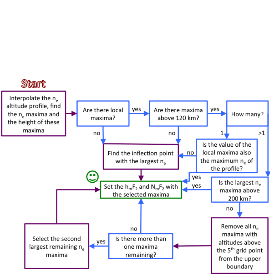
4.2. PYTHON 51
Figure 4.1: Process for finding the hmF2from a GITM electron density altitude profile.
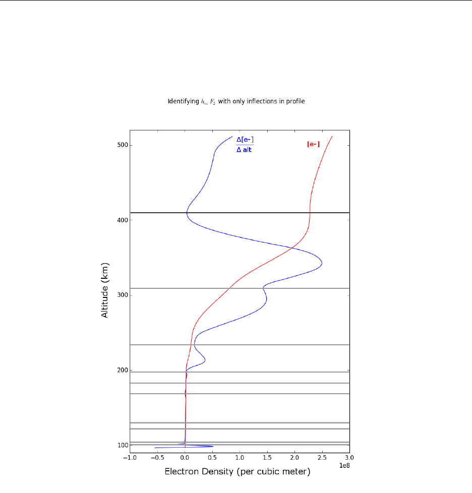
52 CHAPTER 4. OUTPUTS
Figure 4.2: Electron density profile (red) and height derivative of the electron density profile (blue) for an instance
where GITM does not show a clear F2peak. The hmF2is identified by choosing the inflection point (local minima
from the height derivative of the electron density profile) with the largest electron density (dark grey line). The light
grey lines show the remaining locations of inflection points.

4.2. PYTHON 53
appendobs: Add any type of data to an existing GitmTime object. The data can be directly appended
or matched to the existing GitmTime data. Three match options are available: nearest neighbor, running
average, and running median. The latter two options compute a central value and standard deviation using
a specified location/time window about each GitmTime data point.
sat dateloc ticks: Define axis ticks that include all the information necessary to know where measure-
ments lie in spacetime. This is most useful when plotting data along a satellite orbit.
load multiple gitm bin: A routine to load a list of GITM output binary files into GitmBin data structures. The
output is a list of the GitmBin structures, where each element in the list contains the data from a GITM output
binary.
set sat dateloc label: Create a label for the ticks created by GitmTime.sat dateloc ticks. Outputs the label
onto a plot on the right end of the x-axis.
You can load multiple GITM binary files into a data structure with UT dependence by entering the following
commands. Commands outside of ipython are preceded by a ‘$’. Again, the output files used are produced by running
the default UAM.in file.
$ ls 3DALL_t021124_000*> test.list
$ ipython
In [1]: import spacepy
In [2]: import gitm # Load the local version of gitm.py, which may be more up-to-date
In [3]: import gitm_time as gt
In [4]: gtdata = gt.GitmTime(‘test.list’)
In [5]: print gtdata[’time’][:]
[datetime.datetime(2002, 11, 24, 0, 0)
datetime.datetime(2002, 11, 24, 0, 5)]
In [6]: print gtdata[’dLon’][0,:,10,27]
[ -30. -10. 10. 30. 50. 70. 90. 110. 130. 150. 170. 190.
210. 230. 250. 270. 290. 310. 330. 350. 370. 390.]
In [7]: print gtdata[’dLat’][0,10,:,27]
[-105. -95. -85. -75. -65. -55. -45. -35. -25. -15. -5. 5.
15. 25. 35. 45. 55. 65. 75. 85. 95. 105.]
In [8]: print gtdata[’Altitude’][0,10,10,:]
[ 96660.90047544 98330.45023772 100000. 101669.54976228
103348.94180562 105050.15497984 106788.53042153 108584.61276626
110467.61429397 112482.48190265 114698.91401856 117219.51380361
120200.6752566 123855.40706002 128245.43857411 133349.83464183
139220.53740507 145894.02746965 153389.42319611 161708.33330952
170836.59866663 180746.14929878 191399.58798926 202753.75931196
214763.18484817 227382.89781152 240569.83529396 254283.5502381
268486.11667059 283141.61144778 298215.46358093 313673.89525175
329480.19139848 345605.83193525 362018.21624294 378685.73558327
395578.19775965 412667.22510966 429926.74623085 447332.78448625
464864.02590453 482501.63589793 500229.1662886 518032.39821451
535899.14534895 553819.03817939 571783.3052721 589784.56266012
607816.61836022 625874.29578468 643953.27746286 662049.96890339
680161.38144647 698272.79398955]
gitm plot rout.py
Common routines used to format and analyze GITM data.

54 CHAPTER 4. OUTPUTS
choose contour map: A routine to choose an appropriate color map based on whether the plot will be black
and white or color, and whether data data range will be centered about zero or not.
add colorbar: Add a color bar to a contour plot.
find order of magnitude: Find the order of magnitude of a specified number.
center polar cap: Adjust radial coordinates to produce a centered polar plot. Necessary for the northern hemi-
sphere, where polar plots assume the radial (latitude) coordinates should be centered at zero instead of 90◦. This
routine does not depend on SpacePy.
find data limits: Find the upper and lower limits for a specified data key in a list of GITM data structures at a
specified location (either single indices or the entire range are permitted for latitude, longitude, and altitude).
find data limits irange: Find the upper and lower limits for a specified data key in a list of GITM data struc-
tures at a specified location range (upper and lower limits or the entire range are permitted for latitude, longitude,
and altitude).
find data limits ivalues: Establish the appropriate axis limits for a list of GitmBin files at a range or specific
latitude, longitude, or altitude.
glon to localtime: Compute the local time given a longitude and universal time.
localtime to glon: Find the longitude at a specified universal time and local time.
find lon lat index: Find the indexes for the location closest to a specified latitude and longitude.
retrieve key from web name: Find a data key given a website-friendly version of data key names.
find alt index: Find the index closest to the specified altitude. Altitude may be specified in km or m.
match cindi key: A routine to retrieve a CINDI data key from a GITM key or vice versa.
add geomagnetic equator: A routine to add a line showing the geomagnetic equator (specified by IGRF-10)
to an existing plot. Line style and color may be specified.
add subsolar point: A routine to find the location of the subsolar point at a specified Universal Time using
the Pysolar routines. Returns the geographic location of the point and will also add a marker to a plot.
add solar terminator: Computes the location of the solar terminator using the Pysolar routines. Returns
numpy arrays of the geographic coordinates of the solar terminator and will also add a line denoting the solar
terminator to a plot.
find sunside twilight sza: A routine to find the maximum angular distance between the solar terminator and
the sunlight side with conjugate flux tube feet in darkness using Pysolar routines. The solar zenith angle cor-
responding to the sunlight boundary is returned. The entire day is searched to identify the sunlight boundary
given any degree of magnetic declination.
create contour input array: Creates contour input at a specified location between GITM grid points.
create linear input array: Creates linear input at a specified location between GITM grid points.
get meq offset: Find the offset in degrees between the geographic and geomagnetic equators at a specified
longitude.
This example shows how the index for a specified altitude can be found. Note that GITM saves altitude in meters.

4.2. PYTHON 55
In [1]: import spacepy
In [2]: import gitm
In [3]: import gitm_plot_rout as gpr
In [4]: gdata = gitm.GitmBin(‘3DALL_t021124_000000.bin’)
In [5]: ialt = gpr.find_alt_index(gdata, 10, 10, 250.0, "km")
In [6]: print ialt, gdata[’Altitude’][10,10,ialt]
27 254283.550238
solar rout.py
Routines that use Pysolar to find the location of the solar terminator and subsolar point.
subsolar point: Finds the geographic location of the subsolar point at a specified Universal Time.
lat lon2spherical xyz: Converts latitude and longitude to spherical coordinates. Assumes a spherical earth.
spherical xyz2lat lon: Converts from spherical coordinates to geographic latitude and longitude, assuming a
spherical earth.
get solar terminator xyz matrix: Finds the location of the solar terminator in spherical coordinates.
get terminator lat lon coordinates: Finds the location of the solar terminator in geographic coordinates using
input from a solar-oriented spherical coordinate system.
get solar terminator lat lon: Finds the location of the solar terminator at a specified time in geographic
coordinates.
gitm loc rout.py
Routines used to find certain locations or values, as well as routines to align or match points in different data sets.
find nearest location: A routine to find the nearest neighbor in a 1, 2, or 3D coordinate system.
find nearest value: A routine to find the nearest neighbor to a specified value.
find nearest datetime: A routine to find the nearest neighbor between datetime objects.
match running average: Provide running averages at specified times and locations.
match running median: Provide running medians at specified times and locations.
gitm inst loc: A routine to align GITM and instrument data.
gitm net loc: A routine to align GITM and data from a large network of instruments.
gitm time obs loc: A routine to find, through interpolation, the GITM value at a specific observation location
when only one spatial coordinate needs to be aligned.
gitm 3D global plots.py
Routines to build and output GITM output variable contour (recommended) or scatter plots over a geographic range.
Several different standard plot formats are available, and routines useful for creating custom figures are also included.
The Earth’s continental boundaries may be included in any output figure. If they are, shading in the night time region
of the globe may also be included.

56 CHAPTER 4. OUTPUTS
gitm single 3D image: This is a basic visualization routine that creates a filled contour plot of a single output
variable from a GITM 3D at a specified altitude or 2D bin file. The output variable is plotted as a function of
latitude and longitude over the entire globe, though the latitude range may be limited. The output plot may be
polar or rectangular and if the rectangular option is chosen, the geomagnetic equator may also be included in
the output figure. Sample output of the electron temperature is shown in figure 4.3 (a) and (b).
gitm single nsglobal 3D image: A quick way to examine GITM output at both poles. This routine creates
two polar contour plots centered at the geographic northern and southern poles for a single output variable from
a GITM 3D at a specified altitude or 2D bin file. The equatorial and polar latitude boundaries may both be
specified, though they cannot change between hemispheres. Sample output of the electron temperature is shown
in figure 4.3 (c)
gitm global 3D snapshot: A snapshot of a single GITM output over the entire globe. This routine creates two
polar contour plots centered at the geographic northern and southern poles and extending to a specified latitude
and a single rectangular plot containing the latitudes equatorward of this point for a single output variable from
a GITM 3D at a specified altitude or 2D bin file. The geomagnetic equator may also be included in the output
figure. Sample output of the electron temperature is shown in figure 4.3 (d)
gitm mult 3D slices: This routine creates a single plot containing multiple global contours of a GITM output
variable from a 3D or 2D bin file at a list of specified altitudes. These plots may be either polar or rectangular,
with or without the geomagnetic equator, and within a specified latitude range. Sample output of the electron
temperature is shown in figure 4.4.
This example shows how to reproduce Figure 4.3 (a).
In [1]: import spacepy
In [2]: import gitm
In [3]: import gitm_3D_global_plots as g3d
In [4]: import matplotlib.pyplot as plt
In [5]: plt.ion() # This makes the plotting happen interactively
In [6]: gdata = gitm.GitmBin(‘3DALL_t021124_000000.bin’)
In [7]: title = "%s UT" % (gdata[‘time’])
In [8]: f = g3d.plot_single_3D_image("polar", "eTemperature", gdata, title,
"example_polar_plot.png", True, 27, 90, 0)
plot 3D global.py
Routines to build contour or scatter plots over a geographic range. Several different standard plot formats are available,
and routines useful for creating custom figures are also included. The Earth’s continental boundaries may be included
in any output figure. If they are, shading in the night time region of the globe may also be included. Input data must
be provided in separate numpy arrays (1D or 2D for scatter plots, 2D for contour plots).
plot single 3D image: This is a basic visualization routine that creates a filled contour or a colored scatter
plot of a single output variable. The output variable is plotted as a function of latitude and longitude over the
entire globe, though the latitude range may be limited. The output plot may be polar or rectangular and if the
rectangular option is chosen, the geomagnetic equator may also be included in the output figure. If the polar
option is used, the latitude range cannot extend beyond ±90◦. If the rectangular option is used, the geomagnetic
equator may also be plotted.
plot single nsglobal 3D image: A quick way to examine a variable at both poles. This routine creates two polar
contour or scatter plots centered at the geographic northern and southern poles for a single output variable. The
equatorial and polar latitude boundaries may both be specified, though they cannot change between hemispheres.
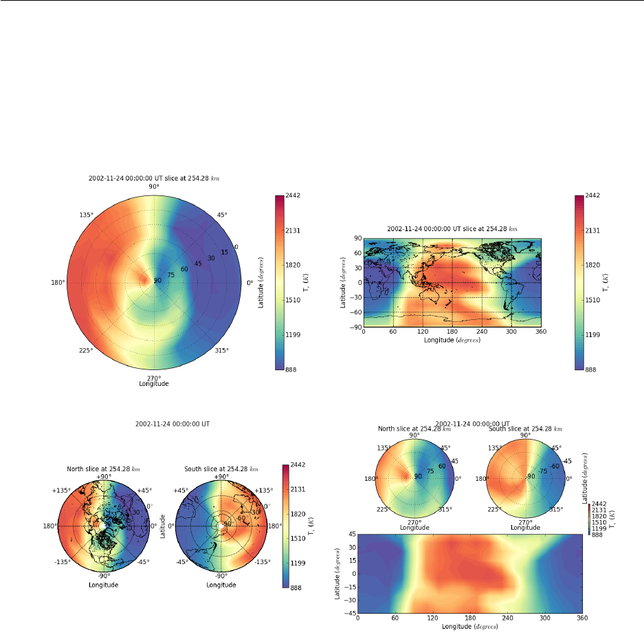
4.2. PYTHON 57
(a) (b)
(c) (d)
Figure 4.3: GITM electron temperature at 456.63 km altitude for: (a) northern latitudes, (b) over the entire globe, (c)
over the entire globe, as viewed from the poles, and (d) as a global snapshot.
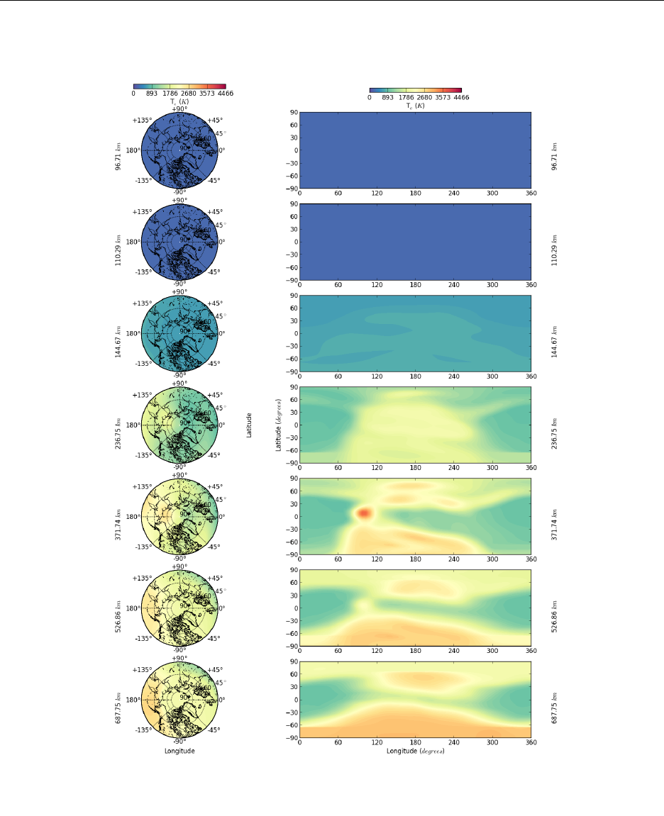
58 CHAPTER 4. OUTPUTS
(a) (b)
Figure 4.4: GITM electron temperature at seven altitude slices for (a) northern latitudes and (b) the entire globe.

4.2. PYTHON 59
plot global 3D snapshot: A snapshot of an output variable over the entire globe. This routine creates two
polar contour or scatter plots centered at the geographic northern and southern poles and extending to a specified
latitude as well as a single rectangular plot containing the latitudes equatorward of this point. The geomagnetic
equator may be output over the data.
plot mult 3D slices: This routine creates a single plot containing multiple global contour or scatter plots for
a single variable at specific indices (corresponding to different altitude, universal times, et cetera). These plots
may be either polar or rectangular (with or without the geomagnetic equator). Sample output of the electron
temperature is shown in figure 4.4. The numpy arrays containing the data may be 2D or 3D for scatter plots or
3D for contour plots. Any dimension may contain the indices to iterate over for the subfigures.
plot nsglobal subfigure: This routine creates a subfigure with two polar contour or scatter plots centered
at the geographic northern and southern poles for a single output variable. The equatorial and polar lati-
tude boundaries may both be specified, though they cannot change between hemispheres. This is used by
plot single nsglobal 3D image and may also be used to create a subplot with this format.
plot snapshot subfigure: This routine creates a subfigure with two polar dials and a rectangular region showing
the equatorial latitudes for a single output variable. This is used by plot global 3D snapshot and may also be
used to create a subplot with this format.
plot rectangular 3D global: This routine plots a single rectangular filled contour or colored scatter for an
output variable as a function of latitude and longitude. Options exist to control the colorbar, ticks, labels, and
more. A handle to the contour plot is returned to allow the output to be further manipulated depending on what
other subplots are included in the output figure.
plot polar 3D global: This routine plots a single polar filled contour for a GITM output variable at a specified
altitude index as a function of latitude and longitude. Title, colorbar, labels, and more may be specified using
input options. A handle to the contour plot is returned to allow the output to be further manipulated depending
on what other subplots are included in the output figure. The longitude at the top of the plot may also be
specified, this allows one to ensure a specific local time is always located at the top of the dial using a routine
like localtime to glon.
gitm alt plots.py
Routines to build and output GITM output variable linear and contour plots over an altitude range. Several different
standard plot formats are available, and routines useful for creating custom figures are also included.
gitm single alt image: Creates a single linear or contour altitude plot.
gitm mult alt image: Creates a figure with multiple linear or contour altitude plots.
gitm alt slices: Creates a figure with a contour plot showing the altitude dependence of a quantity as a function
of latitude or longitude with several linear altitude slices at specified locations. An example is shown in figure 4.5
This example shows how to reproduce Figure 4.5.
In [1]: import spacepy
In [2]: import gitm
In [3]: import gitm_alt_plots as gap
In [4]: import gitm_plot_rout as gpr
In [5]: import matplotlib.pyplot as plt
In [6]: plt.ion() # This makes the plotting happen interactively
In [7]: gdata = gitm.GitmBin(‘3DALL_t021124_000000.bin’)
In [8]: title = "%s UT" % (gdata[‘time’])
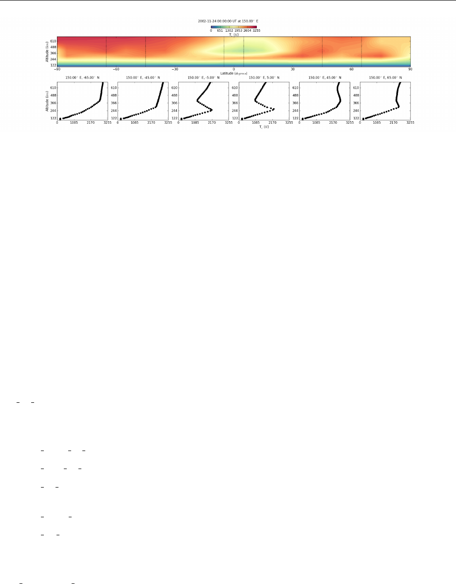
60 CHAPTER 4. OUTPUTS
Figure 4.5: GITM electron temperature at a constant longitude with six latitude slices.
In [9]: lat_index = list()
In [10]: lon_index = list()
In [11]: (ilon, ilat) = gpr.find_lon_lat_index(gdata, 150.0, -65.0, "degrees")
In [12]: lon_index.append(ilon)
In [13]: lat_index.append(ilat)
In [14]: (ilon, ilat) = gpr.find_lon_lat_index(gdata, 150.0, -45.0, "degrees")
In [15]: lat_index.append(ilat)
In [16]: (ilon, ilat) = gpr.find_lon_lat_index(gdata, 150.0, -5.0, "degrees")
In [17]: lat_index.append(ilat)
In [18]: (ilon, ilat) = gpr.find_lon_lat_index(gdata, 150.0, 5.0, "degrees")
In [19]: lat_index.append(ilat)
In [20]: (ilon, ilat) = gpr.find_lon_lat_index(gdata, 150.0, 45.0, "degrees")
In [21]: lat_index.append(ilat)
In [22]: (ilon, ilat) = gpr.find_lon_lat_index(gdata, 150.0, 65.0, "degrees")
In [23]: lat_index.append(ilat)
In [24]: f = gap.plot_alt_slices("eTemperature", gdata, lat_index, lon_index,
title, "example_alt_plot.png")
plot alt profiles.py
Routines to build and output linear and contour plots over an altitude range. Several different standard plot formats
are available, and use any numpy array as input.
plot single alt image: Creates a single linear or contour altitude plot.
plot mult alt image: Creates a figure with multiple linear or contour altitude plots.
plot alt slices: Creates a figure with a contour plot showing the altitude dependence of a quantity as a function
of latitude or longitude with several linear altitude slices at specified locations.
plot linear alt: Plots the the linear altitude dependence of a quantity, with altitude on the y-axis.
plot 3D alt: Plots the altitude dependence of a quantity as the function of another spatiotemporal coordinate
with the spatiotemporal coordinate on the x-axis, altitude on the y-axis, and the desired quantity as a color
contour.
gitm comparison plots.py
Routines to make plots that compare GITM data with observations. The observational sources include satellites,
ground-based receivers, and receiver networks.

4.2. PYTHON 61
extract data matched arrays: Extract points from matched data arrays for elements where neither array
contains a specified ‘bad’ value.
extract gitm time arrays: Routine to extract all positions with valid data from a GitmTime object and con-
struct numpy arrays. A single universal time, longitude, latitude, and/or altitude may be specified.
plot net gitm comp: A routine to create a plot comparing 2D GITM data (such as VTEC or hmF2) to ob-
servations taken from a network of instruments over the globe. The map format may be rectangular, polar, or
a combination (provided by plot nsglobal subfigure or plot snapshot subfigure). The top subfigure shows the
observations as a scatter figure, the middle subfigure shows the GITM data as a contour, and the bottom sub-
figure shows the difference between the two as a scatter plot. The difference must be computed outside of this
program, and so may be the difference, absolute difference, percent difference, or any other type of comparison.
An example is shown in Figure 4.6.
plot sat gitm comp: Routine to plot satellite and GITM data to show how a single physical quantity varies
over the orbit. Four panels are included; the top panel shows the raw satellite data and the GITM data along the
track. The second panel shows the matched GITM/satellite data. The third panel shows the difference between
the satellite and GITM data. The fourth panel shows the percent difference 100*(sat-GITM)/sat.
load files.py
Routines to load certain types of data files into a dictionary of numpy arrays, where each data type is used to specify
the dictionary keys.
loadCINDIorbit ASCII: Loads the Coupled Ion Neutral Dynamics Investigation ASCII files provided by the
UT Dallas website.
loadMadrigalVTEC ASCII: Loads the GPS TEC ASCII files provided by the Millstone Hill Madrigal site.
loadGITMsat ASCII: Loads the satellite file used as input for a GITM run.
loadMadrigalVTEC HDF5: Loads the GPS TEC HDF5 files provided by the Millstone Hill Madrigal site.
read files.py
Routines to read certain file formats and load the data into a dictionary of numpy arrays, where each data type is used
to specify the dictionary keys.
loadASCII data header: Loads an ASCII file with header lines denoted by a ‘#’ .
loadASCII data hline: Loads an ASCII file with a specified number of header lines.
loadASCII index profile: Loads an ASCII file with header lines denoted by a ‘#’ that has been broken up into
indexed blocks (blocks separated by double newlines, or indexes as specified by gnuplot). The indexed structure
is maintained in the output dictionary by providing a list of numpy arrays for each data column.
load multASCII data: Loads multiple ASCII files into a single output dictionary.
loadnetCDF data: Loads netCDF files into an output dictionary.
combine data dictionaries: Combines multiple data dictionaries into a single dictionary, including only the
data keys common to all of the inputted data dictionaries.
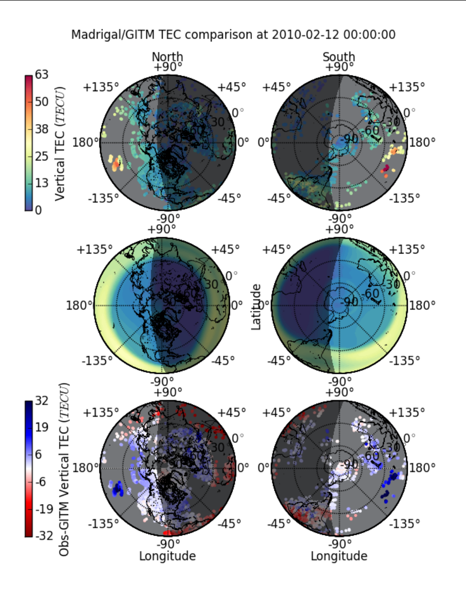
62 CHAPTER 4. OUTPUTS
Figure 4.6: Madrigal and GITM vertical TEC comparison.

4.2. PYTHON 63
read gps bin.py
A script to read a VMR GPS binary file, providing data at a specified Universal Time.
GpsFile: Class containing all of the data from the VMR GPS binary file.
read header: Reads the VMR GPS binary file header, allowing data to be easily located as desired.
read time: Read in all the GPS data at the specified Universal Time. The specified time and the file times
do not have to be perfectly aligned, as long as the specified time falls between the first and last time in the
GPS file, the data with the closest temporal proximity will be returned.
write files.py
Routines to write output files.
writeASCII file: A routine to create an ASCII file from a string or list of strings. Will overwrite any file of the
same name that already exists.
writeASCII data w sorttext: A routine to create an ASCII file from a data dictionary of dictionaries. The first
layer of keys is used to provide the data columns, the second layer is output as additional data column(s) where
the keys are output as strings. Datetime columns are output as two strings, one containing the date information
and a second one containing the time of day information.
plot stats.py
Routines to compute and plot common statistics.
add stat to line: Computes the moments, first through third quartiles, and mode(s) (as desired) for a dataset
and outputs the statistics as a formatted text line that can be output to a file and in a list.
add stat box: Computes the moments, first through third quartiles, and mode(s) (as desired) for a dataset and
outputs the statistics in a text box onto a plot and in a list.
plot hist w stats: Calculates and plots a histogram of a specified dataset, as well as the moments, first through
third quartiles, and mode(s) (as desired).
plot lat lt stats: Calculates and plots histograms and statistics for a specified dataset broken up into latitude
and local time regions.
lat lt stat lines: Calculates statistics for a specified dataset broken up into latitude and local time regions,
providing a formatted string with the statistics for each region taking up a line.
gitm movie script.py
This is a python script that can be run either from ipython using the command run gitm movie script.py
or the command line using the command python gitm movie script.py. Input to this program is prompted
interactively, and includes:
•Ordered list of GITM binary files: A list of GITM binary files in chronological order (or what-
ever other order the movie should be played in).
•GITM plot type (rectangular, polar, nspolar, snapshot): The keyword for the desired
plot type. These are the plot types shown in figure 4.3, where polar corresponds to panel (a), rectangular to
panel (b), nspolar to panel (c), and snapshot to panel (d).

64 CHAPTER 4. OUTPUTS
•At this point, the routine enters a while-loop to allow multiple movies to be made for the same list of GITM
binary files
–GITM key to plot on z axis (eg Temperature): The data key corresponding to the data
type to plot on the z axis. A list of data keys can be found by typing ‘gdata.keys()’ into ipython after
loading one of the listed GITM binaries.
–Altitude to plot z value at (eg 250): Altitude to plot, may be specified in km or m. For
2D parameters, a value must be entered, but doesn’t matter.
–Units of altitude (km or m): Units of altitude entered above.
–Use map of Earth? (empty for False): Enter any value to include a Basemap plot of the
earth, enter a carriage return to exclude the map.
–The latitude limits needed depend on the plot type
∗nspolar Polar latitude limit (degrees): Specify the polar latitude limit (positive, same
for both hemispheres).
∗nspolar Equatorial latitude limit (degrees): Specify the equatorial latitude limit
(positive, same for both hemispheres).
∗snapshot Polar latitude limit (degrees): Specify the polar latitude limit (positive,
same for both hemispheres).
∗polar/rectangular Northern latitude limit (degrees): Specify the northernmost lati-
tude (may be negative).
∗polar/rectangular Southern latitude limit (degrees): Specify the southernmost lat-
itude (must be smaller/more negative than the northernmost limit)
–Load another z axis key? (empty for False): Enter any value to include another movie
or, enter a carriage return finish.
With this information, movies with appropriate z-variable ranges will be plot as .png files and combined into a
movie using FFmpeg. The image and movie files will be named using the plot type, z parameter, and altitude to
distinguish them.
Bibliography
Ali, A. A., K. Agarwal, A. M. D’Amato, A. J. Ridley, and D. S. Bernstein (2012, August). Retrospective-Cost
Subsystem Identification for the Global Ionosphere-Thermosphere Model. In AIAA Guidance, Navigation, and
Control Conference and Exhibit, Minneapolis, MN (USA), pp. 1–12. University of Michigan.
Anderson, J. L., T. Hoar, K. Raeder, H. Liu, N. Collins, R. Torn, and A. Avellano (2009, September). The Data
Assimilation Research Testbed: A Community Facility. Bulletin of the American Meteorological Society 90(9),
1283–1296.
Chakravarthy, S. R. and S. Osher (1983, July). High resolution applications of the Osher upwind scheme for the Euler
equations . 6th Computational Fluid Dynamics Conference, 363–372.
Chamberlin, P. C., T. N. Woods, and F. G. Eparvier (2007). Flare irradiance spectral model (FISM): Daily component
algorithms and results. Space Weather 5(7), S07005.
Chamberlin, P. C., T. N. Woods, and F. G. Eparvier (2008, May). Flare Irradiance Spectral Model (FISM): Flare
component algorithms and results. Space Weather 6, S05001.
Covington, A. (1948). Solar noise observations on 10.7 centimeters. Proceedings of the IRE 36(4), 454–457.
Fuller-Rowell, T. J. and D. S. Evans (1987, July). Height-integrated Pedersen and Hall conductivity patterns inferred
from the TIROS-NOAA satellite data. Journal of Geophysical Research 92(A7), 7606–7618.
Hanson, W. B. and R. Cohen (1968). Photoelectron heating efficiency in the ionosphere. Journal of Geophysical
Research 73(3), 831–840.
Newell, P. T., T. Sotirelis, J. M. Ruohoniemi, J. F. Carbary, K. Liou, J. P. Skura, C. I. Meng, C. Deehr, D. Wilkinson,
and F. J. Rich (2002). OVATION: Oval variation, assessment, tracking, intensity, and online nowcasting. Annales
Geophysicae 20(7), 1039–1047.
Richmond, A. D. (1995). Ionospheric electrodynamics using magnetic apex coordinates. Journal of Geomagnetism
and Geoelectricity 47(2), 191–212.
Ridley, A. J. and E. A. Kihn (2004, April). Polar cap index comparisons with AMIE cross polar cap potential, electric
field, and polar cap area. Geophysical Research Letters 31, L07801.
Roe, P. L. (1986). Characteristic-based schemes for the Euler equations. Annual review of fluid mechanics 18(1),
337–365.
65
