GreatSPN User Manual
User Manual: Pdf
Open the PDF directly: View PDF ![]() .
.
Page Count: 138 [warning: Documents this large are best viewed by clicking the View PDF Link!]
- Informal introduction to the formalisms
- Getting started
- GUI in depth
- Solvers
- Structural analyzers
- Performance bounds solver
- Analytic solvers
- Simulators
- Extended SWN features
- Multiple experiments
- Compositionality in GreatSPN
- Export to other tools
- Net description files
- Known bugs and Warnings
- Installation

User’s Manual
(version 2.0.2)
Performance Evaluation group
Dipartimento di Informatica
Universit`
a di Torino (Italy)
Preface
This manual comes out from the collection and the integration of the documentation, produced by
several people of the Performance Evaluation group and of the Petri net community, regarding different
aspects of the GreatSPN tool.
In particular, among the people who contributed to the realization of this manual, I would like to thank
(in alphabetical order): Cosimo Anglano, who firstly wrote the Getting started for the previous ver-
sion of GreatSPN and gave the layout schema for the chapt. 3; Claudio Bertoncello, who implemented
and documented the part related to the computation of refined performance indices for SWN models;
Massimiliano De Pierro, who took care of the installation procedure of the tool and of its documen-
tation; Susanna Donatelli and Giuliana Franceschinis, who provided the documentation regarding the
GreatSPN2.0.2 solvers and the grammars and gave the guidelines to the drafting of the manual; Liliana
Ferro, who implemented and documented the translator of nets produced in GreatSPN2.0.2 format into
the PROD format; Rossano Gaeta, who took care of the extended SWN features; Serge Haddad, Patrice
Moreaux and M. Sene, who wrote the part related to the set of tools PERFSWN; Andras Horv´
ath, who
implemented and carefully documented the compositionality in GreatSPN2.0.2 and the MultiSolve used
to launch multiple experiments; and, finally, Marina Ribaudo, who wrote the introductory part related
to the Petri Net formalisms and to the history of the GreatSPN tool.
The manual is organized as follows:
in chapt. 1an informal introduction to the Petri Net formalisms is given; chapt. 2is the tutorial to
the use of GreatSPN2.0.2 tool; chapt. 3contains an in-depth presentation of the GUI GreatSPN2.0.2
features; in chapt. 4the GreatSPN2.0.2 solvers are examined and the MultiSolve multiple experimenter
is described; chapt. 5describes how the compositionality has been implemented in GreatSPN2.0.2 ;
chapt. 6is devoted to the translators from GreatSPN2.0.2 to the other tools. In appendix Athe Great-
SPN2.0.2 grammars are listed and commented; in appendix Ba list of known current bugs is given
together with the list of the warnings emphasized along the manual. Finally, in appendix CGreat-
SPN2.0.2 installation instructions are given.
Simona Bernardi.
2
Contents
1 Informal introduction to the formalisms 6
1.1 History of GreatSPN ........................................ 6
1.2 Petri Nets .............................................. 8
1.3 Stochastic Petri Nets ........................................ 10
1.4 Generalized Stochastic Petri Nets .................................. 11
1.4.1 A GSPN example ...................................... 12
1.5 Stochastic Well Formed Nets .................................... 14
1.5.1 A SWN example ...................................... 15
2 Getting started 17
2.1 The Readers–Writers GSPN model ................................. 17
2.2 Starting GreatSPN ......................................... 18
2.3 Creating the Readers–Writers model ................................ 18
2.4 Saving and printing the model ................................... 23
2.5 Analysis of the Readers-Writers model ............................... 25
2.6 Colored version of the Readers-Writers model ........................... 29
2.7 Analysis of the SWN Readers-Writers model ........................... 33
3 GUI in depth 35
3.1 The Menu Bar ............................................ 37
3.1.1 File Menu .......................................... 37
3.1.2 Edit Menu ......................................... 40
3.1.3 View Menu ......................................... 47
3.1.4 Grid Menu ......................................... 47
3.1.5 Zoom Menu ......................................... 48
3.1.6 Rescale Menu ........................................ 48
3.1.7 GSPN Menu ........................................ 48
3.1.8 SWN Menu ......................................... 51
3
3.1.9 E-GSPN Menu ....................................... 53
3.1.10 Help Menu ......................................... 53
3.2 The Object bar ........................................... 54
3.2.1 Places ............................................ 54
3.2.2 Transitions ......................................... 57
3.2.3 Arcs ............................................. 63
3.2.4 Marking parameters .................................... 64
3.2.5 Rate parameters ....................................... 66
3.2.6 Result definitions ...................................... 67
3.2.7 Changing place/transition tags ............................... 69
3.2.8 Colour definition ...................................... 69
4 Solvers 74
4.1 Structural analyzers ......................................... 74
4.1.1 Invariants .......................................... 76
4.1.2 Minimal deadlocks and traps ................................ 77
4.1.3 Implicit places ....................................... 78
4.1.4 ECS-Confusion-ME-SC-CC ................................ 79
4.1.5 Structural boundedness ................................... 80
4.2 Performance bounds solver ..................................... 81
4.2.1 Modules .......................................... 81
4.2.2 Result file structure ..................................... 81
4.3 Analytic solvers ........................................... 82
4.3.1 GSPN solvers ........................................ 82
4.3.2 SWN solvers ........................................ 85
4.4 Simulators .............................................. 86
4.4.1 GSPN simulation ...................................... 86
4.4.2 SWN simulation ...................................... 87
4.5 Extended SWN features ....................................... 88
4.5.1 Transient analysis of SWN models ............................. 88
4.5.2 Simulation of SWN models with GEN transitions ..................... 88
4.5.3 Refined perfomance results ................................. 90
4.5.4 The result .stat file ..................................... 96
4.5.5 Number of batches in a simulation run ........................... 96
4.5.6 Inclusion of “reset” transitions ............................... 97
4.6 Multiple experiments ........................................ 97
4
5 Compositionality in GreatSPN 102
5.1 Composition of two labelled SWNs ................................ 102
5.2 The algebra package ........................................ 104
5.2.1 Composition module .................................... 104
5.2.2 Remove module ...................................... 107
6 Export to other tools 108
6.1 Model checking: PROD translator ................................. 108
6.1.1 Installation ......................................... 108
6.1.2 Use of the PROD translator ................................ 109
6.2 Kronecker solutions: APNN translator ............................... 118
6.3 Tgif translator ............................................ 118
6.4 Fluid nets translator ......................................... 118
6.5 Refinement of SWN performance indexes: PERFSWN ...................... 119
A Net description files 121
A.1 Format of the .net file ........................................ 122
A.2 Format of the .def file ........................................ 123
A.3 Grammars .............................................. 124
A.4 Extended SWN grammar ...................................... 127
B Known bugs and Warnings 129
B.1 Warnings .............................................. 130
C Installation 131
C.1 System requirements for compiling the tool ............................ 131
C.2 Compiling and installing the tool .................................. 132
C.3 Setting the environment ....................................... 133
5
Chapter 1
Informal introduction to the formalisms
This chapter contains a brief history of GreatSPN and recalls part of the background material necessary to use the
package. The Petri net formalism and some stochastic extensions are briefly described in the following sections.
The descriptions are very concise and the reader may find major details about these formalisms in the book [4].
1.1 History of GreatSPN
The first impulse to the development of the GreatSPN package stemmed from the research pursued by the Torino
group on generalized stochastic Petri nets (GSPN). GSPNs were initially developed as a tool for the specifica-
tion and performance evaluation of computer architectures at the Dipartimento di Elettronica of the Politecnico
di Torino and at the Dipartimento di Informatica of the Universit`
a di Torino [3], in the frame of the Progetto
Finalizzato Informatica of the Italian Consiglio Nazionale delle Ricerche, MUMICRO project. The development
of GSPNs was stimulated by the results on SPNs described in the Ph.D. thesis of M. K. Molloy [31]. In GSPNs
a new class of transitions (called immediate) that fire in zero time with priority over timed transitions was in-
troduced. A solution algorithm that exploits the reduction of the size of the Reachability Set (RS) due to the
presence of immediate transitions was first described in [3].
Several computer programs were developed as part of PhD thesis to implement the steady-state numerical
solution of GSPN models, eventually leading to the first documented software package for their analysis. This
package allowed one to experiment with the new modeling tool and gain insight into the memory and CPU
time requirements of the solution algorithms as functions of the size of GSPN models. The weak points of this
package were poor portability and flexibility of the programs, and the lack of a graphical interface, which is the
most natural type of support for the definition of GSPN models. Subsequent efforts were devoted to designing
a package with the following characteristics: (1) user friendliness – in particular the availability of a graphical
interface for model definition was considered a must to satisfy this requirement –, (2) portability, (3) modularity
and easy upgradability, and (4) efficiency of the analysis modules.
The first step in this direction was the implementation of the software tool described in [10]. A decomposition
6

was pursued both of the software tool and of the analysis steps. Several intermediate results were identified and
stored in the form of separate files. Several independent programs cooperate to the production of final result
files by taking as input intermediate result files produced by running other modules of the tool. Thanks to
this modular software architecture [14], the tool was easily upgraded and adapted to different uses as soon as
new theoretical results provided new analysis algorithms. From the functional point of view, earlier versions of
GreatSPN included a graphical interface (based on the SunView package and on the PixRect utilities for basic
graphics), all the algorithms for the generation and steady-state or transient solution of the “underlying Markov
chain” of a GSPN, and a new algorithm for the analysis of a class of models containing a mix of exponentially
distributed and deterministic timed transitions (DSPN) [5]. A Monte Carlo simulation program with confidence
interval estimation was also introduced for two main reasons: (1) to provide a tool for performance evaluation in
the general case of Timed Transitions Petri Nets (TTPN) that are not analytically solvable and (2) to provide a tool
for the validation of models when numerical solutions cannot be implemented due to the size of the Reachability
Graph (RG), which is equal to the number of states of the underlying Markov chain1.
GreatSPN started to become an interesting and useful support tool for performance modeling, and many re-
search and education institutions asked for permission to have it, so that the Dipartimento di Informatica of the
Universit`
a di Torino began its free distribution. Using the package on increasingly larger and more complex mod-
els, we soon realised the need for some model validation and “debugging” tool. From this need, the Torino group
started to look more carefully at the traditional techniques and algorithms used in the classical Petri net theory for
the study of qualitative structural and behavioral properties. Major improvements in the validation capabilities of
the package were achieved with the implementation of algorithms for the computation of Place- and Transition-
invariants, that allowed an easy check of structurally necessary or sufficient conditions for boundedness and er-
godicity before the exhaustive enumeration of the state space. More specific and powerful structural analysis
techniques were also proposed for the qualitative validation of GSPNs [15] and included in GreatSPN. A major
check-point was undertaken with the release 1.3 [11], which included all the structural analysis techniques for
the validation of the underlying Petri net structure of a GSPN model. Major improvements in the validation ca-
pabilities of the package were achieved with the implementation of algorithms for the computation of Place- and
Transition- invariants, and of the specific structural analysis techniques for the qualitative validation of GSPNs
proposed in [15].
At this point the weakest part of the package was the simulation feature, which used a very straightforward
(and inefficient) Monte Carlo non event-driven technique for the generation of the sample paths. The same
structural properties computed for the model validation were then reconsidered from a different perspective: they
were used for the optimization of the data structures of the analysis and simulation programs [13]. This idea
led to a completely new set of solution and simulation programs, and eventually to the implementation of the
interactive simulation facilities [7] of GreatSPN 1.4.
1In any case simulation usually requires costly and long computations.
7
One of the drawbacks of versions 1.3 and 1.4 was that they comprised both modules written in Pascal and
modules written in C. In version GreatSPN 1.5 all the Pascal modules were rewritten in C in order to increase
portability. Moreover, new algorithms and techniques were implemented for the efficient and direct construction
of the Tangible Reachability Graph (TRG) [18,8], further reducing the space and time requirements of this phase
with respect to the technique proposed in [13]. In this version the possibility of general marking dependence
for transition rates has been restricted: immediate transition weights are now constants, while in the case of
timed transition the preferred way of expressing marking dependency is through the degree of enabling; general
marking dependency for timed transitions is still possible, but its implementation is less efficient than that of
enabling dependence. In version 1.6, the graphical interface was rewritten based on XView, a public domain
toolkit (included in the MIT distribution tape of X11R5). The basic structure and features of the graphical
interface of GreatSPN 1.3 were retained. Minor changes were introduced in order to present the control items in
a more rational way. Some features have been added in a straightforward way in order to allow the visualization
of the new structural, behavioral, and performance results obtained by the new analysis modules.
GreatSPN 1.7 represents a new major check-point for the package. New algorithms have been added for
the fast computation of performance bounds based on linear programming techniques [16], working at a purely
structural level. The computed bounds depend only on the average firing delay of the transitions while they do
not depend on the p.d.f. of such delays. Algorithms have also been added for the analysis of high-level Petri net
models providing the user with the possibility of designing models of complex systems in a more compact way.
The chosen high-level formalism is Stochastic Well-Formed nets (SWNs), for which efficient algorithms have
been defined, that automatically generate a compact RG (called Symbolic RG) exploiting the model symmetries
[19,23,21]. The major objective of GreatSPN 1.7 was thus a consolidation of the package to allow an easier
distribution, as well as a broader application scope, with more emphasis on the validation and the simulation of
models and on the derivation of fast performance bounds.
Research is still going on, and will eventually produce new implementations to be introduced in GreatSPN
on hierarchical modeling [17] and on the exploitation of parallel processing techniques for the efficient analysis
of large models [22,24]. Concerning the graphical interface, porting under OSF/Motif is being considered.
1.2 Petri Nets
Introduced for the first time in the sixties [34], Petri nets (PN) are a graphical and mathematical modeling tool
for describing concurrent systems. A PN is a 5-tuple (P,T,I,O,H), where Pis the set of places, Tis the set of
transitions, and I,O,H, are functions that defines weighted input, output and inhibitor arcs between places and
transitions. PNs incorporate a notion of (distributed) state which is denoted by a function M:P→IN, called
marking.
A PN system is given by a PN structure plus an initial marking and it is defined as a 6-tuple (P,T,I,O,H,M0)
8
where M0represents the initial distribution of tokens in the places of the net.
PN have an associated graphical representation, where places are circles, transitions are bars, input and output
functions are weighted arrows, and inhibitor function are circle headed arrows. The marking is represented by
inscribing place pwith M(p)tokens, represented as black dots.
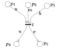
Transitions describe events that may modify the system state and the firing rule defines the dynamic behaviour
of PN models. For example, in the net below, transition tis enabled if M(p1)≥n,M(p2)≥m,and M(p3)<h.
Once enabled, transition tcan fire consuming ntokens from place p1,mfrom p2and depositing utokens into p4
and vinto p5.
Figure 1.1: Example of enabling and firing.
An important consideration is that the enabling and firing rules for a generic transition tare “local”: indeed,
only local information (i.e. input, inhibitor and output places) need to be considered to establish whether tcan fire
and to compute the change of marking. This justifies the assertion that the PN marking is intrinsically distributed.
A marking M0is said to be immediately reachable from Mif M0can be obtained by firing a transition enabled
in M. The set of transitions enabled in the marking Mis denoted with E(M)and the firing of a transition tis
denoted with M[tiM0.
Two transitions are said to be in conflict if they share input places and the firing of one transition disables the
other by removing the token in the common input places.
Starting from the initial marking M0it is possible to compute the set of all the reachable markings, the so
called Reachability Set (RS) of the model. The RS does not contain information about the transition sequences
fired to reach each marking. This information is captured by the Reachability Graph (RG) whose nodes are
labelled with the reachable markings and whose arcs are labelled with the transitions that the system has to fire
to move from state to state.
PN models can be used for the (qualitative) analysis of logical properties of systems. Classical analysis
techniques are structural (graph-based) analysis and reachability analysis which investigate, for example, the
boundedness of the model or the presence of deadlocks.
9

1.3 Stochastic Petri Nets
Classical PN models include no notion of time and for this reason they have been traditionally used for the qual-
itative analysis of logical properties of systems. Several authors have proposed augmented PN models which
include temporal specifications, so that a quantitative performance analysis of systems is possible. The introduc-
tion of temporal specifications in a PN has been done mostly by associating a delay with transitions. Stochastic
Petri Nets (SPN) [30] are PN in which transition firing delays are exponentially distributed random variables:
each transition tiis associated with a random firing delay whose probability density function is a negative expo-
nential with rate λi. Syntactically this extension amounts to adding a function W:T→IR+such that the delay
associated to a transition tis a random variable, distributed as a negative exponential, of rate W(t). Thus a SPN
system is defined as a 7-tuple (P,T,I,O,H,W,M0)where P,T,I,O,H,M0are defined as in PNs and Wspecifies
the rates to be associated with transitions.
The semantics of SPNs is described by a race model. When a marking simultaneously enables several
(conflicting and/or concurrent) transitions, all activities associated with these transitions are assumed to execute
in parallel, so that the next marking change is due to the transition whose firing delay in the present marking is
minimum, i.e., to the transition that wins the race. The firing of the winning transition implies that the activity
associated with it in the model is completed. The behaviour of the losing transitions can be specified in different
ways. Indeed, it is possible for these transitions to either remember the time during which they have already been
enabled (and thus worked), or not. However, the use of exponential distributions for the definition of temporal
specifications makes unnecessary the distinction between the distribution of the delay itself, and the distribution
of the remaining delay after a change of state, thus avoiding the need for the specification of the behaviour of the
transitions that do not fire in a given marking.
When the set of enabled transitions E(M)contains more than one element, the probability that transition tiis
the one that actually fires can be obtained from the temporal specifications as
P{ti|M}=W(ti)
∑
tj∈E(M)
W(tj)=λi
∑
tj∈E(M)
λj
The definitions of the RS and the RG are still valid for SPNs but in this case the arcs of the RG are labelled with
transition names and transition rates.
Molloy [31] showed that, due to the memoryless property of the exponential distribution of firing delays,
SPN are isomorphic to continuous-time Markov chains (CTMC) in which
1. the states of the CTMC are in one-to-one correspondence with the SPN markings (Mi↔i);
2. the transition rate from state i(corresponding to marking Mi) to state j(Mj) of the CTMC is equal to the
sum of the rates of the transitions that connect the corresponding markings in the RG of the net.
10
The translation of a SPN model into a CTMC is thus conceptually very simple. The RS of the SPN is generated,
and the firing rates of enabled transitions are used to construct the state transition rate matrix Qof the CTMC.
If the CTMC is ergodic, it is possible to compute the steady state probability distribution of the markings
solving the matrix equation
πQ=0
with the additional constraint
∑
i
πi=1
where πis the vector of the steady state probabilities. From the steady state distribution it is possible to obtain
quantitative estimates of the behaviour of the SPN.
Difficulties may arise due to the computational complexity of the algorithm for this solution, when the number
of reachable markings grows. This is the main problem associated with the utilisation of SPN which are otherwise
very easy to employ, even for inexperienced users.
1.4 Generalized Stochastic Petri Nets
Sometimes it is not desirable to associate a random time with each transition of a model, since one would rather
associate times only with the events that are believed to have the largest impact on system performance. For
instance, the time required to test the condition to enter in a while loop can be considered negligible with respect
to the time required to execute the body of the loop.
SPN models in which logical actions are represented by transitions whose firings take no time are known by
the name of generalized SPN (GSPN) [3,15]. Transitions that fire in zero time are called immediate (represented
as black bars) to be distinguished from the transitions whose associated delays are exponentially distributed,
which are called timed (represented as rectangular boxes).
Immediate transitions fire with priority over timed transitions and it is assumed that different priority levels
can be defined over immediate transitions. Priorities equal to zero are associated with timed transitions, priorities
equal or greater than one are associated with immediate transitions. Syntactically, this extension amounts to
adding a priority function π:T→IN which assigns a natural number to each transition. A GSPN system is
defined as a 8-tuple (P,T,I,O,H,W,π,M0).
In GSPN the delay associated with a timed transition tis a random variable, distributed as a negative expo-
nential, of rate W(t). In the case of an immediate transition tinstead, the value W(t)specifies a weight.
When two or more timed transitions tiare in conflict, the selection of the one that fires first is done according
to the race policy. When two or more immediate transitions tiare in conflict the selection of the one that fires first
is done using the weights W(ti), normalised in such a way as to obtain a discrete probability distribution function.
Due to the presence of immediate transitions, the RS of a GSPN model contains two different types of
markings that are classified as tangible and vanishing. A tangible marking is a state in which no immediate
11
transitions are enabled and therefore the system spends some time in that state, while a vanishing marking is a
state in which at least an immediate transition is enabled and therefore the time spent in a vanishing marking is
equal to zero.
The execution of a GSPN model is not identical to a sample function of a Markov process, due to the existence
of multiple discontinuities at the time instants corresponding to the entrance into vanishing markings. It is
however possible to remove these markings from the analysis, since they do not contribute to the measurable
behaviour of the model. The performance of a GSPN model can thus be analyzed by examining its evolution
through the set of tangible markings only. It has been shown [3,15] that there is a correspondence between GSPN
models and CTMCs. Performance indices such as, for example, transition throughputs and the mean number of
tokens in a place, can be associated with a GSPN model. They are computed starting from either the transient or
the steady state probabilities of the associated CTMC.
Another extension that has been introduced by some authors is the possibility of defining marking dependent
rates: the rate of the transition is therefore a function of the state of the system. If the dependence is only from
the input and output place of the transition we still preserve the inherent distribution of the state proper of Petri
nets, if we allow instead any type of dependence, then the locality of the firing of transition can be completely
destroyed.
1.4.1 A GSPN example
To give an idea of the GSPN formalism we briefly describe an example that will be also used in Section 1.5.1 to
describe the coloured formalism of Stochastic Well Formed nets. All the details about the construction and the
analysis of GSPN models will be discussed in the next chapters.
The example, taken from the telecommunication area, is a multiple server cyclic polling system [6] compris-
ing a set of waiting lines in which customers that arrive from the external world queue up waiting for service. A
set of servers cyclically visit the queues providing service to the waiting customers. Upon service completion a
customer departs from the system and the server proceeds to the next queue.
The net in Figure 1.2(a) shows the GSPN model of a generic queue i: place p(i)
arepresents the number of
free positions in the queue, whose maximum capacity is equal to Kas specified by its initial marking. Timed
transition T(i)
amodels the customer arrival process; customers waiting for a server are queued in place p(i)
q.
Immediate transition t(i)
smodels the start of a service and it can fire only when a customer is waiting in place p(i)
q
and no other customers are currently served, i.e. when place p(i)
s, (representing customers being served) is empty.
Finally the firing of timed transition T(i)
srepresents the service completion.
The GSPN model of the servers behaviour when polling queue i, is depicted in Figure 1.2(b): a token in
place p(i)
prepresents the presence of a server at queue i. The two immediate transitions t(i)
sand t(i)
whave priority
2 and 1 respectively. Transition t(i)
sshould fire if a waiting customer is found in queue iso that service can be
provided. If no customers are waiting, the server bypasses the queue (firing of transitions t(i)
w) and walks towards
12
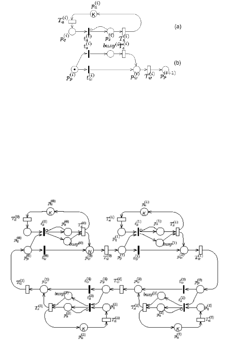
Figure 1.2: GSPN representations of a queue and a server.
the next queue (firing of timed transition T(i)
w). The reason for assigning a higher priority to transition t(i)
sis
to force the fact that a server can bypass a queue only if there is no possibility for it to provide service. Place
busy(i)represents the condition “server busy serving a customer at queue i” and transition T(i)
srepresents the
corresponding ongoing service. Notice that both models in Figure 1.2 include immediate transition t(i)
sand timed
transition T(i)
s; the transitions with common names represent the same events in the two submodels.
The GSPN model of a polling system with four queues can be obtained by composition of four copies the
submodel N(i)
qrepresenting the ith queue and four copies of the submodel N(i)
srepresenting the behaviour of a
Figure 1.3: GSPN representation of a cyclic polling system.
13

server at queue i(i=0,1,2,3). Submodel N(i)
qcan be composed with submodel N(i)
sby merging the transitions
with same label (that is, immediate transition t(i)
sand timed transition T(i)
s). On the other hand, the ring topology is
obtained by superposition of places with the same name belonging to submodels2N(i)
sand N(i+1)
s. The resulting
model is depicted in Figure 1.3. The number of servers is parametric and it is modelled by assigning Ntokens to
place p(0)
win the initial marking. Also the queues capacity Kis parametric and is specified by the initial markings
of places p(i)
a(i=0,1,2,3).
1.5 Stochastic Well Formed Nets
Stochastic Well Formed Nets (SWN) [21] are a coloured extension of SPNs that allows one to build a more
compact and parametric representation of a symmetric system by folding similar subnets. In this way it is possible
to represent very concisely systems that would have required a huge uncoloured net. When similar subnets are
folded, some additional annotation is needed to distinguish tokens that end up being in the same folded place.
These annotations constitute the colour structure of the net.
Tokens are no longer indistinguishable: each token can be regarded as an instance of a data structure whose
meaning depends on the place to which the token belongs. The place colour domain (denoted C(p)) is defined
as the Cartesian product of basic colour classes, possibly with repetitions of the same basic colour class. Each
basic colour class is a finite set of basic objects and it is usually defined by enumeration of its elements (e.g.
C={c1,c2,...cn}). Colour classes may be ordered and may be partitioned into disjoint subsets called static
subclasses.
Transitions’ colour domains (denoted C(t)) are defined analogously to places’ colour domains. Transitions
can be seen as procedures with formal parameters, the parameters being determined by the corresponding domain.
The enabling check of a transition and the state change caused by its firing depend on the arc functions that
label the arcs connecting the transition to input, inhibitor and output places.
Arc functions are formal sums of tuples structured according to the corresponding place colour domain. If
the place colour domain is the Cartesian product of kbasic colour classes, then the corresponding arc function
is a weighted sum of k-tuples. The jth element in each k-tuple is a weighted sum of three basic functions, the
identity function (denoted by a variable), the successor function (“!”), and the synchronisation function (“S”).
The weights of the sum may be numbers or predicates. Predicates are logical expressions used to test either
equality of pairs of basic objects, selected by some identity/successor function, or to check the membership of a
selected basic object in a given static subclass.
A major interest of SWNs is that they provide a modeling framework in which the intrinsic symmetries are
automatically detected and used naturally as a way for reducing the size of the underlying state space. The reduc-
tion is obtained thanks to the original concept of symbolic marking. Informally a symbolic marking corresponds
2The increment i+1 is modulo 4.
14
to an equivalence class representing a set of ordinary markings characterised by a common future behaviour.
These ordinary markings in fact enable the same transitions whose firings lead to new ordinary states which are
still equivalent, i.e. belong to the same symbolic marking. Symbolic markings are obtained by disregarding the
identities of the objects within the places of the net and considering only their number. Colour classes are par-
titioned into dynamic subclasses and the only relevant information is the cardinality of these subclasses (i.e. the
number of objects they contain). This shows how many elements in the net have the same behaviour at the same
time.
This type of partitioning varies from one marking to another, hence it must not be confused with the static
subclass partitioning which is part of the colour class definition.
With the introduction of dynamic subclasses places no longer contain coloured tokens but symbolic tokens
whose components are expressed in terms of dynamic subclasses. All the ordinary markings which can be
obtained by assigning identities to the objects of the dynamic subclasses belong to the same symbolic marking.
Asymbolic enabling rule and a symbolic firing rule, which operate directly on the symbolic marking repre-
sentation, and an efficient algorithm for the generation of an aggregated state space called symbolic reachability
graph (SRG) have been defined [21] and implemented.The SRG describes the evolution of a SWN model through
a set of macro-states, the symbolic markings, that represent sets of more detailed states which are equivalent.
Several properties valid for the SRG have been introduced. For example, the equivalence between the SRG
and the RG from the point of view of the reachability of the markings ensures that no information is lost by
analysing the SRG instead of the RG. Formulae have been defined to compute both the number of ordinary mark-
ings belonging to the same equivalence class and the number of ordinary firings represented by each symbolic
firing.
The SRG corresponds to a lumped version of the complete RG and this aggregation is reflected also at the
level of the underlying Markov process. In [20] it has been proved that the SRG is isomorphic to an aggregated
Markov process that can be used to compute the same performance estimates that can be computed from the
general technique based on the RG, but with a lower computational cost.
1.5.1 A SWN example
Figure 1.4 shows the SWN model of the polling system example that has been obtained by folding all the replicas
of the submodels N(i)
qand N(i)
sforming the GSPN model in Figure 1.3, into a single net structure.
The tokens carry information to distinguish the customers associated with different queues. We thus need
one colour class defined as Q={q1,q2,...,qM}that represents the Mqueues.
In the polling system the ring connection induces a circular order relation among queues, characterised by
the “next queue” relation. Qis thus defined to be an ordered colour class with the possibility of applying the
successor function to any of its element (i.e., !qi=q(i+1)modM).
The initial marking of place pais K· hSiwhere Krepresents the maximum capacity of each queue and
15
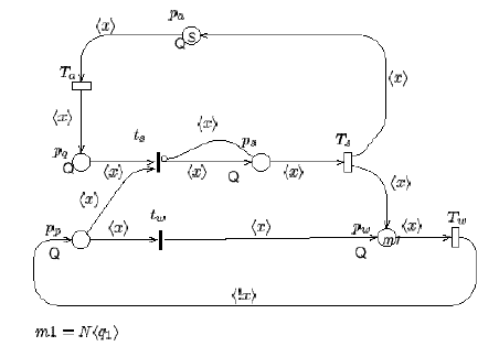
hSiis a special symbol denoting all the coloured tokens belonging to the place colour domain, i.e. K· hSi=
K· hq1i+...+K· hqMi; the initial marking of place pwrepresents the initial position of the Nservers and it is
equal to N· hq1ias we are assuming that all servers are initially polling the first queue of the ring.
The identity function hxilabelling the arcs binds any element qj∈Qto the variable x. For example, transition
Tahas a parameter xof type Qand a coloured transition instance is obtained assigning actual basic objects to this
parameter. The coloured transition instance of Tathat assigns q2to parameter xis enabled in the initial marking.
Its firing removes the coloured token hq2ifrom place paand adds it in place pqthus modeling an arrival to
the second queue. This is due to the fact that the same variable xlabels both the input and output arcs of Ta,
actually denoting the same coloured token. When one of the Nservers polls the second queue (i.e., when place
ppcontains the coloured token hq2i) the service can be provided and the immediate coloured transition instance
of tsbinding the parameter xto q2can fire.
The inhibitor arc connecting tsand psprevents the enabling of transition tsfor any coloured token hqjipresent
in place ps. A server that polls a queue in which another server is working will bypass that queue (i.e., transition
twwill fire) because in the modeled system only one customer can be served in each queue. A server moving to
the next queue is modeled by means of the combined presence of the identity function hxiand successor function
h!xilabelling the input and the output arcs of transition Tw.
Figure 1.4: SWN representation of the cyclic polling system.
The SWN model in Figure 1.4 is parametric in the queue capacities (K), in the number of servers (N) and also
in the number of queues in the system (|Q|). An important feature of this coloured model is that the service policy
may be easily modified; for example it is possible to model a random service policy instead of the cyclic one, by
simply replacing the successor function labelling the output arc of transition Twwith an identity function hyiplus
the predicate [x6=y]to model the movement of a server to a different queue. Observe that such a variation in the
GSPN model would require much more complex structure manipulation.
16
Chapter 2
Getting started
After GreatSPN2.0.2 has been installed and the user environment has been set up according to the directions given
in the Appendix C, the user can start the package and build and analyze his/her models. The aim of this chapter
is to quickly introduce the user to (modeling) using GreatSPN2.0.2 . By following this tutorial, the user will be
able to construct a Petri Net model and to analyze it by means of the GreatSPN2.0.2 graphical interface. The
reader interested in a more in-depth presentation of the various GreatSPN2.0.2 features may refer to Chapter 3.
Throughout this chapter we shall use as an example the model of the well-known multiple-reader-single-writer
problem in the access of a shared data base.
2.1 The Readers–Writers GSPN model
Let us consider a set of “processes” concurrently accessing a shared data base. When a process issues an access
request, it declares whether a read or a write operation is required. Read operations may proceed concurrently
with each other, while write operations require an exclusive access in order to maintain the consistency of the
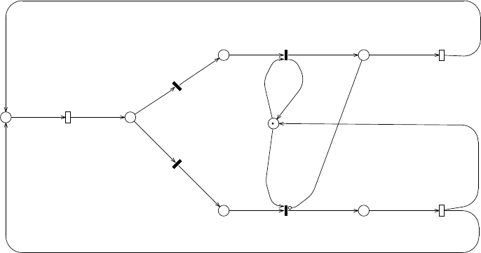
data base. A GSPN model of this system is depicted in Figure 2.1. A token in place think represents a process
performing some local activity. After a random amount of time, a data base access request is issued (timed
transition arrival fires). The type of request (read or write) is randomly chosen with equal probability (immediate
transitions isread and iswrite have the same weight). If the operation is a read, then the access is granted if no
other process is performing a write operation on the data base (place nowrite is marked), otherwise the process
waits in place Rqueue until the access can be performed safely. The beginning of a read operation is represented
by the firing of transition StartR, that has two effects. First, place nowrite is marked, meaning that other readers
can access the data base. Second, place reading is marked, forbidding therefore the access to any writer process
(there is an inhibitor arc from place reading to transition StartW). After the firing of the timed transition EndR,
the status of the process is reset to “thinking”.
Conversely, if the requested operation is a write, the process waits (in place Wqueue) until access can be
granted, i.e. when no other process is performing a write access (place nowrite is marked) and no other process
17
P= 5
think
P
writing
reading
Wqueue
Rqueue
choice
nowrite
isw=0.200000
isr=0.800000
wr=0.500000
rr=2.000000
arr=1.000000
arrival
EndW
EndR
StartW
iswrite
isread
StartR
Equeue
Figure 2.1: The Readers–Writers GSPN model
is performing a read access (place reading is empty). At the completion of the write operation, modeled by the
firing of transition EndW, the absence of write access is signaled to other processes by marking place nowrite,
and the status of the process is reset to “thinking”.
2.2 Starting GreatSPN
GreatSPN2.0.2 is started by typing greatspn on the command line and pressing <Return>. After a few seconds
the Control Panel, depicted in Fig. 2.2, pops up and the user can start a work session.
WARNING! When GreatSPN2.0.2 GUI is launched for the first time a window is displayed before the Control
Panel pops-up in which it is asked to the user to fill in the corresponding areas if he/she desires to change the
default setting for some environment variables (see chapt. 3for a more detailed description of this window). The
user has to press the “OK” button to confirm either the modification made in the window areas or the default
settings: the information contained in this window are saved into the $HOME/.greatspn file.
To create a new model, the user has just to start creating places and transitions (as discussed in Section 2.3),
while if the user desires to modify an already created model, he/she can retrieve it by using the File menu.
2.3 Creating the Readers–Writers model
To create (or to modify) a model, the user selects the action to be performed and the object type (e.g. places,
immediate transitions, place markings, etc.) on which the action will be applied. The general principle of
18
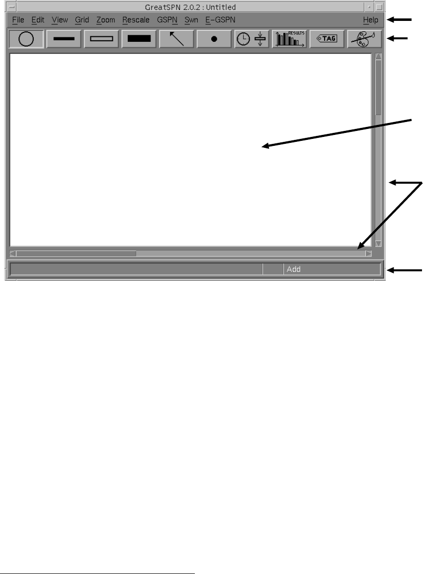
Menu bar
Object bar
Canvas
Status bar
Scrollbars
Figure 2.2: The GreatSPN2.0.2 Control Panel
behavior of the GreatSPN2.0.2 graphical interface is that the action selected by the user from the Action menu
(shown in Fig. 2.3) becomes the default action until a new one is chosen, and such action affects only objects
of the type currently selected. The current action is displayed in the status bar on the right. The Action pop-up
menu is activated by pressing the right mouse button on any position of the GreatSPN2.0.2 working area. To
select an action, the user has to click with the left mouse button over the desired pull-down option1. An object
type is selected by moving the mouse cursor on one of the icons of the objects bar (see Figure 2.2) and by clicking
over it with the left mouse button. The object currently selected remains highlighted until another object type is
chosen. The mouse help window, activated by selecting Help→Mouse Help, displays the action associated with
each mouse button. Let us start the creation of the Readers–Writers GSPN model by creating the set of places
first. To create places, we set the type of object to “place” by selecting the place icon in the object bar (indicated
by a circle), and after this operation the shape of the mouse cursor is changed into a circle. After the selection of
the Action→Add option, we can move the mouse cursor within the working area and start laying down the places
of the net by clicking the left mouse button in the proper position, in order to obtain the screen image shown in
Figure 2.4. The GreatSPN2.0.2 graphical interface displays only a window on the real working area, that can be
1In the rest of this manual we shall use the notation Menu Item→Option to denote an option in a specific menu item of the menu
bar. For example, Action→Create denotes the Create option of the Action menu.
19
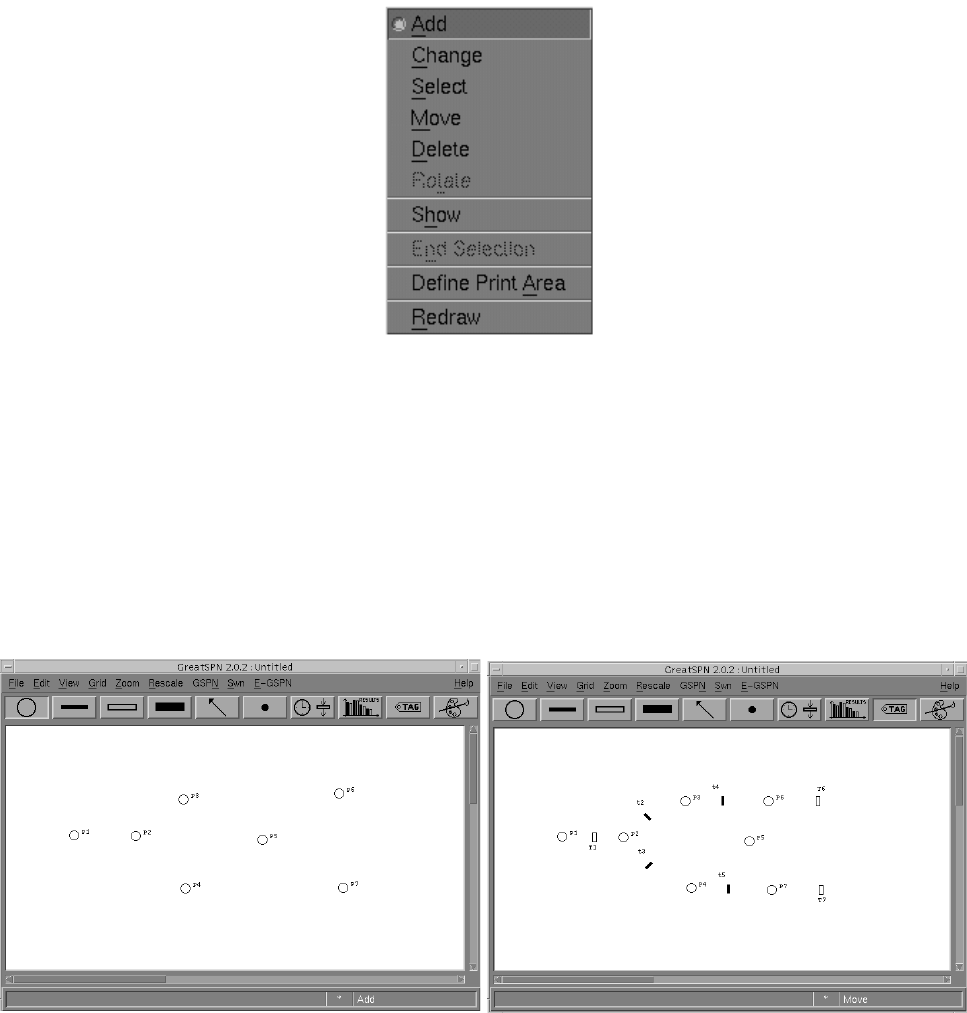
Figure 2.3: The GreatSPN2.0.2 action menu
scrolled in all the directions by using the scrollbars placed on the right and bottom sides of the Control Panel.
To create the transitions we proceed as for places, that is by first choosing one of the three transition icons
available, i.e. deterministic (represented by a thick black box), exponential (represented by a white box), and
immediate (represented by a thin black box), and then by creating them. Note that we don’t need to select the
Action→Add action again, since we didn’t change the selection done when places were created. The screen
situation after the addition of transitions looks like Figure 2.5. Note that we have created transitions having
Figure 2.4: Place layout of the Readers–Writers model
of Fig. 2.1
Figure 2.5: Place and transition layout of the Readers–
Writers model
different orientations. To change the orientation of a transition, we can use the middle mouse button (each time
this button is clicked, the transition rotates of 45 degrees clockwise) before clicking the left button to actually
create the transition itself.
20
After a place or a transition has been placed on the working area, it can be moved by selecting the Action→Move
option. An object can be dragged on the canvas by clicking on it with the left mouse button, by moving the cursor
on its new position and by clicking the left button again.
The editor assigns default names (“tags”) to places (Px) and transitions (Tx for timed and tx for immediate)
where xis an integer representing the objects creation order. Such tags are displayed if the View→Tag option
has been selected. Tags overlapping other objects of the net can be moved around in the same way as places or
transitions, that is by selecting the Action→Move option after clicking on the tag icon, and by clicking on the
place or transition to which the tag is associated.
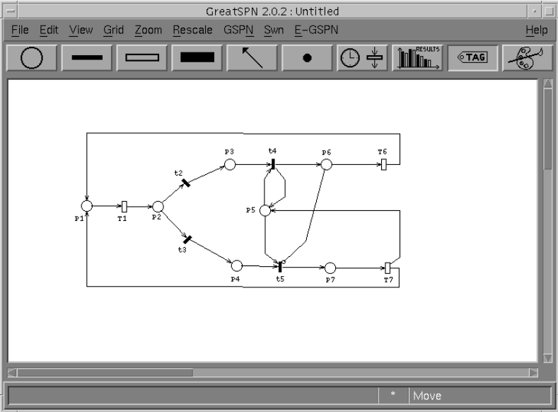
Now that we have created the nodes of our Petri net, we are ready to connect them with arcs. This can be
accomplished by choosing the arc icon in the object bar (indicated by an upward arrow). Again, if we didn’t
redefine the default action, we don’t need to re-select the Action→Add option. To create an input arc from place
P1 to transition T1 (see Figure 2.6), we have to click the leftmost button of the mouse twice: first over place P1,
and then over transition T1. The output arc connecting transition T1 to place P2 can be created by clicking the
left mouse button first over T1, and then over P2. The inhibitor arc connecting place P6 to transition t5 is created
Figure 2.6: Creating arcs
by first clicking over P6 with the middle mouse button, and then over t5 with the left button. In the case of the
output arc connecting transition T7 to place P1, for aesthetical reasons we want to put two intermediate points
21
between the place and the transition, rather then connecting them with a straight line. Intermediate points are
added by just clicking the left mouse button over the desired position, provided that it is not too close to a node
of the net.
In Petri nets it is forbidden to draw arcs connecting either places to places or transitions to transitions. Great-
SPN2.0.2 enforces this rule by forbidding the creation of such arcs. Note that once one has started the drawing
of an arc, there is no way to interrupt the action, so if we realize that we started to draw an arc that we shouldn’t,
the only way to get out is to complete the arc and to delete it afterwards. To delete an arc (or, more generally, an
instance of the currently–selected object), we have to click over the object we want to delete after the selection
of the Action→Delete option.
Now the topology of the network is complete, and we may proceed defining the initial marking. Place
marking can defined either directly, by associating an integer number of tokens with the place, or by means of a
rate parameter which has been previously defined. In either case, the association of an initial marking with a place
is performed by clicking with the left mouse button over the place we want to consider after the Action→Change
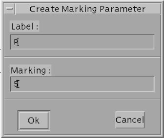
option and the place icon have been selected. To create a marking parameter the user has to click over the token
icon (graphically represented as a black dot) and to select the Action→Add option. After that, the user has to
move the cursor in an empty canvas region and click the left mouse button. A dialog box (see Fig. 2.7 will pop-
up, and will ask us to enter the name of a marking parameter (in our case the name is ”P”) and the corresponding
numerical value (a positive integer).
Figure 2.7: Dialog box for the creation of marking parameters
After clicking on the button “Ok” of the above dialog box, the definition of the marking parameter (“P=5”)
will appear on the chosen canvas position. Starting from this moment, the name “P” can be used as initial
marking specification for any place in the net. In our example, two places hold a non-null initial marking, and
we can define that by clicking the left mouse button on each of them. The Change Place Properties window (see
Fig.2.8) will pop up, so that the place marking can be changed by specifing the initial value in the “Marking:”
area.
22
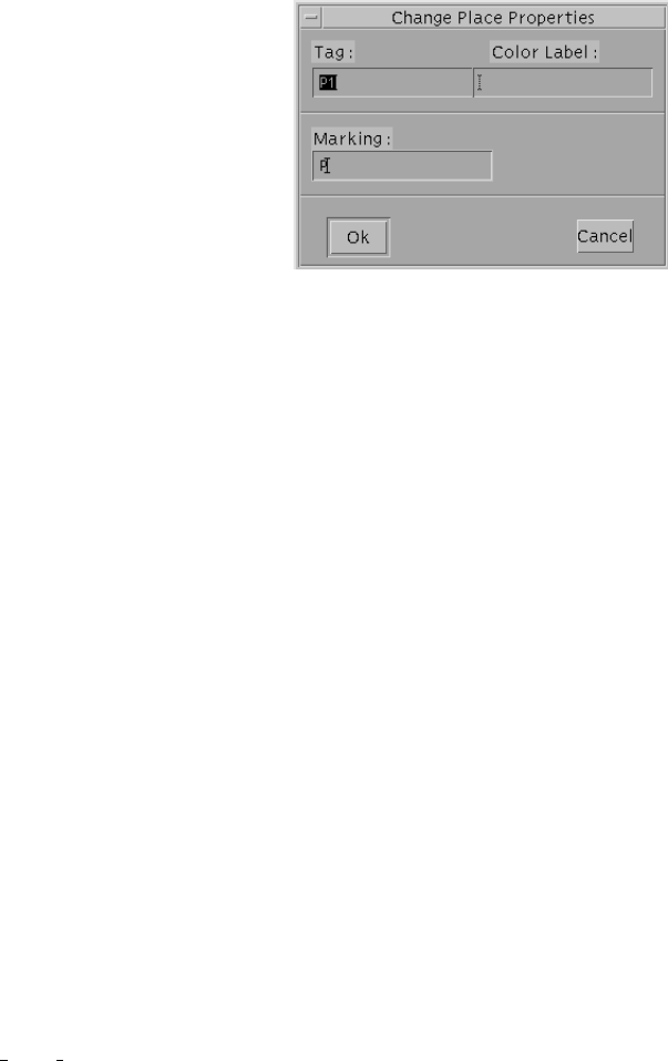
Figure 2.8: Dialog box for changing place properties.
Alternatively, the same action can be performed by selecting the token icon. The initial marking of a place can
be specified either as a nonnegative integer value or by using the name of an already-defined marking parameter.
As the network specification is complete, we may display a “nicer” version with rounded arcs by selecting
the View→Spline option. This produces a net looking like the one depicted in Fig. 2.9.
So far we have retained the default names given by the editor at the moment of the object creation. Although
this is useful to speed up the editing procedure, it may yield to a poor model readability, that can be improved
by giving meaningful names to places and transitions. Tags can be modified by selecting the “tag” object, by
choosing the Action→Change option and by pointing and clicking the left mouse button on the corresponding
place or transition. A dialog box will pop up and will ask the user to specify the new object tag.
2.4 Saving and printing the model
After the model definition has been completed, we can save its description and/or print it using several different
formats, by means of the File menu. A model is saved by selecting the File→Save option. If the model had
been previously saved, this operation will cause the old description to be overwritten. If one wants to keep
the old description, he/she can use the File→Save As option of the above menu to specify a new name for
the net. The net description files are saved in the user directory defined by setting the environment variable
GSPN NET DIRECTORY (as specified in the $HOME/.greatspn file of the user: see the Appendix C for details).
GreatSPN2.0.2 provides the possibility of specify comments, which are saved with the net description and which
can be subsequently re-edited. To add a comment, simply select File→Comment option, and use the Edit Net
Comment dialog box which pops-up. To create printouts of a model, or Encapsulated PostScript (EPS) files
suitable for inclusion in L
A
T
EXdocuments, we have to select the File→Print option. This option affects only that
portion of the model that is included in the currently-defined print area, that is displayed as surrounded by a
dotted line if the View→Print Area option is selected (see Fig. 2.9). To define the print area, we have to:
1. select the Action→Define Print Area option (the cursor shape will be changed into a cross);
23
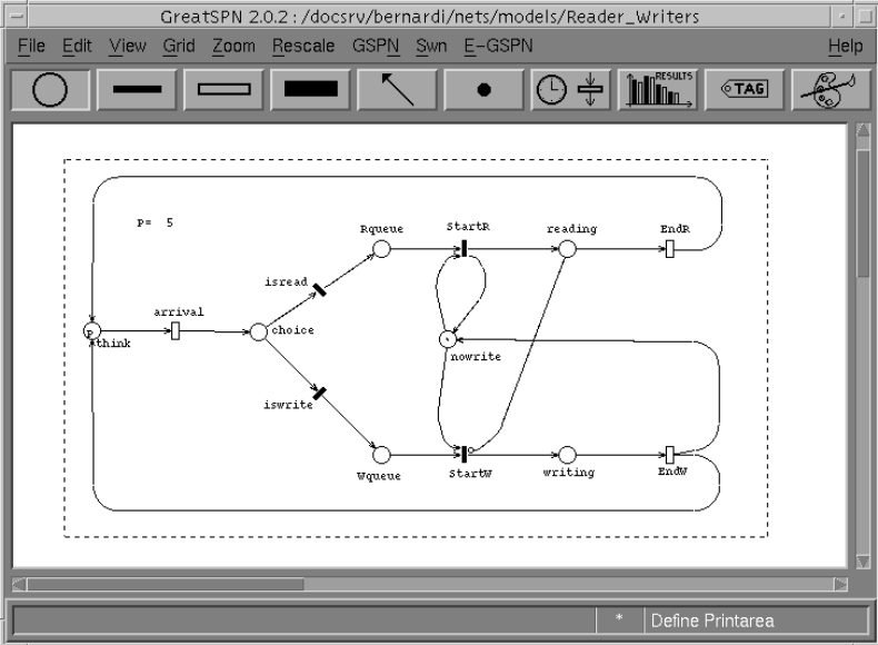
Figure 2.9: Print area used for the Readers-Writers model
2. click with the left mouse button over the canvas point corresponding to the upper-left corner of the print
area;
3. move the mouse cursor on the lower-right corner of the desired print area and click either the left or the
middle mouse button.
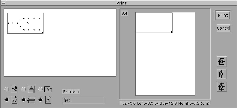
After the above operations have been completed, the File→Print command must be selected to cause the Print
dialog box (shown in Fig. 2.10) to pop up. In the window contained in the leftmost part of the Print dialog box,
GreatSPN2.0.2 shows an overview of the entire working area (remember that only a window on a portion of the
working area is shown in the Control Panel). The print area is surrounded by a thin black frame, that can be
adjusted (allowing the redefinition of the print area) by positioning the mouse cursor over the lower-right corner
(indicated by a small black square) and dragging it by clicking with the left mouse button without releasing the
mouse button.
The six icons displayed just below the above window allow us to set:
•the format of the output , that can be chosen between raw PostScript (by clicking on the PS icon) and
Encapsulated PostScript (by clicking on the TeX icon);
24
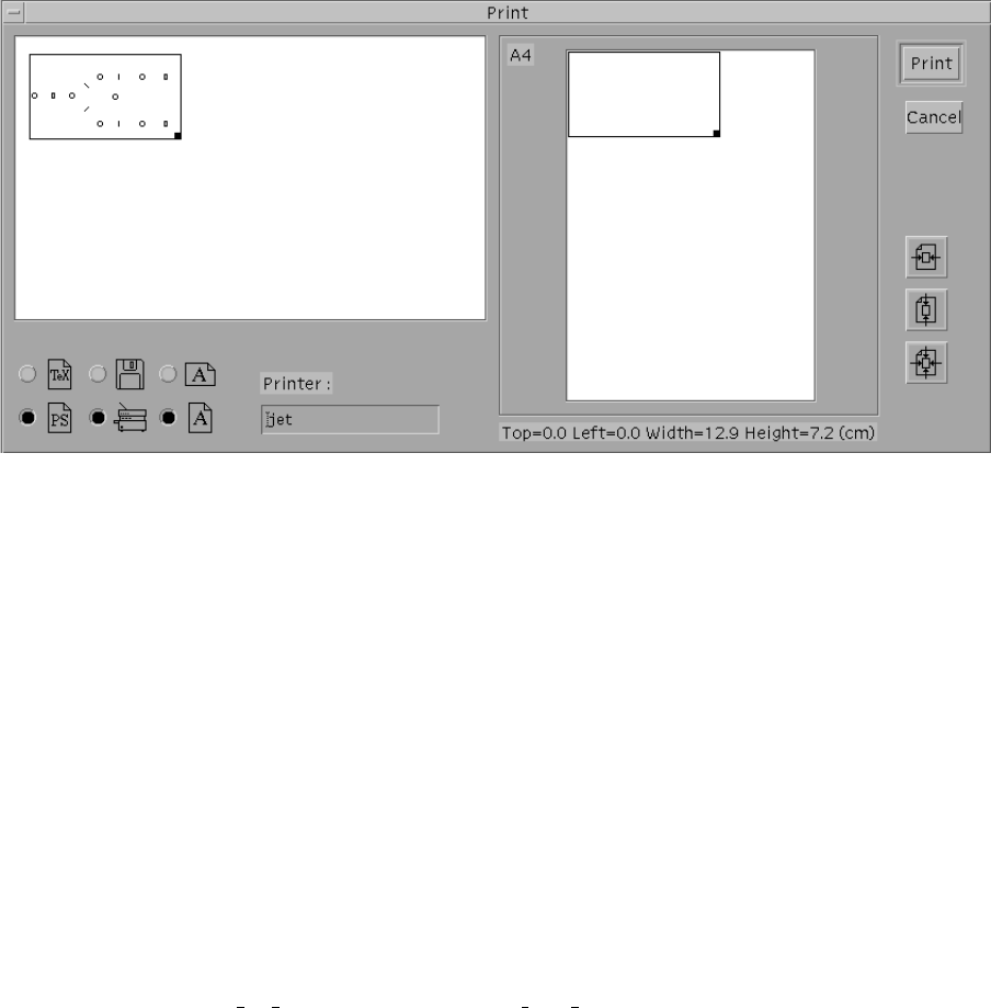
Figure 2.10: GreatSPN2.0.2 Print dialog box
•the destination of the output, that can be either a file (Diskette icon) or a PostScript printer (Printer icon):
if the EPS format is chosen then only a printout on a file is allowed;
•the orientation of the output, that can be either portrait or landscape (the two Aicons).
The right part of the Print dialog box contains a window that shows the page layout (an a A4 size sheet is
assumed). The placement of the print area over the sheet can be changed either by dragging the thin black
rectangle or by clicking over one of the three icons placed at the right of the window (that allow centering the
picture on either dimension). Finally, the printout with the desired options is performed by clicking with the
left mouse button on the “Print” button. If we decided to save the printout on a file, GreatSPN2.0.2 will ask the
user (by means of a suitable dialog box) to enter a file name that will be placed either in the default PostScript
(PS) or Encapsulated Postscript (EPS) directory. The default PS and EPS directories can be set by means of the
environment variables GSPN PS DIRECTORY and GSPN EPS DIRECTORY in the $HOME/.greatspn file (see
Appendix C).
2.5 Analysis of the Readers-Writers model
Once we have defined both the net structure and the initial marking of the Readers–Writers model we can have
a first understanding of its dynamic behavior by playing the “token game”. GreatSPN2.0.2 provides the user
of an interactive token game that can be started by selecting the GSPN→Simulation... option. The Simulation
window pops up and all the transitions of the model that are enabled in the initial marking become blinking (see
Fig. 2.11). To simulate a possible behavior of the modeled system we have simply to click with the leftmost
25
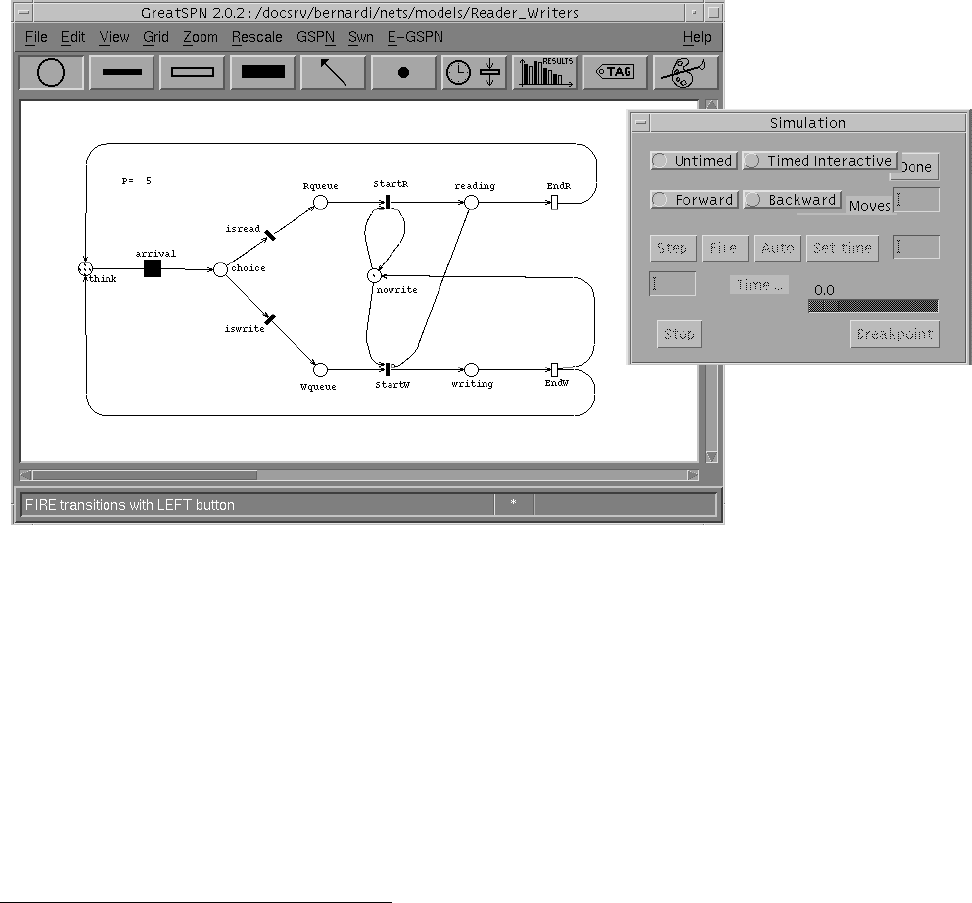
button of the mouse over the enabled (i.e. blinking) transition we want it to fire. In our running example, only
transition arrival is enabled in the initial marking; by clicking on it, the firing action is executed, i.e. a token is
removed from the input place think and a token is added to the output place choice. The new reached marking
enables the two immediate transitions isread, iswrite: we can choose to fire one of them and to simulate the
corresponding firing action (and so on). By default the “Untimed” and the “Forward” options of the Simulation
window are set to play the forward token game: it is possible to play the backward token game by setting the
“Backward” option in the Simulation dialog box.
Figure 2.11: Token game of the Readers–Writers model.
GreatSPN2.0.2 provides the user with a set of structural analysis algorithms that can be used to validate the
models. The user can access the above algorithms by selecting the GSPN→Struct option.2For example, the com-
putation of minimal-support, canonical Place Invariants (by means of a modified Martinez–Silva algorithm [29])
can be accomplished by means of the option GSPN→Struct→P invariants.GreatSPN2.0.2 will visualize the
Console window (shown in Fig. 2.12), allowing one to start the P–invariant computation by clicking with the left
mouse button over the “Start” button. At the end of the above computation, the Console window will contain the
results, as displayed in Fig. 2.13.
After a GSPN model has been constructed and validated, it can be analyzed by means of the different perfor-
2WARNING! Before launching a GreatSPN2.0.2 solver be sure that the hostname set in the “Hostname:” left area of the
File→Options window is the name of the machine on which the Control Panel has been started.
26
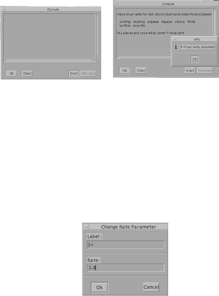
Figure 2.12: GreatSPN2.0.2 Console Figure 2.13: Results of P–invariant computation
for the Readers–Writers model
mance evaluation techniques provided by GreatSPN2.0.2 . Before starting the performance analysis of a given
GSPN model, its performance–related parameters must be defined. The default rates associated with transitions
can be displayed on the screen by selecting the View→Rate option. Rates overlapping some other object of the
net can be moved around in the same way as tags, by selecting the Action→Move action after the icon corre-
sponding to rates (indicated by a clock close to a timed transition) has been selected. Transition rates may be
defined as positive real numbers, name of rate parameters, or marking–dependent expressions, governed by a
context–free grammar (described in Appendix A). In this example we will only use rate parameter specifications,
that are created much in the same way as marking parameter, by choosing the Action→Add action together with
the rate icon. A dialog box (see Fig. 2.14) will pop up, allowing us to specify the name and the definition of
rate parameters. We will define three rate parameters for transition rates: arr = 1.0,rr = 2.0, and wr = 0.5;
and two rate parameters for choice probabilities between conflicting immediate transitions: isr = 0.8, and isw =
0.2. After their definition, the above parameters can be used to specify the transition rates (weights) by choosing
Figure 2.14: Dialog box for the creation of rate parameters
27
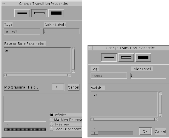
the Action→Change action with the exponential (immediate) transition type selected, by clicking with the left
mouse button over the appropriate transitions and by filling the Rate or Rate Parameter (Weight) field of the
corresponding Change Transition Properties window (see Fig.2.15).
(A) (B)
Figure 2.15: Windows for defining/changing properties of timed (A) and immediate (B) transitions.
The same window, depicted in Fig.2.15(A), allows the specification of the enabling dependence. The default
enabling dependence for timed transition is of the “infinite server” type, but it can be changed by choosing the ap-
propriate option (Infinite, Marking Dependent, 1-Server, and Load Dependent). In our example, only the arrival
and the endR transitions are of the “infinite server” type, so the enabling dependence of all the other ones must
be changed to 1-Server. To change the priorities of immediate transitions, use the scrollbar on the bottom-left
of the Change Transition Properties window (Fig.2.15(B)) of the corresponding transitions to increase/decrease
their priorities.
With the specification of transition rates and probabilities as shown in Fig. 2.16, we have completed the spec-
ification of the behavior of the model. GreatSPN2.0.2 provides three different performance analysis methods,
namely computation of bounds for the throughput of transitions, Markovian solution and simulation. In this chap-
ter we present an example of the Markovian solution of the Readers–Writers GSPN model, while the other tech-
niques will be covered in Chapter 4. The Steady–State solution of the Embedded Markov Chain corresponding to
the GSPN model of the Readers–Writers system of Fig. 2.16 is obtained by selecting the GSPN→Solve→GSPN
Solution→Steady State option. The Console window will pop-up again, and after we click with the left button
on the “Start” button, GreatSPN2.0.2 will start the analysis phase. At the end of the analysis, GreatSPN2.0.2
28
P= 5
writing
reading
Wqueue
Rqueue
choice
think
P
nowrite
arr=1.000000
rr=2.000000
wr=0.500000
isr=0.800000
isw=0.200000
EndW
wr
EndR
inf-server
rr
arrival
inf-server
arr
StartW
1.000000
iswrite
isw
isread
isr
StartR
1.000000
Figure 2.16: The Readers–Writers model with transition rate/probability specification
will show on the screen the values of the throughput of the various timed and immediate transitions, as well
as the values of the defined performance indices (see Figure 2.17). We can visualize the distributions of token
into places by selecting the Action→Show action together with the result icon, and by clicking on the place of
interest. In Fig. 2.18 it is shown the token distribution for place Wqueue.
2.6 Colored version of the Readers-Writers model
Let us suppose that the processes which are concurrently accessing to the shared data base have different be-
haviors; in particular, a group of them access to the data base only to perform a write operation, while another
group can issue either a writing or a reading request. In this section we describe how to obtain the colored Great-
SPN2.0.2 version of readers-writers model (see Fig.2.19) that captures the different behavior of the two kinds of
processes. Starting from the previous non-colored model of the readers-writers system we first need to define the
basic color classes representing the two kinds of processes. To create (or to modify) a basic color class definition
simply click with the left mouse button on the color icon (indicated by a palette and a paintbrush) of the object
bar and pop-up the Action menu, using the right mouse button, in order to select the “Add” option as the current
action. After these operations, choose a place in the canvas to locate the definition of the class and click with
the left mouse button: the Create Color Definition window pops-up (see Fig.2.20). The top left area named as
“Label:” has to be filled with the name of the color class. The “Colorset” toggle, by default, is already switched
on (a black dot is displayed in the circle near the toggle), indicating that the current definition is a definition of a
29
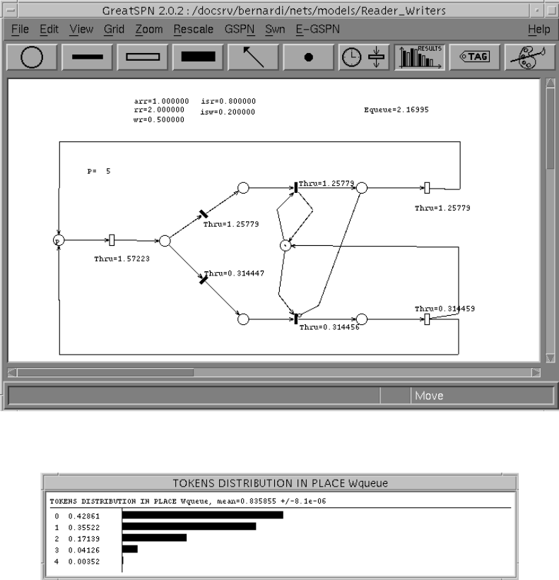
Figure 2.17: GreatSPN2.0.2 canvas after the Readers–Writers GSPN model has been solved
Figure 2.18: Token distribution in place Wqueue
basic color class. In the “Definition:” area, the definition of the basic color class is written using the SWN syntax
(see Appendix A): in the example the class Pis the unordered union of two static subclasses P1 and P2. These
two colored subclasses have to be defined as well, following the same procedure described above for the color
class definition, i.e., by recalling and filling the areas of the Create Color Definition window for each of them
(see Fig.2.21). In our example, we have used two different alternatives of the SWN syntax to express the subsets
of colors P1 and P2: the color subclass P1 is defined as the set of two elements p1, p2 while the color subclass
P2 is a set of three elements c1, c2, c3. Once the basic color classes has been defined, we proceed as follows:
•add color domains to places that may contain colored tokens. To modify place attributes, click on the place
icon and select from the Action menu the Change option; place color domain Phas to be written on the
30
think
PM0
writing
P
reading
P
Wqueue
P
Rqueue
P
choice
Pnowrite
arr=1.000000
rr=2.000000
wr=0.500000
isr=0.800000
isw=0.200000
arrival
EndW
EndR
iswrite
[d(x)=P2]
StartW
isread
StartR
<x>
<x>
<x>
<x> <S>
<x>
<x>
<x>
<x>
<x> <x>
<x>
<x>
<x><x>
Equeue
P2:c
M0:m
P1:c
P:c
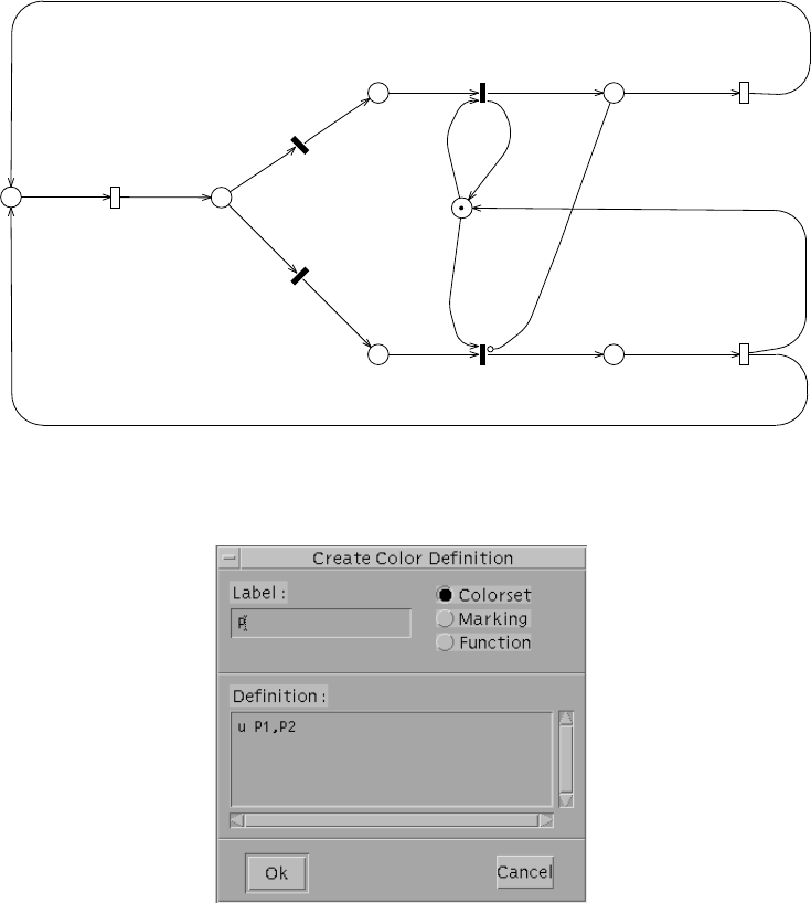
Figure 2.19: SWN model of the Readers-Writers system.
Figure 2.20: Create Color Definition window.
“Color label:” area of the Change Place Properties window (see Fig.2.8). In the model of Fig.2.19, all the
places have color domains, except for place nowrite;
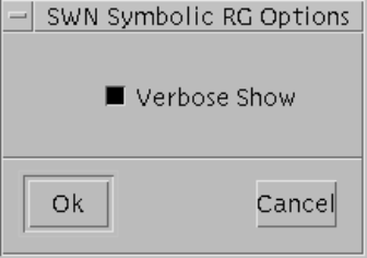
•add color attributes to the corresponding input/output arcs. To modify arc attributes, press the arc icon
(we don’t need to select again the Action→Change option since it is the current action), and click on the
interested arc with the left mouse button; the Change Arc Properties window of Fig.2.22 pops-up. Press the
“Color” toggle to set the right area into “Color” mode and then add in the area the color function according
to the SWN syntax. In the model of Fig.2.19, all the arcs are characterized by the identity function hxi,
except for the input/output arcs of the non colored place and for the inhibitor arc connecting place reading
31
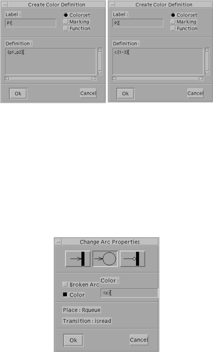
Figure 2.21: Definition of static subclasses.
to the transition StartW that is labeled with the whole place color domain function hSi;
•add a guard to the transition iswrite. A way to model the constraint that only the processes belonging
to the static subclass P2 are allowed to issue a writing request to the data base is to add a guard to the
transition iswrite. To modify transition attributes, press one of the transition icons and select the interested
transition: one of the Change Transition Properties windows of Fig.2.15 pops-up, depending on the type of
transition, allowing to fill in the “Color Label:” area the guard according to the SWN syntax. In the model
of Fig.2.19, transition iswrite can fire only when its input place contains a colored token hxibelonging to
the static subclass P2.
Figure 2.22: Change Arc Properties window.
32
Finally, we define the colored marking parameter M0 of the SWN model of Fig.2.19 by pressing the color
icon of the object bar and by selecting the Action→Add option. The Change Color Definition window pops up
again by clicking with the left mouse button on a location in the canvas. To define a colored marking parameter
switch on the “Marking” toggle and then fill in the “Label:” and the “Definition:” areas with the name of the
parameter (M0) and its definition (hS P1i+hS P2i) respectively. The initial marking of the SWN model of
Fig.2.19, is then set by adding to the “Marking:” area of the Change Place Properties window related to the
place think the colored marking parameter M0.
2.7 Analysis of the SWN Readers-Writers model
Concerning the analysis of SWN models, GreatSPN2.0.2 supports the reachability graph generation (both or-
dinary and symbolic) with the corresponding Markovian solution, both in steady state and transient, and the
simulation: in this section we will describe how to obtain the symbolic reachability graph (SRG) of the Readers-
Writers model of Fig.2.19 and its corresponding Markovian solution, for a depth description of the different
analysis techniques see Chapt.4.
Once the SWN model has been saved, we can compute the symbolic reachability graph by choosing from
the Swn→Symbolic sub-menu the Compute RG option. In case last modifications of the current loaded model
have not been saved before launching a GreatSPN2.0.2 solver a warning window will pop-up asking to the user
for saving or aborting the request. The request of computing the symbolic reachability graph of the SWN model
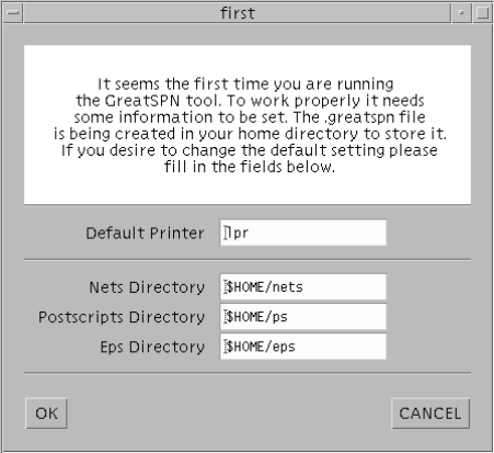
will cause the Console window of Fig.2.12 to pop-up; it is then possible to obtain a verbose description of the
symbolic reachability graph by setting on the “Verbose Show” toggle of the SWN Symbolic RG Options window
(see Fig.2.23) which appears after the “Start” button of the Console window has been pressed.
Figure 2.23: SWN Symbolic RG Options window.
Finally, choose “OK” button of the SWN Symbolic RG Options window to launch the GreatSPN2.0.2 solver.
The execution is displayed on the Console window and the results are visualized in the GreatSPN2.0.2 canvas: the
SWN model of Fig.2.19 is characterized by 45 Tangible Symbolic Markings (which correpond to 209 Tangible
Ordinary markings) and no deadlocks are found. Results are saved in different files: the symbolic reachability
33
graph is saved in file netname.srgP5, transition throughputs and performance indices defined by the user are
contained instead in netname.sta file.
34
Chapter 3
GUI in depth
This chapter is a reference guide containing a detailed description of the various options provided by the Control
Panel (CP). The CP is a unified graphical interface used for model specification and analysis. It is based on the
X-windows systems and exploits the Motif libraries. The CP provides a graphical editor for Petri Net models
(both colored and uncolored), as well as a set of pull-down menus providing access to the solver modules of the
package.
Figure 3.1: The initial window that appears when the tool is invoked for the first time after the installation.
Starting GreatSPN2.0.2 After the GreatSPN2.0.2 package has been installed correctly (see Appendix C), to
invoke the CP, type greatspn followed by a carriage return. When GreatSPN2.0.2 GUI is launched for the first
time after the installation a previous window (Fig.3.1) pops-up in which it is asked to the user either to confirm
or to change the default settings of the following GreatSPN2.0.2 environment variables:
35
•GSPN DEFAULT PRINTER, containing the name of the default printer;
•GSPN NET DIRECTORY, containing the path directory of the net description files;
•GSPN PS DIRECTORY, containing the path directory of the printout of the nets in raw PostScript format;
•GSPN EPS DIRECTORY, containing the path directory of the printout of the nets in EncapsulatedPostcript
format.
If the “OK” button is chosen then the settings are saved into the $HOME/.greatspn file and the CP window
(Fig.3.2) appears on the user’s terminal.
Menu bar
Object bar
Canvas
Status bar
Scrollbars
Figure 3.2: The GreatSPN2.0.2 Control Panel
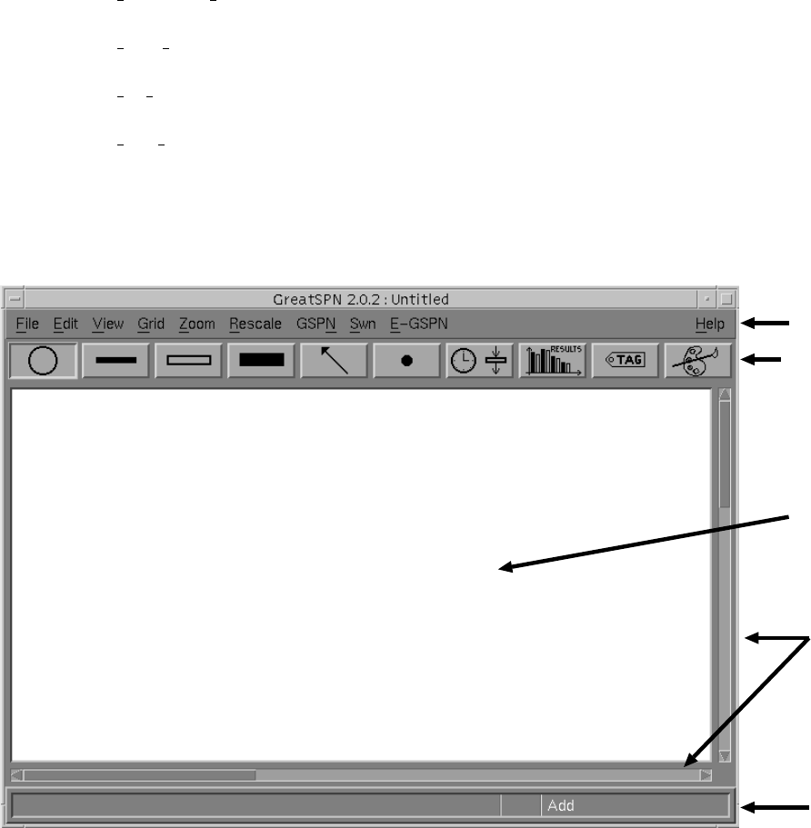
Control Panel Description As seen from Fig.3.2, the top portion of the window contains 10 menu items, each
of them has a pull-down menu that provides several options. The menu items and their options allow to specify
and solve the current loaded Petri net model. The object bar is just below the menu bar and it contains 10 icons
which allow to perform operations, such as add/delete/change etc., on a specific object of the model. Petri net
models are displayed in the canvas. The CP window shows only a part of the whole canvas and scrollbars,
36

located on the right and on the bottom of the CP, allow to show different parts of it. Finally, on the bottom part
of the CP there is the status bar, in which appropriate status messages and/or error messages are displayed.
3.1 The Menu Bar
To access the menus, position the cursor (which appears as an arrow) on the desired menu item. Press the left
mouse button and hold it down (which highlights the particular option chosen) to walk through the menu options.
Click (i.e., release the left mouse button) on a particular option to select it.
In the following we list and describe the possible options offered by each menu item. The notation Menu
Item→Option is used to denote an option within a specific menu item.
3.1.1 File Menu
The File menu contains the following options:
File→New to edit a new model. The previous loaded one is discarded: if its last modifications performed have
not been saved, GreatSPN2.0.2 prompts the user with a message asking if a save action is desired before editing
a new model.
File→Open to load a previously-saved model. A window pops up (Fig.3.3) allowing to navigate within direc-
tories selected by the filter and to choose the model to be loaded. By default, the filter is set on the user directory
defined by the environment variable GSPN NET DIRECTORY.
File→Merge to merge a Petri Net model previously defined to the current loaded model. This option is not
available in the current version of GreatSPN. Merging of two GreatSPN2.0.2 models can be performed using the
Composition module, described in detail in chapt.5.
File→Save to save the current model using the corresponding name. If the model is new, GreatSPN2.0.2 will
ask the user to provide a name.
File→Save As... either to save the current model with a name, if the model is new, or to save it under a different
name (i.e., to make a copy of it).
File→Remove Results to remove all the result files created during the analysis of the current loaded model.
File→Remove All to remove all the files related to the current loaded model, included the net definition files.
37
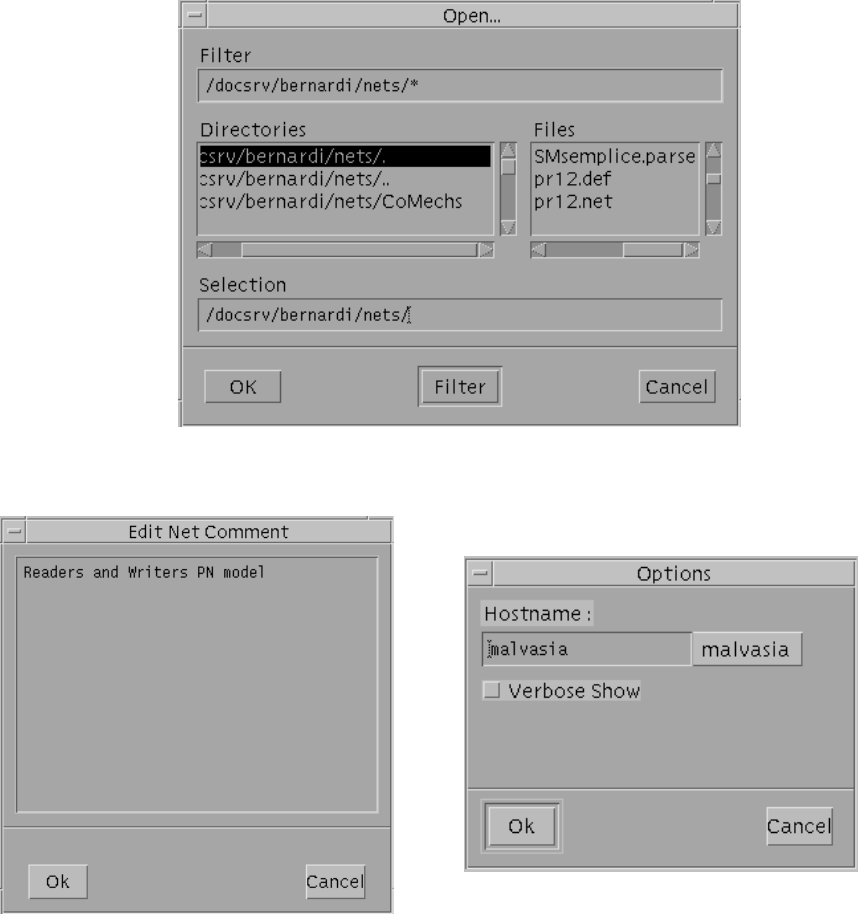
Figure 3.3: GreatSPN2.0.2 Open dialog box.
Figure 3.4: Comment editor display
Figure 3.5: Options display
File→Comment... to specify a comment which is saved as part of the net description. The window of Fig. 3.4
pops up, allowing to edit the comment. To save the edited comment click with the left mouse button on the “OK”
button. To abort the action, click on the “Cancel” button.
File→Options... to specify the machine on which the solution programs will be executed. The Option win-
dow of Fig. 3.5 pops up; the “Hostname:” right button is labeled with the name of the machine on which
GreatSPN2.0.2 has been started, while in the “Hostname:” left box appears the name of the machine on which
38
GreatSPN2.0.2 has been launched the last time.
WARNING! The “Hostname” left box has to be updated with the name of the machine on which GreatSPN2.0.2
has been launched in order to ensure that GreatSPN2.0.2 solvers work properly: therefore simply press on the
“Hostname:” button, then the name written on the button will be automatically copied into the “Hostname:” left
box.
The “Verbose Show” option allows the user to require a verbose output during the execution of the analysis
programs.
File→Print... to print the current loaded model. This option affects only that portion of the current loaded
model that is included in the currently-defined print area, that is displayed as surrounded by a dotted line if the
View→Print Area option is selected. To define the print area, we have to:
1. activate the Action menu (Fig.3.7) by pressing the right mouse button on any position of the canvas and
select the Action→Define Print Area option (the cursor shape will be changed into a cross);
2. click with the left mouse button over the canvas point corresponding to the upper-left corner of the print
area;
3. move the mouse cursor on the lower-right corner of the desired print area and click either the left or the
middle mouse button.
The File→Print... option causes the Print dialog box (shown in Fig. 3.6) to pop up. In the window contained in
Figure 3.6: GreatSPN2.0.2 Print dialog box
the leftmost part of the Print dialog box, GreatSPN2.0.2 shows an overview of the entire working area (remember
that only a window on a portion of the working area is shown in the CP). The print area is surrounded by a thin
39

black frame, that can be adjusted (allowing the redefinition of the print area) by positioning the mouse cursor
over the lower-right corner (indicated by a small black square) and dragging it by clicking with the left mouse
button without releasing the mouse button. The six icons displayed just below the above window allow us to set:
•the format of the output, that can be chosen between raw PostScript (by clicking on the “PS” icon) and
Encapsulated PostScript (by clicking on the “TeX” icon);
•the destination of the output, that can be either a file (“Diskette” icon) or a PostScript printer (“Printer”
icon): if the EPS format is chosen then only a printout on a file is allowed;
•the orientation of the output, that can be either portrait or landscape (the two “A” icons).
The right part of the Print dialog box contains a window that shows the page layout (an A4 size sheet is assumed).
The placement of the print area over the sheet can be changed either by dragging the thin black rectangle or by
clicking over one of the three icons placed at the right of the window (that allow centering the picture on either
dimension). Finally, the printout with the desired options is performed by clicking with the left mouse button on
the “Print” button. If we decided to save the printout on a file, GreatSPN2.0.2 will ask the user (by means of a
suitable dialog box) to enter a file name that will be placed either in the default PostScript (PS) or Encapsulated
Postscript (EPS) directory. The default PS and EPS directories are the ones specified by the environment variables
GSPN PS DIRECTORY and GSPN EPS DIRECTORY, respectively, which are located in the $HOME/.greatspn
file.
File→Exit to terminate GreatSPN2.0.2 session. If the current loaded model has not been saved since its last
modification, GreatSPN2.0.2 will prompt a message asking the user if he/she wishes to save it.
3.1.2 Edit Menu
The Edit menu allows to graphically edit portions of the model; some of the options of the Edit menu are available
only if a portion of the model has been selected. The model portion affected by the Edit options can be selected
in the following way. First, activate the Action menu (Fig.3.7) and choose the Action→Select option. Then,
position the mouse pointer on the upper left corner of the desired area, click and hold down the middle mouse
button, move the mouse pointer on the lower right corner of the above area, and then release it by clicking with
the left mouse button. The Edit menu contains the following options:
Edit→Undo to undo the effects of the last modification performed on the layout of the model. This option is
not available when the Select action is active.
40
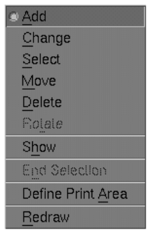
Figure 3.7: Action menu options.
Edit→Add to make a copy of the objects, i.e., places, transitions and subnets, located in the selected area. The
copied objects can be dragged around following the movements of the mouse cursor and eventually placed on
the desired location by clicking the left mouse button. Arcs connecting the selected object are also copied and
the added places/transitions are renamed. Same operation can be performed by activating the Add option of the
Action menu. To terminate the Add option, set the End Selection option selected either from the Edit menu or
from the Action menu.
Edit→Delete to delete all the items placed on the selected area.
Edit→End Selection to disactivate the selected area.
Edit→Move to move on the canvas the objects contained in the selected area. The starting and terminating
nodes of arcs are not changed.
Edit→Modify to modify the layout of currently-selected area. Allowed transformations are:
•clockwise rotation of a multiple of 45 degrees;
•flip X-axis: change the sign of the x coordinates of the selected objects obtaining a vertical mirror trans-
formation;
•flip Y-axis: change the sign of the y coordinates of the selected objects obtaining a horizontal mirror
transformation;
41
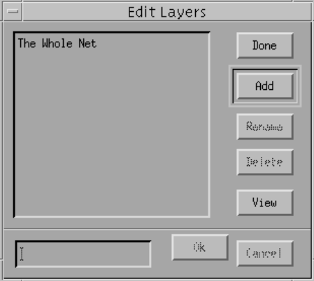
Figure 3.8: Edit layer window.
•mirror: the vertical and the horizontal lines crossing at the current mouse position in the canvas represent
traces of two mirrors with respect to which an image copy of the selected subnet may be created by clicking
the left (or middle) mouse button.
Edit→Layers... to edit the layers of the current loaded net. Layers can be set visible or not, independently
of each other. This GreatSPN2.0.2 feature can be effectively exploited to develop “dense” nets with numerous
crossing arcs, as in the case of places representing global states of a system that must be tested by many logically
distinct subnets. When this option is selected the Edit Layers window of Fig.3.8 pops-up, allowing to create,
destroy, rename and set visible or not layers of the net. When a GreatSPN2.0.2 model is created “The Whole
Net” layer, representing the whole model, is automatically generated and, by default, is set visible.
In order to describe how to generate layers of a current loaded model, let us consider the example of a fault-
tolerant multiprocessor system in which processors may access a common memory through a bus. The basic
fault-free behavior has been modeled by the net shown in Fig.3.9. Place running contains tokens representing
processors running on their own private memory. Transition memreq models the time necessary for a processor
to issue a shared memory access request. Immediate transition startacc represents the start of a shared memory
access using the bus. Timed transition access models the time needed to complete a shared memory access and to
release the bus. The net of Fig.3.9 is our starting point in the construction of a more complex model including not
only the normal system operation, but also the activities related to fault detection and recovery. This initial net
can be thought of as the first layer of the more complex model. Our first modeling step will be the definition of
two layers, which will be called run and repair, representing the normal operation of the system and the activities
related to reconfigurations and repairs of faulty processors, respectively. After loading our initial net description,
42
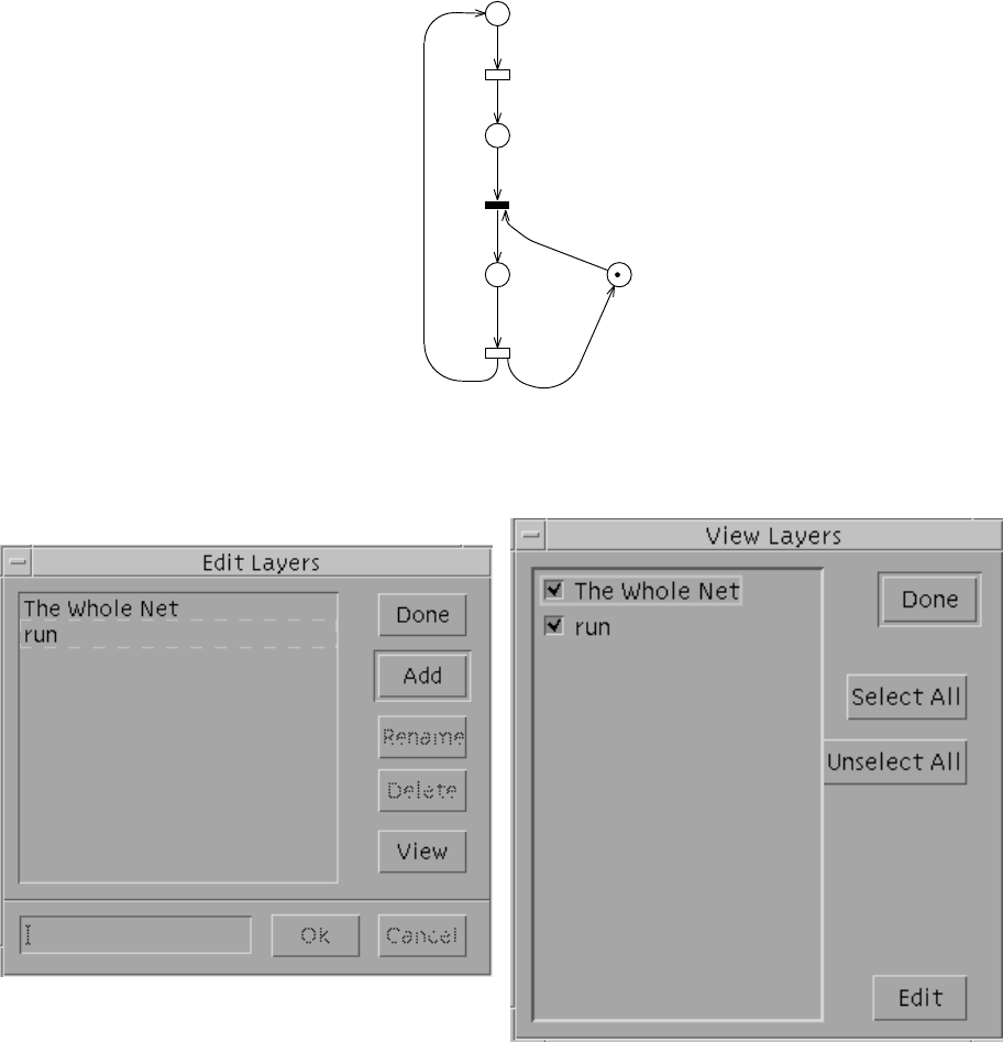
P= 2
bus
access
wait
running
P
memreq
access
startacc
Figure 3.9: Fault-free multiprocessor system model.
Figure 3.10: Edit layer window after the newly
added layer. Figure 3.11: View layer window.
the first operation is to open the Edit Layers window, by selecting the Edit→Layers... option, that appears as the
one of Fig.3.8 since no layers have already been added. Click on the “Add” button to activate the box located at
the left bottom of the window and write in that box the name of the new layer (run) to be created. Click on the
“OK” button to confirm the previous operation: the new layer run has been added to the list of the current layers
of the net, shown on the main box of the window (see Fig.3.10). When we click the “View” button the View Layer
43
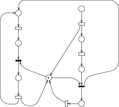
window pops-up, see Fig.3.11: this window allows to set a layer visible (with the associated box checked) or not
(with the associated box empty) by simply clicking on the corresponding box. In order to notify the editor that
the objects already defined in the net must belong to the run layer, we have to perform the following operations:
•select the objects: 1) set Action→Select option from the Action menu (Fig.3.7) 2) click with the middle
mouse button over the canvas point corresponding to the upper-left corner of the select area 3) move the
mouse cursor on the lower-right corner of the desired select area and 4) click either the left or the middle
mouse button;
•switch off the “The Whole Net” layer in the View Layers window (Fig.3.11);
•choose the Action→Add option from the Action menu (Fig.3.7).
In this way the content of the selected subnet is added to the run layer. Now we may proceed to the definition of a
new layer; click on the “Add” button of the Edit Layer window and define the new layer repair. Note that after this
action, the newly added layer as well the “The Whole Net” layer are both switched on in the View layer window,
while the other layers (in the current example, the layer run) are all switched off. In this situation, any object
created is automatically added both to the net description and to the repair layer. We can then start to add objects
in the usual way, until the net depicted in Fig.3.12 is obtained. The subnet corresponding to this new repair
P= 2
bus
access
wait
running
P
recfail
repair
waitbus
recrep
memreq
access recrep
repair
recfail
startacc
getbus
Figure 3.12: The first two layers of the fault-tolerant system example.
layer has its particular meaning: transition recfail represents the reconfiguration of the system needed after the
detection of a processor failure. Place repair models the faulty processor held off-line. Transition repair models
the time needed to repair or substitute the faulty processor. Transition recrep represents the reconfiguration
needed after the repair or substitution of the faulty processor in order to put it on-line again.
44
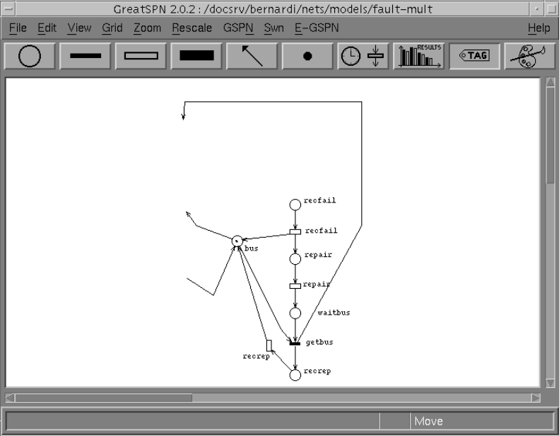
Note that places running and bus should belong to both repair and run layers. We can include them in the
new layer repair by selecting them, switching off the “The Whole Net” layer, and by choosing the Action→Add
option from the Action menu. Unfortunately, as shown in Fig.3.13, this operation has included into repair layer
not only the two places, but also the two arcs connected to them. These arcs can be removed from the layer by:
•choosing the Action→Delete option from the Action menu (Fig.3.7),
•activating the arc icon from the object bar,
•picking the arcs in excess with the left button of the mouse.
Figure 3.13: Inclusion of places ‘running’ and ‘bus’ into ‘repair’ layer.
Similarly, we should define two more layers as depicted in Fig.3.14, representing the failure detection and
the priority given to recovery procedures over normal operation, respectively.
Fig.3.15 shows the appearance of the complete net with all the layers switched on. Compare the level of
readability of this last figure, with that of the sequence of the four layers shown separately. Note also that the
last two layers are not easily recognized as ‘proper’ subnets, and would not be easily managed by tools based on
hierarchical decomposition concepts.
45
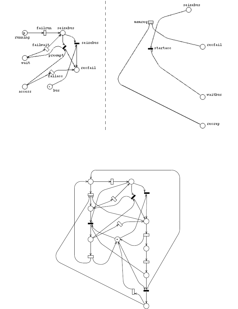
(A) (B)
Figure 3.14: The ‘fail’ (A) and the ‘priority’ (B) layers.
P= 2
recrep
waitbus
recfail
seizebus
bus
access
wait
running
P
repair
memreq
recrep
repair
recfail
failacc
failwait
failrun
access
startacc
preempt
getbus
seizebus
Figure 3.15: The complete net with all the layers switched on.
In fact, different layers can be associated with different hierarchical views of the system, but in general the
use of layers is not limited to hierarchy; they can be used to partition a complex ‘flat’ model just in ‘slices’ among
which no hierarchy is defined, as in our example.
46
3.1.3 View Menu
This menu allows to set several options concerning the graphical display of the current loaded Petri net model.
Options remain set until they are deactivated. The View menu contains the following options:
View→Spline to display arcs with splines. Splines are slower to draw, but often result in nets easier to under-
stand.
View→Tag to show/hide the names of the net objects.
View→Rate to show/hide the transition rates.
View→Overview to show/hide net overview.
View→Find... this option is not available in the current version of the package.
View→Print Area to show/hide the print area. When the View→Print Area option is set the current print area
is surrounded by a thin broken frame. To change print area definition, choose the Action→Define Print Area
from the Action menu (Fig.3.7), the cursor shape will be changed into a cross; click with the left mouse button
over the canvas point corresponding to the upper-left corner of the desired print area; move the mouse cursor on
the lower-right corner of the desired print area and click either the left or the middle mouse button.
View→Layers... to pop-up the View Layer dialog box (Fig.3.11): the layers of the loaded net are listed in the
left box; each layer can be set visible (the associated check-box checked) or not visible (the associated check-box
empty) by clicking on its corresponding check-box. To close the View Layer dialog box click on the “Done”
button; to set visible all the defined layers click on the “Select All” button; to set not visible all the defined layers
click on the “Unselect All” button. The “Edit” button located on the bottom-right of the dialog box allows to
pop-up the Edit Layer window (see Fig.3.8).
3.1.4 Grid Menu
The Grid menu allows to set grid in the canvas in order to simplify a regular layout of the net. The size of the
gap between points in the grid ranges from one pixel to 50 pixels (the default gap size is one pixel which mean
the “None” option is set). When a grid is set, objects are added and moved in the nearest point of the grid with
respect to the mouse cursor position.
47
3.1.5 Zoom Menu
The Zoom menu allows to show the objects of the current loaded net at five different ”zoom” levels, by selecting
the proper zooming factor (1, 3/2, 2, 1/2, 3/4 ). “Zoom” operation causes the resizing of all the objects contained
in the canvas during a GreatSPN2.0.2 session, however it doesn’t affect the actual dimension of the objects of
the net. The default zoom factor of the editor is 1.
3.1.6 Rescale Menu
Net coordinates of the current net can be rescaled by selecting the Rescale menu which contains sixteen different
rescale factors ranging from 0.5 to 2. Choosing one of the rescaling factors, the coordinates of all the objects
contained in the canvas are multiplied by that coefficient.
WARNING! Rescaling is completely different from zooming the net: “zoom” operation affects only the editor
view of the net while “rescale” operation affects the actual coordinates of the objects of the net.
The following three subsections give a short explanation of the GSPN of the SWN and of the E-GSPN menus
respectively; a depth description of the GreatSPN2.0.2 solvers is given in Chapt. 4.
The choice of launching either a structural (GSPN→Struct submenu) or a numerical analyzer (GSPN→Solve
submenu) for GSPN models, as well as the choice of carrying out either a numerical analysis or a simulation run
on a SWN model (SWN menu) - or on a E-GSPN model (E-GSPN menu) - causes the Console window of
Fig.3.16 to pop-up: to launch the corresponding execution module press the “Start” button. When a solution
module is launched, then the “Interrupt” button becomes active: press it to interrupt the execution of the current
solution module.
WARNING! In some cases, the “Interrupt” action actually does not kill the launched process but only some
sub-processes originated by the former: then it is better to check from a terminal if the process is still alive or
not.
When the “Clear” button is pressed then a previous computed solution is removed. Finally the “OK” button
allows to close the Console window.
3.1.7 GSPN Menu
The GSPN menu contains the options that allows to launch GreatSPN2.0.2 solvers for GSPN models.
GSPN→Struct to compute the structural properties of the current loaded GSPN model. It pops-up a sub-menu
which contains in turns the following options:
•P-invariants: to compute the minimal-support non-negative place invariants;
48
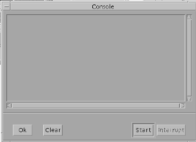
Figure 3.16: GreatSPN2.0.2 Console
•T-invariants: to compute the minimal support transition invariants;
•Minimal deadlocks: to compute the minimal deadlocks, i.e., the sets of places that once emptied cannot
be marked anymore;
•Minimal traps: to compute the minimal traps, i.e., the sets of places that once marked cannot loose tokens
anymore;
•ECS Confusion ME SC CC: to compute the ECS, Extended Conflict Sets of immediate transitions, Con-
fusion between transitions (non free-choice conflicts), ME, structural and marking Mutual Exclusion be-
tween transitions, SC, Structural Conflicts between non-mutually exclusive transitions, and CC, structural
Causal Connection between transitions.
•Structural boundedness: to verify the structural boundedness and, in case of unbounded nets, to compute
the transition sequences that can arbitrarily increase the marking of some place.
The computation of the above structural properties requires that the net description is saved on a file.
GSPN→Solve to carry out analysis of the current loaded GSPN model, in particular:
•Compute TRG: to generate the Tangible Reachability Graph;
•Compute EMC: to compute the Embedded Markov Chain, that is the CTMC associated to the TRG;
•GSPN solution: to compute the CTMC solution, i.e., the probability distribution of the number of tokens
in each place and the performance results. GSPN solution can be obtained both in steady state and in
transient state.
49
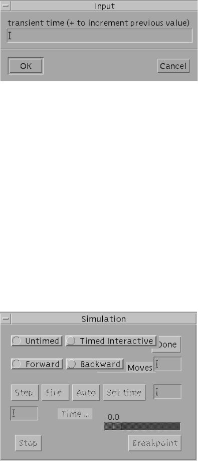
In case of transient solution request, when the “Start” button of the Console window (Fig.3.16) is pressed,
the Input window of Fig.3.17 appears. The value (positive real) of the time instant at which the transient
solution will be computed has to be inserted in the corresponding box transient time .....
Figure 3.17: GreatSPN2.0.2 Input window
GSPN→Simulation... to play the interactive token-game and to launch the interactive simulation. When this
option is chosen the Simulation window pops-up (Fig.3.18) and all the transitions of the current loaded model
that are enabled in the initial marking become blinking.
Token game. To simulate a possible behavior of the current loaded GSPN model simply click with the leftmost
button of the mouse over the enabled (i.e. blinking) transition you want to fire it. By default the “Untimed” and
the “Forward” options of the Simulation window are set to play the forward token game: it is possible to play the
backward token game by setting the “Untimed” and “Backward” options in the Simulation dialog box.
“Moves” area allows to set the slowness of the token flow from the input places of the firing transition to its
output places: higher is the value filled in this area slower is the token flow.
Figure 3.18: GreatSPN2.0.2 Simulation window
Simulation. To activate the interactive simulation of the current loaded GSPN model set the “Timed Interactive”
option: when this option is set, then the “Step”, “Fire”, “Auto”, “Set time”, “Stop” and “Breakpoint” buttons
become available. To simulate the behavior step-by-step press the “Step” button: the area located below this
50
button allows to set the number of automatic firings, e.g., if you fill in the value 2, then two successive firings are
displayed. Press the “Auto” button to start the simulation run: the firing sequences are displayed in the canvas
automatically until an interruption command is given by the user. To interrupt the execution press the “Stop”
button, the transition throughputs computed up to the interruption (transient results) are visualized in the canvas
and they are saved in the netname.sta file. To restart the simulation from the interrupted point press the “Auto”
button again. To terminate the simulation execution press the “Stop” button first, and then the “Done” button.
WARNING! The interactive simulation does not work properly on some GSPN models: to use simulation tech-
niques on a GSPN model in order to obtain performance results is better to use the simulation solvers available
from the E-GSPN menu.
3.1.8 SWN Menu
The SWN menu contains the following options:
SWN→Symbolic to compute solution of SWN models. In particular:
•Simulation: to launch the simulation for colored models using an abstract representation of markings, i.e.,
symbolic markings;
•Compute RG: to compute the Symbolic Reachability Graph of the model and to obtain performance
indices in steady state;
•Transient: to compute the Symbolic Reachability Graph of the model and to obtain performance indices
in transient state.
SWN→Ordinary
•Simulation: to launch the simulator for colored models using ordinary markings;
•Compute RG: to compute the Reachability Graph of the model and to obtain performance indices in steady
state;
•Transient: to compute the Reachability Graph of the model and to obtain performance indices in transient
state.
SWN Reachability Graph computation The launch of a Reachability Graph solver - either symbolic or ordi-
nary - is carried out by pressing the “Start” button of the Console window (Fig. 3.16) and it causes a RG Options
window (see Fig. 3.19) to appear. It is possible to obtain a verbose description of the symbolic (or ordinary)
reachability graph by setting on the “Verbose Show” toggle of this window an by choosing the “OK” button. The
execution is displayed on the Console window and the results are visualized in the GreatSPN2.0.2 canvas.
51

Figure 3.19: SWN Reachability Graph Options window.
SWN simulation The launch of a SWN simulation - either symbolic or ordinary - is carried out by pressing the
“Start” button of the Console window (Fig. 3.16) and it causes a Simulation Options window (see Fig. 3.19) to
appear. Through this window, the user can modify the default values of the simulation parameters, in particular:
•“Initial Transitory”: the length of initial transitory period that has not to be taken into account for the
computation of the performance measures;
•“Batch Spacing”: the length of evolution phase between batches that has to be discarted;
•“Minimum Batch Length”: the dimension of the minimum batch;
•“Maximum Batch Length”: the dimension of the maximum batch;
•“Seed”: the seed of the random number generator;
•“Accuracy”: the precision of the approximation in the parameters estimation;
•“Confidence Level”: the confidence level in the parameters estimation.
All these parameters, except for the confidence level, can be modified by typing directly in the corresponding
area of the Simulation Options window. The “Confidence Level” can be changed instead by choosing the desired
value from the pull-down menu that pops up when the corresponding toggle is clicked. To obtain a verbose
description of the simulation results set the “Verbose Show” toggle of this window.
Click on the “OK” button to confirm the settings: the simulation execution is displayed on the Console
window and the results are visualized in the GreatSPN2.0.2 canvas.
SWN transient The launch of a SWN transient solver - either symbolic or ordinary - is carried out by pressing
the “Start” button of the Console window (Fig. 3.16) and it causes the Input window of Fig. 3.17) to appear. As
is the case of GSPN transient solutions, the transient time... area of this window has to be filled in with the value
(positive real) of the time instant at which the SWN transient solution will be computed.
52
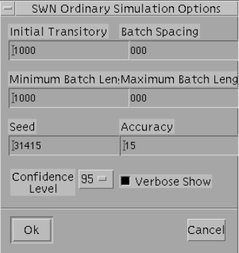
Figure 3.20: SWN Simulation Options window.
3.1.9 E-GSPN Menu
The E-GSPN menu concerns the Extended-GSPN models, that is GSPN models in which firing times of timed
transitions can have more general distributions than the negative exponential. The E-GSPN menu contains the
following options:
E-GSPN→Simulation to launch the simulation;
E-GSPN→Compute RG to compute the Reachability Graph of the model and to obtain the performance indices
in steady state;
E-GSPN→Transient to compute the Reachability Graph of the model and to obtain performance indices in
transient state.
All the solvers launched from the E-GSPN menu come from the same source files used for producing the
SWN solvers and they have the same functionalities of the latters.
WARNING! Note that the solvers lauched from the E-GSPN menu work also if the file netname.dis, used for
the general temporal specifications of the timed transitions, has not been created (or it is not located in the same
directory where the net definition files of the current model are saved).
3.1.10 Help Menu
The Help menu, located on the right of the menu bar, contains the following options:
53
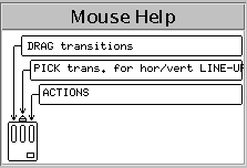
Help→Mouse Help to display information about the use of the mouse buttons; the Mouse Help window pos-up
(Fig.3.21) describing the current functions of the mouse buttons. To remove the Mouse Help window, deactivate
the Help→MouseHelp option.
Figure 3.21: Mouse help window.
Help→About when this option is chosen a window displaying the current release of GreaSPN pops-up: to
remove the window, click on the “OK” button.
3.2 The Object bar
The object bar, located just below the menu bar on the GreatSPN2.0.2 Control Panel (see Fig. 3.2), contains 10
icons which allow to perform operations - add/delete/change... - on a specific object of the PN model. To execute
an operation on a specific object:
•activate the Action menu (see Fig. 3.7) by pressing the right mouse button on any position in the canvas;
•click with the left mouse button over the desired action: the selected action is displayed on the status bar
of the CP and it becomes the default action until a new one is chosen;
•select the object type by clicking on the corresponding icon button of the object bar: the default action will
affect only the objects of the type currently selected.
Depending on the type of action activated and of the type of selected object, different windows will pop-up; in
the following, going from the left to the right, each icon of the object bar is described, together with the possible
actions that can be carried out on the corresponding object type.
3.2.1 Places
It is the first icon of the object bar and it is depicted as a circle.
Add: add a new place operation causes the shape of the mouse cursor to change into a circle: to locate the new
place in the canvas, move the mouse cursor and click the left mouse button in the desired position.
54
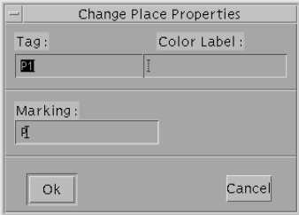
Figure 3.22: Dialog box for changing place properties.
Change: change place properties operation causes the dialog box of Fig. 3.22 to pop-up.
This dialog box is characterized by the “Tag:” area, that contains the name of the place, the “Color Label:”
area, that contains the color domain definition in case of colored places (SWN models) and the “Marking:”
area, that contains either a non negative number or a marking parameter which indicates the initial marking
of the place. To change one of the above mentioned place properties (either place name or color domain
or initial marking), click with the left (middle) mouse button over the corresponding area of the Change
Place Properties dialog box in order to activate it and write the proper definition.
Renaming of places via GUI is subject to the constraint that places of a model must to have distincts tags
(i.e., names); the attempt of renaming a place with an existing tag (i.e., with a string corresponding to the
name of another place of the current model) provokes an error message window to pop-up. This constraint
has been introduced to avoid problems in the computation of performance results, in particular performance
indices that are functions of the places with the same name. However, if the modeler wants to define places
with the same tag, then he/she has to modify directly the net definition file of the model.
WARNING! The assignment of an undefined initial marking parameter to a place provokes an error
message window to pop-up. This type of control is not carried out for the color domain definition: be
careful then to assign a correct color domain to a place, i.e., both by following the SWN grammar (see
Table A.1 of Appendix A) and by defining basic color classes before.
Select: select a place operation allows to select a specific place of the current loaded model by clicking over
the place with the left mouse button; this action causes a broken rectangle to surround the place. Selection
operation is normally used along with other operations, e.g., with the Add action to make a copy of the
place together with its input and output sets. To reset the Select operation, choose in the Action menu
the End Selection option (the broken rectangle that surrounds the selected area, in this case a place, will
disappear).
Move: move a place operation causes the shape of the mouse cursor to change into a cross; to move a place
55
simply click with the left mouse button over the place to be moved, move the mouse cursor to choose the
desired location in the canvas to put the place and click again to fix the place in the desired location.
Delete: delete a place operation allows to delete a place present in the canvas; to delete an existing place click
over the place to be removed with the left mouse button.
Show: show a place operation allows to visualize place properties; to choose the property of a place to be
displayed click with the right mouse button over the place to pop-up the Place Property menu and then
click with the left mouse button over the corresponding option to set the desired property. The Place
Property menu contains the following options:
P-invariants To display P-invariants the place belongs to: all the places belonging to the same P-invariant
start blinking and a Show menu pops-up in which the algebraic expression of the current P-invariant is
visualized (this expression is also visualized on the status bar).
Minimal deadlocks To display minimal deadlocks the place belongs to: all the places belonging to the
same minimal deadlock start blinking and a Show menu pops-up in which the algebraic expression of the
current minimal deadlock is visualized (this expression is also visualized on the status bar).
Minimal traps to display minimal traps the place belongs to: all the places belonging to the same mini-
mal trap start blinking and a Show menu pops-up in which the algebraic expression of the current minimal
trap is visualized (this expression is also visualized on the status bar).
WARNING! To visualize the above properties, i.e., P-invariants, minimal deadlocks and minimal traps it
is necessary to launch the corresponding structural solvers before, by choosing the related options on the
GSPN→Struct submenu, otherwise a window will pop-up displaying a warning message of type: Sorry,
no up-to-date place invariants (or deadlocks or traps) available.
Implicit places To display pairs of implicit places : the couple of implicit places start blinking and a
Show menu pops-up in which the implication is visualized (it is also visualized on the status bar).
Absolute Marking Bounds To display the structural bounds on the number of tokens in a place. To
compute the upper bound click with the left mouse button over the place, while to compute the lower
bound click with the left-right (or middle) mouse buttons; bounds are visualized both on the Show window
which pops-up and on the status bar. In case of unboundedness, a message will be displayed.
56

Average Marking Bounds To display the bounds for the steady state mean of a place. Bounds are
obtained from the net structure, the initial marking and the transition rates by solving a linear programming
problem. To compute the upper bound click with the left mouse button over the place, while to compute the
lower bound click with the left-right (or middle) mouse buttons; bounds are visualized both on the Show
window which pops-up and on the status bar. In case of unboundedness, a message will be displayed.
WARNING! Absolute and average marking bounds can be computed only if the lp solve package[28],
used for solving linear programming problems, has been installed and the GreatSPN2.0.2 environment
variable GSPN2LPSOLVE has been set with the path-name of the executable.
End Show To reset the Show option.
3.2.2 Transitions
There are three icons corresponding to a transition object: the IMM icon, depicted as a thin black bar, the EXP
icon, depicted as a thick white bar, and the DET icon, depicted as a thick black bar. These icons correspond,
respectively, to an immediate transition object, an exponentially distributed timed transition object and a deter-
ministic distributed timed transition object.
Add: add a transition operation causes the shape of the mouse cursor to change into the corresponding transition
icon - IMM,EXP or DET - depending on the type of transition selected. To locate the new transition in the
canvas, move the mouse cursor and click the left mouse button in the desired position.
Change: change a transition properties operation causes a dialog box to pop-up.
Timed transitions.
The dialog box in this case is the one of Fig. 3.23(A) in which the EXP icon, located on the top of the win-
dow, is pressed. In case DET icon is pressed, i.e., it is the Change Transition Properties for a deterministic
transition, the bottom part of the dialog box, which concerns the type of server semantics to be set, is not
present. The common areas of the dialog box for exponentially distributed transitions and for deterministic
distributed transitions are the followings:
- “Tag:” it contains the name of the transition. By default, names of timed transitions are of type T#,
where #is a number given in progressive order with respect to the transition creation.
- “Color Label:” it contains the guard definition of the transition (SWN models). No syntactical control
is carried out for the guard of its definition.
- “Rate or Rate Parameter:” for exponentially distributed transitions, it contains either the value of
the rate or the name of a rate parameter. In the latter case the rate parameter has to be previously
57

(A) (B)
Figure 3.23: Windows for defining/changing properties of timed (A) and immediate (B) transitions.
defined, otherwise an error message will be displayed. For deterministic distributed transitions, values
assigned in this area are considered as delays. By default, the rate (delay) value assigned is 1.0.
WARNING! In case of timed transition, a zero value as transition rate is accepted even though this
assignment will cause a segmentation fault when launching the solutions. Transition rates assigned from
GUI, are stored in the net definition file with at most six decimal digits, i.e., if you assign a value lower
than 10E−6 to a transition rate then the value will be truncated at the 6th decimal digit in the .net file.
To change one of the above mentioned transition properties (either transition name or guard or rate), click
with the left (middle) mouse button over the corresponding area of the Change Transition Properties dialog
box in order to activate it and write the proper definition.
For exponentially distributed transitions, GreatSPN2.0.2 allows the user to define different server seman-
tics. Let µ(M)be the marking dependent parameter of the negative exponential distribution F(x,M) =
Pr{X≤x}=1−e−µ(M)xassociated to a timed transition t, and let ED(t,M)be the enabling degree of
tin marking M, then depending on the semantics adopted for the timed transition, a different marking
dependent firing rate µ(M)is assigned.
Infinite Every enabling set of tokens is processed as soon as it forms in the input places of the transition. Its
corresponding firing delay is generated at this time, and the timers associated with all these enabling
sets run down to zero concurrently. Multiple enabling sets of tokens are thus processed in parallel.
58
The firing rate of tis given by the function µ(M) = ED(t,M)µ, where µis the value set in the “Rate
or Rate Parameter:” area of the Change Transition Properties window. This semantics is the default
option, i.e., the “Infinite” toggle of the Change Transition Properties dialog box is switched on.
Marking Dependent Firing rate of tis function of the marking of a subset of places of the net; this subset
of places is not necessary equal to the set of input and inhibitor places of the transition. To choose this
option, click with the left (left-right) mouse button over the “Marking Dependent” toggle to switch
it on and to define the function µ(M)in the “Marking Dependent Definition” area, follow the syntax
given in Table A.3 of Appendix A. It is possible to display the grammar on line by clicking over the
“MD Grammar Help ...” button.
K-Server In case of single server semantics, i.e., K=1, random firing delay is set when the transition
becomes first enabled, new delays are generated upon transition firing if the transition is still enabled
in the new marking. This means that enabling sets of tokens are processed serially and that the
temporal specification associated with the transition is independent of the enabling degree, i.e., the
firing rate of transition tis given by the (constant) function µ(M) = µ, where µis the value set in
the “Rate or Rate Parameter:” area of the Change Transition Properties window. In case of multiple
server semantics, i.e., K∈ {2,...,127}, enabling sets of tokens are processed as soon as they form in
the input places of the transition up to the maximum degree of parallelism K. For larger values of the
enabling degree, the timers associated with new enabling sets of tokens are set only when the number
of concurrently running timers decreases below the value K. The firing rate of transition tis given by
the function µ(M) = min(ED(t,M),K)µ. To choose this option, click with the left (left-right) mouse
button over the “1-Server” toggle to switch it on: the scrollbar located at the bottom left of the dialog
box becomes active. In case of K-Servers semantics, with K>1 move the scrollbar by keeping the
mouse button pressed to fix the desired value for K. The “1-Server” toggle will be changed into
“K-Server” toggle automatically when the mouse button will be released.
Load Dependent Firing rate of tis a function, given in tabular form, of its enabling degree µ(M) =
f(ED(t,M)). This semantics is a particular case of marking dependent semantics in which the firing
rate of twhen ED(t,M) = Kcorresponds to the the throughput of a short-circuited queueing network
in which exactly Kjobs are circulating in it (i.e., trepresents the load-dependent equivalent server).
To choose the load dependent server semantics switch on the “Load Dependent” toggle to activate
the scrollbar, then move the scrollbar by keeping the mouse button pressed to fix the desired value
MAX (it corresponds to the maximum population of the short-circuited queueing network). When
the mouse button is released, MAX lines are added in the area located above the scrollbar and they
appear as follows:
Rate --> 1.000000
59
2 --> 1.000000
3 --> 1.000000
...
MAX --> 1.000000
Each line is of type # --> ratevalue, apart from the first one in which the string Rate replaces the
number 1, where ratevalue corresponds to the value assigned to the firing rate when the enabling
degree of the transition is equal to #. By default, all the ratevalue are equal to 1.000000. To change
one of the ratevalue, click with the left mouse button over the corresponding line: automatically,
the ratevalue appears on the “Rate or Rate Parameter (Weight)” area. Type the desired value and
then press <Return> command: the new value for the ratevalue will be set and the corresponding
line in the area above the scrollbar will be updated.
Immediate transitions.
The dialog box in this case is the one of Fig. 3.23(B) in which the IMM icon, located on the top of the
window, is pressed. It is characterized by the following areas:
- “Tag:” it contains the name of the transition. By default, names of immediate transitions are of type
t#, where #is a number given in progressive order with respect to the transition creation.
- “Color Label:” it contains the guard definition of the transition (SWN models). No syntactical control
is carried out for the guard at the moment of its definition.
- “Weight:” it contains the weight of the transition. By default the weight value assigned is 1.0.
Admissible values are non-negative real numbers, in case of conflict among different immediate
transitions a normalization of the weight is performed when the solution are launched.
To change one of the above mentioned transition properties (either transition name or guard or weight),
click with the left (middle) mouse button over the corresponding area of the Change Transition Properties
dialog box in order to activate it and write the proper definition.
Finally, on the bottom-left part of the Change Transition Properties dialog box, there is a scrollbar that
allows to assign a priority level to the transition. By default, the priority level is one; the admissible
priority levels range from 1 to 126. To change the priority level of the current immediate transition, simply
click with the mouse button over the scrollbar and move it by keeping the mouse button pressed until you
find the desired value.
WARNING! Renaming of transitions via GUI is subject to the constraint that transitions of a model must
to have distincts tags (i.e., names); the attempt of renaming a transition with an existing tag (i.e., with a
string corresponding to the name of another transition of the same type) provokes an error message window
60
to pop-up. This constraint has been introduced to avoid problems in the computation of performance
results, in particular performance indices that are functions of the transitions with the same name. However,
if the modeler wants to define transitions with the same tag, then he/she has to modify directly the net
definition file of the model.
Select: select a transition operation allows to select a specific transition of the current loaded model by clicking
over the transition with the left mouse button; this action causes a broken rectangle to surround the transi-
tion. Selection operation is normally used along with other operations, e.g., with the Add action to make
a copy of the transition together with its input and output sets. To reset the Select operation, choose in the
Action menu the End Selection option (the broken rectangle that surrounds the selected area, in this case a
transition, will disappear).
Move: move a transition operation causes the shape of the mouse cursor to change into a cross; to move a
transition simply click with the left mouse button over the transition to be moved, move the mouse cursor
to choose the desired location in the canvas to put the transition and click again to fix the transition in the
desired location.
Delete: delete a transition operation allows to delete a transition present in the canvas; to delete an existing
transition click over the transition to be removed with the left mouse button.
Rotate: rotate a transition operation causes the shape of the mouse cursor to change into a transition icon
(either IMM or EXP or DET icon depending on which transition icon is set on the object bar); to rotate a
transition click over the transition with the left mouse button: each “click” of the mouse button will rotate
the transition clockwise of a multiple of 45 degrees.
Show: show a transition operation allows to visualize transition properties; to choose the property of a transition
to be displayed click with the right mouse button over the transition to pop-up the Transition Property
menu and then click with the left mouse button over the corresponding option to set the desired property.
The Transition Property menu contains the following options:
T-invariants To display T-invariants the transition belongs to: all the transitions belonging to the same
T-invariant start blinking and a Show menu pops-up in which the algebraic expression of the current T-
invariant is visualized (this expression is also visualized on the status bar).
ECS To display the Extended Conflict Sets (ECS) of the set of immediate transitions: all the immediate
transitions belonging to the same ECS start blinking and a Show menu pops-up in which the algebraic
expression of the current ECS is visualized (this expression is also visualized on the status bar).
61
WARNING! Since the ECSs are computed only on the subset of immediate transitions, then to visualize
them it is necessary that the IMM icon of the object bar is set. Otherwise, if another transition icon
(either EXP of DET) is set, the show ECS operation causes a warning message to pop-up (i.e., “Sorry, NO
Ext.Conflict Sets is computed for timed transitions”) although the request has been carried out by clicking
on a specific immediate transition.
ME To display the pairs of transitions that are structurally mutually exclusive.
SC To display the pair of transitions that are in structural conflict relation.
CC To display the pair of transitions that are in causal connection relation.
Unbounded Sequences To display the firing sequences of transition that add tokens to an unbounded
place. Click over the unbounded place, the place and the unbounded firing sequence start blinking alter-
nately and the algebraic expression of the firing sequence is displayed in the Show window that pops-up; to
visualize all the unbounded firing sequences, click repeatedly over the same unbounded place, each click
of the mouse allows, in turn, to show a unbounded firing sequence.
WARNING! To visualize the above properties, i.e., T-invariants, ECS, ME, SC, CC, and Unbounded
Sequences it is necessary to launch the corresponding structural solvers before, by choosing the related
options on the GSPN→Struct submenu, otherwise a window will pop-up displaying a warning message of
type: “Sorry, no up-to-date transition invariants (or conflict sets or ...) available”.
Actual liveness Bounds To display the actual liveness bounds of a transition.
LP liveness Bounds To display the liveness bounds of a transition.
LP throughput Bounds To display the bounds for the steady state throughput of a transition. Bounds are
obtained from the net structure, the initial marking and the transition rates by solving a linear programming
problem. To compute the upper bound click with the left mouse button over the transition, while to compute
the lower bound click with the left-right (or middle) mouse buttons; bounds are visualized both on the Show
window which pops-up and on the status bar. In case of unboundedness, a message will be displayed.
End Show To reset the Show option.
62
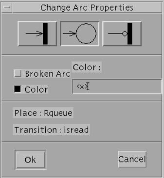
3.2.3 Arcs
It is the fifth icon of the object bar and it is depicted as an arrow.
Add: add an arc operation causes the shape of the mouse cursor to change into an arrow: to connect a place
(transition) to a transition (place) click with the left mouse button over the place (transition) first, and then
click over the transition (place) with the left mouse button. To add an inhibitor arc click with the middle
mouse button over the inhibitor place (inhibited transition) first and them click over the inhibited transition
(inhibitor place) with the left mouse button.
WARNING! Since, by definition of PNs, it is not possible to have an arc connecting two objects of the
same type, GreatSPN2.0.2 does not allow to connect either two transitions or two places with an arc. In
case, you have clicked on the first object and then you realize that this was not you intended to do, it is
better to continue and to terminate the add arc operation and then to delete the just added wrong arc than
to suspend the operation by activating another action since a suspended arc provokes a segmentation fault.
Change: change an arc operation causes the dialog box of Fig.3.24 to pop-up. The upper part of the dialog
Figure 3.24: Change Arc Properties window.
box contains three icons. Always, only one of them is active and it indicates the current type of arc; in
particular, going from the left to the right, the first icon represents an input arc, the second represents an
output arc and the third one represents an inhibitor arc with respect to the transition. The tags of the place
and of the transition connected with the arc are displayed in the bottom part of the dialog box. For example,
the dialog box of Fig. 3.24 displays the properties of the output arc which connects transition isread to the
place Rqueue. Below the three icons, there are two toggles: the “Broken Arc” toggle and the “Color”
toggle.
63
•“Broken Arc”: when it is not set, i.e., the corresponding rectangle is white, then the arc is fully
displayed in the canvas; when it is set, i.e., the corresponding rectangle is black, then the arc is
partially displayed in the canvas, this means that only the ending parts of the broken line representing
the arc are displayed.
WARNING! To draw a broken arc it is necessary to break the line representing the arc with at least
two intermediate points first, then to set the “Broken Arc” toggle.
•“Color”: it is related with the area located on the right of the toggle. When it is not set, i.e., the cor-
responding rectangle is white, then the “Multiplicity” area contains the multiplicity value associated
to the arc. When it is set (in case of SWN models), i.e., the corresponding rectangle is black, then the
“Color:” area contains the arc function associated to the arc. Arc function definitions are given in the
SWN definition grammar of Table A.1 of Appendix A.
By default, the two toggles described above are not set and the arc multiplicity is equal to one.
Move: move an arc operation allows to draw the arc as a broken line by adding some intermediate points. To
add an intermediate point just click with the left mouse button over the arc and move the mouse cursor in
the canvas to choose the point as intermediate one, then fix the point by clicking again with the left mouse
button. To change the source (destination) of an arc, click with the middle mouse button over the source
(destination) object and then click with the left mouse button over the new source (destination) object.
Delete: delete an arc operation allows to delete an arc present in the canvas; to delete an existing arc click over
the arc to be removed with the left mouse button.
3.2.4 Marking parameters
It is the sixth icon of the object bar and it is depicted as a token.
Add: add a marking parameter operation is used to create a new marking parameter that will be used as initial
marking of the GSPN system when solutions are launched. When this action is active, the shape of the
mouse cursor is an arrow, click on a free location of the canvas to fix the position of the marking parameter
that is going to be defined: this action causes the dialog box of Fig. 3.25 to pop-up.
The dialog box is characterized by two areas: the “Label:” area, that has to be filled with the name of the
marking parameter, and the “Marking:” area, that has to be filled with a non negative integer. To fill in the
areas of the Create Marking Parameter dialog box click over the corresponding areas to activate them and
then type the related name or value. Finally, either click over the “OK” button to confirm the settings or
click over the “Cancel” button to do not confirm.
The attempt to insert a negative value in the “Marking:” area causes a warning message to be displayed.
The name of the marking parameter has to be unique in the current loaded model.
64

Figure 3.25: Create Marking Parameter dialog box.
Change: change a marking parameter allows to change specification of an existing marking parameter. To
change the specifications of an existing marking parameter click over the marking parameter located some-
where in the canvas: this action causes a dialog box similar to the one of Fig. 3.25 to pop-up1.
To change the values in the areas of the Change Marking Parameter dialog box click over the corresponding
areas to activate them and then overwrite the old values with the new ones. Finally, either click over the
“OK” button to confirm the changes or click over the “Cancel” button to keep the old settings.
Select: select a marking parameter operation allows to select a specific marking parameter of the current loaded
model by clicking over the marking parameter with the left mouse button; this action causes a broken rect-
angle to replace the marking parameter. Selection operation is normally used along with other operations,
e.g., with the Move action to move the marking parameter in a different location of the canvas. To reset the
Select operation, choose in the Action menu the End Selection option (the broken rectangle that replaces
the selected marking parameter, will disappear).
Move: move a marking parameter operation causes the shape of the mouse cursor to change into an arrow;
to move a marking parameter simply click with the left mouse button over the marking parameter to be
moved, move the mouse cursor to choose the desired location in the canvas to put the marking parameter
and click again to fix the marking parameter in the desired location.
Delete: delete a marking parameter operation allows to delete a marking parameter present in the canvas; to
delete an existing marking parameter click over the marking parameter to be removed with the left mouse
button.
1Actually, the dialog box differs only for the title that in case of change action is Change Marking Parameter.
65
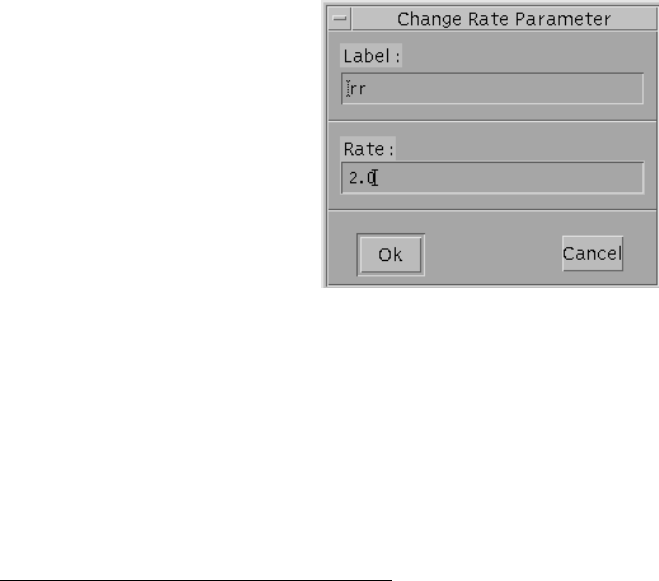
3.2.5 Rate parameters
It is the seventh icon of the object bar and it is depicted with a clock and a transition.
Add: add a rate parameter operation is used to create a new rate parameter that will be used in the temporal
specifications of one or more timed transitions of the GSPN system. When this action is active, the shape of
the mouse cursor is an arrow, click on a free location of the canvas to fix the position of the rate parameter
that is going to be defined: this action causes a dialog box similar to the one of of Fig. 3.26 to pop-up2.
The dialog box is characterized by two areas: the “Label:” area, that has to be filled with the name of the
rate parameter, and the “Rate:” area, that has to be filled with a non negative integer. To fill in the areas
of the Create Rate Parameter dialog box click over the corresponding areas to activate them and then type
the related name or value. Finally, either click over the “OK” button to confirm the settings or click over
the “Cancel” button to do not confirm.
The attempt to insert a negative value in the “Rate:” area causes a warning message to be displayed. The
name of the rate parameter has to be unique in the current loaded model.
Change: change a rate parameter allows to change specification of an existing rate parameter. To change the
specifications of an existing rate parameter click over the rate parameter located somewhere in the canvas:
this action causes the dialog box of Fig. 3.26 to pop-up.
Figure 3.26: Change Rate Parameter dialog box.
To change the values in the areas of the Change Rate Parameter dialog box click over the corresponding
areas to activate them and then overwrite the old values with the new ones. Finally, either click over the
“OK” button to confirm the changes or click over the “Cancel” button to keep the old settings.
Select: select a rate parameter operation allows to select a specific rate parameter of the current loaded model
by clicking over the rate parameter with the left mouse button; this action causes a broken rectangle to
2Actually, the dialog box differs only for the title that in case of create action is Create Rate Parameter.
66
replace the rate parameter. Selection operation is normally used along with other operations, e.g., with the
Move action to move the rate parameter in a different location of the canvas. To reset the Select operation,
choose in the Action menu the End Selection option (the broken rectangle that replaces the selected rate
parameter, will disappear).
Move: move a rate parameter operation causes the shape of the mouse cursor to change into an arrow; to move
a rate parameter simply click with the left mouse button over the rate parameter to be moved, move the
mouse cursor to choose the desired location in the canvas to put the rate parameter and click again to fix
the rate parameter in the desired location.
Delete: delete a rate parameter operation allows to delete a rate parameter present in the canvas; to delete an
existing rate parameter click over the rate parameter to be removed with the left mouse button.
Show: show rate parameters operation allows to visualize the rates/rate parameters associated to the timed
transitions as well as the weight associated to the immediate transitions of the current loaded model; this
action causes the View→Rate option to be switched on.
End Show: To reset the Show option.
3.2.6 Result definitions
It is the eighth icon of the object bar and it is depicted with a bar diagram.
Add: add a result operation is used to create a user-defined performance result by following the grammar syntax
of Tab. A.3. When this action is active, the shape of the mouse cursor is an arrow, click on a free location
of the canvas to fix the position of the performance result name that is going to be defined: this action
causes a dialog box similar to the one of Fig. 3.27 to pop-up. The dialog box is characterized by two
areas: the “Label:” area that has to be filled with the name of the performance result, e.g., in Fig. 3.27 the
name Equeue has been assigned; and the “Definition:” area that has to be filled with the definition of the
performance result, e.g., in Fig. 3.27, the performance result has been defined as the sum of the steady state
number of tokens in place Rqueue and of the steady state number of tokens in place Wqueue. It is possible
to display the grammar on line by clicking over the “Res Grammar Help...” button.
WARNING! In case of steady state solutions, both the capital and the small letters E,e (P,p) can be used
to define the mean (the probability). In case of transient solutions, instead, the small letter has to be used.
Change: change a result operation allows to change specifications of an existing user-defined performance re-
sult. To change a previous definition of a given performance result, click over its name located somewhere
in the canvas: this action causes the dialog-box of Fig. 3.27 to pop-up. To change the values in the areas of
67
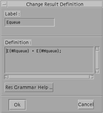
Figure 3.27: Change Result Definition dialog box.
the Change Result Definition dialog box click over the corresponding areas to activate them and then over-
write the old values with the new ones. Finally, either click over the “OK” button to confirm the changes
or click over the “Cancel” button to keep the old settings.
Select: select a result operation allows to select a specific user-defined performance result of the current loaded
model by clicking over the performance result name with the left mouse button; this action causes a broken
rectangle to superpose the performance result name. Selection operation is normally used along with other
operations, e.g., with the Move action to move the performance result name in a different location of the
canvas. To reset the Select operation, choose in the Action menu the End Selection option (the broken
rectangle that superposes the selected performance result name, will disappear).
Move: move a result operation causes the shape of the mouse cursor to change into an arrow; to move a perfor-
mance result simply click with the left mouse button over the performance result to be moved, move the
mouse cursor to choose the desired location in the canvas to put the performance result and click again to
fix it in the desired location.
Delete: delete a result operation allows to delete a performance result present in the canvas; to delete an existing
performance result click over the performance result to be removed with the left mouse button.
Show: show result operation allows either to visualize the definition of the performance result or, in case of
GSPN models, to display the token distribution in places. In the first case, just click with the left mouse
button over the interested performance result name: a Show window will pop-up displaying the current def-
inition of the result. In the second case, instead, click with the left mouse button over the interested place:
a window similar to the one of Fig. 3.28 will pop-up displaying the token distribution of the place, either
68
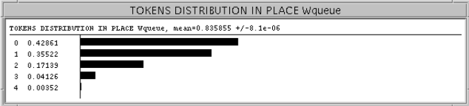
steady state or transient depending on which solver has been launched last. To quit a Token distribution
window, click with the left mouse button over it.
Figure 3.28: Token distribution dialog box
3.2.7 Changing place/transition tags
It is the ninth icon of the object bar and it is depicted as a label.
Change: change tag operation allows to change the label of an object (i.e., place, transition, marking parame-
ter,...) of the current loaded model. To change the label of a given object click over it with the left mouse
button: the corresponding Change ... window will pop-up.
Move: move tag operation allows to move the label of a transition (place): to move the label of a given transition
(place) click with the left mouse button over the label, move the mouse cursor to choose the desired location
in the canvas to put it and click again to fix the label in the desired location.
3.2.8 Colour definition
It is the tenth icon of the object bar and it is depicted with a palette and a paintbrush.
Add: create a color definition operation allows to define basic color classes, static subclasses, initial colored
markings (ordinary and symbolic) and colored functions (i.e., guards and color domain). When this action
is active, the shape of the mouse cursor is an arrow, click on a free location of the canvas to fix the position
of the colored object that is going to be defined: this action causes the Create Color Definition dialog to
pop-up (see Fig. 3.29). The dialog box is characterized by the following areas: the “Label:” area that
has to be filled with the name of the colored object, e.g., in Fig.3.29 the name Phas been assigned to a
colored class; and the “Definition:” area that has to be filled with the definition of the colored object, e.g.,
in Fig. 3.29, the colored class has been defined as the unordered union of two static subsclasses named as
P1 and P2 (see the SWN grammar of Table A.1). The type of the colored object is indicated by switching
on one of the three toggles that are located on the top-right part of the dialog box:
•“Colorset”: to define either a colored class or a colored static subclass;
69
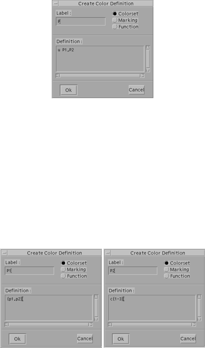
Figure 3.29: Create Color Definition window.
•“Marking”: to define an initial colored marking, either ordinary or symbolic;
•“Function”: to define a guard or a color domain.
To switch on a toggle, click over the empty circle located near the name of the toggle with the left mouse
button.
Examples of static subclass definition In Fig. 3.30 examples of static subclass definition is given: in
both the Create Color Definition dialog boxes, the toggle “Colorset” is switched on; the name of the
subclasses P1 and P2, respectively, are filled in the corresponding “Label” areas. Static subclass P1 is
defined as the set containing two colors p1 and p2. Static subclass P2, instead, is defined as a set of three
colors c1,c2 and c3. Both the definitions are correct in the GreatSPN2.0.2 syntax.
Figure 3.30: Definition of static subclasses.
70
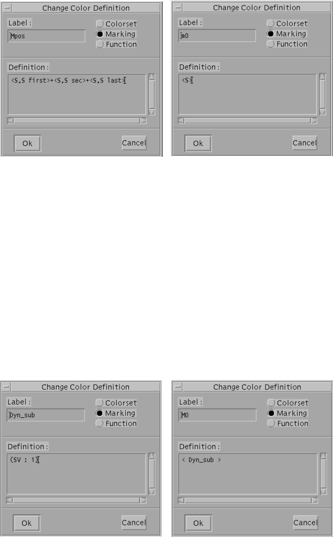
Examples of initial marking definition In Fig.3.31 examples of initial ordinary (colored) marking def-
inition is given:
Figure 3.31: Definition of initial ordinary colored markings.
the toggle “Marking” is switched on; the name of the initial markings Mpos and m0, respectively, are filled
in the corresponding “Label” areas. Initial marking Mpos has to be assigned to a place that has a color
domain defined as the cartesian product of two colored classes say Xand Yrespectively. Mpos is the set
containing all the combinations of pairs of colors in which the first element belongs to the class X(the first
component of the place color domain) and the second element belongs to one of the static subclasses tt
first, sec, last of the colored class Y. Initial marking m0 has to be assigned to a place that has a color domain
defined as a single colored class; it is the set of all the elements belonging to the place color domain.
In the SWN syntax <S> is the standard notation for the whole place color domain.
In Fig.3.32 an example of initial symbolic marking definition is given. Symbolic initial markings contain
Figure 3.32: Definition of initial symbolic colored markings.
71
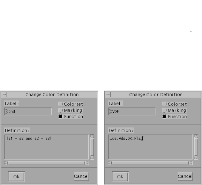
dynamic subclasses and they are used when it is necessary to initialize a place of the net with a fixed number
of elements belonging to the place color domain independently from their identity. The left dialog box of
Fig. 3.32 shows the definition of the dynamic subclass Dyn sub: it is a colored object of type “Marking”
defined as a set containing a single element drawn from the static subclass SV. The right dialog box of
Fig. 3.32 shows the definition of the symbolic initial marking for a place whose color domain contains the
static subclass SV: the initial marking is simply defined as the dynamic subclass Dyn sub.
WARNING! SWN models in which symbolic initial marking are used can be analyzed only with symbolic
solver.
Example of function definition In Fig.3.33 examples of colored function definition is given:
Figure 3.33: Definition of colored functions.
the toggle “Function” is switched on; the name of the functions cond and IVOF, respectively, are filled
in the corresponding “Label” areas. Function cond is a macro defined as the guard [s1 = s2 and s2 =
s3] that has to be assigned to a color label of a transition; function IVOF, instead, is a macro defined as the
cartesian product of the following colored classes Ide,Vds,OK and Flag that has to be assigned to a place
color domain.
Change: change color operation allows to modify the colored definitions and the color attribute of the objects
(place/transition/arc). To change a previous specification of a given colored definition (or a colored attribute
of an object), click over the colored definition name (the object) located somewhere in the canvas: this
action causes the corresponding Change dialog-box to pop-up. For example, in case of modification of a
colored definition, to change the values in the areas of the Change Color Definition dialog box click over
the corresponding areas to activate them and then overwrite the old values with the new ones. Finally,
either click over the “OK” button to confirm the changes or click over the “Cancel” button to keep the old
72
settings.
Select: select a color definition operation allows to select a specific color definition of the current loaded model
by clicking over the color definition name with the left mouse button; this action causes a broken rectangle
to superpose the color definition name. Selection operation is normally used along with other operations,
e.g., with the Move action to move the color definition name in a different location of the canvas. To
reset the Select operation, choose in the Action menu the End Selection option (the broken rectangle that
superposes the selected color definition name, will disappear).
Move: move a color operation causes the shape of the mouse cursor to change into an arrow; to move a either
a color definition or a color label (place color domain, guard, arc expression) simply click with the left
mouse button over the colored item to be moved, move the mouse cursor to choose the desired location in
the canvas to put it and click again to fix it in the desired location.
Delete: delete a color operation allows to delete a color definition present in the canvas; to delete an existing
color definition click over the color definition result to be removed with the left mouse button.
Show: show a color definition operation allows to visualize the definition of the colored item.
73
Chapter 4
Solvers
GreatSPN2.0.2 is composed of many separate programs that cooperate in the costruction and analysis of PN
models by sharing files. Using network file system capabilities, different analysis modules can be run on different
machines in a distributed computing environment.
All solution modules use special storage techniques to save memory both for intermediate result files and
for program data structures. The more restrictive constraints are on the Reachability Graph construction phases;
the current practical limit depends on the specific model, but indicatively ranges from few hundred thousands
up to few millions markings on Pentium III PCs with 256 MB of memory. The current modular structure of
GreatSPN2.0.2 is shown in Figure 4.1, in which rectangles represent program modules while ovals represent both
the intermediate and the result files generated by the modules. In this chapter we will describe the GreatSPN2.0.2
modules and result files related to the analysis of a GSPN/SWN model, while the compositionality aspect and
the links to other tools will be dealt in chapters 5and 6respectively.
Elimination of result files The elimination of all the files resulting from the solvers execution can be performed
either through the GUI (see File→Remove Results option in Chapt. 3) or by typing the following command:
> RMNET [-n] netdirectory/netname
where netdirectory is the directory in which the GSPN model has been saved and netname is the name of the net
(without extensions). If the -n option is used then also the net definition files are removed.
4.1 Structural analyzers
The structural analysis portion of the GreatSPN2.0.2 package implements most of the classical structural analysis
techniques for the analysis of Place/Transition nets, plus the ad-hoc techniques proposed by our group for the
detection of conflicts, mutual exclusion and confusion in the framework of nets with priorities and inhibitor
arcs. All the modules that support the structural analysis of a GSPN model read the net description files (see
74
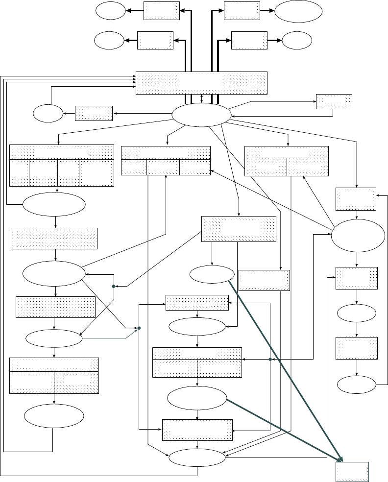
TRG and TRS files
Information on
model liveness
EMC generation
EMC files
Results
Structural properties
files
MC solution
Transient Steady state
Computation of
performance indices
Marking probability
distribution
Analysis of TRG structure
Deadlock and
home states Liveness
GSPN simulation
Engine Measurer Statistics
SRG and EMC
generation
SRG
SWN simulation
Colored Symbolic
GreatSPN2.0.2
GUI
MultiSolve
GUI
Bounds Net
description files
Results
Results
collector
Nets description
files (instances)
Tgif
translator
APNN
translator
PROD
translator
APNNnet
Tgifnet
table files
Plot
generator
Fluid net
translator
GNUplot
files
Generation of information
for efficient marking coding
Information for
marking encoding
TRG and TRS generation
Non-markovian
PNs simulation
algebra
PRODnet,
PROBEmacros
Fluid net
export to
CPN-AMI
Structural analysis
P-inv
T-inv ecs,cc,sc,
me,bnd,
unb,sub
deadlock
trap implicit
places
Figure 4.1: Graphical representation of the modular structure of GreatSPN2.0.2 .
75

the appendix A for their format definition) and produce one or more intermediate result files in ASCII form. A
complete list is given in table 4.1. They are all independent of each other apart from struct.c which depends
on the result file produced by module pinvar.c (since the mutual exclusion property is computed based on the
knowledge of the elementary P-invariant as well as the net structure). Result files contain sequences of either sets
or bags of transitions and/or places, according to the following descriptions.
extension format description
.bnd N pairs upper and lower bound for tokens in places
.cc T pairs causal connection
.ecs T sets ECS and confusion structures
.impl P bags implicant places for implicit place
.mdead P sets minimal deadlocks
.me T pairs mutual exclusion
.mtrap P sets minimal traps
.pin P bags place invariants
.sc T pairs structural conflict
.sub T sets immediate subnet partition
.tin T bags transition invariants
.unb T bags structurally unbounded places and transition sequences
Table 4.1: List of structural result files.
4.1.1 Invariants
4.1.1.1 Modules
pinvar.c,tinvar.c: compute minimal-support, canonical Place and Transition invariants, respectively, with
a modified Martinez-Silva algorithm [29]. P(T)-invariants modules can be launched either through the Great-
SPN2.0.2 GUI (see Chapt.3) or from a terminal. In the latter case the following commands have to be used:
> pinv netdirectory/netname for P-invariant computation and
> tinv netdirectory/netname for T-invariant computation,
where netname is the name of the GreatSPN2.0.2 net and netdirectory is the directory containing netname. The
commands compute and display the P(T)-invariant of the model.
76
4.1.1.2 Result files structure
.pin file: contains a list of Bags of places to be interpreted as the P-invariants computed on the net description
contained in the corresponding .net file.
First line: integer containing the total number of bags in the file.
Subsequent lines (one per P-invariant): integer containing the number of non-null entries of the bag, followed on
the same line by one pair of integers per non-null entry: the first integer of the pair represents the multiplicity;
the second integer of the pair represent the ordinal number of the place (position of the place in the list of places
as contained in the .net file).
Last Line: always 0 as a first integer of the line (a null Bag).
.tin file: contains a list of Bags of transitions to be interpreted as the T-invariants computed on the net description
contained in the corresponding .net file.
First line: integer containing the total number of bags in the file.
Subsequent lines (one per T-invariant): integer containing the number of non-null entries of the bag, followed on
the same line by one pair of integers per non-null entry: the first integer of the pair represents the multiplicity;
the second integer of the pair represent the ordinal number of the transition (position of the transition in the list
of transitions as contained in the .net file).
Last line: always 0 as a first integer of the line (a null Bag).
4.1.2 Minimal deadlocks and traps
4.1.2.1 Module
deadlock.c: compute minimal Deadlocks or Traps with a modified Alaiwan-Toudic algorithm [1]. Minimal
deadlocks and traps computation and visualization can be obtained either by choosing the corresponding options
in the Net→Struct menu of the GreatSPN2.0.2 GUI (see Chapt.3) or by launching the following commands from
a terminal:
> deadl netdirectory/netname for minimal deadlocks computation and
> traps netdirectory/netname for traps computation,
where netname is the name of the GreatSPN2.0.2 net and netdirectory is the directory containing netname.
4.1.2.2 Result files structure
.mdead file: contains a list of Sets of places to be interpreted as the minimal deadlocks computed on the net
description contained in the corresponding .net file.
First line: integer containing the total number of sets in the file.
77
Subsequent lines (one per minimal deadlock): integer containing the number of non-null entries of the set,
followed on the same line by one integer per non-null entry representing the ordinal number of the place (position
of the place in the list of places as contained in the .net file).
Last line: always 0 as a first integer of the line (a null Set).
.mtrap file: contains a list of Sets of places to be interpreted as the minimal traps computed on the net description
contained in the corresponding .net file.
First line: integer containing the total number of sets in the file.
Subsequent lines (one per minimal trap): integer containing the number of non-null entries of the set, followed
on the same line by one integer per non-null entry representing the ordinal number of the place (position of the
place in the list of places as contained in the .net file).
Last line: always 0 as a first integer of the line (a null Set).
4.1.3 Implicit places
4.1.3.1 Module
implp.c: verifies structurally implicit places with Silva’s algorithm [35]. Implicit place verification can be
checked either through the GreatSPN2.0.2 GUI (see Chapt.3) or by launching the following command from a
terminal:
> implp netdirectory/netname placenumber
where netname is the name of the GreatSPN2.0.2 net, netdirectory is the directory containing netname and
placenumber is the number of the place of the net to be tested as appears in the net definition file netname.net.
4.1.3.2 Result file structure
.impl file: contains a list of bags of places containing the implicant places of a given places tested for the
property of being implicit. The place is not implicit if no bag of implicant places is found.
First line: an integer containing the number of bags of implicant places, listed in the following of the file, one
bag per line.
Each implicant places line: first integer containing the number N≥2 of non-null entries of the bag, followed on
the same line by one pair of integers per non-null entry: the first integer of the pair represents the multiplicity;
the second integer of the pair represent the ordinal number of the place. The last entry of the bag represents the
implicit place itself.
Last line: always 0 as a first integer of the line (a null Bag).
78
4.1.4 ECS-Confusion-ME-SC-CC
4.1.4.1 Module
struct.c computes structural token bounds for places and structural conflict, mutual exclusion, causal con-
nection, extended conflict sets, structural confusion, and subnets of independent higher priority transitions, for
priority nets with inhibitor arcs, as described in [12,33,2].
4.1.4.2 Result files structure
.cc file: contains a description of the causal connection relations (CC) holding for each transition. One line is
listed per transition, the i-th line referring to the i-th transition (transition in position iin the list of transition as
contained in the .net file).
Each line: contains the set of transition in CC relation with the current one. The first integer tell the number of
non-null entries of the set; then one integer follows per non-null element, with the ordinal number of the transi-
tion.
.ecs file: contains both a description of the Extended Conflict Sets of immediate transitions (ECSs), and the
possible confusion relations. These two results are stored as two subsequent lists, each one terminated by a 0
character on a separate line.
One line per ECS: an integer representing the number of transitions in the current ECS, followed on the same
line by one integer per non-null item of the set representing the ordinal number of an immediate transition (i.e.
the position of the immediate transition in the list of transitions as contained in the .net file).
Last line of the ECS list: One integer value = 0 used as a list terminator.
One line per confusion relation: a first integer representing the ordinal number of the confused ECS, i.e. the
position of the ECS description line in the above list; a second integer containing the number N≥3 of transitions
in confusion relation; two integers containing the ordinal numbers of two transitions of the current ECS that are in
confusion relation with each other; a possible list of integers (as many as N−3) representing the ordinal number
of the transition originating the confusion.
Last line of the confusion list: one integer value = 0 used as a list terminator.
.me file: contains a description of the mutual exclusion relations (ME) holding between transition pairs. One line
is listed per transition pair in ME relation.
Each line: contains two integers with the ordinal numbers of the transitions in ME relation (i.e. their position in
the list of transitions as contained in the .net file).
Last line: one integer value = 0 used as a list terminator.
79
.sc file: contains a description of the structural conflict relations SC holding for each transition. One line is
listed per transition, the i-th line referring to the i-th transition (transition in position iin the list of transitions as
contained in the .net file).
Each line: contains the set of transition in SC relation with the current one. The first integer tell the number of
non-null entries of the set; then one integer follows per non-null element, with the ordinal number of the transi-
tion.
.sub file: contains the partition of the net in subnets of independent immediate transitions.
First line: an integer containing the number N≥1 of subnets in which the net is partitioned. The first subnet
contains all timed transitions, while the following ones contain independent sets of immediate transitions.
After the first line the file is organized in two subsequent lists of subnet description lines. The first list contains
two consecutive lines per subnet. The second list contains one line per subnet.
Each of the following n=1,...,Npairs of consecutive lines: First line of the pair: set of places of the n-th,
stored as a first integer with the number of non-null entries of the set, followed by one integer number per entry
containing the ordinal number of the place.
Second line of the pair: set of transitions of the n-th subnet, stored as a first integer with the number of non-null
entries of the set, followed by one integer number per entry containing the ordinal number of the transition.
Each of the following 2N+nlines (n=1,...,N)set of input/inhibition places of the n-th subnet, stored as a first
integer with the number of non-null entries of the set , followed by one integer number per entry containing the
ordinal number of the place.
4.1.5 Structural boundedness
4.1.5.1 Module
unbound.c: verifies the structural unboundedness and associated unbounded transition sequences with a modi-
fied version of Molloy’s method [32];
4.1.5.2 Result files structure
.bnd file: contains a description of the upper and lower bounds on the number of tokens in each place of the net.
One line is listed per place, the i-th line referring to the i-th (place in position iin the list of places as contained
in the .net file).
Each line: contains a pair of integers. The first integer tells the lower bound for the number of tokens in the cor-
responding current place. The second integer tells the upper bound for the number of tokens in the corresponding
current place.
80

.unb file: contains a list of sets of unbounded places together with the transitions bags that, if fireable as transition
sequences, make them unbounded. One line is used to store one set of unbounde places and their corresponding
transition bag. The list is terminated by a line containing only the integer value 0.
Each line: first integer containing the number of non-null entries of the set of unbounded places, followed on the
same line by one integer per non-null entry representing the ordinal number of the place (position of the place
in the list of places as contained in the .net file). Always on the same line, one integer follows containing the
number of non-null entry: the first integer of the pair represents the multiplicity; the second integer of the pair
represent the ordinal number of the transition.
Last line: always 0 as a first integer of the line (a null Set).
4.2 Performance bounds solver
GreatSPN2.0.2 package includes modules for the computation of the performance structural bounds of both
places and transitions of the net. Bounds are obtained from the net structure, the initial marking and the transition
rates by solving a linear programming problem (LPP) presented in[16].
4.2.1 Modules
disab lp.c: 1) decomposes the marking vector in disabling components for each immediate transition with more
than one input/inhibition arcs; 2) produces the reachability constraints; 3) produces the throughput flow balance
constraints for every place; 4) detects the vanishing places; 5) produces the Extended Free Choice throughput
constraints; 6) produces the inequalities for Persistent or Age Memory or Preselection Timed Transitions. Struc-
tural conflicts of immediate transitions are optimized.
WARNING! The case of conflict with race policy and with enabling memory policy for timed transitions is not
properly handled. The net description is assumed not to contain such cases.
flow lp.c: produces equations of type: ∀p∈P:∑t∈•pxtW(t,p)≥∑t∈p•xtW(p,t), i.e., the throughput flow
balance constraints for all places.
mark lp.c: produces equations of type M=M0+Cσ, i.e., the reachability constraints, for a predefined list of
marking vectors.
4.2.2 Result file structure
The performance bound modules produce the list of result files given in Table 4.2 in ASCII format.
WARNING! In order to obtain correct results, to compute performance bounds of a transition, launch the
performance bound solver on a place first.
81

extension format description
.lp disab ascii list of all the constraints of the LPP
.lp in ascii place/transition name whose bounds are computed and list of all the constraints of the LPP
.lp mark ascii linear programming equations
.lp out ascii solution of the LPP
Table 4.2: List of performance bounds result files.
4.3 Analytic solvers
Analytic solvers produce the list of intermediate and result files given in Table4.3. Sets are described in ASCII
files as lists of either place or transition ordinal numbers1. Bags are described in ASCII files as lists of pairs of
natural numbers representing the multiplicity and the ordinal number of either places or transitions.
Unsigned compacts in the range [0,222 −1]are stored in non-ASCII files using a compact coding in one, two,
or three bytes 2
WARNING!
1. The maximum capacity of each place is MAX =255 even though this constraint is not signalled when an
analytic module is launched from the GUI.
2. If the net is characterized by an initial dead marking, the launch of an analytic solver provokes a segmen-
tation fault.
3. Reachability graph generator does not produce the RG in case of nets with all immediate transitions.
4.3.1 GSPN solvers
4.3.1.1 Reachability Graph generator
Modules grg.c, grg prep.c, grg stndrd.c perform the Reachability Graph expansion of a GSPN model
by reading the net description files. The algorithm begins by putting the initial marking into the Reachability
Set, then all the enabled transitions in newly found markings are fired. Timed transition firing proceeds using a
breadth-first policy, while immediate transition paths are followed depth-first until a tangible marking is reached.
1As ordinal number we mean the number of line in the net definition file that describes the place or the transition
2Numbers in the range [0,127]are encoded in a single byte, with the most significant bit set to 0; numbers in the range [128,214 −1]
are encoded in two bytes, with the two most significant bits of the first byte set to 10; numbers in the range [214,222 −1]are encoded in
three bytes, with the two most significant bits of the first byte set to 11. Since most of the information is recorded using small integers
(falling in the range [0,127], this coding technique allows the use of only one byte for each piece of information most of the times.
82

extension format description
GSPN models
.grg ascii data structure description for reachability graph
.aecs T sets actual conflicts sets found in the reachability graph
.rgr aux ascii auxiliary information on reachability graph
.crgr special code coded tangible reachability graph
.ctrs uns. bytes coded tangible reachability set
.livlck uns. comp. terminal strongly connected components of the RG
.liveness N lists enabling and liveness bounds for transitions
.gmt ascii data structure description for EMC construction
.doubles C doubles floating point numbers contained in the EMC
.emc special code compact coded EMC state transition matrix
.epd and .mpd C doubles marking probability distribution vectors
.gst ascii data structure description for performance result computation
.tpd C doubles token probability distributions in places
.sta ascii output performance results
Table 4.3: List of analytical result files.
The ordering of the markings in the Reachability Set resulting from this firing policy is exploited by the following
modules of the package to implement a very efficient reduction of vanishing markings in the case that no-zero
time loop is present. In the program data structure, markings are lexicographically ordered by means of a balanced
binary tree in order to improve the efficiency of the search procedures. GSPN Reachability Graph generator can
be launched either through the GreatSPN2.0.2 GUI (see Chapt.3) or by typing the following command from a
terminal:
> newRG netdirectory/netname
where netdirectory is the directory in which the GSPN model has been saved and netname is the name of the net
(without extensions).
Module show stndrd.c displays the Tangible Reachability Graph (TRG) of a GSPN model without net-dependent
files compilation. To display the TRG of a GSPN model already generated use the following command from a
terminal:
> showRG netdirectory/netname [opt]
where netdirectory is the directory in which the GSPN model has been saved and netname is the name of the net
(without extensions). Possible display options [opt] are:
83

-s to show the Tangible Reachability Set;
-t to show the Tangible Reachability Graph (default option);
-r to show the Reverse Tangible Reachability Graph.
4.3.1.2 TRG structure analyzer
Module strong con.c computes the livelocks and the deadlock states of the TRG of a GSPN model.
Module liveness.c computes transition enabling and liveness bounds of a GSPN model: in particular, it takes
the TRG and its associated livelock description as inputs and computes the actual bounds for infinite server timed
transitions.
To launch the reachability graph generator and the structure analyzer of the created TRG of a GSPN model
from a terminal, use the following command:
> checkRG netdirectory/netname
where netdirectory is the name of the directory in which the GSPN model has been saved and netname is the
name of the net without extensions.
4.3.1.3 Markov Chain generator
Modules gmt prep.c, gmt stndrd.c: converts the Tangible Reachability Graph of a GSPN model into the
corresponding Continuous Time Markov Chain (CTMC) without net-dependent files compilation. The module
uses a depth-first algorithm to follow the immediate transition tangible to tangible paths and keep tracks of the
resulting probabilities of already followed paths to achieve a higher computational efficiency. To launch the
Reachability Graph generator and the CTMC generator from a terminal use the following command:
newMT netdirectory/netname
where netdirectory is the name of the directory in which the GSPN model has been saved and netname is the
name of the net without extensions.
To display the infinitesimal generator matrix, type the following command:
shownmtx netdirectory/netname
where netdirectory is the name of the directory in which the GSPN model has been saved and netname is the
name of the net without extensions.
4.3.1.4 Steady State solver
ggsc.c: computes the steady-state solution of the CTMC underlying a GSPN model. The solver has been
implemented using standard sparse matrix computation algorithms, adapted to the solution of a set of linearly
84
dependent equations augmented with the probability normalization condition. The Gauss elimination (actually a
modified L-U direct decomposition) proceeds without pivoting to preserve the sparse band-diagonal structure of
the matrix resulting from the breadth-first firing of the Reachability Graph. Indeed, row or column permutation
would determine a large fill-in during the elimination phase, thus making impractical the analysis of large ma-
trices. Despite this simplification the algorithm exhibits a very good numerical stability, due to the fact that the
diagonal elements used as pivot, actually are (by definition) partial pivots, since they are made equal to the sum of
all the other elements in the row as proved in[26]. Indeed it is possible to use this method even in case of “stiff”
problems with matrix entries differing up to eight orders of magnitude on machines with 64 bit floating-point
representation. The size of the matrix to be solved can range up to 1023 ×1023. In case of larger matrices it is
necessary to resort the Gauss-Seidel iterative method. In the present implementation, sparse matrices of order up
to 32000-64000 can be solved, but the convergence is badly affected by ill-conditioned or “stiff” problems. To
launch the Steady State solver from a terminal use the following command:
newSO netdirectory/netname
where netdirectory is the name of the directory in which the GSPN model has been saved and netname is the
name of the net without extensions.
To display the state probability vector, type the following command from a terminal:
showprob netdirectory/netname
where netdirectory is the name of the directory in which the GSPN model has been saved and netname is the
name of the net without extensions.
4.3.1.5 Transient solver
gtrc.c: computes the transient solution of the CTMC underlying a GSPN model using a matrix exponentiation
algorithm. The major problem in this case is a “good” choice of the time integration step: large integration steps,
depending on the matrix eigenvalues, can result in large round-off errors and poor numerical stability; on the
other hand, steps that are too small may involve unnecessary row by column matrix products. In our program
an initial estimate of the optimal integration step is made according to the maximum transition rate found in the
matrix; then the step is dynamically adjusted in order to keep it as large as possible, without incurring in too large
round-off errors during vector addition.
4.3.2 SWN solvers
to be completed
85

4.4 Simulators
4.4.1 GSPN simulation
GSPN simulator uses a “Natural Regeneration” method mechanism[27] to provide point of estimates of the aver-
age number of tokens in each place together with their confidence intervals, as well as to collect the user defined
statistical results. Machine-independent congruent pseudo-random sequence generators are used to implement
stochastic transition timings. This program provides a bypass to other solution modules, and can be effectively
exploited to obtain results in case of analytically untractable models. GSPN simulator can be launched through
the GreatSPN2.0.2 GUI (see Chapt.3).
4.4.1.1 Modules
engine control.c: simulation control and communication module for the simulation engine.
engine event.c: event-driven simulation kernel for simulation engine of GreatSPN2.0.2 package. The program
allows both normal (forward) and reversed (backward) simulation. Periodic checkpoints are stored on file in order
to allow both extended backtracking and possibility of continuation and resume of previous runs.
engine pn.c: PN routines for the simulation engine. No marking dependency is allowed for immediate tran-
sitions. This module is derived from “grg stndrd.c ” and it uses similar data structures and the same type of
optimization techniques.
measure checkpoint.c: checkpoint routines for measurer module of GreatSPN2.0.2 .
measure pn.c: module for the definition of measurement of performance indices for GSPN simulation.
4.4.1.2 Result file structure
In this part the files resulting from the launch of a GSPN simulator are described.
extension format description
.etrace ascii
.mtrace ascii
.strace ascii
.tpd C doubles token probability distributions in places
.sta ascii output performance results
Table 4.4: List of GSPN simulation result files.
86

4.4.2 SWN simulation
4.4.2.1 Modules
SWN simulators can be launched either through the GreatSPN2.0.2 GUI (see Chapt.3) or by typing the following
commands from a terminal:
> swn ord sim [opt] netdirectory/netname
for ordinary simulation and
> swn sym sim [opt] netdirectory/netname
for symbolic simulation[], where netdirectory is the name of the directory in which the net definition files are
located and netname is the name of the net model without extensions. [opt] represents the following list of
options that allow to set the parameters for a simulation run:
-f first tr length to set the length of evolution phase between batchs that must be discarded;
-t tr length to set the length of initialization phase;
-m min btc to set the dimension of the minimum batch;
-M max btc to set the dimension of maximum batch dimension;
-a approx to set the precision of the approximation in the parameters estimation;
-c conf level to set the confidence level in the parameters estimation;
-s seed to set the seed for the random numbers generation;
-o start to set the starting time for debug output.
WARNING! The results computed from a simulation run are basically the mean number of token in places
and throughputs of transitions and they are all independent from the color classes. Refined results - color class
dependent - and, in general, user defined results can be obtained by using the extended SWN ordinary simulation
(see Section 4.5).
4.4.2.2 Result file structure
In this part the files resulting from the launch of a SWN simulator are described.
extension format description
.simresCl1n1Cl2n2...Clnnnascii output performance results
.sta ascii output performance results
Table 4.5: List of SWN simulation result files.
87

4.5 Extended SWN features
Several extensions have been developed for the SWN analysis modules; in the following we will describe the
most important new added features.
4.5.1 Transient analysis of SWN models
The SWN reachability analysis prototypes have been interfaced with the transient analysis software developed
for the GSPN models (implementing a numerical approach based on a randomization technique).
4.5.2 Simulation of SWN models with GEN transitions
The simulation of SWN models with ordinary marking has been extended to include generally distributed firing
time transitions (GEN transitions), diferent memory policies and several policies for the disabling and re-enabling
of firing instances.
Temporal specifications of GEN transitions have to be defined in a file named as netname.dis, where netname
is the name of the SWN model constructed with GreatSPN2.0.2 , and located in the same directory of the net
specification files. netmame.dis is an ASCII form file, in which each row represents the temporal specification of
a GEN transition of the corresponding SWN model. Table 4.6 shows the line syntax, expressed in BNF format,
to be used for the temporal specifications of GEN transitions. All the terminal keywords are represented as C-
language strings within quotation marks except for the following terms: <real number >, indicates a positive
real number, and <integer >, indicates a non negative integer number. Notation #(XX){...}denotes the repetition
of the string in braces for a number of times derived by interpreting the string XX as a natural number.
4.5.2.1 Rescheduling/descheduling policies
Rescheduling and descheduling policies need to be defined in case of GEN transitions characterized by multi-
ple/infinite server semantics. Rescheduling policy defines which transition instance of a multiple enabled GEN
transition previously suspended has to be inserted again in the event list. Descheduling policy defines, instead,
which transition instance of a multiple enabled GEN transition which decreases its enabling degree has to be
removed from the event list. Possible choices are:
RANDOM : the transition instance is chosen randomly;
FIRST DRAWN : the transition instance among those suspended/enabled that was first generated;
LAST DRAWN : the transition instance among those suspended/enabled that was last generated;
FIRST SCHED : in case of descheduling, the enabled transition instance with the least scheduling time. In
case of rescheduling, the suspended transition instance with the least value of the timer;
88

<row >::= <tr name > <firing pol > <reschedule pol > <deschedule pol > <distrib >
<firing pol >::= “AGE” |“ENABLING”
<reschedule pol >::= <pol >
<deschedule pol >::= <pol >
<pol >::= “RANDOM” |“FIRST DRAWN” |“LAST DRAWN” |
“FIRST SCHED” |“LAST SCHED”
<distrib >::= “DET” |“ERL” <n stage >|
“IPO” <n stage >#(<n stage >){<rate >} |
“IPER” <n stage >#(<n stage >){<prob > <rate >}|
“UNIF” <lower > <upper >|“NORM” <mean > <devstd >|
“BAR” <n unif >#(<n unif >){<lower > <upper > <prob >}
<n stage >::= <integer >
<n unif >::= <integer >
<rate >::= <real number >
<prob >::= <real number >
<lower >::= <real number >
<upper >::= <real number >
<mean >::= <real number >
<devstd >::= <real number >
Table 4.6: BNF format of a line of the .dis file
LAST SCHED : in case of descheduling, the enabled transition instance with the greatest scheduling time. In
case of rescheduling, the suspended transition instance with the greatest value of the timer.
4.5.2.2 Firing time distributions of the GEN transitions
SWN simulator allows to specify for each GEN transition of the model one the following types of distributions:
DET Deterministic distribution D[τ]: no further parameter needs to be specified. The delay value τis read
from the net definition file .net and it corresponds to the value associated either to the rate or to the rate
parameter of the transition. Rate/rate parameter has to be defined during the model specification via the
GreatSPN2.0.2 GUI.
ERL Erlang distribution Erl[k,λ]: the number of stages kmust be specified as parameter. The stage rate λis
read from the net definition file .net file and it corresponds to the value associated either to the rate or to
the rate parameter of the transition.
IPO Ipo-exponential distribution Ipo[k,λ1,...,λk]: the number of stages kand the stage rates {λi}i=1,...,kmust
be specified as parameters list.
89

IPER Hyper-exponential distribution Hyp[k,(α1,λ1),...,(αk,λk)]: the number of stages kand the pairs de-
scribing the probability and the rate of each stage {(αi,λi)}i=1,...,k, must be specified as parameters list.
UNIF Uniform distribution U[l,u]: the lower land upper ubounds must be specified as parameters.
NORM Normal distribution N(µ,σ): the mean value µand the standard deviation σmust be specified as pa-
rameters.
BAR Composition of Uniform Distributions ∑k
i=1piU[li,ui]: the number of uniform distributions kand, for each
uniform distribution Ui, the lower bound li, the upper bound uiand the associated probability pimust be
specified as parameters list.
WARNING! When constructing the SWN model via GUI, all the GEN transitions have to be specified as they
were negative exponential distributed, i.e. white-box transitions also in case of deterministic transitions.
How to launch the simulation Launch the SWN ordinary simulator (see command 4.4.2.1) from a terminal
together with the desired simulation options. Assuming the executable module swn ord sim is located in the
directory ./experiment, then the SWN model has to be saved in the subdirectory ./experiment/nets.
4.5.3 Refined perfomance results
The statistical analysis module of SWN ordinary simulation has been extended to estimate structured performance
indexes. Besides the aggregated mean number of tokens and transition throughput, it is possible to estimate the
mean number of tokens that satisfy criteria based on the place color domain as well as the estimation of transition
throughput when the firing instances satisfy a given predicate.
4.5.3.1 Mean number of tokens in a place
GreatSPN2.0.2 allows to define the mean number of tokens in a place at the following levels of detail:
1. mean number of tokens with no color distinction (simple performance index);
2. mean number of tokens for each element of the static partition the place color domain is made of. It
is a structured performance index consisting of ndifferent values where nis the cardinality of the static
partition of the place color domain (maximum refinement);
3. mean number of tokens that satisfy a given predicate on the place color domain (intermediate refinement).
Example 1 Let us assume that a place phas been characterized by the following place color domain:
90

CD(p)=Cl1×Cl1×Cl2
Cl1 = sub1cl1∪sub2cl1∪sub3cl1
Cl2 = sub1cl2∪sub2cl2
Then a color consists of a triplet hCl1 1,Cl1 2,Cl2 1iwhere Cl1 1 ∈subicl1,Cl1 2 ∈sub jcl1,and Cl2 1 ∈
subkcl2,for i,j∈ {1,2,3},k∈ {1,2}.
1. Case of simple performance index. In GreatSPN2.0.2 syntax has to be defined as:
E{#p }
We obtain a unique performance result that represents the mean number of tokens in place pand it is com-
puted considering tokens without identities.
2. Case of maximum refinement. In the GreatSPN2.0.2 syntax has to be defined as:
E{#p(*)}
We get a result for each element of the static partition of the place color domain that represents the mean
number of tokens whose colors belong to the element. In case of ex. 1, we obtain 18 results of type
p[subicl1,sub jcl1,subkcl2] = mi jk,i,j∈ {1,2,3},k∈ {1,2}, where mi jk is the mean number of tokens
whose colors belong to the element hsubicl1,sub jcl1,subkclkiof the static partition of the place color
domain.
3. Case of intermediate refinement. Between the two previous level of details, there are different types of
means number of tokens in place pthat can be obtained; we have classified them with respect to their
granularity in projection, selection and general predicate means.
Projection. This type of results are obtained by performing a projection with respect to those component
classes of the place color domain we are interested in. In ex.1, we can choose to project the color domain
of place pwith respect to the second and the third component classes, in GreatSPN2.0.2 syntax:
E{#p(Cl1 2,Cl2)}
where Cl1 2 indicates the second repetition of the colored class Cl13, obtaining for each subset Cl1×
sub jcl1×subkcl2j∈ {1,2,3},k∈ {1,2}of the static partition of the place color domain, the mean num-
ber of tokens mpjk, whose colors belong to that subset. Geometrically, the color domain of place pcan be
represented by a parallelepiped: its projection with respect to the second and the third component classes
results in the rectangle highlighted in Fig. 4.2 lying on the plane Cl1 2×Cl2.
3The third component, since it is a unique repetition of the colored class Cl2, is referred by using the name of the class without
specifying its repetition, i.e., Cl2 1 = Cl2.
91
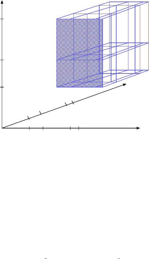
Cl1_2
Cl2
Cl1_1
sub1cl1 sub2cl1 sub3cl1
sub1cl1
sub2cl1
sub3cl1
sub1cl2 sub2cl2
Figure 4.2: Projection of the color domain of place p.
The following relations hold among these means and the ones obtained in case of maximum refinement:
mpjk =
3
∑
i=1
mi jk,j∈ {1,2,3},k∈ {1,2}.
Selection. This type of results are obtained by performing a selection among the set of means got from
projection operation. The selection operation allows to extract the means number of tokens whose colors
belong to a specific element of the static partition of the place color domain we are interested in. In ex.1,
among the six means mpjk we can choose to compute only the two means mp2k,k∈ {1,2}by defining the
following structured result:
E{#p(Cl1 2,Cl2) | SEL = [d(Cl1 2) = sub2cl1] }
WARNING! The selection operation can contain only predicates that specify the membership (or not
membership) of a color belonging to the defined projection of the place color domain.
General predicate. This type of results are obtained by extracting specific elements of the place color
domain when its component classes are made of subclasses containing more than one element. General
predicates are applied after a projection operation and, in case, a selection operation have been performed.
In ex.1, the structured result:
E{#p(Cl1_2,Cl2) |
SEL = [d(Cl1_2) = sub2cl1)], COND = [d(Cl1_1) <> sub1cl1 and Cl1_1 <> Cl1_2] }
92

consists of two means and it is obtained by giving two constraints over the elements of the place color
domain: 1) the first component of a color do not have to belong to the static subclass sub1cl1 of the color
class Cl1; 2) the firsts two components of a color have to be different as well in case they belong to the
same static subclass. For example, let us assume that the static subclasses are defined as the following sets
of elements:
sub1cl1 = {a}
sub2cl1 = {b,c}
sub3cl3 = {d}
sub1cl2 = {e,f}
sub1cl2 = {g,h,l}
and, in a given reachable marking of the net, the place pcontains tokens with the following colors:
hc,d,ei,ha,b,ei,hb,b,hi,hd,b,ei,hc,b,gi
Then, in the computation of the two means, tokens in place pcharacterized by one of the first three colors
will not be considered (color hc,d,eiis eliminated by the selection predicate, color ha,b,eiis eliminated
by the first part of the COND predicate, while color hb,b,hiis eliminated by the second part of the COND
predicate). Instead, tokens characterized by one of the last two colors will contribute to the computation of
the two means mp21,mp22.
4.5.3.2 Transition throughput
Similarly to the mean number of tokens in a place, in case of transition throughput as well, GreatSPN2.0.2 allows
to define results at the following levels of details:
1. transition throughput with no color distinction of the firing instances (simple performance index);
2. transition throughput for each element of the static partition of transition color domain is made of. It
is a structured performance index consisting of ndifferent values where nis the cardinality of the static
partition of the transition color domain (maximum refinement);
3. transition throughput for those colored instances that satisfy a given predicate on the transition color do-
main (intermediate refinement).
The only difference with respect to the mean number of tokens in a place is the notation: for the computation
of transition throughputs we can use directly the variables appearing on the input/output arcs of the transition
instead of using the notation ClassName i to indicate the i(th)component, belonging to the class ClassName, of
a variable.
Example 2 Let us have a transition T, depicted in Fig. 4.3, with two input places and an output place. All
the arcs are characterized by the identity function: the variables of the two input arcs are equal to hxiand hyi,
93
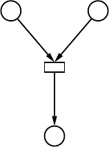
Cl1 Cl1
Cl2
T
<x> <y>
<z>
Figure 4.3: Domain of transition T.
respectively, and the variable of the output arc is equal to hzi. Input places have color domains equal to Cl1
and the output place has color domain equal to Cl2, where Cl1,Cl2 are defined in ex.1, then the transition color
domain is defined as Cl1×Cl1×Cl2.
1. Case of simple performance index. In GreatSPN2.0.2 syntax has to be defined as:
X{#T }
We obtain a unique performance result that represents the mean throughput of transition Tand it is com-
puted considering firing instances without identities.
2. Case of maximum refinement. In the GreatSPN2.0.2 syntax has to be defined as:
X{#T(*)}
We get a result for each element of the static partition of the transition color domain that represents the
mean throughputs of the firing instances whose colors belong to the element. In case of ex. 2, we obtain
18 results of type T[subicl1,sub jcl1,subkcl2] = Xi jk,i,j∈ {1,2,3},k∈ {1,2}, where Xi jk is the mean
throughput of the firing instances whose colors belong to the element hsubicl1,sub jcl1,subkclkiof the
static partition of the transition color domain.
3. Case of intermediate refinement. Between the two previous level of details, there are different types of
(mean) throughputs of transition Tthat can be obtained; as is the case of the mean number of tokens in a
place, we have classified the results with respect to their granularity in projection, selection and general
predicate mean throughputs.
Projection. This type of results are obtained by performing a projection with respect to those component
classes of the transition color domain we are interested in. In ex.2, we can choose to project the color do-
main of transition Twith respect to the second and the third component classes, in GreatSPN2.0.2 syntax:
E{#T(y,z)}
94
where yis the variable belonging to the second repetition of the colored class Cl1 and zis the variable be-
longing to the colored class Cl2, obtaining for each subset Cl1×sub jcl1×subkcl2j∈ {1,2,3},k∈ {1,2}
of the static partition of the transition color domain, the mean throughputs X pjk of the firing instances
whose colors belong to that subset. The following relations hold among these mean throughputs and the
ones obtained in case of maximum refinement:
X pjk =
3
∑
i=1
Xi jk,j∈ {1,2,3},k∈ {1,2}.
Selection. This type of results are obtained by performing a selection among the set of means got from pro-
jection operation. The selection operation allows to extract the mean throughputs of firing instances whose
colors belong to a specific element of the static partition of the transition color domain we are interested
in. In ex.2, among the six means X pjk we can choose to compute only the two means X p2k,k∈ {1,2}by
defining the following structured result:
E{#T(y,z) | SEL = [d(y) = sub2cl1] }
General predicate. This type of results are obtained by extracting specific elements of the transition color
domain when its component classes are made of subclasses containing more than one element. General
predicates are applied after a projection operation and, in case, a selection operation have been performed.
In ex.2, the structured result:
E{#T(y,z) |
SEL = [d(y) = sub2cl1)], COND = [d(x) <> sub1cl1 and x <> y] }
consists of two mean throughputs and it is obtained by giving two constraints over the elements of the
transition color domain: 1) the first component of a color do not have to belong to the static subclass
sub1cl1 of the color class Cl1; 2) the firsts two components of a color have to be different as well in case
they belong to the same static subclass.
4.5.3.3 Probability
In GreatSPN2.0.2 it is also possible to specify as performance result to compute the probability that a certain
logic condition be satisfied. Logic conditions are expressed in terms of place markings and, as in cases of mean
computations, they may be either color-independent or color-dependent: in the last case structured probability
results will be obtained. In GreatSPN2.0.2 syntax to compute a probability result the keyword Pis used instead
of the keyword E(see the SWN extended grammar of Appendix A).
95

<row >::= <user index >|<tr name >|<place name >
<user index >::= <index name >“NOPRIORITY” |<index name >“ACC” <approx val >
<tr name >::= <string >
<place name >::= <string >
<index name >::= <string >
<approx val >::= <real number >
Table 4.7: BNF format of a row of the .stat file
4.5.4 The result .stat file
The .stat file contains, for each row, these kinds of information:
•a place (transition) name, in this case during a simulation run of a SWN model the mean number of
tokens (transition throughput) will be computed without taking into account the colors (simple performance
indices).
•a user-defined performance index name along with one of the following keywords: 1) “NOPRIORITY”, in
this case the index will not considered in the test of convergence during a simulation run; 2) “ACC”, in this
case the default value assigned to the approximation parameter of the simulator is replaced for this index
by the value that follows the keyword.
The row syntax of the .stat file, expressed in BNF format, is shown in Table 4.7. All the terminal keywords
are represented as C-language strings within quotation marks except for the following terms: <real number >,
indicates a positive real number, and <string >, indicates any non-empty character string not containing blank
characters.
WARNING! If the .stat file does not exist, then all the performance indices (both the user-defined and the default
ones) are computed. Viceversa, if the .stat file exists, the default indices (not colored mean number of tokens in
places and not colored transition throughputs) are computed only if a row with the corresponding object name
(place/transition) appears. Instead, the user-defined performance indices, if they are not specified in a different
manner in the .stat file, they are always computed (i.e., they have priority).
4.5.5 Number of batches in a simulation run
The option -e has been added to the SWN simulator option-list, it allows to set the maximum number of batches
during a simulation run.
96
4.5.6 Inclusion of “reset” transitions
The SWN model specification has been enriched by using a special transition, named reset transition, with the
following semantics: when a reset transition is enabled its firing brings the model back to the initial marking. A
further generalization (not yet implemented) is the possibility of specifying any marking to be reached through
the firing of a reset transition; this extension has been introduced to ease the modeling task in several application
field (e.g., in system availability analysis).
4.6 Multiple experiments
MultiSolve is a simple graphical interface to the solution algorithms of GreatSPN2.0.2 . It allows to perform
multiple experiments with different parameters and to create figures depicting the results of the experiments.
SW Requirements In order to run correctly, MultiSolve requires the following software to be installed:
•Java (version 1.2.2 or higher);
•GreatSPN2.0.2 package;
•Gnuplot (version 3.7 or higher). To download it visit[25]).
Starting MultiSolve To invoke MultiSolve simply type multisolve followed by a carriage return. This causes
a window as shown in Fig.4.4 to appear on the user’s terminal.
How to launch a set of experiments We describe how to use MultiSolve by means of an example. Let us
suppose we have constructed the simple net depicted in Fig. 4.5 by using GreatSPN2.0.2 package.
The net is characterized by the rate parameter r1 which has been assigned to transitions T1 and T3 and by
the two measures res1=p{#P1=1}; and res2=p{#P3=1};.
The first step is to load the net to work with on MultiSolve. This can be done either by clicking on the button
labeled as Choose a net placed in the upper left corner of the window, or by typing directly the name of the net
without extension into the uppermost text field.
The second step is to define the parameters that are used in the experiments. Since MultiSolve is designed
for creating figures containing multiple curves that reflect measures, we have to define
1. the parameters of the individual curves,
2. the parameter that corresponds to the x-axis of the figure,
3. the measures that corresponds to the y-axis of the figure.
97
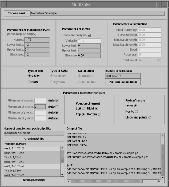
Figure 4.4: MultiSolve
The parameters of the individual curves are defined in the left upper panel of the window. A list of names of
parameters may be given in the text-field labeled Names. The entries of the list are separated by spaces. Each
entry may be the name of a transition, a rate parameter, or a marking parameter. In the other three text-fields of
the panel the user defines the set of values the parameters take. These three text-fields contain lists with as many
entries as many parameters were chosen. In the case of the example given in Fig.4.4 the rate parameter r1 takes
the values 1 and 2, while the rate of transition T3 takes the values 2 and 4. The experiments will be carried out
considering all the 4 different combinations. The text-fields of this panel may remain empty.
Parameters of the x-axis are defined in the middle upper panel. In case of transient analysis one has to define
the lower and the upper limit of the transient time, and the step-size that will be used to step ahead in time. If
steady-state analysis is performed the variable that corresponds to the x-axis has to be given as well. As before,
this variable may be the name of a transition, a rate parameter, or a marking parameter.
98
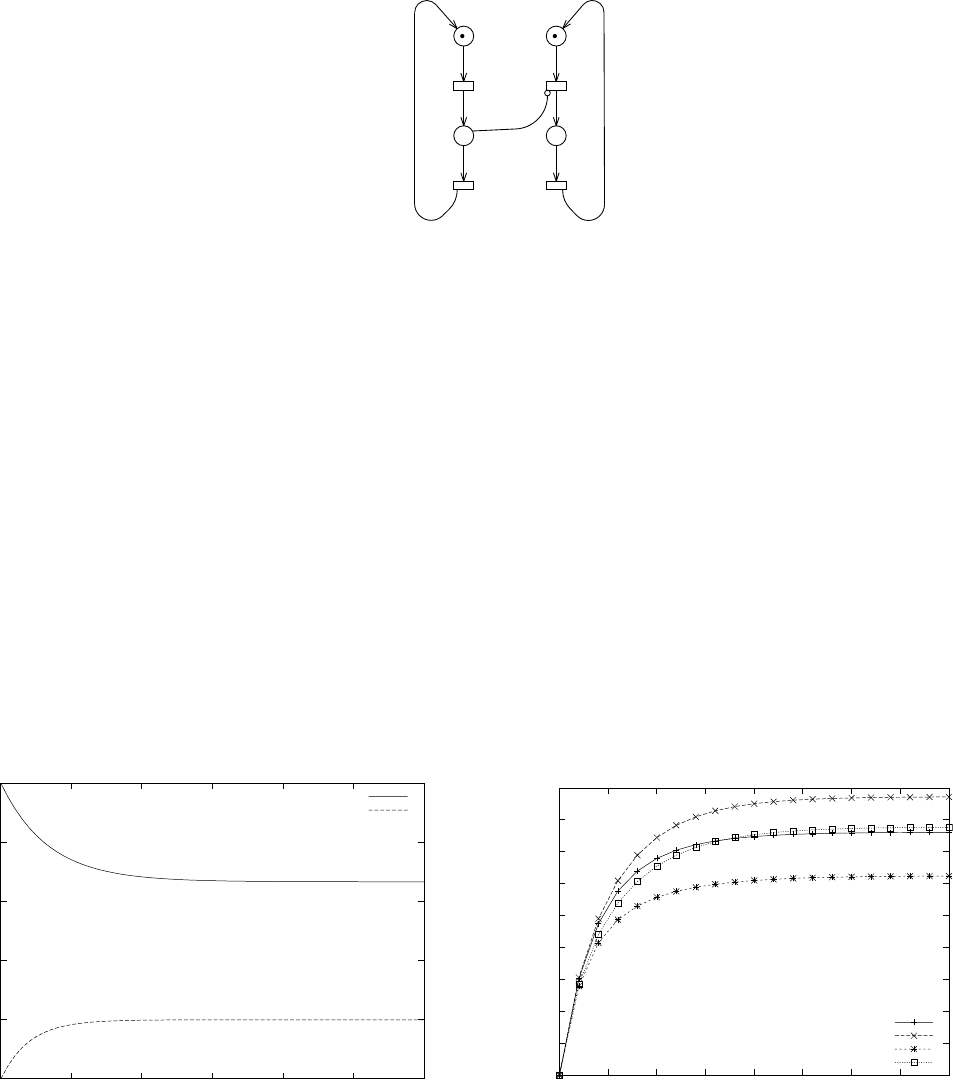
m= 1
P2
P4
P1
P3
r1=1.000000
T3
T1
T4
T2
res1
res2
Figure 4.5: A simple example
The measures that will be computed have to be given in the text-field called Results to calculate. This text-
field contains a list separated by spaces in which an entry is either a measure already defined in the net or the
name of a transition. If the name of a transition is given then the throughput of the transition is computed. In case
of our example the two measures and a transition name compose the set of results to calculate.
Having defined the parameters of the figure, we have to choose the type of analysis to perform. One has
define the type of net to work with. A net may be a GSPN or a SWN, a SWN may be ordinary or symmetric.
In case of steady-state analysis the user may choose between exact (analytic) or simulative solution. The above
choices can be made by selecting appropriately among the options represented by the check-buttons named Type
of net, Type of SWN and Calculation. In case of simulation the parameters of the simulation can be modified
in the right upper panel of the window.
The calculations are performed by clicking on the button named Perform calculations. The results of the
0
0.2
0.4
0.6
0.8
1
0 0.5 1 1.5 2 2.5 3
Time
res1,r1=1,T3=2
res2,r1=1,T3=4
Figure 4.6: Example I
0
0.05
0.1
0.15
0.2
0.25
0.3
0.35
0.4
0.45
0 0.5 1 1.5 2 2.5 3 3.5 4
Throughput
Time
T4, case I
T4, case II
T4, case III
T4, case IV
Figure 4.7: Example II
99
calculations are saved in a file in table format. The name of the file is composed by the name of the net and
the extension results. The first column of the file contains the values along the x-axis. The other columns
corresponds to a measure with a combination of parameters. In the case of the example in Fig.4.4, the file contains
13 columns: the first describes the transient time, while the other 12 correspond to the 4×3 parameter-measure
combinations. For example, the second column of the file gives the value of the measure res1 for different values
of transient time in case of r1=1,T3=1. The first line of the file gives the description of each column.
Having performed the calculations it is possible to create figures. Parameters of the figure are set on the three
panels under the title Parameters to create.... One can set the minimum and maximum values along the axises
(or let gnuplot to determine it automatically), define the position of the legend and the style of the curve. The set
of possible curves are listed in the bottom left side of the window. By clicking on the entries of the list the user
chooses which curves will be part of the figure (multiple selection is possible by holding down CTRL or SHIFT).
By clicking on the button Create plot file a file is created with gnuplot commands; the file is loaded into the
text-area Gnuplot file. The user may modify the gnuplot commands (to learn more about Gnuplot see manual
at [25]) and then by clicking Make postscript the commands in the text-area are executed.
Fig.4.6 was created by the settings shown in Figure 4.4 not modifying the text-area. The maximum of the
x-axis is set to 3, the position of the legend is top right, the curves are plotted by lines. Another example is given
in Fig.4.7. In this case the throughput of transition T4 is depicted. The position of the legend is changed, the
style of the curve is “lines and points”. The titles of the curves are changed by modifying the gnuplot commands.
Moreover, a title is given to the y-axis by the command set ylabel ’Throughput’.
Example of steady state analysis is shown in Fig.4.8. The steady-state value of the throughput of transition
T4 is depicted as a function of the rate of transition T3 for 4 different values of the parameter r1. The four
text-fields describing the x-axis are set to T3, 0.2, 6, 0.6 from top to bottom. Grid is added to the figure by
adding the command set grid to the gnuplot text-area.
WARNING! It is important to note that MultiSolve does not perform exhaustive check of the parameters
provided by the user. The parameters are checked only in a syntactic manner. Hence, in order to control if the
desired experiments are possible on the chosen net, it is always suggested to perform some computations using
GreatSPN2.0.2 itself before using MultiSolve.
100
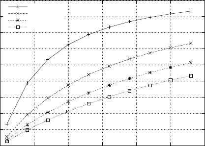
0
0.05
0.1
0.15
0.2
0.25
0.3
0.35
0.4
0.45
0123456
T3
T4,r1=2
T4,r1=6
T4,r1=10
T4,r1=14
Figure 4.8: Example III
101
Chapter 5
Compositionality in GreatSPN
The composition of two labelled GSPNs/SWNs is performed by means of the superposition of either (1) transi-
tions or (2) places of matching labels or by applying both kinds of superposition simultaneously.
Both the nets involved in the operation may have non-injective labelling, i.e. the same label may appear
connected to two or more transitions or places.
Constraints
1. Only one of the two nets may be multilabelled, i.e. one net (from now on we assume that the 1st operand)
may contain places, transitions with multiple labels. This constraint is motivated by the fact that having
two multilabelled operands the definition of the operators is a non-trivial task.
2. Concerning SWN models, the colour domains of those places which are to be superposed have to be
identical.
In the next section, we give an informal description of composition of two labelled SWNs implemented in
the GreatSPN2.0.2 package, similar considerations can be done for labelled GSPNs.
5.1 Composition of two labelled SWNs
In the following, instead of giving a rigorous definition, the functioning of the operators will be described. First,
we concentrate on the case in which only transitions are superposed.
Let’s us consider the labelled SWN N=hP,T,Pre,Post,Inh,pri,C,cd,w,λiobtained by the composition
of N1and N2in which:
•the set of places in the resulting net is simply the union of the sets of places, i.e. P=P1SP2(renaming of
place names may be necessary in order to avoid matching names). The colour domain function cd gives
cd1(p)if p∈P1,cd2(p)otherwise.
102
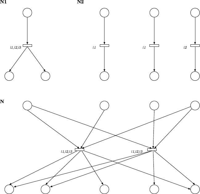
P1 A,B
t1
P3P2
A A,B
< x,y >
< !x,y >< x >
[d(x)=d1]
P4 A
t2
< x >
[d(x)=d2]
P5
A
< x >
P6 B
t3
< x >
P7
B
< !x >
P8 A
t4
< x >
P9
A
< !x >
P1 A,B
P3P2
A A,B
< x,y >
< !x,y >
< x >
[d(x)=d1] and [d(x1)=d2]
P4 A
P5
A
P6 B
P7
B
P8 A
P9
A
t12
< x,y > < x1 >
[d(x)=d1]
t11
< x >
< !x,y > < x1 >
< !x1 >
< x1 >
< x2 >
< !x2 > < !x2 >
< x2 >
Figure 5.1: A multilabelled, non-injective example
•The unlabelled transitions are considered non-observable with respect to the composition, and those whose
labels do not appear in the other operand, are not involved in superposition. These transitions are simply
copied into T(as for places, renaming may be necessary). To show how the operation proceeds to super-
pose transitions let us assume that N1is multilabelled, while N2is not, and the labelling is non-injective.
Let T2(l)denote the set of transitions t0of T2with l∈λ(t0), where λ(t)gives the set of labels of t. In N
there will be a replica of t∈T1for each element in Nl∈λ(t),T2(l)6=/
0T2(l), where Nis the cartesian product.
An example is shown in Fig. 5.1, for transition t1:λ(t1) = {l1,l2,l3}and the above defined cartesian
product has the elements {t2,t4}and {t3,t4}. In the composed net t11 (t12) is obtained by superposing
t1,t2 and t4 (t1,t3 and t4).
If two arcs connected to different transitions that are involved in the same superposition have identical
variable names in their arc expression, then these variables are renamed in the arc expression of all the
arcs connected to one of the two transitions. If these variables appear in the guard of the transition whose
arcs’ expressions are changed, the renaming is performed in the guard as well. As an example, in Fig. 5.1,
103

during the superposition of t1,t2 and t4 the variable xof the arcs and guard function connected to t2 is
renamed to x1. (As it will be mentioned in Section 5.2 the implemented version of the algorithm allows the
user to override the above described renaming rule to “unify” values of the nets.) When two superposed
transitions have both a guard function these guard functions are joined with logical and relation.
•The matrices Pre,Post,Inh describing the arc structure of Nare built in the following way: the arcs of N1
and N2connected to transitions that are not involved in superposition are simply copied into N. An arc
connected to a transition involved in superpositions will have as many instances as the times the transition
is superposed. In our example the arc P1-t1 has two instances in the composed net: P1-t11 and P1-t12.
•The priority function pri gives the same value as before for the transitions that are not involved in super-
position. A transition resulting from superposition inherits the priority value from the involved transition
of N1. The labelling functions λand ware handled similarly to the priority one. We assume that there are
not marking dependent rates and weights, and we basically leave the user the task of redefining pri and w
for the final net1.
•The set of basic colour classes Cand their definitions are assumed to be common for N1and N2.
The operation to superpose places is the direct counterpart of the operation described above. However to
superpose places is less complicated as it does not require renaming of arc or guard expressions and we are
assuming that places to be superposed have the same colour domain.
The simultaneous application of superposing places and transitions has two features that were not shown in
the above description. First, having an arc whose place (transition) is involved in np(nt) superpositions, there will
be np·ntinstances of the arc in the composed net connecting all the instances of its place with all the instances of
its transition. Second, having two arcs whose places and transitions are superposed, the arc expressions of these
two arcs are added. An example for the latter is shown in Fig. 5.2 where the arc expressions of the arcs P1 −t1
and P3 −t2 are summed.
5.2 The algebra package
The GreatSPN2.0.2 package algebra consists of the Composition and the Remove modules; in the following
we will give a description of the usage of both of them.
5.2.1 Composition module
The Composition module allows to perform the composition of two GSPNs/SWNs by using and producing
GreatSPN format. The modeler may build the component nets using the graphical interface of GreatSPN2.0.2 .
1To find a more sophisticated and compositional way to handle pri and wis an open question, attempts to address this problem may
be found in the literature.
104
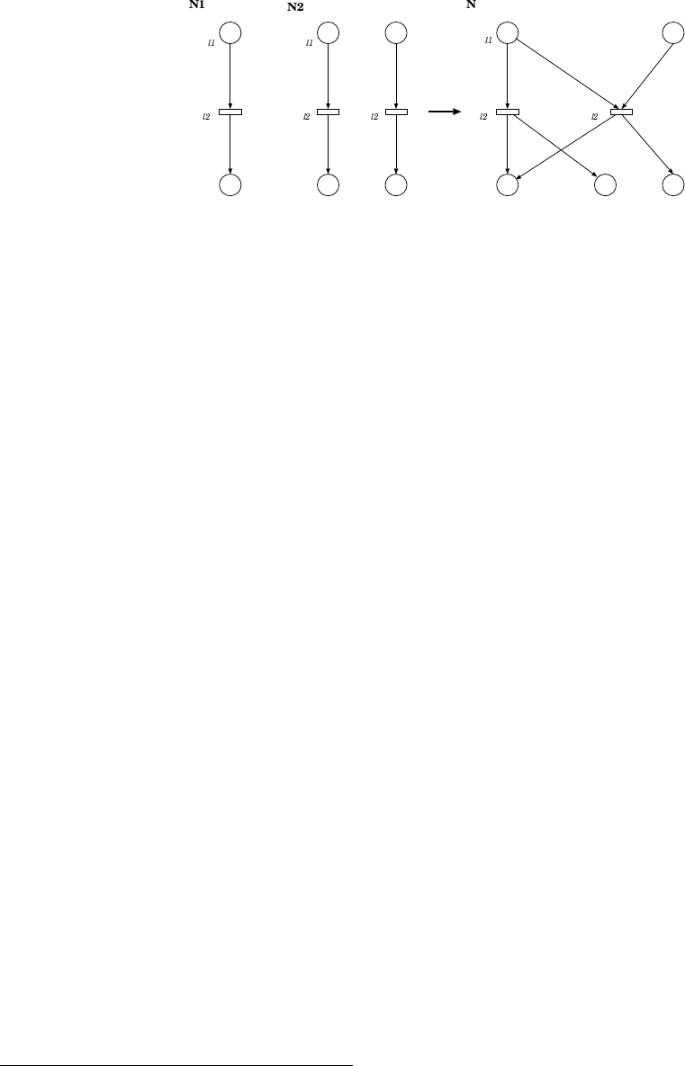
P1 A
t1
< x >
[d(x)=d2]
P2
A
< !x >
P3 A
t2
< x >
P4
A
< x >
P5 A
t3
< x >
P6
A
< !x >
P1 A
t11
< x > + < x1 >
[d(x)=d2]
P2
A
< !x >
P4
A
P5 A
t12
< x 1>
P6
A
< !x1 >
< x1 >
< !x >
< x >
[d(x)=d2]
Figure 5.2: Superposition of places and transitions
Labels are encoded in the name of the transitions and places, so both transition and place names have the structure
tag|label1|label2..., where tag is the name of the transition or place followed by its labels separated by bars.
The user may define the set of labels to be used for subnets composition. This feature may be useful when
composition involves more than two nets and hence is performed in several steps: in this case the modeler can
select which labels are to be considered at each stage of the composition.
The Composition module creates a graphical representation of the composed net in which the “shape” of
the original components is maintained: in case of transitions (or places) with multiple instances in the resulting
net, the additional instances are placed around the position of the originating place/transition, moreover the arcs
that connect places and transitions belonging to different subnets are drawn as “broken arcs” in the resulting
net, to improve its readability. The user has some options to control the layout of the final net by indicating the
placement of each component.
A small example for the output of the tool is given in Fig. 5.32: the example demonstrates another feature of
the tool: if a variable name starts with the character #, it is not renamed during the superposition. This allows the
modeler to use the same variables in different components, so as to “unify” values.
The Composition module is launched from the prompt of a console window by typing the command algebra
followed by a list of input parameters. When it is launched without parameters the complete synopsis is diplayed:
Usage:
algebra [switches] net1 net2 operator restfile resultname [placement shiftx shifty]
Switches: -no_ba: no broken arcs will be used between subnets
-rs number: result will be rescaled by number
Operators: ’t’: Superposition Over Transitions
’p’: Superposition Over Places
2Note that GreatSPN2.0.2 does not draw arc expressions on broken arcs, so those in the figure are written “by hand”.
105
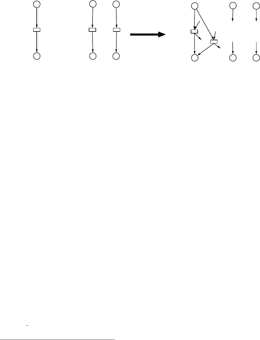
P3
B
P4
B
P6
A
P5
A
T3|l1
<x>
<x>
T2|l1
<#y>
<#y>
N2
P2
A,B
P1
A
T1|l1
<x>
<!x,#y>
N1
P2
A,B
P1
A
P3
B
P4
BP6
A
P5
A
T2|l1
<x> T1|l1
P5
<y>
<!x,y>
T1|l1
P6 <y>
T1|l1
T2|l1
P3
<x1>
<x>
T2|l1
<x1>
<!x,y> P4
N
Figure 5.3: Superposition using SWN
’b’: Superposition Over Places & Transitions
restfile: contains the labels to be used for synchronization
placement: 1 ---> net1 net2
2 ---> net1
net2
3 ---> net2 is shifted by (shiftx,shifty)
The two operands net1 and net2 are the GreatSPN2.0.2 names (without extensions) of the two nets that have
to be composed3, the resulting composed GSPN/SWN is saved in resultname. The first operand net1 may
be multilabelled. The operator is defined by operator and may be tto superpose transitions, pto superpose
places or bto superpose both places and transitions. The set of labels over which the superposition will be
performed may be restricted to a given subset of labels, these subsets are listed in the file restfile, this file has
the following format:
transition={tl1|tl2}
place={pl1|pl2|pl3}
The labels that are not given in this file are not considered during the operation. If the file does not exist all
labels are considered. The last three arguments may be used to define the placement of the components: if the
parameter placement is 1 (2) the two nets are placed next to each other horizontally (vertically), if it is 3 the
second net is shifted by (shiftx,shifty) with respect to the first net. Further options that can be set launching
the command:
•-no ba to visualize all the arcs in the composed net; by default, the arcs connecting objects belonging to
different components are not entirely displayed, i.e., they are broken;
3If the nets to be composed are saved in a directory different from the current one, the complete path is required
106

•-rs number to rescale the composed net by a factor given by number.
Merging of two models Composition module can be use also to merge two no-labelled GreatSPN2.0.2 models.
Let us assume model1 and model2 be the names of two models, then the command:
algebra model1 model2 t nolabel model1 2 [placement shiftx shifty]
where the file nolabel contains the following line:
transition={}
merges the two models saving the result in file names as model1 2.
5.2.2 Remove module
Together with the Composition module, the package algebra includes also the Remove module that has been im-
plemented to eliminate labels and the character #from the nets. Typing the command remove without parameters
the following output is displayed:
Usage:
remove net1 net2 function [labelfile]
net1: Net to work on
net2: Resulting Net
Functions: ’l’: Remove labels
’#’: Remove ’#’-s
’b’: Do both
labelfile: contains the labels to be removed
(if not given all labels are removed)
net1 is the name (without extensions) of the input net while net2 is the name of the output one. As function l,
#or bmay be given to eliminate labels, the characters #or both, respectively. The set of labels to be deleted may
be a subset of the set of all the labels, and these subsets may be defined the same way as described for restfile
in case of the algebra command.
107
Chapter 6
Export to other tools
6.1 Model checking: PROD translator
The PROD translator module is an interface to the PROD tool[36], it translates a GSPN/SWN model defined
in GreatSPN2.0.2 format into the corresponding model described in PROD format. The PROD translator also
produces a file containing a list of useful macros to be used during model-checking performed by means of
queries during a probe session.
6.1.1 Installation
Source files are all stored into the tar-zipped file PRODtranslDDMMYY.tar.gz, where DDMMYY is a date
(DD=day,MM=month,YY=year). To install the PROD translator the C compilator gcc, the lexical and syn-
tactic analyzers lex and yacc are required. The installation procedure consists in the execution of the following
commands:
gunzip PRODtransl.tar.gz
tar xvf PRODtransl.tar
cd PRODtransl
install-transl
As result of such execution a directory PRODtransl is created. This directory contains the following subdi-
rectories:
•SOURCE: contains the source files of the translator;
•DOCS: contains the documentation related to the translator;
•bin: contains the executable files prod-translator and ExploreRG.
108

prod-translator is the module that allows to translate a GSPN/SWN model defined in GreatSPN2.0.2 for-
mat to the corresponding PROD model; while ExploreRG is a script file that contains the sequence of commands
the user have to execute to perfom pre-processing of the translated net, to generate its reachability graph (RG),
to compute the strongly connected components of RG, to launch the interactive program probe and, finally, to
remove all the files created during the RG generation once the analysis of the model has been finished and the
probe session has been closed.
6.1.2 Use of the PROD translator
Once the installation procedure has been performed it is possible to translate a GreatSPN2.0.2 model through the
command:
prod-translator netname
where netname is the name of a GSPN/SWN model created with GreatSPN2.0.2 without extensions1. The
translation procedure produces the following output files:
•netname prod.net: that contains the PROD net description;
•netname prod.macro: that contains a list of macros to be used during the model checking performed
through the interactive program probe;
•netname prod funz.c,netname prod funz.h: these files are generated only in case of SWN models and
contain information related to the coloured definitions of the net. In case of translation of a SWN model
the subdirectory netname prod.src has to be created - if not already existent - where these files have to be
move to.
Alternatively, if the user wants to give a different name from the one assigned by default to the translated net, the
following command has to be used:
prod-translator netname myprodnet
where netname is the name of the GreatSPN2.0.2 model to be translated and myprodnet is the desired name
for the translated PROD model. So the following files will be generated:
myprodnet.net – myprodnet.macro – myprodnet funz.c – myprodnet funz.h
6.1.2.1 Nets with inhibitor arcs
Since the PROD tool doesn’t allow to define inhibitor arcs, additional information are required to the user if the
GreatSPN2.0.2 model contains inhibitor arcs in order to carry out a properly translation of such arcs into test arcs
1The GreatSPN2.0.2 net definition files netname.def and netname.net have to be stored both in the same directory
109
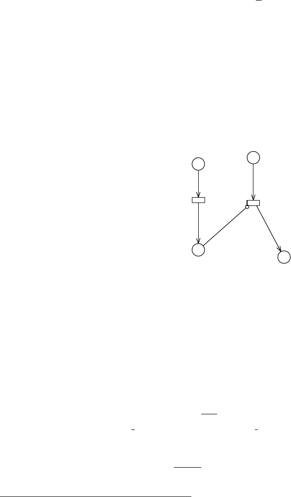
on the complementary places. During the translation of a GSPN model with inhibitor arcs, if the file netname.bnd
does not exist in the current directory, the user has to give the upper bound, i.e. maximum capacity, of each place
having an outgoing inhibitor arc. For example, if the place p1 of a GSPN model has an outgoing inhibitor arc,
then there will be following request:
Please, introduce bound for place <p1 >: 5 2
If the bound of a place is unknown, we suggest to set the value 255 that is the maximum bound allowed for a
place in a GreatSPN2.0.2 model. In case of a SWN model, then the user has to provide:
•the initial marking of the complementary place of an inhibitor place, and
•the function to be assigned to the test arc that connects the complementary place to the inhibited transition;
both of these information have to be given using the GreatSPN2.0.2 syntax. Let us consider the net of Fig.6.1:
P4
C
P2
CS
P3
C
S
P5
C
t4
t3
<x>
<x>
<S-y> <y>
<y>
S:m
C:c
C1:c
Figure 6.1: SWN net with an inhibitor arc
during the translation execution, the following requests will be displayed:
Please, introduce initial marking for the dual place of p4
domain of place p4: C
M0(p4) = 0
Use ’e’ for empty initial marking : <S>
Please, introduce arc function for inhibitor arc <S-y>
between place p4 and transition t4
function for input/output arc: <S-y>
It is possible to define an empty initial marking using the GreatSPN2.0.2 expression 0<S> or simply the e
2From here until the end of this chapter the underlined character represents the input given by the user.
110

letter. If we add an arc from t4 to p4 with arc function <x>in the net of Fig.6.1 and the guard [x<> y]to the
transition t4, then the following requests will be displayed:
Please, introduce arc function for inhibitor arc <S-y>
between place p4 and transition t4
(there is also an output arc from t4 to p4 with function <x>)
function for input arc: <S-y>
function for output arc: <S-y-x>
6.1.2.2 SWN nets with symbolic markings
When a SWN net contains a symbolic marking, then only one of the possible assignments is considered in the
translation into the corresponding PROD net. Hence, the reachability graph of the PROD net will be reduced
with respect to the one obtained from the GreatSPN2.0.2 model. For example, let’s consider the following
GreatSPN2.0.2 symbolic marking:
M2 : <M1>, M1 : (C:2), C : u C1, C1 = a1,a2,a3
it corresponds to the following different PROD ordinary markings:
< .a1..a2. >,< .a2..a3. >,< .a1. > +< .a3. >
So if only one of the above assignments is considered then the reachability graph of the PROD net is 1/3 of
the one obtained for the GreatSPN2.0.2 one.
6.1.2.3 The script ExploreRG
Once the GreatSPN2.0.2 net has been translated into the PROD net it is then possible to perform model-checking
using the PROD tool. To investigate the reachability graph (RG) of the PROD net netname prod the following
command have to be executed:
prod netname prod.init
netname prod
strong netname prod
probe -l netname prod.macro netname prod
that perform the corresponding actions:
111

preprocessing of netname prod
RG generation of netname prod
computation of the strongly connected components of the RG of netname prod
activation of the analyzer of the RG of nomerete prod
After the last command has been launched, the interactive RG analyzer probe is running (it is in prompt state
0#); it is then possible to submit queries to investigate the RG of the net. Besides the basic queries of the PROD
syntax, the user can exploit the predefined macros contained in the file netname prod.macro that can be displayed
from the probe prompt with the command defs.
Alternatively to the command
probe -l netname prod.macro netname prod
the commands probe netname prod and load netname prod.macro have to be launched.
The command quit causes the termination of the probe session and hence the ending of the RG inspection.
Afterwards, we suggest to execute the command:
prod netname prod.clean
that removes all the files produced during the RG generation. The sequence of commands listed at the beginning
of this paragraph included this last command is summarized in the script file ExploreRG that defines a macro
command to be used as follows:
ExploreRG netname prod
this command generates the RG of the PROD net defined in netname prod, allows to inspect the RG through
queries, included the ones predefined in the file netname prod.macro and finally, removes all the files created
during the RG generation.
6.1.2.4 The pre-defined macros
All the predefined macros generated by the PROD translator are stored in the file netname prod.macro: they
can be used during the inspection of the RG of the net netname prod through the interactive analyzer probe.
Besides the macro definitions, the definitions of the marking parameters and of the coloured tokens of the net are
also listed. Some macros takes account of the characteristics of the translated net, others are independent of the
structure of the net. Moreover, some macros are simply alias of some probe commands such as:
#define qv query verbose
#define qn query node
#define qmn query mute node
#define qvn query verbose node
Let us consider a net with the following subsets of transitions:
112

•T1,T2,T3 timed transitions (exponential);
•t4,t6 timed transitions (deterministic);
•t5,t7 immediate transitions with priority G1;
•t8,t9 immediate transitions with priority G2;
a first group of macros consists of a list of definitions of the above subsets of transitions:
#define TEMP CLASS (\ exponential timed
T1(1) || T2(1) || T3(1)) transitions subset
#define DET CLASS (\ deterministic timed
t4(1) || t6(1)) transitions subset
#define G1 CLASS (\ immediate transitions with
t5(1) || t7(1)) priority G1 subset
#define G2 CLASS (\ immediate transitions with
t8(1) || t9(1)) priority G2 subset
#define IMM CLASS (\ immediate transitions
G1 CLASS || G2 CLASS) subset
The second group of macros consists of a set of queries to be used as a command from the probe prompt, the
probe’s answer will be of type:
8 PATH
built set %12
that means that either 8 paths or 8 markings, satisfy the submitted query and the result of the query is saved into
a set denoted as %12.
During the queries it is possible to “jump” from a node of the RG to another through the command goto n
where n is the number that identifies a node of the RG.
In the following the second group of macros is listed:
1. TangMark
detects the set of tangible markings of the net, deadlock markings are not included;
2. VanMark
detects the set of vanishing markings of the net;
3. M0pathTO(markSet)
detects and displays the set of paths P such that P=Sn
i=1Piwhere Piis the shortest path from M0to Mi,
Mi∈markSet and markSet={M1,..,Mn};
113

4. PathTO(markSet)
detects and displays the set of paths P such that P=Sn
i=1Piwhere Piis the shortest path from the current
marking to Mi,Mi∈markSet and markSet={M1,..,Mn};
5. Deadlock
detects the set of deadlock markings;
6. M0pathTOdeadlock
detects and displays the set of the shortest paths from M0to each deadlock marking;
7. PathTOdeadlock
detects and displays the set of the shortest paths from the current marking to each deadlock marking;
8. Livelock
displays all the livelocks of the net;
9. M0pathTOlivelock(livelockSet)
detects and displays the set of the shortest paths from M0to each marking belonging to the livelock
livelockSet, where livelockSet is a set of the form %%n where n is its identifier number3;
10. PathTOlivelock(livelockSet)
detects and displays the set of the shortest paths from the current marking to each of the markings belonging
to livelockSet, such set have to be of the form %%n where n is its identifier number;
11. AllMarkEnabOnly(lastset,transSet)
detects and displays the set of markings in which only transitions belonging to the set transSet are en-
abled;
12. ExistPathM1toM2(lastset,mark1,mark2)
detects and displays the shortest path from marking mark1 to the marking mark2, if no path is found
between the two markings the answer to this query is 0 PATH;
13. AllPathM1toM2(lastset,mark1,mark2)
detects and displays all the paths, without loops, from mark1 to mark2, if no path is found between the two
markings the answer to this query is 0 PATH;
14. MarkingSetEnab(trans)
detects and displays the set of markings that enable transition
t trans;
3In probe the strongly connected components of RG, hence the livelocks, are denoted as %%n.
114

15. TransEnab(mark)
detects and displays the set of transitions enabled in marking mark;
16. Successor(mark, trans)
detects and displays the marking M1reached from marking mark after the firing of trans, i.e.: mark[trans >M1
17. Enable(mark,trans)
verifies if the marking mark enables the transition trans;
18. Mark(node)
displays the marking identified by the number node;
19. MarkSetEnabOR(setT1,setT2)
detects and displays the following set of markings:
markSet ={Mi|Mi[tv∨Mi[twwhere tv∈setT1 ∧tw∈setT2}
i.e the set of markings that enable at least either a transition of the set setT1 or a transition of the set setT2;
20. MarkSetEnabAND(lastset,setT1,setT2)
detects and displays the following set of markings:
markSet ={Mi|Mi[tv∧Mi[twwhere tv∈setT1 ∧tw∈setT2}
i.s. the set of markings that enable at least a transition of the set setT1 and at least a transition of the set
setT2;
21. MarkBelongSet(lastset,mark,markSet)
verifies if the marking mark belongs to the set of markings markSet;
22. LogicCond(formula)
detects and displays the set of markings that satisfy condition expressed by formula.
We emphasize the form of the parameters appeared in some macros of the previous list and not explicitly de-
scribed:
•lastset has to be the number of the last set computed by probe, usually the one obtained as a result from
the last submitted query;
•transSet is a set of transitions, it has to be expressed with the same syntax used for the definition of the
sets TEMP CLASS and IMM CLASS, that is:
115

Transname1(1) || Transname2(1) || ....
•mark is a marking that corresponds to a node of RG, it has to be expressed as n, that is the number that
identifies the node of RG, for example:
TransEnab(5)
where 5represents a marking of RG.
•markSet is a set of markings and it has to be expressed as %n where n is the number that identifies the set
containing the considered markings; it can be either a basic set defined by probe or a set obtained as a
result of a query4, for example:
MarkBelongIns(4,10,%2)
where 4is the last set created by probe,10 represents a marking and %2 is a set of markings.
•formula is a formula that can be expressed using the PROD grammar5:
formula ::= (formula)|not formula |formula and formula |
formula or formula |expr
expr ::= simple expr |mark == mark |mark != mark |
mark >=mark |mark <=mark |mark <mark |
mark >mark |op1 expr |expr op2 expr
simple expr ::= card( mark )|(expr )|digits
mark ::= simple mark |mark +mark |simple expr simple mark
simple mark ::= place name |empty |< . rangelist . > |
< .. > |(mark )
Non terminal symbols op1 and op2 are respectively the unary and the binary operators used in the expres-
sions of the C programming language. Let us consider some examples of formulae accepted by the PROD
grammar:
card(p1)>=card(p2) the total number of tokens in place p1
is equal to the total number of tokens in place p2
card(p1)==N the total number of tokens in place p1
is equal to the value of the parameter N
p1==p2 the marking in place p1 is equal to the marking in place p26.
4It is worth to notice that in general the sets generated by probe are sets of paths, the markings are considered as paths of zero length.
5The grammar described in the following is simplified, for a full description see the PROD reference manual[36]
116
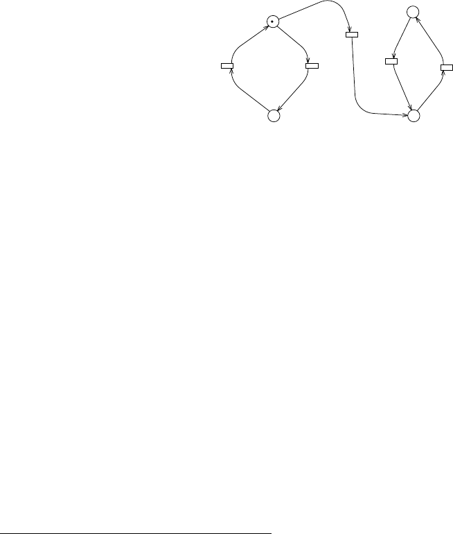
p1<N p2 the marking in place p1 is less than the marking in place p2
multiplied by the value of the parameter N7.
Let us see some example on the usage of the macro 22, that accept as a input parameter a formula:
0#LogicCond( card(p1)==2 and p2==empty)
detects the set of markings in which the place p1 is marked with 2 tokens and the place p2 is empty;
0#LogicCond( p1==(<.a1,p1.>+<.a2,p2.>))
detects the set of markings in which the marking of place p1 is the one specified by the query.
Symbols a1,p1,a2,p2 are numeric constants that represent coloured tokens.
P1
P2 P3
P4
t4
t5
t3
t2
t1
Figure 6.2: GSPN net with a livelock
Macros 9 and 10 do not guarantee that the paths found are the shortest paths that brings to a livelock, really
it should be verified that every path does not contain more than one node belonging to the livelock.
Let us consider the net of Fig.6.2 the following queries can be submitted:
0#livelock
Component %%0
------------------------------------------------
1, 3
%%0 has 2 nodes
------------------------------------------------
1 nontrivial terminal strongly connected components
------------------------------------------------
0#M0pathTOlivelock(%%0)
PATH
Node 0, belongs to strongly connected component %%1
P1: <..>
6The number of occurrences of a single coloured token is compared in the two markings.
7The marking Np2 is obtained from the marking of the place p2 by multiplying the occurrences of each coloured token Ntimes.
117

Arrow 0: transition t3, precedence class 0
Node 1, belongs to strongly connected component %%0
P3: <..>
------------------------------------------------
PATH
Node 0, belongs to strongly connected component %%1
P1: <..>
Arrow 0: transition t3, precedence class 0
Node 1, belongs to strongly connected component %%0
P3: <..>
Arrow 0: transition t4, precedence class 0
Node 3, belongs to strongly connected component %%0
P4: <..>
------------------------------------------------
2 paths
Built set %1
------------------------------------------------
Two paths have been detected, but only the first one is the shortest path that brings the net to the livelock. We
can then select the shortest path by means of the query:
ExistPathM1toM2(1 8,0,1).
6.2 Kronecker solutions: APNN translator
The APNN translator transforms the GreatSPN2.0.2 net description files into a corresponding APNN notation:
the GreatSPN2.0.2 layers are interpreted as a partition of the net into subnets which synchronize over transitions
(Superposed GSPNS), for a subsequent application of Kronecker based solution methods.
6.3 Tgif translator
The gspn2tgif program translates a model defined in GreatSPN2.0.2 format into a Tgif [9].obj file: each net
object is translated into a Tgif graphical object so that the graphical appearance of the converted GSPN/SWN
model can then be modified using the Tgif GUI.
6.4 Fluid nets translator
The net2fspn translator provided with the FSPNEdit software package, transforms the .net files saved by Great-
SPN2.0.2 into the .fspn files required by the solution components of the FSPN analysis tool. User can then add
8This is the identifier number of the set obtained with the previous query.
118
fluid places and continuous arcs to the generated files and analyze them using the tools provided by the FSPNEdit
package. In particular the generated FSPN may be solved either by simulation (using the software component
FSPNsim) or by numerical analysis (using FSPNsolve).
6.5 Refinement of SWN performance indexes: PERFSWN
PERFSWN is a set of tools providing an interactive framework to define, compute and present to the user steady
state performance indices of SWN insofar as these indices relate only to static subclasses of the SWN. These tools
complement GreatSPN2.0.2 to exploit the SRG and the steady state probability vector of the SWN. In addition to
GreatSPN2.0.2 , PERFSWN leans on several Perl scripts that we have developed and on the interactive numerical
environment Scilab (available at http://www-rocq.inria.fr/scilab).
The user environment is composed of several working sessions. A GreatSPN2.0.2 session is dedicated to
SWN definition and computation of performance indices available in the tool. A Scilab session supplements
GreatSPN2.0.2 to compute various performance indices and to provide graphical presentations of data (plots,
graphs, etc). Beside these two sessions, the user can enter commands into a terminal session to run the interface
software which extracts results and compute new ones from GreatSPN2.0.2 results.
A typical sequence of operation in PERFSWN is the following. The user defines its SWN with the graphical
interface of GreatSPN2.0.2 . Next, he asks GreatSPN2.0.2 for the computation of the Symbolic Reachability
(SRG) with output into an ASCII file, alone, or together with the solution of the aggregated Markov chain of
the SWN. Under the terminal session, the user can now process the Tangible Symbolic Reachability Set (TSRS)
and obtain a Scilab script version of the solution vector b
πfor the TSRS. If no change is done to the structure of
the SWN, the TSRS does not need to be reloaded when new stochastic parameters are given. Then he begins its
Scilab session by loading the TSRS and b
π(i.e. running our corresponding scripts). Consequently, the user works
with data from the TSRS and the vector b
πinto the Scilab session. If needed, the user asks for specific symbolic
firings in the terminal session. He can now compute the throughput of these transition firings into theScilab
session by calling interactively functions of our libraries.
PERFSWN benefits from all features of Scilab for the definition of high level functions (for instance reward
functions based on the static partitio ns of the symbolic markings), as well as for the management of the working
session (save and restore of sessions, batch execution, etc.).
Computation of performance indices (in steady state) is based on the (colored) token distributions, the through-
put of transitions and the response times of subnets. The general method to obtain a performance index (say a)
is to define a reward function giving, for each tangible marking m∈TRS, a reward value r(m)contributing to
a. Then we have a=E(r) = ∑m∈TRS r(m)π(m). PERFSWN is able to compute these indices, provided that they
relate to the number of tokens per static subclasses only. PERFSWN extracts the TSRS with the static partitions
of all tangible symbolic markings (the canonical representations are discarded) into a Scilab session. Moreover,
119
firings instances of a given transition are retrieved from the SRG based on a boolean expression we call a bindings
formula. The syntax of bindings formulae is the classical combination of logic (or, and, not) with basic boolean
expressions giving the static subclass of the instantiation of a variable of the transition.
PERFSWN provides two basic Scilab libraries for performance indices computation. swn.sci is dedicated
to specific SWN functions (for instance, display symbolic markings, find markings with specific property, define
and compute reward functions). In addition to performance computations, the user can in this way, examine
several qualitative properties of the system. The second library, perf.sci, is a set of general purpose functions
useful in the area of performance evaluation. It provides the user with mean reward computation from a user
defined reward function (for instance over symbolic markings), distribution computation, like tokens distribution
in one or several places, plot of cumulative distributions functions, etc. Obviously this library could be easily
extended by any user.
120

Appendix A
Net description files
The GreatSPN2.0.2 net description is stored in two ASCII files called netname.net and netname.def respec-
tively.
The .net description file contains the description of the structure of a GreatSPN2.0.2 model according to the
following Backus-Naur Form (BNF) format. Capital keywords are non-terminals, while terminals are represented
as C language strings. The following special terminals are used: empty indicates void fields; string indicates
any non-empty character string not containing blank characters; space indicates any sequence of blank and tab
characters; natural indicates a non-negative integer; pint indicates a positive integer; preal indicates a positive
real; coords indicates a pair of non-negative real number representing object coordinates with a space between
them. The notation #(XX)... denotes the repetition of the string in braces for a number of times derived by
interpreting the string XX as a natural number. Moreover we used C-like notation /* comments */ to comment
some lines.
The *.def description file contains the description of additional information of a GreatSPN2.0.2 model. In
particular:
•definition of the coloured part (SWN models only) according to the SWN BNF grammar given in Table A.1;
•definition of rate parameters according to the Marking-Dependent Rate Definition BNF grammar given in
Table A.2;
•definition of (no default) results, to be computed using either markovian or simulator solvers, according to
the Result Definition BNF grammar given in Table A.3.
In addition to the special terminal keywords adopted previously, in the definition of the *.net file, we use also the
following ones: special terminal keyword <assign> to indicate a marking dependent rate parameter definition;
<result> to indicate a result definition; <fun def> to indicate a coloured definition.
121
A.1 Format of the .net file
NETFILE ::= COMMENT NOOBJS MARKS PLACES RATES GROUPS TRANS LAYERS
COMMENT ::= "|0|\n" COMHEAD "|\n"
COMHEAD ::= empty "|\n" | "Comment on this GSPN:\n" { COMLINE "\n" }
COMLINE ::= space | string | empty | COMLINE space | COMLINE string
NOOBJS ::= "f" space NM space NP space NR space NT space NG
space "0" space NL space "\n"
NM ::= natural /* number of marking parameters */
NP ::= natural /* number of places */
NR ::= natural /* number of rate parameters */
NT ::= natural /* number of transitions */
NG ::= natural /* number of groups */
NL ::= natural /* number of layers */
MARKS ::= #(NM) { NAME space MVAL space coords LEVELS "\n" }
NAME ::= string
MVAL ::= pint
LEVELS ::= space "0" | space pint LEVELS
PLACES ::= #(NP) {NAME space PMARK space coords space coords LEVELS COL "\n" }
PMARK ::= natural | "-" MPINDX
MPINDX ::= pint /* 0 < #(MPINDX) <= #(NM) in case of GSPN */
COL ::= empty | coords string
RATES ::= #(NR){ NAME space RVAL space coords LEVELS "\n" }
RVAL ::= preal
GROUPS ::= #(NG){NAME space coords space PRI "\n" }
PRI ::= pint /* priority */
TRANS ::= #(NT){NAME space TRATE space TSERV space TKND space TINP space
TROT space coords space coords space coords LEVELS COL "\n"
LDCOEFFS TIARCS TOUT TOARCS TINH THARCS }
TRATE ::= preal | "-" RPINDX | MDRATE
RPINDX ::= pint /* 0 < #(RPINDX) <= #(NR) */
MDRATE ::= "-510" /* A MD rate is defined in file .def */
TSERV ::= natural | "-" LDPOP
LDPOP ::= pint /* max population of LD equivalent server */
TKND ::= EXPT | DETT | IMMT
122
EXPT ::= "0"
DETT ::= "127"
IMMT ::= pint /* priority level group s.t. 0 < #(IMMT) < #(NG) */
TINP ::= natural /* No. Input Arcs */
TROT ::= "0" | "1" | "2" | "3" /* rotation coefficient */
LDCOEFFS ::= (#(LDPOP) - 1){ preal "\n" }
TIARCS ::= #(TINP){ AMULT space APLACE space APOINTS LEVELS
COL "\n" APLIST }
AMULT ::= pint /* arc multiplicity */
APLACE ::= pint /* place index s.t. 0 < #(APLACE) <= #(NP) */
APOINTS ::= natural /* No. intermediate points for broken arcs */
APLIST ::= #(APOINTS){ coords "\n" }
TOUT ::= natural "\n" /* No. Output Arcs */
TOARCS ::= #(TOUT){AMULT space APLACE space APOINTS LEVELS
COL "\n" APLIST }
TINH ::= natural "\n" /* No. Inhibitor Arcs */
THARCS ::= #(TINH){AMULT space APLACE space APOINTS LEVELS
COL "\n" APLIST }
LAYERS ::= { NAME "\n" } /* list of Layer names
one per layer used in objects */
A.2 Format of the .def file
DEFMD ::= "|" TI "\n" RATE_DEF "\n"
TI ::= pint /* transition relative position inside ".net" */
RATE_DEF ::= <assign>
RESULT ::= RES RESULT | "|\n"
RES ::= "|" NAME space coords space ":" space RES_DEF "\n"
NAME ::= string
RES_DEF ::= <result>
COLOR ::= COL COLOR | empty
COL ::= "(" NAME space CT space coords space "(@" CT "\n"
<fun_def> "\n ))"
CT ::= "c" | "f" | "m"
123

A.3 Grammars
The SWN syntax (Table A.1), the marking-dependent rate definition grammar (Table A.2) and the performance
result definition grammar (Table A.3) are given according to the following BNF format.
All the terminal keywords are represented as C-language strings in quotation marks except for the following
terms: <real number >indicates a positive real number, <integer >indicates a non negative integer number,
<string >indicates any non-empty character string not containing blank characters and <empty >indicates
void fields. Concerning the <color class type >keyword it can assume either “o” or “u” values which stand for
“ordered” and “unordered” respectively.
<fun def >::= <color class description >|
<static subsclass description >|
<initial marking description >|
<dynamic subclass description >
<color class description >::= <color class type > <static subclasses list >
<static subclasses list >::= <static subclass name >|
<static subclasses list >“,” <static subclass name >
<color class type >::= “o” |“u”
<static subclass description >::= <string >“{”<integer >–<integer >“}”|
“{”<objects list >“}”
<objects list >::= <object name >|<objects list >“,” <object name >
<place color domain description >::= <color classes list >|<empty >
<color classes list >::= <color class name >|
<color class name >“,” <color classes list >
<arc function description >::= <empty >|<coefficient >“ID” |
<ordinary function >
<ordinary function >::= <coefficient >
[<predicate >]“<”<function list >“>”|
<ordinary function > <sum op > <coefficient >
[<predicate >]“<”<function list >“>”
<function list >::= <function kernel >|
<function kernel >“,” <function list >
<function kernel >::= <term >|<function kernel > <sum op > <term >
<term >::= <synchronization term >|<projection term >|
<successor term >|<predecessor term >
<synchronization term >::= <coefficient >“S” |
124

<coefficient >“S” <static subclass name >
<projection term >::= <coefficient > <function name >
<successor term >::= <coefficient >“!” <function name >
<predecessor term >::= <coefficient >“ˆ” <function name >
<initial marking description >::= <short marking >|<ordinary marking >
<short marking >::= <coefficient >“S”
<ordinary marking >::= <coefficient >“<”<marking list >“>”|
<ordinary marking > <sum op >
<coefficient >“<”<marking list >“>”
<marking list >::= <marking item >|<marking list >“,” <marking item >
<marking item >::= <dynamic subclass name >|“S” <static subclass name >|
“S” |<object name >
<cardinality >::= <integer >|
“|”<color class name >“.”<static subclass name >“|”|
“|<color class name >“|”
<object name >::= <string >
<dynamic subclass description >::= “(” <static subclass name >“:” <cardinality >[“:” <integer >]“)”
<predicate >::= <predicate >“or” <pterm >|<pterm >
<pterm >::= <pterm >“and” <pfatt >|<pfatt >
<pfatt >::= “(” <predicate >“)” |
“d” “(” <string >“)” <eqop > <d operand >
|<string > <eqop > <str operand >
<d operand >::= “d” “(” <string >“)” |<static subclass name >
<str operand >::= <string >|“!” <string >|“ˆ” <string >
<color class name >::= <string >
<function name >::= <string >
<static subclass name >::= <string >
<dynamic subclass name >::= <string >
<coefficient >::= <integer >|
“|”<color class name >“.”<static subclass name >“|”|
“|”<color class name >“|”|<empty >
<sum op >::= “+” |“–”
<eqop >::= “=” |“<>”
Table A.1: SWN syntax for the GreatSPN2.0.2 package.
125

<assign >::= {“when” <logic cond >“:” <value >“;”}
“ever” <value >“;”
<logic cond>::= <compare >|“˜”<logic cond >|“(” <logic cond >“)” |
<logic cond >“&” <logic cond >|<logic cond >“o” <logic cond >
<compare >::= <marking > <comp oper > <integ const >
<marking >::= “#” <place name >
<place name >::= <string >
<comp oper >::= “=” |“/=” |“>”|“<”|“>=” |“<=”
<integ const >::= <integer >|<mark par >|<marking >
<mark par >::= <string >
<value >::= <real val >|“(” <value >“)” |<value > <arithm op > <value >
<real val >::= <real number >|<marking >|<rate par >
<rate par >::= <string >
<arithm op >::= “+” |“–” |“*” |“/”
Table A.2: BNF of the marking-dependent rate definition grammar.
<result >::= <sum >“;”
<sum >::= <item >|<item >“+” <sum >|<item >“–” <sum >
<item >::= [ <real val >] “p{”<logic cond >“}”|[<real val >] “P{”<logic cond >“}”|
[<real val >] “e{”<marking >“}”|[<real val >] “E{”<marking >“}”|
[<real val >] “e{”<marking >“/” <logic cond >“}”|
[<real val >] “E{”<marking >“/” <logic cond >“}”
<real val >::= <real number >|<rate par >
<rate par >::= <string >
<logic cond >::= <compare >|“˜”<logic cond >|“(” <logic cond >”)” |
<logic cond >“&” <logic cond >|<logic cond >“o” <logic cond >
<compare >::= <marking > <comp oper > <integ const >
<marking >::= “#” <place name >
<place name >::= <string >
<comp oper >::= “=” |“/=” |“>”|“<”|“>=” |“<=”
<integ const >::= <integer >|<mark par >|<marking >
<mark par >::= <string >
Table A.3: BNF of the performance result definition grammar.
126

A.4 Extended SWN grammar
The SWN grammar has been extended to allow the definition of the refined performance indices. In particular,
the extended grammar allows to define four main categories of performance indices:
•linear combinations of mean number of token in places and probabilities;
•linear combinations of throughputs;
•average crossing times;
•multiple results.
Table A.4 formalizes the extension according to the following BNF format. All the terminal keywords are
represented as C-language strings in quotation marks except for the following terms: <real number >indicates
a positive real number, <integer >indicates a non negative integer number, <string >indicates any non-empty
character string not containing blank characters.
<result >::= <sum >“;” |<sum t >“;” |
<item fam >“;” |<sum >“/” <sum t >“;”
<sum >::= <item >|<item >“+” <sum >|<item >“-” <sum >
<item >::= [ <real val >] “P{”<logic cond >“}”|
[<real val >] “E{”<marking >“}”|
[<real val >] “E{”<marking >“/” <logic cond >“}”
<marking >::= “#” <place name >|“#” <place name >“[” <pred >“]”
<sum t >::= <item t >|<item t >“+” <sum t >|<item t >“-” <sum t >
<item t >::= [ <real val >] “X{”<marking t >“}”|
[<real val >] “X{”<marking t >“/” <logic cond >“}”
<marking t >::= “#” <transition name >|
“#” <transition name >“[” <pred >“]”
<item fam >::= [ <real val >] “E{”<marking fam >“}”|
[<real val >] “E{”<marking fam >“/” <logic cond >“}”|
[<real val >] “X{”<marking fam >“}”|
[<real val >] “X{”<marking fam >“/” <logic cond >“}”
<marking fam >::= “#” <obj name >“(*)” |
“#” <obj name >“(*)|SEL=[” <pred >“]” |
“#” <obj name >“(*)|SEL=[” <pred >“], COND=[” <pred >“]” |
“#” <obj name >“(*)|COND=[” <pred >“]” |
127

“#” <obj name >“(”<obj list >“)” |
“#” <obj name >“(”<obj list >“)|SEL=[” <pred >“]” |
“#” <obj name >“(”<obj list >“)|SEL=[” <pred >“], COND=[” <pred >“]” |
“#” <obj name >“(”<obj list >“)|COND=[” <pred >“]”
<place name >::= <string >
<transition name >::= <string >
<obj list >::= <obj name >|<obj list >“,” <obj name >
<obj name >::= <string >
<real val >::= <real number >|<rate par >
<rate par >::= <string >
<logic cond >::= <compare >|“˜”<logic cond >|“(” <logic cond >“)” |
<logic cond >“and” <logic cond >|<logic cond >“or” <logic cond >
<compare >::= <marking > <comp oper > <integ const >|
<multiset def > <comp oper > <multiset >
<comp oper >::= <rel op >|“>”|“<”|“>=” |“<=”
<integ const >::= <integer >|<mark par >|<marking >
<multiset >::= <multiset const >|<multiset def >
<multiset def >::= “#” <place name >“(*)” |“#” <place name >“(” <class list >“)” |
“#” <place name >“(*)[” <pred >“]” |
“#” <place name >“(” <class list >“)[” <pred >“]”
<multiset const >::= “[” <real number >“] <”<obj list >“>|
“[” <real number >“]<”<obj list >“>+” <multiset const >
<class list >::= <class name >|<class list >“,” <class name >
<class name >::= <string >
<mark par >::= <string >
<pred >::= <compare p >|“(” <pred >“)” |<pred >“and” <pred >|<pred >“or” <pred >
<compare p >::= “d(” <obj name >“)” <rel op > <subclass >
<rel op >::= “=” |“<>”
<subclass >::= <string >
Table A.4: SWN extended syntax for colored performance indices
definition.
128
Appendix B
Known bugs and Warnings
A lot of bugs presented in the previous version of GreatSPN2.0.2 have been discovered and eliminated. However
some of “known” bugs still remain in the current version and a list of them follows, in the next section a summary
of warnings is given.
1. Simulation of GSPN models: to terminate correctly the simulation without provoke an infinite loop when
the “Timed interactive” option of the Simulation window is chosen together with the “Auto” mode it it is
good choice to press the “Stop” button first and then to click on the “Done” button, instead of pressing
directly the “Done” button.
2. Places with the same tag: it may occur that when places are copied by using the Select and Add options
from the Action menu, the new added places are created with the same tags of the copied ones.
3. SWN syntax is not checked at editor level.
4. transitions rates of order of magnitude less than 10−6are cut off (i.e. only the first six decimals are
considered) when saved from GUI into the net definition file.
5. It may occur that when transitions with different priorities are renamed the priority groups are not updated
once the net is saved or different priority groups are saved with the same name.
6. syntax error in the warning text appearing in the window that pops-up when the File→RemoveResults
option is chosen.
7. The View→Overview does not work correctly.
8. The File→Merge option has not been implemented.
129
B.1 Warnings
1. Before launching a GreatSPN2.0.2 solver be sure that the hostname set in the “Hostname:” left area of the
File→Options window is the name of the machine on which the Control Panel has been started.
2. Rescaling is completely different from zooming the net: ”zoom” operation affects only the editor view of
the net while ”rescale” operation affects the actual coordinates of the objects of the net.
3. The interactive simulation does not work properly on some GSPN models: to use simulation techniques
on a GSPN model is better to transform it into an equivalent SWN model, i.e., with the same state space,
and to launch the ordinary simulation available for SWN models.
4. Performance bound solver: the case of conflict with race policy and with enabling memory policy for timed
transitions is not properly handled. The net description is assumed not to contain such cases.
5. Performance bound solver: to obtain correct results in case of computation of performance bounds for
transition throughputs, launch the solver on a place first.
6. The maximum capacity of each place is MAX =255 even though this constraint is not signalled when an
analytic module is launched from the GUI.
7. If the net is characterized by an initial dead marking, the launch of an analytic solver provokes a segmen-
tation fault.
8. Reachability graph generator does not produce the RG in case of nets with all immediate transitions.
9. SWN simulation: the results computed from a simulation run are basically the mean number of token in
places and throughputs of transitions and they are all independent from the color classes. Refined results
- color class dependent and, in general, user defined results - can be obtained by using the extended SWN
simulation (see Section4.5).
10. SWN simulation in case of models with GEN transitions: when constructing the SWN model via GUI,
all the GEN transitions have to be specified as they were negative exponential distributed, i.e. white-box
transitions also in case of deterministic transitions.
11. Multiple experiments: MultiSolve does not perform exhaustive check of the parameters provided by the
user. The parameters are checked only in a syntactic manner. Hence, in order to control if the desired
experiments are possible on the chosen net, it is always suggested to perform some computations using
GreatSPN2.0.2 itself before using MultiSolve.
130
Appendix C
Installation
The GreatSPN2.0.2 package has been successfully compiled on various Linux distribution (Mandrake, Slack-
ware, Red Hat) coming with OpenMotif as well as SunOS5.x systems. In particular the following “combinations”
of machines and environment are the one that have been tested at our site:
SunOS 4.1.3 SunOS 5.5,5.6,5.7,5.8 (SPARC) SunOS 5.5.1,5.6 (INTEL)
gcc 2.5.8 gcc 2.7.2 gcc 2.7.2
Motif 1.2 Motif 1.2 Motif 1.2
X11R5 X11R5 X11R5
Linux Redhat 4.1,Slackware,Mandrake,SuSE 7.1 (INTEL)
gcc
Motif 2.0
X11R6
You can try other combinations, but please remember that some features of GreatSPN2.0.2 do make use of
interprocess communication, so that recompilation for whatever Unix/Linux system may not work.
C.1 System requirements for compiling the tool
- the following utilities should be available at the command line prompt (modify the PATH environment
variable if not):
make GNU make, which is different from the classical /bin/make command;
gcc GNU C-compiler;
lex & yacc (or flex & bison) lexical analyser and parser generator;
131
sh standard shell and command interpreter;
rsh remote shell (in case the user wants to launch GreatSPN2.0.2 solvers on remote machines): it must
work without asking password, that is to say if M is a remote machine on which you have an account,
the rsh M command should not ask for a password; if this is not the case, ask your system manager
about, or you will get misterious error at run time, saying that you do not have privilige to execute
solution programs;
- X11 and Motif runtime environments: in particular, GreatSPN2.0.2 makes use of Motif libraries (Mrm and
Xm), thus to compile the tool you need the Xt and Motif development environments being installed on your
system;
- the user-interface-language (uil) compiler: it is used to define the widgets of the GreatSPN2.0.2 GUI
(comes with Motif distribution but often is not included in the default installation).
WARNING! If the which uil command does not find it, ask your system manager to find it for you or
to install it if it is not already there. If you are using the Lesstif clone of Motif be sure that it works.
C.2 Compiling and installing the tool
To compile and install the GreatSPN2.0.2 package go through the following steps:
- get the zipped archive greatspn-2.1-src.tar.gz;
- create a new directory - the install directory - where you want to locate the tool, e.g., /usr/local/GreatSPN/;
- umcompress and extract the archive into the install directory by using the commands
gunzip greatspn-2.0.2-src.tar.gz
tar -xvf greatspn-2.0.2-src.tar /usr/local/GreatSPN/
- move to the subdirectory SOURCE, where the source code and the makefiles are placed:
cd /usr/local/GreatSPN/SOURCES/
- Currently two makefiles are given, one for SunOS platforms and the other for Linux platforms; according
to the system your machine is running, edit the appropriate makefile. Only the first lines of the makefile
closed between the #-filled lines have to be changed: you will find some examples of common settings
placed in the commented lines. Check your system and make the right modifications;
- return to the shell prompt and type the command:
make -f Makefile.<platform> <target>
132

where <platform> is the name of the installation platform, i.e., SunOS5.x or Linux-OpenMotif, and
<target> has to be replaced with the desired installation options. If you want to install the overall package
omit <target>, otherwise type any combination of the options: greatspn,algebra and multisolve;
- if everything goes right you will find in the current directory two new subdirectories:
/usr/local/GreatSPN/bin and /usr/local/GreatSPN/<platform>
the former contains the executable (they are all shell-scripts) and the latter the binaries of the tool;
- to launch the GreatSPN2.0.2 GUI type the command: greatspn. To launch the MultiSolve GUI type the
command: multisolve, see sect. 4.6 (chapt.4) for information about how to use it. To launch the algebra
composition module type the command: algebra, see chapt.5for information about how to use it.
C.3 Setting the environment
To run GreatSPN2.0.2 is necessary to set the GreatSPN2.0.2 environment variables, in particular:
- the /usr/local/GreatSPN/bin directory has to be added to the user path environment variable;
- the user LD LIBRARY PATH environment variable has to be set appropriately before running GreatSPN2.0.2
. This variable has to contain the paths to the Motif and X11 libraries and if it is not set at all, errors of
the type can’t find xyz appears, while when it is not set to the right path a segmentation fault error usually
occurs. The path us dufferent under Solaris, SunOS and Linux; in our environment, the command to set
the appropriate values are:
- For SunOS4 (non Solaris):
setenv LD LIBRARY PATH "/usr/local/X11R5/lib:/usr/lib"
- For SunOS5 (Solaris):
setenv LD LIBRARY PATH "/usr/openwin/lib:/usr/lib"
- For Solaris on PC: setenv LD LIBRARY PATH "/usr/dt/lib"
but they may be different on your system;
- the GreatSPN2.0.2 environment variable GSPN2LPSOLVE has to be set equal to the pathname of the exe-
cutable lp solve, i.e., GSPN2LPSOLVE = /usr/local/GreatSPN/bin/lp solve.
WARNING! Currently, the GreatSPN2.0.2 installation procedure does not include the installation of the
lp solve package: you have to install the package separately, see[28] to download it (version 3.2).
133

- the MULTISOLVE AWK environment variable has to be set with the path of the awk utility, i.e.,
MULTISOLVE AWK = /usr/xpg4/bin/awk.
The following GreatSPN2.0.2 environment variables:
•GSPN DEFAULT PRINTER, containing the name of the default printer;
•GSPN NET DIRECTORY, containing the path directory of the net description files;
•GSPN PS DIRECTORY, containing the path directory of the printout of the nets in raw PostScript format;
•GSPN EPS DIRECTORY, containing the path directory of the printout of the nets in EncapsulatedPostcript
format;
are set at the moment the GreatSPN2.0.2 GUI is launched for the first time: a window pops-up in which it is
asked to the user to fill in the areas corresponding to the above environment variables if he/she want to change
the default ones. Default options are:
GSPN_DEFAULT_PRINTER= "lpr"
GSPN_NET_DIRECTORY= "$HOME/nets"
GSPN_PS_DIRECTORY= "$HOME/ps"
GSPN_EPS_DIRECTORY= "$HOME/eps"
and they are saved in the $HOME/.greatspn file.
And finally.... We hope that you have been able to build and install GreatSPN2.0.2 with litle cost in patience
and time. If you can’t make your way through it, you can contact us at the following e-mail address:
greatspn@di.unito.it
Moreover any comment and suggestion on the installation procedure will be highly appreciated.
Good luck,
the PE group of the University of Torino.
134
Bibliography
[1] J. R. Agre and S. K. Tripathi. Approximate solution to multichain queueing networks with state dependent
service rates. Performance Evaluation, 5(1):45–55, February 1985.
[2] M. Ajmone Marsan, G. Balbo, G. Chiola, and G. Conte. Generalized stochastic Petri nets revisited: Ran-
dom switches and priorities. In Proc. Int. Workshop on Petri Nets and Performance Models, pages 44–53,
Madison, WI, USA, August 1987. IEEE-CS Press.
[3] M. Ajmone Marsan, G. Balbo, and G. Conte. A class of generalized stochastic Petri nets for the performance
analysis of multiprocessor systems. ACM Transactions on Computer Systems, 2(1), May 1984.
[4] M. Ajmone Marsan, G. Balbo, G. Conte, S. Donatelli, and G. Franceschinis. Modelling with Generalized
Stochastic Petri Nets. John Wiley, 1995.
[5] M. Ajmone Marsan and G. Chiola. On Petri nets with deterministic and exponentially distributed firing
times. In Proc. 7th European Workshop on Application and Theory of Petri Nets, pages 151–165, Oxford,
England, June 1986. reprinted in G. Rozenberg, ed., Advances on Petri Nets ’87, LNCS 266, pp.132–145,
Springer Verlag, 1987.
[6] M. Ajmone Marsan, S. Donatelli, and F. Neri. GSPN models of Markovian multiserver multiqueue systems.
Performance Evaluation, 11(4):227–240, 1990.
[7] G. Balbo and G. Chiola. Stochastic Petri net simulation. In Proc. 1989 Winter Simulation Conference,
Washington D.C., December 1989.
[8] G. Balbo, G. Chiola, G. Franceschinis, and G. Molinar Roet. On the efficient construction of the tangible
reachability graph of generalized stochastic Petri nets. In Proc. Int. Workshop on Petri Nets and Performance
Models, Madison, WI, USA, August 1987. IEEE-CS Press.
[9] W.C. Cheng. Tgif’s Home Page. http://bourbon.cs.umd.edu:8001/tgif/.
[10] G. Chiola. A software package for the analysis of generalized stochastic Petri net models. In Proc. Int.
Workshop on Timed Petri Nets, Torino, Italy, July 1985. IEEE-CS Press.
135
[11] G. Chiola. A graphical Petri net tool for performance analysis. In Proc. 3rd Int. Workshop on Modeling
Techniques and Performance Evaluation, Paris, France, March 1987. AFCET.
[12] G. Chiola. Structural analysis for generalized stochastic Petri nets: Some results and prospects. In Proc. 8th
European Workshop on Application and Theory of Petri Nets, pages 317–332, Zaragoza, Spain, June 1987.
[13] G. Chiola. Compiling techniques for the analysis of stochastic Petri nets. In R. Puigjaner and D. Potier,
editors, Proc. 4th Int. Conf. Modeling Techniques and Tools for Computer Performance Evaluation, Palma
de Mallorca, Spain, September 1988. Plenum Press, New York.
[14] G. Chiola. GreatSPN 1.5 software architecture. In Proc. 5th Int. Conf. Modeling Techniques and Tools for
Computer Performance Evaluation, Torino, Italy, February 1991.
[15] G. Chiola, M. Ajmone Marsan, G. Balbo, and G. Conte. Generalized Stochastic Petri Nets: A Definition at
the Net Level and its Implications. IEEE Transactions on Software Engineering, 19(2):89–107, February
1993.
[16] G. Chiola, J. Campos, J.M. Colom, M. Silva, and C. Anglano. Operational analysis of timed Petri nets and
applications to the computation of performance bounds. In Proc. 5th Intern. Workshop on Petri Nets and
Performance Models, pages 128–137, Toulouse, France, October 1993. IEEE-CS Society Press.
[17] G. Chiola and S. Donatelli. A framework for studying sets of related Petri net models. Technical Report
90/51, Universit´
e Paris 6, 4 Place Jussieu, 75252 Paris Cedex 05, France, July 1990. IBP Tech. Report.
[18] G. Chiola, S. Donatelli, and G. Franceschinis. GSPN versus SPN: what is the actual role of immediate
transitions? In Proc. 4th Intern. Workshop on Petri Nets and Performance Models, pages 20–31, Melbourne,
Australia, December 1991. IEEE-CS Press.
[19] G. Chiola, C. Dutheillet, G. Franceschinis, and S. Haddad. On well-formed coloured nets and their sym-
bolic reachability graph. In Proc. 11th International Conference on Application and Theory of Petri Nets,
Paris, France, June 1990. Reprinted in High-Level Petri Nets. Theory and Application, K. Jensen and G.
Rozenberg (editors), Springer Verlag, 1991.
[20] G. Chiola, C. Dutheillet, G. Franceschinis, and S. Haddad. Stochastic well-formed coloured nets and
multiprocessor modelling applications. In K. Jensen and G. Rozenberg, editors, High-Level Petri Nets.
Theory and Application. Springer Verlag, 1991.
[21] G. Chiola, C. Dutheillet, G. Franceschinis, and S. Haddad. Stochastic well-formed coloured nets for sym-
metric modelling applications. IEEE Transactions on Computers, 42(11):1343–1360, November 1993.
136

[22] G. Chiola and A. Ferscha. Distributed simulation of Petri nets. Parallel and Distributed Technology,
1(3):33–50, August 1993.
[23] G. Chiola, R. Gaeta, and M. Ribaudo. Designing an efficient tool for Stochastic Well-Formed Coloured Petri
Nets. In R. Pooley and J. Hillston, editors, Proc. 6th Int. Conference on Modelling Techniques and Tools for
Computer Performance Evaluation, pages 391–395, Edinburg, UK, September 1992. Antony Rowe Ltd.
[24] S. Donatelli. Superposed generalized stochastic Petri nets: definition and efficient solution. In Proc. 15th
International Conference on Application and Theory of Petri Nets, Zaragoza, Spain, June 1994.
[25] Gnuplot central. http://www.gnuplot.org.
[26] W.H. Harrod and R.J. Plemmons. Comparison of Some Direct Methods for Computing Stationary Distri-
butions of Markov Chains. SIAM Journal Sci. Stat. Comput., 5, June 1984.
[27] S.S. Lavenberg. Statistical Analysis of Simulation Outputs. Technical report, IBM Research Report, 1980.
Yorktown Heights, NY.
[28] lp solve: library for solving linear programming problems. http://www.cpan.org/modules/by-
category/11 String Lang Text Proc/Number/WIMV/.
[29] J. Martinez and M. Silva. A simple and fast algorithm to obtain all invariants of a generalized Petri net.
In Proc. 2nd European Workshop on Application and Theory of Petri Nets, Bad Honnef, West Germany,
September 1981. Springer Verlag.
[30] M. K. Molloy. Performance analysis using stochastic Petri nets. IEEE Transaction on Computers,
31(9):913–917, September 1982.
[31] M.K. Molloy. On the Integration of Delay and Throughput Measures in Distributed Processing Models.
PhD thesis, UCLA, Los Angeles, CA, 1981. Ph.D. Thesis.
[32] M.K. Molloy. Fast bounds for stochastic Petri nets. In Proc. Int. Workshop on Timed Petri Nets, Torino,
Italy, July 1985. IEEE-CS Press.
[33] M.K. Molloy. Balanced stochastic Petri nets. Technical report, Carnagie-Mellon University, Pittsburgh, PA,
USA, November 1986. Dept. of Computer Science Report.
[34] C.A. Petri. Communication with automata. Technical Report RADC-TR-65-377, Rome Air Dev. Center,
New York, NY, 1966. Tech. Rep. RADC-TR-65-377.
[35] M. Silva. Las Redes de Petri en la Automatica y la Informatica. Ed. AC, Madrid, Spain, 1985. in Spanish.
137
