Manual 5.0
User Manual: Pdf
Open the PDF directly: View PDF ![]() .
.
Page Count: 56
- 1 Introduction
- 2 Discrete symmetry in micrOMEGAs.
- 3 Downloading and compilation of micrOMEGAs.
- 4 Global Parameters and constants
- 5 Setting of model parameters, spectrum calculation, parameter display.
- 6 Relic density calculation.
- 7 Direct detection.
- 8 Indirect detection
- 9 Neutrino signal from the Sun and the Earth
- 10 Cross sections and decays.
- 11 Tools for model independent analysis
- 12 Constraints from colliders
- 13 Additional routines for specific models
- 14 Tools for new model implementation.
- 15 Mathematical tools.
- A An updated routine for bs in the MSSM
Date: May 15, 2018
The user’s manual, version 5.0
D. Barducci1, G. B´elanger2, J. Bernon3, F. Boudjema2, J. Da Silva2,
A. Goudelis4, S. Kraml5, U. Laa6A. Pukhov7, A. Semenov8,
B. Zaldivar2,9.
1) SISSA and INFN, Sezione di Trieste, via Bonomea 265, 34136 Trieste, Italy
2) UGA, USMB, CNRS, LAPTh, F-74940 Annecy, France
3) Institute for Advanced Studies, The Hong Kong University of Science and
Technology, Clear Water Bay, Kowloon, Hong Kong S.A.R, China
4)LPTHE, Sorbonne Universit´es, UPMC, CNRS, F-75252 Paris Cedex, France
5) Laboratoire de Physique Subatomique et de Cosmologie, Universit´e Grenoble-Alpes,
CNRS/IN2P3, 53 Avenue des Martyrs, F-38026 Grenoble, France
6) Monash University, Melbourne, Victoria 3800 Australia.
7) Skobeltsyn Inst. of Nuclear Physics, Moscow State Univ., Moscow 119992, Russia
8) Joint Institute for Nuclear Research (JINR) 141980, Dubna, Russia
9) Departamento de F´ısica Te´orica, UAM, 28049 Madrid, Spain
Abstract
We give an up-to-date description of the micrOMEGAs functions. Only the rou-
tines which are available for the users are described. Examples on how to use these
functions can be found in the sample main programs distributed with the code.
Contents
1 Introduction 3
2 Discrete symmetry in micrOMEGAs.3
3 Downloading and compilation of micrOMEGAs.4
3.1 File structure of micrOMEGAs. . . . . . . . . . . . . . . . . . . . . . . . . . 4
3.2 Compilation of CalcHEP and micrOMEGAs routines. . . . . . . . . . . . . . . 5
3.3 Module structure of main programs. . . . . . . . . . . . . . . . . . . . . . . 6
3.4 Compilation of codes for specific models. . . . . . . . . . . . . . . . . . . . 7
3.5 Command line parameters of main programs. . . . . . . . . . . . . . . . . 7
4 Global Parameters and constants 8
5 Setting of model parameters, spectrum calculation, parameter display. 10
6 Relic density calculation. 12
6.1 Switches and auxilary routines . . . . . . . . . . . . . . . . . . . . . . . . . 12
6.2 Calculation of relic density for one-component Dark Matter models. . . . . 13
6.3 Calculation of relic density for two-component Dark Matter models. . . . . 16
6.4 Calculation of relic density for freeze-in. . . . . . . . . . . . . . . . . . . . 17
1
7 Direct detection. 19
7.1 Amplitudes for elastic scattering . . . . . . . . . . . . . . . . . . . . . . . . 19
7.2 Scattering on nuclei . . . . . . . . . . . . . . . . . . . . . . . . . . . . . . . 20
7.3 Auxiliary routines . . . . . . . . . . . . . . . . . . . . . . . . . . . . . . . . 21
8 Indirect detection 21
8.1 Interpolation and display of spectra . . . . . . . . . . . . . . . . . . . . . . 21
8.2 Annihilation spectra . . . . . . . . . . . . . . . . . . . . . . . . . . . . . . 22
8.3 Distribution of Dark Matter in Galaxy. . . . . . . . . . . . . . . . . . . . . 23
8.4 Photon signal . . . . . . . . . . . . . . . . . . . . . . . . . . . . . . . . . . 24
8.5 Propagation of charged particles. . . . . . . . . . . . . . . . . . . . . . . . 25
9 Neutrino signal from the Sun and the Earth 25
9.1 Comparison with IceCube results . . . . . . . . . . . . . . . . . . . . . . . 27
10 Cross sections and decays. 27
11 Tools for model independent analysis 29
12 Constraints from colliders 31
12.1 The Higgs sector . . . . . . . . . . . . . . . . . . . . . . . . . . . . . . . . 31
12.1.1 Lilith . . . . . . . . . . . . . . . . . . . . . . . . . . . . . . . . . . . 31
12.1.2 HiggsBounds and HiggsSignals . . . . . . . . . . . . . . . . . . . . . 32
12.1.3 Automatic generation of interface files . . . . . . . . . . . . . . . . 33
12.2 Searches for New particles . . . . . . . . . . . . . . . . . . . . . . . . . . . 34
12.2.1 SModelS . . . . . . . . . . . . . . . . . . . . . . . . . . . . . . . . . 34
12.2.2 Other limits . . . . . . . . . . . . . . . . . . . . . . . . . . . . . . . 36
13 Additional routines for specific models 36
13.1 MSSM . . . . . . . . . . . . . . . . . . . . . . . . . . . . . . . . . . . . . . 37
13.2 The NMSSM . . . . . . . . . . . . . . . . . . . . . . . . . . . . . . . . . . 39
13.3 The CPVMSSM . . . . . . . . . . . . . . . . . . . . . . . . . . . . . . . . . 39
13.4 The UMSSM . . . . . . . . . . . . . . . . . . . . . . . . . . . . . . . . . . 40
14 Tools for new model implementation. 41
14.1 Main steps . . . . . . . . . . . . . . . . . . . . . . . . . . . . . . . . . . . . 41
14.2 Automatic width calculation . . . . . . . . . . . . . . . . . . . . . . . . . . 42
14.3 Using LanHEP for model file generation. . . . . . . . . . . . . . . . . . . . 42
14.4 QCD functions . . . . . . . . . . . . . . . . . . . . . . . . . . . . . . . . . 43
14.5 SLHA reader . . . . . . . . . . . . . . . . . . . . . . . . . . . . . . . . . . 43
14.5.1 Writing an SLHA input file . . . . . . . . . . . . . . . . . . . . . . 46
14.6 Routines for diagonalisation. . . . . . . . . . . . . . . . . . . . . . . . . . . 46
15 Mathematical tools. 47
A An updated routine for b→sγ in the MSSM 49
2
1 Introduction
micrOMEGAs is a code to calculate the properties of cold dark matter (CDM) in a generic
model of particle physics. First developed to compute the relic density of dark matter, the
code also computes the rates for dark matter direct and indirect detection. micrOMEGAs
computes CDM properties in the framework of a model of particle interactions presented in
CalcHEP format [1]. It is assumed that the model is invariant under a discrete symmetry
like R-parity (even for all standard particles and odd for some new particles including
the dark matter candidate) which ensures the stability of the lightest odd particle (LOP).
Similarly in two-component dark matter models, a discrete symmetrie that guarantees the
stability of the lightest particle in each of the two dark matter sectors is assumed. The
CalcHEP package is included in micrOMEGAs and used for matrix elements calculations.
All annihilation and coannihilation channels are included in the computation of the relic
density. This manual gives an up-to-date description of all micrOMEGAs functions. The
methods used to compute the different dark matter properties are described in references
[2–7]. These references also contain a more complete description of the code. In the
following the cold dark matter candidate also called LOP or weakly-interactive massive
particle (WIMP) will be denoted by χ. Starting with version 5.0, micrOMEGAs also allows
to compute the abundance of feebly interacting dark matter candidates (FIMP) through
the freeze-in mechanism [8]
micrOMEGAs contains both C and Fortran routines. Below we describe only the C-
version of the routines, in general we use the same names and the same types of argument
for both C and Fortran functions. We always use double(real*8) variables for float point
numbers and int(INTEGER) for integers. In this manual we use FD for file descriptor
variables, the file descriptors are FILE* in C and channel number in Fortran. For C-
functions which return values different from integer and real number, the first parameter
in the corresponding Fortran subroutine presents the return value. The symbol &before
the names of variables in C-functions stands for the address of the variable. It is used
for output parameters. In Fortran calls there is no need for &since all parameters are
passed via addresses. In C programs one can substitute NULL for any output parameter
which the user chooses to ignore. In Fortran one can substitute cNull, iNull, r8Null
for unneeded parameters of character,integer and real*8 type respectively.
A few C-functions use pointer variables that specify an address in the computer mem-
ory. Because pointers do not exist in Fortran, we use an INTEGER*8 variable whose length
is sufficient to store a computer address.
The complete format for all functions can be found in include/.h (for C) or include/_f.h
(for Fortran). Examples on how to use these functions are provided in the MSSM/main.c[F]
file.
2 Discrete symmetry in micrOMEGAs.
micrOMEGAs exploits the fact that models of dark matter exhibit a discrete symmetry
and that the fields of the model transform as φ→ei2πXφφwhere the charge |Xφ|<1.
The particles of the Standard Model are assumed to transform trivially under the discrete
symmetry, Xφ= 0. In the following all particles with charge Xφ6= 0 will be called odd and
the lightest odd particle will be stable. If neutral, it can be considered as a DM candidate.
3
Typical examples of discrete symmetries used for constructing single DM models are Z2
and Z3. Multi-component DM can arise in models with larger discrete groups. A simple
example is a model with Z2×Z′
2symmetry, the particles charged under Z2(Z′
2) will belong
to the first (second) dark sector. The lightest particle of each sector will be stable and
therefore a potential DM candidate. Another example is a model with a Z4symmetry.
The two dark sectors contain particles with Xφ=±1/4 and Xφ= 1/2 respectively. The
lightest particle with charge 1/4 is always stable while the lightest particle of charge 1/2
is stable only if its decay into two particles of charge 1/4 is kinematically forbidden.
micrOMEGAs assumes that all odd particles have names starting with ’~’, for example,
~o1 for the lightest neutralino. In versions 4.X, to distinguish the particles with different
transformation properties with respect to the discrete group, that is particles belonging
to different ’dark’ sectors, we use the convention that the names of particles in the second
’dark’ sector starts with ’~~’. Note that micrOMEGAs does not check the symmetry of the
Lagrangian, it assumes that the name convention correctly identifies all particles with the
same discrete symmetry quantum numbers. For models with FIMPs, new particles are
considered to be in thermal equilibrium with the SM bath (B) unless explicitly defined as
being feeble, ie belonging to F. Both Band Fcan contain odd or even particles.
3 Downloading and compilation of micrOMEGAs.
To download micrOMEGAs, go to
http://lapth.cnrs.fr/micromegas
and unpack the file received, micromegas_5.0.tgz, with the command
tar -xvzf micromegas_5.0.tgz
This should create the directory micromegas_5.0/which occupies about 67Mb of disk
space. You will need more disk space after compilation of specific models and generation
of matrix elements. In case of problems and questions
email: micromegas@lapth.cnrs.fr
3.1 File structure of micrOMEGAs.
calc calculator
calchep.ini specify the fonts for graphics in CalCHEP
Makefile to compile the kernel of the package
README short description on how to run the code
CalcHEP_src/ generator of matrix elements for micrOMEGAs
Packages/ external codes
clean to remove compiled files
man/ contains the manual: description of micrOMEGAs routines
newProject to create a new model directory structure
sources/ micrOMEGAs code
include/ include files for micrOMEGAs routines or external codes
lib/ contains library micromegas.a when micrOMEGAs is compiled
MSSM model directory
MSSM/
4

Makefile to compile the code and executable for this model
main.c[pp] main.F files with sample main programs
lib/ directory for routines specific to this model
Makefile to compile the auxiliary code library lib/aLib.a
*.c *.f *.h *.inc source codes of auxiliary functions
lanhep/ directory containing lanhep source model files
work/ CalcHEP working directory for the generation of
matrix elements
Makefile to compile the library work/work aux.a
models/ directory for files which specifies the model
files *1.mdl are used in micrOMEGAs sessions. Other *.mdl files
are intended for CalcHEP interactive sessions
vars1.mdl free variables
func1.mdl constrained variables
prtcls1.mdl particles
lgrng1.mdl Feynman rules
tmp/ auxiliary directories for CalcHEP sessions
results/
so_generated/ storage of matrix elements generated by CalcHEP
Directories of other models which have the same structure as MSSM/
NMSSM/ Next-to-Minimal Supersymmetric Model [9,10]
CPVMSSM/ MSSM with complex parameters [11,12]
UMSSM/ U(1) extensions of the MSSM [13,14]
IDM/ Inert Doublet Model [15]
LLL_singlet/ Simplified model with singlet charged lepton and real scalar DM
LHM/ Little Higgs Model [16]
SingletDM/ Singlet scalar DM model with Z2symmetry [17]
Z3IDM/ Inert doublet model with Z3discrete symmetry [18,19]
Z4IDSM/ Inert doublet and singlet model with Z4symmetry [18,19]
ZpPortal/ Simplified model with a Z’ portal and fermion DM
mdlIndep/ For model independent computation of DM signals
Other models can be downloaded on the web, http://lapth.cnrs.fr/micromegas,
for example : RHNM, a right-handed Neutrino Model [20], SM4, a toy model with a 4th
generation of leptons and neutrino DM, as well as Z5M, a two scalar singlets with a Z5
symmetry model.
3.2 Compilation of CalcHEP and micrOMEGAs routines.
CalcHEP and micrOMEGAs are compiled by gmake. Go to the micrOMEGAs directory and
launch
gmake
If gmake is not available, then make should work like gmake. In principle micrOMEGAs
defines automatically the names of Cand Fortran compilers and the flags for compila-
tion. If you meet a problem, open the file which contains the compiler specifications,
CalcHEP_src/FlagsForSh, improve it, and launch [g]make again. The file is written in
sh script format and looks like
5
# C compiler
CC="gcc"
# Flags for C compiler
CFLAGS="-g -fsigned-char"
# Disposition of header files for X11
HX11=
# Disposition of lX11
LX11="-lX11"
# Fortran compiler
FC="gfortran"
FFLAGS="-fno-automatic"
........
After a successful definition of compilers and their flags, micrOMEGAs rewrites the file
FlagsForSh into FlagsForMake and substitutes its contents in all Makefiles of the package.
[g]make clean deletes all generated files, but asks permission to delete FlagsForSh.
[g]make flags only generates FlagsForSh. It allows to check and change flags
before compilation of codes.
3.3 Module structure of main programs.
Each model included in micrOMEGAs is accompanied with sample files for C and Fortran
programs which call micrOMEGAs routines, the main.c,main.F files. These files consist of
several modules enclosed between the instructions
#ifdef XXXXX
....................
#endif
Each of these blocks contains some code for a specific problem
#define MASSES_INFO //Displays information about mass spectrum
#define CONSTRAINTS //Displays B_>sgamma, Bs->mumu, etc
#define HIGGSBOUNDS //calls HiggsBounds/HiggsSignal to constrain the Higgs sector
#define LILITH //calls LiLith to constrain the Higgs sector
#define SModelS //calls SModelS to constrain the new physics sector
#define OMEGA //Calculates the relic density
#define FREEZEIN //Calculates the relic density in the freeze-in mechanism
#define INDIRECT_DETECTION //Signals of DM annihilation in galactic halo
#define LoopGAMMA //Gamma-Ray lines - available only in some models
#define RESET_FORMFACTORS //Redefinition of Form Factors and other
//parameters
#define CDM_NUCLEON //Calculates amplitudes and cross-sections
//for DM-nucleon collisions
#define CDM_NUCLEUS //Calculates number of events for 1kg*day
//and recoil energy distribution for various nuclei
#define NEUTRINO //Calculates flux of solar neutrinos and
//the corresponding muon flux
#define DECAYS //Calculates decay widths and branching ratios
#define CROSS_SECTIONS //Calculates cross sections
#define CLEAN //Removes intermediate files.
6
There is a flag
#define SHOWPLOTS //which switches on graphic facilities of \micro.
Note that HiggsBounds and HiggsSinals are no longer included in the micrOMEGAs’s
distribution, they are uploaded from our website at first compilation when the option is
activated.
All these modules are completely independent. The user can comment or uncomment
any set of define instructions to suit his/her need.
3.4 Compilation of codes for specific models.
After the compilation of micrOMEGAs one has to compile the executable to compute DM
related observables in a specific model. To do this, go to the model directory, say MSSM,
and launch
[g]make
It should generate the executable main using the main.c source file. In general
gmake main=filename.ext
generates the executable filename based on the source file filename.ext. For ext we sup-
port 3 options: ’c’ ,’F’,’cpp’ which correspond to C,FORTRAN and C++ sources. [g]make
called in the model directory automatically launches [g]make in subdirectories lib and
work to compile
lib/aLib.a - library of auxiliary model functions, e.g. constraints,
work/work_aux.a - library of model particles, free and dependent parameters.
3.5 Command line parameters of main programs.
The default versions of main.c/F programs need some arguments which have to be spec-
ified in command lines. If launched without arguments main explains which parameter
are needed. As a rule main needs the name of a file containing the numerical values of
the free parameters of the model. The structure of a file record should be
Name Value # comment ( optional)
For instance, an Inert Doublet model (IDM) input file contains
Mh 125 # mass of SM Higgs
MHC 200 # mass of charged Higgs ~H+
MH3 200 # mass of odd Higgs ~H3
MHX 63.2 # mass of ~X particle
la2 0.01 # \lambda_2 coupling
laL 0.01 # 0.5*(\lambda_3+\lambda_4+\lambda_5)
In other cases, different inputs can be required. For example, in the MSSM with input
parameters defined at the GUT scale, the parameters have to be provided in a command
line. Launching ./main will return
7

This program needs 4 parameters:
m0 common scalar mass at GUT scale
mhf common gaugino mass at GUT scale
a0 trilinear soft breaking parameter at GUT scale
tb tan(beta)
Auxiliary parameters are:
sgn +/-1, sign of Higgsino mass term (default 1)
Mtp top quark pole mass
MbMb Mb(Mb) scale independent b-quark mass
alfSMZ strong coupling at MZ
Example: ./main 120 500 -350 10 1 173.1
4 Global Parameters and constants
The list of the global parameters and their default values are given in Tables 1,2.
The numerical value for any of these parameters can be simply reset anywhere in the
code. The numerical values of the scalar quark form factors can also be reset by the
calcScalarQuarkFF routine presented below. Some physical values evaluated by micrOMEGAs
also are presented as global variables, see Table 3.
Table 1: Global input parameters of micrOMEGAs
Name default value units comments
deltaY 0 Difference between DM/anti-DM abundances
K dif 0.0112 kpc2/Myr The normalized diffusion coefficient
L dif 4 kpc Vertical size of the Galaxy diffusive halo
Delta dif 0.7 Slope of the diffusion coefficient
Tau dif 1016 s Electron energy loss time
Vc dif 0 km/s Convective Galactic wind
Fermi a 0.52 fm nuclei surface thickness
Fermi b -0.6 fm parameters to set the nuclei radius with
Fermi c 1.23 fm RA=cA1/3+b
Rsun 8.5 kpc Distance from the Sun to the center of the Galaxy
Rdisk 20 kpc Radius of the galactic diffusion disk
rhoDM 0.3 GeV/cm3Dark Matter density at Rsun
Vearth 225.2 km/s Galaxy velocity of the Earth
Vrot 220 km/s Galaxy rotation velocity at Rsun
Vesc 600 km/s Escape velocity at Rsun
All physical constants used in relic density calculations are defined in the file
include/micromegas_aux.h, they are listed in Table 4.
8
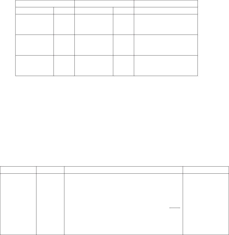
Table 2: Global parameters of micrOMEGAs: nucleon quark form factors
Proton Neutron
Name value Name value comments
ScalarFFPd 0.0191 ScalarFFNd 0.0273
ScalarFFPu 0.0153 ScalarFFNu 0.011 Scalar form factor
ScalarFFPs 0.0447 ScalarFFNs 0.0447
pVectorFFPd -0.427 pVectorFFNd 0.842
pVectorFFPu 0.842 pVectorFFNu -0.427 Axial-vector form factor
pVectorFFPs -0.085 pVectorFFNs -0.085
SigmaFFPd -0.23 SigmaFFNd 0.84
SigmaFFPu 0.84 SigmaFFNu -0.23 Tensor form factor
SigmaFFPs -0.046 SigmaFFNs -0.046
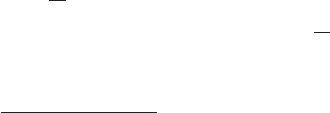
Table 3: Evaluated global variables
Name units comments Evaluated by
CDM1 character name of first DM particle sortOddParticles
CDM2 character name of second DM particle sortOddParticles
Mcdm1 GeV Mass of the first Dark Matter particle sortOddParticles
Mcdm2 GeV Mass of the second DM particles sortOddParticles
Mcdm GeV min(Mcdm1,Mcdm2) if both exist sortOddParticles
dmAsymm Asymmetry between relic density of DM-DM darkOmega[FO]
fracCDM2 fraction of CDM2 in relic density. darkOmega2
Tstart, Tend GeV Temperature interval
for solving the differential equation darkOmega[2]
9

Name Value Units Description
MPlank 1.22091 ×10¹⁹ GeV Planck mass
EntropyNow 2.8912 ×10⁹m−3Present day entropy, s0
RhoCrit100 10.537 GeVm−3ρc/h2or ρfor H= 100km/s/Mpc
Table 4: Some useful constants included in micrOMEGAs.
5 Setting of model parameters, spectrum calculation,
parameter display.
The independent parameters that characterize a given model are listed in the file
work/models/vars1.mdl. Three functions can be used to set the value of these parame-
ters:
•assignVal(name,val)
•assignValW(name,val)
assign value val to parameter name. The function assignVal returns a non-zero value if
it cannot recognize a parameter name while assignValW writes an error message.
•readVar(fileName)
reads parameters from a file. The file should contain two columns with the following
format (see also Section 3.5)
name value
readVar returns zero when the file has been read successfully, a negative value when the
file cannot be opened for reading and a positive value corresponding to the line where a
wrong file record was found.
Note that in Fortran, numerical constants should be specified as Real*8, for example
call assignValW(’SW’, 0.473D0)
A common mistake is to use Real*4.
The constrained parameters of the model are stored in work/models/func1.mdl.
Some of these parameters are treated as public parameters. The public parameters include
by default all particle masses and all parameters whose calculation requires external func-
tions (except simple mathematical functions like sin,cos, ... ). The parameters needed
for the calculation of any public parameters in work/models/func1.mdl are also treated
as public. It is possible to enlarge the list of public parameters. There are two ways to do
this. One can type *before a parameter name to make it public or one can add a special
record in work/models/func1.mdl
%Local! |
Then all parameters listed above this record become public.
The calculation of the particle spectrum and of all public model constraints is done
with:
•sortOddParticles(txt)
which also sorts the odd particles with increasing masses. This routine fills the text
parameters CDM1 and CDM2 with the names of the lightest odd particle starting with one
10
and two tildes respectively and assigns the value of the mass of the lightest odd particle
in each sector to the global parameters Mcdm1 and Mcdm2. For models with only one
DM candidate, micrOMEGAs will set CDM2=NULL and Mcdm2=0 (in Fortran the string is
filled by space symbols). This routine returns a non zero error code for a wrong set of
parameters, for example parameters for which some constraint cannot be calculated. The
name of the corresponding constraint is written in txt. This routine has to be called after
a reassignment of any input parameter.
•qNumbers(pName, &spin2,&charge3,&cdim)
returns the quantum numbers for the particle pName. Here spin2 is twice the spin of
the particle; charge3 is three times the electric charge; cdim is the dimension of the
representation of SU(3)c, it can be 1,3,−3,6,−6 or 8. The parameters spin2, charge3,
cdim are variables of type int. The value returned is the PDG code. If pName does not
correspond to any particle of the model then qNumbers returns zero.
•pdg2name(nPDG)
returns the name of the particle which PDG code is nPDG. If this particle does not
exist in the model the return value is NULL. In the FORTRAN version this function is
Subroutine pdg2name(pName,nPDG) and the character variable pName consists of white
spaces if the particle does not exist in the model.
•antiParticle(pName)
returns the name of the anti-particle for the particle pName.
•pMass(pName)
returns the numerical value of the particle mass.
•nextOdd(n, &pMass)
returns the name and mass of the nth odd particle assuming that particles are sorted ac-
cording to increasing masses. For n= 0 the output specifies the name and the mass of the
CDM candidate. In the FORTRAN version this function is Subroutine nextOdd(pName,n,pMass)
•findVal(name,&val)
finds the value of variable name and assigns it to parameter val. It returns a non-zero
value if it cannot recognize a parameter name.
•findValW(name)
returns the value of variable name and writes an error message if it cannot recognize a
parameter name.
The variables accessible by these two commands are all free parameters and the con-
strained parameters of the model (in file model/func1.mdl) treated as public.
The following routines are used to display the value of the independent and the con-
strained public parameters:
•printVar(FD)
prints the numerical values of all independent and public constrained parameters into FD
•printMasses(FD, sort)
prints the masses of ’odd’ particles (those whose names started with ~). If sort 6= 0 the
masses are sorted so the mass of the CDM is given first.
•printHiggs(FD, sort)
prints the masses and widths of ’even’ colorless scalars.
11

6 Relic density calculation.
6.1 Switches and auxilary routines
•VWdecay,VZdecay
Switches to turn on/off processes with off-shell gauge bosons in the final state for DM an-
nihilation and particle decays. If VW/VZdecay=1, the 3-body final states will be computed
for annihilation processes only while if VW/VZdecay=2 they will be included in coanni-
hilation processes as well. By default the switches are set to (VW/VZdecay=1).1Note
that micrOMEGAs calculates the width of each particle only once and stores the result in
Decay Table. A second call to the function pWidth (whether an explicit call or within the
computation of a cross section) will return the same result even if the user has changed
the VW/VZdecay switch. We recommend to call
•cleanDecayTable()
after changing the switches to force micrOMEGAs to recalculate the widths taking into
account the new value of VW/VZdecay. In Fortran, the subroutine
•setVVdecay(VWdecay,VZdecay) changes the switches and calls cleanDecayTable().
The sortOddParticles command which must be used to recompute the particle spec-
trum after changing the model parameters also clears the decay table.
If the particle widths were stored in a SLHA file (Susy Les Houches Accord [21])
downloaded by micrOMEGAs, then the SLHA value will be used, the widths then do not
depend on the VW/VZdecay switches. To avoid downloading particle widths, one can use
slhaRead(fileName,mode=4) to read the content of the SLHA file, see the description in
Section 14.5.
The temperature dependence of the effective number of degrees of freedom can be set
with
•loadHeffGeff(char*fname)
allows to modify the temperature dependence of the effective number of degrees of freedom
by loading the file fname which contains a table of heff (T), gef f (T) . A positive return
value corresponds to the number of lines in the table. A negative return value indicates
the line which creates a problem (e.g. wrong format), the routine returns zero when the
file fname cannot be opened. The default file is std_thg.tab and is downloaded automat-
ically if loadHeffGeff is not called in the user’s main program [22]. Five other files are
provided in the sources/data directory: HP_A_thg.tab,HP_B_thg.tab,HP_B2_thg.tab,
HP_B3_thg.tab, and HP_C_thg.tab. They correspond to sets A, B, B2, B3, C in [23]. The
user can substitute his/her own table as well, if so, the file must contain three columns
containing the numerical values for T,heff ,geff , the data file can also contain comments
for lines starting with #.
These functions are accessed via
•gEff(T)
returns the effective number of degrees of freedom for the energy density of radiation at
a bath temperature T, only SM particles are included.
•hEff(T)
returns the effective number of degrees of freedom for the entropy density of radiation at
a bath temperature T.
1Including the 3-body final states can significantly increase the execution time for the relic density
computation.
12

•hEffLnDiff(T)
returns the derivative of heff with respect to the bath temperature, dlog(hef f (T))
dlog(T).
•Hubble(T)
returns the Hubble expansion rate at a bath temperature T. This applies for the radiation-
dominated era and is valid for T&100eV.
•improveCrossSection( p1,p2,p3,p4, Pcm, &cs)
allows to substitute a new cross-section for a given process. Here p1,p2 are the names
of particles in the initial state and p3,p4 those in the final state. Pcm is the center of
mass momentum and cs is the cross-section in [pb]. This function is useful if for example
the user wants to include her/his one-loop improved cross-section calculation in the relic
density computation.This function has to be written by the user. The corresponding code
can be placed in the directory lib.micrOMEGAs will call this routine substituting &cs
by the new calculated cross-section. The dummy version of this routine contained in
micrOMEGAs does not change the default cross section.
6.2 Calculation of relic density for one-component Dark Matter
models.
All routines to calculate the relic density in version 3 are available in further versions.
For these routines, the difference between the two dark sectors is ignored. These routines
are intended for models with either a Z2or Z3discrete symmetry.
•vSigma(T,Beps,fast)
calculates the thermally averaged cross section for DM annihilation times velocity at a
temperature T [GeV],
σv(T) = T
8π4n(T)2Zds√sK1√s
TX
˜α, ˜
β
p2
˜α˜
β(s)g˜αg˜
β
X
x≥y
σ˜α˜
β→xy(s) + 1
2X
x˜γ
σ˜α˜
β→x˜γ(s)(1)
n(T) = T
2π2X
˜α
g˜αm2
˜αK2(m˜α
T),(2)
Here ˜α,˜
β, ˜γis used for Odd particles and x,yfor Even particles. σ˜α˜
β→x[˜γ/y]is the cross
section for the corresponding process averaged over the spins of incoming particles and
summed over the spins of outgoing particles. σvshould represent the rate of disappear-
ance of Odd particles, therefore when a final state particle has a non-zero decay branching
ratio to odd particles, the annihilation cross section for this process is multiplied by the
corresponding branching ratio of the decays into SM particles. For the same reason cross
sections for semi - annihilation processes contribute to vSigma with a factor 1
2.K1, K2are
modified Bessel functions of the second kind, and m˜αand g˜αstand for the mass and the
number of degrees of freedom of particle ˜α. Note, that if ˜α6=˜
βthen each σ˜α˜
βterm will
be presented twice. The value for σvis expressed in [pb ·c]. The parameter Beps defines
the criteria for including coannihilation channels as for darkOmega described below. The
fast = 1/0/−1 option switches between the fast/accurate/very accurate calculation.
13

The global array vSigmaTCh contains the contribution of different channels to vSigma.
vSigmaTCh[i].weight specifies the relative weight of the ith channel,
vSigmaTCh[i].prtcl[j] (j=0, 4) defines the particles names for the ith channel.
The last record in vSigmaTCh array has zero weight and NULL particle names. In the For-
tran version, the function vSigmaTCh(i,weight,pdg,process) serves the same purpose.
This function returns 0 if iexceeds the number of annihilation channels and 1 otherwise,
i≥1. The variable real*8 weight gives the relative contribution of each annihilation
channel and integer pdg(5) contains the codes of incoming and outgoing particles in the
annihilation process. character*40 process contains a textual description of annihilation
processes.
•vSigmaCC(T,cc,mode)
calculates the thermally averaged cross section ×velocity for 2 →2, 2 →3, and 2 →4
processes. Tis the temperature in [GeV], cc is the address of the code for each process.
This address can be obtained by the function newProcess presented in Section 10. The
returned value is given in [c·pb].
If mode 6= 0, vSigmaCC calculates the contribution of a given process to the total
annihilation cross section, see Eq.1. The incoming particles should belong to the odd
sector. For 2 →2 processes the result after summation over all subprocesses should
be identical to the one obtained via vSigma above. For this mode, vSigmaCC includes
combinatoric factors: 2 if ˜α6=˜
β, an additional factor 2 if the incoming state is not
self-conjugated, and a factor 1
2for semi-annihilation.
If mode = 0, vSigmaCC is defined by the integral
< vσ˜α˜
β→X>T=1
2T m2
˜αm2
˜
βK2(m˜α
T)K2(m˜
β
T)Zds√sK1(√s
T)p2
cm(s)σ˜α˜
β→X(pcm(s))
where pcm is the center of mass momentum of incoming particles. Note that
lim
T→0vSigmaCC(T,cc,0) = lim
pcm→0σ(pcm)vrel(pcm)
where vrel(pcm) is the relative velocity of incoming particles. The result of vSigmaCC can
be different from that of vSigma described above when there is an important contribution
from NLSP’s to the total number density of DM particles.
•darkOmega(&Xf,fast,Beps,&err)
calculates the dark matter relic density Ωh2. This routine solves the differential evolution
equation using the Runge-Kutta method. Xf=Mcdm/Tfcharacterizes the freeze-out
temperature which is defined by the condition Y(Tf) = 2.5Yeq(Tf). For asymmetric
DM this condition reads 2pY+(Tf)Y−(Tf) = 2.5Yeq(Tf). The value of Xfis given for
information and is also used as an input for the routine that gives the relative contribution
of each channel to Ωh2, see printChannels below. The fast = 1 flag forces the fast
calculation (for more details see Ref. [3]). This is the recommended option and gives
an accuracy around 1%. The parameter Beps defines the criteria for including a given
coannihilation channel in the computation of the thermally averaged cross-section, [3].
The recommended value is Beps = 10−4−10−6whereas if Beps = 1 only annihilation of
the lightest odd particle is computed. Non-zero error code means that the temperature
where thermal equilibrium between the DM and SM sectors is too large Mcdm/T < 2 or
T > 105GeV.
14

darkOmega solves the differential equation for the abundance Y(T) in the temperature
interval [Tend,Tstart] defined by the conditions Y(Tstart)≈1.1Yeq(Tstart), Y(Tend)≈
10Yeq(Tend). For temperatures below Tend, the contribution for Yeq is neglected and the
differential equation is integrated explicitely. The solution in the interval [Tend,Tstart]
interval is tabulated and can be displayed via the function YF(T). The equilibrium abun-
dance can be accessed with the function Yeq(T).
•darkOmegaFO(&Xf, fast, Beps)
calculates the dark matter relic density Ωh2using the freeze-out approximation.
•printChannels(Xf,cut,Beps,prcnt,FD)
writes into FD the contributions of different channels to (Ωh2)−1. Here Xf is an input
parameter which should be evaluated first in darkOmega[FO]. Only the channels whose
relative contribution is larger than cut will be displayed. Beps plays the same role as in
the darkOmega[FO] routine. If prcnt 6= 0 the contributions are given in percent. Note
that for this specific purpose we use the freeze-out approximation.
•oneChannel(Xf,Beps,p1,p2,p3,p4)
calculates the relative contribution of the channel p1,p2 →p3,p4 to (Ωh2)−1. p1,...,p4
are particle names. To sum over several channels one can write "*" instead of a particle
name, e.g "*" in place of p1.
•omegaCh is an array that contains the relative contribution and particle names for each
annihilation channel. In the Fortran version one uses instead the function
omegaCh(i,weight,pdg,process). These array and function are similar to vSigmaTCh
described above. The array omegaCh if filled after calling either darkOmegaFO or printChannels.
There is an option to calculate the relic density in models with DM -DM asymmetry.
In this case we assume that the number difference DM -DM is conserved in all reactions.
Thus a small difference in initial abundances can lead to a large DM asymmetry after
freeze-out as is the case for the baryon asymmetry.
•deltaY
describes the difference between the DM and anti-DM abundances for the models where
the number of DM particles minus the number of anti-DM is conserved in decays and
collisions. In such models deltaY is a constant during the thermal evolution of the
Universe, see Ref. [7].
•dmAsymm
is defined by the equation
Ω±= Ω1±dmAsymm
2
and evaluated by micrOMEGAs while calculating the relic density with an initial asymmetry
deltaY, see [7]. This parameter can also be reset after the relic density computation and
will then be taken into account for direct and indirect detection rates.
•darkOmegaExt(&Xf, vs_a, vs_sa)
calculates the dark matter relic density Ωh2for annihilation cross sections provided by
external functions. Here vs_a is the annihilation cross section in [c·pb] as a function of
the temperature in [GeV] units while vs_sa is the semi-annihilation cross section. vs_a
is required for all models, while vs_sa is relevant only for models where semi-annihilation
occurs. The user can substitute NULL for vs_sa when semi-annihilation is not possible.
darkOmegaExt can also be used if 2 →2 processes do not contribute to DM annihila-
15

tion. In this case the appropriate annihilation or semi-annihilation cross sections can be
calculated by vSigmaCC and the tabulated results stored in vs_a and vs_sa. Note that
if the user substitute some function which is not in tabular form, darkOmegaExt can be
slow as it has not been optimized.
darkOmegaExt solves the Runge-Kutta equation in the interval [Tstart, Tend] where
Tstart is defined automatically while Tend has a fixed value 10−3GeV. darkOmegaExt is
sensitive to effect of DM asymmetry.
6.3 Calculation of relic density for two-component Dark Matter
models.
•darkOmega2(fast, Beps)
Calculates Ωh2for either one- or two-components DM models. In the former case it
should give the same result as darkOmega. The parameters fast and Beps have the same
meaning as for the darkOmega routine. The returned value corresponds to the sum of the
contribution of the two DM components to Ωh2.darkOmega2 also calculates the global
parameter fracCDM2 which represents the mass fraction of CDM2 in the total relic density
Ω = Ω1+ Ω2(3)
fracCDM2 =Ω2
Ω(4)
This parameter is then used in routines which calculate the total signal from both DM
candidates in direct and indirect detection experiments, nucleusRecoil,calcSpectrum,
and neutrinoFlux. The user can change the global fracCDM2 parameter before the
calculation of these observables to take into account the fact that the value of the DM
fraction in the Milky Way could be different than in the early Universe.
The routines that were described in section 6.2 are not available for two-component
DM models. In particular the individual channel contribution to the relic density cannot
be computed and DM asymmetry is ignored. After calling darkOmega2 the user can check
the cross sections for each class of reactions (but not for individual processes) which were
tabulated during the calculation of the relic density. The functions
•vsabcd F(T)
computes the sum of the cross sections for each class of reactions (a, b, c, d = 0,1,2)
tabulated during the calculation of the relic density. Here Tis the temperature in [GeV]
and the return value is vσ in [c·pb]. These functions are defined in the interval [Tstart
,Tend] where Tstart is a global parameter defined by darkOmega2,Tend=10−3GeV.
Specifically the functions available are
vs1100F vs1110F vs1120F vs1112F vs1122F vs1210F vs1211F
vs1220F vs1222F vs2200F vs2210F vs2220F vs2211F vs2221F
The temperature dependence of the abundances can also be called by the user, the
functions are named Y1F(T) and Y2F(T) and are defined only in the interval T∈[Tend,Tstart].
The equilibrium abundances are accessible via the Yeq1(T),Yeq2(T) functions and the
deviation from equilibrium by the functions dY1F(T)= Y1F(T)-Y1eq(T) and
dY2F(T)=Y2F(T)-Y2eq(T).
16

6.4 Calculation of relic density for freeze-in.
Several routines are provided in micrOMEGAs to compute the DM abundance in freeze-in
scenarios. These can be found in the file sources/freezein.c. The first line of this file
contains the statement
//#define NOSTATISTICS
This statement can be uncommented for micrOMEGAs to compute the relic density as-
suming a Maxwell-Boltzman distribution. This option is faster.
The auxiliary functions that are needed for the computation of the factors from statistical
quantum mechanics are
•Stat2(P/T, xY, x1, x2, η1, η2),
returns the Sfunction defined in Eq. (5), that takes into account particle statistical
distributions for the decay of a mediator Y→a, b of fixed momentum P.
S(P/T, xY, xa, xb, ηa, ηb) = 1
2
1
Z
−1
dcθ
eEY/T
(eEa(cθ)/T −ηa)(eEb(cθ)/T −ηb).(5)
where xi≡mi/T ,Ea, Ebare the energies of the outgoing particles and ηi≡ ±eµi/T and
µiis the chemical potential.
•K1to2(x1, x2, x3, η1, η2, η3),
returns the ˜
K1function defined in Eq. (6), that takes into account particle statistical
distributions.
˜
K1(x1, x2, x3, η1, η2, η3)≡1
(4π)2pCMTZ3
Y
i=1 d3pi
Ei
1
eEi/T −ηieE1/T δ4(P1−P2−P3)
(6)
The code does not check whether or not a particle is in thermal equilibrium with the SM
thermal bath and that it is the responsability of the user to specify which particles belong
to the bath, B, or are out of equilibrium, F. This can be done through the function
•toFeebleList(particle_name)
which assigns the particle particle_name to the list of feebly interacting ones (i.e. those
which belong to F). Feebly interacting particles can be odd or even. This function can
be called several times to include more than one particle. All odd or even particles that
are not in this list are assumed to be in thermal equilibrium with the SM and belong to
B. The treatment of the particles that belong to Ffor the computation of Ωh2within
the freeze-in routines is described below. Calling toFeebleList(NULL) will reassign all
particles to B.
The actual computation of the freeze-in DM abundance can be performed with the
help of three functions:
•darkOmegaFiDecay(TR, Name, KE, plot)
calculates the DM abundance from the decay of the particle Name into all odd FP. Here
we assume that all odd FP will decay into the lightest one which is the DM. TR is the
reheating temperature and KE is a switch to specify whether the decaying particle is in
17
kinetic equilibrium (KE=1) or not (KE=0) with the SM. The equations used for the three
different cases are described in [8]. Numerically, the latter two methods give very similar
results, however the function with KE=1 is faster. The switch plot=1 displays on the
screen Y(T) for the decaying particle and dY/d log(T) for DM.
•darkOmegaFi22(TR, Process, vegas, plot, &err)
calculates the DM abundance taking into account only DM production via the 2 →2
process defined by the parameter Process. For example "b,B ->~x1,~x1" for the pro-
duction of DM (here ~x1) via b¯
bscattering. This routine allows the user to extract the
contribution of individual processes. TR is the reheating temperature. When the switch
vegas=1, the collision term is integrated directly as described in [8]. The execution
time for this option is quite long, it is intended mostly for precision checks. The switch
plot=1 displays on the screen dY/d log(T) for DM. Note that the temperature profile
for DM production obtained by darkOmegaFiDecay and darkOmegaFi22 can be different.
For example, in the case of a s-channel resonance, the temperature for DM production
corresponds to the one of the mediator decay for darkOmegaFiDecay and the temperature
at which the mediator is created for darkOmegaFi22.err is the returned error code, it
has the following meaning
1: the requested processes does not exist
2: 2 →2 process is expected
3: can not calculate local parameters // some constrain parameters can not be calculated.
4: the reheating temperature is too small, (TR<1keV )
5: one of the incoming particles belong to F.
6: None of the outgoing particles are odd and feeble.
7: There is an on-shell particle in t/u channel
8: A numerical integral cannot be performed precisely.
When substituting NULL for the error code, the error message is displayed on the screen
and in this case the message does not appear in the address of the variable used for passing
the error code.
•darkOmegaFi(TR, &err)
calculates the DM abundance after summing over all 2 →2 processes involving particles
in the bath Bin the initial state and at least one particle in Fin the final state. The rou-
tine checks the decay modes of all bath particles and if one of them has no decay modes
into two other bath particles, the 2 →2 processes involving this particle are removed
from the summation and instead the contribution to the DM abundance computed from
the routine darkOmegaFiDecay is included in the sum. This is done to avoid appearance
of poles in the corresponding 2 →2 cross-section. We recommend for such models to
compute individual 2 →2 processes with darkOmegaFi22 described above. As before, we
assume that all odd FIMPs will decay into the lightest one which is the DM. TRhas the
same meaning as above. err is the returned error code, err=1 if feeble particles have not
been defined.
•printChannelsFi(cut,prcnt,filename)
writes into the file filename the contribution of different channels to Ωh2. The cut param-
18
eter specifies the lowest relative contribution to be printed. If prcnt 6= 0, the contributions
are given in percent. The routine darkOmegaFi fills the array omegaFiCh which contains
the contribution of different channels ( 2 →2 or 1 →2) to Ωh2. omegaFiCh[i].weight
specifies the relative weight of the ith channel, omegaFiCh[i].prtcl[j] (j=0, 4) defines the
particles names for the ith channel. The last record in the array omegaFiCh has zero
weight and NULL particle names.
Note that if no particle has been declared as being feebly interacting, the freeze-out rou-
tines darkOmega,darkOmegaFO, and darkOmega2 [24] will work exactly like in previous
versions of micrOMEGAs. A non-empty list of FIMPs, however, will affect these routines
since micrOMEGAs will exclude all odd particles in this list from the computation of the
relic density via freeze-out. For example, if the DM is a bath particle, excluding FPs can
impact the freeze-out computation of Ωh2when they are nearly degenerate in mass with
the DM, hence could potentially contribute to coannihilation processes. Note also that
if, for example, the lightest odd particle (the DM) belongs to Fand the user computes
the freeze-out abundance of the lightest odd bath particle, the resulting value of ΩLBP h2
will be automatically rescaled by a factor MLF P /MLBP , where MLBP (MLF P ) is the mass
of the lightest odd particle in B(F). Conversely, if the DM belongs to Band the user
computes the freeze-in abundance of the lightest feeble odd particle, the corresponding
result for ΩLF P h2will be rescaled by MLBP /MLF P . In other words, the answer obtained
in both of these cases corresponds to the predicted density of the dark matter particles
and not the heavier ones. Besides, micrOMEGAs does not check whether the decay rate of
an odd particle to the feeble particles is much smaller than H(TF O) which would justify
the fact that they should not be included in the freeze-out computation.
7 Direct detection.
7.1 Amplitudes for elastic scattering
•nucleonAmplitudes(CDM,pAsi,pAsd,nAsi,nAsd)
calculates the amplitudes for CDM-nucleon elastic scattering at zero momentum. pAsi(nAsi)
are spin independent amplitudes for protons(neutrons) whereas pAsd(nAsd) are the cor-
responding spin dependent amplitudes. Each of these four parameters is an array of
dimension 2. The zeroth (first) element of these arrays gives the χ-nucleon amplitudes
whereas the second element gives χ-nucleon amplitudes. Amplitudes (in GeV−2) are
normalized such that the total cross section for either χor χcross sections is
σtot =4M2
χM2
N
π(Mχ+MN)2(|ASI |2+ 3|ASD|2) (7)
nucleonAmplitudes depends implicitly on form factors which describe the quark con-
tents in the nucleon. These form factors are global parameters (see Table 1for default
values)
T ypeFFPq T ypeFFNq
where T ype is either ”Scalar”, ”pVector”, or ”Sigma”, FFP and FFN denote proton and
neutron and qspecifies the quark, d, u or s. Heavy quark coefficients are calculated
automatically.
19

micrOMEGAs automaticaly takes into account loop contributions from box diagrams
as calculated in [25] (DM spin 1/2 case) and [26] (DM spin 0 and 1 cases).
•calcScalarQuarkFF(mu/md,ms/md,σπN ,σs)
computes the scalar coefficients for the quark content in the nucleon from the quark mass
ratios mu/md, ms/mdas well as from σπN and σs. The default values given in Table 2
are obtained for σs= 42MeV, σπN = 34MeV, mu/md= 0.56, ms/md= 20.2 [27]. The
function calcScalarQuarkFF(0.553,18.9,55.,243.5) will reproduce the default values of the
scalar quark form factors used in micrOMEGAs2.4 and earlier versions.
7.2 Scattering on nuclei
•nucleusRecoil(f,A,Z,J,Sxx,dNdE)
This is the main routine of the direct detection module. The input parameters are:
⋄f- the DM velocity distribution normalized such that
Z∞
0
vf(v)dv = 1
The units are km/s for v and s2/km2for f(v).
⋄A- atomic number of nucleus;
⋄Z- number of protons in the nucleus, predefined values for a wide set of isotopes
are called with Z{Name};
⋄J- nucleus spin, predefined values for a wide set of isotopes are called with
J{Name}{atomic number}.
⋄Sxx - is a routine which calculates nucleus form factors for spin-dependent interac-
tions (S00,S01,S11), it depends on the momentum transfer in fm−1. The available
form factors are
SxxF19 SxxNa23 SxxNa23A SxxAl27 SxxSi29 SxxSi29A
SxxK39 SxxGe73 SxxGe73A SxxNb92 SxxTe125 SxxTe125A
SxxI127 SxxI127A SxxXe129 SxxXe129A
SxxXe131 SxxXe131A SxxXe131B
The last character is used to distinguish different implementations of the form factor
for the same isotope, see details in [5].
The form factors for the spin independent (SI) cross section are defined by a Fermi dis-
tribution and depend on the global parameters Fermi_a,Fermi_b,Fermi_c.
The returned value gives the number of events per day and per kilogram of detector
material. The result depends implicitly on the global parameter rhoDM, the density of
DM near the Earth. The distribution over recoil energy is stored in the array dNdE which
by default has Nstep = 200 elements. The value in the ith element corresponds to
dNdE[i] = dN
dE |E=i∗keV ∗step
20

in units of (1/keV/kg/day). By default step is set to 1.
dNdERecoil(E,dNdE) interpolates the dNdE table.
For a complex WIMP, nucleusRecoil averages over χand χ. For example for 73Ge,
a call to this routine will be:
nucleusRecoil(Maxwell,73,Z_Ge,J_Ge73,SxxGe73,dNdE);
•setRecoilEnergyGrid(step,Nstep)
changes the values of step and Nstep for the computation of dNdE.
•Maxwell(v)
returns
f(v) = cnorm
vZ
|~v|<vmax
d3~v exp −(~v −VEarth)2
∆v2δ(v − |~v|)
which corresponds to the isothermal model. Default values for the global parameters
∆v= Vrot, vmax = Vesc, Vearth are listed in Table 1.cnorm is the normalization factor.
This function is an argument of the nucleusRecoil function described above.
•nucleusRecoil0(f,A,Z,J,Sp,Sn,dNdE)
is similar to the function nucleusRecoil except that the spin dependent nuclei form
factors are described by Gauss functions whose values at zero momentum transfer are
defined by the coefficients Sp,Sn [5]. Predefined values for the coefficients Sp,Sn are
included for the nuclei listed in nucleusrecoil as well as 3He,133Cs. Their names are
Sp {Nucleus Name}{Atomic Number}
Sn {Nucleus Name}{Atomic Number}
One can use this routine for nuclei whose form factors are not known.
7.3 Auxiliary routines
An auxiliary routine is provided to work with the energy spectrum computed with nucleusRecoil
and nucleusRecoil0.
•cutRecoilResult(dNdE,E1,E2)
calculates the number of events in an energy interval defined by the values E1,E2 in keV.
8 Indirect detection
8.1 Interpolation and display of spectra
Various spectra and fluxes of particles relevant for indirect detection are stored in arrays
with NZ=250 elements. To decode and interpolate the spectrum array one can use the
following functions:
•SpectdNdE(E,spectTab)
interpolates the tabulated spectra and returns the particle distribution dN/dE where E
is the energy in GeV. For a particle number distribution the returned value is given in
GeV−1while a particle flux is expressed in (sec cm2sr GeV )−1.
21

To display the spectra as a function of energy one can use
•displaySpectra(title, Emin, Emax, N, nu1,lab1,...)
which displays several spectra. Here title contains some text, Emin,Emax are the lower
and upper limits, and Nis the number of spectra to display. Each spectrum is defined
with two arguments, nu1 designates the spectrum array and lab1 contains some text to
label the spectrum.
Even though the user does not need to know the structure of the spectrum array, we de-
scribe it below. The first (zeroth) element of the array contains the maximum energy Emax.
As a rule Emax is the mass of the DM particle. The ith element (1 ≤i < N Z −1) of the
spectrum array contains the value of EidN
dEiwhere Ei=EmaxeZi(i),Zi(i)=−7 ln 10 i−1
NZ 1.5.
That is the array covers the energy interval Emax ≥E > 10−7Emax.
•addSpectrum(Spect,toAdd)
sums the spectra toAdd and Spect and writes the result in Spect. For example, this
routine can be useful for summing spectra with different maximal energy.
•spectrMult(Spec, func)
allows to multiply the spectrum Spec by any energy dependent function func
•spectrInt(Emin,Emax,Spec)
integrates a spectrum/flux, Spec from Emin to Emax.
•spectrInfo(Emin,Spec,&Etot)
provides information on the spectra. The returned value and Etot corresponds respec-
tively to
Ntot =
Emax
Z
Emin
SpectdNdE(E, Spec)dE =spectrInt(Emin, Emax, Spec)
Etot =
Emax
Z
Emin
E SpectdNdE(E, Spec)dE
where the first element of the table Spec contains the value of Emax.
8.2 Annihilation spectra
•calcSpectrum(key,Sg,Se,Sp,Sne,Snm,Snl,&err)
calculates the spectra of DM annihilation at rest and returns σv in cm3/s . The calcu-
lated spectra for γ,e+, ¯p,νe,νµ,ντare stored in arrays of dimension NZ as described
above: Sg,Se,Sp,Sne,Snm,Snl. To remove the calculation of a given spectra, substi-
tute NULL for the corresponding argument. key is a switch to include the polarisation
of the W, Z bosons (key=1) or photon radiation (key=2). Note that final state photon
radiation (FSR) is always included. When key=2 the 3-body process χχ′→XX +γ
is computed for those subprocesses which either contain a light particle in the t-channel
(of mass less than 1.2 Mcdm) or an outgoing W when Mcdm>500GeV. The FSR is then
subtracted to avoid double counting. Only the electron/positron spectrum is modified
with this switch. When key=4 the contibutions for each channel to the total annihilation
22

rate are written on the screen. More than one option can be switched on simultaneously
by adding the corresponding values for key. For example both the Wpolarization and
photon radiation effects are included if key=3. A problem in the spectrum calculation
will produce a non zero error code, err 6= 0. calcSpectrum interpolates and sums spectra
obtained by Pythia. The spectra tables are provided only for Mcdm>2GeV. The results
for a dark matter mass below 2 GeV will therefore be wrong, for example an antiproton
spectrum with kinematically forbidden energies will be produced. A warning is issued for
Mcdm<2GeV.
•vSigmaCh
is an array that contains the relative contribution and particle names for each annihila-
tion channel. It is similar to vSigmaTCh described in Section 6.2. Note that the list of
particles contains five elements to allow to include gamma radiation. For 2->2 processes
vSigmaCh[n].prtcl[4]=NULL. The array vSigmaCh is filled by calcSpectrum. In the For-
tran version one uses instead the function
vSigmaCh(i,weight,pdg,process)
which is similar to the Fortran vSigmaTCh described in Section 6.2.
8.3 Distribution of Dark Matter in Galaxy.
The indirect DM detection signals depend on the DM density in our Galaxy. The DM
density is given as the product of the local density at the Sun with the halo profile function
ρ(r) = ρ⊙Fhalo(r) (8)
In micrOMEGAs ρ⊙is a global parameter rhoDM and the Zhao profile [28]
Fhalo(r) = R⊙
rγrα
c+Rα
⊙
rα
c+rαβ−γ
α
(9)
with α= 1, β = 3, γ = 1, rc = 20[kpc] is used by default. R⊙, the distance from the
Sun to the galactic center, is also a global parameter, Rsun. The parameters of the Zhao
profile can be reset by
•setProfileZhao(α,β,γ,rc)
The function to set another density profile is
•setHaloProfile(Fhalo(r))
where Fhalo(r) is any function which depends on the distance from the galactic center,
r, defined in [kpc] units. For instance, setHaloProfile(hProfileEinasto) sets Einasto
profile
Fhalo(r) = exp −2
α r
R⊙α
−1
where by default α= 0.17, but can be changed by
•setProfileEinasto(α)
The command setHaloProfile(hProfileZhao) sets back the Zhao profile. Note that
both setProfileZhao and setProfileEinasto call setHaloProfile to define the cor-
responding profile.
Dark matter annihilation in the Galaxy depends on the average of the square of the
DM density, < ρ2>. This quantity can be significantly larger than < ρ >2when clumps
23
of DM are present [29]. In micrOMEGAs, we use a simple model where fcl is a constant
that characterizes the fraction of the total density due to clumps and where all clumps
occupy the same volume Vcl and have a constant density ρcl. Assuming clumps do not
overlap, we get
< ρ2>=ρ2+fclρclρ. (10)
This simple description allows to demonstrate the main effect of clumps: far from the
Galactic center the rate of DM annihilation falls as ρ(r) rather than as ρ(r)2. The pa-
rameters ρcl and fcl have zero default values. The routine to change these values is
•setClumpConst(fcl,ρcl)
To be more general, one could assume that ρcl and fcl depend on the distance from the
galactic center. The effect of clumping is then described by the equation
< ρ2>(r) = ρ(r)(ρ(r) + ρeff
clump(r)),(11)
and the function
•setRhoClumps(ρef f
clump)
allows to implement a more sophisticated clump structure. To return to the default
treatment of clumps call setRhoClumps(rhoClumpsConst) or setClumpConst.
8.4 Photon signal
The photon flux does not depend on the diffusion model parameters but on the angle
φbetween the line of sight and the center of the galaxy as well as on the annihilation
spectrum into photons
•gammaFluxTab(fi,dfi,sigmav,Sg,Sobs)
multiplies the annihilation photon spectrum with the integral over the line of sight and
over the opening angle to give the photon flux. fi is the angle between the line of sight
and the center of the galaxy, dfi is half the cone angle which characterizes the detector
resolution (the solid angle is 2π(1−cos(dfi)) , sigmav is the annihilation cross section, Sg
is the DM annihilation spectra. Sobs is the spectra observed in 1/(GeV cm^2 s ) units.
The function gammaFluxTab can be used for the neutrino spectra as well.
•gammaFluxTabGC(l,b,dl,db,sigmav,Sg,Sobs)
is similar to gammaFluxTab but uses standard galactic coordinates. Here lis the galactic
longitude (measured along the galactic equator from the galactic center, and bis the lati-
tude (the angle above the galactic plane). Both land bare given in radians. The relation
between the angle fi used above and the galactic coordinates is fi= cos−1(cos(l) cos(b)).
gammaFluxTabGC integrates the flux over a rectangle [(l, b)−(l+dl, b +db)].
•gammaFlux(fi,dfi,dSigmavdE)
computes the photon flux for a given energy E and a differential cross section for photon
production, dSigmavdE. For example, one can substitute dSigmavdE=σvSpectdNdE(E,SpA)
where σv and SpA are obtained by calcSpectrum. This function can also be used to com-
pute the flux from a monochromatic gamma-ray line by substituting the cross section at
fixed energy (in cm3/s) instead of dSigmavdE, for example the cross sections obtained
with the loopGamma function in the MSSM, NMSSM, CPVMSSM models (vcsAA and
vcsAZ). In this case the flux of photons can be calculated with
gammaFlux(fi,dfi,2*vcsAA+vcsAZ).
•gammaFluxGC(l,b,dl,db,vcs)
is the analog of gammaFlux when using standard galactic coordinates.
24
8.5 Propagation of charged particles.
The observed spectrum of charged particles strongly depends on their propagation in the
Galactic Halo. The propagation depends on the global parameters
K_dif, Delta_dif, L_dif, Rsun, Rdisk
as well as
Tau_dif (positrons), Vc_dif (antiprotons)
•posiFluxTab(Emin,sigmav, Se, Sobs)
computes the positron flux at the Earth. Here sigmav and Se are values obtained by
calcSpectrum.Sobs is the positron spectrum after propagation. Emin is the energy cut
to be defined by the user. Note that a low value for Emin increases the computation time.
The format is the same as for the initial spectrum. The function SpectrdNdE(E,Sobs)
described above can also be used for the interpolation, in this case the flux is returned in
(GeV s cm2sr)−1.
•pbarFlux(E,dSigmavdE)
computes the antiproton flux for a given energy Eand a differential cross section for
antiproton production, dSigmavdE. For example, one can substitute
dSigmavdE=σvSpectdNdE(E,SpP)
where σv and SpP are obtained by calcSpectrum. This function does not depend on
the details of the particle physics model and allows to analyse the dependence on the
parameters of the propagation model.
•pbarFluxTab(Emin,sigmav, Sp, Sobs)
computes the antiproton flux, this function works like posiFluxTab,
•solarModulation(Phi, mass, stellarTab, earthTab)
takes into account modification of the interstellar positron/antiproton flux caused by the
electro-magnetic fields in the solar system. Here Phi is the effective Fisk potential in
MeV, mass is the particle mass, stellarTab describes the interstellar flux, earthTab is
the calculated particle flux in the Earth orbit.
Note that for solarModulation and for all *FluxTab routines one can use the same
array for the spectrum before and after propagation.
9 Neutrino signal from the Sun and the Earth
This module does not work yet in case of 2DM
After being captured, DM particles concentrate in the center of the Sun/Earth and
then annihilate into Standard Model particles. These SM particles further decay pro-
ducing neutrinos that can be observed at the Earth. The neutrino spectra originating
from different annihilation channels into SM particles and taking into account oscillations
and Sun medium effects were computed both in WimpSim [30] and in PPPC4DMν[31].
We use the set of tables provided by these two groups as well as those from DMν[32]
which were included in previous versions of micrOMEGAs. The new global parameter
25

WIMPSIM allows to choose the neutrino spectra. The default value WIMPSIM=0 2corre-
sponds to the PPPC4DMνspectra while WIMPSIM=1 corresponds to the WimpSim spectra
and WIMPSIM=-1 to the DMνspectra.
•neutrinoFlux(f,forSun,nu, nu_bar)
calculates the muon neutrino/anti-neutrino fluxes near the surface of the Earth. Here
fis the DM velocity distribution normalized such that R∞
0vf(v)dv = 1. The units are
km/s for v and s2/km2for f(v). For example, one can use the same Maxwell function
introduced for direct detection. This routine implicitly depends on the WIMPSIM switch.
If forSun==0 then the flux of neutrinos from the Earth is calculated, otherwise this
function computes the flux of neutrinos from the Sun. The calculated fluxes are stored
in nu and nu bar arrays of dimension NZ=250. The neutrino fluxes are expressed in
[1/Year/km2].
•muonUpward(nu,Nu,muon)
calculates the muon flux which results from interactions of neutrinos with rocks below the
detector. Here nu and Nu are input arrays containing the neutrino/anti-neutrino fluxes
calculated by neutrinoFlux.muon is an array which stores the resulting sum of µ+,µ−
fluxes. SpectdNdE(E,muon) gives the differential muon flux in [1/Year/km2/GeV] units.
The muon flux weakly depends on the propagation medium, e.g. rock or ice. The energy
lost during propagation is described by the equation [33]
dE
dx =−(α+βE)ρ(12)
For propagation in ice (the switch forRocks=0), micrOMEGAs substitutes ρ= 1.0 g/cm3,
α= 0.00262 GeVcm2/g, β= 3.5×10⁻⁶cm2/g [34], while for propagation in rocks, ρ=
2.6 g/cm3,α= 0.002 GeVcm2/g, β= 3.0×10⁻⁶cm2/g [33]. The result depends on the
ratio α/β .
•muonContained(nu,Nu,rho, muon) calculates the flux of muons produced in a given
detector volume.This function has the same parameters as muonUpward except that the
outgoing array gives the differential muon flux resulting from neutrinos converted to muons
in a km3volume given in [1/Year/km3/GeV] units. rho is the density of the detector in
g/cm3.
•atmNuFlux(nu,cs,E)
returns the atmospheric muon neutrinos (nu > 0) and anti-neutrinos spectrum (nu < 0)
in [1/Year/km^2] units for a given cosine of the zenith angle, cs. This function is based
on [35].
Two functions allow to estimate the background from atmospheric neutrinos creating
muons after interaction with rocks below the detector or with water inside the detector.
•ATMmuonUpward(cosFi,E) calculates the sum of muon and anti-muon fluxes resulting
from the interaction of atmospheric neutrinos with rocks in units of [1/Year/km2/GeV/Sr].
cosFi is the energy between the direction of observation and the direction to the center
of Earth. Eis the muon energy in GeV. The result depends on the forRock switch.
•ATMmuonContained(cosFi, E, rho) calculates the muon flux caused by atmospheric
neutrinos produced in a given (detector) volume. The returned value for the flux is given
2Since PPPC4DMνdoes not provide neutrino specrtra produced at the center of the Earth, in this
case and for WIMPSIM=0 micrOMEGAs uses the DMνspectra.
26

in 1/Year/km3/GeV/Sr.rho is the density of the detector in g/cm3units. cosFi and E
are the same as above.
9.1 Comparison with IceCube results
These functions are described in [36] and allow to compare the predictions for the neutrino
flux from DM captured in the Sun with results of IceCube22.
•IC22nuAr(E)
effective area in [km2] as a function of the neutrino energy, Aνµ(E)
•IC22nuBarAr(E)
effective area in [km2] as a function of the anti-neutrino energy, A¯νµ(E)).
•IC22BGdCos(cs)
angular distribution of the number of background events as a function of cos φ,dNbg
dcos ϕ.
•IC22sigma(E)
neutrino angular resolution in radians as a function of energy.
•exLevIC22( nu_flux, nuB_flux,&B)
calculates the exclusion confidence level for number of signal events generated by given νµ
and ¯νµfluxes, [36]. The fluxes are assumed to be in [GeV km2Year]−1. This function uses
the IC22BGdCos(cs) and IC22sigma(E) angular distribution for background and signal
as well as the event files distributed by IceCube22 with φ < φcut = 8◦. The returned
parameter Bis a Bayesian factor representing the ratio of likelihood functions for the
model with given fluxes and the model with null signal. See details in [36].
•fluxFactorIC22(exLev, nu,nuBar)
For given neutrino, nu, and anti-neutrino fluxes, nuBar, this function returns the factor
that should be applied to the fluxes (neutralino-proton cross sections) to obtain a given
exclusion level exLev in exLevIC22. This is used to obtain limits on the SD cross section
for a given annihilation channel.
10 Cross sections and decays.
The calculation of particle widths, decay channels and branching fractions can be done
by the functions
•pWidth(particleName,&address)
returns directly the particle width. If the 1->2 decay channels are kinematically acces-
sible then only these channels are included in the width when VWdecay,VZdecay= 0. If
not, pWidth compiles all open 1->3 channels and use these for computing the width. If
all 1->3 channels are kinematically forbidden, micrOMEGAs compiles 1->4 channels. If
VWdecay(VZdecay)6= 0, then micrOMEGAs also computes the processes with virtual W(Z)
and adds these to the 1->2 decay channels. Note that 1->3 decay channels with a virtual
W will be computed even if the mass of the decaying particle exceeds the threshold for
1->2 decays by several GeV’s. This is done to ensure a proper matching of 1->2 and
1->3 processes. For particles other than gauge bosons, an improved routine with 3-body
processes and a matching between the 1->2 and 1->3 calculations is kept for the future.
The returned parameter address gives an address where information about the decay
channels is stored. In C, the address should be of type txtList. For models which read a
27

SLHA parameter file, the values of the widths and branchings are taken from the SLHA
file unless the user chooses not to read this data, see (Section 14.5) for details.
•printTxtList(address,FD)
lists the decays and their branching fractions and writes them in a file. address is the
address returned by pWidth.
•findBr(address,pattern)
finds the branching fraction for a specific decay channel specified in pattern, a string
containing the particle names in the CalcHEP notation. The names are separated by
commas or spaces and can be specified in any order.
•slhaDecayPrint(pname,delVirt,FD)
uses pWidth described above to calculate the width and branching ratios of particle pname
and writes down the result in SLHA format. The return value is the PDG particles code.
In case of problem, for instance wrong particle names, this function returns zero. This
function first computes 1 →2 decays. If such decays are kinematically forbidden then
1→3 decay channels are computed. Decays via virtual W/Z bosons will be listed via
their decay products when delV irt 6= 0.
•newProcess(procName)
compiles the codes for any 2 →2 or 1 →2 reaction. The result of the compilation
is stored in the shared library in the directory work/so-generated/. The name of the
library is generated automatically.
The newProcess routine returns the address of the compiled code for further usage.
If the process can not be compiled, then a NULL address is returned. 3
Note that it is also possible to compute processes with polarized massless beams, for
example for a polarized electron beam use e% to designate the initial electron.
•procInfo1(address,&ntot,&nin,&nout)
provides information about the total number of subprocesses (ntot) stored in the library
specified by address as well as the number of incoming (nin) and outgoing (nout) par-
ticles for these subprocesses. Typically, for collisions (decays), nin=2(1) and nout=2,3.
NULL can be substitute if this information is not needed.
•procInfo2(address,nsub,N,M)
fills an array of particle names Nand an array of particle masses Mfor the subprocess nsub
(1 ≤nsub ≤ntot) . These arrays have size nin +nout and the elements are listed in the
same order as in CalcHEP starting with the initial state, see the example in MSSM/main.c.
•cs22(address,nsub,P,c1,c2,&err)
calculates the cross-section for a given 2 →2 process, nsub, with center of mass momen-
tum P(GeV). All model parameters except the strong coupling GG can be specified with
the functions findVal[W]/assignVal[W] described in Section 5. The strong coupling GG
is defined via the scale parameter GGscale. The differential cross-section is integrated
within the range c1<cos θ < c2. θis the angle between ~p1and ~p3in the center-of-mass
frame. Here ~p1(~p3) denote respectively the momentum of the first initial(final) particle.
err contains a non zero error code if nsub exceeds the maximum value for the number of
subprocesses (given by the argument ntot in the routine procInfo1). To set the polar-
ization of the initial massless beam, define Helicity[i] where i= 0,1 for the 1th and
2nd particles respectively. The helicity is defined as the projection of the particle spin on
3The Fortran version of newProcess returns integer*8.
28
the direction of motion. It ranges from [-1,1] for spin 1 particles and from [-0.5,0.5] for
spin 1/2 particles. By definition a left handed particle has a positive helicity.
•hCollider(Pcm,pp,nf, Qren,Qfac, pName1,pName2,Tmin,wrt) calculates the cross
section for particle production at hadron colliders. Here Pcm is the beam energy in the
center-of-mass frame. pp is 1(−1) for pp(p¯p) collisions, nf ≤5 defines the number of quark
flavors taken into account. The parameters Qren and Qfac define the renormalisation and
factorization scales respectively. pName1 and pName2 are the names of outgoing particles.
If Tmin ≤0 then hCollider calculates the total cross section for the 2-body final state
process. Otherwise it calculates the cross section for
proton, [a]proton -> pName1, pName2, jet
where Tmin >0 defines the cut on the jet transversee momentum. The jet content is
defined by the parameter nf. If Qfact ≤0, then running ˆsis used for the factorization
scale. If Qren ≤0, ˆsis used for the renormalization scale for a 2 →2 process and pTof
the jet is used for the renormalization scale for a process with a jet in the final state. The
last argument in the hCollider routine allows to switch on/off (wrt=1/0) the printing of
the contribution of individual channels to the total cross section. The value returned is
the total cross section in [pb].
One of the arguments pName1,pName2 can be NULL. Then the cross section for 2 →1
or 2 →1 + jet process will be calculated. In Fortran, one should pass a blank string
instead of NULL.
By default hCollider uses the cteq6l structure function built-in the micrOMEGAs code.
One can set any other parton distribution included in either micrOMEGAs or LHAPDF.
The list of structure functions in micrOMEGAs can be obtained with the command
•PDFList
and one of these can be activated by
•setPDF(name)
To work with other PDF’s available in LHAPDF one should first define the environment
variable LHAPDFPATH which specifies the path to the LHAPDF library. Then micrOMEGAs
Makefile links it automatically. The list of available LHAPDF distributions can be ob-
tained with the command
•LHAPDFList
and one of these can be activated by
•setLHAPDF(nset,name)
where nset specifies the subset number. Note, that if a wrong input is provided, setLHAPDF
terminates the execution.
The parton densities are defined by the function
•parton_distr(pdg,x,q)
where pdg is the PDG code of a particle. Note that parton_distr defines the parton
number density and contains a factor 1/x with respect to the definition used in LHAPDF.
11 Tools for model independent analysis
A model independent calculation of the DM observables is also available. After specifying
the DM mass, the cross sections for DM spin dependent and spin independent scatter-
ing on proton and neutron, the DM annihilation cross section times velocity at rest and
29
the relative contribution of each annihilation channel to the total DM annihilation cross
section, one can compute the direct detection rate on various nuclei, the fluxes for pho-
tons, neutrinos and antimatter resulting from DM annihilation in the galaxy and the
neutrino/muon fluxes in neutrino telescopes.
All the routines presented here depend implicitly on the global parameter Mcdm except
for basicSpectra and basicNuSpectra . These routines do not take into account the
multi-component structure of DM and, in particular, possible differences between DM
and anti-DM. To use these for multi-component DM the user has to perform a summation
over the different DM components.
•nucleusRecoilAux(f,A,Z,J,Sxx,csIp,csIn,csDp,csDn,dNdE)
This function is similar to nucleusRecoil. The additional input parameters include
csIp(csIn) the SI cross sections for WIMP scattering on protons(neutrons) and csDp(csDn)
the SD cross sections on protons(neutrons). A negative value for one of these cross sections
is interpreted as a destructive interference between the proton and neutron amplitudes.
Note that the rate of recoil depends implicitly on the WIMP mass, the global parameter
Mcdm. The numerical value for the global parameter has to be set before calling this func-
tion.
•nucleusRecoil0Aux(f,A,Z,J,Sp,Sn,csIp,csIn,csDp,csDn,dNdE) is the correspond-
ing modification of nucleusRecoil0.
For indirect detection, we also provide a tool for model independent studies
•basicSpectra(Mass,pdgN,outN,Spectr)
computes the spectra of outgoing particles and writes the result in an array of dimension
250, Spectr,pdgN is the PDG code of the particles produced in the annihilation of a pair
of WIMPs. To get the spectra generated by transverse and longitudinal W’s substitute
pdgN= 24 +′T′and 24 +′L′correspondingly. In the same manner pdgN= 23 +′T′and
23+′L′provides the spectra produced by a polarized Z boson. outN specifies the outgoing
particle,
outN = {0,1,2,3,4,5}for {γ, e+, p−, νe, νµ, ντ}
The Mass parameter defines the mass of the DM particle. Note that the propagation
routines for e+, p−, γ can be used after this routine as usual. Note that the result
of basicSpectra are not valid for Mcdm <2GeV as explained in the description of
calcSpectrum.
To get indirect detection signals one can substitute the obtained spectra in the
[photon/posi/pbar]FluxTab routines. As long as one keeps the default setting CDM1=CDM2=NULL
these routines will use the Mcdm parameter to calculate the number density of DM particles.
•captureAux(f,forSun,Mass,csIp,csIn,csDp,csDn)
calculates the number of DM particles captured per second assuming the cross sections
for spin-independent and spin-dependent interactions with protons and neutrons csIp,
csIn, csDp, csDn are given as input parameters (in [pb]). A negative value for one of
the cross sections is interpreted as a destructive interference between the proton and neu-
tron amplitudes. The first two parameters have the same meaning as in the neutrinoFlux
routine Section 9. The result depends implicitly on the global parameters rhoDM and Mcdm
in Table 1.
•basicNuSpectra(forSun,Mass,pdg, pol, nu_tab, nuB_tab)
calculates the νµand ¯νµspectra corresponding to the pair annihilation of DM in the
center of the Sun/Earth into a particle-antiparticle pair with PDG code pdg.Mass is the
30

DM mass. Note that this routine depends implicitly on the global parameter WIMPSIM
(1,0,-1) which selects the neutrino spectra computed by WimpSim [30], PPPC4DMν[31]
and DMν[32]. The parameter pol selects the spectra for polarized particles available in
PPPC4DMν.pol=-1(1) corresponds to longitudinal (transverse) polarisation of vec-
tor bosons or to left-handed (right-handed) polarisation of fermions, pol=0 is used for
unpolarized spectra. When polarized spectra are not available, the unpolarized ones are
generated irrespective of the value of pol. The parameter outN is 1 for muon neutrino and
-1 for anti-neutrino. The resulting spectrum is stored in the arrays nu_tab and nuB_tab
with NZ=250 elements.
The files main.c/F in the directory mdlIndep contain an example of the calculation of
the direct detection, indirect detection and neutrino telescope signals using the routines
described in this section. The numerical input data in this sample file corresponds to
’MSSM/mssmh.dat’.
12 Constraints from colliders
12.1 The Higgs sector
To obtain the limits on the Higgs sector for models with one or several Higgs bosons,
the predictions for the signal strengths of the 125 GeV Higgs can be compared to the
latest results of the LHC, for this an interface to the public code HiggsSignals [37] or
Lilith [38] is provided. Moreover the exclusion limits obtained from Higgs searches in
different channels at LEP, Tevatron and the LHC can be applied to other Higgses in the
model using HiggsBounds [39].
12.1.1 Lilith
Lilith [38] is a Python library that is used to construct a global likelihood function
Lfrom the latest ATLAS and CMS results on the 125 GeV Higgs. 4The Lilith in-
puts are the set of reduced couplings of the 125 GeV state, i.e., couplings normalized
by the SM ones, as well as the branching ratios of Higgs decays to invisible, BRinv, or
to undetected non-SM final states, BRundetected = 1 −BRinv −PBR(H→SM SM). By
default, the automatic generation of the input file assumes that only DM contributes to
the invisible width. Note that the reduced couplings of the 125 GeV Higgs are defined
for all the models provided with micrOMEGAs with the exception of the Zγ coupling. The
latter is computed within Lilith assuming that only SM particles run in the loop. The
file include/Lilith.inc (or Lilith.inc_f) contains the instructions to launch Lilith
using a system call. The input file Lilith_in.xml for Lilith can be created by two
commands
LilithMDL("Lilith_in.xml")
LilithMO("Lilith_in.xml")
4Lilith can test Higgs bosons with masses within the [123,128] GeV interval, a warning will be issued
if no such state can be found. In the case where two or more states have masses within this interval,
their signal strengths will be summed incoherently and an effective Higgs state will be tested against the
LHC measurements.
31
both also return the number of neutral Higgs particles. LilithMDL requires that the
reduced couplings be defined in lib/lilith.c of the model. These files are defined for all
models provided with micrOMEGAs and should be written by the user for new models. On
the other hand LilithMO generates automatically the input file required by Lilith. The
functionality of LilithMO is described in Section 12.1.3. As input parameters, Lilith
also requires the number of free parameters, n_par, and a reference likelihood point,
m2logL_reference. Those are defined in the main.c file of each model and set to 0 by
default.
The SLHA output file, Lilith_out.slha, consists of six entries which are respectively
the log-likelihood evaluated at a parameter space point P,−2 log L(P), the number of
experimental degrees of freedom, nexp, the reference likelihood point, the number of de-
grees of freedom, ndf, the p-value, pand the database version. For a detailed description
of the various output and their interpretation see [38]. For example, one could flag or
exclude points with too low p-value. In this context, a point with a p-value smaller than
0.3173, 0.0455, 0.0027 could be excluded at more than the 1σ, 2σ, 3σlevels, respectively.
12.1.2 HiggsBounds and HiggsSignals
Constraints on the properties of the 125 GeV Higgs boson can also be obtained with
HiggsSignals. Moreover exclusion limits provided by the experimental LHC and Teva-
tron collaborations on additional Higgs bosons are obtained through an interface to
HiggsBounds [40]. Theses codes are no longer distributed with micrOMEGAs but are down-
loaded when required. The file include/hBandS.inc contains the instructions to call both
HiggsBounds and HiggsSignals, in particular the options for running HiggsSignals are
set in this file by fixing the Dataset,Method and PDF parameters. Moreover the interface
uses the effective coupling option for specifying the input see [39] for more details. Two
functions can be used to generate the input SLHA file, HB.in
hbBlocksMDL("HB.in",&NchHiggs)
hbBlocksMO("HB.in",&NchHiggs)
Both return the number of neutral Higgses and NchHiggs gives the number of charged
Higgs particles. The function hbBlocksMDL is located in lib/hbBlocks.c for each model
and contains the appropriate definition of the reduced couplings, it needs to be rewritten
for new models implemented by the user. The function hbBlocksMDL generates auto-
matically the required input file for any model and is thus very convenient to use for
new models. The content of this function is described in Section 12.1.3. Note that the
theoretical uncertainty on the mass of the Higgs boson should be specified in the SLHA
BLOCK DMASS, see the example given in main.[c/F] to set the uncertainty at 2 GeV.
The complete outputs of HiggsBounds and HiggsSignals are stored in the files HB.out
and HS.out respectively and can be accessed and read by the user using the slhaval func-
tion [41]. The screen output of micrOMEGAs contains the following information
HB(version number): result obsratio channel
where result = 0,1,−1 denotes respectively whether a parameter point is excluded at
95% CL, not excluded, or invalid; obsratio gives the ratio of the theoretical expectation
32
relative to the observed value for the most constraining channel specified in channel.
The HiggsSignals output displayed on the screen is simply
HS(version number): Nobservables chi^2 pval
where Nobservables gives the number of observables used in the fit, chi^2 the associated
χ2and pval the p-value. The interpretation of these values is left to the user, see [37]
for a detailed description.
12.1.3 Automatic generation of interface files
The functions LiLithMO and hbBlocksMO contain two routines that allow to extract the
couplings contained in the model file, lgrng1.mdl. The first routine returns a description
of a given vertex. The format used is
lVert* vv=getLagrVertex(name1,name2,name3,name4);
where name1,..,name4 are the names of the particles included in the vertex; for vertices
with three particles, name4 should be replaced by NULL. The return parameter vv is the
memory address of a structure which contains information about the vertex:
•vv->GGpower - power of strong coupling included in vertex
•vv->nTerms - number of different Lorentz structures in vertex
•vv->SymbVert[i] - text form of Lorentz structures i∈[0, nT erms]
The second routine allows to obtain the numerical coefficients corresponding to each
Lorentz structure. The command is
getNumCoeff(vv,coeff)
with coeff[i] the numerical coefficient for SymbVert[i]. Note that the strong coupling
is factored out of the coefficients.
All the QCD-neutral scalars belonging to the even sector (not designated with ~) are
considered as Higgs particles. For each of these, micrOMEGAs calculates the couplings to
SM fermions and massive bosons and writes down into the interface file the ratio of these
couplings to the corresponding SM Higgs coupling. Note that the couplings of the Higgs
to SM fermions can significantly depend on the QCD scale; micrOMEGAs assumes that the
quark masses entering the vertices are obtained at the same scale in both the SM and the
new model, thus the scale dependence in the reduced couplings to fermions disappears.
The loop-induced couplings of the Higgs to gluons and photons are calculated by the
LiLithMO/hbBlocksMO routines whether or not the Hgg and Hγγ vertices are already
implemented in the Lagrangian. This includes NLO-QCD corrections and is performed
as described in [7,42].
The various branching ratios and widths of the Higgs required by HiggsBounds,HiggsSignals
or Lilith are also written automatically in the interface file. When these values are pro-
vided in an SLHA file, they will be used. Otherwise LiLithMO/hbBlocksMO check the exis-
tence of H→gg and H→γγ in the table of decays generated from the model Lagrangian.
33

If found, the branching ratios and total widths are written in the interface file without
comparing with the internal calculations. If not found, then LiLithMO/hbBlocksMO add
these channels and recompute the total widths and all branching ratios.
12.2 Searches for New particles
12.2.1 SModelS
LHC limits on new (odd) particles can be obtained using SModelS [43,44], a code which
tests Beyond the Standard Model (BSM) predictions against Simplified Model Spec-
tra (SMS) results from searches for R-parity conserving SUSY by ATLAS and CMS.
SModelS v1.1.1 decomposes any BSM model featuring a Z2symmetry into its SMS com-
ponents using a generic procedure where each SMS is defined by the vertex structure and
the SM final state particles; BSM particles are described only by their masses, produc-
tion cross sections and branching ratios. The underlying assumption is that differences
in the event kinematics (e.g. from different production mechanisms or from the spin of
the BSM particle) do not significantly affect the signal selection efficiencies. Within this
assumption, SModelS can be used for any BSM model with a Z2symmetry as long as all
heavier odd particles decay promptly to the dark matter candidate. Note that due to the
Z2symmetry only pair production is considered, and missing transverse energy (MET)
is always implied in the final state description. This code is no longer distributed with
micrOMEGAs but is downloaded when required.
SModelS needs three input files:
•an SLHA-type input file, containing the mass spectrum, decay tables5and produc-
tion cross sections for the parameter point under investigation;
•particles.py defining the particle content of the model, specifically which particles
are even (“R-even”) and which ones are odd (“R-odd”) under the Z2symmetry;
•a file for setting the run parameters, parameters.ini.
The first two are located in the same directory as main.c and are automatically written
by micrOMEGAs by calling the function
smodels(Pcm, nf, csMinFb, fileName, wrt)
where Pcm is the proton beam energy in GeV and nf is the number of parton flavors used
to compute the production cross sections of the Z2-odd particles. (Note that u,d, ¯u,
¯
dand gluons are always included while s,c, and bquarks are included for nf = 3,4,5
respectively.) csMinFb defines the minimum production cross section in pb for Z2-odd
particles; processes with lower cross sections are not added to the SLHA file passed to
SModelS, here denoted by fileName. Finally, wrt is a steering flag for the screen output;
if wrt 6= 0 the computed cross sections will be also written on the screen. The call of
smodels() is by default done in the file micromegas_5.0.X/include/SMODELS.inc. For
this functionality, the user first needs to specify which series of LHC results should be
considered. This is done by setting in main.c the switch
LHCrun =LHC8 and/or LHC13
5Note that all decay products in the decay table need to be on-shell.
34

for Run 1 (8 TeV ), Run 2 (13 TeV) or both. This determines whether 8 TeV or 13 TeV
cross sections or both will be appended to the SLHA file, which in turn determines
which simplified model results will be considered from the SModelS database. Parameters
needed for running SModelS can be set in the file parameters.ini, for example the
parameters sigmacut which is the cutoff cross section for topologies to be considered
in the decomposition. For more information on the different options and parameters
available, see the SModelSv1.1 manual [45].
An SLHA-type output is written to smodels.in.smodelsslha, (or an alternative
name selected by the user). This output consists of the blocks,
•SModelS Settings lists the SModelS code and database versions as well as input
parameters for the decomposition.
•SModelS Exclusion contains as the first line the status information if a point is
excluded (1), not excluded (0), or not tested ( −1). The latter can occur in scenarios
with long-lived charged particles or in scenarios where no matching SMS results are
found.
If a point is excluded (status 1), this is followed by a list of all results with R > 1,
sorted by their Rvalues, Ris defined as the ratio of the predicted theory cross
section and the corresponding experimental upper limit. For each of these results,
the SMS topology identifier (entry 0) (so-called Tx-name, see [46] for an explanation
of the terminology), the Rvalue (entry 1), a measure of condition violation (entry
2), and the analysis identifier (entry 3) are listed.
If the point is not excluded (status 0), the result with the highest Rvalue is given
instead to show whether a point is close to the exclusion limit or not.
•SModelS Missing Topos lists up to ten missing topologies sorted by their weights
(= σ×BR). Each entry consists of the line number, the √sin TeV, the weight
and a description of the topology in the SModelS bracket notation. Note that this
information is useful mainly for points that are not excluded.
Additional blocks SModelS Outside Grid,SModelS Long Cascade,
SModelS Asymmetric Branches provide information about the coverage by Simplified
Models. In order to exploit decay channels involving a SM-like Higgs for which the
experimental collaborations assume SM branching ratios for the hwith the mass fixed to
mh= 125 GeV, micrOMEGAs checks whether neutral scalar particles with a mass in the
range 123–128 GeV have branching ratios to W W, ZZ, ττ, b¯
bwithin 15% of those of a SM
Higgs of the same mass. The corresponding particle will be identified as a SM Higgs by
an entry of type
25 : "higgs",
-25 : "higgs"
in the rEven dictionary in the file particles.py. Note that the name higgs is reserved
for a SM-like Higgs and should not be assigned generically. If no particle of that name is
identified in particles.py, then the corresponding SMS results requiring a Higgs in the
final state are not used by SModelS to constrain the parameter point.
35

12.2.2 Other limits
Limits from searches for a new massive Abelian gauge boson at the LHC, from LEP on
an invisible Zas well as limits on light neutralinos from LEP are provided through the
functions:
•Zinvisible()
returns 1 and prints a WARNING if the invisible width of the Zboson of the Standard
Model is larger than 0.5 MeV ( [47]) and returns 0 if this constraint is fulfilled. This
routine can be used in any model with one DM where the Zboson is uniquely defined by
its PDG=23 and whether the neutral LSP is its own antiparticle or not.
•Zprimelimits()
returns 0 if the scenario considered is not excluded by Z′constraints, 1 if the point is
excluded and 2 if both subroutines dealing with Z′constraints cannot test the given
scenario. The routine can be used for any Z′uniquely defined by the PDG code 32.
Currently two types of searches defined in different subroutines of Zprimelimits() are
implemented. The latest Z′search in the dilepton final state at √s= 13 TeV from AT-
LAS [48] is considered in the first subroutine Zprime_dilepton. If the scenario considered
is allowed or not tested by Zprime_dilepton, a second subroutine called Zprime_dijet
analyses the point using constraints from LHC dijet searches at √s= 8 TeV [49–51]
and at √s= 13 TeV [52,53]. This subroutine uses the recasting performed in [54] for a
combination of ATLAS and CMS searches. Zprimelimits() returns 1 if MZ′<0.5 TeV
and 2 for points for which the narrow-width approximation is not valid, i.e. Γ/MZ′>0.3.
•LspNlsp_LEP()
checks the ocmpatibility with the upper limit [55] on the cross section for the produc-
tion of neutralinos σ(e+e−→˜χ0
1˜χ0
i), i6= 1, when the heavier neutralino decays into
quark pairs and the LSP, ˜χ0
i→˜χ0
1q¯q. The function returns σ×BR =Piσ(e+e−→
˜χ0
1˜χ0
i)×BR(˜χ0
i→˜χ0
1q¯q) in pb as well as a flag greater than one if σ×BR > 0.1(0.5) pb
if mNLSP >(<)100 GeV [55]. This function can also be applied for non-SUSY models
which feature the same signature, in this case the function will compute the cross section
for production of the LSP and any other neutral particle from the odd sector which can
decay into the LSP and a Zboson.
•monoJet(pName1,pName2)
computes the cross section for p, p →pName1,pName2+jet at √s= 8 TeV where pName1,
pName2 are the names of neutral outgoing particles and jet includes light quarks (u,d,s)
and gluons. The function returns the resulting CL obtained with the CLs technique [56,57]
for each signal region (SR) of the 8 TeV mono-jet CMS analysis [58] and chooses the most
constraining one.
13 Additional routines for specific models
The models included in micrOMEGAs contain some specific routines which we describe
here for the sake of completeness. The current distribution includes the following mod-
els: MSSM, NMSSM, CPVMSSM, UMSSM, IDM (inert doublet model), LHM(little Higgs model),
Z3IDM (Inert doublet model with Z3symmetry), Z4IDSM (Inert doublet and singlet model
36
with Z5symmetry) as well as three freeze-in models for which there are currently no
additional routines (SingletDM, ZpPortal, LLL_scalar).
Some of these models contain a special routine for reading the input parameters:
•readVarMSSM,readVarNMSSM,readVarCPVMSSM,readVarlHiggs,readVarRHNM.
These routines are similar to the general readVar routine described in Section 5but they
write a warning when a parameter is not found in the input file and display the default
values for these parameters.
The supersymmetric models contain several additional routines to calculate the spec-
trum and compute various constraints on the parameter space of the models. Some
functions are common to the MSSM,NMSSM,CPVMSSM,UMSSM models:
•o1Contents(FD)
prints the neutralino LSP components as the ˜
B, ˜
W , ˜
h1,˜
h2fractions. For the NMSSM the
fifth component is the singlino fraction ˜
Sand for the UMSSM the sixth component is the
bino’ fraction ˜
B′. The sum of the squares of the LSP components should add up to 1.
13.1 MSSM
The MSSM has a long list of low scale independent model parameters, those are specified
in the SLHA file [21,59]. They are directly implemented as parameters of the model.
For EWSB scenarios the input parameters are the soft parameters, the names of these
parameters are given in the MSSM/mssm[1/2].par files. The user can assign new values
to these parameters by means of assignVal or readVarMSSM.
•spectEwsbMSSM()
calculates the masses of Higgs and supersymmetric particles in the MSSM including one-
loop corrections starting from weak scale input parameters.
In these functions spect stands for one of the spectrum calculators suspect,isajet,
spheno, or softSusy. The default spectrum calculator package is SuSpect. To work with
another package one has to specify the appropriate path in MSSM/lib/Makefile. For this,
the environment variables ISAJET,SPHENO or SOFTSUSY must be redefined accordingly.
Note that we also provide a special interface for ISAJET to read a SLHA file. This means
that the user must first compile the executable isajet_slha which sets up the SLHA
interface in ISAJET. Specific instructions are provided in the README file.
For other MSSM scenarios, the parameters at the electroweak symmetry breaking scale
are derived from an input at high scale. The same codes suspect,isajet,spheno, or
softSusy are used for this.The corresponding routines are:
•spectSUGRA(tb,MG1,MG2,MG3,Al,At,Ab,signMu,MHu,MHd,Ml1,Ml3,Mr1,Mr3,Mq1,Mq3,
Mu1,Mu3,Md1,Md3)
assumes that all input parameters except tb and signMu are defined at the GUT scale.
The SUGRA/CMSSM scenario is a special case of this general routine.
•spectSUGRAnuh(tb,MG1,MG2,MG3,Al,At,Ab,Ml1,Ml3,Mr1,Mr3,Mq1,Mq3,
Mu1,Mu3,Md1,Md3,mu,MA)
realizes a SUGRA scenario with non universal Higgs parameters. Here the Mhu, MHd
parameters in the Higgs potential are replaced with the mu parameter defined at the
EWSB scale and MA, the pole mass of the CP-odd Higgs. The signMu parameter is
omitted because mu is defined explicitly.
•spectAMSB(am0,m32,tb,sng).
37

does the same as above within the AMSB model.
We have an option to directly read a SLHA input file, this uses the function
•lesHinput(file_name)
which returns a non-zero number in case of problem.
The routines for computing constraints are (see details in [3]).
•deltarho()
calculates the ∆ρparameter in the MSSM. It contains for example the stop/sbottom
contributions, as well as the two-loop QCD corrections due to gluon exchange and the
correction due to gluino exchange in the heavy gluino limit.
•bsgnlo(&SMbsg)
returns the value of the branching ratio for b→sγ, see Appendix A. We have included
some new contributions beyond the leading order that are especially important for high
tan β.SMbsg gives the SM contribution.
•bsmumu()
returns the value of the branching ratio Bs→µ+µ−in the MSSM. It includes the loop
contributions due to chargino, sneutrino, stop and Higgs exchange. The ∆mbeffect rele-
vant for high tan βis taken into account.
•btaunu()
computes the ratio between the MSSM and SM branching fractions for ¯
B+→τ+ντ.
•gmuon()
returns the value of the supersymmetric contribution to the anomalous magnetic moment
of the muon.
•Rl23()
computes the ratio of the MSSM to SM value for Rl23 in K+→µν due to a charged higgs
contribution, see Eq.70 in [7].
•dtaunu(&dmunu)
computes the branching ratio for D+
s→τ+ντ.dmunu gives the branching ratio for D+
s→
µ+νµ
•masslimits()
returns a positive value and prints a WARNING when the choice of parameters conflicts
with a direct accelerator limits on sparticle masses from LEP. The constraint on the light
Higgs mass from the LHC is included.
We have added a routine for an interface with superIso [60]. This code is not in-
cluded in micrOMEGAs so one has first to define the global environment variable superIso
to specify the path to the package.
•callSuperIsoSLHA()
launches superIso and downloads the SLHA file which contains the results. The return
value is zero when the program was executed successfully. Results for specific observ-
ables can be obtained by the command slhaValFormat described in section (14.5). Both
superIso and callSuperIsoSLHA use a file interface to exchange data. The delFiles
flag specifies whether to save or delete the intermediate files.
•loopGamma(&vcs_gz,&vcs_gg)
calculates σv for loop induced processes of neutralino annihilation into γZ and into γγ.
The result is given in cm3
s. In case of a problem the function returns a non-zero value.
38

13.2 The NMSSM
As in the MSSM there are specific routines to compute the parameters of the model as
specified in SLHA. The spectrum calculator is NMSPEC [9] in the NMSSMTools_5.0.1 pack-
age [61].
•nmssmEWSB()
calculates the masses of Higgs and supersymmetric particles in the NMSSM starting from
the weak scale input parameters [62]. These can be downloaded by the readVarNMSSM
routine.
•nmssmSUGRA(m0,mhf,a0,tb,sgn,Lambda,aLambda,aKappa)
calculates the parameters of the NMSSM starting from the input parameters of the
CNMSSM.
The routines for computing constraints are taken from NMSSMTools (see details
in [4]).
•bsgnlo(&M,&P), bsmumu(&M,&P), btaunu(&M,&P), gmuon(&M,&P)
are the same as in the MSSM case. Here the output parameters Mand Pgive information
on the lower/upper experimental limits [63]
•deltaMd(&M,&P),deltaMs(&M,&P)
compute the supersymmetric contribution to the B0
d,s −B0d,s mass differences, ∆Mdand
∆Ms.
•NMHwarn(FD)
is similar to masslimits except that it also checks the constraints on the Higgs masses,
returns the number of warnings and writes down warnings in the file FD.
•loopGamma(&vcs_gz,&vcs_gg)
calculates σv for loop induced processes of neutralino annihilation into γZ and into γγ.
The result is given in cm3
s. In case of a problem the function returns a non-zero value.
13.3 The CPVMSSM
The independent parameters of the model include, in addition to some standard model
parameters, only the weak scale soft SUSY parameters. The independent parameters are
listed in CPVMSSM/work/models/vars1.mdl. Masses, mixing matrices and parameters
of the effective Higgs potential are read directly from CPsuperH [11,64], together with
the masses and the mixing matrices of the neutralinos, charginos and third generation
sfermions. Masses of the first two generations of sfermions are evaluated (at tree-level)
within micrOMEGAs in terms of the independent parameters of the model.
The routines for computing constraints are taken from CPsuperH, [65]
•bsgnlo(), bsmumu(), btaunu(), gmuon()
are the same as in the MSSM case.
•deltaMd(),deltaMs()
are the same as in the NMSSM case.
•Bdll()
computes the supersymmetric contribution to the branching fractions for Bd→τ+τ−in
the CPVMSSM.
39

•ABsg()
computes the supersymmetric contribution to the asymmetry for B→Xsγ.
•EDMel(),EDMmu(),EDMTl()
return the value of the electric dipole moment of the electron, de, the muon,dµ, and of
Thallium, dT l in units of ecm.
13.4 The UMSSM
The independent parameters of the UMSSM are the standard model parameters and
weak scale soft SUSY parameters listed in UMSSM/work/models/vars1.mdl. All masses,
mixing matrices and parameters of the different sectors of the model are computed by
micrOMEGAs [13,14].
Some routines for computing constraints were taken from the MSSM and were adapted
to the UMSSM. For example
•masslimits() which is essentially the same as in the MSSM except that the constraint
on the light Higgs mass from the LHC was removed as other routines in the UMSSM
include this constrain, or
•deltarho()
calculates the ∆ρparameter in the UMSSM where in addition to MSSM contributions
a pure UMSSM tree-level contribution from the extended Abelian gauge boson sector is
included. Two other routines in C are included, Zinvisible() and Zprimelimits() that
were defined above.
The remaining routines for computing B-physics, K-physics and Higgs observables as
well as the anomalous magnetic moment of the muon were taken from NMSSMTools_5.0.1
and adapted to the UMSSM [13,66]. To call these routines use umssmtools(PDG_LSP)
where PDG_LSP is the PDG code of the LSP. The result is contained in four files (UMSSM_inp.dat,
UMSSM_spectr.dat,UMSSM_decay.dat and SM_decay.dat) and the WARNING messages
from these routines can be displayed with slhaWarnings(stdout).
As in the NMSSM the following routines are available :
•bsg(&M,&P), bsmumu(&M,&P), btaunu(&M,&P), gmuon(&M,&P),deltamd(&M,&P),
deltams(&M,&P).
as well as the routines
•bdg(&M,&P), bdmumu(&M,&P), bxislllow(&M,&P), bxisllhigh(&M,&P),
bxisnunu(&M,&P), bpkpnunu(&M,&P), bksnunu(&M,&P),
rdtaul(&M,&P), rdstaul(&M,&P)
to compute respectively b→dγ,Bd→µ+µ−, the b→sl+l−transition in the low
([1,6] GeV2) and high (≥14.4 GeV2)m2
l+l−ranges, B→Xsν¯ν,B+→K+ν¯ν,B→K∗ν¯ν,
RD≡BR(B+→Dτ+ντ)
BR(B+→Dl+νl)and RD∗≡BR(B+→D∗τ+ντ)
BR(B+→D∗l+νl).
The K-physics observables K+→π+ν¯ν,KL→π0ν¯ν, ∆MKand ǫKcan be computed
respectively with
•kppipnunu(&M,&P), klpi0nunu(&M,&P), deltamk(&M,&P), epsk(&M,&P).
See the README of the UMSSM for further details.
40
14 Tools for new model implementation.
It is possible to implement a new particle physics model in micrOMEGAs. For this the
model must be specified in the CalcHEP format. micrOMEGAs then relies on CalcHEP to
generate the libraries for all matrix elements entering DM calculations. Below we describe
the main steps and tools for implementing a new model.
14.1 Main steps
•The command ./newProject MODEL
MODEL launched from the root micrOMEGAs directory creates the directory MODEL.
This directory and the subdirectories contain all files needed to run micrOMEGAs
with the exception of the new model files.
•The new model files in the CalcHEP format should then be included in the subdirec-
tory MODEL/work/models. The files needed are vars1.mdl,func1.mdl,prtcls1.mdl,
lgrng1.mdl,extlib1.mdl. For more details on the format and content of model
files see [1].
•For odd particles and for the Higgs sector it is recommended to use the widths
that are (automatically) calculated internally by CalcHEP/micrOMEGAs. For this
one has to add the ’!’ symbol before the definition of the particle’s width in the file
prtcls1.mdl, for example
Full name | P | aP|PDG |2*spin| mass |width |color|
Higgs 1 |h1 |h1 |25 |0 |Mh1 |!wh1 |1 |
•Some models contain external functions, if this is the case they have to be compiled
and stored in the MODEL/lib/aLib.a library. These functions should be written in
C and both functions and their arguments have to be of type double. The library
aLib.a can also contain some functions which are called directly from the main
program. The MODEL/Makefile automatically launches make in the lib directory
and compiles the external functions provided the prototypes of these external func-
tions are specified in MODEL/lib/pmodel.h. The user can of course rewrite his own
—lib/Makefile if need be.
If the new aLib.a library needs some other libraries, their names should be added
to the SSS variable defined in MODEL/Makefile.
The MODEL directory contains both C and FORTRAN samples of main routines. In
these sample main programs it is assumed that input parameters are provided in a separate
file. In this case the program can be launched with the command:
./main data1.par
Note that for the direct detection module all quarks must be massive. However the cross
sections do not depend significantly on the exact numerical values for the masses of light
quarks.
41
14.2 Automatic width calculation
Automatic width calculation can be implemented by inserting the ’ !’ symbol before the
name of the particle width in the CalcHEP particle table (file prtcls1.mdl). In this case
the width parameter should not be defined as a free or constrained parameter. Actually
the pWidth function described in section 10 is used for width calculation in this case. We
recommend to use the automatic width calculation for all particles from the ’odd’ sector
and for Higgs particles. For models which use SLHA parameter transfer (Section 14.5),
the automatic width option will use the widths contained in the SLHA file unless the user
chooses the option to ignore this data in the SLHA file, see section 14.5.
14.3 Using LanHEP for model file generation.
For models with a large number of parameters and various types of fields/particles such
as the MSSM, it is more convenient to use an automatic tool to implement the model.
LanHEP is a tool for Feynman rules generation. A few minor modifications to the default
format of LanHEP have to be taken into account to get the model files into the micrOMEGAs
format.
•The lhep command has to be launched with the -ca flag
lhep -ca source_file
•The default format for the file prtcls1.mdl which specifies the particle content has
to be modified to include a column containing the PDG code of particles. For this,
first add the following command in the LanHEP source code, before specifying the
particles
prtcformat fullname:
’Full Name ’, name:’ P ’, aname:’ aP’, pdg:’ number ’,
spin2,mass,width, color, aux, texname: ’> LaTeX(A) <’,
atexname:’> LateX(A+) <’ .
Then for each particle define the PDG code. For instance:
vector ’W+’/’W-’: (’W boson’, pdg 24, mass MW, width wW).
•LanHEP does not generate the file extlib1.mdl.micrOMEGAs works without this
file but it is required for a CalcHEP interactive session. The role of this file is to
provide the linker with the paths to all user’s libraries needed at compilation. For
example for the lib/aLib.a library define
$CALCHEP/../MODEL/lib/aLib.a
For examples see the extlib1.mdl files in the directory of the models provided.
42

14.4 QCD functions
Here we describe some QCD functions which can be useful for the implementation of a
new model.
•initQCD(alfsMZ,McMc,MbMb,Mtp)
This function initializes the parameters needed for the functions listed below. It has to
be called before any of these functions. The input parameters are the QCD coupling at
the Z scale, αs(MZ), the quark masses, mc(mc), mb(mb) and mt(pole).
•alphaQCD(Q)
calculates the running αsat the scale Qin the MS scheme. The calculation is done using
the NNLO formula in [67]. Thresholds for the b-quark and t-quark are included in nfat
the scales mb(mb) and mt(mt) respectively.
•MtRun(Q), MbRun(Q), McRun(Q)
calculates top, bottom and charm quarks running masses evaluated at NNLO.
•MtEff(Q), MbEff(Q), McEff(Q),
calculates effective top, bottom and charm quark masses using [67]
M2
eff (Q) = M(Q)21 + 5.67a+ (35.94 −1.36nf)a2
+ (164.14 −nf(25.77 −0.259nf))a3(13)
where a=αs(Q)/π,M(Q) and αs(Q) are the quark masses and running strong coupling
in the MS-scheme. In micrOMEGAs, we use the effective quark masses calculated at the
scale Q= 2Mcdm. In some special cases one needs a precise treatment of the light quarks
masses. The function
•MqRun(M2GeV, Q)
returns the running quark mass defined at a scale of 2 GeV. The corresponding effective
mass needed for the Higgs decay width is given by
•Mqeff(M2GeV, Q)
14.5 SLHA reader
Very often the calculation of the particle spectra for specific models is done by some
external program which writes down the particle masses, mixing angles and other model
parameters in a file with the so-called SLHA format [21,59]. The micrOMEGAs program
contains routines for reading files in the SLHA format. Such routines can be very useful
for the implementation of new models.
In general a SLHA file contains several pieces of information which are called blocks. A
block is characterized by its name and, sometimes, by its energy scale. Each block contains
the values of several physical parameters characterized by a key. The key consists in a
sequence of integer numbers. For example:
BLOCK MASS # Mass spectrum
# PDG Code mass particle
25 1.15137179E+02 # lightest neutral scalar
37 1.48428409E+03 # charged Higgs
BLOCK NMIX # Neutralino Mixing Matrix
1 1 9.98499129E-01 # Zn11
1 2 -1.54392008E-02 # Zn12
43
BLOCK Au Q= 4.42653237E+02 # The trilinear couplings
1 1 -8.22783075E+02 # A_u(Q) DRbar
2 2 -8.22783075E+02 # A_c(Q) DRbar
•slhaRead(filename,mode)
downloads all or part of the data from the file filename.mode is an integer which
determines which part of the data should be read form the file, mode= 1*m1+2*m2+4*m4
where
m1 = 0/1 - overwrites all/keeps old data
m2 = 0/1 - reads DECAY /does not read DECAY
m4 = 0/1 - reads BLOCK/does not read BLOCK
For example mode=2 (m1=0,m2=1) is an instruction to overwrite all previous data and read
only the information stored in the BLOCK sections of filename. In the same manner
mode=3 is an instruction to add information from DECAY to the data obtained previously.
slhaRead returns the values:
0 - successful reading
-1 - can not open the file
-2 - error in spectrum calculator
-3 - no data
n>0 - wrong file format at line n
•slhaValExists(BlockName, keylength, key1, key2,...)
checks the existence of specific data in a given block. BlockName can be substituted
with any case spelling. The keylength parameter defines the length of the key set
{key1,key2,...}. For example slhaValExists("Nmix",2,1,2) will return 1 if the neu-
tralino mass mixing element Zn12 is given in the file and 0 otherwise.
•slhaVal(BlockName,Q, keylength, key1, key2,......)
is the main routine which allows to extract the numerical values of parameters. BlockName
and keylength are defined above. The parameter Qdefines the scale dependence. This
parameter is relevant only for the blocks that contain scale dependent parameters, it will
be ignored for other blocks, for example those that give the particle pole masses. In
general a SLHA file can contain several blocks with the same name but different scales
(the scale is specified after the name of the block). slhaVal uses the following algorithm
to read the scale dependent parameters. If Qis less(greater) than all the scales used in
the different blocks for a given parameter slhaVal returns the value corresponding to
the minimum(maximum) scale contained in the file. Otherwise slhaVal reads the values
corresponding to the two scales Q1and Q2just below and above Qand performs a linear
interpolation with respect to log(Q) to evaluate the returned values.
Recently it was proposed to use an extension of the SLHA interface to transfer Flavour
Physics data [68]. Unfortunately the structure of the new blocks is such that they cannot
be read with the slhaVal routine. We have added two new routines for reading such data
•slhaValFormat(BlockName, Q, format)
where the format string allows to specify data which one would like to extract from the
given block BlockName. For instance, to get the b→sγ branching ratio from the block
44
Block FOBS # Flavour observables
# ParentPDG type value q NDA ID1 ID2 ID3 ... comment
5 1 2.95061156e-04 0 2 3 22 # BR(b->s gamma)
521 4 8.35442304e-02 0 2 313 22 # Delta0(B->K* gamma)
531 1 3.24270419e-09 0 2 13 -13 # BR(B_s->mu+ mu-)
...
one has to use the command slhaValFormat("FOBS", 0., "5 1 %E 0 2 3 22"). In
this command the format string is specified in C-style. The same routine can be used to
read HiggsBound SLHA output.
A block can also contain a textual information. For example, in HIGGSBOUNDS a block
contains the following records,
Block HiggsBoundsResults
#CHANNELTYPE 1: channel with the highest statistical sensitivity
1 1 328 # channel id number
1 2 1 # HBresult
1 3 0.72692779334500290 # obsratio
1 4 1 # ncombined
1 5 ||(p p)->h+..., h=1 where h is SM-like (CMS-PAS-HIG-12-008)|| # text description of channel
In particular, the last record contains the name of the channel which gives the strongest
constraint on the Higgs. To extract the name of this channel one can use the new function
•slhaSTRFormat("HiggsBoundsResults","1 5 || %[^|]||",channel);
which will write the channel name in the text parameter channel.
•slhaWarnings(fileName)
writes into the file the warnings or error message stored in the SPINFO block and returns
the number of warnings. If FD=NULL the warnings are not written in a file.
•slhaWrite(fileName)
writes down the information stored by readSLHA into the file. This function can be used
for testing purposes.
SLHA also describes the format of the information about particle decay widths. Even
though micrOMEGAs also performs the width calculation, one might choose to read the
information from the SLHA file.
•slhaDecayExists(pNum)
checks whether information about the decay of particle pNum exists in the SLHA file.
pNum is the particle PDG code. This function returns the number of decay channels. In
particular zero means that the SLHA file contains information only about the total width,
not on branching ratios while -1 means that even the total width is not given.
•slhaWidth(pNum)
returns the value of particle width.
•slhaBranch(pNum,N, nCh)
returns the branching ratio of particle pNum into the N-th decay channel. Here
0<N<=slhaDecayExists(pNum). The array nCh is an output which specifies the PDG
numbers of the decay products, the list is terminated by zero.
The functions slhaValExists,slhaVal,slhaDecayExists,slhaWidth can be used
directly in CalcHEP model files, see an example in
MSSM/work/models/func3.mdl. Note that in this example the call to slhaRead is done
within the function suspectSUGRAc.
45
14.5.1 Writing an SLHA input file
We have included in the micrOMEGAs package some routines which allow to write an SLHA
input file and launch the spectrum generator via the CalcHEP constraints menu. This way
a new model can be implemented without the use of external libraries. The routines are
called from func1.mdl, see example below.
•openAppend(fileName)
deletes the input file fileName and stores its name. This file will then be filled with the
function aPrintF.
•aPrintF(format,...)
opens the file fileName and writes at the end of the file the input parameters needed in
the SLHA format or in any other format understood by the spectrum calculator. The
arguments of aPrintF are similar to the arguments of the standard printf function.
•System(command, ...) generates a command line which is launched by the standard
system C-function. The parameter command works here like a format string and can
contain %s, %d elements. These are replaced by the next parameters of the System call.
For example to write directly the SLHA model file needed by SuSpect to compute
the spectrum in a CMSSM(SUGRA) model, one needs to add the following sequence in
the func1.mdl model file.
open |openAppend("suspect2_lha.in")
input1|aPrintF("Block MODSEL # Select model\n 1 1 # SUGRA\n")
input2|aPrintF("Block SMINPUTS\n 5 %E#mb(mb)\n 6 %E#mt(pole)\n",MbMb,Mtp)
input3|aPrintF("BLOCK MINPAR\n 1 %E #m0\n 2 %E #m1/2\n ",Mzero,Mhalf)
input4|aPrintF("3 %E #tb\n 4 %E #sign(mu)\n 5 %E #A0\n",tb,sgn,A0)
sys |System("./suspect2.exe")
rd |slhaRead("suspect2_lha.out",0)
It is possible to cancel the execution of a program launched with System if it runs
for too long. For this we have introduced two global parameters sysTimeLim and
sysTimeQuant.sysTimeLim sets a time limit in milliseconds for System execution, if
sysTimeLim==0 (the default value) the execution time is not checked. The time interval
between checks of the status of the program launched with System is specified by the
parameter sysTimeQuant, the default value is set to 10. Note that it is preferable not too
use too large a value for sysTimeQuant as it defines the lower time limit for a system call.
In Fortran use call setSysTimeLim(sysTimeLim,sysTimeQuant) to reset the default
time control parameters.
The function prototypes are available in
CalcHEP_src/c_source/SLHAplus/include/SLHAplus.h
14.6 Routines for diagonalisation.
Very often in a new model one has to diagonalize mass matrices. Here we present some
numerical routines for diagonalizing matrices. Our code is based on the jacobi routine
provided in [69]. To use the same routine for a matrix of arbitrary size, we use a C option
that allows to write routines with an arbitrary number of arguments.
•initDiagonal() should be called once before any other rDiagonal(A) routine described
below. initDiagonal() assigns zero value to the internal counter of eigenvalues and
rotation matrices. Returns zero.
46
•rDiagonal(d,M11,M12,..M1d,M22,M23...Mdd)
diagonalizes a symmetric matrix of dimension d. The d(d+ 1)/2 matrix elements, Mij
(i≤j), are given as arguments. The function returns an integer number id which serves
as an identifier of eigenvalues vector and rotation matrix.
•MassArray(id, i)
returns the eigenvalues miordered according to their absolute values.
•MixMatrix(id,i,j)
returns the rotation matrix Rij where
Mij =X
k
RkimkRkj
A non-symmetric matrix, for example the chargino mass matrix in the MSSM, is
diagonalized by two rotation matrices,
Mij =X
k
UkimkVkj .
•rDiagonalA(d,M11,M12..M1d,M21,M22...Mdd)
diagonalizes a non-symmetric matrix, the d2matrix elements, Mij, are given as arguments.
The eigenvalues and the Vrotation matrix are calculated as above with MassArray and
MixMatrix.
•MixMatrixU(id,i,j)
returns the rotation matrix Uij .
The function prototypes can be found in
CalcHEP_src/c_source/SLHAplus/include/SLHAplus.h
15 Mathematical tools.
Some mathematical tools used by micrOMEGAs are available only in C format. Prototypes
of these functions can be found in
include/micromegas_aux.h
•gauss(F,x1,x2,N)
performs Gauss N-point integration for N < 8.
•simpson(F, x1, x2, eps,&err)
numerical integration of the function F(x) in the interval [x1, x2] with relative precision
eps.simpson uses an adaptive algorithm for integrand evaluation and increases the
number of function calls in the regions where the integrand has peaks. Non-zero error
code err means
1: NaN in integrand
2: Integration needs too many points
3: Too deep recursion
In case of error simpson returns result of 7 points Gauss integration.
•odeint(Y, Dim, x1, x2, eps,h1, deriv)
solves a system of Dim differential equations in the interval [x1, x2]. The Dim component
array Ycontains the starting variables at x1 as an input and is replaced by the resulting
47

values at x2 as an output. eps determines the precision of the calculation and h1 gives
an estimation of step of calculation. The function deriv calculates Y′
i=dYi/dx with the
call deriv(x, Y, Y ′). The Runge-Kutta method is used, see details in [69].
•stiff ( first, x1, x2, Dim, Y, Yscal, eps, &htry,derivs)
•stifbs( first, x1, x2, Dim, Y, Yscal, eps, &htry,derivs)
these two functions solve stiff differential equations. Both routines are slightly adapted
codes from [69]. Here the parameters x1, x2, Dim, Y have the same meaning as in the
routine odeint above. The parameter first should be set to one for the first call to
routines with a given number of equations Dim and to zero for subsequent calls. The
flag first is used for memory allocation. If Yscale=NULL the parameter eps defines the
absolute precision of calculation (δYi< eps). Otherwise, the precision is defined by the
condition δYi< epsY scalei. The parameter htry defines the initial step of integration
and contains the last step of integration used during calculations. The function derivs
evaluates the differential equation F=dY/dx and its partial derivatives:
derivs(x, Y, F, h, dFdx,dFdY) where dFdY[i*Dim+j]= dFi
dYj
This routine can be called with parameters dFdx=NULL and dFdY=NULL. The parameter h
presents current step of integration and can be used for numerical evaluation of dFdx.
•polint3(x,Dim,X,Y)
performs cubic interpolation for Dim-dimension arrays X,Y. Similar functions, polint1
performs linear interpolations.
•spline(x, y, dim, y2)
•splint(x, y, y2, dim, double x0, &y0)
spline constructs cubic spline and splint calculates spline interpolation y0for a given
point x0. Here xand yare a grid of function arguments and function values yi=Y(xi).
The function spline fills an array of second derivatives y2 which is used by splint.
•buildInterpolation(F,x1,x2,eps,delt, &Dim,&X,&Y)
constructs a cubic interpolation of the function Fin the interval [x1, x2]. eps controls the
precision of interpolation. If eps < 0 the absolute precision is fixed, otherwise a relative
precision is required. The delt parameter limits distance between interpolation points:
|xi−xi+1|< delt|x2−x1|. The function checks that after removing any grid point,
the function at that point can be reproduced with a precision eps using only the other
points. It means that the expected precision of interpolation is about eps/16. Dim gives
the number of points in the constructed grid. Xand Yare variables of the double* type.
The function allocates memory for Dim array for each of these parameters. X[i] contains
the x-grid while Y[i] = F(X[i]).
•bessI0(x), bessI1(x), bessK0(x), bessK1(x), bessK2(x) the Bessel functions
I0,I1,K1,K2.
•K1pole(x)=K1(1
x)e1
xq2
πx
•K2pole(x)=K2(1
x)e1
xq2
πx
micrOMEGAs uses these functions for calculating the relic density. For small values of
x=T/Mcdm, these functions are written as polynomials in x, thus the large exponentials
are cancelled symbolically when taking ratios of Bessel functions.
•FeldmanCousins(n0, b,cl)
is the Feldman-Cousins [70] function for Poisson distribution. Here n0 is the observed
number of events, b- expected background, cl<1 - the requested confidence level. As-
48
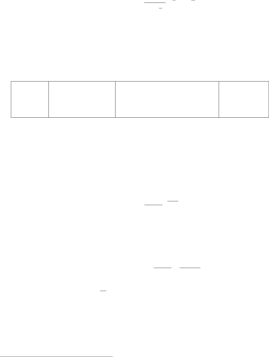
suming that there is some number of signal events in addition to background, this function
sets the upper limit on the number of signal events compatible with n0 and cl.
•ch2pval(ndf,chi2)
returns the p-value assuming a χ2distribution with ndf degrees of freedom ( expected
χ2) and chi2 is the observed χ2.
ch2pval(k, q) = Z∞
q
1
2kΓ(k
2)Qk
2−1e−Q
2dQ
•displayPlot(title,xName,xMin,xMax,lScale, N, ...)6
displays several curves/histograms on one plot. Here title contains some text, xName
is the name of a variable, xMin,xMax are the lower and upper limits. If lScale 6=0, a
logarithmic scale is used for the x axis.
Nis the number of curves/histograms to display. After the parameter N,displayPlot
expects N×4 parameters, where each tetrad can contain
text label dimension of array array of data array of error
text label dimension of array array of data NULL
text label 0 double *f(double x) NULL
text label 0 double *f(double x, void *arg) arg
where the first line is used for an histogram with error bars, the second line for a tabulated
function, the third for a function f(x) and the fourth for a function f(x,arg) which also
depends on some arguments contained in the structure arg. For a linear scale lScale=0,
the arrays of data and errors should correspond to a grid
xi= xMin + (i+ 0.5)(xMax −xMin)/Dim ,
where i= 0, ..., Dim −1. For logarithmic scale
xi= xMin ·xMax
xMin i+0.5
Dim
A An updated routine for b→sγ in the MSSM
The calculation of b→sγ was described in micromegas1.3 [3]. The branching fraction
reads
B(¯
B→Xsγ) = B(¯
B→Xce¯ν)
V∗
tsVtb
Vcb
26αem
πf(z0)KN LO(δ) (14)
where αem = 1./137.036, the factor KNLO involves the photon energy cut-off parameter
δand f(z0) = 0.542 −2.23(√z0−0.29) depends on z0= (mc/mb)2defined in terms
of pole masses. In the code the standard model and Higgs contribution at NLO were
included as well as the leading order SUSY contributions. However in the last few years
the NNLO standard model contribution has been computed [71] and shown to lead to
large corrections, shifting the standard model value by over 10%. It was also argued that
the NNLO SM result could be reproduced from the NLO calculation by appropriately
choosing the scale for the c-quark mass [72,73].
6This function is not available in Fortran
49
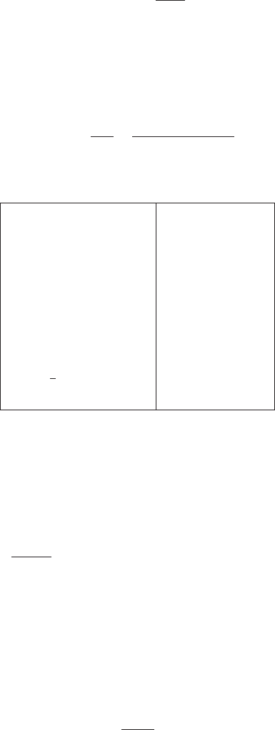
In this improved version of the bsgnlo routine, we have changed the default value for
the parameter z1= (mc/mb)2where mcis the MS running charm mass mc(mb). Taking
z1= 0.29 allows to reproduce the NNLO result. It is therefore no longer necessary to
apply a shift to the micrOMEGAs output of b→sγ to reproduce the SM value.
We have also updated the default values for the experimentally determined quantities
in Eq. 14, see Table 5, and we have replaced the factor f(z0) by Csl where
Csl =
Vub
Vcb
2Γ( ¯
B→Xce¯ν)
Γ( ¯
B→Xue¯ν)(15)
accounts for the mcdependence in ¯
B→Xce¯ν.
B(¯
B→Xce¯ν) 0.1064 [74]
Csl 0.546 [73]
|V∗
tsVtb/Vcb|20.9613 [74]
A0.808
λ0.2253
¯ρ0.132
¯η0.341
mb/ms50
λ2≈1
4(m2
B∗−m2
B)0.12GeV2[75]
αs(MZ) 0.1189
Table 5: Default values in micrOMEGAs
The CKM matrix elements in the Wolfenstein parametrisation given in Table 5are
used to compute the central value of ckmf at order λ4,
ckmf =
V∗
tsVtb
Vcb
2
= 1 + λ2(2¯ρ−1) + λ4(¯ρ2+ ¯η2−A2) (16)
With these default values the NLO- improved SM contribution is B(¯
B→Xsγ)|SM =
3.27×10⁻⁴which corresponds to the result of Gambino and Giordano [73] after correcting
for the slightly different CKM parameter used (ckmf = 0.963).
We have performed a comparison with superIso3.1 which includes the NNLO SM
calculation for 105randomly generated MSSM scenarios. The results are presented in
Fig. 1after applying a correction factor in superISO to account for the different value
for the overall factor F=B(¯
B→Xce¯ν)
V∗
tsVtb
Vcb
2/Csl. The ratio of Fmicro/FISO = 0.942.
The two codes agree within 5% most of the time.
References
[1] A. Pukhov. CalcHEP 2.3: MSSM, structure functions, event generation, batchs, and
generation of matrix elements for other packages. 2004.
[2] G. Belanger, F. Boudjema, A. Pukhov, and A. Semenov. MicrOMEGAs: A Program
for calculating the relic density in the MSSM. Comput. Phys. Commun., 149:103–120,
2002.
50
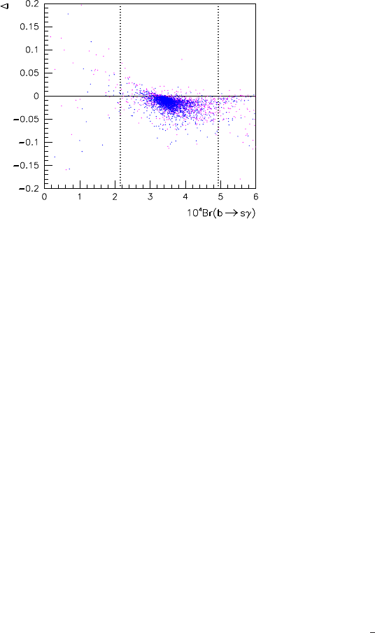
Figure 1: Relative difference for B(¯
B→sγ) between micromegas2.4 and superIso3.1. the
vertical lines show the 3σexperimentally measured value.
[3] G. Belanger, F. Boudjema, A. Pukhov, and A. Semenov. micrOMEGAs: Version
1.3. Comput. Phys. Commun., 174:577–604, 2006.
[4] G. Belanger, F. Boudjema, A. Pukhov, and A. Semenov. MicrOMEGAs 2.0: A
Program to calculate the relic density of dark matter in a generic model. Comput.
Phys. Commun., 176:367–382, 2007.
[5] G. Belanger, F. Boudjema, A. Pukhov, and A. Semenov. Dark matter direct detection
rate in a generic model with micrOMEGAs 2.2. Comput. Phys. Commun., 180:747–
767, 2009.
[6] G. Belanger, F. Boudjema, P. Brun, A. Pukhov, S. Rosier-Lees, P. Salati, and A. Se-
menov. Indirect search for dark matter with micrOMEGAs2.4. Comput. Phys. Com-
mun., 182:842–856, 2011.
[7] G. Belanger, F. Boudjema, A. Pukhov, and A. Semenov. micrOMEGAs 3: A program
for calculating dark matter observables. Comput. Phys. Commun., 185:960–985, 2014.
[8] Genevive Blanger, Fawzi Boudjema, Andreas Goudelis, Alexander Pukhov, and
Bryan Zaldivar. micrOMEGAs5.0 : freeze-in. 2018.
[9] Ulrich Ellwanger and Cyril Hugonie. NMSPEC: A Fortran code for the sparticle and
Higgs masses in the NMSSM with GUT scale boundary conditions. Comput. Phys.
Commun., 177:399–407, 2007.
[10] G. Belanger, F. Boudjema, C. Hugonie, A. Pukhov, and A. Semenov. Relic density
of dark matter in the NMSSM. JCAP, 0509:001, 2005.
[11] J. S. Lee, A. Pilaftsis, Marcela Carena, S. Y. Choi, M. Drees, John R. Ellis, and
C. E. M. Wagner. CPsuperH: A Computational tool for Higgs phenomenology in the
51
minimal supersymmetric standard model with explicit CP violation. Comput. Phys.
Commun., 156:283–317, 2004.
[12] G. Belanger, F. Boudjema, S. Kraml, A. Pukhov, and A. Semenov. Relic density of
neutralino dark matter in the MSSM with CP violation. Phys. Rev., D73:115007,
2006.
[13] Jonathan Da Silva. Supersymmetric Dark Matter candidates in light of constraints
from collider and astroparticle observables. PhD thesis, Annecy, LAPTH, 2013.
[14] G. Belanger, J. Da Silva, U. Laa, and A. Pukhov. Probing U(1) extensions of the
MSSM at the LHC Run I and in dark matter searches. JHEP, 09:151, 2015.
[15] Riccardo Barbieri, Lawrence J. Hall, and Vyacheslav S. Rychkov. Improved nat-
uralness with a heavy Higgs: An Alternative road to LHC physics. Phys. Rev.,
D74:015007, 2006.
[16] Alexander Belyaev, Chuan-Ren Chen, Kazuhiro Tobe, and C. P. Yuan. Phenomenol-
ogy of littlest Higgs model with T−parity: including effects of T−odd fermions.
Phys. Rev., D74:115020, 2006.
[17] John McDonald. Thermally generated gauge singlet scalars as selfinteracting dark
matter. Phys. Rev. Lett., 88:091304, 2002.
[18] Genevieve Belanger, Kristjan Kannike, Alexander Pukhov, and Martti Raidal. Im-
pact of semi-annihilations on dark matter phenomenology - an example of ZNsym-
metric scalar dark matter. JCAP, 1204:010, 2012.
[19] Genevive B´elanger, Kristjan Kannike, Alexander Pukhov, and Martti Raidal. Mini-
mal semi-annihilating ZNscalar dark matter. JCAP, 1406:021, 2014.
[20] Genevieve Belanger, Alexander Pukhov, and Geraldine Servant. Dirac Neutrino Dark
Matter. JCAP, 0801:009, 2008.
[21] Peter Z. Skands, B.C. Allanach, H. Baer, C. Balazs, G. Belanger, et al. SUSY Les
Houches accord: Interfacing SUSY spectrum calculators, decay packages, and event
generators. JHEP, 0407:036, 2004.
[22] P. Gondolo, J. Edsjo, P. Ullio, L. Bergstrom, Mia Schelke, and E. A. Baltz. Dark-
SUSY: Computing supersymmetric dark matter properties numerically. JCAP,
0407:008, 2004.
[23] Mark Hindmarsh and Owe Philipsen. WIMP dark matter and the QCD equation of
state. Phys. Rev., D71:087302, 2005.
[24] G. Blanger, F. Boudjema, A. Pukhov, and A. Semenov. micrOMEGAs4.1: two dark
matter candidates. Comput. Phys. Commun., 192:322–329, 2015.
[25] Manuel Drees and Mihoko Nojiri. Neutralino - nucleon scattering revisited. Phys.
Rev., D48:3483–3501, 1993.
52
[26] Junji Hisano, Ryo Nagai, and Natsumi Nagata. Effective Theories for Dark Matter
Nucleon Scattering. JHEP, 05:037, 2015.
[27] J. Beringer et al. Review of Particle Physics (RPP). Phys. Rev., D86:010001, 2012.
[28] HongSheng Zhao. Analytical models for galactic nuclei. Mon. Not. Roy. Astron.
Soc., 278:488–496, 1996.
[29] Julien Lavalle, Jonathan Pochon, Pierre Salati, and Richard Taillet. Clumpiness of
dark matter and positron annihilation signal: computing the odds of the galactic
lottery. Astron. Astrophys., 462:827–848, 2007.
[30] Mattias Blennow, Joakim Edsjo, and Tommy Ohlsson. Neutrinos from WIMP anni-
hilations using a full three-flavor Monte Carlo. JCAP, 0801:021, 2008.
[31] Pietro Baratella, Marco Cirelli, Andi Hektor, Joosep Pata, Morten Piibeleht, and
Alessandro Strumia. PPPC 4 DMν: a Poor Particle Physicist Cookbook for Neutri-
nos from Dark Matter annihilations in the Sun. JCAP, 1403:053, 2014.
[32] Marco Cirelli, Nicolao Fornengo, Teresa Montaruli, Igor A. Sokalski, Alessandro Stru-
mia, and Francesco Vissani. Spectra of neutrinos from dark matter annihilations.
Nucl. Phys., B727:99–138, 2005. [Erratum: Nucl. Phys.B790,338(2008)].
[33] Arif Emre Erkoca, Mary Hall Reno, and Ina Sarcevic. Muon Fluxes From Dark
Matter Annihilation. Phys. Rev., D80:043514, 2009.
[34] Dmitry Chirkin and Wolfgang Rhode. Muon Monte Carlo: A High-precision tool for
muon propagation through matter. 2004.
[35] Morihiro Honda, T. Kajita, K. Kasahara, S. Midorikawa, and T. Sanuki. Calculation
of atmospheric neutrino flux using the interaction model calibrated with atmospheric
muon data. Phys. Rev., D75:043006, 2007.
[36] G. B´elanger, J. Da Silva, T. Perrillat-Bottonet, and A. Pukhov. Limits on dark matter
proton scattering from neutrino telescopes using micrOMEGAs. JCAP, 1512(12):036,
2015.
[37] Philip Bechtle, Sven Heinemeyer, Oscar St˚al, Tim Stefaniak, and Georg Weiglein.
HiggsSignals: Confronting arbitrary Higgs sectors with measurements at the Teva-
tron and the LHC. Eur. Phys. J., C74:2711, 2014.
[38] Jeremy Bernon and Beranger Dumont. Lilith: a tool for constraining new physics
from Higgs measurements. Eur. Phys. J., C75(9):440, 2015.
[39] Philip Bechtle, Oliver Brein, Sven Heinemeyer, Oscar St˚al, Tim Stefaniak, et al.
HiggsBounds−4: Improved Tests of Extended Higgs Sectors against Exclusion Bounds
from LEP, the Tevatron and the LHC. Eur. Phys. J., C74:2693, 2014.
[40] Philip Bechtle, Oliver Brein, Sven Heinemeyer, Georg Weiglein, and Karina E.
Williams. HiggsBounds 2.0.0: Confronting Neutral and Charged Higgs Sector Predic-
tions with Exclusion Bounds from LEP and the Tevatron. Comput. Phys. Commun.,
182:2605–2631, 2011.
53

[41] G. Belanger, F. Boudjema, and A. Pukhov. micrOMEGAs : a code for the calculation
of Dark Matter properties in generic models of particle interaction. In The Dark
Secrets of the Terascale, pages 739–790, 2013.
[42] A. Djouadi, J. Kalinowski, and M. Spira. HDECAY: A Program for Higgs boson
decays in the standard model and its supersymmetric extension. Comput. Phys.
Commun., 108:56–74, 1998.
[43] Sabine Kraml, Suchita Kulkarni, Ursula Laa, Andre Lessa, Wolfgang Magerl, Doris
Proschofsky-Spindler, and Wolfgang Waltenberger. SModelS: a tool for interpreting
simplified-model results from the LHC and its application to supersymmetry. Eur.
Phys. J., C74:2868, 2014.
[44] Sabine Kraml, Suchita Kulkarni, Ursula Laa, Andre Lessa, Veronika Magerl,
Wolfgang Magerl, Doris Proschofsky-Spindler, Michael Traub, and Wolfgang Wal-
tenberger. SModelS v1.0: a short user guide. 2014.
[45] Federico Ambrogi, Sabine Kraml, Suchita Kulkarni, Ursula Laa, Andre Lessa,
Veronika Magerl, Jory Sonneveld, Michael Traub, and Wolfgang Waltenberger.
SModelS v1.1 user manual: Improving simplified model constraints with efficiency
maps. Comput. Phys. Commun., 227:72–98, 2018.
[46] http://smodels.hephy.at/wiki/SmsDictionary.
[47] Ayres Freitas. Higher-order electroweak corrections to the partial widths and branch-
ing ratios of the Z boson. JHEP, 04:070, 2014.
[48] Morad Aaboud et al. Search for high-mass new phenomena in the dilepton final state
using proton–proton collisions at √s= 13 TeV with the ATLAS detector. 2016.
[49] Georges Aad et al. Search for new phenomena in the dijet mass distribution using p−p
collision data at √s= 8 TeV with the ATLAS detector. Phys. Rev., D91(5):052007,
2015.
[50] Vardan Khachatryan et al. Search for resonances and quantum black holes using dijet
mass spectra in proton-proton collisions at √s= 8 TeV. Phys. Rev., D91(5):052009,
2015.
[51] Vardan Khachatryan et al. Search for narrow resonances in dijet final states at
p(s) = 8 TeV with the novel CMS technique of data scouting. Phys. Rev. Lett.,
117(3):031802, 2016.
[52] Georges Aad et al. Search for new phenomena in dijet mass and angular distributions
from pp collisions at √s= 13 TeV with the ATLAS detector. Phys. Lett., B754:302–
322, 2016.
[53] Vardan Khachatryan et al. Search for narrow resonances decaying to dijets in proton-
proton collisions at p(s) = 13 TeV. Phys. Rev. Lett., 116(7):071801, 2016.
[54] Malcolm Fairbairn, John Heal, Felix Kahlhoefer, and Patrick Tunney. Constraints
on Z’ models from LHC dijet searches. 2016.
54

[55] G. Abbiendi et al. Search for chargino and neutralino production at √s= 192 - 209
GeV at LEP. Eur. Phys. J., C35:1–20, 2004.
[56] Alexander L. Read. Presentation of search results: The CL(s) technique. J. Phys.,
G28:2693–2704, 2002.
[57] Alexander L. Read. Modified frequentist analysis of search results (The CL(s)
method). In Workshop on confidence limits, CERN, Geneva, Switzerland, 17-18
Jan 2000: Proceedings, 2000.
[58] Vardan Khachatryan et al. Search for dark matter, extra dimensions, and unparti-
cles in monojet events in proton-proton collisions at √s= 8 TeV. Eur. Phys. J.,
C75(5):235, 2015.
[59] B. C. Allanach et al. SUSY Les Houches Accord 2. Comput. Phys. Commun., 180:8–
25, 2009.
[60] A. Arbey and F. Mahmoudi. SuperIso Relic v3.0: A program for calculating relic
density and flavour physics observables: Extension to NMSSM. Comput. Phys. Com-
mun., 182:1582–1583, 2011.
[61] http://www.th.u-psud.fr/NMHDECAY/nmssmtools.html.
[62] Ulrich Ellwanger and Cyril Hugonie. NMHDECAY 2.0: An Updated program for
sparticle masses, Higgs masses, couplings and decay widths in the NMSSM. Comput.
Phys. Commun., 175:290–303, 2006.
[63] Florian Domingo and Ulrich Ellwanger. Updated Constraints from BPhysics on the
MSSM and the NMSSM. JHEP, 12:090, 2007.
[64] J. S. Lee, M. Carena, J. Ellis, A. Pilaftsis, and C. E. M. Wagner. CPsuperH2.0: an
Improved Computational Tool for Higgs Phenomenology in the MSSM with Explicit
CP Violation. Comput. Phys. Commun., 180:312–331, 2009.
[65] http://www.hep.man.ac.uk/u/jslee/CPsuperH.html.
[66] Florian Domingo. Update of the flavour-physics constraints in the NMSSM. 2015.
[67] S. Eidelman et al. Review of particle physics. Particle Data Group. Phys. Lett.,
B592:1–1109, 2004.
[68] F. Mahmoudi et al. Flavour Les Houches Accord: Interfacing Flavour related Codes.
Comput. Phys. Commun., 183:285–298, 2012.
[69] W. H. Press, S. A. Teukolsky, W. T. Vetterling, and B. P. Flannery. Numerical
Recipes: The Art of Scientific Computing.
[70] Gary J. Feldman and Robert D. Cousins. A Unified approach to the classical statis-
tical analysis of small signals. Phys. Rev., D57:3873–3889, 1998.
[71] M. Misiak et al. Estimate of B(¯
B→Xsγ) at O(α2
s). Phys. Rev. Lett., 98:022002,
2007.
55
[72] Mikolaj Misiak and Matthias Steinhauser. NNLO QCD corrections to the anti-B —¿
X(s) gamma matrix elements using interpolation in m(c). Nucl. Phys., B764:62–82,
2007.
[73] Paolo Gambino and Paolo Giordano. Normalizing inclusive rare B decays. Phys.
Lett., B669:69–73, 2008.
[74] K. Nakamura et al. Review of particle physics. J. Phys., G37:075021, 2010.
[75] W. M. Yao et al. Review of Particle Physics. J. Phys., G33:1–1232, 2006.
56
