Manual SPECFEM2D

User Manual: Pdf

Open the PDF directly: View PDF .
Page Count: 56

Contents
1 Introduction
- 1.1 Citation
- 1.2 Support
2 Getting Started
- 2.1 Visualizing the subroutine calling tree of the source code
- 2.2 Becoming a developer of the code, or making small modifications in the source code
3 Mesh Generation
4 Running the Solver xspecfem2D
5 Adjoint Simulations
6 Doing tomography, i.e., updating the model based on the sensitivity kernels obtained
7 Oil and gas industry simulations
8 Information for developers of the code, and for people who want to learn how the technique works
Notes & Acknowledgments
Copyright
Bibliography
A Troubleshooting
B License

User Manual

COMPUTATIONAL INFRASTRUCTURE FOR GEODYNAMICS (CIG)

Version 7.0

CNRS (FRANCE)

PRINCETON UNIVERSITY (USA)

SPECFEM 2D

SPECFEM2D

User Manual

Version 7.0

December 12, 2017

Authors

The SPECFEM2D package was ﬁrst developed by Dimitri Komatitsch and Jean-Pierre Vilotte at Institut de Physique

du Globe (IPGP) in Paris, France from 1995 to 1997 and then by Dimitri Komatitsch at Harvard University (USA),

Caltech (USA) and then CNRS and University of Pau (France) from 1998 to 2005. The story started on April 4,

1995, when Prof. Yvon Maday from CNRS and University of Paris, France, gave a lecture to Dimitri Komatitsch

and Jean-Pierre Vilotte at IPG about the nice properties of the Legendre spectral-element method with diagonal mass

matrix that he had used for other equations. We are deeply indebted and thankful to him for that. That followed a

visit by Dimitri Komatitsch to OGS (Istituto Nazionale di Oceanograﬁa e di Geoﬁsica Sperimentale) in Trieste, Italy,

in February 1995 to meet with Géza Seriani and Enrico Priolo, who introduced him to their 2D Chebyshev version

of the spectral-element method with a non-diagonal mass matrix. We are deeply indebted and thankful to them for that.

Since then it has been developed and maintained by a development team: in alphabetical order, Étienne Bachmann,

Alexis Bottero, Quentin Brissaud, Paul Cristini, Dimitri Komatitsch, Jesús Labarta, Nicolas Le Goff, Pieyre Le Loher,

Qinya Liu, Youshan Liu, Roland Martin, René Matzen, Christina Morency, Daniel Peter, Carl Tape, Jeroen Tromp,

Jean-Pierre Vilotte, Zhinan Xie.

The code is released open-source under the GNU version 3 license, see the license at the end of this manual.

Current and past main participants or main sponsors of the SPECFEM project

(in no particular order)

Contents

Contents 3

1 Introduction 5

1.1 Citation .................................................. 6

1.2 Support .................................................. 8

2 Getting Started 9

2.1 Visualizing the subroutine calling tree of the source code ........................ 10

2.2 Becoming a developer of the code, or making small modiﬁcations in the source code ......... 10

3 Mesh Generation 11

3.1 How to use SPECFEM2D ......................................... 11

3.2 How to use Gmsh to generate an external mesh ............................. 13

3.3 How to use Cubit/Trelis to generate an external mesh .......................... 14

3.3.1 Note about Cubit/Trelis built-in Python ............................. 15

3.4 Notes about absorbing PMLs ....................................... 15

3.5 Controlling the quality of an external mesh ............................... 16

3.6 Controlling how the mesh samples the wave ﬁeld ............................ 18

4 Running the Solver xspecfem2D 19

4.1 How to run elastic wave simulations ................................... 23

4.2 How to run axisymmetric wave simulations ............................... 23

4.3 How to run anisotropic wave simulations ................................. 25

4.4 How to run poroelastic wave simulations ................................. 26

4.5 Coupled simulations ........................................... 27

4.6 How to choose the time step ....................................... 28

4.7 How to set plane waves as initial conditions ............................... 28

4.8 Note on the viscoelastic model used ................................... 29

4.9 Note on viscoelasticity in the 2D plane strain approximation ...................... 29

5 Adjoint Simulations 30

5.1 How to obtain ﬁnite sensitivity kernels .................................. 30

5.2 Remarks about adjoint runs and solving inverse problems ........................ 31

5.3 Caution .................................................. 31

6 Doing tomography, i.e., updating the model based on the sensitivity kernels obtained 32

7 Oil and gas industry simulations 33

8 Information for developers of the code, and for people who want to learn how the technique works 34

Notes & Acknowledgments 35

CONTENTS 4

Bibliography 38

A Troubleshooting 45

B License 46

Chapter 1

Introduction

SPECFEM2D allows users to perform 2D and 2.5D (i.e., axisymmetric) simulations of acoustic, elastic, viscoelastic,

and poroelastic seismic wave propagation as well as full waveform imaging (FWI) or adjoint tomography.

In ﬂuids, SPECFEM2D uses the classical linearized Euler equation; thus if you have sharp local variations

of density in the ﬂuid (highly heterogeneous ﬂuids in terms of density) or if density becomes extremely small

in some regions of your model (e.g. for upper-atmosphere studies), before using the code please make sure the

linearized Euler equation is a valid approximation in the case you want to study. For more details on that see

e.g. Jensen et al. [2011].

The 2D spectral-element solver accommodates regular and unstructured meshes, generated for example by Cubit

(http://cubit.sandia.gov), Gmsh (http://geuz.org/gmsh) or GiD (http://www.gid.cimne.

upc.es). Even mesh creation packages that generate triangles, for instance Delaunay-Voronoi triangulation codes,

can be used because each triangle can then easily be decomposed into three quadrangles by linking the barycenter to

the center of each edge; while this approach does not generate quadrangles of optimal quality, it can ease mesh creation

in some situations and it has been shown that the spectral-element method can very accurately handle distorted mesh

elements.

With version 7.0, the 2D spectral-element solver accommodates Convolution PML absorbing layers and well as

higher-order time schemes (4th order Runge-Kutta and LDDRK4-6). Convolution or Auxiliary Differential Equation

Perfectly Matched absorbing Layers (C-PML or ADE-PML) are described in Martin et al. [2008b,c], Martin and Ko-

matitsch [2009], Martin et al. [2010], Komatitsch and Martin [2007].

The solver has adjoint capabilities and can calculate ﬁnite-frequency sensitivity kernels [Tromp et al.,2008,Peter

et al.,2011] for acoustic, (an)elastic, and poroelastic media. The package also considers 2D SH and P-SV wave propa-

gation. Finally, the solver can run both in serial and in parallel. See SPECFEM2D (http://www.geodynamics.

org/cig/software/packages/seismo/specfem2d) for the source code.

The SEM is a continuous Galerkin technique [Tromp et al.,2008,Peter et al.,2011], which can easily be made dis-

continuous [Bernardi et al.,1994,Chaljub,2000,Kopriva et al.,2002,Chaljub et al.,2003,Legay et al.,2005,Kopriva,

2006,Wilcox et al.,2010,Acosta Minolia and Kopriva,2011]; it is then close to a particular case of the discontinuous

Galerkin technique [Reed and Hill,1973,Lesaint and Raviart,1974,Arnold,1982,Johnson and Pitkäranta,1986,

Bourdel et al.,1991,Falk and Richter,1999,Hu et al.,1999,Cockburn et al.,2000,Giraldo et al.,2002,Rivière and

Wheeler,2003,Monk and Richter,2005,Grote et al.,2006,Ainsworth et al.,2006,Bernacki et al.,2006,Dumbser and

Käser,2006,De Basabe et al.,2008,de la Puente et al.,2009,Wilcox et al.,2010,De Basabe and Sen,2010,Étienne

et al.,2010], with optimized efﬁciency because of its tensorized basis functions [Wilcox et al.,2010,Acosta Minolia

and Kopriva,2011]. In particular, it can accurately handle very distorted mesh elements [Oliveira and Seriani,2011].

It has very good accuracy and convergence properties [Maday and Patera,1989,Seriani and Priolo,1994,Deville

et al.,2002,Cohen,2002,De Basabe and Sen,2007,Seriani and Oliveira,2008,Ainsworth and Wajid,2009,2010,

CHAPTER 1. INTRODUCTION 6

Melvin et al.,2012]. The spectral element approach admits spectral rates of convergence and allows exploiting hp-

convergence schemes. It is also very well suited to parallel implementation on very large supercomputers [Komatitsch

et al.,2003,Tsuboi et al.,2003,Komatitsch et al.,2008,Carrington et al.,2008,Komatitsch et al.,2010b] as well as

on clusters of GPU accelerating graphics cards [Komatitsch,2011,Michéa and Komatitsch,2010,Komatitsch et al.,

2009,2010a]. Tensor products inside each element can be optimized to reach very high efﬁciency [Deville et al.,2002],

and mesh point and element numbering can be optimized to reduce processor cache misses and improve cache reuse

[Komatitsch et al.,2008]. The SEM can also handle triangular (in 2D) or tetrahedral (in 3D) elements [Wingate and

Boyd,1996,Taylor and Wingate,2000,Komatitsch et al.,2001,Cohen,2002,Mercerat et al.,2006] as well as mixed

meshes, although with increased cost and reduced accuracy in these elements, as in the discontinuous Galerkin method.

Note that in many geological models in the context of seismic wave propagation studies (except for instance for

fault dynamic rupture studies, in which very high frequencies or supershear rupture need to be modeled near the fault,

see e.g. Benjemaa et al. [2007,2009], de la Puente et al. [2009], Tago et al. [2010]) a continuous formulation is

sufﬁcient because material property contrasts are not drastic and thus conforming mesh doubling bricks can efﬁciently

handle mesh size variations [Komatitsch and Tromp,2002,Komatitsch et al.,2004,Lee et al.,2008,2009a,b].

For a detailed introduction to the SEM as applied to regional seismic wave propagation, please consult Peter et al.

[2011], Tromp et al. [2008], Komatitsch and Vilotte [1998], Komatitsch and Tromp [1999], Chaljub et al. [2007] and

in particular Lee et al. [2009b,a,2008], Godinho et al. [2009], van Wijk et al. [2004], Komatitsch et al. [2004]. A

detailed theoretical analysis of the dispersion and stability properties of the SEM is available in Cohen [2002], De

Basabe and Sen [2007], Seriani and Oliveira [2007], Seriani and Oliveira [2008] and Melvin et al. [2012].

The SEM was originally developed in computational ﬂuid dynamics [Patera,1984,Maday and Patera,1989] and

has been successfully adapted to address problems in seismic wave propagation. Early seismic wave propagation ap-

plications of the SEM, utilizing Legendre basis functions and a perfectly diagonal mass matrix, include Cohen et al.

[1993], Komatitsch [1997], Faccioli et al. [1997], Casadei and Gabellini [1997], Komatitsch and Vilotte [1998] and

Komatitsch and Tromp [1999], whereas applications involving Chebyshev basis functions and a non-diagonal mass

matrix include Seriani and Priolo [1994], Priolo et al. [1994] and Seriani et al. [1995]. In the Legendre version that

we use in SPECFEM the mass matrix is purposely slightly inexact but diagonal (but can be made exact if needed, see

Teukolsky [2015]), while in the Chebyshev version it is exact but non diagonal.

All SPECFEM2D software is written in Fortran2003 with full portability in mind, and conforms strictly to the

Fortran2003 standard. It uses no obsolete or obsolescent features of Fortran. The package uses parallel programming

based upon the Message Passing Interface (MPI) [Gropp et al.,1994,Pacheco,1997].

This new release of the code includes support for GPU graphics card acceleration [Komatitsch,2011,Michéa and

Komatitsch,2010,Komatitsch et al.,2009,2010a].

The code uses the plane strain convention when the standard P-SV equation case is used, i.e., the off-plane strain

zz is zero by deﬁnition of the plane strain convention but the off-plane stress σzz is not equal to zero, one has

σzz =λ(xx+yy). This implies, as in any plain strain software package, that the P-SV source is a line source along the

direction perpendicular to the plane (see ﬁle discussion_of_2D_sources_and_approximations_from_Pilant_1979.pdf

for more details).

1.1 Citation

You can ﬁnd all the references below in BIBT

EXformat in ﬁle doc/USER_MANUAL/bibliography.bib.

If you use this code for your own research, please cite at least one article written by the developers of the package,

for instance:

•Tromp et al. [2008],

•Peter et al. [2011],

CHAPTER 1. INTRODUCTION 7

•Vai et al. [1999],

•Lee et al. [2009a],

•Lee et al. [2008],

•Lee et al. [2009b],

•Komatitsch et al. [2010a],

•Komatitsch et al. [2009],

•Liu et al. [2004],

•Chaljub et al. [2007],

•Komatitsch and Vilotte [1998],

•Komatitsch and Tromp [1999],

•Komatitsch et al. [2004],

•Morency and Tromp [2008],

•Blanc et al. [2016],

• and/or other articles from http://komatitsch.free.fr/publications.html.

If you use the C-PML absorbing layer capabilities of the code, please cite at least one article written by the developers

of the package, for instance:

•Xie et al. [2014],

•Xie et al. [2016].

If you use the UNDO_ATTENUATION option of the code in order to produce full anelastic/viscoelastic sensitivity

kernels, please cite at least one article written by the developers of the package, for instance (and in particular):

•Komatitsch et al. [2016].

More generally, if you use the attenuation (anelastic/viscoelastic) capabilities of the code, please cite at least one article

written by the developers of the package, for instance:

•Komatitsch et al. [2016],

•Blanc et al. [2016].

If you use the kernel capabilities of the code, please cite at least one article written by the developers of the package,

for instance:

•Tromp et al. [2008],

•Peter et al. [2011],

•Liu and Tromp [2006],

•Morency et al. [2009].

If you use the SCOTCH / CUBIT non-structured capabilities, please cite:

•Martin et al. [2008a].

If you use axisymmetric geometries please also cite:

•Bottero et al. [2016]

The corresponding BibT

EX entries may be found in ﬁle doc/USER_MANUAL/bibliography.bib.

CHAPTER 1. INTRODUCTION 8

1.2 Support

This material is based upon work supported by the USA National Science Foundation under Grants No. EAR-0406751

and EAR-0711177, by the French CNRS, French Inria Sud-Ouest MAGIQUE-3D, French ANR NUMASIS under

Grant No. ANR-05-CIGC-002, and European FP6 Marie Curie International Reintegration Grant No. MIRG-CT-

2005-017461. Any opinions, ﬁndings, and conclusions or recommendations expressed in this material are those of the

authors and do not necessarily reﬂect the views of the USA National Science Foundation, CNRS, Inria, ANR or the

European Marie Curie program.

Chapter 2

Getting Started

To download the SPECFEM2D software package, type this:

git clone --recursive --branch devel https://github.com/geodynamics/specfem2d.git

We recommend that you add ulimit -S -s unlimited to your .bash_profile ﬁle and/or limit

stacksize unlimited to your .cshrc ﬁle to suppress any potential limit to the size of the Unix stack.

Then, to conﬁgure the software for your system, run the configure shell script. This script will attempt to guess

the appropriate conﬁguration values for your system. However, at a minimum, it is recommended that you explicitly

specify the appropriate command names for your Fortran compiler (another option is to deﬁne FC, CC and MPIF90 in

your .bash_proﬁle or your .cshrc ﬁle):

./configure FC=gfortran CC=gcc

If you want to run in parallel, i.e., using more than one processor core, then you would type

./configure FC=gfortran CC=gcc MPIFC=mpif90 --with-mpi

You can replace the GNU compilers above (gfortran and gcc) with other compilers if you want to; for instance for

Intel ifort and icc use FC=ifort CC=icc instead.

Before running the configure script, you should probably edit ﬁle flags.guess to make sure that it contains

the best compiler options for your system. Known issues or things to check are:

Intel ifort compiler See if you need to add -assume byterecl for your machine. In the case of that

compiler, we have noticed that initial release versions sometimes have bugs or issues that can lead to

wrong results when running the code, thus we strongly recommend using a version for which at least one

service pack or update has been installed.

IBM compiler See if you need to add -qsave or -qnosave for your machine.

Mac OS You will probably need to install XCODE.

IBM Blue Gene machines Please refer to the manual of SPECFEM3D_Cartesian, which contains detailed in-

structions on how to run on Blue Gene.

The SPECFEM2D software package relies on the SCOTCH library to partition meshes. The SCOTCH library

[Pellegrini and Roman,1996] provides efﬁcient static mapping, graph and mesh partitioning routines. SCOTCH is a

free software package developed by François Pellegrini et al. from LaBRI and Inria in Bordeaux, France, download-

able from the web page https://gforge.inria.fr/projects/scotch/. In case no SCOTCH libraries

can be found on the system, the conﬁguration will bundle the version provided with the source code for compilation.

The path to an existing SCOTCH installation can to be set explicitly with the option --with-scotch-dir. Just as

an example:

./configure FC=ifort MPIFC=mpif90 --with-mpi --with-scotch-dir=/opt/scotch

CHAPTER 2. GETTING STARTED 10

If you use the Intel ifort compiler to compile the code, we recommend that you use the Intel icc C compiler to compile

Scotch, i.e., use:

./configure CC=icc FC=ifort MPIFC=mpif90

For further details about the installation of SCOTCH, go to subdirectory scotch_5.1.11/ and read INSTALL.txt.

You may want to download more recent versions of SCOTCH in the future from (http://www.labri.fr/

perso/pelegrin/scotch/scotch_en.html) . Support for the METIS graph partitioner has been discon-

tinued because SCOTCH is more recent and performs better.

When compiling the SCOTCH source code, if you get a message such as: "ld: cannot ﬁnd -lz", the Zlib com-

pression development library is probably missing on your machine and you will need to install it or ask your system

administrator to do so. On Linux machines the package is often called "zlib1g-dev" or similar. (thus "sudo apt-get

install zlib1g-dev" would install it)

You may edit the Makefile for more speciﬁc modiﬁcations. Especially, there are several options available:

•-DUSE_MPI compiles with use of an MPI library.

•-DUSE_SCOTCH enables use of graph partitioner SCOTCH.

After these steps, go back to the main directory of SPECFEM2D/ and type

make

to create all executables which will be placed into the folder ./bin/.

By default, the solver runs in single precision. This is ﬁne for most application, but if for some reason you want

to run the solver in double precision, run the configure script with option “--enable-double-precision”.

Keep in mind that this will of course double total memory size and will also make the solver around 20 to 30% slower

on many processors.

If your compiler has problems with the use mpi statements that are used in the code, use the script called

replace_use_mpi_with_include_mpif_dot_h.pl in the root directory to replace all of them with include

‘mpif.h’ automatically.

If you have problems conﬁguring the code on a Cray machine, i.e. for instance if you get an error message

from the configure script, try exporting these two variables: MPI_INC=$CRAY_MPICH2_DIR/include and

FCLIBS=" ", and for more details if needed you can refer to the utils/Cray_compiler_information

directory.

2.1 Visualizing the subroutine calling tree of the source code

Packages such as doxywizard can be used to visualize the subroutine calling tree of the source code. Doxywizard

is a GUI front-end for conﬁguring and running doxygen.

2.2 Becoming a developer of the code, or making small modiﬁcations in the

source code

If you want to develop new features in the code, and/or if you want to make small changes, improvements, or bug

ﬁxes, you are very welcome to contribute. To do so, i.e. to access the development branch of the source code with

read/write access (in a safe way, no need to worry too much about breaking the package, there is a robot called

BuildBot that is in charge of checking and validating all new contributions and changes), please visit this Web page:

https://github.com/geodynamics/specfem2d/wiki/Using-Hub.

To visualize the call tree (calling tree) of the source code, you can see the Doxygen tool available in directory

doc/call_trees_of_the_source_code.

Chapter 3

Mesh Generation

3.1 How to use SPECFEM2D

Mesher

Partitioner

Databases

Solver

CUBIT, Gmsh, GiD

SCOTCH

xmeshfem2D

xspecfem2D

Figure 3.1: Schematic workﬂow for a SPECFEM2D simulation. The executable xmeshfem2D creates the GLL mesh

points and assigns speciﬁc model parameters. The executable xspecfem2D solves the seismic wave propagation.

To run the mesher, please follow these steps:

• edit the input ﬁle DATA/Par_file, which describes the simulation. The default DATA/Par_file pro-

vided in the root directory of the code contains detailed comments and should be almost self-explanatory

(note that some of the older DATA/Par_file ﬁles provided in the EXAMPLES directory work ﬁne but

some of the comments they contain may be obsolete or even wrong; thus refer to the default DATA/Par_file

instead for reliable explanations). If you need more details we do not have a detailed description of all the

parameters for the 2D version in this manual but you can ﬁnd useful information in the manuals of the 3D ver-

sions, since many parameters and the general philosophy is similar. They are available at (https://github.

com/geodynamics/specfem3d/tree/master/doc/USER_MANUAL). To create acoustic (ﬂuid) re-

gions, just set the S wave speed to zero and the code will see that these elements are ﬂuid and switch to the right

equations there automatically, and automatically match them with the solid regions

• if you are using an external mesher (like GiD or CUBIT / Trelis), you should set read_external_mesh to

.true.:

CHAPTER 3. MESH GENERATION 12

mesh_file is the ﬁle describing the mesh : ﬁrst line is the number of elements, then a list of 4 nodes (quadri-

laterals only) forming each elements on each line.

nodes_coords_file is the ﬁle containing the coordinates (xand z) of each node: number of nodes on the

ﬁrst line, then coordinates x and z on each line.

materials_file is the number of the material for every element : an integer ranging from 1 to nbmodels

on each line.

free_surface_file is the ﬁle describing the edges forming the acoustic free surface: number of edges on

the ﬁrst line, then on each line: number of the element, number of nodes forming the free surface (1 for

a point, 2 for an edge), the nodes forming the free surface for this element. If you do not want any free

surface, just put 0 on the ﬁrst line; you then get a rigid surface instead.

axial_elements_file is the ﬁle describing the axial elements in the case of an axisymmetric simulation.

See Section 4.2.

absorbing_surface_file is the ﬁle describing the edges forming the absorbing boundaries: number of

edges on the ﬁrst line, then on each line: number of the element, number of nodes forming the absorbing

edge (must always be equal to 2), the two nodes forming the absorbing edge for this element, and then the

type of absorbing edge: 1 for BOTTOM, 2 for RIGHT, 3 for TOP and 4 for LEFT. Only two nodes per

element can be listed, i.e., the second parameter of each line must always be equal to 2. If one of your

elements has more than one edge along a given absorbing contour (e.g., if that contour has a corner) then

list it twice, putting the ﬁrst edge on the ﬁrst line and the second edge on the second line. Do not list

the same element with the same absorbing edge twice or more, otherwise absorption will not be correct

because the edge integral will be improperly subtracted several times. If one of your elements has a single

point along the absorbing contour rather than a full edge, do NOT list it (it would have no weight in the

contour integral anyway because it would consist of a single point). If you use 9-node elements, list only

the ﬁrst and last points of the edge and not the intermediate point located around the middle of the edge;

the right 9-node curvature will be restored automatically by the code.

tangential_detection_curve_file contains points describing the envelope, that are used for the

source_normal_to_surface and rec_normal_to_surface. Should be ﬁne grained, and or-

dered clockwise. Number of points on the ﬁrst line, then (x,z) coordinates on each line.

• if you have compiled with MPI, you must specify the number of processes.

Then type

./bin/xmeshfem2D

to create the mesh (which will be stored in directory OUTPUT_FILES/). xmeshfem2D is serial; it will output

several ﬁles called Database??????.bin, one for each process.

500

1000

1500

2000

2500

3000

3500

0 500 1000 1500 2000 2500 3000 3500 4000

'OUTPUT_FILES.default.M2_UPPA/gridfile.gnu'

Figure 3.2: Example of a grid ﬁle generated by xmeshfem2D and visualized with gnuplot (within gnuplot, type

‘plot "OUTPUT_FILES/gridfile.gnu" w l’).

Regarding mesh point numbering in the ﬁles created by the mesher, we use the classical convention of 4-node and

9-node ﬁnite elements:

CHAPTER 3. MESH GENERATION 13

4....7....3

. .

. eta .

.|.

8 9--xi 6

. .

1....5....2

the local coordinate system being ξand η(xi and eta). Note that this convention is used to describe the geometry

only. In the solver the wave ﬁeld is then described based on high-order Lagrange interpolants at Gauss-Lobatto-

Legendre points, as is classical in spectral-element methods.

3.2 How to use Gmsh to generate an external mesh

Gmsh1is a 3D ﬁnite element grid generator which can be used for the generation of quadrangle and hexahedral

meshes. It is therefore a good candidate for generating meshes which can be processed by SPECFEM2D. Only two

modules of Gmsh are of interest for the SPECFEM2D users : the geometry and the mesh modules. An example is

given in directory EXAMPLES/Gmsh_example which illustrates the generation of an external mesh using these two

modules. The model that is considered consists of a homogeneous square containing two circles ﬁlled with a different

material.

The geometry is generated by loading ﬁle SqrCirc.geo into Gmsh. The end of the .geo ﬁle contains several

lines which are required in order to deﬁne the sides of the box and the media. This is done using the following

conventions :

Physical Line("Top") = {1}; line corresponding to the top of the box

Physical Line("Left") = {2}; line corresponding to the left side of the box

Physical Line("Bottom") = {3}; line corresponding to the bottom of the box

Physical Line("Right") = {4}; line corresponding to the right side of the box

Physical Surface("M1") = {10}; surrounding medium

Physical Surface("M2") = {11,12}; interior of the two circles

For instance, if you want to ﬁll the two circles with two different materials, you will have to write :

Physical Surface("M1") = {10}; surrounding medium

Physical Surface("M2") = {11}; interior of the big circle

Physical Surface("M3") = {12}; interior of the small circle

and, consequently, you will have to deﬁne a new medium numbered 3in the Par_file.

Then, a 2D mesh can be created and saved after selecting the appropriate options in Gmsh : All quads in

Subdivision algorithm and 1or 2in Element order whether you want a 4 or 9 node mesh. This operation

will generate a SqrCirc.msh ﬁle which must be processed to get all the ﬁles required by SPECFEM2D when using

an external mesh (see previous section). This is done by running a python script called LibGmsh2Specfem.py,

located in directory utils/Gmsh:

python LibGmsh2Specfem.py SqrCirc -t A -b A -r A -l A

Where the options -t,-b,-r and -l represent the different sides of the model (top, bottom, right and left) and can

take the values Aor Fif the corresponding side is respectively absorbing or free. All boundaries are absorbing by

default. The connections of the generated ﬁlenames to the ﬁlenames indicated in the previous section are :

•Mesh_SqrCirc is the mesh_file

1freely available at the following address : http://www.geuz.org/gmsh/

CHAPTER 3. MESH GENERATION 14

Figure 3.3: Geometry and mesh of the two circle model generated with Gmsh

•Material_SqrCirc is the material_file

•Nodes_SqrCirc is the nodes_coords_file

•Surf_abs_SqrCirc is the absorbing_surface_file

•Surf_free_SqrCirc is the free_surface_file

In addition, four ﬁles like free_surface_file corresponding to the sides of the model are generated.

3.3 How to use Cubit/Trelis to generate an external mesh

Trelis (that was known as Cubit)2is a 2D/3D ﬁnite element grid generator distributed by Csimsoft which can be used

for the generation of quadrangle and hexahedral meshes. Trelis has a convenient interface with Python (module cubit)

which allows to create meshes from Python scripts. To get started with Cubit/Trelis we recommend you the step-

by-step tutorials available at: http://www.csimsoft.com/tutorials.jsp Many powerful graphical tools

are available, and very useful, but we will focus here on the command line functionalities and especially the Python

interface which is the real force of Cubit/Trelis.

To get started we recommend to the inpatients to open Cubit/Trelis and to click on the following symbol: . Then

select the ﬁles of type Python Files (*.py) and play the following script:

utils/cubit2specfem2d/simplest2DexampleWithPmls.py

In the case you want to perform an axisymmetric simulation, we recommend you rather to play:

utils/cubit2specfem2d/simpleAxisym2dMesh.py

It will create a simple mesh with PMLs. Then re-click on and play:

utils/cubit2specfem2d/cubit2specfem2d.py

This script will create (in current directory) all the mesh ﬁles necessary for a SPECFEM2D simulation. Other com-

mented examples are available. We particularly recommend you to look at the folder

EXAMPLES/paper_axisymmetry_example beginning by reading the README available there. Read care-

fully the comments in these scripts, they are helpful. Another way to use Python together with Cubit/Trelis is to use

2available at http://www.csimsoft.com/

CHAPTER 3. MESH GENERATION 15

the script tab. This tab is a real Python terminal that can be used to pass command line python instruction to Cu-

bit/Trelis through the cubit module. In the case of the Script tab is not visible in the command line panel (at the bottom

of the screen) do:

Tools -> Options... -> Layout [-> Cubit Layout] -> Show script tab

This tab will allow you to play the scripts one line after another directly in Cubit/Trelis. With this you should be able

to understand how to create meshes and export them under SPECFEM2D format.

3.3.1 Note about Cubit/Trelis built-in Python

Beware, there are some (annoying) differences between cubit built-in Python and the actual Python langage:

•"aString" + ’anotherString’ can cause problems even after being stored:

a = "aString"

b = a + ’anotherString’

Example which is not working:

pathToMeshDir = pathToSpecfem + ’EXAMPLES/paper_axisymmetry_example/MESH’

cubit.cmd(’cd \"’+pathToMeshDir+’\"’)

• No comments after double dots:

Example which is not working:

if True: # Just a dummy comment

print "Ok!"

This example works without the comment.

•os.makedirs("~/aDirectory/") does not work. It creates a directory named ~

!!!!! To remove that do: rm -R ./~ AND NEVER rm -rf ~ !!!!!

•sys.argv can not be used

• No comments """ """ at the beginning of a script

And probably many others! Think about that before getting mad.

3.4 Notes about absorbing PMLs

If you use CPML, an additional ﬁle listing the CPML elements is needed. Its ﬁrst line is the total number of CPML

elements, and then a list of all the CPML elements, one per line. The format of these lines is: in the ﬁrst column the

CPML element number, and in the second column a ﬂag as follows:

Table 3.1: Deﬁnition of ﬂags for CPML elements

Flag Meaning

1 element belongs to a X CPML layer only (either in Xmin or in Xmax)

2 element belongs to a Y CPML layer only (either in Ymin or in Ymax)

3 element belongs to both a X and a Y CPML layer (i.e., to a CPML corner)

In order to see how to add PML layers to a mesh / model created with an external mesher such as ‘Gmsh’, see the

examples in directory EXAMPLES/CPML_absorbing_layers.

If you use PML, the mesh elements that belong to the PML layers can be acoustic or elastic, but not viscoelastic nor

poroelastic. Then, when deﬁning your model, you should deﬁne these absorbing elements as either acoustic or elastic.

If you forget to do that, the code will ﬁx the problem by automatically converting the viscoelastic or poroelastic PML

CHAPTER 3. MESH GENERATION 16

elements to elastic. This means that strictly speaking the PML layer will not be perfectly matched any more, since the

physical model will change from viscoelastic or poroelastic to elastic at the entrance of the PML, but in practice this

is sufﬁcient and produces only tiny / negligible spurious reﬂections.

If you use PML and an external mesh (created using an external meshing tool such as Gmsh, CUBIT/TRELIS or

similar), try to have elements inside the PML as regular as possible, i.e. ideally non-deformed rectangles obtained by

‘extrusion’ of the edge mesh elements meshing the outer edges of the computational domain without PML; by doing

so, the PMLs obtained will be far more stable in time (PML being weakly unstable from a mathematical point of view,

very deformed mesh elements inside the PMLs can trigger instabilities much more quickly).

If you have an existing CUBIT (or similar) mesh stored in SPECFEM2D format but do not know how to assign

CPML ﬂags to it, we have created a small serial Fortran program that will do that automatically for you. That program

is utils/CPML/convert_external_layers_of_a_given_mesh_to_CPML_layers2D.f90. When you create the PML layers

using that script, you do not need to mark (i.e. assign to physical entities with a speciﬁc name) those external layers in

the mesher. However you still need to specify the boundary of the mesh as you where doing in the case of absorbing

conditions. The script will automatically extract the elements on the PML. It will ask you for a thickness for the

PML layers. Suppose that you have created a region with a 1-meter size element, when it will prompt for the PML

thickness you can enter 3.1 and it will create a PML 3 element thick. Always input a slightly larger (5-10%) size

because the element might be slightly skewed, or if you have not created your PML region via extrusion/webcut in

CUBIT/TRELIS.

To stabilize PMLs it also helps to add a transition layer of geometrically-regular non-PML elements, in which

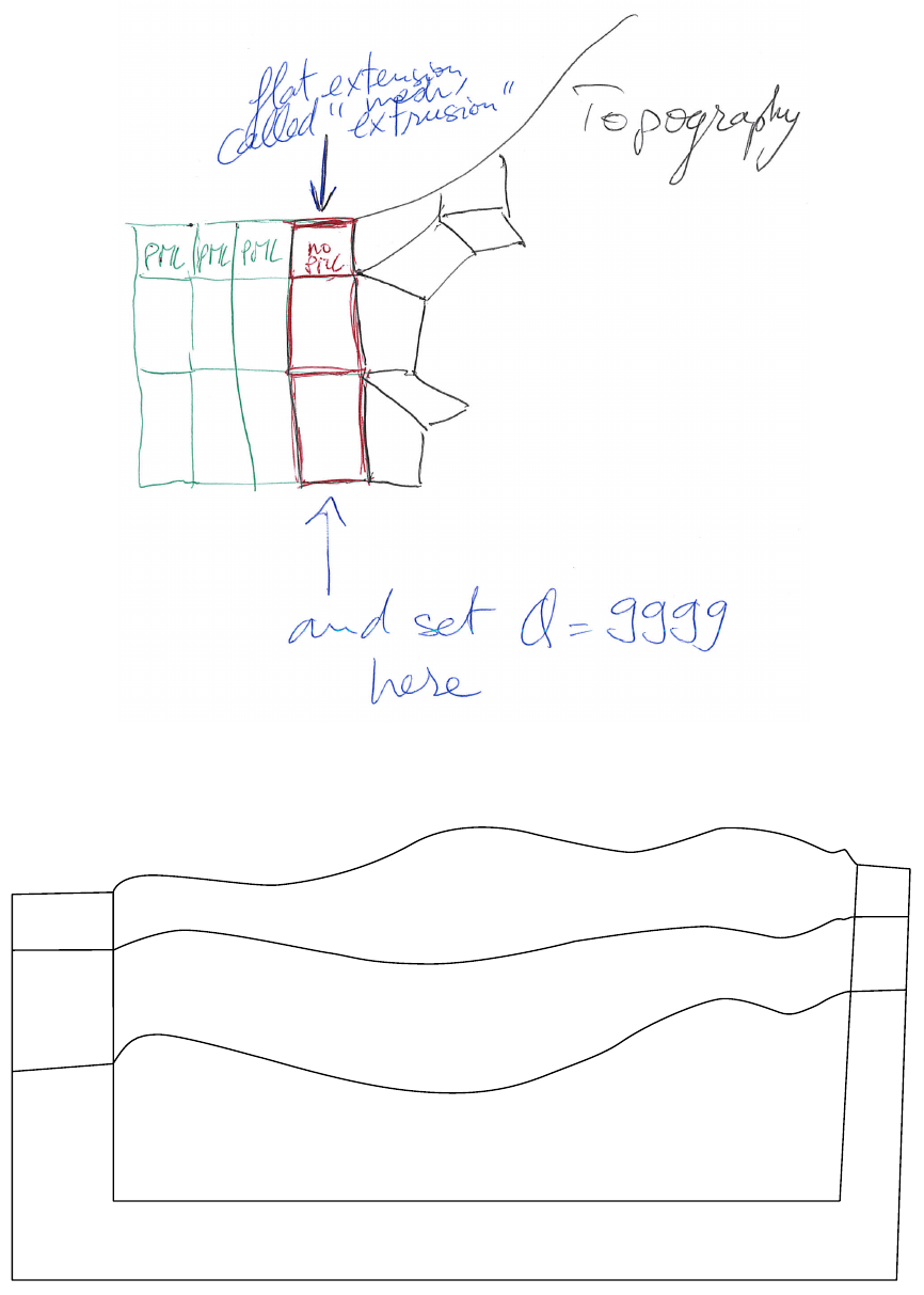
attenuation is also turned off (i.e. Qκ=Qµ= 9999 in that layer), as in the red layer of Figure 3.4. Our tools

in directory in directory utils/CPML should soon (Dimitri: TO DO ONE DAY) implement that transition layer

automatically.

To be more precise:

1/ If one wants to use PML layers, they should NOT mark the layers according to that python script - the reason

is that the xmeshfem2d does not recognize those CPML ﬂags. If whoever developed the script adjusts it to solve this

problem - this might be a great relief for users; as of now no physical identiﬁers are needed for those layers.

2/ HOWEVER, the "Top", "Bottom", "Left"," and "Right" boundaries of the model, need to be re-assigned to outer

boundaries of the model - that will be the leftmost boundary of the left -bounding PML , rightmost of the right PML,

topmost for the Top PML (if there is one) and the bottom boundary of the bottom layer. Those and only those lines

need to have the mentioned identiﬁers (opposite to the example with the two-holed square with Stacey conditions).

3/ There is no need to create Top PML in case one wants it to be reﬂective; as the fortran script that assigns the

ﬂag will ignore the elements that sit within PML-layer thickness distance to the top.

4/ The Fortran program utils/CPML/convert_external_layers_of_a_given_mesh_to_CPML_layers2D.f90 that ﬂags

the PML elements does not create additional elements; it simply takes the elements within chosen distance from the

boundaries, that sit in the interior of model and marks them as absorbing.

If you use PML and an external velocity and density model (e.g., setting ﬂag “MODEL” to tomography), you

should be careful because mathematically a PML cannot handle heterogeneities along the normal to the PML edge

inside the PML layer. This comes from the fact that the damping proﬁle that is deﬁned assumes a constant velocity

and density model along the normal direction. Thus, you need to modify your velocity and density model in order for

it to be 1D inside the PML, as shown in Figure 3.5. This applies to the bottom layer as well; there you should make

sure that your model is 1D and thus constant along the vertical direction. To summarize, only use a 2D velocity and

density model inside the physical region, and in all the PML layers extend it by continuity from its values along the

inner PML edge.

3.5 Controlling the quality of an external mesh

To examine the quality of the elements in your externally build mesh, type

./bin/xcheck_quality_external_mesh

(and answer "3" to the ﬁrst question asked). This code will tell you which element in the whole mesh has the worst

quality (maximum skewness, i.e. maximum deformation of the element angles) and it should be enough to modify

this element with the external software package used for the meshing, and to repeat the operation until the maximum

CHAPTER 3. MESH GENERATION 17

Figure 3.4: Mesh extrusion for PML (green elements) and a non-PML stabilization layer (red elements).

Use a

horizontally

1D velocity

model here

PML

Use a vertically-1D velocity model here

Figure 3.5: How to modify your external 2D velocity and density model in order to use PML. Such a modiﬁcation is

not needed when using Stacey absorbing boundary conditions (but such conditions are signiﬁcantly less efﬁcient).

CHAPTER 3. MESH GENERATION 18

skewness of the whole mesh is less or equal to about 0.75 (above is dangerous: from 0.75 to 0.80 could still work, but

if there is a single element above 0.80 the mesh should be improved).

The code also shows a histogram of 20 classes of skewness which tells how many element are above the skewness

= 0.75, and to which percentage of the total this amounts. To see this histogram, you could type:

gnuplot plot_mesh_quality_histogram.gnu

This tool is useful to estimate the mesh quality and to see it evolve along the successive corrections.

3.6 Controlling how the mesh samples the wave ﬁeld

To examine (using Gnuplot) how the mesh samples the wave ﬁeld, type

gnuplot plot_points_per_wavelength_histogram.gnu

and also check the following histogram printed on the screen or in the output ﬁle:

histogram of min number of points per S wavelength (P wavelength in

acoustic regions)

(too small: poor resolution of calculations - too big = wasting

memory and CPU time)

(threshold value is around 4.5 points per wavelength in elastic media

and 5.5 in acoustic media)

If you see that you have a signiﬁcant number of mesh elements below the threshold indicated, then your simulations

will not be accurate and you should create a denser mesh. Conversely, if you have a signiﬁcant number of mesh

elements above the threshold indicated, the mesh your created is too dense, it will be extremely accurate but the

simulations will be slow; using a coarser mesh would be sufﬁcient and would lead to faster simulations.

Chapter 4

Running the Solver xspecfem2D

To run the solver, type

bin/xspecfem2D

from within the main working directory (use mpirun or equivalent if you compiled with parallel support). This

will output the seismograms and snapshots of the wave fronts at different time steps in directory OUTPUT_FILES/.

To visualize them, type "gs OUTPUT_FILES/vect*.ps" to see the Postscript ﬁles (in which the wave ﬁeld is

represented with small arrows, ﬂuid/solid matching interfaces with a thick pink line, and absorbing edges with a thick

green line) and "gimp OUTPUT_FILES/image*.gif" to see the colour snapshot showing a pixelized image of

one of the two components of the wave ﬁeld (or pressure, depending on what you have selected for the output in

DATA/Par_file).

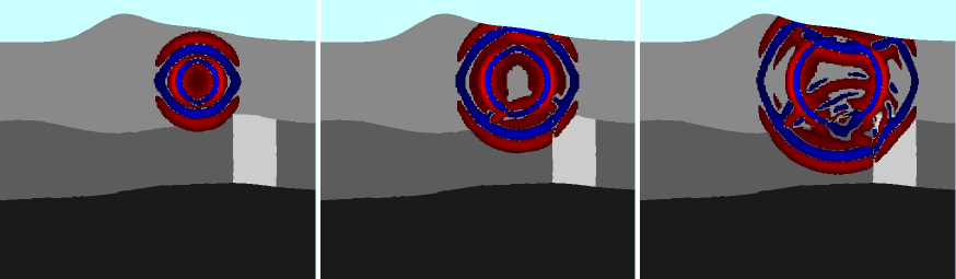
Figure 4.1: Waveﬁeld snapshots of the default example generated by xspecfem2D when parameter

output_color_image is set to .true.. To create smaller (subsampled) images you can change double pre-

cision parameter factor_subsample_image = 1.0 to a higher value in ﬁle DATA/Par_file. This can be

useful in the case of very large models. The number of pixels of the image in each direction must be smaller than

parameter NX_NZ_IMAGE_MAX deﬁned in ﬁle SETUP/constants.h.in, again to avoid creating huge images in

the case of very large models.

Please consider these following points, when running the solver:

• the DATA/Par_file given with the code works ﬁne, you can use it without any modiﬁcation to test the code

• the seismograms OUTPUT_FILES/*.sem*are simple ASCII ﬁles with two columns: time in the ﬁrst column

and amplitude in the second, therefore they can be visualized with any tool you like, for instance “gnuplot”; if

you prefer to output binary seismograms in Seismic Unix format (which is a simple binary array dump) you can

use parameter SU_FORMAT, in which case all the seismograms will be written to a single ﬁle with the extension

*.bin. Depending on your installation of the Seismic Unix package you can use one of these two commands:

CHAPTER 4. RUNNING THE SOLVER XSPECFEM2D 20

surange < Uz_file_single.bin

suoldtonew < Uz_file_single.bin | surange

to see the header info. Replace surange with suxwigb to see wiggle plots for the seismograms.

• if ﬂag MODEL in DATA/Par_file is set to default, the velocity and density model is determined using the

nbmodels and nbregions devices. Otherwise, nbmodels values are ignored and the velocity and density

model is determined from a user supplied ﬁle or subroutine.

• when compiling with Intel ifort, use “-assume byterecl” option to create binary PNM images displaying

the wave ﬁeld

• there are a few useful scripts and Fortran routines in directory utils/.

• you can ﬁnd a Fortran code to compute the analytical solution for simple media that we use as a reference in

benchmarks in many of our articles at (http://www.spice-rtn.org/library/software/EX2DDIR).

That code is described in: Berg et al. [1994]

Notes about DATA/Par_file parameters

The default DATA/Par_file provided in the root directory of the code contains detailed comments and should

be almost self-explanatory (note that some of the older DATA/Par_file ﬁles provided in the EXAMPLES

directory work ﬁne but some of the comments they contain may be obsolete or even wrong; thus refer to the

default DATA/Par_file instead for reliable explanations).

USE_TRICK_FOR_BETTER_PRESSURE This option can only be used so far if all the receivers record pressure and

are in acoustic elements. Use a trick to increase accuracy of pressure seismograms in ﬂuid (acoustic) elements:

use the second derivative of the source for the source time function instead of the source itself, and then record

potential_acoustic() as pressure seismograms instead of potential_dot_dot_acoustic();

this is mathematically equivalent, but numerically signiﬁcantly more accurate because in the explicit Newmark

time scheme acceleration is accurate at zeroth order while displacement is accurate at second order, thus in ﬂuid

elements potential_dot_dot_acoustic() is accurate at zeroth order while potential_acoustic()

is accurate at second order and thus contains signiﬁcantly less numerical noise.

READ_VELOCITIES_AT_f0 shift (i.e. change) velocities read from the input ﬁle to take average physical disper-

sion into account, i.e. if needed change the reference frequency at which these velocities are deﬁned internally

in the code: by default, the velocity values that are read at the end of this Par_ﬁle of the code are supposed to be

the unrelaxed values, i.e. the velocities at inﬁnite frequency. We may want to change this and impose that the

values read are those for a given frequency (here f0_attenuation). (when we do this, velocities will then slightly

decrease and waves will thus slightly slow down)

nbmodels With MODEL = default chosen, a variety of simple velocity and density models can be deﬁned using

the nbmodels device.

I: model_number 1 rho Vp Vs 0 0 QKappa Qmu 0 0 0 0 0 0

II: model_number 2 rho c11 c13 c15 c33 c35 c55 c12 c23 c25 0 0 0

III: model_number 3 rhos rhof phi c kxx kxz kzz Ks Kf Kfr etaf mufr Qmu

IV: model_number -1 0 0 A 0 0 0 0 0 0 0 0 0 0

To make a given region acoustic, use I and make Vs be zero.

To make a given region isotropic elastic, use I and make Vs be nonzero. See Section 4.1 for more details.

To make a given region anisotropic, use II. See Section 4.2 for more details.

To make a given region poroeslatic, use III. See Section 4.3 for more details.

When viscoelasticity is turned on, the Vp and Vs values that are read here are the UNRELAXED ones i.e. the

values at inﬁnite frequency unless the READ_VELOCITIES_AT_f0 parameter above is set to true, in which case

CHAPTER 4. RUNNING THE SOLVER XSPECFEM2D 21

they are the values at frequency f0. Please also note that Qmu is always equal to Qs, but Qkappa is in general not

equal to Qp. To convert one to the other see doc/note_on_Qkappa_versus_Qp.pdf and utils/attenuation/conversion_from_Qkappa_Qmu_to_Qp_Qs_from_Dahlen_Tromp_959_960.f90.

nbregions With MODEL = default chosen, a variety of simple layered model conﬁgurations can be speciﬁed

using the nbregions device.

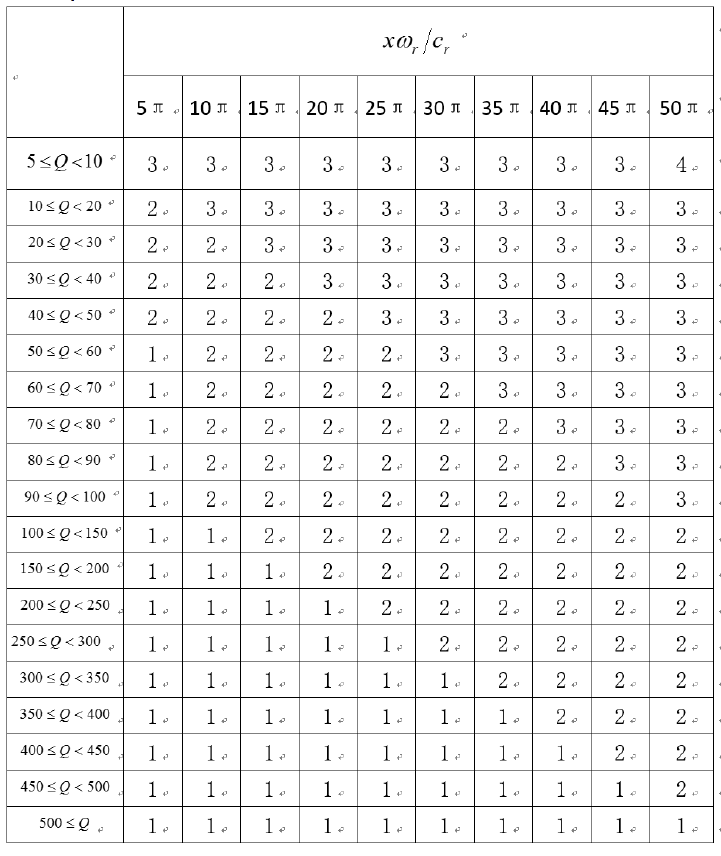
Regarding attenuation (viscoelasticity), in the Par_ﬁle you need to select the number of standard linear solids

(N_SLS) to use to mimic a constant Qquality factor. Using N_SLS = 3 is always safe. If (and only if) you know what

you are doing, you can try to reduce that in order to reduce the cost of the simulations. Figure 4.2 shows values that

you can consider using (again, if and only if you know what you are doing). That table has been created by Zhinan

Xie using a comparison between results obtained with a truly-constant Qand results obtained with its approximation

based on N_SLS standard linear solids. The comparison is performed using the time-frequency misﬁt and goodness-

of-ﬁt criteria proposed by Kristeková et al. [2009]. The table is drawn for a dimensionless parameter representing the

distance of propagation.

Figure 4.2: Table showing how you can select a value of N_SLS smaller than 3, if and only if you know what you are

doing.

CHAPTER 4. RUNNING THE SOLVER XSPECFEM2D 22

Notes about DATA/SOURCE parameters

The SOURCE ﬁle located in the DATA/ directory should be edited in the following way:

source_surf Set this ﬂag to .true. to force the source to be located at the surface of the model, otherwise the

sol be placed inside the medium

xs source location xin meters

zs source location zin meters

source_type Set this value equal to 1for elastic forces or acoustic pressure, set this to 2for moment tensor

sources. For a plane wave including converted and reﬂected waves at the free surface, P wave = 1, S wave = 2,

Rayleigh wave = 3; for a plane wave without converted nor reﬂected waves at the free surface, i.e. the incident

wave only, P wave = 4, S wave = 5. (incident plane waves are turned on by parameter initialfield in

DATA/Par_file).

time_function_type Choose a source-time function: set this value to 1to use a Ricker, 2the ﬁrst derivative, 3

a Gaussian, 4a Dirac or 5a Heaviside source-time function.

f0 Set this to the dominant frequency of the source. For point-source simulations using a Heaviside source-time

function (time_function_type = 5), we recommend setting the source frequency parameter f0 equal to

a high value, which corresponds to simulating a step source-time function, i.e., a moment-rate function that is a

delta function.

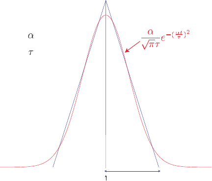
The half duration of a source is obtained by 1/f0. If the code will use a Gaussian source-time function

(time_function_type = 3) (i.e., a signal with a shape similar to a ‘smoothed triangle’, as explained

in Komatitsch and Tromp [2002] and shown in Fig 4.3), the source-time function uses a half-width of half

duration. We prefer to run the solver with half duration set to zero and convolve the resulting synthetic

seismograms in post-processing after the run, because this way it is easy to use a variety of source-time functions.

Komatitsch and Tromp [2002] determined that the noise generated in the simulation by using a step source time

function may be safely ﬁltered out afterward based upon a convolution with the desired source time function

and/or low-pass ﬁltering. Use the serial code convolve_source_timefunction.f90 and the script

convolve_source_timefunction.sh for this purpose, or alternatively use signal-processing software

packages such as SAC (www.llnl.gov/sac). Type

make xconvolve_source_timefunction

to compile the code and then set the parameter hdur in convolve_source_timefunction.sh to the

desired half-duration.

t0 For single sources, we recommend to set the time shift parameter t0 equal to 0.0. The time shift parameter would

simply apply an overall time shift to the synthetics (according to the time shift of the ﬁrst source), something

that can be done in the post-processing. This time shift parameter can be non-zero when using multiple sources.

anglesource angle of the source (for a force only); for a plane wave, this is the incidence angle. For moment

tensor sources this parameter is unused.

Mxx,Mzz,Mxz Moment tensor components (valid only for moment tensor sources, source_type = 2). Note

that the units for the components of a moment tensor source are different in SPECFEM2D and in SPECFEM3D:

SPECFEM3D: in SPECFEM3D the moment tensor components are in dyne*cm

SPECFEM2D: in SPECFEM2D the moment tensor components are in N*m

To go from strike / dip / slip to CMTSOLUTION moment-tensor format using the classical formulas (of e.g.

Aki and Richards [1980] you can use these two small C programs from SPECFEM3D_GLOBE:

./utils/strike_dip_rake_to_CMTSOLUTION.c

./utils/CMTSOLUTION_to_AkiRichards.c

CHAPTER 4. RUNNING THE SOLVER XSPECFEM2D 23

half duration

source decay rate

half duration

tCMT

Figure 4.3: Comparison of the shape of a triangle and the Gaussian function actually used.

but then it is another story to make a good 2D approximation of that, because in plain-strain P-SV what you get

is the equivalent of a line source in the third direction (orthogonal to the plane) rather than a 3D point source

For more details on this see e.g. Section 7.3 "Two-dimensional point sources" of the book of Pilant [1979]. That

book being hard to ﬁnd, we scanned the related pages in ﬁle

discussion_of_2D_sources_and_approximations_from_Pilant_1979.pdf in the same di-

rectory as this users manual. Another very useful reference addressing that is Helmberger and Vidale [1988]

and its recent extension [Li et al.,2014].

factor ampliﬁcation factor

Note, the zero time of the simulation corresponds to the center of the triangle/Gaussian, or the centroid time of

the earthquake. The start time of the simulation is t=−1.2∗half duration +t0 (the factor 1.2 is to make sure

the moment rate function is very close to zero when starting the simulation; Heaviside functions use a factor 2.0), the

half duration is obtained by 1/f0. If you prefer, you can ﬁx this start time by setting the parameter USER_T0 in the

constants.h ﬁle to a positive, non-zero value. The simulation in that case would start at a starting time equal to

-USER_T0.

4.1 How to run elastic wave simulations

For isotropic elastic materials, there are two options:

P-SV: To run a P-SV waves calculation propagating in the x-zplane, set p_sv = .true. in the Par_file.

SH: To run a SH (membrane) waves calculation travelling in the x-zplane with a y-component of motion, set p_sv

= .false.

This feature is only implemented for elastic materials and sensitivity kernels can be calculated (see Tape et al. [2007]

for details on membrane surface waves).

An optional useful Python script called SEM_save_dir.py is provided. It allows one to automatically save all

the parameters and results of a given simulation.

4.2 How to run axisymmetric wave simulations

Axisymmetric simulations are possible in SPECFEM2D. For these simulations the 2D domain simulated is physically

the meridional 2D shape of an axisymmetric 3D domain. We invite you to read our publication [Bottero et al.,2016]

as an introduction. To set the geometry as axisymmetric turn the ﬂag AXISYM to .true. in the Par_file:

CHAPTER 4. RUNNING THE SOLVER XSPECFEM2D 24

AXISYM = .true.

The left border of the model becomes then a symmetry axis. The waveﬁeld calculated is then physically a 3D wave-

ﬁeld obtained by revolution of a 2D waveﬁeld around its left border.

Note about the source:

In axisymmetric geometry the whole model is symmetric with respect to this axis, including the source. Hence if the

source is not on the axis it will physically have a circular shape. This is still possible and relevant for some applica-

tions as non destructive testing but is most of the time unwanted. This has to be kept in mind. In acoustic medium, as

an explosion in a ﬂuid is naturally axisymmetric, the waveﬁeld generated has the correct 3D shape. However, if the

source is put in an elastic solid, its 3D radiation pattern will be axisymmetric.

Getting started:

To get started a simple example is available in EXAMPLES/axisymmetric_case_AXISYM_option, we en-

courage you to read the README ﬁle you will ﬁnd there. This example contains an example of the use of AXISYM

option plus a validation using the semi-analytical code OASES (Schmidt [2004]). In this example the domain studied

is a water layer lying above a viscoelastic medium. The source is an explosion in the water and the domain is bounded

with PMLs.

Note about external meshers:

Using external meshers is possible in axisymmetric geometry. An example is available in

EXAMPLES/paper_axisymmetry_example with the mesher Cubit/Trelis (http://www.csimsoft.com/

trelis). We invite you to check this example and read the previous chapter for more details. The only difference

with plane-strain geometry is that SPECFEM2D needs an additional ﬁle deﬁning axial elements. The path to this ﬁle

has to be given in the Par_file:

axial_elements_file = /path/to/the/axial_elements_file

The axial elements ﬁle has the following structure:

1 2 8456 8457

2 2 8457 8458

3 2 8458 8459

4 2 8459 8460

623 2 171 204

1053 2 172 9512

1054 2 172 173

1055 2 173 174

...

Which is similar to free surface ﬁles. Hence the ﬁrst line contains the number of axial elements, then the other lines

contain four columns: element id, number of nodes describing an axial element (always 2), ﬁrst node id, second node

id. Note that the axis elements must include the possible (up and/or down) PMLs elements in contact with the axis. For

simplicity we assume that the mesh elements that are in contact with the symmetry axis are in contact with it by a full

edge rather than by a single point, i.e. we exclude cases as that of Figure 4.4. This amounts to imposing that the left-

most layer of elements in the mesh be structured rather than non structured; The rest of the mesh can be non structured.

Note about the resolution:

In axisymmetry a different quadrature is used in the axial elements making the number of points per wavelength nec-

essary a slightly bigger (≈25%) than in plane-strain.

Note about a small remaining bug:

It has to be noted that a small bug is still hiding somewhere in the code. Indeed the output signals generated are correct

in the whole domain except in the element containing the source. This small bug has not been solved so far but not

prevent to use the code.

CHAPTER 4. RUNNING THE SOLVER XSPECFEM2D 25

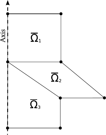
Figure 4.4: For simplicity we exclude cases in which the mesh elements that are in contact with the symmetry axis

are in contact with it by a single point instead of by a full edge, such as element ¯

Ω2here. This amounts to imposing

that the leftmost layer of elements in the mesh be structured rather than non structured; The rest of the mesh can be

non structured.

Note about a demo code to learn:

A simplistic demo code is available in

utils/small_SEM_solver_in_Fortran_without_MPI_to_learn. This simple code is useful to learn

how the spectral-element method works in both plane-strain and axisymmetric geometries. Have a look to it if in-

terested. Once in its directory, type ./make_Fortran_2D_axisymmetric.csh and then ./xspecfem2D to

compile and run. The bug discussed above is not present in this small code.

4.3 How to run anisotropic wave simulations

Following Carcione et al. [1988a], we use the classical reduced Voigt notation to represent symmetric tensors [Helbig,

1994,Carcione,2007]:

The constitutive relation of a heterogeneous anisotropic and elastic solid is expressed by the general-

ized Hooke’s law, which can be written as

σij =cijklεkl, i, j, k = 1,...,3,

where tis the time, xis the position vector, σij (x, t)and εij (x, t)are the Cartesian components of the

stress and strain tensors respectively, and cijkl(x)are the components of a fourth-order tensor called the

elasticites of the medium. The Einstein convention for repeated indices is used.

To express the stress-strain relation for a transversely isotropic medium we introduce a shortened

matrix notation commonly used in the literature. With this convention, pairs of subscripts concerning the

elasticities are replaced by a single number according to the following correspondence:

(11) →1,(22) →2,(33) →3,

(23) = (32) →4,(31) = (13) →5,(12) = (21) →6.

Thus in the most general 2D case we have the following convention for the stress-strain relationship:

CHAPTER 4. RUNNING THE SOLVER XSPECFEM2D 26

! implement anisotropy in 2D

sigma_xx = c11*dux_dx + c13*duz_dz + c15*(duz_dx + dux_dz)

sigma_zz = c13*dux_dx + c33*duz_dz + c35*(duz_dx + dux_dz)

sigma_xz = c15*dux_dx + c35*duz_dz + c55*(duz_dx + dux_dz)

! sigma_yy is not equal to zero in the plane strain formulation

! but is used only in post-processing if needed,

! to compute pressure for display or seismogram recording purposes

sigma_yy = c12*dux_dx + c23*duz_dz + c25*(duz_dx + dux_dz)

where the notations are for instance duz_dx = d(Uz) / dx.

4.4 How to run poroelastic wave simulations

Check the following new inputs in Par_file:

In section "# geometry of model and mesh description":

TURN_VISCATTENUATION_ON,Q0, and FREQ0 deal with viscous damping in a poroelastic medium. Q0 is

the quality factor set at the central frequency FREQ0. For more details see Morency and Tromp [2008].

In section "# time step parameters":

SIMULATION_TYPE deﬁnes the type of simulation

(1) forward simulation

(2) UNUSED (purposely, for compatibility with the numbering convention used in our 3D codes)

(3) adjoint method and kernels calculation

In section "# source parameters":

The code now support multiple sources. NSOURCE is the number of sources. Parameters of the sources are

displayed in the ﬁle SOURCE, which must be in the directory DATA/. The components of a moment tensor

source must be given in N.m, not in dyne.cm as in the DATA/CMTSOLUTION source ﬁle of the 3D version of

the code.

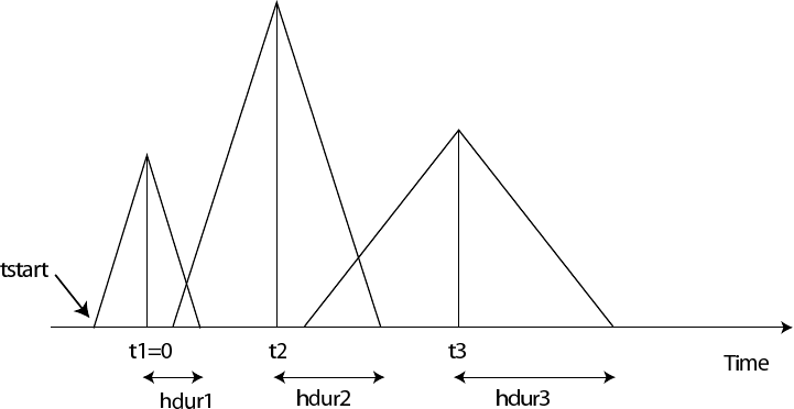
Figure 4.5: Example of timing for three sources. The center of the ﬁrst source triangle is deﬁned to be time zero. Note

that this is NOT in general the hypocentral time, or the start time of the source (marked as tstart). The time shift

parameter t0 in the SOURCE ﬁle would be t1(= 0),t2,t3in this case, and the half-duration parameter, f0, would be

hdur1 = 1/f01,hdur2 = 1/f02,hdur3 = 1/f03for the sources 1, 2, 3 respectively.

CHAPTER 4. RUNNING THE SOLVER XSPECFEM2D 27

In section "# receiver line parameters for seismograms":

SAVE_FORWARD determines if the last frame of a forward simulation is saved (.true.) or not (.false)

In section "# deﬁne models....":

There are three possible types of models:

I: (model_number 1 rho Vp Vs 0 0 QKappa Qmu 0 0 0 0 0 0) or

II: (model_number 2 rho c11 c13 c15 c33 c35 c55 c12 c23 c25 0 0 0) or

III: (model_number 3 rhos rhof phi c kxx kxz kzz Ks Kf Kfr etaf mufr Qmu).

For isotropic elastic/acoustic material use Iand set Vs to zero to make a given model acoustic, for anisotropic

elastic use II, and for isotropic poroelastic material use III. The mesh can contain acoustic, elastic, and

poroelastic models simultaneously.

For anisotropic elastic media the last three parameters, c12 c23 c25, are used only when the user asks

the code to compute pressure for display or seismogram recording purposes. Thus, if you do not know these

parameters for your anisotropic material and/or if you do not plan to display or record pressure you can ignore

them and set them to zero. When pressure is used these three parameters are needed because the code needs to

compute σyy, which is not equal to zero in the plane strain formulation.

rho_s = solid density

rho_f = ﬂuid density

phi = porosity

tort = tortuosity

permxx = xx component of permeability tensor

permxz = xz,zx components of permeability tensor

permzz = zz component of permeability tensor

kappa_s = solid bulk modulus

kappa_f = ﬂuid bulk modulus

kappa_fr = frame bulk modulus

eta_f = ﬂuid viscosity

mu_fr = frame shear modulus

Qmu = shear quality factor

Note: for the poroelastic case, mu_s is irrelevant. For details on the poroelastic theory see Morency and Tromp

[2008].

get_poroelastic_velocities.f90 allows to compute cpI, cpII, and cs function of the source dominant

frequency. Notice that for this calculation we use permxx and the dominant frequency of the ﬁrst source, f0(1).

Caution if you use several sources with different frequencies and if you consider anistropic permeability.

4.5 Coupled simulations

The code supports acoustic/elastic, acoustic/poroelastic, elastic/poroelastic, and acoustic, elastic/poroelastic simula-

tions. Elastic/poroelastic coupling supports anisotropy, but not attenuation for the elastic material.

CHAPTER 4. RUNNING THE SOLVER XSPECFEM2D 28

4.6 How to choose the time step

Three different explicit conditionally-stable time schemes can be used for elastic, acoustic (ﬂuid) or coupled elas-

tic/acoustic media: the Newmark method, the low-dissipation and low-dispersion fourth-order six-stage Runge-Kutta

method (LDDRK4-6) presented in Berland et al. [2006], and the classical fourth-order four-stage Runge-Kutta (RK4)

method. Currently the last two methods are not implemented for poroelastic media. According to De Basabe and Sen

[2010] and Berland et al. [2006], with different degrees N=N GLLX −1of the GLL basis functions the CFL bounds

are given in the following tables. Note that by default the SPECFEM solver uses NGLLX = 5 and thus a degree N=

4, which is thus the value you should use in most cases in the following tables. You can directly compare these values

with the value given in sentence ‘Max stability for P wave velocity’ in ﬁle output_solver.txt to see whether you

set the correct ∆tin Par_file or not. For elastic simulation, the CFL value given in output_solver.txt does

not consider the Vp/Vsratio, but the CFL limit slight decreases when Vp/Vsincreases. In viscoelastic simulations the

CFL limit does not change compared to the elastic case because we use a rational approximation of a constant quality

factor Q, which has no attenuation effect on zero-frequency waves. Additionally, if you use C-PML absorbing layers in

your simulations, which are implemented for the Newmark and LDDRK4-6 techniques but not for the classical RK4),

the CFL upper limit decreases to approximately 95% of the limit without absorbing layers in the case of Newmark and

to 85% in the case of LDDRK4-6.

Table 4.1: CFL upper bound for an acoustic (ﬂuid) simulation.

Degree NNewmark LDDRK4-6 RK4

1 0.709 1.349 1.003

2 0.577 1.098 0.816

3 0.593 1.129 0.839

4 0.604 1.150 0.854

5 0.608 1.157 0.860

6 0.608 1.157 0.860

7 0.608 1.157 0.860

8 0.607 1.155 0.858

9 0.607 1.155 0.858

10 0.607 1.155 0.858

Table 4.2: CFL upper bound for an elastic simulation with Vp/Vs=√2.

Degree NNewmark LDDRK4-6 RK4

1 0.816 1.553 1.154

2 0.666 1.268 0.942

3 0.684 1.302 0.967

4 0.697 1.327 0.986

5 0.700 1.332 0.990

6 0.700 1.332 0.990

7 0.700 1.332 0.990

8 0.699 1.330 0.989

9 0.698 1.328 0.987

10 0.698 1.328 0.987

4.7 How to set plane waves as initial conditions

To simulate propagation of incoming plane waves in the simulation domain, initial conditions based on analytical

formulae of plane waves in homogeneous model need to be set. No additional body or boundary forces are required.

To set up this scenario:

CHAPTER 4. RUNNING THE SOLVER XSPECFEM2D 29

Par_file:

• switch on initialfield = .true.

• at this point setting add_bielak_condition does not seem to help with absorbing boundaries, there-

fore, it should be turned off.

SOURCE:

•zs has to be the same as the height of the simulation domain deﬁned in interfacesfile.

•xs is the x-coordinate of the intersection of the initial plane wave front with the free surface.

•source_type = 1 for a plane P wave, 2 for a plane SV wave, 3 for a Rayleigh wave.

•angleforce can be negative to indicate a plane wave incident from the right (instead of the left)

4.8 Note on the viscoelastic model used

The model used is a constant Q, thus with no dependence on frequency (Q(f)= constant). See e.g. Blanc et al. [2016].

However in practice for technical reasons it is approximated based on the sum of different Generalized Zener body

mechanisms and thus the code outputs the band in which the approximation is very good, outside of that range it

can be less accurate. The logarithmic center of that frequency band is the f0 parameter deﬁned (in Hz) in input ﬁle

DATA/SOURCE.

4.9 Note on viscoelasticity in the 2D plane strain approximation

In 2D plane strain, one spatial dimension is much greater than the others (see for example: http://www.engineering.

ucsb.edu/~hpscicom/projects/stress/introge.pdf) and thus κ=λ+µin 2D plane strain (in-

stead of κ=λ+2

3µin 3D). See for example Carcione et al. [1988b] equation (A9), and equation 6 in http:

//cherrypit.princeton.edu/papers/paper-99.pdf.

In 2D axisymmetric I think the 2/3 coefﬁcient is OK, but it would be worth doublechecking.

Chapter 5

Adjoint Simulations

5.1 How to obtain ﬁnite sensitivity kernels

1. Run a forward simulation:

•SIMULATION_TYPE = 1

•SAVE_FORWARD = .true.

•seismotype = 1 (we need to save the displacement ﬁelds to later on derive the adjoint source. Note: if

the user forgets it, the program corrects it when reading the proper SIMULATION_TYPE and SAVE_FORWARD

combination and a warning message appears in the output ﬁle)

Important output ﬁles (for example, for the elastic case, P-SV waves):

•absorb_elastic_bottom*****.bin

•absorb_elastic_left*****.bin

•absorb_elastic_right*****.bin

•absorb_elastic_top*****.bin

•lastframe_elastic*****.bin

•AA.S****.BXX.semd

•AA.S****.BXZ.semd

2. Deﬁne the adjoint source:

• Use adj_seismogram.f90

• Edit to update NSTEP,nrec,t0,deltat, and the position of the cut to pick any given phase if needed

(tstart,tend), add the right number of stations, and put one component of the source to zero if needed.

• The output ﬁles of adj_seismogram.f90 are AA.S****.BXX.adj and AA.S****.BXZ.adj,

for P-SV waves (and AA.S****.BXY.adj, for SH (membrane) waves). Note that you will need these

three ﬁles (AA.S****.BXX.adj,AA.S****.BXY.adj and AA.S****.BXZ.adj) to be present in

the SEM/ directory together with the absorb_elastic_****.bin and lastframe_elastic.bin

ﬁles to be read when running the adjoint simulation.

3. Run the adjoint simulation:

• Make sure that the adjoint source ﬁles absorbing boundaries and last frame ﬁles are in the OUTPUT_FILES/

directory.

•SIMULATION_TYPE = 3

•SAVE_FORWARD = .false.

CHAPTER 5. ADJOINT SIMULATIONS 31

Output ﬁles (for example for the elastic case):

•snapshot_rho_kappa_mu*****

•snapshot_rhop_alpha_beta*****

which are the primary moduli kernels and the phase velocities kernels respectively, in ascii format and at the

local level, that is as “kernels(i,j,ispec)”.

5.2 Remarks about adjoint runs and solving inverse problems

SPECFEM2D can produce the gradient of the misﬁt function for a tomographic inversion, but options for using the

gradient within an iterative inversion are left to the user (e.g., conjugate-gradient, steepest descent). The plan is to

include some examples in the future.

The algorithm is simple:

1. calculate the forward wave ﬁeld s(x, t)

2. calculate the adjoint wave ﬁeld s†(x, t)

3. calculate their interaction s(x, t)·s†(x, T −t)(these symbolic, temporal and spatial derivatives should be

included)

4. integrate the interactions, which is summation in the code.

That is all. Step 3 has some tricks in implementation, but which can be skipped by regular users.

If you look into SPECFEM2D, besides “rhop_ac_kl” and “rho_ac_kl”, there are more variables such as

“kappa_ac_kl” and “rho_el_kl” etc. “rho” denotes density ρ(“kappa” for bulk modulus κetc.), “ac”

denotes acoustic (“el” for elastic), “kl” means kernel (and you may ﬁnd “k” as well, which is the interaction at each

time step, i.e., before doing time integration).

5.3 Caution

Please note that:

• at the moment, adjoint simulations do not support anisotropy, attenuation, and viscous damping.

• you will need AA.S****.BXX.adj,AA.S****.BXY.adj and AA.S****.BXZ.adj to be present in

directory SEM/ even if you are just running an acoustic or poroelastic adjoint simulation.

–AA.S****.BXX.adj is the only relevant component for an acoustic case.

–AA.S****.BXX.adj and AA.S****.BXZ.adj are the only relevant components for a poroelastic

case.

Chapter 6

Doing tomography, i.e., updating the model

based on the sensitivity kernels obtained

The process is described in the same chapter of the manual of SPECFEM3D. Please refer to it.

Chapter 7

Oil and gas industry simulations

The SPECFEM2D package provides compatibility with industrial (oil and gas industry) types of simulations. These

features include importing Seismic Unix (SU) format wavespeed models into SPECFEM2D, output of seismograms

in SU format with a few key parameters deﬁned in the trace headers and reading adjoint sources in SU format etc.

There is one example given in EXAMPLES/INDUSTRIAL_FORMAT, which you can follow.

We also changed the relationship between adjoint potential and adjoint displacement in ﬂuid region (the relation-

ship between forward potential and forward displacement remains the same as previously deﬁned). The new deﬁnition

is critical when there are adjoint sources (in other words, receivers) in the acoustic domain, and is the direct conse-

quence of the optimization problem.

s≡1

ρ∇φ

p≡ −κ(∇ · s) = −∂2

tφ

∂2

ts†≡ −1

ρ∇φ†

p†≡ −κ∇ · s†=φ†

Chapter 8

Information for developers of the code, and

for people who want to learn how the

technique works

You can get a very simple 1D version of a demo code (there is one in Fortran and one in Python):

git clone --recursive https://github.com/geodynamics/specfem1d.git

We also have simple 3D demo source codes that implement the SEM in a single, small program, in directory

utils/small_SEM_solvers_in_Fortran_and_C_without_MPI_to_learn of the specfem3d package. They are useful to

learn how the spectral-element method works, and how to write or modify a code to implement it. Also useful to test

new ideas by modifying these simple codes to run some tests. We also have a similar, even simpler, demo source code

for the 2D case in directory

utils/small_SEM_solver_in_Fortran_without_MPI_to_learn of the specfem2d package.

For information on how to contribute to the code, i.e., for how to make your modiﬁcations, additions or improvements

part of the ofﬁcial package, see https://github.com/geodynamics/specfem3d/wiki .

Notes & Acknowledgments

The Gauss-Lobatto-Legendre subroutines in gll_library.f90 are based in part on software libraries from the

Massachusetts Institute of Technology, Department of Mechanical Engineering (Cambridge, Massachusetts, USA).

The non-structured global numbering software was provided by Paul F. Fischer (Brown University, Providence, Rhode

Island, USA, now at Argonne National Laboratory, USA).

Please e-mail your feedback, bug reports, questions, comments, and suggestions to the CIG Computational Seis-

mology Mailing List (cig-seismo@geodynamics.org).

Main historical authors: Dimitri Komatitsch and Jeroen Tromp

CNRS, France and Princeton University, USA

This program is free software; you can redistribute it and/or modify it under the terms of the GNU General Public

License as published by the Free Software Foundation (see Appendix B).

Please note that by contributing to this code, the developer understands and agrees that this project and contribution

are public and fall under the open source license mentioned above.

Evolution of the code:

version 7.0, Dimitri Komatitsch, Zhinan Xie, Paul Cristini, Roland Martin and Rene Matzen, July 2012:

added support for Convolution PML absorbing layers; added higher-order time schemes (4th order Runge-Kutta and

LDDRK4-6); many small or moderate bug ﬁxes

version 6.2, many developers, April 2011:

restructured package source code into separate src/ directories; added conﬁgure & Makeﬁle scripts and a PDF manual

in doc/; added user examples in EXAMPLES/; added a USER_T0 parameter to ﬁx the onset time in simulation

version 6.1, Christina Morency and Pieyre Le Loher, March 2010:

added SH (membrane) waves calculation for elastic media; added support for external fully anisotropic media; ﬁxed

some bugs in acoustic kernels

version 6.0, Christina Morency and Yang Luo, August 2009:

support for poroelastic media; adjoint method for acoustic/elastic/poroelastic

version 5.2, Dimitri Komatitsch, Nicolas Le Goff and Roland Martin, February 2008:

support for CUBIT and GiD meshes; MPI implementation of the code based on domain decomposition with METIS

or SCOTCH; general ﬂuid/solid implementation with any number, shape and orientation of matching edges; ﬂuid po-

tential of density ∗displacement instead of displacement; absorbing edges with any normal vector; general numbering

of absorbing and acoustic free surface edges; cleaned implementation of attenuation as in Carcione (1993); merged

loops in the solver for efﬁciency; simpliﬁed input of external model; added CPU time information; translated many

comments from French to English

version 5.1, Dimitri Komatitsch, January 2005:

more general mesher with any number of curved layers; Dirac and Gaussian time sources and corresponding convo-

lution routine; option for acoustic medium instead of elastic; receivers at any location, not only grid points; moment-

tensor source at any location, not only a grid point; color snapshots; more ﬂexible DATA/Par_ﬁle with any number of

comment lines; Xsu scripts for seismograms; subtract t0 from seismograms; seismograms and snapshots in pressure

in addition to vector ﬁeld

version 5.0, Dimitri Komatitsch, May 2004:

CHAPTER 8. INFORMATION FOR DEVELOPERS OF THE CODE, AND FOR PEOPLE WHO WANT TO LEARN HOW THE TECHNIQUE WORKS37

got rid of useless routines, suppressed commons etc.; weak formulation based explicitly on stress tensor; implementa-

tion of full anisotropy; implementation of attenuation based on memory variables

based on SPECFEM2D version 4.2, June 1998

France

itself based on SPECFEM2D version 1.0, 1995

Bibliography

C. A. Acosta Minolia and D. A. Kopriva. Discontinuous Galerkin spectral element approximations on moving meshes.

J. Comput. Phys., 230(5):1876–1902, 2011. doi: 10.1016/j.jcp.2010.11.038.

M. Ainsworth and H. Wajid. Dispersive and dissipative behavior of the spectral element method. SIAM Journal on

Numerical Analysis, 47(5):3910–3937, 2009. doi: 10.1137/080724976.

M. Ainsworth and H. Wajid. Optimally blended spectral-ﬁnite element scheme for wave propagation and nonstandard

reduced integration. SIAM Journal on Numerical Analysis, 48(1):346–371, 2010. doi: 10.1137/090754017.

M. Ainsworth, P. Monk, and W. Muniz. Dispersive and dissipative properties of discontinuous Galerkin ﬁnite element

methods for the second-order wave equation. Journal of Scientiﬁc Computing, 27(1):5–40, 2006. doi: 10.1007/

s10915-005-9044-x.

K. Aki and P. G. Richards. Quantitative seismology, theory and methods. W. H. Freeman, San Francisco, USA, 1980.

700 pages.

D. N. Arnold. An interior penalty ﬁnite element method with discontinuous elements. SIAM Journal on Numerical

Analysis, 19(4):742–760, 1982. doi: 10.1137/0719052.

M. Benjemaa, N. Glinsky-Olivier, V. M. Cruz-Atienza, J. Virieux, and S. Piperno. Dynamic non-planar crack rupture

by a ﬁnite volume method. Geophys. J. Int., 171(1):271–285, 2007. doi: 10.1111/j.1365-246X.2006.03500.x.

M. Benjemaa, N. Glinsky-Olivier, V. M. Cruz-Atienza, and J. Virieux. 3D dynamic rupture simulation by a ﬁnite

volume method. Geophys. J. Int., 178(1):541–560, 2009. doi: 10.1111/j.1365-246X.2009.04088.x.

P. Berg, F. If, P. Nielsen, and O. Skovegaard. Analytic reference solutions. In K. Helbig, editor, Modeling the Earth for

oil exploration, Final report of the CEC’s GEOSCIENCE I Program 1990-1993, pages 421–427. Pergamon Press,

Oxford, United Kingdom, 1994.

J. Berland, C. Bogey, and C. Bailly. Low-dissipation and low-dispersion fourth-order Runge-Kutta algorithm. Com-

puters and Fluids, 35:1459–1463, 2006.

M. Bernacki, S. Lanteri, and S. Piperno. Time-domain parallel simulation of heterogeneous wave propagation on

unstructured grids using explicit, nondiffusive, discontinuous Galerkin methods. J. Comput. Acoust., 14(1):57–81,

2006.

C. Bernardi, Y. Maday, and A. T. Patera. A new nonconforming approach to domain decomposition: the Mortar

element method. In H. Brezis and J. L. Lions, editors, Nonlinear partial differential equations and their applications,

Séminaires du Collège de France, pages 13–51, Paris, 1994. Pitman.

E. Blanc, D. Komatitsch, E. Chaljub, B. Lombard, and Z. Xie. Highly accurate stability-preserving optimization of

the Zener viscoelastic model, with application to wave propagation in the presence of strong attenuation. Geophys.

J. Int., 205(1):427–439, 2016. doi: 10.1093/gji/ggw024.

A. Bottero, P. Cristini, D. Komatitsch, and M. Asch. An axisymmetric time-domain spectral-element method for full-

wave simulations: Application to ocean acoustics. J. Acoust. Soc. Am., 140(5):3520–3530, 2016. doi: 10.1121/1.

4965964.

BIBLIOGRAPHY 39

F. Bourdel, P.-A. Mazet, and P. Helluy. Resolution of the non-stationary or harmonic Maxwell equations by a discon-

tinuous ﬁnite element method: Application to an E.M.I. (electromagnetic impulse) case. In Proceedings of the 10th

international conference on computing methods in applied sciences and engineering, pages 405–422, Commack,

NY, USA, 1991. Nova Science Publishers.

J. M. Carcione. Wave ﬁelds in real media: Theory and numerical simulation of wave propagation in anisotropic,

anelastic, porous and electromagnetic media. Elsevier Science, Amsterdam, The Netherlands, second edition,

2007.

J. M. Carcione, D. Kosloff, and R. Kosloff. Wave propagation simulation in an elastic anisotropic (transversely

isotropic) solid. Q. J. Mech. Appl. Math., 41(3):319–345, 1988a.

J. M. Carcione, D. Kosloff, and R. Kosloff. Wave propagation simulation in a linear viscoelastic medium. Geophys. J.

Int., 95:597–611, 1988b.

L. Carrington, D. Komatitsch, M. Laurenzano, M. Tikir, D. Michéa, N. Le Goff, A. Snavely, and J. Tromp. High-

frequency simulations of global seismic wave propagation using SPECFEM3D_GLOBE on 62 thousand processor

cores. In Proceedings of the SC’08 ACM/IEEE conference on Supercomputing, pages 60:1–60:11, Austin, Texas,

USA, Nov. 2008. IEEE Press. doi: 10.1145/1413370.1413432. Article #60, Gordon Bell Prize ﬁnalist article.

F. Casadei and E. Gabellini. Implementation of a 3D coupled Spectral Element solver for wave propagation and

soil-structure interaction simulations. Technical report, European Commission Joint Research Center Report

EUR17730EN, Ispra, Italy, 1997.

E. Chaljub. Modélisation numérique de la propagation d’ondes sismiques en géométrie sphérique : application à la

sismologie globale (Numerical modeling of the propagation of seismic waves in spherical geometry: application to

global seismology). PhD thesis, Université Paris VII Denis Diderot, Paris, France, 2000.

E. Chaljub, Y. Capdeville, and J. P. Vilotte. Solving elastodynamics in a ﬂuid-solid heterogeneous sphere: a parallel

spectral-element approximation on non-conforming grids. J. Comput. Phys., 187(2):457–491, 2003.

E. Chaljub, D. Komatitsch, J. P. Vilotte, Y. Capdeville, B. Valette, and G. Festa. Spectral element analysis in seismol-

ogy. In R.-S. Wu and V. Maupin, editors, Advances in wave propagation in heterogeneous media, volume 48 of

Advances in Geophysics, pages 365–419. Elsevier - Academic Press, London, UK, 2007.

B. Cockburn, G. E. Karniadakis, and C.-W. Shu. Discontinuous Galerkin Methods: Theory, Computation and Appli-

cations. Springer-Verlag, Heidelberg, Germany, 2000.

G. Cohen. Higher-order numerical methods for transient wave equations. Springer-Verlag, Berlin, Germany, 2002.

349 pages.

G. Cohen, P. Joly, and N. Tordjman. Construction and analysis of higher-order ﬁnite elements with mass lumping for

the wave equation. In R. Kleinman, editor, Proceedings of the second international conference on mathematical

and numerical aspects of wave propagation, pages 152–160. SIAM, Philadelphia, Pennsylvania, USA, 1993.

J. D. De Basabe and M. K. Sen. Grid dispersion and stability criteria of some common ﬁnite-element methods for

acoustic and elastic wave equations. Geophysics, 72(6):T81–T95, 2007. doi: 10.1190/1.2785046.

J. D. De Basabe and M. K. Sen. Stability of the high-order ﬁnite elements for acoustic or elastic wave propagation

with high-order time stepping. Geophys. J. Int., 181(1):577–590, 2010. doi: 10.1111/j.1365-246X.2010.04536.x.

J. D. De Basabe, M. K. Sen, and M. F. Wheeler. The interior penalty discontinuous Galerkin method for elastic wave

propagation: grid dispersion. Geophys. J. Int., 175(1):83–93, 2008. doi: 10.1111/j.1365-246X.2008.03915.x.

J. de la Puente, J. P. Ampuero, and M. Käser. Dynamic rupture modeling on unstructured meshes using a discontinuous

Galerkin method. J. Geophys. Res., 114:B10302, 2009. doi: 10.1029/2008JB006271.

M. O. Deville, P. F. Fischer, and E. H. Mund. High-Order Methods for Incompressible Fluid Flow. Cambridge

University Press, Cambridge, United Kingdom, 2002. 528 pages.

BIBLIOGRAPHY 40

M. Dumbser and M. Käser. An arbitrary high-order discontinuous Galerkin method for elastic waves on un-

structured meshes-II. The three-dimensional isotropic case. Geophys. J. Int., 167(1):319–336, 2006. doi:

10.1111/j.1365-246X.2006.03120.x.

V. Étienne, E. Chaljub, J. Virieux, and N. Glinsky. An hp-adaptive discontinuous Galerkin ﬁnite-element method for

3-D elastic wave modelling. Geophys. J. Int., 183(2):941–962, 2010. doi: 10.1111/j.1365-246X.2010.04764.x.

E. Faccioli, F. Maggio, R. Paolucci, and A. Quarteroni. 2D and 3D elastic wave propagation by a pseudo-spectral

domain decomposition method. J. Seismol., 1:237–251, 1997.

R. S. Falk and G. R. Richter. Explicit ﬁnite element methods for symmetric hyperbolic equations. SIAM Journal on

Numerical Analysis, 36(3):935–952, 1999. doi: 10.1137/S0036142997329463.

F. X. Giraldo, J. S. Hesthaven, and T. Warburton. Nodal high-order discontinuous Galerkin methods for the spherical

shallow water equations. J. Comput. Phys., 181(2):499–525, 2002. doi: 10.1006/jcph.2002.7139.

L. Godinho, P. A. Mendes, A. Tadeu, A. Cadena-Isaza, C. Smerzini, F. J. Sánchez-Sesma, R. Madec, and D. Ko-

matitsch. Numerical simulation of ground rotations along 2D topographical proﬁles under the incidence of elastic

plane waves. Bull. seism. Soc. Am., 99(2B):1147–1161, 2009. doi: 10.1785/0120080096.

W. Gropp, E. Lusk, and A. Skjellum. Using MPI, portable parallel programming with the Message-Passing Interface.

MIT Press, Cambridge, USA, 1994.

M. J. Grote, A. Schneebeli, and D. Schötzau. Discontinuous Galerkin ﬁnite element method for the wave equation.

SIAM Journal on Numerical Analysis, 44(6):2408–2431, 2006. doi: 10.1137/05063194X.

K. Helbig. Foundations of anisotropy for exploration seismics. In K. Helbig and S. Treitel, editors, Handbook of

Geophysical exploration, section I: Seismic exploration, volume 22. Pergamon, Oxford, England, 1994.

D. V. Helmberger and J. E. Vidale. Modeling strong motions produced by earthquakes with two-dimensional numerical

codes. Bull. seism. Soc. Am., 78(1):109–121, 1988.

F. Q. Hu, M. Y. Hussaini, and P. Rasetarinera. An analysis of the discontinuous Galerkin method for wave propagation

problems. J. Comput. Phys., 151(2):921–946, 1999. doi: 10.1006/jcph.1999.6227.

F. B. Jensen, W. Kuperman, M. Porter, and H. Schmidt. Computational Ocean Acoustics. Springer-Verlag, Berlin,

Germany, 2nd edition, 2011. 794 pages.

C. Johnson and J. Pitkäranta. An analysis of the discontinuous Galerkin method for a scalar hyperbolic equation.

Math. Comp., 46:1–26, 1986. doi: 10.1090/S0025-5718-1986-0815828-4.

D. Komatitsch. Méthodes spectrales et éléments spectraux pour l’équation de l’élastodynamique 2D et 3D en milieu

hétérogène (Spectral and spectral-element methods for the 2D and 3D elastodynamics equations in heterogeneous

media). PhD thesis, Institut de Physique du Globe, Paris, France, 1997. 187 pages.

D. Komatitsch. Fluid-solid coupling on a cluster of GPU graphics cards for seismic wave propagation. C. R. Acad.

Sci., Ser. IIb Mec., 339:125–135, 2011. doi: 10.1016/j.crme.2010.11.007.

D. Komatitsch and R. Martin. An unsplit convolutional Perfectly Matched Layer improved at grazing incidence for

the seismic wave equation. Geophysics, 72(5):SM155–SM167, 2007. doi: 10.1190/1.2757586.

D. Komatitsch and J. Tromp. Introduction to the spectral-element method for 3-D seismic wave propagation. Geophys.

J. Int., 139(3):806–822, 1999. doi: 10.1046/j.1365-246x.1999.00967.x.

D. Komatitsch and J. Tromp. Spectral-element simulations of global seismic wave propagation-I. Validation. Geophys.

J. Int., 149(2):390–412, 2002. doi: 10.1046/j.1365-246X.2002.01653.x.

D. Komatitsch and J. P. Vilotte. The spectral-element method: an efﬁcient tool to simulate the seismic response of 2D

and 3D geological structures. Bull. seism. Soc. Am., 88(2):368–392, 1998.

BIBLIOGRAPHY 41

D. Komatitsch, R. Martin, J. Tromp, M. A. Taylor, and B. A. Wingate. Wave propagation in 2-D elastic media

using a spectral element method with triangles and quadrangles. J. Comput. Acoust., 9(2):703–718, 2001. doi:

10.1142/S0218396X01000796.

D. Komatitsch, S. Tsuboi, C. Ji, and J. Tromp. A 14.6 billion degrees of freedom, 5 teraﬂops, 2.5 terabyte earthquake

simulation on the Earth Simulator. In Proceedings of the SC’03 ACM/IEEE conference on Supercomputing, pages

4–11, Phoenix, Arizona, USA, Nov. 2003. ACM. doi: 10.1145/1048935.1050155. Gordon Bell Prize winner article.

D. Komatitsch, Q. Liu, J. Tromp, P. Süss, C. Stidham, and J. H. Shaw. Simulations of ground motion in the Los

Angeles basin based upon the spectral-element method. Bull. seism. Soc. Am., 94(1):187–206, 2004. doi: 10.1785/

0120030077.

D. Komatitsch, J. Labarta, and D. Michéa. A simulation of seismic wave propagation at high resolution in the inner

core of the Earth on 2166 processors of MareNostrum. Lecture Notes in Computer Science, 5336:364–377, 2008.

D. Komatitsch, D. Michéa, and G. Erlebacher. Porting a high-order ﬁnite-element earthquake modeling application to

NVIDIA graphics cards using CUDA. Journal of Parallel and Distributed Computing, 69(5):451–460, 2009. doi:

10.1016/j.jpdc.2009.01.006.

D. Komatitsch, G. Erlebacher, D. Göddeke, and D. Michéa. High-order ﬁnite-element seismic wave propagation

modeling with MPI on a large GPU cluster. J. Comput. Phys., 229(20):7692–7714, 2010a. doi: 10.1016/j.jcp.2010.

06.024.

D. Komatitsch, L. P. Vinnik, and S. Chevrot. SHdiff/SVdiff splitting in an isotropic Earth. J. Geophys. Res., 115(B7):

B07312, 2010b. doi: 10.1029/2009JB006795.

D. Komatitsch, Z. Xie, E. Bozda˘

g, E. Sales de Andrade, D. Peter, Q. Liu, and J. Tromp. Anelastic sensitivity kernels

with parsimonious storage for adjoint tomography and full waveform inversion. Geophys. J. Int., 206(3):1467–1478,

2016. doi: 10.1093/gji/ggw224.

D. A. Kopriva. Metric identities and the discontinuous spectral element method on curvilinear meshes. Journal of

Scientiﬁc Computing, 26(3):301–327, 2006. doi: 10.1007/s10915-005-9070-8.

D. A. Kopriva, S. L. Woodruff, and M. Y. Hussaini. Computation of electromagnetic scattering with a non-conforming

discontinuous spectral element method. Int. J. Numer. Methods Eng., 53(1):105–122, 2002. doi: 10.1002/nme.394.

M. Kristeková, J. Kristek, and P. Moczo. Time-frequency misﬁt and goodness-of-ﬁt criteria for quantitative compari-

son of time signals. Geophys. J. Int., 178(2):813–825, 2009. doi: 10.1111/j.1365-246X.2009.04177.x.

S. J. Lee, H. W. Chen, Q. Liu, D. Komatitsch, B. S. Huang, and J. Tromp. Three-dimensional simulations of seismic

wave propagation in the Taipei basin with realistic topography based upon the spectral-element method. Bull. seism.

Soc. Am., 98(1):253–264, 2008. doi: 10.1785/0120070033.

S. J. Lee, Y. C. Chan, D. Komatitsch, B. S. Huang, and J. Tromp. Effects of realistic surface topography on seismic

ground motion in the Yangminshan region of Taiwan based upon the spectral-element method and LiDAR DTM.

Bull. seism. Soc. Am., 99(2A):681–693, 2009a. doi: 10.1785/0120080264.

S. J. Lee, D. Komatitsch, B. S. Huang, and J. Tromp. Effects of topography on seismic wave propagation: An example

from northern Taiwan. Bull. seism. Soc. Am., 99(1):314–325, 2009b. doi: 10.1785/0120080020.

A. Legay, H. W. Wang, and T. Belytschko. Strong and weak arbitrary discontinuities in spectral ﬁnite elements. Int. J.

Numer. Methods Eng., 64(8):991–1008, 2005. doi: 10.1002/nme.1388.

P. Lesaint and P. A. Raviart. On a ﬁnite element method for solving the neutron transport equation (Proc. Symposium,

Mathematical Research Center). In U. of Wisconsin-Madison, editor, Mathematical aspects of ﬁnite elements in

partial differential equations, volume 33, pages 89–123, New York, USA, 1974. Academic Press.

D. Li, D. Helmberger, R. W. Clayton, and D. Sun. Global synthetic seismograms using a 2-D ﬁnite-difference method.

Geophys. J. Int., 197(2):1166–1183, 2014. doi: 10.1093/gji/ggu050.

BIBLIOGRAPHY 42

Q. Liu and J. Tromp. Finite-frequency kernels based on adjoint methods. Bull. seism. Soc. Am., 96(6):2383–2397,

2006. doi: 10.1785/0120060041.

Q. Liu, J. Polet, D. Komatitsch, and J. Tromp. Spectral-element moment tensor inversions for earthquakes in Southern

California. Bull. seism. Soc. Am., 94(5):1748–1761, 2004. doi: 10.1785/012004038.

Y. Maday and A. T. Patera. Spectral-element methods for the incompressible Navier-Stokes equations. In State of the

art survey in computational mechanics, pages 71–143, 1989. A. K. Noor and J. T. Oden editors.

R. Martin and D. Komatitsch. An unsplit convolutional perfectly matched layer technique improved at grazing inci-

dence for the viscoelastic wave equation. Geophys. J. Int., 179(1):333–344, 2009. doi: 10.1111/j.1365-246X.2009.

04278.x.

R. Martin, D. Komatitsch, C. Blitz, and N. Le Goff. Simulation of seismic wave propagation in an asteroid based upon

an unstructured MPI spectral-element method: blocking and non-blocking communication strategies. Lecture Notes

in Computer Science, 5336:350–363, 2008a.

R. Martin, D. Komatitsch, and A. Ezziani. An unsplit convolutional perfectly matched layer improved at grazing

incidence for seismic wave equation in poroelastic media. Geophysics, 73(4):T51–T61, 2008b. doi: 10.1190/1.

2939484.

R. Martin, D. Komatitsch, and S. D. Gedney. A variational formulation of a stabilized unsplit convolutional perfectly

matched layer for the isotropic or anisotropic seismic wave equation. Comput. Model. Eng. Sci., 37(3):274–304,

2008c. doi: 10.3970/cmes.2008.037.274.

R. Martin, D. Komatitsch, S. D. Gedney, and E. Bruthiaux. A high-order time and space formulation of the unsplit

perfectly matched layer for the seismic wave equation using Auxiliary Differential Equations (ADE-PML). Comput.

Model. Eng. Sci., 56(1):17–42, 2010. doi: 10.3970/cmes.2010.056.017.

T. Melvin, A. Staniforth, and J. Thuburn. Dispersion analysis of the spectral-element method. Quarterly Journal of

the Royal Meteorological Society, 138(668):1934–1947, 2012. doi: 10.1002/qj.1906.

E. D. Mercerat, J. P. Vilotte, and F. J. Sánchez-Sesma. Triangular spectral-element simulation of two-dimensional

elastic wave propagation using unstructured triangular grids. Geophys. J. Int., 166(2):679–698, 2006.

D. Michéa and D. Komatitsch. Accelerating a 3D ﬁnite-difference wave propagation code using GPU graphics cards.

Geophys. J. Int., 182(1):389–402, 2010. doi: 10.1111/j.1365-246X.2010.04616.x.

P. Monk and G. R. Richter. A discontinuous Galerkin method for linear symmetric hyperbolic systems in inhomoge-

neous media. Journal of Scientiﬁc Computing, 22-23(1-3):443–477, 2005. doi: 10.1007/s10915-004-4132-5.

C. Morency and J. Tromp. Spectral-element simulations of wave propagation in poroelastic media. Geophys. J. Int.,

175:301–345, 2008.

C. Morency, Y. Luo, and J. Tromp. Finite-frequency kernels for wave propagation in porous media based upon adjoint

methods. Geophys. J. Int., 179:1148–1168, 2009. doi: 10.1111/j.1365-246X.2009.04332.

S. P. Oliveira and G. Seriani. Effect of element distortion on the numerical dispersion of spectral-element methods.

Communications in Computational Physics, 9(4):937–958, 2011.

P. S. Pacheco. Parallel programming with MPI. Morgan Kaufmann Press, San Francisco, USA, 1997.

A. T. Patera. A spectral element method for ﬂuid dynamics: laminar ﬂow in a channel expansion. J. Comput. Phys.,

54:468–488, 1984.

F. Pellegrini and J. Roman. SCOTCH: A software package for static mapping by dual recursive bipartitioning of

process and architecture graphs. Lecture Notes in Computer Science, 1067:493–498, 1996.

D. Peter, D. Komatitsch, Y. Luo, R. Martin, N. Le Goff, E. Casarotti, P. Le Loher, F. Magnoni, Q. Liu, C. Blitz,

T. Nissen-Meyer, P. Basini, and J. Tromp. Forward and adjoint simulations of seismic wave propagation on fully

unstructured hexahedral meshes. Geophys. J. Int., 186(2):721–739, 2011. doi: 10.1111/j.1365-246X.2011.05044.x.

BIBLIOGRAPHY 43

W. L. Pilant. Elastic waves in the Earth, volume 11 of "Developments in Solid Earth Geophysics" Series. Elsevier

Scientiﬁc Publishing Company, Amsterdam, The Netherlands, 1979. 506 pages.

E. Priolo, J. M. Carcione, and G. Seriani. Numerical simulation of interface waves by high-order spectral modeling

techniques. J. Acoust. Soc. Am., 95(2):681–693, 1994.

W. H. Reed and T. R. Hill. Triangular mesh methods for the neutron transport equation. Technical Report LA-UR-73-

479, Los Alamos Scientiﬁc Laboratory, Los Alamos, USA, 1973.

B. Rivière and M. F. Wheeler. Discontinuous ﬁnite element methods for acoustic and elastic wave problems. Contem-

porary Mathematics, 329:271–282, 2003.

H. Schmidt. OASES Version 3.1 user guide and reference manual. Center for Ocean Engineering, Massachusetts

Institute of Technology, USA, 2004. Available at acoustics.mit.edu/faculty/henrik/oases.html.

G. Seriani and S. P. Oliveira. Optimal blended spectral-element operators for acoustic wave modeling. Geophysics,

72(5):SM95–SM106, 2007. doi: 10.1190/1.2750715.

G. Seriani and S. P. Oliveira. Dispersion analysis of spectral-element methods for elastic wave propagation. Wave

Motion, 45:729–744, 2008. doi: 10.1016/j.wavemoti.2007.11.007.

G. Seriani and E. Priolo. A spectral element method for acoustic wave simulation in heterogeneous media. Finite

Elements in Analysis and Design, 16:337–348, 1994.

G. Seriani, E. Priolo, and A. Pregarz. Modelling waves in anisotropic media by a spectral element method. In

G. Cohen, editor, Proceedings of the third international conference on mathematical and numerical aspects of wave

propagation, pages 289–298. SIAM, Philadephia, PA, 1995.

J. Tago, V. M. Cruz-Atienza, V. Étienne, J. Virieux, M. Benjemaa, and F. J. Sánchez-Sesma. 3D dynamic rupture with

anelastic wave propagation using an hp-adaptive Discontinuous Galerkin method. In Abstract S51A-1915 presented

at 2010 AGU Fall Meeting, San Francisco, California, USA, Dec. 2010.

C. Tape, Q. Liu, and J. Tromp. Finite-frequency tomography using adjoint methods - Methodology and examples using

membrane surface waves. Geophys. J. Int., 168(3):1105–1129, 2007. doi: 10.1111/j.1365-246X.2006.03191.x.

M. A. Taylor and B. A. Wingate. A generalized diagonal mass matrix spectral element method for non-quadrilateral

elements. Appl. Num. Math., 33:259–265, 2000.

S. A. Teukolsky. Short note on the mass matrix for Gauss-Lobatto grid points. J. Comput. Phys., 283:408–413, 2015.

doi: 10.1016/j.jcp.2014.12.012.

J. Tromp, D. Komatitsch, and Q. Liu. Spectral-element and adjoint methods in seismology. Communications in

Computational Physics, 3(1):1–32, 2008.

S. Tsuboi, D. Komatitsch, C. Ji, and J. Tromp. Broadband modeling of the 2002 Denali fault earthquake on the Earth

Simulator. Phys. Earth planet. Inter., 139(3-4):305–313, 2003. doi: 10.1016/j.pepi.2003.09.012.

R. Vai, J. M. Castillo-Covarrubias, F. J. Sánchez-Sesma, D. Komatitsch, and J. P. Vilotte. Elastic wave propagation

in an irregularly layered medium. Soil Dynamics and Earthquake Engineering, 18(1):11–18, 1999. doi: 10.1016/

S0267-7261(98)00027-X.

K. van Wijk, D. Komatitsch, J. A. Scales, and J. Tromp. Analysis of strong scattering at the micro-scale. J. Acoust.

Soc. Am., 115(3):1006–1011, 2004. doi: 10.1121/1.1647480.

L. C. Wilcox, G. Stadler, C. Burstedde, and O. Ghattas. A high-order discontinuous Galerkin method for wave

propagation through coupled elastic-acoustic media. J. Comput. Phys., 229(24):9373–9396, 2010. doi: 10.1016/j.

jcp.2010.09.008.

B. A. Wingate and J. P. Boyd. Spectral element methods on triangles for geophysical ﬂuid dynamics problems. In

A. V. Ilin and L. R. Scott, editors, Proceedings of the Third International Conference on Spectral and High-order

Methods, pages 305–314, Houston, Texas, 1996. Houston J. Mathematics.

BIBLIOGRAPHY 44

Z. Xie, D. Komatitsch, R. Martin, and R. Matzen. Improved forward wave propagation and adjoint-based sensitivity

kernel calculations using a numerically stable ﬁnite-element PML. Geophys. J. Int., 198(3):1714–1747, 2014. doi:

10.1093/gji/ggu219.

Z. Xie, R. Matzen, P. Cristini, D. Komatitsch, and R. Martin. A perfectly matched layer for ﬂuid-solid problems:

Application to ocean-acoustics simulations with solid ocean bottoms. J. Acoust. Soc. Am., 140(1):165–175, 2016.

doi: 10.1121/1.4954736.

Appendix A

Troubleshooting

FAQ

Regarding the structure of some of the database ﬁles

Question: Can anyone tell me what the columns of the SPECFEM2D boundary condition ﬁles in SPECFEM2D/DATA/

Mesh_canyon are?

SPECFEM2D/DATA/Mesh_canyon/canyon_absorbing_surface_file

SPECFEM2D/DATA/Mesh_canyon/canyon_free_surface_file

Answer: canyon_absorbing_surface_file refers to parameters related to the absorbing conditions: The

ﬁrst number (180) is the number of absorbing elements (nelemabs in the code). Then the columns are:

column 1: the element number

column 2: the number of nodes of this element that form the absorbing surface

column 3: the ﬁrst node

column 4: the second node

canyon_free_surface_file refers to the elements of the free surface (relevant for enforcing free surface

condition for acoustic media): The ﬁrst number (160) is the number of elements of the free surface. Then the columns

are (similar to the absorbing case):

column 1: the element number

column 2: the number of nodes of this element that form the absorbing surface

column 3: the ﬁrst node

column 4: the second node

Concerning the free surface description ﬁle, nodes/edges pertaining to elastic elements are discarded when the ﬁle

is read (if for whatever reason it was simpler to include all the nodes/edges on one side of a studied area and that there

are among them some elements that are elastic elements, only the nodes/edges of acoustic elements are kept).

These ﬁles are opened and read in meshfem2D.F90 using subroutines read_abs_surface() and read_

acoustic_surface(), which are in part_unstruct.F90

Appendix B

License

GNU GENERAL PUBLIC LICENSE

Version 3, 29 June 2007

Everyone is permitted to copy and distribute verbatim copies of this

license document, but changing it is not allowed.

Preamble

The GNU General Public License is a free, copyleft license for software and other kinds of works.

The licenses for most software and other practical works are designed to take away your freedom to share and

change the works. By contrast, the GNU General Public License is intended to guarantee your freedom to share

and change all versions of a program–to make sure it remains free software for all its users. We, the Free Software

Foundation, use the GNU General Public License for most of our software; it applies also to any other work released

this way by its authors. You can apply it to your programs, too.

When we speak of free software, we are referring to freedom, not price. Our General Public Licenses are designed

to make sure that you have the freedom to distribute copies of free software (and charge for them if you wish), that

you receive source code or can get it if you want it, that you can change the software or use pieces of it in new free

programs, and that you know you can do these things.

To protect your rights, we need to prevent others from denying you these rights or asking you to surrender the rights.

Therefore, you have certain responsibilities if you distribute copies of the software, or if you modify it: responsibilities

to respect the freedom of others.

For example, if you distribute copies of such a program, whether gratis or for a fee, you must pass on to the

recipients the same freedoms that you received. You must make sure that they, too, receive or can get the source code.

And you must show them these terms so they know their rights.

Developers that use the GNU GPL protect your rights with two steps: (1) assert copyright on the software, and (2)

offer you this License giving you legal permission to copy, distribute and/or modify it.

For the developers’ and authors’ protection, the GPL clearly explains that there is no warranty for this free software.

For both users’ and authors’ sake, the GPL requires that modiﬁed versions be marked as changed, so that their problems

will not be attributed erroneously to authors of previous versions.

Some devices are designed to deny users access to install or run modiﬁed versions of the software inside them,

although the manufacturer can do so. This is fundamentally incompatible with the aim of protecting users’ freedom to

change the software. The systematic pattern of such abuse occurs in the area of products for individuals to use, which

is precisely where it is most unacceptable. Therefore, we have designed this version of the GPL to prohibit the practice

for those products. If such problems arise substantially in other domains, we stand ready to extend this provision to

those domains in future versions of the GPL, as needed to protect the freedom of users.

Finally, every program is threatened constantly by software patents. States should not allow patents to restrict

development and use of software on general-purpose computers, but in those that do, we wish to avoid the special

APPENDIX B. LICENSE 47

danger that patents applied to a free program could make it effectively proprietary. To prevent this, the GPL assures

that patents cannot be used to render the program non-free.

The precise terms and conditions for copying, distribution and modiﬁcation follow.

TERMS AND CONDITIONS

0. Deﬁnitions.

“This License” refers to version 3 of the GNU General Public License.

“Copyright” also means copyright-like laws that apply to other kinds of works, such as semiconductor masks.

“The Program” refers to any copyrightable work licensed under this License. Each licensee is addressed as

“you”. “Licensees” and “recipients” may be individuals or organizations.

To “modify” a work means to copy from or adapt all or part of the work in a fashion requiring copyright

permission, other than the making of an exact copy. The resulting work is called a “modiﬁed version” of the

earlier work or a work “based on” the earlier work.

A “covered work” means either the unmodiﬁed Program or a work based on the Program.

To “propagate” a work means to do anything with it that, without permission, would make you directly or sec-

ondarily liable for infringement under applicable copyright law, except executing it on a computer or modifying

a private copy. Propagation includes copying, distribution (with or without modiﬁcation), making available to

the public, and in some countries other activities as well.

To “convey” a work means any kind of propagation that enables other parties to make or receive copies. Mere

interaction with a user through a computer network, with no transfer of a copy, is not conveying.

An interactive user interface displays “Appropriate Legal Notices” to the extent that it includes a convenient and

prominently visible feature that (1) displays an appropriate copyright notice, and (2) tells the user that there is

no warranty for the work (except to the extent that warranties are provided), that licensees may convey the work

under this License, and how to view a copy of this License. If the interface presents a list of user commands or

options, such as a menu, a prominent item in the list meets this criterion.

1. Source Code.

The “source code” for a work means the preferred form of the work for making modiﬁcations to it. “Object

code” means any non-source form of a work.

A “Standard Interface” means an interface that either is an ofﬁcial standard deﬁned by a recognized standards

body, or, in the case of interfaces speciﬁed for a particular programming language, one that is widely used

among developers working in that language.

The “System Libraries” of an executable work include anything, other than the work as a whole, that (a) is

included in the normal form of packaging a Major Component, but which is not part of that Major Component,

and (b) serves only to enable use of the work with that Major Component, or to implement a Standard Interface

for which an implementation is available to the public in source code form. A “Major Component”, in this

context, means a major essential component (kernel, window system, and so on) of the speciﬁc operating system

(if any) on which the executable work runs, or a compiler used to produce the work, or an object code interpreter

used to run it.

The “Corresponding Source” for a work in object code form means all the source code needed to generate,

install, and (for an executable work) run the object code and to modify the work, including scripts to control

those activities. However, it does not include the work’s System Libraries, or general-purpose tools or generally

available free programs which are used unmodiﬁed in performing those activities but which are not part of the

work. For example, Corresponding Source includes interface deﬁnition ﬁles associated with source ﬁles for the

work, and the source code for shared libraries and dynamically linked subprograms that the work is speciﬁcally

designed to require, such as by intimate data communication or control ﬂow between those subprograms and

other parts of the work.

The Corresponding Source need not include anything that users can regenerate automatically from other parts

of the Corresponding Source.

The Corresponding Source for a work in source code form is that same work.

APPENDIX B. LICENSE 48

2. Basic Permissions.

All rights granted under this License are granted for the term of copyright on the Program, and are irrevocable

provided the stated conditions are met. This License explicitly afﬁrms your unlimited permission to run the un-

modiﬁed Program. The output from running a covered work is covered by this License only if the output, given

its content, constitutes a covered work. This License acknowledges your rights of fair use or other equivalent,

as provided by copyright law.

You may make, run and propagate covered works that you do not convey, without conditions so long as your

license otherwise remains in force. You may convey covered works to others for the sole purpose of having

them make modiﬁcations exclusively for you, or provide you with facilities for running those works, provided

that you comply with the terms of this License in conveying all material for which you do not control copyright.

Those thus making or running the covered works for you must do so exclusively on your behalf, under your

direction and control, on terms that prohibit them from making any copies of your copyrighted material outside

their relationship with you.

Conveying under any other circumstances is permitted solely under the conditions stated below. Sublicensing is

not allowed; section 10 makes it unnecessary.

3. Protecting Users’ Legal Rights From Anti-Circumvention Law.

No covered work shall be deemed part of an effective technological measure under any applicable law fulﬁll-

ing obligations under article 11 of the WIPO copyright treaty adopted on 20 December 1996, or similar laws

prohibiting or restricting circumvention of such measures.

When you convey a covered work, you waive any legal power to forbid circumvention of technological measures

to the extent such circumvention is effected by exercising rights under this License with respect to the covered

work, and you disclaim any intention to limit operation or modiﬁcation of the work as a means of enforcing,

against the work’s users, your or third parties’ legal rights to forbid circumvention of technological measures.

4. Conveying Verbatim Copies.

You may convey verbatim copies of the Program’s source code as you receive it, in any medium, provided

that you conspicuously and appropriately publish on each copy an appropriate copyright notice; keep intact all

notices stating that this License and any non-permissive terms added in accord with section 7 apply to the code;

keep intact all notices of the absence of any warranty; and give all recipients a copy of this License along with

the Program.

You may charge any price or no price for each copy that you convey, and you may offer support or warranty

protection for a fee.

5. Conveying Modiﬁed Source Versions.

You may convey a work based on the Program, or the modiﬁcations to produce it from the Program, in the form

of source code under the terms of section 4, provided that you also meet all of these conditions:

(a) The work must carry prominent notices stating that you modiﬁed it, and giving a relevant date.

(b) The work must carry prominent notices stating that it is released under this License and any conditions

added under section 7. This requirement modiﬁes the requirement in section 4 to “keep intact all notices”.

copy. This License will therefore apply, along with any applicable section 7 additional terms, to the whole

of the work, and all its parts, regardless of how they are packaged. This License gives no permission to

license the work in any other way, but it does not invalidate such permission if you have separately received

it.

(d) If the work has interactive user interfaces, each must display Appropriate Legal Notices; however, if the

Program has interactive interfaces that do not display Appropriate Legal Notices, your work need not make

them do so.

A compilation of a covered work with other separate and independent works, which are not by their nature

extensions of the covered work, and which are not combined with it such as to form a larger program, in or

APPENDIX B. LICENSE 49

on a volume of a storage or distribution medium, is called an “aggregate” if the compilation and its resulting

works permit. Inclusion of a covered work in an aggregate does not cause this License to apply to the other parts

of the aggregate.

6. Conveying Non-Source Forms.

You may convey a covered work in object code form under the terms of sections 4 and 5, provided that you also

convey the machine-readable Corresponding Source under the terms of this License, in one of these ways:

(a) Convey the object code in, or embodied in, a physical product (including a physical distribution medium),

accompanied by the Corresponding Source ﬁxed on a durable physical medium customarily used for soft-

ware interchange.

(b) Convey the object code in, or embodied in, a physical product (including a physical distribution medium),

accompanied by a written offer, valid for at least three years and valid for as long as you offer spare parts

or customer support for that product model, to give anyone who possesses the object code either (1) a copy

of the Corresponding Source for all the software in the product that is covered by this License, on a durable

physical medium customarily used for software interchange, for a price no more than your reasonable cost

of physically performing this conveying of source, or (2) access to copy the Corresponding Source from a

network server at no charge.

Source. This alternative is allowed only occasionally and noncommercially, and only if you received the

object code with such an offer, in accord with subsection 6b.

(d) Convey the object code by offering access from a designated place (gratis or for a charge), and offer

equivalent access to the Corresponding Source in the same way through the same place at no further

charge. You need not require recipients to copy the Corresponding Source along with the object code. If

the place to copy the object code is a network server, the Corresponding Source may be on a different

server (operated by you or a third party) that supports equivalent copying facilities, provided you maintain

clear directions next to the object code saying where to ﬁnd the Corresponding Source. Regardless of what

server hosts the Corresponding Source, you remain obligated to ensure that it is available for as long as

needed to satisfy these requirements.

(e) Convey the object code using peer-to-peer transmission, provided you inform other peers where the object

code and Corresponding Source of the work are being offered to the general public at no charge under

subsection 6d.

A separable portion of the object code, whose source code is excluded from the Corresponding Source as a

System Library, need not be included in conveying the object code work.

A “User Product” is either (1) a “consumer product”, which means any tangible personal property which is

normally used for personal, family, or household purposes, or (2) anything designed or sold for incorporation

into a dwelling. In determining whether a product is a consumer product, doubtful cases shall be resolved in

favor of coverage. For a particular product received by a particular user, “normally used” refers to a typical or

common use of that class of product, regardless of the status of the particular user or of the way in which the

particular user actually uses, or expects or is expected to use, the product. A product is a consumer product

regardless of whether the product has substantial commercial, industrial or non-consumer uses, unless such uses

represent the only signiﬁcant mode of use of the product.

“Installation Information” for a User Product means any methods, procedures, authorization keys, or other

information required to install and execute modiﬁed versions of a covered work in that User Product from

a modiﬁed version of its Corresponding Source. The information must sufﬁce to ensure that the continued

functioning of the modiﬁed object code is in no case prevented or interfered with solely because modiﬁcation

has been made.

If you convey an object code work under this section in, or with, or speciﬁcally for use in, a User Product, and

the conveying occurs as part of a transaction in which the right of possession and use of the User Product is

transferred to the recipient in perpetuity or for a ﬁxed term (regardless of how the transaction is characterized),

the Corresponding Source conveyed under this section must be accompanied by the Installation Information.

APPENDIX B. LICENSE 50

But this requirement does not apply if neither you nor any third party retains the ability to install modiﬁed

object code on the User Product (for example, the work has been installed in ROM).

The requirement to provide Installation Information does not include a requirement to continue to provide sup-

port service, warranty, or updates for a work that has been modiﬁed or installed by the recipient, or for the User

Product in which it has been modiﬁed or installed. Access to a network may be denied when the modiﬁca-

tion itself materially and adversely affects the operation of the network or violates the rules and protocols for

communication across the network.

Corresponding Source conveyed, and Installation Information provided, in accord with this section must be in

a format that is publicly documented (and with an implementation available to the public in source code form),

and must require no special password or key for unpacking, reading or copying.

7. Additional Terms.

“Additional permissions” are terms that supplement the terms of this License by making exceptions from one

or more of its conditions. Additional permissions that are applicable to the entire Program shall be treated as

though they were included in this License, to the extent that they are valid under applicable law. If additional

permissions apply only to part of the Program, that part may be used separately under those permissions, but the

entire Program remains governed by this License without regard to the additional permissions.

When you convey a copy of a covered work, you may at your option remove any additional permissions from

that copy, or from any part of it. (Additional permissions may be written to require their own removal in certain

cases when you modify the work.) You may place additional permissions on material, added by you to a covered

work, for which you have or can give appropriate copyright permission.

Notwithstanding any other provision of this License, for material you add to a covered work, you may (if

authorized by the copyright holders of that material) supplement the terms of this License with terms:

(a) Disclaiming warranty or limiting liability differently from the terms of sections 15 and 16 of this License;

(b) Requiring preservation of speciﬁed reasonable legal notices or author attributions in that material or in the

Appropriate Legal Notices displayed by works containing it; or

material be marked in reasonable ways as different from the original version; or

(d) Limiting the use for publicity purposes of names of licensors or authors of the material; or

(e) Declining to grant rights under trademark law for use of some trade names, trademarks, or service marks;

(f) Requiring indemniﬁcation of licensors and authors of that material by anyone who conveys the material

(or modiﬁed versions of it) with contractual assumptions of liability to the recipient, for any liability that

these contractual assumptions directly impose on those licensors and authors.

All other non-permissive additional terms are considered “further restrictions” within the meaning of section

10. If the Program as you received it, or any part of it, contains a notice stating that it is governed by this

License along with a term that is a further restriction, you may remove that term. If a license document contains

a further restriction but permits relicensing or conveying under this License, you may add to a covered work

material governed by the terms of that license document, provided that the further restriction does not survive

such relicensing or conveying.

If you add terms to a covered work in accord with this section, you must place, in the relevant source ﬁles, a

statement of the additional terms that apply to those ﬁles, or a notice indicating where to ﬁnd the applicable

terms.

Additional terms, permissive or non-permissive, may be stated in the form of a separately written license, or

stated as exceptions; the above requirements apply either way.

8. Termination.

APPENDIX B. LICENSE 51

You may not propagate or modify a covered work except as expressly provided under this License. Any attempt

otherwise to propagate or modify it is void, and will automatically terminate your rights under this License

(including any patent licenses granted under the third paragraph of section 11).

However, if you cease all violation of this License, then your license from a particular copyright holder is

reinstated (a) provisionally, unless and until the copyright holder explicitly and ﬁnally terminates your license,

and (b) permanently, if the copyright holder fails to notify you of the violation by some reasonable means prior

to 60 days after the cessation.

Moreover, your license from a particular copyright holder is reinstated permanently if the copyright holder

notiﬁes you of the violation by some reasonable means, this is the ﬁrst time you have received notice of violation

of this License (for any work) from that copyright holder, and you cure the violation prior to 30 days after your

receipt of the notice.

Termination of your rights under this section does not terminate the licenses of parties who have received copies

or rights from you under this License. If your rights have been terminated and not permanently reinstated, you

do not qualify to receive new licenses for the same material under section 10.

9. Acceptance Not Required for Having Copies.

You are not required to accept this License in order to receive or run a copy of the Program. Ancillary prop-

agation of a covered work occurring solely as a consequence of using peer-to-peer transmission to receive a

copy likewise does not require acceptance. However, nothing other than this License grants you permission

to propagate or modify any covered work. These actions infringe copyright if you do not accept this License.

Therefore, by modifying or propagating a covered work, you indicate your acceptance of this License to do so.

10. Automatic Licensing of Downstream Recipients.

Each time you convey a covered work, the recipient automatically receives a license from the original licensors,

to run, modify and propagate that work, subject to this License. You are not responsible for enforcing compliance

by third parties with this License.

An “entity transaction” is a transaction transferring control of an organization, or substantially all assets of one,

or subdividing an organization, or merging organizations. If propagation of a covered work results from an

entity transaction, each party to that transaction who receives a copy of the work also receives whatever licenses

to the work the party’s predecessor in interest had or could give under the previous paragraph, plus a right to

possession of the Corresponding Source of the work from the predecessor in interest, if the predecessor has it or

can get it with reasonable efforts.

You may not impose any further restrictions on the exercise of the rights granted or afﬁrmed under this License.

For example, you may not impose a license fee, royalty, or other charge for exercise of rights granted under

this License, and you may not initiate litigation (including a cross-claim or counterclaim in a lawsuit) alleging

that any patent claim is infringed by making, using, selling, offering for sale, or importing the Program or any

portion of it.

11. Patents.

A “contributor” is a copyright holder who authorizes use under this License of the Program or a work on which

the Program is based. The work thus licensed is called the contributor’s “contributor version”.

A contributor’s “essential patent claims” are all patent claims owned or controlled by the contributor, whether

already acquired or hereafter acquired, that would be infringed by some manner, permitted by this License,

of making, using, or selling its contributor version, but do not include claims that would be infringed only

as a consequence of further modiﬁcation of the contributor version. For purposes of this deﬁnition, “control”

includes the right to grant patent sublicenses in a manner consistent with the requirements of this License.

Each contributor grants you a non-exclusive, worldwide, royalty-free patent license under the contributor’s

essential patent claims, to make, use, sell, offer for sale, import and otherwise run, modify and propagate the

contents of its contributor version.

In the following three paragraphs, a “patent license” is any express agreement or commitment, however denomi-

nated, not to enforce a patent (such as an express permission to practice a patent or covenant not to sue for patent

APPENDIX B. LICENSE 52

infringement). To “grant” such a patent license to a party means to make such an agreement or commitment not

to enforce a patent against the party.

If you convey a covered work, knowingly relying on a patent license, and the Corresponding Source of the

work is not available for anyone to copy, free of charge and under the terms of this License, through a publicly

available network server or other readily accessible means, then you must either (1) cause the Corresponding

Source to be so available, or (2) arrange to deprive yourself of the beneﬁt of the patent license for this particular

work, or (3) arrange, in a manner consistent with the requirements of this License, to extend the patent license to

downstream recipients. “Knowingly relying” means you have actual knowledge that, but for the patent license,

your conveying the covered work in a country, or your recipient’s use of the covered work in a country, would

infringe one or more identiﬁable patents in that country that you have reason to believe are valid.

If, pursuant to or in connection with a single transaction or arrangement, you convey, or propagate by procuring

conveyance of, a covered work, and grant a patent license to some of the parties receiving the covered work

authorizing them to use, propagate, modify or convey a speciﬁc copy of the covered work, then the patent

license you grant is automatically extended to all recipients of the covered work and works based on it.

A patent license is “discriminatory” if it does not include within the scope of its coverage, prohibits the exercise

of, or is conditioned on the non-exercise of one or more of the rights that are speciﬁcally granted under this

License. You may not convey a covered work if you are a party to an arrangement with a third party that is in

the business of distributing software, under which you make payment to the third party based on the extent of

your activity of conveying the work, and under which the third party grants, to any of the parties who would

receive the covered work from you, a discriminatory patent license (a) in connection with copies of the covered

work conveyed by you (or copies made from those copies), or (b) primarily for and in connection with speciﬁc

products or compilations that contain the covered work, unless you entered into that arrangement, or that patent

license was granted, prior to 28 March 2007.

Nothing in this License shall be construed as excluding or limiting any implied license or other defenses to

infringement that may otherwise be available to you under applicable patent law.

12. No Surrender of Others’ Freedom.

If conditions are imposed on you (whether by court order, agreement or otherwise) that contradict the conditions

of this License, they do not excuse you from the conditions of this License. If you cannot convey a covered work

so as to satisfy simultaneously your obligations under this License and any other pertinent obligations, then as

a consequence you may not convey it at all. For example, if you agree to terms that obligate you to collect a

royalty for further conveying from those to whom you convey the Program, the only way you could satisfy both

those terms and this License would be to refrain entirely from conveying the Program.

13. Use with the GNU Affero General Public License.

Notwithstanding any other provision of this License, you have permission to link or combine any covered work

with a work licensed under version 3 of the GNU Affero General Public License into a single combined work,

and to convey the resulting work. The terms of this License will continue to apply to the part which is the

covered work, but the special requirements of the GNU Affero General Public License, section 13, concerning

interaction through a network will apply to the combination as such.

14. Revised Versions of this License.

The Free Software Foundation may publish revised and/or new versions of the GNU General Public License

from time to time. Such new versions will be similar in spirit to the present version, but may differ in detail to

address new problems or concerns.

Each version is given a distinguishing version number. If the Program speciﬁes that a certain numbered version

of the GNU General Public License “or any later version” applies to it, you have the option of following the

terms and conditions either of that numbered version or of any later version published by the Free Software

Foundation. If the Program does not specify a version number of the GNU General Public License, you may

choose any version ever published by the Free Software Foundation.

If the Program speciﬁes that a proxy can decide which future versions of the GNU General Public License can

be used, that proxy’s public statement of acceptance of a version permanently authorizes you to choose that

version for the Program.

APPENDIX B. LICENSE 53

Later license versions may give you additional or different permissions. However, no additional obligations are

imposed on any author or copyright holder as a result of your choosing to follow a later version.

15. Disclaimer of Warranty.

THERE IS NO WARRANTY FOR THE PROGRAM, TO THE EXTENT PERMITTED BY APPLICABLE

LAW. EXCEPT WHEN OTHERWISE STATED IN WRITING THE COPYRIGHT HOLDERS AND/OR

OTHER PARTIES PROVIDE THE PROGRAM “AS IS” WITHOUT WARRANTY OF ANY KIND, EITHER

EXPRESSED OR IMPLIED, INCLUDING, BUT NOT LIMITED TO, THE IMPLIED WARRANTIES OF

MERCHANTABILITY AND FITNESS FOR A PARTICULAR PURPOSE. THE ENTIRE RISK AS TO THE

QUALITY AND PERFORMANCE OF THE PROGRAM IS WITH YOU. SHOULD THE PROGRAM PROVE

DEFECTIVE, YOU ASSUME THE COST OF ALL NECESSARY SERVICING, REPAIR OR CORRECTION.

16. Limitation of Liability.

IN NO EVENT UNLESS REQUIRED BY APPLICABLE LAW OR AGREED TO IN WRITING WILL ANY

GRAM AS PERMITTED ABOVE, BE LIABLE TO YOU FOR DAMAGES, INCLUDING ANY GENERAL,

SPECIAL, INCIDENTAL OR CONSEQUENTIAL DAMAGES ARISING OUT OF THE USE OR INABIL-

ITY TO USE THE PROGRAM (INCLUDING BUT NOT LIMITED TO LOSS OF DATA OR DATA BEING

RENDERED INACCURATE OR LOSSES SUSTAINED BY YOU OR THIRD PARTIES OR A FAILURE OF

THE PROGRAM TO OPERATE WITH ANY OTHER PROGRAMS), EVEN IF SUCH HOLDER OR OTHER

PARTY HAS BEEN ADVISED OF THE POSSIBILITY OF SUCH DAMAGES.

17. Interpretation of Sections 15 and 16.

If the disclaimer of warranty and limitation of liability provided above cannot be given local legal effect accord-

ing to their terms, reviewing courts shall apply local law that most closely approximates an absolute waiver of

all civil liability in connection with the Program, unless a warranty or assumption of liability accompanies a

copy of the Program in return for a fee.

END OF TERMS AND CONDITIONS

How to Apply These Terms to Your New Programs

If you develop a new program, and you want it to be of the greatest possible use to the public, the best way to

achieve this is to make it free software which everyone can redistribute and change under these terms.

To do so, attach the following notices to the program. It is safest to attach them to the start of each source ﬁle

to most effectively state the exclusion of warranty; and each ﬁle should have at least the “copyright” line and a

pointer to where the full notice is found.

This program is free software: you can redistribute it and/or modify

it under the terms of the GNU General Public License as published by

the Free Software Foundation, either version 3 of the License, or

(at your option) any later version.

This program is distributed in the hope that it will be useful,

but WITHOUT ANY WARRANTY; without even the implied warranty of

MERCHANTABILITY or FITNESS FOR A PARTICULAR PURPOSE. See the

GNU General Public License for more details.

You should have received a copy of the GNU General Public License

along with this program. If not, see <http://www.gnu.org/licenses/>.

Also add information on how to contact you by electronic and paper mail.

If the program does terminal interaction, make it output a short notice like this when it starts in an interactive

mode:

APPENDIX B. LICENSE 54

<program> Copyright (C) <year> <name of author>

This program comes with ABSOLUTELY NO WARRANTY; for details type ‘show w’.

This is free software, and you are welcome to redistribute it

under certain conditions; type ‘show c’ for details.

The hypothetical commands show w and show c should show the appropriate parts of the General Public

License. Of course, your program’s commands might be different; for a GUI interface, you would use an “about

box”.

You should also get your employer (if you work as a programmer) or school, if any, to sign a “copyright

disclaimer” for the program, if necessary. For more information on this, and how to apply and follow the GNU

GPL, see http://www.gnu.org/licenses/.

The GNU General Public License does not permit incorporating your program into proprietary programs. If

your program is a subroutine library, you may consider it more useful to permit linking proprietary applications

with the library. If this is what you want to do, use the GNU Lesser General Public License instead of this

License. But ﬁrst, please read http://www.gnu.org/philosophy/why-not-lgpl.html.

Manual SPECFEM2D

Navigation menu

Versions of this User Manual:

Views

Navigation