Manual.v5.16
manual.v5.16
manual.v5.16
manual.v5.16
User Manual: Pdf
Open the PDF directly: View PDF ![]() .
.
Page Count: 361 [warning: Documents this large are best viewed by clicking the View PDF Link!]
- Introduction
- Governing equations
- Introduction
- Propagation
- Source terms
- General concepts
- Snl: Discrete Interaction Approximation (DIA)
- Snl: Full Boltzmann Integral (WRT)
- Snl: Generalized Multiple DIA (GMD)
- Snl: Two-Scale Approximation (TSA)
- Snl: Nonlinear Filter
- Sin + Sds: WAM cycle 3
- Sin + Sds: Tolman and Chalikov 1996
- Sin + Sds: WAM cycle 4 (ECWAM)
- Sin + Sds: Ardhuin et al. 2010
- Sin + Sds: Zieger et al. 2015
- Sln: Cavaleri and Malanotte-Rizzoli 1981
- Sbot: JONSWAP bottom friction
- Sbot: SHOWEX bottom friction
- Smud: Dissipation by viscous mud (D&L)
- Smud: Dissipation by viscous mud (Ng)
- Sdb: Battjes and Janssen 1978
- Str: Triad nonlinear interactions (LTA)
- Sbs: Bottom scattering
- Source terms for wave-ice interactions
- Sice: Damping by sea ice (simple)
- Sice: Damping by sea ice (generalization of Liu et al.)
- Sice: Damping by sea ice (Shen et al.)
- Sice: Frequency-dependent damping by sea ice
- Sis: Diffusive scattering by sea ice (simple)
- Sis: Floe-size dependent scattering and dissipation
- Sref: Energy reflection at shorelines and icebergs
- Second-order spectrum and free infragravity waves
- Sxx: User defined
- Air-sea processes
- Output parameters
- Numerical approaches
- Spectral discretization
- Splitting of the wave action equation
- Depth variations in time
- Spatial propagation
- General concepts
- Traditional regular grids
- First-order scheme
- Second-order scheme (UNO)
- Third-order scheme (UQ)
- Curvilinear grids
- Triangular unstructured grids
- Spherical Multiple-Cell (SMC) grid
- The Garden Sprinkler Effect
- No GSE alleviation
- Booij and Holthuijsen 1987
- Spatial averaging
- Unresolved obstacles
- Continuously moving grids
- General concepts
- Rotated grids
- Intra-spectral propagation
- Non-ice source term integration
- Ice source terms integration
- Simple ice blocking (IC0)
- Winds and currents
- Use of tidal analysis
- Wave crest and height space-time extremes
- Spectral partitioning
- Spatial and temporal tracking of wave systems
- Nesting
- Wave Model Structure and Data Flow
- Program design
- The wave model routines
- The data assimilation interface
- Auxiliary programs
- General concepts
- The grid preprocessor
- The initial conditions program
- The boundary conditions program
- The NetCDF boundary conditions program
- The input field preprocessor
- The NetCDF input field preprocessor
- The tide prediction program
- The generic shell
- Automated grid splitting for ww3_multi (ww3_gspl)
- The multi-grid shell
- Grid Integration
- Gridded output post-processor
- Gridded NetCDF output post-processor
- Gridded output post-processor for GrADS
- Gridded GRIB output post-processor
- Point output post-processor
- Point output NetCDF post-processor
- Point output post-processor for GrADS
- Track output post-processor
- Spatial and temporal tracking of wave systems
- Installing, Compiling and Running the wave model
- System documentation
- References
- Managing multiple model versions
- Setting model time steps
- Setting up nested runs
- Setting up for distributed machines (MPI)
- Mosaic approach with non-regular grids
- Ocean-Waves-Atmosphere coupling with OASIS

U. S. Department of Commerce
National Oceanic and Atmospheric Administration
National Weather Service
National Centers for Environmental Prediction
5830 University Research Court
College Park, MD 20740
Technical Note
User manual and system documentation of
WAVEWATCH III R
version 5.16 †
The WAVEWATCH III R
Development Group ‡
(WW3DG)
Environmental Modeling Center
Marine Modeling and Analysis Branch
October 2016
To refer to this manual, please use the following citation:
The WAVEWATCH III R
Development Group (WW3DG), 2016: User man-
ual and system documentation of WAVEWATCH III R
version 5.16. Tech.
Note 329, NOAA/NWS/NCEP/MMAB, College Park, MD, USA, 326 pp.
+ Appendices.
†MMAB Contribution No. 329.
‡See Section 1.4 for WW3DG group description.
‡Code manager email: jessica.meixner@noaa.gov
This page is intentionally left blank.
i
Contents
1 Introduction 1
1.1 About this manual . . . . . . . . . . . . . . . . . . . . . . . . 1
1.2 Licensing terms .......................... 3
1.3 Copyrights and trademarks . . . . . . . . . . . . . . . . . . . 5
1.4 The WAVEWATCH III R
Development Group (WW3DG) . . 5
1.5 Acknowledgments . . . . . . . . . . . . . . . . . . . . . . . . 9
2 Governing equations 11
2.1 Introduction . . . . . . . . . . . . . . . . . . . . . . . . . . . 11
2.2 Propagation . . . . . . . . . . . . . . . . . . . . . . . . . . . 13
2.3 Source terms . . . . . . . . . . . . . . . . . . . . . . . . . . . 14
2.3.1 General concepts . . . . . . . . . . . . . . . . . . . . . 14
2.3.2 Snl: Discrete Interaction Approximation (DIA) . . . . 16
2.3.3 Snl: Full Boltzmann Integral (WRT) . . . . . . . . . . 18
2.3.4 Snl: Generalized Multiple DIA (GMD) . . . . . . . . . 22
2.3.5 Snl: Two-Scale Approximation (TSA) . . . . . . . . . 25
2.3.6 Snl: Nonlinear Filter . . . . . . . . . . . . . . . . . . . 29
2.3.7 Sin +Sds: WAM cycle 3 . . . . . . . . . . . . . . . . . 31
2.3.8 Sin +Sds: Tolman and Chalikov 1996 . . . . . . . . . 32
2.3.9 Sin +Sds: WAM cycle 4 (ECWAM) . . . . . . . . . . 39
2.3.10 Sin +Sds: Ardhuin et al. 2010 . . . . . . . . . . . . . 42
2.3.11 Sin +Sds: Zieger et al. 2015 . . . . . . . . . . . . . . . 48
2.3.12 Sln: Cavaleri and Malanotte-Rizzoli 1981 . . . . . . . 55
2.3.13 Sbot: JONSWAP bottom friction . . . . . . . . . . . . 56
2.3.14 Sbot: SHOWEX bottom friction . . . . . . . . . . . . . 57
2.3.15 Smud: Dissipation by viscous mud (D&L) . . . . . . . 59
2.3.16 Smud: Dissipation by viscous mud (Ng) . . . . . . . . 60
2.3.17 Sdb: Battjes and Janssen 1978 . . . . . . . . . . . . . . 61
2.3.18 Str: Triad nonlinear interactions (LTA) . . . . . . . . 63
2.3.19 Sbs: Bottom scattering . . . . . . . . . . . . . . . . . . 64
2.4 Source terms for wave-ice interactions . . . . . . . . . . . . . 66
2.4.1 Sice: Damping by sea ice (simple) . . . . . . . . . . . . 67
2.4.2 Sice: Damping by sea ice (generalization of Liu et al.) 69
2.4.3 Sice: Damping by sea ice (Shen et al.) . . . . . . . . . 70
2.4.4 Sice: Frequency-dependent damping by sea ice . . . . . 73
2.4.5 Sis: Diffusive scattering by sea ice (simple) . . . . . . 75
ii
2.4.6 Sis: Floe-size dependent scattering and dissipation . . 76
2.4.7 Sref : Energy reflection at shorelines and icebergs . . . 80
2.4.8 Second-order spectrum and free infragravity waves . . 83
2.4.9 Sxx: User defined . . . . . . . . . . . . . . . . . . . . . 85
2.5 Air-sea processes . . . . . . . . . . . . . . . . . . . . . . . . . 86
2.5.1 General concepts . . . . . . . . . . . . . . . . . . . . . 86
2.5.2 Sea-state dependent τ: Reichl et al. 2014 . . . . . . . 88
2.5.3 Sea-state dependent τ: Donelan et al. 2012 . . . . . . 90
2.6 Output parameters . . . . . . . . . . . . . . . . . . . . . . . . 91
3 Numerical approaches 100
3.1 Spectral discretization . . . . . . . . . . . . . . . . . . . . . . 100
3.2 Splitting of the wave action equation . . . . . . . . . . . . . . 101
3.3 Depth variations in time . . . . . . . . . . . . . . . . . . . . . 103
3.4 Spatial propagation . . . . . . . . . . . . . . . . . . . . . . . 104
3.4.1 General concepts . . . . . . . . . . . . . . . . . . . . . 104
3.4.2 Traditional regular grids . . . . . . . . . . . . . . . . . 106
First-order scheme . . . . . . . . . . . . . . . . . 107
Second-order scheme (UNO) . . . . . . . . . . . 108
Third-order scheme (UQ) . . . . . . . . . . . . . 108
3.4.3 Curvilinear grids . . . . . . . . . . . . . . . . . . . . . 111
3.4.4 Triangular unstructured grids . . . . . . . . . . . . . . 112
3.4.5 Spherical Multiple-Cell (SMC) grid . . . . . . . . . . . 115
3.4.6 The Garden Sprinkler Effect . . . . . . . . . . . . . . 120
No GSE alleviation . . . . . . . . . . . . . . . . 120
Booij and Holthuijsen 1987 . . . . . . . . . . . . 121
Spatial averaging . . . . . . . . . . . . . . . . . 124
3.4.7 Unresolved obstacles . . . . . . . . . . . . . . . . . . . 126
3.4.8 Continuously moving grids . . . . . . . . . . . . . . . 127
General concepts . . . . . . . . . . . . . . . . . 127
3.4.9 Rotated grids . . . . . . . . . . . . . . . . . . . . . . . 129
3.5 Intra-spectral propagation . . . . . . . . . . . . . . . . . . . . 131
3.5.1 General concepts . . . . . . . . . . . . . . . . . . . . . 131
3.5.2 First-order scheme . . . . . . . . . . . . . . . . . . . . 132
3.5.3 Second-order scheme (UNO) . . . . . . . . . . . . . . 133
3.5.4 Third-order scheme (UQ) . . . . . . . . . . . . . . . . 133
3.6 Non-ice source term integration . . . . . . . . . . . . . . . . . 134
3.7 Ice source terms integration . . . . . . . . . . . . . . . . . . . 138

iii
3.8 Simple ice blocking (IC0). . . . . . . . . . . . . . . . . . . . 139
3.9 Winds and currents . . . . . . . . . . . . . . . . . . . . . . . 140
3.10 Use of tidal analysis . . . . . . . . . . . . . . . . . . . . . . . 141
3.11 Wave crest and height space-time extremes . . . . . . . . . . 142
3.12 Spectral partitioning . . . . . . . . . . . . . . . . . . . . . . . 146
3.13 Spatial and temporal tracking of wave systems . . . . . . . . 147
3.14 Nesting . . . . . . . . . . . . . . . . . . . . . . . . . . . . . . 150
3.14.1 Traditional one-way nesting . . . . . . . . . . . . . . . 150
3.14.2 Two-way nesting . . . . . . . . . . . . . . . . . . . . . 151
4 Wave Model Structure and Data Flow 155
4.1 Program design . . . . . . . . . . . . . . . . . . . . . . . . . . 155
4.2 The wave model routines . . . . . . . . . . . . . . . . . . . . 156
4.3 The data assimilation interface . . . . . . . . . . . . . . . . . 159
4.4 Auxiliary programs . . . . . . . . . . . . . . . . . . . . . . . . 160
4.4.1 General concepts . . . . . . . . . . . . . . . . . . . . . 160
4.4.2 The grid preprocessor . . . . . . . . . . . . . . . . . . . 162
4.4.3 The initial conditions program . . . . . . . . . . . . . . 180
4.4.4 The boundary conditions program . . . . . . . . . . . . 182
4.4.5 The NetCDF boundary conditions program . . . . . . 184
4.4.6 The input field preprocessor . . . . . . . . . . . . . . . 185
4.4.7 The NetCDF input field preprocessor . . . . . . . . . 188
4.4.8 The tide prediction program . . . . . . . . . . . . . . . 190
4.4.9 The generic shell . . . . . . . . . . . . . . . . . . . . . 192
4.4.10 Automated grid splitting for ww3 multi (ww3 gspl) . . 201
4.4.11 The multi-grid shell . . . . . . . . . . . . . . . . . . . . 204
4.4.12 Grid Integration . . . . . . . . . . . . . . . . . . . . . . 216
4.4.13 Gridded output post-processor . . . . . . . . . . . . . . 218
4.4.14 Gridded NetCDF output post-processor . . . . . . . . 220
4.4.15 Gridded output post-processor for GrADS . . . . . . . 222
4.4.16 Gridded GRIB output post-processor . . . . . . . . . . 224
4.4.17 Point output post-processor . . . . . . . . . . . . . . . 226
4.4.18 Point output NetCDF post-processor . . . . . . . . . . 231
4.4.19 Point output post-processor for GrADS . . . . . . . . . 234
4.4.20 Track output post-processor . . . . . . . . . . . . . . . 236
4.4.21 Spatial and temporal tracking of wave systems . . . . . 237
iv
5 Installing, Compiling and Running the wave model 242
5.1 Introduction . . . . . . . . . . . . . . . . . . . . . . . . . . . 242
5.2 Installing files . . . . . . . . . . . . . . . . . . . . . . . . . . . 242
5.3 Compiling and linking . . . . . . . . . . . . . . . . . . . . . . 252
5.4 Selecting model options . . . . . . . . . . . . . . . . . . . . . 256
5.4.1 Mandatory switches . . . . . . . . . . . . . . . . . . . 256
5.4.2 Optional switches . . . . . . . . . . . . . . . . . . . . 260
5.4.3 Default model settings . . . . . . . . . . . . . . . . . . 264
5.5 Modifying the source code . . . . . . . . . . . . . . . . . . . . 264
5.6 Running test cases . . . . . . . . . . . . . . . . . . . . . . . . 266
6 System documentation 272
6.1 Introduction . . . . . . . . . . . . . . . . . . . . . . . . . . . 272
6.2 The preprocessor . . . . . . . . . . . . . . . . . . . . . . . . . 272
6.3 Program files . . . . . . . . . . . . . . . . . . . . . . . . . . . 274
6.3.1 Wave model modules . . . . . . . . . . . . . . . . . . 274
6.3.2 Multi-grid modules . . . . . . . . . . . . . . . . . . . . 287
6.3.3 Data assimilation module . . . . . . . . . . . . . . . . 289
6.3.4 Auxiliary programs . . . . . . . . . . . . . . . . . . . 289
6.4 Optimization . . . . . . . . . . . . . . . . . . . . . . . . . . . 292
6.5 Internal data storage . . . . . . . . . . . . . . . . . . . . . . . 293
6.5.1 Grids . . . . . . . . . . . . . . . . . . . . . . . . . . . 293
6.5.2 Distributed memory concepts. . . . . . . . . . . . . . 298
6.5.3 Multiple grids . . . . . . . . . . . . . . . . . . . . . . 301
6.6 Variables in modules . . . . . . . . . . . . . . . . . . . . . . . 303
6.6.1 Parameter settings in modules . . . . . . . . . . . . . 304
6.6.2 Data structures . . . . . . . . . . . . . . . . . . . . . . 308
References 310
APPENDICES
A Managing multiple model versions A.1

v
B Setting model time steps B.1
B.1 Individual grids . . . . . . . . . . . . . . . . . . . . . . . . . . B.1
B.2 Mosaics of grids . . . . . . . . . . . . . . . . . . . . . . . . . B.3
C Setting up nested runs C.1
C.1 Using ww3 shel . . . . . . . . . . . . . . . . . . . . . . . . . . C.1
C.2 Using ww3 bound and/or unstructured grids . . . . . . . . . . C.3
C.3 Using ww3 multi . . . . . . . . . . . . . . . . . . . . . . . . . C.4
D Setting up for distributed machines (MPI) D.1
D.1 Model setup . . . . . . . . . . . . . . . . . . . . . . . . . . . D.1
D.2 Common errors . . . . . . . . . . . . . . . . . . . . . . . . . . D.4
D.3 MPI point-to-point communication errors . . . . . . . . . . . D.5
E Mosaic approach with non-regular grids E.1
E.1 Introduction . . . . . . . . . . . . . . . . . . . . . . . . . . . E.1
E.2 SCRIP-WW3 . . . . . . . . . . . . . . . . . . . . . . . . . . . E.1
E.3 SCRIP Operation . . . . . . . . . . . . . . . . . . . . . . . . E.2
E.4 Optimization and common problems . . . . . . . . . . . . . . E.3
E.5 Limitations . . . . . . . . . . . . . . . . . . . . . . . . . . . . E.5
F Ocean-Waves-Atmosphere coupling with OASIS F.1
F.1 Introduction . . . . . . . . . . . . . . . . . . . . . . . . . . . F.1
F.2 Interfacing with OASIS3-MCT . . . . . . . . . . . . . . . . . F.2
F.3 Compiling with OASIS3-MCT . . . . . . . . . . . . . . . . . F.2
F.4 Launch a coupling simulation . . . . . . . . . . . . . . . . . . F.3
F.5 Limitations . . . . . . . . . . . . . . . . . . . . . . . . . . . . F.3
This page is intentionally left blank.
1
1 Introduction
1.1 About this manual
This document describes the governing equations (Chapter 2), numerical
approaches (Chapter 3), model structure and data flow (Chapter 4), in-
stalling, compiling and running (Chapter 5) of WAVEWATCH III. Further
details on the general code structure and implementation of different aspects
are given in Chapter 6. A user wishing to install the model may thus jump
directly to Chapter 5, and then successively modify input files in example
runs (Chapter 4). However this will not replace a thorough knowledge of
WAVEWATCH III that can be obtained by following Chapters 2through 5.
This is the user manual and system documentation of version 5.16 of
the third-generation wind-wave modeling framework WAVEWATCH III R
.
While code management of this system is undertaken by the National Cen-
ter for Environmental Prediction (NCEP) the model development relies on
a community of developers (see below). It is based on WAVEWATCH I
and WAVEWATCH II as developed at Delft University of Technology, and
NASA Goddard Space Flight Center, respectively. WAVEWATCH III differs
from its predecessors in all major aspects; i.e., governing equations, program
structure, numerical and physical approaches.
The format of a combined user manual and system documentation has
been chosen to give users the necessary background to include new physical
and numerical approaches in the framework according to their own specifi-
cations. This approach became more important as WAVEWATCH III de-
veloped into a wave modeling framework. By design, a user can apply his
or her numerical and/or physical approaches, and thus develop a new wave
model based on the WAVEWATCH III framework. In such an approach, op-
timization, parallelization, nesting, input and output service programs from
the framework can be easily shared between actual models. Whereas this
document is intended to be complete and self-contained, this is not the case
for all elements in the system documentation. For additional system details,
reference is made to the source code, which is fully documented. Note that
a best practices guide for code development for WAVEWATCH III is now
available (Tolman,2010c,2014b).
2
The present model version (5.16) is the new public version based on the last
official model release (version 4.18). Since the latter release the following
modifications have been made:
•Preparing for next model version, adding optional instrumentation
to code for profiling of memory use (model version 5.00).
•Optimization of IC3 (ice source function). Added non-dispersive
variant of ”turbulence under ice” ice source function to IC2. This is
simpler than the existing version and requires fewer free parameters.
Method is selected by the user. Added fluxes for momentum and
energy associated with ice source functions. Preliminary scheme for
scattering of waves by ice (model version 5.01).
•Revisiting OpenMP parallelisms in the model. Revising previous
OpenMP-only approach and introducing Hybrid MPI-OpenMP ap-
proach initiated by Farid Parpia of IBM (model version 5.02).
•Implementing tripole grid functionality for first order scheme, and
for gradient calculations (e.g. for refraction by depth/current gra-
dients). Adding test case for tripole grid to regtests (model version
5.03).
•Adding capability to handle cpp macros (model version 5.04).
•Upgrade to ST6 physics (model version 5.05).
•Adding the NCEP coupler capability (model version 5.06).
•Adding OASIS coupler capability (model version 5.07).
•Series of bug fix updates (model version 5.08).
•Updates to SMC grid type (model version 5.09).
•Adding sea ice scattering and creep dissipation source terms (model
version 5.10).
•Introducing namelists formats for input files. Traditional way of
providing inputs is still possible using the inp suffix (model version
5.11).
•Sea-state dependent stress-calculations are added. Updates to the
restart files related to file size and optimization of initialization from
restart files. Note, this means restart files are not backwards com-
patible (model version 5.12).
•Adding TSA as a nonlinear wave-wave interaction source term op-
tion (model version 5.13).
•Adding the capability for calculating space-time extremes (model
version 5.14).

3
•Optimization of wvae system tracking (model version 5.15).
•Final preparations for distribution (model version 5.16).
Up to date information on this model can be found (including bugs and bug
fixes) on the WAVEWATCH III web page,
http://polar.ncep.noaa.gov/waves/wavewatch/
and comments, questions and suggestions should be directed to the code
manager, Jessica Meixner (jessica.meixner@noaa.gov), or the general WAVE-
WATCH III users mailing group list
ncep.list.wwatch3.users@lstsrv.ncep.noaa.gov
NCEP will redirect questions regarding contributions from outside NCEP
to the respective authors of the codes. You may subscribe to the WAVE-
WATCH III users mailing list at the following web page:
https://www.lstsrv.ncep.noaa.gov/mailman/listinfo/ncep.list.wwatch3.users
1.2 Licensing terms
Starting with model version 3.14, WAVEWATCH III is distributed under the
following licensing terms:
start of licensing terms
Software, as understood herein, shall be broadly interpreted as being inclusive
of algorithms, source code, object code, data bases and related documenta-
tion, all of which shall be furnished free of charge to the Licensee.
Corrections, upgrades or enhancements may be furnished and, if fur-
nished, shall also be furnished to the Licensee without charge. NOAA,
however, is not required to develop or furnish such corrections, upgrades
or enhancements.
NOAA’s software, whether that initially furnished or corrections or up-
grades, are furnished as is. NOAA furnishes its software without any warranty
4
whatsoever and is not responsible for any direct, indirect or consequential
damages that may be incurred by the Licensee. Warranties of merchantabil-
ity, fitness for any particular purpose, title, and non-infringement, are specif-
ically negated.
The Licensee is not required to develop any software related to the li-
censed software. However, in the event that the Licensee does so, the Licensee
is required to offer same to NOAA for inclusion under the instant licensing
terms with NOAA’s licensed software along with documentation regarding its
principles, use and its advantages. This includes changes to the wave model
proper including numerical and physical approaches to wave modeling, and
boundary layer parameterizations embedded in the wave model The Licensee
is encouraged but not obligated to provide pre-and post processing tools for
model input and output. The software required to be offered shall not include
additional models to which the wave model may be coupled, such as oceanic
or atmospheric circulation models. The software provided by the Licensee
shall be consistent with the latest model version available to the Licensee,
and interface routines to the software provided shall conform to programming
standards as outlined in the model documentation. The software offered to
NOAA shall be offered as is, without any warranties whatsoever and without
any liability for damages whatsoever. NOAA shall not be required to include
a Licensee’s software as part of its software. Licensee’s offered software shall
not include software developed by others.
A Licensee may reproduce sufficient software to satisfy its needs. All
copies shall bear the name of the software with any version number as well
as replicas of any applied copyright notice, trademark notice, other notices
and credit lines. Additionally, if the copies have been modified, e.g. with
deletions or additions, this shall be so stated and identified.
All of Licensee’s employees who have a need to use the software may have
access to the software but only after reading the instant license and stating,
in writing, that they have read and understood the license and have agreed to
its terms. Licensee is responsible for employing reasonable efforts to assure
that only those of its employees that should have access to the software, in
fact, have access.
The Licensee may use the software for any purpose relating to sea state
prediction.
No disclosure of any portion of the software, whether by means of a media
or verbally, may be made to any third party by the Licensee or the Licensee’s
employees

5
The Licensee is responsible for compliance with any applicable export or
import control laws of the United States.
end of licensing terms
The software will be distributed through our web site after the Licensee has
agreed to the license terms.
1.3 Copyrights and trademarks
WAVEWATCH III R
c
2009-2016 National Weather Service, National Oceanic
and Atmospheric Administration. All rights reserved. WAVEWATCH III R
is a trademark of the National Weather Service. No unauthorized use without
permission.
1.4 The WAVEWATCH III R
Development Group (WW3DG)
The development of WAVEWATCH III R
relies on the efforts of a team of
developers that have worked tirelessly to make this an effective community
tool. With the expansion of physical and numerical parameterizations avail-
able, the list of contributors to this model keeps growing. The development
group consists of a core group of developers that are involved in overall code
development, debugging and optimization as well as a larger group that has
either made or continues to make contributions to physics packages and nu-
merics. The following is a list of contributors (both past and present) of this
development group (in alphabetic order):
Mickael Accensi (Ifremer, France)
NetCDF for input and output (ww3 prnc, ww3 ounf, ww3 ounp), namelist
input files for ww3 multi, and general code development support.
Jose-Henrique Alves (SRG at NOAA/NCEP/EMC, USA)
Support of code development at NCEP, shallow water physics packages,
development of space-time wave-height extremes approach.
6
Fabrice Ardhuin (CNRS, France, previously at SHOM then Ifremer)
Various physics packages (ST3, ST4, BS1, BT4, IG1, REF1, IS2...),
interface with unstructured grid schemes, tidal analysis, and some I/O
aspects (estimation of fluxes, adaptation of NetCDF).
Alexander Babanin (University of Melbourne, Australia)
ST6 project leader, source functions (wind input, whitecapping dissi-
pation, swell dissipation, negative input, physical constraints)
Francesco Barbariol (ISMAR-CNR, Italy)
Development of a space-time wave-height extremes approach.
Alvise Benetazzo (ISMAR-CNR, Italy)
Development of a space-time wave-height extremes approach.
Anne-Claire Bennis (University of Caen, France, previously at SHOM, France)
Coupling with 3D flow model using PALM.
Jean Bidlot (ECMWF, UK)
Updates to physics package ST3.
Nico Booij (Delft University of Technology, The Netherlands, retired)
Original design of source code pre-processor (w3adc), basic method
of documentation and other programming habits. Spatially varying
wavenumber grid.
Guillaume Boutin (Ifremer, France)
Contribution to IS2 and IC2.
Tim Campbell (Naval Research Laboratory, USA)
Search and regrid utilities, irregular grids, regression testing shell script,
and overall code development support.
Dmitry V. Chalikov (Formerly UCAR at NOAA/NCEP/EMC)
Co-author of the Tolman and Chalikov (1996) input and dissipation
parameterizations and source code.
Arun Chawla (NOAA/NCEP/EMC, USA)
Support of code development at NCEP, GRIB packing, automated grid
generation software (Chawla and Tolman,2007,2008).
7
Sukun Cheng (while at Clarkson University, USA)
Original author of the code that was ported into WW3 (for model
version 5) as the improved “IC3” parameterization for effect of sea ice
on waves.
Clarence Collins (while an NRL/ASEE post-doc, USA)
Origination of IC4 (sea ice source function).
Jean-Fran¸cois Filipot (France Energy Marine, formerly at SHOM then Ifre-
mer, France).
Unification of whitecapping and breaking in ST4.
Mike Foreman (IOS, Canada)
Versatile tidal analysis package.
Isaac Ginis (University of Rhode Island, USA)
Development of source code for sea-state dependent wind stress calcu-
lations (FLD1, FLD2).
Tetsu Hara (University of Rhode Island, USA)
Development of source code for sea-state dependent wind stress calcu-
lations (FLD1, FLD2).
Peter Janssen (ECMWF, United Kingdom)
Original version of WAM-Cycle 4 package (ST3), canonical transform
for the second order wave spectrum.
Fabien Leckler (Ifremer, France)
Breaking parameters from source terms and contributions to ST4.
Jian-Guo Li (UK MetOffice, United Kingdom)
SMC grid, second order UNO schemes and rotated grids.
Kevin Lind (DoD PETTT, USA)
Improvements to performance of some multi-grid functions.
Jessica Meixner (IMSG at NOAA/NCEP/EMC, USA)
Coupled modeling development, tripole grids, general code develop-
ment support and code manager for WAVEWATCH III.
Mark Orzech (Naval Research Laboratory, USA)
Source terms for effects of mud (BT8, BT9).
8
Roberto Padilla–Hern´andez (IMSG at NOAA/NCEP/EMC, USA)
Support of code development at NCEP, editing.
William Perrie (Bedford Institute of Oceanography, Canada)
Two-Scale Approximations for non-linear interactions (NL4).
Arshad Rawat (MIO, Mauritius and Ifremer, France)
Contribution to second order spectrum and free infragravity wave sources
(IG1).
Brandon Reichl (NOAA/GFDL and Princeton University; Formerly at Uni-
versity of Rhode Island, USA)
Development and coding of source code for sea-state dependent wind
stress calculations (FLD1, FLD2).
W. Erick Rogers (Naval Research Laboratory, USA)
Irregular grids, source terms for effects of sea ice (e.g. in IC1, IC2, IC3,
IC4, IC5) and mud (BT8, BT9), adaptation/interfacing of conserva-
tive remapping software, tripole grid, regression tests, and overall code
development support.
Aron Roland (T. U. Darmstadt, Germany)
Advection on unstructured (triangle-based) grids and meshing tools.
Caroline Sevigny (UQAR, Canada)
Contribution to ice scattering including ice break-up.
Hayley Shen (Clarkson Univ.)
Supervised contributions by Zhao and Cheng on the “IC3” parameter-
ization for effect of sea ice on waves.
Mathieu Dutour Sikiric (IRB, Croatia)
Multi-grid computations with unstructured (triangle-based) grids.
Mark Szyszka (RPS Group, Australia)
Identifying several bugs in the code development process and providing
fixes for Openmp issues.
Hendrik L. Tolman (DOC/NOAA/NWS/OSTI, USA).
General code architecture, original WAVEWATCH-I, II and III models.
Ongoing model development.
9
Bash Toulany (Bedford Institute of Oceanography, Canada)
Two-Scale Approximations for non-linear interactions (NL4).
Barbara Tracy (US Army Corps of Engineers, ERDC-CHL, USA, retired)
Spectral partitioning.
Gerbrant Ph. van Vledder (Delft University of Technology, NL)
Webb-Resio-Tracy exact nonlinear interaction routines, as well as some
of the original service routines.
Andr´e van der Westhuysen (IMSG at NOAA/NCEP/EMC, USA)
Support of code development at NCEP, wave system tracking, addition
of triad interactions.
Ian Young (University of Melbourne, Australia) ST6 source functions (wind
input, whitecapping dissipation).
Xin Zhao (while at Clarkson University, USA)
Original author of the code that was ported into WW3 (model version
4) as the “IC3” parameterization for effect of sea ice on waves.
Stefan Zieger (Bureau of Meteorology, Australia)
ST6 source term package, code and testing.
1.5 Acknowledgments
The WAVEWATCH III wind wave model started by Hendrik Tolman with
the development of the WAVEWATCH model at Delft University and WAVE-
WATCH II at NASA, Goddard Space Flight Center in the early 1990s. The
development of WAVEWATCH III has transitioned from being a task un-
dertaken by a single person or group to a community modeling framework.
We are thankful to all our partners in the scientific community who have un-
dertaken the development of this modeling system as part of their research
activities. We are also extremely grateful to the larger user community who
have tirelessly worked with us to identify bugs and other issues in the model.
WAVEWATCH III Development Team, October 2016
10
This page is intentionally left blank.

11
2 Governing equations
2.1 Introduction
Waves or spectral wave components in water with limited depth and non-
zero mean currents are generally described using several phase and amplitude
parameters. Phase parameters are the wavenumber vector k, the wavenum-
ber k, the direction θand several frequencies. If effects of mean currents
on waves are to be considered, a distinction is made between the relative or
intrinsic (radian) frequency σ(= 2πfr), which is observed in a frame of ref-
erence moving with the mean current, and the absolute (radian) frequency ω
(= 2πfa), which is observed in a fixed frame of reference. The direction θis
by definition perpendicular to the crest of the wave (or spectral component),
and equals the direction of k. Equations given here follow the geometrical
optics approximation, which is exact in the limit when scales of variation
of depths and currents are much larger than those of an individual wave1.
Diffraction, scattering and interference effects that are neglected by this ap-
proximation can be added a posteriori as source terms in the wave action
equation. Under this approximation of slowly varying current and depth,
the quasi-uniform (linear) wave theory then can be applied locally, giving
the following dispersion relation and Doppler-type equation to interrelate
the phase parameters
σ2=gk tanh kd , (2.1)
ω=σ+k·U,(2.2)
where dis the mean water depth and Uis the (depth- and time- averaged over
the scales of individual waves) current velocity. The assumption of slowly
varying depths and currents implies a large-scale bathymetry, for which wave
diffraction can generally be ignored. The usual definition of kand ωfrom
the phase function of a wave or wave component implies that the number of
wave crests is conserved (see, e.g., Phillips,1977;Mei,1983)
1Even with a factor 5 change in wave height over half a wavelength, the geometrical
optics approximation can provide reasonable results as was shown over submarine canyons
(Magne et al.,2007)

12
∂k
∂t +∇ω= 0 .(2.3)
From Eqs. (2.1) through (2.3) the rates of change of the phase parame-
ters can be calculated (e.g., Christoffersen,1982;Mei,1983;Tolman,1990,
equations not reproduced here).
For monochromatic waves, the amplitude is described as the amplitude,
the wave height, or the wave energy. For irregular wind waves, the (random)
variance of the sea surface is described using the surface elevation variance
density spectra (in the wave modeling community usually denoted as energy
spectra). The variance spectrum Fis a function of all independent phase pa-
rameters, i.e., F(k, σ, ω), and furthermore varies in space and time at scales
larger than those of individual waves, e.g., F(k, σ, ω;x, t). However, it is usu-
ally assumed that the individual spectral components satisfy the linear wave
theory (locally), so that Eqs. (2.1) and (2.2) interrelate k,σand ω. Conse-
quently only two independent phase parameters exist, and the local and in-
stantaneous spectrum becomes two-dimensional. Within WAVEWATCH III
the basic spectrum is the wavenumber-direction spectrum F(k, θ), which has
been selected because of its invariance characteristics with respect to physics
of wave growth and decay for variable water depths. The output of WAVE-
WATCH III, however, consists of the more traditional frequency-direction
spectrum F(fr, θ). The different spectra can be calculated from F(k, θ) us-
ing straightforward Jacobian transformations
F(fr, θ) = ∂k
∂fr
F(k, θ) = 2π
cg
F(k, θ),(2.4)
F(fa, θ) = ∂k
∂fa
F(k, θ) = 2π
cg1 + k·U
kcg−1
F(k, θ),(2.5)
cg=∂σ
∂k =nσ
k, n =1
2+kd
sinh 2kd ,(2.6)
where cgis the so-called group velocity. From any of these spectra one-
dimensional spectra can be generated by integration over directions, whereas
integration over the entire spectrum by definition gives the total variance E
(in the wave modeling community usually denoted as the wave energy).
In cases without currents, the variance (energy) of a wave package is
a conserved quantity. In cases with currents the energy or variance of a
spectral component is no longer conserved, due to the work done by current

13
on the mean momentum transfer of waves (Longuet-Higgins and Stewart,
1961,1962). In a general sense, however, wave action A≡E/σ is conserved
(e.g., Whitham,1965;Bretherthon and Garrett,1968). This makes the wave
action density spectrum N(k, θ)≡F(k, θ)/σ the spectrum of choice within
the model. Wave propagation then is described by
DN
Dt =S
σ,(2.7)
where D/Dt represents the total derivative (moving with a wave compo-
nent) and Srepresents the net effect of sources and sinks for the spectrum
F. Because the left side of Eq. (2.7) generally considers linear propagation
without scattering, effects of nonlinear wave propagation (i.e., wave-wave in-
teractions) and partial wave reflections arise in S. Propagation and source
terms will be discussed separately in the following sections.
2.2 Propagation
In a numerical model, a Eulerian form of the balance equation (2.7) is needed.
This balance equation can either be written in the form of a transport equa-
tion (with velocities outside the derivatives), or in a conservation form (with
velocities inside the derivatives). The former form is valid for the vector
wavenumber spectrum N(k;x, t) only, whereas valid equations of the latter
form can be derived for arbitrary spectral formulations, as long as the corre-
sponding Jacobian transformation as described above is well behaved (e.g.,
Tolman and Booij,1998). Furthermore, the conservation equation conserves
total wave energy/action, unlike the transport equation. This is an impor-
tant feature of an equation when applied in a numerical model. The balance
equation for the spectrum N(k, θ;x, t) as used in WAVEWATCH III is given
as (for convenience of notation, the spectrum is henceforth denoted simply
as N):
∂N
∂t +∇x·˙xN+∂
∂k ˙
kN +∂
∂θ ˙
θN =S
σ,(2.8)
˙x =cg+U,(2.9)
˙
k=−∂σ
∂d
∂d
∂s −k·∂U
∂s ,(2.10)

14
˙
θ=−1
k∂σ
∂d
∂d
∂m +k·∂U
∂m,(2.11)
where cg= (cgsin θ, cgcos θ,sis a coordinate in the direction θand mis
a coordinate perpendicular to s. Equation (2.8) is valid for Cartesian coor-
dinates. For large-scale applications, this equation is usually transferred to
spherical coordinates, defined by longitude λand latitude φ, but maintaining
the definition of the local variance (i.e., per unit surface, as in WAMDIG,
1988)
∂N
∂t +1
cos φ
∂
∂φ ˙
φN cos θ+∂
∂λ ˙
λN +∂
∂k ˙
kN +∂
∂θ ˙
θgN=S
σ,(2.12)
˙
φ=cgcos θ+Uφ
R,(2.13)
˙
λ=cgsin θ+Uλ
Rcos φ,(2.14)
˙
θg=˙
θ−cgtan φcos θ
R,(2.15)
where Ris the radius of the earth and Uφand Uλare current components.
Equation (2.15) includes a correction term for propagation along great circles,
using a Cartesian definition of θwhere θ= 0 corresponds to waves traveling
from west to east. WAVEWATCH III can be run using either Cartesian or
Spherical coordinates. Note that unresolved obstacles such as islands can be
included in the equations. In WAVEWATCH III this is done at the level of
the numerical scheme, as is discussed in section 3.4.7. Also, depth variations
at the scale of the wavelength can be introduced by a scattering source term
described in section 2.3.19.
Finally, both Cartesian and spherical coordinates can be discretized in
many ways, using quadrangles (rectangular, curvilinear or SMC grids) and
triangles. That aspect is treated in chapter 3.
2.3 Source terms
2.3.1 General concepts
In deep water, the net source term Sis generally considered to consist of
three parts, an atmosphere-wave interaction term Sin, which is usually a
15
positive energy input but can also be negative in the case of swell, a nonlin-
ear wave-wave interactions term Snl and a wave-ocean interaction term that
generally contains the dissipation Sds. The input term Sin is dominated by
the exponential wind-wave growth term, and this source term generally de-
scribes this dominant process only. For model initialization, and to provide
more realistic initial wave growth, a linear input term Sln can also be added
in WAVEWATCH III.
In shallow water additional processes have to be considered, most notably
wave-bottom interactions Sbot (e.g., Shemdin et al.,1978). In extremely shal-
low water, depth-induced breaking (Sdb) and triad wave-wave interactions
(Str) also become important. Also available in WAVEWATCH III are source
terms for scattering of waves by bottom features (Ssc), wave-ice interactions
(Sice), reflection off shorelines or floating objects such as icebergs (Sref ),
which can include sources of infragravity wave energy, and a general purpose
slot for additional, user defined source terms (Sxx).
This defines the general source terms used in WAVEWATCH III as
S=Sln +Sin +Snl +Sds +Sbot +Sdb +Str +Ssc +Sice +Sref +Sxx .(2.16)
Other source terms could be easily added. Those source terms are defined
for the energy spectra. In the model, however, most source terms are directly
calculated for the action spectrum. The latter source terms are denoted as
S ≡ S/σ.
The explicit treatment of the nonlinear interactions defines third-generation
wave models. Therefore, the options for the calculation of Snl will be dis-
cussed first, starting in section 2.3.2.Sin and Sds represent separate pro-
cesses, but are often interrelated, because the balance of these two source
terms governs the integral growth characteristics of the wave energy. Several
combinations of these basic source terms are available, and are described in
section 2.3.7 and following. The description of linear input starts in sec-
tion 2.3.12, and section 2.3.13 and following describe available additional
processes, mostly related to shallow water and sea ice.
A third-generation wave model effectively integrates the spectrum only
up to a cut-off frequency fhf (or wavenumber khf ), that is ideally equal to
the highest discretization frequency. In practice the source terms parameter-
ization or the time step used may not allow a proper balance to be obtained,
and thus fhf may be taken within the model frequency range. Above the
cut-off frequency a parametric tail is applied (e.g., WAMDIG,1988)

16
F(fr, θ) = F(fr,hf , θ)fr
fr,hf −m
,(2.17)
which is easily transformed to any other spectrum using the Jacobian trans-
formations as discussed above. For instance, for the present action spectrum,
the parametric tail can be expressed as (assuming deep water for the wave
components in the tail)
N(k, θ) = N(khf , θ)fr
fr,hf −m−2
,(2.18)
the actual values of mand the expressions for fr,hf depend on the source
term parameterization used, and will be given below.
Before actual source term parameterizations are described, the definition
of the wind requires some attention. In cases with currents, one can either
consider the wind to be defined in a fixed frame of reference, or in a frame of
reference moving with the current. Both definitions are available in WAVE-
WATCH III, and can be selected during compilation. The output of the
program, however, will always be the wind speed which is not in any way
corrected for the current.
The treatment of partial ice coverage (ice concentration) in the source
terms follows the concept of a limited air-sea interface. This means that the
momentum transferred from the atmosphere to the waves is limited. There-
fore, input and dissipation terms are scaled by the fraction of ice concentra-
tion. The nonlinear wave-wave interaction term can be used in areas of open
water and ice (Polnikov and Lavrenov,2007). The scaling is implemented so
that it is independent of the source term selected.
2.3.2 Snl: Discrete Interaction Approximation (DIA)
Switch: NL1
Origination: WAM model
Provided by: H. L. Tolman
Nonlinear wave-wave interactions can be modeled using the discrete interac-
tion approximation (DIA, Hasselmann et al.,1985). This parameterization

17
λnl C
ST6 0.25 3.00 107
WAM-3 0.25 2.78 107
ST4 (Ardhuin et al.) 0.25 2.50 107
Tolman and Chalikov 0.25 1.00 107
Table 2.1: Default constants in DIA for input-dissipation packages.
was originally developed for the spectrum F(fr, θ). To assure the conserva-
tive nature of Snl for this spectrum (which can be considered as the ”final
product” of the model), this source term is calculated for F(fr, θ) instead of
N(k, θ), using the conversion (2.4).
Resonant nonlinear interactions occur between four wave components
(quadruplets) with wavenumber vector k1through k4. In the DIA, it is
assumed that k1=k2. Resonance conditions then require that
k1+k2=k3+k4
σ2=σ1
σ3= (1 + λnl)σ1
σ4= (1 −λnl)σ1
,(2.19)
where λnl is a constant. For these quadruplets, the contribution δSnl to the
interaction for each discrete (fr, θ) combination of the spectrum correspond-
ing to k1is calculated as
δSnl,1
δSnl,3
δSnl,4
=D
−2
1
1
Cg−4f11
r,1×
F2
1F3
(1 + λnl)4+F4
(1 −λnl)4−2F1F3F4
(1 −λ2
nl)4,(2.20)
where F1=F(fr,1, θ1) etc. and δSnl,1=δSnl(fr,1, θ1) etc., Cis a proportion-
ality constant. The nonlinear interactions are calculated by considering a
limited number of combinations (λnl, C). In practice, only one combination
is used. Default values for different source term packages are presented in
Table 2.1.

18
This source term is developed for deep water, using the appropriate dis-
persion relation in the resonance conditions. For shallow water the expression
is scaled by the factor D(still using the deep-water dispersion relation, how-
ever)
D= 1 + c1
¯
kd 1−c2¯
kde−c3¯
kd .(2.21)
Recommended (default) values for the constants are c1= 5.5, c2= 5/6
and c3= 1.25 (Hasselmann and Hasselmann,1985). The overbar notation
denotes straightforward averaging over the spectrum. For an arbitrary pa-
rameter zthe spectral average is given as
¯z=E−1Z2π
0Z∞
0
zF (fr, θ)dfrdθ , (2.22)
E=Z2π
0Z∞
0
F(fr, θ)dfrdθ . (2.23)
For numerical reasons, however, the mean relative depth is estimated as
¯
kd = 0.75ˆ
kd , (2.24)
where ˆ
kis defined as
ˆ
k=1/√k−2.(2.25)
The shallow water correction of Eq. (2.21) is valid for intermediate depths
only. For this reason the mean relative depth ¯
kd is not allowed to become
smaller than 0.5 (as in WAM). All above constants can be reset by the user
in the input files of the model (see Section 4.4.2).
2.3.3 Snl: Full Boltzmann Integral (WRT)
Switch: NL2
Origination: Exact-NL model
Provided by: G. Ph. van Vledder
The second method for calculating the nonlinear interactions in WAVE-
WATCH III is the so-called Webb-Resio-Tracy method (WRT), which is

19
based on the original work on the six-dimensional Boltzmann integral for-
mulation of Hasselmann (1962,1963a,b), and additional considerations by
Webb (1978), Tracy and Resio (1982) and Resio and Perrie (1991).
The Boltzmann integral describes the rate of change of action density of
a particular wavenumber due to resonant interactions between pairs of four
wavenumbers. To interact, these wavenumbers must satisfy the following
resonance conditions
k1+k2=k3+k4
σ1+σ2=σ3+σ4,(2.26)
which is a more general version of the resonance conditions (2.19). The
rate of change of action density N1at wavenumber k1due to all quadruplet
interactions involving k1is given by
∂N1
∂t =ZZZG(k1,k2,k3,k4)δ(k1+k2−k3−k4)δ(σ1+σ2−σ3−σ4)
×[N1N3(N4−N2) + N2N4(N3−N1)] dk2dk3dk4,(2.27)
where the action density Nis defined in terms of the wavenumber vector
k,N=N(k). The term Gis a complicated coupling coefficients for which
expressions have been given by Herterich and Hasselmann (1980). In the
WRT method a number of transformations are made to remove the delta
functions. A key element in the WRT method is to consider the integration
space for each (k1,k3) combination (see Resio and Perrie,1991)
∂N1
∂t = 2 ZT(k1,k3)dk3,(2.28)
in which the function Tis given by
T(k1,k3) = ZZ G(k1,k2,k3,k4)δ(k1+k2−k3−k4)
×δ(σ1+σ2−σ3−σ4)θ(k1,k3,k4)
×[N1N3(N4−N2) + N2N4(N3−N1)] dk2dk4,(2.29)
in which
θ(k1,k3,k4) = 1 when |k1−k3| ≤ |k1−k4|
0 when |k1−k3|>|k1−k4|(2.30)

20
The delta functions in Eq. (2.29) determine a region in wavenumber space
along which the integration should be carried out. The function θdetermines
a section of the integral which is not defined due to the assumption that k1is
closer to k3than k2. The crux of the Webb method consists of using a local
coordinate system along a so-named locus, that is, the path in kspace given
by the resonance conditions for a given combination of k1and k3. To that
end the (kx, ky) coordinate system is replaced by a (s, n) coordinate system,
where s(n) is the tangential (normal) direction along the locus. After some
transformations, the transfer integral can then be written as a closed line
integral along the closed locus
T(k1,k3) = IG
∂W (s, n)
∂n
−1
θ(k1,k3,k4)
×[N1N3(N4−N2) + N2N4(N3−N1)] ds , (2.31)
in which Gis the coupling coefficient and |∂W/∂n|is the gradient term of
a function representing the resonance conditions (see Van Vledder,2000).
Numerically, the Boltzmann integral is computed as the finite sum of many
line integrals Tfor all discrete combinations of k1and k3. The line integral
(2.31) is solved by dividing the locus in typically 30 pieces, such that the
discretized version is given as:
T(k1,k3)≈
ns
X
i=1
G(si)W(si)P(si) ∆si,(2.32)
in which P(si) is the product term for a given point on the locus, nsis the
number of segments, and siis the discrete coordinate along the locus. Finally,
the rate of change for a given wavenumber k1is given by
∂N(k1)
∂t ≈
nk
X
ik3=1
nθ
X
iθ3=1
k3T(k1,k3) ∆kik3∆θiθ3,(2.33)
where nkand nθare the discrete number of wavenumbers and directions in
the computational grid, respectively. Note that although the spectrum is
defined in terms of the vector wavenumber k, the computational grid in a
wave model is more conveniently defined in terms of the absolute wavenumber
and wave direction (k, θ) to assure directional isotropy of the calculations.
Taking all wavenumbers k1into account produces the complete source term
21
due to nonlinear quadruplet wave-wave interactions. Details of the efficient
computation of a locus for a given combination of the wavenumbers k1and
k3can be found in Van Vledder (2000,2002a,b).
It should be noted that these exact interaction calculations are extremely
expensive, typically requiring 103to 104times more computational effort
than the DIA. Presently, these calculations can therefore only be made for
highly-idealized test cases involving a limited spatial grid.
The nonlinear interactions according to the WRT method have been im-
plemented in WAVEWATCH III using the portable subroutines developed
by Van Vledder (2002b). In this implementation, the computational grid of
the WRT method is taken identical to the discrete spectral grid of WAVE-
WATCH III. In addition, the WRT routines inherit the power of the para-
metric spectral tail as in the DIA. Choosing a higher resolution than the
computational grid of WAVEWATCH III for computing the nonlinear inter-
actions is possible in theory, but this does not improve the results and is
therefore not implemented.
Because nonlinear quadruplet wave-wave interactions at high frequencies
are important, it is recommended to choose the maximum frequency of the
wave model about five times the peak frequency of the spectra that are ex-
pected to occur in a wave model run. Note that this is important as the
spectral grid determines the range of integration in Eq. (2.33). The recom-
mended number of frequencies is about 40, with a frequency increment factor
1.07. The recommended directional resolution for computing the nonlinear
interactions is about 10◦. For specific purposes other resolutions may be
used, and some testing with other resolutions may be needed.
An important feature of most algorithms for the evaluation of the Boltz-
mann integral is that the integration space can be pre-computed. This is
also the case for the subroutine version of the WRT method used in WAVE-
WATCH III. In the initialization phase of the wave model the integration
space, consisting of the discretized paths of all loci, together with the inter-
action coefficients and gradient terms, are computed and stored in a binary
data file. For each water depth such a data file is generated and stored in
the current directory. The names of these data files consist of a keyword,
“quad”, followed by the keyword “xxxx”, with xxxx the water depth in me-
ters, or 9999 for deep water. The extension of the binary data file is “bqf”
(Binary Quadruplet File, BQF). If a BQF file exists, the program checks if
this BQF file has been generated with the proper spectral grid. If this is
not the case, the existing BQF file is overwritten with the correct BQF file.

22
During a wave model run with various depths, the optimal BQF is used, by
looking at the nearest water depths for which a valid BQF file has been gen-
erated. In addition, the result is rescaled using the ratio of the depth scaling
factors (2.21) for the target depth and the depth corresponding to the BQF
file.
2.3.4 Snl: Generalized Multiple DIA (GMD)
Switch: NL3
Origination: WAVEWATCH III
Provided by: H. L. Tolman
The GMD has been developed as an extension to the DIA. Its development is
documented in a set of Technical notes (Tolman,2003a,2005,2008b,2010b),
reports (Tolman and Krasnopolsky,2004;Tolman,2009a,2011b), and papers
(Tolman,2004,2013a). As part of the development of the GMD, a holistic ge-
netic optimization technique was developed (Tolman and Grumbine,2013).
A package to perform this optimization within WAVEWATCH III was first
provided by Tolman (2010a). The most recent version of this package is
version 1.5 (Tolman,2014a).
The GMD expands on the DIA in three ways. First, the definition of
the representative quadruplets is expanded. Second, the equations are devel-
oped for arbitrary depths, including the description of strong interactions in
extremely shallow water (e.g., Webb,1978). Third, multiple representative
quadruplets are used.
The GMD allows for arbitrary configurations of the representative quadru-
plet, by expanding on the resonance conditions (2.19) as
σ1=a1σr
σ2=a2σr
σ3=a3σr
σ4=a4σr
θ12 =θ1±θ12
,(2.34)
where a1+a2=a3+a4to satisfy the general resonance conditions (2.26),
σris a reference frequency, and θ12 is the angular gap between the wave-
numbers k1and k2. The latter parameter can either be implicit to the

23
Table 2.2: One, two, or three parameter definitions of the representative
quadruplet in the GMD. kdor (σd, θd) represents the discrete spectral grid
point for which the discrete interaction contributions are evaluated. All
quadruplets are aligned with the discrete directions by taking k1+k2//kd.
parameters a1a2a3a4θ12 σr
(λ) 1 1 1 + λ1−λ0σd
(λ, µ) 1 + µ1−µ1 + λ1−λimplied*σd
(λ, µ, θ12) 1 + µ1−µ1 + λ1−λfree σd
1+µ
*assuming k1+k2=k3+k4= 2kd
quadruplet definition, or can be an explicitly tunable parameter. With this,
a one- (λ), two- (λ, µ) or three-parameter (λ, µ, θ12) quadruplet definition
have been constructed as outlined in Table 2.2. Note that, unlike in the
DIA, all quadruplets are evaluated for the actual water depth and frequency.
In the GMD, the discrete interaction are computed for arbitrary depths.
Somewhat surprisingly, interactions computed for the F(f, θ) spectrum and
converted to the native WAVEWATCH III spectrum N(k, θ) using a Ja-
cobian transformation proved more easily optimizable than computing the
interaction contributions for the latter spectrum directly. Furthermore, a
two-component scaling function was introduced with a ‘deep’ scaling func-
tion for the traditionally represented weak interactions in intermediate to
deep water, and a ‘shallow’ scaling function representing strong interactions
in extremely shallow water. With these modifications, the discrete interac-

24
tion contributions (2.20) of the DIA become
δSnl,1
δSnl,2
δSnl,3
δSnl,4
=
−1
−1
1
1
1
nq,d
CdeepBdeep +1
nq,s
CshalBshal×
cg,1F1
k1σ1
cg,2F2
k2σ2cg,3F3
k3σ3
+cg,4F4
k4σ4
−cg,3F3
k3σ3
cg,4F4
k4σ4cg,1F1
k1σ1
+cg,2F2
k2σ2 ,(2.35)
where Bdeep and Bshal are the deep and shallow water scaling functions
Bdeep =k4+mσ13−2m
(2π)11 g4−mc2
g
,(2.36)
Bshal =g2k11
(2π)11 cg
(kd)n,(2.37)
with mand nas tunable parameters, Cdeep and Cshal in Eq. (2.35) are the
corresponding deep and shallow water tunable proportionality constants, and
nq,d and nq,s are the number of representative quadruplets with deep and
shallow water scaling, respectively, representing the feature of the GMD that
multiple representative quadruplets can be used.
In the namelists snl3 and anl3 the user defines the number of quadru-
plets, and per quadruplet λ,µ,θ12,Cdeep and Cshal. Values of mand nare
defined once, and used for all quadruplets. Finally relative depth below which
deep water scaling is not used and above which shallow water scaling is not
used are defined. Examples of some of the GMD configurations from Tolman
(2010b) are included in the example input file ww3 grid.inp in Section 4.4.2.
The default setting is to reproduce the traditional DIA.
Note that the GMD is significantly more complex that the DIA formu-
lation, and requires evaluation of the quadruplet layout for every spectral
frequency (compared to a single layout used for the DIA). For effective com-
putation, quadruplet layouts are pre-computed and stored in memory for a
set of nondimensional depths. Even with these and other optimizations, the
GMD is roughly twice as expensive to compute for a single representative
quadruplet than the DIA when using the one-parameter quadruplet layout.
Using the two- or three-parameter quadruplet layout, the GMD has four

25
rather than two quadruplet realizations, making the GMD per quadruplet
four times as expensive as the traditional DIA. Using multiple representative
quadruplets is linearly additive in computational costs. For more in depth as-
sessment of computational costs of a model including the GMD, see Tolman
(2010b) and Tolman (2013a).
2.3.5 Snl: The Two-Scale Approximation (TSA) and the Full
Boltzmann Integral (FBI)
Switch: NL4 with INDTSA=1 for TSA or 0 for FBI
Origination: Full Boltzmann Integral
Provided by: B. Toulany, W. Perrie, D. Resio & M. Casey
The Boltzmann integral describes the rate of change of action density of a
particular wavenumber due to resonant interactions among four wavenum-
bers. The wavenumbers must satisfy a resonance:
k1+k2=k3+k4.(2.38)
The Two-Scale Approximation (TSA) for calculating the nonlinear in-
teractions that is implemented in WAVEWATCH III is based on papers by
Resio and Perrie (2008) (hereafter RP08), Perrie and Resio (2009), Resio et al.
(2011) and Perrie et al. (2013). A description of TSA with respect to the
Boltzmann integral is similar to the description for the WRT method. Here,
we focus on the TSA derivation and the differences with the WRT method.
Starting from RP08 Eq. (2), the integral of the transfer rate from wave-
number k3to wavenumber k1, denoted T(k1,k3), satisfies:
∂n(k1)
∂t =Z Z T(k1,k3)dk3(2.39)
which can be re-written (as in RP08) as:
T(k1,k3) = 2 I[n1n3(n4−n2) + n2n4(n3−n1)]C(k1,k2,k3,k4)
ϑ(|k1−k4| − |k1−k3|)
∂W
∂η
−1
ds
≡2IN3Cϑ
∂W
∂η
−1
ds (2.40)
26
as a line integral on contour sand where the function Wis given by
W=ω1+ω2−ω3−ω4(2.41)
where ϑis the Heaviside function and k2=k2(s, k1,k3). Here, niis the
action density at kiand function Wis given by W=ω1+ω2−ω3−ω4
requiring that the interactions conserve energy on s, which is the locus of
points satisfying W= 0 and ηis the local orthogonal to the locus s. Note
that Eq.(2.40) is similar to Eq. (2.31) of WRT in section 2.3.3 with coupling
coefficient Cequal to the WRT coupling coefficient Gdivided by 2.
TSA and FBI For FBI, as well as for WRT, we numerically compute the
discretized form of Eq.(2.40) as a finite sum of many line integrals (around
locus s) of T(k1,k3) for all discrete combinations of k1and k3. The line inte-
gral is determined by dividing the locus into a finite number of segments, each
with the length ds. A complete ‘exact’ computation is expensive, requiring
103−104times DIAs run time.
The methodology for TSA is to decompose a directional spectrum into a
parametric (broadscale) spectrum and a (local-scale) nonparametric residual
component. The residual component allows the decomposition to retain the
same number of degrees of freedom as the original spectrum, a prerequisite
for the nonlinear transfer source term in 3G models. As explained in the
cited literature, this decomposition leads to a representation of the nonlin-
ear wave-wave interactions in terms of the broadscale interactions, local-scale
interactions, and the cross terms: the interactions between the broadscale
and local-scale components of the spectrum. This method allows the broad-
scale interactions and certain portions of the local-scale interactions to be
pre-computed. TSA’s accuracy is dependent on the accuracy of the parame-
terization used to represent the broadscale component.
We begin by decomposing a given action density spectrum niinto the
parametric broadscale term ˆniand a residual local-scale (or ‘perturbation-
scale’) term n′
i. The broadscale term ˆniis assumed to have a JONSWAP-type
form, depending on only a few parameters,
n′
i=ni−ˆni(2.42)
TSA’s accuracy depends on ˆni, in that if the number of degrees of freedom
used for ˆniapproaches the number of degrees of freedom in a given wave
spectrum ni, the local-scale n′
ibecomes quite small, and thus, TSA is very

27
accurate. However, it is time-consuming to set up large multi-dimensional
sets of pre-computed matrices for ˆni. Therefore an optimal TSA formulation
must minimize the number of parameters needed for ˆni. However, even for
complicated multi-peaked spectra ni, a small set of parameters can be used
to let ˆnicapture most of the spectra so that the residual n′
i, can be small
(RP08; Perrie and Resio (2009)).
RP08 describe the partitioning of niso that the transfer integral Tin
Eq. (2.40) consists of the sum of broadscale terms ˆni, denoted B,local-scale
terms n′
i, denoted L, and cross-scale terms of ˆniand n′
i, denoted X. Thus
the nonlinear transfer term can be represented as,
Snl(f, θ) = B+L+X(2.43)
where Bdepends on JONSWAP-type parameters xiand can be pre-computed,
Snl(f, θ)broadscale =B(f, θ, x1,...,xn).(2.44)
TSA needs to find accurate efficient approximations for L+X. If all terms
in Eq. (2.43) are computed as in FBI, this might result in an 8×increase
in the computations, compared to Bin Eq. (2.43). While this approach can
provide a means to examine the general problem of bimodal wave spectra,
for example in mixed seas and swells, by subtracting the interactions for a
single spectral region from the interactions for the sum of the two spectral
regions, it does not provide the same insight as the use of the split density
function, where the cross-interaction terms can be examined algebraically.
In any case, to simplify Eq. (2.43), terms involving n′
2and n′
4are ne-
glected assuming that these local-scale terms are deviations about the broad-
scale terms, ˆn2and ˆn4, which are supposed to capture most of the spectra,
whereas n′
2and n′
4, with their positive/negative differences and products tend
to cancel. TSA’s ability to match the FBI (or WRT) results for test spectra is
used to justify the approach. Moreover, the broadscale terms ˆn2and ˆn4, tend
to have much longer lengths along locus sand therefore should contribute
more to the net transfer integral. Thus, RP08 show that
Snl(k1) = B+L+X=B+ZZIN3
∗C
∂W
∂n
−1
dsk3dθ3dk3,(2.45)
where N3
∗is what’s left from all the cross terms, after neglecting terms in-
volving n′
2and n′
4,
N3
∗= ˆn2ˆn4(n′
3−n′
1)+n′
1n′
3(ˆn4−ˆn2)+ ˆn1n′
3(ˆn4−ˆn2)+n′
1ˆn3(ˆn4−ˆn2), . (2.46)

28
and they use known scaling relations, with specific parameterizations, for
example for f−4or f−5based spectra. To implement this formulation, we
generally fit each peak separately.
It should be noted that to speed up the computation, a pre-computed
set of multi-dimensional arrays, for example the grid geometry arrays and
the gradient array, which are functions of spectral parameters, number of
segments on the locus and depth, are generated and saved in a file with
filename ‘grd dfrq nrng nang npts ndep.dat’, for example, ‘grd 1.1025-
35 36 30 37.dat’, etc.
The flow chart for TSA’s main subroutine W3SNL4 in w3snl4md.ftn is
as follows:
/
|
|*** It’s called from:
| -----------------
| (1) W3SRCE in w3srcemd.ftn; to calc. & integrate source term
| at single pt
| (2) GXEXPO in gx_outp.ftn; to perform point output
| (3) W3EXPO in ww3_outp.ftn; to perform point output
| (4) W3EXNC in ww3_ounp.ftn; to perform point output
|*** It can also be called from:
| (5) W3IOGR in w3iogrmd.ftn; to perform I/O of "mod_def.ww3"
|
W3SNL4 -->|
|
|*** It calls:
| ---------
| /
| |
| |*** It’s called from:
| | -----------------
| | W3SNL4 in w3snl4md.ftn; main TSA subr.
| |*** It can also be called from: subr W3IOGR
| | W3IOGR in w3iogrmd.ftn; I/O of mod_def.ww3
| |
| |*** It calls:
| | ---------
| |--> wkfnc (function)
| |--> cgfnc (function)
|(1) |
|--> INSNL4 -->| /
| | |--> shloxr (uses function wkfnc)
| |--> gridsetr -->|--> shlocr

29
| | |--> cplshr
| | \
|(2) \
|--> optsa2
|
| /
|(3) | if (ialt=2)
|--> snlr_tsa -->|--> interp2
| |
| \
|
|
| /
|(4) | if (ialt=2)
|--> snlr_fbi -->|--> interp2
| |
| \
|
\
2.3.6 Snl: Nonlinear Filter
Switch: NLS
Origination: WAVEWATCH III
Provided by: H. L. Tolman
When the DIA of Eqs. (2.19) and (2.20) is applied with a quadruplet where
λnl is small enough so that the resulting quadruplet is not resolved by the dis-
crete spectral grid, then the resulting numerical form of the DIA corresponds
to a simple diffusion tensor. If this tensor is filtered so that it is applied to
the high-frequency tail of the spectrum only, then a conservative filter re-
sults, which retains all conservation properties of the nonlinear interactions
(Tolman,2008b,2011a). This filter can be used as a part of a parameteri-
zation of nonlinear interactions. For instance, it was shown to be effective
in removing high-frequency spectral noise in some GMD configurations in
Figs. 5 and 6 of Tolman (2011a). Since it is essential that the quadruplet
is not resolved by the spectral grid, the free parameter of the filter defining
the quadruplet is the relative offset of quadruplets 3 and 4 in the discrete
frequency grid (α34, 0 < α34 <1), from which λnl is computed as

30
λnl =α34(Xσ−1),(2.47)
where Xσis the increment factor for the discrete frequency grid, typically
Xσ= 1.1 [Eq. (3.1)]. Using the native spectral description of WAVE-
WATCH III, the change in spectral density δNiat quadruplet component
i, is written in the form of a discrete diffusion equation as (Tolman,2011a,
page 294)
δN3
δN1
δN4
=N1
0
1
0
+N1
S∆t
N1
1
−2
1
,(2.48)
with
S=Cnlf k4σ12
(2π)9g4cgN2
1
k2
1N3
k3
+N4
k4−2N1
k1
N3
k3
N4
k4,(2.49)
where Cnlf is the proportionality constant of the DIA used in the filter. The
DIA results in changes Sfor two mirror-image quadruplets (Saand Sb).
A JONSWAP style filter (Φ) is applied to localize the smoother at higher
frequencies only, with
Φ(f) = exp "−c1f
c2fp−c3#,(2.50)
where c1through c3are tunable parameters. The latter three parameters
need to be chosen such that Φ(fp)≈0, Φ(f > 3fp)≈1 and that Φ ≈0.5 for
frequencies moderately larger than fp. This can be achieved by setting
c1= 1.25, c2= 1.50, c3= 6.00.(2.51)
Accounting for the redistribution of the changes Sa,b over the neighboring
discrete spectral grids points, the effective nondimensional strengths ( ˜
Sa,b)
of the interactions for both quadruplets become
˜
Sa= Φ(f)M1Sa∆t/N1,˜
Sb= Φ(f)M1Sb∆t/N1,(2.52)
where N1is the action density at the center component of the quadruplet,
and M1is a factor accounting for the redistribution of the contribution over
the discrete spectral grid (for details, see Tolman,2011a). To convert this
DIA into a stable diffusive filter, |˜
Sa,b|should be limited to ˜
Smax ≈0.5

31
(e.g., Fletcher,1988). The maximum change is distributed over the two
quadruplets using
˜
Sm,a =|˜
Sa|˜
Smax
|˜
Sa|+|˜
Sb|,˜
Sm,b =|˜
Sb|˜
Smax
|˜
Sa|+|˜
Sb|,(2.53)
and the normalized changes ˜
Saand ˜
Sbare limited as
−˜
Sm,a ≤˜
Sa≤˜
Sm,a,−˜
Sm,b ≤˜
Sb≤˜
Sm,b.(2.54)
With this, the free parameters of the conservative nonlinear filter are α34
in Eq. (2.47), Cnlf in Eq. (2.49), ˜
Smax in Eq. (2.53), and c1through c3in
Eq. (2.50), All these parameters can de adjusted by the user through the
namelist snls in ww3 grid.inp (parameters a34 ,fhfc,dnm,fc1,fc2 and
fc3, respectively). Note that this filter is applied in addition to a parame-
terization of Snl, but does not replace it. Hence, it is used on concert with a
full parameterization of Snl, described in the preceding sections.
2.3.7 Sin +Sds: WAM cycle 3
Switch: ST1
Origination: WAM model
Provided by: H. L. Tolman
The input and dissipation source terms of WAM cycles 1 through 3 are based
on Snyder et al. (1981) and Komen et al. (1984) (see also WAMDIG,1988).
The input source term is given as
Sin(k, θ) = Cin
ρa
ρw
max 0,28 u∗
ccos(θ−θw)−1σ N(k, θ),(2.55)
u∗=u10p(0.8 + 0.065u10)10−3,(2.56)
where Cin is a constant (Cin = 0.25), ρa(ρw) is the density of air (water),
u∗is the wind friction velocity (Charnock,1955;Wu,1982), cis the phase
velocity σ/k,u10 is the wind speed at 10 m above the mean sea level and θw
is the mean wind direction. The corresponding dissipation term is given as

32
Sds(k, θ) = Cds ˆσk
ˆ
kˆα
ˆαP M 2
N(k, θ),(2.57)
ˆσ=σ−1−1,(2.58)
ˆα=Eˆ
k2g−2,(2.59)
where Cds is a constant (Cds =−2.36 10−5), ˆαP M is the value of ˆαfor a pm
spectrum (ˆαP M = 3.02 10−3) and where ˆ
kis given by Eq. (2.25).
The parametric tail [Eqs. (2.17) and (2.18)] corresponding to these source
terms is given by2m= 4.5 and by
fhf = max h2.5ˆ
fr,4fP M i,(2.60)
fP M =g
28 u∗
,(2.61)
where fP M is the Pierson and Moskowitz (1964) frequency, estimated from
the wind friction velocity u∗. The shape and attachment point of this tail is
hardcoded to the present model. The tunable parameters Cin,Cds and αP M
are preset to their default values, but can be redefined by the user in the
input files of the model.
2.3.8 Sin +Sds: Tolman and Chalikov 1996
Switch: ST2
Origination: WAVEWATCH III
Provided by: H. L. Tolman
The source term package of Tolman and Chalikov (1996) consists of the input
source term of Chalikov and Belevich (1993) and Chalikov (1995), and two
dissipation constituents. The input source term is given as
Sin(k, θ) = σ β N(k, θ),(2.62)
2originally, WAM used m= 5, present setting used for consistent limit behavior (e.g.,
Tolman,1992).

33
where βis a nondimensional wind-wave interaction parameter, which is ap-
proximated as
104β=
−a1˜σ2
a−a2,˜σa<−1
a3˜σa(a4˜σa−a5)−a6,−1≤˜σa<Ω1/2
(a4˜σa−a5)˜σa,Ω1/2≤˜σa<Ω1
a7˜σa−a8,Ω1≤˜σa<Ω2
a9(˜σa−1)2+a10 ,Ω2≤˜σa
(2.63)
where
˜σa=σ uλ
gcos(θ−θw) (2.64)
is the non-dimensional frequency of a spectral component, θwis the wind
direction and uλis the wind velocity at a height equal to the ‘apparent’ wave
length
λa=2π
k|cos(θ−θw)|.(2.65)
The parameters a1−a10 and Ω1,Ω2in Eq. (2.63) depend on the drag coeffi-
cient Cλat the height z=λa:
Ω1= 1.075 + 75CλΩ2= 1.2 + 300Cλ
a1= 0.25 + 395Cλ, a3= (a0−a2−a1)/(a0+a4+a5)
a2= 0.35 + 150Cλ, a5=a4Ω1
a4= 0.30 + 300Cλ, a6=a0(1 −a3)
a9= 0.35 + 240Cλ, a7= (a9(Ω2−1)2+a10)/(Ω2−Ω1)
a10 =−0.05 + 470Cλ, a8=a7Ω1
a0= 0.25a2
5/a4
(2.66)
The wave model takes the wind urat a given reference height zras its
input, so that uλand Cλneed to be derived as part of the parameterization.
Excluding a thin surface layer adjusting to the water surface, the mean wind
profile is close to logarithmic
uz=v∗
κln z
z0,(2.67)

34
where κ= 0.4 is the Von K`arm`an constant, and z0is the roughness parame-
ter. This equation can be rewritten in terms of the drag coefficient Crat the
reference height zras (Chalikov,1995)
Cr=κ2[R−ln(C)]2,(2.68)
where
R= ln zrg
χ√αu2
r,(2.69)
where χ= 0.2 is a constant, and where αis the conventional nondimensional
energy level at high frequencies. An accurate explicit approximation to these
implicit relations is given as
Cr= 10−30.021 + 10.4
R1.23 + 1.85.(2.70)
The estimation of the drag coefficient thus requires an estimate of the
high-frequency energy level α, which could be estimated directly from the
wave model. However, the corresponding part of the spectrum is generally
not well resolved, tends to be noisy, and is tainted by errors in several source
terms. Therefore, αis estimated parametrically as (Janssen,1989)
α= 0.57 u∗
cp3/2
.(2.71)
As the latter equation depends on the drag coefficient, Eqs. (2.69) through
(2.71) formally need to be solved iteratively. Such iterations are performed
during the model initialization, but are not necessary during the actual
model run, as u∗generally changes slowly. Note that Eq. (2.71) can be
considered as an internal relation to the parameterization of Cr, and can
therefore deviate from actual model behavior without loss of generality. In
Tolman and Chalikov (1996), Cris therefore expressed directly in terms of
cp.
Using the definition of the drag coefficient and Eq. (2.67) the roughness
parameter z0becomes
z0=zrexp −κC−1/2
r,(2.72)
and the wind velocity and drag coefficient at height λbecome

35
uλ=ur
ln(λa/z0)
ln(zr/z0),(2.73)
Cλ=Crua
uλ2
,(2.74)
Finally, Eq. (2.71) requires an estimate for the peak frequency fp. To ob-
tain a consistent estimate of the peak frequency of actively generated waves,
even in complex multimodal spectra, this frequency is estimated from the
equivalent peak frequency of the positive part of the input source term (see
Tolman and Chalikov,1996)
fp,i =RR f−2c−1
gmax [ 0 ,Swind(k, θ) ] df dθ
RR f−3c−1
gmax [ 0 ,Swind(k, θ) ] df dθ ,(2.75)
from which the actual peak frequency is estimated as (the tilde identifies
nondimensional parameter based on u∗and g)
˜
fp= 3.6 10−4+ 0.92 ˜
fp,i −6.3 10−10 ˜
f−3
p,i .(2.76)
All constants in the above equations are defined within the model. The user
only defines the reference wind height zr.
During testing of a global implementation of WAVEWATCH III including
this source term (Tolman,2002f), it was found that its swell dissipation
due to opposing or weak winds was severely overestimated. To correct this
deficiency, a filtered input source term is defined as
Si,m =
Sifor β≥0 or f > 0.8fp
XsSifor β < 0 and f < 0.6fp
XsSifor β < 0 and 0.6fp< f < 0.8fp
,(2.77)
where fis the frequency, fpis the peak frequency of the wind sea as computed
from the input source term, Siis the input source term (2.62), and 0 < Xs<1
is a reduction factor for Si, which is applied to swell with negative βonly
(defined by the user). Xsrepresents a linear reduction of Xswith fpproviding
a smooth transition between the original and reduced input.
The drag coefficient that follows from Eq. (2.71) becomes unrealistically
high for hurricane strength wind speeds, leading to unrealistically high wave
growth rates. To alleviate this, the drag coefficient at the reference height

36
Crcan be capped with a maximum allowed drag coefficient Cr,max, either as
a simple hard limit
Cr= min(Cr, Cr,max),(2.78)
or with a smooth transition
Cr=Cr,max tanh(Cr/Cr,max).(2.79)
Selection of the capped drag coefficient occurs at the compile stage of the
code. The cap level and cap type can be set by the user. Defaults settings
are Cr,max = 2.5 10−3and Eq. (2.78).
The corresponding dissipation source term consists of two constituents.
The (dominant) low-frequency constituent is based on an analogy with energy
dissipation due to turbulence,
Sds,l(k, θ) = −2u∗h k2φ N(k, θ),(2.80)
h= 4 Z2π
0Z∞
fh
F(f, θ)df dθ1/2
.(2.81)
φ=b0+b1˜
fp,i +b2˜
f−b3
p,i .(2.82)
where his a mixing scale determined from the high-frequency energy content
of the wave field and where φis an empirical function accounting for the
development stage of the wave field. The linear part of Eq. (2.82) describes
dissipation for growing waves. The nonlinear term has been added to allow
for some control over fully grown conditions by defining a minimum value
for φ(φmin) for a minimum value of fp,i (fp,i,min). If φmin is below the linear
curve, b2and b3are given as
b2=˜
fb3
p,i,min φmin −b0−b1˜
fp,i,min,(2.83)
b3= 8 .(2.84)
If φmin is above the linear curve, b2and b3are given as
˜
fa=φmin −b0
b1
,˜
fb= max n˜
fa−0.0025 ,˜
fp,i,min o,(2.85)
b2=˜
fb3
bhφmin −b0−b1˜
fbi,(2.86)

37
b3=b1˜
fb
φmin −b0−b1˜
fb
.(2.87)
The above estimate of b3results in ∂φ/∂ ˜
fp,i = 0 for ˜
fp,i =˜
fb. For ˜
fp,i <˜
fb,
φis kept constant (φ=φmin).
The empirical high-frequency dissipation is defined as
Sds,h(k, θ) = −a0u∗
g2
f3αB
nN(k, θ),(2.88)
B=a1fu∗
g−a2
,
αn=σ6
cgg2αrZ2π
0
N(k, θ)dθ , (2.89)
where αnis Phillips’ nondimensional high-frequency energy level normalized
with αr, and where a0through a2and αrare empirical constants. This
parameterization implies that m= 5 in the parametric tail, which has been
preset in the model. Note that in the model Eq. (2.89) is solved assuming a
deep water dispersion relation, in which case αnis evaluated as
αn=2k3
αr
F(k).(2.90)
The two constituents of the dissipation source term are combined using a
simple linear combination, defined by the frequencies f1and f2.
Sds(k, θ) = ASds,l + (1 − A)Sds,h ,(2.91)
A=
1 for f < fl,
f−f2
f1−f2for f1≤f < f2,
0 for f2≤f .
(2.92)
To enhance the smoothness of the model behavior for frequencies near the
parametric cut-off fhf , a similar transition zone is used between the prognos-
tic spectrum and the parametric high-frequency tail as in Eq. (2.18)
N(ki, θ) = (1 − B)N(ki, θ) + BN(ki−1, θ)fi
fi−1−m−2
,(2.93)

38
Tuned to : a0a1a2b0b1φmin
KC stable 4.8 1.7 10−42.0 0.3 10−30.47 0.003
KC unstable 4.5 2.3 10−31.5 −5.8 10−30.60 0.003
Table 2.3: Suggested constants in the source term package of Tolman and
Chalikov. KC denotes Kahma and Calkoen (1992,1994). First line repre-
sents default model settings.
where iis a discrete wavenumber counter, and Bis defined similarly to A,
ranging from 0 to 1 between f2and fhf .
The frequencies defining the transitions and the length scale hare prede-
fined in the model as
fhf = 3.00 fp,i
f1= 1.75 fp,i
f2= 2.50 fp,i
fh= 2.00 fp,i
.(2.94)
Furthermore, fp,i,min = 0.009 and αr= 0.002 are preset in the model. All
other tunable parameters have to be provided by the user. Suggested and
default values are given in Table 2.3.
Test results of these source terms in a global model implementation
(Tolman,2002f) suggested that (i) the model tuned in the classical way to
fetch-limited growth for stable conditions underestimates deep-ocean wave
growth (a deficiency apparently shared by the WAM model) and that (ii)
effects of stability on the growth rate of waves (Kahma and Calkoen,1992,
1994) should be included explicitly in the parameterization of the source
terms. Ideally, both problems would be dealt with by theoretical investiga-
tion of the source terms. Alternatively, the wind speed ucan be replaced by
an effective wind speed ue. In Tolman (2002f) the following effective wind
speed is used :
ue
u=co
1 + C1+C2−1/2
,(2.95)
C1=c1tanh [max(0, f1{ST − ST o})] ,(2.96)
C2=c2tanh [max(0, f2{ST − ST o})] ,(2.97)

39
ST =hg
u2
h
Ta−Ts
T0
,(2.98)
where ST is a bulk stability parameter, and Ta,Tsand T0are the air, sea
and reference temperature, respectively. Furthermore, f1≤0, c1and c2
have opposite signs and f2=f1c1/c2. Following Tolman (2002f), default
settings of c0= 1.4, c1=−0.1, c2= 0.1, f1=−150 and ST o=−0.01
in combination with the tuning to stable stratification wave growth data
(‘KC stable’ parameter values in Table 2.3) are used. Note that this effective
wind speed was derived for winds at 10 m height. The wind correction can
be switched off by the user during compilation of the model, and default
parameter settings can be redefined by the user in the program input files.
2.3.9 Sin +Sds: WAM cycle 4 (ECWAM)
Switch: ST3
Origination: WAM model
Provided by: F. Ardhuin
The wind-wave interaction source terms described here are based on the wave
growth theory of Miles (1957), modified by Janssen (1982). The pressure-
slope correlations that give rise to part of the wave generation are parameter-
ized following Janssen (1991). A wave dissipation term due to shear stresses
variations in phase with the orbital velocity is added for the swell part of the
spectrum, based on the swell decay observations of Ardhuin et al. (2009a).
This parameterization was further extended by Abdalla and Bidlot (2002)
to take into account a stronger gustiness in unstable atmospheric conditions.
This effect is included in the present parameterization and is activated with
the STAB3 switch. Efforts have been made to make the present implemen-
tation as close as possible to the one in the ECWAM model (Bidlot et al.,
2005), in particular the stress lookup tables were verified to be identical.
Later modifications include the addition of a negative part in the wind input
to represent swell dissipation.
The source term reads (Janssen,2004)
Sin(k, θ) = ρa
ρw
βmax
κ2eZZ4u⋆
C+zα2cospin (θ−θu)σN (k, θ) + Sout(k, θ),
(2.99)

40
where ρaand ρware the air and water densities, βmax is a non-dimensional
growth parameter (constant), κis von K´arm´an’ constant, and pin is a con-
stant that controls the directional distribution of Sin. In the present im-
plementation the air/water density ratio ρa/ρwis constant. We define Z=
log(µ) where µis given by Janssen (1991) Eq. (16), and corrected for inter-
mediate water depths, so that
Z= log(kz1) + κ/ [cos (θ−θu) (u⋆/C +zα)] ,(2.100)
where z1is a roughness length modified by the wave-supported stress τw, and
zαis a wave age tuning parameter3. The roughness z1is defined as,
U10 =u⋆
κlog zu
z1(2.101)
z1=α0
τ
p1−τw/τ ,(2.102)
where τ=u2
⋆, and zuis the height at which the wind is specified. These two
equations provide an implicit functional dependence of u⋆on U10 and τw/τ.
This relationship is then tabulated (Janssen,1991;Bidlot et al.,2007).
An important part of the parameterization is the calculation of the wave-
supported stress τw,
τw=Zkmax
0Z2π
0
Sin(k′, θ)
C(cos θ, sin θ) dk′dθ+τhf (u⋆, α) (cos θu,sin θu),
(2.103)
which includes the resolved part of the spectrum, up to kmax, as well as
the stress supported by shorter waves, τhf . Assuming a f−Xdiagnostic tail
beyond the highest frequency, τhf is given by
3Although this tuning parameter zαis not well described in WAM-Cycle4 documen-
tation, it has an important effect on wave growth. Essentially it shifts the wave age of
the long waves, which typically increases the growth, and even generates waves that travel
faster than the wind. This accounts for some gustiness in the wind and should possibly be
resolution-dependent. For reference, this parameter was not properly set in early versions
of the SWAN model, as discovered by R. Lalbeharry.

41
τhf (u⋆, α) = u2
⋆
g2
σX
max2πσ
2πCg(kmax)Z2π
0
N(kmax, θ) max {0,cos (θ−θu)}3dθ
×βmax
κ2Z0.05∗g/u⋆
σmax
eZhf Z4
hf
σX−4dσ(2.104)
where the second integral is a function of u⋆and the Charnock coefficient
αonly, which is easily tabulated. In practice the calculation is coded with
X= 5, and the variable Zhf is defined by,
Zhf (σ) = log(kz1) + min {κ/ (u⋆/C +zα),20}.(2.105)
This parameterization is sensitive to the spectral level at kmax. A higher
spectral level will lead to a larger value of u⋆and thus positive feedback on
the wind input via z1. This sensitivity is exacerbated by the sensitivity of
the high-frequency spectral level to the presence of swell via the dissipation
term.
A linear damping of swells was introduced in the operational ECWAM
model in September 2009. It takes the form given by Janssen (2004)
Sout(k, θ) = 2s1κρa
ρwu⋆
C2cos (θ−θu)−κC
u⋆log(kz0)(2.106)
where s1is set to 1 when this damping is used and 0 otherwise. For s1= 0
the parameterization is the WAM4 or BJA parameterization (see Table 2.4).
Due to the increase in high-frequency input compared to WAM3, the
dissipation function was adapted by Janssen (1994) from the WAM3 dissi-
pation, and later reshaped by Bidlot et al. (2005). That later modification
is referred to as ”BJA” for Bidlot, Janssen and Abdallah. A more recent
modification, strongly improved the model results for Pacific swells, at the
price of an underestimation of the highest sea states. This corresponds to the
ECMWF WAM model contained in the IFS version CY38R1 (Bidlot,2012).
Note that these parameters were optimized for use of neutral winds from the
operational ECMWF analysis. Using these with other wind products may
require a re-tuning of these coefficients. For example, with NCEP or CF-
SRR winds, the value of BETAMAX should probably be reduced or ZWND
increased.

42
The generic form of the WAM4 dissipation term is,
Sds (k, θ)WAM =Cdsα2σ"δ1
k
k+δ2k
k2#N(k, θ) (2.107)
where Cds is a non-dimensional constant δ1and δ2are weight parameters,
k=RkpN(k, θ) dθ
RN(k, θ) dθ1/p
(2.108)
with pa constant power. Similarly, the mean frequency is defined as
σ=RσpN(k, θ) dθ
RN(k, θ) dθ1/p
,(2.109)
so that the mean steepness is α=Ek2.
The mean frequency also occurs in the definition of the maximum fre-
quency of prognostic integration of the source terms. Since the definition of
that frequency may be different from that of the source term it is defined
with another exponent ptail.
Unfortunately these parameterizations are sensitive to swell. An increase
in swell height typically reduces dissipation at the windsea peak because the
mean wavenumber kand thus the mean steepness αare reduced. For p < 2,
as in the WAM-Cycle 4 and BJA parameterizations, this sensitivity is much
larger and opposite to the expected effect of short wave modulation by long
waves.
The source term code was generalized to allow the use of WAM4, BJA
or others ECWAM parameterization, via a simple change of the parameters
in the namelists SIN3 and SDS3, see Tables 2.4 and 2.5. At present, the
default values of the namelist parameters correspond to BJA (Bidlot et al.,
2005).
2.3.10 Sin +Sds: Ardhuin et al. 2010
Switch: ST4
Origination: WAVEWATCH III
Provided by: F. Ardhuin

43
Par. WWATCH var. namelist WAM4 BJA Bidlot 2012
zuZWND SIN3 10.0 10.0 10.0
α0ALPHA0 SIN3 0.01 0.0095 0.0095
βmax BETAMAX SIN3 1.2 1.2 1.2
pin SINTHP SIN3 2 2 2
zαZALP SIN3 0.0110 0.0110 0.0080
s1SWELLF SIN3 0.0 0.0 1.0
Table 2.4: Parameter values for WAM4, BJA and the 2012 update in the
ECWAM model. Source term parameterizations that can be reset via the
SIN3 and SDS3 namelist. BJA is generally better than WAM4. The default
parameters in ST3 corresponds to BJA. Please note that the name of the
variables only apply to the namelists. In the source term module the names
are slightly different, with a doubled first letter, in order to differentiate the
variables from the pointers to these variables.
Par. WWATCH var. namelist WAM4 BJA Bidlot 2012
Cds SDSC1 SDS3 -4.5 -2.1 -1.33
pWNMEANP SDS3 -0.5 0.5 0.5
ptail WNMEANPTAIL SDS3 -0.5 0.5 0.5
δ1SDSDELTA1 SDS3 0.5 0.4 0.5
δ2SDSDELTA2 SDS3 0.5 0.6 0.5
Table 2.5: Parameter values for WAM4, BJA and the update by Bidlot
(2012). Source term parameterizations that can be reset via the SDS3
namelist. BJA is generally better than WAM4. Please note that the name
of the variables only apply to the namelists. In the source term module the
names are slightly different, with a doubled first letter, in order to differen-
tiate the variables from the pointers to these variables.

44
This parameterization uses a positive part of the wind input taken from WAM
cycle 4, with an ad hoc reduction of u⋆is implemented in order to allow a
balance with a saturation-based dissipation. This correction also reduces the
drag coefficient at high winds. This is done by reducing the wind input for
high frequencies and high winds. For this, u⋆in eq. (2.99) is replaced by
u′
⋆(k) defined for each frequency as
(u′
⋆)2=u2
⋆(cos θu,sin θu)− |su|Zk
0Z2π
0
Sin (k′, θ)
C(cos θ, sin θ) dk′dθ,
(2.110)
where the sheltering coefficient |su| ∼ 1 can be used to tune the stresses
at high winds, which would be largely overestimated for su= 0. For su>
0 this sheltering is also applied within the diagnostic tail in eq. (2.104),
which requires the estimation of a 3-dimensional look-up table for the high
frequency stress, the third parameter being the energy level of the tail.
The swell dissipation parameterization of Ardhuin et al. (2009a) is acti-
vated by setting s1to a non-zero integer value, and is given by a combination
of the viscous boundary layer value,
Sout,vis (k, θ) = −s5
ρa
ρwn2k√2νσoN(k, θ),(2.111)
with the turbulent boundary layer expression
Sout,tur (k, θ) = −ρa
ρw16feσ2uorb,s/gN(k, θ),(2.112)
giving the full term
Sout (k, θ) = rvisSout,vis (k, θ) + rturSout,tur (k, θ),(2.113)
where the two weights rvis and rtur are defined from a modified air-sea bound-
ary layer significant Reynolds number Re = 2uorb,sHs/νa
rvis = 0.5(1 −tanh((Re −Rec)/s7),(2.114)
rtur = 0.5(1 + tanh((Re −Rec)/s7).(2.115)
The significant surface orbital velocity is defined by
uorb,s = 2 ZZ σ3N(k, θ)dkdθ1/2
.(2.116)
45
The first equation (2.111) is the linear viscous decay by Dore (1978), with
νathe air viscosity and s5is an O(1) tuning parameter. A few tests have
indicated that a threshold Rec= 2×105×(4 m/Hs)(1−s6)provides reasonable
result with s6= 0, although it may also be a function of the wind speed, and
we have no explanation for the dependence on Hs. With s6= 1, a constant
threshold close to 2 ×10⁵provides similar – but less accurate – results.
Eq. (2.112) is a parameterization for the nonlinear turbulent decay. When
comparing model results to observations, it was found that the model tended
to underestimate large swells and overestimate small swells, with regional
biases. This defect is likely due, in part, to errors in the generation or non-
linear evolution of theses swells. However, it was chosen to adjust feas a
function of the wind speed and direction,
fe=s1fe,GM + [|s3|+s2cos(θ−θu)] u⋆/uorb,(2.117)
where fe,GM is the friction factor given by Grant and Madsen’s (1979) theory
for rough oscillatory boundary layers without a mean flow, using a roughness
length adjusted to rztimes the roughness for the wind z1. The coefficient
s1is an O(1) tuning parameter, and the coefficients s2and s3are two other
adjustable parameters for the effect of the wind on the oscillatory air-sea
boundary layer. When s2<0, wind opposing swells are more dissipated than
following swells. Further, if s3>0, Sout is applied to the entire spectrum
and not just the swell.
The dissipation term is parameterized from the wave spectrum saturation.
Because the directional wave spectra were too narrow when using a satura-
tion spectrum integrated over the full circle (Ardhuin and Boyer,2006), the
integration is restricted over a sector of half-width ∆θ,
B′(k, θ) = Zθ+∆θ
θ−∆θ
σk3cossB (θ−θ′)N(k, θ′)dθ′.(2.118)
As a result, a sea state with two systems of same energy but opposite direction
will typically produce less dissipation than a sea state with all the energy
radiated in the same direction.
We finally define our dissipation term as the sum of the saturation-based

46
Par. WWATCH var. namelist TEST471 TEST471f TEST405 TEST500
zuZWND SIN4 10.0 10.0 10.0 10.0
α0ALPHA0 SIN4 0.0095 0.0095 0.0095 0.0095
βmax BETAMAX SIN4 1.43 1.33 1.55 1.52
pin SINTHP SIN4 2 2 2 2
zαZALP SIN4 0.006 0.006 0.006 0.006
suTAUWSHELTER SIN4 0.3 0.3 0.0 1.0
s1SWELLF SIN4 0.66 0.66 0.8 0.8
s2SWELLF2 SIN4 -0.018 -0.018 -0.018 -0.018
s3SWELLF3 SIN4 0.022 0.022 0.015 0.015
RecSWELLF4 SIN4 1.5×1051.5×105105105
s5SWELLF5 SIN4 1.2 1.2 1.2 1.2
s6SWELLF6 SIN4 0. 0. 0. 0.
s7SWELLF7 SIN4 3.6×1053.6×1050.0 0.0
zrZ0RAT SIN4 0.04 0.04 0.04 0.04
z0,max Z0MAX SIN4 1.002 1.002 0.002 1.002
Table 2.6: Parameter values for TEST471, TEST471f, TEST405 and
TEST500 source term parameterizations that can be reset via the SIN4
namelist. TEST471 generally provides the best results at global scale when
using ECMWF winds, with the only serious problem being a low bias for
Hs>8 m. TEST451f corresponds to a retuning for CSFR wind reanalysis
from NCEP/NCAR (Saha et al.,2010), and has almost no bias all the way
to Hs= 15 m. Simulations and papers prepared before March 2012, used
slightly different values, e.g. TEST441 and TEST441f can be recovered by
setting SWELLF7 to 0, and TEST471 also used su= 1 and a few other
adjustements (see manual of version 4.18). TEST405 is slightly superior for
short fetches, and TEST500 is intermediate in terms of quality but it also
includes depth-induced breaking in the same formulation, and thus may be
more appropriate for depth-limited conditions. Please note that the name
of the variables only apply to the namelists. In the source term module the
names are slightly different, with a doubled first letter, in order to differenti-
ate the variables from the pointers to these variables, and the SWELLFx are
combined in one array SSWELLF. Bold values are different from the default
values set by ww3 grid.

47
term and a cumulative breaking term Sbk,cu,
Sds(k, θ) = σCsat
ds
B2
rδdmax {B(k)−Br,0}2
+ (1 −δd) max {B′(k, θ)−Br,0}2iN(k, θ)
+Sbk,cu(k, θ) + Sturb(k, θ).(2.119)
where
B(k) = max {B′(k, θ), θ ∈[0,2π[}.(2.120)
The combination of an isotropic part (the term that multiplies δd) and a
direction-dependent part (the term with 1 −δd) was intended to allow some
control of the directional spread in resulting spectra.
The cumulative breaking term Sbk,cu represents the smoothing of the
surface by big breakers with celerity C′that wipe out smaller waves of
phase speed C. Due to uncertainties in the estimation of this effect in var-
ious observations, we use the theoretical model of Ardhuin et al. (2009b).
Briefly, the relative velocity of the crests is the norm of the vector difference,
∆C=|C−C′|, and the dissipation rate of short wave is simply the rate of
passage of the large breaker over short waves, i.e. the integral of ∆CΛ(C)dC,
where Λ(C)dCis the length of breaking crests per unit surface that have ve-
locity components between Cxand Cx+dCx, and between Cyand Cy+dCy
(Phillips,1985). Here Λ is inferred from breaking probabilities. Based on
Banner et al. (2000, figure 6, bT= 22 (ε−0.055)2), and taking their satura-
tion parameter εto be of the order of 1.6pB′(k, θ), the breaking probability
of dominant waves is approximately
P= 56.8max{pB′(k, θ)−pB′
r,0}2.(2.121)
However, because they used a zero-crossing analysis, for a given wave scale,
there are many times when waves are not counted because the record is
dominated by another scale: in their analysis there is only one wave at any
given time. This tends to overestimate the breaking probability by a factor
of 2 (Filipot et al.,2010), compared to the present approach in which it is
considered that several waves (of different scales) may be present at the same
place and time. This effect is corrected simply dividing Pby 2.
With this approach the spectral density of crest length (breaking or not)
per unit surface l(k) such that Rl(k)dkxdky, we take
l(k) = 1/(2π2k),(2.122)

48
and the spectral density of breaking crest length per unit surface is Λ(k) =
l(k)P(k). Assuming that any breaking wave instantly dissipates all the en-
ergy of all waves with frequencies higher than a factor rcu or more, the cu-
mulative dissipation rate is simply given by the rate at which these shorter
waves are taken over by larger breaking waves, times the spectral density,
namely
Sbk,cu(k, θ) = −CcuN(k, θ)Zf′<rcu f
∆CΛ(k′)dk′,(2.123)
where rcu defines the maximum ratio of the frequencies of long waves that
will wipe out short waves. This gives the source term,
Sbk,cu(k, θ) = −14.2Ccu
π2N(k, θ)
Zr2
cuk
0Z2π
0
max npB(f′, θ′)−pBr,0o2dθ′dk′.(2.124)
We shall take rcu = 0.5, and Ccu is a tuning coefficient expected to be of
order 1, which also corrects for errors in the estimation of l.
Finally, the wave-turbulence interaction term of Teixeira and Belcher (2002)
and Ardhuin and Jenkins (2006), is given by
STURB
ds (k, θ) = −2Cturbσcos(θu−θ)kρau2
⋆
gρw
N(k, θ).(2.125)
The coefficient Cturb is of order 1 and can be used to adjust for ocean strati-
fication and wave groupiness.
All relevant source term parameters can be set via the namelists SIN4 and
SDS4 to yield parameterizations TEST441b, TEST405, both described by
Ardhuin et al. (2010) or TEST500 described by Filipot and Ardhuin (2012)
(see Tables 2.6 and 2.7). Please note that the DIA constant Chas been
slightly adjusted in TEST441b, C= 2.5×10⁷. TEST441f corresponds to a
re-tuned wind input formulation when using NCEP/NCAR winds.
2.3.11 Sin +Sds: Zieger et al. 2015
Switch: ST6
Origination: AUSWEX, Lake George
Provided by: A. Babanin, I. Young, M. Donelan, E. Rogers, S. Zieger

49
Par. WWATCH var. namelist TEST471 TEST451 TEST405 TEST500
pWNMEANP SDS4 0.5 0.5 0.5 0.5
ptail WNMEANPTAIL SDS4 0.5 0.5 0.5 0.5
fFM FXFM3 SDS4 2.5 9.9 2.5 9.9
SDSC1 SDS4 0 0 0 1.0
Csat
ds SDSC2 SDS4 −2.2×10⁻⁵−2.2×10⁻⁵−2.2×10−50.0
CBCK
ds SDSBCK SDS4 0 0 0 0.185
CHCK
ds SDSHCK SDS4 0 0 1.5 1.5
∆θSDSDTH SDS4 80 80 80 80
BrSDSBR SDS4 0.0009 0.0009 0.00085 0.0009
Ccu SDSCUM SDS4 -0.40344 -0.40344 0.0 -0.40344
sBSDSCOS SDS4 2.0 2.0 0.0 2.0
B0SDSC4 SDS4 1.0 1.0 1.0 1.0
psat SDSP SDS4 2.0 2.0 2.0 2.0
Cturb SDSC5 SDS4 0.0 0.0 0.0 0.0
δdSDSC6 SDS4 0.3 0.3 0.3 0.3
CNLPROP SNL1 2.5×1072.5×1072.7×1072.5×107
Table 2.7: Same as Table 2.6, for the SDS4 and SNL1 namelists. Bold
values are different from the default values set by ww3 grid.
This version implements observation-based physics for deep-water source/sink
terms. These include wind input source term, and sink terms due to negative
wind input, whitecapping dissipation and wave-turbulence interactions (swell
dissipation). The wind input and whitecapping dissipation source terms are
based on measurements taken at Lake George, Australia; wave-turbulence
dissipation on laboratory experiments and field observations of swell decay;
negative input on laboratory testing. Constraint is imposed on the total wind
energy input through the wind stress, known independently.
Wind input. Apart from first direct field measurements of the wind input
under strong wind forcing, the Lake George experiment revealed a number
of new physical features for wind-wave exchange, previously not accounted
for: (i) full air-flow separation that leads to a relative reduction of wind
input for conditions of strong winds/steep waves; (ii) dependence of the wave
growth rate on wave steepness, which signifies nonlinear behavior of the wind-
input source function; (iii) enhancement of input in the presence of wave
breaking (Donelan et al.,2006;Babanin et al.,2007) (the last feature was
not implemented in here). Following Rogers et al. (2012), this input source

50
term is formulated as
Sin(k, θ) = ρa
ρw
σ γ(k, θ)N(k, θ),(2.126)
γ(k, θ) = GpBnW, (2.127)
G= 2.8−1 + tanh(10pBnW−11),(2.128)
Bn=A(k)N(k)σ k3,(2.129)
W=U
c−12
.(2.130)
In (2.126)−(2.130)ρaand ρware densities of air and water, respectively,
Uis wind speed, crefers to wave phase speed, σis radian frequency and
kis wavenumber. The spectral saturation (2.129), introduced by Phillips
(1984), is a spectral measure of steepness ak. The omni-directional action
density is obtained by integration over all directions: N(k) = RN(k, θ)dθ.
The inverse of the directional spectral narrowness A(k) is defined as
A−1(k) = R2π
0[N(k, θ)/Nmax(k)]dθ, where Nmax(k) = maxN(k, θ), for all
directions θ∈[0,2π] (Babanin and Soloviev,1987).
Donelan et al. (2006) parameterized the growth rate (2.127) in terms of
winds 10 m above the mean surface. Wave models typically employ fric-
tion velocity u⋆=τ /ρa. Wind speed scaling U= 28u⋆is adopted from
Snyder et al. (1981) and Komen et al. (1984) following equation (2.55).
W1= max20,U
ccos(θ−θw)−1,(2.131)
W2= min20,U
ccos(θ−θw)−1.(2.132)
The directional distribution of Wis implemented as the sum of favorable
winds (2.131) and adverse winds (2.132), so that they complement one an-
other (i.e. W={W1∪W2}, see Negative Input later this section):
W=W1−a0W2.(2.133)
Wind input constraint. One important part of the input is the calcula-
tion of the momentum flux from the atmosphere to the ocean, which must
agree with the flux received by the waves. At the surface, the stress ~τ can
be written as the sum of the viscous and wave-supported stress: ~τ =~τv+~τw.

51
The wave-supported stress ~τwis used as the principal constraint for the wind
input and cannot exceed the total stress ~τ ≤~τtot. Here the total stress is de-
termined by the flux parameterization: ~τtot =ρau⋆|u⋆|. The wave-supported
stress τwcan be calculated by integration over the wind-momentum-input
function:
~τw=ρwgZ2π
0Zkmax
0
Sin(k′, θ)
ccos θ, sin θdk′dθ. (2.134)
Computation of the wave-supported stress (2.134) includes the resolved part
of the spectrum up to the highest discrete wavenumber kmax, as well as the
stress supported by short waves. To account for the latter, an f−5diagnostic
tail is assumed beyond the highest frequency in the energy density spectrum.
In order to satisfy the constraint and in the case of ~τ > ~τtot, a wavenumber
dependent factor Lis applied to reduce energy from the high frequency part
of the spectrum: Sin(k′) = L(k′)Sin(k′) with
L(k′) = minn1,expµ[1 −U/c]o.(2.135)
The reduction (2.135) is a function of wind speed and phase speed and follows
an exponential form designed to reduce energy from the discrete part of the
spectrum. The strength of reduction is controlled by coefficient µ, which has
a greater impact at high frequencies and only little impact on the energy-
dominant part of the spectrum. The value of µis dynamically calculated by
iteration at each integration time step (Tsagareli et al.,2010).
The drag coefficient is given by
Cd×104= 8.058 + 0.967U10 −0.016U2
10,(2.136)
which was selected and implemented as switch FLX4. The parameterization
was proposed by Hwang (2001) and accounts for saturation, and further
decline for extreme winds, of the sea drag at wind speeds in excess of 30 m s−1.
To prevent u⋆from dropping to zero at very strong winds (U10 ≥50.33m s−1)
expression (2.136) was modified to yield u⋆= 2.026m s −1.Important! In
ST6, bulk adjustment to any uniform bias in the wind input field is done in
terms of the wind stress parameter u⋆rather than U10. In order to achieve
that, the factor in expression Cd×104on the left hand side of (2.136) was
substituted with Cd×FAC and added as the FLX4 namelist parameter
CDFAC (see Bulk Adjustment at the end of this section). The viscous drag
52
coefficient,
Cv×103= 1.1−0.05U10,(2.137)
was parameterized by Tsagareli et al. (2010) as a function of wind speed
using data from Banner and Peirson (1998).
Negative Input. Apart from the positive input, ST6 also has a negative
input term in order to attenuate growth of waves in those parts of wave
spectrum where adverse component of the wind stress is present (2.131–
2.132). The growth rate for adverse winds is negative (Donelan,1999) and
is applied after the constraint of the wave-supported stress τwis met. The
value of a0(in 2.133) is a tuning parameter in the parameterization of the
input and is adjustable through the SIN6 namelist parameter SINA0.
Whitecapping Dissipation. For dissipation due to wave breaking, the
Lake George field study revealed a number of new features: (i) the thresh-
old behavior of wave breaking (Babanin et al.,2001). The waves do not
break unless they exceed a generic steepness in which case the wave breaking
probability depends on the level of excedence above this threshold steepness.
For waves below the critical threshold, whitecapping dissipation is zero. (ii)
the cumulative dissipative effect due to breaking and dissipation of short
waves affected by longer waves (Donelan,2001;Babanin and Young,2005;
Moon et al.,2006;Young and Babanin,2006;Babanin et al.,2010), (iii) non-
linear dissipation function at strong winds (Moon et al.,2006;
Babanin et al.,2007), (iv) bimodal distribution of the directional spread-
ing of the dissipation (Young and Babanin,2006;Babanin et al.,2010) (the
last feature was not implemented in ST6). Following Rogers et al. (2012),
the whitecapping dissipation term is implemented as:
Sds(k, θ) = hT1(k, θ) + T2(k, θ)iN(k, θ),(2.138)
where T1is the inherent breaking term, expressed as the traditional function
of wave spectrum, and T2, expressed as an integral of the wave spectrum be-
low wavenumber k, accounts for the cumulative effect of short-wave breaking
or dissipated due to longer waves at each frequency/wavenumber. The inher-
ent breaking term T1is the only breaking-dissipation term if this frequency
is at or below the spectral peak. Once the peak moves below this particular
frequency, T2becomes active and progressively more important as the peak
downshifts further.

53
The threshold spectral density FTis calculated as
FT(k) = εT
A(k)k3,(2.139)
where kis the wavenumber and with εT= 0.0352being an empirical constant
(Babanin et al.,2007;Babanin,2011).
FT(k) = εT
A(k)k3.(2.140)
Let the level of exceedence above the critical threshold spectral density (at
which stage wave breaking is predominant) be defined as ∆(k) = F(k)−
FT(k). Furthermore, let F(k) be a generic spectral density used for normal-
ization, then the inherent breaking component can be calculated as
T1(k) = a1A(k)σ
2π∆(k)
F(k)p1
.(2.141)
The cumulative dissipation term is not local in frequency space and is based
on an integral that grows towards higher frequencies, dominating at smaller
scales:
T2(k) = a2
k
Z0
A(k)cg
2π∆(k)
F(k)p2
dk. (2.142)
The dissipation terms (2.141)−(2.142) depend on five parameters: a generic
spectral density F(k) used for normalization, and four coefficients a1,a2,p1,
and p2. The coefficients p1and p2control the strength of the normalized
threshold spectral density ∆(k)/F(k) of the dissipation terms. Namelist
parameter SDSET changes between the spectral density F(k) and threshold
spectral density FT(k) for normalization in (2.141)–(2.142). According to
Babanin et al. (2007) and Babanin (2009), the directional narrowness pa-
rameter is set to unity A(k)≈1 in Eqs. (2.140)−(2.142).
Rogers et al. (2012) calibrated the dissipation terms based on duration-
limited academic tests. Calibration coefficients used in ST6 and listed in
Table 2.8 differ somewhat from those of Rogers et al. (2012) mainly due to
the fact that the wave-supported stress ~τwis implemented in the form of
vector components and the scaling model for wind speed is customizable in
the wind input parameterization.

54
Parameter WWATCH var. namelist vers. 4.18 vers. 5.16
FTSDSET SDS6 T T
a1SDSA1 SDS6 6.24E-7 3.74E-7
p1SDSP1 SDS6 4 4
a2SDSA2 SDS6 8.74E-6 5.24E-6
p2SDSP2 SDS6 4 4
a0SINA0 SIN6 0.04 0.09
b1is constant CSTB1 SWL6 n/a F
b1,B1SWLB1 SWL6 0.25E-3 0.0032
FAC CDFAC FLX4 1.00E-4 1.00E-4
CNLPROP SNL1 3.00E7 3.00E7
Table 2.8: Summary of calibration parameters for ST6 source terms. Values
tabulated represent default model settings. Abbreviation “n/a” indicates
that the variable is not applicable in that release of the code.
Swell Dissipation. In the absence of wave breaking, other mechanisms
of wave attenuation are present. Here, they are referred to as swell dissi-
pation and parameterized in terms of the interaction of waves with oceanic
turbulence (Babanin,2011). This mechanism, however, remains active for
the wind-generated waves too. Its contribution across the spectrum is small,
if the spectrum is above the wave-breaking threshold, but it is dominant
at the front face of the spectrum, or even at the peak in case of the full
Pierson-Moscowitz development.
Sswl(k, θ) = −2
3b1σpBnN(k, θ).(2.143)
By making coefficient b1in Eq. (2.143) dependent on steepness the large
gradient in the spatial bias in wave height can be reduced:
b1=B12√E kp.(2.144)
In Eq. (2.144), B1is a scaling coefficient, Eis the total sea surface vari-
ance Eq. (2.23) and kpis the peak wavenumber. Eq. (2.144) can be flagged
through the SWL6 namelist parameter CSTB1.The value for the coefficient
B1in Eq. (2.144) and/or b1in Eq. (2.143) is customizable through the

55
SWL6 namelist parameter SWLB1 (see Table 2.8).
Bulk Adjustments. The source term ST6 has been calibrated with flux
parameterization FLX4. Bulk adjustment to the wind filed can be achieved by
re-scaling the drag parameterization FLX4 through the FLX4 namelist pa-
rameter CDFAC=1.0E-4. This has a similar effect to tuning variable βmax
in ST4 source term package, equations (2.99) and (2.104), which is cus-
tomizable through namelist parameter BETAMAX (see section 2.3.9–2.3.10).
Ardhuin et al. (2011a) and Rascle and Ardhuin (2013) listed different sets of
values that allow us to adjust to different wind fields. When optimizing the
wave model, it is recommended to only re-tune parameters a0,b1and FAC.
Again, FAC can potentially eliminate a bias in the wind field, which typi-
cally changes with the selection of the reanalysis product. This reduction was
tested for extreme wind conditions such as hurricanes (Zieger et al.,2015).
In global hindcast, the coefficient for the negative input can be used to tune
the bulk of wave height in scatter comparisons, whereas the scaling coefficient
for swell dissipation primarily effect large sea states. When the discrete in-
teraction approximation (DIA) is used to compute the four-wave interaction
the default value for the proportionality constant changes to C= 3.00 107.
Limitations of the code: In cases where the minimum time step for dy-
namical source term integration is much smaller than the overall time step
(i.e. less than 1/15th) the model becomes unstable. The issue is known and
will be removed in a future revision.
2.3.12 Sln: Cavaleri and Malanotte-Rizzoli 1981
Switch: LN1
Origination: Pre-WAM
Provided by: H. L. Tolman
A linear input source term is useful to allow for the consistent spin-up of
a model from quiescent conditions, and to improve initial wave growth be-
havior. The parameterization of Cavaleri and Malanotte-Rizzoli (1981) is
available in WAVEWATCH III, with a filter for low-frequency energy as in-

56
troduced by Tolman (1992). The input term can be expressed as
Slin(k, θ) = 80 ρa
ρw2
g−2k−1max [0, u∗cos(θ−θw)]4G , (2.145)
where ρaand ρware the densities of air and water, respectively, and where
Gis the filter function
G= exp "−f
ffilt −4#.(2.146)
In Tolman (1992) the filter frequency ff ilt was given as the Pierson-Moskowitz
frequency fP M , which in turn was estimated as in Eq. (2.61). In the present
implementation, the filter can be related to both fP M and the cut-off fre-
quency of the prognostic part of the spectrum fhf as defined in Eq. (2.17)
ffilt = max [αP M fP M , αhf fhf ],(2.147)
where the constants αP M and αhf are user-defined. Default values of these
constants are set to αP M = 1 and αhf = 0.5. Addition of the dependency on
fhf assures consistent growth behavior at all fetches, without the possibility
of low-frequency linear growth to dominate at extremely short fetches.
2.3.13 Sbot: JONSWAP bottom friction
Switch: BT1
Origination: JONSWAP experiment
Provided by: H. L. Tolman
A simple parameterization of bottom friction is the empirical, linear JON-
SWAP parameterization (Hasselmann et al.,1973), as used in the WAM
model (WAMDIG,1988). Using the notation of Tolman (1991), this source
term can be written as
Sbot(k, θ) = 2Γ n−0.5
gd N(k, θ),(2.148)
where Γ is an empirical constant, which is estimated as Γ = −0.038 m2s−3
for swell (Hasselmann et al.,1973), and as Γ = −0.067 m2s−3for wind seas

57
(Bouws and Komen,1983). nis the ratio of phase velocity to group velocity
given by (2.6). The default value for Γ = −0.067 can be redefined by the
user by changing the SBT1 namelist parameter GAMMA.
2.3.14 Sbot: SHOWEX bottom friction
Switch: BT4
Origination: Crest model
Provided by: F. Ardhuin
A more realistic parameterization for sandy bottoms is based on the eddy
viscosity model by Grant and Madsen (1979) and a roughness parameteriza-
tion that includes the formation of ripples and transition to sheet flow. The
parameterization of Tolman (1994), was adjusted by Ardhuin et al. (2003)
to field measurements from the DUCK’94 and SHOWEX experiments on the
North Carolina continental shelf. The parameterization has been adapted
to WAVEWATCH III by also including a sub-grid parameterization for the
variability of the water depth, as given by Tolman (1995b). This parameter-
ization is activated by the switch BT4.
The source term can be written as
Sbot(k, θ) = −feub
σ2
2gsinh2(kd)N(k, θ),(2.149)
where feis a dissipation factor that is a function of the r.m.s. bottom orbital
displacement amplitude aband the Nikuradse roughness length kN, and ub
is the r.m.s. of the bottom orbital velocity.
The present bed roughness parameterization (2.150)–(2.156) contains seven
empirical coefficients listed in Table 2.9.
The roughness kNis decomposed in a ripple roughness krand a sheet
flow roughness ks,
kr=ab×A1ψ
ψcA2
,(2.150)
ks= 0.57 u2.8
b
[g(s−1)]1.4
a−0.4
b
(2π)2.(2.151)

58
Par. WWATCH var. namelist SHOWEX Tolman (1994)
A1RIPFAC1 BT4 0.4 1.5
A2RIPFAC2 BT4 -2.5 -2.5
A3RIPFAC3 BT4 1.2 1.2
A4RIPFAC4 BT4 0.05 0.0
σdSIGDEPTH BT4 0.05 user-defined
A5BOTROUGHMIN BT4 0.01 0.0
A6BOTROUGHFAC BT4 1.00 0.0
Table 2.9: Parameter values for the SHOWEX bottom friction (default val-
ues) and the original parameter values used by Tolman (1994). Source term
parameters can be modified via the BT4 namelist. Please note that the name
of the variables only apply to the namelists. In the source term module the
seven variables are contained in the array SBTCX.
In Eqs. (2.150) and (2.151)A1and A2are empirical constants, sis the
sediment specific density, ψis the Shields number determined from uband
the median sand grain diameter D50,
ψ=f′
wu2
b/[g(s−1) D50],(2.152)
with f′
wthe friction factor of sand grains (determined in the same way as
fewith D50 instead of kras the bottom roughness), and ψcis the critical
Shields number for the initiation of sediment motion under sinusoidal waves
on a flat bed. We use an analytical fit (Soulsby,1997)
ψc=0.3
1 + 1.2D∗
+ 0.055 [1 −exp (−0.02D∗)] ,(2.153)
D∗=D50 g(s−1)
ν21/3
,(2.154)
where νis the kinematic viscosity of water.
When the wave motion is not strong enough to generate vortex ripples,
i.e. for values of the Shields number less than a threshold ψrr,kNis given by
a relic ripple roughness krr. The threshold is
ψrr =A3ψc.(2.155)

59
Below this threshold, kNis given by
krr = max {A5m,A6D50, A4ab}for ψ < ψrr.(2.156)
2.3.15 Smud: Dissipation by viscous mud (D&L)
Switch: BT8
Origination: NRL/SWAN
Provided by: M. Orzech and E. Rogers
Two formulations for wave damping by viscous fluid mud have been imple-
mented in WAVEWATCH III based on earlier implementations in a SWAN
code at NRL. As with wave damping by ice (Sect. 2.4.1), both rely on the
concept of complex wave number (Eq. (2.176)). Both treat the mud layer
as a viscous fluid, and both assume that the mud depth is comparable to its
Stokes’ boundary layer thickness. The first formulation (Dalrymple and Liu
(1978); hereafter D&L) is a numerical solution. The second formulation (Ng
(2000); hereafter Ng) is an analytical, asymptotic solution, so calculations
tend to be much faster than with D&L. For the range of mud characteristics
used by Rogers and Holland (2009), which are based on field measurements
(and estimates), the methods produce very similar results.
In each case, the mud-induced dissipation is added to contributions from
other source/sink terms in Eq. (2.8).
Smud = 2kiCg,mud,(2.157)
where ki=imag(kmud) and Cg,mud is the mud-modified wave group velocity.
The above follows from exponential decay of a single wave train with
initial amplitude a0:
a=a0e−kix.(2.158)
Both methods operate by solving for a modified dispersion relation, where
the wavenumber being solved for, kmud, is a complex number. The D&L
method uses an iterative procedure for this dispersion relation. For details,
see Section 2 and Appendix B of Dalrymple and Liu (1978). Descriptions
specific to BT9 (Ng) are given in the following section.
To activate viscous mud effects with the (D&L) routines, the user specifies
BT8 in the switch parameter file.

60
In the case where any of the new ice and mud source functions are acti-
vated with the switches IC1,IC2,IC3,BT8, or BT9,ww3 shel will anticipate
instructions for 8 new fields (5 for ice, then 3 for mud). These are given prior
to the “water levels” information. The new fields can also be specified as
homogeneous field using ww3 shel.inp. The mud parameters are mud density
(kg/m3), mud thickness (m), and mud viscosity (m2/s), in that order.
The user is referred to the regression tests ww3 tbt1.1 ww3 tbt2.1 for
examples of how to use the new mud source functions.
Limitations of the code: In the case of ww3 multi, the interface for the
necessary mud and ice forcing fields has only been implemented when using
the namelist type of input file. In the case of mud, though the kris calculated,
its effect is not passed back to the main program. The only effect is via ki
(dissipation). Full implementation of kr, already possible with IC3, and will
be available in a future version of the model.
Limitations of the physics: 1) Both models (BT8,BT9) neglect elasticity in
the mud layer. 2) Non-Newtonian response of the mud (e.g. as a thixotropic
fluid) is not available. 3) Mud thickness should be interpreted not as the total
mud thickness, but rather as the thickness of the fluidized mud layer. This
value is notoriously difficult to determine in practice (Rogers and Holland
(2009)). Fortunately, since WAVEWATCH III supports nonstationary and
non-uniform input for the mud parameters, it is possible to address items (2)
and (3) via coupling with a numerical model of the mud layer: no additional
changes to the WAVEWATCH III code are required for this.
2.3.16 Smud: Dissipation by viscous mud (Ng)
Switch: BT9
Origination: NRL/SWAN
Provided by: M. Orzech and E. Rogers
To activate viscous mud effects with the Ng routines, the user specifies BT9
in the switch parameter file. The Ng method computes kias:
ki≈Dmud ≡δm(B′
r+B′
i)k12
sinh2k1d+ 2k1d,(2.159)
Here, δmis the Stokes boundary layer thickness for mud, dis water depth,
and k1is leading order term of the real part of the mud-modified wave number

61
kmud, respectively, in a Taylor expansion about the mud-water interface, and
Dmud is the leading order term in the full expansion of ki.B′is a complex
coefficient affecting the depth profile of the velocities. For additional details,
see Section 2.3.15 and Ng (2000).
2.3.17 Sdb: Battjes and Janssen 1978
Switch: DB1 / MLIM
Origination: Pre-WAM
Provided by: J. H. G. M. Alves
The implementation in WAVEWATCH III of depth-induced breaking algo-
rithms is intended to extend the applicability of the model to within shallow
water environments, where wave breaking, among other depth-induced trans-
formation processes, becomes important.
For this reason the approach of Battjes and Janssen (1978, henceforth
denoted as BJ78), which is based on the assumption that all waves in a
random field exceeding a threshold height, defined as a function of bottom
topography parameters, will break. For a random wave field, the fraction
of waves satisfying this criterion is determined by a statistical description
of surf-zone wave heights (i.e., a Rayleigh-type distribution, truncated at a
depth-dependent wave-height maximum).
The bulk rate δof spectral energy density dissipation of the fraction of
breaking waves, as proposed by BJ78, is estimated using an analogy with
dissipation in turbulent bores as
δ= 0.25 QbfmH2
max,(2.160)
where Qbis the fraction of breaking waves in the random field, fmis the
mean frequency and Hmax is the maximum individual height a component in
the random wave field can reach without breaking (conversely, above which
all waves would break). In BJ78 the maximum wave height Hmax is defined
using a Miche-type criterion (Miche,1944),
¯
kHmax =γMtanh(¯
kd),(2.161)
where γMis a constant factor. This approach also removes energy in deep-
water waves exceeding a limiting steepness. This can potentially result in

62
double counting of dissipation in deep-water waves. Alternatively, Hmax can
be defined using a McCowan-type criterion, which consists of simple constant
ratio
Hmax =γ d, (2.162)
where dis the local water depth and γis a constant derived from field and
laboratory observation of breaking waves. This approach will exclusively
represent depth-induced breaking. Although more general breaking criteria
for Hmax as a simple function of local depth exist (e.g., Thornton and Guza,
1983), it should be noted that the coefficient γrefers to the maximum height
of an individual breaking wave within the random field. McCowan (1894)
calculated the limiting wave-height-to-depth ratio for a solitary wave prop-
agating on a flat bottom to be 0.78, which is still used presently as a con-
servative criteria in engineering applications. The average value found by
Battjes and Janssen (1978) was γ= 0.73. More recent analyses of waves
propagating over reefs by Nelson (1994,1997) suggest a ratio of 0.55.
The fraction of breaking waves Qbis determined in terms of a Rayleigh-
type distribution truncated at Hmax (i.e., all broken waves have a height
equal to Hmax), which results in the following expression:
1−Qb
−ln Qb
=Hrms
Hmax 2
,(2.163)
where Hrms is the root-mean-square wave height. In the current imple-
mentation, the implicit equation (2.163) is solved for Qbiteratively. With
the assumption that the total spectral energy dissipation δis distributed
over the entire spectrum so that it does not change the spectral shape
(Eldeberky and Battjes,1996) the following depth-induced breaking dissi-
pation source function is obtained
Sdb(k, θ) = −αδ
EF(k, θ) = −0.25 α Qbfm
H2
max
EF(k, θ),(2.164)
where Eis the total spectral energy, and α= 1.0 is a tunable parameter.
The user can select between Eqs. (2.161) and (2.162), and adjust γand α.
Defaults are Eq. (2.162), γ= 0.73 and α= 1.0.

63
2.3.18 Str: Triad nonlinear interactions (LTA)
Switch: TR1
Origination: SWAN
Provided by: A. Van der Westhuysen
Nonlinear triad interactions are modelled using the LTA model of (Eldeberky,
1996). This stochastic model is based on the Boussinesq-type deterministic
equations of (Madsen and Sorensen,1993). These deterministic equations
are ensemble averaged, and the hierarchy of spatial evolution equations trun-
cated by a zero-fourth-order-cumulant assumption, yielding a set of equations
for the spectral and bispectral evolution in one-dimension. The bispectrum
appearing in the spectral evolution equation is split up into a biamplitude
and a biphase. The biphase corresponding to the self interaction of the peak
frequency σpis parameterised as a function of the local Ursell number by
β(σp, σp) = −π
2+π
2tanh 0.2
Ur ,(2.165)
in which the spectrally based Ursell number Ur is given by
Ur =g
8√2π2
HsTm012
d2.(2.166)
The biamplitude is obtained by spatially integrating the evolution equa-
tion for the bispectrum, by which the biamplitude is rendered a spatially local
function. This results in a expression for the biamplitude which has a spa-
tially slowly-varying component and a fast-oscillating component, of which
the latter is neglected. Using the derived expressions for the biphase and
biamplitude, the spectral evolution equation (a one-equation model) can be
solved. To reduce the computational cost even further, the complete set of all
interacting triads are represented by only the set of self sum interactions, that
is, triads in which a component of frequency σinteracts with a component of
the same frequency to exchange energy flux with a component of frequency
σ+σ= 2σ. The final expression for the effect of triad interactions on a com-
ponent with frequency σis made up of two contributions—one adding energy
flux to σ(transferred flux arriving from 1/2σ) and one subtracting energy
flux from σ(transfer going to 2σ). The expression implemented, adapted for
radian frequencies, reads:

64
Snl3(σ, θ) = S−
nl3(σ, θ) + S+
nl3(σ, θ),(2.167)
with
S+
nl3(σ, θ) = max[0, αEB2πccgJ2|sin β|E2(σ/2, θ)−2E(σ/2, θ)E(σ, θ)],
(2.168)
and
S−
nl3(σ, θ) = −2S+
nl3(2σ, θ).(2.169)
Because of a Jacobian in the transfer of the energy flux from σto 2σ, the flux
density arriving at 2σis half that leaving σ(hence the factor 2 appearing in
Eq. (2.169)). The interaction coefficient J, describing self interaction in the
nonlinearity range 0 ≤Ur ≤1, is given by (Madsen and Sorensen,1993):
J=k2
σ/2(gd + 2c2
σ/2)
kσd(gd +2
15 gd3k2
σ−2
5σ2d2).(2.170)
The LTA formulation is implemented along each propagation direction of
the directional spectrum, yielding an isotropic, directionally decoupled rep-
resentation of triad interaction. The value of the proportionality coefficient
is set at αEB = 0.05. The results produced by the LTA are furthermore quite
sensitive to the choice of the frequency up to which the interactions are cal-
culated, denoted here as fmax,EB. (Eldeberky,1995) recommends that the
interactions be computed up to a frequency of 2.5 times the mean frequency
(fmax,EB = 2.5fm01).
2.3.19 Sbs: Bottom scattering
Switch: BS1
Origination: CREST model
Provided by: F. Ardhuin
Waves propagating over a sloping bottom are partially reflected. In the
limit of small variation in water depth ∆dwith respect to the mean water
depth d, the reflection coefficient is proportional to the bottom spectrum
Kreisel (1949) and leads to a redistribution of wave energy in direction. This

65
process may be formulated as a source term, which leads to accurate reflection
coefficients when considering the evolution of the spectrum over scales larger
than the bottom auto-correlation length, with reasonable accuracy up to
∆d/d ≃0.6 (Ardhuin and Magne,2007). The source term reads,
Sbs(k) = π
2Z2π
0
k′2M2(k,k′)
σσ′k′C′
g+k·UFB(k−k′) [N(k′)−N(k)] dθ′,(2.171)
with the coupling coefficient
M(k,k′)≃Mb(k,k′) = gk·k′
cosh(kd) cosh(k′d)(2.172)
where the effect of bottom-induced current and elevation changes are ne-
glected, as appropriate for low to moderate current velocity relative to the
intrinsic phase speed, i.e. U/C < 0.3. For larger Froude numbers, in partic-
ular in near-blocking conditions, the present implementation is not expected
to be accurate. In Eq. (2.171), kand k′are related by the resonance condi-
tion, ω=ω′, i.e. σ+k·U=σ′+k′·U, where Uis the phase advection
velocity (see, e.g., WISE Group,2007).
The bottom spectrum FB(k) is specified in the file bottom spectrum.inp.
This spectrum may be determined from multi-beam bathymetric data. In the
absence of detailed bathymetric data, the sand dune spectrum may be pa-
rameterized based on the work of Hino (1968). Recent observations generally
confirm the earlier data on sand dune spectra (Ardhuin and Magne,2007),
with a non-dimensional constant spectrum for large k, i.e. FB(k)∼k−4.
The bottom spectrum is double-sided for simplicity of calculation and
normalized such that the bottom variance (in square meters) is
< d2>=Z∞
−∞ Z∞
−∞
FB(kx, ky)dkxdky.(2.173)
In the present implementation this bottom spectrum is assumed to be the
same at all grid points.
The source term is computed according to different methods depending
on the value of the current. For zero current, the interactions only involves
waves of the same frequency and the interaction is always the same and
linear in terms of the directional spectrum. In this case the interaction is
expressed as a matrix problem. Namely, the directional spectrum Fis a
66
vector of NTH components, and the source term is a vector of same size
that is obtained by the matrix multiplication S=MF with Ma square
(NTH,NTH) array. This array is a function of the bottom spectrum and
the non-dimensional depth kd. This scattering matrix is precomputed and di-
agonalized as a preprocessing step for a finite number of wavenumber magni-
tudes (Ardhuin and Herbers,2002). The cost of this preprocessing increases
linearly with the number of discrete wavenumbers.
For non-zero current, the interaction pattern depends on the current mag-
nitude and direction (magnitude only for an isotropic bottom spectrum), and
a precomputation of the scattering matrix would increase the overhead cost
by at least one order of magnitude. In the present implementation, the inter-
action integration with non-zero current is recomputed at every source term
call.
2.4 Source terms for wave-ice interactions
Wave-ice interaction processes have been the topic of many investigations.
In general, wave-ice interactions require a description of the ice properties
that usually include at least the ice concentration (fraction of ocean surface
covered by ice), mean ice thickness, and maximum floe diameter. Indeed,
the ice is often broken into pieces (the floes) that can have a wide variety of
sizes, and these sizes strongly modify the dispersion and wave-ice interaction
processes.
In the present version of WAVEWATCH III R
, the different options for
treating the ice are the result of ongoing research effort and are not com-
pletely self-consistent. In particular, the forcing fields may take different
meanings for different source terms. There are now 4 different version of dis-
sipation processes activated with the switches IC1,IC2,IC3, and IC4 that
can be combined with 2 different versions of scattering effects IS1 and IS2.
The second scatering routine, because it was the only routine to use a maxi-
mum floe diameter, also contains an estimation of ice break-up and resulting
maximum floe diameter and some dissipation due to creep.
At present it is not possible to combine dissipation parametrizations de-
signed for frazil or pancake ice ( IC3 or IC4) with a parametrization designed
for the ice pack, such as IC2. Further, all parameterizations are not yet com-
pletely consistent: for example the floe size is not yet taken into account in

67
some modified dispersion relations that take into account the ice, and the
spatial variability of the ice properties, in particular the thickness, is gen-
erally not taken into account. As a result, the various ice effects have only
been tested in very few real conditions (e.g. Ardhuin et al.,2016). We ex-
pect to have a more streamlined way of combining various processes in future
versions of WAVEWATCH III R
, possibly using a maximum floe diameter to
call one or the other routines.
In several source terms, a modified dispersion relation can be used. In par-
ticular IC2 and IS2 share the optional use of the Liu and Mollo-Christensen
(1988) dispersion relation for unbroken ice,
σ2=gkice +Bk5
ice/1/tanh(kiceH) + ρicehkice
ρw,(2.174)
cg= (g+ (5 + 4kiceM)Bk5
ice)/(2σ(1 + kiceM)2).(2.175)
Band Mquantify the effects of, respectively, ice bending due to waves
and ice inertia. The group velocity under the ice, derived from the same
relation, is used in the module W3SIS2MD and computed in W3DISPMD. See
Liu and Mollo-Christensen (1988) for details.
This equation is only solved when ICEDISP=TRUE in the MISC namelist.
Otherwise, kice =k, just like in open water. Note that the effect of kice is
limited to wave breaking and dissipation, and is not passed back to the main
program.
2.4.1 Sice: Damping by sea ice (simple)
Switch: IC1
Origination: WAVEWATCH III/NRL
Provided by: E. Rogers and S. Zieger
Experimental routines for representation of the effect of ice on waves have
been implemented using the switches IC1,IC2, and IC3. These effects can
be presented in terms of a complex wavenumber
k=kr+iki,(2.176)

68
with the real part krrepresenting impact of the sea ice on the physical wave-
length and propagation speeds, producing effects analogous to shoaling and
refraction by bathymetry, whereas the imaginary part of the complex wave-
number, ki, is an exponential decay coefficient ki(x, y, t, σ) (depending on lo-
cation, time and frequency, respectively), producing wave attenuation. The
kiis introduced as Sice/E =−2cgki, where Sice is a source term (see also
Komen et al. (1994), pg. 170).
The effect of sea ice on kiis used for all three of the source functions
(IC1,IC2,IC3). The effect of sea ice on krhas been implemented for IC3,
does not apply to IC1, and has not been implemented for IC2.
With the ice source functions, IC1,IC2, and IC3, ice concentration is
not a required input, but if ice concentration has been read in, the source
function will be scaled by ice concentration.
In the case of ice, up to five parameters are allowed. These can be referred
to generically as Cice,1,Cice,2,...,Cice,5. The meaning of the ice parameters will
vary depending on which Sice routine is selected.
In the case where any of the ice and mud source functions are activated
with the switches IC1,IC2,IC3,BT8, or BT9,ww3 shel will anticipate intruc-
tions for 8 fields (5 for ice, then 3 for mud). These are given prior to the
“water levels” information. The new fields can also be specified as homoge-
neous field using ww3 shel.inp.
The reader is referred to the regression tests ww3 tic1.1-3 and ww3 tic2.1
for examples of how to use the new ice source functions.
The first implemented method (IC1) is for the user to specify ki(x, t),
which is uniform in frequency space, Cice,1=ki. The parameters Cice,2,...,Cice,5
are not used. An example setting is Cice,1= 2 ×10⁻⁵. Descriptions specific
to IC2 and IC3 are given in following sections.
Limitations of the code: The interface for the new mud and ice coefficients
have only been implemented for ww3 shel. Interface for ww3 multi will be
available in a future revision.
Limitations of the physics: The scattering of waves from sea ice is not con-
sidered via IC1,IC2,IC3. This is an important physical process (Wadhams,
1975), but since it is conservative, it should be treated separately from
the source functions IC1,IC2,IC3, which are intended to represent non-
conservative effects of sea ice. This work is in progress.

69
2.4.2 Sice: Damping by sea ice (generalization of Liu et al.)
Switch: IC2
Origination: WAVEWATCH III/NRL
Provided by: E. Rogers, S. Zieger, F. Ardhuin
This method for representing the dissipation of wave energy by wave-ice inter-
action is based on the papers by Liu and Mollo-Christensen (1988), Liu et al.
(1991) and Ardhuin et al. (2015). The main input ice parameters is the ice
thickness (in meters) that can vary spatially and temporally and is the forcing
field Cice,1.
This is a model for attenuation by a sea ice cover, derived on the assump-
tion that dissipation is caused by friction in the boundary layer below the
ice, with the ice modeled as a continuous thin elastic plate. The original
form by Liu and Mollo-Christensen (1988) is activated by setting the IC2
namelist SIC2 parameter IC2DISPER = .TRUE.. That form assumes that
the boundary layer is always laminar but it uses an eddy viscosity νthat can
vary spatially and is the forcing field Cice,2.
With IC2 and IC3, the sea ice effects requires solution of a new dispersion
relation. For IC2, the key equations are:
σ2= (gkr+Bk5
r)/(coth(krhw) + krM),(2.177)
cg= (g+ (5 + 4krM)Bk5
r)/(2σ(1 + krM)2),(2.178)
α= (√νσkr)/(cg√2(1 + krM)).(2.179)
In our notation, hwis water depth and hiis ice thickness. The variables Band
Mquantify the effects of the bending of the ice and inertia of the ice, respec-
tively. Both of these variables depend on hi(see Liu and Mollo-Christensen,
1988;Liu et al.,1991).
In the case of IC2, though the kris calculated, its effect is not passed back
to the main program. The only effect is via ki(dissipation).
Ardhuin et al. (2015) distinguish between laminar and turbulent regimes,
allowing this is activated by setting IC2DISPER = .FALSE.. In that case the
dissipation goes from a laminar form using the molecular viscosity multiplied
by an empirical adjustment factor IC2VISC to a turbulent form, amplified
by a factor IC2TURB, for Reynolds numbers above a user-defined threshold

70
IC2REYNOLDS. This transition is smoothed over a range IC2SMOOTH to take
into account the random nature of the wave field. In the turbulent regime, the
friction factor is estimated from a user-specified under-ice roughness length
IC2ROUGH, expected to be of the order of 10−4m. The parameter IC2TURBS is
an ad hoc enhancement of turbulent dissipation in the Southern hemisphere
that was introduced for test purposes to investigate sources of bias. This will
be deprecated in future versions. It now appears that combining IC2 with
creep dissipation in IS2 can provide good results for dominant waves in both
hemispheres.
2.4.3 Sice: Damping by sea ice (Shen et al.)
Switch: IC3
Origination: Clarkson U. Fortran-77 code
Provided by: E. Rogers, X. Zhao, S. Cheng, S. Zieger
The third method for representing wave-ice interaction is taken from
Wang and Shen (2010). This model treats the ice as a visco-elastic layer.
Cice,1is used for ice thickness (m); Cice,2is used for the viscosity (m2s−1);
Cice,3is used for density (kg m−3); Cice,4is used for effective shear modulus
(Pa); Cice,5is not used. An example setting is Cice,1...4= [0.1,1.0,917.0,0.0].
In WAVEWATCH III version 4, this method of Sice (IC3) was much more
expensive than IC1 or IC2. This issue is largely addressed in model version
5.
The namelist SIC3 is introduced in model version 5. The namelist pa-
rameters are summarized in a list here, and some are discussed in further
detail below.
IC3CHENG Solution technique new in version 5. Default =
TRUE.
IC3HILIM Optional limiter on ice thickness. Default=100
(i.e. by default, the option is not used).
IC3KILIM Optional limiter on dissipation rate ki. Default=100
(i.e. by default, the option is not used).
USECGICE When set to TRUE, the model will include the
effect of ice on the group velocity. Default =
FALSE.

71
IC3VISC If user wishes to use an effective viscosity that is
constant and uniform, this can now be done via
namelist. Default=N/A.
IC3ELAS As with IC3VISC, but for effective elasticity. De-
fault=N/A.
IC3DENS As with IC3VISC, but for ice density. Default=N/A.
IC3HICE As with IC3VISC, but for ice thickness. Default=N/A.
IC3MAXCNC Parameter which can be used to optionally switch
to another dissipation for some ice conditions
(see below). Default=100 (i.e. option is not
used). Normal range is 0 to 1.
IC3MAXTHK Idem. Default=100 (i.e. option is not used).
Normal range is 0 to 10 meters.
IC2REYNOLDS Parameter associated with IC2 non-dispersive tur-
bulent boundary layer scheme. Default=1.5e+5.
IC2ROUGH Idem. Default=0.02.
IC2SMOOTH Idem. Default=7.0e+4.
IC2VISC Idem. Default=2.0.
IC2TURB Idem. Default=2.0.
IC2TURBS Idem. Default=0.0.
The IC3CHENG option is new in model version 5. When set to TRUE, the
model will use an alternative solution technique provided by S. Cheng. This
has two important features. First, stability is improved, such that there is
no need to use the ice limiter, i.e. the IC3HILIM parameter. Second, this
method requires that three of four ice rheology parameters be stationary and
uniform, input via namelist parameters (see below).
If IC3CHENG is set to FALSE, the user is advised to use the ice thickness
limiter IC3HILIM to ensure stability (value of 25 to 100 cm is suggested). The
parameter IC3KILIM was required for stable and fast computations in some
prior development versions of WAVEWATCH III, but is now unnecessary
and may be ignored by the user.
In model version 4.18, four ice rheology parameters (ice thickness, effec-
tive viscosity, effective elasticity, and ice density) were allowed to be non-
stationary and non-uniform. This could be provided using ww3 prep. Or in
cases where ww3 shel is used and non-uniform input is unnecessary, the “ho-
mogeneous” option of ww3 shel was available for rheology input. In model
version 5, an option is added to specify the four ice rheology parameters via

72
the namelist SIC3. Two restrictions apply: 1) If IC3CHENG is set to FALSE
and USECGICE is set to TRUE, the namelist method cannot be used, and 2) If
IC3CHENG is set to TRUE, the namelist method must be used for three of the
rheology parameters (effective viscosity, effective elasticity, and ice density).
If IC3CHENG is set to TRUE or USECGICE is set to FALSE, the fourth ice rhe-
ology parameter (ice thickness) can be input by either method (namelist or
non-namelist). The model performs error checking to ensure that the user
has specified input for each parameter by a single method (neither method
of input is assumed to supercede the other).
The krmodified by ice is incorporated into the governing equation (2.8)
via the cg(group velocity) and c(phase velocity) calculations on the left-hand
side; e.g. Rogers and Holland (2009, and subsequent unpublished work). The
modified wavenumber krproduces effects analogous to shoaling and refraction
by bathymetry. To activate the shoaling effect, the model should be operated
with namelist variable USECGICE = TRUE. To activate the refraction effect,
the model should be compiled with switch REFRX. With this switch, the
model computes refraction based on spatial gradients in phase velocity that
include ice effects, rather than the simpler wave dispersion relation without
ice. These effects are demonstrated in the regression test ww3 tic1.3 which
is provided with the code.
The group velocity using IC3CHENG solver with zero ice thickness does
not collapse exactly to that from the open water dispersion relation. [This is
caused by numerical error in the calculation cg=∂σ
∂k =∆σ
∆k. This calculation
will be improved in a subsequent patch.] These small differences in group
speed will result in slight shoaling and refraction errors if these effects are
turned on. Error for ice thickness=zero was found to be less than 10% and
was frequency dependent. This has been avoided by skipping the solver if
ice thickness is exactly zero. If ice thickness is close to but not exactly zero,
then the issue may persist. The solutions from CHENG for other parameters
(effective viscosity, effective shear modulus) as they approach zero were not
tested. Small but material difference have also noted between the solutions
from IC3CHENG set to FALSE vs. TRUE for the same ice inputs.
As noted above, USECGICE = TRUE is required for the shoaling effect.
However, since some ice rheology will lead to an increase in group velocity,
the user is advised to be careful with this option. The group velocity affects
the CFL criterion, which may require that the user reduce the time step
size. USECGICE = FALSE is recommended for users that do not wish to worry
about this issue.

73
In model version 5, a non-default option is added which causes the dissipa-
tion parameterization to change for some ice conditions. If ice concentration
exceeds IC3MAXCNC and ice thickness exceeds IC3MAXTHK, the IC2 dissipation
(more specifically, the non-default, non-dispersive boundary layer scheme
sub-option of IC2) is used in place of the dispersion-based dissipation esti-
mate of Wang and Shen (2010). See description of IC2 for more information.
Since it is non-dispersive, this feature should not be used with USECGICE =
TRUE.
2.4.4 Sice: Frequency-dependent damping by sea ice
Switch: IC4
Origination: WAVEWATCH III/NRL
Provided by: C. Collins and E. Rogers
The fourth option (IC4) for damping of waves by sea ice gives methods to
implement one of several simple, empirical/parametric forms for the dissipa-
tion of wave energy by sea ice. The motivation for IC4 is to provide a simple,
flexible, and efficient source term which reproduces, albeit in a highly pa-
rameterized way, some basic physics of wave-ice interaction. The method is
set by the integer value (presently 1 to 6) for IC4METHOD namelist parame-
ter: 1) an exponential fit to the field data of Wadhams et al. (1988), 2) the
polynomial fit in Meylan et al. (2014), 3) a quadratic fit to the calculations
of Kohout and Meylan (2008) given in Horvat and Tziperman (2015), 4) Eq.
1 of Kohout et al. (2014), 5) a simple step function with up to 4 steps (may
be nonstationary and non-uniform), and 6) a simple step function with up
to 10 steps (must be stationary and uniform). All but the fourth method
of IC4 feature frequency-dependent attenuation. With the fourth method,
attenuation varies with waveheight but is uniform across the frequencies.
In the following discussion we use IC4M1 to denote IC4 method 1, and so
forth. IC4 appears in the switch and namelist IC4METHOD=1 (for example)
appears in the file ww3 grid.inp. Whereas in IC1,Cice,1is the user-determined
attenuation, for IC4M1,IC4M2, and IC4M4 Cice,n are constants of the equa-
tions. For IC4M3,Cice,1is ice thickness. For IC4M5,Cice,n controls the step
function. Note that Cice,n may be provided by the user as non-stationary
and non-uniform using methods analogous to methods used to input water

74
levels.
IC4M1: an exponential equation was chosen to fit the data contained in
table 2 of Wadhams et al. (1988) which results in preferential attenuation of
high frequency waves. This parameterizes the well-known low-pass filtering
effect of ice. The equation has the following form:
α= exp −2πCice,1
σ−Cice,2(2.180)
The values determined from the data are Cice,1...2= [0.18,7.3] but these may
be tweaked for attenuation of a qualitatively similar character.
IC4M2:Meylan et al. (2014) used a polynomial to fit their data. The
additional physics parameterized here is the so-called roll-over effect where
the attenuation levels off at the higher frequencies. The equation is the
following:
α=Cice,1+Cice,2hσ
2πi+Cice,3hσ
2πi2+Cice,4hσ
2πi3+Cice,5hσ
2πi4(2.181)
From Meylan et al. (2014), the suggested values for the coefficients are Cice,1...5=
[0,0,2.12 ×10−3,0,4.59 ×10−2].
IC4M3:Horvat and Tziperman (2015) fit a quadratic equation to the at-
tenuation coefficient calculated by Kohout and Meylan (2008) as a function
of frequency, T, and ice thickness, h. Attenuation increases for thicker ice
and higher frequencies (lower periods). The number of coefficients of the
quadratic equation were prohibitively large to be user-determined, so the
equation is hardwired in and the tunable parameter, Cice,1, is ice thickness
h. For reference, the equation is the following:
ln α(T, h) = −0.3203 + 2.058h−0.9375T−0.4269h2+ 0.1566hT + 0.0006T2
(2.182)
Be advised, the equation itself was an extrapolation of the original range of h
used to calculate the attenuation coefficients in Kohout and Meylan (2008)
which was between 0.5 and 3 m, see Horvat and Tziperman (2015).
IC4M4:Kohout et al. (2014) found that attenuation was a function of
significant wave height. Attenuation increased linearly with Hsuntil Hs=
3mat which point attenuation is capped, thus:
α=Cice,1×Hsfor Hs≤3m
α=Cice,2for Hs>3m(2.183)
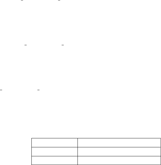
75
The values given in Kohout et al. (2014) are Cice,1...2= [5.35×10−6,16.05×
10−6]. See regression test ww3 tic1.1/input IC4/M4 for examples.
IC4M5: This is a simple step function with up to 4 steps. It is controlled by
the optionally nonstationary and non-uniform parameters Cice,1...7. Parame-
ters Cice,1...4control the step levels, which are in terms of dissipation rate, ki,
in radians per meter. Parameters Cice,5...7control the step boundaries (given
in Hz). See regression test ww3 tic1.1/input IC4/M5 for examples.
IC4M6: This is a simple step function with up to 10 steps. It is controlled
by the stationary and uniform namelist parameters IC4KI and IC4FC. Array
IC4KI controls the step levels, which are in terms of dissipation rate, ki, in
radians per meter. Array IC4FC controls the step boundaries (given in Hz).
See regression test ww3 tic1.1/input IC4/M6 for examples.
2.4.5 Sis: Diffusive scattering by sea ice (simple)
Switch: IS1
Origination: WAVEWATCH III/NRL
Provided by: S. Zieger
The non-conservative effect of ice on waves has been implemented in switches
IC1 through IC3 (see Section 2.4.1–2.4.3). The conservative effect of sea
ice has been implemented in switch IS1 and represents a simple form of
scattering. It is assumed that the floe size is smaller than the grid size and
that a fraction αice of the incoming wave energy is scattered isotropically.
The fraction is determined from sea ice concentration ICE using a simple
linear transfer function
αice = max {0, C1ICE + C2}.(2.184)
The coefficients C1and C2are customizable through namelist SIS1 with
namelist parameters ISC1 and ISC2. At each discrete frequency and direction
the wave energy is reduced by the amount of αice and redistributed to all
direction in the same discrete frequency to conserve energy.

76
2.4.6 Sis: Floe-size dependent scattering and dissipation
Switch: IS2
Origination: WAVEWATCH III
Provided by: F. Ardhuin, C. Sevigny, G. Boutin, D. Dumont, T. Williams
The implementation of this scattering term generally follows the approach
of Meylan and Masson (2006), to which has been added an estimation of the
breakup of the ice by waves to be able to update a maximum floe size diame-
ter. Finally a creep-based dissipation was also combined with the scattering.
The scattering source term currently uses a back-scatter that is uniform
in all directions, giving the action-conserving formulation,
Sis(k, θ)
σ=Z2π
0
βis,MIZ[sscatN(k, θ′)−N(k, θ)]dθ′.(2.185)
where sscat is set to 1.0 by default but can be modified by IS2BACKSCAT in
namelist SIS2.
The determination of scattering coefficients βis,MIZ is based on the theo-
retical reflection coefficient αn(σ, h) for waves with a normal incidence going
from a half-plane of open water to a half-plane of ice-covered water with a
constant ice thickness h. Values of αn(σ, h) as computed by Kohout and Meylan
(2008) are tabulated in the W3SIS2MD module. Following Dumont et al.
(2011), the broken ice is treated as a series of such ice-water interfaces.
Neglecting multiple reflections, the scattering parameterization defines the
attenuation per unit time as if the ice-covered part of a grid cell was a suc-
cession of floes of mean diameter Dmwith a partial reflection αn(σ, h) for
each floe, giving,
βis,MIZ = ICE cgαn(σ, h)/Dm,(2.186)
where ICE is the ice concentration.
The estimation of the mean floe diameter Dmis based on an assumed
power law for the number of floes of diameter D, taken proportional to D−γ.
This power low is further assumed to apply for Dranging from the minimum
Dmin and a maximum Dmax. The average is thus given by
Dm=γ
γ−1×D−γ+1
max −D−γ+1
min
D−γ
max −D−γ
min
.(2.187)

77
At present Dmin is a user-supplied value. Dmax can either be provided as a
forcing field, e.g. from an ice model or some observations, or, if the namelist
parameter IS2BREAK is set to TRUE, estimated from the breaking of the ice
by the local wave field. If the namelist parameter IS2DUPATE is set to TRUE,
small values of Dmax will persist even if the waves become too small to be
able to break the ice to that size. This is probably the proper model use
when external forcing/coupling is available (e.g. advection of ice properties
in an ice model). On the contrary, if IS2DUPDATE is set to FALSE, the value
of Dmax will be always adjusted to the local sea state, even if that means
increasing Dmax.
Ice breaking by waves of wavelength λis assumed to produce floes of di-
ameter λ/2. In the parametrization, ice breaking occurs if the three following
criteria are fulfilled (Williams et al.,2013):
1. λ/2≥Dmin and λ/2≤Dmax
2. Dmax > Dc, as it exists a critical diameter, which depends on ice prop-
erties, below which no flexural failure is possible
3. ε > εc, the strain due to the incoming wave has to be greater than a
defined critical strain
The first criterion is simply checking that the new value of Dmax will be larger
than Dmin and smaller than the previous value of Dmax.
The second criterion relies on Mellor (1986), who defines Dcas
Dc=π4Y∗h3
48ρg(1 −ν2)1/4
.(2.188)
The third criterion corresponds to the flexural strain threshold. The
horizontal strain caused by waves is related to the curvature of the ice layer,
which, in one dimension is ε= 0.5h∂2ηice/∂x2. The strain variance is given
hε2i=h
22Zk2
k1
k4
iceF(k)dk, (2.189)
where his the ice thickness and kice is the wavenumber 2π/λice. Borrowing
from wave breaking ideas (Banner et al.,2000), the integration of the curva-
ture variance is limited around the local wavenumber kice. We also note that

78
we have defined an effective minimum ice thickness hmin so that, if h < hmin,
the strain variance is computed with h=hmin to avoid unbreakable elastic
thin ice in the model that does not correspond to usual observations. We
thus take Dmax to be half the wavelength of the shortest waves for which the
following criterion is met
Fbreak √ε2>σc
Y∗,(2.190)
where σcis the ice flexural strength. Fbreak is a factor representing random
waves and adjustable with the SIS2 namelist parameter IS2BREAKF. It should
in theory depend on the duration for which the ice is forced by the waves, and,
based on the typical maximum value over 500 Rayleigh-distributes waves, was
taken to be Fbreak = 3.6. Fbreak Esis thus the maximum strain for random
waves.
Creep dissipation was added in this routine, following Wadhams (1973),
because it critically depends on the floe size. It assumes that the floes de-
formation is not fully elastic, and that the secondary creep under the wave-
induced cyclic causes the dissipation of wave energy into heat. We use the
ice flow law dε
dt ij
=τ2
B3σ′
i,j,(2.191)
Bis the flow law constant and is a function of ice temperature. Using
the normalized parameter estimated by Cole et al. (1998) from laboratory
experiments, A= 1011, and a uniform ice temperature of 270 K gives a value
of B= 107s1/3. The volumic dissipation rate is
de
dt =|σ4
xx/(2B)3|.(2.192)
Also, the cyclic deformation of the ice can require a much larger elastic
energy than the gravity potential energy, but this is only true if the ice
is not broken. As a result, working with a wave elevation spectrum E(k)
could introduce large changes in E(k) when the ice is broken or reformed.
Instead we prefer to work with an energy spectrum RCgE(k)/Cg,ice, using
the coefficient Rintroduced by Wadhams (1973), which is the ratio of elastic
to gravity potential energies. For unbroken ice Ris
R= 1 + CR
4Y∗h3π4
3ρgλ4(1 −ν2),(2.193)

79
where we have been careful that Wadhams (1973) used 2hfor the ice thick-
ness, and CRis by default set to 1.0 using the namelist parameter IS2BREAKE,
but it can be set to zero to work with the true elevation spectrum instead.
This factor Ris also applied in the calculation of ice breakup by the waves.
The creep dissipation is linearized as Screep =−αcreepEice. The coefficient
αcreep was adapted from the Wadhams (1973) monochromatic formula and is
equal to
αcreep = 0.05Bh5Y∗
2B(1 −ν2)4
I3k4C2
g
ρgCgice R2FZk2
k1
k4
iceE(k)dk, (2.194)
where I3=1
πRπ
0sin4βdβ.Fbroken is a heuristic smooth transition from un-
broken to broken ice, so that the dissipation gradually goes to zero for waves
much longer than the floe sizes, because in that case the ice does not deform
and produces no dissipation of wave energy,
Fbroken = tanh Dmax −Cλλice
DmaxCsmooth .(2.195)
Creep is computed after updating Dmax. The two parameters in this smooth
transition Cλand Csmooth are set to 0.4 and 0.2 by the adjustable namelist
parameters IS2CREEPD and IS2CREEPC.
Finally we recall the various model parameters used in IS2 in the following
table. Some are defined as constants in the W3IS2MD module, others can be
adjusted with the SIS2 namelist.
Parameters Symbol namelist parameter default values
Minimum floe size Dmin N. A. 20 m
Initial floe size Dinit N. A. 1000 m
Ice fragility ξN. A. 0.9
Ice density ρice N. A. 922.5 kg m−3
Effective Young Modulus Y∗N. A. 5.49 GPa
Poisson Coefficient νN. A. 0.3
Flexural strength σcN. A. 0.27 MPa
Flow law parameter nIS2CREEPN 3
Flow law parameter BIS2CREEPB 107s1/3
Correction for elastic energy CRIS2BREAKE 1.0

80
2.4.7 Sref : Energy reflection at shorelines and icebergs
Switch: REF1
Origination: WAVEWATCH III
Provided by: F. Ardhuin
Reflections by shorelines and icebergs is activated by using the REF1 switch
and setting namelists parameters REFCOAST,REFSUBGRID or REFBERG (in
namelist REF1) to non-zero values that are the target reflection coefficients
R2
0for the wave energy. If the IG1 switch is also used, then the energy source
at the shoreline also includes free infragravity waves in both ingoing and
outgoing directions. That particular source is described in section 2.4.8.
From these values R2
0may be varied with wave height and period following
a Miche-type parameter: this is activated by setting REFFREQ to a non-zero
value, and is based on the field measurements of Elgar et al. (1994). These
coefficients can also be made to vary spatially, by setting REFMAP to a non-
zero value. In that case ww3 grid will expect to find a extra line after the
reading of the water depths and obstructions in ww3 grid.inp.
Wave reflection at the shoreline varies from a fraction of a percent to about
50% of the incoming wave energy, and may have important consequences for
the directional wave spectrum, and the wave climate in otherwise sheltered
locations (O’Reilly et al.,1999). Wave reflection is also extremely important
for the generation of seismic noise by ocean waves.
Because reflection involve wave trains with different directions, in a model
like WAVEWATCH III, their interaction can only be represented through a
source term in the right hand side. Nevertheless, this is physically linked to
propagation.
In practice, for the regular and curvilinear grids, the reflection source term
puts into the reflected wave directions the proper amount of energy that will
be taken away by propagation at the next time step. When neglecting the
cross-shore current, this is
Sref (k, θ) = ZR2(k, θ, θ′)Cg(k)
∆A[cos(θ−θq)∆q+ sin(θ−θp)∆p]N(k, θ′)dθ′,
(2.196)
where R2is an energy reflection coefficient, and ∆pand ∆qare the grid spac-
ing along the two axes of the grid, and ∆Ais the cell area. The definition of

81
the shoreline direction from the land/sea mask is explained in Ardhuin et al.
(2011b). This has not been tested for the SMC grids, and it is not expected
to work for that type of grid.
In the case of unstructured grids, the spectral density of outgoing direc-
tions on the boundary is directly set to the expected reflected value and the
boundary condition is handled specifically by the the numerical schemes.
The reflection coefficient R2is taken to be non-zero only for the directions
for which cos(θ−θ′)<0, and its magnitude is the product of a reflection
coefficient R2
0(k), integrated over the scattered directions θ, and a directional
distribution R2(θ, θ′) around the specular direction θs,
R2(k, θ, θ′) = R2
0(k)R2(θ, θ′).(2.197)
This directional distribution takes three forms:
•isotropic in all directions opposite to the incoming direction: this is for
sub-grid islands and icebergs or sharp shoreline angles,
•proportional to cos(θ−θs)2for moderate shoreline angles,
•proportional to cos(θ−θs)nfor small shoreline angles (nearly straight
shoreline). Where n= 4 by default and can be changed to any value us-
ing the REFCOSP STRAIGHT namelist parameter in the REF1 namelist.
That parameterization is described in detail by Ardhuin and Roland (2012).
In the case of icebergs and sub-grid islands, the reflected energy is redis-
tributed evenly in all directions within 90◦of the direction opposite to the
incoming waves. For resolved lands, a mean direction perpendicular to shore
θnwas defined from the land or sea status of the 8 grid points surrounding
the local point (Fig. 2.1).
For each model grid point adjacent to land, the analysis of the land-sea
geometry gives one value of θnamong 16 possible directions. Together with
any incoming wave direction θithis defines a specular reflection direction
θr= 2θn−θi+π. For each spectral component of direction θigoing towards
the coast (i.e. such that cos(θi−θn)>0), the total reflection is R2times the
incoming energy. This reflected energy R2E(f)M(f, θi) is redistributed over
directions around the specular reflection direction θr, with a broad distribu-
tion taken proportional to cosn(θ−θr), where the power nis a function of
the local shoreline geometry.
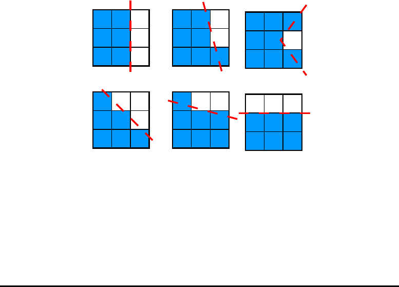
82
1
234
5
6 7 8
1
234
5
6 7 8
Sea Land
1
234
5
6 7 8
0 0 0
straight coast mild corner sharp corner
1
234
5
6 7 8
1
234
5
6 7 8
1
234
5
6 7 8
0 0 0
straight coast mild corner straight coast
Figure 2.1: Examples of determination of the shoreline orientation and ge-
ometry using the land/sea mask. For any sea point (number 0) which is the
ocean (in blue) and has at least one neighbor in land (in white) the eight
neighbors, numbered from 1 to 8 are used to define the shoreline geometry.
For ‘mild’ corners and straight coasts, the estimated shoreline orientation
(dashed line) is used to compute the directional distribution of the reflected
wave energy.

83
For this purpose we distinguish three different shoreline geometries rela-
tive to the local point as illustrated by Fig. 2.1: we set n= 2 for a straight
coast (three connected land points among the neighbors), n= 1 for a mild
corner (two land points among the neighbors), and n= 0 at a sharp corner
(only one land point, among the 4 closest neighbors) which corresponds to the
same treatment done for sub-grid islands and icebergs. Changing these values
of nin the range 0 to 2 has little effect on our results. n= 1 corresponds to
a Lambertian surface approximation, which is used for electromagnetic wave
scattering from rough surfaces. A pure specular reflection would be obtained
with ninfinite. A more rigorous treatment should use the distribution of the
shoreline orientation at at the scale of the ocean wavelength, namely of the
order of 100 m.
2.4.8 Second-order spectrum and free infragravity waves
Switch: IG1
Origination: WAVEWATCH III
Provided by: F. Ardhuin
WARNING: A bug has been identified with IG wave sources in unstructured
grids. A model patch using an older version of the code will be provided
shortly.
The linear dispersion relation used in section 2.1 is a good approximation
for most of the wave energy but a significant part of the spectrum at high
frequencies, with typical frequencies above three times the windsea wave
peak (e.g. Leckler,2013). In shallow water, another strongly nonlinear part
of the spectrum is found at very low frequencies, which are called infragravity
waves.
In the case of horizontally homogeneous conditions over a flat bottom,
both low and high frequency non-linear components can be estimated from
the linear wave spectrum, using perturbation theory (e.g. Hasselmann,1962).
Also, the non-linear evolution of a homogeneous wave field is better described
in terms of this ‘linearized spectrum’. It is thus practical to work with this
‘linearized spectrum’ and convert to the observable spectrum that contains
non-linear components when post-processing the model results. One method
to perform this transformation is a canonical transformation proposed by
84
Krasitskii (1994). The properties of this transformation were further explored
by Janssen (2009) and implemented for post-processing in the ECMWF ver-
sion of the WAM model.
The code for the canonical transform written by P. Janssen was interfaced
with WAVEWATCH III. Using the IG1 switch and setting the parameter
IGADDOUTP = 2 in the SIG1 namelist, this canonical transformed, which
conserves energy, will be used for the output point spectra. If IGADDOUTP =
1, then the second-order spectrum is added on top of the model spectrum
using the theory (e.g. Hasselmann,1962). That option does not conserve
energy and is not consistent at high frequency because the quasi-linear term
in the second-order spectrum are ignored (Janssen,2009).
However, when comparing to measurements, one should be aware that
different measuring devices have different responses to the nonlinear part of
the spectrum. In particular surface-following buoys also linearize the spec-
trum, and the second-order pressure field is not related to the second-order
elevation via the relations used for linear waves. The canonical transform
is thus only applicable for wave gauges that measure elevation at a fixed
location.
When the wave field is not homogeneous, the nonlinear properties of the
waves lead to an exchange of energy between different modes. In shallow wa-
ter this usually results in the transfer of energy to infragravity waves, that are
released along shorelines and travel as free waves. The IG1 switch allows the
parameterization of that effect with several methods. These are very crude
parameterizations compared to the full hydrodynamic solution that would
require solving the bispectral evolution across the surf zone at a very high
spatial resolution (e.g. Herbers and Burton,1997). The default namelist set-
tings correspond to the parameterization presented by Ardhuin et al. (2014).
In practice the free infragravity wave energy is added via the Sref source
term, by setting the SIG1 namelist IGSOURCE to 1 or 2.
In the first method, activated with IGSOURCE =1, the second-order spec-
trum is computed using either the Hasselmann perturbation (IGMETHOD =
1) or the canonical transform (any other value of IGMETHOD) as described in
Janssen (2009). This approach may lead to better directional distribution of
IG wave energy but it is still being tested. The second method, activated
with IGSOURCE = 2, and the free IG spectrum is given by the following ex-
pressions,

85
AIG =HsT2
m0,−2,(2.198)
b
EIG(f) = 1.2α2
1
kg2
cg2πf
(AIG/4)2
∆f
[min(1., 0.015Hz/f)]1.5,(2.199)
b
EIG(f, θ) = b
EIG(f)/(2π),(2.200)
where the mean period is defined as Tm0,−2=pm−2/m0with the moments
mn=Z0.5 Hz
fmin Hz
E(f)fndf, (2.201)
and the empirical coefficient α1is of the order of 10−3s−1, and is set by the
SIG1 namelist parameter IGEMPIRICAL. The minimum frequency fmin used
to define Tm0,−2is set by the namelist parameter IGMAXFREQ and it is also
the maximum frequency of the IG band over which this source of energy
is applied. Also, in this band the IG energy at the coast can be added on
top of pre-existing energy, or the pre-existing energy can be reset to zero.
That latter behavior is the default and controlled by IGBCOVERWRITE = 1.
For other choices, (IGBCOVERWRITE = 0), the results are very sensitive to
the maximum shoreline reflection coefficient allowed (REFRMAX parameter in
namelist REF1).
Finally, IG energy can also be added for frequencies beyond fmin, this is
the default behavior and it is activated by setting IGSWELLMAX = TRUE. For
that part of the IG wave field, the IG wave source is now reduced by a factor
4 which is now hard-coded in w3ref1md.ftn. This should be adjusted together
with the maximum reflection which is defined by the REF1 namelist param-
eter REFRMAX. In the present version, the option IGSWELLMAX = TRUE does
not work well with unstructured grids. We thus advise to use IGSWELLMAX =
FALSE for these grids, this will unfortunately lead to a spectral gap between
the IG band and the swell-windsea band.
2.4.9 Sxx: User defined
Switch: XXn
Origination: —
Provided by: user
86
This slot is intended for a source term that is not yet classified in Eq. (2.16).
Almost by definition, it cannot be provided here.
2.5 Air-sea processes
2.5.1 General concepts
Additional subroutines are provided within WAVEWATCH III for use as part
of coupled ocean-wave or ocean-atmosphere systems. These subroutines are
designed to compute additional quantities related to the surface wave field
which are intended to be passed to external models (e.g. ocean models). The
motivation for these subroutines is to allow the external model to include the
impact of waves on quantities such as the wind stress and the upper ocean
turbulence.
Sea-state dependent air-sea fluxes The air-sea momentum flux, or the
total wind stress, is the sum of the momentum flux into both surface waves
and subsurface currents. Coupled atmosphere-ocean models that do not con-
sider the impact of the surface gravity wave field typically compute the total
wind stress based on an empirical relationship between the wind speed and
the wind stress (via a drag coefficient, Cd). The provided FLD subroutines al-
lows the computation of the total wind stress based on the WAVEWATCH III
wavenumber-direction spectrum for use in coupled numerical models.
To the leading order, the total wind stress is equal to the sum of the
momentum flux into surface waves (form drag of surface waves) and the
momentum flux directly into the subsurface currents (through viscous stress).
The momentum flux into the waves may be expressed as an integral of the
wave variance spectrum multiplied by the wave growth rate (momentum-
uptake rate). A few assumptions are needed to calculate the wave form drag.
First, the wave form drag is sensitive at the leading order to the level of the
high frequency waves (or the spectral tail). This part of the wave spectrum
contains a great deal of uncertainty within the wave model, and therefore
may need to be separately parameterized for computing the wind stress.
An assumption must therefore be made to parameterize the high frequency,
which is not constrained by observational data and wind speeds above 15
87
m/s. Second, assumptions of the wave growth-rate function are needed since
it has historically been parameterized from either the wind speed or the wind
stress. In either case, empirical coefficients are needed within the growth-rate
function based on wavelength and wave direction relative to the wind and/or
stress. Third, there is feedback due to the wave form drag on the turbulence
profile and the wind profile within the wave boundary layer (roughly the
upper 10 meters above the air-sea interface). How important this feedback
is on determining the wind stress and the mean wind profile is not entirely
understood. Finally, the growth rate is known to be different over breaking
and non-breaking waves. However, there are no simple methods for explicitly
including the breaking wave impact within wind-stress calculation models.
Therefore, no separation is made in either of the present FLD subroutines
between breaking and non-breaking wave growth-rates.
The total air-sea momentum flux can be expressed (to the leading order)
as:
~τ =~τν+~τf,(2.202)
where ~τνis the viscous stress vector and ~τfis the wave form drag. At the
air-sea interface, the wave form drag can be computed as the contribution of
the momentum flux into all waves:
~τf=ρwZkmax
kmin Zπ
−π
βg(k, θ)σF (k, θ)dθ~
kdk, (2.203)
where ρwis the water density, kis the wavenumber, θis the wave direc-
tion, σis the angular frequency, βg(k, θ) is the growth rate, F(k, θ) is the
wave variance spectrum, and kmin and kmax are the minimum and maxi-
mum wavenumbers of contributing waves. The expression for the growth
rate varies based on the theory applied in the model, and will be described
separately for each theory in their following descriptions.
The spectral tail at wind speeds above 15 m/s is not well constrained
observationally or theoretically. Therefore, the spectral tail level in the FLD
subroutines has been empirically parameterized such that the mean drag
coefficient corresponds to the standard bulk drag coefficient used within the
modeling system. In this way, the mean value of the wind stress will not be
modified by using any explicit sea state dependent wind stress formulation,
but the stress will deviate from the mean based on the sea-state. It is assumed
that the tail level is a function of a wind speed only and is independent of
sea states.

88
2.5.2 Sea-state dependent τ: Reichl et al. 2014
Switch: FLD1
Origination: WAVEWATCH III
Provided by: B. Reichl
Wind stress according to Reichl et al., 2014 In Reichl et al. (2014)
the total stress is constant in height, but is decomposed into two components
as a function of height as:
~τ =~τt(z) + ~τf(z),(2.204)
where τtis the turbulent stress and is equal to the viscous stress very near
the surface. The wave form stress can be expressed as:
~τf(z) = ρwZk=δ/z
kmin Zπ
−π
βg(k, θ)σF (k, θ)dθ~
kdk, (2.205)
that is, the wave form stress at height zis equal to the integration of the
wave form stress at the surface for wavenumbers below k=δ/z, where δ/k is
the inner layer height (Hara and Belcher,2004) for waves at a wavenumber
k. This expression is derived by assuming that the wave-induced stress is
significant from the surface up to the inner layer height, but is negligible
further above. Since at the surface
~τ =~τν+~τf(z= 0) = ~τν+ρwZkmax
kmin Zπ
−π
βg(k, θ)σF (k, θ)dθ~
kdk, (2.206)
the turbulent stress at a height zcan be expressed as:
~τt(z) = ~τν+ρwZkmax
k=δ/z Zπ
−π
βg(k, θ)σF (k, θ)dθ~
kdk. (2.207)
In this model it is assumed that the turbulent stress at the inner layer
height z=δ/k determines the growth rate of waves at wavenumber k:
βg(k, θ) = cβσ|τt(z=δ/k)|
ρwc2cos2(θ−θτ),(2.208)

89
where θτis the direction of the turbulent stress at the inner layer height.
The turbulent stress at the inner layer height is used in place of the total
wind stress because longer waves reduce the effective wind forcing on shorter
waves (wave sheltering).
The growth rate coefficient cβvaries depending on the ratio of the wave
phase speed to the local turbulent friction velocity (friction velocity at the
inner layer height), ul
⋆=pτt(z=δ/k)/ρa).
cβ=
25 : cos(θ−θw)>0 : c/ul
⋆<10
10 + 15 cos[π(c/u⋆−10)/15] : : 10 ≤c/ul
⋆<25
−5 : : 25 ≤c/ul
⋆
−25 : cos(θ−θw)<0
(2.209)
The wind profile is explicitly calculated using the energy conservation
constraint in the wave boundary layer. From the top of the viscous sublayer
to the inner layer height of the shortest waves the wind shear is expressed as:
d~u
∂z =ρa
κz
~τν
ρa
3/2~τν
~τν·~τtot
for zν< z < δ/kl.(2.210)
Between the inner layer height of the shortest waves and that of the longest
waves the wind shear is expressed as:
d~u
∂z ="δ
z2˜
Fwk=δ
z+ρa
κz
~τt(z)
ρa
3/2#×~τt(z)
~τt(z)·~τtot
for δ/kl≤z, (2.211)
where ˜
Fw(k=δ/z) is the energy uptake by surface waves:
˜
Fw(k=δ/z) = ρwZπ
−π
βg(k, θ)gF (k, θ)kdθ. (2.212)
Finally, above the inner layer height of the longest waves the wave effect is
negligible and the wind shear is aligned in the direction of the wind stress:
d~u
dz =u⋆
κz
~τtot
|~τtot|.(2.213)
Note that when using the FLD1 switch, internal variables and output
values of the viscous stress, friction velocity, surface roughness length and
Charnock parameter are recalculated and overwritten.

90
2.5.3 Sea-state dependent τ: Donelan et al. 2012
Switch: FLD2
Origination: UMWM
Provided by: B. Reichl
Wind stress according to Donelan et al., 2012 In Donelan et al.
(2012) the growth rate parameter in Eq. (2.203) is expressed as:
βg(k, θ) = A1σuλ/2cos(θ−θw)−cuλ/2cos(θ−θw)−c
c2
ρa
ρw
,(2.214)
A1=
0.11,:uλ/2cos θ > c, for wind forced sea
0.01 : 0 < uλ/2cos θ < c, for swell faster than the wind
0.1 : cos θ < 0,for swell opposing the wind
(2.215)
where A1is the proportionality coefficient determined empirically (so that
modeled wave spectra agree with field observations), uλ/2is the wind speed
at the height of half the wavelength (up to 20 m), θwis the wind direction,
and cis the wave phase speed. The wind speed is calculated using the law
of the wall for rough surfaces:
u(z) = u⋆
κln z
z0,(2.216)
where κis the von K´arm´an coefficient (default 0.4). The viscous stress is
calculated from the law of the wall for smooth surfaces. The viscous drag
coefficient, Cdνis adjusted to account for sheltering:
Cd′
ν=Cdν
31 + 2Cdν
Cdν+Cdf,(2.217)
where Cdfis the wave form drag coefficient. The viscous stress can then be
solved for as:
~τν=ρaCd′
ν|uz|uz.(2.218)
Note that when using the FLD2 switch, internal variables and output
values of the viscous stress, friction velocity, surface roughness length and
Charnock parameter are recalculated and overwritten.

91
Group Name Elements
I Forcing Fields 10
II Mean Wave Parameters 16
III Spectrum Parameters 6
IV Partitions Parameters 8
V Atmosphere-Waves Layer 10
VI Wave-Ocean Layer 11
VII Wave-Bottom Layer 5
VIII Spectrum parameters 6
IX Numerical Diagnostics 5
X User Defined 2
Table 2.10: Groups in new double-indexing output field structure.
2.6 Output parameters
The wave model provides output of gridded fields of mean wave parameters.
Some of these parameters can also be found in the output for selected points.
For activation of the output see Section 4.4.9
Since version 4.XX (. . . ), WAVEWATCH III output fields are defined by
a double-indexing structure, where the first index refers to a functional group
that parameters belong to, and the second number is the index for a given
parameter within its group. Groups are defined according to Table 2.10.
Below, a brief denifition of output field parameters is provided. A ta-
ble with definitions may be found in the sample ww3 shel.inp file, in Sec-
tion 4.4.9. That input file also provides a list of flags indicating if output
parameters are available in different field output file types (ASCII, grib,
igrads, NetCDF).
Selection of field outputs in input files for a given output type, may be
made in two ways. For F and T flags, this option is activated if the user adds
F or T to the first line of the output field selection part for a given inp file.
There are 10 groups of parameters the user can choose from (reflecting the
internal double-index structure of the code itself). If the first flag of a group
line is set to F then that group will not produce output, and a second line for
parameter flags is not expected. If the group flag is set to T, then a second

92
group line is expected containing parameter flags. Examples of F/T flag use
are given in Section 4.4.9. All parameters that are a function of frequency
(e.g. EF or USF) require the setting of specific namelist parameters, in the
OUTS namelist. This is to reduce the memory use if these parameters are
not needed.
For namelists, the first line is set to N, and the next line contains param-
eter symbols. Examples are given in Section 4.4.11 and Section 4.4.14. The
names for these namelists are the bold names below, for example HS.
All parameters listed below are available in ASCII and NetCDF output
files. If selected output file types are grads or grib, some parameters may not
be available. Availability (or not) is identified in the first two columns in the
field output parameter table within the example input file in Section 4.4.9.
That table also identifies, for all parameters, the internal WAVEWATCH III
code tags, the output tags (names used is ASCII file extensions, NetCDF
variable names and namelist-based selection (see also Section 4.4.14), and
the long parameter name/definition.
I) Forcing fields
1) DPT The mean water depth (m). This includes varying water levels.
2) CUR The mean current velocity (vector, m/s).
3) WND The mean wind speed (vector, m/s). This wind speed is
always the speed as input to the model, i.e., is not corrected for the
current speed.
4) AST The air-sea temperature difference (◦C).
5) WLV Water level.
6) ICE Ice concentration.
7) IBG Wave attenuation due to icebergs: this parameter is the inverse
of the e-folding scale associated to the loss of wave energy in a field
of small icebergs (Ardhuin et al.,2011b).
8) D50 Sediment median grain size (D50).
9) IC1 Ice thickness.
10) IC5 Ice flow diameter.
II) Standard mean wave parameters
1) HS Significant wave height (m) [see Eq. (2.23)]
Hs= 4√E . (2.219)

93
2) LM Mean wave length (m) [see Eq. (2.22)]
Lm= 2πk−1.(2.220)
3) T02 Mean wave period (s) [see Eq. (2.22)]
Tm02 = 2π/pσ2.(2.221)
4) T0M1 Mean wave period (s) [see Eq. (2.22)]
Tm0,−1= 2πσ−1.(2.222)
5) T01 Mean wave period (s) [see Eq. (2.22)]
Tm0,1= 2πσ . (2.223)
6) FP Peak frequency (Hz), calculated from the one-dimensional fre-
quency spectrum using a parabolic fit around the discrete peak.
7) DIR Mean wave direction (degr., meteorological convention)
θm= atan b
a,(2.224)
a=Z2π
0Z∞
0
cos(θ)F(σ, θ)dσ dθ , (2.225)
b=Z2π
0Z∞
0
sin(θ)F(σ, θ)dσ dθ . (2.226)
8) SPR Mean directional spread (degr.; Kuik et al.,1988)
σθ="2(1−a2+b2
E21/2)#1/2
,(2.227)
9) DP Peak direction (degr.), defined like the mean direction, using
the frequency/wavenumber bin containing of the spectrum F(k) that
contains the peak frequency only.
10) HIG Infragravity height.
11) MXE Max surface elev (Space-time extreme, STE)
12) MXES St Dev of max surface elev (STE)
13) MXH Max wave height (STE)

94
14) MXHC Max wave height from crest (STE)
15) SDMH St Dev of MXC (STE)
16) SDMHC St Dev of MXHC (STE)
III) Spectral parameters (first 5 moments and wavenumbers).
All these parameters are a function of frequency and thus these are three-
dimensional arrays. Because of the large memory use, the computation
of these parameters requires the activation of switches in the OUTS
namelist.
1) EF Wave frequency spectrum (m2/Hz)
E(f) = 2πZF(σ, θ)dθ . (2.228)
2) TH1M Mean direction for each frequency (degr.; Kuik et al.,1988)
θ1(f) = atan b1(f)
a1(f),(2.229)
a1(f) = 2πZ2π
0Z∞
0
cos(θ)F(σ, θ) dθ , (2.230)
b1(f) = 2πZ2π
0Z∞
0
sin(θ)F(σ, θ) dθ . (2.231)
3) STH1M First directional spread for each frequency (degr.; )
σ1(f) = "2(1−a1(f)2+b1(f)2
E(f)21/2)#1/2
,(2.232)
4) TH2M Mean direction from a2and b2(degr.)
θ2(f) = atan b2(f)
a2(f),(2.233)
a2(f) = 2πZ2π
0Z∞
0
cos(2θ)F(σ, θ) dθ , (2.234)
b2(f) = 2πZ2π
0Z∞
0
sin(2θ)F(σ, θ) dθ . (2.235)

95
5) STH2M Directional spreading from a2and b2(degr.)
σ2(f) = "0.5(1−a2(f)2+b2(f)2
E(f)21/2)#1/2
,(2.236)
6) WN Wavenumbers k(σ) (rad/m)
σ2=gk tanh(kD),(2.237)
IV) Spectral partition parameters
These output parameters are based on partitioning of the spectrum into
individual wave fields.
1) PHS Wave heights Hsof partitions of the spectrum (see below).
2) PTP Peak (relative) periods of partitions of the spectrum (parabolic
fit).
3) PLP Peak wave lengths of partitions of the spectrum (from peak
period).
4) PSP Mean direction of partitions of the spectrum.
5) Directional spread of partition of the spectrum Cf. Eq. (2.227).
6) PWS Wind sea fraction of partition of the spectrum. The method
of Hanson and Phillips (2001) is used, implemented as described
in Tracy et al. (2007). With this, a ‘wind sea fraction’ Wis in-
troduced
W=E−1E|Up>c ,(2.238)
where Eis the total spectral energy, and E|Up>c is the energy
in the spectrum for which the projected wind speed Upis larger
than the local wave phase velocity c=σ/k. The latter defines
an area in the spectrum under the direct influence of the wind.
To allow for nonlinear interactions to shift this boundary to lower
frequencies, and subsequently to have fully grown wind seas inside
this are, Upincludes a multiplier Cmult
Up=CmultU10 cos(θ−θw).(2.239)
The multiplier can be set by the user. The default value is Cmult =
1.7.

96
7) TWS Wind sea fraction of the entire spectrum.
8) PNR Number of partitions found in the spectrum.
V) Atmosphere-waves layer
1) UST The friction velocity u∗(scalar). Definition depends on se-
lected source term parameterization (m/s). An alternative vector
version of the stresses is available for research (requires user inter-
vention in the code).
2) CHA Charnock parameter for air-sea friction (without dimensions)
3) CGE Energy flux (W/m)
CgE=ρwgCgE . (2.240)
4) FAW Wind to wave energy flux
5) TAW Net wave-supported stress (wind to wave momentum flux)
6) TWA Negative part of the wave-supported stress
7) WCC Wave to wind momentum flux
8) WCF Whitecap coverage (without dimensions)
9) WCH Whitecap mean thickness (m)
10) WCM Mean breaking wave height (m) (NOT AVAILABLE YET)
VI) Wave-ocean layer
1) SXY Radiation stresses
Sxx =ρwgZZ n−0.5 + ncos2θF(k, θ)dkdθ , (2.241)
Sxy =ρwgZZ nsin θcos θ F (k, θ)dkdθ , (2.242)
Syy =ρwgZZ n−0.5 + nsin2θF(k, θ)dkdθ , (2.243)
where
n=1
2+kd
sinh 2kd .(2.244)
2) TWO Wave to ocean momentum flux
3) BHD Bernoulli head (m2/s2)
J=gZZ k
sinh 2kd F(k, θ)dkdθ , (2.245)

97
4) FOC Wave to ocean energy flux (W/m2)
5) TUS Stokes volume transport (m2/s)
(Mw
x, Mw
y) = gZZ (kcos(θ), k sin(θ))
σF(k, θ)dkdθ , (2.246)
6) USS Stokes drift at the sea surface (m/s)
(Ussx, Ussy ) = gZZ σcosh 2kd(kcos(θ), k sin(θ))
sinh2kd F(k, θ)dkdθ ,
(2.247)
7) P2S Second order pressure variance (m2) and peak period of this
pressure (s) which contributes to acoustic and seismic noise,
Fp2D(k= 0) = Z∞
0
4σ
CgZπ
0
F(k, θ)F(k, θ +π)dθdk , (2.248)
8) USF Frequency spectrum of Stokes drift at the sea surface (m/s/Hz)
(Ussx(f), Ussy(f)) = gZZ σcosh 2kd(kcos(θ), k sin(θ))
sinh2kd F(k, θ)2π
Cg
dθ,
(2.249)
9) P2L Frequency spectrum of the second order pressure (m2s) which
contributes to acoustic and seismic noise,
Fp2D(k= 0, f) = 2σ
πZπ
0
4π2
C2
g
F(k, θ)F(k, θ +π)dθ . (2.250)
10) TWI Wave to sea ice stress
11) FIC Wave to sea ice energy flux
VII) Wave-bottom layer
1) ABR Near-bottom rms excursion amplitude
ab,rms =2ZZ 1
sinh2kd F(k, θ)dkdθ1/2
.(2.251)
2) UBR Near-bottom rms orbital velocity
ub,rms =2ZZ σ2
sinh2kd F(k, θ)dkdθ1/2
.(2.252)
98
3) BED Bedform parameters: ripple height and directions (NOT TESTED
YET)
4) FBB Energy dissipation in WBBL
5) TBB Momentum loss in WBBL
VIII) Spectrum parameters
1) MSS Mean square slopes in xand ydirections (zonal and meridional
components of slopes variances).
2) MSC Spectral tail level (without dimensions)
3) WL02 East/X North/Y mean wavelength component
4) AXT Correl sea surface gradients (x,t)
5) AYT Correl sea surface gradients (y,t)
6) AXY Correl sea surface gradients (x,y)
IX) Numerical diagnostics
1) DTD Average time step in the source term integration (s).
2) FC Cut-off frequency fc(Hz, depends on parameterization of input
and dissipation).
3) CFX Maximum CFL number for spatial advection
4) CFD Maximum CFL number for angular advection
5) CFK Maximum CFL number for wavenumber advection
X) User defined
1) U1 Slot for user defined parameter (requires modification of code).
2) U2 Idem.
99
This page is intentionally left blank.

100
3 Numerical approaches
The Wave Action Equation in Cartesian (2.8) or spherical (2.12) coordinates
is the basic equations of the wave model. However, modified versions of these
equations are used in the model, where (a) they are solved on a variable
wavenumber grid (see below), where (b) modified versions of these equations
are used to properly describe dispersion for discretized equations in selected
numerical schemes (see Section 3.4), and where (c) sub-grid obstacles such
as islands are considered (see Section 3.4).
3.1 Spectral discretization
If Eq. (2.8) or Eq. (2.12) is solved directly, an effective reduction of spectral
resolution occurs in shallow water (see Tolman and Booij,1998). This loss of
resolution can be avoided if the equation is solved on a variable wavenumber
grid, which implicitly incorporates the kinematic wavenumber changes due
to shoaling. Such a wavenumber grid corresponds to a spatially and tem-
porally invariant grid in relative frequency (Tolman and Booij,1998). The
corresponding local wavenumber grid can be calculated directly from the in-
variant frequency grid and the dispersion relation (2.1), and hence becomes
a function of the local depth d. To accommodate economical calculations of
Snl and allow a good separation of swell frequencies, a frequency discretiza-
tion with exponentially increasing increments is adopted, so that the varying
frequency resolution is proportional to the local frequency,
σm+1 =Xσσm,(3.1)
where mis a discrete grid counter in k-space. Xσis defined by the user in
the input files of the program. Traditionally, in most applications of third-
generation models Xσ≃1.1 is used.
The effects of a spatially varying grid will be discussed for the Cartesian
Eq. (2.8) only. Adaptation to the spherical grid is trivial. Denoting the
variable wavenumber grid with κ, the balance equation becomes
∂
∂t
N
cg
+∂
∂x
˙xN
cg
+∂
∂y
˙yN
cg
+∂
∂κ
˙κN
cg
+∂
∂θ
˙
θN
cg
=S
σcg
,(3.2)

101
˙κ∂k
∂κ =c−1
g
∂σ
∂d ∂d
∂t +U· ∇xd−k·∂U
∂s .(3.3)
3.2 Splitting of the wave action equation
In WAVEWATCH III Eq. (3.2) is solved using a fractional step method.
The first step treats the temporal variations of the depth, and correspond-
ing changes in the wavenumber grid. As is discussed by Tolman and Booij
(1998), this step can be invoked sparsely. By splitting off effects of (tem-
poral) water level variations, the grid becomes invariant, and the depth be-
comes quasi-steady for the remaining fractional steps. Other fractional steps
consider spatial propagation, intra-spectral propagation and source terms.
Starting with version 5.10, the source term Sis further split into non-ice
Sno ice and ice Sice source term. For a single model grid, the following se-
quence of integration is performed by the W3WAVE routine:
1. Update of water level
2. Intra-spectral part 1: integration over ∆tg/2 of ∂
∂t
N
cg+∂
∂κ
˙κN
cg+∂
∂θ
˙
θN
cg= 0
3. Spatial propagation: integration over ∆tgof ∂
∂t
N
cg+∂
∂x
˙xN
cg+∂
∂y
˙yN
cg= 0
4. Intra-spectral part 2: integration over ∆tg/2 of ∂
∂t
N
cg+∂
∂κ
˙κN
cg+∂
∂θ
˙
θN
cg= 0
5. Source term integration: integration over ∆tgof ∂
∂t
N
cg=Sno ice
σcg
6. Ice source term integration: integration over ∆tgof ∂
∂t
N
cg=Sice
σcg
The succession of these 6 steps is, in the limit ∆tg→0, equivalent to the
integration of Eq. (3.2) over a global time step ∆tg.
This splitting in multiple steps allows an efficient vectorization and paral-
lelization at the same time. The time splitting furthermore allows for the use
of separate partial or dynamically adjusted time steps in the different frac-
tional steps of the model. WAVEWATCH III makes a distinction between 4
different time steps.

102
1) The ‘global’ time step ∆tg, is the common step of all the splitted
sub-integrations. In that sense, it is the smallest time step for which
a physically meaningful solution can be obtained, because all terms
in the equation have been integrated. As a result, this is a possible
time step for evaluating model output or coupling with other models,
and, in the case of a multi-grid system, it is the time step at which
communication between grids is performed. In the case of a forced
– not coupled – model, input winds and currents are interpolated at
this global step. This time step is provided by the user in the input
file of ww3 grid, but can be reduced within the model to reach a
requested input or output time.
2) The second time step is the time step for spatial propagation. This is
not used for triangular-based grids, for which the advection step is –
in the case of explicit schemes – adjusted internally for each spectral
component. For other grid types, the user supplies a reference max-
imum propagation time step for the lowest model frequency ∆tp,r,
assuming no currents, and no grid motion. For the frequency with
counter m, the maximum time step ∆tp,m is calculated within the
model as
∆tp,m =˙xp,r
˙xp,m
∆tp,r ,(3.4)
where ˙xp,r is the maximum advection speed for the longest waves
without currents or grid motion, and ˙xp,m is the actual maximum
advection speed (including current) for frequency m. If the propaga-
tion time step is smaller than the global time step, the propagation
effects are calculated with a number of successive smaller time steps.
This generally implies that several partial time steps are used for the
lowest frequency, but that the highest frequencies are propagated
over the interval ∆tgwith a single calculation. The latter results
in a significantly more efficient model, particularly if higher-order
accurate propagation schemes are used. Note that ∆tp,m may be de-
fined bigger than ∆tg, and that this has potential impact in model
economy for cases with (strong) currents.
3) The third time step is the time step for intra-spectral propagation.
For large-scale and deep-water grids this time step can generally be
taken equal to the global time step ∆tg. For shallow water grids,
smaller intra-spectral propagation time steps allow for larger effects
103
of refraction within the stability constraints of the scheme. Note
that the order of invoking spatial and intra-spectral propagation is
alternated to enhance numerical accuracy. If strong refraction of
long period swells occur, this may result in a notable undulation of
mean wave parameters. This can be avoided by setting this time
step to an even integer fraction of ∆tg.
4) The final time step is the time step for the integration of the source
terms, which is dynamically adjusted for each separate grid point
and global time step ∆tg(see Section 3.6). This results in more
accurate calculations for rapidly changing wind and wave conditions,
and a more economical integration for slowly varying conditions. In
order to limit the calculation time, a minimum time step is defined
by the user.
The following sections deal with the separate steps in the fractional step
method, and various subjects associated with this. The main issue are cov-
ered in Section 3.3, which addresses treatment of temporal variations of the
water depth, Section 3.4 which addresses spatial propagation, Section 3.5
which addresses intra-spectral propagation, and Sections 3.6 and 3.7 which
address the numerical integration of non-icea and ice source terms. The
other sections deal with additional numerical approaches and techniques,
covering the treatment of winds and currents (Section 3.9), including tides
(Section 3.10), calculating space-time extremes (Section 3.11), treatment of
ice (Section 3.8), spectral partitioning and the corresponding tracking of wave
systems in space and time (Sections 3.12,3.13), and nesting (Section 3.14).
3.3 Depth variations in time
Temporal depth variations result in a change of the local wavenumber grid.
Because the wavenumber spectrum is invariant with respect to temporal
changes of the depth, this corresponds to a simple interpolation of the spec-
trum from the old grid to the new grid, without changes in the spectral shape.
As discussed above, the new grid simply follows from the globally invariant
frequency grid, the new water depth dand the dispersion relation Eq. (2.1).

104
The time step of updating the water level is generally dictated by physical
time scales of water level variations, but not by numerical considerations
(Tolman and Booij,1998).
The interpolation to the new wavenumber grid is performed with a simple
conservative interpolation method. In this interpolation the old spectrum is
first converted to discrete action densities by multiplication with the spectral
bin widths. This discrete action then is redistributed over the new grid cf.
a regular linear interpolation. The new discrete actions then are converted
into a spectrum by division by the (new) spectral bin widths. The conversion
requires a parametric extension of the original spectrum at high and low
frequencies because the old grid generally will not completely cover the new
grid. Energy/action in the old spectrum at low wavenumbers that are not
resolved by the new grid is simply removed. At low wavenumbers in the
new grid that are not resolved by the old grid zero energy/action is assumed.
At high wavenumbers in the new grid the usual parametric tail is applied if
necessary. The latter correction is rare, as the highest wavenumbers usually
correspond to deep water.
In practical applications the grid modification is usually relevant for a
small fraction of the grid points only. To avoid unnecessary calculations,
the grid is transformed only if the smallest relative depth kd in the discrete
spectrum is smaller than 4. Furthermore, the spectrum is interpolated only
if the spatial grid point is not covered by ice, and if the largest change of
wavenumber is at least 0.05∆k.
3.4 Spatial propagation
3.4.1 General concepts
Spatial propagation in WAVEWATCH III is described by the first terms of
Eq. (3.2). For spherical coordinates [Eq. (2.12)], the corresponding spatial
propagation step becomes
∂N
∂t +∂
∂φ ˙
φN+∂
∂λ ˙
λN= 0 ,(3.5)
where the propagated quantity Nis defined as N ≡ N c−1
gcos φ. For the
Cartesian grid, a similar equation is found for N ≡ N c−1
g. In this section

105
equations for the more complicated spherical grid are presented only. Con-
version to a Cartesian grid is generally a simplification and is trivial.
Equation (3.5) in form is identical to the conventional deep-water propa-
gation equation, but includes effects of both limited depths and currents. At
the land-sea boundaries, wave action propagating toward the land is assumed
to be absorbed without reflection, and waves propagating away from the coast
are assumed to have no energy at the coastline. For so-called ‘active bound-
ary points’ where boundary conditions are prescribed, a similar approach is
used. Action traveling toward such points is absorbed, whereas action at the
boundary points is used to estimate action fluxes for components traveling
into the model.
The spatial grids can use two different coordinate systems, either a ‘flat’
Cartesian coordinate system typically used for small scale and idealized test
applications, and a spherical (latitude-longitude) system used for most real-
world applications. In model version 3.14, the coordinate system was se-
lected at compile time with the XYG or LLG switches. In more recent model
versions, the grid type is now a variable defined in ww3 grid and stored in
the mod def.ww3 file.
There is an option for spherical grids to have simple closure, to be periodic
in the longitude direction, e.g. so that energy can propagate east from the
maximum longitude in the grid to the minimum longitude in the grid. This
closure is “simple” insofar as the index for latitude does not change across this
“seam”. A “not simple” type of closure is also permitted: this is associated
with tripole grids. The tripole grid is a type of irregular grid and so this
closure is discussed further in (3.4.3).
Up to model version 3.14, WAVEWATCH III considered only regular dis-
crete grids, where the two main grid axes (x, y) are discretized using constant
increments ∆xand ∆y. In model version 5.16 additional options have been
included, including curvilinear grids and unstructured grids. In the following
sections these grid approaches will be discussed, before additional propaga-
tion issues are addressed, covering the Garden Sprinkler Effect (3.4.6), con-
tinuously moving grids (3.4.8) unresolved islands (3.4.7), and rotated grids
(3.4.9).
106
3.4.2 Traditional regular grids
Propagation schemes for traditional regular grids are selected at compile time
using switches. Several schemes are available in WAVEWATCH III. These
schemes are described in order of complexity below.

107
First-order scheme Switch: PR1
Origination: WAVEWATCH III
Provided by: H. L. Tolman
A simple and cheap first order upwind scheme has been included, mainly
for testing during development of WAVEWATCH III. To assure numerical
conservation of action, a flux or control volume formulation is used. The flux
between grid points with counters iand i−1 in φ-space (Fi,−) is calculated
as
Fi,−=h˙
φbNuin
j,l,m ,(3.6)
˙
φb= 0.5˙
φi−1+˙
φij,l,m ,(3.7)
Nu=Ni−1for ˙
φb≥0
Nifor ˙
φb<0,(3.8)
where j,land mare discrete grid counters in λ-, θ- and k-spaces, respectively,
and nis a discrete time step counter. ˙
φbrepresents the propagation velocity
at the ‘cell boundary’ between points iand i−1, and the subscript udenotes
the ‘upstream’ grid point. At land-sea boundaries, ˙
φbis replaced by ˙
φat the
sea point. Fluxes between points iand i+ 1 (Fi,+) are obtained by replacing
i−1 with iand iwith i+ 1. Fluxes in λ-space are calculated similarly,
changing the appropriate grid counters and increments. The ‘action density’
(Nn+1) at time n+ 1 is estimated as
Nn+1
i,j,l,m =Nn
i,j,l,m +∆t
∆φ[Fi,−− Fi,+] + ∆t
∆λ[Fj,−− Fj,+],(3.9)
where ∆tis the propagation time step, and ∆φand ∆λare the latitude and
longitude increments, respectively. Equations (3.6) through (3.8) with N= 0
on land and applying Eq. (3.9) on sea points only automatically invokes the
required boundary conditions.
Note that Eq. (3.9) represents a two-dimensional implementation of the
scheme, for which the norm of the actual advection vectors needs to be used
in Eq. (3.4). Note furthermore, that this implies a CFL criterion for the full
equation, which is generally more stringent than that for a scheme where
λand φpropagation are treated separately as in the third order schemes

108
discussed below. For a grid with equal increments in both directions, this
results in a maximum time step that is a factor 1/√2 smaller for the first
order scheme than for the third order schemes.
Second-order scheme (UNO)
Switch: UNO
Origination: MetOffice
Provided by: J.-G. Li
The upstream non-oscillatory 2nd order (UNO) advection scheme (Li,2008)
is an extension of the MINMOD scheme (Roe,1986). In the UNO scheme,
the interpolated wave action value at the mid-flux point for the cell face
between cell i-1 and cell iis given by
N∗
i−=Nc+sign (Nd−Nc)(1 −C)
2min (|Nu−Nc|,|Nc−Nd|),(3.10)
where i- is the cell face index; C=˙
φb∆t/∆φis the absolute CFL number;
and the subscripts u,cand dindicate the upstream, central and down-
stream cells, respectively, relative to the given i- cell face velocity ˙
φb. If
˙
φb>0, u=i-2, c=i-1, d=ifor the cell face between cell i-1 and cell i.
If ˙
φb≤0 then u=i+1, c=i,d=i-1. Details of the UNO scheme are given
in Li (2008) alongside standard numerical tests which demonstrate that the
UNO scheme on Cartesian multiple-cell grids is non-oscillatory, conservative,
shape-preserving, and faster than its classical counterpart as long as the CFL
number is less than 1.0.
The flux and cell value update follow the same formulations as the first
order upstream scheme, that is,
Fi−=˙
φbN∗
i−;Nn+1
i=Nn
i+∆t
∆φ(Fi−− Fi+),(3.11)
where Fi+is the flux for the cell face between cell iand cell i+1. It can
be estimated with a mid-flux value similar to (3.10) but with ireplaced
with i+1. An advective-conservative hybrid operator (Leonard et al.,1996)
that reduces the time-splitting error is used to extend the UNO schemes to
multi-dimensions.

109
Third-order scheme (UQ)
Switch: UQ
Origination: WAVEWATCH III
Provided by: H. L. Tolman
The third-order accurate scheme available in WAVEWATCH III is the QUICK-
EST scheme (Leonard,1979;Davis and More,1982) combined with the UL-
TIMATE TVD (total variance diminishing) limiter (Leonard,1991). This
is the default propagation scheme for WAVEWATCH III. This scheme is
third-order accurate in both space and time, and has been selected based
on the extensive intercomparison of higher-order finite difference schemes
for water quality models (see Cahyono,1994;Falconer and Cayhono,1993;
Tolman,1995a). This scheme is applied to propagation in longitudinal and
latitudinal directions separately, alternating the direction to be treated first.
In the QUICKEST scheme the flux between grid points with counters i
and i−1 in φ-space (Fi,−) is calculated as4
Fi,−=h˙
φbNbin
j,l,m ,(3.12)
˙
φb= 0.5˙
φi−1+˙
φi,(3.13)
Nb=1
2h(1 + C)Ni−1+ (1 −C)Nii−1−C2
6CU ∆φ2,(3.14)
CU =(Ni−2−2Ni−1+Ni) ∆φ−2for ˙
φb≥0
(Ni−1−2Ni+Ni+1 ) ∆φ−2for ˙
φb<0,(3.15)
C=˙
φb∆t
∆φ,(3.16)
where CU is the (upstream) curvature of the action density distribution,
and where Cis a CFL number including a sign to identify the propagation
direction. Like the first order scheme, this scheme gives stable solutions for
|C| ≤ 1. To assure that this scheme does not generate aphysical extrema,
it is used in combination with the ULTIMATE limiter. This limiter uses
the central, upstream and downstream action density (suffices c,uand d,
respectively), which are defined as
4Fluxes (Fi,+) between grid points with counters i+ 1 and iagain are obtained by
substituting the appropriate indices.

110
Nc=Ni−1,Nu=Ni−2,Nd=Nifor ˙
φb≥0
Nc=Ni,Nu=Ni+1 ,Nd=Ni−1for ˙
φb<0.(3.17)
To assess if the initial state and the solution show similar monotonic or non-
monotonic behavior, the normalized action ˜
Nis defined
˜
N=N − Nu
Nd− Nu
.(3.18)
If the initial state is monotonic (i.e., 0 ≤˜
Nc≤1), the (normalized) action
at the cell boundary Nbis limited to
˜
Nc≤˜
Nb≤1,˜
Nb≤˜
NcC−1.(3.19)
otherwise ˜
Nb=˜
Nc.(3.20)
An alternative scheme is necessary if one of the two grid points adjacent to
the cell boundary is on land or represents an active boundary point. In such
cases, Eqs. (3.7) and (3.14) are replaced by
˙
φb=˙
φs,(3.21)
Nb=Nu,(3.22)
where the suffix sindicates the (average of) the sea point(s). This boundary
condition represents a simple first order upwind scheme, which does not
require the limiter (3.17) through (3.20).
The final propagation scheme, similar to Eq. (3.9), becomes
Nn+1
i,j,l,m =Nn
i,j,l,m +∆t
∆φ[Fi,−− Fi,+].(3.23)
The scheme for propagation in λ-space is simply obtained by rotating indices
and increments in the above equations.5
Note that the ULTIMATE QUICKEST scheme is implemented as alter-
nate one-dimensional schemes, for which the maxima of component advection
5The ‘soft’ boundary treatment as described on page 31 of Tolman (2002e) is no longer
available, because it is incompatible with the advanced nesting techniques introduced in
model version 3.14.

111
speeds need to be used in Eq. (3.4). For consistency, the same time steps are
always used for λand φpropagation for a given component.
3.4.3 Curvilinear grids
Origination: WAVEWATCH III(NRL Stennis)
Provided by: W. E. Rogers, T. J. Campbell
As an extension to traditional “regular” grids, computations may be made
on “irregular” grids within WAVEWATCH III . This makes it possible to
run the model on alternate grid projections (e.g. Lambert conformal conic),
rotated grids, or shoreline-following grids with higher resolution near shore,
though the restrictions on time step from the conditionally stable schemes
still apply. The same propagation schemes are utilized for irregular grids as
for regular grids (Section 3.4.2).
The implementation is described in detail in Rogers and Campbell (2009),
and summarized here: a Jacobian is used to convert the entire domain be-
tween the normal, curving space, and a straightened space. This conversion
is performed only within the propagation routine, rather than integrating
the entire model in straightened space. A simple, three step process is used
every time the propagation subroutine is called (i.e. every time step and
every spectral component): first, the dependent variable (wave action den-
sity) is converted to straightened space using a Jacobian; second, the wave
action density is propagated via subroutine calls for each (of two) grid axes;
third, the wave action density is converted back to normal, curved space.
The actual flux computation is not significantly modified from its original,
regular grid form. The same process occurs, regardless of grid type (regular
or irregular); for regular grids, the Jacobian is unity.
Regarding the user interface: in ww3 grid.inp, a string is used to indicate
the grid type. In cases where this grid string is ‘RECT’, the model processes
input for a regular grid. In case where this grid string is ‘CURV’ , the model
processes input for an irregular grid. [Note that with WAVEWATCH III
version 4.00, the coordinate system (i.e. degrees vs. meters) and the clo-
sure type (e.g. global/wrapping grid) are also specified in ww3 grid.inp ; the
switches LLG and XYG are deprecated.]
With WAVEWATCH III version 5, capability is added to run on a special

112
type of curvilinear grid, the “tripole grid” using the first-order propagation
scheme. In the northern hemisphere, this grid type uses two poles instead
of one, and both are over land to prevent singularities in grid spacing. This
type of grid is sometimes used in ocean models, e.g. (Murray,1996) and
(Metzger et al.,2014). No special switch is required, and the grid is read
in as any other irregular grid would be, but the user must specify a closure
type (CSTRG) of TRPL in ww3 grid.inp. Specific details can be found in the
documentation for ww3 grid.inp in Section 4.4.2. Propagation and gradient
calculations are modified to deal with the new closure method. The TRPL
closure type is compatible only with the first-order PR1 propagation scheme.
An attractive feature of the tripole grid is that it allows the user to run a
single grid which extends all the way to the North Pole. However, though
the three poles are over land, there is still a convergence of meridians at the
sea points nearest to them, meaning that the grid spacing in terms of real
distances (which determines the maximum propagation time step) is still
highly variable. More efficient grid spacing (meaning: with less variation
of grid spacing in terms of real distances) can be achieved through the use
of the multi-grid capability. Though this scheme addresses singularities in
grid spacing at the pole, it does not address the singularity associated with
definition of wave direction.
3.4.4 Triangular unstructured grids
Origination: WWM-II
Provided by: A. Roland, F. Ardhuin, M. Dutour-Sikiri´c
Triangle-based grids can be used in WAVEWATCH III by using numerical
schemes based on contour residual distribution (RD) (see Roland,2009, for
a review). These efficient schemes have initially been implemented in the
Wind Wave Model-II (WWM-II) and have subsequently been evaluated in
WWIII (e.g. Ardhuin et al.,2009b;Magne et al.,2010). This option is acti-
vated by setting the grid string to ‘UNST’ in ww3 grid.inp. Four schemes have
been implemented, and the choice of one or the other is done with the UNST
namelist. These are the CRD-N-scheme (1st order), the CRD-PSI-scheme
(better than 1st order, 2nd order on triangular structured grids), the CRD-
FCT-scheme (2nd order space-time), and the implicit N-scheme. The default
113
is the most efficient but diffusive explicit N-scheme. An implicit variant of
the RD-Schemes using the method of lines and the N-Scheme for the space
discretization was implemented in the SWAN model by Zijlema (2010). We
note that these advection schemes do not include corrections for the gar-
den sprinkler effect (GSE). These can be particularly visible for waves going
around islands surrounded by deep water. In that case, the diffusion of the
N scheme can compensate the GSE.
In practice the grid can be easily generated, using the PolyMesh interface
(software developed by Aron Roland), from a shoreline polygons database
(e.g. Wessel and Smith,1996) and a list of depth soundings, regular or irreg-
ular.
In this method the evolution of the spectrum at the nodes, where it is
evaluated, is based on the redistribution over the nodes of the flux conver-
gence into the median dual cells associated with the nodes (see Figure 3.1).
For any spectral component, the advection equation, Eq. (3.5), is solved on
the median dual cells: the incoming flux into a cell gives the rate of change
of the wave action at the corresponding node. The various schemes imple-
mented have different discretizations for the estimation of this flux. The
schemes have been presented in (see Roland,2009, for a review) and Roland
(2012).
The equivalent of the CFL condition for explicit finite difference schemes
on regular grids is the ratio of the dual cell area divided by the product of the
time step and all positive flux into the dual cell. Because the spectral levels
are imposed on the boundary for the positive fluxes, the boundary nodes are
excluded from this CFL calculation and the incoming energy is set to zero,
whereas the outgoing energy is fully absorbed.
The boundary condition at the shoreline depends on the wave direction
relative to the shoreline orientation. This particular treatment is enforced
using the ‘IOBPD’ array which is updated whenever the grid points status map
‘MAPSTA’ changes. The grid geometry is also used to define local gradients of
the water depth and currents. All other operations, such as interpolation of
the forcing on the grid and interpolation from the grid onto output locations,
is performed using linear interpolation in triangles.
All the triangle geometry operations assume a locally flat Earth. Depth
and current gradients on the grid are estimated at the nodes by weighting
with their angle the gradients over each triangle connected to the node.
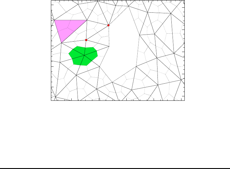
114
1.20‘ 1.00‘ 0.80‘ 0.60‘ 0.40‘
Longitude ( 5dW)
25.40‘
25.50‘
25.60‘
25.70‘
25.80‘
Latitude (48dN)
91.4
91.6
91.8
92.0
92.2
y (km)
Node
Triangle
Median dual
cell
Coastline Node
1
2
3
4
5
6
1
2
3
4
5
Figure 3.1: Example of a region of a triangle-based mesh, with in this case
the small Island of Bannec, France. If the depth is greater than the minimum
depth, the nodes of the shoreline are active. These are characterized by a
larger number of neighbor nodes (6 in the example chosen) than neighbor
triangles (5 in the same example).

115
3.4.5 Spherical Multiple-Cell (SMC) grid
Switch: SMC
Origination: WAVEWATCH III(MetOffice)
Provided by: J.-G. Li
The Spherical Multiple-Cell (SMC) grid6(Li,2011) is an extension of the
Cartesian multiple-cell grid (Li,2003) onto the spherical coordinate system.
It is an unstructured grid but retains the conventional lat-lon grid cells so that
all propagation formulations on the spherical coordinates are still applicable
and hence all the finite difference schemes. The SMC grid relaxes the CFL
restriction at high latitudes in a similar fashion as the reduced grid (Rasch,
1994). Polar cells are introduced to remove the polar singularity of the
differential transport equation by switching to an integral equation. The
upstream non-oscillatory 2nd order (UNO) advection schemes (Li,2008) is
implemented on the SMC grid for both spatial and inter-spectral propagation.
This 2nd order scheme can be replaced with a 3rd order scheme using the
PSMC namelist logical variable UNO3. The UNO3 scheme is similar to the
UQ scheme but replacing the flux limiters with the UNO 2nd order scheme.
A simple rotation scheme is used for wave refraction-induced rotation and
the great circle turning (Li,2012). The refraction scheme is unconditionally
stable for any time step but the maximum refraction induced rotation angle is
limited by the maximum possible refraction angle towards the local gradient
direction. Diffusion term similar to the Booij and Holthuijsen (1987) for
alleviation of the garden sprinkler effect is used but the diffusion coefficient
is simplified to a single homogeneous parameter (Dnn as in Eq. (3.32)). An
additional 1-2-1 weighted averaging scheme is also available by the PSMC
namelist logic variable AVERG. Reduction of computing time with this SMC
grid is significant in comparison with the conventional grid, thanks to the
relaxed time step restriction at high latitudes and removal of land points from
the model. A remedy for the invalided scalar assumption at high latitude is
provided to extend the global wave model into the entire Arctic Ocean (Li,
2016). This Arctic part can be activated by adding the ARC switch along
side the SMC switch.
The SMC grid can be used for replacing the regular lat-lon grid so that
6Presently this grid is activated by a compile switch and can only be used as a stand-
alone grid. This will become a run time option in upcoming model versions.

116
the model domain can be extended to high latitudes or even the North Pole
without reducing the time step. This application requires few changes to
the regular grid model except for preparing a few extra input files, including
the cell array and face array files. The cell array can be generated with the
existing regular grid bathymetry by using the sea points only and merging
cells in the longitudinal directions at a few latitude steps (Li,2011).
Another important use of the SMC grid is for multi-resolution grids. The
base level SMC grid cell can be refined into 4 quarterly cells by halving both
the longitude and latitude grid lengths. Any cell on this refined level can
be further divided into another 4 quarterly cells. This refinement can go on
as required, resulting in multi-resolution grids in a few refined levels. For
consistency, the single resolution SMC grid is considered to have only one
level. Wind forcing will remain to be at the base level resolution for all
SMC grids (one level or multi-level) and it will be interpolated on to the
refined levels (if any) inside the WW3 model. The normal regular grid input
files, such as the water depth, land-sea masks, and sub-grid obstruction, are
no longer required, replaced with sea-point only cell and face arrays and a
sub-grid obstruction file. The water depth is stored in the cell array in the
last (5-th) column as an integer in meter. The masks will be defined inside
ww3 grid with the sea-point cell array.
One important feature of the SMC grid is that it is an unstructured grid,
that is, the cells are not required to be listed side by side as in their physical
position. For the convenience of multi-resolution SMC grid, the cells are
sorted by their sizes so that cells on one given level are grouped together in
one sub-loop for a shared sub-time-step. The base level time step is halved
as the grid length for the refined level sub-step. This effectively avoids the
model to be slowed down by the refined cells due to their CFL restrictions.
Neighboring cells information for propagation schemes are provided with cell
face arrays, which are pre-calculated for the given cell array list. So there
is no need to expand the sea point only SMC grid cells onto a full grid for
propagation. Fig. 3.2 illustrates how SMC cell arrays are defined and Fig. 3.3
shows the Arctic region in a 6-12-25 km three level SMC grid. The golden
and red circles mark the global and Arctic parts in the SMC6-25 grid. The
Arctic part within the golden circle requires a fixed reference direction to
define its wave directional bins. The global part (up to the golden circle) can
be run independently without the Arctic part. The 4 rows from the red to
the golden circles are duplicated in the Arctic part as boundary cells if the
Arctic part is activated with the ARC option. Separate cell and face arrays
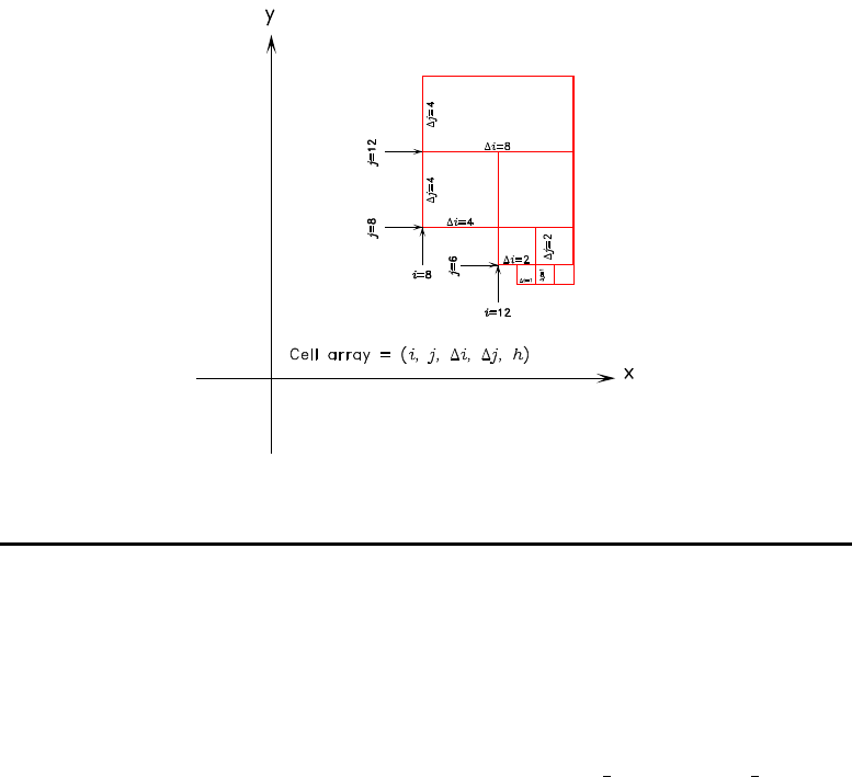
117
Figure 3.2: Illustration of cell arrays used in the SMC grid.
are used for the Arctic part and they are merged into the global ones within
the wave model for propagation.
Some IDL and F90 programs have been developed for generation of SMC
grid cell and face arrays and visualization of the grid mesh and wave fields
but they have not been formally included in the WW3 package yet. An
IDL program (Glob50SMCels.pro) is provided in smc docs/SMCG TKs/ to
generate a global 50km SMC grid using a 50km regular grid bathymetry
ASCII input file (G50kmBathy.dat). Face array generation is done with two
F90 programs, one for the global part (G50SGlSide.f90) and one for the
Arctic part (G50SAcSide.f90). Due to the special treatment of the polar cell
(Li,2012), face arrays for the Arctic polar cell requires a different approach
than other cells. The cell array file has to be sorted with a simple Linux script
(countcells) before it is fed into the face array generation program. The face
arrays also need to be sorted with a Linux script (countijsd) to determine
the multi-level sub-loop counts. An independent spectral propagation test
(G50SMCSRGD.f90) can be run to test the cell and face arrays and its output
can be visualized with an IDL script, g50smstrspb.pro, which uses the saved
projection files from the SMC grid visualization program, g50smcgrids.pro.
By modifying the projection parameters in g50smcgrids.pro, users can choose
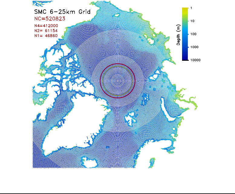
118
Figure 3.3: The Arctic region in a 6-12-25km multi-resolution SMC grid.

119
a projection view point (in lat-lon degree) and save the projection for model
output visualization. The sub-grid obstruction file can be generated with the
idl script Glob50SMCObstr.pro.
Compilation of the SMC grid option is similar to that for the regular
lat-lon grid except for that the SMC switch is substituted for the PR2 UNO
combination switches. Note that the SMC grid is built inside the regular lat-
lon grid type so regular lat-lon grid parameters, such as NX, NY, SX, SY,
X1, and Y1, are still required for SMC grid in ww3 grid.inp file at the base
resolution level. The regular lat-lon grid water depth, land-sea masks, and
sub-grid obstruction input files are no longer required and they are replaced
with SMC grid sea point only files (depth is stored in the cell array and
subgrid obstruction in G50GObstr.dat). The depth and land-sea mask input
lines in ww3 grid.in are, however, kept for passing parameters, such as the
minimumu depth. Due to the merges at high latitudes and refined resolutions
if any, regular grid mapping arrays are modified slightly for consistency with
the SMC grid cells. Refer to the regression test regtests/ww3 tp2.10 for an
example of a 3-level SMC grid model for the Lake Erie.
Output for the SMC grid can be processed by the ww3 outf program as
either the fully expanded regular lat-lon grid output at the base resolution
level or as ASCII output at all SMC grid cell points (type-4). The regular
grid format output can be viewed as other regular grid output but the re-
fined resolution cells have been converted into corresponding base resolution
cells for a multi-resolution grid. The all cell ASCII output gives field values
at the cell center so its resolution conforms with the SMC grid. Visualiza-
tion of the all cell ASCII output can be done with the aid of the input cell
array file because the output cell sequency is the same as the input cell ar-
ray. The IDL script g50smcswhglb.pro is an example program to plot the
global 50km SMC grid SWH output. It uses the projection files produced by
g50smcgrids.pro. Users are encouraged to develop their own grid-generating
and post-processing programs in other languages.
It is recommended to read the smc docs/SMC Grid Guide.pdf for more
information or to contact Jian-Guo.Li@metoffice.gov.uk for any help
about the SMC grid.

120
3.4.6 The Garden Sprinkler Effect
The higher-order accurate propagation schemes are sufficiently free of numer-
ical diffusion for the so-called ‘Garden Sprinkler Effect’ (GSE) to occur, i.e., a
continuous swell field disintegrates into a set of discrete swell fields due to the
discrete description of the spectrum (Booij and Holthuijsen,1987, Fig. 3c).
Several GSE alleviation methods are available in WAVEWATCH III, as de-
scribed in the following sections.
No GSE alleviation Switch: PR0 / PR1
Origination: WAVEWATCH III
Provided by: H. L. Tolman
In case of no propagation (switch PR0) or for the first-order propagation
scheme in a traditional or curvilinear grid no GSE alleviation is available or
needed.

121
Booij and Holthuijsen 1987
Switch: PR2
Origination: WAVEWATCH III
Provided by: H. L. Tolman
The classical GSE alleviation method is from Booij and Holthuijsen (1987),
who derived an alternative propagation equation for the discrete spectrum,
including a diffusive correction to account for continuous dispersion in spite
of the discrete spectral description. This correction influences spatial propa-
gation only, which for general spatial coordinates (x, y) becomes
∂N
∂t +∂
∂x ˙xN − Dxx
∂N
∂x +∂
∂y ˙yN − Dyy
∂N
∂y −2Dxy
∂2N
∂x∂y = 0 ,(3.24)
Dxx =Dss cos2θ+Dnn sin2θ , (3.25)
Dyy =Dss sin2θ+Dnn cos2θ , (3.26)
Dxy = (Dss −Dnn) cos θsin θ , (3.27)
Dss = (∆cg)2Ts/12 ,(3.28)
Dnn = (cg∆θ)2Ts/12 ,(3.29)
where Dss is the diffusion coefficient in the propagation direction of the dis-
crete wave component, Dnn is the diffusion coefficient along the crest of the
discrete wave component and Tsis the time elapsed since the generation of
the swell. In the present fractional step method the diffusion can be added
as a separate step
∂N
∂t =∂
∂x Dxx
∂N
∂x +∂
∂y Dyy
∂N
∂y + 2Dxy
∂2N
∂x∂y .(3.30)
This equation is incorporated with two simplifications, the justification of
which is discussed in Tolman (1995a). First, the swell ‘age’ Tsis kept con-
stant throughout the model (defined by the user, no default value available).
Secondly, the diffusion coefficients Dss and Dnn are calculated assuming deep
water
Dss =(Xσ−1) σm
2km2Ts
12 ,(3.31)

122
Dnn =σm
2km
∆θ2Ts
12 ,(3.32)
where Xσis defined as in Eq. (3.1). With these two assumptions, the diffusion
tensor becomes constant throughout the spatial domain for each separate
spectral component.
Equation (3.30) is solved using a forward-time central-space scheme. At
the cell interface between points iand i−1 in φ(x) space, the term in
brackets in the first term on the right side of Eq. (3.30) (denoted as Di,−) is
estimated as
Dxx
∂N
∂x ≈ Di,−=Dxx Ni− Ni−1
∆xj,l,m
.(3.33)
Corresponding values for counters iand i+1, and for gradients in λ(y) space
again are obtained by rotating indices and increments. If one of the two grid
points is located on land, Eq. (3.33) is set to zero. The mixed derivative at
the right side of Eq. (3.30) (denoted as Dij,−−) is estimated for the grid point
iand i−1 in x-space and jand j−1 in y-space as
Dij,−− =Dxy −Ni,j +Ni−1,j +Ni,j−1− Ni−1,j−1
0.5(∆xj+ ∆xj−1) ∆yl,m
.(3.34)
Note that the increment ∆xis a function of ydue to the use of the spherical
grid. This term is evaluated only if all four grid points considered are sea
points, otherwise it is set to zero. Using a forward in time discretization
of the first term in Eq. (3.30), and central in space discretizations for the
remainder of the first and second term on the right side, the final algorithm
becomes
Nn+1
i,j,l,m =Nn
i,j,l,m +∆t
∆x(Di,+− Di,−) + ∆t
∆y(Dj,+− Dj,−)
+∆t
4(Dij,−− +Dij,−++Dij,+−+Dij,++).(3.35)
Stable solutions are obtained for (e.g., Fletcher,1988, Part I section 7.1.1)
Dmax ∆t
min(∆x, ∆y)2≤0.5,(3.36)

123
where Dmax is the maximum value of the diffusion coefficient (typically
Dmax =Dnn). Because this stability criterion is a quadratic function of
the grid increment, stability can become a serious problem at high latitudes
for large scale applications. To avoid this putting undue constraints on the
time step of a model, a corrected swell age Ts,c is used
Ts,c =Tsmin (1,cos(φ)
cos(φc)2),(3.37)
where φcis a cut-off latitude defined by the user.
The above diffusion is needed for swell propagation, but is not realistic
for growing wind seas. For wind seas, the ULTIMATE QUICKEST scheme
without the dispersion correction is sufficiently smooth to render stable fetch-
limited growth curves (Tolman,1995a). To remove minor oscillations, a small
isotropic diffusion is used for growing wave components. To assure that this
diffusion is small and equivalent for all spectral components, it is calculated
from a preset cell Reynolds (or cell Peclet) number R=cg∆xD−1
g= 10,
where Dgis the isotropic diffusion for growing components
Dg=cgmin(∆x, ∆y)
R.(3.38)
The diffusion for swell and for wind seas are combined using a linear com-
bination depending on the nondimensional wind speed or inverse wave age
u10c−1=u10kσ−1as
Xg= min 1,max 0,3.3k u10
σ−2.3,(3.39)
Dss =XgDg+ (1 −Xg)Dss,p ,(3.40)
Dnn =XgDg+ (1 −Xg)Dnn,p ,(3.41)
where the suffix pdenotes propagation diffusion as defined in Eqs. (3.31) and
(3.32). The constants in Eqs (3.38) and (3.39) are preset in the model.

124
Spatial averaging
Switch: PR3
Origination: WAVEWATCH III
Provided by: H. L. Tolman
The major drawback of the above GSE alleviation method is its potential
impact on model economy as discussed in relation to Eq. (3.36) and in Tolman
(2001,2002a). For this reason, an alternative additional GSE alleviation
method has been developed for WAVEWATCH III.
This method which represents the default for WAVEWATCH III, replaces
the additional diffusion step (3.30) with a separate fractional step in which
direct averaging of the field of energy densities for a given spectral component
is considered. The area around each grid point over which the averaging is
performed extends in the propagation (s) and normal (n) directions as
±γa,s ∆cg∆ts,±γa,n cg∆θ∆tn,(3.42)
where γa,s and γa,n are tunable constants, the default value of which is set
to 1.5. This averaging is illustrated in Fig. 3.4. Note that these values
may require some retuning for practical applications, as discussed in Tolman
(2002a). Appendix A of the latter paper presents details of the averag-
ing scheme, including conservation considerations. Consistency with the
Booij and Holthuijsen (1987) approach furthermore implies that γa,s and γa,n
should vary with the spatial grid resolution (see Chawla and Tolman,2008,
Appendix).
Note that this kind of averaging with dominant directions sand nis
similar to the Booij and Holthuijsen (1987) diffusion method, that uses the
same main directions. The averaging method, however, never influences the
time step, because it is completely separated from the actual propagation.
Moreover, if explicit schemes are used with typically cg∆t/∆x < 1, it is
obvious that the averaging over the area as defined in (3.42) will generally
require information at directly neighboring spatial grid points only, as in
Fig. 3.4. Furthermore, this method does not require high-latitude filtering.
As is illustrated in Tolman (2002a,d), this method gives virtually identical
results as the previous method, but does so at slightly lower costs. For high-
resolution applications, the averaging method may become dramatically more
economical.

125
θ
Figure 3.4: Schematic of spatial averaging GSE alleviation technique. Solid
circles and dotted lines represent the spatial grid. Hatched area represent
averaging area to be considered. Corner point values are obtained from the
central grid point and the gray points. The latter values are obtained by
interpolation from adjacent grid points (from Tolman,2002a).
Finally, the GSE can be alleviated somewhat by assuring that the dis-
crete spectral directions do not coincide with spatial grid lines. This can be
achieved by defining the first discrete direction θ1as
θ1=αθ∆θ , (3.43)
where −0.5≤αθ≤0.5 can be defined by the user. Note that setting α6= 0
is beneficial to the first-order scheme, but has negligible impact on the third-
order scheme.
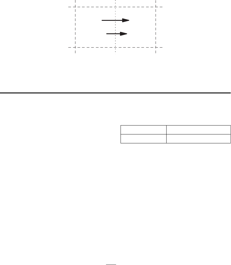
126
cell i cell i+1
Flux F out of cell i
Flux αF into cell i +1
Figure 3.5: Treatment of unresolved obstacles. Common cell boundary (dot-
ted line) has transparency α. Dashed lines represent other cell boundaries.
Numerical flux from left to right.
3.4.7 Unresolved obstacles
Origination: WAVEWATCH III
Provided by: H. L. Tolman
Even at the time of the original tuning of WAVEWATCH III version 1.15
(Tolman,2002f), it was clear that unresolved islands groups are a major
source of local wave model errors. This was illustrated in some more de-
tail in Tolman (2001, Fig. 3), and Tolman et al. (2002, Fig. 8). In WAVE-
WATCH III, a methodology from SWAN (Booij et al.,1999;Holthuijsen et al.,
2001) was adopted to apply the effects of unresolved obstacles at the cell
boundaries of the spatial grid within the numerical scheme. In this ap-
proach, the numerical fluxes between cells through their common boundary
are suppressed according to the degree of obstruction provided by the unre-
solved obstacle. In this approach, the numerical propagation scheme of the
ULTIMATE QUICKEST scheme of Eq. (3.23) is modified as
Nn+1
i,j,l,m =Nn
i,j,l,m +∆t
∆φ[αi,−Fi,−−αi,+Fi,+],(3.44)
where αi,−and αi,+are ‘transmissions’ of the corresponding cell boundaries,
ranging from 0 (closed boundary) to 1 (no obstructions). For outflow bound-
aries, transparencies by definition are 1, otherwise energy will artificially
accumulate in cells. For inflow boundaries, transparencies less than 1 result
in elimination of obstructed energy at the cell boundary. This approach is
illustrated in Fig. 3.5. Note that a similar approach is easily adopted in the

127
first- and second-order schemes. Note, furthermore, that an alternate ob-
struction approach with obstructions as a function of the spectral direction
θhas been used by Hardy and Young (1996) and Hardy et al. (2000).
Two methods for defining the obstructions are available in the model. The
first defines the obstructions directly at the grid boundary. This requires the
generation of staggered depth-transparency grids. The second allows the
user to define depths and transparencies at the same grid. In this case, the
transparency at the inflow boundary becomes 0.5(1 + αi), and the outflow
transparency by definition is 1. To complete the total transparency αi, the
next cell in the flow direction will have an inflow transparency 2αi/(1 +
αi). If consecutive cells are partially obstructed, the product of individual
transparencies is applied.
This approach can also be used to continuously model the effects of ice
coverage on wave propagation. This is discussed in Section 3.8. Details of
the sub-grid treatment of islands and ice can be found in Tolman (2003b).
A study of impacts of this approach in large-scale wave models is presented
in Tolman (2002d,2003b).
The default setting of WAVEWATCH III is to not include sub-grid mod-
eling of obstacles. Generating obstruction grids can be labor intensive. For
this reason, an automated approach for generating bottom and obstruction
grids was developed by Chawla and Tolman (2007,2008). Note that this
option does not involve compile-level choices, but is entirely controlled from
the grid preprocessor (see Chapter 4).
3.4.8 Continuously moving grids
Switch: MGx
Origination: WAVEWATCH III
Provided by: H. L. Tolman
In order to address wave growth issues in rapidly changing, small scale
conditions such as hurricanes, an option to add a given continuous advection
speed to the grid has been added to the model in model version 3.02. This
model version is described in detail in Tolman and Alves (2005). Here, only
a cursory description is given.
WARNING

128
The continuously moving grid version of WAVEWATCH III is only
intended for testing wave model properties in highly-idealized con-
ditions. This model version should only be used for deep water
without mean currents and land masses. Furthermore, to avoid
complications with great circle propagation, only a Cartesian grid
should be used. The option is furthermore implemented only for
propagation options pr1 and pr3. Note that this is not checked
in the scripts or programs at either the compile or run time level.
This option is not considered to be for general application.
WARNING
For the above described application Eq. (2.8) can be written as
∂N
∂t + ( ˙x −vg)· ∇xN=S
σ,(3.45)
where vgrepresents the advection velocity of the grid. This option is selected
when compiling the model. A second compile level option allows for adding
the grid advection velocity vgto the wind field. This allows for a simple
method to assure mass conservation of a wind field independent of the actual
and instantaneous grid advection velocity. The advection velocity vgcan vary
in time and is provided by the user at the run time of the model (see below).
For the simplified conditions for which Eq. (3.45) is valid, the implemen-
tation of the moving grids is trivial if it is considered that this equation is
equivalent to
∂N
∂t +∇x·(˙x −vg)N=S
σ,(3.46)
which in turn implies that the advection velocity vgcan be added directly to
˙x for arbitrary numerical schemes solving Eq. (2.8). Because this influences
the net advection velocity, it also influences stability characteristics. This
impact has been accounted for automatically by including the moving grid
velocity in the calculation of the actual propagation time step in Eq (3.4).
Hence, the user need to provide a proper maximum propagation time step
representative for vg=0only.
The motion of the grid has an apparent influence on the Garden Sprinkler
Effect (GSE), due to the different retention time in the grid of spectral com-
ponents with identical frequency but different propagation direction. Current
GSE alleviation methods tend to be more efficient for younger swells than

129
for older swells. Hence, swells with longer retention time in the moving grid
tend to show a more pronounced GSE (see Tolman and Alves,2005). To
mitigate this apparent imbalance in GSE alleviation, Eq. (3.42) is replaced
with
±γaγa,s ∆cg∆ts,±γaγa,n cg∆θ∆tn,(3.47)
γa=|˙
x|
|˙
x−vg|p
(3.48)
where γais a correction factor accounting for the grid movement, and where
the power pis a parameter allows for some tuning. With this modification,
the effects of the GSE can be distributed more evenly over the grid by rescal-
ing the amount of smoothing applied with the expected residence time of cor-
responding spectral component in the moving grid (see Tolman and Alves,
2005).
To switch on the moving grid option or the corrections of the wind field
or GSE, three optional switches are added to the WAVEWATCH III source
code (also see, Section 5.4:
mgp Apply advection correction for continuous moving grid.
mgw Apply wind correction for continuous moving grid.
mgg Apply GSE alleviation for continuous moving grid.
The advection velocity and direction is input to the shell similar to the input
of homogeneous currents (see bottom of file ww3 shel.inp in Section 4.4.9), ex-
changing the keyword ‘CUR’ with ‘MOV’. The advection velocity can be changed
in time like all homogeneous input fields. An example of running with a
moving grid model is given in test case ww3 ts3. A similar capability exist
in ww3 multi.inp in Section 4.4.11, and is tested in test case mww3 test 05.
3.4.9 Rotated grids
Switch: RTD
Origination: WAVEWATCH III (MetOffice)
Provided by: J.-G. Li

130
The rotated grid is a latitude-longitude (lat-lon) grid and is obtained by
rotating the North Pole to a new position at latitude φpand longitude λp
in the standard latitude-longitude system. The new pole position is chosen
so that the model domain of interest may be placed around the rotated
equatorial area for a evenly-spaced lat-lon mesh. For this reason the rotated
grid is also known as Equatorial grid. For instance, the North Atlantic and
European wave (NAEW) model used in the UK Met Office uses a rotated
pole at 37.5N, 177.5E so that London, UK (˜51.5N 0.0E) is almost on the
rotated equator. This rotated grid allows a much more evenly spaced lat-
lon mesh in the NAEW domain than the standard lat-lon grid in the same
area. In WAVEWATCH III the rotated grid is implemented with minimum
changes to the original lat-lon grid. In fact, the rotated grid is treated just
like the standard lat-lon grid inside the model. Only input and output files
are modified for the rotated grid. Users should choose the regular lat-lon
grid along with the RTD switch to use the rotated grid. Model input files,
like wind, current and ice files should be mapped on to the rotated grid. For
convenience of nesting in standard lat-lon grid, boundary conditions for the
rotated grid use standard lat-lon grid points, which are converted into rotated
grid lat-lon inside WAVEWATCH III ˙
The list of 2D spectral output locations
in ww3 shel.inp are also specified in standard lat-lon. All directional output
such as wind direction, peak direction, 2D spectra, etc. are converted into
standard lat-lon orientation. The full grid output are still on rotated grid
but 2D spectra locations have been converted into standard lat-lon.
Four subroutines are provided in module w3servmd.ftn for rotated grid
conversion:
w3spectn Turns wave spectrum anti-clockwise by AnglD
w3acturn Turns wave action(k,nth) anti-clockwise by AnglD
w3lltoeq Convert standard into rotated lat/lon plus AnglD
w3eqtoll Reverse of w3lltoeq, but AnglD unchanged
These subroutines are self-contained and can be extracted outside the model
for pre- or post-processing of rotated grid files. Some conversion tools have
been developed based on these subroutines but have not been included in
WAVEWATCH III yet. Refer to the regression test regtests/ww3 tp2.11
for an example of a rotated grid model (NAEW). Users may find more
information in smc docs/Rotated Grid.pdf or contact Jian-Guo Li for help
(Jian-Guo.Li@metoffice.gov.uk).

131
3.5 Intra-spectral propagation
3.5.1 General concepts
The third step of the numerical fractional step algorithm considers refraction
and residual (current-induced) wavenumber shifts. Irrespective of the spatial
grid discretization and coordinate system, the equation to be solved in this
step becomes
∂N
∂t +∂
∂k ˙
kgN+∂
∂θ ˙
θgN= 0 ,(3.49)
˙
kg=∂σ
∂d
U· ∇xd
cg−k·∂U
∂s ,(3.50)
where ˙
kgis the wavenumber velocity relative to the grid, and ˙
θgis given by
(2.15) and (2.11). This equation does not require boundary conditions in
θ-space, as the model by definition uses the full (closed) directional space. In
k-space, however, boundary conditions are required. At low wavenumbers,
it is assumed that no wave action exists outside the discrete domain. It
is therefore assumed that no action enters the model at the discrete low-
wavenumber boundary. At the high-wavenumber boundary, transport across
the discrete boundary is calculated assuming a parametric spectral shape as
given by Eq. (2.18). The derivatives of the depth as needed in the evaluation
of ˙
θare mostly determined using central differences. For points next to land,
however, one-sided differences using sea points only are used.
Propagation in θ-space can cause practical problems in an explicit numer-
ical scheme, as the refraction velocity can become extreme for long waves in
extremely shallow water or due to strong current shears. Similarly, the prop-
agation in k-space suffers from similar problems in very shallow water. To
avoid the need of extremely small time steps due to refraction, the propaga-
tion velocities in θ-space and k-space (2.11) are filtered,
˙
θ=Xrd(λ, φ, k)˙
θd+˙
θc+˙
θg,(3.51)
where the indices d,cand grefer to the depth, current and great-circle related
fraction of the refraction velocity in (2.11). The filter factor Xrd is calculated
for every wavenumber and location separately, and is determined so that the
CFL number for propagation in θ-space due to the depth refraction term

132
cannot exceed a pre-set (user defined) value (default 0.7). This corresponds
to a reduction of the bottom slope for some low frequency wave components.
For mid-latitudes, the affected components are expected to carry little energy
because they are in extremely shallow water. Long wave components carrying
significant energy are usually traveling toward the coast, where their energy
is dissipated anyway. This filtering is also important for short waves, and
close to the pole. The effect of this filter can be tested by reducing the
time steps for intraspectral refraction and by looking at the maximum CFL
numbers in the output of the model. These are computed just before the
filter is applied.
The spectral space is always discretized with constants directional incre-
ments and a logarithmic frequency grid (3.1) to accommodate computations
of the nonlinear interaction Snl. First, second and third orders schemes are
available, and are presented in the following sections.
3.5.2 First-order scheme
Switch: PR1
Origination: WAVEWATCH III
Provided by: H. L. Tolman
In the first order scheme the fluxes in θ- and k-space are calculated using
Eqs. (3.6) through (3.8) (replacing Nwith Nand rotating the appropriate
counters). The complete first order scheme becomes
Nn+1
i,j,l,m =Nn
i,j,l,m +∆t
∆θ[Fl,−− Fl,+] + ∆t
∆km
[Fm,−− Fm,+],(3.52)
where ∆φis the directional increment, and ∆kmis the (local) wavenumber
increment. The low-wavenumber boundary conditions is applied by taking
Fm,−= 0 for m= 1, and the high wavenumber boundary condition is calcu-
lated using the parametric approximation (2.18) for N, extending the discrete
grid by one grid point to high wavenumbers.

133
3.5.3 Second-order scheme (UNO)
Switch: UNO
Origination: Met Office
Provided by: J.-G. Li
The UNO scheme for the directional θ-space is identical to the regular grid
one assuming that the directional bins are regularly spaced. For the k-
space, however, the UNO scheme uses its irregular version, which uses local
gradients instead of differences to estimate wave action value at the mid-flux
point for the cell face between spectral bin i-1 and i, that is:
N∗
i−=Nc+sign (Nd−Nc)∆kc− |˙
ki−|∆t
2min |Nu−Nc
ku−kc|,|Nc−Nd
kc−kd|,
(3.53)
where i- is the wave number kbin index; the subscripts u,cand dindicate
the upstream, central and downstream cells, respectively, relative to the given
i- face velocity ˙
ki−;kcis the central bin wave number and ∆kcis the central
bin widith. Details of the irregular grid UNO scheme are given in Li (2008).
Boundary conditions for the θ-space is the natural periodic condition. For
the k-space, two more zero spectral bins are added to each end of the wave
spectral domain as the UNO scheme is 2nd order in accuracy.
3.5.4 Third-order scheme (UQ)
Switch: UQ
Origination: WAVEWATCH III
Provided by: H. L. Tolman
The ULTIMATE QUICKEST scheme for the θ-space is implemented similar
to the scheme for physical space, with the exception that the closed direction
space does not require boundary conditions. The variable grid spacing in
k-space requires some modifications to the scheme as outlined by (Leonard,
1979, Appendix). Equations (3.12) through (3.16) then become
Fm,−=h˙
kg,b Nbin
i,j,l ,(3.54)

134
˙
kg,b = 0.5˙
kg,m−1+˙
kg,m ,(3.55)
Nb=1
2h(1 + C)Ni−1+ (1 −C)Nii−1−C2
6CU ∆k2
m−1/2,(3.56)
CU =
1
∆km−1hNm−Nm−1
∆km−1/2−Nm−1−Nm−2
∆km,−3/2ifor ˙
kb≥0
1
∆kmhNm+1−Nm
∆km+1/2−Nm−Nm−1
∆km−1/2ifor ˙
kb<0,(3.57)
C=˙
kg,b ∆t
∆km−1/2
,(3.58)
where ∆kmis the discrete band or cell width at grid point m, and where
∆km−1/2is the distance between grid points with counters mand m−1. The
ULTIMATE limiter can be applied as in Eqs. (3.17) through (3.20), if the
CFL number of Eq. (3.58) is used. At the low- and high-wavenumber bound-
aries the fluxes again are estimated using a first-order upwind approach, with
boundary conditions as above defined for the first-order scheme. The final
scheme in k-space becomes
Nn+1
i,j,l,m =Nn
i,j,l,m +∆t
∆km
[Fm,−− Fm,+],(3.59)
3.6 Non-ice source term integration
The source terms not involving ice are accounted for by solving
∂N
∂t =Sno ice .(3.60)
As in WAM, a semi-implicit integration scheme is used. In this scheme the
discrete change of action density ∆Nbecomes (WAMDIG,1988)
∆N(k, θ) = S(k, θ)
1−ǫD(k, θ)∆t,(3.61)
where Drepresents the diagonal terms of the derivative of Swith respect to
N(WAMDIG,1988, Eqs. 4.1 through 4.10), and where ǫdefines the offset

135
of the scheme. Originally, ǫ= 0.5 was implemented to obtain a second-
order accurate scheme. Presently, ǫ= 1 is used because it is more ap-
propriate for the large time steps in the equilibrium range of the spectrum
(Hargreaves and Annan,1998,2001) and it results in much smoother inte-
gration of the spectrum. The change of ǫhas little impact on mean wave
parameters, but makes the dynamical time stepping as described below more
economical.
The semi-implicit scheme is applied in the framework of a dynamic time-
stepping scheme (Tolman,1992). In this scheme, integration over the global
time step ∆tgcan be performed in several dynamic time steps ∆td, depending
on the net source term S, a maximum change of action density ∆Nmand
the remaining time in the interval ∆tg. For the nth dynamic time step in the
integration over the interval ∆tg, ∆tn
dis calculated in three steps as
∆tn
d= min
f<fhf "∆Nm
|S| 1 + ǫD ∆Nm
|S| −1#,(3.62)
∆tn
d= max [ ∆tn
d,∆td,min],(3.63)
∆tn
d= min "∆tn
d,∆tg−
n−1
X
i=1
∆ti
d#,(3.64)
where ∆tmin is a user-defined minimum time step, which is added to avoid
excessively small time steps. The corresponding new spectrum Nnbecomes
Nn= max 0, Nn−1+S∆td
1−ǫD∆td.(3.65)
The maximum change of action density ∆Nmis determined from a para-
metric change of action density ∆Npand a filtered relative change ∆Nr
∆Nm(k, θ) = min [ ∆Np(k, θ),∆Nr(k, θ) ] ,(3.66)
∆Np(k, θ) = Xp
α
π
(2π)4
g2
1
σk3,(3.67)
∆Nr(k, θ) = Xrmax [ N(k, θ), Nf],(3.68)
Nf= max ∆Np(kmax, θ), Xfmax
∀k,θ {N(k, θ)},(3.69)

136
XpXrXf∆td,min
WAM equivalent π
24 10−3∆t∞(≥1) – ∆tg
suggested 0.1-0.2 0.1-0.2 0.05 ≈0.1∆tg
default setting 0.15 0.10 0.05 –
Table 3.1: User-defined parameters in the source term integration scheme
where Xp,Xrand Xfare user-defined constants (see Table 3.1), αis a pm
spectrum energy level (set to α= 0.62 ×10⁻⁴) and kmax is the maximum
discrete wavenumber. The parametric spectral shape in (3.67) corresponds
in deep water to the well-known high-frequency shape of the one-dimensional
frequency spectrum F(f)∝f−5. The link between the filter level and the
maximum parametric change in (3.69) is used to assure that the dynamic
time step remains reasonably large in cases with extremely small wave ener-
gies. A final safeguard for stability of integration is provided by limiting the
discrete change of action density to the maximum parametric change (3.67)
in conditions where Eq. (3.63) dictates ∆tn
d. In this case Eq. (3.63) becomes
a limiter as in the WAM model. Impacts of limiters are discussed in detail
in for instance Hersbach and Janssen (1999,2001), Hargreaves and Annan
(2001) and Tolman (2002c).
The dynamic time step is calculated for each grid point separately, adding
additional computational effort only for grid points in which the spectrum
is subject to rapid change. The source terms are re-calculated for every
dynamic time step.
It is possible to compile WAVEWATCH III without using a linear growth
term. In such a case, waves can only grow if some energy is present in
the spectrum. In small-scale applications with persistent low wind speeds,
wave energy might disappear completely from part of the model. To assure
that wave growth can occur when the wind increases, a so-called seeding
option is available in WAVEWATCH III (selected during compilation). If the
seeding option is selected, the energy level at the seeding frequency σseed =
min(σmax,2πfhf ) is required to at least contain a minimum action density

137
Nmin(kseed, θ) = 6.25 ×10−41
k3
seed σseed
max 0. , cos2(θ−θw)
min 1,max 0,|u10|
Xseedgσ−1
seed −1,(3.70)
where gσ−1
seed approximates the equilibrium wind speed for the highest discrete
spectral frequency. This minimum action distribution is aligned with the
wind direction, goes to zero for low wind speeds, and is proportional to the
integration limiter (3.67) for large wind speeds. Xseed ≥1 is a user-defined
parameter to shift seeding to higher frequencies. Seeding starts if the wind
speed reaches Xseed times the equilibrium wind speed for the highest discrete
frequency, and reaches its full strength for twice as high wind speeds. The
default model settings include the seeding algorithm, with Xseed = 1.
In model version 3.11, surf-zone physics parameterizations have been in-
troduced. Such physics, particularly depth-induced breaking, operate on
much smaller time scales than deep water and limited-depth physics outside
the surf zone. To assure reasonable behavior for larger time steps, an addi-
tional optional limiter has been adopted from the SWAN model, which can
be used instead of modeling surf-breaking explicitly. This limiter is similar
to the Miche style maximum wave height in the depth-limited wave breaking
source term of Eq. (2.161). In this limiter, the maximum wave energy Emis
computed as
Em=1
16[γlim tanh(¯
kd)/¯
k]2,(3.71)
where γlim is a factor comparable to γMin Eq. (2.161), with the caveat that
γMis representative for an individual wave, whereas γlim is representative
for the significant wave height. For monochromatic waves, the original ex-
pression by Miche (1944) would correspond to γlim = 0.94 and replacing Hs
by the height Hof the waves. Here this idea is applied to random waves.
In shallow water, this limits Hsto be less than γlimd. If the total spectral
energy Eis larger than the maximum energy Em, the limiter is applied by
simply rescaling the spectrum by the factor E/Em, loosely following the ar-
gumentation from Eldeberky and Battjes (1996) and used in Section 2.3.17.
This limiter can be switched on or off in the compilation of the model, and
γlim can be adjusted by the user. The default is set to γlim = 1.6 because

138
Hrms values close to dhave indeed been recorded and thus taking a ratio
Hs/Hrms of 1.4, using 1.6 allows this large steepness to be exceeded by some
margin. Note that this limiter should be used as a ‘safety valve’ only, and
hence that it should be less strict than the breaking criterion in the surf-
breaking or whitecapping source terms, if these source terms are modeled
explicitly.
Also, this limiter does not guarantee that all parts of the spectrum are
realistic. Indeed, the use of a mean wavenumber, as in the Komen et al.
dissipation, makes it possible to have unrealistically steep short waves in
the presence of swell. A future extension of this limiter could be to limit the
steepness with a partial spectral integration in frequencies, to make sure that
waves of all scales are indeed not too steep.
3.7 Ice source terms integration
Because the attenuation and scattering in the ice can be very strong (al-
though they are linear), it is convenient to perform a separate integration of
the ice terms Sice =Sid +Sis. This combines a dissipation term
Sid/σ =βidN, (3.72)
and a scattering term which is of the form
Sis(k, θ)
σ=Z2π
0
βis[N(k, θ′)−N(k, θ)]dθ′,(3.73)
in which the scattering coefficient βis is a priori a function of the difference in
direction between incident θ′and scattered θdirections, as well as the shape
of ice floes. In general the directional spectrum N(k, .) is a vector with NTH
(number of directions) components, and the source term is a vector of the
same size given by the matrix product S/σ =MN(k, .) where Mis a positive
symmetric square NTH by NTH matrix with components given from the
βid values. The matrix Mis easily diagonalized as
M=V DV T,(3.74)
where Dis a diagonal matrix containing all eigenvalues and Vis the array
of eigenvectors, and VTis its transpose. As a result the split wave action
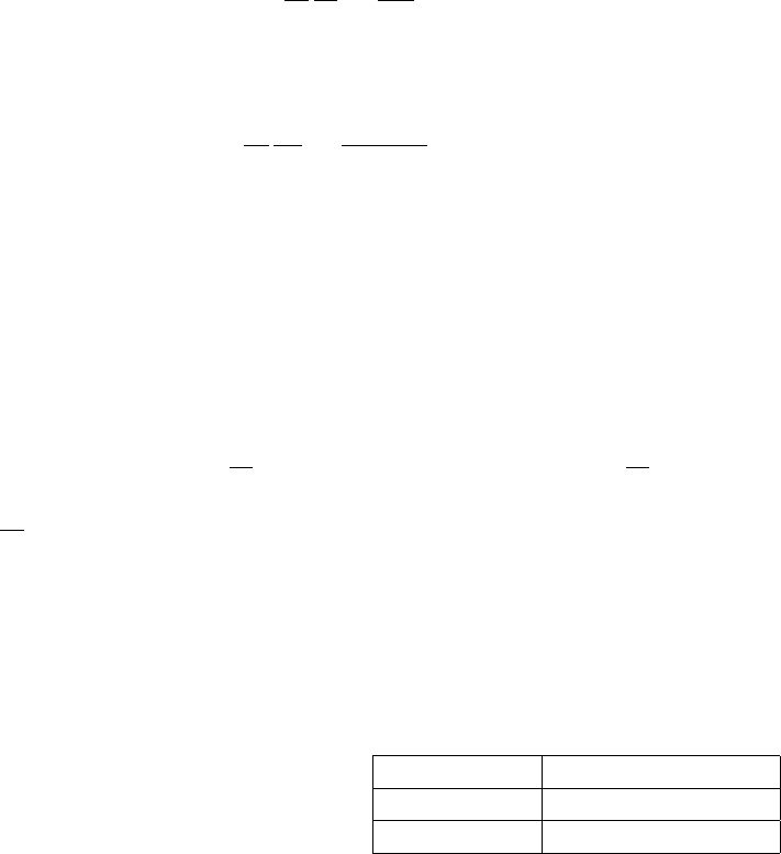
139
equation for ice source terms
∂
∂t
N
cg
=Sid
σcg
,(3.75)
can be rewritten for the action Niof each eigenvector Viwith eigenvalue λi
as ∂
∂t
Ni
cg
=βid +λi
σcg
Ni,(3.76)
which has the following exact solution
Ni(t+ ∆tg) = Ni(t) exp [(βid +λi) + ∆tg].(3.77)
In all cases the eigenvector corresponding to an isotropic spectrum has
an eigenvalue λ=βid. In the case of an isotropic back-scatter, the other
eigenvalues are all equal to (βid +βis). This decomposition over the two
eigenspaces simplifies the solution to
N(t+ ∆tg) = exp(βid∆tg)N(t) + exp [(βid +βis) ∆tg]N(t)−N(t),(3.78)
where Nis the average over all directions. As a result, for a spatially homo-
geneous field, the spectrum exponentially tends to isotropy over a time scale
1/(βid).
3.8 Simple ice blocking (IC0)
Switch: IC0
Origination: WAVEWATCH III
Provided by: H. L. Tolman
Ice covered sea is considered as ‘land’ in WAVEWATCH III, assuming zero
wave energy and boundary conditions at ice edges are identical to boundary
conditions at shore lines. Grid points are taken out of the calculation if
the ice concentration becomes larger than a user-defined concentration. If
the ice concentration drops below its critical value, the corresponding grid
point is ‘re-activated’. The spectrum is then initialized with a PM spectrum
based on the local wind direction with a peak frequency corresponding to

140
the second-highest discrete frequency in the grid. A low energy spectrum is
used to assure that spectra are realistic, even for shallow coastal points.
The above discontinuous ice treatment represents the default model set-
ting in WAVEWATCH III. In the framework of the modeling of unresolved
obstacles as discussed in Section 3.4.7, a continuous method is also avail-
able, as given by Tolman (2003b). In this method, a user-defined critical
ice concentration at which obstruction begins (ǫc,0) and is complete (ǫc,n)
are given (defaults are ǫc,0=ǫc,n = 0.5, i.e., discontinuous treatment of
ice). From these critical concentrations, corresponding decay length scales
are calculated as
l0=ǫc,0min(∆x, ∆y),(3.79)
ln=ǫc,n min(∆x, ∆y),(3.80)
from which cell transmissions in xand y(αxand αy, respectively) are calcu-
lated as
αx=
1 for ǫ∆x < l0
0 for ǫ∆x > ln
ln−ǫ∆x
ln−l0otherwise
, αy=
1 for ǫ∆y < l0
0 for ǫ∆y > ln
ln−ǫ∆y
ln−l0otherwise
.(3.81)
Details of this model can be found in Tolman (2003b).
Updating of the ice map within the model takes place at the discrete
model time approximately half way in between the valid times of the old and
new ice maps. The map will not be updated, if the time stamps of both ice
fields are identical.
The above description pertains to the switch IC0. Note that either ice
transmissions for propagation (IC0), or ice as a source term can be used (IC1,
IC2,IC3), but not both approaches at the same time.
3.9 Winds and currents
Model input mainly consists of wind and current fields. Within the model,
winds and currents are updated at every time step ∆tgand represent values
at the end of the time step considered. Several interpolation methods are
available (selected during compilation). By default, the interpolation in time

141
consists of a linear interpolation of the velocity and the direction (turning the
wind or current over the smallest angle). The wind speed or current velocity
can optionally be corrected to (approximately) conserve the energy instead
of the wind velocity. The corresponding correction factor Xuis calculated as
Xu= max 1.25 ,u10,rms
u10,l ,(3.82)
where u10,l is the linearly interpolated velocity and u10,rms is the rms inter-
polated velocity. Finally, winds can optionally be kept constant and changed
discontinuously (option not available for current).
Note that the auxiliary programs of WAVEWATCH III include a program
to pre-process input fields (see Section 4.4.6). This program transfers gridded
fields to the grid of the wave model. For winds and currents this program
utilizes a bilinear interpolation of vector components. This interpolation can
be corrected to (approximately) conserve the velocity or the energy of the
wind or the current by utilizing a correction factor similar to Eq. (3.82).
3.10 Use of tidal analysis
Origination: WAVEWATCH III
Provided by: F. Ardhuin
In order to reduce the volume of input files, the water levels and currents can
be defined by their tidal amplitudes and phases. This is made possible by
using the TIDE switch which activates the detection of the needed information
in current.ww3 and level.ww3 files. The tidal analysis can be performed
from NetCDF current or water level files, using the ww3 prnc preprocessing
program. In that case the analysis method uses the flexible tide analysis
package by Foreman et al. (2009). The precomputed tidal constituents can
be used at run time by ww3 shel.
However, that method may not be very efficient due to the large memory
required to store a large number of tidal constituents because, like other forc-
ing parameters, they are not decomposed across processors: each processor
stores the full spatial grid of forcing parameters. To avoid this, the tidal
constituents can be used to generated time series with the tidal prediction
program ww3 prtide, which produces the usual current.ww3 or level.ww3 files.

142
The choice of tidal constituents for the analysis and prediction are spec-
ified in the input files for ww3 prnc and ww3 prtide. Two short-cuts are
defined. VFAST is the following selection of 20 components, Z0 (mean), SSA,
MSM, MSF, MF, 2N2, MU2, N2, NU2, M2, S2, K2, MSN2, MN4, M4, MS4,
S4, M6, 2MS6, and M8. When using ww3 shel to do the tidal prediction,
the time step for currents or water is set to 1800 s.
In ww3 prtide, there is also a quality check on the values of the tidal
constituents that is performed: unrealistically large values of the amplitudes
for some constituents can be defined in ww3 prtide.inp. For model grid points
where these are exceeded, all components are set to zero, except for UNST
grids, in which the neighbors are searched to provide a reasonable value and
avoid strong gradients.
3.11 Wave crest and height space-time extremes
Origination: WAVEWATCH III(ISMAR, NCEP)
Provided by: Barbariol, F., Benetazzo, A., Alves, J.H.G.M.
Space-Time (ST) extreme waves are modeled in WAVEWATCH III based
on the Euler Characteristics (EC) approach, which states that for a given
multi-dimensional (2-D space + time), statistically homogeneous and sta-
tionary Gaussian random wave field, the probability of exceedance of the
maximal sea surface elevation is approximated by means of the mean value
of the EC (Fedele et al.,2012). The ST extreme elevation model used here
was formulated by Fedele (2012) for Gaussian sea waves, and extended to
second-order nonlinear spatial wave fields by Fedele et al. (2013) and spatio-
temporal fields by Benetazzo et al. (2015). The proposed ST extreme linear
model was assessed with numerical simulations (Barbariol et al.,2015), while
the extension to second-order nonlinear waves was verified using stereo imag-
ing (Fedele et al.,2013;Benetazzo et al.,2015). According to those models,
the probability of exceedance of the second-order nonlinear ST maximal crest
height η2STmis approximated (for large threshold z2with respect to the stan-
dard deviation of the surface elevation σ) as:
P(η2STm> z2)≈N3Dz1
σ2+N2Dz1
σ+N1Dexp −z2
1
2σ2,(3.83)

143
where the nonlinear threshold z2is related to its linear approximation z1via
the Tayfun quadratic equation using the steepness parameter µ, strictly valid
in deep waters, which accounts for bandwidth effects. Parameters N3D,N2D,
and N1Dexpress the average number of 3D, 2D, and 1D waves within the
ST region, respectively, and are determined from the moments mijl of the
directional wave spectrum S(k, θ) defined as follows:
mijl =Zki
xkj
yωlS(k, θ)dkdθ. (3.84)
The average number of waves in Eq. (3.83) also depends on the size
of the spatio-temporal domain, namely the spatial dimension Xalong the
mean direction of wave propagation, the spatial dimension Yorthogonal to
the mean direction of wave propagation, and the duration D. The expected
value ¯η2STm(output parameter STMAXE, in meters) of the random variable
η2STmis given by
¯η2STm=E{η2STm}=
σ"(h1+µ
2h2
1) + γh1−2N3Dh1+N2D
N3Dh2
1+N2Dh1+N1D−1
(1 + µh1)#,(3.85)
where γ≈0.5772 is the Euler-Mascheroni constant, and h1is the dimen-
sionless (with respect to the standard deviation σ) most probable (mode)
extreme value, which is the largest solution of the implicit equation in h
N3Dh2+N2Dh+N1Dexp −h2
2= 1.(3.86)
The standard deviation σ2m(output parameter STMAXD, in meters)
of the crest height η2STmis given by:
σ2m=std(η2STm) = σπ
√6h1−2N3Dh1+N2D
N3Dh2
1+N2Dh1+N1D−1
(1 + µh1).
(3.87)
The expected value of the ST extreme crest-to-trough wave height is
obtained using the Quasi-Determinism (QD) model, which predicts the mean
shape of ST wave groups close to the apex of their development. According to
the QD model the expected value of the crest-to-trough height ¯
H1cm (output

144
parameter HCMAXE, in meters) of the wave with linear extreme crest
height ¯η1STmis expressed as
¯
H1cm =E{H1cm }= ¯η1STm(1 −ψ∗
1/σ2),(3.88)
where ψ∗
1<0 is the value of the first minimum of the temporal autocovariance
function computed from the spectrum as
ψ1(τ) = ZS(ω) cos (ωτ )dω, (3.89)
and ¯η1STmψ∗
1/σ2<0 is the expected displacement of the wave trough pre-
ceding or following the expected linear extreme crest height ¯η1STm, which is
computed using Eq. (3.85) after letting the wave steepness µ= 0. For a
given linear group, the height ¯
H1cm is generally smaller than the maximum
expected wave height ¯
H1m(output parameter HMAXE, in meters), which
is computed as
¯
H1m=E{H1m}= ¯η1STmp2(1 −ψ∗
1/σ2).(3.90)
The effect on wave heights of second-order nonlinearities is generally
small, particularly in narrow band seas, and it will be neglected in the present
implementation to reduce the computational cost. Uncertainty of estimates
of ¯
H1cm (output parameter HCMAXD, in meters) and ¯
H1m(output pa-
rameter HMAXD, in meters) are determined using the standard deviation
of η1STm(σ1m, which is computed using Eq. (3.87) after letting the wave
steepness µ= 0) as follows:
std(H1m) = σ1mp2(1 −ψ∗
1/σ2),
std(H1cm ) = σ1m(1 −ψ∗
1/σ2).(3.91)
In WAVEWATCH III, for each time step at all grid points, ST extremes
are computed over the spatio-temporal region XY D; the default values for
X= 1000 m, Y= 1000 m, and D= 1200 s can be redefined by the user
in the model input file ww3 grid.inp as namelists STDX (variable X), STDY
(variable Y), STDT (variable D). In the present implementation, only the
prognostic part of the spectrum is used for extreme computation. For addi-
tional implementation details, underlying approximations, assumptions and
a full set of references for the fundamental theoretical and empirical frame-
work underlying the ST extremes parameters used here, see Fedele (2012)
and Barbariol et al. (2016).

145
To activate the computation of wave crest and height space-time extremes
in WAVEWATCH III, the user has to specify values of the MISC namelist
parameters STDX,STDY and STDT in ww3 grid.inp different to -1 (the latter is
a default value that avoids computer overheads when these parameters are
not wanted). STDX and STDY are spatial dimensions over which extremes are
calculated. STDT is the time length over which extremes are calculated. If
STDX and STDY are left at default values (-1), but STDT has a namelist value
different to default (e.g., greater than 0), then extreme values are provided
over time, for a point. Conversely, if STDT is kept at default (-1) and STDX
and STDY are greater than zero, instantaneous extreme values are computed
over space. When all three parameters are greater than zero, space-time
probabilities and values are computed.
Wave crest and height space-time extremes outputs follow the standard
WAVEWATCH III parameter framework, and have to be specified as namelists
or flags in ww3 shel.inp or ww3 multi.inp, in which case they are included in
the standard gridded binary output files during a model run. Consequently,
they also have to be specified in gridded output post-processors for obtain-
ing a final human-readable form. Space-time extremes output parameters
available in WAVEWATCH III are provided in Table 3.2.
Internal Label User-Interface Label Description
STMAXE MXE Max surface elev (STE)
STMAXD MXES STD of max crest (STE)
HMAXE MXH Max wave height (STE)
HCMAXE MXHC Max wvhgt from crest (STE)
HMAXD SDMH STD of MXH (STE)
HCMAXD SDMHC STD of MXHC (STE)
Table 3.2: User-defined parameters in the computation of wave crest and
height space-time extremes.

146
3.12 Spectral partitioning
Origination: APL Wave / XWaves / IMEDS
Provided by: B. Tracy
Fig. 3.6 shows an example surface plot of an energy density spectrum at
one grid point at a specific time. The amount of energy density at each
frequency-direction intersection is shown by this surface. The surface is di-
vided into shaded areas or partitions representing energy from sub-peaks
within the spectrum. Fig. 3.6 shows four spectral partitions, an area of
windsea and three swell trains. The total energy represented by this spec-
trum can be defined by bulk parameters, such as the significant wave height
Hs. The shaded areas, called partitions of the spectrum, show spectral sub-
features that give more information about this grid point’s energy situation.
WAVEWATCH III has point and field output options available to provide
quantitative descriptions of these individual spectral partition such as par-
tition wave height, peak period of partition (parabolic fit), peak wavelength
of partition, mean direction of partition, wind-sea fraction of partition (W)
using Eq. (2.238), and the number of partitions. In the field output, these
parameters correspond to spectral partitioned output fields 1through 8and
can be found in Section 2.6.
Since the two-dimensional spectrum in Fig. 3.6 looks like a topological
surface, it is logical to apply an image processing partitioning algorithm that
treats the spectral surface like a topographical surface. The partitioning
shown in Fig. 3.6 is based on a digital image processing watershed algorithm
(Vincent and Soille,1991) first prototyped by Hanson and Jensen (2004) for
the analysis of ocean wave data. The US continental divide where everything
to the east goes into the Atlantic Ocean and everything to the west goes into
the Pacific Ocean is a typical example of a watershed line. The oceans
represent minima that determine the watershed line. If the spectral surface
is inverted, the spectral peaks become catchments and watershed lines or
partition boundaries can be determined using the Vincent and Soille (1991)
algorithm. Calculation of parameters for each spectral partition can then be
accomplished and wave system analysis as described in Hanson and Phillips
(2001) can be applied. Hanson and Jensen (2004) and Hanson et al. (2006)
used a MATLAB code to apply the Vincent and Soille (1991) algorithm7.
7Now available as XWaves from http://www.WaveForceTechnologies.com, replacing
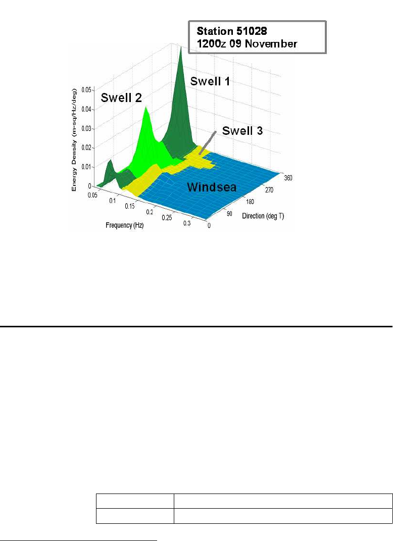
147
Figure 3.6: Surface plot of an energy density spectrum showing spectral
partitions for windsea and three swell trains. This is a snapshot of hind-
casted conditions at Christmas Island (NOAA buoy 51028) at 12:00 UTC on
November 9, 2000.
This code has been transformed to an efficient FORTRAN routine for use in
WAVEWATCH IIIsince version 3.11. Coding follows the Vincent and Soille
(1991) paper but incorporates an efficient sort routine (O(n)) discussed in
Tracy et al. (2006).
3.13 Spatial and temporal tracking of wave systems
Origination: IFP Swan
Provided by: Van der Westhuysen, Hanson, Devaliere
the previous APL WAVES package

148
The spectral partitioning procedure described above is carried out within
the spectral space, independently at each geographical grid point. As a
result, there is no coherence between the identified partitions over geograph-
ical space and in time. Following Voorrips et al. (1997), Hanson and Phillips
(2001) and Devaliere et al. (2009), a spatial correlation step is therefore ap-
plied. This is done by means of an outwardly running spiral, originating at
an arbitrary point (typically the center) inside the computational domain.
Figure 3.7 presents an example of such a tracking spiral on a regular compu-
tational grid over a coastal domain featuring landmass. At the spiral origin
(location 1), each spectral partition is assigned an initial system index. The
spatial correlation is then determined for each subsequent geographical loca-
tion (2, 3, 4, ...) moving outward along the spiral. At each new geographical
location, the peak period Tp, peak direction θpand significant wave height
Hm0 of each of its spectral partitions are correlated with the spatial means
˜
Tn
p,i,˜
θn
p,i and ˜
Hn
m0,i of the corresponding parameters at its neighboring geo-
graphical grid points (indicated by the superscript n) previously assigned a
system i. the partition at the present grid point is assigned to the neighboring
system ithat minimizes the following Goodness-of-Fit (GoF) function:
GoFi= Tp−˜
Tn
p,i
∆Tn!2
+ θp−˜
θn
p,i
∆θn!2
+ Hm0 −˜
Hn
m0,i
∆Hn!2
,(3.92)
where ∆Tn, ∆θnand ∆Hnare combining criteria (Van der Westhuysen et al.,
2016). If either of the first two terms on the right hand side of (3.92) exceed
unity for the closest match, the difference is considered too great and a new
wave system is assigned to that partition. Here, the search range for neigh-
boring points is set at 1, so that a maximum of four previously-associated
neighbors can be found (e.g. location 15 will have the previously processed
neighbors 3, 4, 5 and 14). In some cases, iterative combining is required.
The next step is to correlate these wave systems over time. Each system
iat the current time level tis associated with its closest match amongst
the systems jat the previous time level (t−1). Three characteristics of
the wave systems are considered in this process, namely: (i) the spatial
mean peak wave period over the system, ˜
Ts
p,t,i, with s denoting the system
mean, (ii) the spatial mean peak wave direction, ˜
θs
p,t,i and (iii) the number of
overlapping grid points between the two systems in geographical space ∩i,j .
These characteristics are combined to form the following GoF function:
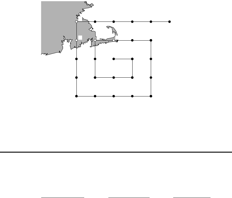
149
1 22
33455
6
77 8 9 1010
11
12
13131415161717
18
19
20
2121 22
Figure 3.7: Example of a tracking spiral on a regular computational grid over
a coastal domain featuring landmass (shaded). Black dots indicate active grid
points and white dots indicate inactive (dry) grid points.
GoFi,j = ˜
Ts
p,t,i −˜
Ts
p,t−1,j
∆Ts!2
+ ˜
θs
p,t,i −˜
θs
p,t−1,j
∆θs!2
+Nt−1,j − ∩i,j
0.5Nt−1,j 2
,
(3.93)
where ∆Tsand ∆θsare combining criteria, and Nis the total number of
grid points in a system, see Van der Westhuysen et al. (2016). In order to
focus the tracking process on high-energy regions in the wave field, the spa-
tial mean period and peak direction values of each system are weighted with
the square of the significant wave height. System iat the current time level
tis assigned the system jfrom the previous time level (t−1) that minimizes
(3.93). If any of the three terms on the right hand side of (3.93) exceed unity
for the system that minimizes (3.93), a new system number is assigned. For
the last term, this implies a minimum spatial overlap requirement, arbitrar-
ily set at 50%. This term mostly has an impact over basin scale domains,
where systems are typically smaller than the computational area. In order to
improve robustness, the details of identified systems are stored for five time
levels, after which the system association is released.

150
-space
6
time
c
c
c
c
c
c
c
c
c
c
c
c
s
s
s
s
c
c
c
c
c
c
c
c
c
c
c
c
‘land’
sea -
bound. data
bound. scheme
internal scheme
-
Figure 3.8: Traditional one-way nesting approach as used in ww3 shel. One-
dimensional representation in space and time, symbols represent grid points.
3.14 Nesting
Origination: WAVEWATCH III
Provided by: H. L. Tolman
Traditionally, wave models only consider one-way nesting, with boundary
data from low-resolution grids being provided to high-resolution grids. This
approach has always been available in WAVEWATCH III, and is discussed
in Section 3.14.1. In model version 3.14, a multi-grid wave model driver was
introduced, considering full two-way nesting between grids. This approach
is discussed in Section 3.14.2. The illustrations below consider regular grids,
but the principles discussed are applicable to curvilinear and triangular grids
too.
3.14.1 Traditional one-way nesting
The conventional wave model program ww3 shel considers a single wave
model grid. This program includes options to transfer boundary conditions
from large-scale runs to small-scale runs. Each run can simultaneously accept
one data set with boundary conditions, and generate up to 9 data sets with
boundary conditions. To assure conservation of wave energy with incom-

151
patible depths and currents, the boundary data consists of energy spectra
F(σ, θ). The data file consists of spectra at grid points of the generating run,
and information needed to interpolate spectra at the requested boundary
points. The size of the transfer files is thus minimized if the input points for
a small-scale run are located on grid lines in the large-scale run. When used
as input, the spectra are interpolated in space and time for every global time
step ∆tg, using a linear interpolation of spectral components.
The numerical approach for including boundary data in a wave model
is illustrated in Fig. 3.8. Active boundary points are assigned in the grid
to separate sea points from land points or from otherwise deactivated grid
points. Between the active boundary points and sea points, a local boundary
scheme is applied (typically first order). In the internal sea points of the
model, the selected propagation scheme is used.
Practical aspects of the conventional one-way nesting approach are dis-
cussed in more detail in Appendix C.
3.14.2 Two-way nesting
Model version 3.14 includes an option to use the multi-grid or mosaic ap-
proach to wave modeling with the program ww3 multi (Tolman,2006,2007,
2008a). In this program, an arbitrary number of grids with arbitrary resolu-
tions is considered, with data exchange between grids at each relevant model
time step. The grids are given a rank number, where lower rank corresponds
to lower resolution, and equal rank corresponds to similar resolution (but not
necessarily equal resolution). Three types of data transfer between grids are
considered:
•Transfer of data from lower to higher rank grids.
•Transfer of data from higher to lower rank grids.
•Transfer of data between grids with equal rank.
Data transfer from lower to higher ranked grids is accomplished by pro-
viding boundary data to the higher ranked grid, as in the traditional one-way
nesting approach described in the previous section and in Fig. 3.8.
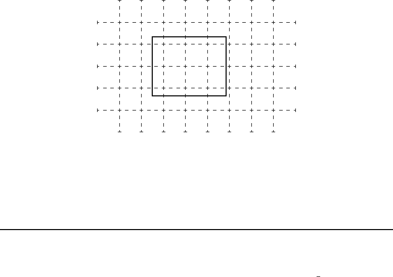
152
c
c
c
c
c
c
c
c
c
c
c
c
c
c
c
c
c
c
c
c
c
c
c
c
c
c
c
c
c
c
c
c
c
c
c
c
c
c
c
c
c
c
c
c
c
c
c
c
c
c
c
c
c
c
v
v
v
v
v
v
v
v
v
Figure 3.9: Concept for reconciling lower ranked grid with higher ranked
grid in two-way nesting approach. ◦and hashed lines represent the higher
ranked grid points and grid boxes, respectively, •and solid lines represent
lower ranked grid and central grid box.
When this approach is combined with data transfer from higher to lower
rank, a full two-way nesting approach is established. In ww3 multi the data
at the lower ranked grids is reconciled with the data at the higher ranked
grids after the higher ranked grids have ‘caught up’ in time with the lower
ranked grids. Considering that the resolution of the lower ranked grid by
definition is lower that the resolution of the higher ranked grid, a natural
way to estimate the wave energy in the lower ranked grid El,i from energy in
the higher ranked grid Eh,j is
El,i =Xwi,j Eh,j ,(3.94)
where iand jare grid counters in the two grids, and where wi,j are averaging
weights. The weights can be defined consistent with conservation of wave
energy as the surface of the grid box jin the higher ranked grid that covers
the grid box iin the lower ranked grid, normalized with the surface of the
lower ranked grid box i. This is illustrated in Fig. 3.9. To avoid circular
reconciliation, grid points in the lower ranked grid that contribute to the
boundary data in the higher ranked grid are not updated in this manner.
Overlapping grids with similar rank cannot use the above two-way nesting
technique to consistently exchange data. Instead, all such grids are propa-
gated one time step, after which the grids are reconciled as is illustrated in

153
c
c
c
c
c
c
c
c
c
c
c
c
c
c
c
c
c
c
c
c
c
c
c
c
c
c
c
c
c
c
c
c
c
c
c
s
s
s
s
s
s
s
s
s
s
s
s
s
s
s
s
s
s
s
s
s
s
s
s
s
s
s
s
s
s
s
s
s
s
s
-
A B C
Figure 3.10: Concept for reconciling grids with identical rank and therefore
similar resolution. ◦represents points of grid 1, •represents grid 2.
Fig. 3.10. For grid 1 (◦in Fig. 3.10) two areas can be distinguished. In area
C, the influence of the boundary has propagated into the grid since the last
reconciliation. The actual depth of penetration depends on the stencil width
of the numerical scheme, and the number of propagation time steps. In areas
A and B, information from the boundary has not yet penetrated, and this
area can be considered as the ‘interior’ of grid 1. Similarly, area A represents
the boundary penetration depth for grid 2 (•in Fig. 3.10) whereas B and C
represent the interior of grid 2. A simple and consistent reconciliation be-
tween grid 1 and 2 uses data from grid 1 exclusively in area A (interpolating
data from grid 1 to grid points in grid 2 as necessary), and uses data from
grid 2 exclusively in area C. In area B, where interior parts of both grids over-
lap, a consistent solution can be found by using weighted averages from both
grids. Note that this approach is easily extended to multiple overlapping
grids.
Note that for explicit numerical propagation schemes and overlapping
grids with identical resolution and coinciding grid points, solutions for over-
lapping grids and the compatible single grid can be identical, as long as the
overlap areas are sufficiently wide.
The two-way nesting techniques in ww3 multi are largely automated. Each
grid is prepared individually, with its own preferred time stepping informa-
tion. Locations where each grid expects to get boundary data from lower

154
ranked grids are marked as in the one-way nesting approach. All other book-
keeping needed to implement the two-way nesting techniques are automated,
although some iterations may be needed to assure that all input boundary
points defined in each grid can be provided with boundary data from other
grids in the multi-grid application. Alternatively, each grid can obtain data
from an external data file as in the traditional nesting approach. In the
present implementation, each grid has to obtain all boundary data from a
single file, or from other grids in the multi-grid application, but cannot re-
ceive data from file and grids simultaneously. Details on the management
algorithm developed to run all grid simultaneously can be found in Tolman
(2007, section 3.4) and Tolman (2008a), and will not be reproduced here.
Note that the grids used in ww3 multi do not need to have the same
spectral discretization. Spectra are converted on the fly in ww3 multi. Details
on the numerical techniques used for this approach can be found in Tolman
(2007, section 3.5.5). Grid generation for multiple grids in such an approach
can be cumbersome, and consistency between grids is required for consistent
model results. For this reason automated grid generation utilities have been
developed by Chawla and Tolman (2007,2008).

155
4 Wave Model Structure and Data Flow
4.1 Program design
The core of WAVEWATCH III is the wave model subroutine. The wave
model routine can be called by either a stand-alone program shell or any
other program that requires dynamically updated wave data. Two such pro-
grams are provided with the WAVEWATCH III release. Auxiliary programs
include a grid preprocessor, a program to generate artificial initial conditions,
a generic program shell (and a corresponding input pre-processor) and out-
put post-processors. In the discussion of the model below, file names will be
identified by the file type font, the contents of a file by the code type font
and fortran program elements by the fortran type font.
The main wave model routine is w3wave. Data files are identified with
the file extension .ww3, except in the multi-grid wave model ww3 multi, where
the file extension identifies an individual grid. For simplicity, the file ex-
tension .ww3 will be used throughout this chapter. A relational diagram
including the basic data flow is presented in Fig. 4.1.
The grid preprocessor writes a model definition file mod def.ww3 with bot-
tom and obstruction information and parameter values defining the physical
and numerical approaches. The wave model requires initial conditions, con-
sisting of a restart file restart.ww3, written by either the wave model itself,
or by the initial conditions program. If this file is not available, the wave
model will be initialized automatically, depending on the ability of the model
to start from calm conditions. If linear growth or spectral seeding is switch
on, the model will start from calm conditions (Hs= 0), otherwise the ini-
tial conditions will consist of a parametric fetch-limited spectrum based on
the initial wind field (see the corresponding option in the initial conditions
program).
The wave model routine (w3wave) optionally generates up to 9 restart
files restartn.ww3, where nrepresents a single digit integer number. The wave
model also optionally reads boundary conditions from the file nest.ww3 and
generates boundary conditions for consecutive runs in nestn.ww3. The model
furthermore dumps raw data to the output files out grd.ww3 ,out pnt.ww3,
track o.ww3 and partition.ww3 (gridded mean wave parameters, spectra at
locations, spectra along tracks, and partitioned wave data, respectively).

156
The tracks along which spectra are to be presented is defined in the file
track i.ww3. Note that the wave model does not write to standard output,
because this would be inconvenient if WAVEWATCH III is part of an inte-
grated model. Instead, it maintains its own log file log.ww3 and optionally
a test output files test.ww3 for a shared memory version of the model, or
testnnn.ww3 for distributed memory versions, where nnn is the processor
number starting with 1. Finally, various output post-processors are available
(binary post-processing of raw gridded fields, point output and track output
files; NetCDF and GRIB(2) packing of wave data; post-processing for later
GrADS graphical processing of gridded and spectral data). A more detailed
description of all program elements and their input files is given below. Note
that the source codes of each routine are fully documented. This documen-
tation is an additional source of information about WAVEWATCH III.
Files specific to WAVEWATCH III are opened by name within the pro-
gram. The unit numbers, however, have to be defined by the user8, guaran-
teeing the largest possible flexibility for implementation in integrated models.
Next to the wave model subroutine, an initialization routine and an inter-
face routine for data assimilation are provided. The latter routine is intended
to be run side by side with the wave model routine. The routine includes a
generic interface that provides all necessary model components to perform
full spectral data assimilation. This routine is integrated into the generic
wave model shell, which is set up to perform time step managements for a
wave model with or without data assimilation. The shell also provides a
simple yet flexible way to provide the data assimilation scheme with various
types of data. Data assimilation has not yet been included in the multi-grid
wave model shell.
4.2 The wave model routines
As discussed above, the actual wave model is a subroutine. To run the
model, a program shell is needed. WAVEWATCH III is provided with a
simple stand-alone shell as will be discussed in Section 4.4.9, and with a
more complex multi-grid model shell as will be discussed in Section 4.4.11.
The present section concentrates on the wave model subroutines.
8Except for ww3 multi.

157
grid data
?
grid preprocessor
?
mod def.ww3
?
-
@@
@
?
initial cond. -restart.ww3
@
@R
restart.ww3
nest.ww3 wave model
-
partition.ww3
out pnt.ww3
out grd.ww3
?
log.ww3
test.ww3
?
6
track i.ww3
track o.ww3
output
postprocessing
program
shell
or
integrated
program
input files
?
input preprocessor
?
file subrout. program
-data transfer by file
Figure 4.1: Basic program elements and data flow

158
| input | output |
|-------------|---------------|
step | pass | date time | b w l c i d | g p t r b f c |
-------|------|---------------------|-------------|---------------|
0 | 1 | 1968/06/06 00:00:00 | F | X X |
8 | 1 | 02:00:00 | | X |
12 | 1 | 03:00:00 | | X |
16 | 1 | 04:00:00 | | X |
24 | 1 | 06:00:00 | X | X X |
32 | 2 | 08:00:00 | | X |
36 | 2 | 09:00:00 | | L |
40 | 2 | 10:00:00 | | X |
48 | 2 | 12:00:00 | X X | L L |
-------+------+---------------------+-------------+---------------+
Figure 4.2: Example action table from file log.ww3.
The wave model initialization routine w3init performs model initializa-
tion for a single wave model grid. This includes setting up part of the I/O
system by defining unit numbers, initializing internal time management, pro-
cessing the model definition file (mod def.ww3), processing initial conditions
(restart.ww3), preparing model output, and calculating grid-dependent pa-
rameters. If the model is compiled for an MPI environment, all necessary
communication for both calculations and output are determined and initial-
ized (the model uses persistent MPI communication throughout).
The wave model routine w3wave can be called any number of times to
propagate the wave field for a single grid in time after the initialization has
taken place. After some initial checks, the subroutine interpolates winds and
currents, updates ice concentrations and water levels, propagates the wave
field, and applies the selected source terms for a number of time steps. The
internal time step is defined by the interval for which the calculations are
to be performed, and by the requested output times. At the end of the
calculations, the routine provides the calling program with the requested
fields of wave data. A documentation of the interface of w3wave can be
found in the source code (w3wavemd.ftn).
Apart from the raw data files as described above, the program maintains
a log file log.ww3. This file is opened by w3init (contained in w3wave in

159
w3wavemd.ftn), which writes some self-explanatory header information to this
file. Each consecutive call to w3wave adds several lines to an ‘action table’
in this log file as is shown in Fig. 4.2. The column identified as ‘step’ shows
the discrete time step considered. The column identified as ‘pass’ identifies
the sequence number of the call to w3wave; i.e., 3 identifies that this action
took place in the third call to w3wave. The third column shows the ending
time of the time step. In the input and output columns the corresponding
actions of the model are shown. An Xidentifies that the input has been
updated, or that the output has been performed. An Findicates a first field
read, and an Lidentifies the last output. The seven input columns identify
boundary conditions (b), wind fields (w), water levels (l), current fields (c),
ice concentrations (i), and data for assimilation (d), respectively. Note that
data assimilation takes place at the end of the time step after the wave
routine call. The seven output columns identify gridded output (g), point
output (p), output along tracks (t), restart files (r), boundary data (b), and
partitioned spectral data (f), and output for coupling (c), respectively.
For the multi-grid wave model (Tolman,2008a,ww3 multi) a set of rou-
tines is build around the basic wave model routines. The three main routines
are the initialization routine wminit, a time stepping routine wmwave and
a finalization routine wmfinl, with similar functions as the routines for a
single grid as described above. Note that he raw input and output files are
generated for separate grid in the mosaic, and are identified by replacing
the standard file extension ’.ww3’ with a unique identifier for each individual
grid. Log files are maintained for each individual grid, as well as an overall
log file log.mww3.
4.3 The data assimilation interface
As discussed above, the wave model subroutine is supplemented with a data
assimilation interface routine (w3wdas in w3wdasmd.ftn). This routine is
integrated in the stand-alone shell (see Section 4.4.9) to provide time step
management of a combined wave model / data assimilation scheme. It has
not yet been integrated in the multi-grid model driver, although it is ac-
counted for in the multi-grid model management algorithm. In this a fairly
simple approach is assumed where data assimilation is performed at selected
times, while the wave model marches forward in time. In the setup of the
160
shell, the data assimilation is performed after the model has reached the tar-
get time, but has not yet produced output. After the data assimilation is
performed, the wave model routine is called again only to generate output
as requested. Thus, the wave model output for a given time will include the
effects of data assimilation for that specific target time.
The generic program shell also processes several types of data to be as-
similated, and passes it on to the data assimilation interface routine. All data
needs to be preprocessed using the wave model input preprocessor (see Sec-
tion 4.4.6), and will be recognized by the generic shell by file name. Presently,
up to three different data files can be used. Tentatively, these could be mean
wave parameters, one dimensional spectral data, and two dimensional spec-
tral data, respectively. This is, however, not hardwired to the model and in
fact needs to be defined by the user.
Presently, no data assimilation packages are available. User supplied data
assimilation schemes can be included in the wave model using the interface
routine (w3wdas in w3wdasmd.ftn), the documentation of which should be
sufficient for the necessary programming. Details on how to add user supplied
software to the WAVEWATCH III compilation system can be found in the
following chapter. NCEP is presently working on wave data assimilation
techniques, but presently has no plans to distribute wave data assimilation
software.
4.4 Auxiliary programs
4.4.1 General concepts
All auxiliary programs presented here, with the exception of the track output
post-processor, read input from a pre-defined input file. The first character on
the first line of the input file will be considered to be the comment character,
identifying comment lines in the input file. This comment character has to
appear on the first position of input lines to be effective. In all examples in
the following sections lines starting with ’$’ therefore only contain comment.
The programs furthermore all write formatted output to the standard output
unit.
In the following sections, all available auxiliary programs are described
using an example input file with all options included (partially as comment).

161
These files are identical to the distributed example input files. The sections
furthermore show the name of the executable program, the program name (as
appears in the program statement), the source code file and input and output
files and their unit numbers (in brackets behind the file name). Input and
output files marked with ∗are optional. The intermediate files mentioned
below are all unformatted, and are not described in detail here. Each
file is written and read by a single routine, to which reference is made for
additional documentation.
mod def.ww3 Subroutine w3iogr (w3iogrmd.ftn).
out grd.ww3 Subroutine w3iogo (w3iogomd.ftn).
out pnt.ww3 Subroutine w3iopo (w3iopomd.ftn).
track o.ww3 Subroutine w3iotr (w3iotrmd.ftn).
restart.ww3 Subroutine w3iors (w3iorsmd.ftn).
nest.ww3 Subroutine w3iobc (w3iobcmd.ftn).
partition.ww3 Subroutine w3iosf (w3iosfmd.ftn).
Preprocessing and compilation of the programs is discussed in the following
two chapters. Examples of test runs of the model are provided with the
source code.

162
4.4.2 The grid preprocessor
Program : ww3 grid (w3grid)
Code : ww3 grid.ftn
Input : ww3 grid.inp (10) Formatted input file for program.
’grid file’ ∗(user) File with bottom depths.
’obstr. file’ ∗(user) File with sub-grid obstructions.
’mask file’ ∗(user) File with grid mask.
Output : standard out (6) Formatted output of program.
mod def.ww3 (20) Model definition file in WAVE-
WATCH III format.
mask.ww3 ∗(20) Land-sea mask file (switch o2a).
Scratch : ww3 grid.scratch (90) Formatted scratch file.
Note that bottom and obstruction data may be in same file.
start of example input file (traditional form)
$ -------------------------------------------------------------------- $
$ WAVEWATCH III Grid preprocessor input file $
$ -------------------------------------------------------------------- $
$ Grid name (C*30, in quotes)
$
’TEST GRID (GULF OF NOWHERE) ’
$
$ Frequency increment factor and first frequency (Hz) ---------------- $
$ number of frequencies (wavenumbers) and directions, relative offset
$ of first direction in terms of the directional increment [-0.5,0.5].
$ In versions 1.18 and 2.22 of the model this value was by definiton 0,
$ it is added to mitigate the GSE for a first order scheme. Note that
$ this factor is IGNORED in the print plots in ww3_outp.
$
1.1 0.04118 25 24 0.
$
$ Set model flags ---------------------------------------------------- $
$ - FLDRY Dry run (input/output only, no calculation).
$ - FLCX, FLCY Activate X and Y component of propagation.
$ - FLCTH, FLCK Activate direction and wavenumber shifts.
$ - FLSOU Activate source terms.
$
F T T T F T
$
$ Set time steps ----------------------------------------------------- $
163
$ - Time step information (this information is always read)
$ maximum global time step, maximum CFL time step for x-y and
$ k-theta, minimum source term time step (all in seconds).
$
900. 950. 900. 300.
$
$ Start of namelist input section ------------------------------------ $
$ Starting with WAVEWATCH III version 2.00, the tunable parameters
$ for source terms, propagation schemes, and numerics are read using
$ namelists. Any namelist found in the folowing sections up to the
$ end-of-section identifier string (see below) is temporarily written
$ to ww3_grid.scratch, and read from there if necessary. Namelists
$ not needed for the given switch settings will be skipped
$ automatically, and the order of the namelists is immaterial.
$ As an example, namelist input to change SWELLF and ZWND in the
$ Tolman and Chalikov input would be
$
$ &SIN2 SWELLF = 0.1, ZWND = 15. /
$
$ Define constants in source terms ----------------------------------- $
$
$ Stresses - - - - - - - - - - - - - - - - - - - - - - - - - - - - - -
$ TC 1996 with cap : Namelist FLX3
$ CDMAX : Maximum allowed CD (cap)
$ CTYPE : Cap type :
$ 0: Discontinuous (default).
$ 1: Hyperbolic tangent.
$ Hwang 2011 : Namelist FLX4
$ CDFAC : re-scaling of drag
$
$ Linear input - - - - - - - - - - - - - - - - - - - - - - - - - - - -
$ Cavaleri and M-R : Namelist SLN1
$ CLIN : Proportionality constant.
$ RFPM : Factor for fPM in filter.
$ RFHF : Factor for fh in filter.
$
$ Exponential input - - - - - - - - - - - - - - - - - - - - - - - - -
$ WAM-3 : Namelist SIN1
$ CINP : Proportionality constant.
$
$ Tolman and Chalikov : Namelist SIN2
$ ZWND : Height of wind (m).
$ SWELLF : swell factor in (n.nn).
$ STABSH, STABOF, CNEG, CPOS, FNEG :
$ c0, ST0, c1, c2 and f1 in . (n.nn)
164
$ through (2.65) for definition of
$ effective wind speed (!/STAB2).
$ WAM4 and variants : Namelist SIN3
$ ZWND : Height of wind (m).
$ ALPHA0 : minimum value of Charnock coefficient
$ Z0MAX : maximum value of air-side roughness z0
$ BETAMAX : maximum value of wind-wave coupling
$ SINTHP : power of cosine in wind input
$ ZALP : wave age shift to account for gustiness
$ TAUWSHELTER : sheltering of short waves to reduce u_star
$ SWELLFPAR : choice of swell attenuation formulation
$ (1: TC 1996, 3: ACC 2008)
$ SWELLF : swell attenuation factor
$ Extra parameters for SWELLFPAR=3 only
$ SWELLF2, SWELLF3 : swell attenuation factors
$ SWELLF4 : Threshold Reynolds number for ACC2008
$ SWELLF5 : Relative viscous decay below threshold
$ Z0RAT : roughness for oscil. flow / mean flow
$ BYDRZ input : Namelist SIN6
$ SINA0 : factor for negative input
$ SINU10 : wind speed scaling option
$
$ Nonlinear interactions - - - - - - - - - - - - - - - - - - - - - - -
$ Discrete I.A. : Namelist SNL1
$ LAMBDA : Lambda in source term.
$ NLPROP : C in sourc term. NOTE : default
$ value depends on other source
$ terms selected.
$ KDCONV : Factor before kd in Eq. (n.nn).
$ KDMIN, SNLCS1, SNLCS2, SNLCS3 :
$ Minimum kd, and constants c1-3
$ in depth scaling function.
$ Exact interactions : Namelist SNL2
$ IQTYPE : Type of depth treatment
$ 1 : Deep water
$ 2 : Deep water / WAM scaling
$ 3 : Shallow water
$ TAILNL : Parametric tail power.
$ NDEPTH : Number of depths in for which
$ integration space is established.
$ Used for IQTYPE = 3 only
$ Namelist ANL2
$ DEPTHS : Array with depths for NDEPTH = 3
$ Gen. Multiple DIA : Namelist SNL3
$ NQDEF : Number of quadruplets.
165
$ MSC : Scaling constant ’m’.
$ NSC : Scaling constant ’N’.
$ KDFD : Deep water relative filter depth,
$ KDFS : Shallow water relative filter depth,
$ Namelist ANL3
$ QPARMS : 5 x NQDEF paramaters describing the
$ quadruplets, repeating LAMBDA, MU, DT12.
$ Cdeep and Cshal. See examples below.
$ Two Scale Approx. : Namelist SNL4
$ INDTSA : Index for TSA/FBI computations
$ (0 = FBI ; 1 = TSA)
$ ALTLP : Index for alternate looping
$ (1 = no ; 2 = yes)
$
$ Traditional DIA setup (default):
$
$ &SNL3 NQDEF = 1, MSC = 0.00, NSC = -3.50 /
$ &ANL3 QPARMS = 0.250, 0.000, -1.0, 0.1000E+08, 0.0000E+00 /
$
$ GMD3 from 2010 report (G13d in later paper) :
$
$ &SNL3 NQDEF = 3, MSC = 0.00, NSC = -3.50 /
$ &ANL3 QPARMS = 0.126, 0.000, -1.0, 0.4790E+08, 0.0000E+00 ,
$ 0.237, 0.000, -1.0, 0.2200E+08, 0.0000E+00 ,
$ 0.319, 0.000, -1.0, 0.1110E+08, 0.0000E+00 /
$
$ G35d from 2010 report:
$
$ &SNL3 NQDEF = 5, MSC = 0.00, NSC = -3.50 /
$ &ANL3 QPARMS = 0.066, 0.018, 21.4, 0.170E+09, 0.000E+00 ,
$ 0.127, 0.069, 19.6, 0.127E+09, 0.000E+00 ,
$ 0.228, 0.065, 2.0, 0.443E+08, 0.000E+00 ,
$ 0.295, 0.196, 40.5, 0.210E+08, 0.000E+00 ,
$ 0.369, 0.226, 11.5, 0.118E+08, 0.000E+00 /
$
$ Nonlinear filter based on DIA - - - - - - - - - - - - - - - - - - -
$ Namelist SNLS
$ A34 : Relative offset in quadruplet
$ FHFC : Proportionality constants.
$ DMN : Maximum relative change.
$ FC1-3 : Constants in frequency filter.
$
$ Whitecapping dissipation - - - - - - - - - - - - - - - - - - - - -
$ WAM-3 : Namelist SDS1
$ CDIS, APM : As in source term.
166
$
$ Tolman and Chalikov : Namelist SDS2
$ SDSA0, SDSA1, SDSA2, SDSB0, SDSB1, PHIMIN :
$ Constants a0, a1, a2, b0, b1 and
$ PHImin.
$
$ WAM4 and variants : Namelist SDS3
$ SDSC1 : WAM4 Cds coeffient
$ MNMEANP, WNMEANPTAIL : power of wavenumber
$ for mean definitions in Sds and tail
$ SDSDELTA1, SDSDELTA2 : relative weights
$ of k and k^2 parts of WAM4 dissipation
$ SDSLF, SDSHF : coefficient for activation of
$ WAM4 dissipation for unsaturated (SDSLF) and
$ saturated (SDSHF) parts of the spectrum
$ SDSC2 : Saturation dissipation coefficient
$ SDSC4 : Value of B0=B/Br for wich Sds is zero
$ SDSBR : Threshold Br for saturation
$ SDSP : power of (B/Br-B0) in Sds
$ SDSBR2 : Threshold Br2 for the separation of
$ WAM4 dissipation in saturated and non-saturated
$ SDSC5 : coefficient for turbulence dissipation
$ SDSC6 : Weight for the istropic part of Sds_SAT
$ SDSDTH: Angular half-width for integration of B
$
$ BYDRZ : Namelist SDS6
$ SDSET : Select threshold normalization spectra
$ SDSA1, SDSA2, SDSP1, SDSP2 :
$ Coefficients for dissipation terms T1 and T2
$ : Namelist SWL6
$ SWLB1 : Coefficient for swell dissipation
$
$ Bottom friction - - - - - - - - - - - - - - - - - - - - - - - - - -
$ JONSWAP : Namelist SBT1
$ GAMMA : Bottom friction emprical constant
$
$
$ Surf breaking - - - - - - - - - - - - - - - - - - - - - - - - - - -
$ Battjes and Janssen : Namelist SDB1
$ BJALFA : Dissipation constant (default = 1)
$ BJGAM : Breaking threshold (default = 0.73)
$ BJFLAG : TRUE - Use Hmax/d ratio only (default)
$ FALSE - Use Hmax/d in Miche formulation
$
$ Dissipation in the ice - - - - - - - - - - - - - - - - - - - - - -
167
$ Generalization of Liu et al. : Namelist SIC2
$ IC2DISPER : If true uses Liu formulation with eddy viscosity
$ If false, uses the generalization with turbulent
$ to laminar transition
$ IC2TURB : empirical factor for the turbulent part
$ IC2ROUGH : under-ice roughness length
$ IC2REYNOLDS: Re number for laminar to turbulent transition
$ IC2SMOOTH : smoothing of transition reprensenting random waves
$ IC2VISC : empirical factor for viscous part
$
$
$ Scattering in the ice & creep dissipations- - - - - - - - - - - - -
$ Generalization of Wiliams et al. : Namelist SIS2
$ ISC1 : scattering coefficient (default = 1)
$ IS2BACKSCAT : fraction of energy back-scattered (default = 1 )
$ IS2BREAK : TRUE - changes floe max diameter
$ : FALSE - does not change floe max diameter
$ IS2C1 : scattering in pack ice
$ IS2C2 : frequency dependance of scattering in pack ice
$ IS2C3 : frequency dependance of scattering in pack ice
$ ISBACKSCAT : fraction of scattered energy actualy redistributed
$ IS2DISP : use of ice-specific dispersion relation (T/F)
$ FRAGILITY : parameter between 0 and 1 that gives the shape of FSD
$ IS2DMIN : minimum floe diameter in meters
$ IS2DAMP : multiplicative coefficient for dissipation term from
$ IS2UPDATE : TRUE - updates the max floe diameter with forcing only
$ : FALSE - updates the max floe diameter at each time step
$
$ Triad nonlinear interactions - - - - - - - - - - - - - - - - - - - -
$ Lumped Triad Interaction (LTA) : Namelist STR1 (To be implemented)
$ PTRIAD1 : Proportionality coefficient (default 0.05)
$ PTRIAD2 : Multiple of Tm01 up to which interaction
$ is computed (2.5)
$ PTRIAD3 : Ursell upper limit for computing
$ interactions (not used, default 10.)
$ PTRIAD4 : Shape parameter for biphase
$ computation (0.2)
$ PTRIAD5 : Ursell number treshold for computing
$ interactions (0.01)
$
$ Shoreline reflections - - - - - - - - - - - - - - - - - - - - - - - -
$ ref. parameters : Namelist REF1
$ REFCOAST : Reflection coefficient at shoreline
$ REFFREQ : Activation of freq-dependent ref.
$ REFMAP : Scale factor for bottom slope map
168
$ REFRMAX : maximum ref. coeffient (default 0.8)
$ REFFREQPOW: power of frequency
$ REFICEBERG: Reflection coefficient for icebergs
$ REFSUBGRID: Reflection coefficient for islands
$ REFCOSP_STRAIGHT: power of cosine used for
$ straight shoreline
$
$ Bound 2nd order spectrum and free IG - - - - - - - - - - - - - - - - -
$ IG1 parameters : Namelist SIG1
$ IGMETHOD : 1: Hasselmann, 2: Krasitskii-Janssen
$ IGADDOUTP : activation of bound wave correction
$ in ww3_outp / ww3_ounp
$ IGSOURCE : 1: uses bound waves, 2: empirical
$ IGSTERMS : > 0 : no source term in IG band
$ IGMAXFREQ : maximum frequency of IG band
$ IGEMPIRICAL: constant in empirical free IG source
$ IGBCOVERWRITE: T: Replaces IG spectrum, does not add
$ IGSWELLMAX: T: activates free IG sources for all freq.
$
$
$ Propagation schemes ------------------------------------------------ $
$ First order : Namelist PRO1
$ CFLTM : Maximum CFL number for refraction.
$
$ UQ/UNO with diffusion : Namelist PRO2
$ CFLTM : Maximum CFL number for refraction.
$ DTIME : Swell age (s) in garden sprinkler
$ correction. If 0., all diffusion
$ switched off. If small non-zero
$ (DEFAULT !!!) only wave growth
$ diffusion.
$ LATMIN : Maximum latitude used in calc. of
$ strength of diffusion for prop.
$
$ UQ/UNO with averaging : Namelist PRO3
$ CFLTM : Maximum CFL number for refraction.
$ WDTHCG : Tuning factor propag. direction.
$ WDTHTH : Tuning factor normal direction.
$
$ Note that UQ and UNO schemes have no tunable parameters.
$ All tuneable parameters are associated with the refraction
$ limitation and the GSE alleviation.
$
$ Unstructured grids ------------------------------------------------ $
$ UNST parameters : Namelist UNST
169
$ UGOBCAUTO : TRUE: OBC points are taken from type 15 elements
$ FALSE: OBC points must be listed in ww3_grid.inp
$ UGOBCDEPTH: Threshold ( < 0) depth for OBC points if UGOBCAUTO is TRUE
$ EXPFSN : Activation of N scheme
$ EXPFSPSI : Activation of PSI scheme
$ EXPFSFCT : Activation of FCT scheme
$ IMPFSN : Activation of N implicit scheme
$
$ SMC grid propagation : Namelist PSMC and default values
$ CFLTM : Maximum CFL no. for propagation, 0.7
$ DTIME : Swell age for diffusion term (s), 0.0
$ LATMIN : Maximum latitude (deg) for GCT, 86.0
$ RFMAXD : Maximum refraction turning (deg), 80.0
$ LvSMC : No. of refinement level, default 1
$ ISHFT : Shift number of i-index, default 0
$ JEQT : Shift number of j-index, default 0
$ NBISMC : No. of input boundary points, 0
$ UNO3 : Use 3rd order advection scheme, .FALSE.
$ UNO3 : Add extra spatial averaging, .FALSE.
$ &PSMC DTIME = 39600.0, LATMIN=85.0, RFMAXD = 36.0, LvSMC=3, JEQT=1344 /
$
$ Output of 3D arrays------------------------------------------------- $
$ In order to limit the use of memory, arrays for 3D output fiels (i.e.
$ variables that are a function of both space and frequency, are not
$ declared, and thus cannot be used, unless specified by namelists.
$ NB: Output of ’first 5’ moments E, th1m, sth1m, th2, sth2m allows to estimate the full
$ directional spectrum using, e.g. MEM (Lygre&Krogstad 1986).
$
$ Parameters (integers) : Namelist OUTS
$ For the frequency spectrum E(f)
$ E3D : <=0: not declared, > 0: declared
$ I1E3D : First frequency index of output (default is 1)
$ I2E3D : Last frequency index of output (default is NK)
$ For the mean direction th1m(f), and spread sth1m(f)
$ TH1MF, STH1MF : <=0: not declared, > 0: declared
$ I1TH1MF, I1STH1MF: First frequency index of output (default is 1)
$ I2TH1MF, I2STH1MF: First frequency index of output (default is 1)
$ For the mean direction th2m(f), and spread sth2m(f)
$ TH2MF, STH2MF : <=0: not declared, > 0: declared
$ I1TH2MF, I1STH2MF: First frequency index of output (default is 1)
$ I2TH2MF, I2STH2MF: First frequency index of output (default is 1)
$ For 2nd order pressure at K=0 (source of microseisms & microbaroms)
$ P2SF : <=0: not declared, > 0: declared
$ I1P2SF : First frequency index of output (default is 1)
$ I2P2SF : Last frequency index of output (default is NK)
170
$
$ Miscellaneous ------------------------------------------------------ $
$ Misc. parameters : Namelist MISC
$ CICE0 : Ice concentration cut-off.
$ CICEN : Ice concentration cut-off.
$ PMOVE : Power p in GSE aleviation for
$ moving grids in Eq. (D.4).
$ XSEED : Xseed in seeding alg. (!/SEED).
$ FLAGTR : Indicating presence and type of
$ subgrid information :
$ 0 : No subgrid information.
$ 1 : Transparancies at cell boun-
$ daries between grid points.
$ 2 : Transp. at cell centers.
$ 3 : Like 1 with cont. ice.
$ 4 : Like 2 with cont. ice.
$ XP, XR, XFILT
$ Xp, Xr and Xf for the dynamic
$ integration scheme.
$ IHMAX : Number of discrete levels in part.
$ HSPMIN : Minimum Hs in partitioning.
$ WSM : Wind speed multiplier in part.
$ WSC : Cut of wind sea fraction for
$ identifying wind sea in part.
$ FLC : Flag for combining wind seas in
$ partitioning.
$ NOSW : Number of partitioned swell fields
$ in field output.
$ FMICHE : Constant in Miche limiter.
$ STDX : Space-Time Extremes X-Length
$ STDY : Space-Time Extremes Y-Length
$ STDT : Space-Time Extremes Duration
$ P2SF : ......
$
$ Diagnostic Sea-state Dependent Stress- - - - - - - - - - - - - - - - -
$ Reichl et al. 2014 : Namelist FLD1
$ TAILTYPE : High Frequency Tail Method
$ 0: Constant value (prescribed)
$ 1: Wind speed dependent
$ (Based on GFDL Hurricane
$ Model Z0 relationship)
$ TAILLEV : Level of high frequency tail
$ (if TAILTYPE==0)
$ Valid choices:
$ Capped min: 0.001, max: 0.02
171
$ TAILT1 : Tail transition ratio 1
$ TAILT1*peak input frequency
$ is the first transition point of
$ the saturation specturm
$ Default is 1.25
$ TAILT1 : Tail transition ratio 2
$ TAILT2*peak input frequency
$ is the second transition point of
$ the saturation specturm
$ Default is 3.00
$ Donelan et al. 2012 : Namelist FLD2
$ TAILTYPE : See above (FLD1)
$ TAILLEV : See above (FLD1)
$ TAILT1 : See above (FLD1)
$ TAILT2 : See above (FLD1)
$
$ In the ’Out of the box’ test setup we run with sub-grid obstacles
$ and with continuous ice treatment.
$
&MISC CICE0 = 0.25, CICEN = 0.75, FLAGTR = 4 /
&FLX3 CDMAX = 3.5E-3 , CTYPE = 0 /
$ &SDB1 BJGAM = 1.26, BJFLAG = .FALSE. /
$
$ Mandatory string to identify end of namelist input section.
$
END OF NAMELISTS
$
$ Define grid -------------------------------------------------------- $
$
$ Five records containing :
$
$ 1 Type of grid, coordinate system and type of closure: GSTRG, FLAGLL,
$ CSTRG. Grid closure can only be applied in spherical coordinates.
$ GSTRG : String indicating type of grid :
$ ’RECT’ : rectilinear
$ ’CURV’ : curvilinear
$ ’UNST’ : unstructured (triangle-based)
$ FLAGLL : Flag to indicate coordinate system :
$ T : Spherical (lon/lat in degrees)
$ F : Cartesian (meters)
$ CSTRG : String indicating the type of grid index space closure :
$ ’NONE’ : No closure is applied
$ ’SMPL’ : Simple grid closure : Grid is periodic in the
$ : i-index and wraps at i=NX+1. In other words,
$ : (NX+1,J) => (1,J). A grid with simple closure
172
$ : may be rectilinear or curvilinear.
$ ’TRPL’ : Tripole grid closure : Grid is periodic in the
$ : i-index and wraps at i=NX+1 and has closure at
$ : j=NY+1. In other words, (NX+1,J<=NY) => (1,J)
$ : and (I,NY+1) => (NX-I+1,NY). Tripole
$ : grid closure requires that NX be even. A grid
$ : with tripole closure must be curvilinear.
$ 2 NX, NY. As the outer grid lines are always defined as land
$ points, the minimum size is 3x3.
$
$ Branch here based on grid type
$
$ IF ( RECTILINEAR GRID ) THEN
$
$ 3 Grid increments SX, SY (degr.or m) and scaling (division) factor.
$ If CSTRG=’SMPL’, then SX is set to 360/NX.
$ 4 Coordinates of (1,1) (degr.) and scaling (division) factor.
$
$ ELSE IF ( CURVILINEAR GRID ) THEN
$
$ 3 Unit number of file with x-coordinate.
$ Scale factor and add offset: x <= scale_fac * x_read + add_offset.
$ IDLA, IDFM, format for formatted read, FROM and filename.
$ IDLA : Layout indicator :
$ 1 : Read line-by-line bottom to top.
$ 2 : Like 1, single read statement.
$ 3 : Read line-by-line top to bottom.
$ 4 : Like 3, single read statement.
$ IDFM : format indicator :
$ 1 : Free format.
$ 2 : Fixed format with above format descriptor.
$ 3 : Unformatted.
$ FROM : file type parameter
$ ’UNIT’ : open file by unit number only.
$ ’NAME’ : open file by name and assign to unit.
$
$ If the above unit number equals 10, then the x-coord is read from this
$ file. The x-coord must follow the above record. No comment lines are
$ allowed within the x-coord input.
$
$ 4 Unit number of file with y-coordinate.
$ Scale factor and add offset: y <= scale_fac * y_read + add_offset.
$ IDLA, IDFM, format for formatted read, FROM and filename.
$ IDLA : Layout indicator :
$ 1 : Read line-by-line bottom to top.
173
$ 2 : Like 1, single read statement.
$ 3 : Read line-by-line top to bottom.
$ 4 : Like 3, single read statement.
$ IDFM : format indicator :
$ 1 : Free format.
$ 2 : Fixed format with above format descriptor.
$ 3 : Unformatted.
$ FROM : file type parameter
$ ’UNIT’ : open file by unit number only.
$ ’NAME’ : open file by name and assign to unit.
$
$ If the above unit number equals 10, then the y-coord is read from this
$ file. The y-coord must follow the above record. No comment lines are
$ allowed within the y-coord input.
$
$ ELSE IF ( UNSTRUCTURED GRID ) THEN
$ Nothing to declare: all the data will be read from the GMESH file
$ END IF ( CURVILINEAR GRID )
$
$ 5 Limiting bottom depth (m) to discriminate between land and sea
$ points, minimum water depth (m) as allowed in model, unit number
$ of file with bottom depths, scale factor for bottom depths (mult.),
$ IDLA, IDFM, format for formatted read, FROM and filename.
$ IDLA : Layout indicator :
$ 1 : Read line-by-line bottom to top.
$ 2 : Like 1, single read statement.
$ 3 : Read line-by-line top to bottom.
$ 4 : Like 3, single read statement.
$ IDFM : format indicator :
$ 1 : Free format.
$ 2 : Fixed format with above format descriptor.
$ 3 : Unformatted.
$ FROM : file type parameter
$ ’UNIT’ : open file by unit number only.
$ ’NAME’ : open file by name and assign to unit.
$
$ If the above unit number equals 10, then the bottom depths are read from
$ this file. The depths must follow the above record. No comment lines are
$ allowed within the depth input. In the case of unstructured grids, the file
$ is expected to be a GMESH grid file containing node and element lists.
$
$ ------------------------------------------------------------------------
$ Example for rectilinear grid with spherical (lon/lat) coordinate system.
$ Note that for Cartesian coordinates the unit is meters (NOT km).
$
174
’RECT’ T ’NONE’
12 12
1. 1. 4.
-1. -1. 4.
-0.1 2.50 10 -10. 3 1 ’(....)’ ’NAME’ ’bottom.inp’
$
6 6 6 6 6 6 6 6 6 6 6 6
6 6 6 5 4 2 0 2 4 5 6 6
6 6 6 5 4 2 0 2 4 5 6 6
6 6 6 5 4 2 0 2 4 5 6 6
6 6 6 5 4 2 0 0 4 5 6 6
6 6 6 5 4 4 2 2 4 5 6 6
6 6 6 6 5 5 4 4 5 6 6 6
6 6 6 6 6 6 5 5 6 6 6 6
6 6 6 6 6 6 6 6 6 6 6 6
6 6 6 6 6 6 6 6 6 6 6 6
6 6 6 6 6 6 6 6 6 6 6 6
6 6 6 6 6 6 6 6 6 6 6 6
$
$ ------------------------------------------------------------------------
$ Example for curvilinear grid with spherical (lon/lat) coordinate system.
$ Same spatial grid as preceding rectilinear example.
$ Note that for Cartesian coordinates the unit is meters (NOT km).
$
$ ’CURV’ T ’NONE’
$ 12 12
$
$ 10 0.25 -0.5 3 1 ’(....)’ ’NAME’ ’x.inp’
$
$ 1 2 3 4 5 6 7 8 9 10 11 12
$ 1 2 3 4 5 6 7 8 9 10 11 12
$ 1 2 3 4 5 6 7 8 9 10 11 12
$ 1 2 3 4 5 6 7 8 9 10 11 12
$ 1 2 3 4 5 6 7 8 9 10 11 12
$ 1 2 3 4 5 6 7 8 9 10 11 12
$ 1 2 3 4 5 6 7 8 9 10 11 12
$ 1 2 3 4 5 6 7 8 9 10 11 12
$ 1 2 3 4 5 6 7 8 9 10 11 12
$ 1 2 3 4 5 6 7 8 9 10 11 12
$ 1 2 3 4 5 6 7 8 9 10 11 12
$ 1 2 3 4 5 6 7 8 9 10 11 12
$
$ 10 0.25 0.5 3 1 ’(....)’ ’NAME’ ’y.inp’
$
$ 1 1 1 1 1 1 1 1 1 1 1 1
175
$ 2 2 2 2 2 2 2 2 2 2 2 2
$ 3 3 3 3 3 3 3 3 3 3 3 3
$ 4 4 4 4 4 4 4 4 4 4 4 4
$ 5 5 5 5 5 5 5 5 5 5 5 5
$ 6 6 6 6 6 6 6 6 6 6 6 6
$ 7 7 7 7 7 7 7 7 7 7 7 7
$ 8 8 8 8 8 8 8 8 8 8 8 8
$ 9 9 9 9 9 9 9 9 9 9 9 9
$ 10 10 10 10 10 10 10 10 10 10 10 10
$ 11 11 11 11 11 11 11 11 11 11 11 11
$ 12 12 12 12 12 12 12 12 12 12 12 12
$
$ -0.1 2.50 10 -10. 3 1 ’(....)’ ’NAME’ ’bottom.inp’
$
$ 6 6 6 6 6 6 6 6 6 6 6 6
$ 6 6 6 5 4 2 0 2 4 5 6 6
$ 6 6 6 5 4 2 0 2 4 5 6 6
$ 6 6 6 5 4 2 0 2 4 5 6 6
$ 6 6 6 5 4 2 0 0 4 5 6 6
$ 6 6 6 5 4 4 2 2 4 5 6 6
$ 6 6 6 6 5 5 4 4 5 6 6 6
$ 6 6 6 6 6 6 5 5 6 6 6 6
$ 6 6 6 6 6 6 6 6 6 6 6 6
$ 6 6 6 6 6 6 6 6 6 6 6 6
$ 6 6 6 6 6 6 6 6 6 6 6 6
$ 6 6 6 6 6 6 6 6 6 6 6 6
$
$ -------------------------------------------------------------
$ SMC grid use the same spherical lat-lon grid parameters
$ ’RECT’ T ’SMPL’
$ 1024 704
$ SMC grid base level resolution dlon dlat and start lon lat
$ 0.35156250 0.23437500 1.
$ 0.17578125 -78.6328125 1.
$
$ Normal depth input line is used to passing the minimum depth
$ though the depth file is not read for SMC grid.
$ -0.1 10.0 30 -1. 1 1 ’(....)’ ’NAME’ ’SMC25Depth.dat’
$ SMC cell and face arrays and obstruction ratio:
$ 32 1 1 ’(....)’ ’S6125MCels.dat’
$ 33 1 1 ’(....)’ ’S6125ISide.dat’
$ 34 1 1 ’(....)’ ’S6125JSide.dat’
$ 31 1.0 1 1 ’(...)’ ’NAME’ ’SMC25Subtr.dat’
$ The input boundary cell file is only needed when NBISMC > 0.
$ 35 1 1 ’(....)’ ’S6125Bundy.dat’
176
$ Extra cell and face arrays for Arctic part if ARC is selected.
$ 36 1 1 ’(....)’ ’S6125MBArc.dat’
$ 37 1 1 ’(....)’ ’S6125AISid.dat’
$ 38 1 1 ’(....)’ ’S6125AJSid.dat’
$ Normal land-sea mask file input line is kept but file is not used.
$ 39 1 1 ’(....)’ ’NAME’ ’S6125Masks.dat’
$ Boundary cell id list file (unit 35) is only required if boundary
$ cell number entered above is non-zero. The cell id number should be
$ the sequential number in the cell array (unit 32) S625MCels.dat.
$
$ If sub-grid information is available as indicated by FLAGTR above,
$ additional input to define this is needed below. In such cases a
$ field of fractional obstructions at or between grid points needs to
$ be supplied. First the location and format of the data is defined
$ by (as above) :
$ - Unit number of file (can be 10, and/or identical to bottom depth
$ unit), scale factor for fractional obstruction, IDLA, IDFM,
$ format for formatted read, FROM and filename
$
10 0.2 3 1 ’(....)’ ’NAME’ ’obstr.inp’
$
$ *** NOTE if this unit number is the same as the previous bottom
$ depth unit number, it is assumed that this is the same file
$ without further checks. ***
$
$ If the above unit number equals 10, the bottom data is read from
$ this file and follows below (no intermediate comment lines allowed,
$ except between the two fields).
$
0 0 0 0 0 0 0 0 0 0 0 0
0 0 0 0 0 0 0 0 0 0 0 0
0 0 0 0 0 0 0 0 0 0 0 0
0 0 0 0 0 0 0 0 0 0 0 0
0 0 0 0 0 0 0 0 0 0 0 0
0 0 0 0 0 0 5 0 0 0 0 0
0 0 0 0 0 0 5 0 0 0 0 0
0 0 0 0 0 0 4 0 0 0 0 0
0 0 0 0 0 0 4 0 0 0 0 0
0 0 0 0 0 0 5 0 0 0 0 0
0 0 0 0 0 0 5 0 0 0 0 0
0 0 0 0 0 0 0 0 0 0 0 0
$
0 0 0 0 0 0 0 0 0 0 0 0
0 0 0 0 0 0 0 0 0 0 0 0
0 0 0 0 0 0 0 0 0 0 0 0
177
0 0 0 0 0 0 0 0 0 0 0 0
0 0 0 0 0 0 0 0 5 5 5 0
0 0 0 0 0 0 0 0 0 0 0 0
0 0 0 0 0 0 0 0 0 0 0 0
0 0 0 0 0 0 0 0 0 0 0 0
0 0 0 0 0 0 0 0 0 0 0 0
0 0 0 0 0 0 0 0 0 0 0 0
0 0 0 0 0 0 0 0 0 0 0 0
0 0 0 0 0 0 0 0 0 0 0 0
$
$ *** NOTE size of fields is always NX * NY ***
$
$ Input boundary points and excluded points -------------------------- $
$ The first line identifies where to get the map data, by unit number
$ IDLA and IDFM, format for formatted read, FROM and filename
$ if FROM = ’PART’, then segmented data is read from below, else
$ the data is read from file as with the other inputs (as INTEGER)
$
10 3 1 ’(....)’ ’PART’ ’mapsta.inp’
$
$ Read the status map from file ( FROM != PART ) --------------------- $
$
$ 3 3 3 3 3 3 3 3 3 3 3 3
$ 3 2 1 1 1 1 0 1 1 1 1 3
$ 3 2 1 1 1 1 0 1 1 1 1 3
$ 3 2 1 1 1 1 0 1 1 1 1 3
$ 3 2 1 1 1 1 0 0 1 1 1 3
$ 3 2 1 1 1 1 1 1 1 1 1 3
$ 3 2 1 1 1 1 1 1 1 1 1 3
$ 3 2 1 1 1 1 1 1 1 1 1 3
$ 3 2 1 1 1 1 1 1 1 1 1 3
$ 3 2 1 1 1 1 1 1 1 1 1 3
$ 3 2 1 1 1 1 1 1 1 1 1 3
$ 3 3 3 3 3 3 3 3 3 3 3 3
$
$ The legend for the input map is :
$
$ 0 : Land point.
$ 1 : Regular sea point.
$ 2 : Active boundary point.
$ 3 : Point excluded from grid.
$
$ Input boundary points from segment data ( FROM = PART ) ------------ $
$ An unlimited number of lines identifying points at which input
$ boundary conditions are to be defined. If the actual input data is
178
$ not defined in the actual wave model run, the initial conditions
$ will be applied as constant boundary conditions. Each line contains:
$ Discrete grid counters (IX,IY) of the active point and a
$ connect flag. If this flag is true, and the present and previous
$ point are on a grid line or diagonal, all intermediate points
$ are also defined as boundary points.
$
2 2 F
2 11 T
$
$ Close list by defining point (0,0) (mandatory)
$
0 0 F
$
$ Excluded grid points from segment data ( FROM != PART )
$ First defined as lines, identical to the definition of the input
$ boundary points, and closed the same way.
$
0 0 F
$
$ Second, define a point in a closed body of sea points to remove
$ the entire body of sea points. Also close by point (0,0)
$
0 0
$
$ Sedimentary bottom map if namelist &SBT4 SEDMAPD50 = T
$
$ 22 1. 1 1 ’(f10.6)’ ’NAME’ ’SED.txt’
$
$ Output boundary points --------------------------------------------- $
$ Output boundary points are defined as a number of straight lines,
$ defined by its starting point (X0,Y0), increments (DX,DY) and number
$ of points. A negative number of points starts a new output file.
$ Note that this data is only generated if requested by the actual
$ program. Example again for spherical grid in degrees. Note, these do
$ not need to be defined for data transfer between grids in the multi
$ grid driver.
$
1.75 1.50 0.25 -0.10 3
2.25 1.50 -0.10 0.00 -6
0.10 0.10 0.10 0.00 -10
$
$ Close list by defining line with 0 points (mandatory)
$
0. 0. 0. 0. 0

179
$
$ -------------------------------------------------------------------- $
$ End of input file $
$ -------------------------------------------------------------------- $
end of example input file (traditional form)

180
4.4.3 The initial conditions program
Program : ww3 strt (w3strt)
Code : ww3 strt.ftn
Input : ww3 strt.inp (10) Formatted input file for program.
mod def.ww3 (20) Model definition file.
Output : standard out (6) Formatted output of program.
restart.ww3 (20) Restart file in WAVEWATCH III
format.
start of example input file (traditional form)
$ -------------------------------------------------------------------- $
$ WAVEWATCH III Initial conditions input file $
$--------------------------------------------------------------------- $
$ type of initial field ITYPE .
$
1
$
$ ITYPE = 1 ---------------------------------------------------------- $
$ Gaussian in frequency and space, cos type in direction.
$ - fp and spread (Hz), mean direction (degr., oceanographic
$ convention) and cosine power, Xm and spread (degr. or m) Ym and
$ spread (degr. or m), Hmax (m) (Example for lon-lat grid in degr.).
$
$ 0.10 0.01 270. 2 1. 0.5 1. 0.5 2.5
0.10 0.01 270. 2 0. 1000. 1. 1000. 2.5
$ 0.10 0.01 270. 2 0. 1000. 1. 1000. 0.01
$ 0.10 0.01 270. 2 0. 1000. 1. 1000. 0.
$
$ ITYPE = 2 ---------------------------------------------------------- $
$ JONSWAP spectrum with Hasselmann et al. (1980) direct. distribution.
$ - alfa, peak freq. (Hz), mean direction (degr., oceanographical
$ convention), gamma, sigA, sigB, Xm and spread (degr. or m) Ym and
$ spread (degr. or m) (Example for lon-lat grid in degr.).
$ alfa, sigA, sigB give default values if less than or equal to 0.
$
$ 0.0081 0.1 270. 1.0 0. 0. 1. 100. 1. 100.
$
$ ITYPE = 3 ---------------------------------------------------------- $
$ Fetch-limited JONSWAP
$ - No additional data, the local spectrum is calculated using the
$ local wind speed and direction, using the spatial grid size as
$ fetch, and assuring that the spectrum is within the discrete

181
$ frequency range.
$
$ ITYPE = 4 ---------------------------------------------------------- $
$ User-defined spectrum
$ - Scale factor., defaults to 1 if less than or equal 0.
$ - Spectrum F(f,theta) (single read statement)
$
$ -0.1
$ 0 0 0 0 0 0 0 0 0 0 0 0 0 0 0 0 0 0 0 0 0 0 0 0 0
$ 0 1 1 1 0 0 0 0 0 0 0 0 0 0 0 0 0 0 0 0 0 0 0 0 0
$ 0 1 4 2 1 0 0 0 0 0 0 0 0 0 0 0 0 0 0 0 0 0 0 0 0
$ 0 0 1 1 0 0 0 0 0 0 0 0 0 0 0 0 0 0 0 0 0 0 0 0 0
$ 0 0 0 0 0 0 0 0 0 0 0 0 0 0 0 0 0 0 0 0 0 0 0 0 0
$ 0 0 0 0 0 0 0 0 0 0 0 0 0 0 0 0 0 0 0 0 0 0 0 0 0
$ 0 0 0 0 0 0 0 0 0 0 0 0 0 0 0 0 0 0 0 0 0 0 0 0 0
$ 0 0 0 0 0 0 0 0 0 0 0 0 0 0 0 0 0 0 0 0 0 0 0 0 0
$ 0 0 0 0 0 0 0 0 0 0 0 0 0 0 0 0 0 0 0 0 0 0 0 0 0
$ 0 0 0 0 0 0 0 0 0 0 0 0 0 0 0 0 0 0 0 0 0 0 0 0 0
$ 0 0 0 0 0 0 0 0 0 0 0 1 1 1 1 0 0 0 0 0 0 0 0 0 0
$ 0 0 0 0 0 0 0 0 0 0 1 2 3 2 1 1 0 0 0 0 0 0 0 0 0
$ 0 0 0 0 0 0 0 0 0 1 3 9 7 5 3 2 1 0 0 0 0 0 0 0 0
$ 0 0 0 0 0 0 0 0 0 0 1 3 4 3 2 1 0 0 0 0 0 0 0 0 0
$ 0 0 0 0 0 0 0 0 0 0 0 1 1 1 1 0 0 0 0 0 0 0 0 0 0
$ 0 0 0 0 0 0 0 0 0 0 0 0 0 0 0 0 0 0 0 0 0 0 0 0 0
$ 0 0 0 0 0 0 0 0 0 0 0 0 0 0 0 0 0 0 0 0 0 0 0 0 0
$ 0 0 0 0 0 0 0 0 0 0 0 0 0 0 0 0 0 0 0 0 0 0 0 0 0
$ 0 0 0 0 0 0 0 0 0 0 0 0 0 0 0 0 0 0 0 0 0 0 0 0 0
$ 0 0 0 0 0 0 0 0 0 0 0 0 0 0 0 0 0 0 0 0 0 0 0 0 0
$ 0 0 0 0 0 0 0 0 0 0 0 0 0 0 0 0 0 0 0 0 0 0 0 0 0
$ 0 0 0 0 0 0 0 0 0 0 0 0 0 0 0 0 0 0 0 0 0 0 0 0 0
$ 0 0 0 0 0 0 0 0 0 0 0 0 0 0 0 0 0 0 0 0 0 0 0 0 0
$ 0 0 0 0 0 0 0 0 0 0 0 0 0 0 0 0 0 0 0 0 0 0 0 0 0
$
$ ITYPE = 5 ---------------------------------------------------------- $
$ Starting from calm conditions.
$ - No additional data.
$
$ -------------------------------------------------------------------- $
$ End of input file $
$ -------------------------------------------------------------------- $
end of example input file (traditional form)

182
4.4.4 The boundary conditions program
Program : ww3 bound (w3bound)
Code : ww3 bound.ftn
Input : ww3 bound.inp (10) Formatted input file for program.
mod def.ww3 (20) Model definition file.
’spectra file’ ∗(user) File(s) with wave spectra.
Output : standard out (6) Formatted output of program.
nest.ww3 (33) Boundary conditions file.
start of example input file (traditional form)
$ -------------------------------------------------------------------- $
$ WAVEWATCH III Ascii boundary input processing $
$--------------------------------------------------------------------- $
$
$ Boundary option: READ or WRITE
$
WRITE
$
$ Interpolation method: 1: nearest
$ 2: linear interpolation
2
$
$ Verbose mode [0-1]
$
0
$
$ List of spectra files. These ASCII files use the WAVEWATCH III
$ format as described in the ww3_outp.inp file. The files are
$ defined relative to the directory in which the program is run.
$
$ Examples of such files can be found at (for example):
$ ftp://polar.ncep.noaa.gov/pub/waves/develop/glw.latest_run/
$ (the *.spec.gz files)
$ http://tinyurl.com/iowagaftp/HINDCAST/GLOBAL/2009_ECMWF/SPEC
$
$ If data is used other than from previous WAVEWATCH III runs, then
$ this data will need to be converted to the WAVEWATCH III format.
$
$ In the case of NetCDF files see ww3_bounc.inp
$
SPECTRI/mww3.W004N476.spec
SPECTRI/mww3.W0042N476.spec

183
SPECTRI/mww3.W0044N476.spec
SPECTRI/mww3.W0046N476.spec
SPECTRI/mww3.W0048N476.spec
SPECTRI/mww3.W005N476.spec
SPECTRI/mww3.W0052N476.spec
SPECTRI/mww3.W0054N476.spec
SPECTRI/mww3.W0056N476.spec
SPECTRI/mww3.W0058N489.spec
SPECTRI/mww3.W006N478.spec
SPECTRI/mww3.W006N482.spec
SPECTRI/mww3.W006N486.spec
SPECTRI/mww3.W006N489.spec
’STOPSTRING’
$
$ -------------------------------------------------------------------- $
$ End of input file $
$ -------------------------------------------------------------------- $
end of example input file (traditional form)

184
4.4.5 The NetCDF boundary conditions program
Program : ww3 bounc (w3bounc)
Code : ww3 bounc.ftn
Input : ww3 bound.inp (10) Formatted input file for program.
mod def.ww3 (20) Model definition file.
’spectra file’ ∗(user) File(s) with wave spectra, in
NetCDF.
Output : standard out (6) Formatted output of program.
nest.ww3 (33) Boundary conditions file.
start of example input file (traditional form)
$ -------------------------------------------------------------------- $
$ WAVEWATCH III NetCDF boundary input processing $
$--------------------------------------------------------------------- $
$
$ Boundary option: READ or WRITE
$
WRITE
$
$ Interpolation method: 1: nearest
$ 2: linear interpolation
2
$ Verbose (0, 1, 2)
1
$
$ List of spectra files. These NetCDF files use the WAVEWATCH III
$ format as described in the ww3_ounp.inp file. The files are
$ defined relative to the directory in which the program is run.
$
SPECTRA_NC/ww3.62163_spec.nc
SPECTRA_NC/ww3.62069_spec.nc
’STOPSTRING’
$
$ -------------------------------------------------------------------- $
$ End of input file $
$ -------------------------------------------------------------------- $
end of example input file (traditional form)

185
4.4.6 The input field preprocessor
Program : ww3 prep (w3prep)
Code : ww3 prep.ftn
Input : ww3 prep.inp (10) Formatted input file for program.
mod def.ww3 (11) Model definition file.
’user input’∗(user) See example below.
Output : standard out (6) Formatted output of program.
level.ww3∗(12) Water levels file.
current.ww3∗(12) Current fields file.
wind.ww3∗(12) Wind fields file.
ice.ww3∗(12) Ice fields file.
data0.ww3∗(12) Assimilation data (‘mean’).
data1.ww3∗(12) Assimilation data (‘1-D spectra’).
data2.ww3∗(12) Assimilation data (‘2-D spectra’).
start of example input file (traditional form)
$ -------------------------------------------------------------------- $
$ WAVEWATCH III Field preprocessor input file $
$ -------------------------------------------------------------------- $
$ Major types of field and time flag
$ Field types : IC1 Ice thickness.
$ IC5 Ice floe mean diameter.
$ ICE Ice concentrations.
$ ISI Icebergs and sea ice.
$ LEV Water levels.
$ WND Winds.
$ WNS Winds (including air-sea temp. dif.)
$ CUR Currents.
$ DAT Data for assimilation.
$
$ Format types : AI Transfer field ’as is’.
$ LL Field defined on rectilinear grid (in same
$ coordinate system as model grid)
$ F1 Field defined on curvilinear grid (in same
$ coordinate system as model grid), coordinates
$ of each grid point given in separate file.
$ F2 Like F1, composite of 2 fields.
$
$ - Format type not used for field type ’DAT’.
$
186
$ Time flag : If true, time is included in file.
$ Header flag : If true, header is added to file.
$ (necessary for reading, FALSE is used only for
$ incremental generation of a data file.)
$
’ICE’ ’LL’ F T
$
$ Additional time input ---------------------------------------------- $
$ If time flag is .FALSE., give time of field in yyyymmdd hhmmss format.
$
19680606 053000
$
$ Additional input format type ’LL’ ---------------------------------- $
$ Grid range (degr. or m) and number of points for axes, respectively.
$ Example for longitude-latitude grid.
$
-0.25 2.5 15 -0.25 2.5 4
$
$ Additional input format type ’F1’ or ’F2’ -------------------------- $
$ Three or four additional input lines, to define the file(s) with
$ the grid information :
$ 1) Discrete size of input grid (NXI,NYI) and T/F flag identifying
$ closure in longitudes ("CLO"). Tripole input is not supported.
$ 2) Define type of file using the parameters FROM, IDLA, IDFM (see
$ input for grid preprocessor), and a format
$ 3) Unit number and (dummy) name of first file.
$ 4) Unit number and (dummy) name of second file (F2 only).
$
$ 15 3
$ ’UNIT’ 3 1 ’(.L.L.)’
$ 10 ’ll_file.1’
$ 10 ’ll_file.2’
$
$ Additional input for data ------------------------------------------ $
$ Dimension of data (0,1,2 for mean pars, 1D or 2D spectra), "record
$ length" for data, data value for missing data
$
$ 0 4 -999.
$
$ Define data files -------------------------------------------------- $
$ The first input line identifies the file format with FROM, IDLA and
$ IDFM, the second (third) lines give the file unit number and name.
$
’UNIT’ 3 1 ’(..T..)’ ’(..F..)’
10 ’data_file.1’

187
$ 10 ’data_file.2’
$
$ If the above unit numbers are 10, data is read from this file
$ (no intermediate comment lines allowed),
$ This example is an ice concentration field.
$
1. 1. 1. 1. 1. 1. 0. 0. 0. 0. 0. 0. 0. 0. 0.
1. 1. .5 .5 .5 0. 0. 0. 0. 0. 0. 0. 0. 0. 0.
0. 0. 0. 0. 0. 0. 0. 0. 0. 0. 0. 0. 0. 0. 0.
0. 0. 0. 0. 0. 0. 0. 0. 0. 0. 0. 0. 0. 0. 0.
$
$ This example is mean parameter assimilation data
$ First record gives number of data records, data are read as as
$ individual records of reals with record length as given above
$
$ 3
$ 1.5 1.6 0.70 10.3
$ 1.7 1.5 0.75 9.8
$ 1.9 1.4 0.77 11.1
$
$ -------------------------------------------------------------------- $
$ End of input file $
$ -------------------------------------------------------------------- $
end of example input file (traditional form)
Note that the optional output files are specific to ww3 shel and ww3 multi,
but are not processed by the actual wave model routines. These files are
consequently not needed if the wave model routines are used in a different
shell or in an integrated program. However, the routines reading and writing
these files are system-independent and could therefore be used in customized
applications of the basic wave model. The reading and writing of these
files is performed by the subroutine w3fldg (w3fldsmd.ftn). For additional
documentation and file formats reference if made to this routine.

188
4.4.7 The NetCDF input field preprocessor
Program : ww3 prnc (w3prnc)
Code : ww3 prnc.ftn
Input : ww3 prnc.inp (10) Formatted input file for program.
mod def.ww3 (11) Model definition file.
’user input’∗(user) See example below.
Output : standard out (6) Formatted output of program.
level.ww3∗(12) Water levels file.
current.ww3∗(12) Current fields file.
wind.ww3∗(12) Wind fields file.
ice.ww3∗(12) Ice fields file.
data0.ww3∗(12) Assimilation data (‘mean’).
data1.ww3∗(12) Assimilation data (‘1-D spectra’).
data2.ww3∗(12) Assimilation data (‘2-D spectra’).
start of example input file (traditional form)
$ -------------------------------------------------------------------- $
$ WAVEWATCH III Field preprocessor input file $
$ -------------------------------------------------------------------- $
$ Major types of field and time flag
$ Field types : IC1 Ice thickness.
$ IC5 Ice floe mean diameter.
$ ICE Ice concentrations.
$ ISI Icebergs and sea ice.
$ LEV Water levels.
$ WND Winds.
$ WNS Winds (including air-sea temp. dif.)
$ CUR Currents.
$ DAT Data for assimilation.
$
$ Format types : AI Transfer field ’as is’. (ITYPE 1)
$ LL Field defined on regular longitude-latitude
$ or Cartesian grid. (ITYPE 2)
$ Format types : AT Transfer field ’as is’, performs tidal
$ analysis on the time series (ITYPE 6)
$ When using AT, another line should be added
$ with the choice of tidal constituents:
$ ALL or FAST or VFAST or a list: e.g. ’M2 S2’
$
$ - Format type not used for field type ’DAT’.

189
$
$ Time flag : If true, time is included in file.
$ Header flag : If true, header is added to file.
$ (necessary for reading, FALSE is used only for
$ incremental generation of a data file.)
$
’WND’ ’LL’ T T
$
$ Name of spatial dimensions------------------------------------------ $
$ NB: time dimension is expected to be called ’time’ and must respect
$ Julian or Gregorian calendar with leap day.
$
longitude latitude
$
$ Variables to use --------------------------------------------------- $
$
U V
$
$ Additional time input ---------------------------------------------- $
$ If time flag is .FALSE., give time of field in yyyymmdd hhmmss format.
$
$ 19680606 053000
$
$ Define data files -------------------------------------------------- $
$ The input line identifies the filename using for the forcing field.
$
’wind.nc’
$
$ -------------------------------------------------------------------- $
$ End of input file $
$ -------------------------------------------------------------------- $
end of example input file (traditional form)
See note at the end of the previous section (4.4.6) for tools that can be used
to pack input files in custom programs.

190
4.4.8 The tide prediction program
Program : ww3 prtide (w3tide)
Code : ww3 prtide.ftn
Input : ww3 prtide.inp (10) Formatted input file for program.
mod def.ww3 (20) Model definition file.
current.ww3 tide
or level.ww3 tide
(user) File with tidal constituents.
Output : standard out (6) Formatted output of program.
current.ww3 or
level.ww3
(33) Level or current forcing.
start of example input file (traditional form)
$ -------------------------------------------------------------------- $
$ WAVEWATCH III Field preprocessor input file $
$ -------------------------------------------------------------------- $
$ types of field
$ Field types : LEV Water levels.
$ CUR Currents.
’CUR’
$
$ List of tidal constituents------------------------------------------ $
$
Z0 M2
$
$ Maximum allowed values ------------------------------------------ $
$ First line: name of tidal constituents for which the max. are defined
$ these should be chosen among the ones avaialable in the
$ tidal analysis.
$ If analysis was performed with ww3_prnc, the default list
$ is Z0 SSA MSM MSF MF 2N2 MU2 N2 NU2 M2 S2 K2 MSN2 MN4 M4
$ MS4 S4 M6 2MS6 M8
$ Second line: values of maximum magnitude of the amplitude
$ at points where not values are defined or where these maxima are
$ exceeded, the constituents are extrapolated from neighbors
$ (e.g. tidal flats ...)
Z0 SSA MSF
1.0 0.5 0.5
$
$ Start time step end time
19680606 000000 1800 19680607 120000
$
$ Define data files -------------------------------------------------- $

191
$ The input line identifies the filename using for the forcing field.
$
’ww3_tide’
$ -------------------------------------------------------------------- $
$ End of input file $
$ -------------------------------------------------------------------- $
end of example input file (traditional form)
The user-provided file current.ww3 tide or level.ww3 tide is a binary file that
can be obtained by running ww3 prnc with the ’AT’ option and then re-
naming the resulting file current.ww3 or level.ww3 into current.ww3 tide or
level.ww3 tide . The choice of tidal constituents used for the tidal prediction
can be a subset of the ones present in these files or all of them.
Because of wetting and drying or grid mismatches, the tidal constituents
may be erroneous or absent for some of the WAVEWATCH III nodes. The
erroneous ones can be detected using a maximum amplitude on particular
components. When the amplitudes exceeds these maxima, then the tidal
constituents are extrapolated from the nearest nodes. This feature has only
been tested on triangular meshes.

192
4.4.9 The generic shell
Program : ww3 shel (w3shel)
Code : ww3 shel.ftn
Input : ww3 shel.inp (10) Formatted input file for program.
mod def.ww3 (30) Model definition file.
restart.ww3 (30) Restart file.
nest.ww3∗(33) Boundary conditions file.
level.ww3∗(11) Water levels file.
current.ww3∗(12) Current fields file.
wind.ww3∗(13) Wind fields file.
ice.ww3∗(14) Ice fields file.
data0.ww3∗(15) Assimilation data.
data1.ww3∗(16) Assimilation data.
data2.ww3∗(17) Assimilation data.
track i.ww3∗(22) Output track information.
Output : standard out (6) Formatted output of program.
log.ww3 (20) Output log of wave model (see Sec-
tion 4.2).
test.ww3∗(6/21) Test output of wave model.
restartn.ww3∗(30) Restart file(s).
nestn.ww3∗(34-42) Nesting file(s).
out grd.ww3∗(31) Raw output of gridded fields.
out pnt.ww3∗(32) Raw output of spectra.
track o.ww3∗(23) Raw output of spectra along tracks.
Scratch : ww3 shel.scratch (90) Formatted scratch file.
start of example input file (traditional form)
$ -------------------------------------------------------------------- $
$ WAVEWATCH III shell input file $
$ -------------------------------------------------------------------- $
$ Define input to be used with F/T/C flag for use or nor or coupling and
$ T/F flag for definition as a homogeneous field.
$
$ Include ice and mud parameters only if IC1/2/3/4 used :
F F Ice parameter 1
F F Ice parameter 2
193
F F Ice parameter 3
F F Ice parameter 4
F F Ice parameter 5
F F Mud parameter 1
F F Mud parameter 2
F F Mud parameter 3
F F Water levels
F F Currents
T T Winds
T Ice concentrations
F Assimilation data : Mean parameters
F Assimilation data : 1-D spectra
F Assimilation data : 2-D spectra
$
$ Time frame of calculations ----------------------------------------- $
$ - Starting time in yyyymmdd hhmmss format.
$ - Ending time in yyyymmdd hhmmss format.
$
19680606 000000
19680606 060000
$
$ Define output data ------------------------------------------------- $
$
$ Define output server mode. This is used only in the parallel version
$ of the model. To keep the input file consistent, it is always needed.
$ IOSTYP = 1 is generally recommended. IOSTYP > 2 may be more efficient
$ for massively parallel computations. Only IOSTYP = 0 requires a true
$ parallel file system like GPFS.
$
$ IOSTYP = 0 : No data server processes, direct access output from
$ each process (requires true parallel file system).
$ 1 : No data server process. All output for each type
$ performed by process that performs computations too.
$ 2 : Last process is reserved for all output, and does no
$ computing.
$ 3 : Multiple dedicated output processes.
$
2
$
$ Five output types are available (see below). All output types share
$ a similar format for the first input line:
$ - first time in yyyymmdd hhmmss format, output interval (s), and
$ last time in yyyymmdd hhmmss format (all integers).
$ Output is disabled by setting the output interval to 0.
$
194
$ ------------------------------------------------------------------- $
$
$ Type 1 : Fields of mean wave parameters
$ Standard line and line with logical flags to activate output
$ fields as defined in section 2.4 of the manual. The logical
$ flags are not supplied if no output is requested. The logical
$ flags can be placed on multiple consecutive lines. However,
$ the total number and order of the logical flags is fixed.
$ The raw data file is out_grd.ww3,
$ see w3iogo.ftn for additional doc.
$
19680606 000000 3600 19680608 000000
$----------------------------------------------------------------
$ Output request flags identifying fields.
$
$ The table below provides a full definition of field output parameters
$ as well as flags indicating if they are available in different field
$ output output file types (ASCII, grib, NetCDF).
$ Further definitions are found in section 2.4 of the manual.
$
$ Selection of field outputs may be made in two ways:
$ F/T flags: first flag is set to F, requests made per group (1st line)
$ followed by parameter flags (total of 10 groups).
$ Namelists: first line is set to N, next line contains parameter
$ symbol as per table below.
$
$ Example of F/T flag use is given in this sample ww3_shel.inp, below.
$ For namelist usage, see the sample ww3_ounf.inp for an example.
$
$ ----------------------------------------
$ Output field parameter definitions table
$ ----------------------------------------
$
$ All parameters listed below are available in output file of the types
$ ASCII and NetCDF. If selected output file types are grads or grib,
$ some parameters may not be available. The first two columns in the
$ table below identify such cases by flags, cols 1 (GRB) and 2 (GXO)
$ refer to grib (ww3_grib) and grads (gx_outf), respectively.
$
$ Columns 3 and 4 provide group and parameter numbers per group.
$ Columns 5, 6 and 7 provide:
$ 5 - code name (internal)
$ 6 - output tags (names used is ASCII file extensions, NetCDF
$ variable names and namelist-based selection (see ww3_ounf.inp)
$ 7 - Long parameter name/definition
195
$
$ G G
$ R X Grp Param Code Output Parameter/Group
$ B O Numb Numbr Name Tag Definition
$ --------------------------------------------------
$ 1 Forcing Fields
$ -------------------------------------------------
$ T T 1 1 DW DPT Water depth.
$ T T 1 2 C[X,Y] CUR Current velocity.
$ T T 1 3 UA WND Wind speed.
$ T T 1 4 AS AST Air-sea temperature difference.
$ T T 1 5 WLV WLV Water levels.
$ T T 1 6 ICE ICE Ice concentration.
$ T T 1 7 IBG IBG Iceberg-induced damping.
$ T T 1 8 D50 D50 Median sediment grain size.
$ T T 1 9 IC1 IC1 Ice thickness.
$ T T 1 10 IC5 IC5 Ice flow diameter.
$ -------------------------------------------------
$ 2 Standard mean wave Parameters
$ -------------------------------------------------
$ T T 2 1 HS HS Wave height.
$ T T 2 2 WLM LM Mean wave length.
$ T T 2 3 T02 T02 Mean wave period (Tm02).
$ T T 2 4 T0M1 T0M1 Mean wave period (Tm0,-1).
$ T T 2 5 T01 T01 Mean wave period (Tm01).
$ T T 2 6 FP0 FP Peak frequency.
$ T T 2 7 THM DIR Mean wave direction.
$ T T 2 8 THS SPR Mean directional spread.
$ T T 2 9 THP0 DP Peak direction.
$ T T 2 10 HIG HIG Infragravity height
$ T T 2 11 STMAXE MXE Max surface elev (STE)
$ T T 2 12 STMAXD MXES St Dev of max surface elev (STE)
$ T T 2 13 HMAXE MXH Max wave height (STE)
$ T T 2 14 HCMAXE MXHC Max wave height from crest (STE)
$ T T 2 15 HMAXD SDMH St Dev of MXC (STE)
$ T T 2 16 HCMAXD SDMHC St Dev of MXHC (STE)
$ -------------------------------------------------
$ 3 Spectral Parameters (first 5)
$ -------------------------------------------------
$ F F 3 1 EF EF Wave frequency spectrum
$ F F 3 2 TH1M TH1M Mean wave direction from a1,b2
$ F F 3 3 STH1M STH1M Directional spreading from a1,b2
$ F F 3 4 TH2M TH2M Mean wave direction from a2,b2
$ F F 3 5 STH2M STH2M Directional spreading from a2,b2
$ F F 3 6 WN WN Wavenumber array
196
$ -------------------------------------------------
$ 4 Spectral Partition Parameters
$ -------------------------------------------------
$ T T 4 1 PHS PHS Partitioned wave heights.
$ T T 4 2 PTP PTP Partitioned peak period.
$ T T 4 3 PLP PLP Partitioned peak wave length.
$ T T 4 4 PDIR PDIR Partitioned mean direction.
$ T T 4 5 PSI PSPR Partitioned mean directional spread.
$ T T 4 6 PWS PWS Partitioned wind sea fraction.
$ T T 4 7 PWST TWS Total wind sea fraction.
$ T T 4 8 PNR PNR Number of partitions.
$ -------------------------------------------------
$ 5 Atmosphere-waves layer
$ -------------------------------------------------
$ T T 5 1 UST UST Friction velocity.
$ F T 5 2 CHARN CHA Charnock parameter
$ F T 5 3 CGE CGE Energy flux
$ F T 5 4 PHIAW FAW Air-sea energy flux
$ F T 5 5 TAUWI[X,Y] TAW Net wave-supported stress
$ F T 5 6 TAUWN[X,Y] TWA Negative part of the wave-supported stress
$ F F 5 7 WHITECAP WCC Whitecap coverage
$ F F 5 8 WHITECAP WCF Whitecap thickness
$ F F 5 9 WHITECAP WCH Mean breaking height
$ F F 5 10 WHITECAP WCM Whitecap moment
$ -------------------------------------------------
$ 6 Wave-ocean layer
$ -------------------------------------------------
$ F F 6 1 S[XX,YY,XY] SXY Radiation stresses.
$ F F 6 2 TAUO[X,Y] TWO Wave to ocean momentum flux
$ F F 6 3 BHD BHD Bernoulli head (J term)
$ F F 6 4 PHIOC FOC Wave to ocean energy flux
$ F F 6 5 TUS[X,Y] TUS Stokes transport
$ F F 6 6 USS[X,Y] USS Surface Stokes drift
$ F F 6 7 [PR,TP]MS P2S Second-order sum pressure
$ F F 6 8 US3D USF Spectrum of surface Stokes drift
$ F F 6 9 P2SMS P2L Micro seism source term
$ F F 6 10 TAUICE TWI Wave to sea ice stress
$ F F 6 11 PHICE FIC Wave to sea ice energy flux
$ -------------------------------------------------
$ 7 Wave-bottom layer
$ -------------------------------------------------
$ F F 7 1 ABA ABR Near bottom rms amplitides.
$ F F 7 2 UBA UBR Near bottom rms velocities.
$ F F 7 3 BEDFORMS BED Bedforms
$ F F 7 4 PHIBBL FBB Energy flux due to bottom friction
197
$ F F 7 5 TAUBBL TBB Momentum flux due to bottom friction
$ -------------------------------------------------
$ 8 Spectrum parameters
$ -------------------------------------------------
$ F F 8 1 MSS[X,Y] MSS Mean square slopes
$ F F 8 2 MSC[X,Y] MSC Spectral level at high frequency tail
$ F F 8 3 WL02[X,Y] WL02 East/X North/Y mean wavelength compon
$ F F 8 4 ALPXT AXT Correl sea surface gradients (x,t)
$ F F 8 5 ALPYT AYT Correl sea surface gradients (y,t)
$ F F 8 6 ALPXY AXY Correl sea surface gradients (x,y)
$ -------------------------------------------------
$ 9 Numerical diagnostics
$ -------------------------------------------------
$ T T 9 1 DTDYN DTD Average time step in integration.
$ T T 9 2 FCUT FC Cut-off frequency.
$ T T 9 3 CFLXYMAX CFX Max. CFL number for spatial advection.
$ T T 9 4 CFLTHMAX CFD Max. CFL number for theta-advection.
$ F F 9 5 CFLKMAX CFK Max. CFL number for k-advection.
$ -------------------------------------------------
$ 10 User defined
$ -------------------------------------------------
$ F F 10 1 U1 User defined #1. (requires coding ...)
$ F F 10 2 U2 User defined #1. (requires coding ...)
$ -------------------------------------------------
$
$ Section 4 consist of a set of fields, index 0 = wind sea, index
$ 1:NOSWLL are first NOSWLL swell fields.
$
$ Actual active parameter selection section
$
$ (1) Forcing Fields
T
$ DPT CUR WND AST WLV ICE IBG D50 IC1 IC5
TTTTTFFFFF
$ (2) Standard mean wave Parameters
T
$ HS LM T02 T0M1 T01 FP DIR SPR DP
TTTTTTTTT
$ (3) Frequency-dependent parameters
T
$ EF TH1M STH1M TH2M STH2M WN
T T T F F F
$ (4) Spectral Partition Parameters
T
$ PHS PTP PLP PDIR PSPR PWS TWS PNR
198
T T T T T T T T
$ (5) Atmosphere-waves layer
T
$ UST CHA CGE FAW TAW TWA WCC WCF WCH WCM
TTTTTTTTTT
$ (6) Wave-Ocean layer
T
$ SXY TWO BHD FOC TUS USS P2S USF P2L TWI FIC
TTTTTTTFFFF
$ (7) Wave-bottom layer
T
$ ABR UBR BED FBB TBB
TTTTT
$ (8) Spectrum parameters
T
$ MSS MSC WL02 AXT AYT AXY
T T T T T T
$ (9) Numerical diagnostics
T
$ DTD FC CFX CFD CFK
TTTTT
$ (10) User defined (NOEXTR flags needed)
F
$ U1 U2
$ T T
$
$----------------------------------------------------------------
$
$ Type 2 : Point output
$ Standard line and a number of lines identifying the
$ longitude, latitude and name (C*10) of output points.
$ The list is closed by defining a point with the name
$ ’STOPSTRING’. No point info read if no point output is
$ requested (i.e., no ’STOPSTRING’ needed).
$ Example for spherical grid.
$ The raw data file is out_pnt.ww3,
$ see w3iogo.ftn for additional doc.
$
$ NOTE : Spaces may be included in the name, but this is not
$ advised, because it will break the GrADS utility to
$ plots spectra and source terms, and will make it more
$ difficult to use point names in data files.
$
19680606 000000 900 19680608 000000
$
199
-0.25 -0.25 ’Land ’
0.0 0.0 ’Point_1 ’
2.0 1.0 ’Point_2 ’
1.8 2.2 ’Point_3 ’
2.1 0.9 ’Point_4 ’
5.0 5.0 ’Outside ’
$
0.0 0.0 ’STOPSTRING’
$
$ Type 3 : Output along track.
$ Flag for formatted input file.
$ The data files are track_i.ww3 and
$ track_o.ww3, see w3iotr.ftn for ad. doc.
$
19680606 000000 1800 19680606 013000
T
$
$ Type 4 : Restart files (no additional data required).
$ The data file is restartN.ww3, see
$ w3iors.ftn for additional doc.
$
19680606 030000 3600 19680607 030000
$
$ Type 5 : Boundary data (no additional data required).
$ The data file is nestN.ww3, see
$ w3iobcmd.ftn for additional doc.
$
19680606 000000 3600 20010102 000000
$
$ Type 6 : Separated wave field data (dummy for now).
$ First, last step IX and IY, flag for formatted file
$
19680606 000000 3600 20010102 000000
0 999 1 0 999 1 T
$
$ Type 7 : Coupling. (must be fully commented if not used with switch COU)
$ Namelist type selection is used here.
$ Diagnostic fields to exchange. (see namcouple for more information)
$
$ 19680606 000000 3600 20010102 000000
$ N
$
$ - Sent fields by ww3:
$ - Ocean model : T0M1 OHS DIR BHD TWO UBR FOC TAW TUS USS LM DRY
$ - Atmospheric model : CHA AHS TP (or FP)

200
$
$ CHA
$
$ - Received fields by ww3:
$ - Ocean model : SSH CUR
$ - Atmospheric model : WND
$
$ WND
$
$ Homogeneous field data --------------------------------------------- $
$ Homogeneous fields can be defined by a list of lines containing an ID
$ string ’LEV’ ’CUR’ ’WND’, date and time information (yyyymmdd
$ hhmmss), value (S.I. units), direction (current and wind, oceanogr.
$ convention degrees)) and air-sea temperature difference (degrees C).
$ ’STP’ is mandatory stop string.
$ Also defined here are the speed with which the grid is moved
$ continuously, ID string ’MOV’, parameters as for ’CUR’.
$
’LEV’ 19680606 010000 1.00
’CUR’ 19680606 073125 2.0 25.
’WND’ 19680606 000000 20. 145. 2.0
’MOV’ 19680606 013000 4.0 25.
’STP’
$
$ -------------------------------------------------------------------- $
$ End of input file $
$ -------------------------------------------------------------------- $
end of example input file (traditional form)

201
4.4.10 Automated grid splitting for ww3 multi (ww3 gspl)
Program : ww3 gspl (w3gspl)
Code : ww3 gspl.ftn
Input : ww3 gspl.inp (10) Formatted input file for program.
mod def.xxx (11) Model definition file of grid to be
split.
Output : standard out (6) Formatted output of program.
xxx.bot (11) File with bathymetry for sub-grid.
xxx.obst (11) File with obstructions for sub-grid.
xxx.mask (11) File with mask for sub-grid.
xxx.tmpl (11) ww3 grid.inp for sub-grid.
ww3 multi.xxx.n(11) Template for part of ww3 multi.inp
that needs to be modified.
ww3.ww3 gspl (35) GrADS file with map of sub-grids
(with switch o16).
ww3.ctl (35) GrADS map control file (o16).
start of example input file (traditional form)
$ -------------------------------------------------------------------- $
$ WAVEWATCH III Grid splitting input file $
$ -------------------------------------------------------------------- $
$ Grid identifier (file extension for mod_def file of grid to be split)
$
’glo_2d’
$
$ Number of sub-grids to be created, maximum number of iterations,
$ target grid point count std in percent. user defined halo extension
$ (default should be 2, used because of inconsistencies between halo
$ computation in this code and in the main wave model code). Increase
$ the latter number if ww3_multi fails on halo overlaps between
$ equally ranked grids.
$
12 250 0.75 2
$
$ IDLA, IDFM, scale and RFORM for bottom, obstruction and mask files.
$ Note that the third file is integers. Suggest IDFM = 1 and IDLA = 1
$
3 2 1.0 ’(12F11.3)’
3 2 1.0 ’(26F5.2)’
3 2 1 ’(66I2)’

202
$
$ lowest and highest fraction of communicator to be used for grid.
$ and flag for running grids side-by-side inside fraction
$ F: for test purposes only, defeats most reasons for splitting
$ T: normal operations
$
0.4 1. F
$ -------------------------------------------------------------------- $
$ End of input file $
$ -------------------------------------------------------------------- $
end of example input file (traditional form)
To further automate the splitting of the grid, a script ww3 gspl.sh is provided.
This script runs ww3 gspl, and subsequently generated the mod def files for
all sub-grids. If a file ww3 multi.inp is provided, then this file is updated too.
The workings of the script are shown with the -h command line flag, which
results in the output of the script as shown in Fig. 4.3.

203
Usage: ww3_gspl.sh [options] gridID nr_grid
Required:
gridID : name of master grid to be split up
nr_grid : number of sub-grids to be generated
Options:
-a : use entire assigned cummunicator for each grid
-h : help, print this.
-i : create template file ww3_gint.inp_tmpl for
later integration of output into single grid.
-d data_dir : directory with ww3_grid.inp and ancilary data
* default is working directory
* relative unless starting with ’/’
-e halo_ext : set halo extension, default is 2
-o output_dir : directory for std out redirects
* default is working directory
* relative unless starting with ’/’
-n n_iter : maximum number of interations in ww3_gspl
* default = 350
-t target : target accuracy in ww3_gspl (%)
* default = 0.75
-f comm_first : communicator fraction (first).
* default = 0.
-l comm_last : communicator fraction (last).
* default = 1.
-s ww3_multi.inp : name of input file to be modified.
* Not set as default.
-r : replace file defined under -s, otherwise add .new
-v : verbose, show program output
Figure 4.3: Options for ww3 gspl.sh, as obtained by running it with the -h
command line option.

204
4.4.11 The multi-grid shell
Program : ww3 multi (w3mlti)
Code : ww3 multi.ftn
Input : ww3 multi.nml (8) Input file for multi-grid wave model:
alternative namelist form.
Input : ww3 multi.inp (8) Input file for multi-grid wave model:
traditional format.
Output : standard out (6) Formatted output of program.
log.mww3 (9) Output log of wave model driver.
test.mww3∗(auto) Test output of wave model.
This wave model program requires and produces a plethora of input and
output files consistent with those of ww3 shel in Section 4.4.9, where file
extensions .ww3 are replaced by an identifier for a specific grid. Note that all
files are opened by name, and that the unit number assignment is dynamic
and automatic.
In order to make all existing features available there is a new version of
the input file that uses namelists. This is the version that will be supported
in the future as it allows a more flexible addition of new features. Please
note that the namelist form is not supported by GCC compilers
before version 4.8.2.
start of example input file (namelist form)
! -------------------------------------------------------------------- !
! Define top-level model parameters via domain_def_nml namelist
! * namelist must be terminated with /
! * definitions & defaults:
! domain%nrinp = 0 ! Number of grids defining input fields.
! domain%nrgrd = 1 ! Number of wave model grids.
! domain%nmove = 1 ! Number of moving grid inputs.
! domain%unipts = f ! Flag for using unified point output file.
! domain%iostyp = 1 ! Output server type as in ww3_shel.nml
! domain%upproc = f ! Flag for dedicated process for unified point output.
! domain%pshare = f ! Flag for grids sharing dedicated output processes.
! domain%flghg1 = f ! Flag for masking computation in two-way nesting
! domain%flghg2 = f ! Flag for masking at printout time
! domain%start = ’19680606 000000’ ! Start date for the entire model
! domain%stop = ’19680607 000000’ ! Stop date for the entire model
! -------------------------------------------------------------------- !
&domain_def_nml
205
domain%nrinp = 3
domain%nrgrd = 5
domain%unipts = t
domain%start = ’20100101 120000’
domain%stop = ’20101231 000000’
/
! -------------------------------------------------------------------- !
! Define each input grid via the input_grid_nml namelist
! * namelist must be terminated with /
! * input(i)%name must be set for each active input grid i
! * definitions & defaults:
! input(i)%name = ’unset’
! input(i)%forcing%water_levels = f
! input(i)%forcing%currents = f
! input(i)%forcing%winds = f
! input(i)%forcing%ice_conc = f
! input(i)%forcing%ice_param1 = f
! input(i)%forcing%ice_param2 = f
! input(i)%forcing%ice_param3 = f
! input(i)%forcing%ice_param4 = f
! input(i)%forcing%ice_param5 = f
! input(i)%forcing%mud_density = f
! input(i)%forcing%mud_thickness = f
! input(i)%forcing%mud_viscosity = f
! input(i)%assim%mean = f
! input(i)%assim%spec1d = f
! input(i)%assim%spec2d = f
! -------------------------------------------------------------------- !
&input_grid_nml
input(1)%name = ’atm’
input(1)%forcing%winds = t
input(1)%forcing%mud_viscosity = t
input(1)%assim%mean = t
input(2)%name = ’ocn’
input(2)%forcing%water_levels = t
input(2)%forcing%currents = t
input(3)%name = ’ice’
input(3)%forcing%ice_conc = t
input(3)%forcing%ice_param1 = t
206
input(3)%forcing%ice_param2 = t
/
! -------------------------------------------------------------------- !
! Define each model grid via the model_grid_nml namelist
! * namelist must be terminated with /
! * model(i)%name must be set for each active model grid i
! * definitions & defaults:
! model(i)%name = ’unset’
! model(i)%forcing%water_levels = ’no’
! model(i)%forcing%currents = ’no’
! model(i)%forcing%winds = ’no’
! model(i)%forcing%ice_conc = ’no’
! model(i)%forcing%ice_param1 = ’no’
! model(i)%forcing%ice_param2 = ’no’
! model(i)%forcing%ice_param3 = ’no’
! model(i)%forcing%ice_param4 = ’no’
! model(i)%forcing%ice_param5 = ’no’
! model(i)%forcing%mud_density = ’no’
! model(i)%forcing%mud_thickness = ’no’
! model(i)%forcing%mud_viscosity = ’no’
! model(i)%assim%mean = ’no’
! model(i)%assim%spec1d = ’no’
! model(i)%assim%spec2d = ’no’
! model(i)%resource%rank_id = i
! model(i)%resource%group_id = 1
! model(i)%resource%sibling_id = 0
! model(i)%resource%comm_frac = 0.00,1.00
! model(i)%resource%bound_flag = f
!
! model(4)%forcing = ’no’ ’no’ ’no’ ’no’ ’no’ ’no’
!
! model(2)%resource = 1 1 0 0.00 1.00 f
! -------------------------------------------------------------------- !
&model_grid_nml
model(1)%name = ’grd1’
model(1)%forcing%winds = ’atm’
model(1)%forcing%currents = ’ocn’
model(1)%forcing%water_levels = ’ocn’
model(2)%name = ’grd2’
207
model(2)%forcing%winds = ’atm’
model(2)%forcing%currents = ’ocn’
model(2)%forcing%water_levels = ’ocn’
model(2)%forcing%ice_conc = ’ice’
model(3)%name = ’grd3’
model(3)%forcing%winds = ’atm’
model(3)%forcing%currents = ’ocn’
model(3)%forcing%water_levels = ’ocn’
model(3)%forcing%ice_conc = ’ice’
model(4)%name = ’grd4’
model(5)%name = ’grd5’
model(4)%forcing = ’ocn’ ’ocn’ ’atm’ ’ice’ ’ice’ ’ice’
model(5)%forcing = ’ocn’ ’ocn’ ’atm’ ’ice’ ’ice’ ’ice’
model(1)%resource = 1 1 0 0.00 0.50 t
model(2)%resource = 2 1 0 0.25 0.75 f
model(3)%resource = 3 1 0 0.50 1.00 f
model(4)%resource = 4 1 0 0.00 1.00 f
model(5)%resource = 4 1 0 0.00 1.00 f
model(5)%resource%bound_flag = t
/
! -------------------------------------------------------------------- !
! Define the output types point parameters via output_type_nml namelist
! * namelist must be terminated with /
! * alltype will apply the output types for all the model grids
! * type(i) will apply the output types for the model grid number i
! * need domain%unipts equal true to use a unified point output file
! * the point file is a space separated values per line : lon lat ’name’
! * the full list of field names is :
! DPT CUR WND AST WLV ICE IBG D50 IC1 IC5 HS LM T02 T0M1 T01 FP DIR SPR
! DP HIG EF TH1M STH1M TH2M STH2M WN PHS PTP PLP PDIR PSPR PWS TWS PNR
! UST CHA CGE FAW TAW TWA WCC WCF WCH WCM SXY TWO BHD FOC TUS USS P2S
! USF P2L TWI FIC ABR UBR BED FBB TBB MSS MSC DTD FC CFX CFD CFK U1 U2
! * output track file formatted (t) or unformated (f)
! * definitions & defaults:
! alltype%point%name = ’unset’
! alltype%point%file = ’unset’
208
! alltype%field%list = ’unset’
! alltype%track%format = t
! alltype%partition%x0 = 0
! alltype%partition%xn = 0
! alltype%partition%nx = 0
! alltype%partition%y0 = 0
! alltype%partition%yn = 0
! alltype%partition%ny = 0
! alltype%partition%format = t
!
! type(3)%track%format = f
! -------------------------------------------------------------------- !
&output_type_nml
alltype%point%name = ’points’
alltype%point%file = ’points.list’
alltype%field%list = ’HS DIR SPR’
type(3)%field%list = ’HS DIR SPR WND ICE CUR LEV’
/
! -------------------------------------------------------------------- !
! Define output dates via output_date_nml namelist
! * namelist must be terminated with /
! * alldate will apply the output dates for all the model grids
! * date(i) will apply the output dates for the model grid number i
! * start and stop times are with format ’yyyymmdd hhmmss’
! * if time stride is equal ’0’, then output is disabled
! * time stride is given in seconds
! * it is possible to overwrite a global output date for a given grid
! * definitions & defaults:
! alldate%field%start = ’19680606 000000’
! alldate%field%stride = ’0’
! alldate%field%stop = ’19680607 000000’
! alldate%point%start = ’19680606 000000’
! alldate%point%stride = ’0’
! alldate%point%stop = ’19680607 000000’
! alldate%track%start = ’19680606 000000’
! alldate%track%stride = ’0’
! alldate%track%stop = ’19680607 000000’
! alldate%restart%start = ’19680606 000000’
! alldate%restart%stride = ’0’
! alldate%restart%stop = ’19680607 000000’
! alldate%boundary%start = ’19680606 000000’
209
! alldate%boundary%stride = ’0’
! alldate%boundary%stop = ’19680607 000000’
! alldate%partition%start = ’19680606 000000’
! alldate%partition%stride = ’0’
! alldate%partition%stop = ’19680607 000000’
!
! alldate%restart = ’19680606 000000’ ’0’ ’19680607 000000’
!
! date(3)%partition%startdate = ’19680606 000000’
! -------------------------------------------------------------------- !
&output_date_nml
alldate%field%start = ’20100101 000000’
alldate%field%stride = ’3600’
alldate%field%stop = ’20101231 000000’
alldate%point%start = ’20100101 000000’
alldate%point%stride = ’3600’
alldate%point%stop = ’20101231 000000’
alldate%restart = ’20101231 000000’ ’43200’ ’20501231 000000’
date(5)%partition%start = ’20100601 000000’
date(5)%partition%stride = ’3600’
date(5)%partition%start = ’20101201 000000’
/
! -------------------------------------------------------------------- !
! Define homogeneous input via homonegenous_input_nml namelist
! * namelist must be terminated with /
! * the number of moving grid inputs is defined by domain_def%nmove
! * each homogeneous input must start from index 1 to nmove
! * if speed is equal 0, then the moving grid is desactivated
! * definitions & defaults:
! homogeneous%n_moving = 0
! homogeneous(1)%moving%start = ’19680606 000000’
! homogeneous(1)%moving%speed = 0
! homogeneous(1)%moving%direction = 0
! homogeneous(1)%moving%gradient = 0
! ...
! homogeneous(3)%moving%start = ’19680606 000000’
! -------------------------------------------------------------------- !
&homogeneous_input_nml
homogeneous(1)%moving%start = ’20100610 000000’

210
homogeneous(1)%moving%speed = 5.
homogeneous(1)%moving%direction = 90.
/
end of example input file (namelist form)

211
start of example input file (traditional form)
$ -------------------------------------------------------------------- $
$ WAVEWATCH III multi-grid model driver input file $
$ -------------------------------------------------------------------- $
$
$ *******************************************************************
$ *** NOTE : This is an example file from the mww3_test_05 script ***
$ *** Unlike other input example files this one CANNOT ***
$ *** be run as an independent interactive run ***
$ *******************************************************************
$
$ The first input line sets up the general multi-grid model definition
$ by defining the following six parameters :
$
$ 1) Number of wave model grids. ( NRGRD )
$ 2) Number of grids defining input fields. ( NRINP )
$ 3) Flag for using unified point output file. ( UNIPTS )
$ 4) Output server type as in ww3_shel.inp
$ 5) Flag for dedicated process for unified point output.
$ 6) Flag for grids sharing dedicated output processes.
$
3 1 T 1 T T
$
$ -------------------------------------------------------------------- $
$ If there are input data grids defined ( NRINP > 0 ), then these
$ grids are defined first. These grids are defined as if they are wave
$ model grids using the file mod_def.MODID. Each grid is defined on
$ a separate input line with MODID, and eight input flags identifying
$ the presence of 1) water levels 2) currents 3) winds 4) ice and
$ 5-7) assimilation data as in the file ww3_shel.inp.
$
’input’ F F T F F F F
$
$ In this example, we need the file mod_def.input to define the grid
$ and the file wind.input to provide the corresponding wind data.
$
$ -------------------------------------------------------------------- $
$ If all point output is gathered in a unified point output file
$ ( UNIPTS = .TRUE. ), then the output spectral grid needs to be
$ defined. Ths information is taken from a wave model grid, and only
$ the spectral definitions from this grid are relevant. Define the
$ name of this grid here
$
’points’
$
212
$ In this example, we need the file mod_def.points to define the
$ spectral output grid, and the point output will be written to the
$ file out_pnt.points
$
$ -------------------------------------------------------------------- $
$ Now each actual wave model grid is defined using 13 parameters to be
$ read from a single line in the file. Each line contains the following
$ parameters
$ 1) Define the grid with the extension of the mod_def file.
$ 2-8) Define the inputs used by the grids with 8 keywords
$ corresponding to the 8 flags defining the input in the
$ input files. Valid keywords are:
$ ’no’ : This input is not used.
$ ’native’ : This grid has its own input files, e.g. grid
$ grdX (mod_def.grdX) uses ice.grdX.
$ ’MODID’ : Take input from the grid identified by
$ MODID. In the example below, all grids get
$ their wind from wind.input (mod_def.input).
$ 9) Rank number of grid (internally sorted and reassigned).
$ 10) Group number (internally reassigned so that different
$ ranks result in different group numbers.
$ 11-12) Define fraction of communicator (processes) used for this
$ grid.
$ 13) Flag identifying dumping of boundary data used by this
$ grid. If true, the file nest.MODID is generated.
$
’grd1’ ’no’ ’no’ ’input’ ’no’ ’no’ ’no’ ’no’ 1 1 0.00 1.00 F
’grd2’ ’no’ ’no’ ’input’ ’no’ ’no’ ’no’ ’no’ 2 1 0.00 1.00 F
’grd3’ ’no’ ’no’ ’input’ ’no’ ’no’ ’no’ ’no’ 3 1 0.00 1.00 F
$ ’grd1’ ’no’ ’no’ ’input’ ’no’ ’no’ ’no’ ’no’ 1 1 0.00 0.50 F
$ ’grd2’ ’no’ ’no’ ’input’ ’no’ ’no’ ’no’ ’no’ 2 1 0.25 0.75 F
$ ’grd3’ ’no’ ’no’ ’input’ ’no’ ’no’ ’no’ ’no’ 3 1 0.50 1.00 F
$
$ In this example three grids are used requiring the files
$ mod_def.grdN. All files get their winds from the grid ’input’
$ defined by mod_def.input, and no other inputs are used. In the lines
$ that are commented out, each grid runs on a part of the pool of
$ processes assigned to the computation.
$
$ -------------------------------------------------------------------- $
$ Starting and ending times for the entire model run
$
19680606 000000 19680607 000000
$
$ -------------------------------------------------------------------- $
213
$ Specific multi-scale model settings (single line).
$ Flag for masking computation in two-way nesting (except at
$ output times).
$ Flag for masking at printout time.
$
F F
$
$ -------------------------------------------------------------------- $
$ Conventional output requests as in ww3_shel.inp. Will be applied
$ to all grids.
$
19680606 000000 3600 19680607 000000
$----------------------------------------------------------------
$
$ Output request flags identifying fields as in ww3_shel.inp. See that
$ file for a full documentation of field output options. Namelist type
$ selection is used here (for alternative F/T flags, see ww3_shel.inp).
$
N
DPT CUR WND HS T0M1 FP DP PHS PTP PDIR
$
$----------------------------------------------------------------
$
$ NOTE: If UNIPTS = .TRUE. then the point output needs to be defined
$ here and cannot be redefined below.
$
19680606 000000 3600 19680608 000000
0.E3 0.E3 ’eye ’
0.E3 50.E3 ’mN ’
-35.E3 35.E3 ’mNW ’
-50.E3 0.E3 ’mW ’
-35.E3 -35.E3 ’mSW ’
0.E3 -50.E3 ’mS ’
35.E3 -35.E3 ’mSE ’
50.E3 0.E3 ’mE ’
35.E3 35.E3 ’mNE ’
0.E3 100.E3 ’aN ’
-70.E3 70.E3 ’aNW ’
-100.E3 0.E3 ’aW ’
-70.E3 -70.E3 ’aSW ’
0.E3 -100.E3 ’aS ’
70.E3 -70.E3 ’aSE ’
100.E3 0.E3 ’aE ’
70.E3 70.E3 ’aNE ’
0.E3 210.E3 ’bN ’
214
-150.E3 150.E3 ’bNW ’
-210.E3 0.E3 ’bW ’
-150.E3 -150.E3 ’bSW ’
0.E3 -210.E3 ’bS ’
150.E3 -150.E3 ’bSE ’
210.E3 0.E3 ’bE ’
150.E3 150.E3 ’bNE ’
0.E3 800.E3 ’cN ’
-550.E3 550.E3 ’cNW ’
-800.E3 0.E3 ’cW ’
-550.E3 -550.E3 ’cSW ’
0.E3 -800.E3 ’cS ’
550.E3 -550.E3 ’cSE ’
800.E3 0.E3 ’cE ’
550.E3 550.E3 ’cNE ’
0.E3 0.E3 ’STOPSTRING’
$
$ Four additional output types: see ww3_shel.inp for documentation.
$
$ track output
19680606 000000 0 19680608 000000
$
$ restart files
19680606 000000 0 19680608 000000
$
$ boundary output
19680606 000000 0 19680608 000000
$
$ separated wave field data
19680606 000000 0 19680608 000000
$
$ -------------------------------------------------------------------- $
$ Output requests per grid and type to overwrite general setup
$ as defined above. First record per set is the grid name MODID
$ and the output type number. Then follows the standard time string,
$ and conventional data as per output type. In mww3_test_05 this is
$ not used. Below, one example generating partitioning output for
$ the inner grid is included but commented out.
$
$ ’grd3’ 6
$ 19680606 000000 900 19680608 000000
$ 0 999 1 0 999 1 T
$
$ -------------------------------------------------------------------- $
$ Mandatory end of output requests per grid, identified by output

215
$ type set to 0.
$
’the_end’ 0
$
$ -------------------------------------------------------------------- $
$ Moving grid data as in ww3_shel.inp. All grids will use same data.
$
’MOV’ 19680606 000000 5. 90.
’STP’
$
$ -------------------------------------------------------------------- $
$ End of input file $
$ -------------------------------------------------------------------- $
end of example input file (traditional form)

216
4.4.12 Grid Integration
Program : ww3 gint (w3gint)
Code : ww3 gint.ftn
Input : ww3 gint.inp (10) Formatted input file for program.
mod def.* (20) Model definition files in WAVE-
WATCH III format for base and tar-
get grids
out grd.* (30+) Gridded field files in WAVE-
WATCH III format for base grids
Output : standard out (6) Formatted output of program.
out grd.* (30+) Gridded field files in WAVE-
WATCH III format for target
grid
This post processor program takes field data from several overlapping grids
and produces a unified output file. The different model definition and field
output files are identified by the unique identifier associated with each specific
grid. At this moment the program works with curvilinear and rectilinear
grids.
start of example input file (traditional form)
$ -------------------------------------------------------------------- $
$ WAVEWATCH III Grid integration input file $
$ -------------------------------------------------------------------- $
$ Time, time increment and number of outputs
$
19680606 060000 10800. 1
$
$ Total number of grids (NGR). The code assumes that the first NGR-1
$ grids are the input grids and the last grid is the target grid in
$ which the output fields are to be interpolated. It also assumes
$ that all the grids have the same output fields switched on
$
$ NGR
$
4
$
$ Grid Ids
$
’grd1’

217
’grd2’
’grd3’
’grd4’
$
$ In this example grd1, grd2 and grd3 are the input grids. For each
$ of these grids a mod_def.grdN and an out_grd.grdN are available.
$ The target grid is grd4, and a mod_def.grd4 is also made available.
$ Upon execution of the code an out_grd.grd4 is generated via
$ interpolation of output fields from the various out_grd.grdN
$ (N varying from 1 to 3) files.
$
$ -------------------------------------------------------------------- $
$ End of input file $
$ -------------------------------------------------------------------- $
end of example input file (traditional form)
Note that this program can be used in concert with the grid splitting program
ww3 gspl, and that ww3 gspl.sh has an option to produce a template input
file for his program (see Section 4.4.10).

218
4.4.13 Gridded output post-processor
Program : ww3 outf (w3outf)
Code : ww3 outf.ftn
Input : ww3 outf.inp (10) Input file for gridded output post-
processor.
mod def.ww3 (20) Model definition file.
out grd.ww3 (20) Raw gridded output data.
Output : standard out (6) Formatted output of program.
...∗(50) Transfer file.
start of example input file (traditional form)
$ -------------------------------------------------------------------- $
$ WAVEWATCH III Grid output post-processing $
$--------------------------------------------------------------------- $
$ Time, time increment and number of outputs
$
19680606 060000 10800. 1
$
$ Output request flags identifying fields as in ww3_shel.inp. See this
$ file for a full documentation of the field output options.
$
N
DPT HS FP T01 WL02 ALPXT ALPYT ALPXY
$
$ Output type ITYPE [0,1,2,3], and IPART [ 0,...,NOSWLL ]
$
1 0
$ -------------------------------------------------------------------- $
$ ITYPE = 0, inventory of file.
$ No additional input, the above time range is ignored.
$
$ -------------------------------------------------------------------- $
$ ITYPE = 1, print plots.
$ IX,IY range and stride, flag for automatic scaling to
$ maximum value (otherwise fixed scaling),
$ vector component flag (dummy for scalar quantities),
$
1 12 1 1 12 1 F T
$
$ -------------------------------------------------------------------- $
$ ITYPE = 2, field statistics.
$ IX,IY range.

219
$
$ 1 12 1 12
$
$ -------------------------------------------------------------------- $
$ ITYPE = 3, transfer files.
$ IX, IY range, IDLA and IDFM as in ww3_grid.inp.
$ The additional option IDLA=5 gives longitude, latitude
$ and parameter value(s) per record (defined points only),
$
$ 2 11 2 11 1 2
$
$ For each field and time a new file is generated with the file name
$ ww3.yymmddhh.xxx, where yymmddhh is a conventional time indicator,
$ and xxx is a field identifier. The first record of the file contains
$ a file ID (C*13), the time in yyyymmdd hhmmss format, the lowest,
$ highest and number of longitudes (2R,I), id. latitudes, the file
$ extension name (C*$), a scale factor (R), a unit identifier (C*10),
$ IDLA, IDFM, a format (C*11) and a number identifying undefined or
$ missing values (land, ice, etc.). The field follows as defined by
$ IDFM and IDLA, defined as in the grid preprocessor. IDLA=5 is added
$ and gives a set of records containing the longitude, latitude and
$ parameter value. Note that the actual data is written as an integers.
$
$ -------------------------------------------------------------------- $
$ End of input file $
$ -------------------------------------------------------------------- $
end of example input file (traditional form)
The extension of the file name of transfer files for itype = 3 identifies the
content of the file. The file extension for each data type is given in Table 4.1
on page 240.

220
4.4.14 Gridded NetCDF output post-processor
Program : ww3 ounf (w3ounf)
Code : ww3 ounf.ftn
Input : ww3 ounf.inp (10) Input file for gridded output post-
processor.
mod def.ww3 (20) Model definition file.
out grd.ww3 (20) Raw gridded output data.
NC globatt.inp (994) Additional global attributes.
Output : standard out (6) Formatted output of program.
∗.nc () NetCDF file
start of example input file (traditional form)
$ -------------------------------------------------------------------- $
$ WAVEWATCH III Grid output post-processing $
$--------------------------------------------------------------------- $
$ First output time (yyyymmdd hhmmss), increment of output (s),
$ and number of output times.
$
19850101 000000 3600. 1000
$
$ Fields requested --------------------------------------------------- $
$
$ Output request flags identifying fields as in ww3_shel.inp. See that
$ file for a full documentation of field output options. Namelist type
$ selection is used here (for alternative F/T flags, see ww3_shel.inp).
$
$ DPT CUR WND AST WLV ICE IBG D50 IC1 IC5 HS LM T02 T0M1 T01 FP DIR SPR
$ DP HIG EF TH1M STH1M TH2M STH2M WN PHS PTP PLP PDIR PSPR PWS TWS PNR
$ UST CHA CGE FAW TAW TWA WCC WCF WCH WCM SXY TWO BHD FOC TUS USS P2S
$ USF P2L TWI FIC ABR UBR BED FBB TBB MSS MSC DTD FC CFX CFD CFK U1 U2
$
N
DPT HS FP T01
$
$--------------------------------------------------------------------- $
$ netCDF version [3,4]
$ and variable type 4 [2 = SHORT, 3 = it depends , 4 = REAL]
$ swell partitions [0 1 2 3 4 5]
$ variables in same file [T] or not [F]
$
3 4

221
0 1 2
T
$
$ -------------------------------------------------------------------- $
$ File prefix
$ number of characters in date [4(yearly),6(monthly),8(daily),10(hourly)]
$ IX and IY ranges [regular:IX NX IY NY, unstructured:IP NP 1 1]
$
ww3.
6
1 1000000 1 1000000
$
$ For each field and time a new file is generated with the file name
$ ww3.date_xxx.nc , where date is a conventional time indicator with S3
$ characters, and xxx is a field identifier.
$
$ -------------------------------------------------------------------- $
$ End of input file $
$ -------------------------------------------------------------------- $
end of example input file (traditional form)
When a single field is put in the file, the abbreviated field name (file exten-
sions from ww3 outf) for each data type is given in Table 4.1 on page 240.

222
4.4.15 Gridded output post-processor for GrADS
Program : gx outf (gxoutf)
Code : gx outf.ftn
Input : gx outf.inp (10) Input file for gridded output post-
processor.
mod def.ww3 (20) Model definition file.
out grd.ww3 (20) Raw gridded output data.
Output : standard out (6) Formatted output of program.
ww3.grads (50) GrADS data file.
ww3.ctl (51) GrADS control file.
start of example input file (traditional form)
$ -------------------------------------------------------------------- $
$ WAVEWATCH III Grid output post-processing ( GrADS ) $
$--------------------------------------------------------------------- $
$ Time, time increment and number of outputs.
$
19680606 000000 3600. 25
$
$ Output request flags identifying fields as in ww3_shel.inp. See that
$ file for a full documentation of field output options. Namelist type
$ selection is used here (for alternative F/T flags, see ww3_shel.inp).
$
N
DPT HS FP T01
$
$----------------------------------------------------------------
$ Grid range in discrete counters IXmin,max, IYmin,max, flags for
$ including sea and boundary points in map
$
0 999 0 999 T T
$
$ NOTE : In the Cartesian grid version of the code, X and Y are
$ converted to longitude and latitude assuming that 1 degree
$ equals 100 km if the maximum of X or Y is larger than 1000km.
$ For maxima between 100 and 1000km 1 degree is assumed to be
$ 10km etc. Adjust labels in GrADS scripts accordingly.
$
$ -------------------------------------------------------------------- $
$ End of input file $
$ -------------------------------------------------------------------- $

223
end of example input file (traditional form)
This post-processor generates input files with gridded model parameters for
the Grid Analysis and Display System (GrADS, Doty,1995). Although
GrADS can also work with GRIB files, the present preprocessor is prefer-
able, as the data file also gives access to a land-sea-ice map.

224
4.4.16 Gridded GRIB output post-processor
Program : ww3 grib (w3grib)
Code : ww3 grib.ftn
Input : ww3 grib.inp (10) Input file for gridded output post-
processor.
mod def.ww3 (20) Model definition file.
out grd.ww3 (20) Raw gridded output data.
Output : standard out (6) Formatted output of program.
gribfile (50) GRIB file.
start of example input file (traditional form)
$ -------------------------------------------------------------------- $
$ WAVEWATCH III Grid output post-processing ( GRIB ) $
$--------------------------------------------------------------------- $
$ Time, time increment and number of outputs.
$
19680606 000000 3600. 3
$
$ Output request flags identifying fields as in ww3_shel.inp. See that
$ file for a full documentation of field output options. Namelist type
$ selection is used here (for alternative F/T flags, see ww3_shel.inp).
$
N
DPT HS FP T01
$
$ Additional info needed for grib file
$ Forecast time, center ID, generating process ID, grid definition
$ and GDS/BMS flag
$
19680606 010000 7 10 255 192
$
$ -------------------------------------------------------------------- $
$ End of input file $
$ -------------------------------------------------------------------- $
end of example input file (traditional form)
This post-processor packs fields of mean wave parameters in GRIB format,
using GRIB version II and NCEP’s w3 and bacio library routines, or in
225
GRIB2, using NCEPS’s operational package. Additional packing data can
be found in Table 4.1 on page 240.
The GRIB packing is performed using the NCEP’s GRIB tables as de-
scribed in NCEP (1998). Because the w3 and bacio routine are not fully
portable, they are not supplied with the code. The user will have to pro-
vide corresponding routines. It is suggested that such routines are activated
with additional WAVEWATCH III switches in the mandatory switch group
containing the ‘nogrb’ switch, as if presently the case with the NCEP rou-
tines. The GRIB2 packing is performed according to WMO (2001), and is
performed with NCEP’s standard operational packages.
Table 4.1 shows the kpds(5) data values for GRIB packing. For the par-
titioned data, the first number identifies the wind sea, the second number
identifies swell. Most data are packed as surface data (kpds(6) = 0). For
the partitioned swell fields, however, consecutive fields are packed at consec-
utive levels, with the level type indicator set to (kpds(6) = 241). kpds(7)
identifies the actual level or swell field number.
Table 4.1 shows several kpds data values for GRIB2 packing. The first
number in the table represents listsec0(2), which identifies the discipline
type (e.g., oceanography, meteorology, etc.) The second number represents
kpds(1), which identifies the parameter category (e.g., waves, circulation,
ice, etc.) within the discipline type. The third number represents kpds(2),
which identifies the actual parameter. For the partitioned data, A/B means
A for wind sea and B for swell. Additionally kpds(10) = 0 for surface data,
and kpds(10) = 241 to pack consecutive swell fields at consecutive levels.
kpds(12) identifies the actual level or swell field number.
Although the above input file contains flags for all 31 output fields of
WAVEWATCH III, not all fields can be packed in GRIB. If a parameter is
chosen for which GRIB packing is not available, a message will be printed to
standard output. Table 4.1 shows which parameter can be packed in GRIB.
Note that at NCEP the conversions from GRIB to GRIB2 coincided with the
introduction of partitioned wave model output. This required some duplicate
definitions in GRIB and some apparent inconsistencies between GRIB and
GRIB2 packing.

226
4.4.17 Point output post-processor
Program : ww3 outp (w3outp)
Code : ww3 outp.ftn
Input : ww3 outp.inp (10) Input file for point output post-
processor.
mod def.ww3 (20) Model definition file.
out pnt.ww3 (20) Raw point output data.
NC globatt.inp (994) Additional global attributes.
Output : standard out (6) Formatted output of program.
tabnn.ww3 ∗(nn) Table of mean parameters where nn
is a two-digit integer.
...∗(user) Transfer file.
start of example input file (traditional form)
$ -------------------------------------------------------------------- $
$ WAVEWATCH III Point output post-processing $
$--------------------------------------------------------------------- $
$ First output time (yyyymmdd hhmmss), increment of output (s),
$ and number of output times.
$
19680606 060000 3600. 7
$
$ Points requested --------------------------------------------------- $
$ Define points for which output is to be generated.
$
$ 1
$ 2
3
$ 4
$
$ mandatory end of list
-1
$
$ Output type ITYPE [0,1,2,3,4]
$
1
$ -------------------------------------------------------------------- $
$ ITYPE = 0, inventory of file.
$ No additional input, the above time range is ignored.
$
$ -------------------------------------------------------------------- $
227
$ ITYPE = 1, Spectra.
$ - Sub-type OTYPE : 1 : Print plots.
$ 2 : Table of 1-D spectra
$ 3 : Transfer file.
$ - Scaling factors for 1-D and 2-D spectra Negative factor
$ disables, output, factor = 0. gives normalized spectrum.
$ - Unit number for transfer file, also used in table file
$ name.
$ - Flag for unformatted transfer file.
$
1 0. 0. 33 F
$
$ The transfer file contains records with the following contents.
$
$ - File ID in quotes, number of frequencies, directions and points.
$ grid name in quotes (for unformatted file C*21,3I,C*30).
$ - Bin frequencies in Hz for all bins.
$ - Bin directions in radians for all bins (Oceanographic conv.).
$ -+
$ - Time in yyyymmdd hhmmss format | loop
$ -+ |
$ - Point name (C*10), lat, lon, d, U10 and | loop | over
$ direction, current speed and direction | over |
$ - E(f,theta) | points | times
$ -+ -+
$
$ The formatted file is readable using free format throughout.
$ This data set can be used as input for the bulletin generator
$ w3split.
$
$ -------------------------------------------------------------------- $
$ ITYPE = 2, Tables of (mean) parameter
$ - Sub-type OTYPE : 1 : Depth, current, wind
$ 2 : Mean wave pars.
$ 3 : Nondimensional pars. (U*)
$ 4 : Nondimensional pars. (U10)
$ 5 : ’Validation table’
$ 6 : WMO standard output
$ - Unit number for file, also used in file name.
$
$ 6 66
$
$ If output for one point is requested, a time series table is made,
$ otherwise the file contains a separate tables for each output time.
$
228
$ -------------------------------------------------------------------- $
$ ITYPE = 3, Source terms
$ - Sub-type OTYPE : 1 : Print plots.
$ 2 : Table of 1-D S(f).
$ 3 : Table of 1-D inverse time scales
$ (1/T = S/F).
$ 4 : Transfer file
$ - Scaling factors for 1-D and 2-D source terms. Negative
$ factor disables print plots, factor = 0. gives normalized
$ print plots.
$ - Unit number for transfer file, also used in table file
$ name.
$ - Flags for spectrum, input, interactions, dissipation,
$ bottom, ice and total source term.
$ - scale ISCALE for OTYPE=2,3
$ 0 : Dimensional.
$ 1 : Nondimensional in terms of U10
$ 2 : Nondimensional in terms of U*
$ 3-5: like 0-2 with f normalized with fp.
$ - Flag for unformatted transfer file.
$
$ 1 0. 0. 50 T T T T T T T 0 F
$
$ The transfer file contains records with the following contents.
$
$ - File ID in quotes, number of frequencies, directions and points,
$ flags for spectrum and source terms (C*21, 3I, 6L)
$ - Bin frequencies in Hz for all bins.
$ - Bin directions in radians for all bins (Oceanographic conv.).
$ -+
$ - Time in yyyymmdd hhmmss format | loop
$ -+ |
$ - Point name (C*10), depth, wind speed and | loop | over
$ direction, current speed and direction | over |
$ - E(f,theta) if requested | points | times
$ - Sin(f,theta) if requested | |
$ - Snl(f,theta) if requested | |
$ - Sds(f,theta) if requested | |
$ - Sbt(f,theta) if requested | |
$ - Sice(f,theta) if requested | |
$ - Stot(f,theta) if requested | |
$ -+ -+
$ -------------------------------------------------------------------- $
$ ITYPE = 4, Spectral partitions and bulletins
$ - Sub-type OTYPE : 1 : Spectral partitions

229
$ 2 : Bulletins ASCII format
$ 3 : Bulletins CSV format
$ 4 : Bulletins ASCII and CSV formats
$ - Unit number for transfer file, also used in table file
$ name.
$ - Reference date/time in YYYYMMDD HHMMSS format, used for
$ including in bulletin legend, and computing forecast time
$ in CSV type output (if the first field is negative, the
$ reference time becomes the first simulation time slice)
$ - Three-character code indicating time zone (UTC, EST etc)
$
$ 4 2 19680606 060000 ’UTC’
$
$ The transfer file contains records with the following contents.
$
$ - File ID in quotes, number of frequencies, directions and points.
$ grid name in quotes (for unformatted file C*21,3I,C*30).
$ - Bin frequencies in Hz for all bins.
$ - Bin directions in radians for all bins (Oceanographic conv.).
$ -+
$ - Time in yyyymmdd hhmmss format | loop
$ -+ |
$ - Point name (C*10), lat, lon, d, U10 and | loop | over
$ direction, current speed and direction | over |
$ - E(f,theta) | points | times
$ -+ -+
$
$ -------------------------------------------------------------------- $
$ End of input file $
$ -------------------------------------------------------------------- $
end of example input file (traditional form)
In previous releases of WAVEWATCH III spectral bulletins were generated
using spectral data transfer file generated with itype = 1 and otype = 3
and the w3split program (see section 5.2). This is an obsolescent code that
is produced here for backward compatibility only. This program reads the
following five records from standard input (no comment lines allowed) :
•Name of output location.
•Identifier for run to be used in table.
230
•Name of input file.
•Logical identifying UNFORMATTED input file.
•Name of output file.
All above strings are read as characters using free format, and therefore need
to be enclosed in quotes.

231
4.4.18 Point output NetCDF post-processor
Program : ww3 ounp (w3ounp)
Code : ww3 ounp.ftn
Input : ww3 ounp.inp (10) Input file for point output post-
processor.
mod def.ww3 (20) Model definition file.
out pnt.ww3 (20) Raw point output data.
Output : standard out (6) Formatted output of program.
...∗(user) Transfer file.
start of example input file (traditional form)
$ -------------------------------------------------------------------- $
$ WAVEWATCH III NETCDF Point output post-processing $
$--------------------------------------------------------------------- $
$ First output time (yyyymmdd hhmmss), increment of output (s),
$ and number of output times.
$
19850101 000000 3600. 1000
$
$ Points requested --------------------------------------------------- $
$
$ Define points index for which output is to be generated.
$ If no one defined, all points are selected
$ One index number per line, negative number identifies end of list.
$ 1
$ 2
$ mandatory end of list
-1
$
$--------------------------------------------------------------------- $
$ file prefix
$ number of characters in date [4(yearly),6(monthly),8(daily),10(hourly)]
$ netCDF version [3,4]
$ points in same file [T] or not [F]
$ and max number of points to be processed in one pass
$ output type ITYPE [0,1,2,3]
$ flag for global attributes WW3 [0] or variable version [1-2-3-4]
$ flag for dimensions order time,station [T] or station,time [F]
$
ww3.
6
4
232
T 150
1
0
T
$
$ -------------------------------------------------------------------- $
$ ITYPE = 0, inventory of file.
$ No additional input, the above time range is ignored.
$
$ -------------------------------------------------------------------- $
$ ITYPE = 1, netCDF Spectra.
$ - Sub-type OTYPE : 1 : Print plots.
$ 2 : Table of 1-D spectra
$ 3 : Transfer file.
$ 4 : Spectral partitioning.
$ - Scaling factors for 1-D and 2-D spectra Negative factor
$ disables, output, factor = 0. gives normalized spectrum.
$
3 1 0
$
$ The transfer file contains records with the following contents.
$
$ - File ID in quotes, number of frequencies, directions and points.
$ grid name in quotes (for unformatted file C*21,3I,C*30).
$ - Bin frequencies in Hz for all bins.
$ - Bin directions in radians for all bins (Oceanographic conv.).
$ -+
$ - Time in yyyymmdd hhmmss format | loop
$ -+ |
$ - Point name (C*10), lat, lon, d, U10 and | loop | over
$ direction, current speed and direction | over |
$ - E(f,theta) | points | times
$ -+ -+
$
$ -------------------------------------------------------------------- $
$ ITYPE = 2, netCDF Tables of (mean) parameter
$ - Sub-type OTYPE : 1 : Depth, current, wind
$ 2 : Mean wave pars.
$ 3 : Nondimensional pars. (U*)
$ 4 : Nondimensional pars. (U10)
$ 5 : ’Validation table’
$ 6 : WMO standard output
$ 4
$
$ -------------------------------------------------------------------- $

233
$ ITYPE = 3, netCDF Source terms
$ - Sub-type OTYPE : 1 : Print plots.
$ 2 : Table of 1-D S(f).
$ 3 : Table of 1-D inverse time scales
$ (1/T = S/F).
$ 4 : Transfer file
$ - Scaling factors for 1-D and 2-D source terms. Negative
$ factor disables print plots, factor = 0. gives normalized
$ print plots.
$ - Flags for spectrum, input, interactions, dissipation,
$ bottom, ice and total source term.
$ - scale ISCALE for OTYPE=2,3
$ 0 : Dimensional.
$ 1 : Nondimensional in terms of U10
$ 2 : Nondimensional in terms of U*
$ 3-5: like 0-2 with f normalized with fp.
$
$ 4 0 0 T T T T T T T 0
$
$ The transfer file contains records with the following contents.
$
$ - File ID in quotes, number of frequencies, directions and points,
$ flags for spectrum and source terms (C*21, 3I, 6L)
$ - Bin frequencies in Hz for all bins.
$ - Bin directions in radians for all bins (Oceanographic conv.).
$ -+
$ - Time in yyyymmdd hhmmss format | loop
$ -+ |
$ - Point name (C*10), depth, wind speed and | loop | over
$ direction, current speed and direction | over |
$ - E(f,theta) if requested | points | times
$ - Sin(f,theta) if requested | |
$ - Snl(f,theta) if requested | |
$ - Sds(f,theta) if requested | |
$ - Sbt(f,theta) if requested | |
$ - Sice(f,theta) if requested | |
$ - Stot(f,theta) if requested | |
$ -+ -+
$
$ -------------------------------------------------------------------- $
$ End of input file $
$ -------------------------------------------------------------------- $
end of example input file (traditional form)

234
4.4.19 Point output post-processor for GrADS
Program : gx outp (gxoutp)
Code : gx outp.ftn
Input : gx outp.inp (10) Input file for point output post-
processor.
mod def.ww3 (20) Model definition file.
out pnt.ww3 (20) Raw point output data.
Output : standard out (6) Formatted output of program.
ww3.spec.grads (30) GrADS data file with spectra and
source terms.
ww3.mean.grads (31) File with mean wave parameters.
ww3.spec.ctl (32) GrADS control file.
start of example input file (traditional form)
$ -------------------------------------------------------------------- $
$ WAVEWATCH III Point output post-processing ( GrADS ) $
$--------------------------------------------------------------------- $
$ First output time (yyyymmdd hhmmss), increment of output (s),
$ and number of output times.
$
19680606 000000 3600. 7
$
$ Points requested --------------------------------------------------- $
$ Define points for which output is to be generated.
$
$ 1
$ 2
3
$ 4
$ mandatory end of list
-1
$
$ -------------------------------------------------------------------- $
$ Flags for plotting F, Sin, Snl, Sds, Sbt, Sice, Stot
$
TTTTTTT
$
$ NOTE : In the Cartesian grid version of the code, X and Y are
$ converted to km. Use source_xy.gs instead of source.gs
$
$ -------------------------------------------------------------------- $

235
$ End of input file $
$ -------------------------------------------------------------------- $
end of example input file (traditional form)
This post-processor is intended to generate data files with which GrADS
(see previous section) can plot polar plots of spectra and source terms. To
achieve this, spectra and source terms are store as ”longitude-latitude” grids.
For each output point a different name is generated for the data, typically
locnnn. When the data file is loaded in GrADS, the variable loc001 will
contain a spectral grid for the first requested output point at level 1, the
input source term at level 2, etc. For the second output point the data is
stored in loc002 etc. The actual output point names are passed to GrADS
through the control file ww3.spec.ctl. Wave heights and environmental data
are obtained from ww3.mean.grads The user, however, need not be aware of
the details of the GrADS data files and data storage. The GrADS scripts
spec.gs,source.gs and 1source.gs are provided to automatically generate spec-
tral plots from the output files of this post-processor.
Note: for the GrADS scripts to work properly, the names of the output
points should not contain spaces.

236
4.4.20 Track output post-processor
Program : ww3 trck (w3trck)
Code : ww3 trck.ftn
Input : track o.ww3 (11) Raw track output data.
Output : standard out (6) Formatted output of program.
track.ww3 (51) Formatted data file.
This post-processor does not require a formatted input file with program
commands. It will simply convert the entire unformatted file to an integer
compressed formatted file. The file contains the following header records :
•File identifier (character string of length 34).
•Number of frequencies and directions, first direction and directional
increment (radians, oceanographic convention).
•Radian frequencies of each frequency bin.
•Corresponding directional bin size times frequency bin size to obtain
discrete energy per bin.
For each output point the following records are printed :
•Date and time in yyyymmdd hhmmss format, longitude and latitude in
degrees, and a status identifier ‘ice’, ‘lnd’ or ‘sea’. The following two
records are written only for sea points.
•Water depth in meters, current and wind u and v components in meters
per second, friction velocity in meters per second, air-sea temperature
difference in degrees centigrade and scale factor for spectrum.
•The entire spectrum in integer packed format (can be read using free
format).

237
4.4.21 Spatial and temporal tracking of wave systems
Program : ww3 systrk (w3systrk)
Code : ww3 systrk.ftn
Input : ww3 systrk.inp (10) Formatted input file for program.
partition.ww3 (11) Spectral partition file.
sys restart.ww3∗(12) Restart file with system memory.
sys mask.ww3∗(13) Mask file.
Output : sys log.ww3 (20) Output log (appended with proces-
sor number in parallel run).
sys coord.ww3 (21) Lat/lon coordinates of fields.
sys hs.ww3 (22) Significant wave height fields of in-
dividual wave systems.
sys tp.ww3 (23) Peak period fields of individual
wave systems.
sys dir.ww3 (24) Peak direction fields of individual
wave systems
sys dspr.ww3 (25) Direction spread fields of individual
wave systems.
sys pnt.ww3 (26) Point output file for significant wave
height, peak period, and peak direc-
tion.
sys restart1.ww3 (27) Restart file.
*.nc ( ) NetCDF file.
start of example input file (traditional form)
$ -------------------------------------------------------------------- $
$ WAVEWATCH III Spatial and temporal tracking of wave systems $
$--------------------------------------------------------------------- $
$ File name for raw partition data
$
’partition.ww3’
$
$ First time level (yyyymmdd hhmmss), time increment and number of
$ time levels to process.
$
20091122 000000 3600 4
$
$ Output type [1,3,4] [text file, netCDF version 3, netCDF version 4]
$ Note for NetCDF version 3 the TRKNC switch is needed and

238
$ for NetCDF version 4 the TRKNC and NC4 switches are needed.
1
$
$ Wave tracking domain. First line: longitude limits, longitude intervals
$ (NX-1); second line: latitude limits, latitude intervals (NY-1).
$
100. 275. 175
0. 55. 55
$
$ Parameters of tracking algorithm ----------------------------------- $
$ - dirKnob (deg), perKnob (s), hsKnob (m), wetPts (frac),
$ dirTimeKnob (deg), tpTimeKnob (s)
$ - seedLat, seedLon
$
10. 1. 0.25 0.1 10. 1.
0. 0.
$
$ Output points ------------------------------------------------------ $
$ Longitude, latitude. End with 0. 0. string on last line.
$
222.54 40.75
199.42 19.02
205.94 23.55
290.35 31.98
347.60 48.70
337.00 21.00
197.94 24.32
206.10 23.56
0. 0.
$ -------------------------------------------------------------------- $
$ End of input file $
$ -------------------------------------------------------------------- $
end of example input file (traditional form)
Program currently implemented for regular grids only. The spatial and tem-
poral tracking is performed on the basis of the spectral partition data file.
Both the time interval and geographic domain over which wave systems are
tracked can be subsets of the data contained in the partition file. The combin-
ing parameters dirKnob and perKnob are used to influence the strictness of
the system combining algorithm in geographic space, and dirTimeKnob and
perTimeKnob are the corresponding parameters in temporal space. Lower

239
values imply stricter criteria, which results in smaller, more numerous sys-
tems. This also typically increases the processing time. Recommended values
are given above. These values can be influenced locally, for example around
an island, by defining a mask file sys mask.ww3. Parameters hsKnob and
wetPts are a low-energy and small system filters—all wave systems with an
average Hm0 below hsKnob or with a size of less than wetPts*100% of the
overall domain size are purged. Parameters seedLat and seedLon influence
the origin of the wave system search spiral, with default at the center of
model domain (indicated by 0. 0.). At the end of a tracking run, the end
state of system memory is stored in sys restart1.ww3. This file, renamed as
sys restart.ww3, can be used to restart a tracking sequence from this previous
system memory state.

240
group field description file GRIB1 GRIB2
extension data data
1 1 depth .dpt – –
1 2 mean current components .cur – –
1 3 wind speed .wnd 32 0,2,1
wind direction 31 0,2,0
wind u33 0,2,2
wind v34 0,2,3
1 4 air-sea temp. dif. .dt – –
1 5 water level .wlv – 10,3,1
1 6 ice coverage .ice 91 10,2,0
2 1 wave height Hs.hs 100 10,0,3
2 2 mean wave length .l – –
2 3 mean wave period Tm0,2.t02 – –
2 4 mean wave period Tm0,1.t 103 10,0,15
2 5 mean wave period Tm0,−1.tm1 – –
2 6 peak frequency fp.fp 108 10,0,11
2 7 mean wave direction θm.dir 101 –
2 8 directional spread σ.spr – –
2 9 peak direction θp.dp 107 10,0,10
4 1 Hsof partition .phs 102,105 10,0,5/8
4 2 Tpof partition .ptp 110,106 10,0,6/9
4 3 Lpof partition .plp – –
4 4 θmof partition .pdir 109,104 10,0,4/7
4 5 σof partition .psi – –
4 6 wind sea fraction of part. .pws – –
4 7 total wind sea fraction .wsf – –
4 8 number of partitions .pnr – –
5 1 friction velocity comp. .ust – –
5 2 Charnock parameter for air side .cha – –
5 3 Energy flux RCgE(f)df .CgE – –
5 4 Wind to wave energy flux .faw – –
5 5 Wave-supported stress .taw – –
5 6 Upward wave-supported stress .twa – –
5 7 Whitecap coeverage .wcc – –
5 8 Average whitecap foam thickness .wcf – –
5 9 Significant breaking wave height .wch – –
5 10 Whitecap moment .wcm – –
Table 4.1: Field output post processors ancillary data.

241
group field description file GRIB1 GRIB2
extension data data
6 1 radiation stress .Sxy – –
6 2 Breaking wave momentum flux .two – –
6 3 Bernoulli head .J – –
6 4 Breaking wave energy flux .foc – –
6 5 Stokes transport .tus – –
6 6 Surface Stokes drift .uss – –
6 7 Second order pressure at k= 0 .p2s – –
7 1 near-bottom amplitude .cfd – –
7 2 near-bottom velocity .ubr – –
7 3 bedform parameters .bed – –
7 4 Energy flux to bot. boundary layer .fbb – –
7 5 Momentum flux to bot. boundary layer .tbb – –
8 1 mean square slopes .mss – –
8 2 Phillips constant .msc – –
9 1 average time step .dtd – –
9 2 cut-off frequency fc.fc – –
9 3 cut-off frequency fc.fc – –
9 4 maximum CFL for X-Y advection .cfx – –
9 5 maximum CFL for θadvection .cfd – –
9 6 maximum CFL for kadvection .cfk – –
10 1 user defined #1 .us1 – –
10 2 user defined #2 .us2 – –
Table 4.1, continued.

242
5 Installing, Compiling and Running the wave
model
5.1 Introduction
WAVEWATCH III is written in ANSI standard FORTRAN-90, with no
machine-dependent elements, so that WAVEWATCH III can be installed
without modifications on most platforms. WAVEWATCH III utilizes its own
preprocessor to select model options at the compile level, and to switch test
output on or off. This approach proved to be efficient during the development
of WAVEWATCH III, but complicates its installation. To minimize compli-
cations, a set of UNIX/Linux scripts is provided to automate the installation
in general and the use of the preprocessor in particular. This option is not
supported for other operation systems like MS products. If the code is to be
compiled on one of the latter platforms, it is suggested to extract a working
code in a UNIX/Linux environment using the utility w3 source (see below),
and then to port this clean code to the platform of choice.
WARNING
If version 5.16 is implemented as an upgrade to previous versions
of WAVEWATCH III, please note that this version may not be
compatible with previous model versions. It is therefore prudent
NOT to install the new version of WAVEWATCH III on top of the
old version. See Appendix Afor suggestions on managing multiple
model version.
WARNING
5.2 Installing files
In its packaged public version (tar file distribution), WAVEWATCH III is
contained in several files:

243
install wwatch3 tar The WAVEWATCH III install program.
wwatch3.[VERTAG].model.tar Archive file containing source codes (ftn
directory), programs and scripts controlling the compiling and
linking of and code management of WAVEWATCH III(aux and
bin directories), and sample input files (inp directory).
wwatch3.[VERTAG].regtests.tar Archive file containing several regres-
sion test cases.
wwatch3.[VERTAG].cases.tar Archive file containing several large tests
involving real case scenarios.
The label [VERTAG] is typically a version number for the model package,
which may be followed or preceded by alpha-numeric tags describing other
characteristics of the distribution package (e.g., v4.18.beta for the beta ver-
sion 4.18 etc).
As the first step of installing WAVEWATCH III, these files have to be
copied to a work directory on the machine on which WAVEWATCH III will
be installed. Because this directory will be the ‘home’ directory of WAVE-
WATCH III, it is suggested that a new directory is created (see also warning
in previous section). Furthermore install wwatch3 tar has to be made exe-
cutable by typing
chmod 700 install wwatch3 tar
after which the installation of the files is started by typing
install wwatch3 tar
at your Linux/Unix prompt.
WARNING
The install program will ask for a compiler to compile some auxil-
iary FORTRAN codes. Unlike the actual WAVEWATCH III source
code, these programs are still written in FORTRAN-77. It is there-
fore sufficient to point toward the generic FORTRAN-77 compiler
on the system. The install ww3 tar script allows the user to set
pre-defined choices that will point the FORTRAN-77 to a generic
executable f77. This may not be available on your system, so make
sure that an appropriate choice is made during the installation pro-
cess.
WARNING

244
When install wwatch3 tar is executed for the first time, it will ask the user
to identify the directory in which WAVEWATCH III will be installed. This
has to confirm that the installation directory is the current directory. Next,
the script jumps to the most crucial option, which determines if a local or
generic install is to be performed.
The type of install deals with where to save the traditional wwatch3.env
file, containing the general user-dependent directory and basic FORTRAN
and C compiler choices. The local install will save this at the same location as
the package is being installed, which is the main WAVEWATCH III directory.
This results in a standalone version that allows multiple installations (or
other branches or the trunk) to co-exist without interference. The general
install means wwatch.env will be save in the user’s home directory in the form
$HOME/.wwatch3.env, and that this will be the main or central installation
in that work area. The existence of a general install does not preclude the
existence of multiple local installs, but the user has to be mindful of which
code is being invoked when using the general install (things can get very
confusing if not kept explicitly on track).
After a choice is made for local or generic install, the script will search for
existing config files. If none is found, it will print a message that it cannot
find the setup file, and ask some questions. The same questions are asked if
a setup file is found, except that the intention there is to confirm the existing
options have not changed. In any case, having a pre-existing setup or not, the
script will give the user an opportunity to revise defaults/existing and change
if needed. The script will echo the existing options, and the default/existing
answers or options are shown in square brackets.
Other than the generic or local wwatch.env files, a third alternate setup
file may be specified prior to running install wwatch3 tar by setting WWATCH3 ENV
in the user environment. The setup can be modified by rerunning the install
program, or by manually editing the setup file. The ‘home’ directory of
WAVEWATCH III can only be changed by editing or removing the local or
generic wwatch3.env or by changing WWATCH3 ENV in the user environment.
WARNING
In case you decide to use the generic installation, you have to make
sure that the model installation directory is either $HOME/wwatch3
or if it has a different name, it is linked to $HOME/wwatch3. If this
is not the case the generic install may fail or compromise other
pre-existing installations.

245
WARNING
After the setup file is processed, the install program asks if the user wants
to continue with the installation. If the user chooses to continue, the program
will look for the archive files. If no files are found, the archive files do not
reside in the home directory, or the home directory is erroneously defined,
the installation will exit. Check the location of the archive files, and the
‘home’ directory of WAVEWATCH III (see previous paragraphs).
After files to be unpacked have been identified, the program will ask if
old files should be overwritten automatically. If the user chooses ‘n’, the
program will ask permission to overwrite each file that already exists. Files
that contain user specific information, such as compile and link options, will
never be replaced by the install program.
As the first step of the actual installation, the install program checks if
the following directories exist in the ‘home’ directory of WAVEWATCH III.
arc Archive directory.
aux Raw auxiliary programs (source codes etc.).
bin Executables and shell scripts for compiling and linking.
exe WAVEWATCH III executables.
ftn Source code and makefile.
inp Input files.
mod Module files.
obj Object files.
test Scripts with test cases.
work Auxiliary work directory.
All these directories are generated by the install program install wwatch3, ex-
cept for the archive directory, which is generated by arc wwatch3 (see below).
Unlike previous version, where the user could choose which parts of the
package were to be installed, the current install ww3 tar script installs the
entire updated package without prompting.
Installation of the auxiliary programs will first process source codes of
auxiliary programs, using the compiler as defined by the user in the setup
file. Note that these codes are still in fixed format FORTRAN-77.
w3adc.f WAVEWATCH III FORTRAN preprocessor.
w3prnt.f Print files (source codes) including page and line
numbers.

246
w3list.f Generate a generic source code listing.
w3split.f Generate spectral bulletin identifying individual wave
fields within a spectrum from the spectral output of
the point output post-processor (see Section 4.4.17).
This is a legacy code superseded by generating bul-
letins directly from ww3 outp. It is retained here
for historical reasons only.
The above source codes are stored in the directory aux and the executa-
bles are stored in the directory bin. A more detailed description of these
programs (including instructions on running the executables) can be found
in the documentation included in the above source code files. After the com-
pilation of these programs, several UNIX shell scripts and auxiliary files are
installed in the bin directory.
ad3 Script to run the preprocessor w3adc and the com-
pile script comp for a given source code file.
ad3 test Test version of ad3, showing modifications to origi-
nal source file. This script does not compile code.
all switches Generates a list of all w3adc switches present in the
source code files.
arc wwatch3 Program to archive versions of WAVEWATCH III
in the directory arc.
comp.gen Generic compiler script. The actual compiler script
comp will be copied from this script if it does not
exists.
comp.xxx The compiler script comp for a specific hardware-
compiler combination.
find switch Script to find WAVEWATCH III source code files
containing compiler switches (or arbitrary strings).
install ww3 svn Script to install WAVEWATCH III from the svn
repository.
install ww3 tar Script to install WAVEWATCH III from tar files.
link.gen Generic linker script. Actual script is link.
link.xxx The link script comp for a specific hardware-compiler
combination.
list Script to print source code listing using w3prnt.
ln3 Script to make symbolic link of source code file to
work directory.

247
make MPI Script to separately compile MPI and non-MPI pro-
grams.
make OMP Script to separately compile OpenMP and single
threaded programs.
make HYB Script to separately compile hybrid MPI-OpenMP
and single threaded programs.
make makefile.sh Script to generate the of the makefile based on
selections in the file switch).
switch.gen Generic file with preprocessor switches (Section 5.4).
switch.xxx Examples of preprocessor switches provided by users
or developers.
w3 clean Script to clean up work and scratch directories by
removing files generated during compilation or test
runs.
w3 make Script to compile and link components of WAVE-
WATCH III using a makefile.
w3 new Script to touch correct source code files to account
for changes in compiler switches in combination with
the makefile.
w3 setup Script for creating/editing the WAVEWATCH III
environment setup file. The default setup file is
${HOME}/.wwatch3.env. An alternate setup file
can be specified with the WWATCH3 ENV environment
variable.
w3 source Script to generate a true FORTRAN source code
for any of he WAVEWATCH III program elements.
ww3 gspl.sh Script to automate use of ww3 gspl program (see
Section 4.4.10).
The use of these scripts is explained in Section 5.3. Note that the above
scripts acquire setup information from the WAVEWATCH III environment
setup file defined by WWATCH3 ENV, or, if that is not defined, from the generic
setup file .wwatch3.env in the home directory of the user, or the local setup
file wwatch3.env in the directory where the wave model package is being
installed.
After installation in the bin directory, several GrADS scripts are installed
in the aux directory.
cbarn.gs Semi-standard GrADS script for displaying color

248
bars.
colorset.gs Script to define colors used in shading.
profile.gs Script to display profiling data generated by ww3 multi.
source.gs Script for composite plot of spectra and source terms
(2-D polar or Cartesian plots in color or in black and
white).
1source.gs Script to plot single source term.
spec.gs Script to plot spectra.
spec ids.gen Data file used by spectral / source scripts.
This directory also has various additional tools in and documentations,
see the actual directory for its contents. These include contributed Matlab
scripts, IDL scripts and tools, and a manual on using SMG type grids.
As the final step of aux processing, some links between directories are
established.
Finally, the install program lists manual modifications required by or
suggested to the user. These messages are printed only if the compile and
link system are installed. An example of an installation session using the
script install ww3 tar is provided below for a case where local install was
chosen.
249
GUIDE >> tar zxvf wwatch3.beta.v4.18.tar.gz
install_ww3_tar
guide.beta.v4.18.pdf
manual.beta.v4.18.pdf
wwatch3.beta.v4.18.model.tar
wwatch3.beta.v4.18.regtests.tar
GUIDE >> ls -l
total 354836
-rw-------. 1 wd20ha wd2 197909 Jan 14 10:11 guide.beta.v4.18.pdf
-rwx------. 1 wd20ha wd2 38670 Jan 14 10:12 install_ww3_tar
-rw-------. 1 wd20ha wd2 3545855 Jan 14 10:12 manual.beta.v4.18.pdf
-rw-------. 1 wd20ha wd2 135690240 Jan 14 10:12 wwatch3.beta.v4.18.model.tar
-rw-------. 1 wd20ha wd2 123136000 Jan 14 10:12 wwatch3.beta.v4.18.regtests.tar
-rw-------. 1 wd20ha wd2 100731957 Mar 13 15:05 wwatch3.beta.v4.18.tar.gz
GUIDE >> ./install_ww3_tar
===================================
------ Installing WAVEWATCH III v.4 ------
===================================
Script for installing package from tar files.
Requires files in same directory as script.
Continue? [y|n] y
===================================
------ Installing WAVEWATCH III v.4 ------
===================================
from tar source
This installation requires a configuration file (wwatch3.env).
The current version allows two types of env files:
- A local [L] wwatch3.env (Allowing multiple independent installations).
- A generic [G] dot-file .wwatch3.env (Old-fashioned option).
[L] Installs new, uses existing or updates env file in current directory.
[G] Installs new, uses existing or updates env file in home directory,
(home is presumably /export/emc-lw-jhalves/wd20ha}).
Type your choice now: G
Installing in
/export/emc-lw-jhalves/wd20ha/WW3_GUIDE
OK ? [y/n] y
250
Setting up environment variables.
Previous setup file not found. Variables will be set to defaults.
(User must check to see if these setting are appropriate.)
Creating wwatch3.env locally (also in home if G option chosen).
Printer (listings) : printer
FORTRAN comp. (aux only) : f77
C Compiler (aux only) : cc
Scratch directory : /export/emc-lw-jhalves/wd20ha/WW3_GUIDE/tmp
Save source code : yes
Save listings : yes
Update settings ? [y/n] y
Modifying set-up
Type n new settings, or press ENTER to keep [current ones]:
Printer for listings [printer] :
Compiler for aux. [f77] : gfortran
Compiler for aux. [cc] : gcc
Scratch space [/export/emc-lw-jhalves/wd20ha/WW3_GUIDE/tmp] :
Save source code files (*.f) [yes] :
Save listing files [yes] :
Modified settings:
Printer (listings) : printer
FORTRAN comp. (aux only) : gfortran
C Compiler (aux only) : gcc
Scratch directory : /export/emc-lw-jhalves/wd20ha/WW3_GUIDE/tmp
Save sources : yes
Save listings : yes
New settings OK ? [y/n] y
Continue with actual implementation ? [y/n] y
[==========================SCREEN OUTPUT OMMITTED=============================]
251
===============================
--- Final remarks ---
==============================================================
To run the WAVEWATCH III executables and the scripts to generate
and update these executables from arbitrary directories, add the
following directories to the path of your interactive shell :
/export/emc-lw-jhalves/wd20ha/WW3_GUIDE/bin
/export/emc-lw-jhalves/wd20ha/WW3_GUIDE/exe
Note that ’comp’ and ’link’ and ’switch’ are user/machine specific.
Several comp and link files for known compilers are found in:
/export/emc-lw-jhalves/wd20ha/WW3_GUIDE/bin
If you cannot find one that suits your machine/preferences,
create custom scripts based on the existing ones and add to bin.
===============================
--- End of program ---
===============================
GUIDE >> ls -l
total 3708
drwx------. 2 wd20ha wd2 4096 Mar 13 15:45 arc
drwx------. 6 wd20ha wd2 4096 Mar 13 15:45 aux
drwx------. 2 wd20ha wd2 4096 Mar 13 15:45 bin
drwx------. 2 wd20ha wd2 4096 Mar 13 15:45 exe
drwx------. 3 wd20ha wd2 4096 Mar 13 15:45 ftn
-rw-------. 1 wd20ha wd2 197909 Jan 14 10:11 guide.beta.v4.18.pdf
drwx------. 2 wd20ha wd2 4096 Mar 13 15:45 inp
lrwxrwxrwx. 1 wd20ha wd2 21 Mar 13 15:45 install_ww3_tar -> ./bin/install_ww3_tar
-rw-------. 1 wd20ha wd2 3545855 Jan 14 10:12 manual.beta.v4.18.pdf
drwx------. 2 wd20ha wd2 4096 Mar 13 15:45 mod
drwx------. 2 wd20ha wd2 4096 Mar 13 15:45 obj
drwx------. 40 wd20ha wd2 4096 Mar 13 15:45 regtests
drwx------. 2 wd20ha wd2 4096 Mar 13 15:45 tmp
drwx------. 2 wd20ha wd2 4096 Mar 13 15:45 work
-rw-------. 1 wd20ha wd2 324 Mar 13 15:44 wwatch3.env

252
5.3 Compiling and linking
Compilation of WAVEWATCH III is performed using the script w3 make
in the bin directory9. If this script is used without parameters, all basic
programs of WAVEWATCH III are compiled. Optionally, names of programs
to be compiled can be given as part of the compile command. For instance
w3 make ww3 grid ww3 strt
will compile the grid preprocessor and the initial conditions program only.
w3 make uses several of the scripts described in the previous section. A
graphical representation is given in Fig. 5.1. If necessary, the script w3 make
uses the scripts make makefile.sh to generate a makefile. make makefile.sh
generates a list of modules to be linked, based on the program switches in
the file switch (see Section 5.4), and checks all needed sources for module
dependencies. If switches have been changed since the last call to w3 make,
w3 new is used to ‘touch’ relevant source code or to delete relevant object
files. After the makefile has been completed, the standard UNIX make utility
is used to compile and link the programs. Instead of directly using the FOR-
TRAN compiler, the makefile invokes the preprocessor and compile scripts
ad3 and comp, and the link script link. The script ad3 uses the extension of
the file name to determine the necessary action. Files with extension .ftn are
processed by w3adc, files with extension .f or .f90 are send to the script comp
directly. Although a user could try out several of these scripts interactively,
he or she generally needs to run w3 make only.
Before a first attempt is made at compiling, user intervention is required in
three scripts/files. For convenience of debugging and development, links to
these three files are made in the work directory work. The files in the work
directory are
comp Compiler script. This script requires the correct
definition of the compiler and its options. Linked
to ../bin/comp
link Linker script. This script requires the correct def-
inition of the linker and its options. Linked to
../bin/link
9Note that before running w3 make several user interventions are needed as described
in the remainder of this section.
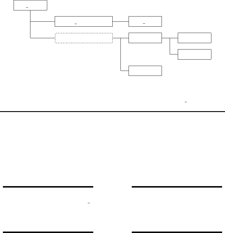
253
w3 make
make makefile.sh
make (unix)
w3 new
ad3
link
w3adc
comp
1
1,2,3 1
1 4
1Suitable for interactive use.
2If makefile does not exist.
3If switch file has been updated.
4Files with extension .ftn only.
Figure 5.1: General layout of the compiler program w3 make.
switch File containing a list of switches as recognized by
the preprocessor w3adc. Linked to ../bin/switch.
The file provided with WAVEWATCH III should
result in a hardware independent code.
WARNING
The auxiliary scripts w3 make etc. use the switch,comp and link
files from the ./bin directory under the WAVEWATCH III home
directory, NOT from the local directory.
WARNING
After the appropriate changes have been made, or the appropriate example
scripts have been copied in, (parts of) WAVEWATCH III can be compiled
and linked. When the program is compiled for the first time, it is suggested
to compile program parts one-by-one to avoid lengthy errors messages, and
to set up error capturing in comp. A good place to start is compilation of
the simple test code ctest. First go to the directory work and make a link
to the source code of this routine by typing
ln3 ctest

254
This link is made to facilitate later inclusion of errors to test or set-up error
capturing in the script comp. The inner workings of the preprocessor w3adc
can be seen by typing the command
ad3 test ctest
which will show how the actual source code is constructed from ctest.ftn,
include files and program switches. Next, the compilation of this subroutine
can be tested by typing
ad3 ctest 1
which invokes both the preprocessor w3adc and the compile script comp. The
1 at the end of this line activates test output. If it is omitted, this command
should result in a single line of output, identifying that the routine is being
processed. If ad3 works as expected, an object file obj/ctest.o is generated. If
requested during the initial set up, a source code and listing file (ctest.f and
ctest.l) can be found in the scratch directory. The listing file is also retained
if compilation errors are detected by comp. At this time, it is prudent to test
error capturing in the script comp by adding errors and warnings to ctest.ftn
in the work directory. The error capturing is discussed in some detail in
the documentation of comp. After comp has been tested, and the errors
in ctest.ftn have been removed, the link to the work directory and the file
obj/ctest.o can be deleted.
After a single routine has been compiled successfully, the next step is to
try to compile and link an entire program. The grid preprocessor can be
compiled by typing
w3 make ww3 grid
If the compilation appears successful, and if the input files have been installed
(see above), the grid preprocessor can be tested by typing
ww3 grid
in the work directory. If the input files have been installed, a link to the
input file ww3 grid.inp will be present in the work directory, and the grid
preprocessor will run and send its output to the screen. Output files of the
grid preprocessor will appear in the work directory. When a program is
compiled for the first time, the operating system might not be able to find
the executable. If this occurs, try to type

255
rehash
or open a new shell to work from. In this way all separate programs can be
compiled and tested. To clean up all temporarily files (such as listings) and
data files of the test runs, type
w3 clean
Note that w3 make only checks the switch file for changes. If the user changes
the compile options in the compile and link scripts comp and link, it is advised
to force the recompilation of the entire program. This can be achieved by
typing
w3 new all or w3 new
before invoking w3 make. This might also be useful if the compilation is
unsuccessful for no apparent reason.
Compilation of the WAVEWATCH III NetCDF enabled programs re-
quires the environment variable WWATCH3 NETCDF be set to either NC3 (com-
pile with NetCDF version 3.x) or NC4 (compile with NetCDF version 4.x).
If the script variable is set to WWATCH3 NETCDF = NC3, then the following
environment variables are required
NETCDF LIBDIR Path to where the NetCDF-3 libraries are in-
stalled.
NETCDF INCDIR Path to where the NetCDF-3 include files are
installed.
If WWATCH3 NETCDF = NC4, then the following environment variable is re-
quired.
NETCDF CONFIG Path to the NetCDF-4 nc-config utility program.
The nc-config utility program (part of the NetCDF-4 install) is used to deter-
mine the appropriate compile and link flags for the WWATCH3 NETCDF = NC4
compile. The NetCDF-4 compile requires NetCDF version 4.1.1 or higher.
Use the command
nc-config --version
to check the version of the installed NetCDF. Compiling with the NC4 switch
requires WWATCH3 NETCDF = NC4 and the NetCDF-4 installation compiled
with the NetCDF-4 API enabled. Use
256
nc-config --has-nc4
to check if the installed NetCDF has the NetCDF-4 API enabled.
Two additional remarks need to be made regarding parallel versions of the
model (OpenMP and MPI versions). First, complications may occur when
preparing executables for running in an MPI environment. Such complica-
tions are discussed in Appendix D. Secondly, the OpenMP code should be
compiled using directives only, i.e., do not use compiler options that auto-
matically thread the code.
5.4 Selecting model options
The file switch in the bin directory contains a set of strings identifying model
options to be selected. Many options are available. Of several groups of
options it is mandatory to select exactly one. These mandatory switches are
described in Section 5.4.1. Other switches are optional, and are described
in Section 5.4.2. Default model setting are identified in Section 5.4.3. The
order in which the switches appear in switch is arbitrary. How these switches
are included in the source code files is described in Section 6.2.
5.4.1 Mandatory switches
Of each of the below groups of switches exactly one has to be selected.
The first group of switches controls the selection of machine-dependent code.
With the introduction of FORTRAN-90 this set of switches should have be-
come obsolete. Problems with some compilers have prompted the retention
of the second switch.
f90 FORTRAN-90 style date and time capturing and program
abort.
dum Dummy to be used if WAVEWATCH III is to be installed
on previously untried hardware.
Hardware model (first group) and message passing protocol (second group).
Note that these two groups share a switch. This implies that the mpi switch
can only be used in combination with the dist switch.
257
shrd Shared memory model.
dist Distributed memory model.
shrd Shared memory model, no message passing.
mpi Message Passing Interface (MPI).
Word length used to determine record length in direct access files
lrb4 4 byte words.
lrb8 8 byte words.
Compilation as a subroutine (called by a coupled model system using PALM)
or a stand-alone program.
nopa Compilation as a stand-alone program
palm Compilation as a subroutine
Selection of propagation schemes and GSE alleviation method. These repre-
sent two sets of switches with some shared switches between the groups. Note
that the second set of switches is secondary to the selection of program mod-
ules in the first set of switches, and therefore, does not have a user-defined
option.
pr0 No propagation scheme / GSE alleviation used.
pr1 First order propagation scheme, no GSE alleviation.
pr2 Higher-order schemes with Booij and Holthuijsen (1987)
dispersion correction.
pr3 Higher-order schemes with Tolman (2002a) averaging tech-
nique.
prx Experimental (user supplied).
pr0 No propagation scheme used.
pr1 First-order propagation scheme.
uno Second-order (UNO) propagation scheme.
uq Third-order (UQ) propagation scheme.
Selection of flux computation:
flx0 No routine used; flux computation included in source terms,
flx1 Friction velocity according to Eq. (2.56).
flx2 Friction velocity from Tolman and Chalikov input.
258
flx3 Idem, with cap of Eq. (2.78) or (2.79).
flx4 Friction velocity according to Eq. (2.136).
flxx Experimental (user supplied).
Selection of linear input:
ln0 No linear input.
seed Spectral seeding of Eq. (3.70).
ln1 Cavaleri and Malanotte-Rizzoli with filter.
lnx Experimental (user supplied).
Selection of input and dissipation. stabnswitches are optional and addi-
tional to corresponding stnswitch:
st0 No input and dissipation used.
st1 WAM3 source term package.
st2 Tolman and Chalikov (1996) source term package. See also
the optional stab2 switch.
stab2 Enable stability correction (2.95) - (2.98) for st2.
st3 WAM4 and variants source term package.
stab3 Enable stability correction from Abdalla and Bidlot (2002)
for st4.
st4 Ardhuin et al. (2010) source term package.
st6 BYDRZ source term package.
stx Experimental (user supplied).
Selection of nonlinear interactions:
nl0 No nonlinear interactions used.
nl1 Discrete interaction approximation (DIA).
nl2 Exact interaction approximation (WRT).
nl3 Generalized Multiple DIA (GMD).
nl4 Two-scale approximation (TSA).
nlx Experimental (user supplied).
Selection of bottom friction:
bt0 No bottom friction used.
bt1 JONSWAP bottom friction formulation.
bt4 SHOWEX bottom friction formulation.
bt8 Dalrymple and Liu formulation (fluid mud seafloor).
259
bt9 Ng formulation (fluid mud seafloor).
btx Experimental (user supplied).
Selection of term for damping by sea ice:
ic0 No damping by sea ice.
ic1 Simple formulation.
ic2 Liu et al. formulation.
ic3 Wang and Shen formulation.
ic4 Frequency-dependent damping by sea ice.
Selection of term for scattering by sea ice:
is0 No scattering by sea ice.
is1 Diffusive scattering by sea ice (simple).
is2 Floe-size dependent scattering and dissipation.
Selection of term for reflection:
ref0 No reflection.
ref1 Enables reflection of shorelines and icebergs
Selection depth-induced breaking of :
db0 No depth-induced breaking used.
db1 Battjes-Janssen.
dbx Experimental (user supplied).
Selection of triad interactions:
tr0 No triad interactions used.
tr1 Lumped Triad Interaction (LTA) method.
trx Experimental (user supplied).
Selection of bottom scattering:
bs0 No bottom scattering used.
bs1 Magne and Ardhuin.
bsx Experimental (user supplied).
Selection of supplemental source term:
xx0 No supplemental source term used.
260
xxx Experimental (user supplied).
Selection of method of wind interpolation (time):
wnt0 No interpolation.
wnt1 Linear interpolation.
wnt2 Approximately quadratic interpolation.
Selection of method of wind interpolation (space):
wnx0 Vector interpolation.
wnx1 Approximately linear speed interpolation.
wnx2 Approximately quadratic speed interpolation.
Selection of method of current interpolation (time):
crt0 No interpolation.
crt1 Linear interpolation.
crt2 Approximately quadratic interpolation.
Selection of method of current interpolation (space):
crx0 Vector interpolation
crx1 Approximate linear speed interpolation.
crx2 Approximate quadratic speed interpolation.
Switch for user supplied GRIB package.
nogrb No package included.
ncep1 NCEP GRIB1 package for IBM SP.
ncep2 NCEP GRIB2 package for IBM SP.
5.4.2 Optional switches
All switches below activate model behavior if selected, but do not require
particular combinations. The following switches control optional output for
WAVEWATCH III programs.
o0 Output of namelists in grid preprocessor.
o1 Output of boundary points in grid preprocessor.

261
o2 Output of the grid point status map in grid preprocessor.
o2a Generation of land-sea mask file mask.ww3 in grid prepro-
cessor.
o2b Output of obstruction map in grid preprocessor.
o2c Print status map in format as read by ww3 grid.
o3 Additional output in loop over fields in field preprocessor.
o4 Print plot of normalized one-dimensional energy spectrum
in initial conditions program.
o5 Id. two-dimensional energy spectrum.
o6 Id. spatial distribution of wave heights (not adapted for
distributed memory).
o7 Echo input data for homogeneous fields in generic shell.
o7a Diagnostic output for output points.
o7b Idem in ww3 multi.
o8 Filter field output for extremely small wave heights in wave
model (useful for some propagation tests).
o9 Assign a negative wave height to negative energy in wave
model. Used in testing phase of new propagation schemes.
o10 Identify main elements of multi-grid model extensions in
standard output.
o11 Additional log output on management algorithm in log.mww3.
o12 Identify removed boundary points in overlapping grids (cen-
ter).
o13 Identify removed boundary points in overlapping grids (edge).
o14 Generate log file with buoy data buoy log.ww3 for output
type ITYPE = 0 in ww3 outp.
o15 Generate log file with time stamps of input data file times.XXX
in ww3 prep.
o16 Generate GrADS output of grid partitioning in ww3 gspl.
The following switches enable parallelization of the model using OpenMP di-
rectives, also known as ‘threading’. Before model version 5.01, threading and
parallelization using the mpi switch could no be used simultaneously. With
version 5.01, pure MPI,pure OMP and hybrid MPI-OMP approaches became
available. Switches used in version 5.01 and higher are not compatible with
switches used in previous model versions.
ompg General loop parallelization directives used for both ex-
clusive OpenMP parallelization and hybrid MPI-OpenMP

262
parallelization.
ompx Idem, but for directives used only for exclusive OpenMP
parallelization.
omph Idem, but for directives used only for hybrid MPI-OpenMP
parallelization.
Note that these switches can only be used in certain combinations, as enforced
in the model installation scripts (particularly make makefile.sh. A pure MPI
approach requires the dist and mpi switches. A pure OpenMP approach re-
quires the shrd,ompg and ompx switches, and the hybrid approach requires
the dist,mpi,ompg, and omph switches.
The following switches are associated with the continuously moving grid op-
tions. The first switch activates the option, the other two are optional addi-
tions.
mgp Activate propagation correction in Eq. (3.45).
mgw Apply wind correction in moving grid approach.
mgg Activate GSE alleviation correction in Eq. (3.48).
The following compiler dependent switches are available. They may not have
been maintained for recent compiler versions.
c90 Compiler directives for Cray C90 (vectorization).
nec Compiler directives for NEC SX6/SX8 (vectorization).
Furthermore the following miscellaneous switches are available:
arc Arctic grid option for SMC grid10.
cou Activates the calculation of variables required for coupling
dss0 Switch off frequency dispersion in diffusive dispersion cor-
rection.
fld1 Sea-state dependent τReichl et al. (2014) (Section 2.5.2).
fld2 Sea-state dependent τDonelan et al. (2012) (Section 2.5.3).
ig1 Second-order spectrum and free infragravity waves (Sec-
tion 2.4.8.
mlim Use Miche-style shallow water limiter of Eq. (3.71).
mpibdi Experimental parallelization of multi-grid model initializa-
tion.
10 Not yet fully tested according to author.

263
mpit Test output for MPI initializations.
mprf Profiling of individual models and nesting in ww3 multi.
nc4 Activates the NetCDF-4 API in the NetCDF pre- and post-
processing programs.
ncc NCEP coupler.
nco Code modifications for operational implementation at NCO
(NCEP Central Operations). Mostly changes unit numbers
and file names. Not recommended for general use.
nls Activate nonlinear smoother (Section 2.3.6).
nnt Generate file test data nnn.ww3 with spectra and nonlin-
ear interactions for training and testing of NNIA.
oasis Initializes OASIS Coupler (App. F.3).
oasacm OASIS atmospheric model coupling fields(App. F.3).
oasocm OASIS oceanic model coupling fields (App. F.3).
refrx Enables refraction based on spatial gradients in phase ve-
locity (Section 2.4.3)
reft Test output for shoreline reflection (which is activated with
ref1).
rtd Rotated grid option.
rwnd Correct wind speed for current velocity.
sEnable subroutine tracing in the main WAVEWATCH III
subroutines by activating calls to the subroutine strace.
scrip Enable SCRIP remapping routines (App. E.3)
scripnc Enable storage of remapping weights in NetCDF files (App.
E.3)
sec1 Enable the use of global time steps less than 1 s, but does
not allow output at time steps less than 1 s.
smc Activate SMC grid.
tEnable test output throughout the program(s).
tn Id.
tdyn Dynamic increment of swell age in diffusive dispersion cor-
rection (test cases only).
tide Enables tidal analysis: used for pre-processing of input
files, run-time tidal prediction in ww3 shel or tidal pre-
diction with ww3 prtide.
tidet test output for tidal analysis.
trknc Activates the NetCDF API in the wave system tracking
post-processing program. Selecting TRKNC alone will gen-

264
erate NetCDF-3 files. Selecting both TRKNC and NC4 will
generate NetCDF-4 files.
xw0 Swell diffusion only in ULTIMATE QUICKEST scheme.
xw1 Id. wave growth diffusion only.
5.4.3 Default model settings
Up to model version 3.14, the NCEP operational model setup was considered
as the default model setup. However, with subsequent versions of WAVE-
WATCH III, the model has evolved into a modeling framework rather than
a single model. With this, WAVEWATCH III is run differently at various
centers, and a clear “default” model version can no longer be identified.
Nevertheless, in order to be able to concisely identify in publications ex-
actly which model setup is used, “default” configurations of various centers
are now provided in the bin directory. These configurations are provided
in example switch files and README files, such as switch NCEP st2 and
README.NCEP. Note that these files are provided to simplify referring to
model version, but do not imply an endorsement of the specific model con-
figuration.; in this context, it should be noted that by nature, model versions
at operational centers are in a continuous state of development.
5.5 Modifying the source code
Source code can obviously be modified by editing the source code files in the
ftn directory. However, it is usually more convenient to modify source code
files from the work directory work. This can be done by generating a link
between the ftn and work directories. Such a link can be generated by typing
ln3 filename
where filename is the name of a source code or include file, with or without
its proper extension. Working from the work directory is recommended for
several reasons. First, the program can be tested from the same directory,
because of similar links to the input files. Secondly, links to the relevant
switch, compile and link programs are also available in this directory. Third,

265
it makes it easy to keep track of files which have been changed (i.e., only
those files to which links have been created might have been changed), and
finally, source codes will not disappear if files (links) are accidentally removed
from the work directory.
Modifying source codes is straightforward. Adding new switches to ex-
isting subroutines, or adding new modules requires modification of the au-
tomated compilation scripts. If a new subroutine is added to an existing
module, no modifications are necessary. If a new module is added to WAVE-
WATCH III, the following steps are required to include it in the automatic
compilation:
1) Add the file name to sections 2.b and c of make makefile.sh to
assure that the file is included in the makefile under the correct
conditions.
2) Modify section 3.b of this script accordingly to assure that the
proper module dependency is checked. Note that the dependency
with the object code is checked, allowing for multiple or inconsis-
tent module names in the file.
3) Run script interactively to assure that makefile is updated.
For details of inclusion, see the actual scripts. Adding a new switch to the
compilation systems requires the following actions:
1) Put switch in required source code files.
2) If the switch is part of a new group of switches, add a new ’key-
word’ to w3 new.
3) Update files to be touched in w3 new if necessary.
4) Update make makefile.sh with the switch and/or keyword.
These modifications need only be made if the switch selects program parts.
For test output etc., it is sufficient to simply add the switch to the source
code. Finally, adding an old switch to an additional subroutine requires these
actions:
1) Update files to be touched in w3 new.
If WAVEWATCH III is modified, it is convenient to maintain copies of
previous versions of the code and of the compilation scripts. To simplify this,
an archive script (arc wwatch3) is provided. This script generates tar files that

266
can be reinstalled by the install program install wwatch3. The archive files
are gathered in the directory arc. The names of the archive files can contain
user defined identifiers (if no identifier is used, the name will be identical
to the original WAVEWATCH III files). The archive program is invoked by
typing
arc wwatch3
The interactive input to this script is self-explanatory. An archive file can be
re-installed by copying the corresponding tar files to the WAVEWATCH III
home directory, renaming them to the file names expected by the install
program, and running the install program.
For co-developers using the NCEP svn repository, changes in the code
should be made using the best practices as outlined in (Tolman,2014c).
5.6 Running test cases
If WAVEWATCH III is installed and compiled successfully, it can be tested
by running different program elements interactively from the work directory.
The switch settings in the generic switch file correspond to the activated
inputs in the example input files. It should therefore be possible to run all
model elements by typing
ww3 grid | more
ww3 strt | more
ww3 bound | more
ww3 prep | more
ww3 shel | more
ww3 outf | more
ww3 outp | more
ww3 ounf | more
ww3 ounp | more
ww3 trck | more
ww3 grib | more
gx outf | more
gx outp | more

267
where the more command is added to allow for on-screen inspection of the
output. This | more can be replaced by redirection to an output file, e.g.
ww3 grid > ww3 grid.out
Note that ww3 grib will only provide GRIB output if a user-supplied packing
routine is linked in. Note furthermore that no simple interactive test case
for ww3 multi is provided. GrADS can then be run from the work directory
to generate graphical output for these calculations. All intermediate output
files are placed in the work directory, and can be removed conveniently by
typing
w3 clean
Up to version 3.14, WAVEWATCH III was provided with a set of simple
tests to established assess the proper behavior of the basic functionality of
the model. In the early development of the next release of the model, Erick
Rogers and Tim Campbell converted these in regression tests that could be
run more easily in an automated version. Up to model version 4.06, these
modified tests were gathered in the nrltest directory, while keeping the old
tests in the test directory. In model version 4.07, the nrltest were adopted
as the new test cases for WAVEWATCH III in a new regtests directory,
while eventually the remaining real-world test cases in test were moved to
the cases directory, while discontinuing the test directory completely. The
following regression tests are available in the regtests directory.
ww3 tp1.1 1D propagation around the world along the equator
(no land).
ww3 tp1.2 1D propagation, along meridian (no land).
ww3 tp1.3 1D propagation, shoaling test.
ww3 tp1.4 1D propagation, spectral refraction (x).
ww3 tp1.5 1D propagation, spectral refraction (y).
ww3 tp1.6 1D propagation, wave blocking by current.
ww3 tp1.7 1D propagation, IG wave generation.
ww3 tp1.8 1D propagation, wave breaking on a beach.
ww3 tp1.9 1D propagation, Beji and Battjes (1993) barred flume
case.
ww3 tp2.1 2D propagation under angle with grid.
ww3 tp2.2 2D propagation over half the globe without land
(with directional spread).

268
ww3 tp2.3 2D propagation, GSE test.
ww3 tp2.4 2D propagation, East Pacific curvilinear grid test.
ww3 tp2.5 2D propagation, Arctic Grid, curvilinear grid test.
ww3 tp2.6 2D propagation, Limon Harbor unstructured grid
test.
ww3 tp2.7 Reflection on a 2D unstructured grid.
ww3 tp2.8 Tidal constituents on a 2D regular grid.
ww3 tp2.9 Tests for obstruction grids.
ww3 tp2.10 Tests for SMC grid.
ww3 tp2.11 Tests for rotated grid.
ww3 tp2.12 Test for system tracking.
ww3 tp2.13 Test for propagation under angle with grid (tripole)
ww3 tp2.14 Test for toy-model using OASIS coupler.
ww3 tp2.15 Test for space-time extremes parameters.
ww3 ts1 Source term test, time limited growth.
ww3 ts2 Source term test, fetch limited growth.
ww3 ts3 Source term test, hurricane with single moving grid.
ww3 tic1.1 Wave-ice interaction, 1D test of Sice.
ww3 tic1.2 Wave-ice interaction, 1D test of “shoaling” effect.
ww3 tic1.3 Wave-ice interaction, 1D test of refraction effect.
ww3 tic1.4 Wave-ice interaction, 1D test with ice floes and ice
thickness.
ww3 tic2.1 Wave-ice interaction, 2D test of Sice.
ww3 tic2.2 Wave-ice interaction, 2D test with non-uniform ice.
ww3 tic2.3 Wave-ice interaction, 2D test with uniform ice with
increasing thickness.
ww3 tbt1.1 Wave-mud interaction, 1D test of Smud.
ww3 tbt2.1 Wave-mud interaction, 2D test of Smud.
mww3 test 01 Test for expanded grid mask with wetting and dry-
ing, etc.
mww3 test 02 Two-way nesting test with single inner grid.
mww3 test 03 Overlapping grids and two-way nesting tests (6-grid
version with beach in high-resolution grids.)
mww3 test 04 Current or sea-mount test for two-way nesting with
stationary swell conditions.
mww3 test 05 Three nested hurricane grids with moving grids test.
mww3 test 06 Tests for irregular grid(s) w/ ww3 multi.
mww3 test 07 Tests for unstructured grid(s) w/ ww3 multi.

269
mww3 test 08 Tests with wind and ice input.
These regression tests are now run using the run test script in the regtests/bin
directory (primary author: Tim Campbell). How to run this script, including
options, is shown by running
run test -h
The output of running this command is shown here in Fig. 5.2. The test cases
are stored in directories under the regtests directory, e.g. regtests/ww3 tp1.1.
For example, the contents of /ww3 tp1.1 might be
info A file containing information about the test case.
input A permanent directory containing input files for the
test case.
work PR3 A scratch directory for model output (in this exam-
ple, filename is such because the user had specified
“run test -w work PR3 ...”).
Also provided now is a matrix if regression tests, used by the code developers
to assure that new model versions do not break older model versions. The
core of this matrix is the file regtests/bin/matrix.base. An example of how to
run this is given in regtests/bin/matrix zeus HLT, which is Hendrik’s driver
for the matrix at the NCEP Zeus R&D computer11. To run this, make a link
to it in the regtests directory and execute after setting the desired option
flags in the script. This will make a file matrix in retests, which can then be
run interactively or in batch mode as desired. The file can also be manually
edited further if so desired. The bin directory under regtests contains the
following tools.
cleanup Cleanup work directories.
comp switch Compare switches inside and across test cases. comp switch
-h provides documentation.
matrix.base Core script to generate matrix of test cases.
matrix.comp Script to compare output of matrix of test cases
between separately checked out model versions.
matrix zeus HLT Example of driver for matrix.base.
11 Please build your own driver for your own setup using this as a blueprint, rather than
editing this file.

270
run test Basic test script as described above.
Note that efficient running of the matrix of regression tests requires a min-
imization of the need to recompile code between regression tests. This is
achieved by the ordering of the regression tests in matrix.base. A way to as-
sure that identical switch files are identified as such is to systematically sort
them. This can be done with the script sort switch in the main bin directory.
This script will add default values of missing switches and can also be used
to remove or add switches from the file. Run
comp switch -h
for documentation of the script.
Finally, the cases directory hold the real-world test cases as described below.
mww3 case 01 Atlantic case with five grids focusing on Trondheim.
mww3 case 02 Pacific case with three grids focusing on Alaska.
mww3 case 03 Original multi-grid case used as global model at
NCEP.
Each of these cases is a single script executing the entire model run. Before
executing the script, compile the model with the switches indicated in the
documentation at the head of the script. Additional data used by these
scripts is contained in the directories
mww3 data 00 Wind fields and ice data used by all example cases.
mww3 data nn Specific data needed for script mww3 case nn.
These examples can be used as blueprints for setting up other real model
applications.

271
Usage: run_test [options] source_dir test_name
Required:
source_dir : path to top-level of WW3 source
test_name : name of test case (directory)
Options:
-a ww3_env : use WW3 environment setup file <ww3_env>
: *default is <source_dir>/wwatch3.env
: *file will be created if it does not already exist
-c cmplr : setup comp & link files for specified cmplr
-C : enable coupling using OASIS3-mct
-d : invoke main program using gdb (non-parallel)
-e : prompt for changes to existing WW3 environment
-f : force pre- and post-processing programs to be compiled
: non-MPI (i.e., with SHRD switch); default is all programs
: compiled with unmodified switch settings
-g grid_string : use ww3_grid_<grid_string>.inp
-G : create GrADS data files using gx_outX.inp
-h : print usage and exit
-i inpdir : use inputs in test_name/<inpdir> (default test_name/input)
-m grid_set : execute multi-model test
: *grid names are obtained from input/<grid_set>
: *ww3_multi_<grid_set> will execute instead of ww3_shel
: *to execute a single model test case with ww3_multi use
: grid_set = none
-n nproc : specify <nproc> processors for parallel run
: *some <runcmd> programs do not require <nproc>
: *ignored if -p <runcmd> or -O is not specified
-o outopt : limit output post-processing based on <outopt>
: native : post-process only native output
: netcdf : post-process only NetCDF output
: both : post-process both native and NetCDF output
: * default is native
: * note that required input files must be present for
: selected output post-processing to occur
-O : parallel run using OpenMP paradigm and OMP_NUM_THREADS
environment variable and number of processors defined with
the -n np option
-p runcmd : run in parallel using <runcmd> to start program
: *MPICH or OpenMPI: mpirun or mpiexec (default <nproc> = 1)
: *IBM with Loadleveler: poe (no <nproc> required)
: *LSF: mpirun.lsf (no <nproc> required)
-q program : exit script after program <program> executes
-r program : only execute program <program>
-s switch_string : use switch_<switch_string>
-S : create stub file <finished>. with end data and time.
tests not executed if file is found.
-t nthrd : Threading option. (this is system dependant and can be used
: only for the hybrid option)
-w work_dir : run test case in test_name/work_dir (default test_name/work)
Figure 5.2: Options for run test, as obtained by running it with the -h com-
mand line option.

272
6 System documentation
6.1 Introduction
In this chapter a brief system documentation is presented. Discussed are the
custom preprocessor used by WAVEWATCH III (Section 6.2), the contents
of the different source code files (Section 6.3), optimization (Section 6.4), and
the internal data storage (Section 6.5). For a more elaborate documentation,
reference is made to the source code itself, which is fully documented.
6.2 The preprocessor
The WAVEWATCH III source code files are not ready to use FORTRAN
files; mandatory and optional program options still have to be selected, and
test output may be activated12. Compile level options are activated using
‘switches’. The arbitrary switch ’swt’ is included in the WAVEWATCH III
files as comment of the form !/swt, where the switch name swt is followed
by a space or by a ’/’. If a switch is selected, the preprocessor removes the
comment characters, thus activating the corresponding source code line. If ’/’
follows the switch, it is also removed, thus allowing the selective inclusion of
hardware-dependent compiler directives etc. The switches are case sensitive,
and available switches are presented in Section 5.4. Files which contain the
switch c/swt can be found by typing
find switch ’!/SWT’
A list of all switches included in the WAVEWATCH III files can be obtained
by typing
all switches
12 Exceptions are some modules that are not originally part of WAVEWATCH III, like
the exact interaction modules. Such modules with the extension .f of .f90 bypass the
preprocessor and get copied to the work directory with the .f extension.

273
0 1
constants.ftn’ constants.f’
’F90 NOGRB LRB4 SHRD NOPA PR3 UQ FLX2 LN1 ST2 STAB2
NL1 BT1 DB1 MLIM TR0 BS0 XX0 WNX1 WNT1 CRX1 CRT1
O0 O1 O2 O3 O4 O5 O6 O7 O11 O14’
Figure 6.1: Example input for w3adc.
Pre-processing is performed by the program w3adc. This program is found
in the file w3adc.f, which contains a ready to compile FORTRAN source
code and a full documentation13. Various properties of w3adc are set in
parameter statements in w3adc.f, i.e., the maximum length of switches,
the maximum number of include files, the maximum number of lines in an
include file and the line length. w3adc reads its ‘commands’ from standard
input. An example input file for w3adc is given in Fig. 6.1. Line-by-line, the
input consists of
→Test indicator and compress indicator.
→File names of the input and output code.
→Switches to be turned on in a single string (see Section 5.4).
→Additional lines with include files can be given, but these are no longer
used in the automated compile system.
A test indicator 0 disables test output, and increasing values increase the
detail of the test output. A compress indicator 0 leaves the file as is. A
compress indicator 1 results in the removal of all comment lines indicated
by ’!’, except for empty switches, i.e., lines starting with ’!/’. A compress
indicator 2 results in the subsequent removal of all comments. Comment
lines are not allowed in this input file. The above input for w3adc is read
using free format. Therefore quotes are needed around strings. Echo and
test output is send to the standard output device. To facilitate the use of
the preprocessor, several UNIX scripts are provided with WAVEWATCH III
13 Presently still in fixed-format FORTRAN-77.

274
as discussed in Section 5.3. Note that compiler directives are protected from
file compression by defining them using a switch.
6.3 Program files
The WAVEWATCH III source code files are stored in files with the extension
ftn14. Starting with version 2.00, the code has been organized in modules.
Only the main programs are not packaged in modules. Originally, variables
were bundled with the code modules, resulting in a single static data struc-
ture. In model version 3.06, a separate dynamical data structure was intro-
duced, allow for the presence of multiple wave grids in a single program, as
a preparation for the development of the the multi-grid model driver.
The subroutines contained in the modules are described in some detail
below. The relation between the various subroutines is graphically depicted
in Figs. 6.2 and 6.3. Three groups of codes are considered. The first are
the main wave model subroutine modules, which are generally identified by
the file name structure w3xxxxmd.ftn. These modules are described in Sec-
tion 6.3.1. The second group consists of modules specific to the multi-grid
wave model driver, which are generally identified by the file name structure
wmxxxxmd.ftn. These modules are described in Section 6.3.2. The final group
consists of auxiliary programs and wave model drivers, and is described in
Section 6.3.4. Section 6.3.3 briefly describes the data assimilation module.
6.3.1 Wave model modules
At the core of the wave model are the wave model initialization module and
the wave model module.
Main wave model initialization module w3initmd.ftn
w3init The initialization routine w3init, which prepares the
wave model for computations (internal).
w3mpii MPI initialization (internal).
w3mpio MPI initialization for I/O (internal).
14 with the exception of some modules provided by others.
275
w3mpip MPI initialization for I/O (internal, point output only).
Main wave model module w3wavemd.ftn
w3wave The actual wave model w3wave.
w3gath Data transpose to gather data for spatial propagation
in a single array (internal).
w3scat Corresponding scatter operation (internal).
w3nmin Calculate minimum number of sea points per processor
(internal).
The main wave model routines and all other subroutines require a data struc-
ture to exist. The data structure is contained in the following modules.
Define model grids and parameter settings w3gdatmd.ftn
w3nmod Set number of grids to be considered.
w3dimx Set dimensions for spatial grid and allocate storage.
w3dims Set dimensions for spectral grid and allocate storage.
w3setg Set pointers to selected grid.
w3dimug Set dimensions for arrays specific to the triangle-based
grids (grid connectivity ...).
w3gntx Develop unstructured grid structures.
Dynamic wave data describing sea state w3wdatmd.ftn
w3ndat Set number of grids to be considered.
w3dimw Set dimensions and allocate storage.
w3setw Set pointers to selected grid.
Auxiliary storage w3adatmd.ftn
w3naux Set number of grids to be considered.
w3dima, w3xdma, w3dmnl
Set dimensions and allocate storage.
w3seta, w3xeta
Set pointers to selected grid.

276
Model output w3odatmd.ftn
w3nout Set number of grids to be considered.
w3dmo2, w3dmo3, w3dmo5
Set dimensions and allocate storage.
w3seto Set pointers to selected grid.
Model input w3idatmd.ftn
w3ninp Set number of grids to be considered.
w3dimi Set dimensions and allocate storage.
w3seti Set pointers to selected grid.
The input fields such as winds and currents are transferred to the model
through the parameter list of w3wave. The information is processed within
w3wave by the routines in the following module.
Input update module w3updtmd.ftn
w3ucur Interpolation in time of current fields.
w3uwnd Interpolation in time of wind fields.
w3uini Generate initial conditions from the initial wind field.
w3ubpt Updating of boundary conditions in nested runs.
w3uice Updating of the ice coverage.
w3ulev Updating of water levels.
w3utrn Updating grid box transparencies.
w3ddxy Calculation of spatial derivatives of the water depth.
w3dcxy Calculation of spatial derivatives of the currents.
There are seven types of WAVEWATCH III data files (other than the pre-
processed input fields, which are part of the program shall rather than the
actual wave model). The corresponding routines are gathered in six modules.
I/O module (mod def.ww3)w3iogrmd.ftn
w3iogr Reading and writing of mod def.ww3.
I/O module (out grd.ww3)w3iogomd.ftn
w3outg Calculation of gridded output parameters.

277
w3iogo Reading and writing of out grd.ww3.
I/O module (out pnt.ww3)w3iopomd.ftn
w3iopp Processing of requests for point output.
w3iope Calculating point output data.
w3iopo Reading and writing of out pnt.ww3.
I/O module (track o.ww3)w3iotrmd.ftn
w3iotr Generate track output in track o.ww3.
I/O module (restart.ww3)w3iorsmd.ftn
w3iors Reading and writing of restartn.ww3.
I/O module (nest.ww3)w3iobcmd.ftn
w3iobc Reading and writing of nestn.ww3.
I/O module (partition.ww3)w3iofsmd.ftn
w3iofs Writing of partition.ww3.
There are presently several propagation schemes and GSE alleviation tech-
niques available for rectangular and curvilinear grids, as well as a ’slot’ for
a user supplied propagation routine, and there are four schemes for triangle-
based grids. The propagation schemes are packaged in the following modules.
Propagation module (first order, no GSE alleviation) w3pro1md.ftn
w3map1 Generation of auxiliary maps.
w3xyp1 Propagation in physical space.
w3ktp1 Propagation in spectral space.
Propagation module (higher order scheme with GSE diffusion) w3pro2md.ftn
w3map2 Generation of auxiliary maps.
w3xyp2 Propagation in physical space.
w3ktp2 Propagation in spectral space.
278
Propagation module (higher order scheme with GSE averaging) w3pro3md.ftn
w3map3 Generation of auxiliary maps.
w3mapt Generation of transparency maps.
w3xyp3 Propagation in physical space.
w3ktp3 Propagation in spectral space.
Propagation module (slot for user supplied routines) w3proxmd.ftn
w3xypx Propagation in physical space.
w3ktpx Propagation in spectral space.
Propagation module (generic UQ) w3uqckmd.ftn
w3qcknRoutines performing ULTIMATE QUICKEST scheme
in arbitrary spaces (1: regular grid. 2: irregular grid
3: regular grid with obstructions).
Propagation module (generic UNO) w3uqckmd.ftn
w3uno, w3unor w3unos
Like UQ schemes above.
SMC grid routines w3psmcmd.ftn
W3PSMC Spatial propagation on SMC grid.
W3KSMC Spectral modification by GCT and refraction.
SMCxUNO2/3 Irregular grid mid-flux on U-faces by UNO2/3.
SMCyUNO2/3 Irregular grid mid-flux on V-faces by UNO2/3.
SMCxUNO2r/3r Regular grid mid-flux on U-faces by UNO2/3.
SMCyUNO2r/3r Regular grid mid-flux on V-faces by UNO2/3.
SMCkUNO2 Shift in k-space due to refraction by UNO2.
SMCGradn Evaluate field gradient at cell centre.
SMCAverg 1-2-1 weighted average for centre field.
SMCGtCrfr Refraction and GCT rotation in theta.
SMCDHXY Evaluate depth gradient and refraction limiter.
SMCDCXY Evaluate current velocity gradient.
W3GATHSMC W3SCATSMC
Gather and scatter spectral components.
279
Triangle-based propagation schemes w3profsmd.ftn
w3xypug Interface to the unstructured propagation schemes.
w3cflug Computes the maximum CFL number for spatial prop-
agation.
w3xypfsn2 N-scheme.
w3xypfspsi2 PSI-scheme.
w3xypfsnimp Implicit version of the N-scheme.
w3xypfsfct2 FCT-scheme.
bcgstab Part of the iterative SPARSKIT solver, used for the
implicit scheme.
The source term calculation and integration is contained in several modules.
The module w3srcemd.ftn manages the general calculation and integration.
Additional modules contain the actual source term options.
Source term integration module w3srcemd.ftn
w3srce Integration of source terms.
Flux (stress) module (Wu, 1980) w3flx1md.ftn
w3flx1 Calculation of stresses.
Flux (stress) module (Tolman and Chalikov) w3flx2md.ftn
w3flx2 Calculation of stresses.
Flux (stress) module (Tolman and Chalikov, capped) w3flx3md.ftn
w3flx3 Calculation of stresses.
Flux (stress) module (slot for user supplied routines) w3flxxmd.ftn
w3flxx Calculation of stresses.
inflxx Initialization routine.
Linear input (Cavaleri and Malanotte Rizzoli) w3sln1md.ftn
w3sln1 Calculation Slin.

280
Linear input (slot for user supplied routines) w3slnxmd.ftn
w3slnx Calculation Slin.
inslnx Corresponding initialization routine.
Input and dissipation module (dummy version) w3src0md.ftn
w3spr0 Calculation of mean wave parameters (single grid point).
Input and dissipation module (WAM-3) w3src1md.ftn
w3spr1 Calculation of mean wave parameters (single grid point).
w3sin1 Calculation of Sin.
w3sds1 Calculation of Sds.
Input and dissipation module Tolman and Chalikov 1996 w3src2md.ftn
w3spr2 Calculation of mean wave parameters (single grid point).
w3sin2 Calculation of Sin.
w3sds2 Calculation of Sds.
inptab Generation of the interpolation table for β.
w3beta Function to calculate β(internal).
Input and dissipation module WAM-4 and ECWAM. w3src3md.ftn
w3spr3 Calculation of mean wave parameters (single grid point).
w3sin3 Calculation of Sin.
w3sds3 Calculation of Sds.
tabu stress Tabulation of wind stress as a function of U10 and τw
tabu tauhf Tabulation of the short waves-supported stress
calc ustar Computes friction velocity using stress table
Input and dissipation module Ardhuin et al. 2010 w3src4md.ftn
w3spr4 Calculation of mean wave parameters (single grid point).
w3sin4 Calculation of Sin.
w3sds4 Calculation of Sds.
tabu stress Tabulation of wind stress as a function of U10 and τw
tabu tauhf Tabulation of the short waves-supported stress

281
tabu tauhf2 Tabulation of the short waves-supported stress with
sheltering
tabu swellft Tabulation of oscillatory friction factor for negative
part of Sin.
calc ustar Computes friction velocity using stress table
Input and dissipation module BYDRZ w3src6md.ftn
w3spr6 Integral parameter calculation following st1.
w3sin6 Observation-based wind input.
w3sds6 Observation-based dissipation.
irange Generate a sequence of integer values.
lfactor Calculate reduction factor for Sin.
tauwinds Normal stress calculation for Sin.
polyfit2 Quadratic fit using least-squares.
Input and dissipation module (slot for user supplied routines) w3srcxmd.ftn
w3sinx Calculation of Sin.
w3sdsx Calculation of Sds.
Swell dissipation module w3swldmd.ftn
w3swl4 Ardhuin et al (2010+) swell dissipation.
w3swl6 Babanin (2011) swell dissipation.
irange Generate a sequence of integer values.
Nonlinear interaction module (DIA) w3snl1md.ftn
w3snl1 Calculation of Snl.
insnl1 Initialization for Snl.
Nonlinear interaction module (WRT) w3snl2md.ftn
w3snl2 Interface routine for Snl.
insnl2 Initialization for Snl.
These routines provide the interface to the WRT routines. The WRT routines
are provided in the files mod constants.f90,mod fileio.f90,mod xnl4v4.f90, and
serv xnl4v4.f90. For details on these files, see Van Vledder (2002b).
Nonlinear interaction module (GMD) w3snl3md.ftn

282
w3snl3 Calculation of Snl.
expand Expand spectral space.
expan2 Map form expanded to original spectral space.
insnl3 Initialization for Snl.
Nonlinear interaction module (slot for user supplied routines) w3snlxmd.ftn
w3snlx Calculation of Snl.
insnlx Initialization for Snl.
Nonlinear high-frequency filter w3snlsmd.ftn
w3snls Calculation of filter.
expand Expand spectral space.
insnls Initialization for filter.
Bottom friction module (JONSWAP) w3sbt1md.ftn
w3bt1 Calculation of Sbot.
Bottom friction module (SHOWEX) w3sbt4md.ftn
insbt4 Initialization of Sbot)
tabu erf Table or error function.
w3sbt4 Calculation of Sbot, and energy and momentum fluxes
to the bottom boundary layer.
Fluid mud dissipation (Dalrymple and Liu,1978)w3sbt8md.ftn
w3sbt8 Source term.
283
Fluid mud dissipation (Ng,2000)w3sbt9md.ftn
w3sbt9 Source term.
Bottom friction module (slot for user supplied routines) w3sbtxmd.ftn
w3sbtx Calculation of Sbot.
insbtx Initialization of Sbot.
Depth induced breaking module (Battjes-Janssen) w3sdb1md.ftn
w3sdb1 Calculation of Sdb.
Depth induced breaking module (slot for user supplied routines) w3sdbxmd.ftn
w3sdbx Calculation of Sdb.
insdbx Initialization of Sdb.
Triad interactions module (LTA) w3str1md.ftn
w3str1 Calculation of Str.
Triad interactions module (slot for user supplied routines) w3strxmd.ftn
w3strx Calculation of Str.
instrx Initialization of Str.
Bottom scattering module w3sbs1md.ftn
w3sbs1 Calculation of Sbs and associated momentum flux to
the bottom.
insbs1 Initialization of Sbs.
Bottom scattering module (slot for user supplied routines) w3sbsxmd.ftn
w3sbsx Calculation of Sbs.
insbsx Initialization of Sbs.

284
Wave-ice interactions (simple) w3sic1md.ftn
w3sic1 Calculation of Sid.
Wave-ice interactions (Liu et al.) w3sic2md.ftn
w3sic2 Calculation of Sid.
Interpolation tables.
Wave-ice interactions Wang and Shen (2010)w3sic3md.ftn
w3sic3 Calculation of Sid.
bsdet Calculate the determinant for the dispersion relation.
wn complex Calculate complex wavenumber in ice.
cmplx root muller Find root for complex numbers.
fun zhao Wrapper for functions below.
func0 zhao, finc1 zhao
w3sis2 Calculation of Sis.
Waves scattering in ice and ice break-up w3sis2md.ftn
Shoreline reflection w3ref1md.ftn
w3ref1 Calculation of Sref .
Module for unclassified source term (slot for user supplied routines) w3sxxxmd.ftn
w3sxxx Calculation of Sxx.
insxxx Initialization of Sxx.
To complete the basic wave model, several additional modules are needed.
For the actual contents of the service modules see the documentation in the
source code files.
constants.ftn Physical and mathematical constants and Kelvin
functions.
w3arrymd.ftn Array manipulation routines including ’print plot’
routines.
w3bullmd.ftn Perform bulletin style output for output points.
w3cspcmd.ftn Conversion of spectral discretization.

285
w3init w3iogr
w3iors
w3iopp
w3mpii
w3mpio
w3mpip
w3flgrdupdt
Figure 6.2: Subroutine structure for wave model initialization routine with-
out service routines, data base management routines and MPI calls. Note
that w3iogr on reading data in calls all necessary initialization routines for
interpolation tables and physics parameterizations.
w3dispmd.ftn Routines to solve the Laplace dispersion relation
(linear waves, flat bottom, no ice), including in-
terpolation tables. Includes also ice corrections in
liu foreward dispersion and liu inverse dispersion.
w3gsrumd.ftn Regridding utilities.
w3partmd.ftn Perform spectral partitioning for a single spectrum.
w3servmd.ftn General service routines.
w3timemd.ftn Time management routines.
w3triamd.ftn Basic routines for triangle-based grids: reading, in-
terpolation, definition of miscellaneous arrays, de-
termination of boundary points.
This completes the description of the basic wave model routines. The re-
lation between the initialization routine and other routines is illustrated in
Fig. 6.2. A similar relational diagram for the wave model routine is presented
in Fig. 6.3.
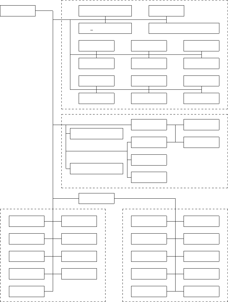
286
w3wave
input
w3ice3wncg w3ucur
ug gradients w3dzxy / smcdxy
w3uwnd w3uini w3iobc
w3ubpt w3uice w3ulev
w3mapnw3utrn w3nmin
w3cflug w3cflxy w3nmin
propagation
w3ktpn
w3gath(smc)
w3xypn
w3xypug
w3psmc
w3scat(smc)
w3qckn
w3unon
source terms
w3srce
w3sprnw3flxn
w3slnnw3sinn
w3snlnw3sdsn
w3swlnw3sbtn
w3sicn. . .
output
w3cprt w3outg
w3iogo w3iope
w3iopo w3iotr
w3iors w3iobc
w3iosf
Figure 6.3: Subroutine structure for wave model routine without service
routines, routines managing the data structures, and mpi routines. ‘. . . ’
identifies additional source term routines.

287
6.3.2 Multi-grid modules
The multi-grid wave model shel ww3 multi provides a shell around the basic
wave model as described in the previous section. This shell manages the side-
by-side running of multiple wave model grids, and all communication between
the grids. To achieve this various additional modules have been developed.
At the core are the initialization, multi-grid model and finalization routines.
Initialization of multi-grid model wminitmd.ftn
wminit Multi-grid model initialization.
Running of multi-grid model wmwavemd.ftn
wmwave Multi-grid model execution.
wmprnt Printing to log file.
wmbcst Non-blocking MPI broadcast.
wmwout Idem.
Finalizing of multi-grid model wmfinlmd.ftn
wmfinl Multi-grid model finalization.
These routines are designed to become part of a coupled model. For the
structure of the actual wave model routine, reference is made to Tolman
(2007). The resulting wave model driver ww3 multi consequently becomes
extremely simple; it initializes the MPI environment, and then calls the above
three modules consecutively.
The main multi-grid wave model routines require an expansion of the
data structure used by WAVEWATCH III. Furthermore, main activities are
gathered in subroutines in various modules.
Data storage wmmdatmd.ftn
wmndat Set number of grids to be considered.
wmdimd, wmdimm
Set dimensions and allocate storage.
wmsetm Set pointers to selected grid.
288
Determine grid relations wmgridmd.ftn
wmglow Relations to lower ranked grids.
wmghgh Relations to higher ranked grids.
wmgeql Relations between equal ranked grids.
wmrspc Determine need for spectral conversion between grids.
Update model input wmupdtmd.ftn
wmupdt General input update routine.
wmupd1 Update input from native files using w3fldsmd.ftn from
Section 6.3.4.
wmupd2 Update input from pore-defined input grids.
wmupdv Update vector fields.
wmupds Update scalar fields.
Perform internal communications wminiomd.ftn
wmiobs Stage internal boundary data.
wmiobg Gather internal boundary data.
wmiobf Finalize wmiobs (MPI only).
wmiohs Stage internal high to low rank data.
wmiohg Gather internal high to low rank data.
wmiohf Finalize wmiohs (MPI only).
wmioes Stage internal data between equal ranked grids.
wmioeg Gather internal data between equal ranked grids.
wmioef Finalize wmioes (MPI only).
Unify point output to single file wmiopomd.ftn
wmiopp Initialization routine.
wmiopo Data gather and write routine (using w3iopo in w3iopomd.ftn).
To complete the multi-grid wave model, one additional service module is
needed. For the actual contents of the service module see the documentation
in the source code files.
wmunitmd.ftn Dynamic unit number assignment
wmscrpmd.ftn SCRIP utilities.
289
6.3.3 Data assimilation module
WAVEWATCH III R
includes a data assimilation module that can work
in conjunction with the main wave model routine, and is integrated in the
generic program shell. The module is intended as an interface to a data
assimilation package to be provided by the user.
Data assimilation module w3wdasmd.ftn
w3wdas Data assimilation interface.
6.3.4 Auxiliary programs
WAVEWATCH III R
has several auxiliary pre- and post-processors, and two
wave model shells (see Section 4.4). These auxiliary programs and some
additional routines are stored in the following files. Generally, subroutines
used only by the programs are stored as internal subroutines with the main
program. There is no need for using the module structure in this case. The
exception is an additional module w3fldsmd.ftn which deals with the data
flow of input fields for the wave model between the field pre-processor and
the stand-alone model shell. The latter module does not have any explicit
WAVEWATCH III dependencies, and can therefore be integrated in any
custom data pre-processor.
Input data file management module w3fldsmd.ftn
w3fldo Opening and checking of data files for w3shel.
w3fldg Reading and writing of data files for w3shel (model
input).
w3fldd Reading and writing of data files for w3shel (data
assimilation).
w3fldp Prepare interpolation of input fields from arbitrary
grids.
w3fldh Management of homogeneous input fields in w3shel.
w3fldm Process moving grid data in w3shel.

290
Grid pre-processing program ww3 grid.ftn
w3grid The grid preprocessor.
readnl Reading namelist input (internal).
Initial conditions program ww3 strt.ftn
w3strt The initial conditions program.
Boundary conditions program ww3 bound.ftn
Boundary conditions program (NetCDF) ww3 bound.ftn
w3bound The boundary conditions program (NetCDF).
Input field pre-processing program ww3 prep.ftn
Input field pre-processing program from NetCDF files ww3 prnc.ftn
w3prep Pre-processor for the input fields for the generic shell.
Tide pre-processing program ww3 prtide.ftn
w3prtide Pre-processor for tides.
Generic wave model program ww3 shel.ftn
w3shel The generic program shell.
Grid splitting for ww3 multi ww3 gspl.ftn
w3gspl The grid splitting program.
grinfo, grtrim grfill, grlost, grsqrg, grsngl, grsepa, grfsml, grfrlg, gr1grd
Routines to incrementally adjust individual grids.
Generic wave model program ww3 multi.ftn
w3mlti The multi-grid program shell.
Grid output integration for ww3 multi ww3 gint.ftn
w3gint The post-processing program for integrating gridded
fields of mean wave parameters.
w3exgi Actual output routine (internal).
Gridded data post-processing program ww3 outf.ftn
w3outf The post-processing program for gridded fields of mean
wave parameters.
w3exgo Actual output routine (internal).

291
Gridded data post-processing program (NetCDF) ww3 ounf.ftn
w3ounf The post-processing program for gridded fields of mean
wave parameters, using NetCDF3 or NetCDF4 libraries
for Fortran90.
w3crnc Creation of NetCDF files, definition of dimensions and
header data.
w3exnc Actual output routine (internal).
Gridded data post-processing program (GrADS) gx outf.ftn
gxoutf The post-processing program for converting gridded
fields of mean wave parameters to input files for GrADS.
gxexgo Actual output routine (internal).
Gridded data post-processing program (GRIB) ww3 grib.ftn
w3grib The post-processing program for generating GRIB files.
w3exgb Actual output routine (internal).
Point post-processing program ww3 outp.ftn
w3outp The post-processing program output at selected loca-
tions.
w3expo Actual output routine (internal).
Point post-processing program ww3 ounp.ftn
w3ounp The post-processing program output at selected loca-
tions using NetCDF.
w3crnc Creation of NetCDF files, definition of dimensions and
header data.
w3exnc Actual output routine (internal).
Point post-processing program (GrADS) gx outp.ftn
gxoutp The post-processing program for converting output at
selected locations to input files for GrADS.
gxexpo Actual output routine (internal).

292
Track output post-processing program ww3 trck.ftn
w3trck Converting unformatted direct access track output file
to integer-packed formatted file.
Wave field tracking post-processing program ww3 systrk.ftn
w3systrk Tracking wave fields in space and time.
6.4 Optimization
The source code of WAVEWATCH III is written in ANSI standard FOR-
TRAN 90, and has been compiled and run on a variety of platforms ranging
from PC’s to supercomputers.
Optimization for vector computers has been performed by structuring
the code in long vector loops where possible. Optimization was originally
performed for the Cray YMP and C90. Note that some compiler directives
for vectorization have been used. Note also that the vector optimization has
not been updated since about 1997, and therefore needs to be revisited if
the model is implemented on a vector machine. Vectorization directives are
activated by the corresponding preprocessor switch (c90).
Parallelization for shared memory machines using threading has been im-
plemented using standard OpenMP directives. Such parallelization takes
place mainly in the loop calling the source term routine w3srce and the
different propagation routines. OpenMP directives are activated by the cor-
responding preprocessor switches (ompn).
Parallelization for distributed memory machines is discussed in some de-
tail in section 6.5.2.
Note that an important part of the optimization is the use of interpolation
tables for the solution of the dispersion relation and for the calculation of
the wind-wave interaction parameter.

293
l
a
t
i
t
u
d
e
longitude
ny
ny-1
ny-2
...
...
3
2
1
(nx) 1 2 3 ... ... nx-2 nx-1 nx (1)
Figure 6.4: Layout of the spatial grid. Grid points are denoted as boxes,
dotted boxes denoted repeated columns for global model applications.
6.5 Internal data storage
The remainder of this chapter will deal with the internal data storage used by
WAVEWATCH III. In Section 6.5.1 the layout of a single wave model grid as
used in ww3 shel is discussed. In Section 6.5.2 the parallelization approaches
for a single grid are discussed. In Section 6.5.3 the simultaneous storage of
multiple wave grids is discussed. Finally, the actual wave model variables are
described in Section 6.6. Note that the code is fully documented, including
the variables defining the data storage.
6.5.1 Grids
For convenience and economy of programming, spatial and spectral grids are
considered separately. This approach is inspired by the splitting technique
described in chapter 3. For spatial propagation, a simple ‘rectangular’ spatial
grid is used, as is illustrated in Fig. 6.4. The grid can either be a Cartesian
‘(x, y)’ grid, a spherical grid (with regular steps on latitude and longitude), a
curvilinear grid, or a triangle-based grid. In a spherical grid, the longitudes
294
are denoted throughout the program by the counter ix, and latitudes by
the counter iy, and the corresponding grid dimensions (nx,ny). All spatial
field arrays are dynamically allocated within the code, corresponding work
arrays are usually automatic, to allow for thread-safe code. The closure of
the grid in case of a global applications is handled within the model, and
does not require user intervention. To simplify the calculation of derivatives
of in particular the current, the outer grid points (ix=1,nx, unless the grid
is global) and (iy=1,ny) will be considered as land points, inactive points or
active boundary points. The minimum grid size therefore is nx=3, ny=3,
except for triangle-based grids. In that latter case, all the nodes are listed as
a long vector of dimension nx, while ny=1, allowing to keep the same code
structure. Input arrays are typically assumed to be of the form
array(nx,ny) ,
and are read row by row (see also chapter 4). Within the program, however,
they are typically stored with rotated indices
array(ny,nx) .
This makes it easier to provide global closure, which typically requires ex-
tension of the x axis. Furthermore, such two-dimensional array are usually
treated as one-dimensional arrays, to increase vector lengths. The array
array, its one-dimensional equivalent varray and ixy are defined as
array(my,mx) , varray(my*mx) ,
ixy = iy + (ix-1)*my .
Note that this representation of the grid is used internally within the model
only.
The spectral grid for a given spatial grid point (ix,iy) is defined similarly,
using a directional counter ith and a wavenumber counter ik (Fig. 6.5). The
size of the spectral grid is set using dynamic allocation. As with the spatial
grid, the internal description of the spectrum ais defined as
a(nth,nk) ,
and equivalent one-dimensional arrays are used throughout the program.

295
w
a
v
e
n
u
m
b
e
r
direction
nk
nk-1
nk-2
...
...
3
2
1
(nth) 1 2 3 ... ... ... ... nth (1)
Figure 6.5: Layout of the spectral grid. Dotted boxes denoted repeated
columns for directional closure.
Inside the model, directions are always Cartesian, θ= 0◦corresponds to
propagation from west to east (positive xor ix direction), and θ= 90◦
corresponds to propagation from south to north (positive yor iy direction).
Output directions use other conventions, as is discussed in Chapter 4.
The storage of the wave spectra accounts for the majority of the memory
required by the model, because the splitting technique used assures that any
part of the model operates on a small subset of the entire wave field. To
minimize the amount of memory needed, only spectra for actual sea points
are stored. Sea points are here defined as points where spectra are potentially
needed. This includes active boundary points, and sea points covered by ice.
For archiving purposes, a one-dimensional sea point grid is defined using the
counter isea. Spectra are then stored as
a(ith,ik,isea) .
An example of the layout of this storage grid in relation to the full grid of
Fig. 6.4 is given in Fig. 6.6. Obviously, the relation between the storage grid
and the full spatial grid requires some bookkeeping. For this purpose, two
‘maps’ mapfs and mapsf are defined.

296
l
a
t
i
t
u
d
e
(iy)
longitude (ix)
8
7
6
5
4
3
2
1
12345678
@
@
@
@
@
@
@
@
@
@
@
@
@
@
@
@
@
@
@
@
@
@
@
@
@
@
@
@
@
@
@
@
@
@
@
@
@
@
@
@
@
@
@
@
@
@
@
@
@
@
@
@
@
@
@
@
@
@
@
@
@
@
@
@
@
@
@
@
@
@
@
@
@
@
@
@
@
@
@
@
@
@
@
@
@
@
@
@
@
@1 2 3 4
@
@
@
@
@
@
@
@
@
@5
@
@
@
@
@
@
@
@
@
@
@
@
@
@
@
@
@
@
@
@6 7 8
@
@
@
@
@
@
@
@
@
@
@
@
@
@
@
@
@
@
@
@9
@
@
@
@
@
@
@
@
@
@
@
@
@
@
@
@
@
@
@
@10 11 12
@
@
@
@
@
@
@
@
@
@
@
@
@
@
@
@
@
@
@
@13
@
@
@
@
@
@
@
@
@
@
@
@
@
@
@
@
@
@
@
@
@
@
@
@
@
@
@
@
@
@14 15 16 17 18
@
@
@
@
@
@
@
@
@
@
@
@
@
@
@
@
@
@
@
@
@
@
@
@
@
@
@
@
@
@
@
@
@
@
@
@
@
@
@
@19 20 21 22
@
@
@
@
@
@
@
@
@
@
@
@
@
@
@
@
@
@
@
@
@
@
@
@
@
@
@
@
@
@
@
@
@
@
@
@
@
@
@
@
@
@
@
@
@
@
@
@
@
@23 24 25
@
@
@
@
@
@
@
@
@
@
@
@
@
@
@
@
@
@
@
@
@
@
@
@
@
@
@
@
@
@
@
@
@
@
@
@
@
@
@
@
@
@
@
@
@
@
@
@
@
@
@
@
@
@
@
@
@
@
@
@
@
@
@
@
@
@
@
@
@
@
@
@
@
@
@
@
@
@
@
@
@
@
@
@
@
@
@
@
@
@
Figure 6.6: An example of the one-dimensional storage grid for spectra.
Hatched grid boxes denote land points. Numbers within the grid boxes show
the grid counter isea of the storage grid.
mapsf(isea,1) = ix ,
mapsf(isea,2) = iy ,
mapsf(isea,3) = ixy ,
mapfs(iy,ix) = vmapfs(ixy) = isea ,
where mapfs(iy,ix) = 0 for land points. Finally, status maps mapsta(iy,ix)
and mapst2(iy,ix) are maintained to identify sea, land, active boundary and
ice points. mapsta represents the main status map for the grid;
mapsta(iy,ix) = 0 for excluded points,
mapsta(iy,ix) = 1 for sea points,
mapsta(iy,ix) = 2 for active boundary points.
Sea points and active boundary point which are not considered in the wave
model due to the presence of ice are marked by their corresponding negative
status indicator (-1 or -2). mapst2 contains secondary information. For
excluded points mapsta)iy,ix) = 0, this map distinguished between land
points mapst2(iy,ix) = 0 and otherwise excluded points mapst2(iy,ix)

297
= 1. For sea points that are disabled mapsta(iy,ix) < 0, consecutive
bits in mapst2 identify the reason for deactivation (bit value 1 indicating
deactivation).
bit identifies
1 Ice coverage
2 Point dried out
3 Land in moving grid or inferred in nesting
4 Masked in two-way nesting
Two additional considerations have been made. First, the two status
maps can be collapsed into a single map for storage. To assure that the
storage is backward compatible with the previous mode version, the two
maps are combined into a single map maptmp
maptmp = mapsta + 8 * mapst2
considering that only the first few bits of mapsta contain data. It is this
map MAPTMP that is saved in NetCDF files. The original maps can be
recovered as
mapsta = mod ( maptmp + 2 , 8 ) - 2
mapst2 = maptmp - mapsta
Second, a single map is used in the graphics output program, to simplify the
plotting of the status of grid points. In the graphics files, the map is defined
as
map implies
2 Active boundary point
1 Active sea point
0 Land point (including as identified in MAPST2
-1 Point covered by ice, but wet
-2 Dry point, not covered by ice
-3 Dry point covered by ice
-4 Point masked in the two-way nesting scheme
-5 Other disabled point

298
Similarly, a single map can be used to simplify processing in the grid prepa-
ration program ww3 grid. In this map a distinction is made between points
as follows:
map implies
3 Excluded points
2 Active boundary point
1 Active sea point
0 Land point
6.5.2 Distributed memory concepts.
The general grid structure described in the previous paragraph is used for
both shared and distributed memory versions of the model, with some minor
differences. For the distributed memory version of the model, not all data is
kept at each processor. Instead, each spectrum is kept at a single processor
only. The spectra on the storage grid are distributed over the available
processors with a constant stride. Because only part of the spectra are stored
locally on a given processor, a distinction needs to be made between the
above global sea point counter isea, and the local sea point counter jsea. If
the actual number of processors used in the computation is naproc, and if
iaproc is the processor number ranging form 1 to naproc, these parameters
are related in the following way
isea = iaproc + (jsea-1) naproc ,
jsea = 1 + (isea-1) / naproc ,
iaproc = 1 + mod(isea-1,naproc) .
In model version 3.10, a further refinement was introduced. The actual num-
ber of processors naproc can be smaller than the total number of processors
used by the program (ntproc). Processors where naproc <iaproc ≤nt-
proc are reserved for output processing only.
With this data distribution, source terms and intra-spectral propagation
can be calculated at the each given processor without the need for com-
munication between processors. For spatial propagation, however, a data
transpose is required where the spectral components (ith,ik) for all spatial
grid points have to be gathered at a single processor. After propagation has
299
been performed, the modified data have to be scattered back to their ‘home’
processor. Individual spectral components are assigned to specific processors
in such a way that the number of partial propagation steps to be performed
by each processor is roughly identical. This makes a good load balance pos-
sible. The actual algorithm can be found in section 4.d of the subroutine
w3init (w3initmd.ftn).
The data transpose for the gather operation is implemented in two steps
using the Message Passing Interface (MPI) standard (e.g. Gropp et al.,1997).
First, values for each spatial grid point for a given spectral bin (ith,ik) are
gathered in a single target processor in a one-dimensional array store(isea),
which then is converted to the full two-dimensional field of spectral compo-
nents. After propagation has been performed, the transpose for the scatter
operation reverses this process, using the same one-dimensional array store.
Whereas the algorithm for distributing spatial propagation over individual
processors assures a global (per time step) load balance, it does not assure
that communication is synchronized, because not each calculation at each
processor will take the same effort. To avoid that this results in a load im-
balance, non-blocking communication has been used. Furthermore, the one-
dimensional array store(isea) is replaced by store(isea,ibuf), where the
added dimension of the array supplies an actively managed buffer space (see
w3gath and w3scat in w3wavemd.ftn). These buffers allow that spare clock
cycles as may occur during communication can be used for calculation, and
that hiding of communication behind calculation will occur if the hardware
is capable of doing this. To avoid problems with incompatibilities between
FORTRAN and MPI, separate gather and scatter data arrays are used. The
buffered data transposes are graphically depicted in Fig. 6.7. More details
can be found in Tolman (2002b).
In principle only the storage array a(ith,ik,jsea) is influenced by the
data distribution. Input fields, maps and output fields of mean wave param-
eters in principle are retained at full resolution at each grid point. Full maps
are available at each processor at each phase of the calculation. Input and
output fields generally contain pertinent data at the stride naproc only.
Distributed memory also requires modifications to the I/O. Input files
are read completely by each separate processor. The type of file output is
determined by the I/O type indicator iostyp.
300
SSSSS
Sw
QQQQ
Qs
-
3
7 -
S
S
S
S
S
So
Q
Q
Q
Q
Qk
+
/
processors with
native data.
1
2
3
. . .
naproc
1-D full-grid array with
single spectral component.
active
buffer space
corresponding
2-D array.
propagate
at target processor
Figure 6.7: Data transpose in distributed memory model version. First, the
data is moved from left to right in the figure during the gather operation.
After the calculation is performed, the data is moved from right to left in the
scatter operation.
iostyp implies
0 Restart file written from each individual process.
1 Each file written from assigned process.
2 Each file written from a single dedicated output process.
3 Dedicated output processes for each output type.
Note that the restart file is a direct access file, so that each processor can
efficiently gather only the locally stored spectra, without the need of reading
through the entire file. The restart file is either written by each individual
process directly, or all data is funneled through a dedicated processor. The
first method requires a parallel file system, the second method is generally
applicable.
The present algorithm for data distribution has been chosen for several
reasons. First, it results in an automatic and efficient load balancing with
respect to the (dynamic) integration of source terms, the exclusion of ice
covered grid points, and of intra-spectral propagation. Secondly, the com-
munication by definition becomes independent of the numerical propagation
scheme, unlike for the more conventional domain decomposition. In the
latter case, only a so-called ‘halo’ of boundary data needs to be converted

301
to neighboring ‘blocks’ of grid points. The size of the halo depends on the
propagation scheme selected. The main disadvantage of the present data dis-
tribution scheme is that the amount of data to be communicated each time
step is much larger than for a more conventional domain decomposition, par-
ticularly when relatively small numbers of processors are used. On an IBM
RS6000 SP, on which the distributed memory version of WAVEWATCH III
was tested, the relatively large amount of communication did not constitute
a significant part of the overall time of computation, and the model shows
excellent scaling behavior for up to O(100) processors (Tolman,2002b).
More recently, hybrid parallelization techniques have been developed us-
ing a combination of a course scale domain decomposition and a local data
transpose, using approaches already available in ww3 multi. To accommo-
date this, the file ww3 gspl(.sh) tools were introduced in model version 4.10.
Although this approach still needs some work with respect to the model mem-
ory footprint in the initialization in ww3 multi, initial scaling results obtained
with this approach are encouraging (see Tolman,2013b).
6.5.3 Multiple grids
So far, only a single wave model grid has been considered. To make it possible
to run several model grids in a single program, a data structure needs to be
devised in which all different model grids and internal work arrays for all
models are retained simultaneously, with a simple mechanism to choose the
actual wave model grid to work on. In order to achieve this, some FORTRAN
90 features (e.g., Metcalf and Reid,1999) are used in the following way:
1) Define one or more data structures in the model code that contain
the model setup and relevant work arrays, using a type declara-
tion.
2) Construct arrays of these data structures, with each element of the
array defining a separate model grid.
3) Redefine the basic parameters describing the model such as the
number of grid points nx and ny as pointers, and point these
to the proper element of the proper data structures to generate
instantaneous aliases.

302
!/
!/ Data structures
!/
TYPE GRID
INTEGER :: NX, NY, NSEA
REAL, POINTER :: ZB(:)
END TYPE GRID
!/
!/ Data storage
!/
TYPE(GRID), TARGET, ALLOCATABLE :: GRIDS(:)
!/
!/ Data aliasses
!/
INTEGER, POINTER :: NX, NY, NSEA
REAL, POINTER :: ZB(:):
!/
Figure 6.8: Example of the data structure declarations used in w3gdatmd.ftn
to define multiple spatial grids in the wave model. For simplicity, the example
considers only the grid dimensions nx,ny and nsea, and the bottom depth
array zb.
In this way it is possible to define a multi-model data structure, while keeping
the layout of all original variables describing the model unchanged inside the
model subroutines. Such a structure and its usage are illustrated in Figs. 6.8
and 6.9 with an example from the actual source code. Note that the pointer
arrays like zb inside the structures are assigned memory as
allocate grids(imod)%zb(nsea)
After this statement, the alias pointer zb again needs to be pointed to the
proper element of the structure for this alias to properly point to the newly
allocated space. For this reason, the subroutine w3dimx, which allocates the
arrays in this structure, includes at the end a call to the subroutine w3setx,

303
!
NX => GRIDS(IMOD)%NX
NY => GRIDS(IMOD)%NY
NSEA => GRIDS(IMOD)%NSEA
!
ZB => GRIDS(IMOD)%ZB
!
Figure 6.9: Example of the source code used to activate the pointer aliases
in Fig. 6.8 for the model number imod.
which in turn sets all pointer aliases for the selected grid. The same is true
for other subroutines setting array sizes in other structures.
6.6 Variables in modules
In the documentation of model versions up to version 3.14, all public and
private variables in modules were described in the present and following
sections. All these parameters are also documented in the source code of
the model. Keeping two separate unlinked copies of the documentations is
becoming a daunting task with little benefit to the model user and devel-
oper. Hence, from model version 5.16 on, the main documentation of the
variables in the code is kept up to date in the source code itself, and second
full documentation in the manual is no longer maintained. In this manual,
we now only describe parameter definitions, as they may influence model
behavior, and identify critical versions of I/O elements of the code. The file
name of the module is given at the right margin of the start of each list. The
second column of each list identifies the type of the variable. i,r,land
crepresent integer, real, logical and character, aidentifies an array, and p
identifies a parameter declaration. All variables are public, unless marked
with ∗. The following sections account for parameter settings in modules
(and programs), and give a top level description of what is stored in the data
structures, and where these data structures are located in the code.

304
6.6.1 Parameter settings in modules
Several modules have internally used parameter settings. Here only parame-
ter settings that are generally usable or impact model behavior are presented.
Physical and mathematical constants : constants.ftn
grav rp Acceleration of gravity g. (m s−2)
dwat rp Density of water. (kg m−3)
dair rp Density of air. (kg m−3)
nu air rp Kinematic viscosity of air (m2s−1)
nu water rp Kinematic viscosity of water (m2s−1)
sed sd rp Specific gravity of sediment (–)
kappa rp Von Karman’s constants (–)
pi rp π.
tpi rp 2π.
hpi rp 0.5π.
tpiinv rp (2π)−1.
hpiinv rp (0.5π)−1.
rade rp Conversion factor from radians to degrees.
dera rp Conversion factor from degrees to radians.
radius rp Radius of the earth. (m)
g2pi3i rp g−2(2π)−3.
g1pi1i rp g−1(2π)−1.
Wave model initialization module : w3initmd.ftn
critos rp Critical fraction of resources used for output only (trig-
gers warning output).
wwver cp Version number of the main program.
switches cp Switches taken from bin/switch.
I/O module (mod def.ww3) : w3iogrmd.ftn
vergrd cp∗Version number of file mod def.ww3.
idstr cp∗ID string for file.
I/O module (out grd.ww3) : w3iogomd.ftn
verogr cp∗Version number of file out grd.ww3.

305
idstr cp∗ID string for file.
I/O module (out pnt.ww3) : w3iopomd.ftn
veropt cp∗Version number of file out pnt.ww3.
idstr cp∗ID string for file.
acc cp Relative offset below which output point is moved to
grid point.
I/O module (track o.ww3) : w3iotrmd.ftn
vertrk cp∗Version number of file track o.ww3.
idstri cp∗ID string for file track i.ww3.
otype cp Array dimension.
I/O module (restart.ww3) : w3iorsmd.ftn
verini cp∗Version number of file restart.ww3.
idstr cp∗ID string for file.
lrb cp Word length set with lrbnswitch.
I/O module (nest.ww3) : w3iobcmd.ftn
verbpt cp∗Version number of file nest.ww3.
idstr cp∗ID string for file.
I/O module (partition.ww3) : w3iosfmd.ftn
vertrt cp∗Version number of file partition.ww3.
idstr cp∗ID string for file.
Multi-grid model input update : wmupdtmd.ftn
swpmax ip Maximum number of extrapolation sweeps allowed to
make maps match in conversion from input from input
grid to wave model grid.
Several routines contain interpolation tables that are set up with parameter
statements, including
Solving the dispersion relation : w3dispmd.ftn

306
nar1d ip Dimension of interpolation tables.
dfac rp Maximum nondimensional water depth kd.
ecg1 ra Table for calculating group velocities from the fre-
quency and the depth.
ewn1 ra Id. wavenumbers.
n1max i Largest index in tables.
dsie r Nondimensional frequency increment.
Shallow water quadruplet lookup table for GMD : w3snl3md.ftn
nkd ip Number of nondimensional depths in storage array.
kdmin rp Minimum relative depth in table.
kdmax rp Maximum relative depth in table.
lammax rp Maximum value for λor µ.
delthm rp Maximum angle gap θ12 (◦).
Shallow water lookup table for nonlinear filter : w3snlsmd.ftn
nkd ip Number of nondimensional depths in storage array.
kdmin rp Minimum relative depth in table.
kdmax rp Maximum relative depth in table.
abmax rp Maximum value for a34.
Lookup table for βin Tolman and Chalikov 1996 : w3src2md.ftn
nrsiga ip Array dimension (σa).
nrdrag ip Array dimension (Cd).
sigamx rp Maximum nondimensional frequency ˜σa.
dragmx rp Maximum drag coefficient Cd
Lookup table for . . . in WAM-4 / ECWAM : w3src3md.ftn
kappa rp von K´arm´an’s constant.
nu air rp air viscosity.
itaumax ip size of stress dimension.
jumax ip size of wind dimension.
iustar ip size of ustar dimension.
ialpha ip size of Charnock dimension.
ilevtail ip size of tail level dimension.
umax rp Maximum wind speed in table.
tauwmax rp Maximum ustar in table.
307
eps1 rp Small number for stress convergence.
eps2 rp Small number for stress convergence.
niter ip Number of iterations in stress table.
xm ip power of TAUW/TAU in roughness parameterization.
jtot ip Number of points in discretization of tail.
Lookup tables Ardhuin et al. 2010 : w3src3md.ftn
Combination of previous two sets of parameters.
Table of error functions in bottom friction : w3sbt4md.ftn
sizeerftable ip Size of table for erf function.
xerfmax rp Maximum value of x in table of erf(x).
wsub rpa Weights for 3-point Gauss-Hermitte quadrature.
xsub rpa x values for 3-point Gauss-Hermitte quadrature.
Some model parameters are set using parameter statements.
Source term computation and integration : w3srcemd.ftn
offset rp∗Offset ǫin Eq. (3.61).
Auxiliary data storage : w3adatmd.ftn
mpibuf ip Number of buffers used in MPI data transpose.
Some service routines contain parameters that can be used to influence, for
instance, the model output.
Array I/O including text outputs : w3arrymd.ftn
icol ip∗Set maximum columns on output (now set to 80).
nfrmax ip∗Set maximum number of frequency in spectral print
plots (now set to 50).
Automatic unit number assignment : wmunitmd.ftn
unitlw ip Lowest unit number to be considered.
unithg ip Highest unit number to be considered.
inplow, inphgh
ip Range of input file unit numbers.
308
outlow, outhgh
ip Range of output file unit numbers.
scrlow, scrhgh
ip Range of scratch file unit numbers.
Creating spectral bulletins : w3bullmd.ftn
nptab, nfld, npmax, bhsmin, bhsdrop, dhsmax,
dptmx, ddmmax, ddwmax, agemin
i/rp Setting of size of bulletin as well as various filter val-
ues.
6.6.2 Data structures
As outlined in Section 6.5.3, the core of the wave model consists of a set of
data structures allowing for the consecutive storage of data for multiple grids.
The individual storage structures are contained in the following modules:
w3gdatmd.ftn In formation for spatial and spectral grids, and all
physical and numerical model parameters.
w3wdatmd.ftn The actual wave data, consisting of spectra and the
fields like u∗that are needed to hot-start the model.
w3adatmd.ftn Auxiliary fields and parameters.
w3odatmd.ftn Output data.
w3idatmd.ftn Input data.
wmmdatmd.ftn Data specific to the multi-grid model.
The data structures are fully documented in the above files, and the docu-
mentation is no linger reproduced here in the manual.
309
This page is intentionally left blank.
310
References
Abdalla, S. and J. R. Bidlot, 2002: Wind gustiness and air density effects and
other key changes to wave model in CY25R1. Tech. Rep. Memomrandum
R60.9/SA/0273, Research Department, ECMWF, Reading, U. K.
Ardhuin, F. and A. Boyer, 2006: Numerical modelling of sea states: valida-
tion of spectral shapes (in French). Navigation,54, 55–71.
Ardhuin, F., B. Chapron and F. Collard, 2009a: Ocean swell evolution from
distant storms. Geophys. Res. Lett.,36.
Ardhuin, F., F. Collard, B. Chapron, F. Girard-Ardhuin, G. Guitton,
A. Mouche and J. Stopa, 2015: Estimates of ocean wave heights and at-
tenuation in sea ice using the SAR wave mode on Sentinel-1A. Geophys.
Res. Lett.,42, 2,317–2,325.
Ardhuin, F., J. Hanafin, Y. Quilfen, B. Chapron, P. Queffeulou, M. Obrebski,
J. Sienkiewicz and D. Vandermark, 2011a: Calibration of the IOWAGA
global wave hindcast (1991-2011) using ECMWF and CFSR winds. in Proc.
12th Int. Workshop on Wave Forecasting and Hindcasting, pp. 1–13.
Ardhuin, F. and T. H. C. Herbers, 2002: Bragg scattering of random surface
gravity waves by irregular seabed topography. J. Fluid Mech.,451, 1–33.
Ardhuin, F. and A. D. Jenkins, 2006: On the interaction of surface waves
and upper ocean turbulence. J. Phys. Oceanogr.,36(3), 551–557.
Ardhuin, F. and R. Magne, 2007: Scattering of surface gravity waves by
bottom topography with a current. J. Fluid Mech.,576, 235–264.
Ardhuin, F., L. Mari´e, N. Rascle, P. Forget and A. Roland, 2009b: Observa-
tion and estimation of Lagrangian, Stokes and Eulerian currents induced
by wind and waves at the sea surface. J. Phys. Oceanogr.,39(11), 2,820–
2,838.
Ardhuin, F., W. C. O’Reilly, T. H. C. Herbers and P. F. Jessen, 2003: Swell
transformation across the continental shelf. Part I: Attenuation and direc-
tional broadening. J. Phys. Oceanogr.,33, 1,921–1,939.
Ardhuin, F., A. Rawat and J. Aucan, 2014: A numerical model for free
infragravity waves: definition and validation at regional and global scales.
Ocean Mod.,77, 20–32.
Ardhuin, F., W. E. Rogers, A. V. Babanin, J. Filipot, R. Magne, A. Roland,
A. van der Westhuysen, P. Queffeulou, J. Lefevre, L. Aouf and F. Collard,
2010: Semiempirical dissipation source functions for ocean waves. Part
I: Definition, calibration, and validation. J. Phys. Oceanogr.,40, 1,917–
1,941.
311
Ardhuin, F. and A. Roland, 2012: Coastal wave reflection, directional spread,
and seismoacoustic noise sources. J. Geophys. Res.,117, C00J20.
Ardhuin, F., P. Sutherland, M. Doble and P. Wadhams, 2016: Ocean waves
across the Arctic: Attenuation due to dissipation dominates over scattering
for periods longer than 19 s. Geophys. Res. Lett.,43(11), 5775–5783.
Ardhuin, F., J. Tournadre, P. Queffelou and F. Girard-Ardhuin, 2011b: Ob-
servation and parameterization of small icebergs: Drifting breakwaters in
the Southern Ocean. Ocean Mod.,39, 405–410.
Babanin, A. V., 2009: Breaking of ocean surface waves. Acta Phys. Slovaca,
59(4), 305–535.
Babanin, A. V., 2011: Breaking and dissipation of ocean surface waves. Cam-
bridge University Press, 480 pp.
Babanin, A. V., M. L. Banner, I. R. Young and M. A. Donelan, 2007: Wave-
follower field measurements of the wind-input spectral function. Part iii:
Parameterization of the wind-input enhancement due to wave breaking. J.
Phys. Oceanogr.,37, 2,764–2,775.
Babanin, A. V. and Y. P. Soloviev, 1987: Parameterization of width of di-
rectional energy distributions of wind-generated waves at limited fetches.
Izvestiya, Atmos. and Oceanic Phys.,23, 645–651.
Babanin, A. V., K. N. Tsagareli, I. R. Young and D. J. Walker, 2010: Numer-
ical investigation of spectral evolution of wind waves. Part II: Dissipation
term and evolution tests. J. Phys. Oceanogr.,40, 667–683.
Babanin, A. V. and I. R. Young, 2005: Two-phase behaviour of the spec-
tral dissipation of wind waves. in Proc. Fifth Int. Symp. Ocean Waves
Measurement and Analysis.
Babanin, A. V., I. R. Young and M. L. Banner, 2001: Breaking probabilities
for dominant surface waves on water of finite constant depth. J. Geophys.
Res.,106, 11,659–11,676.
Banner, M. L., A. V. Babanin and I. R. Young, 2000: Breaking probability
for dominant waves on the sea surface. J. Phys. Oceanogr.,30, 3,145–3,160.
Banner, M. L. and W. L. Peirson, 1998: Tangential stress beneath wind-
driven air–water interfaces. J. Fluid Mech.,364, 115–145.
Barbariol, F., J.-H. G. M. Alves, A. Benetazzo, F. Bergamasco, L. Bertotti,
S. Carniel, L. Cavaleri, Y. Y. Chao, A. Chawla, A. Ricchi, M. Sclavo and
H. L. Tolman, 2016: Numerical modeling of space-time wave extremes
using WAVEWATCH III. Ocean Dynamics,Under rev.
Barbariol, F., A. Benetazzo, S. Carniel and M. Sclavo, 2015: Space-time
wave extremes: The role of metocean forcings. J. Phys. Oceanogr.,45(7),
312
1,897–1,916.
Battjes, J. A. and J. P. F. M. Janssen, 1978: Energy loss and set-up due
to breaking of random waves. in Proc. 16th Int. Conf. Coastal Eng., pp.
569–587. ASCE.
Benetazzo, A., F. Barbariol, F. Bergamasco, A. Torsello, S. Carniel and
M. Sclavo, 2015: Observation of extreme sea waves in a space-time ensem-
ble. J. Phys. Oceanogr.,45(9), 2,261–2,275.
Bidlot, J.-R., 2012: Present status of wave forecasting at E.C.M.W.F. in
Proceedings of ECMWF workshop on ocean wave forecasting, June.
Bidlot, J. R., S. Abdalla and P. A. E. M. Janssen, 2005: A revised formu-
lation for ocean wave dissipation in CY25R1. Tech. Rep. Memorandum
R60.9/JB/0516, Research Department, ECMWF, Reading, U. K.
Bidlot, J. R., P. A. E. M. Janssen and S. Abdalla, 2007: A revised formulation
of ocean wave dissipation and its model impact. Tech. Rep. Memorandum
509, ECMWF, Reading, U. K.
Booij, N. and L. H. Holthuijsen, 1987: Propagation of ocean waves in discrete
spectral wave models. J. Comput. Physics,68, 307–326.
Booij, N., R. C. Ris and L. H. Holthuijsen, 1999: A third-generation wave
model for coastal regions, 1. Model description and validation. J. Geophys.
Res.,104, 7,649–7,666.
Bouws, E. and G. J. Komen, 1983: On the balance between growth and
dissipation in an extreme depth-limited wind-sea in the southern North
Sea. J. Phys. Oceanogr.,13, 1,653–1,658.
Bretherthon, F. P. and C. J. R. Garrett, 1968: Wave trains in inhomogeneous
moving media. Proc. Roy. Soc. London,A 302, 529–554.
Cahyono, 1994: Three-dimensional numerical modelling of sediment trans-
port processes in non-stratified estuarine and coastal waters. Ph.D. Thesis,
University of Bradford, 315 pp.
Cavaleri, L. and P. Malanotte-Rizzoli, 1981: Wind-wave prediction in shallow
water: Theory and applications. J. Geophys. Res.,86, 10,961–10,973.
Chalikov, D. V., 1995: The parameterization of the wave boundary layer. J.
Phys. Oceanogr.,25, 1,333–1,349.
Chalikov, D. V. and M. Y. Belevich, 1993: One-dimensional theory of the
wave boundary layer. Bound. Layer Meteor.,63, 65–96.
Charnock, H., 1955: Wind stress on a water surface. Quart. J. Roy. Meteor.
Soc.,81, 639–640.
Chawla, A. and H. L. Tolman, 2007: Automated grid generation for WAVE-
WATCH III. Tech. Note 254, NOAA/NWS/NCEP/MMAB, 71 pp.
313
Chawla, A. and H. L. Tolman, 2008: Obstruction grids for spectral wave
models. Ocean Mod.,22, 12–25.
Christoffersen, J. B., 1982: Current depth refraction of dissipative water
waves. Series Paper 30, Institute of Hydrodynamics and Hydraulic Engi-
neering, Techn. Univ. Denmark.
Cole, D., R. Johnson and G. Durell, 1998: Cyclic loading and creep response
of aligned first-year sea ice. J. Geophys. Res.,103(C10), 21,751–21,758.
Dalrymple, R. A. and P. L. F. Liu, 1978: Waves over soft muds: A two-layer
fluid model. J. Phys. Oceanogr.,986, 1,121–1,131.
Davis, R. W. and E. F. More, 1982: A numerical study of vortex shedding
from rectangles. J. Fluid Mech.,116, 475–506.
Devaliere, E. M., J. L. Hanson and R. Luettich, 2009: Spatial tracking of
numerical wave model output using a spiral search algorithm. in 2009 WRI
World Congress on Computer Science and Information Engineering, Los
Angeles, CA, Vol. 2, pp. 404–408.
Donelan, M. A., 1999: Wind-induced growth and attenuation of laboratory
waves. in Wind-over-wave couplings: Perspectives and prospects, pp. 183–
194. Clarendon Press.
Donelan, M. A., 2001: A nonlinear dissipation function due to wave breaking.
in Proc. ECMWF Workshop on Ocean Wave Forecasting, pp. 87–94.
Donelan, M. A., A. V. Babanin, I. R. Young and M. L. Banner, 2006: Wave
follower measurements of the wind-input spectral function. Part II. Pa-
rameterization of the wind input. J. Phys. Oceanogr.,36, 1,672–1,689.
Donelan, M. A., M. Curcic, S. S. Chen and A. K. Magnusson, 2012: Modeling
waves and wind stress. J. Geophys. Res.,117, 1–26.
Dore, B. D., 1978: Some effects of the air-water interface on gravity waves.
Geophys. Astrophys. Fluid. Dyn.,10, 215–230.
Doty, B., 1995: The grid analysis and display system GrADS. COLA,
http://www.iges.org/grads.
Dumont, D., A. Kohout and L. Bertino, 2011: A wave-based model for the
marginal ice zone including a floe breaking parameterization. J. Geophys.
Res.,116(C4), C04001.
Eldeberky, Y., 1995: Personal communication with R. Ris. Tech. rep.
Eldeberky, Y., 1996: Nonlinear transformationations of wave spectra in the
nearshore zone. Ph.D. thesis, Delft University of Technology, Delft, The
Netherlands.
Eldeberky, Y. and J. A. Battjes, 1996: Spectral modelling of wave breaking:
Application to boussinesq equations. J. Geophys. Res.,101, 1,253–1,264.
314
Elgar, S., T. H. C. Herbers and R. T. Guza, 1994: Reflection of ocean surface
gravity waves from a natural beach. J. Phys. Oceanogr.,24, 1,503–1,511.
Falconer, R. A. and Cayhono, 1993: Water quality modelling in well mixed es-
tuaries using higher order accurate differencing schemes. in S. S. Y. Wang,
editor, Advances in Hydro- Science and Engineering, pp. 81–92. CCHE,
University of Mississippi.
Fedele, F., 2012: Space–time extremes in short-crested storm seas. J. Phys.
Oceanogr.,42(9), 1,601–1,615.
Fedele, F., A. Benetazzo, G. Gallego, P.-C. Shih, A. Yezzi, F. Barbariol and
F. Ardhuin, 2013: Space-time measurements of oceanic sea states. Ocean
Mod.,70, 103–115.
Fedele, F., G. Gallego, A. Yezzi, A. Benetazzo, L. Cavaleri, M. Sclavo and
M. Bastianini, 2012: Euler characteristics of oceanic sea states. Mathemat-
ics and Computers in Simulation,82(6), 1,102–1,111.
Filipot, J.-F. and F. Ardhuin, 2012: A unified spectral parameterization for
wave breaking: From the deep ocean to the surf zone. J. Geophys. Res.,
117(C11).
Filipot, J.-F., F. Ardhuin and A. Babanin, 2010: A unified deep-to-
shallow-water wave-breaking probability parameterization. J. Geophys.
Res.,115(C4).
Fletcher, C. A. J., 1988: Computational techniques for fluid dynamics, part
I and II. Springer, 484 pp.
Foreman, M. G. G., J. Y. Cherniawsky and V. A. Ballantyne, 2009: Ver-
satile harmonic tidal analysis: Improvements and applications. J. Atmos.
Oceanic Techn.,26, 806–817.
Grant, W. D. and O. S. Madsen, 1979: Combined wave and current interac-
tion with a rough bottom. J. Geophys. Res.,84, 1,797–1,808.
Gropp, W., E. Lusk and A. Skjellum, 1997: Using MPI: Portable parallel
programming with the message-passing interface. MIT Press, 299 pp.
Hanson, J. L. and R. E. Jensen, 2004: Wave system diagnostics for numer-
ical wave models. in 8th international workshop on wave hindcasting and
forecasting, JCOMM Tech. Rep. 29, WMO/TD-No. 1319.
Hanson, J. L. and O. M. Phillips, 2001: Automated analysis of ocean surface
directional wave spectra. J. Atmos. Oceanic Techn.,18, 177–293.
Hanson, J. L., B. A. Tracy, H. L. Tolman and D. Scott, 2006: Pacific hindcast
performance evaluation of three numerical wave models. in 9th interna-
tional workshop on wave hindcasting and forecasting, JCOMM Tech. Rep.
34. Paper A2.
315
Hara, T. and S. Belcher, 2004: Wind profile and drag coefficient over mature
ocean surface wave spectra. J. Phys. Oceanogr.,34, 2345–2358.
Hardy, T. A., L. B. Mason and J. D. McConochie, 2000: A wave model for
the Great Barrier Reef. Ocean Eng.,28, 45–70.
Hardy, T. A. and I. R. Young, 1996: Field study of wave attenuation on an
offshore coral reef. J. Geophys. Res.,101, 14,311–14,326.
Hargreaves, J. C. and J. D. Annan, 1998: Integration of source terms in
WAM. in Proceedings of the 5th International Workshop on Wave Fore-
casting and Hindcasting, pp. 128–133.
Hargreaves, J. C. and J. D. Annan, 2001: Comments on “Improvement of the
short fetch behavior in the ocean wave model (WAM)”. J. Atmos. Oceanic
Techn.,18, 711–715.
Hasselmann, K., 1962: On the non-linear energy transfer in a gravity wave
spectrum, Part 1. General theory. J. Fluid Mech.,12, 481–500.
Hasselmann, K., 1963a: On the non-linear transfer in a gravity wave spec-
trum, Part 2, Conservation theory, wave-particle correspondence, irre-
versibility. J. Fluid Mech.,15, 273–281.
Hasselmann, K., 1963b: On the non-linear transfer in a gravity wave spec-
trum, Part 3. Evaluation of energy flux and sea-swell interactions for a
Neuman spectrum. J. Fluid Mech.,15, 385–398.
Hasselmann, K., T. P. Barnett, E. Bouws, H. Carlson, D. E. Cartwright,
K. Enke, J. A. Ewing, H. Gienapp, D. E. Hasselmann, P. Kruseman,
A. Meerburg, P. M¨uller, D. J. Olbers, K. Richter, W. Sell and H. Walden,
1973: Measurements of wind-wave growth and swell decay during the Joint
North Sea Wave Project (JONSWAP). Erg¨anzungsheft zur Deutschen Hy-
drographischen Zeitschrift, Reihe A(8),12, 95 pp.
Hasselmann, S. and K. Hasselmann, 1985: Computations and parameteriza-
tions of the nonlinear energy transfer in a gravity-wave spectrum, Part I:
A new method for efficient computations of the exact nonlinear transfer
integral. J. Phys. Oceanogr.,15, 1,369–1,377.
Hasselmann, S., K. Hasselmann, J. H. Allender and T. P. Barnett, 1985:
Computations and parameterizations of the nonlinear energy transfer in a
gravity-wave spectrum, Part II: Parameterizations of the nonlinear energy
transfer for application in wave models. J. Phys. Oceanogr.,15, 1,378–
1,391.
Herbers, T. H. C. and M. C. Burton, 1997: Nonlinear shoaling of directionally
spread waves on a beach. J. Geophys. Res.,102(C9), 21,101–21,114.
Hersbach, H. and P. A. E. M. Janssen, 1999: Improvement of the short fetch
316
behavior in the wave ocean model (WAM). J. Atmos. Oceanic Techn.,16,
884–892.
Hersbach, H. and P. A. E. M. Janssen, 2001: Reply to comments on “Im-
provement of the short fetch behavior in the wave ocean model (WAM)”.
J. Atmos. Oceanic Techn.,18, 716–721.
Herterich, K. and K. Hasselmann, 1980: A similarity relation for the non-
linear energy transfer in a finite-depth gravity-wave spectrum. J. Fluid
Mech.,97, 215–224.
Hino, M., 1968: Equilibrium-range spectra of sand waves formed by flowing
water. J. Fluid Mech.,34(3), 565–573.
Holthuijsen, L. H., N. Booij, R. C. Ris, I. G. Haagsma, A. T. M. M. Kieften-
burg and E. E. Kriezi, 2001: SWAN Cycle III version 40.11 user manual.
Delft University of Technology, Department of Civil Engineering, P.O. Box
5048, 2600 GA Delft, The Netherlands, see http://swan.ct.tudelft.nl.
Horvat, C. and E. Tziperman, 2015: A prognostic model of sea-ice floe size
and thickness distribution. The Cryosphere,9, 2,119–2,134.
Hwang, P. A., 2001: A note on the ocean surface roughness spectrum. J.
Atmos. Oceanic Techn.,28, 436–443.
J. Larson, R. Jacob, E. O., 2005: The model coupling toolkit: A new for-
tran90 toolkit for building multiphysics parallel coupled models. Int. J.
High Perf. Comp. App.,19(3), 277–292.
Janssen, P. A. E. M., 1982: Quasilinear approximation for the spectrum of
wind-generated water waves. J. Fluid Mech.,117, 493–506.
Janssen, P. A. E. M., 1989: Wind-induced stress and the drag of air-flow
over sea waves. J. Phys. Oceanogr.,19, 745–754.
Janssen, P. A. E. M., 1991: Quasi-linear theory of of wind wave generation
applied to wave forecasting. J. Phys. Oceanogr.,21, 1,631–1,642.
Janssen, P. A. E. M., 2004: The interaction of ocean waves and wind. Cam-
bridge University Press.
Janssen, P. A. E. M., 2009: On some consequences of the canonical trans-
formation in the Hamiltonian theory of water waves. J. Fluid Mech.,637,
1–44.
Jones, P. W., 1998: A User’s Guide for SCRIP: A Spherical Coordinate
Remapping and Interpolation Package, Version 1.5. 29 pp.
Jones, P. W., 1999: First- and second-order conservative remapping schemes
for grids in spherical coordinates. Mon. Wea. Rev.,127, 2,204–2,210.
Kahma, K. K. and C. J. Calkoen, 1992: Reconciling discrepancies in the
observed growth rates of wind waves. J. Phys. Oceanogr.,22, 1,389–1,405.
317
Kahma, K. K. and C. J. Calkoen, 1994: Dynamics and modelling of ocean
waves. Chap. II.8 Growth curve observations, pp. 174–182. Cambridge
Univ. Press.
Kohout, A., M. Williams, S. Dean and M. Meylan, 2014: Storm-induced
sea-ice breakup and the implications for ice extent. Nature,509, 604–607.
Kohout, A. L. and M. H. Meylan, 2008: An elastic plate model for wave
attenuation and ice floe breaking in the marginal ice zone. J. Geophys.
Res.,113(C9).
Komen, G. J., L. Cavaleri, M. Donelan, K. Hasselmann, S. Hasselmann and
P. A. E. M. Janssen, 1994: Dynamics and modelling of ocean waves. Cam-
bridge University Press, 532 pp.
Komen, G. J., S. Hasselmann and K. Hasselmann, 1984: On the existence of
a fully developed wind-sea spectrum. J. Phys. Oceanogr.,14, 1,271–1,285.
Krasitskii, V. P., 1994: On reduced equations in the Hamiltonian theory of
weakly nonlinear surface waves. J. Fluid Mech.,272, 1–20.
Kreisel, G., 1949: Surface waves. Quart. Journ. Appl. Math., pp. 21–44.
Kuik, A. J., G. P. Van Vledder and L. Holthuijsen, 1988: A method for the
routine analysis of pitch-and-roll buoy wave data. J. Phys. Oceanogr.,18,
1,020–1,034.
Leckler, F., 2013: Observation and modelling of wave breaking. Ph.D. thesis,
Universit´e de Bretagne Occidentale, Brest, France.
Leonard, B. P., 1979: A stable and accurate convective modelling procedure
based on quadratic upstream interpolation. Comput. Methods Appl. Mech.
Engng.,18, 59–98.
Leonard, B. P., 1991: The ULTIMATE conservative difference scheme
applied to unsteady one-dimensional advection. Comput. Methods Appl.
Mech. Engng.,88, 17–74.
Leonard, B. P., A. P. Lock and M. K. MacVean, 1996: Conservative explicit
unrestricted-time-step multidimensional constancy-prexerving advection
schemes. Mon. Wea. Rev.,124, 2,588–2,606.
Li, J. G., 2003: A multiple-cell flat-level model for atmospheric tracer dis-
persion over complex terrain. Bound. Layer Meteor.,107, 289–322.
Li, J. G., 2008: Upstream nonoscillatory advection schemes. Mon. Wea. Rev.,
136, 4,709–4,729.
Li, J. G., 2011: Global transport on a spherical multiple-cell grid. Mon. Wea.
Rev.,139, 1,536–1,555.
Li, J. G., 2012: Propagation of ocean surface waves on a spherical multiple-
cell grid. J. Comput. Physics,231(24), 8,262–8,277.

318
Li, J. G., 2016: Ocean surface waves in an ice-free Arctic Ocean. Ocean
Dynamics,66(8), 989–1,004.
Liu, A. K., B. Holt and P. W. Vachon, 1991: Wave propagation in the
marginal ice zone: model predictions and comparisons with buoy and syn-
thetic aperture radar data. J. Geophys. Res.,96(C3), 4,605–4,621.
Liu, A. K. and E. Mollo-Christensen, 1988: Wave propagation in a solid ice
pack. J. Phys. Oceanogr.,18, 1,702–1,712.
Longuet-Higgins, M. S. and R. W. Stewart, 1961: The changes in amplitude
of short gravity waves on steady non-uniform currents. J. Fluid Mech.,10,
529–549.
Longuet-Higgins, M. S. and R. W. Stewart, 1962: Radiation stress and mass
transport in gravity waves, with application to ’surf-beats’. J. Fluid Mech.,
10, 529–549.
Madsen, P. and O. Sorensen, 1993: Bound waves and triad interactions in
shallow water. J. Ocean Engng.,20(4), 359–388.
Magne, R., F. Ardhuin and A. Roland, 2010: Waves forecast and hincast
from global ocean to the beach. Eur. J. of Environ. and Civil Eng.,14(2),
149–162.
Magne, R., K. Belibassakis, T. H. C. Herbers, F. Ardhuin, W. C. O’Reilly
and V. Rey, 2007: Evolution of surface gravity waves over a submarine
canyon. J. Geophys. Res.,112(C1).
McCowan, J., 1894: On the highest wave of permanent type. Philosophical
Magazine,38, 351–358.
Mei, C. C., 1983: The applied dynamics of ocean surface waves. Wiley, New
York, 740 pp.
Mellor, M., 1986: Mechanical behavior of sea ice. in N. Untersteiner, editor,
The Geophysics of Sea Ice, NATO ASI Series, pp. 165–281. Springer US,
DOI: 10.1007/978-1-4899-5352-0 3.
Metcalf, M. and J. Reid, 1999: FORTRAN 90/95 explained, second edition.
Oxford University Press, 341 pp.
Metzger, E. J., O. M. Smedstad, P. G. Thoppil, H. E. Hurlburt, J. A. Cum-
mings, A. J. Wallcraft, L. Zamudio, D. S. Franklin, P. G. Posey, M. W.
Phelps, P. J. Hogan, F. L. Bub and C. J. Dehaan, 2014: US Navy oper-
ational global ocean and Arctic ice prediction systems. Oceanogr.,27(3),
32–43.
Meylan, M., L. Bennets and A. Kohout, 2014: In situ measurements and
analysis of ocean waves in the Antarctic marginal ice zone. Geophys. Res.
Lett.,41(C14), 5,046–5,051.
319
Meylan, M. H. and D. Masson, 2006: Physics-based parameterization of
air-sea momentum flux at high wind speeds and its impact on hurricane
intensity predictions. Ocean Mod.,11, 417–427.
Miche, A., 1944: Mouvements ondulatoire de la mer en profondeur croissante
ou d´ecroissante. Forme limite de la houle lors de son d´eferlement. Appli-
cation aux digues maritimes. Deuxi`eme partie. Mouvements ondulatoires
p´eriodiques en profondeur r´eguli`erement d´ecroissante. Annales des Ponts
et Chauss´ees,114, 25–78,131–164, 270–292,369–406.
Miles, J. W., 1957: On the generation of surface waves by shear flows. J.
Fluid Mech.,3.
Moon, I. J., I. Ginnis, T. Hara and B. Thomas, 2006: Physics-based param-
eterization of air-sea momentum flux at high wind speeds and its impact
on hurricane intensity predictions. Mon. Wea. Rev.,135, 2,869–2,878.
Murray, R. J., 1996: Explicit generation of orthogonal grids for ocean models.
J. Comput. Physics,126(2), 251–273.
NCEP, 1998: GRIB. Office Note 388, NOAA/NWS/NCEP, Available by
anonymous ftp from ftp://nic.fb4.noaa.gov.
Nelson, R. C., 1994: Depth limited wave heights in very flat regions. Coastal
Eng.,23, 43–59.
Nelson, R. C., 1997: Height limits in top down and bottom up wave envi-
ronments. Coastal Eng.,32, 247–254.
Ng, C., 2000: Water waves over a muddy bed: a two-layer Stokes’ boundary
layer model. Coastal Eng.,40(3), 221–242.
O’Reilly, W. C., R. T. Guza and R. J. Seymour, 1999: Wave prediction in
the Santa Barbara Channel. in 5th California Islands Symposium, March
29-31. Mineral Management Service, Santa Barbara CA.
Perrie, W. and D. T. Resio, 2009: A two-scale approximation for efficient rep-
resentation of nonlinear energy transfers in a wind wave spectrum. Part II:
Application to observed wave spectra. J. Phys. Oceanogr.,39(10), 2,451–
2,476.
Perrie, W., B. Toulany, D. T. Resio, A. Roland and J.-P. Auclair, 2013: A
two-scale approximation for wave-wave interactions in an operational wave
model. Ocean Mod.,70, 38 – 51.
Phillips, O. M., 1977: The dynamics of the upper ocean, second edition.
Cambridge Univ. Press, 336 pp.
Phillips, O. M., 1984: On the response of short ocean wave components at
a fixed wavenumber to ocean current variations. J. Phys. Oceanogr.,14,
1,425–1,433.
320
Phillips, O. M., 1985: Spectral and statistical properties of the equilibrium
range in wind-generated gravity waves. J. Fluid Mech.,156, 505–531.
Pierson, W. J. and L. Moskowitz, 1964: A proposed spectral form for fully
developed wind seas based on the similarity theory of S. A. Kitaigorodskii.
J. Geophys. Res.,69, 5,181–5,190.
Polnikov, V. G. and I. V. Lavrenov, 2007: Calculation of the nonlinear energy
transfer through the wave spectrum at the sea surface covered with broken
ice. Oceanol.,47, 334–343.
R. Jacob, J. Larson, E. O., 2005: M×N communication and parallel inter-
polation in CCSM3 using the model coupling toolkit. Int. J. High Perf.
Comp. App.,19(3), 293–307.
Rasch, P. J., 1994: Conservative shape-preserving two-dimensional transport
on a spherical reduced grid. Mon. Wea. Rev.,122, 1,337–1,350.
Rascle, N. and F. Ardhuin, 2013: A global wave parameter database for
geophysical applications. Part 2: Model validation with improved source
term parameterization. Ocean Mod.,70, 174–188.
Reichl, B. G., T. Hara and I. Ginis, 2014: Sea state dependence of the wind
stress over the ocean under hurricane winds. J. Geophys. Res.,119(1),
30–51.
Resio, D. T., C. E. Long and W. Perrie, 2011: The role of nonlinear mo-
mentum fluxes on the evolution of directional wind-wave spectra. J. Phys.
Oceanogr.,41(4), 781–801.
Resio, D. T. and W. Perrie, 1991: A numerical study of nonlinear energy
fluxes due to wave–wave interactions. Part 1: Methodology and basic re-
sults. J. Fluid Mech.,223, 603–629.
Resio, D. T. and W. Perrie, 2008: A two-scale approximation for efficient
representation of nonlinear energy transfers in a wind wave spectrum. Part
I: Theoretical development. J. Phys. Oceanogr.,38(12), 2,801–2,816.
Roe, P. L., 1986: Characteristic-based schemes for the Euler equations. Ann.
Rev. Fluid Mech,18, 337–365.
Rogers, W. E., A. V. Babanin and D. W. Wang, 2012: Observation-consistent
input and whitecapping dissipation in a model for wind-generated surface
waves: Description and simple calculations. J. Atmos. Oceanic Techn.,29,
1,329–1,346.
Rogers, W. E. and T. J. Campbell, 2009: Implementation of curvilinear co-
ordinate system in the WAVEWATCH III model. report NRL/MR/7320–
09-9193, Naval Research Laboratory, Stennis Space Center, MS.
Rogers, W. E. and K. Holland, 2009: A study of dissipation of wind-waves
321
by mud at Cassino Beach, Brazil: Prediction and inversion. Cont. Shelf
Res.,29, 676–690.
Roland, A., 2009: Development of WWM II: Spectral wave modelling on
unstructured meshes. Ph.D. thesis, Technische Universit¨at Darmstadt, In-
stitute of Hydraulic and Water Resources Engineering.
Roland, A., 2012: Application of residual distribution (RD) schemes to the
geographical part of the wave action equation. in Proceedings of ECMWF
workshop on ocean wave forecasting, June.
Saha, S., S. Moorthi, H. Pan, X. Wu, J. Wang, S. Nadiga, P. Tripp, R. Kistler,
J. Woollen, D. Behringer, H. Liu, D. Stokes, R. Grumbine, G. Gayno,
J. Wang, Y. Hou, H. Chuang, H. Juang, J. Sela, M. Iredell, R. Treadon,
D. Kleist, P. V. Delst, D. Keyser, J. Derber, M. Ek, J. Meng, H. Wei,
R. Yang, S. Lord, H. van den Dool, A. Kumar, W. Wang, C. Long,
M. Chelliah, Y. Xue, B. Huang, J. Schemm, W. Ebisuzaki, R. Lin, P. Xie,
M. Chen, S. Zhou, W. Higgins, C. Zou, Q. Liu, Y. Chen, Y. Han, L. Cucu-
rull, R. Reynolds, G. Rutledge and M. Goldberg, 2010: The NCEP climate
forecast system reanalysis. Bull. Am. Meteor. Soc.,91, 1,015–1,057.
Shemdin, O., K. Hasselmann, S. V. Hsiao and K. Heterich, 1978: Nonlinear
and linear bottom interaction effects in shallow water. in Turbulent fluxes
through the sea surface, wave dynamics and prediction, pp. 347–365. NATO
Conf. Ser. V, Vol 1.
Snyder, R. L., F. W. Dobson, J. A. Elliott and R. B. Long, 1981: Array
measurements of atmospheric pressure fluctuations above surface gravity
waves. J. Fluid Mech.,102, 1–59.
Soulsby, R., 1997: Dynamics of marine sands, a manual for practical appli-
cations. Thomas Telford Publications, London.
Teixeira, M. A. C. and S. E. Belcher, 2002: On the distortion of turbulence
by a progressive surface wave. J. Fluid Mech.,458, 229–267.
Thornton, E. B. and R. T. Guza, 1983: Transformation of wave height dis-
tribution. J. Geophys. Res.,88, 5,925–5,938.
Tolman, H. L., 1990: The influence of unsteady depths and currents of tides
on wind wave propagation in shelf seas. J. Phys. Oceanogr.,20, 1,166–
1,174.
Tolman, H. L., 1991: A third-generation model for wind waves on slowly
varying, unsteady and inhomogeneous depths and currents. J. Phys. Oce-
anogr.,21, 782–797.
Tolman, H. L., 1992: Effects of numerics on the physics in a third-generation
wind-wave model. J. Phys. Oceanogr.,22, 1,095–1,111.
322
Tolman, H. L., 1994: Wind-waves and moveable-bed bottom-friction. J.
Phys. Oceanogr.,24, 994–1,009.
Tolman, H. L., 1995a: On the selection of propagation schemes for a spectral
wind wave model. Office Note 411, NWS/NCEP, 30 pp + figures.
Tolman, H. L., 1995b: Sub-grid modeling of moveable-bed bottom-friction
in wind-wave models. Coastal Eng.,26, 57–75.
Tolman, H. L., 2001: Improving propagation in ocean wave models. in B. L.
Edge and J. M. Hemsley, editors, 4th International Symposium on Ocean
Wave Measurement and Analysis, pp. 507–516. ASCE.
Tolman, H. L., 2002a: Alleviating the garden sprinkler effect in wind wave
models. Ocean Mod.,4, 269–289.
Tolman, H. L., 2002b: Distributed memory concepts in the wave model
WAVEWATCH III. Parallel Computing,28, 35–52.
Tolman, H. L., 2002c: Limiters in third-generation wind wave models. The
Global Atmosphere and Ocean System,8, 67–83.
Tolman, H. L., 2002d: Testing of WAVEWATCH III version 2.22
in NCEP’s NWW3 ocean wave model suite. Tech. Note 214,
NOAA/NWS/NCEP/OMB, 99 pp.
Tolman, H. L., 2002e: User manual and system documentation of WAVE-
WATCH III version 2.22. Tech. Note 222, NOAA/NWS/NCEP/MMAB,
133 pp.
Tolman, H. L., 2002f: Validation of WAVEWATCH III version 1.15 for a
global domain. Tech. Note 213, NOAA/NWS/NCEP/OMB, 33 pp.
Tolman, H. L., 2003a: Optimum Discrete Interaction Approximations for
wind waves. Part 1: Mapping using inverse modeling. Tech. Note 227,
NOAA/NWS/NCEP/MMAB, 57 pp. + Appendices.
Tolman, H. L., 2003b: Treatment of unresolved islands and ice in wind wave
models. Ocean Mod.,5, 219–231.
Tolman, H. L., 2004: Inverse modeling of Discrete Interaction Approxima-
tions for nonlinear interactions in wind waves. Ocean Mod.,6, 405–422.
Tolman, H. L., 2005: Optimum Discrete Interaction Approximations for
wind waves. Part 2: Convergence of model integration. Tech. Note 247,
NOAA/NWS/NCEP/MMAB, 74 pp. + Appendices.
Tolman, H. L., 2006: Toward a third release of WAVEWATCH III; a multi-
grid model version. in 9th international workshop on wave hindcasting and
forecasting, JCOMM Tech. Rep. 34. Paper L1.
Tolman, H. L., 2007: Development of a multi-grid version of WAVEWATCH
III. Tech. Note 256, NOAA/NWS/NCEP/MMAB, 194 pp. + Appendices.
323
Tolman, H. L., 2008a: A mosaic approach to wind wave modeling. Ocean
Mod.,25, 35–47.
Tolman, H. L., 2008b: Optimum Discrete Interaction Approximations
for wind waves. Part 3: Generalized multiple DIAs. Tech. Note 269,
NOAA/NWS/NCEP/MMAB, 117 pp.
Tolman, H. L., 2009a: Practical nonlinear interaction algorithms. in 11th
international workshop on wave hindcasting and forecasting & coastal haz-
ards symposium, JCOMM Tech. Rep. 52, WMO/TD-No. 1533. Paper J2.
Tolman, H. L., 2009b: User manual and system documenta-
tion of WAVEWATCH III TM version 3.14. Tech. Note 276,
NOAA/NWS/NCEP/MMAB, 194 pp. + Appendices.
Tolman, H. L., 2010a: A genetic optimization package for the General-
ized Multiple DIA in WAVEWATCH III R
. Tech. Note 289, Ver. 1.0,
NOAA/NWS/NCEP/MMAB, 21 pp.
Tolman, H. L., 2010b: Optimum Discrete Interaction Approximations
for wind waves. Part 4: Parameter optimization. Tech. Note 288,
NOAA/NWS/NCEP/MMAB, 175 pp.
Tolman, H. L., 2010c: WAVEWATCH III R
development best practices. Tech.
Note 286, Ver. 0.1, NOAA/NWS/NCEP/MMAB, 19 pp.
Tolman, H. L., 2011a: A conservative nonlinear filter for the high-frequency
range of wind wave spectra. Ocean Mod.,39, 291–300.
Tolman, H. L., 2011b: On the impact of nonlinear interaction parameteri-
zations in practical wave models. in 12th international workshop on wave
hindcasting and forecasting & 3rd coastal hazards symposium. Paper I15,
10 pp.
Tolman, H. L., 2013a: A Generalized Multiple Discrete Interaction Approxi-
mation for resonant four-wave nonlinear interactions in wind wave models
with arbitrary depth. Ocean Mod.,70, 11–24.
Tolman, H. L., 2013b: Scaling of WAVEWATCH III R
on massively-
parallel computer architectures. Part I: hybrid parallelization. Tech. note,
NOAA/NWS/NCEP/MMAB, In Preparation.
Tolman, H. L., 2014a: A genetic optimization package for the General-
ized Multiple DIA in WAVEWATCH III R
. Tech. Note 289, Ver. 1.4,
NOAA/NWS/NCEP/MMAB, 21 pp. + Appendix.
Tolman, H. L., 2014b: WAVEWATCH III R
development best practices.
Tech. Note 286, Ver. 1.1, NOAA/NWS/NCEP/MMAB, 23 pp.
Tolman, H. L., 2014c: WAVEWATCH III R
development best practices. Tech.
Note 286, Ver. 1.1, NOAA/NWS/NCEP/MMAB, 23 pp.
324
Tolman, H. L. and J. H. G. M. Alves, 2005: Numerical modeling of wind
waves generated by tropical cyclones using moving grids. Ocean Mod.,9,
305–323.
Tolman, H. L., B. Balasubramaniyan, L. D. Burroughs, D. V. Chalikov,
Y. Y. Chao, H. S. Chen and V. M. Gerald, 2002: Development and imple-
mentation of wind generated ocean surface wave models at NCEP. Wea.
Forecasting,17, 311–333.
Tolman, H. L. and N. Booij, 1998: Modeling wind waves using wavenumber-
direction spectra and a variable wavenumber grid. The Global Atmosphere
and Ocean System,6, 295–309.
Tolman, H. L. and D. V. Chalikov, 1996: Source terms in a third-generation
wind-wave model. J. Phys. Oceanogr.,26, 2,497–2,518.
Tolman, H. L. and R. W. Grumbine, 2013: Holistic genetic optimization of a
Generalized Multiple Discrete Interaction Approximation for wind waves.
Ocean Mod.,70, 25–37.
Tolman, H. L. and V. M. Krasnopolsky, 2004: Nonlinear interactions in prac-
tical wind wave models. in 8th international workshop on wave hindcasting
and forecasting, JCOMM Tech. Rep. 29, WMO/TD-No. 1319. Paper E1.
Tracy, B., E.-M. Devaliere, T. Nicolini, H. L. Tolman and J. L. Hanson,
2007: Wind sea and swell delineation for numerical wave modeling. in
10th international workshop on wave hindcasting and forecasting & coastal
hazards symposium, JCOMM Tech. Rep. 41, WMO/TD-No. 1442. Paper
P12.
Tracy, B. and D. T. Resio, 1982: Theory and calculation of the nonlinear
energy transfer between sea waves in deep water. WES Report 11, US
Army Corps of Engineers.
Tracy, F. T., B. Tracy and D. T. Resio, 2006: ERDC MSRC Resource. Tech.
Rep. Fall 2006, US Army Corps of Engineers.
Tsagareli, K. N., A. V. Babanin, D. J. Walker and I. R. Young, 2010: Numer-
ical investigation of spectral evolution of wind waves. Part I: Wind-input
source function. J. Phys. Oceanogr.,40, 656–666.
Valcke, S., 2013: The OASIS3 coupler: a European climate modelling com-
munity software. Geosci. Model Dev.,6, 373–388.
Van der Westhuysen, A. J., J. L. Hanson and E. M. Devaliere, 2016: Spatial
and temporal tracking of wave systems. J. Atmos. Oceanic Techn., ‘In
prep.
Van Vledder, G. P., 2000: Improved method for obtaining the integration
space for the computation of nonlinear quadruplet wave-wave interaction.
325
in Proceedings of the 6th International Workshop on Wave Forecasting and
Hindcasting, pp. 418–431.
Van Vledder, G. P., 2002a: Improved parameterizations of nonlinear four
wave interactions for application in operational wave prediction models.
Report 151a, Alkyon, The Netherlands.
Van Vledder, G. P., 2002b: A subroutine version of the Webb/Resio/Tracy
method for the computation of nonlinear quadruplet interactions in a wind-
wave spectrum. Report 151b, Alkyon, The Netherlands.
Vincent, L. and P. Soille, 1991: Watersheds in digital spaces: An efficient
algorithm based on immersion simulations. IEEE Transactions of Pattern
Analysis and Machine Intelligence,13, 583–598.
Voorrips, A. C., V. K. Makin and S. Hasselmann, 1997: Assimilation of wave
spectra from pitch-and-roll buoys in a North Sea wave model. J. Geophys.
Res.,102, 5,829–5,849.
Wadhams, P., 1973: Attenuation of swell by sea ice. J. Geophys. Res.,78(18),
3,552–3,563.
Wadhams, P., 1975: Airborne laser profiling of swell in an open ice field. J.
Geophys. Res.,80(33), 4,520–4,528.
Wadhams, P., V. Squire, D. Goodman, A. Cowan and S. Moore, 1988: The
attenuation rates of ocean waves in the marginal ice zone. J. Geophys.
Res.,93, 6,799–6,818.
WAMDIG, 1988: The WAM model – A third generation ocean wave predic-
tion model. J. Phys. Oceanogr.,18, 1,775–1,810.
Wang, R. and H. H. Shen, 2010: Gravity waves propagating into an ice-
covered ocean: A viscoelastic model. J. Geophys. Res.,115(C6).
Webb, D. J., 1978: Non-linear transfers between sea waves. Deep-Sea Res.,
25, 279–298.
Wessel, P. and W. Smith, 1996: A global self-consistent hierarchical high
resolution shoreline database. J. Geophys. Res.,101, 8,741–8,743.
Whitham, G. B., 1965: A general approach to linear and non-linear dispersive
waves using a Lagrangian. J. Fluid Mech.,22, 273–283.
Williams, T. D., L. G. Bennetts, V. A. Squire, D. Dumont and L. Bertino,
2013: Wave-ice interactions in the marginal ice zone. Part 1: Theoretical
foundations. Ocean Mod.,70(1), 81–91.
WISE Group, 2007: Wave modelling - the state of the art. Progress in
Oceanography,75, 603–674.
WMO, 2001: WMO MANUAL ON CODES VOLUME I - International
codes; part B - binary codes. Publication Number 306, WMO.
326
Wu, J., 1982: Wind-stress coefficients over sea surface from breeze to hurri-
cane. J. Geophys. Res.,87, 9,704–9,706.
Young, I. R. and A. V. Babanin, 2006: Spectral distribution of energy dissi-
pation of wind-generated waves due to dominant wave breaking. J. Phys.
Oceanogr.,36, 376–394.
Zieger, S., A. V. Babanin, W. E. Rogers and I. R. Young, 2015: Observation-
based source terms in the third-generation wave model WAVEWATCH.
Ocean Mod.,96, 2–25.
Zijlema, M., 2010: Computation of wind-wave spectra in coastal waters with
SWAN on unstructured grids. Coastal Eng.,57(3), 267 – 277.
APPENDICES
This page is intentionally left blank.

A.1
A Managing multiple model versions
WARNING
If version 5.16 is implemented as an upgrade to previous versions
of WAVEWATCH III, please note that this version may not be
compatible with previous model versions. It is therefore prudent
NOT to install the new version of WAVEWATCH III on top of the
old version.
WARNING
When WAVEWATCH III is first installed, the user needs to define a ‘home’
directory for WAVEWATCH III. This information is stored in .wwatch3.env in
the users home directory, or locally with the implementation (option selected
in installation script), and is used by virtually all WAVEWATCH III utility
scripts. If a new model version is developed or installed, it is prudent to do
this in a new directory, to avoid loss of previous work or issues of possible
incompatibility of model versions. In order to have the proper scripts work
with the proper model version, the user has several basic options.
•Dynamically update the environment file .wwatch3.env to point to the
proper directory in which the present work is done.
•Use an environment file stored locally with the implementation (option
introduced in model version 5.16).
•Point the environment file .wwatch3.env to a generic directory name like
wwatch3, and store various model versions in directories with specific
names like wwatch3 3.14 or wwatch3 dev. Then make the generic name
wwatch3 a symbolic link to the specific directory to select that directory
to work with.
At NCEP, the second and third method are used, depending on the prefer-
ences of the team member.
This page is intentionally left blank.

B.1
B Setting model time steps
Model time steps are set on a grid-by-grid basis and are considered as a part
of the model setup in the model definition file mod def.ww3. This implies that
in a multi-grid model set-up (using the model driver ww3 multi) each grid
is associated with its own time step setting. In this section some guidance
is given for setting time steps for individual grids, and for grids in a mosaic
approach. Examples of practical time step setting for practical grids can be
found in the individual grids used in the test cases mww3 case 01 through
mww3 case 03.
B.1 Individual grids
A basic wave model grid requires the definition of four time steps as is de-
scribed in Section 3.2 on page 101 of this manual. Typically, the first step
to consider is the CFL time step for spatial propagation, that is, the second
of the four time steps defined in ww3 grid.inp for the grid considered. The
critical CFL number Ccthat identifies stability of the numerical scheme is
defined as [compare Eq. (3.16)]
Cc=cg,max∆t
min(∆x, ∆y),(B.1)
where cg,max is the maximum group velocity, and ∆t, ∆x, and ∆yare time
and space increments. The maximum group velocity is the group velocity
for the lowest discrete model frequency. Noting that for a given frequency
the largest group velocity occurs in intermediate water depth, this maximum
velocity is approximately 1.15 times the deep water group velocity for the
lowest discrete spectral frequency. Note that the CFL number formally in-
cludes affects of currents [Eq. (2.9)] and grid movement [Eq. (3.45)]. The
latter two effects are accounted for internally in the model by adjusting the
corresponding minimum time step dynamically depending on the current ve-
locity and the grid movement speed. Hence, the user can define this minimum
propagation time step ignoring currents and grid movement. For the schemes
used here the critical CFL number is 1.
The second time step to consider is the overall time step (the first time
step identified in ww3 grid.inp).For maximum numerical accuracy, this time
B.2
step should be set smaller than or equal to the above CFL time step. How-
ever, particularly in spherical grids, the critical CFL condition occurs only in
a few grid points. In most grid points, CFL numbers will be much smaller.
In such grids, accuracy does not suffer significantly if the overall time step
is take as 2 to 4 times the critical CFL time steps. Such a setting generally
has a major positive impact on model economy. The key to numerical ac-
curacy is the interpretation of the CFL number. this number represents the
normalized distance over which information propagates in a single time step.
Inaccuracy occurs if information propagates over several grid boxes before
source terms are applied. With CFL ≈1 and the overall time step four
times the CFL time step, information will propagate over four grid boxes
before source terms are applied. This may lead to model inaccuracies. If,
however, the maximum CFL number is 1, but the average CFL number is
only 0.25, as is the case even for the lowest frequency in many spherical grids,
information only propagates over one grid box in a single overall time step,
and no issues with accuracy develop.
An effective overall time step also considers requested time intervals at
which model forcing is available, and at which model output is requested.
If input and output time steps are multiple integer times the overall time
step, a balanced and consistent numerical integration scheme exists, although
the model does not require this. Most important in this consideration is
reproducibility of results. If input or output time steps are modified so that
they are no longer an integer multiple of the overall model time step, then
the actual discrete time stepping in the model will be modified by these input
and output time steps, and hence an impact on actual model results may be
expected. Such an impact may be notable, but is generally very minor.
The third time step to consider is the maximum refraction (and wavenum-
ber shift) time step. For maximum model economy, this time step should
be set equal to (or larger than) the overall time step. However, this will
alternate the order of spatial and refraction computations for consecutive
model time steps, which in cases of strong refraction may lead to a minor
oscillation of wave parameter with a period of 2∆t. Such oscillations can
be avoided altogether by setting the maximum refraction time step to half
the overall time step. Considering the minor cost of the refraction term in
the model, this generally has a negligible impact on model economy. The
preferred refraction time step is therefore half the overall model time step.
One note of caution is appropriate with setting this time step. To as-
sure numerical stability, the characteristic refraction velocities are filter as in

B.3
Eq. (3.51). This filtering suppresses refraction in cases with rapidly chang-
ing bottom topography. The impact of this filtering is reduced when the
refraction time step is reduced. It is therefore prudent to test a model grid
with much smaller intra-spectral model time steps to assess the impact of
this filtering.
The final time step to set is the minimum time step for the dynamical
source term integration in Section 3.6. This is a safety valve to avoid pro-
hibitively small time steps in the source term integration. Depending on the
grid increment size this is typically set to 5 to 15s. Note that increasing this
time step does not necessarily improve model economy; a larger minimum
source term integration time step will increase the spectral noise in the inte-
gration, which in turn may reduce the average source term integration time
step!
B.2 Mosaics of grids
Considerations for time step settings for individual grids making up a mosaic
model using ww3 multi are in principle identical to those for individual grids
as discussed in the previous section. Additional considerations are:
•Overall time steps for individual grids do not need to ‘match’ in any
way for the management algorithm for the mosaic approach to work
properly. However, if identically ranked grids share overall time steps,
and if integer ratios between time steps of grids with different ranks are
employed, then it will be much easier to follow and predict the working
of the management algorithm,
•If two grids with identical rank overlap, then the required width of
the overlap area will be defined by the stencil width of the numerical
scheme, and the number of times this scheme is called for the longest
wave component (ratio of overall time step to maximum CFL time
step). Thus, model economy for individual grids will improve with
increased overall model time step, but the required overlap of equally
ranked grids will then increase, reducing the economy of the mosaic
approach.
This page is intentionally left blank.

C.1
C Setting up nested runs
C.1 Using ww3 shel
The mechanics of running nested models using the single-grid wave model
program ww3 shel in principle is simple. A large scale model produces a file
with boundary data, for instance nest1.ww3. This file is then renamed to
nest.ww3 and put in the directory in which the nested (small scale) model is
run. The small scale model then will automatically process the file and up-
date the boundary conditions as required and available. Setting up the nest-
ing consistently is more involved. A simple step-by-step method is presented
here. Another possibility, described in the next subsection is to assemble the
nest.ww3 file from spectral output using ww3 bound.
1) The first step is to set up the large scale model completely, but
without generating boundary data for the nested model(s). Include
the proper wind fields, graphical outputs etc. Test this model until
you are satisfied that it works properly.
2) Set up the small scale model, for the moment ignoring the boundary
conditions. Take into consideration that the boundary conditions
ideally should coincide with grid lines in the large scale model to
minimize the file size of the boundary data files. Set up this model
in the same way as the large scale model, and test it thoroughly.
3) When the small scale model is set up satisfactorily in the above
way, the boundary conditions need to be defined. Go into the file
ww3 grid.inp for the small scale model, and mark all the intended
input boundaries as outlined in the documentation in section 4.4.2.
Make sure that the model switch !/O1 is selected in the switch file,
and recompile if necessary. Run ww3 grid and save the screen out-
put. The output of this program now includes a list of all points that
are marked as input boundary points. Also make sure that stored
copies of mod def.ww3 for the small scale model (if any) are properly
updated.
4) The next step is to include all the input boundary points in the
above list as output boundary points in the large scale model. Keep

C.2
the list handy, and go to the file ww3 grid.inp for the large scale
model. Add all points of the above list as output boundary points
as indicated in the documentation in section 4.4.2. Make sure that
all data (an no other data) is sent to a single file, and run ww3 grid
with the proper input file. This should now give a list of output
boundary points that should be consistent with the above list of
input boundary points. Note that the order in which the points
occur in the list is inconsequential. Again make sure that stored
copies of mod def.ww3 for the large scale model (if any) are properly
updated.
5) If there are discrepancies between the two lists of points, iterate
between the two previous steps until the list are consistent.
6) The next step is to start generating the boundary data from the large
scale model. This requires the nesting output to be activated in the
large scale model. The output is already set up and included in the
model definition file (mod def.ww3) of the large scale model in the
above steps. It now needs to be activated by setting the beginning
time, time increment and ending time in the input file ww3 shel.inp
for the actual model run of the large scale model. This step does not
need to be performed if a second or consecutive nest is added. The
large scale model will now produce the file with boundary data. If
this is the first nest included the output file will be nest1.ww3. This
file needs to be saved for use in the small scale model.
7) To include the nesting data in the small scale model, the above
boundary data file needs to be renamed to nest.ww3 and needs to be
put in the directory from which ww3 shel for the small scale model is
run. If the small scale model has properly defined the input bound-
ary points in its definition file mod def.ww3, it will automatically
process the file nest.ww3 and update the boundary data as available.
At this point, two additional tests are recommended.
•When first running the small scale model with the file nest.ww3
present, pay close attention to the output of ww3 shel to as-
sure that (i) the program reports that the file nest.ww3 has been
processed and has been found OK, and (ii) that no additional

C.3
warnings are present regarding incompatible or missing bound-
ary data. Also check the log file log.ww3 to assure that the
boundary data are updated at the expected times.
•When all data apparently are processed, it is illustrative and
prudent to make a model run of the small scale model where
the wind fields are switched off in ww3 shel.inp, and where no
restart file restart.ww3 is made available. In such a model run,
wave energy can only enter the domain from the boundaries.
This is a good test to assure that the boundary data is passed
from the large scale model to the small scale model as expected.
Additional nested models can be added in the same way. Adding a second
level nest from the small scale model is also done in the same way. The model
is presently set up for producing up to 9 files with boundary data per model
run. There are no limitations on the number of consecutive (‘telescoping’)
nests.
C.2 Using ww3 bound and/or unstructured grids
In some circumstances it is difficult or impossible to know in advance the
position of the forcing points for small scale model when running the large
scale model. This is the case if one wants to run a coastal zoom using
boundary condition from an on-line or third-party database.
In this case, it is possible to generate nest.ww3 file from spectral output
using ww3 bound. This is particularly handy also for unstructured grids due
to the irregular spacing of points on the boundary. ww3 bound takes a list
of spectra files, which should have the same spectral grid, and generates a
nest.ww3. The interpolation coefficients are determined from the positions of
the nearest available spectra and the positions of the active boundary points
in the small scale model.

C.4
C.3 Using ww3 multi
Performing two-way nesting in the wave model driver ww3 multi is greatly
simplified compared to using the wave model driver ww3 shel, because all
data transfer needed is performed internally in the multi-grid wave model
routines. A mosaic model system is set up by iteratively going through the
following steps.
1) Set up a grid using the ww3 grid utility. Define the grid, its ac-
tive boundary points and all other model information such as time
steps, but do not attempt to generate output nesting data for other
grids. This will be assessed automatically by the multi-grid wave
model routines in ww3 multi. Note that the lowest ranked grid can
optionally use active boundary data, either as read from file or to be
kept constant during computation. Higher ranked grids will require
active boundary point in order to be valid in the mosaic approach,
2) Add this grid as an extra grid to the input file ww3 multi.inp with
the appropriate rank number. Running ww3 multi will identify dis-
crepancies between grids and requested boundary data points that
can be resolved iteratively, and other discrepancies between grids.
It can be tedious to remove such discrepancies by hand. The grid
generation package of Chawla and Tolman (2007,2008) checks for
such discrepancies automatically, and is therefore recommended for
grid generation for this version of WAVEWATCH III.
Note that grid on which input data fields are defined can be added in a similar
way. Note that the use of land-sea masks in oceanic input fields (current,
water level and ice) is recommended to assure realistic input values at coastal
points.
Generally, lower ranked grids are developed first, although grid of any
rank could be added at any time.

D.1
D Setting up for distributed machines (MPI)
D.1 Model setup
In order to run WAVEWATCH III on a distributed memory machine us-
ing MPI, two requirements need to be met. First, all executables need to
be compiled properly. This implies that the codes are compiled with the
proper WAVEWATCH III options (switches), and with the proper compiler
options. Second, the parallel version of the model needs to be run in a
proper parallel environment. This implies that the parallel codes are run on
a multi-processor machine, invoking the proper parallel environment on that
machine. These two issues are discussed in some detail below.
Of all the WAVEWATCH III programs described in section 4, only three
benefit from a parallel implementation with MPI: the actual models ww3 shel
and ww3 multi, and the initial conditions program ww3 strt.ww3 strt is typi-
cally not used in operational environments, and can generally be run in single
processor mode. The main reason for running ww3 strt in multi-processor
mode is to reduce its memory requirements. These three codes are the only
codes that manipulate all spectra for all grid points simultaneously, and hence
require much more memory than all other WAVEWATCH III programs. An
added benefit (other than reduced run times) of running these programs in
parallel is that the parallel versions of these programs require less memory
per processor if the number of processors is increased.
Considering the above, it is sufficient for most implementations on parallel
machines to compile only the main programs ww3 shel and ww3 multi with
the MPI options. All other WAVEWATCH III programs with the exception
of ww3 strt are designed for single-processor use. The latter programs should
not be run in a parallel environment, because this will lead to I/O errors
in output files. Furthermore, there is no possible gain in run time for these
codes in a parallel environment due to their design. Because all programs
share subroutines, it is important to assure that this compilation is done
correctly, that is, that the subroutines and main programs are compiled with
compatible compiler settings. This implies that subroutines that are shared
between parallel and non-parallel programs should be compiled individually
for each application.
The first step for compiling the MPI version of programs is to assure that

D.2
the proper compiler and compiler options are used. Examples of this for an
IBM system using the xlf compiler, and a Linux system using the Portland
compiler can be found in the example comp and link scripts provided with
the distribution of WAVEWATCH III.
The second step is to invoke the proper compile options (switches) in
compiling all parts of WAVEWATCH III. Most programs will be compiled
for single-processor use. To assure that all subroutines are consistent with
the main programs to which they are linked, the compile procedure should
be divided into two parts. A simple script that will properly compile all
WAVEWATCH III programs is given in Fig. D.1. An expanded version of
this example is now available as
make MPI
Alternatively, the commands in the script can be run interactively, while
directly editing the switch file when appropriate.
An alternative way of consistently compiling the code is to first extract
all necessary subroutines per code using w3 source, then put the sources and
the makefile in individual directories, and compile using the make command.
In this case the code for ww3 shel and ww3 multi are extracted using the
appropriate MPI switches, whereas all other codes are extracted using the
switches for the shared memory architecture.
After all codes have been compiled properly, the actual wave models
ww3 shell and ww3 multi needs to be run in the proper parallel environment.
The actual parallel environment depends largely on the computer system
used. For instance, on NCEP’s IBM systems, the number of processors and
the proper environment is set in ‘job cards’ at the beginning of the script.
The code is then directed to the parallel environment by invoking it as
poe ww3 shel
Conversely, on many Linux types systems, the MPI implementation includes
the mpirun command which is typically used in the form
mpirun -np $NP ww3 shel
where the -np $NP option typically requests a number of processes from a
resource file ($NP is a shell script variable with a numerical value). For details
of running parallel codes on your system, please refer to the manual or user
support (if available).

D.3
#!/bin/sh
# Generate appropriate switch file for shared and
# distributed computational environments
cp switch switch.hold
sed -e ’s/DIST/SHRD/g’ \
-e ’s/MPI //g’ switch.hold > switch.shrd
sed ’s/SHRD/DIST MPI/g’ switch.hold > switch.MPI
# Make all single processor codes
cp switch.shrd switch
w3_make ww3_grid ww3_strt ww3_prep ww3_outf ww3_outp \
ww3_trck ww3_grib gx_outf gx_outp
# Make all parallel codes
cp switch.MPI switch
w3_make ww3_shel ww3_multi
# Go back to a selected switch file
cp switch.shrd switch
# cp switch.hold switch
# Clean up
rm -f switch.hold switch.shrd switch.MPI
w3_clean
# end of script
Figure D.1: Simple script to assure proper compilation of all WAVE-
WATCH III codes in a distributed (MPI) environment. This script assumes
that the shrd switch is selected in the switch file before the script is run.

D.4
Note that the as a part of the parallel model setup, I/O options are
available to select between parallel and non-parallel file systems (see also
Tolman,2003a).
D.2 Common errors
Some of the most common errors made in attempting to run ww3 shel and
ww3 multi under MPI are:
•Running in a parallel environment with a serial code (no MPI in com-
pilation).
This will result in corrupted data files, because all processes are at-
tempting to write to the same file. This can be identified by the stan-
dard output of ww3 shel. The proper parallel version of the code will
produce each output line only once. The non-parallel version will pro-
duce one copy of each output line for each individual process started.
•You are running in a parallel environment with a serial code (programs
other than intended MPI codes).
This will result in corrupted data files, because all processes are at-
tempting to write to the same file. This can be identified by the stan-
dard output of the programs, which will produce multiple copies of each
output line.
•ww3 shel or ww3 multi are compiled properly, but not run in a parallel
environment.
On some systems, this will result in automatic failure of the execution
of ww3 shel. If this does not occur, this can only be traced by using
system tools for tracking when and where the code is running.
•During compilation serial and parallel compiled subroutines are mixed.
This is the most common source of compiling, linking and run time
errors of the code. Follow the steps outlined in the previous section to
avoid this.

D.5
D.3 MPI point-to-point communication errors
Running ww3 multi in parallel with several large overlapping grids involves
a large number of concurrently active MPI point-to-point communications
(MPI send/recv pairs). For correct execution, each active MPI message must
have a unique envelope (send id, recv id, tag, communicator) with an allowed
tag value. In this context two types of MPI point-to-point communication
errors may occur: (1) the MPI message tag value exceeds an upper-bound or
(2) two or more MPI messages have the same envelope. The first error may
result in ww3 multi crashing with a MPI “invalid tag” error or an internal
tag upper-bound exceeded error. The second error may result in spectra sent
from one MPI task to another being delivered to the wrong location. The
second error is more difficult to detect in that it is not trapped by MPI and
may only be manifested as strange results in model output.
To address these possible errors the allowed ranges of MPI tags for the
different sets of point-to-point communication in ww3 multi are controlled by
the MT AGB,MT AG0, MT AG1, MT AG2, and MT AG UB parameters
defined in WMMDATMD. These parameters must satisfy MT AGB ≥0 and
7∗NRGRD −1≤MT AG0< M T AG1< MT AG2< MT AG UB ≤
MP I T AG U B, where M P I T AG U B is the tag upper-bound for the MPI
implementation.
The value of MP I T AG UB for a specific MPI implementation can be
obtained at run-time using the MP I COM M GET AT T R routine. An
MPI implementation is free to set the value of M P I T AG U B larger than the
minimum set by the MPI standard (32767 = 215 −1). In the current release
version of OpenMPI, the value of MP I T AG U B is 2147483647 (231 −1).
On the Cray XC40 with Cray MPICH, the value of MP I T AG U B is much
smaller, that is, 2097151 (221 −1). As the currently known lowest value of
MP I T AG U B amongst available parallel platforms, the Cray XC40 value
is used to set MT AG UB in WMMDATMD.
If an MPI tag value exceeds the upper-bound (MP I T AG U B) imposed
by the MPI implementation, ww3 multi may crash with a MPI “invalid tag”
error. If an MPI tag value exceeds one of the internal tag upper-bounds,
ww3 multi will crash with error code 1001 and a report of which tag upper-
bound was exceeded. What follows is a description of the allowed MPI tag
ranges and how they are set.
The MT AGB parameter is only used as the tag lower-bound for blocking

D.6
communication that does not overlap with other point-to-point communica-
tion. Hence it is sufficent to set MT AGB to the lowest allowed MPI tag
value of 0.
In addition to being the tag lower-bound for communication of internal
boundary data in WMINIOMD, the MT AG0 parameter is used in WMIOPOMD
as the tag upper-bound for the unified point output communication. To
ensure that the unified point output communication tag values are ≥0,
MT AG0 must be at least 7∗NRGRD −1. A generous setting of MT AG0 =
1000 is used in WMMDATMD.
The allowed tag range for point-to-point communication of internal bound-
ary data (WMINIOMD:WMIOBS) is (M T AG0, M T AG1]. Given that this
communication involves only the boundary points of the model grids a gen-
erous setting of MT AG1 = 10000 is used in WMMDATMD.
The allowed tag range for point-to-point communication from high rank
to low rank grids (WMINIOMD:WMIOHS) is (M T AG1, M T AG2]. The al-
lowed tag range for point-to-point communication between equal rank model
grids (WMINIOMD:WMIOES) is (M T AG2, M T AG UB]. The high-rank-to-
low-rank and equal-rank communications involve both boundary and interior
points of model grids. Hence, the allowed tag ranges for these two communi-
cation sets should be larger than the allowed range for the communication of
internal boundary data. In nested grid applications (e.g., a single global grid
with several regional nests) the required tag range for high-rank-to-low-rank
communications will be larger than the required tag range for the equal-rank
communications. The setting of M T AG2 = 1500000 is used in WMMDATMD
to give a larger portion of the total allowed range of tags for the high-rank-
to-low-rank communications. Other multiple grid applications may require
adjusting MT AG2.
E.1
E Mosaic approach with non-regular grids
E.1 Introduction
WAVEWATCH III version 3.14 (Tolman,2009b) introduced multi-grid ca-
pability. This capability is described above (Section 3.14.2). With model
version 4, there is an option to use irregular grids or unstructured grids, as
described in Section 3.4.3 and Section 3.4.4, respectively. Unfortunately, the
methods described in Section 3.14.2 are not general, as they are intended for
regular grids only. Some new capabilities are implemented in 5.16 to accom-
modate irregular and unstructured grids within the multi-grid approach.
The core component for communication from lower rank grids to higher
rank grids of Tolman (2008a) is an interpolation in space to provide boundary
data at the higher spatial resolution. For version 5.16 the technique was
generalized by making calls to the grid-search-utility (GSU) implemented in
WAVEWATCH III version 4 by T. Campbell. Other generalizations were
made to ancillary components of this routine.
The core component for communication from higher rank grids to lower
rank grids of Tolman (2008a) is a conservative remapping operation: the
spectral density of a larger (low rank) grid cell is updated based on the
spectral densities of the overlapping smaller (high rank) grid cells, weighted
according to the fraction of the larger cell that is covered by each smaller cell,
keeping in mind that a smaller cell may be overlapping with more than one
larger cell. For version 5.16 the technique was generalized by making calls to
an external software package, SCRIP-WW3, which is described below. The
remapping weights are stored in a FORTRAN “derived data type” array.
Generalizations were also made to ancillary components of the remapping
routine, for example to the logic used to calculate distances to the boundaries,
to deal with masked points and land points, etc.
E.2 SCRIP-WW3
The SCRIP-WW3 software package is adapted from the SCRIP (Spheri-
cal Coordinate Remapping and Interpolation Package) software package of

E.2
Jones (1998), which we refer to here as SCRIP-LANL. SCRIP-WW3 is based
on SCRIP-LANL v1.5. The primary difference between SCRIP-LANL and
SCRIP-WW3 is that the former is a standalone code using NetCDF files for
user interface, and the latter is modified to run within WAVEWATCH III
with communication via system memory. Further, SCRIP-WW3 only utilizes
the conservative remapping feature, whereas SCRIP-LANL has a number of
other optional uses, such as bi-linear remapping.
The conservative remapping used in SCRIP is based on Jones (1999). In
this method, for each source/destination grid pair, line integrals are com-
puted around all cells in each grid while keeping track of intersections with
the other grid, resulting in area of overlap between grids. The method is de-
signed for use with a spherical coordinate system (as opposed to treating lat-
itudes and longitudes as if they are x- any y-axes in a Cartesian system) and
includes special logic for handling longitude wrapping (the so-called “branch
cut”) and cells that include a pole. It also allows for unstructured grids, with
arbitrary number of cell corners. The grid corner coordinates must be given
in an order which traces the outside of a grid cell in a counterclockwise di-
rection. The software allows either first- or second-order remapping; weights
for both are calculated in SCRIP-WW3. At present, only the first-order
remapping is implemented in WAVEWATCH III : Jones (1999) points out
that there is virtually no advantage to using the second-order method when
mapping from a fine grid to a coarse grid.
E.3 SCRIP Operation
SCRIP-WW3 is activated by including SCRIP in the file switch. If the user
attempts to use irregular or unstructured grids within ww3 multi without this
switch, this will result in an error message and program termination. SCRIP-
WW3 is not required for ww3 shel (traditional one-way nesting), and is not
required for ww3 multi with only regular grids, since original methods for
remapping are retained in the code for this purpose. SCRIP-WW3 source
files are kept in a separate directory /ftn/SCRIP/, since it is modified 3rd
party software. With the SCRIP switch, the build system ( ww3 make ) will
automatically compile files from this directory and link them into ww3 multi.
A user may also optionally include the switch SCRIPNC along with
SCRIP. This feature requires NetCDF. Instructions for using NetCDF in

E.3
WAVEWATCH III are found in Section 5.3 and in the file w3 make. With
SCRIPNC activated, for each source/destination grid pair, a NetCDF file
will be created, e.g. rmp src to dst conserv 002 001.nc, with 002 and 001
referring to the source and destination grid respectively; the numbering of
grids is assigned by ww3 multi and is indicated in screen output of that
program. This .nc file contains all information required by WAVEWATCH III
for remapping. Additional diagnostic information about the remapping can
be included in the .nc file by adding the switch T38. Note: switch should
include either ‘SCRIP SCRIPNC’ or ‘SCRIP’; using SCRIPNC without
SCRIP will result in a compile error.
Though it is not required, SCRIP-WW3 may be utilized for remapping
between regular grids. In the case of spherical (lat/lon) grids, there may
be slight differences using SCRIP-WW3, since SCRIP-WW3 calculates areas
based on real distances, and the non-SCRIP approach uses degrees lat/lon.
E.4 Optimization and common problems
SCRIP-WW3 routines are not parallelized. Therefore, if ww3 multi is run
with many processes, each process will perform identical calculations of all
weights. For remapping between grids with large numbers of points, this can
make the preparations for ww3 multi time-consuming, e.g. 3 to 10 minutes,
which can be prohibitively expensive for routine, operational use. To deal
with this problem, SCRIP-WW3 has been adapted to allow use of remap-
ping weights that were computed in a prior application of ww3 multi. If the
appropriate .nc files are found by ww3 multi, it will simply read the remap-
ping data from these files, and SCRIP will not be called. Of course, if any
grids have been changed since the prior run, or if moving grids are used,
pre-computed weights should not be used.
An additional feature is provided for user convenience: if a file named
SCRIP STOP is found in the run directory, ww3 multi will terminate after
the .nc files are created. The content of SCRIP STOP is unimportant; it
may be an empty file. When this feature is used, remapping operations
will be distributed among processes: rmp src to dst conserv 002 001.nc is cre-
ated by process 1, rmp src to dst conserv 003 001.nc is created by process 2,
etc., which will dramatically improve performance in cases where a signifi-
cant number of grids are used. To clarify, there are two modes of operation

E.4
that are targetted with this feature: Mode A) Precalculate weights, where
SCRIP STOP exists and .nc files do not exist. Mode B) Use precalculated
weights, where SCRIP STOP does not exist and .nc files do exist. If both files
types exist (through accident) in the work directory, ww3 multi will fail with
an error. In a hypothetical operational context, Mode A is used for the first
run and Mode B is used for all subsequent runs with the same grid set. The
scalability is limited by the most expensive remapping pair, i.e. load bal-
ancing is an issue. For a case where 12 remapping pairs are calculated and
each pair requires 1/12th of the computation time, speed-up will be by factor
twelve. For another case with 12 remapping pairs, where one remapping pair
takes 50% of computation time, speed-up will be by factor two only. Note
that resources are maximized by using a number of processes equal to the
number of remapping pairs: extra processes will not be used.
To further explain the options available to users, take an example of a
multi-grid system with 9 grids and 12 remapping pairs, with many sea points,
run twice a day for several months, for a total of 1000 forecasts. The user
may handle this in different ways:
1) Using SCRIP,SCRIPNC, and MPI, and using the SCRIP STOP
feature, the calculation of weights will be done in parallel. The
first time the model is applied, this may take 5 to 10 minutes to
calculate remapping weights (Mode A above) and 20 minutes to
perform the model forecast (Mode B above). For forecasts 2 to
1000, only the 20 minutes to perform the model forecast (Mode
B) is needed.
2) Using SCRIP,SCRIPNC and the SCRIP STOP feature, but cre-
ating the .nc files running in serial mode and running the forecast
with MPI, the first time the model is applied, this may take 20
minutes to calculate remapping weights and 20 minutes to per-
form the model forecast. For forecasts 2 to 1000, only the 20
minutes to perform the model forecast is needed.
3) Using SCRIP,SCRIPNC, and MPI, without using the SCRIP STOP
feature, the calculation of weights will not be done in parallel, and
will even be slower than if run in serial, because of communica-
tions. The first time the model is applied, this may take 40 min-
utes to calculate remapping weights and 20 minutes to perform
the model forecast. For forecasts 2 to 1000, only the 20 minutes
to perform the model forecast is needed.

E.5
4) Using SCRIP and MPI, running on 12 processors, the calculation
of weights will not be done in parallel, will be slow, and will need
to be computed each time. For all forecasts 1 to 1000, this may
take 40 minutes to calculate remapping weights and 20 minutes
to perform the model forecast.
In some cases, SCRIP-WW3 will return suspicious values for some points,
which will result in warning message(s) in the screen output. When this
occurs for a small fraction of grid points, our experience (from analysis of
the diagnostic output in the .nc files) is that the remapping weights are valid,
since the problem points are at edges where WAVEWATCH III does not use
the weights. However, when this occurs for a large fraction of grid points, it
is likely that SCRIP-WW3 has truly failed. In this case, WAVEWATCH III
stops with an error message. Our experience is that this occurs most often
for overlapping regular grids with a large number of coincident line segments.
A workaround exists: it can be remedied by adding an artificial offset to one
of the grids. It was already possible to specify an offset in ww3 grid.inp in the
grid description, but since that offset is intended as a real quantity, this other,
artificial offset is implemented separately as a namelist option. It is GSHIFT
under namelist group MISC. An example namelist would be: MISC GSHIFT
= 1.0D-6. A smaller number will result in less regridding error, though
the number must be sufficient large to actually have the intended beneficial
effect. We recommend to determine this by trial-and-error, varying by factor
10 each time.
E.5 Limitations
Two features are not yet addressed, and will be addressed in a later version:
1) Communication between equal rank grids is still limited to regular
grids. If one of the grids is irregular or unstructured, ww3 multi
will terminate with an error message. It is possible to have non-
regular grids as part of a multi-grid system which includes equal
rank grids, as long as the overlapping equal-ranked grids are all
regular.
2) The “input grid” (or “F modid”) option for defining input fields
(e.g. winds) is not implemented yet for irregular or unstructured

E.6
grids. If this is attempted, ww3 multi will terminate with an error
message. The “native” input grid option should be used instead.
Attribution statement: This section was written by E. Rogers. The coding
and testing for this effort was performed by E. Rogers, M. Dutour, A. Roland,
F. Ardhuin, and K. Lind. Technical advice was given by H. Tolman and T.
Campbell.

F.1
F Ocean-Waves-Atmosphere coupling with
OASIS
F.1 Introduction
WAVEWATCH III has been interfaced with OASIS3-MCT to allow coupling
simulations with atmosphere and/or ocean models. OASIS (Ocean Atmo-
sphere Sea Ice Soil)1– note that waves are missing in that acronym – is a
coupling software developed by the CERFACS and CNRS (Valcke,2013).
The current OASIS3-MCT version is interfaced with MCT, the Model Cou-
pling Toolkit (J. Larson,2005;R. Jacob,2005). developed by the Argonne
National Laboratory. The OASIS coupler is also interfaced with the SCRIP
library developed by Los Alamos National Laboratory. All the information
on how to use the OASIS coupler is present in the oasis user guide. Here we
will just add the information about the use of OASIS in WAVEWATCH III.
In a nutshell, OASIS3-MCT ...
•... is totally parallelized
•... doesn’t have an executable (we don’t need to give it processes when
we launch a coupling simulation)
•... is able to exchange 2D and 3D fields
•... is able to exchange fields in parallel
•... support unstructured grids
•... uses an input file called namcouple that allows changes to the cou-
pling characteristics (exchange time, interpolation type, number of ex-
change fields) without recompiling the code...
1https://verc.enes.org/oasis/

F.2
F.2 Interfacing with OASIS3-MCT
To communicate with another model, a component model (ocean, wave or at-
mosphere) needs to include a few specific calls to the OASIS3-MCT coupling
library. To use these OASIS’s functions in WAVEWATCH III we created 3
new modules:
•w3oacpmd.ftn, module containing common functions for atmosphere
and ocean coupling. These functions are called before the temporal
loop, in the ww3 shel program.
•w3ogcmmd.ftn and w3agcmmd.ftn, modules containing specific func-
tions for, respectively, waves-ocean coupling and waves-atmosphere
coupling. These functions are called in the temporal loop.
F.3 Compiling with OASIS3-MCT
To use or not these coupling functions 4 switches were created:
•switch COU, to perform the coupling : reading the ww3 shel.inp input file
and define the number of variable exchanged and the time exchange.
•switch OASIS, to initialize the coupler OASIS w3oacpmd.ftn
•switch OASACM and/or OASOCM, to send/receive the coupling fields to/from
the atmospheric model w3agcmmd.ftn and/or the oceanic model w3ogcmmd.ftn
To allow the use of OASIS, WAVEWATCH III R
should be compiled
with the following switches. For a coupling with an atmospheric circulation
model
COU OASIS OASACM
and with an ocean circulation model
COU OASIS OASOCM
and both ocean and atmosphere circulation models

F.3
COU OASIS OASACM OASOCM
Only the program ww3 shel is compiled with the OASIS library, all the
other programs can be used as usual.
The switches for interpolation in time of the wind and current forcing
fields must not be used regarding the fact that coupling mechanisms cannot
provided the future value of the forcing field. Depending on the type of
coupling, the switch WNT0 must be set for atmospheric coupling and the
switch CRT0 must be set for oceanic coupling.
F.4 Launch a coupling simulation
To launch a coupling simulation, for example with Intel Mpi, we need the:
•input files for WW3 : ww3 shel.inp, and the usual *.ww3 files.
•input file for OASIS : namcouple
•input files for ocean/atmosphere models : files depends on the model
To launch a coupling simulation, the mpirun command should be used as
follows
mpirun -np $nbre cores WW3 exe WW3 : -np $nbre cores OA exe OA
F.5 Limitations
A few limitations are not yet addressed, and will be addressed in a later
version:
•the coupling with OASIS is only coding for ww3 shel program, not yet
for the ww3 multi
•in the WW3 suite, there are 2 versions of SCRIP, one for OASIS and
one for the ww3 multi
•...
