Open Foam User Manual PFM
User Manual: Pdf
Open the PDF directly: View PDF ![]() .
.
Page Count: 316 [warning: Documents this large are best viewed by clicking the View PDF Link!]
- Getting help
- Lessons learned
- I Installation
- II General Remarks about OpenFOAM
- Units and dimensions
- Files and directories
- Controlling OpenFOAM
- Usage of OpenFOAM
- III Pre-processing
- Mesh basics
- Geometry creation & other pre-processing software
- blockMesh
- snappyHexMesh
- foamyHexMesh
- cfMesh
- checkMesh
- extrudeMesh
- Salome
- Gmsh
- enGrid
- Mesh converters
- Other mesh manipulation tools
- Surface mesh manipulation tools
- Initialize Fields
- Case manipulation
- IV Modelling
- Turbulence-Models
- Eulerian multiphase modelling
- Boundary conditions
- The fvOption framework
- The Lagrangian world
- V Solver
- Solution Algorithms
- pimpleFoam
- twoPhaseEulerFoam
- twoPhaseEulerFoam-2.3
- multiphaseEulerFoam
- driftFluxFoam
- VI Postprocessing
- VII External Tools
- VIII Updates
- IX Source Code & Programming
- Understanding some C and C++
- Under the hood of OpenFOAM
- Solver algorithms
- Namespaces
- Keyword lookup from dictionary
- OpenFOAM specific datatypes
- OpenFOAM specific macros for convenient programming
- Time management
- The registry
- I/O - input & output
- Making an argument – passing arguments
- Turbulence models
- Debugging mechanism
- A glance behind the run-time selection and debugging magic
- General remarks on OpenFOAM programming
- X Theory
- Discretization
- Momentum diffusion in an incompressible fluid
- The incompressible k- turbulence model
- Some theory behind the scenes of LES
- The use of phi
- Derivation of the IATE diameter model
- Derivation of the MRF approach
- XI Appendix
- Bibliography
- List of Abbreviations

OpenFOAM
A little User-Manual
Gerhard Holzinger∗†
30th January 2018
Abstract
This document is a collection of my own experience on learning and using OpenFOAM. Herein, knowledge
and background information is assembled which may be useful to others when learning to use OpenFOAM.
WARNING:
During the assembly of this manual OpenFOAM and other tools, e.g. pyFoam, have been continuously
updated. This manual was started with OpenFOAM-2.0.x installed and over the time the author has worked
with all major point releases of OpenFOAM and the development versions. Consequently it is possible that
some parts my be outdated by the time you read this. Furthermore, functionalities may have been extended,
modified or superseded. Nevertheless, this manual is intended to cast some light on the inner workings of
OpenFOAM and explain the usage in a rather practical way.
Furthermore, this document is, and will always be, work in progress. As it is extended whenever something
interesting is encountered or learned, parts of the document will always be fragmentary. All errors and
omissions are the sole product of the author.
All information contained in this manual can be found in the internet (http://www.openfoam.org,http:
//www.cfd-online.com/Forums/openfoam/); or it was gathered by trial and error (What happens if ...?
Why did that happen?!).
This offering is not approved or endorsed by ESI®Group, ESI-OpenCFD®or the OpenFOAM®
Foundation, the producer of the OpenFOAM®software and owner of the OpenFOAM®trademark.
∗K1MET GmbH, Linz, Austria, http://www.k1-met.com
†Particulate Flow Modelling, Johannes Kepler University, Linz, Austria, http://www.jku.at/pfm/
1

Contents
1 Getting help 11
2 Lessons learned 12
2.1 Philosophy .............................................. 12
2.2 Learning by using OpenFOAM ................................... 13
2.3 Learning by tinkering with OpenFOAM .............................. 14
I Installation 15
3 Install OpenFOAM 15
3.1 Prerequistes .............................................. 15
3.2 Download the sources ........................................ 15
3.3 Compile the sources ......................................... 16
3.4 Install paraView ........................................... 16
3.5 Remove OpenFOAM ......................................... 16
3.6 Install several versions of OpenFOAM ............................... 17
4 Updating the repository release of OpenFOAM 17
4.1 Version management ......................................... 17
4.2 Check for updates .......................................... 18
4.3 Check for updates only ........................................ 18
4.4 Install updates ............................................ 19
4.5 Problems with updates ........................................ 19
5 Install third-party software 20
5.1 Install pyFoam ............................................ 20
5.2 Install swak4foam ........................................... 20
5.3 Compile external libraries ...................................... 21
6 Setting up the environment 21
6.1 Sourcing OpenFOAM ........................................ 21
6.2 Useful helpers ............................................. 22
II General Remarks about OpenFOAM 23
7 Units and dimensions 23
7.1 Unit inspection ............................................ 23
7.2 Dimensionens ............................................. 25
7.3 Kinematic viscosity vs. dynamic viscosity ............................. 26
7.4 Pitfall: pressure vs. pressure .................................... 26
8 Files and directories 27
8.1 Required directories ......................................... 27
8.2 Supplemental directories ....................................... 28
8.3 Files in system ............................................ 28
9 Controlling OpenFOAM 29
9.1 The means of exerting control .................................... 29
9.2 Syntax of the dictionaries ...................................... 30
9.3 The controlDict ........................................... 32
9.4 Run-time modifcations of dictionaries ............................... 37
9.5 The fvSolution dictionary ..................................... 37
9.6 Command line arguments ...................................... 37
This offering is not approved or endorsed by ESI®Group, ESI-OpenCFD®or the OpenFOAM®
Foundation, the producer of the OpenFOAM®software and owner of the OpenFOAM®trademark. 2

10 Usage of OpenFOAM 38
10.1 Use OpenFOAM ........................................... 38
10.2 Abort an OpenFOAM simulation .................................. 40
10.3 Terminate an OpenFOAM simulation ............................... 41
10.4 Continue a simulation ........................................ 44
10.5 Do parallel simulations with OpenFOAM ............................. 44
10.6 Using tools .............................................. 48
III Pre-processing 49
11 Mesh basics 49
11.1 Basics of the mesh .......................................... 49
12 Geometry creation & other pre-processing software 50
12.1 blockMesh ............................................... 50
12.2 CAD software ............................................. 50
12.3 Salome ................................................. 51
12.4 GMSH ................................................. 51
13 blockMesh 52
13.1 The block ............................................... 52
13.2 The blockMeshDict ......................................... 52
13.3 Create multiple blocks ........................................ 62
13.4 Grading ................................................ 63
13.5 Parametric meshes by the help of m4 and blockMesh ....................... 65
13.6 Trouble-shooting ........................................... 69
14 snappyHexMesh 70
14.1 Documentation ............................................ 70
14.2 Work flow ............................................... 70
14.3 Example: Bath Tub ......................................... 71
15 foamyHexMesh 73
15.1 Crude comparison between a snappy and a foamy bath tub ................... 74
16 cfMesh 75
16.1 Usage ................................................. 75
17 checkMesh 77
17.1 Definitions ............................................... 78
17.2 Pitfalls ................................................. 83
17.3 Useful output ............................................. 86
18 extrudeMesh 86
18.1 Control ................................................ 86
19 Salome 89
19.1 Export & Conversion ......................................... 89
20 Gmsh 90
21 enGrid 90
22 Mesh converters 91
22.1 fluentMeshToFoam and fluent3DMeshToFoam ........................... 91
22.2 ideasUnvToFoam ........................................... 91
22.3 Pitfall: length units ......................................... 92
This offering is not approved or endorsed by ESI®Group, ESI-OpenCFD®or the OpenFOAM®
Foundation, the producer of the OpenFOAM®software and owner of the OpenFOAM®trademark. 3

23 Other mesh manipulation tools 92
23.1 transformPoints ............................................ 92
23.2 topoSet ................................................ 92
23.3 setsToZones .............................................. 93
23.4 refineMesh ............................................... 93
23.5 renumberMesh ............................................ 94
23.6 subsetMesh .............................................. 97
23.7 createPatch .............................................. 97
23.8 stitchMesh ............................................... 97
24 Surface mesh manipulation tools 97
24.1 surfaceAdd .............................................. 97
24.2 surfaceSubset ............................................. 98
24.3 surfaceFeatureExtract ........................................ 98
24.4 Third party surface manipulation tools ............................... 98
24.5 The Linux command line ...................................... 98
25 Initialize Fields 99
25.1 Basics ................................................. 99
25.2 setFields ................................................100
25.3 mapFields ...............................................102
26 Case manipulation 106
26.1 changeDictionary ...........................................106
26.2 The allmighty Linux Terminal ....................................108
IV Modelling 111
27 Turbulence-Models 111
27.1 Organisation .............................................111
27.2 Categories ...............................................116
27.3 RAS-Models ..............................................116
27.4 LES-Models ..............................................118
27.5 Pitfalls .................................................119
28 Eulerian multiphase modelling 122
28.1 Phase model class ..........................................123
28.2 Phase system classes .........................................128
28.3 Turbulence modelling ........................................130
28.4 Interfacial momentum exchange ...................................130
28.5 Diameter models ...........................................131
29 Boundary conditions 133
29.1 Base types ...............................................133
29.2 Primitive types ............................................134
29.3 Derived types .............................................134
29.4 Pitfalls .................................................134
29.5 Time-variant boundary conditions .................................135
30 The fvOption framework 136
30.1 Controlling space & time ......................................136
30.2 Porosity models ............................................137
31 The Lagrangian world 138
31.1 Background ..............................................138
31.2 Libraries ................................................139
31.3 Cloudy, with a chance of particles ..................................140
31.4 Cloudy Templates ..........................................142
31.5 Run-time post-processing ......................................144
31.6 Times of Use .............................................144
31.7 Sub models ..............................................145
This offering is not approved or endorsed by ESI®Group, ESI-OpenCFD®or the OpenFOAM®
Foundation, the producer of the OpenFOAM®software and owner of the OpenFOAM®trademark. 4

V Solver 147
32 Solution Algorithms 147
32.1 SIMPLE ................................................147
32.2 PISO ..................................................149
32.3 PIMPLE ................................................149
32.4 Block-coupled solution ........................................149
33 pimpleFoam 150
33.1 Governing equations .........................................150
33.2 The PIMPLE Algorithm – or, what’s under the hood? ......................152
34 twoPhaseEulerFoam 157
34.1 General remarks ...........................................157
34.2 Solver algorithm ...........................................157
34.3 Momentum exchange between the phases .............................159
34.4 Kinetic Theory ............................................162
35 twoPhaseEulerFoam-2.3 162
35.1 Physics ................................................162
35.2 Naming scheme ............................................162
35.3 Solver capabilities ..........................................163
35.4 Turbulence models ..........................................163
35.5 Energy equation ...........................................170
35.6 Momentum equation .........................................171
35.7 Interfacial interaction ........................................173
35.8 Interfacial momentum exchange ...................................176
35.9 MRF method - avoiding errors ...................................182
36 multiphaseEulerFoam 182
36.1 Fields .................................................182
36.2 Momentum exchange .........................................183
37 driftFluxFoam 184
37.1 Governing equations .........................................184
37.2 incompressibleTwoPhaseInteractingMixture ..........................186
37.3 Mixture viscosity models .......................................186
37.4 Relative velocity models - hindered settling ............................188
37.5 settlingFoam .............................................190
VI Postprocessing 192
38 functions 192
38.1 Stay up to date ............................................192
38.2 Definition ...............................................193
38.3 Control ................................................194
38.4 probes .................................................195
38.5 fieldAverage ..............................................196
38.6 faceSource ...............................................197
38.7 cellSource ...............................................198
38.8 Execute C++ code as functionObject ...............................199
38.9 Execute functions after a simulation has finished .........................200
39 sample 201
39.1 Usage .................................................201
39.2 sampleDict ..............................................201
39.3 Update OpenFOAM-4 ........................................203
40 ParaView 203
40.1 View the mesh ............................................204
41 postProcess 204
41.1 Usage .................................................205
This offering is not approved or endorsed by ESI®Group, ESI-OpenCFD®or the OpenFOAM®
Foundation, the producer of the OpenFOAM®software and owner of the OpenFOAM®trademark. 5

VII External Tools 206
42 pyFoam 206
42.1 Installation ..............................................206
42.2 pyFoamPlotRunner ..........................................206
42.3 pyFoamPlotWatcher .........................................206
42.4 pyFoamClearCase ...........................................211
42.5 pyFoamCloneCase ..........................................211
42.6 pyFoamDecompose ..........................................211
42.7 pyFoamDisplayBlockMesh ......................................212
42.8 pyFoamCaseReport ..........................................213
43 swak4foam 213
43.1 Installation ..............................................213
43.2 simpleSwakFunctionObjects .....................................214
44 blockMeshDG 215
44.1 Installation ..............................................215
44.2 Usage .................................................215
44.3 Pitfalls .................................................215
VIII Updates 217
45 General remarks 217
46 OpenFOAM 217
46.1 OpenFOAM-2.1.x ...........................................217
46.2 OpenFOAM-2.2.x ...........................................217
46.3 OpenFOAM-2.3.x ...........................................217
IX Source Code & Programming 219
47 Understanding some C and C++ 219
47.1 Definition vs. Declaration ......................................219
47.2 Namespaces ..............................................219
47.3 const correctness ...........................................220
47.4 Function inlining ...........................................221
47.5 Constructor (de)construction ....................................222
47.6 Object orientation ..........................................224
47.7 Templates ...............................................224
48 Under the hood of OpenFOAM 225
48.1 Solver algorithms ...........................................226
48.2 Namespaces ..............................................226
48.3 Keyword lookup from dictionary ..................................226
48.4 OpenFOAM specific datatypes ...................................229
48.5 OpenFOAM specific macros for convenient programming .....................237
48.6 Time management ..........................................238
48.7 The registry ..............................................247
48.8 I/O - input & output .........................................251
48.9 Making an argument – passing arguments .............................255
48.10Turbulence models ..........................................256
48.11Debugging mechanism ........................................259
48.12A glance behind the run-time selection and debugging magic ..................260
49 General remarks on OpenFOAM programming 264
49.1 Preparatory tasks ...........................................264
49.2 Start from existing code .......................................265
49.3 Create the source code from scratch ................................266
49.4 Using a user-created libraries ....................................267
49.5 Pitfalls .................................................267
49.6 Tips ..................................................268
This offering is not approved or endorsed by ESI®Group, ESI-OpenCFD®or the OpenFOAM®
Foundation, the producer of the OpenFOAM®software and owner of the OpenFOAM®trademark. 6

X Theory 269
50 Discretization 269
50.1 Temporal discretization .......................................269
50.2 Spatial discretization .........................................269
50.3 Continuity error correction .....................................269
51 Momentum diffusion in an incompressible fluid 272
51.1 Governing equations .........................................272
51.2 Implementation ............................................272
52 The incompressible k-turbulence model 273
52.1 The k-turbulence model in literature ...............................273
52.2 The k-turbulence model in OpenFOAM .............................274
52.3 The k-turbulence model in bubbleFoam and twoPhaseEulerFoam ...............276
52.4 Modelling the production of turbulent kinetic energy .......................277
53 Some theory behind the scenes of LES 281
53.1 LES model hierarchy .........................................281
53.2 Eddy viscosity models ........................................282
54 The use of phi 286
54.1 The question .............................................286
54.2 Implementation ............................................286
54.3 The math ...............................................288
54.4 Summary ...............................................289
55 Derivation of the IATE diameter model 289
55.1 Number density transport equation .................................290
55.2 Interfacial area transport equation .................................290
55.3 Interfacial curvature transport equation ..............................292
55.4 Interaction models ..........................................294
55.5 Appendix ...............................................298
56 Derivation of the MRF approach 300
56.1 Preliminary observations .......................................300
56.2 Mass conservation equation .....................................300
56.3 Momentum conservation equation ..................................301
56.4 Notes on the implementation of the MRF Approach .......................302
XI Appendix 305
57 Useful Linux commands 305
57.1 Getting help ..............................................305
57.2 Finding files ..............................................305
57.3 Find files and scan them .......................................306
57.4 Scan a log file .............................................306
57.5 Running in scripts ..........................................307
57.6 diff ...................................................308
57.7 Case setup ...............................................309
57.8 Miscellaneous .............................................309
58 Archive data 310
Bibliography 313
List of Abbreviations 316
This offering is not approved or endorsed by ESI®Group, ESI-OpenCFD®or the OpenFOAM®
Foundation, the producer of the OpenFOAM®software and owner of the OpenFOAM®trademark. 7

List of Figures
1 The top face of the generic block of Figure 3 ............................. 50
2 The STL mesh of a circular area generated by OpenSCAD ...................... 51
3 The generic block ............................................. 52
4 A block with a poly-line at the left side. The red line indicates the poly-line. This figure makes
it obvious that edges defines in the blockMeshDict serve to compute the locations of the block’s
internal nodes. The block itself however, does not obey the poly-line. ................ 56
5 The initial velocity field depending on the order of the wall and banana.Left: Setting as in
Listing 96. Right:wall and banana have changed places. ...................... 59
6 The mesh of two merged blocks ..................................... 61
7 The mesh of two merged blocks. .................................... 61
8 Two connected blocks .......................................... 62
9 Two unconnected blocks ......................................... 63
10 The mesh of a stirred tank with a Rushton impeller, stator baffles and an aeration device. . . . . 68
11 The blocks of a parametric mesh consisting of nine blocks. ...................... 70
12 A bath tub. The outlet patch is marked grey at the very bottom of the drain tube. ........ 71
13 A badly chosen featureAngle causes snappy to add incomplete boundary layers. ......... 72
14 The boundary layers added by snappy. On the left, layer addition went as we intended it to do; on
the right, we see the effect of the (missing) keyword slipFeatureAngle of the addLayersControls
dictionary of snappyHexMeshDict.................................... 72
15 A collapsing boundary layer. Maybe we did not want the mesh that way, however, we told snappy
to create it exactly that way. ...................................... 73
16 A bath tub with a background mesh enclosing the STL-surface of the bath tub. .......... 74
17 SnappyBathTub ............................................. 74
18 FoamyBathTub .............................................. 75
19 Poor feature edge resolution caused by not providing information on feature edges. Note, the
whole geometry is bounded by a single patch. ............................. 76
20 Resolved feature edge of the bath tub. In this case, the boundary consists of two patches: the
top surface and the rest. ......................................... 77
21 Definition of non-orthogonality for internal faces ........................... 78
22 Definition of non-orthogonality for boundary faces .......................... 79
23 Definition of skewness of internal faces ................................. 80
24 Definition of skewness of boundary faces ................................ 82
25 Face warpage ............................................... 83
26 A distorted mesh ............................................. 84
27 Sets created by checkMesh in the sets directory. ........................... 86
28 The mesh for a 2D study generated from an STL surface. ...................... 87
29 A cheap 90°pipe bend. The outlet patch of the original mesh was extruded along the sector of
a circle. .................................................. 88
30 Subsequent mesh extrusions: sector,linearNormal and linearDirection............. 88
31 Grow a wall! The walls patch of the pipe mesh was extruded using the linearNormal model. . . 89
32 Mesh export issue in Salome with the UNV format. .......................... 89
33 An extruded 2D mesh of quad elements created with Gmsh. ..................... 90
34 Meshes by enGrid: left: tet-mesh with prismatic boundary layer, right: polyhedral mesh with
boundary layer. .............................................. 91
35 A faulty cell set definition. The red cells are part of the cell set. All other cells are blue. ..... 93
36 An example of a refined mesh. The refined region is marked in red. ................. 94
37 A simple mesh with 8 cells and different cell labelling schemes. ................... 95
38 The connectivity graph of our mesh. .................................. 95
39 The matrix structure of the connectivity graph of Figure 38 ..................... 96
40 Scrambled cell sets caused by mesh renumbering ........................... 97
41 The mapped field .............................................105
42 The unmapped fields ...........................................106
43 Established flow and modified boundary condition ..........................108
44 The class hierarchy of the basis of the old turbulence model framework. ..............112
45 The class hierarchy of the basis of the new turbulence model framework. ..............113
This offering is not approved or endorsed by ESI®Group, ESI-OpenCFD®or the OpenFOAM®
Foundation, the producer of the OpenFOAM®software and owner of the OpenFOAM®trademark. 8

46 The (templated) class hierarchy of the new turbulence model framework. ..............114
47 The class hierarchy of the elementary turbulence models of the new turbulence model framework. 115
48 The class hierarchy of a selection of turbulence models of the new turbulence model framework. . 116
49 Modelling approach on the example of a gas-liquid two-phase system. ...............123
50 Modelling approach on the example of a gas-liquid two-phase system. ...............131
51 Schematic diagrams of doubly-linked lists. ...............................141
52 The class hierarchy needed for intrusive lists of objects of type T;..................142
53 The class hierarchy of the class basicKinematicCloud........................143
54 A set of polygons has been defined to count and remove traversing particles. In this case of a
cylinder in laminar cross-flow, particles are inserted through the inlet patch. The ParticleCollector
cloud function object was set to remove all counted particles, which is clearly visible in this snapshot.146
55 Flow chart of the SIMPLE algorithm ..................................148
56 Flow chart of the PISO algorithm ....................................149
57 Flow chart of the PIMPLE algorithm ..................................153
58 Flow chart of the main loop of twoPhaseEulerFoam ..........................158
59 Flow chart of the operations in alphaEqn.H ..............................160
60 Air volume fraction of the bubble column. Initial field (left) and solution at t= 10 s (right). . . . 169
61 Linear blending: f1 over α........................................175
62 Hyperbolic blending: f1 over α.....................................176
63 Velocity vectors of the gaseous phase at the inlet boundary (red vectors) in an aerated stirred
tank. That the gas inlet boundary lies within the MRF zone. On the left, we see the initial
condition and on the right we see the boundary condition after the constraints by the MRF
method have been applied. ........................................182
64 A part of the directory tree after the simulation ended ........................196
65 The content of the postProcessing folder ..............................198
66 Directory tree after compilation of a coded functionObject ......................200
67 Select the proper representation to view the mesh ...........................204
68 The Courant number plotted with pyFoamPlotWatcher........................207
69 The Courant number based on the relative velocity plotted with pyFoamPlotWatcher .......208
70 The average volume fraction plotted with pyFoamPlotWatcher and a custom regular expression . 210
71 The execution time plotted over time with pyFoamPlotWatcher....................211
72 Screenshot of pyFoamDisplayBlockMesh ................................213
73 Double grading problem .........................................216
74 Class hierarchy of some injection models for Lagrangian particles. An intermediate base class is
used to reduce code duplication from closely related, yet different injection models. ........229
75 The three arguments of Eq. (143) plotted over x...........................241
76 A partial view of the class hierarchy involving regIOobject;.....................247
77 The base classes of the class objectRegistry;.............................248
78 Graphic representation of inheritance of the turbulence model classes. ...............257
79 Inheritance of RAS turbulence models .................................258
80 First layer of the class hierarchy of the LES models of OpenFOAM .................282
81 Class hierarchy of the eddy viscosity models in OpenFOAM .....................283
82 A screenshot of Meld ...........................................309
List of Tables
1 Run-time cavity test case ........................................ 39
2 Comparison of hard disk space consumption .............................. 40
3 Valid and invalid face definitions .................................... 50
4 Overview of diameter modelling in Eulerian multiphase solvers ...................131
5 Levels of coupling between Lagrangian particles and (Eulerian) flow ................138
6 Turbulence model combinations for phase-inversion cases. ......................170
7 Naming scheme of quanities of twoPhaseEulerFoam ..........................217
8 Comparison of the eddy viscosity models of OpenFOAM .......................283
9 Comparison of disk space reduction ...................................310
10 Comparison of disk space reduction ...................................310
This offering is not approved or endorsed by ESI®Group, ESI-OpenCFD®or the OpenFOAM®
Foundation, the producer of the OpenFOAM®software and owner of the OpenFOAM®trademark. 9

11 Comparing the resulting file size of the mesh archive file for various conditions/treatments. All file
or folder sizes were determined with the Linux command du -sh FILE. The mesh was compressed
using the LZMA algorithm at maximum compression: tar -cv constant/polyMesh | lzma -9
> polyMesh.tar.xz............................................311
This offering is not approved or endorsed by ESI®Group, ESI-OpenCFD®or the OpenFOAM®
Foundation, the producer of the OpenFOAM®software and owner of the OpenFOAM®trademark. 10

1 Getting help
Apart from this manual, there are lots of resources on the internet to find help on OpenFOAM.
•The OpenFOAM User Guide
http://www.openfoam.org/docs/user/
•The CFD Online Forum
http://www.cfd-online.com/Forums/openfoam/
•The OpenFOAM Wiki
http://openfoamwiki.net/index.php/Main_Page
The OpenFOAM Wiki is maintained by a community of developers behind the OpenFOAM-extend project.
This wiki covers not only the OpenFOAM but also tools that developed for OpenFOAM, e.g. pyFoam or
swak4foam.
•The CoCoons Project
http://www.cocoons-project.org/
This is a community driven effort to create a documentation on solvers, utilities and modelling.
•The materials of the course CFD with open source software of Chalmers University
http://www.tfd.chalmers.se/~hani/kurser/OS_CFD/
•The CAELinux Wiki
http://caelinux.org/wiki/index.php/Doc:OpenFOAM
CAELinux is a collection of open source CAE software including several CFD codes (OpenFOAM,
Code_Saturne, Gerris, Elmer).
•Q&A on the internets
You can find questions – and hopefully answers – on the various Q&A sites on the internets, such as
StackExchange (http://stackexchange.com/), which is a collection of Q&A site specific to a topic or
region of interest.
There, a site specific to OpenFOAM is currently proposed and is in need of participation.
http://area51.stackexchange.com/proposals/88229/openfoam-technology
Currently, OpenFOAM questions tend to get posted on the Computational Science Q&A site .
http://scicomp.stackexchange.com/
•Word of mouth
https://github.com/ParticulateFlow/OSCCAR-doc/blob/master/openFoamUserManual_PFM.pdf
This is where this manual is hosted.
This offering is not approved or endorsed by ESI®Group, ESI-OpenCFD®or the OpenFOAM®
Foundation, the producer of the OpenFOAM®software and owner of the OpenFOAM®trademark. 11

2 Lessons learned
•For production-use we strongly recommend to use the point-releases of OpenFOAM. As the development
versions of OpenFOAM continuously get updated, OpenFOAM’s behaviour might change. Thus, users are
advised to base their work entirely on point-releases of OpenFOAM. That way, once your simulation cases
run, they will run indefinitely, or as long as you are able to install the respective version of OpenFOAM
on a computer.
•Keep an eye on developments in OpenFOAM. A more recent version might provide some functionality or
feature you desperately need. Even if you added this feature yourself to e.g. your custom solver or model,
the developers of OpenFOAM might provide a cleaner or more powerful implementation of that feature.
As it is easily possible to install several versions of OpenFOAM side by side on a computer, play around
with the latest version.
•Build the source-code documentation of your local installation. It is located e.g. in $HOME/OpenFOAM/
OpenFOAM-2.3.x/doc/Doxygen if you installed OpenFOAM in your home directory. This makes you
independent of being online and the doxygen gives you e.g. a very well-structured overwiew of a classes
methods and members.
•Study the code. Even as “the documentation is in the code” does not sound helpful at all, the code in
fact tells you what is going on provided you are able to make sense of the C++ syntax. Become familiar
with basic concepts of object-oriented (OO) software design.
•The more I used and tinkered with OpenFOAM, the more I am convinced that its design is really ingenious.
However, it takes time and effort to come to this conclusion. It is also probably a matter of taste.
•Document your own work and stuff you tried. There is no need to create hundreds of pages, but paper or
dead electrons have a longer memory as mere mortal humans. Furthermore, the fact “I have already tried
X at some point in the past, and I wrote it down at Y” is more likely to be remembered than “I tried X,
and that’s how it went in all detail”.
2.1 Philosophy
OpenFOAM is largely following the general rules of the UNIX philosophy – see e.g. Eric S. Raymond [14] or
http://www.catb.org/esr/writings/taoup/html/ch01s06.html – by accident, by design or by law.
1. Rule of Modularity: Write simple parts connected by clean interfaces.
We see this rule in action, when we take a look at all the small pre- and post-processing
2. Rule of Clarity: Clarity is better than cleverness.
3. Rule of Composition: Design programs to be connected to other programs.
OpenFOAM’s extensive use of text files can be interpreted as a consequence of the Rule of Composition.
The structured, textual formal makes it easy to define and interpret OpenFOAM’s in- and output.
4. Rule of Separation: Separate policy from mechanism; separate interfaces from engines.
5. Rule of Simplicity: Design for simplicity; add complexity only where you must.
6. Rule of Parsimony: Write a big program only when it is clear by demonstration that nothing else will do.
Again, OpenFOAM is a large collection of specialized tools, rather than a big monolithic – one size fits
nobody – monster.
7. Rule of Transparency: Design for visibility to make inspection and debugging easier.
Here, we quote Eric S. Raymond1: “A software system is transparent when you can look at it and
immediately understand what it is doing and how.” CFD is admittedly very complex, however, the close-
to-mathematical notation of OpenFOAM’s high-level code, can be seen as an example of OpenFOAM’s
obedience to the Rule of Transparency.
8. Rule of Robustness: Robustness is the child of transparency and simplicity.
1http://www.catb.org/esr/writings/taoup/html/ch01s06.html
This offering is not approved or endorsed by ESI®Group, ESI-OpenCFD®or the OpenFOAM®
Foundation, the producer of the OpenFOAM®software and owner of the OpenFOAM®trademark. 12
9. Rule of Representation: Fold knowledge into data so program logic can be stupid and robust.
Although this rule was stated without object-orientation in mind, we can observe, that OpenFOAM’s data
structures and classes absorb much of the complexity. Thus, the top level solver source code looks quite
unspectacular.
10. Rule of Least Surprise: In interface design, always do the least surprising thing.
We see this rule in action, when we look at all the shared command line options. All tools that support
time selection offer common options, such as latestTime or noZero.
11. Rule of Silence: When a program has nothing surprising to say, it should say nothing.
This rule is obeyed by most function objects, which provide the user with the choice of deactivating
writing to the Terminal. This output may be useful during testing. As soon as the case is properly set up,
however, it is sufficient for the function object to write its output to the corresponging file in the folder
postProcessing.
12. Rule of Repair: When you must fail, fail noisily and as soon as possible.
Ever noticed the FOAM FATAL ERROR messages?
13. Rule of Economy: Programmer time is expensive; conserve it in preference to machine time.
If we allow ourselves a very broad view of this rule, we might postulate, that OpenFOAM’s mechanism to
specify default values for keywords2is one example for following this rule from a user’s perspective, i.e.
it is the user’s time which is conserved.
14. Rule of Generation: Avoid hand-hacking; write programs to write programs when you can.
We can see the heavy use of templates as an example of OpenFOAM following the Rule of Generation.
The TurbulenceModels framework3is an example of a modelling framework, which is coded once and
applied in several different incarnations.
However, this applies only in a wider sense, since this rule was stated not with C++’s templates in mind.
15. Rule of Optimization: Prototype before polishing. Get it working before you optimize it.
16. Rule of Diversity: Distrust all claims for “one true way”.
OpenFOAM offers the user plenty of choice such as the solvers to use, the solution algorithms, and
discretisation and interpolation schemes.
17. Rule of Extensibility: Design for the future, because it will be here sooner than you think.
OpenFOAM sometimes exhibits a different behaviour based on its version, or the format of the input files.
See Section 29.4.1 for an example on differences in the input syntax of fixedValue boundary conditions.
The important lesson in this case is to allow for evolution of the code without breaking compatibility.
2.2 Learning by using OpenFOAM
•Numerical errors can ruin your day in CFD. Not every simulation crash is the fault of some bug in
OpenFOAM. The numerics of CFD is also keen to crash simulations.
•Never deactivate the unit checking of OpenFOAM. FYI: It can be done in the global controlDict in the
etc directory of your OpenFOAM installation.
•Many classes provide optional debug information. Debug flags can be controlled via a global controlDict
as well as the case’s controlDict.
•Play around! A great part of learning is trial and error. Although many of us regard themselves as
scientists or aspire to become scientists, never disregard the value of plain trail and error.
2See Section 48.3.2
3See Section 27.
This offering is not approved or endorsed by ESI®Group, ESI-OpenCFD®or the OpenFOAM®
Foundation, the producer of the OpenFOAM®software and owner of the OpenFOAM®trademark. 13

2.3 Learning by tinkering with OpenFOAM
2.3.1 I learned something today.
•Have a look at the test directory in the applications folder of your installation, e.g. in $HOME/OpenFOAM/
OpenFOAM-2.3.x/applications/test. There, you find examples of how to use certain data structures,
which may be exactly what you need when implementing something.
•Create your own test application, if you are about to implement something new. With a test application,
you can keep the problem nearly primitive, thus, allowing yourself more mental freedom to explore and
to learn. Later, you might be more likely to implement your solver / library with less bugs and errors.
•OpenFOAM makes heavy use of C++’s language features and other smart moves in OO software design.
Thus, make sure you understand the basics of the following concepts / language features before you try
to study / modify the code of OpenFOAM. Your life gets easier if you do.
inheritance virtually everything of OpenFOAM is described and implemented using the concept of classes.
Classes can be derived from other classes to implement an is a relationship, i.e. every cat is an animal
but not vice versa.
Note: C++ support multiple inheritance, i.e. a class can be derived from a number of classes, not just
one. Other programming languages are (slightly) different in this aspect, e.g. Java allows you to derive
only from one class, however, you can implement interfaces.
poly-morphism is a wider concept, however it applies also to inheritance and classes.
templates allow the user to write code for as-of-yet unspecified data types. Container classes are the prime
example for the use of templates (or generics as this concept is called in Java).
Examples of the excellent use of the aforementioned concepts is the turbulence modelling framework discussed
in Section 27.1.2, or the lagrangian modelling framework discussed in Section 31.2.
2.3.2 Trouble with the code?
it does not compile
•Due to the heavy use of templates the syntax and the compiler error messages are quite lengthy and often
hard to read. However, the compiler error message might contain exactly the information you need to
track down the error, e.g. a data-type mismatch. Familiarize yourself with C++’s syntax if you haven’t
already.
it does not run
•Spurious crashes (e.g. caused by floating point errors) may be an indication of class members being
un-initialized.
•No offence, but it’s most probably your fault.
This offering is not approved or endorsed by ESI®Group, ESI-OpenCFD®or the OpenFOAM®
Foundation, the producer of the OpenFOAM®software and owner of the OpenFOAM®trademark. 14

Part I
Installation
3 Install OpenFOAM
3.1 Prerequistes
OpenFOAM is easily installed by following the instructions from this website: http://www.openfoam.org/
download/git.php.
First of all, you need to make sure all required packages are installed on your system. This is easily done
via the package management software. OpenFOAM is a software made primarily for Linux systems. It can also
be installed on Mac or Windows plattforms. However, the authors uses a Ubuntu-Linux system, therefore this
manual will be based on the assumption that a Linux system is used.
su do apt - ge t i ns ta ll git - core
sudo apt - get ins tall build - essential flex bison cmake zlib1g - dev qt4 - dev - tool s libqt4 - dev
gnu pl ot libr eadl ine - dev libxt - d ev
su do apt - ge t i ns ta ll libscotch - dev lib openmp i - de v
Listing 1: Installation of required packages
If OpenFOAM is to be used by a single user, then the User Manual suggests to install OpenFOAM in the
$HOME/OpenFOAM directory.
3.2 Download the sources
First of all the source files need to be downloaded. This is done with the version control software Git. After-
wards we change into the new directory and check for updates. All steps to perform the described operations
are listed in Listing 2.
cd $HOME
mkdir Ope nFO AM
cd OpenFOAM
gi t c lone g it : // g it hu b . com / Ope nF OA M / Op enFOAM -2.1. x . git
cd OpenFOAM -2.1. x
git pull
Listing 2: Installation von openFOAM
Prior to compiling the sources some environment variables have to be defined. In order to do that a line (see
Listing 3) has to added to the file $HOME/.bashrc.
sou rce $ HOME / O pe nF OA M / Op enFOAM -2.1. x / et c / ba sh rc
Listing 3: Addition to .bashrc
When the command source $HOME/.bashrc is issued or when a new Terminal is opened this change is
effective. Now with the defined environment variables OpenFOAM can be installed on the system. Before
compiling a system check can be made by running foamSystemCheck.
use r@host :∼/ O penF OAM / OpenFOAM -2.1. x$ f oa mSyst em Ch eck
Checking ba sic s ystem ... --- - ---- - ----- - ---- - ----- - ---- - --
Shell : / bi n / bash
Host: host
OS : Linux vers ion 2.6.32 -39 - ge neric
User: user
Syste m c heck : P ASS
==================
Continue OpenFOAM inst all ation .
IThis offering is not approved or endorsed by ESI®Group, ESI-OpenCFD®or the OpenFOAM®
Foundation, the producer of the OpenFOAM®software and owner of the OpenFOAM®trademark. 15

Listing 4: foamSystemCheck
3.3 Compile the sources
If the system check produced to error messages then OpenFOAM can be compiled. This is done by executing
./Allwmake. This is an installation script that takes care of all required operations. Compiling OpenFOAM
can be done by using more than one processor to save time. In order to do this, an environment variable needs
to be set before invoking ./Allwmake. Listing 5shows how to compile OpenFOAM using 4 processors.
exp ort W M_NCOMP PROC S =4
./ Allwma ke
Listing 5: Parallel compilation using 4 processes.
For working with OpenFOAM a user directory needs to be created. The name of this directory consists of
the username and the version number of OpenFOAM. With version 2.1.x this folder needs to be named like
this: user-2.1.x
3.4 Install paraView
paraView is a post processing tool, see http://www.paraview.org/. The OpenFOAM Foundation distributes
paraView from its homepage and recommends to use this version. The source code can be downloaded from
http://www.openfoam.org/ in an archive, e.g. ThirdParty-2.1.0.tgz. This archive has to be unpacked into
a folder named correspondingly to the OpenFOAM directory, e.g. ThirdParty-2.1.x when OpenFOAM-2.1.x
is used. This naming scheme is mandatory because there is an environment variable that points to the location
of paraView. As there is no development of paraView by the OpenFOAM developers, there is no repository
release of third-party tools.
Subsequently paraView can be compiled by the use of an installation script. Afterwards some plug-ins for
paraView need to be compiled.
cd $WM_THIRD_PARTY_DIR
./makeParaView
cd $ FOA M_ UTIL ITI ES / p ost Pr oce ss ing / g raphics / PV 3Re aders
wmSET
./ Allwclean
./ Allwma ke
Listing 6: Installation of paraView
3.5 Remove OpenFOAM
If OpenFOAM is to be removed from the system, then a few simple operations do the job4, provided the
installation was done following the installation guidelines of OpenFOAM5.
Listing 7shows how OpenFOAM can be removed from the system. We assume, we want to remove an
installation of OpenFOAM-2.0.1. The first line changes the working directory to the installation directory of
OpenFOAM. This folder contains all files of the OpenFOAM installation. Listing 8shows the content of the
~/OpenFOAM. In this example, two versions of OpenFOAM are installed.
The second line removes all files of OpenFOAM and the third line removes the files of the user related to
OpenFOAM. The last line of Listing 7removes a hidden folder. If there are several versions of OpenFOAM
installed, then this folder should not be removed.
4http://www.cfd-online.com/Forums/openfoam-installation/57512-completely-remove-openfoam-start-fresh.html
5http://www.openfoam.org/download/git.php
IThis offering is not approved or endorsed by ESI®Group, ESI-OpenCFD®or the OpenFOAM®
Foundation, the producer of the OpenFOAM®software and owner of the OpenFOAM®trademark. 16

cd ∼/OpenFOAM
rm -rf Open FOAM - 2.0.1
rm - rf user -2.0.1
cd
rm -rf ∼/. OpenF OAM
Listing 7: Removing OpenFOAM
cd ∼/OpenFOAM
ls -1
user -2. 0. x
user -2. 1. x
Op enF OAM - 2.0. x
Op enF OAM - 2.1. x
ThirdParty -2 .0. x
ThirdParty -2 .1. x
Listing 8: Content of ~/OpenFOAM
Another thing to remove is the entry in the .bashrc file in the home directory. Delete the line shown in
Listing 3.
3.6 Install several versions of OpenFOAM
It is possible to install several versions of OpenFOAM on the same machine. However due to the fact that Open-
FOAM relies on some environment variables some precaution is needed. See http://www.cfd-online.com/
Forums/blogs/wyldckat/931-advanced-tips-working-openfoam-shell-environment.html for detailed in-
formation about OpenFOAM and the Linux shell.
The most important fact about installing several versions of OpenFOAM is to keep the seperated.
4 Updating the repository release of OpenFOAM
4.1 Version management
OpenFOAM is distributed in two different ways. There is the repository release that can be downloaded using
the Git repository. The version number of the repository release is marked by the appended x, e.g. OpenFOAM
2.1.x. This release is updated regularly and is in some ways a development release. Changes and updates are
released quickly, however, there is a larger possibility of bugs in this release. Because this release is updated
frequently an OpenFOAM installation of version 2.1.x on one system may or will be different to another instal-
lation of version 2.1.x on an other system. Therefore, each installation has an additional information to mark
different builds of OpenFOAM. The version number is accompanied by a hash code to uniquely identify the
various builds of the repository release, see Listing 9. Whenever OpenFOAM is updated and compiled anew,
this hash code gets changed. Two OpenFOAM installations are on an equal level, if the build is equal.
Bui ld : 2. 1. x -9 d 3 44 f 6a c 6a f
Listing 9: Complete version identification of repository releases
Apart from the repository release there are also pack releases. These are upadated periodically in longer
intervals than the repository release. The version number of a pack release contains no x, e.g. OpenFOAM
2.1.1. In contrast to the repository release all installations of the same version number are equal. Due to the
longer release cycle the pack release is regarded to be less prone to software bugs.
There are several types of those releases. The are precompiled packages for widely used Linux distributions
(Ubuntu, SuSE and Fedora) and also a source pack. The source pack can be installed on any system on which
the source codes compile (usually all kinds of Linux running computers, e.g. high performance computing
clusters, or even computers running other operation systems, e.g. Mac OSX6or even Windows7).
6See http://openfoamwiki.net/index.php/Howto_install_OpenFOAM_v21_Mac
7See http://openfoamwiki.net/index.php/Tip_Cross_Compiling_OpenFOAM_in_Linux_For_Windows_with_MinGW
IThis offering is not approved or endorsed by ESI®Group, ESI-OpenCFD®or the OpenFOAM®
Foundation, the producer of the OpenFOAM®software and owner of the OpenFOAM®trademark. 17

4.2 Check for updates
If OpenFOAM was installed from the repository release, updating is rather simple. To update OpenFOAM
simply use Git to check if there are newer source files available. Change in the Terminal to the root directory
of the OpenFOAM installation and execute git pull.
If there are newer files in the repository Git will download them and display a summary of the changed files.
use r@host :∼$ cd $FOAM_INST_DIR
use r@host :∼/ O penF OA M$ cd OpenFOAM -2.1. x
use r@host :∼/ O penF OAM / OpenFOAM -2.1. x$ git pu ll
rem ot e : C ou nt ing ob je ct s : 67 , done .
remot e : Comp re ss in g obj ec ts : 1 00% ( 13 /1 3) , done .
remot e : T otal 44 ( d elta 32) , r eused 43 ( delta 31)
Unp ac ki ng ob ject s : 100% ( 44 /44) , d one .
Fr om git :/ / g ithu b . com / Op en FO AM / O pen FOAM -2.1. x
72 f 00f7 ..21 ed3 7f m aster -> origi n / master
Updating 72 f00f7 ..21 ed37f
Fast - forwar d
.../ ext rude / ex tr udeT oRegi on Mesh / c reat eSh el lMe sh . C | 10 + -
.../ ext rude / ex tr udeT oRegi on Mesh / c reat eSh el lMe sh . H | 7 + -
.../extrudeToRegionMesh/extrudeToRegionMesh.C | 157 ++++++++-----
.../ Tem plates / Kin ema ti cCl ou d / Kin em ati cC lou d .H | 6 + -
.../ Tem plates / Kin ema ti cCl ou d / Kin em aticC loudI . H | 7 +
.../ base Cla sse s / kinem aticC lo ud / ki ne mat ic Clo ud . H | 47 ++++++ -
6 f il es c han ged , 193 i ns ert io n s ( +) , 41 d ele ti on s ( -)
Listing 10: There are updates available
If OpenFOAM is up to date, then Git will output a corresponding message.
use r@host :∼/ O penF OAM / OpenFOAM -2.1. x$ git pu ll
Alr eady up - to - date .
Listing 11: OpenFOAM is up to date
4.3 Check for updates only
If you want to check for updates only, without actually making an update, Git can be invoked using a special
option (see Listings 12 and 13). In this case Git only checks the repository and displays its findings without
actually making any changes. The option responsible for this is --dry-run. Notice, that git fetch is called
instead of git pull 8.
use r@host :∼$ cd O pe nF OAM / Op enFOA M -2.0. x/
use r@host :∼/ O penF OAM / OpenFOAM -2.0. x$ git fetch --dry - run - v
remot e : Cou nt ing o bj ects : 189 , done .
remot e : Comp re ss in g obj ec ts : 1 00% ( 57 /5 7) , done .
remote : To tal 120 ( delt a 89) , reus ed 93 ( delta 62)
Rec eiving ob jects : 100% (120/120) , 17.05 KiB , done .
Res olvi ng de ltas : 10 0% ( 89/8 9) , com plet ed with 56 l ocal obje cts .
Fr om git :/ / g ithu b . com / Op en FO AM / O pen FOAM -2.0. x
5ae2802..97cf67d master -> origin/master
use r@host :∼/ O penF OAM / OpenFOAM -2.0. x$
Listing 12: Check for updates only – updates available
use r@host :∼$ cd O pe nF OAM / Op enFOA M -2.1. x/
use r@host :∼/ O penF OAM / OpenFOAM -2.1. x$ git fetch --dry - run - v
Fr om git :/ / g ithu b . com / Op en FO AM / O pen FOAM -2.1. x
= [ up to date ] ma ster -> origi n / mast er
use r@host :∼/ O penF OAM / OpenFOAM -2.1. x$
Listing 13: Check for updates only – up to date
8git pull calls git fetch to download the remote files and then calls git merge to merge the retrieved files with the local files.
So checking for updates is actually done by git fetch.
IThis offering is not approved or endorsed by ESI®Group, ESI-OpenCFD®or the OpenFOAM®
Foundation, the producer of the OpenFOAM®software and owner of the OpenFOAM®trademark. 18

4.4 Install updates
After updates have been downloaded by git pull the changed source files need to be compiled in order to
update the executables. This is done the same way as is it done when installing OpenFOAM. Simply call
./Allwmake to compile. This script recognises changes, so unchanged files will not be compiled again. So,
compiling after an update takes less time than compiling when installing OpenFOAM.
4.4.1 Workflow
Listing 14 shows the necessary commands to update an existing OpenFOAM installation. However this applies
only for repository releases (e.g. OpenFOAM-2.1.x). The point releases (every version of OpenFOAM without
an x in the version number) are not updated in the same sense as the repository releases. For simplicity an update
of a point release (OpenFOAM-2.1.0 →OpenFOAM-2.1.1) can be treated like a complete new installation, see
Section 3.6.
The first two commands in Listing 14 change to the directory of the OpenFOAM installation. Then the
latest source files are downloaded by invoking git pull.
The statement in red can be omitted. However if the compilation ends with some errors, this command
usually does the trick, see Section 4.5.2. The last statement causes the source files to be compiled. If wclean all
was not called before, then only the files that did change are compiled. If wclean all was invoked then
everything is compiled. This may or will take much longer.
If there is enough time for the update (e.g. overnight), then wclean all should be called before compiling.
This will in most cases make sure that compilation of the updated sources succeeds.
cd $FOAM_INST_DIR
cd OpenFOAM -2.1. x
git pull
wclean all
./ Allwma ke
Listing 14: Update an existing OpenFOAM installation. The complete workflow
4.4.2 Trouble-shooting
If compilation reports some errors it is helpful to call ./Allwmake again. This reduces the output of the
successful operations considerably and the actual error messages of the compiler are easier to find.
4.5 Problems with updates
4.5.1 Missing packages
If there has been an upgrade of the operating system9it can happen, that some relevant packages have been
removed in the course of the update (e.g. if these packages are only needed to compile OpenFOAM and the OS
’thinks’ that these packages aren’t in use). Consequently, if recompiling OpenFOAM fails after an OS upgrade,
missing packages can be the cause.
4.5.2 Updated Libraries
When libraries have been updated, they have to be recompiled. Otherwise solvers would call functions that are
not (yet) implemented. In order to avoid this problem the corresponding library has to be recompiled.
wclean all
Listing 15: Prepare recompilation with wclean
The brute force variant would be, to recompile OpenFOAM as a whole, instead of recompiling a updated
library.
9An upgrade of an OS is indicated by a higher version number of the same (Ubuntu 11.04 →Ubuntu 11.10). An update leaves
the version number unchanged.
IThis offering is not approved or endorsed by ESI®Group, ESI-OpenCFD®or the OpenFOAM®
Foundation, the producer of the OpenFOAM®software and owner of the OpenFOAM®trademark. 19

4.5.3 Updated sources fail to compile
In some cases, e.g. when there were changes in the organisation of the source files, the sources fail to compile
right away. Or, if there is any other reason the sources won’t compile and the cause is not found, then a complete
recompilation of OpenFOAM may be the solution of choice. Although compiling OpenFOAM takes its time,
this may take less time than tracking down all errors.
To recompile OpenFOAM the sources need to be reset. Instead of deleting OpenFOAM and installing it
again, there is a simple command that takes care of this.
git cl ean - dfx
Listing 16: Reset the sources using git
The command listed in Listing 16 causes git to erase all files git does not track. That means all files that
are not part of the git-repository are deleted. In this case, this is the official git-repository of OpenFOAM. git
clean removes all files that are not under version control recursively starting from the current directory. The
option -d means that also untracked folders are removed.
After the command from Listing 16 is executed, the sources have to be compiled as described in Section 3.3.
4.5.4 Own code fails to run
Updating your repository release of OpenFOAM leads to interesting effects. When libraries of OpenFOAM are
updated, their implementation might change. Even if the updated code is fully compatible with the previous
one, the compiled libaries might look different after the update. Thus, even if the update maintains code-
compatibility10, the update might break binary compatibility. Thus, a recompilation of your own code following
the update of the underlying OpenFOAM installation is required.
Lost binary compatibility after an update of OpenFOAM leads to segmentation faults when loading a library
with lost binary compatibility. This happens because our own solvers dynamically load the required libraries of
OpenFOAM at start-up and the memory layout of certain objects of the library has changed since the update.
See the following resources for further information on this topic:
•https://community.kde.org/Policies/Binary_Compatibility_Issues_With_C%2B%2B
•https://en.wikipedia.org/wiki/Binary_code_compatibility
•https://en.wikipedia.org/wiki/Source_code_compatibility
Losing binary compatibility happens not after every update, and it also does not happen to every library.
Thus, you may encounter such problems long after the update, and after you successfully used other solvers
and libraries of your creation. Thus, the source of the issues described in this Section may not be immediately
clear to the user. Thus, if your code suddenly fails to run properly for no good reason, recomile and see what
happens.
5 Install third-party software
The software presented in this section is optional. Without this software OpenFOAM is complete and perfectly
useable. However, the software mentioned in this section can be very useful for specific tasks.
5.1 Install pyFoam
See http://openfoamwiki.net/index.php/Contrib_PyFoam#Installation for the instructions on the instal-
lation of pyFoam.
5.2 Install swak4foam
See http://openfoamwiki.net/index.php/Contrib/swak4Foam for instructions on installing swak4foam.
10This is the general behaviour of an update. In an ideal world only newer versions are allowed to introduce incompatibility.
IThis offering is not approved or endorsed by ESI®Group, ESI-OpenCFD®or the OpenFOAM®
Foundation, the producer of the OpenFOAM®software and owner of the OpenFOAM®trademark. 20

5.3 Compile external libraries
There is the possibility to extend the functionality of OpenFOAM with additional external libraries, i.e. libraries
for OpenFOAM from other sources than the developers of OpenFOAM. One example of such an external library
is a large eddy turbulence model from https://github.com/AlbertoPa/dynamicSmagorinsky. The source
code is stored in OpenFOAM/AlbertoPa/.
Such a library is compiled with wmake libso. This is also the case when libraries of OpenFOAM have been
modified. The reason why typing wmake libso is sufficient is because all information wmake requieres is stored
in the files Make/files and Make/options. These files tell wmake – and therefore also the compiler – where to
find necessary libraries and where to put the executable. A more detailed description of this two files can be
found in Section 49.2.2.
To use an external library the solver needs to be told so. See Section 9.3.3.
cd O penFOAM / AlbertoPa / d ynam icSma go ri ns ky
wmake libso
Listing 17: Compilation of a library
6 Setting up the environment
6.1 Sourcing OpenFOAM
OpenFOAM makes use of plenty of environment variables, see Section 9.1.1 for a brief discussion. In order to use
OpenFOAM, we need to assign values to the variables. Another task enabling the convenient use of OpenFOAM
is to add the directories in which OpenFOAM executables are located to the system’s $PATH variable.
The name of this section stems from the Linux command source, which is used in setting up the proper
environment for using OpenFOAM. Setting up the environment for using OpenFOAM can be done in two ways,
which are discussed below. Each of these variants involves editing a .bashrc file11. This .bashrc file can be
either a systemwide one for systemwide installations, or belonging to the user who installed OpenFOAM in
his/her home directory.
Once the OpenFOAM environment has been sourced in a Terminal, OpenFOAM is ready to use as long as
the Terminal is open.
6.1.1 Permanently sourcing OpenFOAM
If we only use one OpenFOAM installation, we could permanently source OpenFOAM. In this case, once this is
set up, OpenFOAM is ready for use without any further user action. To achieve this, we add the following line
to the appropriate .bashrc file. In the case of a single user’s installation, this would be the file $HOME/.bashrc.
The $HOME/.bashrc file is loaded every time a Terminal is opened. Thus, if we add the command of Listing 18
to the $HOME/.bashrc file, then OpenFOAM is ready to use, whenever the user opens a Terminal. This also
applies to login shells, thus remote connections via SSH or systems without any graphical desktop are covered
as well.
sourc e $HOME / O pe nF OA M / Op enF OAM -4.0/ etc / b ashr c
Listing 18: Permanently sourcing OpenFOAM
6.1.2 Sourcing OpenFOAM on demand
Permanently sourcing OpenFOAM is impossible if we want to use several OpenFOAM versions alongside each
other. If we have OpenFOAM-3.0 and OpenFOAM-4.1 installed on our system, where should/does $FOAM_SRC
point to?
In this case, we need a solution to set up the OpenFOAM environment on demand for a specific version
of OpenFOAM. Again, we need to add instructions to the .bashrc file. However, now we add definitions for
aliases. An alias is a placeholder for a set of instructions, which are to executed only on demand. Since, we
11If you for some reason unthinkable to the author do not want to edit any .bashrc file, you can simply enter the instruction
shown in Listing 18 into the Terminal whenever you want to use OpenFOAM.
IThis offering is not approved or endorsed by ESI®Group, ESI-OpenCFD®or the OpenFOAM®
Foundation, the producer of the OpenFOAM®software and owner of the OpenFOAM®trademark. 21

add the alias definitions to the .bashrc file, the aliases we defined are available in every Terminal. However,
in contrast to sourcing OpenFOAM permanently, the OpenFOAM environment is set up only when we invoke
the alias. An alias is a conventient way to save on typing effort, since we can assign one or several commands
of arbitrary length12 to a rather short alias. We are free to choose the alias’ name, as long as this name does
not collide with an existing command13.
In Listing 19 two aliases are shown for enabling OpenFOAM-3.0 and OpenFOAM-4.1. If we want to use
OpenFOAM-3.0, we simply type of30 into the Terminal, this will source the environment for OpenFOAM-3.0.
The use of these four letter aliases, which include the major and minor version number of OpenFOAM, saved
us from typing a 46 character command to enable the OpenFOAM environment.
alias o f30 =’ s ou rce $HOME / O pe nF OAM / Op enFOAM -3 .0/ etc / bashrc ’
alias o f41 =’ s ou rce $HOME / O pe nF OAM / Op enFOAM -4 .1/ etc / bashrc ’
Listing 19: Sourcing OpenFOAM on demand by using an alias
6.2 Useful helpers
12There is a limit on how long a single command can be. On the author’s Linux system, this is north of 2 million bytes.
13We can, in fact, define an alias which has the same name as an existing command. In this case, the alias “shadows” the
corresponding command. This is used in Ubuntu Linux to add some eye candy, e.g. for ls, which is shadowed by alias ls=’ls
–color=auto’. In this case, the Terminal expands the alias, whenever a user types ls.
IThis offering is not approved or endorsed by ESI®Group, ESI-OpenCFD®or the OpenFOAM®
Foundation, the producer of the OpenFOAM®software and owner of the OpenFOAM®trademark. 22
Part II
General Remarks about OpenFOAM
7 Units and dimensions
This section discusses the treatment of physical units (e.g. meter, second, etc.) and dimensions (scalar, vector,
etc.) in OpenFOAM. In OpenFOAM physical units are referred to as dimensions and they are covered by the
class dimensionSet. The dimensionality (a quantity being a scalar or a vector) is treated implicitely by the
data types. The data types scalar or vector do not need any further specification of their dimensionality.
7.1 Unit inspection
Basically, OpenFOAM uses the International System of Units, short: SI units. Nevertheless, also other units
can be used. In that case it is important to remember, that some physical constant, e.g. the universal gas
constant, are stored in SI units. Consequently the values need to be adapted if other units that SI should be
used.
OpenFOAM performs in addition to its calculations also a inspection of the physical units of all involved
variables and constants. For fields, like the velocity, or constants, like viscosity, the unit has to be specified.
The unit is defined in the dimension set. Units in the International System of Units are defined as products of
powers of the SI base units.
[Q] = kgαmβsγKδmolAζcdη(1)
A dimension set contains the exponents of (1) that define the desired unit. With the dimension set OpenFOAM
is able to perform unit checks.
dim ens ion s [0 1 -2 0 0 0 0];
Listing 20: False dimensions for U
--> FOAM FATAL ERROR :
inc ompatib le dim ens ions for ope rat ion
[U[0 1 -3 0 0 0 0] ] + [U [0 1 -4 0 0 0 0] ]
Fr om fu nc t io n c he c kM et h od ( c on st fvMatrix < T ype >& , c on st f vM at rix < Type >&)
in file / h ome / user / O penF OA M / OpenFOAM -2.1. x / src / f in it eV ol um e / lnI nc lu de / f vMat ri x .C at l ine
1316.
FOAM a bor ting
Listing 21: Incompatible dimensions for summation
Listing 20 shows an incorrect definition of the dimension of the velocity, e.g. in the file 0/U.m/s2has been
defined instead of m/s. OpenFOAM recognises this false definition, because mathematical operations do not
work out anymore. Listing 21 shows a corresponding error message produced by two summands having different
units. Therefore, OpenFOAM aborts and displays an error message.
7.1.1 An important note on the base units
The order in which the base units are specified differs between OpenFOAM and many publications dealing with
SI units, compare (2) and (3). The order of the base units as it is used by OpenFOAM swaps the first two base
units. As the list of base units in [3,2] starts with the metre followed by the kilogram, OpenFOAM reverses this
order and begins with the kilogram followed by the metre. Also the fourth, fifth and sixth base units appear in
a different position.
[Q]OpenFOAM = kgαmβsγKδmolAζcdη(2)
[Q]SI = mαkgβsγAδKmolζcdη(3)
II This offering is not approved or endorsed by ESI®Group, ESI-OpenCFD®or the OpenFOAM®
Foundation, the producer of the OpenFOAM®software and owner of the OpenFOAM®trademark. 23

Eq. (2) is based on the source code of OpenFOAM, see Listing 22. Eq. (3) is based on [3,2].
1// - D efine an enu me ra ti on f or t he names of the dim en si on ex po nents
2enum dimensionType
3{
4MASS , // kil ogr am kg
5LENGTH , // metre m
6TIME , // second s
7TEMPERATURE , // Kelvin K
8MOLES , // mole mol
9CURRENT , // Ampere A
10 LUMINOUS_INTENSITY // Candela Cd
11 };
Listing 22: The definition of the order of the base units in the file dimensionSet.H
The reason for changing the order of the base units may be motivated from a CFD based point of view.
For fluid dynamics involving compressible flows as well as reactive flows and combustion the first five units of
OpenFOAM’s set of base units suffice.
7.1.2 Input syntax of units
Listing 23 shows the definition of a phase in a two-phase problem. Notice the difference between the first two
definitions and the third one. The unit of dis defined by the full set of seven exponents, whereas the other two
units (rho and nu) are defined only by five exponents. Apparently it is allowed to omit the last two exponents
(defining candela and ampere).
Defining units with five entries (for kilogram, metre, second, kelvin and mol) seems to be perfectly ap-
propiate. Neither the OpenFOAM User Guide [39] or the OpenFOAM Programmer’s Guide [38] mention this
behaviour. Defining a unit with an other number of values than five or seven leads to an error (see Listing 24).
phaseb
{
rho rho [ 1 -3 0 0 0 ] 1000;
nu nu [ 0 2 -1 0 0 ] 1e -06;
d d [ 0 1 0 0 0 0 0 ] 0.00048;
}
Listing 23: Definition of the unit
--> FOAM FATAL IO ERROR :
wrong t oken type - expected Scalar , found on line 22 the punctua tio n token ’] ’
fi le : / home / user / O pe nF OAM / user -2 .1. x/ run / t woP ha seE ul er Foa m / bed / co ns ta nt / t ra ns por tP rop er tie s ::
phase b :: nu at line 2 2.
From f unc tion operator > >( Ist ream & , Scalar &)
in file lnI nclude / Scala r .C at line 91.
FOAM exiting
Listing 24: Erroneous definition of units
7.1.3 Programming syntax of units
Single numbers or entire fields in OpenFOAM are not only read from file, they are also calculated from ex-
isting ones or they created completely new, independent of existing quantities. Let’s take a look on how to
create dimensioned quantities from the programming point of view. In OpenFOAM there are dimensioned
and undimensioned data types, e.g. there are the data types scalar and dimensionedScalar. The type
dimensionedScalar is basically a scalar with an additional dimensionSet.
II This offering is not approved or endorsed by ESI®Group, ESI-OpenCFD®or the OpenFOAM®
Foundation, the producer of the OpenFOAM®software and owner of the OpenFOAM®trademark. 24

Calculating dimensioned quantities
Calculated fields inherit their dimension set from the involved operations and operands. Listing 25 shows the
creation of the kinetic energy field Kfrom the square of the velocity fields14. The newly created field, bears
the name K, as this is passed as an argument to the constructor. The dimension set of the field Kis derived
from the constructor’s second argument. Since all mathematical operations on numeric types are mirrored for
dimensions, any mathematical operation on a dimensioned type not only yields a numerical result, it also yields
a resulting dimension. In this case the resulting dimension is square metre per square second.
1Info << " C reat ing field ki neti c e nergy K \n " << endl;
2volScalarField K("K", 0.5* magSq r (U ));
Listing 25: Computing the kinetic energy fields
Creating dimensioned quantities
When creating a dimensioned quantity from scratch, the dimension set needs to be stated explicitely. In Listing
26 the dimension set is explicitely passed to the constructor of dimensionedScalar as the second argument.
Note the use of the five argument constructor of dimensionSet. As the last two SI units (for current and lu-
minous intensity) are scarcely needed in fluid dynamics, the five argument constructor is a convenience feature
of this data type.
1dimensionedScalar foo(" fo o ", d im en si on Se t (0 , 3 , 0 , 0 , 0) , s calar ( 1.0) )
Listing 26: Create a new variable of the dimensionedScalar datatype
Always explicitely stating the dimension set with its 5 or 7 exponents would seriously bloat the code for no
benefit. Thus, there are a number of global constants of the data type dimensionSet. These constants define
the most common dimension sets and offer a very convenient short-hand notation15 as seen in Listing 27.
1dimensionedScalar bar(" ba r ", dimless , scala r (0.0) )
Listing 27: Create a new variable of the dimensionedScalar datatype
Since all mathematical operations performed on the numeric part of a dimensioned quantity are also per-
formed on the dimension set, the class dimensionSet implements mathematical operations. We can use these
and the global short-hands to define the dimension set of our new dimensioned quantity. In Listing 28, we
needlessly compute the dimension set for a velocity, however, this Listing demonstrates the use of mathematical
operations on dimension sets.
1dimensionedScalar baz(" ba z ", d im Le ng th / dimT ime , 42.0)
Listing 28: Create a new variable of the dimensionedScalar datatype
7.2 Dimensionens
Fields in fluid mechanics can be scalars, vectors or tensors. There are in OpenFOAM different data types to
distinguish between quantities of different dimension.
volScalarField A scalar field throughout the whole computaional domain, e.g. pressure.
volScalarField p
volVectorField A vector field throughout the whole domain, e.g. velocity.
volVectorField U
14The kinetic energy is defined in textbooks as k=1/2ρu2, which involves the fluid density ρ, which the definition in Listing
25 is lacking. However, the fluid density field rho enters the scene as second argument in the terms of the energy transport
equation, as can be seen in the temporal derivative and convective terms of rhoPimpleFoam’s energy equation: fvc::ddt(rho, K)
+ fvc::div(phi, K). Thus, OpenFOAM’s kinetic energy Kis in fact a specific kinetic energy.
15You can find these definitions in $FOAM_SRC/OpenFOAM/dimensionSet/dimensionSets.C
II This offering is not approved or endorsed by ESI®Group, ESI-OpenCFD®or the OpenFOAM®
Foundation, the producer of the OpenFOAM®software and owner of the OpenFOAM®trademark. 25

volTensorField A tensor field throughtout the whole domain, e.g. Reynolds stresses.
volTensorField Rca
surfaceScalarField A scalar field, defined on surfaces (surfaces of the finiten volumes), e.g. flux.
surfaceScalarField phi
dimensionedScalar A scalara constant throughout the whole domain (i.e. no field quantity).
dimensionedScalar nu
7.2.1 Dimension check
The data type defines also, as described before, the dimension of a quantity. The dimension of a quantity defines
the syntax how quantities have to be entered.
Listing 30 shows the error message OpenFOAM displays when the value of a scalar quantity is entered as a
vector (Listing 29).
dim ens ion s [ 0 0 0 0 0 0 0 ];
int erna lFi eld unifo rm ( 0 0 0 ) ;
boundaryField
{
inlet
{
type fix edV alue ;
value unifo rm 0;
}
Listing 29: Erroneous definition of α
--> FOAM FATAL IO ERROR :
wrong t oken type - expected Scalar , found on line 19 the punctua tio n token ’( ’
fi le : / home / user / O pe nF OAM / user -2 .1. x/ run / t woP ha seE ul er Foa m / bed /0 / alpha :: int er na lFi el d at line
19.
From f unc tion operator > >( Ist ream & , Scalar &)
in file lnI nclude / Scala r .C at line 91.
FOAM exiting
Listing 30: Error message caused by invalid dimension
7.3 Kinematic viscosity vs. dynamic viscosity
To determine if OpenFOAM uses the kinematic viscosity [Ns/m2=Pas] or the dynamic viscosity [m2/s] one
has simply to take a look on the dimension.
nu nu [ 0 2 -1 0 0 0 0 ] 0. 01;
Listing 31: dimensions of the viscosity
The type of viscosity is primarily determined by the used solver, e.g. compressible or incompressible.
7.4 Pitfall: pressure vs. pressure
The definition of pressure in OpenFOAM differs between the compressible and incompressible solvers. Com-
pressible solvers work with the pressure itself. Incompressible solvers use a modified pressure. The reason for
this is, because of ρ=const the incompressible equations are divided by the density and to eliminate density
entirely the modified pressure is introduced into the pressure term.
ˆp=p
ρ(4)
For this reason the entries in the 0/p files differ depending on the solver in use. This is visible by the unit of
pressure.
II This offering is not approved or endorsed by ESI®Group, ESI-OpenCFD®or the OpenFOAM®
Foundation, the producer of the OpenFOAM®software and owner of the OpenFOAM®trademark. 26

7.4.1 Incompressible
The unit of the pressure in an incompressible solver is defined by (4)
[ˆp] = N
m2·m3
kg = N m
kg =kgm
s2·m
kg =m2
s2(5)
dim ens ion s [0 2 -2 0 0 0 0];
Listing 32: Unit of pressure - incompressible
7.4.2 Compressible
The unit of the pressure in a compressible solver is the physical unit of pressure.
[p] = N
m2=
kgm
s2
m2=kg
ms2(6)
dim ens ion s [ 1 -1 -2 0 0 0 0 ];
Listing 33: Unit of pressure - compressible
7.4.3 Pitfall: Pressure in incompressible multi-phase problems
When solving a multi-phase problem in an Eulerian-Eulerian fashion, for each phase a momentum equation is
solved. In most cases it is assumed that the pressure is equal in all phases. For this reason the incompressible
equations can not be divided by the density, because each phase has a different density and therefore, the
modified pressure would be differnt for each phase. To avoid this issue, incompressible Euler-Euler solvers, like
bubbleFoam,twoPhaseEulerFoam or multiPhaseEulerFoam, use the physical pressure like compressible solvers
do.
8 Files and directories
OpenFOAM saves its data not in a single file, like Fluent does, it uses several different files. Depending on its
purpose a specific file is located in one of several folders.
8.1 Required directories
An OpenFOAM case has a minimal set of files and directories. The directory that contains those folders is
called the root directory of the case or case directory. Listing 34 shows the output of the commands pwd and
ls when they are invoked from a case directory. The first command returns the absolute path of the current
working directory. The second command prints the contents of the current folder. When ls is invoked without
any options it returns the names of all non-hidden files and folders. In this case there are three subdirectories
(0,constant and system). The fact that these three items are directories and not files is indicated by a different
color. If ls is called with the option -l are more detailed list is printed. This detailed list indicates if an entry
is a file or a directory.
use r@host :∼/ O penFOAM / user -2. 1. x/ run / ico Foam / c avit y$ pwd
/ ho me / user / Op en FOAM / user - 2.1. x / run / i co Foam / cav ity
use r@host :∼/ O penFOAM / user -2. 1. x/ run / ico Foam / c avit y$ ls
0 constant system
use r@host :∼/ O penFOAM / user -2. 1. x/ run / ico Foam / c avit y$ ls -l
ins gesamt 12
drwxrwxr -x 2 user group 4096 Okt 2 14:53 0
drwxrwxr -x 3 user group 4096 Okt 2 14 :53 constant
drwxrwxr -x 2 user group 4096 Okt 2 14 :53 sys tem
Listing 34: Case directory
II This offering is not approved or endorsed by ESI®Group, ESI-OpenCFD®or the OpenFOAM®
Foundation, the producer of the OpenFOAM®software and owner of the OpenFOAM®trademark. 27

0This is the first of the time-directories. It contains the initial and boundary conditions of all variable quan-
tities. A case does not have to start at time t= 0. However, if there is no specific reason for a case to
start at another time that t= 0, a case will always begin at time t= 0. The name of a time-directory is
simply the number of elapsed seconds.
constant This folder contains all files dealing with constant quantities as well as the mesh.
polymesh This is a subdirectory of constant. In this folder all files defining the mesh reside.
system In this folder all files that control the solver or other tools are located
In the course of computing the case two kinds of folders are created. First of all, at defined times all information
is written two the harddisk. A new time-directory is created with the number of elapsed seconds in its name. In
this folder all kinds of files are saved. The number of files is equal or larger than in the 0-directory containing
the initial conditions.
The second category of directory subsumes all kinds of folders created for all kind of reasons or by all kind
of tools, see Section 8.2 for a brief introduction to some of the more common of them.
8.2 Supplemental directories
Directories described in this Section may be created in the course of a computation.
8.2.1 processor*
If a case is solved in parallel, i.e. the case is computed using more than one processor at the time. In this case
the computational domain has to be decomposed into several parts, to divide the problem between the involved
parallel processes. The tool that is used to decompose the case created the processor*-directories. The * stands
for a consecutive number starting with 0. So, if a case is to be solved using 4 parallel processes, then the domain
has to be split into 4 parts. Therefore, the folders processor0 to processor3 are created.
Every one of the parallel*-directories contains a 0- and also a constant-directory containing only the mesh.
The system-directory remains in the case folder. See Section 10.5 for more information about conducting parallel
calculations.
8.2.2 functions
functions or functionObjects perform all kind of operations during the computation. Each function creates a
folder of the same name to save its data in. See Section 38 for more information about functions.
8.2.3 sets
If the tool sample has been used, then all data generated by sample is stored in a folder named sets. See Section
39 for more information about sample.
8.3 Files in system
In the directory named system there are three files for controlling the solver. This files are necessary to run a
simulation. Besides them there may also be additional files controlling other tools.
8.3.1 The main files
This files have to be present in the system folder to be able to run a calculation
controlDict This file contains the controls related to time steps, output interval, etc.
fvSchemes In this file the finite volume discretisation schemes are defined
fvSolution This files contains controls related to the mathematical solver, solver algorithms and tolerances.
II This offering is not approved or endorsed by ESI®Group, ESI-OpenCFD®or the OpenFOAM®
Foundation, the producer of the OpenFOAM®software and owner of the OpenFOAM®trademark. 28

8.3.2 Additional files
This list contains a selection of the most common files to be found in the system-directory.
probesDict Alternative to the use of the file probesDict,probes can also be defined in the file controlDict.
decomposeParDict Used by decomposePar. In this file the number of subdomains and the method of decom-
position are defined.
setFieldsDict Necessary for the tool setFields to initialise field quantities.
sampleDict Definitions for the post-processing tool sample.
9 Controlling OpenFOAM
9.1 The means of exerting control
Classical UNIX applications know several means of controlling their configuration [14]:
•System-wide run-control files
An example for these are files in /etc on Linux or UNIX systems. For OpenFOAM, such system-wide
run-control files are located in $FOAM_ETC, which might be home/user/OpenFOAM/OpenFOAM-3.0.0/etc.
There, we can find the global controlDict, controlling OpenFOAM’s behaviour installation-wide.
•System-wide environment variables
Such a system-wide variable on a Linux system is $HOSTNAME, which is the name associated to identify
the computer within a network. This name is the same for all users logged in at a certain machine, and
it can and should not be changed by a user. For OpenFOAM such system-wide environment variables are
$FOAM_ETC,$FOAM_INST_DIR or $WM_THIRD_PARTY_DIR. This variables are equal for all users of a certain
installation.
The distinction between system-wide and user-defined settings blurs, when we install OpenFOAM in our
home directory, then we are the administrator and the single user of our installation. This distinction was
made for clusters, which provide one installation to many users.
•User-defined run-control files
A perfect example of a user-defined run-controlled file is the file .bashrc in the user’s home directory.
This file contains user-specific settings. During the installation process of OpenFOAM, this file needs to
be edited to make the OpenFOAM installation available to the user.
•User-set environment variables
These aren’t quite common. On a Linux or UNIX system, a user might set the $EDITOR variable, then
applications, which might call an editor can simply query this variable to call the preferred editor of the
user.
•Switches and arguments passed on the command line
These are very common. A widely known example are the command line arguments -h,-help or --help
for displaying a summary of the application usage.
The order of the above listed means of control is descending from the system-level down to the per-execution
level. With the freedom to choose between five mechanisms to control the behaviour of an application comes
great responsibility to the software developer to choose wisely. Nobody wants to pass the same, never-changing
command line arguments every time an application in run. Otherwise, user often do not have the possibility to
edit system-wide run-control files, so these might be a bad location for settings which change on a daily basis.
9.1.1 Variables
Variables are the best place to store information, which is repeatedly needed. E.g. it would make no sense to
specify the installation directory of OpenFOAM in every run-control file which needs to know where OpenFOAM
is installed on the system, instead a variable $FOAM_INST_DIR is defined in one of OpenFOAM’s global run-
control files. In all other run-control files, which need to know the installation path, this variable is used. Thus,
information redundancy is avoided. Imagine the poor cluster administrators, if some information were stored
II This offering is not approved or endorsed by ESI®Group, ESI-OpenCFD®or the OpenFOAM®
Foundation, the producer of the OpenFOAM®software and owner of the OpenFOAM®trademark. 29
in multiple places, and this information were to change. Good luck finding and updating ALL occurances of
this data.
Variables offer the freedom to use the same name (i.e. the variable) regardless of what the actual information
is. OpenFOAM is always installed at $FOAM_INST_DIR, whether that is /home/user/OpenFOAM,/opt/OpenFOAM
or /home/user/Desktop/important_softWare.
9.1.2 Dictionaries
Dictionaries are the run-control files of OpenFOAM. Most of the controls of OpenFOAM are set in so called
dictionaries. An important dictionary is the file controlDict. Dictionaries offer a convenient way to store
structured information of arbitrary size, which would be rather impossible using variables or command line
arguments. Imagine typing all contents of controlDict every time you run a solver.
The distinction between global and local dictionaries saves ourselves from messing up the OpenFOAM
installation when fiddling with a case’s set-up.
9.1.3 Command line arguments
Besides the dictionaries, there are also command-line arguments to control certain aspects of OpenFOAM’s
solvers and utilities. Command line arguments are the best way to pass information to an application that
might change from one run to the other, even when the case is the same.
An example is the -parallel command line switch. Regardless of whether we run a case with a single
process or in parallel, the case’s settings are unchanged. Thus, it would be inconsistent to tell the solver to run
in parallel via a case file.
Command line switches are command line arguments, which do not need any additional information. Adding
-help to a solver name is sufficient to make the solver display its usage summary. A command line argument,
on the other hand, needs additional information. An example is the -time argument used to tell post-processing
tools on which time steps to act upon. Passing -time alone without any further information leaves the tool
clueless and it will issue an error message.
9.2 Syntax of the dictionaries
The dictionaries need to comply a certain format. The OpenFOAM User Guide states, that the dictionaries
follow a syntax similar to the C++ syntax.
The file format follows some general principles of C++ source code.
The most basic format to enter data in a dictionary is the key-value pair. The value of a key-value pair can
be any sort of data, e.g. a number, a list or a dictionary.
9.2.1 Keywords - the banana test
As OpenFOAM offers no graphical menus, in some cases allowed entries are not visible at a glance. If a key
expects a value of a finite set of data, then the user can enter a value that is definitely not applicable, e.g.
banana. Then OpenFOAM produces an error message with a list of allowed entries.
--> FOAM FATAL IO ERROR :
e xp e ct e d s t ar tT im e , f i r st Ti m e o r l at e st T im e f o un d ’ b ana na ’
Listing 35: Wrong keyword, or the banana test
Listing 35 shows the error message that is displayed when the value banana is assigned to the key startFrom
that controls at which time a simulation should start. The error message contains a note that is formated in
this way: expected X, Y or Z found ABC.
If in a dictionary several key-value pairs are erroneous, only the first one produces an error, as OpenFOAM
aborts all further operations.
II This offering is not approved or endorsed by ESI®Group, ESI-OpenCFD®or the OpenFOAM®
Foundation, the producer of the OpenFOAM®software and owner of the OpenFOAM®trademark. 30

Pitfall: assumptions & default values
In some cases the banana test behaves differently than expected. Listing 36 shows the warning message Open-
FOAM returns, when the banana test is used with the control compression of controlDict. See Section 9.3.2
for a description of this control. In this case, OpenFOAM does not abort but continues to run the case. In-
stead of returning an error message and exiting, OpenFOAM simply assumes a value in place of the invalid entry.
--> FOAM W arning :
Fr om f un ctio n IOs tr eam :: com pr ess io nE nu m ( co nst w ord &)
in file db / IOs trea ms / IOstreams / IOst ream . C at line 80
ba d c o mp re ssi on s pe ci fi er ’ bana na ’ , u sing ’ u nc om pr es se d ’
Listing 36: Failed banana test
9.2.2 Mandatory and optional settings
Some settings are expected by the solver to be made. If they are not present, OpenFOAM will return an error
message. Other settings have a default value, which is used if the user does not specify a value. In this sense,
settings can be divided into mandatory and optional ones.
As mandatory settings causes an error if they are not set, a simulation can be run only if all mandatory
settings were made.
About errors
•There will be an error when mandatory settings were not made.
•There is no error message if an optional setting (that is necessary) was omitted. All optional controls have
a default value and will be in place.
•There is no error message if a setting was made and that setting is not needed. The solver simply ignores
it. Consequently the definition of a variable time step in controlDict does not necessarily mean, that the
simulation is performed with variable time steps, e.g. if icoFoam (a fixed time step solver) is used.
•Sometimes an error message points to the setting of a keyword that is actually not faulty. See Section
9.2.3.
See Section 48.3 for a detailed discussion – including a thorough look at some source code – about reading
keywords from dictionaries.
9.2.3 Pitfall: semicolon (;)
Similar to C++, lines are terminated by a semicolon. Listing 37 shows the content of the file U1 in the 0-
directory. The line defining the boundary condition (BC) for the outlet was not terminated properly. Listing
38 shows the provoked error message. This error message does not mention outlet, but rather walls –keyword
walls is undefined. The definiton of the boundary condition for the walls comes after the outlet definition. One
reason for this may be, that OpenFOAM terminates reading the file after the missing semicolon causes a syntax
error, and therefore the boundary condition for the walls remain undefined.
This example demonstrates that the error messages are sometimes not very meaningful if they are taken
literally. The error was made at the definiton of the BC for the outlet. If only the definition. of the BC of the
walls is examined, the cause for the error message will remain unclear, because the BC definition of the walls is
perfectly correct.
dim ens ion s [0 1 -1 0 0 0 0];
i nt ern alF iel d uni fo rm (0 0 0 ) ;
boundaryField
{
inlet
{
type fix edV alue ;
II This offering is not approved or endorsed by ESI®Group, ESI-OpenCFD®or the OpenFOAM®
Foundation, the producer of the OpenFOAM®software and owner of the OpenFOAM®trademark. 31

value unifo rm (0 0 0.03704) ;
}
outlet
{
type zeroGradient
}
walls
{
type fix edV alue ;
value unifo rm (0 0 0) ;
}
}
Listing 37: Missing semicolon in the definition of the BC
--> FOAM FATAL IO ERROR :
key word wa lls is un de fine d in d ic ti on ar y "/ home / use r / Op en FO AM / user - 2.1. x / run / t wo Ph ase Eu le rFo am
/ ca se /0/ U1 :: b ou nd ar yF ie ld "
fi le : / home / user / O pe nF OAM / user -2 .1. x/ run / t woP ha seE ul er Foa m / ca se / 0/ U1 :: b ou nd ar yF ie ld fr om line
25 to line 47.
From fu nction d ictio nary :: subDic t ( const w ord & key word ) const
in file db / dictio nar y / d ictionary . C at line 461.
FOAM exiting
Listing 38: Error message caused by missing semicolon
9.2.4 Switches
Besides key-value pairs there are switches. These enable or disable a function or a feature. Consequently, they
only can have a logical value.
Allowed values are: on/off, true/false or yes/no. See Section 48.4.1 for a detailed discussion about valid
entries.
9.3 The controlDict
In this dictionary controls regarding time step, simulation time or writing data to hard disk are located.
The settings in the controlDict are not only read by the solvers but also by all kinds of utilities. E.g. some
mesh modification utilities obey the settings of the keywords startFrom and startTime. This has to be kept
in mind when using a number of utilities for pre-processing.
9.3.1 Time control
In this Section the most important controls with respect to time step and simulation time are listed. This list
makes no claim of completeness.
startFrom controls the start time of the simulation. There are three possible options for this keyword.
firstTime the simulation starts from the earliest time step from the set of time directories.
startTime the simulation starts from the time specified by the startTime keyword entry.
latestTime the simulation starts from the latest time step from the set of time directories.
startTime start time from which the simulation starts. Only relevant if startFrom startTime has been
specified. Otherwise this entry is completely ignored16.
stopAt controls the end of the simulation. Possible values are {endTime, nextWrite, noWriteNow, writeNow}.
endTime the simulation stops when a specified time is reached.
16If the simulation is set to start from firstTime or latestTime, this keyword can be omitted or the value of this keyword can be
anything – startTime banana does not lead to an error, what would be the case if the simulation started from a specific start time.
II This offering is not approved or endorsed by ESI®Group, ESI-OpenCFD®or the OpenFOAM®
Foundation, the producer of the OpenFOAM®software and owner of the OpenFOAM®trademark. 32
writeNow the simulation stops after the current time step is completed and the current solution is
written to disk.
endTime end time for the simulation
deltaT time step of the simulation if the simulation uses fixed time steps. In a variable time step simulation
this value defines the initial time step.
adjustTimeStep controls whether time steps are of fixed or variable length.17 If this keyword is omitted, a
fixed time step is assumed by default.
runTimeModifiable controls whether or not OpenFOAM should read certain dictionaries (e.g. controlDict)
at the beginning of each time step. If this option is enabled, a simulation can be stopped by using setting
stopAt to one of these values {nextWrite, noWriteNow, writeNow}, see Section 10.2.
9.3.2 Data writing
In controlDict the controls regarding data writing can be found. Often, it is not necessary to save every time
step of a simulation. OpenFOAM offers several ways to define how and when the data is to be written to the
hard disk.
writeControl controls the timing of writing data to file. Allowed values are {adjustableRunTime, clockTime,
cpuTime, runTime, timeStep}.
runTime when this option is chosen, then every writeInterval seconds the data is written.
adjustableRunTime this option allows the solver to adjust the time step, so that every writeInterval
seconds the data can be written. Otherwise the times at which data is written does not exactly match
the entry in writeInterval. I.e. for a 1 s interval the data is written at t= 1.0012,2.0005, . . . s.
timeStep the data is written every writeInterval time steps.
writeInterval scalar that controls the interval of data writing. This value gets its meaning from the value
assigned to writeControl.
writeFormat controls how the data is written to hard disk. It is possible to write text files or binary files.
Consequently, the options are {ascii, binary}.
writePrecision controls the precision of the values written to the hard disk.
writeCompression controls whether to compress the written files or not. By default compression is disabled.
When it is activated, all written files are compressed using gzip.
timeFormat controls the format that is used to write the time step folders.
timePrecision specifies the number of digits after the decimal point. The default value is 6.
purgeWrite this setting control whether to clear out old time steps. The default value is 0, which means
that no clearing out will be conducted. For enabling clearing out old time steps, valid values are positive
integer numbers. If enabled with a non-zero value N, only the last Ntime steps will be retained. Once
the simulation has written Ntime steps to disk, for every new time step saved, the oldest one will be
deleted. The initial time step is not affected and will always remain in the case18.
17This keyword is important only for solvers featuring variable time stepping. A fixed time step solver simply ignores this control
without displaying any warning or error message.
18In the file TimeIO.C we see, that each time we reach write-time, the current time step is added to a FIFO stack. Subsequently,
the stack’s size is checked against the purgeWrite value. If the stack is larger, then one item will be removed.
II This offering is not approved or endorsed by ESI®Group, ESI-OpenCFD®or the OpenFOAM®
Foundation, the producer of the OpenFOAM®software and owner of the OpenFOAM®trademark. 33

Pitfall: timePrecision
OpenFOAM is able to automatically increase the value of timePrecision parameter if need arises, e.g. due
to a reduction in (dynamic) time step size19. This is typically the case when a simulation diverges and the
(dynamic) time step gets decreased by orders of magnitudes. However, simulations that do not diverge may
also create the need for an increase in time precision.
Inc reased the ti mePr eci sion from 6 to 7 to di sti nguish bet ween t ime Nam es at time 4.708 84
Listing 39: Exemplary solver output in the case of an automatic increase of the timePrecision value.
If a simulation that increased its time precision is to be restarted or continued from the latest time step, then
the chosen time precision may not be sufficient to represent the present time step values, i.e. a timePrecision
of 3 is not sufficient to represent the latest time step at t= 0.1023 s. OpenFOAM will apply rounding to the
reach the selected number of digits behind the comma. Consequently, OpenFOAM will fail to find files at time
t= 0.102 s.
This behaviour is hard to detect for an unaware user. The only clue for detection lies in this case in the
fourth digit behind the comma, which is present in only in the name of the time step directory but not in
the timeName that is looked up by OpenFOAM. Listing 40 shows the according error message and a directory
listing of the case directory. It is up to the reader to decide whether this is an easy to spot error. The author
took some time, which motivated him to elaborate on this issue in this little collection of errors and misbehaviour.
--> FOAM FATAL IO ERROR : canno t fi nd file
file : / home / ger hard / O penFOAM / user -2.3. x/ run / icoFoam / c avity / 0.10 2/ p at line 0.
From fu nct ion reg IOo bje ct :: readStream ()
in file db / reg IOobj ect / r eg IOobj ec tRead . C at line 73.
FOAM exiting
use r@host :∼/ O penFOAM / user -2. 3. x/ run / ico Foam / c avit y$ ls
0 0.1023 constant sys tem
use r@host :∼/ O penFOAM / user -2. 3. x/ run / ico Foam / c avit y$
Listing 40: Exemple of an error caused by an automatic increase of the timePrecision value in the previous
simulation run. We fail to restart the simulation as OpenFOAM is not able to find the correct time step.
9.3.3 Loading additional Libraries
Additional libraries can be loaded with an instruction in controlDict. Listing 41 shows how an external library
(in this case a turbulence model that is not included in OpenFOAM) is included. This model can be found
athttps://github.com/AlbertoPa/dynamicSmagorinsky/.
libs ( " l ib dyna mi cSma gori ns kyMo de l . so" ) ;
Listing 41: Load additional libraries; controlDict entry
9.3.4 functions
functions, or functionObjects as they are called in OpenFOAM, offer a wide variety of extra functionality, e.g.
probing values or run-time post-processing. See Section 38.
functions can be enabled or disabled at run-time.
19A dynamic increase of the timePrecision value in simulations with fixed time steps indicates a setting in which the time
precision is not sufficient to adequately represent the time step. This leads to a automatic increase of time precision after the first
time step is written to disk. I.e. if ∆tcan’t be represented with timePrecision number of digits after the comma, then t1+ ∆t
also can’t be represented. Thus, t1and t1+ ∆twould get the same time name and would consequently be indistinguishable. See
Section 48.6.3 on more implementation details on this matter.
II This offering is not approved or endorsed by ESI®Group, ESI-OpenCFD®or the OpenFOAM®
Foundation, the producer of the OpenFOAM®software and owner of the OpenFOAM®trademark. 34

9.3.5 Outsourcing a dictionary
Some definitions can be outsourced in a seperate dictionary, e.g. the definition of a probe-functionObject.
All inclusive
In this case the probe is defined completely in controlDict.
functions
{
probes1
{
ty pe pro bes ;
f un c ti o nO b je c tL i bs (" l ib sa m pl i ng . so ") ;
fields
(
p
U
);
out pu tCo nt rol out put Time ;
outputInterval 0.01;
probeLocations
(
(0.5 0.5 0.05)
);
}
}
Listing 42: Definition of a probe in controlDict
Seperate probesDict
In this case the definition of the probe is done in a seperate file – the probesDict. In controlDict the name of
this dictionary is assigned to the keyword dictionary. This dictionary has be located in the system-directory of
the case. It is not possible to assign the path of this dictionary to this keyword.
functions
{
probes1
{
ty pe pro bes ;
f un c ti o nO b je c tL i bs (" l ib sa m pl i ng . so ") ;
dic tio nary probesDict ;
}
}
Listing 43: External definition of probes; Entry in controlDict
fields
(
p
U
);
out pu tCo nt rol out put Time ;
outputInterval 0.01;
probeLocations
(
(20.5 0.5 0. 05)
);
Listing 44: Definition of probes in the file probesDict
II This offering is not approved or endorsed by ESI®Group, ESI-OpenCFD®or the OpenFOAM®
Foundation, the producer of the OpenFOAM®software and owner of the OpenFOAM®trademark. 35

Everything external
There is also the possibility to move the whole definition of a functionObject into a seperate file. In this case
the macro #include is used. This macro is similar to the pre-processor macro if C++.
functions
{
# inclu de " cut tingP lane "
}
Listing 45: Completely external definition of a functionObject; Entry in controlDict
cuttingPlane
{
type surfaces ;
f un c ti o nO b je c tL i bs (" l ib sa m pl i ng . so ") ;
out pu tCo nt rol out put Time ;
sur fac eF orm at r aw ;
fields ( alpha1 );
interpolationScheme cellPoint;
surfaces
(
yNormal
{
type cuttingPlane;
pla neType poi nt And No rma l ;
pointAndNormalDict
{
bas ePoint (0 0.1 0) ;
normalVector (0 1 0);
}
int er po la te tr ue ;
}
);
}
Listing 46: Definition of a cuttingPlane functionObject in a seperate file named cuttingPlane
9.3.6 Pitfalls
timePrecision
If the time precision is not sufficient, then OpenFOAM issues a warning message and increases the time precision
without aborting a running simulation.
Listing 47 shows such a warning message. The simulation time exceeded 100 s and OpenFOAM figured that
the time precision was not sufficient anymore.
--> FOAM W arning :
From f unc tion Time :: o per ator ++()
in file db / Time / Time . C at l ine 1024
Inc reased the ti mePr eci sion from 6 to 13 to disting uis h between timeNames at time 100.001
Listing 47: Warning message: automatic increase of time precision
A side effect of this increase in time precision was a slight offset in simulation time. The time step of this
simulation was 0.001 s and the time steps were written every 0.5 s. As it is clearly visible in Listing 48, the
names of the time step folders indicate this offset. This effect on the time step folder names was the reason, the
automatic increase of time precision was noticed by the author.
However, automatic increase of time precision has no negative effect on a simulation. This purpose of this
section is to explain the cause for this effect.
II This offering is not approved or endorsed by ESI®Group, ESI-OpenCFD®or the OpenFOAM®
Foundation, the producer of the OpenFOAM®software and owner of the OpenFOAM®trademark. 36

101.5000000002
101.0000000002
100.5000000002
100
99.5
99
98.5
Listing 48: Time step folders after increase of time precision
9.4 Run-time modifcations of dictionaries
If the switch runTimeModifiable is set true,on or yes; certain files (e.g. controlDict or fvSolution) are read anew,
if a file has changed. In this way, e.g. the write interval can be changed during the simulation. If OpenFOAM
detects a run-time modification it issues a message on the Terminal.
reg IOo bject :: read IfMo dif ied () :
Re - r ea ding ob ject con tr ol Di ct from f ile "/ home / user / O pe nF OAM / user -2 .1. x/ run /
mul ti ph aseEu le rF oam / bub bleCo lumn / system / c ont rolDict "
Listing 49: Detected modifaction of controlDict at run-time of the solver
9.5 The fvSolution dictionary
The file fvSolution contains all settings controlling the solvers and the solution algorithm. This file must
contain two dictionaries. The first controls the solvers and the second controls the solution algorithm.
9.5.1 Solver control
The solvers dictionary contains settings that determine the work of the solvers (e.g. solution methods, toler-
ances, etc.).
9.5.2 Solution algorithm control
The dictionary controlling the solution algorithm is named after the solution algorithm itself. I.e. the name of
the dictionary controlling the PIMPLE algorithm is PIMPLE. Note, that the name of this dictionary is in upper
case letters unlike most other dictionaries.
Listing 50 shows an example of a PIMPLE dictionary. See Section 33.2 for a detailed discussion on the PIM-
PLE algorithm.
PIMPLE
{
nOuterCorrectors 1;
nCo rre ctors 2;
nNonOrthogonalCorrectors 0;
pRefCell 0;
pRe fVa lue 0;
}
Listing 50: The PIMPLE dictionary
9.6 Command line arguments
OpenFOAM’s solvers and utilities can be controlled by a set of command line arguments. Some of them are
common to all or many executables, some might be special to a certain tool.
9.6.1 Getting help: -help
The most important command line argument is -help. This is common to all solvers and tools of OpenFOAM
and it displays a summary of the respective tool.
II This offering is not approved or endorsed by ESI®Group, ESI-OpenCFD®or the OpenFOAM®
Foundation, the producer of the OpenFOAM®software and owner of the OpenFOAM®trademark. 37

9.6.2 Getting in control: -dict
Certain tools expect to find a specific dictionary containing necessary information. With the -dict option, the
user can tell the executable, where to look for the dictionary. To the authors knowledge, all tools expecting a
dictionary assume a default location and filename. E.g. in older versions of OpenFOAM blockMesh expected to
find a dictionary named blockMeshDict in the constant/polyMesh sub-directory of the case’s root, in newer
versions it checks also the system directory. If the use chooses to put the dictionary containing into a different
folder, he or she can do so, however, the path to the dictionary now needs to be passed using the -dict command
line argument.
no control dict
The help summary displayed by -help, in some cases, describes the -dict options as follows: read control dic-
tionary from specified location. However, the dictionary specified with the -dict option is not the controlDict.
Thus, all entries that go into controlDict need to go into controlDict. For some tools the description of
the -dict option seems a little ambiguous. What is meant by control dictionary in this case is the dictio-
nary controlling this specific tool, such as blockMeshDict controlls blockMesh or snappyHexMeshDict controls
snappyHexMesh.
10 Usage of OpenFOAM
10.1 Use OpenFOAM
In the most simple case, Listing 51 represents a complete simulation-run.
blockMesh
checkMesh
icoFoam
paraFoam
Listing 51: Compute a simple simulation case
The first command, blockMesh, creates the mesh. The geometry has to be defined in blockMeshDict.checkMesh
performs, as the name suggests, checks on the mesh. The third command is also the name of the solver. All
solvers of OpenFOAM are invoked simply by their name. The last command opens the post-processing tool
ParaView.
There are additional tasks that extend the sequence of commands shown in Listing 51. These can be
•Convert a mesh created by an other meshing tool, e.g. import a Fluent mesh
•Initialise fields
•Set up an parallel simulation; see Section 10.5
10.1.1 Redirect output and save time
The solver output can be printed to the Terminal or redirected to a file. Listing 52 shows how the solver output
is redirected to a file named foamRun.log.
mpi run - np N ico Fo am - p ar al lel > f oa mR un . log
Listing 52: Redirect output to a file
Redirecting the solver output does not only create a log file, it also save the time that is needed to print the
output to the Terminal. In some cases this can reduce simulation time drastically. However, writing to hard
disk also takes its time.
II This offering is not approved or endorsed by ESI®Group, ESI-OpenCFD®or the OpenFOAM®
Foundation, the producer of the OpenFOAM®software and owner of the OpenFOAM®trademark. 38

Time steps Cells Print to Terminal Redirect to file
executionTime clockTime executionTime clockTime
5000 400 6,36 9 4,6 6
10000 400 12,71 18 9,22 10
12500 400 15,8 23 11,54 12
25000 400 32,33 47 22,99 23
5000 1600 9,74 11 9,3 10
5000 6400 282,19 283 282,83 283
Table 1: Run-time cavity test case
executionTime is the time the processor takes to calculate the solution of the case. clockTime is the time
that elapses between start and end of the simulation, this is the time the wall clock indicates. The value of
the clockTime is always larger than the value of the executionTime, because computing the solution is not the
only task the processor of the system performs. Consequently, the value of the ClockTime depends on external
factors, e.g. the system load.
Redirect output to nowhere
If the output of a program is of no interest it can be redirected to virtually nowhere to prevent it from being
displayed on the Terminal. Listing 53 shows haw this is done. /dev/null is a special file on unix-like systems
that discards all data written to it.
mpi run - np N ico Fo am - p ar al le l > / dev / null
Listing 53: Redirect output to nowhere
10.1.2 Run OpenFOAM in the background, redirect output and read log
In Section 10.1.1 the redirection of the solver output was explained. To monitor the progress of running
calculation the end of the log can be read with the tail command.
Listing 54 shows how a simlation with icoFoam is started and the solver output is redirected. The &at
the end of the line causes the invoked command to be executed in the background. The Terminal remains
therefore available. Otherwise the Terminal would be waiting for icoFoam to finish before executing any further
commands.
The second command invoked in Listing 54 prints the last 5 lines of the log file to the Terminal. tail returns
the last lines of a text file. Without the parameter -n tail returns by default the last 10 lines.
use r@host :∼/ O penFOAM / user -2. 1. x/ run / ico Foam / c avit y$ icoF oam > foamR un . log &
[1] 10416
use r@host :∼/ O penFOAM / user -2. 1. x/ run / ico Foam / c avit y$ tail foamRu n .log -n 5
Exe cuti onT ime = 0.74 s ClockTime = 1 s
Time = 1.12
Cou ra nt Nu mber mean : 0.4 44 32 9 ma x : 1 .7 04 27
use r@host :∼/ O penFOAM / user -2. 1. x/ run / ico Foam / c avit y$
Listing 54: Read redirected output from log file while the solver is running
10.1.3 Save hard disk space
OpenFOAM saves the data of the solution in intervals in time directories. The name of a time directory rep-
resents the time of the simulation. Listing 55 shows the content of a case directory after the simulation has
finished. Besides the three folders that define the case (0,constant and system) there are more time directories
and a probes1 -folder present.
II This offering is not approved or endorsed by ESI®Group, ESI-OpenCFD®or the OpenFOAM®
Foundation, the producer of the OpenFOAM®software and owner of the OpenFOAM®trademark. 39

use r@host :∼/ O penFOAM / user -2. 1. x/ run / ico Foam / c avit y$ ls
0 0.1 0.2 0.3 0.4 0.5 0.6 0.7 0.8 0.9 1 const ant probe s1 syste m
use r@host :∼/ O penFOAM / user -2. 1. x/ run / ico Foam / c avit y$
Listing 55: List folder contents
The probes1 -directory contains the data generated by the functionObject named probes1. The time-directories
contain the solution data of the whole computational domain. Listing 56 shows the contents of the 0- and the
0.1 -directory. Typically, time-directories generated in the course of the computation contain more data than
the 0-directory defining the initial conditions.
use r@host :∼/ O pe nF OA M / user -2 .1. x/ run / i co Fo am / c av it yBi na ry$ l s 0
p U
use r@host :∼/ O pe nF OA M / user -2 .1. x/ run / i co Fo am / c av it yBi na ry$ l s 0 .1
p phi U unifo rm
use r@host :∼/ O pe nF OA M / user -2 .1. x/ run / i co Fo am / c av it yBi na ry$
Listing 56: List folder contents
Using binary files or compressing files
In general the time-directories use the majority of the hard disk space a completed case takes. If the time-
directories are saved in binary instead of ascii format, these use generally a little less space. Another advantage
of storing time step data in binary format, the time step data has full precision.
OpenFOAM also offers the possibility to compress all files in the time step directories. For compression
OpenFOAM uses gzip, this is indicated by the files names in the time step directories, i.e. alpha1.gz instead
alpha1.
Table 2shows a comparison of hard disk use. The most reduction is achieved by compressing ascii data files.
However, storing the time step data in ascii has the disadvantage that the numerical precision is limited to the
number of digits stated with the writePrecision keyword in the controlDict. In this case writePrecision
was set to 6, i.e. numbers have up to 6 significant digits. Compressing the binary files shows less effect than
compressing the ascii files, which indicates that the binary files contain less redundant bytes.
Write settings Used space reduction
ascii 45.5 MB
ascii,compressed 16.7 MB 28.8 MB -63.3 %
binary 33.8 MB 11.7 MB -25.7 %
binary,compressed 28.8 MB 16.7 MB -36.7 %
Table 2: Comparison of hard disk space consumption
Make sure to avoid unnecessary output
Disk space can easily be wasted by writing everything to disk. Not only writing too many time steps to disk
can waste space, functionObjects can be the culprit too. See 38.6.3.
10.2 Abort an OpenFOAM simulation
An OpenFOAM simulation ends when the simulation time reaches the value specified with the endTime keyword
in controlDict. However, we also need to be able to stop a simulation prematurely. This section explains how
to end a simulation in a controlled manner, i.e. the current state of the solution is written to the harddisk in
order to be able to continue the simulation at a later time.
As a prerequisite, the runTimeModifiable flag has to be enabled in controlDict. This keyword controls
whether controlDict is monitored for changes during the run-time of the simulation. This is necessary for this
method to work. Otherwise, the simulation will stop at endTime.
To abort a simulation we simply need to change the value of the stopAt entry in controlDict from endTime
to writeNow. When OpenFOAM detects the change and re-reads controlDict, this causes OpenFOAM to finish
its current time step and write the state of the solution to disk before ending the run.
II This offering is not approved or endorsed by ESI®Group, ESI-OpenCFD®or the OpenFOAM®
Foundation, the producer of the OpenFOAM®software and owner of the OpenFOAM®trademark. 40
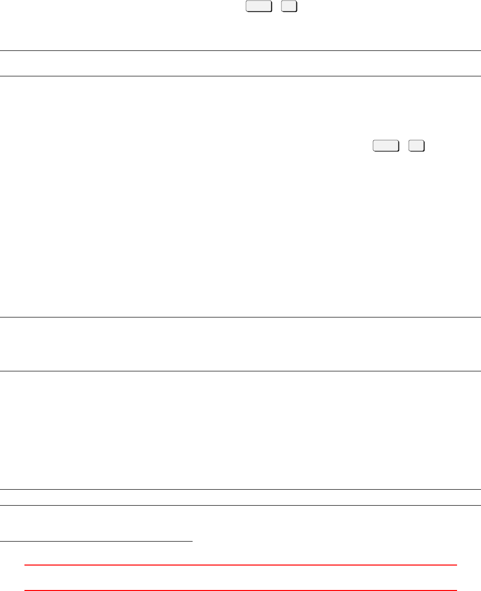
10.3 Terminate an OpenFOAM simulation
This section describes how to terminate a running OpenFOAM simulation. See Section 10.2 on how to abort a
simulation in a controlled manner, i.e. saving the current solution and stop the simulation.
This section explains how terminate a running simulation immediately and without saving the current
solution. Use this approach when you wouldn’t use the solution anyway, e.g. because you chose incorrect
settings.
10.3.1 Terminate a process in the foreground
If a command is executed in the Terminal without any additional parameters the process runs in the foreground.
The Terminal is therefore busy and can not be used until the process is finished. When a process is running
in the foreground it can easily terminated by pressing CTRL +C. Listing 57 features the GNU command
sleep. The only function of this command is to pause for a specified amount of time. With this command the
permature termination of a process can be tried.
use r@host :∼$ s leep 3
use r@host :∼$
Listing 57: Keep the Terminal busy
10.3.2 Terminate a background process
If a process runs in the background, the Terminal is free to be used for further tasks while the process is
running. In this case, the background process can not be terminated by pressing CTRL +Cbecause the
Operating System can not tell which background process the user wants to terminate.
Identify the process
On UNIX based systems every process is identified by a unique number. This is the PID, the process identifier.
The PID is equivalent to a licence plate for a car. During run-time this number is unique. However, after a
process has finished the PID of this process is available for other, later processes.
To find out which processes are currently running, invoke the command ps. This lists all running processes.
Without any further parameters only the processes that were executed from the current Terminal are listed.
Listing 58 shows the result if a new Terminal is opened and ps is called. The first entry – bash – is the Terminal
itself. The second entry – ps – is the only other process active at the time ps looks for all running processes.
The PID is listed in the first column of Listing 58. Depending on the parameters passed to ps the output can
be formatted differently.
use r@host :∼$ ps
PID TTY TIME CMD
13490 pts /1 00:00: 00 bash
13714 pts /1 00:00: 00 ps
use r@host :∼$
Listing 58: List processes in a fresh Terminal
The output of 58 is rather dull. However, there are lots of parameters telling ps what to do. The option -e
makes ps list all systemwide running processes. The output of such a call can be quite long, because ps lists all
processes started by the users as well as all system processes20.
The option -F controls the output format of ps. In this case -F stands for extra full. This means the output
contains a lot of information. Another option to display much information is -l. This option truncates the
names of the processes to 15 characters, whereas -F displays not only the full name of the process, it also
displays the parameters with which the processes were called.
ps - eF
Listing 59: List all running processes of the system
ps displays much information about a process. For terminating a process only the PID is necessary.
20System processes are processes run by the Operating System itself.
II This offering is not approved or endorsed by ESI®Group, ESI-OpenCFD®or the OpenFOAM®
Foundation, the producer of the OpenFOAM®software and owner of the OpenFOAM®trademark. 41

Search in the list of processes
The output of ps is a list which can be quite long. To terminate a certain process its PID has to be known.
Searching a number in a list of numbers can be quite painful and errorprone. Therefore it would be handy to
search in the list ps has returned for the desired process.
Before all else, grep does the trick. And now for something more detailed. grep is a program that searches
the lines of its input for a certain pattern. grep can use a file or the standard input as its input. As it is
unpractical to redirect the output of ps into a file only for grep to read it, we directly redirect the output of ps
to the input of grep. This is achieved by the use of a pipe.
Listing 60 shows how this is done. The first part of the command invoked – ps -eF – calls ps to list
all processes currently running in great detail. The option -F is used to make sure long process names can
be distinguished, e.g. to tell buoyantBoussinesqPimpleFoam apart from buoyantBoussinesqSimpleFoam.
Both are standard solvers of OpenFOAM. The bold part are the first 15 characters of the solver’s name. If the
option -F was omitted and both solvers were running, the results of ps would be ambiguous.
The second part of the command invoked in Listing 60 shows the call of grep.grep can be called with one or
two arguments. If only one argument is passed to grep,grep uses the standard input as input. If grep is called
with two parameters, the second argument has to specify the file from which grep has to read. As grep is called
with only one argument, it reads from the standard input.
Because it would be even more boring to type the list returned by ps we redirect the output of ps to the
standard input of grep. This is done by the pipe. The character |marks the connection of two processes in the
Terminal. The command left of the |passes its output directly to the command specified right of the |.
Now we can read and interpret Listing 60. It shows the output of the search for all running processes con-
taining the pattern Foam. In this case a parallel computation is going on. The first line of the result is mpirun.
This process controls the parallel running solvers. The next four lines are the four instances of the solver. How
parallel simulation works is explained in Section 10.5. The second last entry of the result is grep waiting for
input21. The last line of the result is the pdf viewer which displays this document at that time. This example
shows that is important to choose the pattern wisely, the search may return unexpected results.
use r@host :∼$ ps -ef | grep Fo am
user 11005 5117 0 17: 11 pts /2 00: 00:0 5 mpirun -np 4 twoPhas eEule rFoam - p ar al le l
user 11006 11005 99 17:11 pts /2 00:40:27 twoP has eEul erFoam - p ar all el
user 11007 11005 99 17:11 pts /2 00:40:28 twoPhas eEul erFoam - p ar al lel
user 11008 11005 99 17:11 pts /2 00:40:27 twoPhas eEul erFoam - p ar al lel
user 11009 11005 99 17:11 pts /2 00:40:26 twoP has eEul erFoam - p ar all el
us er 1 16 73 1 11 16 0 17:52 p ts / 12 0 0: 00 :0 0 grep - - co lor = au to Foam
us er 3 2041 1 0 Aug01 ? 00: 00 :3 1 evi nce / tm p / lyx _t mp di r . J 18 462 / l yx _t mp bu f0 / op en
FoamUserManual_CDLv2.pdf
use r@host :∼$
Listing 60: Search for processes
List only specified processes
You can tell ps directly in which processes you are interested. The option -C of ps makes ps list only those
processes that stem from a certain command. Listing 61 shows the output when ps -C twoPhaseEulerFoam
is typed into the Terminal. In this case also there are four parallel processes running. Notice, that only the
processes directly related to the solvers are shown. No other results are displayed unlike in Listing 60.
One has to bear in mind, that ps -C does not search for patterns. If the command name passed to ps as an
argument is misspelled, ps will not display the desired result. Listing 62 shows the effect of typos in this case.
The truncation of the process name in the list does not affect the search if the passed command name is equal
or longer than the truncated process name. The first two commands issued in Listing 62 result in a list of all
running instances of the solver. If the passed argument is shorter than the truncated process name – the third
command – ps does not output any results. Also if there is a typo in the passed argument, ps does not find
anything.
use r@host :∼$ ps -C twoP hase Eul erFo am
PID TTY TIME CMD
21On most Unix-like systems processes connected by a pipe are started at the same time. For this reason grep is already running
while ps is listing all running processes.
II This offering is not approved or endorsed by ESI®Group, ESI-OpenCFD®or the OpenFOAM®
Foundation, the producer of the OpenFOAM®software and owner of the OpenFOAM®trademark. 42

11006 pts /2 00:47: 44 tw oP haseE ul erF o
11007 pts /2 00:47: 44 two Pha se Euler Fo
11008 pts /2 00:47: 44 two Pha se Euler Fo
11009 pts /2 00:47: 43 tw oP haseE ul erF o
use r@h ost :∼$
Listing 61: List all instances of twoPhaseEulerFoam
use r@host :∼$ ps -C twoPhaseEulerFoa
PID TTY TIME CMD
12741 pts /0 00:00: 34 two Pha se Euler Fo
12742 pts /0 00:00: 34 two Pha se Euler Fo
12743 pts /0 00:00: 34 two Pha se Euler Fo
12744 pts /0 00:00: 34 two Pha se Euler Fo
use r@host :∼$ ps -C two Phas eEul erFo
PID TTY TIME CMD
12741 pts /0 00:00: 36 two Pha se Euler Fo
12742 pts /0 00:00: 36 two Pha se Euler Fo
12743 pts /0 00:00: 36 two Pha se Euler Fo
12744 pts /0 00:00: 36 two Pha se Euler Fo
use r@host :∼$ ps -C twoPhaseEulerF
PID TTY TIME CMD
use r@host :∼$ ps -C twP hase Eule rFoa
PID TTY TIME CMD
Listing 62: List all instances of twoPhaseEulerFoam – the effect of typos
Terminate
The operating system interacts with running processes using signals. The user can also send signals to processes
using the command kill.kill sends by default the termination signal. To identify the process to which the signal
is to be sent, the PID of this process has to be passed as an argument.
Listing 63 shows how the programm sleep is executed, all running processes are listed, the running instance
of sleep is terminated and the running processes are listed again. When ps was executed the second time, a
message is displayed stating the process has been terminated22. If the process would not have been terminated
the message at the “natural” end of the process would be like in Listing 6423.
use r@host :∼$ sleep 20 &
[1] 13063
use r@host :∼$ ps
PID TTY TIME CMD
12372 pts /0 00:00: 00 bash
13063 pts /0 00:00: 00 sleep
13064 pts /0 00:00: 00 ps
use r@host :∼$ kill 1 3063
use r@host :∼$ ps
PID TTY TIME CMD
12372 pts /0 00:00: 00 bash
13065 pts /0 00:00: 00 ps
[1]+ Be endet sleep 20
use r@host :∼$
Listing 63: Terminate a process using kill
use r@host :∼$ s leep 1 &
[1] 13126
use r@host :∼$ ps
PID TTY TIME CMD
12372 pts /0 00:00: 00 bash
13127 pts /0 00:00: 00 ps
[1]+ Fertig sleep 1
use r@host :∼$
22On other systems this message is displayed immediately – see Listing 65. In this case the procedure was tried on the local
computing cluster.
23A system with English language setting the message would read Terminated if the process would have been terminated and
Done if the process would have been allowed to finish.
II This offering is not approved or endorsed by ESI®Group, ESI-OpenCFD®or the OpenFOAM®
Foundation, the producer of the OpenFOAM®software and owner of the OpenFOAM®trademark. 43

Listing 64: The natural end of a process
use r@clust er user > sleep 10 &
[1] 31406
use r@clust er user > k ill 31406
user@cluster user>
[1] T erm ina ted sleep 10
user@cluster user>
Listing 65: Terminate a process using kill on a different machine
10.4 Continue a simulation
If a simulation has ended at the end time or if it has been aborted there may be the need to continue the
simulation. The most important setting to enable a simulation to be continued has to be made in the file
controlDict. There, the keyword startFrom controls from which time the simulation will be started.
The easiest way to continue a simulation is to set the startFrom parameter to latestTime. Then, if
necessary, the value of endTime needs to be adjusted. After this changes, the simulation can be continued by
simply invoking the solver in the Terminal.
10.5 Do parallel simulations with OpenFOAM
OpenFOAM is able to do parallel simulations. There is no great difference between calculating a case with one
single process or using many parallel processes. The only obvious additional task is to split the computation
domain into several pieces. This step is called domain decomposition. After the domain is decomposed several
instances of the solver are running the case on a subdomain each. Additionally, the invokation of the solver
differs from the single process case.
10.5.1 Starting a parallel simulation
To enable a simulation using several parallel instances of a solver, OpenFOAM uses the MPI standard in the
implementation of OpenMPI. OpenMPI ensures that all parallel instances of the solver run synchronously.
Otherwise the simulation would generate no meaningful results. In order to be able to manage all parallel
processes the simulation has to started using the command mpirun.
Listing 66 shows how a parallel simulation using 4 parallel processes is started. The solver outputs are
redirected into a file called > foamRun.log and the simulation runs in the background of the Terminal. So the
same Terminal can be used to monitor the progress of the calculation. See Section 10.1.2 for a discussion about
running a process in the background.
The output message in the Listing shows the PID of the running instance of mpirun. This PID can be used
to terminate the parallel calculation, like it is explained in Section 10.3.2.
use r@host :∼$ m pi run - np 4 ico Fo am - p ar al le l > f oa mR un . l og &
[1] 11099
use r@host :∼$
Listing 66: Run OpenFOAM with 4 processes
The number of processes, in this case 4, has to be equal the number of processor* folders. These folders are
created by decomposePar and their number is defined in decomposeParDict. See Section 10.5.2 for information
about domain decomposition.
If this numbers – the number of processor* folders and the number of parallel processes with which mpirun
is invoked – are not equal OpenFOAM issues an error message similar to Listing 67. In this case the domain
was decomposed into 4 subdomains and it was tried to start the parallel simulation with 2 processes. If the
parallel simulation is called with too many processes, OpenFOAM issues an error message like in Listing 68.
The first example shows, that OpenFOAM reacts differently whether the parallel job was started with loo little
or too many processes.
II This offering is not approved or endorsed by ESI®Group, ESI-OpenCFD®or the OpenFOAM®
Foundation, the producer of the OpenFOAM®software and owner of the OpenFOAM®trademark. 44

[0] --> FOAM FATAL ERROR :
[0] "/ h ome / use r / Op en FO AM / user - 2.1. x / run / i co Foam / c avity / syste m / dec omp os eP arD ic t " s pe ci fi es 4
pro ces sor s but job was start ed with 2 pro ces sor s .
Listing 67: Run OpenFOAM with too little parallel processes
[0] --> FOAM FATAL ERROR :
[0] numbe r of pr oce ssor di rec tor ies = 4 is not equal to the nu mber of p roc essors = 8
Listing 68: Run OpenFOAM with too many parallel processes
Pitfall: -parallel
The parameter -parallel is important. If this parameter is omitted, the solver will be executed ntimes.
Listing 69 shows the output of the command ls when it is run with mpirun with two processes. In this case ls
is simply run twice.
If the parameter -parallel is missing, the same happens as in the case of ls. The simulation is run by n
processes at roughly the same time. Listing 70 shows the first lines of output of a situation where the -parallel
parameter was omitted. All solvers start the calculation of the whole case and write their output to the Ter-
minal. The output appears on the Terminal in the order as it is generated by the solvers – in other words, the
output on the Terminal is completely disarranged. If the -parallel parameter is missing, there is also no check
if the processor* folders are present.
use r@host :∼/ O penFOAM / user -2. 1. x/ run / ico Foam / c avit y$ mpirun -np 2 ls
0 constant system
0 constant system
use r@host :∼/ O penFOAM / user -2. 1. x/ run / ico Foam / c avit y$
Listing 69: Run ls using 2 processes
use r@host :∼/ O penFOAM / user -2. 1. x/ run / ico Foam / c avit y$ mpirun -np 4 icoFoam
/*---------------------------------------------------------------------------*\
| === === === | |
| \\ / F ield | O penF OAM : The Open Sour ce CFD T oolbox |
| \\ / O p er at ion | V er sion : 2.1. x |
| \\ / A nd | Web : ww w . Op en FO AM . org |
| \\/ M anip ula tion | |
\*---------------------------------------------------------------------------*/
Bui ld : 2. 1. x -6 e 8 9b a 0b c d1 5
Exec : ico Foam
Date : Jan 29 2013
Time : 10: 51: 12
Host : "host"
PID : 25622
/*---------------------------------------------------------------------------*\
| === === === | |
| \\ / F ield | O penF OAM : The Open Sour ce CFD T oolbox |
| \\ / O p er at ion | V er sion : 2.1. x |
| \\ / A nd | Web : ww w . Op en FO AM . org |
| \\/ M anip ula tion | |
\*---------------------------------------------------------------------------*/
Bui ld : 2. 1. x -6 e 8 9b a 0b c d1 5
Exec : ico Foam
Listing 70: Run icoFoam without the -parallel parameter
Pitfall: domain decomposition
If there was no domain decompositin prior to starting a parallel simulation, OpenFOAM will issue an corre-
sponding error message.
II This offering is not approved or endorsed by ESI®Group, ESI-OpenCFD®or the OpenFOAM®
Foundation, the producer of the OpenFOAM®software and owner of the OpenFOAM®trademark. 45

[0] --> FOAM FATAL ERROR :
[0] t wo Ph as eEu le rFo am : can not op en case dir ec to ry "/ home / u ser / Op en FO AM / user - 2.1. x / run /
two Ph as eEul erF oa m / te stC olum n / proce sso r0 "
[0]
[0] FOAM p arallel run exiting
Listing 71: Missing domain decomposition
Pitfall: domain resonstruction
After a parallel simulation has ended, all data is residing in the processor* folders. If paraView is started –
without prior domain reconstruction – paraView will only find the data of the 0 directory.
10.5.2 Domain decomposition
Before a parallel simulation can be started the domain has to be decomposed into the correct number of
subdomains – one for each parallel process. The parallel processes calculate on their own subdomain and
exchange data of the border regions at the end of each time step. This is also the reason why the parallel
processes have to be synchonous. Otherwise, processes with a lower computational load would overtake other
processes and they would exchange data from different times.
Just before starting the simulation the domain has to be decomposed. The tool decompsePar is used for
this purpose. Other operations, e.g. initialising fields using setFields have to take place before the domain
decomposition. decomposePar reads from decomposeParDict in the system directory. This file has to contain
al least the number of subdomains and the decomposition method.
decomposePar creates the processor* directories in the case directory. Inside the processor* folders a 0and
aconstant folder are created. The 0folder contains the initial and boundary conditions of the subdomain and
the constant folder contains a polyMesh folder containing the mesh of the subdomain.
All parallel processes read from the same system directory, as the information stored there is not affected
by the domain decomposition. Also the files in the constant directory are not altered.
Pitfall: Existing decomposition
If the domain has already been decomposed and decomposePar is called again, e.g. because the number of
subdomains has been changed or some fields have been reinitialised, OpenFOAM issues an error message.
Listing 72 shows an example. In this case the domain has already been decomposed into 2 subdomains and the
attempt is made to decompose it again. OpenFOAM always issues an error message, whether the number of
subdomains has changes or not.
The resulting error message proposes two possible solutions. The first is to invoke decomposePar with the
-force option to make decomposePar remove the processor* folders before doing its job. The second proposed
solution is to manually remove the processor* folders. In this case the error message contains the proper com-
mand to do so. The user can retype the command or copy and paste it into the Terminal.
--> F OA M F AT AL ER RO R : C ase is a lre ad y d eco mp o se d w ith 2 d omain s , u se th e - f or ce o pt io n or
manually
remove processor d ire cto ries bef ore decompo sin g . e .g.,
rm -rf / home / user / Ope nF OA M / user -2.1 . x/ run / ico Foam / c avit y / pr oc es so r *
Listing 72: Already decomposed domain
Time management with decomposePar
In the course of an update of OpenFOAM decompose gained the option -time. This enhancement took place
between the release of OpenFOAM 2.1.0 and OpenFOAM 2.1.1. Such enhancements typically first appear in
the respository release OpenFOAM 2.1.x. So, it may be, that some installations of OpenFOAM 2.1.x contain
this feature and some not depending on the time of installation or the time of the last update.
The option time lets the user specify a time from which or a time range in which the domain is to be
decomposed. Listing 73 shows some examples of how this option works.
II This offering is not approved or endorsed by ESI®Group, ESI-OpenCFD®or the OpenFOAM®
Foundation, the producer of the OpenFOAM®software and owner of the OpenFOAM®trademark. 46

The option -latestTime makes decomposePar use the latest time step as starting time step for the subdo-
mains.
use r@host :∼/ O penFOAM / user -2. 1. x/ run / ico Foam / c avit y$ ls
0 0.1 0.2 con stant probes1 processor0 p roc ess or1 p roc essor2 system
use r@host :∼/ O pe nF OA M / user -2 .1. x/ run / i co Fo am / cav it y$ de com po seP ar -time 0 .1 :0 .2 - f orce > / dev /
null
use r@host :∼/ O penFOAM / user -2. 1. x/ run / ico Foam / c avit y$ ls pr ocessor0
0.1 0.2 co nst ant
use r@host :∼/ O pe nF OA M / user -2 .1. x/ run / i co Fo am / cav it y$ de com po seP ar -time 0.2 - f orce > / dev / null
use r@host :∼/ O penFOAM / user -2. 1. x/ run / ico Foam / c avit y$ ls pr ocessor0
0.2 co nst ant
use r@host :∼/ O penFOAM / user -2. 1. x/ run / ico Foam / c avit y$
Listing 73: Time management with decomposePar
10.5.3 Domain reconstruction
To be able to look at the results the data has to be reassembled again. This job is done by reconstructPar. This
tool collects all data of the processor* folders and reconstructs the original domain using all the generated time
step data. After reconstructPar has finished the data of the whole domain resides in the case directory and the
data of the subdomains resides in the processor* folders.
Listing 74 shows the content of the case directory after a parallel simulation has finished. The first command
is a simple call of ls to display the contents of the case directory. This is not different from the situation before
the parallel simulation was started with the exception of the log file. However, this log file could be from a
previous run. So, listing the contents after a parallel simulation has finished carries no real information.
The second command lists the contents of the processor0 directory. In this directory – as well as in all other
processor* folders – there is time step data. The third command reconstructs the domain. After this tool has
finished, the case directory also contains time step data. The last command lists the contents of the processor0
folder again. This data has not been removed. So, a finished parallel case stores its time step data twice and
therefore uses a lot of space.
use r@host :∼/ O penFOAM / user -2. 1. x/ run / ico Foam / c avit y$ ls
0 co nstant foa mRun . log probe s1 proce sso r0 pr oce sso r1 processor 2 pro ces sor 3 syste m
use r@host :∼/ O penFOAM / user -2. 1. x/ run / ico Foam / c avit y$ ls pr ocessor0
0 0.1 0.2 0.3 0.4 0.5 co nst ant
use r@host :∼/ O pe nF OA M / user -2 .1. x/ run / i co Fo am / cav it y$ rec on str uc tPa r > f oa mRe co nst ru ct . lo g &
[1] 26269
use r@host :∼/ O penFOAM / user -2. 1. x/ run / ico Foam / c avit y$ ls
0 0.1 0.2 0.3 0.4 0.5 co nst ant foa mRec onst ruc t . log f oamRun . log pro bes1 p roc essor0
pro ces sor 1 pro cessor2 proc ess or3 sys tem
[1 ]+ F er ti g rec ons tr uct Par > f oa mR eco nst ru ct . lo g
use r@host :∼/ O penFOAM / user -2. 1. x/ run / ico Foam / c avit y$ ls pr ocessor0
0 0.1 0.2 0.3 0.4 0.5 co nst ant
use r@host :∼/ O penFOAM / user -2. 1. x/ run / ico Foam / c avit y$
Listing 74: A finished parallel simulation
Time management
If a simulation has been startet from t=t1the domain has to be reconstructed for times t>t1. Calling re-
constructPar without any options regarding time, the program starts reconstructing the domain at the earliest
time. To prevent the tool from reconstructing already reconstructed time steps the -time option can be used.
Listing 75 shows how simulation results are reconstructed for t≤60 s.
r ec o ns t ru c tP a r - ti me 6 0:
Listing 75: Zeitparameter für reconstructPar
Another option to reconstruct only the new time steps is the command line option -newTimes. By using
this option the proper time span to reconstruct is automatically determined.
II This offering is not approved or endorsed by ESI®Group, ESI-OpenCFD®or the OpenFOAM®
Foundation, the producer of the OpenFOAM®software and owner of the OpenFOAM®trademark. 47

10.5.4 Run large studies on computing clusters
Simulating parallel on a machine brings some advantages and enables the user to run even large simulations
on a workstation. However, if the cases is very large, or parametric studies are to be conducted, using the
workstation can be counter productive. Therefore, simulating on a computing cluster is the method of choice
for large scale calculations. The user can follow a two step method.
1. Set up the case and run some test simulations, e.g. for a small number of time steps, on the workstation
to ensure the simulation runs
2. Do the actual simulation on the cluster
The fact, that OpenFOAM runs on a great number of platforms enables the user to do simulations on the
workstation as well as on a big cluster with tens or hundreds of processors.
Run OpenFOAM using a script
Section 57.5 explaines how to set up a script that runs multiple cases.
10.6 Using tools
OpenFOAM consists besides of solvers of a great collection of tools. These tools are used for all kind of
operations.
All solvers and tools of OpenFOAM24 assume that they are called from the case directory. If an executable
is to be called from another directory the path to the case diretory has to be specified. Then the option -case
has to be used to specify this path.
Listing 76 shows the error message displayed by the tool fluentMeshToFoam as it was executed from the
polyMesh directory. The tool added the relative path system/controlDict to the currect working directory.
This resulted in an invalid path to controlDict as the error message tells the user. Actually, the error message
states that the file could not be found. This does not solely imply an invalid path. The file could simply be
missing.
--> FOAM FATAL IO ERROR :
cannot find f ile
fi le : / home / user / O pe nF OAM / user -2 .1. x/ run / i coFo am / t estC as e / con stan t / pol yM esh / syste m / con tr ol Di ct
at line 0.
From fu nct ion reg IOo bje ct :: readStream ()
in file db / reg IOobj ect / r eg IOobj ec tRead . C at line 73.
FOAM exiting
Listing 76: Wrong path
The correct usage of the -case option is shown in Listung 77. There the correct path to the case directory
– two levels upwards – is specified using ../...25
use r@host :∼/ O penF OAM / user -2.1. x/run / icoFo am / tes tCase / con stan t / po lyMe sh$ fl ue nt 3DMes hT oF oa m -
ca se . ./ .. c ase Me sh . m sh
Listing 77: Specify the correct path to the case
24No exeption known to the author.
25On most Linux or Unix systems .refers to the current directory and .. refers to the directory above the current one. To
change in the Terminal one directory upwards on Linux cd .. does the job and on MS-DOS or Windows cd.. is the proper
command.
Also, on Linux systems the tilda refers to the home directory of the current user.
II This offering is not approved or endorsed by ESI®Group, ESI-OpenCFD®or the OpenFOAM®
Foundation, the producer of the OpenFOAM®software and owner of the OpenFOAM®trademark. 48

Part III
Pre-processing
This part of the document deals with all issues related to pre-processing, i.e. all the tasks necessary to set-up a
valid simulation case. The majority of the following sections deal with the mesh. The final sections of this part
deal with general case manipulation and initialisation.
11 Mesh basics
11.1 Basics of the mesh
11.1.1 Files
A mesh is defined by OpenFOAM using several files. All of these files reside in constant/polyMesh/. The
names of these files are rather self explanatory, the rest is explained in the OpenFOAM User Guide [39].
boundary contains a list of all faces forming the boundary patches
faces contains the definition of all faces. A face is defined by the points that form the face.
neighbour contains a list of the neighbouring cells of the faces
owner contains a list of the owning cells of the faces
points contains a list of the coordinates of all points
The description of a mesh is based on the faces. The geometry is discretised into finite volumes – the cells.
Each cell is delimited by a number of faces, e.g. a hexahedron has 6 faces. The faces can be divided into two
groups. Boundary faces border only one cell. These faces make up the boundary patches. All other faces can
be seen as the connection between two cells and are called internal faces. A face bordering more than two cells
is not possible. An internal face is, by definition, owned by one cell and neighboured by the other one. So, the
two cells connected by a face can be destincted.
This five files are absolutely necessary to describe a mesh regardless of how the mesh was created in the
first place. However, some ways of creating a mesh produce additional files. Listing 78 shows a list of all files
created with Gambit and converted by fluentMeshToFoam.
use r@host :∼/ O penF OAM /user -2.1. x /run / tw oP haseE ul er Fo am / column Case$ ls c onst ant / po lyMesh /
boundary cel lZo nes fac es faceZones nei ghb our own er points p ointZones
Listing 78: Content of constant/polyMesh
11.1.2 Definitions
Face
A face is defined by the vertices or points that are part of the face. The points need to be stated in an order
which is defined by the face normal vector pointing to the outside of the cell or the block. The way faces are
defined is the same for cells of the mesh or for blocks of the geometry.
To elaborate this further we look at the top face of the generic block of Figure 3in Figure 1. The vertices
with the numbers 4, 5, 6 and 7 are part of the face. The face normal vector – denoted by nin Figure 1– that
points outwards of the block is parallel to the local zaxis. Therefore we need to specify the vertices defining
the face in counter-clockwise circular order, when we look at the block from the top. The direction of rotation
is marked in Figure 1with the +sign. The starting vertex is arbitrary but it must not appear twice in the list.
III This offering is not approved or endorsed by ESI®Group, ESI-OpenCFD®or the OpenFOAM®
Foundation, the producer of the OpenFOAM®software and owner of the OpenFOAM®trademark. 49
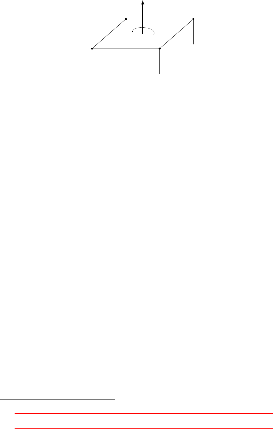
n
+
67
4 5
Figure 1: The top face of the generic block of Figure 3
Correct definitions
(4 5 6 7) (7 4 5 6) (6 7 4 5) (5 6 7 4)
Wrong direction of rotation
(7 6 5 4) (4 7 6 5) (5 4 7 6) (6 5 4 7)
Non-circular Starting point repeated
(7 5 6 4) (4 5 6 7 4)
Table 3: Valid and invalid face definitions
12 Geometry creation & other pre-processing software
There are many ways to create a geometry. There is a great number of CAD software, there is a number of
CFD pre-processors capable of creating geometries and there is the good old blockMeshDict.
This section is about the different ways to generate the geometry for creating a finite volume mesh.
12.1 blockMesh
blockMesh is one of OpenFOAMs own pre-processing tools. It is able to create the domain geometry and the
corresponding mesh. See Section 13 for a discussion on blockMesh. For the reason of simplicity all aspects of
blockMesh – geometry creation as well as meshing – are covered in Section 13.
12.2 CAD software
There is a great number of CAD software around. Each CAD program usually uses its own file format. However
most CAD programs support exporting the geometry in different formats, e.g. STL, IGES, SAT. If CAD software
is used to create the geometry the data has to be exported to be used by a meshing program. A common file
format for this purpose is the STL format. snappyHexMesh can be used with STL26 geometry definitions.
12.2.1 OpenSCAD
OpenSCAD [http://www.openscad.org/] is an open source CAD tool for creating solid 3D CAD models. A
CAD model is created by using primitve shapes (cubes, cylinders, etc.) or by extruding 2D paths. Models are
not created interactively like in other CAD software. The user writes an input script which is interpreted by
OpenSCAD. This makes it easy to create parametric models.
For further information on usage see the documentation http://en.wikibooks.org/wiki/OpenSCAD_User_
Manual.
Pitfall: STL mesh quality
OpenSCAD is a tool to create CAD models. Therefore the requirements on the produced STL mesh are
completely different than on a mesh for CFD simulations. OpenSCAD produces STL meshes that define the
26STL is infact a surface mesh enclosing the geometry. Therefore the term STL mesh or STL surface mesh is also valid.
III This offering is not approved or endorsed by ESI®Group, ESI-OpenCFD®or the OpenFOAM®
Foundation, the producer of the OpenFOAM®software and owner of the OpenFOAM®trademark. 50
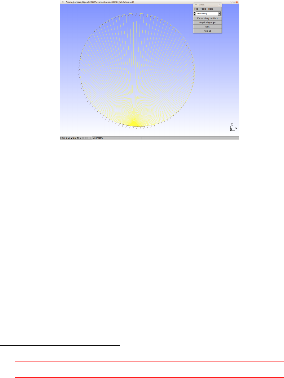
geometry correctly but the mesh is of a bad quality from a CFD point of view.
Figure 2shows the STL mesh of a circular area. All triangles defining the circular area share one vertex.
This vertex is probably the base point for the mesh creation of OpenSCAD. From a CFD point of view the
triangular face elements are highly distorted and have a bad aspect ratio. However from a CAD point of view
these triangles are prefectly sufficient to represent the circular area.
If a finite volume mesh is to be derived from the STL surface mesh (e.g. with GMSH) problems may arise.
If the only purpose of the STL mesh is to represent some geometry – like it is the case with snappyHexMesh –
then this quality issues can be ignored.
Figure 2: The STL mesh of a circular area generated by OpenSCAD
12.3 Salome
Salome [http://www.salome-platform.org/] is a powerful open source pre-processing software developed by
EDF. Salome can be used to create a geometry interactively or by interpreting a python script27. Salome comes
with a number of internal and external meshing utilities. Salome has also a post-processing module.
Salome is a part of a collection of open source software developed by EDF. Salome serves as the pre- and
post-processor for Code_Aster (structural analysis) and Code_Saturne (CFD).
12.3.1 Geometry
Salome can be used for geometry generation only. A common way of doing so, is to use Salome’s meshing
module to create a surface mesh of the CAD geometry, which can be exporting using the STL format. The
resulting STL file can then be used by other meshing tools, e.g. snappyHexMesh.
12.3.2 Mesh
Salome can also used to create the geometry and subsequently the mesh. This mesh needs to be exported by
Salome in the UNV format, which can be converted by the ideasUnvToFoam utility of OpenFOAM.
See http://caelinux.org/wiki/index.php/Doc:Salome for documentation and usage examples of Salome,
and Section 19 for some further points on creating the mesh with Salome.
12.4 GMSH
GMSH is a meshing tool with some pre- and post-processing capabilities [http://www.geuz.org/gmsh/]. The
meshes generated by GMSH can be converted to OpenFOAM’s format using the gmshToFoam utility.
27Salome can be controlled completely by Python. Thus parametric geometry or mesh creation is possible.
III This offering is not approved or endorsed by ESI®Group, ESI-OpenCFD®or the OpenFOAM®
Foundation, the producer of the OpenFOAM®software and owner of the OpenFOAM®trademark. 51
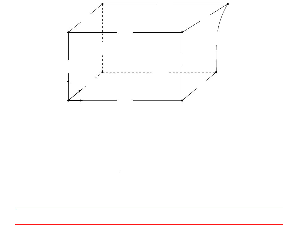
13 blockMesh
blockMesh is used to create a mesh. The geometry is defined in blockMeshDict. This file also contains all
necessary parameters needed to create the mesh, e.g. the number of cells. Therefore, blockMesh is a combined
tool to define and mesh a geometry in contrast to other meshers that use CAD files to import a geometry
created by some other software.
13.1 The block
The geometry created by blockMesh is based on the generic block. Figure 3shows a generic block.
The blue numbers are the local vertex numbers of the block. The vertices are numbered counter-clockwise28
in the local x−yplane starting at the origin of the local coordinates29. Then the vertices above the local x−y
plane are counter-clockwise numbered starting with the vertex on the local zaxis.
The local vertex numbers are important when defining the block. The first part of the blockMeshDict is
generally a list of vertices. From this vertices the blocks are constructed. A block is defined by a list of 8 vertices
which have to be ordered in a way to match the local vertices. Therefore the first entry in the list of vertices
is the local 0 vertex, then the local 1 vertex follows. The local vertex numbers define the order in which the
vertices have to passed when constructing a block.
The coordinate system originating from vertex 0 are the local coordinates. The local coordinates are im-
portant when specifying the number of cells or mesh grading (see simpleGrading in Section 13.4). The local
coordinate axes do not need to be parallel or to coincide with the global coordinate axes.
The edges are also numbered and have a direction. Starting with the edge parallel to the local xaxis the
edges are numbered counter-clockwise starting with the edge emanating from the origin of the local coordinates.
Next the edges parallel to the local yaxis are numbered and finally the edges parallel to the local zaxis. The
edge number is important when specifying a grading for each edge individually (see edgeGrading in Section
13.4).
As it is indicated on Figure 3, the edges do not need to be parallel or straight. See Section 13.2.4 on how to
define curved edges.
0→
%
5
↑
8
3→
%
7
%
6
2→
↑
9
↑
10
%
4
1→
↑
11
23
67
0 1
4 5
x
y
z
Figure 3: The generic block
13.2 The blockMeshDict
The file blockMeshDict defines the geometry and controls the meshing process of blockMesh. Listing 79 shows
a reduced example of the blockMeshDict. This file was taken from the cavity tutorial case.
28In mathematics the positive direction of rotation is generally determined with the right-hand or cork-screw rule. Let the thumb
of your right hand point in the positive direction of the rotation axis, then the fingers of the right hand point in the positive
direction of revolution.
29If we number all vertices in the x−yplane then the local zaxis is the axis of revolution. Thus the counter-clockwise direction
is the mathematically positive direction of revolution.
III This offering is not approved or endorsed by ESI®Group, ESI-OpenCFD®or the OpenFOAM®
Foundation, the producer of the OpenFOAM®software and owner of the OpenFOAM®trademark. 52

/* - -- - - -- - - -- - --- - - -- - --- - - -- - - -- -* - C + + -* - -- - - -- - - - -- - - -- - - - -- - - --- - - --- - - -*\
| === === === | |
| \\ / F ield | O penF OAM : The Open Sour ce CFD T oolbox |
| \\ / O p er at ion | V er sion : 2.1. x |
| \\ / A nd | Web : ww w . Op en FO AM . org |
| \\/ M anip ula tion | |
\*---------------------------------------------------------------------------*/
FoamFile
{
version 2.0;
forma t asc ii ;
class dictionary ;
object bloc kMe sh Dic t ;
}
//*************************************//
con vert ToMe ter s 0.1;
vertices
(
(0 0 0) // 0
(0 0 0.1) // 1
...
);
blocks
(
hex (0 1 2 3 4 5 6 7) (20 20 1) s impl eGradin g (1 1 1)
);
edges
(
);
boundary
(
mov ing Wal l
{
type wall;
faces
(
(3 7 6 2)
);
}
...
);
mergePatchPairs
(
);
// ************************************************************************* //
Listing 79: A minimal blockMeshDict
13.2.1 convertToMeters
convertToMeters is a scaling factor to convert the vertex coordinates of blockMeshDict into meters. If the
vertex coordinates are entered in an other unit than meters, this value has to be chosen accordingly. Listing 80
shows how to set this factor if the vertex coordinates are entered in millimeters.
con vert ToMe ter s 0.0 01;
Listing 80: convertToMeters
If the keyword convertToMeters is missing in the blockMeshDict, then no scaling is used, i.e. the default
value of 1 is assumed.
III This offering is not approved or endorsed by ESI®Group, ESI-OpenCFD®or the OpenFOAM®
Foundation, the producer of the OpenFOAM®software and owner of the OpenFOAM®trademark. 53

To make sure if a scaling factor has been used, the output of blockMesh can be checked. Listing 81 shows
the message issued by blockMesh regarding the scaling factor defined with convertToMeters.
Creating points with scale 0.1
Listing 81: Output of blockMesh when convertToMeters is set to 0.1
convertToMeters is a uniform scaling factor. Non-uniform scaling or other operations can be performed
with another tool. See Section 23.1 and 25.3.4.
13.2.2 vertices
The vertices sub-dictionary contains a list of vertices. Each vertexs is defines by its coordinates in the global
coordinate system. By default OpenFOAM treats these coordinates as in metres. However, with the help of
the keyword convertToMeters, the vertices can be specified in other units.
The index of a vertex in this list is also the global number of this vertex, which is needed when constructing
blocks from the vertices. Remember, counting starts from zero. Thus the first vertex is the list of vertices can
be addressed by its index 0. A way to keep oneself aware of this fact is to add comments30 to the vertex list as
in Listing 79.
13.2.3 blocks
The only valid entry in the blocks sub-dictionary is the hex keyword. The blocks section of the blockMeshDict
contains a list of hex commands. Listing 82 shows an example of a block definition with the hex keyword.
After the word hex a list of eight numbers defining the eight vertices of the block follows. The order of the
entries in this list is the same order as the local vertex numbers of the block in Figure 3.
Then a list of three positive integer numbers follows. These numbers tell blockMesh how many cells need
to be created in the direction of the local coordinate axes. Thus, the first number is the number of cells in the
local xdirection.
The next entry is a word stating the grading of the edges. This entry is in fact redundant. In OpenFOAM-
2.1.x only the last entry, the list of expansion ratio, controls the grading. The third entry could even be omitted.
However, maybe future versions of OpenFOAM make use of this entry. So the author does not advocate to
omit this parameter.
The last entry of the block definition is a list of either three or twelve positive numbers. This numbers define
the expansion ratio of the grading. In the case of three numbers, simpleGrading is applied. If twelve numbers
are stated, then edgeGrading is performed.
If the list contains only one entry, then all edges share the same expansion ratio. Any other number of
entries in this list leads to an error.
hex (0 1 2 3 4 5 6 7) (20 20 1) s impl eGradin g (2 4 1)
Listing 82: The hex command in blockMeshDict.
Setting up cell zones
The cells belonging to a block can be assigned to a cell set at mesh creation by inserting the name of the
to-be-created cell set between the vertex list and the list with the number of cells. This feature is not really
documented in the official OpenFOAM User Guide, however, it seems to be present in OpenFOAM ever since.
hex (0 1 2 3 4 5 6 7) CE LL_SET_ NAME (20 20 1) si mpl eGra din g (2 4 1)
Listing 83: The hex command in blockMeshDict with a cell set definition.
30As OpenFOAM treats its dictionaries much in the same way as C/C++ source files are treated by the C/C++ compiler.
Therefore comments work the same way as they do in C or C++.
III This offering is not approved or endorsed by ESI®Group, ESI-OpenCFD®or the OpenFOAM®
Foundation, the producer of the OpenFOAM®software and owner of the OpenFOAM®trademark. 54

Creating a block with 6 faces
The hex instruction can also be used to create a prism with a triangular cross-section. Such blocks are needed
for simulations that make use of axi-symmetry. See the User Manual [39] for instructions on this topic.
13.2.4 edges
The edges sub-dictionary contains pairs of vertices that define an edge. By default edges are straight, by
explicitely specifying the shape of the edge, curved edges can be created. This sub-dictionary can be omitted.
Listing 84 shows the message issued by blockMesh when edges is omitted.
No non - lin ear edges de fine d
Listing 84: Output of blockMesh when edges is omitted
Otherwise, blockMesh issues a message as in Listing 85 regardless whether curved edges are actually created or
only an empty edges sub-dictionary is present.
Creating curved ed ges
Listing 85: Output of blockMesh when edges is present
Creating arcs
With the keyword arc a circular arc between two vertices can be created. Listing 86 shows the definition of a
circular arc between the vertices 0 and 3. In order to define a circular arc three points are necessary. Therefore
the third point follows the indizes of the two vertices defining the edge.
edges
(
arc 0 3 (0 0.5 0.05)
);
Listing 86: Definition of a circular edges in the edges sub-dictionary
The keyword arc can not be used to define a straight edge. If the two vertices and the additional interpo-
lation point are co-linear, blockMesh will abort issuing an error message as in Listing 87.
--> FOAM FATAL ERROR :
Inval id arc de finition - are the poi nts co - lin ear ? Denom =0
From fu nct ion cyl indrica lCS arc Edge :: cal cAn gle ()
in file curvedE dge s / a rcEdge .C at line 55.
FOAM a bor ting
Listing 87: Output of blockMesh when the three points defining an arc are co-linear
Creating splines
The keyword spline defines a spline. After the two vertices defining the edge a list of interpolation points has
to follow.
edges
(
spline 0 3 ((0 0.25 0.05) (0 0.75 0.05) )
);
Listing 88: Definition of a spline in the edges sub-dictionary
III This offering is not approved or endorsed by ESI®Group, ESI-OpenCFD®or the OpenFOAM®
Foundation, the producer of the OpenFOAM®software and owner of the OpenFOAM®trademark. 55
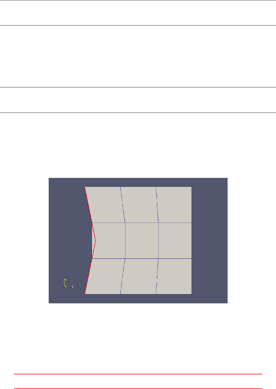
Creating a poly-line
Other than a spline, a poly-line connects several points with straight lines.
edges
(
polyLine 0 3 ((0 0.25 0.05) (0 0.75 0.05) )
);
Listing 89: Definition of a poly-line in the edges sub-dictionary
Creating a straight line
For the sake of completeness there is the keyword line. This keyword takes the two vertices defining the edge
as arguments. Straight lines are created by blockMesh by default. So there is no need for the user to specify
straight lines.
edges
(
line 0 3
);
Listing 90: Definition of a line in the edges sub-dictionary
Summary
Edges defined within the blockMeshDict are used to compute the locations of a block’s internal nodes. The
edge however, is approximated linearly as shown in Figure 4, i.e. the number of cells along the edge determine
the resolution of the edges.
Figure 4: A block with a poly-line at the left side. The red line indicates the poly-line. This figure makes it
obvious that edges defines in the blockMeshDict serve to compute the locations of the block’s internal nodes.
The block itself however, does not obey the poly-line.
Another feature of the edge definition is, that the two vertices defining the edge can be supplied in any
order.
III This offering is not approved or endorsed by ESI®Group, ESI-OpenCFD®or the OpenFOAM®
Foundation, the producer of the OpenFOAM®software and owner of the OpenFOAM®trademark. 56

Pitfalls
Edge creation of blockMesh sometimes fails silently31. If we define an arc between two vertices not directly
connected by an edge, e.g. the vertices 0 and 2 in Figure 3, then blockMesh proceeds without any warning or
error. The faulty edge definition seems to be simply ignored. This, silence in the face of error might make it
hard for the user building his or her blockMeshDict to spot the reason why the definition of curved edges does
not result in curved edges.
13.2.5 boundary
The boundary list contains a dictionary per patch. This dictionary contains the type of the patch and the list
of faces composing the patch. Listing 91 shows an example of how a patch consisting of one face is defined.
boundary
(
inlet
{
ty pe pat ch ;
faces
(
(0 3 2 1)
);
}
...
);
Listing 91: The boundary list of blockMeshDict
Pitfall: defaultFaces
If faces are forgotten in the boundary definition, then blockMesh creates an additional patch named defaultFaces.
This patch has an empty boundary condition automatically assigned. Listing 92 shows a warning message issued
by blockMesh. In this case some faces were missing in the boundary definition. This, however, does not cause
blockMesh to abort mesh generation. If a 2D mesh is to be created, the creation of the default patch with an
empty boundary condition can be expected behaviour. However, it is not advisible to rely this kind of default
behaviour when building a case.
Creating bl ock mesh topolo gy --> FOAM War nin g :
From fu nct ion polyM esh :: polyMesh (... construct fr om shapes ...)
in file meshes / polyMesh / poly Me shFr omSh ap eMes h .C at line 903
Found 6 u nd ef in ed faces in mesh ; add ing to d efau lt patc h .
Listing 92: A warning message of blockMesh caused by an incomplete boundary definition.
If faces are forgotten in the creation of a 3D mesh, this behaviour might hide the source of error. blockMesh
quietly creates the mesh with the default patch – save the warning message as in Listing 92. Running the case
with the errorneous mesh definition will not immediately crash the solver. Even the fact that none of the fields
have a boundary condition specified for the default patch does not cause the solver to abort. A patch with an
empty boundary condition does not require any further entries in the field-files (e.g. Uor p). OpenFOAM knows
already all it needs to know about this specific patch and there is no reason to throw an error message. When
the case is run with a 3D mesh and one or more empty patches, the solver starts running without complaints.
At some point the solution might run into numerical trouble.
Only running checkMesh is able to give an indication to detect such kind of error. Listing 93 shows the
warning message issued by checkMesh when a 3D mesh contains one empty default patch. Although, the warn-
ing states that there is something wrong with the mesh, in the end checkMesh reports no failed mesh checks.
Checking topology ...
B ou nd ar y d e fi ni t io n OK .
31An example non blockMesh failing noisily is the definition of a co-linear interpolation point for an arc.
III This offering is not approved or endorsed by ESI®Group, ESI-OpenCFD®or the OpenFOAM®
Foundation, the producer of the OpenFOAM®software and owner of the OpenFOAM®trademark. 57

*** To tal n umber of faces on empty patches is not di vis ibl e by the num ber of c ells in the mesh
. Hence this mesh is not 1D or 2D.
Listing 93: A warning message of checkMesh caused by an incomplete boundary definition of a 3D mesh.
Patch groups
Patches can be grouped to save ourselves the hassle to prescript large numbers of identical boundary con-
ditions. Patch groups were introduced with OpenFOAM-2.2.0 see http://openfoam.org/release/2-2-0/
pre-processing-macros-patch-groups/. All boundaries of the constraint type, e.g. empty or processor,
are automatically added to patch groups of the same name. Furthermore, since OpenFOAM-2.3.032, the patches
of the type wall are added to a group named wall. Also, with OpenFOAM-2.3.0 the order of precedence for
defining boundary conditions for fields was defined:
1. An exact match of the patch name, e.g. inlet
2. A match by a patchGroup
3. A match by regular expression, e.g. “wallPatch.*” for wallPatch0815
2
(
wall 4(0 1 2 3)
empty 1(4)
)
Listing 94: The automatically defined patch groups of the cavity tutorial of icoFoam. The list was created
with the method groupPatchIDs() of the Foam::polyBoundaryMesh and printed to Terminal with the Info
statement.
Pitfall: multiple patch group membership
If patches are members of more than two groups, and the boundary conditions are specified via group mem-
bershio, then the actual boundary condition that get applied is kind of undetermined. Some tests done by the
author suggest that the last patch group entry in the field file prevails.
To demonstrate the issue, the cavity tutorial was slightly modified. The three patches representing the fixed
walls, are members of the patch group wall by default and are members of the patch group banana, see Listing
95 below.
3
(
wall 4(0 1 2 3)
banana 3(1 2 3)
empty 1(4)
)
Listing 95: The patch groups of the modified cavity tutorial of icoFoam.
The velocity field BC definition was changed to employ patch groups.
boundaryField
{
mov ing Wal l
{
type fix edV alue ;
value unifo rm (1 0 0) ;
}
wall
{
ty pe noSlip ;
}
32http://openfoam.org/release/2-3-0/pre-processing/
III This offering is not approved or endorsed by ESI®Group, ESI-OpenCFD®or the OpenFOAM®
Foundation, the producer of the OpenFOAM®software and owner of the OpenFOAM®trademark. 58
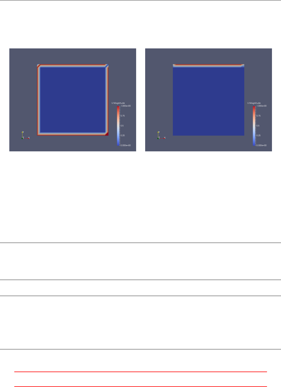
banana
{
type fix edV alue ;
val ue un ifo rm ( -1 0 0 ) ;
}
}
Listing 96: The velocity field boundary conditions of the modified cavity tutorial. The entry for frontAndBack
is omitted for brevity. Only movingWall is specified by exact patch name. The fixed walls are specified via
patch groups.
The resulting initial velocity field depends on the order of the entries for wall and banana.
Figure 5: The initial velocity field depending on the order of the wall and banana.Left: Setting as in Listing
96.Right:wall and banana have changed places.
Thus, users are suggested to avoid situations involving multiple group membership when specifying boundary
conditions via patch groups.
Pitfall: identical names of patches and patchGroups
When patches have the same name as a patchGroup, OpenFOAM may issue a warning or exit with an error.
Up to, and including, OpenFOAM-4.0 a warning message was issued, as in Listing 97. In later versions, Open-
FOAM aborts with an error, as in Listing 98.
--> FOAM W arning :
From fu nct ion const Foam :: Ha shTable <Foam :: List < int > , Foam :: word >& Foam :: p oly Bo und ar yMes h ::
gro upPa tch IDs () c onst
in file meshes / po lyMesh / poly Bound ar yMe sh / p olyB oun da ryMes h .C at line 448
Patch f ixe dWall01 specifies a group b anana whic h is also a pat ch name . This might g ive
p ro bl em s l at er on .
Listing 97: OpenFOAM is warning about identical names of a patch and a patchGroup.
--> FOAM FATAL ERROR :
Patch ’ fi xedWall 01 ’ specifies the g roup ’banana ’ which cl ashes with a patch name .
Please choose patch name s which are not patch ty pe / grou p names .
From fu nct ion const Foam :: Ha shTable <Foam :: List < int > , Foam :: word >& Foam :: p oly Bo und ar yMes h ::
gro upPa tch IDs () c onst
in file meshes / po lyMesh / poly Bound ar yMe sh / p olyB oun da ryMes h .C at line 448.
FOAM exiting
Listing 98: Identical names for patches and patchGroups are not allowed anymore.
III This offering is not approved or endorsed by ESI®Group, ESI-OpenCFD®or the OpenFOAM®
Foundation, the producer of the OpenFOAM®software and owner of the OpenFOAM®trademark. 59

Pitfall: patches
In older versions of OpenFOAM, there was a patches sub-dictionary instead of the boundary sub-dictionary,
see http://www.openfoam.org/version2.0.0/meshing.php. In some tutorial cases the old patches sub-
dictionary can be found. However, it is recommended to use the boundary sub-dictionary because in some cases
the use of the patches sub-dictionary results in errors.
To find out if there are still tutorial cases present that use the patches sub-dictionary the command of
Listing 99 searches all files with the name blockMeshDict in the tutorials for the word patches.
fi nd $ FO A M_ T UT O RI A LS - na me b l oc k Me s hD i ct | x ar gs g re p p at ch e s
Listing 99: Find cases that still use the patches sub-dictionary in the blockMeshDict to define the boundaries
13.2.6 mergePatchPairs
The mergePatchPairs list contains pairs of patches that need to be connected by the mesher.
Nothing to merge
This entry can be omitted. Listing 100 shows the message issued by blockMesh when mergePatchPairs is
omitted.
There are no merge pat ch pairs edges
Listing 100: Output of blockMesh when mergePatchPairs is omitted
Patches to merge
When two patches need to be merged, then the patch pair needs to be stated in the mergePatchPairs list. The
first patch of the pair is considered the master patch the second is the slave patch. The reason and consequences
of this are described in the official User Manual [39].
mergePatchPairs
(
( maste r s lave )
);
Listing 101: The mergePatchPairs list in the blockMeshDict
If the patches that are part of the merging operation contain faces which are unaffected by the merging, the
merge operation will fail. When the blocks of Figure 9are to be connected, then the patch pair consists only
of the face (1 2 6 5) and (12 15 11 8). If one of the two patches contains an additional face, blockMesh will
crash with an error. Thus the patches need to be defined as in Listing 102.
boundary
(
master
{
ty pe pat ch ;
faces
(
(1 2 6 5)
);
}
slave
{
ty pe pat ch ;
faces
(
(12 15 11 8)
III This offering is not approved or endorsed by ESI®Group, ESI-OpenCFD®or the OpenFOAM®
Foundation, the producer of the OpenFOAM®software and owner of the OpenFOAM®trademark. 60
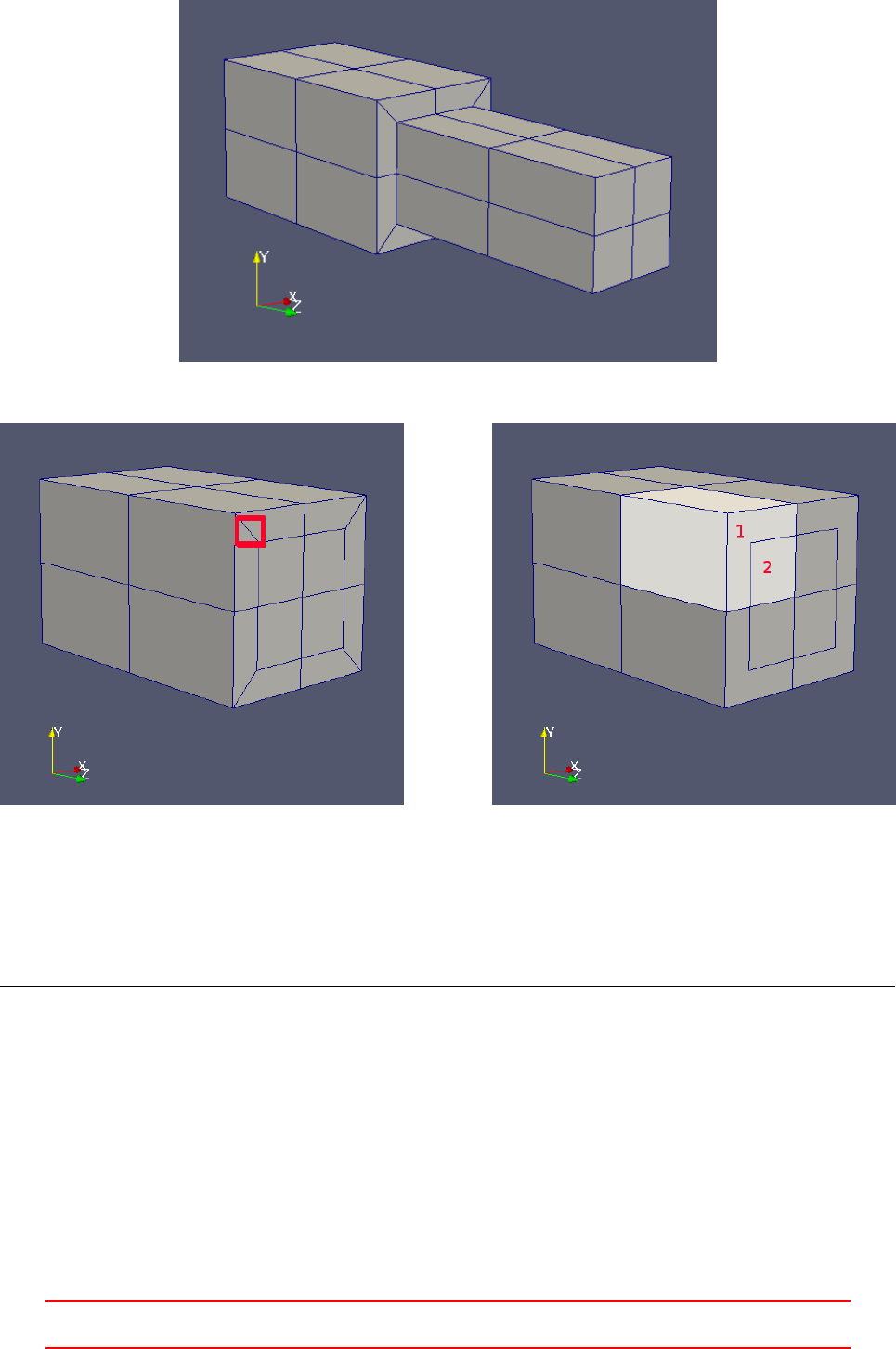
Figure 6: The mesh of two merged blocks
Figure 7: The mesh of two merged blocks. Left: screenshot of ParaView. Right: edited image to depict the
actual faces.
);
}
...
);
Listing 102: The patch definitions needed to connect the blocks of Figure 9with mergePatchPairs in the
boundary sub-dictionary
blockMesh creates hanging nodes in order to connect the mesh of the blocks. Figure 6shows the mesh of
two merged blocks. Figure 7shows the larger of the two blocks. The diagonal lines – one of them is marked
with a red square in Figure 7– are artefacts of the depiction of ParaView. The diagonal line that divides the
L-shaped area is not present in the mesh. The right image in Figure 7was edited with an image manipulation
program to reflect the actual situation of the mesh. During the merging operation the face touching the second
block is divided to match the second block. Thus, a quadrangular cell face is divided to two faces. The face
denoted with the red 1 consists of 6 nodes and the face with the red 2 constists of four nodes.
III This offering is not approved or endorsed by ESI®Group, ESI-OpenCFD®or the OpenFOAM®
Foundation, the producer of the OpenFOAM®software and owner of the OpenFOAM®trademark. 61
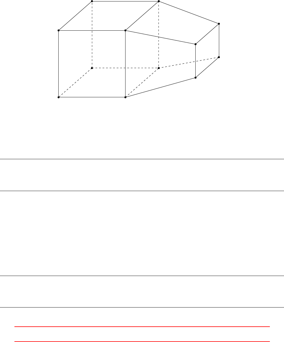
13.3 Create multiple blocks
A single block is almost never sufficient to model the geometry of a CFD problem. blockMesh offers the possibility
to create an arbitrary number of blocks which can be connected. If blocks are constructed in a fashion that
they share vertices, then they are connected by blockMesh by default.
13.3.1 Connected blocks
Figure 8shows two connected blocks. These blocks share vertices. Therefore, the blocks are connected auto-
matically.
23
67
0 1
4 5
9
10
11
8
Figure 8: Two connected blocks
Listing 103 shows the blocks sub-dictionary to create two connected blocks as they are depicted in Figure
8. The global vertex numbering is arbitrary. However, the order in which the vertex numbers are listed after
the hex keyword corresponds with the local vertex numbering of the generic block in Figure 3.
blocks
(
hex (0 1 2 3 4 5 6 7) (10 10 10) s imp leGr ading (1 1 1)
hex (1 9 10 2 5 8 11 6) (10 10 10) simpl eGra din g (1 1 1)
);
Listing 103: The blocks entries in blockMeshDict to create the connected blocks of Figure 8
13.3.2 Unconnected blocks
Figure 9shows a situation in which two blocks were created that share no vertices. Creating multiple blocks is
done simply by adding a further entry in the blocks list. The blocks are connected by the statements in the
mergePatchPairs section of the blockMeshDict.
Listing 104 shows the blocks sub-dictionary to create two unconnected blocks as they are depicted in Figure
9.
blocks
(
hex (0 1 2 3 4 5 6 7) (10 10 10) s imp leGr ading (1 1 1)
hex (8 9 10 11 12 13 14 15) (10 10 10) si mpl eGra din g (1 1 1)
);
Listing 104: The blocks entries in blockMeshDict to create the unconnected blocks of Figure 9
III This offering is not approved or endorsed by ESI®Group, ESI-OpenCFD®or the OpenFOAM®
Foundation, the producer of the OpenFOAM®software and owner of the OpenFOAM®trademark. 62
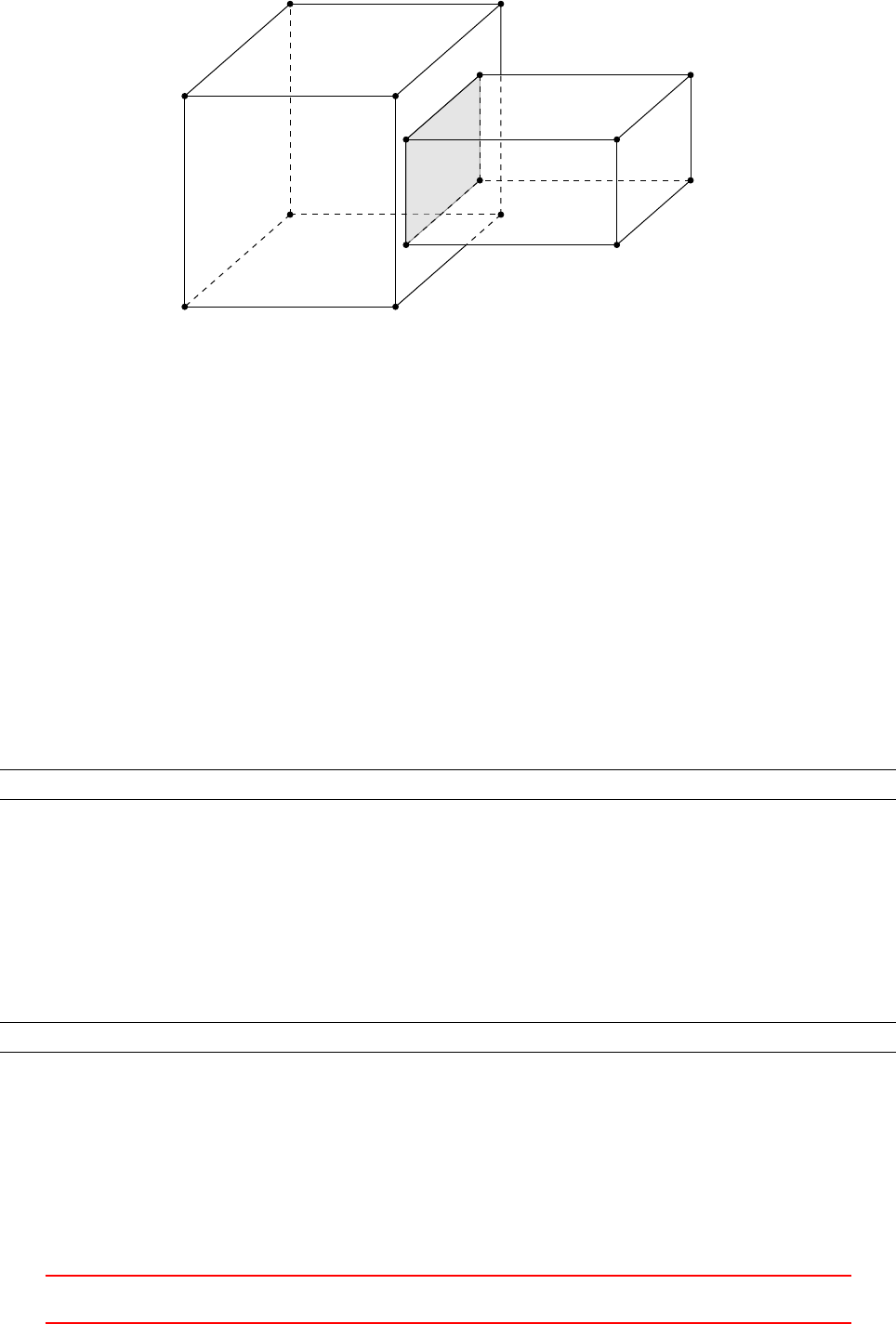
23
67
0 1
4 5
8 9
10
12 13
1415
11
Figure 9: Two unconnected blocks
In order to generate a connected mesh of the two blocks, the mergePatchPairs section of the blockMeshDict
has to be provided with the two touching patches.
13.4 Grading
In the file blockMeshDict the grading can be defined globally for the edges of the block or for all edges
individually. The grading is specified by the expansion ratio. This is the ratio of the widths of the first and the
last cell along an edge. The direction of an edge is defined in the general definition of a block (see OpenFOAM
Users Manual [39]).
simpleGrading
The global grading is defined for all edges parallel to the local x,yand zdirection of the block. In Listing 105
the grading of all edges parallel to the local xaxis oy the block is one, the grading of all edges parallel to the
local yaxis is two and the grading of all edges parallel to the local zaxis is three.
sim pleG rad ing (1 2 3)
Listing 105: simpleGrading
edgeGrading
With the keyword edgeGrading the grading of each edge of the block is specified individually. Therefore, the
value of this keyword is a list with 12 numbers. The numbering of the edges – the list index corresponds to the
edge number – is defined in the general definition of a block (see OpenFOAM Users Manual [39]). Listing 106
has the same effect as Listing 105.
edg eGr ading (1 1 1 1 2 2 2 2 3 3 3 3)
Listing 106: edgeGrading
Pitfall: inconsistent grading
When a mesh consists of more than one block, then the grading of coincident edges must be consistent, i.e.
these edges must have the same grading. In Listing 107 the grading of the last block is erroneous – the grading
is set to 2 instead of 3. The error message caused by this fault is shown in Listing 108. The message mentions
the blocks 5 and 8. This is correct, because OpenFOAM counts – like C, C++ and many more programming
III This offering is not approved or endorsed by ESI®Group, ESI-OpenCFD®or the OpenFOAM®
Foundation, the producer of the OpenFOAM®software and owner of the OpenFOAM®trademark. 63

languages – from 0. Therefore, block 8 is the ninth block.
blocks
(
hex (0 16 20 4 1 17 21 5) (30 5 10) si mple Gra ding (1 0.5 0.33) // 1
hex (1 17 21 5 2 18 22 6) (30 5 2) s imp leGr adi ng (1 0.5 1) // 2
hex (2 18 22 6 3 19 23 7) (30 5 15) si mple Grading (1 0.5 3) // 3
hex (4 20 24 8 5 21 25 9) (30 2 10) si mple Gra ding (1 1 0.33) // 4
hex (5 21 25 9 6 22 26 10) (30 2 2) si mpl eGra din g (1 1 1) // 5
hex (6 22 26 10 7 23 27 11) (30 2 15) s impl eGr adin g (1 1 3) // 6
hex (8 24 28 12 9 25 29 13) (30 5 10) s impl eGr adin g (1 2 0.33) // 7
hex (9 25 29 13 10 26 30 14) (30 5 2) s imp leGr adi ng (1 2 1) // 8
hex (10 26 30 14 11 27 31 15) (30 5 15) s impl eGr adin g (1 2 2) // 9
);
Listing 107: Inconsistent grading
--> FOAM FATAL ERROR :
Inc onsiste nt point locations be tween bl ock pair 5 and 8
probably due to incon siste nt gr adin g .
From fu nct ion blockMesh :: c alcM erg eInf o ()
in file blo ckM esh / bloc kMe shMe rge . C at line 294.
FOAM exiting
Listing 108: Error message caused by inconsistent grading
Pitfall: inconsistent discretisation
When a mesh consists of more than one block, then the number of cells of neighbouring blocks must be con-
sistent, i.e. the blocks must have the same number of cells along coincident axes. In Listing 109 the number
of cells of the first block is erroneous – the number is set to 44 instead of 45 along the local zdirection. The
error message caused by this faulty definition is shown in Listing 110. The message mentions the blocks 0 and
1. This error message indicates more clearly – other than Listing 108 – that OpenFOAM counts from 0.
blocks
(
hex (0 1 5 4 8 9 13 12 ) (9 1 44) simp leGradi ng (1 1 1) // 1
hex (1 2 6 5 9 10 14 13 ) (2 1 45) simp leGr adi ng (1 1 1) // 2
hex (2 3 7 6 10 11 15 14 ) (9 1 45) sim ple Grad ing (1 1 1) // 3
);
Listing 109: Inconsistent discretisation
--- > FOAM F ATAL ERROR :
Inc onsiste nt num ber of faces betw een block pair 0 and 1
From fu nct ion blockMesh :: c alcM erg eInf o ()
in file blo ckM esh / b loc kM esh Me rge . C at line 221.
FOAM exiting
Listing 110: Error message caused by inconsistent discretisation
Interesting observation
The source code also allows to state a list with only one entry. This is not documented in the official User
Manual [39].
Listing 111 prooves this observation in the form of the responsible source code. The first command reads a
scalar list from the input stream is. Then the three valid cases – one, three or twelve entries – are handled If
none of the three branches of the if-else branching is entered an error is reported.
III This offering is not approved or endorsed by ESI®Group, ESI-OpenCFD®or the OpenFOAM®
Foundation, the producer of the OpenFOAM®software and owner of the OpenFOAM®trademark. 64

This code listing is a beautiful example of deducting the behaviour of a program from its source code. Un-
fortunately not all parts of OpenFOAMs source code are that easy to read and understand.
1s ca la r Li st e xp Ra tio s ( is )
2
3if ( exp Rat ios . size () == 1)
4{
5// identical in x / y/z - d ire cti ons
6expan d_ = expRatios [0];
7}
8else if ( expRatios . size () == 3)
9{
10 // x - d ire ct i on
11 expan d_ [0] = e xpR ati os [0];
12 expan d_ [1] = e xpR ati os [0];
13 expan d_ [2] = e xpR ati os [0];
14 expan d_ [3] = e xpR ati os [0];
15
16 // y - d ir e ct io n
17 expan d_ [4] = e xpR ati os [1];
18 expan d_ [5] = e xpR ati os [1];
19 expan d_ [6] = e xpR ati os [1];
20 expan d_ [7] = e xpR ati os [1];
21
22 // z - d ir e ct io n
23 expan d_ [8] = e xpR ati os [2];
24 expan d_ [9] = e xpR ati os [2];
25 expan d_ [10] = e xpRatios [2];
26 expan d_ [11] = e xpRatios [2];
27 }
28 else if ( exp Rati os . size () == 12)
29 {
30 expan d_ = e xpRa tios ;
31 }
32 else
33 {
34 FatalErrorIn
35 (
36 " blo ck Des cr ipt or :: b lo ckD es cri pt or "
37 " ( con st p o in tF i el d & , c on st cu r ve dEd geL i st & , I st re am &) "
38 ) << " Unkno wn de fi nition of e xp ansion r atios : " << ex pRa tio s
39 << exit ( FatalEr ror ) ;
40 }
Listing 111: Some content of blockDescriptor.C
13.5 Parametric meshes by the help of m4 and blockMesh
In blockMeshDict only plain text is allowed, i.e. no symbols can be used. Also, no calculations can be made
by blockMesh with the exception of the keyword convertToMeters.
13.5.1 The blockMeshDict prototype
If the user wants to create parametrised meshes, i.e. properties of the mesh are calculated from certain pa-
rameters, an additional working step is necessary. In order to create a parametric mesh a prototype of the file
blockMeshDict is needed. This prototype contains symbols. Listing 112 shows the block definition of such a
prototype. This block definition is not fully parametric, only the number of cells is calculated. Note, that in
local ydirection only one cell is used for discretisation. This indicates a 2D problem.
blocks
(
hex (0 1 5 4 8 9 13 12 ) ( N1x 1 N1z ) s imp leGr adi ng (1 1 1) // 1
hex (1 2 6 5 9 10 14 13 ) ( N2x 1 N1z ) s imp leGr ading (1 1 1) // 2
hex (2 3 7 6 10 11 15 14 ) ( N1x 1 N1z ) simp leG radi ng (1 1 1) // 3
);
Listing 112: Block definition of the prototype
III This offering is not approved or endorsed by ESI®Group, ESI-OpenCFD®or the OpenFOAM®
Foundation, the producer of the OpenFOAM®software and owner of the OpenFOAM®trademark. 65

13.5.2 The macro programming language m4
In order to replace the symbols of the prototype with meaningful numbers, the prototype has to be processed
by a macro programming language interpreter. In this case the programming language m4 33 is used. The
interpreter of this language scans the prototype for valid expressions (macros) and replaces them with their
result.
To replace a symbol of the prototype with a meaningful number, a macro has to be defined. Listing 113
shows the definition of the symbols used in Listing 112. In the first line a general variable his defined. The
second and the third instruction calculate the number of cells in the local xdirection based on the variable h.
The last instruction calculates the number of cells in the local zdirection.
define(h ,2)
define( N1x , ‘ eval( 9* h ) ’)
define( N2x , ‘ eval( 2* h ) ’)
define( N1z , ‘ eval(45* h) ’)
Listing 113: Block definition of the prototype
This kind of parametrisation allows to specify a multiplier for the number of cells. The discretisation length
can not be refined gradually this way. Specifying the discretisation length requires more complex math than
integer operations.
Complex math - first shot
The builtin mathematic macros of m4 are restricted to integer operations only. As m4 supports system calls,
floating point calculations can be done by an external program. Consequently, the symbol is replaced by the
result of the system call.
In Listing 114 some variables are defined. In line 13 a macro is defined that passes its arguments to the
operating system via a system call. The argument of the command esyscmd gets executed in the command
line. This is the reason for the rather complicated argument of esyscmd. The output of the command echo is
the input of the command bc34. Note the use of the pipe.
The input of the command echo is composed of three successive operations that need to be performed
by the calculator. The first instruction says that two digits after the decimal point should be used. The
second instruction calculates the difference between the first two arguments and the last instruction divides
this difference by the third argument. These operations compute first the length of the block that needs to be
descretised. Then by dividing this length by the discretisation length the number of cells is calculated.
The output is then formatted by the macro format. Note the formatting string %.0f. This causes the result
to loose its digits after the decimal point. This step is absolutely necessary, because only integers are allowed
to define the number of cells.
1// # enter dis cret iza tion length
2define(dx ,0.005)
3define(dz ,0.005)
4
5// # enter x c oor din ates
6define(x1 ,0 .0555)
7define(x2 ,0 .0945)
8
9// # enter heig hts (z c oordi nat es )
10 define(H1 , 0.20)
11
12 // # relDiff : ( $1 - $2) / $3 # dec imal p laces tr uncated ( done by format %.0 f)
13 define( re lDi ff , ‘ format( ‘% .0 f ’, esyscmd( e cho " s ca le = 2; a = $1 - $2 ; a / $3 " | bc ) ) ’)
14
15 define(N1x ,‘ re lDif f (x1 ,0, dx ) ’)
16 define( N2x , ‘ r elD if f ( x2 , x1 , dx ) ’)
17
18 define(N1z ,‘ re lDif f (H1 ,0, dz ) ’)
33m4 is part of the GNU project. See http://www.gnu.org/software/m4/manual/index.html
34bc is a calculator program. It is part of the GNU project.
III This offering is not approved or endorsed by ESI®Group, ESI-OpenCFD®or the OpenFOAM®
Foundation, the producer of the OpenFOAM®software and owner of the OpenFOAM®trademark. 66

Listing 114: Block definition of the prototype
Listing 114 allows to calculate the number of cells from a specified discretisation length. Due to rounding
operations the specified discretisation length is not exactly met. Listing 115 shows the result after the macros
from Listings 112 and 114 have been processed.
blocks
(
hex (0 1 5 4 8 9 13 12 ) (11 1 40) si mpl eGra din g (1 1 1) // 1
hex (1 2 6 5 9 10 14 13 ) (7 1 40) simp leG radi ng (1 1 1) // 2
hex (2 3 7 6 10 11 15 14 ) (11 1 40) simp leG radi ng (1 1 1) // 3
);
Listing 115: Resulting parametric block definition
Complex math - the better solution
The above described way to do mathematical operations is not very elegant. At this place a more elaborate
solution is presented.
Listing 116 shows some examples taken from a m4 script found in the tutorials. The first statement changes
the delimiter for comments. By changing the delimiter to //, comments have the same delimiter as C or C++.
Remember, OpenFOAM dictionaries follow the C++ syntax, therefore, anything following a // is treated as a
comment. Now, commented lines are always treated as comments by m4 as well as OpenFOAM. See the first
line of Listing 114. There, the // starts a comment for OpenFOAM and the #starts a comment for m4. Setting
the delimiter for comments to be the same as in C++ removes an ambiguity and a possible source for errors.
The second line of Listing 116 redefines the quote delimiter. Changing this delimiters from the standard to
the brackets is probably done to improve readability.
In line 4of Listing 116 a macro named calc is defined. This macro also uses a system call to outsource the
actual math. In this case the interpreter of the script programming language Perl35 is called. This interpreter
receives a command line argument and an instruction. The command line argument -e tells the interpreter
that only one line of code will follow. The interpreter will interpret this single line and exit. The instruction
print ($1) is a function that prints its argument on the standard output. The argument of the print function
is the argument of the calc macro. Therefore, the mathematical operation can be written directly in the code.
See line 9for an example. There, the symbols rb and Rb are replaced my m4 by their definition. The argument
of the calc macro is passed via the system call to the Perl interpreter. As Perl is able to do mathematical
operations, the interpreter computes the result of the expression and executes the function print. The macro
esyscmd returns the standard output of the command it executed.
Line 12 of Listing 116 shows that even more complex math – e.g. using trigonometric functions – is possible.
1cha nge com (//)
2cha ngequote ([ ,])
3
4define( cal c , [ esyscmd( p er l - e ’ pri nt ( $ 1 ) ’) ])
5
6define(rb , 0.5)
7define(Rb , 0.7)
8
9define( ri , c al c ( 0.5 *( rb + R b )) )
10
11 define(pi , 3.14 159 265 )
12 define( ca0 , calc ( co s (( pi / 18 0) * a 0 )) )
Listing 116: Doing complex math with m4
13.5.3 Conclusion
Parametric meshes can be created by using the macro language m4, this is demonstrated in real live by the
OpenFOAM tutorials. Also the author of this work has done so; up to a level which prompted his colleagues
35See http://www.perl.org/
III This offering is not approved or endorsed by ESI®Group, ESI-OpenCFD®or the OpenFOAM®
Foundation, the producer of the OpenFOAM®software and owner of the OpenFOAM®trademark. 67
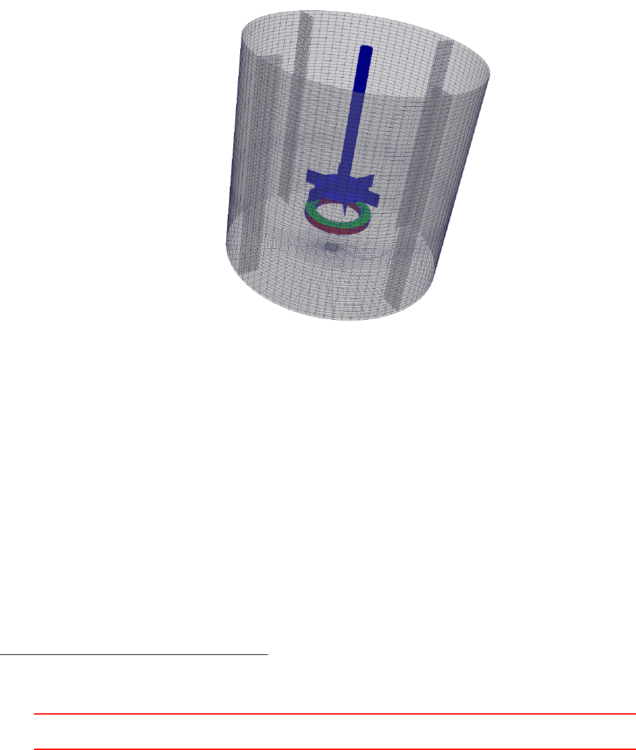
to make fun of him. This highlights the major shortcoming of using m4 for parametric meshes. At some point,
the parametric geometry creation poses the need for complex math or even high-level data structures. Thus,
we soon are in need of a general purpose programming (or scripting) language.
The mesh in Figure 10 was created with a parametric geometry. It features a variable, user-selectable number
of rotor-paddles nband stator-baffles np, with the contraint of that numbers being an integer divisor of 12. The
two numbers nband npare independent of each other, as demonstrated in Figure 10. The infinitely thin baf-
fles and paddles are created by preventing selected blocks from getting connected by the use of collocated points.
nb, np∈ {1,2,3,4,6,12}(7)
In total the mesh shown in Figure 10 consists of 459 blocks. This mesh (most probably36) would have
been impossible to create using m4. The scripting language of choice for this mesh was python37, which is an
interpreted high-level, general-purpose programming language.
Figure 10: The mesh of a stirred tank with a Rushton impeller, stator baffles and an aeration device.
Thus, we conclude this section on using m4 for geometry creation with Eric S. Raymond’s view on m4 :
The m4 macro language supports conditionals and recursion. The combination can be used to
implement loops, and this was intended; m4 is deliberately Turing-complete. But actually trying to
use m4 as a general-purpose language would be deeply perverse.
This quote from Eric S. Raymond [14] should not be seen as trying to discourage the use of m4 for simple
task. It is intended to point out the limitations of macro languages. The limitation met and experienced by the
author are the following:
Math In the sections above, we discussed two ways to perform complex mathematical operations within an
m4 script, by utilizing bc or perl via a system call. In python, we can do complex math directly, without
having to perform system calls to programs which, might or might not be installed on the user’s system.
Data structures The mesh generation script for the stirred tank makes use of python’s high-level data struc-
ture reflecting the organisation of the points on the geometry Thus, the resulting script is far better to
understand than an even less complex m4 script.
36After some initial attempts, the author gave up.
37https://www.python.org/
III This offering is not approved or endorsed by ESI®Group, ESI-OpenCFD®or the OpenFOAM®
Foundation, the producer of the OpenFOAM®software and owner of the OpenFOAM®trademark. 68

File I/O With m4, all we can do is macro substitution. Thus, everything comes from one file and goes to
one file. With a high-level language such as python, we can write several files. Thus, all files containing
geometric information can be written by the same script, e.g. the blockMeshDict and the topoSetDict(s).
This improves maintainability and reduces code duplication and manual labour.
13.6 Trouble-shooting
13.6.1 Don’t be misled by error messages
During manually building a small mesh with blockMesh by hand, i.e. writing the blockMeshDict using nothing
but an ordinary text editor, I made a rather interesting observation. To save myself the effort of scrolling back
and forth between the vertex list and the patch definition, I copied a part of the vertex list and pasted it right
where I specified the boundary faces. Thus, vertex definitions ended up, where patch definitions are expected.
After I ran blockMesh without removing the vertex definitions from the list of patches, blockMesh unsurprisingly
failed. However, this example shows that OpenFOAM’s error messages can be misleading.
Listing 117 shows the output of blockMesh resulting from the above outlined scenario. The warning message
correctly reports an unexpected input, the error message however, reports a hanging pointer. The hanging
pointer is certainly caused by the faulty entry, however, the error message does not indicate an error within the
blockMeshDict. In this case, the warning message bears the relevant information, hence users are advised to
carefully read OpenFOAM’s output (warning and error messages) in case something goes wrong.
Creating topology blocks
Creating topology patc hes
--> FOAM W arning :
From fu nction entry :: get Keywo rd ( key Type & , Ist ream &)
in file db / dictio nar y / entry/ e ntryIO .C at line 80
Rea ding / home / user / O penF OA M / user -4.0 / run / me sh ing / tes tC as e / sy stem / b lo ck Me sh Dic t . bou ndar y
found on line 135 the pu nctu ati on token ’(’
expected either } or EOF
...
--> FOAM FATAL ERROR :
han ging po in ter at i ndex 8 ( size 12) , c an not d er ef er en ce
From fu nct ion const T & Foam :: UPtrList <T >:: o pera tor []( Foam :: label ) c onst [ with T = Foam ::
entry ; Fo am :: l abel = int ]
in file / h ome / use r / Op en FOAM / OpenFOAM -4.0/ src / Ope nFOA M / lnI nc lu de / U Pt rL is tI . H at line 1 07.
FOAM a bor ting
#0 Foam :: error :: p rintStack ( Foa m :: O strea m &) at ??:?
Listing 117: The output of blockMesh with a faulty blockMeshDict. The red dots indicate removed warning
messages were removed for brevity.
This observation the warning message carries more useful information than the error message might apply
also to other parts of the OpenFOAM framework.
13.6.2 Viewing the blocks with ParaView
A mesh created by blockMesh consists of blocks. Listing 118 shows how ParaView can be used to visualise the
blocks.
p ar aF oa m - b lo ck
Listing 118: Visualising the blocks
This way, only the blocks are displayed. ParaView only reads the file blockMeshDict. Figure 11 shows the
blocks of a parametric mesh. It consists of nine blocks. The image shows also the numbers of the vertices.
III This offering is not approved or endorsed by ESI®Group, ESI-OpenCFD®or the OpenFOAM®
Foundation, the producer of the OpenFOAM®software and owner of the OpenFOAM®trademark. 69
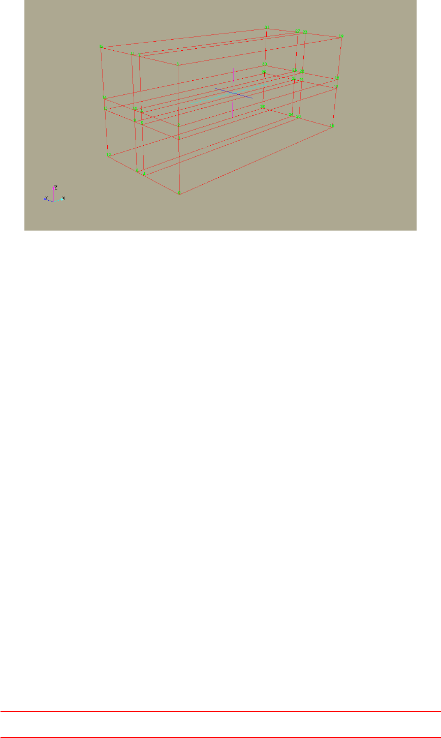
Figure 11: The blocks of a parametric mesh consisting of nine blocks.
13.6.3 Viewing the blocks with pyFoam
Troubleshooting can be difficult when blockMesh doesn’t create a mesh and displays some error messages instead.
See Section 13.6.2 for the discussion of a tool which is able to display the blocks as they are defined in
blockMeshDict. This tool even works, when blockMesh fails due to an errorneous definition in blockMeshDict.
14 snappyHexMesh
snappyHexMesh, also referred to as snappy, is a meshing tool that is able to mesh the space around an ar-
bitrary triangulated surface, e.g. an STL surface-mesh. This is generally the case in external aerodynamics.
snappyHexMesh can only be used in conjunction with blockMesh, since it requires a background mesh.
14.1 Documentation
Unfortunately, the complexity of snappyHexMesh outweighs the available on-board documentation. The on-
board documentation (User Guide) can be found in doc/Guides-a4 or doc/Guides-usletter of your lo-
cal OpenFOAM installation or online at http://www.openfoam.org/docs/user/. You find a commented
snappyHexMeshDict at $FOAM_UTILITIES/mesh/generation/snappyHexMesh. This is the case for all utilities
which are controlled by an utility-specific dictionary file, such as decomposePar,topoSet and many more.
Individual features of snappy are in some cases discussed in the release notes of the release with which
these features were rolled out. Another source of good documentation of snappy are presentations held at the
OpenFOAM Workshops. An internet search with appropriate keywords will point the reader to them, since
some of them are publicly available on the internets.
As with any other tool, the reader is encouraged to run the tutorials provided by OpenFOAM and play
around with them. The tutorial cases also provide a good starting base for building your own cases.
14.2 Work flow
The creation of a mesh by snappyHexMesh is following a two step approach:
1. The background mesh is created by blockMesh. This is absolutely necessary to the later work of snappy.
It is advised for the background mesh to consist of all-hex cells with an aspect ratio of 1, i.e. cube-shaped
cells. It is furthermore beneficial to have many intersections of the background mesh’s cell-edges with the
tri-surface.
2. snappyHexMesh then perfoms three basic steps:
III This offering is not approved or endorsed by ESI®Group, ESI-OpenCFD®or the OpenFOAM®
Foundation, the producer of the OpenFOAM®software and owner of the OpenFOAM®trademark. 70
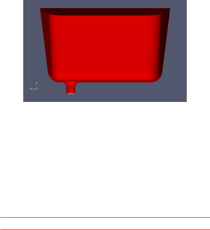
(a) Castellating
The tri-surface is approximated by splitting and removing cells outside the tri-surface.
Cell splitting The cells of the background mesh near the objects surface are refined.
Cell removal Cells of the background mesh inside the object are removed.
(b) Snapping
Cell snapping The remaining background mesh is modified in order to reconstruct the surface of
the object.
(c) Layer addition
Layer addition Additional hexahedral cells are introduced on the boundary surface of the object
to ensure a good mesh quality.
14.3 Example: Bath Tub
With the help of an actual example, we will now discuss some of snappyHexMesh’s features, as problems and
insights most often come with pratical use. Our bath tub has a non-trivial shape, thus we are not inclined to
painfully create the blockMeshDict by hand or by script. For complicated geometries a sophisticated meshing
tool such as snappy is the way to go.
Figure 12: A bath tub. The outlet patch is marked grey at the very bottom of the drain tube.
14.3.1 Boundary layers
Boundary layers are added in the last stage of snappy’s operation. These are added on a per-patch basis. Thus,
it is not possible to add layers only to parts of a patch. On the patch itself, we can control the regions in which
to add a layer by the keyword featureAngle. The operation of the layer addition stage is controlled by the
addLayersControls dictionary of snappyHexMeshDict.
Some of the entries of the addLayersControls dictionary are self-explanatory, such as the layers dictionary
specifying the patches on which to add layers of cells. However, other parameters are not that obvious in their
meaning.
featureAngle
The featureAngle is the angle between two consecutive faces. This parameter controls the behaviour of the
layer addition stage at corners and bends.
III This offering is not approved or endorsed by ESI®Group, ESI-OpenCFD®or the OpenFOAM®
Foundation, the producer of the OpenFOAM®software and owner of the OpenFOAM®trademark. 71
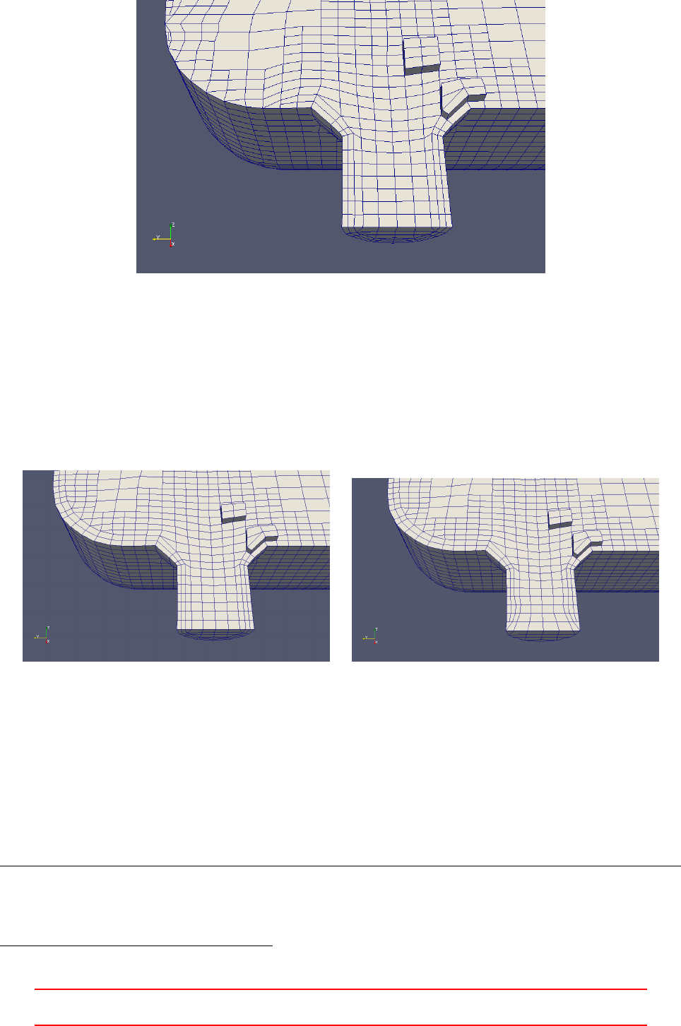
Figure 13: A badly chosen featureAngle causes snappy to add incomplete boundary layers.
slipFeatureAngle
At the outlet patch of our domain, the layer added to the wall patch meets the outlet patch, i.e. vertices need
to be added to the outlet patch in order to properly grow a layer of cells onto the wall patch. See the left side of
Figure 14. In order to achieve this, we must be able to alter the outlet patch during layer addition even though,
we do not add a layer to the outlet patch itself.
This feature is discussed in the release notes38 of OpenFOAM-2.2.0.
Figure 14: The boundary layers added by snappy. On the left, layer addition went as we intended it to do; on
the right, we see the effect of the (missing) keyword slipFeatureAngle of the addLayersControls dictionary
of snappyHexMeshDict.
Exclude patches
We have to freedom to tell snappyHexMesh to leave patches alone. Thus, during layer addition these patches
remain untouched. This allows us to reverse the effect we achieved with the slipFeatureAngle parameter. By
specifically exluding the outlet from any layer addition activity (see Listing 119), we end up with a collapsing
cell layer at the boundary of the outlet patch, see Figure 15.
layers
{
bathTub
{
nSurfaceLayers 2;
38http://www.openfoam.org/version2.2.0/snappyHexMesh.php
III This offering is not approved or endorsed by ESI®Group, ESI-OpenCFD®or the OpenFOAM®
Foundation, the producer of the OpenFOAM®software and owner of the OpenFOAM®trademark. 72
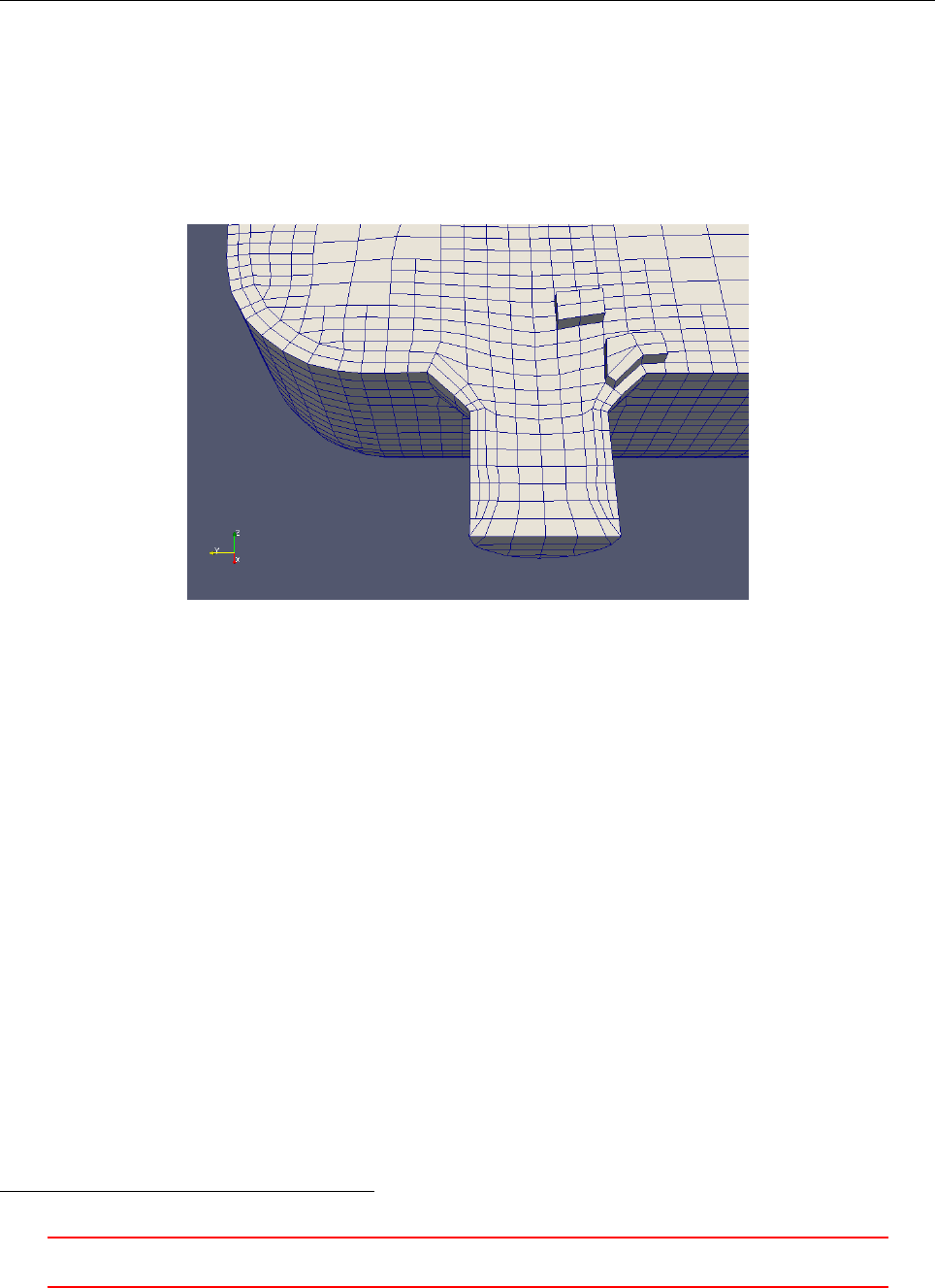
}
outlet
{
nSurfaceLayers 0;
}
}
Listing 119: The layers sub-dictionary of the addLayersControl dictionary: specifically excluding a patch
from layer addition.
This example of use may most probably not meet practical requirements, however, it demonstrates how
snappy works. The take-away message might be that nSurfaceLayers beats slipFeatureAngle.
A non-academic (read less-useless) theoretical use-case for excluding patches from layer addition might be,
when we later merge different meshes. In that case, we might want to preserve some patches for the merging
operation.
Figure 15: A collapsing boundary layer. Maybe we did not want the mesh that way, however, we told snappy
to create it exactly that way.
14.3.2 Pitfalls, sources of error and hints on malfunction
Run time
If snappyHexMesh is finished in less than a second, then something is wrong. As snappyHexMesh performs up
to three work intensive steps (castellation, snapping and layer addition), a run of snappyHexMesh takes a couple
of seconds or even longer (tens of seconds).
Units
When creating a mesh with snappyHexMesh different scales (meter vs. millimeter) of the background mesh and
the STL-mesh are a frequent source of error. Check the following things:
1. The unit of the vertex coordinates in blockMeshDict
2. The value of the convertToMeters keyword in blockMeshDict
3. The unit in which the STL was created
15 foamyHexMesh
With OpenFOAM-2.3.039 the new meshing tool foamyHexMesh was released. This tool is to some degree
similar to snappyHexMesh. The main distinction between foamyHexMesh and snappyHexMesh is that meshes
39http://www.openfoam.org/version2.3.0/foamyHexMesh.php
III This offering is not approved or endorsed by ESI®Group, ESI-OpenCFD®or the OpenFOAM®
Foundation, the producer of the OpenFOAM®software and owner of the OpenFOAM®trademark. 73
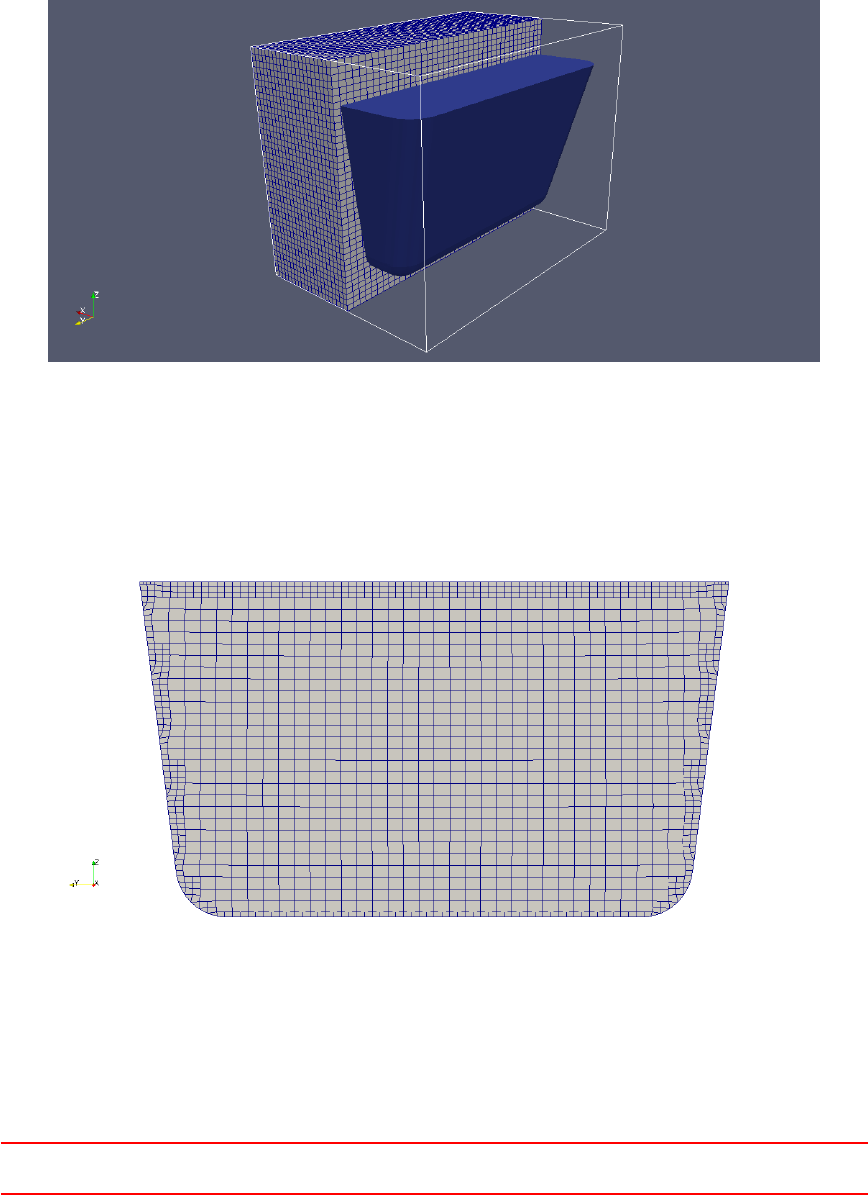
by foamyHexMesh are better aligned with the boundary surfaces. This is achieved by a different mode of
operation. foamyHexMesh generates an internal tetrahedral mesh fitting the boundaries, and then generates
and massages the dual mesh of this internal tetrahedral mesh.
15.1 Crude comparison between a snappy and a foamy bath tub
In this section we compare the way foamy- and snappyHexMesh work on the example of meshing a bath tub.
For this demonstration an STL-surface of a bath tub was created using OpenSCAD.
Figure 16 shows the outline and a part of the background mesh as well as our bath tub.
Figure 16: A bath tub with a background mesh enclosing the STL-surface of the bath tub.
15.1.1 SnappyBathTub
A first, the bath tub is meshed using snappyHexMesh. Figure 17 shows the resulting mesh. We clearly see, that
the interior cells are aligned with the global coordinate axes. At the side walls, this leads to some minor flaws.
Figure 17: SnappyBathTub
15.1.2 FoamyBathTub
Next, the bath tub was meshed using foamyHexMesh. In Figure 18 we see a good alignment of the cells with
the boundaries. The interior cells are not aligned with the global coordinate axes.
III This offering is not approved or endorsed by ESI®Group, ESI-OpenCFD®or the OpenFOAM®
Foundation, the producer of the OpenFOAM®software and owner of the OpenFOAM®trademark. 74
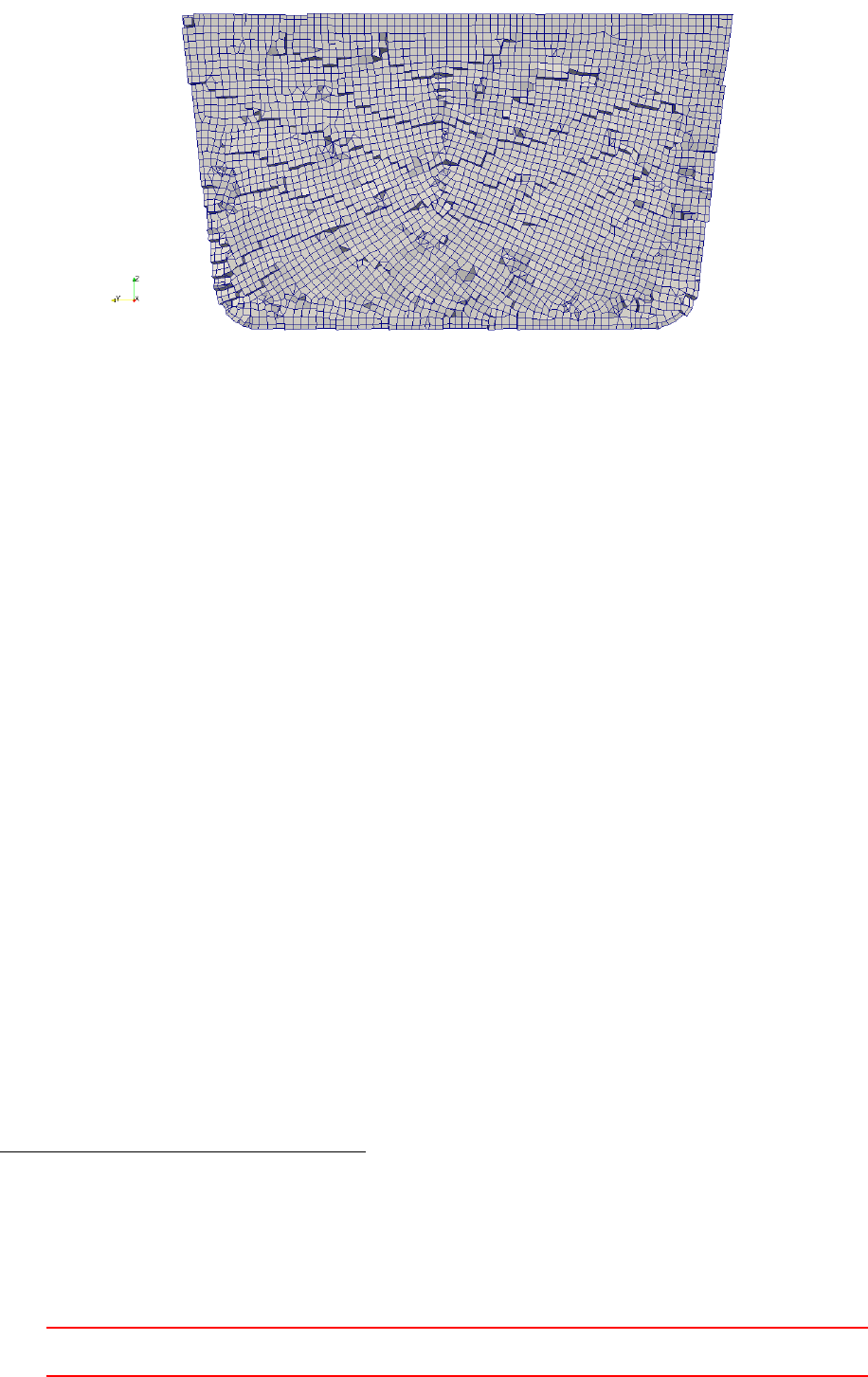
Figure 18: FoamyBathTub
16 cfMesh
cfMesh is a collection of meshing tools40 provided by the company Creative Fields. This company offers the
basic cfMesh suite under the GPL for free. At the time of writing cfMesh consists of four meshing tools which
offer a workflow comparable to the workflow offered by snappy- and foamyHexMesh.
The meshing tools of cfMesh generate their mesh based on a user-provided surface-triangulation of the
geometry. There is no need for a background mesh similar as it is the case with foamyHexMesh. All of the
tools are capable of generating boundary layers on all or on selected surfaces. All the tools are controlled by a
dictionary named meshDict, which resides in the system directory. In general the control of the user over the
meshing tools is not as tight as with snappy- or foamyHexMesh. However, this less tight control manifests itself
in a lightweight control dictionary compared to snappy- and foamyHexMesh.
The meshers of cfMesh are:
cartesian2DMesh is the tool to generate 2D meshes
tetMesh generates tetrahedral meshes
cartesianMesh generates meshes consisting mainly of hexahedrals, similar to snappyHexMesh
pMesh generates polyhedral meshes
cfMesh also provides a range of utilities (21 at the time of writing) for various tasks.
16.1 Usage
16.1.1 To treat feature edges, or not to ...
Feature edges must be specified explicitely by the user for cfMesh to obey theses edges.
In the case of the bath tub, which has a single patch a boundary, we see the effect of not providing feature
edges explicitely in Figure 19. In this case the provided STL surface was not obeyed perfectly in favour of nicer
cells. If we wanted to resolve the feature edge, we need to split the boundary of the geometry into more than
one patch. As the edges between neighbouring patches are resolved by default by the mesher, diving the bath
tub’s boundary into several patches would solve the problem shown in Figure 19.
40http://cfmesh.com/
III This offering is not approved or endorsed by ESI®Group, ESI-OpenCFD®or the OpenFOAM®
Foundation, the producer of the OpenFOAM®software and owner of the OpenFOAM®trademark. 75
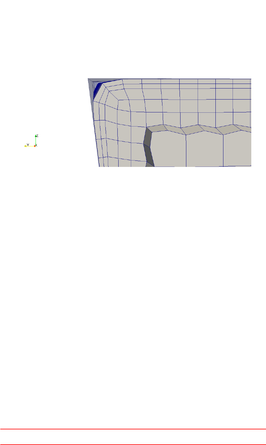
Figure 19: Poor feature edge resolution caused by not providing information on feature edges. Note, the whole
geometry is bounded by a single patch.
If we want to resolve a feature edge which is not the boundary of two patches, we can use the utility tool
surfaceFeatureEdges to extract the feature edges from the geometry. This tools checks the angles of neighbour-
ing triangles of the surface triangulation and creates additional patches. E.g. the patch wall is divided into the
patches wall_0 to wall_N, if the specified feature angle results in wall being divided into Nindividual zones.
cfMesh resolves the edges between neighbouring patches by default. Thus, the mesher is agnostic of our feature
edge treatment. After finishing meshing, the mesher can rename patches. This feature of the mesher allows us
to combine all the intermediate patches back into our initial wall patch.
III This offering is not approved or endorsed by ESI®Group, ESI-OpenCFD®or the OpenFOAM®
Foundation, the producer of the OpenFOAM®software and owner of the OpenFOAM®trademark. 76
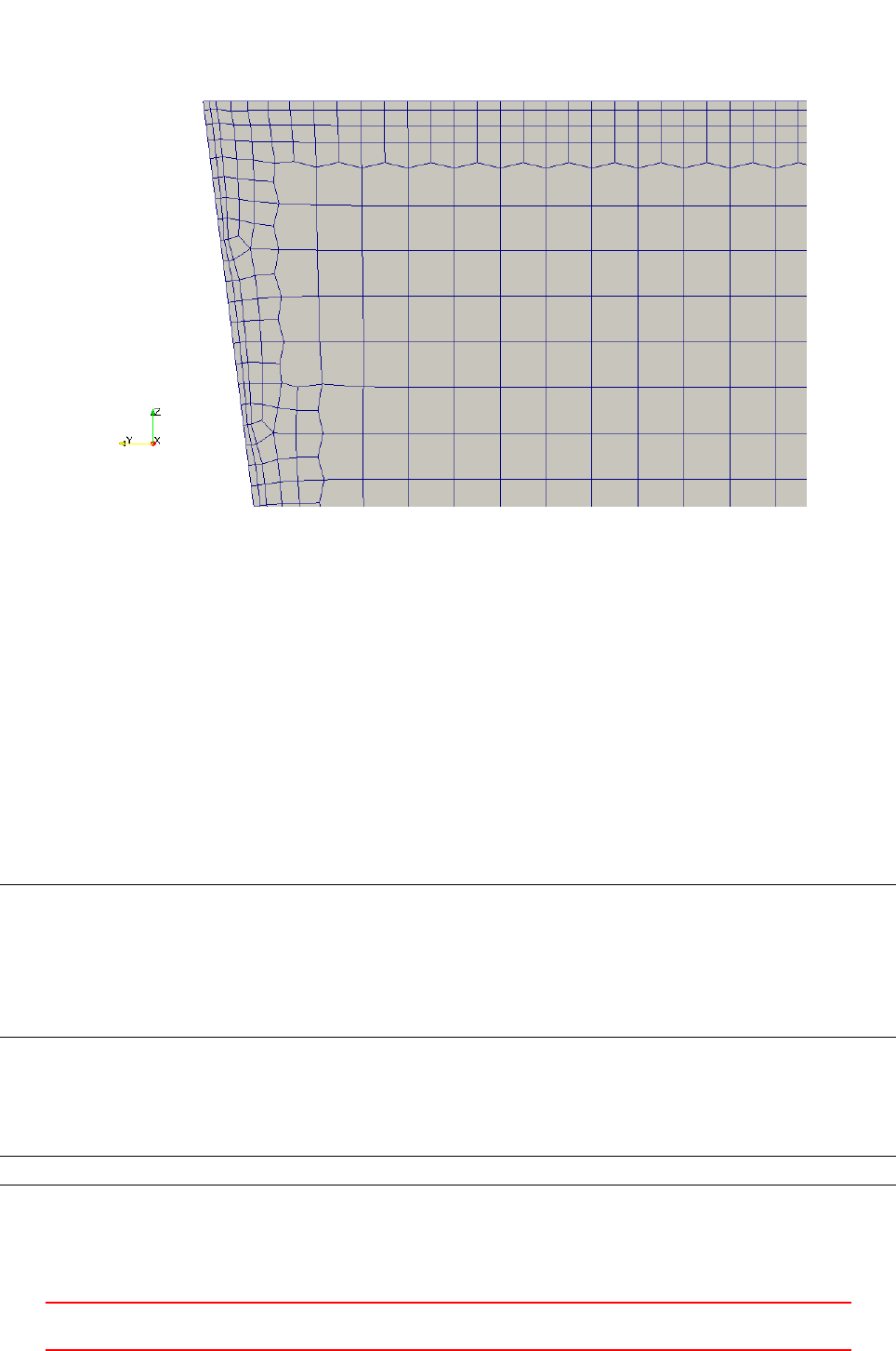
Figure 20: Resolved feature edge of the bath tub. In this case, the boundary consists of two patches: the top
surface and the rest.
We note in Figure 20 the hanging nodes inserted by the mesher to join the different refinement levels. These
hanging nodes protrude from the face they are inserted into. This prevents the faces connecting the cells of
different refinement level from being coplanar, as it is the case with snappyHexMesh.
17 checkMesh
checkMesh is a tool to perform tests on an existing mesh. checkMesh is simply invoked by its name. Like other
tools, checkMesh assumes to be called from the case directory. When checkMesh is to be called from an other
location than the case directory, the path to the case directory has to be specified with the option -case.
Listing 120 shows an error message produced by checkMesh, if checkMesh has been called with no mesh
present. In this case the tool can’t find the files specified in Section 11.1.
--> FOAM FATAL ERROR :
Cannot find f ile " points " in d ire cto ry " polyM esh " in times 0 down to constant
From fu nct ion Time :: fin dIn stance ( const fileNam e &, const word & , const IO obj ect :: rea dOption ,
const word &)
in file db / Time / find Ins tance .C at line 188.
FOAM exiting
Listing 120: No mesh present
A more thorough testing is performed when checkMesh is called with two additional options. Then checkMesh
performs some further tests.
che ck Me sh - al lG eom et ry - al lT opo lo gy
Listing 121: Do more checks
checkMesh has also the -latestTime option like many other OpenFOAM tools. This option is particularly
useful when examining meshes created by snappyHexMesh.snappyHexMesh stores intermediate meshes if it is
III This offering is not approved or endorsed by ESI®Group, ESI-OpenCFD®or the OpenFOAM®
Foundation, the producer of the OpenFOAM®software and owner of the OpenFOAM®trademark. 77
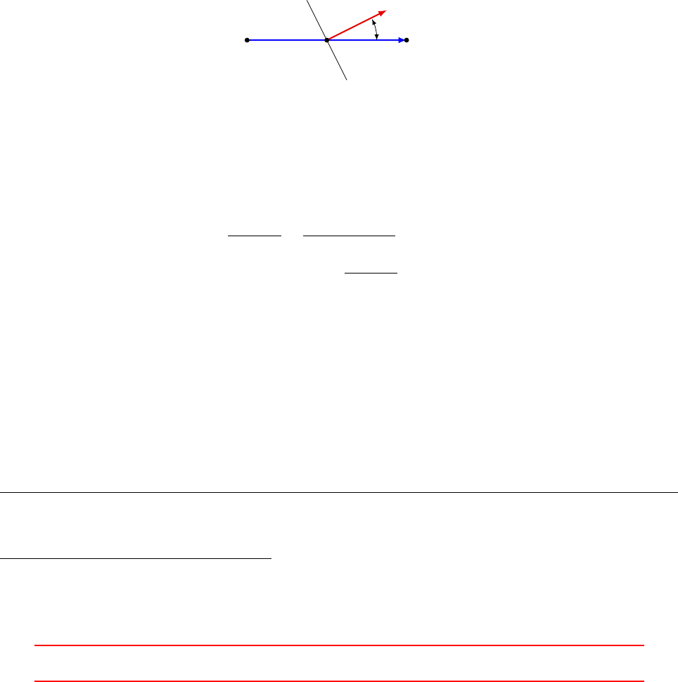
not told otherwise. By default, after a completed run of snappyHexMesh there are the background mesh and the
results of the three basic stages of a snappyHexMesh run (castellation, snapping and layer addition). Depending
on which of these steps are active up to four meshes may be present. Restricting checkMesh to the final mesh
reduces runtime and avoids the unnecessary examination of an intermediate mesh.
17.1 Definitions
In order to understand the output of checkMesh it is necessary to define some quantities calculated by checkMesh.
17.1.1 Face non-orthogonality
Non-orthogonality is a property of the faces of the mesh. We need to discriminate between internal faces and
boundary faces.
Internal faces
Each internal face connects two cells. The non-orthogonality is the angle between the vector connecting the cell
centres and the face normal vector. In Figure 21 the vector connecting the cell centres is denoted dand the
face normal vector41 S.
d
S
P N
f
θ
Figure 21: Definition of non-orthogonality for internal faces
In a perfectly orthogonal mesh the vectors dand Sare parallel. If a mesh is non-orthogonal these vectors
draw an angle as in Figure 21. This angle can be calculated from dand Sby Eq. 10.
d·S=||d|| ||S|| cos(θ)(8)
d·S
||d|| ||S|| =||d|| ||S||cos(θ)
||d|| ||S|| = cos(θ)(9)
θ= arccos( d·S
||d|| ||S||)(10)
Eq. 10 can also be found in the sources of OpenFOAM in the function faceNonOrthogonality in the file
cellQuality.C42. Listing 122 shows a loop over all faces. For each face the non-orthogonality is computed.
The vectors dand sare the connecting vector between the cell centres, and the face area vector, respectively.
The scalar cosDDotS is the angle θof Figure 21.
Note the two precautions that were taken to avoid numerical issues. First, the denominator is the sum of
the product of the magnitudes and VSMALL.VSMALL is a number with a very small value to prevent division by
zero. Second, the argument of the acos function is min(1.0, (d & s)/(mag(d)*magS + VSMALL)). Keeping
the argument of the arc-cosine equal or below 1 makes perfectly sense, because the arc-cosine is defined only
for values between -1 and 1. The limit of -1 is inherently ensured. The inner product of two vectors is always
positive. VSMALL is also positive.
1f or Al l ( ne i , f ac eI )
2{
3vec tor d = cen tr es [ ne i [ fa ceI ]] - c en tr es [ own [ f aceI ] ];
4vecto r s = a reas [ faceI ];
41The face normal vector or face area vector is a vector normal to a face. The length of this vector is equal to the area of the
face.
42In the file cellQuality.C there are two methods defined: nonOrthogonality() and faceNonOrthogonality(). Comparing the
code of this two methods reveals, that they compute the same thing. However, the method nonOrthogonality() returns the affected
cells, whereas faceNonOrthogonality() returns the affected faces.
III This offering is not approved or endorsed by ESI®Group, ESI-OpenCFD®or the OpenFOAM®
Foundation, the producer of the OpenFOAM®software and owner of the OpenFOAM®trademark. 78
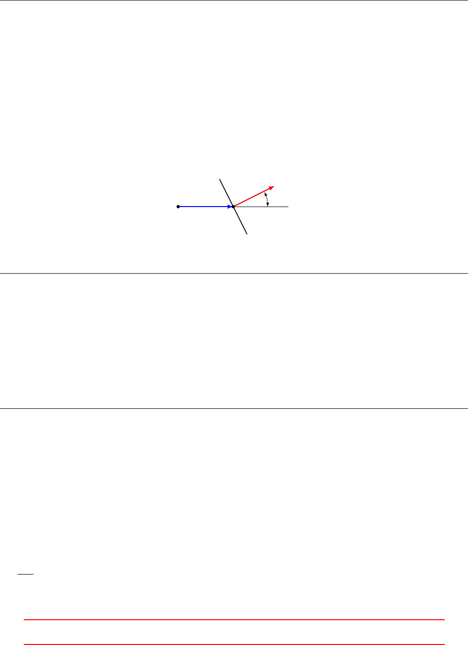
5sca lar ma gS = ma g (s ) ;
6
7scalar c osD DotS =
8rad ToDe g ( Fo am :: acos ( min (1.0 , ( d & s )/( mag (d)* m agS + V SM ALL ))) );
9resul t [ faceI ] = c osDD ot S ;
10 }
Listing 122: A detail of the function faceNonOrthogonality in the file cellQuality.C
The non-orthogonality reported by checkMesh is the angle θof Figure 21. Therefore the reported non-
orthogonality lies in the range between 0 and 90. A non-orthogonality of 0 means the mesh is orthogonal and
consists of hexahedra (cuboids) or regular tetrahedra. Listing 126 shows the output of checkMesh. In this case
the mesh is orthogonal, the maximum and average non-orthogonality is 0.
Listing 128 shows the output of checkMesh in case of a non-orthogonal mesh. Listing 129 indicates that a
non-orthogonality of above 70 triggers checkMesh to issue a warning message.
Boundary faces
Non-orthogonality is also defined for boundary faces. Figure 22 shows a schematic boundary face with its face
center f. Non-orthogonality of boundary faces is defined as the angle in degrees between the face area vector S
and the vector d, which connects the cell center Pand the face center f.
d
S
P
f
θ
Figure 22: Definition of non-orthogonality for boundary faces
1const l ab e lU Li st & f a ce Ce lls = m es h_ . b o un dar yM e sh ( ) [ pat ch I ]. f ac eC ell s ( ) ;
2const vectorF iel d :: subField f aceCent res = mesh_ . bound ary Mesh ()[ patchI ]. face Cen tres () ;
3const v ec t or Fi e ld : : s ub Fi e ld fa ceA re as = m es h_ . b o un da r yM e sh () [ pa tch I ]. fac eA r ea s ( ) ;
4
5f or Al l ( ne i , f ac eI )
6{
7vecto r d = fac eC en tr es [ fac eI ] - cen tres [ f aceCells [ fac eI ]];
8vecto r s = a reas [ faceI ];
9sca lar ma gS = ma g (s ) ;
10
11 scalar c osD DotS =
12 rad ToDe g ( Fo am :: acos ( min (1.0 , ( d & s )/( mag (d)* m agS + V SM ALL ))) );
13 result [ glo ba lF aceI ++] = c os DDot S ;
14 }
Listing 123: A detail of the function faceNonOrthogonality in the file cellQuality.C
17.1.2 Face skewness
OpenFOAM defines skewness in a mesh different than other tools, e.g. Gambit. The reason for this OpenFOAM-
specific definition is that this definition is associated with the definition of a skewness error in [26] as part of
mesh induced discretisation errors.
Skewness is a property of the faces of the mesh. We need to discriminate between internal faces and boundary
faces.
Internal faces
Each internal face connects two cells. Figure 23 shows the cell centres Pand Nof two adjacent cells. The
face faceP N is the face connecting these two cells. The point Fis the face centre of the face faceP N . The line
c=P N connects the cell centres. This connecting line intersects with the face faceP N . This intersection point
Idivides the line cinto the two parts c1and c2.
III This offering is not approved or endorsed by ESI®Group, ESI-OpenCFD®or the OpenFOAM®
Foundation, the producer of the OpenFOAM®software and owner of the OpenFOAM®trademark. 79
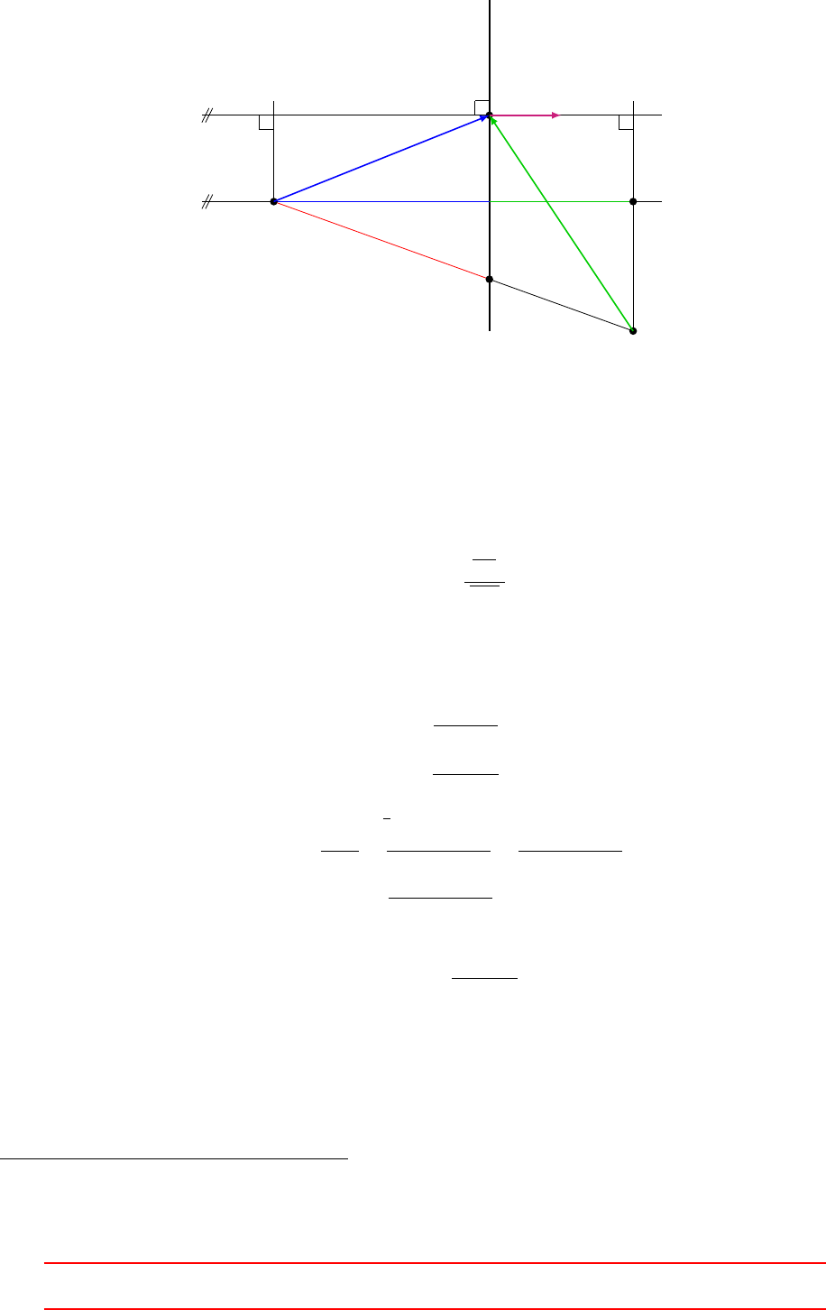
faceP N
c1
c2
dOwn dNei
P
N
F
I
X
Af
do
dn
Figure 23: Definition of skewness of internal faces
To calculate the location of Ithe length of c1is of key interest because the skewness is defined in Eq. 11.
The location (the vector to) the points P,Nand Fare easily obtained. From this three vectors do,dnand c
is computed. With doand dnthe inner product with the face area vector Afis computed to obtain dOwn and
dNei43.
skewness =|IF |
|P N|(11)
do=~
F−~
P(12)
dn=~
F−~
N(13)
c=~
N−~
P(14)
dOwn =do·Af
||Af|| (15)
dNei =dn·Af
||Af|| (16)
6(XP N) = α(17)
cos(α) = dOwn
c1
=dOwn + dNei
c1+c2
=dOwn + dNei
||c|| (18)
c1=dOwn
dOwn + dNei ||c|| (19)
~
I=~
P+c1c(20)
skewness =||~
F−~
I||
||c|| (21)
Note that both ~
Pand care vectors. The reader hopefully excuses this lack of consistency in mathematical
notation. ~
Pdenotes the position vector of the point P. In this case the symbol ~
Pis prefered to Pin order to
use symbols that can be found in Figure 23.
Listing 124 shows a detail of the function faceSkewness from the file cellQuality.C44. There a loop over
all internal faces is traversed. The loop body contains the calculation of the skewness. First dOwn and dNei
are computed. Then the location of the point Iis determined. The variable faceIntersection of the type
43dOwn and dNei are actual variable names. Therefore these symbols are written in typewriter font.
44In the file cellQuality.C there are two methods defined: skewness() and faceSkewness(). Comparing the code of this
two methods reveals, that they compute the same thing. However, the method skewness() returns the affected cells, whereas
faceSkewness() returns the affected faces.
III This offering is not approved or endorsed by ESI®Group, ESI-OpenCFD®or the OpenFOAM®
Foundation, the producer of the OpenFOAM®software and owner of the OpenFOAM®trademark. 80

point contains the position vector to the point I– the point at which the connection line between the cell
centres intersects the face. Finally, the skewness is calculated (compare Eq. 21). Notice the precaution against
a possible division by zero (adding VSMALL to the denominator).
1f or Al l ( ne i , f ac eI )
2{
3scalar dOwn = mag
4(
5( fac eC trs [ fa ceI ] - c ellC tr s [ own [ faceI ]]) & areas [ f aceI ]
6) / mag ( a re as [ f aceI ]) ;
7
8scalar dNei = mag
9(
10 ( cel lC trs [ nei[ fa ceI ]] - fac eCtr s [ face I ]) & a reas [ faceI ]
11 ) / mag ( a re as [ f aceI ]) ;
12
13 point faceIntersection =
14 cel lC tr s [ own [ fa ceI ]]
15 + ( dOwn /( dOwn + dNei ) )*( c el lC trs [ nei [ faceI ]] - c el lCtr s [ own [ faceI ]]) ;
16
17 resul t [ faceI ] =
18 mag ( face Ctrs [ fac eI ] - f ace In te rs ect io n )
19 /( ma g ( ce ll Ct rs [ nei [ fac eI ]] - c el lC tr s [ own [ fa ceI ]]) + VSMAL L );
20 }
Listing 124: A detail of the function faceSkewness in the file cellQuality.C
Boundary faces
Skewness is also defined and checked for boundary faces. Figure 24 shows the sketch of a boundary face with
its face center FC. The vector dfrom the cell center Pto the face center FCis depicted in red. At the point
FCwe see the face normal vector n. If we project the vector don the vector nwe gain the face-intersection
point FI. This is the point, where the face normal departing from the cell center intersects with the face. The
face-intersection does not necessarily need to be part of the face, as it is the case in Figure 24.
We then compute the vector f, which is the connection between the points FIand FC. The ratio of the
magnitudes of the vectors fand ddefines the skewness of a boundary face.
Listing 125 shows the code that computes the skewness of the boundary faces. The points Pand FCare
returned by the methods faceCells() and faceCentres(). The normal vector nis easily computed from the
face-area vector given by the method faceAreas().
n=faceAreas[faceI]/mag(faceAreas[faceI]) (22)
d=faceCentres[faceI] - cellCtrs[faceCells[faceI]] (23)
~
FI=cellCtrs[faceCells[faceI]] +((faceCentres[faceI] - cellCtrs[faceCells[faceI]])&n)*n
(24)
~
FI=~
P+ (d·n)n(25)
f=faceCentres[faceI] - faceIntersection (26)
f=~
FC−~
FI(27)
1lab el g l ob alF ac e I = m es h_ . n I nt e rn alF ace s () ;
2
3forAl l ( mesh_ . bou nd aryMe sh () , pat chI )
4{
5const labelUList & fac eCe lls =
6mes h_ . b ou n da ryM esh ( ) [ pa tc hI ]. f ac e Ce ll s () ;
7
8const vectorF iel d :: s ubF ield faceC ent res =
9mes h_ . b ou n da ryM esh ( ) [ pa tc hI ]. f ace Ce n tr es () ;
10 const vectorF iel d :: s ubF ield face Are as =
11 mes h_ . b ou n da ryM esh ( ) [ pa tc hI ]. f ac e Ar ea s () ;
12
13 forAl l ( faceCe ntres , faceI )
III This offering is not approved or endorsed by ESI®Group, ESI-OpenCFD®or the OpenFOAM®
Foundation, the producer of the OpenFOAM®software and owner of the OpenFOAM®trademark. 81
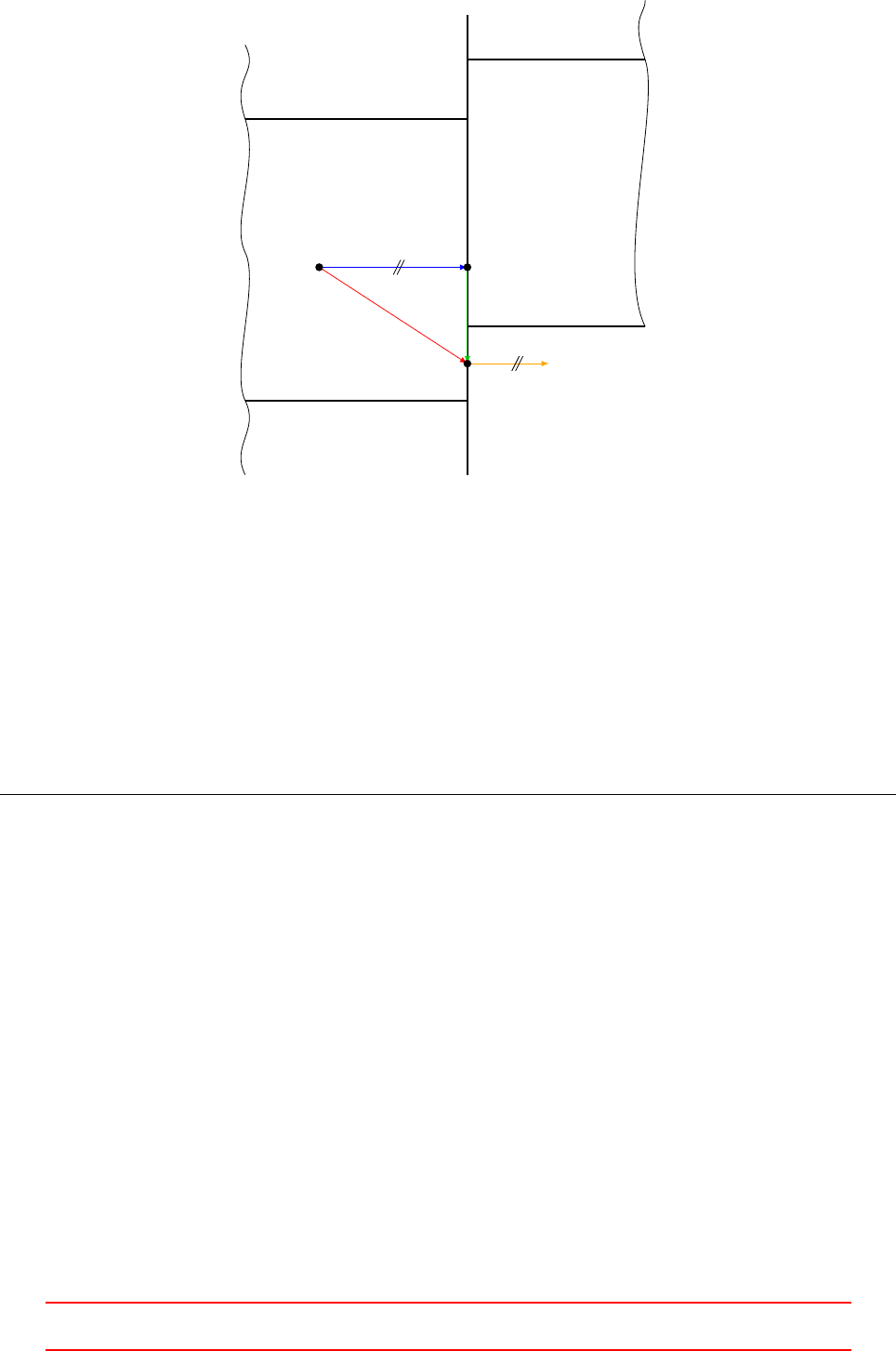
P
FI
FCn
d
f
Figure 24: Definition of skewness of boundary faces
14 {
15 vecto r n = fac eAreas [ fa ceI ]/ mag ( fac eA reas [ faceI ]) ;
16
17 point fa ce In ter se ct io n = cel lCtr s [ faceC el ls [ f aceI ]]
18 + (( f ac eC en tres [ faceI ] - cel lCtr s [ fa ce Ce lls [ fa ceI ]]) &n) *n;
19
20 result [ gl ob alF aceI ++] = mag ( faceC ent res [ faceI ] - fac eI nters ec tion )
21 /(
22 mag ( fa ce Ce nt re s [ faceI ] - c el lCtr s [ faceCells [ fac eI ]])
23 + VSMALL
24 );
25 }
26 }
Listing 125: A detail of the function faceSkewness in the file cellQuality.C
17.1.3 Face concavity
pending
17.1.4 Face warpage
A face is warped, when its vertices do not lie within a plane. Figure 25 shows a simplified situation of a
warped face. Any three points, which do not fall onto a single line, span a plane. In Figure 25 the area vec-
tor S1of the triangle ∆457 is parallel to the face area vector Sf. Thus, we identify point 6 as being out-of-plane.
III This offering is not approved or endorsed by ESI®Group, ESI-OpenCFD®or the OpenFOAM®
Foundation, the producer of the OpenFOAM®software and owner of the OpenFOAM®trademark. 82
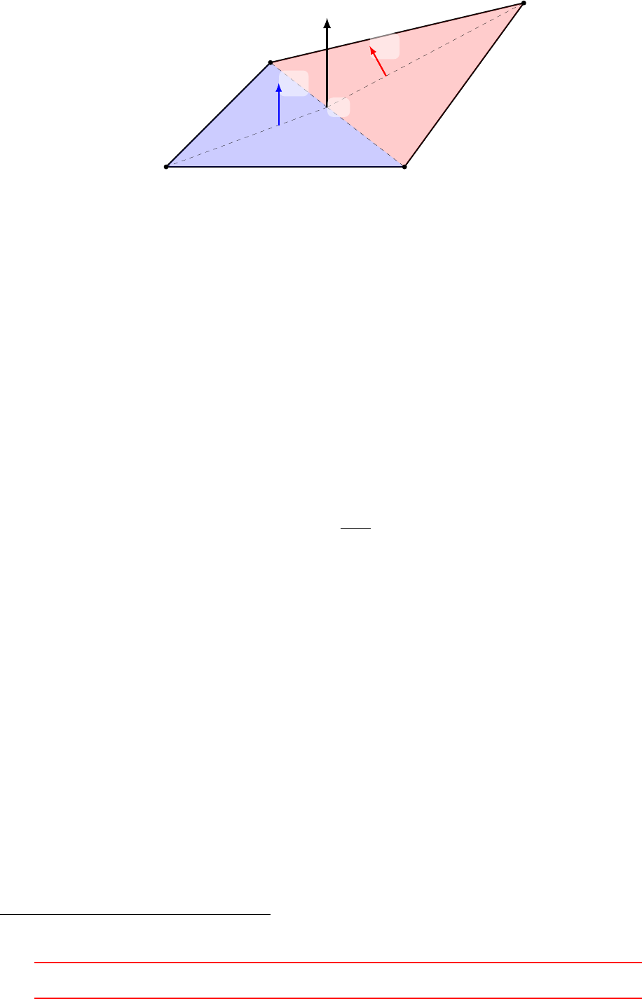
Sf
S1
S2
6
7
4 5
cf
Figure 25: Face warpage
If we decompose the face into individual triangles, we can compare the individual triangle area vectors to the
face normal vector. In Figure 25 a crude decomposition is chosen for simplicity. In OpenFOAM’s internals, the
individual triangles are defined by the face center and two consecutive vertices of the face. As, face vertices need
to be stored consecutive, a simple loop over the vertices of a face is sufficient to generate all individual triangles.
Thus, in OpenFOAM’s implementation of the test for warpage, the face of Figure 25 would be decomposed into
four triangles, as indicated by the thin dashed lines.
We bear in mind, that in OpenFOAM a face area vector has two important properties. It is normal to
the face’s plane and its magnitude is proportional to the face’s area45. By diving the face area vector by its
magnitude we gain the face normal vector, see (29).
OpenFOAM checks for warpage by computing the inner product of the triangle area vectors with the face
normal vector, and summing up the results, see (30). This sum is equal to the magnitude of the face area vector,
when all vertices are in-plane. If the two vectors of an inner product are not parallel, then the magnitude of
the inner product is smaller by the cosine of the enclosed angle.
ka·bk=kakkbkcos(α)(28)
nf=Sf
kSfk(29)
Sf
?
=X
i
nf·Si(30)
17.1.5 Cell concavity
When a cell is concave
17.2 Pitfalls
The results of checkMesh need to be taken with a grain of salt. Therefore, it is helpful to know how checkMesh
defines the qualitity measures it tests for (Section 17.1) and also to know about the shortcomings of the tests
performed by checkMesh (Section 17.2).
The tests performed by checkMesh do not necessarily guarantee the mesh to be suitable for simulation.
Furthermore, if a mesh fails a test, that does not necessariliy mean that it is unsuitable for calculation.
17.2.1 Mesh quality - aspect ratio
checkMesh performs a number of quality checks. However, the user has to be careful. checkMesh does only
check if a mesh makes a simulation impossible. There are some situations in which checkMesh does not issue
an error or a warning, however, a mesh can nevertheless be unsuitable for a successful calculation.
The aspect ratio is the ratio of the largest and the smallest dimension of the cells. For the aspect ratio there
are no limits. Listing 126 shows the output of checkMesh when a mesh with high aspect ratio cells is tested.
45Since a length can not be an area in terms of physical units, we avoid the statement, that the face normal vectors length is the
face’s area. However, the factor of proportionality is 1.
III This offering is not approved or endorsed by ESI®Group, ESI-OpenCFD®or the OpenFOAM®
Foundation, the producer of the OpenFOAM®software and owner of the OpenFOAM®trademark. 83
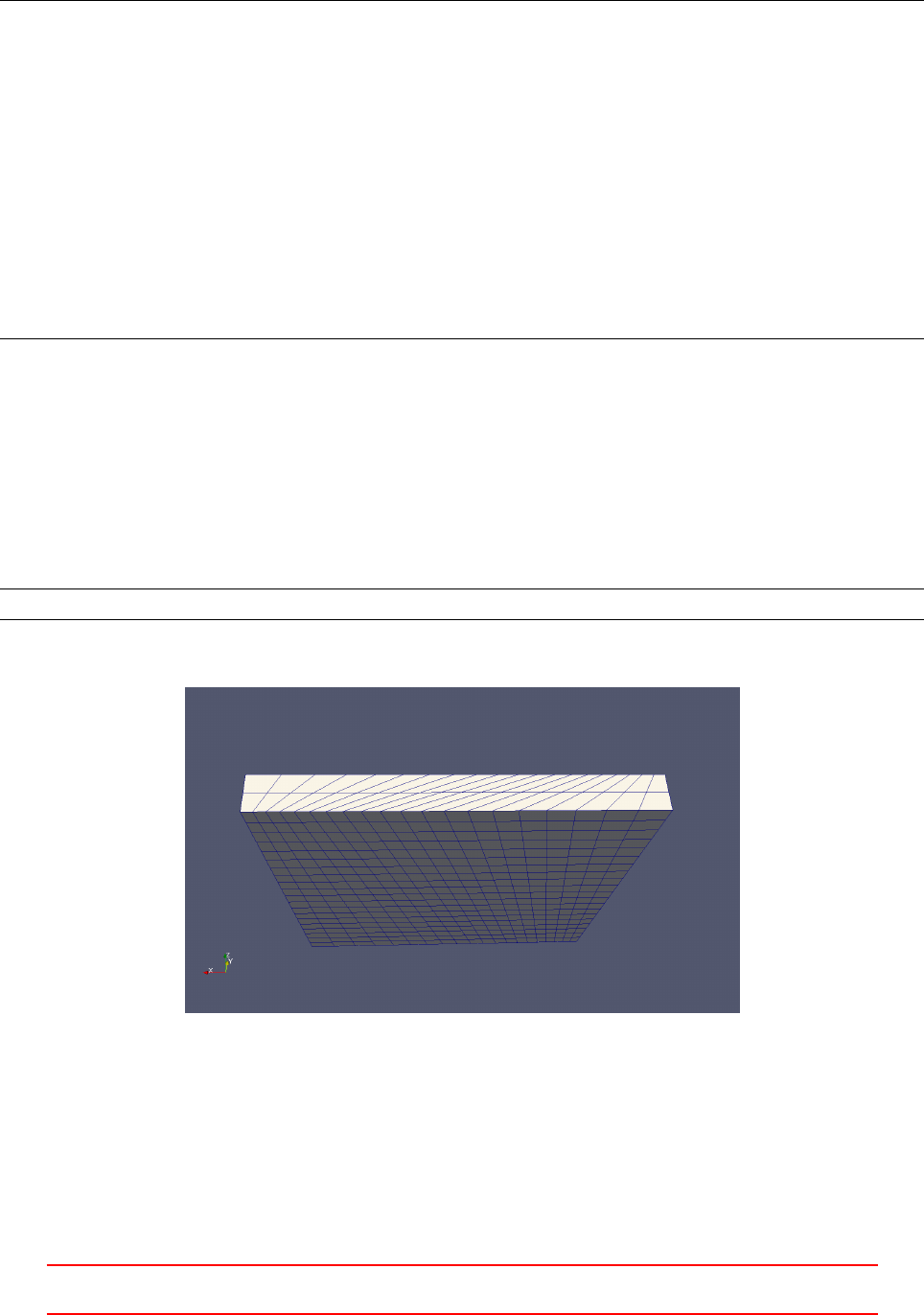
Although checkMesh does not complain, the mesh is not suitable for simulation. Even with extremely small
time steps numerical problems appear.
Checking geometry ...
Overa ll domain boundin g box (0 0 0) (0.1 0.1 0.01)
M esh ( non - e mpt y , no n - w ed g e ) d i re c ti o ns (1 1 1 )
Me sh ( non - e mpty ) dir ec ti ons (1 1 1)
B ou nd ar y op en ne s s ( - 9. 51633 e -1 7 1 .1 77 91 e - 18 - 4. 51 751 e - 17 ) OK .
Ma x c el l o p en ne ss = 1 .3 55 25 e - 16 O K .
Ma x a sp ect r at io = 1 00 O K .
Minim um face area = 2.5e -07. Maxim um face area = 2.5e -05. Face area magnit ude s OK .
Mi n vol um e = 1 .2 5 e - 09 . M ax v ol um e = 1. 25 e - 09 . To ta l v ol um e = 0 .0 00 1 . Ce ll vo lu mes OK .
Mesh non - or thog onality Max: 0 a verage : 0
Non - o r th ogo nal ity ch ec k OK .
Fa ce py ra m id s OK .
Ma x s k ew ne ss = 2e -0 6 OK .
Coupl ed poi nt locati on m atch ( ave rage 0) OK.
Me sh OK .
End
Listing 126: checkMesh output for a mesh with high aspect ratio
17.2.2 Mesh quality - skewness
There are different ways to calculate the skewness of a finite volume cell. To test whether checkMesh complains
about high skewness, a mesh is distorted by the use of edge grading. Figure 26 shows this mesh. Parallel edges
are graded alternately – alternating between the expand ratio and its reciprocal value. Listing 127 shows the
grading settings. The test case for this examination is the cavity case of icoFoam. This case can be found in
the tutorials.
hex (0 1 2 3 4 5 6 7) (20 20 2) e dgeGrad ing (3 0.33 3 0.33 1 1 1 1 1 1 1 1)
Listing 127: Block definition in blockMeshDict to achieve high skewness
Figure 26: A distorted mesh
checkMesh issues no warnings for the value pair 3and 0.33. The values 4and 0.25 cause a warning about severly
non-orthogonal faces.
However, a simulation is impossible for much lower values. The simulation runs for the value pair 1.33 and
0.75. The values 1.4and 0.714 cause the simulation to crash. The limits of stability of a simulation are therefore
reached earlier than the limits of checkMesh.
To conclude this section, the user should bear the folling statement in mind. Numerical problems of a sim-
ulation may be caused by bad mesh quality. In some cases – like the one presented above – bad mesh quality is
III This offering is not approved or endorsed by ESI®Group, ESI-OpenCFD®or the OpenFOAM®
Foundation, the producer of the OpenFOAM®software and owner of the OpenFOAM®trademark. 84

the root of the problem, but checkMesh issues no warnings. However, the values of the quality characteristics
may give a hint. Some manuals of CFD software propose numerical ranges for characteristics like aspect ratio
to ensure good quality.
Checking geometry ...
Overa ll domain boundin g box (0 0 0) (0.1 0.1 0.01)
M esh ( non - e mpt y , no n - w ed g e ) d i re c ti o ns (1 1 1 )
Me sh ( non - e mpty ) dir ec ti ons (1 1 1)
Boundary openness (4. 235 16e -18 9 .035 02e -18 1 .609 36e -16) OK.
Ma x c el l o p en ne ss = 1 .6 72 51 e - 16 O K .
Ma x a sp ect r at io = 3.6 30 59 OK .
Minim um face area = 1.42648 e -05. M aximu m face area = 7.169 4 e -05. Face area ma gnitudes OK .
Min volume = 1.03854 e -07. Max volume = 1.69673 e -07. Total volume = 0.0001. Cell v olumes OK
.
Mesh non - ort ho gon ality Max: 69. 4798 av erage : 32.809 2 Non - orth ogona lit y check OK.
Fa ce py ra m id s OK .
Ma x s k ew ne ss = 2 .3 54 85 OK .
Coupl ed poi nt locati on m atch ( ave rage 0) OK.
Me sh OK .
End
Listing 128: checkMesh output for the distorted mesh; grading ratios 3and 0.33
Checking geometry ...
Overa ll domain boundin g box (0 0 0) (0.1 0.1 0.01)
M esh ( non - e mpt y , no n - w ed g e ) d i re c ti o ns (1 1 1 )
Me sh ( non - e mpty ) dir ec ti ons (1 1 1)
Boundary openness (4. 235 16e -18 -6.21157e -18 1. 18585 e -16) OK .
Ma x c el l o p en ne ss = 2 .3 76 64 e - 16 O K .
Ma x a sp ect r at io = 4.2 37 06 OK .
Minim um face area = 1.2 3181 e -05. Maxi mum face area = 8. 67874e - 05. Face area magnitude s OK .
Min volume = 1.0 0882 e -07. Max vol ume = 1 .84055 e -07. Total v olume = 0.0001. Ce ll vo lumes OK
.
Me sh non - o rt hog on ali ty Max : 7 3. 16 35 av er ag e : 3 6. 21 31
* Numbe r of seve re ly non - o rt hogonal faces : 80.
Non - o r th ogo nal ity ch ec k OK .
<< W ri ti ng 80 non - o rt ho go na l faces to se t n onO rt hoF ac es
Fa ce py ra m id s OK .
Ma x s k ew ne ss = 2 .9 39 78 OK .
Coupl ed poi nt locati on m atch ( ave rage 0) OK.
Me sh OK .
End
Listing 129: checkMesh output for the distorted mesh; grading ratios 4and 0.25
17.2.3 Possible non-pitfall: twoInternalFacesCells
If a mesh for a two-dimensional simulation is created and checked using checkMesh with the -allTopology
option enabled46, then checkMesh will issue a message like in Listing 130. This message indicates, that there
are cells present with only two internal faces. This message can be ignored when 2D meshes are concerned. The
corner cells of a rectangular mesh have – by definition – only two internal faces.
Checking topology ...
B ou nd ar y d e fi ni t io n OK .
Cell to face addre ssi ng OK .
Poi nt u sa ge OK .
Upp er t r ia ng u la r o rd e ri ng O K .
Fa ce ve rt i ce s OK .
T op ol o gi ca l c el l zip - up c he ck OK .
Fac e - f ac e c on nec tiv it y OK .
46When the -allTopology option is enabled, checkMesh performs two additional topological checks. Checking the face connec-
tivity is one of these checks.
III This offering is not approved or endorsed by ESI®Group, ESI-OpenCFD®or the OpenFOAM®
Foundation, the producer of the OpenFOAM®software and owner of the OpenFOAM®trademark. 85
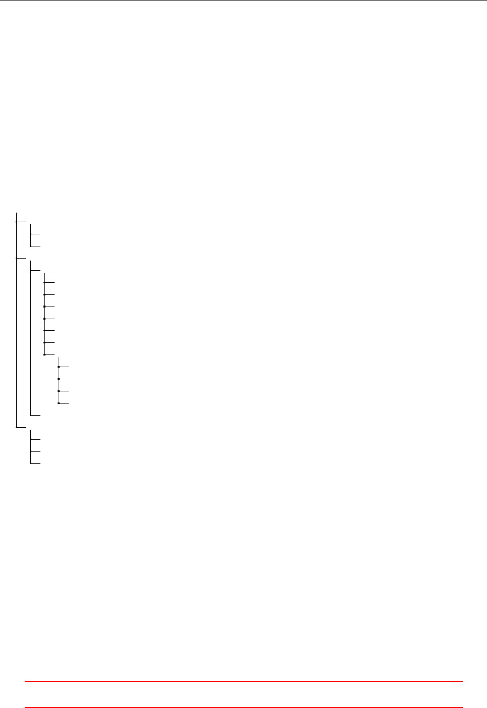
<< W ri ti ng 4 c ells w ith two non - b ou nd ar y fa ce s to set t woI nte rna lFa ce sCe lls
Number of r egion s : 1 ( OK ) .
Listing 130: checkMesh output for a 2D mesh with -allTopology option set.
If this message appears when a 3D mesh is examined, then there is probably some error in the definition of
the mesh. A cell in a 3D mesh should have at least three internal faces. A message stating the presence of cells
with two internal faces in a 3D mesh indicates non-connected regions.
17.3 Useful output
The output of checkMesh in Listing 130 also shows another interesting thing to know about checkMesh. The
line «Writing 4 cells with two non-boundary faces to set twoInternalFacesCells tells the user that
checkMesh created a set of cells that are found to have some problems.
Figure 27 shows the content of the case which resulted in Figure 26. There we see a directory named sets
inside the polyMesh folder. The sets folder was created by checkMesh and inside this folder checkMesh stores
any sets it creates. The file names are rather self-explanatory, e.g. the file skewFaces contains all faces which
failed the test for skewness. All these cell or face sets can be viewed with paraView.
.
0
p
U
constant
polyMesh
blockMeshDict
boundary
faces
neighbour
owner
points
sets
lowQualityTetFaces
nonOrthoFaces
skewFaces
underdeterminedCells
transportProperties
system
controlDict
fvSchemes
fvSolution
Figure 27: Sets created by checkMesh in the sets directory.
18 extrudeMesh
extrudeMesh is a rather special tool. OpenFOAM lists extrudeMesh under the mesh generation tools, however,
extrudeMesh has a role between mesh generation and mesh manipulation. We can do mesh generation, e.g.
extruding one cell layer from a 2D STL surface in order to prepare the mesh for a 2D study in OpenFOAM.
However, we can also do mesh manipulation, which is essentially mesh extension, as we “grow” cell layers on
surfaces.
18.1 Control
extrudeMesh is controlled by the file extrudeMeshDict. This file contains all necessary settings for using this
tool, which can roughly be divided into the categories: “where to grow”, “what to grow”, and “how to grow”.
III This offering is not approved or endorsed by ESI®Group, ESI-OpenCFD®or the OpenFOAM®
Foundation, the producer of the OpenFOAM®software and owner of the OpenFOAM®trademark. 86
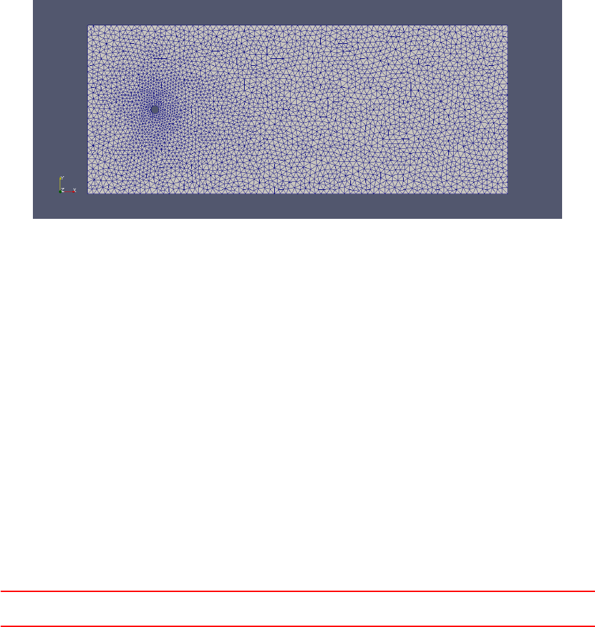
18.1.1 Source surface
The basis for cell extrusion can be either a patch of an existing mesh or an STL surface. In the case of a patch
or a mesh, the source may also be another case, e.g. extrude patch X from case Y to create the mesh of case Z.
18.1.2 Layer control
The “what to grow” part consists of the number of cells in thickness direction of the new cell layer, the thickness
and an optional expansion ratio.
18.1.3 Extrusion models
The extrusion models control the “how to grow”. There is a number of models available, some of which will be
discussed below.
Plane extrusion
The plane extrusion model is specifically for the creation of (quasi) 2D meshes. A single layer of cells is extruded
in normal direction to the povided surface. By default the front and back patches are created to be of type
empty.
In Figure 28 we see the mesh created from an STL, which was created by GMSH. In this case we could also
have used GMSH to create a mesh with a single cell in thickness direction.
Figure 28: The mesh for a 2D study generated from an STL surface.
Sector extrusion
Figure 29 shows the result of the sector extrusion model. For this model, the user needs to specify a point in
space (axisPnt), an axis of rotation (axis) and an angle. In this case the outlet patch of the original mesh
(shown in grey) was extruded. The original mesh was created by blockMesh and consists of 5 blocks (easily
scripted with e.g. Python). The axisPnt lies in the plane of the outlet patch, however, the point is well outside
the patch. The distance between the axisPnt and the centerline of the original pipe mesh determines the radius
of the pipe bend. The positive x-axis was selected as axis. The newly generated cells are by default added to
acellSet named addedCells.
This use of extrudeMesh opens a rather cheap way to create good meshes of pipe bends. The blockMeshDict
for a straight pipe is easily scripted, and by extruding along the section of a circle, the mesh is continued along
a bend. Directly scripting the blockMeshDict for a pipe bend would definitely be a little bit harder.
The sector extrusion model also has a 2D “cousin”, which is called wedge. The class underlying the wedge
extrusion model is derived from the sector model. However, the wedge model is the axisymmetric analogue of
the plane model. Thus, only one cell layer is created, which is centered about the source surface, i.e. the cell
layer is extruded half the angle in both directions from the source surface.
III This offering is not approved or endorsed by ESI®Group, ESI-OpenCFD®or the OpenFOAM®
Foundation, the producer of the OpenFOAM®software and owner of the OpenFOAM®trademark. 87
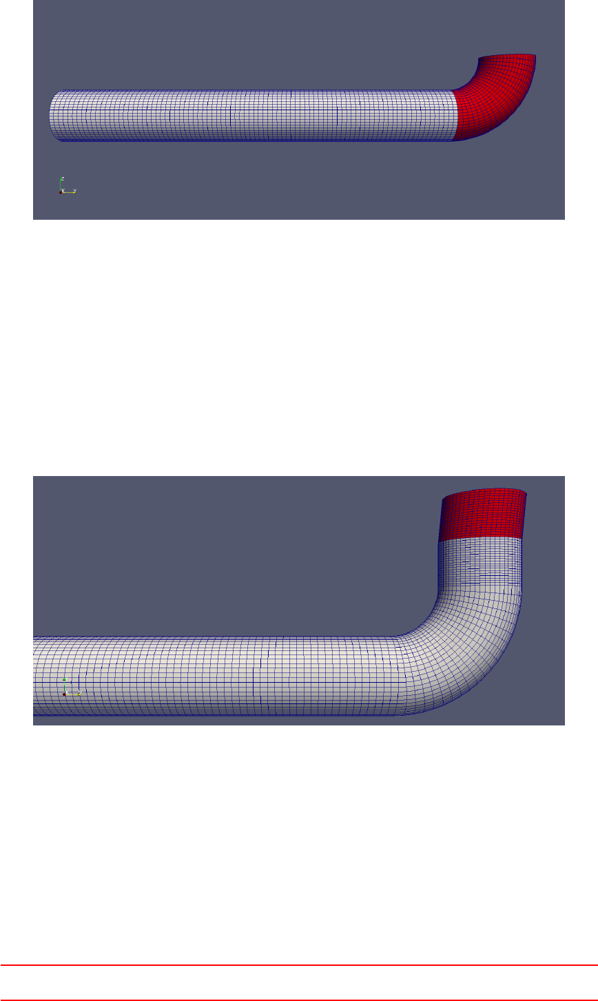
Figure 29: A cheap 90°pipe bend. The outlet patch of the original mesh was extruded along the sector of a
circle.
Linear extrusion
There are two models for linear extrusion in extrudeMesh. There is linearNormal, which extrudes in normal
direction of the underlying surface. This can be used to grow a cell layer on the pipe’s wall, see Figure 31.
Furthermore, there is linearDirection, which extrudes cells along a specified direction.
In Figure 30 we see the result of subsequent use of extrudeMesh. Unfortunately, at the time of writing
(using OpenFOAM-4.0), extrudeMesh does not offer the -dict option. Thus, we need to repeatedly edit the
extrudeMeshDict for subsequent applications of extrudeMesh. First, a bend was created by using the sector
model. Afterwards a straight pipe section was created using linearNormal, which is followed by a slanted pipe
section, which was created using linearDirection.
Figure 30: Subsequent mesh extrusions: sector,linearNormal and linearDirection.
III This offering is not approved or endorsed by ESI®Group, ESI-OpenCFD®or the OpenFOAM®
Foundation, the producer of the OpenFOAM®software and owner of the OpenFOAM®trademark. 88
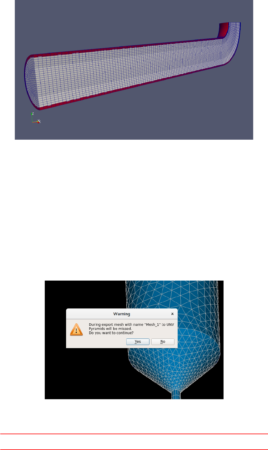
Figure 31: Grow a wall! The walls patch of the pipe mesh was extruded using the linearNormal model.
19 Salome
The Salome platform is a powerful multitool, which features a meshing module. This meshing module offers a
number of meshing tools.
19.1 Export & Conversion
Meshes can be exported by Salome into several formats. The go-to procedure for OpenFOAM-use is to export
the mesh in the UNV format and use the ideasUnvToFoam mesh converter.
19.1.1 Salome’s native UNV export
However, there is an issue when using the UNV format. Apparently, see Figure 32, Salome’s mesh export tool
for the UNV format does not export pyramid cells.
Figure 32: Mesh export issue in Salome with the UNV format.
III This offering is not approved or endorsed by ESI®Group, ESI-OpenCFD®or the OpenFOAM®
Foundation, the producer of the OpenFOAM®software and owner of the OpenFOAM®trademark. 89
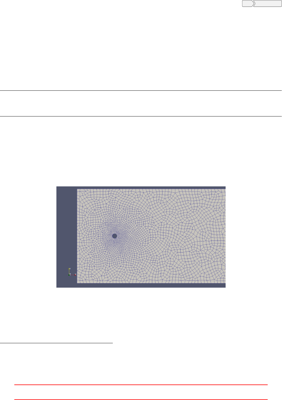
19.1.2 salomeToOpenFOAM
A third-party Python script47 can be used to export a mesh containing pyramid cells to OpenFOAM. This
script directly writes the essential files48. In order to export a mesh, simply select it in the Object Browser of
Salome and then execute the salomeToOpenFOAM.py Python script. This can be done by using File Load Script
menu.
19.1.3 Pitfall: Check your patches/patch types
In Salome we are able to define patches by creating face groups. These face groups are translated to patches,
when exporting the mesh. However, Salome has no way to distinguish between general patches and wall patches.
Thus, you may want to check constant/polyMesh/boundary for the patch types.
With Salome’s native export to UNV function, all patches are equal. After importing with OpenFOAM’s
native ideasUnvToFoam converter all patches are of the type patch. You need to take care yourself, to assign
the type wall to wall patches49. The third party conversion script salomeToOpenFOAM.py makes all patches
wall patches, when their names contain the word wall.
1if " wall " in gname . lower () :
2fileBoundary.write(" w all ; \ n" )
3else:
4fileBoundary.write(" p at ch ;\ n " )
Listing 131: Determining the patch type in salomeToOpenFOAM.py.
20 Gmsh
Gmsh50 is a 3D finite element meshing software. Gmsh is operated via its GUI or via ASCII input files in
Gmsh’s own scripting language. Gmsh is able to create all cell shapes from tets to hexes. The meshes generated
by GMSH can be converted to OpenFOAM’s format using the gmshToFoam utility.
Figure 33: An extruded 2D mesh of quad elements created with Gmsh.
21 enGrid
enGrid51 is an open source mesh generation software with CFD applications in mind. It uses the netgen52
meshing library. enGrid primarily creates tet meshes, however, it also allows for the creation of prismatic
47https://github.com/nicolasedh/salomeToOpenFOAM
48The files boundary,faces,neighbour,owner and points in constant/polyMesh.
49If this has not been done, the wall functions of turbulent simulations will complain about patch/data types.
50http://gmsh.info/
51https://github.com/enGits/engrid/wiki
52https://sourceforge.net/projects/netgen-mesher/
III This offering is not approved or endorsed by ESI®Group, ESI-OpenCFD®or the OpenFOAM®
Foundation, the producer of the OpenFOAM®software and owner of the OpenFOAM®trademark. 90
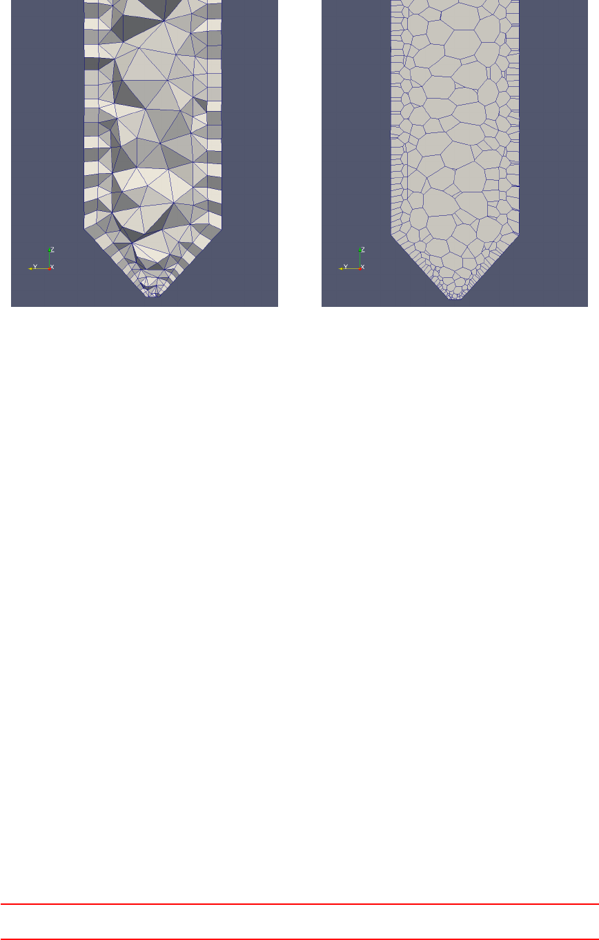
boundary layers and the conversion of tets to polyhedras. enGrid natively exports its meshes to OpenFOAM.
enGrid is operated via its GUI.
Figure 34: Meshes by enGrid: left: tet-mesh with prismatic boundary layer, right: polyhedral mesh with
boundary layer.
22 Mesh converters
To use meshes created by programs other than blockMesh there is a number of converters. The User Guide [39]
lists the following converters:
•fluentMeshToFoam
•starToFoam
•gambitToFoam
•ideasToFoam
•cfx4ToFoam
The names of the converters are pretty self explanatory.
22.1 fluentMeshToFoam and fluent3DMeshToFoam
fluentMeshToFoam converts meshes stored in the *.msh file format into the format of OpenFOAM. To be
more specific, fluentMeshToFoam converts only 2D meshes, whereas 3D meshes can be converted using flu-
ent3DMeshToFoam.
The converter expects the path to the *.msh file as an argument. The converter saves the mesh in the format
of OpenFOAM in the constant/polymesh directory.
If converter is invoked from a directory other than the case directory, then the path to the case directory
has to be specified via an additional argument. See Section 10.6.
If the mesh was created using an other dimension than in metres, the command line parameter -scale can
be used to correct the scaling. OpenFOAM expects the mesh data to be expressed in metres.
All other possible option can be displayed with this command line parameter fluentMeshToFoam -help.
22.2 ideasUnvToFoam
ideasUnvToFoam is a converter which is commonly used to convert meshes in the UNV format to OpenFOAM’s
format, Salome is a well-known meshing software, which exports meshes in the UNV format, see Section 19.
III This offering is not approved or endorsed by ESI®Group, ESI-OpenCFD®or the OpenFOAM®
Foundation, the producer of the OpenFOAM®software and owner of the OpenFOAM®trademark. 91
22.3 Pitfall: length units
Third party meshes may be based on millimetres instead of metres as expected by OpenFOAM. Point coordinates
will be interpreted by OpenFOAM as being expressed in metres, i.e. Pin file = (120,240, left(120 0) mm will
be read by OpenFOAM as Pin mesh = (120,240,0) m. Thus, the imported mesh will be scaled by a factor of
1000.
Some mesh converters (e.g. fluent3DMeshToFoam) offer a -scale option to fix the length scales along with
mesh conversion. Other mesh converters (e.g. ideasUnvToFoam) do not offer such a scaling function. However,
there is a utility (transformPoints) which, among other tasks, can be used to correct the length scales of the mesh.
Always run run checkMesh, ideally with its options -allGeometry and
-allTopology, to, first, check the mesh quality, and secondly, to check the
mesh bounding box. The bounding box will be expressed in metres, as any
other length in OpenFOAM. This will give you a chance to spot a millimetre
vs. metre situation.
Listing 132 shows the relevant lines of checkMesh’s output. Unless, we calculate meteorological flows, a
simulation domain in kilometre scale seems a bit off.
Checking geometry ...
Overa ll domain bo und ing box ( -752.264 -325 -684.294) ( 752.264 1400 3754.35)
Listing 132: The bounding box of our mesh
23 Other mesh manipulation tools
23.1 transformPoints
The tool transformPoints can be used to scale, translate or rotate the points a mesh. Section 25.3.4 contains a
case in which this tool can be useful.
23.1.1 Rotation
Rotating the geometry can be specified in two ways.
Using two vectors
Here, the rotation is defined by providing a vector before and after the rotation. From these two vectors, the
transformation matrix can be computed
Yaw, Pitch and Roll
There are actually two options: rollPitchYaw and yawPitchRoll. Here, the rotation is defined by specifying
three angles in degrees, which are subsequently applied to the x-axis, the y-axis and the z-axis.
23.2 topoSet
The tool topoSet creates point, face or cell sets from a geometric definition. There are a number of ways to
define the geometric region containing the intended points, faces or cells.
23.2.1 Usage
The dictionary topoSetDict is used to define the geometric region. Find some examples in the tutorials using
the following command.
fi nd $ FO A M_ T UT O RI A LS - na me t o po S et D ic t
Listing 133: Find examples for the use of topoSet
A face or cell set will contain only faces or cells whose centres lie within the specified geometric region.
III This offering is not approved or endorsed by ESI®Group, ESI-OpenCFD®or the OpenFOAM®
Foundation, the producer of the OpenFOAM®software and owner of the OpenFOAM®trademark. 92
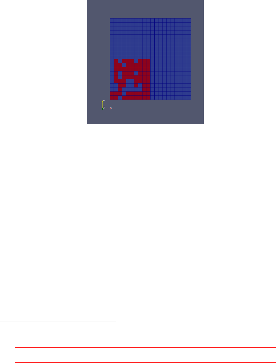
23.2.2 Pitfall: The definition of the geometric region
To demonstrate the function of topoSet a cell set was defined for the cavity tutorial-case. The mesh of the
cavity case is 1×1×0.1 m and the box defining the cell set was chosen to be 0.5×0.5×0.05 m. The dimensions
of this box are simply half the dimensions of the mesh. However, only cells whose cell centre is located in the
box are contained in the cell set. As the mesh is one cell in depth and 0.1 m in depth, all the cell centres are
exactly at z= 0.05 m. Due to inevitable numerical errors in calculating the cell centre53, the numerical errors
decided whether a cell was included into the cell set or not.
To avoid this error, always make sure the geometric region contains all the intended cells.
Figure 35: A faulty cell set definition. The red cells are part of the cell set. All other cells are blue.
23.2.3 Pitfall: renumbered mesh
At the point of writing the utility renumberMesh does not consider cell sets54. If renumberMesh is called after
cell sets were created by topoSet, the cell set is invalid. The reason for this is, that the cell labels of the cell
set remain unchanged as renumberMesh completely relabels the mesh. Thus, the cell set still exists and the
number of cells is unchanged, however, as other cells bear the labels of the original members of the cell set, the
cell set is invalid.
To resolve this problem, topoSet needs to be run after renumberMesh. This even works in parallel, when the
case has been decomposed.
23.3 setsToZones
The utility setsToZones serves the purpose to:
Add pointZones/faceZones/cellZones to the mesh from similar named pointSets/faceSets/cellSets
[39].
This utility is needed when we create some cellSets which we later want to use e.g. with a functionObject (the
cellSource functionObject acts on all cells or on a cellZone). cellSets can be created with topoSet. After we
ran topoSet we simply run setsToZones without any further parameters or providing a dictionary. setsToZones
creates cellZones which contain the same cells as the corresponding cellSets.
23.4 refineMesh
The tool refineMesh is used – just as the name suggests – to refine a mesh.
53The location of the cell centre is not stored in any file, thus this quantity has to be computed.
54This behaviour was reported in bug report 1377 (http://openfoam.org/mantisbt/view.php?id=1377).
III This offering is not approved or endorsed by ESI®Group, ESI-OpenCFD®or the OpenFOAM®
Foundation, the producer of the OpenFOAM®software and owner of the OpenFOAM®trademark. 93
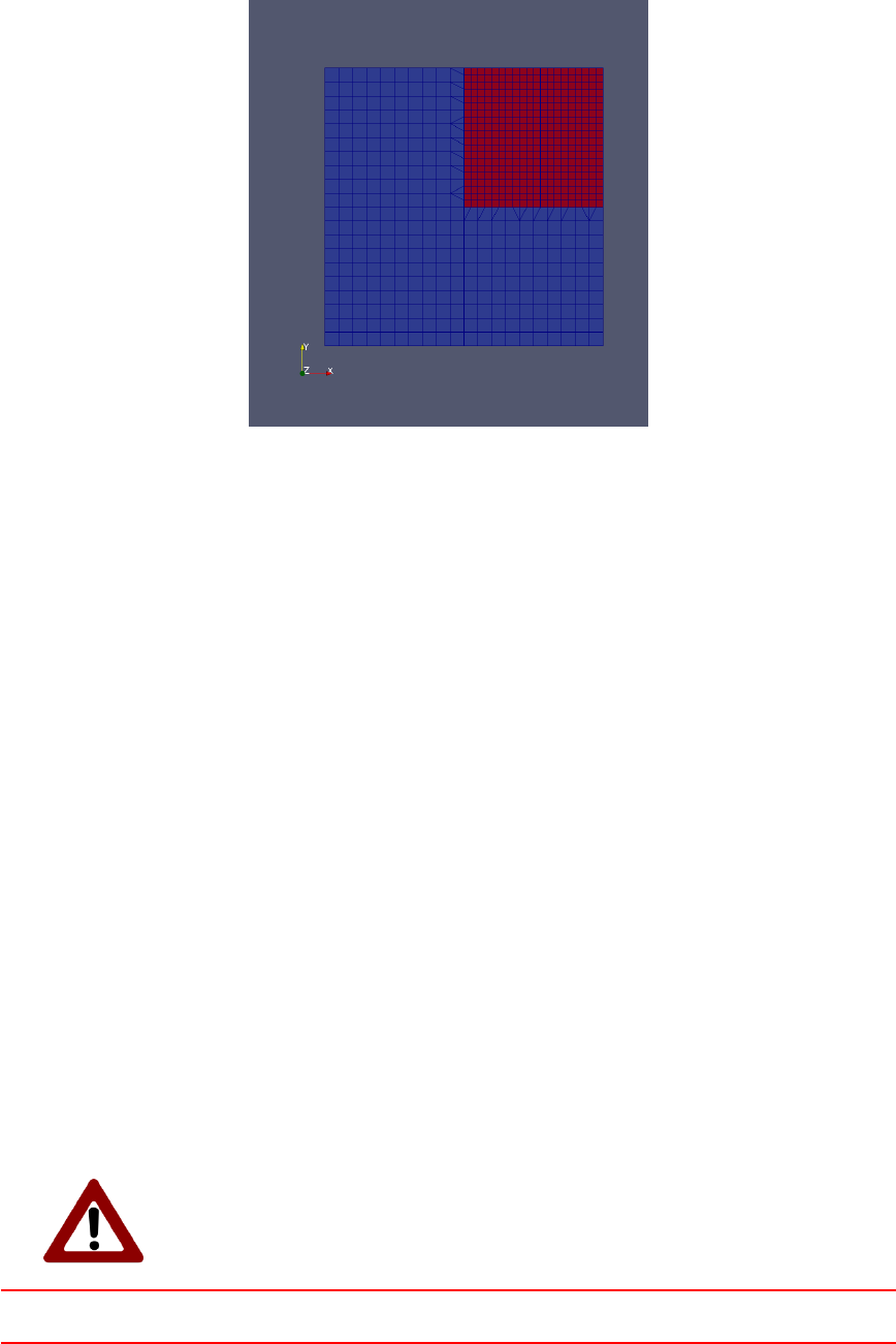
23.4.1 Usage
First a cell set has to be defined, this can be done using the tool topoSet.
With the dictionary refineMeshDict the rules for refining a particular cell set can be stated. When rules
have been defined in refineMeshDict , then the command line option -dict has to be used.
Figure 36: An example of a refined mesh. The refined region is marked in red.
23.4.2 Pitfall: no command line parameters
If the tool refineMesh is called without any command line parameters then the whole mesh is refined. For
refineMesh to obey the rules set in the refineMeshDict the command line option -dict has to used when
calling refineMesh. See this useful post in the CFD-Online Forum http://www.cfd-online.com/Forums/
openfoam-meshing-utilities/61518-blockmesh-cellset-refinemesh.html#post195725
Notice the different meaning of the -dict command line option of the tools topoSet and refineMesh. If you
are in doubt about this difference, check the summary of the command line usage printed by the -help option.
23.5 renumberMesh
23.5.1 General information
The tool renumberMesh modifies the arrangement of the cells of the mesh in order to create lower bandwidth for
the numerical solution. For further information about the role and the influence of the bandwidth in numerical
simulation see books on the numerical solution of large equation systems, e.g. [25].
Renumbering the mesh can reduce computation times as it re-arranges the data to benefit the numerical
solution of the resulting equation system. The benefit of renumbering the mesh strongly depends on several
factors. However, testing is recommended.
Renumbering the mesh even has an effect at the simplest possible simulation case – the cavity case of the
tutorials. This mesh consists of a single block and it is quasi 2D (i.e. it is only 1 block in depth). The mesh
resolution was chosen to 40 ×40 ×1, resulting in 1600 cells. icoFoam was run for 10 s. Execution time was
reduced by renumberMesh from 6.18 s to 6.08 s.
A simulation with a mesh consisting of 120000 cells defined by 9 blocks was run for 5 s of simulated time
with twoPhaseEulerFoam. Execution time was reduced by renumberMesh from 9383.81 s to 9273.13 s.
Even though the reduction of execution time is small in this examples, this reduction comes at no cost.
Running renumberMesh takes little time and at run-time of the simulation no additional work has to be done.
Run renumberMesh before any other tools which generate sets or zones. Why
the order of execution of certain tools is significant is explained in Section
23.5.3 on a case which went slightly wrong.
III This offering is not approved or endorsed by ESI®Group, ESI-OpenCFD®or the OpenFOAM®
Foundation, the producer of the OpenFOAM®software and owner of the OpenFOAM®trademark. 94
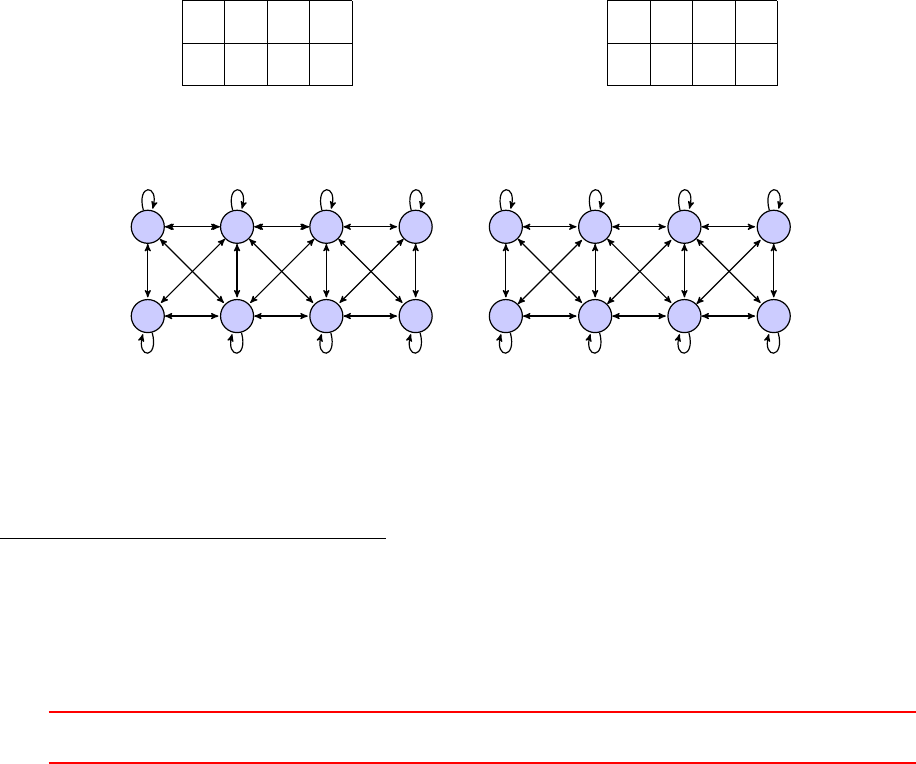
23.5.2 Background
The discretized finite volume problem results in a linear equation system, which is usually expressed in matrix-
form.
Ax =b(31)
The vector xcontains the field values at the cell centers. The matrix Acontains non-zero elements for each
pair of neighbouring cells. This is a consequence of our assumption that only adjacent cells interact. If we
used some sort of higher order discretisation or interpolation, we might get into a situation where also second
neighbours interact. However, for sake of ease, we limit ourselves in this discussion to direct neighbours.
Regardless of our computational mesh being one-, two- or three dimensional, we label all cells with positive
ascending integers. Thus, we can store the values of a scalar field into a vector. The number of elements of this
vector (N) is equal to the number of cells in our domain. Consequently, the matrix Ais of the size N×N.
However, as only adjacent cells interact, most of the elements of Awill be zero-entries.
If the cells with the labels iand jare adjacent, then the elements aij and aji of Awill be non-zero. Since
we focus on the general structure of Awe do not care whether aij equals aji, or if both of them are actually
non-zero55.
The arrangement of the cells – or, to be more precise, the labelling – has a strong impact on the structure
of the matrix A, i.e. the distribution of the non-zero elements.
A simple example
Here we examine the effect of cell labelling with a very simple example. Figure 37 shows a simple mesh with 8
cells. Two different cell labelling schemes are indicated by the numbers inside the cells.
In Figure 38 we see the connections between the cells depicted as a graph. A N×Nmatrix can be from
the interaction perspective seen as a graph with Nnodes. An edge between the nodes iand jrepresents the
non-zero elements aij and aji.
0 1 2 3
4 5 6 7
0 2 4 6
1 3 5 7
Figure 37: A simple mesh with 8 cells and different cell labelling schemes.
0 1 2 3
4 5 6 7
0 2
1
4
3 5
6
7
Figure 38: The connectivity graph of our mesh.
Figure 39 shows the corresponding matrix structure. The labelling scheme on the right hand side of Figures
37 and 38 results in a matrix with a lower bandwidth.
55The upwind differencing scheme causes the downstream cell to depend on the upstream cell. However, the upstream cell is not
directly influenced by the downstream cell.
III This offering is not approved or endorsed by ESI®Group, ESI-OpenCFD®or the OpenFOAM®
Foundation, the producer of the OpenFOAM®software and owner of the OpenFOAM®trademark. 95

01234567
0∗ ∗ 0 0 ∗ ∗ 0 0
1∗∗∗0∗∗∗0
2 0 ∗∗∗0∗∗∗
3 0 0 ∗ ∗ 0 0 ∗ ∗
4∗ ∗ 0 0 ∗ ∗ 0 0
5∗∗∗0∗∗∗0
6 0 ∗∗∗0∗∗∗
7 0 0 ∗ ∗ 0 0 ∗ ∗
01234567
0∗∗∗∗0000
1∗∗∗∗0000
2∗∗∗∗∗∗0 0
3∗∗∗∗∗∗0 0
4 0 0 ∗∗∗∗∗∗
5 0 0 ∗∗∗∗∗∗
60000∗∗∗∗
70000∗∗∗∗
Figure 39: The matrix structure. A * denotes a non-zero element. Notice the lower bandwidth of the matrix on
the right hand side. The number of zero-entries is equal, however, the different distribution leads to a different
numerical behaviour.
23.5.3 Pitfall: sets and zones will break my bones
The use of renumberMesh carries a certain risk. In simulation cases which make use of tools like topoSet and
renumberMesh, the order in which those tools are invoked is of importance. Update: This has been resolved
at some point. In OpenFOAM-4.0 this is no issue any more.
The reason behind this, is the way OpenFOAM stores its mesh information. The only actual geometric
information is stored in the list of points in the file constant/polyMesh/points. The faces are defined via the
point labels of the points defining the mesh. Thus, if the points Pk,Pm,Puand Pwdefine a face, then the entry
in constant/polyMesh/faces for this very face reads (k m u w). The same principle applys for the definition
of cells. There, the labels of the faces defining the cell are stored. This way, no redundant information is stored.
If we define a cellSet with topoSet e.g. all cells within a certain geometrical region we simply store the cell
labels of all cells for which the condition is fulfilled. Thus, if we now run renumberMesh, we shuffle the cells
within the mesh. No actual change is applied in the mesh, however, the cell with the label Awhich was at the
location (xA, yA, zA)before renumbering, may or most certainly will be at location (xB, yB, zB)with B6=A
after renumbering.
Figure 40 shows the simulation domain of an aerated stirred tank. The red cells are part of a cellZone
on which source terms using the fvOptions mechanism act56. A run of renumberMesh after the cellZone was
created caused the cellZone to get scrambled. However, the simulation worked nontheless and yielded some
unexpected results.
56Have a look on the injection tutorial of twoPhaseEulerFoam-2.3.x.
III This offering is not approved or endorsed by ESI®Group, ESI-OpenCFD®or the OpenFOAM®
Foundation, the producer of the OpenFOAM®software and owner of the OpenFOAM®trademark. 96
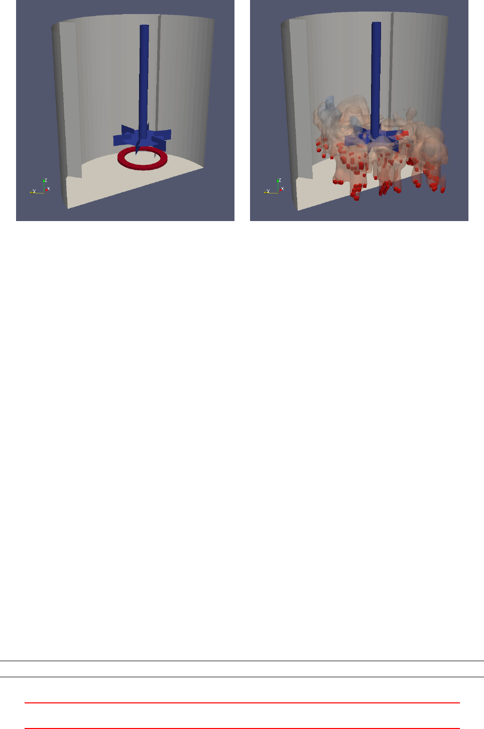
Figure 40: Left: The cut-away of the walls of a stirred tank with the rotor (blue) and the aeration device
(red). The aeration device is a cellZone on which source terms are applied via the fvOptions mechanism in
OpenFOAM-2.3.x.
Right: The stirred tank was simulated using parallel processes. After decomposing the domain, a parallel
renumbering of the mesh was conducted. Renumbering the subdomains scrambled the cellZone within their re-
spective subdomains. The transparent iso-volume shows the gas-phase volume fraction 0.25 s into the simulation.
The cells of the cellZone act as source for the gas-phase, although not on their original location.
23.6 subsetMesh
subsetMesh is a tool to remove certain cells from a mesh. The tool expects the name of a cellSet as a command
line argument. The cells of this cellSet will remain in the resulting mesh, all other cells are removed.
Pitfall: sets and zones will break my bones
At the time of writing (OpenFOAM-4.0), subsetMesh does not treat cellSets or cellZones. Thus, when we use
subsetMesh to remove large parts of the mesh, then the cellSet may contain cells that are no longer part of the
mesh. This error will be felt when the cell indices associated with the cellSet or cellZone are larger than the
total number of cells in the mesh. Otherwise, if the cell indices are smaller than the total number of cells, the
cellSet might still be valid from OpenFOAM’s point of view, but it may contain different cells.
23.7 createPatch
23.8 stitchMesh
24 Surface mesh manipulation tools
OpenFOAM ships with a number of surface mesh manipulation tools. A probable use-case for this kind of tools
is doing some preprocessing on STLs prior to creating a mesh with snappyHexMesh or cfMesh.
24.1 surfaceAdd
This tool can be used to merge two STLs into one file. With the command line switch -mergeRegions regions
with an equal name get joined into one region. Otherwise the two regions would remain separate, regardless of
having the same name.
sur fa ce Add - m erg eR eg ion s i nput 1 . stl i np ut 2 . stl o ut . st l
Listing 134: Usage of surfaceAdd when joining two STL files.
III This offering is not approved or endorsed by ESI®Group, ESI-OpenCFD®or the OpenFOAM®
Foundation, the producer of the OpenFOAM®software and owner of the OpenFOAM®trademark. 97

24.2 surfaceSubset
With this tool a subset of an STL can be extracted. Via the surfaceSubsetDict various conditions can be
specified to define the subset. The user provides the STL to operate on (input.stl) and a file name for the
subset to be stored in (outSubset.stl). The faces of the subset get removed from the original STL.
sur fac eS ubs et s ur fa ceS ubs etD ic t i np ut . stl o ut Su bs et . stl
Listing 135: Usage of surfaceSubset when extracting a certain subset from an STL.
24.3 surfaceFeatureExtract
This is a tool to extract features from an STL. E.g. snappyHexMesh pays extra attention to geometric features
which are explicitely provided, surfaceFeatureExtract is a tool to generate the necessary data. The tool is
controlled by the surfaceFeatureExtractDict.
24.4 Third party surface manipulation tools
24.4.1 surfaceFeatureEdges
With this tool, provided by cfMesh (see Section 16), feature edges can be extracted from a surface mesh file,
e.g. an STL.
sur f ace F eatu reEd ges -an gle 30 inp ut . stl out . ftr
Listing 136: Usage of surfaceFeatureEdges when extracting feature edges from an STL.
24.5 The Linux command line
When doing some pre-processing with ASCII STLs the linux command line offers some nice features. Listing
137 shows the basic syntax of an STL file in ASCII format. STLs can be stored on harddisk either in ASCII,
i.e. in plain text, or in binary format (non-human-readable). An STL file consists of solids, which are defined
by their bounding surface.
solid SOL IDN AME
facet normal X Y Z
outer loop
vertex X Y Z
vertex X Y Z
vertex X Y Z
endloop
endfacet
...
endsolid
Listing 137: The basic syntax of an STL in ASCII format. See https://en.wikipedia.org/wiki/STL_(file_
format) for more on this.
24.5.1 Renaming solids
Certain CAD tools do not offer the feature to name a part. E.g. OpenSCAD names the exported STL solid
OpenSCAD_Model. If our STL pre-processing based on an STL generated by OpenSCAD yields an STL file per
patch, a likely result when using surfaceSubset, we end up with a number of STLs, containing each one solid
named OpenSCAD_Model. Now, we need to assign proper names to the solids, i.e. the STL solid of the file
inlet.stl should be named inlet.
When the STL is in ASCII format, we can use sed57 to perform a simple text replacement. Since an STL
is very unlikely to contain the string OpenSCAD_Model, we simply can tell sed to replace every occurance of
OpenSCAD_Model with inlet.
57https://www.gnu.org/software/sed/manual/sed.html
III This offering is not approved or endorsed by ESI®Group, ESI-OpenCFD®or the OpenFOAM®
Foundation, the producer of the OpenFOAM®software and owner of the OpenFOAM®trademark. 98

sed -i s / Ope nS CA D_ Mo de l / inlet /g inlet . stl
Listing 138: Renaming STL an solid with sed.
24.5.2 Joining STL files
If our pre-processing left us with a large number of STL files, e.g. an STL file for each patch, which is a likely
result when using surfaceSubset, we might need to join these STLs, e.g. because the meshing tool expects only
one STL to contain all the information. Joining text files is a task easily done from the command line with the
tool cat58, however, this could also be done using surfaceAdd. Other than with surfaceAdd, joining STLs with
this approach is limited to STLs containing different solids.
Listing 139 shows how to join three STLs, each containing one solid, i.e. the information of one patch. The
first line is simply a copy operation. Alternatively, we might use cp or mv for the first operation. Note, that the
resulting STL gets written to a different folder, constant/triSurface is a folder in which some meshing tools
expect STLs. The second and third lines show how to append the output of cat to the specified file.
The difference between the first and the following lines is the redirection operator (> vs. >>), see e.g.
https://en.wikipedia.org/wiki/Redirection_(computing). The > operator simply redirects the output
to the specified file, if this was used in the second line, then the contents from the first line would get overwritten
in myDomainMesh.stl. Using the >> operator redirects and appends the output to the specified file. Using the
> operator in the first line ensures to overwrite an eventual existing file.
cat wa lls . stl > c onstant / t riSurface / myD omain Mesh .stl
cat in let . stl >> c onstant / tr iSurf ace / m yDoma inMes h . stl
cat outle t . stl > > c on st an t / t ri Su rf ac e / m yD oma in Mes h . stl
Listing 139: Joining STL files with cat.
25 Initialize Fields
25.1 Basics
There are two ways to define the initial value of a field quantity. The first is to set the field to a uniform value.
Listing 140 shows the 0/U file of the cavity tutorial. There the internal field is set to a uniform value.
If a non-uniform initialisation is desired, then a list of values for all cells is needed instead. Listing 147 shows
some lines of such a definition. Entering such a nonuniform list by hand would be very tiresome. To spare the
user of such a painful and exhausting task, there are some tools to provide help.
/*--------------------------------*- C++ -*----------------------------------*\
| === === === | |
| \\ / F ield | O penF OAM : The Open Sour ce CFD T oolbox |
| \\ / O p er at ion | V er sion : 2.1. x |
| \\ / A nd | Web : ww w . Op en FO AM . org |
| \\/ M anip ula tion | |
\*---------------------------------------------------------------------------*/
FoamFile
{
version 2.0;
forma t asc ii ;
class volVectorField;
object U;
}
//*************************************//
dim ens ion s [0 1 -1 0 0 0 0];
i nt ern alF iel d uni fo rm (0 0 0 ) ;
boundaryField
{
mov ing Wal l
58https://en.wikipedia.org/wiki/Cat_(Unix)
III This offering is not approved or endorsed by ESI®Group, ESI-OpenCFD®or the OpenFOAM®
Foundation, the producer of the OpenFOAM®software and owner of the OpenFOAM®trademark. 99

{
type fix edV alue ;
value unifo rm (1 0 0) ;
}
fix edW all s
{
type fix edV alue ;
value unifo rm (0 0 0) ;
}
frontAndBack
{
ty pe empty ;
}
}
// ************************************************************************* //
Listing 140: The file 0/U of the cavity tutorial
25.2 setFields
setFields is a utility that allows to define geometrical regions within the domain and to assign field values
to those regions. setFields reads this definitions from a file in the system-directory – the setFieldsDict. To
initialize the field quantities setFields has to be executed after creating the mesh. setFields needs to read all
files defining the mesh59.
In Listing 141 a box is defined in which the field alpha1 is set to a different value.
/*--------------------------------*- C++ -*----------------------------------*\
| === === === | |
| \\ / F ield | O penF OAM : The Open Sour ce CFD T oolbox |
| \\ / O p er at ion | V er sion : 2.1. x |
| \\ / A nd | Web : ww w . Op en FO AM . org |
| \\/ M anip ula tion | |
\*---------------------------------------------------------------------------*/
FoamFile
{
version 2.0;
forma t asc ii ;
class d ictionary ;
object setF iel ds Dic t ;
}
//*************************************//
defaultFieldValues
(
volScalarFieldValue alpha1 1
);
regions
(
boxToCell
{
box ( -0.3 -0.3 0) (0.3 0.3 0.26) ;
fieldValues
(
volScalarFieldValue alpha1 0
);
}
);
// ************************************************************************* //
Listing 141: setFieldsDict
59Only the file neighbour can be missing for setFields not to crash.
III This offering is not approved or endorsed by ESI®Group, ESI-OpenCFD®or the OpenFOAM®
Foundation, the producer of the OpenFOAM®software and owner of the OpenFOAM®trademark. 100

25.2.1 Defining regions
In Listing 141 we see the list named regions containing dictionaries defining regions in which to set field values.
The boxToCell dictionary very much resembles something we also can see in the topoSetDict dictionary. In
fact, setFields internally uses the machinery to create cell sets as topoSet does. A quick look into the main
source files of setFields and topoSet reveals, that both make use of the class topoSetSource, which describes
itself in the header file as: Base class of a source for a topoSet. All actual cell sources, such as boxToCell
or cylinderToCell, directly inherit from topoSetSource. Thus, all cell sources available to topoSet, are also
available to setFields. Such is the beauty of object-oriented programming.
25.2.2 Pitfalls
A nice, little collection of what may go wrong.
Geometric region is not part of the domain
If the geometric region, in which to initialise a field with a specified value, lies outside the domain, setFields
does not issue any warning or error message.
Geometric region covers the whole domain
This may happen if the geometric region is defined with respect to the vertex coordinates found in blockMeshDict.
When the vertex coordinates are entered in millimeters – and convertToMeters is set appropiately – then it may
happen, that the geometric region, based on the vertex coordinates in millimeters, is too large by the factor of
1000.
Listing 142 and 143 show the root of such a situation. The plan is to create a box and initialise it in a way,
that the domain is half filled with one phase. The definition of the box in the setFieldsDict relies solely on the
vertex coordinates ignoring the scaling factor convertToMeters resulting in a way too large box. After executing
setFields the domain is completely filled with one phase instead of half filled.
con ve rtToM et ers 1e -3;
vertices
(
(0 0 0)
(50 0 0)
(50 0 250)
(0 0 250)
(0 50 0)
(50 50 0)
(50 50 250)
(0 50 250)
);
Listing 142: blockMeshDict entry for a box of 50 ×50 ×250 mm
regions
(
boxToCell
{
box (0.0 0.0 0.0) (50.0 50.0 125.0) ;
fieldValues
(
volScalarFieldValue alpha1 0
);
}
);
Listing 143: setFieldsDict entry for a box of 50 ×50 ×125 m
III This offering is not approved or endorsed by ESI®Group, ESI-OpenCFD®or the OpenFOAM®
Foundation, the producer of the OpenFOAM®software and owner of the OpenFOAM®trademark. 101

Field not found
If the setFieldsDict specifies a field which is not present, then OpenFOAM issues an error message similar to
Listing 144. In this case the file setFieldsDict was copied from a case which uses the old naming scheme of
twoPhaseEulerFoam, i.e. alpha instead of alpha1. See Section 46.1.1 for further information about the nam-
ing scheme. Therefore, the dictionary contained a definition for the field alpha which was not present in the
0-directory.
Setti ng field defau lt valu es
--> FOAM W arning :
From f unc tion void set Cell Fiel dTy p e ( const f vMesh & mesh , const labelList & select edCells ,
Istream& fieldValueStream)
in file set Fie lds . C at line 103
Field alpha not found
--> FOAM FATAL IO ERROR :
wrong t oken type - ex pected word , found on line 19 the label 1
fi le : / home / user / O pe nF OAM / user -2 .1. x/ run / t woP ha seE ul er Foa m / b ub bl eC ol um n / syste m / set Fi el ds Dic t ::
def a ult F iel d Val u es at line 19.
From f unc tion operator > >( Ist ream & , wor d &)
in file pri mi ti ve s / str ings / w ord / wo rdIO . C at line 74.
FOAM exiting
Listing 144: Missing field
25.3 mapFields
mapFields is a utility to transfer field data from a source mesh to target mesh. This may be useful after the
mesh of case has been refined and existing solution data is to be used for initialising the case with the refined
mesh. mapFields preserves the format of the data, if the source data was stored in binary format, the target
data will also be binary.
To use mapFields the file mapFieldsDict has to be existent in the system folder of the case60.mapFields
expects as the only mandatory argument the path to the source case. The current directory is assumed to be
the case directory of the target case. If there is no specification regarding time, the latest time steps of both
cases are processes. That means the latest time step of the source case is mapped to the latest time step of the
target case.
Listing 145 shows the last lines of output of mapFields. With lines like interpolating alpha mapFields
indicates that it is processing some field data. Even when source and target meshes are equal and no interpo-
lation is needed, mapFields displays lines like interpolating alpha anyway.
Sourc e t ime : 0 .325
Targe t t ime : 0
Create meshes
Sourc e m esh size : 81000 Ta rget mesh size : 273 375
Mappi ng fields for time 0 .325
int erpo lat ing alpha
int erpo lat ing p
int erpo lat ing k
int erpo lat ing epsi lon
int erpo lat ing Theta
int erpo lat ing Ub
int erpo lat ing Ua
End
60In the most basic case mapFieldsDict contains no other information than the header and empty definitions. Although this file
may seem of no use, it has to exist in the system folder, and it has to contain the header and the empty definitions.
III This offering is not approved or endorsed by ESI®Group, ESI-OpenCFD®or the OpenFOAM®
Foundation, the producer of the OpenFOAM®software and owner of the OpenFOAM®trademark. 102

Listing 145: Output of mapFields
25.3.1 Pitfall: Missing files
mapFields issues no warning or error message when the source case contains no data. Listing 146 shows the
output of mapFields as the target case contained no 0-directory. Only the missing lines containing statements
like interpolating alpha indicate that something is amiss and no field data is processed.
Sourc e t ime : 0 .325
Targe t t ime : 0
Create meshes
Sourc e m esh size : 81000 Ta rget mesh size : 273 375
Mappi ng fields for time 0 .325
End
Listing 146: Output of mapFields; Missing target 0-directory
25.3.2 Pitfall: Unsuitable files
In the files containing the field data the values of the boundary fields as well as the values of the internal fields
can be entered homogeneously (by the keyword uniform) or inhomogeneously (with the keyword nonuniform).
Inhomogeneous field values have to be entered as a list of values. This list is preceded by the number of entries
as well as the nature of the value. Listing 147 shows the beginning lines of the definition of a nonuniform vector
field. The general syntax for such a list is the following:
nonuniform List<TYPE> COUNT ( VALUES )
the list. A wrong value of COUNT leads to reading errors.
If data is to be mapped from a source case, the source case’s data will always be stored as a nonuniform list.
Otherwise, mapping the data would make no sense, as uniform fields are most easily defined. If the data of the
target case is uniform, then mapping makes no problems.
If the data of the target case is nonuniform – for whatever reason – then it is necessary that the nonuniform
lists have the same length. Otherwise, mapFields will exit with an error message like in Listing 148. The target
case should always be set up with uniform fields to avoid such errors. This is most easily done by removing the
definition of the internal field. In the tutorials sometimes files with an .org file extension can be found. This
is a way to preserve the uniform field data in the 0-directory without causing any trouble.
dim ens ion s [0 1 -1 0 0 0 0];
int ern al Fie ld non un if orm List < ve cto r >
1600
(
(0. 0001742 91 -0. 00017 1512 0)
(0. 0001710 22 -0. 00014 3648 0)
( -0.00 02592 97 0.00 030 577 2 0)
( -0.00 03806 71 0.00 037 493 7 0)
( -0.00182755 0 .00 0930701 0)
Listing 147: An inhomogeneous internal field definition in the file 0/U
Mappi ng fields for time 0 .325
int erpo lat ing alpha
--> FOAM FATAL IO ERROR :
size 81000 is not equ al to the given value of 10125
III This offering is not approved or endorsed by ESI®Group, ESI-OpenCFD®or the OpenFOAM®
Foundation, the producer of the OpenFOAM®software and owner of the OpenFOAM®trademark. 103

/*--------------------------------*- C++ -*----------------------------------*\
| === === === | |
| \\ / F ield | O penF OAM : The Open Sour ce CFD T oolbox |
| \\ / O p er at ion | V er sion : 2.1. x |
| \\ / A nd | Web : ww w . Op en FO AM . org |
| \\/ M anip ula tion | |
\*---------------------------------------------------------------------------*/
FoamFile
{
version 2.0;
forma t asc ii ;
class d ictionary ;
location " syste m ";
object mapF iel ds Dic t ;
}
//*************************************//
patchMap ( ) ;
cuttingPatches ( );
// ************************************************************************* //
Listing 149: The file mapFieldsDict
fi le : / home / user / O pe nF OAM / user -2 .1. x/ run / t woP ha seE ul er Foa m / Ca se / 0/ a lpha fro m l ine 18 to line
39.
Fr om f unct io n Field < Type >:: Field ( c onst w ord & keyword , c onst di ction ary &, const label )
in file / h ome / user / O penF OA M / OpenFOAM -2.1. x / src / Ope nF OA M / lnI nclu de / F ield . C at l ine 236.
FOAM exiting
Listing 148: Error message of mapFields; unequal number of values
25.3.3 Pitfall: Mapping data from a 2D to a 3D mesh
In this section we deal with some difficulties of the mapFields utility. We have finished a simulation on a 2D
mesh. The geometry of the 2D case is 20 cm ×2 cm ×45 cm.
Now we want to transfer the 2D data to a 3D mesh to initialise the 3D simulation. The geometry of the 3D
simulation is 20 cm ×5 cm ×45 cm. Note the different dimension in y-direction.
Listing 149 shows the mapFieldsDict that was used. Because of the great similarity of the geometry, no
entries are necessary.
The problem
Figure 41 shows the result of the mapFields run. Only the field values inside the 2D domain were altered. The
part of the 3D domain that lies outside the 2D domain remains unchanged. This behaviour is not satisfactory.
The work-around
One way to solve this problem would be to choose the 2D domain of a similar size as the 3D domain. However,
if the 2D is already finished, then it would take some time to re-simulate the case with a redefined geometry.
Another solution is:
1. define the 3D domain to be of the same size as the 2D domain
2. map the fields
3. redefine the 3D domain to its intended size, without changing the total number of cells
III This offering is not approved or endorsed by ESI®Group, ESI-OpenCFD®or the OpenFOAM®
Foundation, the producer of the OpenFOAM®software and owner of the OpenFOAM®trademark. 104
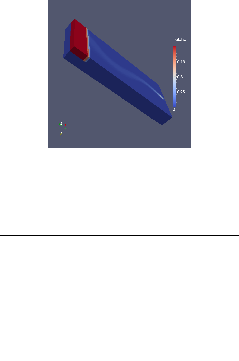
Figure 41: The mapped field
25.3.4 The work-around: Mapping data from a 2D to a 3D mesh
The work-around to the problem of the previous section is rather unelegant. A 2D mesh that has the same
depth as the 3D mesh but is discretised with only 1 cell in depth will have a very bad aspect ratio.
A more elegant solution is to transform the mesh after the 2D simulation has finished. In our example, the
2D mesh has the dimensions 20 cm ×2 cm ×45 cm and the 3D mesh is 20 cm ×5 cm ×45 cm big.
With the tool transformPoints the mesh can be scaled selectively in the three dimensions of space. Listing
150 shows how transformPoints can be used to scale the 2D mesh in y-direction by the factor of 2.5. After this
scaling operation the 2D mesh has the desired dimensions of 20 cm ×5 cm ×45 cm.
t ra n sf orm Poi n ts - s ca le ’(1.0 2.5 1.0) ’
Listing 150: Scaling the 2D mesh in y-direction with transformPoints
After the mesh transformation the utility mapFields can be used to map the field from the scaled 2D mesh
to the 3D mesh.
25.3.5 The importance of mapping
The purpose of this example is to highlight the need for the mapFields utility. A simulation of the bubble
column has been made. Now, the user decides to change the size of the inlet patch. Thanks to the parametric
mesh, this can be done easily only by changing some numbers in the file blockMeshDict.m4. See Section 13.5
for a discussion on creating a parametric mesh.
After the user changed the coordinates of some points, meshing yields a new mesh with the same number of
cells as the old mesh had. Because the number of cells did not change, the data files from the finished simulation
fit the new one. The user simply copies the necessary files from the latest time step of the finished simulation
to the initial time step of the new simulation.
Starting the simulation resulted in a floating point exception. However, after reducing the time step, the
simulation proceeded without any further errors. Figure 42 shows the initial alpha and U1 fields of the new
simulation. Due to a change in the numbering of the cells, the formerly smooth fields are now completely
III This offering is not approved or endorsed by ESI®Group, ESI-OpenCFD®or the OpenFOAM®
Foundation, the producer of the OpenFOAM®software and owner of the OpenFOAM®trademark. 105
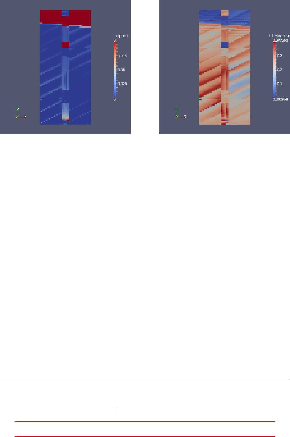
Figure 42: The unmapped fields
distorted. The single blocks of the mesh can be distinguished from the figures. This indicates, that OpenFOAM
numbers the cells block-wise.
25.3.6 Pitfall: binary files
If the source case has binary data files, then the boundary conditions need to be defined before mapping the
fields. Therefore, the boundary conditions need to be defined in a suitable ascii file. Then, the fields can be
mapped. Editing a binary file with a text editor may render this file defective.
26 Case manipulation
This section contains a discussion on tools for the manipulation of the simulation case which to not create or
modify the mesh or are used for initialisation. Utilities for the before mentioned tasks are already disussed in
previous sections.
26.1 changeDictionary
The utility changeDictionary can be used to modify a dictionary, except those residing in system. We can of
course manipulate any of our dictionaries using a simple text editor, even from the command line (emacs,vim,
nano, etc.).
A possible scenario in which changeDictionary comes in handy is when we do spin-up simulations, i.e. run
the simulation for a certain time with e.g. reduced inflow and continue afterwards with full inflow61. This
approach might improve the stability of the simulation.
Another case in which changeDictionary proofes to be quite important is when we want to change boundary
value of fields we have gained from a previous simulation. Editing ascii files which measure in the megabytes
can be very tiresome with some text editors. If the files are stored in binary, using a text editor might not be
an option anymore. In this changeDictionary provides a neat way to change boundary values.
Listing 151 shows a simple example of the changeDictionaryDict.
dictionaryReplacement
{
U
{
61In such a scenario we also would need to manipulate controlDict to increase the endTime. Well, we can’t have everything.
III This offering is not approved or endorsed by ESI®Group, ESI-OpenCFD®or the OpenFOAM®
Foundation, the producer of the OpenFOAM®software and owner of the OpenFOAM®trademark. 106

boundaryField
{
inlet
{
type fix edV alue ;
val ue un ifo rm (20 0 0) ;
}
}
}
}
Listing 151: A simple changeDictionaryDict used to change an inlet velocity
By default changeDictionary operates only on dictionaries living in the time step directories. By adding the
command line option -constant the dictionaries of the constant folder can be edited.
26.1.1 A spin-up simulation
In this section we discuss what is termed a spin-up simulation in this manual. This simulation is intended to
run without user intervention once the simulation is started. In this case we assume we have set up a simulation
with a reduced inflow. Thus, the flow establishes within the domain in a much gentler regime. After the flow
is established we increase the inflow to the desired value. Again, the build-up of the flow within the domain
happens in a gentler manner, as there is already a slower flow present through out the domain. Thus, we avoid
punching the quiescent fluid in the domain with full force at the inlet62.
Listing 152 shows the Allrun script for such a kind of simulation. In Line 11 the solver is run for the first
time. Since none of the lines in the script is terminated by the ampersand (&), execution waits for the command
of the current line to finish until the next command is invoked. Thus, we save to assume all commands are run
in the stated order.
In Line 14 the log-file generated by runApplication is renamed (moving a file within a directory is essentially
renaming). The reason for this operation is, that runApplication checks if there is already a log present. If
there is, runApplication does not run the specified application.
In Line 15 changeDictionary is called. This is the step in which, in our example, we increase the inlet
velocity. In Line 16 we use the GNU tool sed to edit controlDict63.
In Line 19 we call the solver for the second time. Here it is crucial that the keyword startAt is set to
latestTime in controlDict.
In Line 20 we apply the same renaming to the solver-log of the second run. This is not necessary in priciple,
however, if we are to perform to automated processing of the logs, then a consistent naming scheme might be
very helpful.
1# !/ bi n / sh
2cd ${0%/*} || exit 1# run from this dir ect ory
3
4# Source t uto rial run functions
5. $ WM_ PRO JE CT_ DIR / bin / tools / R un Fu nct io ns
6
7# Create the mesh u sing blockMesh
8run Appl ica tion b loc kMe sh
9
10 # Run the sol ver
11 run Appl ica tion p imp leFoam
12
13 # prepa re second run
14 mv log . p im pl eF oam log . p im ple Foa mR un0 1
15 runApplication changeDictionary
16 sed -i ’ s/ e ndTim e 20/ end Time 40/g ’ sys tem / co nt ro lDict
17
18 # Run the sol ver again
19 run Appl ica tion p imp leFoam
20 mv log . p im pl eF oam log . p im pl eFo am 02
62Such a simple kind of thing could also be achieved with time-dependent boundary conditions. However, there are solvers which
do not support time-variant boundary conditions, or we want to do something nastier, which can’t be achieved with time-variant
bounary conditions.
63We could also do the edit manually with any text editor, as controlDict will never reach megabytes or be stored in binary
format. However, the whole idea of the spin-up simulation idea is to avoid manual intervention.
III This offering is not approved or endorsed by ESI®Group, ESI-OpenCFD®or the OpenFOAM®
Foundation, the producer of the OpenFOAM®software and owner of the OpenFOAM®trademark. 107
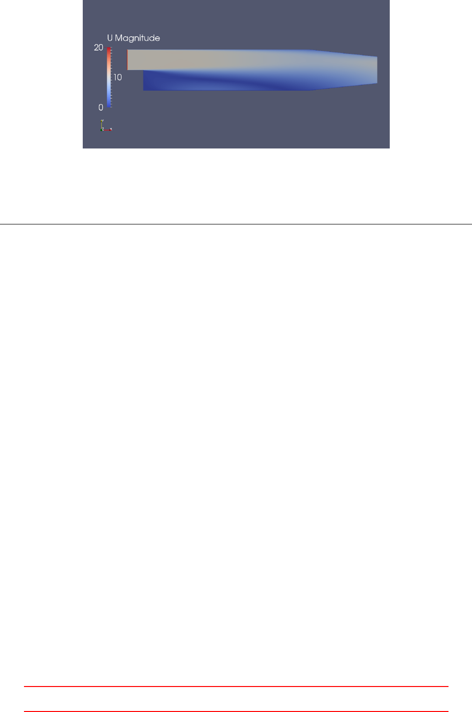
Figure 43: The established flow field and the increased inlet boundary condition of the pitzDaily tutorial case
at t= 1 s
21
22 # ----------------------------------------------------------------- end-of-file
Listing 152: The Allrun script of a spin-up simulation
The Allrun script was applied to a slightly modified pitzDaily tutorial case. A appropriate changeDictionaryDict
file Listing 151 was added to the system directory, otherwise the tutorial is untouched. Figure 43 shows the
flow field after changeDictionary was called. The increased inlet velocity is displayed as well as the established
flow from the initial run with an inlet velocity of (10 0 0).
26.2 The allmighty Linux Terminal
This section covers case manipulation we can do with the tools available in the Linux Terminal. The reason
for this, is partly that for certain tasks there is to the authors knowledge no tool provided by OpenFOAM, or
that the task can be done more conveniently with the tools of the Terminal rather than OpenFOAM’s tools.
The primary reason we are able to manipulate cases with the might of the tools we find in a Linux Terminal
is that everthing is a text file in OpenFOAM’s case definition. If there is one thing Linux, or UNIX in general,
has an over-abundance, it is test editors and text editing tools. This is due to a design decision of the UNIX
creators which is best clarifed by quoting Eric S. Raymond [14]:
Unix tradition strongly encourages writing programs that read and write simple, textual, stream-
oriented, device-independent formats. Under classic Unix, as many programs as possible are written
as simple filters, which take a simple text stream on input and process it into another simple text
stream on output.
Despite popular mythology, this practice is favored not because Unix programmers hate graphical
user interfaces. It’s because if you don’t write programs that accept and emit simple text streams,
it’s much more difficult to hook the programs together.
Text streams are to Unix tools as messages are to objects in an object-oriented setting. The
simplicity of the text-stream interface enforces the encapsulation of the tools. More elaborate forms
of inter-process communication, such as remote procedure calls, show a tendency to involve programs
with each others’ internals too much.
With a little help from a friend
If we combine the powers of the Linux Terminal and OpenFOAM’s tools, anything is possible. In remainder
of this section, some case manipulation scenarios of the combined use of the tools provided by Linux and
OpenFOAM are presented
26.2.1 Rename a patch and edit the corresponding boundary condition
If we are in the lucky situation to have a symmetric mesh, we can remove half the domain and apply a symmetry
constraint on the newly formed boundary. This is achived by the following sequence of steps:
III This offering is not approved or endorsed by ESI®Group, ESI-OpenCFD®or the OpenFOAM®
Foundation, the producer of the OpenFOAM®software and owner of the OpenFOAM®trademark. 108

1. Select all cells belonging to one half of the domain with topoSet
2. Remove the cells of the other half of the domain with subsetMesh
3. Change the definition of the newly formed boundary to a symmetry plane with createPatch.
After executing this steps, the mesh has a new symmetry boundary, however, all the fields retain their
oldInternalFaces boundary introduced by subsetMesh. Thus, we need to rename the boundary condition
in all fields and change the type of the boundary condition to symmetry.
Change BC type
We can change the type of a boundary condition with the tools changeDictionary or foamDictionary. The
task of bulk-renaming is not possible with either of the tools. The tool changeDictionary is controlled by the
changeDictionaryDict file. Within this file, we can use wildcards for the patch names, however, we can not
use a wildcard for field names. Listings 153 and 154 show an allowed use-case of wildcards and one impossible
use-case in changeDictionaryDict.
Our task, change the BC type for all fields, falls under the latter category. We could, however, work around
this issue if we included all fields in the changeDictionaryDict.
T
{
boundaryField
{
".*"
{
type zeroGradient;
}
}
}
Listing 153: Possible use of wildcards with changeDictionary: Change all boundary conditions of the field Tto
zeroGradient.
".*"
{
boundaryField
{
oldInternalFaces
{
type symmetry ;
}
}
}
Listing 154: Impossible use of wildcards with changeDictionary: Change the type of the boundary condition
for the patch oldInternalFaces of all fields to symmetry.
The tool foamDictionary can also be used to change the type of a boundary condition. This tool is controlled
by command line arguments, Listing 155 shows how the tool is called.
f oa m Di ct i on a ry FI LE - ent ry bo und ary Fie ld . o ld Int e rn a lF ace s - se t "{ t ype sym me try ; }"
Listing 155: Calling up foamDictionary to change the type of the BC of the patch oldInternalFaces for the
field defined in FILE.
However, we can only pass one file at a time. This is where the Linux Terminal comes into play. With
a simple for loop, we can loop over all files contained in the 0directory and call foamDictionary for each
individual file. Done!
for file in 0/*; do
f oa m Di c ti o na r y $ fi le - e nt ry b ou n da r yF i el d . o l dI n te r n al F ac e s - set " { t yp e s y mm et ry ; } "
done
Listing 156: Changing the type of the BC of the patch oldInternalFaces for all fields.
III This offering is not approved or endorsed by ESI®Group, ESI-OpenCFD®or the OpenFOAM®
Foundation, the producer of the OpenFOAM®software and owner of the OpenFOAM®trademark. 109

Rename all BCs for all fields
Next, we would like to change the patch name in all field files. This operation is necessary, as createPatch
operates only on the mesh. The fields are untouched by this tool. As we used createPatch to change the name
and the type of the oldInternalFaces boundary for the mesh, we need to change the boundary name also for
the fields.
This operation is a simple find&replace, which can be done with any text editor. For the sake of automa-
tion, we use the stream editor sed. Again, we loop over all files present in the 0directory and we apply the
find&replace operation on each file.
for file in 0/*; do
sed -i ’ s/ old Inter na lFa ce s / symmetry /g ’ $file
done
Listing 157: Changing the name of the of the patch oldInternalFaces for all fields to symmetry.
26.2.2 Rename phases
The multi-phase solvers of OpenFOAM64 use the phase name as file extension in order to distinguish fields
and files, e.g. U.air and U.water. In Listing 158 we see the content of the 0directory of the bubble column
tutorial. This clearly demonstrates the use of file extensions to distinguish phases.
alpha . air al phat . wat er e psil on . water k. wa ter p The ta U. wa ter
alpha . air . orig eps ilon . ai r k . air nut . ai r p_rgh T. wa ter
Listing 158: The content of the 0directory of the bubble column tutorial.
If we wanted to simulate nitrogen gas in water, we would need to rename all files in order to follow this
convention. Manually renaming files is tedious and can be automated by the use of the tools available in the
Linux Terminal.
Rename files
First, we want to rename all files in order for them to have the proper file extension. This helps avoiding
confusion. Thus, we use find to search for all files with the file extension air and pass them to rename, which
renames the files according to the specified pattern.
find . -name ’ *. air ’ | xa rg s renam e . ai r . n it rog en
Listing 159: Replacing the file extension air with the file extension nitrogen in all files in and below the
current folder.
Replace text
Next, we need to replace the old phase name within the files itself. Again we use find to search for all files and
pass them to sed, which replaces all text fitting the specified pattern. Note: applying sed to all files can lead
to some trouble, as the text “pair” also gets treated and thus becomes “pnitrogen”. However, if the application
of sed causes such a side effect, OpenFOAM will crash if vital entries were damaged in this way.
fi nd . - type f | xargs sed -i s / air / n it ro ge n /g
Listing 160: Replacing the word air with the word nitrogen in all files in and below the current folder.
64From the release of OpenFOAM-2.3.0 onwards, see http://openfoam.org/release/2-3-0/multiphase/.
III This offering is not approved or endorsed by ESI®Group, ESI-OpenCFD®or the OpenFOAM®
Foundation, the producer of the OpenFOAM®software and owner of the OpenFOAM®trademark. 110

Part IV
Modelling
27 Turbulence-Models
27.1 Organisation
The way the source for the turbulence models is organized changed over the time65 the author is dealing with
OpenFOAM. With the release of OpenFOAM-2.3.066 a new, (even) more general, way of code organisation was
rolled out.
The old way relied essentially on namespaces and inheritance to achieve generality and abstraction. The new
way to do stuff is based on templates, inheritance and inheritance from templates. This section discusses both
ways of code organisation. Especially the new way – with all its template madness – may lead to difficulties to
understand the code at first glances. Thus, the author hopes to be able to shed some light into the mysteries
of the new way to do things.
With the release of OpenFOAM-3.0, the transition to the new turbulence modelling framework has been
completed67. There is no $FOAM_SRC/turbulenceModels directory anymore in the sources. Thus, the discussion
of the old ways is on its way to be of purely historical interest. However, the author hopes, that even the outdated
sections of this ever-growing collection of stuff may provide some insights.
27.1.1 The old ways
Although, this section is not intended as a rant against everything new, the organisation was easier to under-
stand. You can inspect it at $FOAM_SRC/turbulenceModels. The old turbulence modelling framework is based
on namespaces to draw the distinction between compressible and incompressible models.
The multiphase solvers within this old framework either use a turbulence model on mixture quantities
(multiphaseEulerFoam or interFoam), or the turbulence model was applied to the continuous phase only
(twoPhaseEulerFoam). Within the old framework, only one turbulence model was applied in multiphase simu-
lations
Figure 44 shows the organisation of the old turbulence modelling framework. The class hierarchy is dupli-
cated to some degree with largely identical or equivalent classes in each namespace, i.e. Foam::compressible
and Foam::incompressible. A comparison of the files RASModel.H and RASModel.C in the namespaces
Foam::compressible and Foam::incompressible reveals that these files share more common lines than they
have differing lines.
This issue is also addressed in the release notes of the new turbulence framework in even more pressing
terms:
The issue of compressibility has been managed for many years using two distinct turbulence mod-
elling frameworks, one for constant density flows and another for variable density flows. However,
neither framework is appropriate for multiphase systems, in conservative form, for which the phase-
fraction must be included into all transport and source terms of the turbulence property equations.
Code is largely duplicated between the two frameworks, which is inconsistent with the OpenFOAM
code development policy to minimise code duplication to promote code maintainablity and sustain-
ability. Extension of the current code architecture to multiphase flows would increase the number of
hierarchies from two to four, one for each combination of phase-fraction and density representation.
65Since beginning of 2012 or OpenFOAM-2.0.x.
66http://www.openfoam.org/version2.3.0/multiphase.php
67http://openfoam.org/version3.0.0/
IV This offering is not approved or endorsed by ESI®Group, ESI-OpenCFD®or the OpenFOAM®
Foundation, the producer of the OpenFOAM®software and owner of the OpenFOAM®trademark. 111
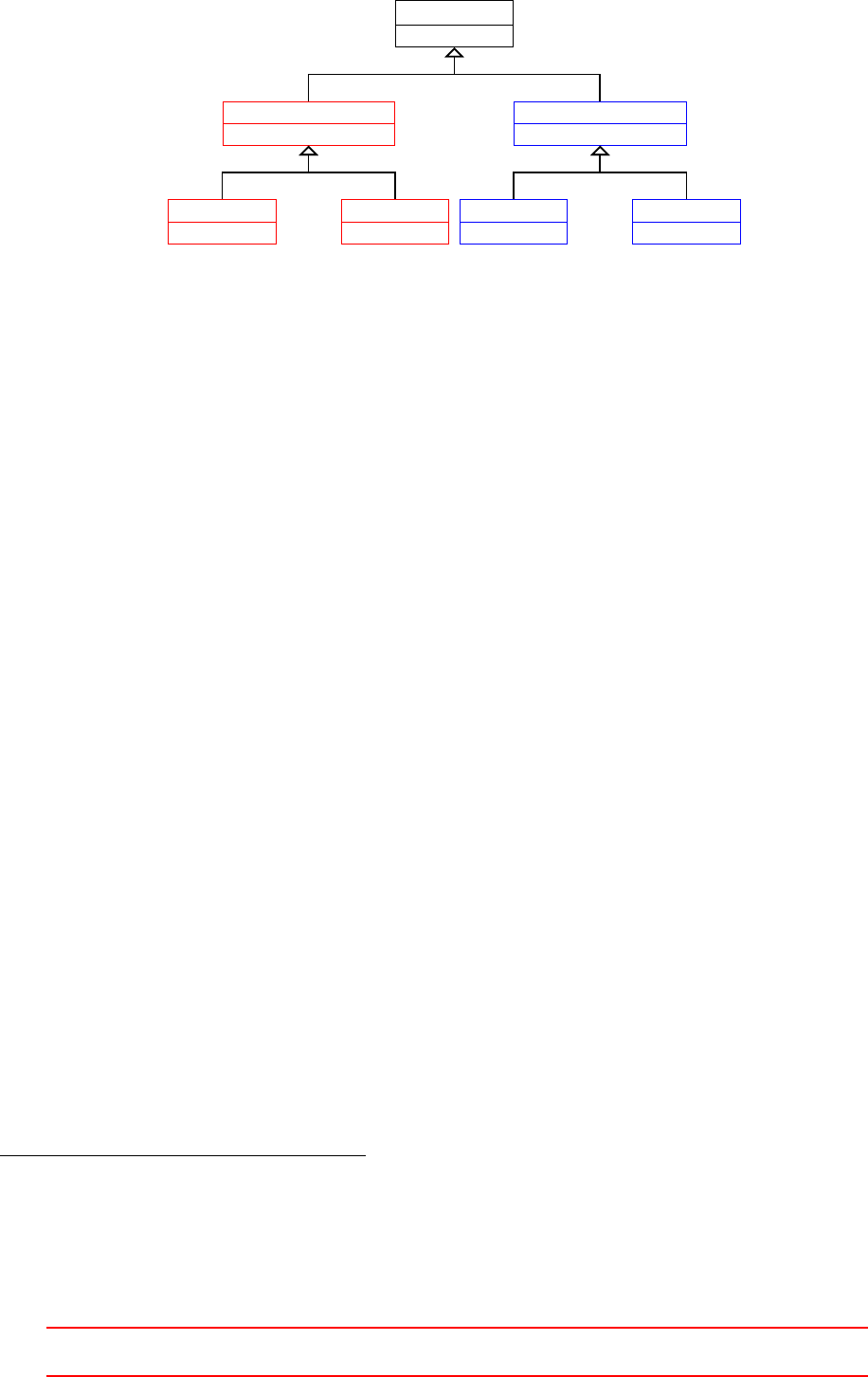
regIOobject
turbulenceModel
Foam::incompressible
RASModel LESModel
turbulenceModel
Foam::compressible
RASModel LESModel
Figure 44: The class hierarchy of the basis of the old turbulence model framework. The namespaces
Foam::incompressible and Foam::compressible are indicated by the colours red and blue.
27.1.2 The new order
The new framework for all turbulence models is located at $FOAM_SRC/TurbulenceModels, notice the capital
T68. The use of templates is necessary, since this framework is meant to be used by all solvers of OpenFOAM
at some point of time. All solvers means compressible and incompressible, as well as single- and multiphase.
This makes sense, since the concept of turbulence is general, and not related to the specific sitation in question.
The advantages of this approach is best said by the release note itself:
This new framework is very powerful and supports all of the turbulence modelling requirements
needed so far. It will be enhanced and extended in future OpenFOAM releases to include a wide
range of models and sub-models, with the expectation to replace the current dual hierarchies of
turbulence models, to aid code maintainability and sustainability.
Initially the new turbulence modelling framework was introduced with an update of the multiphase solvers.
In the OpenFOAM-2.3.0 release only twoPhaseEulerFoam and DPMFoam. As time progresses more and more
solvers are updated to use the new framework instead of the old. By the time of writing this paragraph (October
2015) dozens of solvers in the OpenFOAM-dev repository were already ported.
One to rule them all
Whenever, a certain concept manifests itself in a variety of incarnations69, the developers of OpenFOAM take
this rough quote from Lord of the Rings by heart. A single turbulence model class was created to be applied
to whatever physics OpenFOAM implements. For this to work, this most basic turbulence model contains only
the things which can be abstracted enough to apply everything. The most trivial example of this (a feature
independent of compressibiltiy or the number of phases involved), is the sheer existence of a turbulence model70.
Figure 45 shows the basic class hierarchy of the new turbulence framework. Besides this basic, non-templated
class hierarchy, there is the templated hierarchy of the implementing classes. The basic classes represent the
very abstraction. On top of the familiy tree is the class IOdictionary, which provides the IO facilities. From
using OpenFOAM, we know, that there is a dictionary controlling the turbulence modelling. By deriving the
turbulence model class from IOdictionary, the turbulence model is its dictionary.
From IOdictionary the class turbulenceModel is derived. Note the lower case letter at the beginning.
This is not the only base class for turbulence models, we will also encounter a capital letter class. As already
mentioned, OpenFOAM makes heavy use of the file system’s case sensitivity. Thus, we need to pay attention
to the letter (turbulenceModel 6=TurbulenceModel).
The class turbulenceModel declares a large number of pure virtual functions which the derived classes down
the family tree inevitably need to implement. This class is the source-code-wise incarnation of the fact that
there is a turbulence model. No further information is as of this point known to the turbulence model, except
68This is one of the reasons why OpenFOAM is not readily available on Windows, since it assumes that the file system is
case-sensitive. In fact, OpenFOAM makes heavy use of case-sensitivity of the file system. Microsoft, however, reminds us not to
expect, e.g. NTFS, to be case-sensitive. See: https://msdn.microsoft.com/en-us/library/aa365247%28VS.85%29.aspx#naming_
conventions
69Such as turbulence is present in single-phase, multi-phase, compressile, and incompressible flow.
70This is not a non-statement, however trivial this might sound. We can relate the existence of turbulence modelling to a certain
class, namely turbulenceModel, which is derived from IOdictionary, and serves as the absolute basis for everything further down
the family tree.
IV This offering is not approved or endorsed by ESI®Group, ESI-OpenCFD®or the OpenFOAM®
Foundation, the producer of the OpenFOAM®software and owner of the OpenFOAM®trademark. 112
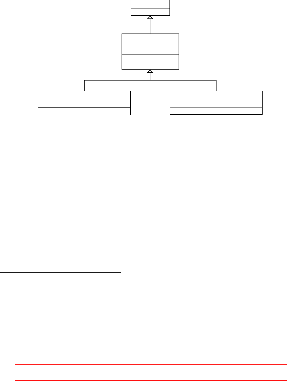
that it is a turbulence model. The data of this class is consequently sparse. The most important data members
of this class are references to the run-time object and the mesh. More information can be found in the file
$FOAM_SRC/TurbulenceModels/turbulenceModels/turbulenceModel.H.
From the class turbulenceModel two classes are derived: incompressibleTurbulenceModel and compressibleTurbulenceModel.
These two classes represent the fact, that flow can be considered incompressible or compressible. The conse-
quence of this difference can be seen in the treatment of the density by these two classes. In Figure 45 we see,
that the incompressible turbulence model has a geometricOneField as density data member, in contrast to
the compressible model, which has a reference to the actual density field.
IOdictionary
turbulenceModel
Time& runTime_
fvMesh& mesh_
Time& time()
fvMesh& mesh()
incompressibleTurbulenceModel
geometricOneField rho_
compressibleTurbulenceModel
volScalarField& rho_
Figure 45: The class hierarchy of the basis of the new turbulence model framework.
Many to rule the many
The distinction between incompressible and compressible, as well as, single-phase and multi-phase, turbulence
modelling is made by passing appropriate template parameters to the base class TurbulenceModel. Note that
TurbulenceModel is derived from the template parameter BasicTurbulenceModel. In Figure 46 we see the
(templated) class hierarchy of the new turbulence modelling framework. This class hierarchy is related to the
classes depicted in Figure 45 by the use of the template parameter BasicTurbulenceModel, which is either
incompressibleTurbulenceModel or compressibleTurbulenceModel, note the lower case first letter.
The distinction between incompressible and compressible modelling is made by the template parameters
Rho and BasicTurbulenceModel. In the case of incompressible models a geometricOneField71 is passed for
the parameter Rho. The distinction between single-phase and multi-phase modelling is made by the template
parameter Alpha. In the case of single-phase modelling a geometricOneField is passed.
The approach, that TurbulenceModel is derived from its template parameter BasicTurbulenceModel, which
is either an incompressibleTurbulenceModel or compressibleTurbulenceModel, which in turn are derived
from a common base class, demonstrates the great flexibility a high-level programming language, such as C++.
However, the presence of templates and their heavy, sophisticated use – as demonstrated in OpenFOAM – raises
the bar when it comes to reading the source code and finding out what is happening.
71The header file of the class geometricOneField describes its intention as follows:
A class representing the concept of a GeometricField of 1 used to avoid unnecessary manipulations for objects which are known
to be one at compile-time.
Used for example as the density argument to a function written for compressible to be used for incompressible flow.
IV This offering is not approved or endorsed by ESI®Group, ESI-OpenCFD®or the OpenFOAM®
Foundation, the producer of the OpenFOAM®software and owner of the OpenFOAM®trademark. 113
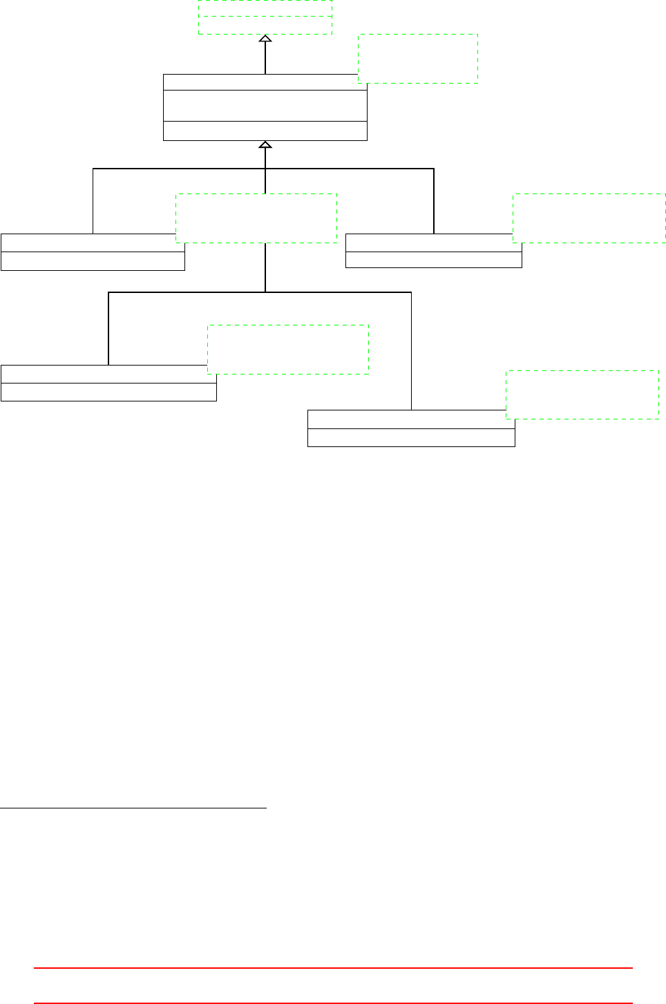
BasicTurbulenceModel
TurbulenceModel
Alpha& alpha_,
TransportModel& transportModel_
Alpha& alpha()
Alpha
Rho
BasicTurbulenceModel
TransportModel
IncompressibleTurbulenceModel CompressibleTurbulenceModel
geometricOneField
geometricOneField
incompressibleTurbulenceModel
TransportModel
geometricOneField
Rho
compressibleTurbulenceModel
TransportModel
PhaseIncompressibleTurbulenceModel
Alpha
geometricOneField
incompressibleTurbulenceModel
TransportModel
PhaseCompressibleTurbulenceModel
Alpha
Rho
compressibleTurbulenceModel
TransportModel
Figure 46: The base class TurbulenceModel has four template parameters and it is derived from one of its
template parameters. Note, that the four derived classes – the four incarnations of the turbulence model – differ
in the template parameters.
Branching the family tree
In turbulence modelling, we can identify three elementary choices: we can treat a fluid flow as laminar, or
apply a RAS or LES turbulence model. This basic choice is reflected in the three classes derived from the
template parameter in Figure 47. Since RAS and LES turbulence models are turbulence models72, those
two base classes are derived from the common template parameter BasicTurbulenceModel. The nature of
BasicTurbulenceModel has been discussed above.
By treating the laminar case as a turbulence model, the OpenFOAM developers got rid of the special case
laminar flow. In Figure 47, the behaviour of the laminar turbulence model is indicated by the methods R()
and nut(). The laminar turbulence returns zero (with the appropriate dimension) for all turbulent quantities.
Thus, the method R(), which computes the Reynolds stress tensor, returns a volumetric73 field of symmetric
tensors will all-zero components74. This behaviour is indicated in Figure 47 with the (= 0) appended to the
method’s names.
The class eddyViscosity is a class which implements the ideas behind the Boussinesq hypothesis, which is
discussed below.
72Again, we encounter an is a relationship, which is a strong hint for relating two classes by inheritance.
73I.e. all values are defined at the cell centers.
74In the file laminar.C, we find this expression in the constructor of the returned tensor field: dimensionedSymmTensor("R",
sqr(this->U_.dimensions()), symmTensor::zero).
IV This offering is not approved or endorsed by ESI®Group, ESI-OpenCFD®or the OpenFOAM®
Foundation, the producer of the OpenFOAM®software and owner of the OpenFOAM®trademark. 114
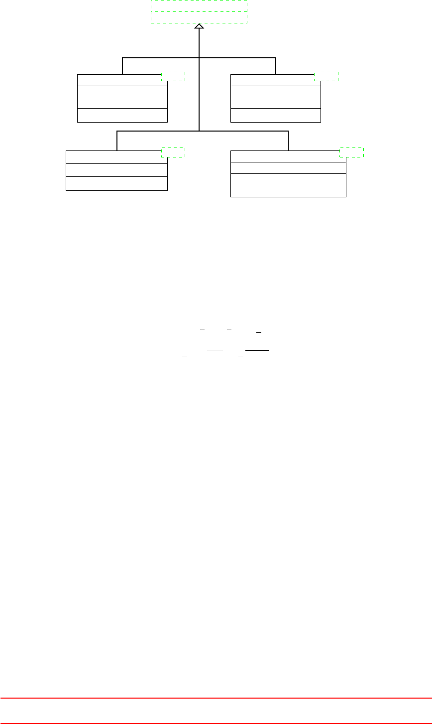
BasicTurbulenceModel ⇒BTM
RASModel
Switch printCoeffs_
Switch turbulence_
volScalarField nuEff()
LESModel
Switch printCoeffs_
Switch turbulence_
volScalarField nuEff()
BTM BTM
eddyViscosityModel
volScalarField nut_
volSymmTensorField R()
laminar
volSymmTensorField R() = 0
volScalarField nut() = 0
BTM BTM
Figure 47: The class hierarchy of the elementary turbulence models of the new turbulence model framework.
Note the shorthand notation BTM for the class BasicTurbulenceModel.
Further down the family tree
A great number of turbulence models are based on the so-called Boussinesq hypothesis which computes the
Reynolds stresses from an eddy viscosity µtand the mean strain-rate tensor, and was proposed by Boussinesq
[10] [50].
R=µt∇u+∇uT−2
3ρIk(32)
k=1
2X
i
u0
iu0
i=1
2u0·u0(33)
The quantity kis the specific kinetic energy of the turbulent fluctuations. A great part of literature refers
to kas turbulent kinetic energy [41,25,6,7], most probably for reasons of keeping the vocabulary short. The
unit tensor Iis often denoted with the Kronecker delta δij in literature.
The Boussinesq hypothesis is common to both RAS and LES turbulence models. This can be translated into
a class relationship. In Figure 48 we see how the kEpsilon and the Smagorinsky turbulence models are derived.
Those two models are discussed since these are widely used. The class eddyViscosityModel implements the
general idea of the Boussinesq hypothesis, thus, it is the common base for both turbulence models. In the case
of LES models, an intermediate class (lesEddyViscosityModel) is in between the class eddyViscosityModel
and the actual turbulence model. This class serves to hold data and define methods specific to LES models
using the Boussinesq hypothesis.
The distinction between RAS models and LES models is made by the template parameter inserted in
eddyViscosityModel. In the case of RAS models, the template parameter of eddyViscosityModel from which
e.g. the kEpsilon model is derived is RASModel<BasicTurbulenceModel>. Since RASModel is derived from
BasicTurbulenceModel, the class RASModel is a BasicTurbulenceModel. Thus, this operation is perfectly
valid. In the case of LES models, LESModel<BasicTurbulenceModel> is inserted as the template parameter of
eddyViscosityModel.
Sounds complicated, which it probably also is. Nevertheless, we admire the versatility of generality of the
new turbulence modelling framework and stomach the mental pain caused by all the template and inheritance
wizardry.
IV This offering is not approved or endorsed by ESI®Group, ESI-OpenCFD®or the OpenFOAM®
Foundation, the producer of the OpenFOAM®software and owner of the OpenFOAM®trademark. 115
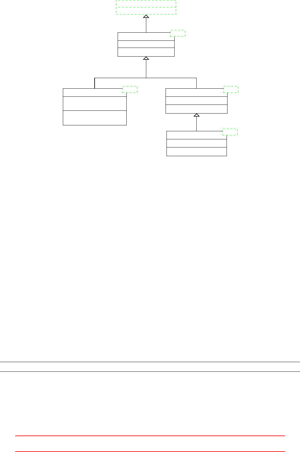
BasicTurbulenceModel ⇒BTM
eddyViscosityModel
volScalarField k()
BTM
⇒EVM
kEpsilon
volScalarField k_
volScalarField epsilon_
volScalarField k()
volScalarField epsilon()
BTM lesEddyViscosityModel
dimensionedScalar Ce_
volScalarField epsilon()
BTM
Smagorinsky
dimensionedScalar Ck_
volScalarField k()
BTM
EVM<RASModel<BTM>> EVM<LESModel<BTM>>
Figure 48: The class hierarchy of a selection of turbulence models of the new turbulence model framework.
Note the shorthand notation BTM for the class BasicTurbulenceModel, and EVM for eddyViscosityModel.
The method signature in italics of the class eddyViscosityModel indicates a pure virtual function. This
method has to be implemented by the classes derived from eddyViscosityModel. In the case of the kEpsilon
class it is the class derived directly from eddyViscosityModel which implements k(). In the case of the
Smagorinsky class, the pure virtual function was inherited via lesEddyViscosityModel. A class containing a
pure virtual function can not be instantiated, thus, there can be no usable turbulence model lesEddyViscosityModel.
This class can only serve as an intermediary.
Disclaimer
Everthing of Section 27 after this point has been created a while ago. The some of the content of the sub-sections
below might be outdated by the time you read this.
27.2 Categories
The desired category of turbulence models can be specified in the file turbulenceProperties. There are three
possible entries.
laminar The flow is modelled laminar
RASModel A Reynolds averaged turbulence model (RAS-model) is used.
LESModel Turbulence is modelled by a large-eddy model.
The file turbulenceProperties contains only one entry. In case of a large eddy simulation, this entry reads:
sim ul ation Ty pe LE SMod el ;
Listing 161: turbulenceProperties
27.3 RAS-Models
The entry in the file turbulenceProperties specifies only the class of turbulence models. The exact turbulence
model is specified in the file RASProperties. This file must contain all necessary parameters.
IV This offering is not approved or endorsed by ESI®Group, ESI-OpenCFD®or the OpenFOAM®
Foundation, the producer of the OpenFOAM®software and owner of the OpenFOAM®trademark. 116

Listing 162 shows the content of RASProperties. In this case a k-model is used and no further parameters
are necessary.
RASModel kEpsilon;
t ur bu l en ce on ;
p ri nt C oe ff s on ;
Listing 162: RASProperties
Depending on the exact model more parameters can be necessary.
27.3.1 Keywords
RASModel The name of the turbulence model. At this place laminar can also be chosen. The banana test
(see Section 9.2.1) delivers a list of available models.
--> FOAM FATAL ERROR :
Unkno wn RASMo del t ype banana
Valid RA SMod el type s :
17
(
LRR
LamBremhorstKE
LaunderGibsonRSTM
LaunderSharmaKE
LienCubicKE
LienCubicKELowRe
LienLeschzinerLowRe
NonlinearKEShih
RNGkEpsilon
SpalartAllmaras
kEpsilon
kOmega
kOmegaSST
kkLOmega
laminar
qZeta
realizableKE
)
Listing 163: Possible RAS-model entries in RASProperties
turbulence This is a switch to activate or deactivate the turbulence modelling. Allowed values are: on/off,
true/false or yes/no.
If this switch is deactivated, then a laminar simulation is conducted. This way of choosing a laminar
model is not recommended, see Section 27.5.1.
printCoeffs If this switch is enabled, then the solver will display the coefficients of the selected turbulence
model.
Even if the switch turbulence is disabled, the solver will display the coefficients at the beginning of the
simulation, see Listing 170. The coefficients are not displayed only when RASModel laminar is chosen.
optional parameters Some models accept optional parameters to override the default values of the model.
Listing 164 shows how the coefficients of the k-model can be overridden.
kEpsilonCoeffs
{
Cmu 0.09;
C1 1.44;
C2 1.92;
C3 -0.33;
sigmak 1.0;
sigmaEps 1.11; // O rig inal val ue :1.44
IV This offering is not approved or endorsed by ESI®Group, ESI-OpenCFD®or the OpenFOAM®
Foundation, the producer of the OpenFOAM®software and owner of the OpenFOAM®trademark. 117

}
Listing 164: Definition of model parameters in RASProperties
27.3.2 Pitfall: meaningless Parameters
In the above section it was shown how to override default values of the model constants. In this procedure,
there is one source of error hidden. This is not an actual error, but it can lead to a fruitless search for an error.
If nonsensical parameters are added to the kEpsilonCoeffs dictionary, these will be read and also printed.
Listing 165 shows the kEpsilonCoeffs dictionary of the file RASProperties. This dictionary is used to override
default values of the model constants. A fake model constant has been added to this dictionary.
Listing 166 shows parts of the solver output, when this dictionary is used in a simulation. All constants of
the dictionary are read and printed again. It seems as if the constant banana is part of the turbulence model.
Varying this parameter yields no results, which is no error.
The reason for this behaviour is, there is no check whether the defined constants in the dictionary make
sense or not.
kEpsilonCoeffs
{
Cmu 0.09;
C1 1.44;
C2 1.92;
C3 -0.33;
sigmak 1.0;
sigmaEps 1.11; // O rig inal val ue :1.44
banana 0.815; // nonsen se parameter
}
Listing 165: Definition of model parameters in RASProperties
Sel ecting RAS turbulence m odel kE psi lon
kEpsilonCoeffs
{
Cmu 0.09;
C1 1.44;
C2 1.92;
C3 -0.33;
sigmak 1.0;
sigmaEps 1 .11;
banana 0.815;
}
Starting time loop
Listing 166: Solver output
27.4 LES-Models
27.4.1 Keywords
The keywords turbulence and printCoeffs have the same meaning with LES models. There is also the
possibility – depending on the selected model – of defining optional parameters.
LESModel The name of the turbulence model. At this place laminar can also be chosen. The banana test
(see Section 9.2.1) delivers a list of available models. Listing 167 shows the result of such a banana test.
The model dynamicSmagorinsky was loaded from an external library. See Section 9.3.3 for how to include
external libraries.
--> FOAM FATAL ERROR : U nkno wn LE SModel type banan a
Valid LE SMod el type s :
16
IV This offering is not approved or endorsed by ESI®Group, ESI-OpenCFD®or the OpenFOAM®
Foundation, the producer of the OpenFOAM®software and owner of the OpenFOAM®trademark. 118

(
DeardorffDiffStress
LRRDiffStress
Smagorinsky
SpalartAllmaras
SpalartAllmarasDDES
SpalartAllmarasIDDES
dynLagrangian
dynOneEqEddy
dynamicSmagorinsky
homogeneousDynOneEqEddy
homogeneousDynSmagorinsky
kOmegaSSTSAS
laminar
mixedSmagorinsky
oneEqEddy
spectEddyVisc
)
Listing 167: Possible LES-model entries in LESProperties
27.4.2 Algebraic sub-grid models
Algebraic sub-grid models introduce no further transport equation to the simulation. The turbulent viscosity
is calculated from existing quantities.
27.4.3 Dynamic sub-grid models
The dynamic sub-grid models calculate the model constant CSfrom known quantities instead of prescribing a
fixed value. The way how CSis calculated is determined by the sub-grid model.
27.4.4 One equation models
A further class of LES turbulence models are one equation models. These models add one further equation to
the problem. Usually, an additional equation for the sub-grid scale turbulent kinetic energy is solved.
27.5 Pitfalls
27.5.1 Laminar Simulation
As already mentioned – see Section 27.3 – turbulence modelling can be deactivated in a some ways.
In the following, different ways to conduct a laminar simulation are listed. This list applys only to solvers
that utilize the generic turbulence modelling of OpenFOAM:
1. turbulenceProperties:simulationType laminar
This is the most general way to turn turbulence modelling off. turbulenceProperties controls the generic
turbulence class. The generic turbulence class can take the form of the laminar,RASModel or LESModel
class, see Figure 78. This is controlled by the parameter simulationType.
Sel ecting turbul enc e model type lamin ar
Listing 168: Solver output for simulationType laminar
2. RASProperties:RASModel laminar
LESProperties:LESModel laminar
In this case, a certain turbulence modelling strategy is chosen (RASModel or LESModel). However, there
is a dummy turbulence model for laminar simulation. This dummy turbulence model is derived from the
base class RASModel but it implements a laminar model. See Figure 79. Therefore, RASModel laminar
selects the laminar RAS turbulence model. In this point RASModel and LESModel behave similar.
IV This offering is not approved or endorsed by ESI®Group, ESI-OpenCFD®or the OpenFOAM®
Foundation, the producer of the OpenFOAM®software and owner of the OpenFOAM®trademark. 119

Sel ecting turbul enc e model type RASModel
Sel ecting RAS turbulence m odel la minar
Listing 169: Solver output for RASModel laminar
3. RASProperties:turbulence off
The switch turbulence can be used to enable or disable turbulence modelling. When the calculation is
started, the turbulence model specified is used. However, in the source code of the solver, there is the test
whether turbulence modelling is active or not. See Listing 205.
Sel ecting turbul enc e model type RASModel
Sel ecting RAS turbulence m odel kE psi lon
kEpsilonCoeffs
{
Cmu 0.09;
C1 1.44;
C2 1.92;
sigmaEps 1 .3;
}
Listing 170: Solver output for turbulence off
Solver output
The last two prossibilities to conduct a laminar simulation can lead to confusion because the solver output
contains word like RASmodel or RAS turbulence model. See Listings 169 and 170. In both cases the simulation
is laminar. In order to avoid this source of confusion, the user should use the parameter simulationType to
perform a laminar calculation.
Independent from all other settings, printCoeffs prints the model constants of the selected turbulence
model. This may also lead to confusion, when e.g. turbulence off is chosen to conduct a laminar simulation.
Exceptions
The above explanation only applies to solvers that utilize the generic turbulence models of OpenFOAM. However,
there is no rule without its exceptions.
simpleFoam This solver uses only RAS turbulence models. Therefore, the entries of the file turbulenceProperties
are redundant and the only ways to control turbulence modelling are items 2and 3of the list above.
twoPhaseEulerFoam This solver has the k-turbulence model hardcoded. Only item 3of the list above
applies to this solver. See Section 27.5.2 for a detailled discussion.
bubbleFoam The same as twoPhaseEulerFoam.
multiphaseEulerFoam This solver only uses LES turbulence models. Items 2and 3of the list above apply.
27.5.2 Turbulence models in twoPhaseEulerFoam
In the solver twoPhaseEulerFoam, the use of the k-turbulence model is hardcoded. This means that the solver
does not use the generic turbulence modelling ususally used by OpenFOAMs solvers. The only choice the user
of twoPhaseEulerFoam has is whether to enable or disable the k-turbulence model.
For this reason, the file constant/turbulenceProperties is not needed any more. This file can savely be
deleted.
Another consequence of the k-turbulence model being hardcoded into twoPhaseEulerFoam is that the
keyword turbulenceProperties in the file RASproperties is also not needed any more. This entry is only
read if the generic turbulence modelling is used and if there is any choice of which RAS-model to use. The
only mandatory keyword in RASproperties is the switch turbulence. This switch is the only way to decide
whether to use turbulence modelling or not with twoPhaseEulerFoam. Solvers which use the generic turbulence
modelling offer three possible ways to disable turbulence modelling, see Section 27.5.1.
IV This offering is not approved or endorsed by ESI®Group, ESI-OpenCFD®or the OpenFOAM®
Foundation, the producer of the OpenFOAM®software and owner of the OpenFOAM®trademark. 120

27.5.3 Laminar simulation with twoPhaseEulerFoam
If twoPhaseEulerFoam is used and a laminar simulation is conducted, then the presence of the files like 0/k or
0/epsilon is mandatory. The solver read this files regardless of the fact, that a laminar simulation is conducted.
This is due to the fact that the use of the k-model is hardcoded into twoPhaseEulerFoam.
Other solvers read this files based on the condition if and which turbulence model is used. Otherwise there
would be the need for all possible files (0/k,0/epsilon,0/omega, etc.) to be present in any case, which would
be utter madness.
27.5.4 Initial and boundary conditions
All turbulence models can be divided into classes depending on their mathematical properties.
Algebraic models These models add an algebraic equation to the problem. The turbulent viscosity is com-
puted from known quantities using an algebraic equation (e.g. the Baldwin-Lomax model)
One equation models These models introduce an additional transport equation to the problem. The eddy
viscosity is computed from this additional quantity (e.g. the Spalart-Allmaras model)
Two equation models These models introduce two additional transport equations to the problem. The eddy
viscosity is computed from these additional quantities (z.B. k-, k-ω)
Every field quantity of a turbulence model needs its initial and boundary conditions. Consequently, there may
be the need for additional files in the 0-directory. One way to find out which files are needed is to look at the
tutorials. There, a case may be found which utilises the needed turbulence model.
If a simulation is started and the solver is missing files – i.e. the solver tries to read files which are not
present – then OpenFOAM will issue a corresponding error message. Listing 171 shows an error message of a
case with a missing 0/k file.
Sel ecting turbul enc e model type RASModel
Sel ecting RAS turbulence m odel kE psi lon
--> FOAM FATAL IO ERROR : canno t f ind file
fi le : / home / user / O pe nF OAM / user -2 .1. x/ run / p is oFoa m / cavit y /0/ k at line 0.
From fu nct ion reg IOo bje ct :: readStream ()
in file db / reg IOobj ect / r eg IOobj ec tRead . C at line 73.
FOAM exiting
Listing 171: Solver error message: missing file
27.5.5 Additional files
RAS turbulence models produce additional files. Most RAS models calculate the turbulent viscositiy from
certain quantities. These quantities are usually field quantities and depend on the used turbulence model.
However, the aim of all RAS turbulence models is to calculate the turbulent viscosity. The turbulent viscosity
itself is a field quantity.
Listing 172 shows the folder contents before and after a simulation with pisoFoam. The 0-directory contains
only the mandatory files, in this case pressure and velocity as well as the turbulent quantities k and .
After the simulation has finished, the 0-directory contains more files. The reason for creating the *.old files
is not known. However, the turbulence model created the file nut for storing the turbulent viscosity.
The file phi as well as the folder uniform is created by the solver.
use r@host :∼/ O pe nF OA M / user -2 .1. x/ run / p is oF oa m / ras / ca vi ty $ ls
0 constant system
use r@host :∼/ O pe nF OA M / user -2 .1. x/ run / p is oF oa m / ras / ca vi ty $ ls 0/
epsilon k p U
use r@host :∼/ O pe nF OA M / user -2 .1. x/ run / p is oF oa m / ras / ca vi ty $ p is oF oa m > / dev / null
use r@host :∼/ O pe nF OA M / user -2 .1. x/ run / p is oF oa m / ras / ca vi ty $ ls
0 0.5 1 constant s ystem
use r@host :∼/ O pe nF OA M / user -2 .1. x/ run / p is oF oa m / ras / ca vi ty $ ls 0/
eps il on e ps il on . ol d k k . ol d n ut p U
IV This offering is not approved or endorsed by ESI®Group, ESI-OpenCFD®or the OpenFOAM®
Foundation, the producer of the OpenFOAM®software and owner of the OpenFOAM®trademark. 121

use r@host :∼/ O pe nF OA M / user -2 .1. x/ run / p is oF oa m / ras / ca vi ty $ ls 0.5/
epsilon k nut p phi U uniform
use r@host :∼/ O pe nF OA M / user -2 .1. x/ run / p is oF oa m / ras / ca vi ty $
Listing 172: Folder contents at the begin and the end of a simulation
The 0-directories of some tutorial cases may already contain such additional files, e.g. nut. In some cases
the 0-directory may also contain several of such files due to a change in the naming scheme. Listing 173 shows
the contents of the 0-directory of the pitzDaily tutorial case of simpleFoam. The case has not been run, so the
files nut and nuTilda have not been generated by the solver. None of these two files is necessary to run the
case with the k-turbulence model.
epsilon k nut nuTilda p U
Listing 173: The content of the 0-directory of the pitzDaily tutorial case of simpleFoam
27.5.6 Spalart-Allmaras
The Spalart-Allmaras is a one-equation turbulence model. Although it introduces only one additional equation
to the problem it needs two additional files in the 0-directory. Listing 174 shows the content of the 0-folder
of the airFoil2D tutorial case of simpleFoam. The files nut and nuTilda are both necessary to run the case.
The former contains the turbulent viscosity and the latter contains the transported quantity of the turbulence
model. Therefore, the rule one additional transport equation entails one additional data file is not violated.
Because the viscosity is not constant it has to be defined in a file in the 0-directory. And, because the
viscosity is not the transported quantity of the Spalart-Allmaras model another file is added to the 0-directory.
nut nuTil da p U
Listing 174: The content of the 0-directory of the airFoil2D tutorial case of simpleFoam
28 Eulerian multiphase modelling
In Eulerian two-phase modelling both phases are considered continua even though one phase might consist of
dispersed phase elements (DPEs) such as bubbles, drops or particles. In these simulations the two phases can
be distinguished into a continuous phase and a dispersed phase. This naming scheme refers to the physical
situation. Within the (Eulerian) mathematical description, however, both phases are continua.
As two momentum equations are solved (one per phase), each phase has its own velocity field. However,
there is only one pressure field. Thus, the pressure is the same for both phases; this also applies to the VOF
method. Due to the fact that two continuity75 and two momentum equations are solved, this approach is often
referred to as two fluid model.
The Eulerian description of multi-phase flow is not limited to two phases, however, for reasons of simplicity,
we limit ourselves to the case of two phases.
75The constraint that the sum of all volume fraction fields must yield unity, i.e. Piαi
!
= 1, allows for one continuity equation
to be eliminated. In the case of two phases, only one continuity equation needs to be solved. However, both continuity equation
can be combined.
IV This offering is not approved or endorsed by ESI®Group, ESI-OpenCFD®or the OpenFOAM®
Foundation, the producer of the OpenFOAM®software and owner of the OpenFOAM®trademark. 122
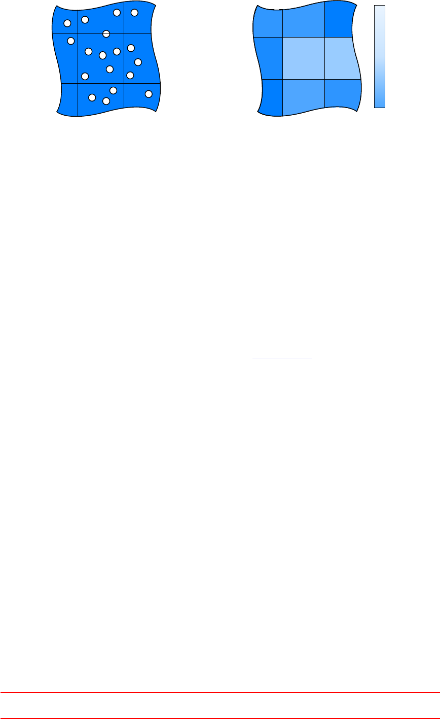
(a) Discrete bubbles in a continuous
liquid.
gas
liquid
(b) Continuum approach.
Figure 49: Modelling approach on the example of a gas-liquid two-phase system.
As the DPEs are considered to be a continuous phase, their properties are averaged over each cell of the
computational domain. Thus, the properties of the dispersed phase are the mean properties of the dispersed
matter. If all DPEs have equal properties (e.g. diameter, density, etc.), then the dispersed phase is referred to as
being mono-disperse. Only in the case of mono-dispersity, the averaging over the cells introduces no additional
errors. If the DPEs have variable properties (e.g. a diameter range), then the dispersed phase is referred to as
being poly-disperse. The correct handling of poly-dispersity requires additional considerations on the models.
28.1 Phase model class
One of the strenghts of object oriented programming is that the class structure in the source code can reflect
the properties and relations of real-world things.
The phase model class in the various two- and multi-phase solvers of OpenFOAM is one example of how
techniques of object oriented programming can be applied. In terms of a multi-phase problem in fluid dynamics
we distinguish different phases.
We now violate the unwritten law of to not cite Wikipedia[Citation needed].
Phase (matter), a physically distinctive form of a substance, such as the solid, liquid, and gaseous
states of ordinary matter—also referred to as a "macroscopic state"
http://en.wikipedia.org/wiki/Phase
In fluid dynamics phase is a commonly used term. When we intend our code to represent the reality we want
to describe as closely as possible we need to introduce the concept of the phase into our source code. From a
programming point of view properties of a phase – such as viscosity, velocity, etc. – are easy to implement. The
viscosity of a phase is simply a field of values, velocity is another field of values.
Object orientation allows us to translate the idea of the phase into programming language. The basic idea
is that a phase has a viscosity, it also has a velocity. We now create a class named phaseModel and this class
needs to have a viscosity, a velocity and everthing else a phase needs to fit our needs.
The phase model classes follow the code of best practice in object oriented programming to hide internal
data from the outer world and to provide access via the classes methods (data encapsulation, see http://www.
tutorialspoint.com/cplusplus/cpp_data_encapsulation.htm).
No phases, please
In the single-phase solvers of OpenFOAM – such as simpleFoam – the concept of a phase is not used. As there
is only one temperature and velocity to deal with, the concept of phases is not needed. In the single-phase
solvers the phase-properties (viscosity, velocity, density, etc.) are linked according to the physical relations that
are taken into account, but the concept of a phase is missing.
28.1.1 A comparison of the phase models in OpenFOAM-2.2
In this section we want to compare the implementation of the phase model class of the two solvers twoPhaseEuler-
Foam and multiphaseEulerFoam.
IV This offering is not approved or endorsed by ESI®Group, ESI-OpenCFD®or the OpenFOAM®
Foundation, the producer of the OpenFOAM®software and owner of the OpenFOAM®trademark. 123

twoPhaseEulerFoam
The phase model class in twoPhaseEulerFoam-2.2.x collects the properties of a phase and offers an interface
for accessing these properties. Listing 175 shows the essence of the header file of the phase model class. The
listing is syntactically correct, however all pre-processor instruction (e.g. the #include statements) have been
removed. Furthermore, most of the comments have been removed and the formatting has been adapted to
reduce the line number. The purpose of Listing 175 is to present the data members and methods of the class
by actual source code.
1namespace Foam
2{
3
4class phaseModel
5{
6// Pri vate data
7dic ti onary dict_ ;
8wo rd nam e_ ;
9dimensionedScalar d_;
10 dimensionedScalar nu_;
11 dim ens io ned Sc al ar rho_ ;
12 volVectorField U_;
13 autoPtr < sur faceScalarField > p hiPt r_ ;
14
15 public:
16 // Mem ber Fu nct ion s
17 const word & n ame () const {return n ame_ ; }
18
19 const dimensionedScalar& d() const {return d_ ; }
20
21 const d im en si on ed Sca la r & nu () const {return nu_ ; }
22
23 const dime ns ione dSca lar & rho () const {return rho_ ; }
24
25 const volVectorField& U() const {return U_ ; }
26
27 volVectorField& U() { return U_ ; }
28
29 const surf ac eScal ar Fi eld & phi () con st {return ph iP tr _ ( ) ; }
30
31 sur fa ce Sc ala rF ie ld & phi () { return p hiP tr _ ( ) ; }
32 };
33
34 }// End n ame spa ce Foam
Listing 175: A boiled-down version of the file phaseModel.H
The phase model class of twoPhaseEulerFoam-2.2.x contains all phase properties needed for an incompressible
two-phase solver that makes use of an important consequence of being limited to two phase problems. By
taking a look on the members of the class we see that there is no volume fraction field. In two phase problems
one volume fraction field (alpha1) suffices as the volume fraction field of the other phase is instantly known
(alpha2 = 1 - alpha1). Thus, the volume fraction can be treated seperately from other phase information.
Another missing item is the pressure. Most two- or multi-phase Eulerian solvers assume/use a common
pressure for all phases. Thus, the pressure is independent of the phases and can be treated seperately.
multiphaseEulerFoam
One difference between the phase model class used in twoPhaseEulerFoam and the one used in multiphaseEuler-
Foam follows directly from the simplification made in the two-phase case. When dealing with an arbitrary
number of phases, each phase must keep track of its own volume fraction. Thus, the volume fraction must be
included into the phase model.
The straight-forward way would be to add another reference to the data members. As the volume fraction
field is a scalar field, this reference would be a reference to a volScalarField. In multiphaseEulerFoam a
more subtle approach was chosen. This also presents the application of another object-oriented programming
technique.
The phase model class of multiphaseEulerFoam is derived from the class volScalarField. Thus, the phase
model class is among other things its own the volume fraction field.
IV This offering is not approved or endorsed by ESI®Group, ESI-OpenCFD®or the OpenFOAM®
Foundation, the producer of the OpenFOAM®software and owner of the OpenFOAM®trademark. 124

Listing 176 shows a stripped version of the header file of multiphaseEulerFoam’s phase model class. Again,
large parts of the file have been removed leaving only the data members and the methods of the class.
1namespace Foam
2{
3
4class phaseModel
5:
6public volScalarField
7{
8// Pri vate data
9wo rd nam e_ ;
10 dic tio nary phaseDict_ ;
11 dimensionedScalar nu_;
12 dim en si on ed Sca la r kappa _ ;
13 dimensionedScalar Cp_;
14 dim ens io ned Sc al ar rho_ ;
15 volVectorField U_;
16 volVectorField DDtU_;
17 sur fa ce Sc alarF ie ld phi Alp ha_ ;
18 autoPtr < sur faceScalarField > p hiPt r_ ;
19 autoPtr < diame terM odel > dPt r_ ;
20
21 public:
22
23 // Mem ber Fu nct ion s
24 const word & n ame () const {return n ame_ ; }
25
26 const word & key word () const {return n am e () ; }
27
28 tmp <volScalarField > d() c onst ;
29
30 const d im en si on ed Sca la r & nu () const {return nu_ ; }
31
32 const dime ns ion ed Scal ar & kappa () const {return kappa_; }
33
34 const d im en si on ed Sca la r & Cp () const {return Cp_ ; }
35
36 const dime ns ione dSca lar & rho () const {return rho_ ; }
37
38 const volVectorField& U() const {return U_ ; }
39
40 volVectorField& U() { return U_ ; }
41
42 const volVectorField& DDtU() const {return D DtU_ ; }
43
44 vol Ve cto rF iel d & DDtU () { return DDtU_ ; }
45
46 const surf ac eScal ar Fi eld & phi () const {return p hi Ptr _ () ; }
47
48 sur fa ce Scala rF ie ld & phi () { return p hiP tr _ ( ) ; }
49
50 const surf ac eSca larF ield & phi Alp ha () const {return phiAlpha_ ; }
51
52 sur fa ceSc alar Fiel d & phiAlpha () { return phi Alp ha_ ; }
53
54 void correct();
55
56 bool read(co nst dic tiona ry & pha seD ict ) ;
57 };
58
59 }// End n ame spa ce Foam
Listing 176: A boiled-down version of the file phaseModel.H
The statements following the class keyword and the class name indicates the derivation of a class. The class
name (phaseModel) and the name of the class we are deriving from (volScalarField) are separated by a colon
(:). The name of the base class (volScalarField) is preceded by a visibility specifier (public). Here, we see a
prototype of a class definition. The class we define (phaseModel) is derived from a base class (volScalarField).
IV This offering is not approved or endorsed by ESI®Group, ESI-OpenCFD®or the OpenFOAM®
Foundation, the producer of the OpenFOAM®software and owner of the OpenFOAM®trademark. 125

class phaseModel : public volScalarField
{
/* some c ++ code */
}
This example highlights, that the class phaseModel is derived from the class volScalarField. This infor-
mation alone does no proof that the phase model is its own volume fraction field. However, a glance on the
constructor in the implementation file brings clarity.
In Listing 177 we see, that the first instruction in the initialisation list of the constructor reads the vol-
ume fraction field of the respective phase. This proofes that the phase model is in fact its own volume
fraction field. For an explanation why we come to this conclusion we refer to any C++ textbook or on-
line resource that covers the concept of inheritance, see e.g. http://www.learncpp.com/cpp-tutorial/
114-constructors-and-initialization-of-derived-classes/ or [45].
// * * * * * * * * * * * * * * * * Constru cto rs * * * * * * * * * * * * * * //
Foam :: p haseModel :: phaseM ode l
(
const word & name ,
const dictionary & phaseDict ,
const fvMesh & mesh
)
:
volScalarField
(
IOobject
(
" alpha " + name ,
me sh . time () . tim eN ame () ,
mesh ,
IOobject :: MUST_READ ,
IOobject :: AU TO_WRITE
) ,
mesh
) ,
name_ ( name ) ,
// code con tin ues
Listing 177: The first few lines of the constructor of the phase model.
Besides being its own volume fraction field the phase model class of multiphaseEulerFoam was extended by
several fields bearing information for the simulation of thermodynamics.
We can also observe the rudiment of giving the phase model a more active role. The phase model class
of twoPhaseEulerFoam is simply an information carrier. The phase model of multiphaseEulerFoam features a
method named correct(). The correct() method is used in many models for actions performed at every time
step. However, in multiphaseEulerFoam-2.2.x this method is empty.
With OpenFOAM-2.1.0 the class diameterModel was introduced into multiphaseEulerFoam and compress-
ibleTwoPhaseEulerFoam. The phase model class of multiphaseEulerFoam uses a diameter model class for keep-
ing track of the dispersed phase’s diameter. The diameter model offers the choice of computing the diameter of
the dispersed phase elements from thermodynamic quantities besides using a constant diameter. Thus, the data
member dimensionedScalar d_ is replaced by a reference to a diameter model (autoPtr<diameterModel> dPtr_).
28.1.2 A comparison of the phase models in OpenFOAM-2.3
In this section we want to compare the implementation of the phase model class of the two solvers twoPhaseEuler-
Foam and multiphaseEulerFoam.
A comment on multiphaseEulerFoam
The phase model class used for multiphaseEulerFoam in OpenFOAM-2.2.x and OpenFOAM-2.3.x differs very
little with respect to the class’s methods and members. Listing 178 shows that the header files of the phaseModel
class of multiphaseEulerFoam differs only in the copyright notice. The implementation file shows slightly greater
IV This offering is not approved or endorsed by ESI®Group, ESI-OpenCFD®or the OpenFOAM®
Foundation, the producer of the OpenFOAM®software and owner of the OpenFOAM®trademark. 126

differences76. However, the behaviour of this class can be considered nearly identical in OpenFOAM-2.2.x and
OpenFOAM-2.3.x.
use r@host :∼/ O penFOAM$ diff
OpenFOAM -2.2. x / ap pli catio ns / sol vers / multiph ase / m ul ti ph ase Eu le rF oam / phase Mod el / phaseModel /
pha seM odel .H
OpenFOAM -2.3. x / applic ation s / solvers / m ul tiph as e / mu lt ip ha se Eu le rF oa m / mul ti ph as eS ystem /
pha seM odel / phaseMod el .H
5 c5
< \\ / A nd | Cop yri ght ( C ) 2011 Op enF OAM Foundatio n
---
> \\ / A nd | Cop yri ght ( C ) 20 11 -2013 O penFOAM F oundation
Listing 178: The output of diff for the file phaseModel.H of the solver multiphaseEulerFoam of the versions
OpenFOAM-2.2.x and OpenFOAM-2.3.x as of May 201477.
twoPhaseEulerFoam
The two-phase model of twoPhaseEulerFoam-2.3.x makes heavy use of abstractions. The phase model class is
used in conjunction with a class for the two-phase system.
1namespace Foam
2{
3
4class phaseModel
5:
6p u b l i c volScalarField ,
7p u b l i c tr a n s p o r t M o d e l
8{
9// P r i v a t e d at a
10 const twoPhaseSystem& f l u i d _ ;
11 word name_ ;
12 d i c t i o n a r y phaseDict_ ;
13 s c a l a r alphaMax_ ;
14 autoPtr<rhoThermo> thermo_ ;
15 v o l V e c t o r F i e l d U_;
16 s u r f a c e S c a l a r F i e l d alphaPhi_ ;
17 s u r f a c e S c a l a r F i e l d alphaRhoPhi_ ;
18 autoPtr<s u r f a c e S c a l a r F i e l d > phiPtr_ ;
19 autoPtr<diameterModel> dPtr_ ;
20 autoPtr<PhaseCompress ible TurbulenceModel<phaseModel> > t u rbulence _ ;
21
22 p u b l i c :
23
24 // Member F u n c t i o n s
25 const word& name ( ) const {return name_ ; }
26
27 const twoPhaseSystem& f l u i d ( ) const {return f l u i d _ ; }
28
29 const phaseModel& o therP hase ( ) const ;
30
31 s c a l a r alphaMax ( ) const {return alphaMax_ ; }
32
33 tmp<v o l S c a l a r F i e l d > d ( ) const ;
34
35 const PhaseCompressibleTurbulenceModel<phaseModel>&
36 turbulence () const ;
37
38 PhaseCompressibleTurbulenceModel<phaseModel>&
39 turbulence () ;
40
41 const rhoThermo& thermo ( ) const {return thermo_ () ; }
42
43 rhoThermo& thermo ( ) { return thermo_ ( ) ; }
76The diff of the implementation file would be too long to be shown at this place. For general information on diff see Section
57.6.
77OpenFOAM Builds compared: 2.2.x-61b850bc107b and 2.3.x-0eb39ebe0f07.
IV This offering is not approved or endorsed by ESI®Group, ESI-OpenCFD®or the OpenFOAM®
Foundation, the producer of the OpenFOAM®software and owner of the OpenFOAM®trademark. 127

44
45 tmp<v o l S c a l a r F i e l d > nu ( ) const {return thermo_−>nu ( ) ; }
46
47 tmp<s c a l a r F i e l d > nu ( const l a b e l p a t c h i ) const {return thermo_−>nu ( p a t c h i ) ; }
48
49 tmp<v o l S c a l a r F i e l d > mu( ) const {return thermo_−>mu( ) ; }
50
51 tmp<s c a l a r F i e l d > mu( const l a b e l p a t c h i ) const {return thermo_−>mu( p a t c h i ) ; }
52
53 tmp<v o l S c a l a r F i e l d > kappa ( ) const {return thermo_−>kappa ( ) ; }
54
55 tmp<v o l S c a l a r F i e l d > Cp ( ) const {return thermo_−>Cp ( ) ; }
56
57 const v o l S c a l a r F i e l d& rho ( ) const {return thermo_−>r ho ( ) ; }
58
59 const v o l V e c t o r F i e l d& U( ) const {return U_; }
60
61 v o l V e c t o r F i e l d& U( ) { return U_; }
62
63 const s u r f a c e S c a l a r F i e l d& phi ( ) const {return phiPtr_ ( ) ; }
64
65 s u r f a c e S c a l a r F i e l d& phi ( ) { return phiPtr_ ( ) ; }
66
67 const s u r f a c e S c a l a r F i e l d& alph aPhi ( ) const {return alphaPhi_ ; }
68
69 s u r f a c e S c a l a r F i e l d& alph aPhi ( ) { return alphaPhi_ ; }
70
71 const s u r f a c e S c a l a r F i e l d& alphaRhoPhi ( ) const {return alphaRhoPhi_ ; }
72
73 s u r f a c e S c a l a r F i e l d& alphaRhoPhi ( ) { return alphaRhoPhi_ ; }
74
75 void c o r r e c t ( ) ;
76
77 v i r t u a l boo l r e ad ( const d i c t i o n a r y& p h a s e P r o p e r t i e s ) ;
78
79 v i r t u a l boo l r ead ( ) { r e t u r n t r u e ; }
80 } ;
81
82 }// End namespace Foam
Listing 179: A boiled-down version of the file phaseModel.H
The data members of the phase model class in twoPhaseEulerFoam-2.3.x contain a reference to the two-phase
model class. This makes the phase model class aware of the other phase. The data members also contain a
reference to a turbulence model and a thermophysical model. This is up to now the greatest generalisation we
could observe in the multi-phase solvers of OpenFOAM.
28.2 Phase system classes
In a multiphase solver we can not only create an abstraction for the physical phase, e.g. water. We can
also create an abstraction for the multi-phase system, i.e. the entirety of the involved phases. Again, multi-
phaseEulerFoam was the forerunner for this idea. Since the introduction of multiphaseEulerFoam there is a
class named multiphaseSystem. In twoPhaseEulerFoam-2.3 the class twoPhaseSystem was introduced. The
most obvious purpose of this class is the implementation of the phase continuity equation. In both solvers the
solution of the continuity equation(s) hides behind the function call fluid.solve().
28.2.1 The class twoPhaseSystem
We now take a detailled look on the class twoPhaseSystem. This class was introduced with twoPhaseEulerFoam-
2.3 and this class seems to be a consequent continuation of ideas introduced in the class multiphaseSystem. We
focus on the class twoPhaseSystem, since the class multiphaseSystem has not really evolved from the release of
OpenFOAM-2.1 til the release of OpenFOAM-2.3. The header and the implementation file are largely identical.
Phase models
Two data members of the class are the two involved phase models phase1_ and phase2_. The class provides
methods to access this phase models. There is also a method to access the other phase. As there are only two
IV This offering is not approved or endorsed by ESI®Group, ESI-OpenCFD®or the OpenFOAM®
Foundation, the producer of the OpenFOAM®software and owner of the OpenFOAM®trademark. 128

phases involved, this operation is possible.
Phase pair models
In order to cover all possible flow situations the momentum exchange models are defined in the case pair-wise
in a separated fashion, i.e. drag for air dispersed in water (bubbly flow) and drag for water dispersed in air
(droplet flow).
The classes phasePair and orderedPhasePair provide an elegant way to deal with this situation. The
phase pair models are used for blending the interfacial momentum exchange models.
Momentum exchange models
The class has member variables for the interfacial momentum exchange models. Listing 180 shows the members
of the class related to momentum exchange models. The templated class BlendedInterfacialModel<> provides
functionality that is needed for all momentum exchange models. As the class name suggests, the blending is
covered by this class. The template parameter of this class stands for any one of the interfacial momentum
exchange models.
1// - Drag mo del
2au toPtr < B le nd edInt er fa ci al Mo de l < dra gModel > > drag_ ;
3// - V irtu al mass mod el
4autoPtr < Ble ndedI nte rfaci alM odel < virtu alMa ssMo del > > virt ual Mass_ ;
5// - Heat tra nsfe r model
6autoPtr < Ble nd edInt erf acial Model < hea tTra nsfe rModel > > h eatTr ansfe r_ ;
7// - Lift mo del
8au toPtr < B le nd edInt er fa ci al Mo de l < lif tModel > > lift_ ;
9// - Wall lub ri ca ti on mo del
10 autoPtr < Ble ndedI nterf aci alMod el < wal lLu bricationMo del > > w allLu br icati on _ ;
11 // - Wall lub ri ca ti on mo del
12 autoPtr < Ble ndedI nte rfaci alM odel < tur bul en tDi spers ion Mo del > > t ur bu lent Dispe rs io n_ ;
Listing 180: The declaration of the momentum exchange members of the class twoPhaseSystem in
twoPhaseSystem.H
A momentum exchange model alone is nice, but what we really need are the contribution to the momentum
equation. Thus, the class twoPhaseSystem provides methods to access the respective force terms or the respec-
tive coefficients. We have seen this force terms and coefficients in action in Section 35.6.
1// - R eturn the dr ag c oe ff ic ie nt
2tmp < volSc alar Fiel d > dra gCoeff () c onst ;
3// - R eturn the vir tual mass co ef fi ci ent
4tmp < volSc alar Fiel d > virt ua lM assCo ef f () con st ;
5// - R eturn the he at t ra nsfe r c oeffi ci ent
6tmp < volSc alar Fiel d > heat Tr an sf er Co eff () con st ;
7// - R eturn the li ft for ce
8tmp < volVe ctor Fiel d > lif tForce () c onst ;
9// - R eturn the wa ll l ub ri ca ti on forc e
10 tmp < volVe ctor Fiel d > wall Lu br ic at io nF or ce () con st ;
11 // - R eturn the wa ll l ub ri ca ti on forc e
12 tmp < volVe ctor Fiel d > turb ul ent Di sp er si on Fo rce () c onst ;
Listing 181: The declaration of the accessing methods for the momentum exchange coefficients of the class
twoPhaseSystem in twoPhaseSystem.H
28.2.2 The class multiphaseSystem
The solver multiphaseEulerFoam uses the class multiphaseSystem. This class seems to be the ancestor of the
class twoPhaseSystem.
IV This offering is not approved or endorsed by ESI®Group, ESI-OpenCFD®or the OpenFOAM®
Foundation, the producer of the OpenFOAM®software and owner of the OpenFOAM®trademark. 129
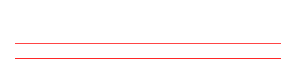
Phase pair
The class multiphaseSystem declares a nested class interfacePair. A nested class is a class definition within
another class. Thus, the nested class is hidden from the outside world78.
The phase pair class is used to deal with surface tension, which by definition is a property of a pair of phases,
and drag.
28.3 Turbulence modelling
28.3.1 Modelling strategies
The problem of turbulence modelling in multi-phase problems can be tackled in one of the following fashions. The
methods are sorted by their perceived computational cost. Whereas the first two methods may be equivalent,
the last is definitely more expensive in terms of memory and computational time. However, each of these
methods has its strengths and weaknesses, and its use cases.
Continuous phase only This model solves computes the turbulent properties of the continuous phase and
assumes an algebraic relationship between the turbulent properties of the continuous and the dispersed
phase. The influence of turbulence on the dispersed phase can also be neglected alltogether. In the Fluent
Theory Guide [6] it is noted: [...] is the appropriate model when the concentrations of the secondary
phases are dilute. In this case, interparticle collisions are negligible and the dominant process in the
random motion of the secondary phases is the influence of the primary-phase turbulence. In Fluent this
approach is referred to as dispersed turbulence model.
Mixture In this approach the turbulence model is evaluated for the mixture of all phases, i.e. the mixture
velocity and mixture density are inserted into the turbulence model. The turbulent quantities of each
individual phase are computed with the density ratio between the mixture and the corresponding phase.
The applicability of this model is described in the Fluent Theory Guide [6] as follows: [...] is applicable
when phases separate, for stratified (or nearly stratified) multiphase flows, and when the density ratio
between phases is close to 1.
Per-phase In this case each phase has its own turbulent properties. Because there are additional transport
equations to be solved per phase, this model is the most computational intensive. The Fluent Theory
Guide [6] states: [...] is the appropriate choice when the turbulence transfer among the phases plays a
dominant role.
28.3.2 Implementation in OpenFOAM
In Section 27.1 the frameworks for implementing turbulence modelling within OpenFOAM are discussed. Now
we take a look on multi-phase turbulence and OpenFOAM’s frameworks for modelling turbulence.
The old framework, see Section 27.1.1, allow only for the first two of the described strategies, since only
one turbulence model is employed by the multiphase solvers. The turbulence model is generally a global object
within the solver, as is also the mesh or the run-time object.
The new framework allows for greater flexibility. In the Eulerian multiphase solvers, the turbulence model
has been moved to the phase model. Thus, each phase has its own turbulence model. This allows for all three
modelling strategies discussed in Section 28.3.1. The turbulence modelling employed by twoPhaseEulerFoam
within the new framework is discussed in Section 35.4.
28.4 Interfacial momentum exchange
On the RHS of the momentum equation there are two types of source terms. The first term Fq,i is a force
density acting on the phase q. The second term is a force (density) coefficient Kqp,i which is multiplied by the
relative velocity uR=up−uqbetween the phases qand p.
The models for interfacial momentum transfer in OpenFOAM are implemented in a way, such that these
models return either a force or a force coefficient79. The distinction between forces and force coefficents is a
78See http://pic.dhe.ibm.com/infocenter/compbg/v121v141/topic/com.ibm.xlcpp121.bg.doc/language_ref/cplr061.html
for details.
79The correct denomination would be force density and force density coefficient. In the source files of OpenFOAM related to
these models, Fq,i and Kqp,i are referred to as force and force coefficient, most probably for the sake of reducing typing effort. As
OpenFOAM keeps track of the physical units of its variables, we can see from the actual source codes, that the force Fq,i is in fact
a force density.
IV This offering is not approved or endorsed by ESI®Group, ESI-OpenCFD®or the OpenFOAM®
Foundation, the producer of the OpenFOAM®software and owner of the OpenFOAM®trademark. 130
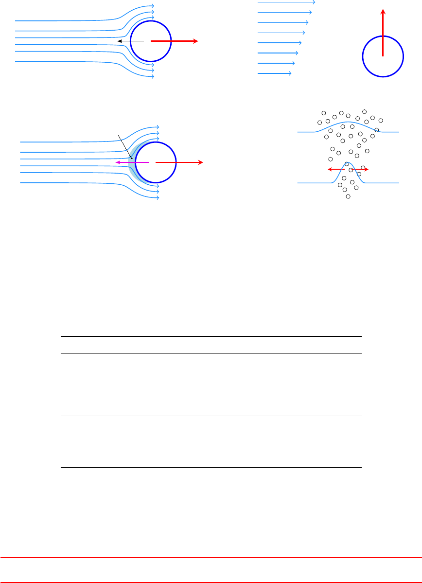
matter of convenience. Contributions directly proportional to the velocity, e.g. drag, can be treated differently
than contributions indirectly proportional to the velocity, e.g. the virtual mass force which is proportional to
the time derivative of the relative velocity. Terms directly proportional to the velocity are numerically treated
differently than other terms.
The interfacial momentum transfer due to drag, lift and virtual mass are based on the force acting on
a single bubble. The turbulent dispersion force is observed when the turbulent eddies of the liquid phase
interact with a swarm of bubbles. This interaction tends to disperse bubble swarms [34]. Figure 50 gives a
schematic representation of the different momentum exchange mechanisms between the liquid and the gas phase.
Fdrag
(a) Drag; the black arrow indicates the relative velocity
Flift
(b) Lift
Fvirtual mass
Virtual mass
(c) Virtual mass; the purple arrow indicates the relative acceleration
Ft.-disp.
(d) Turbulent dispersion
Figure 50: Modelling approach on the example of a gas-liquid two-phase system.
28.5 Diameter models
As mentioned in the previous Section, diameter models were introduced at some point in the multiphase mod-
els. The multiphaseEulerFoam offered since its introduction in version 2.1.0 two diameter models (constant and
isothermal). With twoPhaseEulerFoam-2.3 a further diameter model was introduced, which is available only in
twoPhaseEulerFoam.
OpenFOAM Constant, no model Constant Isothermal IATE
twoPhaseEulerFoam
2.0.x x
2.1.x x
2.2.x x
2.3.x x x x
multiphaseEulerFoam
2.1.x x x
2.2.x x x
2.3.x x x
Table 4: Overview of diameter modelling in Eulerian multiphase solvers
28.5.1 No model
The older versions of twoPhaseEulerFoam (≤2.2.x) use no model for the diameter of the dispersed phase
elements (DPE). In all of these versions the phase diameter is a scalar of type dimensionedScalar that is read
IV This offering is not approved or endorsed by ESI®Group, ESI-OpenCFD®or the OpenFOAM®
Foundation, the producer of the OpenFOAM®software and owner of the OpenFOAM®trademark. 131

from the transportProperties dictionary.
28.5.2 Constant
The constantDiameter diameter model is the implementation of a constant diameter in a framework that
allows for a variable diameter.
Internally, the diameter is still a scalar which is read from transportProperties respectively from phaseProperties.
However, the phase model returns the diameter as a field quantity. Listing 182 shows how a volScalarField
is returned. The private variable d_ is of the type dimensionedScalar.
1Foam :: tmp < Foam :: v olS calar Field >
2Fo am :: d ia m et er M od e ls : : c on sta nt : : d ()
3const
4{
5return tmp < Fo am :: vol Scal ar Fiel d >
6(
7new volScalarField
8(
9IOobject
10 (
11 "d",
12 pha se _ . U () . t ime ( ) . tim eN am e () ,
13 pha se _ . U () . m esh ( )
14 ) ,
15 pha se _ . U () . m esh ( ) ,
16 d_
17 )
18 );
19 }
Listing 182: Accessing the diameter in constantDiameter.
28.5.3 Isothermal
Gas bubbles change their diameter as the ambient pressure changes. The isothermalDiameter model imple-
ments this behaviour by assuming the change of state to be isothermal.
Generally, the ideal gas law (34) governs the state of a gas.
pV =nRT (34)
under the assumption of an isothermal state
pV =const (35)
Next we introduce the bubble volume
V=d3π
6(36)
Thus, we gain the relation
p1d3
1
π
6=p2d3
2
π
6(37)
This leads to the isothermal diameter model
d2=3
rd1
p1
p2
(38)
For the isothermalDiameter model the user needs to specify a reference pressure and diameter. Listing
183 shows the d() method of the class isothermalDiameter. The reference pressure p0_ and diameter d0_ are
private data members of the class80. With Eqn. (38) the local diameter is computed (Line 10).
80An underscore (_) as suffix to the variable name apparently indicates private variables. Although the coding style guidelines
of OpenFOAM (http://openfoam.org/contrib/code-style.php) do not explicitely say so. However, this is recommended style by
other communities, e.g. http://geosoft.no/development/cppstyle.html.
IV This offering is not approved or endorsed by ESI®Group, ESI-OpenCFD®or the OpenFOAM®
Foundation, the producer of the OpenFOAM®software and owner of the OpenFOAM®trademark. 132

1Foam :: tmp < Foam :: v olS calar Field >
2Fo am :: d ia m et er M od e ls : : i so t he rm a l :: d ()
3const
4{
5const v ol S ca l ar Fie ld & p = p ha se _ . U () . db () . l oo ku pO bj ec t < v ol Sc al arF ie ld >
6(
7"p"
8);
9
10 return d0 _ * pow ( p0_ /p, 1 .0 /3 .0 ) ;
11 }
Listing 183: The method d() of the class isothermalDiameter.
28.5.4 IATE
IATE stands for interfacial area transport equation. This model is based on [23]. The IATE diameter model
solves a transport equation for the interfacial curvature kappai_.
Solves for the interfacial curvature per unit volume of the phase rather than interfacial area per
unit volume to avoid stability issues relating to the consistency requirements between the phase
fraction and interfacial area per unit volume.
Class description in IATE.H
In Section 55 we cover the derviation of the governing equations implemented in OpenFOAM from the equations
in [23].
29 Boundary conditions
When the geometry of a problem is meshed, then the boundary patches – i.e. the faces delimiting the geometry
– need to be specified. Every boundary patch is of a certain type. In Section 29.1 the possible types are
discussed.
29.1 Base types
29.1.1 Geometric boundaries
Some kinds of boundary patches can be described purely geometrically. The numerical treatment of this kind
of patches is inherently clear to the solver and needs no more modelling.
symmetry plane If a problem is symmetric, then only half of the domain needs to be modelled. The boundary
that lies in the symmetry plane is of type symmetry plane.
empty OpenFOAM creates always three-dimensional meshes. If a two-dimensional simulation needs to be
conducted, then the mesh must be one cell in thickness. The boundaries that are parallel to the considered
plane must be of the type empty to cause the simulation to be two-dimensional.
wedge If a geometry is axisymmetric, then the problem can be simplified. In this case, only a part of the
geometry – a wedge – is modelled. The additional boundaries are of type wedge.
cyclic Cyclic boundary.
processor A boundary between sub-domains created during the domain decomposition is of type processor.
29.1.2 Complex boundaries
Some kinds of boundary patches are more than just a geometric boundary of the domain. E.g. on a wall, the
no-slip condition usually applies, therefore there is need for further modelling.
patch This is the generic type for all boundaries. A boundary is of this type, if none of the following types
applies.
wall This is a special type for walls. This type is mandatory for using wall models when modelling turbulence.
IV This offering is not approved or endorsed by ESI®Group, ESI-OpenCFD®or the OpenFOAM®
Foundation, the producer of the OpenFOAM®software and owner of the OpenFOAM®trademark. 133

The boundaries of the types patch and wall need to be specified further. These boundaries can have boundary
conditions of the primitive or derived types.
29.2 Primitive types
The most important primitive type boundary conditions are:
fixedValue The value of a quantity is prescribed directly.
fixedGradient The gradient of a quantity is prescribed directly.
zeroGradient The gradient of a quantity is prescribed to zero.
type fix edV alue ;
value unifo rm (0 0 0) ;
Listing 184: fixedValue boundary condition
29.3 Derived types
The boundary condition of the derived types are derived from the boundary conditions of the primitive types.
The boundary conditions of this type can be used to model more complex situations.
29.3.1 inletOutlet
The behaviour of the inletOutlet boundary condition depends of the flow direction. If the flow is directed out-
wards, then a zeroGradient boundary condition is applied. If the flow is inwards, then a fixed value is prescribed.
The value of the inflowing quantity is provided by the inletvalue keyword. The value keyword has to be
present, but it is not relevant.
type inle tOu tlet ;
i nl et V al ue uni fo rm (0 0 0 ) ;
value unifo rm (0 0 0) ;
Listing 185: inletOutlet boundary condition
29.3.2 surfaceNormalFixedValue
The surfaceNormalFixedValue boundary condition prescribes the norm of a vector field. The direction is taken
from the surface normal vector of the patch. A positive value for refValue means, that this quantity is directed
in the same direction as the surface normal vector. A negative value means the opposite direction.
type surfaceNormalFixedValue;
refValue unifo rm -0.1;
Listing 186: surfaceNormalFixedValue boundary condition
29.3.3 pressureInletOutletVelocity
This boundary condition is a combination of pressureInletVelocity and inletOutlet.
29.4 Pitfalls
29.4.1 Syntax
When assigning a fixedValue boundary condition, OpenFOAM expects the keyword uniform or nonuniform
after the value keyword.
Listing 187 shows the file 0/k. There the inlet boundary definition differs from Listing 184. Note the missing
uniform keyword. The reaction of OpenFOAM differs from the value after the keyword version.
IV This offering is not approved or endorsed by ESI®Group, ESI-OpenCFD®or the OpenFOAM®
Foundation, the producer of the OpenFOAM®software and owner of the OpenFOAM®trademark. 134

Listing 188 shows the warning message OpenFOAM issues, when the value after the keyword version is
2.0 like in Listing 187. In this case, OpenFOAM assumes uniform.
If the value after the keyword version is 2.1, then OpenFOAM will issue an error message like in Listing
189.
In both cases OpenFOAM-2.1.x was used. The author assumes the reason for this distinction between version
2.0 and 2.1 lies in an extension of the possible boundary conditions See the release notes of OpenFOAM-2.1.0
(http://www.openfoam.org/version2.1.0/boundary-conditions.php).
FoamFile
{
version 2.0;
forma t asc ii ;
class volScalarField;
object k;
}
//*************************************//
dim ens ion s [0 2 -2 0 0 0 0];
int ernal Field u nifo rm 1e -8;
boundaryField
{
inlet
{
type fixedValu e ;
value 1e -8;
}
Listing 187: The file 0/k
--> FOAM W arning :
Fr om f unct io n Field < Type >:: Field ( c onst w ord & keyword , c onst di ction ary &, const label )
in file / h ome / user / O penF OA M / OpenFOAM -2.1. x / src / Ope nF OA M / lnI nclu de / F ield . C at l ine 262
Rea ding "/ ho me / user / Op en FOAM / user - 2.1. x / run / t wo Ph as eEu le rFo am / b ub ble Pl um e / case /0/ k ::
bou ndar yFi eld :: i nlet " from line 25 to line 26
e xp ec t ed ke y wo rd ’ uni fo rm ’ or ’ n on un if or m ’ , a ss um i ng d ep re c at e d F ie ld fo rm a t f ro m Fo am
version 2.0.
Listing 188: Warning message: missing keywords
--> FOAM FATAL IO ERROR :
expected keywo rd ’ uniform ’ or ’ nonun iform ’ , found on line 26 the doub leS cala r 1e -08
fi le : / home / user / O pe nF OAM / user - 2.1. x / run / t wo Ph ase Eu ler Fo am / bub bl eP lu me / case /0/ k :: b ou nda ry Fi el d
:: inlet from line 25 to line 26.
Fr om f unct io n Field < Type >:: Field ( c onst w ord & keyword , c onst di ction ary &, const label )
in file / h ome / user / O penF OA M / OpenFOAM -2.1. x / src / Ope nF OA M / lnI nclu de / F ield . C at l ine 278.
FOAM exiting
Listing 189: Warning message: missing keywords
29.5 Time-variant boundary conditions
Time-variant boundary conditions can help to avoid problems from an inept initialisation of the solution data.
The most easy initialisation is to prescribe all values to be zero throughout the domain, see Listing 140 in
Section 25.
At the start of a simulation when the non-zero values of some boundary meet the zero values of the neigh-
bouring cells stability problems may arise due to the large relative velocities. One solution would be to choose
a very small time step at the beginning. Another solution would be to prescribe a time-variant boundary con-
dition. Thus, the field-values at the boundary are initially small and grow during a certain time span to their
final value.
IV This offering is not approved or endorsed by ESI®Group, ESI-OpenCFD®or the OpenFOAM®
Foundation, the producer of the OpenFOAM®software and owner of the OpenFOAM®trademark. 135

29.5.1 uniformFixedValue
This boundary condition is an generalisation of the fixedValue BC. See http://www.openfoam.org/version2.
1.0/boundary-conditions.php.
Listing 190 shows the definition of a time-variant boundary condition with a fixed value. Between the time
t= 0.0 s and t= 5.0 s the value of the boundary condition is linearly interpolated between the values for both
ends of the interval. After this interval has ended, the value of the boundary condition remains constant.
inlet
{
type unif orm Fi xedV alue ;
uniformValue table
(
( 0.0 (0.0 0.0 0.0) )
( 5.0 (0.0 0.0 0.1) )
);
}
Listing 190: Definition of a time-variant boundary condition
Pitfall: old two-phase solvers
This boundary condition does not work with two-phase solvers of old OpenFOAM versions. With OpenFOAM-4
using time-variant boundary conditions poses no problem anymore.
30 The fvOption framework
The fvOption framework handles sources and constraints of our numerical flow model. The fvOption framework
allows us to plug various constraints or sources into an existing solver without any solver modification. Besides
general sources and constraints, there is a number of specialised sources representing a specific physical models,
e.g. the effect of a porous zone on the momentum equation.
Motivation
The use of the fvOption framework is best explained on an example. Equation (39) shows a convective trans-
port equation for a general scalar C, e.g. a passive tracer concentration. On the RHS, we see the general,
linearized source term. If, in our example, the tracer enters the simulation domain through the inlet, then all is
well and an inlet BC for the tracer concentration Csuffices. If, however, the tracer is introduced via a probe,
which we do not want to resolve with our mesh81, then we need a mechanism to introduce the tracer Cwithin
our simulation domain. This is where fvOptions come to the rescue. These offer us to specify, at the location
of the tip of the probe, an injection rate or a fixed value for the field C.
∂C
∂t +∇·(Cu) = Su+SpC(39)
The fvOption framework offers a fixed-value constraint and a semi-implicit source, with which we can model
our tracer generating probe.
30.1 Controlling space & time
A number of fvOptions are derived from the base class cellSetOption, which implements control over when
and where the fvOption is to be active. This is used for porous zones, which make up only part of the simulation
domain, or for tracer injection, which might be of limited duration.
The active time of the fvOptions derived from cellSetOption is controlled by the keywords timeStart
and duration. The region in which the option is to be acting can be selected by providing the name of a cellSet
or a cellZone. by specifying points in space, or by provinding cell labels.
This, however, does not apply to all fvOptions. For some of them, a restriction to a limited time span or a
certain region would make no sense at all, e.g. for considering buoyant forces on the momentum equation.
81E.g. the smoke probe used in wind tunnels for the study of external aerodynamics.
IV This offering is not approved or endorsed by ESI®Group, ESI-OpenCFD®or the OpenFOAM®
Foundation, the producer of the OpenFOAM®software and owner of the OpenFOAM®trademark. 136

30.2 Porosity models
The fvOptions framework can be used to model the influence of porous zones on the flow, e.g. the catalytic
converter in an exhaust system. The presence of a porous medium acts as a sink in the fluid’s momentum
equation.
Listing 191 shows the momentum equation of pimpleFoam. Here, the contributions from the fvOptions
framework are on the RHS. A porosity model will introduce a negative term on the RHS, since porous zones
require additional force to drive the fluid through them.
1fv m :: ddt ( U) + f vm :: div ( phi , U )
2+ MRF . DDt (U) + turbu lence - > d iv De vR ef f ( U)
3==
4fvO ptions ( U)
Listing 191: The momentum equation in the file UEqn.H of pimpleFoam
30.2.1 fixedCoeff
The fixedCoeff model calculates a momentum contribution Swhich is proportional to the velocity and the
squared velocity. The model features two model constants: αand β.
S=−ρRef (α+β|u|)u(40)
or a little rearranged
S=−ρRef α|u|+β|u|2u
In OpenFOAM’s implementation αand βare vectorial quantities. In addition with a reference coordinate
system for the porous zone, anisotropic porosity can be considered. Isotropic porosity is then a special case
covered by choosing all components of αand βto be equal.
30.2.2 powerLaw
The powerLaw model computes a momentum contribution S, which is proportional to a model constant C0and
the C1-th power of the velocity. The powerLaw model does not support anisotropy.
S=−ρ C0|u|(C1−1) u(41)
or a little rearranged
S=−ρ C0|u|C1eu
30.2.3 DarcyForchheimer
The DarcyForchheimer model is very similar to the fixedCoeff model. It also has two contributions propor-
tional to the linear and the squared velocity. This model is a combination of the Darcy model U=−κ
µ
dp
dx,
which is valid for laminar flow, and the its extension to higher Reynolds numbers, known as Forchheimer model
−dp
dx=µ
κU+ρ
k2U2. The Darcy model is proportional to κ, the permeability of the porous medium, [κ] = m2.
The Forchheimer model introduces k2, the inertial permeability, [k2]=m.
There are two model constants of OpenFOAM’s implementation of the DarcyForchheimer model. The
Darcy coefficient dis the inverser permeability d=1
κ, and the Forchheimer coefficient fis the inverse inertial
permeability f=1
k2.
S=−(µ d +1/2ρ|u|f)u(42)
or a little rearranged
S=−ρν d|u|+1/2f|u|2eu
In OpenFOAM’s implementation dand fare vectorial quantities, as are the coefficients of the fixedCoeff
model. In addition with a reference coordinate system for the porous zone, anisotropic porosity can be consid-
ered. Isotropic porosity is then a special case covered by choosing all components of dand fto be equal.
IV This offering is not approved or endorsed by ESI®Group, ESI-OpenCFD®or the OpenFOAM®
Foundation, the producer of the OpenFOAM®software and owner of the OpenFOAM®trademark. 137

31 The Lagrangian world
In OpenFOAM not only the finite volume method (FVM), which is part of the Eulerian world, is implemented.
There are also Lagrangian methods available. The Lagrangian methods available in OpenFOAM cover fields
such as:
•molecular dynamics
•discrete particle method
•sprays
•general Lagrangian particle tracking
•reacting and combusting particles
This section covers general Lagrangian particle tracking. The basics behind the Lagrangian methods apply to
all models listed above, e.g. the molecule and the spray parcel are based on the particle class.
31.1 Background
31.1.1 Interaction between Lagrangian particles and Eulerian flow
The coupling between Lagrangian particles and the surrounding (Eulerian) flow can be characterised by their
degree of interaction.
one-way two-way four-way
flow acts on particles flow acts on particles flow acts on particles
particles act on the flow particles act on the flow
particle-particle collisions
e.g. snow drift e.g. dense particulate flows e.g. fluidized beds
Table 5: Levels of coupling between Lagrangian particles and (Eulerian) flow
Controlling the level of interaction
OpenFOAM’s Lagrangian model library is able to accommodate for one-way, two-way and four-way interaction.
31.1.2 Particle tracking
For particle tracking there are two general approaches, the lose-find method and the face-to-face method [37,30].
Knowing the cell in which a particle is located is important when interaction with the flow fields is to be
considered.
The lose-find method tracks the particle along its path according to its velocity. The information on the cell
in which the particle is located, however, is lost in this process. Hence, this method is referred to as lose-find.
Whenever, the current cell in which the particle is located is needed, the neighbouring cells need to be searched
until the particle is found. This approach can pose some problems [37].
The face-to-face method, which is implemented by OpenFOAM, tracks the particles to the cell faces, updates
the cell information and tracks the particle further on [30]. Thus, only once at the start of the simulation the
cells at the particles’ locations need to be searched. During the simulation the cell index to which a particle
belongs is continuously updated whenever the particle crosses a cell face.
Barycentric tracking
With the release of OpenFOAM-5.0, the LPT algorithm was changed to barycentric tracking82, see also the
relevant commit message83. Barycentric tracking has been implemented to increase the robustness of the
tracking algorithm.
82https://cfd.direct/openfoam/free-software/barycentric-tracking/
83https://github.com/OpenFOAM/OpenFOAM-dev/commit/371762757dbe3cd38a3841a547a9bc8c1aff0b85
IV This offering is not approved or endorsed by ESI®Group, ESI-OpenCFD®or the OpenFOAM®
Foundation, the producer of the OpenFOAM®software and owner of the OpenFOAM®trademark. 138

31.2 Libraries
OpenFOAM offers two choices for implementing or using Lagrangian particle tracking (LPT). A discussion on
these can be found in [32].
particle
The class particle is the root of all LPT in OpenFOAM, since it implements the tracking (i.e. the motion) of
the particles itself.
31.2.1 basic solidParticle
The basic choice for LPT is the class solidParticle, which is derived from particle. The class solidParticle
adds little to its ancestor class. The two additional data members are the particle’s diameter and velocity. The
two most important methods of solidParticle are move() and hitWallPatch(). With these two methods the
particle’s drag (via modifying the particle’s velocity in move()) and the wall interaction (i.e. wall collision, via
modifying the particle’s velocity in hitWallPatch()) can be implemented. This is sufficient for one-way and
two-way coupled simulations.
31.2.2 intermediate parcels
The advanced implementation of LPT in OpenFOAM is the intermediate library84 in $FOAM_SRC/lagrangian.
This library contains some heavily templated classes which provide a general framework to implement a range
of additional models for LPT, e.g. collision modelling, heat transfer or reactions. The intermediate library was
first published with OpenFOAM-1.5beta85.
The basis for LPT itself is again the class particle, although hidden under layers of templates, Listings 192
and 193 show a prime example of OpenFOAM’s template insanity.
1namespace Foam
2{
3typedef ReactingMultiphaseParcel
4<
5ReactingParcel
6<
7ThermoParcel
8<
9KinematicParcel
10 <
11 particle
12 >
13 >
14 >
15 > basicReactingMultiphaseParcel;
16
17 /* the rest of the code ... */
Listing 192: The class definition of the ReactingMultiphaseParcel class, in
basicReactingMultiphaseParcel.H
The class KinematicParcel is an example for the hardships one faces when trying to understand C++.
KinematicParcel is a templated class, with ParcelType as template parameter. In addition KinematicParcel
also is derived from its template parameter ParcelType.
Thus, KinematicParcel is a templated class built around ParcelType, however, it is a ParcelType too (by
inheritance).
1template <class ParcelT ype >
2class Kine mati cPa rcel
3:
4public Par cel Typ e
5{
84$FOAM_SRC/lagrangian/intermediate is actually a library, since it is a separate compilation unit and is compiled into $(FOAM_
LIBBIN)/liblagrangianIntermediate.
85http://www.openfoam.org/download/version1.5beta.php
IV This offering is not approved or endorsed by ESI®Group, ESI-OpenCFD®or the OpenFOAM®
Foundation, the producer of the OpenFOAM®software and owner of the OpenFOAM®trademark. 139

6public:
7
8/* the rest of the code ... */
Listing 193: The class definition of the KinematicParcel class, in KinematicParcel.H
To underpin the claim made, that particle is the very root of LPT, we have a look at the most basic
parcel-based class of the intermediate library of OpenFOAM. Listing 194 shows the definition of the class
basicKinematicParcel, which is the class particle passed to the templated class KinematicParcel as a tem-
plate parameter. From one of the above paragraphs, we know that this means also that basicKinematicParcel
is derived from particle, hence it is a particle.
1namespace Foam
2{
3typedef Kin emat ic Parc el < p article > b as icK in ema tic Pa rce l ;
4
5template <>
6inline bool contiguous < b asi cKi nematicParc el >()
7{
8retur n t rue ;
9}
10 }
Listing 194: The class definition of the basicKinematicParcel class, in basicKinematicParcel.H
31.3 Cloudy, with a chance of particles
In OpenFOAM and its class layout there is the distinction between the single particle and the entirety of all
particles. The particle class defines the features and the behaviour of the single particle. The Lagrangian solver,
however, needs to deal with all particles. Not all particles are equal, but the solver should not have to deal with
this. In order to provide a common interface for the solver, OpenFOAM’s creators thought of the cloud class.
The cloud86 is class acts as a connection between the solver and the individual particles. It makes sure that
commands are passed on to all particles within the cloud.
31.3.1 The code to rule them all
This section is one of the many examples of OpenFOAM’s sources being case-sensitive. The class Cloud and
the class cloud are completey different things. Admittedly, Cloud is derived from cloud, thus every Cloud is
acloud, however, not vice-versa. Always keep in mind: case matters.
The Cloud
A class is best described by taking a look on the code that actually defines it. Listing 195 shows from which
classes Cloud is derived from. Looking at the inheritance actually tells us what the class Cloud is, since an
inheritance relation is an “is a” relation. If A is derived from B, then A is a B.
The listing shows us, that Cloud is a cloud and a IDLList. This poses two new questions, what is a cloud
and a IDLList?
1template <class ParticleType >
2class Cloud
3:
4public cloud ,
5public IDLList < Parti cleTyp e >
6{
7// code
8}
Listing 195: The class definition of Cloud in the file Cloud.H; the ancestry.
In anticipation of the following paragraphs we can state, that the inheritance from two base classes is an
example of applied division of labour. As we will see, the cloud heritage is in charge of input and output (I/O)
whereas the IDLList legacy deals with the management of the single particles which form the cloud.
86Not to be mixed up with the “cloud” in terms of information technology (IT) as in cloud storage, cloud computing, etc..
IV This offering is not approved or endorsed by ESI®Group, ESI-OpenCFD®or the OpenFOAM®
Foundation, the producer of the OpenFOAM®software and owner of the OpenFOAM®trademark. 140
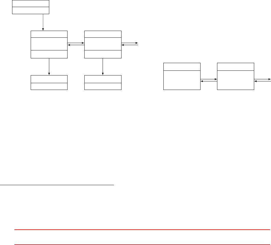
The cloud
The class cloud is an object registry similar to the mesh class87.cloud is derived from the class objectRegistry,
and so are fvMesh and Time. This enables us to register fields with the particle cloud. The class objectRegistry
is in turn derived from regIOobject which is in turn derived from IOobject. Thus, the ancestry of cloud
allows us to read and write the particle cloud to disk88. See Sections 48.7 and 48.8 for a more detailed discussion
on I/O and the concepts around the class regIOobject.
The IDLList
The IDLList is an intrusive doubly-linked list. The concept of a linked list is taught at programming classes
when it comes to objects and data-structures. The traditional linked-list consists of a list class and a node class.
The node class contains a pointer to, or the list-element itself. If the node class is implemented in a generic
fashion, using templates, then one list implementation is sufficient for all datatypes. Otherwise, the node class
would need to be implemented specifically for every datatype that is to be used by the list.
An intrusive linked-list is a very efficient implementation of a linked-list. However, the actual layout differs
from the standard layout of a linked list89. In an intrusive list, the list element serves also as the node. Figure
51 compares the schematic layouts of traditional and intrusive linked lists.
Intrusive linked-lists are generally considered as being much more efficient than traditional linked-lists90. One
of the downsides of using intrusive lists is that the implementation of the datatype which is to be used within
the list is mangled with the implementation of the list itself. Generally, this (mangling the implementation
of unrelated concepts) is considered a bad practice in object-oriented design (OOD). However, due to the
performance gain, intrusive lists are widely used in fields where performance beats conformity with standards,
such as computer games or number crunching.
List
Node* head
Node
Node* prev
Node* next
MyClass* val
Node
Node* prev
Node* next
MyClass* val
...
MyClass
elem
MyClass
elem
(a) Traditional doubly-linked list.
MyClass
Link prev
Link next
// class data
MyClass
Link prev
Link next
// class data
...
(b) Intrusive doubly-linked list.
Figure 51: Schematic diagrams of doubly-linked lists.
Again, we can take a look at the actual source code to find out what is really going on. Figure 52 shows the
class diagram behind the singly- and doubly-linked intrusive lists. This diagram is in fact a great example of
how far C++ developers can go with abstraction and encapsulation. The classes SLListBase and DLListBase
define the behaviour as being single-linked or doubly-linked. The classes UILList and ILList are more or
less helper or base classes. The class UILList provides STL-conforming iterators, whereas ILList adds some
member functions. The reason for UILList and ILList being separate classes is unknown to the author.
In the case of classic linked lists (non-intrusive lists, either singly- or doubly-linked), the class LList derived
from its template parameter LListBase provides the base class for concrete non-intrusive linked lists.
87In fact the class polyMesh is derived from objectRegistry.fvMesh is in turn derived from polyMesh. The mesh in a solver
or an utility application is of the type fvMesh. Almost all solvers and utilties include the file createMesh.H, which resides in
OpenFOAM/include of your installation.
88Fields, such as volScalarField and others, are also derived from regIOobject via GeometricField and DimensionedField.
89http://www.boost.org/doc/libs/1_43_0/doc/html/intrusive/intrusive_vs_nontrusive.html
90http://www.boost.org/doc/libs/1_58_0/doc/html/intrusive/performance.html
IV This offering is not approved or endorsed by ESI®Group, ESI-OpenCFD®or the OpenFOAM®
Foundation, the producer of the OpenFOAM®software and owner of the OpenFOAM®trademark. 141
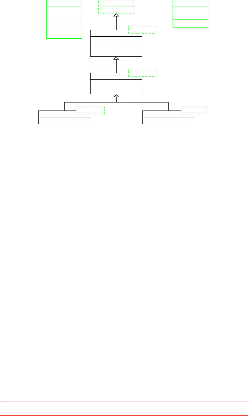
ListBase
UILList
T* first()
T* last()
ListBase, T
ILList
clear()
ListBase, T
DLListBase
link* first_
link* last_
label nElmts_
link* first()
link* last()
SLListBase
link* first_
label nElmts_
link* first()
IDLList DLListBase ISLList SLListBase
Figure 52: The class hierarchy needed for intrusive lists of objects of type T; this diagram can be regarded as a
subset of the class diagram for singly- and doubly-linked lists, both classic and intrusive.
31.4 Cloudy Templates
The Lagrangian models are modularized by making heavy use of inheritance and templating. This compart-
mentalisation of functionality and data is done for the clouds as well as the particles themselves. This approach
makes perfect sense as particles of the type X need a cloud of the type X to make X’s properties available to
the outside world (i.e. the solver using model X). To be more specific, if we want to solve heat transport with
Lagrangian particles, the particles themselves need to provide appropriate data (temperature) and methods
(heat transfer), as well as the cloud needs to offer appropriate methods (heat transfer from the particles to the
carrier phase and vice versa). Thus, most of the points discussed below hold also for the particles.
The templates for both the clouds and the particles create a framework which allows to create specific clouds
and particles simply by combining the templates carrying the intended functionality.
31.4.1 Base classes
kinematicCloud
This virtual abstract class (note the lower case k in kinematic) specifies the behaviour of the templated class
KinematicCloud (note the capital K in the class’ name).
thermoCloud
Also the virtual abstract class thermoCloud declares some abstract methods, i.e. methods that a derived class
must implement.
31.4.2 Templates
There are two kinds of cloud templates: the ones that are derived from a base class and their template parameter
CloudType, and the ones that are solely derived from their template parameter. In the following we try to shed
some light into the tempest of templates.
Base class + template parameter
One example for such a cloud template is the class KinematicCloud (note the capital K). This class is derived
from the class kinematicCloud (minor k) and its template parameter CloudType. The base class defines the
behaviour of the kinematic part, and the template parameter allows to add additional functionality.
A class passed as a template parameter can provide data and methods as well as a separate base class. How-
ever, pure abstract methods can realistically only be provided via the separate base class. The kinematicCloud
IV This offering is not approved or endorsed by ESI®Group, ESI-OpenCFD®or the OpenFOAM®
Foundation, the producer of the OpenFOAM®software and owner of the OpenFOAM®trademark. 142
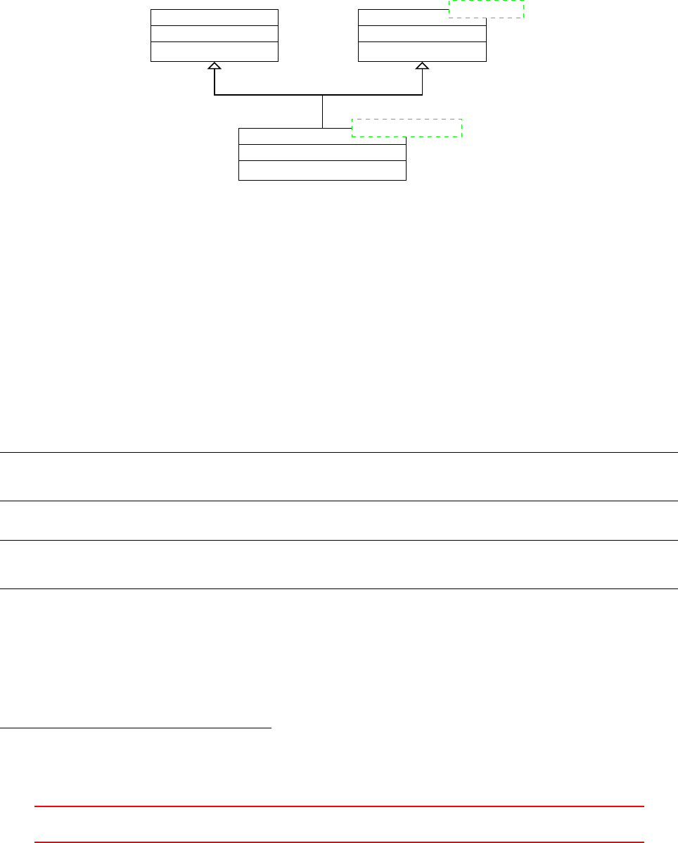
(lower case k) base class provides, among others, the pure virtual method nParcels(), which returns the total
number of parcels. If this method was provided by the KinematicCloud (capital K) template class, then we
would not be able to instantiate the basicKinematicCloud, as in Listing 197, since we can not create objects
of abstract classes.
Template parameter
The classes CollidingCloud and MPPICCloud are templated clouds, which are derived only from their template
parameter. Both classes provide modelling for particle-particle interactions91.
Cloud ParticleType
kinematicCloud
label nParcels()
KinematicCloud
label nParcels()
CloudType : Cloud
Figure 53: The class hierarchy of the class basicKinematicCloud.
31.4.3 Derived clouds
The derived cloud classes are the classes which we can actually use. The most basic derived cloud class is
basicKinematicCloud, which offers the minimal set of functionality. As we see in Listing 196, the basicKinematicCloud
is build from the KinematicCloud template with a Cloud of basicKinematicParcels92 as template parameter.
Here the dual templated hell of Lagrangian modelling reveals itself nicely. The template parameter of Cloud is
a particle type basicKinematicParcel. The definition of this particle type is shown in Listing 197. The type
basicKinematicParcel is also the most basic particle type provided by the Lagrangian intermediate library
of OpenFOAM.
We note, that the kinematic cloud is a cloud of kinematic particles. The kinematic particle class provides
the means to move the particle around and the kinematic cloud type provides the means to move the particles
collectively. This is useful since a solver using Lagrangian particles does not operate on the individual particles.
1namespace Foam {
2typedef Kin em at ic Cl ou d < C loud < b as icK in ema ti cPa rc el > > b asi cKi n em at i cC lou d ;
3}
Listing 196: The class definition of basicKinematicCloud in the file basicKinematicCloud.H
1namespace Foam {
2typedef Kin emat ic Parc el < p article > b as icK in ema tic Pa rce l ;
3}
Listing 197: The class definition of basicKinematicParcel in the file basicKinematicParcel.H
To substantiate the claim from above, that the templates allow us to build custom Lagrangian models,
we take a look at some more derived clouds. In Listing 198 we see the definition of a cloud class, which of-
fers heat transfer modelling. This class throws the ThermoCloud template into the mix of the already known
KinematicCloud class. In combination with Listing 199, we see that the basicThermoCloud is a Cloud of
basicThermoParcels. Again, the type of the cloud is reflected in the type of the parcel.
91See https://openfoam.org/release/2-3-0/dpm/
92As the reader might remember, the class Cloud takes a template parameter ParticleType.
IV This offering is not approved or endorsed by ESI®Group, ESI-OpenCFD®or the OpenFOAM®
Foundation, the producer of the OpenFOAM®software and owner of the OpenFOAM®trademark. 143

1namespace Foam {
2typedef ThermoCloud
3<
4KinematicCloud
5<
6Cloud
7<
8basicThermoParcel
9>
10 >
11 > basicThermoCloud;
12 }
Listing 198: The class definition of basicThermoCloud in the file basicThermoCloud.H
1namespace Foam {
2typedef Therm oPar cel < K in em atic Pa rcel < partic le >> b as icT he rm oPa rc el ;
3}
Listing 199: The class definition of basicThermoParcel in the file basicThermoParcel.H
31.5 Run-time post-processing
The cloud class offers function object to perform some run-time post-processing. These can be found at $FOAM_
SRC/lagrangian/intermediate/submodels/CloudFunctionObjects. Among the cloud function objects are
ones for counting particles crossing a certain patch or computing the volume fraction field of the lagrangian
particles. See Section 31.7.2 for a more detailled discussion on cloud function objects.
31.6 Times of Use
31.6.1 Not so telling error messages
Out of domain
As OpenFOAM’s Lagrangian particle framework keeps track of the cells in which a particle is located, a
Lagrangian solver needs to determine the cell label of each particle’s initial position. OpenFOAM’s particle
tracking algorithm is described among other resources in [33,30,37].
When a particle is placed outside the domain, i.e. the position in the positions file is outside the domain,
OpenFOAM is unable to find a cell label for this very particle. Note that failing to find a cell which contains the
particle’s location may happen also for other reasons than placing it outside the domain. As the error message
in Listing 200 suggests, this might also happen through a combination of insufficient write precision and do-
main decomposition or reconstruction. However, plainly putting them outside the domain is also a possibility,
especially, when a script is used to create the initial particle distribution.
--> FOAM FATAL ERROR :
cell , tetFace and tetPt se arch fa ilure at positi on (0 .0026 0.0026 0.45 02)
for r equ est ed cell 0
If this is a restar t or re constru ct ion / d ecomp ositi on etc . it is likely that the write
pre cis ion is not s uff icie nt .
Eit he r i nc re as e ’ w ri te Pr ec is io n ’ or set ’ w ri te Fo rm at ’ to ’ bi nar y ’
From fu nct ion void Foam :: parti cle :: in itCe llFa ceP t ()
in file / h ome / user / O penF OA M / OpenFOAM -2.3. x / src / l ag ra ngia n / basic / l nI nc lu de / p ar ti cleI . H at
line 758.
FOAM a bor ting
Listing 200: Error message issued by OpenFOAM when a Lagrangian simulation is started with particle positions
defined outside of the domain; checkMesh reports for this case an Overall domain bounding box (0 0 0) (0.15
0.15 0.45); Note the position (Line 3) at which the search failure occurs
IV This offering is not approved or endorsed by ESI®Group, ESI-OpenCFD®or the OpenFOAM®
Foundation, the producer of the OpenFOAM®software and owner of the OpenFOAM®trademark. 144

31.7 Sub models
31.7.1 Injection models
The are a number of models to insert Lagrangian particles or parcels into the simulation domain.
Common controls inherited from base classes
The injection models have a number of base classesm which determine common behaviour and provide common
data. Common control parameters are the start of injection (SOI), and the mass to be injected (massTotal).
ManualInjection
The manualInjection model is probably the simplest model. The user needs to provide the to-be-injected
particle mass and the injection positions. All parcels are introduced at SOI.
CellZoneInjection
The cellZoneInjection model works similar to the manual injection model. The locations at which parcels
are injected, however, are determined using a user-provided cellSet. The actual injection locations are randomly
distributed across the cellSet. The number of inserted parcels is determined by the volume of the cellSet and
the user-specified target parcel number density. All parcels are introduced at once at SOI.
FieldActivatedInjection
The fieldActivatedInjection model is also related to the manual injection model. In addition to the user-
provided injection locations, a scalar factor and the names of a threshold field and a referenceField have to be
specified. Parcels are injected only at locations at which the following relation holds:
factor*referenceField[celli] >=thresholdField[celli] (43)
Parcel injection is controlled by the injector positions read from the positions file. All positions, which fulfil
the condition above are valid injector positions. Furthermore, the number of parcels per injector (parcelsPerInjector)
has to be specified. Each injector injects parcelsPerInjector parcels which account for a parcelsPerInjector-
th of massTotal. Parcels are injected from SOI onwards until massTotal is reached.
PatchInjection
The patchInjection model introduces parcels at a patch rather than within a volume like the models discussed
above. This injection model implements a classical inflow condition for Lagrangian particles. The injection
position on the patch is chosen randomly. Parcels are injected from SOI until massTotal is reached.
31.7.2 CloudFunctionObjects
CloudFunctionObject are, similar to the standard functionObjects for fields, function objects for Lagrangian
clouds. The main purpose of OpenFOAM’s cloud function objects – judging by the implemented ones at the
time of writing – is post-processing. However, cloud function objects can also be used to actively influence the
Lagrangian particles.
PatchPostProcessing
This cloud function object can be used to accumulate data from all particles leaving the domain through a
specified patch. Thus, e.g. a residence time distribution (RTD) can be generated using this data.
FacePostProcessing
This cloud function object serves a similar purpose as the PatchPostProcessing cloud function object, only this
one acts on face sets.
IV This offering is not approved or endorsed by ESI®Group, ESI-OpenCFD®or the OpenFOAM®
Foundation, the producer of the OpenFOAM®software and owner of the OpenFOAM®trademark. 145
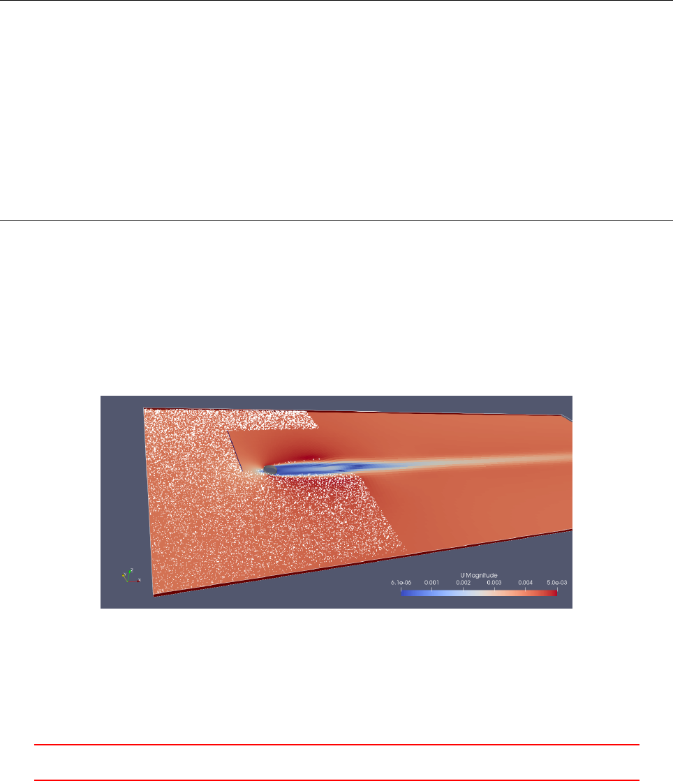
VoidFraction
This cloud function object can be used to create the volume fraction field associated with the particles. Thus,
the name VoidFraction can be misleading.
If we take a look at the code, we clearly see that the volume fraction of the particles is computed. In Listing
201, we see the two methods of this cloud function object which are responsible for computing the result. The
field theta is initialized to zero, this is not shown in the listing. In the method postMove(), which is called for
each parcel after it has moved within the current timestep, the particle’s volume is added to the field theta.
In the method postEvolve(), which is called after evolving the Lagrangian cloud for the current time step has
been completed, the field theta is divided by the mesh’s volume, i.e. a field in which the value of a cell is that
cell’s volume.
Thus, as in each cell the volume of the particles is accumulated and subsequently divided by the volume of
the cell, we end up with the volume fraction of the particles.
1template <class CloudType > void Foam :: VoidF ract ion < Clo udType >:: p os tM ove
2(
3// ...
4)
5{
6vol Scal arF ield & theta = t het aPt r_ () ;
7the ta [ cel li ] + = dt *p . n Pa rt ic l e () *p . v ol um e () ;
8}
9
10 template <class CloudType > void Foam :: VoidF ract ion < Clo udType >:: pos tE volve ()
11 {
12 vol Scal arF ield & theta = t het aPt r_ () ;
13 const fvMesh & mesh = this - > ow ne r ( ) . me sh () ;
14 theta . p rim it ive Fi eld Re f () /= mesh . time () . de lt aT Va lu e () * mesh .V() ;
15 C lo ud F un ct ion Ob j ec t < C loudTy pe > :: p ost Ev o lv e ( ) ;
16 }
Listing 201: Two methods of VoidFraction.C
ParticleCollector
The ParticleCollector cloud function object can be used to count particles traversing an arbitrary surface defined
by a set of polygons or the area enclosed by concentric circles. The data accumulated by this cloud function
object involves the accumulated particle mass and the mass flow rate passing through the surface.
Optionally, counted particles can be removed from the simulation.
Figure 54: A set of polygons has been defined to count and remove traversing particles. In this case of a cylinder
in laminar cross-flow, particles are inserted through the inlet patch. The ParticleCollector cloud function object
was set to remove all counted particles, which is clearly visible in this snapshot.
IV This offering is not approved or endorsed by ESI®Group, ESI-OpenCFD®or the OpenFOAM®
Foundation, the producer of the OpenFOAM®software and owner of the OpenFOAM®trademark. 146
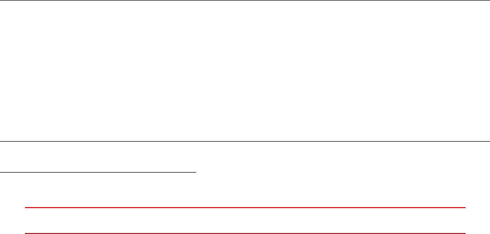
Part V
Solver
32 Solution Algorithms
The solution of the Navier-Stokes equations require solving the coupled equations of velocity and pressure fields.
There are several solution algorithms that try to decouple the equations and compute the velocity and pressure
separately. In order to decouple the computation of velocity and pressure, a predictor-corrector strategy is
followed. This approach is referred to in literature on numerical methods as segregated solution.
The alternative to solving for velocity and pressure in a segregated fashion is to solve for the fully coupled –
also referred to as block coupled – equation system. In general, the momentum equation yields three equations
for the three velocity components and the pressure equation, which is derived from the continuity equation,
yields an equation for pressure. Instead of solving each of the four discretized equations individually, the fully
coupled set of equations could also be solved for. This translates a possible improvement in converge rate,
however, it also encompasses a much larger memory requirement and an altered convergence behaviour.
This section will deal with the segregated solution methods, as they are the most commonly used. In the
last sub-section we will briefly discuss coupled methods.
32.1 SIMPLE
Figure 55 shows the flow chart of the SIMPLE algorithm. The SIMPLE algorithm predicts the velocity and
then corrects both the pressure and the velocity. This is repeated until a convergence criteria is reached. The
labels in Figure 55 are related to the terminology used in the source code of the simpleFoam solver. The solution
procedure can be described as follows
1. Check if convergence is reached – simple.loop()
2. Predict the velocities using the momentum predictor– UEqn.H
3. Correct the pressure and the velocities– pEqn.H
4. Solve the transport equations for the turbulence model93–turbulence->correct()
5. Go back to step 1
In OpenFOAM the SIMPLE algorithm is used for steady-state solvers.
32.1.1 Predictor
The predictor of simpleFoam is a momentum predictor.
1// Mom ent um pre dic tor
2tmp <fvVectorMatrix > UEqn
3(
4fv m : : d iv ( phi , U )
5+ turbu lence - > divDevReff (U)
6==
7sources(U)
8);
9
10 UE qn () . r el ax () ;
11
12 s ou rc es . c o ns tr ain ( U Eqn () ) ;
13
14 solve ( UEqn () == -fvc :: grad (p));
Listing 202: Predictor in UEqn.H of simpleFoam
93In case of a laminar simulation an empty function is called. Turbulence is modelled in OpenFOAM in a very generic way.
Therefore, a laminar simulation uses the laminar turbulence model.
VThis offering is not approved or endorsed by ESI®Group, ESI-OpenCFD®or the OpenFOAM®
Foundation, the producer of the OpenFOAM®software and owner of the OpenFOAM®trademark. 147
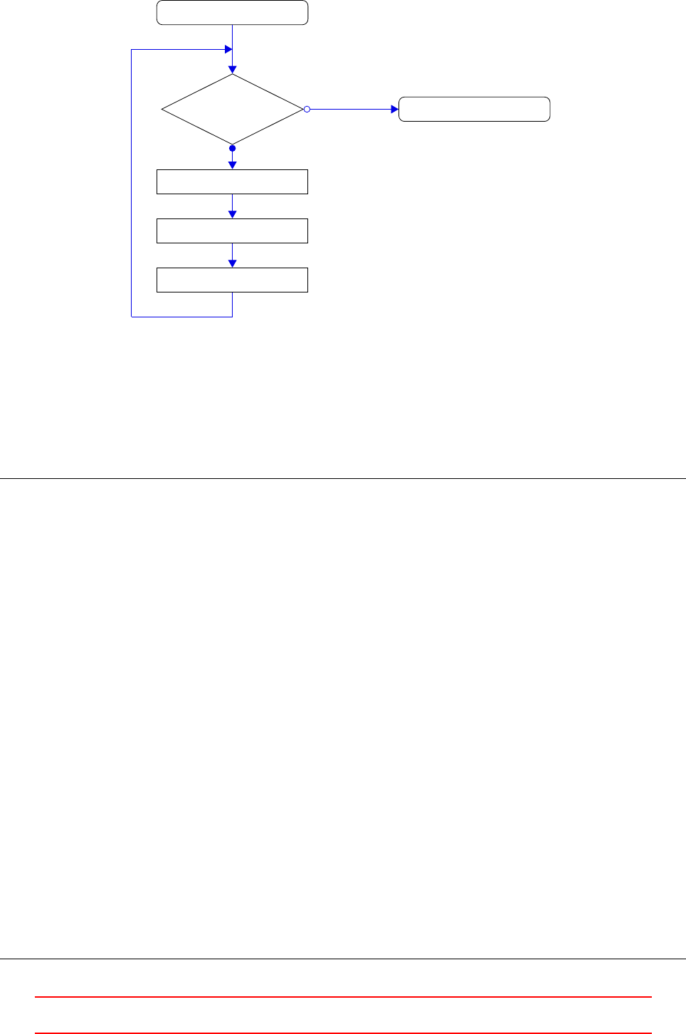
Start of time step
simple.loop()
UEqn.H
pEqn.H
turbulence->correct()
End of time step
true
false
Figure 55: Flow chart of the SIMPLE algorithm
32.1.2 Corrector
The corrector is used to correct the pressure field by using the predicted velocity. This corrected pressure is
used to correct the velocities by solving the continuity equation.
The non-orthogonal pressure corrector loop is necessary only for non-orthogonal meshes [39].
p . b ou n da ryF iel d () . u pd a te Coe ff s () ;
v ol S ca la r Fi e ld rAU (1 .0 / UEqn ( ) .A ( ) );
U = r AU * U Eq n () . H () ;
UE qn . c le ar () ;
phi = fvc :: i nterp ola te (U, " i nt er po la te ( HbyA )") & m es h . Sf () ;
a dj u st P hi ( phi , U , p ) ;
// Non - orthogonal press ure c orre ctor loop
while (simple.correctNonOrthogonal())
{
fvScalarMatrix pEqn
(
fv m :: l ap la ci an ( rAU , p ) == f vc :: div ( ph i )
);
pE qn . s et Re fe re nc e ( pR efCell , p Re fV al ue ) ;
pE qn . s ol ve () ;
if ( sim ple . fin al Non Or th og on alI te r () )
{
phi -= p Eqn . flux ();
}
}
#include "continuityErrs.H"
// Exp licitly relax pr ess ure for mom entum co rrecto r
p . rel ax () ;
// Mom ent um cor rec tor
U -= rAU * fv c :: g rad (p) ;
U.correctBoundaryConditions();
sources.correct(U);
Listing 203: Corrector in pEqn.H of simpleFoam
VThis offering is not approved or endorsed by ESI®Group, ESI-OpenCFD®or the OpenFOAM®
Foundation, the producer of the OpenFOAM®software and owner of the OpenFOAM®trademark. 148
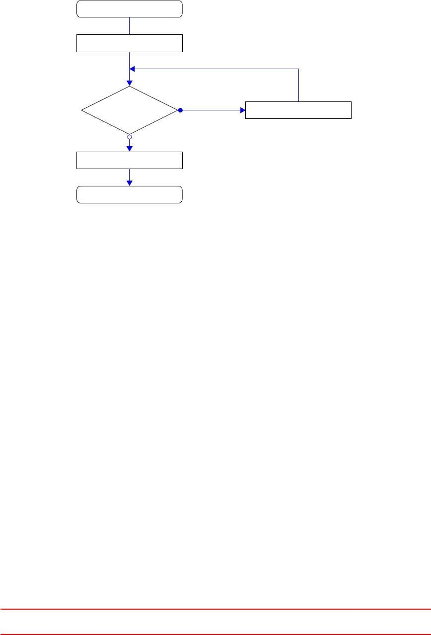
32.2 PISO
The PISO algorithm also follows the predictor-corrector strategy. Figure 56 shows the flow chart of the PISO
algorithm. The velocity is predicted using the momentum predictor. Then, the pressure and the velocity
is corrected until a predefined number of iterations is reached. Afterwards, the transport equations of the
turbulence model are solved.
Start of time step
UEqn.H
PISO loop
turbulence->correct()
End of time step
pEqn.H
true
false
Figure 56: Flow chart of the PISO algorithm
32.3 PIMPLE
The PIMPLE algorithm, which is a combination of the SIMPLE and PISO algorithms, is discussed further in
Sections 33 and 33.2.
32.4 Block-coupled solution
The block-coupled approach is something completely different than the aforementioned segregated algorithms.
In block-coupled solutions all equations (three equations for velocity and one for pressure) are solved at the
same time. This requires the construction of a fully coupled, discretised equation system for all four variables.
Thus, block-coupled solvers have a much larger memory footprint than sequential solvers.
32.4.1 Block-coupled solvers
The foam-extend project https://foam-extend.sourceforge.io/, at the time of writing, distributes two
solvers using the block-coupled solution approach.
blockCoupledScalarTransportFoam
This solver is derived from the standard scalarTransportFoam solver and solves the transport of two coupled
passive scalars.
∇·(uT) + ∇·(DT∇T) = α(Ts−T)(44)
∇·(DT s∇Ts) = α(T−Ts)(45)
pUCoupledFoam
This solver is a steady state solver for incompressible, turbulent single phase flow. This solver solves for velocity
and pressure simultaneously.
VThis offering is not approved or endorsed by ESI®Group, ESI-OpenCFD®or the OpenFOAM®
Foundation, the producer of the OpenFOAM®software and owner of the OpenFOAM®trademark. 149
33 pimpleFoam
pimpleFoam is a transient incompressible solver using the PIMPLE alogorithm, which is a combination of PISO
and SIMPLE. The solver is described in the file pimpleFoam.C as follows:
Large time-step transient solver for incompressible, flow using the PIMPLE
(merged PISO-SIMPLE) algorithm.
Turbulence modelling is generic, i.e. laminar, RAS or LES may be selected.
33.1 Governing equations
33.1.1 Continuity equation
The general continuity equation reads as follows:
∂ρ
∂t +∇·(ρu)=0 (46)
we now assume incompressible fluids: ρ=const
∇·u= 0 (47)
or in alternative notation
div(u)=0 (48)
∂ui
∂xi
= 0 (49)
33.1.2 Momentum equation
Departing from the Navier-Stokes equations, the momentum equation of pimpleFoam are derived.
∂ρu
∂t +∇(ρuu) + ∇·τ=−∇p+g(50)
because we assume a constant density we can divide by ρ
∂u
∂t +∇(uu) + 1
ρ∇·τ=−∇p
ρ+g
ρ(51)
The last term is defined a general source term
∂u
∂t +∇(uu) + 1
ρ∇·τ=−∇p
ρ+Q(52)
the shear stresses and the pressure are denoted by new symbols: τ
ρ=Reff und p
ρ=p
∂u
∂t +∇(uu) + ∇·Ref f =−∇p+Q(53)
The Boussinesq hypothesis allows us to add the Reynolds stresses to the shear stresses. This stress tensor
– containing shear as well as Reynolds stresses – is denoted Reff , the effective stress tensor. Both RAS as well
as LES turbulence models are based on the Boussinesq hypothesis.
Reff =−νeff ∇u+ (∇u)T(54)
Reff
ij =−νeff ∂ui
∂xj
+∂uj
∂xi(55)
VThis offering is not approved or endorsed by ESI®Group, ESI-OpenCFD®or the OpenFOAM®
Foundation, the producer of the OpenFOAM®software and owner of the OpenFOAM®trademark. 150
The trace of τfulfills the continuity equation for incompressible fluids
tr(Reff ) = Reff
ii =−2νeff ∂ui
∂xi= 0 (56)
∂ui
∂xi
=∇·u= 0 (57)
Therefore, we can replace Ref f with the deviatoric part of Reff
Reff = dev(Reff )
| {z }
deviatoric part
+1
3tr(Reff )I
| {z }
hydrostatic part
(58)
dev(Reff ) = Reff −1
3tr(Reff )
| {z }
=0
I(59)
Therefore, the momentum equation can be rewritten
∂u
∂t +∇(uu) + ∇·dev(Ref f )
| {z }
=div(dev(Ref f ))
=−∇p+Q(60)
Finally, we use Eq. (54)
Reff =−νeff ∇u+ (∇u)T(54)
to gain
∂u
∂t +∇(uu) + ∇·dev(−νef f ∇u+ (∇u)T)=−∇p+Q(61)
33.1.3 Implementation
The momentum equation is implemented in the file UEqn.H. The first two terms of Eq. (61) can easily be
identified in the source code in Listing 204.
The first term is the local derivative of the momentum – due to the incompressibility of the fluid, the density
was eliminated – can be found in line 5of Listing 204. Here, the instruction in the source code reads very much
the same as the mathematical notation.
∂u
∂t ⇔fvm::ddt(U)
The second term of Eq. (61) is the convective transport of momentum. The use of the identifier phi should
not lead to confusion. In order to read the equations from the source code, phi can be replaced with Uwithout
changing the meaning of the equations. The reason why phi is used in the source code lies in the solution
procedure. See Section 54 for a detailled discussion about phi.
∇(uu)
| {z }
div(uu)
⇔fvm::div(phi, U)
The third term of Eq. (61) is the diffusive momentum transport term. Diffusive momentum transport is
caused by the laminar viscosity as well as turbulence. Therefore, the turbulence model handles this term. See
line 7of Listing 204.
∇·dev(Reff )
| {z }
=div(dev(Ref f ))
⇔turbulence->divDevReff(U)
VThis offering is not approved or endorsed by ESI®Group, ESI-OpenCFD®or the OpenFOAM®
Foundation, the producer of the OpenFOAM®software and owner of the OpenFOAM®trademark. 151

The terms on the rhs of Eq. (61) are the pressure gradient and the source term.
−∇p
|{z}
=−grad p⇔-fvc::grad(p))
Q⇔sources(U)
1// Solve the Momentum eq uation
2
3tmp <fvVectorMatrix > UEqn
4(
5fv m :: ddt ( U)
6+ fvm :: div (phi , U)
7+ turbu lence - > divDevReff (U)
8);
9
10 UE qn () . r el ax () ;
11
12 s ou rc es . c o ns tr ain ( U Eqn () ) ;
13
14 v ol S ca la r Fi e ld rAU (1 .0 / UEqn ( ) .A ( ) );
15
16 if ( pim pl e . m o me n tu m Pr e di cto r () )
17 {
18 solve ( UEqn () == -fvc :: grad (p) + sources ( U ));
19 }
Listing 204: The file UEqn.H of pimpleFoam
33.2 The PIMPLE Algorithm – or, what’s under the hood?
This Section deals with the way pimpleFoam and twoPhaseEulerFoam, which also uses the PIMPLE algo-
rithm, work. Therefore, we examine the implementation of pimpleFoam. Listing 205 shows the main loop of
pimpleFoam.
The first instruction is the loop over all time steps. Then there are some operations – the three #include
instructions – concerning time step control. After incrementing the time step (Line 7), the PIMPLE loop comes
(from Line 10 onwards).
Inside this loop, first the momentum equation is solved (Line 12), then the pressure correction loop is entered
(Line 17).
At the end of the PIMPLE loop the turbulent equations94 – if there are any present95 – are solved (Line
22). At the end of each time step the data is written.
1while ( run Time . run () )
2{
3#include "readTimeControls.H"
4#include " CourantNo . H"
5#include " setDeltaT . H"
6
7runTime++;
8
9// --- Pres sure - v eloc ity PIM PLE corrector loop
10 while ( p imp le . l oop ( ) )
11 {
12 #include " UE qn . H"
13
14 // --- P res sur e corrector loop
15 while ( p imp le . c or re ct () )
16 {
17 #include " pE qn . H"
18 }
19
94In case of a k-model, there are two transport equations to be solved. Other turbulence models require the solution of less or
none transport equation.
95In case of a laminar simulation, no operation is carried out.
VThis offering is not approved or endorsed by ESI®Group, ESI-OpenCFD®or the OpenFOAM®
Foundation, the producer of the OpenFOAM®software and owner of the OpenFOAM®trademark. 152
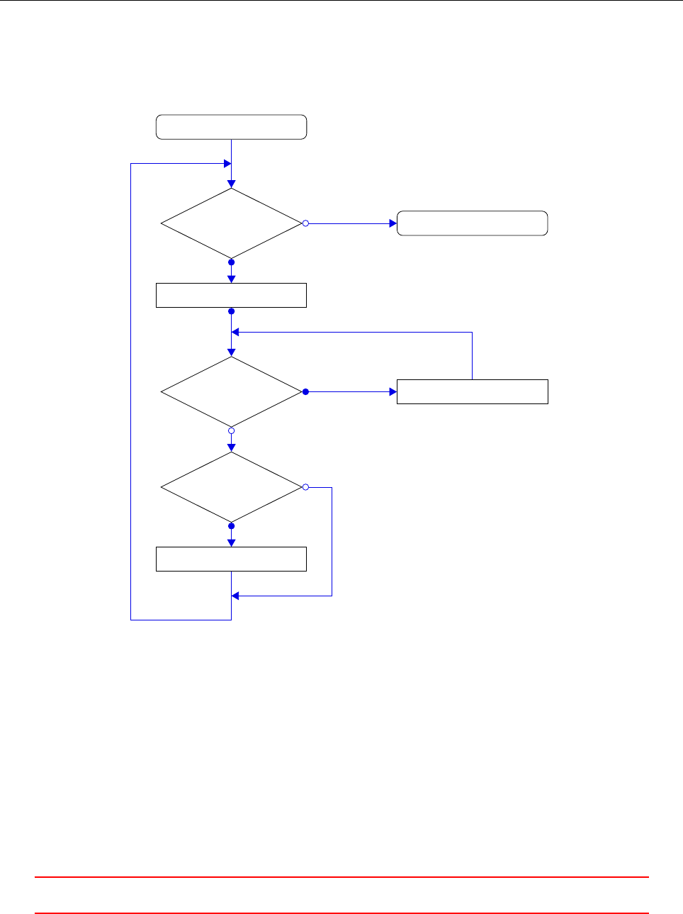
20 if ( pim ple . tu rbCo rr ())
21 {
22 tur bule nc e - > c or re ct ( ) ;
23 }
24 }
25
26 r un Ti me . w ri te () ;
27 }
Listing 205: The main loop of pimpleFoam
Figure 57 shows the flow chart of the PIMPLE algorithm. This algorithm is executed every time step. If the
PIMPLE loop is entered only once, then the algorithm is essentially the same as the PISO algorithm. Listing
212 draws this conclusion from the code itself.
Start of time step
pimple.loop()
UEqn.H
pimple.correct()
turbCorr()
turbulence->correct()
End of time step
pEqn.H
true
false
true
false
true
false
Figure 57: Flow chart of the PIMPLE algorithm
33.2.1 readTimeControls.H
In line 3of Listing 205 the file readTimeControls.H is included to the source code using the #include prepro-
cessor macro. This is a very common way to give the code of OpenFOAM structure and order. Code which is
used repeatedly is outsourced into a seperate file. This file is then included with the #include macro. Thus,
code duplication is prevented. The file readTimeControls.H might be included into every solver that is able to
use variable time steps. If this code was not outsourced into a seperate file, this code would be found in every
variable time step solver. Maintaining this code, would be tiresome and prone to errors.
Listing 349 shows the contents of readTimeControls.H. The first instruction reads from controlDict the
adjustTimeStep parameter. If there is no entry matching the name of the parameter ("adjustTimeStep"), then
VThis offering is not approved or endorsed by ESI®Group, ESI-OpenCFD®or the OpenFOAM®
Foundation, the producer of the OpenFOAM®software and owner of the OpenFOAM®trademark. 153

1const bool adjustTimeStep =
2r un Ti me . c o nt rol Di c t () . l oo k up OrD e fa ult ( "adjustTimeStep",false ) ;
3scalar maxCo =
4r un Ti me . c o nt rol Di c t () . loo ku pO rDe fa ul t < s cal ar > ( " ma xC o " , 1.0) ;
5scalar m axD elt aT =
6r un Ti me . c o nt rol Di c t () . loo ku pO rDe fa ul t < s cal ar > ( " m ax De lta T " , GREAT ) ;
Listing 206: The content of readTimeControls.H
a default value is used. So, omitting the parameter adjustTimeStep in controlDict will result in a simulation
with a fixed time step.
This is a very straight forward example of determining the behaviour of a solver using only the source code.
In this case the names of the source file as well as variable and function names are rather self explaining. In
other cases one has to dig deeply into the code to learn about what a certain command does.
33.2.2 pimpleControl
Examining the files pimpleControl.H and pimpleControl.C will generate some knowledge of the inner life of
pimpleFoam.
Solution controls
Listings 207 and 208 show parts of pimpleControl.H and pimpleControl.C. Listing 207 shows the declaration
of protected96 data in pimpleControl.H.
1// Protected data
2// Sol uti on con tro ls
3// - Maximum numbe r of PIMPLE co rrectors
4label nCorrPIMPLE_;
5
6// - M axim um numb er of PISO cor re ctors
7label nC orr PISO_ ;
8
9// - C urre nt PISO c or rector
10 label corrPISO_ ;
11
12 // - Flag to indica te whethe r to only solve tu rbulence on final iter
13 bool turbOnFinalIterOnly_;
14
15 // - C on verged flag
16 bool con ver ged_ ;
Listing 207: Protected data in pimpleControl.H
1void Foam :: pim ple Contr ol :: read ()
2{
3sol uti on Co ntr ol :: read ( false );
4
5// Read sol ution con tro ls
6const dictionary & pim pleDict = dict () ;
7
8n Co rrP IM P LE _ = p im p le Di c t . l oo kup Or De fau lt < la bel >( "nOuterCorrectors", 1 ) ;
9
10 nCo rrP ISO _ = pim pleDict . lo oku pOrDefau lt < label >( " nC or rec tors ", 1) ;
11
12 t ur b On F in a lI t er O nl y _ = p im pl e Di ct . l oo ku pO rD efa ul t < Swit ch >( "turbOnFinalIterOnly",t rue ) ;
13 }
Listing 208: Read solution controls in pimpleControl.C
96Most programming languages provide access specifiers to specify the visibility of variables. The keyword protected means,
that the variables can be accessed only inside the class pimpleControl and all classes inherited from pimpleControl.
VThis offering is not approved or endorsed by ESI®Group, ESI-OpenCFD®or the OpenFOAM®
Foundation, the producer of the OpenFOAM®software and owner of the OpenFOAM®trademark. 154

Reading the code we can see which keyword in the PIMPLE dictionary – it is a part of the fvSolution dictionary
(see Section 9.5) – is connected to which variable in the code. Three of the protected variables of Listing 207
are assigned in Listing 208. One of them has the same name in both the code and the dictionary. The other
two have different names.
Pitfall: no sanity checks
The two variables nCorrPimple and nCorrPiso control the solution algorithm. If the corresponding entry in
the PIMPLE dictionary in fvSolution is missing, then default values are used, see Section 48.3 for details behind
the method lookupOrDefault(). However, the user can provide any number in fvSolution as long as it is
legal97. Thus, a zero or negative number is a legal entry from the source codes point of view. With respect to
the solution algorithm a zero or negative entry makes no sense at all.
The connection between keywords and the algorithm
The keyword nOuterCorrectors translates – with the help of Listing 208 to the variable nCorrPIMPLE_. This
variable controls how often the PIMPLE loop is traversed. Listing 209 shows parts of the definition of the
function loop() of the class pimpleControl. The return value of this function decides whether the PIMPLE
loop is entered or not. In line 5of Listing 209 an internal counter is incremented – the ++ operator of C++
adds 1 to the variable the operator is applied to. Afterwards, the internal counter is compared to the value
of nCorrPIMPLE_. If this internal counter is then equal to the sum of nCorrPIMPLE_ + 1, then the function
loop() returns false.
The internal counter is initialised to the value of 0. Listing 210 shows the constructor of the class solutionControl.
The class pimpleControl is derived from solutionControl. So, every instance of pimpleControl has an inter-
nal counter corr_ inherited from solutionControl. Line 9of Listing 210 how the counter corr_ is initialised
to zero.
1bool Foam :: pim ple Contr ol :: loop ()
2{
3re ad () ;
4
5corr_ ++;
6
7/* code removed for the sake of br evity */
8
9if ( corr_ == n Co rr PI MP LE _ + 1)
10 {
11 if ( (! r esi d ua lCo n tr ol_ . e mp ty ( ) ) && ( n Co r rP IMP LE _ != 1 ) )
12 {
13 Info << algo rit hmNa me_ << ": not c onv erg ed within "
14 << nCorrPIMPLE_ << " iterati ons " << endl;
15 }
16
17 corr_ = 0;
18 mesh_ . data :: r emove ("finalIteration");
19 retur n f alse ;
20 }
21
22 /* code con tin ues */
Listing 209: Some content of pimpleControl.C
1Foam :: s olut ionC ontr ol :: sol utio nCon trol ( fvMesh & mesh , const word & algo ri th mN am e )
2:
3mesh_ ( mesh ) ,
4residualControl_(),
5algorithmName_(algorithmName),
6nNo nOrth Corr_ (0) ,
7momentumPredictor_(true) ,
8tra ns on ic_ ( false ) ,
9corr_ (0) ,
10 cor rNon Ort ho_ (0)
11 {}
97See Section 48.4.2 for details on the label datatype.
VThis offering is not approved or endorsed by ESI®Group, ESI-OpenCFD®or the OpenFOAM®
Foundation, the producer of the OpenFOAM®software and owner of the OpenFOAM®trademark. 155

Listing 210: The constructor of the class solutionControl in solutionControl.C
The keyword nCorrectors translates – with the help of Listing 208 to the variable nCorrPISO_. This
variable controls how often the PISO loop – or the corrector loop – is traversed. Listing 207 shows, that there
are two variables related to the PISO loop, nCorrPISO_ and corrPISO_. The first variable is the limit and the
second is the counter.
nCorrPISO_ is read from the fvSolution dictionary by the use of the nCorrectors keyword. This number
tells the solver, how many times the corrector loop should be traversed. The corrector loop is a feature of the
PISO algorithm. Hence, the maximum number of corrector loop iterations is called nCorrPISO_.
The variable corrPISO_ is declared in the constructor of the class pimpleControl, see Listing 212. There
the variable is initialised to zero.
Listing 211 shows the definition of the function correct() of the class pimpleControl. The return value of
this function controls if the corrector loop is entered. In line 3the counter corrPISO_ is incremented every time
this function is called. In line 10 the value of the counter is compared to the maximum number of corrector
loop iterations.
1inline bool F oam :: pim pleCont rol :: correct ()
2{
3cor rPI SO_ ++;
4
5if ( debug )
6{
7Info << algo rit hmNa me_ << " corre ct : corrPI SO = " << cor rP IS O_ << endl ;
8}
9
10 if ( corrPISO_ <= nCo rr PIS O_ )
11 {
12 retur n t rue ;
13 }
14 else
15 {
16 cor rPI SO_ = 0;
17 retur n f alse ;
18 }
19 }
Listing 211: The inline function correct() in pimpleControlI.H
PIMPLE or PISO algorithm
Listing 212 shows parts of the code of the constructor of the class pimpleControl. At first some data fields are
set to initial values. Then the read() function is called, this function is shown in Listing 208. After reading the
solution controls the variable nCorrPIMPLE_ is tested. If this value is equal to one, then the solution algorithm
equates the PISO algorithm. In this case an according message is printed to the Terminal.
1Foam :: p impl eCo ntro l :: p imp leCo ntr ol ( fvMes h & mesh ) :
2s ol u ti onC ont r ol ( me sh , "PIMPLE") ,
3nCorrPIMPLE_(0),
4nCo rrP ISO_ (0) ,
5cor rPI SO_ (0) ,
6turbOnFinalIterOnly_(true) ,
7con ve rg ed_ ( false )
8{
9re ad () ;
10
11 if (nCorrPIMPLE_ > 1)
12 {
13 /* code removed for shortness of lis ting */
14 }
15 else
16 {
17 Info << nl << algo rith mNa me_ << " : Ope ra ti ng so lver in PISO mo de " << nl < < endl ;
18 }
VThis offering is not approved or endorsed by ESI®Group, ESI-OpenCFD®or the OpenFOAM®
Foundation, the producer of the OpenFOAM®software and owner of the OpenFOAM®trademark. 156

19 }
Listing 212: Constuctor of pimpleControl in pimpleControl.C
34 twoPhaseEulerFoam
This section is valid for OpenFOAM-2.0 til OpenFOAM-2.2.
34.1 General remarks
twoPhaseEulerFoam is a solver for two-phase problems. According to the CFD-Online Forum (http://www.
cfd-online.com/Forums/openfoam/) this solver as well as bubbleFoam is based on the PhD thesis of Henrik
Rusche [42]. In the course of an update of OpenFOAM-2.1.x in July 2012 the solution algorithm of the continuity
equation was changed.
34.1.1 Turbulence
twoPhaseEulerFoam can only use the k-turbulence model. This model is so to say hardcoded and can only be
turned on or off.
34.1.2 Kinetic theory
twoPhaseEulerFoam can make use of the kinetic theory for granular simulations, e.g. air flowing through a bed
of small particles. This model can also be turned on or off.
In the following sections kinetic theory is ignored for the reason of keeping listings and explanations short.
34.2 Solver algorithm
twoPhaseEulerFoam is based on the PIMPLE algorithm. However, there are some modifications necessary for
solving two-phase problems. Listing 213 shows the main part of this solver. The first two lines inside the main
loop (pimple.loop()) differ from pimpleFoam. These lines deal with the two-phase continuity equation and
the inter-phase momentum exchange coefficients.
Next, in line 6, comes the momentum predictor It contains the momentum equations for both phases and
solves them subsequently, thus the filename UEqns.H.
After the predictor comes the corrector. The corrector is in fact a corrector loop. Inside this loop
(pimple.correct()) the correction of pressure and velocity is computed. Inside the corrector loop (line 15)
there is also a conditional second call of the continuity equation. The condition consists of two boolean state-
ments. The first is a boolean variable, which is set in a dictionary by the user. The second is generated by the
solution control.
After the corrector loop the total time derivatives of the velocities are calculated. Finally, the turbulent
transport equations are solved. In this case it is the k-model that is called explicitly (line 23).
1// --- Pres sure - velocity PIM PLE corrector l oop
2while ( p imp le . l oop ( ) )
3{
4#include " alphaEqn . H"
5#include "liftDragCoeffs.H"
6#include " UE qns .H"
7
8// --- P res sur e corrector loop
9while ( p imp le . c or re ct () )
10 {
11 #include " pE qn . H"
12
13 if ( c or rectA lp ha && ! pim ple . fi na lIte r () )
14 {
15 #include " alphaEqn . H"
16 }
17 }
VThis offering is not approved or endorsed by ESI®Group, ESI-OpenCFD®or the OpenFOAM®
Foundation, the producer of the OpenFOAM®software and owner of the OpenFOAM®trademark. 157
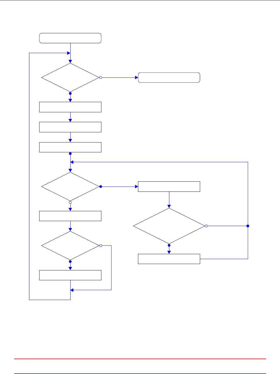
18
19 #include " DD tU . H"
20
21 if ( pim ple . tu rbCo rr ())
22 {
23 #include " kEpsilon . H"
24 }
25 }
Listing 213: The main loop of twoPhaseEulerFoam
Figure 58 shows the flow chart of all operations that are performed during one time step.
Start of time step
pimple.loop()
alphaEqn.H
liftDrag.H
UEqn.H
pimple.correct()
DDtU.H
turbCorr()
kEpsilon.H
End of time step
pEqn.H
correctAlpha()
& !finalIter()
alphaEqn.H
true
false
true
false
true
false
true
false
Figure 58: Flow chart of the main loop of twoPhaseEulerFoam
34.2.1 Continuity
The continuity equation is implemented in the file alphaEqn.H.
VThis offering is not approved or endorsed by ESI®Group, ESI-OpenCFD®or the OpenFOAM®
Foundation, the producer of the OpenFOAM®software and owner of the OpenFOAM®trademark. 158

Second call
In line 15 of Listing 213 the continuity equation is called again inside an if-statement. The condition depends
on two boolean expressions.
The first, correctAlpha, is controlled by the fvSolution dictionary. Assigning a value to this keyword – the
keyword has the same name as the boolean variable in the source code – is mandatory. The reading operation
of this keyword from the dictionary can be found in the source file readTwoPhaseEulerFoamControls.H and is
shown in Listing 214.
Three keywords are looked up from the fvSolution dictionary. All of them are related to the solving
algorithm for the continuity equation. Those entries are read from the dictionary by invoking the function
lookup(). See Section 48.3 for a detailed discussion about looking up keywords from dictionaries.
1#include "readTimeControls.H"
2
3int nA lp haCor r ( read Int ( pi mple . dict () . lo okup ( " nA lph aCo rr " )));
4int nA lp ha Su bC yc le s ( re adIn t ( pimp le . di ct () . looku p (" n Alpha Su bCy cl es " )));
5Switch c or re ct Alpha ( p imple . dict (). lo okup ( "correctAlpha"));
Listing 214: The content of readTwoPhaseEulerFoamControls.H
The second boolean expression controlling the second call in line 15 of Listing 213 is controlled by the number
of iterations of the PIMPLE loop. See Section 33.2 for a discussion about the PIMPLE algorithm.
The expression pimple.finalIter() is true when the last iteration of the PIMPLE algorithm is entered.
Therefore, the expression !pimple.finalIter() is true if, and only if, the value of nOuterCorrectors or
nCorrPIMPLE_ is greater than one. Because only then, there is more than one PIMPLE iteration and only then,
there is an iteration other than the final one.
If the PIMPLE loop is traversed only once, then alphaEqn.H is not entered a second time.
The file alphaEqn.H
The examination of the file alphaEqn.H results in the flow chart in Figure 59. The corrector loop is traversed a
specified number of times. This number is set by the keyword nAlphaCorr of the fvSolution dictionary. The
corrector loop is a simple for loop.
Inside the corrector loop is a sub-cycle loop. Inside this loop the continuity equation is solved. After the
sub-cycle the volume fraction of the continuous phase is updated. The sub-cycle loop is also traversed a specified
number of times. This number is set by the keyword nAlphaSubCycles of the fvSolution dictionary.
When the corrector loop is not entered anymore, the mixture density is updated.
34.3 Momentum exchange between the phases
34.3.1 Drag
The solver twoPhaseEulerFoam offers a number of drag models. In the sources of twoPhaseEulerFoam there
are this models
•Ergun
•Gibilaro
•GidaspowErgunWenYu
•GidaspowSchillerNaumann
•SchillerNaumann
•SyamlalOBrien
•WenYu
The equations behind this models can be found in [17] or [49].
Drag is considered in the governing equations by the use of the so-called drag-function K. This drag-function
is either computed directly, or it is computed by the use of the drag coefficient Cd. The drag force is the product
of the drag-function and the relative velocity between the phases Ur[17].
VThis offering is not approved or endorsed by ESI®Group, ESI-OpenCFD®or the OpenFOAM®
Foundation, the producer of the OpenFOAM®software and owner of the OpenFOAM®trademark. 159
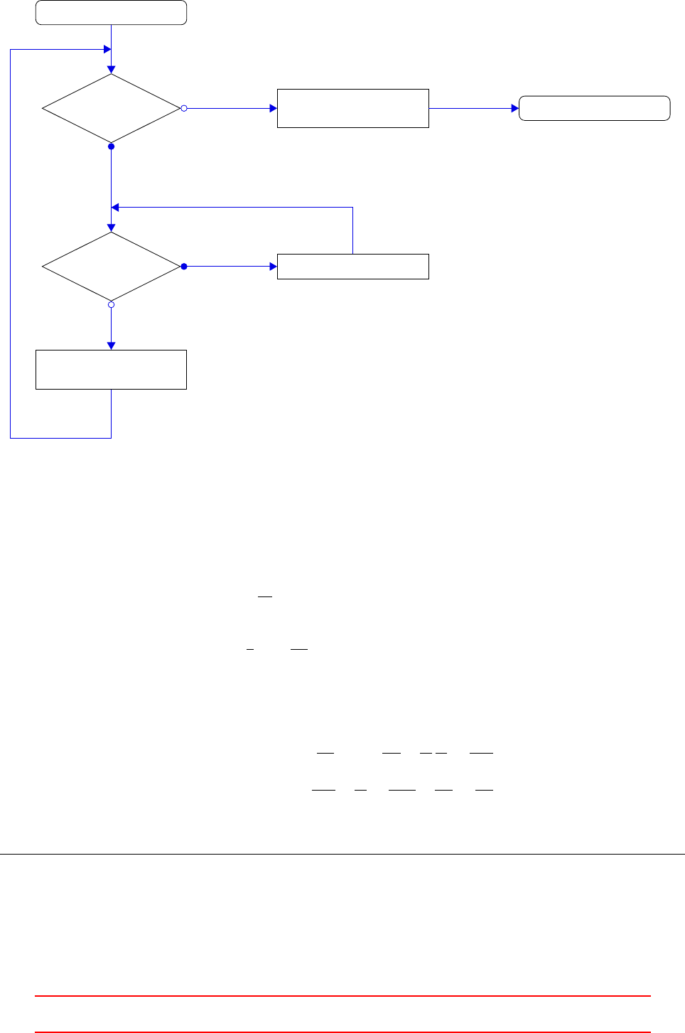
Start
corrector loop
sub-cycle
alpha2 = scalar(1)
- alpha1
rho = alpha1*rho1
+ alpha2*rho2 End
solve continuity
true
false
true
false
Figure 59: Flow chart of the operations in alphaEqn.H
Schiller-Naumann drag
We use the Schiller-Naumann drag model as an expample to demonstrate how OpenFOAM calculates the drag
force. This drag model utilizes a drag coefficient that is a function of the Reynolds number.
Cd=(24
Re 1+0.15Re0.687if Re ≤1000
0.44 if Re > 1000 (62)
K=3
4CdρB
Ur
dA
(63)
The drag coefficient is dimensionless, whereas the product of the drag-function Kand the relative velocity
has the dimension of a force density.
[K]=[Cd]·[ρB]·[Ur
dA
]=1·kg
m3·m
s
1
m=kg
m3s
[K·Ur] = kg
m3s·m
s=kgm
s2·1
m3=N
m3
Listing 215 shows, how the drag-function is computed by the Schiller-Naumann drag model.
Foam :: tmp < Foam :: v olS calar Field > Foam :: Sch ille rNau man n :: K
(
const volScalarField& Ur
)const
{
v ol S ca la r Fi e ld R e ( max ( Ur * p ha se a_ . d () / p ha se b_ . nu ( ) , s ca lar ( 1. 0 e -3 ) ));
volScalarField Cds
(
VThis offering is not approved or endorsed by ESI®Group, ESI-OpenCFD®or the OpenFOAM®
Foundation, the producer of the OpenFOAM®software and owner of the OpenFOAM®trademark. 160

ne g ( Re - 1 00 0) * (2 4.0 *(1 .0 + 0 .15* p ow ( Re , 0 .6 87 ) ) / Re )
+ pos ( Re - 1 00 0) * 0. 44
);
return 0.7 5* Cds * p has eb _ . r ho ( ) * Ur / p ha se a_ . d () ;
}
Listing 215: Calculation of the drag-function in the file SchillerNaumann.H
The drag force contributes to the momentum balance. Probably for numerical reasons, one part of the drag
is considered in the momentum equation and the other part is considered in the pressure equation.
34.3.2 Lift
The lift model of twoPhaseEulerFoam is described in [42]. The lift model computes the lift force on a rigid
sphere in shear flow. The force density is calculated from the relative velocity between the phases and the
vorticity of the mixture.
FL
VB
=CLρc|Ur×(∇ × Uc)|(64)
mit
Ur=UA−UB
Uc=αUA+ (1 −α)
| {z }
=β
UB
ρc=αρA+βρB
The lift force is computed in the file liftDragCoeffs.H. The vector field liftCoeff contains the lift force
density.
vol Ve cto rF ie ld lif tC oe ff ( Cl *( beta * rhob + alpha * rhoa ) *( Ur ^ fvc :: curl ( U)) );
Listing 216: Berechnung Auftriebskraft; liftDragCoeffs.H
The dimensions of the field liftCoeff is the dimension of a force density.
[lif tCoeff] = [CL]·[ρc]·[Ur×(∇ × Uc)] = 1 ·kg
m3·m
s
1
m
m
s=kgm
s2·1
m3=N
m3
34.3.3 Virtual mass
The virtual mass – an accelerating bubble needs not only to accelerate its own mass, it also needs to accelerate
some of the displaced fluid – is considered in the momentum equation.
MA,V M =βρB
ρA
CV M DBUB
Dt−DAUA
Dt(65)
In the source code, the momentum exchange term due to virtual mass is split into two parts. One part is
included in the rhs of the momentum equation, the other is considered in the lhs. This seperation is probably
for numerical reasons.
UaEqn =
(
( sca lar (1) + Cvm * rhob * bet a / rhoa ) *
(
fv m :: ddt ( Ua )
+ fvm :: div (phia , Ua , " di v ( phia , Ua ) " )
- f vm : : Sp ( f vc : : di v ( ph ia ) , Ua )
)
VThis offering is not approved or endorsed by ESI®Group, ESI-OpenCFD®or the OpenFOAM®
Foundation, the producer of the OpenFOAM®software and owner of the OpenFOAM®trademark. 161

+/* other terms */
==
/* other terms */
- b eta / rhoa *( lif tC oe ff - Cvm * rh ob * DDtUb )
);
Listing 217: Terms including virtual mass in the file UEqns.H
34.4 Kinetic Theory
For the simulation of dense gas-solid particulate flows the particulate phase can be modelled using the kinetic
theory model.
35 twoPhaseEulerFoam-2.3
This section is valid for OpenFOAM-2.3.
With the release of OpenFOAM-2.3 the two-phase Eulerian solver twoPhaseEulerFoam has seen some major
changes. See the release notes for further details: http://www.openfoam.org/version2.3.0/multiphase.php.
35.1 Physics
The most important change in twoPhaseEulerFoam from version ≤2.2.x to 2.3is that the solver is based on
a completely different set of physical models. In version 2.3 phases are modelled using OpenFOAMs thermo-
physical models. The phases are considered compressible, therefore all simplifications when considering a phase
incompressible do not hold anymore.
35.1.1 Pressure
In twoPhaseEulerFoam-2.3 the pressure is now a real physical pressure. In an incompressible simulation the
absolute value of the pressure has no meaning, only pressure differences count. In a compressible model, the
absolute value of the pressure has an effect, e.g. when using the isothermalDiameter diameter model to
determine the diameter of the dispersed phase elements.
Thus, when migrating a simulation case from OpenFOAM-2.2 or lower to 2.3, check the pressure initial
condition and the boundary conditions.
35.1.2 Temperature
As the new version of the solver uses thermo-physical models for the phases, the user is required to specify not
only the thermo-physical properties of the phases, the user also has to provide initial and boundary conditions
for the temperature of both phases. Thus, two additional fields are present – or need to be present – in the
time directories, e.g. T.air and T.water.
35.2 Naming scheme
The overhaul of twoPhaseEulerFoam in version 2.3 aims for reuseability and generality of the solver code itself
as well as of the case data. A general distinction of data concerning a single phase and data concerning the
whole simulation case can be made.
Case data is named as usual (e.g. fvSchemes,controlDict,g, etc.). Data related to a specific phase is
now stored in files with a filename that consists of two parts. The naming scheme follows the well known
FILENAME.EXTENSION naming scheme. In this case FILENAME denotes the type of information and EXTENSION
denotes the phase itself. This naming scheme is much more general than other naming schemes that are/were
used in OpenFOAM (cf. U1, U2 vs. Uwater, Uair vs. U.air, U.water).
Listing 218 shows the contents of the 0and constant folders of the bubble column tutorial case. There
we see the FILENAME.EXTENSION naming scheme applied. As each phase has a velocity and a temperature, we
see two files for velocity and temperature. The volume fraction is an exception, as there are only two phase
considered, the volume fraction of water is easily calculated, i.e. alpha.water = 1.0 - alpha.air. As the
pressure is share by all phases, the pressure file has no file-extension. In the constant folder there is also data
VThis offering is not approved or endorsed by ESI®Group, ESI-OpenCFD®or the OpenFOAM®
Foundation, the producer of the OpenFOAM®software and owner of the OpenFOAM®trademark. 162

that applies to one phase and data that applies to the simulation case. The files gand phaseProperties have
no extensions because they contain no information specific to one phase. The thermophysical properties of the
phases air and water are stored in the appropiate files.
The naming scheme that was introduced with twoPhaseEulerFoam-2.3 is fit to create a material data library.
The was the phases or the phase data is organized within the solver is now independent of the way the phase
data is organized within the case.
use r@host :∼/ O penF OAM / OpenFOA M - 2.3. x/ t uto ria ls / mu ltip ha se / tw oP ha se Eul er Fo am / RAS / bu bbleC olumn $
ls 0 -1
alpha . a ir
alpha . a ir . org
epsilon.air
epsil on . w ater
k . air
k. wa ter
nu t . air
nu t . wate r
p
T . air
Theta
T. wa ter
U . air
U. wa ter
use r@host :∼/ O penF OAM / OpenFOA M - 2.3. x/ t uto ria ls / mu ltip ha se / tw oP ha se Eul er Fo am / RAS / bu bbleC olumn $
ls consta nt -1
g
phaseProperties
polyMesh
thermophysicalProperties.air
thermophysicalProperties.water
turbulenceProperties.air
turbulenceProperties.water
Listing 218: Content of the 0and constant folders of the bubble column tutorial case of twoPhaseEulerFoam
in OpenFOAM-2.3.x
35.3 Solver capabilities
Not only the naming scheme is more general in version 2.3, also the solver itself is more generalized.
Compressibility all phases are treated as compressible. In the file thermophysicalProperties the behaviour
of a phase can be specified.
Energy equation twoPhaseEulerFoam solves an energy equation for all phases. This can not be turned off.
Phase interaction has been extended. A great number of models specific for gas-liquid systems have been
included.
Turbulence Turbulence is treated in a more general way. A number of turbulence models can be used in
contrast to earlier versions of twoPhaseEulerFoam that had kEpsilon hard-coded.
35.4 Turbulence models
twoPhaseEulerFoam-2.3 uses a whole new class of turbulence models. As the governing equations of twoPhaseEuler-
Foam – namely the momentum equation – aren’t phase intensive anymore, also the governing equations of the
turbulence model are formulated in their general multi-phase form98.
This limits the choice of turbulence models to a small number of multi-phase turbulence models. Listings
219 and 220 show the list of available turbulence models at the time of writing (May 2014).
Valid RA SMod el type s :
6
98http://www.openfoam.org/version2.3.0/multiphase.php
VThis offering is not approved or endorsed by ESI®Group, ESI-OpenCFD®or the OpenFOAM®
Foundation, the producer of the OpenFOAM®software and owner of the OpenFOAM®trademark. 163

(
LaheyKEpsilon
continuousGasKEpsilon
kEpsilon
kineticTheory
mixtureKEpsilon
phasePressure
)
Listing 219: Valid RAS turbulence models of twoPhaseEulerFoam.
Valid LE SMod el type s :
5
(
Nic eno KEq n
Smagorinsky
SmagorinskyZhang
continuousGasKEqn
kEqn
)
Listing 220: Valid LES turbulence models of twoPhaseEulerFoam.
35.4.1 Naming scheme
One feature of the multi-phase turbulence model framework is that the additional turbulent viscosity is now
named nut, regardless of whether a RAS or an LES model is used. This is possible, since both additional
viscosities stem from the application of the Boussinesq-hypothesis.
In single-phase simulations an LES turbulence model works with the field nuSgs, whereas a RAS model uses
nut. See textbooks on CFD for the theory behind RAS and LES turbulence models and the origin and meaning
of νtand νsgs [25]. Sections 52 and 53 cover the incompressible k−model respectively some basics on LES
turbulence models.
35.4.2 kEpsilon
Listing 221 shows the governing equations of the compressible multi-phase formulation of the k−model. The
governing equations are largely equivalent to the compressible formulation of the single-phase k−model. The
formulation deviates from the compressible single-phase formulation in two aspects. First, the convective term
is corrected with the continuity error, see Lines 5and 18. Furthermore, there is an additional source term on
the RHS, see Lines 11 and 24.
1tmp < fvSca larM atri x > epsEqn
2(
3fv m :: dd t ( alpha , rho , e ps ilo n_ )
4+ fvm :: div ( alphaR hoPhi , eps ilon _ )
5- fvm :: Sp(fvc :: ddt (alpha , rho ) + fvc :: div ( al phaRh oPh i ), epsilon_ )
6- f vm :: lap la ci an ( a lpha * rho * D eps il on Ef f () , eps il on _ )
7==
8C1 _ * alph a * rho * G * ep si lo n_ / k_
9- f vm :: S uSp ( (( 2.0 /3 .0 ) * C1_ + C3_ ) * al pha * rho *divU , e ps il on _ )
10 - f vm :: Sp ( C2_ * a lpha * r ho * e ps il on _ /k_ , e ps il on _ )
11 + e psil onS ourc e ()
12 );
13
14 tmp <fvScalarMatrix > kEqn
15 (
16 fv m :: ddt ( alpha , rho , k_ )
17 + fvm :: div ( alphaR hoPhi , k_)
18 - fvm :: Sp(fvc :: ddt (alpha , rho ) + fvc :: div ( al phaRh oPh i ), k_)
19 - f vm :: lap la ci an ( a lpha * rho * D kEff () , k_ )
20 ==
21 alpha * r ho *G
22 - f vm : : S uSp ( (2 . 0/ 3. 0) * a lp ha * rh o * divU , k_ )
23 - f vm : : Sp ( a lp ha * rho * e p si lo n_ / k_ , k_ )
24 + k Sourc e ()
VThis offering is not approved or endorsed by ESI®Group, ESI-OpenCFD®or the OpenFOAM®
Foundation, the producer of the OpenFOAM®software and owner of the OpenFOAM®trademark. 164

25 );
Listing 221: Governing equations of the kEpsilon turbulence model.
35.4.3 LaheyKEpsilon
The LaheyKEpsilon turbulence model is a derivation of the standard kEpsilon turbulence model, see Listing
222. The LaheyKEpsilon turbulence model is an extension of the standard k−model to account for the effect
of the dispersed phase on the turbulence of the continuous phase. This effect is referred to as bubble induced
turbulence (BIT).
There are essentially two ways to account for BIT. One follows the idea of Sato and Sekoguchi [43], there
an additional viscosity models the effect of the increased turbulence caused by the wakes of the bubbles. The
other approach is based on the work of Pfleger and Becker [40]. They included additional source terms in the
transport equations for kand .
The Lahey model uses with its standard coefficients both approaches.
1template <class BasicTurbu len ceM ode l >
2class LaheyKEpsilon
3:
4public kEpsilon < BasicTu rbu lenc eMode l >
5{
6/* class defini tio n */
7}
Listing 222: The first lines of the LaheyKEpsilon turbulence model definition.
Pitfall: the other phase
When using the LaheyKEpsilon model for one phase phase, the other phase is not allowed to be modelled
as laminar. Listing 223 shows the method phaseTransferCoefficient() of the LaheyKEpsilon turbulence
model. In Line 13 of Listing 223 we find the function call gasTurbulence.k() in the denominator. If laminar
is chosen as turbulence model for the other phase, then the method k() of the laminar turbulence model is
called. Listing 224 shows the definition of this method. We easily see, that the zero return value will cause
problems in the phaseTransferCoeff() method of the LaheyKEpsilon turbulence model.
1template <class BasicTurbu len ceM ode l >
2tmp <volScalarField >
3Lahey KEpsi lon < B asicTurbule nce Model >:: p ha se Tr an sfe rC oe ff () con st
4{
5const volVectorField& U = this - > U_ ;
6const alphaField & alpha = this ->alpha_;
7const rho Fiel d & rho = this - > rho _ ;
8const turb ulen ceM odel & g asT urbu len ce = this - > g a sT urb ule nce ( ) ;
9return
10 (
11 ma x ( alp ha Inv ers io n_ - alpha , sca lar ( 0) )
12 * rh o
13 * min ( g as Tur bul enc e . e ps il on ( ) / g as Tur bul enc e . k () , 1 .0 / U . ti me () . d el ta T () )
14 );
15 }
Listing 223: The method phaseTransferCoeff() of the LaheyKEpsilon turbulence model.
1template <class BasicTurbu len ceM ode l >
2Foam :: tmp < Foam :: v olS calar Field >
3Fo am :: l amina r < B as ic T ur bu len ce M od el >: : k () const
4{
5return tmp <volScalarField >
6(
7new volScalarField
8(
9IOobject
10 (
VThis offering is not approved or endorsed by ESI®Group, ESI-OpenCFD®or the OpenFOAM®
Foundation, the producer of the OpenFOAM®software and owner of the OpenFOAM®trademark. 165

11 IOobject :: g roupName ( "k",this -> U _ . gr ou p () ) ,
12 this -> runT ime_ . time Name () ,
13 this -> mesh_ ,
14 IOobject :: NO_READ ,
15 IOobject :: NO _WR ITE
16 ) ,
17 this -> mesh_ ,
18 dimensionedScalar(" k " , s qr ( this - > U_ . d im en s io ns () ) , 0 .0)
19 )
20 );
21 }
Listing 224: The method k() of the laminar turbulence model.
Pitfall: the dispersed phase
It is not possible to assign the LaheyKEpsilon turbulence model to the dispersed phase, either to the dispersed
phase alone or to both phases. In any case the attempt to do so results in a segmentation fault when first using
the turbulence model at the initialisation of the simulation case. The reason for this is not entirely known to
the author.
35.4.4 mixtureKEpsilon
Usage
The k−model is computed for the mixture, i.e. the transport equations are solved for using the mixture
properties. Thus, the solution variables are named km and epsilonm, see Listing 225.
DIL UPBiCG : So lvin g for epsilonm , Initi al re sidual = 0.0114325 , F inal resi du al = 2 .791 17 e -09 ,
No I ter ati ons 2
DIL UPBiCG : So lving for km , Ini tial r esi dua l = 0.0078252 , F inal r esidual = 6.13173 e -09 , No
Ite rat ion s 2
Listing 225: Solver output of twoPhaseEulerFoam using the mixtureKEpsilon turbulence model.
In order to use the mixture k−model, it needs to be specified in both turbulenceProperties files. Listing
226 shows the resulting error message when mixtureKEpsilon is specified for only one of the phases. As the
turbulence model for the mixture applies to both phases, it needs to be specified for both phases.
--> FOAM FATAL ERROR :
looku p of tu rb ule nc ePr op er tie s . wa ter f rom obj ec tR eg is try re gi on0 s ucces sful
but it is not a mix tureKEps ilo n , it is a L ahe yKEp sil on
Fr om fu nc t io n o bje ctR e gi st r y : : l oo ku pO bj ec t < T ype >( c on st wo rd &) c on st
in file / h ome / user / O penF OA M / OpenFOAM -2.3. x / src / Ope nF OA M / lnI nclu de / o bj ec tRe gis tr yTe mpl ate s .
C at line 181.
FOAM a bor ting
Listing 226: Solver output of twoPhaseEulerFoam when the mixtureKEpsilon turbulence model is specified for
only one of the two phases.
Theory
The governing equations of the mixture k−model can be found in the sources at \$FOAM_SRC/TurbulenceModels/
phaseCompressible/RAS/mixtureKEpsilon and in [9]. The biggest difference between the equations stated in
[9] and the code of mixtureKEpsilon can be found in the Lines 5and 18 of Listing 227. There, the continuity
equation of the mixture appears on the of the governing equations. This minor difference between the formula-
tion of the equation can be resolved in two steps. First, we take a look on the first two terms of the governing
VThis offering is not approved or endorsed by ESI®Group, ESI-OpenCFD®or the OpenFOAM®
Foundation, the producer of the OpenFOAM®software and owner of the OpenFOAM®trademark. 166

equations in [9] (local derivative and convective term), see Eqns. (66) to (69).
∂ρmm
∂t +∇·(ρmumm) + . . . (66)
ρm
∂m
∂t +m
∂ρm
∂t +m∇·(ρmum) + ρmum·∇m+. . . (67)
ρm
∂m
∂t +m∂ρm
∂t +∇·(ρmum)
| {z }
=0
+ρmum·∇m+. . . (68)
ρm
∂m
∂t +ρmum·∇m+. . . (69)
In order to derive equations equivalent to the code implemented in OpenFOAM, we begin with Eq. (69) and
use the product rule of differentiation, cf. Eqns. (66) and (67).
ρm
∂m
∂t +ρmum·∇m+. . . (69)
∂ρmm
∂t −m
∂ρm
∂t +∇·(ρmumm)−m∇·(ρmum) + . . . (70)
∂ρmm
∂t +∇·(ρmumm)−m∂ρm
∂t +∇·(ρmum)+. . . (71)
Eq (71) is now equivalent to the first terms of the equation of Listing 227. The exact reason why this formu-
lation was chosen is unknown to the author, a probable reason might be a better numerical behaviour.
1tmp < fvSca larM atri x > epsEqn
2(
3fv m :: ddt ( rh om , e ps il onm )
4+ fvm :: div (phim , eps ilon m )
5- fvm :: Sp( fvc :: ddt (rhom ) + fvc :: div ( phim ) , e psil onm )
6- fvm :: lap la ci an ( D ep si lo nE ff ( r hom * n utm ) , e ps ilon m )
7==
8C1 _ * rh om * Gm * e ps il on m / km
9- f vm :: S uSp ( (( 2.0 /3 .0 ) * C1_ ) * rhom * divUm , e ps il on m )
10 - f vm :: Sp ( C2_ * rhom * eps il on m / km , e ps il on m )
11 + e psil onS ourc e ()
12 );
13
14 tmp < fvSca larM atri x > km Eqn
15 (
16 fv m :: ddt ( rh om , km )
17 + fvm : : di v ( phim , k m )
18 - fvm :: Sp( fvc :: ddt (rhom ) + fvc :: div ( phim ) , km )
19 - fvm :: lap la ci an ( DkEff ( r hom * n utm ), km )
20 ==
21 rh om * Gm
22 - fvm :: Su Sp ( (2 .0 /3 .0 ) * rhom * divUm , km )
23 - f vm : : Sp ( r ho m * e ps il o nm / km , km )
24 + k Sourc e ()
25 );
Listing 227: Governing equations of the mixtureKEpsilon turbulence model.
The basic relations between the turbulent quantities of the mixture and the turbulence quantities of the
individual phases are based on the turbulence response coefficient Ct, which is the ratio between the r.m.s.
values of the velocity fluctuations of the dispersed and the continuous phase [9].
Ct=U0
d
U0
c
(72)
VThis offering is not approved or endorsed by ESI®Group, ESI-OpenCFD®or the OpenFOAM®
Foundation, the producer of the OpenFOAM®software and owner of the OpenFOAM®trademark. 167

with this coefficient, we can now express the following relations, which we can find in the file mixtureKEpsilon.C
ρm=αcρc+αdρd(73)
C2
c=ρm
αcρc+C2
tαdρd
(74)
kc=C2
ckm(75)
kd=C−t2kc(76)
c=C2
cm(77)
d=C2
tc(78)
νt=Cµ
k2
m
m
(79)
νc,eff =νc+νt(80)
νd,eff =νd+C2
t
νc
νd
νt(81)
What remains to clarify is how the turbulence response coefficient Ctis determined. OpenFOAM imple-
ments the model proposed by Issa [24] and validated by Hill [18] [42,9]. Furthermore, the turbulence response
coefficient is modified to account for the influence of the dispersed phase’s volume fraction αd, see e.g. [42,9].
Ct,0=3 + β
1 + β+ 2ρd/ρc
(82)
β=2AdL2
e
ρcνcRet
(83)
Ret=U0
cLe
νc
(84)
Le=Cµ
k3
/2
c
c
(85)
U0
c=r2kc
3(86)
Ct(αd) = 1 + (Ct,0−1)e−f(αd)(87)
f(αd) = 180αd−4.71·103α2
d+ 4.26·104α3
d(88)
35.4.5 SmagorinskyZhang LES
The SmagorinskyZhang turbulence model is a zero equation LES turbulence model. This turbulence model
corrects the turbulent viscosity by a contribution due to bubble induced turbulence (BIT) [53]. As there is no
use of turbulent quantities of the other phase, there is no limitation in turbulence model choice for the other
phase.
35.4.6 NicenoKEqn LES
The NicenoKEqn turbulence model is an LES model which solves a transport equation for the unresolved
turbulent kinetic energy kSGS . Similar to the model of Lahey, the model of Niceno is able to account for effects
of bubble induced turbulence. This is done through an additional viscosity and/or an additional source term in
the transport equation for the turbulent kinetic energy.
Similar to the Lahey model, the Niceno model accesses turbulent quantities of the other phase, for this
reason it is not possible to model the other phase as a laminar phase. As we can see in Line 13 of Listing 228,
the Niceno model takes the square root of the gas phase’s turbulent kinetic energy, when computing the phase
transfer coefficient. The method k() of the laminar turbulence models returns zero for the turbulent kinetic
energy. This triggers a floating point exception (FPE).
1template <class BasicTurbu len ceM ode l >
2tmp <volScalarField >
3NicenoKEqn < B asicT urb ulenceModel >:: pha se Tr an sfe rC oe ff () con st
VThis offering is not approved or endorsed by ESI®Group, ESI-OpenCFD®or the OpenFOAM®
Foundation, the producer of the OpenFOAM®software and owner of the OpenFOAM®trademark. 168
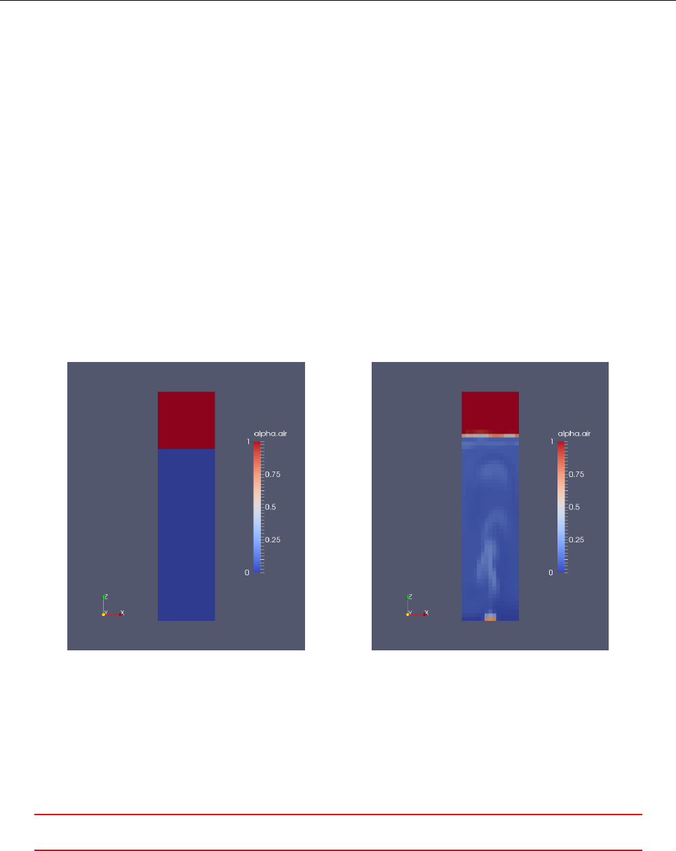
4{
5const volVectorField& U = this - > U_ ;
6const alphaField & alpha = this ->alpha_;
7const rho Fiel d & rho = this - > rho _ ;
8const turb ulen ceM odel & g asT urbu len ce = this - > g a sT urb ule nce ( ) ;
9return
10 (
11 ma x ( alp ha Inv ers io n_ - alpha , sca lar ( 0) )
12 * rh o
13 * mi n (this - > C e_ * s qrt ( g asT urb ule nce . k () ) / this -> d elta () , 1. 0/ U . ti me () . d el ta T () )
14 );
15 }
Listing 228: The method phaseTransferCoeff() of the Niceno turbulence model.
35.4.7 Pitfall: phase inversion
Phase inversion is the situation when the volume fraction of the continuous phase vanishes in some regions. As
almost all terms of the governing equations are weighted with the volume fraction alpha, a vanishing volume
fraction can lead to serious numerical problems.
The following example demonstrates the problems which may be faced when dealing with phase inversion.
An air-water bubble column is modelled including some of the air above the water surface. Figure 60 shows the
air volume fraction within the bubble column.
When mixtureKEpsilon is selected as turbulence model, the volume fraction is not included in the governing
equation, so phase inversion poses no big problem, see Listing 227 or Eq. (71).
When kEpsilon is selected for the liquid phase, the volume fraction in the governing equations is the volume
fraction of the liquid phase. This volume fraction vanishes above the water surface. Thus, in parts of the domain
the solution of the governing equations faces numerical problems. The governing equations can still be solved in
this case, but preconditioning the resulting matrix equation fails. Preconditioning is a step that is intended to
improve the iterative solution of the resulting matrix equation. In the case of the kEpsilon turbulence model
for the liquid phase, the only way to avoid crashing the simulation is to use a -solver with no preconditioning.
The -solver and the smooth solver fail completely.
Figure 60: Air volume fraction of the bubble column. Initial field (left) and solution at t= 10 s (right).
Table 6lists possible model choices for two-phase simulations including phase-inversion.
VThis offering is not approved or endorsed by ESI®Group, ESI-OpenCFD®or the OpenFOAM®
Foundation, the producer of the OpenFOAM®software and owner of the OpenFOAM®trademark. 169

Liquid Gas constraints / remarks
kEpsilon laminar solver: PBiCG, preconditioner: none
mixtureKEpsilon mixtureKEpsilon
Lahey continuousKEqn
SmagorinskyZhang laminar
Niceno laminar solver: PBiCG, preconditioner: none
Niceno continuousKEqn
Table 6: Turbulence model combinations for phase-inversion cases.
35.5 Energy equation
In OpenFOAM-2.3 the twoPhaseEulerFoam solver incorporates the functionality of compressibleTwoPhaseEuler-
Foam99. Accounting for compressibility necessitates the solution of the energy equation. The solving of the
energy equation requires the specification of additional discretisation schemes and a solver in fvSchemes and
fvSolution. Depending on the simulation parameters the energy equation is solved in terms of the enthalpy h
or internal energy e.
The energy equation is formulated in a generic form in terms of he. The actual decision to solve for hor e
is made at run-time after the thermophysical properties of the two phases have been read.
Besides the internal energy or enthalpy the energy equation involves also the kinetic energy K, which is in
fact a specific kinetic energy. Listing 229 shows how this kinetic energy is computed. This source code translates
into the following mathematical relation.
Ki=1
2|Ui|2(89)
Info << " C reat ing field ki neti c e nergy K \n " << endl;
v ol S ca la r Fi e ld K 1 ( I Oo bj ec t :: g rou pN ame ( " K" , p ha se 1 . n am e () ) , 0 .5 * m ag Sqr ( U 1 )) ;
v ol S ca la r Fi e ld K 2 ( I Oo bj ec t :: g rou pN ame ( " K" , p ha se 2 . n am e () ) , 0 .5 * m ag Sqr ( U 2 )) ;
Listing 229: Definition of the kinetic energy field in the file createFields.H of twoPhaseEulerFoam.
The solution of the energy equation can not be deactivated. Even if thermophysical parameters are chosen
to represent incompressible phases, the energy equation will be solved each time step.
35.5.1 Governing equations
Listing 230 shows the energy equation for one phase. In Line 3we see the local derivative and the convection
term of the generic internal energy/ enthalpy he. In Line 5is the local derivative and the convection term of
the specific kinetic energy K.
In the Lines 4and 6we see a correction for the continuity error. See Section 50.3 for a detailed discussion.
From Lines 8to 10 we see the term regarding the mechanical work done. Here we see a conditional expression
depending whether the equation is solved for internal energy or enthalpy. All other terms in the equation are
formulated generically. Besides the use of the abstract he, which is internal energy or enthalpy, the use of the
variable Cpv is also a characteristic of this generic formulation. This variable stands for either the heat capacity
at constant pressure or the heat capacity at constant volume.
Lines 12 to 17 contain the diffusive heat flux. Line 19 represents the heat flux between the two phases. Line
22 contains possible heat sources.
Lines 20 and 21 can be considered a numerical trick. If we ignore the fvm::Sp() for a while and add the
terms of the two lines, we see that they add up to zero. Adding zero is mathematically allowed. If we do
not ignore the fvm::Sp(), we need to find out, what is happening. fvm::Sp() is an implicit source term, i.e.
the contribution of this term goes into the system matrix of the resulting linear equation system. An implicit
source term not only contributes to the system matrix, these terms go into the diagonal entries of the system
matrix. When solving linear equation systems iteratively, it is preferable to work on a diagonally dominant
system matrix [25]. Exactly, this is achieved by the Lines 20 and 21. The term in Line 21 adds to the diagonal
of the system matrix, whereas the term of Line 20 adds to the right hand side of the ensuing linear equa-
tion system. As both sides of the equation have been equally treated, nothing was done wrong mathematically.
99http://www.openfoam.org/version2.3.0/multiphase.php
VThis offering is not approved or endorsed by ESI®Group, ESI-OpenCFD®or the OpenFOAM®
Foundation, the producer of the OpenFOAM®software and owner of the OpenFOAM®trademark. 170

However, as diagonal dominance is numerically a good thing, the convergence behaviour was probably improved.
1fvScalarMatrix he1Eqn
2(
3fv m :: ddt ( al pha 1 , rho1 , he1 ) + fvm :: div ( alp ha RhoP hi1 , h e1 )
4- f vm : : Sp ( c on tEr r1 , h e1 )
5+ fvc :: ddt ( alpha1 , rho1 , K1 ) + fvc :: div ( alph aRhoPh i1 , K1 )
6- c on tE rr1 * K1
7+ (
8he 1 . name () == t he rm o1 . p ha seP rop ert yN ame ( "e")
9? fvc :: ddt ( alph a1 )* p + fvc :: div (al phaPhi1 , p )
10 : - alp ha 1 * dpdt
11 )
12 - fvm :: laplacian
13 (
14 fvc :: i nterp olate ( a lpha1 )
15 * fvc :: int erpolate ( the rmo1 . alphaE ff ( phase1 . tu rbulence (). mut ())),
16 he1
17 )
18 ==
19 h ea t Tr a ns fer C oe f f *( the rm o2 . T () - the rm o1 . T () )
20 + hea tTr ans fe rCo eff * he1 / Cpv1
21 - f vm : : Sp ( h ea t Tr a ns f er Coe f f / Cpv 1 , h e1 )
22 + f vO pti on s ( alpha1 , rho1 , he 1 )
23 );
Listing 230: Energy equation in the file EEqns.H of twoPhaseEulerFoam.
35.6 Momentum equation
Due to the changes on the modelling side and some restructuring, the momentum equation has a different form
compared to previous versions of this solver.
The most general form of the momentum conservation equation for two-phase flow is as follows100
∂αqρquq
∂t +∇·(αqρququq)− ∇·τq=X
i
Fq,i +X
i
Kpq,i (up−uq)(90)
with
Kpq,i =−Kqp,i
Kqq,i = 0
35.6.1 Units
Now we shall take a short look on the units of this equation. Each term of the equation has to have the same
unit. We take the local derivative to determine the unit of all terms in this equation.
∂αqρquq
∂t =1
s
kg
m3
m
s=1
m3
kg m
s2
|{z}
N
=N
m3(91)
We see that all terms of the momentum equation have the unit of a force density. On the RHS of the
momentum equation we have two kinds of source terms.
The first kind of source terms – Fi– can be referred to as body forces, e.g. the gravitational force. This is
consistent with our observation, that this terms have the unit of a force density.
[Fi]!
=N
m3=kg
m2s2(92)
100The phase qis the considered phase and phase pdenotes the other phase.
VThis offering is not approved or endorsed by ESI®Group, ESI-OpenCFD®or the OpenFOAM®
Foundation, the producer of the OpenFOAM®software and owner of the OpenFOAM®trademark. 171

The second kind of source terms – Kpq,i (up−uq)– are phase interaction terms. This terms are the product
of a coefficient Kpq,i with the relative velocity uR=up−uq. Such a phase interaction term might be due to
drag. Now we determine the unit of the interphase momentum exchange coefficient Kpq,i.
[Kpq,i (up−uq)] !
=N
m3=1
s
kg
m3
m
s(93)
[Kpq,i] = kg
m3s(94)
35.6.2 Implemented equations
Listing 231 shows one of the momentum conservation equations. On Line 3we see the local derivative and the
convective term. The origin of the term in Line 4is explained in 50.3. On Line 5we see a term stemming from
the MRF approach. On Line 6is the momentum diffusion.
On the RHS there are a number of force terms. Although, they are named *Force, they are in fact force
density terms. On Line we see a part of the drag force. The force due to gravity and the other part of the drag
are considered in the pressure equation [42].
1U1Eqn =
2(
3fv m :: ddt ( a lph a1 , rh o1 , U 1 ) + fv m :: div ( a lp ha Rho Ph i1 , U1 )
4- f vm : : Sp ( c on tEr r1 , U1 )
5+ mrfZones ( alpha 1 * rho1 + v irtualMassC oef f , U1 )
6+ p ha se 1 . t ur bu l en ce () . d iv D ev Rh o Re f f ( U1 )
7==
8- liftForce
9- wallLubricationForce
10 - turbulentDispersionForce
11 - virtualMassCoeff
12 *(
13 fv m :: ddt ( U1 )
14 + fvm : : di v ( phi1 , U 1 )
15 - f vm : : Sp ( f vc : : di v ( ph i1 ) , U1 )
16 - DDtU2
17 )
18 + f vOp tio ns ( alpha1 , rho1 , U1)
19 );
20 U1E qn . rel ax () ;
21 U1E qn += f vm : : Sp ( d ra gC oe ff , U 1 );
22 fvO ptions . con st rain ( U1Eqn );
Listing 231: The code of the momentum conservation equation of phase 1 of twoPhaseEulerFoam in UEqns.H
The interfacial momentum exchange terms are computed prior to the construction of the momentum equa-
tion. Listing 232 shows the relevant lines of the file Ueqns.H. Wee see that the momentum exchange terms are
provided by some methods. We know that the variable fluid is of the type twoPhaseSystem. Thus, the meth-
ods called to compute the momentum exchange terms are methods of the class twoPhaseSystem, see Section
28.2.1.
1vol Sc al ar Fi el d d ra gCoe ff ( f luid . d ragC oe ff ());
2
3volScalarField virtualMassCoeff(fluid.virtualMassCoeff());
4vol Ve ct or Fi el d l if tFor ce ( f luid . l iftF or ce ());
5v ol V ec to r Fi e ld w al l Lu b ri c at i on F or c e ( f lu id . w a ll L ub r ic a ti o nF o rc e () ) ;
6volVectorField turbulentDispersionForce(fluid.turbulentDispersionForce());
Listing 232: The definition of the interfacial momentum exchange force terms of the momentum conservation
equations of twoPhaseEulerFoam in UEqns.H
VThis offering is not approved or endorsed by ESI®Group, ESI-OpenCFD®or the OpenFOAM®
Foundation, the producer of the OpenFOAM®software and owner of the OpenFOAM®trademark. 172

35.7 Interfacial interaction
35.7.1 Blending
The interfacial momentum exchange models need to work over the whole range of flow situations. These range
from α1= 0 to α1= 1. In order to well-posedness of the governing equations special care needs to be taken for
the case of phase inversion.
There are three options for blending available: none, linear and hyperbolic.
// create x
if ( mod el_ . valid () )
{
x () += mo del_ - > K () *( f1 () - f2 () ) ;
}
if ( model1I n2_ . valid ())
{
x () += m od el 1I n2 _ - > K () * (1 - f1 ) ;
}
if ( model2I n1_ . valid ())
{
x () += m od el 2I n1_ - > K () * f2 ;
}
// other code
return x;
Listing 233: The application of blending; part of the method K() in BlendedInterfacialModel.C
No Blending
The blending model none, which is defined in the files noBlending.H and noBlending.C, is quite instructive.
This blending model, which is essentially a non-model, returns the blending factors f1 and f2 as it is demanded
by the base class of all blending models.
As there is no blending with the none blending model, the user needs to specify which phase is the contin-
uous phase. In twoPhaseEulerFoam-2.3 there is no implicit assumption on which phase is the dispersed and
which is continuous. Listing 234 shows how the none blending model is selected. There we also see the explicit
specification of the continuous phase.
blending
{
default
{
type none;
con ti nu ous Ph as e water ;
}
}
Listing 234: Choosing not to use blending as the blending method
Now, we have a look on the blending factors returned by the none model. Listing 235 shows the definition of
the methods f1() and f2(). These methods return a newly created temporary scalar field (volScalarField)
that is in turn created from a constant expression.
In the case of f1(), the constant expression is phase2.name() != continuousPhase\_ which returns a
boolean value. In the case of f2() the corresonding expression is phase1.name() == continuousPhase\_,
which also returns a boolean value. Here, we enter the realm of implicit type conversions101. Implicit type
conversions are part of the language’s standard. Thus, if we look up the working draft of the C++11standard,
we find the following sentence in the section on Integral promotions:
101See e.g. http://en.cppreference.com/w/cpp/language/implicit_cast
VThis offering is not approved or endorsed by ESI®Group, ESI-OpenCFD®or the OpenFOAM®
Foundation, the producer of the OpenFOAM®software and owner of the OpenFOAM®trademark. 173

A prvalue of type bool can be converted to a prvalue of type int, with false becoming zero and
true becoming one.
Thus, we find that the blending factors returned by none are of the values zero or one, which is the set of
values we would expect in this case. If the boolean expressions yield the correct factors can be tried out with a
simple pen-and-paper test. Choose a continuous phase (i.e. phase2 is the continuous phase) and evaluate all ex-
pressions (i.e. determine the values of f1 and f2, and apply these values on the expressions found in Listing 233.).
Foam :: tmp < Foam :: v olS calar Field > Foam :: ble ndin gMet hod s :: noBlending :: f1
(
const phaseModel & phase1 , c onst ph ase Model & phase2
)const
{
const fvMesh & mesh ( phase1 . mesh () ) ;
return
tmp <volScalarField >
(
new volScalarField
(
IOobject ( /* a rgu men ts rem oved */ ) ,
mesh ,
dimensionedScalar
(
"f",
dimless ,
phase 2 . name () != c ont in uo usP ha se_
)
)
);
}
Foam :: tmp < Foam :: v olS calar Field > Foam :: ble ndin gMet hod s :: noBlending :: f2
(
const phaseModel & phase1 , c onst ph ase Model & phase2
)const
{
const fvMesh & mesh ( phase1 . mesh () ) ;
return
tmp <volScalarField >
(
new volScalarField
(
IOobject ( /* a rgu men ts rem oved */ ) ,
mesh ,
dimensionedScalar
(
"f",
dimless ,
phase 1 . name () == c ont in uo usP ha se_
)
)
);
}
Listing 235: Computing the blending factors. The arguments of the constructor of the IOobject class have
been removed to save space.
Linear
As we saw from the none model, the blending factors f1 and f2 have two extreme values, i.e. zero and one.
The model name linear suggests that this models yields a linear variation between these two limiting values.
The linear blending model was two model parameters, shown in Listing 236. These represent the limits up
to which a phase can be considered to be fully dispersed, i.e. a clear distinction between dispersed phase and
continuous phase is possible. The second parameter is the limit up to which the phases can be considered partly
dispersed. These two limits are necessary, as the solver is intended to handle phase inversion, i.e. situations in
which one phase is the dispersed phase in only parts of the domain.
VThis offering is not approved or endorsed by ESI®Group, ESI-OpenCFD®or the OpenFOAM®
Foundation, the producer of the OpenFOAM®software and owner of the OpenFOAM®trademark. 174
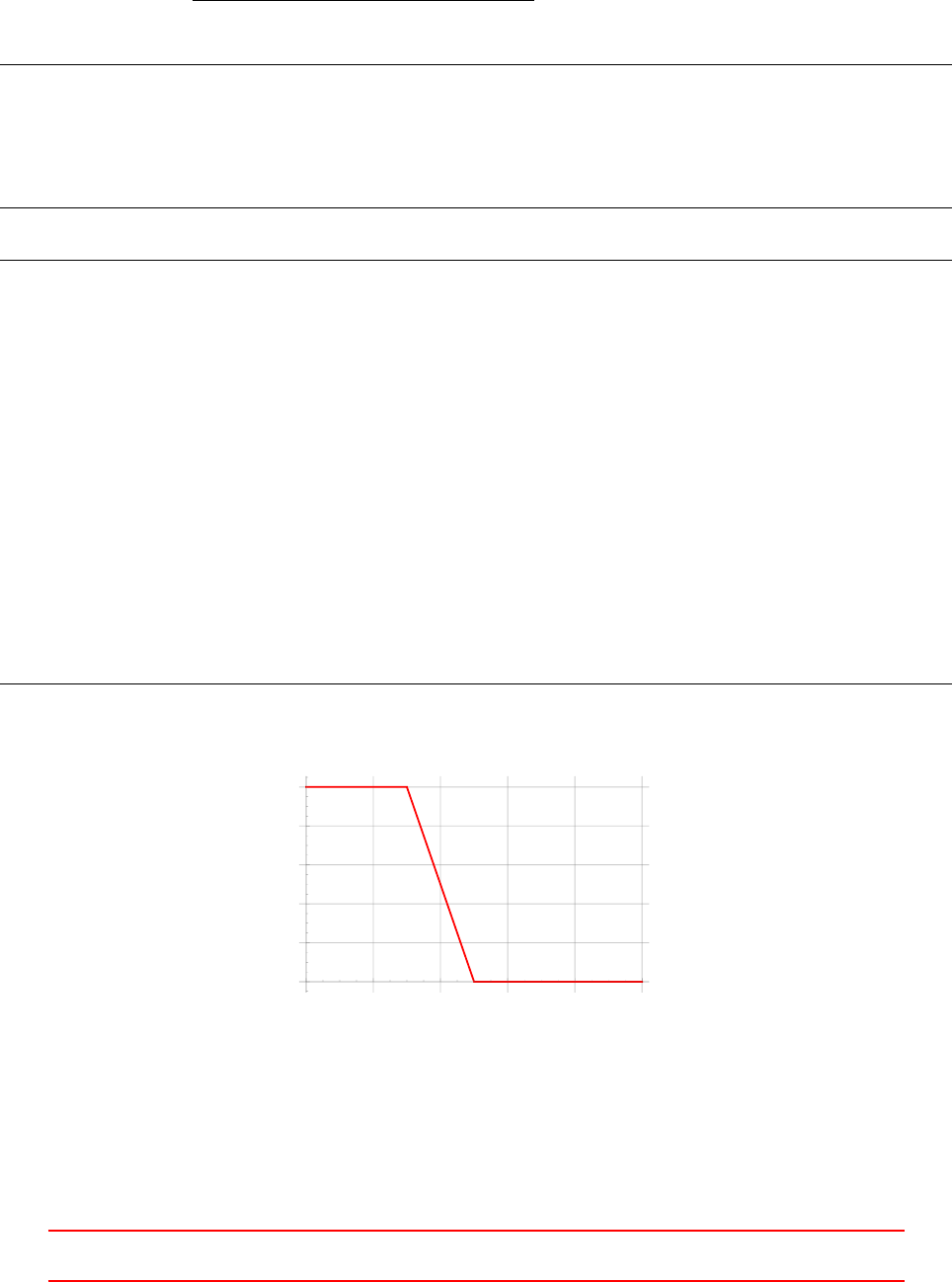
The definition of the blending factor f1 is shown in Listing 237. We limit the discussion on f1, as the other
blending factor is defined analogously. The interested reader is encouraged to analyse f2. The code of Listing
237 can be translated into equation (95).
f1(α) =
1if α≤maxFullyDispersedAlpha
α−maxFullyDispersedAlpha
maxPartlyDispersedAlpha−maxFullyDispersedAlpha if α≤maxPartlyDispersedAlpha
0if α > maxPartlyDispersedAlpha
(95)
// - Maximum fra ction of phas es which can be co nsidered fully dispersed
Ha shTable < d imen si oned Sc alar , word , word :: hash >
maxFullyDispersedAlpha_;
// - Maximum fra ction of phas es which can be co nsidered par tly di spe rse d
Ha shTable < d imen si oned Sc alar , word , word :: hash >
maxPartlyDispersedAlpha_;
Listing 236: Model parameters of the linear blending model; declaration in the file linear.H
Foam :: tmp < Foam :: v olS calar Field > Foam :: ble ndin gMet hod s :: linea r :: f1
(
const phaseModel & phase1 , c onst ph ase Model & phase2
)const
{
const dimensionedScalar
m ax Ful lA l ph a ( m a xF u ll y Di s pe r se d Al p ha _ [ p ha se 1 . n am e () ]) ;
const dimensionedScalar
max Pa rt Alpha ( m ax Pa rtl yD is pe rse dA lp ha_ [ p hase 1 .name () ]);
return
min
(
max
(
(phase1 - maxFullAlpha)
/(maxPartAlpha - maxFullAlpha + SMALL),
scalar (0 .0)
) ,
scalar (1 .0)
);
}
Listing 237: Computing the linear blending factor f1 in the file linear.C
0.2 0.4 0.6 0.8 1.0
α
0.2
0.4
0.6
0.8
1.0
f1
Figure 61: The value of f1 over α; model parameters are set to maxFullAlpha = 0.3and maxPartAlpha = 0.5;
these settings are taken from the bubble column tutorial case of twoPhaseEulerFoam.
Hyperbolic
The hyperbolic blending model offers a continuous function for the blending factor for the whole range of the
dispersed phase’s volume fraction, see Figure 62. Again, we analyse only the definition of f1 and leave the
reader the opportunity to follow the argument made, with the definition of f2.
VThis offering is not approved or endorsed by ESI®Group, ESI-OpenCFD®or the OpenFOAM®
Foundation, the producer of the OpenFOAM®software and owner of the OpenFOAM®trademark. 175
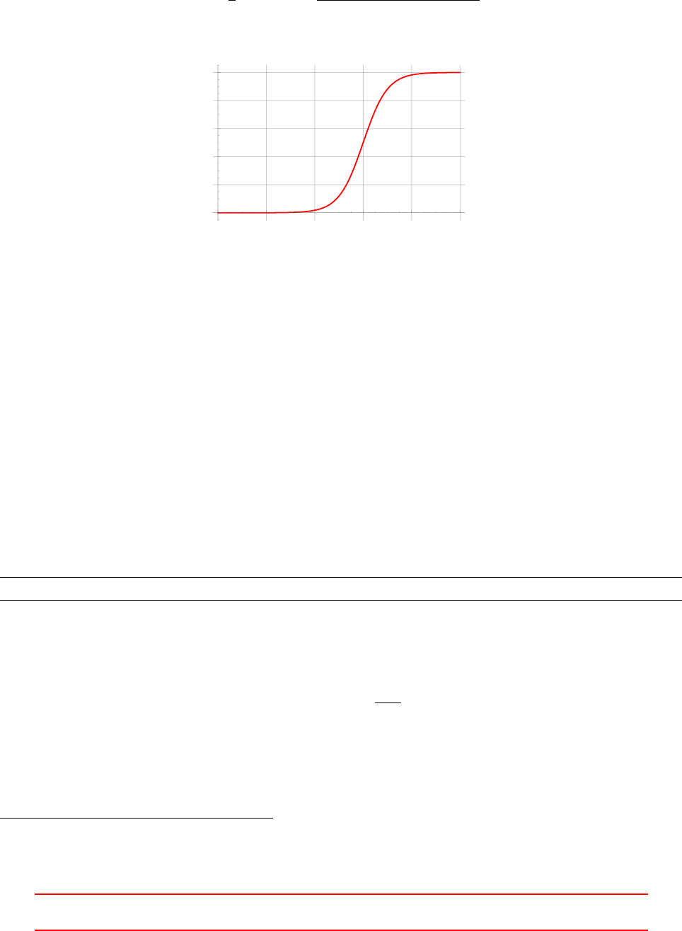
The hyperbolic blending model needs in total three model parameters. The parameter transitionAlphaScale
controls how steep the transition between 0 and 1 is. The other two parameters are maxDispersedAlpha for
each phase. At this parameter the blending function (96) has the value 1/2.
f1(α) = 1
21 + tanh 4(α−maxDispersedAlpha
transitionAlphaScale ) (96)
0.2 0.4 0.6 0.8 1.0
α
0.2
0.4
0.6
0.8
1.0
f1
Figure 62: The value of f1 over α; model parameters are set to maxDispersedAlpha = 0.6and
transitionAlphaScale = 0.4;
35.8 Interfacial momentum exchange
35.8.1 Drag
Units
From viewing the governing equations we saw, that the drag term consists of a coefficient and the relative
velocity between the phases.
Fdrag =Kpq,drag (up−uq)(97)
We find the same structure in the terms of the implemented equations. The Listing below shows one part
of the drag term – as the drag term consists of the coefficient and a velocity difference, we can split the term
up into two contributing parts.
U1E qn += f vm : : Sp ( d ra gC oe ff , U 1 );
As we know from our considerations about the units of the terms of the momentum equation, the drag force
contribution in general needs to have the unit of a force density. Thus, we determined the unit of the coefficient,
see Eqn. (94).
[dragCoeff]!
=kg
m3s(98)
By having a close look on the base class for the drag models, we can check the unit of the coefficient. The
base class of the drag model has a static data member that carries the information about the unit of the provided
coefficient. In fact, all interfacial momentum exchange models have such a member. In the header file of the
base class for the drag models, a constant static member102 dimK is declared.
102A static data member of a class exists only once for all instances of this class, i.e. regardless of how many actual objects of this
class exist, the data member exists only once. This makes perfect sense for common properties such as the unit of the coefficient,
which is the same for all drag models.
VThis offering is not approved or endorsed by ESI®Group, ESI-OpenCFD®or the OpenFOAM®
Foundation, the producer of the OpenFOAM®software and owner of the OpenFOAM®trademark. 176

// - C oe ff ic ie nt dimens ions
static co nst dimensionSet dimK;
In the implementation file, the static data member is initialised to the appropriate value. In Section 7we
reviewed OpenFOAMs feature to provide physical units. There we can see, that the order of units in a
dimensionSet is [kg m s K mol].
const Foam :: dim ensio nSe t Foam :: dr agMo del :: dimK (1, -3, -1 , 0 , 0) ;
Thus, we see, that the drag force coefficient has indeed the unit we derived from our earlier considerations.
Returning the output
Other than the drag models of prior versions of twoPhaseEulerFoam (version 2.2 and below), the drag models in
twoPhaseEulerFoam-2.3 return the product of drag coefficient CDand the Reynolds number Re. Consequently,
the method returning the output of the individual drag models is named CdRe().
The drag model itself, i.e. the base class returns the drag force coefficient K. This drag force coefficient is
provided by the method K() which is a method of the base class dragModel. The base class also has a pure
virtual method named CdRe(). Pure virtual means that derived classes need to implement this method and that
we are unable to create an instance of the base class itself. We only can create instances of one of the derived
classes. As a derived class must implement all pure virtual methods, we are guaranteed that these methods
actually exist. The Listings 238 and 239 show the relevant parts of code of the class dragModel. The method
K() calls the method CdRe(), see Line 5of Listing 239.
1// - Drag coe ff ic ie nt
2virtual tmp < volSc alar Fiel d > CdRe () con st = 0;
3
4// - The drag funct io n K used in the m om entu m equ at ion
5// d dt ( a lph a1 * r ho1 * U1 ) + . .. = . .. K *( U1 - U2 )
6// d dt ( a lph a2 * r ho2 * U2 ) + . .. = . .. K *( U2 - U1 )
7virtual tmp <volScalarField > K() c onst ;
Listing 238: The declaration of the methods K() and CdRe() in dragModel.H
1Foam :: tmp < Foam :: v olS calar Field > Foam :: dragModel ::K() const
2{
3return
40.75
5* Cd Re ()
6* ma x ( pair _ . dis pe rs ed () , r es id ual Al pha _ )
7* s war mC or r ec ti on _ - > Cs ()
8* p ai r_ . c ont in u ou s ( ) . rho ()
9* p ai r_ . c ont in u ou s ( ) . nu ()
10 / sqr ( p ai r_ . d isp er s ed () . d () ) ;
11 }
Listing 239: The definition of the method K() in dragModel.C
If we translate Listing 239 into math we yield
K=3
4CDRe αCS
ρCνC
d2
B
(99)
Now, we insert the definition of the bubble Reynolds number
K=3
4CD
dBUR
νC
αCS
ρCνC
d2
B
(100)
K=3
4αCSCD
ρC
dB
UR(101)
If we now take a look on the units
[K] = ρC
dB
UR=kg
m3
1
m
m
s=kg
m3s(102)
VThis offering is not approved or endorsed by ESI®Group, ESI-OpenCFD®or the OpenFOAM®
Foundation, the producer of the OpenFOAM®software and owner of the OpenFOAM®trademark. 177

Again, we find the proper physical unit for the drag force coefficient.
Here we show the definition of the method CdRe() from the class SchillerNaumann as an example since the
Schiller Naumann drag model is well known.
1Foam :: tmp < Foam :: v olS calar Field > Foam :: dragModel s :: Sch il ler Nauma nn :: CdRe () c onst
2{
3v ol S ca la r Fi e ld R e ( pa ir _ . Re () ) ;
4
5return
6ne g (Re - 1 000) *24 .0 *( 1. 0 + 0.15* p ow (Re , 0 .6 87 ) )
7+ pos ( Re - 1 00 0) * 0. 44 * ma x ( Re , r esi du a lR e_ ) ;
8}
Listing 240: The relevant lines of code in SchillerNaumann.C
Swarm correction
The drag models offer swarm correction of the drag force, since it is observed that swarms of bubbles behave
different from single bubbles. At the time of writing (September 2014) there are two choices.
noSwarm This model simply returns unity when swarmCorrection_->Cs() is called.
TomiyamaSwarm This model computes the swarm correction factor according to [48].
The Tomiyama swarm correction factor depends on the bubble volume fraction αand a model parameter l.
CS,T omiyama = (1 −α)3−2l(103)
Both swarm correction models are derived from an abstract base class swarmCorrection. Thus the frame-
work is ready for future extension of model choice.
35.8.2 Lift
The lift force on a dispersed phase element (DPE) is defined as
FL=CLαρC(UR×(∇ × U)) (104)
with
CLlift force coefficient
αvolume fraction of the dispersed phase
ρCdensity of the continuous phase
URrelative velocity between the phases
Umixture velocity
Units
In contrast to the drag model, the lift model provides the actual force term for the governing equations. The
base class of the lift models declares a static consant data member dimF for storing the unit of the force term
computed by the list model.
// - For ce d im en si on s
static co nst dimensionSet dimF;
In the implementation file liftModel.C the static data member is initialized and it has indeed the unit of
a force density. Note: the order of units in a dimensionSet is [kg m s K mol].
[Fi]!
=N
m3=kg
m2s2(92)
const Foam :: dim ensio nSe t Foam :: li ftMo del :: dimF (1, -2, -2 , 0 , 0) ;
VThis offering is not approved or endorsed by ESI®Group, ESI-OpenCFD®or the OpenFOAM®
Foundation, the producer of the OpenFOAM®software and owner of the OpenFOAM®trademark. 178

Returning the output
The general computation of the lift force is done – similar to the drag models – within the method F() of the
base class. The base class calls the method Cl() of the concrete lift model for the lift force coefficient. This is
similar to the method K() of the drag model base class calling the method CdRe() of the concrete drag model
classes.
The method F() of the base class returns the force density field due to the lift force.
1// - Lift coe ff ic ie nt
2virtual tmp <volScalarField > Cl() const = 0;
3
4// - Lift fo rce
5virtual tmp <volVectorField > F() c onst ;
Listing 241: The declaration of the methods F() and Cl() in liftModel.H
1Foam :: tmp < Foam :: v olV ector Field > Foam :: liftModel ::F() const
2{
3return
4Cl ()
5* pair_ . d is pers ed ()
6* p ai r_ . c ont in u ou s ( ) . rho ()
7*(
8pair_ . Ur () ^ fvc :: curl ( pair _ . co nt inuo us () .U() )
9);
10 }
Listing 242: The definition of the method F() in liftModel.H
The actual lift force coefficient is provided by the concrete lift force model. Again, analogue to the drag
model classes, the base class for the lift models declares the pure virtual method Cl(). This means, every lift
model derived from the base class has to implement Cl() and we are not able to create an instance of the base
class itself. Thus, the existance of the method Cl() is guaranteed. The implementation of Cl() is the remaining
degree of freedom for the individual lift force models.
There are several choices available to the user:
noLift this model returns a zero field when either F() or Cl() is called. This class overwrites the method
F() which is inherited from the base class with its own implementation. Thus, when F() is called,
the implementation of the class noLift is called, i.e. noLift::F(). All other lift force models do not
implement F(), thus, liftModel::F() is called.
constantCoefficient this model is the easiest implementation of a lift force model. The constant lift force coef-
ficient CLis provided by the user. Cl() simply returns this value in the form of the appropriate data type,
i.e. the coefficient provided by the user is a dimensionless number (declared as const dimensionedScalar Cl_;),
however, the method Cl() returns a volScalarField.
lift force model X there are several models available that compute the lift force coefficient from flow proper-
ties.
35.8.3 Virtual mass
The class structure for the virtual mass models follow the example of the drag and lift models. There is an
abstract base class providing a method F() for the force term FV M due to virtual mass. The force term due to
virtual mass if defined as
FV M =CV M αρC(105)
with
CV M virtual mass coefficient
αvolume fraction of the dispersed phase
ρCdensity of the continuous phase
VThis offering is not approved or endorsed by ESI®Group, ESI-OpenCFD®or the OpenFOAM®
Foundation, the producer of the OpenFOAM®software and owner of the OpenFOAM®trademark. 179

The derived classes provide the virtual mass coefficient CV M via the method Cvm(). The user has the choice
between:
noVirtualMass this class returns zero when F() is called. This model overwrites the method F() with its
own implementation returning a zero field. All other classes make use of the base classes implementation
of F() which all derived classes inherited. The method Cvm() also returns a zero field.
Foam :: tmp < Foam :: v olS calar Field >
Fo am :: v ir t ua l Ma s sM ode l s :: n o Vi rt u al M as s :: K () c onst
{
return Cv m () * d ime n si o ne dSc a la r ( " zero " , dimDe nsity , 0) ;
}
constantVirtualMassCoefficient this class computes the contribution due to virtual mass based on a con-
stant virtual mass coefficient CV M which is provided by the user.
Lamb this model computes the virtual mass coefficient CV M depending on the aspect ratio of the dispersed
phase elements. With the help of aspect ratio models a particle shape different from spheres and even
shape variation can be modelled within some limits.
35.8.4 Aspect ratio models
When dealing with non-spherical bubbles or particles, the shape has to be considered in the interfacial momen-
tum exchange models. One way of dealing with this situation is to formulate those models to incorporate the
aspect ratio of the dispersed phase elements.
Here, the aspect ratio models come into play. These compute the aspect ratio of the dispersed phase elements
depending on material and possibly flow properties. However, the influence of shape can also be considered
using other approaches.
The aspect ratio is used in the TomiyamaAnalytic drag model and the Lamb virtual mass model. The inter-
ested reader can find this out by invoking the following commands.
cd $ FOAM _APP / solv ers / multip hase / tw oP ha se Eu le rF oa m / int er facia lM od el s
find - name *. C | xa rgs grep ’ pa ir _ . E () ’
The second command is a combination of a find command and a grep command. find finds all files with the
file extension .C and grep searches this files for the pattern pair_.E(). This pattern is the function call which
returns the aspect ratio Eof a phase pair.
35.8.5 Wall lubrication
The wall lubrication force pushes bubbles away from the walls. The class structure is similar to the aforemen-
tioned models. There is an abstract base class and derived classes implementing a specific model. The base
class declares the pure virtual method F() which returns the force term due to wall lubrication. The derived
class have to implement this method.
There is a derived class named noWallLubrication which simply implements the method F() in way to
return a zero field. There are also three models computing the wall lubrication force.
35.8.6 Turbulent dispersion
Turbulent dispersion describes the effect of turbulent motion of the liquid phase on the gas phase. The models
are also derived from an abstract base class. There is a class named noTurbulentDispersion which returns a
zero field for the force term and there are a number of classes implementing individual models. The base class
declares the method F() as a pure virtual method. This means there is no generic formulation as in the case of
the drag or lift models.
VThis offering is not approved or endorsed by ESI®Group, ESI-OpenCFD®or the OpenFOAM®
Foundation, the producer of the OpenFOAM®software and owner of the OpenFOAM®trademark. 180

constantTurbulentDispersionCoefficient
The constant coefficient model implements the following model for the force due to turbulent dispersion.
FT D =CT D αρCkC∇α(106)
with
CT D turbulent dispersion coefficient
αvolume fraction of the dispersed phase
ρCdensity of the continuous phase
kCkinetic turbulent energy of the continuous phase
Burns
The Burns model implements the following model for the force due to turbulent dispersion.
FT D =KDrag
νC,t
σ∇α1 + α
1−α(107)
with
KDrag drag force coefficient due to drag
αvolume fraction of the dispersed phase
νC,t turbulent viscosity of the continuous phase
σsurface tension
Note that Kdrag is not evaluated by calling method K() of the class dragModel. Listing 243 shows the actual
code that computes the force term of the Burns model.
The reason for computing the drag force coefficient K“by hand” rather than calling dragModel::K() might
be the run-time. By not calling K() we can save one virtual function call103. The operations to compute K
have to be done anyway, so there is a net saving of one virtual function call.
1Foam :: tmp < Foam :: v olV ector Field >
2Fo am :: t urb u le n tD i sp e rsi o nM o de l s :: B ur ns :: F ( ) const
3{
4const f vM es h & m es h ( pai r_ . p ha se 1 () . mesh () ) ;
5const dra gModel &
6drag
7(
8me sh . loo kupO bjec t < dragModel >
9(
10 IOobject :: g rou pNa me ( drag Mode l :: typ eName , pair_ . name () )
11 )
12 );
13
14 return
15 - 0.75
16 * dr ag . CdRe ()
17 * pair_ . d is pers ed ()
18 * p ai r_ . c ont in u ou s ( ) . nu ()
19 * pair _ . continuou s (). tu rbulence (). nut ()
20 /(
21 sigma_
22 * sqr ( p ai r_ . d isp er s ed () . d () )
23 )
24 * p ai r_ . c ont in u ou s ( ) . rho ()
25 * fvc : : gr ad ( p ai r_ . c on t in uo u s () )
26 *(1.0 + pair_ . dispers ed () / max ( pair_ . con ti nuou s () , res id ua lA lp ha _ ));
27 }
Listing 243: The definition of the method F() in the file Burns.C
103Virtual function calls are considered to be more expensive in terms of run-time than direct function calls, since the correct
function to call has to determined at run-time [15].
VThis offering is not approved or endorsed by ESI®Group, ESI-OpenCFD®or the OpenFOAM®
Foundation, the producer of the OpenFOAM®software and owner of the OpenFOAM®trademark. 181
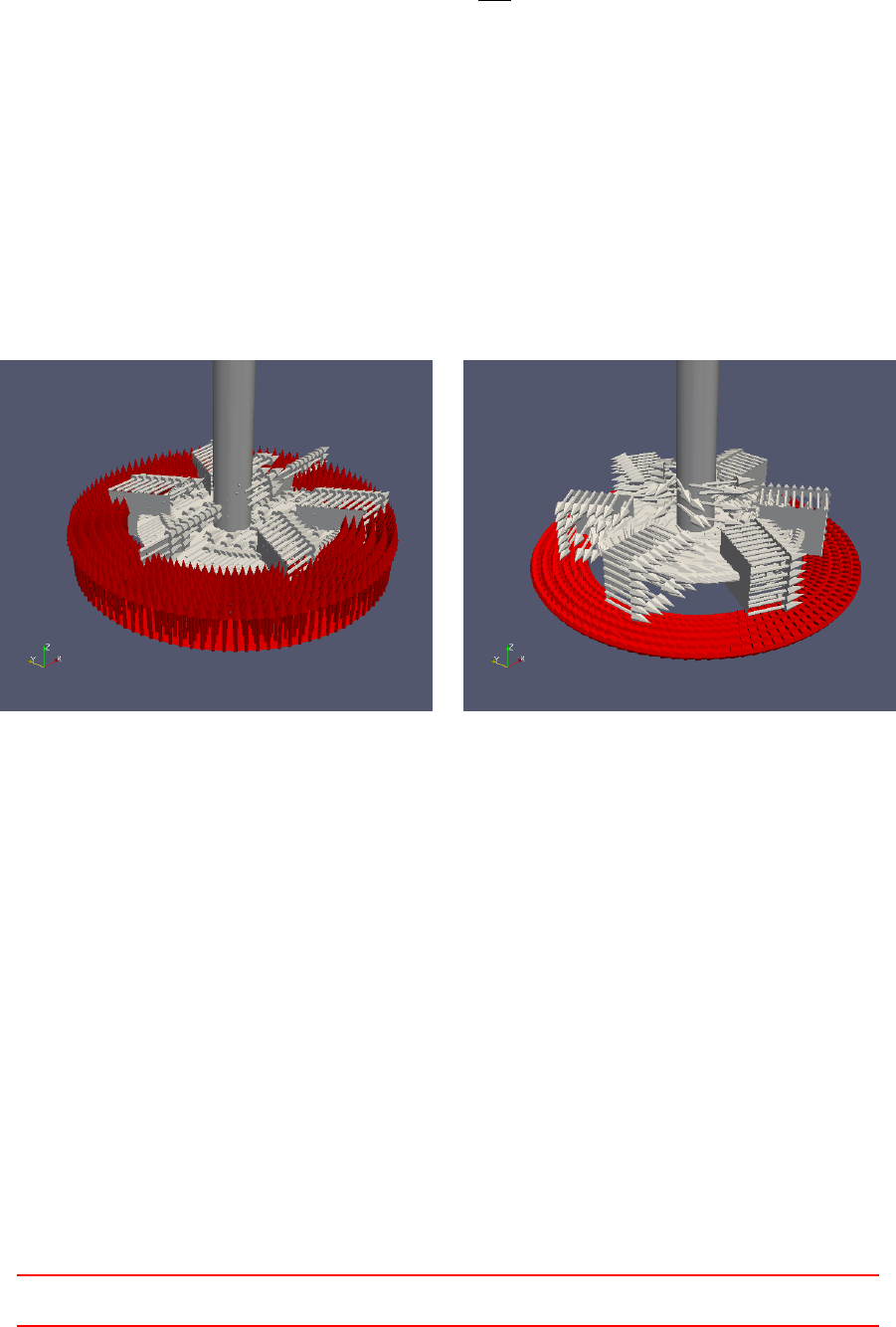
Gosman
The Gosman model implements the following model for the force due to turbulent dispersion.
FT D =KDrag
νC,t
σ∇α(108)
35.9 MRF method - avoiding errors
The MRF method can be used to simulate stirred vessels. By the time of writing, this is the only way to do
so with the Eulerian multiphase solvers, since none of the Eulerian solvers has dynamic mesh capabiltiy. The
basics behind the MRF method are discussed in Section 56.
35.9.1 Inlet boundaries and MRF zones
The MRF method corrects the velocities at the boundaries within the MRF zone. Thus, if a gas inlet BC is
placed within the MRF zone, the simulation takes an unintended route. In Figure 63 we see the outcome of a
gas inlet boundary placed within an MRF zone. Note, the tangential alignment of the velocity vectors on the
right image. The initial inlet definition (visible on the left image) is overridden by the MRF’s constraint.
Figure 63: Velocity vectors of the gaseous phase at the inlet boundary (red vectors) in an aerated stirred tank.
That the gas inlet boundary lies within the MRF zone. On the left, we see the initial condition and on the right
we see the boundary condition after the constraints by the MRF method have been applied.
36 multiphaseEulerFoam
multiphaseEulerFoam is an Eulerian solver for nphases. This solver differs in some points from the solver
twoPhaseEulerFoam.
36.1 Fields
The naming scheme of the fields differs from other multiphase solvers. multiphaseEulerFoam directly uses names
(e.g. Uair, Uwater, Uoil, etc.).
36.1.1 alphas
A specialty of multiphaseEulerFoam is the field alphas. This field does not represent the volume fraction of
a certain phase and is therefore not bounded by 0 and 1. This field is used to represent all phases in a single
scalar field. alphas is computed by summing up the products of phase index and phase fraction.
VThis offering is not approved or endorsed by ESI®Group, ESI-OpenCFD®or the OpenFOAM®
Foundation, the producer of the OpenFOAM®software and owner of the OpenFOAM®trademark. 182

alphas =
n−1
X
i=0
i∗αi(109)
Because alphas is computed quantity, the file alphas can be missing in the 0-directory.
36.2 Momentum exchange
The parameters for the momentum exchange, e.g. the drag model, need to be specified pair-wise.
36.2.1 drag
drag
(
( ai r w ater )
{
type bl ende d ;
air
{
type Sch iller Nauma nn ;
residualPhaseFraction 0;
residualSlip 0;
}
water
{
type Sch iller Nauma nn ;
residualPhaseFraction 0;
residualSlip 0;
}
resi dual Ph aseF ra ctio n 1e -2;
residualSlip 1e-2;
}
/* f urt her defi n itio n s */
Listing 244: Pair-wise definition of the drag model in the file transportProperties
36.2.2 virtual mass
The coefficients for considering virtual mass must also be specified pair-wise. Listing 245 shows how the coeffi-
cients for virtual mass are specified in the damBreak tutorial.
virtualMass
(
( ai r w ater ) 0.5
( ai r oi l ) 0. 5
( ai r m er cu ry ) 0. 5
( wat er oil ) 0. 5
( water merc ury ) 0.5
( oi l m er cu ry ) 0. 5
);
Listing 245: Pair-wise definition of Coefficients for virtual mass in the file transportProperties
36.2.3 lift force
Currently (OpenFOAM 2.1.1) there is no lift model in multiphaseEulerFoam.
VThis offering is not approved or endorsed by ESI®Group, ESI-OpenCFD®or the OpenFOAM®
Foundation, the producer of the OpenFOAM®software and owner of the OpenFOAM®trademark. 183

37 driftFluxFoam
driftFluxFoam is a solver of OpenFOAM to simulate e.g. settling of disperse particles in a liquid. driftFluxFoam
is the successor of settlingFoam, which has been discontinued with the release of OpenFOAM-2.3.1104.
settlingFoam was used by Brennan [11] in his thesis, which contains a lot of information on deriving the
drift flux model from the Eulerian two-fluid model equations. The header of driftFluxFoam describes this
solver as follows:
Solver for 2 incompressible fluids using the mixture approach with the drift-flux approximation for
relative motion of the phases.
Used for simulating the settling of the dispersed phase and other similar separation problems.
driftFluxFoam complys with the generic solver design of OpenFOAM, thus this solver can use all available
turbulence models. It also can use the MRF method and the fvOptions framework.
37.1 Governing equations
The governing equations for the mixture are derived from the two-fluid model [11,21].
37.1.1 Mixture continuity equation
The mixture continuity equation can be easily derived by adding the continuity equations of the two phases:
∂αkρk
∂t +∇·(αkρkuk)=0 (110)
with the constitutive relations
ρm=α1ρ1+α2ρ2(111)
ρmum=α1ρ1u1+α2ρ2u2(112)
we gain
∂ρm
∂t +∇·(ρmum)=0 (113)
37.1.2 Mixture momentum equation
Derivation from literature
The derivation of the mixture momentum equation is analogous to the derivation of the mixture continuity
equation. Therefore, we skip the general derivation and refer the interested reader to the appropriate liter-
ature [11,21]. In this section, we want to focus on the derivation of the specific equations implemented in
driftFluxFoam.
We start from the derivation given in the appendix of Brennan [11]:
∂ρmum
∂t +∇·(ρmumum) = −∇pm+∇·τ+τt−Xαkρkukmukm+ρmg+Mk(114)
we pay special attention to the diffusion stress Pαkρkukmukm, which represents momentum diffusion due to
the relative motion between the phases.
Xαkρkukmukm =α1ρ1u1mu1m+α2ρ2u2mu2m(115)
For convenience we introduce the symbol τdm for the diffusion stress
τdm =Xαkρkukmukm (116)
104http://www.openfoam.org/version2.3.1/
VThis offering is not approved or endorsed by ESI®Group, ESI-OpenCFD®or the OpenFOAM®
Foundation, the producer of the OpenFOAM®software and owner of the OpenFOAM®trademark. 184

with ukm, the velocity of the phase krelative to the mixture’s centre of mass; ukm is also referred to as diffusion
velocity of the phase k
ukm =uk−um(117)
Ishii and Hibiki [21] states a relation between the diffusion velocities of the two phases:
α1ρ1u1m+α2ρ2u2m=0(118)
Thus, we can eliminate u1mfrom the diffusion stress τdm
τdm =α1ρ1α2ρ2
α1ρ12
u2
2m+α2ρ2u2
2m(119)
τdm =α2ρ2u2
2mα2ρ2
α1ρ1
+ 1(120)
τdm =α2ρ2u2
2mα2ρ2+α1ρ1
α1ρ1(121)
τdm =α2ρ2u2
2mρm
α1ρ1(122)
τdm =ρm
α2
α1
ρ2
ρ1
u2
2m(123)
Implementation
From the source code in Listing 246 we see the diffusion stress an the fourth term on the LHS of the momentum
equation.
1fvVectorMatrix UEqn
2(
3fv m : : d dt ( rho , U )
4+ fvm :: div ( rhoPhi , U)
5+ MRF . DDt ( rho , U )
6+ fvc :: div ( UdmModel . tauDm ())
7+ turbu lence - > div De vRh oReff ( U)
8==
9f vO p ti o ns ( rho , U )
10 );
Listing 246: The momentum equation of driftFluxFoam
Next, we take a look at the implementation of the diffusion stress.
1tmp < vo lSy mmT ens orF iel d > Foam :: rel ativ eV eloc ityM odel :: tauDm () const
2{
3vol Sc al ar Fi eld beta c ( alph ac _ * rhoc_ );
4vol Sc al ar Fi eld beta d ( alph ad _ * rhod_ );
5
6// C alc ula te the rela tiv e velocit y of the continuous phase w . r .t the mean
7vol Ve ct or Fi el d Ucm ( beta d* Udm_ / betac ) ;
8
9return tmp < volSymmTensorField >
10 (
11 new volSymmTensorField
12 (
13 " t au Dm " ,
14 betad * s qr ( Ud m_ ) + b etac * s qr ( Ucm )
15 )
16 );
17 }
Listing 247: The diffusion stress of driftFluxFoam computed by the relativeVelocityModel
VThis offering is not approved or endorsed by ESI®Group, ESI-OpenCFD®or the OpenFOAM®
Foundation, the producer of the OpenFOAM®software and owner of the OpenFOAM®trademark. 185
And now, we translate the source code into some math:
τbm =βdu2
dm +βcu2
cm (124)
with
βd=αdρd(125)
βc=αcρc(126)
ucm =βd
βc
udm (127)
we gain
τbm =βdu2
dm +βcβd
βc2
u2
dm (128)
τbm =βdu2
dm 1 + βd
βc(129)
τbm =αdρdu2
dm 1 + αdρd
αcρc(130)
τbm =αdρdu2
dm αcρc+αdρd
αcρc(131)
τbm =αdρdu2
dm
ρm
αcρc
(132)
τbm =ρm
αd
αc
ρd
ρc
u2
dm (133)
We notice, that (133) derived from the source code, equals (123), derived from literature with phase 2 being
the disperse phase d.
Relative velocity
The diffusion velocity udm and the drift velocity udj are linked by a constitutive relation:
udm =ρ1
ρm
udj (134)
We find this relation also in the source code in Listings 252 and 253. Ishii and Hibiki [21] state, that in the
case of dispersed two-phase flow the drag correlation should be expressed in terms of the drift velocity udj .
The relative velocity models provide a method that returns udm, however, in the source code of the Listings
252 and 253 we find relation (134) translated into C++. There, the expression for udm consists of the density
ratio and a relation for the drift velocity, which links the terminal velocity of a single particle and the volume
fraction of the disperse phase.
37.2 incompressibleTwoPhaseInteractingMixture
The class incompressibleTwoPhaseInteractingMixture serves as the transport model for driftFluxFoam.
This class holds all the information of the two phases and provides the mixture quantities. driftFluxFoam
solves the momentum and pressure equations for the mixture. Thus, this solver is in between a single-phase
solver and a full two-fluid solver such as twoPhaseEulerFoam.
Via this transport model, the mixture quantities propagate to the turbulence model, since the turbulence
model receives a transport model class as template parameter at construction. This is one example for the
versatility of the new, templated turbulence modelling framework. The precursor settlingFoam had a hard-
coded k−turbulence model. Also the viscosity model was kind of hard-coded.
37.3 Mixture viscosity models
Settling equippment is often operated with solids concentrations at which the presence of the solid particles
affect fluid properties. Besides using the mixture density, a mixture viscosity also has to be used.
VThis offering is not approved or endorsed by ESI®Group, ESI-OpenCFD®or the OpenFOAM®
Foundation, the producer of the OpenFOAM®software and owner of the OpenFOAM®trademark. 186

37.3.1 mixtureViscosityModel
The class mixtureViscosityModel is the abstract base class for the actual viscosity models. This class serves a
similar purpose as the base class for the single-phase viscosity models viscosityModel located in $FOAM_SRC/
transportModels/incompressible/viscosityModels/viscosityModel. These two base classes are rather
similar and there are only slight differences in their implementations.
37.3.2 slurry
The slurry mixture viscosity model is a correction for the Newtonian viscosity with reference to Thomas [47].
µ=µc1+2.5αd+ 10.05α2
d+ 0.00273 e16.6α(135)
The source code computing the mixture viscosity is a direct translation of the math above into C++.
1Foam :: tmp < Foam :: v olS calar Field >
2Fo am :: mixt ur eVi sc os ity Mo de ls :: s lurry :: mu( cons t volScalarField& muc) const
3{
4return
5(
6muc *(1.0 + 2.5* a lpha_ + 10.05 * sqr ( alpha_ ) + 0.0 0273 * exp ( 16.6* a lpha _ ))
7);
8}
Listing 248: The calculation of the mixture viscosity by the slurry mixture viscosity model.
37.3.3 plastic
The plastic viscosity model is based on a generic viscosity model (136) for liquids exhibiting plastic behaviour.
τ=aCb α (136)
The plastic model implemented in driftFluxFoam translates to:
µ= min [µc+k∗(10n α −1) , µmax](137)
Listing 249 shows the source code computing the mixture viscosity. The -1 in the second term ensures, that
we retain the laminar viscosity of the continuous phase in the case the dispersed volume fraction vanishes, since
anything to the power of zero equals one.
1Foam :: tmp < Foam :: v olS calar Field >
2Foam :: mi x ture Visc osit yMod e ls :: pla stic :: mu ( const volScalarField& muc) const
3{
4return min
5(
6muc
7+ plasticViscosityCoeff_
8*(
9pow
10 (
11 scalar (10) ,
12 plasticViscosityExponent_*alpha_
13 ) - scala r (1)
14 ) ,
15 muMax_
16 );
17 }
Listing 249: The calculation of the mixture viscosity by the plastic mixture viscosity model.
37.3.4 BinghamPlastic
BinghamPlastic is a Bingham plastic model.
VThis offering is not approved or endorsed by ESI®Group, ESI-OpenCFD®or the OpenFOAM®
Foundation, the producer of the OpenFOAM®software and owner of the OpenFOAM®trademark. 187

37.4 Relative velocity models - hindered settling
In this section we use the symbol vfor the velocity to follow the notation of Brennan [11] as well as the source
code of OpenFOAM.
37.4.1 The base class
The base class holds the data common to the derived models. The base class holds the private field Udm_ for
the diffusion velocity udm and declares an abstract method correct(). The method correct() is used by the
derived classes to compute the diffusion velocity Udm_.
The method Udm() of the base class simply returns Udm_, and the method tauDm() returns the diffusion
stress computed from the diffusion velocity.
The diffusion velocity
The class for the relative velocity model holds a vector field for the diffusion velocity. The internal field values
are determined from the actual model in use, however, the boundary conditions are taken over from the mixture
velocity field.
This, we can read from the source code of the base class. In Listing 250 we see the initializer responsible for
the diffusion velocity.
1Udm_
2(
3IOobject
4(
5" Ud m ",
6a lp ha c_ . t im e () . t im eN am e () ,
7alp hac_ . m esh () ,
8IOobject :: NO_READ ,
9IOobject :: AU TO_WRITE
10 ) ,
11 alp hac_ . m esh () ,
12 dimensionedVector(" U dm " , d im Ve lo ci ty , v ec tor :: z er o ) ,
13 m ix tu re . U () . b o un dar y Fi el d () . t yp es ()
14 )
Listing 250: The initializer entry for Udm_ in the constructor of the relativeVelocityModel class.
For the interpretation of Listing 250 we need to dig out the appropriate constructor of the class GeometricField105.
In Listing 251 we see that the constructor receives five arguments, of which the last has a default value. If we
pass only four arguments, the fifth will be determined from the default value.
1// - C on st ru ct or give n IOobject , mesh , dim ension ed < Type > and patch types .
2GeometricField
3(
4const IOo bjec t &,
5const Mesh &,
6const d im en si on ed < Ty pe > & ,
7const wor dLis t & wantedPatch Type s ,
8const wor dLi st & a ctu alPa tchT ypes = wordLi st ()
9);
Listing 251: The signature of the constructor called by the code in Listing 250.
If we compare the arguments of the constructor call of Listing 250 and the signature in Listing 251, we see
that the first argument passed is clearly an IOobject. The second argument is a reference to the mesh itself,
which is obvious from the call to alphac_.mesh() in Listing 250.
The third argument determines the type of the field as well as the initial value. The template parameter
Type determines whether the field is a scalar, a vector or a tensor field. As a dimensionedVector is passed in
Listing 250,Type evaluates to vector106.
105Bear in mind, that volVectorField and others are specialisations of the templated class GeometricField.
106Bear in mind, that dimensionedVector is a specialisation of the templated class dimensioned<Type> and dimensionedVector
is a shorthand for dimensioned<vector>.
VThis offering is not approved or endorsed by ESI®Group, ESI-OpenCFD®or the OpenFOAM®
Foundation, the producer of the OpenFOAM®software and owner of the OpenFOAM®trademark. 188

The fourth argument is a list of patch types, since we passed only one dimensioned value as the third
argument, there has been no information passed on the boundary conditions of the field up to now. By passing
the list of boundary types of the mixture velocity field (mixture.U()), the boundary conditions of the field
Udm_ are specified.
As there is no fifth argument passed in Listing 250, the return value of the call wordList() is used.
37.4.2 simple
The model named simple is similar to the model used by Brennan [11] with attribution to Dahl [12]. This
model is very similar to the Vesilind [51] model (139), Brennan [11] explains the change of the base from the
Euler number eto the base 10 with a closer fit to experimental data gathered by Dahl [12].
vs=v010−kα (138)
The implementation of the simple model is more or less a direct translation from math (138) to C++. In
the exponent the maximum of the dispersed volume fraction and zero is taken to avoid numerical trouble from
negative values of the volume fraction. Reversing the sign in an exponent is never a good idea in numerical
simulation.
1void Foam :: rel ativ eVel ocit yM odel s :: simple :: correct ()
2{
3Ud m_ = ( r hoc_ / rho () )* V0_ * pow ( sca la r (10) , - a_ * max ( alphad_ , sca lar (0) ) );
4}
Listing 252: The calculation of the dispersed diffusion velocity Udm_ by the simple relative velocity model.
37.4.3 general
The model referred to as general is most probably basedon the model of Takács [46], there is no reference to
any literature in the header file. The Takács [46] model (140) is a so-called double-exponential model based on
the model of Vesilind [51], see (139) [19,11].
vs=v0e−nX (139)
vs=v0e−rhX−e−rpX(140)
with
vssettling velocity
v0maximum settling velocity
nmodel parameter
rhsettling parameter for hindered settling
rpsettling parameter for low solids concentration
Xsuspended solids concentration
(141)
The implementation .
1void Foam :: re l ativ eVel ocit y Mode ls :: gen eral :: cor rect ()
2{
3Udm_ =
4( r ho c_ / rh o () )
5* V0 _
6*(
7ex p (- a_ * max ( a lp ha d_ - r es id ua lAlp ha _ , sca lar ( 0) ))
8- e xp (- a1_ * max ( alp ha d_ - r es id ua lA lp ha_ , s cala r (0) ) )
9);
10 }
Listing 253: The calculation of the dispersed diffusion velocity Udm_ by the general relative velocity model.
VThis offering is not approved or endorsed by ESI®Group, ESI-OpenCFD®or the OpenFOAM®
Foundation, the producer of the OpenFOAM®software and owner of the OpenFOAM®trademark. 189

37.5 settlingFoam
Here we take a closer look on settlingFoam (of OpenFOAM-2.2.x), which is the predecessor of driftFluxFoam.
By comparing the implementations of these two solvers we can observe the transition of the OpenFOAM source
code base to a more encapsulated approach.
37.5.1 Mixture viscosity
settlingFoam was/is restricted to the plastic or Bingham viscosity models. Listing 254 shows the code of
settlingFoam, which computes the mixture viscosity. This code is located in a source file, which is included
into the body of the PIMPLE loop of the solver.
Thus, for this solver, the treatment of mixture viscosity is not encapsulated. The viscosity models are not
located in separate files and the code of the solver itself contains all the knowledge of the viscosity models.
Extending the solver with one or more mixture viscosity models would entail building an extended if-cascade
within the file correctViscosity.H.
1{
2/* com pute plasti c v isc osi ty */
3mul = muc +
4plasticViscosity
5(
6/* code removed for bre vity */
7);
8
9if (BinghamPlastic)
10 {
11 vol Scal arF ield tauy = yiel dSt res s
12 (
13 /* see yiel dSt ress .H */
14 );
15 mul =
16 /* comput e co ntr ibution of yiel d stress */
17 + mul ;
18 }
19
20 mu l = mi n ( mul , m uM a x ) ;
21 }
Listing 254: The calculation of the mixture viscosity in the file correctViscosity.H of settlingFoam of
OpenFOAM-2.2.x. Comments added by the author.
37.5.2 Relative velocity models
settlingFoam of OpenFOAM-2.2.x offers the same choice of relative velocity models as driftFluxFoam at the
time of writing. However, implementation-wise we note, that model selection is, again, done in an if-statement
cascade.
1if ( VdjMod el == "general")
2{
3Vd j = V 0 *
4(
5ex p (- a* max ( alp ha - alphaMin , sca la r (0) ))
6- e xp ( - a1 * m ax ( a lp ha - a lp haM in , s ca lar ( 0) ) )
7);
8}
9else if ( VdjModel == "simple")
10 {
11 Vdj = V0 *pow (10.0 , -a* alpha );
12 }
13 else
14 {
15 Fat al Er ro rI n ( ar gs . e xecu ta bl e () )
16 << " U nkno wn VdjModel : " << V djM ode l
17 << abort ( F at al Error ) ;
18 }
VThis offering is not approved or endorsed by ESI®Group, ESI-OpenCFD®or the OpenFOAM®
Foundation, the producer of the OpenFOAM®software and owner of the OpenFOAM®trademark. 190

19
20 Vdj.correctBoundaryConditions();
Listing 255: The calculation of the relative velocity in the file calcVdj.H of settlingFoam of OpenFOAM-2.2.x.
37.5.3 Turbulence
Turbulence in settlingFoam was/is implemented in a similar fashion as in twoPhaseEulerFoam of that time.
Both solvers feature a hard-coded k−turbulence model, which is adapted to the solvers needs.
VThis offering is not approved or endorsed by ESI®Group, ESI-OpenCFD®or the OpenFOAM®
Foundation, the producer of the OpenFOAM®software and owner of the OpenFOAM®trademark. 191
Part VI
Postprocessing
There are two principal possibilities for post processing in OpenFOAM. First, there are tools that are executed
after a simulation has finished. This tools work on the written data of the solution. sample and paraView are
two examples for such tools.
Besides that, there is run-time post processing. Run-time post processing performs certain operations on the
solution data as it is generated. Consequently, run-time post processing allows for a much finer time resolution.
The functions objects – e.g. for calculating forces or force coefficients – are an example for run-time post
processing. The big disadvantage of this method is, that the user has to know the intended post processing
steps before starting a simulation. See http://www.openfoam.com/features/runtime-postprocessing.php
for more information about run-time post processing.
38 functions
A function objects - in general - are objects, which are used in a similar manner as a function. This main benefit
of function objects is that they can have a permanent state. This state can be used to store data between “calls”
of the function object. A very illustrative example is OpenFOAM’s function object fieldAverage, which computes
the temporal average of fields. This function object needs to update itself with every time step computed and
the current time-averaged fields need to be preserved between “calls” of fieldAverage.
Function objects usually serve one specific purpose, e.g. compute the time average of a field quantity. Thus,
there is a large, ever growing number of function objects available in OpenFOAM. Some of which are listed
below to give an impression of the wide range of tasks currently covered by OpenFOAM’s function objects:
fieldAverage compute the temporal average of field quantities
the fieldValue family compute the spatial average (or other operations) of field quantities
forces compute the forces on a body (surface)
forceCoeffs compute force coefficients, e.g. for drag, lift and torque
sampledSet save the field values of a certain region, e.g. along a line
probes save field values at certain points
streamLine compute streamlines
scalarTransport solve a passive scalar transport equation
codedFunctionObject implement your own function object in a not-entirely-from-scratch framework
The list above is only a small selection of available functions. Check out OpenFOAM’s sources for a complete
overwiew on available function objects107.
38.1 Stay up to date
Run-time post-processing with function objects is a feature of OpenFOAM which is very much in the realm of
application and daily use, in contrast to the inner workings of the mesh class. Thus, function objects recieve
much attention from the developers in form addition of new function objects, extending the features of existing
function objects or reorganizing and renaming existing function objects.
The first two points (addition and extension) are clearly for the benefit of the users, whereas the latter
one (reorganisation) most probably benefits the developers in reducing code duplication or easing maintenance.
Reorganisation might go hand in hand with renaming of function objects108. In such a case your might need to
modify the function object definitions of your cases when migrating them to a newer109 version.
107New users might hate this statement, but the documentation is in the code.
108As an illustrative example, the function object for processing field values within a cell set has changed its name from cellSource
(OpenFOAM-3.0) over volRegion (OpenFOAM-4.0) to volFieldValue (OpenFOAM-5.0). This has been done, most probably, to
keep the naming scheme consistent with the underlying class names or make the name descriptive of its task. However, as in many
aspects of life in general, there is no unique, best way to do things. In this case, the function object’s name can describe what it is
or what it does. Both ways are equally valid and there might even be more aspects to choose from.
109The same is the case for migrating cases to older versions, however, using the current version should be the norm.
VI This offering is not approved or endorsed by ESI®Group, ESI-OpenCFD®or the OpenFOAM®
Foundation, the producer of the OpenFOAM®software and owner of the OpenFOAM®trademark. 192

Apart from all the other benefits of using the latest version of OpenFOAM, especially when it comes to
function objects, you might be able to save yourself from developing a function object for your needs, if a newer
version of OpenFOAM already contains a function object implementing the functionality you need.
38.2 Definition
Function objects are defined in the file controlDict. There, a function dictionary is created which contains all
necessary informations. Listing 256 shows the basic structure of such a definition.
Every function has a name. This name is stated at the place of the NAME placeholder in Listing 256. This
name is also the name of the folder OpenFOAM creates in the case directory. There, all data generated by the
function object is stored.
Each function object also has a type. This type needs to be specified at the place of the TYPE placeholder.
The type needs to be from the list of the available functions. To find out, which functions are available, the
banana-trick110 can be used. Listing 257 shows the error message that is caused by the banana-trick.
The placeholder LIBRARY marks the place where the name of the library needs to entered. A function object
is not a program that is executeable on its own. It is merely a library that is used by other programs. In
our case, the function objects are called by the solvers. Therefore, the function objects are not compiled into
executeables. The compiler creates libraries when the function objects are compiled. This libraries contain the
functions in a machine readable form.
The keyword enabled is optional. With this keyword function objects can be excluded from execution.
functions
{
NAME
{
type TYPE;
f un c ti o nO b je ctL i bs (" L IBR AR Y " ) ;
ena bled true ;
/*
Def ini tio n
*/
}
}
Listing 256: Definition of function objects in the file controlDict
--> FOAM FATAL ERROR :
Unkno wn funct ion type ba nana
Valid functions are :
13
(
cel lSo urc e
fac eSo urc e
fieldAverage
fieldCoordinateSystemTransform
fieldMinMax
nearWallFields
patchProbes
probes
rea dFi eld s
sets
str eam Lin e
surfaceInterpolateFields
surfaces
)
Listing 257: Output of the banana-trick; applied to the keyword type
110If OpenFOAM expects a keyword from a limited set of allowed keywords, stating an invalid keyword usually causes OpenFOAM
to print the list of allowed entries.
VI This offering is not approved or endorsed by ESI®Group, ESI-OpenCFD®or the OpenFOAM®
Foundation, the producer of the OpenFOAM®software and owner of the OpenFOAM®trademark. 193
38.3 Control
All function objects are related more or less directly to the base class functionObject, which is defined in the
file $FOAM_SRC/OpenFOAM/db/functionObjects/functionObject/functionObject.H. This class defines the
smallest common behaviour of all function objects. Thus, it may pay off to study this class, as all we learn from
it applies to all function objects.
38.3.1 Time control
The stages of function objects
Some OpenFOAM function objects might have some internal state which needs to be updated, whereas others
might have no need for an internal state. Simple function object, which write selected data to disk might fall
under the latter category, e.g. the function object surfaceRegion from the fieldValue family of function
objects simply writes the data from specified patches to disk. This is done only at write time.
On the other hand, function objects might need to compute data from the solution data and thus need an
internal state, e.g. the fieldAverage function object needs to continuously update its internal fields for the
temporal averages, even if it writes them less frequently to disk.
Thus, the operational stages of a function object are divided in execute (for updating its internal state) and
write (for writing data, and computing to-be-written-data, which is not an internal state).
Execution & write control
The attributes of function objects for when-to-write are writeControl and writeInterval, in older versions
of OpenFOAM these were outputControl and outputInterval. These control when and how often the data
from the function object is written to disk.
A similar pair of controls (executeControl and executeInterval) exists for controlling when the function
object is executed, i.e. its internal state is updated.
Enablement
The enabled flag controls whether the function object is enabled. This takes a boolean value and control
whether to execute the function object or not. This might be useful for testing or debugging simulation cases.
This flag allows you to define function objects and stop them from being used without deleting them from
controlDict. A rather brute-force alternative to this flag, from the case file editing perspective, would be to
comment the function object definition. However, changing the flag from on to off and vice-versa requires less
characters changed than commenting and uncommenting111.
The pair timeStart and timeEnd control when to begin using a function object and when to stop. These
controls are optional and are in most cases omitted. The default behaviour, when these controls are omitted, is
to execute function objects from the start of the simulation and to execute them until the simulation finishes.
In fact, the default values are a negative, ridiculously large number112 for timeStart and a ridiculously large
number for timeEnd. Thus, no reasonable simulation will start before the default value of timeStart or run
any longer than the default value of timeEnd. This way, there is no need for conditional statements, a simple
comparison against the current time suffices.
38.3.2 Region control
The region keyword controls to which mesh region the function object applys. This can be omitted in all cases
with only one mesh region, as stating the mesh region is superfluous. However, there are cases in OpenFOAM
with more than one mesh region, such as conjugated heat transfer simulations. In this case we have one mesh
(region) for the fluid region and one mesh (region) for the solid parts of our domain to solve for heat transfer.
In this case we can use a function object to log the average temperature of both the fluid and the solid regions.
Thus, we specify two function objects to evaluate the volumetric average temperature, however, we need to
specify the region for which the function objects are to be executed.
111Admittedly, with the use of multi line comments (/* no comment */), the amount of changed characters is four, compared to
one or two when using the enabled flag. Potential savings are minuscule.
112The source code of the scalar class defines a static variable VGREAT, which is close to the maximum representable floating point
number. VGREAT and similar static variables are frequently used for initialisation of variables.
VI This offering is not approved or endorsed by ESI®Group, ESI-OpenCFD®or the OpenFOAM®
Foundation, the producer of the OpenFOAM®software and owner of the OpenFOAM®trademark. 194

The (abstract113) base class responsible for selecting a mesh region to operate on is regionFunctionObject.
A number of function objects are derived more or less directly from regionFunctionObject. Among these are
function objects of the fieldValues family as well as fieldMinMax and fieldAverage.
38.4 probes
The function probes saves the values of certain field quantities at specific points in space. Listing 258 shows an
example of the definition of a probes function object.
This function object is of the type probes. The name of the function object is probes1. The data generated
by this function is stored in the directory probes1. This directory contains a sub-directory. The name of
this sub-directory corresponds to the time at which the simulation is started. This prevents files from being
overwritten in case a simulation is continued at some point in time.
Figure 64 shows the directory tree after a simulation ended. There, the folder probes1 contains a sub-
directory named 0. This is the time the simulation started. The 0folder contains the files pand U.
The keywords outputControl and outputInterval are optional. They control – as their names suggest –
the way the data is written to the hard drive.
fields contains the names of the fields that are of interest. probeLocations contains a set of points. The
data of a specified field is computed for this locations and written to a file. The name of this file is the fields of
interest. Listing 258 will result in two files. The file pcontains the values of the pressure for all locations, the
file Uwill contain the values of the velocity at all locations.
The function probes is contained in the file libsampling.so. This information can be gained from the
tutorials. See Section 57.3 for more information about how to search the tutorials for specific information.
functions
{
probes1
{
ty pe probes ;
f un c ti o nO b je c tL i bs (" l ib sa m pl i ng . so ") ;
ena bled true ;
out pu tCont rol tim eSte p ;
outputInterval 1;
fields
(
p
U
);
probeLocations
(
( 0.0254 0.0253 0 )
( 0.0508 0.0253 0 )
);
}
}
Listing 258: The definition of probes in the file controlDict
113The class regionFunctionObject inherits two pure virtual methods from its base class functionObjecttexttt which it does
not implement. Thus, regionFunctionObject is an abstract class.
VI This offering is not approved or endorsed by ESI®Group, ESI-OpenCFD®or the OpenFOAM®
Foundation, the producer of the OpenFOAM®software and owner of the OpenFOAM®trademark. 195

caseDirectory
0
More time steps
constant
polyMesh
probes1
0
p
U
system
Figure 64: A part of the directory tree after the simulation ended
38.4.1 Pitfalls
Probe location outside the domain
If the probe location is outside of the domain OpenFOAM will issue a warning message and continue with the
simulation.
--> FOAM W arning :
From fu nct ion fin dEl emen ts :: fin dEl emen ts ( co nst f vMesh &)
in file probe s / probes . C at line 102
Did not find l oca tion ( 0.075 0 0.48) in any cell . Sk ipp ing locat ion .
Listing 259: probe location outside of the domain
Unknown or non-existent field
If the probes dictionary contains fields that are not present to be probed, then no warning or error message will
be issued. OpenFOAM simply continues computation. If the dictionary contains no valid fields to be probed,
then the probe function will not be executed. Consequently no folder for storing the data will be created.
38.5 fieldAverage
fieldAverage computes time-averaged fields. Listing lst:fieldAverageControlDict shows an example of how this
function is set up.
functions
{
fieldAverage1
{
type fieldAverage;
f un c ti o nO b je ctL i bs ( " l i bf i el d Fu n ct i onO b je c ts . so " ) ;
ena bled true ;
out pu tCo nt rol out put Time ;
fields
(
Ua
{
me an o n ;
pri me 2M ean o ff ;
base time;
}
);
}
}
Listing 260: Definition of a fieldAverage function object in the file controlDict
The fieldAverage function object can be provided with a averaging window size and name to compute a
sliding average. In this case, the resulting averaged field bears the window name as a file name suffix besides
VI This offering is not approved or endorsed by ESI®Group, ESI-OpenCFD®or the OpenFOAM®
Foundation, the producer of the OpenFOAM®software and owner of the OpenFOAM®trademark. 196

the field name and the suffix Mean. With this feature, multiple averages of a field can be computed. Listing 261
shows two averages of the field U.water.
If no window is specified, fieldAverage computes the average from the start time of the function object. The
resulting field bears the name of the to-be-averaged field and the suffix Mean. If a window size and a window
name is specified, the resulting field’s name is extended with the window name.
U. wa ter U . wa terM ea n U . wa te rM ea n_ w1
Listing 261: Multiple averages of the field U.water
38.6 faceSource
38.6.1 Average over a plane
faceSource extracts data from surfaces (faces). Listing 262 shows how the average of a field quantity over a
cutting plane is set up.
functions
{
faceObj1
{
type fac eSo urce ;
f un c ti o nO b je ctL i bs (" l ib f ie l dF u nc t io n Ob j ec t s . so ") ;
ena bled true ;
out pu tCo nt rol out put Time ;
// O utpu t to log & fi le ( t rue ) or to file on ly
log t rue ;
// Out put f ield values as well
val ue Ou tput fa lse ;
// Type of source : patch/ faceZone / s am pledS ur face
source sampledSurface;
sampledSurfaceDict
{
// Sam pli ng on tri Sur fac e
type cuttingPlane;
pla neType p oi ntA nd Nor ma l ;
pointAndNormalDict
{
bas ePoint ( 0 0 0.3 ) ;
normalVector ( 0 0 1 );
}
int er po la te true ;
}
// O pe ra ti on : a re aA ver ag e / su m / wei gh ted Ave ra ge .. .
ope ration are aAv erage ;
fields
(
alpha
);
}
}
Listing 262: Definition of a faceSource function object in the file controlDict
38.6.2 Compute volumetric flow over a boundary
Listing 263 shows the definition of a function object that is used to compute the volumetric flow over a boundary
face. The key points for this are the definition of a weight field and the use of the summation operation. The
weight field is automatically applied to the processed field, there is no need to specifically an operation such as
VI This offering is not approved or endorsed by ESI®Group, ESI-OpenCFD®or the OpenFOAM®
Foundation, the producer of the OpenFOAM®software and owner of the OpenFOAM®trademark. 197
weightedSum. If no weight field is defined, no weight field is used.
functions
{
faceIn
{
type fac eSo urce ;
f un c ti o nO b je ctL i bs (" l ib f ie l dF u nc t io n Ob j ec t s . so ") ;
ena bled true ;
out pu tCont rol tim eSte p ;
log t rue ;
val ue Ou tput fa lse ;
sourc e pa tch ;
sou rce Name sparge rInle t ;
sur fac eF orm at raw ;
operation sum;
weightField alpha1;
fields
(
phi1
);
}
}
Listing 263: Definition of a faceSource function object in the file controlDict
38.6.3 Pitfall: valueOutput
The option valueOutput writes the field values on the sampled surface to disk. This can lead to massive disk
space usage when setting outputControl to timeStep. In this case the field values are written for every time
step. The option valueOutput should be disabled unless it is really needed.
Figure 65 shows the contents of the postProcessing folder after two time steps have been written to disk.
For each sampled field the field values on the sampled patch are written to disk in files in the surface folder.
postProcessing
faceObj1
0
faceSource.dat
surface
0.1
phi_patch_outlet.raw
p_patch_outlet.raw
U_patch_outlet.raw
0.2
phi_patch_outlet.raw
p_patch_outlet.raw
U_patch_outlet.raw
Figure 65: The content of the postProcessing folder
38.7 cellSource
The cellSource function object acts on all cells of the mesh or on the cells of a cellZone.
Listing 264 shows the definition of a cellSource function object. In this case, a part of the domain is contained
in the cellZone left. The function object calculates the volume-average value of the volume fraction of air. The
keyword valueOutput is set to the value false and marked as evil by the comment for reasons explained in
Section 38.6.3.
1functions
VI This offering is not approved or endorsed by ESI®Group, ESI-OpenCFD®or the OpenFOAM®
Foundation, the producer of the OpenFOAM®software and owner of the OpenFOAM®trademark. 198

2{
3airContent_left
4{
5type cel lSo urce ;
6functionObjectLibs ("libfieldFunctionObjects.so");
7enabled true;
8out pu tCont rol tim eSte p ;
9log true ;
10 valueOutput false ;// evil
11 source c ellZ one ;
12 sou rc eN am e l eft ;
13 ope rat ion vol Ave rag e ;
14
15 fields
16 (
17 alpha . a ir
18 );
19 }
20 }
Listing 264: A usage example of the cellSource function object
38.8 Execute C++ code as functionObject
OpenFOAM makes it possible to execute C++ code as a functionObject114. This feature is disabled by default.
To activate it a flag has to be changed. This is done for a single user in ~/.OpenFOAM/$WM_PROJECT_VERSION/controlDict
or system wide in $WM_PROJECT_DIR/etc/controlDict. In one of these files the flag shown in Listing 265 has
to be set to one. It can be, that the first of these files does not exist, i.e. there are no user specific settings.
The question of precedence (User setting over system wide setting) has not been pursued by the author.
Listing 266 shows an example of this feature. The field quantities U1,U2and pare read in and some
calculated values are printed to the Terminal.
// Allow case - supplied C ++ code (# code Stream , c ode dFix edVa lue )
allowSystemOperations 1;
Listing 265: Allow case-supplied C++ code
1extraInfo
2{
3ty pe coded ;
4functionObjectLibs ( "libutilityFunctionObjects.so" );
5redirectType average;
6code
7#{
8const v ol V ec t or Fie ld & U1 = mesh ( ) . lo ok upO bj ec t < v ol Ve ct or Fie ld >( " U 1 ") ;
9const v ol V ec t or Fie ld & U2 = mesh ( ) . lo ok upO bj ec t < v ol Ve ct or Fie ld >( " U 2 ") ;
10 Info << " m ax U1 = " < < ma x ( ma g ( U1 ) ). va lu e ( ) << " , U 2 = " << ma x ( ma g ( U2 ) ). va lu e ( ) << e ndl ;
11 const v ol S ca l ar Fie ld & p = m es h () . l oo ku pO bj ec t < v ol Sc al ar Fi e ld > ( "p");
12 Info << " p min / max = " < < min ( p) . val ue () < < " , " < < ma x (p ) . valu e () << e ndl ;
13 #};
14 }
Listing 266: Define a functionObject using C++
When the solver is invoked, the so called coded functionObject is compiled on the fly. Listing 267 shows a
portion of the solver output. Between the entry into the time loop and the first calculations, the code is read
from controlDict and pasted into a template of a coded functionObject.
Starting time loop
Using dy na mi cC od e fo r f un cti on Ob je ct e xtra In fo at l ine 69 in "/ home / user / O penF OA M / user -2. 1. x /
run / tw oP ha seE ul er Fo am / b ub bleCo lumn / sy stem / c ontro lDict :: fun ctions :: extraInfo "
114The release notes of OpenFOAM-2.0.0 suggest that this feature was introduced with version 2.0.0. See http://www.openfoam.
org/version2.0.0/
VI This offering is not approved or endorsed by ESI®Group, ESI-OpenCFD®or the OpenFOAM®
Foundation, the producer of the OpenFOAM®software and owner of the OpenFOAM®trademark. 199
Cre at in g ne w l ib ra ry in " d yna mi cC ode / a ve ra ge / p la tf or ms / l in ux6 4G ccD POp t / lib /
libaverage_731fed868edc5a1d75988808649ac874cf00e044.so"
Inv okin g " wma ke -s l ibso / home / u ser / Op en FO AM / user - 2.1. x / run / t wo Ph as eEu le rFo am / b ub bl eC ol um n /
dyn amicC ode / avera ge "
wma ke LnI nc lud e : l inki ng include files to ./ l nInc lude
Making d ependency list for source file func ti on Obje ct Temp late . C
Making depend enc y list for source file Fil terF u ncti onObj ectT e mpla te .C
’/ ho me / us er / O penF OA M / user -2. 1. x / run / t woP ha seE ul er Foa m / b ub bl eC ol um n / dyna mi cC od e / avera ge /. ./
pla tf or ms / l in ux 64G ccD PO pt / lib / l ib a ve rag e_73 1fe d 86 8ed c 5a 1d7 5 98 880 8 64 9ac 874c f00 e 04 4 . so ’ is
up to date .
Cou ra nt Nu mb er mean : 1.6 85 17 e -05 ma x : 0 .0 03 63
Max Ur C ourant Numb er = 0.00363
Time = 0 .001
MULES : Solvi ng for alpha1
Listing 267: On the fly compilation of C++ coded functionObjects
OpenFOAM creates a directory named dynamicCode in the case directory. There, all files related to the
coded functionObject can be found, source files as well as binaries. Figure 66 shows the directory tree after
OpenFOAM compiled the coded functionObject.
caseDirectory
0
constant
polyMesh
dynamicMesh
average
lnInclude
Make
linux64GccDPOpt
platforms
linux64GccDPOpt
libs
system
Figure 66: Directory tree after compilation of a coded functionObject
38.9 Execute functions after a simulation has finished
38.9.1 execFlowFunctionObjects
execFlowFunctionObjects is a post-processing tool of OpenFOAM. This tool allows the user to execute function
objects after a simulation is finished. Normally, function objects are executed during the simulation. However,
in some cases it is useful to apply a function to the data set of a already completed simulation, e.g. for testing
the function.
Defining function objects in a seperate file
Listing 268 shows a file which contains only the definition of a function object. For the sake of clarity, this
file is named functionDict. Defining functions in a seperate file reflects the division of labor in some way.
The file controlDict is controlling the solver, whereas the file functionDict defines the function objects. The
file functionDict can be included into the file controlDict by an #include statement. See Section 9.3.5 for
examples.
FoamFile
{
version 2.0;
forma t asc ii ;
class d ictionary ;
location " syste m ";
object functionDict;
VI This offering is not approved or endorsed by ESI®Group, ESI-OpenCFD®or the OpenFOAM®
Foundation, the producer of the OpenFOAM®software and owner of the OpenFOAM®trademark. 200

}
//*************************************//
functions
{
probes1
{
ty pe pro bes ;
f un c ti o nO b je c tL i bs (" l ib sa m pl i ng . so ") ;
dic tio nary probesDict ;
}
}
Listing 268: Define functions in a seperate dictionary. The file functionDict
Run execFlowFunctionObejcts
execFlowFunctionObjects has to be told, that the functions are defined in a seperate file. By default, the tool
reads the file controlDict. By using the parameter -dict the user can specify an alternative file containing
the function dictionary.
e xe c F lo w Fu n ct i o nO b je c ts - no Flo w - d ic t f un c ti o nD ic t
Listing 269: Invokation of execFlowFunctionObjects
38.9.2 postAverage
postAverage is a small tool that is also designed to run functions on a already completed simulation. See Section
??.
39 sample
sample is a simple post processor. This tool is controlled by the file sampleDict.sample extracts data from
the solution of a specific region. sample can extract data from the following geometric regions:
•from one or several points in space
•along a line
•on a face
sample is usually executed after a simulation has finished.
39.1 Usage
The simplest way to use sample is to call the command sample. In this case sample looks for a file named
sampleDict located in the system directory. With the -dict an alternative file with a different name can be
specified. However, this file has to reside in the system directory.
By default sample operates on all time steps. The option -latestTime can be used to sample only the latest
solution data. The option -time can be used to specify a certain time or a time range to operate on.
Specifying a limited number of time steps to perform sampling on significantly reduces the time needed for
this operation. The disk space used by the data generated by sample is usually in the order of up to a few
megabytes. Therefore saving hard disk space is not an issue when using sample.
39.2 sampleDict
The file sampleDict controls what and where data is to be sampled.
VI This offering is not approved or endorsed by ESI®Group, ESI-OpenCFD®or the OpenFOAM®
Foundation, the producer of the OpenFOAM®software and owner of the OpenFOAM®trademark. 201

39.2.1 Output format
There are 6 possible output formats (csv, gnuplot, jplot, raw, vtk, xmgr). The difference between the listed
formats is the way how the data is organised inside the file.
sample creates one file for scalar quantities and one for vector quantities. The names of the data files
are built from the names of the sampled fields, the output format and the name of the geometric set. E.g.
lineXuniform_Ua_Ub.csv, this file contains the velocity fields Ua and Ub along the line lineXuniform. The
data format of the sampled data is comma seperated values (csv).
39.2.2 Fields
The fields that are to be sampled are listed in the list fields.
Invalid entries are ignored, without any warning message. In the example of Listing 270 the list of fields
contains the name banana. However, there is no field named banana, so sample will simply ignore this entry –
sample will not issue any warning or error message. Thus, a typo in the sampleDict is not that easy to find.
sample reports no warning but the intended field is not sampled. Always double check the entries in the fields
sub-dictionary for typos, especially when sampling fields with composite names, e.g. U2Mean or U2Prime2Mean.
// Fields to sample.
fields
(
alpha
banana
Ua
Ub
);
Listing 270: Fields to sample in the file sampleDict
39.2.3 Geometric regions
The geometric regions on which sample can operate are
sets A set can contain one or several points or a line. Along a line, points can be distributed in an equidistant
fashion.
surfaces A surface can be defined in several ways. Possible are, among others, cutting planes or iso-surfaces.
39.2.4 Pitfalls
Missing keywords
If the keywords sets and surfaces are missing in sampleDict, sample will run without producing any error mes-
sages or any data. If in Listing 271 the word banana would be replaced by sets and orange by surfaces,sample
would work as expected. If sample is called with a sampleDict like in Listing 271,sample produces no data and
issues no warning.
set Fo rm at raw ;
sur fac eF orm at vtk ;
formatOptions
{
ensight
{
forma t asci i ;
}
}
interpolationScheme cellPoint;
fields
(
VI This offering is not approved or endorsed by ESI®Group, ESI-OpenCFD®or the OpenFOAM®
Foundation, the producer of the OpenFOAM®software and owner of the OpenFOAM®trademark. 202

p
U
);
banana
(
lineX1
{
type unifo rm ;
axis distance ;
start ( 0.00 15 0.502 7 0.05) ;
end (0.09 95 0.5 027 0.05) ;
nPoints 20;
}
);
orange
(
);
Listing 271: Not working example of sampleDict
Faulty line definition
If the data along a line is to be sampled and the definition of the line is errorneous so that the line is outside
the domain, sample will issue a warning message. Listing 272 shows an example of such a warning message.
However, sample will not report an error and it will finish its run. So, when the output of sample is not checked,
this might go unnoticed.
--> FOAM W arning :
From fu nct ion sam ple dSe ts :: comb ineS ampl edSe ts (..)
in file sam pledSet / sa mpledSet s / sam pledS ets . C at line 102
Sample set lineX0 has zero points.
Listing 272: Warning message of sample due to a faulty line definition
39.3 Update OpenFOAM-4
The post processing utility sample and others have been superseded by the tool postProcess, which bundles
post processing tasks. Fortunately, not all is lost. All utilities that are superceded by postProcess issue a
warning message about them being obsolete now. However, this message contains very helpful information on
how to proceed. In the case of sample, existing sampleDicts can be used further with little modification.
sample has been sup erceded by the post Process uti lity :
p os t Pr oc e ss - func s am pl e
To re - u se e xi sti ng ’ sa mple Dict ’ f il es si mp ly add t he f oll ow i ng en tr ie s :
type sets;
li bs (" l ibs am p li ng . so ") ;
and run
p os t Pr oc e ss - func s a mp leD ic t
Listing 273: Warning message in OpenFOAM-4 when trying to use sample
40 ParaView
ParaView is a graphical post-processor. This program is called by invoking the command paraFoam.paraFoam
is a script that calls ParaView with additional OpenFOAM libraries.
VI This offering is not approved or endorsed by ESI®Group, ESI-OpenCFD®or the OpenFOAM®
Foundation, the producer of the OpenFOAM®software and owner of the OpenFOAM®trademark. 203
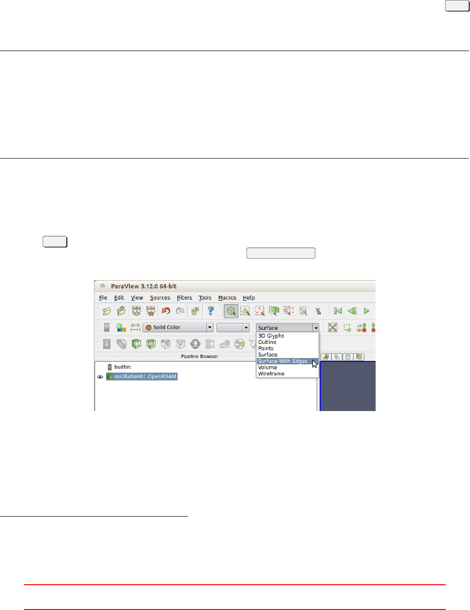
40.1 View the mesh
Besides viewing and post-processing simulation results, ParaView can be used to view the mesh. When refining
a mesh it is important to check neighbouring blocks for the transition of mesh fineness. Figure 26 in Section 17
shows an example how ParaView displays a mesh.
Pitfall: default selection
If a user works on the refinement of the mesh and the definition of boundary conditions has not been made,
then calling ParaView can crash because of its default selection of the pressure field. After pressing the Apply
button ParaView tries to read in all selected fields. In case of a faulty definition of the boundary fields, this
ends in the termination of the program. Listing 274 shows a corresponding error message.
--> FOAM FATAL IO ERROR :
key word bo ttom is u nd ef in ed in d ic ti on ar y "/ ho me / us er / O penF OA M / user -2. 1. x / run / i coFo am / cas e01
/0 / p :: b ou n da r yF ie l d "
fi le : / home / user / O pe nF OAM / user - 2.1. x / run / i co Foam / c ase0 1 /0 /p :: b ou nd ar yFi el d from line 25 to
line 35.
From fu nction d ictio nary :: subDic t ( const w ord & key word ) const
in file db / dic tionary / dicti ona ry . C at line 461.
FOAM exiting
Listing 274: Reading error due missing boundary field definition
Viewing the mesh
In this case the pressure field has to be manually unselected. If no fields are selected, paraView only reads
the mesh information. Therefore, it is possible to view the mesh without the rest of the case properly set up.
After the Apply button has been pressed and paraView has read all the data, the user has to choose from the
representation drop-down menu in the toolbar the option Surface with edges .
Figure 67: Select the proper representation to view the mesh
41 postProcess
With OpenFOAM-4.0 the function object framework was rewritten. In the course of this rewrite a postProcess
utility was introduced and a postProcess option was added to most of the solvers115. The postProcess utility
also supersedes certain post-processing utilities, e.g. sample.
115Counting the solvers with find $FOAM_SOLVERS -name ’files’ | xargs grep ’EXE’ | wc yielded a number of 82 solvers, of
which 73 included the postProcess.H header file, which provided the postProcess option. The second number was determined with
the following command: find $FOAM_SOLVERS -name ’*.C’ | xargs grep ’\#include[[:space:]]\"postProcess.H\"’ | wc.
VI This offering is not approved or endorsed by ESI®Group, ESI-OpenCFD®or the OpenFOAM®
Foundation, the producer of the OpenFOAM®software and owner of the OpenFOAM®trademark. 204

41.1 Usage
41.1.1 Pre-configured function objects
There are a number of pre-configured function objects, which are ready to use with postProcess. These
can be found in $FOAM_ETC/caseDicts/postProcessing. They can also be listed using the -list option of
postProcess.
use r@host :∼$ p o st Pro ce s s - l is t
Listing 275: Determine the extrema by magnitude of a velocity field
41.1.2 Passing parameters
Listing 276 shows how to determine the mininum and maximum magnitude of a velocity field.
use r@host :∼$ p os tP roces s - field s ’( U. w ater ) ’ - func " m in Ma xM ag ni tu de ( U. water )"
Listing 276: Determine the extrema by magnitude of a velocity field
Listing 277 shows how to process two velocity fields at once, we simply pass the names of the fields in a
comma-separated list.
use r@host :∼$ p os tP roces s - field s ’( U. air U . water )’ - func " minM ax Ma gn it ud e (U.air , U. wate r )"
Listing 277: Determine the extrema by magnitude of two velocity fields
In Listing 278 we process a single velocity field and pass additional parameters to the function object. In
this case, we do not want to know the location of the minimum and maximum velocity magnitude.
use r@host :∼$ p os tP roc es s - fi el ds ’(U. air ) ’ - func " m inM ax Mag nit ud e ( U.air , l oc at io n = of f )"
Listing 278: Determine the extrema by magnitude of a velocity field with no location
After running our function objects, we see that data was written into the postProcessing directory. We note
that the folder names correspond to the argument passed via the -func option.
use r@host :∼$ ls postProcessing
m in M a xM a gn i t ud e ( U . air , l oc at i on = o ff ) m i nM a x Ma g ni t u de ( U . air , U . w at e r )
Listing 279: The contents of the postProcessing directory after running two function objects from the above
listings
VI This offering is not approved or endorsed by ESI®Group, ESI-OpenCFD®or the OpenFOAM®
Foundation, the producer of the OpenFOAM®software and owner of the OpenFOAM®trademark. 205

Part VII
External Tools
Besides paraView, there are a number of other useful tools, which do not come from the OpenFOAM Foundation.
This section will cover such tools.
42 pyFoam
pyFoam is a collection of useful Python116 scripts. These scripts are mostly written to serve one specific task.
Further information can be found at http://openfoamwiki.net/index.php/Contrib_PyFoam.
42.1 Installation
The installation of pyFoam is described at http://openfoamwiki.net/index.php/Contrib_PyFoam#Installation.
The major prerequisite for the use of pyFoam is, that a Python interpreter is installed. To check if a Python
interpreter is installed on the system, simply type python --version in the Terminal. If a version number is
displayed, like Python 2.7.3, then Python is installed. Otherwise, the operating system would display an error
message, stating that the command python can not be found.
Further information about Python are found at http://python.org/ and http://docs.python.org/.
42.2 pyFoamPlotRunner
The script pyFoamPlotRunner starts a simulation and plots the residuals like Fluent would do.
use r@host :∼/ O pe nF O AM / use r - 2. 1. x / run / t wo P ha s eE ule r Fo am / c ol um n Ca se $ py F oa m Pl o tR unn e r . py
twoPhaseEulerFoam
Listing 280: Calling pyFoamPlotRunner
42.2.1 Plotting options
Listing 281 shows the plotting options offered by pyFoam.
What to plot
------------
Pre def ine d qu ant iti es that the pr ogram lo oks for and plots
-- no - d ef au lt S wi tc h off the d ef ault pl ots ( l ine ar , con ti nui ty and
bound )
-- no - li near Don ’t plot the lin ear solver co nverg ence
-- no - c ontinuit y Don ’t plot the c onti nuity info
-- no - bo und Don ’ t p lot the bo undi ng of v ar iabl es
-- with - ite rat ion s Plot the n umber of itera tio ns of the line ar so lver
-- with - c oura nt P lot the courant - n umbe rs of the flow
-- with - execution Plot the execution time of each time - step
-- with - d el tat ’ Pl ot the timestep - si ze time - s tep
-- with - a ll S witc h a ll p os si bl e pl ot s on
Listing 281: Plotting flags of the pyFoamPlot* utilities
42.3 pyFoamPlotWatcher
The script pyFoamPlotWatcher is intended to visualize solution data (e.g. residuals, time steps, Courant number,
etc.) after the simulation has finished. This requires that the solver output is written into a file, see Section
10.1.1.pyFoamPlotWatcher does essentially the same job as pyFoamPlotRunner with the difference that the
former tool is for finished simulations and the latter monitors a running simulation. So the description of the
features of pyFoamPlotWatcher holds also true for pyFoamPlotRunner.
116Python is an interpreted programming language.
VII This offering is not approved or endorsed by ESI®Group, ESI-OpenCFD®or the OpenFOAM®
Foundation, the producer of the OpenFOAM®software and owner of the OpenFOAM®trademark. 206
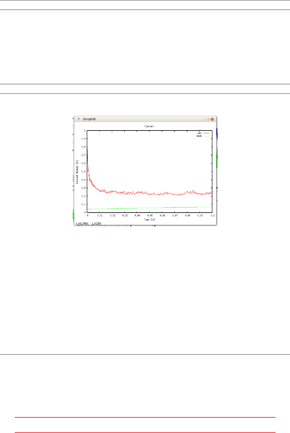
use r@host :∼/ O pe nF O AM / use r - 2. 1. x / run / t wo P ha s eE ule r Fo am / c ol um n Ca se $ py F oa m Pl o tW a tc her . py LO GF IL E
Listing 282: Calling pyFoamPlotWatcher
By default pyFoamPlotWatcher plots the curves of the residuals, continuity information and bounded vari-
ables. With options several other curves can be plotted (e.g. time step, iterations, Courant number, etc.). With
regular expressions user specified data can be extracted from the log file.
Listing 283 shows the invokation of pyFoamPlotWatcher to plot additionally to the default selection also the
Courant number. The processing of the solver output stored in the file LOGFILE is limited with the option --end
with a specific value – 0.1 s in this case. There is also a --start option. The plot created by the command in
Listing 283 is shown in Figure 68.
p yF o am P lo t Wa t ch e r . py LO GF IL E - - end = 0. 1 - - with - c ou ra nt
Listing 283: Calling pyFoamPlotWatcher with some options
Figure 68: The Courant number plotted with pyFoamPlotWatcher.
42.3.1 Custom regular expressions
With regular expressions pyFoamPlotWatcher can extract arbitrary data from the solver output. This section
elaborates this feature by the example of plotting the Courant number based on the relative velocity of a
two-phase solver.
General information
pyFoamPlotWatcher has no option to display the history of the Courant number based on Ur, the relative velocity
between the phases. Listing 284 shows some lines of the solver output of the two-phase solver twoPhaseEuler-
Foam. The line in red displays the Courant number based on the relative velocity Ur. The line above the
red colored line displays the Courant number based on the mixture velocity, see Section 48.6.4 and 48.6.4
for information on the definition of the Courant number and the Courant number of the two-phase solver
twoPhaseEulerFoam.
DIL UPBiCG : So lvin g for k , Ini tial residual = 0.000 8249 21 , Fi nal res idua l = 1 .47595 e -06 , No
Ite rat ion s 2
Exe cuti onT ime = 70870.7 s ClockTime = 71186 s
Cal cul ating averages
Coura nt Num ber mean : 0 .10 3485 max : 0 .42 251 7
Max Ur Courant Number = 0.448791
deltaT = 0.0 038 092 9
VII This offering is not approved or endorsed by ESI®Group, ESI-OpenCFD®or the OpenFOAM®
Foundation, the producer of the OpenFOAM®software and owner of the OpenFOAM®trademark. 207
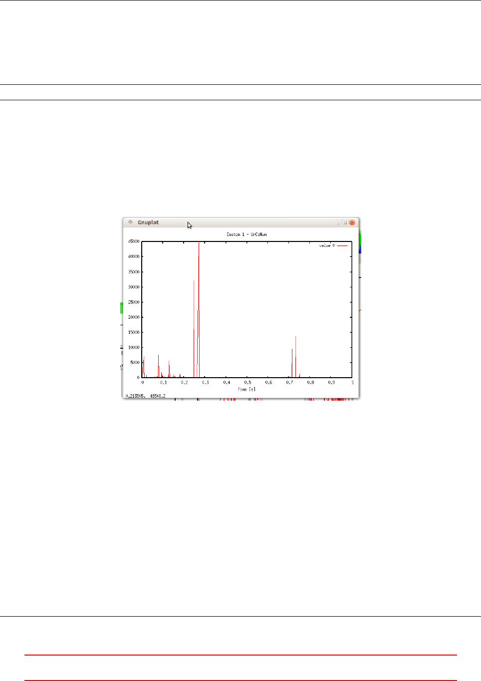
Time = 72. 584 8
MULES : Solvi ng for alpha1
MULES : Solvi ng for alpha1
Listing 284: Some lines of the solver output of twoPhaseEulerFoam
Extracting the information
To extract the information from the log file we need to create a file containing the regular expression.
{" e xpr ": " Max U r C ou ra nt Num be r = (% f %) " ," n am e ":" U rC oN um "}
Listing 285: The file customRegexp
If pyFoamPlotWatcher finds a file named customRegexp in the case directory, this file will be processed
automatically. If the file containing the regular expression has another name or is located inanother place the
option --regexp-file=REG_EXP_FILE can be used to specify the path to that file.
Listing 285 contains comma seperated entries ("expr" and "name"). The values are seperated by a colon
from the name of the entries (e.g. "name":"UrCoNum"). The first entry contains the regular expression to
extract the data. The second provides the name of the extracted data, but this entry can be omitted.
Figure 69: The Courant number based on the relative velocity plotted with pyFoamPlotWatcher
The absurdly high value of the Courant number indicates that the simulation did not go well. The need
for plotting the Courant number based on Ur emanated from a trouble-shooting episode. Thus this section was
written to preserve the gained knowledge.
42.3.2 Custom regular expression revisited
The plotting utilities of pyFoam (pyFoamPlotRunner and pyFoamPlotWatcher) accept custom regular expres-
sions also in a different format than the format of Listing 285. This new format was introduced with version 0.5.3.
See http://openfoamwiki.net/index.php/Contrib_PyFoam#Plotting_with_customRegexp-files for fur-
ther information. The new format looks resembles an OpenFOAM dictionary.
Listing 286 shows an example of the solver output that will be post-processed. The goal is to draw curves of
the quantities of the red line. Listing 287 shows the corresponding regular expression. The plotting utilities of
pyFoam offer the --dump-custom-regegexp option to generate the custom regular expression in the new format
from the old format. Listing 288 is the result of this operation.
DIL UPBiCG : So lvin g for beta , I niti al re sidu al = 0.00030 7666 , Final res id ual = 7.3 6162 e -08 , No
Ite rat ion s 2
VII This offering is not approved or endorsed by ESI®Group, ESI-OpenCFD®or the OpenFOAM®
Foundation, the producer of the OpenFOAM®software and owner of the OpenFOAM®trademark. 208

DIL UPBiCG : So lving for T , Initia l resi dua l = 0.000514273 , Final r esi dua l = 2.572 79e -07 , No
Ite rat ion s 1
Concentration = 0.0509085 Min T = 0.00498731 Max T = 0.218343
Bubble load = 0.0062 319 8 Min beta = 0 Max beta = 0.0677904
Time = 1 9.96
Listing 286: Some lines of the solver output to post-process
{" e xpr ": " C o nc e nt ra t io n = ( % f %) M in T = (% f %) M ax T = ( % f %) " ," n am e " :" C o nc en t ra t io n " ," t it le s
": [" avg " ," min " ," max "]}
Listing 287: The custom regular expression in the odl format
Custom01
{
accumulation first;
enabled yes;
ex pr " C o nc ent r at io n = ( % f %) Min T = (% f %) Max T = (% f %) ";
name Cus to m01_ Co ncen trat io n ;
persist no;
raisit no;
theTitle " C ustom 1 - C on ce nt ratio n ";
titles
(
avg
min
max
);
type re gula r ;
wi th lin es ;
xla bel " Time [ s ]" ;
}
Listing 288: The custom regular expression in the new format
42.3.3 Special treatment of certain characters
Note that the solver output we processed so far contained no parentheses. The parentheses are interpreted by
the regular expression. In order to deal with parentheses in the solver output they need to be escaped properly.
The same is true for brackets. So the following example is also valid, when brackets are contained in the solver
output that is to be processed with regular expressions.
Listing 289 shows some lines of solver output of twoPhaseEulerFoam. The line marked in red contains
parentheses. In order to post-process these lines with regular expressions these parentheses need to be escaped
in the regular epxression. Listing 290 shows the corresponding regular expression. Note the escaped parentheses
marked in red.
Time = 19. 995 7
MULES : Solvi ng for alpha1
MULES : Solvi ng for alpha1
Dispersed phase volume fraction = 0.0168317 Min(alpha1) = 3.92503e-87 Max(alpha1) = 0.2
GA MG : Solving for p , I niti al re sidual = 9.4 6269 e -05 , Final resid ua l = 1.6 57 11 e -06 , No
Ite rat ion s 1
ti me step con ti nu ity e rrors : sum l ocal = 2 .088 26 e -05 , g loba l = 4.5157 4e -08 , c um ul ative =
-0.0334048
Listing 289: Some lines of the solver output of twoPhaseEulerFoam
{" e xpr ": " D i sp er sed ph as e v olu me fr ac tio n = (% f % ) M in\(alpha1\) = ( % f %) M ax\( alpha1\) = (% f %)
" ," n am e ":" V ol um e f ra ct io n " ," t it le s " :[ " avg " ," min " ," ma x "]}
Listing 290: The regular expression to extract the information about the volume fraction
Not only the parentheses have a special meaning in regular expressions. An internet search117 or detailed
knowledge on regular expressions will yield the knowledge which characters have to be escaped.
117E.g. http://stackoverflow.com/questions/399078/what-special-characters-must-be-escaped-in-regular-expressions
VII This offering is not approved or endorsed by ESI®Group, ESI-OpenCFD®or the OpenFOAM®
Foundation, the producer of the OpenFOAM®software and owner of the OpenFOAM®trademark. 209
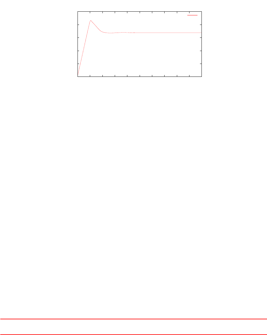
42.3.4 Ignoring stuff
Listing 290 extracts three numbers from the line marked in Listing 289. Using this regular expression plots all
three curves. If we are interested in only the first number – the average volume fraction – we replace the second
and third (%f%) with a .+ to ignore the second and third number. In this special case this seems an overkill
– we could also delete parts of the expression since we are only interested in the first number – but if we are
interested in the first and the third number, then we need to ignore the second number.
42.3.5 Producing images
The Figures 68 and 69 are screenshots of the images plotted by pyFoamPlotWatcher. However, there is the
option --hardcoded that tells the pyFoam plot utilities to save the plots on the disk. By default a PNG image
is produced but with the option --format-of-hardcopy=HARDCOPYFORMAT other formats can be chosen.
Figure 70 shows the plot produced by the regular expression of Listing 290.
0
0.005
0.01
0.015
0.02
0.025
0 2 4 6 8 10 12 14 16 18 20
Time [s]
Custom 1 - Volume fraction
avg
Figure 70: The average volume fraction plotted with pyFoamPlotWatcher and a custom regular expression
42.3.6 Writing data
Producing images is often not enough for post-processing. The option --write-files causes pyFoam to write
the extracted data to the hard drive. Thus the extracted data can be processed by other programs.
42.3.7 Case analysis
The option --with-all generate a number of plots that can be helpful to examine the performance of simulation
case. See Listing 281 for an explanation of the available plots.
VII This offering is not approved or endorsed by ESI®Group, ESI-OpenCFD®or the OpenFOAM®
Foundation, the producer of the OpenFOAM®software and owner of the OpenFOAM®trademark. 210
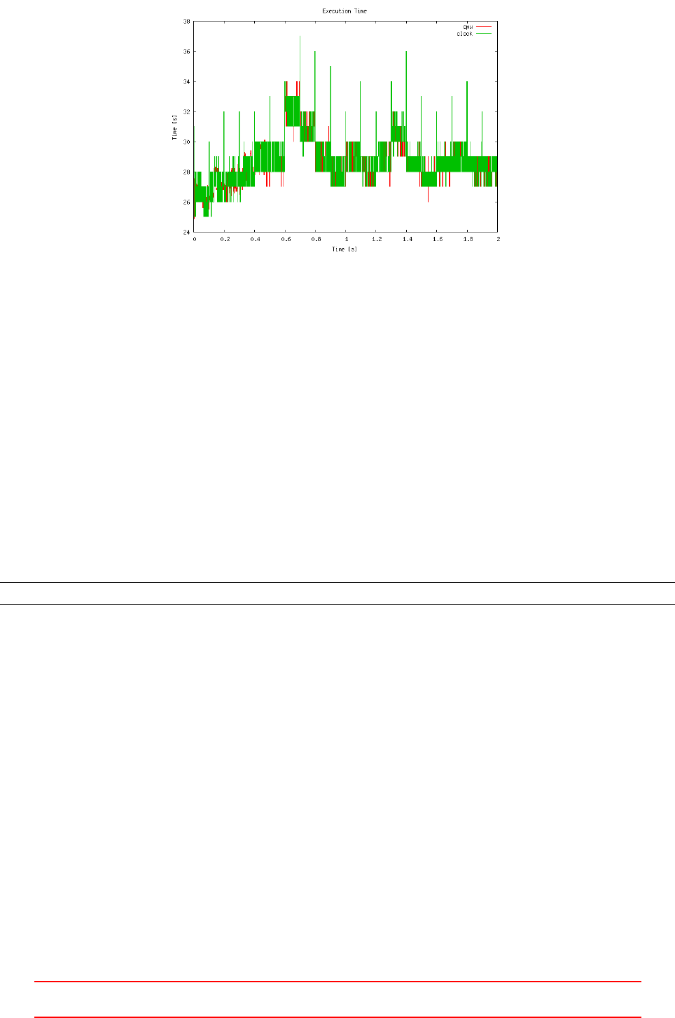
Figure 71: The execution time plotted over time with pyFoamPlotWatcher. The occasional writing of the data
to harddisk are clearly visible as spikes in the execution time.
42.4 pyFoamClearCase
As the name implies, pyFoamClearCase cleans the case directory. This script deletes all time directories save
the 0directory. By the use of command line options, a finer control of the actions of pyFoamClearCase is
possible. Some of these options are:
–keep-last keep the last time step
–keep-regular keep all time steps
–after=T delete all time steps for t>T
–remove-processor delete the processor* directories
The script is invoked by typing its name in the Terminal. Listing 291 shows how this script is executed. The
options cause pyFoamClearCase to keep the last time directory and to remove all processor* folders.
p yF o am C le a rC a se . py . - -k eep - l as t - - remov e - p roc es s or
Listing 291: Calling pyFoamClearCase
Note the file ending .py after the name of the script. This ending indicates, that the script is written in Python.
It also indicates, that pyFoamClearCase is an executable script rather than a program on its own.
42.5 pyFoamCloneCase
This script is used to copy a case. By default the 0, the constant and the system directory are copied. Addi-
tionally, there are various command line arguments to control the operation of the script, e.g. copy also the
latest time step or the processor* directories.
42.6 pyFoamDecompose
This script is used to decompose the computational domain. Other than the tool decomposePar, this script
does not need an existing decomposeParDict. This script receives command line arguments, generates the
decomposeParDict and calls decomposePar.
In Listing 292 the script is called with two arguments. The first argument is the path to the case directory.
In this case the dot refers to the currect directory. The second argument is the number of sub-domains. From
this arguments, pyFoamDecompose creates a decomposeParDict. The first argument is necessary to tell the
script where to save the newly created file. The second argument is the most fundamental information for
domain decomposition – the number of sub-domains.
VII This offering is not approved or endorsed by ESI®Group, ESI-OpenCFD®or the OpenFOAM®
Foundation, the producer of the OpenFOAM®software and owner of the OpenFOAM®trademark. 211

There is a large number of additional arguments which allow to exert more control over the way the domain
is decomposed.
p yF o am Dec omp o se . py . 4
Listing 292: Invokation of pyFoamDecompose
Listing 293 contains the decomposeParDict created by the command of Listing 292.
//*********//
FoamFile
{
version 0.5;
forma t a scii ;
ro ot " ROOT ";
case " CA SE " ;
class dic tio nary ;
obj ect n ix ;
}
method scotch;
num berO f Sub d oma i ns 4;
scotchCoeffs
{
}
Listing 293: The file decomposeParDict generated by pyFoamDecompose decomposeParDict
The output of pyFoamDecompose is stored in the file Decomposer.logfile.
42.7 pyFoamDisplayBlockMesh
If there is a problem with mesh topology and one isn’t able to find the error in the blockMeshDict, this tool
can be of great help. pyFoamDisplayBlockMesh does exactly what the name of the tool suggests. It reads
blockMeshDict and displays the topology of the mesh. One might think, that that’s exactly what is described in
Section 13.6.2 (display the blocks with paraView). However, if the definition of the mesh is erroneous, blockMesh
will not create a mesh and paraView is therefore not able to display the blocks.
pyFoamDisplayBlockMesh is a tool that allows the user to visualise a faulty mesh. This is of great help
to find e.g. an error in the block definition, especially when there are more than one blocks. In Figure 72 a
screenshot of the GUI of this tool is shown. In the main panel the vertices and the edges are displayed. With
the two sliders below single blocks as well as patches can be marked and coloured. The local axes of a single
block are displayed as tubes labelled with the corresponding names of the axes.
The blocks shown in Figure 72 have a faulty definition, so blockMesh produces an error message instead of
creating a mesh. With the help of this tool, the cause for the error is easily found. The marked block should
be in the right part of the geometry, so vertex number 5 should not be part of this block.
VII This offering is not approved or endorsed by ESI®Group, ESI-OpenCFD®or the OpenFOAM®
Foundation, the producer of the OpenFOAM®software and owner of the OpenFOAM®trademark. 212
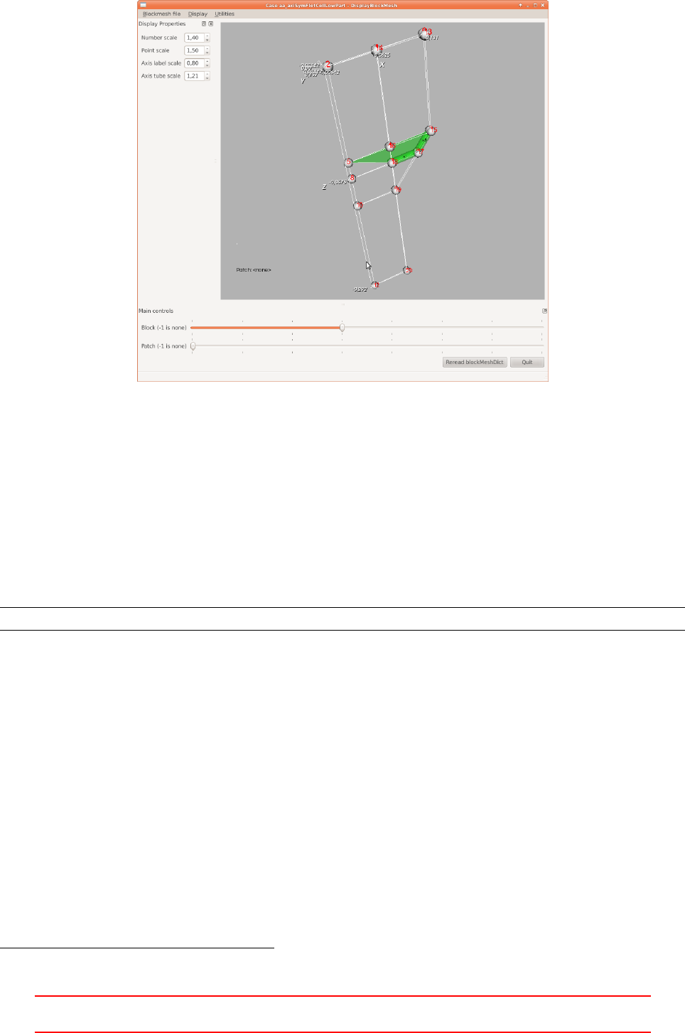
Figure 72: Screenshot of pyFoamDisplayBlockMesh
Right of the main panel the output of the standard meshing utilities blockMesh and checkMesh can be
displayed (not shown in the picture). These utilities can be executed from the menu of this tool. Moreover, the
blockMeshDict can be edited with this tool.
42.8 pyFoamCaseReport
The tool pyFoamCaseReport generates a summary of the simulation case. The amount of information displayed
can be controlled by command line flags. Listing 294 shows how to create a full summary of a case. However,
the full information lies within the dictionaries of the case. This tool provides only selected information.
p yF o am Cas e Re por t . p y --full - rep or t .
Listing 294: Create a summary of the case with pyFoamCaseReport
43 swak4foam
The name swak4foam comes from SWiss Army Knife for Foam.swak4foam evolved from a collection of tools
like groovyBC,funkySetFields and simpleFunctionObjects. The documentation of swak4foam is located at http:
//openfoamwiki.net/index.php/Contrib/swak4Foam.
43.1 Installation
To install swak4foam one needs to download the source code and compile them. The source code of swak4foam
is managed by the use of a subversion118 repository. Listing 295 shows how the source code is downloaded
by subversion. The first command changes the working directory of the terminal to ~/OpenFOAM. The second
command creates a directory named swak4foam. The third command changes the working directory of the
terminal to the newly created folder and the last commands actually downloads the source code to the current
directory.
118subversion, abbreviated SVN, is a version control software to manage software projects.
VII This offering is not approved or endorsed by ESI®Group, ESI-OpenCFD®or the OpenFOAM®
Foundation, the producer of the OpenFOAM®software and owner of the OpenFOAM®trademark. 213

cd ∼/OpenFOAM
mkdir swa k4f oam
cd swak4foam
sv n c he ck ou t htt ps :// o penfoam - e xten d . svn . sou rc ef org e . net / svn root / openfoam - e xten d / tr un k /
Bre ede r_2 .0/ librar ies / swak4Foam /
Listing 295: Installation of swak4foam
After downloading, the sources need to be compiled by calling Allwmake.
43.2 simpleSwakFunctionObjects
simpleSwakFunctionObjects is an extension of simpleFunctionObjects. The functions of this library are used to
post process data and extend functionality of OpenFOAM.
43.2.1 Extrema of a field quantity
If only the extrema of a field quantity are of interest, the tools of OpenFOAM (probes,sample) are of little use.
One way of solving this problem could be, to modify the solver to write the extrema to the standard output.
In Listing 296 some line of the standard output of twoPhaseEulerFoam are shown. This solver prints the mean
value as well as the extrema of the volume fraction of the dispersed phase. The corresponding lines of source
code can serve as a blueprint for a solver modification.
However, if the user is not inclined to modify and compile OpenFOAM solvers, simpleSwakFunctionObjects
provide the solution.
DIL UPBiCG : So lvin g for alpha , I niti al re sidual = 3.4 8391 e -05 , Final resid ua l = 2.9411 1e -12 ,
No I ter ati ons 2
Dis pe rs ed ph as e v ol um e fra ct io n = 0 .00 82 42 76 Min ( al pha ) = -1.66816e -19 Max ( alp ha ) = 0. 6
DIL UPBiCG : So lvin g for alpha , I niti al re sidual = 3.7 1563 e -07 , Final resid ua l = 8.1611 5e -14 ,
No I ter ati ons 2
Dis persed pha se v olum e fra ctio n = 0 .0 08 24 276 Min ( alpha ) = -3.31819e -19 Max ( alp ha ) = 0.6
Listing 296: Solver-Ausgabe von twoPhaseEulerFoam
swakExpression
The function to do the job is called swakExpression. This function is part of the library libsimpleSwakFunc-
tionObjects. Listing 297 shows how this function is set up as a function object in the file controlDict. In this
example the minimal value of the field alpha is saved. Notice the statement in last line of the Listing. This
statement tells the solver to use the specified library. This library contains the function swakExpression. See
Section 9.3.3 for further information about using external libraries.
functions
{
minAlpha
{
type swakExpression;
ver bose true ;
acc umul ati ons ( min );
val ueType int ernal Fie ld ;
exp re ss ion " mi n ( al pha ) ";
}
}
li bs (" l i bs i mp l eSw a kF u nc t io n Obj e ct s . so " ) ;
Listing 297: Definition of the function swakExpression in the file controlDict
VII This offering is not approved or endorsed by ESI®Group, ESI-OpenCFD®or the OpenFOAM®
Foundation, the producer of the OpenFOAM®software and owner of the OpenFOAM®trademark. 214
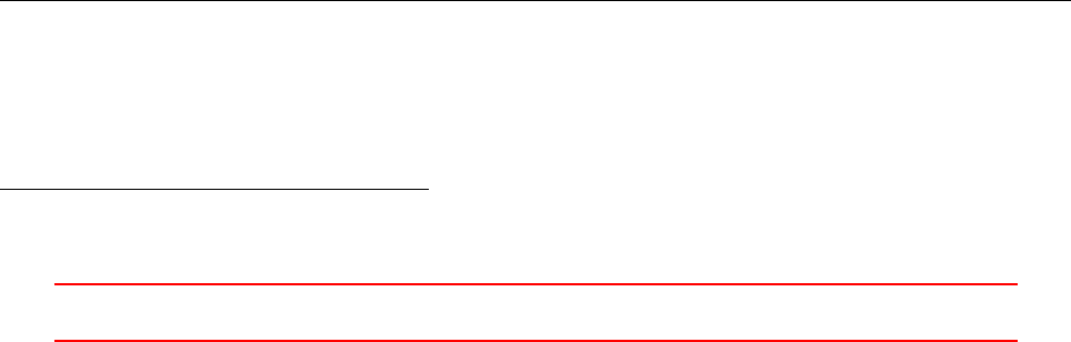
Keywords
This section explains the most important keywords of Listing 297.
type specifies the type the function object
verbose a switch that controls whether the generated data is to be printed on the solver output or not. The
data is written into a file anyway.
accumulations allowed entries: {min,max,average,sum}. Quote from the CFD-Online Forum119:accumu-
lations is only needed if you need ”a single number” to print to the screen. For instance if you use a
swakExpression-FO to print the maximum and minimum of your field to the screen.
valueType defines the type of the geometric region on which the function is applied. Allowed entries:
{internalField cellSet faceZone patch faceSet set surface cellZone}
expression defines the quantity that is sought for. This can be a simple statement or a formula computing a
quantity.
44 blockMeshDG
blockMeshDG is a modification of the meshing tool blockMesh to allow for double grading. Double grading
means, that the ratio between the discretisation length of the middle and the ends of an edge is prescribed.
This tool was developed by some users of OpenFOAM and is was published in the CFD-Online OpenFOAM
Forum (http://www.cfd-online.com/Forums/openfoam/70798-blockmesh-double-grading.html). There
is also a page in the OpenFOAM Wiki (http://openfoamwiki.net/index.php/Contrib_blockMeshDG).
44.1 Installation
The downloaded source code is ready for compilation after unpacking. All necessary entries have already been
made to prevent the new utility to collide with the standard utilities of OpenFOAM. The make script creates
an executable named blockMeshDG.
44.2 Usage
To discern between normal grading and double grading, the expansion ratio needs to be negative for double
grading120. A positive entry causes normal grading to be applied just like it is the case with the standard utility.
44.3 Pitfalls
44.3.1 Uneven number of cells
blockMeshDG obviously has a problem with an uneven number of cells. Figure 73 shows the resulting mesh,
when 15 cells are used for the double graded edge. In this case, although the mesh is of bad quality, checkMesh
reports no error. However, the output of checkMesh contains some indications that something is not alright.
Listing 298 shows some lines of the output of checkMesh. The very high aspect ratio is an indicator that
something is wrong with the mesh. Also the fact that the minimum and maximum values of face area or cell
volume differ by up to three orders of magnitude should lead to the same conclusion. Unfortunately, checkMesh
issues not even a warning message.
Checking geometry ...
Max asp ect ratio = 81 OK .
Minim um face area = 3.8 395 e -08. Ma ximum face area = 1.687 46e -05. F ace area m agn itu des OK.
Mi n v ol um e = 9 .5 987 5 e -11. Max vo lu me = 4 .2 18 64 e - 08. To ta l vol um e = 4 .9 22 14 e - 05. Ce ll
volumes OK.
Mesh non - ort hogonal ity Max : 42. 2304 a verag e : 11 .79 38
Non - o r th ogo nal ity ch ec k OK .
119http://www.cfd-online.com/Forums/openfoam/103504-swak4foam-calculating-velocity-transformations.html
120A negative entry unequal to unity causes blockMesh to crash with a floating point exception. Therefore, using negative entries
for double grading does not alter the standard behaviour.
VII This offering is not approved or endorsed by ESI®Group, ESI-OpenCFD®or the OpenFOAM®
Foundation, the producer of the OpenFOAM®software and owner of the OpenFOAM®trademark. 215
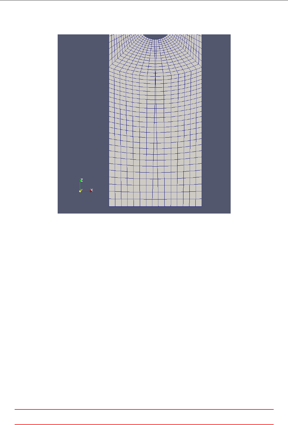
Mi n / ma x e dg e l en gt h = 3.0 79 e - 05 0 . 00 50 8 03 5 O K .
Listing 298: Some output of checkMesh
So far, the only solution to this problem is to use an even number of cells.
Figure 73: Double grading problem
VII This offering is not approved or endorsed by ESI®Group, ESI-OpenCFD®or the OpenFOAM®
Foundation, the producer of the OpenFOAM®software and owner of the OpenFOAM®trademark. 216

Naming scheme old new
Phase a b 1 2
Volume fraction alpha beta alpha1 alpha2
Velocity Ua Ub U1 U2
Density rhoa rhob rho1 rho2
Flux phia phib phi1 phi2
Table 7: Naming scheme of quanities of twoPhaseEulerFoam
Part VIII
Updates
45 General remarks
OpenFOAM is like any other open source project continuously updated. Those updates are integrated relatively
fast into the Git repository (e.g. OpenFOAM 2.1.x). In larger periods a new release of OpenFOAM is published
(e.g. OpenFOAM 2.1.1).
In the course of the creation of this document OpenFOAM evolves as well. In this chapter changes relevant
to this manual will be pointed out.
46 OpenFOAM
46.1 OpenFOAM-2.1.x
46.1.1 Naming scheme of two-phase solvers
The naming scheme of the two-phase solvers of OpenFOAM has been changed after the release of Version 2.1.1.
This change affected OpenFOAM-2.1.x around July 2012. The velocities used by two-phase solvers are now
named U1 and U2 instead of Ua and Ub. The volume fraction is consequently named alpha1. Other variables,
e.g. density, also bear the number of the phase (rho1 and rho2 ). Table 7shows a selection of old and new
names. The bold names are the names of files in the 0-directory.
46.2 OpenFOAM-2.2.x
This section describes changes in behaviour or usage of OpenFOAM-2.2.x compared to OpenFOAM-2.1.x.
46.2.1 fvOptions
The fvOptions mechanism is an abstraction to allow for a generic treatment of physical models. See http:
//www.openfoam.org/version2.2.0/fvOptions.php.
46.2.2 postProcessing
The data generated by a probes function object or by the sample utility is now stored in a folder named
postProcessing. This folder then contains a directory with the same name as the function object.
46.3 OpenFOAM-2.3.x
Although this manual is based on OpenFOAM-2.1 and OpenFOAM-2.2 this section lists some major differences
to OpenFOAM-2.3.
VIII This offering is not approved or endorsed by ESI®Group, ESI-OpenCFD®or the OpenFOAM®
Foundation, the producer of the OpenFOAM®software and owner of the OpenFOAM®trademark. 217

46.3.1 twoPhaseEulerFoam
There have been major changes with the two-phase Eulerian solver twoPhaseEulerFoam. Simulation cases of
OpenFOAM-2.1 or OpenFOAM-2.2 are not directly usable in OpenFOAM-2.3.
See Sections 34 and 35 on details about the twoPhaseEulerFoam solver.
VIII This offering is not approved or endorsed by ESI®Group, ESI-OpenCFD®or the OpenFOAM®
Foundation, the producer of the OpenFOAM®software and owner of the OpenFOAM®trademark. 218

Part IX
Source Code & Programming
47 Understanding some C and C++
In this Section some features of the C++ programming language are discussed.
47.1 Definition vs. Declaration
In C and C++ there is the destinction between the declaration and the definition of a variable. Briefly explained,
declaring a variable only tells the compiler that the variable exists and has a certain type. The declaration does
not specify what the variable actually is.
A definition also tells the compiler what exactly a variable is. This does not necessarily mean that the
variable is assigned a value.
Further information on that matter can be found in [45,27] or http://www.cprogramming.com/declare_
vs_define.html.
47.1.1 A classy example
In Listing 299 we define the class phaseInterface, i.e. we tell the compiler what the class looks like (data
members, methods, etc.). Within the class phaseInterface we want to use the class phaseModel. This class
already exists and is defined elsewhere, so there is no need for us to repeatedly define the class phaseModel.
Creating our own definition of phaseModel would be useless and stupid.
To be able to use the existing class phaseModel we need to introduce this class to the compiler. In Line 4
of Listing 299 we do exactly this. We tell the compiler, that there is a class named phaseModel, that is all the
information needed by now. This is sometimes referred to as forward declaration.
When we compile our class we need to make sure that we include the definition of phaseModel, e.g. via
linking to the library in which phaseModel is defined.
1namespace Foam
2{
3
4class phaseModel ;
5
6class phaseInterface
7{
8// lots of C ++ code
9};
10
11 }
Listing 299: Declaration and definition of classes
47.2 Namespaces
Namespaces are a feature of C++ to support a logical structure within the program. The basic idea behind
namespaces put in simple words is to keep things (variables and functions) visible where they need to be visible.
Like any other method of keeping things neat and tidy you could also survive without namespaces. However,
to loosely quote Prof. Jasak, one of the founders of OpenFOAM: OpenFOAM is an example of how to make
proper use of C++. Therefore, we have a closer look on namespaces in OpenFOAM.
General information about the concept of namespaces can be found here:
•http://www.cplusplus.com/doc/tutorial/namespaces/
•http://www.cprogramming.com/tutorial/namespaces.html
•http://www.learncpp.com/cpp-tutorial/711-namespaces/
Some OpenFOAM specific aspects related to namespaces are discussed in Section 48.2.
IX This offering is not approved or endorsed by ESI®Group, ESI-OpenCFD®or the OpenFOAM®
Foundation, the producer of the OpenFOAM®software and owner of the OpenFOAM®trademark. 219

47.3 const correctness
The const keyword has several uses and using const has some implications.
47.3.1 Constant variables
This is the most easy part. Any variable can be declared constant by using the const keyword. This can
precede the datatype or the variable name. Both lines in Listing 300 are correct statements.
const int li mit = 5;
int const answe r = 42;
Listing 300: Constant variables
47.3.2 Constants and pointers
Pointing to a constant
A pointer can be used to point to a constant variable. The pointer itself is not constant and therefore change-
able. However, the keyword const has to be used when declaring a pointer pointing to a constant variable.
However, a pointer pointing to a constant can also point to a non-constant variable.
int const constVar1 = 42;
const int con stV ar2 = 13;
int va ria ble = 11;
const i nt * poi nter = & c onstVar1 ;
std :: cout << " T he p oi nt er poin ts to " << * p oi nter << std :: endl ;
// cha nge the pointe r
point er = & constVar2 ;
std :: cout << " T he p oi nt er poin ts to " << * p oi nter << std :: endl ;
// point to a non - const ant
point er = & variab le ;
std :: cout << " T he p oi nt er po ints to " < < * p oint er << std :: endl ;
Listing 301: Pointing to constant variables
The pointe r p oints to 42
The pointe r p oints to 13
The pointe r p oints to 11
Listing 302: Output of Listing 301
A constant pointer
A pointer can be constant regardless of the variable it points to. So, the address stored in the pointer can not
be changed, the pointer will always point to the same variable. However, the variable itself can be altered.
Listing 303 shows an example.
int va ria ble = 11;
in t *const co ns tPo in ter1 = & v aria ble ;
std :: cout << " T he c on st an t poi nt er po in ts to " << * c on stP oi nt er 1 << std :: e ndl ;
variable = 79;
std :: cout << " T he c on st an t poi nt er po in ts to " << * c on stP oi nt er 1 << std :: e ndl ;
Listing 303: Using constant pointers
IX This offering is not approved or endorsed by ESI®Group, ESI-OpenCFD®or the OpenFOAM®
Foundation, the producer of the OpenFOAM®software and owner of the OpenFOAM®trademark. 220

The constant p ointe r points to 11
The constant p ointe r points to 79
Listing 304: Output of Listing 303
A constant pointer to a constant
It is also possible to create a constant pointer pointing to a constant variable.
However, the last line of Listing 305 seems a bit unlogical but it isn’t. To get the meaning of this line
correctly, we need to read the left hand side of the assignment from right to left. First of all constpointer4
is the name of the new variable. Secondly, int* const tells the compiler that the new variable is a constant
pointer to an integer. This means, that the pointer itself – the location it points to – can not be changed. The
last statement const at the very beginning of the line, means, that the variable the pointer points to can not
be changed. However, variable is not a constant, so it can be altered anyway. The last line of Listing 305
does not change the nature of the variable variable, but it restricts the pointer to read-only operations. So,
variable can be changed, but not using constPointer4.
int const constVar1 = 42;
int va ria ble = 11;
const i nt *cons t con st Point er2 = & constV ar1 ;
const i nt *cons t con st Po inter 4 = & variable ;
Listing 305: A constant pointer to a constant
47.4 Function inlining
Motivation
Functions that carry out only a small number of operations are not very efficient, because the function call
might take more time than the execution of all the operations. Especially if such a function is often called, the
performance of the program suffers. However, writing functions is a good way to keep the code tidy.
On the one hand, functions enable the programmer to seperate code in a logical way. Code that is written
for a specific task is outsourced into a function with a hopefully meaningful name. This improved readability
and maintainability of the code.
One the other hand is writing functions a proper way to avoid code redundancy. Tasks that are carried out
repeatedly are best put into a function. Therefore, the code has to be written only once and the function can
be used wherever it is necessary.
The inline statement
The solution for this conflict is function inlining. The inline statement allowes the compiler to replace the
function call with the function body, i.e. the operations performed by the function. This enables the programmer
to keep the code tidy without the disadvantage of wasting time for time consuming function calls.
Listing 306 shows the definition of an inline function. The function body contains only two logical oper-
ations. The inline statement precedes the data type of the return value. So, writing inline functions is not
different than writing ordinary functions.
inline bool F oam :: pimpleC ontr ol :: fin alI ter () const
{
return con ve rged_ || ( corr_ == n Co rr PI MP LE _ );
}
Listing 306: The definition of an inline function
The use of the inline statement does not guarantee that the compiler replaces the function call. This depends
on the compiler and the compiler settings.
IX This offering is not approved or endorsed by ESI®Group, ESI-OpenCFD®or the OpenFOAM®
Foundation, the producer of the OpenFOAM®software and owner of the OpenFOAM®trademark. 221

OpenFOAM specifics
The OpenFOAM Code Style Guide (http://www.openfoam.org/contrib/code-style.php) demands from
programmers to seperate the definition of inline and non-inline functions.
Use inline functions where appropriate in a separate classNameI.H file.
Listing 307 shows the contents of the folder pimpleControl. Dividing the code of a program or a module
into *.C and the *.H file is the common way to seperate declarations from the rest of the program. The *.dep
file is generated by the compiler during compilation. The fourth file in the folder is a second header file as
demanded by the Code Style Guide. Listing 306 is a part of pimpleControlI.H.
pimpleControl.C pimpleControl.dep pimpleControl.H pimpleControlI.H
Listing 307: Content of the folder pimpleControl
47.5 Constructor (de)construction
In object oriented programming (OOP) everything is an object. All object are created by a constructor and if
necessary destroyed by a destructor.
47.5.1 General syntax
The constructor is a method of a class like any other function or method121. However, the constructor is bound
to comply some rules.
•The constructor always has the same name as its class
•The constructor has no return value
Listing 308 shows a simple class describing a point in a two-dimensional domain. This class has two construc-
tors. The first constructor receives no arguments and initialises the member variables with zero. The second
constructor receives two integer variables as arguments and uses this variables to initialize the member variables
xPos and yPos.
Writing two or more constructors is possible because C++ supports function overloading. This means there
can be several functions with the same name differing in the input arguments.
1class Point
2{
3int xPos;
4int yPos;
5
6public:
7Point ()
8{
9/* c onstruc tor code */
10 xPos = 0;
11 yPos = 0;
12 }
13 Point ( int x , int y)
14 {
15 xPos = x;
16 yPos = y;
17 }
18 };
Listing 308: A class for a 2D point
121The terms function and method are used interchangeably. However, the method indicates the use of object oriented program-
ming. The term function is also used in procedural programming and does not automatically indicate the use of OOP.
IX This offering is not approved or endorsed by ESI®Group, ESI-OpenCFD®or the OpenFOAM®
Foundation, the producer of the OpenFOAM®software and owner of the OpenFOAM®trademark. 222

Listing 309 demonstrates hot to create new variables of the type Point. The first line creates a variable of
the type Point. Because no arguments are passed in this line, the first constructor of Listing 308 is called by
the compiler.
The second line creates also a point. The numbers inside the parenthesis are passed to the constructor.
Therefore the second constructor of Listing 308 is called and the member variables are initialised based on the
arguments.
1Poi nt p1 ;
2Poi nt p2 ( 3 , 8) ;
Listing 309: Using the class for a 2D point
47.5.2 Copy-Constructor
The copy constructor is used to create a copy of an object. The C++ compiler will create a default copy con-
structor if the programmer does not write one. However, the default copy constructor has restrictions regarding
the handling of complex classes.
1Point :: Point ( Point & p )
2{
3/* copy constru cto r cod e */
4xP os = p . xPo s ;
5yP os = p . yPo s ;
6}
Listing 310: The copy constructor for the 2D point class
Hiding the copy constructor
A copy constructor can be hidden. Therefore, no copying is allowed. To do so, the copy constructor must be
defined using a private modifier.
Listing 311 shows a simple example of a copy constructor that is declared as private. This means the copy
constructor can only be called from within the class itself, i.e. only within the class Point.
Listing 312 shows an example from within the source code of OpenFOAM. There, the copy constructor of
the class turbulenceModel is hidden by declaring it private.
1class Point
2{
3private:
4Point ( Point & p );
5};
Listing 311: Hiding the copy constructor
1class turb ulen ceM odel
2:
3public regIOobject
4{
5private:
6// Pri vate Mem ber Fu nct ion s
7
8// - D isallow defau lt bi twis e co py c on struct
9tur bu le nce Mo de l ( cons t t ur b ul enc e Mo del & ) ;
10
11 /* code con tin ues */
Listing 312: Hiding the copy constructor
IX This offering is not approved or endorsed by ESI®Group, ESI-OpenCFD®or the OpenFOAM®
Foundation, the producer of the OpenFOAM®software and owner of the OpenFOAM®trademark. 223

47.5.3 Initialisation list
A class in C++ can have member variables of any type. Complex classes may need some kind of initialisation
to ensure all variables have a defined state. When an instance of a class is created by the constructor, the
initialisation list contains all statements to initialise member variables of the class.
Listing 313 shows a simple example of a constructor with an initialisation list. Listing 410 in Section 52.2.2
shows an usage example of an initialisation list in the OpenFOAM sources.
1class Rec tan gle
2{
3Point topL eft ;
4Point bo ttomRigh t ;
5
6public:
7Rec tan gle ()
8{
9t op Le ft = P oi nt () ;
10 b ot to m Ri gh t = P oi nt () ;
11 }
12
13 R ec ta ngl e ( P oi nt a , P oi nt b )
14 :
15 topLeft(a),
16 bot tomRight ( b)
17 {
18 /* c onstruc tor code */
19 }
20 }
Listing 313: A constructor with an initialisation list
47.6 Object orientation
47.6.1 Abstract classes
See Section 48.10 for a discussion about the implementation of the generic turbulence models in OpenFOAM.
This generic turbulence modelling makes heavy use of abstract classes and inheritance.
47.7 Templates
OpenFOAM makes heavy122, clever use of templates. Templates are a language feature of C++ that allow for
generic programming. An illustrative example for the use of templates in programming is the implementation
of container classes, e.g. linked lists. Without the use templates, the multiplicity of possible container contents
would force us to implement a vast number of specialized classes, e.g. nodeList,faceList and cellList for
lists of nodes, faces and cells.
Such a problem could be solved by the use of multiple inheritance. This way, we would need to implement
one base class for a list. The specialized classes would then inherit from the base list class and from the class
of the intended content. This solution, however, has several disadvantages [4]. As complexity grows, the path
via multiple inheritance is doomed to become a problem in its own, instead of alleviating or solving the original
problem.
Templates offer us a way to tell a class: use the type T, which can be any type the compiler allows. Thus,
we create one templated container class. Later, when we need to create lists of nodes, faces and cells, we tell
the compiler to substitute Tfor the concrete types. The compiler then generates the appropriate code. Checks
done by the compiler ensure, that specializing a valid templated class produces little to no surprises.
Listing 314 shows the use of templates. We first implement a generic list. Later, we specialize this list for
the types of nodes, faces and cells. The typedef instruction allows us to define a conveniant name. Once this
names are defined, we may even stop being aware that we are using a templated class.
122The command find $FOAM_SRC -name ’*.[CH]’ | xargs grep ’template’ | wc yields 24646 occurances of the word template
in $FOAM_SRC. This makes 12323 occurances within the source code itself – remember the presence and the use of the lnInclude
directories.
IX This offering is not approved or endorsed by ESI®Group, ESI-OpenCFD®or the OpenFOAM®
Foundation, the producer of the OpenFOAM®software and owner of the OpenFOAM®trademark. 224

t em pl at e < c la ss T >
class list
{
// def ine a list of type T
}
typed ef list < node > n ode Lis t ;
typed ef list < face > f ace Lis t ;
typed ef list < cell > c ell Lis t ;
Listing 314: Templated lists
OpenFOAM follows a similar strategy, who would guess from the top-level code, that volScalarField is in
fact a templated class with three template parameters, see Listing reflst:volScalarField. Besides being a more
convenient name123 we also save a lot of typing effort due to the shorter name124. The use of type definitions
–typedef statements – is not mere convencience. Using the full specialisation of GeometricField instead
of volScalarField translates to hardcoding. If the developers of OpenFOAM, at some point, decide to base
volScalarField on the class smartScalar instead of scalar, only one line of code needs to be changed instead
of thousands. Thus, the use of typedefs strongs supports code readability and maintainability [4].
typ ed ef Ge om etri cF ie ld < scal ar , fvP atch Fiel d , v olMes h > v olS ca lar Fi eld ;
Listing 315: The typedef defining volScalarField
47.7.1 Use of templates by OpenFOAM
Since this document is not a book on any specific topic, certain topics are adressed in a manner ranging from
structured to completely random. Templates have already been discussed in a number of sections, mostly de-
scribing the use of templates on specific code examples. Since, there is no fun and varying benefit in restructuring
a large document, we will give pointers to other sections in which templates are discussed:
We discuss the use of templates in Section 27.1 where we compare the implementation of turbulence modelling
in OpenFOAM. There is a non-templated implementation, which was superseded by a templated one starting
from the release of OpenFOAM-2.3.0.
We discuss the use of templates in Section 31 where we take a look at the implementation of Lagrangian
particle tracking with a little excursion to the topic of linked lists.
The use of templates is also discussed in Section 48.3.2 at the example of keyword lookup from dictionary
files.
47.7.2 Do not fear the template
The syntax for templated code is different from the syntax encountered in non-templated code. Here we will
discuss some features of templated code, which may seem mysterious to the novice.
Template template parameter
In the introduction of this section, we stated, that the template parameter Tis a placeholder for a concrete
type. However, the template parameter may itself be a templated class. A templated template parameter is
referred to as template template parameter. We could avoid using template template parameters, however, they
help us to avoid code duplication and lead to safer code [4].
48 Under the hood of OpenFOAM
This section contains short code examples that in some way explain the behaviour of OpenFOAM in certain
situations. All examples in this section are motivated by other parts of this manual. In some cases the source
code of some applications is examined somewhere else.
123volScalarField field carries roughly the same essential information as GeometricField<scalar, fvPatchField, volMesh>.
124We count 15 versus 46 characters. With the command find $FOAM_SRC -name ’*.[CH]’ | xargs grep ’volScalarField’ |
wc we count 8752 occurances of volScalarField in the source code of OpenFOAM-dev at the time of writing. This leads to an
estimated 4376 occurances in the code itself.
IX This offering is not approved or endorsed by ESI®Group, ESI-OpenCFD®or the OpenFOAM®
Foundation, the producer of the OpenFOAM®software and owner of the OpenFOAM®trademark. 225
48.1 Solver algorithms
See Sections 32,33 and 34 in Part V.
48.2 Namespaces
48.2.1 Constants
Physics is full of constants. Therefore it would be nice to have a central location in which physical or mathe-
matical constants are defined. OpenFOAM provides constants within the namespace Foam::constant. There
the pre-defined constants are divided into the groups, such as
•electromagnetic
–mu0 - the magnetic permeability of vacuum
–epsilon0 - the electcial permittivity of vacuum
•physicoChemical
–R- the universal gas constant
•mathematical
–pi -π
–e- the Euler number
In Listing 316 it is demonstrated how to access the constant pi within the source code. Listing 317 shows all
the mathematical constants defined in OpenFOAM-2.2.x. From a computational performance point of view it
makes perfect sense to pre-define often used constants such as two pi. Also note that instead of diving pi by 2.0
it is multiplied with 0.5. Mathematically these operations are equivalent, however, in terms of computational
cost the floating point multiplication is to be preferred over the floating point division as it is much faster [1].
Also note that OpenFOAM does not define eand πon its own, it rather uses the constants provided by the
system library. See e.g. http://www.gnu.org/software/libc/manual/html_node/Mathematical-Constants.
html for the mathematical constants provided by the GNU C library (glibc). Thus eand pi are defined by
accessing M_E and M_PI.
Further note that the constants are declared with the const specifier, which is the only sane way to define
constants in C and C++.
1scalar foo = constant :: ma themati cal :: pi ;
Listing 316: A useless code example demonstrating the access to πwith OpenFOAM’s source code
1const s cala r e ( M_ E );
2const sca lar pi( M_PI ) ;
3const s ca la r t woPi ( 2* pi );
4const s ca la r p iB yT wo ( 0. 5* pi ) ;
Listing 317: The mathematical constants provided by mathematicalConstants.H
In the FOAM-extend the access to e.g. the mathematical constants works the same way. Only the namespace
is named mathematicalConstants instead of constant::mathematical. This is due to the fact that FOAM-
extend is largely based on OpenFOAM-1.6.
48.3 Keyword lookup from dictionary
There are generally two kinds of keywords in a dictionary. There are mandatory keywords and optional ones.
IX This offering is not approved or endorsed by ESI®Group, ESI-OpenCFD®or the OpenFOAM®
Foundation, the producer of the OpenFOAM®software and owner of the OpenFOAM®trademark. 226

48.3.1 Mandatory keywords
When a mandatory keyword is not found in a dictionary, OpenFOAM issues an error message and terminates.
Listing 318 shows the reading operation for three mandatory keywords. The function lookup() can be
examined further in Listing 319.
1#include "readTimeControls.H"
2
3int nA lp haCor r ( read Int ( pi mple . dict () . lo okup ( " nA lph aCo rr " )));
4int nA lp ha Su bC yc le s ( re adIn t ( pimp le . di ct () . looku p (" n Alpha Su bCy cl es " )));
5Switch c or re ct Alpha ( p imple . dict (). lo okup ( "correctAlpha"));
Listing 318: The content of readTwoPhaseEulerFoamControls.H
The code
Line 32 in Listing 319 shows, that the function lookup() simply calls value of lookupEntry(). This method
also calls another method (lookupEntryPtr()) and does the error handling. The error handling routine clearly
shows, that OpenFOAM will terminate in case the keyword wasn’t found (see line 19).
1const Foam :: en try & Foam :: dic tio nar y :: lookupE ntr y
2(
3const word & k eyword ,
4bool recursive ,
5bool patternMatch
6)const
7{
8const entry * ent ryPtr = lo okup Ent ryPt r ( keyword , recursive , p att ernM atc h );
9
10 if ( e nt ry Ptr == NULL )
11 {
12 FatalIOErrorIn
13 (
14 " d ic tion ar y :: loo ku pE nt ry ( c onst w ord &, bool , b ool ) con st " ,
15 *this
16 )
17 << "keyword " << k eyword << " is u nde fin ed in d ictionary "
18 << name ()
19 << exit(FatalIOError);
20 }
21
22 return * entryPtr ;
23 }
24
25 Foam :: I Tst ream & Foam :: dictio nar y :: lookup
26 (
27 const word & k eyword ,
28 bool recursive ,
29 bool patternMatch
30 )const
31 {
32 return l oo ku p En tr y ( keyw or d , r ec ursive , p a tt ern Mat ch ) . s tr ea m () ;
33 }
Listing 319: Some content of dictionary.C
48.3.2 Optional keywords
A method that is used to read an optional keyword from a dictionary is usually provided with a default value.
This default value is used in the case that the keyword is non-existent in the dictionary.
Listing 320 shows the reading operation for three optional keywords. The read function is called with two
arguments. The first is the keyword and the second is the default value. If the function lookupOrDefault()
finds no entry, then the default value is returned.
IX This offering is not approved or endorsed by ESI®Group, ESI-OpenCFD®or the OpenFOAM®
Foundation, the producer of the OpenFOAM®software and owner of the OpenFOAM®trademark. 227

1const bool adjustTimeStep =
2r un Ti me . c o nt rol Di c t () . l oo k up OrD e fa ult ( "adjustTimeStep",false ) ;
3scalar maxCo =
4r un Ti me . c o nt rol Di c t () . loo ku pO rDe fa ul t < s cal ar > ( " ma xC o " , 1.0) ;
5scalar m axD elt aT =
6r un Ti me . c o nt rol Di c t () . loo ku pO rDe fa ul t < s cal ar > ( " m ax De lta T " , GREAT ) ;
Listing 320: The content of readTimeControls.H
The code
Listing 321 shows the definition of the function lookupOrDefault(). This function also calls another function
to lookup the keyword – actually it looks for the value assigned to the specified keyword in the dictionary –
and enters a conditional branch. In case the keyword was found, the corresponding value is returned (line 14).
If the keyword was not found, then the default value is returned (line 18).
In Listing 321 the function is defined with four input arguments. However, in Listing 320 this function is
called with only two arguments.
The solution for this contradiction can be found in the file dictionary.H, where this function is declared.
This declaration can also be found in Listing 322. There, in lines 6and 7, default values for two arguments are
specified. Therefore, the function can be called with only two arguments – with the two arguments that have
no default value125. If the function is called with all its arguments, the passed argument overrides the default
value.
When declaring a function that uses default values for its arguments, the arguments without default value
must precede the arguments that have a default value. Otherwise, there could be ambiguity.
1template <class T >
2T Foam :: dictionary :: loo kupOr Defau lt
3(
4const word & k eyword ,
5const T & deflt ,
6bool recursive ,
7bool patternMatch
8)const
9{
10 const entry * ent ryPtr = lo okup Ent ryPt r ( keyword , recursive , p att ernM atc h );
11
12 if ( ent ryPtr )
13 {
14 return pT ra its < T >( en tr yP tr - > s tr eam () ) ;
15 }
16 else
17 {
18 return deflt ;
19 }
20 }
Listing 321: Some content of dictionaryTemplates.C
1template <class T >
2T loo kupO rDef ault
3(
4const word &,
5const T&,
6bool rec ur siv e = false ,
7bool patternMatch=true
8)const ;
Listing 322: Some content of dictionary.H
125The function could also be called with three argmuents, then the default value of the third argument would be overridden and
the fourth argument would have its default value.
IX This offering is not approved or endorsed by ESI®Group, ESI-OpenCFD®or the OpenFOAM®
Foundation, the producer of the OpenFOAM®software and owner of the OpenFOAM®trademark. 228
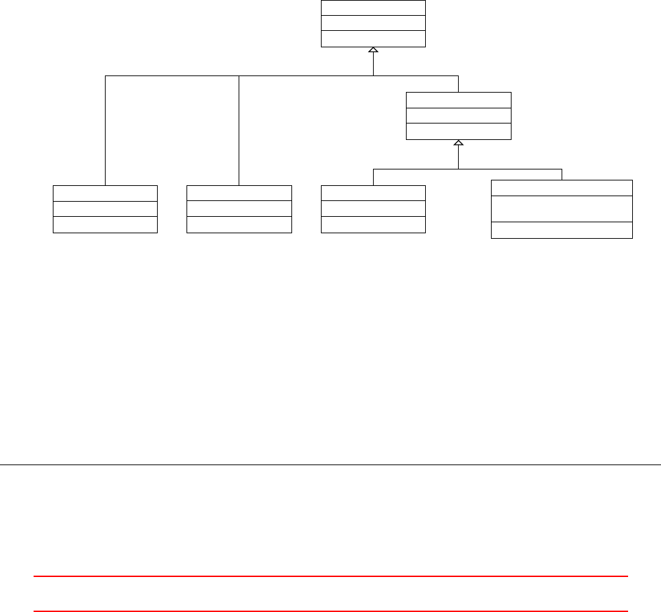
48.3.3 Superseding mandatory keywords
In some cases, a base class might demand the presence of a keyword, which some derived classes make use of
and others do not. This creates the situation that a keyword-value pair must be specified, which, depending on
the user’s choice, has an effect or not.
However, as the keyword is demanded by the base class, it remains mandatory, regardless of the derived
class’ behaviour. A derived class can not alter the behaviour of its base class. Thus, in some edge cases a
keyword-value pair has to be provided even though it does nothing.
The decision of how to distribute the necessary data among the base class and its derived classes may not
always be as straight forward. Apart from the two obvious limiting cases: data needed only by one specific
derived class, and data needed by all derived classes; the decision of what data to put where is up to the software
designers.
If a sufficient number of derived classes are very similar to eachother, then an intermediate base class might
be warranted. With an intermediate base class, data common to all classes derived from the intermediate base
class can be handed over to the intermediate base class. However, the class hierarchy of a certain model can
not always exactly reflect the inner logic of data usage of that model family.
In Figure 74 we see such an example of an intermediate base class. The data members shown in the class dia-
gram are read by their respective classes as mandatory entries. The base class InjectionModel reads the scalar
massTotal, which is used to determine how many particles to inject. However, some derived injection models
allow for a direct specification of the number of particles, thus rendering the mandatory value for massTotal
moot. In these cases, the injection model issues a warning message informing the user that massTotal has no
effect.
InjectionModel
scalar massTotal_
setPositionAndCell()
patchInjectionBase
word patchName_
PatchInjection
TimeFunction1<scalar>
flowRateProfile_
PatchFlowRateInjection
word phiName_
ManualInjection
word positionsFile_
CellZoneInjection
word cellZoneName_
Figure 74: Class hierarchy of some injection models for Lagrangian particles. An intermediate base class is used
to reduce code duplication from closely related, yet different injection models.
48.4 OpenFOAM specific datatypes
48.4.1 The Switch datatype
A lot of settings in dictionaries are switches to activate or deactivate a feature. Listing 323 shows the part of
the source code defining all valid values. Inside the source code a switch can only be true or false, as the class
Switch is used as a boolean data type. However, in the dictionaries a switch can have more values – provided
they denote a decision. Human languages usually have more ways of answering a yes-no question, this may be
the motivation for allowing this range of values for switches.
1// NB : val ue s c ho se n s uc h t ha t b it wi se ’& ’ 0 x 1 y ie ld s th e b oo l v al ue
2// I NVALI D is also e val uat es to false , but don ’t rely on that
3const c har * Foam :: Switch :: names [ Foa m :: Switc h :: INVALI D +1] =
4{
5" f al se " ," t rue ",
6" of f "," on " ,
7"no"," ye s ",
IX This offering is not approved or endorsed by ESI®Group, ESI-OpenCFD®or the OpenFOAM®
Foundation, the producer of the OpenFOAM®software and owner of the OpenFOAM®trademark. 229

8"n"," y " ,
9"f"," t " ,
10 " no ne " ," true " ,// is the re a r ea so na bl e cou nt erp ar t to " none "?
11 "invalid"
12 };
Listing 323: Some content of Switch.C
Listing 324 shows an example of how the Switch datatype can be used in the code. This example reads from
the transportProperties dictionary. If no valid entry named testSwitch is present, then the value of the
switch is set to false. Notice the second argument of the method lookupOrDefault(), it reads Switch(false).
This means, that a new object of the type Switch is created with the boolean value false being passed to the
constructor of the class Switch. This new object of type Switch is then used – if necessary – as default value
for the switch named testSwitch.
1Switch t estSwitch ( tra ns por tP roper ti es . lo okupOrDe fault < Switch >( " t es tSw it c h " , Switch(fals e )));
Listing 324: Usage example of the Switch datatype
48.4.2 The label datatype
When examining the solution algorithms, like in Section 33.2, counters can be found. OpenFOAM uses a
datatype called label for such counters, e.g. see Listing 207.
The following applies to versions prior to OpenFOAM-3.0
The most obvious datatype for a counter would be the integer datatype int. Listing 325 contains some lines of
the file label.H, where this datatype is defined. Depending on system or compilation parameters, label is of
the type int,long or long long126.
Listing 325 shows the definition of label in case int is used as the underlying datatype.
1namespace Foam
2{
3typedef int label ;
4
5static const label la belM in = I NT_M IN ;
6static const label la belM ax = I NT_M AX ;
7
8inline label readLabel ( Istre am & is )
9{
10 return r ea dI nt ( is ) ;
11 }
12
13 }// End n ame spa ce Foam
Listing 325: Some content of label.H
The following applies to versions from OpenFOAM-3.0 onwards
OpenFOAM offers, at the time of writing, essentially two choices for the size of the label datatype: 32 or 64
bit. This, essentially boils down to the decision of whether to use int32_t or int64_t. Since, the data types
int,long and long long only guarantee a minimum size127, the fixed-width integers128 int32_t or int64_t
are used as a base for the label data type.
The label size can be selected prior to compilation with the compiler option WM_LABEL_SIZE, which can take
the value of 32 or 64. From the compiler option and some pre-processor macros the integer type is constructed.
126In C as well as in C++ the domain of long is greater or equal than the domain of int.long long was defined in the C99
standard of C and was later introduced to the C++11 standard. The domain of long long is again larger or equal than the domain
of long. The type long long uses at least 64 bit. So it is on 64 bit systems the largest possible datatype. The datatype long can
use – depending on the compiler – 32 or 64 bit. The type long long guarantees the use of 64 bit.
127See http://en.cppreference.com/w/cpp/language/types
128See http://en.cppreference.com/w/cpp/types/integer
IX This offering is not approved or endorsed by ESI®Group, ESI-OpenCFD®or the OpenFOAM®
Foundation, the producer of the OpenFOAM®software and owner of the OpenFOAM®trademark. 230

1#define I NT _A D D_ SIZ E ( x ,s , y ) x # # s ## y
2#define I NT _ AD D_D EF_ S IZ E ( x ,s , y ) I NT _ AD D_S IZE ( x ,s , y)
3#define INT _S IZE (x , y ) I N T_ A DD _ DE F_S I ZE ( x , WM _LA BE L_ SI ZE , y )
4
5# if W M_LA BEL _SIZ E != 32 && W M_LA BEL _SIZ E != 64
6# error " label .H: WM_ LABEL_S IZE must be set to ei ther 32 or 64 "
7# endif
8
9namespace Foam
10 {
11
12 typedef I NT _ SI ZE ( int , _ t ) l ab el ;
13
14 /* code r emo ved for brevi ty */
15
16 }
Listing 326: Some content of label.H
In Listing 326, we see some helper macros, and a sanity check. The sanity check throws an error if the label
size is not 32 or 64. The last line of Listing 326 is the actual typedef for the label data type129. The macro
INT_SIZE is used via several helper macros and the compiler option WM_LABEL_SIZE to construct a fixed-width
integer data type int32_t or int64_t. The ## operator in the INT_ADD_SIZE macro is used to concatenate the
macro’s arguments130.
48.4.3 The scalar datatype
Similar, to the integer data type, there is an OpenFOAM-specific floating-point data type, the scalar. A
scalar is depending on the compiler settings either a float or a double. In 2018131 an extended precision double
was added as another option.
The basic floating-point data type float is 32 bits wide132, i.e. its binary representation takes up 32 bits.
The double type uses twice the number of bits, hence the name double. Using either float or double for
computing is ofter referred to as using single or double precision.
OpenFOAM follows this convention by naming the corresponding compiler option WM_PRECISION_OPTION.
This can have the value SP or DP, for single precision or double precision. The latest addition133, long double134,
can be chosen by the value LP.
Using fixed-width data types, integers as well as floating-point types, makes the application more portable,
e.g. binary result files computed by one computer can be opened and processed on a different computer,
provided that both OpenFOAM installations are based on the same data type size, e.g. 32 bit integers and
double precision floating-points.
Listing 327 shows the definition of the type floatScalar, which refers to the standard data type float.
Analogously, there is also a type doubleFloat, which refers to the standard data type double. By introducing
the type scalar, OpenFOAM’s source code is independent of the floating-point type which is actually used. The
types floatScalar and doubleScalar are intermediaries to aid the selection by the user prior to compilation.
The types floatScalar and doubleScalar are mainly used by low-level code tasked with input and output
(I/O). No applications (solvers and utilities) and no high-level libraries, e.g. turbulence, use these data types.
All high-level code is abstracted from the actual floating-point data type.
1namespace Foam
2{
3
4typed ef float floatScalar;
5
6/* code r emo ved for brevi ty */
Listing 327: Some content of floatScalar.H
129See https://en.wikipedia.org/wiki/Typedef
130See https://en.wikibooks.org/wiki/C_Programming/Preprocessor_directives_and_macros
131See https://github.com/OpenFOAM/OpenFOAM-dev/commit/d82cc36c5af97e799a82fadf455e06d192ae1e65
132See https://en.wikipedia.org/wiki/IEEE_754
133See footnote 131
134See https://en.wikipedia.org/wiki/Long_double
IX This offering is not approved or endorsed by ESI®Group, ESI-OpenCFD®or the OpenFOAM®
Foundation, the producer of the OpenFOAM®software and owner of the OpenFOAM®trademark. 231

Listing 328 shows the relevant lines of the file scalar.H which defines the type scalar based on the evalua-
tion of WM_SP or WM_DP. Depending on whether WM_SP or WM_DP has been defined, the type scalar refers to
floatScalar or doubleScalar.
1# if d efin ed ( WM_ SP )
2
3// Def ine scalar as a float
4namespace Foam
5{
6typedef flo at Scala r scala r ;
7/* code removed for bre vity */
8}
9
10 #elif defin ed ( WM_ DP )
11
12 // Define scalar as a double
13 namespace Foam
14 {
15 typedef doubleScalar scalar;
16 /* code r emo ved for brevi ty */
17 }
18
19 # endif
Listing 328: Some content of scalar.H
48.4.4 The tmp<> datatype
There is a special class for all temporary data. Because there is no memory management in C++ the programmer
has to delete unused variables. The author assumes that the tmp class for all kinds of temporary data is meant
to distinguish temporary variables from other variables.
The tmp class uses a technique called generic programming.
48.4.5 The IOobject datatype
The class IOobject handles the behaviour of all kinds of data structures. Although, there are no variables of the
type IOobject, understanding some parts of this class will help to understand certain aspects of OpenFOAM.
Listings 329 and 330 show some examples from the sources of the solver twoPhaseEulerFoam. There, the
class IOobject is used in the creation of fields as well as the creation of dictionary objects.
In Listing 329 two volScalarField variables are created. The constructor of the class volScalarField
receives two arguments. In both cases the first argument is an IOobject.
Let us read the arguments of the IOobject constructor call. The first argument is the name of the IOobject.
The two last arguments are the read and write flags.
In the case of the fields alpha1 and alpha2 the read and write flags are different. The field alpha1 is read
at the start of the application. The write flag causes the field alpha1 to be written to disk, whenever the data
is written. The field alpha2 on the contrary is not written to disk and the application also does not try to read
it.
The name of the IOobject is also the name which the application uses as file name. Therefore the field
alpha1 will be written to disk in a file named alpha1. Also when the application tries to read alpha1, it tries
to read from the file alpha1.
1volScalarField alpha1
2(
3IOobject
4(
5"alpha1",
6runTi me . t im eNam e () ,
7mesh ,
8IOobject :: MUST_READ ,
9IOobject :: AU TO_WRITE
10 ) ,
11 mesh
12 );
IX This offering is not approved or endorsed by ESI®Group, ESI-OpenCFD®or the OpenFOAM®
Foundation, the producer of the OpenFOAM®software and owner of the OpenFOAM®trademark. 232

13
14 volScalarField alpha2
15 (
16 IOobject
17 (
18 "alpha2",
19 runTi me . t im eNam e () ,
20 mesh ,
21 IOobject :: NO_READ ,
22 IOobject :: NO _WR ITE
23 ) ,
24 scalar(1) - alpha1
25 );
Listing 329: Definition of volume fraction fields in createFields.H
Listing 330 shows the definition of an IOdictionary. The constructor of the class IOdictionary receives
also an IOobject as argument. Again, the name of the IOobject is also the name of the file the application
tries to read when reading in the dictionary. Notice also the read flag. This flag causes the application to check
if the file has been modified during run-time. If this is the case, the file will be read again.
1IOdictionary ppProperties
2(
3IOobject
4(
5"ppProperties",
6runTi me . c on stan t () ,
7mesh ,
8IOobject::MUST_READ_IF_MODIFIED ,
9IOobject :: NO _WR ITE
10 )
11 );
Listing 330: Definition of a dictionary in readPPProperties.H
Read & write flags
In the constructor so called read and write flags are provided as arguments, see e.g. Lines 8and 9of Listing
330.
Listing 331 shows the available read/write flags. The flag MUST_READ_IF_MODIFIED was introduced with
OpenFOAM-2.0.0135. The available read flags offer quite some flexibility.
1// - E nu me ra ti on de fi ning the val id s tate s of an IOobjec t
2enum objectState
3{
4GOOD ,
5BAD
6};
7
8// - E nu me ra ti on de fi ning the read opt ions
9enum rea dOp tio n
10 {
11 MUST_READ ,
12 MUST_READ_IF_MODIFIED ,
13 READ_IF_PRESENT ,
14 NO_READ
15 };
16
17 // - E nu me ra ti on de fi ning the wri te o pt ions
18 enum writeOption
19 {
20 AUT O_W RIT E = 0,
21 NO_WRITE = 1
22 };
Listing 331: Definition of the object states and read/write flags of IOobject in IOobject.H
135http://www.openfoam.org/version2.0.0/runtime-control.php
IX This offering is not approved or endorsed by ESI®Group, ESI-OpenCFD®or the OpenFOAM®
Foundation, the producer of the OpenFOAM®software and owner of the OpenFOAM®trademark. 233

Pitfall: Solving for a NO_READ field
The author stumbled across an interesting error during modifying a solver. This falls into the category copy &
paste error. However, the author wishes to share the experience.
If we like to extend an existing solver with a scalar transport equation, we need to create the field we want
to solve for, in our case a volScalarField. There are plenty of files from which we can copy the relevant code.
Listing 332 shows an example. The name of the field was changed as was the write flag. Since we want to create
colourful images, the write flags needs to be set to AUTO_WRITE. However, no care was taken of the read flag.
1volScalarField T
2(
3IOobject
4(
5"T",
6runTi me . t im eNam e () ,
7mesh ,
8IOobject :: NO_READ ,
9IOobject :: AU TO_WRITE
10 ) ,
11 mesh ,
12 dimensionedScalar(" zero ", dime nsi onSet (0 , 0 , 0 , 0 , 0) , 0.0)
13 );
Listing 332: Creating a field with an IOobject::NO_READ read flag.
After we created out field T, and composed the transport equation for this field (TEqn), we want to solve
this transport equation. However, the call TEqn.solve() yields some unexpected outcome. Listing 333 shows
the error message issued by OpenFOAM.
--> FOAM FATAL ERROR :
val u eIn t erna lCoe ffs canno t be cal led for a ca lcul ated F vPat chFi eld
on p atch i nl et of f ie ld T in file "/ h ome / user / Ope nF OA M / user -2.3. x / ru n / foo / c ase /0/ T"
You are pr oba bly tr ying to solve for a field with a d efa ult bo undary co ndi tio n .
Fr om fu nc t io n c al c ul at e dF vPa tc h Fi eld < T ype > :: v a lu e In t er n al C oe f fs ( co ns t tmp < s ca la rF ie ld >&)
const
in file fields / fvPatc hFiel ds / basic / calcu lat ed / ca lc ul at edFv Pa tchF ie ld .C at line 154.
FOAM exiting
Listing 333: Error message of OpenFOAM caused by trying to solve for a no-read field.
At first, the message seems counter-intuitive, since we checked the boundary conditions in the file Tover
and over. Also changing the boundary conditions does not produce a different outcome.
The error message says, we wanted to solve for a field with default boundary conditions. This is perfectly
true, however, we need to find out why. Since, we created the field with a NO_READ flag, no boundary conditions
were provided. Thus, OpenFOAM assigns default boundary conditions. This is also the case if we leave patches
in the boundaryField dictionary of the files that are read from disk.
Continued Problems
Changing the read flag in Listing 332 alone does not solve the problem. Changing the read flag from NO_READ
to MUST_READ yields the same error message as in Listing 333.
The reason for this are the arguments of the constructor call in Listing 332. If a field is to be read from
disk, we must not pass a value (Line 12 in Listing 332).
For our modified solver to work, we need to remove the argument passed in Line 12 in Listing 332. The
developers of OpenFOAM have forseen this case, thus OpenFOAM issues a warning message, when a value is
passed to a constructor with a MUST_READ or MUST_READ_IF_MODIFIED read flag, see Listing 334.
--> FOAM W arning :
Fr om fu nc t io n G eo me tri cF ie ld < Ty pe , P at ch Fi el d , G eoM es h > :: r e ad IfP res ent ( )
IX This offering is not approved or endorsed by ESI®Group, ESI-OpenCFD®or the OpenFOAM®
Foundation, the producer of the OpenFOAM®software and owner of the OpenFOAM®trademark. 234

in file / h ome / user / O penF OA M / OpenFOAM -2.3. x / src / Ope nF OA M / lnI nclu de / G eom et ri cF iel d .C at line
108
read option IOo bje ct :: MUST_READ or MUS T _REA D_IF _MOD IFIE D sugge sts that
a read co nst ruct or for field T w ould be more appro pri ate .
Listing 334: Warning message of OpenFOAM caused by inappropriate constructor arguments concerning read
flags and initial values.
48.4.6 Random stuff
OpenFOAM features a random number generator (RNG). The generated numbers within the sequence itself –
depending on the quality of the algorithm – are close to being random. Random number generators on computers
are also referred to as pseudo-random number generators as they are generally deterministic. Otherwise, nobody
would be able to write code for such random number generators.
The randomness enters the scene in the form of the initial state of the random number generator, also known
as seed. Choosing a non-constant seed value is key to obtain good random numbers. Using a constant seed value
– using the same value each time the application is run – leads to an ever-recurring random number sequence,
i.e. for the same initial conditions the RNG generates the same sequence of numbers.
The good, the bad and the ugly – in reverse order
The worst thing to do is to use a constant value for seeding the RNG. In Listing 335 we use zero als seed value.
This value is equal every time we run the application. Thus, it comes as no suprise, when the random numbers
we print to the Terminal are always the same, i.e. we print the same sequence of 20 numbers between one and
a hundred every time we run the application containing the code of Listing 335.
1// ran dom s tuff
2#include " Random .H"
3Random ranGen(0);
4
5for (int j = 0; j < 20; j ++)
6{
7In fo < < r an Ge n . i nt ege r (1 , 100) < < e ndl ;
8}
Listing 335: A simple test for random numbers; the ugly.
In order to obtain different sequences, we need to choose a better seed value. In fact, we need to choose a
seed value that is different every time we run our application. The time would be a perfect example for such a
seed value. However, we need to make errors in order to learn something. In the sources, we came across the
method osRandomInteger(). This sounds great, use a random number to seed a random number generator.
On a second thought, this sounds more of a chicken-egg problems, but let’s continue.
So we implement the code of Listing 336, which is simply a different seed value. However, when we run the
code, we find out, that we obtain the same sequences over and over, just as in the previous case.
Digging into the code, we find out, that osRandomInteger() uses the random number generator provided
by POSIX. However, there seems to be no proper seeding of the POSIX random number generator.
1// ran dom s tuff
2#include " Random .H"
3Ran do m r an Ge n ( o s Ra n do mIn teg e r () );
4
5for (int j = 0; j < 20; j ++)
6{
7In fo < < r an Ge n . i nt ege r (1 , 100) < < e ndl ;
8}
Listing 336: A simple test for random numbers, the bad.
As mentioned above, the time is the perfect seed value. However, since we are now at the good solution,
we need something other than time. In Listing 337, we use the PID of the application as the seed value for the
RNG. The PID is unlikely to be equal when the application is run several times. In fact, the kernel of the OS
assigns the PIDs sequentially from a range of integer numbers, e.g. on the authors Linux machine the PID of
IX This offering is not approved or endorsed by ESI®Group, ESI-OpenCFD®or the OpenFOAM®
Foundation, the producer of the OpenFOAM®software and owner of the OpenFOAM®trademark. 235

a process is in the range between 1 and 32768. If the end of the number range is reached, the kernel starts all
over, skipping numbers which are still in use. Furthermore, the PID is guaranteed to be different, when running
an application in parallel, i.e. all the sub-processes have a unique PID.
1// ran dom s tuff
2#include " Random .H"
3Ran do m r an Ge n ( pi d () ) ;
4
5for (int j = 0; j < 20; j ++)
6{
7In fo < < r an Ge n . i nt ege r (1 , 100) < < e ndl ;
8}
Listing 337: A simple test for random numbers; the good.
The even better
As already mentioned, using the time gives us a different seed value every time, the application is run. The
method getTime() returns the number of seconds that have passed since January, 1st 1970. The code of Listing
338 now yields different number sequences every time we run the application. Also, PID-reuse is also not an
issue anymore, since, whenever a PID gets reused, the time is certainly different. As we use the time to seed
the RNG, the year 2038 problem136 is a non-issue to us, since we are only interested in unique values rather
than correct representation of time.
1// ran dom s tuff
2#include " Random .H"
3#include " cl ock .H"
4Random ranGen ( clock :: getTi me () );
5
6for (int j = 0; j < 20; j ++)
7{
8In fo < < r an Ge n . i nt ege r (1 , 100) < < e ndl ;
9}
Listing 338: A simple test for random numbers; the even better.
The perfect
The solution above is nearly perfect, the only issue left is running in parallel. This might seem a non-issue when
we just want to implement random numbers for an application we only will use in serial. However, the trick is
rather easy.
We use the current time as seed value and add the PID. This will ensure, that when multiple processes are
spawned at the same time, when starting a parallel run, each process has its unique seed value thanks to the
contribution of the PID.
1// ran dom s tuff
2#include " Random .H"
3#include " cl ock .H"
4Ran do m r an Ge n ( c lo ck :: g et T im e () + pi d () ) ;
5
6for (int j = 0; j < 20; j ++)
7{
8In fo < < r an Ge n . i nt ege r (1 , 100) < < e ndl ;
9}
Listing 339: A simple test for random numbers; the perfect.
136https://en.wikipedia.org/wiki/Year_2038_problem
IX This offering is not approved or endorsed by ESI®Group, ESI-OpenCFD®or the OpenFOAM®
Foundation, the producer of the OpenFOAM®software and owner of the OpenFOAM®trademark. 236

48.5 OpenFOAM specific macros for convenient programming
48.5.1 For-loops
... for lists
The UList class defines some macros for looping over the contents of the list. We frequently encounter for loops
using statements such as forAll,forAllIter or forAllConstIter. These statements, however, are not part
of the C or C++ programming language, they are macros provided by the UList class.
In Listing 340 we see the definition of the forAll macro.
1#define forAll ( list , i ) \
2for ( Foam :: l abel i =0; i <( list ). size (); i ++)
Listing 340: The definition of the forAll macro in UList.H
When the forAll macro is in use, a for-loop might look as the example in Listing 341.
1forAl l ( someList , i )
2{
3// list body
4}
Listing 341: Using the forAll macro to traverse a list.
The code in Listing 341 is, at compile time, expanded into the code shown in Listing 342.
1for ( Fo am :: lab el i = 0; i < ( som eL is t ) . size ( ); i + +)
2{
3// list body
4}
Listing 342: Expanding the forAll macro. This is what the C++ pre-processor does with Listing 341.
... for containers
For container data types, which have an associated iterator data type, there are the forAllIter and forAllConstIter
macros. The concept of the container is an abstracton to encompass sequenced containers (lists) and associative
containers (hash table). The concept of the iterator is used to decouple the access to elements of the container
from the internal organisation of the container137.
Below, in Listing 343 we see the definition of the forAllIter macro, which uses an iterator to traverse the
container, note the usage of the methods begin() and end(), as well as to access the individual element, access
is shown by example in Listing 344.
1#define for Al lI te r ( Cont ain er , container , iter ) \
2for \
3( \
4Con tainer :: iterator iter = ( container ). begin (); \
5it er != ( c o nt ai ner ) . en d () ; \
6++ iter \
7)
Listing 343: The definition of the forAllIter macro in UList.H
In the example below, in Listing 344, a cloud of Lagrangian particles is traversed, and each particle can be
accessed via the iterator. This piece of code, respectively the developer working on this code, is completely
oblivious of the underlying data structure which the Lagrangian cloud class uses.
By using the iterator for traversing the cloud, and accessing its elements, the developers of OpenFOAM
could change the cloud’s internal way of storing the data without breaking the higher-level code.
137https://en.wikipedia.org/wiki/Iterator_pattern
IX This offering is not approved or endorsed by ESI®Group, ESI-OpenCFD®or the OpenFOAM®
Foundation, the producer of the OpenFOAM®software and owner of the OpenFOAM®trademark. 237

1f or Al l It er ( C loud < s ol idP ar ti cl e > , c , i te r )
2{
3sol idPa rti cle & p = iter () ;
4
5// ...
6}
Listing 344: Using the forAllIter macro to access all particles in a Lagrangian particle cloud.
... for everything else
At the time of writing, OpenFOAM-5 is the current release, such for-loop macros are only defined for the class
UList. Thus, the macro can only be used on data types derived from UList.
If our for-loop is not about traversing a list, or any container data type derived from UList, then we need
to write the for-loop in the traditional fashion.
48.6 Time management
48.6.1 Time stepping
Transient solvers solve the governing equations each time step at least once. Depending on the solution algorithm
there are several inner iterations (iterations within a time step) during one outer iteration.
pimpleFoam
Listing 345 shows the beginning of the main loop of pimpleFoam. After the three include instructions, the
runTime object is incremented. This means, the current time step is incremented to the next time step.
1/* code removed for the sake of br evity */
2
3Info << " \ nSt ar ti ng time loop \n" << endl;
4
5while ( run Time . run () )
6{
7#include "readTimeControls.H"
8#include " CourantNo . H"
9#include " setDeltaT . H"
10
11 runTime++;
12
13 Info << " Ti me = " << runTime . tim eName () << nl << endl ;
14
15 /* code con tin ues */
Listing 345: The beginning of the main loop of pimpleFoam in pimpleFoam.C
pisoFoam
Listing 346 shows the beginning of the main loop of pisoFoam.
1/* code removed for the sake of br evity */
2
3Info << " \ nSt ar ti ng time loop \n" << endl;
4
5while ( run Time . loop () )
6{
7Info << " Ti me = " << runTime . tim eName () << nl << endl ;
8
9#include "readPISOControls.H"
10 #include " CourantNo . H"
11
12 // Pressure - vel ocit y PISO c orre ctor
13 {
14 /* code con tin ues */
IX This offering is not approved or endorsed by ESI®Group, ESI-OpenCFD®or the OpenFOAM®
Foundation, the producer of the OpenFOAM®software and owner of the OpenFOAM®trademark. 238

Listing 346: The beginning of the main loop of pisoFoam in pisoFoam.C
There, there is no incrementation of any runTime object. The explanation for this, lies in the condition
of the while statement. In pisoFoam, the while statement is controlled by the return value of the function
call runTime.loop(). Whereas, in pimpleFoam, the while statement is controlled by the return value of the
function call runTime.run().
Let’s have a closer look on runTime.loop(). Listing 347 shows, that the function loop() calls the function
run() and then increments the runTime object by calling operator++().
The ++ operator of the Time class
Listing 348 shows the first lines of the definition of the ++ operator of the Time class. The last instruction of
Listing 348 set the time value to the current time value plus the time step.
1bool Foam :: Time :: loop ()
2{
3bool r un ni ng = r un ( ) ;
4
5if (running)
6{
7operator ++();
8}
9
10 return running;
11 }
Listing 347: The definition of the function loop() in Time.C
1Foam::Time& Foam::Time::op era tor ++()
2{
3deltaT0_ = delt aTS ave_ ;
4del taTSa ve_ = del taT_ ;
5
6// Save old time name
7const w ord o ld Ti m eN am e = d i me n si o ne dSc a la r :: n ame () ;
8
9setTi me ( va lue () + deltaT_ , t ime Index_ + 1) ;
10
11 /* code removed for the sake of br evity */
Listing 348: The definition of the operator ++ in Time.C
48.6.2 Setting the new time step
Transient simulations can be run with fixed and variable time steps. In a simulation with fixed time step the
time step is constant. The value of the time step must be set before the simulation is started. The time step
influences the accuracy and stability of the simulation. The value of the time step determines the time scales
that can be resolved in the simulation. Via the Courant-Friedrichs-Lewy (CFL) criterion the time step is linked
to the stability of the time integration method.
Most transient OpenFOAM solvers offer the possibility of transient simulations with variable time steps. The
user then provides the limits for the determination of the time steps. The most obvious limit is the maximum
time step maxDeltaT. This is the upper limit for the value of each new time step. This is the parameter for the
user to determine the time scale to be resolved.
The second limit for determining the time steps is the maximum Courant number. This parameters purpose
is to maintain stability of the numerical solution.
Listing 349 shows the code that reads the time controls. The first instruction reads the entry in controlDict
specifying whether to use variable time steps or not. This code is rather self-explanatory. If there is not entry in
controlDict then a fixed time step is used. The other two instructions read values for the maximum Courant
number and the maximum time step. The default value for the maximum Courant number is 1.0, which is the
limit for the explicit Euler time integration method.
IX This offering is not approved or endorsed by ESI®Group, ESI-OpenCFD®or the OpenFOAM®
Foundation, the producer of the OpenFOAM®software and owner of the OpenFOAM®trademark. 239

1const bool adjustTimeStep =
2r un Ti me . c o nt rol Di c t () . l oo k up OrD e fa ult ( "adjustTimeStep",false ) ;
3scalar maxCo =
4r un Ti me . c o nt rol Di c t () . loo ku pO rDe fa ul t < s cal ar > ( " ma xC o " , 1.0) ;
5scalar m axD elt aT =
6r un Ti me . c o nt rol Di c t () . loo ku pO rDe fa ul t < s cal ar > ( " m ax De lta T " , GREAT ) ;
Listing 349: The content of the file readTimeControls.H
Determining the new time step
The value of the new time step has to obey both limit mentioned above, the maximum time step and the
maximum Courant number. In order to prevent oscillations the increase of the time step is damped. Listing
350 shows how the time step is computed each time step.
1if (adjustTimeStep)
2{
3scalar m axDe lta TFac t = maxCo /( CoNum + SMALL ) ;
4scala r d el ta TF ac t = m in ( min ( max Delt aT Fact , 1. 0 + 0 .1* m axD el taT Fa ct ) , 1 .2) ;
5
6runTi me . setDeltaT
7(
8min
9(
10 del taTFact * runTime . d el taTVa lue () ,
11 maxDeltaT
12 )
13 );
14
15 Info << "deltaT = " << runTi me . d el ta TV al ue () << e ndl ;
16 }
Listing 350: The content of the file setDeltaT.H
Let us have a look on what the code is actually doing.
maxDeltaTFact =maxCo
Co +SMALL (142)
deltaTFact = min( min( maxDeltaTFact,1.0+0.1∗maxDeltaTFact),1.2) (143)
The scalar maxDeltaTFact (Line 3in Listing 350 and Eq. (142)) is the relation between the maximum
Courant number and the current Courant number (see Section 48.6.4 on how the Courant number is determined).
The role of the constant SMALL is to prevent division by zero, which would cause the solver to crash.
The scalar deltaTFact is computed from maxDeltaTFact. This line of code (Line 4and Eq. (143)) imple-
ments the damping, i.e. the rate of increase of the time step is limited. The nested use of two min() functions
determines the minimum of three values. The most obvious of these three values is the last argument. If this
value is the smallest, then the next time step is 20 % larger than the last one.
Eq. (143) shows the minimum of the first two arguments in a mathematical way. Figure 75 shows the
three arguments of Eq. (143). We use the symbol xfor the scalar maxDeltaTFact. In Figure 75 the values
for xare greater than one. Eq. (145) elaborates why this is the case. xis the ratio of the maximum Courant
number Comax and the current Courant number Co. As the current Courant number is always smaller than
the maximum Courant number we replace Co with fComax, with f < 1. After cancelling Comax the inverse of
fremains. Thus xis always greater than one.
min(x, 1+0.1x) = (x x < 10
9
1+0.1x x > 10
9
(144)
x=Comax
Co =Comax
f
<1
Comax
=1
f(145)
⇒x > 1(146)
IX This offering is not approved or endorsed by ESI®Group, ESI-OpenCFD®or the OpenFOAM®
Foundation, the producer of the OpenFOAM®software and owner of the OpenFOAM®trademark. 240
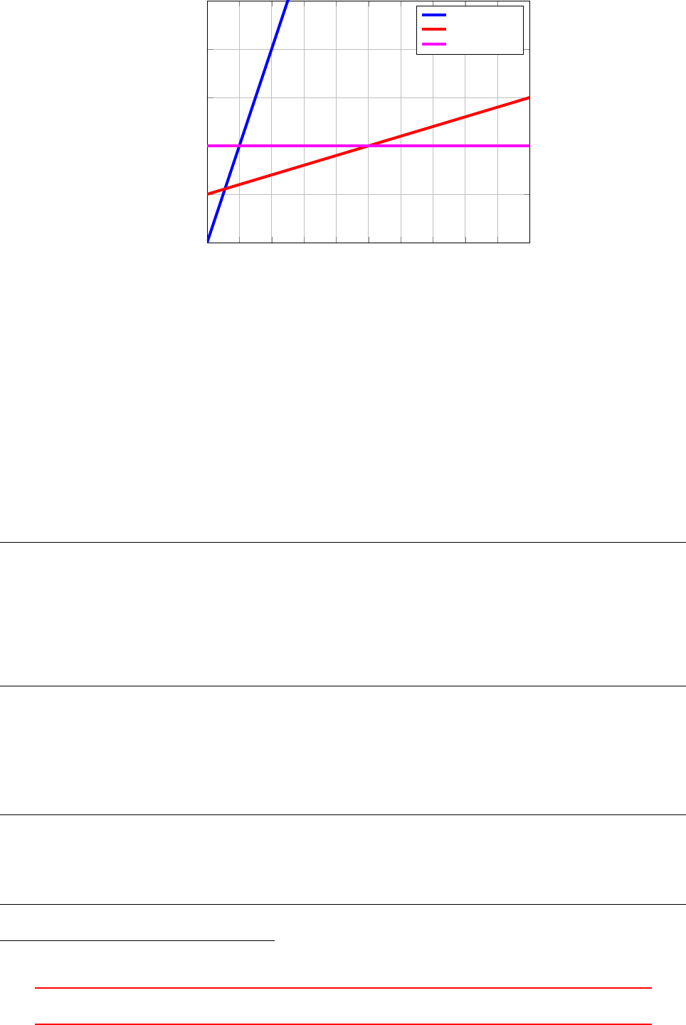
1 1.2 1.4 1.6 1.822.2 2.4 2.6 2.8 3
1
1.1
1.2
1.3
1.4
1.5
x
y
y=x
y= 1 + 0.1x
y= 1.2
Figure 75: The three arguments of Eq. (143) plotted over x
The argument of the function setDeltaT() contains the abidance of the first limit, the maximum time step.
There the minimum of the newly calculated and the maximum time step is passed on.
48.6.3 A note on the passing of time
In this section we will take a closer look at the implementation of the Time class.
Class design
A quick glance at the file Time.H reveals some very interesting information on the nature of time, or more
precisely, the nature of the Time class. Listing 351 shows us, that the class Time class inherits from five base
classes138.
class Time
:
public clock ,
public cpuTime ,
public TimePaths ,
public objectRegistry ,
public TimeState
{
/* class defini tio n */
}
Listing 351: The information on inheritance of the Time class; an extract of Time.H.
The TimeState class
From Listing 351 we see that Time is a TimeState due to inheritance. In Listing 352 we see the information
on inheritance of the timeState class. There we see, that TimeState is a dimensionedScalar.
class Tim eSt ate
:
public dimensionedScalar
{
/* class defini tio n */
}
Listing 352: The information on inheritance of the TimeState class; an extract of TimeState.H.
138Literarily spoken, the Time class is not only Dr. Jekyll and Mr. Hyde, it is also Citizen Kane, Mrs. Robinson and the Tambourine
Man.
IX This offering is not approved or endorsed by ESI®Group, ESI-OpenCFD®or the OpenFOAM®
Foundation, the producer of the OpenFOAM®software and owner of the OpenFOAM®trademark. 241

Distinguishing between time steps
The fact that Time is a TimeState which in turn is a dimensionedScalar helps to understand the Lines 6,13
and 21 of Listing 353. There, the name() method of the dimensionedScalar name space is called.
1Foam::Time& Foam::Time::op era tor ++()
2{
3// some code remov ed for b revity
4
5// Save old time n ame
6const w ord o ld Ti m eN am e = d i me n si o ne dSc a la r :: n ame () ;
7
8setTi me ( va lue () + deltaT_ , t ime Index_ + 1) ;
9
10 // some code remov ed for b revity
11
12 // Check that new time rep rese ntation diffe rs from old one
13 if ( dime nsion ed Scal ar :: name () == o ldT ime Name )
14 {
15 int ol dP recis ion = precision_ ;
16 do
17 {
18 pre cis ion _ ++;
19 s et Ti me ( v al ue () , t im e In de x () ) ;
20 }
21 while ( precision_ < 100 && di mens ion ed Sc alar :: name () == o ldTim eNa me ) ;
22
23 War nin gIn ( " Time :: ope ra to r ++() ")
24 << " I ncreased the ti me Pre ci sio n from " << oldPrecision
25 << " to " << p rec ision_
26 << " to di sti nguish b etween ti meN ame s at time " << value ()
27 << endl;
28
29 if ( pre cis ion_ == 100 && pre cis ion_ != old Prec isi on )
30 {
31 // R each ed limit .
32 War nin gIn ( " Time :: ope ra to r ++() ")
33 << " C urre nt tim e name " << dime nsio nedS cala r :: nam e ()
34 << " is the old as the p rev ious one " << oldTime Nam e
35 << endl
36 << " This migh t resul t in ove rwritin g old re sults ."
37 << en dl ; }
38 }
39 // some code remov ed for b revity
40 }
Listing 353: The increment operator (++) of the Time class; an extract of Time.C.
From Line 23 to 27 of Listing 353 we see the code which generates the warning message we saw in Listing
39 in Section 9.3.2.
In Lines 21 and 29 we find the hard-coded limit for the time precision. If the time precision reaches a value
of 100, then it is no more increased.
Naming the time with precision
In Section 9.3.2 we saw that the value of the timePrecision can be a source of error. We will now elaborate
on the actual causes of this error.
Listing 354 shows the definition of the method timeName(const scalar). This method is used to create a
properly formatted time name139 from a given scalar representing the time. In this method the time precision
comes into play in the form of the data member precision_, which is a static data field of the Time class with a
protected visibility. In this method the time value with high precision is converted to a string representation
(the time name) with limited precision140.
139The data type of the return value of this method is word, which is a string data type of OpenFOAM. Thus, the time name is
a string representation of the time. It is important to note, that the string representation of the time is different than the actual
value of the time.
140It is this method which creates the time name 0.102 from the time value 0.1023, when precision is set to three digits, as it is
the case in the example described in Section 9.3.2.
IX This offering is not approved or endorsed by ESI®Group, ESI-OpenCFD®or the OpenFOAM®
Foundation, the producer of the OpenFOAM®software and owner of the OpenFOAM®trademark. 242

1// - R eturn time n ame of giv en s cala r t ime
2Foam :: word Foam :: Time :: timeN ame ( const scalar t)
3{
4st d :: o st rin gs tre am buf ;
5buf . setf ( i os _bas e :: f mt fl ag s ( fo rm at_ ) , i os _bas e :: f lo at fi el d );
6buf . prec ision ( prec isi on_ );
7buf << t;
8return bu f . st r () ;
9}
Listing 354: The method timeName(const scalar) of the class Time; an extract of Time.C. Note, that the
descriptive comment is taken from the header file Time.H.
When the time is advanced, e.g. using the increment operator of the Time class, the method setTime() is
called. Listing 355 shows the definition of this method. The new time value is passed to this method. In the
second instruction we see how the time name is updated to the new value141.
1void Foam :: Time :: s etTime ( const scalar newTime , const label ne wIndex )
2{
3value () = newTime ;
4dim en si on ed Sc al ar :: name () = timeName ( t im eToUs er Ti me ( newTim e )) ;
5tim eIndex_ = n ewIndex ;
6}
Listing 355: The method setTime() of the class Time; an extract of Time.C.
The method setTime() gets called e.g. by the operator * of the Time class, see Line 8of Listing 353. There,
the time index is increased by one. From the header file of the TimeState class, we see, that the time index
is of the data type label, which is essentially an integer data type. Thus, we see, that the time index is a
consecutive number counting the time steps.
48.6.4 The Courant number
The Courant number Co is the ratio of the time step ∆tand the characteristic convection time scale u/∆x. Eq.
(147) shows the definition of the Courant number. However in a practical CFD code the Courant number will be
computed in a slightly different way. Eq. (148) shows how Eq. (147) is expanded with A/Ato gain a formulation
featuring the flux and the volume of the control volume instead of the velocity and the discretisation length.
Eq. (149) shows the extension of Eq. (148) for a one-dimensional finite volume formulation. The mean of the
fluxes of the faces Eand Wdefines the convective time scale. This definition seems obvious in some way in
the one-dimensional case. For two or three-dimensional cases the choice of how to define the characteristic flux
seems not straight forward.
Co =u∆t
∆x(147)
Co =u∆t
∆x=u∆t
∆x
A
A=φ∆t
∆V(148)
Co =|φE|−|φW|
2∆t
∆V=1
2
(|φE|−|φW|)∆t
∆V(149)
The Courant number in OpenFOAM
In OpenFOAM the Courant number is computed for all cells. In fact OpenFOAM computes a maximum
Courant number, i.e. the largest Courant number of all cells, and a mean Courant number, i.e. the mean
Courant number of all cells.
Listing 356 shows the code responsible for computing the Courant number. Line 8of Listing 356 translates
to Eq. (150). sumPhi is a scalar field containing the sum of the magnitudes of all face fluxes of every cell, i.e.
for each cell the magnitude of the face fluxes are summed up. Eq. (150) holds for every cell.
141The call of timeToUserTime() can be ignored. This method simply returns the passed value. This method has a non-trivial
implementation in the engineTime class, which keeps track of time in terms of engine RPM and crank-shaft angle. engineTime is
derived from Time.
IX This offering is not approved or endorsed by ESI®Group, ESI-OpenCFD®or the OpenFOAM®
Foundation, the producer of the OpenFOAM®software and owner of the OpenFOAM®trademark. 243

Eq. (151) is the mathematical representation of line 11. There the maximum value of the ratio between the
values of sumPhi and the cell volume is determined. Both variables sumPhi and mesh.V() contain values for
every cell. Therefore the gMax() function returns the maximum value.
Eq. (152) represents line 14.
1scalar CoNum = 0.0;
2scalar m ean CoN um = 0.0;
3
4if ( mesh . nIn te rna lF ac es () )
5{
6sca lar Field sumPhi
7(
8fv c :: s u rf ac e Su m ( m ag ( p hi ) ) () . i n te r na lF i el d ()
9);
10
11 CoN um = 0.5* gMax ( s um Phi / mesh . V () . fie ld () ) * r un Tim e . d e lt aTV al u e () ;
12
13 mea nCo Num =
14 0.5*( g Sum ( sum Phi )/ gSum ( mesh .V () . f ield () )) * runTi me . d el ta TV al ue () ;
15 }
16
17 Info << " Cou ra nt Numb er m ean : " << mean CoN um
18 << " ma x : " << CoN um < < endl ;
Listing 356: The content of the file CourantNo.H
sumPhi =X
fi|φfi|(150)
CoNum =1
2max
all cells sumPhi
Vcell ∆t(151)
meanCoNum =1
2PsumPhi
PVcell
∆t(152)
Discussion
The way to compute the Courant number in a three dimensional case is not straight forward as mentioned
above. This section reflects the authors way of understanding. So there is no guarantee of validity. The factor
of 1/2and the summation of φfiis explained by the author as follows.
We base our reflections on a two dimensional control volume. Eq. (154) shows the summation written in
the long form. This equation is then rearranged to yield Eq. (155). In Eq. (155) the summation is reduced to
two terms. These terms are the arithmetic mean of the face flux in the principal directions N−Sand W−E.
This summation is then identified as the L1norm of the mean face fluxes in the principal directions.
The reason for choosing the L1norm is not self-evident. In any case is the L1norm computationally cheaper
than the Euklidian or L2norm. However, the use of the L1norm seems justified since it measures the distance
covered by a movement, see http://en.wikipedia.org/wiki/Taxicab_geometry.
Co =1
2Pfi|φfi|
Vcell
∆t(153)
Co =1
2|φN|+|φE|+|φS|+|φW|
Vcell
∆t(154)
Co =|φN|+|φS|
2+|φE|+|φW|
2
Vcell
∆t(155)
Co =|φ|NS +|φ|W E
Vcell
∆t(156)
Co =k|φ|xik1
Vcell
∆t(157)
IX This offering is not approved or endorsed by ESI®Group, ESI-OpenCFD®or the OpenFOAM®
Foundation, the producer of the OpenFOAM®software and owner of the OpenFOAM®trademark. 244

We indroduce the following symbols
1
2X
fi|φfi|=k|φ|xik1=kΦk1(158)
Co =kΦk1
Vcell
∆t(159)
The way the mean Courant number is computed seems incorrect at the first glance but it isn’t.
Co =kΦk1
Vcell
∆t(159)
The mean value of the quantity xis defined as follows
x=1
N
N
X
i=1
xi(160)
Next we write the mean value of the Courant number. An unmarked summation is a summation over all cells.
Co =1
NXkΦk1
Vcell ∆t(161)
Co =1
NPVcell
PVcell
| {z }
=1
PkΦk1
PkΦk1
| {z }
=1 XkΦk1
Vcell ∆t(162)
Co =PkΦk1
PVcell
1
NPVcell
PkΦk1XkΦk1
Vcell
| {z }
X
∆t(163)
Eq. (163) now resembles Eq. (152). Now we concentrate on the term Xwhich is the only difference between
Eqns. (163) and (152).
X=1
NPVcell
PkΦk1XkΦk1
Vcell (164)
X=PVcell
N
| {z }
=Vcell
1
PkΦk1XkΦk1
Vcell (165)
X=Vcell
PkΦk1XkΦk1
Vcell (166)
X=1
PkΦk1X kΦk1
Vcell
Vcell !(167)
We assume Vcell
Vcell ≈1
X=1
PkΦk1XkΦk1
1(168)
X=PkΦk1
PkΦk1
= 1 (169)
Thus we have shown that the way the mean Courant number meanCoNum is computed is actually the mean
Courant number Co. However, this attempt of a proof is based on some assumptions.
First, the way the author explains the meaning of the summation of the face fluxes relies on hexahedral
cells. The argument made seems not to be applicable on tetrahedral cells. Secondly, the assumption Vcell
Vcell ≈1
is valid for homogeneous grids. For a uniform grid this assumption would be ideally fulfilled. If the volume of
the largest and smallest cells differs a lot this assumption is not justified.
IX This offering is not approved or endorsed by ESI®Group, ESI-OpenCFD®or the OpenFOAM®
Foundation, the producer of the OpenFOAM®software and owner of the OpenFOAM®trademark. 245
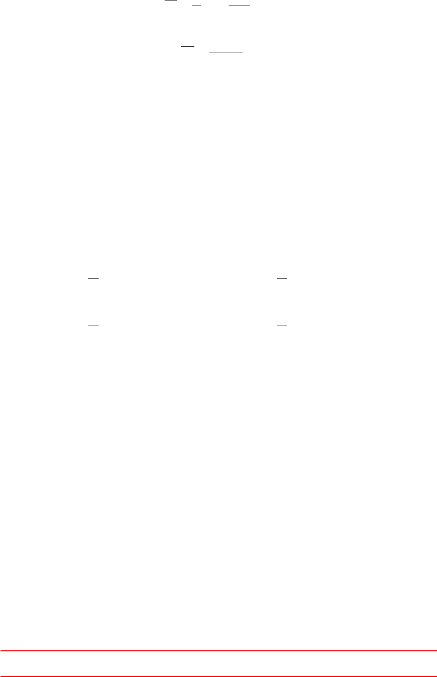
Some thoughts on the computational costs
Why the formula for the mean Courant number is rearranged from
Co =1
NXkΦk1
Vcell ∆t(170)
to
Co =PkΦk1
PVcell
∆t(171)
is unknown to the author.
It is the opinion of the author that this is made for reasons of computational cost. Two times the summation
over all values of a field plus one division is computationally cheaper than an elementwise division of two fields
and one subsequent summation over all elements of the resulting field.
This would be the case if the division operation takes more time than the summation operation which is
very likely the case. Depending on the system the floating point division operation can take several times longer
than a floating point multiplication.
In the first case ntimes one division and one addition needs to be made, with nthe number of field values.
In the second case 2ntimes additions and one division is to be made.
T1=n(Td+Ts)T2= 2nTs+Td(172)
We introduce the factor δ, that is the ratio between Tdand Ts.
T1=n(δTs+Ts)T2= 2nTs+δTs(173)
T1=nTs(1 + δ)T2=Ts(2n+δ)(174)
T1
Ts
=n(1 + δ)T2
Ts
= (2n+δ)(175)
Next we assume that nis very large
T1
Ts
=n(1 + δ)T2
Ts≈2n(176)
So the first formula takes 1 + δoperations, whereas the second formula takes approximately 2noperations. If
δis larger than one, the second formula will take less time for computation. A δsmaller than one is highly
unlikelyor even impossible as the addition is a very simple operation. Remember, δis the ratio between the time
a division takes and the time an addition takes. The actual ratio vary according to the system architecture,
the compiler and the implementation, e.g. [1] reports a factor of 5 to 6 for single and double precision floating
point division. This argument does not consider the memory usage of the operations involved, it only focuses
on the number of floating point operations.
Because the Courant number is computed after every time step the time needed to calculate the Courant
number has an impact on the simulation time.
48.6.5 The two-phase Courant number
In a two-phase simulation there are several choices of how to compute the Courant number. In total, there
are 4 velocity fields (U1,U2,Uand Ur). These are the velocities of the phases 1 and 2 as well as the mixture
and relative velocities. The solver twoPhaseEulerFoam computes the Courant number for the mixture and the
relative velocities.
Listing 357 shows the content of the file CourantNos.H which is part of the source code of this solver. Line 1
computes the mixture Courant number by including the file CourantNo.H. This is the file described in Section
48.6.4. As this code operates on the field phi, which happens to be the flux of the mixture, the mixture Courant
number is computed.
The next lines compute the Courant number based on the relative phase flux. At line 11 the maximum of
this two Courant numbers is determined and stored into the variable CoNum.
CoNum is the Courant number used by the time stepping mechanism. So the variable time steps of the
twoPhaseEulerFoam solver are based on the maximum of the mixture and relative velocity Courant number.
IX This offering is not approved or endorsed by ESI®Group, ESI-OpenCFD®or the OpenFOAM®
Foundation, the producer of the OpenFOAM®software and owner of the OpenFOAM®trademark. 246
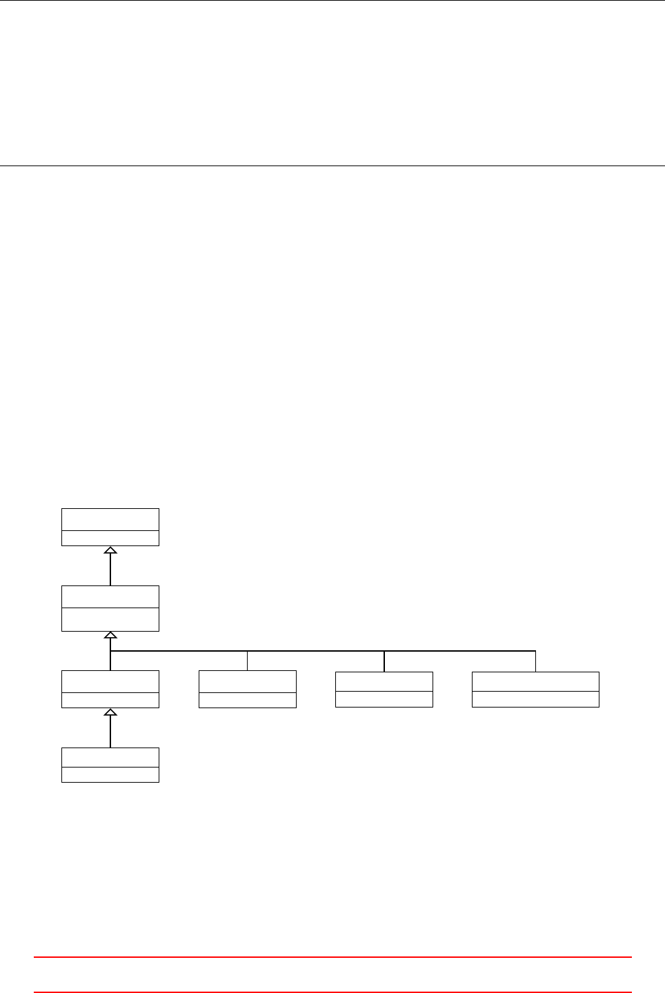
1#include " CourantNo . H"
2
3{
4scalar U rCoNu m = 0.5* gMax
5(
6fv c :: s u rf ac e Su m ( m ag ( p hi 1 - phi2 ) ) () . i nt ern alF iel d () / m es h . V () . f ie ld ()
7)* ru nTim e . de ltaTValu e () ;
8
9Info << " M ax Ur C ou ra nt Nu mber = " << UrC oNum << e ndl ;
10
11 CoNum = ma x ( CoN um , U rC oN um ) ;
12 }
Listing 357: The content of the file CourantNos.H
48.7 The registry
At some point in our study of OpenFOAM’s sources, its documentation or the internet we all came across
words like registered objects or similar expressions. This section tries to cast some light on this topic, or at least
present the thoughts and findings of the author. This section is closely related to Section 48.8.
48.7.1 The classes involved
Here is an extract of the descriptions found in the header files of the respective classes.
IOobject IOobject defines the attributes of an object for which implicit objectRegistry management is
supported, and provides the infrastructure for performing stream I/O.
regIOobject regIOobject is an abstract class derived from IOobject to handle automatic object registration
with the objectRegistry.
objectRegistry registry of regIOobjects
In Figure 76 a detail of the class hierarchy surrounding the class regIOobject is shown.
IOobject
regIOobject
writeData()
objectRegistry
Time
IOdictionary IOField DimensionedField
Figure 76: A partial view of the class hierarchy involving regIOobject; note that this diagram is complete
only for the classes IOobject and regIOobject – meaning IOobject is not derived from any other class and
regIOobject is derived from only IOobject; the other classes have more base classes than shown in this
diagram.
IOobject
This class provides the basic facilities for I/O. In Section 48.4.5 the practical or typical use of this class is shown.
IX This offering is not approved or endorsed by ESI®Group, ESI-OpenCFD®or the OpenFOAM®
Foundation, the producer of the OpenFOAM®software and owner of the OpenFOAM®trademark. 247
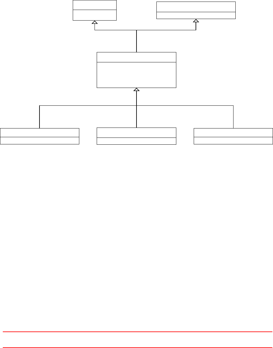
regIOobject
This class is an abstract class as the description in the header mentions. In Figure 76 the name of the pure
virtual method which makes this class an abstract class is shown in an italic font. This means all classes derived
from regIOobject must implement this pure virtual method. This also means, that we can not create an object
of the type regIOobject directly. Thus, in all of OpenFOAM’s sources we find a constructor call for the class
regIOobject only in the initializer list of classes derived from regIOobject.
objectRegistry
The objectRegistry is eponymous to this section. In fact there is not the one registry in OpenFOAM, there
are several. Among others, the classes Time,cloud, and polyMesh are derived from objectRegistry. Figure
77 shows the classes from which objectRegistry is derived.
regIOobject
writeData()
HashTable<regIOobject*>
objectRegistry
Time& time()
objectRegistry& parent()
T& lookupObject(word)
polyMesh
Time cloud
Figure 77: The base classes of the class objectRegistry; this class is derived from regIOobject and
aHashTable; note that the template parameter of the HashTable is a pointer to regIOobject; thus
objectRegistry is an regIOobject as well as a HashTable of regIOobject pointers – this is C++’s tem-
plate madness and inheritance wizardry in action.
objectRegistries: space and time
In OpenFOAM there is usually only one object of the type Time, usually named runTime. There are no solvers
to the knowledge ot the author, which use more than one instance of the class Time. As most solvers also feature
only one mesh, the seperation between Time and polyMesh as being a registry seems to be overdone.
However, there are solvers which feature several meshes, e.g. the conjugate heat transfer solvers. In the
simplest configuration there is one mesh for the solid part of the domain and one mesh for the fluid part of the
domain. However, the solver chtMultiRegionFoam supports an arbitrary number of fluid and solid domains.
In this case the temperature field Tof the solid region ineeds to be registered with the appropriate registry,
namely the mesh of the solid region i. Since the fluid in the fluid region also has a temperature, there will also
be a temperature field Tregistered to the appropriate fluid mesh. Thus, the separation of the object registries,
i.e. mesh(es) and time, saves us from a potential name clash, as we have two temperature fields T. Thus, the
mesh(es) are registered with the object registry runTime, whereas fields are registered with the appropriate
mesh.
An OpenFOAM solver has a number of object registries in use, the most prominent are the runTime and
the mesh objects. For fields it is important to know that they belong to a mesh, since the entity field is a mere
list of values. Only the connection to the mesh gives the field an actual meaning, i.e. the entry at position iin
IX This offering is not approved or endorsed by ESI®Group, ESI-OpenCFD®or the OpenFOAM®
Foundation, the producer of the OpenFOAM®software and owner of the OpenFOAM®trademark. 248

the list is the cell centre value of cell i. Furthermore, the field also needs a connection to the actual time state
of the simulation, otherwise there would be no meaningful way to define or calculate a temporal derivative.
48.7.2 Using the registry
Of what use could a possible object registry be? Well, ask the code.
In Section 57.3 we showed a way to search files for a certain pattern. Now we search all files with the file
extension .C for the pattern lookupObject and count the hits142. Listing 358 shows the command we can use.
First we use find to look for all files with the specified pattern for the file name. The result is then piped to
grep which searches the files for the specified pattern. Lastly, the result of grep is piped to wc, which counts
lines, words and bytes. Thus the first number returned by this sequence of commands tells us the number of
hits. The actual number of hits is approximately half the displayed number, since in the process of building
OpenFOAM from sources, symbolic links are created within the lnInclude folders143.
find $FOAM _SR C - name ’*.C’ | xargs grep ’ lookupOb ject ’ | wc
Listing 358: Find and scan files with file extension .C for the pattern lookupObject and count the hits
The command of Listing 358 results in 1068 hits in the author’s OpenFOAM-2.3.x installation at the time of
writing. 537 of these hits come from symbolic links of lnInclude directories. This means that lookupObject()
gets used a lot. So what is lookupObject() good for?
Need to know vs. want to know
One principle of encapsulation or information hiding is a fundamental principle of object-oriented program-
ming144. The general idea is to hide the actual implementation of something behind a publicly accessible
interface. Thus, the inner workings of a class may change without affecting its use. The iterator concept is
a good example of the benefits of information hiding. Typical container classes implement a feature called
iterators that are used to iterate over all elements of the container. By using the public interface of the iterator,
the actual container behind may be any kind of data structure (a linked list, a vector, a hash table, etc.).
Besides providing and using interfaces for accessing the data of a class it is also a common and good practice
to restrict the scope of data, e.g. temporary data being local to the class or method where it is actually used.
Thus, in the design of the classes we implement we limit the data contained within and/or passed to the class
to the necessary minimum, i.e. the viscosity law used in a solver does not need to know about the solver we
used to solve the discretized equation system. However, there might arise the need to access data, which the
original designers of a certain familiy of classes did not anticipate.
Namespaces & scopes
Another aspect are namespaces and variable scopes within our source codes. A variable is visible in the
namespace and scope it is declared. If we look at the top level code of a solver, e.g. twoPhaseEulerFoam,
we see a lot of #include statements and the main() method of the program. Although, we find no direct
statement involving the namespace, in the file fvCFD.H a statement is hidden which causes the compiler to
use the namespace Foam. This is the reason why we can later e.g. in createFields.H use typenames such as
volScalarField which are defined in the namespace Foam. Otherwise we would need to explicitely specify the
namespace as well, e.g. Foam::volScalarField. Thus, all objects created by a solver such as mesh,runTime,
etc. are visible in the namespace Foam.
Models however, have their own namespaces. Listing 359 shows an example of such a model with its own
namespace. Within the namespace Foam a new namespace diameterModels is created. Within this namespace
the class isothermal is defined. Thus the classes implementing diameter models do not pollute the Foam
namespace.
Although, the diameterModels namespace is a subset of the Foam namespace and everthing declared within
Foam is also visible within Foam::diameterModels, the diameter models are compiled with other models into a
142The method lookupObject() can be used to ask the registry for a registered object. The usefulness will be explained in the
subsequent paragraphs.
143The lnInclude folders collect links to all files of a certain library, thus when compiling a solver that uses this library we need
to include only the lnInclude folder and not the whole directory tree of the library’s sources. This minimizes the number of entries
in the Make/options files.
144Information hiding and encapsulation are often used synonymously, however, strictly spoken they are not exactly the same.
IX This offering is not approved or endorsed by ESI®Group, ESI-OpenCFD®or the OpenFOAM®
Foundation, the producer of the OpenFOAM®software and owner of the OpenFOAM®trademark. 249

shared library. Thus, when these files are compiled, the compiler knows nothing of the objects in the namespace
Foam created in e.g. createFields.H.
namespace Foam
{
namespace diameterModels
{
class isothermal
:
public diameterModel
{
// code removed
}
Listing 359: The class definition of the isothermal class, derived from the class diameterModel in
isothermalDiameter.H
Looking up stuff
Listing 360 shows the definition of the method d() of the class isothermal. For the reasons explained above
isothermal.C and createFields.H being in different compilation units, we can not access the pressure field p
directly from within the method body, even though pis part of the namespace Foam. However, other diameter
models do not need to access the pressure field, e.g. constant which implements a constant diameter.
Foam :: tmp < Foam :: v olS calar Field > Foam :: dia mete rMo dels :: i sot her mal :: d() const
{
const v ol S ca l ar Fie ld & p = p ha se _ . U () . db () . l oo ku pO bj ec t < v ol Sc al arF ie ld >
(
"p"
);
return d0 _ * pow ( p0_ /p, 1 .0 /3 .0 ) ;
}
Listing 360: The definition of the method d() of the class diameterModel in isothermalDiameter.C
The example above shows the value of the lookup mechanism. Since some sub-models operate on some
fields, it is easy to get a reference to the mesh from the field, as it is done in phase_.U().db().phase_ is a
member of the base class of the diameter models145. The call phase_.U() returns a reference to the velocity
field of the phase in question. As the velocity field is registered with the mesh otherwise we wouldn’t know
which velocity value belongs to a certain cell we get a reference to the mesh by calling db(), which is a method
of the class IOobject. This handy mechanism saves us from polluting sub-models with references to the mesh,
the time, to fields we might need at some point or some derived classes might need in special cases.
Thus the lookupObject() method provides a tool for us to get references to fields which at compile-time
may not be declared and thus usable. Remember, the pressure field is declared in the solver’s createFields.H
file, which is in a different compilation unit as the library we are compiling our diameter model for. If the code
of the diameter model and the solver would be in the same compilation unit (the solver’s executable) we would
not need the lookup mechanism. However, since the developers of OpenFOAM aim for modularity, placing
everything into a single compilation unit is against the design principles of modularity and reusability.
The lookupObject() method is templated since we can register anything with the mesh, in fact anything
that is derived from regIOobject, since an objectRegistry is a HashTable of regIOobject pointers. Thus,
at compile-time the method and the compiler do not know exactly which data types it is going to handle.
This is where templates come into play. The templated method is implemented once for the template pa-
rameter, and when we use the method, we simply replace the template parameter with the actual type, as in
lookupObject<volScalarField>("p"). The compiler then does the rest of the work and generates the appro-
priate code. We could resolve this issue without templates by using function overloading at the price of massive
code duplication and poor maintainability.
145It is a convention of OpenFOAM’s developers to append an underscore character (_) to the names of the data members of a
class in order to make them easily distinguishable from method parameters.
IX This offering is not approved or endorsed by ESI®Group, ESI-OpenCFD®or the OpenFOAM®
Foundation, the producer of the OpenFOAM®software and owner of the OpenFOAM®trademark. 250

48.7.3 Printing the registry
If you are curious you can add the following lines of code to a test utility of yours to check what is registered
with the mesh and the runTime object registry. Note that mesh and runTime must be accessible from the place
you put the code into. Also the names of the objects might differ in some cases.
Info << " m esh . nam es () " < < mesh . name s () << nl << endl ;
Info << " r unTi me . names () " << run Time . nam es () << e ndl ;
Listing 361: Printing the contents of the object registries mesh and runTime to Terminal
48.8 I/O - input & output
Some aspects of I/O were already covered in Sections 48.4.5 and 48.3. However as this collection of stuff is
fragmented by design or by the lack of such we cover the topic of I/O in a more general manner.
48.8.1 Output to Terminal - OpenFOAM’s very own printf()
In programming we have often the need to print stuff to the Terminal, e.g. for printf() debugging146. With
C++ general I/O was implemented on the basis of I/O streams. C++’s I/O streams provide a type-safe and
uniform way to implement I/O for both built-in and user-defined types [45]. See Listings 362 and 363 for the
use of C’s printf() function and C++’s streams.
#include < st di o . h >
int main(int argc , char** a rgv )
{
printf(" H ello , W or ld !\ n " );
return 0;
}
Listing 362: The Hello World! example of C.
#include <iostream >
int main ()
{
std :: cout << " H ello World !" < < st d :: endl ;
return 0;
}
Listing 363: The Hello World! example of C++.
OpenFOAM implements its own stream library. The generic stream library of OpenFOAM is based on the
class IOstream. The description of this class in its header file sheds some light on the reasons for doing so:
An IOstream is an abstract base class for all input/output systems; be they streams, files, token
lists etc.
The basic operations are construct, close, read token, read primitive and read binary block. In
addition version control and line number counting is incorporated. Usually one would use the read
primitive member functions, but if one were reading a stream on unknown data sequence one can
read token by token, and then analyse.
OpenFOAM handles all kinds of communication in terms of streams, among others: Terminal I/O with the
user, file I/O and inter-process communication for parallel processing. The Hello World! example for the
OpenFOAM world in Listing 364 looks very similar to the example of C++.
146Named after C’s ubiquitous printf() function, see http://stackoverflow.com/a/189570/2055536
IX This offering is not approved or endorsed by ESI®Group, ESI-OpenCFD®or the OpenFOAM®
Foundation, the producer of the OpenFOAM®software and owner of the OpenFOAM®trademark. 251

#include "Istream.H"
using namespace Foam;
int main(int argc , char * ar gv [ ])
{
Info << " H ello OpenFOA M !" < < endl ;
return 0;
}
Listing 364: The Hello World! example written in OpenFOAM.
Conditional (debug) output
printf() debugging is a very handy, low-level technique to trouble-shoot pieces of code. In the case of actual
debugging, we will remove all lines of code printing to the Terminal once we are done debugging. However, we
might want to create software, which may be either talkative or silent147. In this case we need conditional Info
statements.
Listing 365 shows a Hello World! example with conditional output. This listing is quite lengthy, since we
decided not to use simple boolean to control the conditional output. Instead we opted for a real case scenario,
in which the verbosity is controlled by a command line option. This, however, entailed some more lines of code
to deal with command line parameters.
#include "argList.H"
bool verbose(fa lse );
using namespace Foam;
int main(int argc , char * ar gv [ ])
{
argList::addNote
(
" This is a \" Hello World !\" pro gram for the OpenFOAM world ."
);
argLi st :: noBanner ();
a rg Li st : : n oP a ra ll e l ( ) ;
argLi st :: rem ove Optio n ("noFunctionObjects");
argLi st :: rem ove Optio n (" ca se ");
argLi st :: addBool Option
(
"verbose",
" c on t ro l t he chat ty - ne ss of me "
);
Fo am :: arg List args ( argc , ar gv ) ;
if ( args . opt io nF ou nd ( "verbose"))
{
verbose = true;
}
Info << " H ello OpenFOA M !" < < endl ;
if ( ver bose ) Info << " ... and hello to all other non - O pen FOAM worlds !" << endl;
return 0;
}
Listing 365: The Hello World! example written in OpenFOAM with conditional chattiness.
147Have you ever come across -v or --verbose command line switches when using UNIX or LINUX computers?
IX This offering is not approved or endorsed by ESI®Group, ESI-OpenCFD®or the OpenFOAM®
Foundation, the producer of the OpenFOAM®software and owner of the OpenFOAM®trademark. 252

In addition to the boolean command line switch, we added a note informing the user about the executable.
This note gets displayed, when the usage message is shown by invoking the executable with the command line
option -help. OpenFOAM adds a number of command line parameters by default, thus we remove some of
them (the ones that make no sense for a Hello World! program, such as the parallel option).
The second to last line of code is the one that actually controls the conditional output. This is done by a
good old if statement.
In the source code of the function objects of OpenFOAM-2.3.x we observed another possiblity to define
conditional output. There, we can pass an argument to Info. With OpenFOAM-2.4.x and higher versions this
does not compile anymore. Listing 366
// OpenFOAM -2.3. x
Info(log_)<< " I ncluding po rosity e ffects " << endl;
// OpenFOAM -2.4. x and h ighe r
if ( log_ ) Info << " Inc lu ding porosity effects " << endl;
Listing 366: Implementing conditional output, controlled by the Switch log_, in different OpenFOAM versions.
This example is taken from the force function object. See the file force.C.
A variant of the conditional Info(log_) statement was reinstated in May 2016148, with the Log macro,
which is defined as follows:
// - Repor t wri te to Foam :: Info if the local log swit ch is true
#define Log \
if ( log ) I nfo
Listing 367: The definition of the Log macro, originally for conditional output of function objects. See the file
messageStream.H.
48.8.2 The registry and the I/O or the truth behind runTime.write()
Registering fields with the runTime object registry also allows makes our lives easier when we want to write
the current state of the simulation to disk. In a great number of solvers, possibly in all of them, we find an
instruction like runTime.write() within the main loop of the main method. This call to the method write()
causes fields to be written to disk. As every solver write a different set of fields to disk, we may ask ourselves how
the solver or OpenFOAM knows which fields to write when we call the write() method of the runTime object?
Here, the registry nature of the Time class comes into play. Since we register all our fields, which we eventually
want to read or write, with the runTime object, the runTime object has a list of objects (regIOobjects in fact)
which are to (or might) be written149. In fact, since objectRegistry is derived from the type HashTable, an
object registry is a list of objects which are to (or might) be written150. The call of the write method of the
Time class causes Time to iterate over its self (runTime is a list of regIOobjects by inheritance151) and call the
write() method of every single item within the list. The method write() is defined in the regIOobject class.
The closer look into the sources is revealing if we take some of C++’s rules into consideration. Listing 368
shows us the method that is called when we call write() on runTime, bear in mind that Time is derived in
second generation from regIOobject via the class objectRegistry. The listing shows a call of the method
writeObject().
bool Foam :: re gIOobjec t :: write () c onst
{
return writeObject
(
ti me () . w rit eFo rm a t () ,
IOstream :: cur rentVers ion ,
time().writeCompression()
148https://github.com/OpenFOAM/OpenFOAM-dev/commit/48e58170392e5ef60538cfef28dd70c70a62e17b
149depending on the write flags of the IOobject part of the type. See Section 48.4.5 for a discussion on the read and write flags
of the IOobject class.
150A hash table is not really a list, however, we can iterate over a hash table the same way we can iterate over a list. The
description in the header file of the HashTable class describes the class as being An STL-conforming hash table.
151think around the family tree, e.g. in Figure 77
IX This offering is not approved or endorsed by ESI®Group, ESI-OpenCFD®or the OpenFOAM®
Foundation, the producer of the OpenFOAM®software and owner of the OpenFOAM®trademark. 253

1bool Foam :: Time :: wri teO bje ct
2(
3IOstream :: stream For mat fmt ,
4IOstream :: versio nNum ber ver ,
5IOstream :: com pre ssio nTyp e cmp
6)const
7{
8if ( o ut pu t Ti me () )
9{
10 // some code re moved
11
12 timeDict . regIOo bje ct :: wri teObjec t (fmt , ver , cmp );
13 bool write OK = obj ectR egis try :: w riteObj ect (fmt , ver , cmp );
14
15 // further code removed
Listing 369: Parts of the method writeObject() of the class Time in TimeIO.C
);
}
Listing 368: The method write() of the class regIOobject in regIOobjectWrite.C
If we search the sources of Time and all its base classes we find out that Time,regIOobject and objectRegistry
all define a method called writeObject()152. All of these three methods share the same signature153, i.e. they
receive the same function arguments. Since the call of writeObject() is not further specified for a certain
namespace, it is the method writeObject() of the class Time, which is called when we call runTime.write()
as runTime is of the type Time.
In Listing 369 we see a portion of the definition of the method writeObject() of the class Time. There we
also see calls explicitely to the methods writeObject() of the classes regIOobject and objectRegistry.
Thus, the method writeObject() of all three classes (Time,regIOobject and objectRegistry) are called
when runTime.write() is called. It is worth noticing that the call of regIOobject::writeObject() is invoked
on the timeDict object. The definition of this object is part of the removed code prior to the call. A look into
the source code reveals, that timeDict is an IOdictionary which is a class also derived from regIOobject,
see Figure 76. The call of timeDict.writeObject() is the piece of code which creates the uniform folders
within the time step directories154.
The method writeObject() of the class objectRegistry does the actual iteration over all elements within
the registry. Listing 370 shows the actual iteration over the hash table of regIOobject pointers. For each
element writeObject() is called if the write flag is not set to NO_WRITE. Now the method writeObject() of
the class regIOobject is called, since the iteration is over regIOobject pointers. This call on Line 16 of Listing
370 causes a registered field to be written to disk.
1bool Foam :: o bjec tReg ist ry :: wri teObjec t
2(
3IOstream :: stream For mat fmt ,
4IOstream :: versio nNum ber ver ,
5IOstream :: com pre ssio nTyp e cmp
6)const
7{
8bool ok = true;
9
10 for Al lCons tI ter ( HashTable < r egI Oobject *> , * this , i ter )
11 {
12 // code removed handling debug ou tput
13
14 if ( iter () -> wr it eO pt () != NO _WRI TE )
15 {
152The arguments of the function are dropped in the text for the sake of brevity. In fact there is no method named writeObject()
with an empty parameter list. This can be checked via these commands: find $FOAM_SRC -name ’*.[CH]’ | xargs grep
’writeObject()’
153The function signature consists of the name of the function and its parameters.
154In case you ever wondered where these come from.
IX This offering is not approved or endorsed by ESI®Group, ESI-OpenCFD®or the OpenFOAM®
Foundation, the producer of the OpenFOAM®software and owner of the OpenFOAM®trademark. 254

16 ok = iter () -> writeO bje ct (fmt , ver , cmp ) && ok ;
17 }
18 }
19
20 return ok ;
21 }
Listing 370: Parts of the method writeObject() of the class objectRegistry in objectRegistry.C
In conclusion we have learned by digging the source code of OpenFOAM the magical inner workings of
the call runTime.write(). First the Time class writes its state to disk into the uniform folder and then the
objectRegistry part of the runTime object writes all registered fields. It was already mentioned in Section 48.6
that the class Time has a multiply divided personality. And some of those even bring along an ancestry. This
highlights the need to have a certain understanding of C++ in order to be able to deduce what’s going on from
the sources of OpenFOAM as OpenFOAM makes very heavy use of C++’s language features such as multiple
inheritance, polymorphism and templates. In the context of programming paradigms involved, OpenFOAM
makes use of (among others): object-orientation and generic programming.
48.9 Making an argument – passing arguments
In Listing 365 of Section 48.8 command line arguments were used to influence an application’s behaviour. In
Section 9.1 different means of exterting control over an application are discussed. There, the point was made
that command line arguments are the lowest level of control over an application. Command line arguments
need to be specified each time an application is run. Only default values for optional arguments are permanent.
This section discusses some points about command line arguments.
48.9.1 The order of things
If we study applications, which make use of their own command line arguments, we see that there is certain
order of things. Listing 371 shows a minimal example of how to define command line arguments.
First, the static method addBoolOption method is called to add our own command line argument. Then,
the file setRootCase.H is included. Listing 372 shows the contents of this file. We see that a variable of the type
Foam::argList is created and all command line arguments155 are passed to the constructor of Foam::argList.
The constructor of Foam::argList only performs checks on the validity of the already defined options. In fact
no further options can be added after the call to the constructor of Foam::argList. Once the constructor has
been called, an object named args exists, which can be used to lookup options and extract information.
argLi st :: addBool Option
(
"verbose",
" be m ore t al ka ti v e "
);
#include " set Roo tCase . H"
const bool verbose = args . opti onF ound ("verbose");
Listing 371: The order of things in the source code for defining command line arguments
Fo am :: arg List args ( argc , ar gv ) ;
if (! a rg s . c hec kRo otC ase ( ) )
{
Foam :: FatalErro r . exit () ;
}
Listing 372: The content of the file setRootCase.H
155In C++ argc is the number of command line arguments, and argv is the actual command line arguments. argc and argv
are passed from the Terminal to the main() method of the application, see main()’s method signature: int main(int argc, char
*argv[])
IX This offering is not approved or endorsed by ESI®Group, ESI-OpenCFD®or the OpenFOAM®
Foundation, the producer of the OpenFOAM®software and owner of the OpenFOAM®trademark. 255

48.9.2 Dealing with SPAAAACE!
Having a space in an argument’s name is not really a good idea, since the Terminal generally interprets a
space as the end of an argument. In common UNIX/Linux tools multi-word arguments are generally seperated
with hyphens, e.g. --auto-compress. In the OpenFOAM universe, we see the use of camel case156, e.g.
-noFunctionObjects to deal with multi-word argument names.
However, if we really want to have spaces within our argument’s name, OpenFOAM allows us to do so.
Listing 373 demonstrates how to define an argument named search point.
argLi st :: add Opt ion
(
" s ea rc h p oi nt " ,
"vector",
" f in d t he c el l c o nt a in i ng th e s p ec i fi e d c oo r ds at < v ect or > - eg , ’(1 0 0 ) ’ "
)
/* no comment */
vector v;
if (args.optionReadIfPresent(" s ea rc h p oi nt " , v))
{
Info << " S ea rc hing cell at point : " < < v < < endl ;
}
Listing 373: Reading a point’s coordinates from a command line argument
Using an argument with a space in it, requires taking special care, as shown in Listing 374. Quotes are used
to prevent the Terminal from interpreting the space within the argument’s name as the end of the argument’s
name.
Listing 375 shows the danger of defining arguments with spaces. In this case the quotes were not used, just
as we are used to.
find Ce llB yPo int Coo rds -’ s ea rch point ’ ’( -0 .99 338 9 -1.90411 12. 49 42 ) ’
Listing 374: Passing a point’s coordinate to an application; note the quotes around the argument’s name
use r@host :∼$ find Cell ByPo intC o ords - search point ’( -0.993389 -1.90411 12.4942 ) ’
...
--> FOAM FATAL ERROR :
Wrong number of ar guments , exp ected 0 found 2
Inv al id op ti on : - s ea rc h
FOAM exiting
Listing 375: Passing a point’s coordinate to an application; omitting the quotes around the argument’s name
leads to a misinterpretation
48.10 Turbulence models
In Section 27.2 it is stated that the user can choose between three options.
1. A laminar simulation
2. Using a RAS turbulence model
3. Using a LES turbulence model
This statement is reflected in the relationship between the classes implementing the turbulence models in
OpenFOAM. Object oriented programming allowes the programmer to translate relationships directly from
human language to source code. Two statements can be made about turbulence models
156https://en.wikipedia.org/wiki/Camel_case
IX This offering is not approved or endorsed by ESI®Group, ESI-OpenCFD®or the OpenFOAM®
Foundation, the producer of the OpenFOAM®software and owner of the OpenFOAM®trademark. 256
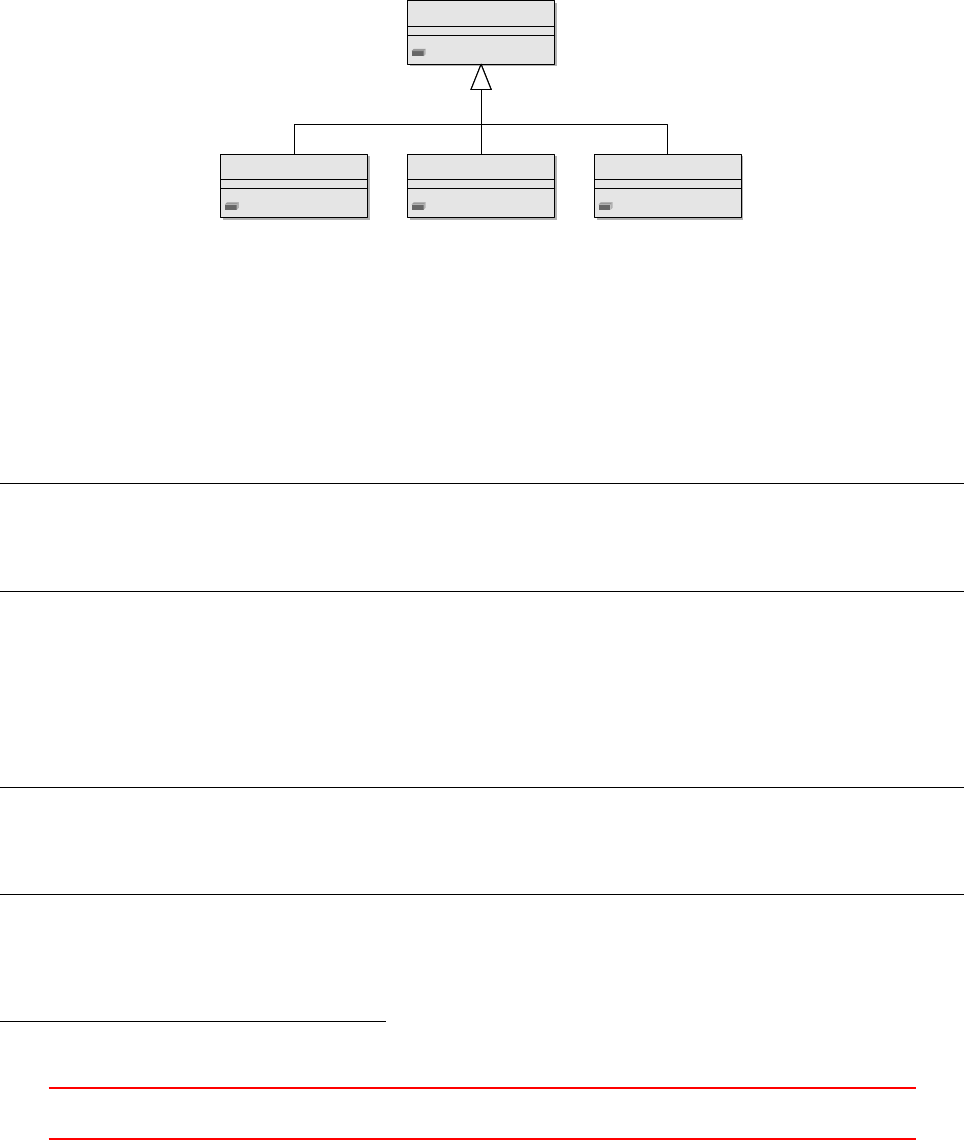
1. All RAS turbulence models are turbulence models, but not all turbulence models are RAS turbulence
models.
2. A RAS turbulence model is not the same as an LES turbulence model, however, both are turbulence
models.
Both statements are reflected by the class diagram of the turbulence models. On the top is the abstract class
turbulenceModel. This abstract class, provides the framework for all derived turbulence classes. Also, all
functionality common to all possible turbulence classes can be defined in this class. All derived classes will then
inherit this functionality.
Each turbulence model is derived from this abstract base class. Each turbulence class will implement specific
functionality individually.
turbulence
divDevReff():
laminar
divDevReff():
RASModel
divDevReff():
LESModel
divDevReff():
Figure 78: Graphic representation of inheritance of the turbulence model classes.
48.10.1 The abstract base class turbulenceModel
The base class turbulenceModel is an abstract class157. It contains several pure-virtual functions. To be able
to call this functions, these functions must be overridden by the classes that are derived from the base class.
A pure-virtual class can not be called. Listing 376 shows the declaration of pure-virtual or abstract methods.
The = 0 indicates that a method is abstract.
// - R eturn the turb ulenc e vis co sity
virtual tmp < volSc alar Fiel d > nut () const = 0;
// - R eturn the eff ec ti ve vi sc os ity
virtual tmp < volSc alar Fiel d > nu Eff () const = 0;
Listing 376: Declaration of the virtual methods in turbulenceModel.H
The base class contains not only virtual functions. It also contains functions that are the same for all derived
classes. Consequently, this functions are implemented by the base class. Listing 377 shows the implementation
of the function nu(). This function is used to access the laminar or molecular viscosity. The laminar viscosity
is a property of the fluid itself and has nothing to do with turbulence. However, the turbulence models need to
access the laminar viscosity.
// - R eturn the lam inar vis cosi ty
inline tmp <volScalarField > nu() const
{
return t ra n sp ort Mod e l_ . nu () ;
}
Listing 377: Implementation of nu() in turbulenceModel.H
Every class derived from an abstract class must at least override the abstract methods. The non-abstract
methods of the base class – like nu() from Listing 377 – can be used by the derived classes. No matter if a RAS
or a LES turbulence model is used, the laminar viscosity will always be the same.
157A class that contains one or more abstract methods is called an abstract class. If a class contains only abstract methods, then
it is sometimes called a pure-abstract class.
IX This offering is not approved or endorsed by ESI®Group, ESI-OpenCFD®or the OpenFOAM®
Foundation, the producer of the OpenFOAM®software and owner of the OpenFOAM®trademark. 257
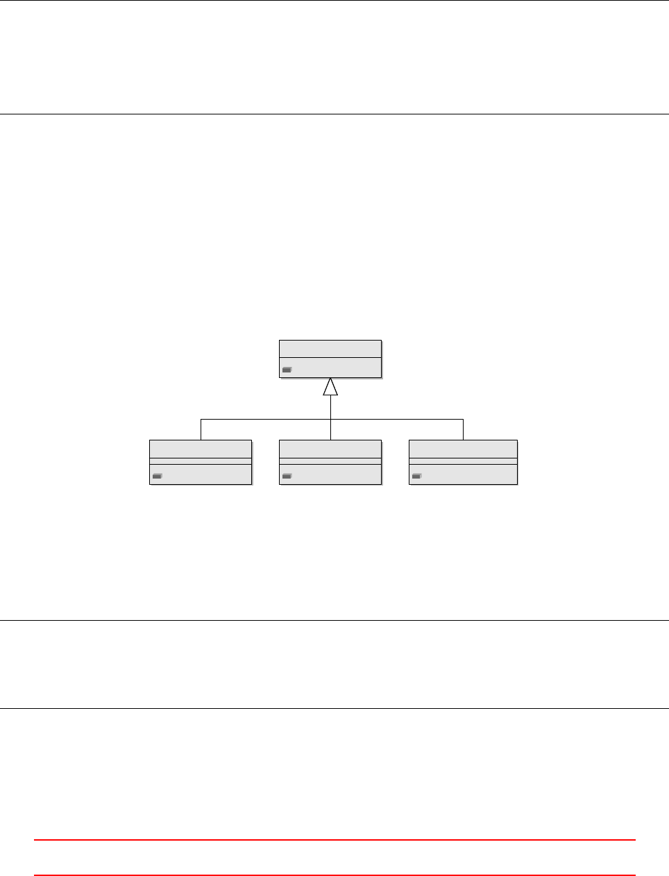
48.10.2 The class RASModel
The class RASModel is derived from the abstract class turbulenceModel. The class RASModel itself is the base
class for all RAS turbulence models. It is also an abstract class because it does not override all abstract methods
inherited from turbulenceModel.
However, the class RASModel implements all methods that are common to all RAS turbulence models. List-
ing 378 shows the implementation of the method nuEff() in the class RASModel.
// - R eturn the eff ec ti ve vi sc os ity
virtual tmp < volSc alar Fiel d > nu Eff () const
{
return tmp <volScalarField >
(
new volScalarField(" n uE ff " , n ut () + nu () )
);
}
Listing 378: Implementation of nuEff() in RASModel.H
The effective viscosity nuEff is calculated from the laminar viscosity, which is a property of the fluid, and the
turbulent viscosity. The turbulent viscosity is a property of the turbulence model. The function nu() in Listing
378 is implemented in the class turbulenceModel, see Listing 377. The function nut() is not implemented by
the class RASModel. Therefore, this method must be implemented by the classes derived from RASModel.
48.10.3 RAS turbulence models
All RAS turbulence models are derived from the class RASModel. Each derived class must implement all
remaining abstract methods. Figure 79 shows a simplified class diagram – there is a number of RAS turbulence
models available in OpenFOAM.
RASModel
divDevReff():
laminar
divDevReff():
kEpsilon
divDevReff():
SpalartAllmaras
divDevReff():
Figure 79: Inheritance of RAS turbulence models
48.10.4 The class kEpsilon
The class kEpsilon is derived from RASModel.
class kEp sil on
:
public RASModel
{
/* class defini tio n */
}
Listing 379: Class definition of kEpsilon in kEpsilon.H
The function nut() has to be implemented by kEpsilon. Listing 380 shows how the function nut() is
implemented. This function simply returns the class member nut_.
IX This offering is not approved or endorsed by ESI®Group, ESI-OpenCFD®or the OpenFOAM®
Foundation, the producer of the OpenFOAM®software and owner of the OpenFOAM®trademark. 258

// - R eturn the turb ulenc e vis co sity
virtual tmp < volSc alar Fiel d > nut () const
{
return nut_;
}
Listing 380: Implementation of nut() in kEpsilon.H
The way how nut_ is calculated differs between the RAS turbulence models. See Listing 408 in Section
52.2.2.
48.11 Debugging mechanism
OpenFOAM brings along a handy debugging mechanism. This mechanism can be used when creating additional
model libraries. The OpenFOAM wiki features a section explaining the built-in debug mechanism158.
The global debug flags – controlling the behaviour of the debugging system-wide – are specified in \$FOAM_SRC/../etc/controlDict-.
From OpenFOAM-2.2.0 onwards the global debug flags can be overridden by stating the debug flags of choice
in the case’s controlDict159.
As this debugging mechanism relys on internal variables no re-compiling is involved when using this kind of
debugging mechanism. This kind of debugging is sometimes referred to as printf debugging160.
By default all debug switches are initialised with a zero value, therefore the debug feature for the specific
class is disabled. However, when the solver sets up the case, the global and local entries are checked. Listing 381
shows the entry in the controlDict to override debug switches. Listing 382 shows the solver output informing
us of the local settings in controlDict.
DebugSwitches
{
DefaultStability 0;
Yoon Lutt rell Atta c hmen t 1;
}
Listing 381: Specifying debug switches in the case’s controlDict
Ove rri din g De bugS wit ches acc ord ing to co ntr olD ict
DefaultStability 0;
Yoon Lutt rell Atta c hmen t 1;
Listing 382: Solver output when specifying debug switches in the case’s controlDict
48.11.1 Using the debugging mechanism
If the debugging mechanism is enabled for a class161, Listing 383 shows how to actually use it. The code is
amazingly simple. The magic behind the scenes provides a variable named debug. We simply use this variable
in an if statement.
// print debug i nfo rmation
if ( debug )
{
// debug action
}
Listing 383: Using the debug mechanism in a class.
158http://openfoamwiki.net/index.php/HowTo_debugging#Getting_built-in_feedback_from_OpenFOAM
159http://www.openfoam.org/version2.2.0/runtime-control.php
160See http://oopweb.com/CPP/Documents/DebugCPP/Volume/techniques.html or http://en.wikipedia.org/wiki/Debugging#
Techniques
161See Section 48.12 on the background of the debugging mechanism.
IX This offering is not approved or endorsed by ESI®Group, ESI-OpenCFD®or the OpenFOAM®
Foundation, the producer of the OpenFOAM®software and owner of the OpenFOAM®trademark. 259

48.11.2 Use case: Write intermediate fields
Listing 384 shows the definition of a method named Ea. For debugging purposes we want to write intermediate
fields to disk. In Line 7of Listing 384 we compute a Reynolds number and store it in ReB. This is used to
generate the return value of the method. In normal operation only the return value is of interest. When
debugging also intermediate results may be of interest. The field ReB is by default not written to disk and
ceases to exist when the scope leaves the method, i.e. when the method is reaches its end the variable ReB is
automatically deleted162.
Note the arguments passed in Line 7. The first is the name of the field. We could omit this argument,
however, when we write the variable ReB to disk the first argument determines the file name. If this argument
was omitted, then an automatically generated name – based on the way the field was generated – would be used.
In this very case the file written would be named max(((mag((U1-U2))*d)|nu),0.001). We easily recognize
the formula of Line 7. A file name containing special characters (non-alphanumerical characters) is generally
not advisible163.
In Line 14 we manually call the write() method. This method is available to all registered input/output
objects164. As we construct the local variable ReB from the registered i/o object Ur we can savely assume that
ReB will also be of this type.
1Foam :: tmp < Foam :: v olS calar Field > Foam :: Yoo nL uttr el lAtt achm en t :: Ea
2(
3const volScalarField& Ur, const dimensionedScalar& dP
4)const
5{
6// do stuff
7volScalarField ReB(" Re B ", ma x ( U r * dB / p ha se 2_ . nu () , s ca la r (1 .0 e -3 ) ) ) ;
8
9// debug instructions
10 if ( debug )
11 {
12 if ( Ur . t ime ( ) . out pu t Ti me () )
13 {
14 Re B . w rite () ;
15 }
16 }
17
18 // do more s tuff
19 }
Listing 384: Manually writing intermediate fields for debugging.
48.12 A glance behind the run-time selection and debugging magic
OpenFOAM offers some amazing features. E.g. at compile-time of a fluid solver nobody knows which turbulence
model will be used with the solver. In fact it can be none at all or any of the available. The same is true for
drag models and the two-phase Eulerian solver with the exception that you can not use no drag law.
The entire wisdom behind the run-time selection mechanism, however, is more complex than what is pre-
sented in this section. Here, we focus on the macros we can find in the source files of the SchillerNaumann drag
model class. We know, this drag model is derived from the base class dragModel. For the run-time selection
mechanism to work, the base class also needs to do some preparations. See http://openfoamwiki.net/index.
php/OpenFOAM_guide/runTimeSelection_mechanism for a discussion on the run-time selection mechanism.
This section hopefully sheds some light into some of the inner workings of the run-time selection mechanism.
We shall now have a look behind the magic powers of OpenFOAM using the SchillerNaumann drag model as
an example. The Listings 385 and 386 (Lines 10 and 3) show the two harmlessly looking lines of code enabling
all the magic.
1namespace Foam
162This behaviour is subsumed under the term automatic variable. See e.g. http://en.cppreference.com/w/cpp/language/
storage_duration
163See e.g. http://www.teamdrive.com/Invalid_characters_in_file_and_folder_names.html
164See http://openfoamwiki.net/index.php/OpenFOAM_guide/Input_and_Output_operations_using_dictionaries_and_the_
IOobject_class and http://openfoamwiki.net/index.php/OpenFOAM_guide/objectRegistry
IX This offering is not approved or endorsed by ESI®Group, ESI-OpenCFD®or the OpenFOAM®
Foundation, the producer of the OpenFOAM®software and owner of the OpenFOAM®trademark. 260

2{
3class Schi ller Nau mann
4:
5public dragModel
6{
7
8public:
9// - R unti me type i nf or ma ti on
10 TypeName ( " Sch ill er Naum ann " );
11 }
12 }
Listing 385: The relevant lines of code in SchillerNaumann.H
1namespace Foam
2{
3d ef i ne T yp e Na m eAn d De b ug ( S ch il ler Na um a nn , 0) ;
4}
Listing 386: The relevant lines of code in SchillerNaumann.C
48.12.1 Part 1 - TypeName
First we will examine Line 10 of Listing 385.
TypeName ( " Sch ill er Naum ann " );
What looks like a function call is actually a preprocesser macro165 with parameters166. The macroTypeName
is defined in the file typeInfo.H. Listing 387 shows its definition.
A\#define macro consists of at least two parts. First comes the identifier, then comes the optional pa-
rameter list in parentheses and at least the replacement token list until the end of the line167. As the macro
is expanded by the preprocessor, the identifier (in this case TypeName) is replaced with the replacement tokes
(all instructions after the parameter list). A macro can not cover more than one line, however, by using the
backslash (\\) the current line is continued with the next line168.
1// - D ecla re a C la ss Name () with ex tra vir tual type i nfo
2#define TypeName ( T ypeNa me Strin g ) \
3Cla ssName ( T yp eName St rin g ); \
4virtu al cons t wo rd & t ype () const {return t ypeN ame ; }
Listing 387: The macro definition in typeInfo.H
Thus, the line TypeName("SchillerNaumann"); expands to.
Cla ssName ( " Sc hille rN aum an n ");
virtu al cons t wo rd & t ype () const {return t ypeN ame ; }
The second line is a function definition. As this function definition is made by the macro, this function is
defined for every class where the TypeName macro is stated in the class definition. This demonstrates one of the
major reasons for using preprocessor macros – the ability to write recurring pieces of code just once.
The first line of the above listing is itself a macro. Listing 388 shows the macro definitions that are necessary
to expand the ClassName macro.
1// - Add typ eN ame i nf or ma ti on from argu me nt \a T yp eN am eS tr in g to a class .
2// Also declares de bug in for mation .
3#define ClassName ( Type NameS tring ) \
4Cla ss Name NoD eb ug ( TypeNa meStr ing ); \
5static int debug
165http://en.wikipedia.org/wiki/C_preprocessor
166See e.g. http://www.cplusplus.com/doc/tutorial/preprocessor/
167https://gcc.gnu.org/onlinedocs/cpp/The-preprocessing-language.html
168https://gcc.gnu.org/onlinedocs/cpp/The-preprocessing-language.html#The-preprocessing-language
IX This offering is not approved or endorsed by ESI®Group, ESI-OpenCFD®or the OpenFOAM®
Foundation, the producer of the OpenFOAM®software and owner of the OpenFOAM®trademark. 261

6
7// - Add typ eN ame i nf or ma ti on from argu me nt \a T yp eN am eS tr in g to a class .
8// Wit hout debug info rma tio n
9#define Cla ss Nam eN oDeb ug ( Ty pe Nam eS tri ng ) \
10 stati c co nst ch ar * typeName_ () { return TypeNameString; } \
11 static const :: Foam :: word typeNa me
Listing 388: Two macro definitions in className.H
Thus, we further expand the TypeName("SchillerNaumann") macro.
stati c co nst ch ar * typeName_ () { return " S ch ille rNa um ann "; } \
static const :: Foam :: word typeNa me
static int debug
virtu al cons t wo rd & t ype () const {return t ypeN ame ; }
As the TypeName("SchillerNaumann") macro was put into the class definition of the verb+SchillerNaumann+
class, the macro added two function definitions (first and last line), one of which is a static method, and two
static variables (the two center line).
Static elements of class (variables or methods) are elements that exist only once for all instances of a class169.
In the case of a two-phase Eulerian solver two instances of the SchillerNaumann class might exist – in the case
this model was specified for both phases. No matter which of the two instances of the class call the method
typeName() it is always the same function called. In this case – returning the name of the class – the use of a
static method makes perfect sense and is the only sensible way to implement this task.
The TypeName("SchillerNaumann") macro is used to create a method that returns the name of the class and
a method that return the name of the type. Obviously, the class name and the type name were not considered
equivalent when designing OpenFOAM170. The variables created by the TypeName("SchillerNaumann") macro
are a static variable containing the type name and a static variable named debug. This debug variable controls
the debug mechanism covered in Section 48.11.
48.12.2 Part 2 - defineTypeNameAndDebug
Now we will examine Line 3of Listing 386 which is repeated just below.
d ef i ne T yp e Na m eAn d De b ug ( S ch il ler Na um a nn , 0) ;
The defineTypeNameAndDebug macro is defined the file className.H.
1// - Define the typeName and debug info rma tion
2#define d ef i ne T yp e Na m eAn d De b ug ( Type , D e bu gSw itc h ) \
3def in eTy pe Na me ( T ype ) ; \
4d ef i ne D eb ugS w it c h ( Typ e , D eb ugS wi t ch )
Listing 389: A macro definition in className.H
Thus our macro expands to two macros.
defineTypeName(SchillerNaumann);
d ef i ne D eb ugS w it c h ( S ch ill er Na uma nn , 0) ;
Listing 390 shows the macro definitions necessary to expand the above two macros.
1// - D efine the ty peN ame , with alte rnati ve lo okup as \ a Name
2#define d ef i ne T yp e Na m eWi t hN a me ( Type , N am e ) \
3const :: Foam :: word Type :: typeNa me ( Name )
4
5// - D efine the typ eN ame
6#define defineTypeName(Type) \
7d ef i ne T yp e Na m eW i th N am e ( Typ e , T yp e :: t y pe Na me_ () )
8
169http://www.tutorialspoint.com/cplusplus/cpp_static_members.htm
170See Section 48.12.3 for an example when class name and type name are different.
IX This offering is not approved or endorsed by ESI®Group, ESI-OpenCFD®or the OpenFOAM®
Foundation, the producer of the OpenFOAM®software and owner of the OpenFOAM®trademark. 262

9// - D efine the debug inform ation , loo kup as \ a N ame
10 #define def i neDe bugS w itch With N ame ( Type , Name , D ebu gSwitch ) \
11 int Type :: d ebug (:: Foam :: debug :: deb ugS wit ch (Name , Deb ugSwitch ) )
12
13 // - D efine the debug in fo rm at io n
14 #define d ef i ne D eb u gS w it ch ( Ty pe , D eb u gS wit ch ) \
15 defi neDe bu gSwi tc hWit hN ame (Type , Type :: typ eNa me_ () , Debu gSw itc h ); \
16 r eg i st e rD e bug S wi t ch W it h Nam e ( T ype , Type , Type :: t y pe Na me_ () )
Listing 390: Four macro definitions in debugName.H
Thus, our macros expand to:
const :: Foam :: word Sch il ler Na uma nn :: typeN ame ( Schi llerN auma nn :: t ype Nam e_ () );
int Sc hille rNau mann :: debug (:: Foam :: debug :: deb ugSwitc h ( Schille rNa umann , 0));
regi ster D ebug Swit c hWit hNam e ( Sc hillerNa uma nn , Sch ill erNauman n , Schi ller Naum ann :: typeName_ () );
The first line of the expansion of the macro defineTypeNameAndDebug(SchillerNaumann, 0) assigns the
return value of the function typeName_() to the static variable typeName. This has the effect that the class
name and the type name have an equal value. However, the way this framework is set up allows for different
names.
The second line assigns the return value of the function call ::Foam::debug::debugSwitch(SchillerNaumann, 0)
to the static variable SchillerNaumann::debug. The reason why the value is not directly used to assign the
value to the static variable is that the called method adds the debug switch to a dictionary, see Listing 391.
The last line of the macro expansion invokes another macro. Listing 392 shows the macro definition of
registerDebugSwitchWithName.
1int Foam :: debug :: deb ug Sw it ch ( c onst c har * name , const int defaultValue)
2{
3return d eb ugS wit che s () . l ook u pO r Ad dDe f au l t
4(
5name, defaultValue , false ,f alse
6);
7}
Listing 391: Adding the debug switch to the dictionary in debug.C
1// - D efine the debug inform ation , loo kup as \ a N ame
2#define r e gi s t er D e bu g S w it c h Wi t h N am e ( Ty pe , T ag , N am e ) \
3class add ## Tag ## T oDeb ug \
4: \
5public :: Foam :: simp leReg IO obje ct \
6{ \
7public: \
8add ## Tag ## ToD ebug ( const char * name ) \
9: \
10 :: Foam :: s im ple Re gIO ob je ct ( Fo am :: d ebug :: add Debu gObj ec t , n ame ) \
11 {} \
12 virtual ∼add ## Tag ## ToDeb ug () \
13 {} \
14 virtual void re ad Dat a ( F oa m :: I st rea m & is ) \
15 { \
16 Ty pe :: d eb ug = r ea dL a be l ( is ) ; \
17 } \
18 virtual void wr it e Da ta ( F oa m :: O str ea m & os ) const \
19 { \
20 os << Type :: deb ug ; \
21 } \
22 }; \
23 add ## Tag ## ToD ebug add ## Tag ## ToDeb ug_ ( Name )
Listing 392: Definition of the registerDebugSwitchWithName macro in debugName.H
48.12.3 A walk in the park: demonstrate some of this magic
In the above sections we took a look behind two very powerful pre-processor macros. So, what is this all for?
IX This offering is not approved or endorsed by ESI®Group, ESI-OpenCFD®or the OpenFOAM®
Foundation, the producer of the OpenFOAM®software and owner of the OpenFOAM®trademark. 263

The turbulence models are very prominent examples for the usefulness of the run-time selection mechanism.
At compile-time – the time we or the OpenFOAM developers compile a solver – nobody knows, what exact
turbulence model we want to use for our simulation. Thus, we need to decide at run-time – at the time the
solver reads all the case information – which turbulence model to use. In order to save us from writing a solver
for each turbulence model, solvers can be written in a generic way. I.e. at the time we compile the solver
nobody, not even the compiler, cares about the actual turbulence model. The base class turbulenceModel tells
the compiler and the solver how a turbulence model works, that is all we need to know at compile time.
However, at run-time we need to decide which turbulence model to use. Fortunately, OpenFOAM takes care
of that and we do not need to bother. In some cases, however, we would like to know which turbulence model
is currently used. We could achieve this by either reading the case data171 or by making use of the run-time
magic.
Listing 393 shows three lines of code. The intention behind this line is to print the return values of the
methods typeName_() and type(). These two methods were provided by the two macros dissected in Sections
48.12.1 and 48.12.2.
1Info << " H appy printf () d ebugging : " << endl;
2In fo << t urbule nce - > ty pe Na me _ () << e ndl ;
3In fo << t urbule nce - > type () << endl ;
Listing 393: Applying some of the magic, the source code.
Listing 394 shows the results of the three lines of code of Listing 393. The code in Listing 393 presumes that
turbulence modelling is used in its generic form, as it is the case in e.g. pimpleFoam. In this example the
variable turbulence is of the type autoPtr<incompressible::turbulenceModel> turbulence.
From the output we see, that the variable turbulence is indeed of type turbulenceModel. However, as the
class turbulenceModel is an abstract base class, no solver will ever actually use turbulenceModel itself172.
In this case, the solver used the kOmega turbulence model. Thus, the method type() returns the name of the
actual turbulence model. Here we also see the sense behind the distinction between the class name and the type
name as discussed some paragraphs above. In the example of an concrete class those are the same. For a base
class, however, this distinction makes perfect sence.
1Happy printf () debugging :
2turbulenceModel
3kOmega
Listing 394: Applying some of the magic, the output.
49 General remarks on OpenFOAM programming
This section covers some general advice for users who want to implement their own models and solvers or modify
existing ones.
49.1 Preparatory tasks
49.1.1 Create user specific directories
In order to be able to distinguish between the standard solvers and models from the solvers and models created
by the user, some new directories have to be created. Not only do we need to keep our models and applications
apart from the models and applications of the standard OpenFOAM installation, we also need to keep our
models and applications from those of other users. Thus, every user will get his or her own user directory.
The name of this user directory follows OpenFOAM’s naming convention which combines the user name and
the version number of OpenFOAM, i.e. user-4.0. Thus, we can also keep our own stuff for OpenFOAM-X
separate from the stuff for OpenFOAM-Y.
171This would mean re-programming existing functionality. The case data related to turbulence modelling was already read by
the constructor of the turbulence model. Manually reading this information again would result in some kind of code duplication.
The more elegant way to solve this problem is to access the information already gathered.
172See Section 48.10 for information about how turbulence models are organized in OpenFOAM.
IX This offering is not approved or endorsed by ESI®Group, ESI-OpenCFD®or the OpenFOAM®
Foundation, the producer of the OpenFOAM®software and owner of the OpenFOAM®trademark. 264

In this, we follow the organisational scheme of OpenFOAM’s standard solvers and models, of which the
source code resides in $WM_PROJECT_DIR/applications/solvers and $WM_PROJECT_DIR/OpenFOAM-2.1.x/
src. Therefore, we need to create some folders to place our sources in: $WM_PROJECT_USER_DIR/applications/
solvers and $WM_PROJECT_USER_DIR/src. Listing 395 lists the necessary commands. Open a Terminal and
type the commands of the Listing to do the job.
cd $WM_PROJECT_USER_DIR
mkdir -p appl icati ons / solve rs
mkdir src
Listing 395: Create the proper directories for a user’s solvers and models
Note the use of the variable $WM_PROJECT_USER_DIR, which resolves to your OpenFOAM installation’s user
directory, which also contains the run-directory ($FOAM_RUN).
49.2 Start from existing code
49.2.1 Copy the sources
If you want to create a new model or solver, it is generally recommended to base it on the model or solver from
OpenFOAM’s standard installation, which comes closest to your intended set of features.
49.2.2 Change compilation settings
Before proceeding any further certain compilation settings have to be changed from the settings of OpenFOAM’s
standard code base.
Change the executable’s or library’s name
The executable’s or library’s name is determined by a setting in the file Make/files of the source code of the
respective solver of model. For a solver the name of the executable is determined by the setting EXE. Listing
397 shows how the name of the executable for the solver pimpleFoam is defined.
EXE = $ ( FOAM_APP BIN ) / pi mpl eFo am
Listing 396: Setting the name of pimpleFoam’s executable in the file Make/files of pimpleFoam’s source code173
Analogously, defining the name of the shared library174 is done by the setting LIB in the file Make/files of
the library’s source code.
LIB = $ ( FOAM_LIB BIN ) / li blagr angia n
Listing 397: Setting the name of the shared object of the Lagrangian particle library in the file Make/files of
Lagrangian library source code
The settings for EXE and LIB are full file paths. Thus, next to the assigment (the =symbol) we find a
directory, the path name separator (the /symbol) and the actual name of the executable or shared library.
Change the executable’s or library’s location
Avoiding mixing up user created solvers and models from the ones provided by OpenFOAM’s standard installa-
tion involves apart from changing the file name of the executable or shared object also the path the executable
or shared object resides in. This is specified, as already shown above, in the file Make/files.
173The executeable does not necessarily have to have the same name as the source file. However, different names can lead to
confusion and make code maintenance harder. Therefore, it is strongly recommended to use consistent names, i.e. to name the
source file SOLVER.C and the executable SOLVER.
174The main purpose of dividing code into applications and libraries is to allow for multiple unconnected applications using
certain implemented behaviour (the libraries). Thus, libraries are shared by an arbitrary number of applications. Hence, libraries
are compiled into files which are referred as shared objects or shared libraries. The names of these files are appended by the filename
extension so, i.e. libraryName.so.
IX This offering is not approved or endorsed by ESI®Group, ESI-OpenCFD®or the OpenFOAM®
Foundation, the producer of the OpenFOAM®software and owner of the OpenFOAM®trademark. 265

For user created solvers and models, users are advised to change the path specifier to FOAM_USER_APPBIN or
FOAM_USER_LIBBIN respectively. Thus, user generated solvers and libraries are also spatially separated175 from
standard solvers and libraries.
If you use a system-wide OpenFOAM installation, then you most probably have only read access to the
FOAM_APPBIN and FOAM_LIBBIN directories. Thus, trying to compile your solver or model will fail, even when
there are no errors. In this case, the resulting error message might contain some hint about missing permissions.
Check Make/files
After adjusting the compilation settings, check and re-check the file Make/files. Listing 398 shows the vital
entries of the file highlighted. In the listing, the source file has the same name as the executable. Furthermore,
the executable will be located in the user’s application directory.
myApplication.C
EXE = $ (FOAM_USER_APPBIN)/myApplication
Listing 398: The content of Make/files
The file Make/files controls what is compiled and where the resulting executable will be stored. Thus,
getting Make/files right will save yourself from breaking something else, i.e. the model or application you
base your new model or application on. On the other hand, the file Make/options controls what is needed to
successfully compile the model or application. Getting Make/options wrong initially will do no harm.
Check Make/options
The file Make/options tells the compiler where to find additional source files, and it tells the linker176 where to
find additional libraries. The file Make/options only needs to be edited, if you use existing models, or source
files from other directories. This, however, is often the case.
The content of the file Make/options is divided in two parts. First, there are the paths for compiler to
look for source files to include. The second part is a list of libraries for the linker to link the current model or
application with.
EXE_INC = \
-I$ ( LIB_ SRC )/ meshTools / lnInclude \
-I$ ( LIB_SRC ) / finite Vo lume / ln Include
LIB_LIBS = \
- lme sh To ols
Listing 399: Content of Make/options
Initial compilation
Once the existing sources have been copied and, most importantly, the compilation settings have been changed,
we can run an initial compilation. Although, at this point, nothing in the source code has changed, running an
initial compilation is recommended to check whether we have got the compilation settings right.
For applications simply execute wmake, for shared libraries the compiler gets an additional parameter:
wmake libso. After the compilation the compiled binary should show up in FOAM_USER_APPBIN or FOAM_USER_LIBBIN
respectively.
49.3 Create the source code from scratch
The steps discussed above may not be needed by certain users. OpenFOAM provides some macros to create the
basic source-code-skeleton for, among others, new applications, boundary conditions or functions objects. In the
case of creating a new application from scratch, the user simply calls the macro foamNewApp and provides the
desired application name. The executable’s path will automatically be set to FOAM_USER_APPBIN. New function
objects or boundary conditions will automatically be compiled into FOAM_USER_LIBBIN.
175by residing in different directories
176Compilation of C or C++ code is usually done in two steps. First all files are compiled and then the object files generated by
the compiler are linked together to form the executable.
IX This offering is not approved or endorsed by ESI®Group, ESI-OpenCFD®or the OpenFOAM®
Foundation, the producer of the OpenFOAM®software and owner of the OpenFOAM®trademark. 266

49.4 Using a user-created libraries
Distinguishing between solvers and libraries is a good thing, since we can create and reuse certain models. If
we want our application to use a model of ourself, we need to tell the compiler and the linker where to find our
(already compiled) model.
In Listing 400 we see the necessary entries for the file Make/options for an application which is to use a
user-created libary with the very creative name myLibrary. The green line in Line 4of the listing tells the
compiler where to find the source code of the library myLibrary.
After the compilation stage finished succesfully, the compiled application needs to be linked to the compiled
library, i.e. shared object. This is shown in the Lines 8and 9of the Listing. The red line defines an additional
directory in which to look for shared objects. As good style dictates us to compile our own libraries into
FOAM_USER_LIBBIN, the additional directory for the linker is FOAM_USER_LIBBIN.
The blue line, Line 9of the Listing, then tells the linker the name of the shared object of myLibrary.
EXE_INC = \
-I$ ( LIB_ SRC )/ meshTools / lnInclude \
-I$ ( LIB_SRC ) / finite Vo lume / ln Include \
-I$(MY_LIB_SRC_PATH)/myLibary/lnInclude
LIB_LIBS = \
- lme sh To ols \
-L$(FOAM_USER_LIBBIN) \
-lmyLibary
Listing 400: Content of Make/options of an application using a user-created library
49.5 Pitfalls
Modifying existing models or creating new ones bears the potential for many bugs and errors. This section
tries to discuss some of them, which either occur regularly or may be difficult to track down. Such a list can
never be complete and it is clearly biased towards the errors made and encountered by the author. These
errors are not necessarily restricted to OpenFOAM, moreover, modifying OpenFOAM involves programming
and programming involves bugs and errors. Enjoy reading.
49.5.1 Segfault due to modified libary and failing to update the solver
Libraries are reusable parts of code, which are independent of the solver(s) using them. However, this in-
dependence may create problems if we modify the library and fail to recompile the solver(s) that are using
said library, even if said solver(s) have not been touched. The problem that might occur is a segmentation
fault (segfault in short) at construction of the modified objects. Unfortunately, a segfault does not produce very
telling error messages, see Listing 401. Note that we assume that compilation of the library finished successfully.
#0 Foam :: error :: printStac k ( Foam :: O str eam &) at ??:?
#1 Foam :: s ig Se gv :: sig Ha nd le r ( int ) a t ?? :?
#2 ? i n "/ lib / x86 _64 - linux - g nu / libc . so .6"
#3 ? in "/ lib / x86_64 - linux - gnu / li bc . so .6" S eg me nt ati on fa ult ( C ore d umpe d )
Listing 401: A segmentation fault
The reason for this behaviour, the solver violently fails at start-up due to a segmentation fault, is that our
modifications to the library changed its memory layout. As we did not recompile the solver, the solver had no
means to learn about the changed memory layout. Thus, at solver start-up, the solver reserves an incorrect
amount of memory for the objects of the library. At construction of these objects, this mismatch causes the
segmentation fault.
Recompiling the solver, which has not been touched seems at first counter-intuitive. However, when the
memory layout of the library changed, the solver will reserve memory according to the old memory layout.
Recompiling the solver will simply update memory allocation.
The tricky bit of this error, is that it does not always occur. If we change a library and our changes do not
alter the memory layout, all is well. No error will occur. This opens the possibility of modifying the library and
running the solver using that library to sometimes work and sometimes cause this error.
IX This offering is not approved or endorsed by ESI®Group, ESI-OpenCFD®or the OpenFOAM®
Foundation, the producer of the OpenFOAM®software and owner of the OpenFOAM®trademark. 267

Further reading
https://stackoverflow.com/questions/2346806/what-is-a-segmentation-fault
https://en.wikipedia.org/wiki/Segmentation_fault
49.6 Tips
Check and double-check that you compile to the user-directories
Always make sure, that you compile your applications to FOAM_USER_APPBIN and your libraries to FOAM_USER_LIBBIN.
The reason for this, and the way how to ensure this, are discussed in 49.2.2.
When modifying a library, also recompile the solver(s) using the library
This mean a seemingly extraneous step177, however, it might prevent weird behaviour. One reason for recom-
piling the solver using a recently modified library was discussed above in Section 49.5.1.
Furthermore, especially when templates are involved, e.g. you modify a templated class, it is vital to compile
the library which provided the templated model and the solver that uses the templated model. Templates need
special attention, care and love, do not neglect them.
177In some cases it is sufficient only to compile the library, e.g. when fixing a type in an Info message.
IX This offering is not approved or endorsed by ESI®Group, ESI-OpenCFD®or the OpenFOAM®
Foundation, the producer of the OpenFOAM®software and owner of the OpenFOAM®trademark. 268
Part X
Theory
This section covers more detailled topics and tries to look under the hood of OpenFOAM from a non-programming
view.
50 Discretization
50.1 Temporal discretization
50.2 Spatial discretization
The purpose of spatial discretization schemes is to compute the face values of fields whose values are stored at
the cell centre. The face values are then used e.g. for computing the spatial derivatives.
50.2.1 upwind scheme
An upwind scheme determines the face value of a quantity simply by choosing the cell centered value of the cell
that is located upwind of the face in question.
50.2.2 linearUpwind scheme
The linearUpwind scheme is equivalent to FLUENTs Second-Order Upwind Scheme.
50.2.3 QUICK scheme
The FLUENT Theory Guide [6] states:
For quadrilateral and hexahedral meshes, where unique upstream and downstream faces and cells
can be identified, ANSYS FLUENT also provides the QUICK scheme for computing a higher-order
value of the convected variable at a face.
50.2.4 MUSCL scheme
50.3 Continuity error correction
In the governing equations of some solvers in OpenFOAM – e.g. in twoPhaseEulerFoam of OpenFOAM-2.3.x –
we find a special correction for the continuity error.
50.3.1 Conserving the form
Before we start our considerations, we take a closer look on the conservation and nonconservation form of a
transport equation. First, we recall the definition of the substantial derivative:
D
Dt=∂
∂t + (u·∇)(177)
For example applied to an arbitrary scalar K
DK
Dt=∂K
∂t +u·∇K(178)
XThis offering is not approved or endorsed by ESI®Group, ESI-OpenCFD®or the OpenFOAM®
Foundation, the producer of the OpenFOAM®software and owner of the OpenFOAM®trademark. 269
Continuity equation
As a first example we look up the differential form of the continuity equation.
conservation form: ∂ρ
∂t +∇·(ρu)=0 (179)
nonconservation form: Dρ
Dt+ρ∇·u= 0 (180)
Both forms are equivalent to each other, since we can express one equation easily by the other one with the
help of some simple mathematical operations.
∂ρ
∂t +∇·(ρu)=0 (181)
∂ρ
∂t +∇ρ·u+ρ∇·u= 0 (182)
∂ρ
∂t +u·∇ρ
| {z }
Dρ
Dt
+ρ∇·u= 0 (183)
Transport equation
For the next example we use the right hand side of the transport equation of enthalpy in a multiphase problem.
This example is motivated by the energy equation of twoPhaseEulerFoam in OpenFOAM-2.3.x. We could also
have used the momentum equation, however, we want to avoid confusion by the repeated occurance of the
velocity.
We look up the energy equation for multiphase flows from a textbook or other resources [6,5]. For the sake of
brevity, we state only the left hand side of the equation. The equation we looked up (Eqn. (184)) happens to be
formulated in the conservation form. We now rearrange the equation in order to gain the nonconservation form.
∂αkρkhk
∂t +∇·(αkρkukhk) = RHS (184)
by partial derivation of the LHS, we gain
∂αkρk
∂t hk+αkρk
∂hk
∂t +hk∇·(αkρkuk) + αkρkuk·∇hk=RHS (185)
hk∂αkρk
∂t +∇·(αkρkuk)
| {z }
I
+αkρk∂hk
∂t +uk·∇hk
| {z }
II
=RHS (186)
We now pay attention to the term marked by I, we recognize the phase-continuity equation which equals
zero. The term marked with II is the substantial derivative of hk. Thus we gain with Eqn. (187), the noncon-
servation form of the energy equation.
αkρk∂hk
∂t +uk·∇hk=RHS (187)
αkρk
Dhk
Dt=RHS (188)
All the operations we applied to get from Eqn. (184) to (187) applied only to the left hand side. Thus, the
distinction in conservation and nonconservation form applies only to the left hand side of the equation.
50.3.2 Continuity error
In theory and in the mathematical sense the conservation and nonconservation forms are equivalent. However,
in we do not solve the s we gain from physics, but the linear equation system stemming from discretizing those
XThis offering is not approved or endorsed by ESI®Group, ESI-OpenCFD®or the OpenFOAM®
Foundation, the producer of the OpenFOAM®software and owner of the OpenFOAM®trademark. 270

PDEs. The resulting linear equation system we solve is not necessarily a direct representation of our initial
PDEs. The difference between the (exact) solution of the system of algebraic equations and the (unknown)
solution of the mathematical model (the PDEs) is generally referred to as discretisation error [26].
We now use Eqns. (184) and (187) to to some rearrangement.
∂αkρkhk
∂t +∇·(αkρkukhk) = αkρk∂hk
∂t +uk·∇hk+hk∂αkρk
∂t +∇·(αkρkuk)(189)
∂αkρkhk
∂t +∇·(αkρkukhk)−hk∂αkρk
∂t +∇·(αkρkuk)=αkρk∂hk
∂t +uk·∇hk(190)
We now want to solve the energy equation. For this we choose the nonconservative form (187).
αkρk∂hk
∂t +uk·∇hk=RHS (187)
Using Eq. (190), we could also write
∂αkρkhk
∂t +∇·(αkρkukhk)−hk∂αkρk
∂t +∇·(αkρkuk)=RHS (191)
Mathematically, Eqns. (187) and (191) are equivalent. However, when we now discretize both equations in
order to solve them numerically, the left hand sides of Eqns. (187) and (191) might actually be different, as the
discretised phase continuity equation might not equal zero.
We now take a break from math and take a look into the source code of twoPhaseEulerFoam-2.3.x. In Listing
403 we see the first terms of the energy equation of one phase. For a discussion on the full energy equations see
Section 35.5.
In Lines 3and 4of Listing 403 we see the left hand side of Eqn. (191).
1fvScalarMatrix he1Eqn
2(
3fv m :: ddt ( al pha 1 , rho1 , he1 ) + fvm :: div ( alp ha RhoP hi1 , h e1 )
4- f vm : : Sp ( c on tEr r1 , h e1 )
5/* other stuff */
6);
Listing 402: The first terms of the energy equation in the file EEqns.H of twoPhaseEulerFoam.
1vol Scal arF ield c ont Err1
2(
3fvc :: ddt (alpha1 , rho1 ) + fvc :: div ( alpha Rho Phi1 )
4- ( f vO pt ions ( alpha1 , rho1 )& r ho1 )
5);
Listing 403: The definition of the continuity error in the file twoPhaseEulerFoam.C.
We can create more resemblance if we repeat Eqn. (191) and name some of the terms. In Listing 403
the definition of the continuity error differs slightly from Eqn. (191). This is due to the fact, that the solver
considers phase sources, see Line 4of Listing 403.
∂αkρkhk
∂t
| {z }
fvm::ddt(alpha1, rho1, he1)
+∇·(αkρkukhk)
| {z }
fvm::div(alphaRhoPhi1, he1)
−hk∂αkρk
∂t +∇·(αkρkuk)
| {z }
contErr1
=RHS (191)
XThis offering is not approved or endorsed by ESI®Group, ESI-OpenCFD®or the OpenFOAM®
Foundation, the producer of the OpenFOAM®software and owner of the OpenFOAM®trademark. 271

51 Momentum diffusion in an incompressible fluid
51.1 Governing equations
In Section 33.1 we discussed the governing equations of a solver for incompressible fluids.
∂u
∂t +∇(uu) + ∇·dev(Ref f )
| {z }
=div(dev(Ref f ))
=−∇p+Q(60)
Reff =−νeff ∇u+ (∇u)T(54)
∂u
∂t +∇(uu) + ∇·dev(−νef f ∇u+ (∇u)T)=−∇p+Q(61)
The momentum diffusion term is handled by the turbulence model.
∇·dev(Reff )
| {z }
=div(dev(Ref f ))
⇔turbulence->divDevReff(U)
51.2 Implementation
All turbulence model of OpenFOAM are based on a generic turbulence model class. Figure 78 in Section 48.10
shows a class diagram. There, it is shown, that all RAS turbulence model classes as well as all LES turbulence
model classes are derived from the same base class. A lot of solvers of OpenFOAM allow the user to choose
between laminar simulation as well as RAS or LES turbulence modelling. Therefore, by the time of writting the
source code, nobody could have known, which turbulence exactly will handle the momentum diffusion term.
To overcome such problems, modern programming languages support a technique called polymorphism. In
the source code the instruction turbulence->divDevReff(U) is called to compute the diffusive term. This
instruction means, that the method divDevReff() of the object turbulence is called.
1// Solve the Momentum eq uation
2
3tmp <fvVectorMatrix > UEqn
4(
5fv m :: ddt ( U)
6+ fvm :: div (phi , U)
7+ turbu lence - > divDevReff (U)
8);
9
10 UE qn () . r el ax () ;
11
12 s ou rc es . c o ns tr ain ( U Eqn () ) ;
13
14 v ol S ca la r Fi e ld rAU (1 .0 / UEqn ( ) .A ( ) );
15
16 if ( pim pl e . m o me n tu m Pr e di cto r () )
17 {
18 solve ( UEqn () == -fvc :: grad (p) + sources ( U ));
19 }
Listing 404: The file UEqn.H of pimpleFoam
The source code of the file createFields.H tells us, that the object turbulence is of the data type
turbulenceModel.
1s in g le P ha s eT r ans p or t Mo d el l ami nar T ra nsp o rt ( U , p hi ) ;
2
3autoPtr < inc om pre ss ibl e :: t urbulenc eMo del > turb ule nce
4(
5inc ompr ess ible :: tu rbul ence Mod el :: New(U , phi , lami narT ran spor t )
6);
Listing 405: The file createFields.H of pimpleFoam
XThis offering is not approved or endorsed by ESI®Group, ESI-OpenCFD®or the OpenFOAM®
Foundation, the producer of the OpenFOAM®software and owner of the OpenFOAM®trademark. 272
By the time of compilation, it is guaranteed that the object turbulence is of the data type turbulenceModel.
However, turbulence will never actually be of the data type turbulenceModel. It will be of a data type derived
from turbulenceModel. The decision which exact method divDevReff() has to be called, will be made at run-
time based on the actual type of turbulence.
Listing 406 shows the declaration of the virtual method divDevReff(). See Section 48.10 for a discussion
on virtual methods. Listing 407 shows how this method is actually implemented by the standard k-turbulence
models of OpenFOAM.
// - Return the sour ce term for the momentu m e qua tion
virtual tmp < fvVec torM atri x > div DevRe ff ( v ol Vecto rF ield & U) const = 0;
Listing 406: Declaration of the virtual Method divDevReff in turbulenceModel.H
tmp < fv VectorMat rix > kEpsil on :: divDev Ref f ( vol Ve cto rF iel d & U ) c onst
{
return
(
- fvm :: lap la cian ( nuE ff () , U )
- f vc :: div ( n uEff () * dev ( T( f vc :: g rad ( U)) ) )
);
}
Listing 407: Implementation of the virtual Method divDevReff in kEpsilon.H
The calculation of divDevReff() is equivalent to Eq. (61).
divDevReff =∇·dev(−ν∇U+ (∇U)T)
=−∇·(ν(∇U))
| {z }
laplacian(nu,U)
− ∇·ν(∇U)T
| {z }
div(nu*dev(T(grad(U))))
The momentum diffusion term is most probably split into two parts for numerical reasons.
52 The incompressible k-turbulence model
52.1 The k-turbulence model in literature
The governing equations for the k-model for a single phase are taken from Wilcox [52].
Eddy viscosity
µT=ρCµ
k2
(192)
Turbulent kinetic energy
ρ∂k
∂t +ρUj
∂k
∂xj
=τij
∂Ui
∂xj−ρ +∂
∂xj(µ+µT
σk
)∂k
∂xj(193)
Dissipation Rate
ρ∂
∂t +ρUj
∂
∂xj
=C1
kτij
∂Ui
∂xj−C2ρ2
k+∂
∂xj(µ+µT
σ
)∂
∂xj(194)
Closure coefficients
C1= 1.44, C2= 1.92, Cµ= 0.09, σk= 1.0, σ= 1.3(195)
The transport equations for kand are reorganized to follow the basic structure
local derivative +convection +diffusion =source & sink terms
XThis offering is not approved or endorsed by ESI®Group, ESI-OpenCFD®or the OpenFOAM®
Foundation, the producer of the OpenFOAM®software and owner of the OpenFOAM®trademark. 273
Turbulent kinetic energy
ρ∂k
∂t +ρUj
∂k
∂xj−∂
∂xj
(µ+µT
σk
)
| {z }
Dk
∂k
∂xj
=τij
∂Ui
∂xj
| {z }
G
−ρ (196)
Dissipation Rate
ρ∂
∂t +ρUj
∂
∂xj−∂
∂xj(µ+µT
σ
)
| {z }
D
∂
∂xj=C1
kτij
∂Ui
∂xj
| {z }
G
−C2ρ2
k(197)
Diffusivity constants
Dk=µ+µT
σk
(198)
D=µ+µT
σ
(199)
The constant expressions in the diffusive terms are combined into the diffusivity constants Dkand D. The
first term on the right hand side of the turbulent kinetic energy equation is the production of turbulent kinetic
energy G.
52.2 The k-turbulence model in OpenFOAM
52.2.1 Governing equations
The governing equations of the k-model of OpenFOAM are basically the same equations as in Section 52.1.
The vector notation is used in this section because the syntax OpenFOAM uses strongly resembles the vector
notation. However, there are some modifications to the equations.
First, the transport equations for kand are divided by the density ρ. Therefore, all terms containing
viscosity contain the kinematic viscosity νinstead of the dynamic viscosity µ.
Secondly, the standard k-model of OpenFOAM has eliminated the model constant σk. Since the value of
this constant is one, this constant has been elimininated. This does not change the behaviour of the model.
However, if the user tries to change this model constant, nothing actually happens. See Section 27.3.2 for a
discussion and an example.
Finally, the convection term is converted into two term by the product rule of differentiation. See Eqn. (201).
Eddy viscosity, see Listing 408
µT=ρ νT
νT=Cµ
k2
(200)
Turbulent kinetic energy, see Listing 409
Uj
∂k
∂xj
=U·∂k
∂x=U·∇k
U·∂k
∂x=∇·(Uk)−(∇·U)k(201)
∂k
∂t +∇·(Uk)−(∇·U)k− ∇·(Dk∇k) = G−(202)
Dissipation Rate
∂
∂t +∇·(U)−(∇·U)− ∇·(D∇) = C1G1
k−C2
2
k(203)
XThis offering is not approved or endorsed by ESI®Group, ESI-OpenCFD®or the OpenFOAM®
Foundation, the producer of the OpenFOAM®software and owner of the OpenFOAM®trademark. 274

Diffusivity constants - Note that σkhas been eliminated from the equations
Dk=DkEff =ν+νT(204)
D=DepsilonEff =ν+νT
σ
(205)
Closure coefficients - default values
C1= 1.44, C2= 1.92, Cµ= 0.09, σ= 1.3(206)
The default values of the model constants can be found in the constructor of the respective turbulence model
class.
52.2.2 The source code
Listing 408 shows the calculation of the eddy viscosity. A (too) short glimpse on the code may lead to confusion,
as the function sqr() meaning taking a variable to the power of two looks similar to sqrt(), which is the square
root.
Listing 409 shows the transport equation for the turbulent viscosity. The last term on the right hand side
is expanded.
=
kk
|{z}
fvm::Sp(epsilon/k, k)
(207)
nu t_ = Cmu_ * sqr ( k_)/ ep si lo n_ ;
Listing 408: Calculation of the eddy viscosity
tmp <fvScalarMatrix > kEqn
(
fv m :: ddt ( k_ )
+ fvm : : di v ( phi_ , k _ )
- f vm : : Sp ( f vc : : di v ( ph i_ ) , k_ )
- f vm : : l ap l ac ia n ( DkE ff () , k_ )
==
G
- f vm : : Sp ( eps il on _ / k_ , k_ )
);
Listing 409: Transport equation for the turbulent kinetic energy
Constructor
Listing 410 shows the first lines of the constructor of the kEpsilon class. The constructor receives five argu-
ments. After the colon (in line 9), the initialisation list follows. This list contains also the default values of the
model constants. See Section 47.5 for details about constructors in C++. In line 18 the default value of the
model constant Cµis defined.
1kEpsilon :: kE psi lon
2(
3const volVectorField& U,
4const surf ac eSca larF ield & phi ,
5tra ns por tM ode l & trans port ,
6const word& turbulenceModelName ,
7const word & mod el Na me
8)
9:
10 R AS Mo de l ( mo de lN am e , U , phi , t ra ns port , t ur b ul e nc e Mo d el Nam e ) ,
11
12 Cmu_
13 (
14 dimen sion ed < sc ala r >:: l oo kup OrA ddT oDi ct
XThis offering is not approved or endorsed by ESI®Group, ESI-OpenCFD®or the OpenFOAM®
Foundation, the producer of the OpenFOAM®software and owner of the OpenFOAM®trademark. 275

15 (
16 " Cm u ",
17 coeffDict_ ,
18 0.09
19 )
20 ) ,
21 /* code con tin ues */
Listing 410: The constructor of the kEpsilon class
52.3 The k-turbulence model in bubbleFoam and twoPhaseEulerFoam
The k-turbulence model is hardcoded in bubbleFoam and twoPhaseEulerFoam. This means, that these solvers
do not use the generic turbulence modelling other than most OpenFOAM solvers.
The question of turbulence modelling in dispersed two-phase flows is not fully answered yet. There are
several strategies:
Per phase The turbulence is modelled for both phases individually.
Mixture The turbulence is modelled based on mixture quantities.
Liquid phase Turbulence is modelled based in the quantites of the liquid phase. The turbulence of the
dispersed phase is either neglected or considered by a model constant.
52.3.1 Governing equations
The k-turbulence model of bubbleFoam and twoPhaseEulerFoam is in some aspects different than the standard
k-turbulence model of OpenFOAM.
1. The diffusivity constants are calculated from the effective viscosity. Compare Eqns. (198,199) and
(213,214)
2. The model constants σkand σare replaced by their reciprocal values.
3. Other than in the standard k-model, the model constant σkis not dropped. By defining a value for the
constant α1,k =1/σk, a value for σkis assigned.
Turbulence modelling in bubbleFoam and twoPhaseEulerFoam is based on the liquid quantities. Turbulence of
the gas phase is considered by the use of the model constant Ct. This constant connects the turbulent viscosity
of the liquid and the gas phase. By setting this constant to zero, turbulence is ignored in the gas phase.
Eddy viscosity
ν2,T =Cµ
k2
(208)
ν2,eff =ν2+ν2,T (209)
ν1,eff =ν1+C2
tν2,T (210)
Turbulent kinetic energy, see Listing 409
∂k
∂t +∇·(U2k)−(∇·U2)k− ∇·(α1,kν2,eff ∇k) = G−(211)
Dissipation Rate
∂
∂t +∇·(U2)−(∇·U2)− ∇·(α1,ν2,eff ∇) = C1G1
k−C2
2
k(212)
XThis offering is not approved or endorsed by ESI®Group, ESI-OpenCFD®or the OpenFOAM®
Foundation, the producer of the OpenFOAM®software and owner of the OpenFOAM®trademark. 276

Diffusivity constants - Note the different definition
α1,k =1
σk
α1, =1
σ
Dk=α1,kν2,ef f =ν2,eff
σk
(213)
D=α1,ν2,eff =ν2,eff
σ
(214)
Closure coefficients - default values
C1= 1.44, C2= 1.92, Cµ= 0.09, α1,k = 1, α1, = 0.76923 (215)
52.3.2 Source code
The transport equations of bubbleFoam and twoPhaseEulerFoam reside in the file kEpsilon.H. Listing 411 shows
the most important lines of kEpsilon.H.
1tmp < v ol Ten so rF ie ld > t gr ad U2 = f vc : : grad ( U2 ) ;
2vol Sc ala rF ie ld G (2* nut2 *( t grad U2 () && dev ( sy mm ( tgr adU2 () )) ));
3
4// Diss ipa tio n eq uat ion
5fvScalarMatrix epsEqn
6(
7fvm :: ddt ( ep silon )
8+ fvm :: div (phi2 , eps ilon )
9- fvm :: Sp( fvc :: div (phi2 ) , e psilo n )
10 - fvm :: laplacian
11 (
12 alp ha 1E ps * nuEf f2 , e psi lon ,
13 " lap laci an ( Dep silonEff , epsil on ) "
14 )
15 ==
16 C1 *G* epsi lon /k
17 - f vm : : Sp ( C2 * e ps il on / k , e ps il on )
18 );
19
20 // Turbulent kinet ic energy equ ati on
21 fvScalarMatrix kEqn
22 (
23 fv m :: ddt ( k)
24 + fvm :: div (phi2 , k)
25 - f vm : : Sp ( f vc : : di v ( ph i2 ) , k )
26 - fvm :: laplacian
27 (
28 a lp ha 1k * nuEf f2 , k ,
29 " lap lacian ( DkEff , k)"
30 )
31 ==
32 G
33 - fvm ::Sp ( ep silo n /k , k )
34 );
35
36 // - Re - c alculate tu rb ul en ce vi sc os ity
37 nu t2 = Cm u * sqr ( k)/ ep si lo n ;
Listing 411: The turbulent transport equations of the bubbleFoam and twoPhaseEulerFoam solver
52.4 Modelling the production of turbulent kinetic energy
When comparing the turbulent equations From literature and the sources, the definition of the production of
turbulent kinetic energy shows great differences.
XThis offering is not approved or endorsed by ESI®Group, ESI-OpenCFD®or the OpenFOAM®
Foundation, the producer of the OpenFOAM®software and owner of the OpenFOAM®trademark. 277
52.4.1 Definitions from literature and source files
The production of turbulent kinetic energy seems to be differently defined.
Thesis of H. Rusche [42] - the basis of bubbleFoam and twoPhaseEulerFoam
Pb= 2ν2,eff ∇Ub·dev ∇Ub+ (∇Ub)T (216)
Source code - kEpsilon.H of bubbleFoam - See Line 2Listing 411
G= 2νT(∇U2: dev(sym(∇U2))) (217)
Source code - standard k-model, kEpsilon.C
G= 2νT|sym(∇U)|2(218)
Ferzinger Peric [25]
P=µT∇U:∇U+ (∇U)T(219)
Wilcox [52]
G=µT∇U:∇U+ (∇U)T−2
3ρkI:∇U(220)
Some definitions use the dynamic viscosity and some others use the kinematic viscosity. For incompressible
fluids, this is no major difference between the definitions.
52.4.2 Different use of viscosity
Eq. (216) is the only definition that makes use of the [42] effective viscosity instead of the turbulent viscosity.
The reason for this is not explained.
However, the FLUENT Theory Guide [6] states that the effective viscosity is used to calculate the production
term when high-Reynolds number versions of the k-model are used. It is not further specified what is meant
with high-Reynolds number versions of the k-model.
52.4.3 Notation
The definitions in Section 52.4.1 are written in vector notation. However, there seems to be a minor flaw in Eq.
(216). There
Pb= 2ν2,eff ∇Ub·dev ∇Ub+ (∇Ub)T (216)
The dot can not denote an inner product. The result only has the correct dimension, if the dot denotes a
contraction. Therefore, the equation should read
Pb= 2ν2,eff ∇Ub: dev ∇Ub+ (∇Ub)T (221)
52.4.4 Definitions from literature
The definition of the production term in Eq. (219) and (220) differ only in the last term.
G=µT∇U:∇Ub+ (∇Ub)T−2
3ρkI:∇U(220)
Using the following identities, the contraction can be replaced by an inner product
I:∇U= tr(∇U) = ∇·U(222)
For incompressible fluids the divergence of the velocity must be zero due to the continuity equation
∇·U= 0 (223)
G=µT∇U:∇Ub+ (∇Ub)T−2
3ρkI:∇U
| {z }
=0
(224)
Therefore, Eqns. (219) and (220) are identical if the fluid is incompressible. We now can examine the
differences of the definitions of the production term, using Eq. (219) as reference equation.
XThis offering is not approved or endorsed by ESI®Group, ESI-OpenCFD®or the OpenFOAM®
Foundation, the producer of the OpenFOAM®software and owner of the OpenFOAM®trademark. 278
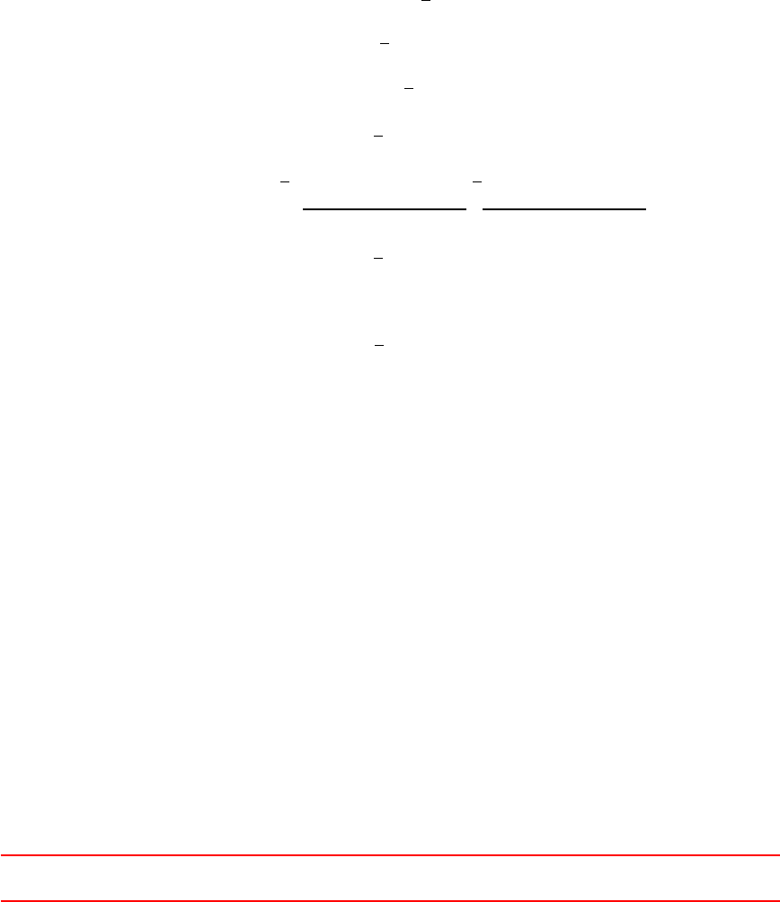
52.4.5 Definitions of Rusche and bubbleFoam
The solvers bubbleFoam and twoPhaseEulerFoam are based on the thesis of H. Rusche [42]. However, the pro-
duction term is defined differently. Compare Eq. (216) and (217).
Pb= 2ν2,eff ∇Ub: dev ∇Ub+ (∇Ub)T (216)
G= 2νT(∇U2: dev(sym(∇U2))) (217)
We ignore the different symbols for the velocity of the continuous phase
U2=Ub(225)
The second operator of the contraction is different in both equations. We ask, if the following equation holds
∇U2: dev(sym(∇U2)) ?
=∇Ub: dev ∇Ub+ (∇Ub)T(226)
With the following identities the question is easily answered
dev(T) = T−1
3tr(T)(227)
sym(T) = 1
2T+ (T)T(228)
dev (sym(∇U2)) = dev 1
2∇U2+ (∇U2)T(229)
dev (sym(∇U2)) = 1
2dev ∇U2+ (∇U2)T(230)
dev (sym(∇U2)) = 1
2(∇U2+ (∇U2)T)−1
3tr(∇U2+ (∇U2)T)
| {z }
=dev(∇U2+(∇U2)T)
(231)
dev (sym(∇U2)) = 1
2dev ∇U2+ (∇U2)T(232)
This leads to the answer
∇U2: dev (sym(∇U2)) = 1
2∇Ub: dev ∇Ub+ (∇Ub)T(233)
The definition of the production term in the source code differs in two ways from the definition in the source
code
1. The use of different viscosities, see Eqns. (216) and (217).
2. A factor of 2, compare Eqns. (226) and (233)
The reason for this differences is not clear. H. Rusche refers to an article which is not available to the author.
52.4.6 Definitions of Ferzinger and bubbleFoam
We now compare the definitions of Ferzinger and bubbleFoam. The definition of Ferzinger is – like the equations
in most other book about turbulence – for single-phase systems. However, bubbleFoam is a two-phase solver.
The question of considering turbulence in two-phase systems is not answered yet. bubbleFoam considers turbu-
lence for the continuous phase by the use of a turbulence model. The turbulence of the disperse phase is linked
to the continuous phase. Therefore, turbulence model equations of bubbleFoam are quite similar to single-phase
turbulence equations.
G= 2νT(∇U2: dev(sym(∇U2))) (217)
P=µT∇U:∇U+ (∇U)T(219)
XThis offering is not approved or endorsed by ESI®Group, ESI-OpenCFD®or the OpenFOAM®
Foundation, the producer of the OpenFOAM®software and owner of the OpenFOAM®trademark. 279
We ignore the different viscosities and ask ourselves
∇U:∇U+ (∇U)T?
= 2 (∇U2: dev(sym(∇U2))) (234)
Inserting Eq. (232) gives
∇U:∇U+ (∇U)T= 2(∇U2: dev(sym(∇U2)))
| {z }
=1
2dev(∇U2+(∇U2)T)
(235)
∇U:∇U+ (∇U)T=∇U2: dev ∇U2+ (∇U2)T(236)
Now we insert Eq. (227) into the rhs of Eq. (236)
∇U:∇U+ (∇U)T=∇U:dev(∇U+ (∇U)T) + 1
3tr(∇U+ (∇U)T)(237)
Using the following identities and Eq. (222)
tr(A+B) = tr(A) + tr(B)(238)
tr(AT) = tr(A)(239)
I:∇U= tr(∇U) = ∇·U(222)
∇U:∇U+ (∇U)T=∇U:dev(∇U+ (∇U)T) + 2
3(∇·U)(240)
The second term of the rhs vanishes according to the continuity equation for an incompressible fluid
∇U:∇U+ (∇U)T=∇U:dev(∇U+ (∇U)T) + 2
3(∇·U)
| {z }
∇·U=0 (241)
Eq. (242) now resembles Eq. (236). Therefore, we proofed that the definition of bubbleFoam is equivalent to
the definition of Ferzinger
∇U:∇U+ (∇U)T=∇U: dev ∇U+ (∇U)T(242)
52.4.7 Definition of standard k-of OpenFOAM
We now compare the definition of the production term of the standard k-model implemented in OpenFOAM
with the definition found in [25].
Source code - standard k-model, kEpsilon.C
G= 2νT|sym(∇U)|2(218)
Ferzinger Peric [25]
P=νT∇U:∇U+ (∇U)T(219)
Starting from Eq. (219), we will use Eq. (242) and Eq. (232)
∇U:∇U+ (∇U)T=∇U: dev ∇U+ (∇U)T(242)
dev ∇U+ (∇U)T= 2 dev (sym(∇U)) (232)
to gain
∇U:∇U+ (∇U)T= 2 ∇U: dev (sym(∇U)) (243)
We use definition (244) to change Eq. (218)
|sym(∇U)|2= sym(∇U) : sym(∇U)(244)
XThis offering is not approved or endorsed by ESI®Group, ESI-OpenCFD®or the OpenFOAM®
Foundation, the producer of the OpenFOAM®software and owner of the OpenFOAM®trademark. 280
Now we pose the question
sym(∇U) : sym(∇U)?
=∇U: dev (sym(∇U)) (245)
The lhs of Eq. (245) corresponds to Eq. (218). The rhs of Eq. (245) was derived from Eq. (219). Now, we use
some identities
dev(T) = T−1
3tr(T)(227)
tr(sym(T)) = tr(T)(246)
to reformulate the rhs of Eq. (245)
∇U: dev (sym(∇U)) = ∇U:sym(∇U)−1
3tr(∇U)(247)
As we now concentrate on incompressible single-phase problems, we can eliminate the second term of the rhs
of Eq. (247) by the use of Eq. (222)
I:∇U= tr(∇U) = ∇·U= 0 (222)
We now have
∇U: dev (sym(∇U)) = ∇U: sym(∇U)(248)
The following equation remains, which is easily proofed by some tensor calculus
sym(∇U) : sym(∇U) = ∇U: sym(∇U)(249)
Every tensor can be decomposed into a symmetric and a skew part
T=sym(T) + skew(T)(250)
sym(T) = 1
2T+TT(251)
skew(T) = 1
2T−TT(252)
Therefore, we can write
T: sym(T) = sym(T) : sym(T) + skew(T) : sym(T)(253)
The following properties of skew tensors let the second contraction vanish
skew(T)
| {z }
aij
: sym(T)
| {z }
sij
(254)
aii = 0 (255)
aij =−aji (256)
skew(T) : sym(T) = aij sij = 0 (257)
Finally, we obtain
T: sym(T) = sym(T) : sym(T)(258)
Therefore, we proofed that the definition of the standard k-model is equivalent to the definition of Ferzinger.
53 Some theory behind the scenes of LES
53.1 LES model hierarchy
The large eddy simulation is based on the spatial filtering of the governing equations. Similar to the Reynolds-
averaged modelling strategy (filtering with respect to time), the large eddy modelling strategy requires some
XThis offering is not approved or endorsed by ESI®Group, ESI-OpenCFD®or the OpenFOAM®
Foundation, the producer of the OpenFOAM®software and owner of the OpenFOAM®trademark. 281
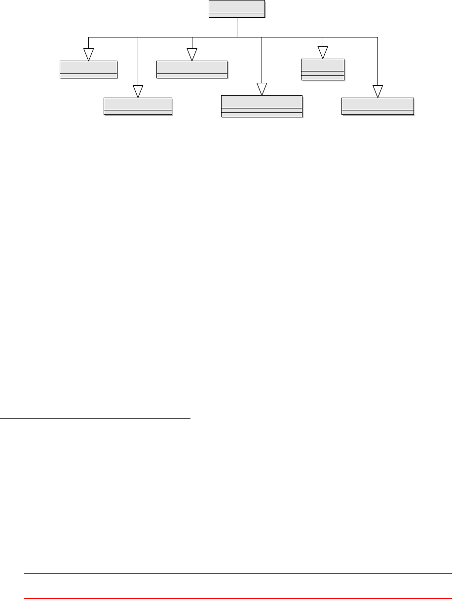
closure models. In principle, the velocity is decomposed into a grid-scale and a sub-grid scale portion. The
grid-scale portion is resolved by the governing equations. The sub-grid scale portion – or the influence of the
sub-grid scale portion on the resolved velocity – needs to be modelled.
Similar to the RANS approach, the closure terms appear in the stress terms of the momentum equations.
There are several modelling strategies to close the equations. The class hierarchy of the LES models of Open-
FOAM reflects the different approaches. Figure 80 shows the first layer of the class hierarchy of the LES models
in OpenFOAM. First layer means that a class derived from the abstract class LESModel may be an abstract
class itself and therefore be the base for other classes178179.
LESModel
DESModel
GenEddyVisc
GenSGSStress
kOmegaSSTSAS
laminar
scaleSimilarity
Figure 80: First layer of the class hierarchy of the LES models of OpenFOAM
The classification according to Figure 80 is not the only possible way to divide all existing LES models into
categories.
53.2 Eddy viscosity models
One of the most common approaches of closing the governing equations when using an LES turbulence mod-
elling strategy are eddy viscosity models. Like the RANS turbulence models, the eddy viscosity models make
use of the Boussinesq hypothesis. The contribution of the sub-grid scale terms is modelled by an additional
viscosity. The effective viscosity is the sum of the laminar viscosity and the sub-grid viscosity.
νeff =ν+νSGS (259)
53.2.1 Class hierarchy
The base class for all eddy viscosity models is GenEddyVisc. Figure 81 shows the class hierarchy with focus on
GenEddyVisc.
53.2.2 Classification
The eddy viscosity models can be divided further based on the way the sub-grid viscosity is computed and the
complexity of the model.
178In a class diagram a class with an italic written name is an abstract class. A class with an upright written name is an actual
class.
179This shows the great advantage of object oriented programming. The class hierarchy of the code reflects the relation between
the objects in reality, e.g. every eddy viscosity model is an LES model, but not every LES model is an eddy viscosity model.
XThis offering is not approved or endorsed by ESI®Group, ESI-OpenCFD®or the OpenFOAM®
Foundation, the producer of the OpenFOAM®software and owner of the OpenFOAM®trademark. 282
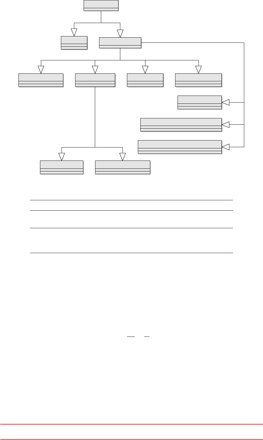
LESModel
laminar GenEddyVisc
dynLagrangian oneEqEddySmagorinsky dynOneEqEddy
Smagorinsky2 mixedSmagorinsky
homogeneousDynOneEqEddy
homogeneousDynSmagorinsky
spectEddyVisc
Figure 81: Class hierarchy of the eddy viscosity models in OpenFOAM
constant coefficient dynamic coefficient
algebraic model Smagorinsky homogeneousDynSmagorinsky
Smagorinsky2 spectEddyVisc
one equation model
oneEqEddy dynOneEqEddy
homogeneousDynOneEqEddy
dynLagrangian
Table 8: Comparison of the eddy viscosity models of OpenFOAM
53.2.3 Eddy viscosity
For dimensional reasons, the eddy viscostiy must be a product of a length and a velocity scale [16]. Eq. (261)
shows the generic equation for the sub-grid viscosity. An additional model constant is the third term in the
product. The way the model constant is computed as well as the choice for the length and velocity scales is
determined by the model.
[νSGS ] = m2
s=m
s·m(260)
νSGS =CSGS lSGS qSGS (261)
A choice that is common to a number of eddy viscosity models in OpenFOAM is to choose the filter width
as the length scale and the square root of the sub-grid kinetic energy as teh velocity scale. Algebraic models
usually calculate the sub-grid kinetic energy from known quantities, e.g. based on the velocity gradient. One
equation models typically solve a transport equation for the sub-grid scale kinetic energy.
XThis offering is not approved or endorsed by ESI®Group, ESI-OpenCFD®or the OpenFOAM®
Foundation, the producer of the OpenFOAM®software and owner of the OpenFOAM®trademark. 283

lSGS = ∆ (262)
[lSGS ]=m (263)
qSGS =pkSGS (264)
[qSGS ] = rm2
s2=m
s(265)
53.2.4 The Smagorinsky LES model
The Smagorinsky eddy viscosity is one of the simplest LES models. From Table 8we see that this is an algebraic
model with a constant model coefficient. This model was published 1963 [44].
Eq. (266) shows the definition of the sub-grid scale viscosity according to the Samgorinsky model as it can
be found in literature [16].
νSGS = (CS∆)2|S|(266)
with
S= sym(∇u) = sym(grad(u))
|T|=√T:T
Some rearrangement of Eq. (266) is necessary to match the form of Definition (261) and (264). Eqns. (267)
to (269) show the necessary steps to match the generic definition of νSGS .
νSGS =C2
S∆
|{z}
lSGS
∆√S:S
| {z }
qSGS
(267)
qSGS =pkSGS = ∆√S:S(268)
⇒kSGS = ∆2S:S(269)
Implementation
The implementation in the source code differs a little from the equations above.
1void Smagorinsky::updateSubGridScaleFields(const volTensorField& gradU)
2{
3nuSgs _ = ck _* de lta () * sq rt ( k( g radU ) );
4nuSgs_.correctBoundaryConditions();
5}
Listing 412: The function updateSubGridScaleFields() in the file Smagorinsky.C
1tmp <volScalarField > k(const tmp < v ol Tens orFi eld >& gradU ) const
2{
3return (2.0* ck_ / ce_ ) * sqr ( d el ta () ) * mag Sqr ( dev ( sy mm ( g radU ) ));
4}
Listing 413: The function k() in the file Smagorinsky.H
Listing 412 shows the implementation of how the sub-grid viscosity is computed by the Smagorinsky model
in OpenFOAM. Listing 413 shows how the model calculates the sub-grid kinetic energy.
nuSgs =ck∆√k(270)
k= 2ck
ce ∆2|dev S|2(271)
XThis offering is not approved or endorsed by ESI®Group, ESI-OpenCFD®or the OpenFOAM®
Foundation, the producer of the OpenFOAM®software and owner of the OpenFOAM®trademark. 284

with
S= sym grad(u)(272)
it follows
nuSgs =ck∆r2ck
ce ∆2|dev S|2(273)
nuSgs =ckr2ck
ce ∆2|dev S|(274)
the comparison with Eq. 266 shows
νSGS = (CS∆)2|S|(266)
⇒C2
S=ckr2ck
ce (275)
Eq. (275) shows how the Smagorinsky constant can be calculated from the model constants. The Smagorin-
sky constant is often stated in publications using or investigating the Smagorinsky model, because it is the only
degree of freedom of the Smagorinsky model.
In OpenFOAM the Smagorinsky model has two model constants. ce is inherited from the class GenEddyVisc.
This constant is used in the definition of the sub-grid dissipation rate. The default value of ce is 1.048 and is
defined in the constructor of the class GenEddyVisc in the file GenEddyVisc.C.
Therefore, the model constant ck is the only degree of freedom of the Smagorinsky model of OpenFOAM.
The default value of ck is 0.094. This results in a default value fofr CSof 0.1995 ≈0.2. The value of CSvaries
in literature depending on the publication from 0.07 to 0.33 [8,35].
1// - Return sub - grid dis ipa tio n rate
2virtual tmp <volScalarField > epsilon() const
3{
4return tmp <volScalarField >
5(
6new volScalarField
7(
8IOobject
9(
10 "epsilon",
11 run Time _ . ti me Name () ,
12 mesh_ ,
13 IOobject :: NO_READ ,
14 IOobject :: NO _WR ITE
15 ) ,
16 ce _ * k () * sq rt ( k () ) / d el ta ()
17 )
18 );
19 }
Listing 414: The function epsilon() in the file GenEddyVisc.H
53.2.5 The oneEqEddy LES model
The oneEqEddy model is one of the standard LES models of OpenFOAM. This model is an one equation eddy
viscosity model with a constant model coefficient. Eq. 276 shows how the sub-grid viscosity is calculated by
the oneEqEddy model. The constant ck has a default value of 0.094.
νSGS =ck∆pkSGS (276)
The transport equation for kSGS
As this model is an one equation model, it introduces an additional equation to the set of equations. This
additional equation is a transport equation for the sub-grid kinetic energy kSGS .kSGS is the kinetic energy of
XThis offering is not approved or endorsed by ESI®Group, ESI-OpenCFD®or the OpenFOAM®
Foundation, the producer of the OpenFOAM®software and owner of the OpenFOAM®trademark. 285

the unresolved protion of the velocity. Thus, kSGS is called sub-grid kinetic energy.
∂kSGS
∂t +∇·(kSGS u)− ∇·(Dk∇kSGS ) = G−SGS (277)
with
Dk=ν+νSGS
G=νSGS |sym(∇u)|2
SGS =ce√kSGS
∆kSGS
Eq. 277 is similar to the transport equation for kof the k-model. Also the definition of the sub-grid viscos-
ity is similar to the definition of the turbulent viscosity of the k-model. This is not very obvious. Therefore,
we shall explore this matter further.
νSGS =ck∆pkSGS (276)
νSGS =ck ce
ce
kSGS
kSGS
√kSGS
√kSGS
∆pkSGS (278)
νSGS =ck cekSGS √kSGS √kSGS
cekSGS √kSGS
∆
(279)
νSGS =ck cek2
SGS
SGS
(280)
Eq. 280 is similar to Eq. 200 – the definition of the turbulent viscosity of the k-model
νT=Cµ
k2
(200)
The product of ck and ce when using their default values gives ck ·ce = 0.0985 which is approximately the
default value of Cµof the k-model, which is Cµ= 0.09.
54 The use of phi
54.1 The question
The governing equations of the solvers of OpenFOAM are written in a special notation that makes it easy
to compare the source codes with equations from a fluid dynamics textbook. In Section 33.1 the governing
equations of the solver pimpleFoam are examined. There, the terms of Eq. 61 are compared with the source
code, see Listing 204. Here, we repeat the comparison of how the convective term is written in the sources and
how this term is expressed mathematically.
∇(uu)
| {z }
div(uu)
⇔fvm::div(phi, U)
We now examine how phi is defined and how we can find phi in the math.
54.2 Implementation
54.2.1 The origin of fields
One way to learn more about phi is to look for its definition in the source code of OpenFOAM.
Listing 415 shows the first lines of the main function of the solver pimpleFoam. The main function of any
C or C++ program is entered, when this program is executed. So, the instructions of Listing 415 are the first
instructions that are executed, when the solver is called.
In line 6of Listing 415 the file createFields.H is included. This file contains instructions that create the
data structures of all fields that are necessary for the solver (e.g. the pressure or the velocity field).
XThis offering is not approved or endorsed by ESI®Group, ESI-OpenCFD®or the OpenFOAM®
Foundation, the producer of the OpenFOAM®software and owner of the OpenFOAM®trademark. 286

1int main(int argc , char * ar gv [ ])
2{
3#include " set Roo tCase . H"
4#include " cre ate Time .H "
5#include " cre ate Mesh .H "
6#include "createFields.H"
7#include " ini tC onti nuit yErr s .H"
8
9/* the rest of the solver */
Listing 415: The first few line of the main function of pimpleFoam in pimpleFoam.C
The file createFields.H contains the content of Listing 416. There, the velocity field Uis created. In line
15 the file createPhi.H is included. There, the field phi is created.
1Info << " R eadi ng f ield U \n" << endl;
2volVectorField U
3(
4IOobject
5(
6"U",
7runTi me . t im eNam e () ,
8mesh ,
9IOobject :: MUST_READ ,
10 IOobject :: AU TO_WRITE
11 ) ,
12 mesh
13 );
14
15 #include " createPhi . H"
Listing 416: The creation of Uand phi in the file createFields.H
54.2.2 How phi is defined
Listing 417 shows the content of the file createPhi.H. From this Listing we see the data type of phi, it is
surfaceScalarField. This tells us, that phi is a scalar, that is defined on the faces of the control volumes
(cells) of the mesh.
Line 13 tells us how phi is defined. There, we find out, that phi is the inner product of the velocity – we
forget for the moment about the function linearInterpolate – and the face surface area vector. In Listing
418 we see the declaration of the function Sf(). In Listing 419 we see, that the variable mesh of Listing 417 is
of the type fvMesh.
1Info << " R eadi ng / calcula ting face flux f ield phi \n" < < endl ;
2
3sur face S cal a rFi e ld phi
4(
5IOobject
6(
7" ph i ",
8runTi me . t im eNam e () ,
9mesh ,
10 IOobject::READ_IF_PRESENT ,
11 IOobject :: AU TO_WRITE
12 ) ,
13 l in e ar I nt erp o la t e ( U) & m es h . Sf ( )
14 );
Listing 417: The creation of phi in the file createPhi.H
1// - R eturn cell f ace area v ec tors
2const s ur fa ce Ve ct or Fie ld & Sf () c onst ;
Listing 418: The declaration of the method Sf() of the class fvMesh in the file fvMesh.H
XThis offering is not approved or endorsed by ESI®Group, ESI-OpenCFD®or the OpenFOAM®
Foundation, the producer of the OpenFOAM®software and owner of the OpenFOAM®trademark. 287

1Foam::Info
2<< " Create mesh for time = "
3<< runTime . ti meName () << Foam :: nl << Foam :: endl ;
4
5Foam :: fvMesh mesh
6(
7Foam :: IO obje ct
8(
9Foam :: fvMesh :: def aultR egion ,
10 runTi me . t im eNam e () ,
11 runTime ,
12 Foam :: IOob jec t :: M UST _RE AD
13 )
14 );
Listing 419: The creation of the mesh in the file createMesh.H
54.3 The math
Now, let us examine the origin of phi from the mathematical point of view. We start with the governing
equations of a solver for incompressible fluids. Therefore, Eq. 61 is repeated below.
∂u
∂t +∇(uu) + ∇·dev(−νef f ∇u+ (∇u)T) = −∇p+Q(61)
This equation is written in diferential form and is valid everywhere in the fluid. In order to use the finite
volume method, we need the governing equations in the integral form. Integrating Eq. (61) over a control
volume yields:
ZV
∂u
∂t +∇(uu) + ∇·dev(−νef f ∇u+ (∇u)T) dV=ZV−∇p+QdV(281)
Now we will have a closer look on the second term of Eq. (281). That is the convective term we already saw
at the beginning of this section.
Using Gauss’ theorem, we replace the integration over the volume of our control volume with the integration
over the surface of the control volume.
ZV∇(uu) dV=I∂V
(uu)·dS(282)
Because our control volume is a polyhedron (in most cases a hexahedron or a tetrahedron), the surface
integral reduces to a sum of intergrals over the faces Sfof the polyhedron.
I∂V
(uu)·dS=X
fZSf
(uu)·dSf(283)
kSfk=Sf(284)
With Sfbeing the surface normal vector of the face f. The norm of this vector is equal to the area of the
face f. We denote with the subscript fthe mean face-value of a quantity.
X
fZSf
(uu)·dSf=X
f
(uu)f·Sf(285)
(uu)f=1
SfZSf
(uu) dSf(286)
(uu)f≈(ufuf)(287)
X
f
(uu)f·Sf≈X
f
(ufuf)·Sf(288)
XThis offering is not approved or endorsed by ESI®Group, ESI-OpenCFD®or the OpenFOAM®
Foundation, the producer of the OpenFOAM®software and owner of the OpenFOAM®trademark. 288
Eq. (288) contains the fundamental assumption or approximation of the finite volume method. It is assumed,
that the mean face-value of the product of the velocities is (approximately) equal to the product of the mean
face-values of the velocity, see Eq. (287). In general, the operations averaging and multiplication are not
commutative.
We are now nearly finished. The rhs of Eq. (288) contains all ingredients we need for phi. A surface area
vector, a velocity and an inner vector product. See Listing 417. However, this ingredients are not in the order
we need. Therefore, there is need for some more math to do.
A general rule of tensor calculus states:
a⊗b·c=a(b·c)(289)
In this document, we omit the symbol ⊗for the sake of brevity.
a⊗b·c= (ab)·c(290)
Eq. (290) looks like the rhs of Eq. (288).
(ufuf)·Sf=uf(uf·Sf)
| {z }
=φf
(291)
uf(uf·Sf) = ufφf(292)
54.4 Summary
Now, after having dug deep into the sources and after having done some math, we can summarize all thoughts
so far. We want to understand this equivalency.
∇(uu)
| {z }
div(uu)
⇔fvm::div(phi, U)
The math tells use the following identities.
ZV∇(uu) dV=I∂V
(uu)·dS(293)
I∂V
(uu)·dS=X
f
(uu)f·Sf(294)
X
f
(uu)f·Sf≈X
f
(ufuf)·Sf(295)
X
f
(ufuf)·Sf=X
f
uf(uf·Sf)(296)
X
f
uf(uf·Sf) = X
f
ufφf(297)
We have shown, that the integral formulation of the convective term can be reformulated to incorporate φ
and uinstead of uu.
55 Derivation of the IATE diameter model
In this section we cover the derivation of OpenFOAMs IATE diameter model from [23].
XThis offering is not approved or endorsed by ESI®Group, ESI-OpenCFD®or the OpenFOAM®
Foundation, the producer of the OpenFOAM®software and owner of the OpenFOAM®trademark. 289
55.1 Number density transport equation
We start with the transport equation for the bubble number density distribution f=f(V, x, t), e.g. from [23].
For sake of readability in most cases we refer to f(V, x, t)simply as f.
The first term of Eqn. (298) is the local rate of change of the bubble number density distribution. The
second term represents convective transport. The third term represents the rate of change due to change of
bubble volume. On the right hand side of the equation are source terms due to bubble interactions Sjand
phase change Sph.
∂f
∂t +∇·(fu) + ∂
∂V fdV
dt=X
j
Sj+Sph (298)
The equation for the bubble number density distribution is much too detailled for most flow studies [29].
Thus, we derive a transport equation for the area concentration ai. The area concentration is a moment of the
bubble number density distribution. Besides the area concentration we can define further quantities based on
the moments of the number density distribution.
Eqn. (299) lists the general definition of the i-th moment miof the probability density function f(x).
mi=Zb
a
f(x)xidx(299)
We now define some moments of the bubble number density distribution.
Total number of bubbles per unit volume n(x, t) = ZVmax
Vmin
f(V, x, t)dV(300)
Volume fraction of bubbles α(x, t) = ZVmax
Vmin
f(V, x, t)VdV(301)
Area concentration of bubbles ai(x, t) = ZVmax
Vmin
f(V, x, t)Ai(V)dV(302)
55.2 Interfacial area transport equation
55.2.1 Deriving the governing equations
We will use Eqn. (302) to derive a transport equation for the area concentration from Eqn. (298). First we
multiply Eqn. (298) by the average interfacial area Ai(V)of bubbles with the volume V.
Ai
∂f
∂t +Ai∇·(fu) + Ai
∂
∂V fdV
dt=Ai
X
j
Sj+Sph
(303)
Then, we integrate Eqn. (303) over all bubble sizes
ZVmax
Vmin Ai
∂f
∂t +Ai∇·(fu) + Ai
∂
∂V fdV
dtdV=ZVmax
Vmin
Ai
X
j
Sj+Sph
dV(304)
Now we will take a closer look on the single terms of Eqn. (304). For the first term, we simply apply Leibnitz
rule. Here it is important to note, that Aiis constant in space and time. With Eqn. (302), we gain the local
derivative of the interfacial area concentration ai.
ZVmax
Vmin
Ai
∂f
∂t dV=∂
∂t ZVmax
Vmin
AifdV(305)
ZVmax
Vmin
Ai
∂f
∂t dV=∂
∂t ai(306)
XThis offering is not approved or endorsed by ESI®Group, ESI-OpenCFD®or the OpenFOAM®
Foundation, the producer of the OpenFOAM®software and owner of the OpenFOAM®trademark. 290
The convective term of Eqn. (304) can be treated in a similar fashion. If the velocity is independent of the
bubble size, we can put the uin front of the integral over all bubble sizes. Thus, we gain the convective term
for the interfacial area concentration.
ZVmax
Vmin
Ai∇·(fu) dV=ZVmax
Vmin ∇·(Aifu) dV(307)
ZVmax
Vmin
Ai∇·(fu) dV=∇· uZVmax
Vmin
AifdV!(308)
ZVmax
Vmin
Ai∇·(fu) dV=∇·(uai)(309)
If the velocity is not independent of the bubble size we can follow a similar strategy to derive a convective
term which is formulated in terms of the interfacial area concentration.
ZVmax
Vmin
Ai∇·(fu) dV=ZVmax
Vmin ∇·ai
ai
AifudV(310)
ZVmax
Vmin
Ai∇·(fu) dV=∇· aiRVmax
Vmin AifudV
ai!(311)
ZVmax
Vmin
Ai∇·(fu) dV=∇·(aiui)(312)
With the average local bubble velocity weighted by the bubble number ui[13]
ui=RVmax
Vmin AifudV
RVmax
Vmin AifdV(313)
The third term of Eqn. (304) needs more special treatment. In Section 55.5.1 we show the proof for (314).
This term relates to the gas expansion.
ZVmax
Vmin
Ai
∂
∂V fdV
dtdV=−2
3
˙α
αai(314)
The RHS of Eqn. 304 contains the terms due to bubble-bubble interaction and due to phase change.
ZVmax
Vmin Ai
∂f
∂t +Ai∇·(fu) + Ai
∂
∂V fdV
dtdV=ZVmax
Vmin
Ai
X
j
Sj+Sph
dV(304)
There are two approaches to model the source terms due to bubble interaction [31]. One can solve the
integral equation for these source terms (315) or solve algebraic equations using mean parameters (316).
The latter approach assumes monosized bubble, i.e. a bubble breaks up into two equalsized daughter bubbles
[31]. In this approach each bubble interaction results in a change of interfacial area ∆Ai=1
3Ai.
ZVmax
Vmin
AiX
j
SjdV= Φj(315)
Φj=Sj∆Ai(316)
with the interfacial area Ai
Ai=ai
n(317)
XThis offering is not approved or endorsed by ESI®Group, ESI-OpenCFD®or the OpenFOAM®
Foundation, the producer of the OpenFOAM®software and owner of the OpenFOAM®trademark. 291
and bubble number density n,Ψ = 1
36πfor spherical bubbles
n= Ψ a3
i
α2(318)
Φj=1
3
1
Ψα
ai2
Sj(319)
The phase change term can be modelled directly, but within the framework of this manual we will not
consider phase change. Thus we gained a transport equation for the interfacial area concentration ai.
∂ai
∂t +∇·(uai) = 2
3
˙α
αai+X
j
1
3
1
Ψα
ai2
Sj(320)
55.3 Interfacial curvature transport equation
55.3.1 Basic definitions
The IATE diameter model solves a transport equation for the interfacial curvature kappai_.
Solves for the interfacial curvature per unit volume of the phase rather than interfacial area
per unit volume to avoid stability issues relating to the consistency requirements between the phase
fraction and interfacial area per unit volume.
Class description in IATE.H
By looking into the sources, we find the following relations
ai=ακ (321)
dsm =6
κ(322)
Thus, the Sauter mean diameter dsm equals
dsm =6α
ai
(323)
Which corresponds with the definition given in literature [21,22].
dsm =6α
ai
(324)
Listing 420 and 421 show the relevant source code of the IATE diameter model. This source code is the basis
for Eqns. (321) and (322).
1// - R eturn the i nterf ac ial area
2tmp <volScalarField > a() c onst
3{
4return phase_ * kappa i_ ;
5}
Listing 420: Definition of the method a() of the IATE diameter model classin the file IATE.H.
1Foam :: tmp < Foam :: v olS calar Field > Foam :: dia mete rMo dels :: IATE :: dsm () const
2{
3return max (6/ max ( kappa i_ , 6/ dM ax_ ), dMi n_ );
4}
Listing 421: Definition of the method dsm() of the IATE diameter model class in the file IATE.C.
The definition of kappai_ as the interfacial curvature seems a bit counter-intuitive, as the curvature of a
sphere is the inverse of its radius.
XThis offering is not approved or endorsed by ESI®Group, ESI-OpenCFD®or the OpenFOAM®
Foundation, the producer of the OpenFOAM®software and owner of the OpenFOAM®trademark. 292

55.3.2 Derivation of the governing equations
We will now derive the governing equations for the interfacial curvature κfrom the equations for the interfacial
area concentration aiwhich we derived from the transport equations for the bubble size distribution.
Here we will make no further assumptions, as we are simply rearranging the equations. We start from the
transport equation for the interfacial area concentration aiand OpenFOAMs definition of ai.
∂ai
∂t +∇·(uai) = 2
3
˙α
αai+X
j
1
3
1
Ψα
ai2
Sj(320)
ai=ακ (321)
Inserting (321) into (320) yields
∂ακ
∂t +∇·(uακ) = 2
3
˙α
αακ +X
j
1
3
1
Ψα
ακ2Sj(325)
Next, we apply partial derivation of all terms containing κ
α∂κ
∂t +κ∂α
∂t +κ∇·(uα) + αu·∇κ=2
3˙ακ +X
j
1
3
1
Ψ1
κ2
Sj(326)
κ∂α
∂t +∇·(uα)
| {z }
˙α
+α∂κ
∂t +u·∇κ=2
3˙ακ +X
j
1
3
1
Ψ1
κ2
Sj(327)
α∂κ
∂t +u·∇κ=−1
3˙ακ +X
j
1
3
1
Ψ1
κ2
Sj(328)
∂κ
∂t +u·∇κ=−1
3˙ακ
α+X
j
1
3
1
Ψ
1
α1
κ2
Sj(329)
With 1
κ=α
ai
∂κ
∂t +∇(κu)
| {z }
I
−κ∇·u
| {z }
II
=−1
3
˙α
ακ
| {z }
III
+1
3Ψ α
ai2X
j
Sj
α(330)
The form of Eqn. (330) is chosen to match the equations given in [23]. The second term of the RHS has
exactly the same form as the equivalent terms in [23].
55.3.3 Implemented equations
Thus, we have derived a transport equation for κ. However, we still need to check the equations that are
implemented in OpenFOAM. Therefore, we take a look at the source code.
In Listing 422 we see the main code for the transport equation. In Line 4we see the terms marked with I
of Eqn. (330). In Line 5term II of Eqn. (330) is implemented.
1// Construct the interf aci al curvature equation
2fvS cala rMa trix k app aiE qn
3(
4fvm :: ddt ( kappa i_ ) + fvm :: div ( ph ase_ . phi () , kappai _)
5- fvm :: Sp( fvc :: div ( phase_ . phi () ), k appai _ )
6==
7- f vm : : S uSp ( R , k app ai _ )
8// + R ph ( ) / / O mit the nu c le at ion / c on de n sa tio n t er m
9);
Listing 422: Construction of the transport equation in the file IATE.C.
XThis offering is not approved or endorsed by ESI®Group, ESI-OpenCFD®or the OpenFOAM®
Foundation, the producer of the OpenFOAM®software and owner of the OpenFOAM®trademark. 293

The right hand side of the equation in Listing 422 combines all term of the RHS of Eqn. (330) into the term
fvm::SuSp(R, kappai_). The method fvm::SuSp() implements a source term for a matrix equation. The
arguments translate to R * kappai_.
The first term on the RHS of Eqn. (330) is due to the change of bubble volume (dilatation effect). The code
in Listing 423 translates to Eqn. (331).
1// Ini tia lise the acc umulate d sou rce term to the dilatatio n effect
2volScalarField R
3(
4(
5(1.0/3.0)
6/ ma x
7(
8fv c :: a ve rag e ( p ha se _ + p ha se _ . o ld Ti me () ) ,
9residualAlpha_
10 )
11 )
12 *( fvc :: ddt ( phase_ ) + fvc :: div ( phase_ . alphaPhi () ))
13 );
Listing 423: The first term of the RHS of Eqn. (330) of the transport equation in the file IATE.C.
R=1
3
∂α
∂t +∇·(αu)
α(331)
The method call fvm::SuSp(R, kappai_) multiplies Rwith kappai_. Thus we recognize the first term of
the RHS of Eq. (330).
Eqn. (330)III =−1
3
˙α
ακ(332)
OpenFOAM III =−Rκ(333)
R=1
3
˙α
α(334)
III =−1
3
˙α
ακ(335)
The other source terms related to the models for bubble-bubble interaction are added to R. Listing 424 shows
the loop over all sources, note the minus sign.
1// A cc um ul at e the run - time sel ec ta bl e sou rc es
2forAl l ( sources_ , j )
3{
4R -= s our ce s_ [ j ]. R () ;
5}
Listing 424: The second term of the RMS of Eqn. (330) of the transport equation in the file IATE.C.
For the interaction models the minus of Listing 424 cancels the minus of Listing 422.
55.4 Interaction models
OpenFOAM provides a base class for all models related to bubble-bubble interaction. There are several inter-
action mechanisms implemented.
1. Breakage due to impact of turbulent eddies (TI - turbulent impact)
2. Coalescence through random collision driven by turbulent eddies (RC - random collision)
3. Coalescence due to acceleration of the following bubble in the wake of preceding bubble (WE - wake
entrainment)
The base class is named IATEsource and it defines a pure virtual function named R(). This means that every
derived class has to provide its implementation of R(). Besides R(), the base class provides a number of helper
methods that are used in the derived classes, e.g. bubble Reynolds number Re() or the Weber number We().
XThis offering is not approved or endorsed by ESI®Group, ESI-OpenCFD®or the OpenFOAM®
Foundation, the producer of the OpenFOAM®software and owner of the OpenFOAM®trademark. 294

55.4.1 Turbulent impact - TI
In [22,23] the source term due to turbulent impact is stated as:
n= Ψ a3
i
α2(336)
ut=√2k(337)
RT I =CT I nut
Dbexp −W ecr
W e r1−W ecr
W e where W ecr > W e (338)
The Weber number W e can be seen as the ratio of inertia forces and surface tension forces and is defined
as:
W e =ρu2d
σ(339)
with
ρdensity
ucharacteristic velocity
dcharacteristic length scale
σsurface tension
The Weber number is provided by the class IATEsource as the base class for all interaction models. See
Section 55.4.4 for implementation details.
The critical Weber number W ecr and the model constant CT I must be provided by the user in the appropriate
dictionary.
55.4.2 Random collision - RC
In [22,23] the source term due to random collision is stated as:
ut=√2k(340)
RRC =CRC "n2utD2
b
α1
/3
max(α1
/3
max −α1
/3)#"1−exp −Cα1
/3
maxα1
/3
α1
/3
max −α1
/3!# (341)
The model constants CRC ,Cand αmax need to be provided by the user.
55.4.3 Wake entrainment - WE
In [22,23] the source term due to wake entrainment is stated as:
RW E =CW E C1
/3
Dn2D2
bur(342)
The model constant CW E needs to be provided by the user.
55.4.4 Implementation details of the IATEsource class
Weber number
The Weber number is implemented in the class IATEsource, see Listing 425. This definition makes use the
method Ur(), which is also provided by IATEsource.
1Foam :: tmp < Foam :: v olS calar Field > Foam :: dia mete rMo dels :: I ATE sou rce :: We ()
2const
3{
4return o th er P ha se () . r ho ( ) * sqr ( Ur () ) * p ha se () . d () / fl ui d ( ) . si gm a () ;
5}
Listing 425: The definition of the Weber number W e in IATEsource.C
XThis offering is not approved or endorsed by ESI®Group, ESI-OpenCFD®or the OpenFOAM®
Foundation, the producer of the OpenFOAM®software and owner of the OpenFOAM®trademark. 295

Relative velocity
The relative velocity between the bubbles and the surrounding fluid is given by [20,28]. Compare Eqn. (343)
and Listing 426.
ur=√2σg∆ρ
ρ2
L1
/4
(1 −α)1.75 (343)
1Foam :: tmp < Foam :: v olS calar Field > Foam :: dia mete rMo dels :: I ATE sou rce :: Ur () const
2{
3const uniformDimensionedVectorField& g =
4pha se () . U () . db () . l oo ku pO bj ec t < u nif o rm Di m en s io n ed Vec tor F ie ld >( "g") ;
5
6return
7sqrt ( 2.0)
8*pow025
9(
10 flu id () . si gm a ( ) * mag ( g)
11 *( o the rP h as e ( ) . rho () - pha se () . r ho () )
12 / sqr ( oth er P ha se () . r ho ( ) )
13 )
14 * po w ( max (1 - pha se () , s ca la r (0) ) , 1 .75) ;
15 }
Listing 426: The definition of the relative velocity between bubbles and surrounding liquid in IATEsource.C
The IATE implicitely applies only to bubbly systems, i.e. gas-liquid systems. If the IATE model is applied to
the denser phase, then Line 11 of Listing 426 leads to a floating-point exception (FPE). If phase refers to the
liquid phase, then Line 11 evaluates to a negative number. Raising a negative number to a non-integer power
is not possible within the domain of the real numbers. Thus, OpenFOAM will issue an error message due to an
floating-point exception.
Comparing the formulations
Here we take a closer look on the implementation of the source terms. Listing 427 shows the method R() of the
IATEsource class.
1Foam :: tmp < Foam :: v olS calar Field >
2Foam :: d iame terM ode ls :: IAT Esource s :: t urb u len tBre akUp ::R() const
3{
4tmp <volScalarField > tR
5(
6new volScalarField
7(
8IOobject
9(
10 "R",
11 iat e_ . pha se () . U () . t im e () . t im eNa me ( ) ,
12 iat e_ . pha se () . me sh ()
13 ) ,
14 iat e_ . pha se () . U () . m es h () ,
15 dimensionedScalar(" R " , dim le ss / d imTime , 0)
16 )
17 );
18
19 volScalarField R = tR();
20 sca la r C ti = Ct i_ . v al ue () ;
21 sca la r We Cr = W eC r_ . v al ue () ;
22 volScalarField Ut(this - > Ut ( ) );
23 volScalarField We(this - > We ( ) );
24 const v ol S ca l ar Fie ld & d ( i at e_ . d () () ) ;
25
26 for Al l (R , c el li )
27 {
28 if ( We [ c el li ] > W eC r )
29 {
XThis offering is not approved or endorsed by ESI®Group, ESI-OpenCFD®or the OpenFOAM®
Foundation, the producer of the OpenFOAM®software and owner of the OpenFOAM®trademark. 296

30 R[ ce lli ] =
31 (1.0/3.0)
32 * Ct i /d [ celli ]
33 * Ut [ ce ll i ]
34 * s qrt (1 - WeCr / We [ c el li ])
35 * exp ( - We Cr / We [ c el li ] ) ;
36 }
37 }
38
39 return tR ;
40 }
Listing 427: The definition of the method R() in turbulentBreakUp.C
Listing 427 translates to the following mathematical expression:
RT I =1
3
CT I
dsm
utr1−W ecr
W e exp −W ecr
W e where W e > W ecr (344)
Comparing Eqns. (338) and (344) reveals some differences in formulation. This is due to the fact, that Eq.
(338) is a source term for the transport equation for the interfacial area concentration aiand Eq. (344) is a
source term for the transport equation for the interfacial curvature κ.
In the derivation of the curvature equation from the area concentration equation we divided by the volume
fraction. Otherwise, only rearrangement and variable substitution was performed.
For this term we now have a look on the RHS of the equations for aiand κand compare the implementation
of OpenFOAM with the equations stated in literature.
We begin with repeating the equations for aiand κ. The interaction source term Sjcan be found in this
form in [23].
∂ai
∂t +∇·(uai) = 2
3
˙α
αai+X
j
1
3
1
Ψα
ai2
Sj(320)
∂κ
∂t +∇(κu)−κ∇·u=−1
3
˙α
ακ+1
3Ψ α
ai2X
j
Sj
α
| {z }
IV
(330)
The interaction model source terms in the curvature equation of OpenFOAM takes the following form:
∂κ
∂t +∇(κu)−κ∇·u=−1
3
˙α
ακ+X
j
Rjκ
| {z }
IV
(345)
We now compare the terms marked with IV of Eqns. (330) and (345). As these terms must be equal, we
can form the following equation.
1
3Ψ α
ai2X
j
Sj
α=X
j
Rjκ(346)
We now demand, that the summands need to be equal, and we focus on the term for turbulent break-up (TI)
1
3Ψ α
ai21
αCT I nut
Dbexp −W ecr
W e r1−W ecr
W e
| {z }
Sj
=1
3
CT I
dsm
utr1−W ecr
W e exp −W ecr
W e
| {z }
Rj
κ(347)
Next, we cancel all common symbols and expressions, note the different symbols for the bubble diameter
(Db=dsm)
1
Ψα
ai21
αn=κ(348)
XThis offering is not approved or endorsed by ESI®Group, ESI-OpenCFD®or the OpenFOAM®
Foundation, the producer of the OpenFOAM®software and owner of the OpenFOAM®trademark. 297
We now insert the definition of n, see Eq. (336)
1
Ψα
ai21
αΨa3
i
α2=κ(349)
ai
α=κ(350)
We now end up with an equation that is fulfilled, when we look at the definition of κ, see Eqn. (321)
ai=ακ (321)
Thus, we have demonstrated on the example of the source term for turbulent break-up of bubbles, that the
implementation of OpenFOAM follows exactly the model published in [23].
55.5 Appendix
55.5.1 The proof for Eqn. (314)
We use the following symbols.
x=V(351)
f(x) = f(V, x, t)(352)
g(x) = Ai(V)(353)
a=Vmin (354)
b=Vmax (355)
Thus, the LHS of Eqn. (314) becomes
ZVmax
Vmin
Ai
∂
∂V fdV
dtdV=Zb
a
g(x)∂
∂x f(x)dx
dtdx(356)
Now, we apply partial integration
Zb
a
g(x)∂
∂x f(x)dx
dtdx=f(x)dx
dtg(x)b
a−Zb
a
∂g(x)
∂x f(x)dx
dtdx(357)
As f(x)is a probability density distribution it has the following properties
f(a) = f(b)=0 (358)
Thus, the first term of the RHS of Eqn. (357) vanishes
Zb
a
g(x)∂
∂x f(x)dx
dtdx=−Zb
a
∂g(x)
∂x f(x)dx
dtdx(359)
We now take a closer look on the relation between the average interfacial area of a bubble Aiand the volume
of a bubble V.
Ai=d2π(360)
V=d3π
6(361)
⇒d=3
r6V
π(362)
Ai=6V
π2
/3
π(363)
XThis offering is not approved or endorsed by ESI®Group, ESI-OpenCFD®or the OpenFOAM®
Foundation, the producer of the OpenFOAM®software and owner of the OpenFOAM®trademark. 298
Returning to our simplified notation for this proof
g(x) = 6x
π2
/3
π(364)
For Eqn. (359) we also need the derivative of g(x)
∂g(x)
∂x =2
36
π2
/3
(x)−1
/3π(365)
∂g(x)
∂x =2
36
π2
/3x2
/3
xπ(366)
∂g(x)
∂x =2
3
1
x6x
π2
/3
π(367)
∂g(x)
∂x =2
3
g(x)
x(368)
We now insert Eqn. (359) into Eqn. (359).
Zb
a
g(x)∂
∂x f(x)dx
dtdx=−Zb
a
2
3
g(x)
xf(x)dx
dtdx(369)
Zb
a
g(x)∂
∂x f(x)dx
dtdx=−2
3Zb
a
˙x
xf(x)g(x)dx(370)
Next, we take a closer look on the term ˙x
x. Since xis the volume of the bubbles V, we can relate Vto
the void fraction or gas phase volume fraction α. For any control volume VCV we can state, that the volume
of the bubbles Vis equal to the volume fraction times the control volume. Here we neglect mass transfer by
evaporation, see [22] for a derivation considering evaporation.
V=αVCV (371)
˙
V= ˙αVCV (372)
˙
V
V=˙αVCV
αVCV
=˙α
α(373)
˙x
x=˙α
α(374)
We further assume that the rate of change of volume is independent of the volume itself [22,28].
˙
V
V6=f(V)(375)
By using relation (370) and (374) on Eqn. (370), we gain
Zb
a
g(x)∂
∂x f(x)dx
dtdx=−2
3
˙α
αZb
a
f(x)g(x)dx(376)
or by using the other notation, Eqns. (351)-(351)
Zb
a
g(x)∂
∂x f(x)dx
dtdx=−2
3
˙α
αZVmax
Vmin
fAidV(377)
Zb
a
g(x)∂
∂x f(x)dx
dtdx=−2
3
˙α
αai(378)
And by using (302) on (377) we have proofed (314).
XThis offering is not approved or endorsed by ESI®Group, ESI-OpenCFD®or the OpenFOAM®
Foundation, the producer of the OpenFOAM®software and owner of the OpenFOAM®trademark. 299
56 Derivation of the governing equations for the MRF approach
56.1 Preliminary observations
In order to use the MRF approach the mesh has to be divided into different regions. As the MRF approach in
OpenFOAM covers only rotating reference frames180 only rotation can be imposed on a region. A region for
which a non-zero rotation is specified has to be axi-symmetric with respect to the rotational axis. Furthermore,
does older version of OpenFOAM181 only support steady rotation, i.e. the angular velocity ωis constant.
56.1.1 Pitfalls
Axi-symmetric region for MRF rotation
As stated above, the MRF region for applying reference frame rotations has to be axi-symmetric. However,
OpenFOAM performs no checks to test whether this is the case. Thus, on a region axi-symmetic with respect
to the z-axis, may very well be used to prescribe a reference frace rotation around the x-axis. The results will
be blatantly wrong, and the solver might crash. However, if you are unlucky enough, the solver will not crash
and compute woefully wrong results, wasting time and computational resources.
Always check whether the axis of the MRFProperties coincides with the sym-
metry axis of your MRF zone. Furthermore, make sure that origin of the
MRFProperties lies on the symmetry axis of the MRF zone.
56.2 Mass conservation equation
The mass conservation equation for incompressible flows
∇·u= 0 (379)
is valid in all inertial frames of reference. An inertial frame of reference is either fixed in space and time or
moving with a constant translational velocity.
Due to the constraints listed in the previous section we consider only rotating reference frames in the MRF
method. To translate a vector from its representation in the inertial frame of reference to the rotating frame of
reference a rotation matrix Qis used. A rotation matrix has the property that the inverse is also the transposed.
Ru=Qu (380)
u=QTRu(381)
Q−1=QT(382)
The index Rbefore the symbol udenotes that the vector Ruis given in the rotating frame of reference. If
there is no index before the symbol the vector is given in the inertial coordinate system. The index Ris put
before the symbol to prevent the vector Ruto be mistaken as a relative velocity.
Beginning with the mass conservation equation in the inertial coordinate system we derive the mass conser-
vation in the rotating coordinate system.
∇·u= 0 (383)
∇·QTQ
|{z}
=I
u= 0 (384)
∇·QTRu= 0 (385)
180E.g. in Fluent it is possible to prescribe frame motion with unsteady translational and rotational speeds [6]. This leads
essentially to more additional terms in the governing equations. OpenFOAM, however, limits the frame motion to steady rotation.
181Prior to OpenFOAM-3.0, see Section 56.4.2.
XThis offering is not approved or endorsed by ESI®Group, ESI-OpenCFD®or the OpenFOAM®
Foundation, the producer of the OpenFOAM®software and owner of the OpenFOAM®trademark. 300
We use the relation ∇·(A·a) = (∇·A)·a+A: (∇a)and the note that the rotation matrix is constant in
space.
∇·QTRu=∇·QT
| {z }
=0
·Ru+QT: (∇Ru)(386)
∇·QTRu=QT: (∇Ru)(387)
QT: (∇Ru)=0 (388)
Next we multiply the equation from the left with the rotation matrix.
QQT: (∇Ru)=0 (389)
I: (∇Ru)=0 (390)
We remember that the contraction of the unit tensor and a velocity gradient is equal to the divergence of the
velocity.
I: (∇Ru) = ∇·Ru(391)
∇·Ru= 0 (392)
Thus, we showed that the mass convervation equation with the velocity expressed in the rotating coordinate
system has the same formulation as the mass conservation equation in inertial coordinates.
56.3 Momentum conservation equation
When we use a rotating coordinate system, we can decompose the flow velocity in two components. The first is
due to the rotation of the frame of reference and the second is the relative motion between the particle or fluid
parcel under consideration and the rotating reference frame.
u=ω×r+uR(393)
Eq. (393) can also be written in this form using the spin tensor Ω
u=Ωr+uR(394)
The spin tensor is a skew-symmetric tensor that contains the components of ω, the angular velocity vector.
Ω=
0−ωzωy
ωz0−ωx
−ωyωx0
(395)
We now derive the momentum equation for the velocity for the rotating zone starting from the momentum
conservation equation for incompressible Newtonian fluids.
∂u
∂t + (∇u)·u=−∇p
ρ+∇·(ν∇u)(396)
The terms on the LHS are the total time derivate of u. Thus, we can write
du
dt=−∇p
ρ+∇·(ν∇u)(397)
With Eq. (393) we yield
d
dt(Ω r +uR) = −∇p
ρ+∇·(ν∇u)(398)
We consider only steady rotation; thus, the temporal derivative of the spin vanishes
duR
dt+dΩ
dt
|{z}
=0
r+Ωdr
dt=−∇p
ρ+∇·(ν∇u)(399)
duR
dt+Ωu =−∇p
ρ+∇·(ν∇u)(400)
XThis offering is not approved or endorsed by ESI®Group, ESI-OpenCFD®or the OpenFOAM®
Foundation, the producer of the OpenFOAM®software and owner of the OpenFOAM®trademark. 301
We now evaluate the total time derivative of uR
∂uR
∂t +∂uR
∂x
|{z}
=∇uR
dx
dt
|{z}
=u
+Ωu =−∇p
ρ+∇·(ν∇u)(401)
∂uR
∂t + (∇uR)·u+Ωu =−∇p
ρ+∇·(ν∇u)(402)
Now we insert uRfrom Eq. (393) into the local derivative
∂
∂t (u−Ω r)+(∇uR)·u+Ωu =−∇p
ρ+∇·(ν∇u)(403)
As the velocity component due to the steady rotation of the reference frame is constant, the term ∂
∂t (Ω r)will
vanish
∂u
∂t + (∇uR)·u+Ωu =−∇p
ρ+∇·(ν∇u)(404)
The second term on the LHS can be rewritten using the following identity
∇(ab)=(∇·b)a+ (∇a)·b(405)
∂u
∂t +∇·(uRu) + Ωu =−∇p
ρ+∇·(ν∇u)(406)
Thus, we derived the governing equation for the absolute velocity using flux relative to the local frame of
reference.
The contribution from the rotation of the domain is limited to two terms in the governing equation. The
LHS of Eq. (407) contains the relative velocity in the second term. The RHS of Eq. (407) contains the Coriolis
force in the last term.
∂u
∂t +∇·(uRu) = −∇p
ρ+∇·(ν∇u)−Ωu (407)
Eq. (407) corresponds to the momentum equation in absolute velocity formulation that can be found in the
Fluent Theory Manual [6]. Another resource for the MRF approach in OpenFOAM is [36].
56.4 Notes on the implementation of the MRF Approach
Adding Coriolis forces in the cells of the moving zone is not the only operation necessary for the MRF approach.
The boundary conditions of the rotor have to be adjusted. As the rotor is moving the fluid velocity at the rotor
walls is not zero. The velocity at the walls has to equal the solid body rotational velocity of the rotor.
56.4.1 OpenFOAM-2.*
In OpenFOAM-2.2.x the MRF method is part of the fvOptions mechanism182. This is a general mechanism
that allows for run-time selectable physics. The fvOptions framework is a generalization for the source terms in
the momentum equation. Via this framework the MRF approach can be selected along with momentum (e.g.
wind turbine rotors), porosity (i.e. for modelling porous zones) and energy sources (e.g. for regions with heat
transfer).
To provide this flexibility the fvOptions framework is implemented using an abstract class to define the
behaviour of the general source. Derived class implement the actual physics, e.g. the MRF method. Thus the
class MRFSource is derived from option.
The constructor of the class MRFSource calls the method initialise(). This method is defined in the
class MRFSource and calls the method correctBoundaryVelocity of the class MRFZone. In the method
correctBoundaryVelocity the velocity values of boundaries within an MRF-zone are set to the solid body
rotational velocity. Otherwise the no-slip boundary condition would enforce a zero absolute velocity which
would be clearly wrong.
182See http://www.openfoam.org/version2.2.0/fvOptions.php
XThis offering is not approved or endorsed by ESI®Group, ESI-OpenCFD®or the OpenFOAM®
Foundation, the producer of the OpenFOAM®software and owner of the OpenFOAM®trademark. 302

In Listing 428 we see the prescription of the solid body velocity for all faces that lie within the MRF-zone.
On these faces the solid body velocity is prescribed.
urot =ω×(rf ace −rorigin)(408)
1void Foam :: MRFZ one :: co r rect Boun dary V eloc ity ( volV ect orFi eld & U ) const
2{
3const vector O mega = this -> Om eg a () ;
4// Inc lud ed patches
5forAll ( inclu dedF aces _ , patch i )
6{
7const v ec t or Fi e ld & p at chC = m es h_ . C f () . b ou nda ryF iel d () [ pat ch i ];
8v ec to r Fi el d p fl d ( U. b o un da r yF i el d () [ p atc hi ]) ;
9forAll ( incl udedF ac es _ [ patc hi ] , i )
10 {
11 lab el p a tc hF a ce i = i nc l ud e dF ace s_ [ p at ch i ][ i ];
12 pfld [ patchF ace i ] = ( Omega ^ ( patchC [ patchFa cei ] - origi n_ ) );
13 }
14 U. bou nd ar yF ield () [ patchi ] == pfld ;
15 }
16 }
Listing 428: The method correctBoundaryVelocity in the file MRFZone.C
Capabilities and limitations of the MRF approach
The MRF method in OpenFOAM deals only with rotations other than FLUENT, which is also capable of
accounting for translational movement [6]. In both CFD softwares the velocity of the moving reference frame
needs to be constant. This means OpenFOAM is capable of dealing with rotating reference frames that move
with a constant angular velocity.
The boundary of the zone, in which the rotation of the frame of reference is active, must be oriented in a
way, so that the velocity component of the reference frame’s velocity normal to the bounary is zero. This means
for a rotating frame of reference the zone in which this movement is acting needs to be a cylinder183 with its
axis parallel to the axis of rotation of the reference frame.
The FLUENT theory manual says that the MRF method is strictly speaking only valid for steady state
cases [6]. However, FLUENT offers this method for unsteady simulations too [6].
The sliding mesh technique gives more accurate results than the MRF method especially when it comes to
transient simulations. However, the main advantage of the MRF method is its low impact on computational
cost, compared to moving mesh techniques.
56.4.2 OpenFOAM-3.*
With OpenFOAM-3.0.0184 the MRF method was taken out from the fvOptions framework. The developers of
OpenFOAM give the following reason for this mode:
fvOptions does not have the appropriate structure to support MRF as it is based on option
selection by user-specified fields whereas MRF MUST be applied to all velocity fields in the particular
solver. A consequence of the particular design choices in fvOptions made it difficult to support MRF
for multiphase and it is easier to support frame-related and field related options separately.
Currently the MRF functionality provided supports only rotations but the structure will be
generalized to support other frame motions including linear acceleration, SRF rotation and 6DoF
which will be run-time selectable.
As noted in the cited message above, the MRF framework was also generalized. Thus, rotating reference frames
are not limited to steady rotations anymore. Listing 429 shows how this change allows to spin-up reference
frame rotation. This might improve numerical behaviour in the initial stages of the simulation.
183In fact the zone can be any volume defined by any surface of revolution of the rotational axis of the reference frame. However,
the cylinder is the easiest and most convenient choice.
184http://www.openfoam.org/version3.0.0/
XThis offering is not approved or endorsed by ESI®Group, ESI-OpenCFD®or the OpenFOAM®
Foundation, the producer of the OpenFOAM®software and owner of the OpenFOAM®trademark. 303

MRF1
{
cel lZon e rot or ;
activ e yes ;
n on R ot a ti n gP atc h es () ;
ori gi n (0 0 0) ;
axis (0 0 1);
omega table
2(
(0 0.01)
(0.5 104.72)
);
}
Listing 429: Passing a table as angular velocity to the MRF framework.
XThis offering is not approved or endorsed by ESI®Group, ESI-OpenCFD®or the OpenFOAM®
Foundation, the producer of the OpenFOAM®software and owner of the OpenFOAM®trademark. 304

Part XI
Appendix
57 Useful Linux commands
57.1 Getting help
57.1.1 Display –help
Virtually all Linux commands display a summary of the programs purpose and usage. To display this message
the command has to be invoked with one of those parameters: -h,-help,--help. If the wrong parameter is
used the help message is displayed anyway or an error message naming the correct parameter to display the
usage information, see Listing 430.
use r@host :∼$ l s - h el p
ls : i nv al id op ti on -- e
Try ‘ ls --help ’ for more i nfo rmation .
use r@host :∼$
Listing 430: Displaying the help message
Apparently all of the tools and solvers of OpenFOAM185 display such help messages. New Linux and
OpenFOAM users are strongly encouraged to study the help messages to deepen their understanding and
insight.
57.1.2 man pages
Many Linux commands have an additional, more detailed documentation186. This is written in the man pages
(man is short for manual). To display the man pages of a certain command, simply put the name of the command
or program behind the command man. Listing 431 shows how to display the man pages of the Linux command cp.
man cp
Listing 431: Displaying the man pages
The man pages cover general commands of Linux, system call, library function of the C standard library
and much more. On some systems the man pages are only partially or not at all installed by default.
57.2 Finding files
57.2.1 Searching files system wide
Searching for a file on the whole file system can be done by locate. Listing 432 shows the result of the search
for the source file of icoFoam.
use r@host :∼/ O penF OAM /user -2.1. x /run / icoT urb$ lo cate ic oFoam .C
/ home / user / O penF OAM / OpenFOAM -2.0. x / ap plica tions / s olve rs / i ncomp re ssibl e / icoFoam / i coFo am . C
/ home / user / O penF OAM / OpenFOAM -2.1. x / ap plica tions / s olve rs / i ncomp re ssibl e / icoFoam / i coFo am . C
Listing 432: Looking for icoFoam.C
57.2.2 In a certain directory
To find a file in a certain directory and its sub-directories find can be used. Listing 433 shows the command to
search the file LESProperties in the OpenFOAM tutorials.
185No exception is known to the author.
186As an example: the man pages of gcc are longer than 10000 lines.
XI This offering is not approved or endorsed by ESI®Group, ESI-OpenCFD®or the OpenFOAM®
Foundation, the producer of the OpenFOAM®software and owner of the OpenFOAM®trademark. 305

fi nd $ FO A M_ T UT O RI A LS - na me L E SP r op e rt i es
Listing 433: Search LESProperties in the tutorials
57.3 Find files and scan them
How do I define probes? I have seen this already, but where?
To answer this question one has to find all files in which probes can be defined – the controlDict in this
case. Additionally, all of the files returned by the search have to be scanned for the definition of probes. As an
OpenFOAM case consists of a number of text files, it is easy to scan these files for certain keywords. So, the
answer to the question above is: find all controlDicts and scan them for the word probe.
Instead of perfoming this task manually, a single one-liner in the Terminal does the magic. Listing 434 shows
how all files named controlDict in the tutorials are located and scanned for the word probes.
fi nd $ FO A M_ T UT O RI A LS - na me c o nt r ol D ic t | x ar gs g re p ’ p rob es ’ - sl
Listing 434: Find and scan files
find looks for respectively finds all files with the name passed with the option -name in the specified folder
and its folders. xargs executes the passed command line. The output of find is passed to grep as input by a
pipe. grep then scans all files for the word probes.
git it done the other way
If OpenFOAM is installed from a git source code repository, we can also use git to search for patterns. Here,
all (tracked) files are searched for the provided pattern. The reason for using git, is that git tracks file content
in a very efficient way. Thus searching is generally faster, especially if we scan a lot of files. E.g. if we want to
know where in the sources VGREAT is defined.
In the case of the example above, we would need to go to the tutorials directory and then tell git to search
for the pattern “probes”. This causes an overall search, which is not limited to controlDicts. In fact, we find
also some clean-up scripts.
cd $FOA M_TU TORI ALS
git grep p robes
Listing 435: Scan files using git grep
57.4 Scan a log file
grep can scan a text file for a certain pattern. In this example we want to scan the solver output for a certain
pattern. The solver twoPhaseEulerFoam displays after every time step the minimum and maximum value of
the volume fraction α. For αto be physically meaningful, its value has to be of the range 0≤α≤1.
In this example a simulation crashed and the main suspicion is, that there were values of αgreater than
one. Listing 436 shows two lines of solver output. The first line has a maximum value of one. In some cases,
when regions evolve where the continuous phase vanishes, e.g. above a water surface, this value is perfectly
reasonable. The second line comprises a maximum value of αgreater than unity. This value is unphysical,
because a phase can not occupy a certain amount of space – a cell – to more than 100%.
Due to the fact that simulations often do not crash immediately the log file containing the solver output is
hundreds of thousands of lines long. To look for maximum values of αgreater than unity manually is not an
option. We need an one-liner that does that automatically for us. That’s where grep comes in.
Dis persed pha se v olum e fra ctio n = 0 .1 9435 1 Min ( alpha ) = 7.5282 6e -42 Max ( alp ha ) = 1
Dis pe rs ed ph as e v ol um e fra ct io n = 0 .0 60 56 2 Mi n ( alph a ) = 2 .3 02 61 e - 52 Max ( al pha ) = 1 .0 00 03
Listing 436: Example: solver output regarding volume fraction
XI This offering is not approved or endorsed by ESI®Group, ESI-OpenCFD®or the OpenFOAM®
Foundation, the producer of the OpenFOAM®software and owner of the OpenFOAM®trademark. 306

Listing 437 shows how the user can scan the log file for the appropiate pattern. grep expects as first argument
the pattern to look for. The second argument is optional, it specifies the file from which to read. If no file was
specified, grep would read from standard input. The option -c makes grep display only the number of number
of matches. Otherwise, grep would display all lines in which a match was found. In a situation in which the
number of hits could reach hundreds or thousands, displaying all lines with a match could be unwise.
The first command in Listing 437 would detect a match for both lines of Listings 436. So this pattern
’Max(alpha) = 1’ is not useful to find out whether αexceeded unity or not.
The second command in Listing 437 will only detect lines in which αis larger than unity. So, of the two
lines of Listings 436, only the second one would result in a match.
grep ’ Max ( alpha ) = 1 ’ f oamR un . l og - c
grep ’ Max ( alpha ) = 1. ’ f oa mR un . log - c
Listing 437: Scan the log using grep
57.5 Running in scripts
57.5.1 Starting a batch of jobs
To use the computing power of a computing cluster it is a good idea to let the cluster do the work in batches.
To be able to do this, this section explains how to use a script to run a number of simulations sequentially. So,
the cluster can calculate a great number of cases without the need for the user to start each job seperately. This
would be unacceptable when simulating overnights.
The script in Listing 438 starts two parallel simulations inkluding domain decomposition and reconstruction.
The script assumes to start from a directory which contains all two cases. The first group of commands changes
into a subdirectory of the current directory (cd ’./fullColumn_fineV01’). The next commands perform all
tasks of a parallel simulation. Then the script changes to the second case (cd ’../fullColumn_fineV02’).
This is a very basic script. It contains no checks if a simulation has terminated prematurely or any other
useful features.
# !/ bi n / bash
# fine 01
echo ’fine01’
cd ’ ./ f ullC olum n_fi neV0 1 ’
echo ’decomposing’
dec om pos eP ar > foa mDe co mpo se . log
mpi run - np 2 t wo Pha seE ule rFo am - p ar all el > f oa mR un . log
echo ’reconstructing’
rec ons tr uct Pa r > f oam Re con st ruc t . log
# fine 02
echo ’ fin e0 2 ’
cd ’ ../ full C olu m n_f i neV 0 2 ’
echo ’decomposing’
dec om pos eP ar > foa mDe co mpo se . log
mpi run - np 2 t wo Pha seE ule rFo am - p ar all el > f oa mR un . log
echo ’reconstructing’
rec ons tr uct Pa r > f oam Re con st ruc t . log
Listing 438: Using a shell script to start several simulations.
57.5.2 Terminating a running script
There may be need to stop a script from any further execution without terminating the currently running
simulation. This example assumes that a script with name runCalculations is to be terminated. First the PID
XI This offering is not approved or endorsed by ESI®Group, ESI-OpenCFD®or the OpenFOAM®
Foundation, the producer of the OpenFOAM®software and owner of the OpenFOAM®trademark. 307

of runCalculations has to be known. In Section 10.3.2 explains this bit in detail. Listing 438 shows how to look
for the PID. The command in Listing 438 outputs two lines. The first line comes from the running script and
the second line stems from the running parallel calculation. This is because all running processes matching the
pattern run were searched for. Therefore, also the running instance of mpirun was found.
use r@host :∼$ ps -el | grep run
0 S 8553 14913 14517 0 80 0 - 2687 wait pts /11 00: 00:00 runC alcu lati ons
0 S 8553 14917 14913 0 80 0 - 2687 wait pts /11 00: 00:00 mpiru n
use r@host :∼$
Listing 439: Search for PIDs using ps and grep
Terminate the script
If the script was terminated using kill, then the simulation would continue unaffected. Listing 440 shows how
the script is terminated and mpirun continues to be running.
use r@host :∼$ ps -e | grep run
14913 pts /11 00:00:00 r unCa lcul atio ns
14917 pts /11 00:00:00 mpi run
use r@host :∼$ k ill - K IL L 1 49 13
use r@host :∼$ ps -e | grep run
14917 pts /11 00:00:00 mpi run
Listing 440: Use kill to stop a shell script.
Terminate the script and the simulation
To terminate both the script and the simulation – in this example – the running simulation has to be terminated
also. Terminating only the running simulation only, will cause the script to execute the next command. So,
first the script and then the simulation need to be terminated.
57.6 diff
diff is a command line tool that analyses two files and prints a summary of the differences of those files.
Further information on diff can be found in the man-pages or the help-message.
57.6.1 Meld
Meld is a graphical front-end to diff. This allows for a side-by-side comparison of both files under investi-
gation. Parts of the file that differ are highlighted by colors. For more information about Meld see http:
//meldmerge.org/.
XI This offering is not approved or endorsed by ESI®Group, ESI-OpenCFD®or the OpenFOAM®
Foundation, the producer of the OpenFOAM®software and owner of the OpenFOAM®trademark. 308
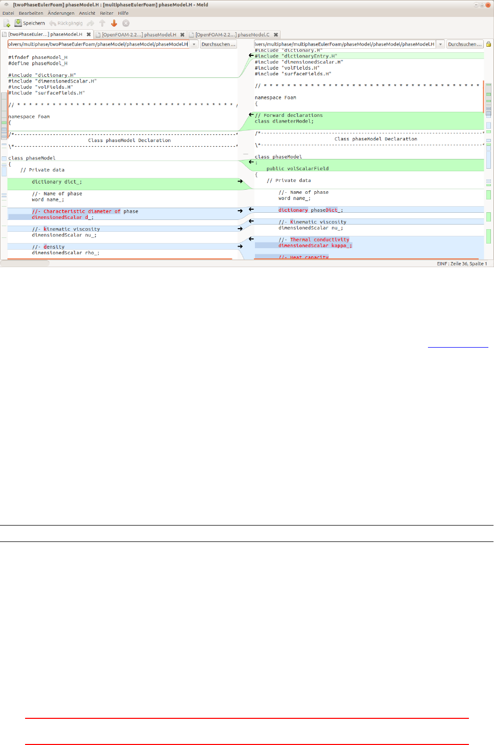
Figure 82: A screenshot of Meld
57.7 Case setup
There are a lot of tasks when setting up a case. Even though we might use a tutorial case as a starting point, a
lot of tedious work might lie ahead of us. Computers are better at certain tasks than we humans[Citation needed].
Thus, we might be better off automating boring tasks. The pyFoam library is a good collection of useful
stuff. However, certains tasks are done by mere one-liners in Linux. This is what this section is about.
57.7.1 Renaming files
The current mult-phase solvers use a naming scheme in which the name of the phase determines the file’s exten-
sion. Thus, the thermophysical properties of the phase air are stored in the file thermophysicalProperties.air.
This causes in certain cases the need to rename a number of files, because we use argon as gaseous phase and
we want to comply with the naming scheme. The dirty hack would be to just exchange the properties of air
with those of argon without changing the naming of the phase.
In Linux there are many ways to perform this sort of task. For mere text substitution a solution based on
regular expressions is the way to go. Listing 441 shows how the command rename is used to rename all files
containing a certain text.
renam e ’ s/ a ir / argon / g ’ ./*
Listing 441: Change the extension of all files having the extension air to argon.
57.8 Miscellaneous
This section contains references to useful scripts or commands explained elsewhere in this document.
Terminate a backround process
See Section 10.3.2.
XI This offering is not approved or endorsed by ESI®Group, ESI-OpenCFD®or the OpenFOAM®
Foundation, the producer of the OpenFOAM®software and owner of the OpenFOAM®trademark. 309

Delete the processor* directories
If one or several simulations have been conducted on a computing cluster, it makes sense so reconstruct the
domain on the cluster. Otherwise the workstation of the user would be blocked for the time needed to complete
reconstruction. After reconstructing the domain the processor* directories still contain all the time step data.
If the processor* folders are deleted on the cluster, the user can afterwards copy the whole case directory to the
workstation without transmitting the solution data twice.
See Section 10.5.2 for how to deal with processor* directories.
Redirect output
Redirecting the output of a program is explained in Section 10.1.1.
58 Archive data
Parametric studies generate a great deal of data. After the post-processing is done all files could be compressed
to save disk space. On Linux systems the tar archiving utility may be the agent of choice. The name tar comes
from tape archive, which is pretty descriptive in terms of the origins of this archiving program. A tar archive
is a single file which contains all archived files and folders. This step alone is only a reorganisation of the data,
fit for the usage of sequential data storage devices like magnetic tapes.
In a second step the tar archive needs to be compressed. For this task there are many possible choices. Linux
systems usually provide programs like gzip, bzip2 or xz. The distinction between archiving and compressing is
probably for historical as well as practical reasons. There is also one paradigm of the UNIX philosophy (Make
each program do one thing well) which supports the segregation in archiving and compression. The compression
programs usually differ in the utilised compression algorithms. There is one rule of thumb stating: The more
data is to be compressed, the longer compression takes.
Table 9lists the achieved compression of a parametric studies with 21 cases totalling in 50 GB of data. The
data was written in ascii format. Compressing the data resulted in a 70+ % reduction of used disk space. If
space consuming cases are to archived, slow algorithms that result in good compression rates should be prefered.
used disk space reduction
21 cases uncompressed 50 GB
compressed: *.tar.bz2 13.7 GB 36.3 GB - 72.6 %
Table 9: Comparison of disk space reduction
Archive log files
In this example log files are archived. In this case the same algorithm achieves an even greater reduction of disk
space usage. This example shows that the achieved compression rate strongly depends on the input data.
used disk space reduction
16 log files uncompressed 2.0 GB
compressed: *.tar.bz2 154.7 MB 1.85 GB - 92.3 %
Table 10: Comparison of disk space reduction
Yet another compression comparison
When archiving OpenFOAM cases, the mesh generation may be very convoluted or time consuming. So it
might be preferable to archive the mesh generation seperately from the actual case. Thus, for the actual case
we might want to include the final mesh and do not bother with mesh creation.
This section compares how three compression tools perform on a Linux system when compressing a mesh.
The mesh in question was created by blockMesh and certain files are in binary format.
XI This offering is not approved or endorsed by ESI®Group, ESI-OpenCFD®or the OpenFOAM®
Foundation, the producer of the OpenFOAM®software and owner of the OpenFOAM®trademark. 310
Listing 442 shows the actual command that were used to compress the mesh.
ta r - cv p ol yM es h | g zip - - bes t > p ol yM es h . ta r .gz
ta r - cv p ol yM es h | bz ip 2 - - bes t > p ol yM es h . tar . bz
ta r - cv p ol yM e sh | l zma -9 > p ol yMe sh . t ar . xz
Listing 442: Compressing the mesh with various tools; note the setting for maximum compression
Listing 443 shows the sizes of the original mesh and its compressed forms. The used compression algo-
rithms differ considerably. Compression was performed with the setting for best compression, the time it took
for each tool to compress the mesh was not recorded. However, the stronger the compression the more time it
takes to compress. Since for archiving purposes disk space is the limiting factor, we chose maximum compression.
use r@host :∼$ du -sh polyMe sh *
23 M p ol yM es h
5 ,3 M p ol yM es h . tar . bz
6 ,2 M p ol yM es h . tar . gz
2 ,6 M p ol yM es h . tar . xz
Listing 443: Comparing the disk usage of a mesh and its various compressions
From the comparison in Listing 443 we see that the LZMA compression algorithm achieves the best com-
pression, followed by BZIP2 and GZIP. All three compression algorithms are widely available in the UNIX world
in the form of open source implementations.
The effects of renumbering and/or writing binary
When playing around with various ways to archive an existing mesh, something quite interesting has been
observed: the archive file-size differs whether the mesh had been renumbered or not. Note that this comparison
only deals with archiving the mesh, no solution data (i.e. fields) have been archived alongside the mesh.
In Table 11 we compare the resulting file size of an archive of a reasonable complex, all-hex mesh with
147262 cells. The required disk space of the mesh itself only differs between writing in ascii or binary format.
Renumbering the mesh does not have an effect, which is not surprising, since renumbering does not add or
remove information. Thus, the required disk space of the mesh should not change due to renumbering.
When it comes to archiving the mesh, however, renumbering certainly has an effect on the resulting file size
of the archive. Compressing the as-is187 mesh yields only a slightly smaller archive, when the mesh was written
in binary format to disk. The big surprise, however, is when we compare the resulting archive file size for the
renumbered mesh. In both cases, ascii and binary, the compressed, renumbered mesh results in a larger archive
file size than the compressed, as-is mesh.
The mesh ascii binary
as-is 22M 16M
renumbered 22M 16M
The archive ascii binary
as-is 1,7M 1,6M
renumbered 2,5M 2,0M
Table 11: Comparing the resulting file size of the mesh archive file for various conditions/treatments. All file
or folder sizes were determined with the Linux command du -sh FILE. The mesh was compressed using the
LZMA algorithm at maximum compression: tar -cv constant/polyMesh | lzma -9 > polyMesh.tar.xz.
We can draw two conclusions from this comparison. The most obvious is, that writing data in binary format
is always favourable over writing in ascii format, especially for uncompressed data. Writing in ascii should only
be used for trouble-shooting. In production, binary is definitely the format of choice. Writing in binary not
only saves disk space in storage, it also provides the maximum read/write precision, since all relevant bits of
each numerical value are stored. In contrast, writing in ascii format only writes a finite number of significant
bits.
187We denote the state of the mesh after mesh-creation by the term as-is in order to distinguish it from the renumbered state.
Mesh creation consists of a call to blockMesh, extruding a patch and finally removing parts of the mesh with subsetMesh. After
these steps, any sets of points, faces or cells are deleted. Also zones of any kind have not been defined. Thus, as-is denotes the
final, minimal mesh.
XI This offering is not approved or endorsed by ESI®Group, ESI-OpenCFD®or the OpenFOAM®
Foundation, the producer of the OpenFOAM®software and owner of the OpenFOAM®trademark. 311
The second conclusion we can draw from the comparison above, is not to store the renumbered mesh. Even
if renumbering would/does188 not increase archive file size, renumbering is an operation we can easily perform
prior to our simulation. The time it takes to renumber the mesh is negligible compared to the overall simulation
time. Thus, we advise to archive meshes in an un-renumbered state. This, in addition to potential savings
on storage, gives future users the choice whether to run the simulation on a renumbered mesh or not. On an
already renumbered mesh it is impossible to determine the benefits of renumbering the mesh with respect to
simulation time or convergence. An operation which can always be performed at demand does not need to be
archived.
188One case of renumbering causing larger archive file sizes does not necessarily mean that this will always cause this effect.
XI This offering is not approved or endorsed by ESI®Group, ESI-OpenCFD®or the OpenFOAM®
Foundation, the producer of the OpenFOAM®software and owner of the OpenFOAM®trademark. 312

References
[1] Intel 64 and IA-32 Architectures Optimization Reference Manual.
[2] The International System of Units, 2006. URL www.bipm.org/en/si/si_brochure.
[3] The International System of Units (SI), 2008. URL http://physics.nist.gov/Pubs/SP330/sp330.pdf.
[4] A. Alexandrescu. Modern C++ Design: Generic Programming and Design Patterns Applied. Addison
Wesley, 2001.
[5] J. D. Anderson. Computational Fluid Dynamics. McGraw-Hill International Editions, 1995.
[6] Inc. ANSYS. FLUENT Theory Guide, 14.5 edition, 2012.
[7] ANSYS, Inc. ANSYS CFX-Solver Theory Guide, 14.0 edition, November 2011.
[8] N. G. Deen B. Niceno, M. T. Dhotre. One.equation sub-grid scale (sgs) modelling for euler-euler large eddy
simulation (eeles) of dispersed bubbly flow. Chemical Engineering Science, 63:3923–3931, 2008.
[9] A. Behzadi, R. I. Issa, and H. Rusche. Modelling of dispersed bubble and droplet flow at high phase
fractions. Chemical Engineering Science, 59:759–770, 2004.
[10] J. Boussinesq. Théorie de l’Écoulement tourbillant. Mem. Présentés par Drivers Savants Acad. Sci. Inst.
Fr., 23:46–50, 1877.
[11] Daniel Brennan. The Numerical Simulation of Two-Phase Flows in Settling Tanks. PhD thesis, Imperial
College of Science, Technology & Medicine, 2001.
[12] C. P. Dahl. Numerical modelling of flow and settling in secondary settling tanks. PhD thesis, Aalborg
University, Denmark, 1993.
[13] J.-M. Delhaye. Some issues related to the modeling of interfacial areas in gas-liquid flows I. the conceptual
issues. Comptes Rendus de l’Académie des Sciences - Series {IIB} - Mechanics, 329(5):397–410, 2001.
[14] Eric S. Raymond. The Art of UNIX Programming. Addison-Wesley, 2003.
[15] Agner Fog. Optimizing software in c++. Technical report, Technical University of Denmark, 2014.
[16] J. Fröhlich. Large Eddy Simulationen turbulenter Strömungen. Teubner, 2006.
[17] E. Peirano & A.-E. Almstedt H. Enwald. Eulerian two-phase flow theory applied to fluidization. Int. J.
Multiphase Flow, 22:21–66, 1996.
[18] David P. Hill. The computer simulation of dispersed two-phase flows. PhD thesis, Imperial College of
Science, Technology and Medicine, 1998.
[19] B. Holenda, I. Pásztor, Á. Kárpáti, and Á Rédey. Comparison of one-dimensional secondary settling tank
models. Technical report, European Water Association (EWA), 2006.
[20] M. Ishii. One-dimensional drift-flux-model and constitutive equations for relative motion between pphase
in various two-phase flow regimes. Technical report, Argonne National Laboratory, 1977.
[21] M. Ishii and T. Hibiki. Thermo-Fluid Dynamics of Two-Phase Flow. Springer, 2nd edition, 2011.
[22] M. Ishii, S. Kim, and J. Uhle. Interfacial area transport equation: model development and benchmark
experiments. International Journal of Heat and Mass Transfer, 45:3111–3123, 2002.
[23] M. Ishii, S. Kim, and J. Kelly. Development of interfacial area transport equation. Nuclear Engineering
and Technology, 37(6):525–536, 2005.
[24] R. I. Issa. A simple model for ct. Private Communications, 1992. see Hill [18].
[25] M. Peric J. H. Ferzinger. Computational Methods for Fluid Dynamics. Springer, 2002.
[26] Hrvoje Jasak. Error Analysis and Estimation for the Finite Volume Method with Applications to Fluid
Flows. PhD thesis, Imperial College of Science, Technology & Medicine, 1996.
XI This offering is not approved or endorsed by ESI®Group, ESI-OpenCFD®or the OpenFOAM®
Foundation, the producer of the OpenFOAM®software and owner of the OpenFOAM®trademark. 313

[27] Brian W. Kernighan and Dennis M. Ritchie. The C Programming Language. Prentice Hall, Inc., 2nd
edition, 1988.
[28] S. Kim, X. Sun, M. Ishii, S. G. Beus, and F. Lincoln. Interfacial area transport and evaluation of source
and sink terms for confined air-water bubbly flow. Nuclear Engineering and Design, 219:61–75, 2002.
[29] G. Kocamustafaogullari and M. Ishii. Foundation of the interfacial area transport equation and its closure
relations. Int. J. Heat Mass Transfer, 38(3):481–493, 1995.
[30] Fabian Peng Kärrholm. Numerical Modelling of Diesel Spray Injection, Turbulence Interaction and Com-
bustion. PhD thesis, Chalmers University of Technology, Göteborg, Sweden, 2008.
[31] Y. Liu, T. Hibiki, and M. Ishii. Modeling of interfacial area transport in two-phase flows. In Advances in
Multiphase Flow and Heat Transfer, volume 4, chapter 1, pages 3–27. Bentham Science Publishers, 2012.
[32] Alejandro López. Lpt for erosion modeling in openfoam – differences between solidparticle and kine-
maticparcel, and how to add erosion modeling. Technical report, Chalmers University of Technol-
ogy, 2014. URL http://www.tfd.chalmers.se/~hani/kurser/OS_CFD_2013/AlejandroLopez/LPT_for_
erosionModelling_report.pdf.
[33] G. B. Macpherson, N. Nordin, and H. G. Weller. Particle tracking in unstructured, arbitrarry polyhedral
meshes for use in cfd and molecular dynamics. Communications in Numerical Methods in Engineering, 25:
263–273, 2009.
[34] Holger Marschall. Towards the Numerical Simulation of Multi-Scale Two-Phase Flows. PhD thesis, Tech-
nische Universität München, 2011.
[35] M. Milelli. A numerical analysis of confined turbulent bubble plumes. PhD thesis, Swiss Federal Institute
of Technology Zurich, 2002.
[36] Hakan Nilsson. Turbomachinery training at ofw8. Technical report, Chalmers University of Technology,
Gothenburg, Sweden, 2013.
[37] Niklas Nordin. Complex Chemistry Modeling of Diesel Spray Combustion. PhD thesis, Chalmers University
of Technology, 2009.
[38] OpenFOAM - Programmer’s Guide. OpenFOAM Foundation, 2.1.0 edition, 2011.
[39] OpenFOAM - User Guide. OpenFOAM Foundation, 2.1.0 edition, 2011.
[40] D. Pfleger and S. Becker. Modelling and simulation of the dynamic flow behaviour in a bubble column.
Chemical Engineering Science, 56:1737–1747, 2001.
[41] S. P. Pope. Turbulent Flows. Cambridge University Press, 2000.
[42] Henrik Rusche. Computational Fluid Dynamics of dispersed two-phase flows at high phase fractions. PhD
thesis, Imperial College of Science, Technology & Medicine, 2002.
[43] Y. Sato and K. Sekoguchi. Liquid velocity distribution in two-phase flow. International Journal of Multi-
phase Flow, 2:79–95, 1975.
[44] J. Smagorinsky. General circulation experiments with the primitive equations; i. the basic experiment.
Monthly Weather Review, 91:99, 1963.
[45] Bjarne Stroustrup. The C++ Programming language. Addison-Wesley, 4th edition, 2013.
[46] Imre Takács. Experiments in Activated Sludge Modelling. PhD thesis, Ghent University, Belgium, 2008.
[47] D. G. Thomas. Transport characteristics of suspension: VIII. a note on the viscosity of Newtonian suspen-
sions of uniform spherical particles. Journal of Colloid Science, 1965.
[48] A. Tomiyama, I. Kataoka, T. Fukuda, and T. Sakaguchi. Drag coefficients of bubbles. 2nd report. drag
coefficient for a swarm of bubbles and its applicability to transient flow. Nippon Kikai Gakkai Ronbunshu,
61(588):2810–2817, 1995.
XI This offering is not approved or endorsed by ESI®Group, ESI-OpenCFD®or the OpenFOAM®
Foundation, the producer of the OpenFOAM®software and owner of the OpenFOAM®trademark. 314

[49] Berend van Wachem. Derivation, implementation and validation of computer simulation models for gas-
solid fluidized beds. PhD thesis, Delft University of Technology, 2000.
[50] H. K. Versteeg and W. Malalasekera. An introduction to computational fluid dynamics – the finite volume
method. Longman Scientific & Technical, 1995.
[51] A. Vesilind. Design of prototype thickeners from batch settling tests. Water Sewage Works, 115(5):302–307,
1968.
[52] David C. Wilcox. Turbulence Modelling for CFD. DCW Industries, Inc., 1994.
[53] D. Zhang, N. G. Deen, and J. A. M. Kuipers. Numerical simulation of the dynamic flow behaviour in a
bubble column: A study of closures for turbulence and interface forces. Chemical Engineering Science, 61:
7593–7608, 2006.
XI This offering is not approved or endorsed by ESI®Group, ESI-OpenCFD®or the OpenFOAM®
Foundation, the producer of the OpenFOAM®software and owner of the OpenFOAM®trademark. 315

Nomenclature
ASCII American Standard Code for Information
Interchange
BC boundary condition
BIT Bubble induced turbulence
CAD computer aided design
CFD Computational fluid dynamics
CG Conjugate gradient
DPE Dispersed phase element
EDF Électricité de France
FIFO A data structure follwing the First In, First
Out principle
FPE Floating-point exception
FVM Finite volume method
GAMG Geometric algebraic multi-grid
gcc GNU compiler collection
GNU GNU is not Unix
GUI graphical user interface
I/O input and output
IATE Interfacial area transport equation
IGES Initial Graphics Exchange Specification
IT Information technology
LES Large eddy simulation
LPT Lagrangian Particle Tracking
LZMA Lempel–Ziv–Markov chain algorithm
MPI message passing interface
MRF multiple reference frame
OO object-oriented
OOD object-oriented design
OOP object oriented programming
OS operating system
PDE Partial differential equation
Perl An interpreted programming language
PID process identifier
PIMPLE An algorithm based on PISO and SIM-
PLE algorithm
PISO Pressure Implicit with Split Operator
POSIX Portable Operating System Interface
RAS Reynolds averaged simulation
RHS Right hand side
RNG random number generator
RTD residence time distribution
SAT Standard ACIS Text
SI Le Système Internationale d’Unités
SIMPLE Semi-Implicit Method for Pressure-
Linked Equations
SOI start of injection
STL Surface Tesselation Language
UNIX an operating system; ancestor of many
modern operating systems, e.g. all kinds
of Linux, Mac OS X.
VOF Volume of fluid
XI This offering is not approved or endorsed by ESI®Group, ESI-OpenCFD®or the OpenFOAM®
Foundation, the producer of the OpenFOAM®software and owner of the OpenFOAM®trademark. 316
