User_Guide_Sept_02_2009 Oslo User Guide
User Manual: Pdf
Open the PDF directly: View PDF ![]() .
.
Page Count: 135 [warning: Documents this large are best viewed by clicking the View PDF Link!]

Optics Software for Layout and Optimization
User Guide
Lambda Research Corporation
25 Porter Road
Littleton, MA 01460
USA
Tel: 978-486-0766
Fax: 978-486-0755
support@lambdares.com
www.lambdares.com

ii
COPYRIGHT
The OSLO software and User Guide are Copyright © 2009 by Lambda Research
Corporation. All rights reserved.
This software is provided with a single user license or with a multi-user network
license. Each license may only be used by one user and on one computer at a time.
The OSLO User Guide contains proprietary information. This information as well
as the rest of the User Guide may not be copied in whole or in part, or reproduced
by any means, or transmitted in any form without the prior written consent of
Lambda Research Corporation.
TRADEMARKS
OSLO® is a registered trademark of Lambda Research Corporation.
TracePro® is a registered trademark of Lambda Research Corporation.
Pentium® is a registered trademark of Intel, Inc.
UltraEdit™ is a trademark of IDM Computer Solutions, Inc.
Windows 95®, Windows 98®, Windows NT®, Windows 2000®, Windows XP®,
Windows Vista®, Windows 7®, and Microsoft® are either registered trademarks or
trademarks of Microsoft Corporation in the United States and/or other countries.

Table of Contents
Table of Contents iii
Preface 1
Chapter 1 - Your first OSLO session 2
Introduction ........................................................................................... 2
Symbols used in this chapter ............................................................. 2
Running OSLO ..................................................................................... 3
The user interface .................................................................................. 3
Spherical mirror example ...................................................................... 6
Defining the lens system data ........................................................... 6
Defining the lens surface data ........................................................... 7
Drawing the lens in the Autodraw window....................................... 8
Plotting the on axis spot diagram ...................................................... 9
Listing the lens surface data ............................................................ 10
Saving the lens ................................................................................ 11
Changing the aperture ..................................................................... 12
Drawing the lens in the graphics window, with “zooming” ........... 13
Finding the best focal plane ............................................................ 14
Plotting the on axis point spread function (PSF) ............................ 15
Extending the rays in the lens drawing ........................................... 16
Calculating the off axis optical path difference (OPD) ................... 16
Optimizing ...................................................................................... 18
Assessing the final design ............................................................... 20
Listing the data ................................................................................ 20
Exiting the program ........................................................................ 20
Conclusion .......................................................................................... 21
Chapter 2 - Configuring OSLO 22
Introduction ......................................................................................... 22
Toolbar menus .................................................................................... 22
Main window .................................................................................. 22
Text window ................................................................................... 22
Graphics window ............................................................................ 23
The status bar ...................................................................................... 23
Preferences .......................................................................................... 24
Designer name (dsgn) ..................................................................... 24
ISO10110 drawing settings (adr1, adr2, adr3, edcm) ..................... 24
Graphics (gems, gacl, gfwb, glab, grax, gfbw, drra, pens) ............. 25
Graphics alternate mode (gfam) ...................................................... 25
No error boxes (noeb) ..................................................................... 25
Tangent check (tanc on) ...................................................................... 25
Compile CCL ...................................................................................... 26
Chapter 3 - The command line 27
Arithmetic calculations ....................................................................... 27
OSLO commands ................................................................................ 27
Assigning values to predefined variables ............................................ 28
Printing ........... .................. .................. .................. .................. ............. 29
The history button ............................................................................... 29
Keyboard shortcuts ......................................................................... 29

iv
The message area ................................................................................. 30
Executing CCL command sequences .................................................. 31
Alphabetic list of system data variables .............................................. 32
Chapter 4 - Lens data entry 34
8 x 30 binoculars: Specification .......................................................... 34
Calculations ......................................................................................... 34
Choosing an eyepiece .......................................................................... 34
Scaling the eyepiece ............................................................................ 36
Choosing a catalog objective ............................................................... 36
Combining the objective and the eyepiece .......................................... 38
Surface decenters and tilts ................................................................... 40
Adding a right angle prism .................................................................. 41
Converting the prism to a Porro prism ................................................ 43
Adding a second Porro prism .............................................................. 44
Completing the design ......................................................................... 45
Chapter 5 - Graphical analysis 47
Introduction ......................................................................................... 47
Opening a new graphics window .................................................... 47
Labeling a graphics window ........................................................... 47
Generating a plot ............................................................................. 48
Saving a plot .................................................................................... 48
Cutting and pasting a plot ................................................................ 48
Lens drawing ....................................................................................... 49
Drawing a lens in 2D ....................................................................... 49
Drawing a lens in 3D ....................................................................... 51
Drawing a lens in 3D with sliders ................................................... 52
Ray intercept curves analysis .............................................................. 53
Ray analysis (RIC) .......................................................................... 53
Ray intercept curves for 2D field points ......................................... 53
Ray intercept curves report graphic ................................................. 54
Chapter 6 - Numerical analysis 56
Introduction ......................................................................................... 56
Finding the edge rays .......................................................................... 56
Graphical estimates ............................................................................. 57
Numerical calculation .......................................................................... 58
From the text window ..................................................................... 58
From the menu headers ................................................................... 58
From the command line (abbreviated) ............................................ 59
By executing in the Edit window .................................................... 60
From the command line (in full) ..................................................... 60
The spreadsheet buffer ........................................................................ 60
Clearing the text window and spreadsheet buffer ........................... 60
Reading from the spreadsheet buffer ............................................... 61
Writing to the spreadsheet buffer .................................................... 61
Scrolling the spreadsheet buffer ...................................................... 62
Chapter 7 - Slider-wheel design 63
1:1 wide angle relay ............................................................................ 63
Introduction ..................................................................................... 63
Defining the starting point ............................................................... 63

Setting up the starting lens .............................................................. 63
Slider-wheel design with ray intercept curves .................................... 65
Plotting the MTF across the field .................................................... 66
Editing the slider-wheel callback command ................................... 66
Listing of the modified slider-wheel callback CCL ........................ 68
Slider-wheel design using MTF at one frequency .............................. 69
Setting clear apertures ..................................................................... 70
Chapter 8 - Programming 71
Introduction ......................................................................................... 71
Defining a new command: sno .... ................. ................... .................. .. 71
Structure of a CCL command ............................................................. 73
Search CCL library: scanccl ............................................................... 74
Defining a new command: ctn ............................................................ 74
Initial version of command ............................................................. 74
Version with formatted output ........................................................ 75
Adding the glass name string .......................................................... 76
Adding headers and documentation ................................................ 76
The text window toolbar ..................................................................... 78
Adding the command sno to the toolbar ......................................... 78
Calling sno from the toolbar ........................................................... 79
Defining a new command: xmt ........................................................... 79
Writing a command xmt to print transmittance values ................... 79
Converting xmt printed output to graphics ..................................... 80
Preserving the text window contents .............................................. 81
Scaling and drawing the axes .......................................................... 81
Adding standard plot commands to xmt ......................................... 82
Error handling ................................................................................. 82
Listing of complete command xmt ................................................. 83
The graphics window toolbar .............................................................. 85
Creating a new icon for xmt .................. ............................. ............. 85
Adding the xmt icon to the graphics window toolbar ..................... 85
Calling xmt from the toolbar icon ................................................... 86
SCP programming: *triplet ................................................................. 86
Load command file programming ....................................................... 88
Chapter 9 - Optimization 89
Optimizing using Seidel aberrations ................................................... 89
Setting up the starting design .......................................................... 89
Defining the error function ............................................................. 90
Description of the Aberration Operands error function .................. 91
Creating a model glass .................................................................... 92
Defining the optimization variables ................................................ 93
Optimization ................................................................................... 93
Choosing a real glass type ............................................................... 94
Final optimization steps .................................................................. 95
Autofocus ........................................................................................ 95
Optimization using finite rays ............................................................. 97
50 mm f/5.6 objective: specification ............................................... 97
Finding a starting design ................................................................. 97
Checking for vignetting in the starting design ................................ 98
Assessing the starting design .......................................................... 99
Defining and validating the error function ...................................... 99
Description of the GENII error function ....................................... 100
Defining the optimization variables .............................................. 101

vi
Optimization .................................................................................. 101
Engineering aspects: edge thicknesses .......................................... 102
Slider-wheels with concurrent optimization on MTF ....................... 103
Adjusting lens thicknesses ............................................................ 103
Engineering aspects: ambiguity avoidance ................................... 104
Engineering aspects: testplate fitting ............................................. 105
Rounding air spaces ...................................................................... 106
Adjusting clear apertures ............................................................... 106
Chapter 10 - Tolerances and drawings 108
50 mm f/5.6 objective: specification ............................................. 108
Defining the tolerance error function:”opcb_dmtf” .......................... 108
Defining the compensator ............................................................. 110
Optimizing on the compensator ........................................................ 110
Calculating decenter tolerances ......................................................... 111
Checking tolerance entries ............................................................ 111
Symmetrical tolerances surface calculation ...................................... 111
Updating symmetrical surface tolerances ...................................... 113
Asymmetric tolerances surface calculation ....................................... 113
Updating asymmetric surface tolerances ....................................... 114
Updating asymmetric component tolerances ................................. 114
Asymmetric tolerances calculation ................................................ 114
Tolerance data listing .................................................................... 115
ISO 10110 component drawing ......................................................... 116
Setting element drawing defaults .................... ............................. . 116
Setting element material properties ............................................... 116
Setting element surface properties ................................................ 117
Element drawing ........................................................................... 118
Appendix 1 - Index of lens data commands 119
Appendix 2 - Graphics reference 122
Alphabetical index ............................................................................. 122
Tabular graphics command reference ............................................... 124
Tabular graphics index ...................................................................... 126
Graphics reference examples ............................................................. 128

1
Preface
Since its inception at the Institute of Optics at the University of Rochester, the software
written by Doug Sinclair has played a key role in the teaching as well as in the performance
of optical design. So OSLO, perhaps more than any other optical design software, shows
signs of its origins in a teaching establishment. The flexibility of the user interface, the open
source nature of much of the code, the CCL programming language which is very similar to
C, and real capability of OSLO-EDU, the free version of OSLO, to carry out real design
tasks, make it the ideal choice for the teaching environment.
This manual has been written to supplement the current documentation for commercial users
of OSLO software. Its second aim is to provide a gentle introduction to the experience of
optical design for those who have only just downloaded OSLO-EDU from the internet. The
first chapter is written expressly for them. More experienced designers may wish to skip
straight to the second chapter.
2
Chapter 1 - Your first OSLO session
Introduction
This chapter gives a click-by-click description of how OSLO can be used to carry out a very
simple task involving synthesis, analysis, and optimization of a spherical concave mirror. It
is in general applicable to all editions of OSLO, including OSLO EDU. This means that
more advanced facilities, which may only be available in OSLO Standard and Premium
editions, are not included.
The exercise will demonstrate the two main modes of calculation:
• the geometrical approximation, in which light is treated as a ray, or the path of a
photon
• the physical mode of calculation, in which the light is treated as propagating as a
wave front, and the results take account of the effects of diffraction.
Symbols used in this chapter
A left-click on the mouse is indicated by a white arrow, and a right-click by the box with the
word “Right”. If a drop-down menu is selected by a left-click, then it is
represented by a black circle and arrow.
Step by step instructions are marked with bullet points. Instructions
about what to do if things go badly wrong are in italics and labeled
HELP! .
Anything typed from the keyboard (whether as a command or as an entry in a dialog box) is
shown in this typeface.
Labels and headers in spreadsheets and dialog boxes are given in this typeface.
Buttons to be clicked are shown in _gray_.
Check-boxes (called “radio buttons” in the documentation) are shown like this:
Messages which appear whenever the cursor hovers above an icon are shown in a shaded
box. These are known as tooltips.
Questions and answers, representing a typical dialog between a lens designer and the
customer, are given in bold type.
Ri
g
ht
Tooltips
Chapter 1 - Your first OSLO session 3
Running OSLO
Running OSLO
• EITHER click on the shortcut icon on the desktop in the Windows desktop,
OR click on Start ►All Programs ► OSLO►OSLO [EDU etc]
Edition...
OR locate the .exe file in C:\Program Files\OSLO
(e.g. osloedu.exe) - in some installations the
directory name is Lambda Research\OSLO).
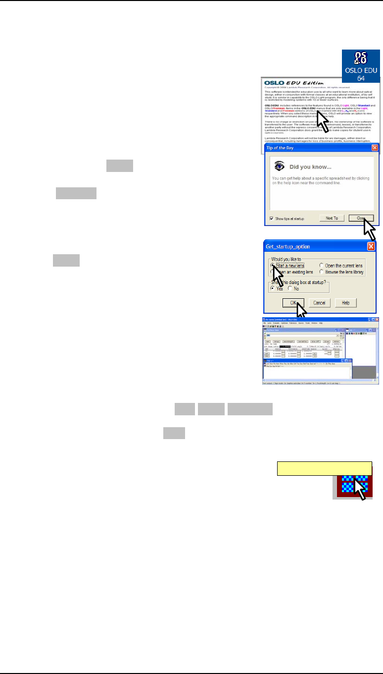
• The program opens with an introductory dialog box.
Click anywhere in the box to close it.
• If a message about re-building the CCL database
appears, click on _OK_
• The “Tip of the Day” is a useful tutorial for new users.
Click on _Close_. Alternatively it can be suppressed
permanently by removing the tick from the box in the
bottom left corner.
• The Get_startup_option window opens.
• Choose the default option: Start a new lens and
click on _OK_
• The OSLO main window should now appear, similar in
appearance to that shown here. We will now discuss the
individual components of this window in detail.
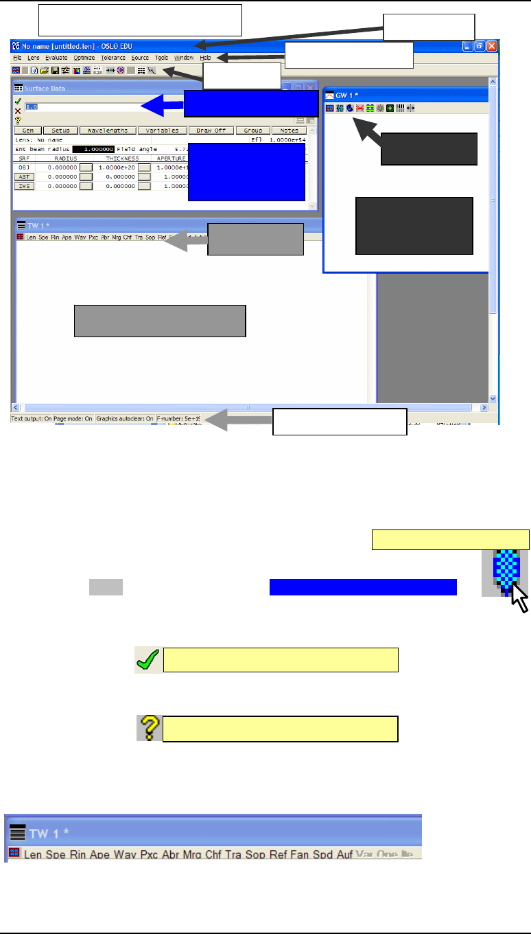
The user interface
A number of terms are defined here, and given in bold print.
At the top of the main window in the blue border is the title
bar, which gives the lens identifier, the file name under
which the current lens was last saved, and the edition of OSLO currently running.
Beneath this lies a row of menu headers, File, Lens, Evaluate, etc, each of which its
own drop-down menu has. Many of the program commands can be accessed through these
menus. The last of the menu headers is Help which gives access to the on-line
documentation. In Windows, this can also be accessed via the F1 key on the keyboard.
Below that is a row of icons forming the main window toolbar,
which give one-click access to the most frequently used control
functions. The first of these is the Setup Window/Toolbar
icon which gives access to a list of further groups of icons which
can be added to the toolbar. Other icons are to Open surface data spreadsheet, Open
a new lens, Open an existing lens, Save the current lens, Open the standard
text editor, etc. Each icon has a description of its function which pops up as a tooltip
when the cursor is placed over the icon.
At the bottom of the main window, there is a status bar which can be expanded and
customized by the user. This will be described in chapter 2.
Setu
p
Window/Toolba
r
4 Your first OSLO session Chapter 1
The user interface
O
p
en surface data s
p
readsheet
Help for the command/spreadsheet
The window which opens in the top left hand corner is called the surface data spreadsheet.
This is the area where all the properties of the lens and its working conditions are defined.
Entering data into this spreadsheet is described in chapter 4. Other spreadsheets are
available, but only one spreadsheet can be open at a time.
HELP! If the surface data spreadsheet does not open, click
on the blue lens icon on the left of the toolbar in the main window. Alternatively,
select from the Lens menu header the option Surface Data Spreadsheet....
Immediately above the surface data spreadsheet is the command line where
OSLO commands are typed. They are executed either by pressing Enter or by clicking
on the green tick:
Online documentation for any command may be accessed by typing the command in the
command line, and then pressing the yellow question mark beside it.
If no command is entered the documentation for any currently open spreadsheet is given.
Below the command line there is a message area, and on the right hand end there is the
history button. The command line is described in detail in chapter 3.
Text window
Graphics
window
Surface data
spreadsheet
Command line
Menu headers
Toolbar
Toolbar
Toolba
r
Status bar
MAIN WINDOW Title ba
r
Accept pending entry/Close spreadsheet
Chapter 1 - Your first OSLO session 5
The user interface
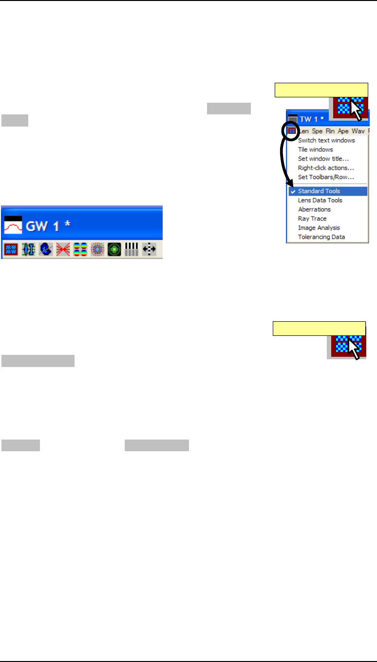
There should also be a text window visible. This is where printed output is directed. Along
the top of this there lays a toolbar consisting of a row of text labels, which are OSLO
commands, executed by clicking. Numerical analysis is described in chapter 6.
HELP! If the text window toolbar does not look like the one in
the diagram, click on the Setup Window/Toolbar icon in the
top left-hand corner of the text window, and select Standard
Tools from the menu. Any or all of the toolbar groups may be
selected for a text window. Either one or two, but not more, text
windows can be shown at a time.
The user may create additional toolbar entries using the CCL
programming language. Detailed instructions of how to do this are
given in chapter on programming, chapter 8.
Also on the main screen there is at least one graphics window. This has a toolbar
consisting of a row of icons. All graphical output is displayed in one of the graphics
windows. Graphical analysis is discussed in chapter 5. There is an index of OSLO graphics
facilities in Appendix 2 at the end of this book.
HELP! If the graphics window toolbar does not look like the
one in the diagram, click on the Setup Window/Toolbar icon
on the left-hand side of the graphics window toolbar, and select
Standard Tools from the menu. Only one of the graphics
window icon groups may be displayed at a time, but different graphics windows may have
different groups. Up to 30 graphics windows may be created and displayed by the user at
any one time. Two more may be generated automatically.
The user may generate icons in any of the graphics toolbars. This is described in chapter 8.
HELP! If you have trouble finding the text window or the graphics window, then from the
Window menu header select Tile Windows. Alternatively you can type the command
tile into the command line and then either click on the green tick or press (Enter)
on the keyboard.
Setu
p
Window/Toolbar
Setu
p
Windo
w
/Toolba
r
6 Your first OSLO session Chapter 1
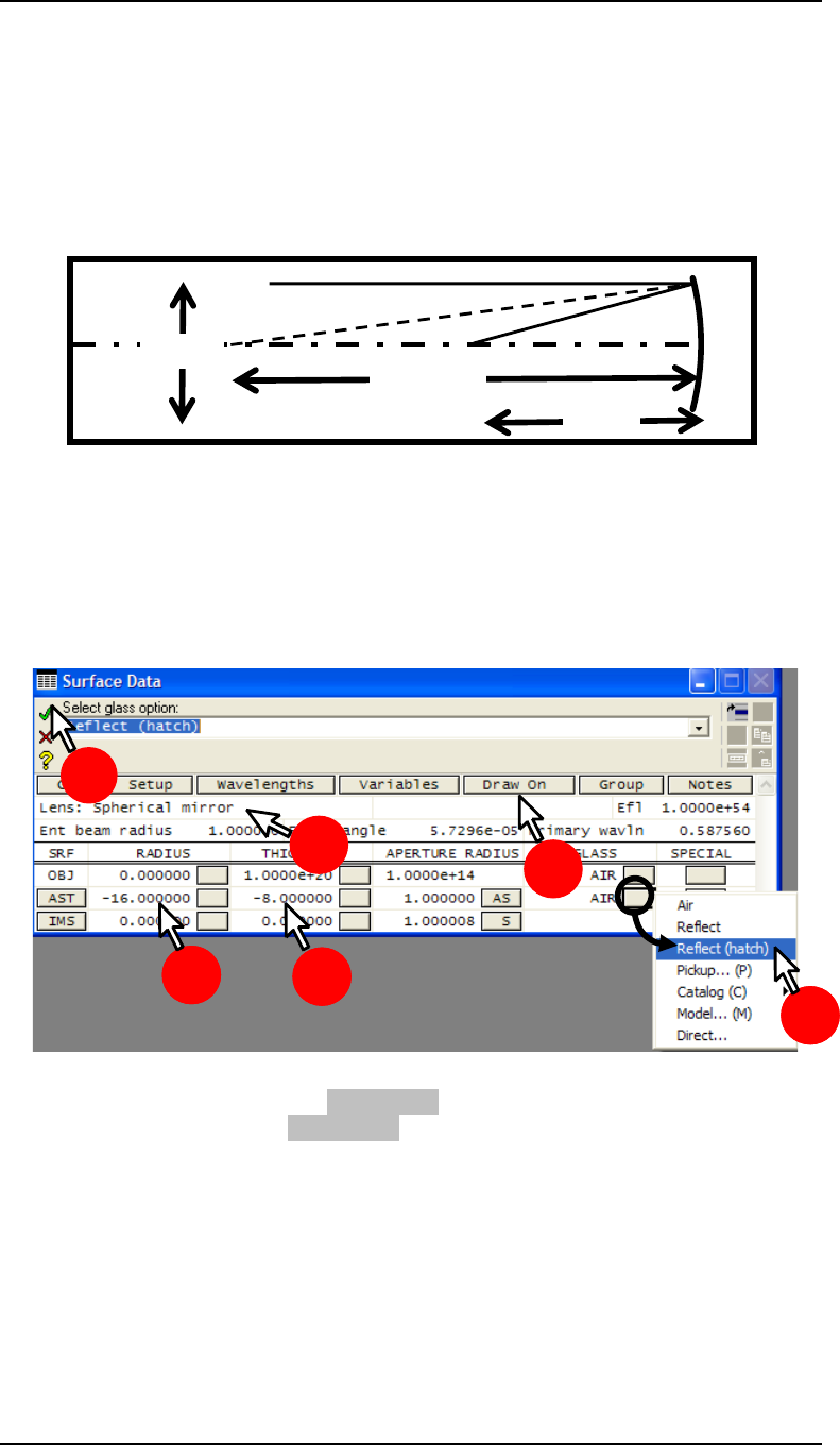
Spherical mirror example
Spherical mirror example
The remainder of this chapter will consist of instructions on how to specify a concave
spherical mirror of radius 16 mm, and then to assess its on-axis performance at apertures of
f/4 and f/2.3. Finally its performance at 18° off axis will be assessed, and the stop position
and image radius of curvature optimized to give the best performance over the field of view.
For clarity, each section will be prefaced by a question from a “customer,” given in bold
type.
Question: Does a spherical mirror working at f/4 give a “diffraction limited”
image at its focus when used with a 2 mm diameter parallel axial beam of green light?
Defining the lens system data
The working conditions of the lens (such as units, paraxial setup data, wavelengths and field
points) are defined by entries in the surface data spreadsheet above the double line.
On the surface data spreadsheet:
1. Left-click with the mouse on _Draw Off_ to open the Autodraw window The label
on the button changes to _Draw On_ while the Autodraw window is active.
2. Add the lens identifier (up to 32 characters): Lens: Spherical mirror
Click once on the green tick.
HELP! If you were to choose a different name for the lens identifier, and the first word of
the name happened to be a valid OSLO command words (such as spe), the name would be
8 mm
R = 16
2 mm
Accept pending entry/Close spreadsheet
1
2
1 4
1 3 1 5
6

Chapter 1 - Your first OSLO session 7
Spherical mirror example
rejected and the relevant command executed instead. To avoid this, the title might be
enclosed in quotation marks: e.g. “spe”.
The default value of Ent beam radius is 1.0 mm, the default primary wavelength is
0.58756 µm (the green helium d-line), and the default units are mm, so for this exercise
these do not need to be changed. Also at this stage it is only necessary to assess the mirror
on axis, so the field angle does not need to be changed from the default value of 1
milliradian.
Defining the lens surface data
Turning now to the data below the double line, the first line (labeled OBJ) refers to the
object space, numbered 0. A parallel beam is the default condition for a new lens. So the
THICKNESS - that is the object distance - is infinity (in OSLO, that means 1020, written
1.0000e+20 lens units). Nothing has to be changed on this line since in the object space a
medium (GLASS) of AIR is also the default. The object radius (1.0000e+14) is calculated
from the field angle by the program, and is not specified by the user.
On the second line for surface 1 (AST):
3. Because the aperture is “f/4” the focal length must be 4 times the beam diameter of 2
mm, and the focal length is half the radius of curvature. Change the RADIUS to a
value of-16 (mm). Since this is measured from the surface to its center, a negative
radius implies a surface concave to the incoming beam.
4. Click on the gray button next to AIR under GLASS and select Reflect (hatch) (or
Reflect - the only difference being the appearance of the drawing).
5. Change the THICKNESS from 0.000000 to: -8 (mm). This is the separation from
surface 1 to surface 2. It is negative because after reflection the light travels in the
opposite direction to the local z-axis.
6. Once again, click on the green tick () to confirm the changes.
Note that for surface 1, the APERTURE RADIUS (1.000000) has AS in the gray box
next to it. A means that this surface is the aperture stop. S means that the size of the
surface is governed by a “paraxial solve,” which means that it will be adjusted to
accommodate (approximately) both axial and off-axis beams without truncation.
On the third line, which corresponds to the image (IMS) a RADIUS of 0.0 means that the
image is plane. Once again its size is the default - it is adjusted using a “paraxial solve.” The
box for the next space (THICKNESS) will used for a defocus value, but is zero at present.
The box showing the medium after the image (GLASS) is of course blank.
There is no need to close the surface data spreadsheet before starting the next section.
8 Your first OSLO session Chapter 1
Spherical mirror example
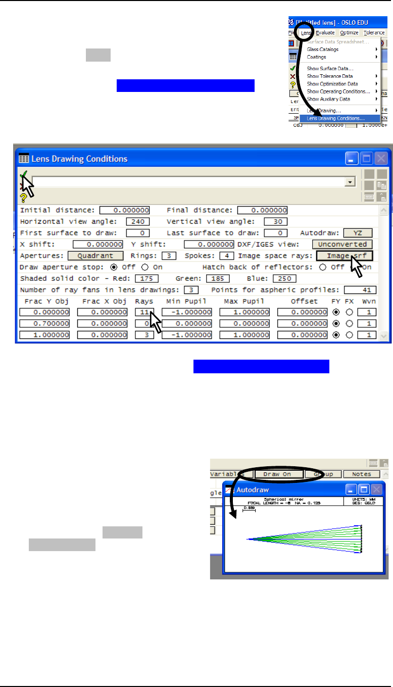
Drawing the lens in the Autodraw window
In the main window:
• Click on the Lens menu header to open the menu list
shown.
• Select the last item, Lens Drawing Conditions ...
The Lens Drawing Conditions spreadsheet will appear. This
is the spreadsheet where the overall appearance of lens system
drawings is determined.
In the Lens Drawing Conditions spreadsheet:
• After Image space rays: select Draw rays to image surface.
• The table at the bottom determines what rays will be displayed. In the column
headed Rays type on the first line 11 for the number of rays to be drawn for
the first (on axis) field point - for which Frac Y Obj = 0.00000. These rays
will be drawn with a green pen.
• Leave everything else unchanged, and close with the green tick .
The Autodraw window should now have the
appearance shown in the diagram, provided the
surface data spreadsheet is open.
HELP! The Autodraw window may be
hidden behind one of the others. If this happens
to be the case, from the Window menu header
select Tile Windows
Chapter 1 - Your first OSLO session 9
Spherical mirror example
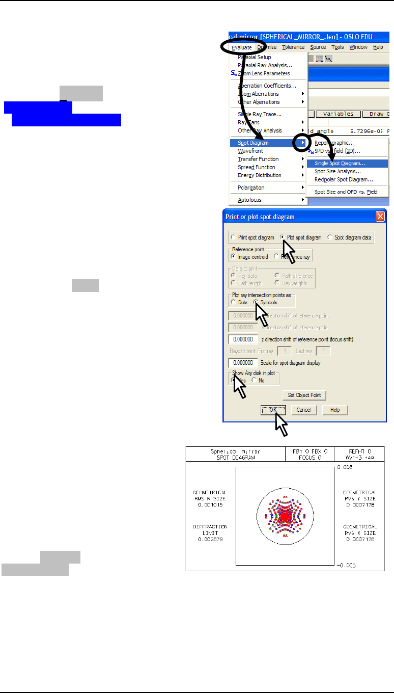
Plotting the on axis spot diagram
A spot diagram is a map of the pattern of rays
incident on the image from a single object point,
using the “geometrical approximation” which
ignores the wave nature of light.
• From the Evaluate menu header select:
Spot Diagram
►Single spot diagram...
• In the Print or plot spot diagram
spreadsheet, click on three radio buttons as
shown:
Plot spot diagram.
Plot ray intersection points as:
Symbols
Show Airy disc in plot:
Yes
• Leave the other entries as defaults; the
axial (FBY = 0, FBX = 0) is the default so
there is no need to use the Set Object
Point button.
• Click on _OK_
The colored symbols in this diagram represent the
distribution in the image plane of rays which
evenly fill the pupil from a single point on axis.
The three colors represent the three default
wavelengths. The black circle represents the first
minimum of the Airy disc, which is the intensity
in the image of a perfect lens of the same
aperture, in monochromatic light of the default
central wavelength of 0.58756 μm.
The most important aspect of the diagram is that
all the rays fall within this circle. This is one of
the criteria by which the assertion can be
made:
Answer: Yes, the image quality
at the focal point is “diffraction
limited” - i.e. limited by the wave
nature of light and not by aberrations.
HELP! Once again, if you have
trouble finding the graphics window,
from the Window menu header select
Tile Windows or type the command
tile into the command line.
• Close the surface data spreadsheet by clicking on the green tick .
10 Your first OSLO session Chapter 1
Spherical mirror example
Listing the lens surface data
• Click on the Len header in the text window to list radii, thicknesses, apertures, glass
types and surface notes:
*LENS DATA
Spherical mirror
SRF RADIUS THICKNESS APERTURE RADIUS GLASS SPE NOTE
OBJ -- 1.0000e+20 1.0000e+14 AIR
AST -16.000000 -8.000000 1.000000 AS REFL_HATCH
IMS -- -- 8.0000e-06 S
• Click on Rin to list the indices and thermal expansion coefficients:
*REFRACTIVE INDICES
SRF GLASS/CATALOG RN1 RN2 RN3 VNBR TCE
0 AIR 1.000000 1.000000 1.000000 -- --
1 REFL_HATCH 1.000000 1.000000 1.000000 -- --
2 IMAGE SURFACE
• Click on Ape to list apertures and any special apertures.
*APERTURES
SRF TYPE APERTURE RADIUS
0 SPC 1.0000e+14
1 CMP 1.000000
2 CMP 8.0000e-06
• Click on Wav to give the wavelengths and the spectral weighting factors on each.
*WAVELENGTHS
CURRENT WV1/WW1 WV2/WW2 WV3/WW3
1 0.587560 0.486130 0.656270
1.000000 1.000000 1.000000
• Click on Pxc to list the focal length and some of the operating conditions.
*PARAXIAL CONSTANTS
Effective focal length: -8.000000 Lateral magnification: -8.0000e-20
Numerical aperture: 0.125000 Gaussian image height: 8.0000e-06
Working F-number: 4.000000 Petzval radius: -8.000000
Lagrange invariant: -1.0000e-06
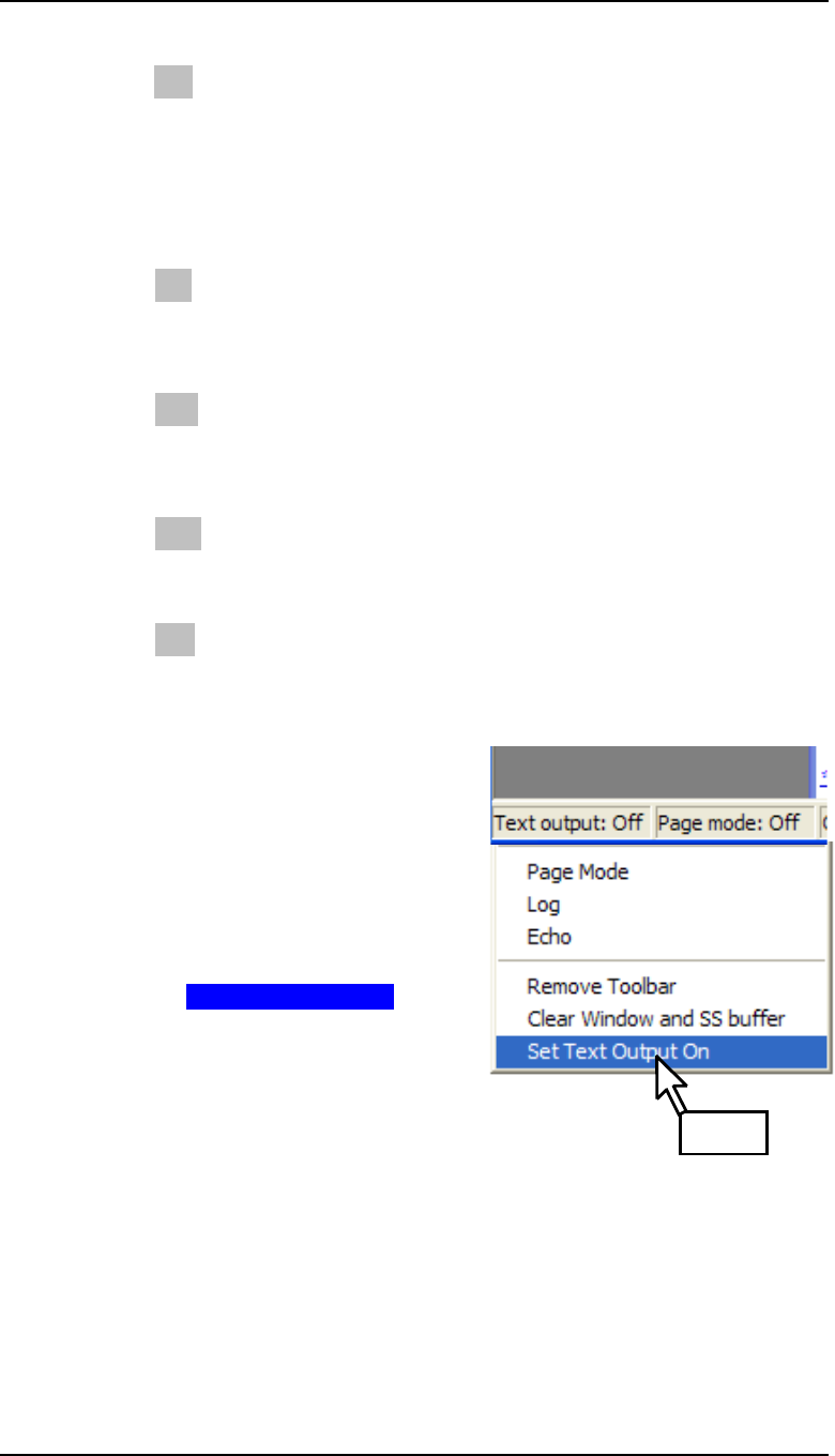
HELP! There are occasions when the text output
gets turned off inadvertently. This is most likely to
occur if a CCL command is interrupted before it
has had time to complete its task. If nothing appears
in the text window when text output is expected,
look at the first panel on the status bar at the
bottom of the main window. If it reads Text output:
Off, right click within the text window, and select
the last menu entry: Set Text Output On.
Right
Chapter 1 - Your first OSLO session 11
Spherical mirror example
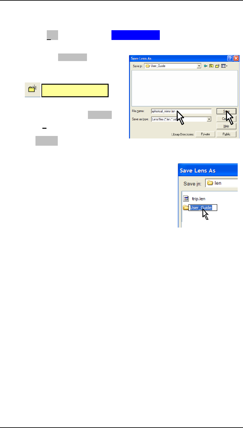
Saving the lens
To create a new folder and save the lens in it:
• From the File menu header select Save Lens as ...
• Of the two buttons labeled Library Directories at the bottom of the Save Lens As
window, click on _Private_
• At the top of the window, click on the
icon:
• Type the name for the new folder:
User_Guide and click on _Open_
• Under File name type:
spherical_mirror
• Click on _Save_ to save the lens with the
file name spherical_mirror.len
Note that OSLO is case insensitive, so this file cannot coexist with another file called, for
example, SPHERICAL_MIRROR.len
• Close the surface data spreadsheet with the green tick
• The lens will be stored in the private lens directory e.g.
C:\Program Files\OSLO\EDU64\private\len in the
newly created \User_Guide subdirectory. The file is in
ASCII format and contains the following text:
// OSLO 6.4 39660 0 16046
LEN NEW "Spherical mirror" -8 2
EBR 1.0
ANG 0.0000572957795
DES "OSLO"
UNI 1.0
// SRF 0
AIR
TH 1.0e+20
AP 9.9999999995e+13
NXT // SRF 1
RFH
RD -16.0
TH -8.0
NXT // SRF 2
AIR
WV 0.58756 0.48613 0.65627
WW 1.0 1.0 1.0
END 2
DLRS 3
DLNR 0 11
An explanation of these commands will be found in Appendix 1.
Create new folder
12 Your first OSLO session Chapter 1
Spherical mirror example
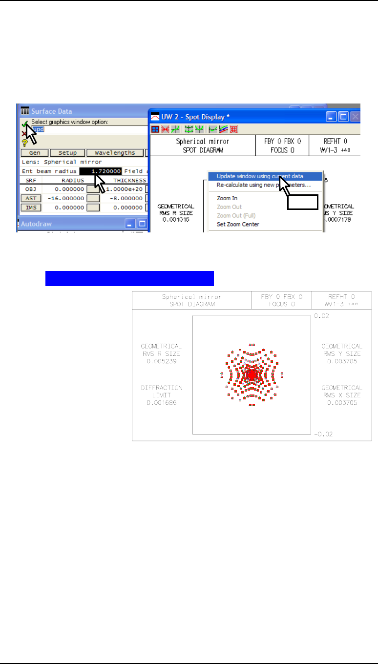
Changing the aperture
Question: If the aperture of the spherical mirror is increased to 3.44 mm is it still
“diffraction limited” at the new aperture?
• In the surface data spreadsheet increase the entrance beam radius from 1 mm to
1.72 mm.
• Confirm with the green tick .
Now recalculate the spot diagram:
• Right-click anywhere inside the graphics window containing the spot diagram plotted
previously.
• Select Update window using current data:
to create the diagram
shown at right.
Because the aperture has
increased, the spot diagram is
bigger (because of greater
aberrations) and the Airy disc
is smaller (it is inversely
proportional to the aperture).
Most of the rays therefore
now lie outside the Airy disc
circle.
Answer: No, it is far from diffraction limited.
Ri
g
ht
Chapter 1 - Your first OSLO session 13
Spherical mirror example
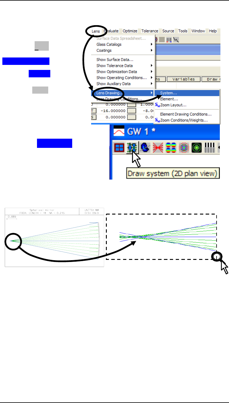
Drawing the lens in the graphics window, with “zooming”
To draw the lens system in a
graphics window:
• From the Lens menu
header select
Lens Drawing ...
► System
• Accepting all the defaults
click on _OK_
Alternatively,
• Click on the first icon in
the graphics window
standard toolbar for Draw
system (2D plan view).
• Select Plan View ...
To view the paths of rays near the focus
at a higher magnification:
• On the graphics window, left-
click-and-drag around the focus
as shown below.
• Left click twice within the graphics window to return to the full frame image.
Note that the zooming action will work on all graphics windows except the Autodraw
window.
Clearly a better focal plane can be chosen, a short distance to the right of the current one.
14 Your first OSLO session Chapter 1
Spherical mirror example
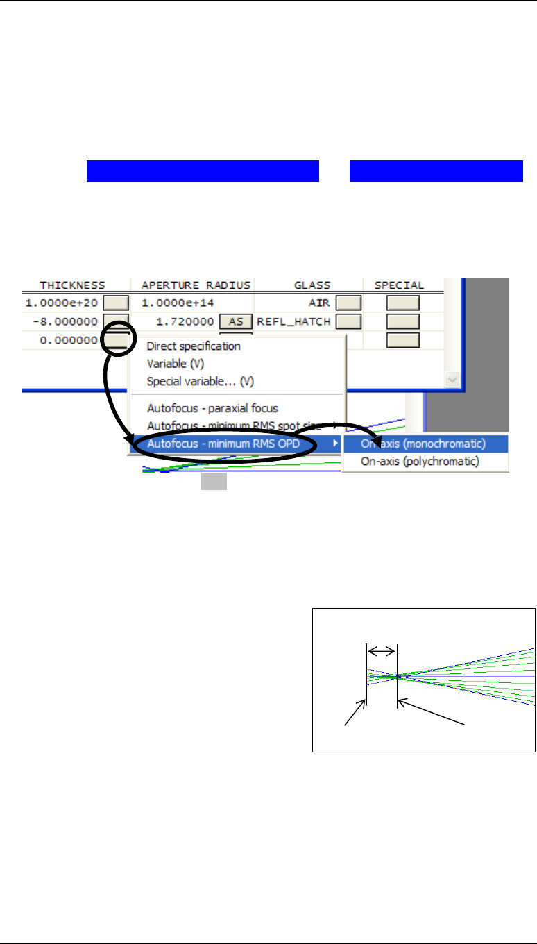
Finding the best focal plane
Question: At this new aperture, where should the focal plane be chosen to give the
best image quality for green light on axis?
This can be found most quickly using the “autofocus” facility in the surface data
spreadsheet, one of a number of built-in optimization functions.
• Open the surface data spreadsheet.
• Click on the gray button next to the thickness for the image surface (surface IMS).
• Select Autofocus - minimize RMS OPD ... ► On-axis (monochromatic)
In this context, RMS OPD refers to the root mean square “optical path difference” (or wave
aberration). This autofocus action has the effect of finding the focal plane which minimizes
the RMS OPD and entering the necessary displacement as the thickness for the image space.
The thickness for the space preceding the image space is left unchanged.
Listing the lens data - click on the Len header in the text window - gives the extent of
defocus needed:
*LENS DATA
Spherical mirror f/2.33
SRF RADIUS THICKNESS APERTURE RADIUS GLASS SPE NOTE
OBJ -- 1.0000e+20 1.0000e+14 AIR
AST -16.000000 -8.000000 1.720000 AS REFL_HATCH
IMS -- 0.023809 0.005127 S
The value listed for the defocus, shown as the
thickness at the image plane, is 0.023809 mm. To
get the actual distance from the mirror to the image
it is necessary to add the defocus value to the
nominal distance of -8 mm.
This is the only case in OSLO where an entry in the
thickness column of the surface data spreadsheet
for a surface affects the axial position of that
surface rather than the surface which follows.
Answer: The best focus at an aperture of f/2.33 is at 7.976 mm from the mirror.
0.023809 mm
Nominal focus Best focus
Chapter 1 - Your first OSLO session 15
Spherical mirror example
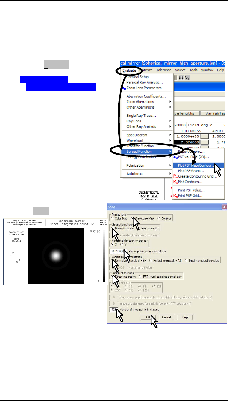
Plotting the on axis point spread function (PSF)
Question: Is the image “diffraction limited” at the new focal plane?
The evaluations carried out hitherto only show approximations to the actual distribution of
light in the image of a point source, since a spot diagram takes no account of diffraction.
To plot the true distribution of light in the image of a monochromatic point source, that is to
say, the point spread function:
• From the Evaluate menu header
select:
Spread Function
►Plot PSF Map/Contour...
In the Sprd window which opens:
• Click on the radio button
Gray scale map
• Click on the radio button
Monochromatic
• Type in 0.01 for the
Size of patch on image surface.
• Click on the radio button:
Normalize to peak of PSF
• Click on the radio button:
Direct integration
• Type in 128 for
Number of lines/points in
drawing
and click on _OK_
Note that the first bright ring around the
central maximum can just be seen.
Note also the figure at the top of the
scale on the right: 0.8123. This figure is
called the “Strehl ratio,” which is the
intensity at the central peak of the image
of a point source, normalized to that of
the Airy diffraction pattern of an ideal lens. The Maréchal criterion states that if the Strehl
ratio exceeds 0.8, a lens system may be described as “diffraction limited”.
Answer: Yes, the image is diffraction limited on axis at the new focal plane.
16 Your first OSLO session Chapter 1
Spherical mirror example
Edit Lens Drawing Conditions
Extending the rays in the lens drawing
• Open the Lens Drawing Conditions spreadsheet by clicking on the
icon in the main window toolbar.
• After Initial distance enter 16.
• Close the spreadsheet with the green tick .
Calculating the off axis optical path difference (OPD)
Question: What is the maximum OPD at full field for a semi-field angle of 18°
(total field angle 36°)?
• Open the surface data spreadsheet.
• Enter 18.0 degrees as the (semi-field) Field angle
• Left click on the gray SRF button for surface 1 (AST) to highlight the whole row.
• Right click to bring up the menu of options.
• Select Insert before to insert a new surface as surface 1.
Right
Chapter 1 - Your first OSLO session 17
Spherical mirror example
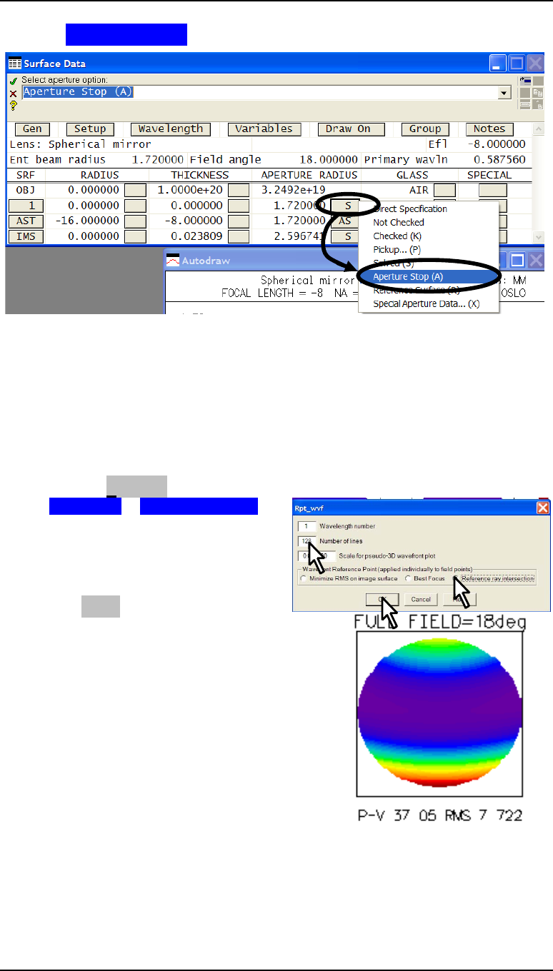
• Under APERTURE RADIUS for the new surface 1, click on the gray button.
• Select Aperture stop (A)
The aperture stop indication (AST) on the gray button under SRF will now move to surface
1, which at the moment is in contact with surface 2.
Note that the aberrations of the rays in the off-axis beam (drawn in blue) are so large that
they can easily be seen in the lens drawing.
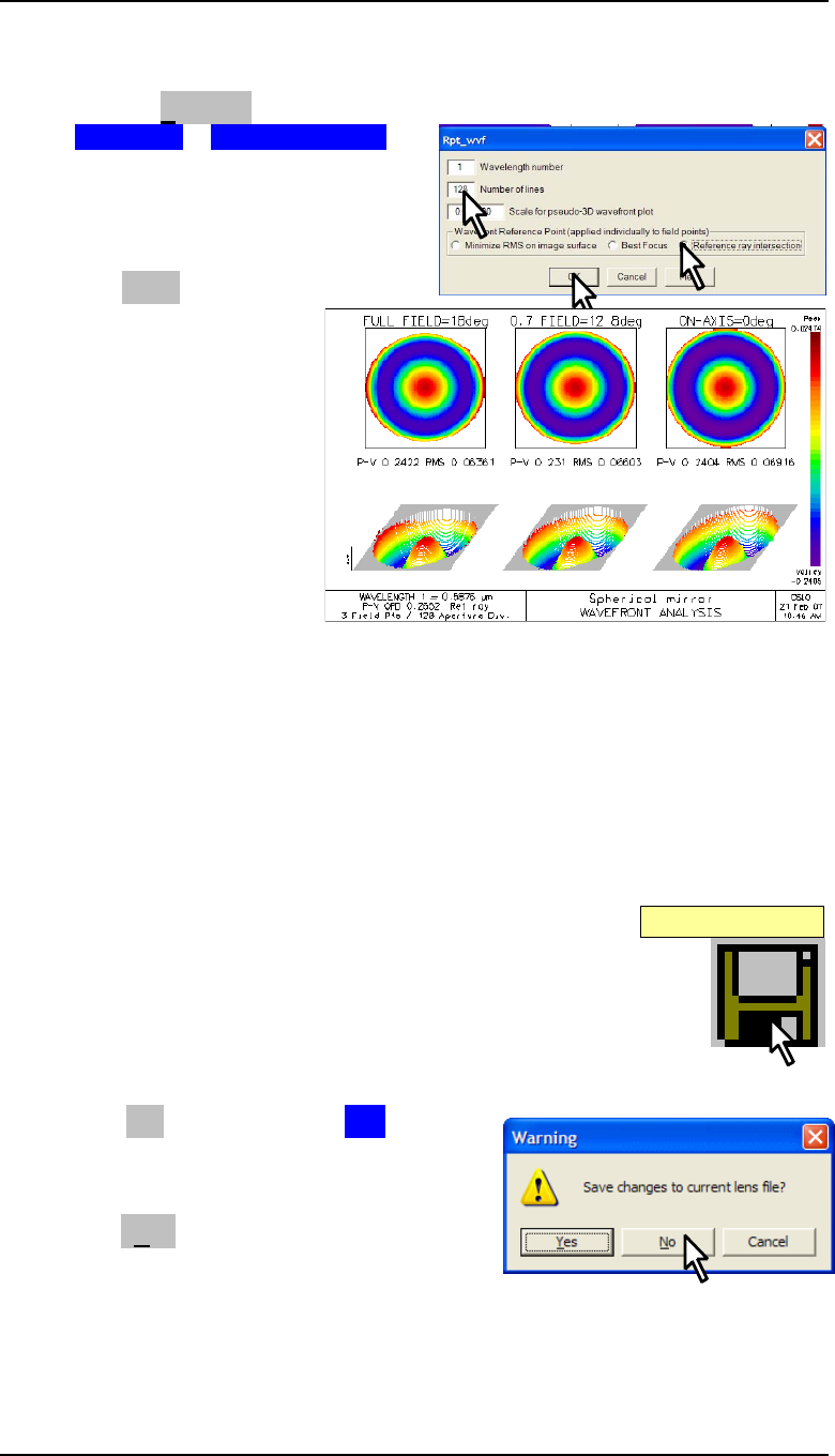
To calculate the optical path difference, or wave aberration, over the whole pupil for three
field points (on axis, 0.7 field and full field):
• From the Evaluate menu header select:
Wavefront ►Report graphic...
and in the dialog box which opens:
• Enter 128 as the Number of lines
• Select Reference ray
intersection
• Click on _OK_
Note the peak-to-valley figure of 37.05 wavelengths
under the map for the full field wave aberration.
Answer: The axial performance is better
than the standard criterion of a quarter of a
wavelength for the diffraction limit, but at full field
off axis the maximum OPD is 37 wavelengths.
18 Your first OSLO session Chapter 1
Spherical mirror example
O
p
en the slider wheel s
p
readsheet
Optimizing
The aperture stop is the limiting aperture of the axial beam. Its longitudinal position
determines the beam which is selected to form the off-axis image, and if the field is large,
this can have a significant effect on image quality.
Also the image has been assessed only over a plane surface - this is of course the usual
convention. For this exercise, however, we will investigate the benefits of allowing the
image to become curved.
Question: Where should the stop be placed, and what curvature of the image is
needed, to obtain the best performance over the whole field?
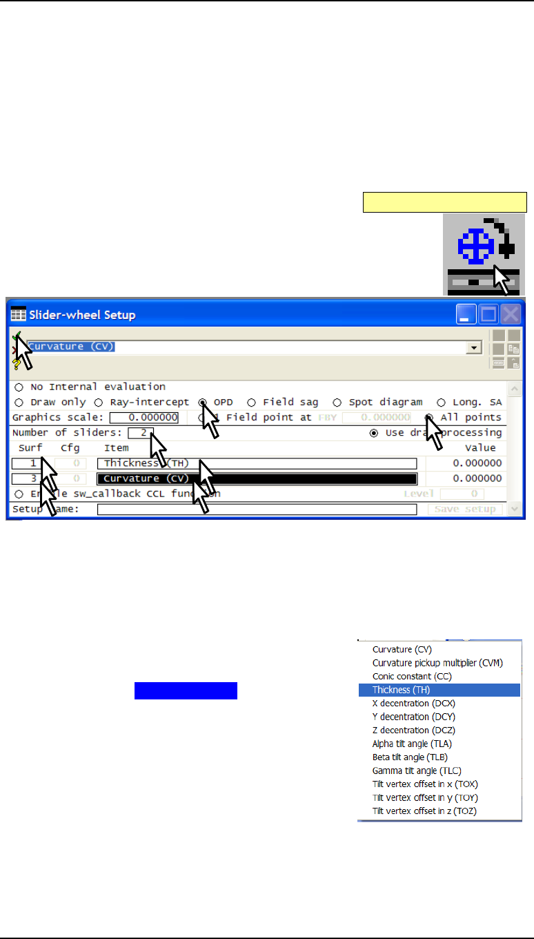
The answer to this question will demonstrate slider wheel
optimization, one of the most useful features of OSLO.
• Close the surface data spreadsheet.
• Open the Slider-wheel Setup spreadsheet, by clicking on the
icon on the main window header.
The entries above the line define the contents of the window(s) which will be displayed
during slider-wheel optimization.
• Select OPD (optical path difference, another name for wavefront aberration)
• Select All points
Entries below the line determine which parameters will be adjusted with slider-wheels:
• Leave the default of 2 for the Number of sliders (up to 32 can be defined at any
one time).
• On the first line, enter 1 under Surf and type th
in the box under Item. Alternatively click on the
box and select Thickness (TH) from the menu of
options.
• On the second line, enter 3 under Surf and type
cv under Item.
• Click on the green tick to close the Slider-
wheel Setup spreadsheet.
The two graphics window which open, GW31 and GW32,
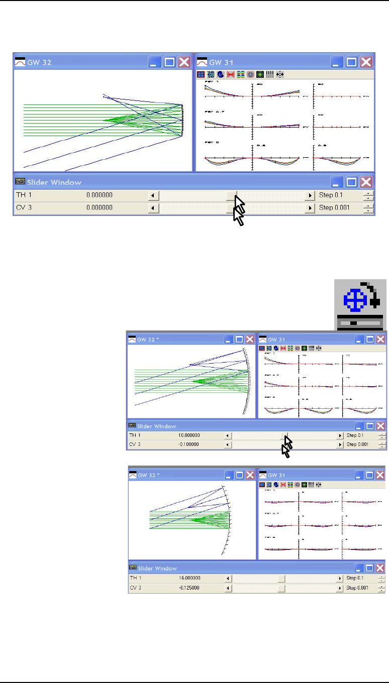
Chapter 1 - Your first OSLO session 19
Spherical mirror example
are specific to slider-wheel optimization. The scrollbar at the right of each slider wheel track
can be used to adjust the step increment of the slider-wheel motion. Changing the step size
also has the effect of centralizing the slider-wheel in the track.
• Watching the lens drawing in GW 32, and the plots of the optical path difference in
GW 31, move the upper slider to the extreme right (th 1 = 10) and the lower slider
to the extreme left (cv 3 = -0.1).
• Once again, open the Slider-wheel Setup spreadsheet, by clicking
on the icon. However this time just close it again immediately. This
has the effect of centralizing the two slider-wheels and re-drawing
both windows with different scales.
Although the OPD graphs
give no indication of scale,
it can be seen that the
performance is much
improved.
• Repeat the
sequence once more
until the best result
is given. This
should be when TH
1 = 16.0 mm and
CV 3 = -0.125
mm-1
Answer: The aperture stop must be at the centre of curvature of the mirror, and the
image surface must be a sphere with its centre at the aperture stop.
20 Your first OSLO session Chapter 1
Spherical mirror example
Save the current lens
Assessing the final design
To evaluate the optical path difference of the new system, once again:
• From the Evaluate menu header select:
Wavefront ►Report graphic...
and in the dialog box which opens:
• Enter 128 as the Number of lines
• Select Reference ray
intersection
• Click on _OK_
The peak-to-valley wave
aberration at the edge of the field
is less than a quarter wavelength,
so the lens is diffraction limited
over the whole (curved) field.
Listing the data
To list the correct prescription of
the final design, the image
separation needs to be adjusted.
In the command line:
• Enter the command: th 2 -7.976 (note the spaces after th and after 2)
SRF 2:
TH -7.976000
• Enter the command: th 3 0;rtg to give the final listing (again note the spaces):
SRF 3:
TH --
*LENS DATA
Spherical mirror
SRF RADIUS THICKNESS APERTURE RADIUS GLASS SPE
OBJ -- 1.0000e+20 3.2492e+19 AIR
1 -- -- 1.720000 S AIR
AST -16.000000 -7.976000 1.720000 AS REFL_HATCH
IMS -8.000000 -- 2.596719 S
• Click on the save lens icon in the main toolbar to save the lens.
Exiting the program
• From the File menu header select Exit. If any
more changes have been made a message label
will give a warning to save the lens, otherwise
those changes will be lost.
• Click on _No_ and the program terminates.
Chapter 1 - Your first OSLO session 21
Conclusion
Conclusion
This introduction shows that OSLO commands can be accessed
from the menu headers, from the text window headers, from
icons or entered directly into the command line. Commands
can also be combined into programs in the languages SCL or
CCL, as will be shown in chapter 8.
Command names are important for accessing the
documentation in the on-line help. Here are some of the
commands that have been used (either explicitly or via the
menus and icons) in this chapter:
file_new Opens a new lens file
uoc drl Updates lens drawing conditions
pls Plots spot diagram
len Lists lens data
save Saves lens
drl Draws lens
auf Autofocus
sprd Plots the point spread function
lse Opens the surface data spreadsheet
rpt_wvf Plots wavefront map at 3 field points
swe Opens the slider-wheel spreadsheet
th Changes a thickness
rtg Lists radii/thicknesses/glass types
exit Terminates OSLO.
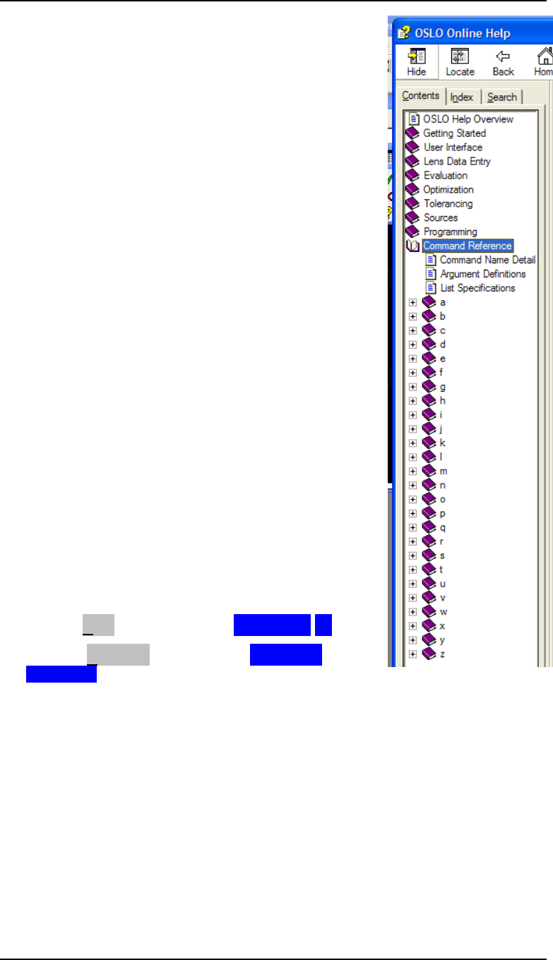
To obtain a full list of commands:
• From the Help menu header select OSLO Help F1
• Select the Contents tab and click on Command
Reference. The commands are listed in the alphabetic
sub-directories shown here.
22
Chapter 2 - Configuring OSLO
Introduction
Some ways in which the user interface can be adapted will be demonstrated in this section,.
It is recommended that these are implemented before proceeding with the remainder of the
exercises in this user guide.
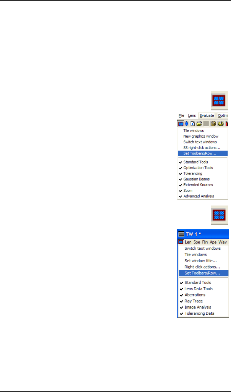
Toolbar menus
This section shows how the toolbars in the main window, the text window, and the graphics
window may be populated with icons/tools.
Main window
On first use of the program, bring up the full range of icons into the main window
toolbar:
• On the left of the main window toolbar, click on the blue and red
window Setup Window/Toolbar icon.
• In the drop-down menu which appears click on Optimization
Tools.
• Repeat for all the other items in the menu (not all the toolbars
listed will be available in Light or EDU versions)
• Click on Set Toolbars/Row... and, if it is not already 3, enter
3.
Text window
Click on the blue and red window Setup Window/Toolbar icon
on the left of the text window header.
• In the drop-down menu which appears click on Lens Data
Tools.
• Repeat for all the other items in the menu.
• Click on Set Toolbars/Row... and enter 3 for Maximum
number of toolbars on first row.
• Click on Switch text windows to open a second text window,
if desired. It will have the same toolbar choices as the first. Only
two text windows may be opened at a time.
Chapter 2 - Configuring OSLO 23
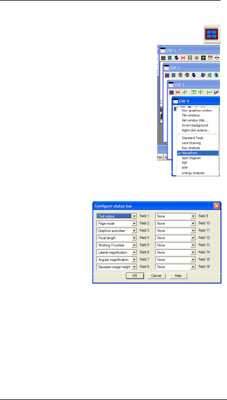
The status bar
Graphics window
Each graphics window supports only a single toolbar, but up to 31 additional
graphics windows may be opened, each with its own choice of toolbar.
• From the Window menu header select:
Graphics►New
• In the header of the graphics window which opens, click
on the Setup Window/Toolbar icon.
• Select one of the toolbar options.
• Repeat twice more to open a total of four graphics
windows. The current one always has a dark blue bar at
the top and an asterisk after the title; the header bars of
the others are light blue.
The status bar
The status bar extends across the bottom of the main window
for its full width. The following is a suggestion - there are
many other possibilities.
• Click twice on the status bar, or from the Window menu
header select Status Bar...
• Leave the parameters for the first three fields unchanged.
• Set the parameters for fields 4 to 8 as follows:
4. Focal length
5. Working F-number
6. Lateral magnification
7. Angular magnification
8. Gaussian image height
For each field, click on the
tab on the right hand side
of the field, and then select
the option from the drop-
down menu. This facility is
especially useful for keeping an eye on paraxial quantities during optimization.
• Click on OK to close the window.
It is not advisable to set more than eight entries as the status bar is limited to 127
characters.

24 Configuring OSLO Chapter 2
Preferences
Preferences
Preferences are parameters which control many of the functions of the program operation,
regardless of what lens is currently open. Status bar settings and preferences, once set, are
preserved after exiting the program. They are stored in a text file called oslo.ini in the
directory /private. This may be read with a text editor, but it must not be altered.
Preferences may be displayed using the show_preference command - e.g.
shp dsgn
or incorporated into print statements - e.g.
printf("Current lens directory is %s\n",str_pref(cdir)).
• Before starting to define preferences, ensure that the surface data spreadsheet is closed.
Designer name (dsgn)
Several of the graphics windows include a space where the designer’s name is listed. The
default for new lenses is OSLO. To change it:
• From the File menu header select Preferences►Set Preference...
• From the gray list, select Designer
• On the prompt Enter string preference type [your_name] (with a maximum of
10 characters, no spaces) into the command line
• Click on the green tick.
Alternatively, just type stp dsgn “[your_name]” in the command line and click on
the green tick Note that this will not affect the current lens in storage, but only new
lenses created after the change.
ISO10110 drawing settings (adr1, adr2, adr3, edcm)
On ISO 10110 drawings there is a space for three lines of standard information, which
normally consists of your company’s name and address:
• From the File menu header select Preferences►Set Preference...
• Select Address1
• Type [your_company_name] (maximum of 36 characters) in the command line under
Enter string preference:
• Alternatively, in the command line type: stp adr1 “your_company_name”.
• Close with the green tick
• Similarly for Address2 and Address3
e.g. stp adr2 “your_street_address”
stp adr3 “your_town”
Commas may be specified instead of decimal points on ISO 10110 drawings:
• From the File menu header select Preferences►Set Preference...
• Select Element_drawing_commas
• Select On under Select Boolean preference:
Chapter 2 - Configuring OSLO 25
Tangent check (tanc on)
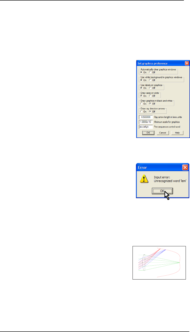
Graphics (gems, gacl, gfwb, glab, grax, gfbw, drra, pens)
Many of the preferences control the appearance of graphics output. For example, when
cutting and pasting graphics into Windows, the scale is generally too big for convenience. A
better scale is given if the gems preference is set to On:
• From the File menu header select Preferences►Set Preference...
• Select Graphics_emf_sizing
• Select On under Select boolean preference:
Several other graphics preferences are collected together for easy access:
• From the File menu header select Preferences ►
Preference groups... ►Graphics
• Modify the entries in the popup box shown in the
illustration as required.
• Click on OK.
Graphics alternate mode (gfam)
If the aspect ratio of exported graphics is reversed (landscape <-
> portrait) then look to see if gfam on
(Graphics_alternate_mode On) has inadvertently been set.
If so:
• Enter the command: stp gfam off
• Close with the green tick
No error boxes (noeb)
Whenever an error message box appears, it needs to be cleared
immediately by clicking on OK. This can be a problem on
occasions, such as during slider-wheel optimization.
It is possible for the user to suppress these error boxes
permanently. If desired:
• From the File menu header select Preferences►Set
Preference...
• Select No_error_boxes
• Under Select boolean preference: select On
Tangent check (tanc on)
• Enter the command tanc on in the command line. This
will turn on the facility which permits rays to be drawn to
highly aspheric surfaces, such as the one illustrated here.
• Close with the green tick
26 Configuring OSLO Chapter 2
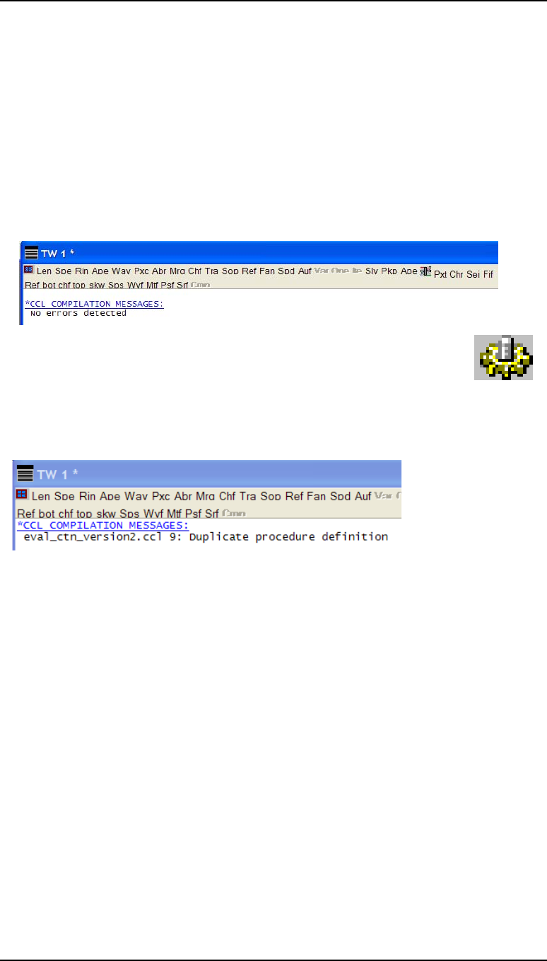
Compile CCL
Compile CCL
To avoid potential problems, it is a good idea to compile all CCL files before starting to use
the program for serious work. To do this:
• From the Tools menu header select Compile CCL ...
• In response to Select compile access: choose Public.
• In response to Select compile option: choose All.
• In response to Enter ccl opts: leave the default entry unchanged - e.g.:
-D _OSLO_EDU_ -D _OSLO_LIGHT_ -D OPENGL_GRAPHICS
• Close with the green tick
• Check that the public CCL directory has compiled without error.
• Repeat for the Private directory, or (not for users of OSLO EDU
version) click on the icon to “Compile all private CCL”.
• Once again confirm that the No errors detected message has
appeared in the current text window.
If an error message is given, then it will be necessary to correct, suppress or delete the file
whose name is shown. For example, the error message:
indicates the error occurs on line 9 of the file eval_ctn_Version2.ccl in the private/ccl
directory. Further details are given in chapter 8.
27
Chapter 3 - The command line
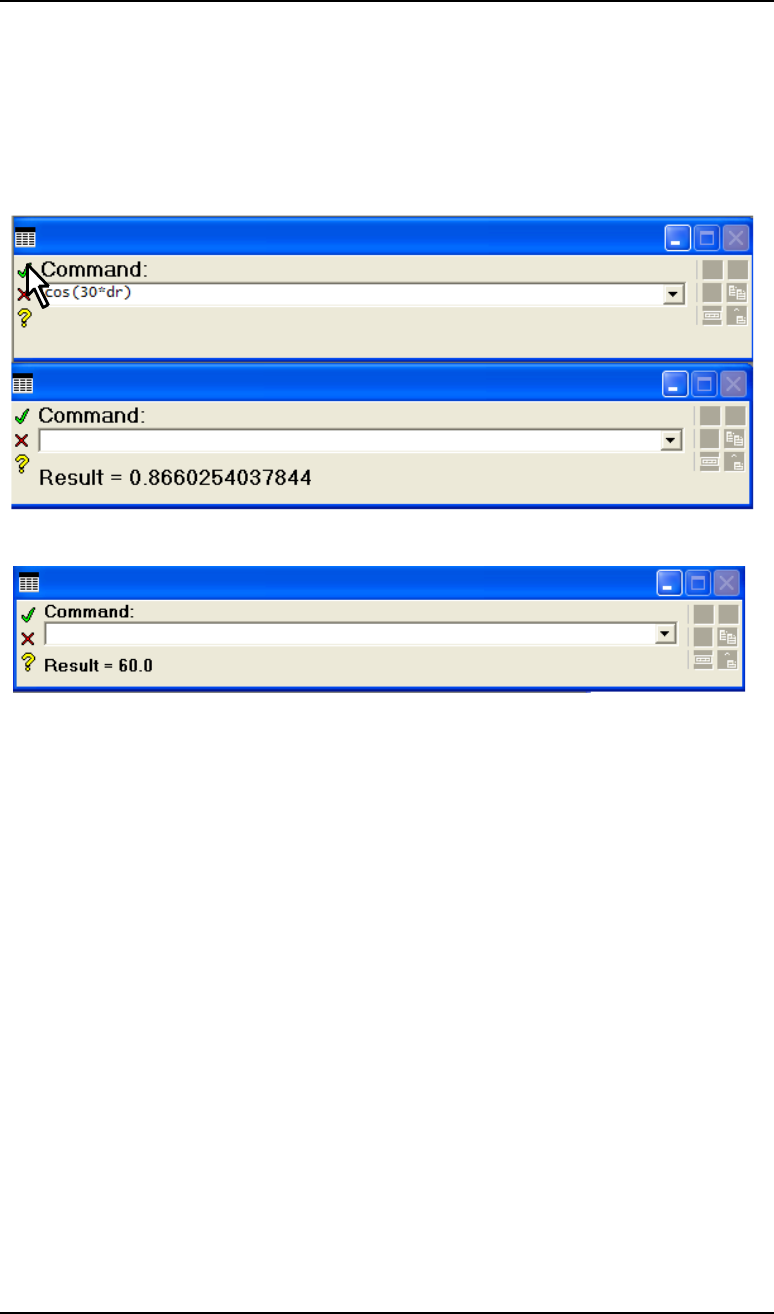
Arithmetic calculations
Simple arithmetic expressions can be evaluated with the result given in the message bar.
• If the surface data spreadsheet is open, close it by clicking on the green tick .
• Type cos(30*dr) and close with Enter or the green tick
• Enter atan2(sqrt(3),1)/dr
The following table gives all the arithmetical functions available in OSLO EDU:
Mathematical: pow (power), exp, log, log10, sqrt, j0,
j1 (Bessel functions)
Trigonometry (all angles are in radians):
sin, cos, tan, asin, acos, atan2
Rounding and limits: fabs, rint, r2int, round, min, max,
floor, ceil
Random numbers: rand (uniform), grand (Gaussian with zero mean)
OSLO commands
The main purpose of the command line is to execute OSLO commands.
• Enter file_open and close with the green tick
• If the message Save changes to current lens file? appears, click on No.

28 The command line Chapter 3
Assigning values to predefined variables
• In the Open lens file window which opens, under
Library directories at the bottom, click on Private.
• Click on trip.len
• Click on Open
• If the surface data spreadsheet opens, close it with the green tick .
Multiple commands are stacked with semicolons. For example, if we require to calculate the
“sag” of the first surface of the triplet (that is, the distance measured along the axis from the
plane through the axial point to the plane through the edge of the clear aperture):
• Enter rtg 1 1;sag 1 6.5
*LENS DATA
DEMO TRIPLET
SRF RADIUS THICKNESS APERTURE RADIUS GLASS SPE NOTE
1 21.250000 V 2.000000 6.500000 K SK16 C
*SURFACE SAG AND SURFACE NORMAL
SURFACE 1
Y X Z (SAG) NVL NVK NVM
6.500000 -- 1.018527 -0.305882 -- 0.952069
Commands can also be issued in a way that initiates a dialog for
subsequent parameters:
• Enter sag ?
• In the command window, in reply to the prompt Enter surface
number: enter 1
• In reply to the prompt Enter y: enter 6.5
• In reply to Enter x: leave the default value 0
• Close with the green tick
*SURFACE SAG AND SURFACE NORMAL
SURFACE 1
Y X Z (SAG) NVL NVK NVM
6.500000 -- 1.018527 -0.305882 -- 0.952069
Assigning values to predefined variables
Values can be allocated, using the command line, to predefined variables. Predefined
variables are a ... h, o ... z (real) i ... n and ii ... nn (integer). Also
pre-defined are seven real arrays with indices 0 - 1999, ua[] ... za [] and three
string arrays of 256 characters astr, bstr, cstr. There are also two predefined
constants, dr (degrees to radians conversion factor), on (=1), off(=0) and pi. All are
case-insensitive.
Allocations remain until OSLO is closed and restarted.
For example we can calculate the z (“sag”) value listed above:
• Enter r=21.25;y=6.5;z=r-r*cos(asin(y/r))
“sa
g
”
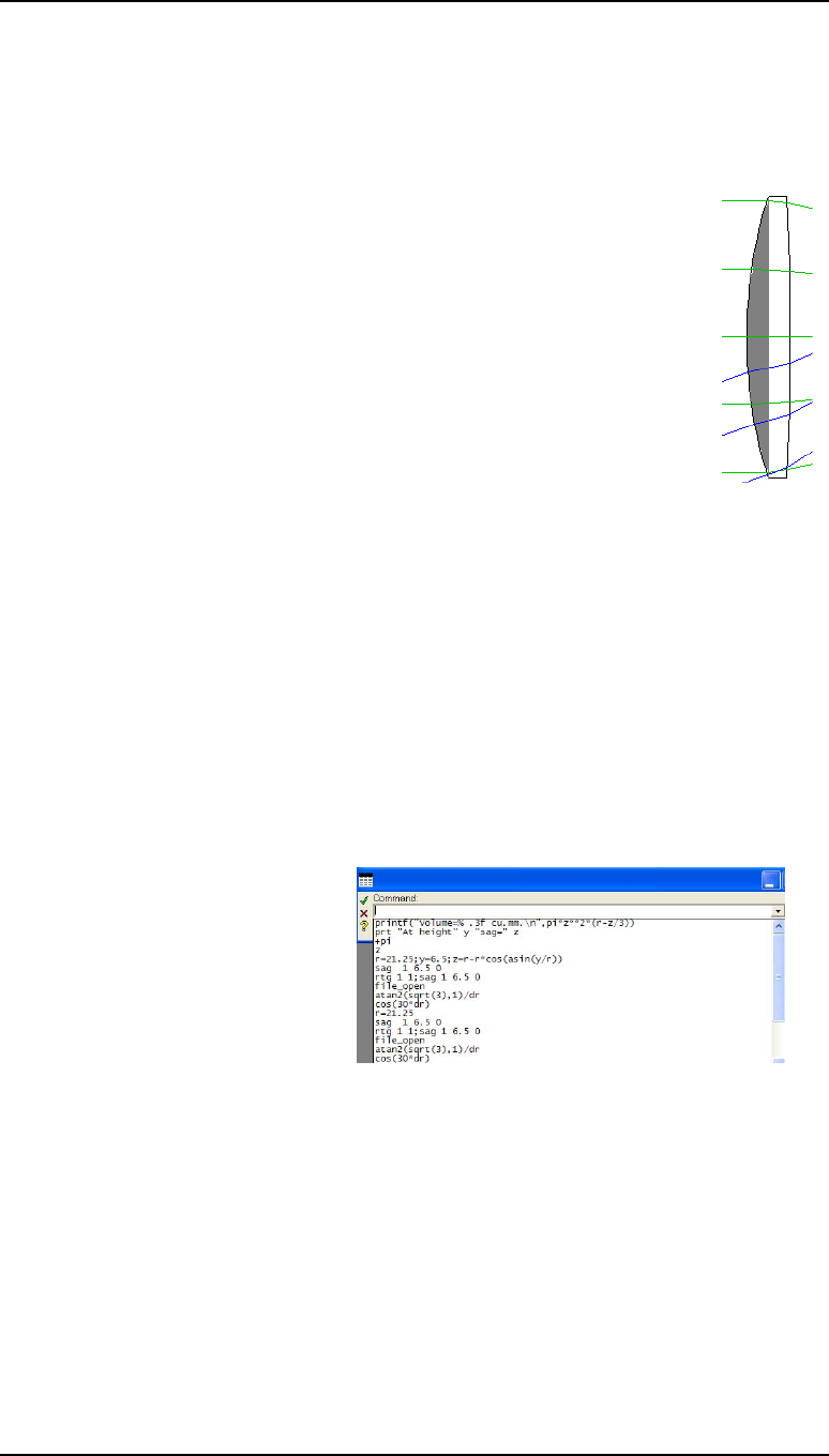
Chapter 3 - The command line 29
Printing
• Enter z.
Result = 1.0185269938148
Here the value of z which appears in the message area is the “sag” of the previous example.
Take care if you use c, f, o, r or v as they are also OSLO command words. pi is π,
but it is also an OSLO command. So do not enter pi on its own, but rather include it in an
arithmetic expression.
• Enter: +pi
Result = 3.1415926535898
Take care when arithmetical calculations are carried out while any
spreadsheet is open. The results of calculations will, if valid, be used as the
contents of the cell which is currently highlighted.
Printing
Results of printing appear in the current text window:
• Enter: prt At height y sag is z
At height 6.500000 sag is 1.018527
For more formal presentation, printed output can be formatted. This command uses the
formatted print command printf to print the volume of the “cap” enclosed by surface 1.
• Enter: aprintf("Volume=% .3f cu.mm.\n",pi*z**2*(r-z/3))
Volume= 68.149 cu.mm.
The first argument is a format string. In it, % .3f is a format specification for the double
precision numeric value; the space after the % reserves a space for a minus sign (if any), 3
gives 3 places after the decimal point and f is the conversion character for floating point
format. Other characters in a format string are printed unmodified, until the final \n which
outputs a new line.
The history button
Previous commands can be called up,
for repeating a command, or
correcting it.
• Click on the history button at
the end of the command line.
• Alternatively, press Shift-
F4. This is known in the
documentation as a keyboard shortcut; some others are listed below.
• Enter: prh to list the last 40 entries in the history buffer.
Keyboard shortcuts
F1 Open the online help
30 The command line Chapter 3
The message area
Ctrl+N Open a new lens
Ctrl+O Open an existing lens
Ctrl+S Save the lens in its current file
In the command line,
Ctrl+X Cut selected text
Ctrl+C Copy selected text
Ctrl+V Paste selected text
Shift+F4 Show the history buffer
Ctrl+PgUp Scroll through the history (Ctrl+PgDn to scroll back)
In the text editor,
Ctrl+E Execute the selected text
Ctrl+G Go to the indicated line number
Ctrl+Z Undo the last edit
Alt+F3 Find text (F3 to find again)
Ctrl+R Replace text (Ctrl-T to replace again)
In a spreadsheet,
Shift-spacebar Insert a new line before the current line
The message area
The message area under the command line can be used for formatted output. For example to
display a string preference:
• Enter:
message("Private dir: %s",str_pref(prid))
Private dir: C:\Program Files\OSLO\Prm64\private
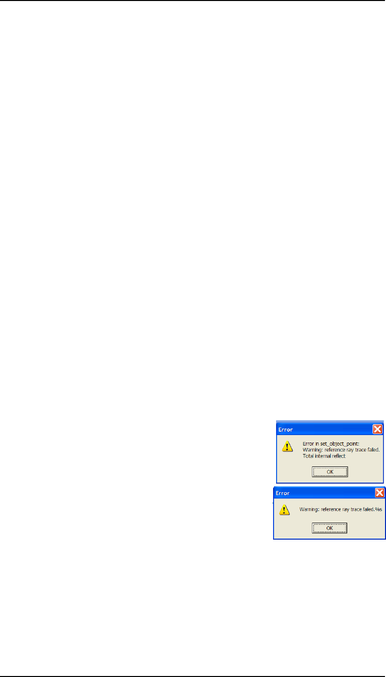
The message area is where error messages can be printed. The message command also
converts error numbers to strings:
• Enter: sop 9 0 0
• Click on OK in the error box.
• Enter: errno
Result = -3152
• Different versions of \OSLO have different error
numbers. To decode an error number, enter: message
errno Again, click on OK in the error box before proceeding.

Chapter 3 - The command line 31
Executing CCL command sequences
Executing CCL command sequences
Valid CCL command sequences which use the pre-defined variables listed above, can be
executed within the command line. The total length of the command string must not exceed
255 characters.
• Enter:
prt lid;for(i=0;i<=ims;i++)prt cv[i] th[i] rn[i][1]
with the result:
DEMO TRIPLET
-- 1.0000e+20 1.000000
0.047059 2.000000 1.620410
-0.006303 6.000000 1.000000
-0.049383 1.000000 1.616592
0.051813 6.000000 1.000000
0.007080 2.000000 1.620410
-0.057854 42.950000 1.000000
-- -- 1.000000
Here the count variable, i, is a pre-defined integer.
The system data variables lid (the lens identifier), cv[i] (the surface curvature, that is,
the reciprocal of the radius), th[i] (the separation from surface i to surface i+1) and
rn[i][1] (the refractive index in the space after surface i at the first wavelength) are all
examples of system data variables which can either be printed, or used in arithmetic
expressions or CCL programs. A list of such variables is given in the next section.
A system data variable such as th cannot, however, be changed by a simple variable
assignment statement such as th[3]=2.0. An attempt to do this will give the error
message:
Input error
Protected variable ‘th’ may not be changed
Rather, it must be changed using the dedicated command which has the same name as the
variable. For example:
• Enter th 3 1.05;rtg
A new image surface may also be defined temporarily in this way:
• Enter ims 3;rtg
The remaining surfaces are unaffected, but they will be lost unless the lens is restored before
the lens is saved again:
• Enter ims 7;rtg
Other commands can be used to change the lens - e.g. the 10th system note, used as a label
in the public lens database:
• Enter sno10 TRIPLET;opc sno
*CONDITIONS: SYSTEM NOTES
10: TRIPLET
A list of lens update commands is given in Appendix 1.

32 The command line Chapter 3
Alphabetic list of system data variables
Alphabetic list of system data variables
The following is a partial list of the system data variables. To obtain a complete list of all
variables exported from OSLO:
• From the Help menu header select OSLO Help F1
• Under the Contents tab select Programming►Accessing Data
►CCL Global Data
aac special aperture action
aan special aperture angle
ad aspheric coefficient in r
4
ae aspheric coefficient in r
6
af aspheric coefficient in r
8
afo afocal flag
ag aspheric coefficient in r
10
agn special aperture group
amo aberration mode
ang field angle
ap apertures
apchk aperture checking flag
appksn aperture pickup surface
apspec aperture spec: ebr, nao, etc.
aptyp aperture type
as0,as1.. aspheric surf coefficients
asi alternate surf intersection flag
asp aspheric surf type
ast aperture stop surf
atp special aperture type
avx1 special ap. x vertex 1
avx2 special ap. x vertex 2
avx3 special ap. x vertex 3
avx4 special ap. x vertex 4
avy1 special ap. y vertex 1
avy2 special ap. y vertex 2
avy3 special ap. y vertex 3
avy4 special ap. y vertex 4
ax1 special ap. ax1
ax2 special ap. ax2
ay1 special ap. ay1
ay2 special ap. ay2
bcr use base coord. for coord
ben tilt and bend flag
caa component aper alpha tilt tol
cab component aper beta tilt tol
cc conic constant
cca component coc alpha tilt tol
ccb component coc beta tilt tol
cct conic constant tol
cdx component x-decenter tol
cdy component y-decenter tol
cns cone slope
curwav current wv number (base 1)
cv curvature
cvdat curvature solve/pickup datum
cvmult curvature pickup datum
cvpksn curvature pickup surf
cvtyp curvature type
cvx toric curvature
dct decenter tol
dcx x decentration (local)
dcy y decentration (local)
dcz z decentration
des designer name
df diffractive surf coefficients
dfcsn diffractive surf pickup
doe diffractive surf type
dor diffraction order
drw surf drawing option
dt decenter-tilt order flag
dth grin step size
dwv design wv (diffractive surf)
dxt x-decenter tol
dzt axial surf shift tol
ebr entrance beam radius
errno message nbr for last error
evza image evaluation coord. system
fcc Fresnel surf substrate conic
fcv Fresnel surf substrate curvature
fldspec field spec: obh, ang, etc.
fno image space working f-number
frn Fresnel surf flag
gc global coord. ref. surf number
gcs global coord. reference surf
gdt gradient index medium type
gih Gaussian image height
glpksn glass pickup surf
gltyp glass type
gmz gradium blank thickness
gnz gradium coefficient
gor grating order
goz gradium offset into blank
gra gradium coefficient
grb gradium coefficient
grc gradium coefficient
grd gradium coefficient
grpcode group code
grptype group type
gsp grating spacing
gwv gradium dispersion data ref.
hor hologram diffraction order
hv1 hologram obj. real/virtual
hv2 hologram ref. real/virtual

Chapter 3 - The command line 33
Alphabetic list of system data variables
hwv hologram construction wv
hx1 hologram object x coord.
hx2 hologram reference x coord.
hy1 hologram object y coord.
hy2 hologram reference y coord.
hz1 hologram object z coord.
hz2 hologram reference z coord.
ims image surf number
ims_1 image surf number minus one
irt irregularity tol
ldp pen for lens drawings
lensym lens symmetry flag
lid lens identifier
nao object space numerical ap.
nap image space numerical ap.
nr1 grin coefficient in r
2
nr2 grin coefficient in r
4
nr3 grin coefficient in z
6
nr4 grin coefficient in z
8
numsap number of special apertures
numw number of wavelengths
nz1 grin coefficient in z
nz2 grin coefficient in z
2
nz3 grin coefficient in z
3
nz4 grin coefficient in z
4
obh object height
pfl perfect lens focal length
pfm perfect lens magnification
pre system pressure (atm)
puk image space axial ray slope
rco coord. return surf number
rd radius of curvature
rdt radius tolerance
rdx toric radius of curvature
rfs reference surf
rn refractive indices
rnt refractive index tol
rod extruded surf spec
rotsym rotational symmetry flag
rtf radius from test glass file
sasd source astigmatic distance
sh radial spline height
ska Sellmeier gradium coefficient
skb Sellmeier gradium coefficient
skc Sellmeier gradium coefficient
sla Sellmeier gradium coefficient
slb Sellmeier gradium coefficient
slc Sellmeier gradium coefficient
spl no. of radial spline surf zone
splpts number of spline points
spt spherical form tol
srftyp surf type
ss radial spline slope
tat tla tilt tol
tbt tlb tilt tol
tce thermal coefft of expansion
tct tlc tilt tol
tem system temperature (deg C)
th thickness
thdat thickness solve/pickup datum
thmult thickness pickup datum
thpksn1 thickness pickup surf
thpksn2 thickness pickup surf
tht thickness tol
thtyp thickness type
tir total internal reflection flag
tla tilt about (local) -x axis (degs)
tlb tilt about (local) -y axis (degs)
tlc tilt about (local) +z axis (degs)
tlt tilt tolerance
toric toric type
tox offset of tilt vertex in x
toy offset of tilt vertex in y
toz offset of tilt vertex in z
trr_fbx fractional x object coord
trr_fby fractional y object coord.
trr_fbz fractional z object coord.
trr_fds field point data
trr_fpt field point number
trr_fxrf reference surf x coord.
trr_fyrf reference surf y coord.
ttun tilt tolerance units
twl tol fringe wavelength
txyc couple x to y tols
uni number of mm in current units
varnbr next variable number
vnt Abbe V-number tol
wav current wavelength number
wv wavelengths
ww wavelength weights
zr Zernike phase surf coefficients
zrt Zernike srf reference ray trace
• Also in the online Help facility, under the Contents tab select
Programming ► Accessing Data ►Other Data to find the definitions of
the following read-only variables:
beg_selection cfg current_pen cursnbr end_selection
fptnbr gfx_window glass_name lensym maxcfg
nbr_pens numw oprnbr raynbr sdsnbr
srfssopen ssb surface_note system_note txt_window
varnbr wav
34
Chapter 4 - Lens data entry
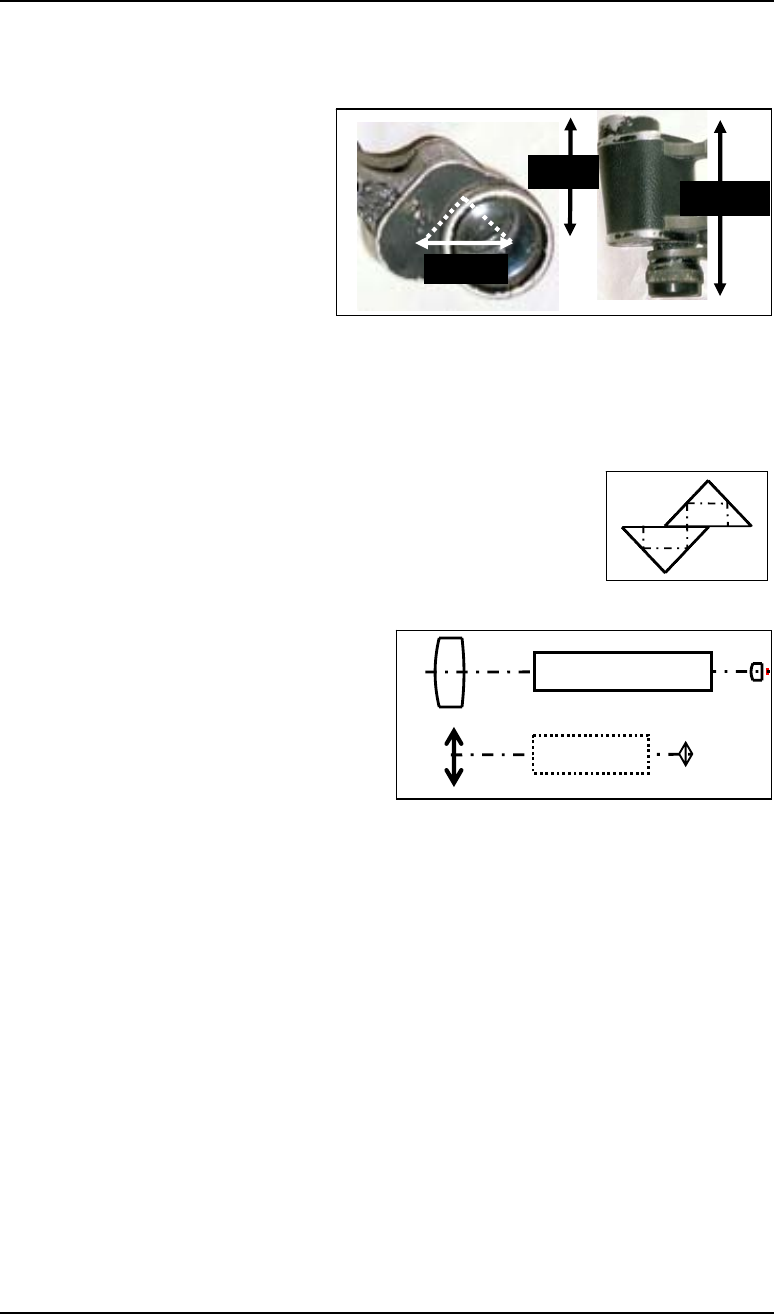
8 x 30 binoculars: Specification
The task which will be used to demonstrate lens data input is the problem of modeling the
binoculars shown in the photographs,
with 8x magnification, a 30 mm
diameter entrance pupil, and a field of
view of 6°. Measurements give an
overall length from the front of the
objective to the back of the eyepiece
of 103 mm. The distance from the
front objective to the eyepiece
mounting plate is 73 mm, and the
offset between the optical axis of the objective and the optical axis of the eyepiece is 28
mm.
Calculations
First of all we will calculate the sizes of the Porro prisms. Since the
offset between the two optical axes is 28 mm, the path perpendicular
to the axis of the binoculars must be 20mm in each prism. The total
glass pass in each prism must therefore be 40mm, and the total glass
path in the two prisms (shown here in an opened-out-view) 80 mm.
The glass which is most commonly used for prisms in the better quality binoculars is Schott
BaK4, which has a refractive index of 1.57.
The prism path length of 80 mm will then
have an “air equivalent” path length of
80/1.57 = 51 mm. This needs to be added to
the physical length (103 mm) to give a total
air equivalent optical path from back to front
of 154 mm. Now, making an allowance of 19
mm for the finite thicknesses of both
eyepiece and objective gives a path between the principal planes, or equivalent thin lenses,
of 135 mm. So, to obtain the desired magnification of x8, the focal lengths required are 120
mm for the objective and 15 mm for the eyepiece.
Choosing an eyepiece
The eyepiece in most common use in prismatic binoculars is the Kellner. This consists of a
plano-convex single element lens, with a cemented doublet near the eye. An eyepiece
suitable for this application can be found in the book “Optical Design For Visual Systems”
by Bruce H. Walker.
Users of OSLO Standard and OSLO Premium:
• Close the surface data spreadsheet.
• From the File menu, select Lens database,
• Select Public.
28 mm
103 mm
73 mm
80 mm
51 mm
Chapter 4 - Lens data entry 35
Choosing an eyepiece
• In the window that opens, click on LENS ID and choose Sort Up.
• Using the scroll bar on the right
find the lens with LENS ID
“Kellner Eyepiece” As a
check, the designer is shown as
bhw/WA, the image surface
number is 7.
• Click on this line to call up the
lens. The aberration curves are
drawn automatically, and the
listing is given in the text
window when Prescription is
selected.
• Open the surface data spreadsheet, and click on the gray Wavelength button.
• Right click to get the choice of pre-defined wavelengths, and select d, F and C
respectively for the three wavelengths.
• In the text window click on Wav
*WAVELENGTHS
CURRENT WV1/WW1 WV2/WW2 WV3/WW3
1 0.587562 0.486133 0.656273
1.000000 1.000000 1.000000
Users of OSLO Light and OSLO EDU:
• From the menu header, choose File > New lens.
• Leave the file name as untitled, leave Custom lens as the option, and enter 6 as the
number of surfaces.
• Fill in the surface data spreadsheet entries as shown. Check the Efl value to confirm
that the data entries are correct.
All users:
Note that the eyepiece has an object at infinity and an image at a finite distance. In other
words, we are tracing the rays from the eye to the intermediate image, in the reverse
direction of travel of the light. Surface 1 is defined as the aperture stop.
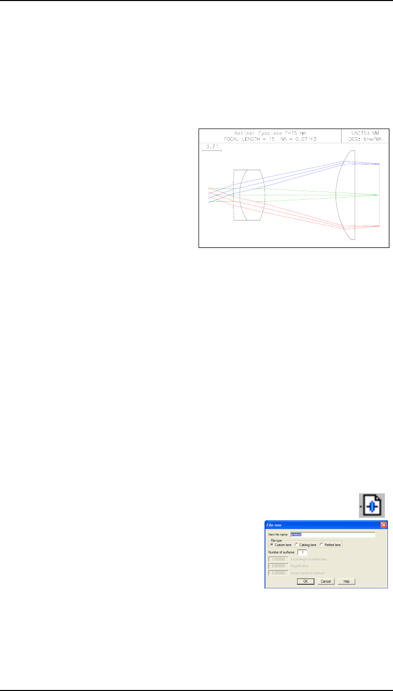
36 Lens data entry Chapter 4
Scaling the eyepiece
Scaling the eyepiece
The eyepiece must now be scaled to give the required focal length of 15 mm:
• In the surface data spreadsheet, click on Draw Off to open the Autodraw window (at
which point Draw Off becomes Draw On).
• After Lens: assign a title: Kellner Eyepiece F=15 mm
• Right click on any of the surface buttons on the left, and choose Scale Lens►Scale To
New Focal Length ...
• Insert 15 (this lens is already specified
in the default units of mm).
• Click on OK.
• List the lens by clicking on Len in the
text window.
*LENS DATA
Kellner Eyepiece F=15 mm
SRF RADIUS THICKNESS APERTURE RADIUS GLASS SPE NOTE
OBJ -- 5.3552e+19 1.9491e+19 AIR
AST -- 2.731166 1.071046 A AIR Ent Pupil
2 81.934981 1.071046 4.284182 F4 C
3 7.979289 4.284182 4.284182 BAK2 C
4 -10.656903 11.942157 4.284182 AIR
5 12.584785 3.213137 7.497319 BAK2 C
6 -- 4.128880 7.497319 AIR
IMS -- -- V 5.221347 *
• Save the eyepiece in the private/len/User_guide directory with the name
bino_ep.len.
Choosing a catalog objective
Rather than design an objective from scratch, the task will be to locate a suitable lens in the
lens manufacturers’ catalogs provided with the program. The focal length required is about
120 mm. While the entrance pupil diameter is 30 mm, allowance must be made for
mounting, say 3 mm on the radius (larger than on an internal lens because of the
need to provide a seal against moisture).
• Click on the third icon on the main window toolbar,
which is the symbol for a new lens.
• In the dialog box which opens, click on OK.
• In the surface data spreadsheet which opens, after
Lens: assign a title (e.g. Objective)
• Change Ent beam radius to 15 mm.
• Change Field angle to 3 degrees.
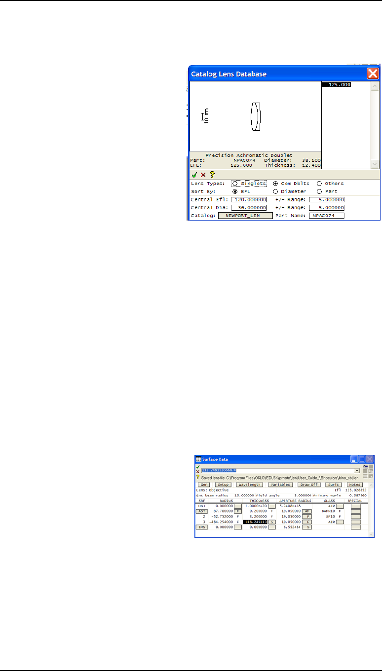
Chapter 4 - Lens data entry 37
Choosing a catalog objective
• Left click on the gray surface button in the first column for surface 2 (IMS) to select the
surface.
• Right click.
• From the drop-down menu, choose the option Insert Catalog Lens...
In the window which appears, make the
following selections:
• First, at the bottom of the screen, for
Catalog: select NEWPORT-LEN
• To find a cemented doublet, click on
the button for Lens types Cem
Dblts
• Leave default Sort By EFL.
• Enter the Central EFL (focal length),
120 mm and +/- Range 5 mm
• Enter the Central Dia, 36 mm and
+/- Range 5 mm.
• Click on the only lens listed, with focal length 125 mm, part number NPAC074.
• Click on the green tick, and the window will close.
• Click on the gray button Group at the top of the surface data spreadsheet to show the
individual surfaces.
• Delete the non-functional first surface: Left click on the gray Srf button to select the
line, right click on the gray button to create the pull-down menu, and select Delete. The
aperture stop indicator (AST) on the surface number button will move to the first
surface of the doublet.
• Set the image distance to the paraxial image distance by clicking on the gray button in
the cell for the thickness of surface number 3 (the back focal distance). Select Solve
(S) > Axial ray height, and after Enter solve value type 0. The thickness value
becomes 118.249113. An S will appear on the gray button next to this, indicating the
presence of a paraxial “solve.” What this means is that as long as the lens is rotationally
symmetrical, and paraxial rays are valid (that is, rays which are traced using linear
formulae, corresponding to light close to the optical axis), then the distance to the next
surface (in this case the image surface) will be adjusted so that the height of the paraxial
marginal ray at the next surface is zero - in other words, the image will always be at the
paraxial focus.
• In the text window, click on Slv to
confirm this definition.
*SOLVES
3 PY --
• Save the lens in the
private/len/User_guide directory
with the name bino_obj.len
• In the text window, click on Len to list the lens.
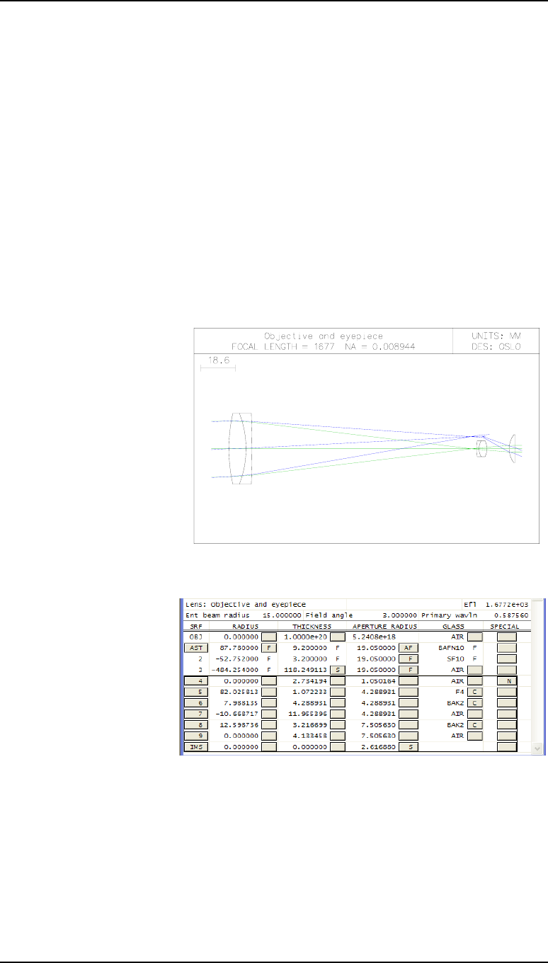
38 Lens data entry Chapter 4
Combining the objective and the eyepiece
*LENS DATA
Objective
SRF RADIUS THICKNESS APERTURE RADIUS GLASS SPE NOTE
OBJ -- 1.0000e+20 5.2408e+18 AIR
AST 87.780000 F 9.200000 F 19.050000 AF BAFN10 F *
2 -52.752000 F 3.200000 F 19.050000 F SF10 F
3 -484.254000 F 118.249113 S 19.050000 F AIR
IMS -- -- 6.552484 S
• Check the lens prescription against the manufacturer’s published catalog.
Combining the objective and the eyepiece
The first task is to combine objective and eyepiece without the prisms.
• Ensure the file with the objective, bino_obj is open.
• Open the surface data spreadsheet.
• If necessary, click on Draw Off to open the Autodraw window.
• Change the title to
Objective and
eyepiece
• Left click on the surface
button for the image
surface (IMS). This will
select surface 4, indicated
by a bold surround.
• Right click on the gray
button IMS, under SRF, to
bring up the options
menu.
• Choose Insert Lens File
...
• In the Merge lens file
window, find the
eyepiece file bino_ep
and click on Open.
At this stage, of course, the
eyepiece is now the wrong
way round.
• Select the seven
surfaces of the eyepiece
and the exit pupil (numbered 4 to IMS)
• Right click anywhere in this group.
• Select Reverse
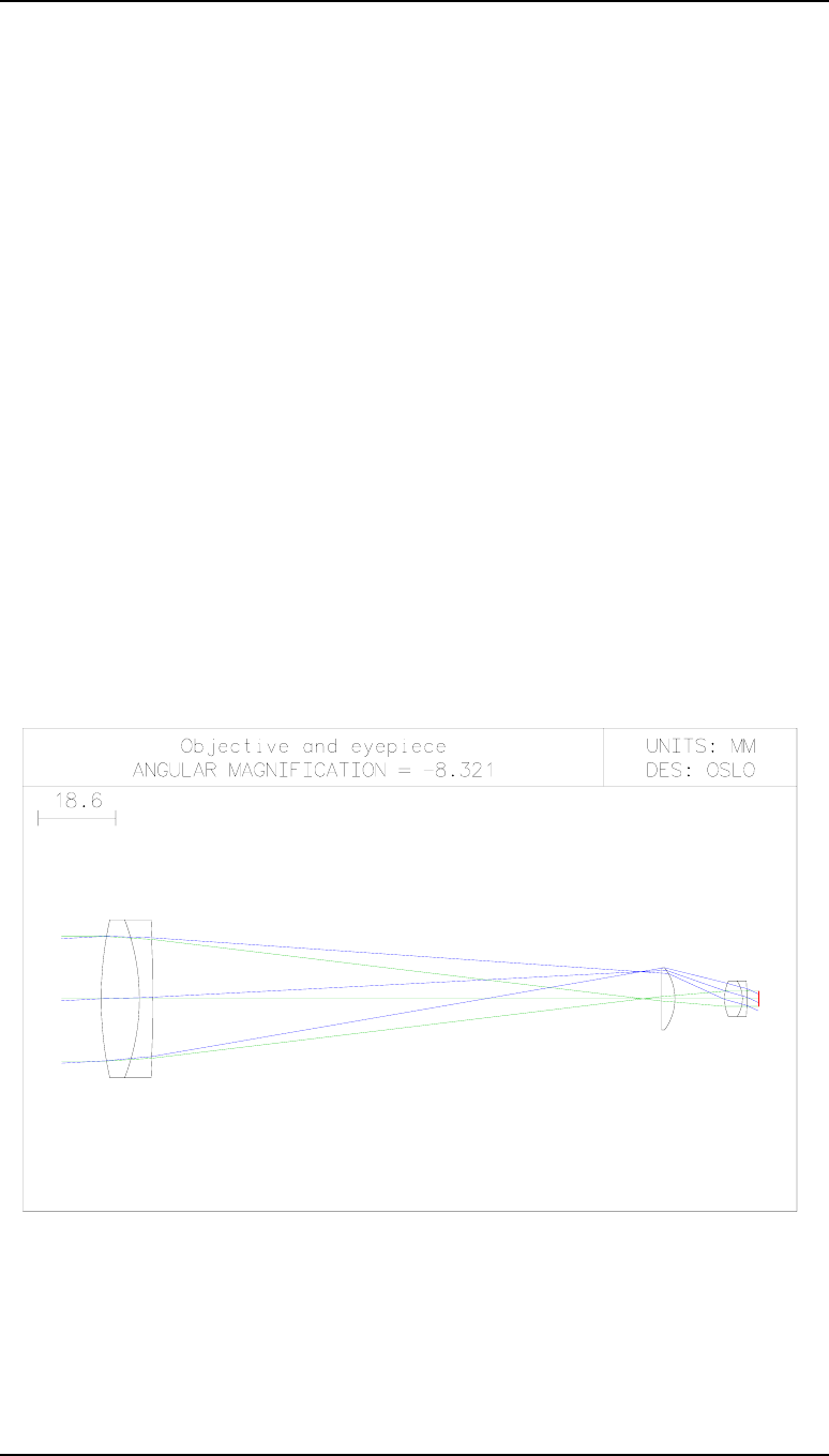
Chapter 4 - Lens data entry 39
Combining the objective and the eyepiece
• Click on Gen at the top of the surface data spreadsheet, and change Evaluation mode
to Afocal. This means that ray aberrations will be angular rather than transverse linear.
• Change the exit pupil (surface 10) aperture radius to 15/8
• Click on surface 10 Special gray button. Select Surface Note (N) and change the
note to Exit pupil. Also under the surface 10 Special button, select Surface
control(F) > General Change Surface appearance in lens drawing: to Drawn,
and change the Pen number to 4 (i.e. red).
• Save the file with the name bino_obj_ep.len
• Click on Len in the text window header.
*LENS DATA
Objective and eyepiece
SRF RADIUS THICKNESS APERTURE RADIUS GLASS SPE NOTE
OBJ -- 1.0000e+20 5.2408e+18 AIR
AST 87.780000 F 9.200000 F 19.050000 AF BAFN10 F *
2 -52.752000 F 3.200000 F 19.050000 F SF10 F
3 -484.254000 F 118.249113 S 19.050000 F AIR
4 -- 4.133458 2.616880 AIR
5 -- 3.216699 7.505630 BAK2 C
6 -12.598736 11.955396 7.505630 AIR
7 10.668717 4.288931 4.288931 BAK2 C
8 -7.988135 1.072233 4.288931 F4 C
9 -82.025813 2.734194 4.288931 AIR
IMS -- -- 1.875000 * Exit Pupil
• Open the surface data spreadsheet and find the Autodraw window.
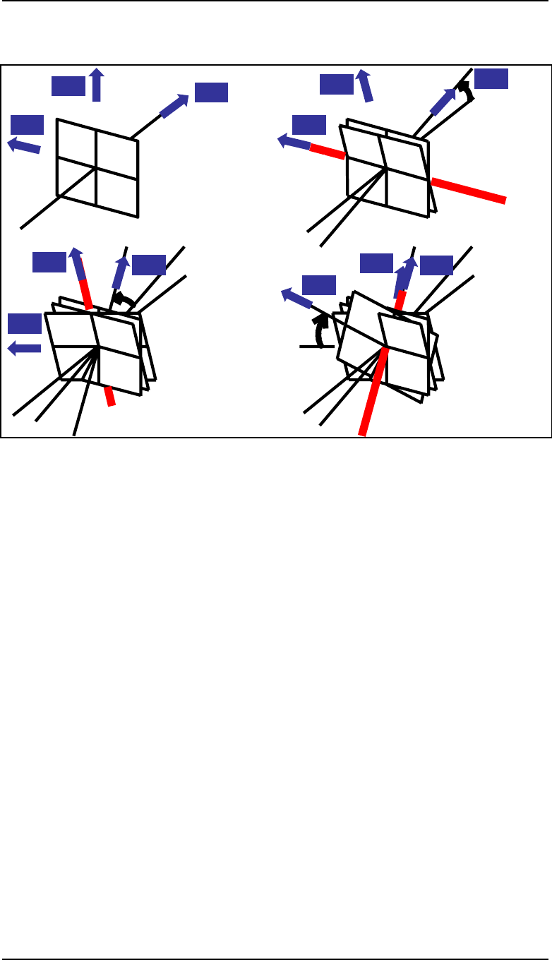
40 Lens data entry Chapter 4
Surface decenters and tilts
Surface decenters and tilts
Before modeling the prisms, we will look at how tilted and decentered surfaces are defined.
The gray button under Special in the surface data spreadsheet includes the option
Coordinates where all this is found.
The default sequence is Decenter, then tilt in which case the sequence of displacements
is:
1. Decenter by DCX along X axis, by DCY along Y axis, and by DCZ along Z axis,
all in system units.
2. Tilt anticlockwise about the new X axis through an angle TLA (degrees)
3. Tilt anticlockwise about the new Y axis through an angle TLB (degrees)
4. Tilt clockwise about the new Z axis through an angle TLC (degrees).
The tilts are shown in the diagram above. If the Tilt, then decenter option is chosen, the
order is reversed.
The effect of decentering or tilting a surface is also to decenter or tilt not only the surface
and its local coordinate axes, but also all the subsequent surfaces in the system.
To tilt only a component or group of surfaces, on the first surface apply the tilt and select
the option Use base coordinate system for coordinate returns to this surface:
YES. On the last surface, select Coordinate return: YES and Return to surface: [first
surface number].
To tilt a single surface, apply the tilt, then select Coordinate return: YES, Return to
surface: [default value, the same surface number] and Use base coordinate system
for coordinate returns to this surface: YES.
Z
Y
X
Z
X
Y
TLA
Z
X
Y
TLB
Z
TLC
X
Y
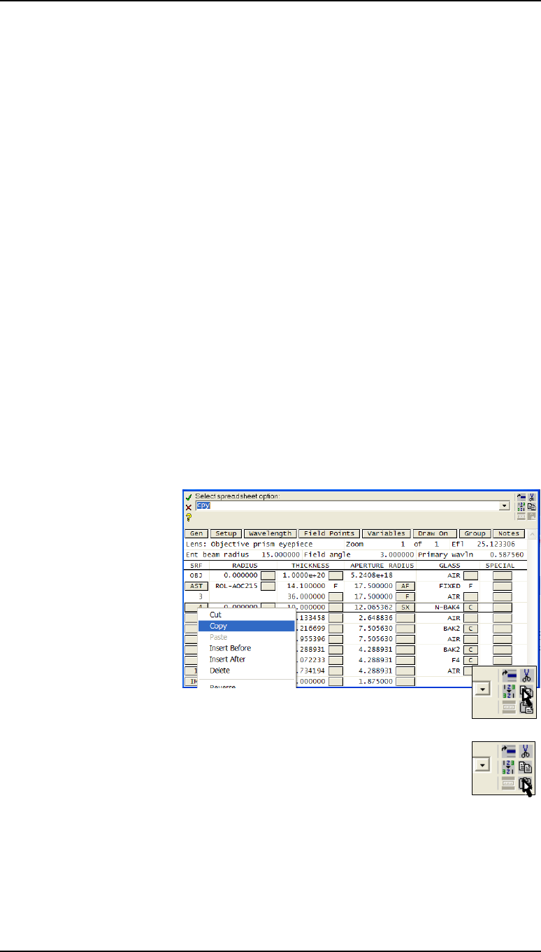
Chapter 4 - Lens data entry 41
Adding a right angle prism
Adding a right angle prism
The task is to model a simple 90° prism. The measurement of the external dimensions of the
binoculars, allowing 3 mm for the case, suggests that the apex of the first prism (20 mm
deep) will be 70 mm behind the front surface of the objective (thickness 12.4 mm), leaving
an air space of 70 - 12.4 - 20 = 37.6 mm between the rear of the objective and the prism.
• Open the surface data spreadsheet.
• Change the lens title to Objective prism eyepiece
• Change the thickness for surface 3 to 37.6. The solve flag (S) disappears.
• Now add an extra surface before surface 4: Left click on the gray surface button for
surface 4, and then either right click on the same button and select Insert before, or
use the shortcut Shift-space.
Users of OSLO EDU will not be able to add the extra surface to the straight-through
binocular, since it will cause the surface count limit (10) to be exceeded. However,
starting with the file consisting of the objective alone (bino_obj) the exercise of adding
the first prism can proceed as described here.
• Change the thickness for the new surface 4 to 10 mm.
• Under the gray button in the column labeled Aperture Radius for this surface (surface
4), select Special Aperture Data (X). Leave the Ap Id: as 0. Change the shape to
Rectangle, keep the Action as Transmit, leave the Group: as 0, and set the semi-
aperture dimensions to:
Xmin = -10 Xmax = 10 Ymin = -10 Ymax = 10 Angle = 0.0
• Change the medium for
surface 4 from air to
glass: Click on the gray
GLASS button, select
Catalog > Schott >
N-BAK4. (For some
versions of OSLO the
current Schott catalog
will be in the directory
be Schott 2004 rather
than Schott).
• Select the entire row of
surface 4. Then right click, selecting Copy. Otherwise right click on the
copy icon on the right of the spreadsheet, shown in the diagram.
• Click on the gray surface button for surface 5. Right click and select
Paste. Otherwise right click the paste icon. The new surface is added
before the one highlighted.
• Once more, click on the gray surface button for surface 5, right click and select Paste.
• Change the Thickness for surface 5 to -10.
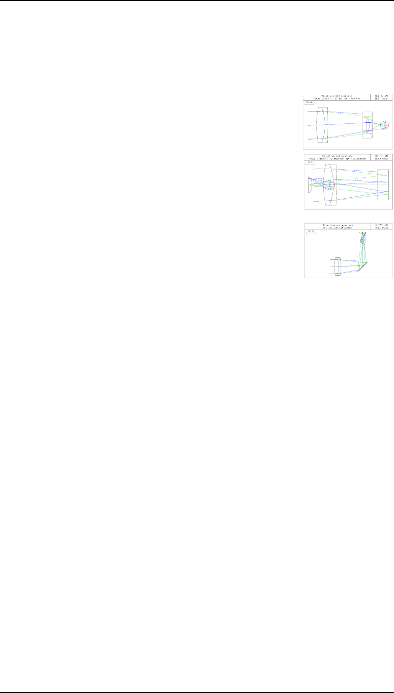
42 Lens data entry Chapter 4
Adding a right angle prism
• Under the Aperture Radius gray button for surface 5, select Special Aperture
Data and set:
Ymin = -14.14 Ymax = 14.14
leaving everything else in this dialog box unchanged.
• From the gray button under Glass for surface 5, select Reflect (hatch).
• Under Glass for surface 6, type AIR
• To change the thickness for surface 6 to an axial ray height
solve, click on the gray button next to thickness for surface 6,
and select Solve (S) > Axial ray height, and after Enter
solve value type 0.
• Under Special for surface 5, select Coordinates (C). Set
TLA = -45, and Tilt and Bend: Yes. Leave everything
else as default.
In most cases, tilting a surface rotates the coordinate system of the
airspace after that surface, and all subsequent surfaces, through the
same angle. However if Tilt and Bend is specified, the rotation is
through twice this angle, corresponding to the law of reflection.
• In the text window, click on Ape to list the special aperture
data for the three surfaces of the prism.
*APERTURES
SRF TYPE APERTURE RADIUS
...
4 CMP 12.022663
Special Aperture Group 0:
0 ATP Rectangle AAC Transmit AAN --
AX1 -10.000000 AX2 10.000000 AY1 -10.000000 AY2 10.000000
5 CMP 11.590322
Special Aperture Group 0:
0 ATP Rectangle AAC Transmit AAN --
AX1 -10.000000 AX2 10.000000 AY1 -14.140000 AY2 14.140000
6 CMP 11.157981
Special Aperture Group 0:
0 ATP Rectangle AAC Transmit AAN --
AX1 -10.000000 AX2 10.000000 AY1 -10.000000 AY2 10.000000
• Click on Len to list the lens data. Note that the three solved aperture radius values seen
on the top-level spreadsheet for surfaces 4, 5 and 6 remain unchanged by the definition
of special apertures (X); these values are ignored.
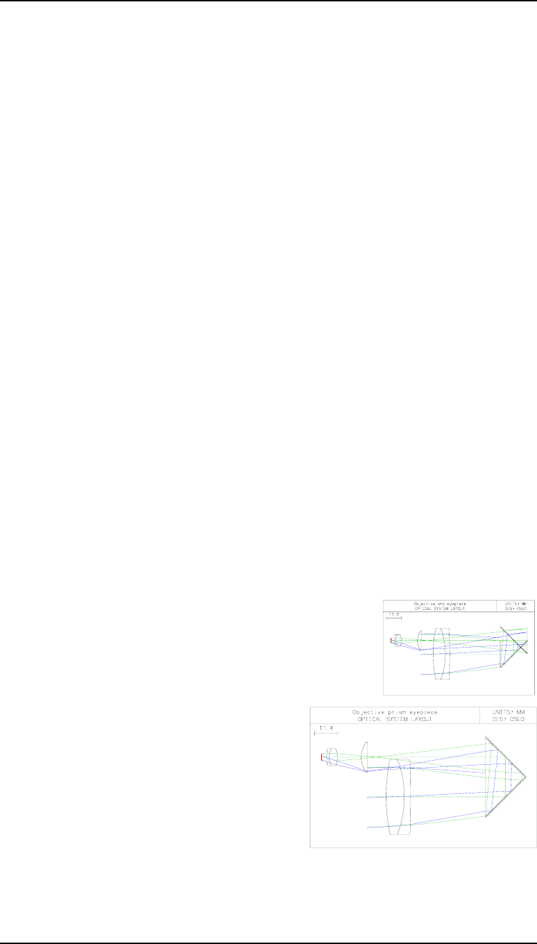
Chapter 4 - Lens data entry 43
Converting the prism to a Porro prism
*LENS DATA
Objective prism eyepiece
SRF RADIUS THICKNESS APERTURE RADIUS GLASS SPE NOTE
OBJ -- 1.0000e+20 5.2408e+18 AIR
AST 87.780000 F 9.200000 F 19.050000 AF BAFN10 F *
2 -52.752000 F 3.200000 F 19.050000 F SF10 F
3 -484.254000 F 37.600000 19.050000 F AIR
4 -- 10.000000 12.022663 SX N-BAK4 C
5 -- -10.000000 11.590322 SX REFL_HATCH *
6 -- -67.900739 S 11.157981 SX AIR
7 -- 4.133458 2.616880 AIR
8 -- 3.216699 7.505630 BAK2 C
9 -12.598736 11.955396 7.505630 AIR
10 10.668717 4.288931 4.288931 BAK2 C
11 -7.988135 1.072233 4.288931 F4 C
12 -82.025813 2.734194 4.288931 AIR
IMS -- -- 1.875000 * Exit Pupil
• Click on Spe to list the surface notes, the coordinate (tilt) data and the surface tag
(pen color etc.) data:
*SURFACE NOTES
13 Exit pupil
*TILT/DECENTER DATA
5 DT 1 DCX -- DCY -- DCZ --
BEN TLA -45.000000 TLB -- TLC --
*SURFACE TAG DATA
1 LMO ELE (3 surfaces)
13 DRW ON
LDP 4
The eyepiece is incorrectly modeled since the signs of all curvatures and thicknesses should
be inverted. For the time being, however, we will ignore this and proceed to the next stage.
Converting the prism to a Porro prism
The Porro prism has two reflecting surfaces at right angles to each other.
• Select the entire row of surface 5. Then right click,
selecting Copy.
• Click on the gray surface button for surface 5. Right click
and select Paste.
• Using the surface data spreadsheet, change the
thickness for surface 5 to -20 mm, and the
thickness for surface 6 to 10 mm.
• Save with the name bino_porro.len.
• In the text window click on Len and Spe.
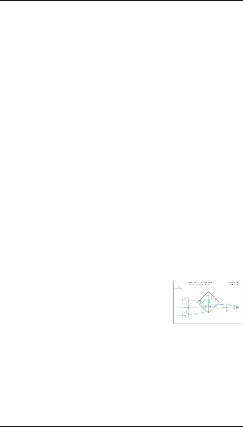
44 Lens data entry Chapter 4
Adding a second Porro prism
*LENS DATA
Objective prism eyepiece
SRF RADIUS THICKNESS APERTURE RADIUS GLASS SPE NOTE
OBJ -- 1.0000e+20 5.2408e+18 AIR
AST 87.780000 F 9.200000 F 19.050000 AF BAFN10 F *
2 -52.752000 F 3.200000 F 19.050000 F SF10 F
3 -484.254000 F 37.600000 19.050000 F AIR
4 -- 10.000000 12.022663 SX N-BAK4 C
5 -- -20.000000 11.590322 SX REFL_HATCH *
6 -- 10.000000 10.725639 SX REFL_HATCH *
7 -- 55.152366 S 10.293298 SX AIR
8 -- 4.133458 2.616880 AIR
9 -- 3.216699 7.505630 BAK2 C
10 -12.598736 11.955396 7.505630 AIR
11 10.668717 4.288931 4.288931 BAK2 C
12 -7.988135 1.072233 4.288931 F4 C
13 -82.025813 2.734194 4.288931 AIR
IMS -- -- 1.875000 * Exit Pupil
*SURFACE NOTES
14 Exit Pupil
*TILT/DECENTER DATA
5 DT 1 DCX -- DCY -- DCZ --
BEN TLA -45.000000 TLB -- TLC --
6 DT 1 DCX -- DCY -- DCZ --
BEN TLA -45.000000 TLB -- TLC --
*SURFACE TAG DATA
1 LMO ELE (3 surfaces)
14 DRW ON
LDP 4
Adding a second Porro prism
We will now add the second Porro prism. Note that users of OSLO EDU will have reached
the 10-surface limit even without the eyepiece, and will have to delete the objective
(surfaces 1 to 3) to complete this section, modifying the surface numbering accordingly.
• In the surface data spreadsheet, select surfaces 4-7.
• Right click, selecting Copy.
• Click on surface 8 to highlight the whole surface, right-
click, and select Paste.
• Under Thickness for surface 7, enter 0. This
automatically deletes the thickness solve on that surface.
• The aperture of surface 12 is not sufficiently large. Convert
it to a solved aperture by just setting the Aperture Radius for surface 8 to 0. The
solved value (6.552484) replaces it immediately.
• Surface 18 is not at the true exit pupil. Click on the gray button under Thickness for
surface 17, and select Solves (S) > Chief ray height... and enter 0.
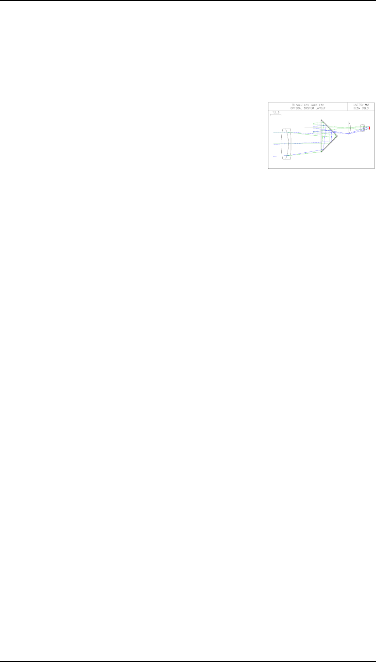
Chapter 4 - Lens data entry 45
Completing the design
Completing the design
The model does not include the 90º rotation about the optical axis of the second prism
relative to the first.
• To rotate the second prism Z axis through an angle of 90°, under Special for
surface 8, select Coordinates (C), and set the tilt angle about the z-axis, TLC =
90 (degrees).
• Change the lens title to: Binoculars complete.
• Save with the file name bino_complete.len
• Enter the commands: drl;drr 0;drr 1 to draw in
2 dimensions.
The full prescription is obtained by clicking on Len Spe and Ape in the text window.
*LENS DATA
Binoculars complete
SRF RADIUS THICKNESS APERTURE RADIUS GLASS SPE NOTE
OBJ -- 1.0000e+20 5.2408e+18 AIR
AST 87.780000 F 9.200000 F 19.050000 AF BAFN10 F *
2 -52.752000 F 3.200000 F 19.050000 F SF10 F
3 -484.254000 F 37.600000 19.050000 F AIR
4 -- 10.000000 12.022663 SX N-BAK4 C
5 -- -20.000000 11.590322 SX REFL_HATCH *
6 -- 10.000000 10.725639 SX REFL_HATCH *
7 -- -- 10.293298 SX AIR
8 -- 10.000000 10.293298 SX N-BAK4 C
9 -- -20.000000 9.860957 SX REFL_HATCH *
10 -- 10.000000 8.996274 SX REFL_HATCH *
11 -- 29.655619 S 8.563933 SX AIR
12 -- 4.133458 6.552484 S AIR
13 -- 3.216699 7.505630 BAK2 C
14 -12.598736 11.955396 7.505630 AIR
15 10.668717 4.288931 4.288931 BAK2 C
16 -7.988135 1.072233 4.288931 F4 C
17 -82.025813 5.649290 S 4.288931 AIR
IMS -- -- 1.875000 * Exit Pupil
*SURFACE NOTES
18 Exit Pupil
*TILT/DECENTER DATA
5 DT 1 DCX -- DCY -- DCZ --
BEN TLA -45.000000 TLB -- TLC --
6 DT 1 DCX -- DCY -- DCZ --
BEN TLA -45.000000 TLB -- TLC --
8 DT 1 DCX -- DCY -- DCZ --
TLA -- TLB -- TLC 90.000000
9 DT 1 DCX -- DCY -- DCZ --
BEN TLA -45.000000 TLB -- TLC --
10 DT 1 DCX -- DCY -- DCZ --
BEN TLA -45.000000 TLB -- TLC --

46 Lens data entry Chapter 4
Completing the design
*SURFACE TAG DATA
1 LMO ELE (3 surfaces)
18 DRW ON
LDP 4
*APERTURES
SRF TYPE APERTURE RADIUS
0 SPC 5.2408e+18
1 FIX 19.050000
2 FIX 19.050000
3 FIX 19.050000
4 CMP 12.022663
Special Aperture Group 0:
0 ATP Rectangle AAC Transmit AAN --
AX1 -10.000000 AX2 10.000000 AY1 -10.000000 AY2 10.000000
5 CMP 11.590322
Special Aperture Group 0:
0 ATP Rectangle AAC Transmit AAN --
AX1 -10.000000 AX2 10.000000 AY1 -14.142136 AY2 14.142136
6 CMP 10.725639
Special Aperture Group 0:
0 ATP Rectangle AAC Transmit AAN --
AX1 -10.000000 AX2 10.000000 AY1 -14.142136 AY2 14.142136
7 CMP 10.293298
Special Aperture Group 0:
0 ATP Rectangle AAC Transmit AAN --
AX1 -10.000000 AX2 10.000000 AY1 -10.000000 AY2 10.000000
8 CMP 10.293298
Special Aperture Group 0:
0 ATP Rectangle AAC Transmit AAN --
AX1 -10.000000 AX2 10.000000 AY1 -10.000000 AY2 10.000000
9 CMP 9.860957
Special Aperture Group 0:
0 ATP Rectangle AAC Transmit AAN --
AX1 -10.000000 AX2 10.000000 AY1 -14.142136 AY2 14.142136
10 CMP 8.996274
Special Aperture Group 0:
0 ATP Rectangle AAC Transmit AAN --
AX1 -10.000000 AX2 10.000000 AY1 -14.142136 AY2 14.142136
11 CMP 8.563933
Special Aperture Group 0:
0 ATP Rectangle AAC Transmit AAN --
AX1 -10.000000 AX2 10.000000 AY1 -10.000000 AY2 10.000000
12 CMP 6.552484
13 SPC 7.505630
14 SPC 7.505630
15 SPC 4.288931
16 SPC 4.288931
17 SPC 4.288931
18 SPC 1.875000

47
Chapter 5 - Graphical analysis
Introduction
In general, the graphics facilities in OSLO are of the most frequently generated using the
icons in the toolbars of the individual graphic windows. Some facilities, however, can only
be accessed from the menu headers, and some only by calling up CCL commands from the
command line.
A comprehensive catalog of the graphics facilities will be found in the Graphics Reference
in the appendix at the end, together with instructions as to how each may be accessed. In
this chapter only lens drawing and ray intercept coordinate reports will be discussed in
detail.
Opening a new graphics window
This exercise shows how a new graphics window can be opened in the top left corner of the
main window, just under the command window.
• From the main window select the Window menu header.
• Choose Graphics > Open and type the following responses into the command
window:
Enter graphics window
number: 0
Enter window width: 320
End to window height: 300
Enter window x: 0
Enter window y: 120
Note that the new window has a dark blue title bar, containing the letters GW 2 *.
GW means that it is a graphics window with no updateable content. The * symbol
means that it is the current window for graphical output. The coordinate system
defines x =0, y = 0 as the top left corner, and the command window covers the area
x = 0 to 600, y = 0 to 100. The point x = 960 (1420 for wide screens), y = 710 is the
bottom right position which can be seen without scrolling.
Labeling a graphics window
• From the main window select the Window menu header.
• Choose Graphics > Title... and type the following response into the command
window:
• Enter window title: Colors.
The title appears in the blue bar at the top of the window. In practice graphics windows are
titled automatically by the graphics command associated with the relevant icon in the
graphics window.
48 Graphical analysis Chapter 5
Introduction
Generating a plot
• Select the Tools menu header.
• Choose Plotting toolkit > Colors
and Pens.
This executes the CCL command
colors, which is stored in the file
graph_tools.ccl in the public/ccl
directory. It shows the pen numbering
used in graphics plots.
Notice that the letters in the title bar
have now changed to UW, meaning
that the graphics window is updateable.
Saving a plot
• Right click on the window and choose Save As ...
• Save the file in any format. The size of the file stored will differ according to the
format chosen. For comparison, the file sizes for the Colors and Pens graphic are
shown:
Windows bitmap BMP 164 kB
Compressed bitmap RLE 29 kB
HP-GL format HGL 29 kB
Windows metafile WMF 118 kB
Placeable Windows metafile WMF 118 kB
Enhanced Windows metafile EMF 182 kB
Cutting and pasting a plot
• Right click on the window and choose Copy to
Clipboard.
• Open a Word document or PowerPoint
presentation, right click, and choose Paste.
• If there are problems with the size of the image
pasted into the new application, look again at the
Graphics Preferences in Chapter 2.
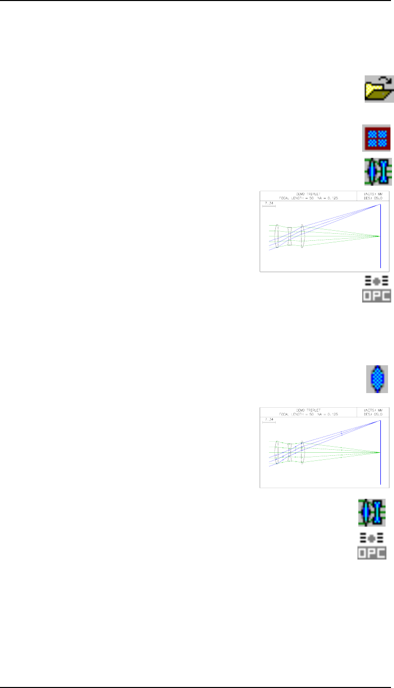
Chapter 5 - Graphical analysis 49
Lens drawing
Lens drawing
Drawing a lens in 2D
This exercise will demonstrate some of the 2D drawing options, using the standard triplet
lens as an example.
• Click on the Open Lens icon in the main window toolbar.
• Open the file in the Private directory, trip.len
• In the graphics window, click on the Setup Window/Toolbar icon.
• Select the Lens Drawing toolbar.
• Click on the Draw system (2D) icon.
This gives a lens drawing including rays as the default.
The corresponding icon in the Standard Tools toolbar gives
the option of a 2D (plan) drawing without rays.
Various options to enhance this drawing will now be
shown.
• Click, in the main window toolbar on the icon
shown here for Edit Lens Drawing Conditions.
• On the fifth line, against Image space rays: select Draw rays to
image surface. The button then reads Image srf
• From the menu header Select File > Preferences > Preference groups >
Graphics... and choose from the menu Use labels on graphics. Select Off.
• Open the surface data spreadsheet.
• Click on the gray button under Special for surface 7 (IMS).
• Select Surface Control (F) > General
• On the second line, against Surface appearance
in lens drawings: select Drawn. Set the Pen
number for surface in lens drawings as 3
(blue).
• Close both spreadsheets.
• Once again click on the Draw system (2D) icon to draw the lens.
• Click again on the icon in the main window toolbar for Edit Lens
Drawing Conditions.
In the ray drawing table at the foot of the spreadsheet, change the three values of the
Frac. Y Obj (FBY) to 0.0, -1.0, +1.0 respectively. Also change the number
of rays in the second fan (Rays) from 0 to 3, Min pupil to -0.4, and Max
pupil to 0.4.
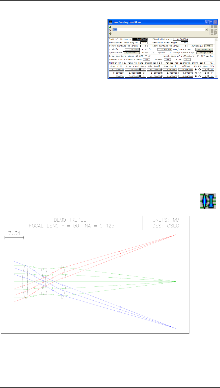
50 Graphical analysis Chapter 5
Lens drawing
In this spreadsheet, for each successive ray fan (where the number of rays plotted is
non-zero) the pen colors cycle through the sequence:
1. Green
2. Blue
3. Red
4. Light-Blue
5. Orange
6. Violet
7. Yellow
8. Black
• Close the Edit Lens Drawing Conditions spreadsheet.
• From the Lens menu header, select Show Operating Conditions .. > Lens
Drawing
*CONDITIONS: LENS DRAWING
Initial distance: -- Final distance: --
Horizontal view angle: 240 Vertical view angle: 30
First surface to draw: 0 Last surface to draw: 0
X shift of drawing: -- Y shift of drawing: --
Drawn apertures (solid): Quadrant Image space rays: Image srf
Rings in aperture (solid): 3 Spokes in aperture (solid): 4
Number of field points (rays): 3 DXF/IGES file view: Unconverted
Draw aperture stop location: Off Hatch back side of reflectors: On
Red value for shaded solid: 175 Green value for shaded solid: 185
Blue value for shaded solid: 250 Points for aspheric profile: 41
Autodraw Options: YZ Profile
Fpt Frac Y Obj Frac X Obj Rays Min Pupil Max Pupil Offset Fan Wvn Cfg
1 -- -- 5 -1.00000 1.00000 -- Y 1 0
2 -1.00000 -- 3 -0.40000 0.40000 -- Y 1 0
3 1.00000 -- 3 -0.40000 0.40000 -- Y 1 0
• Draw the lens in two dimensions by clicking on the icon for Draw
system (2D).
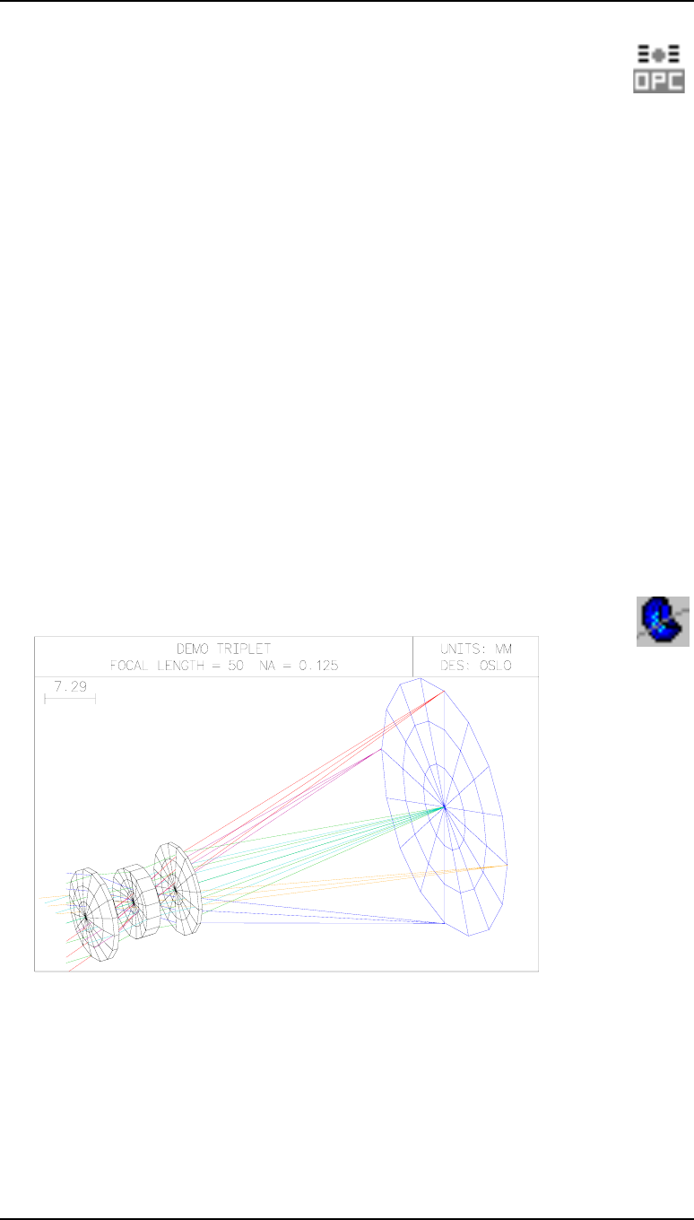
Chapter 5 - Graphical analysis 51
Lens drawing
Drawing a lens in 3D
• Open the Edit Lens Drawing Conditions spreadsheet again.
• On the fifth line, for Apertures: change Quadrant to Full apertures.
For Number of ray fans in lens drawings enter 6, then scroll down
to enter the three new fans with Frac X Obj = 0.0, -1.0, 1.0 respectively.
For the three fans, specify 5, 3 and 3 rays and for the last two fans, change
Min pupil to -0.4, and Max pupil to 0.4.
• Select the radio button for FX for the last three fans.
• Close the Edit Lens Drawing Conditions spreadsheet.
• To list these values, from the Lens menu header, select Show Operating
Conditions > Lens Drawing.
*CONDITIONS: LENS DRAWING
Initial distance: -- Final distance: --
Horizontal view angle: 240 Vertical view angle: 30
First surface to draw: 0 Last surface to draw: 0
X shift of drawing: -- Y shift of drawing: --
Drawn apertures (solid): Full Image space rays: Image srf
Rings in aperture (solid): 3 Spokes in aperture (solid): 4
Number of field points (rays): 6 DXF/IGES file view: Unconverted
Draw aperture stop location: Off Hatch back side of reflectors: On
Red value for shaded solid: 175 Green value for shaded solid: 185
Blue value for shaded solid: 250 Points for aspheric profile: 41
Autodraw Options: YZ Profile
Fpt Frac Y Obj Frac X Obj Rays Min Pupil Max Pupil Offset Fan Wvn Cfg
1 -- -- 5 -1.00000 1.00000 -- Y 1 0
2 -1.00000 -- 3 -0.40000 0.40000 -- Y 1 0
3 1.00000 -- 3 -0.40000 0.40000 -- Y 1 0
4 -- -- 5 -1.00000 1.00000 -- X 1 0
5 -- -1.00000 3 -0.40000 0.40000 -- X 1 0
6 -- 1.00000 3 -0.40000 0.40000 -- X 1 0
• Click on the icon for Draw system (3D solid model).
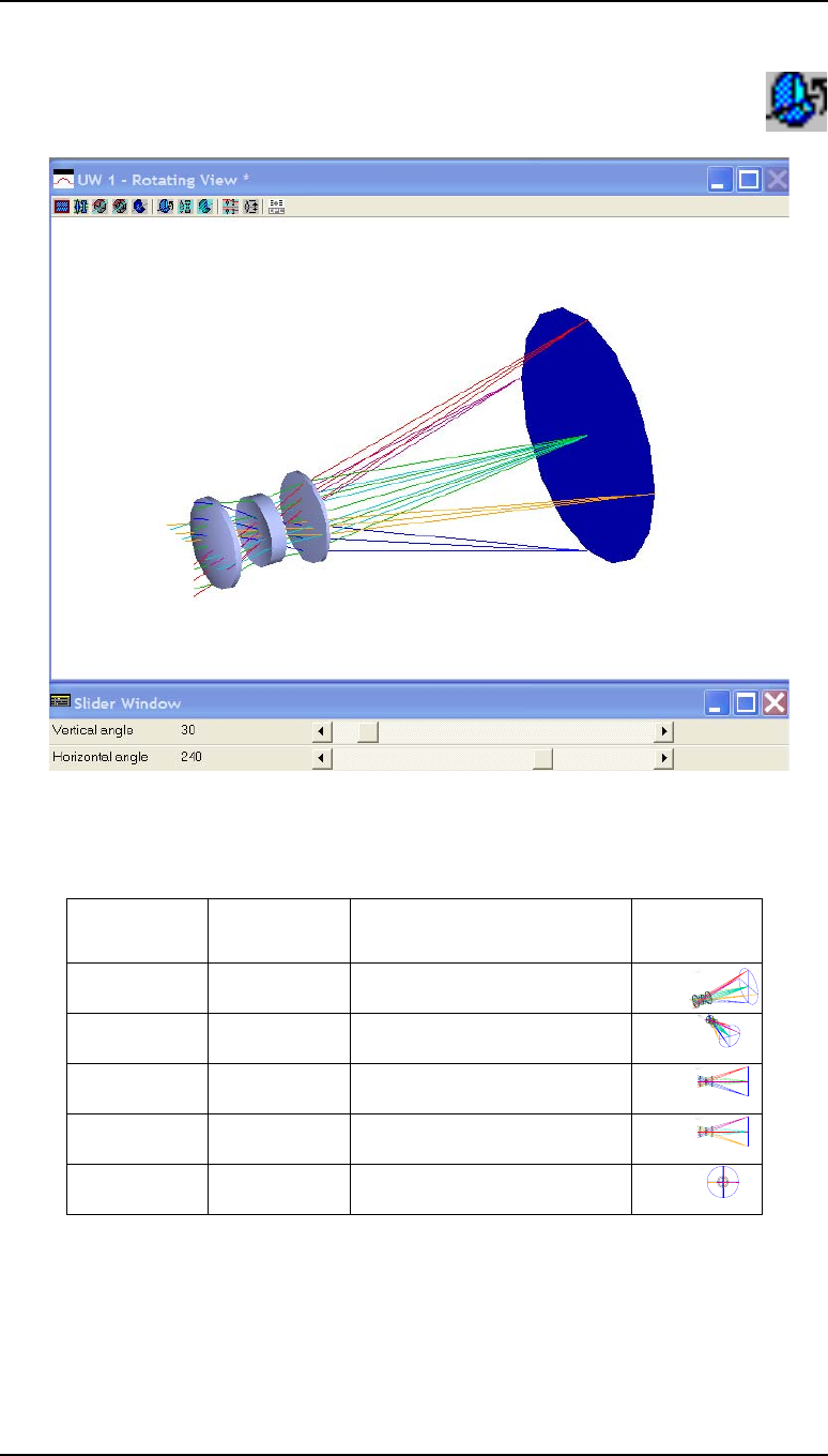
52 Graphical analysis Chapter 5
Lens drawing
Drawing a lens in 3D with sliders
• Click on the icon for Draw system (3D w/slider)
• Select Shaded solid.
• It may be necessary to extend the slider bars to make the slider tracks visible.
• Adjust the sliders according to the following table:
Vertical
view angle Horizontal
view angle Description Example
30º 240º Default
30º 330º Isometric
0º 270º Y - Z (2D plan view)
90º 270º X - Z
0º 360º X - Y view from image
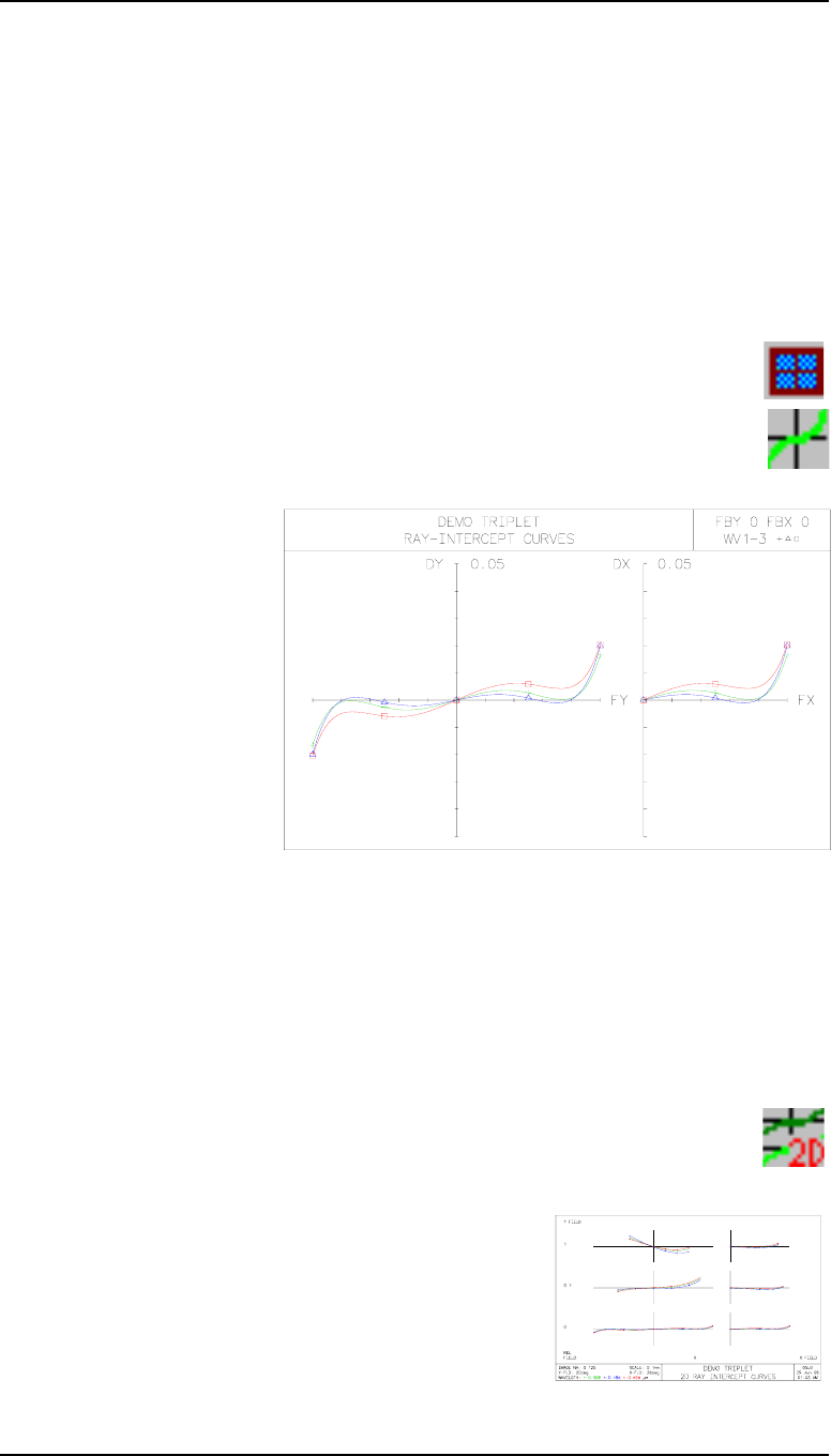
Chapter 5 - Graphical analysis 53
Ray intercept curves analysis
If the lens is saved with a particular 3D view in force, the values of the view angles will be
stored with the lens and used in subsequent 3D drawings. The horizontal and vertical view
angles may also be set in the Edit Lens Drawing Conditions spreadsheet.
Ray intercept curves analysis
The importance of these curves for diagnosis of aberration problems cannot be overstated,
so a detailed description will be given here of this analysis. The lens used for the graphs in
this section is the objective of the binoculars modeled in chapter 3.
Ray analysis (RIC)
• In the graphics window, click on the Setup Window/Toolbar icon.
• Select the Ray Analysis toolbar.
• Click on the icon for RIC Plot. This gives a set of curves representing the
transverse ray aberrations for the default field point, which is on axis (FBY
= 0.0). The left hand graph gives the plot of transverse ray aberrations (DY) in the
meridional section
(the Y - Z section) at
different heights
(FY) in the pupil.
The right hand graph
gives the same
information in the
orthogonal plane -
that is, DX as a
function of FX. The
three curves are
colored according to
the wavelengths,
which, in the visible
at least, are representative provided the order in which the wavelengths are defined
is middle-short-long corresponding to green-blue-red.
If the system is defined as afocal (see under the Gen button in the surface data
spreadsheet) the aberrations are angular values DYA and DXA, expressed as
direction tangents.
Ray intercept curves for 2D field points
Users of OSLO EDU and OSLO Light should skip this section
• Click on the icon for RIC vs Field Points.
This gives the graphs laid out in two dimensions according to the relative field
coordinates FBX, FBY. In this case, three graphs
are given for the three field points defined for this
lens, which are (reading from the bottom) FBY =
0.0 (on axis), FBY = 0.7 and FBY = 1.0 (edge of
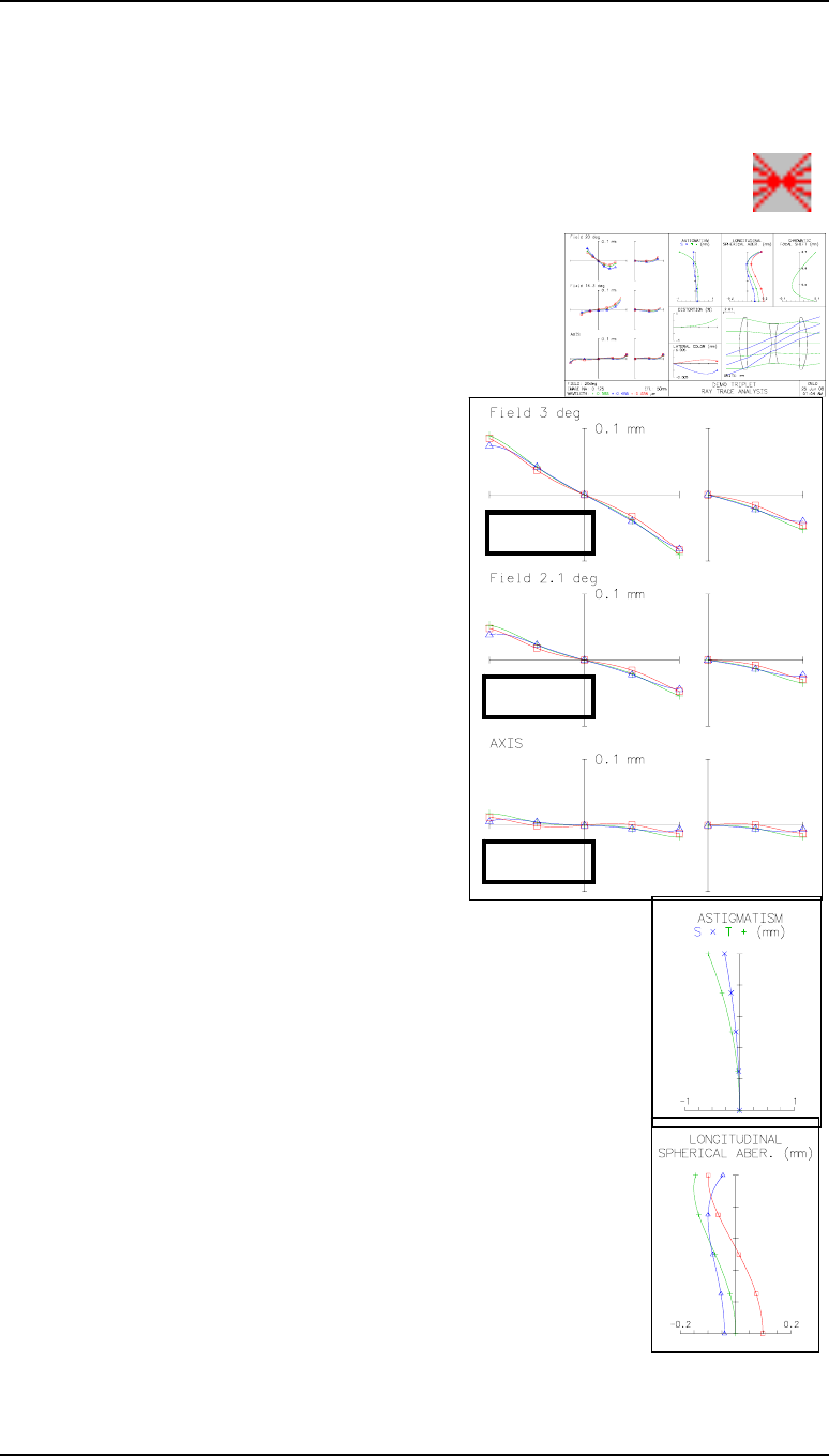
54 Graphical analysis Chapter 5
Ray intercept curves analysis
field). The left-hand column gives DY as a function of FY, the right-hand column
plots DX against FX.
Ray intercept curves report graphic
• Click on the icon for RIC Report Graphic. This icon also appears on
the Standard Tools toolbar. The analysis results are shown as 6 graphs
within the same window, plus a 2D lens drawing.
1. The left-hand group (unlabeled) gives the same ray
intercept curves for three field points as the ray
intercept curves for 2D field points.
This set of curves gives the relationship
between the ray aberrations and their
radial position in the pupil. If more than
three wavelengths are specified, up to 12
sets of curves will be drawn, with
different symbols as well as different
colors to distinguish them.
Most of the other information in the
report (apart from distortion) can be
deduced from these curves.
A designer can use these curves as a
diagnostic tool to analyze the different
types of aberration. This analysis is
important, since different aberrations
require different measures for their
correction. However these graphs do have
limitations. For example, they do not
indicate the aberrations of rays in the four
quadrants between the two orthogonal
planes.
2. The astigmatism curves give the variation of paraxial focus
across the field for the meridional section (the Y-Z section,
labeled T) and the sagittal section (the X-Z section, labeled S).
Results are only shown for the mean wavelength. This curve
can be plotted as a stand-alone, either monochromatically or in
3 colors, using the menu header:
• Evaluate > Ray fans > Single field point ...
• At the top, select Field sags.
• Choose either Monochromatic or Polychromatic.
• Click on OK.
3. The three curves for longitudinal spherical aberration give the
movement of the focal point along the axis for different radii
in the pupil, for the axial image point only, corresponding to
the three wavelengths.
FY
FY
FY FX
FX
FX
DY
DY
DY DX
DX
DX
FBY=1
FBY=.7
FBY=0
DZ
FBY
DZ
FY
Chapter 5 - Graphical analysis 55
Ray intercept curves analysis
The curves for chromatic focal shift represent the axial beam
paraxial longitudinal focal variation with wavelength over the
range 0.4 to 0.7 μm - or over a different range if other
wavelengths are specified. Alternatively, for OSLO Standard
and OSLO Premium users, this curve can be plotted as a stand-
alone, in slightly different format, using the menu header:
• Evaluate > Ray fans > Other ray analysis ...
• From the menu select Chromatic focal shift...
• Enter a wavelength range (or zeros for default).
• Click on OK.
4. Longitudinal spherical aberration curves indicate the errors in
focus DZ of the axial beam as a function of the pupil height
DY. Curves are given for the three specified wavelengths. The
graph is plotted on its own via the menu header:
• Evaluate > Ray fans > Single field point ...
• At the top, choose Longitudinal spherical...
• Click on OK.
5. The curve for distortion shows the departure from
the paraxial magnification as a function of field
height. The distortion graph can be plotted alone in
a different format using the menu header:
• Evaluate > Ray fans > Single field point
...
• At the top, choose Distortion
• Choose either Monochromatic or
Polychromatic.
• Insert a value for the aberration scale (in %).
• Click on OK.
The plots obtained from OSLO EDU and OSLO
Light are different from the one shown here.
6. The curve for lateral color shows the difference
between the heights of the red and green rays, and
between the blue and green rays, as a function of
field height. The graph is not available as a stand-
alone.
To control all the aberration scales, the RIC report graphic
command may be called from the main menu header.
• From the Evaluate menu header select Other
ray analysis>Report Graphic..:
• Fill in the spreadsheet with the required values.
The value of the abscissa scale is omitted as it only
applies to graphs where curves are plotted against
h-tan U rather than DY.
• Click on OK.
DZ
Wv
FBY
FBY
DZ
FY
56
Chapter 6 - Numerical analysis
Introduction
This chapter deals with the text window and the spreadsheet buffer which lies under it. In
order to illustrate the methods of numerical analysis, a simple task concerning the
demonstration triplet lens supplied with the program will be carried out:
For the triplet lens supplied with the program, calculate the transverse ray aberration
of the outermost ray transmitted at the edge of the third component at the edge of the
field, at the central (green) wavelength.
Also estimate the transmittance at the extreme field, as a percentage of the axial
transmittance.
The transverse ray aberration of an off-axis ray in the meridional section is the distance
from the point where this ray intersects the image plane, to the intersection point of the pupil
ray. This is shown in the diagram.
Before we can begin the task we need to locate the edge ray concerned in terms of its
relative pupil height coordinate FY.
Finding the edge rays
• Open the lens in the private directory trip.len. Alternatively it will be found in the
public directory as /public/demo/LT/demotrip.len.
• In the text window, click on Ape to list the apertures. The indication CHK for surfaces
1 and 6 means that in the ray analysis which follows the rays which lie outside these
checked apertures will be obstructed. (Checked clear apertures are indicated by a K in
the Clear Aperture Radii column of the surface data spreadsheet).
DY
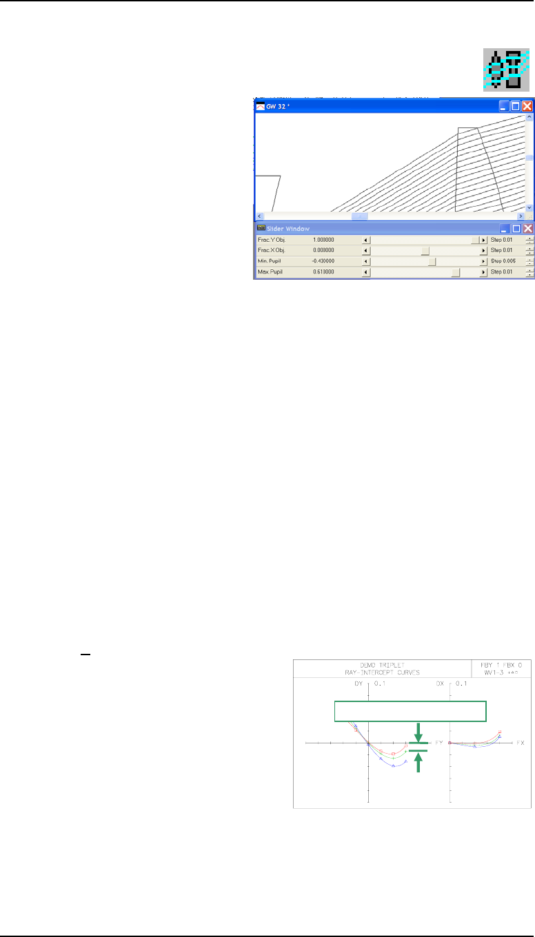
Chapter 6 - Numerical analysis 57
Graphical estimates
*APERTURES
SRF TYPE APERTURE RADIUS
0 SPC 3.6397e+19
1 SPC 6.500000 CHK
2 PKP 6.500000
3 SPC 5.000000
4 SPC 5.000000
5 SPC 6.500000
6 SPC 6.500000 CHK
7 CMP 18.170326
• In the graphics window, click on the
Setup Window/Toolbar icon, and
select the Lens Drawing menu.
• Click on the icon for View Ray
Fans (2D) - Interactive.
• To define the point in the field as the
edge of the field, set the slider-wheel
for Frac Y Obj to 1.0, and leave the
slider-wheel for Frac X Obj at 0.0.
• Adjust the slider-wheels for Min pupil and Max pupil until the extreme rays of the
bundle just pass through the first and last surfaces respectively.
• Note the values of the fractional pupil height for these edge rays: -0.43 and+0.61. The
latter is the value of FY needed for this problem.
Instead of this procedure, users of OSLO Standard and OSLO Premium may use a
quicker method for carrying out vignetting analysis:
• From the Optimize menu header, select: Support routines>Vignetting >
Vignetting analysis.
• Check Copy vignetting data to field point set? No
• Leave the Maximum pupil position to test at 5.0
• Click on OK.
*VIGNETTING FACTORS
FPT CFG FBY FBX FY1 FY2 FXMAX
1 0 -- -- -1.040001 1.040001 1.040001
2 0 0.700000 -- -0.637293 0.810585 0.990811
3 0 1.000000 -- -0.431105 0.612924 0.901827
Graphical estimates
• From the Evaluate menu header select: Ray fans > Single field point ...
and, leaving all the default values
unchanged, click on Set object point
at the foot of the spreadsheet.
• In the Set object point spreadsheet, set
Fractional coordinates of object point
to FBY = 1.00 FBX = 0.00 FBZ =
0.00.
• Close both spreadsheets, and note from the
graph that the value of the transverse ray
aberration required is about -0.015 mm. (To confirm the units, from the Lens menu
header, select: Show operating conditions > General)
DY at WV 1 for ra
y
at FY =
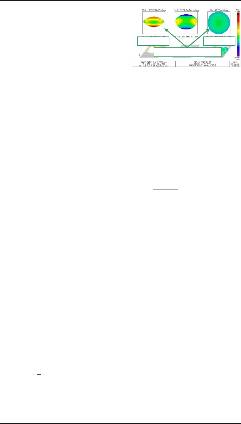
58 Numerical analysis Chapter 6
Numerical calculation
• Click on the Plot report graphics
wavefront analysis icon on the standard
toolbar to get the pupil maps, and note that
the area of the edge-of-field map is about
50% of the area of the on-axis map.
So we can conclude that the transverse ray
aberration of the edge ray is about DY = -0.015
mm; the transmission at this field point is about
50%.
Numerical calculation
From the text window
• In the text window, trace the pupil ray (the ray through the centre of the aperture stop)
from the edge of the object, by clicking on Chf.
• Then to trace a fan of rays in the meridional (Y) section, click on Fan. Set the
Minimum coordinate to be -0.43, the Maximum coordinate to be 0.61,and
Number of rays to be 2, and leave all other options as default values.
• Note the value of DY (transverse ray aberration in lens units) for the edge ray
transmitted:
*TRACE FAN - FBY 1.00, FBX 0.00, FBZ 0.00
RAY FY FRAC RFS DYA DXA DY DX
1 0.610000 0.530358 -0.071477 -- -0.013268 --
2 -0.430000 -0.353777 0.052849 -- 0.055365 --
• Click on Spd in the text window.
• Note the value of the per cent weighted ray transmission:
*SPOT DIAGRAM - FBY 1.00, FBX 0.00, FBZ 0.00 - POLYCHROMATIC
APDIV 17.030000
WAV WEIGHTS:
WW1 WW2 WW3
1.000000 1.000000 1.000000
NUMBER OF RAYS TRACED:
WV1 WV2 WV3
104 104 104
PER CENT WEIGHTED RAY TRANSMISSION: 44.827586
*SPOT SIZES
GEO RMS Y GEO RMS X GEO RMS R DIFFR LIMIT CENTY CENTX
0.021401 0.007555 0.022696 0.003426 -0.002879 --
*WAVEFRONT RS
WAVELENGTH 1
PKVAL OPD RMS OPD STREHL RATIO RSY RSX RSZ
2.224692 0.485250 0.091087 -0.004210 -- --
The conclusion then is that the transverse ray aberration of the edge ray is:
DY = -0.013268 mm,
and the transmission at this field point is:
44.8%
of the on-axis value, excluding the transmittances of optical materials and coatings.
From the menu headers
• From the Evaluate menu header select: Ray fans > Single field point ...
and choose the Command: Print Y ray-fan.
RELATIVE PUPIL AREAS
EDGE OF FIELD ON AXIS

Chapter 6 - Numerical analysis 59
Numerical calculation
• Set Minimum fractional y-component of pupil coordinate (FY) = -.43,
and Maximum fractional y-component of pupil coordinate (FY) = +.61.
Set the Number of rays in fan to the minimum value of 3.
• Leaving all the other default values unchanged, do not close the dialog box, but click on
Set object point at the foot of the spreadsheet.
• In the Set object point spreadsheet, leave the specification as Direct entry Set
Fractional coordinates of object point to FBY = 1.00 FBX = 0.00 FBZ =
0.00.
• Close the Set object point spreadsheet with the green tick, and click on OK in the Trace
fans of rays through lens dialog box:
*TRACE FAN - FBY 1.00, FBX 0.00, FBZ 0.00
RAY FY FRAC RFS DYA DXA DY DX DZ
1 0.610000 0.530358 -0.071477 -- -0.013268 -- --
2 0.090000 0.075914 -0.010854 -- -0.009257 -- --
3 -0.430000 -0.353777 0.052849 -- 0.055365 -- --
• From the Evaluate menu header select: Spot diagram > Single spot diagram...
• Select Spot diagram Data and click on OK (the earlier Set Object Point command is
still valid).
*SPOT DIAGRAM - FBY 1.00, FBX 0.00, FBZ 0.00 - POLYCHROMATIC
APDIV 17.030000
WAV WEIGHTS:
WW1 WW2 WW3
1.000000 1.000000 1.000000
NUMBER OF RAYS TRACED:
WV1 WV2 WV3
104.000000 104.000000 104.000000
PER CENT WEIGHTED RAY TRANSMISSION: 44.827586
SPOT DIAGRAM SYMMETRY: 1.000000
From the command line (abbreviated)
• In the command line, type the following:
sop 1 0 0;trf y 2 -.43 .61;spd 200
and click on the green tick, or press Enter on the keyboard.
60 Numerical analysis Chapter 6
The spreadsheet buffer
*SET OBJECT POINT
FBY FBX FBZ
1.000000 -- --
FYRF FXRF FY FX
-- -- -- --
YC XC YFS XFS OPL REF SPH RAD
18.264293 -- -0.911383 -0.096417 65.421390 61.550663
*TRACE FAN - FBY 1.00, FBX 0.00, FBZ 0.00
RAY FY FRAC RFS DYA DXA DY DX
1 0.610000 0.530358 -0.071477 -- -0.013268 --
2 -0.430000 -0.353777 0.052849 -- 0.055365 --
*SPOT DIAGRAM - FBY 1.00, FBX 0.00, FBZ 0.00 - POLYCHROMATIC
APDIV 200.000000
WAV WEIGHTS:
WW1 WW2 WW3
1.000000 1.000000 1.000000
NUMBER OF RAYS TRACED:
WV1 WV2 WV3
13820 13712 13868
PER CENT WEIGHTED RAY TRANSMISSION: 43.909889
*SPOT SIZES
GEO RMS Y GEO RMS X GEO RMS R DIFFR LIMIT CENTY CENTX
0.020881 0.006382 0.021835 0.003276 -0.003196 --
*WAVEFRONT RS
WAVELENGTH 1
PKVAL OPD RMS OPD STREHL RATIO RSY RSX RSZ
2.711822 0.447068 0.060859 -0.005045 -- --
The new value for the transmission (43.9%) is more accurate than the earlier result since a
finer grid of rays (200 rings, not 17.03, in the pupil) was defined by the spd command.
By executing in the Edit window
• From the Window menu header select: Editor > Open or click the icon.
• Use the history button to call up the last line executed:
sop 1 0 0;trf y 2 -.43 .61;spd 200
• Copy and paste it into the Text editor window.
• Highlight it with the cursor (or press Ctrl-A), and press Ctrl-E. Results are the same.
From the command line (in full)
• In the command line, one might perhaps type the following:
set_object_point(1.0,0.0,0.0,0.0,0.0,1)
trace_fan(y,2,-0.43,0.61)
spot_diagram(chr,none,200)
These forms of the commands are used to make programs self-documenting. The short
forms are more useful for command line entry.
The spreadsheet buffer
The spreadsheet buffer is an array of numerical storage cells, with 1999 rows numbered as
in Microsoft Excel, which underlies each text window. The spreadsheet buffer is used for
conveying the results of numerical OSLO calculations to variables in CCL commands, so it
is important to understand how it works.
Clearing the text window and spreadsheet buffer
There are three ways to do this:
Chapter 6 - Numerical analysis 61
The spreadsheet buffer
• EITHER right click anywhere in the text window and select Clear window and SS
buffer
• OR, from the Window menu header, select: Text > Reset.
• OR, in the command line, Enter twr (or textwin_reset)
To clear the spreadsheet buffer without affecting the printed output in the text window:
• In the command line, enter sbr (or ssbuf_reset)
Reading from the spreadsheet buffer
• In the text editor window, change the first entry so the whole line looks like this:
sbr;sop 1 0 0;trf y 2 -.43 .61;spd 200
• Highlight the line with the cursor, and press Ctrl-E.
• Watching the message area under the command line, click on the text window output to
confirm the following spreadsheet cell allocations:
*SET OBJECT POINT
FBY FBX FBZ
[ a1 ] [ b1 ] [ c1 ]
FYRF FXRF FY FX
[ a2 ] [ b2 ] [ c2 ] [ d2 ]
YC XC YFS XFS OPL REF SPH RAD
[ a3 ] [ b3 ] [ c3 ] [ d3 ] [ e3 ] [ f3 ]
*TRACE FAN - FBY 1.00, FBX 0.00, FBZ 0.00
RAY FY FRAC RFS DYA DXA DY DX
1 [ a4 ] [ b4 ] [ c4 ] [ d4 ] [ e4 ] [ f4 ]
2 [ a5 ] [ b5 ] [ c5 ] [ d5 ] [ e5 ] [ f5 ]
*SPOT DIAGRAM - FBY 1.00, FBX 0.00, FBZ 0.00 - POLYCHROMATIC
APDIV [ a6 ]
WAV WEIGHTS:
WW1 WW2 WW3
[ a7 ] [ b7 ] [ c7 ]
NUMBER OF RAYS TRACED:
WV1 WV2 WV3
13820 13712 13868
PER CENT WEIGHTED RAY TRANSMISSION: [ a8 ]
*SPOT SIZES
GEO RMS Y GEO RMS X GEO RMS R DIFFR LIMIT CENTY CENTX
[ a9 ] [ b9 ] [ c9 ] [ d9 ] [ e9 ] [ f9 ]
*WAVEFRONT RS
WAVELENGTH 1
PKVAL OPD RMS OPD STREHL RATIO RSY RSX RSZ
[ a10 ] [ b10 ] [ c10 ] [ d10 ] [ e10 ] [ f10 ]
Note that integers and headers are not included in the spreadsheet buffer.
• Click on the two numerical results indicated, and note the cell coordinates and values
given in the message area as follows:
e4 = -0.0132683238458
a8 = 43.909889270714
Note also that these results are full precision (to 14 digits).
Writing to the spreadsheet buffer
• In the text editor window, add the command for formatted printing:
aprintf("DY = % 6.6f Trans = %4.1f %%\n",e4,a8)
giving the following output:
62 Numerical analysis Chapter 6
The spreadsheet buffer
DY = -0.013268 Trans = 43.9 %
Note that the contents of cells of the spreadsheet buffer can also be accessed using the real
array ssb(row, column). For example, e4 becomes ssb(4,5) and a8 becomes
ssb(8,1).
The command aprintf places the two values in the spreadsheet buffer, still at full
precision, even though they are printed with fewer places (6 and 1 respectively) after the
decimal point. Note in particular that the cells are filled even if printing is turned off.
• Click on these results to confirm this:
a11 = -0.0132683238458
b11 = 43.909889270714
Scrolling the spreadsheet buffer
This section should be omitted at the first reading, as it describes a feature used only in
advanced programming.
• Type in the command line: sbrow and press Enter
Result = 12
This is the row number of the next row to be written to in the spreadsheet buffer. The
command sbr (ssbuf_reset) remaps the spreadsheet row whose number is the first
argument, with the row number of the second argument. So to renumber the lines so that
any new output is written to row 1 rather than row 12:
• In the text editor window, change the first entry so the whole line looks like this: sbr
12 1;sop 1 0 0;trf y 2 -.43 .61;spd 200
• Highlight it with the cursor, and press Ctrl-E.
Note that the row numbers are the same as before, but this time the rows which had been
previously written are
preserved, and numbered up to
1999.
We can restore the line
numbering by using the sbr
command with a negative index:
• In the command line type:
sbr -12 0
The effect of this is illustrated
in the table. The next row to be
written to (in other words, the
value of the read-only variable
sbrow) is marked with an
asterisk in each case.
Initial row
numbering a-column
Values After
sbr 12 1
After
sbr -12 0
1 1.000 1989 1
2 0.000 1990 2
3 18.264 1991 3
4 0.61 1992 4
5 -0.43 1993 5
6 200.0 1994 6
7 1.000 1995 7
8 43.9 1996 8
9 .02088 1997 9
10 2.71 1998 10
11 -0.013268 1999 11
12* 1* 12*
13 2 13
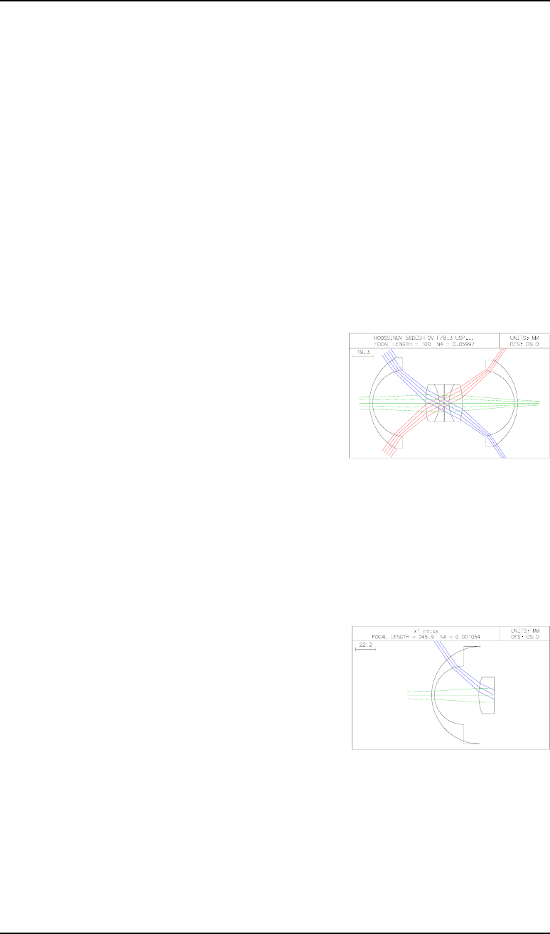
63
Chapter 7 - Slider-wheel design
1:1 wide angle relay
Introduction
The slider-wheel facility is a powerful tool, which allows the user to control any system
variable while watching its effect on any numeric parameter or graphic display. In this
chapter there will be an illustration of how slider-wheels alone can be used to complete a
design task.
The requirement is for a four-element unity magnification relay. The object has a diagonal
of 600 mm. The object to image distance is 451 mm. The distortion must be less than 0.1%
and the design criterion is that the lowest value over the field of the modulation transfer
function at 1.0 cycles/mm must be greater than 0.4. The wavelengths to be used for the MTF
calculation are the usual three (0.58756 μm, 0.48613 μm and 0.65627 μm), weighted
equally.
Defining the starting point
Clearly a symmetrical design is called for. In the public
lens database (OSLO Standard and Premium only)
there is an objective lens designed by Roossinov which
will be used as the basis for the design of a relay lens.
This has the title ROOSSINOV 56DEGHFOV F/8.3
USP2,516,724. It is nearly symmetrical and it has 13
surfaces. The design below has been adapted and
simplified from this for use with all versions of OSLO.
Setting up the starting lens
• From the menu select File>New lens and choose a custom lens with 5 surfaces.
• In the surface data spreadsheet, change the lens title to x1 relay.
• Click on the gray button under Aperture Radius for surface 5, and select Aperture
Stop (A) to move the aperture stop to surface 5.
• Fill in the lens parameters as shown in the diagram
below. The values for Aperture Radius may be
omitted, as these will be adjusted using aperture
radius solves - that is to say, the aperture will be set
at the value equal to the arithmetical sum of the
paraxial marginal and pupil ray heights. This is such
an extreme field angle lens that the results look
unrealistic at first, but this can be corrected later.
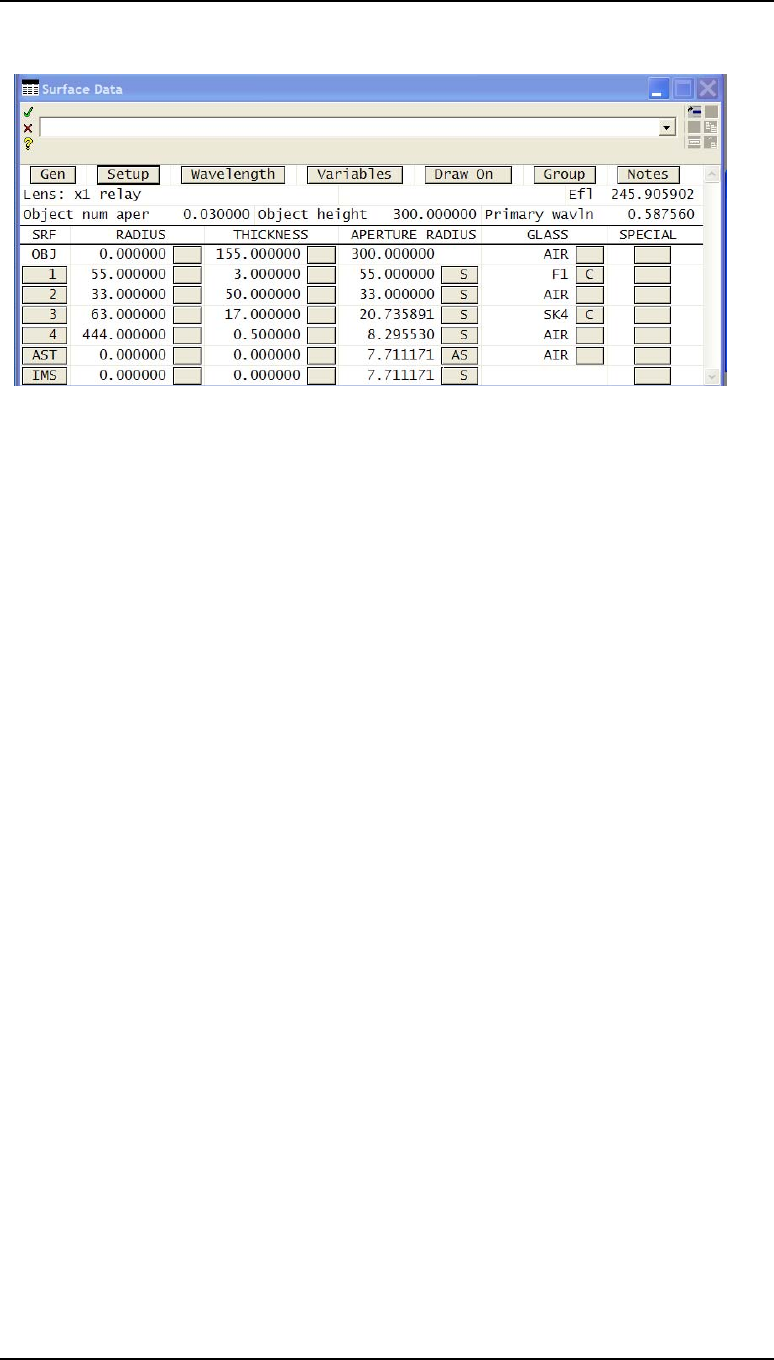
64 Slider wheel design Chapter 7
1:1 wide angle relay
• In the Setup spreadsheet, enter the Object NA as 0.03 and the Object height as
300 mm. Close the Setup spreadsheet.
• Select surfaces 1 to 4, right click and choose Copy.
• Select surface 6 (IMS), right click and select Paste
• Select surfaces 6 to 9, right click and choose Reverse.
• Change the thickness for surface 5 to 0.5 and for surface 9 to 155.
• In the Aperture radius column some are already Solves. Change the remaining
apertures (surfaces 6 to 9) to Solve (S) by setting them to zero.
• Under Radius, click on the gray button for surface 9, choose Minus curvature
pickup, and on the prompt Enter pickup source surface, enter 1. Press Enter
twice more. Define a similar minus curvature pickup for surface 8 from surface 2, for
surface 7 from surface 3 and for surface 6 from surface 4.
• Enter the command ctg to list the lens with curvatures:
x*LENS DATA
x1 relay
SRF CURVATURE THICKNESS APERTURE RADIUS GLASS SPE NOTE
OBJ -- 155.000000 300.000000 AIR
1 0.018182 3.000000 55.000000 S F1 C
2 0.030303 50.000000 33.000000 S AIR
3 0.015873 17.000000 20.735891 S SK4 C
4 0.002252 0.500000 8.295530 S AIR
AST -- 0.500000 7.775659 AS AIR
6 -0.002252 P 17.000000 8.294476 S SK4 C
7 -0.015873 P 50.000000 20.712585 S AIR
8 -0.030303 P 3.000000 33.000000 S F1 C
9 -0.018182 P 155.000000 55.000000 S AIR
IMS -- -- 300.541968 S
• Click on Gen in the Surface data spreadsheet to open the General conditions
spreadsheet.
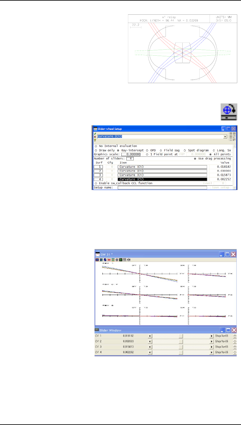
Chapter 7 - Slider wheel design 65
Slider-wheel design with ray intercept curves
• Under Ray aiming mode, select Wide angle mode.
• Close the General conditions spreadsheet.
• Change the Lens drawing conditions to
draw 3 rays for each of the field points
FBY = 0, FBY = -1, FBY = +1.
The lens drawing should now appear as
shown in the diagram.
Slider-wheel design with ray intercept curves
• Open the Slider-wheel Setup spreadsheet by clicking on the icon in the main
window toolbar.
• Select Ray-intercept, All
points, Number of
sliders = 4, and define
sliders on surfaces
1,2,3,4 for the curvature
(cv).
• Close the Slider-wheel Setup
spreadsheet.
At this point the four sliders and two graphics windows, GW31 and GW 32 should become
visible. If not, try using the Tile command, or open and close the Slider-wheel spreadsheet
again.
• The default step size is too large. Click on the lower scroll button at the right-hand end
of each slider-wheel to bring the Step to 1e-05.
• Adjust the sliders to improve
the performance as far as
possible.
• Once the aberrations are too
small to discern at the default
aberration plotting scale,
reopen the Slider-wheel Setup
spreadsheet and close it again
immediately. The aberrations
will be redrawn with a new
scale, and the slider-wheels
re-centered in their tracks.
The step size will still need to
be changed, however.
• If a slider reaches the end-
stop, change the step to re-center it. Note that the graphics zoom feature works on both
windows, and the zoom settings are preserved during slider operation.
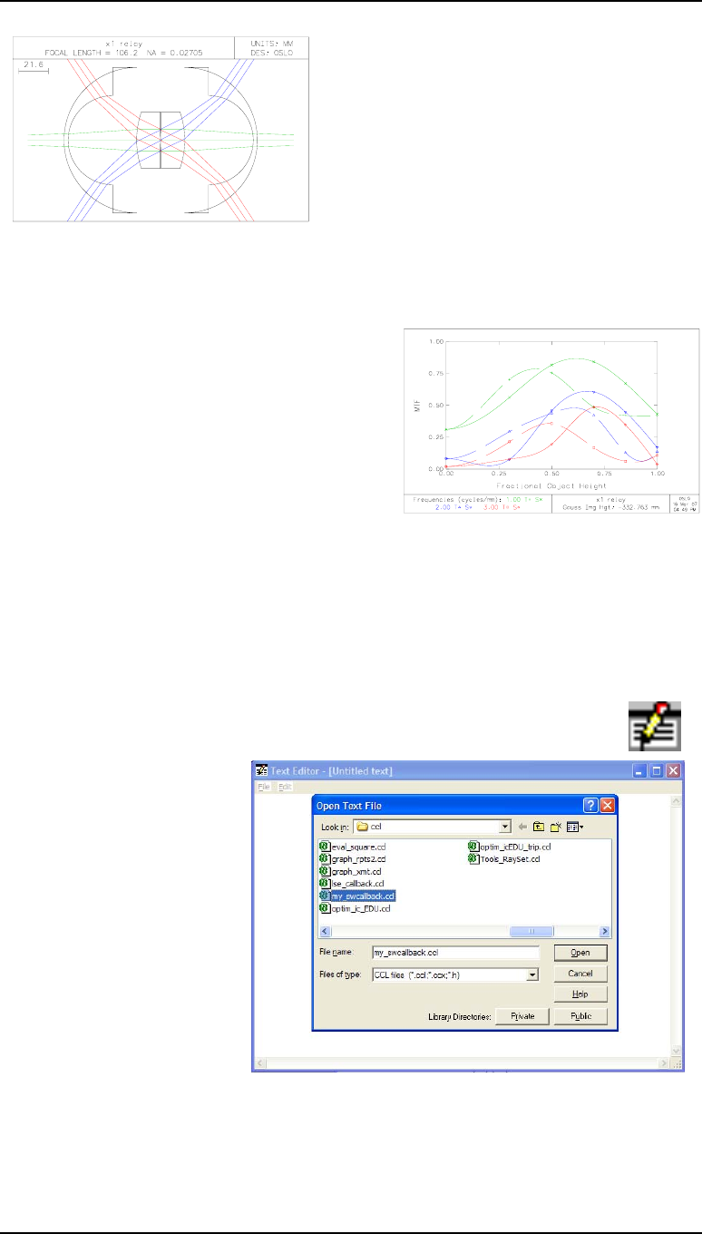
66 Slider wheel design Chapter 7
Slider-wheel design with ray intercept curves
One possible solution, for example, is
CV 1 = 0.018822 (RD 1= 53.130 mm)
CV 2 = 0.030683 (RD 2 = 32.591mm)
CV 3 = .015523 (RD 3 = 64.420 mm)
CV 4 = .002462 (RD 4 = 406.13 mm)
Plotting the MTF across the field
• From the Evaluate menu header select Transfer Function > MTF vs field
• Enter three frequencies in units of cycles per
mm: 1.0, 2.0, and 3.0.
This plots the modulation transfer function at all
points in the field for the three spatial frequencies.
In the example shown here, the upper (green)
curve, which shhows the MTF at 1 cycle per mm,
still falls well below the desired 0.4 level over
part of the field of view.
Editing the slider-wheel callback command
In order to use the slider-wheels to optimize the MTF across the whole field, it will be
necessary first to make a small modification to one of the CCL commands in the
/private/ccl directory. Some users may prefer to skip this exercise and return to it once the
next chapter on programming has been covered.
• Open the text editor either by clicking on the icon, from the menu header
Window > Editor > Open or typing the command ewo.
• In the Text editor window,
click on File > Open.
• At the bottom of the
window which opens,
after Library
Directories: click on
Private.
• Of the files which have a
green icon (*.ccl files)
select
my_swcallback.ccl and
click on Open.
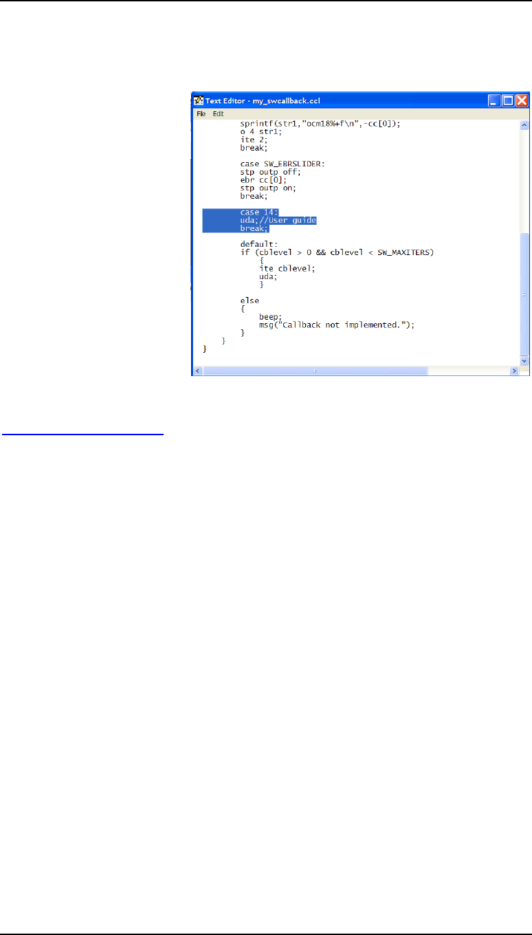
Chapter 7 - Slider wheel design 67
Slider-wheel design with ray intercept curves
This file contains a single command
cmd Sw_callback(int cblevel, int item, int srf)
• Go to line 36 of the file (Ctrl-G or Edit > Goto Line, and enter 36).
• After the last break; and
before the line default:
add the lines:
case 14:
uda; // User guide
break;
When typing this entry you
must take care that the first
line ends with a colon (:),
and the second and the third
with a semicolon (;). On the
second line anything
following the // is treated as
a comment.
• In the text editor window
(not the main window)
click on File > Save. Compilation should be automatic, and the message in the text
window should be:
*CCL COMPILATION MESSAGES: No errors detected
To explain, if the slider-wheel callback CCL is enabled by the user, then the command
Sw_callback is called whenever a slider-wheel is moved. When this happens, the value of
the integer argument called Level is passed to the CCL command, where it appears as the
integer cblevel. This determines which action to be taken by the callback command.
If the sw_callback CCL function is invoked with a value of Level between 1 and 9, that
number of cycles of optimization (iterations) is performed. If Level is 11, then the slider-
wheel controls field angle, and if Level is 13 it controls entrance beam radius. The option
Level = 13 is used in one of the tutorials.
As a result of the change, if the sw_callback CCL function is invoked with a value of
Level equal to 14, then a single command uda will be executed. This command
(update_all in long form) has the effect of updating the graphics in all open updateable
windows (i.e. those marked UW).
All this occurs within the switch statement, with different outcomes according to the value
of cblevel, the switch parameter.
The listing of the modified CCL command is given below.

68 Slider wheel design Chapter 7
Slider-wheel design with ray intercept curves
Listing of the modified slider-wheel callback CCL
/*****************************************************************************************
* This file contains some simple callbacks that are used in the documentation examples *
* with slider-wheel windows. It is meant to be extended by users as needs arise. The *
* callback uses the "cblevel" parameter to designate a particular action. The user then *
* enters the appropriate number in the Slider-wheel Setup window in the cell marked *
* "Level". The value of "Level" is passed to this command as "cblevel" and determines *
* the task to be performed. *
/*****************************************************************************************/
#define SW_MAXITERS 10
#define SW_ANGSLIDER 11
#define SW_DIFFRACTDBLT 12
#define SW_EBRSLIDER 13
cmd Sw_callback(int cblevel, int item, int srf)
{
switch (cblevel)
{
case SW_ANGSLIDER:
stp outp off;
ang cc[0];
stp outp on;
break;
case SW_DIFFRACTDBLT:
sprintf(str1,"ocm18%+f\n",-cc[0]);
o 4 str1;
ite 2;
break;
case SW_EBRSLIDER:
stp outp off;
ebr cc[0];
stp outp on;
break;
case 14:
uda;//User guide
break;
default:
if (cblevel > 0 && cblevel < SW_MAXITERS)
{
ite cblevel;
uda;
}
else
{
beep;
msg("Callback not implemented.");
}
}
}...
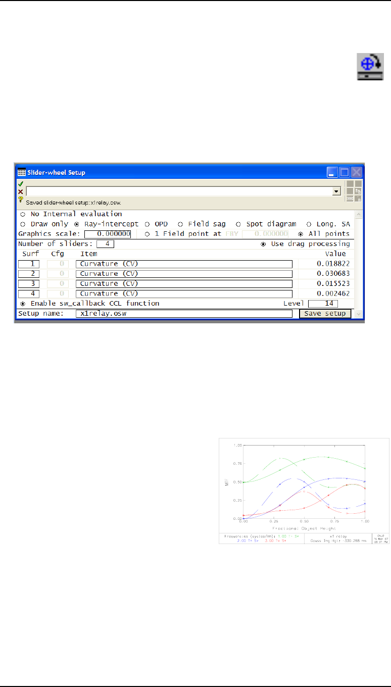
Chapter 7 - Slider wheel design 69
Slider-wheel design using MTF at one frequency
Slider-wheel design using MTF at one frequency
• Plot the MTF curves at the spatial frequencies of 1, 2, and 3 cycles/mm as before.
• Open the slider-wheel spreadsheet.
• Set up the slider-wheels as before, but this time click on Enable
sw_callback CCL function.
• Enter Level as 14.
• Enter the Setup name x1_relay and click on the Save setup button.
This slider-wheel setup (the slider wheel definitions and the other data) is now saved in a
file x1_relay.osw, which is stored in the directory .../private/bin/osw/
• Close the slider-wheel setup spreadsheet.
• On each slider-wheel change the step size to 1e-05 as before (these values are not stored
in the slider-wheel data).
• Adjust the curvatures to maximize the MTF at 1 cycle/mm over the whole field.
One possible solution, illustrated here, is:
CV 1 = 0.01778 (RD 1= 56.237 mm)
CV 2 = 0.03090 (RD 2 = 32.359 mm)
CV 3 = .01585 (RD 3 = 63.079 mm)
CV 4 = .002312 (RD 4 = 432.48 mm)
The smallest MTF value for this design is 0.42.
This completes the design ask.
This example illustrates in microcosm how even a problem with clearly defined objectives
and only 4 variables can have a large number of solutions, all meeting the requirements but
differing in subtle ways.
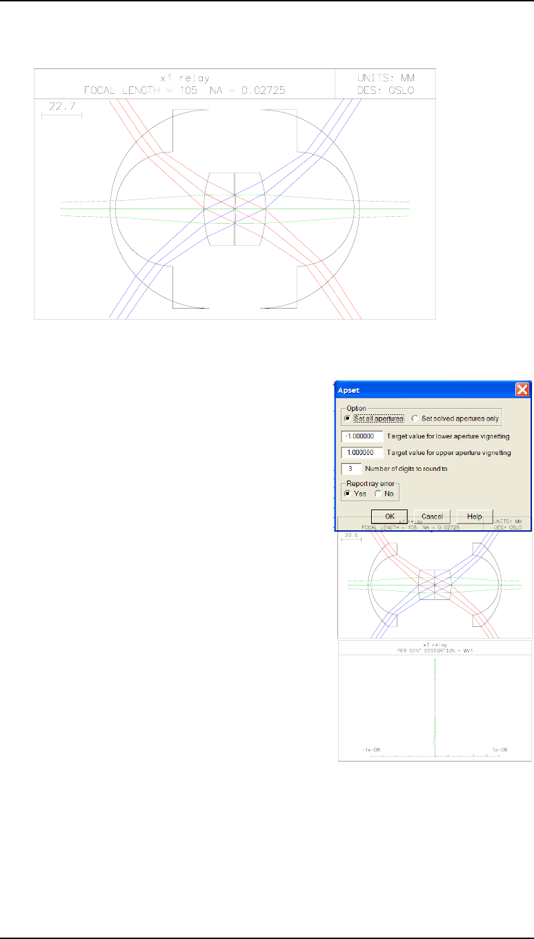
70 Slider wheel design Chapter 7
Slider-wheel design using MTF at one frequency
Setting clear apertures
The apertures at present are based on paraxial ray “solves.” To complete the design, the
clear aperture values must be set in accord with real ray, not paraxial ray, requirements.
• From the Optimize menu header select Support routines > Vignetting > Set
apertures.
• Leaving all the choices as defaults, click on OK.
*APERTURES
SRF TYPE APERTURE RADIUS
0 SPC 300.000000
1 SPC 44.200000
2 SPC 32.000000
3 SPC 15.800000
4 SPC 8.360000
5 SPC 7.950000 CHK
6 SPC 8.360000
7 SPC 15.800000
8 SPC 32.000000
9 SPC 44.300000
10 CMP 300.550935
• If the slider-wheel spreadsheet is re-opened after the
lens is saved, the previous setup will have been
deleted from it. It can be retrieved by clicking in the
Setup name window and right-clicking on
x1_relay.osw from the list presented.
• Finally, enter the command pld mon to confirm
that the level of distortion in the design is indeed
very low.
71
Chapter 8 - Programming
Introduction
This chapter will include the basics of how to create a new command producing textual
output, and how to include that command as one of the options in the text window header
menu. Next there will be how to create a new graphics command, and how to create an icon
for this in one of the graphics window headers. Finally there will be a brief review of the
SCP and CMD languages.
To illustrate these, it is helpful to have a standard lens in storage.
• Click on the icon for Open an existing lens. If the warning message
appears ... Save changes to current lens file? Click on No.
• At the bottom of the window which opens, after Library Directories: click on
Public.
• Select demo > edu and then click on demotrip.len.
• Click on Open.
Defining a new command: sno
In the surface data spreadsheet, the button labeled Notes gives access to the first 5 lines of
the user-defined commentary which is stored with each lens. This consists of up to 10 lines,
but the 6th is reserved for some optimization parameters, and the 10th for the public
database lens class.
The standard OSLO command for listing the system notes is opc sno. There is no
facility for calling this from the text window toolbar. This section shows how a new
command, sno, which lists the system notes, can be written. Then the procedure for adding
a label Sno to the text window (Standard Tools) toolbar will be given, so that the system
notes (up to 10 lines of documentation stored with each lens) can be listed with a single
click.
• First, try out the command from the keyboard. Type the command opc sno
*CONDITIONS: SYSTEM NOTES
1: This Cooke triplet is used throughout the OSLO documentation as an example.
2: It is a minor variation on a lens designed by hand by R. Kingslake (see "Lens
3: Design Fundamentals", pp286-295, Academic Press 1978, ISBN 0-12-408650-1), who
4: used nothing more than a hand calculator! The Cooke triplet was invented by
5: Dennis Taylor in 1893, and is still very widely used as a low-cost objective.
10: COOKE TRIPLET
CCL commands are stored in ASCII, and may be created either using the OSLO standard
text editor, or using UltraEdit-32® from IDM Computer Solution Inc, or (the least
convenient) with Microsoft’s Notepad®. Only the use of the first will be described in this
chapter.
To create the new command:
• If the icon for Open the standard text editor appears on the main
window taskbar, click on it. Otherwise from the Window menu header
select Editor > Open. Alternatively type the command ewo in the

72 Programming Chapter 8
Defining a new command: sno
command line,
• In the editor window, select File > New and type:
cmd sno(void)
{
operating_conds(sno);
}
Note that there is no punctuation
after (void), and there is a
semicolon (;) after the single
line command.
• Highlight the last three lines with the cursor and press Ctrl-E to check that the
program has been entered correctly.
• There are only two menu options in the editor window header. Choose File > Save
as... , click on the gray button labeled Private at the bottom, and choose File
type: CCL files (*.ccl,*.ccx,*.h).
• Enter File name eval_sno and click on Save.
• Compilation takes place automatically:
*CCL COMPILATION MESSAGES:
No errors detected
should be the message which appears in the text window.
• Enter the new command in the command line: sno
• In the text editor window, add the documentation as
//
// Written by [your name] [date]
//
cmd sno(void)
// hlp: <P>SNO</P>
// hlp: <P> Prints the system notes.</P>
{
operating_conds(sno);
}
• In the editor window header, (not the main window) click on File > Save. The
compilation message will appear again:
*CCL COMPILATION MESSAGES:
No errors detected
Each command definition in the private/ccl directory must be unique, so do not attempt to
save the command sno again in a *.ccl file of another name. The error message will be:
*CCL COMPILATION MESSAGES:
eval_sno2.ccl 2: Duplicate procedure definition
and this error will persist until the duplicate procedure definition is removed.

Chapter 8 - Programming 73
Structure of a CCL command
Structure of a CCL command
CCL commands can be created by the user to automate sequences of actions, and to carry
out calculations and plots specific to a user’s requirements. They are stored as ASCII text in
the directory .../private/ccl (not a sub-directory) and must be compiled before use.
The simplest CCL command can have the structure:
cmd command_name1()
{
OSLO_command1;
OSLO_command2;
...etc...
}
This is stored in a file demo_anyfilename.ccl. (Prefixes of user-written command files
should ideally be restricted to demo_, eval_, graph_ and optim_). It is compiled using
the icon (or, in the case of OSLO EDU where the icon is not displayed) the menu sequence
Tools > Compile CCL >Private, or the command ccl.
It is executed using the call:
command_name
For example, the CCL file containing the program;
cmd hallo(void)
{
printf(“Hallo world\n”);
}
may be stored as my_first.ccl, compiled, and then called using the command:
hallo
This is described in detail in Help > OSLO Help > Contents > Programming > CCL
Programming > Using CCL.
With formal parameters, or arguments, the structure of a CCL command might become:
real argument_name1;
int argument_name2;
cmd command_name(real argument_name1,int argument_name2)
{
OSLO_command1(argument_name1,argument_name2);
OSLO_command2(argument_name1,argument_name2);
}
This is compiled and then executed using (for example) either free format:
command_name 1.0 1
or the more formal version, often used within CCL code:
command_name(1.0,1);
In this case the two global variables argument_name1 and argument_name2 might be
used by another CCL command.

74 Programming Chapter 8
Search CCL library: scanccl
Local variables may also be declared. Take, for example, the CCL command:
real argument_name1;
int argument_name2;
cmd command_name(real argument_name1,int argument_name2)
{
real local_variable1;
int local_variable2;
local_variable1=3.0;
local_variable2=4;
print(argument_name1,argument_name2,local_variable1,loca
l_variable2);
}
If this is called using the command
command_name 1.0 2
the output is:
1.000000 2 3.000000 4
Search CCL library: scanccl
Assume that eval_sno.ccl has been added to the private\ccl directory, as described
above.
• From the menu header select Tools > Search CCL library ...
• Under Directory to browse select the option Private
• Select the default option Sort functions by filename and click on OK.
** 8 functions are defined in the private directory:**
** C:\Program Files\OSLO\EDU64\private/ccl/
TYPE FCTN NAME ARGUMENTS LINE DEFINITION FILE
---- --------- --------- ---- ---------------
cmd sno 5 eval_sno.ccl
cmd sw_callback 15 my_swcallback.ccl
int cblevel
int item
int srf
cmd tlex_1 18 dbtutorial.ccl
real tl__radius1
real tl__radius2
real tl__refractive_index
The new command sno appears as the first entry in the list of function names; also given
are the number of lines in the command, and the name of the file in which it was defined.
Defining a new command: ctn
The next new CCL command is an extension of one which appeared in chapter 3.
Initial version of command
• From the Window menu header select: Editor > Open, or type the
command ewo in the command line, or click on the main window toolbar
icon.
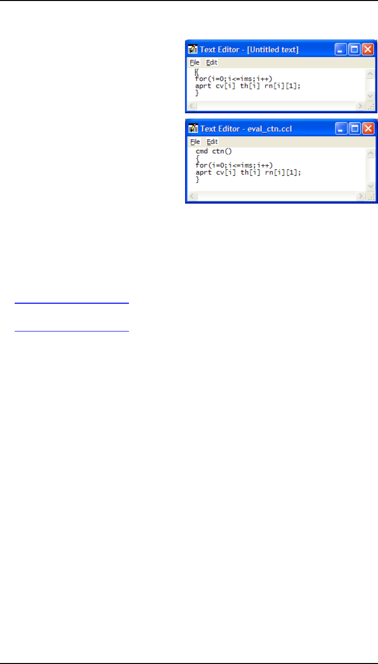
Chapter 8 - Programming 75
Defining a new command: ctn
• Type in the following line:
for(i=0;i<=ims;i++)aprt cv[i] th[i] rn[i][1];
• Split it into two lines and surround
with curly brackets.
• Highlight the whole window (Ctrl-A)
and execute (Ctrl-E).
The following appears in the active
text window:
-- 1.0000e+20 1.000000
0.047059 2.000000 1.620410
-0.006303 6.000000 1.000000
-0.049383 1.000000 1.616592
0.051813 6.000000 1.000000
0.007080 2.000000 1.620410
-0.057854 42.950000 1.000000
-- -- 1.000000
• Add a line at the beginning:
cmd ctn()
• In the Text Editor window click on File > Save as...(F12).
• Ensure first that the bottom window reads Save as type: CCL files.
• Click on Library Directories Private.
• For File name type eval_ctn
• Click on Save.
• Look in the text window. There should be a message
*CCL COMPILATION MESSAGES:
No errors detected
If the message appears:
*CCL COMPILATION MESSAGES:
eval_ctn.ccl 2: Duplicate procedure definition
then there is already a file with extension .ccl in the private/ccl directory containing the line
cmd ctn()Locate it and delete it, or change its extension to .ccx. It may be impossible
to do this if file extensions are hidden. If so, it is necessary to change the Windows file
viewing settings. Under My Computer > Tools > Folder options > View tab > Advanced
Settings > Hide extensions for known file types: Uncheck.
If there is another compilation error, check the listing carefully, especially the one
semicolon and the three different types of bracket:
cmd ctn()
{
for(i=0;i<=ims;i++)
aprt cv[i] th[i] rn[i][1];
}
Extra lines and spaces are not a problem.
• Once compilation is successful, in the command line enter ctn. The output should be
as before.
Version with formatted output
• Change the aprt print statement to:

76 Programming Chapter 8
Defining a new command: ctn
aprintf("%3i %12.8f %9.4g %.6f\n",i,cv[i],th[i],rn[i][1]);
Here, each format specification begins with a % sign:
The format specifier %3i requires that the integer i is to be printed with a field width of 3,
right justified within this width.
The format %12.8f gives a minimum field width for cv[i] of 12 characters, with 8 digits
printed after the decimal point.
The format %9.4g prints th[i] in decimal notation with 4 significant figures, but in
exponential form if it is 10000 or more, or less than 0.00001.
The format %.6f requires n[i] to be printed with 6 digits after the decimal point, and no
minimum field width.
• Save and execute, giving:
0 0.00000000 1e+20 1.000000
1 0.04705882 2 1.620410
2 -0.00630318 6 1.000000
3 -0.04938272 1 1.616592
4 0.05181347 6 1.000000
5 0.00707965 2 1.620410
6 -0.05785363 42.95 1.000000
Adding the glass name string
Glass name strings are not directly accessible. However, the command
get_glass_name(i) copies the name of the glass for the ith surface into a read-only
string glass_name (See under Help > OSLO Help > Contents > Programming >
Accessing Data > Other Data > Data Functions).
• Add an extra pair of curly brackets after the for statement, and insert:
get_glass_name(i);
• Change the print statement to (on a single line):
aprintf("%3i %12.8f %9.4g %.8s %.6f\n"
,i,cv[i],th[i],glass_name,rn[i][1]);
The format %.8s requires the glass_name string to be printed with a maximum of 8
characters.
• List the complete command:
cmd ctn()
{
print(" SRF CV TH GLASS RN");
for(i=0;i<=ims;i++)
{
get_glass_name(i);
aprintf("%3i %12.8f %9.4g %.8s %.6f\n",i,cv[i],th[i],glass_name,rn[i][1]);
}
}
Adding headers and documentation
The following conventions have been established by previous writers of OSLO macros, and
they are worth observing:
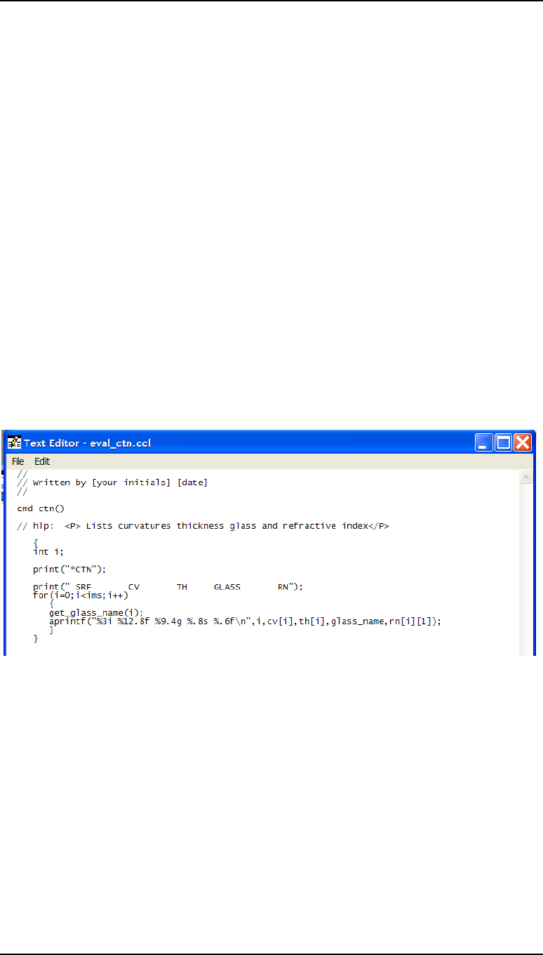
Chapter 8 - Programming 77
Defining a new command: ctn
1. Each CCL file opens with a set of three or more comment lines giving the author,
date, and any update information. e.g.
//
// Written by [Your initials] [Date]
//
2. All documentation for a CCL command is given in HTML format between the
header and the body, commented out and preceded by hlp. For example:
// hlp: <P>Lists curvature, thickness, glass type and refractive index.</P>
3. No default system variables are ever used, so that, for example, the command
sequence
i=92;ctn;prt i
must always give the same result. So declare all variables as local variables within the
command: e.g.
int i;
Of course these can have any name chosen arbitrarily, but by keeping to the default variable
names, the Ctrl-E execution of selections of code within the text editor window can still
proceed, provided the declaration int i; itself is not highlighted.
4. Commands which give just printed output are echoed, preceded by a star, in upper
case. e.g.
print(“*CTN”);
Making these changes, the final version of the command becomes:
The output from a call of the command ctn is:
*CTN
SRF CV TH GLASS RN
0 0.00000000 1e+20 AIR 1.000000
1 0.04705882 2 SK16 1.620410
2 -0.00630318 6 AIR 1.000000
3 -0.04938272 1 F4 1.616592
4 0.05181347 6 AIR 1.000000
5 0.00707965 2 SK16 1.620410
6 -0.05785363 42.95 AIR 1.000000
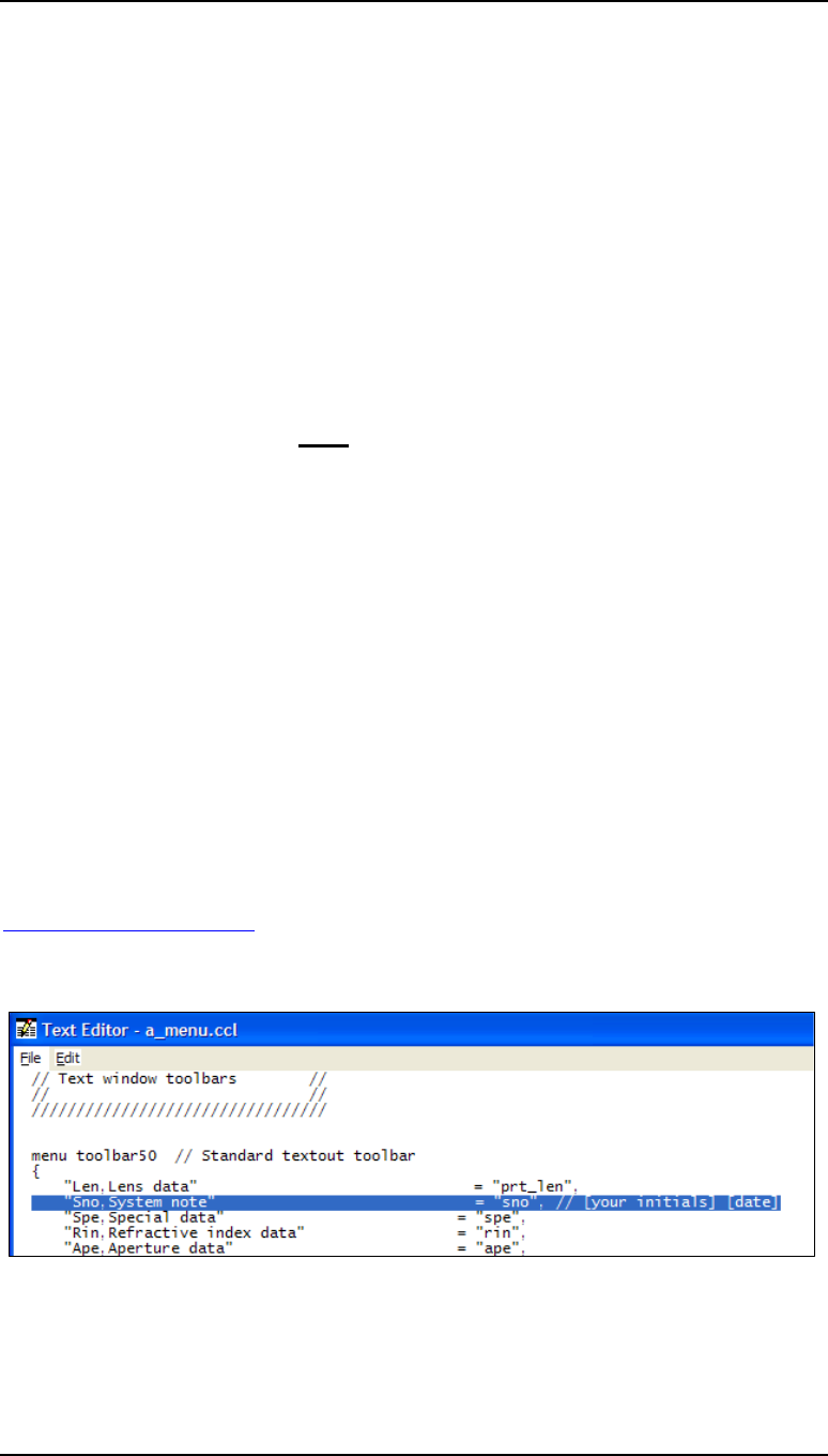
78 Programming Chapter 8
The text window toolbar
The text window toolbar
Commands which generate only printed output are by convention placed in the text window
toolbar. The format for a text window toolbar is:
menu toolbar_number
{
“Label,tooltip_label” = “command”,
“Label2,tooltip_label2” = “command2”,
}
where the first Label (by convention having only 3 or 4 letters) is what appears on the
toolbar, the second, tooltip_label, is more detailed, and only appears in a cream-
colored box when the cursor hovers over the first label. The command may be either CCL
or OSLO command(s). The toolbar_number is toolbar50 for the Standard Tools
text window toolbar.
Adding the command sno to the toolbar
• Still in the Text Editor window, select File > Open and look in the Private CCL
directory. Open the file a_menu.ccl.
• (If there is no file private/ccl/a_menu.ccl, open the file /public/ccl/a_menu.ccl,
and save it as private/ccl/a_menu.ccl)
• Go to line 1339 of this file (Ctrl-G and enter 1339 in the dialog box). This should give
the entries for:
menu toolbar50
• After the line:
“Len,Lens data” = “prt_len”,
add the line (note the comma before the comment):
“Sno,System note” = “sno”,//[your initials][date]
• Compile again by saving the file:
*CCL COMPILATION MESSAGES:
No errors detected
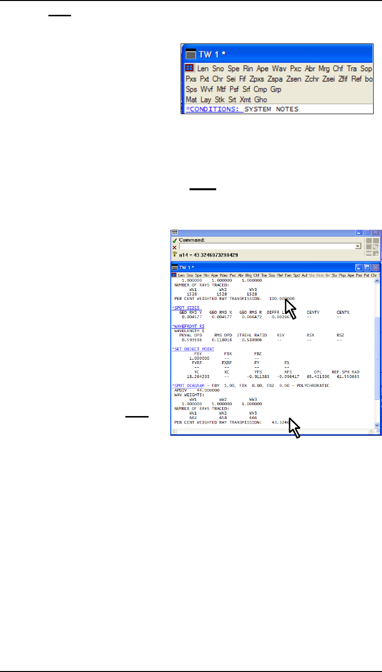
Chapter 8 - Programming 79
Defining a new command: xmt
Calling sno from the toolbar
• Click on Sno in the text window toolbar. If it is not visible, ensure that the Standard
Tools menu has been selected.
Once again the output is:
*CONDITIONS: SYSTEM NOTES
1: This Cooke triplet is used
throughout the OSLO documentation as
an example.
2: It is a minor variation on a lens designed by hand by R. Kingslake (see "Lens
3: Design Fundamentals", pp286-295, Academic Press 1978, ISBN 0-12-408650-1), who
4: used nothing more than a hand calculator! The Cooke triplet was invented by
5: Dennis Taylor in 1893, and is still very widely used as a low-cost objective.
10: COOKE TRIPLET
Defining a new command: xmt
In this exercise a command xmt will be created which plots a graph showing the
transmission fal1-off across the field arising from vignetting. (The effect of coatings and of
the internal transmission of optical
materials, available in OSLO
Premium, is not included in this
analysis).
The command will be modified to
prevent errors occurring when no rays
are transmitted, or when the chief ray
fails. This will demonstrate the use of
an error handler.
Then a new icon will be created, and
placed in the Spot Diagram menu of
the graphics window toolbar to enable
the new command to be called with a
single click.
Writing a command xmt
to print transmittance
values
• Open the lens file /public/demo/EDU/ demotrip.len
• In the Text Editor window, open a new file and type the following in a single line:
sbr;sop 0 0 0;spd 44;sop 1 0 0;spd 44
• Highlight with the cursor, press Ctrl-E and click on the two values of PERCENT
WEIGHTED RAY TRANSMISSION (100.00 and 43.324607) which appear in the text
window. Note the coordinates of the two spreadsheet cells (a6, a14).
• In the text editor, add a second line containing a print command.
prt a6,a14;
• Highlight both lines and press Ctrl-E to confirm the correct values have been printed.
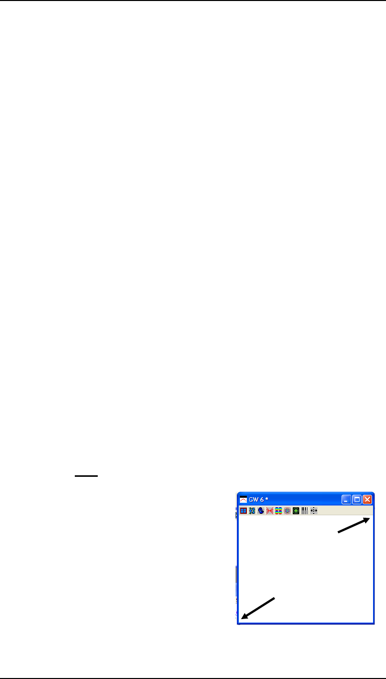
80 Programming Chapter 8
Defining a new command: xmt
• The transmission curve is to be plotted at 50 points over a range of value of FBY from
0.0 to 1.0. Introducing the pre-defined integer i as a variable to count through these
points, and we can generate all the results using a for loop:
sbr;
for(i=0;i<51;i++)
{
sop i*.02 0 0;
spd 44;
}
To extract the relevant values from the spreadsheet, and print them as a neat table, we
must switch off printed output with stp(outp,off) and extract the transmission
values from the spreadsheet. The spreadsheet cell number of the transmission value of
the (i+1)th field point is a(6+8i) or, as a CCL formula, ssb(6+8*i,1). Introducing
the double precision predefined variables x (the value of FBY) and y (the %
transmission), we can use these in a print statement to create the necessary table: prt
x,y; This statement will produce visible output despite the fact that the preference
stp(outp,off); has been called, provided prt and not aprt is used for
printing.
Predefined variables are used at this stage because the Ctrl-E compilation method is
incompatible with either local or global variables.
• So change the program to:
stp(outp,off);
sbr;
for(i=0;i<51;i++)
{
x=i*0.02;
sop(x,0,0);
spd(44);
y=ssb(6+8*i,1);
prt(x,y);
}
stp(outp,on);
• Highlight it all and execute with Ctrl-E to generate the entire list of 51 values giving
the percentage transmission across the field:
-- 100.000000
0.020000 100.000000
0.040000 100.000000
...etc
0.960000 47.120419
0.980000 45.811518
1.000000 43.324607
Converting xmt printed output to graphics
The text window spreadsheet is used as the vehicle
for transferring the printed data into plot commands.
• At the beginning, add the command gwr;
(graphic window reset) to clear the window and
define the dimensions of the plot area to be in the
range x=0 ... 1, y = 0 ... 1.
• Also before the first calculation, add the plot
command, moveto(0,1)- most lenses will
have 100% transmission on axis.
x = 1, y = 1
x = 0, y = 0
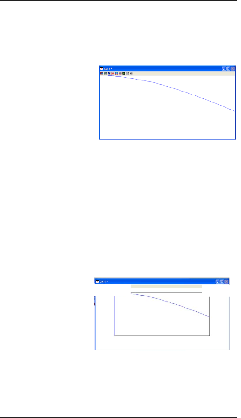
Chapter 8 - Programming 81
Defining a new command: xmt
• Add pen(3) to plot in dark blue.
• Delete the print statement.
• Insert the main plot command, lineto(x,y/100); where the /100 scales the y-
values to keep them within the range 0 ... 1.
• At the end, add gshow; to ensure that the plot output is drawn immediately and not
held in a buffer. It may still be necessary to click on the window to have the graph
drawn in full.
stp(outp,off);
sbr;
gwr;
moveto(0,1);
pen(3);
for(i=0;i<51;i++)
{
x=i*0.02;
sop(x,0,0);
spd(44);
y=ssb(6+8*i,1);
lineto(x,y/100);
}
stp(outp,on);
gshow;
Preserving the text window contents
• In the second line, replace the sbr command by the two lines:
k=sbrow;
sbr(k,1);
• On the third last line, insert the line:
sbr(-k,0);
Here k, a predefined integer variable, has been used to keep the value of sbrow, the index
of the first unwritten row of the spreadsheet.
Scaling and drawing the axes
• After the gwr command, add the following commands to re-scale the window as
illustrated in the diagram, and to draw the axes around the graph: .
window(-0.2,1.2,-35,110);
moveto(0,0);
lineto(1,0);
lineto(1,100);
lineto(0,100);
lineto(0,0);
• Also change the lineto
command to
lineto(x,y) to cover
the new range of y from 0
to 100.
• Finally surround the whole
procedure with curly brackets, add the line cmd xmt() at the top, and save in file
private/ccl/graph_xmt.ccl.
(-0.2, -35) (1.2, -35)
(1.2, 110)
(-0.2, 110)
(0.0, 0.0)
(0.0, 100.0)

82 Programming Chapter 8
Defining a new command: xmt
• Note that up to this point only predefined variables have been used (integers i,k
double precision real x,y). Thus it is possible to highlight and execute part of, or the
whole command (excluding the cmd xmt() header itself) using Ctrl-E. This is helpful
for locating errors.
The listing of the command is as follows:
cmd xmt()
{
stp(outp,off);
k=sbrow;
sbr(k,1);
gwr;
window(-0.2,1.2,-35,110);
moveto(0,0);
lineto(1,0);
lineto(1,100);
lineto(0,100);
lineto(0,0);
moveto(0,100);
pen(3);
for(i=0;i<51;i++)
{
x=i*0.02;
sop(x,0,0);
spd(44);
y=ssb(6+8*i,1);
lineto(x,y);
}
sbr(-k,0);
stp(outp,on);
gshow;
}
Adding standard plot commands to xmt
• Add the pre-processor command at the top of the file:
#include "../../public/ccl/inc/gendefs.h"
• This makes it possible to call the two commonly used graphics commands:
SAVE_DISPLAY_PREFS;
and
RESTORE_DISPLAY_PREFS;
• Following the convention already established, the captions will drawn using the
command sequence:
if (char_pref(glab)) draw_title_block(str1,str2,str3);
where the code for draw_title_block(str1,str2,str3); can be found in the CCL file
public/CCL/graph_tools.ccl
Error handling
• Open the surface data spreadsheet and change the field angle to 30 degrees.
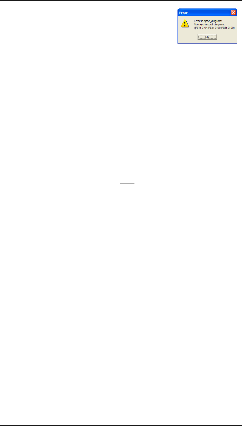
Chapter 8 - Programming 83
Defining a new command: xmt
• Call the xmt procedure. The command will fail when the
transmission falls to zero with an error message as
shown.
The remedy is to add an error handling procedure to reset the
error flag to zero. This will be called from xmt whenever an error
occurs. If a procedure invokes a second procedure, then either
the second must precede the first, or it needs to be declared:
• Add the line at the top, the prototype declaration (note that this one is followed by a
semicolon):
cmd xmt_error_handler();
• Declare an integer global variable xmt_err to carry the error status between the
prcedures.
• Add the error handler command xmt_error_handler at the end.
• The error handler can now be called. Before the window command, add the line:
install_error_handler("xmt_error_handler"); and at the end add the
command to restore the original (default) error handler:
install_error_handler("prefs");
By adding the error handling precautions to the plotting routine, it is possible to prevent the
execution of the spot diagram command if the chief ray has not been traced successfully
and to continue execution of the command with the transmission value set to zero if no rays
have been transmitted in the spot diagram. .
Listing of complete command xmt
• Convert the predefined variables to locally defined variables, i becomes iplt, x
becomes xplt, y becomes yplt, and k becomes ssb_row_sav.
• Add comments, documentation, ticks and captions etc as shown below.
• Save and compile. The whole procedure now looks like this:
//
// Written by [your name] [date]
//
#include "../../public/ccl/inc/gendefs.h"
int xmt_err;//global variable
cmd xmt(void);
cmd xmt_error_handler(void);
cmd xmt(void)
// hlp: <P>XMT</P>
// hlp: <P>Plots the fall in transmission as a function of field
// hlp: arising from central obstructions and vignetting. It does not
// hlp: include the effects of coatings or Fresnel reflections.</P>
// hlp: <P>This CCL command also illustrates how a custom error
// hlp: handler prevents reference ray failures terminating execution
// hlp: of a CCL command; by setting errno=0 within the error handler
// hlp: it permits continued execution of the CCL command even after
// hlp: what would otherwise be a fatal error. </P>

84 Programming Chapter 8
Defining a new command: xmt
{
static int ssb_row_sav,iplt;
static real xplt,yplt;
static char str1[80],str2[80],str3[80];
SAVE_DISPLAY_PREFS;//as defined in gendefs.h
set_preference(output_text, off);//switches off text output
ssb_row_sav = sbrow;//saves row after last row written to in SSB
ssbuf_reset(ssb_row_sav, 1);//initialises spreadsheet buffer
graphwin_reset;//clears graphics window
install_error_handler("xmt_error_handler");// see below
window(-0.2, 1.2, -35, 110);//xmin xmax ymin ymax
moveto(0, 0);// draw x-axis (range 0...1)
lineto(1, 0);
for (iplt = 1; iplt <11; iplt++)
{moveto(iplt*0.1, 0);//draw x-axis ticks
linerel(0, -2);}
moverel(-0.2,-10);
label("Rel.Obj.Ht.");//label x-axis
moveto(0, 0);// draw y-axis (range 0...100)
lineto(0, 100);
for (iplt = 1; iplt <11; iplt++)
{
moveto(0,iplt*10);//draw y-axis ticks
linerel(-0.02,0.0);
}
moverel(-0.1,0);
label("%s","100%");//label y-axis
moveto(0,100);// plot transmission curve
pen(2);//green
for (iplt = 0; iplt <51; iplt++)
{
xplt=iplt*0.02;// xplt=Relative object height (FBY)
yplt=0;
xmt_err=0;
set_object_point(xplt,0.0,0.0);
if (xmt_err==0)// i.e. If sop succeeded ...
{
spot_diagram(44);
if(xmt_err==0)// .. and spd succeeded ...
yplt=ssb(6+8*iplt,1);//..set yplt ...
}// ... else yplt remains zero.
lineto(xplt,yplt);
}
message("");// clears message area
install_error_handler("prefs");// default - see asyst_ccl.ccl
ssbuf_reset(-ssb_row_sav, 0);//restores ss buffer row numbering
set_preference(output_text, on);//switches text output back on
pen(1);// black
if (char_pref(glab))// only if preference graphics_labels ON ...
{
sprintf(str1,"Field angle %.4f",180*ang/pi);
sprintf(str2,"Object height %.6g",obh);
sprintf(str3,"TRANSMITTANCE VS FIELD");
draw_title_block(str1,str2,str3);//see public/graph_tools.ccl
}
gshow;//clears graphics buffer, forces display of graphics
RESTORE_DISPLAY_PREFS;
}
/******** ********* ********* ********* ********* ********* **********/
cmd xmt_error_handler(void)
{
xmt_err=errno;
errno = 0;//clears error to permit CCL execution to continue
}
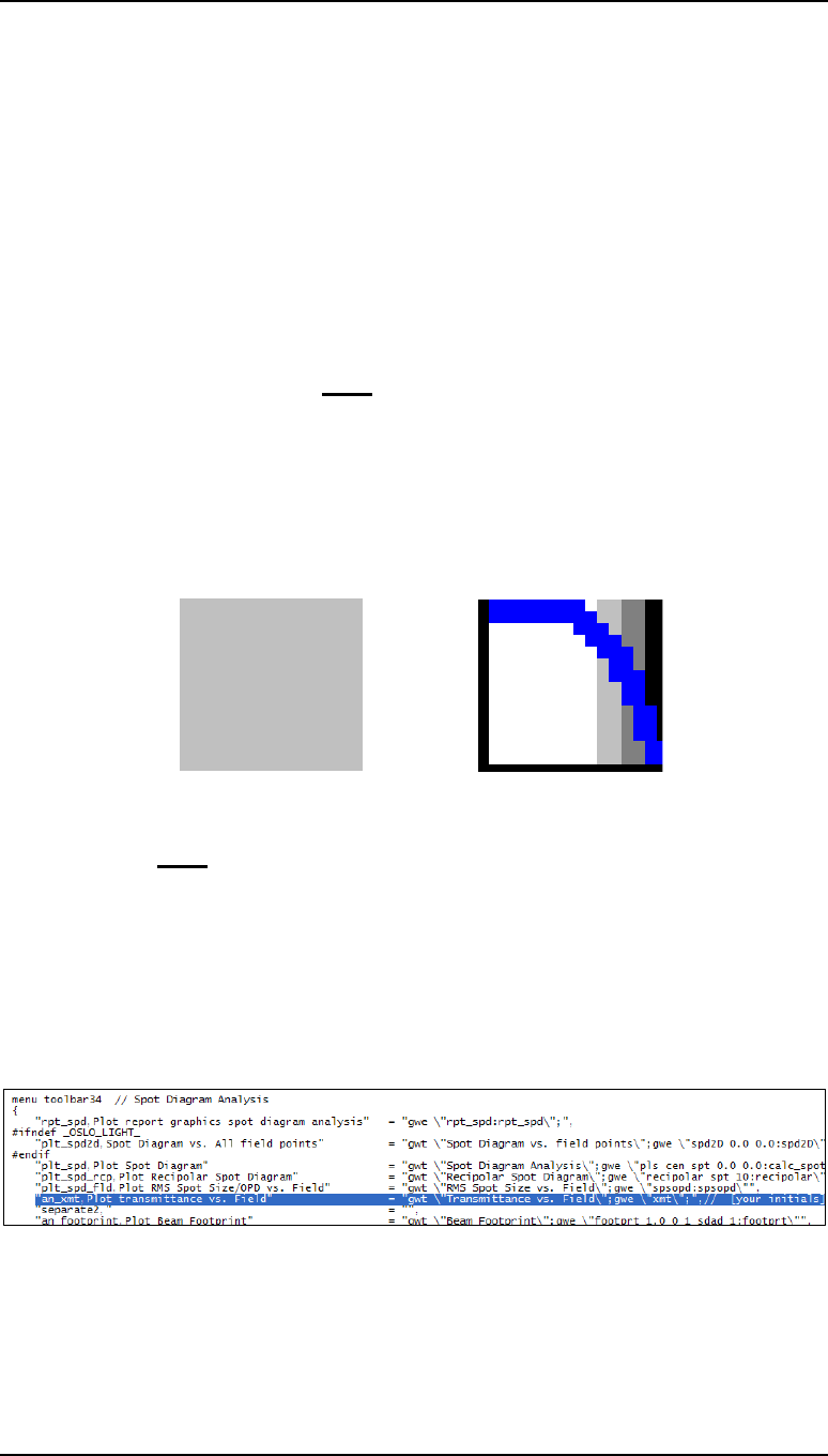
Chapter 8 - Programming 85
The graphics window toolbar
The graphics window toolbar
Commands which generate graphical output are generally called from icons on one of the
graphics window toolbars. The format for a graphics window toolbar is:
menu toolbar_number
{
“bitmap_file, tooltip_label” = “gwt \”window_title\”; gwe \”command\”;”,
...
}
where bitmap_file.bmp is the name of a bitmap file containing the icon, and stored in
the folder /Prm64/bin/bma. Once again, tooltip_label appears in a cream-colored
box when the cursor hovers over the icon. The window_title (up to 48 characters) will
appear in the blue title bar of the updatable graphics window.
Creating a new icon for xmt
• Using the computer file listing facility, locate the redundant blank icon blank1.bmp,
which is the first file in the directory /[Prm64]/bin/bma This is a file 16 x 15 pixels
(all gray) with a palette of 16 colors, plotted at a resolution of 96 pixels per inch.
• Copy it to the same directory, and rename it an_xmt.bmp
• If time permits, modify the image pixel by pixel as shown, using a program such as
Microsoft Paint®, and store it with the same name.
blank1.bmp an_xmt.bmp
Adding the xmt icon to the graphics window toolbar
In a_menu.ccl, the toolbar number is 34 for the Spot Diagram Analysis graphics window.
• Open the Text Editor window, select File > Open and look in the Private CCL
directory. Open the file a_menu.ccl.
• Locate toolbar 34. Go to line 1241 of this file (Ctrl-G and enter 1241 in the dialog
box). On this line (or one nearby) should be the entries for the toolbar menu:
menu toolbar34 // Spot Diagram Analysis
After the line:
"plt_spd_fld,Plot RMS Spot Size/OPD vs. Field" = "gwt \"RMS Spot Size vs.
Field\";gwe \"spsopd:spsopd\"",
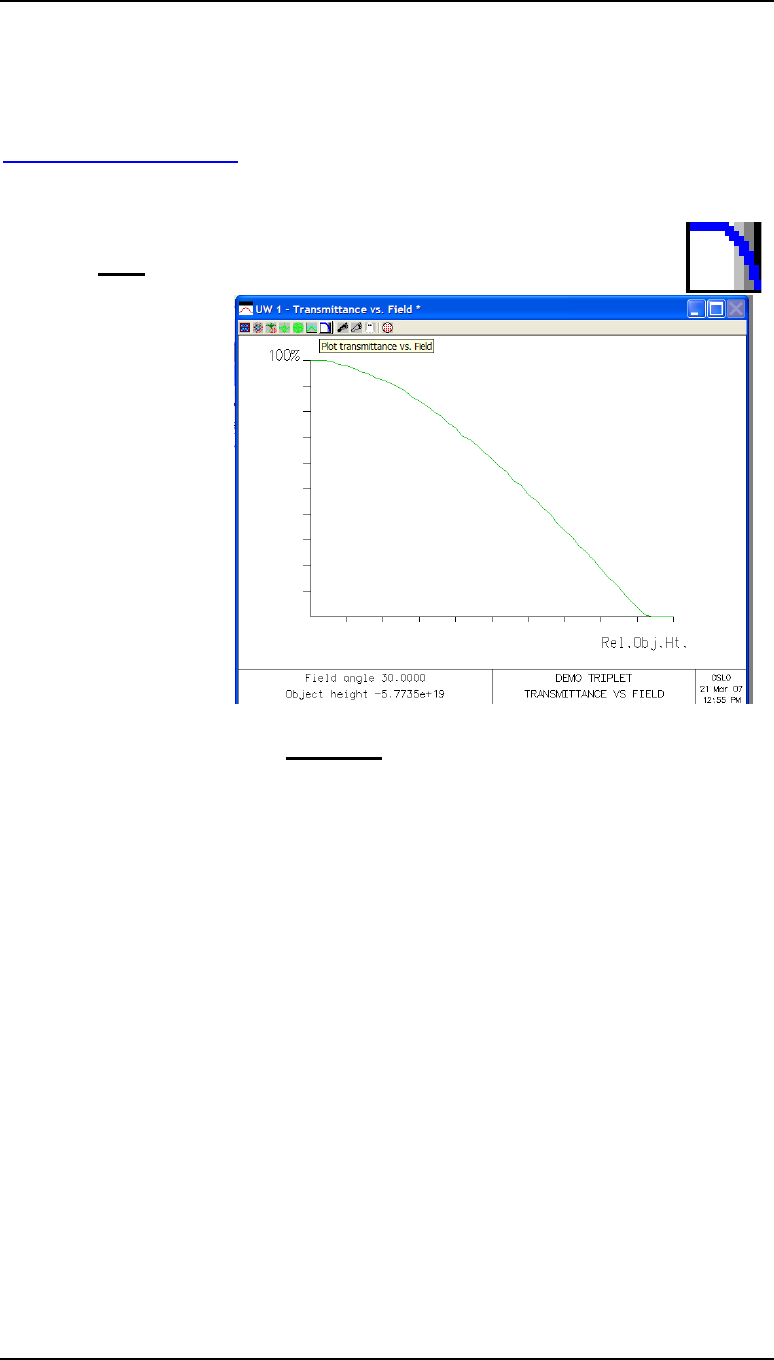
86 Programming Chapter 8
SCP programming: *triplet
add the following, all on one line (note the comma before the comment):
"an_xmt,Plot transmittance vs. Field" = "gwt \"Transmittance
vs. Field\";gwe \"xmt\";", // [your name] [date]
• Save a_menu.ccl.
• Check that compilation is successful:
*CCL COMPILATION MESSAGES:
No errors detected
Calling xmt from the toolbar icon
• Ensure that the lens
in store is the
standard triplet with
30 degrees as the
semi-field angle.
• Open a new graphics
window.
• Click on the Setup
Window/Toolbar
icon, and select the
Spot Diagram menu.
• Click on the xmt icon
shown above.
SCP programming: *triplet
SCP (“star command program”) is the old macro language of OSLO, still supported but
largely replaced by CCL. An SCP command consists of a text file whose name is the same
as the command name, and whose first line is *[cmd_name] without a semicolon. All the
other lines are commands ending with semicolons, and the file named cmd_name.scp
must be stored in the directory /private/scp. The command is not compiled, so errors are
not detected until the commands are executed.
To call an SCP command, type *[cmd_name] into the command line.
• Open the text editor window.
• Click on File > New
• Type the following lines:
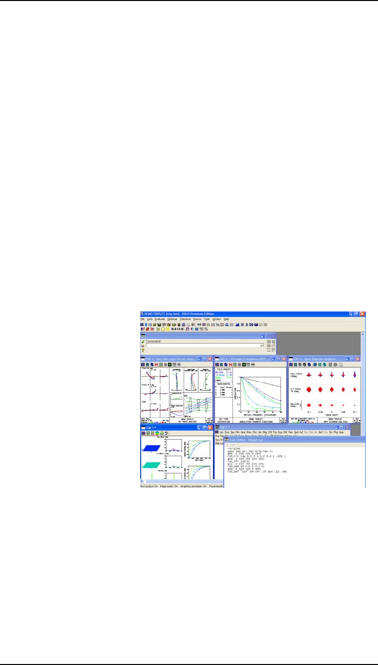
Chapter 8 - Programming 87
SCP programming: *triplet
*triplet
open len pri len trip.len n;
gwo 2 320 300 0 100;
rpt_ric ray 0.1 0 1 0.2 0.1 1 .005;
gwo 3 320 300 320 100;
rpt_tfr 100.0;
gwo 4 320 300 640 100;
rpt_spd 50 0.0 3 0.2 n;
gwo 5 320 300 0 400;
rpt_psf “128” 64 chr .25 aut .12 .06;
The first line must begin with a * and have no semicolon after it. The first gwo command
opens a new graphics window, GW2, which is 320 units wide and 300 high in the top left
corner of the window, just under the command window. Three more windows are defined
in the same way.
• Except for the very first line, the entries may be tested during entry by highlighting
them with the cursor and pressing Ctrl-E.
• In the text editor window, click on File > Save as ...
• Change File type to SCP.
• Click on PRIVATE to store the command in /private/scp/
• Enter file name as triplet.scp. The file name must be the same as the command
name, and only one command is permitted per file. Note that no compilation takes
place, so there is no checking for errors before execution.
• This command opens the
triplet stored in the private
lens directory on
installation, and plots the
ray intersection coordinates,
the MTF, the spot diagram
and the point spread
function at three field point.
Parameters for each of these
commands are chosen to
suit the lens.
• To call this SCP command,
type:
*triplet
including the initial asterisk.
Some examples of SCP commands are given in the directory /public/scp.

88 Programming Chapter 8
Load command file programming
Load command file programming
This is available only in OSLO Standard and Premium versions.
The command lcmd opens a text file and executes the OSLO commands in
sequence. Unlike CCL and SCP files, the location of the file is quite arbitrary, so
this programming language has the advantage that the files can be stored with the
lenses. Semicolons at the end of each line are optional, but including them makes it
easier to check the command file while it is being developed, using Ctrl-E in the
text editor window.
• Open the text editor and type:
//triplet [your name] [date]
open len pri len trip.len n;
gwo 2 320 300 0 100;
rpt_ric ray 0.1 0 1 0.2 0.1 1 .005;
gwo 3 320 300 320 100;
rpt_tfr 100.0;
gwo 4 320 300 640 100;
rpt_spd 50 0.0 3 0.2 n;
gwo 5 320 300 0 400;
rpt_psf “128” 64 chr .25 aut .12 .06;
• In the text editor window, click on File > Save as ...
• Store it as a text file in the private/len directory with type .txt and with the
name triplet.cmd.
• To execute, type in the command line lcmd,search in the private/len
directory for the command file triplet.cmd, and click on Open to execute.
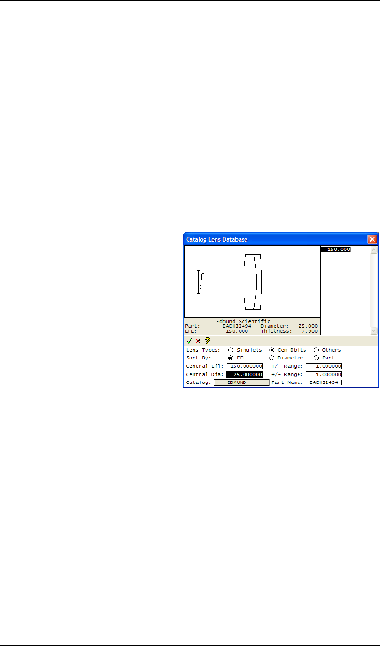
89
Chapter 9 - Optimization
Optimizing using Seidel aberrations
According to Seidel aberration theory, a thin cemented doublet of a specified pair of glass
types (one crown, one flint) may in general be corrected exactly for only two of the three
coefficients for primary axial chromatic aberration (PAC), spherical aberration (SA3), and
coma (CMA3). Using one real and one fictitious glass, however, an exact solution can
always be found.
This exercise will show how to find, using Seidel aberrations alone, the nearest glass in the
Schott catalog to combine with Schott N-BAK4 making a cemented doublet of a focal
length 150 mm, and aperture ratio f/6.3.
Setting up the starting design
• Open a new lens surface spreadsheet.
• Select the image surface. Click on the gray SRF button, right click, and choose Insert
catalog lens.
• Select the EDMUND catalog, and
look for a cemented doublet
focal length 150 mm diameter 25
mm.
• If +/-1 mm ranges are chosen there is
only one result. The Edmund catalog
number for this lens is EACH32494.
The glass types used in this lens are
Schott BK7 for the crown and Schott
SF5 for the flint.
• Set the entrance beam radius to be
150/2/6.3 mm.
• Set the semi field angle to 1°.
• Set wavelength weights 1.0 (0.58756μm) 0.4 (0.48613 μm), 0.6 (0.65627 μm).
• Delete the extra surface, by clicking on the gray SRF button for surface AST, right
click, and choose Delete.
• We need to be able to alter surfaces 1 2 and 3. Click on the gray SRF button for surface
1 (AST), right click, and choose Ungroup.
• Set the image distance at the paraxial back focal point (under thickness for surface 3,
select Solves (S) > Axial ray height > Solve value = 0.0).
• Listing the lens at this stage gives:

90 Optimization Chapter 9
Optimizing using Seidel aberrations
*LENS DATA
Doublet f/6.3 150 mm
SRF RADIUS THICKNESS APERTURE RADIUS GLASS SPE NOTE
OBJ -- 1.0000e+20 1.7455e+18 AIR
AST 91.370000 5.700000 12.500000 A BK7 C
2 -66.210000 2.200000 12.500000 SF5 C
3 -197.710000 146.149598 S 12.500000 AIR
IMS -- -- 2.618244 S
Defining the error function
• First, close all open spreadsheets (this is important).
• Calculate the angle for the marginal axial ray angle at the image for an f/6.3 beam: Type
into the command window 0.5/6.3 and record the result:
Result = 0.0793650793651
• From the Optimize menu header, select Generate error function> Aberration
operands
• Then, in the operands data editor which opens, set non-zero weights for just the four
operands listed below:
OPERAN
D MODE WEIGHT NAME DEFINITION
2 MIN
1.0 PU OCM2+0.07937
5 MIN
1.0 PAC OCM5
9 MIN
1.0 SA3 OCM9
10 MIN
9.0 CMA3 OCM10
For each operand, the MODE is MIN (minimization) rather than CON (constraint) which is
equivalent to an infinite weight. (The latter is rarely of value). The WEIGHT gives the
relative importance of each operand, and here coma has (arbitrarily) been given higher
weight than the other two aberrations. The NAME is for information only, and has no effect
on the optimization process. The DEFINITION is a string OCM followed by the element
number of the optimization common matrix, Ocm[], that contains the value of the relevant
operand calculated by the optimization CCL callback procedure opcb_abs. This string
may include one arithmetical operand and one constant.
For example, operand 2, sets the non-zero target value for PU (the axial ray angle in image
space) to be equal to -0.07937. The entrance beam radius is fixed, so that, by controlling
the value of PU in the image space, the focal length of the lens will be controlled to be at or
near 150 mm since the optimization will seek to reduce the operand PU-0.07937 to zero. Of
course defining operand 21 (EFL) as OCM21-150.0, and assigning it a non-zero weight,
would have had the same effect.
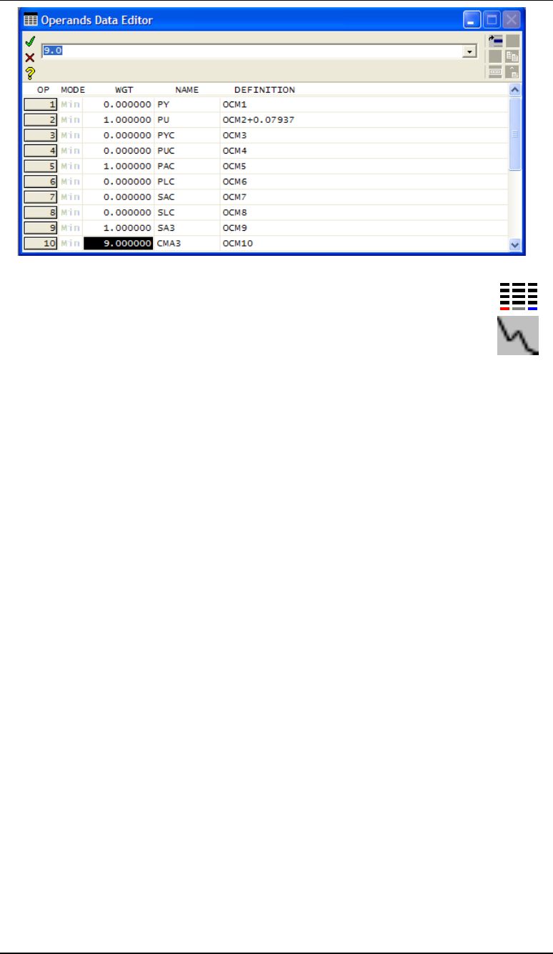
Chapter 9 - Optimization 91
Optimizing using Seidel aberrations
• Close the operands data editor spreadsheet. If it needs to be opened again
press the Edit optimization operands icon.
• Click on the icon to open the optimization conditions spreadsheet.
• Note the entry for the optimization callback, Command for CCL/SCP
operands: opcb_abs
• On the bottom line, under Error function value, select Weighted sum of
squares.
Hence the formula for this error function becomes:
Min error fn = 1 * (PU + 0.07973)2 + 1 * (PAC)2 + 1 * (SA3)2 + 9 * (CMA3)2
• Close the optimization conditions spreadsheet.
To list the starting value of the error function and its component operands:
• In the text window, click on Ope
*OPERANDS
OP MODE WGT NAME VALUE %CNTRB DEFINITION
O 2 M 1.000000 PU 4.4317e-06 0.00 OCM2+0.07937
O 5 M 1.000000 PAC -0.003508 34.19 OCM5
O 9 M 1.000000 SA3 -0.004828 64.76 OCM9
O 10 M 9.000000 CMA3 0.000205 1.05 OCM10
...
MIN ERROR FUNCTION: 3.5988e-05
• To print the minimization error function alone, type the command:
ope erf
MIN ERROR FUNCTION: 3.5988e-05
Description of the Aberration Operands error function
The aberration operands error function consists of a set of predefined operands, including
paraxial ray heights and angles, and Seidel and Buchdahl aberration coefficients. All the
default weights are zero, so that at least one non-zero weight must be specified before it be
used.
The menu header sequence which generates the error function calls the CCL command
opabs_template in file /public/CCL/optim_erfs.ccl. This includes a command:
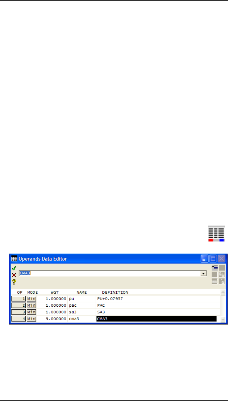
92 Optimization Chapter 9
Optimizing using Seidel aberrations
opt_oprdccl("opcb_abs");
which sets the CCL command opcb_abs (in file /public/CCL/optim_callbaks.ccl) as
the optimization callback. This in turn contains CCL code which is called every time the
error function is evaluated. This callback command, opcb_abs, outputs the values of
Gaussian and Seidel quantities to the text window spreadsheet, and then copies selected
values into the Ocm[] matrix. The key lines of the code from the command opcb_abs are
listed here:
paraxial_trace();
Ocm[2] = ssb(1, 2); // pu
chromatic_abers();
Ocm[5] = ssb(2, 1); // pac
seidel_abers();
Ocm[9] = ssb(3, 1); // sa3
Ocm[10] = ssb(3, 2); // cma3
The relevant lines of CCL in the opabs_template command, which sets up the operands,
are:
operands(new);
opnbr = 0;
opnbr++;o(opnbr, ins, "OCM1 ", 0.0, "PY"); /* Axial ray height */
opnbr++;o(opnbr, ins, "OCM2 ", 0.0, "PU"); /* Axial ray slope */
opnbr++;o(opnbr, ins, "OCM3 ", 0.0, "PYC"); /* Chief ray height */
opnbr++;o(opnbr, ins, "OCM4 ", 0.0, "PUC"); /* Chief ray slope */
opnbr++;o(opnbr, ins, "OCM5 ", 0.0, "PAC"); /* Primary axial color */
opnbr++;o(opnbr, ins, "OCM6 ", 0.0, "PLC"); /* Primary lateral color */
opnbr++;o(opnbr, ins, "OCM7 ", 0.0, "SAC"); /* Secondary axial color */
opnbr++;o(opnbr, ins, "OCM8 ", 0.0, "SLC"); /* Secondary lateral color */
opnbr++;o(opnbr, ins, "OCM9 ", 0.0, "SA3"); /* 3rd-order spherical */
opnbr++;o(opnbr, ins, "OCM10", 0.0, "CMA3"); /* 3rd-order coma*/
...
end();
Users of OSLO Standard and OSLO Premium do have the facility to define the error
function as here described. However they do have a more direct way to define the error
function, using predefined operands with self-explanatory names. This obviates the need for
a CCL callback. The procedure for this is:
• Delete any pre-existing operands using the command sequence:
ope new;end
• Open the operand spreadsheet.
• Add three blank lines and then fill in the entries as shown in the diagram:
• Close the operands data editor spreadsheet and click on Ope to list the operands.
Creating a model glass
Before a glass type can be made variable, it needs to be converted to a “model” glass.
Open the lens data spreadsheet. Change the glass at surface 1 from BK7 to N-BAK4
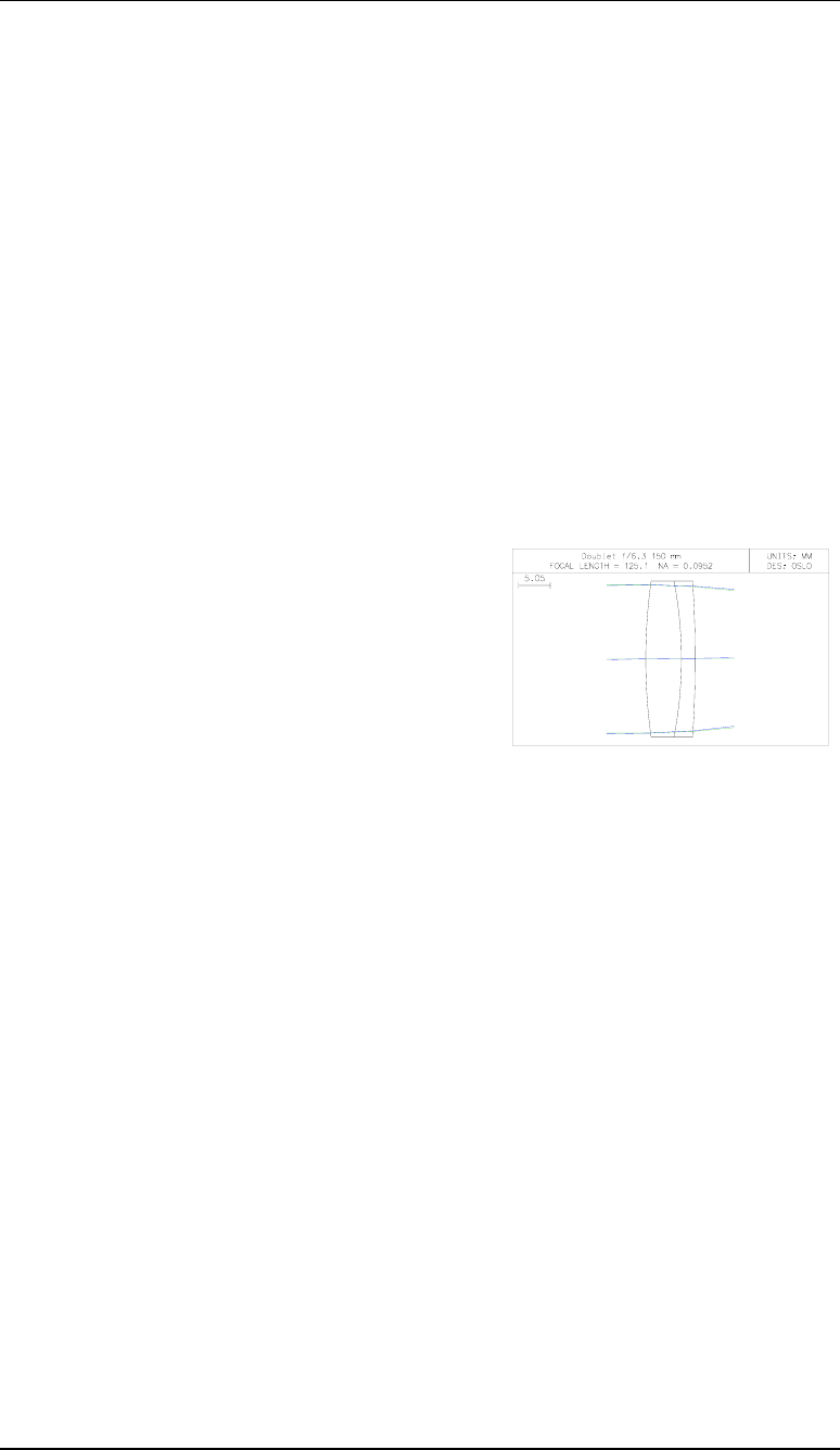
Chapter 9 - Optimization 93
Optimizing using Seidel aberrations
• Under GLASS for the second surface, click on the gray button next to SF5 and select
Model... (M).
• Press Enter three times to accept the default name (GLASS2), refractive index, and
Abbe V-value.
• Click on Rin to list the refractive indices. Although the model glass is specified only by
its refractive index at the d wavelength and Abbe number, the refractive index data for F
and C wavelengths remain almost unchanged.
Defining the optimization variables
• In the surface data spreadsheet, define the variables: Under GLASS for the second
surface GLASS2, click on the gray button, and select Variable RN/DN. (The Special
Variable RN/DN option is exactly equivalent). Note that although the Abbe number is
used to define the dispersion for the model glass it is the OSLO “DN” which is used as a
variable. This is a normalized parameter, best visualized in the index-dispersion plot.
DN takes a value of 0.0 along the line joining N-FK5 and N-SK16, and a value of 1.0
along the line joining N-FK5 and SF11. Nearly all catalog glasses sit between these two
lines, but most of the “normal” glasses tend to cluster about DN = 1.0.
• Click on the variables button at the top of the
spreadsheet, and put an upper limit of 1.0 for the
value of DN, the dispersion parameter for surface
2. Leave the lower limit as 0.
• Also set the minimum value of RN surface 2 as
1.48, the index of FK51, and the maximum
value 1.85, the index of N-LaSF9, the highest
index glass which can be regarded as having reasonable cost and acceptable
environmental properties.
• Click on “Vary all curvatures”.
• Close the variables spreadsheet and the surface data spreadsheet.
• Save the lens. The listing is given here:
*LENS DATA
Doublet f/6.3 150 mm
SRF RADIUS THICKNESS APERTURE RADIUS GLASS SPE NOTE
OBJ -- 1.0000e+20 1.7455e+18 AIR
AST 91.370000 V 5.700000 12.500000 A N-BAK4 C
2 -66.210000 V 2.200000 12.500000 GLASS2 V
3 -197.710000 V 121.451048 S 12.500000 AIR
IMS -- -- 2.182779 S
Optimization
• Using the header of the Text window, list the operands (Ope) and the variables (Var).

94 Optimization Chapter 9
Optimizing using Seidel aberrations
*OPERANDS
OP MODE WGT NAME VALUE %CNTRB DEFINITION
O 1 M -- PY 1.7764e-15 -- OCM1
O 2 M 1.000000 PU -0.015829 2.24 OCM2+0.07937
O 3 M -- PYC 2.182779 -- OCM3
O 4 M -- PUC 0.017260 -- OCM4
O 5 M 1.000000 PAC -0.081694 59.77 OCM5
O 6 M -- PLC -0.000343 -- OCM6
O 7 M -- SAC -0.053498 -- OCM7
O 8 M -- SLC -0.000226 -- OCM8
O 9 M 1.000000 SA3 -0.063974 36.65 OCM9
O 10 M 9.000000 CMA3 0.004069 1.33 OCM10
....
MIN ERROR FUNCTION: 0.011166
*VARIABLES
VB SN CF TYP MIN MAX DAMPING INCR VALUE
V 1 2 - CV -- -- 1.000000 0.000100 0.010945
V 2 3 - CV -- -- 1.000000 0.000100 -0.015103
V 3 4 - CV -- -- 1.000000 0.000100 -0.005058
V 4 3 - RN 1.480000 1.850000 1.000000 0.001000 1.672698
V 5 3 - DN -- 1.000000 1.000000 0.001000 0.929017
• Optimize for 10 cycles (Ite).
*ITERATE FULL 10
NBR DAMPING MIN ERROR CON ERROR PERCENT CHG.
0 1.0000e-08 0.011166 --
1 3.792096 0.002771 -- 75.179931
2 0.002633 6.6051e-06 -- 99.761674
3 0.000615 2.4247e-07 -- 96.329101
4 7.8298e-06 1.0315e-12 -- 99.999575
5 1.2696e-09 2.4261e-19 -- 99.999976
6 1.2696e-09 1.0128e-25 -- 99.999958
7 1.2696e-09 1.0075e-31 -- 99.999901
8 1.269595 8.3919e-32 -- 16.703389
Choosing a real glass type
• Find the DN value of the new glass:
var 5
*VARIABLES
VB SN CF TYP MIN MAX DAMPING INCR VALUE
V 5 2 - DN -- 1.000000 1.000000 0.001000 0.998766
• List its refractive indices and Abbe V-value
rin 2 2
*REFRACTIVE INDICES
SRF GLASS/CATALOG RN1 RN2 RN3 VNBR TCE
2 GLASS2 1.694707 1.711261 1.687937 29.785506 82.000000
• Open the surface data spreadsheet.
• Click on the gray button for surface 2 glass.
• Select FIX and choose the latest Schott catalog (either Schott, or Schott 2004,
depending on the edition of OSLO). In any event the glass chosen should be SF-15.
• Enter rin 2 2:
*REFRACTIVE INDICES
SRF GLASS/CATALOG RN1 RN2 RN3 VNBR TCE
2 SF15 1.698952 1.715461 1.692215 30.067619 79.000000
SCHOTT
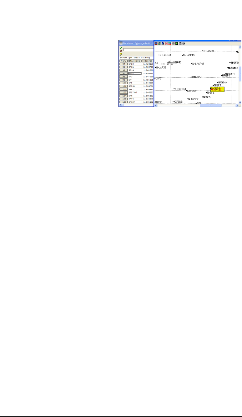
Chapter 9 - Optimization 95
Optimizing using Seidel aberrations
• Open the glass catalog database.
• From the menu header select File >Open database > PUBLIC >
glass_schott.cdb (it may be glass_schott2004.cdb in some versions of OSLO)
• In the GLASSNAME column, click on
SF15.
Note that the glass is highlighted in yellow
on the n-V diagram. The atmospheric and
chemical properties are found in the
column labeled ChemCode (10112).
These are not bad, but a better glass, the
lead- and cadmium-free equivalent is N-
SF15 with a ChemCode of 10111.
• Change the glass for surface 2 to N-SF15: under the gray button for GLASS, select
Catalog > Schott and click on N-SF15 - it is not possible to just type in the name to
replace a model glass.
Final optimization steps
Reoptimize with the remaining parameters (the three surface curvatures).
• Click on Ite:
*ITERATE FULL 10
NBR DAMPING MIN ERROR CON ERROR PERCENT CHG.
0 1.0000e-08 2.7751e-05 --
1 1.0000e-12 2.7540e-05 -- 0.759895
2 1.0000e-12 2.7520e-05 -- 0.073851
3 1.0000e-12 2.7519e-05 -- 0.003876
4 10.000000 2.7519e-05 -- 1.0937e-06
Autofocus
Refocus to minimize the root mean square axial wave aberration, averaged over the three
wavelengths:
• Open the surface data spreadsheet.
• Under the gray THICKNESS button for surface 4 select Autofocus - minimum RMS
OPD > On axis (polychromatic).
• Right click on the text window, and choose Clear window and SS buffer.
• Click on Len
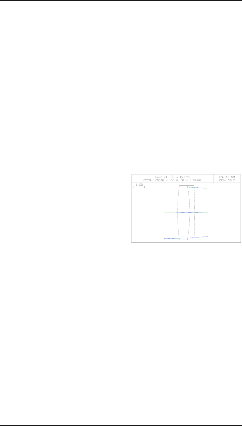
96 Optimization Chapter 9
Optimizing using Seidel aberrations
*LENS DATA
Doublet f/6.3 150 mm
SRF RADIUS THICKNESS APERTURE RADIUS GLASS SPE NOTE
OBJ -- 1.0000e+20 1.7455e+18 AIR
AST 94.166056 V 5.700000 12.500000 A N-BAK4 C
2 -67.121889 V 2.200000 12.500000 N-SF15 C
3 -273.328281 V 146.658952 S 12.500000 AIR
IMS -- 0.080939 2.639626 S
• It is worth combining the distances for surfaces 3 and 4 to avoid confusion: Click on the
defocus value.
b5 = 0.0809387292198
• In the surface data spreadsheet, set the defocus value (thickness surface 4) to 0.
• Also click on the thickness for surface 3, and in the command line add +b5.
146.6589521609103+b5
• Finally, list the lens again:
*LENS DATA
Doublet f/6.3 150 mm
SRF RADIUS THICKNESS APERTURE RADIUS GLASS SPE NOTE
OBJ -- 1.0000e+20 1.7455e+18 AIR
AST 94.166056 V 5.700000 12.500000 A N-BAK4 C
2 -67.121889 V 2.200000 12.500000 N-SF15 C
3 -273.328281 V 146.739891 12.500000 AIR
IMS -- -- 2.639626 S
.

Chapter 9 - Optimization 97
Optimization using finite rays
Optimization using finite rays
The optimization exercise described in this section will be carried on into the tolerance
calculations of the next chapter. Because the starting design is well optimized, the initial
choice of error function and weights is not critical. The GENII error function, which is
given in all versions of OSLO, will be used for the initial design stages.
50 mm f/5.6 objective: specification
Design a triplet objective with a focal length of 50 mm, and a 15º semi-field of view, with
aperture f/5.6. Vignetting is not permitted - that is to say, the full diameter beam must pass
at all field angles. The final detector will be a photographic film with resolution out to 30
cycles/mm, and an MTF of at least 0.1 is required at this spatial frequency. Distortion is not
critical. Only current Schott glass types can be used, and manufacture is to be at
Rodenstock, by traditional methods, with dimensions marked on the final drawing in mm.
Finding a starting design
The most obvious starting point is the standard triplet supplied with the program.
The first task is to set it up with the correct field, aperture and wavelength
weights and to allow the aperture stop (drawn with a red pen) to move separately,
rather than being assigned to an air-glass surface:
• Click on the icon for Open an existing lens.
• At the bottom of the window which opens, after Library Directories: click on
Public.
• Select demo > edu and then click on demotrip.len.
• Click on Open.
• Open the surface data spreadsheet.
• Change the lens identifier to 50 mm f/5.6 +/-15deg
• Click on Wavelength. Define the wavelength weights as 1.0 (.58756) 0.4 (.48613),
0.6 (.65627) and close the wavelength editor.
• Click on Notes, delete all 5 lines of notes and replace with your own annotations.
• Change the entrance beam radius to 4.5 mm. That is, 50/5.6/2, rounded up.
• Change the field angle to 15°
• Click on the gray button for Aperture radius for surface 1, select Not checked.
Repeat for surface 6.
• Click on surface 5.
• Right click and select Insert before
• Change thickness for surface 4 from 6 to 0.0, and thickness for surface 5 frm 0 to
6.0.
• Click on the button for Aperture radius for surface 5, and select Aperture stop.
• Click on the gray button under Special for surface 5 (AST).
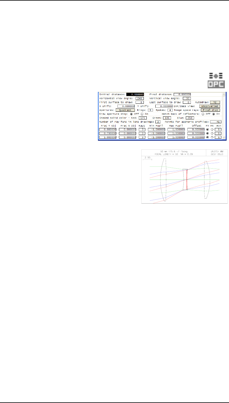
98 Optimization Chapter 9
Optimization using finite rays
• Select Surface Control (F) > General
• On the second line, against Surface appearance in lens drawings: select Drawn.
Set the Pen number for surface in lens drawings as 4 (red).
• Set all the lens aperture radii to Solve. The aperture pickup on surface 2 vanishes.
Checking for vignetting in the starting design
In the triplet provided, the ray drawing conditions have been changed to allow for the
vignetting. The first need is to restore the off-axis beams drawn to their full
diameter.
• Click on the Edit Lens Drawing
Conditions icon.
• In the section which governs
rays drawn at the foot of the
spreadsheet, change the number
of rays for fan No. 2 from 0 to 3.
Set the Min Pupil to -1.0 and
the Max Pupil to +1.0 for fan No. 3.
• Close the Lens Drawing Conditions spreadsheet.
• Draw the lens.
• Click on Len Wav and Pxc to list the lens.
*LENS DATA
50 mm f/5.6 +/-15deg
SRF RADIUS THICKNESS APERTURE RADIUS GLASS SPE NOTE
OBJ -- 1.0000e+20 2.6795e+19 AIR
1 21.250000 2.000000 7.304439 S SK16 C
2 -158.650000 6.000000 6.710505 S AIR
3 -20.250000 1.000000 3.665807 S F4 C
4 19.300000 -- 3.420953 S AIR
AST -- 6.000000 3.420953 AS AIR *
6 141.250000 2.000000 5.931324 S SK16 C
7 -17.285000 42.950000 6.415576 S AIR
IMS -- -- 13.376446 S
*WAVELENGTHS
CURRENT WV1/WW1 WV2/WW2 WV3/WW3
1 0.587560 0.486130 0.656270
1.000000 0.400000 0.600000
*PARAXIAL CONSTANTS
Effective focal length: 50.000541 Lateral magnification: -5.0001e-19
Numerical aperture: 0.089999 Gaussian image height: 13.397605
Working F-number: 5.555616 Petzval radius: -149.381547
Lagrange invariant: -1.205771
Chapter 9 - Optimization 99
Optimization using finite rays
Assessing the starting design
The diagram above indicates the edge thicknesses of the positive components are far too
small for economic manufacture. The center thickness of the negative lens needs increasing
as well. And the stop needs to move away from the second surface of the negative lens to
allow a plane diaphragm plate to be used.
• In the Standard Tools graphics menu, click on the Through-Frequency MTF
icon.
• Right click in the graphics window, and select
Recalculate with new parameters...
• Enter Maximum frequency 30 cycles/mm.
The resolution, especially in the off-axis points, needs
improvement, but otherwise the performance is good.
• Click on the icon for ray intercept curves.
• Right click in the graphics window, and select
Recalculate with new parameters...
• Enter a value of 0.03333 mm (the reciprocal
of the customer-defined spatial frequency) for
the User aberration scale.
The transverse aberrations at all wavelengths in the
meridional (Y) section off axis particularly need to be
reduced.
Defining and validating the error function
• From the Optimize menu header, select Generate error function > GENII Ray
Aberration...
• Fill in the entries for a Design frequency of 30 cycles/mm.
• Fill in the pupil coordinates on the basis of no vignetting: F1 (on axis)
fymax = 1.0 F2 (0.7 field) fymin = -1.0 fymax = 1.0 fx = 1.0
F3 (edge of field) fymin = -1.0 fymax = 1.0 fx = 1.0.
• The tolerance on distortion at both F2 and F3 is distol = 10% (in other
words, distortion will not be tightly controlled).
• Finally click on OK to close the Geniierf spreadsheet.
• Type in the command line ope all to list the operands that have been defined by this
command. (Operands which begin with an underscore are not listed by clicking on the
Ope icon in the text window.)
Only the first 13 are listed below.

100 Optimization Chapter 9
Optimization using finite rays
*OPERANDS
OP MODE WGT NAME VALUE %CNTRB DEFINITION
O 1 M -- _Dy tol 0.005556 -- 0.0055555555556
O 2 M -- _2.1 Dy 0.011667 -- 0.0116666666667
O 3 M -- _2.8 Dy 0.015556 -- 0.0155555555556
O 4 M -- _3 Dy 0.016667 -- 0.0166666666667
O 5 M -- _4 Dy 0.022222 -- 0.0222222222222
O 6 M -- _up Dy/3 0.283656 -- 0.283655904077
O 7 M -- _3.2 up Dy 2.723097 -- 2.72309667914
O 8 M -- _uprime -3.5749e-14 -- PU+0.0899990260196
O 9 M 1.000000 Fnb diff -3.5749e-10 0.00 O8/0.0001
O 10 M 1.000000 Focus diff 0.704983 0.26 DYY(1,1)/O4
O 11 M 1.000000 Axial DY 0.035247 0.00 DY(1,2)/O1
O 12 M 1.000000 Axial OPD -1.189682 0.75 OPD(1,2)/O6
O 13 M 1.000000 Axial DMD 1.828939 1.78 DMD(1,2)/O6
The first weighted operand controls the focal length rather tightly. In the initial stages of
design it is preferable that this be relaxed. So:
• Click on the icon for Edit optimization operands.
• Change the weight for operand 9 from 1.0 to 0.1.
• List the operands, noting in particular any that have contributions above 10%. They
are:
O 21 M 1.000000 0.7 OPD U -5.224602 15.30 OCM21/OCM6
O 22 M 1.000000 0.7 DMD U 4.600139 11.86 OCM22/OCM6
O 24 M 1.000000 0.7 OPD L -4.782094 12.82 OCM24/OCM6
O 36 M 1.000000 1.0 OPD U -5.267896 15.55 OCM36/OCM6
O 37 M 1.000000 1.0 DMD U 6.020660 20.31 OCM37/OCM6
These are respectively, for the 0.7 field point, wave aberration and color for the upper Y-
section ray, and wave aberration for the lower ray; also for the full field, wave aberration
and color for the upper Y-section ray. These are the same aberrations as the plot above
indicates will be causing the greatest reduction in MTF, so the error function has been
validated.
Note that the initial value for the error function is given on the last line of the operand
listing as the root mean square of the weighted contributions:
MIN RMS ERROR: 2.434848
Description of the GENII error function
The GENII error function provided with all versions of the program is remarkably sparse yet
effective. It makes maximum use of the results of ray-tracing from a single marginal ray on
axis, and a chief ray and three rays in the pupil for each of two other field angles. The
aberrations of these rays constitute the error function.
The error function has two weighted operands controlling the Gaussian properties, three to
control the axial image formation (transverse ray aberration DY, wave aberration OPD and
Conrady chromatic variation in wave aberration DMD for color control), and 13 to control
the four rays at each of the off-axis points at FBY = 0.7 and 1.0. This makes a total of 31,
leaving the remaining 19 for necessary data storage.
Because the dimensions of transverse ray aberrations, wavefront aberrations, longitudinal
errors and color are so different, the error function uses scaling factors on each to enable the
default value of unity weighting as the starting value for each operand. For example, the
basic scaling factor on transverse errors is (6 N)-1 where N is the design spatial frequency.
Defining the error function invokes a call to geniierf() (or, for users of OSLO-EDU,
geniierf_lt) which is in public/ccl/optim_erfs.ccl. The OSLO EDU version specifies
geniiops as a callback, which will be found in public/ccl/optim_callbaks.ccl. More
information is available in OSLO Help.
Chapter 9 - Optimization 101
Optimization using finite rays
Defining the optimization variables
• Open the surface data spreadsheet.
• Click on the gray button for thickness 2, and select Variable.
• Repeat for thicknesses 4, 5, 7.
• Click on the Variables button to open the variables spreadsheet.
• Click on the Vary all curvatures button.
• For variable 2 (thickness 4) set a MIN value of 0.5 mm, leaving all other limits as
default.
• Close the variables spreadsheet.
• Close the surface data spreadsheet
• List the optimization variables by clicking on Var:
*VARIABLES
VB SN CF TYP MIN MAX DAMPING INCR VALUE
V 1 2 - TH 0.100000 1.0000e+04 1.000000 0.000450 6.000000
V 2 4 - TH 0.500000 1.0000e+04 1.000000 0.000450 -- *
V 3 5 - TH 0.100000 1.0000e+04 1.000000 0.000450 6.000000
V 4 7 - TH 0.100000 1.0000e+04 1.000000 0.000450 42.950000
V 5 1 - CV -- -- 1.000000 2.2222e-05 0.047059
V 6 2 - CV -- -- 1.000000 2.2222e-05 -0.006303
V 7 3 - CV -- -- 1.000000 2.2222e-05 -0.049383
V 8 4 - CV -- -- 1.000000 2.2222e-05 0.051813
V 9 6 - CV -- -- 1.000000 2.2222e-05 0.007080
V 10 7 - CV -- -- 1.000000 2.2222e-05 -0.057854
There is an asterisk against thickness 4 indicating that the current value of the variable (=0)
violates the permitted range. As a result, the error function has increased.
• Click on the Ope in the text window.
MIN RMS ERROR: 3.772815
Optimization
• Two clicks on the Ite button gives the output shown below for this error function.
*ITERATE FULL 10
NBR DAMPING MIN ERROR CON ERROR PERCENT
CHG.
0 1.0000e-08 3.772815 --
1 1.0000e-05 2.061430 -- 45.360945
2 1.0000e-05 1.548952 -- 24.860311
3 1.0000e-05 1.326489 -- 14.362182
4 6.1580e-06 1.295507 -- 2.335646
5 2.3352e-06 1.292165 -- 0.257970
6 2.3352e-06 1.292093 -- 0.005549
7 0.000144 1.292093 -- 2.4329e-05
*ITERATE FULL 10
NBR DAMPING MIN ERROR CON ERROR PERCENT
CHG.
0 1.0000e-08 1.292093 --
1 1.0000e-08 1.292093 -- --
2 1.0000e-08 1.292093 -- --
If warning messages about clear aperture checking
appear with OSLO EDU they will not affect the result
significantly, although the final error function may differ slightly from the values given
here..

102 Optimization Chapter 9
Optimization using finite rays
The performance has improved considerably - the lowest MTF at 30 cycles/mm is 0.6 (for T
section at .7 field). The prescription is:
*LENS DATA
50 mm f/5.6 +/-15 deg
SRF RADIUS THICKNESS APERTURE RADIUS GLASS SPE NOTE
OBJ -- 1.0000e+20 2.6795e+19 AIR
1 25.838240 V 2.000000 7.591942 S SK16 C
2 -103.139037 V 6.389728 V 7.036229 S AIR
3 -14.888983 V 1.000000 3.888863 S F4 C
4 22.497814 V 0.499055 V 3.683790 S AIR
AST -- 3.457640 V 3.568729 AS AIR *
6 161.514578 V 2.000000 5.108018 S SK16 C
7 -13.810731 V 44.869598 V 5.633273 S AIR
IMS -- -- 13.373470 S
The focal length is 50.05 mm, an error of less than 0.1% so there is no need to increase the
weight on operand 9.
Engineering aspects: edge thicknesses
As this lens is to be made by traditional means, a blank needs to be procured with sufficient
extra diameter to allow each component to be centered by edging. The thicknesses of all the
lenses need to be increased to improve manufacturing yield. Making an allowance of 3 mm
on diameter beyond the largest clear aperture diameter for the mounting (with an extra 1 mm
on the front lens to allow for weather-proofing), and a further 2 mm for the blank, the edge
thickness of each blank should be about 1.5 mm minimum.
To calculate the edge thicknesses of the blanks for the two positive lenses:
• From the Lens menu header select Show Auxiliary Data > Edge Thickness.
• For component 1, enter surface A =1, surface B = 2. Enter the clear semi-diameter
7.6 mm plus 3 mm = 10.6 mm for the y-height at both surfaces:
*DISTANCE FROM SRFA 1 TO SRFB 2
AT YHTA YHTB XHTA XHTB ZSAGA ZSAGB
10.600000 10.600000 -- -- 2.274242 -0.546529
IS XDIS YDIS ZDIS GLOBAL DISTANCE
-- -- -0.820771 0.820771
The edge thickness given (ZDIS) is -0.82 mm, so the centre thickness for surface 1
needs to be increased by about 2.8 mm to reach the target of 1.5 mm.
• Repeating for surface A =6, B = 7, enter 5.6+2.5 = 8.1 mm for the y-height at
both surfaces. otherwise type the command:
eth 6 7 8.1 8.1 0 0
For this lens, the edge thickness of the blank (ZDIS) is -0.83 mm, so the centre
thickness for surface 6 also needs to be increased by about 2.8 mm.
The centre thickness of the negative lens (surface 3) is too thin, and should also be
increased to 1.5 mm.
Rather than making these directly in the spreadsheet, they will be used to illustrate the
process whereby adjustments can be made with simultaneous optimisation.
Chapter 9 - Optimization 103
Slider-wheels with concurrent optimization on MTF
Slider-wheels with concurrent optimization on MTF
Adjusting lens thicknesses
The facility provided by OSLO to carry out slider-wheel optimization on one or more
parameters, with a simultaneous callback to optimization on other variables, is a powerful
design tool. In this context, note that no parameter adjusted with the slider-wheel bars
should be an optimization variable. In the example given here, the slider-wheels will be used
to adjust the lens thicknesses 1 for surfaces 1, 3 and 6, while the optimization on the lens
curvatures, air spaces and image distance will continue to correct performance during each
adjustment.
• Close the surface data spreadsheet.
• Open the slider-wheel spreadsheet.
• Select Ray-intercept curves at All points in the field.
• Define three sliders for Thickness (TH) 1 Thickness (TH) 3 and Thickness (TH)
6.
• Select Enable sw_callback CCL function with Level = 9 (This must be in the
range from 1 to 9 to trigger the Iter function in the callback command.).
• Close the slider-wheel setup spreadsheet.
The text window, the slider-wheel bar and the two temporary slider-wheel windows, GW31
and GW32, should all be visible. The starting value of the error function is 1.292.
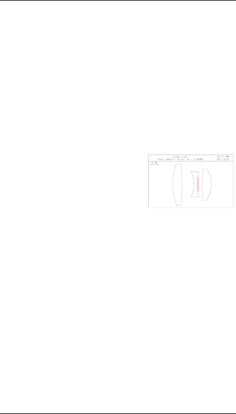
104 Optimization Chapter 9
Slider-wheels with concurrent optimization on MTF
• Increase thickness 1 in steps of 0.1 until it reaches 4.0 giving an error function of 1.309.
• Increase thickness 3 in steps of 0.1 until it reaches 1.5. The error function will be 1.372
• Increase thickness 6 until it reaches 3.0; the error function becomes 1.408.
• Increase thickness 1 to 4.7 and thickness 6 to 4.7, the optimized error function will be
1.480.
• Close the slider wheels and list the lens.
*LENS DATA
50 mm f/5.6 +/-15 deg
SRF RADIUS THICKNESS APERTURE RADIUS GLASS SPE NOTE
OBJ -- 1.0000e+20 2.6795e+19 AIR
1 29.485222 V 4.700000 8.263805 S SK16 C
2 -86.537346 V 6.170610 V 6.982274 S AIR
3 -15.359048 V 1.500000 3.947019 S F4 C
4 21.674799 V 0.498922 V 3.637632 S AIR
AST -- 2.252805 V 3.522903 AS AIR *
6 77.234402 V 4.700000 4.546980 S SK16 C
7 -14.489037 V 44.432412 V 5.759546 S AIR
IMS -- -- 13.376786 S
• Now to check the edge thicknesses, calculate the edge thickness of the front lens
blank at a radius of 8.3+3.0 = 11.3 mm:
eth 1 2 11.3 11.3 0 0
giving a value of 1.7 mm.
• Also find the edge thickness of the third lens
blank at a radius of 5.8+2.5 = 8.3 mm:
eth 6 7 8.3 8.3 0 0
which gives 1.6 mm.
These are both above the 1.5 mm which is required. For the diagram which shows the blank
sizes, the barrel semi-diameters have been rounded upwards to 10 mm, 5.5 mm and 7.5 mm
respectively.
Engineering aspects: ambiguity avoidance
It is extremely hard to tell which of the two surfaces of a nearly equi-concave lens is the
steepest. To avoid assembly errors, we will investigate the effect of making the second lens
truly equi-concave.
• Make the second element equi-concave. Click on the surface 4 gray RADIUS button
and select Minus curvature pickup (P)... with Pickup source surface = 3
Pickup constant = 0, Pickup multiplir = 1.0.
• Reoptimise. The error function is 1.640. This increase is acceptable.

Chapter 9 - Optimization 105
Slider-wheels with concurrent optimization on MTF
*LENS DATA
50mm f/5.6 +/-15 deg
SRF RADIUS THICKNESS APERTURE RADIUS GLASS SPE NOTE
OBJ -- 1.0000e+20 2.6795e+19 AIR
1 26.647695 V 4.700000 8.681421 S SK16 C
2 -361.254520 V 7.067320 V 7.317984 S AIR
3 -18.435016 V 1.500000 3.907032 S F4 C
4 18.435016 P 0.499751 V 3.580456 S AIR
AST -- 2.398524 V 3.464412 AS AIR *
6 42.567801 V 4.700000 4.577052 S SK16 C
7 -16.089048 V 43.427580 V 5.729062 S AIR
IMS -- -- 13.383518 S
Engineering aspects: testplate fitting
• Select the Rodenstock test glass file: Under the File menu header, select Preferences
> Set preference > Test_glass_file and in the command line enter
rodenstock.tgl.
This refers to an ASCII file rodenstock.tgl in the directory OSLO/Prm64/bin/lmo/
which contains 1446 test glass values. Test glass files for other manufacturers are also
available, and the user may create others in the same format if desired.
• Open the surface data spreadsheet.
• For surface 7 (the shortest radius at 16.09 mm) remove the variable curvature (change to
Direct specification).
• Hold down the shift key and left-click the mouse twice on the radius. A value -
16.0766 will appear as the nearest test glass, with a black box around it.
• Click on the green tick to accept this (or shift-left-click to restore the nominal radius).
The letter T appears next to the fitted radius.
• Press Ite to optimize the remaining variables.
• Repeat this sequence for surface 3 - remove the variable, fit the closest test glass,
and optimise remaining variables.
• Repeat this sequence for surface 6 and then again for surface 2.
• Click on Len to list the design. Note the T which appears against each radius which
has bees fitted to a test glass.
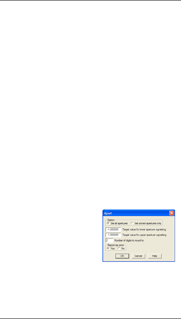
106 Optimization Chapter 9
Slider-wheels with concurrent optimization on MTF
*LENS DATA
50 mm f/5.6 +/-15 deg
SRF RADIUS THICKNESS APERTURE RADIUS GLASS SPE NOTE
OBJ -- 1.0000e+20 2.6795e+19 AIR
1 26.699200 T 4.700000 8.692011 S SK16 C
2 -375.820000 T 7.098400 V 7.328991 S AIR
3 -18.438800 T 1.500000 3.907388 S F4 C
4 18.438800 P 0.499794 V 3.581367 S AIR
AST -- 2.384983 V 3.465615 AS AIR *
6 42.322100 T 4.700000 4.572836 S SK16 C
7 -16.076600 T 43.429946 V 5.724953 S AIR
IMS -- -- 13.380875 S
• Click on Ope in the text window.
MIN RMS ERROR: 1.641164
The error function has risen slightly.
Rounding air spaces
Round the air spaces to avoid giving the impression that they are subject to tight tolerances:
• Change thickness 2 to 7.1, delete the variable and re-optimize.
• Change thickness 4 to 0.5, delete the variable and re-optimize.
• Change thickness 5 to 2.4, delete the variable and re-optimize on the one remaining
variable, the focus.
• Enter the command: ope erf
The error function has risen slightly:
MIN RMS ERROR: 1.645251
Adjusting clear apertures
• Close the variables spreadsheet and the lens data spreadsheet.
• Under the Optimize menu header, select Support routines > Vignetting > Set
apertures and in the dialog box change the
number of digits to 2.
• Click on OK.
*APERTURES
SRF TYPE APERTURE RADIUS
0 SPC 2.6795e+19
1 SPC 8.500000 CHK
2 SPC 8.500000
3 SPC 4.000000
4 SPC 3.600000
5 SPC 3.500000 CHK
6 SPC 5.500000
7 SPC 5.500000 CHK
8 CMP 13.380786
• Remove the Checked aperture (K) indications from surfaces 1, 5 and 7.
• Change the clear aperture surface 4 to 4.0 mm (as this lens is reversible).
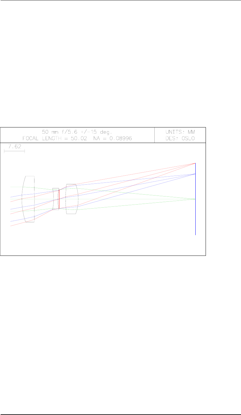
Chapter 9 - Optimization 107
Slider-wheels with concurrent optimization on MTF
• Remove the Pickup (P) from the radius on surface 4, change all the other radii to
Direct specification, but leave the variable on the back focal distance (thickness 7).
• List the lens:
50 mm f/5.6 +/-15 deg.
SRF RADIUS THICKNESS APERTURE RADIUS GLASS SPE NOTE
OBJ -- 1.0000e+20 2.6795e+19 AIR
1 26.699200 4.700000 8.500000 SK16 C
2 -375.820000 7.100000 8.500000 AIR
3 -18.438800 1.500000 4.000000 F4 C
4 18.438800 0.500000 4.000000 AIR
AST -- 2.400000 3.500000 A AIR *
6 42.322100 4.700000 5.500000 SK16 C
7 -16.076600 43.397798 V 5.500000 AIR
IMS -- -- 13.366656 S *
This completes the design of this lens. The next chapter will start from this point as the basis
of the tolerance calculation exercise.

108
Chapter 10 - Tolerances and drawings
50 mm f/5.6 objective: specification
For the lens which is the final design of the triplet describes in the previous section, the task
is to define the surface and component tolerances which, based on root-sum-of-squares
statistics, give an MTF which does not fall below 0.1 at 30 cycles/mm at any of the three
field points. The assumption will be made that in production there will be a uniform
distribution of errors within the tolerance band, and that a focus adjustment will be carried
out on assembly.
This will be accomplished using a CCL command which assesses the MTF at 30 cycles/mm
in both azimuths at 5 field points across the field - with values of FBY of 0.0, ± 0.7 and ±
1.0.
Defining the tolerance error function:”opcb_dmtf”
The CCL routine below will calculate the MTF in 2 azimuths at 5 field points, 10 values in
all. It will then identify the worst (i.e. lowest) of these, and subtract it from the diffraction
limited MTF at the same frequency. The error function consists of a single operand, having
this value.
Subtracting the lowest MTF from the ideal ensures that, as in all optimization operands, the
system with the lowest value of the error function is the best one.
The routine here is a “callback” - that is to say, it is evaluated whenever the error function
is calculated. It places a single value into the real array ocm[1]. This value is then called
using the string OCM1 as the definition of the operand.
• Open the text editor and create a new file:
//
// Written by [your name] [Date]
//
cmd opcb_dmtf(void)
// hlp: <P>Callback for DMTF (degradation in MTF) optimization.
// hlp: OCM1 is max reduction in MTF below ideal MTF at 5 field
// hlp: points for one spatial frequency. Both X & Y are included
// hlp: on axis, as well as field height FBY both +ve and -ve.</P>
{
static double mtfs[10],diff_lim,mtf_min;
static double sf=30.0; //spatial frequency
stp outp off;
k=sbrow;
sbr k 1;//scrolls spread sheet buffer to preserve contents
sop(0,0,0);
mtf(tfr,chr,y,sf,sf,0);
mtf(tfr,chr,x,sf,sf,0);
sop(0.7,0,0);
mtf(tfr,chr,y,sf,sf,0);
mtf(tfr,chr,x,sf,sf,0);
sop(-0.7,0,0);
mtf(tfr,chr,y,sf,sf,0);
mtf(tfr,chr,x,sf,sf,0);
Chapter 10 - Tolerances and drawings 109
Defining the tolerance error function:”opcb_dmtf”
sop(1,0,0);
mtf(tfr,chr,y,sf,sf,0);
mtf(tfr,chr,x,sf,sf,0);
sop(-1,0,0);
mtf(tfr,chr,y,sf,sf,0);
mtf(tfr,chr,x,sf,sf,0);
diff_lim=d5;
if(diff_lim==0) cclabort("Diff limited MTF zero","opcb_dmtf");
mtfs[0]=b5;// Ax T
mtfs[1]=b8;// AX S
mtfs[2]=b14;// +7 T
mtfs[3]=b17;// +7 S
mtfs[4]=b23;// -7 T
mtfs[5]=b26;// -7 S
mtfs[6]=b32;// +1 T
mtfs[7]=b35;// +1 S
mtfs[8]=b41;// -1 T
mtfs[9]=b44;// -1 S
mtf_min=1.0;
for(i=0;i<10;i++)if(mtfs[i]<mtf_min)mtf_min=mtfs[i];
ocm[1]=diff_lim-mtf_min;// DMTF: MAX FALL BELOW DIFFRACTION LIMIT
sbr -k 0;
stp outp on;
}
• Save the command in /private/ccl/ with the name optim_dmtf.ccl, and check correct
compilation.
*CCL COMPILATION MESSAGES:
No errors detected
• Open the optimization conditions spreadsheet.
• Change the entry for the optimization callback, Command for CCL/SCP
operands: opcb_dmtf
• On the bottom line, under Error function value, select Root-mean-square
(RMS).
• Close the optimization conditions spreadsheet.
• Enter the command line ope new;end to delete the existing operand list.
• Open the operands data editor spreadsheet.
• Fill in the name and definition as in the following table:
OP MODE WGT NAME DEFINITION
1 MIN 1.000000 DMTF at 30 OCM1
• Close the operands spreadsheet and list the operands with Ope
*OPERANDS
OP MODE WGT NAME VALUE %CNTRB DEFINITION
O 1 M 1.000000 DMTF at 30 0.408358 100.00 OCM1
MIN RMS ERROR: 0.408358
Since there is only one operand in the error function, the value of the RMS minimization
error is the actual value of DMTF, the degradation in MTF.
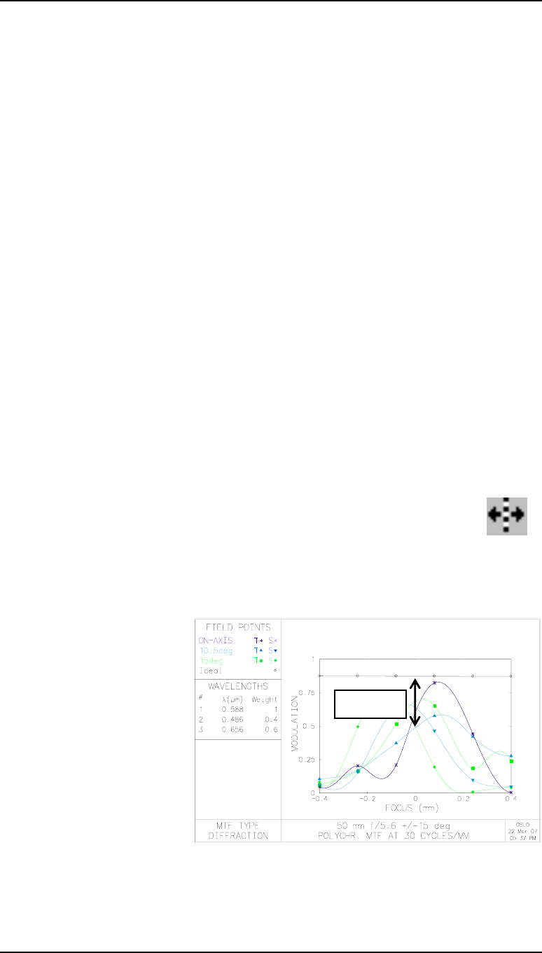
110 Tolerances and drawings Chapter 10
Optimizing on the compensator
Defining the compensator
To enable the widest possible tolerances to be assigned to the lens, one or more
“compensators” can be defined. These represent the adjustments made during assembly
which can partly compensate the errors in the individual components. The most common
compensator is, of course, the focus, and that is the only compensator used in this example.
To define a compensator, the parameter concerned must be defined as an optimization
variable.
• In the text window click on Var.
• Confirm that thickness 7 is variable, and is the only variable.
Before commencing the calculation of tolerances, the compensator must be set to the
optimum position for the nominal design.
Optimizing on the compensator
• To find the best focus, just optimize with Ite and click on Var
*ITERATE FULL 10
NBR DAMPING MIN ERROR CON ERROR PERCENT CHG.
0 1.0000e-08 0.408358 --
1 6.158000 0.367641 -- 9.970860
2 61.580000 0.361620 -- 1.637656
3 379.209640 0.360640 -- 0.271130
4 379.209640 0.360640 -- --
5 379.209640 0.360640 -- --
*VARIABLES
VB SN CF TYP MIN MAX DAMPING INCR VALUE
V 1 7 - TH 0.100000 1.0000e+04 1.000000 0.000450 43.385935
To confirm the choice of focal plane, plot the through-focus MTF at 30 cycles/mm:
• Click on the icon and accepting all defaults.
• Right click in the graphics window, and select Recalculate with new
parameters...
• Enter Frequency 30 cycles/mm.
The curves show that the
ideal focal plane has been
chosen.
The diagram also illustrates
the significance of the
quantity DMTF. It is the
largest drop below the
diffraction limit at any of
the five field points, with
assessment in both sagittal
and tangential directions
(including on axis). This
error function has been
chosen so that asymmetric
tolerances can be included in
DMTF
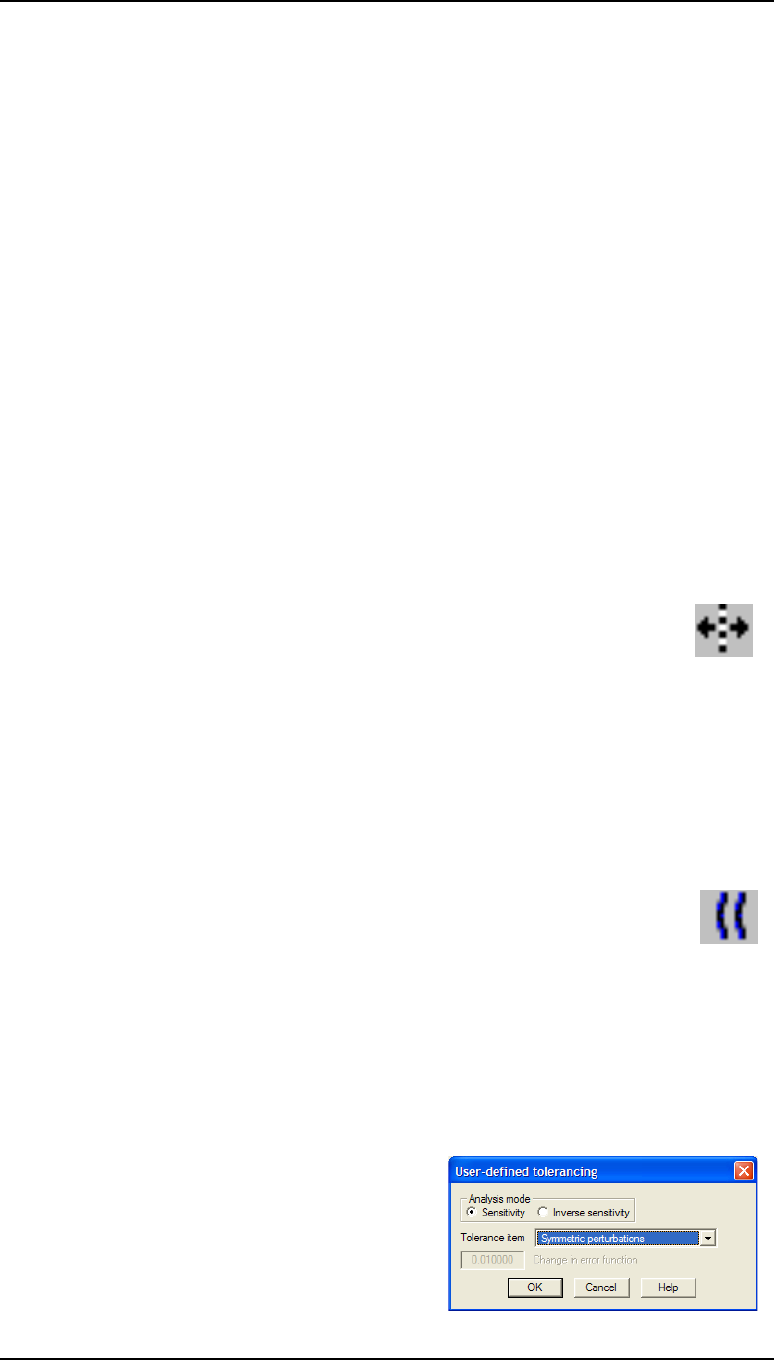
Chapter 10 - Tolerances and drawings 111
Calculating decenter tolerances
the calculation.
• Under the Evaluate menu header, select Transfer function > Print/Plot OTF and
in the dialog box select: Monochromatic, Print function, with Maximum
frequency = 30 line pairs per mm.
In this case the diffraction limit MTF at 30 cycles/mm is 0.86. At the best focus, the
nominal value of the worst MTF at 30 cycles/mm is 0.49, giving a value of DMTF for the
nominal system of 0.36. If the MTF must remain everywhere above 0.1, the value of
DMTF must not increase to more than 0.76.
Calculating decenter tolerances
As an example we will calculate the effect of decentering the second lens by the minimum
amount one can expect from traditional mounting methods:
• Open the surface data spread sheet.
• Under Special for surface 3, select Coordinates (C).
• Enter .075 mm for DCY, and under Use base coordinates for returns to this surface:
select Yes.
• Under Special for surface 4, select Coordinates (C).
• Under Coordinate return: select Yes and under Return to surface: enter 3
• Click on Ope and find the new DMTF value:
MIN RMS ERROR: 0.612975
So DMTF has increased from 0.36 to 0.61, an increase of 0.25. This has used
more than half the entire tolerance budget of 0.40 on one error, so clearly a specialized
mounting method (such as laser centering in the mount) will need to be used to meet the
performance target. That being the case, we will assume that all the component decenter
tolerances can be regarded as zero, and calculate the budget for the remaining errors.
Checking tolerance entries
The default tolerance values assigned to each parameter are the ISO10110 values. Because
there are two successive air spaces (4 and 5), the tolerance on the first one can be removed.
• Click on the Edit Surface Tolerances icon, or select from the menu header
Tolerance > Update tolerance data > Surface.
• Click on Display all surfaces tolerances: Yes.
• For surface 4, set TH TOL (thickness tolerance) to 0.0
• Close the surface tolerances data editor.
Symmetrical tolerances surface calculation
• From the menu header select Tolerance >
User-defined Tolerancing and select
Sensitivity and Symmetric perturbations.

112 Tolerances and drawings Chapter 10
Symmetrical tolerances surface calculation
• A warning message comes up. The error function does not assume rotational symmetry,
so click on OK.
The sensitivity analysis (which may take one or two
minutes) lists 6 power errors, 3 element thicknesses,
2 air spaces, 3 indices and 3 V-values, 17
symmetrical contributions in all. The summary is:
UNCOMPENSATED COMPENSATED
WORST CASE CHANGE 6.019989 3.022531
STANDARD DEVIATION
RSS 1.659396 1.056369
UNIFORM 0.958053 0.609895
GAUSSIAN 0.729824 0.464604
The change in the error function, with focus compensation, for a uniform distribution of
errors within the tolerance band is 0.61 is an indication that the standard tolerances are not
acceptable.
If we allocate 0.33 of the budget of 0.40 to the symmetrical tolerances, then each tolerance
will be allowed 0.33/√17 = 0.08 MTF degradation.
• From the menu header select Tolerance > User-defined Tolerancing and select
Inverse sensitivity and Symmetric perturbations, enter 0.08 for Change in
error function.
*INVERSE SENSITIVITY ANALYSIS
ERROR FUNCTION FOR NOMINAL SYSTEM: 0.360640
ALLOWED CHANGE IN ERROR FUNCTION: 0.080000
POWER ERROR TOLERANCE
ALLOWED TOLERANCE
SRF UNCOMPENSATED COMPENSATED
1 4.204420 109.362285
2 4.416476 72.560814
3 1.941512 1.807345
4 1.910946 1.747543
6 3.571230 3.882230
7 3.599738 27.941716
These tolerances must be tightened from the ISO10110 values of 10, 10, 5, 5, 10 and 10
fringes to 5 fringes throughout.
ELEMENT THICKNESS TOLERANCE
ALLOWED TOLERANCE
SRF UNCOMPENSATED COMPENSATED
1 0.074299 0.096090
3 0.079866 0.246151
6 0.109412 0.337794
The first one needs to be changed to from the ISO10110 value of 0.2 to 0.1 mm.
AIR SPACE TOLERANCE
ALLOWED TOLERANCE
SRF UNCOMPENSATED COMPENSATED
2 0.079453 0.053990
5 0.035223 0.036388
These must be tightened to 0.05 mm.
INDEX OF REFRACTION TOLERANCE
ALLOWED TOLERANCE
SRF UNCOMPENSATED COMPENSATED
1 0.000460 0.006810
3 0.000381 0.000346
6 0.000376 0.000342
These must all be tightened from .001 to 0.0006 (note that the glass type for lens 1 and for
lens 3 are the same, so only one standard of glass need be procured).

Chapter 10 - Tolerances and drawings 113
Asymmetric tolerances surface calculation
ABBE V-NUMBER ERROR (IN %) TOLERANCE
ALLOWED TOLERANCE
SRF UNCOMPENSATED COMPENSATED
1 5.230509 20.247082
3 3.291042 12.443420
6 4.223386 14.964191
These can stay at 0.8%.
Updating symmetrical surface tolerances
• Click on the Edit Surface Tolerances icon, or select from the menu header
Tolerance > Update tolerance data > Surface.
• Change the tolerances on symmetric form error (PWR FR) at all surfaces to 5
• Change the tolerances on thickness (TH TOL) at surfaces 2 and 5 to 0.05.
• Change the tolerance on thickness (TH TOL) at surfaces 1 to 0.1
• Change the tolerances on index (RN TOL) at surfaces 1 3 and 6 to 0.0006.
• Close the surface tolerances data editor.
• Repeat the sensitivity calculation for symmetrical tolerances:
STATISTICAL SUMMARY
UNCOMPENSATED COMPENSATED
WORST CASE CHANGE 4.548071 0.744409
STANDARD DEVIATION
RSS 1.271472 0.472209
UNIFORM 0.734085 0.272630
GAUSSIAN 0.559210 0.207684
COMPENSATOR STATISTICS
COMP MEAN STD DEV MAX RSS
TH 7 -0.011420 0.099581 0.356100 0.483578
• The degradation of 0.27 (less than the 0.33 allowed for) leaves a balance of 0.13 for the
asymmetric tolerances.
Asymmetric tolerances surface calculation
Since the full asymmetrical sensitivity analysis cannot be undertaken with OSLO EDU, the
relevant elements of the sensitivity analysis will be calculated separately.
There are only two surface errors to be considered. These consist of 6 surface irregularity
errors, and 6 surface tilt errors (TLA only), 12 in all. If we allocate the remaining 0.13 of
MTF degradation (that is, the budget of 0.4 minus the 0.27 taken up by symmetrical
tolerances) to these 12 tolerances, then each contribution is 0.13/√12 = 0.038.
• Remove the variable from thickness 7 – focus cannot compensate for asymmetrical
errors.
• Remove the variable from thickness 7, since focus cannot compensate for asymmetrical
errors.
• From the menu header select Tolerance > User-defined Tolerancing and select
Inverse sensitivity and Irregularity fringes, enter 0.038 for Change in error
function.

114 Tolerances and drawings Chapter 10
Asymmetric tolerances surface calculation
*INVERSE SENSITIVITY ANALYSIS
ERROR FUNCTION FOR NOMINAL SYSTEM: 0.360640
ALLOWED CHANGE IN ERROR FUNCTION: 0.038000
IRREGULARITY ERROR TOLERANCE
ALLOWED TOLERANCE
SRF UNCOMPENSATED
1 2.097225
2 2.261429
3 0.816355
4 0.818204
6 1.263006
7 1.188189
The tolerance on both surfaces of the last lens needs to be changed to from the ISO10110
value of 2 fringes to 1 fringe.
• From the menu header select Tolerance > User-defined Tolerancing and select
Inverse sensitivity and Surface tilt tolerance (TLA), and again enter 0.038 for
the Change in error function.
*INVERSE SENSITIVITY ANALYSIS
ERROR FUNCTION FOR NOMINAL SYSTEM: 0.360640
ALLOWED CHANGE IN ERROR FUNCTION: 0.038000
SURFACE TILT TOLERANCE (TLA)
ALLOWED TOLERANCE
SRF UNCOMPENSATED
1 0.139481
2 0.108784
3 0.145052
4 0.161710
6 0.153277
7 0.110764
All these tilt tolerances must be changed to 0.08 degrees (5 minutes).
Updating asymmetric surface tolerances
• Click on the Edit Surface Tolerances icon, or select from the menu header
Tolerance > Update tolerance data > Surface.
• Change the tolerances on irregularity – i.e. asymmetric form error IRR FR - at surfaces
6 and 7 to 1.0
• Change the tolerances on tilt (TA TOL) for all refracting surfaces to 0.1
• Close the surface tolerances data editor.
Updating asymmetric component tolerances
The decision has already been made to center the components precisely.
• Select from the menu header Tolerance > Update tolerance data > Component.
• Change the tolerances on centration (DCY) and tilt (ALPHA) to 0.0
Asymmetric tolerances calculation
• From the menu header select Tolerance > User-defined Tolerancing and select
Sensitivity and Asymmetric perturbations, or type the command: tsn asy.
Only the summary data is given here.

Chapter 10 - Tolerances and drawings 115
Asymmetric tolerances surface calculation
STATISTICAL SUMMARY
UNCOMPENSATED
WORST CASE CHANGE 0.946050
STANDARD DEVIATION
RSS 0.308895
UNIFORM 0.178341
GAUSSIAN 0.135856
• The degradation of 0.18 is a little larger than the 0.13 budget for the asymmetric
tolerances, but note that all tolerance calculations subject to the approximations of
statistics.
Tolerance data listing
• From the Lens menu header select Show tolerance data > Surface.
*SURFACE TOLERANCES
50 mm f/5.6 +/-15 deg
RADIUS RD TOL FRINGES THICKNESS TH TOL RN TOL DECEN TILT
SRF CON CNST CC TOL PWR IRR TLC TOL DZ TOL GLASS V TOL Y/X A/B
1 26.6992 -- 5.00 2.00 4.7000 0.1000 SK16 0.0006 -- 0.0800
-- -- -- -- 0.8000 -- 0.0800
2 -375.8200 -- 5.00 2.00 7.1000 0.0500 AIR -- -- 0.0800
-- -- -- -- -- -- 0.0800
-------------------------------------------------------------------------------
3 -18.4388 -- 5.00 1.00 1.5000 0.1000 F4 0.0006 -- 0.0800
-- -- -- -- 0.8000 -- 0.0800
4 18.4388 -- 5.00 1.00 0.5000 -- AIR -- -- 0.0800
-- -- -- -- -- -- 0.0800
-------------------------------------------------------------------------------
5 -- -- -- -- 2.4000 0.0500 AIR -- -- --
-- -- -- -- -- -- --
-------------------------------------------------------------------------------
6 42.3221 -- 5.00 1.00 4.7000 0.2000 SK16 0.0006 -- 0.0800
-- -- -- -- 0.8000 -- 0.0800
7 -16.0766 -- 5.00 1.00 43.3859 -- AIR -- -- 0.0800
-- -- -- -- -- -- 0.0800
-------------------------------------------------------------------------------
8 -- -- -- -- -- -- -- --
-- -- -- -- --
FRINGE WAVELENGTH: 0.546070
Fringes measured over clear aperture of surface unless indicated.
Tilt tolerances are specified in degrees.
• From the Lens menu header select Show tolerance data > Component.
• All values in this table should be zero.
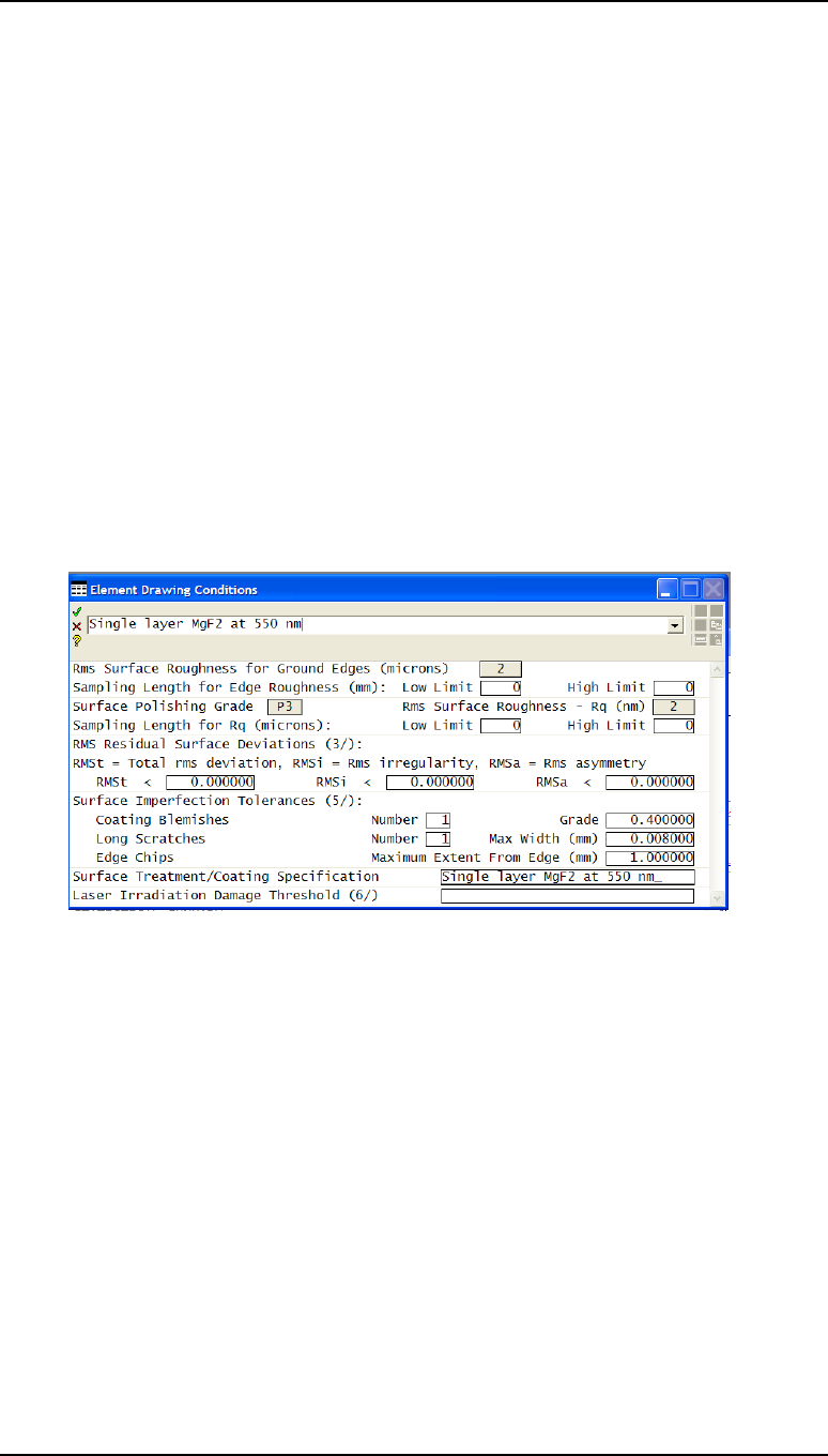
116 Tolerances and drawings Chapter 10
ISO 10110 component drawing
ISO 10110 component drawing
The middle element of the triplet objective will be used to demonstrate this facility.
Setting element drawing defaults
• From the menu header select Lens > Lens Drawing > Element drawing
conditions or type the command: edd
• Set RMS surface roughness for ground edges Rq = 2 (microns) medium.
• Set RMS surface roughness Rq = 2nm (medium)
• Set Surface polishing grade to P3.
• Set Coating blemishes to 1 Grade 0.4. (MIL 80-50 equivalent)
• Set Long scratches to 1 Width 0.008 mm (MIL 80-50 equivalent)
• Set Edge chips: Maximum extent from edge to 1 mm.
• Define Coating specification as Single layer MgF2 550 nm.
• Close the spreadsheet.
Setting element material properties
• From the menu header select Lens > Lens Drawing > Element
• For Left surface of element select 3
• Fill in:
• Part Lens 2 [date]
• Drawing title 50 mm f/5.6
• Diameter 11 mm +0.2/-0.2
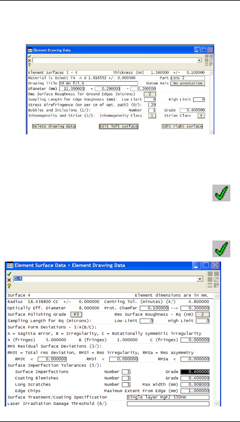
Chapter 10 - Tolerances and drawings 117
ISO 10110 component drawing
• Stress birefringence (0/): 20
• Bubbles and inclusions (1/) Number 1 Grade 0.4
• Striae Class 4.
Setting element surface properties
• Click on Edit left surface.
• Leave most entries unchanged but fill in:
• Surface imperfections Number 1 Grade 0.4
• Click on the green tick to close the spreadsheet.
• Click on Edit right surface.
• Again fill in:
• Surface imperfections Number 1 Grade 0.4
• Click on the green tick twice and the drawing appears.
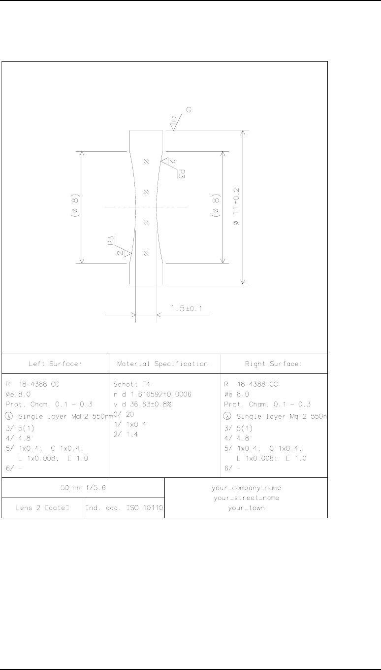
118 Tolerances and drawings Chapter 10
ISO 10110 component drawing
Element drawing
The message appears in the message area:
Element drawing is best viewed in a “portrait window” format.

Appendix 1 119
Graphics reference
Appendix 1 - Index of lens data commands
This table gives an alphabetic listing of the principal commands used in lens data input,
together with the page numbers in the OSLO Program Reference Issue 6.3 (Autumn 2004
edition). The letter in the second column is the label shown on the gray button in the
surface data spreadsheet when the relevant parameter is set. Note that not all of these
commands are available in OSLO-EDU.
Command Explanation Page
ach F array chan 65
ad A aspheric 73
ae A aspheric 73
af A aspheric 73
afo afocal mode 117
ag A aspheric 73
air medium 53
al S aplanatic slv 42
alc S aplanatic slv 42
amo abn mode 118
ang field angle 122
ap aperture 49
apck ap checking 117
apn X special ap 50
ary F lens array 64
as0, as1, etc. A aspheric 75
asi F alt srf intersec 62
ast A aperture stop 27,
50
asp A aspheric 73
ben C tilt & bend 68
bry birefringent 57
cak B crystal axis 57
cal B crystal axis 57
cam B crystal axis 57
cc A conic const 72
cfg oonfiguration 20
cns A cone 79
csd slv delete 41
cslv slv in alt cfgs 118
ctf T test glass cv 45
cv curvature 40
cvx A toric 72
dcx C decentre 67
dcy C decentre 67
dcz C decentre 67
del srf delete 32
des desgr name 118
dlid,dlfd,dlha,dlva,
dlfs,dlls,dlap,dlrs,
dlnr etc
lens and ray
drawing con-
trol
228
to
245
doe D diffractive 85
drw srf drawing 63
ebr ent beam rad 28,
121
ec S edge slv 47
eik E eikonal srf 108
end end data
epxy ray aiming 119
esd E eikonal del 108
fno F number 121
frn F Fresnel 62
gc C global coord 69
gcs C glob ref srf 118
gdt G gradient index 97
gih image height 122
gla medium 54
gor D grating order 85
grd G gradium 100
grp group 34
gsp D grating spc 85
hor D hologram order 86
idd Z zernike 91
ims image srf 27
ins srf insert 32
itf I interferogram 112
inv srf invert 33
jsd Z polarisation 107
kco D kinoform order 89
kdp D kinoform depth 89
ldp F srf dwg pen 64
len begin data
lid lens identifier 20
lme module end 35
lmo module begin 35
lse spreadsheet 17
mco M coating 105
mer insert lens 40
merge_catalog insert catalog
lens 37
nac Q non-sequential 109
nao obj space NA 28,
127
nap im space NA 28,
121

120 Appendix 1
Index of lens data commands
not N surface note 61
nxt next srf
obh object height 28,
122
opdw OPD in waves 118
pfl L perfect lens 70
pfm L perfect lens 70
pi S marg ray solve 41
pic S chief ray solve 42
pk
P pickup 44,
47,
54
pre sys pressure 120
pu S cv solve 41
puc S cv solve 42
puk S ax ray ang 121
py S th solve 46
pyc S th solve 46
pzrt polarization ray
trace 56,
120
raim ray aiming 117
rco C coord return 68
rd radius 40
rdt T test glass rd 45
rev srf reverse 33
rfh refl & hatch 53
rfl reflection 53
rfs R ref srf 50
rod F extrude 63
rtf T testglass fit 45
sasd astig distance 120
scf setup cfg 21
scl scale srfs 40
sdad ap divisions 123
sdaz apodisation 123
sdde diffraction
efficiency 120
sdis im space spd 120
skp F skip 62
sle scale lens 40
sno1, sno2, etc... system notes 126
spl S spline 82
tce F thermal expans
coefficient 120
tem sys temp 120
th thickness 46
tir F tir srf 63
tla C tilt angle 67
tlb C tilt angle 67
tlc C
tilt angle 67
tox C
tilt offset 67
toy C
tilt offset 67
toz C
tilt offset
ucp P
user pickup 44
ung
ungroup 36
uni
units 117
usd U
user sag 110
usr U
user trace 95,
110
utp P
user pickup 47
wod G
Wood lens 99
wrsp
ref sph posn 117
wv1...
wavelengths 26,
124
ww1...
spectral wts 26,
124
zoe A
Zernike 80
zrr A
Zernike 91
zrx A
Zernike 91
zrxr A
Zernike axis 118
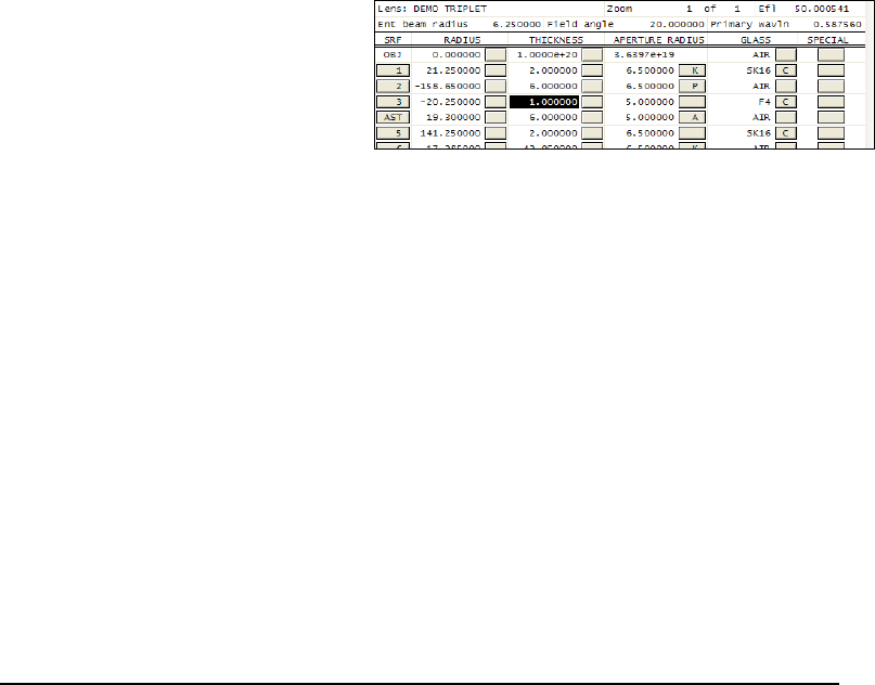
121
In this table, S refers to solves, C refers to tilt/decenter coordinates, and A refers to aspheric
surfaces. Other letters are the flags used in the spreadsheet. A complete listing of the lens
data commands is on pages 508 - 514 of the OSLO Program Reference. These commands
may be used:
1. In the command window, explicitly, as part of an update process:
len upd
gto 2
nxt
th 1.0
end
Note the use of gto, nxt, end. A semicolon has the same effect as
nxt.
2. As part of a CCL command:
{
len upd;
gto(3);
th(1.0);
end;
}
Note the semicolons at the end of each line.
3. In the command window, as a self-contained command:
th 3 1.0
This is called “global editing”
4. As part of a lens file:
NXT //SRF 3
...
TH 1.0
5. Implicitly, when the spread-
sheet is updated, as shown here.
122
Appendix 2 - Graphics reference
Alphabetical index
KEY TO COMMAND REFERENCE (in order of preference)
Standard tools Accessed via graphics window toolbar using the icon shown
Advanced Analysis Accessed via main window toolbar using the icon shown
Tools > Special Accessed via main window menu headers
grindex CCL command accessed via the command line
Function Command Reference Icon OSLO
version Grid
2D-waveguide coupling Tools > Special > 2D - e10
Astigmatism - S & T over field Evaluate > Ray Fans - All d11
Axial chromatic focal shift Ray Analysis All h2
CCL example - 4 graphs Tools > Plotting - All h9
CCL example - contour Tools > Plotting - All b10
CCL example - map Tools > Plotting - All c10
CCL example - pen colours Tools > Plotting - All d10
CCL example - XY graph Tools > Plotting - All d10
Distortion grid plot Ray Analysis All b3
Distortion at all wavelengths Evaluate > Ray Fans - All e11
Doublet - slider-wheel design Tools > Demos - All h1-
Draw system 2D Lens Drawing All a1
Draw system 2D Standard tools All a1
Draw system 3D shaded solid Lens Drawing All d1
Draw system 3D solid Lens Drawing All c1
Draw system 3D variable view Lens Drawing All e1
Draw system 3D wire-frame Lens Drawing All b1
Draw system 3D wire-frame Standard tools All b1
Draw system - conditions Lens Drawing All --
Draw system - zoom lens Lens Drawing h1
Element drawing Lens Drawing All a2
Encircled energy - diffraction Energy All b7
Encircled energy - geometrical Energy All e7
Ensquared energy - diffraction Energy All c7
Ensquared energy - geometrical Energy All f7
Extended source image Extended Source All e9
Footprint - one field point Spot Diagram All e4
Footprint profile - all field points Spot Diagram All f4
Gaussian beam movie Tools > Demos - All
g
10
Appendix 2 123
Graphics reference
Ghost image movie Spot Diagram
g
4
Glass catalogue n-V map Lens >Glass Catalog - All a9
GRIN lens - slider-wheel design Tools > Demos - b11
GRIN axial index grindex - All -
Internal transmittance of glass internal_trans - All -
Incidence angle statistics iangstat - All h11
Lateral chromatic aberration Ray analysis All a3
Lateral colour (pri & sec) Evaluate >Ray Fans - All -
Longitudinal aberration Evaluate >Ray Fans - All c11
LSF/KED - diffraction calc Energy All d7
LSF/KED - geometrical calc Energy All
g
7
MTF over field - 3 frequencies MTF All d6
MTF - one field point MTF All a6
MTF square wave - 1 field point MTF All e6
MTF - thru frequency report MTF All h5
MTF - thru frequency report Standard tools All h5
MTF and spot size thru focus MTF All f6
MTF FFT one field point MTF b6
MTF thru focus - one field point MTF All h6
MTF thru focus across field MTF All a7
MTF thru focus report MTF All
g
6
MTF thru focus report Standard tools All
g
6
OPD - 2D field points Ray Analysis
g
2
OPD - one field point Ray Analysis All f2
OPD contour - one field point Wavefront All f3
OPD interferogram Wavefront All
g
3
OPD map - 2D field points Wavefront d3
OPD map - one field point Wavefront All e3
OPD map/contour report Wavefront All c3
OPD map/contour report Standard tools All c3
OPD report Ray Analysis All e2
Optimization ray set Spot Diagram h4
Partial coherence - bar image Advanced Analysis All
g
9
Photometric plot ridemo - All f11
Pixellated image Extended Sources All f9
Polarisation map Polarization b8
PSF - 2D contour lines Evaluate > Spread fn - b9
PSF - 2D field points PSF b5
PSF - contour PSF All c5
PSF - FFT - contour PSF All e5
PSF - FFT - one field point PSF All f5
124 Appendix 2
Graphics reference
PSF - one field point PSF All d5
PSF - section PSF All
g
5
PSF report PSF All a5
PSF report Standard tools All a5
PTF - thru frequency MTF All c6
Public lens database File> Lens Database - All h8
Ray analysis - 2D field points Ray Analysis d2
Ray analysis - one field point Ray Analysis All c2
Ray analysis report Ray Analysis All b2
Ray analysis report Standard tools All b2
Ray analysis SIGMA format repsig - All
g
11
Ray bundles 2D Lens Drawing All f1
Ray bundles 3D Lens Drawing All
g
1
Ray bundles movie fieldscan - h1
RMS spot size & RMS OPD Spot Diagram All d4
Seidel aberration demo Tools > Demos > Seidel - All f10
Slider-wheel design Standard Tools All c9
Spot diagram - 2D field points Spot Diagram a4
Spot diagram - one field point Spot Diagram All b4
Spot diagram - recipolar Spot Diagram All c4
Spot diagram report Spot Diagram All h3
Spot diagram report Standard tools All h3
Surface reflected phase Polarization f8
Surface reflectivity Polarization d8
Surface transmission Polarization e8
Surface transmitted phase Polarization
g
8
Thin film uniformity Polarization c8
Tolerances - Monte Carlo Tolerances --
Triplet - slider-wheel design Tools > Demos > Triplet - All a11
y-ybar diagram Optimize > Support - All d9
Zoom lens drawing Lens Drawing h1
Zoom lens drawing Zoom h1
Zoom lens report Zoom a8
Tabular graphics command reference
See below.
125
drl;ddr
Standard Tools
Lens Drawing
Lens>Lens Drawing
drl wir;ddr
Standard Tools
Lens Drawing
Lens>Lens Drawing
drl sol;ddr
Standard Tools
Lens Drawing
Lens>Lens Drawing
drl shs;ddr
Standard Tools
Lens Drawing
Lens>Lens Drawing
drlrot sol
Lens Drawing
lensdraw 32
plan 1.0
Lens Drawing
Tools>Demos>Rays
lensdraw 32
oblique 1.0
Lens Drawing
Tools>Demos>Rays
fieldscan
1
dre
Lens Drawing
Lens>Lens Drawing
rpt_ric ray
Standard Tools
Ray Analysis
Evaluate>Other Ray
plr
Ray Analysis
Evaluate>Ray Fans
ric2d_ray
Ray Analysis
Evaluate>Ray Fans
rpt_ric opd
Ray Analysis
Evaluate>Other Ray
plo
Ray Analysis
Evaluate>Ray Fans
ric2d opd
Ray Analysis
Evaluate>Ray Fans
chrshft
Ray Analysis
Evaluate>Other Ray
2
latshft
Ray Analysis
Evaluate>Other Ray
distplt
Ray Analysis
Evaluate>Other Ray
rpt_wvf
Standard Tools
Wavefront
Evaluate>Wavefront
pwf2D
Wavefront
Evaluate>Wavefront
pwf map
Wavefront
Evaluate>Wavefront
pwf con
Wavefront
Evaluate>Wavefront
pwf int
Wavefront
Evaluate>Wavefront
rpt_spd
Standard Tools
Spot Diagram
Evaluate>Spot Diag
3
spd2d
Spot Diagram
Evaluate>Spot Diag
pls
Spot Diagram
Evaluate>Spot Diag
recipolar
Spot Diagram
Evaluate>Spot Diag
spsopd
Spot Diagram
Evaluate>Spot Diag
footprt
Spot Diagram
Optimize>Support
footpro
Spot Diagram
Optimize>Support
ghosts mov
Spot Diagram
Optimize>Support
grst
Spot Diagram
Lens>Show Optim
4
rpt_psf
Standard Tools
PSF
Evaluate>Spread Fn
psf2d
PSF
Evaluate>Spread Fn
sprd con
0.1 dir
PSF
Evaluate>Spread Fn
sprd map
0.1 dir
PSF
Evaluate>Spread Fn
sprd con
0.1 fft
PSF
Evaluate>Spread Fn
sprd map
0.1 fft
PSF
Evaluate>Spread Fn
pss chr
PSF
Evaluate>Spread Fn
rpt_tfr
Standard Tools
MTF
Evaluate>TransferFn
5
plm tfr
MTF
Evaluate>TransferFn
fftmtf
MTF
Evaluate>TransferFn
mtfandptf
MTF
Evaluate>TransferFn
mtf
_
fld
MTF
Evaluate>TransferFn
s
quaremtf
MTF
Evaluate>TransferFn
s
l
_
otfspd
MTF
r
pt
_
tfo
Standard Tools
MTF
Evaluate>TransferFn
plm tfo
MTF
Evaluate>TransferFn
6
fcurv
MTF
Evaluate>TransferFn
prq chr
Energy Analysis
Evaluate>Energy Dis
psq chr
Energy Analysis
Evaluate>Energy Dis
pdl bth
Energy Analysis
Evaluate>Energy Dis
ple geo
Energy Analysis
Evaluate>Energy Dis
ped
Energy Analysis
Evaluate>Energy Dis
pgl bth
Energy Analysis
Evaluate>Energy Dis
zdrl
Zoom
Lens>Lens Drawing
7
zrpt
Zoom
polstate
Polarization
Evaluate>Pol
thunf
Polarization
Evaluate>Pol
surfprop rfl
Polarization
Evaluate>Pol
surfprop tns
Polarization
Evaluate>Pol
surfprop phr
Polarization
Evaluate>Pol
surfprop pht
Polarization
Evaluate>Pol
dblib_open
File>Lens Database
8
open cdb pub
"."
"glass_...cdb";
Lens>Glass Catalogs
pgq chr 64;
sfg xy chr
Evaluate>Spread Fn
sliderwheel
_design
Optimize>SliderW
yybar
Optimize>Support
source
ExtendedSources
Source>View extnd
xsource
“3barh.ima”
ExtendedSources
Source>Pixellated
ppi mon
AdvancedAnalysis
Source>Partial Coh.
gplot_kit
_sample
Tools>Plotting TKit
9
gplot
_
sample
Tools>
Plotting Toolkit
gplot2d
_sample
Tools>Plotting TKit
fill
_
contour
_sample
Tools>Plotting TKit
c
olors
Tools>
Plotting Toolkit
w
vra
Tools>Special>2D
waveguide
s
l
_
3rd
Tools>Demos>Seidel
s
how
_
movie
gbmovie fab
Tools>Demos>Gauss
s
l
_
doublet
Tools>Demos>Doub
10
sl_trp
Tools>Demos>Triplet
gradium demo
Tools>Demos>Grad
pla chr
Evaluate>Ray Fans
plf chr
Evaluate>Ray Fans
pld chr
Evaluate>Ray Fans
ridemo repsig iangstat
11
a b c d e f g h

126 Appendix 2
Graphics reference
Tabular graphics index
Draw system 2D
YZ
Draw system 3D
wire-frame
Draw system 3D
solid
Draw system 3D
shaded solid
Draw system
variable view
Ray fans 2D
for vignetting
Ray fans 3D for
vignetting
Ray fans movi
Element drawing
ISO 10110
Ray analysis report Ray analysis - one
field point*
Ray analysis -
2D field points
OPD report OPD -
1 field point*
OPD
2D field points
Axial chromat
i
focal shift
Lateral chromatic
aberration
Distortion grid plot OPD map/contour
rpt
OPD map - 2D
field points
OPD map - 1 field
point*
OPD contour - 1
field point*
OPD
interferogram
Spot diagram
report
Spot diagram -
2D field points
Spot diagram -
1 field point*
Spot diagram -
recipolar
RMS spot size &
OPD over field
Footprint of beam -
1 field point
Footprint profiles -
all field points
Ghost image movie Optimisation r
a
patterns
Point spread
function report
PSF -
2D field points
PSF - contour PSF map - one field
point
PSF contour (FFT
calc)r
PSF map
(FFT calc)
PSF
section
MTF
thru frequenc
y
MTF - 1 field
point*
MTF 1 field point
(FFT calc)*
Phase - thru
frequency*
MTF over field - 3
frequencies
MTF - square
wave 1 field pt*
MTF & spot size
through focus
MTF through focus
report
MTF through fo
c
1 field pt*
MTF thru focus
across field
Encircled energy
(diffraction calc)
Ensquared en.
(diffraction calc)
LSF & KED
(diffraction calc)
Encircled energy
(geometrical calc)
Ensquared en.
(geometrical calc)
LSF & KED
(geometrical calc)
Zoom lens draw
i
Zoom lens
report
Polarisation map Thin film
uniformity
Surface reflectivity Surface
transmission
Surface
reflected phase
Surface
transmitted phase
Public lens
database
Glass catalogue -
n-V map
PSF
2D contour lines
Slider wheel design y-ybar diagram Extended source
image
Pixellated image Partial coherence -
bar image
CCL exampl
e
4 graphs
CCL example -
XY graph
CCL example -
contour
CCL example -
map
CCL example -
pen colours
2D-waveguide
coupling
Seidel aberration
demo
Gaussian beam
movie
Doublet slide
r
wheel design
Triplet slider wheel
design
GRIN lens slider
wheel design
Longitudinal
aberration
Astigmatism - S &
T over field
Distortion
at 3 wavelengths
Photometric plot Ray analysis
SIGMA format
Incidence angl
statistics
a b c d e f g h

Appendix 2 127
Graphics reference
The 88 examples of OSLO graphics shown in the table below represent almost the full range of graphics output available to users of OSLO Premium
version. Brief descriptions of each graphic example are given above. The routes for accessing these graphics are listed in the tabular command reference
with the following format:
OSLO commands These are given in short form only. They can be typed as shown, and they are also useful as an index to the HELP
facility.
Standard Tools These refer to the groups of icons called up from the top left corner of any graphics window
ExtendedSources These refer to the groups of icons called up from the top left corner of the main window.
Evaluate>Spread Fn These show how most of the graphs can be created from menu headers.
* Graphs indicated are for one field point only, and they can give results only on axis if accessed via the icons. To plot individual graphs for other field
points, either issue the set object point command and then use the command line (for example sop 1 0 0;plr), or work through the menu headers.
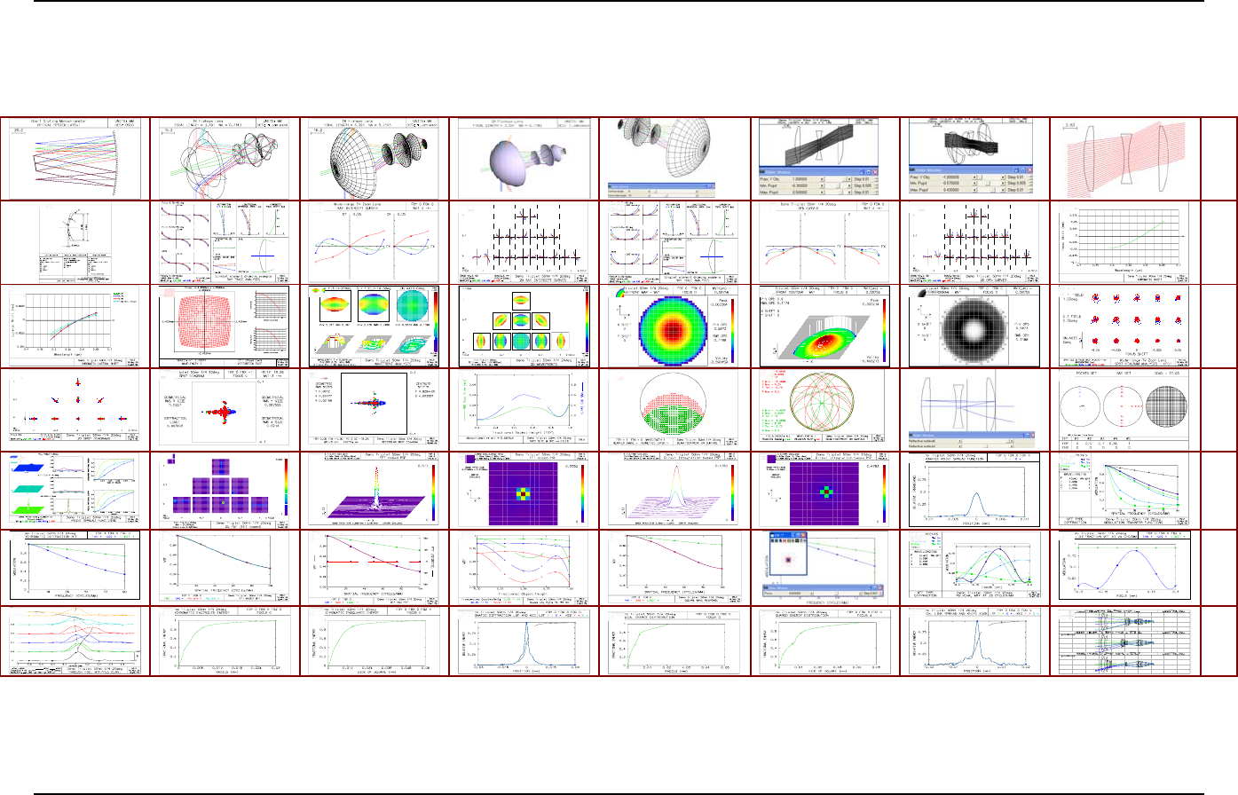
128 Appendix 2
Graphics reference
Graphics reference examples
1
2
3
4
5
6
7
Appendix 2 129
Graphics reference
8
9
10
11
a b c d e f g h
