Phyml Manual

User Manual: Pdf

Open the PDF directly: View PDF .
Page Count: 78

Availability
Authors
Overview
Bug report
Installing PhyML
Program usage.
Inputs & outputs for command-line and PHYLIP interface
Inputs & outputs for the XML interface
Citing PhyML
Other programs
Recommendations on program usage
- PhyML
- PhyTime
Frequently asked questions
Acknowledgements

PhyML – Manual

Version 3.0

January 29, 2018

https://github.com/stephaneguindon/phyml

http://www.atgc-montpellier.fr/phyml

Contents

1 Availability 5

2 Authors 5

3 Overview 6

4 Bug report 6

5 Installing PhyML 6

5.1 Sources and compilation ..................... 6

5.2 Installing PhyML on UNIX-like systems (including Mac OS) . 7

5.3 Installing PhyML on Microsoft Windows ............ 7

5.4 Installing the parallel version of PhyML ............ 7

5.5 Installing PhyML-BEAGLE ................... 8

6 Program usage. 9

6.1 PHYLIP-like interface ...................... 9

6.1.1 Input Data sub-menu ................... 9

6.1.2 Substitution model sub-menu .............. 10

6.1.3 Tree searching sub-menu ................. 13

6.1.4 Branch support sub-menu ................ 14

6.2 Command-line interface ..................... 15

6.3 XML interface ........................... 21

6.4 Parallel bootstrap ......................... 21

7 Inputs & outputs for command-line and PHYLIP interface 22

7.1 Sequence formats ......................... 22

7.1.1 Gaps and ambiguous characters ............. 24

7.1.2 Specifying outgroup sequences .............. 25

7.2 Tree format ............................ 25

7.3 Multiple alignments and trees .................. 26

7.4 Custom amino-acid rate model .................. 27

7.5 Topological constraint ﬁle .................... 27

7.6 Output ﬁles ............................ 28

7.7 Treatment of invariable sites with ﬁxed branch lengths . . . . 29

8 Inputs & outputs for the XML interface 30

8.1 Mixture models in PhyML .................... 30

8.2 Partitions ............................. 31

8.3 Combining mixture and partitions in PhyML: the theory . . . 33

8.4 The XML format and its use in PhyML ............. 35

8.5 Setting up mixture and partition models in PhyML: the basics 37

8.6 XML options ........................... 40

8.6.1 phyml component ..................... 40

8.6.2 topology component ................... 41

8.6.3 ratematrices component ................ 41

8.6.4 equfreqs component ................... 42

8.6.5 branchlengths component ............... 43

8.6.6 siterates component .................. 43

8.6.7 partitionelem and mixtureelem components ..... 45

8.7 A simple example: GTR + Γ4 + I ............... 46

8.8 A second example: LG4X .................... 48

8.9 An example with multiple partition elements .......... 50

8.10 Branch lengths with invariants and partionned data . . . . . . 52

9 Citing PhyML 53

10 Other programs 53

10.1 PhyTime .............................. 53

10.1.1 Installing PhyTime .................... 54

10.1.2 Running PhyTime .................... 54

10.1.3 PhyTime input ...................... 54

10.1.4 Accounting for calibration uncertainty ......... 57

10.1.5 MCMC settings ...................... 58

10.1.6 PhyTime output ..................... 59

10.1.7 An example of PhyTime input and output ﬁles . . . . 60

10.1.8 Citing PhyTime ...................... 62

10.2 PhyloGeo ............................. 64

10.2.1 Installing PhyloGeo .................... 64

10.2.2 Running PhyloGeo .................... 64

10.2.3 Citing PhyloGeo ..................... 65

10.3 PhyREX .............................. 65

10.3.1 Installing PhyREX .................... 66

10.3.2 Running PhyREX ..................... 66

11 Recommendations on program usage 68

11.1 PhyML ............................... 68

11.2 PhyTime .............................. 69

12 Frequently asked questions 70

13 Acknowledgements 71

The software PhyML is provided “as is” without warranty of any kind. In no

event shall the authors or his employer be held responsible for any damage result-

ing from the use of this software, including but not limited to the frustration that

you may experience in using the package. All parts of the source and documen-

tation except where indicated are distributed under the GNU public licence. See

http://www.opensource.org for details.

1 Availability

•Binaries: http://www.atgc-montpellier.fr/phyml

•Sources: http://stephaneguindon.github.io/phyml-downloads/

•Discussion forum: http://groups.google.com/group/phyml-forum

2 Authors

•St´ephane Guindon and Olivier Gascuel conceived the original PhyML

algorithm.

•St´ephane Guindon conceived the PhyTime method.

•St´ephane Guindon, David Welch and Louis Ranjard conceived the Phy-

loGeo method.

•St´ephane Guindon, Wim Hordjik and Olivier Gascuel conceived the

SPR-based tree search algorithm.

•Maria Anisimova and Olivier Gascuel conceived the aLRT method for

branch support.

•St´ephane Guindon, Franck Lethiec, Jean-Francois Dufayard and Vin-

cent Lefort implemented PhyML.

•Jean-Francois Dufayard created the benchmark and implemented the

tools that are used to check PhyML accuracy and performances.

•Vincent Lefort, St´ephane Guindon, Patrice Duroux and Olivier Gas-

cuel conceived and implemented PhyML web server.

•Imran Fanaswala interfaced PhyML with BEAGLE.

•St´ephane Guindon wrote this document.

3 Overview

PhyML [1] is a software package which primary task that is to estimate

maximum likelihood phylogenies from alignments of nucleotide or amino-

acid sequences. It provides a wide range of options that were designed to

facilitate standard phylogenetic analyses. The main strength of PhyML lies

in the large number of substitution models coupled to various options to

search the space of phylogenetic tree topologies, going from very fast and

eﬃcient methods to slower but generally more accurate approaches. It also

implements two methods to evaluate branch supports in a sound statistical

framework (the non-parametric bootstrap and the approximate likelihood

ratio test).

PhyML was designed to process moderate to large data sets. In theory,

alignments with up to 4,000 sequences 2,000,000 character-long can analyzed.

In practice however, the amount of memory required to process a data set

is proportional of the product of the number of sequences by their length.

Hence, a large number of sequences can only be processed provided that

they are short. Also, PhyML can handle long sequences provided that they

are not numerous. With most standard personal computers, the “comfort

zone” for PhyML generally lies around 100-500 sequences less than 10,000

character long. For larger data sets, we recommend using other softwares

such as RAxML [2] or GARLI [3] or Treeﬁnder (http://www.treeﬁnder.de).

4 Bug report

While PhyML is, of course, bug-free (!) (please read the disclaimer care-

fuly...), if you ever come across an issue, please feel free to report it us-

ing the discuss group web site at the following address: https://groups.

google.com/forum/?fromgroups#!forum/phyml-forum. Alternatively, you

can send an email to s.guindon@auckland.ac.nz. Do not forget to mention

the version of PhyML and program options you are using.

5 Installing PhyML

5.1 Sources and compilation

The sources of the program are available free of charge from http:

//stephaneguindon.github.io/phyml-downloads/. The compilation on

UNIX-like systems is fairly standard. It is described in the ‘INSTALL’ ﬁle

that comes with the sources. In a command-line window, go to the directory

that contains the sources and type:

./configure;

make clean;

make V=0;

By default, PhyML will be compiled with optimization ﬂags turned on. It

is possible to generate a version of PhyML that can run through a debugging

tool (such as ddd) or a proﬁling tool (such as gprof) using the following

instructions:

./configure --enable-debug;

make clean;

make V=0;

5.2 Installing PhyML on UNIX-like systems (includ-

ing Mac OS)

Copy PhyML binary ﬁle in the directory you like. For the operating system

to be able to locate the program, this directory must be speciﬁed in the

global variable PATH. In order to achieve this, you will have to add export

PATH="/your path/:$PATH" to the .bashrc or the .bash profile located

in your home directory (your path is the path to the directory that contains

PhyML binary).

5.3 Installing PhyML on Microsoft Windows

Copy the ﬁles phyml.exe and phyml.bat in the same directory. To launch

PhyML, click on the icon corresponding to phyml.bat. Clicking on the icon

for phyml.exe works too but the dimensions of the window will not ﬁt PhyML

PHYLIP-like interface.

5.4 Installing the parallel version of PhyML

Bootstrap analysis can run on multiple processors. Each processor analyses

one bootstraped dataset. Therefore, the computing time needed to perform

Rbootstrap replicates is divided by the number of processors available.

This feature of PhyML relies on the MPI (Message Passing In-

terface) library. To use it, your computer must have MPI installed

on it. In case MPI is not installed, you can dowload it from

http://www.mcs.anl.gov/research/projects/mpich2/. Once MPI is installed,

it is necessary to launch the MPI daemon. This can be done by entering

the following instruction: mpd &. Note however that in most cases, the MPI

daemon will already be running on your server so that you most likely do not

need to worry about this. You can then just go in the phyml/ directory (the

directory that contains the src/,examples/ and doc/ folders) and enter the

commands below:

./configure --enable-mpi;

make clean;

make;

A binary ﬁle named phyml-mpi has now been created in the src/ direc-

tory and is ready to use with MPI. A typical MPI command-line which uses

4 CPUs is given below:

mpirun -n 4 ./phyml-mpi -i myseq -b 100

Please read section 6.4 of this document for more information.

5.5 Installing PhyML-BEAGLE

PhyML can use the BEAGLE [4] library for the likelihood computation.

BEAGLE provides provides signiﬁcant speed-up: the single core version of

PhyML-BEAGLE can be up to 10 times faster than PhyML on a single core

and up to 150 times on Graphical Processing Units. PhyML-BEAGLE will

eventually have of the features of PhyML, even though at the moment the

boostrap and the invariant site options are not available. Also, please note

that in some cases, the ﬁnal log-likelihood reported by PhyML and PhyML-

BEALGE may not exactly match, though the diﬀerences observed are very

minor (in the 10−4to 10−4range).

In order to install PhyML-BEAGLE, you ﬁrst need to download and

install the BEAGLE library available from https://code.google.com/p/

beagle-lib/. Then run the following commands:

./configure --enable-beagle;

make clean;

make;

A binary ﬁle named phyml-beagle will be created in the src/ directory.

The interface to phyml-beagle (i.e., commandline option of PHYLIP-like

interface) is exactly identical to that of PhyML.

6 Program usage.

PhyML has three distinct user-interfaces. The ﬁrst corresponds to a

PHYLIP-like text interface that makes the choice of the options self-

explanatory. The command-line interface is well-suited for people that are

familiar with PhyML options or for running PhyML in batch mode. The

XML interface is more sophisticated. It allows the user to analyse parti-

tionned data using ﬂexible mixture models of evolution.

6.1 PHYLIP-like interface

The default is to use the PHYLIP-like text interface by simply typing ‘phyml’

in a command-line window or by clicking on the PhyML icon (see Section

5.3). After entering the name of the input sequence ﬁle, a list of sub-menus

helps the users set up the analysis. There are currently four distinct sub-

menus:

1. Input Data: specify whether the input ﬁle contains amino-acid or nu-

cleotide sequences. What the sequence format is (see Section 7) and

how many data sets should be analysed.

2. Substitution Model: selection of the Markov model of substitution.

3. Tree Searching: selection of the tree topology searching algorithm.

4. Branch Support: selection of the method that is used to measure branch

support.

‘+’ and ‘-’ keys are used to move forward and backward in the sub-menu list.

Once the model parameters have been deﬁned, typing ‘Y’ (or ‘y’) launches the

calculations. The meaning of some options may not be obvious to users that

are not familiar with phylogenetics. In such situation, we strongly recom-

mend to use the default options. As long as the format of the input sequence

ﬁle is correctly speciﬁed (sub-menu Input data), the safest option for non-

expert users is to use the default settings. The diﬀerent options provided

within each sub-menu are described in what follows.

6.1.1 Input Data sub-menu

[D] ............................... Data type (DNA/AA)

Type of data in the input ﬁle. It can be either DNA or amino-acid sequences

in PHYLIP format (see Section 7). Type Dto change settings.

[I] ...... Input sequences interleaved (or sequential)

PHYLIP format comes in two ﬂavours: interleaved or sequential (see Section

7). Type Ito selected among the two formats.

[M] ....................... Analyze multiple data sets

If the input sequence ﬁle contains more than one data sets, PhyML can

analyse each of them in a single run of the program. Type Mto change

settings.

[R] ............................................ Run ID

This option allows you to append a string that identiﬁes the current PhyML

run. Say for instance that you want to analyse the same data set with two

models. You can then ‘tag’ the ﬁrst PhyML run with the name of the ﬁrst

model while the second run is tagged with the name of the second model.

6.1.2 Substitution model sub-menu

[M] ................. Model of nucleotide substitution

[M] ................ Model of amino-acids substitution

PhyML implements a wide range of substitution models: JC69 [5], K80 [6],

F81 [7], F84 [8], HKY85 [9], TN93 [10] GTR [11,12] and custom for nu-

cleotides; LG [13], WAG [14], Dayhoﬀ [15], JTT [16], Blosum62 [17], mtREV

[18], rtREV [19], cpREV [20], DCMut [21], VT [22] and mtMAM [23] and

custom for amino acids. Cycle through the list of nucleotide or amino-acids

substitution models by typing M. Both nucleotide and amino-acid lists include

a ‘custom’ model. The custom option provides the most ﬂexible way to spec-

ify the nucleotide substitution model. The model is deﬁned by a string made

of six digits. The default string is ‘000000’, which means that the six relative

rates of nucleotide changes: A↔C,A↔G,A↔T,C↔G,C↔Tand

G↔T, are equal. The string ‘010010’ indicates that the rates A↔Gand

C↔Tare equal and distinct from A↔C=A↔T=C↔G=G↔T.

This model corresponds to HKY85 (default) or K80 if the nucleotide fre-

quencies are all set to 0.25. ‘010020’ and ‘012345’ correspond to TN93 and

GTR models respectively. The digit string therefore deﬁnes groups of rela-

tive substitution rates. The initial rate within each group is set to 1.0, which

corresponds to F81 (JC69 if the base frequencies are equal). Users also have

the opportunity to deﬁne their own initial rate values. These rates are then

optimised afterwards (option ‘O’) or ﬁxed to their initial values. The custom

option can be used to implement all substitution models that are special cases

of GTR. Table 1on page 17 gives the correspondence between the ‘standard’

name of the model (see http://mbe.oxfordjournals.org/content/18/6/

897/F2.large.jpg) and the custom model code. The custom model also ex-

ists for protein sequences. It is useful when one wants to use an amino-acid

substitution model that is not hard-coded in PhyML. The symmetric part of

the rate matrix, as well as the equilibrium amino-acid frequencies, are given

in a ﬁle which name is given as input of the program. The format of this ﬁle

is described in the section 7.4.

[F] ................. Optimise equilibrium frequencies

[E] ......... Equilibrium frequencies (empirical/user)

[F] . Amino acid frequencies (empirical/model defined)

For nucleotide sequences, optimising equilibrium frequencies means that the

values of these parameters are estimated in the maximum likelihood frame-

work. When the custom model option is selected, it is also possible to give

the program a user-deﬁned nucleotide frequency distribution at equilibrium

(option E). For protein sequences, the stationary amino-acid frequencies are

either those deﬁned by the substitution model or those estimated by count-

ing the number of diﬀerent amino-acids observed in the data. Hence, the

meaning of the Foption depends on the type of the data to be processed.

[T] .................... Ts/tv ratio (fixed/estimated)

Fix or estimate the transition/transversion ratio in the maximum likelihood

framework. This option is only available when DNA sequences are to be

analysed under K80, HKY85 or TN93 models. The deﬁnition given to this

parameter by PhyML is the same as PAML’s one. Therefore, the value

of this parameter does not correspond to the ratio between the expected

number of transitions and the expected number of transversions during a

unit of time. This last deﬁnition is the one used in PHYLIP. PAML’s manual

gives more detail about the distinction between the two deﬁnitions (http:

//abacus.gene.ucl.ac.uk/software/paml.html).

[V] . Proportion of invariable sites (fixed/estimated)

The proportion of invariable sites, i.e., the expected frequency of sites that

do not evolve, can be ﬁxed or estimated. The default is to ﬁx this proportion

to 0.0. By doing so, we consider that each site in the sequence may accumu-

late substitutions at some point during its evolution, even if no diﬀerences

across sequences are actually observed at that site. Users can also ﬁx this

parameter to any value in the [0.0,1.0] range or estimate it from the data in

the maximum-likelihood framework.

[R] ....... One category of substitution rate (yes/no)

[C] ........... Number of substitution rate categories

[A] ... Gamma distribution parameter (fixed/estimated)

[G] .........‘Middle’ of each rate class (mean/median)

Rates of evolution often vary from site to site. This heterogeneity can be

modelled using a discrete gamma distribution. Type Rto switch this option

on or oﬀ. The diﬀerent categories of this discrete distribution correspond

to diﬀerent (relative) rates of evolution. The number of categories of this

distribution is set to 4 by default. It is probably not wise to go below this

number. Larger values are generally preferred. However, the computational

burden involved is proportional to the number of categories (i.e., an analysis

with 8 categories will generally take twice the time of the same analysis with

only 4 categories). Note that the likelihood will not necessarily increase as the

number of categories increases. Hence, the number of categories should be

kept below a “reasonable” number, say 20. The default number of categories

can be changed by typing C.

The middle of each discretized substitution rate class can be determined

using the mean or the median. PAML, MrBayes and RAxML use the mean.

However, the median is generally associated with greater likelihoods than the

mean. This conclusion is based on our analysis of several real-world data sets

extracted from TreeBase. Despite this, the default option in PhyML is to use

the mean in order to make PhyML likelihoods comparable to those of other

phylogenetic software. One must bare in mind that likelihoods calculated

with the mean approximation are not directly comparable to the likelihoods

calculated using the median approximation.

The shape of the gamma distribution determines the range of rate vari-

ation across sites. Small values, typically in the [0.1,1.0] range, correspond

to large variability. Larger values correspond to moderate to low heterogene-

ity. The gamma shape parameter can be ﬁxed by the user or estimated via

maximum-likelihood. Type Ato select one or the other option.

6.1.3 Tree searching sub-menu

[O] ........................... Optimise tree topology

By default the tree topology is optimised in order to maximise the likelihood.

However, it is also possible to avoid any topological alteration. This option

is useful when one wants to compute the likelihood of a tree given as input

(see below). Type Oto select among these two options.

[S] .................. Tree topology search operations

PhyML proposes three diﬀerent methods to estimate tree topologies. The

default approach is to use simultaneous NNI. This option corresponds to the

original PhyML algorithm [1]. The second approach relies on subtree pruning

and regrafting (SPR). It generally ﬁnds better tree topologies compared to

NNI but is also signiﬁcantly slower. The third approach, termed BEST,

simply estimates the phylogeny using both methods and returns the best

solution among the two. Type Sto choose among these three choices.

[R] ......................... Use random starting tree

[N] .................. Number of random starting trees

When the SPR or the BEST options are selected, is is possible to use random

trees rather than BioNJ or a user-deﬁned tree, as starting tree. If this option

is turned on (type Rto change), ﬁve trees, corresponding to ﬁve random

starts, will be estimated. The output tree ﬁle will contain the best tree

found among those ﬁve. The number of random starts can be modiﬁed by

typing N. Setting the number of random starting trees to Nmeans that

the analysis will take (slightly more than) Ntimes the time required for a

standard analysis where only one (BioNJ) starting tree is used. However,

the analysis of real data sets shows that the best trees estimated using the

random start option almost systematically have higher likelihoods than those

inferred using a single starting tree.

[U] ........ Starting tree (BioNJ/parsimony/user tree)

When the tree topology optimisation option is turned on, PhyML proceeds

by reﬁning an input tree. By default, this input tree is estimated using

BioNJ [24]. The alternative option is to use a parsimony tree. We found

this option specially useful when analysing large data sets with NNI moves

as it generally leads to greater likelihoods than those obtained when starting

from a BioNJ trees. The user can also to input her/his own tree. This tree

should be in Newick format (see Section 7). This option is useful when one

wants to evaluate the likelihood of a given tree with a ﬁxed topology, using

PhyML. Type Uto choose among these two options.

6.1.4 Branch support sub-menu

[B] ................ Non parametric bootstrap analysis

The support of the data for each internal branch of the phylogeny can be es-

timated using non-parametric bootstrap. By default, this option is switched

oﬀ. Typing Bswitches on the bootstrap analysis. The user is then prompted

for a number of bootstrap replicates. The largest this number the more

precise the bootstrap support estimates are. However, for each bootstrap

replicate a phylogeny is estimated. Hence, the time needed to analyse N

bootstrap replicates corresponds to N-times the time spent on the analysis

of the original data set. N= 100 is generally considered as a reasonable

number of replicates.

[A] ................ Approximate likelihood ratio test

When the bootstrap option is switched oﬀ (see above), approximate likeli-

hood branch supports are estimated. This approach is considerably faster

than the bootstrap one. However, both methods intend to estimate diﬀer-

ent quantities and conducting a fair comparison between both criteria is not

straightforward. The estimation of approximate likelihood branch support

comes in multiple ﬂavours. The default is set to aBayes, corresponding to

the approximate Bayes method described in [25]. The approximate likelihood

ratio test (aLRT) [26], ShimodairaHasegawa aLRT (SH-aLRT) statistics are

the other available options.

6.2 Command-line interface

An alternative to the PHYLIP-like interface is the command-line interface.

Users that do not need to modify the default parameters can launch the

program with the ‘phyml -i seq file name’ command. The list of all com-

mand line arguments and how to use them is given in the ‘Help’ section

which is displayed when entering the ‘phyml --help’ command. The avail-

able command-line options are described in what follows.

•-i (or --input)seq file name

seq file name is the name of the nucleotide or amino-acid sequence

ﬁle in PHYLIP format.

•-d (or --datatype)data type

data type is nt for nucleotide (default) and aa for amino-acid se-

quences.

•-q (or --sequential)

Changes interleaved format (default) to sequential format.

•-n (or --multiple)nb data sets

nb data sets is an integer giving the number of data sets to analyse.

•-p (or --pars)

Use a minimum parsimony starting tree. This option is taken into

account when the ‘-u’ option is absent and when tree topology modiﬁ-

cations are to be done.

•-b (or --bootstrap)int

–int >0: int is the number of bootstrap replicates.

–int = 0: neither approximate likelihood ratio test nor bootstrap

values are computed.

–int = -1: approximate likelihood ratio test returning aLRT statis-

tics.

–int = -2: approximate likelihood ratio test returning Chi2-based

parametric branch supports.

–int = -4: SH-like branch supports alone.

–int = -5: (default) approximate Bayes branch supports.

•-m (or --model)model name

model name : substitution model name.

–Nucleotide-based models:HKY85 (default) | JC69 | K80 | F81 |

F84 | TN93 | GTR | custom

The custom option can be used to deﬁne a new substitution model.

A string of six digits identiﬁes the model. For instance, 000000 cor-

responds to F81 (or JC69 provided the distribution of nucleotide

frequencies is uniform). 012345 corresponds to GTR. This option

can be used for encoding any model that is a nested within GTR.

See Section 6.1.2 and Table 1.NOTE: the substitution parameters

of the custom model will be optimised so as to maximise the like-

lihood. It is possible to specify and ﬁx (i.e., avoid optimisation)

the values of the substitution rates only through the PHYLIP-like

interface.

–Amino-acid based models:LG (default) | WAG | JTT | MtREV

MtMam | MtArt | HIVw | HIVb | custom

The custom option is useful when one wants to use an amino-acid

substitution model that is not available by default in PhyML.

The symmetric part of the rate matrix, as well as the equilibrium

amino-acid frequencies, are given in a ﬁle which name is asked

for by the program. The format of this ﬁle is described in section

7.4.

•--aa rate file file name

This option is compulsory when analysing amino-acid sequences under

a ‘custom’ model (see above). file name should provide a rate matrix

and equilibrium amino acid in PAML format (see Section 7.4).

•-f e,m, or “fA,fC,fG,fT”

Nucleotide or amino-acid frequencies.

–e: the character frequencies are determined as follows :

∗Nucleotide sequences: (Empirical) the equilibrium base fre-

quencies are estimated by counting the occurence of the dif-

ferent bases in the alignment.

Name Command-line option

JC69 -m 000000 -f 0.25,0.25,0.25,0.25

F81 -m 000000

K80 -m 010010 -f 0.25,0.25,0.25,0.25

HKY85 -m 010010

TrNef -m 010020 -f 0.25,0.25,0.25,0.25

TrN -m 010020

K81 -m 123321 -f 0.25,0.25,0.25,0.25

K81uf -m 123321

TIMef -m 132241 -f 0.25,0.25,0.25,0.25

TIM -m 132241

TVMef -m 102304 -f 0.25,0.25,0.25,0.25

TVM -m 102304

SYM -m 123456 -f 0.25,0.25,0.25,0.25

GTR -m 123456

Table 1. Nucleotide substitution model names (as deﬁned in [27]) and the

corresponding custom model code used in PhyML.

∗Amino-acid sequences: (Empirical) the equilibrium amino-

acid frequencies are estimated by counting the occurence of

the diﬀerent amino-acids in the alignment.

–m: the character frequencies are determined as follows :

∗Nucleotide sequences: (ML) the equilibrium base frequencies

are estimated using maximum likelihood.

∗Amino-acid sequences: (Model) the equilibrium amino-acid

frequencies are estimated using the frequencies deﬁned by the

substitution model.

–“fA,fC,fG,fT”: only valid for nucleotide-based models. fA,fC,

fG and fT are ﬂoating numbers that correspond to the frequencies

of A, C, G and T respectively.

•-t (or --ts/tv)ts/tv ratio

ts/tv ratio: transition/transversion ratio. DNA sequences only. Can

be a ﬁxed positive value (e.g., 4.0) or type eto get the maximum

likelihood estimate.

•-v (or --pinv)prop invar

prop invar: proportion of invariable sites. Can be a ﬁxed value in the

[0,1] range or type eto get the maximum likelihood estimate.

•-c (or --nclasses)nb subst cat

nb subst cat: number of relative substitution rate categories. Default:

nb subst cat=4. Must be a positive integer.

•-a (or --alpha)gamma

gamma: value of the gamma shape parameter. Can be a ﬁxed posi-

tive value or e to get the maximum likelihood estimate. The value of

this parameter is estimated in the maximum likelihood framework by

default.

•--use median

The middle of each substitution rate class in the discrete gamma dis-

tribution is taken as the median. The mean is used by default.

•--free rates or --freerates

As an alternative to the discrete gamma model, it is possible to esti-

mate the (relative) rate in each class of the (mixture) model and the

corresponding frequencies directly from the data. This model, called

the FreeRate model, has more parameters than the discrete gamma one

but usually provides a signiﬁcantly better ﬁt to the data. See [28] for

more information about this model and an illustration of its use.

•--il

il stands here for integrated (branch) length. This model, described

in [29] in the context of molecular dating, provides an eﬃcient way

to implement the covarion model . Under the integrated length (IL)

model, the length of each edge is described by a distribution of val-

ues, instead of a single value corresponding to the expected number of

substitutions per position along the sequence. Let la,s and lb,s be the

number of substitutions at site salong edges aand b, and la,t and lb,t,

the number of substitutions at site t. Standard models have la,s =la,t

and lb,s =lb,t, or la,s =αla,t and lb,s =αlb,t if rates vary across sites.

The IL model has instead la,s =αla,t and lb,s =βlb,t with α6=β, i.e.

substitution rates vary across sites and edges. The IL approach is some-

how an analytical approximation to the covarion model that, unlike the

covarion model, does not incur any computational overhead compared

to the traditional models. A notable diﬀerence with the plain vanilla

covarion model and the IL model however is that substitution rates are

not autocorrelated along the phylogeny under the IL model.

•--codpos 1,2 or 3

When analysing an alignment of coding sequences, use this option to

consider only the ﬁrst, second or the third coding position for the esti-

mation.

•-s (or --search)move

Tree topology search operation option. Can be either NNI (default,

fast) or SPR (usually slower than NNI but more accurate) or BEST (best

of NNI and SPR search).

•-u (or --inputtree)user tree file

user tree file: starting tree ﬁlename. The tree must be in Newick

format.

•-o params

This option focuses on speciﬁc parameter optimisation.

–params=tlr: tree topology (t), branch length (l) and substitution

rate parameters (r) are optimised.

–params=tl: tree topology and branch lengths are optimised.

–params=lr: branch lengths and substitution rate parameters are

optimised.

–params=l: branch lengths are optimised.

–params=r: substitution rate parameters are optimised.

–params=n: no parameter is optimised.

•--rand start

This option sets the initial tree to random. It is only valid if SPR

searches are to be performed.

•--n rand starts num

num is the number of initial random trees to be used. It is only valid if

SPR searches are to be performed.

•--r seed num

num is the seed used to initiate the random number generator. Must

be an integer.

•--print site lnl

Print the likelihood for each site in ﬁle * phyml lk.txt. For Γ or Γ+I or

FreeRate models, this option returns the posterior probability of each

relative rate class at each site. Such information can then be used to

identify fast- and slow-evolving regions of the alignment.

•--print trace

Print each phylogeny explored during the tree search process in ﬁle

* phyml trace.txt. This option can be useful for monitoring the

progress of the analysis for very large data sets and have an approxi-

mate idea of what the ﬁnal phylogeny will look like.

•--json trace

Print each phylogeny explored during the tree search process in ﬁle

* phyml json trace.txt in JSON format (see http://www.json.org/).

This option can be useful for monitoring the progress of the analysis

for very large data sets and have an approximate idea of what the ﬁnal

phylogeny will look like.

•--run id ID string

Append the string ID string at the end of each PhyML output ﬁle. This

option may be useful when running simulations involving PhyML. It

can also be used to ‘tag’ multiple analysis of the same data set with

various program settings.

•--no memory check

By default, when processing a large data set, PhyML will pause and ask

the user to conﬁrm that she/he wants to continue with the execution

of the analysis despite the large amount of memory required. The

--no memory check skips this question. It is especially useful when

running PhyML in batch mode.

•--no colalias

By default, PhyML preprocesses each alignment by putting together

(or aliasing) the columns that are identical. Use this option to skip

this step but be aware that the analysis might then take more time to

complete.

•--constrained lens

When an input tree with branch lengths is provided, this option will

ﬁnd the branch multiplier that maximises the likelihood (i.e., the rela-

tive branch lengths remain constant)

•--constraint file file name

file name lists the topological constraints under which the tree topol-

ogy search is conducted. This option should be used in conjunction

with -u file name. See Section 7.5 for more information.

•--quiet

Runs PhyML in quiet mode. The program will not pause if the memory

required to run the analysis exceeds 256MB and will not output the

progression of the log-likelihood scores on the standard output.

•--ancestral

PhyML calculates the marginal probabilities of each character state at

each internal node and each site of the sequence alignment.

6.3 XML interface

•--xml=xml file name

xml file name is the name of the XML ﬁle containing the information

required to run the analysis. More details about this type of ﬁle is

given in the section 8.

6.4 Parallel bootstrap

Bootstrapping is a highly parallelizable task. Indeed, bootstrap replicates

are independent from one another. Each bootstrap replicate can then be

analysed separately. Modern computers often have more than one CPU. Each

CPU can therefore be used to process a bootstrap sample. Using this parallel

strategy, performing Rbootstrap replicates on CCPUs ‘costs’ the same

amount of computation time as processing R×Cbootstrap replicates on a

single CPU. In other words, for a given number of replicates, the computation

time is divided by Rcompared to the non-parallel approach.

PhyML sources must be compiled with speciﬁc options to turn on the

parallel option (see Section 5.4). Once the binary ﬁle (phyml) has been

generated, running a bootstrap analysis with, say 100 replicates on 2 CPUs,

can be done by typing the following command-line:

mpd &;

mpirun -np 2 ./phyml -i seqfile -b 100;

The ﬁrst command launches the mpi daemon while the second launches the

analysis. Note that launching the daemon needs to be done only once. The

output ﬁles are similar to the ones generated using the standard, non-parallel,

analysis (see Section 7). Note that running the program in batch mode, i.e.:

mpirun -np 2 ./phyml -i seqfile -b 100 &

will probably NOT work. I do not know how to run a mpi process in batch

mode yet. Suggestions welcome... Also, at the moment, the number of

PHYLIP interleaved

5 80

seq1 CCATCTCACGGTCGGTACGATACACCKGCTTTTGGCAGGAAATGGTCAATATTACAAGGT

seq2 CCATCTCACGGTCAG---GATACACCKGCTTTTGGCGGGAAATGGTCAACATTAAAAGAT

seq3 RCATCTCCCGCTCAG---GATACCCCKGCTGTTG????????????????ATTAAAAGGT

seq4 RCATCTCATGGTCAA---GATACTCCTGCTTTTGGCGGGAAATGGTCAATCTTAAAAGGT

seq5 RCATCTCACGGTCGGTAAGATACACCTGCTTTTGGCGGGAAATGGTCAAT????????GT

ATCKGCTTTTGGCAGGAAAT

ATCKGCTTTTGGCGGGAAAT

AGCKGCTGTTG?????????

ATCTGCTTTTGGCGGGAAAT

PHYLIP sequential

5 40

seq1 CCATCTCANNNNNNNNACGATACACCKGCTTTTGGCAGG

seq2 CCATCTCANNNNNNNNGGGATACACCKGCTTTTGGCGGG

seq3 RCATCTCCCGCTCAGTGAGATACCCCKGCTGTTGXXXXX

seq4 RCATCTCATGGTCAATG-AATACTCCTGCTTTTGXXXXX

seq5 RCATCTCACGGTCGGTAAGATACACCTGCTTTTGxxxxx

Figure 1. PHYLIP interleaved and sequential formats.

bootstrap replicates must be a multiple of the number of CPUs required in

the mpirun command.

7 Inputs & outputs for command-line and

PHYLIP interface

PhyML reads data from standard text ﬁles, without the need for any partic-

ular ﬁle name extension.

7.1 Sequence formats

Alignments of DNA or protein sequences must be in PHYLIP or NEXUS

[30] sequential or interleaved format (Figures 7.1 and 2). For PHYLIP for-

mated sequence alignments, the ﬁrst line of the input ﬁle contains the number

of species and the number of characters, in free format, separated by blank

characters. One slight diﬀerence with PHYLIP format deals with sequence

name lengths. While PHYLIP format limits this length to ten characters,

PhyML can read up to hundred character long sequence names. Blanks

and the symbols “(),:” are not allowed within sequence names because the

Newick tree format makes special use of these symbols. Another slight diﬀer-

ence with PHYLIP format is that actual sequences must be separated from

Nexus nucleotides

[ This is a comment ]

#NEXUS

BEGIN DATA;

DIMENSIONS NTAX=10 NCHAR=20;

FORMAT DATATYPE=DNA;

MATRIX

tax1 ?ATGATTTCCTTAGTAGCGG

tax2 CAGGATTTCCTTAGTAGCGG

tax3 ?AGGATTTCCTTAGTAGCGG

tax4 ?????????????GTAGCGG

tax5 CAGGATTTCCTTAGTAGCGG

tax6 CAGGATTTCCTTAGTAGCGG

tax7 ???GATTTCCTTAGTAGCGG

tax8 ????????????????????

tax9 ???GGATTTCTTCGTAGCGG

tax10 ???????????????AGCGG;

END;

Nexus digits

[ This is a comment ]

#NEXUS

BEGIN DATA;

DIMENSIONS NTAX=10 NCHAR=20;

FORMAT DATATYPE=STANDARD SYMBOLS="0 1 2 3";

MATRIX

tax1 ?0320333113302302122

tax2 10220333113302302122

tax3 ?0220333113302302122

tax4 ?????????????2302122

tax5 10220333113302302122

tax6 10220333113302302122

tax7 ???20333113302302122

tax8 ????????????????????

tax9 ???22033313312302122

tax10 ???????????????02122;

END;

Nexus digits

[ This is a comment ]

#NEXUS

BEGIN DATA;

DIMENSIONS NTAX=10 NCHAR=20;

FORMAT DATATYPE=STANDARD SYMBOLS="00 01 02 03";

MATRIX

tax1 ??00030200030303010103030002030002010202

tax2 0100020200030303010103030002030002010202

tax3 ??00020200030303010103030002030002010202

tax4 ??????????????????????????02030002010202

tax5 0100020200030303010103030002030002010202

tax6 0100020200030303010103030002030002010202

tax7 ??????0200030303010103030002030002010202

tax8 ????????????????????????????????????????

tax9 ??????0202000303030103030102030002010202

tax10 ??????????????????????????????0002010202;

END;

Figure 2. NEXUS formats.

their names by at least one blank character.

A PHYLIP input sequence ﬁle may also display more than a single data

set. Each of these data sets must be in PHYLIP format and two successive

alignments must be separated by an empty line. Processing multiple data

sets requires to toggle the ‘M’ option in the Input Data sub-menu or use

the ‘-n’ command line option and enter the number of data sets to analyse.

The multiple data set option can be used to process re-sampled data that

were generated using a non-parametric procedure such as cross-validation or

jackknife (a bootstrap option is already included in PhyML). This option

is also useful in multiple gene studies, even if ﬁtting the same substitution

model to all data sets may not be suitable.

PhyML can also process alignments in NEXUS format. Although not

all the options provided by this format are supported by PhyML, a few

speciﬁc features are exploited. Of course, this format can handle nucleotide

and protein sequence alignments in sequential or interleaved format. It is also

possible to use custom alphabets, replacing the standard 4-state and 20-state

alphabets for nucleotides and amino-acids respectively. Examples of a 4-state

custom alphabet are given in Figure 2. Each state must here correspond to

one digit or more. The set of states must be a list of consecutive digits

starting from 0. For instance, the list “0, 1, 3, 4” is not a valid alphabet.

Each state in the symbol list must be separated from the next one by a space.

Hence, alphabets with large number of states can be easily deﬁned by using

two-digit number (starting with 00 up to 19 for a 20 state alphabet). Most

importantly, this feature gives the opportunity to analyse data sets made of

presence/absence character states (use the symbols=‘‘0 1’’ option for such

data). Alignments made of custom-deﬁned states will be processed using the

Jukes and Cantor model. Other options of the program (e.g., number of rate

classes, tree topology search algorithm) are freely conﬁgurable. Note that, at

the moment, the maximum number of diﬀerent states is set to 22 in order to

save memory space. It is however possible to lift this threshold by modiﬁying

the value of the variable T MAX ALPHABET in the ﬁle ‘utilities.h’. The

program will then have to be re-compiled.

7.1.1 Gaps and ambiguous characters

Gaps correspond to the ‘-’ symbol. They are systematically treated as un-

known characters “on the grounds that we don’t know what would be there if

something were there” (J. Felsenstein, PHYLIP main documentation). The

likelihood at these sites is summed over all the possible states (i.e., nucleotides

or amino acids) that could actually be observed at these particular positions.

Note however that columns of the alignment that display only gaps or un-

Character Nucleotide Character Nucleotide

AAdenosine Y C or T

GGuanosine K G or T

CCytidine B C or Gor T

TThymidine D A or Gor T

UUridine (=T)H A or Cor T

M A or C V A or Cor G

R A or G−or Nor Xor ? unknown

W A or T(=Aor Cor Gor T)

S C or G

Table 2. List of valid characters in DNA sequences and the corre-

sponding nucleotides.

known characters are simply discarded because they do not carry any phylo-

genetic information (they are equally well explained by any model). PhyML

also handles ambiguous characters such as Rfor Aor G(purines) and Yfor

Cor T(pyrimidines). Tables 2and 3give the list of valid characters/symbols

and the corresponding nucleotides or amino acids.

7.1.2 Specifying outgroup sequences

PhyML can return rooted trees provided outgroup taxa are identiﬁed from

the sequence ﬁle. In order to do so, sequence names that display a ‘*’ char-

acter will be automatically considered as belonging to the outgroup.

The topology of the rooted tree is exactly the same as the unrooted version

of the same tree. In other words, PhyML ﬁrst ignores the distinction between

ingroup and outgroup sequences, builds a maximum likelihood unrooted tree

and then tries to add the root. If the outgroup has more than one sequence,

the position of the root might be ambiguous. In such situation, PhyML tries

to identify the most relevant position of the root by considering which edge

provides the best separation between ingroup and outgroup taxa (i.e., we are

trying to make the outgroup “as monophyletic as possible”).

7.2 Tree format

PhyML can read one or several phylogenetic trees from an input ﬁle. This op-

tion is accessible through the Tree Searching sub menu or the ‘-u’ argument

from the command line. Input trees are generally used as initial maximum

likelihood estimates to be subsequently adjusted by the tree searching al-

Character Amino-Acid Character Amino-Acid

AAlanine LLeucine

RArginine KLysine

Nor BAsparagine MMethionine

DAspartic acid FPhenylalanine

CCysteine PProline

Qor ZGlutamine SSerine

EGlutamic acid TThreonine

GGlycine WTryptophan

HHistidine YTyrosine

IIsoleucine VValine

LLeucine −or Xor ? unknown

KLysine (can be any amino acid)

Table 3. List of valid characters in protein sequences and the corre-

sponding amino acids.

gorithm. Trees can be either rooted or unrooted and multifurcations are

allowed. Taxa names must, of course, match the corresponding sequence

names.

((seq1:0.03,seq2:0.01):0.04,(seq3:0.01,(seq4:0.2,seq5:0.05):0.2):0.01);

((seq3,seq2),seq1,(seq4,seq5));

Figure 3. Input trees. The ﬁrst tree (top) is rooted and has branch lengths.

The second tree (bottom) is unrooted and does not have branch lengths.

7.3 Multiple alignments and trees

Single or multiple sequence data sets may be used in combination with single

or multiple input trees. When the number of data sets is one (nD= 1) and

there is only one input tree (nT= 1), then this tree is simply used as input

for the single data set analysis. When nD= 1 and nT>1, each input tree

is used successively for the analysis of the single alignment. PhyML then

outputs the tree with the highest likelihood. If nD>1 and nT= 1, the same

input tree is used for the analysis of each data set. The last combination is

nD>1 and nT>1. In this situation, the i-th tree in the input tree ﬁle is

used to analyse the i-th data set. Hence, nDand nTmust be equal here.

7.4 Custom amino-acid rate model

The custom amino-acid model of substitutions can be used to implement a

model that is not hard-coded in PhyML. This model must be time-reversible.

Hence, the matrix of substitution rates is symmetrical. The format of the

rate matrix with the associated stationary frequencies is identical to the one

used in PAML. An example is given below:

0.55

0.51 0.64

0.74 0.15 5.43

1.03 0.53 0.27 0.03

0.91 3.04 1.54 0.62 0.10

1.58 0.44 0.95 6.17 0.02 5.47

1.42 0.58 1.13 0.87 0.31 0.33 0.57

0.32 2.14 3.96 0.93 0.25 4.29 0.57 0.25

0.19 0.19 0.55 0.04 0.17 0.11 0.13 0.03 0.14

0.40 0.50 0.13 0.08 0.38 0.87 0.15 0.06 0.50 3.17

0.91 5.35 3.01 0.48 0.07 3.89 2.58 0.37 0.89 0.32 0.26

0.89 0.68 0.20 0.10 0.39 1.55 0.32 0.17 0.40 4.26 4.85 0.93

0.21 0.10 0.10 0.05 0.40 0.10 0.08 0.05 0.68 1.06 2.12 0.09 1.19

1.44 0.68 0.20 0.42 0.11 0.93 0.68 0.24 0.70 0.10 0.42 0.56 0.17 0.16

3.37 1.22 3.97 1.07 1.41 1.03 0.70 1.34 0.74 0.32 0.34 0.97 0.49 0.55 1.61

2.12 0.55 2.03 0.37 0.51 0.86 0.82 0.23 0.47 1.46 0.33 1.39 1.52 0.17 0.80 4.38

0.11 1.16 0.07 0.13 0.72 0.22 0.16 0.34 0.26 0.21 0.67 0.14 0.52 1.53 0.14 0.52 0.11

0.24 0.38 1.09 0.33 0.54 0.23 0.20 0.10 3.87 0.42 0.40 0.13 0.43 6.45 0.22 0.79 0.29 2.49

2.01 0.25 0.20 0.15 1.00 0.30 0.59 0.19 0.12 7.82 1.80 0.31 2.06 0.65 0.31 0.23 1.39 0.37 0.31

8.66 4.40 3.91 5.70 1.93 3.67 5.81 8.33 2.44 4.85 8.62 6.20 1.95 3.84 4.58 6.95 6.10 1.44 3.53 7.09

The entry on the i-th row and j-th column of this matrix corresponds to

the rate of substitutions between amino-acids iand j. The last line in the ﬁle

gives the stationary frequencies and must be separated from the rate matrix

by one line. The ordering of the amino-acids is alphabetical, i.e, Ala, Arg,

Asn, Asp, Cys, Gln, Glu, Gly, His, Ile, Leu, Lys, Met, Phe, Pro, Ser, Thr,

Trp, Tyr and Val.

7.5 Topological constraint ﬁle

PhyML can perform phylogenetic tree estimation under user-speciﬁed topo-

logical constraints. In order to do so, one should use the --constraint file

file name command-line option where file name lists the topological con-

straints. Such constraints are straightforward to deﬁne. For instance, the

following constraints:

((A,B),C,(D,E,F));

indicate that taxa D, E and F belong to the same clade. A, B and C also

belong to the same clade and the two clades hence deﬁned should not overlap.

Under these two constraints, the tree ((A,B),D,((E,F),C)) is not valid. From

the example above, you will notice that the constraints are deﬁned using a

multifurcating tree in NEWICK format. Note that this tree does not need

Sequence ﬁle name : ‘seq’

Output ﬁle name Content

seq phyml tree.txt ML tree

seq phyml stats.txt ML model parameters

seq phyml boot trees.txt ML trees – bootstrap replicates

seq phyml boot stats.txt ML model parameters – bootstrap replicates

seq phyml rand trees.txt ML trees – multiple random starts

seq phyml ancestral seq.txt ancestral sequences

seq phyml ancestral tree.txt ML tree with node labels as in ancestral sequence ﬁle

Table 4. Standard output ﬁles

to display the whole list of taxa. For instance, while the only taxa involved

in specifying topological constraints above are A, B, C, D, E & F, the actual

data set could include more than these six taxa only.

PhyML tree topology search algorithms all rely on improving a start-

ing tree. By default, BioNJ is the method of choice for building this tree.

However, there is no guarantee that the phylogeny estimated with PhyML

does comply with the topological constraints. While it is probably possible

to implement BioNJ with topological constraints, we have not done so yet.

Instead, the same multifurcating tree that deﬁnes the topological constraints

should also be used as starting tree using the -u (--inputtree) option. Al-

together, the command line should look like the following: -u=file name

--constraint file=file name. It is not possible to use as input tree a

non-binary phylogeny that is distinct from that provided in the constraint

tree ﬁle. However, any binary tree compatible with the constraint one can

be used as input tree.

7.6 Output ﬁles

Table 4presents the list of ﬁles resulting from an analysis. Basically, each

output ﬁle name can be divided into three parts. The ﬁrst part is the se-

quence ﬁle name, the second part corresponds to the extension ‘ phyml ’ and

the third part is related to the ﬁle content. When launched with the default

options, PhyML only generates two ﬁles: the tree ﬁle and the model pa-

rameter ﬁle. The estimated maximum likelihood tree is in standard Newick

format (see Figure 3). The model parameters ﬁle, or statistics ﬁle, displays

the maximum likelihood estimates of the substitution model parameters, the

likelihood of the maximum likelihood phylogenetic model, and other impor-

tant information concerning the settings of the analysis (e.g., type of data,

name of the substitution model, starting tree, etc.). Two additional out-

put ﬁles are created if bootstrap supports were evaluated. These ﬁles simply

contain the maximum likelihood trees and the substitution model parameters

estimated from each bootstrap replicate. Such information can be used to

estimate sampling errors around each parameter of the phylogenetic model.

When the random tree option is turned on, the maximum likelihood trees

estimated from each random starting trees are printed in a separate tree ﬁle

(see last row of Table 4).

PhyML estimates ancestral sequences by calculating the marginal (as

opposed to the joint) probability of each character state at each inter-

nal node of the phylogeny. These probabilities are given in the ﬁle

seq phyml ancestral seq.txt. The bulk of this ﬁle is a table where

each row corresponds to a site in the original alignment and a num-

ber corresponding labeling each internal node. It is relatively straight-

forward to identify which number corresponds to which node in the

tree by examining the information provided in the Newick-formatted ﬁle

seq phyml ancestral tree.txt.

7.7 Treatment of invariable sites with ﬁxed branch

lengths

PhyML allows users to give an input tree with ﬁxed topology and branch

lengths and ﬁnd the proportion of invariable sites that maximise the like-

lihood (option -o r). These two options can be considered as conﬂicting

since branch lengths depend on the proportion of invariants. Hence, chang-

ing the proportion of invariants implies that branch lengths are changing too.

More formally, let ldenote the length of a branch, i.e., the expected number

of substitutions per site, and pbe the proportion of invariants. We have

l= (1 −p)l0, where l0is the expected number of substitutions at variable

sites. When asked to optimize pbut leave lunchanged, PhyML does the

following:

1. Calculate l0=l/(1 −p) and leave l0unchanged throughout the opti-

mization.

2. Find the value of pthat maximises the likelihood. Let p∗denote this

value.

3. Set l∗= (1 −p∗)l0and print out the tree with l∗(instead of l).

PhyML therefore assumes that the users wants to ﬁx the branch lengths

measured at variable sites only (i.e., l∗is ﬁxed). This is the reason why

the branch lengths in the input and output trees do diﬀer despite the use

of the the -o r option. While we believe that this approach relies on a

sound rationale, it is not perfect. In particular, the original transformation

of branch lengths (l0=l/(1−p)) relies on a default value for pwith is set to 0.2

in practice. It is diﬃcult to justify the use of this value rather than another

one. One suggestion proposed by Bart Hazes is to avoid ﬁxing the branch

lengths altogether and rather estimate the value of a scaling factor applied

to each branch length in the input tree (option --contrained lens). We

agree that this solution probably matches very well most users expectation,

i.e., “ﬁnd the best value of pwhile constraining the ratio of branch lengths to

be that given in the input tree”. Please feel free to send us your suggestions

regarding this problem by posting on the forum (http://groups.google.

com/group/phyml-forum).

8 Inputs & outputs for the XML interface

8.1 Mixture models in PhyML

PhyML implements a wide range of mixture models. The discrete gamma

model [31] is arguably the most popular of these models in phylogenetics.

However, in theory, mixture models are not restricted to the description of

the variation of substitution rates across sites. For instance, if there are good

reasons to believe that the relative rates of substitution between nucleotides

vary along the sequence alignments, it makes sense to use a mixture of GTR

models. Consider the case where substitutions between Aand Coccur at high

rate in some regions of the alignment and low rate elsewhere, a mixture with

two classes, each class having its own GTR rate matrix, would be suitable.

The likelihood at any site of the alignment is then obtained by averaging the

likelihoods obtained for each GTR rate matrix, with the same weight given

to each of these matrices.

PhyML implements a generic framework that allows users to deﬁne mix-

tures on substitution rates, rate matrices and nucleotide or amino-acid equi-

librium frequencies. Each class of the mixture model is built by assembling

a substitution rate, a rate matrix1and a vector of equilibrium frequencies.

For instance, let {R1, R2, R3}be a set of substitution rates, {M1, M2}a set

of rate matrices and {F1, F2}a set of vectors of equilibrium frequencies. One

1the rate matrix corresponds here the symmetrical matrix giving the so-called “echange-

ability rates”

could then deﬁne the ﬁrst class of the mixture model as C1={R1, M1, F1}, a

second class as C2={R2, M1, F1}, and a third class as C3={R3, M2, F2}. If

R1,R2and R3correspond to slow, medium and fast substitution rates, then

this mixture model allows the fast evolving rates to have their own vector

of equilibrium frequencies and rate matrix, distinct from that found at the

medium or slow evolving sites. The likelihood at any given site Dsof the

alignment is then:

Pr(Ds) =

c=1

Pr(Ds|Cs=c) Pr(Cs=c),

where Pr(Cs=c) is obtained by multiplying the probability (density) of the

three components (i.e., rate, matrix, frequencies). For instance, Pr(C1=

{R1, M1, F1}) = Pr(R1)×Pr(M1)×Pr(F1). We therefore assume here that

substitution rates, rate matrices and equilibrium frequencies are independent

from one another.

Note that, using the same substitution rates, rate matrices and vector

of equilibrium frequencies, it is possible to construct many other mixture

models. For instance, the mixture model with the largest number of classes

can be created by considering all the combinations of these three components.

We would then get a mixture of 3 ×2×2 = 12 classes, corresponding to all

the possible combinations of 3 rates, 2 matrices and 2 vectors of frequencies.

8.2 Partitions

We ﬁrst introduce some terms of vocabulary that have not been presented

before. A partitionned data set, also referred to as partition, is a set of

partition elements. Typically, a partitionned data set will be made of a set

of distinct gene alignments. A partition element will then correspond to one

(or several) of these gene alignments. Note that the biology litterature often

uses the term partition to refer to an element of a partitionned data. We

thus use here instead the mathematical deﬁnition of the terms ‘partition’ and

‘partition element’.

Phylogenetics models usually assume individual columns of an alignment

to evolve independently from one another. Codon-based models (e.g., [32–

35]) are exceptions to this rule since the substitution process applies here to

triplets of consecutive sites of coding sequences. The non-independence of

the substitution process at the three coding positions (due to the speciﬁcities

of the genetic code), can therefore be accounted for. Assuming that sites

evolve independently does not mean that a distinct model is ﬁtted to each

site of the alignment. Estimating the parameters of these models would not

make much sense in practice due to the very limited amount of phylogenetic

signal conveyed by individual sites. Site independence means instead that

the columns of the observed alignment were sampled randomly from the

same “population of columns”. The stochasticity of the substitution process

running along the tree is deemed responsible to the variability of site patterns.

Some parameters of the phylogenetic model are considered to be common

to all the sites in the alignment. The tree topology is typically one such

parameter. The transition/transversion ratio is also generally assumed to be

the same for all columns. Other parameters can vary from site to site. The

rate at which substitutions accumulate is one of these parameters. Hence,

diﬀerent sites can have distinct rates. However, such rates are all “drawn”

from the same probabilitic distribution (generally a discrete Gamma density).

Hence, while diﬀerent sites may have distinct rates of evolution, they all share

the same distribution of rates.

This reasonning also applies on a larger scale. When analysing multiple

genes, one can indeed assume that the same mechanism generated the dif-

ferent site patterns observed for every gene. Here again, we can assume that

all the genes share the same underlying tree topology (commonly refered to

as the “species tree”). Other parameters of the phylogenetic model, such as

branch lengths for instance, might be shared across genes. However, due to

the speciﬁcities of the gene evolution processes, some model parameters need

to be adjusted for each gene separately. To sum up, the phylogenetic analysis

of partitionned data requires ﬂexible models with parameters, or distribution

of parameters, shared across several partition elements and other parameters

estimated separately for each element of the partition.

The likelihood of a data set made of the concatenation of nsequence

alignments noted D(1),D(2), . . . , D(n)is then obtained as follows:

Pr(D(1), D(2), . . . , D(n)) =

i=1

Pr(D(i))

i=1

s=1

Pr(D(i)

s),

where Liis the number of site columns in partition element i. Pr(D(i)

s) is

then obtained using Equation 1, i.e., by summing over the diﬀerent classes of

the mixture model that applies to site sfor partition element i. Hence, the

joint probability of all the partition elements is here broken down into the

product of likelihood of every site for each partition element. As noted just

above, any given component of the mixture model at a given particular site

is shared by the other sites that belong to the same partition element and,

for some of them, by sites in other partition elements (e.g., the same tree

topology is shared by all the sites, throughout all the partition elements).

PhyML implements a wide variety of partition models. The only pa-

rameter that is constrained to be shared by all the partition elements is the

tree topology. This constraint makes sense when considering distantly re-

lated taxa, typically inter-species data. For closely related taxa, i.e., when

analysing intra-species or population-level data, not all the genes might have

the same evolutionary history. Recombination events combined to the in-

complete lineage sorting phenomenon can generate discrepancies between the

gene trees and the underlying species tree (see [36] for a review). The phy-

logenetic softwares BEST [37], STEM [38] and *BEAST [39] are dedicated

to the estimation of species tree phylogenies from the analysis of multi-gene

data and allow gene-tree topologies to vary across genes.

Aside from the tree topology that is common to all the sites and all the

partition elements, other parameters of the phylogenetic model can be either

shared across partition elements or estimated separately for each of these.

When analysing three partition elements, A,Band Cfor instance, PhyML

can ﬁt a model where the same set of branch lengths applies to Aand B

while Chas its own estimated lengths. The same goes for the substitution

model: the same GTR model, with identical parameter values, can be ﬁtted

to Aand Cand JC69 for instance can be used for B. The sections below

give more detailed information on the range of models available and how to

set up the corresponding XML conﬁguration ﬁles to implement them.

8.3 Combining mixture and partitions in PhyML: the

theory

The rationale behind mixture models as implemented in PhyML lies in (1)

the deﬁnition of suitable rate matrices, equilibrium frequency vectors and

relative rates of substitution and (2) the assembly of these components so

as to create the classes of a mixture. The main idea behind partitionned

analysis in PhyML lies in (1) the hypothesis of statistical independance of

the diﬀerent data partition elements and (2) distinct data partition can share

model components such as rate matrices, equilibrium frequencies or distri-

bution of rates across sites. More formally, the likelihood of a data set made

of npartition elements is written as follows:

Pr(D(1), D(2), . . . , D(n)) =

i=1

s=1

Pr(D(i)

i=1

s=1

c=1

Pr(D(i)

s|C =c) Pr(C=c),

where Liis the number of sites in partition element iand Kiis the number

of classes in the mixture model that applies to this same partition element.

Each class of a mixture is made of a rate matrix M, a vector of equilibrium

frequencies Fand a relative rate of substitution R. Branch lengths, Land

tree topology τare also required for the calculation of the likelihood. Hence

we have:

Pr(D(1), D(2), . . . , D(n))

i=1

s=1

c=1

Pr(D(i)

s|C =c) Pr(C=c)

i=1

s=1

Pr(D(i)

s|M(i)

m, F (i)

f, R(i)

r, L(i), τ) Pr(M(i)

m, F (i)

f, R(i)

r)I(m, f, r, i)

where Mi,Fiand Riare the number of rate matrices, vector of equilibrium

frequencies and relative rates that apply to partition element irespectively.

I(m, f, r, i) is an indicator function that takes value 1 if the combination Mm,

Ffand Rris acually deﬁned in the model for this particular partition element

i. Its value is 0 otherwise. In the example given in section 8.1 {R1, R2, R3}is

the set of substitution rates, {M1, M2}the set of rate matrices and {F1, F2}

the set of vectors of equilibrium frequencies. We then deﬁne the ﬁrst class of

the mixture model as C1={R1, M1, F1}, a second class as C2={R2, M1, F1}

and the third as C3={R3, M2, F2}. Hence, we have I(1,1,1, i), I(1,1,2, i)

and I(2,2,3, i) equal to one while the nine other values that this indicator

function takes, corresponding to the possible combinations of two vectors of

frequencies, two matrices and three rates, are all zero.

As stated before, our implementation assumes that the diﬀerent com-

ponents of a mixture are independant. In other words, we have

Pr(M(i)

m, F (i)

f, R(i)

r) = Pr(M(i)

m)×Pr(F(i)

f)×Pr(R(i)

r). In practice, the joint

probability Pr(M(i)

m, F (i)

f, R(i)

r) is obtained as follows:

Pr(M(i)

m, F (i)

f, R(i)

r) = Pr(M(i)

m) Pr(F(i)

f) Pr(R(i)

Pm,f,r Pr(M(i)

m) Pr(F(i)

f) Pr(R(i)

r)I(m, f, r, i)

The probabilities Pr(M(i)

m), Pr(F(i)

f) and Pr(R(i)

r), also called ‘weights’, can

be ﬁxed or estimated from the data.

8.4 The XML format and its use in PhyML

The few paragraphs below are largely inspired from the Wikipedia page that

describes the XML format (http://en.wikipedia.org/wiki/XML). XML

(eXtensible Markup Language) is a markup language that deﬁnes a set of

rules for encoding documents in a format that is both human-readable and

machine-readable. An XML document is divided into markup and content,

which may be distinguished by the application of simple syntactic rules.

Generally, strings that constitute markup either begin with the character ‘<’

and end with a ‘>’. Strings of characters that are not markup are content:

XML markup and content example

content

</markup>

A markup construct that begins with ‘<’ and ends with ‘>’ is called

atag. Tags come in three ﬂavors: (1) start-tags (e.g, <section>), end-

tags (e.g., </section>) and empty-element tags (e.g., <line-break />). A

component either begins with a start-tag and ends with a matching end-

tag or consists only of an empty-element tag. The characters between

the start- and end-tags, if any, are the element’s content, and may con-

tain markup, including other elements, which are called child elements.

In the following example, the element img has two attributes,src and

alt:<img src="madonna.jpg" alt="Foligno Madonna, by Raphael"/>.

Another example would be <step number="3">Connect A to B.</step>

where the name of the attribute is “number” and the value is “3”.

In practice, building a mixture model in a XML ﬁle readable by PhyML is

relatively straightforward. The ﬁrst step is to deﬁne the diﬀerent components

of each class of the mixture. Consider for instance that the ﬁtted model will

have a Gamma distribution with four classes plus a proportion of invariants.

The rate component of the mixture can then be speciﬁed using the following

XML code:

Γ4+I rates

2<siterates id="SiteRates1">

3<weights id="Distrib" family="gamma+inv" alpha=".1" \

4optimise.alpha="yes" pinv="0.4" optimise.pinv="yes">

5</weights>

6<instance id="R1" init.value="1.0"/>

7<instance id="R2" init.value="1.0"/>

8<instance id="R5" init.value="0.0"/>

9<instance id="R3" init.value="1.0"/>

10 <instance id="R4" init.value="1.0"/>

11 </siterates>

In the example above, the <siterates> component completely deﬁnes a

model of substitution rate variation across sites. This component has a par-

ticular identity, i.e., a name associated to it (“SiteRates1” here), which is

not mandatory. This <siterates> component has six sub-components. The

ﬁrst is the <weights> component, followed by ﬁve <instance> components.

The <weights> component deﬁnes the type of distribution that character-

izes the variation of rates across sites. A discrete Gamma plus invariants

is used here. Two parameters specify this distribution: the gamma shape

and the proportion of invariant parameters. Their initial values are set by

using the corresponding attributes and attribute values (alpha="0.1" and

pinv="0.4"). Also, PhyML can optimise these parameters so as to maximise

the likelihood of the whole phylogenetic model (optimise.pinv="yes" and

optimise.alpha="yes"). The following ﬁve <instance> components deﬁne

the rate classes themselves. The id attribute is here mandatory and must be

unique to each class. Note that one of the initial (relative) rate (init.value

attribute) is set to zero. The corresponding rate class (the third in this

example) will then correspond to the invariant site category.

Having speciﬁed the part of the phylogenetic model that describes the

variation of rates across sites, we can now move on to build the rest of the

model. The component below deﬁnes two substitution models:

Rate matrices

2<ratematrices id="RateMatrices">

3<instance id="M1" model="HKY85" tstv="4.0" optimise.tstv="no"/>

4<instance id="M2" model="GTR" optimise.rr="yes"/>

5</ratematrices>

This <ratematrices> component sets out a list of substitution models

(HKY85 and GTR here). Here again, the diﬀerent elements in this list

correspond to the <instance> sub-components. Each instance must have

a unique id attribute for a reason that will become obvious shortly. The

remaining attributes and their functions are described in Section 8.6.3.

The next “ingredient” in our phylogenetic model are vectors of nucleotide

frequencies. The <equfreqs> component below speciﬁes two of such vectors:

Equilibrium frequencies

2<equfreqs id="EquFreq">

3<instance id="F1"/>

4<instance id="F2"/>

5</equfreqs>

Now, we need to assemble these three components (rate variation across

sites, rate matrices and vectors of equilibrium frequencies) into a mixture

model. The <partitionelem> component below deﬁnes one such model:

Mixture model

2<partitionelem id="Part1" file.name="./nucleic.txt" data.type="nt">

3<mixtureelem list="R1, R2, R3, R4, R5"/>

4<mixtureelem list="M1, M1, M1, M2, M2"/>

5<mixtureelem list="F1, F2, F1, F2, F2"/>

6</partitionelem>

The <partitionelem> component deﬁnes a particular partition element.

In this example, the partition element corresponds to the sequence ﬁle

called nucleic.txt, which is an alignment of nucleotide sequences (see the

data.type attribute value). The <mixtureelem> are sub-components of

the <partitionelem> component. Each <mixtureelem> has a list atr-

ribute. Each such list gives the ID of components that have been deﬁned

before. For instance, the ﬁrst <mixtureelem> refers to the ﬁve classes of

the <siterates> component. The ordering of the diﬀerent term in these

list matters a lot since it is directly related to the elements in each class

of the mixture model. Hence, the ﬁrst element in the <list> attribute

of the ﬁrst <mixtureelem> added to the ﬁrst element in the <list> at-

tribute of the second <mixtureelem> plus the the ﬁrst element in <list>

attribute of the third <mixtureelem> deﬁnes the ﬁrst class of the mix-

ture model. Therefore, the mixture model deﬁned above has ﬁve classes:

C1={R1, M1, F1},C2={R2, M1, F2},C3={R3, M1, F1},C4={R4, M2, F2}

and C5={R5, M2, F2}.

8.5 Setting up mixture and partition models in

PhyML: the basics

Mixture models are particularly relevant to the analysis of partitionned data.

Indeed, some features of evolution are gene-speciﬁc (e.g., substitution rates

vary across genes). Models that can accomodate for such variation, as mix-

ture models do, are therefore relevant in this context. However, other evolu-

tionary features are shared across loci (e.g., genes located in the same genomic

region usually have similar GC contents). As a consequence, some compo-

nents of mixture models need to be estimated separately for each partition

element while others should be shared by diﬀerent partition elements.

Below is a simple example with a partitionned data set made of two

elements, corresponding to the sequence alignment ﬁles nucleic1.txt and

nucleic2.txt. Importantly, the number and names of sequences in these

two alignments have to match exactly.

Two sets of branch lengths (one per partition element)

2<branchlengths id="BranchLens">

3<instance id="L1"/>

4<instance id="L2"/>

5</branchlengths>

7<partitionelem id="Part1" file.name="./nucleic1.txt" data.type="nt">

8<mixtureelem list="R1, R2, R3, R4, R5"/>

9<mixtureelem list="L1, L1, L1, L1, L1"/>

10 </partitionelem>

12 <partitionelem id="Part2" file.name="./nucleic2.txt" data.type="nt">

13 <mixtureelem list="R1, R2, R3, R4, R5"/>

14 <mixtureelem list="L2, L2, L2, L2, L2"/>

15 </partitionelem>

Mixture elements with names R1,. . .,R5 refer to the Γ4+I model deﬁned

previsouly (see Section 8.4). The <branchlengths> XML component deﬁnes

a mixture element that had not been introduced before. It deﬁned vectors of

branch lengths that apply to the estimated phylogeny. Two instances of such

vectors are deﬁned: L1 and L2. When examining the two partition elements

(<partitionelem> component), it appears that L1 is associated with Part1

while L2 is associated with Part2. Hence, branch lengths will be estimated

separately for these two partition elements.

Note that a given partition element can only have one branchlengths

instance associated to it. For instance, the example given below is not valid:

Invalid mixture

2<partitionelem id="Part1" file.name="./nucleic1.txt" data.type="nt">

3<mixtureelem list="R1, R2, R3, R4, R5"/>

4<mixtureelem list="L1, L1, L1, L2, L2"/>

5</partitionelem>

In other words, mixture of branch lengths are forbidden. One reason

for this restriction is that mixture of edge lengths sometimes lead to non-

identiﬁable models (i.e., models with distinct sets of branch lengths have the

same likelihood) [40]. But mostly, combining mixture of branch lengths with

mixture of rates appears like a deadly combination. Consider for instance

the following model:

Invalid mixture

2<partitionelem id="Part1" file.name="./nucleic1.txt" data.type="nt">

3<mixtureelem list="R1, R2, R3"/>

4<mixtureelem list="L1, L2, L3"/>

5</partitionelem>

It is here impossible to tell apart branch lengths and substitution rates.

Such model is strongly non-identiﬁable and therefore not relevant.

In the example given above, the same Γ4+I model (i.e. the same gamma

shape parameter and proportion of invariant ) applies to the two partition

elements. It is possible to use two distinct Γ4+I models instead using the

following XML code:

Two distinct Γ4+I models

2<siterates id="SiteRates1">

3<weights id="Distrib1" family="gamma+inv" alpha=".1" \

4optimise.alpha="yes" pinv="0.4" optimise.pinv="yes">

5</weights>

6<instance id="R1" init.value="1.0"/>

7<instance id="R2" init.value="1.0"/>

8<instance id="R5" init.value="0.0"/>

9<instance id="R3" init.value="1.0"/>

10 <instance id="R4" init.value="1.0"/>

11 </siterates>

13 <siterates id="SiteRates2">

14 <weights id="Distrib2" family="gamma+inv" alpha=".1" \

15 optimise.alpha="yes" pinv="0.4" optimise.pinv="yes">

16 </weights>

17 <instance id="R6" init.value="1.0"/>

18 <instance id="R7" init.value="1.0"/>

19 <instance id="R8" init.value="0.0"/>

20 <instance id="R9" init.value="1.0"/>

21 <instance id="R10" init.value="1.0"/>

22 </siterates>

24 <partitionelem id="Part1" file.name="./nucleic1.txt" data.type="nt">

25 <mixtureelem list="R1, R2, R3, R4, R5"/>

26 <mixtureelem list="L1, L1, L1, L1, L1"/>

27 </partitionelem>

29 <partitionelem id="Part2" file.name="./nucleic2.txt" data.type="nt">

30 <mixtureelem list="R6, R7, R8, R9, R10"/>

31 <mixtureelem list="L2, L2, L2, L2, L2"/>

32 </partitionelem>

SiteRates1 and SiteRates2 here deﬁne two distinct Γ4+I models. Each

of these models apply to one of the two partition elements (nucleic1.txt and

nucleic2.txt), allowing them to display diﬀerent patterns of rate variation

across sites.

8.6 XML options

8.6.1 phyml component

Options:

•output.file="filename". The main output ﬁles of PhyML analysis

will be named filename phyml tree and filename phyml stats.

•bootstrap="nreplicates". Run nreplicates replicates for the non-

parametric bootstrap analysis.

•run.id="idstring". PhyML will append the string idstring to each

output ﬁle.

•print.json.trace="yes|true|no|false". PhyML will print the es-

timated trees, the corresponding loglikelihoods and various model pa-

rameters at multiple stages of the estimation process. This option is

useful for monitoring the progress of the analysis when processing large

data sets.

•print.trace="yes|true|no|false". PhyML will print the estimated

trees (and the corresponding loglikelihoods) at multiple stages of the es-

timation process. This option is also useful for monitoring the progress

of the analysis when processing large data sets.

•branch.test="aBayes|aLRT|SH|no". Calculate fast branch support

using the aBayes method [25], aLRT [26] or SH [41] tests. These branch

statistics are much faster to estimate than the bootrap proportions and

usually provide good estimates of the probabilities that the correspond-

ing edges are correctly inferred (see Anisimova et al. 2011 for more pre-

cision). By default and if no bootstrap analysis is performed, branch

supports are estimated using the aBayes approach.

•quiet="yes|no". Runs PhyML in quiet mode when quiet=yes. The

program will not pause if the memory required to run the analysis ex-

ceeds 256MB and will not output the progresssion of the log-likelihood

scores on the standard output.

•memory.check="yes|no". By default, when processing a large data

set, PhyML will pause and ask the user to conﬁrm that she/he wants

to continue with the execution of the analysis despite the large amount

of memory required. Setting memory.check=no skips this question. It

is especially useful when running PhyML in batch mode.

8.6.2 topology component

Options:

•init.tree="bionj"|"user"|"random". Starting tree. Default is

bionj.

•n.rand.starts="X". Number of random starting trees. Default is 5.

•file.name="name of tree file". In case init.tree="user", this at-

tribute is mandatory. name of tree file is a text ﬁle containing a tree

in NEWICK format.

•optimise.tree="yes"|"true"|"no"|"false". The starting tree

topology as deﬁned by init.tree is to be optimised (or not) so as

to maximise the likelihood function.

•search="nni"|"spr"|"none". Tree topology search is conducted us-

ing NNI (fast), SPR (a bit slower but more accurate) or no moves.

Example of ‘topology’ component

2<topology>

3<instance id="T1" init.tree="bionj" optimise.tree="true" \

4search="spr"/>

5</topology>

8.6.3 ratematrices component

Options:

•model="JC69"|"K80"|"F81"|"F84"|"HKY85"|"TN93"|"GTR"|"custom"

for nucleotide data. The default is "HKY85".

amino-acid sequences. The default is "LG".

•model.code="012345". For custom model applied to nucleotide se-

quences: set the string of digits that deﬁne a custom substitution

model. See Table 1on page 17 for more information about the model

codes.

•ratematrix.code="filename". When used in conjunction with

model="customaa",filename is the name of the ﬁle that gives the

rates of substitution between amino-acids as well as their frequences at

equilibrium using PAML rate matrix format. An example of such ﬁle

is provided in phyml/examples/X1.mat.

•optimise.rr="yes"|"true"|"no"|"false". For custom and GTR nu-

cleotide models only: optimise the substitution rate model parameters.

•optimise.tstv="yes"|"true"|"no"|"false". For K80,F84,HKY85

and TN93 models only: optimise the transition/transversion rate ratio.

•tstv="value". For K80,HKY85 and TN93 models only: set the transi-

tion/transversion to a given value.

The ratematrices component has the attribute

optimise.weights=yes/no (default is no). If optimise.weights=yes, then

the probabilities (or weights) or each matrix in the set of matrices deﬁned

by this component (see Equation 1), will be estimated from the data.

Example of ‘ratematrices’ component

2<ratematrices id="RM1" optimise.weights="yes">

3<instance id="M1" model="custom" model.code="000000"/>

4<instance id="M2" model="GTR" optimise.rr="yes"/>

5<instance id="M3" model="WAG"/>

6</ratematrices>

8.6.4 equfreqs component

Options:

•base.freqs="a,b,c,d" where a-d are nucleotide frequencies. Make

sure that these frequencies are separated by comas and no space char-

acter is inserted.

•aa.freqs="empirical|model". Amino-acid frequencies are derived

from counting the number of occurence of each amino-acid in the

alignment (aa.freqs="empirical") or given by the substitution model

(aa.freqs="model").

•optimise.freqs="true|yes|false|no". Nucleotide frequen-

cies can be optimised so as to maximise the likelihood

(optimise.freqs="yes|true").

The equfreqs component has the attribute optimise.weights=yes/no

(default is no). If optimise.weights=yes, then the probabilities (or weights)

or each vector of equilibrium frequencies in the set of vectors deﬁned by this

component (see Equation 1), will be estimated from the data.

Example of ‘equfreqs’ component

2<equfreqs id="EF1" optimise.weights="yes">

3<instance id="F1" base.freqs="0.25,0.25,0.25,0.25"/>

4<instance id="F2" aa.freqs="empirical"/>

5<instance id="F3" optimise.freqs="yes"/>

6</equfreqs>

8.6.5 branchlengths component

Options:

•optimise.lens="yes"|"true"|"no"|"false": branch lengths are op-

timised or not. The default is set to "yes".

Example of ‘branchlengths’ component

2<branchlengths id="BL1">

3<instance id="L1" optimise.lens="yes"/>

4<instance id="L2"/>

5<instance id="L3" optimise.lens="false"/>

6</branchlengths>

8.6.6 siterates component

Options:

•value="val", where "val" is the relative substitution rate for the cor-

responding class.

Asiterate component generally includes a weights element that speciﬁes

the probabilitic distribution of the relative rates. The available options for

such element are:

•family="gamma|gamma+inv|freerates".gamma indicates that the

distribution of the relative rates is set to be a discrete Gamma den-

sity. gamma+inv indicates that the relative rate model is a mixture of

Gamma and invariant sites (this is the common Γ+I model). FreeRate

is a model that does not use any parametric function to describe the

distribution of the relative rates (see [28]). Under this option, relative

rates and the corresponding frequencies of these classes are directly

estimated from the data. While such approach is slightly more com-

putationally demanding than the Γ (or Γ+I) model, it often provides

a signiﬁcantly better ﬁt to the data.

•alpha="value|optimised", where value is a real positive number.

Use this option to set the gamma shape parameter to the selected

value. optimised: the parameter is estimated from the data (see also

next option).

•optimise.alpha="yes|true|no|false". Optimise the shape of the

Gamma distribution of relative rates (or not).

•pinv="value|optimised", where value is in [0,1]. Use this option to

set the proportion of invariants to the selected value. optimised: the

parameter is estimated from the data (see also next option).

•optimise.pinv="yes|true|no|false". Optimise the proportion of

invariable sites (or not).

•optimise.freerates="yes|true|no|false". Optimise the parame-

ters of the FreeRate model, i.e., the relative rates and the corresponding

frequencies.

Example of ‘siterates’ component (discrete gamma model)

2<siterates id="SR1">

3<instance id="R1" init.value="1.0"/>

4<instance id="R2" init.value="1.0"/>

5<instance id="R3" init.value="1.0"/>

6<instance id="R4" init.value="1.0"/>

7<weights id="D1" family="gamma" optimise.alpha="yes" \

8optimise.pinv="no">

9</weights>

10 </siterates>

Setting up an analysis using the FreeRate mixture model of rate variation

across sites [28] requires a bit more work. As in the discrete gamma model,

the FreeRate model relies on deﬁnies classes of (relative) rates. In the discrete

gamma model, each class has the same frequency. This is no longer the case

with FreeRate. It is thus necessary to specify the frequency, or weight, of

each class of rate in the XML ﬁle. The example below illustrates how these

weights are deﬁned in practice:

Example of ‘siterates’ component (FreeRate model)

1

2<siterates id="SR1">

3<instance id="R1" init.value="0.1"/>

4<instance id="R2" init.value="0.7"/>

5<instance id="R3" init.value="1.9"/>

6<instance id="R4" init.value="5.1"/>

7<weights id="D1" family="freerates" optimise.freerates="yes">

8<instance appliesto="R1" value="0.4"/>

9<instance appliesto="R2" value="0.3"/>

10 <instance appliesto="R3" value="0.1"/>

11 <instance appliesto="R4" value="0.1"/>

12 </weights>

13 </siterates>

Note that the weights do not have to sum to one. PhyML rescales them

before starting the analysis such that these weights are transformed into

proper probabilities. The relative rates themselves are rescaled too such that

the weighted average (relative) rate is equal to one after rescaling.

8.6.7 partitionelem and mixtureelem components

Options:

•file.name="inputfilename", where inputfilename is the name of

the input sequence ﬁle (in PHYLIP format) to be analysed.

•data.type="nt|aa". Specify the type of sequences to be processed

(nucleotide of amino-acid sequences).

•interleaved="yes|true|no|false". Interleaved (yes|true) or se-

quential format (no|false) for the sequence alignment.

•optimise.tree.scale="yes|true|no|false". The sum of edge

length (or tree size) is optimized. This option is relevant when dif-

ferent data partition elements point to the same set of edge lengths so

that setting optimise.tree.scale="yes" will ﬁnd the optimal ratio

of tree sizes considering the two elements. In other words, the diﬀerent

trees all share the same (relative) edge lengths but the corresponding

partition elements have diﬀerent mean rates of substitution.

•tree.scale="val".val is the value of the (relative) substitution rate.

By default, its value is set to 1.0.

•print.site.lk="yes|true|no|false". The likelihood at each

site (and other information) will be written in a ﬁle named

inputfilename phyml lk.

Each partitionelem element should include exactly four mixtureelem

elements, corresponding to branch lengths, equilibrium frequencies, sub-

stitution rate model and tree topology. The ordering of in which the

mixtureelem elements are given does not matter, though exceptions apply

for the Γ + Imodel (see below). The n-th element in the list attribute

of each mixtureelem deﬁnes the n-th class of the mixture model. In the

example given below, the ﬁrst class of the mixture is made of the following

elements: T1,F1,R1 and L1, the second class is made of T1,F1,R2 and L1,

etc.

Example of ‘partitionelem’ component

2<partitionelem id="partition1" file.name="./small_p1.nxs" \

3data.type="nt" interleaved="yes">

4<mixtureelem list="T1, T1, T1, T1"/>

5<mixtureelem list="F1, F1, F1, F1"/>

6<mixtureelem list="R1, R2, R3, R4"/>

7<mixtureelem list="L1, L1, L1, L1"/>

8</partitionelem>

In general, the ordering of the mixtureelem elements does not matter.

However, when the model has invariable sites, then the corresponding class

should be ﬁrst in the list of classes provided by mixtureelem. For instance,

in the example above, if the rates are deﬁned as follows:

Example of ‘siterates’ component

2<siterates id="SR1">

3<instance id="R1" init.value="0.0"/>

4<instance id="R2" init.value="1.0"/>

5<instance id="R3" init.value="1.0"/>

6<instance id="R4" init.value="1.0"/>

7<weights id="D1" family="gamma+inv" optimise.alpha="yes" \

8optimise.pinv="no">

9</weights>

10 </siterates>

then R1 corresponds to the invariable rate class (as init.value="0.0").

As R1 is ﬁrst in the mixtureelem (see line 6 in the example of ‘partionelem’

given above), PhyML will print out an explicit error message and bail out.

One way to avoid this shortcoming is to deﬁne mixtureelem as R4, R2, R3,

R1 instead.

8.7 A simple example: GTR + Γ4+I

The example below provides all the required options to ﬁt a Γ4+I model

to a single alignment of nucleotide sequences under the GTR model of sub-

stitution using a SPR search for the best tree topology. The phyml com-

ponent sets the name for the analysis to simple.example, meaning that

each output ﬁle will display this particular string of characters. Also, the

tree and statistics ﬁle names will begin with p1.output. The tree topol-

ogy will be estimated so as to maximise the likelihood and the topology

search algorithm used here is SPR, as indicated by the value of the corre-

sponding attribute (i.e., search="spr"). Only one vector of branch lengths

will be used here since only one partition element will be processed. Hence,

the <branchlengths> component only has one <instance> sub-component.

Also, a single GTR model will apply to all the classes for the mixture model

– the <ratematrices> component has only one <instance> sub-component,

corresponding to this particular substitution model. The next component,

<equfreqs>, indicates that a single vector of equilibrium frequencies will

apply here. Next, the <siterates> component has ﬁve <instance> sub-

components. Four of these correspond to the non-zero relative rates of evo-

lution a deﬁned by a discrete Gamma distribution. The last one (<instance

id="R5" value="0.0"/>) deﬁnes the class of the mixture corresponding to

invariable sites. The <weight> component indicates that a Γ+I model will

be ﬁtted here. The shape parameter of the Gamma distribution and the pro-

portion of invariants will be estimated from the data. The <partitionelem>

gives information about the sequence alignment (the corresponding ﬁle name,

the type of data and the alignment format). The <mixtureelem> components

next deﬁne the mixture model. Each class of the ﬁtted model corresponds to

one column, with the ﬁrst column made of the following elements: T1, M1,

F1, R1 and L1. The second class of the mixture is made of T1, M1, F1,

R2, L1 and so forth.

Simple PhyML XML example

2<phyml runid="simple.example" output.file="p1.output">

4<topology>

5<instance id="T1" init.tree="bionj" optimise.tree="yes" \

6search="spr"/>

7</topology>

9<branchlengths id="BL1">

10 <instance id="L1" optimise.lens="yes"/>

11 </branchlengths>

13 <ratematrices id="RM1">

14 <instance id="M1" model="GTR"/>

15 </ratematrices>

17 <equfreqs id="EF1">

18 <instance id="F1"/>

19 </equfreqs>

21 <siterates id="SR1">

22 <instance id="R1" value="1.0"/>

23 <instance id="R2" value="1.0"/>

24 <instance id="R3" value="1.0"/>

25 <instance id="R4" value="1.0"/>

26 <instance id="R5" value="0.0"/>

27 <weights id="D1" family="gamma+inv" optimise.alpha="yes" \

28 optimise.pinv="yes">

29 </weights>

30 </siterates>

32 <partitionelem id="partition_elem1" file.name=\

33 "./p1.seq" data.type="nt" interleaved="yes">

34 <mixtureelem list="T1, T1, T1, T1, T1"/>

35 <mixtureelem list="M1, M1, M1, M1, M1"/>

36 <mixtureelem list="F1, F1, F1, F1, F1"/>

37 <mixtureelem list="R1, R2, R3, R4, R5"/>

38 <mixtureelem list="L1, L1, L1, L1, L1"/>

39 </partitionelem>

41 </phyml>

8.8 A second example: LG4X

The example below shows how to ﬁt the LG4X model [42] to a given align-

ment of amino-acid sequences (ﬁle M587.nex.Phy). LG4X is a mixture model

with four classes. Each class has its own rate and corresponding frequencies

(hence the use of the FreeRate model below, see the <siterates> com-

ponent). In the particular example given here, the rate values and fre-

quencies are set by the users. These parameters will then be optimized

by PhyML (optimise.freerates="yes"). Each class also has its own rate

matrix and vector of equilibrium frequencies, which need to be provided

by the user (Note that these matrices can be downloaded from the follow-

ing web address: http://www.atgc-montpellier.fr/download/datasets/

models/lg4x/LG4X_4M.txt. They are also provided in the PhyML package

example/lg4x/ directory.)

LG4X

1<phyml run.id="lg4x" output.file="M587.tests" branch.test="no">

3

4<topology>

5<instance id="T1" init.tree="user" file.name="user_tree.txt" \

6search="spr" optimise.tree="no"/>

7</topology>

10

11 <ratematrices id="RM1">

12 <instance id="M1" model="customaa" ratematrix.file="X1.mat"/>

13 <instance id="M2" model="customaa" ratematrix.file="X2.mat"/>

14 <instance id="M3" model="customaa" ratematrix.file="X3.mat"/>

15 <instance id="M4" model="customaa" ratematrix.file="X4.mat"/>

16 </ratematrices>

18

19 <siterates id="SR1">

20 <instance id="R1" init.value="0.197063"/>

21 <instance id="R2" init.value="0.750275"/>

22 <instance id="R3" init.value="1.951569"/>

23 <instance id="R4" init.value="5.161586"/>

24 <weights id="D1" family="freerates" optimise.freerates="yes">

25 <instance appliesto="R1" value="0.422481"/>

26 <instance appliesto="R2" value="0.336848"/>

27 <instance appliesto="R3" value="0.180132"/>

28 <instance appliesto="R4" value="0.060539"/>

29 </weights>

30 </siterates>

32

33 <equfreqs id="EF1">

34 <instance id="F1" aa.freqs="model"/>

35 <instance id="F2" aa.freqs="model"/>

36 <instance id="F3" aa.freqs="model"/>

37 <instance id="F4" aa.freqs="model"/>

38 </equfreqs>

41

42 <branchlengths id="BL1" >

43 <instance id="L1" optimise.lens="yes"/>

44 </branchlengths>

47

48 <partitionelem id="partition1" file.name="M587.nex.Phy" \

49 data.type="aa" interleaved="yes">

50 <mixtureelem list="T1, T1, T1, T1"/>

51 <mixtureelem list="M1, M2, M3, M4"/>

52 <mixtureelem list="F1, F2, F3, F4"/>

53 <mixtureelem list="R1, R2, R3, R4"/>

54 <mixtureelem list="L1, L1, L1, L1"/>

55 </partitionelem>

57 </phyml>

In order to ﬁt the LG4X model to the proteic sequence

ﬁle provided in the examples/ directory, simply type ./phyml

--xml=../examples/lg4x/lg4x.xml (assuming the PhyML binary is in-

stalled in the src/ directory). You can of course slightly tweak the ﬁle

../examples/lg4x/lg4x.xml and use it as a template to ﬁt this model to

another data set.

8.9 An example with multiple partition elements

The example below gives the complete XML ﬁle to specify the analysis

of three partition elements, corresponding to the nucleotide sequence ﬁles

small p1 pos1.seq,small p1 pos2.seq and small p1 pos3.seq in inter-

leaved PHYLIP format. Importantly, the number and names of sequences

in these three alignments match exactly. small p1 pos1.seq is ﬁtted with

the HKY85 model of substitution (with the transition/transversion ratio be-

ing estimated from the data), combined to a Γ4 model of rate variation

across sites (with the gamma shape parameter being estimated from the

data). small p1 pos2.seq is ﬁtted to a custom substitution model with

the constraint A↔G=C↔T. The nucleotide frequencies are set to

4here. The model does not allow substitution rates to vary across sites.

small p1 pos3.seq is ﬁtted using a GTR model conbined to a Γ4+I model

of rate variation across sites. Note that the equilibrium nucleotide frequen-

cies for the fourth and ﬁfth class of the mixture are set to be equal to that

estimated from the ﬁrst partition element (i.e., F1) . The initial phylogeny

is built using BioNJ and the tree topology is to be estimated using a NNI

search algorithm.

Example of PhyML XML file

2<phyml runid="nnisearch" output.file="small_p1_output">

4<topology>

5<instance id="T1" init.tree="bionj" optimise.tree="yes" \

6search="nni"/>

7</topology>

9<branchlengths id="BL1">

10 <instance id="L1" optimise.lens="yes"/>

11 <instance id="L2"/>

12 <instance id="L3"/>

13 </branchlengths>

15 <ratematrices id="RM1">

16 <instance id="M1" model="HKY85" optimise.tstv="yes"/>

17 <instance id="M2" model="custom" model.code="102304" \

18 optimise.rr="yes"/>

19 <instance id="M3" model="GTR"/>

20 </ratematrices>

22 <equfreqs id="EF1">

23 <instance id="F1"/>

24 <instance id="F2" base.freqs="0.25,0.25,0.25,0.25"/>

25 <instance id="F3"/>

26 </equfreqs>

28 <siterates id="SR1">

29 <instance id="R1" value="1.0"/>

30 <instance id="R2" value="1.0"/>

31 <instance id="R3" value="1.0"/>

32 <instance id="R4" value="1.0"/>

33 <weights id="D1" family="gamma" optimise.alpha="yes" \

34 optimise.pinv="no">

35 </weights>

36 </siterates>

38 <siterates id="SR2">

39 <instance id="R8" value="1.0"/>

40 <weights id="D2" family="gamma" optimise.alpha="yes" \

41 optimise.pinv="yes">

42 </weights>

43 </siterates>

45 <siterates id="SR3">

46 <instance id="R10" value="1.0"/>

47 <instance id="R11" value="1.0"/>

48 <instance id="R12" value="1.0"/>

49 <instance id="R13" value="1.0"/>

50 <instance id="R14" value="1.0"/>

51 <weights id="D3" family="gamma" optimise.alpha="yes" \

52 optimise.pinv="yes">

53 </weights>

54 </siterates>

Example of PhyML XML file (ctnd)

2<partitionelem id="partition_elem1" file.name=\

3"./small_p1_pos1.seq" data.type="nt" interleaved="yes">

4<mixtureelem list="T1, T1, T1, T1"/>

5<mixtureelem list="M1, M1, M1, M1"/>

6<mixtureelem list="F1, F1, F1, F1"/>

7<mixtureelem list="R1, R2, R3, R4"/>

8<mixtureelem list="L1, L1, L1, L1"/>

9</partitionelem>

11 <partitionelem id="partition_elem2" file.name=\

12 "./small_p1_pos2.seq" data.type="nt" interleaved="yes">

13 <mixtureelem list="T1"/>

14 <mixtureelem list="M2"/>

15 <mixtureelem list="R8"/>

16 <mixtureelem list="F2"/>

17 <mixtureelem list="L2"/>

18 </partitionelem>

20 <partitionelem id="partition_elem3" file.name=\

21 "./small_p1_pos3.seq" data.type="nt" interleaved="yes">

22 <mixtureelem list="T1, T1, T1, T1, T1"/>

23 <mixtureelem list="M3, M3, M3, M3, M3"/>

24 <mixtureelem list="R10, R11, R12, R13, R14"/>

25 <mixtureelem list="F3, F3, F3, F1, F1"/>

26 <mixtureelem list="L3, L3, L3, L3, L3"/>

27 </partitionelem>

29 </phyml>

8.10 Branch lengths with invariants and partionned

data

Accommodating for models with invariable sites applying to some elements of

a partitioned data, with these elements sharing the same set of edge lengths

can lead to inconsistencies. Consider for instance a partitioned data set

with two elements. Assume that these two elements share the same set of

edge lengths. Also, consider that GTR+I applies to the ﬁrst element and

HKY applies to the second. Now, the expected number of substitutions

per site for the ﬁrst element of the partition is equal to (1 −p)l, where p

is the estimated proportion of invariants and lis the maximum-likelihood

estimate for the length of that speciﬁc edge. For the second element of

the partition, the expected number of substitutions per site is equal to l,

rather than (1 −p)l. While lare common to the two elements, matching

the speciﬁcation of the input model, the actual edge lengths do diﬀer across

the two partition elements. Please be aware that, due to the programming

structure implemented in PhyML, the program will only return one value

here, which will be equal to (1 −p)l.

9 Citing PhyML

The “default citation” for PhyML is:

•“New algorithms and methods to estimate maximum-likelihood phy-

logenies: assessing the performance of PhyML 3.0”. Guindon S., Du-

fayard J.F., Lefort V., Anisimova M., Hordijk W., Gascuel O. 2010,

Systematic Biology, 59(3):307-321

The “historic citation” for PhyML is:

•“A simple, fast and accurate algorithm to estimate large phylogenies by

maximum likelihood” Guindon S., Gascuel O. 2003, Systematic Biology,

52(5):696-704

10 Other programs

PhyML is software package that provides tools to tackle problems other than

estimating maximum likelihood phylogenies. Installing these tools and pro-

cessing data sets is explained is the following sections.

10.1 PhyTime

PhyTime is a program that uses Bayesian sampling techniques to infer phy-

logenies from the analysis of genetic and fossil data. Edge lengths (and node

heights) are expressed in calendar time units as opposed to expected num-

ber of substitutions as in PhyML. PhyTime can thus be used to date past

evolutionary events. The main original features compared to other software

for molecular dating are:

•a model of rate evolution whereby rates can vary along each branch

(other software consider that the rates of evolution vary from one

branch to another but stay constant along any given branch) [29].

•the opportunity to accomodate for uncertainty in calibration infor-

mation. A single time constraint can apply to multiple clades with

corresponding probabilities as determined from prior analysis of fossil

data [43].

10.1.1 Installing PhyTime

Compiling PhyTime is straightforward on Unix-like machines (i.e., linux and

MacOS systems). PhyTime is not readily available for Windows machines

but compilation should be easy on this system too. In the ‘phyml’ directory,

where the ‘src/’ and ‘doc/’ directories stand, enter the following commands:

./configure --enable-phytime;

make clean;

make;

This set of commands generates a binary ﬁle called phytime which can

be found in the ‘src/’ directory.

10.1.2 Running PhyTime

Passing options and running PhyTime on your data set is quite similar to

running PhyML using an XML parameter input ﬁle, i.e., a typical run would

be launched using the following command: ./phytime --xml=./param.xml,

assuming that the phytime binary ﬁle is in the same directory as the XML

control ﬁle param.xml, which happens to be the current directory here. The

main diﬀerences between PhyML and PhyTime are explained below:

•Unlike PhyML, PhyTime requires calibration (along with genetic se-

quence) data as input. The format for deﬁning the relevant time inter-

vals is described below.

•PhyTime does not allow partitionned (i.e., multigene) analysis yet.

10.1.3 PhyTime input

As stated above, PhyTime takes as input an XML ﬁle very similar to those

compatible with PhyML. An example is given thereafter. The ﬁrst part of the

input ﬁle (up to the partitionelem block) corresponds to a standard XML

input ﬁle for PhyML. Note however that the tag name “phytime” replaces

“phyml”. The second part is PhyTime-speciﬁc. Three new tags can be found

here: lineagerates,clade and calibration.

The lineagerates element is used to deﬁne the model of rate variation

across lineages. Its only attribute is model which can take the following

values:

•model=strictclock or model=clock implements the strict clock

model, i.e., all lineages evolve at the same instantaneous rate, at any

point in time.

•model=lognormal or model=normal. The logarithm of the average rate

along each branch is distributed as a normal distribution. The mean

and variance of this distribution are the same for all branches. More

precisely, let Rbbe the average rate of substitution along edge b. We

have Rb=Xb·µ, where µis the “baseline” (or average over lineages)

rate of substitution and Xbis thus the branch-speciﬁc relative rate of

substitution. The lognormal model has log(Xb)∼ N (1, ν), i.e., the

logarithm of the relative rate is normally distributed with mean (mode

and median) set to 1.0 and standard deviation equal to ν.

•model=geometricbrownian or model=brownian or model=geo. The

logarithm of the rate of substitution evolves according to a Brownian

motion process along the tree. More precisely, the logarithm of the rate

of evolution at the end of edge b, noted as Ystop

b= log(Rstop

b), is normally

distributed with variance v:= ν·∆tb, where ∆tbis the (calendar)

time elapsed along edge b, and mean equal to Ystart

b−1

2v, so that

E(Rstop

b) = E(Rstart

b). Under the geometric Brownian motion model,

the average rate of evolution is also random. This variability is taken

into account in the calculation of the transition between nucleotides

or amino-acids along edges. See Guindon, 2012, Syst. Biol. for more

information.

The clade element is used to deﬁne a subset of taxa. Each of these taxa

is given in a taxon element. The value that each taxon takes is a string

corresponding to the name of one of the sequences in the alignment ﬁle. In

the example that follows, Gymno Cycas,Gymno Ginko and Gymno Juniperus

are three taxa that deﬁne a clade called CLADE1. Note that this clade may not

be monophyletic. In fact it is not considered as such during the inference.

The second important element is calibration. It deﬁnes time intervals

corresponding to the time of diversiﬁcation (i.e., the time of the most recent

common ancestor) of the set of taxa the calibration points to. In other words,

a given time interval deﬁnes the calibration for the timing of the crown node

of a given clade. Each interval is deﬁned using the upper and lower tags.

The upper (resp. lower) bound for each interval corresponds to the amount

of time elapsed in upper (resp. lower) time units.

Example of PhyTime XML file

1<phytime run.id="abc" output.file="def" mcmc.chain.len="1E+7" \

2mcmc.sample.every="100" mcmc.print.every="50" mcmc.burnin="10000">

4

5<topology>

6<instance id="T1" init.tree="bionj" optimise.tree="yes"/>

7</topology>

10

11 <ratematrices id="RM1">

12 <instance id="M1" model="HKY85" optimise.tstv="no" tstv="4.0"/>

13 </ratematrices>

16

17 <siterates id="SR1">

18 <instance id="R3" init.value="0.5"/>

19 <instance id="R2" init.value="1.0"/>

20 <instance id="R1" init.value="2.0"/>

21 <weights id="D1" family="freerates" optimise.freerates="no">

22 <instance appliesto="R3" value="0.33"/>

23 <instance appliesto="R2" value="0.33"/>

24 <instance appliesto="R1" value="0.33"/>

25 </weights>

26 </siterates>

28

29 <equfreqs id="EF1">

30 <instance id="F1" optimise.freqs="no"/>

31 </equfreqs>

33

34 <branchlengths id="BL1" >

35 <instance id="L1" optimise.lens="no"/>

36 </branchlengths>

38

39 <partitionelem id="partition1" file.name="./seq.txt" \

40 data.type="nt" interleaved="no">

41 <mixtureelem list="T1, T1, T1"/>

42 <mixtureelem list="M1, M1, M1"/>

43 <mixtureelem list="F1, F1, F1"/>

44 <mixtureelem list="R1, R2, R3"/>

45 <mixtureelem list="L1, L1, L1"/>

46 </partitionelem>

Example of PhyTime XML file (ctnd)

2

3<lineagerates model="clock"/>

5<clade id="CLADE1">

6<taxon value="Gymno_Cycas"/>

7<taxon value="Gymno_Ginkgo"/>

8<taxon value="Gymno_Juniperus"/>

9</clade>

10 <calibration id="CAL1">

11 <lower>290</lower>

12 <upper>452</upper>

13 <appliesto clade.id="CLADE1">

14 </appliesto>

15 </calibration>

17 <clade id="CLADE2">

18 <taxon value="Fagales_Juglans"/>

19 <taxon value="Ophioglossum"/>

20 </clade>

21 <calibration id="CAL2">

22 <lower>0</lower>

23 <upper>10000</upper>

24 <appliesto clade.id="CLADE2">

25 </appliesto>

26 </calibration>

28 </phytime>

10.1.4 Accounting for calibration uncertainty

It is not always obvious to determine with full precision and accuracy where in

the tree a given fossil branches in a priori. For instance, a ﬁrst morphological

feature of an ancestral (fossilized) species might be shared by species A but

not B nor C, while a second feature might be displayed by A and B but not

C. Assuming for simplicity that the true tree topology is ((A,B),C), then the

ﬁrst feature calibrates the most recent common ancestor (MRCA) of A and

B. Indeed, this ancestor cannot be younger than the fossil itself because, if

this was the case, then A and B would display the morphological feature of

interest. In a similar fashion, the second feature suggests that the calibration

should instead apply to the MRCA of A, B and C.

Therefore, assuming that the fossil was discovered in a well-deﬁned ge-

ological layer which age range is known without ambiguity, there is still

uncertainty around the node in the tree this time interval calibrates. In the

particular example given above, it is not clear whether the calibration con-

straints applies to the node corresponding to the MRCA of A and B, or the

root of the tree.

PhyTime accomodates for this uncertainty by giving a probability to the

two scenari: with probability αthe calibration time interval applies to the

MRCA of species A and B and with probability 1−α, this interval calibrates

the age of the MRCA of A, B and C.

It is fairly straightforward to set up an analysis that incorporates prob-

abilistic distributions on calibrations in PhyTime. The section of the XML

ﬁle below gives a simple example whereby the calibration “CAL1” applies to

“CLADE1” (i.e., the smallest clade in the tree that displays the three taxa

Gymno Juniperus,Gymno Sciadopitys and Gymno Cycas) with probability

0.2 and to “CLADE2” (i.e., the smallest clade that displays Gymno Juniperus

and Gymno Sciadopitys) with probability 0.8. Also, calibration CAL2 applies

to CLADE3 with probability 1.0, which is implicit here and thus does not need

to be speciﬁed in the XML ﬁle.

Example of PhyTime XML file with calibration uncertainty

1...

3<clade id="CLADE1">

4<taxon value="Gymno_Juniperus"/>

5<taxon value="Gymno_Sciadopitys"/>

6<taxon value="Gymno_Cycas"/>

7</clade>

9<clade id="CLADE2">

10 <taxon value="Gymno_Juniperus"/>

11 <taxon value="Gymno_Sciadopitys"/>

12 </clade>

14 <clade id="CLADE3">

15 <taxon value="Fagales_Juglans"/>

16 <taxon value="Ophioglossum"/>

17 </clade>

20 <calibration id="CAL1">

21 <lower>50</lower>

22 <upper>400</upper>

23 <appliesto clade.id="CLADE1" probability="0.2"/>

24 <appliesto clade.id="CLADE2" probability="0.8"/>

25 </calibration>

27 <calibration id="CAL2">

28 <lower>300</lower>

29 <upper>500</upper>

30 <appliesto clade.id="CLADE3">

31 </appliesto>

32 </calibration>

34 </phytime>

10.1.5 MCMC settings

PhyTime estimates the joint posterior distribution of the phylogenetic model

parameters using an MCMC algorithm. This algorithm relies on sampling

values of these parameters iteratively. The default number of iterations is

ﬁxed to 1E+07 and values of parameters are recorded every 1E+03 iter-

ation of the MCMC algorithm. The burn-in period, during which tuning

parameters of the MCMC as adjusted, lasts for 1E+04 iterations. These

three parameters can be modiﬁed by setting the values of the attributes

mcmc.chain.len,mcmc.sample.every and mcmc.burnin in the XML pa-

rameter ﬁle accordingly. For instance, the ﬁrst line of this ﬁle could look as

follows:

MCMC settings

1<phytime

2run.id="example" output.file="small" mcmc.chain.len="1E+7"

3mcmc.sample.every="100" mcmc.print.every="50" mcmc.burnin="10000">

The vast majority of analyses will not warrant 1E+07 iterations to con-

verge to the target distribution (i.e., converge to the solution). I thus rec-

ommend monitoring each analysis by loading on a regular basis the statistics

output ﬁle produced by PhyTime and interrupt the analysis once the eﬀective

sample sizes of all parameters have reached 200.

The MCMC algorithm implemented in PhyTime relies on multiple oper-

ators that update diﬀerent parameters, or the same parameter in diﬀerent

ways. The weights of these operators, i.e., the frequency with which they are

applied, were adjusted for the analysis of the plant data set described in [43].

If you think these default values are not suitable for your own analysis, please

feel free to have a look at the function MCMC Complete MCMC in the ﬁle mcmc.c

to make the appropriate changes to the values of mcmc->move weight[XXX],

where XXX is the name of the operator. Alternatively, you might want to

send me an email (guindon@lirmm.fr) if you are unsure about all this.

It is generally very useful to compare the posterior estimates of model

parameters to that obtained from a sampler that ignores sequence data (i.e.,

the Bayesian sampler only takes as input data the calibration information).

Such analysis helps quantifying how sensitive are the marginal posterior es-

timates to the estimates one would get prior collecting and analysing genetic

sequences. The attribute ignore.sequences used in the phytime tag per-

mits to run such analysis. The ﬁrst lines of a corresponding XML ﬁle would

then look as follows:

Sampling from the prior in PhyTime

1<phytime run.id="prior" output.file="seq" ignore.sequences>

10.1.6 PhyTime output

The program PhyTime generates two output ﬁles. Using the XML ﬁle given

above, one of the output ﬁles is called ‘abc def phytime stats.txt’. It

lists the node times and (relative) substitution rates on edges sampled dur-

ing the estimation process. It also gives the sampled values for other pa-

rameters, such as the autocorrelation of rates (parameter ‘nu’), and the

rate of evolution (parameter ‘clock’) amongst others. This output ﬁle

can not be analysed with the program Tracer from the BEAST package

(http://beast.bio.ed.ac.uk/Main_Page) or Icylog (http://tgvaughan.

github.io/icylog/) as some of the columns display non-numerical vari-

ables. It is preferable to process this ﬁle using R here. Section 10.1.7 of

this document gives more information about the statistics output ﬁle. The

second ﬁle is called ‘abc def phytime trees.txt’. It is the list of rooted

trees that were collected during the estimation process, i.e., phylogenies

sampled from the posterior density of trees. This ﬁle can be processed

using the software TreeAnnotator, also part of the BEAST package (see

http://beast.bio.ed.ac.uk/Main_Page) in order to generate conﬁdence

sets for the node time estimates.

10.1.7 An example of PhyTime input and output ﬁles

The directory phyml/examples/phytime/ provides a sequence alignment

(seq.txt) and an XML input ﬁle (param.xml) that can be used to run

an analysis (using the following command: phytime --xml=param.xml).

The XML ﬁle is very similar to that described above and will

thus not be discussed further. The statistics output ﬁle is called

small example phytime stats.txt. The columns of this ﬁle are as follows:

•sample: the index of the iteration in the MCMC algorithm. For in-

stance, a sample value of 100 means that 100 “moves” in the MCMC

have been applied so far, one such move can correspond to an attempt

to modify the tree topology, or height of some internal nodes, etc.

•lnL(posterior): the logarithm of the posterior density of the current

model parameters. It is this function that the MCMC attempts to get

samples from.

•lnL(seq): the logarithm of the conditional probability of the sequence

alignment given the current model parameters.

•lnL(times): the logarithm of the probability density of the phylogeny

evaluated under the birth and death branching process.

•lnL(rates): the logarithm of the probability density of the relative

substitution rates along every edge of the current phylogeny.

•birth: sampled values of the birth parameter. Histogram of these

values provide an estimate of the marginal posterior distribution for

this parameter.

•death: death parameter for the birth-death branching process.

•clock: mean rate of substitution.

•root: age of the root node, i.e. the MRCA of all taxa in the sample.

•tstv: transition/transversion ratio (the substitution model used here

is HKY, as selected in the param.xml ﬁle).

•nu: rate autocorrelation parameter.

•rr0,rr1,rr2,pr0,pr1,pr2: relative rate of substitution and the

corresponding frequencies. The mixture model of rate variation used

in this analysis is the FreeRate model [28] with three rate classes. These

columns give the values of these six parameters (though there are only

four free parameters) sampled from the target (posterior) distribution.

•t(calib:CAL1 clade:CLADE1): sampled age of the MRCA of CLADE1

when calibration CAL1 applies to this particular node.

•t(calib:CAL1 clade:CLADE2): sampled age of the MRCA of CLADE2

when calibration CAL1 applies to this node.

•t(calib:CAL2 clade:CLADE3): sampled age of the MRCA of CLADE3

when calibration CAL2 applies to this node.

•clade(calib:CAL1): the clade id (CLADE1 or CLADE2) calibration CAL1

applies to.

•clade(calib:CAL2): the clade id (CLADE1 or CLADE2) calibration CAL1

applies to.

•br0,. . .,br41: relative rate on all edges in the tree.

•t22,. . .,t42: ages of all internal nodes.

•The remaining columns provides information about the acceptance rate

of various operators in the MCMC and the corresponding tuning pa-

rameters.

The script below can be copied and pasted into R in order to

produce the plots in Figure 4(assuming R was launched from the

phyml/examples/phytime directory). The two plots at the top left and

center give the trace of the node age of the MRCA of CLADE1 when calibra-

tion CAL1 applies to it (left) and that of CLADE2 when the same calibration

CAL1 applies to it (centre). The plot on the top right gives the clade (which

of CLADE1 or CLADE2) the calibration CAL1 applies to. The analysis of these

plots shows the impact of applying the calibration constraint to CLADE1 and

CLADE2 alternatively. When CAL1 applies to CLADE2 (i.e., (Gymno Juniperus

and Gymno Sciadopitys) are pushed towards older values compared to the

situation where the constraint applies to CLADE1 (Gymno Juniperus,Gymno

Sciadopitys and Gymno Cycas). This behaviour makes good sense since the

taxa making up CLADE2 deﬁne a substet of those making up CLADE1. As a

consequence, when CAL1 applies to CLADE1, the MRCA of CLADE2 is “free”

to wander towards younger ages. When this constraint applies to CLADE2

instead, it pushes the age of that nodes (and that of the MRCA of CLADE1)

towards older values, as expected.

R script to produce traces from the PhyTime statistics file

1file=paste("dating_phytime_stats.txt",sep="");

2d=read.table(file,header=T);

3idx=floor(0.1*length(d$sample)):length(d$sample)

4par(mfrow=c(2,3),mar=c(5,4,2,2));

5plot(d$sample[idx],d$t.calib.CAL1_clade.CLADE1.[idx],type="l",

6col="red",ylab="Time",xlab="Sample",main="Time CLADE1 under CAL1")

7plot(d$sample[idx],d$t.calib.CAL1_clade.CLADE2.[idx],type="l",

8col="red",ylab="Time",xlab="Sample",main="Time CLADE2 under CAL1")

9plot(d$sample[idx],d$clade.calib.CAL1.[idx],type="l",col="black",

10 ylab="Clade",xlab="Sample",main="(1->CLADE1, 2->CLADE2)")

11 plot(d$sample[idx],d$lnL.seq.[idx],type="l",col="orange",

12 ylab="log(Probability)",xlab="Sample",main="Likelihood sequences")

13 plot(d$sample[idx],d$lnL.posterior.[idx],type="l",col="orange",

14 ylab="log(density)",xlab="Sample",main="Joint posterior")

15 plot(d$sample[idx],d$lnL.times.[idx],type="l",col="orange",

16 ylab="log(density)",xlab="Sample",main="Branching process")

10.1.8 Citing PhyTime

The “default citation” is:

•Guindon S. “From trajectories to averages: an improved description

of the heterogeneity of substitution rates along lineages”, Systematic

Biology, 2013. 62(1): 22-34.

An earlier article also described some of the methods implemented in

PhyTime:

•Guindon S. “Bayesian estimation of divergence times from large data

sets”, Molecular Biology and Evolution, 2010, 27(8):1768:81.

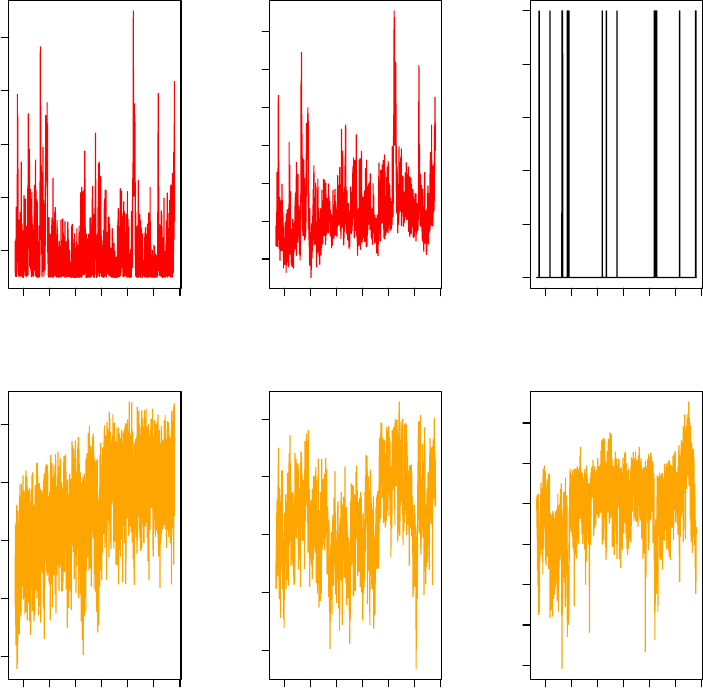
1e+05 3e+05 5e+05 7e+05

60 80 100 120 140

Time CLADE1 under CAL1

Sample

Time

1e+05 3e+05 5e+05 7e+05

20 30 40 50 60 70 80

Time CLADE2 under CAL1

Sample

Time

1e+05 3e+05 5e+05 7e+05

1.0 1.2 1.4 1.6 1.8 2.0

(1−>CLADE1, 2−>CLADE2)

Sample

Clade

1e+05 3e+05 5e+05 7e+05

−23960 −23950 −23940 −23930 −23920

Likelihood sequences

Sample

log(Probability)

1e+05 3e+05 5e+05 7e+05

−24100 −24080 −24060 −24040 −24020

Joint posterior

Sample

log(density)

1e+05 3e+05 5e+05 7e+05

−70 −65 −60 −55 −50 −45 −40

Branching process

Sample

log(density)

Figure 4. Traces from the statistics output ﬁle produced by Phy-

Time.

10.2 PhyloGeo

PhyloGeo is a program that implements the competition-dispersal phylogeog-

raphy model described in Ranjard, Welch, Paturel and Guindon “Modelling

competition and dispersal in a statistical phylogeographic framework”. Ac-

cepted for publication in Systematic Biology.

It implements a Markov Chain Monte Carlo approach that samples from

the posterior distribution of the three parameters of interest in this model,

namely the competition intensity λ, the dispersal bias parameter σand the

overal dispersal rate τ. The data consist in a phylogeny with node heights

proportional to their ages and geographical locations for evety taxon in this

tree. An important assumption of the model is that each node in the phy-

logeny corresponds to a speciation and a dispersal event. As a consequence,

this model does not authorize a given taxon to occupy more than one loca-

tions. Note however that the converse is not true: a given location can be

occupied by several diﬀerent taxa.

10.2.1 Installing PhyloGeo

Compiling PhyloGeo is straightforward on Unix-like machines (i.e., linux and

MacOS systems). PhyloGeo is not readily available for Windows machines

but compilation should be easy on this system too. In the ‘phyml’ directory,

where the ‘src/’ and ‘doc/’ directories stand, enter the following commands:

./configure --enable-geo;

make clean;

make;

This set of commands generates a binary ﬁle called phylogeo which can

be found in the ‘src/’ directory.

10.2.2 Running PhyloGeo

PhyloGeo takes as input a rooted tree ﬁle in Newick format and a ﬁle with

geographical locations for all the tips of the phylogeny. Here is an example

of valid tree and the corresponding spatial locations just below:

Valid PhyloGeo input tree

(((unicaA:1.30202,unicaB:1.30202):1.34596,(((nitidaC:0.94617,(nitidaA:0.31497,

nitidaB:0.31497):0.63120):0.18955,(((mauiensisA:0.00370,mauiensisB:0.00370):0.20068,

(pilimauiensisA:0.05151,pilimauiensisB:0.05151):0.15287):0.78769,(brunneaA:0.10582,

brunneaB:0.10582):0.88625):0.14365):0.80126,(((molokaiensisA:0.03728,

molokaiensisB:0.03728):0.71371,(deplanataA:0.01814,deplanataB:0.01814):0.73285):0.34764,

((parvulaA:0.20487,parvulaB:0.20487):0.40191,(kauaiensisA:0.24276,

kauaiensisB:0.24276):0.36401):0.49186):0.83835):0.71099):1.38043,

(nihoaA:0.05673,nihoaB:0.05673):3.97168);

Valid PhyloGeo spatial location file

nihoaA 23.062222 161.926111

nihoaB 23.062222 161.926111

kauaiensisA 22.0644445 159.5455555

kauaiensisB 22.0644445 159.5455555

unicaA 21.436875 158.0524305

unicaB 21.436875 158.0524305

parvulaA 21.436875 158.0524305

parvulaB 21.436875 158.0524305

molokaiensisA 20.90532 156.6499

molokaiensisB 20.90532 156.6499

deplanataA 20.90532 156.6499

deplanataB 20.90532 156.6499

brunneaA 20.90532 156.6499

brunneaB 20.90532 156.6499

mauiensisA 20.90532 156.6499

mauiensisB 20.90532 156.6499

pilimauiensisA 20.90532 156.6499

pilimauiensisB 20.90532 156.6499

nitidaA 19.7362 155.6069

nitidaB 19.7362 155.6069

nitidaC 19.7362 155.6069

In order to run PhyloGeo, enter the following command: ./phylogeo

./tree file ./spatial location file > phylogeo output. PhyloGeo

will then print out the sampled values of the model parameters in the ﬁle

phylogeo output. This ﬁle can then be used to generate the marginal pos-

terior densities of the model parameters. In particular, evidence for com-

petition corresponds to value of λsmaller than 1.0. Please see the original

article for more information on how to interpret the model parameters.

10.2.3 Citing PhyloGeo

Ranjard, L., Welch D., Paturel M. and Guindon S. “Modelling competition

and dispersal in a statistical phylogeographic framework”. 2014. Systematic

Biology.

10.3 PhyREX

PhyREX is a program that implements the spatial Λ-Fleming-Viot model

[44–49] or ΛV for short. According to this model, the spatial distribution of

individuals in a population is uniform and does not change during the course

of evolution, as opposed to other models such as the very popular isolation

by distance model proposed by Wright and Mal´ecot. The ΛV model does

not suﬀer from the “pain in the torus” [50] and clumps of individuals with

increasing densities do not arise. Also, estimates of migration parameters

are not sensitive to variation in sampling intensities across regions, unlike

“mugration” or “discrete trait analysis” models [51].

PhyREX implements an original data augmentation technique embedded

in a Bayesian sampler to estimate two important biological parameters: the

neighorhood size (N) and the dispersal intensity (σ2). These two parameters

are closely related to the eﬀective size of the population of interest per unit

area since Nis deﬁned as follows: N:= 4πρeσ2, where ρeis the eﬀective

population density.

10.3.1 Installing PhyREX

Compiling PhyREX is straightforward on Unix-like machines (i.e., linux and

MacOS systems). PhyREX is not readily available for Windows machines

but compilation should be easy on this system too. In the ‘phyml’ directory,

where the ‘src/’ and ‘doc/’ directories stand, enter the following commands:

./configure --enable-phyrex;

make clean;

make;

This set of commands generates a binary ﬁle called phyrex which can be

found in the ‘src/’ directory.

10.3.2 Running PhyREX

Example input ﬁles for PhyREX can be found in the

examples/phyrex input files/ directory. PhyRex takes as input a

sequence alignment, in a PhyML-compatible format as well as a text ﬁle

giving the spatial coordinates of each taxon in two dimension. A example of

the coordinates ﬁle is given below:

Valid PhyRex spatial location file

# state.name lon lat

|SouthWest| 0 0

|NorthEast| 10 10

levosl 5.082206 4.133893

kmgcwv 5.914294 4.603446

uhfwja 4.990937 4.445124

ndmwkc 5.178017 4.442268

jpadex 3.747484 4.571090

lqcdcw 7.081925 5.133123

wnsbtg 4.164588 4.720346

ptwgnn 5.711159 4.462993

jhqdsm 3.539525 4.537706

vlnoes 4.613251 4.470530

pfrnpk 4.117791 4.489819

elwdvr 5.649958 4.824092

lptxiv 4.563302 4.005124

The ﬁrst row in this ﬁle gives the names of the columns. It starts with the

‘#’ character signaling a comment. The second and third rows deﬁne the

limits of the population’s habitat. At the moment, this habitat is assumed

to be a rectangle. The position in space of that rectangle are determined by

the coordinates of the bottom-left corner (|SouthWest| 0 0) and the top-

right one (|NorthEast| 10 10). The ‘|’ characters help identify the terms

Figure 5. Statistics ﬁle generated by PhyREX and loaded on Icylog

(http://tgvaughan.github.io/icylog/icylog.html). The traces for the

neighborhood size (top) and the dispersal intensity (bottom) are shown here.

in the list of coordinate corresponding indeed to these two particular points

and should thus not be omitted. The remaining row give the coordinates

of each taxon. Every taxon in the sequence ﬁle should also be listed in the

coordinate ﬁle.

PhyRex uses the same command-line arguments as that used with

PhyML. The only exception being the mandatory argument corresponding

to the coordinate ﬁle. A typical command-line will this look as follows:

./phyrex -i sequence file --coord file=./spatial location file

-c 3 --freerates --il. With this particular set of options, the sequence

alignment will be analysed under a FreeRate model [28] with three rate

classes and a covarion-like model of rate variation across lineaged [29].

Please note that the command-line option --coord file is mandatory.

PhyREX generates correlated samples from the posterior distribution of

the ΛV model parameters. The estimated distributions and related summary

statistics can be monitored during the analysis using the MCMC vizualiza-

tion software Icylog. Figure 5shows the traces for two parameters after

about an hour of calculation on the example data set (36 taxa, 50 geographic

locations).

11 Recommendations on program usage

11.1 PhyML

The choice of the tree searching algorithm among those provided by PhyML

is generally a tough one. The fastest option relies on local and simultaneous

modiﬁcations of the phylogeny using NNI moves. More thorough explorations

of the space of topologies are also available through the SPR options. As these

two classes of tree topology moves involve diﬀerent computational burdens,

it is important to determine which option is the most suitable for the type of

data set or analysis one wants to perform. Below is a list of recommendations

for typical phylogenetic analyses.

1. Single data set, unlimited computing time. The best option here is

probably to use a SPR search (i.e., straight SPR of best of SPR and

NNI). If the focus is on estimating the relationships between species, it

is a good idea to use more than one starting tree to decrease the chance

of getting stuck in a local maximum of the likelihood function. Using

NNIs is appropriate if the analysis does not mainly focus on estimating

the evolutionary relationships between species (e.g. a tree is needed

to estimate the parameters of codon-based models later on). Branch

supports can be estimated using bootstrap and approximate likelihood

ratios.

2. Single data set, restricted computing time. The three tree searching

options can be used depending on the computing time available and

the size of the data set. For small data sets (i.e., <50 sequences),

NNI will generally perform well provided that the phylogenetic signal

is strong. It is relevant to estimate a ﬁrst tree using NNI moves and

examine the reconstructed phylogeny in order to have a rough idea of

the strength of the phylogenetic signal (the presence of small internal

branch lengths is generally considered as a sign of a weak phylogenetic

signal, specially when sequences are short). For larger data sets (>50

sequences), a SPR search is recommended if there are good evidence

of a lack of phylogenetic signal. Bootstrap analysis will generally in-

volve large computational burdens. Estimating branch supports using

approximate likelihood ratios therefore provides an interesting alterna-

tive here.

3. Multiple data sets, unlimited computing time. Comparative genomic

analyses sometimes rely on building phylogenies from the analysis of a

large number of gene families. Here again, the NNI option is the most

relevant if the focus is not on recovering the most accurate picture

of the evolutionary relationships between species. Slower SPR-based

heuristics should be used when the topology of the tree is an important

parameter of the analysis (e.g., identiﬁcation of horizontally transferred

genes using phylogenetic tree comparisons). Internal branch support

is generally not a crucial parameter of the multiple data set analyses.

Using approximate likelihood ratio is probably the best choice here.

4. Multiple data sets, limited computing time. The large amount of data to

be processed in a limited time generally requires the use of the fastest

tree searching and branch support estimation methods Hence, NNI

and approximate likelihood ratios rather than SPR and non-parametric

bootstrap are generally the most appropriate here.

Another important point is the choice of the substitution model. While

default options generally provide acceptable results, it is often warranted to

perform a pre-analysis in order to identify the best-ﬁt substitution model.

This pre-analysis can be done using popular software such as Modeltest [52]

or ProtTest [53] for instance. These programs generally recommend the use of

a discrete gamma distribution to model the substitution process as variability

of rates among sites is a common feature of molecular evolution. The choice

of the number of rate classes to use for this distribution is also an important

one. While the default is set to four categories in PhyML, it is recommended

to use larger number of classes if possible in order to best approximate the

patterns of rate variation across sites [54]. Note however that run times

are directly proportional to the number of classes of the discrete gamma

distribution. Here again, a pre-analysis with the simplest model should help

the user to determine the number of rate classes that represents the best

trade-oﬀ between computing time and ﬁt of the model to the data.

11.2 PhyTime

Analysing a data set using PhyTime should involve three steps based on the

following questions: (1) do the priors seem to be adequate (2) can I use the

fast approximation of the likelihood and (3) how long shall I run the program

for? I explain below how to provide answers to these questions.

•Are the priors adequate? Bayesian analysis relies on speciﬁying the joint

prior density of model parameters. In the case of node age estimation,

these priors essentially describe how rates of substitution vary across

lineages and the probabilistic distribution that node ages have when

ignoring the information provided by the genetic sequences. These

priors vary from tree to tree. It is therefore essential to check the

adequacy of priors for each user-deﬁned input tree. In order to do so,

PhyTime needs to be run with the --no data option. When this option

is required, the sequence data provided as input will be ignored and

the rest of the analysis will proceed normally. The prior distribution

of model parameters, essentially edge rates and node heights, can then

be checked using the program Tracer as one would do for the standard

‘posterior’ analysis.

•Can I use the fast approximation to the likelihood? The suface of the

log-likelihood function can be approximated using a multivariate nor-

mal density. This technique is saving very substantial amounts of com-

putation time. However, like most approximations, there are situations

where it does not provide a good ﬁt to the actual function. This usu-

ally happens when the phylogeny displays a lot of short branches, i.e.,

the signal conveyed by the sequences is weak. It is therefore important

to ﬁrst check whether using the approximate likelihood is reasonable.

In order to do so, it is recommended to ﬁrst run the program without

the approximation, i.e., using the default settings. Once the minimum

value of the ESS of node ages (the last column on the right of the

standard output) has reached 40-50, open the phytime.XXXX output

ﬁle with Tracer and examine the correlation between the exact and

approximate likelihood values. If the correlation is deemed to be good

enough, PhyTime can be re-run using the --fast lk option, which

uses the fast normal approximation to the likelihood function.

•How long shall I run the program for? PhyTime should be run long

enough such that the ESS of each parameter is ‘large enough’. The

last column on the right handside of the standard output gives the

minimum ESS across all internal node heights. It is recommended to

run the program so that this number reaches at least 100.

12 Frequently asked questions

1. PhyML crashes before reading the sequences. What’s wrong ?

•The format of your sequence ﬁle is not recognized by PhyML. See

Section 7

•The carriage return characters in your sequence ﬁles are not rec-

ognized by PhyML. You must make sure that your sequence ﬁle

is a plain text ﬁle, with standard carriage return characters (i.e.,

corresponding to “\n”, or “\r”)

2. The program crashes after reading the sequences. What’s wrong ?

•You analyse protein sequences and did not enter the -d aa option

in the command-line.

•The format of your sequence ﬁle is not recognized by PhyML. See

Section 7

3. Does PhyML handle outgroup sequences ?

•Yes, it does. Outgroup taxa are identiﬁed by adding the ‘*’ sign at

the end of each corresponding sequence name (see Section 7.1.2)

4. Does PhyML estimate clock-constrained trees ?

•No, the PhyML program does not estimate clock-contrained trees.

One can however use the program PhyTime to perform such anal-

ysis but the tree topology will not be estimated.

5. Can PhyML analyse partitioned data, such as multiple gene sequences ?

•We are currently working on this topic. Future releases of the

program will provide options to estimate trees from phylogenomic

data sets, with the opportunity to use diﬀerent substitution mod-

els on the diﬀerent data partitions (e.g., diﬀerent genes). PhyML

will also include speciﬁc algorithms to search the space of tree

topologies for this type of data.

13 Acknowledgements

The development of PhyML since 2000 has been supported by the Centre Na-

tional de la Recherche Scientiﬁque (CNRS) and the Minist`ere de l’´

Education

Nationale.

References

[1] Guindon, S. & Gascuel, O. A simple, fast and accurate algorithm to

estimate large phylogenies by maximum likelihood. Systematic Biology

52, 696–704 (2003).

[2] Stamatakis, A. RAxML-VI-HPC: Maximum likelihood-based phyloge-

netic analyses with thousands of taxa and mixed models. Bioinformatics

22, 2688–2690 (2006).

[3] Zwickl, D. Genetic algorithm approaches for the phylogenetic analysis

of large biological sequence datasets under the maximum likelihood cri-

terion. Ph.D. thesis, The University of Texas at Austin (2006).

[4] Ayres, D. L. et al. Beagle: an application programming interface and

high-performance computing library for statistical phylogenetics. Sys-

tematic Biology 61, 170–173 (2012).

[5] Jukes, T. & Cantor, C. Evolution of protein molecules. In Munro, H.

(ed.) Mammalian Protein Metabolism, vol. III, chap. 24, 21–132 (Aca-

demic Press, New York, 1969).

[6] Kimura, M. A simple method for estimating evolutionary rates of base

substitutions through comparative studies of nucleotide sequences. Jour-

nal of Molecular Evolution 16, 111–120 (1980).

[7] Felsenstein, J. Evolutionary trees from DNA sequences: a maximum

likelihood approach. Journal of Molecular Evolution 17, 368–376 (1981).

[8] Felsenstein, J. PHYLIP (PHYLogeny Inference Package) version 3.6a2

(Distributed by the author, Department of Genetics, University of Wash-

ington, Seattle, 1993).

[9] Hasegawa, M., Kishino, H. & Yano, T. Dating of the Human-Ape split-

ting by a molecular clock of mitochondrial-DNA. Journal of Molecular

Evolution 22, 160–174 (1985).

[10] Tamura, K. & Nei, M. Estimation of the number of nucleotide sub-

stitutions in the control region of mitochondrial DNA in humans and

chimpanzees. Molecular Biology and Evolution 10, 512–526 (1993).

[11] Lanave, C., Preparata, G., Saccone, C. & Serio, G. A new method

for calculating evolutionary substitution rates. Journal of Molecular

Evolution 20, 86–93 (1984).

[12] Tavar´e, S. Some probabilistic and statistical problems on the analysis

of DNA sequences. Lectures on Mathematics in the Life Sciences 17,

57–86 (1986).

[13] Le, S. & Gascuel, O. An improved general amino-acid replacement

matrix. Molecular Biology and Evolution 25, 1307–1320 (2008).

[14] Whelan, S. & Goldman, N. A general empirical model of protein evolu-

tion derived from multiple protein families using a maximum-likelihood

approach. Molecular Biology and Evolution 18, 691–699 (2001).

[15] Dayhoﬀ, M., Schwartz, R. & Orcutt, B. A model of evolutionary change

in proteins. In Dayhoﬀ, M. (ed.) Atlas of Protein Sequence and Structure,

vol. 5, 345–352 (National Biomedical Research Foundation, Washington,

D. C., 1978).

[16] Jones, D., Taylor, W. & Thornton, J. The rapid generation of mutation

data matrices from protein sequences. Computer Applications in the

Biosciences (CABIOS) 8, 275–282 (1992).

[17] Henikoﬀ, S. & Henikoﬀ, J. Amino acid substitution matrices from pro-

tein blocks. PNAS 89, 10915–10919 (1992).

[18] Adachi, J. & Hasegawa, M. MOLPHY version 2.3. programs for molec-

ular phylogenetics based on maximum likelihood. In Ishiguro, M. et al.

(eds.) Computer Science Monographs, 28 (The Institute of Statistical

Mathematics, Tokyo, 1996).

[19] Dimmic, M., Rest, J., Mindell, D. & Goldstein, D. rtREV: an amino acid

substitution matrix for inference of retrovirus and reverse transcriptase

phylogeny. Journal of Molecular Evolution 55, 65–73 (2002).

[20] Adachi, J., P., W., Martin, W. & Hasegawa, M. Plastid genome phy-

logeny and a model of amino acid substitution for proteins encoded by

chloroplast DNA. Journal of Molecular Evolution 50, 348–358 (2000).

[21] Kosiol, C. & Goldman, N. Diﬀerent versions of the Dayhoﬀ rate matrix.

Molecular Biology and Evolution 22, 193–199 (2004).

[22] Muller, T. & Vingron, M. Modeling amino acid replacement. Journal

of Computational Biology 7, 761–776 (2000).

[23] Cao, Y. et al. Conﬂict among individual mitochondrial proteins in re-

solving the phylogeny of eutherian orders. Journal of Molecular Evolu-

tion 47, 307–322 (1998).

[24] Gascuel, O. BioNJ: an improved version of the NJ algorithm based on

a simple model of sequence data. Molecular Biology and Evolution 14,

685–695 (1997).

[25] Anisimova, M., Gil, M., Dufayard, J., Dessimoz, C. & Gascuel, O. Sur-

vey of branch support methods demonstrates accuracy, power, and ro-

bustness of fast likelihood-based approximation schemes. Systematic

Biology 60, 685–699 (2011).

[26] Anisimova, M. & Gascuel, O. Approximate likelihood-ratio test for

branches: a fast, accurate, and powerful alternative. Systematic Biology

55, 539–552 (2006).

[27] Posada, D. & Crandall, K. Selecting models of nucleotide substitution:

an application to human immunodeﬁciency virus 1 (hiv-1). Molecular

Biology and Evolution 18, 897–906 (2001).

[28] Soubrier, J. et al. The inﬂuence of rate heterogeneity among sites on the

time dependence of molecular rates. Molecular Biology and Evolution

(2012).

[29] Guindon, S. From trajectories to averages: an improved description of

the heterogeneity of substitution rates along lineages. Systematic Biology

62, 22–34 (2013).

[30] Maddison, D., Swoﬀord, D. & Maddison, W. NEXUS: an extensible

ﬁle format for systematic information. Systematic Biology 46, 590–621

(1997).

[31] Yang, Z. Maximum likelihood phylogenetic estimation from DNA se-

quences with variable rates over sites: approximate methods. Journal

of Molecular Evolution 39, 306–314 (1994).

[32] Yang, Z. Likelihood ratio tests for detecting positive selection and appli-

cation to primate lysozyme evolution. Molecular Biology and Evolution

15, 568–573 (1998).

[33] Yang, Z. & Nielsen, R. Estimating synonymous and nonsynonymous

substitution rates under realistic evolutionary models. Molecular Biology

and Evolution 17, 32–43 (2000).

[34] Yang, Z. & Nielsen, R. Codon-substitution models for detecting molec-

ular adaptation at individual sites along speciﬁc lineages. Molecular

Biology and Evolution 19, 908–917 (2002).

[35] Guindon, S., Rodrigo, A., Dyer, K. & Huelsenbeck, J. Modeling the

site-speciﬁc variation of selection patterns along lineages. PNAS 101,

12957–12962 (2004).

[36] Degnan, J. & Rosenberg, N. Gene tree discordance, phylogenetic in-

ference and the multispecies coalescent. Trends in Ecology & Evolution

24, 332–340 (2009).

[37] Liu, L. BEST: Bayesian estimation of species trees under the coalescent

model. Bioinformatics 24, 2542–2543 (2008).

[38] Kubatko, L., Carstens, B. & Knowles, L. STEM: species tree estimation

using maximum likelihood for gene trees under coalescence. Bioinfor-

matics 25, 971–973 (2009).

[39] Heled, J. & Drummond, A. Bayesian inference of species trees from

multilocus data. Molecular Biology and Evolution 27, 570–580 (2010).

[40] Matsen, F. & Steel, M. Phylogenetic mixtures on a single tree can mimic

a tree of another topology. Systematic Biology 56, 767–775 (2007).

[41] Shimodaira, H. & Hasegawa, M. Multiple comparisons of log-likelihoods

with applications to phylogenetic inference. Molecular Biology and Evo-

lution 16, 1114–1116 (1999).

[42] Le, S. Q., Dang, C. C. & Gascuel, O. Modeling protein evolution with

several amino acid replacement matrices depending on site rates. Molec-

ular Biology and Evolution 29, 2921–2936 (2012).

[43] Guindon, S. Bayesian molecular dating as a “doubly intractable”

problem. BioRxiv http://biorxiv.org/content/early/2017/02/06/106310

(2017).

[44] Etheridge, A. M. Drift, draft and structure: some mathematical models

of evolution. Banach Center Publ. 80, 121–144 (2008).

[45] Berestycki, N., Etheridge, A. & Hutzenthaler, M. Survival, extinction

and ergodicity in a spatially continuous population model. In Markov

Proc. Rel. Fields (2009).

[46] Barton, N., Etheridge, A. & V´eber, A. A new model for evolution in a

spatial continuum. Electronic Journal of Probability 15 (2010).

[47] Barton, N. H., Kelleher, J. & Etheridge, A. M. A new model for extinc-

tion and recolonization in two dimensions: quantifying phylogeography.

Evolution 64, 2701–2715 (2010).

[48] V´eber, A. & Wakolbinger, A. The spatial Lambda-Fleming-Viot process:

an event-based construction and a lookdown representation. Annales de

l’Institut Henri Poincar´e in press (2014).

[49] Barton, N., Etheridge, A. & V´eber, A. Modelling evolution in a spatial

continuum. Journal of Statistical Mechanics: Theory and Experiment

2013, P01002 (2013).

[50] Felsenstein, J. A pain in the torus: some diﬃculties with models of

isolation by distance. American Naturalist 359–368 (1975).

[51] Lemey, P., Rambaut, A., Drummond, A. J. & Suchard, M. A. Bayesian

phylogeography ﬁnds its roots. PLoS Comput Biol 5, e1000520 (2009).

[52] Posada, D. & Crandall, K. Modeltest: testing the model of DNA sub-

stitution. Bioinformatics 14, 817–918 (1998).

[53] Abascal, F., Zardoya, R. & Posada, D. Prottest: selection of best-ﬁt

models of protein evolution. Bioinformatics 21, 2104–2105 (2005).

[54] Galtier, N. & Jean-Marie, A. Markov-modulated Markov chains and

the covarion process of molecular evolution. Journal of Computational

Biology 11, 727–733 (2004).

Index

κ,11,17

*BEAST, 33

BEAST, 60

BEST, 33

binary characters, 24

BioNJ, 14

bootstrap, 15

parallel, 7,21

bug, 6

command-line options

--constraint file,20

command-line options

--aa rate file,16

--alpha,18

--ancestral,21

--bootstrap,15

--codpos,18

--constrained lens,20

--data type,15

--free rates,18

--il,18

--inputtree,19

--input,15

--json trace,20

--model,16

--multiple,15

--n rand starts,19

--nclasses,18

--no colalias,20

--no memory check,20

--pars,15

--pinv,17

--print site lk,19

--print trace,20

--quiet,21

--r seed,19

--rand start,19

--run id,20

--search,19

--sequential,15

--ts/tv,17

--use median,18

--xml,21

-f,16

-o,19

compilation, 6

covarion, 18

custom models, 17

data partitions, 31,37

FreeRate, 44

frequencies

amino-acid, 16

nucleotide, 16

gamma distribution (discrete)

mean vs. median, 12,18

number of categories, 12,18

shape parameter, 12,18

GARLI, 6

Icylog, 60

input tree, 19

interleaved, 22

invariable sites, 12,17

lg4x, 48

likelihood

print site likelihood, 19

mixture models, 37

mixture models, 30

MPI, 7,21

MRCA, 57

multiple data sets, 15,26

Newick format, 26

NEXUS, 22

NNI, 19

optimisation

substitution parameters, 19

topology, 19

PAML, 11,27

partitionned analysis, 31,37

PHYLIP, 12,22

PhyloGeo, 64

PhyRex, 65

PhyTime, 53

calibration, 54

clade, 55

lineagerates, 54

proportion of invariants, 12,17

random number, 19

random tree, 19

RAxML, 6

run ID, 10,20

sequence format

interleaved, 15

sequential, 15

sequential, 22

SPR, 19

stationary frequencies, 16

STEM, 33

substitution models

amino acids, 16

DNA, 16

Tracer, 60

ts/tv ratio, 11,17

user tree, 19

XML, 30

XML options

branchlengths component, 43

equfreqs component, 42

mixtureelem component, 45

partitionelem component, 45

phyml component, 40

ratematrices component, 41

siterates component, 43

topology component, 41

Phyml Manual

Navigation menu

Versions of this User Manual:

Views

Navigation