Pid Controller
User Manual: Pdf pid-controller
Open the PDF directly: View PDF ![]() .
.
Page Count: 21
- 1 PID controller in SOBEK
- 2 Aim of this document
- 3 Conclusion
- 4 Mass-Spring-Damper system
- 5 Feedback loop, PID-controller
- 6 PID controller (positional)
- 7 PID controller (velocity)
- 8 Determine coefficients from experiments
- 9 Numerical discretisation
- 10 Experiments
- References

DRAFT
Memo
To
To whom it may concern
Date Reference Number of pages
2018-04-18 SVN: 53753 21
From Direct line E-mail
Jan Mooiman +31 (0)88 335 8568
+31 06 4691 4571
jan.mooiman@deltares nl
Subject
PID controller mass-spring-damper system
Copy to
—
Version control information
Location : https://repos.deltares.nl/repos/ds/trunk/doc/user_manuals/
white_papers/sobek/pid-controller/pid.tex
Revision : 53753
Contents
1 PID controller in SOBEK ................................ 2
2 Aim of this document .................................. 3
3 Conclusion . . . . . . . . . . . . . . . . . . . . . . . . . . . . . . . . . . . . . . . 3
4 Mass-Spring-Damper system . . . . . . . . . . . . . . . . . . . . . . . . . . . . . . 3
4.1 Energy of Mass-Spring-Damper system . . . . . . . . . . . . . . . . . . . . 4
5 Feedback loop, PID-controller . . . . . . . . . . . . . . . . . . . . . . . . . . . . . 5
5.1 Unit impulse function . . . . . . . . . . . . . . . . . . . . . . . . . . . . . . 5
5.2 Unit step function ................................ 6
6 PID controller (positional) ................................ 7
6.1 Proportional term ................................ 8
6.2 Derivative term . . . . . . . . . . . . . . . . . . . . . . . . . . . . . . . . . 8
6.3 Integral term .................................. 8
7 PID controller (velocity) . . . . . . . . . . . . . . . . . . . . . . . . . . . . . . . . . 10
8 Determine coefficients from experiments . . . . . . . . . . . . . . . . . . . . . . . . 11
9 Numerical discretisation . . . . . . . . . . . . . . . . . . . . . . . . . . . . . . . . 12
9.1 Mass-Spring-Damper system as system of first order PDE’s . . . . . . . . . 12
9.2 PID controller (positional) . . . . . . . . . . . . . . . . . . . . . . . . . . . 12
9.2.1 Implicit Mass-Spring-Damper system with explicit PID-controller . 12
9.2.2 Implicit Mass-Spring-Damper system with implicit PID-controller . 12
9.2.3 Corrected Mass-Spring-Damper system while using an explicit PID
controller . . . . . . . . . . . . . . . . . . . . . . . . . . . . . . . 13
9.3 PID controller (velocity) . . . . . . . . . . . . . . . . . . . . . . . . . . . . 14
9.3.1 Implicit Mass-Spring-Damper system with explicit velocity PID con-
troller . . . . . . . . . . . . . . . . . . . . . . . . . . . . . . . . 14

DRAFT
Date Reference Page
2018-04-18 SVN: 53753 2/21
9.3.2 Implicit Mass-Spring-Damper system with implicit velocity PID con-
troller . . . . . . . . . . . . . . . . . . . . . . . . . . . . . . . . 14
9.3.3 Corrected Mass-Spring-Damper system while using an explicit ve-
locity PID controller . . . . . . . . . . . . . . . . . . . . . . . . . 14
10 Experiments . . . . . . . . . . . . . . . . . . . . . . . . . . . . . . . . . . . . . . . 15
10.1 Solutions determined by Maplesoft . . . . . . . . . . . . . . . . . . . . . . 16
10.2 Numerical experiments . . . . . . . . . . . . . . . . . . . . . . . . . . . . . 17
10.2.1 Time integration method . . . . . . . . . . . . . . . . . . . . . . 17
10.2.2 Convergence behaviour . . . . . . . . . . . . . . . . . . . . . . . 19
References . . . . . . . . . . . . . . . . . . . . . . . . . . . . . . . . . . . . . . . . . . 21
Used references
•Berdahl and III (2007),
•Callafon (2014),
•Rowell (2004),
•Yon-Ping (Mass-Damper-Spring systems/PID control of the simplest second-order systems,
eq. 23): PD-Controller, desired set-point will not be reached.
•Rao (2009, pg. 13, eq. 2-39): Integral of Dirac delta functions (unit impulse and unit step
response)
•Åström and Murray (2016, pg. 47 eq. 2.19): Unit step response solution.
•Seborg et al. (2011, §8.6.1)
To Do
1 Transfer functions.
1 PID controller in SOBEK
The discretised PID-controller in SOBEK2 read:
fn=fn−1+Kpen+Ki
n
X
j=0
ej+Kden−en−1,(1)
No literaure references are found for this PID-controller (i.e. Equation (1)).
The proposed discretised PID-controller read:
fn=fn−1+Kpen−en−1+Ki∆tnen+Kd
en−2en−1+en−2
∆t(2)
This PID-controller (Equation (2)) is based on the linearisation of the standard PID-controller.
DRAFT
Date Reference Page
2018-04-18 SVN: 53753 3/21
2 Aim of this document
The aim of this document is to find out what each term of the PID-controller does do to a general
system. To reach that goal we look to the Mass-Spring-Damper system without loss of generality.
3 Conclusion
Mathematical physics
• Proportional gain factor: influence on equilibrium state. But it does not reach the required
set-point.
• Integral gain factor: influence on the equilibrium state. You need this term to reach the equi-
librium state.
• Derivative gain factor: Influence transition time to the equilibrium state, but it does not influ-
ence the equilibrium state.
Numerical experiments
Some numerical experiments are performed. Varying time step and varying the time integration
method of the PID-controller. The time integration of the Mass-Spring-Damper-system is implicit.
• Explicit implementation (black box approach of the PID-controller) does have a severe draw
back on the computation time because the ∆tshould be decreased w.r.t. the other methods.
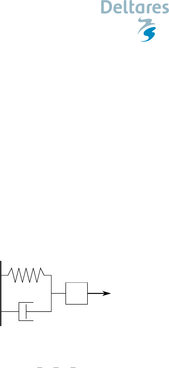
4 Mass-Spring-Damper system
k
cm
f(t)
Figure 1: Drawing of Mass-Spring-Damper system.
Equation of Mass-Spring-Damper system (m > 0,c > 0and k > 0):
m¨x+c˙x+kx =f(t)⇔¨x+c
m˙x+k
mx=1
mf(t)(3)

DRAFT
Date Reference Page
2018-04-18 SVN: 53753 4/21
The natural (free) angular velocity ωnis (c= 0 and f(t)=0):
ωn=rk
m,(4)
The decay time constant τis:
τ=2m
c(5)
and the damping ratio ζis:
ζ=c
2√mk (6)
The damping ratio is related to ωn.
mr2+cr +k= 0 ⇒r1,2=−c±√c2−4mk
2m
Decay of solution is: exp −c
2m, so the decay time constant is: τ=2m
c
Damping rate is: exp (−ζωnt) = exp −ct
2m⇒ζωn=c
2m⇒ζ=c
2ωnm⇒ζ=c
2√km .
The equation can also be written as: ¨x+ 2ζωn˙x+ω2
n= 0
r2+ 2ζωnr+ω2
n= 0 ⇒r1,2=ζωn±1
2p4ζ2ω2
n−4ω2
n⇒r1,2=ζωn±ωnpζ2−1.
Define ωd=ωnp1−ζ2as the frequency for the under damped oscillations.
ζ= 0 not damped (oscillations)
ζ < 1under damped (oscillations)
ζ= 1 critical damped
ζ > 1over damped
4.1 Energy of Mass-Spring-Damper system
Write the Mass-Spring-Damper system as a set of first order of PDE’s, without external forces as:
˙x=v(7)
m˙v=−cv −kx, (8)
The total energy of the system read:
Etot =Ekin +Epot =1
2mv2+1
2kx2(9)
Energy conserving:
d
dtEtot =d
dt 1
2mv2+1
2kx2(10)
=mv ˙v+kx ˙x(11)
Substituting gives:
d
dtEtot =mv −cv −kx
m+kxv =−cv2−vkx +kxv =−cv2(12)
So if c= 0 the system is energy conserving, other wise the system is dissipative. If d
dt Etot = 0 the
Mass-Spring-Damper system is called a Hamiltonian system, if d
dt Etot ≤0the Mass-Spring-Damper
system is called a Lyapunov function.

DRAFT
Date Reference Page
2018-04-18 SVN: 53753 5/21
5 Feedback loop, PID-controller
Implement the feed back loop (external force is dependent on solution, Berdahl and III (2007)) and
an external force as step function (i.e. new setpoint)
f(t) = −Kpx−Kd˙x+u(t)(13)
with
Kpgain factor proportional to x.
Kdgain factor proportional to the time derivative of x(i.e. ˙x, velocity) and
u(t)the unit step function is defined as Rao (2009, pg. 13, eq. 2-28):
u(t) = (0t < 0
1t≥0(14)
After substitution of Equation (13) in Equation (3) (consider only t≥0; assume everything is in rest
for t < 0) we get:
m¨x+c˙x+kx =−Kpx−Kd˙x+u(t)(15)
m¨x+ (c+Kd) ˙x+ (k+Kp)x=u(t)(16)
To evaluate the stepfunction u(t)of Equation (14), we first discuss the solution for the Dirac delta
function (or unit impulse function) and than the unit step function.
5.1 Unit impulse function
To evaluate the Dirac delta function (or unit impulse function):
δ(t−a) = (∞t=a
0t6=a(17)
which satisfies
Z∞
−∞
δ(t−a)dt = 1 (18)
Z∞
−∞
f(t)δ(t−a)dt =f(a)(19)
Suppose g(t)is the solution of the system:
m¨g+c˙g+kg =δ(t)(20)
Integrate this equation from 0to T(T > 0), just the length of the pulse. Resulting in a valid value at
the right hand side
ZT
0
(m¨g+c˙g+kg)dt =ZT
0
δ(t)dt (21)
ZT
0
m¨g dt +ZT
0
c˙g dt +ZT
0
kg dt =ZT
0
δ(t)dt (22)

DRAFT
Date Reference Page
2018-04-18 SVN: 53753 6/21
Taking the limit as T↓0, we obtain (term by term):
lim
T↓0ZT
0
m¨g(t)dt = lim
T↓0m˙g(t)|T
0= lim
T↓0m[ ˙g(T)−˙g(0)] = m˙g(0+) ˙g(t)is discontinue
(23)
lim
T↓0ZT
0
c˙g(t)dt = lim
T↓0cg(t)|T
0= lim
T↓0c[g(T)−g(0)] = 0 g(t)is continue (24)
lim
T↓0ZT
0
kg(t)dt = lim
T↓0ktg(0)|T
0= lim
T↓0k[T g(0) −0g(0)] = 0 because g(0) = 0 (25)
ZT
0
δ(t)dt = 1 (26)
and thus
m˙g(0+)=1 ⇒˙g(0+) = 1
m(27)
Now that we know that the response of a second-order resting system is to change the velocity
(while leaving position unchanged), we can use this fact to obtain the impulse response g(t). In
particular, assuming an underdamped system, we know that the general form of the free response
is given as
g(t) = e−ζωnt(Acos ωdt+Bsin ωdt)(28)
Therefore, with g(0) = 0 and ˙g(0+) = 1/m the response of the system to a unit impulse at t= 0 is
given as
g(t) = (0t≤0
1
mωde−ζωntsin ωdt t > 0(29)
5.2 Unit step function
The unit step function is defined as
u(t−a) = (0t<a
1t≥a(30)
The relation between the δ(t)and u(t)is as follows:
u(t−a) = Zt
−∞
δ(τ−a)dτ (31)
d u(t−a)
dt =δ(τ−a)(32)
The function s(t)is called the step response and satisfies:
m¨s+c˙s+ks =u(t)(33)

DRAFT
Date Reference Page
2018-04-18 SVN: 53753 7/21
The function s(t)will be obtained as follows, starting from the unit impulse solution g(t):
m¨g+c˙g+kg =δ(t)(34)
m¨g+c˙g+kg =d u(t)
dt (35)
Integrating this equation from −∞ to t:
Zt
−∞ md2g
dτ2+cd g
dτ +kgdτ =Zt
−∞
d u(τ)
dτ dτ =u(t)(36)
Using the fundamental theorem of calculus we get
md2
dt2+cd
dt +kZt
−∞
g(τ)dτ =u(t)(37)
It is seen that
s(t) = Zt
−∞
g(τ)dτ (38)
For t≤0we have s(t) = 0 and for t > 0we have (integrating Equation (29))
s(t) = Zt
01
mωd
e−ζωnτsin ωdτdτ (39)
After some calculation, using sin x= (eix −e−ix)/2iand (eix +e−ix)/2 = cos x(Rao, 2009), we
get
s(t) = (0t≤0
1
mω2
n1−e−ζωntcos ωdt+ζωn
ωdsin ωdt t > 0(40)
This solution brings the system to a new equilibrium state:
lim
t→∞ s(t) = 1
mω2
n
(41)
6 PID controller (positional)
Assume that the equilibrium value x(∞)or setpoint (new equilibrium) is a desired value, the error
(deviation) to that value is defined as: e(t) = x(∞)−x(t). This error (deviation) will be investigated.
The PID-controller can been seen as a external force on the Mass-Spring-Damper-system and read:
f(t) = Kpe(t) + KiZt
0
e(τ)dτ +Kd
de(t)
dt ,(42)
where
Kpgain factor proportional to e(t),
Kigain factor proportional to the time integral of e(t)and
Kdgain factor proportional to the time derivative of e(t).

DRAFT
Date Reference Page
2018-04-18 SVN: 53753 8/21
6.1 Proportional term
Consider just the proportional term, so Ki=Kd= 0.
The proportial term Kpe(t)does influence the equilibrium state of the Mass-Spring-Damper system,
but will not reached the desired equilibrium state x(∞).
m¨x+c˙x+kx =Kp(x(∞)−x)(43)
m¨x+c˙x+ (k+Kp)x=Kpx(∞)(44)
So the particular solution will not reach the equilibrium state (limt→∞, and ¨x= ˙x= 0):
lim
t→∞ x(t) = Kp
(k+Kp)x(∞)and k+Kp>0(45)
also the free angular frequency is influenced by the proportional gain Kp
ωn=rk+Kp
mand k+Kp>0(46)
6.2 Derivative term
Consider just the derivative term, so Kp=Ki= 0.
The derivative term Kd˙e(t)does not influence the equilibrium state of the Mass-Spring-Damper
system:
m¨x+c˙x+kx =Kd
d
dt(x(∞)−x)(47)
m¨x+c˙x+kx =Kd( ˙x(∞)−˙x)(48)
With ˙x(∞)=0for the equilibrium state, so
m¨x+c˙x+kx =−Kd˙x(49)
m¨x+ (c+Kd) ˙x+kx = 0 (50)
So, just the damping factor (resistance, friction) is adjusted by the derivative gain Kdand the equi-
librium state is the same as for the homogeneous solution (¨x= ˙x= 0):
lim
t→∞ kx(t)=0 ⇒lim
t→∞ x(t) = 0.(51)
Remark:c+Kd>0other wise the system is unstable, see section 4.1
6.3 Integral term
Consider just the integral term, so Kp=Kd= 0.
The integral term KiRt
0e(τ)dτ does influence the equilibrium state of the Mass-Spring-Damper
system. Switching a Mass-Spring-Damper system to another equilibrium state is done by prescribing

DRAFT
Date Reference Page
2018-04-18 SVN: 53753 9/21
a value other than zero as external force. For example a constant value, the integral of a Dirac delta
function or another bounded integral. Prescribing a constant value of 1will give as equilibrium state
(¨x= ˙x= 0):
lim
t→∞ (m¨x+c˙x+kx) = 1 (52)
kx = 1 ⇒x=1
k(53)
The integral of the Dirac delta function is equal to 1,
Z∞
−∞
δ(t−a)dt = 1 (54)
and will give therefore the same solution as above (Equation (53)).
Prescribing the external force as
f(t) = Zt
0
(x(∞)−x(τ)) dτ (55)
will force the solution x(t)to x(∞), because
lim
t→∞ (x(∞)−x(t)) = 0 (56)
and the integral is bounded (<∞).

DRAFT
Date Reference Page
2018-04-18 SVN: 53753 10/21
7 PID controller (velocity)
Assume that a equilibrium value x(∞)or setpoint (a new equlibrium), is a desired value, the error (deviation) to that value is defined as:
e(t) = x(∞)−x(t), and need to be investigated.
The PID-controller can been seen as a external force on the Mass-Spring-Damper-system and read:
fPID(t) = Kpe(t) + KiZt
0
e(τ)dτ +Kd
de(t)
dt ,equal to Equation (42) (57)
The time derivative (velocity) of the PID-controller (Equation (57)) read:
∂fPID
∂t =Kp
de(t)
dt +Kie(t) + Kd
d2e(t)
dt2(58)
Which comes from the linearisation (i.e. δy =Kδx) of the PID-controller:
fPID(t+δt)−fPID(t) = Kδt (59)
Divide Equation (59) by δt and take limδt→0, we get:
lim
δt→0
fPID(t+δt)−fPID(t)
δt =K(60)
∂fPID
∂t =K=RHS Equation (58) (61)
In discrete form of Equation (58) read, with ∆tn= ∆tis constant, en=x(∞)−xn:
fn−fn−1
∆tn
=Kp
en−en−1
∆tn
+Kien+Kd
en−2en−1+en−2
∆t2(62)
fn=fn−1+ ∆tnKp
en−en−1
∆tn
+Kien+Kd
en−2en−1+en−2
∆t2(63)
fn=fn−1+Kpen−en−1+Ki∆tnen+Kd
en−2en−1+en−2
∆t(64)
DRAFT
Date Reference Page
2018-04-18 SVN: 53753 11/21
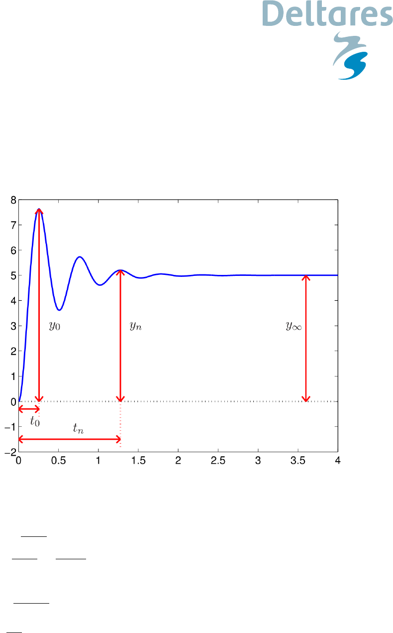
8 Determine coefficients from experiments
Taken from Callafon (2014)
Estimation of model parameters
With the times t0,tnand the values y0,ynand y∞from step response:
Figure 2: Collect data from measurement.
Allows us to estimate:
bωd= 2πn
tn−t0
damped resonance frequency (65)
c
βωn=1
tn−t0
ln y0−y∞
y0−y∞exponential decay term (66)
where n=number of oscillations between tnand t0. With the estimations of bωdand c
βωnwe can now compute
bωn=qbω2
d+c
βω2
nundamped resonance frequency (67)
β=c
βωn
bωn
damping ratio (68)

DRAFT
Date Reference Page
2018-04-18 SVN: 53753 12/21
9 Numerical discretisation
9.1 Mass-Spring-Damper system as system of first order PDE’s
The equation of a Mass-Spring-Damper system
m¨x+c˙x+kx =f(t)(69)
can be written as a system of first order partial differential equations, which read:
˙x=v(70)
m˙v=−cv −kx +f(t)(71)
with initial conditions: ˙x=v= 0 and x= 1. In matrix notation this equation read:
1 0
0m˙x
˙v=0 1
−k−cx
v+0
f(t)(72)
This system of equations in discrete form, with ∆tn+1 =tn+1 −tn, read:
xn+1 −xn
∆tn+1
=vn(73)
mvn+1 −vn
∆tn+1
=−cvn+1 −kxn+1 +f(xn+1 , xn,...)(74)
Rearranging gives:
xn+1 =xn+ ∆tn+1vn(75)
1 + ∆tn+1
mcvn+1 =vn−∆tn+1
mkxn+1 +∆tn+1
mf(xn+1, xn,...)(76)
9.2 PID controller (positional)
9.2.1 Implicit Mass-Spring-Damper system with explicit PID-controller
An explicit discrete form of the PID-controller (Equation (42)) read:
fn=Kpen+Ki
n
X
j=0
ej∆tj+Kd
en−en−1
∆tn
(77)
The system of equations will than read:
xn+1 =xn+ ∆tn+1vn(78)
1 + ∆tn+1
mcvn+1 =vn−∆tn+1
mkxn+1 +
∆tn+1
m
Kpen+Ki
n
X
j=0
ej∆tj+Kd
en−en−1
∆tn
(79)
9.2.2 Implicit Mass-Spring-Damper system with implicit PID-controller
An implicit discrete form of the PID-controller (Equation (42)) read:
fn+1 =Kpen+1 +Ki
n+1
X
j=0
ej∆tj+Kd
en+1 −en
∆tn+1
(80)

DRAFT
Date Reference Page
2018-04-18 SVN: 53753 13/21
The system of equations will than read:
xn+1 =xn+ ∆tn+1vn(81)
1 + ∆tn+1
mcvn+1 =vn−∆tn+1
mkxn+1 +
∆tn+1
m
Kpen+1 +Ki
n+1
X
j=0
ej∆tj+Kd
en+1 −en
∆tn+1
(82)
9.2.3 Corrected Mass-Spring-Damper system while using an explicit PID controller
Therefore we will adjust the Mass-Spring-Damper system for the explicit values used by the PID-controller by adding those terms who
will make the PID-controller implicit.
We will separate Equation (77) from Equation (80). The individual terms belonging to Equation (77) will be placed between square
brackets.
fn+1 =Kpen+1 +Ki
n+1
X
j=0
ej∆tj+Kd
en+1 −en
∆tn+1
(83)
=Kpen+1 −Kpen+ [Kpen] +
Kien+1∆tn+1 +
Ki
n
X
j=0
ej∆tj
+Kd
en+1 −en
∆tn+1
−Kd
en−en−1
∆tn
+Kd
en−en−1
∆tn(84)
The part between square brackets, is equal to Equation (77), which is the PID-controller based on explicit time levels:
fn=Kpen+Ki
n
X
j=0
ej∆tj+Kd
en−en−1
∆tn
(85)
So we get:
fn+1 =Kpen+1 −Kpen+Kien+1∆tn+1 +Kd
en+1 −en
∆tn+1
−Kd
en−en−1
∆tn
+fn(86)
Substitution of Equation (100) in Equation (76) leads to the following system of equations:
xn+1 =xn+ ∆tn+1vn(87)
1 + ∆tn+1
mcvn+1 =vn−∆tn+1
mkxn+1 +
∆tn+1
1
m−Kp(xn+1 −xn) + Kien+1∆tn+1
+Kd
en+1 −en
∆tn+1
−Kd
en−en−1
∆tn
+fn(88)
Some rearranging:
xn+1 =xn+ ∆tn+1vn(89)
1 + ∆tn+1
mcvn+1 =vn−∆tn+1
m(k+Kp)xn+1 +∆tn+1
mKpxn+
+∆tn+1
mKien+1∆tn+1 +
+∆tn+1
mKd
en+1 −en
∆tn+1
−∆tn+1
mKd
en−en−1
∆tn
+∆tn+1
mfn(90)
fnis given by Equation (77).

DRAFT
Date Reference Page
2018-04-18 SVN: 53753 14/21
9.3 PID controller (velocity)
9.3.1 Implicit Mass-Spring-Damper system with explicit velocity PID controller
An explicit discrete form of the PID-controller based on the linearisation (Equation (58)) read:
fn=fn−1+Kpen−en−1+Ki∆t en+Kd
en−2en−1+en−2
∆t,equal to Equation (64) (91)
The system of equations will than read:
xn+1 =xn+ ∆tn+1vn(92)
1 + ∆tn+1
mcvn+1 =vn−∆tn+1
mkxn+1 +
∆tn+1
mfn−1+Kpen−en−1+Ki∆t en+Kd
en−2en−1+en−2
∆t(93)
9.3.2 Implicit Mass-Spring-Damper system with implicit velocity PID controller
An implicit discrete form of the PID-controller based on the linearisation (Equation (58)) read:
fn+1 =fn+Kpen+1 −en+Ki∆t en+1 +Kd
en+1 −2en+en−1
∆t,equal to Equation (64) (94)
The system of equations will than read:
xn+1 =xn+ ∆tn+1vn(95)
1 + ∆tn+1
mcvn+1 =vn−∆tn+1
mkxn+1 +
∆tn+1
mfn+Kpen+1 −en+Ki∆t en+1 +Kd
en+1 −2en+en−1
∆t(96)
9.3.3 Corrected Mass-Spring-Damper system while using an explicit velocity PID controller
Therefore we will adjust the Mass-Spring-Damper system for the explicit values used by the velocity PID-controller by adding those terms
who will make the velocity PID-controller implicit.
We will separate Equation (91) from Equation (94). The individual terms belonging to Equation (91) will be placed between square
brackets. ∆tis constant.
fn+1 =fn+Kpen+1 −en+Ki∆t en+1 +Kd
en+1 −2en+en−1
∆t(97)
=fn−fn−1+fn−1+
+Kpen+1 −2en+en−1+Kpen−en−1
+Kien+1∆tn+1 −Kien∆tn+ [Kien∆tn]
+...+Kd
en−2en−1+en−2
∆t(98)
The part between square brackets, is equal to Equation (91), which is the PID-controller based on explicit time levels:
fn=fn−1+Kpen−en−1+Ki∆t en+Kd
en−2en−1+en−2
∆t(99)
So we get:
fn+1 =...+fn(100)

DRAFT
Date Reference Page
2018-04-18 SVN: 53753 15/21
Substitution of Equation (100) in Equation (76) leads to the following system of equations:
xn+1 =xn+ ∆tn+1vn(101)
1 + ∆tn+1
mcvn+1 =vn−∆tn+1
mkxn+1 +
∆tn+1
m(...+fn)(102)
Some rearranging:
xn+1 =xn+ ∆tn+1vn(103)
1 + ∆tn+1
mcvn+1 =vn+...+∆tn+1
mfn(104)
fnis given by Equation (77).
10 Experiments
Mass-Spring-Damper-system:
m¨x+c˙x+kx =f(t),(105)
f(t) = Kpe(t) + KiZt
0
e(τ)dτ +Kd
de(t)
dt (106)
with
Initial values: x(0) = 1 and ˙x(0) = 0.
Coefficients: m= 100,c= 2,k= 1.
PID gain factors: Kp= 10.0;Ki= 0.05;Kd= 10.0.
Setpoint: 0.5.
e(t) = x(∞)−x(t).
x(∞) = setpoint.
Table 1: Equilibrium solution.
KpKiKdEquili
10.0 0.0 0.0 0.45
0.0 0.05 0.0 0.5
0.0 0.0 10.0 0.0
DRAFT
Date Reference Page
2018-04-18 SVN: 53753 16/21
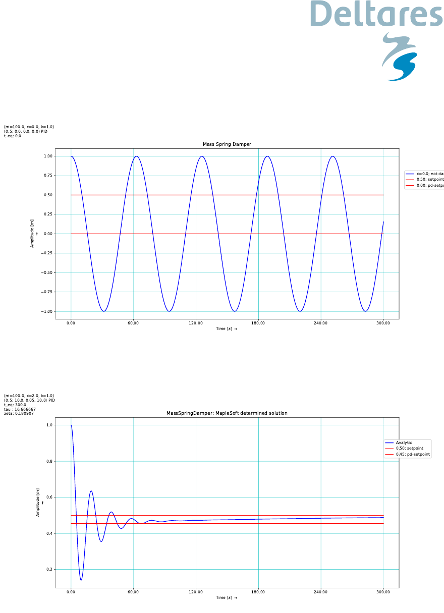
10.1 Solutions determined by Maplesoft
Figure 3: The natural frequency; c=Kp=Ki=Kd= 0.
Figure 4: PID controller on Mass-Spring-Damper using MapleSoft solution. The integral term is
quite small and therefor the influence is noticed after a while.
DRAFT
Date Reference Page
2018-04-18 SVN: 53753 17/21
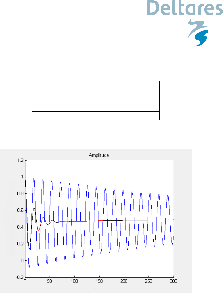
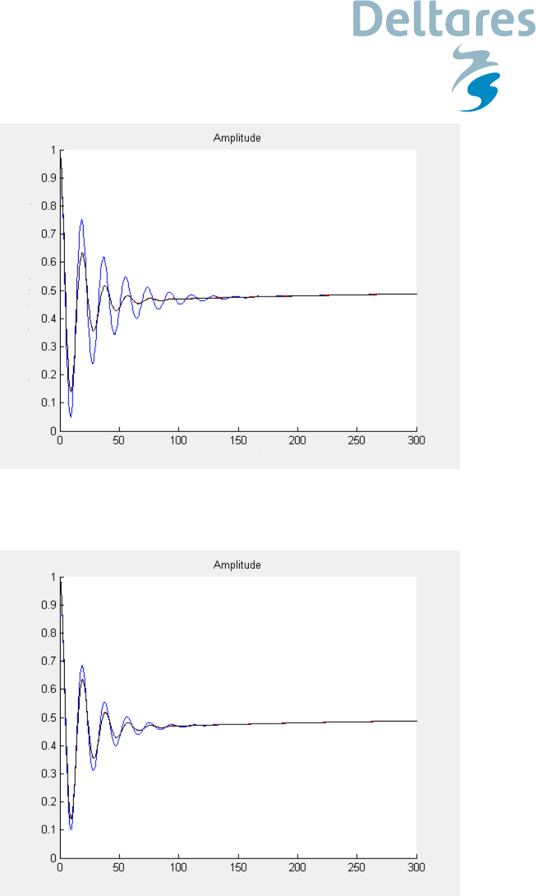
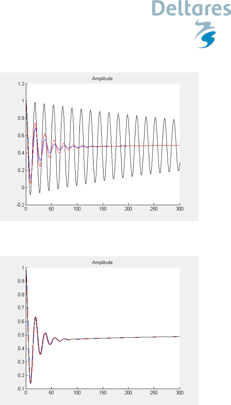
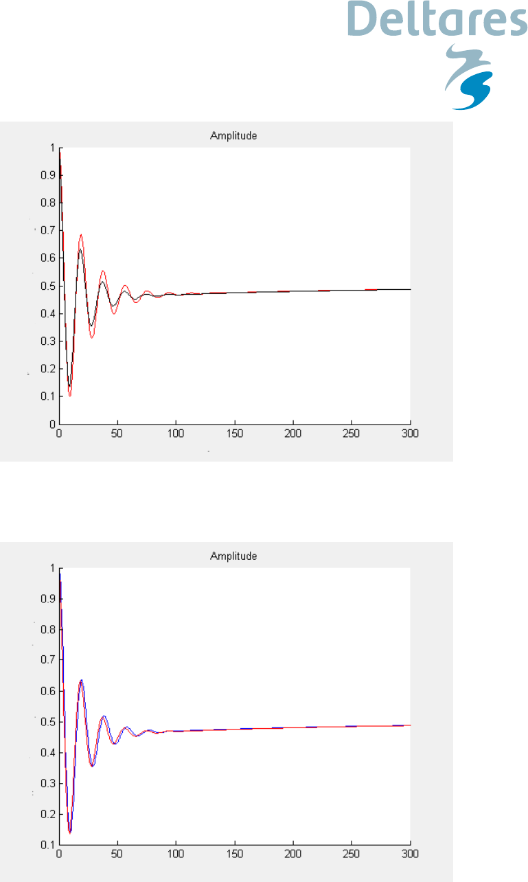
10.2 Numerical experiments
Table 2: Performed numerical experiments.
time integration ∆t
1.0s
∆t
0.5s
∆t
0.25 s
explicit (§9.2.1)XXX
implicit (§9.3.2)XXX
corrected (§9.2.3)XXX
10.2.1 Time integration method
Figure 5: Numerical experiment (∆t= 1 s); explicit (blue, §9.2.1), implicit (red, §9.3.2), corrected
(black, §9.2.3).

DRAFT
Date Reference Page
2018-04-18 SVN: 53753 21/21
References
Åström, K. J. and R. M. Murray (2016). Feedback Systems. Tech. rep. 3.0h/. Caltech (California
Institute of Technology). URL:http : / / www . cds . caltech . edu / ~murray / amwiki /
index.php/Main_Page.
Berdahl, Edgar J. and Julius O. Smith III (2007). PID Control of a Plucked String. Tech. rep. Cen-
ter for Computer Research in Music and Acoustics (CCRMA), and the Department of Electrical
Engineering (REALSIMPLE Project∗). Stanford, CA: Stanford University.
Callafon, R. A. de (2014). Position Control Experiment (MAE171A).URL:http://maecourses.
ucsd.edu/callafon/labcourse/index.html.
Rao, A.V. (2009). Mechanical vibrations: Lecture notes for course EML 4220.URL:http://vdol.
mae.ufl.edu/CourseNotes/EML4220/vibrations.pdf.
Rowell, D. (2004). Review of First- and Second-Order System Response. EducationMIT. URL:http:
//web.mit.edu/2.151/www/Handouts/FirstSecondOrder.pdf.
Seborg, D.E., T.F. Edgar, D.A. Mellichamp, and F.J. Doyle III (2011). Process Dynamics and Control.
John Wiley & Sons, Inc.
Yon-Ping, Chen. Mass-Damper-Spring systems/PID control of the simplest second-order systems.
URL:http://jsjk.cn.nctu.edu.tw/JSJK/DSAS/DSAS_11_12.pdf.
