Pycse Manual
User Manual: Pdf
Open the PDF directly: View PDF ![]() .
.
Page Count: 399 [warning: Documents this large are best viewed by clicking the View PDF Link!]
- Overview
- Basic python usage
- Basic math
- Advanced mathematical operators
- Creating your own functions
- Defining functions in python
- Advanced function creation
- Lambda Lambda Lambda
- Creating arrays in python
- Functions on arrays of values
- Some basic data structures in python
- Indexing vectors and arrays in Python
- Controlling the format of printed variables
- Advanced string formatting
- Math
- Numeric derivatives by differences
- Vectorized numeric derivatives
- 2-point vs. 4-point numerical derivatives
- Derivatives by polynomial fitting
- Derivatives by fitting a function and taking the analytical derivative
- Derivatives by FFT
- A novel way to numerically estimate the derivative of a function - complex-step derivative approximation
- Vectorized piecewise functions
- Smooth transitions between discontinuous functions
- Smooth transitions between two constants
- On the quad or trapz'd in ChemE heaven
- Polynomials in python
- Wilkinson's polynomial
- The trapezoidal method of integration
- Numerical Simpsons rule
- Integrating functions in python
- Integrating equations in python
- Function integration by the Romberg method
- Symbolic math in python
- Is your ice cream float bigger than mine
- Linear algebra
- Potential gotchas in linear algebra in numpy
- Solving linear equations
- Rules for transposition
- Sums products and linear algebra notation - avoiding loops where possible
- Determining linear independence of a set of vectors
- Reduced row echelon form
- Computing determinants from matrix decompositions
- Calling lapack directly from scipy
- Nonlinear algebra
- Statistics
- Data analysis
- Fit a line to numerical data
- Linear least squares fitting with linear algebra
- Linear regression with confidence intervals (updated)
- Linear regression with confidence intervals.
- Nonlinear curve fitting
- Nonlinear curve fitting by direct least squares minimization
- Parameter estimation by directly minimizing summed squared errors
- Nonlinear curve fitting with parameter confidence intervals
- Nonlinear curve fitting with confidence intervals
- Graphical methods to help get initial guesses for multivariate nonlinear regression
- Fitting a numerical ODE solution to data
- Reading in delimited text files
- Interpolation
- Optimization
- Differential equations
- Ordinary differential equations
- Numerical solution to a simple ode
- Plotting ODE solutions in cylindrical coordinates
- ODEs with discontinuous forcing functions
- Simulating the events feature of Matlab's ode solvers
- Mimicking ode events in python
- Solving an ode for a specific solution value
- A simple first order ode evaluated at specific points
- Stopping the integration of an ODE at some condition
- Finding minima and maxima in ODE solutions with events
- Error tolerance in numerical solutions to ODEs
- Solving parameterized ODEs over and over conveniently
- Yet another way to parameterize an ODE
- Another way to parameterize an ODE - nested function
- Solving a second order ode
- Solving Bessel's Equation numerically
- Phase portraits of a system of ODEs
- Linear algebra approaches to solving systems of constant coefficient ODEs
- Delay Differential Equations
- Differential algebraic systems of equations
- Boundary value equations
- Partial differential equations
- Ordinary differential equations
- Plotting
- Plot customizations - Modifying line, text and figure properties
- Plotting two datasets with very different scales
- Customizing plots after the fact
- Fancy, built-in colors in Python
- Picasso's short lived blue period with Python
- Interactive plotting
- key events not working on Mac/org-mode
- Peak annotation in matplotlib
- Programming
- Some of this, sum of that
- Sorting in python
- Unique entries in a vector
- Lather, rinse and repeat
- Brief intro to regular expressions
- Working with lists
- Making word files in python
- Interacting with Excel in python
- Using Excel in Python
- Running Aspen via Python
- Using an external solver with Aspen
- Redirecting the print function
- Getting a dictionary of counts
- About your python
- Automatic, temporary directory changing
- Miscellaneous
- Worked examples
- Peak finding in Raman spectroscopy
- Curve fitting to get overlapping peak areas
- Estimating the boiling point of water
- Gibbs energy minimization and the NIST webbook
- Finding equilibrium composition by direct minimization of Gibbs free energy on mole numbers
- The Gibbs free energy of a reacting mixture and the equilibrium composition
- Water gas shift equilibria via the NIST Webbook
- Constrained minimization to find equilibrium compositions
- Using constrained optimization to find the amount of each phase present
- Conservation of mass in chemical reactions
- Numerically calculating an effectiveness factor for a porous catalyst bead
- Computing a pipe diameter
- Reading parameter database text files in python
- Calculating a bubble point pressure of a mixture
- The equal area method for the van der Waals equation
- Time dependent concentration in a first order reversible reaction in a batch reactor
- Finding equilibrium conversion
- Integrating a batch reactor design equation
- Uncertainty in an integral equation
- Integrating the batch reactor mole balance
- Plug flow reactor with a pressure drop
- Solving CSTR design equations
- Meet the steam tables
- What region is a point in
- Units
- GNU Free Documentation License
- References
- Index

pycse - Python3 Computations in Science and
Engineering
John Kitchin
jkitchin@andrew.cmu.edu
http://kitchingroup.cheme.cmu.edu
Twitter: @johnkitchin
2015-04-25
Contents
1 Overview 9
2 Basic python usage 9
2.1 Basicmath ............................ 9
2.2 Advanced mathematical operators . . . . . . . . . . . . . . . 11
2.2.1 Exponential and logarithmic functions . . . . . . . . . 11
2.3 Creating your own functions . . . . . . . . . . . . . . . . . . . 12
2.4 Defining functions in python . . . . . . . . . . . . . . . . . . . 12
2.5 Advanced function creation . . . . . . . . . . . . . . . . . . . 15
2.6 Lambda Lambda Lambda . . . . . . . . . . . . . . . . . . . . 18
2.6.1 Applications of lambda functions . . . . . . . . . . . . 20
2.6.2 Summary ......................... 21
2.7 Creating arrays in python . . . . . . . . . . . . . . . . . . . . 22
2.8 Functions on arrays of values . . . . . . . . . . . . . . . . . . 25
2.9 Some basic data structures in python . . . . . . . . . . . . . . 27
2.9.1 thelist........................... 27
2.9.2 tuples ........................... 28
1
2.9.3 struct ........................... 28
2.9.4 dictionaries ........................ 29
2.9.5 Summary ......................... 29
2.10 Indexing vectors and arrays in Python . . . . . . . . . . . . . 29
2.10.1 2darrays ......................... 31
2.10.2 Using indexing to assign values to rows and columns . 32
2.10.3 3Darrays ......................... 32
2.10.4 Summary ......................... 33
2.11 Controlling the format of printed variables . . . . . . . . . . . 33
2.12 Advanced string formatting . . . . . . . . . . . . . . . . . . . 36
3 Math 38
3.1 Numeric derivatives by differences . . . . . . . . . . . . . . . 38
3.2 Vectorized numeric derivatives . . . . . . . . . . . . . . . . . 40
3.3 2-point vs. 4-point numerical derivatives . . . . . . . . . . . . 41
3.4 Derivatives by polynomial fitting . . . . . . . . . . . . . . . . 43
3.5 Derivatives by fitting a function and taking the analytical
derivative ............................. 45
3.6 DerivativesbyFFT........................ 47
3.7 A novel way to numerically estimate the derivative of a func-
tion - complex-step derivative approximation . . . . . . . . . 48
3.8 Vectorized piecewise functions . . . . . . . . . . . . . . . . . . 50
3.9 Smooth transitions between discontinuous functions . . . . . 54
3.9.1 Summary ......................... 58
3.10 Smooth transitions between two constants . . . . . . . . . . . 58
3.11 On the quad or trapz’d in ChemE heaven . . . . . . . . . . . 59
3.11.1 Numerical data integration . . . . . . . . . . . . . . . 60
3.11.2 Combining numerical data with quad . . . . . . . . . 62
3.11.3 Summary ......................... 62
3.12 Polynomials in python . . . . . . . . . . . . . . . . . . . . . . 62
3.12.1 Summary ......................... 64
3.13 Wilkinson’s polynomial . . . . . . . . . . . . . . . . . . . . . 65
3.14 The trapezoidal method of integration . . . . . . . . . . . . . 70
3.15 Numerical Simpsons rule . . . . . . . . . . . . . . . . . . . . . 72
3.16 Integrating functions in python . . . . . . . . . . . . . . . . . 72
3.16.1 double integrals . . . . . . . . . . . . . . . . . . . . . . 73
3.16.2 Summary ......................... 74
3.17 Integrating equations in python . . . . . . . . . . . . . . . . . 74
3.18 Function integration by the Romberg method . . . . . . . . . 75
3.19 Symbolic math in python . . . . . . . . . . . . . . . . . . . . 75
2
3.19.1 Solve the quadratic equation . . . . . . . . . . . . . . 75
3.19.2 differentiation . . . . . . . . . . . . . . . . . . . . . . . 76
3.19.3 integration ........................ 76
3.19.4 Analytically solve a simple ODE . . . . . . . . . . . . 76
3.20 Is your ice cream float bigger than mine . . . . . . . . . . . . 77
4 Linear algebra 79
4.1 Potential gotchas in linear algebra in numpy . . . . . . . . . . 79
4.2 Solving linear equations . . . . . . . . . . . . . . . . . . . . . 81
4.3 Rules for transposition . . . . . . . . . . . . . . . . . . . . . . 83
4.3.1 The transpose in Python . . . . . . . . . . . . . . . . 83
4.3.2 Rule1........................... 83
4.3.3 Rule2........................... 84
4.3.4 Rule3........................... 84
4.3.5 Rule4........................... 84
4.3.6 Summary ......................... 84
4.4 Sums products and linear algebra notation - avoiding loops
wherepossible .......................... 85
4.4.1 Old-fashioned way with a loop . . . . . . . . . . . . . 85
4.4.2 The numpy approach . . . . . . . . . . . . . . . . . . 86
4.4.3 Matrix algebra approach. . . . . . . . . . . . . . . . . 86
4.4.4 Another example . . . . . . . . . . . . . . . . . . . . . 86
4.4.5 Lastexample ....................... 87
4.4.6 Summary ......................... 88
4.5 Determining linear independence of a set of vectors . . . . . . 88
4.5.1 another example . . . . . . . . . . . . . . . . . . . . . 90
4.5.2 Near deficient rank . . . . . . . . . . . . . . . . . . . . 90
4.5.3 Application to independent chemical reactions. . . . . 91
4.6 Reduced row echelon form . . . . . . . . . . . . . . . . . . . . 92
4.7 Computing determinants from matrix decompositions . . . . 93
4.8 Calling lapack directly from scipy . . . . . . . . . . . . . . . . 94
5 Nonlinear algebra 96
5.1 Knowyourtolerance....................... 96
5.2 Solving integral equations with fsolve . . . . . . . . . . . . . . 98
5.2.1 Summarynotes......................100
5.3 Method of continuity for nonlinear equation solving . . . . . . 100
5.4 Method of continuity for solving nonlinear equations - Part II 105
5.5 Countingroots ..........................107
5.5.1 Use roots for this polynomial . . . . . . . . . . . . . . 108
3
5.5.2 method1 .........................109
5.5.3 Method2 .........................109
5.6 Finding the nth root of a periodic function . . . . . . . . . . 110
5.7 Coupled nonlinear equations . . . . . . . . . . . . . . . . . . . 113
6 Statistics 114
6.1 Introduction to statistical data analysis . . . . . . . . . . . . 114
6.2 Basicstatistics ..........................115
6.3 Confidence interval on an average . . . . . . . . . . . . . . . . 116
6.4 Are averages different . . . . . . . . . . . . . . . . . . . . . . 117
6.4.1 The hypothesis . . . . . . . . . . . . . . . . . . . . . . 117
6.4.2 Compute the t-score for our data . . . . . . . . . . . . 117
6.4.3 Interpretation . . . . . . . . . . . . . . . . . . . . . . . 118
6.5 Modelselection..........................119
6.6 Numerical propagation of errors . . . . . . . . . . . . . . . . . 128
6.6.1 Addition and subtraction . . . . . . . . . . . . . . . . 128
6.6.2 Multiplication . . . . . . . . . . . . . . . . . . . . . . . 129
6.6.3 Division..........................129
6.6.4 exponents.........................129
6.6.5 the chain rule in error propagation . . . . . . . . . . . 130
6.6.6 Summary .........................130
6.7 Another approach to error propagation . . . . . . . . . . . . . 131
6.7.1 Summary .........................135
6.8 Randomthoughts.........................135
6.8.1 Summary .........................139
7 Data analysis 139
7.1 Fit a line to numerical data . . . . . . . . . . . . . . . . . . . 139
7.2 Linear least squares fitting with linear algebra . . . . . . . . . 141
7.3 Linear regression with confidence intervals (updated) . . . . . 142
7.4 Linear regression with confidence intervals. . . . . . . . . . . 143
7.5 Nonlinear curve fitting . . . . . . . . . . . . . . . . . . . . . . 145
7.6 Nonlinear curve fitting by direct least squares minimization . 147
7.7 Parameter estimation by directly minimizing summed squared
errors ...............................148
7.8 Nonlinear curve fitting with parameter confidence intervals . 151
7.9 Nonlinear curve fitting with confidence intervals . . . . . . . . 153
7.10 Graphical methods to help get initial guesses for multivariate
nonlinear regression . . . . . . . . . . . . . . . . . . . . . . . 154
7.11 Fitting a numerical ODE solution to data . . . . . . . . . . . 159
4
7.12 Reading in delimited text files . . . . . . . . . . . . . . . . . . 160
8 Interpolation 161
8.1 Better interpolate than never . . . . . . . . . . . . . . . . . . 161
8.1.1 Estimate the value of f at t=2. . . . . . . . . . . . . . 161
8.1.2 improved interpolation? . . . . . . . . . . . . . . . . . 162
8.1.3 The inverse question . . . . . . . . . . . . . . . . . . . 163
8.1.4 A harder problem . . . . . . . . . . . . . . . . . . . . 164
8.1.5 Discussion.........................165
8.2 Interpolation of data . . . . . . . . . . . . . . . . . . . . . . . 167
8.3 Interpolation with splines . . . . . . . . . . . . . . . . . . . . 168
9 Optimization 169
9.1 Constrained optimization . . . . . . . . . . . . . . . . . . . . 169
9.2 Finding the maximum power of a photovoltaic device. . . . . 170
9.3 Using Lagrange multipliers in optimization . . . . . . . . . . 173
9.3.1 Construct the Lagrange multiplier augmented function 174
9.3.2 Finding the partial derivatives . . . . . . . . . . . . . 175
9.3.3 Now we solve for the zeros in the partial derivatives . 175
9.3.4 Summary .........................176
9.4 Linear programming example with inequality constraints . . . 176
9.5 Find the minimum distance from a point to a curve. . . . . . 178
10 Differential equations 180
10.1 Ordinary differential equations . . . . . . . . . . . . . . . . . 180
10.1.1 Numerical solution to a simple ode . . . . . . . . . . . 180
10.1.2 Plotting ODE solutions in cylindrical coordinates . . . 182
10.1.3 ODEs with discontinuous forcing functions . . . . . . 183
10.1.4 Simulating the events feature of Matlab’s ode solvers . 185
10.1.5 Mimicking ode events in python . . . . . . . . . . . . 187
10.1.6 Solving an ode for a specific solution value . . . . . . . 190
10.1.7 A simple first order ode evaluated at specific points . 194
10.1.8 Stopping the integration of an ODE at some condition 194
10.1.9 Finding minima and maxima in ODE solutions with
events ...........................195
10.1.10 Error tolerance in numerical solutions to ODEs . . . . 197
10.1.11 Solving parameterized ODEs over and over conveniently201
10.1.12 Yet another way to parameterize an ODE . . . . . . . 202
10.1.13 Another way to parameterize an ODE - nested function203
10.1.14 Solving a second order ode . . . . . . . . . . . . . . . 205
5
10.1.15 Solving Bessel’s Equation numerically . . . . . . . . . 208
10.1.16 Phase portraits of a system of ODEs . . . . . . . . . . 209
10.1.17 Linear algebra approaches to solving systems of con-
stant coefficient ODEs . . . . . . . . . . . . . . . . . . 213
10.2 Delay Differential Equations . . . . . . . . . . . . . . . . . . . 215
10.3 Differential algebraic systems of equations . . . . . . . . . . . 215
10.4 Boundary value equations . . . . . . . . . . . . . . . . . . . . 215
10.4.1 Plane Poiseuille flow - BVP solve by shooting method 215
10.4.2 Plane poiseuelle flow solved by finite difference . . . . 221
10.4.3 Boundary value problem in heat conduction . . . . . . 224
10.4.4 BVPinpycse.......................226
10.4.5 A nonlinear BVP . . . . . . . . . . . . . . . . . . . . . 228
10.4.6 Another look at nonlinear BVPs . . . . . . . . . . . . 231
10.4.7 Solving the Blasius equation . . . . . . . . . . . . . . . 233
10.5 Partial differential equations . . . . . . . . . . . . . . . . . . . 235
10.5.1 Modeling a transient plug flow reactor . . . . . . . . . 235
10.5.2 Transient heat conduction - partial differential equations239
10.5.3 Transient diffusion - partial differential equations . . . 243
11 Plotting 246
11.1 Plot customizations - Modifying line, text and figure properties246
11.1.1 setting all the text properties in a figure. . . . . . . . 249
11.2 Plotting two datasets with very different scales . . . . . . . . 251
11.2.1 Make two plots! . . . . . . . . . . . . . . . . . . . . . . 252
11.2.2 Scaling the results . . . . . . . . . . . . . . . . . . . . 253
11.2.3 Double-y axis plot . . . . . . . . . . . . . . . . . . . . 254
11.2.4 Subplots..........................255
11.3 Customizing plots after the fact . . . . . . . . . . . . . . . . . 256
11.4 Fancy, built-in colors in Python . . . . . . . . . . . . . . . . . 259
11.5 Picasso’s short lived blue period with Python . . . . . . . . . 260
11.6 Interactive plotting . . . . . . . . . . . . . . . . . . . . . . . . 263
11.6.1 Basic mouse clicks . . . . . . . . . . . . . . . . . . . . 263
11.7 key events not working on Mac/org-mode . . . . . . . . . . . 265
11.7.1 Mouse movement . . . . . . . . . . . . . . . . . . . . . 267
11.7.2 key press events . . . . . . . . . . . . . . . . . . . . . 268
11.7.3 Pickinglines .......................269
11.7.4 Picking data points . . . . . . . . . . . . . . . . . . . . 269
11.8 Peak annotation in matplotlib . . . . . . . . . . . . . . . . . . 270
6
12 Programming 272
12.1 Some of this, sum of that . . . . . . . . . . . . . . . . . . . . 272
12.1.1 Nestedlists ........................273
12.2Sortinginpython.........................274
12.3 Unique entries in a vector . . . . . . . . . . . . . . . . . . . . 276
12.4 Lather, rinse and repeat . . . . . . . . . . . . . . . . . . . . . 276
12.4.1 Conclusions........................277
12.5 Brief intro to regular expressions . . . . . . . . . . . . . . . . 278
12.6 Working with lists . . . . . . . . . . . . . . . . . . . . . . . . 279
12.7 Making word files in python . . . . . . . . . . . . . . . . . . . 281
12.8 Interacting with Excel in python . . . . . . . . . . . . . . . . 283
12.8.1 Writing Excel workbooks . . . . . . . . . . . . . . . . 284
12.8.2 Updating an existing Excel workbook . . . . . . . . . 284
12.8.3 Summary .........................285
12.9 Using Excel in Python . . . . . . . . . . . . . . . . . . . . . . 285
12.10Running Aspen via Python . . . . . . . . . . . . . . . . . . . 286
12.11Using an external solver with Aspen . . . . . . . . . . . . . . 289
12.12Redirecting the print function . . . . . . . . . . . . . . . . . . 290
12.13Getting a dictionary of counts . . . . . . . . . . . . . . . . . . 294
12.14Aboutyourpython........................295
12.15Automatic, temporary directory changing . . . . . . . . . . . 296
13 Miscellaneous 298
13.1 Mail merge with python . . . . . . . . . . . . . . . . . . . . . 298
14 Worked examples 300
14.1 Peak finding in Raman spectroscopy . . . . . . . . . . . . . . 300
14.1.1 Summary notes . . . . . . . . . . . . . . . . . . . . . . 305
14.2 Curve fitting to get overlapping peak areas . . . . . . . . . . 305
14.2.1 Notable differences from Matlab . . . . . . . . . . . . 311
14.3 Estimating the boiling point of water . . . . . . . . . . . . . . 311
14.3.1 Summary .........................314
14.4 Gibbs energy minimization and the NIST webbook . . . . . . 314
14.4.1 Compute mole fractions and partial pressures . . . . . 316
14.4.2 Computing equilibrium constants . . . . . . . . . . . . 317
14.5 Finding equilibrium composition by direct minimization of
Gibbs free energy on mole numbers . . . . . . . . . . . . . . . 317
14.5.1 The Gibbs energy of a mixture . . . . . . . . . . . . . 318
14.5.2 Linear equality constraints for atomic mass conservation318
14.5.3 Equilibrium constant based on mole numbers . . . . . 320
7
14.5.4 Summary .........................320
14.6 The Gibbs free energy of a reacting mixture and the equilib-
riumcomposition.........................321
14.6.1 Summary .........................326
14.7 Water gas shift equilibria via the NIST Webbook . . . . . . . 326
14.7.1 hydrogen .........................327
14.7.2 H_{2}O..........................327
14.7.3 CO.............................328
14.7.4 CO_{2}..........................328
14.7.5 Standard state heat of reaction . . . . . . . . . . . . . 328
14.7.6 Non-standard state ∆Hand ∆G............329
14.7.7 Plot how the ∆Gvaries with temperature . . . . . . . 329
14.7.8 Equilibrium constant calculation . . . . . . . . . . . . 330
14.7.9 Equilibrium yield of WGS . . . . . . . . . . . . . . . . 331
14.7.10 Compute gas phase pressures of each species . . . . . 332
14.7.11 Compare the equilibrium constants . . . . . . . . . . . 332
14.7.12Summary .........................333
14.8 Constrained minimization to find equilibrium compositions . 333
14.8.1 summary .........................337
14.9 Using constrained optimization to find the amount of each
phasepresent ...........................337
14.10Conservation of mass in chemical reactions . . . . . . . . . . 340
14.11Numerically calculating an effectiveness factor for a porous
catalystbead ...........................341
14.12Computing a pipe diameter . . . . . . . . . . . . . . . . . . . 344
14.13Reading parameter database text files in python . . . . . . . 346
14.14Calculating a bubble point pressure of a mixture . . . . . . . 349
14.15The equal area method for the van der Waals equation . . . . 350
14.15.1 Compute areas . . . . . . . . . . . . . . . . . . . . . . 353
14.16Time dependent concentration in a first order reversible re-
action in a batch reactor . . . . . . . . . . . . . . . . . . . . . 355
14.17Finding equilibrium conversion . . . . . . . . . . . . . . . . . 357
14.18Integrating a batch reactor design equation . . . . . . . . . . 358
14.19Uncertainty in an integral equation . . . . . . . . . . . . . . . 358
14.20Integrating the batch reactor mole balance . . . . . . . . . . . 359
14.21Plug flow reactor with a pressure drop . . . . . . . . . . . . . 361
14.22Solving CSTR design equations . . . . . . . . . . . . . . . . . 362
14.23Meet the steam tables . . . . . . . . . . . . . . . . . . . . . . 363
14.23.1 Starting point in the Rankine cycle in condenser. . . . 363
14.23.2 Isentropic compression of liquid to point 2 . . . . . . . 364
8
14.23.3 Isobaric heating to T3 in boiler where we make steam 364
14.23.4 Isentropic expansion through turbine to point 4 . . . . 365
14.23.5 To get from point 4 to point 1 . . . . . . . . . . . . . 365
14.23.6Efficiency .........................365
14.23.7 Entropy-temperature chart . . . . . . . . . . . . . . . 365
14.23.8Summary .........................368
14.24What region is a point in . . . . . . . . . . . . . . . . . . . . 368
15 Units 374
15.1 Using units in python . . . . . . . . . . . . . . . . . . . . . . 374
15.1.1 scimath ..........................375
15.2 Handling units with the quantities module . . . . . . . . . . . 376
15.3UnitsinODEs ..........................382
15.4 Handling units with dimensionless equations . . . . . . . . . . 386
16 GNU Free Documentation License 388
17 References 399
18 Index 399
1 Overview
This is a collection of examples of using python in the kinds of scientific
and engineering computations I have used in classes and research. They are
organized by topics.
I recommend the Continuum IO Anaconda python distribution (https:
//www.continuum.io). This distribution is free for academic use, and cheap
otherwise. It is pretty complete in terms of mathematical, scientific and
plotting modules. All of the examples in this book were created run with
the Anaconda python distribution.
2 Basic python usage
2.1 Basic math
Python is a basic calculator out of the box. Here we consider the most basic
mathematical operations: addition, subtraction, multiplication, division and
exponenetiation. we use the print to get the output. For now we consider
integers and float numbers. An integer is a plain number like 0, 10 or -2345.
9

A float number has a decimal in it. The following are all floats: 1.0, -9., and
3.56. Note the trailing zero is not required, although it is good style.
1print(2+4)
2print(8.1 - 5)
6
3.0999999999999996
Multiplication is equally straightforward.
1print(5*4)
2print(3.1 * 2)
20
6.2
Division is almost as straightforward, but we have to remember that
integer division is not the same as float division. Let us consider float division
first.
1print(4.0 / 2.0)
2print(1.0/3.1)
2.0
0.3225806451612903
Now, consider the integer versions:
1print(4/2)
2print(1/3)
2.0
0.3333333333333333
The first result is probably what you expected, but the second may come
as a surprise. In integer division the remainder is discarded, and the result
is an integer.
Exponentiation is also a basic math operation that python supports di-
rectly.
10

1print(3.**2)
2print(3**2)
3print(2**0.5)
9.0
9
1.4142135623730951
Other types of mathematical operations require us to import function-
ality from python libraries. We consider those in the next section.
2.2 Advanced mathematical operators
The primary library we will consider is numpy, which provides many math-
ematical functions, statistics as well as support for linear algebra. For a
complete listing of the functions available, see http://docs.scipy.org/
doc/numpy/reference/routines.math.html. We begin with the simplest
functions.
1import numpy as np
2print(np.sqrt(2))
1.41421356237
2.2.1 Exponential and logarithmic functions
Here is the exponential function.
1import numpy as np
2print(np.exp(1))
2.71828182846
There are two logarithmic functions commonly used, the natural log
function numpy.log and the base10 logarithm numpy.log10.
1import numpy as np
2print(np.log(10))
3print(np.log10(10)) # base10
2.30258509299
1.0
11

There are many other intrinsic functions available in numpy which we
will eventually cover. First, we need to consider how to create our own
functions.
2.3 Creating your own functions
We can combine operations to evaluate complex equations. Consider the
value of the equation x3−log(x)for the value x= 4.1.
1import numpy as np
2x= 3
3print(x**3 - np.log(x))
25.9013877113
It would be tedious to type this out each time. Next, we learn how to
express this equation as a new function, which we can call with different
values.
1import numpy as np
2def f(x):
3return x**3 - np.log(x)
4
5print(f(3))
6print(f(5.1))
25.9013877113
131.02175946
It may not seem like we did much there, but this is the foundation for
solving equations in the future. Before we get to solving equations, we have
a few more details to consider. Next, we consider evaluating functions on
arrays of values.
2.4 Defining functions in python
Compare what’s here to the Matlab implementation.
We often need to make functions in our codes to do things.
1def f(x):
2"return the inverse square of x"
3return 1.0 / x**2
4
5print(f(3))
6print(f([4,5]))
12

Note that functions are not automatically vectorized. That is why we
see the error above. There are a few ways to achieve that. One is to "cast"
the input variables to objects that support vectorized operations, such as
numpy.array objects.
1import numpy as np
2
3def f(x):
4"return the inverse square of x"
5x=np.array(x)
6return 1.0 / x**2
7
8print(f(3))
9print(f([4,5]))
0.111111111111
[ 0.0625 0.04 ]
It is possible to have more than one variable.
1import numpy as np
2
3def func(x, y):
4"return product of x and y"
5return x*y
6
7print(func(2,3))
8print(func(np.array([2,3]), np.array([3,4])))
6
[ 6 12]
You can define "lambda" functions, which are also known as inline or
anonymous functions. The syntax is lambda var:f(var). I think these
are hard to read and discourage their use. Here is a typical usage where
you have to define a simple function that is passed to another function, e.g.
scipy.integrate.quad to perform an integral.
1from scipy.integrate import quad
2print(quad(lambda x:x**3,0,2))
(4.0, 4.440892098500626e-14)
It is possible to nest functions inside of functions like this.
13

1def wrapper(x):
2a= 4
3def func(x, a):
4return a*x
5
6return func(x, a)
7
8print(wrapper(4))
16
An alternative approach is to "wrap" a function, say to fix a parameter.
You might do this so you can integrate the wrapped function, which depends
on only a single variable, whereas the original function depends on two
variables.
1def func(x, a):
2return a*x
3
4def wrapper(x):
5a= 4
6return func(x, a)
7
8print(wrapper(4))
16
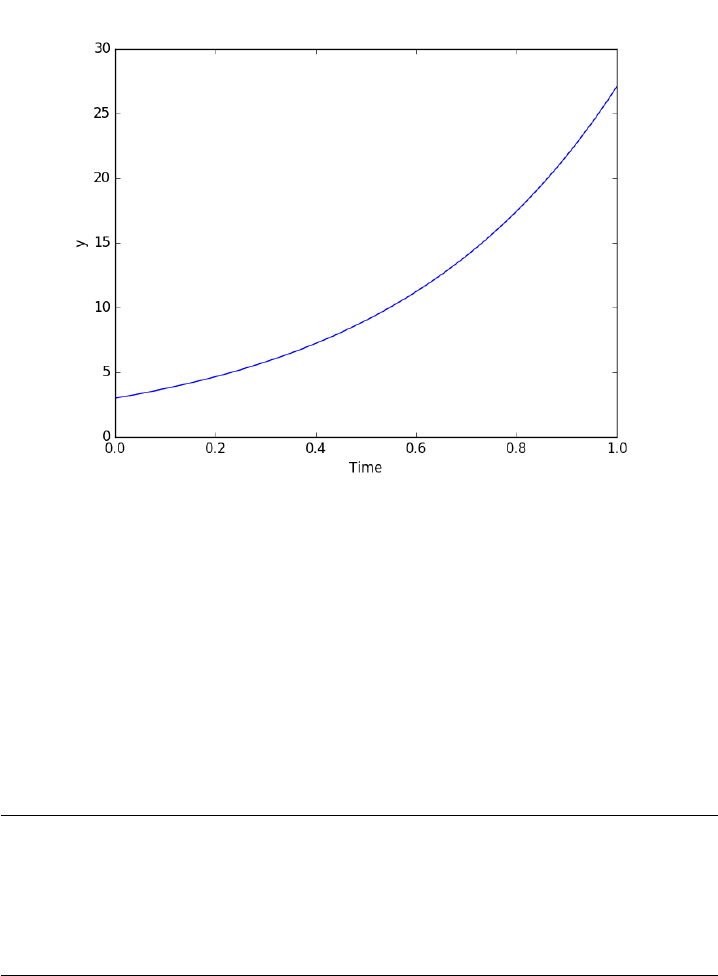
Last example, defining a function for an ode
1from scipy.integrate import odeint
2import numpy as np
3import matplotlib.pyplot as plt
4
5k= 2.2
6def myode(y, t):
7"ode defining exponential growth"
8return k*y
9
10 y0 = 3
11 tspan =np.linspace(0,1)
12 y=odeint(myode, y0, tspan)
13
14 plt.plot(tspan, y)
15 plt.xlabel(’Time’)
16 plt.ylabel(’y’)
17 plt.savefig(’images/funcs-ode.png’)
14
2.5 Advanced function creation
Python has some nice features in creating functions. You can create default
values for variables, have optional variables and optional keyword variables.
In this function f(a,b), aand bare called positional arguments, and they are
required, and must be provided in the same order as the function defines.
If we provide a default value for an argument, then the argument is called
a keyword argument, and it becomes optional. You can combine positional
arguments and keyword arguments, but positional arguments must come
first. Here is an example.
1def func(a, n=2):
2"compute the nth power of a"
3return a**n
4
5# three different ways to call the function
6print(func(2))
7print(func(2,3))
8print(func(2, n=4))
4
8
16
15

In the first call to the function, we only define the argument a, which
is a mandatory, positional argument. In the second call, we define aand n,
in the order they are defined in the function. Finally, in the third call, we
define aas a positional argument, and nas a keyword argument.
If all of the arguments are optional, we can even call the function with no
arguments. If you give arguments as positional arguments, they are used in
the order defined in the function. If you use keyword arguments, the order
is arbitrary.
1def func(a=1, n=2):
2"compute the nth power of a"
3return a**n
4
5# three different ways to call the function
6print(func())
7print(func(2,4))
8print(func(n=4, a=2))
1
16
16
It is occasionally useful to allow an arbitrary number of arguments in a
function. Suppose we want a function that can take an arbitrary number of
positional arguments and return the sum of all the arguments. We use the
syntax *args to indicate arbitrary positional arguments. Inside the function
the variable args is a tuple containing all of the arguments passed to the
function.
1def func(*args):
2sum = 0
3for arg in args:
4sum += arg
5return sum
6
7print(func(1,2,3,4))
10
A more "functional programming" version of the last function is given
here. This is an advanced approach that is less readable to new users, but
more compact and likely more efficient for large numbers of arguments.
16

1import functools,operator
2def func(*args):
3return functools.reduce(operator.add, args)
4print(func(1,2,3,4))
10
It is possible to have arbitrary keyword arguments. This is a common
pattern when you call another function within your function that takes key-
word arguments. We use **kwargs to indicate that arbitrary keyword argu-
ments can be given to the function. Inside the function, kwargs is variable
containing a dictionary of the keywords and values passed in.
1def func(**kwargs):
2for kw in kwargs:
3print(’{0} = {1}’.format(kw, kwargs[kw]))
4
5func(t1=6, color=’blue’)
t1 = 6
color = blue
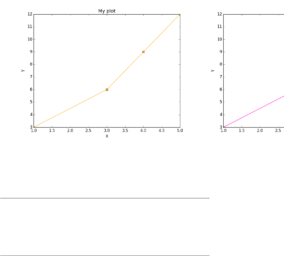
A typical example might be:
1import matplotlib.pyplot as plt
2
3def myplot(x, y, fname=None,**kwargs):
4"make plot of x,y. save to fname if not None. Provide kwargs to plot."
5plt.plot(x, y, **kwargs)
6plt.xlabel(’X’)
7plt.ylabel(’Y’)
8plt.title(’My plot’)
9if fname:
10 plt.savefig(fname)
11 else:
12 plt.show()
13
14 x=[1,3,4,5]
15 y=[3,6,9,12]
16
17 myplot(x, y, ’images/myfig.png’, color=’orange’, marker=’s’)
18
19 # you can use a dictionary as kwargs
20 d={’color’:’magenta’,
21 ’marker’:’d’}
22
23 myplot(x, y, ’images/myfig2.png’,**d)
17
In that example we wrap the matplotlib plotting commands in a function,
which we can call the way we want to, with arbitrary optional arguments.
In this example, you cannot pass keyword arguments that are illegal to the
plot command or you will get an error.
It is possible to combine all the options at once. I admit it is hard to
imagine where this would be really useful, but it can be done!
1import numpy as np
2
3def func(a, b=2,*args, **kwargs):
4"return a**b + sum(args) and print kwargs"
5for kw in kwargs:
6print(’kw: {0} = {1}’.format(kw, kwargs[kw]))
7
8return a**b+np.sum(args)
9
10 print(func(2,3,4,5, mysillykw=’hahah’))
kw: mysillykw = hahah
17
2.6 Lambda Lambda Lambda
Is that some kind of fraternity? of anonymous functions? What is that!?
There are many times where you need a callable, small function in python,
18

and it is inconvenient to have to use def to create a named function. Lambda
functions solve this problem. Let us look at some examples. First, we create
a lambda function, and assign it to a variable. Then we show that variable
is a function, and that we can call it with an argument.
1f=lambda x: 2*x
2print(f)
3print(f(2))
<function <lambda> at 0x10067f378>
4
We can have more than one argument:
1f=lambda x,y: x +y
2print(f)
3print(f(2,3))
<function <lambda> at 0x10207f378>
5
And default arguments:
1f=lambda x, y=3:x+y
2print(f)
3print(f(2))
4print(f(4,1))
<function <lambda> at 0x10077f378>
5
5
It is also possible to have arbitrary numbers of positional arguments.
Here is an example that provides the sum of an arbitrary number of argu-
ments.
1import functools,operator
2f=lambda *x: functools.reduce(operator.add, x)
3print(f)
4
5print(f(1))
6print(f(1,2))
7print(f(1,2,3))
19

<function <lambda> at 0x10077f378>
1
3
6
You can also make arbitrary keyword arguments. Here we make a func-
tion that simply returns the kwargs as a dictionary. This feature may be
helpful in passing kwargs to other functions.
1f=lambda **kwargs: kwargs
2
3print(f(a=1, b=3))
{’b’: 3, ’a’: 1}
Of course, you can combine these options. Here is a function with all
the options.
1f=lambda a, b=4,*args, **kwargs: (a, b, args, kwargs)
2
3print(f(’required’,3,’optional-positional’, g=4))
(’required’, 3, (’optional-positional’,), {’g’: 4})
One of the primary limitations of lambda functions is they are limited
to single expressions. They also do not have documentation strings, so it
can be difficult to understand what they were written for later.
2.6.1 Applications of lambda functions
Lambda functions are used in places where you need a function, but may
not want to define one using def. For example, say you want to solve the
nonlinear equation √x= 2.5.
1from scipy.optimize import fsolve
2import numpy as np
3
4sol, =fsolve(lambda x: 2.5 - np.sqrt(x), 8)
5print(sol)
6.25
20

Another time to use lambda functions is if you want to set a particular
value of a parameter in a function. Say we have a function with an inde-
pendent variable, xand a parameter a, i.e. f(x;a). If we want to find a
solution f(x;a) = 0 for some value of a, we can use a lambda function to
make a function of the single variable x. Here is a example.
1from scipy.optimize import fsolve
2import numpy as np
3
4def func(x, a):
5return a*np.sqrt(x) - 4.0
6
7sol, =fsolve(lambda x: func(x, 3.2), 3)
8print(sol)
1.5625
Any function that takes a function as an argument can use lambda func-
tions. Here we use a lambda function that adds two numbers in the reduce
function to sum a list of numbers.
1import functools as ft
2print(ft.reduce(lambda x, y: x +y, [0,1,2,3,4]))
10
We can evaluate the integral R2
0x2dx with a lambda function.
1from scipy.integrate import quad
2
3print(quad(lambda x: x**2,0,2))
(2.666666666666667, 2.960594732333751e-14)
2.6.2 Summary
Lambda functions can be helpful. They are never necessary. You can al-
ways define a function using def, but for some small, single-use functions,
a lambda function could make sense. Lambda functions have some limita-
tions, including that they are limited to a single expression, and they lack
documentation strings.
21

2.7 Creating arrays in python
Often, we will have a set of 1-D arrays, and we would like to construct a 2D
array with those vectors as either the rows or columns of the array. This may
happen because we have data from different sources we want to combine, or
because we organize the code with variables that are easy to read, and then
want to combine the variables. Here are examples of doing that to get the
vectors as the columns.
1import numpy as np
2
3a=np.array([1,2,3])
4b=np.array([4,5,6])
5
6print(np.column_stack([a, b]))
7
8# this means stack the arrays vertically, e.g. on top of each other
9print(np.vstack([a, b]).T)
[[1 4]
[2 5]
[3 6]]
[[1 4]
[2 5]
[3 6]]
Or rows:
1import numpy as np
2
3a=np.array([1,2,3])
4b=np.array([4,5,6])
5
6print(np.row_stack([a, b]))
7
8# this means stack the arrays vertically, e.g. on top of each other
9print(np.vstack([a, b]))
[[1 2 3]
[4 5 6]]
[[1 2 3]
[4 5 6]]
The opposite operation is to extract the rows or columns of a 2D array
into smaller arrays. We might want to do that to extract a row or column
22

from a calculation for further analysis, or plotting for example. There are
splitting functions in numpy. They are somewhat confusing, so we examine
some examples. The numpy.hsplit command splits an array "horizontally".
The best way to think about it is that the "splits" move horizontally across
the array. In other words, you draw a vertical split, move over horizontally,
draw another vertical split, etc. . . You must specify the number of splits
that you want, and the array must be evenly divisible by the number of
splits.
1import numpy as np
2
3A=np.array([[1,2,3,5],
4[4,5,6,9]])
5
6# split into two parts
7p1, p2 =np.hsplit(A, 2)
8print(p1)
9print(p2)
10
11 #split into 4 parts
12 p1, p2, p3, p4 =np.hsplit(A, 4)
13 print(p1)
14 print(p2)
15 print(p3)
16 print(p4)
[[1 2]
[4 5]]
[[3 5]
[6 9]]
[[1]
[4]]
[[2]
[5]]
[[3]
[6]]
[[5]
[9]]
In the numpy.vsplit command the "splits" go "vertically" down the array.
Note that the split commands return 2D arrays.
1import numpy as np
2
3A=np.array([[1,2,3,5],
23

4[4,5,6,9]])
5
6# split into two parts
7p1, p2 =np.vsplit(A, 2)
8print(p1)
9print(p2)
10 print(p2.shape)
[[1 2 3 5]]
[[4 5 6 9]]
(1, 4)
An alternative approach is array unpacking. In this example, we unpack
the array into two variables. The array unpacks by row.
1import numpy as np
2
3A=np.array([[1,2,3,5],
4[4,5,6,9]])
5
6# split into two parts
7p1, p2 =A
8print(p1)
9print(p2)
[1 2 3 5]
[4 5 6 9]
To get the columns, just transpose the array.
1import numpy as np
2
3A=np.array([[1,2,3,5],
4[4,5,6,9]])
5
6# split into two parts
7p1, p2, p3, p4 =A.T
8print(p1)
9print(p2)
10 print(p3)
11 print(p4)
12 print(p4.shape)
[1 4]
[2 5]
[3 6]
[5 9]
(2,)
24

Note that now, we have 1D arrays.
You can also access rows and columns by indexing. We index an array
by [row, column]. To get a row, we specify the row number, and all the
columns in that row like this [row, :]. Similarly, to get a column, we specify
that we want all rows in that column like this: [:, column]. This approach
is useful when you only want a few columns or rows.
1import numpy as np
2
3A=np.array([[1,2,3,5],
4[4,5,6,9]])
5
6# get row 1
7print(A[1])
8print(A[1, :]) # row 1, all columns
9
10 print(A[:, 2]) # get third column
11 print(A[:, 2].shape)
[4 5 6 9]
[4 5 6 9]
[3 6]
(2,)
Note that even when we specify a column, it is returned as a 1D array.
2.8 Functions on arrays of values
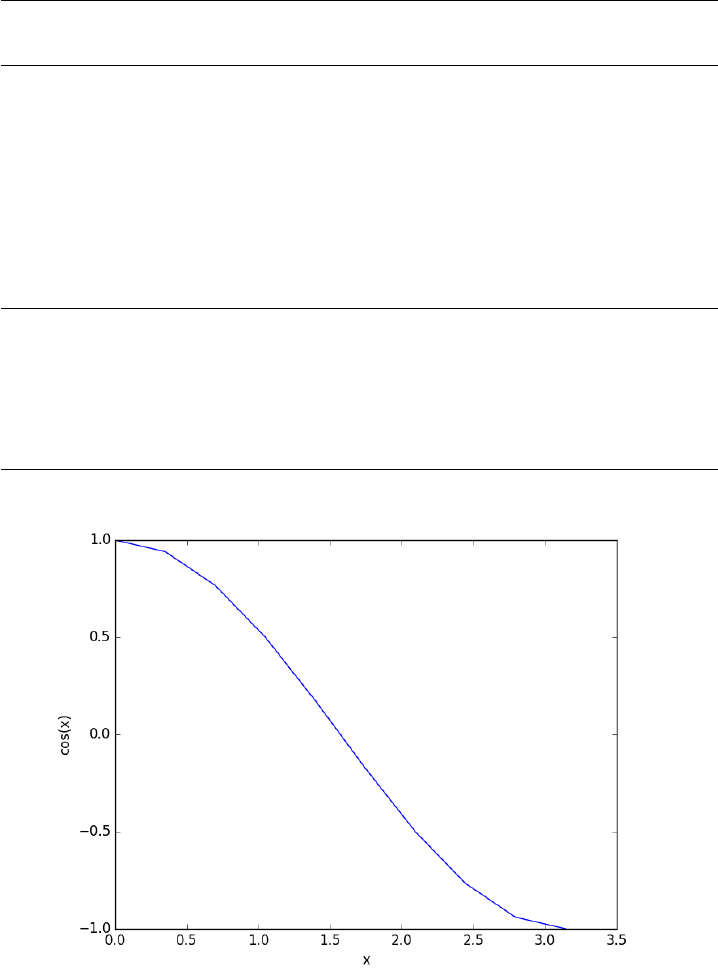
It is common to evaluate a function for a range of values. Let us consider
the value of the function f(x) = cos(x)over the range of 0< x < π. We
cannot consider every value in that range, but we can consider say 10 points
in the range. The numpy.linspace conveniently creates an array of values.
1import numpy as np
2print(np.linspace(0, np.pi, 10))
[ 0. 0.34906585 0.6981317 1.04719755 1.3962634 1.74532925
2.0943951 2.44346095 2.7925268 3.14159265]
The main point of using the numpy functions is that they work element-
wise on elements of an array. In this example, we compute the cos(x)for
each element of x.
25
1import numpy as np
2x=np.linspace(0, np.pi, 10)
3print(np.cos(x))
[ 1. 0.93969262 0.76604444 0.5 0.17364818 -0.17364818
-0.5 -0.76604444 -0.93969262 -1. ]
You can already see from this output that there is a root to the equation
cos(x)=0, because there is a change in sign in the output. This is not a
very convenient way to view the results; a graph would be better. We use
matplotlib to make figures. Here is an example.
1import matplotlib.pyplot as plt
2import numpy as np
3
4x=np.linspace(0, np.pi, 10)
5plt.plot(x, np.cos(x))
6plt.xlabel(’x’)
7plt.ylabel(’cos(x)’)
8plt.savefig(’images/plot-cos.png’)
This figure illustrates graphically what the numbers above show. The
function crosses zero at approximately x= 1.5. To get a more precise
value, we must actually solve the function numerically. We use the function
26

scipy.optimize.fsolve to do that. More precisely, we want to solve the
equation f(x) = cos(x)=0. We create a function that defines that equation,
and then use scipy.optimize.fsolve to solve it.
1from scipy.optimize import fsolve
2import numpy as np
3
4def f(x):
5return np.cos(x)
6
7sol, =fsolve(f, x0=1.5)# the comma after sol makes it return a float
8print(sol)
9print(np.pi / 2)
1.57079632679
1.5707963267948966
We know the solution is π/2.
2.9 Some basic data structures in python
Matlab post
We often have a need to organize data into structures when solving
problems.
2.9.1 the list
A list in python is data separated by commas in square brackets. Here,
we might store the following data in a variable to describe the Antoine
coefficients for benzene and the range they are relevant for [Tmin Tmax].
Lists are flexible, you can put anything in them, including other lists. We
access the elements of the list by indexing:
1c=[’benzene’,6.9056,1211.0,220.79, [-16,104]]
2print(c[0])
3print(c[-1])
4
5a,b =c[0:2]
6print(a,b)
7
8name, A, B, C, Trange =c
9print(Trange)
benzene
[-16, 104]
27

benzene 6.9056
[-16, 104]
Lists are "mutable", which means you can change their values.
1a=[3,4,5, [7,8], ’cat’]
2print(a[0], a[-1])
3a[-1]=’dog’
4print(a)
3 cat
[3, 4, 5, [7, 8], ’dog’]
2.9.2 tuples
Tuples are immutable; you cannot change their values. This is handy in
cases where it is an error to change the value. A tuple is like a list but it is
enclosed in parentheses.
1a=(3,4,5, [7,8], ’cat’)
2print(a[0], a[-1])
3a[-1]=’dog’ # this is an error
2.9.3 struct
Python does not exactly have the same thing as a struct in Matlab. You
can achieve something like it by defining an empty class and then defining
attributes of the class. You can check if an object has a particular attribute
using hasattr.
1class Antoine:
2pass
3
4a=Antoine()
5a.name =’benzene’
6a.Trange =[-16,104]
7
8print(a.name)
9print(hasattr(a, ’Trange’))
10 print(hasattr(a, ’A’))
benzene
True
False
28

2.9.4 dictionaries
The analog of the containers.Map in Matlab is the dictionary in python.
Dictionaries are enclosed in curly brackets, and are composed of key:value
pairs.
1s={’name’:’benzene’,
2’A’:6.9056,
3’B’:1211.0}
4
5s[’C’]= 220.79
6s[’Trange’]=[-16,104]
7
8print(s)
9print(s[’Trange’])
{’A’: 6.9056, ’B’: 1211.0, ’C’: 220.79, ’name’: ’benzene’, ’Trange’: [-16, 104]}
[-16, 104]
1s={’name’:’benzene’,
2’A’:6.9056,
3’B’:1211.0}
4
5print(’C’ in s)
6# default value for keys not in the dictionary
7print(s.get(’C’,None))
8
9print(s.keys())
10 print(s.values())
False
None
dict_keys([’B’, ’name’, ’A’])
dict_values([1211.0, ’benzene’, 6.9056])
2.9.5 Summary
We have examined four data structures in python. Note that none of these
types are arrays/vectors with defined mathematical operations. For those,
you need to consider numpy.array.
2.10 Indexing vectors and arrays in Python
Matlab post There are times where you have a lot of data in a vector or
array and you want to extract a portion of the data for some analysis. For
29

example, maybe you want to plot column 1 vs column 2, or you want the
integral of data between x = 4 and x = 6, but your vector covers 0 < x <
10. Indexing is the way to do these things.
A key point to remember is that in python array/vector indices start at
0. Unlike Matlab, which uses parentheses to index a array, we use brackets
in python.
1import numpy as np
2
3x=np.linspace(-np.pi, np.pi, 10)
4print(x)
5
6print(x[0]) # first element
7print(x[2]) # third element
8print(x[-1]) # last element
9print(x[-2]) # second to last element
[-3.14159265 -2.44346095 -1.74532925 -1.04719755 -0.34906585 0.34906585
1.04719755 1.74532925 2.44346095 3.14159265]
-3.14159265359
-1.74532925199
3.14159265359
2.44346095279
We can select a range of elements too. The syntax a:b extracts the aˆ{th}
to (b-1)ˆ{th} elements. The syntax a:b:n starts at a, skips nelements up to
the index b.
1print(x[1:4]) # second to fourth element. Element 5 is not included
2print(x[0:-1:2]) # every other element
3print(x[:]) # print the whole vector
4print(x[-1:0:-1]) # reverse the vector!
[-2.44346095 -1.74532925 -1.04719755]
[-3.14159265 -1.74532925 -0.34906585 1.04719755 2.44346095]
[-3.14159265 -2.44346095 -1.74532925 -1.04719755 -0.34906585 0.34906585
1.04719755 1.74532925 2.44346095 3.14159265]
[ 3.14159265 2.44346095 1.74532925 1.04719755 0.34906585 -0.34906585
-1.04719755 -1.74532925 -2.44346095]
Suppose we want the part of the vector where x > 2. We could do that
by inspection, but there is a better way. We can create a mask of boolean
(0 or 1) values that specify whether x > 2 or not, and then use the mask as
an index.
30

1print(x[x > 2])
[ 2.44346095 3.14159265]
You can use this to analyze subsections of data, for example to integrate
the function y = sin(x) where x > 2.
1y=np.sin(x)
2
3print(np.trapz( x[x > 2], y[x > 2]))
-1.79500162881
2.10.1 2d arrays
In 2d arrays, we use row, column notation. We use a : to indicate all rows
or all columns.
1a=np.array([[1,2,3],
2[4,5,6],
3[7,8,9]])
4
5print(a[0,0])
6print(a[-1,-1])
7
8print(a[0, :] )# row one
9print(a[:, 0] )# column one
10 print(a[:])
0__dummy_completion__ 1__dummy_completion__
0__dummy_completion__ 1__dummy_completion__
1
9
[1 2 3]
[1 4 7]
[[1 2 3]
[4 5 6]
[7 8 9]]
31

2.10.2 Using indexing to assign values to rows and columns
1b=np.zeros((3,3))
2print(b)
3
4b[:, 0]=[1,2,3]# set column 0
5b[2,2]= 12 # set a single element
6print(b)
7
8b[2]= 6 # sets everything in row 2 to 6!
9print(b)
[[ 0. 0. 0.]
[ 0. 0. 0.]
[ 0. 0. 0.]]
[[ 1. 0. 0.]
[ 2. 0. 0.]
[ 3. 0. 12.]]
[[ 1. 0. 0.]
[ 2. 0. 0.]
[ 6. 6. 6.]]
Python does not have the linear assignment method like Matlab does.
You can achieve something like that as follows. We flatten the array to 1D,
do the linear assignment, and reshape the result back to the 2D array.
1c=b.flatten()
2c[2]= 34
3b[:] =c.reshape(b.shape)
4print(b)
[[ 1. 0. 34.]
[ 2. 0. 0.]
[ 6. 6. 6.]]
2.10.3 3D arrays
The 3d array is like book of 2D matrices. Each page has a 2D matrix on it.
think about the indexing like this: (row, column, page)
1M=np.random.uniform(size=(3,3,3)) # a 3x3x3 array
2print(M)
32

[[[ 0.17900461 0.24477532 0.75963967]
[ 0.5595659 0.43535773 0.88449451]
[ 0.8169282 0.67361582 0.31123476]]
[[ 0.07541639 0.62738291 0.35397152]
[ 0.10017991 0.51427539 0.99643481]
[ 0.26285853 0.60086939 0.60945997]]
[[ 0.15581452 0.94685716 0.20213257]
[ 0.30398062 0.8173967 0.48472948]
[ 0.7998031 0.46701875 0.14776334]]]
1print(M[:, :, 0]) # 2d array on page 0
2print(M[:, 0,0]) # column 0 on page 0
3print(M[1,:,2]) # row 1 on page 2
[[ 0.17900461 0.5595659 0.8169282 ]
[ 0.07541639 0.10017991 0.26285853]
[ 0.15581452 0.30398062 0.7998031 ]]
[ 0.17900461 0.07541639 0.15581452]
[ 0.35397152 0.99643481 0.60945997]
2.10.4 Summary
The most common place to use indexing is probably when a function returns
an array with the independent variable in column 1 and solution in column
2, and you want to plot the solution. Second is when you want to analyze
one part of the solution. There are also applications in numerical methods,
for example in assigning values to the elements of a matrix or vector.
2.11 Controlling the format of printed variables
This was first worked out in this original Matlab post.
Often you will want to control the way a variable is printed. You may
want to only show a few decimal places, or print in scientific notation, or
embed the result in a string. Here are some examples of printing with no
control over the format.
1a= 2./3
2print(a)
3print(1/3)
33

4print(1./3.)
5print(10.1)
6print("Avogadro’s number is ",6.022e23,’.’)
0.6666666666666666
0.3333333333333333
0.3333333333333333
10.1
Avogadro’s number is 6.022e+23 .
There is no control over the number of decimals, or spaces around a
printed number.
In python, we use the format function to control how variables are
printed. With the format function you use codes like {n:format specifier}
to indicate that a formatted string should be used. nis the nˆ{th} argu-
ment passed to format, and there are a variety of format specifiers. Here we
examine how to format float numbers. The specifier has the general form
"w.df" where w is the width of the field, and d is the number of decimals,
and f indicates a float number. "1.3f" means to print a float number with 3
decimal places. Here is an example.
1print(’The value of 1/3 to 3 decimal places is {0:1.3f}’.format(1./3.))
The value of 1/3 to 3 decimal places is 0.333
In that example, the 0 in {0:1.3f} refers to the first (and only) argument
to the format function. If there is more than one argument, we can refer to
them like this:
1print(’Value 0 = {0:1.3f}, value 1 = {1:1.3f}, value 0 = {0:1.3f}’.format(1./3.,1./6.))
Value 0 = 0.333, value 1 = 0.167, value 0 = 0.333
Note you can refer to the same argument more than once, and in arbi-
trary order within the string.
Suppose you have a list of numbers you want to print out, like this:
1for xin [1./3.,1./6.,1./9.]:
2print(’The answer is {0:1.2f}’.format(x))
34

The answer is 0.33
The answer is 0.17
The answer is 0.11
The "g" format specifier is a general format that can be used to indicate a
precision, or to indicate significant digits. To print a number with a specific
number of significant digits we do this:
1print(’{0:1.3g}’.format(1./3.))
2print(’{0:1.3g}’.format(4./3.))
0.333
1.33
We can also specify plus or minus signs. Compare the next two outputs.
1for xin [-1.,1.]:
2print(’{0:1.2f}’.format(x))
-1.00
1.00
You can see the decimals do not align. That is because there is a minus
sign in front of one number. We can specify to show the sign for positive
and negative numbers, or to pad positive numbers to leave space for positive
numbers.
1for xin [-1.,1.]:
2print(’{0:+1.2f}’.format(x)) # explicit sign
3
4for xin [-1.,1.]:
5print(’{0: 1.2f}’.format(x)) # pad positive numbers
-1.00
+1.00
-1.00
1.00
We use the "e" or "E" format modifier to specify scientific notation.
35

1import numpy as np
2eps =np.finfo(np.double).eps
3print(eps)
4print(’{0}’.format(eps))
5print(’{0:1.2f}’.format(eps))
6print(’{0:1.2e}’.format(eps)) #exponential notation
7print(’{0:1.2E}’.format(eps)) #exponential notation with capital E
2.22044604925e-16
2.220446049250313e-16
0.00
2.22e-16
2.22E-16
As a float with 2 decimal places, that very small number is practically
equal to 0.
We can even format percentages. Note you do not need to put the % in
your string.
1print(’the fraction {0} corresponds to {0:1.0%}’.format(0.78))
the fraction 0.78 corresponds to 78%
There are many other options for formatting strings. See http://docs.
python.org/2/library/string.html#formatstrings for a full specifica-
tion of the options.
2.12 Advanced string formatting
There are several more advanced ways to include formatted values in a string.
In the previous case we examined replacing format specifiers by positional
arguments in the format command. We can instead use keyword arguments.
1s=’The {speed} {color} fox’.format(color=’brown’, speed=’quick’)
2print(s)
The quick brown fox
If you have a lot of variables already defined in a script, it is convenient
to use them in string formatting with the locals command:
36

1speed =’slow’
2color=’blue’
3
4print(’The {speed} {color} fox’.format(**locals()))
The slow blue fox
If you want to access attributes on an object, you can specify them
directly in the format identifier.
1class A:
2def __init__(self, a, b, c):
3self.a=a
4self.b=b
5self.c=c
6
7mya =A(3,4,5)
8
9print(’a = {obj.a}, b = {obj.b}, c = {obj.c:1.2f}’.format(obj=mya))
a=3,b=4,c=5.00
You can access values of a dictionary:
1d={’a’:56,"test":’woohoo!’}
2
3print("the value of a in the dictionary is {obj[a]}. It works {obj[test]}".format(obj=d))
the value of a in the dictionary is 56. It works woohoo!
And, you can access elements of a list. Note, however you cannot use -1
as an index in this case.
1L=[4,5,’cat’]
2
3print(’element 0 = {obj[0]}, and the last element is {obj[2]}’.format(obj=L))
element 0 = 4, and the last element is cat
There are three different ways to "print" an object. If an object has a
format function, that is the default used in the format command. It may be
helpful to use the str or repr of an object instead. We get this with !s for
str and !r for repr.
37

1class A:
2def __init__(self, a, b):
3self.a=a; self.b=b
4
5def __format__(self, format):
6s=’a={{0:{0}}} b={{1:{0}}}’.format(format)
7return s.format(self.a, self.b)
8
9def __str__(self):
10 return ’str: class A, a={0} b={1}’.format(self.a, self.b)
11
12 def __repr__(self):
13 return ’representing: class A, a={0}, b={1}’.format(self.a, self.b)
14
15 mya =A(3,4)
16
17 print(’{0}’.format(mya)) # uses __format__
18 print(’{0!s}’.format(mya)) # uses __str__
19 print(’{0!r}’.format(mya)) # uses __repr__
a=3 b=4
str: class A, a=3 b=4
representing: class A, a=3, b=4
This covers the majority of string formatting requirements I have come
across. If there are more sophisticated needs, they can be met with various
string templating python modules. the one I have used most is Cheetah.
3 Math
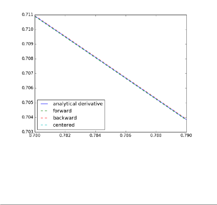
3.1 Numeric derivatives by differences
numpy has a function called numpy.diff() that is similar to the one found
in matlab. It calculates the differences between the elements in your list,
and returns a list that is one element shorter, which makes it unsuitable for
plotting the derivative of a function.
Loops in python are pretty slow (relatively speaking) but they are usually
trivial to understand. In this script we show some simple ways to construct
derivative vectors using loops. It is implied in these formulas that the data
points are equally spaced. If they are not evenly spaced, you need a different
approach.
1import numpy as np
2from pylab import *
3import time
38

4
5’’’
6These are the brainless way to calculate numerical derivatives. They
7work well for very smooth data. they are surprisingly fast even up to
810000 points in the vector.
9’’’
10
11 x=np.linspace(0.78,0.79,100)
12 y=np.sin(x)
13 dy_analytical =np.cos(x)
14 ’’’
15 lets use a forward difference method:
16 that works up until the last point, where there is not
17 a forward difference to use. there, we use a backward difference.
18 ’’’
19
20 tf1 =time.time()
21 dyf =[0.0]*len(x)
22 for iin range(len(y)-1):
23 dyf[i] =(y[i+1]-y[i])/(x[i+1]-x[i])
24 #set last element by backwards difference
25 dyf[-1]=(y[-1]-y[-2])/(x[-1]-x[-2])
26
27 print(’ Forward difference took %f seconds’ %(time.time() -tf1))
28
29 ’’’and now a backwards difference’’’
30 tb1 =time.time()
31 dyb =[0.0]*len(x)
32 #set first element by forward difference
33 dyb[0]=(y[0]-y[1])/(x[0]-x[1])
34 for iin range(1,len(y)):
35 dyb[i] =(y[i] -y[i-1])/(x[i]-x[i-1])
36
37 print(’ Backward difference took %f seconds’ %(time.time() -tb1))
38
39 ’’’and now, a centered formula’’’
40 tc1 =time.time()
41 dyc =[0.0]*len(x)
42 dyc[0]=(y[0]-y[1])/(x[0]-x[1])
43 for iin range(1,len(y)-1):
44 dyc[i] =(y[i+1]-y[i-1])/(x[i+1]-x[i-1])
45 dyc[-1]=(y[-1]-y[-2])/(x[-1]-x[-2])
46
47 print(’ Centered difference took %f seconds’ %(time.time() -tc1))
48
49 ’’’
50 the centered formula is the most accurate formula here
51 ’’’
52
53 plt.plot(x,dy_analytical,label=’analytical derivative’)
54 plt.plot(x,dyf,’--’,label=’forward’)
55 plt.plot(x,dyb,’--’,label=’backward’)
56 plt.plot(x,dyc,’--’,label=’centered’)
57
58 plt.legend(loc=’lower left’)
59 plt.savefig(’images/simple-diffs.png’)
39
Forward difference took 0.000094 seconds
Backward difference took 0.000084 seconds
Centered difference took 0.000088 seconds
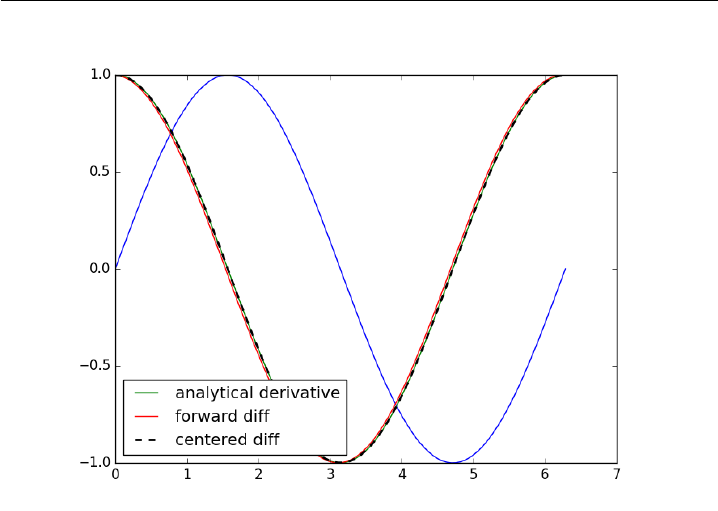
3.2 Vectorized numeric derivatives
Loops are usually not great for performance. Numpy offers some vectorized
methods that allow us to compute derivatives without loops, although this
comes at the mental cost of harder to understand syntax
1import numpy as np
2import matplotlib.pyplot as plt
3
4x=np.linspace(0,2*np.pi, 100)
5y=np.sin(x)
6dy_analytical =np.cos(x)
7
8
9# we need to specify the size of dy ahead because diff returns
10 #an array of n-1 elements
11 dy =np.zeros(y.shape, np.float) #we know it will be this size
12 dy[0:-1]=np.diff(y) /np.diff(x)
13 dy[-1]=(y[-1]-y[-2]) /(x[-1]-x[-2])
14
15
16 ’’’
40
17 calculate dy by center differencing using array slices
18 ’’’
19
20 dy2 =np.zeros(y.shape,np.float) #we know it will be this size
21 dy2[1:-1]=(y[2:] -y[0:-2]) /(x[2:] -x[0:-2])
22
23 # now the end points
24 dy2[0]=(y[1]-y[0]) /(x[1]-x[0])
25 dy2[-1]=(y[-1]-y[-2]) /(x[-1]-x[-2])
26
27 plt.plot(x,y)
28 plt.plot(x,dy_analytical,label=’analytical derivative’)
29 plt.plot(x,dy,label=’forward diff’)
30 plt.plot(x,dy2,’k--’,lw=2,label=’centered diff’)
31 plt.legend(loc=’lower left’)
32 plt.savefig(’images/vectorized-diffs.png’)
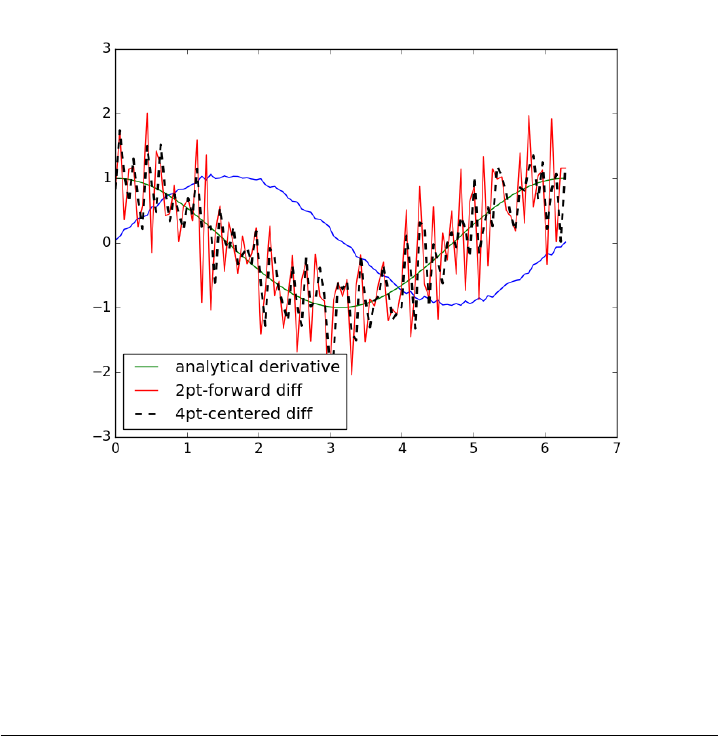
3.3 2-point vs. 4-point numerical derivatives
If your data is very noisy, you will have a hard time getting good deriva-
tives; derivatives tend to magnify noise. In these cases, you have to employ
smoothing techniques, either implicitly by using a multipoint derivative for-
mula, or explicitly by smoothing the data yourself, or taking the derivative
of a function that has been fit to the data in the neighborhood you are
interested in.
41

Here is an example of a 4-point centered difference of some noisy data:
1import numpy as np
2import matplotlib.pyplot as plt
3
4x=np.linspace(0,2*np.pi, 100)
5y=np.sin(x) + 0.1 * np.random.random(size=x.shape)
6dy_analytical =np.cos(x)
7
8#2-point formula
9dyf =[0.0]*len(x)
10 for iin range(len(y)-1):
11 dyf[i] =(y[i+1]-y[i])/(x[i+1]-x[i])
12 #set last element by backwards difference
13 dyf[-1]=(y[-1]-y[-2])/(x[-1]-x[-2])
14
15 ’’’
16 calculate dy by 4-point center differencing using array slices
17
18 \frac{y[i-2] - 8y[i-1] + 8[i+1] - y[i+2]}{12h}
19
20 y[0] and y[1] must be defined by lower order methods
21 and y[-1] and y[-2] must be defined by lower order methods
22 ’’’
23
24 dy =np.zeros(y.shape, np.float) #we know it will be this size
25 h=x[1]-x[0]#this assumes the points are evenely spaced!
26 dy[2:-2]=(y[0:-4]-8*y[1:-3]+8*y[3:-1]-y[4:]) /(12.0 * h)
27
28 # simple differences at the end-points
29 dy[0]=(y[1]-y[0])/(x[1]-x[0])
30 dy[1]=(y[2]-y[1])/(x[2]-x[1])
31 dy[-2]=(y[-2]-y[-3]) /(x[-2]-x[-3])
32 dy[-1]=(y[-1]-y[-2]) /(x[-1]-x[-2])
33
34
35 plt.plot(x, y)
36 plt.plot(x, dy_analytical, label=’analytical derivative’)
37 plt.plot(x, dyf, ’r-’, label=’2pt-forward diff’)
38 plt.plot(x, dy, ’k--’, lw=2, label=’4pt-centered diff’)
39 plt.legend(loc=’lower left’)
40 plt.savefig(’images/multipt-diff.png’)
42
3.4 Derivatives by polynomial fitting
One way to reduce the noise inherent in derivatives of noisy data is to fit
a smooth function through the data, and analytically take the derivative of
the curve. Polynomials are especially convenient for this. The challenge is to
figure out what an appropriate polynomial order is. This requires judgment
and experience.
1import numpy as np
2import matplotlib.pyplot as plt
3from pycse import deriv
4
5tspan =[0,0.1,0.2,0.4,0.8,1]
6Ca_data =[2.0081,1.5512,1.1903,0.7160,0.2562,0.1495]
7
8p=np.polyfit(tspan, Ca_data, 3)
9plt.figure()
10 plt.plot(tspan, Ca_data)
11 plt.plot(tspan, np.polyval(p, tspan), ’g-’)
12 plt.savefig(’images/deriv-fit-1.png’)
13
14 # compute derivatives
15 dp =np.polyder(p)
16
17 dCdt_fit =np.polyval(dp, tspan)
18
43

19 dCdt_numeric =deriv(tspan, Ca_data) # 2-point deriv
20
21 plt.figure()
22 plt.plot(tspan, dCdt_numeric, label=’numeric derivative’)
23 plt.plot(tspan, dCdt_fit, label=’fitted derivative’)
24
25 t=np.linspace(min(tspan), max(tspan))
26 plt.plot(t, np.polyval(dp, t), label=’resampled derivative’)
27 plt.legend(loc=’best’)
28 plt.savefig(’images/deriv-fit-2.png’)
You can see a third order polynomial is a reasonable fit here. There
are only 6 data points here, so any higher order risks overfitting. Here is
the comparison of the numerical derivative and the fitted derivative. We
have "resampled" the fitted derivative to show the actual shape. Note the
derivative appears to go through a maximum near t = 0.9. In this case,
that is probably unphysical as the data is related to the consumption of
species A in a reaction. The derivative should increase monotonically to
zero. The increase is an artefact of the fitting process. End points are
especially sensitive to this kind of error.
44

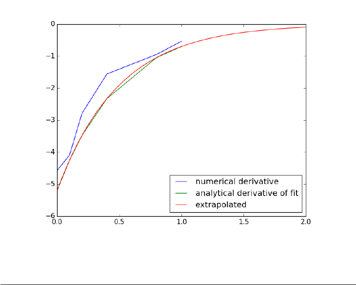
3.5 Derivatives by fitting a function and taking the analyti-
cal derivative
A variation of a polynomial fit is to fit a model with reasonable physics.
Here we fit a nonlinear function to the noisy data. The model is for the con-
centration vs. time in a batch reactor for a first order irreversible reaction.
Once we fit the data, we take the analytical derivative of the fitted function.
1import numpy as np
2import matplotlib.pyplot as plt
3from scipy.optimize import curve_fit
4from pycse import deriv
5
6tspan =np.array([0,0.1,0.2,0.4,0.8,1])
7Ca_data =np.array([2.0081,1.5512,1.1903,0.7160,0.2562,0.1495])
8
9def func(t, Ca0, k):
10 return Ca0 *np.exp(-k*t)
11
12
13 pars, pcov =curve_fit(func, tspan, Ca_data, p0=[2,2.3])
14
15 plt.plot(tspan, Ca_data)
16 plt.plot(tspan, func(tspan, *pars), ’g-’)
17 plt.savefig(’images/deriv-funcfit-1.png’)
18
45

19 # analytical derivative
20 k, Ca0 =pars
21 dCdt = -k*Ca0 *np.exp(-k*tspan)
22 t=np.linspace(0,2)
23 dCdt_res = -k*Ca0 *np.exp(-k*t)
24
25 plt.figure()
26 plt.plot(tspan, deriv(tspan, Ca_data), label=’numerical derivative’)
27 plt.plot(tspan, dCdt, label=’analytical derivative of fit’)
28 plt.plot(t, dCdt_res, label=’extrapolated’)
29 plt.legend(loc=’best’)
30 plt.savefig(’images/deriv-funcfit-2.png’)
Visually this fit is about the same as a third order polynomial. Note
the difference in the derivative though. We can readily extrapolate this
derivative and get reasonable predictions of the derivative. That is true in
this case because we fitted a physically relevant model for concentration vs.
time for an irreversible, first order reaction.
46
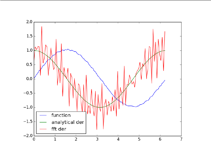
3.6 Derivatives by FFT
1import numpy as np
2import matplotlib.pyplot as plt
3
4N= 101 #number of points
5L=2*np.pi #interval of data
6
7x=np.arange(0.0, L, L/float(N)) #this does not include the endpoint
8
9#add some random noise
10 y=np.sin(x) + 0.05 * np.random.random(size=x.shape)
11 dy_analytical =np.cos(x)
12
13 ’’’
14 http://sci.tech-archive.net/Archive/sci.math/2008-05/msg00401.html
15
16 you can use fft to calculate derivatives!
17 ’’’
18
19 if N% 2 == 0:
20 k=np.asarray(list(range(0, N // 2)) +[0]+list(range(-N// 2 + 1,0)), np.float64)
21 else:
22 k=np.asarray(list(range(0, (N - 1)// 2)) +[0]+list(range(-(N - 1)// 2,0)), np.float64)
23
24 k*= 2 * np.pi /L
25
26 fd =np.real(np.fft.ifft(1.0j * k*np.fft.fft(y)))
47
27
28 plt.plot(x, y, label=’function’)
29 plt.plot(x,dy_analytical,label=’analytical der’)
30 plt.plot(x,fd,label=’fft der’)
31 plt.legend(loc=’lower left’)
32
33 plt.savefig(’images/fft-der.png’)
34 plt.show()
3.7 A novel way to numerically estimate the derivative of a
function - complex-step derivative approximation
Matlab post
Adapted from http://biomedicalcomputationreview.org/2/3/8.pdf
and http://dl.acm.org/citation.cfm?id=838250.838251
This posts introduces a novel way to numerically estimate the derivative
of a function that does not involve finite difference schemes. Finite differ-
ence schemes are approximations to derivatives that become more and more
accurate as the step size goes to zero, except that as the step size approaches
the limits of machine accuracy, new errors can appear in the approximated
results. In the references above, a new way to compute the derivative is
presented that does not rely on differences!
48

The new way is: f0(x) = imag(f(x + i∆x)/∆x) where the function fis
evaluated in imaginary space with a small ∆xin the complex plane. The
derivative is miraculously equal to the imaginary part of the result in the
limit of ∆x→0!
This example comes from the first link. The derivative must be evaluated
using the chain rule. We compare a forward difference, central difference and
complex-step derivative approximations.
1import numpy as np
2import matplotlib.pyplot as plt
3
4def f(x): return np.sin(3*x)*np.log(x)
5
6x= 0.7
7h= 1e-7
8
9# analytical derivative
10 dfdx_a =3*np.cos( 3*x)*np.log(x) +np.sin(3*x) /x
11
12 # finite difference
13 dfdx_fd =(f(x +h) -f(x))/h
14
15 # central difference
16 dfdx_cd =(f(x+h)-f(x-h))/(2*h)
17
18 # complex method
19 dfdx_I =np.imag(f(x +np.complex(0, h))/h)
20
21 print(dfdx_a)
22 print(dfdx_fd)
23 print(dfdx_cd)
24 print(dfdx_I)
1.77335410624
1.77335393925
1.77335410495
1.7733541062373848
These are all the same to 4 decimal places. The simple finite difference
is the least accurate, and the central differences is practically the same as
the complex number approach.
Let us use this method to verify the fundamental Theorem of Calcu-
lus, i.e. to evaluate the derivative of an integral function. Let f(x) =
x2
R1
tan(t3)dt, and we now want to compute df/dx. Of course, this can be
done analytically, but it is not trivial!
49

1import numpy as np
2from scipy.integrate import quad
3
4def f_(z):
5def integrand(t):
6return np.tan(t**3)
7return quad(integrand, 0, z**2)
8
9f=np.vectorize(f_)
10
11 x=np.linspace(0,1)
12
13 h= 1e-7
14
15 dfdx =np.imag(f(x +complex(0, h)))/h
16 dfdx_analytical =2*x*np.tan(x**6)
17
18 import matplotlib.pyplot as plt
19
20 plt.plot(x, dfdx, x, dfdx_analytical, ’r--’)
21 plt.show()
Interesting this fails.
3.8 Vectorized piecewise functions
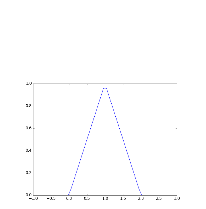
Matlab post Occasionally we need to define piecewise functions, e.g.
f(x)=0, x < 0(1)
=x, 0<=x < 1(2)
= 2 −x, 1<x<= 2 (3)
= 0, x > 2(4)
Today we examine a few ways to define a function like this. A simple
way is to use conditional statements.
1def f1(x):
2if x< 0:
3return 0
4elif (x >= 0)&(x < 1):
5return x
6elif (x >= 1)&(x < 2):
7return 2.0 - x
8else:
9return 0
10
11 print(f1(-1))
12 #print(f1([0, 1, 2, 3])) # does not work!
50
0
This works, but the function is not vectorized, i.e. f([-1 0 2 3]) does not
evaluate properly (it should give a list or array). You can get vectorized
behavior by using list comprehension, or by writing your own loop. This
does not fix all limitations, for example you cannot use the f1 function in
the quad function to integrate it.
1import numpy as np
2import matplotlib.pyplot as plt
3
4x=np.linspace(-1,3)
5y=[f1(xx) for xx in x]
6
7plt.plot(x, y)
8plt.savefig(’images/vector-piecewise.png’)
[<matplotlib.lines.Line2D object at 0x108f55b38>]
Neither of those methods is convenient. It would be nicer if the function
was vectorized, which would allow the direct notation f1([0, 1, 2, 3, 4]). A
simple way to achieve this is through the use of logical arrays. We create
logical arrays from comparison statements.
51
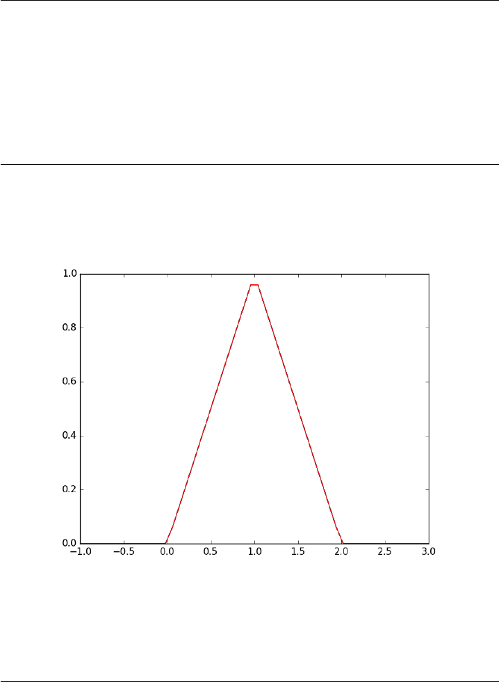
1def f2(x):
2’fully vectorized version’
3x=np.asarray(x)
4y=np.zeros(x.shape)
5y+= ((x >= 0)&(x < 1)) *x
6y+= ((x >= 1)&(x < 2)) *(2-x)
7return y
8
9print(f2([-1,0,1,2,3,4]))
10 x=np.linspace(-1,3);
11 plt.plot(x,f2(x))
12 plt.savefig(’images/vector-piecewise-2.png’)
[ 0. 0. 1. 0. 0. 0.]
[<matplotlib.lines.Line2D object at 0x10b3a6358>]
A third approach is to use Heaviside functions. The Heaviside function
is defined to be zero for x less than some value, and 0.5 for x=0, and 1 for
x >= 0. If you can live with y=0.5 for x=0, you can define a vectorized
function in terms of Heaviside functions like this.
1def heaviside(x):
2x=np.array(x)
3if x.shape != ():
4y=np.zeros(x.shape)
52
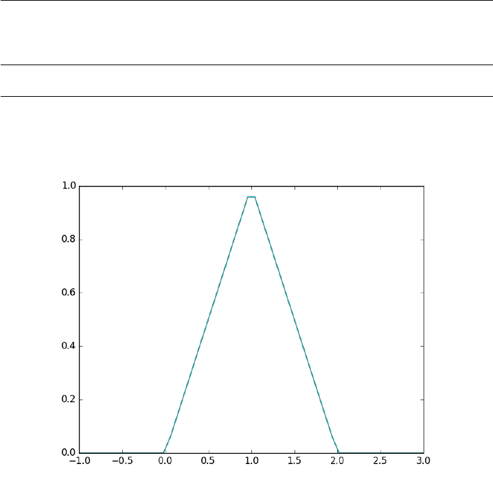
5y[x > 0.0]= 1
6y[x == 0.0]= 0.5
7else:# special case for 0d array (a number)
8if x> 0: y = 1
9elif x== 0: y = 0.5
10 else:y= 0
11 return y
12
13 def f3(x):
14 x=np.array(x)
15 y1 =(heaviside(x) -heaviside(x - 1)) *x# first interval
16 y2 =(heaviside(x - 1)-heaviside(x - 2)) *(2-x) # second interval
17 return y1 +y2
18
19 from scipy.integrate import quad
20 print(quad(f3, -1,3))
(1.0, 1.1102230246251565e-14)
1plt.plot(x, f3(x))
2plt.savefig(’images/vector-piecewise-3.png’)
[<matplotlib.lines.Line2D object at 0x10fc29a20>]
There are many ways to define piecewise functions, and vectorization is
not always necessary. The advantages of vectorization are usually notational
53

simplicity and speed; loops in python are usually very slow compared to
vectorized functions.
3.9 Smooth transitions between discontinuous functions
original post
In Post 1280 we used a correlation for the Fanning friction factor for
turbulent flow in a pipe. For laminar flow (Re < 3000), there is another
correlation that is commonly used: fF= 16/Re. Unfortunately, the cor-
relations for laminar flow and turbulent flow have different values at the
transition that should occur at Re = 3000. This discontinuity can cause a
lot of problems for numerical solvers that rely on derivatives.
Today we examine a strategy for smoothly joining these two functions.
First we define the two functions.
1import numpy as np
2from scipy.optimize import fsolve
3import matplotlib.pyplot as plt
4
5def fF_laminar(Re):
6return 16.0 / Re
7
8def fF_turbulent_unvectorized(Re):
9# Nikuradse correlation for turbulent flow
10 # 1/np.sqrt(f) = (4.0*np.log10(Re*np.sqrt(f))-0.4)
11 # we have to solve this equation to get f
12 def func(f):
13 return 1/np.sqrt(f) -(4.0*np.log10(Re*np.sqrt(f))-0.4)
14 fguess = 0.01
15 f, =fsolve(func, fguess)
16 return f
17
18 # this enables us to pass vectors to the function and get vectors as
19 # solutions
20 fF_turbulent =np.vectorize(fF_turbulent_unvectorized)
Now we plot the correlations.
1Re1 =np.linspace(500,3000)
2f1 =fF_laminar(Re1)
3
4Re2 =np.linspace(3000,10000)
5f2 =fF_turbulent(Re2)
6
7plt.figure(1); plt.clf()
8plt.plot(Re1, f1, label=’laminar’)
9plt.plot(Re2, f2, label=’turbulent’)
10 plt.xlabel(’Re’)
54
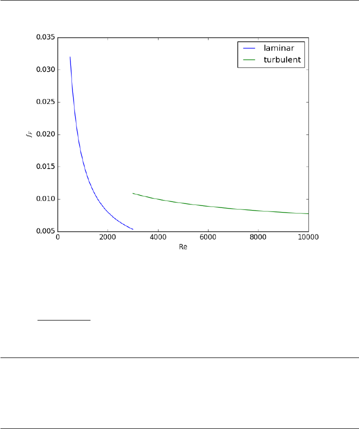
11 plt.ylabel(’$f_F$’)
12 plt.legend()
13 plt.savefig(’images/smooth-transitions-1.png’)
You can see the discontinuity at Re = 3000. What we need is a method to
join these two functions smoothly. We can do that with a sigmoid function.
Sigmoid functions
A sigmoid function smoothly varies from 0 to 1 according to the equation:
σ(x) = 1
1+e−(x−x0)/α . The transition is centered on x0, and αdetermines the
width of the transition.
1x=np.linspace(-4,4);
2y= 1.0 / (1+np.exp(-x/ 0.1))
3plt.figure(2)
4plt.clf()
5plt.plot(x, y)
6plt.xlabel(’x’); plt.ylabel(’y’); plt.title(’$\sigma(x)$’)
7plt.savefig(’images/smooth-transitions-sigma.png’)
55
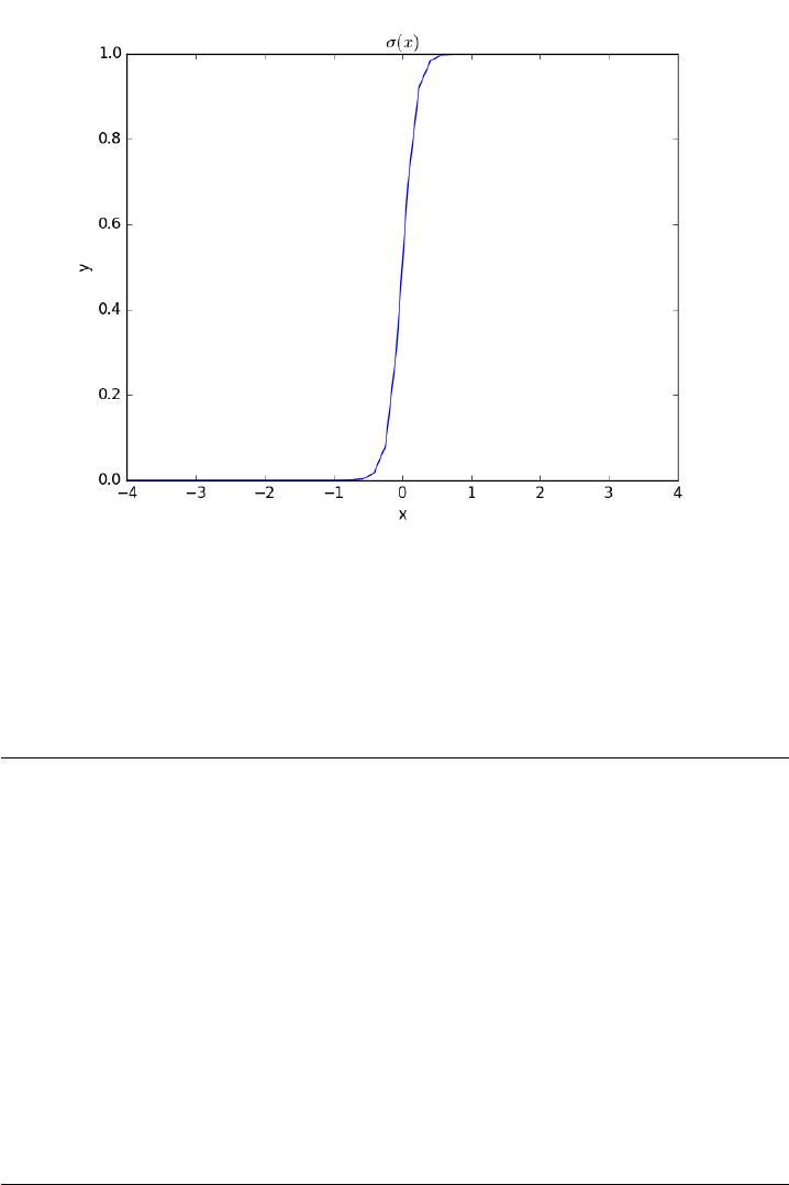
If we have two functions, f1(x)and f2(x)we want to smoothly join,
we do it like this: f(x) = (1 −σ(x))f1(x) + σ(x)f2(x). There is no formal
justification for this form of joining, it is simply a mathematical convenience
to get a numerically smooth function. Other functions besides the sigmoid
function could also be used, as long as they smoothly transition from 0 to
1, or from 1 to zero.
1def fanning_friction_factor(Re):
2’’’combined, continuous correlation for the fanning friction factor.
3the alpha parameter is chosen to provide the desired smoothness.
4The transition region is about +- 4*alpha. The value 450 was
5selected to reasonably match the shape of the correlation
6function provided by Morrison (see last section of this file)’’’
7sigma = 1. / (1+np.exp(-(Re - 3000.0)/ 450.0));
8f=(1-sigma) *fF_laminar(Re) +sigma *fF_turbulent(Re)
9return f
10
11 Re =np.linspace(500,10000);
12 f=fanning_friction_factor(Re);
13
14 # add data to figure 1
15 plt.figure(1)
16 plt.plot(Re,f, label=’smooth transition’)
17 plt.xlabel(’Re’)
18 plt.ylabel(’$f_F$’)
19 plt.legend()
20 plt.savefig(’images/smooth-transitions-3.png’)
56
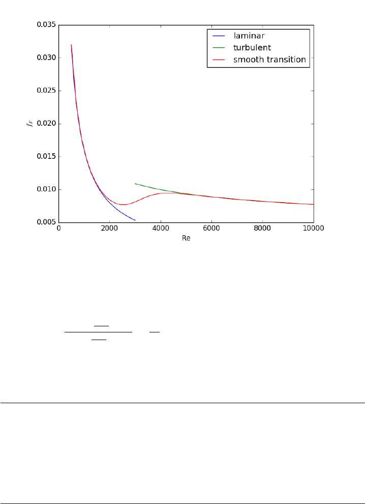
You can see that away from the transition the combined function is
practically equivalent to the original two functions. That is because away
from the transition the sigmoid function is 0 or 1. Near Re = 3000 is a
smooth transition from one curve to the other curve.
Morrison derived a single function for the friction factor correlation over
all Re: f=0.0076(3170
Re )0.165
1+(3171
Re )7.0+16
Re . Here we show the comparison with the
approach used above. The friction factor differs slightly at high Re, because
Morrison’s is based on the Prandlt correlation, while the work here is based
on the Nikuradse correlation. They are similar, but not the same.
1# add this correlation to figure 1
2h, =plt.plot(Re, 16.0/Re +(0.0076 * (3170 / Re)**0.165)/(1 + (3170.0 / Re)**7))
3
4ax =plt.gca()
5handles, labels =ax.get_legend_handles_labels()
6
7handles.append(h)
8labels.append(’Morrison’)
9ax.legend(handles, labels)
10 plt.savefig(’images/smooth-transitions-morrison.png’)
57
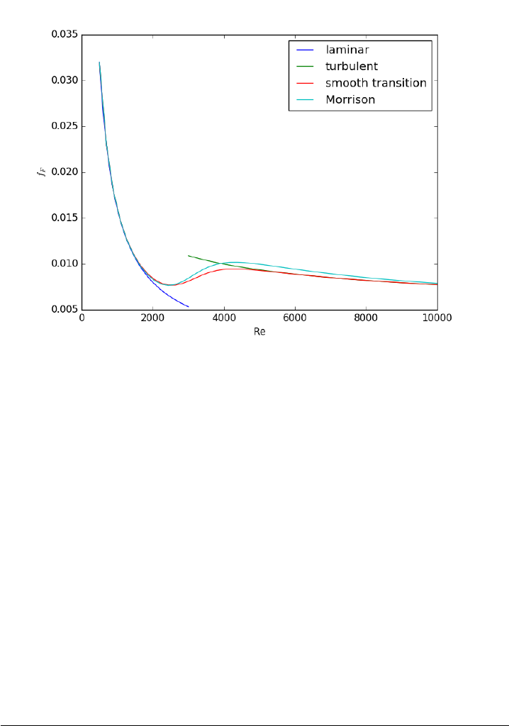
3.9.1 Summary
The approach demonstrated here allows one to smoothly join two discon-
tinuous functions that describe physics in different regimes, and that must
transition over some range of data. It should be emphasized that the method
has no physical basis, it simply allows one to create a mathematically smooth
function, which could be necessary for some optimizers or solvers to work.
3.10 Smooth transitions between two constants
Suppose we have a parameter that has two different values depending on
the value of a dimensionless number. For example when the dimensionless
number is much less than 1, x = 2/3, and when x is much greater than 1,
x = 1. We desire a smooth transition from 2/3 to 1 as a function of x to
avoid discontinuities in functions of x. We will adapt the smooth transitions
between functions to be a smooth transition between constants.
We define our function as x(D) = x0+(x1−x0) ∗(1 −sigma(D, w). We
control the rate of the transition by the variable w
1import numpy as np
2import matplotlib.pyplot as plt
3
58
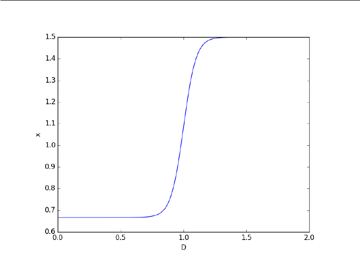
4x0 = 2.0 / 3.0
5x1 = 1.5
6
7w= 0.05
8
9D=np.linspace(0,2,500)
10
11 sigmaD =1.0/(1.0 + np.exp(-(1 - D) /w))
12
13 x=x0 +(x1 -x0)*(1-sigmaD)
14
15 plt.plot(D, x)
16 plt.xlabel(’D’); plt.ylabel(’x’)
17 plt.savefig(’images/smooth-transitions-constants.png’)
This is a nice trick to get an analytical function with continuous deriva-
tives for a transition between two constants. You could have the transition
occur at a value other than D = 1, as well by changing the argument to the
exponential function.
3.11 On the quad or trapz’d in ChemE heaven
Matlab post
What is the difference between quad and trapz? The short answer is that
quad integrates functions (via a function handle) using numerical quadra-
ture, and trapz performs integration of arrays of data using the trapezoid
59

method.
Let us look at some examples. We consider the example of computing
R2
0x3dx. the analytical integral is 1/4x4, so we know the integral evaluates
to 16/4 = 4. This will be our benchmark for comparison to the numerical
methods.
We use the scipy.integrate.quad command to evaluate this R2
0x3dx.
1from scipy.integrate import quad
2
3ans, err =quad(lambda x: x**3,0,2)
4print(ans)
4.0
you can also define a function for the integrand.
1from scipy.integrate import quad
2
3def integrand(x):
4return x**3
5
6ans, err =quad(integrand, 0,2)
7print(ans)
4.0
3.11.1 Numerical data integration
if we had numerical data like this, we use trapz to integrate it
1import numpy as np
2
3x=np.array([0,0.5,1,1.5,2])
4y=x**3
5
6i2 =np.trapz(y, x)
7
8error =(i2 - 4)/ 4
9
10 print(i2, error)
4.25 0.0625
Note the integral of these vectors is greater than 4! You can see why
here.
60

1import numpy as np
2import matplotlib.pyplot as plt
3x=np.array([0,0.5,1,1.5,2])
4y=x**3
5
6x2 =np.linspace(0,2)
7y2 =x2**3
8
9plt.plot(x, y, label=’5 points’)
10 plt.plot(x2, y2, label=’50 points’)
11 plt.legend()
12 plt.savefig(’images/quad-1.png’)
The trapezoid method is overestimating the area significantly. With
more points, we get much closer to the analytical value.
1import numpy as np
2
3x2 =np.linspace(0,2,100)
4y2 =x2**3
5
6print(np.trapz(y2, x2))
4.00040812162
61

3.11.2 Combining numerical data with quad
You might want to combine numerical data with the quad function if you
want to perform integrals easily. Let us say you are given this data:
x = [0 0.5 1 1.5 2]; y = [0 0.1250 1.0000 3.3750 8.0000];
and you want to integrate this from x = 0.25 to 1.75. We do not have
data in those regions, so some interpolation is going to be needed. Here is
one approach.
1from scipy.interpolate import interp1d
2from scipy.integrate import quad
3import numpy as np
4
5x=[0,0.5,1,1.5,2]
6y=[0,0.1250,1.0000,3.3750,8.0000]
7
8f=interp1d(x, y)
9
10 # numerical trapezoid method
11 xfine =np.linspace(0.25,1.75)
12 yfine =f(xfine)
13 print(np.trapz(yfine, xfine))
14
15 # quadrature with interpolation
16 ans, err =quad(f, 0.25,1.75)
17 print(ans)
2.53199187838
2.5312499999999987
These approaches are very similar, and both rely on linear interpolation.
The second approach is simpler, and uses fewer lines of code.
3.11.3 Summary
trapz and quad are functions for getting integrals. Both can be used with
numerical data if interpolation is used. The syntax for the quad and trapz
function is different in scipy than in Matlab.
Finally, see this post for an example of solving an integral equation using
quad and fsolve.
3.12 Polynomials in python
Matlab post
62

Polynomials can be represented as a list of coefficients. For example, the
polynomial 4∗x3+ 3 ∗x2−2∗x+ 10 = 0 can be represented as [4, 3, -2,
10]. Here are some ways to create a polynomial object, and evaluate it.
1import numpy as np
2
3ppar =[4,3,-2,10]
4p=np.poly1d(ppar)
5
6print(p(3))
7print(np.polyval(ppar, 3))
8
9x= 3
10 print(4*x**3 + 3*x**2 -2*x+ 10)
139
139
139
numpy makes it easy to get the derivative and integral of a polynomial.
Consider: y= 2x2−1. We know the derivative is 4x. Here we compute
the derivative and evaluate it at x=4.
1import numpy as np
2
3p=np.poly1d([2,0,-1])
4p2 =np.polyder(p)
5print(p2)
6print(p2(4))
4 x
16
The integral of the previous polynomial is 2
3x3−x+c. We assume C= 0.
Let us compute the integral R4
22x2−1dx.
1import numpy as np
2
3p=np.poly1d([2,0,-1])
4p2 =np.polyint(p)
5print(p2)
6print(p2(4)-p2(2))
63

3
0.6667 x - 1 x
35.3333333333
One reason to use polynomials is the ease of finding all of the roots using
numpy.roots.
1import numpy as np
2print(np.roots([2,0,-1])) # roots are +- sqrt(2)
3
4# note that imaginary roots exist, e.g. x^2 + 1 = 0 has two roots, +-i
5p=np.poly1d([1,0,1])
6print(np.roots(p))
[ 0.70710678 -0.70710678]
[-0.+1.j 0.-1.j]
There are applications of polynomials in thermodynamics. The van der
waal equation is a cubic polynomial f(V) = V3−pnb+nRT
pV2+n2a
pV−n3ab
p=
0, where aand bare constants, pis the pressure, Ris the gas constant, T
is an absolute temperature and nis the number of moles. The roots of this
equation tell you the volume of the gas at those conditions.
1import numpy as np
2# numerical values of the constants
3a= 3.49e4
4b= 1.45
5p= 679.7 # pressure in psi
6T= 683 # T in Rankine
7n= 1.136 # lb-moles
8R= 10.73 # ft^3 * psi /R / lb-mol
9
10 ppar =[1.0,-(p*n*b+n*R*T)/p, n**2*a/p, -n**3*a*b/p];
11 print(np.roots(ppar))
[ 5.09432376+0.j 4.40066810+1.43502848j 4.40066810-1.43502848j]
Note that only one root is real (and even then, we have to interpet 0.j
as not being imaginary. Also, in a cubic polynomial, there can only be two
imaginary roots). In this case that means there is only one phase present.
3.12.1 Summary
Polynomials in numpy are even better than in Matlab, because you get
a polynomial object that acts just like a function. Otherwise, they are
functionally equivalent.
64
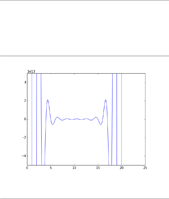
3.13 Wilkinson’s polynomial
Wilkinson’s polynomial is defined as w(x) = Q20
i=1(x−i) = (x−1)(x−
2) . . . (x−20).
This innocent looking function has 20 roots, which are 1,2,3,. . . ,19,20.
Here is a plot of the function.
1import matplotlib.pyplot as plt
2import numpy as np
3
4@np.vectorize
5def wilkinson(x):
6p=np.prod(np.array([x -ifor iin range(1,21)]))
7return p
8
9x=np.linspace(0,21,1000)
10 plt.plot(x, wilkinson(x))
11 plt.ylim([-5e13,5e13])
12 plt.savefig(’./images/wilkinson-1.png’)
Let us consider the expanded version of the polynomial. We will use
sympy to expand the polynomial.
1from sympy import Symbol, Poly
2from sympy.polys.polytools import poly_from_expr
3
65

4x=Symbol(’x’)
5W= 1
6for iin range(1,21):
7W=W*(x-i)
8
9print(W.expand())
10
11 P,d =poly_from_expr(W.expand())
12 print(P)
x**20 - 210*x**19 + 20615*x**18 - 1256850*x**17 + 53327946*x**16 - 1672280820*x**15 + 40171771630*x**14 - 756111184500*x**13 + 11310276995381*x**12 - 135585182899530*x**11 + 1307535010540395*x**10 - 10142299865511450*x**9 + 63030812099294896*x**8 - 311333643161390640*x**7 + 1206647803780373360*x**6 - 3599979517947607200*x**5 + 8037811822645051776*x**4 - 12870931245150988800*x**3 + 13803759753640704000*x**2 - 8752948036761600000*x + 2432902008176640000
Poly(x**20 - 210*x**19 + 20615*x**18 - 1256850*x**17 + 53327946*x**16 - 1672280820*x**15 + 40171771630*x**14 - 756111184500*x**13 + 11310276995381*x**12 - 135585182899530*x**11 + 1307535010540395*x**10 - 10142299865511450*x**9 + 63030812099294896*x**8 - 311333643161390640*x**7 + 1206647803780373360*x**6 - 3599979517947607200*x**5 + 8037811822645051776*x**4 - 12870931245150988800*x**3 + 13803759753640704000*x**2 - 8752948036761600000*x + 2432902008176640000, x, domain=’ZZ’)
The coefficients are orders of magnitude apart in size. This should make
you nervous, because the roots of this equation are between 1-20, but there
are numbers here that are O(19). This is likely to make any rounding errors
in the number representations very significant, and may lead to issues with
accuracy of the solution. Let us explore that.
We will get the roots using numpy.roots.
1import numpy as np
2from sympy import Symbol
3from sympy.polys.polytools import poly_from_expr
4
5x=Symbol(’x’)
6W= 1
7for iin range(1,21):
8W=W*(x-i)
9
10 P,d =poly_from_expr(W.expand())
11 p=P.all_coeffs()
12 x=np.arange(1,21)
13 print(’\nThese are the known roots\n’,x)
14
15 # evaluate the polynomial at the known roots
16 print(’\nThe polynomial evaluates to {0} at the known roots’.format(np.polyval(p, x)))
17
18 # find the roots ourselves
19 roots =np.roots(p)
20 print(’\nHere are the roots from numpy:\n’, roots)
21
22 # evaluate solution at roots
23 print(’\nHere is the polynomial evaluated at the calculated roots:\n’, np.polyval(p, roots))
These are the known roots
[ 1 2 3 4 5 6 7 8 9 10 11 12 13 14 15 16 17 18 19 20]
The polynomial evaluates to [0 0 0 0 0 0 0 0 0 0 0 0 0 0 0 0 0 0 0 0] at the known roots
66

Here are the roots from numpy:
[ 20.00060348 18.99388894 18.02685247 16.91622268 16.14133991
14.77906016 14.22072943 12.85642119 12.08967018 10.96640641
10.01081017 8.99768263 8.00033976 6.99997228 6.0000001
5.00000024 3.99999998 3. 2. 1. ]
Here is the polynomial evaluated at the calculated roots:
[70862552367104.0 40966734728192.0 21045323877376.0 9730381314560.00
5297656354816.00 1637083049984.00 1072991384064.00 335341826560.000
143322307584.000 44270514688.0000 15650462720.0000 4228162560.00000
914166272.000000 150146048.000000 -1730048.00000000 -5285376.00000000
-2747904.00000000 -538112.000000000 -54272.0000000000 -17408.0000000000]
The roots are not exact. Even more to the point, the polynomial does
not evaluate to zero at the calculated roots! Something is clearly wrong
here. The polynomial function is fine, and it does evaluate to zero at the
known roots which are integers. It is subtle, but up to that point, we are
using only integers, which can be represented exactly. The roots function
is evidently using some float math, and the floats are not the same as the
integers.
If we simply change the roots to floats, and reevaluate our polynomial,
we get dramatically different results.
1import numpy as np
2from sympy import Symbol
3from sympy.polys.polytools import poly_from_expr
4
5x=Symbol(’x’)
6W= 1
7for iin range(1,21):
8W=W*(x -i)
9
10 P,d=poly_from_expr(W.expand())
11 p=P.all_coeffs()
12 x=np.arange(1,21, dtype=np.float)
13 print(’\nThese are the known roots\n’,x)
14
15 # evaluate the polynomial at the known roots
16 print(’\nThe polynomial evaluates to {0} at the known roots’.format(np.polyval(p, x)))
These are the known roots
[ 1. 2. 3. 4. 5. 6. 7. 8. 9. 10. 11. 12. 13. 14. 15.
16. 17. 18. 19. 20.]
67

The polynomial evaluates to [0 0 55296.0000000000 425984.000000000 1024000.00000000 9068544.00000000
35825664.0000000 75235328.0000000 198567936.000000 566272000.000000
757796864.000000 1418231808.00000 2411708416.00000 3807354880.00000
6303744000.00000 11150557184.0000 17920108544.0000 16046678016.0000
38236565504.0000 54726656000.0000] at the known roots
This also happens if we make the polynomial coefficients floats. That
happens because in Python whenever one element is a float the results of
math operations with that element are floats.
1import numpy as np
2from sympy import Symbol
3from sympy.polys.polytools import poly_from_expr
4
5x=Symbol(’x’)
6W= 1
7for iin range(1,21):
8W=W*(x -i)
9
10 P,d =poly_from_expr(W.expand())
11 p=[float(x) for xin P.all_coeffs()]
12 x=np.arange(1,21)
13 print(’\nThese are the known roots\n’,x)
14
15 # evaluate the polynomial at the known roots
16 print(’\nThe polynomial evaluates to {0} at the known roots’.format(np.polyval(p, x)))
These are the known roots
[ 1 2 3 4 5 6 7 8 9 10 11 12 13 14 15 16 17 18 19 20]
The polynomial evaluates to [ 0.00000000e+00 0.00000000e+00 5.52960000e+04 4.25984000e+05
1.02400000e+06 9.06854400e+06 3.58256640e+07 7.52353280e+07
1.98567936e+08 5.66272000e+08 7.57796864e+08 1.41823181e+09
2.41170842e+09 3.80735488e+09 6.30374400e+09 1.11505572e+10
1.79201085e+10 1.60466780e+10 3.82365655e+10 5.47266560e+10] at the known roots
Let us try to understand what is happening here. It turns out that the
integer and float representations of the numbers are different! It is known
that you cannot exactly represent numbers as floats.
1import numpy as np
2from sympy import Symbol
3from sympy.polys.polytools import poly_from_expr
68

4
5x=Symbol(’x’)
6W= 1
7for iin range(1,21):
8W=W*(x -i)
9
10 P,d=poly_from_expr(W.expand())
11 p=P.all_coeffs()
12 print(p)
13 print(’{0:<30s}{1:<30s}{2}’.format(’Integer’,’Float’,’\delta’))
14 for pj in p:
15 print(’{0:<30d}{1:<30f}{2:3e}’.format(int(pj), float(pj), int(pj) -float(pj)))
[1, -210, 20615, -1256850, 53327946, -1672280820, 40171771630, -756111184500, 11310276995381, -135585182899530, 1307535010540395, -10142299865511450, 63030812099294896, -311333643161390640, 1206647803780373360, -3599979517947607200, 8037811822645051776, -12870931245150988800, 13803759753640704000, -8752948036761600000, 2432902008176640000]
Integer Float \delta
1 1.000000 0.000000e+00
-210 -210.000000 0.000000e+00
20615 20615.000000 0.000000e+00
-1256850 -1256850.000000 0.000000e+00
53327946 53327946.000000 0.000000e+00
-1672280820 -1672280820.000000 0.000000e+00
40171771630 40171771630.000000 0.000000e+00
-756111184500 -756111184500.000000 0.000000e+00
11310276995381 11310276995381.000000 0.000000e+00
-135585182899530 -135585182899530.000000 0.000000e+00
1307535010540395 1307535010540395.000000 0.000000e+00
-10142299865511450 -10142299865511450.000000 0.000000e+00
63030812099294896 63030812099294896.000000 0.000000e+00
-311333643161390640 -311333643161390592.000000 -6.400000e+01
1206647803780373360 1206647803780373248.000000 0.000000e+00
-3599979517947607200 -3599979517947607040.000000 0.000000e+00
8037811822645051776 8037811822645051392.000000 0.000000e+00
-12870931245150988800 -12870931245150988288.000000 0.000000e+00
13803759753640704000 13803759753640704000.000000 0.000000e+00
-8752948036761600000 -8752948036761600000.000000 0.000000e+00
2432902008176640000 2432902008176640000.000000 0.000000e+00
Now you can see the issue. Many of these numbers are identical in integer
and float form, but some of them are not. The integer cannot be exactly
represented as a float, and there is a difference in the representations. It is
a small difference compared to the magnitude, but these kinds of differences
get raised to high powers, and become larger. You may wonder why I used
"0:<30s>" to print the integer? That is because pj in that loop is an object
69

from sympy, which prints as a string.
This is a famous, and well known problem that is especially bad for this
case. This illustrates that you cannot simply rely on what a computer tells
you the answer is, without doing some critical thinking about the problem
and the solution. Especially in problems where there are coefficients that
vary by many orders of magnitude you should be cautious.
There are a few interesting webpages on this topic, which inspired me
to work this out in python. These webpages go into more detail on this
problem, and provide additional insight into the sensitivity of the solutions
to the polynomial coefficients.
1. http://blogs.mathworks.com/cleve/2013/03/04/wilkinsons-polynomials/
2. http://www.numericalexpert.com/blog/wilkinson_polynomial/
3. http://en.wikipedia.org/wiki/Wilkinson%27s_polynomial
3.14 The trapezoidal method of integration
Matlab post See http://en.wikipedia.org/wiki/Trapezoidal_rule
Zb
a
f(x)dx ≈1
2
N
X
k=1
(xk+1 −xk)(f(xk+1) + f(xk))
Let us compute the integral of sin(x) from x=0 to π. To approximate
the integral, we need to divide the interval from ato binto Nintervals. The
analytical answer is 2.0.
We will use this example to illustrate the difference in performance be-
tween loops and vectorized operations in python.
1import numpy as np
2import time
3
4a= 0.0; b =np.pi;
5N= 1000;# this is the number of intervals
6
7h=(b -a)/N; # this is the width of each interval
8x=np.linspace(a, b, N)
9y=np.sin(x); # the sin function is already vectorized
10
11 t0 =time.time()
12 f= 0.0
13 for kin range(len(x) - 1):
14 f+= 0.5 * ((x[k+1]-x[k]) *(y[k+1]+y[k]))
15
16 tf =time.time() -t0
70

17 print(’time elapsed = {0} sec’.format(tf))
18
19 print(f)
time elapsed = 0.03262186050415039 sec
1.99999835177
1t0 =time.time()
2Xk =x[1:-1]-x[0:-2]# vectorized version of (x[k+1] - x[k])
3Yk =y[1:-1]+y[0:-2]# vectorized version of (y[k+1] + y[k])
4
5f= 0.5 * np.sum(Xk *Yk) # vectorized version of the loop above
6tf =time.time() -t0
7print(’time elapsed = {0} sec’.format(tf))
8
9print(f)
time elapsed = 0.03238797187805176 sec
1.99999340709
In the last example, there may be loop buried in the sum command. Let
us do one final method, using linear algebra, in a single line. The key to
understanding this is to recognize the sum is just the result of a dot product
of the x differences and y sums.
1t0 =time.time()
2f= 0.5 * np.dot(Xk, Yk)
3tf =time.time() -t0
4print(’time elapsed = {0} sec’.format(tf))
5
6print(f)
time elapsed = 0.012599945068359375 sec
1.99999340709
The loop method is straightforward to code, and looks alot like the
formula that defines the trapezoid method. the vectorized methods are not
as easy to read, and take fewer lines of code to write. However, the vectorized
methods are much faster than the loop, so the loss of readability could be
worth it for very large problems.
The times here are considerably slower than in Matlab. I am not sure if
that is a totally fair comparison. Here I am running python through emacs,
which may result in slower performance. I also used a very crude way of
timing the performance which lumps some system performance in too.
71

3.15 Numerical Simpsons rule
A more accurate numerical integration than the trapezoid method is Simp-
son’s rule. The syntax is similar to trapz, but the method is in scipy.integrate.
1import numpy as np
2from scipy.integrate import simps, romb
3
4a= 0.0; b =np.pi / 4.0;
5N= 10 # this is the number of intervals
6
7x=np.linspace(a, b, N)
8y=np.cos(x)
9
10 t=np.trapz(y, x)
11 s=simps(y, x)
12 a=np.sin(b) -np.sin(a)
13
14 print(’trapz = {0} ({1:%} error)’.format(t, (t -a)/a))
15 print(’simps = {0} ({1:%} error)’.format(s, (s -a)/a))
16 print(’analy = {0}’.format(a))
trapz = 0.7066579803798914 (-0.063470% error)
simps = 0.707058914216065 (-0.006769% error)
analy = 0.7071067811865475
You can see the Simpson’s method is more accurate than the trapezoid
method.
3.16 Integrating functions in python
Matlab post
Problem statement
find the integral of a function f(x) from a to b i.e.
Zb
a
f(x)dx
In python we use numerical quadrature to achieve this with the scipy.integrate.quad
command.
as a specific example, lets integrate
y=x2
from x=0 to x=1. You should be able to work out that the answer is
1/3.
72

1from scipy.integrate import quad
2
3def integrand(x):
4return x**2
5
6ans, err =quad(integrand, 0,1)
7print(ans)
0.33333333333333337
3.16.1 double integrals
we use the scipy.integrate.dblquad command
Integrate f(x, y) = ysin(x) + xcos(y)over
π <=x <= 2π
0<=y <=π
i.e.
R2π
x=πRπ
y=0 ysin(x) + xcos(y)dydx
The syntax in dblquad is a bit more complicated than in Matlab. We
have to provide callable functions for the range of the y-variable. Here
they are constants, so we create lambda functions that return the constants.
Also, note that the order of arguments in the integrand is different than in
Matlab.
1from scipy.integrate import dblquad
2import numpy as np
3
4def integrand(y, x):
5’y must be the first argument, and x the second.’
6return y*np.sin(x) +x*np.cos(y)
7
8ans, err =dblquad(integrand, np.pi, 2*np.pi,
9lambda x: 0,
10 lambda x: np.pi)
11 print (ans)
-9.869604401089358
we use the tplquad command to integrate f(x, y, z) = ysin(x) + zcos(x)
over the region
0<=x <=π
0<=y <= 1
−1<=z <= 1
73

1from scipy.integrate import tplquad
2import numpy as np
3
4def integrand(z, y, x):
5return y*np.sin(x) +z*np.cos(x)
6
7ans, err =tplquad(integrand,
80, np.pi, # x limits
9lambda x: 0,
10 lambda x: 1,# y limits
11 lambda x,y: -1,
12 lambda x,y: 1)# z limits
13
14 print (ans)
1.9999999999999998
3.16.2 Summary
scipy.integrate offers the same basic functionality as Matlab does. The syn-
tax differs significantly for these simple examples, but the use of functions
for the limits enables freedom to integrate over non-constant limits.
3.17 Integrating equations in python
A common need in engineering calculations is to integrate an equation over
some range to determine the total change. For example, say we know the
volumetric flow changes with time according to dν/dt =αt, where α= 1
L/min and we want to know how much liquid flows into a tank over 10
minutes if the volumetric flowrate is ν0= 5 L/min at t= 0. The answer to
that question is the value of this integral: V=R10
0ν0+αtdt.
1import scipy
2from scipy.integrate import quad
3
4nu0 = 5 # L/min
5alpha = 1.0 # L/min
6def integrand(t):
7return nu0 +alpha *t
8
9t0 = 0.0
10 tfinal = 10.0
11 V, estimated_error =quad(integrand, t0, tfinal)
12 print(’{0:1.2f} L flowed into the tank over 10 minutes’.format(V))
100.00 L flowed into the tank over 10 minutes
That is all there is too it!
74

3.18 Function integration by the Romberg method
An alternative to the scipy.integrate.quad function is the Romberg method.
This method is not likely to be more accurate than quad, and it does not
give you an error estimate.
1import numpy as np
2
3from scipy.integrate import quad, romberg
4
5a= 0.0
6b=np.pi / 4.0
7
8print(quad(np.sin, a, b))
9print(romberg(np.sin, a, b))
(0.2928932188134524, 3.2517679528326894e-15)
0.292893218813
3.19 Symbolic math in python
Matlab post Python has capability to do symbolic math through the sympy
package.
3.19.1 Solve the quadratic equation
1from sympy import solve, symbols, pprint
2
3a, b, c, x =symbols(’a,b,c,x’)
4
5f=a*x**2 + b*x+c
6
7solution =solve(f, x)
8print(solution)
9pprint(solution)
[(-b + sqrt(-4*a*c + b**2))/(2*a), -(b + sqrt(-4*a*c + b**2))/(2*a)]
_____________ _____________
2 2
-b + -4ac + b -b + -4ac + b
,
2a 2a
The solution you should recognize in the form of b±√b2−4ac
2aalthough
python does not print it this nicely!
75

3.19.2 differentiation
you might find this helpful!
1from sympy import diff
2
3print(diff(f, x))
4print(diff(f, x, 2))
5
6print(diff(f, a))
2*a*x + b
2*a
x**2
3.19.3 integration
1from sympy import integrate
2
3print(integrate(f, x)) # indefinite integral
4print(integrate(f, (x, 0,1))) # definite integral from x=0..1
a*x**3/3 + b*x**2/2 + c*x
a/3 + b/2 + c
3.19.4 Analytically solve a simple ODE
1from sympy import Function, Symbol, dsolve
2f=Function(’f’)
3x=Symbol(’x’)
4fprime =f(x).diff(x) -f(x) # f’ = f(x)
5
6y=dsolve(fprime, f(x))
7
8print(y)
9print(y.subs(x,4))
10 print([y.subs(x, X) for Xin [0,0.5,1]]) # multiple values
f(x) == C1*exp(x)
f(4) == C1*exp(4)
[f(0) == C1, f(0.5) == 1.64872127070013*C1, f(1) == E*C1]
It is not clear you can solve the initial value problem to get C1.
The symbolic math in sympy is pretty good. It is not up to the capability
of Maple or Mathematica, (but neither is Matlab) but it continues to be
developed, and could be helpful in some situations.
76

3.20 Is your ice cream float bigger than mine
Float numbers (i.e. the ones with decimals) cannot be perfectly represented
in a computer. This can lead to some artifacts when you have to compare
float numbers that on paper should be the same, but in silico are not. Let
us look at some examples. In this example, we do some simple math that
should result in an answer of 1, and then see if the answer is "equal" to one.
1print(3.0 * (1.0/3.0))
2print(1.0 == 3.0 * (1.0/3.0))
1.0
True
Everything looks fine. Now, consider this example.
1print(49.0 * (1.0/49.0))
2print(1.0 == 49.0 * (1.0/49.0))
0.9999999999999999
False
The first line shows the result is not 1.0, and the equality fails! You can
see here why the equality statement fails. We will print the two numbers to
sixteen decimal places.
1print(’{0:1.16f}’.format(49.0 * (1.0 / 49.0) ))
2print(’{0:1.16f}’.format(1.0))
3print(1 - 49.0 * (1.0 / 49.0))
0.9999999999999999
1.0000000000000000
1.1102230246251565e-16
The two numbers actually are not equal to each other because of float
math. They are very, very close to each other, but not the same.
This leads to the idea of asking if two numbers are equal to each other
within some tolerance. The question of what tolerance to use requires
thought. Should it be an absolute tolerance? a relative tolerance? How
large should the tolerance be? We will use the distance between 1 and the
nearest floating point number (this is eps in Matlab). numpy can tell us this
number with the np.spacing command.
Below, we implement a comparison function from
77

1# Implemented from Acta Crystallographica A60, 1-6 (2003). doi:10.1107/S010876730302186X
2
3import numpy as np
4print(np.spacing(1))
5
6def feq(x, y, epsilon):
7’x == y’
8return not((x <(y -epsilon)) or (y <(x -epsilon)))
9
10 print(feq(1.0,49.0 * (1.0/49.0), np.spacing(1)))
2.22044604925e-16
True
For completeness, here are the other float comparison operators from
that paper. We also show a few examples.
1import numpy as np
2
3def flt(x, y, epsilon):
4’x < y’
5return x<(y -epsilon)
6
7def fgt(x, y, epsilon):
8’x > y’
9return y<(x -epsilon)
10
11 def fle(x, y, epsilon):
12 ’x <= y’
13 return not(y <(x -epsilon))
14
15 def fge(x, y, epsilon):
16 ’x >= y’
17 return not(x <(y -epsilon))
18
19 print(fge(1.0,49.0 * (1.0/49.0), np.spacing(1)))
20 print(fle(1.0,49.0 * (1.0/49.0), np.spacing(1)))
21
22 print(fgt(1.0 + np.spacing(1), 49.0 * (1.0/49.0), np.spacing(1)))
23 print(flt(1.0-2*np.spacing(1), 49.0 * (1.0/49.0), np.spacing(1)))
True
True
True
True
As you can see, float comparisons can be tricky. You have to give a lot
of thought to how to make the comparisons, and the functions shown above
are not the only way to do it. You need to build in testing to make sure
your comparisons are doing what you want.
78

4 Linear algebra
4.1 Potential gotchas in linear algebra in numpy
Numpy has some gotcha features for linear algebra purists. The first is that
a 1d array is neither a row, nor a column vector. That is, a=aTif ais a
1d array. That means you can take the dot product of awith itself, without
transposing the second argument. This would not be allowed in Matlab.
1import numpy as np
2
3a=np.array([0,1,2])
4print(a.shape)
5print(a)
6print(a.T)
7
8
9print(np.dot(a, a))
10 print(np.dot(a, a.T))
(3,)
[0 1 2]
[0 1 2]
5
5
Compare the syntax to the new Python 3.5 syntax:
1print(a @ a)
5
Compare the previous behavior with this 2d array. In this case, you
cannot take the dot product of bwith itself, because the dimensions are
incompatible. You must transpose the second argument to make it dimen-
sionally consistent. Also, the result of the dot product is not a simple scalar,
but a 1 ×1 array.
1b=np.array([[0,1,2]])
2print(b.shape)
3print(b)
4print(b.T)
5
6print(np.dot(b, b)) # this is not ok, the dimensions are wrong.
7print(np.dot(b, b.T))
8print(np.dot(b, b.T).shape)
79

(1, 3)
[[0 1 2]]
[[0]
[1]
[2]]
Traceback (most recent call last):
File "<stdin>", line 1, in <module>
ValueError: shapes (1,3) and (1,3) not aligned: 3 (dim 1) != 1 (dim 0)
[[5]]
(1, 1)
Try to figure this one out! x is a column vector, and y is a 1d vector.
Just by adding them you get a 2d array.
1x=np.array([[2], [4], [6], [8]])
2y=np.array([1,1,1,1,1,2])
3print(x +y)
[[333334]
[555556]
[777778]
[ 9 9 9 9 9 10]]
Or this crazy alternative way to do the same thing.
1x=np.array([2,4,6,8])
2y=np.array([1,1,1,1,1,1,2])
3
4print(x[:, np.newaxis] +y)
[[3333334]
[5555556]
[7777778]
[ 9 9 9 9 9 9 10]]
In the next example, we have a 3 element vector and a 4 element vector.
We convert bto a 2D array with np.newaxis, and compute the outer product
of the two arrays. The result is a 4 ×3 array.
1a=np.array([1,2,3])
2b=np.array([10,20,30,40])
3
4print(a *b[:, np.newaxis])
80

[[ 10 20 30]
[ 20 40 60]
[ 30 60 90]
[ 40 80 120]]
These concepts are known in numpy as array broadcasting. See http:
//www.scipy.org/EricsBroadcastingDoc and http://docs.scipy.org/
doc/numpy/user/basics.broadcasting.html for more details.
These are points to keep in mind, as the operations do not strictly follow
the conventions of linear algebra, and may be confusing at times.
4.2 Solving linear equations
Given these equations, find [x1, x2, x3]
x1−x2+x3= 0 (5)
10x2+ 25x3= 90 (6)
20x1+ 10x2= 80 (7)
reference: Kreysig, Advanced Engineering Mathematics, 9th ed. Sec.
7.3
When solving linear equations, we can represent them in matrix form.
The we simply use numpy.linalg.solve to get the solution.
1import numpy as np
2A=np.array([[1,-1,1],
3[0,10,25],
4[20,10,0]])
5
6b=np.array([0,90,80])
7
8x=np.linalg.solve(A, b)
9print(x)
10 print(np.dot(A,x))
11
12 # Let us confirm the solution.
13 # this shows one element is not equal because of float tolerance
14 print(np.dot(A,x) == b)
15
16 # here we use a tolerance comparison to show the differences is less
17 # than a defined tolerance.
18 TOLERANCE = 1e-12
19 print(np.abs((np.dot(A, x) -b)) <= TOLERANCE)
[ 2. 4. 2.]
81

[ 0. 90. 80.]
[ True True True]
[ True True True]
It can be useful to confirm there should be a solution, e.g. that the
equations are all independent. The matrix rank will tell us that. Note that
numpy:rank does not give you the matrix rank, but rather the number of
dimensions of the array. We compute the rank by computing the number of
singular values of the matrix that are greater than zero, within a prescribed
tolerance. We use the numpy.linalg.svd function for that. In Matlab you
would use the rref command to see if there are any rows that are all zero,
but this command does not exist in numpy. That command does not have
practical use in numerical linear algebra and has not been implemented.
1import numpy as np
2A=np.array([[1,-1,1],
3[0,10,25],
4[20,10,0]])
5
6b=np.array([0,90,80])
7
8# determine number of independent rows in A we get the singular values
9# and count the number greater than 0.
10 TOLERANCE = 1e-12
11 u, s, v =np.linalg.svd(A)
12 print(’Singular values: {0}’.format(s))
13 print(’# of independent rows: {0}’.format(np.sum(np.abs(s) >TOLERANCE)))
14
15 # to illustrate a case where there are only 2 independent rows
16 # consider this case where row3 = 2*row2.
17 A=np.array([[1,-1,1],
18 [0,10,25],
19 [0,20,50]])
20
21 u, s, v =np.linalg.svd(A)
22
23 print(’Singular values: {0}’.format(s))
24 print(’# of independent rows: {0}’.format(np.sum(np.abs(s) >TOLERANCE)))
Singular values: [ 27.63016717 21.49453733 1.5996022 ]
# of independent rows: 3
Singular values: [ 6.02105520e+01 1.63994657e+00 1.72274992e-15]
# of independent rows: 2
Matlab comparison
82

4.3 Rules for transposition
Matlab comparison
Here are the four rules for matrix multiplication and transposition
1. (AT)T=A
2. (A+B)T=AT+BT
3. (cA)T=cAT
4. (AB)T=BTAT
reference: Chapter 7.2 in Advanced Engineering Mathematics, 9th edi-
tion. by E. Kreyszig.
4.3.1 The transpose in Python
There are two ways to get the transpose of a matrix: with a notation, and
with a function.
1import numpy as np
2A=np.array([[5,-8,1],
3[4,0,0]])
4
5# function
6print(np.transpose(A))
7
8# notation
9print(A.T)
[[ 5 4]
[-8 0]
[ 1 0]]
[[ 5 4]
[-8 0]
[ 1 0]]
4.3.2 Rule 1
1import numpy as np
2
3A=np.array([[5,-8,1],
4[4,0,0]])
5
6print(np.all(A == (A.T).T))
True
83

4.3.3 Rule 2
1import numpy as np
2A=np.array([[5,-8,1],
3[4,0,0]])
4
5B=np.array([[3,4,5], [1,2,3]])
6
7print(np.all( A.T+B.T== (A +B).T))
True
4.3.4 Rule 3
1import numpy as np
2A=np.array([[5,-8,1],
3[4,0,0]])
4
5c= 2.1
6
7print(np.all((c*A).T== c*A.T))
True
4.3.5 Rule 4
1import numpy as np
2A=np.array([[5,-8,1],
3[4,0,0]])
4
5B=np.array([[0,2],
6[1,2],
7[6,7]])
8
9print(np.all(np.dot(A, B).T== np.dot(B.T, A.T)))
True
4.3.6 Summary
That wraps up showing numerically the transpose rules work for these ex-
amples.
84

4.4 Sums products and linear algebra notation - avoiding
loops where possible
Matlab comparison
Today we examine some methods of linear algebra that allow us to avoid
writing explicit loops in Matlab for some kinds of mathematical operations.
Consider the operation on two vectors aand b.
y=
n
X
i=1
aibi
a = [1 2 3 4 5]
b = [3 6 8 9 10]
4.4.1 Old-fashioned way with a loop
We can compute this with a loop, where you initialize y, and then add the
product of the ith elements of a and b to y in each iteration of the loop.
This is known to be slow for large vectors
1a=[1,2,3,4,5]
2b=[3,6,8,9,10]
3
4sum = 0
5for iin range(len(a)):
6sum =sum +a[i] *b[i]
7print(sum)
125
This is an old fashioned style of coding. A more modern, pythonic
approach is:
1a=[1,2,3,4,5]
2b=[3,6,8,9,10]
3
4sum = 0
5for x,y in zip(a,b):
6sum += x*y
7print(sum)
125
85

4.4.2 The numpy approach
The most compact method is to use the methods in numpy.
1import numpy as np
2
3a=np.array([1,2,3,4,5])
4b=np.array([3,6,8,9,10])
5
6print(np.sum(a *b))
125
4.4.3 Matrix algebra approach.
The operation defined above is actually a dot product. We an directly
compute the dot product in numpy. Note that with 1d arrays, python knows
what to do and does not require any transpose operations.
1import numpy as np
2
3a=np.array([1,2,3,4,5])
4b=np.array([3,6,8,9,10])
5
6print(np.dot(a, b))
125
4.4.4 Another example
Consider y=n
P
i=1
wix2
i. This operation is like a weighted sum of squares.
The old-fashioned way to do this is with a loop.
1w=[0.1,0.25,0.12,0.45,0.98];
2x=[9,7,11,12,8];
3y= 0
4for wi, xi in zip(w,x):
5y+= wi *xi**2
6print(y)
162.39
Compare this to the more modern numpy approach.
86

1import numpy as np
2w=np.array([0.1,0.25,0.12,0.45,0.98])
3x=np.array([9,7,11,12,8])
4y=np.sum(w *x**2)
5print(y)
162.39
We can also express this in matrix algebra form. The operation is equiv-
alent to y=~x ·Dw·~xTwhere Dwis a diagonal matrix with the weights on
the diagonal.
1import numpy as np
2w=np.array([0.1,0.25,0.12,0.45,0.98])
3x=np.array([9,7,11,12,8])
4y=np.dot(x, np.dot(np.diag(w), x))
5print(y)
162.39
This last form avoids explicit loops and sums, and relies on fast linear
algebra routines.
4.4.5 Last example
Consider the sum of the product of three vectors. Let y=n
P
i=1
wixiyi. This
is like a weighted sum of products.
1import numpy as np
2
3w=np.array([0.1,0.25,0.12,0.45,0.98])
4x=np.array([9,7,11,12,8])
5y=np.array([2,5,3,8,0])
6
7print(np.sum(w *x*y))
8print(np.dot(w, np.dot(np.diag(x), y)))
57.71
57.71
87

4.4.6 Summary
We showed examples of the following equalities between traditional sum
notations and linear algebra
ab =
n
X
i=1
aibi
xDwxT=
n
X
i=1
wix2
i
xDwyT=
n
X
i=1
wixiyi
These relationships enable one to write the sums as a single line of python
code, which utilizes fast linear algebra subroutines, avoids the construction
of slow loops, and reduces the opportunity for errors in the code. Admittedly,
it introduces the opportunity for new types of errors, like using the wrong
relationship, or linear algebra errors due to matrix size mismatches.
4.5 Determining linear independence of a set of vectors
Matlab post Occasionally we have a set of vectors and we need to determine
whether the vectors are linearly independent of each other. This may be
necessary to determine if the vectors form a basis, or to determine how many
independent equations there are, or to determine how many independent
reactions there are.
Reference: Kreysig, Advanced Engineering Mathematics, sec. 7.4
Matlab provides a rank command which gives you the number of singu-
lar values greater than some tolerance. The numpy.rank function, unfortu-
nately, does not do that. It returns the number of dimensions in the array.
We will just compute the rank from singular value decomposition.
The default tolerance used in Matlab is max(size(A))*eps(norm(A)). Let
us break that down. eps(norm(A)) is the positive distance from abs(X) to
the next larger in magnitude floating point number of the same precision as
X. Basically, the smallest significant number. We multiply that by the size
of A, and take the largest number. We have to use some judgment in what
the tolerance is, and what "zero" means.
1import numpy as np
2v1 =[6,0,3,1,4,2];
3v2 =[0,-1,2,7,0,5];
88

4v3 =[12,3,0,-19,8,-11];
5
6A=np.row_stack([v1, v2, v3])
7
8# matlab definition
9eps =np.finfo(np.linalg.norm(A).dtype).eps
10 TOLERANCE =max(eps *np.array(A.shape))
11
12 U, s, V =np.linalg.svd(A)
13 print(s)
14 print(np.sum(s >TOLERANCE))
15
16 TOLERANCE = 1e-14
17 print(np.sum(s >TOLERANCE))
[ 2.75209239e+01 9.30584482e+00 1.15680550e-15]
2
2
You can see if you choose too small a TOLERANCE, nothing looks
like zero. the result with TOLERANCE=1e-14 suggests the rows are not
linearly independent. Let us show that one row can be expressed as a linear
combination of the other rows.
The number of rows is greater than the rank, so these vectors are not
independent. Let’s demonstrate that one vector can be defined as a linear
combination of the other two vectors. Mathematically we represent this as:
x1v1 +x2v2 =v3
or
[x1x2][v1; v2] = v3
This is not the usual linear algebra form of Ax = b. To get there, we
transpose each side of the equation to get:
[v1.T v2.T][x_1; x_2] = v3.T
which is the form Ax = b. We solve it in a least-squares sense.
1A=np.column_stack([v1, v2])
2x=np.linalg.lstsq(A, v3)
3print(x[0])
[ 2. -3.]
This shows that v3 = 2*v1 - 3*v2
89

4.5.1 another example
1#Problem set 7.4 #17
2import numpy as np
3
4v1 =[0.2,1.2,5.3,2.8,1.6]
5v2 =[4.3,3.4,0.9,2.0,-4.3]
6
7A=np.row_stack([v1, v2])
8U, s, V =np.linalg.svd(A)
9print(s)
[ 7.57773162 5.99149259]
You can tell by inspection the rank is 2 because there are no near-zero
singular values.
4.5.2 Near deficient rank
the rank command roughly works in the following way: the matrix is con-
verted to a reduced row echelon form, and then the number of rows that
are not all equal to zero are counted. Matlab uses a tolerance to determine
what is equal to zero. If there is uncertainty in the numbers, you may have
to define what zero is, e.g. if the absolute value of a number is less than
1e-5, you may consider that close enough to be zero. The default tolerance
is usually very small, of order 1e-15. If we believe that any number less
than 1e-5 is practically equivalent to zero, we can use that information to
compute the rank like this.
1import numpy as np
2
3A=[[1,2,3],
4[0,2,3],
5[0,0,1e-6]]
6
7U, s, V =np.linalg.svd(A)
8print(s)
9print(np.sum(np.abs(s) > 1e-15))
10 print(np.sum(np.abs(s) > 1e-5))
[ 5.14874857e+00 7.00277208e-01 5.54700196e-07]
3
2
90

4.5.3 Application to independent chemical reactions.
reference: Exercise 2.4 in Chemical Reactor Analysis and Design Funda-
mentals by Rawlings and Ekerdt.
The following reactions are proposed in the hydrogenation of bromine:
Let this be our species vector: v = [H2 H Br2 Br HBr].T
the reactions are then defined by M*v where M is a stoichometric matrix
in which each row represents a reaction with negative stoichiometric coef-
ficients for reactants, and positive stoichiometric coefficients for products.
A stoichiometric coefficient of 0 is used for species not participating in the
reaction.
1import numpy as np
2
3# [H2 H Br2 Br HBr]
4M=[[-1,0,-1,0,2], # H2 + Br2 == 2HBR
5[0,0,-1,2,0], # Br2 == 2Br
6[-1,1,0,-1,1], #Br+H2==HBr+H
7[0,-1,-1,1,1], # H + Br2 == HBr + Br
8[1,-1,0,1,-1], #H+HBr==H2+Br
9[0,0,1,-2,0]] # 2Br == Br2
10
11 U, s, V =np.linalg.svd(M)
12 print(s)
13 print(np.sum(np.abs(s) > 1e-15))
14
15 import sympy
16 M=sympy.Matrix(M)
17 reduced_form, inds =M.rref()
18
19 print(reduced_form)
20
21 labels =[’H2’,’H’,’Br2’,’Br’,’HBr’]
22 for row in reduced_form.tolist():
23 s=’0 = ’
24 for nu,species in zip(row,labels):
25 if nu != 0:
26
27 s+= ’ {0:+d}{1}’.format(int(nu), species)
28 if s!= ’0 = ’:
29 print(s)
[ 3.84742803e+00 3.32555975e+00 1.46217301e+00 4.15614917e-16
2.11915542e-17]
3
Matrix([[1, 0, 0, 2, -2], [0, 1, 0, 1, -1], [0, 0, 1, -2, 0], [0, 0, 0, 0, 0], [0, 0, 0, 0, 0], [0, 0, 0, 0, 0]])
0 = +1H2 +2Br -2HBr
0 = +1H +1Br -1HBr
0 = +1Br2 -2Br
91

6 reactions are given, but the rank of the matrix is only 3. so there are
only three independent reactions. You can see that reaction 6 is just the
opposite of reaction 2, so it is clearly not independent. Also, reactions 3 and
5 are just the reverse of each other, so one of them can also be eliminated.
finally, reaction 4 is equal to reaction 1 minus reaction 3.
There are many possible independent reactions. In the code above, we
use sympy to put the matrix into reduced row echelon form, which enables
us to identify three independent reactions, and shows that three rows are all
zero, i.e. they are not independent of the other three reactions. The choice
of independent reactions is not unique.
4.6 Reduced row echelon form
There is a nice discussion here on why there is not a rref command in numpy,
primarily because one rarely actually needs it in linear algebra. Still, it is
so often taught, and it helps visually see what the rank of a matrix is that
I wanted to examine ways to get it.
1import numpy as np
2from sympy import Matrix
3
4A=np.array([[3,2,1],
5[2,1,1],
6[6,2,4]])
7
8rA, pivots =Matrix(A).rref()
9print(rA)
Matrix([[1.00000000000000, 0, 0], [0, 1.00000000000000, 0], [0, 0, 1.00000000000000]])
This rref form is a bit different than you might get from doing it by
hand. The rows are also normalized.
Based on this, we conclude the Amatrix has a rank of 2 since one row
of the reduced form contains all zeros. That means the determinant will be
zero, and it should not be possible to compute the inverse of the matrix,
and there should be no solution to linear equations of Ax =b. Let us check
it out.
1import numpy as np
2from sympy import Matrix
3
4A=np.array([[3,2,1],
5[2,1,1],
6[6,2,4]])
92

7
8print(np.linalg.det(A))
9print(np.linalg.inv(A))
10
11 b=np.array([3,0,6])
12
13 print(np.linalg.solve(A, b))
6.66133814775e-16
[[ 3.00239975e+15 -9.00719925e+15 1.50119988e+15]
[ -3.00239975e+15 9.00719925e+15 -1.50119988e+15]
[ -3.00239975e+15 9.00719925e+15 -1.50119988e+15]]
[ 1.80143985e+16 -1.80143985e+16 -1.80143985e+16]
There are "solutions", but there are a couple of red flags that should
catch your eye. First, the determinant is within machine precision of zero.
Second the elements of the inverse are all "large". Third, the solutions are all
"large". All of these are indications of or artifacts of numerical imprecision.
4.7 Computing determinants from matrix decompositions
There are a few properties of a matrix that can make it easy to compute
determinants.
1. The determinant of a triangular matrix is the product of the elements
on the diagonal.
2. The determinant of a permutation matrix is (-1)**n where n is the
number of permutations. Recall a permutation matrix is a matrix
with a one in each row, and column, and zeros everywhere else.
3. The determinant of a product of matrices is equal to the product of
the determinant of the matrices.
The LU decomposition computes three matrices such that A=P LU .
Thus, det A= det Pdet Ldet U.Land Uare triangular, so we just need
to compute the product of the diagonals. Pis not triangular, but if the
elements of the diagonal are not 1, they will be zero, and then there has
been a swap. So we simply subtract the sum of the diagonal from the length
of the diagonal and then subtract 1 to get the number of swaps.
1import numpy as np
2from scipy.linalg import lu
93

3
4A=np.array([[6,2,3],
5[1,1,1],
6[0,4,9]])
7
8P, L, U =lu(A)
9
10 nswaps =len(np.diag(P)) -np.sum(np.diag(P)) - 1
11
12 detP =(-1)**nswaps
13 detL =np.prod(np.diag(L))
14 detU =np.prod(np.diag(U))
15
16 print(detP *detL *detU)
17
18 print(np.linalg.det(A))
24.0
24.0
According to the numpy documentation, a method similar to this is used
to compute the determinant.
4.8 Calling lapack directly from scipy
If the built in linear algebra functions in numpy and scipy do not meet your
needs, it is often possible to directly call lapack functions. Here we call a
function to solve a set of complex linear equations. The lapack function for
this is ZGBSV. The description of this function (http://linux.die.net/
man/l/zgbsv) is:
ZGBSV computes the solution to a complex system of linear equations
A * X = B, where A is a band matrix of order N with KL subdiagonals
and KU superdiagonals, and X and B are N-by-NRHS matrices. The LU
decomposition with partial pivoting and row interchanges is used to factor
A as A = L * U, where L is a product of permutation and unit lower
triangular matrices with KL subdiagonals, and U is upper triangular with
KL+KU superdiagonals. The factored form of A is then used to solve the
system of equations A * X = B.
The python signature is (http://docs.scipy.org/doc/scipy/reference/
generated/scipy.linalg.lapack.zgbsv.html#scipy.linalg.lapack.zgbsv):
lub,piv,x,info = zgbsv(kl,ku,ab,b,[overwrite_ab,overwrite_b])
We will look at an example from http://www.nag.com/lapack-ex/
node22.html.
We solve Ax =bwith
94

A=
−1.65 + 2.26i−2.05 −0.85i0.97 −2.84i0
6.30i−1.48 −1.75i−3.99 + 4.01i0.59 −0.48i
0−0.77 + 2.83i−1.06 + 1.94i3.33 −1.04i
0 0 4.48 −1.09i−0.46 −1.72i
(8)
and
b=
−1.06 + 21.50i
−22.72 −53.90i
28.24 −38.60i
−34.56 + 16.73i
.(9)
The Amatrix has one lower diagonal (kl = 1) and two upper diagonals
(ku = 2), four equations (n = 4) and one right-hand side.
1import scipy.linalg.lapack as la
2
3# http://www.nag.com/lapack-ex/node22.html
4import numpy as np
5A=np.array([[-1.65 + 2.26j,-2.05 - 0.85j,0.97 - 2.84j,0.0 ],
6[6.30j,-1.48 - 1.75j,-3.99 + 4.01j,0.59 - 0.48j],
7[0.0,-0.77 + 2.83j,-1.06 + 1.94j,3.33 - 1.04j],
8[0.0,0.0,4.48 - 1.09j,-0.46 - 1.72j]])
9
10 # construction of Ab is tricky. Fortran indexing starts at 1, not
11 # 0. This code is based on the definition of Ab at
12 # http://linux.die.net/man/l/zgbsv. First, we create the Fortran
13 # indices based on the loops, and then subtract one from them to index
14 # the numpy arrays.
15 Ab =np.zeros((5,4),dtype=np.complex)
16 n, kl, ku = 4,1,2
17
18 for jin range(1,n+ 1):
19 for iin range(max(1, j -ku), min(n, j +kl) + 1):
20 Ab[kl +ku +1+i-j- 1,j- 1]=A[i-1, j-1]
21
22 b=np.array([[-1.06 + 21.50j],
23 [-22.72 - 53.90j],
24 [28.24 - 38.60j],
25 [-34.56 + 16.73j]])
26
27 lub, piv, x, info =la.flapack.zgbsv(kl, ku, Ab, b)
28
29 # compare to results at http://www.nag.com/lapack-ex/examples/results/zgbsv-ex.r
30 print(’x = ’,x)
31 print(’info = ’,info)
32
33 # check solution
34 print(’solved: ’,np.all(np.dot(A,x) -b< 1e-12))
95

35
36 # here is the easy way!!!
37 print(’\n\nbuilt-in solver’)
38 print(np.linalg.solve(A,b))
x = [[-3.+2.j]
[ 1.-7.j]
[-5.+4.j]
[ 6.-8.j]]
info = 0
solved: True
built-in solver
[[-3.+2.j]
[ 1.-7.j]
[-5.+4.j]
[ 6.-8.j]]
Some points of discussion.
1. Kind of painful! but, nevertheless, possible. You have to do a lot
more work figuring out the dimensions of the problem, how to setup
the problem, keeping track of indices, etc. . .
But, one day it might be helpful to know this can be done, e.g. to debug
an installation, to validate an approach against known results, etc. . .
5 Nonlinear algebra
Nonlinear algebra problems are typically solved using an iterative process
that terminates when the solution is found within a specified tolerance.
This process is hidden from the user. The canonical standard form to solve
is f(X)=0.
5.1 Know your tolerance
Matlab post
V=ν(CAo −CA)
kC2
A
with the information given below, solve for the exit concentration. This
should be simple.
96

Cao = 2*u.mol/u.L;
V = 10*u.L;
nu = 0.5*u.L/u.s;
k = 0.23 * u.L/u.mol/u.s;
1import numpy as np
2from scipy.integrate import odeint
3import matplotlib.pyplot as plt
4
5# unit definitions
6m= 1.0
7L=m**3 / 1000.0
8mol = 1.0
9s= 1.0
10
11 # provide data
12 Cao = 2.0 * mol /L
13 V= 10.0 * L
14 nu = 0.5 * L/s
15 k= 0.23 * L/mol /s
16
17 def func(Ca):
18 return V-nu *(Cao -Ca)/(k *Ca**2)
Let us plot the function to estimate the solution.
1c=np.linspace(0.001,2)*mol /L
2
3plt.clf()
4plt.plot(c, func(c))
5plt.xlabel(’C (mol/m^3)’)
6plt.ylim([-0.1,0.1])
7plt.savefig(’images/nonlin-tolerance.png’)
[<matplotlib.lines.Line2D object at 0x112c9acf8>]
<matplotlib.text.Text object at 0x112c50908>
(-0.1, 0.1)
97
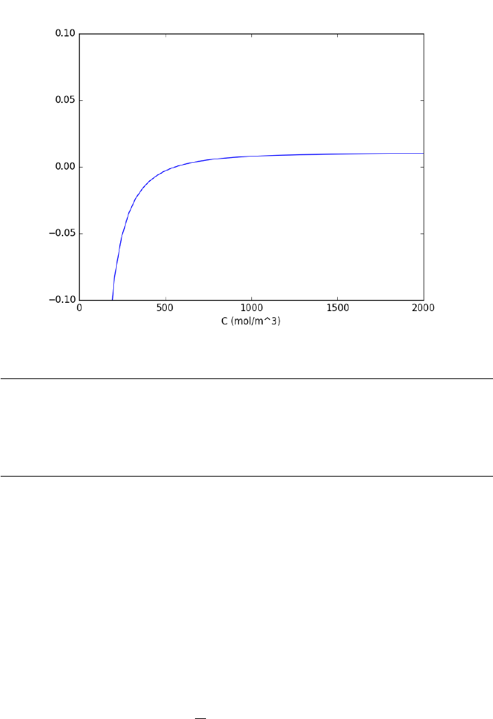
Now let us solve the equation. It looks like an answer is near C=500.
1from scipy.optimize import fsolve
2
3cguess = 500
4c, =fsolve(func, cguess)
5print(c)
6print(func(c))
7print(func(c) /(mol /L))
559.583745606
-1.73472347598e-18
-1.73472347598e-21
Interesting. In Matlab, the default tolerance was not sufficient to get a
good solution. Here it is.
5.2 Solving integral equations with fsolve
Original post in Matlab
Occasionally we have integral equations we need to solve in engineering
problems, for example, the volume of plug flow reactor can be defined by
this equation: V=RF a
F a(V=0) 1
radF a where rais the rate law. Suppose we
know the reactor volume is 100 L, the inlet molar flow of A is 1 mol/L, the
98

volumetric flow is 10 L/min, and ra=−kCa, with k= 0.23 1/min. What
is the exit molar flow rate? We need to solve the following equation:
100 = ZF a
F a(V=0)
1
−kF a/ν dF a
We start by creating a function handle that describes the integrand. We
can use this function in the quad command to evaluate the integral.
1import numpy as np
2from scipy.integrate import quad
3from scipy.optimize import fsolve
4
5k= 0.23
6nu = 10.0
7Fao = 1.0
8
9def integrand(Fa):
10 return -1.0 / (k *Fa /nu)
11
12 def func(Fa):
13 integral,err =quad(integrand, Fao, Fa)
14 return 100.0 - integral
15
16 vfunc =np.vectorize(func)
We will need an initial guess, so we make a plot of our function to get
an idea.
1import matplotlib.pyplot as plt
2
3f=np.linspace(0.01,1)
4plt.plot(f, vfunc(f))
5plt.xlabel(’Molar flow rate’)
6plt.savefig(’images/integral-eqn-guess.png’)
[<matplotlib.lines.Line2D object at 0x10c583ac8>]
<matplotlib.text.Text object at 0x10a0aad30>
99
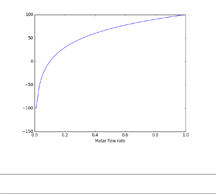
Now we can see a zero is near Fa = 0.1, so we proceed to solve the
equation.
1Fa_guess = 0.1
2Fa_exit, =fsolve(vfunc, Fa_guess)
3print(’The exit concentration is {0:1.2f} mol/L’.format(Fa_exit /nu))
The exit concentration is 0.01 mol/L
5.2.1 Summary notes
This example seemed a little easier in Matlab, where the quad function
seemed to get automatically vectorized. Here we had to do it by hand.
5.3 Method of continuity for nonlinear equation solving
Matlab post Adapted from Perry’s Chemical Engineers Handbook, 6th edi-
tion 2-63.
We seek the solution to the following nonlinear equations:
2 + x+y−x2+ 8xy +y3= 0
1+2x−3y+x2+xy −yex= 0
In principle this is easy, we simply need some initial guesses and a non-
linear solver. The challenge here is what would you guess? There could be
100

many solutions. The equations are implicit, so it is not easy to graph them,
but let us give it a shot, starting on the x range -5 to 5. The idea is set a
value for x, and then solve for y in each equation.
1import numpy as np
2from scipy.optimize import fsolve
3
4import matplotlib.pyplot as plt
5
6def f(x, y):
7return 2+x+y-x**2 + 8*x*y+y**3;
8
9def g(x, y):
10 return 1 + 2*x- 3*y+x**2 + x*y-y*np.exp(x)
11
12 x=np.linspace(-5,5,500)
13
14 @np.vectorize
15 def fy(x):
16 x0 = 0.0
17 def tmp(y):
18 return f(x, y)
19 y1, =fsolve(tmp, x0)
20 return y1
21
22 @np.vectorize
23 def gy(x):
24 x0 = 0.0
25 def tmp(y):
26 return g(x, y)
27 y1, =fsolve(tmp, x0)
28 return y1
29
30
31 plt.plot(x, fy(x), x, gy(x))
32 plt.xlabel(’x’)
33 plt.ylabel(’y’)
34 plt.legend([’fy’,’gy’])
35 plt.savefig(’images/continuation-1.png’)
/Users/jkitchin/anaconda3/lib/python3.5/site-packages/scipy/optimize/minpack.py:161: RuntimeWarning: The iteration is not making good progress, as measured by the
improvement from the last ten iterations.
warnings.warn(msg, RuntimeWarning)
/Users/jkitchin/anaconda3/lib/python3.5/site-packages/scipy/optimize/minpack.py:161: RuntimeWarning: The iteration is not making good progress, as measured by the
improvement from the last five Jacobian evaluations.
warnings.warn(msg, RuntimeWarning)
[<matplotlib.lines.Line2D object at 0x10c59a400>, <matplotlib.lines.Line2D object at 0x10c57c358>]
<matplotlib.text.Text object at 0x10a0aad30>
<matplotlib.text.Text object at 0x10a3af898>
<matplotlib.legend.Legend object at 0x10a3afb70>
101
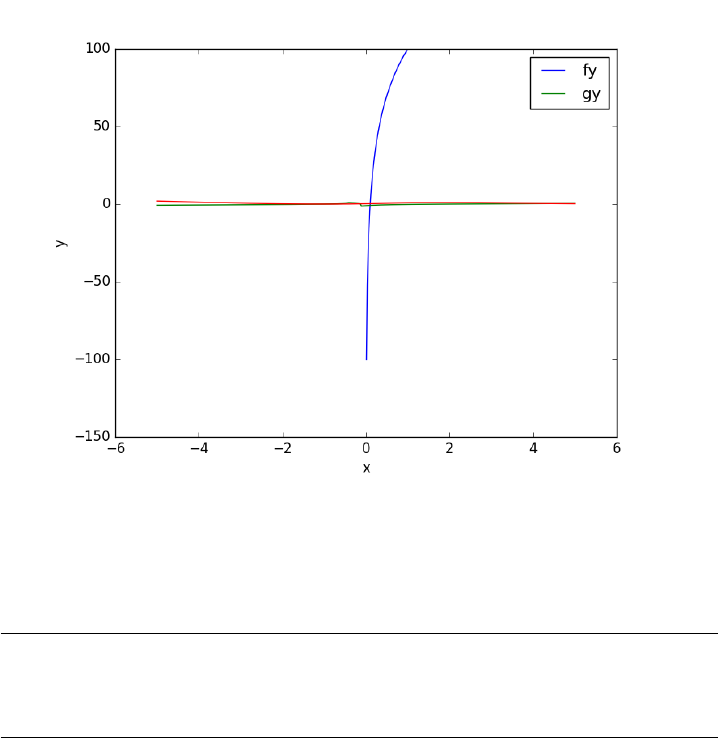
You can see there is a solution near x = -1, y = 0, because both functions
equal zero there. We can even use that guess with fsolve. It is disappointly
easy! But, keep in mind that in 3 or more dimensions, you cannot perform
this visualization, and another method could be required.
1def func(X):
2x,y =X
3return [f(x, y), g(x, y)]
4
5print(fsolve(func, [-2,-2]))
[ -1.00000000e+00 1.28730858e-15]
We explore a method that bypasses this problem today. The principle
is to introduce a new variable, λ, which will vary from 0 to 1. at λ= 0 we
will have a simpler equation, preferrably a linear one, which can be easily
solved, or which can be analytically solved. At λ= 1, we have the original
equations. Then, we create a system of differential equations that start at
the easy solution, and integrate from λ= 0 to λ= 1, to recover the final
solution.
We rewrite the equations as:
f(x, y) = (2 + x+y) + λ(−x2+ 8xy +y3)=0
g(x, y) = (1 + 2x−3y) + λ(x2+xy −yex)=0
102

Now, at λ= 0 we have the simple linear equations:
x+y=−2
2x−3y=−1
These equations are trivial to solve:
1x0 =np.linalg.solve([[1.,1.], [2.,-3.]],[ -2,-1])
2print(x0)
[-1.4 -0.6]
We form the system of ODEs by differentiating the new equations with
respect to λ. Why do we do that? The solution, (x,y) will be a function of
λ. From calculus, you can show that:
∂f
∂x
∂x
∂λ +∂f
∂y
∂y
∂λ =−∂f
∂λ
∂g
∂x
∂x
∂λ +∂g
∂y
∂y
∂λ =−∂g
∂λ
Now, solve this for ∂x
∂λ and ∂y
∂λ . You can use Cramer’s rule to solve for
these to yield:
\∂x∂λ&=& ∂f /∂y∂g/∂λ−∂f /∂λ∂g/∂y
∂f /∂x∂g/∂y−∂f/∂y∂g/∂x
(10)
(11)
∂y
∂λ&=&∂f /∂λ∂g/∂x −∂f/∂x∂g/∂λ
∂f/∂x∂g/∂y −∂f/∂y∂g/∂x (12)
For this set of equations:
\∂f/∂x &=& 1 - 2λx + 8λy
(13)
(14)
∂f/∂y &=& 1 + 8 λx + 3 λyˆ2
(15)
(16)
∂g/∂x &=& 2 + 2 λx + λy - λy eˆx
(17)
(18)
∂g/∂y &=& -3 + λx - λeˆx
(19)
103

Now, we simply set up those two differential equations on ∂x
∂λ and ∂y
∂λ ,
with the initial conditions at λ= 0 which is the solution of the simpler linear
equations, and integrate to λ= 1, which is the final solution of the original
equations!
1def ode(X, LAMBDA):
2x,y =X
3pfpx = 1.0 - 2.0 * LAMBDA *x+8*LAMBDA *y
4pfpy = 1.0 + 8.0 * LAMBDA *x+ 3.0 * LAMBDA *y**2
5pfpLAMBDA = -x**2 + 8.0 * x*y+y**3;
6pgpx =2.+2.*LAMBDA *x+LAMBDA *y-LAMBDA *y*np.exp(x)
7pgpy = -3. + LAMBDA *x-LAMBDA *np.exp(x)
8pgpLAMBDA =x**2 + x*y-y*np.exp(x);
9dxdLAMBDA =(pfpy *pgpLAMBDA -pfpLAMBDA *pgpy) /(pfpx *pgpy -pfpy *pgpx)
10 dydLAMBDA =(pfpLAMBDA *pgpx -pfpx *pgpLAMBDA) /(pfpx *pgpy -pfpy *pgpx)
11 dXdLAMBDA =[dxdLAMBDA, dydLAMBDA]
12 return dXdLAMBDA
13
14
15 from scipy.integrate import odeint
16
17 lambda_span =np.linspace(0,1,100)
18
19 X=odeint(ode, x0, lambda_span)
20
21 xsol, ysol =X[-1]
22 print(’The solution is at x={0:1.3f}, y={1:1.3f}’.format(xsol, ysol))
23 print(f(xsol, ysol), g(xsol, ysol))
The solution is at x=-1.000, y=0.000
-1.27746598729e-06 -1.15873818131e-06
You can see the solution is somewhat approximate; the true solution is x
= -1, y = 0. The approximation could be improved by lowering the tolerance
on the ODE solver. The functions evaluate to a small number, close to
zero. You have to apply some judgment to determine if that is sufficiently
accurate. For instance if the units on that answer are kilometers, but you
need an answer accurate to a millimeter, this may not be accurate enough.
This is a fair amount of work to get a solution! The idea is to solve a
simple problem, and then gradually turn on the hard part by the lambda
parameter. What happens if there are multiple solutions? The answer you
finally get will depend on your λ= 0 starting point, so it is possible to miss
solutions this way. For problems with lots of variables, this would be a good
approach if you can identify the easy problem.
104

5.4 Method of continuity for solving nonlinear equations -
Part II
Matlab post Yesterday in Post 1324 we looked at a way to solve nonlinear
equations that takes away some of the burden of initial guess generation.
The idea was to reformulate the equations with a new variable λ, so that at
λ= 0 we have a simpler problem we know how to solve, and at λ= 1 we
have the original set of equations. Then, we derive a set of ODEs on how
the solution changes with λ, and solve them.
Today we look at a simpler example and explain a little more about what
is going on. Consider the equation: f(x) = x2−5x+ 6 = 0, which has two
roots, x= 2 and x= 3. We will use the method of continuity to solve this
equation to illustrate a few ideas. First, we introduce a new variable λas:
f(x;λ)=0. For example, we could write f(x;λ) = λx2−5x+ 6 = 0. Now,
when λ= 0, we hve the simpler equation −5x+ 6 = 0, with the solution
x= 6/5. The question now is, how does xchange as λchanges? We get that
from the total derivative of how f(x, λ)changes with λ. The total derivative
is:
df
dλ =∂f
∂λ +∂f
∂x
∂x
∂λ = 0
We can calculate two of those quantities: ∂f
∂λ and ∂f
∂x analytically from
our equation and solve for ∂x
∂λ as
∂x
∂λ =−∂f
∂λ/∂f
∂x
That defines an ordinary differential equation that we can solve by inte-
grating from λ= 0 where we know the solution to λ= 1 which is the solution
to the real problem. For this problem: ∂f
∂λ =x2and ∂f
∂x =−5+2λx.
1import numpy as np
2from scipy.integrate import odeint
3import matplotlib.pyplot as plt
4
5def dxdL(x, Lambda):
6return -x**2 / (-5.0 + 2 * Lambda *x)
7
8x0 = 6.0/5.0
9Lspan =np.linspace(0,1)
10 x=odeint(dxdL, x0, Lspan)
11
12 plt.plot(Lspan, x)
13 plt.xlabel(’$\lambda$’)
14 plt.ylabel(’x’)
15 plt.savefig(’images/nonlin-contin-II-1.png’)
105
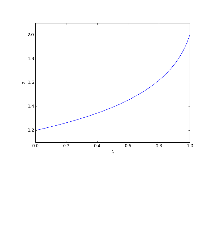
We found one solution at x=2. What about the other solution? To get
that we have to introduce λinto the equations in another way. We could
try: f(x;λ) = x2+λ(−5x+ 6), but this leads to an ODE that is singular at
the initial starting point. Another approach is f(x;λ) = x2+6+λ(−5x),
but now the solution at λ= 0 is imaginary, and we do not have a way to
integrate that! What we can do instead is add and subtract a number like
this: f(x;λ) = x2−4 + λ(−5x+ 6 + 4). Now at λ= 0, we have a simple
equation with roots at ±2, and we already know that x= 2 is a solution.
So, we create our ODE on dx/dλ with initial condition x(0) = −2.
1import numpy as np
2from scipy.integrate import odeint
3import matplotlib.pyplot as plt
4
5def dxdL(x, Lambda):
6return (5*x- 10)/(2*x-5*Lambda)
7
8x0 = -2
9Lspan =np.linspace(0,1)
10 x=odeint(dxdL, x0, Lspan)
11
12 plt.plot(Lspan, x)
13 plt.xlabel(’$\lambda$’)
106
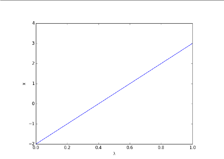
14 plt.ylabel(’x’)
15 plt.savefig(’images/nonlin-contin-II-2.png’)
Now we have the other solution. Note if you choose the other root,
x= 2, you find that 2 is a root, and learn nothing new. You could choose
other values to add, e.g., if you chose to add and subtract 16, then you
would find that one starting point leads to one root, and the other starting
point leads to the other root. This method does not solve all problems
associated with nonlinear root solving, namely, how many roots are there,
and which one is "best" or physically reasonable? But it does give a way
to solve an equation where you have no idea what an initial guess should
be. You can see, however, that just like you can get different answers from
different initial guesses, here you can get different answers by setting up the
equations differently.
5.5 Counting roots
Matlab post The goal here is to determine how many roots there are in a
nonlinear function we are interested in solving. For this example, we use a
cubic polynomial because we know there are three roots.
f(x) = x3+ 6x2−4x−24
107
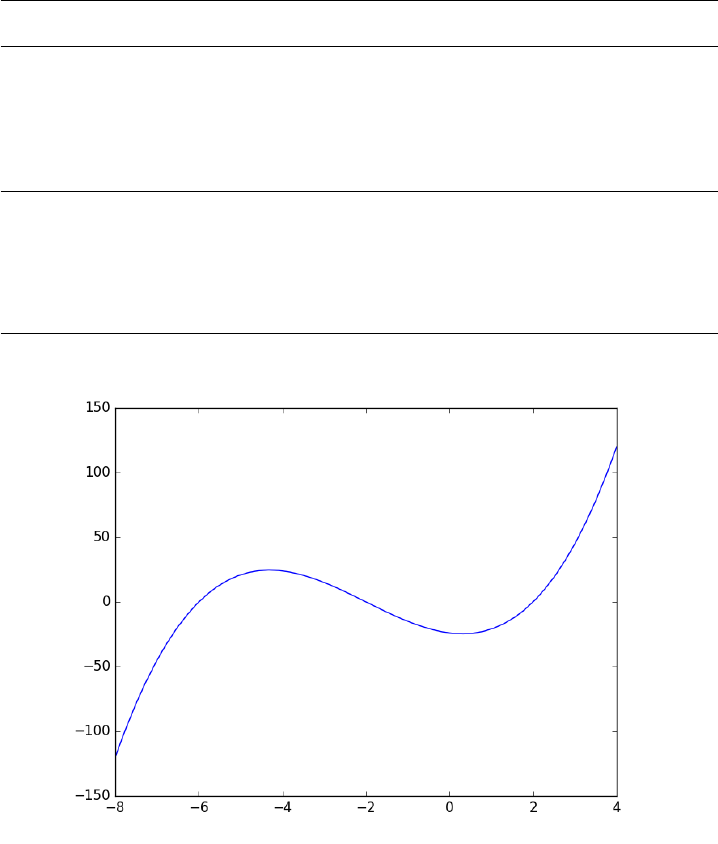
5.5.1 Use roots for this polynomial
This ony works for a polynomial, it does not work for any other nonlinear
function.
1import numpy as np
2print(np.roots([1,6,-4,-24]))
[-6. 2. -2.]
Let us plot the function to see where the roots are.
1import numpy as np
2import matplotlib.pyplot as plt
3
4x=np.linspace(-8,4)
5y=x**3 + 6 * x**2 - 4*x- 24
6plt.plot(x, y)
7plt.savefig(’images/count-roots-1.png’)
Now we consider several approaches to counting the number of roots in
this interval. Visually it is pretty easy, you just look for where the function
crosses zero. Computationally, it is tricker.
108

5.5.2 method 1
Count the number of times the sign changes in the interval. What we have to
do is multiply neighboring elements together, and look for negative values.
That indicates a sign change. For example the product of two positive or
negative numbers is a positive number. You only get a negative number
from the product of a positive and negative number, which means the sign
changed.
1import numpy as np
2import matplotlib.pyplot as plt
3
4x=np.linspace(-8,4)
5y=x**3 + 6 * x**2 - 4*x- 24
6
7print(np.sum(y[0:-2]*y[1:-1]< 0))
3
This method gives us the number of roots, but not where the roots are.
5.5.3 Method 2
Using events in an ODE solver python can identify events in the solution to
an ODE, for example, when a function has a certain value, e.g. f(x) = 0.
We can take advantage of this to find the roots and number of roots in this
case. We take the derivative of our function, and integrate it from an initial
starting point, and define an event function that counts zeros.
f0(x)=3x2+ 12x−4
with f(-8) = -120
1import numpy as np
2from pycse import odelay
3
4def fprime(f, x):
5return 3.0 * x**2 + 12.0*x- 4.0
6
7def event(f, x):
8value =f# we want f = 0
9isterminal =False
10 direction = 0
11 return value, isterminal, direction
12
13 xspan =np.linspace(-8,4)
109

14 f0 = -120
15
16 X, F, TE, YE, IE =odelay(fprime, f0, xspan, events=[event])
17 for te, ye in zip(TE, YE):
18 print(’root found at x = {0: 1.3f}, f={1: 1.3f}’.format(te, float(ye)))
root found at x = -6.000, f= 0.000
root found at x = -2.000, f= 0.000
root found at x = 2.000, f= 0.000
5.6 Finding the nth root of a periodic function
There is a heat transfer problem where one needs to find the nˆth root of
the following equation: xJ1(x)−BiJ0(x)=0where J0and J1are the Bessel
functions of zero and first order, and Bi is the Biot number. We examine
an approach to finding these roots.
First, we plot the function.
1from scipy.special import jn, jn_zeros
2import matplotlib.pyplot as plt
3import numpy as np
4
5Bi = 1
6
7def f(x):
8return x*jn(1, x) -Bi *jn(0, x)
9
10 X=np.linspace(0,30,200)
11 plt.plot(X, f(X))
12 plt.savefig(’images/heat-transfer-roots-1.png’)
110
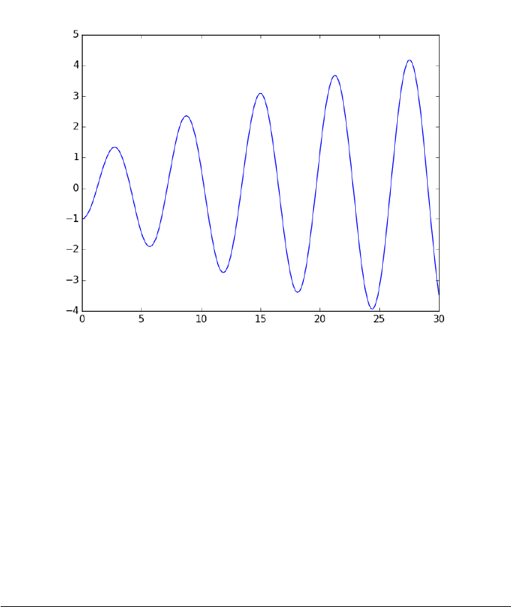
You can see there are many roots to this equation, and we want to be
sure we get the nˆ{th} root. This function is pretty well behaved, so if you
make a good guess about the solution you will get an answer, but if you
make a bad guess, you may get the wrong root. We examine next a way
to do it without guessing the solution. What we want is the solution to
f(x)=0, but we want all the solutions in a given interval. We derive a new
equation, f0(x)=0, with initial condition f(0) = f0, and integrate the ODE
with an event function that identifies all zeros of ffor us. The derivative
of our function is df/dx =d/dx(xJ1(x)) −BiJ0
0(x). It is known (http:
//www.markrobrien.com/besselfunct.pdf) that d/dx(xJ1(x)) = xJ0(x),
and J0
0(x) = −J1(x). All we have to do now is set up the problem and run
it.
1from pycse import *# contains the ode integrator with events
2
3from scipy.special import jn, jn_zeros
4import matplotlib.pyplot as plt
5import numpy as np
6
7Bi = 1
8
9def f(x):
10 "function we want roots for"
11 return x*jn(1, x) -Bi *jn(0, x)
12
111

13 def fprime(f, x):
14 "df/dx"
15 return x*jn(0, x) -Bi *(-jn(1, x))
16
17 def e1(f, x):
18 "event function to find zeros of f"
19 isterminal =False
20 value =f
21 direction = 0
22 return value, isterminal, direction
23
24 f0 =f(0)
25 xspan =np.linspace(0,30,200)
26
27 x, fsol, XE, FE, IE =odelay(fprime, f0, xspan, events=[e1])
28
29 plt.plot(x, fsol, ’.-’, label=’Numerical solution’)
30 plt.plot(xspan, f(xspan), ’--’, label=’Analytical function’)
31 plt.plot(XE, FE, ’ro’, label=’roots’)
32 plt.legend(loc=’best’)
33 plt.savefig(’images/heat-transfer-roots-2.png’)
34
35 for i, root in enumerate(XE):
36 print(’root {0} is at {1}’.format(i, root))
root 0 is at 1.2557837640729235
root 1 is at 4.079477427934495
root 2 is at 7.15579903773092
root 3 is at 10.270985121143715
root 4 is at 13.398397381859922
root 5 is at 16.53115870938385
root 6 is at 19.66672767595721
root 7 is at 22.80395034851908
root 8 is at 25.94222881771057
root 9 is at 29.081221488671474
112
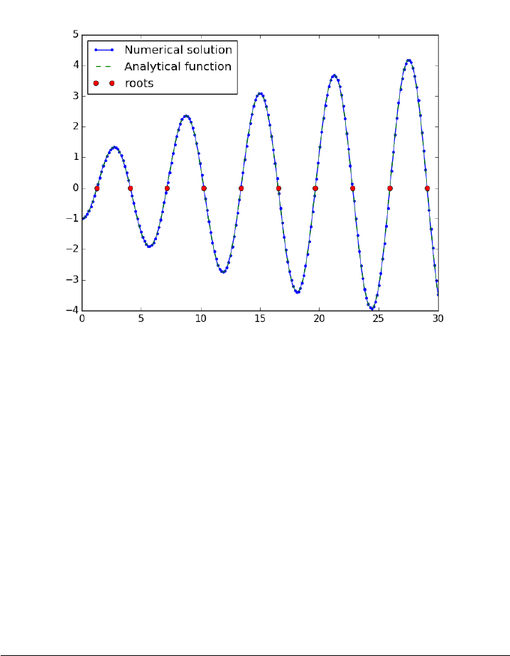
You can work this out once, and then you have all the roots in the
interval and you can select the one you want.
5.7 Coupled nonlinear equations
Suppose we seek the solution to this set of equations:
y=x2(20)
y= 8 −x2(21)
To solve this we need to setup a function that is equal to zero at the
solution. We have two equations, so our function must return two values.
There are two variables, so the argument to our function will be an array of
values.
1from scipy.optimize import fsolve
2
3def objective(X):
4x,y=X# unpack the array in the argument
5z1 =y-x**2 # first equation
6z2 =y-8+x**2 # second equation
7return [z1, z2] # list of zeros
8
113

9x0, y0 = 1,1# initial guesses
10 guess =[x0, y0]
11 sol =fsolve(objective, guess)
12 print(sol)
13
14 # of course there may be more than one solution
15 x0, y0 = -1,-1 # initial guesses
16 guess =[x0, y0]
17 sol =fsolve(objective, guess)
18 print(sol)
[ 2. 4.]
[-2. 4.]
6 Statistics
6.1 Introduction to statistical data analysis
Matlab post
Given several measurements of a single quantity, determine the average
value of the measurements, the standard deviation of the measurements and
the 95% confidence interval for the average.
1import numpy as np
2
3y=[8.1,8.0,8.1]
4
5ybar =np.mean(y)
6s=np.std(y, ddof=1)
7
8print(ybar, s)
8.06666666667 0.057735026919
Interesting, we have to specify the divisor in numpy.std by the ddof
argument. The default for this in Matlab is 1, the default for this function
is 0.
Here is the principle of computing a confidence interval.
1. Compute the average
2. Compute the standard deviation of your data
3. Define the confidence interval, e.g. 95% = 0.95
114

4. Compute the student-t multiplier. This is a function of the confidence
interval you specify, and the number of data points you have minus 1.
You subtract 1 because one degree of freedom is lost from calculating
the average.
The confidence interval is defined as ybar ±T_multiplier*std/sqrt(n).
1from scipy.stats.distributions import t
2ci = 0.95
3alpha = 1.0 - ci
4
5n=len(y)
6T_multiplier =t.ppf(1.0 - alpha / 2.0,n- 1)
7
8ci95 =T_multiplier *s/np.sqrt(n)
9
10 print(’T_multiplier = {0}’.format(T_multiplier))
11 print(’ci95 = {0}’.format(ci95))
12 print(’The true average is between {0} and {1} at a 95% confidence level’.format(ybar -ci95, ybar +ci95))
T_multiplier = 4.302652729911275
ci95 = 0.14342175766370865
The true average is between 7.9232449090029595 and 8.210088424330376 at a 95% confidence level
6.2 Basic statistics
Given several measurements of a single quantity, determine the average value
of the measurements, the standard deviation of the measurements and the
95% confidence interval for the average.
This is a recipe for computing the confidence interval. The strategy is:
1. compute the average
2. Compute the standard deviation of your data
3. Define the confidence interval, e.g. 95% = 0.95
4. compute the student-t multiplier. This is a function of the confidence
interval you specify, and the number of data points you have minus 1. You
subtract 1 because one degree of freedom is lost from calculating the average.
The confidence interval is defined as ybar +- T_multiplier*std/sqrt(n).
1import numpy as np
2from scipy.stats.distributions import t
115

3
4y=[8.1,8.0,8.1]
5
6ybar =np.mean(y)
7s=np.std(y)
8
9ci = 0.95
10 alpha = 1.0 - ci
11
12 n=len(y)
13 T_multiplier =t.ppf(1-alpha/2.0, n-1)
14
15 ci95 =T_multiplier *s/np.sqrt(n-1)
16
17 print([ybar -ci95, ybar +ci95])
[7.9232449090029595, 8.210088424330376]
We are 95% certain the next measurement will fall in the interval above.
6.3 Confidence interval on an average
scipy has a statistical package available for getting statistical distributions.
This is useful for computing confidence intervals using the student-t tables.
Here is an example of computing a 95% confidence interval on an aver-
age.
1import numpy as np
2from scipy.stats.distributions import t
3
4n= 10 # number of measurements
5dof =n- 1 # degrees of freedom
6avg_x = 16.1 # average measurement
7std_x = 0.01 # standard deviation of measurements
8
9# Find 95% prediction interval for next measurement
10
11 alpha = 1.0 - 0.95
12
13 pred_interval =t.ppf(1-alpha/2.0, dof) *std_x /np.sqrt(n)
14
15 s=[’We are 95% confident the next measurement’,
16 ’ will be between {0:1.3f} and {1:1.3f}’]
17 print(’’.join(s).format(avg_x -pred_interval, avg_x +pred_interval))
We are 95% confident the next measurement will be between 16.093 and 16.107
116

6.4 Are averages different
Matlab post
Adapted from http://stattrek.com/ap-statistics-4/unpaired-means.
aspx
Class A had 30 students who received an average test score of 78, with
standard deviation of 10. Class B had 25 students an average test score of 85,
with a standard deviation of 15. We want to know if the difference in these
averages is statistically relevant. Note that we only have estimates of the
true average and standard deviation for each class, and there is uncertainty
in those estimates. As a result, we are unsure if the averages are really
different. It could have just been luck that a few students in class B did
better.
6.4.1 The hypothesis
the true averages are the same. We need to perform a two-sample t-test of
the hypothesis that µ1−µ2= 0 (this is often called the null hypothesis).
we use a two-tailed test because we do not care if the difference is positive
or negative, either way means the averages are not the same.
1import numpy as np
2
3n1 = 30 # students in class A
4x1 = 78.0 # average grade in class A
5s1 = 10.0 # std dev of exam grade in class A
6
7n2 = 25 # students in class B
8x2 = 85.0 # average grade in class B
9s2 = 15.0 # std dev of exam grade in class B
10
11 # the standard error of the difference between the two averages.
12 SE =np.sqrt(s1**2 / n1 +s2**2 / n2)
13
14 # compute DOF
15 DF =(n1 - 1)+(n2 - 1)
See the discussion at http://stattrek.com/Help/Glossary.aspx?Target=
Two-sample%20t-test for a more complex definition of degrees of freedom.
Here we simply subtract one from each sample size to account for the esti-
mation of the average of each sample.
6.4.2 Compute the t-score for our data
The difference between two averages determined from small sample numbers
follows the t-distribution. the t-score is the difference between the difference
117

of the means and the hypothesized difference of the means, normalized by
the standard error. we compute the absolute value of the t-score to make
sure it is positive for convenience later.
1tscore =np.abs(((x1 -x2) - 0)/SE)
2print(tscore)
1.99323179108
6.4.3 Interpretation
A way to approach determinining if the difference is significant or not is
to ask, does our computed average fall within a confidence range of the
hypothesized value (zero)? If it does, then we can attribute the difference
to statistical variations at that confidence level. If it does not, we can say
that statistical variations do not account for the difference at that confidence
level, and hence the averages must be different.
Let us compute the t-value that corresponds to a 95% confidence level
for a mean of zero with the degrees of freedom computed earlier. This means
that 95% of the t-scores we expect to get will fall within ±t95.
1from scipy.stats.distributions import t
2
3ci = 0.95;
4alpha =1-ci;
5t95 =t.ppf(1.0 - alpha/2.0, DF)
6
7print(t95)
2.00574599354
since tscore < t95, we conclude that at the 95% confidence level we
cannot say these averages are statistically different because our computed
t-score falls in the expected range of deviations. Note that our t-score is
very close to the 95% limit. Let us consider a smaller confidence interval.
1ci = 0.94
2alpha =1-ci;
3t95 =t.ppf(1.0 - alpha/2.0, DF)
4
5print(t95)
1.92191364181
118

at the 94% confidence level, however, tscore > t94, which means we
can say with 94% confidence that the two averages are different; class B
performed better than class A did. Alternatively, there is only about a 6%
chance we are wrong about that statement. another way to get there
An alternative way to get the confidence that the averages are different
is to directly compute it from the cumulative t-distribution function. We
compute the difference between all the t-values less than tscore and the
t-values less than -tscore, which is the fraction of measurements that are
between them. You can see here that we are practically 95% sure that the
averages are different.
1f=t.cdf(tscore, DF) -t.cdf(-tscore, DF)
2print(f)
0.948605075732
6.5 Model selection
Matlab post
adapted from http://www.itl.nist.gov/div898/handbook/pmd/section4/
pmd44.htm
In this example, we show some ways to choose which of several models
fit data the best. We have data for the total pressure and temperature of
a fixed amount of a gas in a tank that was measured over the course of
several days. We want to select a model that relates the pressure to the gas
temperature.
The data is stored in a text file download PT.txt , with the following
structure:
Run Ambient Fitted
Order Day Temperature Temperature Pressure Value Residual
1 1 23.820 54.749 225.066 222.920 2.146
...
We need to read the data in, and perform a regression analysis on P vs.
T. In python we start counting at 0, so we actually want columns 3 and 4.
1import numpy as np
2import matplotlib.pyplot as plt
3
4data =np.loadtxt(’data/PT.txt’, skiprows=2)
119
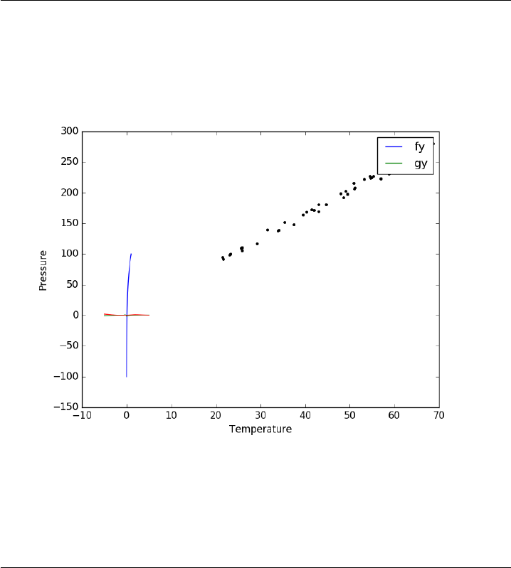
5T=data[:, 3]
6P=data[:, 4]
7
8plt.plot(T, P, ’k.’)
9plt.xlabel(’Temperature’)
10 plt.ylabel(’Pressure’)
11 plt.savefig(’images/model-selection-1.png’)
[<matplotlib.lines.Line2D object at 0x110b2cb38>]
<matplotlib.text.Text object at 0x10a0aad30>
<matplotlib.text.Text object at 0x10a3af898>
It appears the data is roughly linear, and we know from the ideal gas law
that PV = nRT, or P = nR/V*T, which says P should be linearly correlated
with V. Note that the temperature data is in degC, not in K, so it is not
expected that P=0 at T = 0. We will use linear algebra to compute the line
coefficients.
1A=np.vstack([T**0, T]).T
2b=P
3
4x, res, rank, s =np.linalg.lstsq(A, b)
5intercept, slope =x
6print(’b, m =’, intercept, slope)
7
120

8n=len(b)
9k=len(x)
10
11 sigma2 =np.sum((b -np.dot(A,x))**2)/(n -k)
12
13 C=sigma2 *np.linalg.inv(np.dot(A.T, A))
14 se =np.sqrt(np.diag(C))
15
16 from scipy.stats.distributions import t
17 alpha = 0.05
18
19 sT =t.ppf(1-alpha/2.,n-k) # student T multiplier
20 CI =sT *se
21
22 print(’CI = ’,CI)
23 for beta, ci in zip(x, CI):
24 print(’[{0} {1}]’.format(beta -ci, beta +ci))
b, m = 7.74899739238 3.93014043824
CI = [ 4.76511545 0.1026405 ]
[2.9838819463763695 12.514112838386989]
[3.8274999407885466 4.032780935691978]
The confidence interval on the intercept is large, but it does not contain
zero at the 95% confidence level.
The Rˆ2 value accounts roughly for the fraction of variation in the data
that can be described by the model. Hence, a value close to one means nearly
all the variations are described by the model, except for random variations.
1ybar =np.mean(P)
2SStot =np.sum((P -ybar)**2)
3SSerr =np.sum((P -np.dot(A, x))**2)
4R2 =1-SSerr/SStot
5print(R2)
0.993715411798
1plt.figure(); plt.clf()
2plt.plot(T, P, ’k.’, T, np.dot(A, x), ’b-’)
3plt.xlabel(’Temperature’)
4plt.ylabel(’Pressure’)
5plt.title(’R^2 = {0:1.3f}’.format(R2))
6plt.savefig(’images/model-selection-2.png’)
<matplotlib.figure.Figure object at 0x110c7ba20>
[<matplotlib.lines.Line2D object at 0x110ceec50>, <matplotlib.lines.Line2D object at 0x110ceeef0>]
121
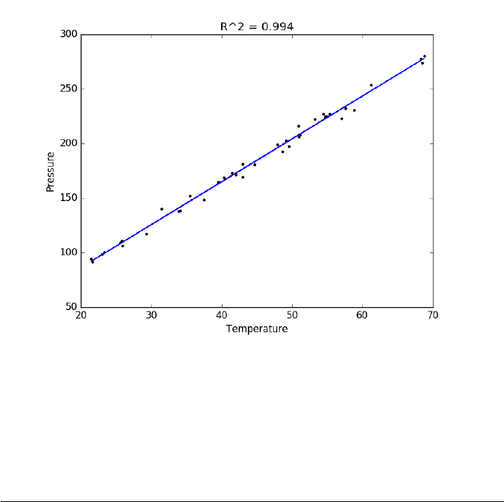
<matplotlib.text.Text object at 0x110ca7908>
<matplotlib.text.Text object at 0x110caf9b0>
<matplotlib.text.Text object at 0x110cd0358>
The fit looks good, and Rˆ2 is near one, but is it a good model? There
are a few ways to examine this. We want to make sure that there are no
systematic trends in the errors between the fit and the data, and we want
to make sure there are not hidden correlations with other variables. The
residuals are the error between the fit and the data. The residuals should
not show any patterns when plotted against any variables, and they do not
in this case.
1residuals =P-np.dot(A, x)
2
3plt.figure()
4
5f, (ax1, ax2, ax3) =plt.subplots(3)
6
7ax1.plot(T,residuals,’ko’)
8ax1.set_xlabel(’Temperature’)
9
10
11 run_order =data[:, 0]
12 ax2.plot(run_order, residuals,’ko ’)
13 ax2.set_xlabel(’run order’)
14
122
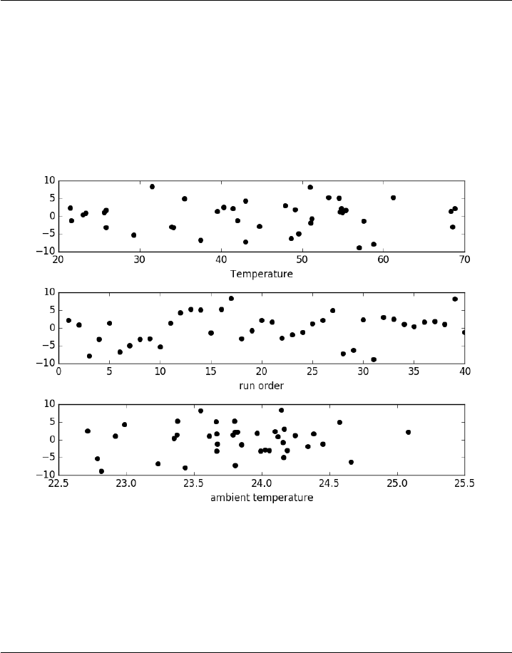
15 ambientT =data[:, 2]
16 ax3.plot(ambientT, residuals,’ko’)
17 ax3.set_xlabel(’ambient temperature’)
18
19 plt.tight_layout() # make sure plots do not overlap
20 plt.savefig(’images/model-selection-3.png’)
<matplotlib.figure.Figure object at 0x111443c88>
[<matplotlib.lines.Line2D object at 0x1116859e8>]
<matplotlib.text.Text object at 0x1114960f0>
[<matplotlib.lines.Line2D object at 0x111685a20>]
<matplotlib.text.Text object at 0x111610198>
[<matplotlib.lines.Line2D object at 0x1116859b0>]
<matplotlib.text.Text object at 0x111642a20>
There may be some correlations in the residuals with the run order. That
could indicate an experimental source of error.
We assume all the errors are uncorrelated with each other. We can use a
lag plot to assess this, where we plot residual[i] vs residual[i-1], i.e. we look
for correlations between adjacent residuals. This plot should look random,
with no correlations if the model is good.
1plt.figure(); plt.clf()
2plt.plot(residuals[1:-1], residuals[0:-2],’ko’)
123
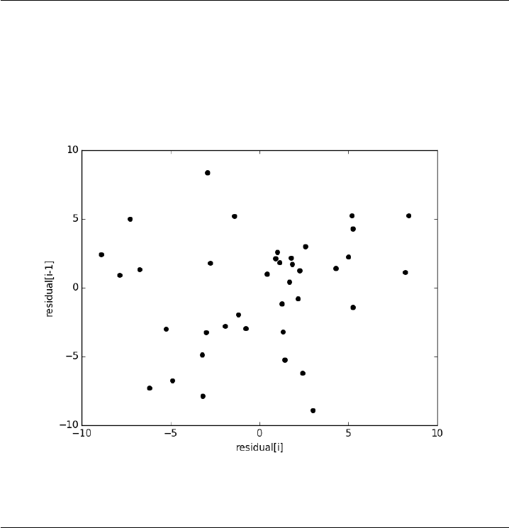
3plt.xlabel(’residual[i]’)
4plt.ylabel(’residual[i-1]’)
5plt.savefig(’images/model-selection-correlated-residuals.png’)
<matplotlib.figure.Figure object at 0x1116b75c0>
[<matplotlib.lines.Line2D object at 0x111a1ab70>]
<matplotlib.text.Text object at 0x1119d47b8>
<matplotlib.text.Text object at 0x1119db8d0>
It is hard to argue there is any correlation here.
Lets consider a quadratic model instead.
1A=np.vstack([T**0, T, T**2]).T
2b=P;
3
4x, res, rank, s =np.linalg.lstsq(A, b)
5print(x)
6
7n=len(b)
8k=len(x)
9
10 sigma2 =np.sum((b -np.dot(A,x))**2)/(n -k)
11
12 C=sigma2 *np.linalg.inv(np.dot(A.T, A))
13 se =np.sqrt(np.diag(C))
14
124

15 from scipy.stats.distributions import t
16 alpha = 0.05
17
18 sT =t.ppf(1-alpha/2.,n-k) # student T multiplier
19 CI =sT *se
20
21 print(’CI = ’,CI)
22 for beta, ci in zip(x, CI):
23 print(’[{0} {1}]’.format(beta -ci, beta +ci))
24
25
26 ybar =np.mean(P)
27 SStot =np.sum((P -ybar)**2)
28 SSerr =np.sum((P -np.dot(A,x))**2)
29 R2 =1-SSerr/SStot
30 print(’R^2 = {0}’.format(R2))
[ 9.00353031e+00 3.86669879e+00 7.26244301e-04]
CI = [ 1.38030344e+01 6.62100654e-01 7.48516727e-03]
[-4.799504121232999 22.806564732889544]
[3.2045981368070393 4.528799444091239]
[-0.006758922969064756 0.008211411570350779]
R^2 = 0.9937219694072356
You can see that the confidence interval on the constant and Tˆ2 term
includes zero. That is a good indication this additional parameter is not
significant. You can see also that the Rˆ2 value is not better than the one
from a linear fit, so adding a parameter does not increase the goodness of
fit. This is an example of overfitting the data. Since the constant in this
model is apparently not significant, let us consider the simplest model with
a fixed intercept of zero.
Let us consider a model with intercept = 0, P = alpha*T.
1A=np.vstack([T]).T
2b=P;
3
4x, res, rank, s =np.linalg.lstsq(A, b)
5
6n=len(b)
7k=len(x)
8
9sigma2 =np.sum((b -np.dot(A,x))**2)/(n -k)
10
11 C=sigma2 *np.linalg.inv(np.dot(A.T, A))
12 se =np.sqrt(np.diag(C))
13
14 from scipy.stats.distributions import t
15 alpha = 0.05
16
125
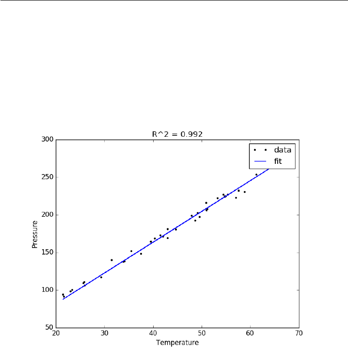
17 sT =t.ppf(1-alpha/2.0,n-k) # student T multiplier
18 CI =sT *se
19
20 for beta, ci in zip(x, CI):
21 print(’[{0} {1}]’.format(beta -ci, beta +ci))
22
23 plt.figure()
24 plt.plot(T, P, ’k. ’, T, np.dot(A, x))
25 plt.xlabel(’Temperature’)
26 plt.ylabel(’Pressure’)
27 plt.legend([’data’,’fit’])
28
29 ybar =np.mean(P)
30 SStot =np.sum((P -ybar)**2)
31 SSerr =np.sum((P -np.dot(A,x))**2)
32 R2 =1-SSerr/SStot
33 plt.title(’R^2 = {0:1.3f}’.format(R2))
34 plt.savefig(’images/model-selection-no-intercept.png’)
[4.056801244949384 4.123083498991817]
<matplotlib.figure.Figure object at 0x111a1ae10>
[<matplotlib.lines.Line2D object at 0x111c23b70>, <matplotlib.lines.Line2D object at 0x111c23e10>]
<matplotlib.text.Text object at 0x111a3be48>
<matplotlib.text.Text object at 0x111c06550>
<matplotlib.legend.Legend object at 0x111c326a0>
<matplotlib.text.Text object at 0x111c187f0>
The
126
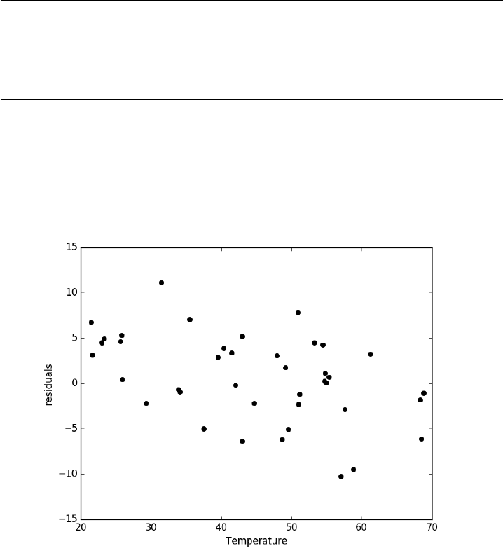
fit is visually still pretty good, and the Rˆ2 value is only slightly worse. Let
us examine the residuals again.
1residuals =P-np.dot(A,x)
2
3plt.figure()
4plt.plot(T,residuals,’ko’)
5plt.xlabel(’Temperature’)
6plt.ylabel(’residuals’)
7plt.savefig(’images/model-selection-no-incpt-resid.png’)
<matplotlib.figure.Figure object at 0x111c32c88>
[<matplotlib.lines.Line2D object at 0x111a5f710>]
<matplotlib.text.Text object at 0x111c5d6a0>
<matplotlib.text.Text object at 0x111c65d68>
You can see a slight trend of decreasing value of the residuals as the
Temperature increases. This may indicate a deficiency in the model with
no intercept. For the ideal gas law in degC: P V =nR(T+ 273) or P=
nR/V ∗T+ 273 ∗nR/V , so the intercept is expected to be non-zero in this
case. Specifically, we expect the intercept to be 273*R*n/V. Since the molar
density of a gas is pretty small, the intercept may be close to, but not equal
to zero. That is why the fit still looks ok, but is not as good as letting the
127

intercept be a fitting parameter. That is an example of the deficiency in our
model.
In the end, it is hard to justify a model more complex than a line in this
case.
6.6 Numerical propagation of errors
Matlab post
Propagation of errors is essential to understanding how the uncertainty in
a parameter affects computations that use that parameter. The uncertainty
propagates by a set of rules into your solution. These rules are not easy to
remember, or apply to complicated situations, and are only approximate for
equations that are nonlinear in the parameters.
We will use a Monte Carlo simulation to illustrate error propagation.
The idea is to generate a distribution of possible parameter values, and
to evaluate your equation for each parameter value. Then, we perform
statistical analysis on the results to determine the standard error of the
results.
We will assume all parameters are defined by a normal distribution with
known mean and standard deviation.
6.6.1 Addition and subtraction
1import numpy as np
2import matplotlib.pyplot as plt
3
4N= 1e4 # number of samples of parameters
5
6A_mu = 2.5; A_sigma = 0.4
7B_mu = 4.1; B_sigma = 0.3
8
9A=np.random.normal(A_mu, A_sigma, size=N)
10 B=np.random.normal(B_mu, B_sigma, size=N)
11
12 p=A+B
13 m=A-B
14
15 plt.hist(p)
16 plt.show()
17
18 print(np.std(p))
19 print(np.std(m))
20
21 print(np.sqrt(A_sigma**2 + B_sigma**2)) # the analytical std dev
(array([ 2.00000000e+00, 1.90000000e+01, 1.90000000e+02,
128

1.00800000e+03, 2.43300000e+03, 3.20400000e+03,
2.21700000e+03, 7.61000000e+02, 1.56000000e+02,
1.00000000e+01]), array([ 4.37827788, 4.78610393, 5.19392997, 5.60175601, 6.00958205,
6.4174081 , 6.82523414, 7.23306018, 7.64088623, 8.04871227,
8.45653831]), <a list of 10 Patch objects>)
0.491531788514
0.495333805189
0.5
6.6.2 Multiplication
1F_mu = 25.0; F_sigma = 1;
2x_mu = 6.4; x_sigma = 0.4;
3
4F=np.random.normal(F_mu, F_sigma, size=N)
5x=np.random.normal(x_mu, x_sigma, size=N)
6
7t=F*x
8print(np.std(t))
9print(np.sqrt((F_sigma /F_mu)**2 + (x_sigma /x_mu)**2)*F_mu *x_mu)
11.8683624528
11.8726576637
6.6.3 Division
This is really like multiplication: F / x = F * (1 / x).
1d=F/x
2print(np.std(d))
3print(np.sqrt((F_sigma /F_mu)**2 + (x_sigma /x_mu)**2)*F_mu /x_mu)
0.295540277244
0.289859806243
6.6.4 exponents
This rule is different than multiplication (Aˆ2 = A*A) because in the previ-
ous examples we assumed the errors in A and B for A*B were uncorrelated.
in A*A, the errors are not uncorrelated, so there is a different rule for error
propagation.
129

1t_mu = 2.03; t_sigma = 0.01*t_mu; # 1% error
2A_mu = 16.07; A_sigma = 0.06;
3
4t=np.random.normal(t_mu, t_sigma, size=(1, N))
5A=np.random.normal(A_mu, A_sigma, size=(1, N))
6
7# Compute t^5 and sqrt(A) with error propagation
8print(np.std(t**5))
9print((5*t_sigma /t_mu) *t_mu**5)
1.7454605614
1.7236544062149992
1print(np.std(np.sqrt(A)))
2print(1.0 / 2.0 * A_sigma /A_mu *np.sqrt(A_mu))
0.00747831865757
0.00748364738749
6.6.5 the chain rule in error propagation
let v = v0 + a*t, with uncertainties in vo,a and t
1vo_mu = 1.2; vo_sigma = 0.02;
2a_mu = 3.0; a_sigma = 0.3;
3t_mu = 12.0; t_sigma = 0.12;
4
5vo =np.random.normal(vo_mu, vo_sigma, (1, N))
6a=np.random.normal(a_mu, a_sigma, (1, N))
7t=np.random.normal(t_mu, t_sigma, (1, N))
8
9v=vo +a*t
10
11 print(np.std(v))
12 print(np.sqrt(vo_sigma**2 + t_mu**2 * a_sigma**2 + a_mu**2 * t_sigma**2))
3.62167603078
3.61801050303
6.6.6 Summary
You can numerically perform error propagation analysis if you know the
underlying distribution of errors on the parameters in your equations. One
benefit of the numerical propogation is you do not have to remember the
error propagation rules, and you directly look at the distribution in nonlinear
cases. Some limitations of this approach include
130

1. You have to know the distribution of the errors in the parameters
2. You have to assume the errors in parameters are uncorrelated.
6.7 Another approach to error propagation
In the previous section we examined an analytical approach to error prop-
agation, and a simulation based approach. There is another approach to
error propagation, using the uncertainties module (https://pypi.python.
org/pypi/uncertainties/). You have to install this package, e.g. pip
install uncertainties. After that, the module provides new classes of
numbers and functions that incorporate uncertainty and propagate the un-
certainty through the functions. In the examples that follow, we repeat the
calculations from the previous section using the uncertainties module.
Addition and subtraction
1import uncertainties as u
2
3A=u.ufloat((2.5,0.4))
4B=u.ufloat((4.1,0.3))
5print(A +B)
6print(A -B)
6.6+/-0.5
-1.6+/-0.5
Multiplication and division
1F=u.ufloat((25,1))
2x=u.ufloat((6.4,0.4))
3
4t=F*x
5print(t)
6
7d=F/x
8print(d)
160+/-12
3.91+/-0.29
Exponentiation
1t=u.ufloat((2.03,0.0203))
2print(t**5)
3
131

4from uncertainties.umath import sqrt
5A=u.ufloat((16.07,0.06))
6print(sqrt(A))
7# print np.sqrt(A) # this does not work
8
9from uncertainties import unumpy as unp
10 print(unp.sqrt(A))
34.5+/-1.7
4.009+/-0.007
4.009+/-0.007
Note in the last example, we had to either import a function from un-
certainties.umath or import a special version of numpy that handles uncer-
tainty. This may be a limitation of the uncertainties package as not all
functions in arbitrary modules can be covered. Note, however, that you can
wrap a function to make it handle uncertainty like this.
1import numpy as np
2
3wrapped_sqrt =u.wrap(np.sqrt)
4print(wrapped_sqrt(A))
4.009+/-0.007
Propagation of errors in an integral
1import numpy as np
2import uncertainties as u
3
4x=np.array([u.ufloat((1,0.01)),
5u.ufloat((2,0.1)),
6u.ufloat((3,0.1))])
7
8y=2*x
9
10 print(np.trapz(x, y))
8.0+/-0.6
Chain rule in error propagation
1v0 =u.ufloat((1.2,0.02))
2a=u.ufloat((3.0,0.3))
3t=u.ufloat((12.0,0.12))
4
5v=v0 +a*t
6print(v)
132

37+/-4
A real example? This is what I would setup for a real working example.
We try to compute the exit concentration from a CSTR. The idea is to
wrap the "external" fsolve function using the uncertainties.wrap function,
which handles the units. Unfortunately, it does not work, and it is not clear
why. But see the following discussion for a fix.
1from scipy.optimize import fsolve
2
3Fa0 =u.ufloat((5.0,0.05))
4v0 =u.ufloat((10.,0.1))
5
6V=u.ufloat((66000.0,100)) # reactor volume L^3
7k=u.ufloat((3.0,0.2)) # rate constant L/mol/h
8
9def func(Ca):
10 "Mole balance for a CSTR. Solve this equation for func(Ca)=0"
11 Fa =v0 *Ca # exit molar flow of A
12 ra = -k*Ca**2 # rate of reaction of A L/mol/h
13 return Fa0 -Fa +V*ra
14
15 # CA guess that that 90 % is reacted away
16 CA_guess =0.1*Fa0 /v0
17
18 wrapped_fsolve =u.wrap(fsolve)
19 CA_sol =wrapped_fsolve(func, CA_guess)
20
21 print(’The exit concentration is {0} mol/L’.format(CA_sol))
__main__:1: UserWarning: Obsolete: either use ufloat(nominal_value, std_dev), ufloat(nominal_value, std_dev, tag), or the ufloat_fromstr() function, for string representations. Code can be automatically updated with python -m uncertainties.1to2 -w ProgramDirectory.
TypeError: Cannot cast array data from dtype(’O’) to dtype(’float64’) according to the rule ’safe’
Traceback (most recent call last):
File "<stdin>", line 1, in <module>
File "/Users/jkitchin/anaconda3/lib/python3.5/site-packages/uncertainties/core.py", line 656, in f_with_affine_output
f_nominal_value = f(*args_values, **kwargs)
File "/Users/jkitchin/anaconda3/lib/python3.5/site-packages/scipy/optimize/minpack.py", line 146, in fsolve
res = _root_hybr(func, x0, args, jac=fprime, **options)
File "/Users/jkitchin/anaconda3/lib/python3.5/site-packages/scipy/optimize/minpack.py", line 224, in _root_hybr
ml, mu, epsfcn, factor, diag)
minpack.error: Result from function call is not a proper array of floats.
Traceback (most recent call last):
File "<stdin>", line 1, in <module>
NameError: name ’CA_sol’ is not defined
I got a note from the author of the uncertainties package explaining the
cryptic error above, and a solution for it. The error arises because fsolve does
133

not know how to deal with uncertainties. The idea is to create a function
that returns a float, when everything is given as a float. Then, we wrap the
fsolve call, and finally wrap the wrapped fsolve call!
•Step 1. Write the function to solve with arguments for all unitted
quantities. This function may be called with uncertainties, or with
floats.
•Step 2. Wrap the call to fsolve in a function that takes all the param-
eters as arguments, and that returns the solution.
•Step 3. Use uncertainties.wrap to wrap the function in Step 2 to get
the answer with uncertainties.
Here is the code that does work:
1import uncertainties as u
2from scipy.optimize import fsolve
3
4Fa0 =u.ufloat((5.0,0.05))
5v0 =u.ufloat((10.,0.1))
6
7V=u.ufloat((66000.0,100.0)) # reactor volume L^3
8k=u.ufloat((3.0,0.2)) # rate constant L/mol/h
9
10 # Step 1
11 def func(Ca, v0, k, Fa0, V):
12 "Mole balance for a CSTR. Solve this equation for func(Ca)=0"
13 Fa =v0 *Ca # exit molar flow of A
14 ra = -k*Ca**2 # rate of reaction of A L/mol/h
15 return Fa0 -Fa +V*ra
16
17 # Step 2
18 def Ca_solve(v0, k, Fa0, V):
19 ’wrap fsolve to pass parameters as float or units’
20 # this line is a little fragile. You must put [0] at the end or
21 # you get the NotImplemented result
22 guess =0.1*Fa0 /v0
23 sol =fsolve(func, guess, args=(v0, k, Fa0, V))[0]
24 return sol
25
26 # Step 3
27 print(u.wrap(Ca_solve)(v0, k, Fa0, V))
0.00500+/-0.00017
It would take some practice to get used to this, but the payoff is that
you have an "automatic" error propagation method.
Being ever the skeptic, let us compare the result above to the Monte
Carlo approach to error estimation below.
134

1import numpy as np
2from scipy.optimize import fsolve
3
4N= 10000
5Fa0 =np.random.normal(5,0.05, (1, N))
6v0 =np.random.normal(10.0,0.1, (1, N))
7V=np.random.normal(66000,100, (1,N))
8k=np.random.normal(3.0,0.2, (1, N))
9
10 SOL =np.zeros((1, N))
11
12 for iin range(N):
13 def func(Ca):
14 return Fa0[0,i] -v0[0,i] *Ca +V[0,i] *(-k[0,i] *Ca**2)
15 SOL[0,i] =fsolve(func, 0.1 * Fa0[0,i] /v0[0,i])[0]
16
17 print(’Ca(exit) = {0}+/-{1}’.format(np.mean(SOL), np.std(SOL)))
Ca(exit) = 0.005007316200125377+/-0.00017141142140602455
I am pretty content those are the same!
6.7.1 Summary
The uncertainties module is pretty amazing. It automatically propagates
errors through a pretty broad range of computations. It is a little tricky for
third-party packages, but it seems doable.
Read more about the package at http://pythonhosted.org/uncertainties/
index.html.
6.8 Random thoughts
Matlab post
Random numbers are used in a variety of simulation methods, most
notably Monte Carlo simulations. In another later example, we will see
how we can use random numbers for error propagation analysis. First, we
discuss two types of pseudorandom numbers we can use in python: uniformly
distributed and normally distributed numbers.
Say you are the gambling type, and bet your friend $5 the next random
number will be greater than 0.49. Let us ask Python to roll the random
number generator for us.
1import numpy as np
2
3n=np.random.uniform()
135

4print(’n = {0}’.format(n))
5
6if n> 0.49:
7print(’You win!’)
8else:
9print(’you lose.’)
n = 0.2932019329044865
you lose.
The odds of you winning the last bet are slightly stacked in your favor.
There is only a 49% chance your friend wins, but a 51% chance that you
win. Lets play the game a lot of times times and see how many times you
win, and your friend wins. First, lets generate a bunch of numbers and look
at the distribution with a histogram.
1import numpy as np
2
3N= 10000
4games =np.random.uniform(size=N)
5
6wins =np.sum(games > 0.49)
7losses =N-wins
8
9print(’You won {0} times ({1:%})’.format(wins, float(wins) /N))
10
11 import matplotlib.pyplot as plt
12 count, bins, ignored =plt.hist(games)
13 plt.savefig(’images/random-thoughts-1.png’)
You won 5111 times (51.110000%)
136
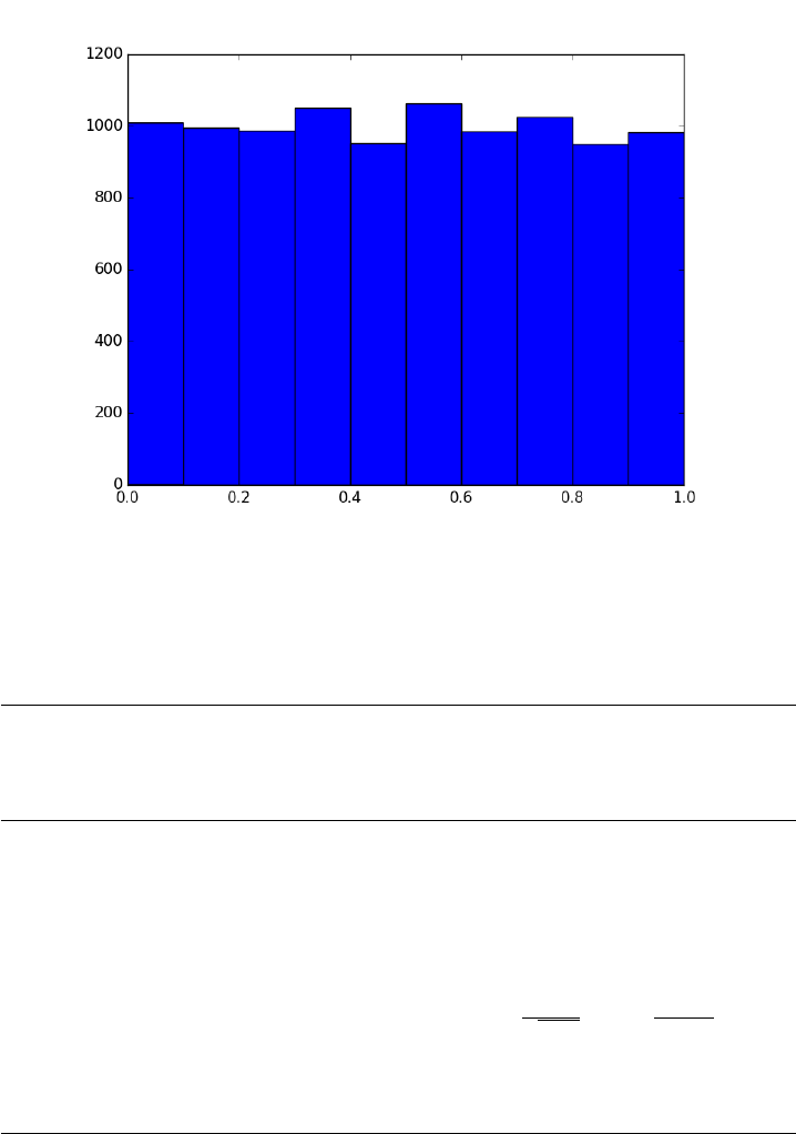
As you can see you win slightly more than you lost.
It is possible to get random integers. Here are a few examples of getting
a random integer between 1 and 100. You might do this to get random
indices of a list, for example.
1import numpy as np
2
3print(np.random.random_integers(1,100))
4print(np.random.random_integers(1,100,3))
5print(np.random.random_integers(1,100, (2,2)))
11
[50 72 79]
[[14 37]
[77 92]]
The normal distribution is defined by f(x) = 1
√2πσ2exp(−(x−µ)2
2σ2)where
µis the mean value, and σis the standard deviation. In the standard
distribution, µ= 0 and σ= 1.
1import numpy as np
2
3mu = 1
137
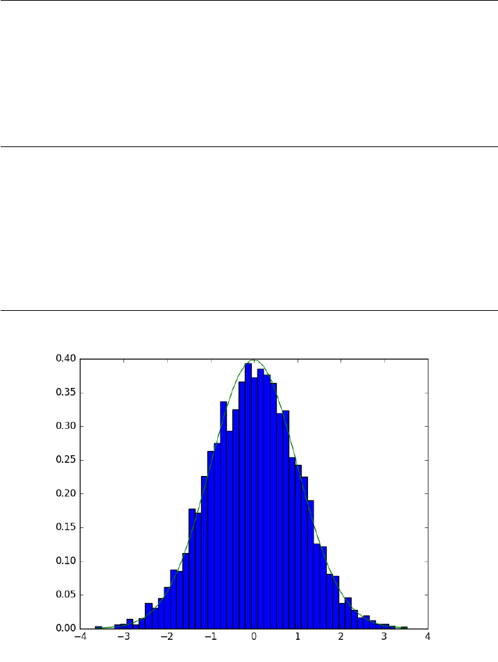
4sigma = 0.5
5print(np.random.normal(mu, sigma))
6print(np.random.normal(mu, sigma, 2))
0.9794466646232775
[ 1.58062379 0.71593225]
Let us compare the sampled distribution to the analytical distribution.
We generate a large set of samples, and calculate the probability of getting
each value using the matplotlib.pyplot.hist command.
1import numpy as np
2import matplotlib.pyplot as plt
3
4mu = 0; sigma = 1
5
6N= 5000
7samples =np.random.normal(mu, sigma, N)
8
9counts, bins, ignored =plt.hist(samples, 50, normed=True)
10
11 plt.plot(bins, 1.0/np.sqrt(2*np.pi *sigma**2)*np.exp(-((bins -mu)**2)/(2*sigma**2)))
12 plt.savefig(’images/random-thoughts-2.png’)
What fraction of points lie between plus and minus one standard devia-
tion of the mean?
138

samples >= mu-sigma will return a vector of ones where the inequality
is true, and zeros where it is not. (samples >= mu-sigma) & (samples
<= mu+sigma) will return a vector of ones where there is a one in both
vectors, and a zero where there is not. In other words, a vector where both
inequalities are true. Finally, we can sum the vector to get the number of
elements where the two inequalities are true, and finally normalize by the
total number of samples to get the fraction of samples that are greater than
-sigma and less than sigma.
1import numpy as np
2import matplotlib.pyplot as plt
3
4mu = 0; sigma = 1
5
6N= 5000
7samples =np.random.normal(mu, sigma, N)
8
9a=np.sum((samples >= (mu -sigma)) &(samples <= (mu +sigma))) /float(N)
10 b=np.sum((samples >= (mu - 2*sigma)) &(samples <= (mu + 2*sigma))) /float(N)
11 print(’{0:%} of samples are within +- standard deviations of the mean’.format(a))
12 print(’{0:%} of samples are within +- 2standard deviations of the mean’.format(b))
68.400000% of samples are within +- standard deviations of the mean
95.820000% of samples are within +- 2standard deviations of the mean
6.8.1 Summary
We only considered the numpy.random functions here, and not all of them.
There are many distributions of random numbers to choose from. There are
also random numbers in the python random module. Remember these are
only pseudorandom numbers, but they are still useful for many applications.
7 Data analysis
7.1 Fit a line to numerical data
Matlab post
We want to fit a line to this data:
1x=[0,0.5,1,1.5,2.0,3.0,4.0,6.0,10]
2y=[0,-0.157,-0.315,-0.472,-0.629,-0.942,-1.255,-1.884,-3.147]
We use the polyfit(x, y, n) command where n is the polynomial order,
n=1 for a line.
139

1import numpy as np
2
3p=np.polyfit(x, y, 1)
4print(p)
5slope, intercept =p
6print(slope, intercept)
[-0.31452218 0.00062457]
-0.3145221843 0.000624573378839
To show the fit, we can use numpy.polyval to evaluate the fit at many
points.
1import matplotlib.pyplot as plt
2
3xfit =np.linspace(0,10)
4yfit =np.polyval(p, xfit)
5
6plt.plot(x, y, ’bo’, label=’raw data’)
7plt.plot(xfit, yfit, ’r-’, label=’fit’)
8plt.xlabel(’x’)
9plt.ylabel(’y’)
10 plt.legend()
11 plt.savefig(’images/linefit-1.png’)
[<matplotlib.lines.Line2D object at 0x10d776e10>]
[<matplotlib.lines.Line2D object at 0x10d776f98>]
<matplotlib.text.Text object at 0x10b1bb7f0>
<matplotlib.text.Text object at 0x10b1cdeb8>
<matplotlib.legend.Legend object at 0x101981fd0>
140
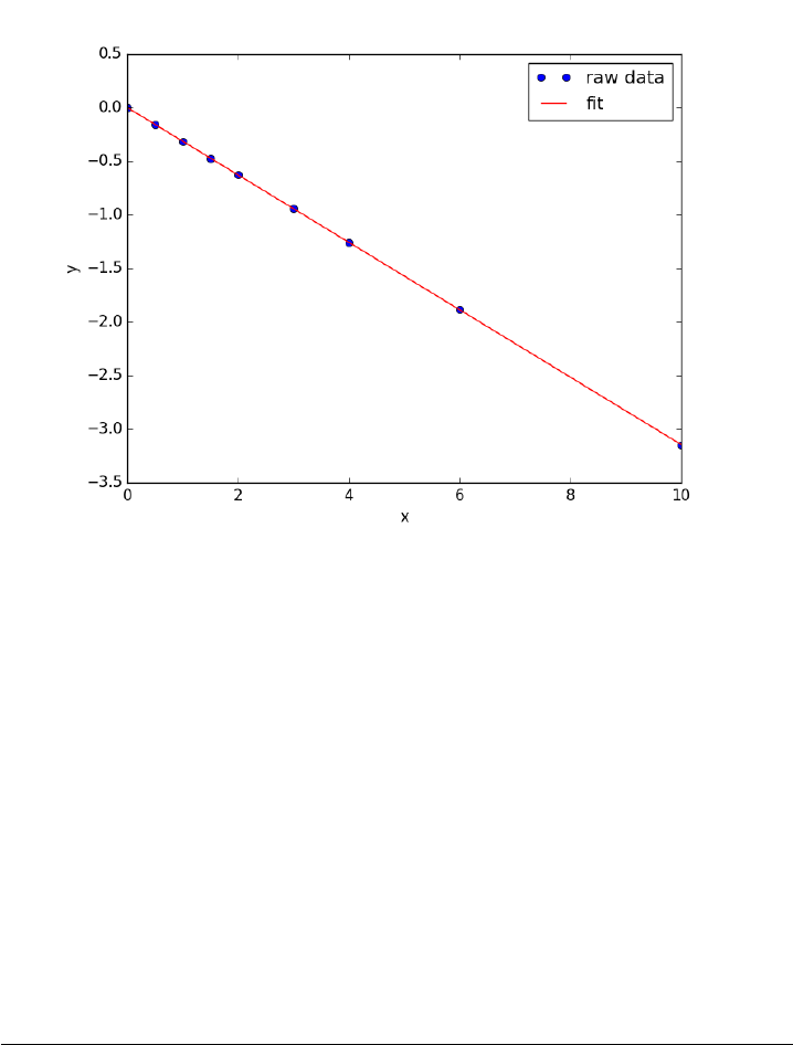
7.2 Linear least squares fitting with linear algebra
Matlab post
The idea here is to formulate a set of linear equations that is easy to solve.
We can express the equations in terms of our unknown fitting parameters
pias:
x1^0*p0 + x1*p1 = y1
x2^0*p0 + x2*p1 = y2
x3^0*p0 + x3*p1 = y3
etc...
Which we write in matrix form as Ap =ywhere Ais a matrix of column
vectors, e.g. [1, x_i]. Ais not a square matrix, so we cannot solve it as
written. Instead, we form ATAp =ATyand solve that set of equations.
1import numpy as np
2x=np.array([0,0.5,1,1.5,2.0,3.0,4.0,6.0,10])
3y=np.array([0,-0.157,-0.315,-0.472,-0.629,-0.942,-1.255,-1.884,-3.147])
4
5A=np.column_stack([x**0, x])
6
7M=np.dot(A.T, A)
141
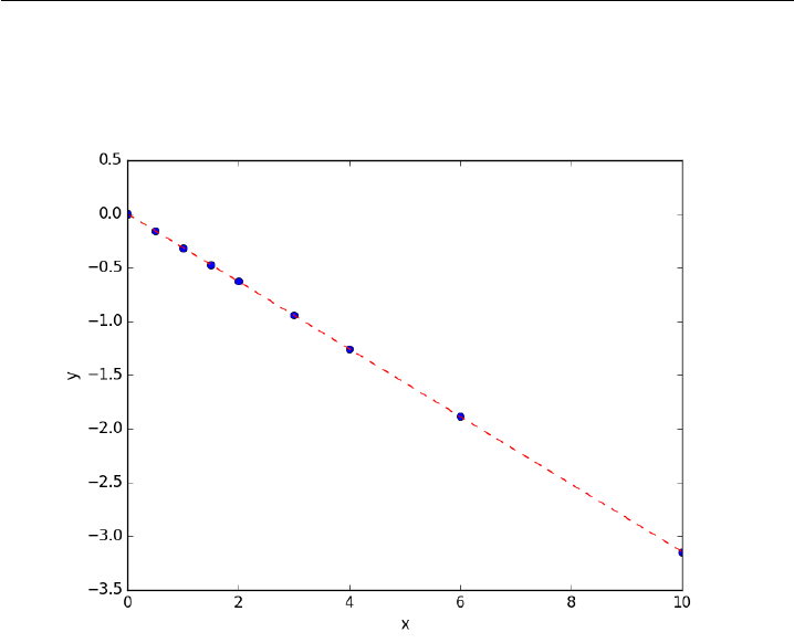
8b=np.dot(A.T, y)
9
10 i1, slope1 =np.dot(np.linalg.inv(M), b)
11 i2, slope2 =np.linalg.solve(M, b) # an alternative approach.
12
13 print(i1, slope1)
14 print(i2, slope2)
15
16 # plot data and fit
17 import matplotlib.pyplot as plt
18
19 plt.plot(x, y, ’bo’)
20 plt.plot(x, np.dot(A, [i1, slope1]), ’r--’)
21 plt.xlabel(’x’)
22 plt.ylabel(’y’)
23 plt.savefig(’images/la-line-fit.png’)
0.00062457337884 -0.3145221843
0.000624573378839 -0.3145221843
This method can be readily extended to fitting any polynomial model,
or other linear model that is fit in a least squares sense. This method does
not provide confidence intervals.
7.3 Linear regression with confidence intervals (updated)
Matlab post Fit a fourth order polynomial to this data and determine the
142

confidence interval for each parameter. Data from example 5-1 in Fogler,
Elements of Chemical Reaction Engineering.
We want the equation Ca(t) = b0 + b1∗t+b2∗t2+b3∗t3+b4∗t4fit
to the data in the least squares sense. We can write this in a linear algebra
form as: T*p = Ca where T is a matrix of columns [1 t tˆ2 tˆ3 tˆ4], and
p is a column vector of the fitting parameters. We want to solve for the p
vector and estimate the confidence intervals.
pycse now has a regress function similar to Matlab. That function just
uses the code in the next example (also seen here).
1from pycse import regress
2import numpy as np
3time =np.array([0.0,50.0,100.0,150.0,200.0,250.0,300.0])
4Ca =np.array([50.0,38.0,30.6,25.6,22.2,19.5,17.4])*1e-3
5
6T=np.column_stack([time**0, time, time**2, time**3, time**4])
7
8alpha = 0.05
9p, pint, se =regress(T, Ca, alpha)
10 print(pint)
[[ 4.90747574e-02 5.09057619e-02]
[ -3.49867288e-04 -2.45825348e-04]
[ 5.40268291e-07 2.14670133e-06]
[ -7.67338615e-09 7.03689639e-10]
[ -3.23368790e-12 1.06276264e-11]]
7.4 Linear regression with confidence intervals.
Matlab post Fit a fourth order polynomial to this data and determine the
confidence interval for each parameter. Data from example 5-1 in Fogler,
Elements of Chemical Reaction Engineering.
We want the equation Ca(t) = b0 + b1∗t+b2∗t2+b3∗t3+b4∗t4fit
to the data in the least squares sense. We can write this in a linear algebra
form as: T*p = Ca where T is a matrix of columns [1 t tˆ2 tˆ3 tˆ4], and
p is a column vector of the fitting parameters. We want to solve for the p
vector and estimate the confidence intervals.
1import numpy as np
2from scipy.stats.distributions import t
3
4time =np.array([0.0,50.0,100.0,150.0,200.0,250.0,300.0])
5Ca =np.array([50.0,38.0,30.6,25.6,22.2,19.5,17.4])*1e-3
6
143

7T=np.column_stack([time**0, time, time**2, time**3, time**4])
8
9p, res, rank, s =np.linalg.lstsq(T, Ca)
10 # the parameters are now in p
11
12 # compute the confidence intervals
13 n=len(Ca)
14 k=len(p)
15
16 sigma2 =np.sum((Ca -np.dot(T, p))**2)/(n -k) # RMSE
17
18 C=sigma2 *np.linalg.inv(np.dot(T.T, T)) # covariance matrix
19 se =np.sqrt(np.diag(C)) # standard error
20
21 alpha = 0.05 # 100*(1 - alpha) confidence level
22
23 sT =t.ppf(1.0 - alpha/2.0,n-k) # student T multiplier
24 CI =sT *se
25
26 for beta, ci in zip(p, CI):
27 print(’{2: 1.2e} [{0: 1.4e} {1: 1.4e}]’.format(beta -ci, beta +ci, beta))
28
29 SS_tot =np.sum((Ca -np.mean(Ca))**2)
30 SS_err =np.sum((np.dot(T, p) -Ca)**2)
31
32 # http://en.wikipedia.org/wiki/Coefficient_of_determination
33 Rsq =1-SS_err/SS_tot
34 print(’R^2 = {0}’.format(Rsq))
35
36 # plot fit
37 import matplotlib.pyplot as plt
38 plt.plot(time, Ca, ’bo’, label=’raw data’)
39 plt.plot(time, np.dot(T, p), ’r-’, label=’fit’)
40 plt.xlabel(’Time’)
41 plt.ylabel(’Ca (mol/L)’)
42 plt.legend(loc=’best’)
43 plt.savefig(’images/linregress-conf.png’)
5.00e-02 [ 4.9680e-02 5.0300e-02]
-2.98e-04 [-3.1546e-04 -2.8023e-04]
1.34e-06 [ 1.0715e-06 1.6155e-06]
-3.48e-09 [-4.9032e-09 -2.0665e-09]
3.70e-12 [ 1.3501e-12 6.0439e-12]
R^2 = 0.9999869672459532
144
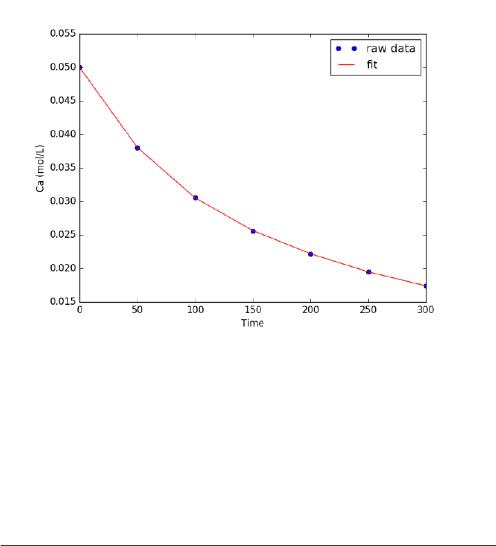
A fourth order polynomial fits the data well, with a good Rˆ2 value. All
of the parameters appear to be significant, i.e. zero is not included in any
of the parameter confidence intervals. This does not mean this is the best
model for the data, just that the model fits well.
7.5 Nonlinear curve fitting
Here is a typical nonlinear function fit to data. you need to provide an
initial guess. In this example we fit the Birch-Murnaghan equation of state
to energy vs. volume data from density functional theory calculations.
1from scipy.optimize import leastsq
2import numpy as np
3
4vols =np.array([13.71,14.82,16.0,17.23,18.52])
5
6energies =np.array([-56.29,-56.41,-56.46,-56.463,-56.41])
7
8def Murnaghan(parameters, vol):
9’From Phys. Rev. B 28, 5480 (1983)’
10 E0, B0, BP, V0 =parameters
11
12 E=E0 +B0 *vol /BP *(((V0 /vol)**BP) /(BP - 1)+ 1)-V0 *B0 /(BP - 1.0)
13
14 return E
15
145
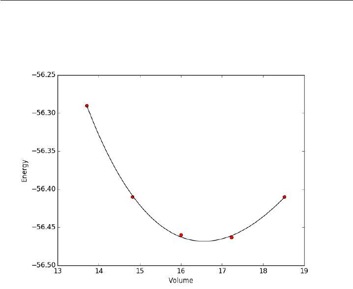
16 def objective(pars, y, x):
17 #we will minimize this function
18 err =y-Murnaghan(pars, x)
19 return err
20
21 x0 =[-56.0,0.54,2.0,16.5]#initial guess of parameters
22
23 plsq =leastsq(objective, x0, args=(energies, vols))
24
25 print(’Fitted parameters = {0}’.format(plsq[0]))
26
27 import matplotlib.pyplot as plt
28 plt.plot(vols,energies, ’ro’)
29
30 #plot the fitted curve on top
31 x=np.linspace(min(vols), max(vols), 50)
32 y=Murnaghan(plsq[0], x)
33 plt.plot(x, y, ’k-’)
34 plt.xlabel(’Volume’)
35 plt.ylabel(’Energy’)
36 plt.savefig(’images/nonlinear-curve-fitting.png’)
Fitted parameters = [-56.46839641 0.57233217 2.7407944 16.55905648]
Figure 1: Example of least-squares non-linear curve fitting.
146

See additional examples at http://docs.scipy.org/doc/scipy/reference/
tutorial/optimize.html.
7.6 Nonlinear curve fitting by direct least squares minimiza-
tion
Here is an example of fitting a nonlinear function to data by direct mini-
mization of the summed squared error.
1from scipy.optimize import fmin
2import numpy as np
3
4volumes =np.array([13.71,14.82,16.0,17.23,18.52])
5
6energies =np.array([-56.29,-56.41,-56.46,-56.463,-56.41])
7
8def Murnaghan(parameters,vol):
9’From PRB 28,5480 (1983’
10 E0 =parameters[0]
11 B0 =parameters[1]
12 BP =parameters[2]
13 V0 =parameters[3]
14
15 E=E0 +B0*vol/BP*(((V0/vol)**BP)/(BP-1)+1)-V0*B0/(BP-1.)
16
17 return E
18
19 def objective(pars,vol):
20 #we will minimize this function
21 err =energies -Murnaghan(pars,vol)
22 return np.sum(err**2)#we return the summed squared error directly
23
24 x0 =[-56.,0.54,2.,16.5]#initial guess of parameters
25
26 plsq =fmin(objective,x0,args=(volumes,)) #note args is a tuple
27
28 print(’parameters = {0}’.format(plsq))
29
30 import matplotlib.pyplot as plt
31 plt.plot(volumes,energies,’ro’)
32
33 #plot the fitted curve on top
34 x=np.linspace(min(volumes),max(volumes),50)
35 y=Murnaghan(plsq,x)
36 plt.plot(x,y,’k-’)
37 plt.xlabel(’Volume ($\AA^3$)’)
38 plt.ylabel(’Total energy (eV)’)
39 plt.savefig(’images/nonlinear-fitting-lsq.png’)
Optimization terminated successfully.
Current function value: 0.000020
147
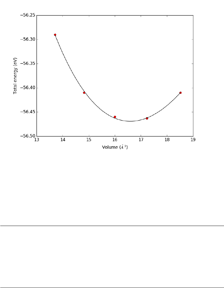
Iterations: 137
Function evaluations: 240
parameters = [-56.46932645 0.59141447 1.9044796 16.59341303]
Figure 2: Fitting a nonlinear function.
7.7 Parameter estimation by directly minimizing summed
squared errors
Matlab post
1import numpy as np
2import matplotlib.pyplot as plt
3
4x=np.array([0.0,1.1,2.3,3.1,4.05,6.0])
5y=np.array([0.0039,1.2270,5.7035,10.6472,18.6032,42.3024])
6
7plt.plot(x, y)
8plt.xlabel(’x’)
9plt.ylabel(’y’)
10 plt.savefig(’images/nonlin-minsse-1.png’)
148
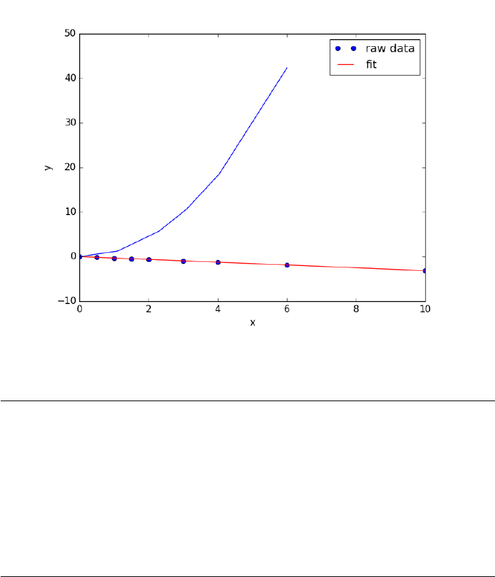
[<matplotlib.lines.Line2D object at 0x10d7a38d0>]
<matplotlib.text.Text object at 0x10b1bb7f0>
<matplotlib.text.Text object at 0x10b1cdeb8>
We are going to fit the function y=xato the data. The best awill
minimize the summed squared error between the model and the fit.
1def errfunc_(a):
2return np.sum((y -x**a)**2)
3
4errfunc =np.vectorize(errfunc_)
5
6arange =np.linspace(1,3)
7sse =errfunc(arange)
8
9plt.figure()
10 plt.plot(arange, sse)
11 plt.xlabel(’a’)
12 plt.ylabel(’$\Sigma (y - y_{pred})^2$’)
13 plt.savefig(’images/nonlin-minsse-2.png’)
<matplotlib.figure.Figure object at 0x10d851eb8>
[<matplotlib.lines.Line2D object at 0x10bc065c0>]
<matplotlib.text.Text object at 0x10b1c5d68>
<matplotlib.text.Text object at 0x10e57eb00>
149
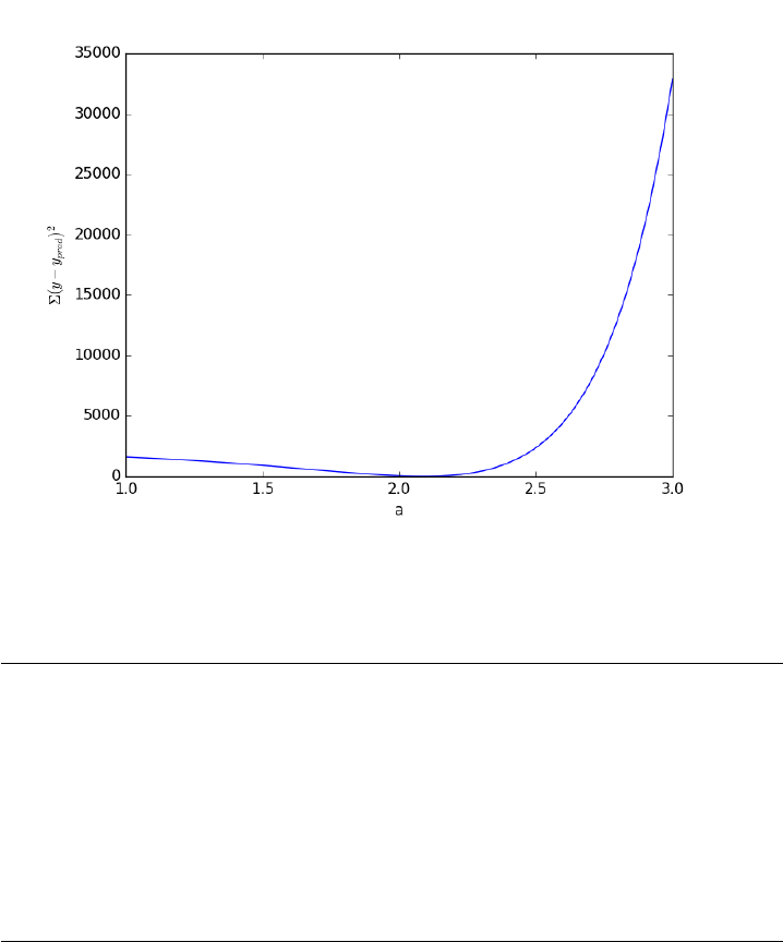
Based on the graph above, you can see a minimum in the summed
squared error near a= 2.1. We use that as our initial guess. Since we
know the answer is bounded, we use scipy.optimize.fminbound
1from scipy.optimize import fminbound
2
3amin =fminbound(errfunc, 1.0,3.0)
4
5print(amin)
6
7plt.figure()
8plt.plot(x, y, ’bo’, label=’data’)
9plt.plot(x, x**amin, ’r-’, label=’fit’)
10 plt.xlabel(’x’)
11 plt.ylabel(’y’)
12 plt.legend(loc=’best’)
13 plt.savefig(’images/nonlin-minsse-3.png’)
2.09004838933
<matplotlib.figure.Figure object at 0x110c47c50>
[<matplotlib.lines.Line2D object at 0x110f28080>]
[<matplotlib.lines.Line2D object at 0x110ecb198>]
<matplotlib.text.Text object at 0x110edbc88>
<matplotlib.text.Text object at 0x110ee3da0>
<matplotlib.legend.Legend object at 0x110f28320>
150
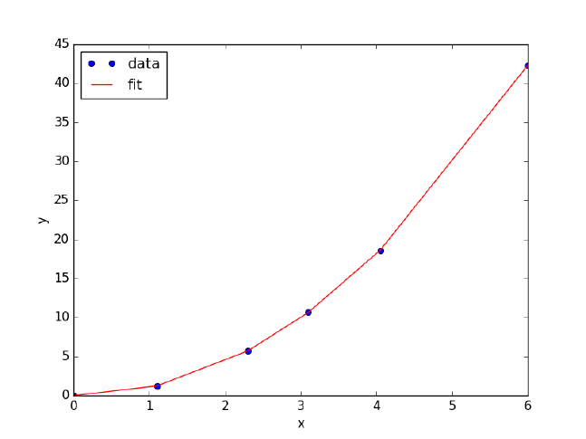
We can do nonlinear fitting by directly minimizing the summed squared
error between a model and data. This method lacks some of the features
of other methods, notably the simple ability to get the confidence interval.
However, this method is flexible and may offer more insight into how the
solution depends on the parameters.
7.8 Nonlinear curve fitting with parameter confidence inter-
vals
Matlab post
We often need to estimate parameters from nonlinear regression of data.
We should also consider how good the parameters are, and one way to do
that is to consider the confidence interval. A confidence interval tells us a
range that we are confident the true parameter lies in.
In this example we use a nonlinear curve-fitting function: scipy.optimize.curve_-
fit to give us the parameters in a function that we define which best fit the
data. The scipy.optimize.curve_fit function also gives us the covariance ma-
trix which we can use to estimate the standard error of each parameter.
Finally, we modify the standard error by a student-t value which accounts
for the additional uncertainty in our estimates due to the small number of
data points we are fitting to.
We will fit the function y=ax/(b+x)to some data, and compute the
151

95% confidence intervals on the parameters.
1# Nonlinear curve fit with confidence interval
2import numpy as np
3from scipy.optimize import curve_fit
4from scipy.stats.distributions import t
5
6x=np.array([0.5,0.387,0.24,0.136,0.04,0.011])
7y=np.array([1.255,1.25,1.189,1.124,0.783,0.402])
8
9# this is the function we want to fit to our data
10 def func(x, a, b):
11 ’nonlinear function in a and b to fit to data’
12 return a*x/(b +x)
13
14 initial_guess =[1.2,0.03]
15 pars, pcov =curve_fit(func, x, y, p0=initial_guess)
16
17 alpha = 0.05 # 95% confidence interval = 100*(1-alpha)
18
19 n=len(y) # number of data points
20 p=len(pars) # number of parameters
21
22 dof =max(0,n-p) # number of degrees of freedom
23
24 # student-t value for the dof and confidence level
25 tval =t.ppf(1.0-alpha/2., dof)
26
27 for i, p,var in zip(range(n), pars, np.diag(pcov)):
28 sigma =var**0.5
29 print(’p{0}: {1} [{2} {3}]’.format(i, p,
30 p-sigma*tval,
31 p+sigma*tval))
32
33 import matplotlib.pyplot as plt
34 plt.plot(x,y,’bo ’)
35 xfit =np.linspace(0,1)
36 yfit =func(xfit, pars[0], pars[1])
37 plt.plot(xfit,yfit,’b-’)
38
39 plt.legend([’data’,’fit’],loc=’best’)
40 plt.savefig(’images/nonlin-curve-fit-ci.png’)
p0: 1.3275314145379786 [1.3005365921998688 1.3545262368760884]
p1: 0.026461556970080666 [0.023607653829234403 0.02931546011092693]
152
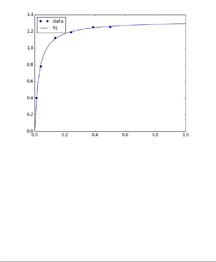
You can see by inspection that the fit looks pretty reasonable. The
parameter confidence intervals are not too big, so we can be pretty confident
of their values.
7.9 Nonlinear curve fitting with confidence intervals
Our goal is to fit this equation to data y=c1exp(−x) + c2∗xand compute
the confidence intervals on the parameters.
This is actually could be a linear regression problem, but it is convenient
to illustrate the use the nonlinear fitting routine because it makes it easy
to get confidence intervals for comparison. The basic idea is to use the
covariance matrix returned from the nonlinear fitting routine to estimate
the student-t corrected confidence interval.
1# Nonlinear curve fit with confidence interval
2import numpy as np
3from scipy.optimize import curve_fit
4from scipy.stats.distributions import t
5
6x=np.array([ 0.1,0.2,0.3,0.4,0.5,0.6,0.7,0.8,0.9,1. ])
7y=np.array([ 4.70192769,4.46826356,4.57021389,4.29240134,3.88155125,
83.78382253,3.65454727,3.86379487,4.16428541,4.06079909])
9
10 # this is the function we want to fit to our data
11 def func(x,c0, c1):
153

12 return c0 *np.exp(-x) +c1*x
13
14 pars, pcov =curve_fit(func, x, y, p0=[4.96,2.11])
15
16 alpha = 0.05 # 95% confidence interval
17
18 n=len(y) # number of data points
19 p=len(pars) # number of parameters
20
21 dof =max(0, n-p) # number of degrees of freedom
22
23 tval =t.ppf(1.0 - alpha / 2.0, dof) # student-t value for the dof and confidence level
24
25 for i, p,var in zip(range(n), pars, np.diag(pcov)):
26 sigma =var**0.5
27 print(’c{0}: {1} [{2} {3}]’.format(i, p,
28 p-sigma*tval,
29 p+sigma*tval))
30
31 import matplotlib.pyplot as plt
32 plt.plot(x,y,’bo ’)
33 xfit =np.linspace(0,1)
34 yfit =func(xfit, pars[0], pars[1])
35 plt.plot(xfit,yfit,’b-’)
36 plt.legend([’data’,’fit’],loc=’best’)
37 plt.savefig(’images/nonlin-fit-ci.png’)
c0: 4.967139664393268 [4.626744765672402 5.3075345631141335]
c1: 2.1099511262769086 [1.7671162242697824 2.452786028284035]
7.10 Graphical methods to help get initial guesses for mul-
tivariate nonlinear regression
Matlab post
Fit the model f(x1,x2; a,b) = a*x1 + x2ˆb to the data given below. This
model has two independent variables, and two parameters.
We want to do a nonlinear fit to find a and b that minimize the summed
squared errors between the model predictions and the data. With only
two variables, we can graph how the summed squared error varies with
the parameters, which may help us get initial guesses. Let us assume the
parameters lie in a range, here we choose 0 to 5. In other problems you
would adjust this as needed.
1import numpy as np
2from mpl_toolkits.mplot3d import Axes3D
3import matplotlib.pyplot as plt
4
5x1 =[1.0,2.0,3.0,4.0,5.0,6.0]
154
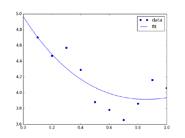
Figure 3: Nonlinear fit to data.
6x2 =[0.2,0.4,0.8,0.9,1.1,2.1]
7X=np.column_stack([x1, x2]) # independent variables
8
9f=[3.3079,6.6358,10.3143,13.6492,17.2755,23.6271]
10
11 fig =plt.figure()
12 ax =fig.gca(projection =’3d’)
13
14 ax.plot(x1, x2, f)
15 ax.set_xlabel(’x1’)
16 ax.set_ylabel(’x2’)
17 ax.set_zlabel(’f(x1,x2)’)
18
19 plt.savefig(’images/graphical-mulvar-1.png’)
20
21 arange =np.linspace(0,5);
22 brange =np.linspace(0,5);
23
24 A,B =np.meshgrid(arange, brange)
25
26 def model(X, a, b):
27 ’Nested function for the model’
28 x1 =X[:, 0]
29 x2 =X[:, 1]
30
31 f=a*x1 +x2**b
155

32 return f
33
34 @np.vectorize
35 def errfunc(a, b):
36 # function for the summed squared error
37 fit =model(X, a, b)
38 sse =np.sum((fit -f)**2)
39 return sse
40
41 SSE =errfunc(A, B)
42
43 plt.clf()
44 plt.contourf(A, B, SSE, 50)
45 plt.plot([3.2], [2.1], ’ro’)
46 plt.figtext( 3.4,2.2,’Minimum near here’, color=’r’)
47
48 plt.savefig(’images/graphical-mulvar-2.png’)
49
50 guesses =[3.18,2.02]
51
52 from scipy.optimize import curve_fit
53
54 popt, pcov =curve_fit(model, X, f, guesses)
55 print(popt)
56
57 plt.plot([popt[0]], [popt[1]], ’r*’)
58 plt.savefig(’images/graphical-mulvar-3.png’)
59
60 print(model(X, *popt))
61
62 fig =plt.figure()
63 ax =fig.gca(projection =’3d’)
64
65 ax.plot(x1, x2, f, ’ko’, label=’data’)
66 ax.plot(x1, x2, model(X, *popt), ’r-’, label=’fit’)
67 ax.set_xlabel(’x1’)
68 ax.set_ylabel(’x2’)
69 ax.set_zlabel(’f(x1,x2)’)
70
71 plt.savefig(’images/graphical-mulvar-4.png’)
[ 3.21694798 1.9728254 ]
[ 3.25873623 6.59792994 10.29473657 13.68011436 17.29161001
23.62366445]
156
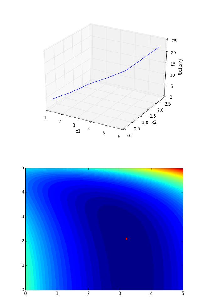
157
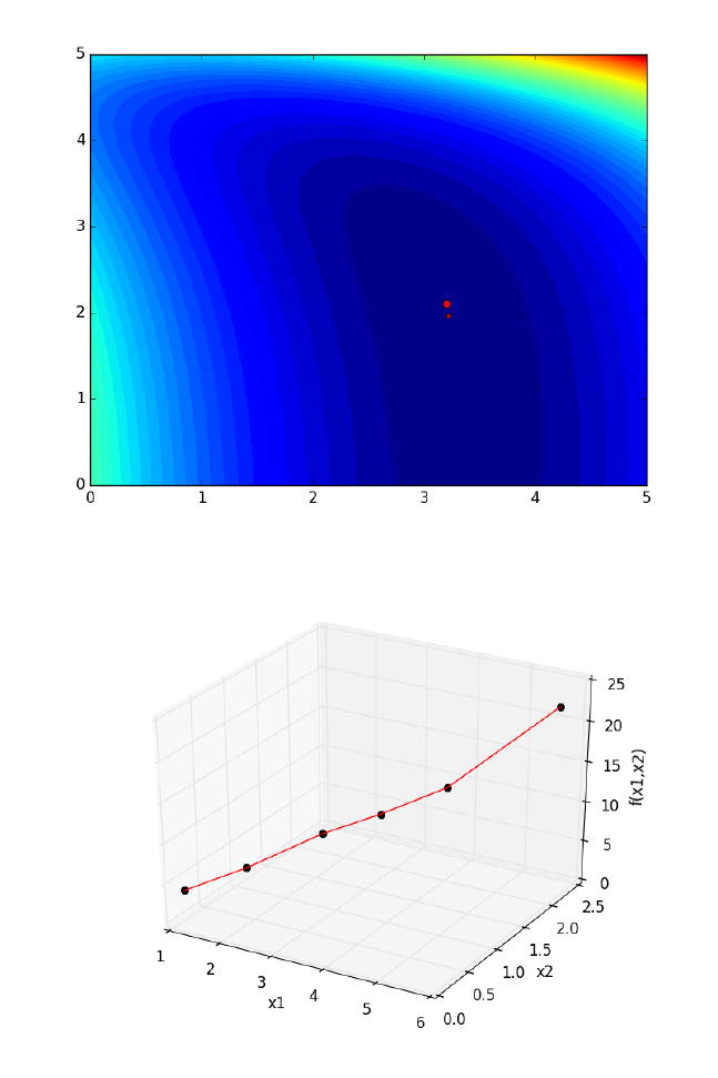
It can be difficult to figure out initial guesses for nonlinear fitting prob-
lems. For one and two dimensional systems, graphical techniques may be
useful to visualize how the summed squared error between the model and
data depends on the parameters.
158

7.11 Fitting a numerical ODE solution to data
Matlab post
Suppose we know the concentration of A follows this differential equa-
tion: dCA
dt =−kCA, and we have data we want to fit to it. Here is an
example of doing that.
1import numpy as np
2from scipy.optimize import curve_fit
3from scipy.integrate import odeint
4
5# given data we want to fit
6tspan =[0,0.1,0.2,0.4,0.8,1]
7Ca_data =[2.0081,1.5512,1.1903,0.7160,0.2562,0.1495]
8
9def fitfunc(t, k):
10 ’Function that returns Ca computed from an ODE for a k’
11 def myode(Ca, t):
12 return -k*Ca
13
14 Ca0 =Ca_data[0]
15 Casol =odeint(myode, Ca0, t)
16 return Casol[:,0]
17
18 k_fit, kcov =curve_fit(fitfunc, tspan, Ca_data, p0=1.3)
19 print(k_fit)
20
21 tfit =np.linspace(0,1);
22 fit =fitfunc(tfit, k_fit)
23
24 import matplotlib.pyplot as plt
25 plt.plot(tspan, Ca_data, ’ro’, label=’data’)
26 plt.plot(tfit, fit, ’b-’, label=’fit’)
27 plt.legend(loc=’best’)
28 plt.savefig(’images/ode-fit.png’)
[ 2.58893455]
159
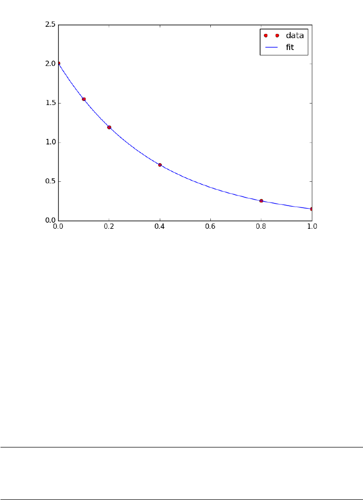
7.12 Reading in delimited text files
Matlab post
sometimes you will get data in a delimited text file format, .e.g. sepa-
rated by commas or tabs. Matlab can read these in easily. Suppose we have
a file containing this data:
1 3
3 4
5 6
4 8
It is easy to read this directly into variables like this:
1import numpy as np
2
3x,y =np.loadtxt(’data/testdata.txt’, unpack=True)
4
5print(x, y)
[ 1. 3. 5. 4.] [ 3. 4. 6. 8.]
160
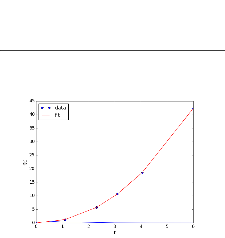
8 Interpolation
8.1 Better interpolate than never
Matlab post
We often have some data that we have obtained in the lab, and we want
to solve some problem using the data. For example, suppose we have this
data that describes the value of f at time t.
1import matplotlib.pyplot as plt
2
3t=[0.5,1,3,6]
4f=[0.6065,0.3679,0.0498,0.0025]
5plt.plot(t,f)
6plt.xlabel(’t’)
7plt.ylabel(’f(t)’)
8plt.savefig(’images/interpolate-1.png’)
[<matplotlib.lines.Line2D object at 0x110ecb358>]
<matplotlib.text.Text object at 0x110edbc88>
<matplotlib.text.Text object at 0x110ee3da0>
8.1.1 Estimate the value of f at t=2.
This is a simple interpolation problem.
161

1from scipy.interpolate import interp1d
2
3g=interp1d(t, f) # default is linear interpolation
4
5print(g(2))
6print(g([2,3,4]))
0.20885
[ 0.20885 0.0498 0.03403333]
The function we sample above is actually f(t) = exp(-t). The linearly
interpolated example is not too accurate.
1import numpy as np
2print(np.exp(-2))
0.135335283237
8.1.2 improved interpolation?
we can tell interp1d to use a different interpolation scheme such as cubic
polynomial splines like this. For nonlinear functions, this may improve the
accuracy of the interpolation, as it implicitly includes information about the
curvature by fitting a cubic polynomial over neighboring points.
1g2 =interp1d(t, f, ’cubic’)
2print(g2(2))
3print(g2([2,3,4]))
0.10848181818181851
[ 0.10848182 0.0498 0.08428727]
Interestingly, this is a different value than Matlab’s cubic interpolation.
Let us show the cubic spline fit.
1plt.figure()
2plt.plot(t, f)
3plt.xlabel(’t’)
4plt.ylabel(’f(t)’)
5
6x=np.linspace(0.5,6)
7fit =g2(x)
8plt.plot(x, fit, label=’fit’)
9plt.savefig(’images/interpolation-2.png’)
162
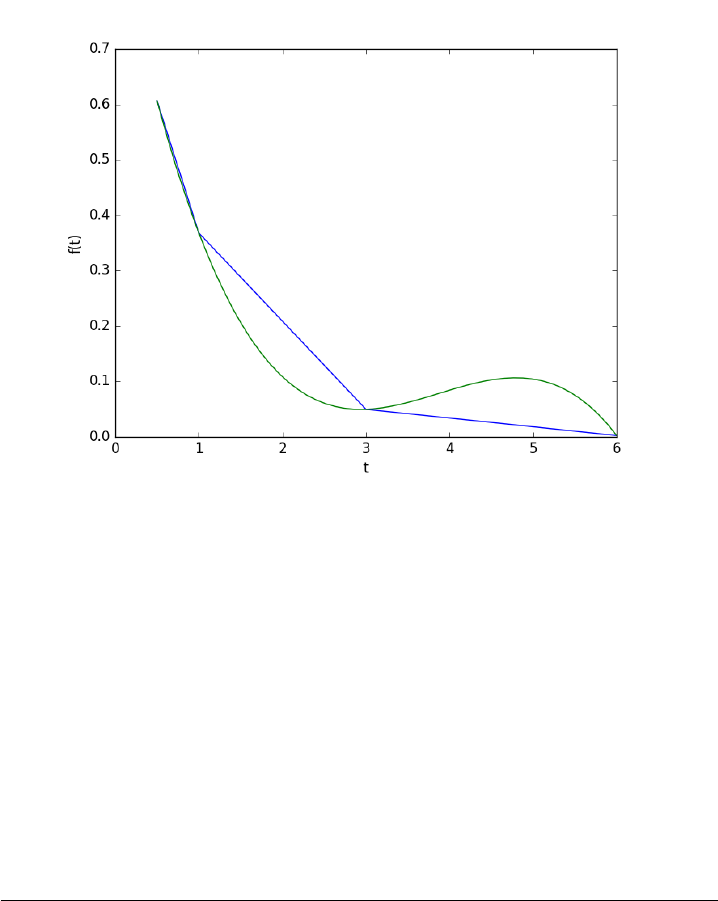
<matplotlib.figure.Figure object at 0x110ef9208>
[<matplotlib.lines.Line2D object at 0x1115bde10>]
<matplotlib.text.Text object at 0x1118dd5f8>
<matplotlib.text.Text object at 0x1118e4cc0>
[<matplotlib.lines.Line2D object at 0x1118d8240>]
Wow. That is a weird looking fit. Very different from what Matlab
produces. This is a good teaching moment not to rely blindly on interpola-
tion! We will rely on the linear interpolation from here out which behaves
predictably.
8.1.3 The inverse question
It is easy to interpolate a new value of f given a value of t. What if we want
to know the time that f=0.2? We can approach this a few ways.
method 1 We setup a function that we can use fsolve on. The function
will be equal to zero at the time. The second function will look like 0 = 0.2
- f(t). The answer for 0.2=exp(-t) is t = 1.6094. Since we use interpolation
here, we will get an approximate answer.
163

1from scipy.optimize import fsolve
2
3def func(t):
4return 0.2 - g(t)
5
6initial_guess = 2
7ans, =fsolve(func, initial_guess)
8print(ans)
2.0556428796
method 2: switch the interpolation order We can switch the order
of the interpolation to solve this problem. An issue we have to address
in this method is that the "x" values must be monotonically increasing.
It is somewhat subtle to reverse a list in python. I will use the cryptic
syntax of [::-1] instead of the list.reverse() function or reversed() function.
list.reverse() actually reverses the list "in place", which changes the contents
of the variable. That is not what I want. reversed() returns an iterator
which is also not what I want. [::-1] is a fancy indexing trick that returns a
reversed list.
1g3 =interp1d(f[::-1], t[::-1])
2
3print(g3(0.2))
2.055642879597611
8.1.4 A harder problem
Suppose we want to know at what time is 1/f = 100? Now we have to decide
what do we interpolate: f(t) or 1/f(t). Let us look at both ways and decide
what is best. The answer to 1/exp(−t) = 100 is 4.6052
interpolate on f(t) then invert the interpolated number
1def func(t):
2’objective function. we do some error bounds because we cannot interpolate out of the range.’
3if t< 0.5: t=0.5
4if t> 6: t = 6
5return 100 - 1.0 / g(t)
6
7initial_guess = 4.5
8a1, =fsolve(func, initial_guess)
9print(a1)
10 print(’The %error is {0:%}’.format((a1 - 4.6052)/4.6052))
164

5.52431289641
The %error is 19.958154%
invert f(t) then interpolate on 1/f
1ig =interp1d(t, 1.0 / np.array(f))
2
3def ifunc(t):
4if t< 0.5:
5t=0.5
6elif t> 6:
7t= 6
8return 100 - ig(t)
9
10 initial_guess = 4.5
11 a2, =fsolve(ifunc, initial_guess)
12 print(a2)
13 print(’The %error is {0:%}’.format((a2 - 4.6052)/4.6052))
3.6310782241
The %error is -21.152649%
8.1.5 Discussion
In this case you get different errors, one overestimates and one underesti-
mates the answer, and by a lot: ±20%. Let us look at what is happening.
1import matplotlib.pyplot as plt
2import numpy as np
3from scipy.interpolate import interp1d
4
5t=[0.5,1,3,6]
6f=[0.6065,0.3679,0.0498,0.0025]
7
8x=np.linspace(0.5,6)
9
10
11 g=interp1d(t, f) # default is linear interpolation
12 ig =interp1d(t, 1.0 / np.array(f))
13
14 plt.figure()
15 plt.plot(t, 1/np.array(f), ’ko ’, label=’data’)
16 plt.plot(x, 1/g(x), label=’1/interpolated f(x)’)
17 plt.plot(x, ig(x), label=’interpolate on 1/f(x)’)
18 plt.plot(x, 1/np.exp(-x), ’k--’, label=’1/exp(-x)’)
19 plt.xlabel(’t’)
20 plt.ylabel(’1/f(t)’)
21 plt.legend(loc=’best’)
22 plt.savefig(’images/interpolation-3.png’)
165
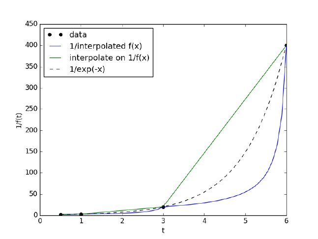
<matplotlib.figure.Figure object at 0x1115c3860>
[<matplotlib.lines.Line2D object at 0x111629400>]
[<matplotlib.lines.Line2D object at 0x1115d47b8>]
[<matplotlib.lines.Line2D object at 0x111629e48>]
[<matplotlib.lines.Line2D object at 0x111910668>]
<matplotlib.text.Text object at 0x1118f2780>
<matplotlib.text.Text object at 0x1118ed2b0>
<matplotlib.legend.Legend object at 0x111915588>
You can see that the 1/interpolated f(x) underestimates the value, while
interpolated (1/f(x)) overestimates the value. This is an example of where
you clearly need more data in that range to make good estimates. Neither
interpolation method is doing a great job. The trouble in reality is that you
often do not know the real function to do this analysis. Here you can say the
time is probably between 3.6 and 5.5 where 1/f(t) = 100, but you can not
read much more than that into it. If you need a more precise answer, you
need better data, or you need to use an approach other than interpolation.
For example, you could fit an exponential function to the data and use that
to estimate values at other times.
So which is the best to interpolate? I think you should interpolate the
quantity that is linear in the problem you want to solve, so in this case I
think interpolating 1/f(x) is better. When you use an interpolated function
166

in a nonlinear function, strange, unintuitive things can happen. That is why
the blue curve looks odd. Between data points are linear segments in the
original interpolation, but when you invert them, you cause the curvature
to form.
8.2 Interpolation of data
Matlab post
When we have data at two points but we need data in between them we
use interpolation. Suppose we have the points (4,3) and (6,2) and we want
to know the value of y at x=4.65, assuming y varies linearly between these
points. we use the interp1d command to achieve this. The syntax in python
is slightly different than in matlab.
1from scipy.interpolate import interp1d
2
3x=[4,6]
4y=[3,2]
5
6ifunc =interp1d(x, y)
7
8print(ifunc(4.65))
9
10
11 ifunc =interp1d(x, y, bounds_error=False)# do not raise error on out of bounds
12 print(ifunc([4.65,5.01,4.2,9]))
2.675
[ 2.675 2.495 2.9 nan]
The default interpolation method is simple linear interpolation between
points. Other methods exist too, such as fitting a cubic spline to the data
and using the spline representation to interpolate from.
1from scipy.interpolate import interp1d
2
3x=[1,2,3,4];
4y=[1,4,9,16]; # y = x^2
5
6xi =[1.5,2.5,3.5]; # we want to interpolate on these values
7y1 =interp1d(x,y)
8
9print(y1(xi))
10
11 y2 =interp1d(x,y,’cubic’)
12 print(y2(xi))
13
167

14 import numpy as np
15 print(np.array(xi)**2)
[ 2.5 6.5 12.5]
[ 2.25 6.25 12.25]
[ 2.25 6.25 12.25]
In this case the cubic spline interpolation is more accurate than the
linear interpolation. That is because the underlying data was polynomial in
nature, and a spline is like a polynomial. That may not always be the case,
and you need some engineering judgement to know which method is best.
8.3 Interpolation with splines
When you do not know the functional form of data to fit an equation, you
can still fit/interpolate with splines.
1# use splines to fit and interpolate data
2from scipy.interpolate import interp1d
3from scipy.optimize import fmin
4import numpy as np
5import matplotlib.pyplot as plt
6
7x=np.array([ 0,1,2,3,4])
8y=np.array([ 0.,0.308,0.55,0.546,0.44 ])
9
10 # create the interpolating function
11 f=interp1d(x, y, kind=’cubic’, bounds_error=False)
12
13 # to find the maximum, we minimize the negative of the function. We
14 # cannot just multiply f by -1, so we create a new function here.
15 f2 =interp1d(x, -y, kind=’cubic’)
16 xmax =fmin(f2, 2.5)
17
18 xfit =np.linspace(0,4)
19
20 plt.plot(x,y,’bo’)
21 plt.plot(xfit, f(xfit),’r-’)
22 plt.plot(xmax, f(xmax),’g*’)
23 plt.legend([’data’,’fit’,’max’], loc=’best’, numpoints=1)
24 plt.xlabel(’x data’)
25 plt.ylabel(’y data’)
26 plt.title(’Max point = ({0:1.2f}, {1:1.2f})’.format(float(xmax),
27 float(f(xmax))))
28 plt.savefig(’images/splinefit.png’)
Optimization terminated successfully.
Current function value: -0.575712
168
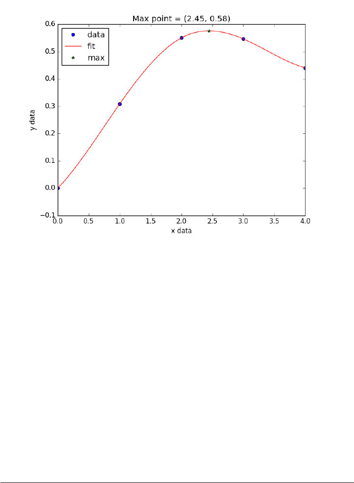
Iterations: 12
Function evaluations: 24
Figure 4: Illustration of a spline fit to data and finding the maximum point.
There are other good examples at http://docs.scipy.org/doc/scipy/
reference/tutorial/interpolate.html
9 Optimization
9.1 Constrained optimization
Matlab post
adapted from http://en.wikipedia.org/wiki/Lagrange_multipliers.
Suppose we seek to minimize the function f(x, y) = x+ysubject to
the constraint that x2+y2= 1. The function we seek to maximize is an
unbounded plane, while the constraint is a unit circle. We could setup a
Lagrange multiplier approach to solving this problem, but we will use a
constrained optimization approach instead.
169

1from scipy.optimize import fmin_slsqp
2
3def objective(X):
4x,y=X
5return x+y
6
7def eqc(X):
8’equality constraint’
9x,y=X
10 return x**2 + y**2 - 1.0
11
12 X0 =[-1,-1]
13 X=fmin_slsqp(objective, X0, eqcons=[eqc])
14 print(X)
Optimization terminated successfully. (Exit mode 0)
Current function value: -1.41421356237
Iterations: 5
Function evaluations: 20
Gradient evaluations: 5
[-0.70710678 -0.70710678]
9.2 Finding the maximum power of a photovoltaic device.
A photovoltaic device is characterized by a current-voltage relationship. Let
us say, for argument’s sake, that the relationship is known and defined by
i= 0.5−0.5∗V2
The voltage is highest when the current is equal to zero, but of course
then you get no power. The current is highest when the voltage is zero,
i.e. short-circuited, but there is again no power. We seek the highest power
condition, which is to find the maximum of iV . This is a constrained op-
timization. We solve it by creating an objective function that returns the
negative of (ıV\), and then find the minimum.
First, let us examine the i-V relationship.
1import matplotlib.pyplot as plt
2import numpy as np
3
4V=np.linspace(0,1)
5
6def i(V):
7return 0.5 - 0.5 * V**2
8
9plt.figure()
10 plt.plot(V, i(V))
11 plt.savefig(’images/iV.png’)
170
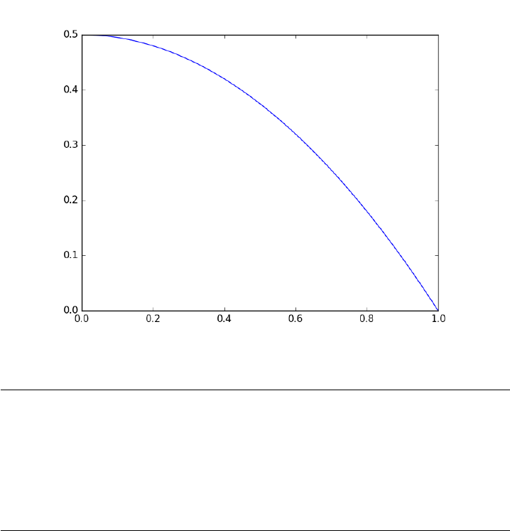
<matplotlib.figure.Figure object at 0x11193ec18>
[<matplotlib.lines.Line2D object at 0x111d43668>]
Now, let us be sure there is a maximum in power.
1import matplotlib.pyplot as plt
2import numpy as np
3
4V=np.linspace(0,1)
5
6def i(V):
7return 0.5 - 0.5 * V**2
8
9plt.plot(V, i(V) *V)
10 plt.savefig(’images/P1.png’)
[<matplotlib.lines.Line2D object at 0x111d437f0>]
171
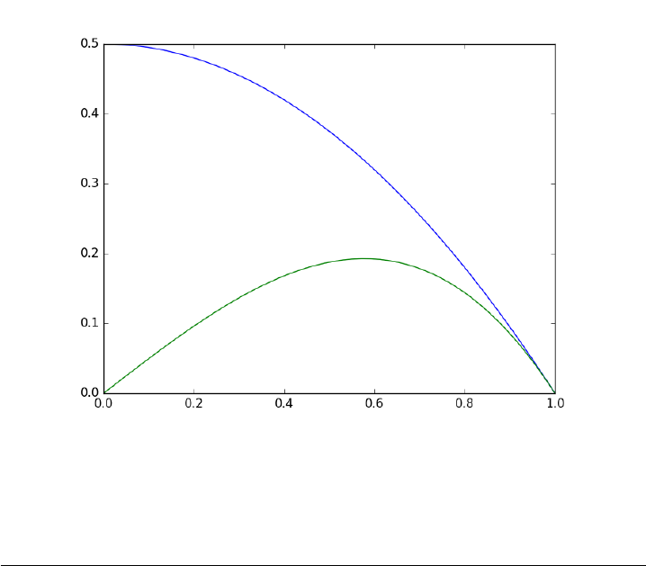
You can see in fact there is a maximum, near V=0.6. We could solve
this problem analytically by taking the appropriate derivative and solving
it for zero. That still might require solving a nonlinear problem though. We
will directly setup and solve the constrained optimization.
1from scipy.optimize import fmin_slsqp
2import numpy as np
3import matplotlib.pyplot as plt
4
5def objective(X):
6i,V=X
7return -i*V
8
9def eqc(X):
10 ’equality constraint’
11 i,V=X
12 return (0.5 - 0.5 * V**2)-i
13
14 X0 =[0.2,0.6]
15 X=fmin_slsqp(objective, X0, eqcons=[eqc])
16
17 imax, Vmax =X
18
19
20 V=np.linspace(0,1)
21
22 def i(V):
23 return 0.5 - 0.5 * V**2
24
172
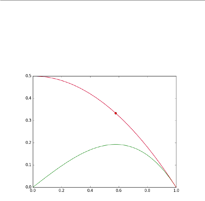
25 plt.plot(V, i(V), Vmax, imax, ’ro’)
26 plt.savefig(’images/P2.png’)
Optimization terminated successfully. (Exit mode 0)
Current function value: -0.192450127337
Iterations: 5
Function evaluations: 20
Gradient evaluations: 5
[<matplotlib.lines.Line2D object at 0x111946470>, <matplotlib.lines.Line2D object at 0x11192c518>]
You can see the maximum power is approximately 0.2 (unspecified units),
at the conditions indicated by the red dot in the figure above.
9.3 Using Lagrange multipliers in optimization
Matlab post (adapted from http://en.wikipedia.org/wiki/Lagrange_
multipliers.)
Suppose we seek to maximize the function f(x, y) = x+ysubject to
the constraint that x2+y2= 1. The function we seek to maximize is
an unbounded plane, while the constraint is a unit circle. We want the
maximum value of the circle, on the plane. We plot these two functions
here.
173
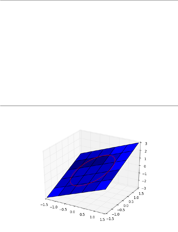
1import numpy as np
2
3x=np.linspace(-1.5,1.5)
4
5[X, Y] =np.meshgrid(x, x)
6
7import matplotlib as mpl
8from mpl_toolkits.mplot3d import Axes3D
9import matplotlib.pyplot as plt
10
11 fig =plt.figure()
12 ax =fig.gca(projection=’3d’)
13
14 ax.plot_surface(X, Y, X +Y)
15
16 theta =np.linspace(0,2*np.pi);
17 R= 1.0
18 x1 =R*np.cos(theta)
19 y1 =R*np.sin(theta)
20
21 ax.plot(x1, y1, x1 +y1, ’r-’)
22 plt.savefig(’images/lagrange-1.png’)
9.3.1 Construct the Lagrange multiplier augmented function
To find the maximum, we construct the following function: Λ(x, y;λ) =
f(x, y) + λg(x, y)where g(x, y) = x2+y2−1 = 0, which is the constraint
174

function. Since g(x, y)=0, we are not really changing the original function,
provided that the constraint is met!
1import numpy as np
2
3def func(X):
4x=X[0]
5y=X[1]
6L=X[2]# this is the multiplier. lambda is a reserved keyword in python
7return x+y+L*(x**2 + y**2 - 1)
9.3.2 Finding the partial derivatives
The minima/maxima of the augmented function are located where all of
the partial derivatives of the augmented function are equal to zero, i.e.
∂Λ/∂x = 0,∂Λ/∂y = 0, and ∂Λ/∂λ = 0. the process for solving this is
usually to analytically evaluate the partial derivatives, and then solve the
unconstrained resulting equations, which may be nonlinear.
Rather than perform the analytical differentiation, here we develop a
way to numerically approximate the partial derivatives.
1def dfunc(X):
2dLambda =np.zeros(len(X))
3h= 1e-3 # this is the step size used in the finite difference.
4for iin range(len(X)):
5dX =np.zeros(len(X))
6dX[i] =h
7dLambda[i] =(func(X+dX)-func(X-dX))/(2*h);
8return dLambda
9.3.3 Now we solve for the zeros in the partial derivatives
The function we defined above (dfunc) will equal zero at a maximum or
minimum. It turns out there are two solutions to this problem, but only
one of them is the maximum value. Which solution you get depends on the
initial guess provided to the solver. Here we have to use some judgement to
identify the maximum.
1from scipy.optimize import fsolve
2
3# this is the max
4X1 =fsolve(dfunc, [1,1,0])
5print(X1, func(X1))
6
7# this is the min
175

8X2 =fsolve(dfunc, [-1,-1,0])
9print(X2, func(X2))
[ 0.70710678 0.70710678 -0.70710678] 1.41421356237
[-0.70710678 -0.70710678 0.70710678] -1.41421356237
9.3.4 Summary
Three dimensional plots in matplotlib are a little more difficult than in Mat-
lab (where the code is almost the same as 2D plots, just different commands,
e.g. plot vs plot3). In Matplotlib you have to import additional modules in
the right order, and use the object oriented approach to plotting as shown
here.
9.4 Linear programming example with inequality constraints
Matlab post
adapted from http://www.matrixlab-examples.com/linear-programming.
html which solves this problem with fminsearch.
Let us suppose that a merry farmer has 75 roods (4 roods = 1 acre)
on which to plant two crops: wheat and corn. To produce these crops, it
costs the farmer (for seed, water, fertilizer, etc. ) $120 per rood for the
wheat, and $210 per rood for the corn. The farmer has $15,000 available
for expenses, but after the harvest the farmer must store the crops while
awaiting favorable or good market conditions. The farmer has storage space
for 4,000 bushels. Each rood yields an average of 110 bushels of wheat or 30
bushels of corn. If the net profit per bushel of wheat (after all the expenses)
is $1.30 and for corn is $2.00, how should the merry farmer plant the 75
roods to maximize profit?
Let xbe the number of roods of wheat planted, and ybe the number of
roods of corn planted. The profit function is: P= (110)(1.3)x + (30)(2)y=
143x+ 60y
There are some constraint inequalities, specified by the limits on ex-
penses, storage and roodage. They are:
$120x+ $210y <= $15000 (The total amount spent cannot exceed the
amount the farm has)
110x+ 30y <= 4000 (The amount generated should not exceed storage
space.)
x+y <= 75 (We cannot plant more space than we have.)
0<=xand0<=y(all amounts of planted land must be positive.)
176

To solve this problem, we cast it as a linear programming problem, which
minimizes a function f(X) subject to some constraints. We create a proxy
function for the negative of profit, which we seek to minimize.
f = -(143*x + 60*y)
1from scipy.optimize import fmin_cobyla
2
3def objective(X):
4’’’objective function to minimize. It is the negative of profit,
5which we seek to maximize.’’’
6x,y=X
7return -(143*x+ 60*y)
8
9def c1(X):
10 ’Ensure 120x + 210y <= 15000’
11 x,y =X
12 return 15000 - 120 * x- 210*y
13
14 def c2(X):
15 ’ensure 110x + 30y <= 4000’
16 x,y =X
17 return 4000 - 110*x- 30 * y
18
19 def c3(X):
20 ’Ensure x + y is less than or equal to 75’
21 x,y =X
22 return 75-x-y
23
24 def c4(X):
25 ’Ensure x >= 0’
26 return X[0]
27
28 def c5(X):
29 ’Ensure y >= 0’
30 return X[1]
31
32 X=fmin_cobyla(objective, x0=[20,30], cons=[c1, c2, c3, c4, c5])
33
34 print(’We should plant {0:1.2f} roods of wheat.’.format(X[0]))
35 print(’We should plant {0:1.2f} roods of corn’.format(X[1]))
36 print(’The maximum profit we can earn is ${0:1.2f}.’.format(-objective(X)))
We should plant 21.88 roods of wheat.
We should plant 53.12 roods of corn
The maximum profit we can earn is $6315.62.
Normal return from subroutine COBYLA
NFVALS = 40 F =-6.315625E+03 MAXCV = 4.547474E-13
X = 2.187500E+01 5.312500E+01
177

This code is not exactly the same as the original post, but we get to
the same answer. The linear programming capability in scipy is currently
somewhat limited in 0.10. It is a little better in 0.11, but probably not as
advanced as Matlab. There are some external libraries available:
1. http://abel.ee.ucla.edu/cvxopt/
2. http://openopt.org/LP
9.5 Find the minimum distance from a point to a curve.
A problem that can be cast as a constrained minimization problem is to find
the minimum distance from a point to a curve. Suppose we have f(x) = x2,
and the point (0.5, 2). what is the minimum distance from that point to
f(x)?
1import numpy as np
2import matplotlib.pyplot as plt
3from scipy.optimize import fmin_cobyla
4
5P=(0.5,2)
6
7def f(x):
8return x**2
9
10 def objective(X):
11 x,y =X
12 return np.sqrt((x -P[0])**2 + (y -P[1])**2)
13
14 def c1(X):
15 x,y =X
16 return f(x) -y
17
18 X=fmin_cobyla(objective, x0=[0.5,0.5], cons=[c1])
19
20 print(’The minimum distance is {0:1.2f}’.format(objective(X)))
21
22 # Verify the vector to this point is normal to the tangent of the curve
23 # position vector from curve to point
24 v1 =np.array(P) -np.array(X)
25 # position vector
26 v2 =np.array([1,2.0 * X[0]])
27 print(’dot(v1, v2) = ’,np.dot(v1, v2))
28
29 x=np.linspace(-2,2,100)
30
31 plt.plot(x, f(x), ’r-’, label=’f(x)’)
32 plt.plot(P[0], P[1], ’bo’, label=’point’)
33 plt.plot([P[0], X[0]], [P[1], X[1]], ’b-’, label=’shortest distance’)
34 plt.plot([X[0], X[0]+ 1], [X[1], X[1]+2.0*X[0]], ’g-’, label=’tangent’)
35 plt.axis(’equal’)
178
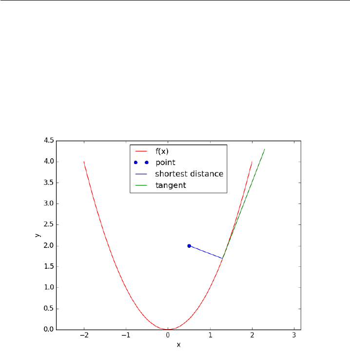
36 plt.xlabel(’x’)
37 plt.ylabel(’y’)
38 plt.legend(loc=’best’)
39 plt.savefig(’images/min-dist-p-func.png’)
The minimum distance is 0.86
dot(v1, v2) = 0.000336477214214
Normal return from subroutine COBYLA
NFVALS = 44 F = 8.579598E-01 MAXCV = 0.000000E+00
X = 1.300793E+00 1.692061E+00
In the code above, we demonstrate that the point we find on the curve
that minimizes the distance satisfies the property that a vector from that
point to our other point is normal to the tangent of the curve at that point.
This is shown by the fact that the dot product of the two vectors is very
close to zero. It is not zero because of the accuracy criteria that is used to
stop the minimization is not high enough.
179

10 Differential equations
The key to successfully solving many differential equations is correctly clas-
sifying the equations, putting them into a standard form and then picking
the appropriate solver. You must be able to determine if an equation is:
•An ordinary differential equation Y0=f(x, Y )with
–initial values (good support in python/numpy/scipy)
–boundary values (not difficult to write code for simple cases)
•Delay differential equation
•Differential algebraic equations
•A partial differential equation
The following sections will illustrate the methods for solving these kinds
of equations.
10.1 Ordinary differential equations
10.1.1 Numerical solution to a simple ode
Matlab post
Integrate this ordinary differential equation (ode):
dy
dt =y(t)
over the time span of 0 to 2. The initial condition is y(0) = 1.
to solve this equation, you need to create a function of the form: dydt
= f(y, t) and then use one of the odesolvers, e.g. odeint.
1import numpy as np
2from scipy.integrate import odeint
3import matplotlib.pyplot as plt
4
5def fprime(y,t):
6return y
7
8tspan =np.linspace(0,25)
9y0 = 1
10 ysol =odeint(fprime, y0, tspan)
11 plt.figure(figsize=(4,3))
12 plt.plot(tspan, ysol, label=’numerical solution’)
13 plt.plot(tspan, np.exp(tspan), ’r--’, label=’analytical solution’)
180
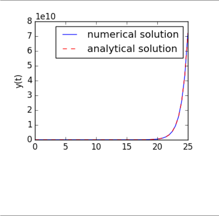
14 plt.xlabel(’time’)
15 plt.ylabel(’y(t)’)
16 plt.legend(loc=’best’)
17 plt.savefig(’images/simple-ode.png’)
The numerical and analytical solutions agree.
Now, suppose you want to know at what time is the solution equal to 3?
There are several approaches to this, including setting up a solver, or using
an event like approach to stop integration at y=3. A simple approach is to
use reverse interpolation. We simply reverse the x and y vectors so that y
is the independent variable, and we interpolate the corresponding x-value.
1import numpy as np
2from scipy.integrate import odeint
3import matplotlib.pyplot as plt
4
5def fprime(y,t):
6return y
7
8tspan =np.linspace(0,2)
9y0 = 1
10 ysol =odeint(fprime, y0, tspan)
11
12 from scipy.interpolate import interp1d
13
14 ip =interp1d(ysol[:,0], tspan) # reverse interpolation
15 print(’y = 3 at x = {0}’.format(ip(3)))
181

y = 3 at x = 1.098547805640928
10.1.2 Plotting ODE solutions in cylindrical coordinates
Matlab post
It is straightforward to plot functions in Cartesian coordinates. It is
less convenient to plot them in cylindrical coordinates. Here we solve an
ODE in cylindrical coordinates, and then convert the solution to Cartesian
coordinates for simple plotting.
1import numpy as np
2from scipy.integrate import odeint
3
4def dfdt(F, t):
5rho, theta, z =F
6drhodt = 0 # constant radius
7dthetadt = 1 # constant angular velocity
8dzdt = -1 # constant dropping velocity
9return [drhodt, dthetadt, dzdt]
10
11 # initial conditions
12 rho0 = 1
13 theta0 = 0
14 z0 = 100
15
16 tspan =np.linspace(0,50,500)
17 sol =odeint(dfdt, [rho0, theta0, z0], tspan)
18
19 rho =sol[:,0]
20 theta =sol[:,1]
21 z=sol[:,2]
22
23 # convert cylindrical coords to cartesian for plotting.
24 X=rho *np.cos(theta)
25 Y=rho *np.sin(theta)
26
27 from mpl_toolkits.mplot3d import Axes3D
28 import matplotlib.pyplot as plt
29 fig =plt.figure()
30 ax =fig.gca(projection=’3d’)
31 ax.plot(X, Y, z)
32 plt.savefig(’images/ode-cylindrical.png’)
182
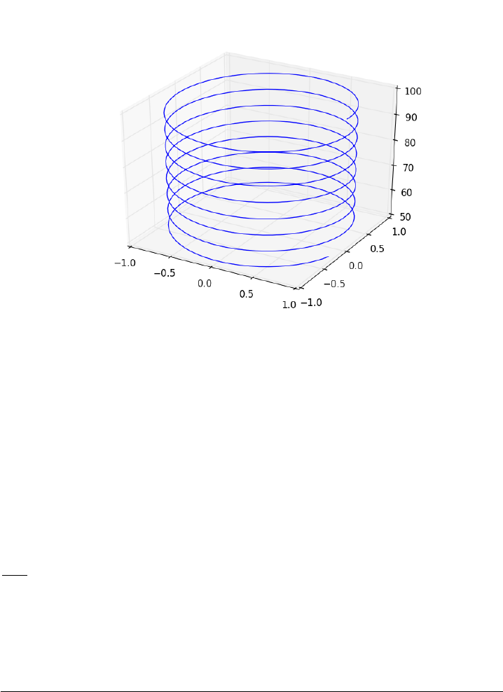
10.1.3 ODEs with discontinuous forcing functions
Matlab post
Adapted from http://archives.math.utk.edu/ICTCM/VOL18/S046/paper.
pdf
A mixing tank initially contains 300 g of salt mixed into 1000 L of water.
At t=0 min, a solution of 4 g/L salt enters the tank at 6 L/min. At t=10
min, the solution is changed to 2 g/L salt, still entering at 6 L/min. The
tank is well stirred, and the tank solution leaves at a rate of 6 L/min. Plot
the concentration of salt (g/L) in the tank as a function of time.
A mass balance on the salt in the tank leads to this differential equation:
dMS
dt =νCS,in(t)−νMS/V with the initial condition that MS(t= 0) = 300.
The wrinkle is that the inlet conditions are not constant.
CS,in(t) =
0t≤0,
4 0 < t ≤10,
2t > 10.
1import numpy as np
2from scipy.integrate import odeint
3import matplotlib.pyplot as plt
4
5V= 1000.0 # L
183
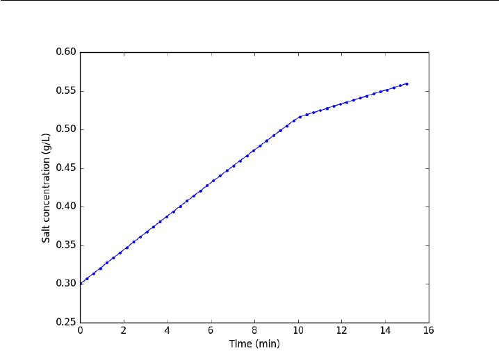
6nu = 6.0 # L/min
7
8def Cs_in(t):
9’inlet concentration’
10 if t< 0:
11 Cs = 0.0 # g/L
12 elif (t > 0)and (t <= 10):
13 Cs = 4.0
14 else:
15 Cs = 2.0
16 return Cs
17
18 def mass_balance(Ms, t):
19 ’$\frac{dM_S}{dt} = \nu C_{S,in}(t) - \nu M_S/V$’
20 dMsdt =nu *Cs_in(t) -nu *Ms /V
21 return dMsdt
22
23 tspan =np.linspace(0.0,15.0,50)
24
25 M0 = 300.0 # gm salt
26 Ms =odeint(mass_balance, M0, tspan)
27
28 plt.plot(tspan, Ms/V, ’b.-’)
29 plt.xlabel(’Time (min)’)
30 plt.ylabel(’Salt concentration (g/L)’)
31 plt.savefig(’images/ode-discont.png’)
You can see the discontinuity in the salt concentration at 10 minutes due
to the discontinous change in the entering salt concentration.
184

10.1.4 Simulating the events feature of Matlab’s ode solvers
The ode solvers in Matlab allow you create functions that define events that
can stop the integration, detect roots, etc. . . We will explore how to get a
similar effect in python. Here is an example that somewhat does this, but it
is only an approximation. We will manually integrate the ODE, adjusting
the time step in each iteration to zero in on the solution. When the desired
accuracy is reached, we stop the integration.
It does not appear that events are supported in scipy. A solution is at
http://mail.scipy.org/pipermail/scipy-dev/2005-July/003078.html,
but it does not appear integrated into scipy yet (8 years later ;).
1import numpy as np
2from scipy.integrate import odeint
3
4def dCadt(Ca, t):
5"the ode function"
6k= 0.23
7return -k*Ca**2
8
9Ca0 = 2.3
10
11 # create lists to store time span and solution
12 tspan =[0, ]
13 sol =[Ca0,]
14 i= 0
15
16 while i< 100:# take max of 100 steps
17 t1 =tspan[i]
18 Ca =sol[i]
19
20 # pick the next time using a Newton-Raphson method
21 # we want f(t, Ca) = (Ca(t) - 1)**2 = 0
22 # df/dt = df/dCa dCa/dt
23 # = 2*(Ca - 1) * dCadt
24 t2 =t1 -(Ca - 1.0)**2 / (2*(Ca - 1)*dCadt(Ca, t1))
25
26 f=odeint(dCadt, Ca, [t1, t2])
27
28 if np.abs(Ca - 1.0)<= 1e-4:
29 print(’Solution reached at i = {0}’.format(i))
30 break
31
32 tspan += [t2]
33 sol.append(f[-1][0])
34 i+= 1
35
36 print(’At t={0:1.2f} Ca = {1:1.3f}’.format(tspan[-1], sol[-1]))
37
38 import matplotlib.pyplot as plt
39 plt.plot(tspan, sol, ’bo’)
40 plt.savefig(’images/event-i.png’)
185
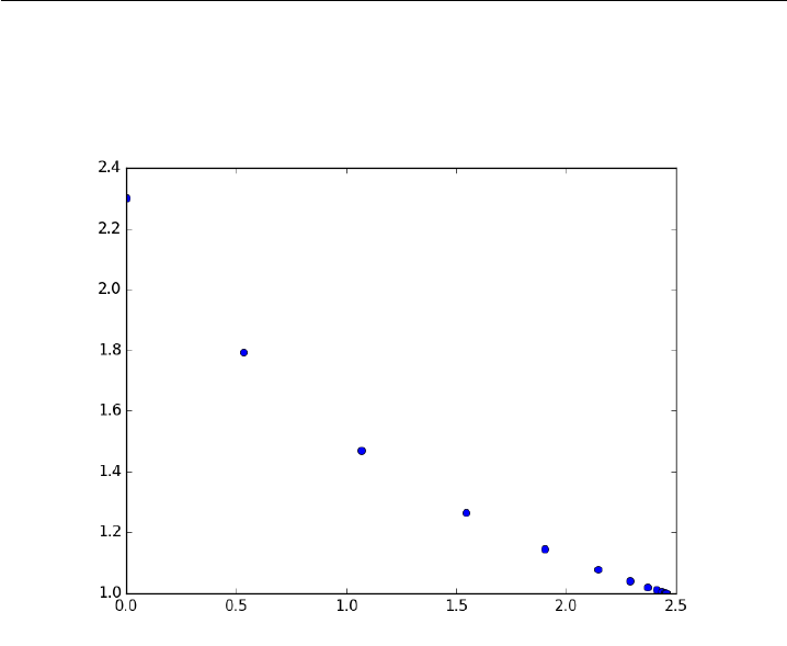
Solution reached at i = 15
At t=2.46 Ca = 1.000
This particular solution works for this example, probably because it is
well behaved. It is "downhill" to the desired solution. It is not obvious this
would work for every example, and it is certainly possible the algorithm
could go "backward" in time. A better approach might be to integrate
forward until you detect a sign change in your event function, and then
refine it in a separate loop.
I like the events integration in Matlab better, but this is actually pretty
functional. It should not be too hard to use this for root counting, e.g. by
counting sign changes. It would be considerably harder to get the actual
roots. It might also be hard to get the positions of events that include the
sign or value of the derivatives at the event points.
ODE solving in Matlab is considerably more advanced in functionality
than in scipy. There do seem to be some extra packages, e.g. pydstools,
scikits.odes that add extra ode functionality.
186

10.1.5 Mimicking ode events in python
The ODE functions in scipy.integrate do not directly support events like the
functions in Matlab do. We can achieve something like it though, by digging
into the guts of the solver, and writing a little code. In previous example I
used an event to count the number of roots in a function by integrating the
derivative of the function.
1import numpy as np
2from scipy.integrate import odeint
3
4def myode(f, x):
5return 3*x**2 + 12*x-4
6
7def event(f, x):
8’an event is when f = 0’
9return f
10
11 # initial conditions
12 x0 = -8
13 f0 = -120
14
15 # final x-range and step to integrate over.
16 xf = 4 #final x value
17 deltax = 0.45 #xstep
18
19 # lists to store the results in
20 X=[x0]
21 sol =[f0]
22 e=[event(f0, x0)]
23 events =[]
24 x2 =x0
25 # manually integrate at each time step, and check for event sign changes at each step
26 while x2 <= xf: #stop integrating when we get to xf
27 x1 =X[-1]
28 x2 =x1 +deltax
29 f1 =sol[-1]
30
31 f2 =odeint(myode, f1, [x1, x2]) # integrate from x1,f1 to x2,f2
32 X+= [x2]
33 sol += [f2[-1][0]]
34
35 # now evaluate the event at the last position
36 e+= [event(sol[-1], X[-1])]
37
38 if e[-1]*e[-2]< 0:
39 # Event detected where the sign of the event has changed. The
40 # event is between xPt = X[-2] and xLt = X[-1]. run a modified bisect
41 # function to narrow down to find where event = 0
42 xLt =X[-1]
43 fLt =sol[-1]
44 eLt =e[-1]
45
46 xPt =X[-2]
187

47 fPt =sol[-2]
48 ePt =e[-2]
49
50 j= 0
51 while j< 100:
52 if np.abs(xLt -xPt) < 1e-6:
53 # we know the interval to a prescribed precision now.
54 print(’x = {0}, event = {1}, f = {2}’.format(xLt, eLt, fLt))
55 events += [(xLt, fLt)]
56 break # and return to integrating
57
58 m=(ePt -eLt)/(xPt -xLt) #slope of line connecting points
59 #bracketing zero
60
61 #estimated x where the zero is
62 new_x = -ePt /m+xPt
63
64 # now get the new value of the integrated solution at that new x
65 f=odeint(myode, fPt, [xPt, new_x])
66 new_f =f[-1][-1]
67 new_e =event(new_f, new_x)
68
69 # now check event sign change
70 if eLt *new_e > 0:
71 xPt =new_x
72 fPt =new_f
73 ePt =new_e
74 else:
75 xLt =new_x
76 fLt =new_f
77 eLt =new_e
78
79 j+= 1
80
81
82 import matplotlib.pyplot as plt
83 plt.plot(X, sol)
84
85 # add event points to the graph
86 for x,e in events:
87 plt.plot(x,e,’bo ’)
88 plt.savefig(’images/event-ode-1.png’)
x = -6.000000064427802, event = -1.7486012637846216e-15, f = -1.7486012637846216e-15
x = -1.9999999623352318, event = -1.4918621893399531e-15, f = -1.4918621893399531e-15
x = 1.9999998869505784, event = -1.4432899320127035e-15, f = -1.4432899320127035e-15
188
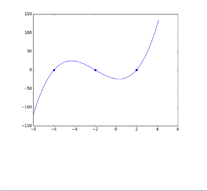
That was a lot of programming to do something like find the roots of the
function! Below is an example of using a function coded into pycse to solve
the same problem. It is a bit more sophisticated because you can define
whether an event is terminal, and the direction of the approach to zero for
each event.
1from pycse import *
2import numpy as np
3
4def myode(f, x):
5return 3*x**2 + 12*x-4
6
7def event1(f, x):
8’an event is when f = 0 and event is decreasing’
9isterminal =True
10 direction = -1
11 return f, isterminal, direction
12
13 def event2(f, x):
14 ’an event is when f = 0 and increasing’
15 isterminal =False
16 direction = 1
17 return f, isterminal, direction
18
19 f0 = -120
20
21 xspan =np.linspace(-8,4)
22 X, F, TE, YE, IE =odelay(myode, f0, xspan, events=[event1, event2])
189
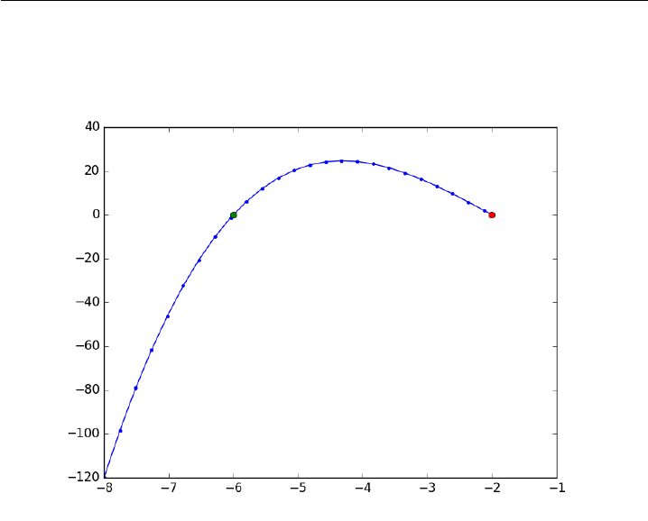
23
24 import matplotlib.pyplot as plt
25 plt.plot(X, F, ’.-’)
26
27 # plot the event locations.use a different color for each event
28 colors =’rg’
29
30 for x,y,i in zip(TE, YE, IE):
31 plt.plot([x], [y], ’o’, color=colors[i])
32
33 plt.savefig(’images/event-ode-2.png’)
34 print(TE, YE, IE)
[-6.0000001 -1.99999997] [[ 6.72906175e-13]
[ 2.22044605e-16]] [1 0]
10.1.6 Solving an ode for a specific solution value
Matlab post The analytical solution to an ODE is a function, which can be
solved to get a particular value, e.g. if the solution to an ODE is y(x) =
exp(x), you can solve the solution to find the value of x that makes y(x)=2.
In a numerical solution to an ODE we get a vector of independent variable
values, and the corresponding function values at those values. To solve for a
particular function value we need a different approach. This post will show
one way to do that in python.
190

Given that the concentration of a species A in a constant volume, batch
reactor obeys this differential equation dCA
dt =−kC2
Awith the initial con-
dition CA(t=0)=2.3mol/L and k= 0.23 L/mol/s, compute the time it
takes for CAto be reduced to 1 mol/L.
We will get a solution, then create an interpolating function and use
fsolve to get the answer.
1from scipy.integrate import odeint
2from scipy.interpolate import interp1d
3from scipy.optimize import fsolve
4import numpy as np
5import matplotlib.pyplot as plt
6
7k= 0.23
8Ca0 = 2.3
9
10 def dCadt(Ca, t):
11 return -k*Ca**2
12
13 tspan =np.linspace(0,10)
14
15 sol =odeint(dCadt, Ca0, tspan)
16 Ca =sol[:,0]
17
18 plt.plot(tspan, Ca)
19 plt.xlabel(’Time (s)’)
20 plt.ylabel(’$C_A$ (mol/L)’)
21 plt.savefig(’images/ode-specific-1.png’)
[<matplotlib.lines.Line2D object at 0x111d65a20>]
<matplotlib.text.Text object at 0x111b35cc0>
<matplotlib.text.Text object at 0x111b433c8>
191

You can see the solution is near two seconds. Now we create an inter-
polating function to evaluate the solution. We will plot the interpolating
function on a finer grid to make sure it seems reasonable.
1ca_func =interp1d(tspan, Ca, ’cubic’)
2
3itime =np.linspace(0,10,200)
4
5plt.figure()
6plt.plot(tspan, Ca, ’.’)
7plt.plot(itime, ca_func(itime), ’b-’)
8
9plt.xlabel(’Time (s)’)
10 plt.ylabel(’$C_A$ (mol/L)’)
11 plt.legend([’solution’,’interpolated’])
12 plt.savefig(’images/ode-specific-2.png’)
<matplotlib.figure.Figure object at 0x111d65a90>
[<matplotlib.lines.Line2D object at 0x111fac128>]
[<matplotlib.lines.Line2D object at 0x111fac3c8>]
<matplotlib.text.Text object at 0x111f67e48>
<matplotlib.text.Text object at 0x111f71550>
<matplotlib.legend.Legend object at 0x111f53588>
192
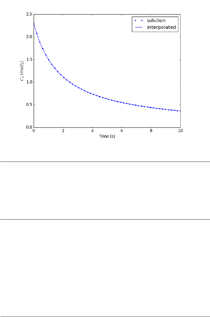
that loos pretty reasonable. Now we solve the problem.
1tguess = 2.0
2tsol, =fsolve(lambda t: 1.0 - ca_func(t), tguess)
3print(tsol)
4
5# you might prefer an explicit function
6def func(t):
7return 1.0 - ca_func(t)
8
9tsol2, =fsolve(func, tguess)
10 print(tsol2)
2.4574668235
2.4574668235
That is it. Interpolation can provide a simple way to evaluate the nu-
merical solution of an ODE at other values.
For completeness we examine a final way to construct the function. We
can actually integrate the ODE in the function to evaluate the solution at
the point of interest. If it is not computationally expensive to evaluate
the ODE solution this works fine. Note, however, that the ODE will get
integrated from 0 to the value t for each iteration of fsolve.
193

1def func(t):
2tspan =[0, t]
3sol =odeint(dCadt, Ca0, tspan)
4return 1.0 - sol[-1]
5
6tsol3, =fsolve(func, tguess)
7print(tsol3)
2.45746688202
10.1.7 A simple first order ode evaluated at specific points
Matlab post
We have integrated an ODE over a specific time span. Sometimes it
is desirable to get the solution at specific points, e.g. at t = [0 0.2 0.4
0.8]; This could be desirable to compare with experimental measurements
at those time points. This example demonstrates how to do that.
dy
dt =y(t)
The initial condition is y(0) = 1.
1from scipy.integrate import odeint
2
3y0 = 1
4tspan =[0,0.2,0.4,0.8]
5
6def dydt(y, t):
7return y
8
9Y=odeint(dydt, y0, tspan)
10 print(Y[:,0])
[ 1. 1.22140275 1.49182469 2.22554103]
10.1.8 Stopping the integration of an ODE at some condition
Matlab post In Post 968 we learned how to get the numerical solution to an
ODE, and then to use the deval function to solve the solution for a particular
value. The deval function uses interpolation to evaluate the solution at other
valuse. An alternative approach would be to stop the ODE integration when
the solution has the value you want. That can be done in Matlab by using
an "event" function. You setup an event function and tell the ode solver to
use it by setting an option.
194

Given that the concentration of a species A in a constant volume, batch
reactor obeys this differential equation dCA
dt =−kC2
Awith the initial con-
dition CA(t=0)=2.3mol/L and k= 0.23 L/mol/s, compute the time it
takes for CAto be reduced to 1 mol/L.
1from pycse import *
2import numpy as np
3
4k= 0.23
5Ca0 = 2.3
6
7def dCadt(Ca, t):
8return -k*Ca**2
9
10 def stop(Ca, t):
11 isterminal =True
12 direction = 0
13 value =1.0-Ca
14 return value, isterminal, direction
15
16 tspan =np.linspace(0.0,10.0)
17
18 t, CA, TE, YE, IE =odelay(dCadt, Ca0, tspan, events=[stop])
19
20 print(’At t = {0:1.2f} seconds the concentration of A is {1:1.2f} mol/L.’.format(t[-1], float(CA[-1])))
At t = 2.46 seconds the concentration of A is 1.00 mol/L.
10.1.9 Finding minima and maxima in ODE solutions with events
Matlab post Today we look at another way to use events in an ode solver.
We use an events function to find minima and maxima, by evaluating the
ODE in the event function to find conditions where the first derivative is
zero, and approached from the right direction. A maximum is when the fisrt
derivative is zero and increasing, and a minimum is when the first derivative
is zero and decreasing.
We use a simple ODE, y0=sin(x)∗e−0.05x, which has minima and
maxima.
1from pycse import *
2import numpy as np
3
4def ode(y, x):
5return np.sin(x) *np.exp(-0.05 * x)
6
7def minima(y, x):
8’’’Approaching a minumum, dydx is negatime and going to zero. our event function is increasing’’’
9value =ode(y, x)
195
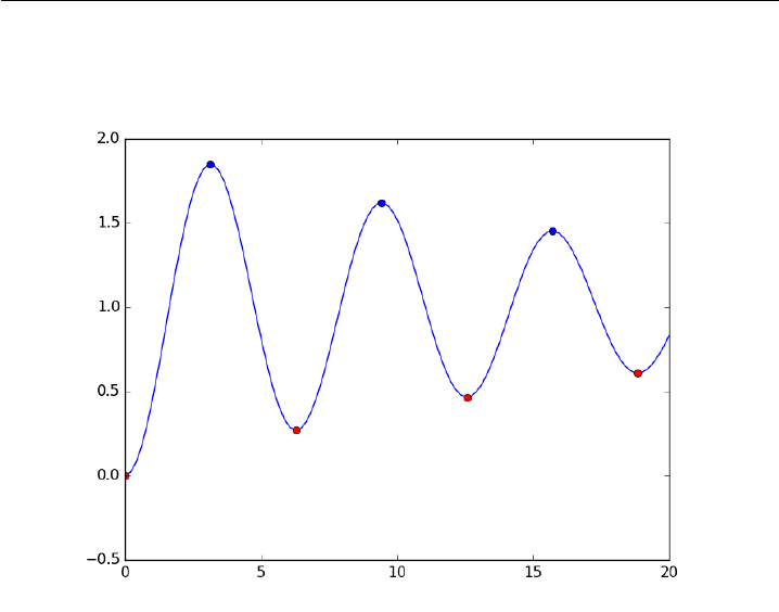
10 direction = 1
11 isterminal =False
12 return value, isterminal, direction
13
14 def maxima(y, x):
15 ’’’Approaching a maximum, dydx is positive and going to zero. our event function is decreasing’’’
16 value =ode(y, x)
17 direction = -1
18 isterminal =False
19 return value, isterminal, direction
20
21 xspan =np.linspace(0,20,100)
22
23 y0 = 0
24
25 X, Y, XE, YE, IE =odelay(ode, y0, xspan, events=[minima, maxima])
26 print(IE)
27 import matplotlib.pyplot as plt
28 plt.plot(X, Y)
29
30 # blue is maximum, red is minimum
31 colors =’rb’
32 for xe, ye, ie in zip(XE, YE, IE):
33 plt.plot([xe], [ye], ’o’, color=colors[ie])
34
35 plt.savefig(’./images/ode-events-min-max.png’)
[0101010]
196

10.1.10 Error tolerance in numerical solutions to ODEs
Matlab post Usually, the numerical ODE solvers in python work well with
the standard settings. Sometimes they do not, and it is not always obvious
they have not worked! Part of using a tool like python is checking how well
your solution really worked. We use an example of integrating an ODE that
defines the van der Waal equation of an ideal gas here.
we plot the analytical solution to the van der waal equation in reduced
form here.
1import numpy as np
2import matplotlib.pyplot as plt
3
4Tr = 0.9
5Vr =np.linspace(0.34,4,1000)
6
7#analytical equation for Pr
8Prfh =lambda Vr: 8.0 / 3.0 * Tr /(Vr - 1.0 / 3.0)-3.0/(Vr**2)
9Pr =Prfh(Vr) # evaluated on our reduced volume vector.
10
11 # Plot the EOS
12 plt.clf()
13 plt.plot(Vr,Pr)
14 plt.ylim([0,2])
15 plt.xlabel(’$V_R$’)
16 plt.ylabel(’$P_R$’)
17 plt.savefig(’images/ode-vw-1.png’)
[<matplotlib.lines.Line2D object at 0x10e4b4550>]
(0, 2)
<matplotlib.text.Text object at 0x10e447a90>
<matplotlib.text.Text object at 0x10e44eac8>
197
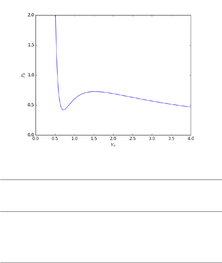
we want an equation for dPdV, which we will integrate we use symbolic
math to do the derivative for us.
1from sympy import diff, Symbol
2Vrs =Symbol(’Vrs’)
3
4Prs = 8.0 / 3.0 * Tr /(Vrs - 1.0/3.0)- 3.0/(Vrs**2)
5print(diff(Prs,Vrs))
-2.4/(Vrs - 0.333333333333333)**2 + 6.0/Vrs**3
Now, we solve the ODE. We will specify a large relative tolerance criteria
(Note the default is much smaller than what we show here).
1from scipy.integrate import odeint
2
3def myode(Pr, Vr):
4dPrdVr = -2.4/(Vr - 0.333333333333333)**2 + 6.0/Vr**3
5return dPrdVr
6
7Vspan =np.linspace(0.334,4)
8Po =Prfh(Vspan[0])
9P=odeint(myode, Po, Vspan, rtol=1e-4)
10
11 # Plot the EOS
12 plt.plot(Vr,Pr) # analytical solution
198
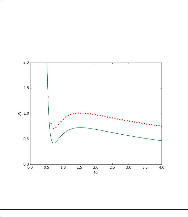
13 plt.plot(Vspan, P[:,0], ’r.’)
14 plt.ylim([0,2])
15 plt.xlabel(’$V_R$’)
16 plt.ylabel(’$P_R$’)
17 plt.savefig(’images/ode-vw-2.png’)
[<matplotlib.lines.Line2D object at 0x11069b0f0>]
[<matplotlib.lines.Line2D object at 0x11069bc88>]
(0, 2)
<matplotlib.text.Text object at 0x10e447a90>
<matplotlib.text.Text object at 0x10e44eac8>
You can see there is disagreement between the analytical solution and
numerical solution. The origin of this problem is accuracy at the initial
condition, where the derivative is extremely large.
1print(myode(Po, 0.34))
-53847.34378179728
We can increase the tolerance criteria to get a better answer. The de-
faults in odeint are actually set to 1.49012e-8.
199
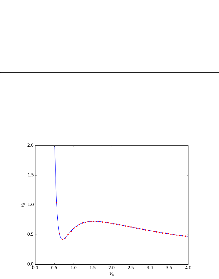
1Vspan =np.linspace(0.334,4)
2Po =Prfh(Vspan[0])
3P=odeint(myode, Po, Vspan)
4
5# Plot the EOS
6plt.clf()
7plt.plot(Vr,Pr) # analytical solution
8plt.plot(Vspan, P[:,0], ’r.’)
9plt.ylim([0,2])
10 plt.xlabel(’$V_R$’)
11 plt.ylabel(’$P_R$’)
12 plt.savefig(’images/ode-vw-3.png’)
[<matplotlib.lines.Line2D object at 0x10e48cef0>]
[<matplotlib.lines.Line2D object at 0x10e48feb8>]
(0, 2)
<matplotlib.text.Text object at 0x108fc76a0>
<matplotlib.text.Text object at 0x10b2d2fd0>
The problem here was the derivative value varied by four orders of mag-
nitude over the integration range, so the default tolerances were insufficient
to accurately estimate the numerical derivatives over that range. Tighten-
ing the tolerances helped resolve that problem. Another approach might be
to split the integration up into different regions. For instance, if instead of
200

starting at Vr = 0.34, which is very close to a sigularity in the van der waal
equation at Vr = 1/3, if you start at Vr = 0.5, the solution integrates just
fine with the standard tolerances.
10.1.11 Solving parameterized ODEs over and over conveniently
Matlab post Sometimes we have an ODE that depends on a parameter, and
we want to solve the ODE for several parameter values. It is inconvenient to
write an ode function for each parameter case. Here we examine a convenient
way to solve this problem; we pass the parameter to the ODE at runtime.
We consider the following ODE:
dCa
dt =−kCa(t)
where kis a parameter, and we want to solve the equation for a couple
of values of kto test the sensitivity of the solution on the parameter. Our
question is, given Ca(t= 0) = 2, how long does it take to get Ca = 1, and
how sensitive is the answer to small variations in k?
1import numpy as np
2from scipy.integrate import odeint
3import matplotlib.pyplot as plt
4
5def myode(Ca, t, k):
6’ODE definition’
7dCadt = -k*Ca
8return dCadt
9
10 tspan =np.linspace(0,0.5)
11 k0 = 2
12 Ca0 = 2
13
14 plt.figure(); plt.clf()
15
16 for kin [0.95 * k0, k0, 1.05 * k0]:
17 sol =odeint(myode, Ca0, tspan, args=(k,))
18 plt.plot(tspan, sol, label=’k={0:1.2f}’.format(k))
19 print(’At t=0.5 Ca = {0:1.2f} mol/L’.format(sol[-1][0]))
20
21 plt.legend(loc=’best’)
22 plt.xlabel(’Time’)
23 plt.ylabel(’$C_A$ (mol/L)’)
24 plt.savefig(’images/parameterized-ode1.png’)
At t=0.5 Ca = 0.77 mol/L
At t=0.5 Ca = 0.74 mol/L
At t=0.5 Ca = 0.70 mol/L
201
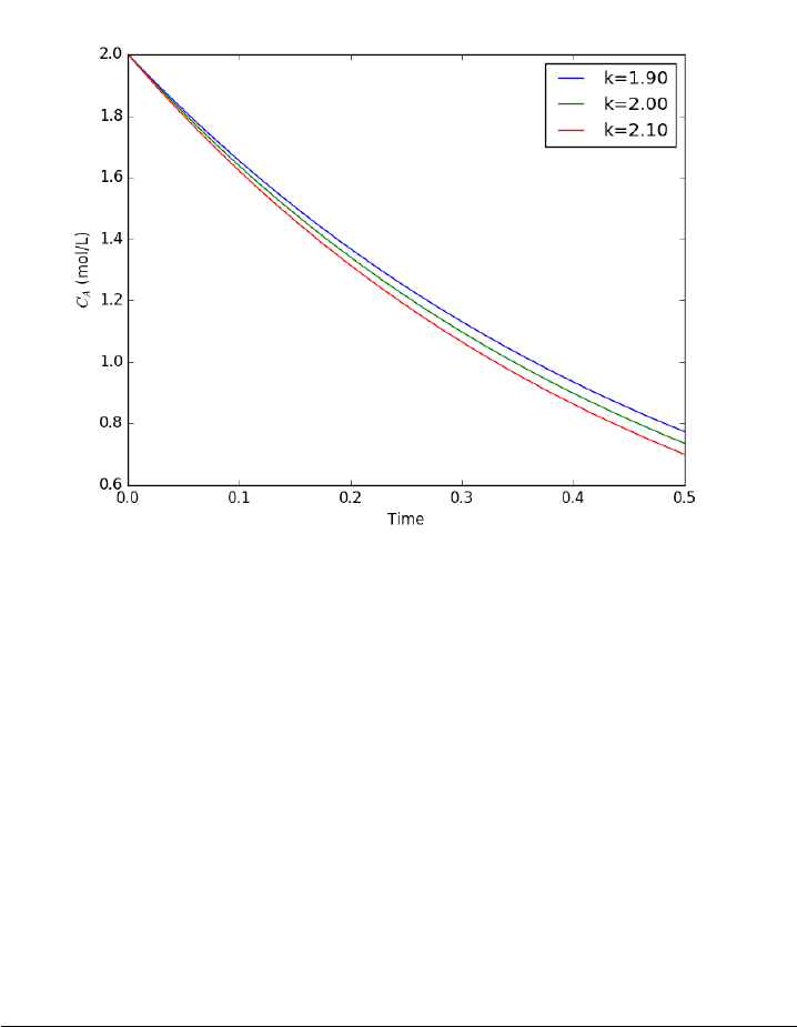
You can see there are some variations in the concentration at t = 0.5.
You could over or underestimate the concentration if you have the wrong
estimate of $k$! You have to use some judgement here to decide how long
to run the reaction to ensure a target goal is met.
10.1.12 Yet another way to parameterize an ODE
Matlab post We previously examined a way to parameterize an ODE. In
those methods, we either used an anonymous function to parameterize an
ode function, or we used a nested function that used variables from the
shared workspace.
We want a convenient way to solve dCa/dt =−kCa for multiple values
of k. Here we use a trick to pass a parameter to an ODE through the initial
conditions. We expand the ode function definition to include this parameter,
and set its derivative to zero, effectively making it a constant.
1import numpy as np
2from scipy.integrate import odeint
3import matplotlib.pyplot as plt
4
5def ode(F, t):
6Ca, k =F
7dCadt = -k*Ca
8dkdt = 0.0
202
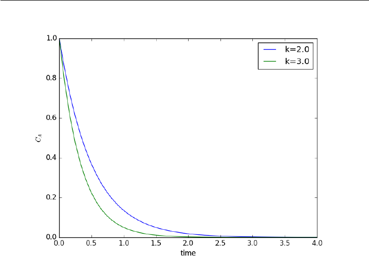
9return [dCadt, dkdt]
10
11 tspan =np.linspace(0,4)
12
13 Ca0 = 1;
14 K=[2.0,3.0]
15 for kin K:
16 F=odeint(ode, [Ca0, k], tspan)
17 Ca =F[:,0]
18 plt.plot(tspan, Ca, label=’k={0}’.format(k))
19 plt.xlabel(’time’)
20 plt.ylabel(’$C_A$’)
21 plt.legend(loc=’best’)
22 plt.savefig(’images/ode-parameterized-1.png’)
I do not think this is a very elegant way to pass parameters around
compared to the previous methods, but it nicely illustrates that there is
more than one way to do it. And who knows, maybe it will be useful in
some other context one day!
10.1.13 Another way to parameterize an ODE - nested function
Matlab post We saw one method to parameterize an ODE, by creating an
ode function that takes an extra parameter argument, and then making a
function handle that has the syntax required for the solver, and passes the
parameter the ode function.
203

Here we define the ODE function in a loop. Since the nested function is
in the namespace of the main function, it can "see" the values of the variables
in the main function. We will use this method to look at the solution to the
van der Pol equation for several different values of mu.
1import numpy as np
2from scipy.integrate import odeint
3import matplotlib.pyplot as plt
4
5MU =[0.1,1,2,5]
6tspan =np.linspace(0,100,5000)
7Y0 =[0,3]
8
9for mu in MU:
10 # define the ODE
11 def vdpol(Y, t):
12 x,y =Y
13 dxdt =y
14 dydt = -x+mu *(1-x**2)*y
15 return [dxdt, dydt]
16
17 Y=odeint(vdpol, Y0, tspan)
18
19 x=Y[:,0];y=Y[:,1]
20 plt.plot(x, y, label=’mu={0:1.2f}’.format(mu))
21
22 plt.axis(’equal’)
23 plt.legend(loc=’best’)
24 plt.savefig(’images/ode-nested-parameterization.png’)
25 plt.savefig(’images/ode-nested-parameterization.svg’)
204
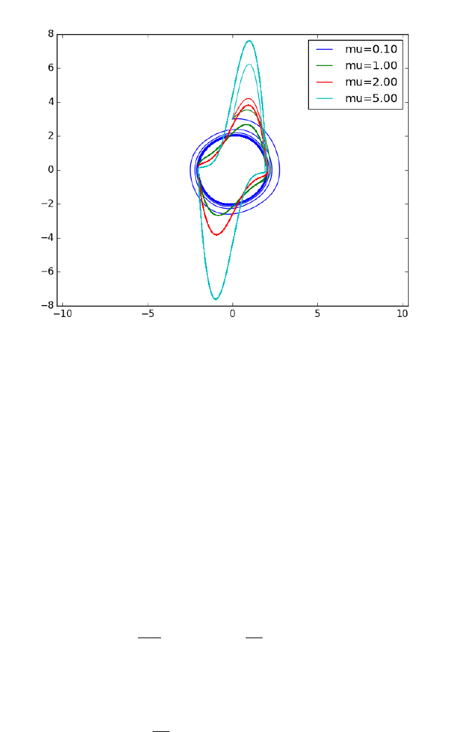
You can see the solution changes dramatically for different values of mu.
The point here is not to understand why, but to show an easy way to study
a parameterize ode with a nested function. Nested functions can be a great
way to "share" variables between functions especially for ODE solving, and
nonlinear algebra solving, or any other application where you need a lot of
parameters defined in one function in another function.
10.1.14 Solving a second order ode
Matlab post
The odesolvers in scipy can only solve first order ODEs, or systems of
first order ODES. To solve a second order ODE, we must convert it by
changes of variables to a system of first order ODES. We consider the Van
der Pol oscillator here:
d2x
dt2−µ(1 −x2)dx
dt +x= 0
µis a constant. If we let y=x−x3/3http://en.wikipedia.org/
wiki/Van_der_Pol_oscillator, then we arrive at this set of equations:
dx
dt =µ(x−1/3x3−y)
205

dy
dt =µ/x
here is how we solve this set of equations. Let µ= 1.
1from scipy.integrate import odeint
2import numpy as np
3
4mu = 1.0
5
6def vanderpol(X, t):
7x=X[0]
8y=X[1]
9dxdt =mu *(x - 1./3.*x**3 - y)
10 dydt =x/mu
11 return [dxdt, dydt]
12
13 X0 =[1,2]
14 t=np.linspace(0,40,250)
15
16 sol =odeint(vanderpol, X0, t)
17
18 import matplotlib.pyplot as plt
19 x=sol[:, 0]
20 y=sol[:, 1]
21
22 plt.plot(t,x, t, y)
23 plt.xlabel(’t’)
24 plt.legend((’x’,’y’))
25 plt.savefig(’images/vanderpol-1.png’)
26
27 # phase portrait
28 plt.figure()
29 plt.plot(x,y)
30 plt.plot(x[0], y[0], ’ro’)
31 plt.xlabel(’x’)
32 plt.ylabel(’y’)
33 plt.savefig(’images/vanderpol-2.png’)
206
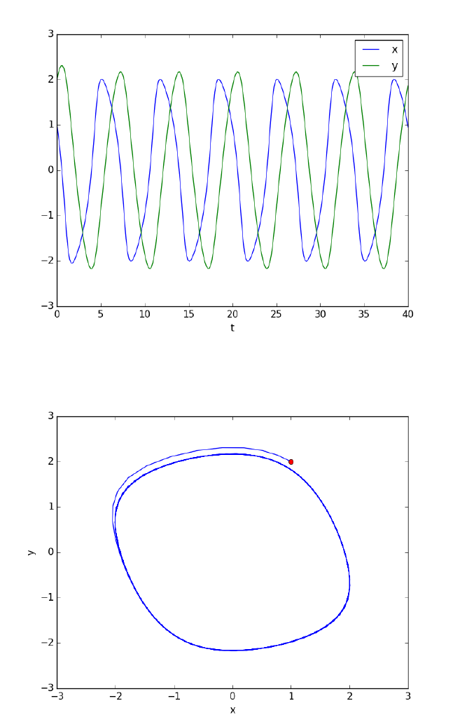
Here is the phase portrait. You can see that a limit cycle is approached,
indicating periodicity in the solution.
207

10.1.15 Solving Bessel’s Equation numerically
Matlab post
Reference Ch 5.5 Kreysig, Advanced Engineering Mathematics, 9th ed.
Bessel’s equation x2y00+xy0+(x2−ν2)y= 0 comes up often in engineering
problems such as heat transfer. The solutions to this equation are the Bessel
functions. To solve this equation numerically, we must convert it to a system
of first order ODEs. This can be done by letting z=y0and z0=y00 and
performing the change of variables:
y0=z
z0=1
x2(−xz −(x2−ν2)y
if we take the case where ν= 0, the solution is known to be the Bessel
function J0(x), which is represented in Matlab as besselj(0,x). The initial
conditions for this problem are: y(0) = 1 and y0(0) = 0.
There is a problem with our system of ODEs at x=0. Because of the
1/x2term, the ODEs are not defined at x=0. If we start very close to zero
instead, we avoid the problem.
1import numpy as np
2from scipy.integrate import odeint
3from scipy.special import jn # bessel function
4import matplotlib.pyplot as plt
5
6def fbessel(Y, x):
7nu = 0.0
8y=Y[0]
9z=Y[1]
10
11 dydx =z
12 dzdx = 1.0 / x**2 * (-x*z-(x**2 - nu**2)*y)
13 return [dydx, dzdx]
14
15 x0 = 1e-15
16 y0 = 1
17 z0 = 0
18 Y0 =[y0, z0]
19
20 xspan =np.linspace(1e-15,10)
21 sol =odeint(fbessel, Y0, xspan)
22
23 plt.plot(xspan, sol[:,0], label=’numerical soln’)
24 plt.plot(xspan, jn(0, xspan), ’r--’, label=’Bessel’)
25 plt.legend()
26 plt.savefig(’images/bessel.png’)
208
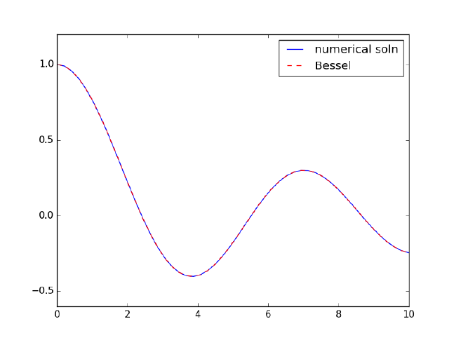
You can see the numerical and analytical solutions overlap, indicating
they are at least visually the same.
10.1.16 Phase portraits of a system of ODEs
Matlab post An undamped pendulum with no driving force is described by
y00 +sin(y)=0
We reduce this to standard matlab form of a system of first order ODEs
by letting y1=yand y2=y0
1. This leads to:
y0
1=y2
y0
2=−sin(y1)
The phase portrait is a plot of a vector field which qualitatively shows
how the solutions to these equations will go from a given starting point.
here is our definition of the differential equations:
To generate the phase portrait, we need to compute the derivatives y0
1
and y0
2at t= 0 on a grid over the range of values for y1and y2we are
interested in. We will plot the derivatives as a vector at each (y1, y2) which
will show us the initial direction from each point. We will examine the
solutions over the range -2 < y1 < 8, and -2 < y2 < 2 for y2, and create a
grid of 20 x 20 points.
209

1import numpy as np
2import matplotlib.pyplot as plt
3
4def f(Y, t):
5y1, y2 =Y
6return [y2, -np.sin(y1)]
7
8y1 =np.linspace(-2.0,8.0,20)
9y2 =np.linspace(-2.0,2.0,20)
10
11 Y1, Y2 =np.meshgrid(y1, y2)
12
13 t= 0
14
15 u,v=np.zeros(Y1.shape), np.zeros(Y2.shape)
16
17 NI, NJ =Y1.shape
18
19 for iin range(NI):
20 for jin range(NJ):
21 x=Y1[i, j]
22 y=Y2[i, j]
23 yprime =f([x, y], t)
24 u[i,j] =yprime[0]
25 v[i,j] =yprime[1]
26
27
28 Q=plt.quiver(Y1, Y2, u, v, color=’r’)
29
30 plt.xlabel(’$y_1$’)
31 plt.ylabel(’$y_2$’)
32 plt.xlim([-2,8])
33 plt.ylim([-4,4])
34 plt.savefig(’images/phase-portrait.png’)
<matplotlib.text.Text object at 0x108fc76a0>
<matplotlib.text.Text object at 0x10b2d2fd0>
(-2, 8)
(-4, 4)
210
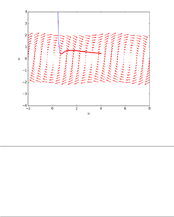
Let us plot a few solutions on the vector field. We will consider the solu-
tions where y1(0)=0, and values of y2(0) = [0 0.5 1 1.5 2 2.5], in otherwords
we start the pendulum at an angle of zero, with some angular velocity.
1from scipy.integrate import odeint
2
3plt.clf()
4for y20 in [0,0.5,1,1.5,2,2.5]:
5tspan =np.linspace(0,50,200)
6y0 =[0.0, y20]
7ys =odeint(f, y0, tspan)
8plt.plot(ys[:,0], ys[:,1], ’b-’)# path
9plt.plot([ys[0,0]], [ys[0,1]], ’o’)# start
10 plt.plot([ys[-1,0]], [ys[-1,1]], ’s’)# end
11
12
13 plt.xlim([-2,8])
14 plt.savefig(’images/phase-portrait-2.png’)
15 plt.savefig(’images/phase-portrait-2.svg’)
[<matplotlib.lines.Line2D object at 0x1115db518>]
[<matplotlib.lines.Line2D object at 0x1115dbf60>]
[<matplotlib.lines.Line2D object at 0x1115e07b8>]
[<matplotlib.lines.Line2D object at 0x10b2cd438>]
[<matplotlib.lines.Line2D object at 0x1115e4ac8>]
[<matplotlib.lines.Line2D object at 0x112048588>]
211
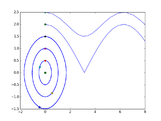
[<matplotlib.lines.Line2D object at 0x1115f64e0>]
[<matplotlib.lines.Line2D object at 0x10b2a53c8>]
[<matplotlib.lines.Line2D object at 0x1115f4dd8>]
[<matplotlib.lines.Line2D object at 0x10b39d1d0>]
[<matplotlib.lines.Line2D object at 0x10b2ed3c8>]
[<matplotlib.lines.Line2D object at 0x11205def0>]
[<matplotlib.lines.Line2D object at 0x110fb8160>]
[<matplotlib.lines.Line2D object at 0x10b312c18>]
[<matplotlib.lines.Line2D object at 0x10e4c2c50>]
[<matplotlib.lines.Line2D object at 0x1115ed588>]
[<matplotlib.lines.Line2D object at 0x1115f0ac8>]
[<matplotlib.lines.Line2D object at 0x1115f0e10>]
(-2, 8)
What do these figures mean? For starting points near the origin, and
small velocities, the pendulum goes into a stable limit cycle. For others, the
trajectory appears to fly off into y1 space. Recall that y1 is an angle that
has values from −πto π. The y1 data in this case is not wrapped around
to be in this range.
212

10.1.17 Linear algebra approaches to solving systems of constant
coefficient ODEs
Matlab post Today we consider how to solve a system of first order, con-
stant coefficient ordinary differential equations using linear algebra. These
equations could be solved numerically, but in this case there are analytical
solutions that can be derived. The equations we will solve are:
y0
1=−0.02y1+ 0.02y2
y0
2= 0.02y1−0.02y2
We can express this set of equations in matrix form as: "y0
1
y0
2#=
"−0.02 0.02
0.02 −0.02 #" y1
y2#
The general solution to this set of equations is
"y1
y2#=hv1v2i"c10
0c2#exp " λ10
0λ2#" t
t#!
where "λ10
0λ2#is a diagonal matrix of the eigenvalues of the constant
coefficient matrix, hv1v2iis a matrix of eigenvectors where the ith col-
umn corresponds to the eigenvector of the ith eigenvalue, and "c10
0c2#is
a matrix determined by the initial conditions.
In this example, we evaluate the solution using linear algebra. The initial
conditions we will consider are y1(0) = 0 and y2(0) = 150.
1import numpy as np
2
3A=np.array([[-0.02,0.02],
4[0.02,-0.02]])
5
6# Return the eigenvalues and eigenvectors of a Hermitian or symmetric matrix.
7evals, evecs =np.linalg.eigh(A)
8print(evals)
9print(evecs)
[-0.04 0. ]
[[ 0.70710678 0.70710678]
[-0.70710678 0.70710678]]
The eigenvectors are the columns of evecs.
Compute the cmatrix
V*c = Y0
213

1Y0 =[0,150]
2
3c=np.diag(np.linalg.solve(evecs, Y0))
4print(c)
[[-106.06601718 0. ]
[ 0. 106.06601718]]
Constructing the solution
We will create a vector of time values, and stack them for each solution,
y1(t)and Y2(t).
1import matplotlib.pyplot as plt
2
3t=np.linspace(0,100)
4T=np.row_stack([t, t])
5
6D=np.diag(evals)
7
8# y = V*c*exp(D*T);
9y=np.dot(np.dot(evecs, c), np.exp(np.dot(D, T)))
10
11 # y has a shape of (2, 50) so we have to transpose it
12 plt.plot(t, y.T)
13 plt.xlabel(’t’)
14 plt.ylabel(’y’)
15 plt.legend([’$y_1$’,’$y_2$’])
16 plt.savefig(’images/ode-la.png’)
[<matplotlib.lines.Line2D object at 0x10e68da20>, <matplotlib.lines.Line2D object at 0x10e68dba8>]
<matplotlib.text.Text object at 0x10de72b70>
<matplotlib.text.Text object at 0x10de7d860>
<matplotlib.legend.Legend object at 0x10e692c50>
214
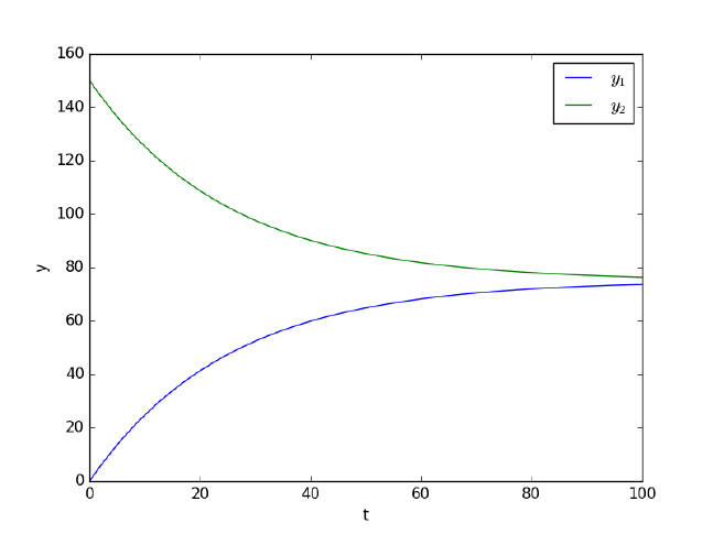
10.2 Delay Differential Equations
In Matlab you can solve Delay Differential equations (DDE) (Matlab post).
I do not know of a solver in scipy at this time that can do this.
10.3 Differential algebraic systems of equations
There is not a builtin solver for DAE systems in scipy. It looks like pysundials
may do it, but it must be compiled and installed.
10.4 Boundary value equations
I am unaware of dedicated BVP solvers in scipy. In the following examples
we implement some approaches to solving certain types of linear BVPs.
10.4.1 Plane Poiseuille flow - BVP solve by shooting method
Matlab post
One approach to solving BVPs is to use the shooting method. The
reason we cannot use an initial value solver for a BVP is that there is not
enough information at the initial value to start. In the shooting method,
we take the function value at the initial point, and guess what the function
215

derivatives are so that we can do an integration. If our guess was good, then
the solution will go through the known second boundary point. If not, we
guess again, until we get the answer we need. In this example we repeat the
pressure driven flow example, but illustrate the shooting method.
In the pressure driven flow of a fluid with viscosity µbetween two station-
ary plates separated by distance dand driven by a pressure drop ∆P/∆x,
the governing equations on the velocity uof the fluid are (assuming flow in
the x-direction with the velocity varying only in the y-direction):
∆P
∆x=µd2u
dy2
with boundary conditions u(y= 0) = 0 and u(y=d) = 0, i.e. the
no-slip condition at the edges of the plate.
we convert this second order BVP to a system of ODEs by letting u1=u,
u2=u0
1and then u0
2=u00
1. This leads to:
du1
dy =u2
du2
dy =1
µ
∆P
∆x
with boundary conditions u1(y= 0) = 0 and u1(y=d)=0.
for this problem we let the plate separation be d=0.1, the viscosity µ= 1,
and ∆P
∆x=−100.
First guess We need u_1(0) and u_2(0), but we only have u_1(0). We
need to guess a value for u_2(0) and see if the solution goes through the
u_2(d)=0 boundary value.
1import numpy as np
2from scipy.integrate import odeint
3import matplotlib.pyplot as plt
4
5d= 0.1 # plate thickness
6
7def odefun(U, y):
8u1, u2 =U
9mu = 1
10 Pdrop = -100
11 du1dy =u2
12 du2dy =1.0/mu *Pdrop
13 return [du1dy, du2dy]
14
15 u1_0 = 0 # known
16 u2_0 = 1 # guessed
17
18 dspan =np.linspace(0, d)
19
20 U=odeint(odefun, [u1_0, u2_0], dspan)
216
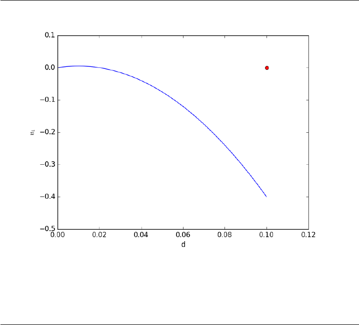
21
22 plt.plot(dspan, U[:,0])
23 plt.plot([d],[0], ’ro’)
24 plt.xlabel(’d’)
25 plt.ylabel(’$u_1$’)
26 plt.savefig(’images/bvp-shooting-1.png’)
Here we have undershot the boundary condition. Let us try a larger
guess.
Second guess
1import numpy as np
2from scipy.integrate import odeint
3import matplotlib.pyplot as plt
4
5d= 0.1 # plate thickness
6
7def odefun(U, y):
8u1, u2 =U
9mu = 1
10 Pdrop = -100
11 du1dy =u2
12 du2dy =1.0/mu *Pdrop
13 return [du1dy, du2dy]
14
15 u1_0 = 0 # known
16 u2_0 = 10 # guessed
217
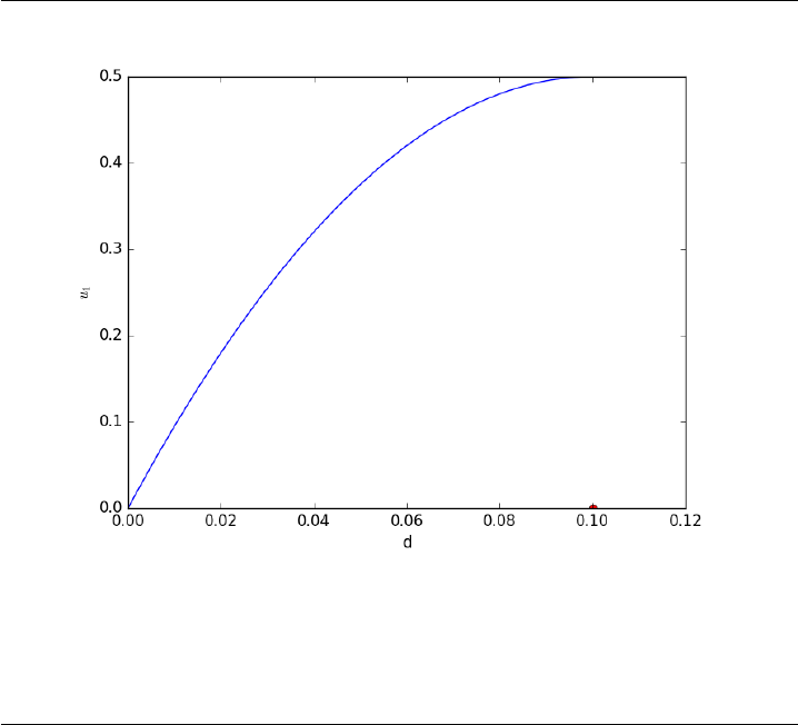
17
18 dspan =np.linspace(0, d)
19
20 U=odeint(odefun, [u1_0, u2_0], dspan)
21
22 plt.plot(dspan, U[:,0])
23 plt.plot([d],[0], ’ro’)
24 plt.xlabel(’d’)
25 plt.ylabel(’$u_1$’)
26 plt.savefig(’images/bvp-shooting-2.png’)
Now we have clearly overshot. Let us now make a function that will
iterate for us to find the right value.
Let fsolve do the work
1import numpy as np
2from scipy.integrate import odeint
3from scipy.optimize import fsolve
4import matplotlib.pyplot as plt
5
6d= 0.1 # plate thickness
7Pdrop = -100
8mu = 1
9
10 def odefun(U, y):
11 u1, u2 =U
12 du1dy =u2
218
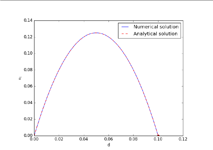
13 du2dy =1.0/mu *Pdrop
14 return [du1dy, du2dy]
15
16 u1_0 = 0 # known
17 dspan =np.linspace(0, d)
18
19 def objective(u2_0):
20 dspan =np.linspace(0, d)
21 U=odeint(odefun, [u1_0, u2_0], dspan)
22 u1 =U[:,0]
23 return u1[-1]
24
25 u2_0, =fsolve(objective, 1.0)
26
27 # now solve with optimal u2_0
28 U=odeint(odefun, [u1_0, u2_0], dspan)
29
30 plt.plot(dspan, U[:,0], label=’Numerical solution’)
31 plt.plot([d],[0], ’ro’)
32
33 # plot an analytical solution
34 u= -(Pdrop) *d**2 / 2 / mu *(dspan /d-(dspan /d)**2)
35 plt.plot(dspan, u, ’r--’, label=’Analytical solution’)
36
37
38 plt.xlabel(’d’)
39 plt.ylabel(’$u_1$’)
40 plt.legend(loc=’best’)
41 plt.savefig(’images/bvp-shooting-3.png’)
219

You can see the agreement is excellent!
This also seems like a useful bit of code to not have to reinvent regularly,
so it has been added to pycse as BVP_sh. Here is an example usage.
1from pycse import BVP_sh
2import matplotlib.pyplot as plt
3
4d= 0.1 # plate thickness
5Pdrop = -100
6mu = 1
7
8def odefun(U, y):
9u1, u2 =U
10 du1dy =u2
11 du2dy =1.0/mu *Pdrop
12 return [du1dy, du2dy]
13
14 x1 = 0.0; alpha = 0.0
15 x2 = 0.1; beta = 0.0
16 init = 2.0 # initial guess of slope at x=0
17
18 X,Y =BVP_sh(odefun, x1, x2, alpha, beta, init)
19 plt.plot(X, Y[:,0])
20 plt.ylim([0,0.14])
21
22 # plot an analytical solution
23 u= -(Pdrop) *d**2 / 2 / mu *(X /d-(X /d)**2)
24 plt.plot(X, u, ’r--’, label=’Analytical solution’)
25 plt.savefig(’images/bvp-shooting-4.png’)
220
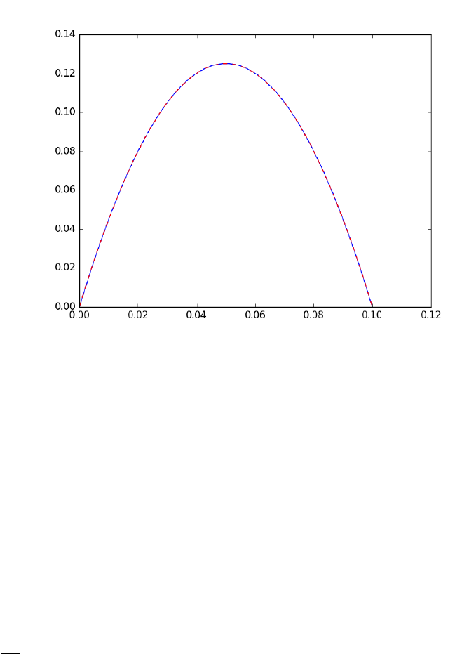
10.4.2 Plane poiseuelle flow solved by finite difference
Matlab post
Adapted from http://www.physics.arizona.edu/~restrepo/475B/Notes/
sourcehtml/node24.html
We want to solve a linear boundary value problem of the form: y” =
p(x)y’ + q(x)y + r(x) with boundary conditions y(x1) = alpha and y(x2)
= beta.
For this example, we solve the plane poiseuille flow problem using a finite
difference approach. An advantage of the approach we use here is we do not
have to rewrite the second order ODE as a set of coupled first order ODEs,
nor do we have to provide guesses for the solution. We do, however, have to
discretize the derivatives and formulate a linear algebra problem.
we want to solve u” = 1/mu*DPDX with u(0)=0 and u(0.1)=0. for
this problem we let the plate separation be d=0.1, the viscosity µ= 1, and
∆P
∆x=−100.
The idea behind the finite difference method is to approximate the
derivatives by finite differences on a grid. See here for details. By dis-
cretizing the ODE, we arrive at a set of linear algebra equations of the form
Ay =b, where Aand bare defined as follows.
221

A=
2 + h2q1−1 + h
2p1000
−1−h
2p22 + h2q2−1 + h
2p20 0
0.........0
0 0 −1−h
2pN−12 + h2qN−1−1 + h
2pN−1
0 0 0 −1−h
2pN2 + h2qN
y=
yi
.
.
.
yN
b=
−h2r1+ (1 + h
2p1)α
−h2r2
.
.
.
−h2rN−1
−h2rN+ (1 −h
2pN)β
1import numpy as np
2
3# we use the notation for y’’ = p(x)y’ + q(x)y + r(x)
4def p(x):
5return 0
6
7def q(x):
8return 0
9
10 def r(x):
11 return -100
12
13 #we use the notation y(x1) = alpha and y(x2) = beta
14
15 x1 = 0; alpha = 0.0
16 x2 = 0.1; beta = 0.0
17
18 npoints = 100
19
20 # compute interval width
21 h=(x2-x1)/npoints;
22
23 # preallocate and shape the b vector and A-matrix
24 b=np.zeros((npoints - 1,1));
25 A=np.zeros((npoints - 1, npoints - 1));
26 X=np.zeros((npoints - 1,1));
27
28 #now we populate the A-matrix and b vector elements
29 for iin range(npoints - 1):
30 X[i,0]=x1 +(i + 1)*h
31
222

32 # get the value of the BVP Odes at this x
33 pi =p(X[i])
34 qi =q(X[i])
35 ri =r(X[i])
36
37 if i== 0:
38 # first boundary condition
39 b[i] = -h**2 * ri +(1+h/2*pi)*alpha;
40 elif i== npoints - 1:
41 # second boundary condition
42 b[i] = -h**2 * ri +(1-h/2*pi)*beta;
43 else:
44 b[i] = -h**2 * ri # intermediate points
45
46 for jin range(npoints - 1):
47 if j== i: # the diagonal
48 A[i,j] =2+h**2 * qi
49 elif j== i- 1:# left of the diagonal
50 A[i,j] =-1-h/2*pi
51 elif j== i+ 1:# right of the diagonal
52 A[i,j] =-1+h/2*pi
53 else:
54 A[i,j] = 0 # off the tri-diagonal
55
56 # solve the equations A*y = b for Y
57 Y=np.linalg.solve(A,b)
58
59 x=np.hstack([x1, X[:,0], x2])
60 y=np.hstack([alpha, Y[:,0], beta])
61
62 import matplotlib.pyplot as plt
63
64 plt.plot(x, y)
65
66 mu = 1
67 d= 0.1
68 x=np.linspace(0,0.1);
69 Pdrop = -100 # this is DeltaP/Deltax
70 u= -(Pdrop) *d**2 / 2.0 / mu *(x /d-(x /d)**2)
71 plt.plot(x,u,’r--’)
72
73 plt.xlabel(’distance between plates’)
74 plt.ylabel(’fluid velocity’)
75 plt.legend((’finite difference’,’analytical soln’))
76 plt.savefig(’images/pp-bvp-fd.png’)
223
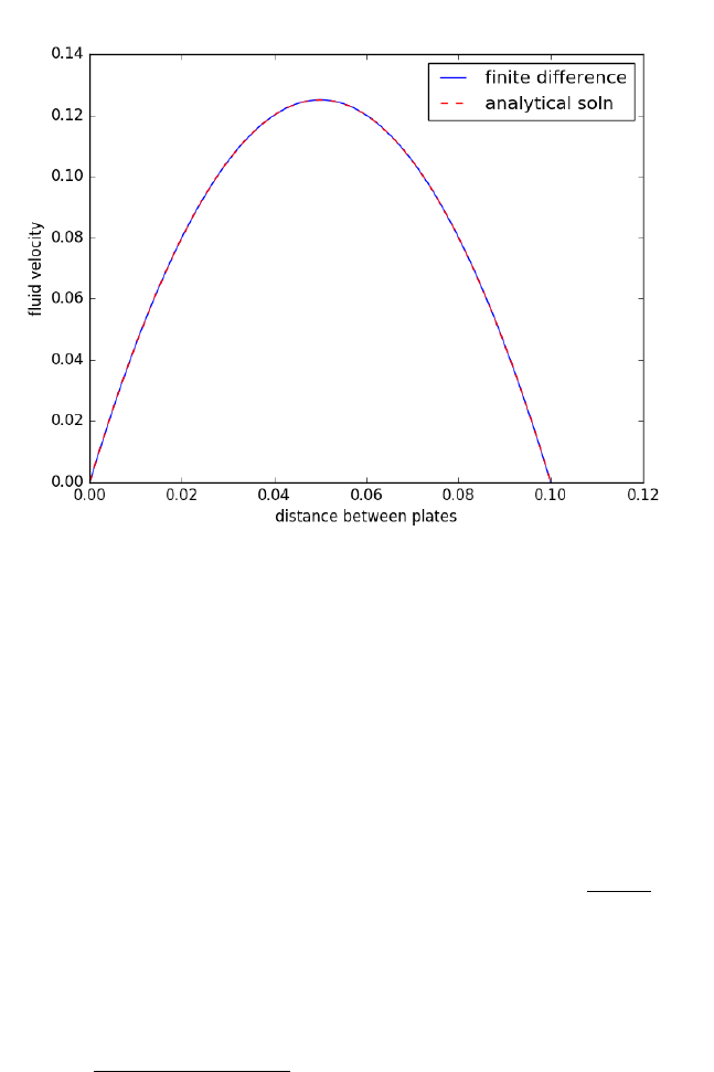
You can see excellent agreement here between the numerical and analyt-
ical solution.
10.4.3 Boundary value problem in heat conduction
Matlab post
For steady state heat conduction the temperature distribution in one-
dimension is governed by the Laplace equation:
∇2T= 0
with boundary conditions that at T(x=a) = TAand T(x=L) = TB.
The analytical solution is not difficult here: T=TA−TA−TB
Lx, but we
will solve this by finite differences.
For this problem, lets consider a slab that is defined by x=0 to x=L,
with T(x= 0) = 100, and T(x=L) = 200. We want to find the function
T(x) inside the slab.
We approximate the second derivative by finite differences as
f00(x)≈f(x−h)−2f(x)+f(x+h)
h2
Since the second derivative in this case is equal to zero, we have at each
discretized node 0 = Ti−1−2Ti+Ti+1. We know the values of Tx=0 =α
and Tx=L=β.
224

A=
−2 1 0 0 0
1−2 1 0 0
0.........0
0 0 1 −2 1
0 0 0 1 −2
x=
T1
.
.
.
TN
b=
−T(x= 0)
0
.
.
.
0
−T(x=L)
These are linear equations in the unknowns xthat we can easily solve.
Here, we evaluate the solution.
1import numpy as np
2
3#we use the notation T(x1) = alpha and T(x2) = beta
4x1 = 0; alpha = 100
5x2 = 5; beta = 200
6
7npoints = 100
8
9# preallocate and shape the b vector and A-matrix
10 b=np.zeros((npoints, 1));
11 b[0]= -alpha
12 b[-1]= -beta
13
14 A=np.zeros((npoints, npoints));
15
16 #now we populate the A-matrix and b vector elements
17 for iin range(npoints ):
18 for jin range(npoints):
19 if j== i: # the diagonal
20 A[i,j] = -2
21 elif j== i- 1:# left of the diagonal
22 A[i,j] = 1
23 elif j== i+ 1:# right of the diagonal
24 A[i,j] = 1
25
26 # solve the equations A*y = b for Y
27 Y=np.linalg.solve(A,b)
28
225
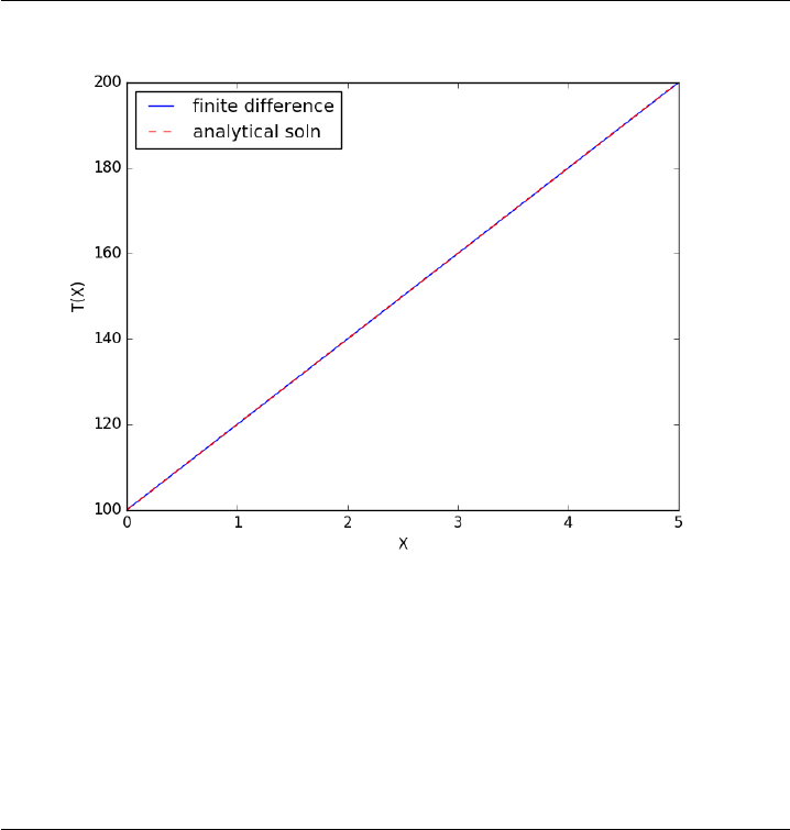
29 x=np.linspace(x1, x2, npoints + 2)
30 y=np.hstack([alpha, Y[:,0], beta])
31
32 import matplotlib.pyplot as plt
33
34 plt.plot(x, y)
35
36 plt.plot(x, alpha +(beta -alpha)/(x2 -x1) *x, ’r--’)
37
38 plt.xlabel(’X’)
39 plt.ylabel(’T(X)’)
40 plt.legend((’finite difference’,’analytical soln’), loc=’best’)
41 plt.savefig(’images/bvp-heat-conduction-1d.png’)
10.4.4 BVP in pycse
I thought it was worthwhile coding a BVP solver into pycse. This function
(bvp_L0) solves y00(x) + p(x)y0(x) + q(x)y(x) = r(x)with constant value
boundary conditions y(x0) = αand y(xL) = β.
Fluids example for Plane poiseuelle flow (y00(x) = constant,y(0) = 0
and y(L)=0:
1from pycse import bvp_L0
2
3# we use the notation for y’’ = p(x)y’ + q(x)y + r(x)
226
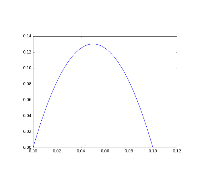
4def p(x): return 0
5def q(x): return 0
6def r(x): return -100
7
8#we use the notation y(x1) = alpha and y(x2) = beta
9
10 x1 = 0; alpha = 0.0
11 x2 = 0.1; beta = 0.0
12
13 npoints = 100
14
15 x,y=bvp_L0(p, q, r, x1, x2, alpha, beta, npoints=100)
16 print(len(x))
17
18 import matplotlib.pyplot as plt
19 plt.plot(x, y)
20 plt.savefig(’images/bvp-pycse.png’)
100
Heat transfer example y00(x)=0,y(0) = 100 and y(L) = 200.
1from pycse import bvp_L0
2
3# we use the notation for y’’ = p(x)y’ + q(x)y + r(x)
4def p(x): return 0
5def q(x): return 0
6def r(x): return 0
227
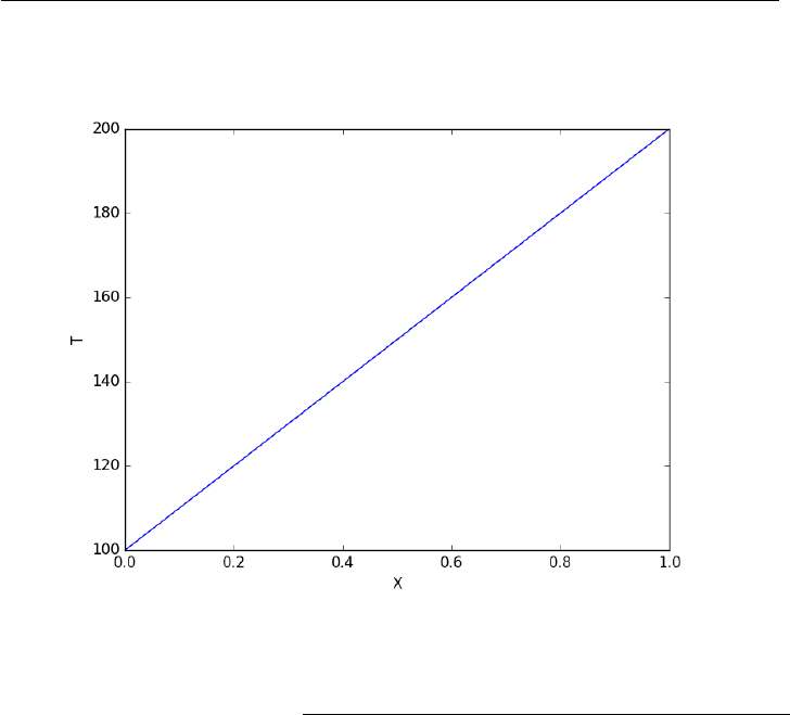
7
8#we use the notation y(x1) = alpha and y(x2) = beta
9
10 x1 = 0; alpha = 100
11 x2 = 1; beta = 200
12
13 npoints = 100
14
15 x,y=bvp_L0(p, q, r, x1, x2, alpha, beta, npoints=100)
16 print(len(x))
17
18 import matplotlib.pyplot as plt
19 plt.plot(x, y)
20 plt.xlabel(’X’)
21 plt.ylabel(’T’)
22 plt.savefig(’images/ht-example.png’)
100
10.4.5 A nonlinear BVP
Adapted from Example 8.7 in Numerical Methods in Engineering with Python
by Jaan Kiusalaas.
We want to solve y00(x) = −3y(x)y0(x)with $y(0) = 0 and y(2) = 1
using a finite difference method. We discretize the region and approximate
the derivatives as:
228

y00(x)≈yi−1−2yi+yi+1
h2
y0(x)≈yi+1−yi−1
2h
We define a function y00(x) = F(x, y, y0). At each node in our discretized
region, we will have an equation that looks like y00(x)−F(x, y, y0)=0, which
will be nonlinear in the unknown solution y. The set of equations to solve
is:
y0−α= 0 (22)
yi−1−2yi+yi+1
h2+ (3yi)(yi+1 −yi−1
2h)=0 (23)
yL−β= 0 (24)
Since we use a nonlinear solver, we will have to provide an initial guess
to the solution. We will in this case assume a line. In other cases, a bad
initial guess may lead to no solution.
1import numpy as np
2from scipy.optimize import fsolve
3import matplotlib.pyplot as plt
4
5x1 = 0.0
6x2 = 2.0
7
8alpha = 0.0
9beta = 1.0
10
11 N= 11
12 X=np.linspace(x1, x2, N)
13 h=(x2 -x1) /(N - 1)
14
15 def Ypp(x, y, yprime):
16 ’’’define y’’ = 3*y*y’ ’’’
17 return -3.0 * y*yprime
18
19 def residuals(y):
20 ’’’When we have the right values of y, this function will be zero.’’’
21
22 res =np.zeros(y.shape)
23
24 res[0]=y[0]-alpha
25
26 for iin range(1,N- 1):
27 x=X[i]
28 YPP =(y[i - 1]-2*y[i] +y[i + 1]) /h**2
29 YP =(y[i + 1]-y[i - 1]) /(2*h)
30 res[i] =YPP -Ypp(x, y[i], YP)
31
32 res[-1]=y[-1]-beta
33 return res
229
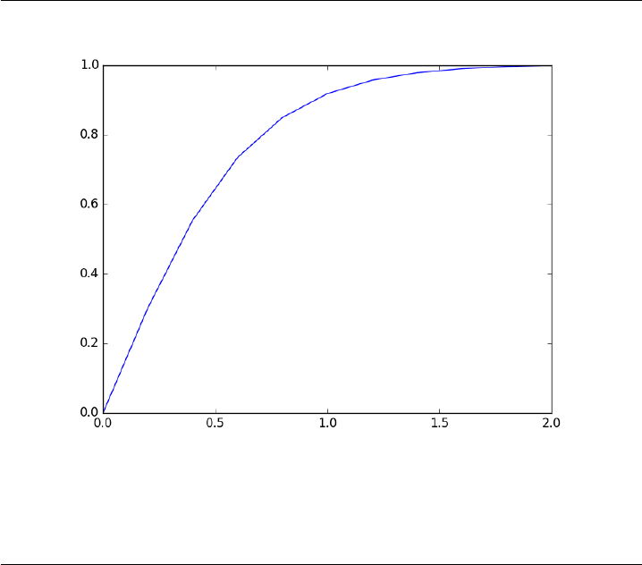
34
35 # we need an initial guess
36 init =alpha +(beta -alpha) /(x2 -x1) *X
37
38 Y=fsolve(residuals, init)
39
40 plt.plot(X, Y)
41 plt.savefig(’images/bvp-nonlinear-1.png’)
That code looks useful, so I put it in the pycse module in the function
BVP_nl. Here is an example usage. We have to create two functions, one
for the differential equation, and one for the initial guess.
1import numpy as np
2from pycse import BVP_nl
3import matplotlib.pyplot as plt
4
5x1 = 0.0
6x2 = 2.0
7
8alpha = 0.0
9beta = 1.0
10
11 def Ypp(x, y, yprime):
12 ’’’define y’’ = 3*y*y’ ’’’
13 return -3.0 * y*yprime
14
15 def BC(X, Y):
230
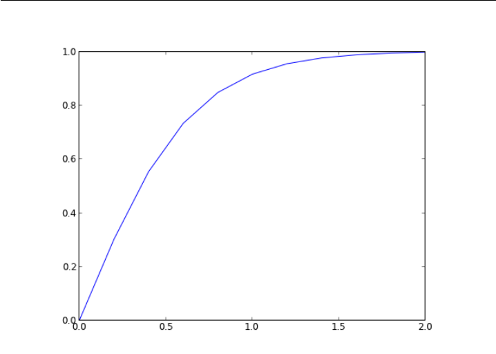
16 return [alpha -Y[0], beta -Y[-1]]
17
18 X=np.linspace(x1, x2)
19 init =alpha +(beta -alpha) /(x2 -x1) *X
20
21 x,y=BVP_nl(Ypp, X, BC, init)
22
23 plt.plot(x, y)
24 plt.savefig(’images/bvp-nonlinear-2.png’)
The results are the same.
10.4.6 Another look at nonlinear BVPs
Adapted from http://www.mathworks.com/help/matlab/ref/bvp4c.html
Boundary value problems may have more than one solution. Let us
consider the BVP:
y00 +|y|= 0 (25)
y(0) = 0 (26)
y(4) = −2(27)
231

We will see this equation has two answers, depending on your initial
guess. We convert this to the following set of coupled equations:
y0
1=y2(28)
y0
2=−|y1|(29)
y1(0) = 0 (30)
y1(4) = −2(31)
This BVP is nonlinear because of the absolute value. We will have to
guess solutions to get started. We will guess two different solutions, both of
which will be constant values. We will use pycse.bvp to solve the equation.
1import numpy as np
2from pycse import bvp
3import matplotlib.pyplot as plt
4
5def odefun(Y, x):
6y1, y2 =Y
7dy1dx =y2
8dy2dx = -np.abs(y1)
9return [dy1dx, dy2dx]
10
11 def bcfun(Y):
12 y1a, y2a =Y[0][0], Y[1][0]
13 y1b, y2b =Y[0][-1], Y[1][-1]
14
15 return [y1a, -2-y1b]
16
17 x=np.linspace(0,4,100)
18
19 y1 = 1.0 * np.ones(x.shape)
20 y2 = 0.0 * np.ones(x.shape)
21
22 Yinit =np.vstack([y1, y2])
23
24 sol =bvp(odefun, bcfun, x, Yinit)
25
26 plt.plot(x, sol[0])
27
28 # another initial guess
29 y1 = -1.0 * np.ones(x.shape)
30 y2 = 0.0 * np.ones(x.shape)
31
32 Yinit =np.vstack([y1, y2])
33
34 sol =bvp(odefun, bcfun, x, Yinit)
35
36 plt.plot(x, sol[0])
37 plt.legend([’guess 1’,’guess 2’])
38 plt.savefig(’images/bvp-another-nonlin-1.png’)
232
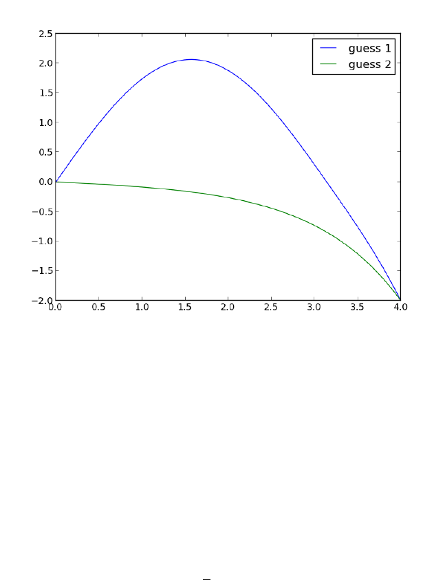
This example shows that a nonlinear BVP may have different solutions,
and which one you get depends on the guess you make for the solution. This
is analogous to solving nonlinear algebraic equations (which is what is done
in solving this problem!).
10.4.7 Solving the Blasius equation
In fluid mechanics the Blasius equation comes up (http://en.wikipedia.
org/wiki/Blasius_boundary_layer) to describe the boundary layer that
forms near a flat plate with fluid moving by it. The nonlinear differential
equation is:
f000 +1
2ff 00 = 0 (32)
f(0) = 0 (33)
f0(0) = 0 (34)
f0(∞) = 1 (35)
This is a nonlinear, boundary value problem. The point of solving this
equation is to get the value of f00(0) to evaluate the shear stress at the plate.
We have to convert this to a system of first-order differential equations.
Let f1=f,f2=f0
1and f3=f0
2. This leads to:
233

f0
1=f2(36)
f0
2=f3(37)
f0
3=−1
2f1f3(38)
f1(0) = 0 (39)
f2(0) = 0 (40)
f2(∞)=1 (41)
It is not possible to specify a boundary condition at ∞numerically, so
we will have to use a large number, and verify it is "large enough". From the
solution, we evaluate the derivatives at η= 0, and we have f00(0) = f3(0).
We have to provide initial guesses for f_1, f_2 and f_3. This is the
hardest part about this problem. We know that f_1 starts at zero, and is
flat there (f’(0)=0), but at large eta, it has a constant slope of one. We will
guess a simple line of slope = 1 for f_1. That is correct at large eta, and
is zero at η=0. If the slope of the function is constant at large η, then the
values of higher derivatives must tend to zero. We choose an exponential
decay as a guess.
Finally, we let a solver iteratively find a solution for us, and find the
answer we want. The solver is in the pycse module.
1import numpy as np
2from pycse import bvp
3
4def odefun(F, x):
5f1, f2, f3 =F
6return [f2,
7f3,
8-0.5 * f1 *f3]
9
10 def bcfun(F):
11 return [F[0][0], # f1(0) = 0
12 F[1][0], # f2(0) = 0
13 1.0 - F[1][-1]] # f2(inf) = 1
14
15 eta =np.linspace(0,6,100)
16 f1init =eta
17 f2init =np.exp(-eta)
18 f3init =np.exp(-eta)
19
20 Finit =np.vstack([f1init, f2init, f3init])
21
22 sol =bvp(odefun, bcfun, eta, Finit)
23
234
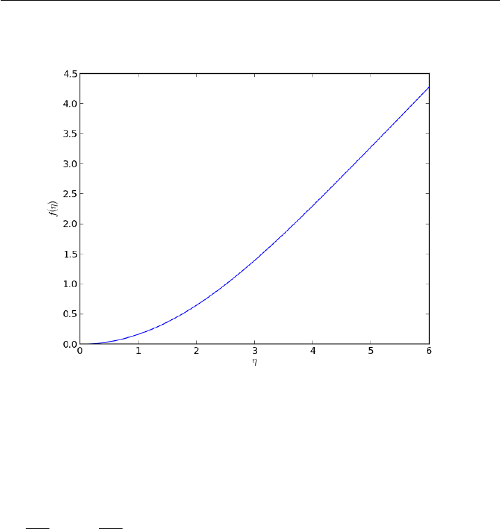
24 print("f’’(0) = f_3(0) = {0}".format(sol[2,0]))
25
26 import matplotlib.pyplot as plt
27 plt.plot(eta, sol[0])
28 plt.xlabel(’$\eta$’)
29 plt.ylabel(’$f(\eta)$’)
30 plt.savefig(’images/blasius.png’)
That solution agrees well with reported solutions.
10.5 Partial differential equations
10.5.1 Modeling a transient plug flow reactor
Matlab post
The PDE that describes the transient behavior of a plug flow reactor
with constant volumetric flow rate is:
∂CA
∂dt =−ν0∂CA
∂dV +rA.
To solve this numerically in python, we will utilize the method of lines.
The idea is to discretize the reactor in volume, and approximate the spatial
derivatives by finite differences. Then we will have a set of coupled ordinary
differential equations that can be solved in the usual way. Let us simplify
the notation with C=CA, and let rA=−kC2. Graphically this looks like
this:
235
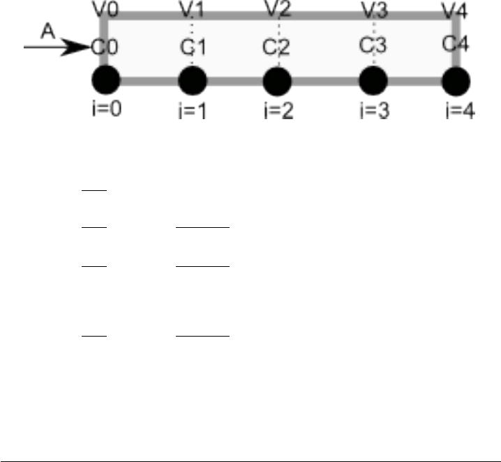
This leads to the following set of equations:
dC0
dt = 0 (entrance concentration never changes) (42)
dC1
dt =−ν0
C1−C0
V1−V0−kC2
1(43)
dC2
dt =−ν0
C2−C1
V2−V1−kC2
2(44)
.
.
. (45)
dC4
dt =−ν0
C4−C3
V4−V3−kC2
4(46)
Last, we need initial conditions for all the nodes in the discretization.
Let us assume the reactor was full of empty solvent, so that Ci= 0 at t= 0.
In the next block of code, we get the transient solutions, and the steady
state solution.
1import numpy as np
2from scipy.integrate import odeint
3
4Ca0 = 2 # Entering concentration
5vo = 2 # volumetric flow rate
6volume = 20 # total volume of reactor, spacetime = 10
7k= 1 # reaction rate constant
8
9N= 100 # number of points to discretize the reactor volume on
10
11 init =np.zeros(N) # Concentration in reactor at t = 0
12 init[0]=Ca0 # concentration at entrance
13
14 V=np.linspace(0, volume, N) # discretized volume elements
15 tspan =np.linspace(0,25)# time span to integrate over
16
17 def method_of_lines(C, t):
18 ’coupled ODES at each node point’
19 D= -vo *np.diff(C) /np.diff(V) -k*C[1:]**2
20 return np.concatenate([[0], #C0 is constant at entrance
21 D])
22
236
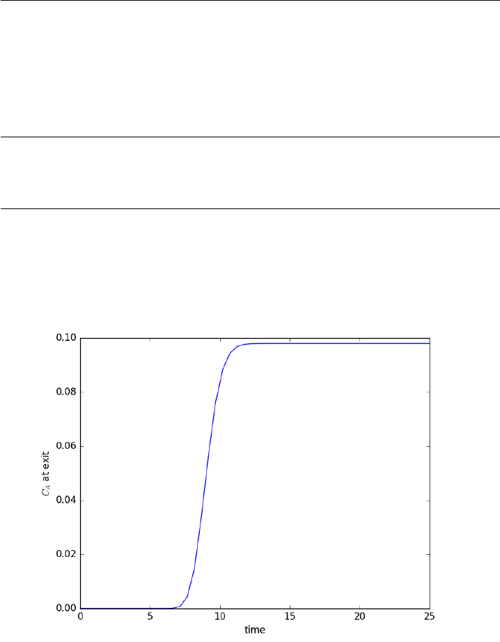
23 sol =odeint(method_of_lines, init, tspan)
24
25 # steady state solution
26 def pfr(C, V):
27 return 1.0 / vo *(-k*C**2)
28
29 ssol =odeint(pfr, Ca0, V)
The transient solution contains the time dependent behavior of each
node in the discretized reactor. Each row contains the concentration as a
function of volume at a specific time point. For example, we can plot the
concentration of A at the exit vs. time (that is, the last entry of each row)
as:
1import matplotlib.pyplot as plt
2plt.plot(tspan, sol[:, -1])
3plt.xlabel(’time’)
4plt.ylabel(’$C_A$ at exit’)
5plt.savefig(’images/transient-pfr-1.png’)
[<matplotlib.lines.Line2D object at 0x10f3e7a20>]
<matplotlib.text.Text object at 0x10f3bf6a0>
<matplotlib.text.Text object at 0x10f3d1d68>
237
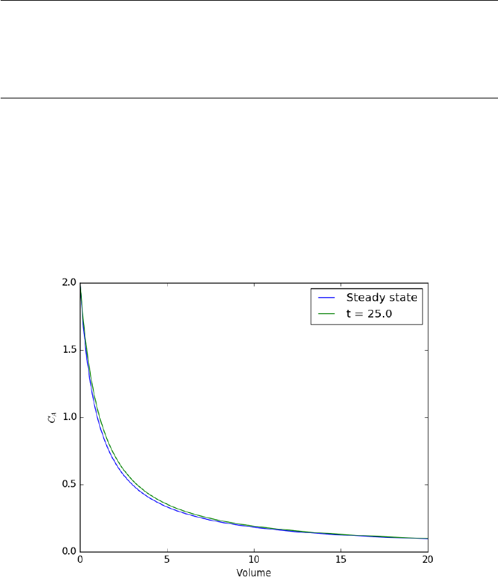
After approximately one space time, the steady state solution is reached
at the exit. For completeness, we also examine the steady state solu-
tion.
1plt.figure()
2plt.plot(V, ssol, label=’Steady state’)
3plt.plot(V, sol[-1], label=’t = {}’.format(tspan[-1]))
4plt.xlabel(’Volume’)
5plt.ylabel(’$C_A$’)
6plt.legend(loc=’best’)
7plt.savefig(’images/transient-pfr-2.png’)
<matplotlib.figure.Figure object at 0x10f410d68>
[<matplotlib.lines.Line2D object at 0x1111056a0>]
[<matplotlib.lines.Line2D object at 0x111105f98>]
<matplotlib.text.Text object at 0x10fd794a8>
<matplotlib.text.Text object at 0x10fd81b70>
<matplotlib.legend.Legend object at 0x11110e1d0>
There is some minor disagreement between the final transient solution
and the steady state solution. That is due to the approximation in discretiz-
ing the reactor volume. In this example we used 100 nodes. You get better
agreement with a larger number of nodes, say 200 or more. Of course, it
238

takes slightly longer to compute then, since the number of coupled odes is
equal to the number of nodes.
We can also create an animated gif to show how the concentration of
A throughout the reactor varies with time. Note, I had to install ffmpeg
(http://ffmpeg.org/) to save the animation.
1from matplotlib import animation
2
3# make empty figure
4fig =plt.figure()
5ax =plt.axes(xlim=(0,20), ylim=(0,2))
6line, =ax.plot(V, init, lw=2)
7
8def animate(i):
9line.set_xdata(V)
10 line.set_ydata(sol[i])
11 ax.set_title(’t = {0}’.format(tspan[i]))
12 ax.figure.canvas.draw()
13 return line,
14
15
16 anim =animation.FuncAnimation(fig, animate, frames=50, blit=True)
17
18 anim.save(’images/transient_pfr.mp4’, fps=10)
http://kitchingroup.cheme.cmu.edu/media/transient_pfr.mp4
You can see from the animation that after about 10 time units, the
solution is not changing further, suggesting steady state has been reached.
10.5.2 Transient heat conduction - partial differential equations
Matlab post adapated from http://msemac.redwoods.edu/~darnold/math55/
DEproj/sp02/AbeRichards/slideshowdefinal.pdf
We solved a steady state BVP modeling heat conduction. Today we
examine the transient behavior of a rod at constant T put between two heat
reservoirs at different temperatures, again T1 = 100, and T2 = 200. The rod
will start at 150. Over time, we should expect a solution that approaches
the steady state solution: a linear temperature profile from one side of the
rod to the other.
∂u
∂t =k∂2u
∂x2
at t= 0, in this example we have u0(x) = 150 as an initial condition.
with boundary conditions u(0, t) = 100 and u(L, t) = 200.
In Matlab there is the pdepe command. There is not yet a PDE solver
in scipy. Instead, we will utilze the method of lines to solve this problem.
We discretize the rod into segments, and approximate the second derivative
239

in the spatial dimension as ∂2u
∂x2= (u(x+h)−2u(x) + u(x−h))/h2at each
node. This leads to a set of coupled ordinary differential equations that is
easy to solve.
Let us say the rod has a length of 1, k= 0.02, and solve for the time-
dependent temperature profiles.
1import numpy as np
2from scipy.integrate import odeint
3import matplotlib.pyplot as plt
4
5N= 100 # number of points to discretize
6L= 1.0
7X=np.linspace(0, L, N) # position along the rod
8h=L/(N - 1)
9
10 k= 0.02
11
12 def odefunc(u, t):
13 dudt =np.zeros(X.shape)
14
15 dudt[0]= 0 # constant at boundary condition
16 dudt[-1]= 0
17
18 # now for the internal nodes
19 for iin range(1, N-1):
20 dudt[i] =k*(u[i + 1]- 2*u[i] +u[i - 1]) /h**2
21
22 return dudt
23
24 init = 150.0 * np.ones(X.shape) # initial temperature
25 init[0]= 100.0 # one boundary condition
26 init[-1]= 200.0 # the other boundary condition
27
28 tspan =np.linspace(0.0,5.0,100)
29 sol =odeint(odefunc, init, tspan)
30
31
32 for iin range(0,len(tspan), 5):
33 plt.plot(X, sol[i], label=’t={0:1.2f}’.format(tspan[i]))
34
35 # put legend outside the figure
36 plt.legend(loc=’center left’, bbox_to_anchor=(1,0.5))
37 plt.xlabel(’X position’)
38 plt.ylabel(’Temperature’)
39
40 # adjust figure edges so the legend is in the figure
41 plt.subplots_adjust(top=0.89, right=0.77)
42 plt.savefig(’images/pde-transient-heat-1.png’)
43
44
45 # Make a 3d figure
46 from mpl_toolkits.mplot3d import Axes3D
47 fig =plt.figure()
48 ax =fig.add_subplot(111, projection=’3d’)
240

49
50 SX, ST =np.meshgrid(X, tspan)
51 ax.plot_surface(SX, ST, sol, cmap=’jet’)
52 ax.set_xlabel(’X’)
53 ax.set_ylabel(’time’)
54 ax.set_zlabel(’T’)
55 ax.view_init(elev=15, azim=-124)# adjust view so it is easy to see
56 plt.savefig(’images/pde-transient-heat-3d.png’)
57
58 # animated solution. We will use imagemagick for this
59
60 # we save each frame as an image, and use the imagemagick convert command to
61 # make an animated gif
62 for iin range(len(tspan)):
63 plt.clf()
64 plt.plot(X, sol[i])
65 plt.xlabel(’X’)
66 plt.ylabel(’T(X)’)
67 plt.title(’t = {0}’.format(tspan[i]))
68 plt.savefig(’___t{0:03d}.png’.format(i))
69
70 import subprocess
71 print(subprocess.call([’convert’,’-quality’,’100’,’___t*.png’ ’images/transient_heat.gif’]))
72 print(subprocess.call([’rm’,’___t*.png’])) #remove temp files
1
1
This version of the graphical solution is not that easy to read, although
with some study you can see the solution evolves from the initial condition
which is flat, to the steady state solution which is a linear temperature ramp.
241
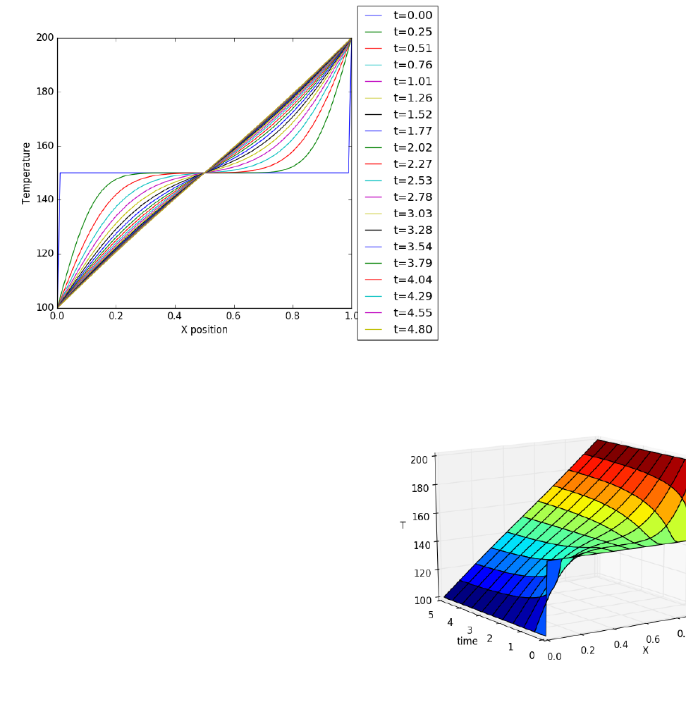
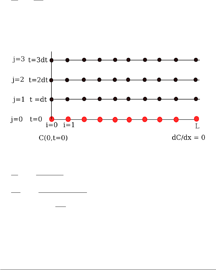
10.5.3 Transient diffusion - partial differential equations
We want to solve for the concentration profile of component that diffuses
into a 1D rod, with an impermeable barrier at the end. The PDE governing
this situation is:
∂C
∂t =D∂2C
∂x2
at t= 0, in this example we have C0(x)=0as an initial condition, with
boundary conditions C(0, t)=0.1and ∂C/∂x(L, t)=0.
We are going to discretize this equation in both time and space to arrive
at the solution. We will let ibe the index for the spatial discretization, and
jbe the index for the temporal discretization. The discretization looks like
this.
Note that we cannot use the method of lines as we did before because
we have the derivative-based boundary condition at one of the boundaries.
We approximate the time derivative as:
∂C
∂t i,j ≈Ci,j+1−Ci,j
∆t
∂2C
∂x2i,j ≈Ci+1,j −2Ci,j +Ci−1,j
h2
We define α=D∆t
h2, and from these two approximations and the PDE,
we solve for the unknown solution at a later time step as:
Ci,j+1 =αCi+1,j + (1 −2α)Ci,j +αCi−1,j
We know Ci,j=0 from the initial conditions, so we simply need to iterate
to evaluate Ci,j , which is the solution at each time step.
See also: http://www3.nd.edu/~jjwteach/441/PdfNotes/lecture16.
pdf
1import numpy as np
2import matplotlib.pyplot as plt
243

3
4N= 20 # number of points to discretize
5L= 1.0
6X=np.linspace(0, L, N) # position along the rod
7h=L/(N - 1)# discretization spacing
8
9C0t = 0.1 # concentration at x = 0
10 D= 0.02
11
12 tfinal = 50.0
13 Ntsteps = 1000
14 dt =tfinal /(Ntsteps - 1)
15 t=np.linspace(0, tfinal, Ntsteps)
16
17 alpha =D*dt /h**2
18 print(alpha)
19
20 C_xt =[] # container for all the time steps
21
22 # initial condition at t = 0
23 C=np.zeros(X.shape)
24 C[0]=C0t
25
26 C_xt += [C]
27
28 for jin range(1, Ntsteps):
29 N=np.zeros(C.shape)
30 N[0]=C0t
31 N[1:-1]=alpha*C[2:] +(1-2*alpha) *C[1:-1]+alpha *C[0:-2]
32 N[-1]=N[-2]# derivative boundary condition flux = 0
33 C[:] =N
34 C_xt += [N]
35
36 # plot selective solutions
37 if jin [1,2,5,10,20,50,100,200,500]:
38 plt.plot(X, N, label=’t={0:1.2f}’.format(t[j]))
39
40 plt.xlabel(’Position in rod’)
41 plt.ylabel(’Concentration’)
42 plt.title(’Concentration at different times’)
43 plt.legend(loc=’best’)
44 plt.savefig(’images/transient-diffusion-temporal-dependence.png’)
45
46 C_xt =np.array(C_xt)
47 plt.figure()
48 plt.plot(t, C_xt[:,5], label=’x={0:1.2f}’.format(X[5]))
49 plt.plot(t, C_xt[:,10], label=’x={0:1.2f}’.format(X[10]))
50 plt.plot(t, C_xt[:,15], label=’x={0:1.2f}’.format(X[15]))
51 plt.plot(t, C_xt[:,19], label=’x={0:1.2f}’.format(X[19]))
52 plt.legend(loc=’best’)
53 plt.xlabel(’Time’)
54 plt.ylabel(’Concentration’)
55 plt.savefig(’images/transient-diffusion-position-dependence.png’)
0.36136136136136143
244
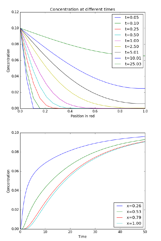
The solution is somewhat sensitive to the choices of time step and spatial
discretization. If you make the time step too big, the method is not stable,
and large oscillations may occur.
245
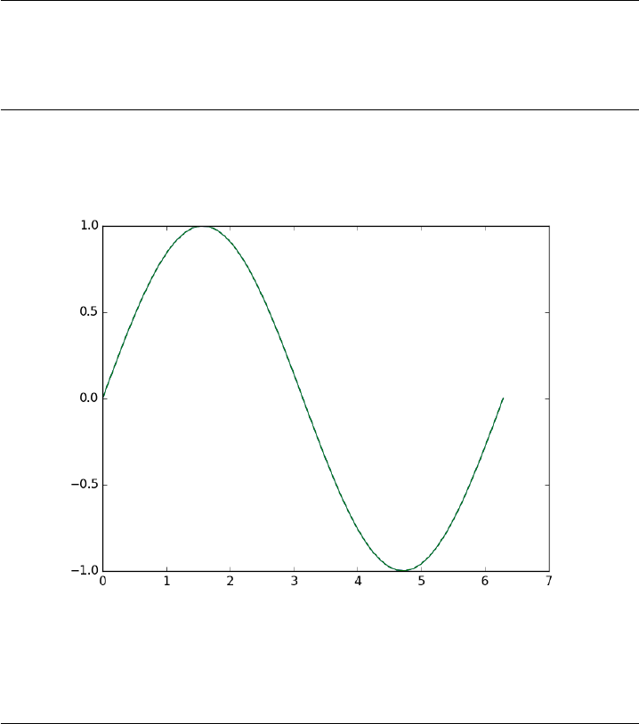
11 Plotting
11.1 Plot customizations - Modifying line, text and figure
properties
Matlab post
Here is a vanilla plot.
1import numpy as np
2import matplotlib.pyplot as plt
3
4x=np.linspace(0,2*np.pi)
5plt.plot(x, np.sin(x))
6plt.savefig(’images/plot-customization-1.png’)
[<matplotlib.lines.Line2D object at 0x10b361630>]
Lets increase the line thickness, change the line color to red, and make
the markers red circles with black outlines. I also like figures in presentations
to be 6 inches high, and 4 inches wide.
1import numpy as np
2import matplotlib.pyplot as plt
3
246

4x=np.linspace(0,2*np.pi)
5
6plt.figure(figsize=(4,6))
7plt.plot(x, np.sin(x), lw=2, color=’r’, marker=’o’, mec=’k’, mfc=’b’)
8
9plt.xlabel(’x data’, fontsize=12, fontweight=’bold’)
10 plt.ylabel(’y data’, fontsize=12, fontstyle=’italic’, color=’b’)
11 plt.tight_layout() # auto-adjust position of axes to fit figure.
12 plt.savefig(’images/plot-customization-2.png’)
247
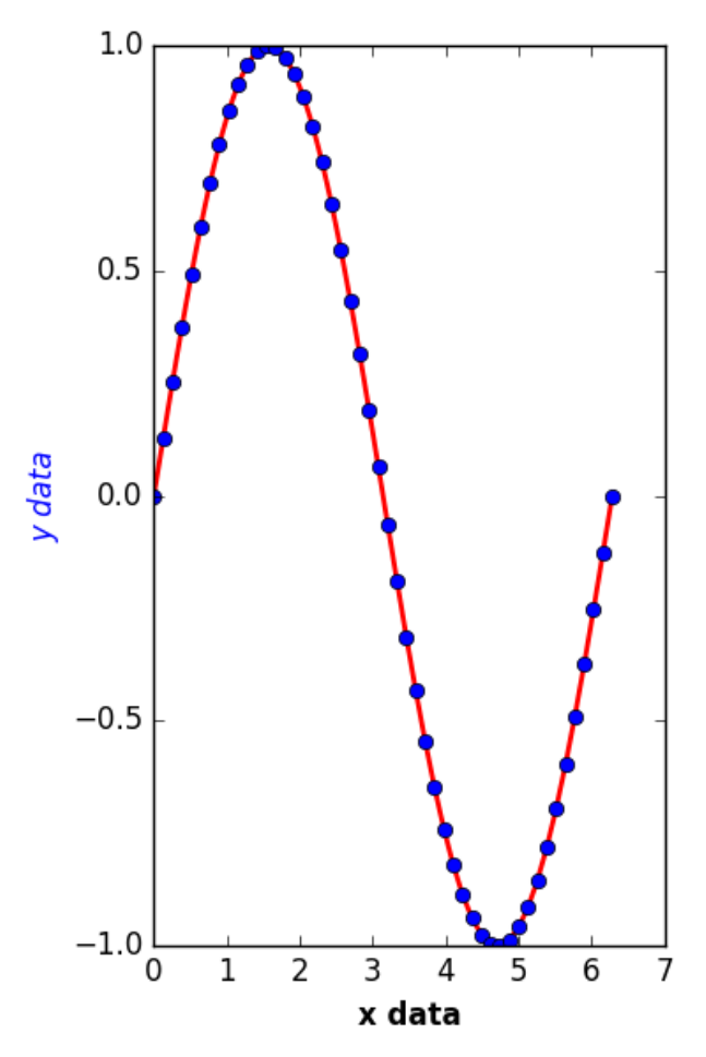
248

11.1.1 setting all the text properties in a figure.
You may notice the axis tick labels are not consistent with the labels now.
If you have many plots it can be tedious to try setting each text property.
Python to the rescue! With these commands you can find all the text
instances, and change them all at one time! Likewise, you can change all
the lines, and all the axes.
1import numpy as np
2import matplotlib.pyplot as plt
3
4x=np.linspace(0,2*np.pi)
5
6plt.figure(figsize=(4,6))
7plt.plot(x, np.sin(x), lw=2, color=’r’, marker=’o’, mec=’k’, mfc=’b’)
8
9plt.xlabel(’x data’, fontsize=12, fontweight=’bold’)
10 plt.ylabel(’y data’, fontsize=12, fontstyle=’italic’, color=’b’)
11
12 # set all font properties
13 fig =plt.gcf()
14 for oin fig.findobj(lambda x:hasattr(x, ’set_fontname’)
15 or hasattr(x, ’set_fontweight’)
16 or hasattr(x, ’set_fontsize’)):
17 o.set_fontname(’Arial’)
18 o.set_fontweight(’bold’)
19 o.set_fontsize(14)
20
21 # make anything you can set linewidth to be lw=2
22 def myfunc(x):
23 return hasattr(x, ’set_linewidth’)
24
25 for oin fig.findobj(myfunc):
26 o.set_linewidth(2)
27
28 plt.tight_layout() # auto-adjust position of axes to fit figure.
29 plt.savefig(’images/plot-customization-3.png’)
249
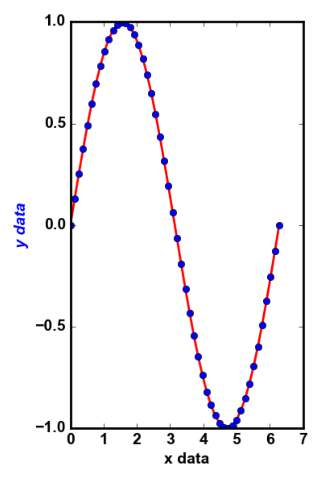
There are many other things you can do!
250
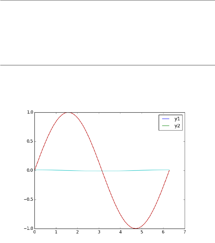
11.2 Plotting two datasets with very different scales
Matlab plot
Sometimes you will have two datasets you want to plot together, but
the scales will be so different it is hard to seem them both in the same plot.
Here we examine a few strategies to plotting this kind of data.
1import numpy as np
2import matplotlib.pyplot as plt
3
4x=np.linspace(0,2*np.pi)
5y1 =np.sin(x);
6y2 = 0.01 * np.cos(x);
7
8plt.plot(x, y1, x, y2)
9plt.legend([’y1’,’y2’])
10 plt.savefig(’images/two-scales-1.png’)
11 # in this plot y2 looks almost flat!
[<matplotlib.lines.Line2D object at 0x10b350550>, <matplotlib.lines.Line2D object at 0x10b371710>]
<matplotlib.legend.Legend object at 0x10b430e48>
251
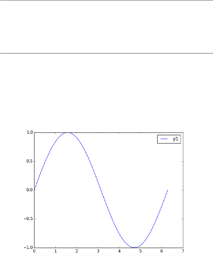
11.2.1 Make two plots!
this certainly solves the problem, but you have two full size plots, which
can take up a lot of space in a presentation and report. Often your goal
in plotting both data sets is to compare them, and it is easiest to compare
plots when they are perfectly lined up. Doing that manually can be tedious.
1plt.figure()
2plt.plot(x,y1)
3plt.legend([’y1’])
4plt.savefig(’images/two-scales-2.png’)
5
6plt.figure()
7plt.plot(x,y2)
8plt.legend([’y2’])
9plt.savefig(’images/two-scales-3.png’)
<matplotlib.figure.Figure object at 0x10b43ec18>
[<matplotlib.lines.Line2D object at 0x1090f5240>]
<matplotlib.legend.Legend object at 0x1090f53c8>
<matplotlib.figure.Figure object at 0x1090f5c18>
[<matplotlib.lines.Line2D object at 0x1090baac8>]
<matplotlib.legend.Legend object at 0x1090b5be0>
252
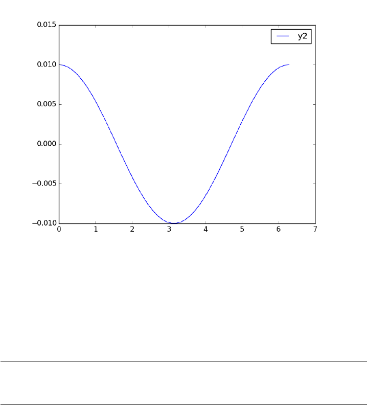
11.2.2 Scaling the results
Sometimes you can scale one dataset so it has a similar magnitude as the
other data set. Here we could multiply y2 by 100, and then it will be similar
in size to y1. Of course, you need to indicate that y2 has been scaled in the
graph somehow. Here we use the legend.
1plt.figure()
2plt.plot(x, y1, x, 100 * y2)
3plt.legend([’y1’,’100*y2’])
4plt.savefig(’images/two-scales-4.png’)
<matplotlib.figure.Figure object at 0x109124b70>
[<matplotlib.lines.Line2D object at 0x10b096400>, <matplotlib.lines.Line2D object at 0x10b096e10>]
<matplotlib.legend.Legend object at 0x10b09a550>
253
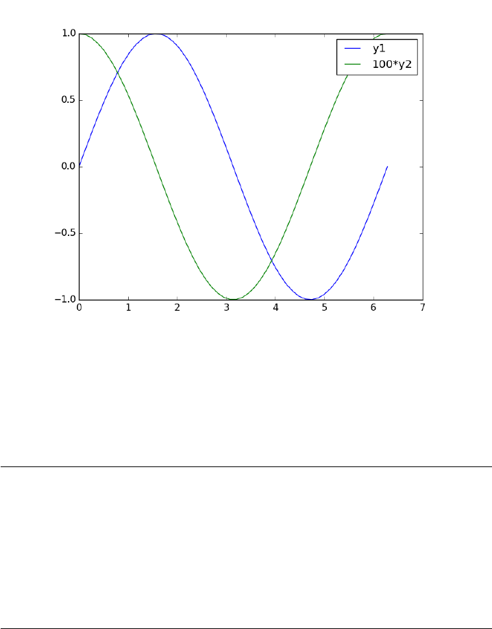
11.2.3 Double-y axis plot
Using two separate y-axes can solve your scaling problem. Note that each
y-axis is color coded to the data. It can be difficult to read these graphs
when printed in black and white
1fig =plt.figure()
2ax1 =fig.add_subplot(111)
3ax1.plot(x, y1)
4ax1.set_ylabel(’y1’)
5
6ax2 =ax1.twinx()
7ax2.plot(x, y2, ’r-’)
8ax2.set_ylabel(’y2’, color=’r’)
9for tl in ax2.get_yticklabels():
10 tl.set_color(’r’)
11
12 plt.savefig(’images/two-scales-5.png’)
[<matplotlib.lines.Line2D object at 0x10f772c88>]
<matplotlib.text.Text object at 0x10b0ce390>
[<matplotlib.lines.Line2D object at 0x10f796518>]
<matplotlib.text.Text object at 0x10f786518>
254
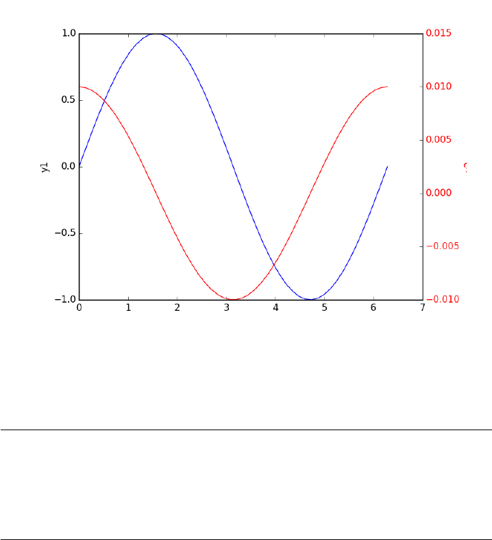
11.2.4 Subplots
An alternative approach to double y axes is to use subplots.
1plt.figure()
2f, axes =plt.subplots(2,1)
3axes[0].plot(x, y1)
4axes[0].set_ylabel(’y1’)
5
6axes[1].plot(x, y2)
7axes[1].set_ylabel(’y2’)
8plt.savefig(’images/two-scales-6.png’)
<matplotlib.figure.Figure object at 0x10f7828d0>
[<matplotlib.lines.Line2D object at 0x110131470>]
<matplotlib.text.Text object at 0x1100b7ac8>
[<matplotlib.lines.Line2D object at 0x110131cf8>]
<matplotlib.text.Text object at 0x110106898>
255
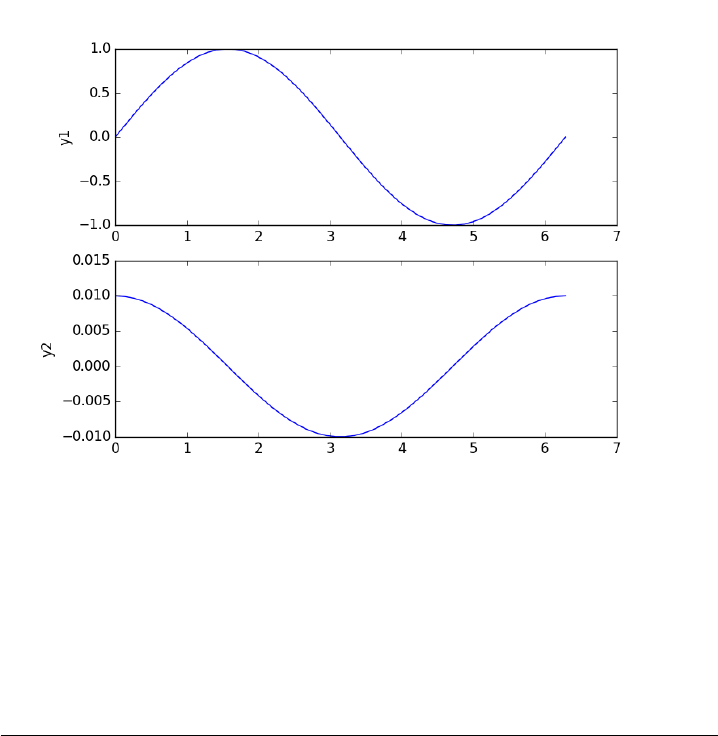
11.3 Customizing plots after the fact
Matlab post Sometimes it is desirable to make a plot that shows the data
you want to present, and to customize the details, e.g. font size/type and
line thicknesses afterwards. It can be tedious to try to add the customization
code to the existing code that makes the plot. Today, we look at a way to
do the customization after the plot is created.
1import numpy as np
2import matplotlib.pyplot as plt
3
4x=np.linspace(0,2)
5y1 =x
6y2 =x**2
7y3 =x**3
8
9plt.plot(x, y1, x, y2, x, y3)
10 xL =plt.xlabel(’x’)
11 yL =plt.ylabel(’f(x)’)
12 plt.title(’plots of y = x^n’)
13 plt.legend([’x’,’x^2’,’x^3’], loc=’best’)
14 plt.savefig(’images/after-customization-1.png’)
15
16 fig =plt.gcf()
17
18 plt.setp(fig, ’size_inches’, (4,6))
256
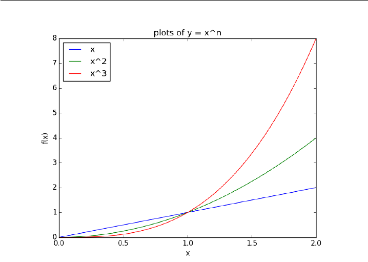
19 plt.savefig(’images/after-customization-2.png’)
20
21
22 # set lines to dashed
23 from matplotlib.lines import Line2D
24 for oin fig.findobj(Line2D):
25 o.set_linestyle(’--’)
26
27 #set(allaxes,’FontName’,’Arial’,’FontWeight’,’Bold’,’LineWidth’,2,’FontSize’,14);
28
29 import matplotlib.text as text
30 for oin fig.findobj(text.Text):
31 plt.setp(o, ’fontname’,’Arial’,’fontweight’,’bold’,’fontsize’,14)
32
33 plt.setp(xL, ’fontstyle’,’italic’)
34 plt.setp(yL, ’fontstyle’,’italic’)
35 plt.savefig(’images/after-customization-3.png’)
257
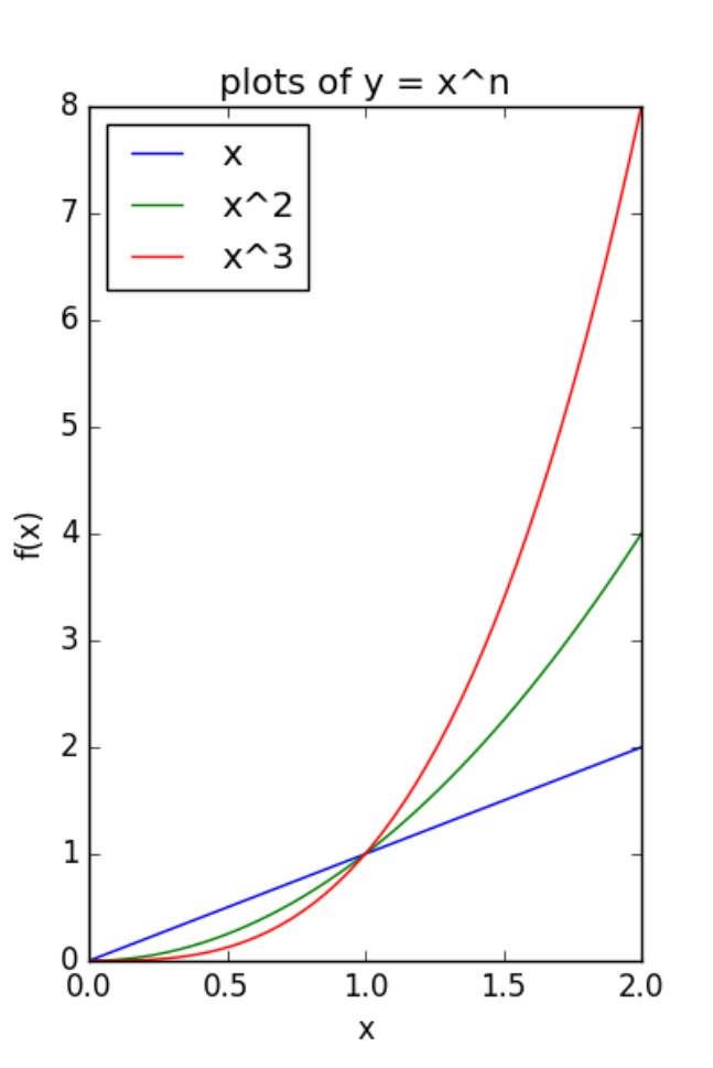
258
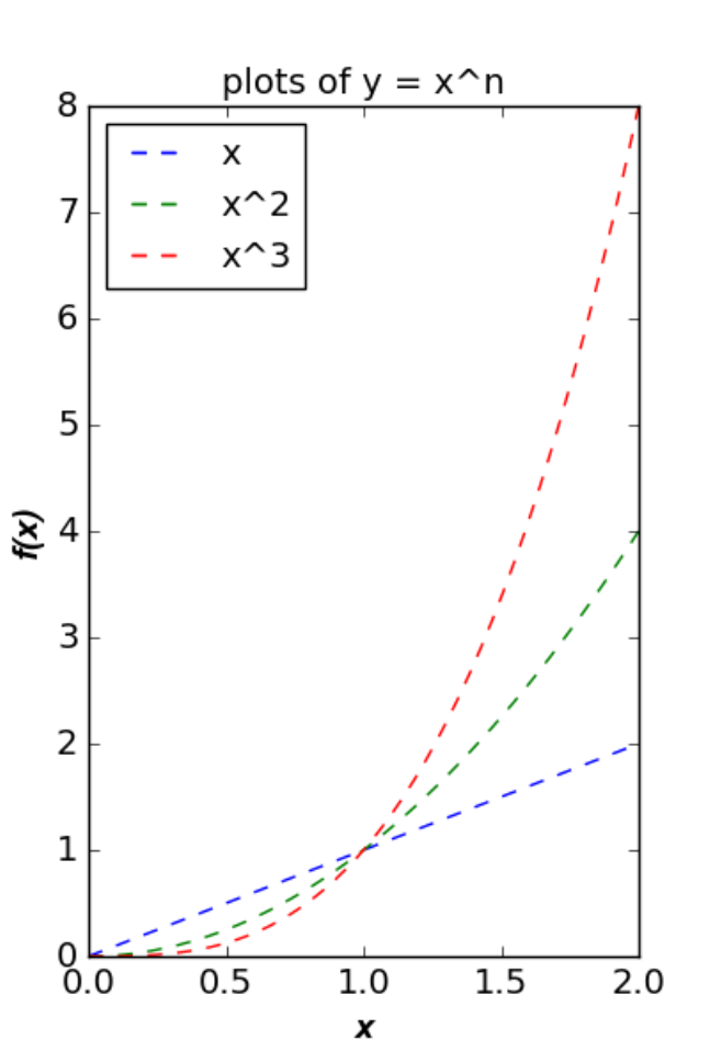
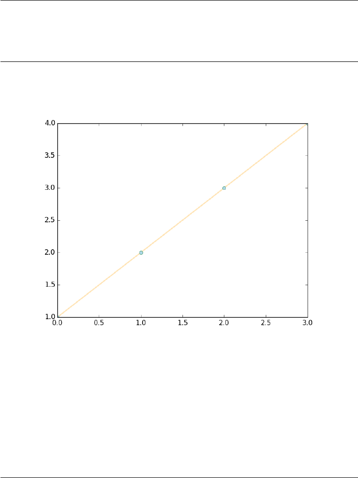
Matplotlib has a lot of built-in colors. Here is a list of them, and an
example of using them.
1import matplotlib.pyplot as plt
2from matplotlib.colors import cnames
3print(cnames.keys())
4
5plt.plot([1,2,3,4], lw=2, color=’moccasin’, marker=’o’, mfc=’lightblue’, mec=’seagreen’)
6plt.savefig(’images/fall-colors.png’)
dict_keys([’orangered’, ’salmon’, ’firebrick’, ’dimgrey’, ’white’, ’darkseagreen’, ’cornflowerblue’, ’brown’, ’bisque’, ’thistle’, ’darkgoldenrod’, ’cornsilk’, ’papayawhip’, ’lightseagreen’, ’forestgreen’, ’mediumseagreen’, ’antiquewhite’, ’darkorchid’, ’mintcream’, ’saddlebrown’, ’oldlace’, ’darkslategrey’, ’darkgreen’, ’steelblue’, ’paleturquoise’, ’royalblue’, ’red’, ’springgreen’, ’pink’, ’lightcoral’, ’maroon’, ’lightblue’, ’aquamarine’, ’wheat’, ’gray’, ’lightsage’, ’peru’, ’lightpink’, ’greenyellow’, ’slategrey’, ’aliceblue’, ’darkorange’, ’blue’, ’fuchsia’, ’lightgoldenrodyellow’, ’mediumpurple’, ’moccasin’, ’goldenrod’, ’darkcyan’, ’olivedrab’, ’yellowgreen’, ’lavender’, ’lavenderblush’, ’magenta’, ’darkslateblue’, ’mediumblue’, ’burlywood’, ’orange’, ’lightgreen’, ’coral’, ’darkolivegreen’, ’lime’, ’darkslategray’, ’linen’, ’skyblue’, ’palegoldenrod’, ’teal’, ’darkblue’, ’mediumaquamarine’, ’tan’, ’gold’, ’ghostwhite’, ’beige’, ’lemonchiffon’, ’lightsteelblue’, ’ivory’, ’mediumvioletred’, ’mediumturquoise’, ’olive’, ’lightgray’, ’mediumorchid’, ’cadetblue’, ’azure’, ’gainsboro’, ’indigo’, ’deeppink’, ’slategray’, ’midnightblue’, ’mediumspringgreen’, ’honeydew’, ’blueviolet’, ’palegreen’, ’khaki’, ’dimgray’, ’deepskyblue’, ’darkgray’, ’whitesmoke’, ’mediumslateblue’, ’lightslategrey’, ’dodgerblue’, ’darksalmon’, ’indianred’, ’plum’, ’lightslategray’, ’black’, ’darkred’, ’darkviolet’, ’snow’, ’turquoise’, ’navajowhite’, ’powderblue’, ’yellow’, ’peachpuff’, ’chocolate’, ’chartreuse’, ’purple’, ’seashell’, ’darkmagenta’, ’darkgrey’, ’tomato’, ’darkturquoise’, ’cyan’, ’mistyrose’, ’lightsalmon’, ’darkkhaki’, ’aqua’, ’lightyellow’, ’violet’, ’sandybrown’, ’silver’, ’orchid’, ’palevioletred’, ’lawngreen’, ’hotpink’, ’lightgrey’, ’blanchedalmond’, ’lightcyan’, ’sienna’, ’green’, ’lightskyblue’, ’crimson’, ’limegreen’, ’slateblue’, ’navy’, ’sage’, ’floralwhite’, ’seagreen’, ’rosybrown’, ’grey’, ’darksage’])
11.5 Picasso’s short lived blue period with Python
Matlab post
It is an unknown fact that Picasso had a brief blue plotting period with
Matlab before moving on to his more famous paintings. It started from
irritation with the default colors available in Matlab for plotting. After
watching his friend van Gogh cut off his own ear out of frustration with the
ugly default colors, Picasso had to do something different.
1import numpy as np
2import matplotlib.pyplot as plt
260
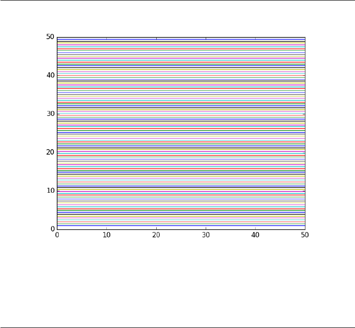
3
4#this plots horizontal lines for each y value of m.
5for min np.linspace(1,50,100):
6plt.plot([0,50], [m, m])
7
8plt.savefig(’images/blues-1.png’)
Picasso copied the table availabe at http://en.wikipedia.org/wiki/
List_of_colors and parsed it into a dictionary of hex codes for new colors.
That allowed him to specify a list of beautiful blues for his graph. Picasso
eventually gave up on python as an artform, and moved on to painting.
1import numpy as np
2import matplotlib.pyplot as plt
3
4c={}
5with open(’color.table’)as f:
6for line in f:
7fields =line.split(’\t’)
8colorname =fields[0].lower()
9hexcode =fields[1]
10 c[colorname] =hexcode
11
12 names =c.keys()
13 names =sorted(names)
14
15 print(names)
261
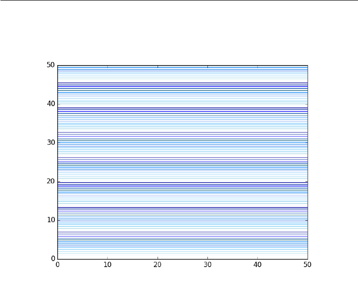
16
17 blues =[c[’alice blue’],
18 c[’light blue’],
19 c[’baby blue’],
20 c[’light sky blue’],
21 c[’maya blue’],
22 c[’cornflower blue’],
23 c[’bleu de france’],
24 c[’azure’],
25 c[’blue sapphire’],
26 c[’cobalt’],
27 c[’blue’],
28 c[’egyptian blue’],
29 c[’duke blue’]]
30
31 ax =plt.gca()
32 ax.set_color_cycle(blues)
33
34 #this plots horizontal lines for each y value of m.
35 for i, m in enumerate(np.linspace(1,50,100)):
36 plt.plot([0,50], [m, m])
37
38 plt.savefig(’images/blues-2.png’)
[’aero’, ’aero blue’, ’african violet’, ’air force blue (raf)’, ’air force blue (usaf)’, ’air superiority blue’, ’alabama crimson’, ’alice blue’, ’alizarin crimson’, ’alloy orange’, ’almond’, ’amaranth’, ’amazon’, ’amber’, ’american rose’, ’amethyst’, ’android green’, ’anti-flash white’, ’antique brass’, ’antique bronze’, ’antique fuchsia’, ’antique ruby’, ’antique white’, ’ao (english)’, ’apple green’, ’apricot’, ’aqua’, ’aquamarine’, ’army green’, ’arsenic’, ’arylide yellow’, ’ash grey’, ’asparagus’, ’atomic tangerine’, ’auburn’, ’aureolin’, ’aurometalsaurus’, ’avocado’, ’azure’, ’azure mist/web’, "b’dazzled blue", ’baby blue’, ’baby blue eyes’, ’baby pink’, ’baby powder’, ’baker-miller pink’, ’ball blue’, ’banana mania’, ’banana yellow’, ’barbie pink’, ’barn red’, ’battleship grey’, ’bazaar’, ’beau blue’, ’beaver’, ’beige’, ’big dip o’ruby’, ’bisque’, ’bistre’, ’bistre brown’, ’bitter lemon’, ’bitter lime’, ’bittersweet’, ’bittersweet shimmer’, ’black’, ’black bean’, ’black leather jacket’, ’black olive’, ’blanched almond’, ’blast-off bronze’, ’bleu de france’, ’blizzard blue’, ’blond’, ’blue’, ’blue (crayola)’, ’blue (munsell)’, ’blue (ncs)’, ’blue (pigment)’, ’blue (ryb)’, ’blue bell’, ’blue sapphire’, ’blue yonder’, ’blue-gray’, ’blue-green’, ’blue-violet’, ’blueberry’, ’bluebonnet’, ’blush’, ’bole’, ’bondi blue’, ’bone’, ’boston university red’, ’bottle green’, ’boysenberry’, ’brandeis blue’, ’brass’, ’brick red’, ’bright cerulean’, ’bright green’, ’bright lavender’, ’bright maroon’, ’bright pink’, ’bright turquoise’, ’bright ube’, ’brilliant lavender’, ’brilliant rose’, ’brink pink’, ’british racing green’, ’bronze’, ’bronze yellow’, ’brown (traditional)’, ’brown (web)’, ’brown-nose’, ’brunswick green’, ’bubble gum’, ’bubbles’, ’buff’, ’bulgarian rose’, ’burgundy’, ’burlywood’, ’burnt orange’, ’burnt sienna’, ’burnt umber’, ’byzantine’, ’byzantium’, ’cadet’, ’cadet blue’, ’cadet grey’, ’cadmium green’, ’cadmium orange’, ’cadmium red’, ’cadmium yellow’, ’café au lait’, ’café noir’, ’cal poly green’, ’cambridge blue’, ’camel’, ’cameo pink’, ’camouflage green’, ’canary yellow’, ’candy apple red’, ’candy pink’, ’capri’, ’caput mortuum’, ’cardinal’, ’caribbean green’, ’carmine’, ’carmine (m&p)’, ’carmine pink’, ’carmine red’, ’carnation pink’, ’carnelian’, ’carolina blue’, ’carrot orange’, ’castleton green’, ’catalina blue’, ’catawba’, ’cedar chest’, ’ceil’, ’celadon’, ’celadon blue’, ’celadon green’, ’celeste (colour)’, ’celestial blue’, ’cerise’, ’cerise pink’, ’cerulean’, ’cerulean blue’, ’cerulean frost’, ’cg blue’, ’cg red’, ’chamoisee’, ’champagne’, ’charcoal’, ’charleston green’, ’charm pink’, ’chartreuse (traditional)’, ’chartreuse (web)’, ’cherry’, ’cherry blossom pink’, ’chestnut’, ’china pink’, ’china rose’, ’chinese red’, ’chinese violet’, ’chocolate (traditional)’, ’chocolate (web)’, ’chrome yellow’, ’cinereous’, ’cinnabar’, ’cinnamon’, ’citrine’, ’citron’, ’claret’, ’classic rose’, ’cobalt’, ’cocoa brown’, ’coconut’, ’coffee’, ’columbia blue’, ’congo pink’, ’cool black’, ’cool grey’, ’copper’, ’copper (crayola)’, ’copper penny’, ’copper red’, ’copper rose’, ’coquelicot’, ’coral’, ’coral pink’, ’coral red’, ’cordovan’, ’corn’, ’cornell red’, ’cornflower blue’, ’cornsilk’, ’cosmic latte’, ’cotton candy’, ’cream’, ’crimson’, ’crimson glory’, ’cyan’, ’cyan (process)’, ’cyber grape’, ’cyber yellow’, ’daffodil’, ’dandelion’, ’dark blue’, ’dark blue-gray’, ’dark brown’, ’dark byzantium’, ’dark candy apple red’, ’dark cerulean’, ’dark chestnut’, ’dark coral’, ’dark cyan’, ’dark electric blue’, ’dark goldenrod’, ’dark gray’, ’dark green’, ’dark imperial blue’, ’dark jungle green’, ’dark khaki’, ’dark lava’, ’dark lavender’, ’dark liver’, ’dark liver (horses)’, ’dark magenta’, ’dark midnight blue’, ’dark moss green’, ’dark olive green’, ’dark orange’, ’dark orchid’, ’dark pastel blue’, ’dark pastel green’, ’dark pastel purple’, ’dark pastel red’, ’dark pink’, ’dark powder blue’, ’dark raspberry’, ’dark red’, ’dark salmon’, ’dark scarlet’, ’dark sea green’, ’dark sienna’, ’dark sky blue’, ’dark slate blue’, ’dark slate gray’, ’dark spring green’, ’dark tan’, ’dark tangerine’, ’dark taupe’, ’dark terra cotta’, ’dark turquoise’, ’dark vanilla’, ’dark violet’, ’dark yellow’, ’dartmouth green’, "davy’s grey", ’debian red’, ’deep carmine’, ’deep carmine pink’, ’deep carrot orange’, ’deep cerise’, ’deep champagne’, ’deep chestnut’, ’deep coffee’, ’deep fuchsia’, ’deep jungle green’, ’deep lemon’, ’deep lilac’, ’deep magenta’, ’deep mauve’, ’deep moss green’, ’deep peach’, ’deep pink’, ’deep ruby’, ’deep saffron’, ’deep sky blue’, ’deep space sparkle’, ’deep taupe’, ’deep tuscan red’, ’deer’, ’denim’, ’desert’, ’desert sand’, ’diamond’, ’dim gray’, ’dirt’, ’dodger blue’, ’dogwood rose’, ’dollar bill’, ’donkey brown’, ’drab’, ’duke blue’, ’dust storm’, ’earth yellow’, ’ebony’, ’ecru’, ’eggplant’, ’eggshell’, ’egyptian blue’, ’electric blue’, ’electric crimson’, ’electric cyan’, ’electric green’, ’electric indigo’, ’electric lavender’, ’electric lime’, ’electric purple’, ’electric ultramarine’, ’electric violet’, ’electric yellow’, ’emerald’, ’english green’, ’english lavender’, ’english red’, ’english violet’, ’eton blue’, ’eucalyptus’, ’fallow’, ’falu red’, ’fandango’, ’fandango pink’, ’fashion fuchsia’, ’fawn’, ’feldgrau’, ’feldspar’, ’fern green’, ’ferrari red’, ’field drab’, ’fire engine red’, ’firebrick’, ’flame’, ’flamingo pink’, ’flattery’, ’flavescent’, ’flax’, ’flirt’, ’floral white’, ’fluorescent orange’, ’fluorescent pink’, ’fluorescent yellow’, ’folly’, ’forest green (traditional)’, ’forest green (web)’, ’french beige’, ’french bistre’, ’french blue’, ’french lilac’, ’french lime’, ’french mauve’, ’french raspberry’, ’french rose’, ’french sky blue’, ’french wine’, ’fresh air’, ’fuchsia’, ’fuchsia (crayola)’, ’fuchsia pink’, ’fuchsia rose’, ’fulvous’, ’fuzzy wuzzy’, ’gainsboro’, ’gamboge’, ’ghost white’, ’giants orange’, ’ginger’, ’glaucous’, ’glitter’, ’go green’, ’gold (metallic)’, ’gold (web) (golden)’, ’gold fusion’, ’golden brown’, ’golden poppy’, ’golden yellow’, ’goldenrod’, ’granny smith apple’, ’grape’, ’gray’, ’gray (html/css gray)’, ’gray (x11 gray)’, ’gray-asparagus’, ’gray-blue’, ’green (color wheel) (x11 green)’, ’green (crayola)’, ’green (html/css color)’, ’green (munsell)’, ’green (ncs)’, ’green (pigment)’, ’green (ryb)’, ’green-yellow’, ’grullo’, ’guppie green’, ’halayà úbe’, ’han blue’, ’han purple’, ’hansa yellow’, ’harlequin’, ’harvard crimson’, ’harvest gold’, ’heart gold’, ’heliotrope’, ’hollywood cerise’, ’honeydew’, ’honolulu blue’, "hooker’s green", ’hot magenta’, ’hot pink’, ’hunter green’, ’iceberg’, ’icterine’, ’illuminating emerald’, ’imperial’, ’imperial blue’, ’imperial purple’, ’imperial red’, ’inchworm’, ’india green’, ’indian red’, ’indian yellow’, ’indigo’, ’indigo (dye)’, ’indigo (web)’, ’international klein blue’, ’international orange (aerospace)’, ’international orange (engineering)’, ’international orange (golden gate bridge)’, ’iris’, ’irresistible’, ’isabelline’, ’islamic green’, ’italian sky blue’, ’ivory’, ’jade’, ’japanese indigo’, ’japanese violet’, ’jasmine’, ’jasper’, ’jazzberry jam’, ’jelly bean’, ’jet’, ’jonquil’, ’june bud’, ’jungle green’, ’kelly green’, ’kenyan copper’, ’keppel’, ’khaki (html/css) (khaki)’, ’khaki (x11) (light khaki)’, ’kobe’, ’kobi’, ’ku crimson’, ’la salle green’, ’languid lavender’, ’lapis lazuli’, ’laser lemon’, ’laurel green’, ’lava’, ’lavender (floral)’, ’lavender (web)’, ’lavender blue’, ’lavender blush’, ’lavender gray’, ’lavender indigo’, ’lavender magenta’, ’lavender mist’, ’lavender pink’, ’lavender purple’, ’lavender rose’, ’lawn green’, ’lemon’, ’lemon chiffon’, ’lemon curry’, ’lemon glacier’, ’lemon lime’, ’lemon meringue’, ’lemon yellow’, ’licorice’, ’light apricot’, ’light blue’, ’light brown’, ’light carmine pink’, ’light coral’, ’light cornflower blue’, ’light crimson’, ’light cyan’, ’light fuchsia pink’, ’light goldenrod yellow’, ’light gray’, ’light green’, ’light khaki’, ’light medium orchid’, ’light moss green’, ’light orchid’, ’light pastel purple’, ’light pink’, ’light red ochre’, ’light salmon’, ’light salmon pink’, ’light sea green’, ’light sky blue’, ’light slate gray’, ’light steel blue’, ’light taupe’, ’light thulian pink’, ’light yellow’, ’lilac’, ’lime (color wheel)’, ’lime (web) (x11 green)’, ’lime green’, ’limerick’, ’lincoln green’, ’linen’, ’lion’, ’little boy blue’, ’liver’, ’liver (dogs)’, ’liver (organ)’, ’liver chestnut’, ’lumber’, ’lust’, ’magenta’, ’magenta (crayola)’, ’magenta (dye)’, ’magenta (pantone)’, ’magenta (process)’, ’magic mint’, ’magnolia’, ’mahogany’, ’maize’, ’majorelle blue’, ’malachite’, ’manatee’, ’mango tango’, ’mantis’, ’mardi gras’, ’maroon (crayola)’, ’maroon (html/css)’, ’maroon (x11)’, ’mauve’, ’mauve taupe’, ’mauvelous’, ’maya blue’, ’meat brown’, ’medium aquamarine’, ’medium blue’, ’medium candy apple red’, ’medium carmine’, ’medium champagne’, ’medium electric blue’, ’medium jungle green’, ’medium lavender magenta’, ’medium orchid’, ’medium persian blue’, ’medium purple’, ’medium red-violet’, ’medium ruby’, ’medium sea green’, ’medium sky blue’, ’medium slate blue’, ’medium spring bud’, ’medium spring green’, ’medium taupe’, ’medium turquoise’, ’medium tuscan red’, ’medium vermilion’, ’medium violet-red’, ’mellow apricot’, ’mellow yellow’, ’melon’, ’metallic seaweed’, ’metallic sunburst’, ’mexican pink’, ’midnight blue’, ’midnight green (eagle green)’, ’midori’, ’mikado yellow’, ’mint’, ’mint cream’, ’mint green’, ’misty rose’, ’moccasin’, ’mode beige’, ’moonstone blue’, ’mordant red 19’, ’moss green’, ’mountain meadow’, ’mountbatten pink’, ’msu green’, ’mughal green’, ’mulberry’, ’mustard’, ’myrtle green’, ’sae/ece amber (color)’]
262

11.6 Interactive plotting
11.6.1 Basic mouse clicks
One basic event a figure can react to is a mouse click. Let us make a graph
with a parabola in it, and draw the shortest line from a point clicked on to
the graph. Here is an example of doing that.
1import matplotlib.pyplot as plt
2import numpy as np
3from scipy.optimize import fmin_cobyla
4
5fig =plt.figure()
6
7def f(x):
8return x**2
9
10 x=np.linspace(-2,2)
11 y=f(x)
12
13 ax =fig.add_subplot(111)
14 ax.plot(x, y)
15 ax.set_title(’Click somewhere’)
16
17 def onclick(event):
18 ax =plt.gca()
19
20 P=(event.xdata, event.ydata)
21
22 def objective(X):
23 x,y =X
24 return np.sqrt((x -P[0])**2 + (y -P[1])**2)
25
26 def c1(X):
27 x,y =X
28 return f(x) -y
29
30 X=fmin_cobyla(objective, x0=[P[0], f(P[0])], cons=[c1])
31
32 ax.set_title(’x={0:1.2f} y={1:1.2f}’.format(event.xdata, event.ydata))
33 ax.plot([event.xdata, X[0]], [event.ydata, X[1]], ’ro-’)
34 ax.figure.canvas.draw() # this line is critical to change the title
35 plt.savefig(’images/interactive-basic-click.png’)
36
37 cid =fig.canvas.mpl_connect(’button_press_event’, onclick)
38 plt.show()
Normal return from subroutine COBYLA
NFVALS = 38 F = 6.953792E-05 MAXCV = 0.000000E+00
X = 1.491871E+00 8.750272E-01
263
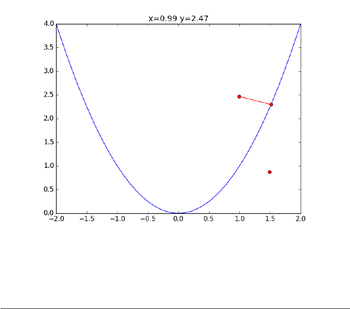
Normal return from subroutine COBYLA
NFVALS = 43 F = 5.510959E-01 MAXCV = 0.000000E+00
X = 1.515237E+00 2.295944E+00
Here is the result from two clicks. For some reason, this only works when
you click inside the parabola. It does not work outside the parabola.
We can even do different things with different mouse clicks. A left click
corresponds to event.button = 1, a middle click is event.button = 2, and a
right click is event.button = 3. You can detect if a double click occurs too.
Here is an example of these different options.
1import matplotlib.pyplot as plt
2import numpy as np
3
4fig =plt.figure()
5
6ax =fig.add_subplot(111)
7ax.plot(np.random.rand(10))
8ax.set_title(’Click somewhere’)
9
10 def onclick(event):
11 ax.set_title(’x={0:1.2f} y={1:1.2f} button={2}’.format(event.xdata, event.ydata, event.button))
12 colors =’ rbg’
13 print(’button={0} (dblclick={2}). making a {1} dot’.format(event.button,
14 colors[event.button],
264
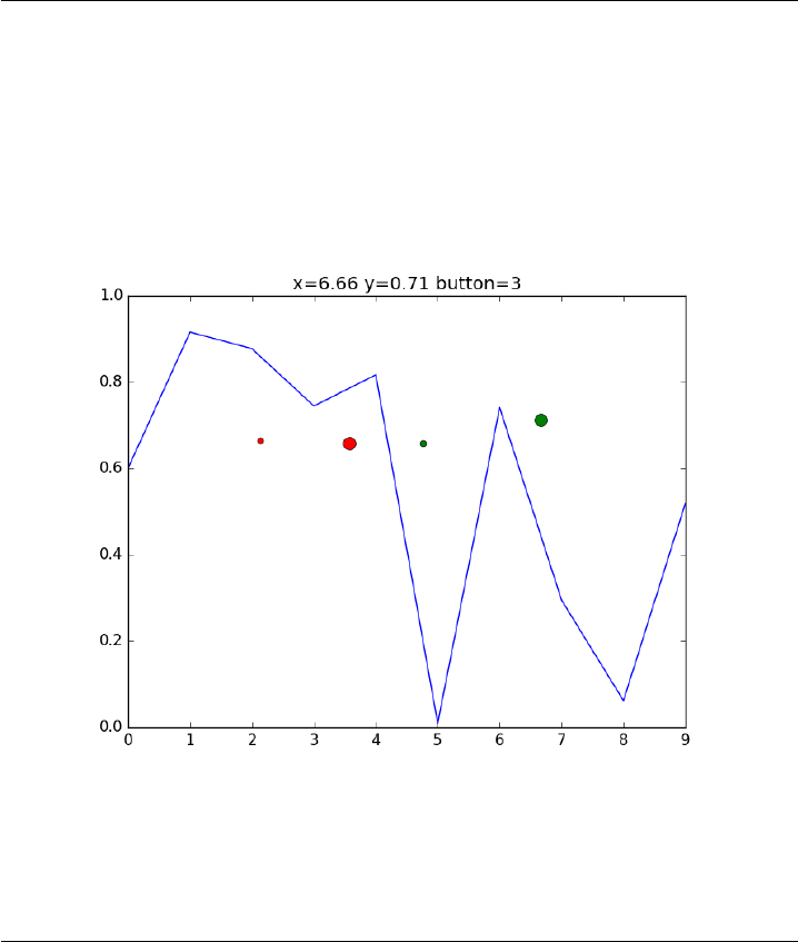
15 event.dblclick))
16
17 ms=5 # marker size
18 if event.dblclick: #make marker bigger
19 ms = 10
20
21 ax.plot([event.xdata], [event.ydata], ’o’, color=colors[event.button], ms=ms)
22 ax.figure.canvas.draw() # this line is critical to change the title
23 plt.savefig(’images/interactive-button-click.png’)
24
25 cid =fig.canvas.mpl_connect(’button_press_event’, onclick)
26 plt.show()
button=1 (dblclick=0). making a r dot
button=1 (dblclick=0). making a r dot
button=1 (dblclick=1). making a r dot
button=3 (dblclick=0). making a g dot
button=3 (dblclick=0). making a g dot
button=3 (dblclick=1). making a g dot
Finally, you may want to have key modifiers for your clicks, e.g. Ctrl-
click is different than a click.
11.7 key events not working on Mac/org-mode
265

1from __future__ import print_function
2import sys
3import numpy as np
4import matplotlib.pyplot as plt
5
6
7def press(event):
8print(’press’, event.key)
9sys.stdout.flush()
10 if event.key == ’x’:
11 visible =xl.get_visible()
12 xl.set_visible(not visible)
13 fig.canvas.draw()
14
15 fig, ax =plt.subplots()
16
17 fig.canvas.mpl_connect(’key_press_event’, press)
18
19 ax.plot(np.random.randx(12), np.random.rand(12), ’go’)
20 xl =ax.set_xlabel(’easy come, easy go’)
21
22 plt.show()
1import matplotlib.pyplot as plt
2import numpy as np
3
4fig =plt.figure()
5
6ax =fig.add_subplot(111)
7ax.plot(np.random.rand(10))
8ax.set_title(’Click somewhere’)
9
10 def onclick(event):
11 print(event)
12 ax =plt.gca()
13 ax.set_title(’x={0:1.2f} y={1:1.2f}’.format(event.xdata, event.ydata))
14 if event.key == ’shift+control’:
15 color =’red’
16 elif event.key == ’shift’:
17 color =’yellow’
18 else:
19 color =’blue’
20
21 ax.plot([event.xdata], [event.ydata], ’o’, color=color)
22 ax.figure.canvas.draw() # this line is critical to change the title
23 plt.savefig(’images/interactive-button-key-click.png’)
24
25 cid =fig.canvas.mpl_connect(’button_press_event’, onclick)
26 plt.show()
MPL MouseEvent: xy=(236,320) xydata=(2.83064516129,0.708333333333) button=1 dblclick=0 inaxes=Axes(0.125,0.1;0.775x0.8)
MPL MouseEvent: xy=(294,295) xydata=(3.88306451613,0.643229166667) button=1 dblclick=0 inaxes=Axes(0.125,0.1;0.775x0.8)
MPL MouseEvent: xy=(309,251) xydata=(4.15524193548,0.528645833333) button=1 dblclick=0 inaxes=Axes(0.125,0.1;0.775x0.8)
266
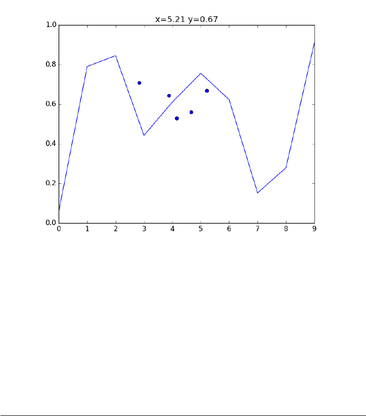
MPL MouseEvent: xy=(337,263) xydata=(4.66330645161,0.559895833333) button=2 dblclick=0 inaxes=Axes(0.125,0.1;0.775x0.8)
MPL MouseEvent: xy=(367,305) xydata=(5.20766129032,0.669270833333) button=1 dblclick=0 inaxes=Axes(0.125,0.1;0.775x0.8)
You can have almost every key-click combination imaginable. This allows
you to have many different things that can happen when you click on a
graph. With this method, you can get the coordinates close to a data point,
but you do not get the properties of the point. For that, we need another
mechanism.
11.7.1 Mouse movement
In this example, we will let the mouse motion move a point up and down a
curve. This might be helpful to explore a function graph, for example. We
use interpolation to estimate the curve between data points.
1import matplotlib.pyplot as plt
2import numpy as np
3from scipy.interpolate import interp1d
4
5# the "data"
6x=np.linspace(0, np.pi)
7y=np.sin(x)
8
9# interpolating function between points
10 p=interp1d(x, y, ’cubic’)
267

11
12 # make the figure
13 fig =plt.figure()
14
15 ax =fig.add_subplot(111)
16 line, =ax.plot(x, y, ’ro-’)
17 marker, =ax.plot([0.5], [0.5],’go’, ms=15)
18
19 ax.set_title(’Move the mouse around’)
20
21 def onmove(event):
22
23 xe =event.xdata
24 ye =event.ydata
25
26 ax.set_title(’at x={0} y={1}’.format(xe, p(xe)))
27 marker.set_xdata(xe)
28 marker.set_ydata(p(xe))
29
30 ax.figure.canvas.draw() # this line is critical to change the title
31
32 cid =fig.canvas.mpl_connect(’motion_notify_event’, onmove)
33 plt.show()
11.7.2 key press events
Pressing a key is different than pressing a mouse button. We can do different
things with different key presses. You can access the coordinates of the
mouse when you press a key.
1import matplotlib.pyplot as plt
2import numpy as np
3
4fig =plt.figure()
5
6ax =fig.add_subplot(111)
7ax.plot(np.random.rand(10))
8ax.set_title(’Move the mouse somewhere and press a key’)
9
10 def onpress(event):
11 print(event.key)rgb
12 ax =plt.gca()
13 ax.set_title(’key={2} at x={0:1.2f} y={1:1.2f}’.format(event.xdata, event.ydata, event.key))
14 if event.key == ’r’:
15 color =’red’
16 elif event.key == ’y’:
17 color =’yellow’
18 else:
19 color =’blue’
20
21 ax.plot([event.xdata], [event.ydata], ’o’, color=color)
22 ax.figure.canvas.draw() # this line is critical to change the title
23 plt.savefig(’images/interactive-key-press.png’)
268

24
25 cid =fig.canvas.mpl_connect(’key_press_event’, onpress)
26 plt.show()
11.7.3 Picking lines
Instead of just getting the points in a figure, let us interact with lines on the
graph. We want to make the line we click on thicker. We use a "pick_event"
event and bind a function to that event that does something.
1import numpy as np
2import matplotlib.pyplot as plt
3
4fig =plt.figure()
5ax =fig.add_subplot(111)
6ax.set_title(’click on a line’)
7
8x=np.linspace(0,2*np.pi)
9
10 L1, =ax.plot(x, np.sin(x), picker=5)
11 L2, =ax.plot(x, np.cos(x), picker=5)
12
13 def onpick(event):
14 thisline =event.artist
15
16 # reset all lines to thin
17 for line in [L1, L2]:
18 line.set_lw(1)
19
20 thisline.set_lw(5)# make selected line thick
21 ax.figure.canvas.draw() # this line is critical to change the linewidth
22
23 fig.canvas.mpl_connect(’pick_event’, onpick)
24
25 plt.show()
11.7.4 Picking data points
In this example we show how to click on a data point, and show which point
was selected with a transparent marker, and show a label which refers to
the point.
1import numpy as np
2import matplotlib.pyplot as plt
3
4fig =plt.figure()
5ax =fig.add_subplot(111)
6ax.set_title(’click on a point’)
7
269
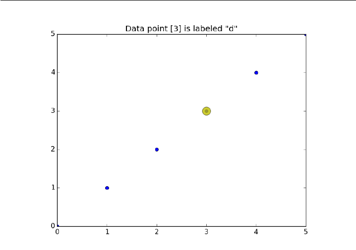
8x=[0,1,2,3,4,5]
9labels =[’a’,’b’,’c’,’d’,’e’,’f’]
10 ax.plot(x, ’bo’, picker=5)
11
12 # this is the transparent marker for the selected data point
13 marker, =ax.plot([0], [0], ’yo’, visible=False, alpha=0.8, ms=15)
14
15 def onpick(event):
16 ind =event.ind
17 ax.set_title(’Data point {0} is labeled "{1}"’.format(ind, labels[ind]))
18 marker.set_visible(True)
19 marker.set_xdata(x[ind])
20 marker.set_ydata(x[ind])
21
22 ax.figure.canvas.draw() # this line is critical to change the linewidth
23 plt.savefig(’images/interactive-labeled-points.png’)
24
25 fig.canvas.mpl_connect(’pick_event’, onpick)
26
27 plt.show()
11.8 Peak annotation in matplotlib
This post is just some examples of annotating features in a plot in matplotlib.
We illustrate finding peak maxima in a range, shading a region, shading
peaks, and labeling a region of peaks. I find it difficult to remember the
detailed syntax for these, so here are examples I could refer to later.
270

1import numpy as np
2import matplotlib.pyplot as plt
3
4w,i=np.loadtxt(’data/raman.txt’, usecols=(0,1), unpack=True)
5
6plt.plot(w, i)
7plt.xlabel(’Raman shift (cm$^{-1}$)’)
8plt.ylabel(’Intensity (counts)’)
9
10 ax =plt.gca()
11
12 # put a shaded rectangle over a region
13 ax.annotate(’Some typical region’, xy=(550,15500), xycoords=’data’)
14 ax.fill_between([700,800], 0, [16000,16000], facecolor=’red’, alpha=0.25)
15
16 # shade the region in the spectrum
17 ind =(w>1019)&(w<1054)
18 ax.fill_between(w[ind], 0, i[ind], facecolor=’gray’, alpha=0.5)
19 area =np.trapz(i[ind], w[ind])
20 x,y=w[ind][np.argmax(i[ind])], i[ind][np.argmax(i[ind])]
21 ax.annotate(’Area = {0:1.2f}’.format(area), xy=(x, y),
22 xycoords=’data’,
23 xytext=(x + 50,y+ 5000),
24 textcoords=’data’,
25 arrowprops=dict(arrowstyle="->",
26 connectionstyle="angle,angleA=0,angleB=90,rad=10"))
27
28
29 # find a max in this region, and annotate it
30 ind =(w>1250)&(w<1252)
31 x,y =w[ind][np.argmax(i[ind])], i[ind][np.argmax(i[ind])]
32 ax.annotate(’A peak’, xy=(x, y),
33 xycoords=’data’,
34 xytext=(x + 350,y+ 2000),
35 textcoords=’data’,
36 arrowprops=dict(arrowstyle="->",
37 connectionstyle="angle,angleA=0,angleB=90,rad=10"))
38
39 # find max in this region, and annotate it
40 ind =(w>1380)&(w<1400)
41 x,y =w[ind][np.argmax(i[ind])], i[ind][np.argmax(i[ind])]
42 ax.annotate(’Another peak’, xy=(x, y),
43 xycoords=’data’,
44 xytext=(x + 50,y+ 2000),
45 textcoords=’data’,
46 arrowprops=dict(arrowstyle="->",
47 connectionstyle="angle,angleA=0,angleB=90,rad=10"))
48
49 # indicate a region with connected arrows
50 ax.annotate(’CH bonds’, xy=(2780,6000), xycoords=’data’)
51 ax.annotate(’’, xy=(2800.,5000.), xycoords=’data’,
52 xytext=(3050,5000), textcoords=’data’,
53 # the arrows connect the xy to xytext coondinates
54 arrowprops=dict(arrowstyle="<->",
55 connectionstyle="bar",
56 ec="k",# edge color
271
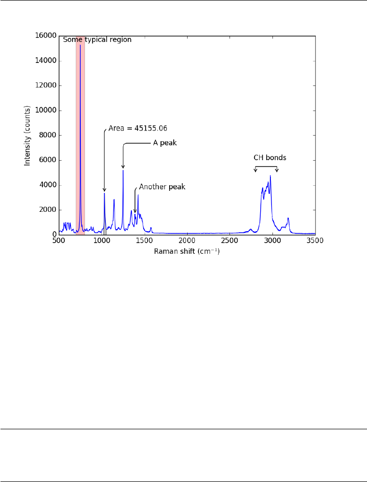
57 shrinkA=0.1, shrinkB=0.1))
58
59 plt.savefig(’images/plot-annotes.png’)
60 plt.show()
12 Programming
12.1 Some of this, sum of that
Matlab plot
Python provides a sum function to compute the sum of a list. However,
the sum function does not work on every arrangement of numbers, and it
certainly does not work on nested lists. We will solve this problem with
recursion.
Here is a simple example.
1v=[1,2,3,4,5,6,7,8,9]# a list
2print(sum(v))
3
4v=(1,2,3,4,5,6,7,8,9)# a tuple
5print(sum(v))
45
272

45
If you have data in a dictionary, sum works by default on the keys. You
can give the sum function the values like this.
1v={’a’:1,’b’:3,’c’:4}
2print(sum(v.values()))
8
12.1.1 Nested lists
Suppose now we have nested lists. This kind of structured data might come
up if you had grouped several things together. For example, suppose we
have 5 departments, with 1, 5, 15, 7 and 17 people in them, and in each
department they are divided into groups.
Department 1: 1 person Department 2: group of 2 and group of 3 De-
partment 3: group of 4 and 11, with a subgroups of 5 and 6 making up the
group of 11. Department 4: 7 people Department 5: one group of 8 and one
group of 9.
We might represent the data like this nested list. Now, if we want to
compute the total number of people, we need to add up each group. We
cannot simply sum the list, because some elements are single numbers, and
others are lists, or lists of lists. We need to recurse through each entry until
we get down to a number, which we can add to the running sum.
1v=[1,
2[2,3],
3[4, [5,6]],
47,
5[8,9]]
6
7def recursive_sum(X):
8’compute sum of arbitrarily nested lists’
9s= 0 # initial value of the sum
10
11 for iin range(len(X)):
12 import types # we use this to test if we got a number
13 if isinstance(X[i], (int,float,complex)):
14 # this is the terminal step
15 s+= X[i]
16 else:
17 # we did not get a number, so we recurse
18 s+= recursive_sum(X[i])
19 return s
20
273

21 print(recursive_sum(v))
22 print(recursive_sum([1,2,3,4,5,6,7,8,9])) # test on non-nested list
45
45
In Post 1970 we examined recursive functions that could be replaced
by loops. Here we examine a function that can only work with recursion
because the nature of the nested data structure is arbitrary. There are
arbitary branches and depth in the data structure. Recursion is nice because
you do not have to define that structure in advance.
12.2 Sorting in python
Matlab post
Occasionally it is important to have sorted data. Python has a few
sorting options.
1a=[4,5,1,6,8,3,2]
2print(a)
3a.sort() # inplace sorting
4print(a)
5
6a.sort(reverse=True)
7print(a)
[4, 5, 1, 6, 8, 3, 2]
[1, 2, 3, 4, 5, 6, 8]
[8, 6, 5, 4, 3, 2, 1]
If you do not want to modify your list, but rather get a copy of a sorted
list, use the sorted command.
1a=[4,5,1,6,8,3,2]
2print(’sorted a = ’,sorted(a)) # no change to a
3print(’sorted a = ’,sorted(a, reverse=True)) # no change to a
4print(’a = ’,a)
sorted a = [1, 2, 3, 4, 5, 6, 8]
sorted a = [8, 6, 5, 4, 3, 2, 1]
a = [4, 5, 1, 6, 8, 3, 2]
This works for strings too:
274

1a=[’b’,’a’,’c’,’tree’]
2print(sorted(a))
[’a’, ’b’, ’c’, ’tree’]
Here is a subtle point though. A capitalized letter comes before a lower-
case letter. We can pass a function to the sorted command that is called on
each element prior to the sort. Here we make each word lower case before
sorting.
1a=[’B’,’a’,’c’,’tree’]
2print(sorted(a))
3
4# sort by lower case letter
5print(sorted(a, key=str.lower))
[’B’, ’a’, ’c’, ’tree’]
[’a’, ’B’, ’c’, ’tree’]
Here is a more complex sorting problem. We have a list of tuples with
group names and the letter grade. We want to sort the list by the letter
grades. We do this by creating a function that maps the letter grades to the
position of the letter grades in a sorted list. We use the list.index function
to find the index of the letter grade, and then sort on that.
1groups =[(’group1’,’B’),
2(’group2’,’A+’),
3(’group3’,’A’)]
4
5def grade_key(gtup):
6’’’gtup is a tuple of (’groupname’, ’lettergrade’)’’’
7lettergrade =gtup[1]
8
9grades =[’A++’,’A+’,’A’,’A-’,’A/B’
10 ’B+’,’B’,’B-’,’B/C’,
11 ’C+’,’C’,’C-’,’C/D’,
12 ’D+’,’D’,’D-’,’D/R’,
13 ’R+’,’R’,’R-’,’R--’]
14
15 return grades.index(lettergrade)
16
17 print(sorted(groups, key=grade_key))
[(’group2’, ’A+’), (’group3’, ’A’), (’group1’, ’B’)]
275

12.3 Unique entries in a vector
Matlab post
It is surprising how often you need to know only the unique entries in
a vector of entries. In python, we create a "set" from a list, which only
contains unique entries. Then we convert the set back to a list.
1a=[1,1,2,3,4,5,3,5]
2
3b=list(set(a))
4print(b)
[1, 2, 3, 4, 5]
1a=[’a’,
2’b’,
3’abracadabra’,
4’b’,
5’c’,
6’d’,
7’b’]
8
9print(list(set(a)))
[’d’, ’b’, ’abracadabra’, ’c’, ’a’]
12.4 Lather, rinse and repeat
Matlab post
Recursive functions are functions that call themselves repeatedly until
some exit condition is met. Today we look at a classic example of recursive
function for computing a factorial. The factorial of a non-negative integer n
is denoted n!, and is defined as the product of all positive integers less than
or equal to n.
The key ideas in defining a recursive function is that there needs to be
some logic to identify when to terminate the function. Then, you need logic
that calls the function again, but with a smaller part of the problem. Here
we recursively call the function with n-1 until it gets called with n=0. 0! is
defined to be 1.
1def recursive_factorial(n):
2’’’compute the factorial recursively. Note if you put a negative
3number in, this function will never end. We also do not check if
4n is an integer.’’’
276

5if n== 0:
6return 1
7else:
8return n*recursive_factorial(n - 1)
9
10 print(recursive_factorial(5))
120
1from scipy.misc import factorial
2print(factorial(5))
120.0
Compare to a loop solution This example can also be solved by a loop.
This loop is easier to read and understand than the recursive function. Note
the recursive nature of defining the variable as itself times a number.
1n= 5
2factorial_loop = 1
3for iin range(1,n+ 1):
4factorial_loop *= i
5
6print(factorial_loop)
120
There are some significant differences in this example than in Matlab.
1. the syntax of the for loop is quite different with the use of the in
operator.
2. python has the nice *= operator to replace a = a * i
3. We have to loop from 1 to n+1 because the last number in the range
is not returned.
12.4.1 Conclusions
Recursive functions have a special niche in mathematical programming.
There is often another way to accomplish the same goal. That is not always
true though, and in a future post we will examine cases where recursion is
the only way to solve a problem.
277

12.5 Brief intro to regular expressions
Matlab post
This example shows how to use a regular expression to find strings match-
ing the pattern :cmd:‘datastring‘. We want to find these strings, and then
replace them with something that depends on what cmd is, and what datas-
tring is.
Let us define some commands that will take datasring as an argument,
and return the modified text. The idea is to find all the cmds, and then
run them. We use python’s eval command to get the function handle from
a string, and the cmd functions all take a datastring argument (we define
them that way). We will create commands to replace :cmd:‘datastring‘ with
html code for a light gray background, and :red:‘some text‘ with html code
making the text red.
1text =r’’’Here is some text. use the :cmd:‘open‘ to get the text into
2a variable. It might also be possible to get a multiline
3:red:‘line
42‘ directive.’’’
5
6print(text)
7print(’---------------------------------’)
Here is some text. use the :cmd:‘open‘ to get the text into
a variable. It might also be possible to get a multiline
:red:‘line
2‘ directive.
---------------------------------
Now, we define our functions.
1def cmd(datastring):
2’ replace :cmd:‘datastring‘ with html code with light gray background’
3s=’<FONT style="BACKGROUND-COLOR: LightGray">%{0}</FONT>’;
4html =s.format(datastring)
5return html
6
7def red(datastring):
8’replace :red:‘datastring‘ with html code to make datastring in red font’
9html =’<font color=red>{0}</font>’.format(datastring)
10 return html
Finally, we do the regular expression. Regular expressions are hard.
There are whole books on them. The point of this post is to alert you
to the possibilities. I will break this regexp down as follows. 1. we want
278

everything between :*: as the directive. ([^:]*) matches everything not a
:. :([^:]*): matches the stuff between two :. 2. then we want everything
between ‘*‘. ([^‘]*) matches everything not a ‘. 3. The () makes a group
that python stores so we can refer to them later.
1import re
2regex =’:([^:]*):‘([^‘]*)‘’
3matches =re.findall(regex, text)
4for directive, datastring in matches:
5directive =eval(directive) # get the function
6text =re.sub(regex, directive(datastring), text)
7
8print(’Modified text:’)
9print(text)
Modified text:
Here is some text. use the <FONT style="BACKGROUND-COLOR: LightGray">%open</FONT> to get the text into
a variable. It might also be possible to get a multiline
<FONT style="BACKGROUND-COLOR: LightGray">%open</FONT> directive.
12.6 Working with lists
It is not too uncommon to have a list of data, and then to apply a function to
every element, to filter the list, or extract elements that meet some criteria.
In this example, we take a string and split it into words. Then, we will
examine several ways to apply functions to the words, to filter the list to get
data that meets some criteria. Here is the string splitting.
1text =’’’
2As we have seen, handling units with third party functions is fragile, and often requires additional code to wrap the function to handle the units. An alternative approach that avoids the wrapping is to rescale the equations so they are dimensionless. Then, we should be able to use all the standard external functions without modification. We obtain the final solutions by rescaling back to the answers we want.
3
4Before doing the examples, let us consider how the quantities package handles dimensionless numbers.
5
6import quantities as u
7
8a = 5 * u.m
9L = 10 * u.m # characteristic length
10
11 print a/L
12 print type(a/L)
13
14 ’’’
15
16 words =text.split()
17 print(words)
[’As’, ’we’, ’have’, ’seen,’, ’handling’, ’units’, ’with’, ’third’, ’party’, ’functions’, ’is’, ’fragile,’, ’and’, ’often’, ’requires’, ’additional’, ’code’, ’to’, ’wrap’, ’the’, ’function’, ’to’, ’handle’, ’the’, ’units.’, ’An’, ’alternative’, ’approach’, ’that’, ’avoids’, ’the’, ’wrapping’, ’is’, ’to’, ’rescale’, ’the’, ’equations’, ’so’, ’they’, ’are’, ’dimensionless.’, ’Then,’, ’we’, ’should’, ’be’, ’able’, ’to’, ’use’, ’all’, ’the’, ’standard’, ’external’, ’functions’, ’without’, ’modification.’, ’We’, ’obtain’, ’the’, ’final’, ’solutions’, ’by’, ’rescaling’, ’back’, ’to’, ’the’, ’answers’, ’we’, ’want.’, ’Before’, ’doing’, ’the’, ’examples,’, ’let’, ’us’, ’consider’, ’how’, ’the’, ’quantities’, ’package’, ’handles’, ’dimensionless’, ’numbers.’, ’import’, ’quantities’, ’as’, ’u’, ’a’, ’=’, ’5’, ’*’, ’u.m’, ’L’, ’=’, ’10’, ’*’, ’u.m’, ’#’, ’characteristic’, ’length’, ’print’, ’a/L’, ’print’, ’type(a/L)’]
279

Let us get the length of each word.
1print([len(word) for word in words])
2
3# functional approach with a lambda function
4print(list(map(lambda word: len(word), words)))
5
6# functional approach with a builtin function
7print(list(map(len, words)))
8
9# functional approach with a user-defined function
10 def get_length(word):
11 return len(word)
12
13 print(list(map(get_length, words)))
[2, 2, 4, 5, 8, 5, 4, 5, 5, 9, 2, 8, 3, 5, 8, 10, 4, 2, 4, 3, 8, 2, 6, 3, 6, 2, 11, 8, 4, 6, 3, 8, 2, 2, 7, 3, 9, 2, 4, 3, 14, 5, 2, 6, 2, 4, 2, 3, 3, 3, 8, 8, 9, 7, 13, 2, 6, 3, 5, 9, 2, 9, 4, 2, 3, 7, 2, 5, 6, 5, 3, 9, 3, 2, 8, 3, 3, 10, 7, 7, 13, 8, 6, 10, 2, 1, 1, 1, 1, 1, 3, 1, 1, 2, 1, 3, 1, 14, 6, 5, 3, 5, 9]
[2, 2, 4, 5, 8, 5, 4, 5, 5, 9, 2, 8, 3, 5, 8, 10, 4, 2, 4, 3, 8, 2, 6, 3, 6, 2, 11, 8, 4, 6, 3, 8, 2, 2, 7, 3, 9, 2, 4, 3, 14, 5, 2, 6, 2, 4, 2, 3, 3, 3, 8, 8, 9, 7, 13, 2, 6, 3, 5, 9, 2, 9, 4, 2, 3, 7, 2, 5, 6, 5, 3, 9, 3, 2, 8, 3, 3, 10, 7, 7, 13, 8, 6, 10, 2, 1, 1, 1, 1, 1, 3, 1, 1, 2, 1, 3, 1, 14, 6, 5, 3, 5, 9]
[2, 2, 4, 5, 8, 5, 4, 5, 5, 9, 2, 8, 3, 5, 8, 10, 4, 2, 4, 3, 8, 2, 6, 3, 6, 2, 11, 8, 4, 6, 3, 8, 2, 2, 7, 3, 9, 2, 4, 3, 14, 5, 2, 6, 2, 4, 2, 3, 3, 3, 8, 8, 9, 7, 13, 2, 6, 3, 5, 9, 2, 9, 4, 2, 3, 7, 2, 5, 6, 5, 3, 9, 3, 2, 8, 3, 3, 10, 7, 7, 13, 8, 6, 10, 2, 1, 1, 1, 1, 1, 3, 1, 1, 2, 1, 3, 1, 14, 6, 5, 3, 5, 9]
[2, 2, 4, 5, 8, 5, 4, 5, 5, 9, 2, 8, 3, 5, 8, 10, 4, 2, 4, 3, 8, 2, 6, 3, 6, 2, 11, 8, 4, 6, 3, 8, 2, 2, 7, 3, 9, 2, 4, 3, 14, 5, 2, 6, 2, 4, 2, 3, 3, 3, 8, 8, 9, 7, 13, 2, 6, 3, 5, 9, 2, 9, 4, 2, 3, 7, 2, 5, 6, 5, 3, 9, 3, 2, 8, 3, 3, 10, 7, 7, 13, 8, 6, 10, 2, 1, 1, 1, 1, 1, 3, 1, 1, 2, 1, 3, 1, 14, 6, 5, 3, 5, 9]
Now let us get all the words that start with the letter "a". This is
sometimes called filtering a list. We use a string function startswith to
check for upper and lower-case letters. We will use list comprehension with
a condition.
1print([word for word in words if word.startswith(’a’)or word.startswith(’A’)])
2
3# make word lowercase to simplify the conditional statement
4print([word for word in words if word.lower().startswith(’a’)])
[’As’, ’and’, ’additional’, ’An’, ’alternative’, ’approach’, ’avoids’, ’are’, ’able’, ’all’, ’answers’, ’as’, ’a’, ’a/L’]
[’As’, ’and’, ’additional’, ’An’, ’alternative’, ’approach’, ’avoids’, ’are’, ’able’, ’all’, ’answers’, ’as’, ’a’, ’a/L’]
A slightly harder example is to find all the words that are actually num-
bers. We could use a regular expression for that, but we will instead use a
function we create. We use a function that tries to cast a word as a float.
If this fails, we know the word is not a float, so we return False.
1def float_p(word):
2try:
3float(word)
4return True
5except ValueError:
6return False
280

7
8print([word for word in words if float_p(word)])
9
10 # here is a functional approach
11 print(list(filter(float_p, words)))
[’5’, ’10’]
[’5’, ’10’]
Finally, we consider filtering the list to find all words that contain certain
symbols, say any character in this string "./=*#". Any of those characters
will do, so we search each word for one of them, and return True if it contains
it, and False if none are contained.
1def punctuation_p(word):
2S=’./=*#’
3for sin S:
4if sin word:
5return True
6return False
7
8print([word for word in words if punctuation_p(word)])
9print(filter(punctuation_p, words))
[’units.’, ’dimensionless.’, ’modification.’, ’want.’, ’numbers.’, ’=’, ’*’, ’u.m’, ’=’, ’*’, ’u.m’, ’#’, ’a/L’, ’type(a/L)’]
<filter object at 0x11034b780>
In this section we examined a few ways to interact with lists using list
comprehension and functional programming. These approaches make it pos-
sible to work on arbitrary size lists, without needing to know in advance how
big the lists are. New lists are automatically generated as results, without
the need to preallocate lists, i.e. you do not need to know the size of the
output. This can be handy as it avoids needing to write loops in some cases
and leads to more compact code.
12.7 Making word files in python
Matlab post
We can use COM automation in python to create Microsoft Word doc-
uments. This only works on windows, and Word must be installed.
1from win32com.client import constants, Dispatch
2import os
3
281

4word =Dispatch(’Word.Application’)
5word.Visible =True
6
7document =word.Documents.Add()
8selection =word.Selection
9
10 selection.TypeText(’Hello world. \n’)
11 selection.TypeText(’My name is Professor Kitchin\n’)
12 selection.TypeParagraph
13 selection.TypeText(’How are you today?\n’)
14 selection.TypeParagraph
15 selection.Style=’Normal’
16
17
18 selection.TypeText(’Big Finale\n’)
19 selection.Style=’Heading 1’
20 selection.TypeParagraph
21
22 H1 =document.Styles.Item(’Heading 1’)
23 H1.Font.Name =’Garamond’
24 H1.Font.Size = 20
25 H1.Font.Bold = 1
26 H1.Font.TextColor.RGB=60000 # some ugly color green
27
28 selection.TypeParagraph
29 selection.TypeText(’That is all for today!’)
30
31
32 document.SaveAs2(os.getcwd() +’/test.docx’)
33 word.Quit()
./test.docx
That is it! I would not call this extra convenient, but if you have a need
to automate the production of Word documents from a program, this is an
approach that you can use. You may find http://msdn.microsoft.com/
en-us/library/kw65a0we%28v=vs.80%29.aspx a helpful link for documen-
tation of what you can do.
I was going to do this by docx, which does not require windows, but it
appears broken. It is missing a template directory, and it does not match
the github code. docx is not actively maintained anymore either.
1from docx import *
2
3# Make a new document tree - this is the main part of a Word document
4document =Docx()
5
6document.append(paragraph(’Hello world. ’
7’My name is Professor Kitchin’
8’How are you today?’))
9
10 document.append(heading("Big Finale",1))
282

11
12 document.append(paragraph(’That is all for today.’))
13
14 document.save(’test.doc’)
12.8 Interacting with Excel in python
Matlab post
There will be times it is convenient to either read data from Excel, or
write data to Excel. This is possible in python (http://www.python-excel.
org/). You may also look at (https://bitbucket.org/ericgazoni/openpyxl/
wiki/Home).
1import xlrd
2
3wb =xlrd.open_workbook(’data/example.xlsx’)
4sh1 =wb.sheet_by_name(u’Sheet1’)
5
6print(sh1.col_values(0)) # column 0
7print(sh1.col_values(1)) # column 1
8
9sh2 =wb.sheet_by_name(u’Sheet2’)
10
11 x=sh2.col_values(0)# column 0
12 y=sh2.col_values(1)# column 1
13
14 import matplotlib.pyplot as plt
15 plt.plot(x, y)
16 plt.savefig(’images/excel-1.png’)
[’value’, ’function’]
[2.0, 3.0]
283

12.8.1 Writing Excel workbooks
Writing data to Excel sheets is pretty easy. Note, however, that this over-
writes the worksheet if it already exists.
1import xlwt
2import numpy as np
3
4x=np.linspace(0,2)
5y=np.sqrt(x)
6
7# save the data
8book =xlwt.Workbook()
9
10 sheet1 =book.add_sheet(’Sheet 1’)
11
12 for iin range(len(x)):
13 sheet1.write(i, 0, x[i])
14 sheet1.write(i, 1, y[i])
15
16 book.save(’data/example2.xls’)# maybe can only write .xls format
12.8.2 Updating an existing Excel workbook
It turns out you have to make a copy of an existing workbook, modify the
copy and then write out the results using the xlwt module.
284

1from xlrd import open_workbook
2
3from xlutils.copy import copy
4
5rb =open_workbook(’data/example2.xls’,formatting_info=True)
6rs =rb.sheet_by_index(0)
7
8wb =copy(rb)
9
10 ws =wb.add_sheet(’Sheet 2’)
11 ws.write(0,0,"Appended")
12
13 wb.save(’data/example2.xls’)
12.8.3 Summary
Matlab has better support for interacting with Excel than python does right
now. You could get better Excel interaction via COM, but that is Windows
specific, and requires you to have Excel installed on your computer. If you
only need to read or write data, then xlrd/xlwt or the openpyxl modules
will server you well.
12.9 Using Excel in Python
, There may be a time where you have an Excel sheet that already has a
model built into it, and you normally change cells in the sheet, and it solves
the model. It can be tedious to do that a lot, and we can use python to do
that. Python has a COM interface that can communicate with Excel (and
many other windows programs. see http://my.safaribooksonline.com/
1565926218 for Python Programming on Win32). In this example, we will
use a very simple Excel sheet that calculates the volume of a CSTR that
runs a zeroth order reaction (−rA=k) for a particular conversion. You set
the conversion in the cell B1, and the volume is automatically computed in
cell B6. We simply need to set the value of B1, and get the value of B6 for a
range of different conversion values. In this example, the volume is returned
in Liters.
1import win32com.client as win32
2excel =win32.Dispatch(’Excel.Application’)
3
4wb =excel.Workbooks.Open(’c:/Users/jkitchin/Dropbox/pycse/data/cstr-zeroth-order.xlsx’)
5ws =wb.Worksheets(’Sheet1’)
6
7X=[0.1,0.5,0.9]
8for xin X:
285

9ws.Range("B1").Value =x
10 V=ws.Range("B6").Value
11 print ’at X = {0} V = {1:1.2f} L’.format(x, V)
12
13 # we tell Excel the workbook is saved, even though it is not, so it
14 # will quit without asking us to save.
15 excel.ActiveWorkbook.Saved =True
16 excel.Application.Quit()
at X = 0.1 V = 22.73 L
at X = 0.5 V = 113.64 L
at X = 0.9 V = 204.55 L
This was a simple example (one that did not actually need Excel at
all) that illustrates the feasibility of communicating with Excel via a COM
interface.
Some links I have found that help figure out how to do this are:
•http://www.numbergrinder.com/2008/11/pulling-data-from-excel-using-python-com/
•http://www.numbergrinder.com/2008/11/closing-excel-using-python/
•http://www.dzone.com/snippets/script-excel-python
12.10 Running Aspen via Python
Aspen is a process modeling tool that simulates industrial processes. It
has a GUI for setting up the flowsheet, defining all the stream inputs and
outputs, and for running the simulation. For single calculations it is pretty
convenient. For many calculations, all the pointing and clicking to change
properties can be tedious, and difficult to reproduce. Here we show how to
use Python to automate Aspen using the COM interface.
We have an Aspen flowsheet setup for a flash operation. The feed consists
of 91.095 mol% water and 8.905 mol% ethanol at 100 degF and 50 psia.
48.7488 lbmol/hr of the mixture is fed to the flash tank which is at 150
degF and 20 psia. We want to know the composition of the VAPOR and
LIQUID streams. The simulation has been run once.
286
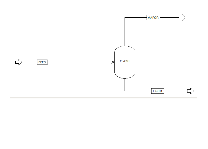
This is an example that just illustrates it is possible to access data from
a simulation that has been run. You have to know quite a bit about the
Aspen flowsheet before writing this code. Particularly, you need to open the
Variable Explorer to find the "path" to the variables that you want, and to
know what the units are of those variables are.
1import os
2import win32com.client as win32
3aspen =win32.Dispatch(’Apwn.Document’)
4
5aspen.InitFromArchive2(os.path.abspath(’data\Flash_Example.bkp’))
6
7## Input variables
8feed_temp =aspen.Tree.FindNode(’\Data\Streams\FEED\Input\TEMP\MIXED’).Value
9print ’Feed temperature was {0} degF’.format(feed_temp)
10
11 ftemp =aspen.Tree.FindNode(’\Data\Blocks\FLASH\Input\TEMP’).Value
12 print ’Flash temperature = {0}’.format(ftemp)
13
14 ## Output variables
15 eL_out =aspen.Tree.FindNode("\Data\Streams\LIQUID\Output\MOLEFLOW\MIXED\ETHANOL").Value
16 wL_out =aspen.Tree.FindNode("\Data\Streams\LIQUID\Output\MOLEFLOW\MIXED\WATER").Value
17
18 eV_out =aspen.Tree.FindNode("\Data\Streams\VAPOR\Output\MOLEFLOW\MIXED\ETHANOL").Value
19 wV_out =aspen.Tree.FindNode("\Data\Streams\VAPOR\Output\MOLEFLOW\MIXED\WATER").Value
20
21 tot =aspen.Tree.FindNode("\Data\Streams\FEED\Input\TOTFLOW\MIXED").Value
22
23 print ’Ethanol vapor mol flow: {0} lbmol/hr’.format(eV_out)
24 print ’Ethanol liquid mol flow: {0} lbmol/hr’.format(eL_out)
25
26 print ’Water vapor mol flow: {0} lbmol/hr’.format(wV_out)
27 print ’Water liquid mol flow: {0} lbmol/hr’.format(wL_out)
28
29 print ’Total = {0}. Total in = {1}’.format(eV_out +eL_out +wV_out +wL_out,
30 tot)
287

31
32 aspen.Close()
Feed temperature was 100.0 degF
Flash temperature = 150.0
Ethanol vapor mol flow: 3.89668323 lbmol/hr
Ethanol liquid mol flow: 0.444397241 lbmol/hr
Water vapor mol flow: 0.774592763 lbmol/hr
Water liquid mol flow: 43.6331268 lbmol/hr
Total = 48.748800034. Total in = 48.7488
It is nice that we can read data from a simulation, but it would be
helpful if we could change variable values and to rerun the simulations.
That is possible. We simply set the value of the variable, and tell Aspen to
rerun. Here, we will change the temperature of the Flash tank and plot the
composition of the outlet streams as a function of that temperature.
1import os
2import numpy as np
3import matplotlib.pyplot as plt
4import win32com.client as win32
5
6aspen =win32.Dispatch(’Apwn.Document’)
7aspen.InitFromArchive2(os.path.abspath(’data\Flash_Example.bkp’))
8
9T=np.linspace(150,200,10)
10
11 x_ethanol, y_ethanol =[], []
12
13 for temperature in T:
14 aspen.Tree.FindNode(’\Data\Blocks\FLASH\Input\TEMP’).Value =temperature
15 aspen.Engine.Run2()
16
17 x_ethanol.append(aspen.Tree.FindNode(’\Data\Streams\LIQUID\Output\MOLEFRAC\MIXED\ETHANOL’).Value)
18 y_ethanol.append(aspen.Tree.FindNode(’\Data\Streams\VAPOR\Output\MOLEFRAC\MIXED\ETHANOL’).Value)
19
20 plt.plot(T, y_ethanol, T, x_ethanol)
21 plt.legend([’vapor’,’liquid’])
22 plt.xlabel(’Flash Temperature (degF)’)
23 plt.ylabel(’Ethanol mole fraction’)
24 plt.savefig(’images/aspen-water-ethanol-flash.png’)
25 aspen.Close()
288
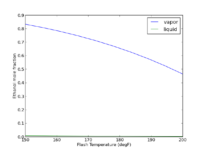
It takes about 30 seconds to run the previous example. Unfortunately,
the way it is written, if you want to change anything, you have to run all
of the calculations over again. How to avoid that is moderately tricky, and
will be the subject of another example.
In summary, it seems possible to do a lot with Aspen automation via
python. This can also be done with Matlab, Excel, and other programming
languages where COM automation is possible. The COM interface is not
especially well documented, and you have to do a lot of digging to figure
out some things. It is not clear how committed Aspen is to maintaining or
improving the COM interface (http://www.chejunkie.com/aspen-plus/
aspen-plus-activex-automation-server/). Hopefully they can keep it
alive for power users who do not want to program in Excel!
12.11 Using an external solver with Aspen
One reason to interact with Aspen via python is to use external solvers to
drive the simulations. Aspen has some built-in solvers, but it does not have
everything. You may also want to integrate additional calculations, e.g.
capital costs, water usage, etc. . . and integrate those results into a report.
Here is a simple example where we use fsolve to find the temperature of
the flash tank that will give a vapor phase mole fraction of ethanol of 0.8.
It is a simple example, but it illustrates the possibility.
289

1import os
2import win32com.client as win32
3aspen =win32.Dispatch(’Apwn.Document’)
4
5aspen.InitFromArchive2(os.path.abspath(’data\Flash_Example.bkp’))
6
7from scipy.optimize import fsolve
8
9def func(flashT):
10 flashT =float(flashT) # COM objects do not understand numpy types
11 aspen.Tree.FindNode(’\Data\Blocks\FLASH\Input\TEMP’).Value =flashT
12 aspen.Engine.Run2()
13 y=aspen.Tree.FindNode(’\Data\Streams\VAPOR\Output\MOLEFRAC\MIXED\ETHANOL’).Value
14 return y- 0.8
15
16 sol, =fsolve(func, 150.0)
17 print ’A flash temperature of {0:1.2f} degF will have y_ethanol = 0.8’.format(sol)
A flash temperature of 157.38 degF will have y_ethanol = 0.8
One unexpected detail was that the Aspen COM objects cannot be as-
signed numpy number types, so it was necessary to recast the argument as
a float. Otherwise, this worked about as expected for an fsolve problem.
12.12 Redirecting the print function
Ordinarily a print statement prints to stdout, or your terminal/screen. You
can redirect this so that printing is done to a file, for example. This might
be helpful if you use print statements for debugging, and later want to save
what is printed to a file. Here we make a simple function that prints some
things.
1def debug():
2print(’step 1’)
3print(3+4)
4print(’finished’)
5
6debug()
step 1
7
finished
Now, let us redirect the printed lines to a file. We create a file object,
and set sys.stdout equal to that file object.
290

1import sys
2print(’__stdout__ before = {0}’.format(sys.__stdout__), file=sys.stdout)
3print(’stdout before = {0}’.format(sys.stdout), file=sys.stdout)
4
5f=open(’data/debug.txt’,’w’)
6sys.stdout =f
7
8# note that sys.__stdout__ does not change, but stdout does.
9print(’__stdout__ after = {0}’.format(sys.__stdout__), file=sys.stdout)
10 print(’stdout after = {0}’.format(sys.stdout), file=sys.stdout)
11
12 debug()
13
14 # reset stdout back to console
15 sys.stdout =sys.__stdout__
16
17 print(f)
18 f.close() # try to make it a habit to close files
19 print(f)
__stdout__ before = <_io.TextIOWrapper name=’<stdout>’ mode=’w’ encoding=’UTF-8’>
stdout before = <_io.TextIOWrapper name=’<stdout>’ mode=’w’ encoding=’UTF-8’>
<_io.TextIOWrapper name=’data/debug.txt’ mode=’w’ encoding=’UTF-8’>
<_io.TextIOWrapper name=’data/debug.txt’ mode=’w’ encoding=’UTF-8’>
Note it can be important to close files. If you are looping through large
numbers of files, you will eventually run out of file handles, causing an error.
We can use a context manager to automatically close the file like this
1import sys
2
3# use the open context manager to automatically close the file
4with open(’data/debug.txt’,’w’)as f:
5sys.stdout =f
6debug()
7print(f, file=sys.__stdout__)
8
9# reset stdout
10 sys.stdout =sys.__stdout__
11 print(f)
<_io.TextIOWrapper name=’data/debug.txt’ mode=’w’ encoding=’UTF-8’>
<_io.TextIOWrapper name=’data/debug.txt’ mode=’w’ encoding=’UTF-8’>
See, the file is closed for us! We can see the contents of our file like
this.
1cat data/debug.txt
291

step 1
7
finished
The approaches above are not fault safe. Suppose our debug function
raised an exception. Then, it could be possible the line to reset the stdout
would not be executed. We can solve this with try/finally code.
1import sys
2
3print(’before: ’, sys.stdout)
4try:
5with open(’data/debug-2.txt’,’w’)as f:
6sys.stdout =f
7# print to the original stdout
8print(’during: ’, sys.stdout, file=sys.__stdout__)
9debug()
10 raise Exception(’something bad happened’)
11 finally:
12 # reset stdout
13 sys.stdout =sys.__stdout__
14
15 print(’after: ’, sys.stdout)
16 print(f) # verify it is closed
17 print(sys.stdout) # verify this is reset
before: <_io.TextIOWrapper name=’<stdout>’ mode=’w’ encoding=’UTF-8’>
during: <_io.TextIOWrapper name=’data/debug-2.txt’ mode=’w’ encoding=’UTF-8’>
Traceback (most recent call last):
File "<stdin>", line 7, in <module>
Exception: something bad happened
after: <_io.TextIOWrapper name=’<stdout>’ mode=’w’ encoding=’UTF-8’>
<_io.TextIOWrapper name=’data/debug-2.txt’ mode=’w’ encoding=’UTF-8’>
<_io.TextIOWrapper name=’<stdout>’ mode=’w’ encoding=’UTF-8’>
1cat data/debug-2.txt
step 1
7
finished
This is the kind of situation where a context manager is handy. Context
managers are typically a class that executes some code when you "enter" the
context, and then execute some code when you "exit" the context. Here we
292

want to change sys.stdout to a new value inside our context, and change it
back when we exit the context. We will store the value of sys.stdout going
in, and restore it on the way out.
1import sys
2
3class redirect:
4def __init__(self, f=sys.stdout):
5"redirect print statement to f. f must be a file-like object"
6self.f=f
7self.stdout =sys.stdout
8print(’init stdout: ’, sys.stdout, file=sys.__stdout__)
9def __enter__(self):
10 sys.stdout =self.f
11 print(’stdout in context-manager: ’,sys.stdout, f=sys.__stdout__)
12 def __exit__(self,*args):
13 sys.stdout =self.stdout
14 print(’__stdout__ at exit = ’,sys.__stdout__)
15
16 # regular printing
17 with redirect():
18 debug()
19
20 # write to a file
21 with open(’data/debug-3.txt’,’w’)as f:
22 with redirect(f):
23 debug()
24
25 # mixed regular and
26 with open(’data/debug-4.txt’,’w’)as f:
27 with redirect(f):
28 print(’testing redirect’)
29 with redirect():
30 print(’temporary console printing’)
31 debug()
32 print(’Now outside the inner context. This should go to data/debug-4.txt’)
33 debug()
34 raise Exception(’something else bad happened’)
35
36 print(sys.stdout)
Here are the contents of the debug file.
1cat data/debug-3.txt
The contents of the other debug file have some additional lines, because
we printed some things while in the redirect context.
1cat data/debug-4.txt
293

See http://www.python.org/dev/peps/pep-0343/ (number 5) for an-
other example of redirecting using a function decorator. I think it is harder
to understand, because it uses a generator.
There were a couple of points in this section:
1. You can control where things are printed in your programs by modi-
fying the value of sys.stdout
2. You can use try/except/finally blocks to make sure code gets executed
in the event an exception is raised
3. You can use context managers to make sure files get closed, and code
gets executed if exceptions are raised.
12.13 Getting a dictionary of counts
I frequently want to take a list and get a dictionary of keys that have the
count of each element in the list. Here is how I have typically done this
countless times in the past.
1L=[’a’,’a’,’b’,’d’,’e’,’b’,’e’,’a’]
2
3d={}
4for el in L:
5if el in d:
6d[el] += 1
7else:
8d[el] = 1
9
10 print(d)
{’b’: 2, ’a’: 3, ’e’: 2, ’d’: 1}
That seems like too much code, and that there must be a list compre-
hension approach combined with a dictionary constructor.
1L=[’a’,’a’,’b’,’d’,’e’,’b’,’e’,’a’]
2
3print(dict((el,L.count(el)) for el in L))
{’b’: 2, ’a’: 3, ’d’: 1, ’e’: 2}
Wow, that is a lot simpler! I suppose for large lists this might be slow,
since count must look through the list for each element, whereas the longer
code looks at each element once, and does one conditional analysis.
Here is another example of much shorter and cleaner code.
294

1from collections import Counter
2L=[’a’,’a’,’b’,’d’,’e’,’b’,’e’,’a’]
3print(Counter(L))
4print(Counter(L)[’a’])
Counter({’a’: 3, ’e’: 2, ’b’: 2, ’d’: 1})
3
12.14 About your python
1import sys
2
3print(sys.version)
4
5print(sys.executable)
6
7print(sys.platform)
8
9# where the platform independent Python files are installed
10 print(sys.prefix)
3.5.1 |Anaconda 2.5.0 (x86_64)| (default, Dec 7 2015, 11:24:55)
[GCC 4.2.1 (Apple Inc. build 5577)]
/Users/jkitchin/anaconda3/bin/python
darwin
/Users/jkitchin/anaconda3
The platform module provides similar, complementary information.
1import platform
2
3print(platform.uname())
4print(platform.system())
5print(platform.architecture())
6print(platform.machine())
7print(platform.node())
8print(platform.platform())
9print(platform.processor())
10 print(platform.python_build())
11 print(platform.python_version())
uname_result(system=’Darwin’, node=’Johns-MacBook-Air.local’, release=’13.4.0’, version=’Darwin Kernel Version 13.4.0: Wed Mar 18 16:20:14 PDT 2015; root:xnu-2422.115.14~1/RELEASE_X86_64’, machine=’x86_64’, processor=’i386’)
Darwin
(’64bit’, ’’)
x86_64
295

Johns-MacBook-Air.local
Darwin-13.4.0-x86_64-i386-64bit
i386
(’default’, ’Dec 7 2015 11:24:55’)
3.5.1
12.15 Automatic, temporary directory changing
If you are doing some analysis that requires you to change directories, e.g.
to read a file, and then change back to another directory to read another file,
you have probably run into problems if there is an error somewhere. You
would like to make sure that the code changes back to the original directory
after each error. We will look at a few ways to accomplish that here.
The try/except/finally method is the traditional way to handle excep-
tions, and make sure that some code "finally" runs. Let us look at two
examples here. In the first example, we try to change into a directory that
does not exist.
1import os,sys
2
3CWD =os.getcwd() # store initial position
4print(’initially inside {0}’.format(os.getcwd()))
5TEMPDIR =’data/run1’ # this does not exist
6
7try:
8os.chdir(TEMPDIR)
9print(’inside {0}’.format(os.getcwd()))
10 except:
11 print(’Exception caught: ’,sys.exc_info()[0])
12 finally:
13 print(’Running final code’)
14 os.chdir(CWD)
15 print(’finally inside {0}’.format(os.getcwd()))
initially inside /Users/jkitchin/Dropbox/books/pycse
Exception caught: <class ’FileNotFoundError’>
Running final code
finally inside /Users/jkitchin/Dropbox/books/pycse
Now, let us look at an example where the directory does exist. We will
change into the directory, run some code, and then raise an Exception.
1import os,sys
2
296

3CWD =os.getcwd() # store initial position
4print(’initially inside {0}’.format(os.getcwd()))
5TEMPDIR =’data’
6
7try:
8os.chdir(TEMPDIR)
9print(’inside {0}’.format(os.getcwd()))
10 print(os.listdir(’.’))
11 raise Exception(’boom’)
12 except:
13 print(’Exception caught: ’,sys.exc_info()[0])
14 finally:
15 print(’Running final code’)
16 os.chdir(CWD)
17 print(’finally inside {0}’.format(os.getcwd()))
initially inside /Users/jkitchin/Dropbox/books/pycse
inside /Users/jkitchin/Dropbox/books/pycse/data
[’_0308azw.def’, ’_BaEA1C.tmp’, ’antoine_data.dat’, ’antoine_database.mat’, ’commonshellsettings.xml’, ’cstr-zeroth-order.xlsx’, ’data.pckl’, ’debug-2.txt’, ’debug-3.txt’, ’debug-4.txt’, ’debug.txt’, ’example.xlsx’, ’example2.xls’, ’example3.xls’, ’example4.xls’, ’example4.xlsx’, ’Flash_Example.apw’, ’Flash_Example.bkp’, ’Flash_Example.def’, ’gc-data-21.txt’, ’memoize-aspen.pkl’, ’PT.txt’, ’raman.txt’, ’run2’, ’test.docx’, ’testdata.txt’]
Exception caught: <class ’Exception’>
Running final code
finally inside /Users/jkitchin/Dropbox/books/pycse
You can see that we changed into the directory, ran some code, and then
caught an exception. Afterwards, we changed back to our original directory.
This code works fine, but it is somewhat verbose, and tedious to write over
and over. We can get a cleaner syntax with a context manager. The context
manager uses the with keyword in python. In a context manager some code
is executed on entering the "context", and code is run on exiting the context.
We can use that to automatically change directory, and when done, change
back to the original directory. We use the contextlib.contextmanager
decorator on a function. With a function, the code up to a yield statement
is run on entering the context, and the code after the yield statement is run
on exiting. We wrap the yield statement in try/except/finally block to make
sure our final code gets run.
1import contextlib
2import os,sys
3
4@contextlib.contextmanager
5def cd(path):
6print(’initially inside {0}’.format(os.getcwd()))
7CWD =os.getcwd()
8
9os.chdir(path)
10 print(’inside {0}’.format(os.getcwd()))
11 try:
297

12 yield
13 except:
14 print(’Exception caught: ’,sys.exc_info()[0])
15 finally:
16 print(’finally inside {0}’.format(os.getcwd()))
17 os.chdir(CWD)
18
19 # Now we use the context manager
20 with cd(’data’):
21 print(os.listdir(’.’))
22 raise Exception(’boom’)
23
24 print
25 with cd(’data/run2’):
26 print(os.listdir(’.’))
initially inside /Users/jkitchin/Dropbox/books/pycse
inside /Users/jkitchin/Dropbox/books/pycse/data
[’_0308azw.def’, ’_BaEA1C.tmp’, ’antoine_data.dat’, ’antoine_database.mat’, ’commonshellsettings.xml’, ’cstr-zeroth-order.xlsx’, ’data.pckl’, ’debug-2.txt’, ’debug-3.txt’, ’debug-4.txt’, ’debug.txt’, ’example.xlsx’, ’example2.xls’, ’example3.xls’, ’example4.xls’, ’example4.xlsx’, ’Flash_Example.apw’, ’Flash_Example.bkp’, ’Flash_Example.def’, ’gc-data-21.txt’, ’memoize-aspen.pkl’, ’PT.txt’, ’raman.txt’, ’run2’, ’test.docx’, ’testdata.txt’]
Exception caught: <class ’Exception’>
finally inside /Users/jkitchin/Dropbox/books/pycse/data
initially inside /Users/jkitchin/Dropbox/books/pycse
inside /Users/jkitchin/Dropbox/books/pycse/data/run2
[’raman.txt’]
finally inside /Users/jkitchin/Dropbox/books/pycse/data/run2
One case that is not handled well with this code is if the directory you
want to change into does not exist. In that case an exception is raised on
entering the context when you try change into a directory that does not
exist. An alternative class based context manager can be found here.
13 Miscellaneous
13.1 Mail merge with python
Suppose you are organizing some event, and you have a mailing list of email
addresses and people you need to send a mail to telling them what room
they will be in. You would like to send a personalized email to each person,
and you do not want to type each one by hand. Python can automate this
for you. All you need is the mailing list in some kind of structured format,
and then you can go through it line by line to create and send emails.
We will use an org-table to store the data in.
298

First name Last name email address Room number
Jane Doe jane-doe@gmail.com 1
John Doe john-doe@gmail.com 2
Jimmy John jimmy-john@gmail.com 3
We pass that table into an org-mode source block as a variable called
data, which will be a list of lists, one for each row of the table. You could
alternatively read these from an excel spreadsheet, a csv file, or some kind
of python data structure.
We do not actually send the emails in this example. To do that you need
to have access to a mail server, which could be on your own machine, or it
could be a relay server you have access to.
We create a string that is a template with some fields to be substituted,
e.g. the firstname and room number in this case. Then we loop through
each row of the table, and format the template with those values, and create
an email message to the person. First we print each message to check that
they are correct.
1import smtplib
2from email.mime.multipart import MIMEMultipart
3from email.mime.text import MIMEText
4from email.utils import formatdate
5
6template =’’’
7Dear {firstname:s},
8
9I am pleased to inform you that your talk will be in room {roomnumber:d}.
10
11 Sincerely,
12 John
13 ’’’
14
15 for firstname, lastname, emailaddress, roomnumber in data:
16 msg =MIMEMultipart()
17 msg[’From’]="youremail@gmail.com"
18 msg[’To’]=emailaddress
19 msg[’Date’]=formatdate(localtime=True)
20
21 msgtext =template.format(**locals())
22 print(msgtext)
23
24 msg.attach(MIMEText(msgtext))
25
26 ## Uncomment these lines and fix
27 #server = smtplib.SMTP(’your.relay.server.edu’)
28 #server.sendmail(’your_email@gmail.com’, # from
29 # emailaddress,
30 # msg.as_string())
31 #server.quit()
299

32
33 print(msg.as_string())
34 print(’------------------------------------------------------------------’)
14 Worked examples
14.1 Peak finding in Raman spectroscopy
Raman spectroscopy is a vibrational spectroscopy. The data typically comes
as intensity vs. wavenumber, and it is discrete. Sometimes it is necessary
to identify the precise location of a peak. In this post, we will use spline
smoothing to construct an interpolating function of the data, and then use
fminbnd to identify peak positions.
This example was originally worked out in Matlab at http://matlab.
cheme.cmu.edu/2012/08/27/peak-finding-in-raman-spectroscopy/
numpy:loadtxt
Let us take a look at the raw data.
1import numpy as np
2import matplotlib.pyplot as plt
3
4w,i=np.loadtxt(’data/raman.txt’, usecols=(0,1), unpack=True)
5
6plt.plot(w, i)
7plt.xlabel(’Raman shift (cm$^{-1}$)’)
8plt.ylabel(’Intensity (counts)’)
9plt.savefig(’images/raman-1.png’)
[<matplotlib.lines.Line2D object at 0x107316860>]
<matplotlib.text.Text object at 0x10b184ac8>
<matplotlib.text.Text object at 0x108f8f9b0>
300
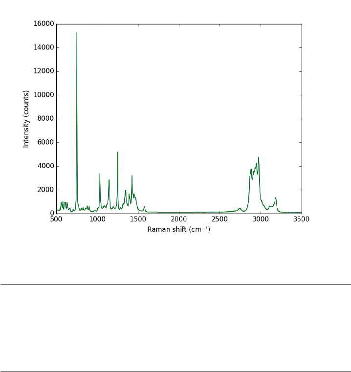
The next thing to do is narrow our focus to the region we are interested
in between 1340 cmˆ{-1} and 1360 cmˆ{-1}.
1ind =(w > 1340)&(w < 1360)
2w1 =w[ind]
3i1 =i[ind]
4
5plt.figure()
6plt.plot(w1, i1, ’b. ’)
7plt.xlabel(’Raman shift (cm$^{-1}$)’)
8plt.ylabel(’Intensity (counts)’)
9plt.savefig(’images/raman-2.png’)
<matplotlib.figure.Figure object at 0x10b1031d0>
[<matplotlib.lines.Line2D object at 0x10b0cf978>]
<matplotlib.text.Text object at 0x10f8f0ef0>
<matplotlib.text.Text object at 0x10f8d5dd8>
301
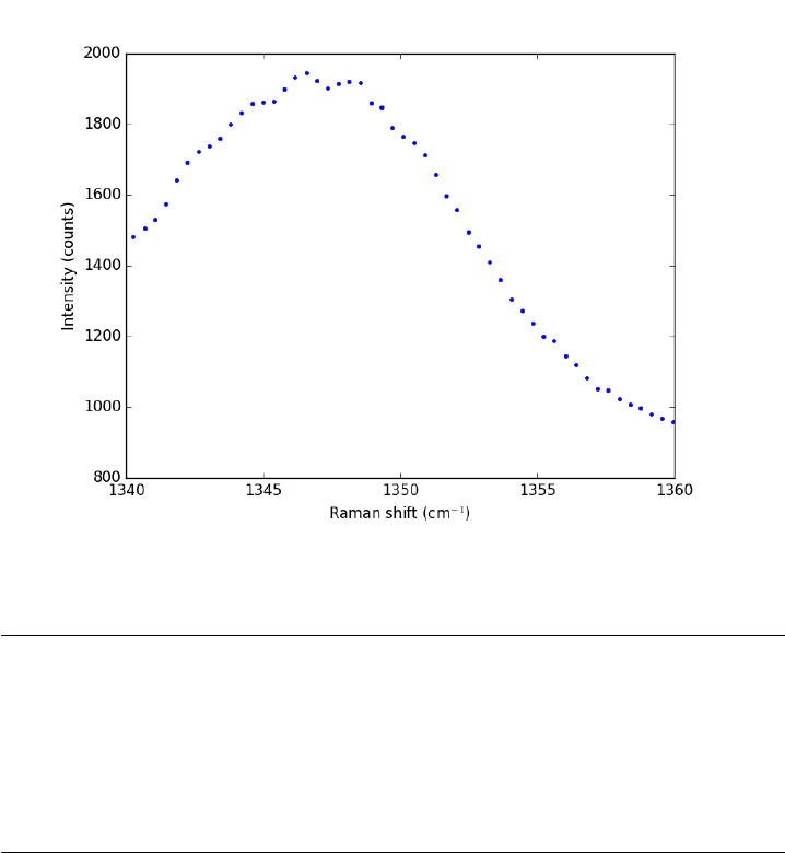
Next we consider a scipy:UnivariateSpline. This function "smooths" the
data.
1from scipy.interpolate import UnivariateSpline
2
3# s is a "smoothing" factor
4sp =UnivariateSpline(w1, i1, k=4, s=2000)
5
6plt.plot(w1, i1, ’b. ’)
7plt.plot(w1, sp(w1), ’r-’)
8plt.xlabel(’Raman shift (cm$^{-1}$)’)
9plt.ylabel(’Intensity (counts)’)
10 plt.savefig(’images/raman-3.png’)
[<matplotlib.lines.Line2D object at 0x10b15a1d0>]
[<matplotlib.lines.Line2D object at 0x10b0efa90>]
<matplotlib.text.Text object at 0x10f8f0ef0>
<matplotlib.text.Text object at 0x10f8d5dd8>
302
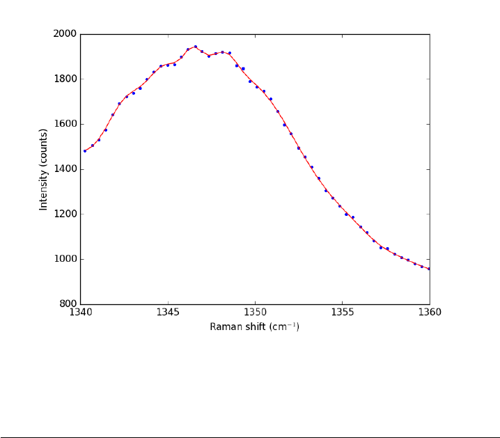
Note that the UnivariateSpline function returns a "callable" function!
Our next goal is to find the places where there are peaks. This is defined by
the first derivative of the data being equal to zero. It is easy to get the first
derivative of a UnivariateSpline with a second argument as shown below.
1# get the first derivative evaluated at all the points
2d1s =sp.derivative()
3
4d1 =d1s(w1)
5
6# we can get the roots directly here, which correspond to minima and
7# maxima.
8print(’Roots = {}’.format(sp.derivative().roots()))
9minmax =sp.derivative().roots()
10
11 plt.clf()
12 plt.plot(w1, d1, label=’first derivative’)
13 plt.xlabel(’Raman shift (cm$^{-1}$)’)
14 plt.ylabel(’First derivative’)
15 plt.grid()
16
17 plt.figure()
18 plt.plot(minmax, d1s(minmax), ’ro ’, label=’zeros’)
19 plt.legend(loc=’best’)
20
21 plt.plot(w1, i1, ’b. ’)
22 plt.plot(w1, sp(w1), ’r-’)
23 plt.xlabel(’Raman shift (cm$^{-1}$)’)
24 plt.ylabel(’Intensity (counts)’)
303
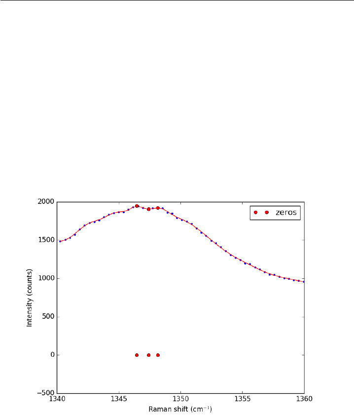
25 plt.plot(minmax, sp(minmax), ’ro ’)
26
27 plt.savefig(’images/raman-4.png’)
Roots = [ 1346.4623087 1347.42700893 1348.16689639]
[<matplotlib.lines.Line2D object at 0x111e705f8>]
<matplotlib.text.Text object at 0x10f8f65f8>
<matplotlib.text.Text object at 0x110bac320>
<matplotlib.figure.Figure object at 0x111e70780>
[<matplotlib.lines.Line2D object at 0x111ec0be0>]
<matplotlib.legend.Legend object at 0x111e75b00>
[<matplotlib.lines.Line2D object at 0x111e75b38>]
[<matplotlib.lines.Line2D object at 0x111e8cc50>]
<matplotlib.text.Text object at 0x111e79ef0>
<matplotlib.text.Text object at 0x111e895f8>
[<matplotlib.lines.Line2D object at 0x111ec0e80>]
In the end, we have illustrated how to construct a spline smoothing inter-
polation function and to find maxima in the function, including generating
some initial guesses. There is more art to this than you might like, since
you have to judge how much smoothing is enough or too much. With too
much, you may smooth peaks out. With too little, noise may be mistaken
for peaks.
304

14.1.1 Summary notes
Using org-mode with :session allows a large script to be broken up into mini
sections. However, it only seems to work with the default python mode in
Emacs, and it does not work with emacs-for-python or the latest python-
mode. I also do not really like the output style, e.g. the output from the
plotting commands.
14.2 Curve fitting to get overlapping peak areas
Today we examine an approach to fitting curves to overlapping peaks to
deconvolute them so we can estimate the area under each curve. We have a
text file that contains data from a gas chromatograph with two peaks that
overlap. We want the area under each peak to estimate the gas composition.
You will see how to read the text file in, parse it to get the data for plotting
and analysis, and then how to fit it.
A line like "# of Points 9969" tells us the number of points we have to
read. The data starts after a line containing "R.Time Intensity". Here we
read the number of points, and then get the data into arrays.
1import numpy as np
2import matplotlib.pyplot as plt
3
4datafile =’data/gc-data-21.txt’
5
6i= 0
7with open(datafile) as f:
8lines =f.readlines()
9
10 for i,line in enumerate(lines):
11 if ’# of Points’ in line:
12 npoints =int(line.split()[-1])
13 elif ’R.Time\tIntensity’ in line:
14 i+= 1
15 break
16
17 # now get the data
18 t, intensity =[], []
19 for jin range(i, i +npoints):
20 fields =lines[j].split()
21 t+= [float(fields[0])]
22 intensity += [int(fields[1])]
23
24 t=np.array(t)
25 intensity =np.array(intensity, np.float)
26
27 # now plot the data in the relevant time frame
28 plt.plot(t, intensity)
29 plt.xlim([4,6])
305
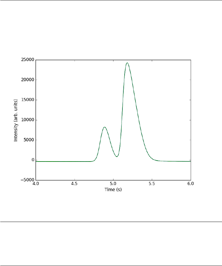
30 plt.xlabel(’Time (s)’)
31 plt.ylabel(’Intensity (arb. units)’)
32 plt.savefig(’images/deconvolute-1.png’)
[<matplotlib.lines.Line2D object at 0x10ee308d0>]
(4, 6)
<matplotlib.text.Text object at 0x10910dc88>
<matplotlib.text.Text object at 0x1090bd198>
You can see there is a non-zero baseline. We will normalize that by the
average between 4 and 4.4 seconds.
1intensity -= np.mean(intensity[(t > 4.0)&(t < 4.4)])
2plt.figure()
3plt.plot(t, intensity)
4plt.xlim([4,6])
5plt.xlabel(’Time (s)’)
6plt.ylabel(’Intensity (arb. units)’)
7plt.savefig(’./images/deconvolute-2.png’)
<matplotlib.figure.Figure object at 0x1090bdfd0>
[<matplotlib.lines.Line2D object at 0x10b0d01d0>]
(4, 6)
<matplotlib.text.Text object at 0x109122da0>
<matplotlib.text.Text object at 0x10912beb8>
306
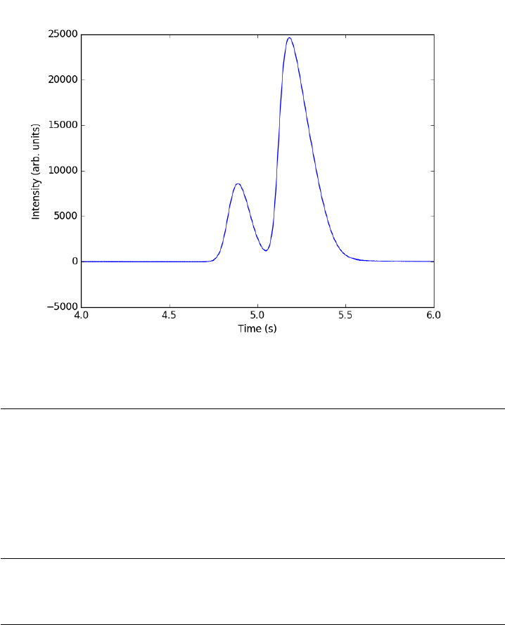
The peaks are asymmetric, decaying gaussian functions. We define a
function for this
1from scipy.special import erf
2
3def asym_peak(t, pars):
4’from Anal. Chem. 1994, 66, 1294-1301’
5a0 =pars[0]# peak area
6a1 =pars[1]# elution time
7a2 =pars[2]# width of gaussian
8a3 =pars[3]# exponential damping term
9f=(a0/2/a3*np.exp(a2**2/2.0/a3**2 + (a1 -t)/a3)
10 *(erf((t-a1)/(np.sqrt(2.0)*a2) -a2/np.sqrt(2.0)/a3) + 1.0))
11 return f
To get two peaks, we simply add two peaks together.
1def two_peaks(t, *pars):
2’function of two overlapping peaks’
3a10 =pars[0]# peak area
4a11 =pars[1]# elution time
5a12 =pars[2]# width of gaussian
6a13 =pars[3]# exponential damping term
7a20 =pars[4]# peak area
8a21 =pars[5]# elution time
9a22 =pars[6]# width of gaussian
10 a23 =pars[7]# exponential damping term
307
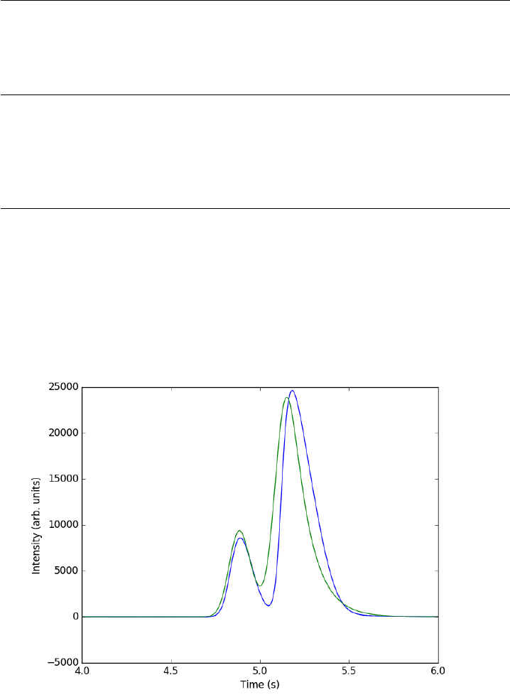
11 p1 =asym_peak(t, [a10, a11, a12, a13])
12 p2 =asym_peak(t, [a20, a21, a22, a23])
13 return p1 +p2
To show the function is close to reasonable, we plot the fitting function
with an initial guess for each parameter. The fit is not good, but we have
only guessed the parameters for now.
1parguess =(1500,4.85,0.05,0.05,5000,5.1,0.05,0.1)
2plt.figure()
3plt.plot(t, intensity)
4plt.plot(t,two_peaks(t, *parguess),’g-’)
5plt.xlim([4,6])
6plt.xlabel(’Time (s)’)
7plt.ylabel(’Intensity (arb. units)’)
8plt.savefig(’images/deconvolution-3.png’)
<matplotlib.figure.Figure object at 0x11049d4a8>
[<matplotlib.lines.Line2D object at 0x11068d4e0>]
[<matplotlib.lines.Line2D object at 0x11068d668>]
(4, 6)
<matplotlib.text.Text object at 0x11055f748>
<matplotlib.text.Text object at 0x110562b00>
Next, we use nonlinear curve fitting from scipy.optimize.curve_fit
308
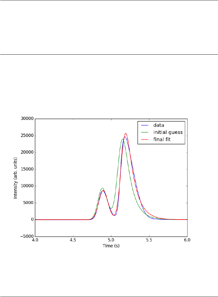
1from scipy.optimize import curve_fit
2
3popt, pcov =curve_fit(two_peaks, t, intensity, parguess)
4print(popt)
5
6plt.plot(t, two_peaks(t, *popt), ’r-’)
7plt.legend([’data’,’initial guess’,’final fit’])
8
9plt.savefig(’images/deconvolution-4.png’)
[ 1.31048111e+03 4.87473757e+00 5.55418109e-02 2.50682818e-02
5.32571369e+03 5.14121371e+00 4.68230128e-02 1.04110303e-01]
[<matplotlib.lines.Line2D object at 0x11115d0b8>]
<matplotlib.legend.Legend object at 0x1106acc18>
The fits are not perfect. The small peak is pretty good, but there is an
unphysical tail on the larger peak, and a small mismatch at the peak. There
is not much to do about that, it means the model peak we are using is not
a good model for the peak. We will still integrate the areas though.
1pars1 =popt[0:4]
2pars2 =popt[4:8]
3
4peak1 =asym_peak(t, pars1)
309

5peak2 =asym_peak(t, pars2)
6
7area1 =np.trapz(peak1, t)
8area2 =np.trapz(peak2, t)
9
10 print(’Area 1 = {0:1.2f}’.format(area1))
11 print(’Area 2 = {0:1.2f}’.format(area2))
12
13 print(’Area 1 is {0:1.2%} of the whole area’.format(area1/(area1 +area2)))
14 print(’Area 2 is {0:1.2%} of the whole area’.format(area2/(area1 +area2)))
15
16 plt.figure()
17 plt.plot(t, intensity)
18 plt.plot(t, peak1, ’r-’)
19 plt.plot(t, peak2, ’g-’)
20 plt.xlim([4,6])
21 plt.xlabel(’Time (s)’)
22 plt.ylabel(’Intensity (arb. units)’)
23 plt.legend([’data’,’peak 1’,’peak 2’])
24 plt.savefig(’images/deconvolution-5.png’)
Area 1 = 1310.48
Area 2 = 5325.71
Area 1 is 19.75% of the whole area
Area 2 is 80.25% of the whole area
<matplotlib.figure.Figure object at 0x11116fd30>
[<matplotlib.lines.Line2D object at 0x111410ac8>]
[<matplotlib.lines.Line2D object at 0x111410c50>]
[<matplotlib.lines.Line2D object at 0x1114184e0>]
(4, 6)
<matplotlib.text.Text object at 0x1113d95f8>
<matplotlib.text.Text object at 0x1113d9588>
<matplotlib.legend.Legend object at 0x11141d550>
310
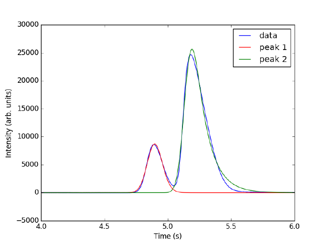
This sample was air, and the first peak is oxygen, and the second peak
is nitrogen. we come pretty close to the actual composition of air, although
it is low on the oxygen content. To do better, one would have to use a
calibration curve.
In the end, the overlap of the peaks is pretty small, but it is still difficult
to reliably and reproducibly deconvolute them. By using an algorithm like
we have demonstrated here, it is possible at least to make the deconvolution
reproducible.
14.2.1 Notable differences from Matlab
1. The order of arguments to np.trapz is reversed.
2. The order of arguments to the fitting function scipy.optimize.curve_fit
is different than in Matlab.
3. The scipy.optimize.curve_fit function expects a fitting function that
has all parameters as arguments, where Matlab expects a vector of
parameters.
14.3 Estimating the boiling point of water
Matlab post
311

I got distracted looking for Shomate parameters for ethane today, and
came across this website on predicting the boiling point of water using the
Shomate equations. The basic idea is to find the temperature where the
Gibbs energy of water as a vapor is equal to the Gibbs energy of the liquid.
1import matplotlib.pyplot as plt
Liquid water (http://webbook.nist.gov/cgi/cbook.cgi?ID=C7732185&
Units=SI&Mask=2#Thermo-Condensed)
1# valid over 298-500
2
3Hf_liq = -285.830 # kJ/mol
4S_liq = 0.06995 # kJ/mol/K
5shomateL =[-203.6060,
61523.290,
7-3196.413,
82474.455,
93.855326,
10 -256.5478,
11 -488.7163,
12 -285.8304]
Gas phase water (http://webbook.nist.gov/cgi/cbook.cgi?ID=C7732185&
Units=SI&Mask=1&Type=JANAFG&Table=on#JANAFG)
Interestingly, these parameters are listed as valid only above 500K. That
means we have to extrapolate the values down to 298K. That is risky for
polynomial models, as they can deviate substantially outside the region they
were fitted to.
1Hf_gas = -241.826 # kJ/mol
2S_gas = 0.188835 # kJ/mol/K
3
4shomateG =[30.09200,
56.832514,
66.793435,
7-2.534480,
80.082139,
9-250.8810,
10 223.3967,
11 -241.8264]
Now, we wan to compute G for each phase as a function of T
1import numpy as np
2
312

3T=np.linspace(0,200)+ 273.15
4t=T/ 1000.0
5
6sTT =np.vstack([np.log(t),
7t,
8(t**2)/ 2.0,
9(t**3)/ 3.0,
10 -1.0 / (2*t**2),
11 0*t,
12 t**0,
13 0*t**0]).T/ 1000.0
14
15 hTT =np.vstack([t,
16 (t**2)/2.0,
17 (t**3)/3.0,
18 (t**4)/4.0,
19 -1.0 / t,
20 1*t**0,
21 0*t**0,
22 -1*t**0]).T
23
24 Gliq =Hf_liq +np.dot(hTT, shomateL) -T*(np.dot(sTT, shomateL))
25 Ggas =Hf_gas +np.dot(hTT, shomateG) -T*(np.dot(sTT, shomateG))
26
27 from scipy.interpolate import interp1d
28 from scipy.optimize import fsolve
29
30 f=interp1d(T, Gliq -Ggas)
31 bp, =fsolve(f, 373)
32 print(’The boiling point is {0} K’.format(bp))
The boiling point is 373.20608131187146 K
1plt.figure(); plt.clf()
2plt.plot(T-273.15, Gliq, T-273.15, Ggas)
3plt.legend([’liquid water’,’steam’])
4
5plt.xlabel(’Temperature $^\circ$C’)
6plt.ylabel(’$\Delta G$ (kJ/mol)’)
7plt.title(’The boiling point is approximately {0:1.2f} $^\circ$C’.format(bp-273.15))
8plt.savefig(’images/boiling-water.png’)
<matplotlib.figure.Figure object at 0x10b4baf28>
[<matplotlib.lines.Line2D object at 0x110cf5da0>, <matplotlib.lines.Line2D object at 0x110cf5f60>]
<matplotlib.legend.Legend object at 0x110cfbef0>
<matplotlib.text.Text object at 0x110ca9978>
<matplotlib.text.Text object at 0x110cbe080>
<matplotlib.text.Text object at 0x110cc28d0>
313

14.3.1 Summary
The answer we get us 0.05 K too high, which is not bad considering we
estimated it using parameters that were fitted to thermodynamic data and
that had finite precision and extrapolated the steam properties below the
region the parameters were stated to be valid for.
14.4 Gibbs energy minimization and the NIST webbook
Matlab post In Post 1536 we used the NIST webbook to compute a temper-
ature dependent Gibbs energy of reaction, and then used a reaction extent
variable to compute the equilibrium concentrations of each species for the
water gas shift reaction.
Today, we look at the direct minimization of the Gibbs free energy of
the species, with no assumptions about stoichiometry of reactions. We only
apply the constraint of conservation of atoms. We use the NIST Webbook
to provide the data for the Gibbs energy of each species.
As a reminder we consider equilibrium between the species CO,H2O,
CO2and H2, at 1000K, and 10 atm total pressure with an initial equimolar
molar flow rate of CO and H2O.
314

1import numpy as np
2
3T= 1000 # K
4R= 8.314e-3 # kJ/mol/K
5
6P= 10.0 # atm, this is the total pressure in the reactor
7Po = 1.0 # atm, this is the standard state pressure
We are going to store all the data and calculations in vectors, so we need
to assign each position in the vector to a species. Here are the definitions
we use in this work.
1 CO
2 H2O
3 CO2
4 H2
1species =[’CO’,’H2O’,’CO2’,’H2’]
2
3# Heats of formation at 298.15 K
4
5Hf298 =[
6-110.53,# CO
7-241.826,# H2O
8-393.51,# CO2
90.0]# H2
10
11 # Shomate parameters for each species
12 # A B C D E F G H
13 WB =[[25.56759,6.096130,4.054656,-2.671301,0.131021,-118.0089,227.3665,-110.5271], # CO
14 [30.09200,6.832514,6.793435,-2.534480,0.082139,-250.8810,223.3967,-241.8264], # H2O
15 [24.99735,55.18696,-33.69137,7.948387,-0.136638,-403.6075,228.2431,-393.5224], # CO2
16 [33.066178,-11.363417,11.432816,-2.772874,-0.158558,-9.980797,172.707974,0.0]] # H2
17
18 WB =np.array(WB)
19
20 # Shomate equations
21 t=T/1000
22 T_H =np.array([t, t**2 / 2.0, t**3 / 3.0, t**4 / 4.0,-1.0 / t, 1.0,0.0,-1.0])
23 T_S =np.array([np.log(t), t, t**2 / 2.0, t**3 / 3.0,-1.0 / (2.0 * t**2), 0.0,1.0,0.0])
24
25 H=np.dot(WB, T_H) # (H - H_298.15) kJ/mol
26 S=np.dot(WB, T_S/1000.0)# absolute entropy kJ/mol/K
27
28 Gjo =Hf298 +H-T*S# Gibbs energy of each component at 1000 K
Now, construct the Gibbs free energy function, accounting for the change
in activity due to concentration changes (ideal mixing).
315

1def func(nj):
2nj =np.array(nj)
3Enj =np.sum(nj);
4Gj =Gjo /(R *T) +np.log(nj /Enj *P/Po)
5return np.dot(nj, Gj)
We impose the constraint that all atoms are conserved from the initial
conditions to the equilibrium distribution of species. These constraints are
in the form of Aeqn=beq, where nis the vector of mole numbers for each
species.
1Aeq =np.array([[ 1,0,1,0], # C balance
2[1,1,2,0], # O balance
3[0,2,0,2]]) # H balance
4
5# equimolar feed of 1 mol H2O and 1 mol CO
6beq =np.array([1,# mol C fed
72,# mol O fed
82]) # mol H fed
9
10 def ec1(nj):
11 ’conservation of atoms constraint’
12 return np.dot(Aeq, nj) -beq
Now we are ready to solve the problem.
1from scipy.optimize import fmin_slsqp
2
3n0 =[0.5,0.5,0.5,0.5]# initial guesses
4N=fmin_slsqp(func, n0, f_eqcons=ec1)
5print N
Optimization terminated successfully. (Exit mode 0)
Current function value: -91.204832308
Iterations: 2
Function evaluations: 13
Gradient evaluations: 2
File "<stdin>", line 1
print N
^
SyntaxError: Missing parentheses in call to ’print’
14.4.1 Compute mole fractions and partial pressures
The pressures here are in good agreement with the pressures found by other
methods. The minor disagreement (in the third or fourth decimal place) is
likely due to convergence tolerances in the different algorithms used.
316

1yj =N/np.sum(N)
2Pj =yj *P
3
4for s, y, p in zip(species, yj, Pj):
5print(’{0:10s}: {1:1.2f} {2:1.2f}’.format(s, y, p))
CO : 0.23 2.28
H2O : 0.23 2.28
CO2 : 0.27 2.72
H2 : 0.27 2.72
14.4.2 Computing equilibrium constants
We can compute the equilibrium constant for the reaction CO +H2O
CO2+H2. Compared to the value of K = 1.44 we found at the end of
Post 1536 , the agreement is excellent. Note, that to define an equilibrium
constant it is necessary to specify a reaction, even though it is not necessary
to even consider a reaction to obtain the equilibrium distribution of species!
1nuj =np.array([-1,-1,1,1]) # stoichiometric coefficients of the reaction
2K=np.prod(yj**nuj)
3print(K)
1.43446295961
14.5 Finding equilibrium composition by direct minimiza-
tion of Gibbs free energy on mole numbers
Matlab post Adapted from problem 4.5 in Cutlip and Shacham Ethane and
steam are fed to a steam cracker at a total pressure of 1 atm and at 1000K at
a ratio of 4 mol H2O to 1 mol ethane. Estimate the equilibrium distribution
of products (CH4, C2H4, C2H2, CO2, CO, O2, H2, H2O, and C2H6).
Solution method: We will construct a Gibbs energy function for the
mixture, and obtain the equilibrium composition by minimization of the
function subject to elemental mass balance constraints.
1import numpy as np
2
3R= 0.00198588 # kcal/mol/K
4T= 1000 # K
5
6species =[’CH4’,’C2H4’,’C2H2’,’CO2’,’CO’,’O2’,’H2’,’H2O’,’C2H6’]
7
317

8# $G_^\circ for each species. These are the heats of formation for each
9# species.
10 Gjo =np.array([4.61,28.249,40.604,-94.61,-47.942,0,0,-46.03,26.13]) # kcal/mol
14.5.1 The Gibbs energy of a mixture
We start with G=P
j
njµj. Recalling that we define µj=G◦
j+RT ln aj,
and in the ideal gas limit, aj=yjP/P ◦, and that yj=nj
Pnj. Since in this
problem, P = 1 atm, this leads to the function G
RT =n
P
j=1
njG◦
j
RT + ln nj
Pnj.
1import numpy as np
2
3def func(nj):
4nj =np.array(nj)
5Enj =np.sum(nj);
6G=np.sum(nj *(Gjo /R/T+np.log(nj /Enj)))
7return G
14.5.2 Linear equality constraints for atomic mass conservation
The total number of each type of atom must be the same as what entered
the reactor. These form equality constraints on the equilibrium composition.
We express these constraints as: Aeqn=bwhere nis a vector of the moles
of each species present in the mixture. CH4 C2H4 C2H2 CO2 CO O2 H2
H2O C2H6
1Aeq =np.array([[0,0,0,2,1,2,0,1,0], # oxygen balance
2[4,4,2,0,0,0,2,2,6], # hydrogen balance
3[1,2,2,1,1,0,0,0,2]]) # carbon balance
4
5# the incoming feed was 4 mol H2O and 1 mol ethane
6beq =np.array([4,# moles of oxygen atoms coming in
714,# moles of hydrogen atoms coming in
82]) # moles of carbon atoms coming in
9
10 def ec1(n):
11 ’equality constraint’
12 return np.dot(Aeq, n) -beq
13
14 def ic1(n):
15 ’’’inequality constraint
16 all n>=0
17 ’’’
18 return n
Now we solve the problem.
318

1# initial guess suggested in the example
2n0 =[1e-3,1e-3,1e-3,0.993,1.0,1e-4,5.992,1.0,1e-3]
3
4#n0 = [0.066, 8.7e-08, 2.1e-14, 0.545, 1.39, 5.7e-14, 5.346, 1.521, 1.58e-7]
5
6from scipy.optimize import fmin_slsqp
7print(func(n0))
8
9X=fmin_slsqp(func, n0, f_eqcons=ec1, f_ieqcons=ic1, iter=900, acc=1e-12)
10
11 for s,x in zip(species, X):
12 print(’{0:10s} {1:1.4g}’.format(s, x))
13
14 # check that constraints were met
15 print(np.dot(Aeq, X) -beq)
16 print(np.all( np.abs( np.dot(Aeq, X) -beq) < 1e-12))
-104.429439817
Iteration limit exceeded (Exit mode 9)
Current function value: nan
Iterations: 101
Function evaluations: 2101
Gradient evaluations: 101
CH4 nan
C2H4 nan
C2H2 nan
CO2 nan
CO nan
O2 nan
H2 nan
H2O nan
C2H6 nan
[ nan nan nan]
False
I found it necessary to tighten the accuracy parameter to get pretty
good matches to the solutions found in Matlab. It was also necessary to
increase the number of iterations. Even still, not all of the numbers match
well, especially the very small numbers. You can, however, see that the
constraints were satisfied pretty well.
Interestingly there is a distribution of products! That is interesting
because only steam and ethane enter the reactor, but a small fraction of
methane is formed! The main product is hydrogen. The stoichiometry of
steam reforming is ideally C2H6+ 4H2O→2CO2+ 7H2. Even though
319

nearly all the ethane is consumed, we do not get the full yield of hydrogen.
It appears that another equilibrium, one between CO, CO2, H2O and H2,
may be limiting that, since the rest of the hydrogen is largely in the water. It
is also of great importance that we have not said anything about reactions,
i.e. how these products were formed.
The water gas shift reaction is: CO +H2OCO2+H2. We can
compute the Gibbs free energy of the reaction from the heats of formation
of each species. Assuming these are the formation energies at 1000K, this is
the reaction free energy at 1000K.
1G_wgs =Gjo[3]+Gjo[6]-Gjo[4]-Gjo[7]
2print(G_wgs)
3
4K=np.exp(-G_wgs /(R*T))
5print(K)
-0.638
1.37887528109
14.5.3 Equilibrium constant based on mole numbers
One normally uses activities to define the equilibrium constant. Since there
are the same number of moles on each side of the reaction all factors that
convert mole numbers to activity, concentration or pressure cancel, so we
simply consider the ratio of mole numbers here.
1print (X[3]*X[6]) /(X[4]*X[7])
1.37887525547
This is very close to the equilibrium constant computed above.
Clearly, there is an equilibrium between these species that prevents the
complete reaction of steam reforming.
14.5.4 Summary
This is an appealing way to minimize the Gibbs energy of a mixture. No
assumptions about reactions are necessary, and the constraints are easy to
identify. The Gibbs energy function is especially easy to code.
320

14.6 The Gibbs free energy of a reacting mixture and the
equilibrium composition
Matlab post
In this post we derive the equations needed to find the equilibrium com-
position of a reacting mixture. We use the method of direct minimization
of the Gibbs free energy of the reacting mixture.
The Gibbs free energy of a mixture is defined as G=P
j
µjnjwhere µj
is the chemical potential of species j, and it is temperature and pressure
dependent, and njis the number of moles of species j.
We define the chemical potential as µj=G◦
j+RT ln aj, where G◦
jis the
Gibbs energy in a standard state, and ajis the activity of species jif the
pressure and temperature are not at standard state conditions.
If a reaction is occurring, then the number of moles of each species
are related to each other through the reaction extent and stoichiometric
coefficients: nj=nj0+νj. Note that the reaction extent has units of moles.
Combining these three equations and expanding the terms leads to:
G=X
j
nj0G◦
j+X
j
νjG◦
j+RT X
j
(nj0+νj) ln aj
The first term is simply the initial Gibbs free energy that is present
before any reaction begins, and it is a constant. It is difficult to evaluate,
so we will move it to the left side of the equation in the next step, because
it does not matter what its value is since it is a constant. The second term
is related to the Gibbs free energy of reaction: ∆rG=P
j
νjG◦
j. With these
observations we rewrite the equation as:
G−X
j
nj0G◦
j= ∆rG +RT X
j
(nj0+νj) ln aj
Now, we have an equation that allows us to compute the change in Gibbs
free energy as a function of the reaction extent, initial number of moles of
each species, and the activities of each species. This difference in Gibbs free
energy has no natural scale, and depends on the size of the system, i.e. on
nj0. It is desirable to avoid this, so we now rescale the equation by the total
initial moles present, nT0and define a new variable 0=/nT0, which is
dimensionless. This leads to:
G−P
j
nj0G◦
j
nT0
= ∆rG0+RT X
j
(yj0+νj0) ln aj
321

where yj0is the initial mole fraction of species jpresent. The mole
fractions are intensive properties that do not depend on the system size.
Finally, we need to address aj. For an ideal gas, we know that Aj=yjP
P◦,
where the numerator is the partial pressure of species jcomputed from the
mole fraction of species jtimes the total pressure. To get the mole fraction
we note:
yj=nj
nT
=nj0+νj
nT0+P
j
νj
=yj0+νj0
1 + 0P
j
νj
This finally leads us to an equation that we can evaluate as a function
of reaction extent:
G−P
j
nj0G◦
j
nT0
=e
e
G= ∆rG0+RT X
j
(yj0+νj0) ln
yj0+νj0
1 + 0P
j
νj
P
P◦
we use a double tilde notation to distinguish this quantity from the
quantity derived by Rawlings and Ekerdt which is further normalized by a
factor of RT . This additional scaling makes the quantities dimensionless,
and makes the quantity have a magnitude of order unity, but otherwise has
no effect on the shape of the graph.
Finally, if we know the initial mole fractions, the initial total pressure,
the Gibbs energy of reaction, and the stoichiometric coefficients, we can
plot the scaled reacting mixture energy as a function of reaction extent. At
equilibrium, this energy will be a minimum. We consider the example in
Rawlings and Ekerdt where isobutane (I) reacts with 1-butene (B) to form
2,2,3-trimethylpentane (P). The reaction occurs at a total pressure of 2.5
atm at 400K, with equal molar amounts of I and B. The standard Gibbs
free energy of reaction at 400K is -3.72 kcal/mol. Compute the equilibrium
composition.
1import numpy as np
2
3R= 8.314
4P= 250000 # Pa
5P0 = 100000 # Pa, approximately 1 atm
6T= 400 # K
7
8Grxn = -15564.0 #J/mol
9yi0 = 0.5; yb0 = 0.5; yp0 = 0.0;# initial mole fractions
10
11 yj0 =np.array([yi0, yb0, yp0])
322

12 nu_j =np.array([-1.0,-1.0,1.0]) # stoichiometric coefficients
13
14 def Gwigglewiggle(extentp):
15 diffg =Grxn *extentp
16 sum_nu_j =np.sum(nu_j)
17 for i,y in enumerate(yj0):
18 x1 =yj0[i] +nu_j[i] *extentp
19 x2 =x1 /(1.0 + extentp*sum_nu_j)
20 diffg += R*T*x1 *np.log(x2 *P/P0)
21 return diffg
There are bounds on how large 0can be. Recall that nj=nj0+νj, and
that nj≥0. Thus, max =−nj0/νj, and the maximum value that 0can
have is therefore −yj0/νjwhere yj0>0. When there are multiple species,
you need the smallest epsilon0
max to avoid getting negative mole numbers.
1epsilonp_max =min(-yj0[yj0 > 0]/nu_j[yj0 > 0])
2epsilonp =np.linspace(1e-6, epsilonp_max, 1000);
3
4import matplotlib.pyplot as plt
5
6plt.plot(epsilonp,Gwigglewiggle(epsilonp))
7plt.xlabel(’$\epsilon$’)
8plt.ylabel(’Gwigglewiggle’)
9plt.savefig(’images/gibbs-minim-1.png’)
__main__:7: RuntimeWarning: divide by zero encountered in log
__main__:7: RuntimeWarning: invalid value encountered in multiply
[<matplotlib.lines.Line2D object at 0x10b458f60>]
<matplotlib.text.Text object at 0x108e8c940>
<matplotlib.text.Text object at 0x10b419fd0>
323
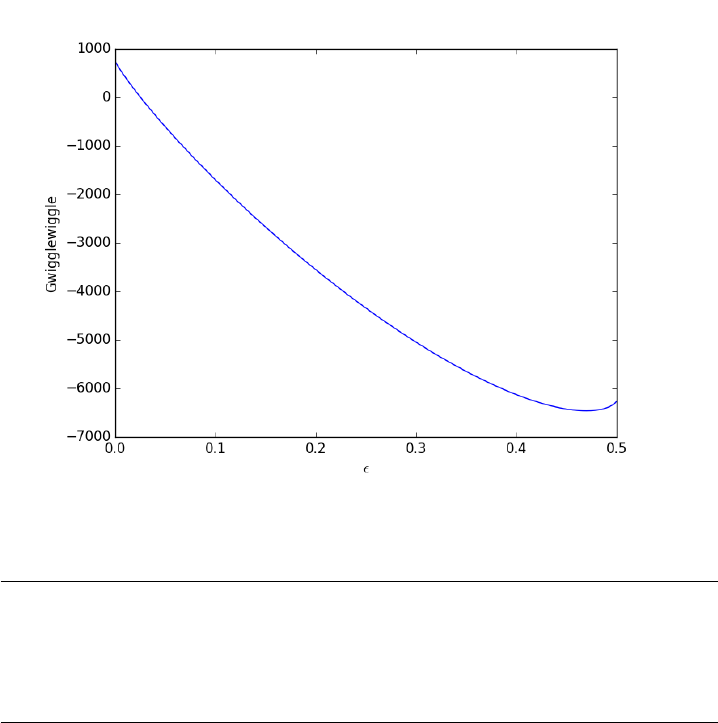
Now we simply minimize our Gwigglewiggle function. Based on the
figure above, the miminum is near 0.45.
1from scipy.optimize import fminbound
2
3epsilonp_eq =fminbound(Gwigglewiggle, 0.4,0.5)
4print(epsilonp_eq)
5
6plt.plot([epsilonp_eq], [Gwigglewiggle(epsilonp_eq)], ’ro’)
7plt.savefig(’images/gibbs-minim-2.png’)
0.46959618249
[<matplotlib.lines.Line2D object at 0x10b46ed68>]
324
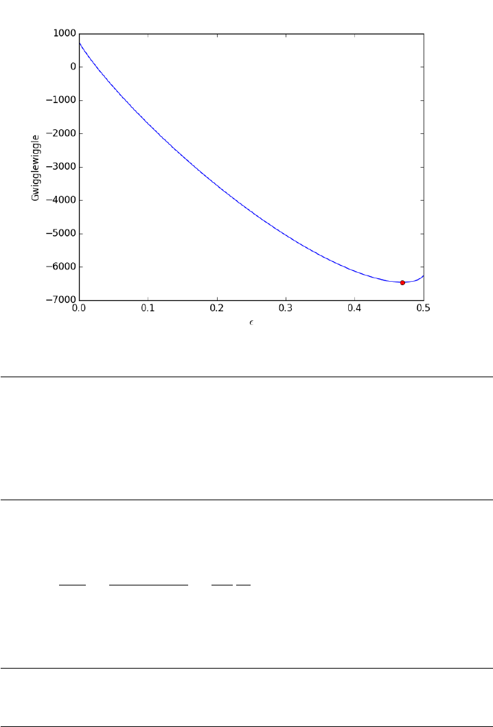
To compute equilibrium mole fractions we do this:
1yi =(yi0 +nu_j[0]*epsilonp_eq) /(1.0 + epsilonp_eq*np.sum(nu_j))
2yb =(yb0 +nu_j[1]*epsilonp_eq) /(1.0 + epsilonp_eq*np.sum(nu_j))
3yp =(yp0 +nu_j[2]*epsilonp_eq) /(1.0 + epsilonp_eq*np.sum(nu_j))
4
5print(yi, yb, yp)
6
7# or this
8y_j =(yj0 +np.dot(nu_j, epsilonp_eq)) /(1.0 + epsilonp_eq*np.sum(nu_j))
9print(y_j)
0.0573220186324 0.0573220186324 0.885355962735
[ 0.05732202 0.05732202 0.88535596]
K=aP
aIaB=ypP/P ◦
yiP/P ◦ybP/P ◦=yP
yiyb
P◦
P.
We can express the equilibrium constant like this :K=Q
j
aνj
j, and com-
pute it with a single line of code.
1K=np.exp(-Grxn/R/T)
2print(’K from delta G ’,K)
3print(’K as ratio of mole fractions ’,yp /(yi *yb) *P0 /P)
4print(’compact notation: ’,np.prod((y_j *P/P0)**nu_j))
325
K from delta G 107.776294742
K as ratio of mole fractions 107.779200065
compact notation: 107.779200065
These results are very close, and only disagree because of the default
tolerance used in identifying the minimum of our function. You could tighten
the tolerances by setting options to the fminbnd function.
14.6.1 Summary
In this post we derived an equation for the Gibbs free energy of a reacting
mixture and used it to find the equilibrium composition. In future posts we
will examine some alternate forms of the equations that may be more useful
in some circumstances.
14.7 Water gas shift equilibria via the NIST Webbook
Matlab post
The NIST webbook provides parameterized models of the enthalpy, en-
tropy and heat capacity of many molecules. In this example, we will examine
how to use these to compute the equilibrium constant for the water gas shift
reaction CO+H2OCO2+H2in the temperature range of 500K to 1000K.
Parameters are provided for:
Cp = heat capacity (J/mol*K) H = standard enthalpy (kJ/mol) S =
standard entropy (J/mol*K)
with models in the form: Cp◦=A+B∗t+C∗t2+D∗t3+E/t2
H◦−H◦
298.15 =A∗t+B∗t2/2 + C∗t3/3 + D∗t4/4−E/t +F−H
S◦=A∗ln(t) + B∗t+C∗t2/2 + D∗t3/3−E/(2 ∗t2) + G
where t=T/1000, and Tis the temperature in Kelvin. We can use this
data to calculate equilibrium constants in the following manner. First, we
have heats of formation at standard state for each compound; for elements,
these are zero by definition, and for non-elements, they have values available
from the NIST webbook. There are also values for the absolute entropy at
standard state. Then, we have an expression for the change in enthalpy from
standard state as defined above, as well as the absolute entropy. From these
we can derive the reaction enthalpy, free energy and entropy at standard
state, as well as at other temperatures.
We will examine the water gas shift enthalpy, free energy and equilib-
rium constant from 500K to 1000K, and finally compute the equilibrium
composition of a gas feed containing 5 atm of CO and H_2 at 1000K.
326

1import numpy as np
2
3T=np.linspace(500,1000)# degrees K
4t=T/1000;
14.7.1 hydrogen
http://webbook.nist.gov/cgi/cbook.cgi?ID=C1333740&Units=SI&Mask=
1#Thermo-Gas
1# T = 298-1000K valid temperature range
2A= 33.066178
3B= -11.363417
4C= 11.432816
5D= -2.772874
6E= -0.158558
7F= -9.980797
8G= 172.707974
9H= 0.0
10
11 Hf_29815_H2 = 0.0 # kJ/mol
12 S_29815_H2 = 130.68 # J/mol/K
13
14 dH_H2 =A*t+B*t**2/2 + C*t**3/3 + D*t**4/4 - E/t+F-H;
15 S_H2 =(A*np.log(t) +B*t+C*t**2/2 + D*t**3/3 - E/(2*t**2)+G);
14.7.2 H_{2}O
http://webbook.nist.gov/cgi/cbook.cgi?ID=C7732185&Units=SI&Mask=
1#Thermo-Gas
Note these parameters limit the temperature range we can examine, as
these parameters are not valid below 500K. There is another set of param-
eters for lower temperatures, but we do not consider them here.
1# 500-1700 K valid temperature range
2A= 30.09200
3B= 6.832514
4C= 6.793435
5D= -2.534480
6E= 0.082139
7F= -250.8810
8G= 223.3967
9H= -241.8264
10
11 Hf_29815_H2O = -241.83 #this is Hf.
12 S_29815_H2O = 188.84
13
14 dH_H2O =A*t+B*t**2/2 + C*t**3/3 + D*t**4/4 - E/t+F-H;
15 S_H2O =(A*np.log(t) +B*t+C*t**2/2 + D*t**3/3 - E/(2*t**2)+G);
327

14.7.3 CO
http://webbook.nist.gov/cgi/cbook.cgi?ID=C630080&Units=SI&Mask=
1#Thermo-Gas
1# 298. - 1300K valid temperature range
2A= 25.56759
3B= 6.096130
4C= 4.054656
5D= -2.671301
6E= 0.131021
7F= -118.0089
8G= 227.3665
9H= -110.5271
10
11 Hf_29815_CO = -110.53 #this is Hf kJ/mol.
12 S_29815_CO = 197.66
13
14 dH_CO =A*t+B*t**2/2 + C*t**3/3 + D*t**4/4 - E/t+F-H;
15 S_CO =(A*np.log(t) +B*t+C*t**2/2 + D*t**3/3 - E/(2*t**2)+G);
14.7.4 CO_{2}
http://webbook.nist.gov/cgi/cbook.cgi?ID=C124389&Units=SI&Mask=
1#Thermo-Gas
1# 298. - 1200.K valid temperature range
2A= 24.99735
3B= 55.18696
4C= -33.69137
5D= 7.948387
6E= -0.136638
7F= -403.6075
8G= 228.2431
9H= -393.5224
10
11 Hf_29815_CO2 = -393.51 # this is Hf.
12 S_29815_CO2 = 213.79
13
14 dH_CO2 =A*t+B*t**2/2 + C*t**3/3 + D*t**4/4 - E/t+F-H;
15 S_CO2 =(A*np.log(t) +B*t+C*t**2/2 + D*t**3/3 - E/(2*t**2)+G);
14.7.5 Standard state heat of reaction
We compute the enthalpy and free energy of reaction at 298.15 K for the
following reaction CO +H2OH2 + CO2.
1Hrxn_29815 =Hf_29815_CO2 +Hf_29815_H2 -Hf_29815_CO -Hf_29815_H2O;
2Srxn_29815 =S_29815_CO2 +S_29815_H2 -S_29815_CO -S_29815_H2O;
328

3Grxn_29815 =Hrxn_29815 - 298.15*(Srxn_29815)/1000;
4
5print(’deltaH = {0:1.2f}’.format(Hrxn_29815))
6print(’deltaG = {0:1.2f}’.format(Grxn_29815))
deltaH = -41.15
deltaG = -28.62
14.7.6 Non-standard state ∆Hand ∆G
We have to correct for temperature change away from standard state. We
only correct the enthalpy for this temperature change. The correction looks
like this:
∆Hrxn(T)=∆Hrxn(Tref ) + X
i
νi(Hi(T)−Hi(Tref ))
Where νiare the stoichiometric coefficients of each species, with appro-
priate sign for reactants and products, and (Hi(T)−Hi(Tref )is precisely
what is calculated for each species with the equations
The entropy is on an absolute scale, so we directly calculate entropy at
each temperature. Recall that H is in kJ/mol and S is in J/mol/K, so we
divide S by 1000 to make the units match.
1Hrxn =Hrxn_29815 +dH_CO2 +dH_H2 -dH_CO -dH_H2O
2Grxn =Hrxn -T*(S_CO2 +S_H2 -S_CO -S_H2O)/1000
14.7.7 Plot how the ∆Gvaries with temperature
1import matplotlib.pyplot as plt
2plt.figure(); plt.clf()
3plt.plot(T,Grxn, label=’$\Delta G_{rxn}$’)
4plt.plot(T,Hrxn, label=’$\Delta H_{rxn}$’)
5plt.xlabel(’Temperature (K)’)
6plt.ylabel(’(kJ/mol)’)
7plt.legend( loc=’best’)
8plt.savefig(’images/wgs-nist-1.png’)
<matplotlib.figure.Figure object at 0x110783a58>
[<matplotlib.lines.Line2D object at 0x1091a3f60>]
[<matplotlib.lines.Line2D object at 0x1091a8940>]
<matplotlib.text.Text object at 0x1107a5d68>
<matplotlib.text.Text object at 0x1107b1470>
<matplotlib.legend.Legend object at 0x1091ae160>
329
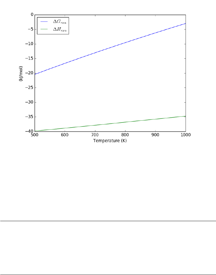
Over this temperature range the reaction is exothermic, although near
1000K it is just barely exothermic. At higher temperatures we expect the
reaction to become endothermic.
14.7.8 Equilibrium constant calculation
Note the equilibrium constant starts out high, i.e. strongly favoring the
formation of products, but drops very quicky with increasing temperature.
1R= 8.314e-3 # kJ/mol/K
2K=np.exp(-Grxn/R/T);
3
4plt.figure()
5plt.plot(T,K)
6plt.xlim([500,1000])
7plt.xlabel(’Temperature (K)’)
8plt.ylabel(’Equilibrium constant’)
9plt.savefig(’images/wgs-nist-2.png’)
<matplotlib.figure.Figure object at 0x1091aeac8>
[<matplotlib.lines.Line2D object at 0x110994390>]
(500, 1000)
<matplotlib.text.Text object at 0x1107a77f0>
<matplotlib.text.Text object at 0x110b22e48>
330
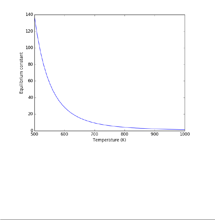
14.7.9 Equilibrium yield of WGS
Now let us suppose we have a reactor with a feed of H_2O and CO at
10atm at 1000K. What is the equilibrium yield of H_2? Let be the extent
of reaction, so that Fi=Fi,0+νi. For reactants, νiis negative, and for
products, νiis positive. We have to solve for the extent of reaction that
satisfies the equilibrium condition.
1from scipy.interpolate import interp1d
2from scipy.optimize import fsolve
3
4#
5#A=CO
6# B = H2O
7#C=H2
8# D = CO2
9
10 Pa0 = 5; Pb0 = 5; Pc0 = 0; Pd0 = 0;# pressure in atm
11 R= 0.082;
12 Temperature = 1000;
13
14 # we can estimate the equilibrium like this. We could also calculate it
15 # using the equations above, but we would have to evaluate each term. Above
16 # we simply computed a vector of enthalpies, entropies, etc... Here we interpolate
17 K_func =interp1d(T,K);
18 K_Temperature =K_func(1000)
331

19
20
21 # If we let X be fractional conversion then we have $C_A = C_{A0}(1-X)$,
22 # $C_B = C_{B0}-C_{A0}X$, $C_C = C_{C0}+C_{A0}X$, and $C_D =
23 # C_{D0}+C_{A0}X$. We also have $K(T) = (C_C C_D)/(C_A C_B)$, which finally
24 # reduces to $0 = K(T) - Xeq^2/(1-Xeq)^2$ under these conditions.
25
26 def f(X):
27 return K_Temperature -X**2/(1-X)**2;
28
29 x0 = 0.5
30 Xeq, =fsolve(f, x0)
31
32 print(’The equilibrium conversion for these feed conditions is: {0:1.2f}’.format(Xeq))
The equilibrium conversion for these feed conditions is: 0.55
14.7.10 Compute gas phase pressures of each species
Since there is no change in moles for this reaction, we can directly calculation
the pressures from the equilibrium conversion and the initial pressure of
gases. you can see there is a slightly higher pressure of H_2 and CO_2
than the reactants, consistent with the equilibrium constant of about 1.44
at 1000K. At a lower temperature there would be a much higher yield of the
products. For example, at 550K the equilibrium constant is about 58, and
the pressure of H_2 is 4.4 atm due to a much higher equilibrium conversion
of 0.88.
1P_CO =Pa0*(1-Xeq)
2P_H2O =Pa0*(1-Xeq)
3P_H2 =Pa0*Xeq
4P_CO2 =Pa0*Xeq
5
6print(P_CO,P_H2O, P_H2, P_CO2)
2.2747854428 2.2747854428 2.7252145572 2.7252145572
14.7.11 Compare the equilibrium constants
We can compare the equilibrium constant from the Gibbs free energy and
the one from the ratio of pressures. They should be the same!
1print(K_Temperature)
2print((P_CO2*P_H2)/(P_CO*P_H2O))
332

1.4352267476228722
1.43522674762
They are the same.
14.7.12 Summary
The NIST Webbook provides a plethora of data for computing thermody-
namic properties. It is a little tedious to enter it all into Matlab, and a little
tricky to use the data to estimate temperature dependent reaction energies.
A limitation of the Webbook is that it does not tell you have the thermo-
dynamic properties change with pressure. Luckily, those changes tend to be
small.
I noticed a different behavior in interpolation between scipy.interpolate.interp1d
and Matlab’s interp1. The scipy function returns an interpolating function,
whereas the Matlab function directly interpolates new values, and returns
the actual interpolated data.
14.8 Constrained minimization to find equilibrium composi-
tions
adapated from Chemical Reactor analysis and design fundamentals, Rawl-
ings and Ekerdt, appendix A.2.3.
Matlab post
The equilibrium composition of a reaction is the one that minimizes the
total Gibbs free energy. The Gibbs free energy of a reacting ideal gas mixture
depends on the mole fractions of each species, which are determined by the
initial mole fractions of each species, the extent of reactions that convert
each species, and the equilibrium constants.
Reaction 1: I+BP1
Reaction 2: I+BP2
Here we define the Gibbs free energy of the mixture as a function of the
reaction extents.
1import numpy as np
2
3def gibbs(E):
4’function defining Gibbs free energy as a function of reaction extents’
5e1 =E[0]
6e2 =E[1]
7# known equilibrium constants and initial amounts
8K1 = 108; K2 = 284;P= 2.5
9yI0 = 0.5; yB0 = 0.5; yP10 = 0.0; yP20 = 0.0
333

10 # compute mole fractions
11 d=1-e1 -e2
12 yI =(yI0 -e1 -e2) /d
13 yB =(yB0 -e1 -e2) /d
14 yP1 =(yP10 +e1) /d
15 yP2 =(yP20 +e2) /d
16 G=(-(e1 *np.log(K1) +e2 *np.log(K2)) +
17 d*np.log(P) +yI *d*np.log(yI) +
18 yB *d*np.log(yB) +yP1 *d*np.log(yP1) +yP2 *d*np.log(yP2))
19 return G
The equilibrium constants for these reactions are known, and we seek
to find the equilibrium reaction extents so we can determine equilibrium
compositions. The equilibrium reaction extents are those that minimize the
Gibbs free energy. We have the following constraints, written in standard
less than or equal to form:
−1≤0
−2≤0
1+2≤0.5
In Matlab we express this in matrix form as Ax=b where
A=
−1 0
0−1
1 1
(47)
and
b=
0
0
0.5
(48)
Unlike in Matlab, in python we construct the inequality constraints as
functions that are greater than or equal to zero when the constraint is met.
1def constraint1(E):
2e1 =E[0]
3return e1
4
5
6def constraint2(E):
7e2 =E[1]
8return e2
9
10
11 def constraint3(E):
12 e1 =E[0]
13 e2 =E[1]
14 return 0.5 - (e1 +e2)
334

Now, we minimize.
1from scipy.optimize import fmin_slsqp
2
3X0 =[0.2,0.2]
4X=fmin_slsqp(gibbs, X0, ieqcons=[constraint1, constraint2, constraint3],
5bounds=((0.01,0.49),
6(0.01,0.49)))
7print(X)
8
9print(gibbs(X))
Iteration limit exceeded (Exit mode 9)
Current function value: nan
Iterations: 101
Function evaluations: 1394
Gradient evaluations: 101
[ nan nan]
nan
One way we can verify our solution is to plot the gibbs function and
see where the minimum is, and whether there is more than one minimum.
We start by making grids over the range of 0 to 0.5. Note we actually
start slightly above zero because at zero there are some numerical imaginary
elements of the gibbs function or it is numerically not defined since there are
logs of zero there. We also set all elements where the sum of the two extents
is greater than 0.5 to near zero, since those regions violate the constraints.
1import numpy as np
2import matplotlib.pyplot as plt
3
4def gibbs(E):
5’function defining Gibbs free energy as a function of reaction extents’
6e1 =E[0]
7e2 =E[1]
8# known equilibrium constants and initial amounts
9K1 = 108; K2 = 284;P= 2.5;
10 yI0 = 0.5; yB0 = 0.5; yP10 = 0.0; yP20 = 0.0;
11 # compute mole fractions
12 d=1-e1 -e2;
13 yI =(yI0 -e1 -e2)/d;
14 yB =(yB0 -e1 -e2)/d;
15 yP1 =(yP10 +e1)/d;
16 yP2 =(yP20 +e2)/d;
17 G=(-(e1 *np.log(K1) +e2 *np.log(K2)) +
18 d*np.log(P) +yI *d*np.log(yI) +
19 yB *d*np.log(yB) +yP1 *d*np.log(yP1) +yP2 *d*np.log(yP2))
20 return G
335
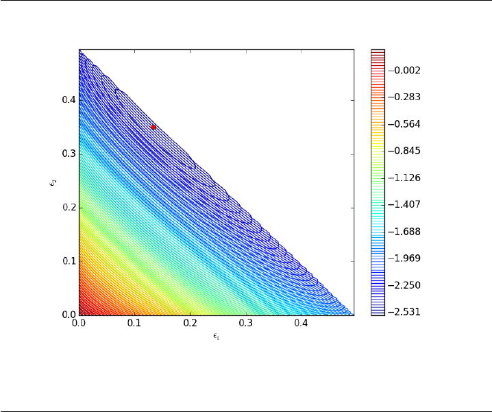
21
22
23 a=np.linspace(0.001,0.5,100)
24 E1, E2 =np.meshgrid(a,a)
25
26 sumE =E1 +E2
27 E1[sumE >= 0.5]= 0.00001
28 E2[sumE >= 0.5]= 0.00001
29
30 # now evaluate gibbs
31 G=np.zeros(E1.shape)
32 m,n =E1.shape
33
34 G=gibbs([E1, E2])
35
36 CS =plt.contour(E1, E2, G, levels=np.linspace(G.min(),G.max(),100))
37 plt.xlabel(’$\epsilon_1$’)
38 plt.ylabel(’$\epsilon_2$’)
39 plt.colorbar()
40
41 plt.plot([0.13336503], [0.35066486], ’ro’)
42
43 plt.savefig(’images/gibbs-minimization-1.png’)
44 plt.savefig(’images/gibbs-minimization-1.svg’)
45 plt.show()
You can see we found the minimum. We can compute the mole fractions
pretty easily.
336

1e1 =X[0];
2e2 =X[1];
3
4yI0 = 0.5; yB0 = 0.5; yP10 = 0; yP20 = 0;#initial mole fractions
5
6d=1-e1 -e2;
7yI =(yI0 -e1 -e2) /d
8yB =(yB0 -e1 -e2) /d
9yP1 =(yP10 +e1) /d
10 yP2 =(yP20 +e2) /d
11
12 print(’y_I = {0:1.3f} y_B = {1:1.3f} y_P1 = {2:1.3f} y_P2 = {3:1.3f}’.format(yI,yB,yP1,yP2))
>>> >>> >>> >>> >>> >>> >>> >>> >>> >>> y_I = 0.031 y_B = 0.031 y_P1 = 0.258 y_P2 = 0.680
14.8.1 summary
I found setting up the constraints in this example to be more confusing than
the Matlab syntax.
14.9 Using constrained optimization to find the amount of
each phase present
The problem we solve here is that we have several compounds containing
Ni and Al, and a bulk mixture of a particular composition of Ni and Al.
We want to know which mixture of phases will minimize the total energy.
The tricky part is that the optimization is constrained because the mixture
of phases must have the overall stoichiometry we want. We formulate the
problem like this.
Basically, we want to minimize the function E=PwiEi, where wiis the
mass of phase i, and Eiis the energy per unit mass of phase i. There are some
constraints to ensure conservation of mass. Let us consider the following
compounds: Al, NiAl, Ni3Al, and Ni, and consider a case where the bulk
composition of our alloy is 93.8% Ni and balance Al. We want to know which
phases are present, and in what proportions. There are some subtleties in
considering the formula and molecular weight of an alloy. We consider the
formula with each species amount normalized so the fractions all add up to
one. For example, Ni_3Al is represented as Ni_{0.75}Al_{0.25}, and the
molecular weight is computed as 0.75*MW_{Ni} + 0.25*MW_{Al}.
We use scipy.optimize.fmin_slsqp to solve this problem, and define two
equality constraint functions, and the bounds on each weight fraction.
Note: the energies in this example were computed by density functional
theory at 0K.
337

1import numpy as np
2from scipy.optimize import fmin_slsqp
3
4# these are atomic masses of each species
5Ni = 58.693
6Al = 26.982
7
8COMPOSITIONS =[’Al’,’NiAl’,’Ni3Al’,’Ni’]
9MW =np.array( [Al, (Ni +Al)/2.0, (3*Ni +Al)/4.0, Ni])
10
11 xNi =np.array([0.0,0.5,0.75,1.0]) # mole fraction of nickel in each compd
12 WNi =xNi *Ni /MW # weight fraction of Ni in each cmpd
13
14 ENERGIES =np.array([0.0,-0.7,-0.5,0.0])
15
16 BNi = 0.938
17
18 def G(w):
19 ’function to minimize. w is a vector of weight fractions, ENERGIES is defined above.’
20 return np.dot(w, ENERGIES)
21
22 def ec1(w):
23 ’conservation of Ni constraint’
24 return BNi -np.dot(w, WNi)
25
26 def ec2(w):
27 ’weight fractions sum to one constraint’
28 return 1-np.sum(w)
29
30 w0 =np.array([0.0,0.0,0.5,0.5]) # guess weight fractions
31
32 y=fmin_slsqp(G,
33 w0,
34 eqcons=[ec1, ec2],
35 bounds=[(0,1)]*len(w0))
36
37 for ci, wi in zip(COMPOSITIONS, y):
38 print(’{0:8s} {1:+8.2%}’.format(ci, wi))
Optimization terminated successfully. (Exit mode 0)
Current function value: -0.233299644373
Iterations: 2
Function evaluations: 12
Gradient evaluations: 2
Al +0.00%
NiAl +0.00%
Ni3Al +46.66%
Ni +53.34%
So, the sample will be about 47% by weight of Ni3Al, and 53% by weight
of pure Ni.
338

It may be convenient to formulate this in terms of moles.
1import numpy as np
2from scipy.optimize import fmin_slsqp
3
4COMPOSITIONS =[’Al’,’NiAl’,’Ni3Al’,’Ni’]
5xNi =np.array([0.0,0.5,0.75,1.0]) # define this in mole fractions
6
7ENERGIES =np.array([0.0,-0.7,-0.5,0.0])
8
9xNiB = 0.875 # bulk Ni composition
10
11 def G(n):
12 ’function to minimize’
13 return np.dot(n, ENERGIES)
14
15 def ec1(n):
16 ’conservation of Ni’
17 Ntot =np.sum(n)
18 return (Ntot *xNiB) -np.dot(n, xNi)
19
20 def ec2(n):
21 ’mole fractions sum to one’
22 return 1-np.sum(n)
23
24 n0 =np.array([0.0,0.0,0.45,0.55]) # initial guess of mole fractions
25
26 y=fmin_slsqp(G,
27 n0,
28 eqcons=[ec1, ec2],
29 bounds=[(0,1)]*(len(n0)))
30
31 for ci, xi in zip(COMPOSITIONS, y):
32 print(’{0:8s} {1:+8.2%}’.format(ci, xi))
Optimization terminated successfully. (Exit mode 0)
Current function value: -0.25
Iterations: 2
Function evaluations: 12
Gradient evaluations: 2
Al +0.00%
NiAl +0.00%
Ni3Al +50.00%
Ni +50.00%
This means we have a 1:1 molar ratio of Ni and Ni_{0.75}Al_{0.25}.
That works out to the overall bulk composition in this particular problem.
Let us verify that these two approaches really lead to the same con-
clusions. On a weight basis we estimate 53.3%wt Ni and 46.7%wt Ni3Al,
339

whereas we predict an equimolar mixture of the two phases. Below we com-
pute the mole fraction of Ni in each case.
1# these are atomic masses of each species
2Ni = 58.693
3Al = 26.982
4
5# Molar case
6# 1 mol Ni + 1 mol Ni_{0.75}Al_{0.25}
7N1 = 1.0; N2 = 1.0
8mol_Ni =1.0*N1 + 0.75 * N2
9xNi =mol_Ni /(N1 +N2)
10 print(xNi)
11
12 # Mass case
13 M1 = 0.533;M2= 0.467
14 MW1 =Ni; MW2 = 0.75*Ni + 0.25*Al
15
16 xNi2 =(1.0 * M1/MW1 + 0.75 * M2 /MW2) /(M1/MW1 +M2/MW2)
17 print(xNi2)
0.875
0.874192746384855
You can see the overall mole fraction of Ni is practically the same in each
case.
14.10 Conservation of mass in chemical reactions
Matlab post
Atoms cannot be destroyed in non-nuclear chemical reactions, hence it
follows that the same number of atoms entering a reactor must also leave
the reactor. The atoms may leave the reactor in a different molecular con-
figuration due to the reaction, but the total mass leaving the reactor must
be the same. Here we look at a few ways to show this.
We consider the water gas shift reaction : CO +H2OH2+CO2. We
can illustrate the conservation of mass with the following equation: νM=
0. Where νis the stoichiometric coefficient vector and Mis a column
vector of molecular weights. For simplicity, we use pure isotope molecular
weights, and not the isotope-weighted molecular weights. This equation
simply examines the mass on the right side of the equation and the mass on
left side of the equation.
1import numpy as np
2nu =[-1,-1,1,1];
340

3M=[28,18,2,44];
4print(np.dot(nu, M))
0
You can see that sum of the stoichiometric coefficients times molecular
weights is zero. In other words a CO and H_2O have the same mass as H_2
and CO_2.
For any balanced chemical equation, there are the same number of each
kind of atom on each side of the equation. Since the mass of each atom is
unchanged with reaction, that means the mass of all the species that are
reactants must equal the mass of all the species that are products! Here we
look at the number of C, O, and H on each side of the reaction. Now if we
add the mass of atoms in the reactants and products, it should sum to zero
(since we used the negative sign for stoichiometric coefficients of reactants).
1import numpy as np
2# C O H
3reactants =[-1,-2,-2]
4products =[1,2,2]
5
6atomic_masses =[12.011,15.999,1.0079]# atomic masses
7
8print(np.dot(reactants, atomic_masses) +np.dot(products, atomic_masses))
0.0
That is all there is to mass conservation with reactions. Nothing changes
if there are lots of reactions, as long as each reaction is properly balanced,
and none of them are nuclear reactions!
14.11 Numerically calculating an effectiveness factor for a
porous catalyst bead
Matlab post
If reaction rates are fast compared to diffusion in a porous catalyst pellet,
then the observed kinetics will appear to be slower than they really are
because not all of the catalyst surface area will be effectively used. For
example, the reactants may all be consumed in the near surface area of
a catalyst bead, and the inside of the bead will be unutilized because no
reactants can get in due to the high reaction rates.
References: Ch 12. Elements of Chemical Reaction Engineering, Fogler,
4th edition.
341

A mole balance on the particle volume in spherical coordinates with
a first order reaction leads to: d2Ca
dr2+2
r
dCa
dr −k
DeCA= 0 with boundary
conditions CA(R) = CAs and dCa
dr = 0 at r= 0. We convert this equation to
a system of first order ODEs by letting WA=dCa
dr . Then, our two equations
become:
dCa
dr =WA
and
dWA
dr =−2
rWA+k
DECA
We have a condition of no flux (WA= 0) at r=0 and Ca(R) = CAs,
which makes this a boundary value problem. We use the shooting method
here, and guess what Ca(0) is and iterate the guess to get Ca(R) = CAs.
The value of the second differential equation at r=0 is tricky because at
this place we have a 0/0 term. We use L’Hopital’s rule to evaluate it. The
derivative of the top is dWA
dr and the derivative of the bottom is 1. So, we
have dWA
dr =−2dWA
dr +k
DECA
Which leads to:
3dWA
dr =k
DECA
or dWA
dr =3k
DECAat r= 0.
Finally, we implement the equations in Python and solve.
1import numpy as np
2from scipy.integrate import odeint
3import matplotlib.pyplot as plt
4
5De = 0.1 # diffusivity cm^2/s
6R= 0.5 # particle radius, cm
7k= 6.4 # rate constant (1/s)
8CAs = 0.2 # concentration of A at outer radius of particle (mol/L)
9
10
11 def ode(Y, r):
12 Wa =Y[0]# molar rate of delivery of A to surface of particle
13 Ca =Y[1]# concentration of A in the particle at r
14 # this solves the singularity at r = 0
15 if r== 0:
16 dWadr =k/ 3.0 * De *Ca
17 else:
18 dWadr = -2 * Wa /r+k/De *Ca
19 dCadr =Wa
20 return [dWadr, dCadr]
21
22 # Initial conditions
23 Ca0 = 0.029315 # Ca(0) (mol/L) guessed to satisfy Ca(R) = CAs
24 Wa0 = 0 # no flux at r=0 (mol/m^2/s)
25
26 rspan =np.linspace(0,R,500)
27
342
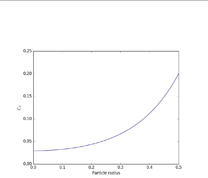
28 Y=odeint(ode, [Wa0, Ca0], rspan)
29
30 Ca =Y[:, 1]
31
32 # here we check that Ca(R) = Cas
33 print(’At r={0} Ca={1}’.format(rspan[-1], Ca[-1]))
34
35 plt.plot(rspan, Ca)
36 plt.xlabel(’Particle radius’)
37 plt.ylabel(’$C_A$’)
38 plt.savefig(’images/effectiveness-factor.png’)
39
40 r=rspan
41 eta_numerical =(np.trapz(k *Ca *4*np.pi *(r**2), r)
42 /np.trapz(k *CAs *4*np.pi *(r**2), r))
43
44 print(eta_numerical)
45
46 phi =R*np.sqrt(k /De)
47 eta_analytical =(3/phi**2)*(phi *(1.0 / np.tanh(phi)) - 1)
48 print(eta_analytical)
At r=0.5 Ca=0.20000148865173356
0.563011348314
0.563003362801
You can see the concentration of A inside the particle is significantly
lower than outside the particle. That is because it is reacting away faster
343

than it can diffuse into the particle. Hence, the overall reaction rate in the
particle is lower than it would be without the diffusion limit.
The effectiveness factor is the ratio of the actual reaction rate in the
particle with diffusion limitation to the ideal rate in the particle if there was
no concentration gradient:
η=RR
0k00aCA(r)4πr2dr
RR
0k00aCAs4πr2dr
We will evaluate this numerically from our solution and compare it to
the analytical solution. The results are in good agreement, and you can
make the numerical estimate better by increasing the number of points in
the solution so that the numerical integration is more accurate.
Why go through the numerical solution when an analytical solution ex-
ists? The analytical solution here is only good for 1st order kinetics in a
sphere. What would you do for a complicated rate law? You might be able
to find some limiting conditions where the analytical equation above is rel-
evant, and if you are lucky, they are appropriate for your problem. If not,
it is a good thing you can figure this out numerically!
Thanks to Radovan Omorjan for helping me figure out the ODE at r=0!
14.12 Computing a pipe diameter
Matlab post A heat exchanger must handle 2.5 L/s of water through a
smooth pipe with length of 100 m. The pressure drop cannot exceed 103
kPa at 25 degC. Compute the minimum pipe diameter required for this
application.
Adapted from problem 8.8 in Problem solving in chemical and Biochem-
ical Engineering with Polymath, Excel, and Matlab. page 303.
We need to estimate the Fanning friction factor for these conditions
so we can estimate the frictional losses that result in a pressure drop for a
uniform, circular pipe. The frictional forces are given by Ff= 2fF∆Lv2
D, and
the corresponding pressure drop is given by ∆P=ρFf. In these equations,
ρis the fluid density, vis the fluid velocity, Dis the pipe diameter, and fFis
the Fanning friction factor. The average fluid velocity is given by v=q
πD2/4.
For laminar flow, we estimate fF= 16/Re, which is a linear equation,
and for turbulent flow (Re > 2100) we have the implicit equation 1
√fF
=
4.0 log(Re√fF)−0.4. Of course, we define Re =Dvρ
µwhere µis the viscosity
of the fluid.
344

It is known that ρ(T) = 46.048 + 9.418T−0.0329T2+ 4.882 ×10⁻⁵−
2.895×10⁻⁸T4and µ= exp −10.547 + 541.69
T−144.53 where ρis in kg/mˆ3 and
µis in kg/(m*s).
The aim is to find Dthat solves: ∆p=ρ2fF∆Lv2
D. This is a nonlinear
equation in D, since D affects the fluid velocity, the Re, and the Fanning
friction factor. Here is the solution
1import numpy as np
2from scipy.optimize import fsolve
3import matplotlib.pyplot as plt
4
5T= 25 + 273.15
6Q= 2.5e-3 # m^3/s
7deltaP = 103000 # Pa
8deltaL = 100 # m
9
10 #Note these correlations expect dimensionless T, where the magnitude
11 #ofTisinK
12
13 def rho(T):
14 return 46.048 + 9.418 * T-0.0329 * T**2 +4.882e-5 * T**3 - 2.895e-8 * T**4
15
16 def mu(T):
17 return np.exp(-10.547 + 541.69 / (T - 144.53))
18
19 def fanning_friction_factor_(Re):
20 if Re < 2100:
21 raise Exception(’Flow is probably not turbulent, so this correlation is not appropriate.’)
22 # solve the Nikuradse correlation to get the friction factor
23 def fz(f): return 1.0/np.sqrt(f) -(4.0*np.log10(Re*np.sqrt(f))-0.4)
24 sol, =fsolve(fz, 0.01)
25 return sol
26
27 fanning_friction_factor =np.vectorize(fanning_friction_factor_)
28
29 Re =np.linspace(2200,9000)
30 f=fanning_friction_factor(Re)
31
32 plt.plot(Re, f)
33 plt.xlabel(’Re’)
34 plt.ylabel(’fanning friction factor’)
35 # You can see why we use 0.01 as an initial guess for solving for the
36 # Fanning friction factor; it falls in the middle of ranges possible
37 # for these Re numbers.
38 plt.savefig(’images/pipe-diameter-1.png’)
39
40 def objective(D):
41 v=Q/(np.pi *D**2 / 4)
42 Re =D*v*rho(T) /mu(T)
43
44 fF =fanning_friction_factor(Re)
45
46 return deltaP -2*fF *rho(T) *deltaL *v**2 / D
345

47
48 D, =fsolve(objective, 0.04)
49
50 print(’The minimum pipe diameter is {0} m\n’.format(D))
The minimum pipe diameter is 0.0389653369530596 m
Any pipe diameter smaller than that value will result in a larger pressure
drop at the same volumetric flow rate, or a smaller volumetric flowrate at
the same pressure drop. Either way, it will not meet the design specification.
14.13 Reading parameter database text files in python
Matlab post
The datafile at http://terpconnect.umd.edu/~nsw/ench250/antoine.
dat (dead link) contains data that can be used to estimate the vapor pressure
of about 700 pure compounds using the Antoine equation
The data file has the following contents:
Antoine Coefficients
log(P) = A-B/(T+C) where P is in mmHg and T is in Celsius
Source of data: Yaws and Yang (Yaws, C. L. and Yang, H. C.,
"To estimate vapor pressure easily. antoine coefficients relate vapor pressure to temperature for almost 700 major organic compounds", Hydrocarbon Processing, 68(10), p65-68, 1989.
ID formula compound name A B C Tmin Tmax ?? ?
-----------------------------------------------------------------------------------
1 CCL4 carbon-tetrachloride 6.89410 1219.580 227.170 -20 101 Y2 0
2 CCL3F trichlorofluoromethane 6.88430 1043.010 236.860 -33 27 Y2 0
3 CCL2F2 dichlorodifluoromethane 6.68619 782.072 235.377 -119 -30 Y6 0
To use this data, you find the line that has the compound you want, and
read off the data. You could do that manually for each component you want
but that is tedious, and error prone. Today we will see how to retrieve the
file, then read the data into python to create a database we can use to store
and retrieve the data.
We will use the data to find the temperature at which the vapor pressure
of acetone is 400 mmHg.
We use numpy.loadtxt to read the file, and tell the function the format
of each column. This creates a special kind of record array which we can
access data by field name.
346

1import numpy as np
2import matplotlib.pyplot as plt
3
4data =np.loadtxt(’data/antoine_data.dat’,
5dtype=[(’id’, np.int),
6(’formula’,’S8’),
7(’name’,’S28’),
8(’A’, np.float),
9(’B’, np.float),
10 (’C’, np.float),
11 (’Tmin’, np.float),
12 (’Tmax’, np.float),
13 (’??’,’S4’),
14 (’?’,’S4’)],
15 skiprows=7)
16
17 names =data[’name’]
18
19 acetone =data[names == ’acetone’]
20
21 # for readability we unpack the array into variables
22 id, formula, name, A, B, C, Tmin, Tmax, u1, u2 =acetone
23
24 T=np.linspace(Tmin, Tmax)
25 P= 10**(A -B/(T+C))
26 plt.plot(T, P)
27 plt.xlabel(’T ($^\circ$C)’)
28 plt.ylabel(’P$_{vap}$ (mmHg)’)
29
30 # Find T at which Pvap = 400 mmHg
31 # from our graph we might guess T ~ 40 ^{\circ}C
32
33 def objective(T):
34 return 400 - 10**(A -B/(T +C))
35
36 from scipy.optimize import fsolve
37 Tsol, =fsolve(objective, 40)
38 print(Tsol)
39 print(’The vapor pressure is 400 mmHg at T = {0:1.1f} degC’.format(Tsol))
40
41 #Plot CRC data http://en.wikipedia.org/wiki/Acetone_%28data_page%29#Vapor_pressure_of_liquid
42 # We only include the data for the range where the Antoine fit is valid.
43
44 Tcrc =[-59.4,-31.1,-9.4,7.7,39.5,56.5]
45 Pcrc =[1,10,40,100,400,760]
46
47 plt.plot(Tcrc, Pcrc, ’bo’)
48 plt.legend([’Antoine’,’CRC Handbook’], loc=’best’)
49 plt.savefig(’images/antoine-2.png’)
56.9792617813
The vapor pressure is 400 mmHg at T = 57.0 degC
347
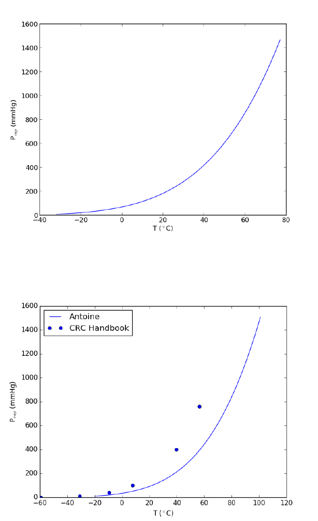
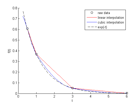

14.14 Calculating a bubble point pressure of a mixture
Matlab post
Adapted from http://terpconnect.umd.edu/~nsw/ench250/bubpnt.
htm (dead link)
We previously learned to read a datafile containing lots of Antoine coef-
ficients into a database, and use the coefficients to estimate vapor pressure
of a single compound. Here we use those coefficents to compute a bubble
point pressure of a mixture.
The bubble point is the temperature at which the sum of the component
vapor pressures is equal to the the total pressure. This is where a bubble of
vapor will first start forming, and the mixture starts to boil.
Consider an equimolar mixture of benzene, toluene, chloroform, acetone
and methanol. Compute the bubble point at 760 mmHg, and the gas phase
composition. The gas phase composition is given by: yi=xi∗Pi/PT.
1import numpy as np
2from scipy.optimize import fsolve
3
4# load our thermodynamic data
5data =np.loadtxt(’data/antoine_data.dat’,
6dtype=[(’id’, np.int),
7(’formula’,’S8’),
8(’name’,’S28’),
9(’A’, np.float),
10 (’B’, np.float),
11 (’C’, np.float),
12 (’Tmin’, np.float),
13 (’Tmax’, np.float),
14 (’??’,’S4’),
15 (’?’,’S4’)],
16 skiprows=7)
17
18 compounds =[’benzene’,’toluene’,’chloroform’,’acetone’,’methanol’]
19
20 # extract the data we want
21 A=np.array([data[data[’name’]== x.encode(encoding=’UTF-8’)][’A’][0]
22 for xin compounds])
23 B=np.array([data[data[’name’]== x.encode(encoding=’UTF-8’)][’B’][0]
24 for xin compounds])
25 C=np.array([data[data[’name’]== x.encode(encoding=’UTF-8’)][’C’][0]
26 for xin compounds])
27 Tmin =np.array([data[data[’name’]== x.encode(encoding=’UTF-8’)][’Tmin’][0]
28 for xin compounds])
29 Tmax =np.array([data[data[’name’]== x.encode(encoding=’UTF-8’)][’Tmax’][0]
30 for xin compounds])
31
32 # we have an equimolar mixture
33 x=np.array([0.2,0.2,0.2,0.2,0.2])
34
349

35 # Given a T, we can compute the pressure of each species like this:
36
37 T= 67 # degC
38 P= 10**(A -B/(T +C))
39 print(P)
40 print(np.dot(x, P)) # total mole-fraction weighted pressure
41
42 Tguess = 67
43 Ptotal = 760
44
45 def func(T):
46 P= 10**(A -B/(T +C))
47 return Ptotal -np.dot(x, P)
48
49 Tbubble, =fsolve(func, Tguess)
50
51 print(’The bubble point is {0:1.2f} degC’.format(Tbubble))
52
53 # double check answer is in a valid T range
54 if np.any(Tbubble <Tmin) or np.any(Tbubble >Tmax):
55 print(’T_bubble is out of range!’)
56
57 # print gas phase composition
58 y=x* 10**(A -B/(Tbubble +C))/Ptotal
59
60 for cmpd, yi in zip(compounds, y):
61 print(’y_{0:<10s} = {1:1.3f}’.format(cmpd, yi))
[ 498.4320267 182.16010994 898.31061294 1081.48181768 837.88860027]
699.654633507
The bubble point is 69.46 degC
y_benzene = 0.142
y_toluene = 0.053
y_chloroform = 0.255
y_acetone = 0.308
y_methanol = 0.242
14.15 The equal area method for the van der Waals equation
Matlab post
When a gas is below its Tc the van der Waal equation oscillates. In the
portion of the isotherm where ∂PR/∂Vr>0, the isotherm fails to describe
real materials, which phase separate into a liquid and gas in this region.
Maxwell proposed to replace this region by a flat line, where the area
above and below the curves are equal. Today, we examine how to identify
where that line should be.
350
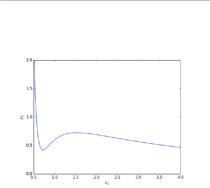
1import numpy as np
2import matplotlib.pyplot as plt
3
4Tr = 0.9 # A Tr below Tc: Tr = T/Tc
5# analytical equation for Pr. This is the reduced form of the van der Waal
6# equation.
7def Prfh(Vr):
8return 8.0 / 3.0 * Tr /(Vr - 1.0 / 3.0)-3.0/(Vr**2)
9
10 Vr =np.linspace(0.5,4,100)# vector of reduced volume
11 Pr =Prfh(Vr) # vector of reduced pressure
12
13 plt.clf()
14 plt.plot(Vr,Pr)
15 plt.ylim([0,2])
16 plt.xlabel(’$V_R$’)
17 plt.ylabel(’$P_R$’)
18 plt.savefig(’images/maxwell-eq-area-1.png’)
[<matplotlib.lines.Line2D object at 0x1113846d8>]
(0, 2)
<matplotlib.text.Text object at 0x111347080>
<matplotlib.text.Text object at 0x111347e48>
The idea is to pick a Pr and draw a line through the EOS. We want
the areas between the line and EOS to be equal on each side of the middle
intersection. Let us draw a line on the figure at y = 0.65.
351
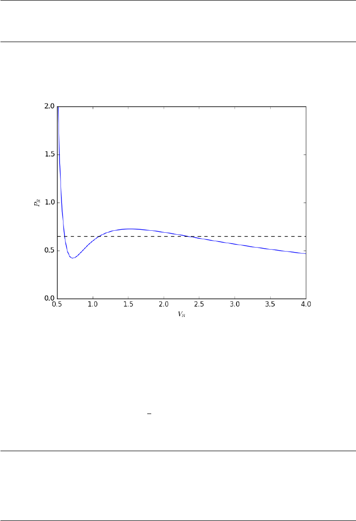
1y= 0.65
2
3plt.plot([0.5,4.0], [y, y], ’k--’)
4plt.savefig(’images/maxwell-eq-area-2.png’)
[<matplotlib.lines.Line2D object at 0x111092f28>]
To find the areas, we need to know where the intersection of the vdW
eqn with the horizontal line. This is the same as asking what are the roots
of the vdW equation at that Pr. We need all three intersections so we can
integrate from the first root to the middle root, and then the middle root
to the third root. We take advantage of the polynomial nature of the vdW
equation, which allows us to use the roots command to get all the roots at
once. The polynomial is V3
R−1
3(1 + 8TR/PR)+3/PR−1/PR= 0. We use
the coefficients t0 get the roots like this.
1vdWp =[1.0,-1. / 3.0 * (1.0 + 8.0 * Tr /y), 3.0 / y, - 1.0 / y]
2v=np.roots(vdWp)
3v.sort()
4print(v)
5
6plt.plot(v[0], y, ’bo’, v[1], y, ’bo’, v[2], y, ’bo’)
7plt.savefig(’images/maxwell-eq-area-3.png’)
352
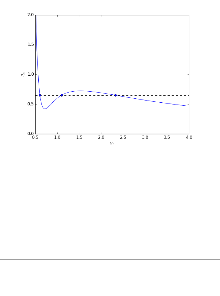
[ 0.60286812 1.09743234 2.32534056]
[<matplotlib.lines.Line2D object at 0x110b2ef98>, <matplotlib.lines.Line2D object at 0x1115a1ac8>, <matplotlib.lines.Line2D object at 0x1115a1588>]
14.15.1 Compute areas
for A1, we need the area under the line minus the area under the vdW curve.
That is the area between the curves. For A2, we want the area under the
vdW curve minus the area under the line. The area under the line between
root 2 and root 1 is just the width (root2 - root1)*y
1from scipy.integrate import quad
2
3A1, e1 =(v[1]-v[0]) *y-quad(Prfh, v[0], v[1])
4A2, e2 =quad(Prfh, v[1], v[2]) -(v[2]-v[1])*y
5
6print(A1, A2)
7print(e1, e2) # interesting these look so large
0.063225945606 0.0580212098122
0.321466743765 -0.798140339268
1from scipy.optimize import fsolve
2
353

3def equal_area(y):
4Tr = 0.9
5vdWp =[1,-1.0 / 3 * (1.0 + 8.0 * Tr /y), 3.0 / y, -1.0 / y]
6v=np.roots(vdWp)
7v.sort()
8A1 =(v[1]-v[0]) *y-quad(Prfh, v[0], v[1])
9A2 =quad(Prfh, v[1], v[2]) -(v[2]-v[1]) *y
10 return A1 -A2
11
12 y_eq, =fsolve(equal_area, 0.65)
13 print(y_eq)
14
15 Tr = 0.9
16 vdWp =[1,-1.0 / 3 * (1.0 + 8.0 * Tr /y_eq), 3.0 / y_eq, -1.0 / y_eq]
17 v=np.roots(vdWp)
18 v.sort()
19
20 A1, e1 =(v[1]-v[0]) *y_eq -quad(Prfh, v[0], v[1])
21 A2, e2 =quad(Prfh, v[1], v[2]) -(v[2]-v[1]) *y_eq
22
23 print(A1, A2)
0.646998351872
0.0617526473994 0.0617526473994
Now let us plot the equal areas and indicate them by shading.
1fig =plt.gcf()
2ax =fig.add_subplot(111)
3
4ax.plot(Vr,Pr)
5
6hline =np.ones(Vr.size) *y_eq
7
8ax.plot(Vr, hline)
9ax.fill_between(Vr, hline, Pr, where=(Vr >= v[0]) &(Vr <= v[1]), facecolor=’gray’)
10 ax.fill_between(Vr, hline, Pr, where=(Vr >= v[1]) &(Vr <= v[2]), facecolor=’gray’)
11
12 plt.text(v[0], 1,’A1 = {0}’.format(A1))
13 plt.text(v[2], 1,’A2 = {0}’.format(A2))
14 plt.xlabel(’$V_R$’)
15 plt.ylabel(’$P_R$’)
16 plt.title(’$T_R$ = 0.9’)
17
18 plt.savefig(’images/maxwell-eq-area-4.png’)
19 plt.savefig(’images/maxwell-eq-area-4.svg’)
[<matplotlib.lines.Line2D object at 0x1113a5b70>]
[<matplotlib.lines.Line2D object at 0x11108fc88>]
<matplotlib.collections.PolyCollection object at 0x1115c9518>
<matplotlib.collections.PolyCollection object at 0x1118da358>
354
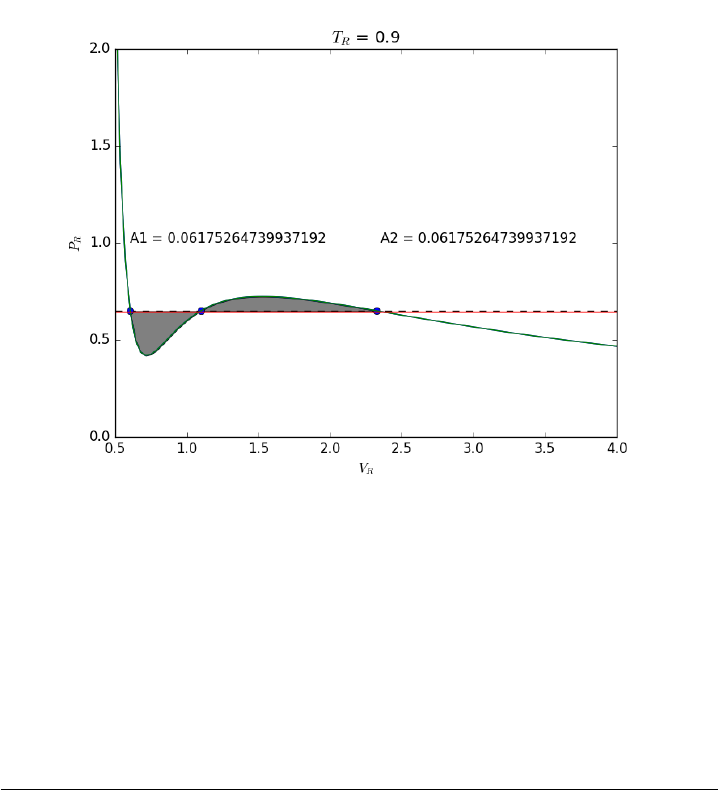
<matplotlib.text.Text object at 0x1115c2ac8>
<matplotlib.text.Text object at 0x1118daef0>
<matplotlib.text.Text object at 0x111347080>
<matplotlib.text.Text object at 0x111347e48>
<matplotlib.text.Text object at 0x111360d68>
14.16 Time dependent concentration in a first order reversible
reaction in a batch reactor
Matlab post
Given this reaction AB, with these rate laws:
forward rate law: −ra=k1CA
backward rate law: −rb=k−1CB
plot the concentration of A vs. time. This example illustrates a set of
coupled first order ODES.
1from scipy.integrate import odeint
2import numpy as np
3
4def myode(C, t):
5# ra = -k1*Ca
6# rb = -k_1*Cb
7# net rate for production of A: ra - rb
355

8# net rate for production of B: -ra + rb
9
10 k1 = 1 # 1/min;
11 k_1 = 0.5 # 1/min;
12
13 Ca =C[0]
14 Cb =C[1]
15
16 ra = -k1 *Ca
17 rb = -k_1 *Cb
18
19 dCadt =ra -rb
20 dCbdt = -ra +rb
21
22 dCdt =[dCadt, dCbdt]
23 return dCdt
24
25 tspan =np.linspace(0,5)
26
27 init =[1,0]# mol/L
28 C=odeint(myode, init, tspan)
29
30 Ca =C[:,0]
31 Cb =C[:,1]
32
33 import matplotlib.pyplot as plt
34 plt.plot(tspan, Ca, tspan, Cb)
35 plt.xlabel(’Time (min)’)
36 plt.ylabel(’C (mol/L)’)
37 plt.legend([’$C_A$’,’$C_B$’])
38 plt.savefig(’images/reversible-batch.png’)
356
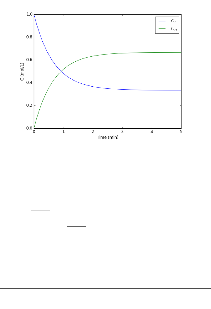
That is it. The main difference between this and Matlab is the order of
arguments in odeint is different, and the ode function has differently ordered
arguments.
14.17 Finding equilibrium conversion
A common problem to solve in reaction engineering is finding the equilibrium
conversion.1A typical problem to solve is the following nonlinear equation:
1.44 = X2
e
(1−Xe)2
To solve this we create a function:
f(Xe)=0=1.44 −X2
e
(1−Xe)2
and use a nonlinear solver to find the value of Xethat makes this function
equal to zero. We have to provide an initial guess. Chemical intuition
suggests that the solution must be between 0 and 1, and mathematical
intuition suggests the solution might be near 0.5 (which would give a ratio
near 1).
Here is our solution.
1from scipy.optimize import fsolve
2
3def func(Xe):
1See Fogler, 4th ed. page 1025 for the setup of this equation.
357

4z= 1.44 - (Xe**2)/(1-Xe)**2
5return z
6
7X0 = 0.5
8Xe, =fsolve(func, X0)
9print(’The equilibrium conversion is X = {0:1.2f}’.format(Xe))
The equilibrium conversion is X = 0.55
14.18 Integrating a batch reactor design equation
For a constant volume batch reactor where A→Bat a rate of −rA=kC2
A,
we derive the following design equation for the length of time required to
achieve a particular level of conversion :
t(X) = 1
kCA0RX
X=0 dX
(1−X)2
if k= 10−3L/mol/s and CA0= 1 mol/L, estimate the time to achieve
90% conversion.
We could analytically solve the integral and evaluate it, but instead we
will numerically evaluate it using scipy.integrate.quad. This function returns
two values: the evaluated integral, and an estimate of the absolute error in
the answer.
1from scipy.integrate import quad
2
3def integrand(X):
4k= 1.0e-3
5Ca0 = 1.0 # mol/L
6return 1./(k*Ca0)*(1./(1-X)**2)
7
8sol, abserr =quad(integrand, 0,0.9)
9print(’t = {0} seconds ({1} hours)’.format(sol, sol/3600))
10 print(’Estimated absolute error = {0}’.format(abserr))
t = 9000.000000000007 seconds (2.500000000000002 hours)
Estimated absolute error = 2.1220327407235617e-07
You can see the estimate error is very small compared to the solution.
14.19 Uncertainty in an integral equation
In a previous example, we solved for the time to reach a specific conversion
in a batch reactor. However, it is likely there is uncertainty in the rate
constant, and possibly in the initial concentration. Here we examine the
effects of that uncertainty on the time to reach the desired conversion.
358

To do this we have to write a function that takes arguments with uncer-
tainty, and wrap the function with the uncertainties.wrap decorator. The
function must return a single float number (current limitation of the uncer-
tainties package). Then, we simply call the function, and the uncertainties
from the inputs will be automatically propagated to the outputs. Let us say
there is about 10% uncertainty in the rate constant, and 1% uncertainty in
the initial concentration.
1from scipy.integrate import quad
2import uncertainties as u
3
4k=u.ufloat((1.0e-3,1.0e-4))
5Ca0 =u.ufloat((1.0,0.01))# mol/L
6
7@u.wrap
8def func(k, Ca0):
9def integrand(X):
10 return 1./(k*Ca0)*(1./(1-X)**2)
11 integral, abserr =quad(integrand, 0,0.9)
12 return integral
13
14 sol =func(k, Ca0)
15 print(’t = {0} seconds ({1} hours)’.format(sol, sol/3600))
t = (9.0+/-0.9)e+03 seconds (2.50+/-0.25 hours)
The result shows about a 10% uncertainty in the time, which is similar
to the largest uncertainty in the inputs. This information should certainly
be used in making decisions about how long to actually run the reactor to
be sure of reaching the goal. For example, in this case, running the reactor
for 3 hours (that is roughly + 2σ) would ensure at a high level of confidence
(approximately 95% confidence) that you reach at least 90% conversion.
14.20 Integrating the batch reactor mole balance
An alternative approach of evaluating an integral is to integrate a differential
equation. For the batch reactor, the differential equation that describes
conversion as a function of time is:
dX
dt =−rAV/NA0.
Given a value of initial concentration, or volume and initial number of
moles of A, we can integrate this ODE to find the conversion at some later
time. We assume that X(t= 0) = 0. We will integrate the ODE over a
time span of 0 to 10,000 seconds.
359
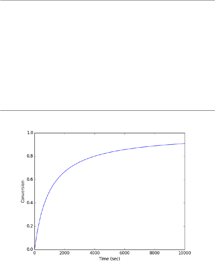
1from scipy.integrate import odeint
2import numpy as np
3import matplotlib.pyplot as plt
4
5k= 1.0e-3
6Ca0 = 1.0 # mol/L
7
8def func(X, t):
9ra = -k*(Ca0 *(1-X))**2
10 return -ra /Ca0
11
12 X0 = 0
13 tspan =np.linspace(0,10000)
14
15 sol =odeint(func, X0, tspan)
16 plt.plot(tspan,sol)
17 plt.xlabel(’Time (sec)’)
18 plt.ylabel(’Conversion’)
19 plt.savefig(’images/2013-01-06-batch-conversion.png’)
You can read off of this figure to find the time required to achieve a
particular conversion.
360

14.21 Plug flow reactor with a pressure drop
If there is a pressure drop in a plug flow reactor, 2there are two equations
needed to determine the exit conversion: one for the conversion, and one
from the pressure drop.
dX
dW =k0
FA01−X
1 + X y(49)
dX
dy =−α(1 + X)
2y(50)
Here is how to integrate these equations numerically in python.
1import numpy as np
2from scipy.integrate import odeint
3import matplotlib.pyplot as plt
4
5kprime = 0.0266
6Fa0 = 1.08
7alpha = 0.0166
8epsilon = -0.15
9
10 def dFdW(F, W):
11 ’set of ODEs to integrate’
12 X=F[0]
13 y=F[1]
14 dXdW =kprime /Fa0 *(1-X) /(1+epsilon*X) *y
15 dydW = -alpha *(1 + epsilon *X) /(2 * y)
16 return [dXdW, dydW]
17
18 Wspan =np.linspace(0,60)
19 X0 = 0.0
20 y0 = 1.0
21 F0 =[X0, y0]
22 sol =odeint(dFdW, F0, Wspan)
23
24 # now plot the results
25 plt.plot(Wspan, sol[:,0], label=’Conversion’)
26 plt.plot(Wspan, sol[:,1], ’g--’, label=’y=$P/P_0$’)
27 plt.legend(loc=’best’)
28 plt.xlabel(’Catalyst weight (lb_m)’)
29 plt.savefig(’images/2013-01-08-pdrop.png’)
Here is the resulting figure.
2Fogler, 4th edition. page 193.
361
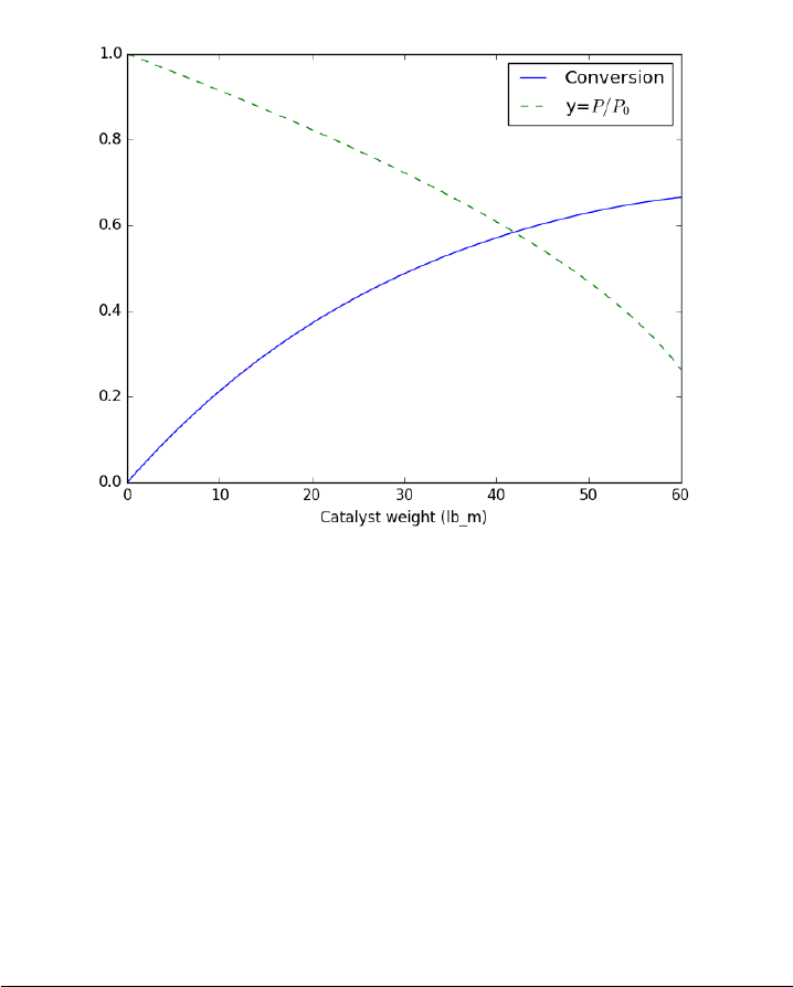
14.22 Solving CSTR design equations
Given a continuously stirred tank reactor with a volume of 66,000 dmˆ3
where the reaction A→Boccurs, at a rate of −rA=kC2
A(k= 3 L/mol/h),
with an entering molar flow of F_{A0} = 5 mol/h and a volumetric flowrate
of 10 L/h, what is the exit concentration of A?
From a mole balance we know that at steady state 0 = FA0−FA+V rA.
That equation simply states the sum of the molar flow of A in in minus the
molar flow of A out plus the molar rate A is generated is equal to zero at
steady state. This is directly the equation we need to solve. We need the
following relationship:
1. FA=v0CA
1from scipy.optimize import fsolve
2
3Fa0 = 5.0
4v0 = 10.
5
6V= 66000.0 # reactor volume L^3
7k= 3.0 # rate constant L/mol/h
8
9def func(Ca):
10 "Mole balance for a CSTR. Solve this equation for func(Ca)=0"
362

11 Fa =v0 *Ca # exit molar flow of A
12 ra = -k*Ca**2 # rate of reaction of A L/mol/h
13 return Fa0 -Fa +V*ra
14
15 # CA guess that that 90 % is reacted away
16 CA_guess =0.1*Fa0 /v0
17 CA_sol, =fsolve(func, CA_guess)
18
19 print(’The exit concentration is {0} mol/L’.format(CA_sol))
The exit concentration is 0.005 mol/L
It is a little confusing why it is necessary to put a comma after the
CA_sol in the fsolve command. If you do not put it there, you get brackets
around the answer.
14.23 Meet the steam tables
Matlab post
We will use the iapws module. Install it like this:
1pip install iapws
Problem statement: A Rankine cycle operates using steam with the con-
denser at 100 degC, a pressure of 3.0 MPa and temperature of 600 degC in
the boiler. Assuming the compressor and turbine operate reversibly, esti-
mate the efficiency of the cycle.
Starting point in the Rankine cycle in condenser.
we have saturated liquid here, and we get the thermodynamic properties
for the given temperature. In this python module, these properties are all
in attributes of an IAPWS object created at a set of conditions.
14.23.1 Starting point in the Rankine cycle in condenser.
We have saturated liquid here, and we get the thermodynamic properties
for the given temperature.
1#import iapws
2#print iapws.__version__
3from iapws import IAPWS97
4
5T1 = 100 + 273.15 #in K
6
7sat_liquid1 =IAPWS97(T=T1, x=0)# x is the steam quality. 0 = liquid
363

8
9P1 =sat_liquid1.P
10 s1 =sat_liquid1.s
11 h1 =sat_liquid1.h
12 v1 =sat_liquid1.v
14.23.2 Isentropic compression of liquid to point 2
The final pressure is given, and we need to compute the new temperatures,
and enthalpy.
1P2 = 3.0 # MPa
2s2 =s1 # this is what isentropic means
3
4sat_liquid2 =IAPWS97(P=P2, s=s1)
5T2, =sat_liquid2.T
6h2 =sat_liquid2.h
7
8# work done to compress liquid. This is an approximation, since the
9# volume does change a little with pressure, but the overall work here
10 # is pretty small so we neglect the volume change.
11 WdotP =v1*(P2 -P1);
12
13 print(’The compressor work is: {0:1.4f} kJ/kg’.format(WdotP))
The compressor work is: 0.0030 kJ/kg
The compression work is almost negligible. This number is 1000 times
smaller than we computed with Xsteam. I wonder what the units of v1
actually are.
14.23.3 Isobaric heating to T3 in boiler where we make steam
1T3 = 600 + 273.15 # K
2P3 =P2 # definition of isobaric
3steam =IAPWS97(P=P3, T=T3)
4
5h3 =steam.h
6s3 =steam.s
7
8Qb, =h3 -h2 # heat required to make the steam
9
10 print(’The boiler heat duty is: {0:1.2f} kJ/kg’.format(Qb))
The boiler heat duty is: 3260.69 kJ/kg
364

14.23.4 Isentropic expansion through turbine to point 4
1steam =IAPWS97(P=P1, s=s3)
2T4, =steam.T
3h4 =steam.h
4s4 =s3 # isentropic
5Qc, =h4 -h1 # work required to cool from T4 to T1
6
7print(’The condenser heat duty is {0:1.2f} kJ/kg’.format(Qc))
The condenser heat duty is 2317.00 kJ/kg
14.23.5 To get from point 4 to point 1
1WdotTurbine, =h4 -h3 # work extracted from the expansion
2print(’The turbine work is: {0:1.2f} kJ/kg’.format(WdotTurbine))
The turbine work is: -946.71 kJ/kg
14.23.6 Efficiency
This is a ratio of the work put in to make the steam, and the net work
obtained from the turbine. The answer here agrees with the efficiency cal-
culated in Sandler on page 135.
1eta = -(WdotTurbine -WdotP) /Qb
2print(’The overall efficiency is {0:1.2%}.’.format(eta))
The overall efficiency is 29.03%.
14.23.7 Entropy-temperature chart
The IAPWS module makes it pretty easy to generate figures of the steam
tables. Here we generate an entropy-Temperature graph. We do this to
illustrate the path of the Rankine cycle. We need to compute the values of
steam entropy for a range of pressures and temperatures.
1import numpy as np
2import matplotlib.pyplot as plt
3
4plt.figure()
5plt.clf()
6T=np.linspace(300,372+273,200)# range of temperatures
7for Pin [0.1,1,2,5,10,20]: #MPa
365

8steam =[IAPWS97(T=t, P=P) for tin T]
9S=[s.sfor sin steam]
10 plt.plot(S, T, ’k-’)
11
12 # saturated vapor and liquid entropy lines
13 svap =[s.sfor sin [IAPWS97(T=t, x=1)for tin T]]
14 sliq =[s.sfor sin [IAPWS97(T=t, x=0)for tin T]]
15
16 plt.plot(svap, T, ’r-’)
17 plt.plot(sliq, T, ’b-’)
18
19 plt.xlabel(’Entropy (kJ/(kg K)’)
20 plt.ylabel(’Temperature (K)’)
21 plt.savefig(’images/iawps-steam.png’)
<matplotlib.figure.Figure object at 0x111c916d8>
[<matplotlib.lines.Line2D object at 0x111d15780>]
[<matplotlib.lines.Line2D object at 0x111c991d0>]
[<matplotlib.lines.Line2D object at 0x111d191d0>]
[<matplotlib.lines.Line2D object at 0x111c99ac8>]
[<matplotlib.lines.Line2D object at 0x111d19a20>]
[<matplotlib.lines.Line2D object at 0x111cdf358>]
[<matplotlib.lines.Line2D object at 0x111c37358>]
[<matplotlib.lines.Line2D object at 0x111c37390>]
<matplotlib.text.Text object at 0x110b2ec18>
<matplotlib.text.Text object at 0x111cecc88>
366
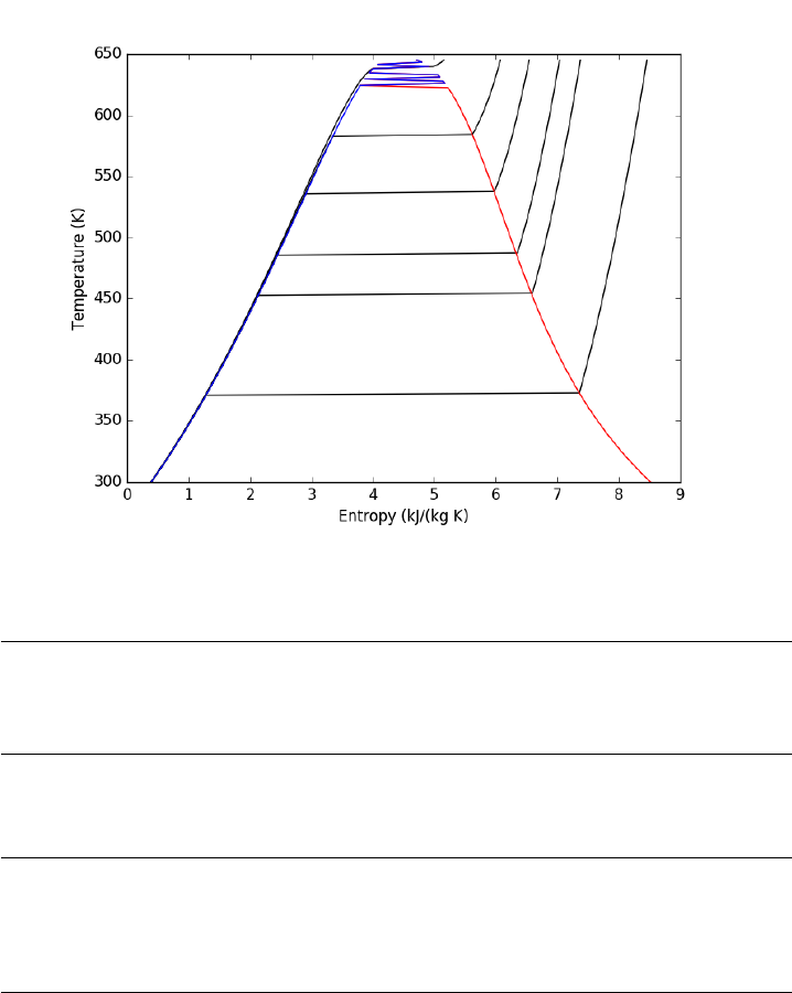
We can plot our Rankine cycle path like this. We compute the entropies
along the non-isentropic paths.
1T23 =np.linspace(T2, T3)
2S23 =[s.sfor sin [IAPWS97(P=P2, T=t) for tin T23]]
3
4T41 =np.linspace(T4, T1 - 0.01)# subtract a tiny bit to make sure we get a liquid
5S41 =[s.sfor sin [IAPWS97(P=P1, T=t) for tin T41]]
And then we plot the paths.
1plt.plot([s1, s2], [T1, T2], ’r-’, lw=4)# Path 1 to 2
2plt.plot(S23, T23, ’b-’, lw=4)# path from 2 to 3 is isobaric
3plt.plot([s3, s4], [T3, T4], ’g-’, lw=4)# path from 3 to 4 is isentropic
4plt.plot(S41, T41, ’k-’, lw=4)# and from 4 to 1 is isobaric
5plt.savefig(’images/iawps-steam-2.png’)
6plt.savefig(’images/iawps-steam-2.svg’)
[<matplotlib.lines.Line2D object at 0x111c124a8>]
[<matplotlib.lines.Line2D object at 0x11108f2b0>]
[<matplotlib.lines.Line2D object at 0x1118e1710>]
[<matplotlib.lines.Line2D object at 0x111da6ef0>]
367
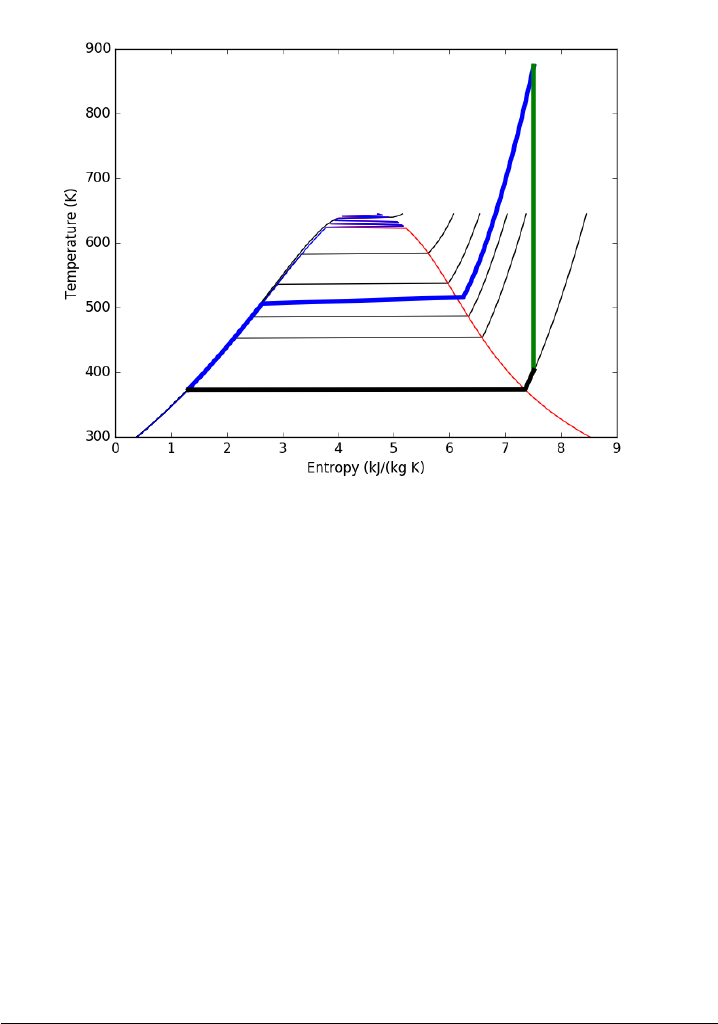
14.23.8 Summary
This was an interesting exercise. On one hand, the tedium of interpolating
the steam tables is gone. On the other hand, you still have to know exactly
what to ask for to get an answer that is correct. The iapws interface is a
little clunky, and takes some getting used to. It does not seem as robust as
the Xsteam module I used in Matlab.
14.24 What region is a point in
Suppose we have a space that is divided by a boundary into two regions,
and we want to know if an arbitrary point is on one region or the other.
One way to figure this out is to pick a point that is known to be in a region,
and then draw a line to the arbitrary point counting the number of times it
crosses the boundary. If the line crosses an even number of times, then the
point is in the same region and if it crosses an odd number of times, then
the point is in the other region.
Here is the boundary and region we consider in this example:
1boundary =[[0.1,0],
2[0.25,0.1],
3[0.3,0.2],
368
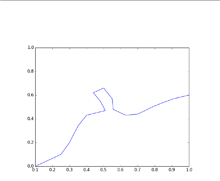
4[0.35,0.34],
5[0.4,0.43],
6[0.51,0.47],
7[0.48,0.55],
8[0.44,0.62],
9[0.5,0.66],
10 [0.55,0.57],
11 [0.556,0.48],
12 [0.63,0.43],
13 [0.70,0.44],
14 [0.8,0.51],
15 [0.91,0.57],
16 [1.0,0.6]]
17
18 import matplotlib.pyplot as plt
19 plt.clf()
20 plt.plot([p[0]for pin boundary],
21 [p[1]for pin boundary])
22 plt.ylim([0,1])
23 plt.savefig(’images/boundary-1.png’)
[<matplotlib.lines.Line2D object at 0x10b417470>]
(0, 1)
In this example, the boundary is complicated, and not described by a
simple function. We will check for intersections of the line from the arbitrary
point to the reference point with each segment defining the boundary. If
369
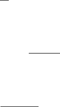
there is an intersection in the boundary, we count that as a crossing. We
choose the origin (0, 0) in this case for the reference point. For an arbitrary
point (x1, y1), the equation of the line is therefore (provided x1 !=0):
y=y1
x1x.
Let the points defining a boundary segment be (bx1, by1) and (bx2,
by2). The equation for the line connecting these points (provided bx1 !=
bx2) is:
y=by1 + by2−by1
bx2−bx1(x−bx1)
Setting these two equations equal to each other, we can solve for the value
of x, and if bx1<=x <=bx2then we would say there is an intersection
with that segment. The solution for x is:
x=mbx1−by1
m−y1/x1
This can only fail if m=y1/x1which means the segments are parallel
and either do not intersect or go through each other. One issue we have to
resolve is what to do when the intersection is at the boundary. In that case,
we would see an intersection with two segments since bx1 of one segment is
also bx2 of another segment. We resolve the issue by only counting inter-
sections with bx1. Finally, there may be intersections at values of xgreater
than the point, and we are not interested in those because the intersections
are not between the point and reference point.
Here are all of the special cases that we have to handle:
370
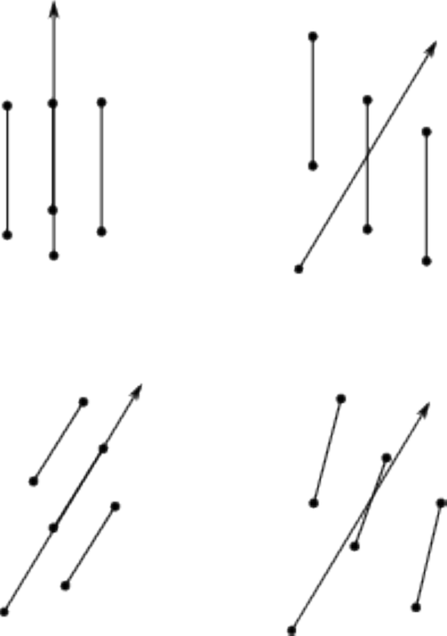
We will have to do float comparisons, so we will define tolerance functions
for all of these. I tried this previously with regular comparison operators,
and there were many cases that did not work because of float comparisons.
In the code that follows, we define the tolerance functions, the function that
handles almost all the special cases, and show that it almost always correctly
371

identifies the region a point is in.
1import numpy as np
2
3TOLERANCE =2*np.spacing(1)
4
5def feq(x, y, epsilon=TOLERANCE):
6’x == y’
7return not((x <(y -epsilon)) or (y <(x -epsilon)))
8
9def flt(x, y, epsilon=TOLERANCE):
10 ’x < y’
11 return x<(y -epsilon)
12
13 def fgt(x, y, epsilon=TOLERANCE):
14 ’x > y’
15 return y<(x -epsilon)
16
17 def fle(x, y, epsilon=TOLERANCE):
18 ’x <= y’
19 return not(y <(x -epsilon))
20
21
22 def fge(x, y, epsilon=TOLERANCE):
23 ’x >= y’
24 return not(x <(y -epsilon))
25
26 boundary =[[0.1,0],
27 [0.25,0.1],
28 [0.3,0.2],
29 [0.35,0.34],
30 [0.4,0.43],
31 [0.51,0.47],
32 [0.48,0.55],
33 [0.44,0.62],
34 [0.5,0.66],
35 [0.55,0.57],
36 [0.556,0.48],
37 [0.63,0.43],
38 [0.70,0.44],
39 [0.8,0.51],
40 [0.91,0.57],
41 [1.0,0.6]]
42
43 def intersects(p, isegment):
44 ’p is a point (x1, y1), isegment is an integer indicating which segment starting with 0’
45 x1, y1 =p
46 bx1, by1 =boundary[isegment]
47 bx2, by2 =boundary[isegment + 1]
48 if feq(bx1, bx2) and feq(x1, 0.0): # both segments are vertical
49 if feq(bx1, x1):
50 return True
51 else:
52 return False
53 elif feq(bx1, bx2): # segment is vertical
54 m1 =y1 /x1 # slope of reference line
372

55 y=m1 *bx1 # value of reference line at bx1
56 if ((fge(y, by1) and flt(y, by2))
57 or (fle(y, by1) and fgt(y,by2))):
58 # reference line intersects the segment
59 return True
60 else:
61 return False
62 else:# neither reference line nor segment is vertical
63 m=(by2 -by1) /(bx2 -bx1) # segment slope
64 m1 =y1 /x1
65 if feq(m, m1): # line and segment are parallel
66 if feq(y1, m *bx1):
67 return True
68 else:
69 return False
70 else:# lines are not parallel
71 x=(m *bx1 -by1) /(m -m1) # x at intersection
72 if ((fge(x, bx1) and flt(x, bx2))
73 or (fle(x, bx1) and fgt(x, bx2))) and fle(x, x1):
74 return True
75 else:
76 return False
77 raise Exception(’you should not get here’)
78
79 import matplotlib.pyplot as plt
80
81 plt.plot([p[0]for pin boundary],
82 [p[1]for pin boundary], ’go-’)
83 plt.ylim([0,1])
84
85 N= 100
86
87 X=np.linspace(0,1, N)
88
89 for xin X:
90 for yin X:
91 p=(x, y)
92 nintersections =sum([intersects(p, i) for iin range(len(boundary) - 1)])
93 if nintersections %2==0:
94 plt.plot(x, y, ’r.’)
95 else:
96 plt.plot(x, y, ’b.’)
97
98 plt.savefig(’images/boundary-2.png’)
373
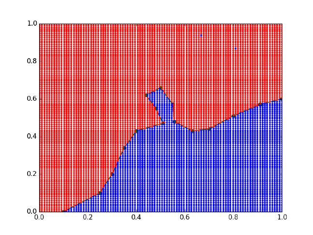
If you look carefully, there are two blue points in the red region, which
means there is some edge case we do not capture in our function. Kudos to
the person who figures it out. Update: It was pointed out that the points
intersect a point on the line.
15 Units
15.1 Using units in python
Units in Matlab
I think an essential feature in an engineering computational environment
is properly handling units and unit conversions. Mathcad supports that
pretty well. I wrote a package for doing it in Matlab. Today I am going to
explore units in python. Here are some of the packages that I have found
which support units to some extent
1. http://pypi.python.org/pypi/units/
2. http://packages.python.org/quantities/user/tutorial.html
3. http://dirac.cnrs-orleans.fr/ScientificPython/ScientificPythonManual/
Scientific.Physics.PhysicalQuantities-module.html
374

4. http://home.scarlet.be/be052320/Unum.html
5. https://simtk.org/home/python_units
6. http://docs.enthought.com/scimath/units/intro.html
The last one looks most promising.
15.1.1 scimath
scimath may only wok in Python2.
1import numpy as np
2from scimath.units.volume import liter
3from scimath.units.substance import mol
4
5q=np.array([1,2,3]) *mol
6print(q)
7
8P=q/liter
9print(P)
That doesn’t look too bad. It is a little clunky to have to import every
unit, and it is clear the package is saving everything in SI units by default.
Let us try to solve an equation.
Find the time that solves this equation.
0.01 = CA0e−kt
First we solve without units. That way we know the answer.
1import numpy as np
2from scipy.optimize import fsolve
3
4CA0 = 1.0 # mol/L
5CA = 0.01 # mol/L
6k= 1.0 # 1/s
7
8def func(t):
9z=CA -CA0 *np.exp(-k*t)
10 return z
11
12 t0 = 2.3
13
14 t, =fsolve(func, t0)
15 print ’t = {0:1.2f} seconds’.format(t)
t = 4.61 seconds
375

Now, with units. I note here that I tried the obvious thing of just
importing the units, and adding them on, but the package is unable to work
with floats that have units. For some functions, there must be an ndarray
with units which is practically what the UnitScalar code below does.
1import numpy as np
2from scipy.optimize import fsolve
3from scimath.units.volume import liter
4from scimath.units.substance import mol
5from scimath.units.time import second
6from scimath.units.api import has_units, UnitScalar
7
8CA0 =UnitScalar(1.0, units =mol /liter)
9CA =UnitScalar(0.01, units =mol /liter)
10 k=UnitScalar(1.0, units =1/second)
11
12 @has_units(inputs="t::units=s",
13 outputs="result::units=mol/liter")
14 def func(t):
15 z=CA -CA0 *float(np.exp(-k*t))
16 return z
17
18 t0 =UnitScalar(2.3, units =second)
19
20 t, =fsolve(func, t0)
21 print ’t = {0:1.2f} seconds’.format(t)
22 print type(t)
t = 4.61 seconds
<type ’numpy.float64’>
This is some heavy syntax that in the end does not preserve the units.
In my Matlab package, we had to "wrap" many functions like fsolve so they
would preserve units. Clearly this package will need that as well. Overall,
in its current implementation this package does not do what I would expect
all the time.3
15.2 Handling units with the quantities module
The quantities module (https://pypi.python.org/pypi/quantities) is
another option for handling units in python. We are going to try the previous
example. It does not work, because scipy.optimize.fsolve is not designed to
work with units.
3Then again no package does yet!
376

1import quantities as u
2import numpy as np
3
4from scipy.optimize import fsolve
5CA0 =1*u.mol /u.L
6CA = 0.01 * u.mol /u.L
7k= 1.0 / u.s
8
9def func(t):
10 return CA -CA0 *np.exp(-k*t)
11
12 tguess =4*u.s
13
14 print(func(tguess))
15
16 print(fsolve(func, tguess))
-0.008315638888734178 mol/L
Traceback (most recent call last):
File "<stdin>", line 1, in <module>
File "/Users/jkitchin/anaconda3/lib/python3.5/site-packages/scipy/optimize/minpack.py", line 146, in fsolve
res = _root_hybr(func, x0, args, jac=fprime, **options)
File "/Users/jkitchin/anaconda3/lib/python3.5/site-packages/scipy/optimize/minpack.py", line 212, in _root_hybr
shape, dtype = _check_func(’fsolve’, ’func’, func, x0, args, n, (n,))
File "/Users/jkitchin/anaconda3/lib/python3.5/site-packages/scipy/optimize/minpack.py", line 26, in _check_func
res = atleast_1d(thefunc(*((x0[:numinputs],) + args)))
File "<stdin>", line 2, in func
File "/Users/jkitchin/anaconda3/lib/python3.5/site-packages/quantities/quantity.py", line 231, in __array_prepare__
res._dimensionality = p_dict[uf](*objs)
File "/Users/jkitchin/anaconda3/lib/python3.5/site-packages/quantities/dimensionality.py", line 348, in _d_dimensionless
raise ValueError("quantity must be dimensionless")
ValueError: quantity must be dimensionless
Our function works fine with units, but fsolve does not pass numbers with
units back to the function, so this function fails because the exponential
function gets an argument with dimensions in it. We can create a new
function that solves this problem. We need to "wrap" the function we want
to solve to make sure that it uses units, but returns a float number. Then,
we put the units back onto the final solved value. Here is how we do that.
1import quantities as u
2import numpy as np
3
4from scipy.optimize import fsolve as _fsolve
5
6CA0 =1*u.mol /u.L
377

7CA = 0.01 * u.mol /u.L
8k= 1.0 / u.s
9
10 def func(t):
11 return CA -CA0 *np.exp(-k*t)
12
13 def fsolve(func, t0):
14 ’wrapped fsolve command to work with units’
15 tU =t0 /float(t0) # units on initial guess, normalized
16 def wrapped_func(t):
17 ’t will be unitless, so we add unit to it. t * tU has units.’
18 return float(func(t *tU))
19
20 sol, =_fsolve(wrapped_func, t0)
21 return sol *tU
22
23 tguess =4*u.s
24
25 print(fsolve(func, tguess))
4.605170185988092 s
It is a little tedious to do this, but we might only have to do it once
if we store the new fsolve command in a module. You might notice the
wrapped function we wrote above only works for one dimensional problems.
If there are multiple dimensions, we have to be a little more careful. In
the next example, we expand the wrapped function definition to do both
one and multidimensional problems. It appears we cannot use numpy.array
element-wise multiplication because you cannot mix units in an array. We
will use lists instead. When the problem is one-dimensional, the function
will take a scalar, but when it is multidimensional it will take a list or array.
We will use try/except blocks to handle these two cases. We will assume
multidimensional cases, and if that raises an exception because the argument
is not a list, we assume it is scalar. Here is the more robust code example.
1import quantities as u
2import numpy as np
3
4from scipy.optimize import fsolve as _fsolve
5
6def fsolve(func, t0):
7’’’wrapped fsolve command to work with units. We get the units on
8the function argument, then wrap the function so we can add units
9to the argument and return floats. Finally we call the original
10 fsolve from scipy. Note: this does not support all of the options
11 to fsolve.’’’
12
13 try:
14 tU =[t /float(t) for tin t0] # units on initial guess, normalized
378

15 except TypeError:
16 tU =t0 /float(t0)
17
18 def wrapped_func(t):
19 ’t will be unitless, so we add unit to it. t * tU has units.’
20 try:
21 T=[x1 *x2 for x1,x2 in zip(t, tU)]
22 except TypeError:
23 T=t*tU
24
25 try:
26 return [float(x) for xin func(T)]
27 except TypeError:
28 return float(func(T))
29
30 sol =_fsolve(wrapped_func, t0)
31 try:
32 return [x1 *x2 for x1,x2 in zip(sol, tU)]
33 except TypeError:
34 return sol *tU
35
36 ### Problem 1
37 CA0 =1*u.mol /u.L
38 CA = 0.01 * u.mol /u.L
39 k= 1.0 / u.s
40
41 def func(t):
42 return CA -CA0 *np.exp(-k*t)
43
44
45 tguess =4*u.s
46 sol1, =fsolve(func, tguess)
47 print(’sol1 = ’,sol1)
48
49 ### Problem 2
50 def func2(X):
51 a,b =X
52 return [a**2 - 4*u.kg**2,
53 b**2 - 25*u.J**2]
54
55 Xguess =[2.2*u.kg, 5.2*u.J]
56 s2a, s2b =fsolve(func2, Xguess)
57 print(’s2a = {0}\ns2b = {1}’.format(s2a, s2b))
sol1 = 4.605170185988092 s
s2a = 1.9999999999999867 kg
s2b = 5.000000000000002 J
That is pretty good. There is still room for improvement in the wrapped
function, as it does not support all of the options that scipy.optimize.fsolve
supports. Here is a draft of a function that does that. We have to return
different numbers of arguments depending on the value of full_output. This
379

function works, but I have not fully tested all the options. Here are three
examples that work, including one with an argument.
1import quantities as u
2import numpy as np
3
4from scipy.optimize import fsolve as _fsolve
5
6def fsolve(func, t0, args=(),
7fprime=None, full_output=0, col_deriv=0,
8xtol=1.49012e-08, maxfev=0, band=None,
9epsfcn=0.0, factor=100, diag=None):
10 ’’’wrapped fsolve command to work with units. We get the units on
11 the function argument, then wrap the function so we can add units
12 to the argument and return floats. Finally we call the original
13 fsolve from scipy. ’’’
14
15 try:
16 tU =[t /float(t) for tin t0] # units on initial guess, normalized
17 except TypeError:
18 tU =t0 /float(t0)
19
20 def wrapped_func(t, *args):
21 ’t will be unitless, so we add unit to it. t * tU has units.’
22 try:
23 T=[x1 *x2 for x1,x2 in zip(t, tU)]
24 except TypeError:
25 T=t*tU
26
27 try:
28 return [float(x) for xin func(T, *args)]
29 except TypeError:
30 return float(func(T))
31
32 sol =_fsolve(wrapped_func, t0, args,
33 fprime, full_output, col_deriv,
34 xtol, maxfev, band,
35 epsfcn, factor, diag)
36
37 if full_output:
38 x, infodict, ier, mesg =sol
39 try:
40 x=[x1 *x2 for x1,x2 in zip(x, tU)]
41 except TypeError:
42 x=x*tU
43 return x, infodict, ier, mesg
44 else:
45 try:
46 x=[x1 *x2 for x1,x2 in zip(sol, tU)]
47 except TypeError:
48 x=sol *tU
49 return x
50
51 ### Problem 1
52 CA0 =1*u.mol /u.L
380

53 CA = 0.01 * u.mol /u.L
54 k= 1.0 / u.s
55
56 def func(t):
57 return CA -CA0 *np.exp(-k*t)
58
59
60 tguess =4*u.s
61 sol1, =fsolve(func, tguess)
62 print(’sol1 = ’,sol1)
63
64 ### Problem 2
65 def func2(X):
66 a,b =X
67 return [a**2 - 4*u.kg**2,
68 b**2 - 25*u.J**2]
69
70 Xguess =[2.2*u.kg, 5.2*u.J]
71 sol, infodict, ier, mesg =fsolve(func2, Xguess, full_output=1)
72 s2a, s2b =sol
73 print(’s2a = {0}\ns2b = {1}’.format(s2a, s2b))
74
75 ### Problem 3 - with an arg
76 def func3(a, arg):
77 return a**2 - 4*u.kg**2 + arg**2
78
79 Xguess =1.5*u.kg
80 arg = 0.0* u.kg
81
82 sol3, =fsolve(func3, Xguess, args=(arg,))
83
84 print(’sol3 = ’, sol3)
sol1 = 4.605170185988092 s
s2a = 1.9999999999999867 kg
s2b = 5.000000000000002 J
sol3 = 2.0 kg
The only downside I can see in the quantities module is that it only
handle temperature differences, and not absolute temperatures. If you only
use absolute temperatures, this would not be a problem I think. But, if
you have mixed temperature scales, the quantities module does not convert
them on an absolute scale.
1import quantities as u
2
3T= 20 * u.degC
4
5print(T.rescale(u.K))
6print(T.rescale(u.degF))
381

20.0 K
36.0 degF
Nevertheless, this module seems pretty promising, and there are a lot
more features than shown here. Some documentation can be found at http:
//pythonhosted.org/quantities/.
15.3 Units in ODEs
We reconsider a simple ODE but this time with units. We will use the
quantities package again.
Here is the ODE, dCa
dt =−kCa with CA(0) = 1.0mol/L and k= 0.23
1/s. Compute the concentration after 5 s.
1import quantities as u
2
3k= 0.23 / u.s
4Ca0 =1*u.mol /u.L
5
6def dCadt(Ca, t):
7return -k*Ca
8
9import numpy as np
10 from scipy.integrate import odeint
11
12 tspan =np.linspace(0,5)*u.s
13
14 sol =odeint(dCadt, Ca0, tspan)
15
16 print(sol[-1])
[ 0.31663678]
No surprise, the units are lost. Now we start wrapping odeint. We
wrap everything, and then test two examples including a single ODE, and
a coupled set of ODEs with mixed units.
1import quantities as u
2import matplotlib.pyplot as plt
3
4import numpy as np
5from scipy.integrate import odeint as _odeint
6
7def odeint(func, y0, t, args=(),
8Dfun=None, col_deriv=0, full_output=0,
9ml=None, mu=None, rtol=None, atol=None,
10 tcrit=None, h0=0.0, hmax=0.0, hmin=0.0,
382
11 ixpr=0, mxstep=0, mxhnil=0, mxordn=12,
12 mxords=5, printmessg=0):
13
14 def wrapped_func(Y0, T, *args):
15 # put units on T if they are on the original t
16 # check for units so we don’t put them on twice
17 if not hasattr(T, ’units’)and hasattr(t, ’units’):
18 T=T*t.units
19 # now for the dependent variable units. Y0 may be a scalar or
20 # a list or an array. we want to check each element of y0 for
21 # units, and add them to the corresponding element of Y0 if we
22 # need to.
23 try:
24 uY0 =[x for xin Y0] # a list copy of contents of Y0
25 # this works if y0 is an iterable, eg. a list or array
26 for i, yi in enumerate(y0):
27 if not hasattr(uY0[i],’units’)and hasattr(yi, ’units’):
28
29 uY0[i] =uY0[i] *yi.units
30
31 except TypeError:
32 # we have a scalar
33 if not hasattr(Y0, ’units’)and hasattr(y0, ’units’):
34 uY0 =Y0 *y0.units
35
36 val =func(uY0, t, *args)
37
38 try:
39 return np.array([float(x) for xin val])
40 except TypeError:
41 return float(val)
42
43 if full_output:
44 y, infodict =_odeint(wrapped_func, y0, t, args,
45 Dfun, col_deriv, full_output,
46 ml, mu, rtol, atol,
47 tcrit, h0, hmax, hmin,
48 ixpr, mxstep, mxhnil, mxordn,
49 mxords, printmessg)
50 else:
51 y=_odeint(wrapped_func, y0, t, args,
52 Dfun, col_deriv, full_output,
53 ml, mu, rtol, atol,
54 tcrit, h0, hmax, hmin,
55 ixpr, mxstep, mxhnil, mxordn,
56 mxords, printmessg)
57
58 # now we need to put units onto the solution units should be the
59 # same as y0. We cannot put mixed units in an array, so, we return a list
60 m,n =y.shape # y is an ndarray, so it has a shape
61 if n> 1:# more than one equation, we need a list
62 uY =[0for yi in range(n)]
63
64 for i, yi in enumerate(y0):
65 if not hasattr(uY[i],’units’)and hasattr(yi, ’units’):
66 uY[i] =y[:,i] *yi.units
383
67 else:
68 uY[i] =y[:,i]
69
70 else:
71 uY =y*y0.units
72
73 y=uY
74
75
76 if full_output:
77 return y, infodict
78 else:
79 return y
80
81 ##################################################################
82 # test a single ODE
83 k= 0.23 / u.s
84 Ca0 =1*u.mol /u.L
85
86 def dCadt(Ca, t):
87 return -k*Ca
88
89 tspan =np.linspace(0,5)*u.s
90 sol =odeint(dCadt, Ca0, tspan)
91
92 print(sol[-1])
93
94 plt.plot(tspan, sol)
95 plt.xlabel(’Time ({0})’.format(tspan.dimensionality.latex))
96 plt.ylabel(’$C_A$ ({0})’.format(sol.dimensionality.latex))
97 plt.savefig(’images/ode-units-ca.png’)
98
99 ##################################################################
100 # test coupled ODEs
101 lbmol = 453.59237*u.mol
102
103 kprime = 0.0266 * lbmol /u.hr /u.lb
104 Fa0 = 1.08 * lbmol /u.hr
105 alpha = 0.0166 / u.lb
106 epsilon = -0.15
107
108 def dFdW(F, W, alpha0):
109 X,y=F
110 dXdW =kprime /Fa0 *(1.0 - X)/(1.0 + epsilon *X) *y
111 dydW =-alpha0 *(1.0 + epsilon *X) /(2.0 * y)
112 return [dXdW, dydW]
113
114 X0 = 0.0 * u.dimensionless
115 y0 = 1.0
116
117 # initial conditions
118 F0 =[X0, y0] # one without units, one with units, both are dimensionless
119
120 wspan =np.linspace(0,60)*u.lb
121
122 sol =odeint(dFdW, F0, wspan, args=(alpha,))
384
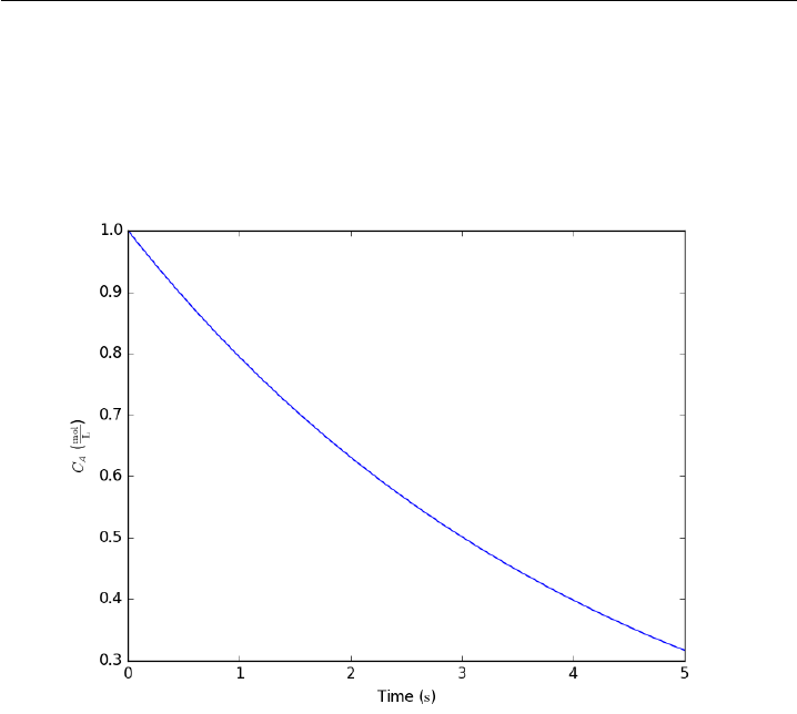
123 X,y=sol
124
125 print(’Test 2’)
126 print(X[-1])
127 print(y[-1])
128
129 plt.figure()
130 plt.plot(wspan, X, wspan, y)
131 plt.legend([’X’,’$P/P_0$’])
132 plt.xlabel(’Catalyst weight ({0})’.format(wspan.dimensionality.latex))
133 plt.savefig(’images/ode-coupled-units-pdrpo.png’)
[ 0.31663678] mol/L
Test 2
0.6655695781563288 dimensionless
0.263300470681
385
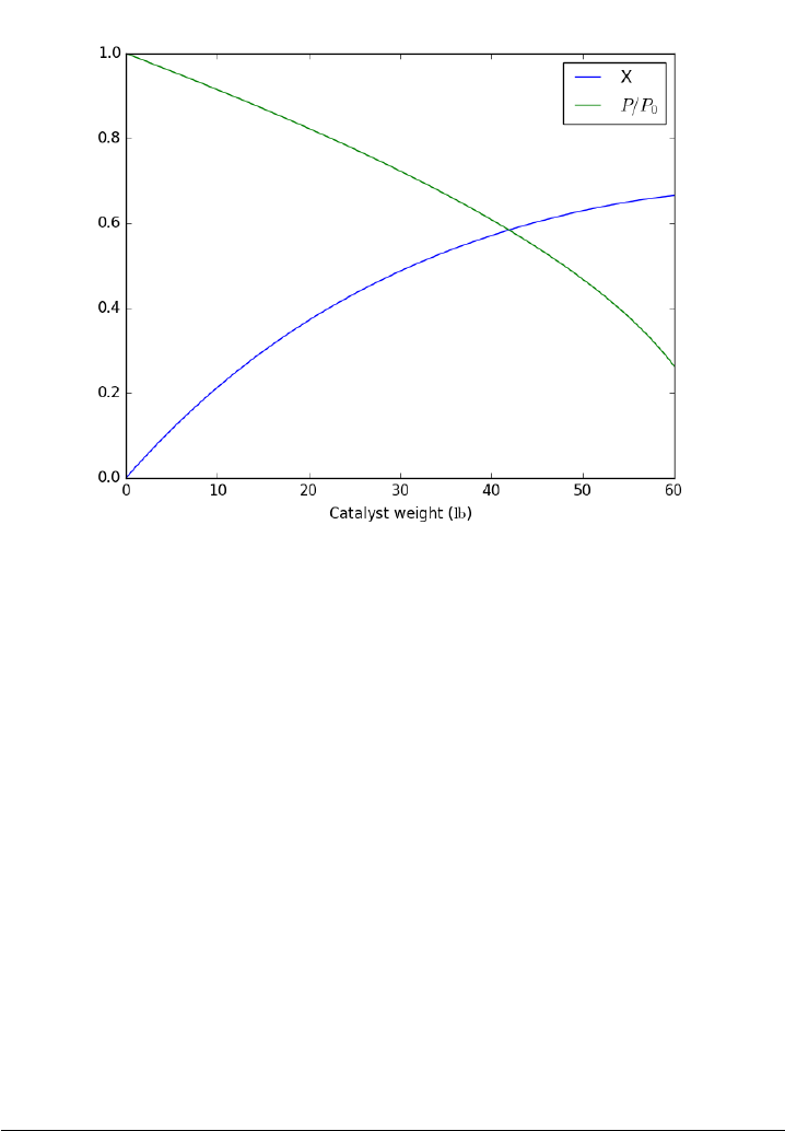
That is not too bad. This is another example of a function you would
want to save in a module for reuse. There is one bad feature of the wrapped
odeint function, and that is that it changes the solution for coupled ODEs
from an ndarray to a list. That is necessary because you apparently cannot
have mixed units in an ndarray. It is fine, however, to have a list of mixed
units. This is not a huge problem, but it changes the syntax for plotting
results for the wrapped odeint function compared to the unwrapped function
without units.
15.4 Handling units with dimensionless equations
As we have seen, handling units with third party functions is fragile, and
often requires additional code to wrap the function to handle the units. An
alternative approach that avoids the wrapping is to rescale the equations
so they are dimensionless. Then, we should be able to use all the standard
external functions without modification. We obtain the final solutions by
rescaling back to the answers we want.
Before doing the examples, let us consider how the quantities package
handles dimensionless numbers.
1import quantities as u
2
386

3a=5*u.m
4L= 10 * u.m# characteristic length
5
6print(a/L)
7print(type(a/L))
0.5 dimensionless
<class ’quantities.quantity.Quantity’>
As you can see, the dimensionless number is scaled properly, and is listed
as dimensionless. The result is still an instance of a quantities object though.
That is not likely to be a problem.
Now, we consider using fsolve with dimensionless equations. Our goal is
to solve CA=CA0exp(−kt)for the time required to reach a desired CA. We
let X=Ca/Ca0and τ=t∗k, which leads to X= exp −τin dimensionless
terms.
1import quantities as u
2import numpy as np
3from scipy.optimize import fsolve
4
5CA0 =1*u.mol /u.L
6CA = 0.01 * u.mol /u.L# desired exit concentration
7k= 1.0 / u.s
8
9# we need new dimensionless variables
10 # let X = Ca / Ca0
11 # so, Ca = Ca0 * X
12
13 #lettau=t*k
14 #sot=tau/k
15
16 X=CA /CA0 # desired exit dimensionless concentration
17
18 def func(tau):
19 return X-np.exp(-tau)
20
21 tauguess = 2
22
23 print(func(tauguess)) # confirm we have a dimensionless function
24
25 tau_sol, =fsolve(func, tauguess)
26 t=tau_sol /k
27 print(t)
-0.1253352832366127 dimensionless
4.605170185988091 s
387

Now consider the ODE dCa
dt =−kCa. We let X=Ca/Ca0, so Ca0dX =
dCa. Let τ=t∗kwhich in this case is dimensionless. That means dτ =kdt.
Substitution of these new variables leads to:
Ca0∗kdX
dτ =−kCa0X
or equivalently: dX
dτ =−X
1import quantities as u
2
3k= 0.23 / u.s
4Ca0 =1*u.mol /u.L
5
6# Let X = Ca/Ca0 -> Ca = Ca0 * X dCa = dX/Ca0
7# let tau = t * k -> dt = 1/k dtau
8
9
10 def dXdtau(X, tau):
11 return -X
12
13 import numpy as np
14 from scipy.integrate import odeint
15
16 tspan =np.linspace(0,5)*u.s
17 tauspan =tspan *k
18
19 X0 = 1
20 X_sol =odeint(dXdtau, X0, tauspan)
21
22 print(’Ca at t = {0} = {1}’.format(tspan[-1], X_sol.flatten()[-1]*Ca0))
Ca at t = 5.0 s = 0.31663677735141815 mol/L
That is pretty much it. Using dimensionless quantities simplifies the
need to write wrapper code, although it does increase the effort to rederive
your equations (with corresponding increased opportunities to make mis-
takes). Using units to confirm your dimensionless derivation reduces those
opportunities.
16 GNU Free Documentation License
GNU Free Documentation License
Version 1.3, 3 November 2008
Copyright (C) 2000, 2001, 2002, 2007, 2008 Free Software Foundation, Inc.
<http://fsf.org/>
Everyone is permitted to copy and distribute verbatim copies
388
of this license document, but changing it is not allowed.
0. PREAMBLE
The purpose of this License is to make a manual, textbook, or other
functional and useful document "free" in the sense of freedom: to
assure everyone the effective freedom to copy and redistribute it,
with or without modifying it, either commercially or noncommercially.
Secondarily, this License preserves for the author and publisher a way
to get credit for their work, while not being considered responsible
for modifications made by others.
This License is a kind of "copyleft", which means that derivative
works of the document must themselves be free in the same sense. It
complements the GNU General Public License, which is a copyleft
license designed for free software.
We have designed this License in order to use it for manuals for free
software, because free software needs free documentation: a free
program should come with manuals providing the same freedoms that the
software does. But this License is not limited to software manuals;
it can be used for any textual work, regardless of subject matter or
whether it is published as a printed book. We recommend this License
principally for works whose purpose is instruction or reference.
1. APPLICABILITY AND DEFINITIONS
This License applies to any manual or other work, in any medium, that
contains a notice placed by the copyright holder saying it can be
distributed under the terms of this License. Such a notice grants a
world-wide, royalty-free license, unlimited in duration, to use that
work under the conditions stated herein. The "Document", below,
refers to any such manual or work. Any member of the public is a
licensee, and is addressed as "you". You accept the license if you
copy, modify or distribute the work in a way requiring permission
under copyright law.
A "Modified Version" of the Document means any work containing the
Document or a portion of it, either copied verbatim, or with
389
modifications and/or translated into another language.
A "Secondary Section" is a named appendix or a front-matter section of
the Document that deals exclusively with the relationship of the
publishers or authors of the Document to the Document’s overall
subject (or to related matters) and contains nothing that could fall
directly within that overall subject. (Thus, if the Document is in
part a textbook of mathematics, a Secondary Section may not explain
any mathematics.) The relationship could be a matter of historical
connection with the subject or with related matters, or of legal,
commercial, philosophical, ethical or political position regarding
them.
The "Invariant Sections" are certain Secondary Sections whose titles
are designated, as being those of Invariant Sections, in the notice
that says that the Document is released under this License. If a
section does not fit the above definition of Secondary then it is not
allowed to be designated as Invariant. The Document may contain zero
Invariant Sections. If the Document does not identify any Invariant
Sections then there are none.
The "Cover Texts" are certain short passages of text that are listed,
as Front-Cover Texts or Back-Cover Texts, in the notice that says that
the Document is released under this License. A Front-Cover Text may
be at most 5 words, and a Back-Cover Text may be at most 25 words.
A "Transparent" copy of the Document means a machine-readable copy,
represented in a format whose specification is available to the
general public, that is suitable for revising the document
straightforwardly with generic text editors or (for images composed of
pixels) generic paint programs or (for drawings) some widely available
drawing editor, and that is suitable for input to text formatters or
for automatic translation to a variety of formats suitable for input
to text formatters. A copy made in an otherwise Transparent file
format whose markup, or absence of markup, has been arranged to thwart
or discourage subsequent modification by readers is not Transparent.
An image format is not Transparent if used for any substantial amount
of text. A copy that is not "Transparent" is called "Opaque".
Examples of suitable formats for Transparent copies include plain
390
ASCII without markup, Texinfo input format, LaTeX input format, SGML
or XML using a publicly available DTD, and standard-conforming simple
HTML, PostScript or PDF designed for human modification. Examples of
transparent image formats include PNG, XCF and JPG. Opaque formats
include proprietary formats that can be read and edited only by
proprietary word processors, SGML or XML for which the DTD and/or
processing tools are not generally available, and the
machine-generated HTML, PostScript or PDF produced by some word
processors for output purposes only.
The "Title Page" means, for a printed book, the title page itself,
plus such following pages as are needed to hold, legibly, the material
this License requires to appear in the title page. For works in
formats which do not have any title page as such, "Title Page" means
the text near the most prominent appearance of the work’s title,
preceding the beginning of the body of the text.
The "publisher" means any person or entity that distributes copies of
the Document to the public.
A section "Entitled XYZ" means a named subunit of the Document whose
title either is precisely XYZ or contains XYZ in parentheses following
text that translates XYZ in another language. (Here XYZ stands for a
specific section name mentioned below, such as "Acknowledgements",
"Dedications", "Endorsements", or "History".) To "Preserve the Title"
of such a section when you modify the Document means that it remains a
section "Entitled XYZ" according to this definition.
The Document may include Warranty Disclaimers next to the notice which
states that this License applies to the Document. These Warranty
Disclaimers are considered to be included by reference in this
License, but only as regards disclaiming warranties: any other
implication that these Warranty Disclaimers may have is void and has
no effect on the meaning of this License.
2. VERBATIM COPYING
You may copy and distribute the Document in any medium, either
commercially or noncommercially, provided that this License, the
copyright notices, and the license notice saying this License applies
391
to the Document are reproduced in all copies, and that you add no
other conditions whatsoever to those of this License. You may not use
technical measures to obstruct or control the reading or further
copying of the copies you make or distribute. However, you may accept
compensation in exchange for copies. If you distribute a large enough
number of copies you must also follow the conditions in section 3.
You may also lend copies, under the same conditions stated above, and
you may publicly display copies.
3. COPYING IN QUANTITY
If you publish printed copies (or copies in media that commonly have
printed covers) of the Document, numbering more than 100, and the
Document’s license notice requires Cover Texts, you must enclose the
copies in covers that carry, clearly and legibly, all these Cover
Texts: Front-Cover Texts on the front cover, and Back-Cover Texts on
the back cover. Both covers must also clearly and legibly identify
you as the publisher of these copies. The front cover must present
the full title with all words of the title equally prominent and
visible. You may add other material on the covers in addition.
Copying with changes limited to the covers, as long as they preserve
the title of the Document and satisfy these conditions, can be treated
as verbatim copying in other respects.
If the required texts for either cover are too voluminous to fit
legibly, you should put the first ones listed (as many as fit
reasonably) on the actual cover, and continue the rest onto adjacent
pages.
If you publish or distribute Opaque copies of the Document numbering
more than 100, you must either include a machine-readable Transparent
copy along with each Opaque copy, or state in or with each Opaque copy
a computer-network location from which the general network-using
public has access to download using public-standard network protocols
a complete Transparent copy of the Document, free of added material.
If you use the latter option, you must take reasonably prudent steps,
when you begin distribution of Opaque copies in quantity, to ensure
that this Transparent copy will remain thus accessible at the stated
392
location until at least one year after the last time you distribute an
Opaque copy (directly or through your agents or retailers) of that
edition to the public.
It is requested, but not required, that you contact the authors of the
Document well before redistributing any large number of copies, to
give them a chance to provide you with an updated version of the
Document.
4. MODIFICATIONS
You may copy and distribute a Modified Version of the Document under
the conditions of sections 2 and 3 above, provided that you release
the Modified Version under precisely this License, with the Modified
Version filling the role of the Document, thus licensing distribution
and modification of the Modified Version to whoever possesses a copy
of it. In addition, you must do these things in the Modified Version:
A. Use in the Title Page (and on the covers, if any) a title distinct
from that of the Document, and from those of previous versions
(which should, if there were any, be listed in the History section
of the Document). You may use the same title as a previous version
if the original publisher of that version gives permission.
B. List on the Title Page, as authors, one or more persons or entities
responsible for authorship of the modifications in the Modified
Version, together with at least five of the principal authors of the
Document (all of its principal authors, if it has fewer than five),
unless they release you from this requirement.
C. State on the Title page the name of the publisher of the
Modified Version, as the publisher.
D. Preserve all the copyright notices of the Document.
E. Add an appropriate copyright notice for your modifications
adjacent to the other copyright notices.
F. Include, immediately after the copyright notices, a license notice
giving the public permission to use the Modified Version under the
terms of this License, in the form shown in the Addendum below.
G. Preserve in that license notice the full lists of Invariant Sections
and required Cover Texts given in the Document’s license notice.
H. Include an unaltered copy of this License.
393
I. Preserve the section Entitled "History", Preserve its Title, and add
to it an item stating at least the title, year, new authors, and
publisher of the Modified Version as given on the Title Page. If
there is no section Entitled "History" in the Document, create one
stating the title, year, authors, and publisher of the Document as
given on its Title Page, then add an item describing the Modified
Version as stated in the previous sentence.
J. Preserve the network location, if any, given in the Document for
public access to a Transparent copy of the Document, and likewise
the network locations given in the Document for previous versions
it was based on. These may be placed in the "History" section.
You may omit a network location for a work that was published at
least four years before the Document itself, or if the original
publisher of the version it refers to gives permission.
K. For any section Entitled "Acknowledgements" or "Dedications",
Preserve the Title of the section, and preserve in the section all
the substance and tone of each of the contributor acknowledgements
and/or dedications given therein.
L. Preserve all the Invariant Sections of the Document,
unaltered in their text and in their titles. Section numbers
or the equivalent are not considered part of the section titles.
M. Delete any section Entitled "Endorsements". Such a section
may not be included in the Modified Version.
N. Do not retitle any existing section to be Entitled "Endorsements"
or to conflict in title with any Invariant Section.
O. Preserve any Warranty Disclaimers.
If the Modified Version includes new front-matter sections or
appendices that qualify as Secondary Sections and contain no material
copied from the Document, you may at your option designate some or all
of these sections as invariant. To do this, add their titles to the
list of Invariant Sections in the Modified Version’s license notice.
These titles must be distinct from any other section titles.
You may add a section Entitled "Endorsements", provided it contains
nothing but endorsements of your Modified Version by various
parties--for example, statements of peer review or that the text has
been approved by an organization as the authoritative definition of a
standard.
394
You may add a passage of up to five words as a Front-Cover Text, and a
passage of up to 25 words as a Back-Cover Text, to the end of the list
of Cover Texts in the Modified Version. Only one passage of
Front-Cover Text and one of Back-Cover Text may be added by (or
through arrangements made by) any one entity. If the Document already
includes a cover text for the same cover, previously added by you or
by arrangement made by the same entity you are acting on behalf of,
you may not add another; but you may replace the old one, on explicit
permission from the previous publisher that added the old one.
The author(s) and publisher(s) of the Document do not by this License
give permission to use their names for publicity for or to assert or
imply endorsement of any Modified Version.
5. COMBINING DOCUMENTS
You may combine the Document with other documents released under this
License, under the terms defined in section 4 above for modified
versions, provided that you include in the combination all of the
Invariant Sections of all of the original documents, unmodified, and
list them all as Invariant Sections of your combined work in its
license notice, and that you preserve all their Warranty Disclaimers.
The combined work need only contain one copy of this License, and
multiple identical Invariant Sections may be replaced with a single
copy. If there are multiple Invariant Sections with the same name but
different contents, make the title of each such section unique by
adding at the end of it, in parentheses, the name of the original
author or publisher of that section if known, or else a unique number.
Make the same adjustment to the section titles in the list of
Invariant Sections in the license notice of the combined work.
In the combination, you must combine any sections Entitled "History"
in the various original documents, forming one section Entitled
"History"; likewise combine any sections Entitled "Acknowledgements",
and any sections Entitled "Dedications". You must delete all sections
Entitled "Endorsements".
395
6. COLLECTIONS OF DOCUMENTS
You may make a collection consisting of the Document and other
documents released under this License, and replace the individual
copies of this License in the various documents with a single copy
that is included in the collection, provided that you follow the rules
of this License for verbatim copying of each of the documents in all
other respects.
You may extract a single document from such a collection, and
distribute it individually under this License, provided you insert a
copy of this License into the extracted document, and follow this
License in all other respects regarding verbatim copying of that
document.
7. AGGREGATION WITH INDEPENDENT WORKS
A compilation of the Document or its derivatives with other separate
and independent documents or works, in or on a volume of a storage or
distribution medium, is called an "aggregate" if the copyright
resulting from the compilation is not used to limit the legal rights
of the compilation’s users beyond what the individual works permit.
When the Document is included in an aggregate, this License does not
apply to the other works in the aggregate which are not themselves
derivative works of the Document.
If the Cover Text requirement of section 3 is applicable to these
copies of the Document, then if the Document is less than one half of
the entire aggregate, the Document’s Cover Texts may be placed on
covers that bracket the Document within the aggregate, or the
electronic equivalent of covers if the Document is in electronic form.
Otherwise they must appear on printed covers that bracket the whole
aggregate.
8. TRANSLATION
Translation is considered a kind of modification, so you may
distribute translations of the Document under the terms of section 4.
396
Replacing Invariant Sections with translations requires special
permission from their copyright holders, but you may include
translations of some or all Invariant Sections in addition to the
original versions of these Invariant Sections. You may include a
translation of this License, and all the license notices in the
Document, and any Warranty Disclaimers, provided that you also include
the original English version of this License and the original versions
of those notices and disclaimers. In case of a disagreement between
the translation and the original version of this License or a notice
or disclaimer, the original version will prevail.
If a section in the Document is Entitled "Acknowledgements",
"Dedications", or "History", the requirement (section 4) to Preserve
its Title (section 1) will typically require changing the actual
title.
9. TERMINATION
You may not copy, modify, sublicense, or distribute the Document
except as expressly provided under this License. Any attempt
otherwise to copy, modify, sublicense, or distribute it is void, and
will automatically terminate your rights under this License.
However, if you cease all violation of this License, then your license
from a particular copyright holder is reinstated (a) provisionally,
unless and until the copyright holder explicitly and finally
terminates your license, and (b) permanently, if the copyright holder
fails to notify you of the violation by some reasonable means prior to
60 days after the cessation.
Moreover, your license from a particular copyright holder is
reinstated permanently if the copyright holder notifies you of the
violation by some reasonable means, this is the first time you have
received notice of violation of this License (for any work) from that
copyright holder, and you cure the violation prior to 30 days after
your receipt of the notice.
Termination of your rights under this section does not terminate the
licenses of parties who have received copies or rights from you under
397
this License. If your rights have been terminated and not permanently
reinstated, receipt of a copy of some or all of the same material does
not give you any rights to use it.
10. FUTURE REVISIONS OF THIS LICENSE
The Free Software Foundation may publish new, revised versions of the
GNU Free Documentation License from time to time. Such new versions
will be similar in spirit to the present version, but may differ in
detail to address new problems or concerns. See
http://www.gnu.org/copyleft/.
Each version of the License is given a distinguishing version number.
If the Document specifies that a particular numbered version of this
License "or any later version" applies to it, you have the option of
following the terms and conditions either of that specified version or
of any later version that has been published (not as a draft) by the
Free Software Foundation. If the Document does not specify a version
number of this License, you may choose any version ever published (not
as a draft) by the Free Software Foundation. If the Document
specifies that a proxy can decide which future versions of this
License can be used, that proxy’s public statement of acceptance of a
version permanently authorizes you to choose that version for the
Document.
11. RELICENSING
"Massive Multiauthor Collaboration Site" (or "MMC Site") means any
World Wide Web server that publishes copyrightable works and also
provides prominent facilities for anybody to edit those works. A
public wiki that anybody can edit is an example of such a server. A
"Massive Multiauthor Collaboration" (or "MMC") contained in the site
means any set of copyrightable works thus published on the MMC site.
"CC-BY-SA" means the Creative Commons Attribution-Share Alike 3.0
license published by Creative Commons Corporation, a not-for-profit
corporation with a principal place of business in San Francisco,
California, as well as future copyleft versions of that license
published by that same organization.
398
"Incorporate" means to publish or republish a Document, in whole or in
part, as part of another Document.
An MMC is "eligible for relicensing" if it is licensed under this
License, and if all works that were first published under this License
somewhere other than this MMC, and subsequently incorporated in whole or
in part into the MMC, (1) had no cover texts or invariant sections, and
(2) were thus incorporated prior to November 1, 2008.
The operator of an MMC Site may republish an MMC contained in the site
under CC-BY-SA on the same site at any time before August 1, 2009,
provided the MMC is eligible for relicensing.
17 References
http://scipy-lectures.github.com/index.html
18 Index
399
