Sbhs New Manual
sbhs-new-manual
User Manual: Pdf
Open the PDF directly: View PDF ![]() .
.
Page Count: 318 [warning: Documents this large are best viewed by clicking the View PDF Link!]

Documentation for
Single Board Heater System
Rakhi R
Rupak Rokade
Inderpreet Arora
Kannan M. Moudgalya
Kaushik Venkata Belusonti
IIT Bombay
October 24, 2015

Contents
List of Scilab Code 7
1 Block diagram explanation of Single Board Heater System 11
1.1 Microcontroller.......................... 11
1.1.1 PWM for heat and speed control . . . . . . . . . . . . . 12
1.1.2 Analog to Digital conversion . . . . . . . . . . . . . . . 14
1.2 Instrumentation amplifier . . . . . . . . . . . . . . . . . . . . . 14
1.3 Communication.......................... 15
1.3.1 Serial port communication . . . . . . . . . . . . . . . . 16
1.3.2 Using USB for Communication . . . . . . . . . . . . . 16
1.4 Display and Resetting the setup . . . . . . . . . . . . . . . . . . 16
2 Performing a Local Experiment on Single Board Heater System 20
2.1 Using SBHS on a Windows OS . . . . . . . . . . . . . . . . . . 21
2.1.1 Installing Drivers and Configuring COM Port . . . . . . 21
2.1.2 Steps to Perform a Local Experiment . . . . . . . . . . 22
2.2 Using Single Board Heater System on a Linux System . . . . . 24
2.3 Summary of procedure to perform a local experiment . . . . . . 27
2.4 Scilab Code under common files . . . . . . . . . . . . . . . . . 28
3 Using Single Board Heater System, Virtually! 34
3.1 Introduction to Virtual Labs at
IITBombay............................ 34
3.2 Evolution of SBHS virtual labs . . . . . . . . . . . . . . . . . . 35
3.3 Current Hardware Architecture . . . . . . . . . . . . . . . . . . 38
3.4 Current Software Architecture . . . . . . . . . . . . . . . . . . 39
3.5 Conducting experiments using the Virtual lab . . . . . . . . . . 39
3.5.1 Registration, Login and Slot Booking . . . . . . . . . . 41
1
3.5.2 Configuring proxy settings and executing python based
client ........................... 42
3.5.3 Executing scilab code . . . . . . . . . . . . . . . . . . 43
3.5.4 Conducting experiments over virtual labs through ARM
basedcomputer...................... 46
3.6 Summary ............................. 47
4 Identification of Transfer Function of a Single Board Heater System
through Step Response Experiment 49
4.1 Conducting Step Test on SBHS locally . . . . . . . . . . . . . . 51
4.2 Conducting Step Test on SBHS, virtually . . . . . . . . . . . . 52
4.3 Identifying First Order and Second Order Transfer Functions . . 53
4.3.1 Determination of First Order Transfer Function . . . . . 53
4.3.2 Procedure......................... 55
4.4 Determination of Second Order Transfer Function . . . . . . . . 56
4.4.1 Procedure......................... 57
4.5 Discussion............................. 58
4.6 ScilabCode............................ 58
5 Identification of Transfer Function of a Single Board Heater System
through Ramp Response Experiment 66
5.1 Conducting Ramp Test on SBHS locally . . . . . . . . . . . . . 69
5.2 Conducting Ramp Test on SBHS, virtually . . . . . . . . . . . . 69
5.3 Identifying First Order Transfer Function . . . . . . . . . . . . 71
5.3.1 Procedure......................... 72
5.4 Discussion............................. 75
5.5 ScilabCode............................ 75
6 Frequency Response Analysis of a Single Board Heater System by
the Application of Sine Wave 81
6.1 Conducting Sine Test on SBHS locally . . . . . . . . . . . . . . 84
6.2 Conducting Sine Test on SBHS, virtually . . . . . . . . . . . . 84
6.3 Frequency Analysis of sine test data . . . . . . . . . . . . . . . 85
6.3.1 Procedure......................... 88
6.4 ScilabCode............................ 92
7 Controlling Single Board Heater System using PID controller 100
7.1 Theory............................... 100
2
7.1.1 Proportional Control Action . . . . . . . . . . . . . . . 101
7.1.2 Integral Control Action . . . . . . . . . . . . . . . . . . 102
7.1.3 Derivative Control Action . . . . . . . . . . . . . . . . 102
7.2 Ziegler-Nichols Rule for Tuning PID Controllers . . . . . . . . 103
7.2.1 FirstMethod ....................... 103
7.2.2 Second Method . . . . . . . . . . . . . . . . . . . . . . 105
7.3 PI Controller using Trapezoidal Approximation . . . . . . . . . 107
7.3.1 Implementing locally . . . . . . . . . . . . . . . . . . . 109
7.3.2 Implementing virtually . . . . . . . . . . . . . . . . . . 109
7.4 Implementing PI Controller using Backward Difference Approxi-
mation............................... 110
7.4.1 Implementing locally . . . . . . . . . . . . . . . . . . . 111
7.4.2 Implementing virtually . . . . . . . . . . . . . . . . . . 112
7.5 Implementing PI Controller using Forward Difference Approxi-
mation............................... 113
7.5.1 Implementing locally . . . . . . . . . . . . . . . . . . . 114
7.5.2 Implementing virtually . . . . . . . . . . . . . . . . . . 115
7.6 Implementing PID Controller using Backward Difference Approx-
imation .............................. 116
7.6.1 Implementing locally . . . . . . . . . . . . . . . . . . . 117
7.6.2 Implementing virtually . . . . . . . . . . . . . . . . . . 118
7.7 Implementing PID Controller using Trapezoidal Approximation
for Integral Mode and Backward Difference Approximation for
theDerivativeMode........................ 119
7.7.1 Implementing locally . . . . . . . . . . . . . . . . . . . 120
7.7.2 Implementing virtually . . . . . . . . . . . . . . . . . . 122
7.8 Implementing PID Controller with Filtering using Backward Dif-
ference Approximation . . . . . . . . . . . . . . . . . . . . . . 122
7.8.1 Implementing locally . . . . . . . . . . . . . . . . . . . 124
7.8.2 Implementing virtually . . . . . . . . . . . . . . . . . . 125
7.9 ScilabCode............................ 126
7.9.1 Scilab code for serial communication . . . . . . . . . . 126
7.9.2 Scilab code for PI controller . . . . . . . . . . . . . . . 127
7.9.3 Scilab code for PID controller . . . . . . . . . . . . . . 129
8 Two Degrees of Freedom (2-DOF) Controller 135
8.1 Introduction to 2-DOF Controller . . . . . . . . . . . . . . . . . 135
8.2 2-DOF Controller Design using the Pole Placement Method [5] . 138
3
8.3 2-DOF Pole Placement Controller Design and Implementation us-
ingSBHS ............................. 141
8.3.1 Procedure to calculate 2DOF parameters using scilab . 143
8.4 Implementing 2DOF controller locally . . . . . . . . . . . . . . 144
8.4.1 Implementing 2-DOF Controller on SBHS, Virtually . . 144
8.5 Performing pure simulation of 2DOF controller . . . . . . . . . 145
8.6 Scilab Code for Local Experiment . . . . . . . . . . . . . . . . 145
8.7 Scilab Code for Virtual Experiment . . . . . . . . . . . . . . . 166
8.8 Scilab Codes Common for both Local and Virtual Experiments . 169
9 PRBS Modeling and Implementation of Pole Placement Controller 175
9.1 PRBSModelling ......................... 175
9.1.1 Issues with Step Test and an Alternate Approach . . . . 176
9.2 Conducting PRBS Test on SBHS locally . . . . . . . . . . . . . 178
9.3 Conducting PRBS Test on SBHS, virtually . . . . . . . . . . . . 179
9.4 Determination of Discrete Time Transfer Function models . . . 181
9.5 Determination of First order Discrete time Transfer Function . . 182
9.6 Determination of Second order Discrete time Transfer Function . 184
9.7 Implementing 2DOF pole-placement controller using PRBS model,
virtually.............................. 186
9.8 Implementing 2DOF pole-placement controller using PRBS model,
locally............................... 188
9.9 Scilab Local codes . . . . . . . . . . . . . . . . . . . . . . . . 188
9.9.1 Identification codes . . . . . . . . . . . . . . . . . . . . 188
9.9.2 Controller codes . . . . . . . . . . . . . . . . . . . . . 193
9.10 Scilab Virtual codes . . . . . . . . . . . . . . . . . . . . . . . . 197
9.10.1 Identification codes . . . . . . . . . . . . . . . . . . . . 197
9.10.2 Controller codes . . . . . . . . . . . . . . . . . . . . . 203
10 Implementing Internal Model Controller for First Order System on
a Single Board Heater System 207
10.1 IMC Design for Single Board Heater System . . . . . . . . . . 207
10.2 Step for Designing IMC for Stable Plant . . . . . . . . . . . . . 209
10.2.1 Implementing IMC locally . . . . . . . . . . . . . . . . 213
10.2.2 Implementing IMC virtually . . . . . . . . . . . . . . . 213
10.3ScilabCode............................ 214
4
11 Design and Implementation of Self Tuning PI and PID Controllers
on Single Board Heater System 217
11.1Introduction............................ 217
11.2Theory............................... 217
11.2.1 Why a Self Tuning Controller? . . . . . . . . . . . . . . 217
11.2.2 The Approach Followed . . . . . . . . . . . . . . . . . 219
11.2.3 Direct synthesis . . . . . . . . . . . . . . . . . . . . . . 219
11.3 Ziegler Nichols Tuning . . . . . . . . . . . . . . . . . . . . . . 221
11.4 Step Test Experiments and Parmeter Estimation . . . . . . . . . 222
11.4.1 Step Test Experiment . . . . . . . . . . . . . . . . . . . 222
11.4.2 Conventional Controller Design . . . . . . . . . . . . . 225
11.4.3 Self Tuning Controller Design . . . . . . . . . . . . . . 226
11.5 PID controller theory . . . . . . . . . . . . . . . . . . . . . . . 228
11.5.1 PI Controller . . . . . . . . . . . . . . . . . . . . . . . 228
11.5.2 PID Controller . . . . . . . . . . . . . . . . . . . . . . 229
11.5.3 Self Tuning Controller . . . . . . . . . . . . . . . . . . 231
11.6 Set Point Tracking . . . . . . . . . . . . . . . . . . . . . . . . 232
11.6.1 PI Controller Designed by Direct Synthesis . . . . . . . 233
11.6.2 PI Controller using Ziegler Nichols Tuning . . . . . . . 235
11.6.3 PID Controller using Ziegler Nichols Tuning . . . . . . 238
11.6.4 Conclusion ........................ 239
11.7 Disturbance Rejection . . . . . . . . . . . . . . . . . . . . . . . 240
11.7.1 PI Controller Designed by Direct Synthesis . . . . . . . 240
11.7.2 PI Controller using Ziegler Nichols Tuning . . . . . . . 243
11.7.3 PID Controller using Ziegler Nichols Tuning . . . . . . 246
11.7.4 Conclusion ........................ 248
11.8 Conducting experiments locally . . . . . . . . . . . . . . . . . 248
11.9 Conducting experiments virtually . . . . . . . . . . . . . . . . . 249
11.10ScilabCodes ........................... 251
11.10.1 Conventional Controller, local . . . . . . . . . . . . . . 252
11.10.2 Self Tuning Controller, local . . . . . . . . . . . . . . . 255
11.10.3 Conventional Controller, virtual . . . . . . . . . . . . . 260
11.10.4 Fan Disturbance in PI Controller . . . . . . . . . . . . . 260
11.10.5 Self Tuning Controller, local . . . . . . . . . . . . . . . 264
12 Model Predictive Control in Single Board Heater System using
SCILAB 268
12.1MPCtheory............................ 268
5
12.2 Implementing MPC . . . . . . . . . . . . . . . . . . . . . . . . 269
12.3 Experiments conducted to implement MPC . . . . . . . . . . . 271
12.4 Sample run to implement MPC . . . . . . . . . . . . . . . . . . 272
12.4.1 Positive Step Change to Set Point and Fan . . . . . . . . 272
12.4.2 Negative Step Change to Set Point and Fan . . . . . . . 275
12.5 Effect of Tuning parameters: Weighting factors, We and Wu . . 277
12.5.1 Positive Step Change and (We, Wu)=(1,1) . . . . . . . . 278
12.5.2 Positive Step Change and (We, Wu)=(10,10) . . . . . . 280
12.5.3 Positive Step Change and (We, Wu)=(40,40) . . . . . . 282
12.5.4 Negative Step Change and (We,Wu)=(1,1) . . . . . . . . 284
12.5.5 Negative Step Change and (We, Wu)=(10,10) . . . . . . 286
12.5.6 Negative Step Change and (We, Wu)=(40,40) . . . . . . 288
12.6 For different We and Wu factors . . . . . . . . . . . . . . . . . 289
12.6.1 We =100 and Wu =2................... 290
12.6.2 We =2 and Wu =100 .................. 292
12.6.3 We =10 and Wu =100.................. 294
12.6.4 We =100 and Wu =10.................. 295
12.6.5 Conclusion on Weighting factor experiments . . . . . . 298
12.7 Effect of Control Horizon Paramter, q . . . . . . . . . . . . . . 298
12.7.1 For positive step change in Set point and Fan speed . . 299
12.7.2 For negative step change in Set point and Fan speed . . . 305
12.7.3 Conclusion on the effect of Control Horizon parameter . 310
12.8 Implementing MPC locally . . . . . . . . . . . . . . . . . . . . 311
12.9 Implementing MPC virtually . . . . . . . . . . . . . . . . . . . 311
12.10Conclusion for MPC project . . . . . . . . . . . . . . . . . . . 312
12.11Acknowledgement . . . . . . . . . . . . . . . . . . . . . . . . 313
12.12General Information on Experiments for this Project . . . . . . . 313
12.13ScilabCode............................ 315
6

List of Scilab Code
2.1 comm.sci ............................ 28
2.2 init.sci.............................. 30
2.3 plotting.sci............................ 31
4.1 label.sci ............................. 58
4.2 costf1.sci............................ 59
4.3 firstorder.sce........................... 60
4.4 costf2.sci............................ 61
4.5 order2heater.sci ........................ 62
4.6 secondorder.sce ......................... 62
4.7 serinit.sce............................ 63
4.8 steptest.sci ........................... 64
4.9 stepc.sce............................. 64
4.10 steptest.sci............................ 65
5.1 ramptest.sci........................... 75
5.2 label.sci ............................. 76
5.3 cost.sci.............................. 76
5.4 costapprox.sci ......................... 77
5.5 ramptest.sci ........................... 77
5.6 ramptest.sce........................... 78
5.7 rampvirtual.sce......................... 78
6.1 sine test.sci ........................... 92
6.2 sinetest.sce ........................... 94
6.3 sinetest.sci............................ 94
6.4 sine2.sce............................. 95
6.5 lable.sci ............................. 96
6.6 bodeplot.sce........................... 96
6.7 labelbode.sci........................... 97
6.8 TFbode.sce ........................... 98
7

6.9 comparison.sce ......................... 98
7.1 serinit.sci............................ 126
7.2 pita.sci ............................. 127
7.3 pibda.sci ............................ 127
7.4 pifda.sci ............................ 128
7.5 pidbda.sci............................ 129
7.6 pidtabda.sci .......................... 130
7.7 pidfilter.sci ........................... 131
7.8 pid bda virtual.sce . . . . . . . . . . . . . . . . . . . . . . . 132
7.9 pid bda virtual.sci . . . . . . . . . . . . . . . . . . . . . . . . 133
8.1 twodofpara.sce......................... 145
8.2 twodof.sci............................ 151
8.3 start.sce ............................. 153
8.4 cindep.sci ............................ 153
8.5 clcoef.sci ............................ 154
8.6 colsplit.sci............................ 155
8.7 cosfilip.sci ........................... 156
8.8 indep.sci............................. 156
8.9 leftprm.sci ........................... 158
8.10 makezero.sci........................... 161
8.11 movesci.sci........................... 161
8.12 polsize.sci............................ 162
8.13 polyno.sci............................ 162
8.14 rowjoin.sci............................ 163
8.15 seshft.sci............................. 164
8.16 t1calc.sci............................. 165
8.17 twodofpara.sce......................... 166
8.18 twodof.sce ........................... 167
8.19 twodof.sci............................ 168
8.20 myc2d.sci ............................ 169
8.21 desired.sci............................ 170
8.22 polmul.sci............................ 170
8.23 polsplit3.sci ........................... 171
8.24 ppim.sci ............................ 172
8.25 xdync.sci ............................ 173
8.26 zpowk.sci ............................ 174
9.1 serinit.sce............................ 188
9.2 costfunction.sci ......................... 189
8

9.3 optimize.sce........................... 189
9.4 prbs.sci ............................. 191
9.5 prbstest.sci............................ 192
9.6 secondorder.sci......................... 192
9.7 start.sce ............................. 193
9.8 prbs.sce ............................. 193
9.9 prbspp.sci............................ 194
9.10 serinit.sce............................ 195
9.11 start.sce ............................. 195
9.12 twodofpara.sce......................... 195
9.13 costfunction.sci . . . . . . . . . . . . . . . . . . . . . . . . . 197
9.14 optimize.sce........................... 198
9.15 prbs.sci ............................. 200
9.16 prbstest.sci............................ 201
9.17 prbstest.sce ........................... 201
9.18 secondorder.sci......................... 202
9.19 prbs.sce ............................. 203
9.20 prbscontrol-virtual.sci . . . . . . . . . . . . . . . . . . . . . . 203
9.21 twodofpara.sce......................... 204
10.1 serinit.sce............................ 214
10.2 imc.sci.............................. 214
10.3 imcvirtual.sce.......................... 215
10.4 imcvirtual.sci.......................... 216
11.1 serinit.sce............................ 251
11.2 pibdadist.sci.......................... 252
11.3 pibda.sci ............................ 253
11.4 pidbdadist.sci ......................... 253
11.5 pidbda.sci............................ 254
11.6 pi bda tuned dist.sci . . . . . . . . . . . . . . . . . . . . . . 255
11.7 pibdatuned.sci......................... 257
11.8 pid bda tuned dist.sci . . . . . . . . . . . . . . . . . . . . . . 258
11.9 pid bda tuned.sci . . . . . . . . . . . . . . . . . . . . . . . . 259
11.10 pibdadist.sci.......................... 260
11.11 pibda.sci ............................ 261
11.12 pidbdadist.sci ......................... 262
11.13 pidbda.sci............................ 263
11.14 pi bda tuned dist.sci . . . . . . . . . . . . . . . . . . . . . . 264
11.15 pibdatuned.sci......................... 264
9

11.16 pid bda tuned dist.sci . . . . . . . . . . . . . . . . . . . . . . 265
11.17 pid bda tuned.sci . . . . . . . . . . . . . . . . . . . . . . . . 266
12.1 mpc.sci ............................. 315
12.2 mpc init local.sce . . . . . . . . . . . . . . . . . . . . . . . . 315
12.3 mpclocal.sci .......................... 316
10
Chapter 1
Block diagram explanation of Single
Board Heater System
Figure1.1 shows the block diagram of ‘Single Board Heater System’(SBHS). Mi-
crocontroller ATmega16 is used at the heart of the setup. The microcontroller can
be programmed with the help of an In-system programmer port(ISP) available on
the board. The setup can be connected to a computer via two serial communica-
tion ports namely RS232 and USB. A particular port can be selected by setting
the jumper to its appropriate place. The communication between PC and setup
takes place via a serial to TTL interface. The µC operates the Heater and Fan
with the help of separate drivers. The driver comprises of a power MOSFET. A
temperature sensor is used to sense the temperature and feed to the µC through
an Instrumentation Amplifier. Some required parameter values are also displayed
along with some LED indications.
1.1 Microcontroller
Some salient features of ATmega16 are listed below:
1. 32 x 8 general purpose registers.
2. 16K Bytes of In-System Self-Programmable flash memory
3. 512 Bytes of EEPROM
4. 1K Bytes of internal Static RAM (SRAM)
11
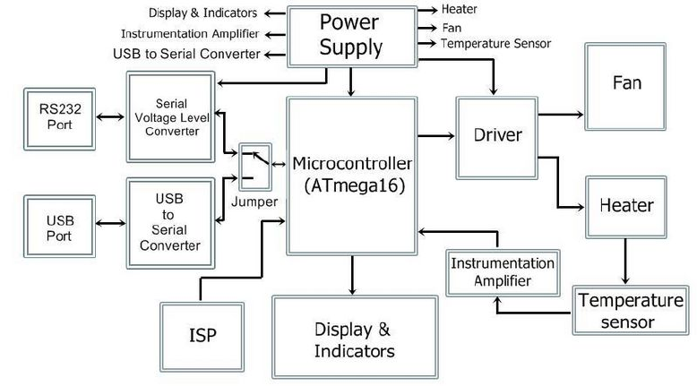
Figure 1.1: Block Diagram
5. Two 8-bit Timer/Counters
6. One 16-bit Timer/Counter
7. Four PWM channels
8. 8-channel,10-bit ADC
9. Programmable Serial USART
10. Up to 16 MIPS throughput at 16 MHz
Microcontroller plays a very important role. It controls every single hardware
present on the board, directly or indirectly. It executes various tasks like, setting up
communication between PC and the equipment, controlling the amount of current
passing through the heater coil, controlling the fan speed, reading the temperature,
displaying some relevant parameter values and various other necessary operations.
1.1.1 PWM for heat and speed control
The Single Board Heater System contains a Heater coil and a Fan. The heater
assembly consists of an iron plate placed at a distance of about 3.5mm from a
12
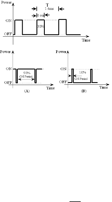
Figure 1.2: Pulse Width Modulation (A): On time is 90% of the total time period,
(B): ON time is 10% of total time period
nichrome coil. When current passes through the coil it gets heated and in turn
raises the temperature of the iron plate. Altering the heat generated by the coil
and also the speed at which the fan is operated, are the objectives of our prime
interest. The amount of power delivered to the Fan and Heater can be controlled
in various ways. The technique used here is called as PWM (abbreviation of Pulse
Width Modulation)technique. PWM is a process in which the duty cycle of the
square wave is modulated.
Duty cycle =TON
T(1.1)
Where TON is the ON time of the wave corresponding to the HIGH state of logic
and T is the total time period of the wave. Power delivered to the load is propor-
tional to TON time of the signal. This is used to control the current flowing through
the heating element and also speed of the fan. An internal timer of the microcon-
troller is used to generate a square wave. The ON time of the square wave depends
on a count value set in the internal timer. The pulse width of the waveform can be
varied accordingly by varying this count value. Thus, PWM waveform is gener-
ated at the appropriate pin of the microcontroller. This generated PWM waveform
is used to control the power delivered to the load (Fan and Heater).
A MOSFET is used to switch at the PWM frequency which indirectly controls the
power delivered to the load. A separate MOSFET is used to control the power
delivered to each of the two loads. The timer is operated at 244Hz.
13

1.1.2 Analog to Digital conversion
As explained earlier, the heat generated by the heater coil is passed to the iron
plate through convection. The temperature of this plate is measured by using a
temperature sensor AD590.
Some of the salient features of AD590 include:
1. Linear current output: 1µA/K
2. Wide range: -55°C to +150°C
3. Sensor isolation from the case
4. Low cost
The output of AD590 is then fed to the microcontroller through an Instrumentation
Amplifier. The signal obtained at the output of the Instrumentation Amplifier is
in analog form. It should be converted in to digital form before feeding as an
input to the microcontroller. ATmega16 features an internal 8-channel , 10 bit
successive approximation ADC (analog to digital converter) with 0-Vcc(0 to Vcc)
input voltage range, which is used for converting the output of Instrumentation
Amplifier. An interrupt is generated on completion of analog to digital conversion.
Here, ADC is initialize to have 206 µs of conversion time . Digital data thus
obtained is sent to the computer via serial port as well as for further processing
required for the on-board display.
1.2 Instrumentation amplifier
Instrumentation Amplifiers are often used in temperature measurement circuits in
order to boost the output of the temperature sensors. A typical three Op-Amp
Instrumentation amplifier is shown in the figure 1.3. The Instrumentation Am-
plifiers (IAs) are mostly preferred, where the sensor is located at a remote place
and therefore is susceptible to signal attenuation, due to their very low DC offsets,
high input impedance, very high Common mode rejection ratio (CMRR). The IAs
have a very high input impedance and hence do not load the input signal source.
IC LM348 is used to construct a 3 Op-Amp IA. IC LM348 contains a set of four
Op-Amps. Gain of the amplifier is given by equation 1.2
Vo
V2−V1
=(1+2Rf
Rg)R2
R1
(1.2)
14
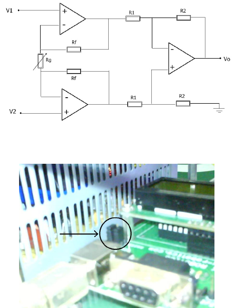
Figure 1.3: 3 Op-Amp Instrumentation Amplifier
Figure 1.4: Jumper arrangement
The value of Rgis kept variable to change the overall gain of the amplifier. The
signal generated by AD590 is in µA/°K. It is converted to mV/°K by taking it
across a 1 KΩresistor. The °K to°C conversion is done by subtracting 273 from
the °K result. One input of the IA is fed with the mV/°K reading and the other
with 273 mV. The resulting output is now in mV/°C. The output of the IA is fed
to the microcontroller for further processing.
1.3 Communication
The set up has the facility to use either USB or RS232 for communication with
the computer. A jumper is been provided to switch between USB and RS232. The
voltages available at the TXD terminal of microcontroller are in TTL (transistor-
15
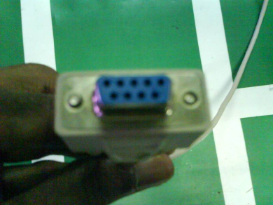
Figure 1.5: RS232 cable
transistor logic). However, according to RS232 standard voltage level below -5V
is treated as logic 1 and voltage level above +5V is treated as logic 0. This con-
vention is used to ensure error free transmission over long distances. For solving
this compatibility issue between RS232 and TTL, an external hardware interface
IC MAX202 is used. IC MAX202 is a +5V RS232 transreceiver.
1.3.1 Serial port communication
Serial port is a full duplex device i.e. it can transmit and receive data at the same
time. ATmega16 supports a programmable Universal Synchronous and Asyn-
chronous Serial Receiver and Transmitter (USART). Its baud rate is fixed at 9600
bps with character size set to 8 bits and parity bits disabled.
1.3.2 Using USB for Communication
After setting the jumper to USB mode connect the set up to the computer using a
USB cable at appropriate ports as shown in the figure 1.8. To make the setup USB
compatible, USB to serial conversion is carried out using IC FT232R. Note that
proper USB driver should be installed on the computer.
1.4 Display and Resetting the setup
The temperature of the plate, percentage values of Heat and Fan and the machine
identification number (MID) are displayed on LCD connected to the microcon-
16
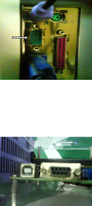
Figure 1.6: Serial port
Figure 1.7: USB communication
17
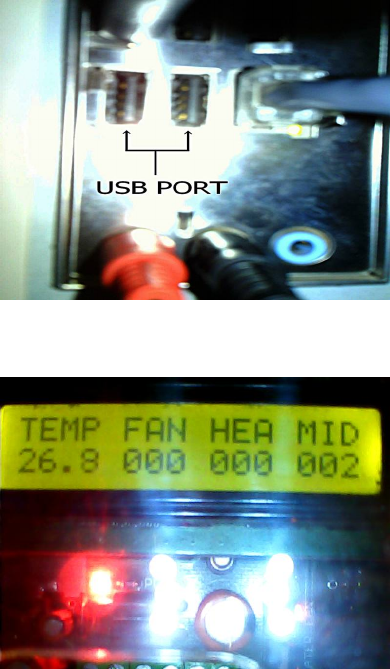
Figure 1.8: USB PORT
Figure 1.9: Display
troller. As shown in figure 1.9, numerals below TEMP indicate the actual tem-
perature of the heater plate in °C. Numerals below HEA and FAN indicate the
respective percentage values at which heater and fan are being operated. Numer-
als below MID corresponds to the device identification number. The set up could
be reset at any time using the reset button shown in figure 1.10. Resetting the
setup takes it to the standby mode where the heater current is forced to be zero
and fan speed is set to the maximum value. Although these reset values are not
displayed on the LCD display these are preloaded to the appropriate units.
18
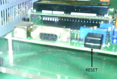
Figure 1.10: Reset
19
Chapter 2
Performing a Local Experiment on
Single Board Heater System
This chapter explains the procedure to use Single Board Heater System locally
with Scilab i.e. when you are physically accessing SBHS using your computer.
An open loop experiment, step test is used for demonstrating this procedure. The
process however remains the same for performing any other experiment explained
in this document, unless specified otherwise.
Hardware and Software Requirements
For working with the Single Board Heater system, following components are re-
quired:
1. SBHS with USB cable and power cable.
2. PC/Laptop with Scilab software installed. Scilab can be downloaded from:
http://www.scilab.org
3. FTDI Virtual Com Port driver corresponding to the OS on your PC. Linux
users do not need this. The driver can be downloaded from:
http://www.ftdichip.com/Drivers/VCP.htm
20
2.1 Using SBHS on a Windows OS
This section deals with the procedure to use SBHS on a Windows Operating Sys-
tem. The Operating System used for this document is Windows 7, 32-bit OS.
If you are using some other Operating System or the steps explained in section
2.1.1 are not sufficient to understand, refer to the official document available on
the main ftdi website at www.ftdichip.com. On the left hand side panel, click
on ’Drivers’. In the drop-down menu, choose ’VCP Drivers’. Then on the web
page page, click on ’Installation Guides’ link. Choose the required OS document.
We would now begin with the procedure.
2.1.1 Installing Drivers and Configuring COM Port
After powering ON the SBHS and plugging in the USB cable to the PC (check
the jumper settings on the board are set to USB communication) for the very first
time, the Welcome to Found New Hardware Wizard dialog box will pop up.
Select the option Install from a list or specific location. Choose
Search for best driver in these locations. Check the box Include
this location in the search. Click on Browse. Specify the path where
the driver is copied as explained earlier (item no.3) and install the driver by click-
ing Next. Once the wizard has successfully installed the driver, the SBHS is ready
for use. Please note that this procedure should be repeated twice.
Now, the communication port number assigned to the computer port to which
the Single Board Heater System is connected, via an RS232 or USB cable should
be identified. For identifying this port number, right click on My Computer and
click on Properties. Then, select the Hardware tab and click on Device
Manager. The list of hardware devices will be displayed. Locate the Ports(COM
& LPT) option and click on it. The various communication ports used by the
computer will be displayed. If the SBHS is connected via RS232 cable, then
look for Communications Port(COM1) else look for USB Serial Port. For RS232
connection, the port number mostly remains COM1. For USB connection it may
change to some other number. Note the appropriate COM number. This process
is illustrated in figure 2.1
Scilab must be installed on your computer. We recommend the use of scilab-
5.3.3. This is because all the codes are created and tested using scilab-5.3.3. These
codes may very well work in higher versions of scilab but one cannot use the same
codes back again in scilab-5.3.3. This is because a software is always backward
compatible, never forward compatible. Scilab for windows or linux can be down-
21
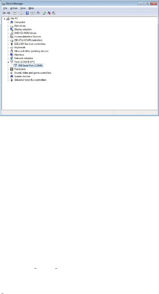
Figure 2.1: Checking Communication Port number
loaded from scilab.org. However, if scilab-5.3.3 for your OS is not available on
scilab.org then one can download it from sbhs.os-hardware.in/downloads.
Installation of scilab on windows is very straight-forward. After you download the
.exe file one has to double click on it and proceed with the instructions given by
the installer. All default options will work. However, note that scilab on windows
requires internet connection during installation.
2.1.2 Steps to Perform a Local Experiment
Go to sbhs.os-hardware.in/downloads. Let us take a look at the downloads
page. There are two versions of the scilab code. One which can be used with
SBHS locally i.e. when you are physically accessing SBHS using your computer
and another to be used for accessing SBHS virtually. This section expects you to
download the local version. On extracting the file that you will download, you
will get a folder scilab codes local. We shall refer to this folder as local for
simplicity. This folder will contain many folders named after the experiment. You
will also find a directory named common-files. We are going to use the folder
named Step test.
1. Launch Scilab from start menu or double click the Scilab icon on the desk-
top (if any). Before executing any scripts which are dependent on other files
22

or scripts, one needs to change the working directory of Scilab. This will
set the directory path in Scilab from where the other necessary files should
be loaded. To change the directory, click on file menu and then choose
”Change directory”. This can also be performed by typing cd<space>folder
path. Change the directory to the folder Step test. There is another
quicker way to make sure you are in the required working directory. Open
the experiment folder. Double click on the scilab file you want to execute.
Doing so will automatically launch scilab and also automatically change the
working directory. To know your working directory at any time, execute the
command pwd in the scilab console.
2. Next, we have to load the content of common-files directory. Notice that
this directory is just outside the Step test directory. The common-files
directory has several functions written in .sci files. These functions are re-
quired for executing any experiment. To load these functions type
getd<space>folder path. The folder path argument will be the com-
plete path to common-files directory. Since this directory is just outside
our Step test directory, the command can be modified to
getd<space>..\common files So now we have all functions loaded.
3. Next we have to load the serial communication toolbox. For doing so we
have to execute the loader.sce file present in the common-files direc-
tory. To do so execute the command
exec<space>..\common files\loader.sce or
exec<space>folder path\loader.sce.
4. Next, click on editor from the menu bar to open the Scilab editor or sim-
ply type editor on the Scilab console and open the file ser init.sce.
Change the value of the variable port2 to the COM number identified for
the connected SBHS. For example, one may enter ’COM5’ as the value for
port2. Notice that there is no space between COM and 5 and COM5 is in
single quotes. Keep all other parameters untouched. Execute this .sce file
by clicking on the execute button available on the menu bar of scilab ed-
itor window. The message COM Port Opened is displayed on successful
implementation. If there are any errors, reconnecting the USB cable and/or
restarting Scilab may help.
5. Next we have to load the function for the step test experiment. This func-
tion is written in step test.sci file. Since we do not have to make any
23

changes in this file we can directly execute it from scilab console without
opening it. Run the command exec<space>step test.sci in scilab con-
sole. The results are illustrated in figure 2.2.
6. Next, type Xcos on the Scilab console or click on Applications and
select Xcos to open Xcos environment. Load the step test.xcos file
from the File menu. The Xcos interface is shown in figure 2.4. The block
parameters can be set by double clicking on the block. To run the code click
on Simulation menu and click on Start. After executing the code in
Xcos successfully the plots as shown in figure 2.5 will be generated. Note
that the values of fan and heater given as input to the Xcos file are reflected
on the board display.
7. To stop the experiment click on the Stop option on the menu bar of the
Xcos environment.
All of the activities mentioned above, from getd<space>..\common files
untill starting the xcos simulation, are coded in a file named start.sce. Execut-
ing this file will do all necessary things automatically with just click of a button.
This file however assumes three things. These are
1. The location of common-files directory is not changed
2. The current working directory is correct
3. The port number mentioned in ser init.sce is correct
2.2 Using Single Board Heater System on a Linux
System
This section deals with the procedure to use SBHS on a Linux Operating System.
The Operating System used for this document is Ubuntu 12.04. For Linux users,
the instructions given in section 2.1 hold true with a few changes as below:
On a linux system, Scilab-5.3.3 can be either installed from available pack-
age manager (synaptic in case of Ubuntu) or its portable version can be down-
loaded from scilab.org or http://sbhs.os-hardware.in/downloads. If in-
stalled from a package manager then scilab can be launched by opening a termi-
nal (Alt+Ctrl+T) and executing the command sudo scilab. If one downloads
24
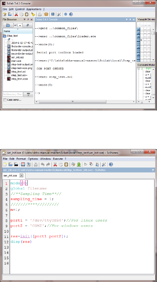
Figure 2.2: Expected responses seen on the console
Figure 2.3: Executing script files
25
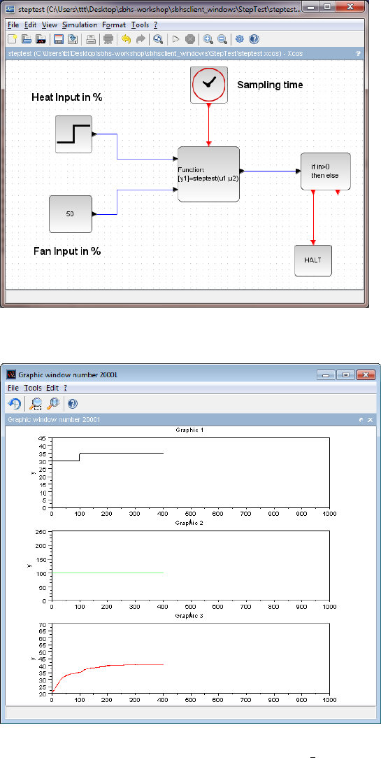
Figure 2.4: Xcos Interface
Figure 2.5: Plot obtained after executing step test.xcos
26
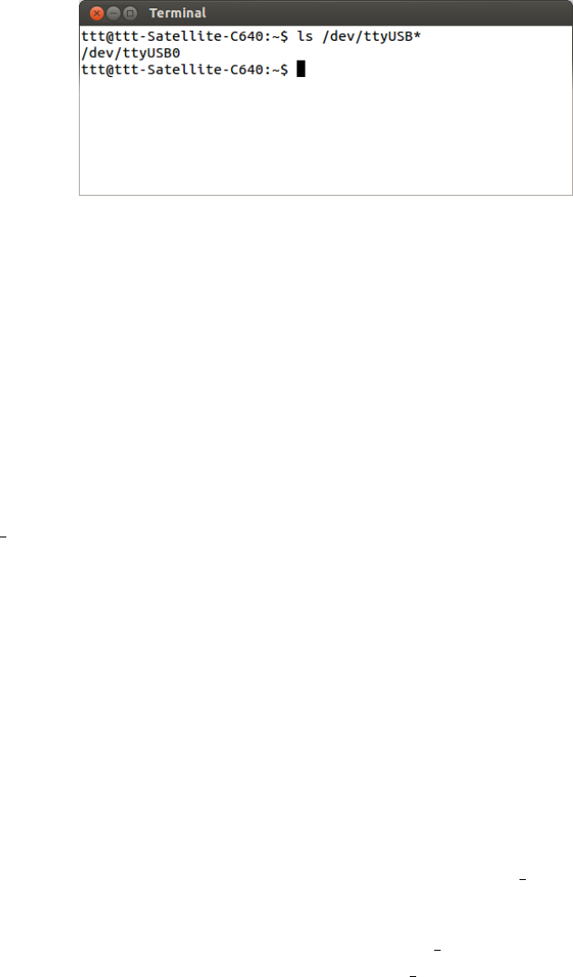
Figure 2.6: Checking the port number in linux (1)
the portable version then first the file has to unpacked. This can be done by right
clicking on it and choosing Extract here. Then one has to open the terminal
and change the directory to scilab/bin. Then the command sudo ./scilab
must be executed to launch scilab. Note that scilab must always be launched with
sudo permisions to be able to communicate with the SBHS.
FTDI COM port drivers are not required for connecting the SBHS to the PC.
After plugging in the USB cable to the PC, check the serial port number by typing
ls /dev/ttyUSB* on the terminal, refer Fig.2.6.
Note down this number and change the value of the variable port1 inside the
ser init.sce file, refer Fig.2.3.
Except for these changes rest all of the steps mentioned in Section 2.1.2 can
be followed.
2.3 Summary of procedure to perform a local exper-
iment
This section sumarrizes and only lists the required commands/activities to be done
in the given order to do a local experiment. It doesnot explain the expected results
etc. The procedure is common for both windows as well as linux users. However,
make sure you have reffered to the earlier sections of this chapter for clarity.
1. Step1: Change/ensure scilab working directory to Step test. Command
pwd can be used to know the present working directory of scilab
2. Step2: Load the functions available in common files directory by execut-
ing the command getd<space>..\common files
27

3. Step3: Load the serial communication toolbox by executing the command
exec<space>..\common files\loader.sce
4. Step4: Ensure correct communication port number in the ser init.sce
file and execute it. Execution can be done using the command
exec<space>ser init.sce
5. Step5: Load step test function by executing command
exec<space>step test.sci
6. Step6: Launch Xcos code for step test and execute it. This can be done
using the command xcos<space>step test.xcos
7. Step7: Execute this xcos code by clicking on the start button available on
the menubar of xcos window. Let the execution run for sufficient time, until
the output reaches a steadstate or untill sufficient data is collected.
Note that advance users can always make use to start.sce file for quickly
performing the experiments.
2.4 Scilab Code under common files
Scilab Code 2.1 comm.sci
1m=1;
2function [ temp ] =comm ( h e a t , f a n )
3global h e a t d i s p f a n d i s p t e m p d i s p s a m p l i n g t i m e m
name h a nd l f i l e n a m e
4
5i f h e a t <0
6h e a t =0
7end
8i f h e a t >100
9h e a t =100
10 end
11 i f fan <0
12 fan=0
13 end
14 i f fan >100
28
15 fan=100
16 end
17
18 w r i t e s e r i a l ( ha n dl , ascii (254) ) ; / / I n p u t H e a t e r ,
w r i t e s e r i a l a c c e p t s
s t r i n g s ; s o
c o n v e r t 2 5 4 i n t o i t s
string
e q u i v a l e n t
19 w r i t e s e r i a l ( ha n dl , ascii ( h e a t ) ) ;
20 w r i t e s e r i a l ( ha n dl , ascii (253) ) ; / / I n p u t F a n
21 w r i t e s e r i a l ( ha n dl , ascii ( f a n ) ) ;
22 w r i t e s e r i a l ( ha n dl , ascii (255) ) ; / / T o r e a d T e m p
23 s l e e p ( 1 0 0 ) ;
24
25 temp =ascii ( r e a d s e r i a l ( h a n d l ) ) ; / / R e a d s e r i a l
r e t u r n s a s t r i n g , s o
c o n v e r t i t t o
i t s i n t e g e r ( a s c i i )
e q u i v a l e n t
26 temp =temp ( 1 ) +0.1*temp ( 2 ) ; / / c o n v e r t t o t e m p w i t h
d e c i m a l p o i n t s
e g : 4 0 . 7
27 epoch=getdate ( ’ s ’ ) ;
28 d t =getdate ( ) ;
29 ms=d t ( 1 0 ) ;
30 epoch=(epoch*10 00)+ms ;
31
32 A=[m, h e a t , f an , temp , e poc h ] ;
33
34 f d f h =f i l e ( ’ open ’ , f i l e n a m e , ’ unknown ’ ) ;
35
36 f i l e ( ’ l a s t ’ , f d f h )
37
38 write ( f d f h , A , ’ ( 7 ( f 1 5 . 1 , 3 x ) ) ’ ) ;
39
40 f i l e ( ’ c l o s e ’ , f d f h ) ;
41
29

42 m=m+1;
43 endfunction
Scilab Code 2.2 init.sci
1global f i l e n a m e m
2function status =i n i t ( p o r t )
3global h an dl f i l e n a m e
4
5OS =g e t o s ( ) ;
6
7i f OS == string ( ’ Linu x ’ )
8port num =p o r t ( 1 ) ;
9handl =o p e n s e r i a l ( port num , ” 96 00 , n , 8 , 0 ” )
10 else
11 p o r t v a l =p o r t ( 2 ) ;
12 num=p a r t ( p o r t v a l , 4 : $ ) ;
13 port num =s t r t o d ( num ) ;
14 handl =o p e n s e r i a l ( port num , ” 96 00 , n , 8 ” )
15 end
16
17 i f (ascii ( h a n d l ) ˜=[])
18 status =string ( ’COM PORT OPENED ’ )
19 else
20 status =string ( ’ERROR: Check p o r t number o r USB
c o n n e c t i o n ’ )
21 end
22
23 m=1 ;
24
25 d t =getdate ( ) ;
26 y e a r =d t ( 1 ) ;
27 month =d t ( 2 ) ;
28 day =d t ( 6 ) ;
29 hou r =d t ( 7 ) ;
30 minutes =d t ( 8 ) ;
31 seconds =d t ( 9 ) ;
32
30

33
34 f i l e 1 =strcat (string ( [ y e a r month day h ou r m i n u t e s
s e c o n d s ] ) , ’−’ ) ;
35 string t x t ;
36 f i l e n a m e =strcat ( [ f i l e 1 , ” t x t ” ] , ’ . ’ ) ;
37
38 endfunction
Scilab Code 2.3 plotting.sci
1function [ ] =p l o t t i n g ( va r , l ow lim , h i g h l i m )
2
3global h e a t d i s p f a n d i s p t e m p d i s p s e t p o i n t d i s p
s a m p l i n g t i m e m
4
5timeTitle =”No . o f s a mp l e s w i t h s a m p l i n g t i m e =”
+string ( s a m p l i n g t i m e )
6i f low lim ˜=[ ] & h i g h l i m ˜ =[ ]
7h e a t m i n =l o w l i m ( 1 )
8fan min =l o w l i m ( 2 )
9temp min =l o w l i m ( 3 )
10 time min =l o w l i m ( 4 )
11
12 heat max =h i g h l i m ( 1 )
13 fan max =h i g h l i m ( 2 )
14 temp max =h i g h l i m ( 3 )
15 ti me m ax =h i g h l i m ( 4 )
16
17 else
18 h e a t m i n =0
19 fan min =0
20 temp min =20
21 time min =0
22
23 heat max =100
24 fan max =100
25 temp max =100
26 ti me m ax =1000
31

27 end
28
29
30
31 i f l e n g t h ( v a r ) ==3
32 h e a t =v a r ( 1 ) ;
33 fan =v a r ( 2 ) ;
34 temp =v a r ( 3 ) ;
35
36 heatdisp=[ h e a t d i s p ; h e a t ] ;
37 subplot (311) ;
38 xtitle ( ” ” , t i m e T i t l e , ” Hea t i n p e r c e n t a g e ” )
39 plot2d ( h e a t d i s p , r e c t =[ t i me m i n , h e a t m i n ,
time max , he a t max ] , s t y l e =1)
40
41 fandisp=[ f a n d i s p ; f an ] ;
42 subplot (312) ;
43 xtitle ( ” ” , t i m e T i t l e , ” Fan i n p e r c e n t a g e ” )
44 plot2d ( f a n d i s p , r e c t =[ ti m e m i n , fa n m in ,
time max , fan m ax ] , s t y l e =2)
45
46 tempdisp=[ t e m p d i s p ; temp ] ;
47 subplot (313)
48 xtitle ( ” ” , t i m e T i t l e , ” T e m p e r a t u r e ( deg
c e l c i u s ) ” )
49 plot2d ( tem p d isp , r e c t =[ t i me m in , temp min ,
time max , temp max ] , s t y l e =5)
50
51
52 e l s e i f l e n g t h ( v a r ) == 4
53
54 h e a t =v a r ( 1 ) ;
55 fan =v a r ( 2 ) ;
56 temp =v a r ( 3 ) ;
57 s e t p o i n t =v a r ( 4 ) ;
58
59 heatdisp=[ h e a t d i s p ; h e a t ] ;
60 subplot (311) ;
32

61 xtitle ( ” ” , t i m e T i t l e , ” Hea t i n p e r c e n t a g e ” )
62 plot2d ( h e a t d i s p , r e c t =[ t i me m i n , h e a t m i n ,
time max , he a t max ] , s t y l e =1)
63
64 fandisp=[ f a n d i s p ; f an ] ;
65 subplot (312) ;
66 xtitle ( ” ” , t i m e T i t l e , ” Fan i n p e r c e n t a g e ” )
67 plot2d ( f a n d i s p , r e c t =[ ti m e m i n , fa n m in ,
time max , fan m ax ] , s t y l e =2)
68
69 tempdisp=[ t e m p d i s p ; temp ] ;
70 setpointdisp=[setpointdisp ; setpoint ]
71 subplot (313)
72 xtitle ( ” ” , t i m e T i t l e , ” T e m p e r a t u r e ( deg
c e l c i u s ) ” )
73 plot2d ( tem p d isp , r e c t =[ t i me m in , temp min ,
time max , temp max ] , s t y l e =5)
74 plot2d ( setpointdisp , rect=[ ti m e m i n , temp min ,
time max , temp max ] , s t y l e =1)
75
76 end
77 endfunction
33
Chapter 3
Using Single Board Heater System,
Virtually!
3.1 Introduction to Virtual Labs at
IIT Bombay
The concept of virtual laboratory is a brilliant step towards strengthening the ed-
ucation system of an university/college, a metropolitan area or even an entire
nation. The idea is to use the ICT i.e. Information and Communications Tech-
nology, mainly the Internet for imparting education or exchange of educational
information. Virtual Laboratory mainly focuses on providing the laboratory fa-
cility, virtually. Various experimental set-ups are hooked up to the internet and
made available to use for the external world. Hence, anybody can connect to that
equipment over the internet and carry out various experiments pertaining to it. The
beauty of this idea is that a college who cannot afford to have some experimental
equipments can still provide laboratory support to their students through virtual
lab, and all that will cost it is a fair Internet connection! Moreover, the laboratory
work does not ends with the college hours, one can always use the virtual lab at
any time and at any place assuming the availability of an internet connection.
A virtual laboratory for SBHS is launched at IIT Bombay. Here is the url to
access it: vlabs.iitb.ac.in/sbhs/. A set of 36 SBHS are made available to use over
the internet 24×7. These individual kits are made available to the users on hourly
basis. We have a slot booking mechanism to achieve this. Since there are 36 SBHS
connected with an hours slot for 24 hrs a day, we have 864 one hour slots a day.
This means that 864 individual users can access the SBHS in a day for an hour.
34
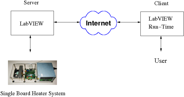
Figure 3.1: SBHS virtual laboratory with remote access using LabVIEW
This also means that up to 6048 users can use the SBHS for an hour in a week and
181440 in a month! A web page is hosted which is the first interface to the user.
The user registers/logs in himself/herself here. The user is also supposed to book
a slot for accessing the SBHS. A database server maintains a record of the data
generated through the web interface. A python script is hosted on the server side
and it helps in connecting the user with the corresponding SBHS placed remotely.
A free and open source scientific computing Software, Scilab, is used by the user
for implementing the experiment on SBHS, in terms of simple Scilab coding.
3.2 Evolution of SBHS virtual labs
In [4], the control algorithm is implemented at the server end and the remote stu-
dent just keys in the parameters, as shown in Figure 3.1. LabVIEW was used
for the implementation of the same. The server end consisted of a computer con-
nected with an SBHS with a full blown copy of LabVIEW installed on it. The
client has a LabVIEW run time engine available for free download from the Na-
tional Instruments website. A few LabVIEW algorithms/experiments were hosted
on the server. The client accesses these algorithm/experiment over the Internet
using a web browser by entering appropriate parameters.
35
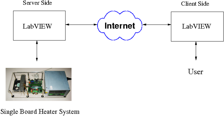
Figure 3.2: SBHS virtual laboratory with remote access and live data sharing
using LabVIEW
It was realized that the learning experience is not complete for this structure.
This is because the server hosts some pre-built LabVIEW algorithms and a user
can only access these few algorithms. The user can in no way change the program
and can only input experimental parameters. Hence, we came up with a new
architecture as shown in the Figure 3.2 that used full blown copies of LabVIEW
at both server and client ends.
This idea uses the DataSocket technology of LabVIEW. Since now the client is
having a complete LabVIEW installation on his/her computer she can now imple-
ment her own algorithms. Thus this architecture did provide a complete learning
experience to the students. There are some shortcomings as well:
•LabVIEW is expensive and students may not be able to afford to buy it. It
is also prohibitively expensive for the Government to distribute it.
•We used the LabVIEW version 8.04, which had restricted scripting lan-
guage. It was tedious to create new control algorithms in it.
This made us shift to free and open source (FOSS) software. We replaced Lab-
VIEW with Java and Scilab as shown in Figure 3.3. Scilab at the server end is
36
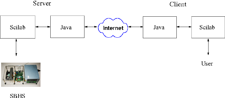
Figure 3.3: SBHS virtual laboratory using open source software
used for communicating with SBHS. Scilab at the client end is used for imple-
menting the algorithms. Java is used at both the server as well as client end for
communication over the Internet thereby connecting the client with the server.
For the above solution, we need a dedicated copy of scilab running at the
server end for every SBHS. One way to do this is to host it on multiple computers
with unique IPs. Hence the number of SBHS we want to host requires as many
computer’s and public IPs thereby making it expensive. Moreover, it also limits
its scalability. The other way to do this is to host multiple java and scilab servers
on the same computer. Hosting many copies of Scilab simultaneously requires a
powerful computer for the server.
For these reasons we decided to take scilab offthe server computer and to use
java alone to communicate with the SBHS directly. Java also communicates with
the client computer. We connected seven SBHS systems to a USB port through
a serial port hub. This architecture was implemented on a Windows Operating
System. We faced the following difficulties in this solution.
•When we connected more than one serial hub to a PC, the port ID could not
be retrieved correctly. Port ID information is required if we want a student
to use the same SBHS for all their experiments during different sessions.
•The experiments required time stamping of the data communicated to and
from the server. But this time stamping was not linear and suffered instabil-
ity.
37
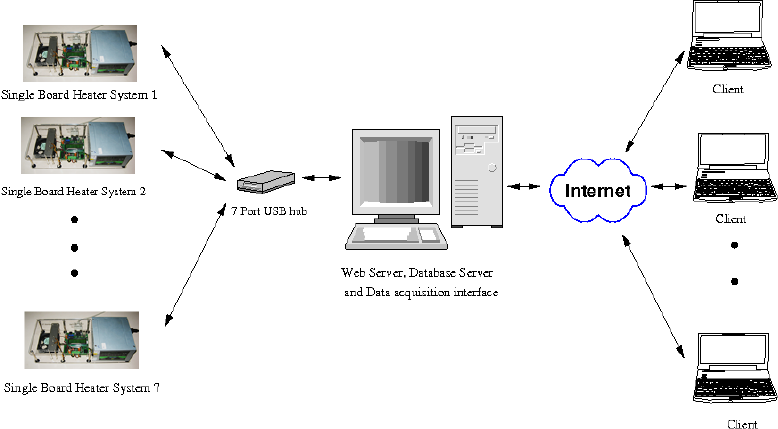
Figure 3.4: Virtual control lab hardware architecture
This made us to completely switch to FOSS with Ubuntu Linux as the OS and is
the current structure of the Virtual lab as shown in Figure 3.6
3.3 Current Hardware Architecture
The current hardware architecture of the virtual single-board heater system lab
involves 36 single-board heater systems connected to the server via multiple 7
and 10-port USB hubs. The server computer is connected to a high speed inter-
network and has enough processing capability to host data acquisition, database,
and web servers. It has been successfully tested for the undergraduate Process
Control course and the graduate Digital Control and Embedded systems courses
conducted at IIT Bombay as well as few workshops over the internet. Currently,
this architecture is integrated with a cameras on each SBHS to facilitate live video
streaming. This gives the user a feel of remote hands-on.
38

Figure 3.5: Home page of SBHS V Labs
3.4 Current Software Architecture
The current software architecture of this virtual SBHS control lab is shown in Fig-
ure 3.6. The server computer runs Ubuntu Linux 12.04.2 OS. It hosts a Apache-
MySQL server. The SBHS server is based on Python-Django framework and is
linked to Apache server using Apache’s WSGI module. The MySQL database
server has the details of all the registered users, their slot details, authentication
keys to allow remote access, etc. As shown in Figure ??, the Python-Django
server has pages for registration, login, slot booking etc. [9]. On the client end,
control algorithms are running in Scilab and a python based client application
communicates with virtual labs server over the Internet.
The steps to be performed before and during each experiment are explained
next.
3.5 Conducting experiments using the Virtual lab
This section explains the procedure to use Single Board Heater System remotely
using Scilab i.e. when you are accessing SBHS remotly using your computer over
39
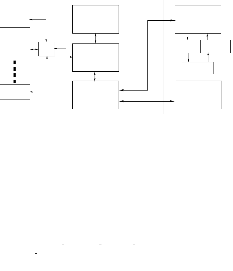
USB
HUBS
MySQL
Server
Database
Python
Server
Django
Apache
Web
Server
Python
Client
based
Web
Browser
file
scilabwrite
file
scilabread
Scilab
Client Computer
SBHS 1
SBHS 2
SBHS 36
Server Computer
Internet
Figure 3.6: Current Architecture of SBHS Virtual Labs
the virtual labs platform. An open loop experiment, step test is used for demon-
strating this procedure. The process however remains the same for performing any
other experiment explained in this section, unless specified otherwise. Let us first
see the required files to be downloaded and installations to be done. Scilab is re-
quired to be installed on your computer. Please refer to Section 2.1.1 and Section
2.2 for the procedure to install scilab on Windows and Linux system, respectively.
SBHS scilab code for your OS, under the section SBHS Virtual Code, must
be downloaded from http://sbhs.os-hardware.in/downloads. For exam-
ple, if you are using a 32-bit linux operating system then you should download
the file SBHS Scilab codes for Linux - (32 bit). The code downloaded
will be in zip format. After the zip is unpacked, you will see scilab experiment
folders such as Step test,Ramp Test,pid controller etc. We will be us-
ing the Step test folder. Do not alter the directory structure. If you want to copy
or move an experiment outside the directory then make sure you also copy the
common files folder. The common files folder must always be one directory
outside the experiment folder. Now given that you have scilab installed and work-
ing and the required scilab code downloaded, let us see the step-by-step procedure
to do a remote experiment.
40
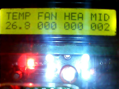
Figure 3.7: Show Video
3.5.1 Registration, Login and Slot Booking
Go to the website sbhs.os-hardware.in and click on the Virtual labs link
available on the left hand side. The home page of Virtual labs is illustrated in Fig
3.5. If you are a first time user, click on the link Login/Register. Fill out the
registration form and submit it. If the registration form is submitted successfully,
you will receive an activation link on your registered Email id. Use this link to
complete the registration process. If you skip this step you will not be able to
login. Registration is a one time process and need not be repeated more than
once. After completing registration login with your username and password. You
should now get the options to Book Slot, Delete Slot etc.
View/Delete slot option allows you to delete your booked slots. This option
however will work only for slots booked for the future. You cannot delete a past or
the current slot. Download log files option gives you the facility to download your
experiment log files. Clicking on it will give you a list of all of the experiments
you had performed. Show video option can be used to see the live video feed of
your SBHS. Web cameras are mounted on every SBHS. You can see the display
of your SBHS as shown in Fig. 3.7.
Clicking on the Book slot option will allow you to book an experiment time
slot. Slots are of 55 minutes duration. Click on the Book slot option. If the current
slot is free, Book now option will appear. Click on it. Else you have to book an
advance slot for the next hour or any other future time using the calender that
appears on this page. There is a limit to how many slots one can book in a day.
We are allowing only two non-consecutive slots, per user, to be booked in a day.
However, there is no limit to how many current slots you book and use. Book an
41
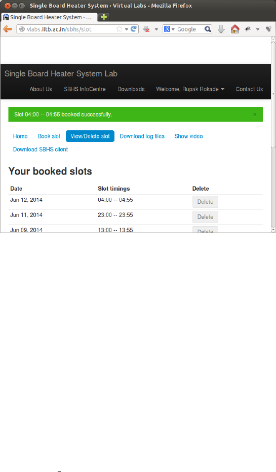
Figure 3.8: Slot booking
experiment slot. Once you successfully book a slot a Slot booked successfully
message highlighted in green color will appear on the top side. This is shown in
Fig. 3.8. It will automatically take you to the View/Delete slot page.
3.5.2 Configuring proxy settings and executing python based
client
After booking a slot, the web activity is over. You may close the web browser
unless you need it open to see live video feed of your SBHS. The next step is
to establish the communication link between the server and your computer. A
python based application is created which handles the network communication.
Let us first see how to do the proxy settings if you are behind a proxy network.
Open the folder common files. Open the file config. This files contains various
arguments whose values must be eneterd to configure proxy.
Do not change the contents of config file if
•You are accessing from inside IIT Bombay OR
•You are accessing from outside IIT Bombay and using an open network
42

such as at home OR using a mobile internet
Change the contents of config file if
•You are outside IIT Bombay and using a proxy network such as at an insti-
tute, office etc.
If you have to put the proxy details, first change the argument use proxy =
Yes (Y should be capital in Yes and N should be capital in No). Fill in the other de-
tails as per your proxy network. If your proxy network allows un-authenticated lo-
gin then make the argument proxy username and proxy password blank. This
proxy setting has to done only once.
Open the Step test folder. Double click on the file run. This will open the
client application as shown in Fig. 3.9. Note that for first time execution, it will
take a minute to open the client application. It will show various parameters re-
lated to the experiment such as SBHS connection, Client version, User login and
Experiment status. The green indicators show that the corresponding activity is
correct or functional. Here it says that the Client application is been able to con-
nect to the server and the client version being used is the latest. The User login and
Experiment status is showing red and will turn green after a registered username
and password is entered. If the SBHS is offline or there are some other issues, the
corresponding error will be displayed and the respective indicator will turn red.
Enter your registered username and password and press login. You should get
the message Ready to execute scilab code. The application also shows the
value of iteration, heat, fan, temperature and time remaining for experimentation.
It also shows the name of log file created for the experiment.
3.5.3 Executing scilab code
Inside the StepTest folder, if on a windows system, double click on the file
stepc.sce. This should automatically launch scilab and also open the stepc.sce
in the scilab editor. It will also automatically change the scilabs working direc-
tory. On a linux system, launch scilab manually. Then change the scilab working
directory to the folder StepTest. This can be done by clicking on File menu and
then selecting change current directory. Next, execute the command getd
../common files. Scilab command getd is used to load all functions defined in
all .sci files inside a specified folder. Here we have some important function files
inside the ../common files directory. Executing this command will load all of
43
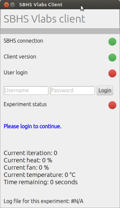
Figure 3.9: Python Client
44
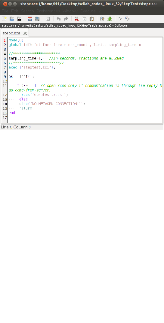
Figure 3.10: stepc.sce file
the functions that the experiment needs. Open the file stepc.sce using the Open
option inside File menu. The file is shown in Fig. 3.10
The experiment sampling time can be set inside the stepc.sce file. You may
want to change it to a higher value if your network is slow. The default value of 1
second works fine in most cases. On the menu bar, click on Execute option and
choose option file with echo. This will execute the scilab code. If the network
is working fine, an xcos diagram will open automatically. If it doesnt open then
see the scilab console for error messages. If you get a No network connection
error message then try executing the scilab code again. The xcos diagram is for
the step test experiment as shown in Fig. 3.11. You can set the value of the heat
and fan. Keep the default values. On the menu bar of the xcos window, click on
start button. This will execute the xcos diagram. If there is no error, you will
get a graphic window with three plots. It will show the value of Heat in % Fan
in % and ..temperature in degree celcius as shown in Fig. 3.12. After sufficient
time of experimentation click on the stop button to stop the experiment. Go to the
StepTest folder. Here you will find a logs folder. This folder will have another
folder named after your username. It will have the log file for your experiment.
Read the log file name as
YearMonthDate hours minutes seconds.txt. This log file contains all the values
45

Figure 3.11: Xcos for step test
of heat fan and temperature. It can be used for further analysis.
3.5.4 Conducting experiments over virtual labs through ARM
based computer
This section talks about accessing the SBHS virtual labs using an ARM based
computer. These ARM based computers could be netbooks, laptops or even tablets
running a Linux operting system. Let us see the additional steps to be follwed for
using over an ARM computer.
1. The scilab codes are separate for windows, linux and ARM based linux.
Download the scilab code from http://sbhs.os-hardware.in/downloads.
You need to download the file against the label SBHS Scilab codes for
ARM under the SBHS Virtual Code section. The name of the file down-
loaded will be sbhs codes arm. This will be a zip file. Extract its connets
in order to use it.
2. Open a terminal by pressing the Alt+Ctrl+T keys together. Change the di-
rectory to sbhs codes arm directory using the cd command. For example,
46
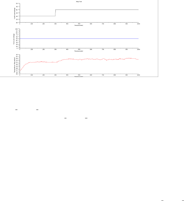
Figure 3.12: Output of Step Test
if the sbhs codes arm folder is saved on the desktop, the command will
look like cd Desktop/sbhs codes arm
3. Execute the command chmod +x install.sh
4. Then execute the command ./install.sh. It may ask you to enter the
sudo password. Hence, this step requires you to know the sudo password of
the computer you are using.
5. With these steps done, now follow the instructions explained in Section
3.5 throughout its subsections. Note that you need NOT download SBHS
Scilab codes for Linux - (32 bit) file while refering to this sec-
tion. This is because all scilab codes are included inside the sbhs codes arm
directory
3.6 Summary
This section summarizes the process to perform an experiment on SBHS using
virtual lab interface. This section assumes that the user has already created an
account and booked a slot as explained in section 3.5.1. It also assumes that the
proxy settings are already done as explained in section 3.5.2. The user should
follow these steps within the booked slot time.
•Step1: Open the StepTest experiment directory
•Step2: Double-click on the file run. Expect the SBHS cient application to
open.
47

•Step3: Enter the username and password inside the SBHS cient application
and press login button. Expect the message Ready to execute scilab
code
•Step4: Switch to the StepTest experiment directory and double-click on the
file stepc.sce. This will launch scilab and also open the file stepc.sce
in the scilab editor. Linux users will have to launch scilab manually. They
also have to change the working directory to StepTest and then open the
stepc.sce file in the scilab editor.
•Step5 Switch to the scilab console and execute the command getd ../
common files
•Step6: Execute the file stepc.sce. Expect the step test xcos diagram to
open automatically. If this doesnt happen, check the scilab console for error
message.
•Step7: Execute the step test xcos daiagram. You may change the input
parameters, if required, before executing. Expect a plot window to open
automatically showing three graphs.
•Step8: Stop the Xcos simulation after the experiment is completed properly.
48

Chapter 4
Identification of Transfer Function
of a Single Board Heater System
through Step Response Experiment
The aim of this experiment is to perform step test on a Single Board Heater System
and to identify system transfer function using step response data. The target group
is anyone who has basic knowledge of control engineering.
We have used Scilab and Xcos as an interface for sending and receiving data.
Xcos diagram is shown in figure 4.1. Heater current and fan speed are the two
inputs for this system. They are given in percentage of maximum. These inputs
can be varied by setting the properties of the input block’s properties in Xcos.
The plots of their amplitude versus number of collected samples are also available
on the scope windows. The output temperature profile, as read by the sensor, is
also plotted. The data acquired in the process is stored on the local drive and is
available to the user for further calculations.
In the step test.xcos file, open the heater block’s parameters to apply a
step change of say 10 percent to the heater at operating point of 30 percent of
heater after 250 seconds. The block parameters of the step input block will have
Step time = 250,Initial value = 30 and Final value = 40. Keep the
fan input constant at 50 percent. Start the experiment and let it continue until you
see the temperature reach the steady state.
The step test data file will be saved in Step test folder. The name of the
file will be the date and time at which the experiment was conducted. A sam-
ple data file is provided in the same folder. The sample data file is named as
step-data-local.txt and step-data-virtual.txt. Refer to the one de-
49
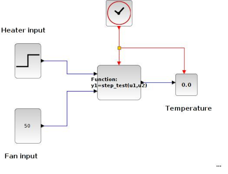
Figure 4.1: Xcos for this experiment
1.0 30.0 50.0 29.3 1412400132192.0
2.0 30.0 50.0 29.5 1412400133044.0
.
.
820.0 40.0 50.0 37.0 1412400950197.0
821.0 40.0 50.0 37.2 1412400951202.0
Table 4.1: Step data obtained after performing local Step Test
50
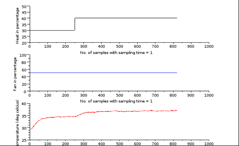
Figure 4.2: Graph shows heater current, fan speed and output temperature
pending on wheather you are performing a local or a virtual experiment. Referring
to the data file thus obtained as shown in table 4.2, the first column in this table
denotes samples. The second column in this table denotes heater in percentage. It
starts at 30 and increases with a step size of 10 units. The third column denotes
the fan in percentage. It has been held constant at 50 percent. The fourth column
refers to the value of temperature. The fifth column denotes time stamp. The
virtual data file will havel four time stamp columns apart from first 3 columns.
These four time stamp columns are client departure, server arrival, server depar-
ture and client arrival. These can be used for advanced control algorithms. These
additional time stamps exist in virtual mode because of the presense of network
delay.
4.1 Conducting Step Test on SBHS locally
The detailed procedure to perform a local experiment is explained in Chapter2.
A summary of the same is provided in section 2.3 It is exactly the same for this
section. The response is as shown in figure 4.2. The output data file is as shown
51
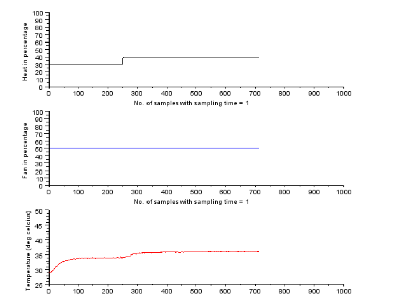
Figure 4.3: Step test Virtual experiment response
in Table 4.2
4.2 Conducting Step Test on SBHS, virtually
The detailed procedure to perform a local experiment is explained in Chapter3.
A summary of the same is provided in section 3.5 It is exactly the same for this
section. The virtual experiment response is shown in figure 4.3. The correspond-
ing data file is shown in table 4.2. The time stamps shown are cut short for better
viewing. This data file can be found in StepTest folder for virtual experiments.
The name of this file is step-data-virtual.txt.
52

0 0 100 29.30 14...8080 14...8955 14...8993 14...8158 0.10000E+01
1 30 50 29.00 14...9364 14...0246 14...0263 14...9442 0.10000E+01
.
.
711 40 50 36.20 14...9375 14...0280 14...0297 14...9437 0.71100E+03
712 40 50 36.10 14...0370 14...2673 14...2691 14...1834 0.71200E+03
Table 4.2: Step data obtained after performing virtual Step Test
4.3 Identifying First Order and Second Order Trans-
fer Functions
In this section we shall determine the first and second order transer function model
using the data obtained after performing step test experiment. Please note that this
procedure is common for data obtained using both local and virtual experiments.
4.3.1 Determination of First Order Transfer Function
Identification of the transfer function of a system is important as it helps us to rep-
resent the physical system mathematically. Once the transfer function is obtained,
one can acquire the response of the system for various inputs without actually
applying them to the system.
Consider the standard first order transfer function given below
G(s)=C(s)
R(s)(4.1)
G(s)=1
τs+1(4.2)
Rewriting the equation, we get
C(s)=R(s)
τs+1(4.3)
A step is given as input to the first order system. The Laplace transform of a step
function is1
s. Hence, substituting R(s)=1
sin equation 4.3, we obtain
C(s)=1
τs+1
1
s(4.4)
53

Solving C(s) using partial fraction expansion, we get
C(s)=1
s−1
s+1
τ
(4.5)
Taking the Inverse Laplace transform of equation 4.5, we get
c(t)=1−e−t
τ(4.6)
From the above equation it is clear that for t=0, the value of c(t) is zero. For t=
∞, c(t) approaches unity. Also, as the value of ‘t ’becomes equal to τ, the value
of c(t) becomes 0.632. τis called the time constant and represents the speed of
response of the system. But it should be noted that, smaller the time constant-
faster the system response. By getting the value of τ, one can identify the transfer
function of the system.
Consider the system to be first order. We try to fit a first order transfer function
of the form
G(s)=K
τs+1(4.7)
to the Single Board Heater System. Because the transfer function approach uses
deviation variables, G(s) denotes the Laplace transform of the gain of the system
between the change in heater current and the change in the system temperature.
Let the change in the heater current be denoted by ∆u. We denote both the time
domain and the Laplace transform variable by the same lower case variable. Let
the change in temperature be denoted by y. Let the current change by a step of size
u. Then, we obtain the following relation between the current and the temperature.
y(s)=G(s)u(s) (4.8)
y(s)=K
τs+1
∆u
s(4.9)
Note that ∆u is the height of the step and hence is a constant. On inversion, we
obtain
y(s)=K[1 −e−t
τ]∆u(4.10)
54

4.3.2 Procedure
1. Download the Analysis folder from the sbhs website. It will be available
under downloads section. Download the file for SBHS Analysis Code
(local & virtual). The name of the file is scilab codes analysis.
The download will be in zip format. Extrat the downloaded zip file. You
will get a folder scilab codes analysis.
2. Open the scilab codes analysis folder and then locate and open the
folder Step Analysis.
3. Open the Kp-tau-order1 folder.
4. Copy the step test data file to the folder Kp-tau-order1.
5. Change the Scilab working directory to Kp-tau-order1 folder under Step Analysis
folder.
6. Open the file firstorder.sce in scilab editor and enter the name of the
data file (with extention) in the filename field.
7. Save and run this code and obtain the plot as shown in figure 4.4.
This code uses the routines label.sci and costf 1.sci
The results presented are obtained for the data file step-data-virtual.txt.
This data file is present under the Step Test directory for local experiments.The
plot thus obtained is reasonably good. See the Scilab plot to get the values of τ
and K. The figure 4.4 shows a screen shot of the same. We obtain τ=58.64, K =
0.23. The transfer function obtained here is at the operating point of 30 percentage
of heat. If the experiment is repeated at a different operating point, the transfer
function obtained will be different. The gain will correspondingly be more at a
higher operating point. This means that the plant is faster at higher temperature.
Thus the transfer function of the plant varies with the operating point. Let the
transfer function we obtain in this experiment be denoted as Gs. We obtain
Gs(s)=0.23
58.64s+1(4.11)
55
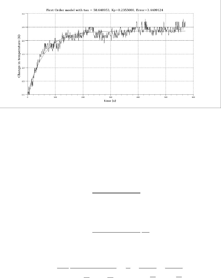
Figure 4.4: Output of the Scilab code firstorder.sce for data file
step-data-local.txt
4.4 Determination of Second Order Transfer Func-
tion
In this section, we explore the efficacy of a second order model of the form
G(s)=K
(τ1s+1)(τ2s+1) (4.12)
The response of the system to a step input of height ∆uis given by
y(s)=K
(τ1s+1)(τ2s+1)
∆u
s(4.13)
Splitting into partial fraction expansion, we obtain
y(s)=K
τ1τ2
1
s+1
τ1! s+1
τ2!=A
s+B
s+1
τ1
+C
s+1
τ2
56

Through Heaviside expansion method, we determine the coefficients:
A=K
B=−Kτ1
τ1−τ2
C=Kτ2
τ1−τ2
On substitution and inversion, we obtain
y(t)=K"1−1
τ1−τ2τ1e−t/τ1−τ2e−t/τ2#(4.14)
We have to determine three parameters K,τ1and τ2through optimization.
Once again, we follow a procedure identical to the first order model. The only
difference is that we now have to determine three parameters. Scilab code
secondorder.sce calculates the gain and two time constants.
4.4.1 Procedure
1. Download the Analysis folder from the sbhs website. It will be available
under downloads section. Download the file for SBHS Analysis Code
(local & virtual). The name of the file is scilab codes analysis.
The download will be in zip format. Extrat the downloaded zip file. You
will get a folder scilab codes analysis.
2. Open the scilab codes analysis folder and then locate and open the
folder Step Analysis.
3. Open the Kp-tau-order2 folder.
4. Copy the step test data file to the folder Kp-tau-order2.
5. Change the Scilab working directory to Kp-tau-order2 folder under Step Analysis
folder.
6. Open the file secondorder.sce in scilab editor and enter the name of the
data file (with extention) in the filename field.
7. Save and run this code and obtain the plot as shown in figure 4.5.
57
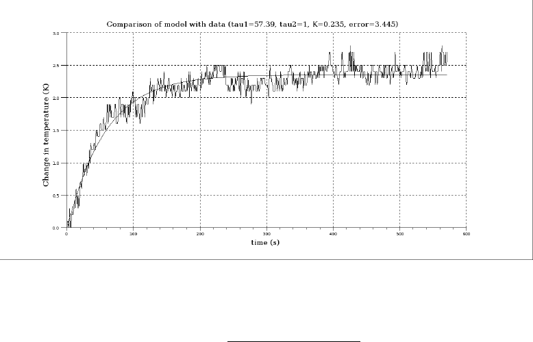
Figure 4.5: Output of the Scilab code secondorder.sce
Gs(s)=0.235
(57.39s+1)(1s+1) (4.15)
The fit is much better now. In particular, the initial inflexion is well captured
by this second order transfer function.
4.5 Discussion
We summarize our findings now. For the first order analysis, the gain is 0.23 and
the time constant τis 58.64 seconds. For the second order analysis, the initial
inflexion is well captured with the two time constants τ1=57.39, τ2=1 and gain
=0.235. Negative steps can also be introduced to make the experiment more
informative. One need not keep a particular input constant. By varying both the
inputs, one can imagine it to be like a step varying disturbance signal.
4.6 Scilab Code
Scilab Code 4.1 label.sci
1/ / Updated (9 −1 2 −0 6 ) , w r i t t e n b y I n d e r p r e e t A r o r a
58

2/ / I n p u t a r g u m e n t s : t i t l e , x l a b e l , y l a b e l a n d t h e i r
f o n t s i z e s
3
4function l a b e l ( tname , t f o n t , l a b e l x , l a b e l y , x y f o n t )
5a=get ( ” c u r r e n t a x e s ” )
6xtitle ( tname , l a b e l x , l a b e l y )
7xgrid
8t=a . t i t l e ;
9t . f o n t s i z e =t f o n t ; / / T i t l e f o n t s i z e
10 t . f o n t s t y l e =2 ; / / T i t l e f o n t s t y l e
11 t . t e x t =tname ;
12
13 u=a . x l a b e l ;
14 u . f o n t s i z e =xyfont ; / / L a b e l f o n t s i z e
15 u . f o n t s t y l e =2 ; / / L a b e l f o n t s t y l e
16
17 v=a . y l a b e l ;
18 v . f o n t s i z e =xyfont ; / / L a b e l f o n t s i z e
19 v . f o n t s t y l e =2 ; / / L a b e l f o n t s t y l e
20
21 / / a . l a b e l f o n t s i z e =3 ;
22
23 endfunction ;
Scilab Code 4.2 costf 1.sci
1function [ f , g , i n d ] =c o s t f 1 ( x , i n d )
2kp =x ( 1 ) ; t a u =x ( 2 ) ;
3y prediction =kp *( 1 −exp(−t/t a u ) ) ;
4f=(norm ( y−y p r e d i c t i o n , 2 ) ) ˆ 2 ;
5g=numdiff ( f u n c 1 , x ) ;
6endfunction
7
8function f=f u n c 1 ( x )
9kp =x ( 1 ) ; t a u =x ( 2 ) ;
10 y prediction =kp *( 1 −exp(−t/t a u ) ) ;
11 f=(norm ( y−y p r e d i c t i o n , 2 ) ) ˆ 2 ;
12 endfunction
59

Scilab Code 4.3 firstorder.sce
1mode ( 0 )
2f i l e n a m e =” s t e p −d a t a −l o c a l . t x t ”
3
4c l f
5e x e c ( ’ c o s t f 1 . s c i ’ ) ;
6e x e c ( ’ l a b e l . s c i ’ ) ;
7d a t a =fscanfMat ( f i l e n a m e ) ;
8t i m e =d a t a ( : , 5 ) ;
9heater =int ( d a t a ( : , 2 ) ) ;
10 fan =i n t ( d a t a ( : , 3) ) ;
11 temp =d a t a ( : , 4 ) ;
12
13
14 l e n =length ( h e a t e r ) ;
15
16 time1 =t i m e −t i m e ( 1 ) ;
17 time2 =time1 /1000;
18
19 l e n =length ( h e a t e r ) ;
20 heaters1 =[ h e a t e r ( 1 ) ; h e a t e r ( 1 : len −1) ] ;
21 d e l h e a t =heater −heaters1 ;
22 i n d =f i n d ( d e l h e a t >1) ;
23
24 step instant =i n d ( $ ) −1;
25
26 t=t i m e 2 ( s t e p i n s t a n t : l e n ) ;
27 t=t−t ( 1 ) ;
28 H=h e a t e r ( s t e p i n s t a n t : l e n ) ;
29 F=f a n ( s t e p i n s t a n t : l e n ) ;
30 T=temp ( s t e p i n s t a n t : l e n ) ;
31 T=T−T ( 1 ) ;
32 d e l t a u =h e a t e r ( s t e p i n s t a n t +1 )−heater (
step instant ) ;
33
60

34 / / f i n d i n g K p a n d T a u b e t w e e n H e a t e r ( H ) a n d
T e m p e r a t u r e ( T )
35 y=T ; / / temperature
36 global ( ’ y ’ , ’ t ’ ) ;
37 x0 =[ . 3 4 0 ] ;
38 / / [ f , x o p t , g o p t ] =o p t i m ( c o s t f 1 , ’ b ’ , [ 0 . 1 0 . 1 ] , [ 5 1 0 0 ] ,
x 0 , ’ a r ’ )
39 [ f , x o p t ] =optim ( c o s t f 1 , x0 ) ;
40 lsterr=s q r t ( f ) ;
41 kp =x o p t ( 1 ) ;
42 t a u =x o p t ( 2 ) ;
43 y prediction =kp *( 1 −exp(−t/t a u ) ) ;
44 plot2d ( t , y p r e d i c t i o n ) ;
45 plot2d ( t , y ) ;
46 title =’ F i r s t Or d er model w i t h t a u =’ ;
47 title =title+string ( t a u ) ;
48 title =title+’ , Kp=’+string ( kp /d e l t a u ) ;
49 title =title+’ , E r r o r =’+string ( l s t e r r )+’ ’ ;
50 l a b e l ( t i t l e , 4 , ’ t im e ( s ) ’ , ’ Change i n t e m p e r a t u r e (K) ’
, 4 ) ;
51 kp =kp /d e l t a u
52 t a u
Scilab Code 4.4 costf 2.sci
1function [ f , g , i n d ] =c o s t f 2 ( x , i n d )
2kp =x ( 1 ) ; t a u 1 =x ( 2 ) ; t a u 2 =x ( 3 ) ;
3y prediction =kp *d e l t a u *( 1 −. . .
4( t a u 1 *exp(−( t ) /t a u 1 )−t a u 2 *exp(−( t ) /t a u 2 ) ) . . .
5/( tau1−t a u 2 ) ) ;
6f=(norm ( T−y p r e d i c t i o n , 2 ) ) ˆ 2 ;
7g=numdiff ( f u n c 2 , x ) ;
8endfunction ;
9function f=f u n c 2 ( x )
10 kp =x ( 1 ) ; t a u 1 =x ( 2 ) ; t a u 2 =x ( 3 ) ;
11 y prediction =kp *d e l t a u *( 1 −. . .
12 ( t a u 1 *exp(−( t ) /t a u 1 )−t a u 2 *exp(−( t ) /t a u 2 ) ) . . .
13 /( tau1−t a u 2 ) ) ;
61

14 f=(norm ( T−y p r e d i c t i o n , 2 ) ) ˆ 2 ;
15 endfunction ;
Scilab Code 4.5 order 2 heater.sci
1function lsterr =o r d e r 2 ( t , H, T , l i m i t s , no )
2x0 =[ 2 200 1 5 0 ] ;
3/ / delta u =u ( 2 ) −u ( 1 ) ; u =u−u ( 1 ) ; y =y−y ( 1 ) ;
4
5d e l t a u =H( 2 ) −H( 1 ) ;
6
7
8[ f , x op t , g o p t ] =optim ( c o s t f 2 , ’ b ’ , [ 0 2 1 ] , [ 1 8 300
3 5 0 ] , x0 , ’ a r ’ , 2 0 0 , 2 0 0 )
9kp =x o p t ( 1 ) ; t a u 1 =x o p t ( 2 ) ; t a u 2 =x o p t ( 3 ) ; l s t e r r =
s q r t ( f ) ;
10 y prediction =kp *d e l t a u *( 1 −. . .
11 ( t a u 1 *exp(−( t ) /t a u 1 )−t a u 2 *exp(−( t ) /t a u 2 ) ) . . .
12 /( tau1−t a u 2 ) ) ;
13 format ( ’ v ’ , 6 ) ; o rd =[ T y p r e d i c t i o n ] ; x =[ t t t ] ;
14 / / x b a s c ( ) ;
15 plot2d ( t , T ) ;
16
17 plot2d ( t , y p r e d i c t i o n ) ;
18 title =’ Com par iso n o f model w i t h d a t a ( t a u 1 =’
19 title =title+string ( t a u 1 ) +’ , t a u 2 =’+string ( t a u 2 )
20 title =title+’ , K=’+string ( kp )
21 title =title+’ , e r r o r =’+string ( l s t e r r ) +’ ) ’
22 l a b e l ( t i t l e , 4 , ’ t im e ( s ) ’ , ’ Change i n t e m p e r a t u r e (K) ’
, 4 ) ;
23 endfunction ;
Scilab Code 4.6 secondorder.sce
1mode ( 0 )
2f i l e n a m e =” s t e p −d a t a −l o c a l . t x t ” ;
3c l f
4e x e c ( ’ c o s t f 2 . s c i ’ ) ;
62

5e x e c ( ’ l a b e l . s c i ’ ) ;
6e x e c ( ’ o r d e r 2 h e a t e r . s c i ’ ) ;
7
8
9d a t a =fscanfMat ( f i l e n a m e ) ;
10 t i m e =d a t a ( : , 5 ) ;
11 heater =int ( d a t a ( : , 2 ) ) ;
12 fan =i n t ( d a t a ( : , 3) ) ;
13 temp =d a t a ( : , 4 ) ;
14
15 / / times =[ t i m e ( 1 ) ; t i m e ( 1 : $ −1 ) ] ;
16 time1 =t i m e −t i m e ( 1 ) ;
17 time2 =time1 /1000;
18
19
20 / / f i n d w h e r e t h e s t e p c h a n g e h a p p e n s
21
22 l e n =length ( h e a t e r ) ;
23 heaters1 =[ h e a t e r ( 1 ) ; h e a t e r ( 1 : len −1) ] ;
24 d e l h e a t =heater −heaters1 ;
25 i n d =f i n d ( d e l h e a t >1) ;
26
27 step instant =i n d ( $ ) −1;
28 t=t i m e 2 ( s t e p i n s t a n t : l e n ) ;
29 t=t−t ( 1 ) ;
30 H=h e a t e r ( s t e p i n s t a n t : l e n ) ;
31 F=f a n ( s t e p i n s t a n t : l e n ) ;
32 T=temp ( s t e p i n s t a n t : l e n ) ;
33 T=T−T ( 1 ) ;
34
35 / / limits =[ 0 , 0 , 5 0 0 , 1 0 ] ; n o =10000; / / f i r s t s t e p
36 / / limits =[ 4 0 0 , 0 , 9 0 0 , 2 6 ] ; n o =5 0 0 0 ; / / s e c o n d s t e p
37 lsterr =o r d e r 2 ( t , H, T , )
Scilab Code 4.7 ser init.sce
1mode ( 0 )
2global f i l e n a m e
63

3/ / * * Sampling Time * * / /
4s a m p l i n g t i m e =1 ;
5/ / / / / / / * * * * /////////
6m=1;
7
8port1 =’/dev /ttyUSB0 ’ ; / / F o r l i n u x u s e r s
9port2 =’COM2’ ; / / F o r w i n d o w s u s e r s
10
11 r e s =i n i t ( [ p o r t 1 p o r t 2 ] ) ;
12 d i s p ( r e s )
Scilab Code 4.8 step test.sci
1mode ( 0 )
2function temp =s t e p t e s t ( h e a t , f a n )
3temp =comm( h e a t , f a n ) ;
4
5p l o t t i n g ( [ h e a t f a n temp ] , [ 2 0 0 25 0 ] , [ 5 0 100 40
1 0 0 0 ] )
6
7m=m+1;
8endfunction
Scilab Code 4.9 stepc.sce
1mode ( 0 )
2global f d f h f d t f n c r fncw m e r r c o u n t y l i m i t s
s a m p l i n g t i m e m
3
4/ / **********************
5s a m p l i n g t i m e =1; / / I n s e c o n d s . F r a c t i o n s a r e a l l o w e d
6/ / **********************/ /
7e x e c ( ” s t e p t e s t . s c i ” ) ;
8
9ok =i n i t ( ) ;
10
11 i f ok ˜=[ ] / / o p e n x c o s o n l y i f c o m m u n i c a t i o n i s
t h r o u g h ( i e r e p l y h a s c o m e f r o m s e r v e r )
64

12 xco s ( ’ s t e p t e s t . x c os ’ ) ;
13 else
14 d i s p ( ”NO NETWORK CONNECTION! ” ) ;
15 r e t u r n
16 end
Scilab Code 4.10 steptest.sci
1function [ s t o p ] =s t e p t e s t ( h e a t , f a n )
2
3[ s t o p , temp ] =comm ( h e a t , f a n ) ; / / N e v e r e d i t t h i s
line
4p l o t t i n g ( [ h e a t f a n temp ] , [ 0 0 25 0 ] , [ 1 0 0 100 50
1 0 0 0 ] )
5
6endfunction
65
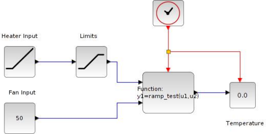
Chapter 5
Identification of Transfer Function
of a Single Board Heater System
through Ramp Response
Experiment
The aim of this experiment is to perform ramp test on a Single Board Heater
System and to identify system transfer function using ramp response data. The
target group is anyone who has basic knowledge of control engineering.
We have used Scilab and Xcos as an interface for sending and receiving data.
Xcos diagram is shown in figure 5.1. Heater current and fan speed are the two
inputs for this system. They are given in percentage of maximum. These inputs
Figure 5.1: Xcos for ramp test experiment
66
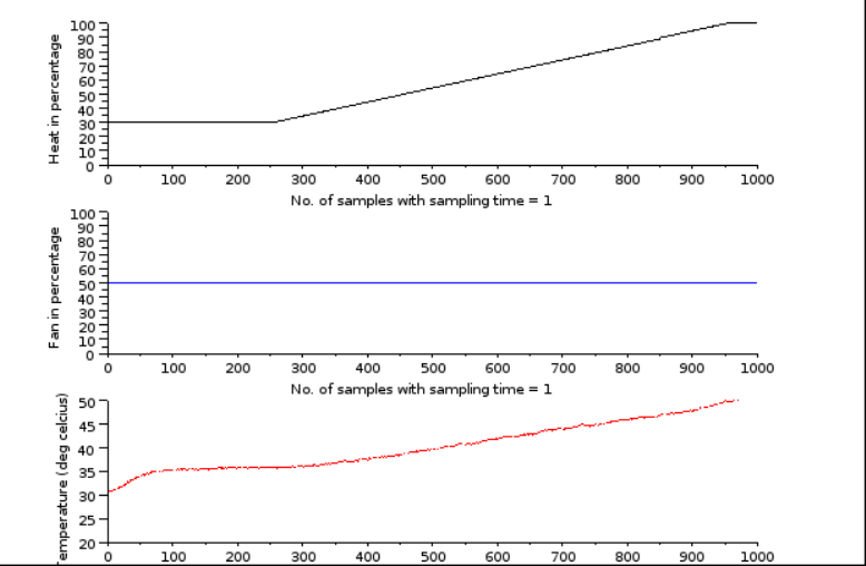
Figure 5.2: Screen shot of ramp test experiment
67

1.0 30.0 50.0 28.1 1416462726532.0
2.0 30.0 50.0 28.1 1416462727574.0
.
999.0 100.0 50.0 47.6 1416463723533.0
1000.0 100.0 50.0 47.6 1416463724533.0
Table 5.1: Ramp data obtained after performing local Step Test
can be varied by setting the properties of the input block’s properties in Xcos.
The plots of their amplitude versus number of collected samples are also available
on the scope windows. The output temperature profile, as read by the sensor, is
also plotted. The data acquired in the process is stored on the local drive and is
available to the user for further calculations.
In the ramp test.xcos file, open the heater block’s parameters to give a ramp
input to the system with some value for slope. For this experiment, we have cho-
sen slope =0.1. Double click on the ramp input block labled as Heater input.
Change the following values in the respective fields: slope =0.1, start time =200,
initial output =20. Keep the fan constant at 100.
The ramp test data file will be saved in Ramp Test folder. The name of the
file will be the date and time at which the experiment was conducted. A sam-
ple data file is provided in the same folder. The sample data file is named as
ramp-data-local.txt and ramp-data-virtual.txt. Refer to the one de-
pending on wheather you are performing a local or a virtual experiment. Refer-
ring to the data file thus obtained as shown in table 6.2, the first column in this
table denotes samples. The second column in this table denotes heater in percent-
age. It starts at 30 and increases with a step size of 10 units. The third column
denotes the fan in percentage. It has been held constant at 50 percent. The fourth
column refers to the value of temperature. The fifth column denotes time stamp.
The virtual data file will have four time stamp columns apart from first 3 columns.
These four time stamp columns are client departure, server arrival, server depar-
ture and client arrival. These can be used for advanced control algorithms. These
additional time stamps exist in virtual mode because of the presense of network
delay.
68

5.1 Conducting Ramp Test on SBHS locally
The detailed procedure to perform a local experiment is explained in Chapter2.
A summary of the same is provided in section 2.3 It is same for this section with
following changes.
1. Step1: The working directory is Ramp test
2. Step2: Same
3. Step3: Same
4. Step4: Same
5. Step5: Load ramp test function by executing command
exec<space>ramp test.sci
6. Step6: Load Xcos code for ramp test using the command
exec<space>ramp test.xcos
7. Step7: Same
5.2 Conducting Ramp Test on SBHS, virtually
The detailed procedure to perform a virtual experiment is explained in Chapter3.
A summary of the same is provided in section 3.5. It is same for this section with
following changes.
1. Step1: The working directory is RampTest. Open this directory.
2. Step2: Same
3. Step3: Same
4. Step4: Switch to the RampTest experiment directory and double-click on
the file ramptest.sce. This will launch scilab and also open the file
ramptest.sce in the scilab editor. Linux users will have to launch scilab
manually. They also have to change the working directory to RampTest and
then open the RampTest file in the scilab editor.
5. Step5: Same
69
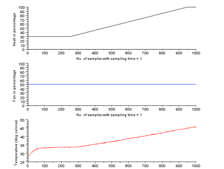
Figure 5.3: Ramp test Virtual experiment response
6. Step6: Execute the file ramptest.sce. Expect the ramp test xcos diagram
to open automatically. If this doesnt happen, check the scilab console for
error message.
7. Step7: Execute the ramptest xcos diagram.
8. Step8: Same
The virtual experiment response is shown in figure 5.3. The corresponding
data file is shown in table 6.2. The time stamps shown are cut short for better
viewing. This data file can be found in RampTest folder for virtual experiments.
The name of this file is step-data-virtual.txt.
70

0 0 100 28.80 14...8993 14...0301 14...0318 14...9040 0.10000E+01
1 30 50 28.80 14...2861 14...4172 14...4189 14...2908 0.10000E+01
.
.
617 66 50 39.10 14...7141 14...8476 14...8494 14...7188 0.61700E+03
618 66 50 39.10 14...8120 14...9456 14...9473 14...8167 0.61800E+03
Table 5.2: Ramp data obtained after performing virtual Ramp Test
5.3 Identifying First Order Transfer Function
In this section we shall determine the first order transer function model using the
data obtained after performing step test experiment. Please note that this proce-
dure is common for data obtained using both local and virtual experiments.
Identification of the transfer function of a system is important as it helps us
to represent the physical system mathematically. Once the transfer function is
obtained, one can acquire the response of the system for various inputs without
actually applying them to the system. Consider the standard first order transfer
function given below
G(s)=C(s)
R(s)(5.1)
G(s)=K
τs+1(5.2)
Combining the previous two equations, we get
C(s)=K(R(s)
τs+1)(5.3)
Let us consider the case of giving a ramp input to this first order system. The
Laplace transform of a ramp function with slope =υis υ
s2. Substituting R(s)=υ
s2
in equation 5.3, we obtain
C(s)=K
τs+1
υ
s2(5.4)
=A
s+B
s2+C
τs+1(5.5)
71

Solving C(s) using Heaviside expansion approach, we get
C(s)=Kυ(1
s2−τ
s+τ2
τs+1)(5.6)
Taking the Inverse Laplace transform of the above equation, we get
c(t)=Kυnt−τ+τe−t
τo(5.7)
The difference between the reference and output signal is the error signal e(t).
Therefore,
e(t)=r(t)−c(t) (5.8)
e(t)=Kυt−Kυt+Kυτ−Kυτe−t
τ(5.9)
e(t)=Kυτ(1 −e−t
τ) (5.10)
Normalizing equation 5.10 for t>> τ, we get
e(t)=τ(5.11)
This means that the error in following the ramp input is equal to τfor large value
of t[7]. Hence, smaller the time constant τ, smaller the steady state error.
5.3.1 Procedure
1. Download the Analysis folder from the sbhs website. It will be available
under downloads section. Download the file for SBHS Analysis Code
(local & virtual). The name of the file is scilab codes analysis.
The download will be in zip format. Extrat the downloaded zip file. You
will get a folder scilab codes analysis.
2. Open the scilab codes analysis folder and then locate and open the
folder Ramp Analysis.
3. Copy the ramp test data file to this folder.
4. Change the Scilab working directory to Ramp Analysis
5. Open the file ramp virtual.sce in scilab editor and enter the name of the
data file (with extention) in the filename field.
72
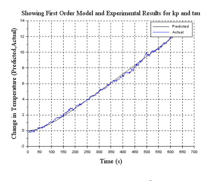
Figure 5.4: Output of the Scilab code ramp virtual.sce
73
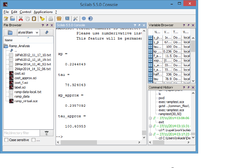
Figure 5.5: Scilab console after executing coderamp virtual.sce
74

6. Save and run this code and obtain the plot as shown in figure 5.4.
This code uses the routines label.sci and costf 1.sci
The results presented are obtained for the data file ramp-data-virtual.txt.
This data file is present under the Ramp Test directory for local experiments. The
plot thus obtained is reasonably good. See the Scilab console to get the values of
τand K. It is as shown in figure 5.5 The figure 5.4 shows a screen shot of the
same. We obtain τ=78.92, K =0.22. The transfer function obtained here is at
the operating point of enterValue percentage of heat. If the experiment is repeated
at a different operating point, the transfer function obtained will be different. The
gain will correspondingly be more at a higher operating point. This means that the
plant is faster at higher temperature. Thus the transfer function of the plant varies
with the operating point. Let the transfer function we obtain in this experiment be
denoted as Gs. We obtain
Gs(s)=0.22
78.92s+1(5.12)
5.4 Discussion
We summarize our findings now. The experiment has been performed by vary-
ing the heater current and keeping the fan speed constant. However, the user is
encouraged to experiment using different combinations of fan speed and heater
current. Negative ramp can also be used to make the experiment more informa-
tive. It is not necessary to keep a particular input constant. For example, you can
try giving a ramp input to the disturbance signal, i.e., the fan input. The system
can also be treated as a second order system. This consideration is necessary as it
increases the accuracy of the acquired transfer function [6].
The necessary codes are listed in the section 5.5.
5.5 Scilab Code
Scilab Code 5.1 ramp test.sci
1mode ( 0 )
75

2function temp =r a m p t e s t ( hea t , f a n )
3temp =comm( h e a t , f a n ) ;
4
5p l o t t i n g ( [ h e a t f a n temp ] , [ 0 0 20 0 ] , [ 1 0 0 100 50
1 0 0 0 ] )
6
7m=m+1;
8endfunction
Scilab Code 5.2 label.sci
1mode (−1) ;
2/ / Updated (9 −1 2 −0 6 ) , w r i t t e n b y I n d e r p r e e t A r o r a
3/ / I n p u t a r g u m e n t s : t i t l e , x l a b e l , y l a b e l a n d t h e i r
f o n t s i z e s
4
5function l a b e l ( tname , t f o n t , l a b e l x , l a b e l y , x y f o n t )
6a=get ( ” c u r r e n t a x e s ” )
7xtitle ( tname , l a b e l x , l a b e l y )
8xgrid
9t=a . t i t l e ;
10 t . f o n t s i z e =t f o n t ; / / T i t l e f o n t s i z e
11 t . f o n t s t y l e =2 ; / / T i t l e f o n t s t y l e
12 t . t e x t =tname ;
13
14 u=a . x l a b e l ;
15 u . f o n t s i z e =xyfont ; / / L a b e l f o n t s i z e
16 u . f o n t s t y l e =2 ; / / L a b e l f o n t s t y l e
17
18 v=a . y l a b e l ;
19 v . f o n t s i z e =xyfont ; / / L a b e l f o n t s i z e
20 v . f o n t s t y l e =2 ; / / L a b e l f o n t s t y l e
21
22 / / a . l a b e l f o n t s i z e =3 ;
23
24 endfunction ;
Scilab Code 5.3 cost.sci
76

1function f=f u n c 1 ( x )
2k=x ( 1 ) ;
3t a u =x ( 2 ) ;
4y prediction =k*( t +t a u *(exp(−t/t a u ) −1 ) ) ;
5f=(norm ( y −y p r e d i c t i o n , 2 ) ) ˆ 2 ;
6endfunction
7
8function [ f , g , i n d 1 ] =c o s t ( x , i n d 1 )
9k=x ( 1 ) ;
10 t a u =x ( 2 ) ;
11 y prediction =k*( t +t a u *(exp(−t/t a u ) −1 ) ) ;
12 f=(norm ( y −y p r e d i c t i o n , 2 ) ) ˆ 2 ;
13 g=numdiff ( f u n c 1 , x ) ;
14 endfunction
Scilab Code 5.4 cost approx.sci
1function f=f u n c a p p r o x ( x )
2k=x ( 1 ) ;
3t a u =x ( 2 ) ;
4y p a p p r o x =k*( t a p p r o x −t a u ) ;
5f=(norm ( y a p p r o x −y p a p p r o x , 2 ) ) ˆ 2 ;
6endfunction
7
8function [ f , g , i n d ] =c o s t a p p r o x ( x , i n d )
9k=x ( 1 ) ;
10 t a u =x ( 2 ) ;
11 y p a p p r o x =k*( t a p p r o x −t a u ) ;
12 f=(norm ( y a p p r o x −y p a p p r o x , 2 ) ) ˆ 2 ;
13 g=numdiff ( f u n c a p p r o x , x ) ;
14 endfunction
Scilab Code 5.5 ramptest.sci
1function [ s t o p ] =r a m p t e s t ( h ea t , f a n )
2
3[ s t o p , temp ] =comm ( h e a t , f a n ) ; / / N e v e r e d i t t h i s
line
77

4p l o t t i n g ( [ h e a t f a n temp ] , [ 0 0 25 0 ] , [ 1 0 0 100 50
1 0 0 0 ] )
5
6endfunction
Scilab Code 5.6 ramptest.sce
1mode ( 0 )
2global f d f h f d t f n c r fncw m e r r c o u n t y l i m i t s
s a m p l i n g t i m e m
3
4/ / **********************
5s a m p l i n g t i m e =1; / / I n s e c o n d s . F r a c t i o n s a r e a l l o w e d
6/ / **********************/ /
7e x e c ( ” r a m p t e s t . s c i ” ) ;
8
9ok =i n i t ( ) ;
10
11 i f ok ˜=[ ] / / o p e n x c o s o n l y i f c o m m u n i c a t i o n i s
t h r o u g h ( i e r e p l y h a s c o m e f r o m s e r v e r )
12 xco s ( ’ r a m p t e s t . x c os ’ ) ;
13 else
14 d i s p ( ”NO NETWORK CONNECTION! ” ) ;
15 r e t u r n
16 end
Scilab Code 5.7 ramp virtual.sce
1mode (−1) ;
2
3/ / filename =” 2 0 A p r 2 0 1 2 1 5 1 0 3 5 . t x t ” ; / / complete
p a t h o f t h e s a v e d d a t a f i l e
4f i l e n a m e =” ramp −d a t a −l o c a l . t x t ” ;
5slope =0 . 1 ; / / c h a n g e t h i s t o t h e s l o p e t h a t y o u h a v e
u s e d i n t h e e x p e r i m e n t
6i n d 1 =3;
7/ / R a m p A n a l y s i s
8e x e c ( ’ c o s t a p p r o x . s c i ’ ) ;
78

9e x e c ( ’ c o s t . s c i ’ ) ;
10 e x e c ( ’ l a b e l . s c i ’ ) ;
11
12 d a t a =fscanfMat ( f i l e n a m e ) ;
13 t i m e =d a t a ( : , 5 ) ;
14 heater =int ( d a t a ( : , 2 ) ) ;
15 fan =i n t ( d a t a ( : , 3) ) ;
16 temp =d a t a ( : , 4 ) ;
17
18
19 l e n =length ( h e a t e r ) ;
20 heaters1 =[ h e a t e r ( 1 ) ; h e a t e r ( 1 : $ −1) ] ;
21 d e l h e a t =abs ( heater −heaters1 ) ;
22 i n d =f i n d ( d e l h e a t >. 5 ) ;
23
24 t=t i m e ( i n d ( 2 ) : i n d ( $ −1) ) ;
25 t=t/1000
26 H=h e a t e r ( i n d ( 2 ) : i n d ( $ −1) ) ;
27 T=temp ( i n d ( 2 ) : i n d ( $ −1) ) ;
28
29 t=t−t ( 1 ) ;
30 T=T−T ( 1 ) ;
31
32 y=T ;
33 x0 =[ . 5 1 00]
34 global ( ’ y ’ , ’ t ’ ) ;
35
36 [ f , x o p t ] =optim ( c o s t , x0 ) ;
37 kp =x o p t ( 1 ) /slope
38 t a u =x o p t ( 2 )
39
40 l e n =length ( t ) ;
41 halfway =c e i l ( l e n /2 ) ;
42
43 t approx =t ( h a l f w a y : l e n ) ;
44 y approx =y ( h a l f w a y : l e n ) ;
45 global ( ’ y a p p ro x ’ , ’ t a p p r o x ’ ) ;
46
79

47 [ f a p p r o x , x o p t a p p r o x ] =optim ( c o s t a p p r o x , x0 ) ;
48 k p a p p r o x =x o p t a p p r o x ( 1 ) /s l o p e ;
49 tau approx =x o p t a p p r o x ( 2 ) ;
50
51 / / D i s p l a y a n d P l o t
52 d i s p ( ’ kp =’ ) ;
53 d i s p ( kp ) ;
54 d i s p ( ’ t a u =’ ) ;
55 d i s p ( t a u ) ;
56 d i s p ( ’ k p a p p r o x =’ ) ;
57 d i s p ( k p a p p r o x ) ;
58 d i s p ( ’tau approx =’ ) ;
59 d i s p ( t a u a p p r o x ) ;
60
61 y p =kp*slope *( t +t a u *(exp(−t/t a u ) −1 ) ) ;
62 y p a p p r o x =kp approx*slope *( t approx −tau approx ) ;
63 y p a p p r o x =y p a p p r o x ’ ;
64 plot2d ( t , [ y p , T ] ) ;
65 l a b e l ( ’ Showing F i r s t O rder Model and E x p e r i m e n t a l
R e s u l t s f o r kp and t a u ’ , 4 , ’ Time ( s ) ’ , ’ Change i n
T e m p e r a t u r e ( P r e d i c t e d , A c t u a l ) ’ , 4 ) ;
66 l e g e n d ( [ ’ P r e d i c t e d ’ ; ’ A c t u a l ’ ] ) ;
80

Chapter 6
Frequency Response Analysis of a
Single Board Heater System by the
Application of Sine Wave
The aim of this experiment is to do a frequency response analysis of a Single
Board Heater System by the application of sine wave. The target group is anyone
who has basic knowledge of control engineering.
We have used Scilab and Xcos as an interface for sending and receiving data.
Xcos diagram is shown in figure 6.1. The heater current is varied sinusoidally.
They are given in percentage of maximum. These inputs can be varied by setting
the properties of the input block’s properties in Xcos. A provision is made to set
the parameters related to it like frequency, amplitude and offset. The temperature
profile thus obtained is the output. In this experiment we are applying a sine
change in the heater current by keeping the fan speed constant. After application
of sine change, wait for sufficient amount of time to allow the temperature to reach
a steady-state. The plots of their amplitude versus number of collected samples
are also available on the scope windows. The output temperature profile, as read
by the sensor, is also plotted. The data acquired in the process is stored on the
local drive and is available to the user for further calculations.
In the sine test.xcos file, open the sinusoid generator block’s param-
eters to set the value of sine magnitude and frequency. For the experiment results
shown, we have chosen Magnitude =10, Frequency =2∗3.14 ∗0.007. Note that
the frequency is to be put in rad/sec. We keep the Phase =0. There is also a
provision to give the sine input with an offset in amplitude. This can be set using
the Offset block. We have choosen offset of 20. The time at which the sine input
81
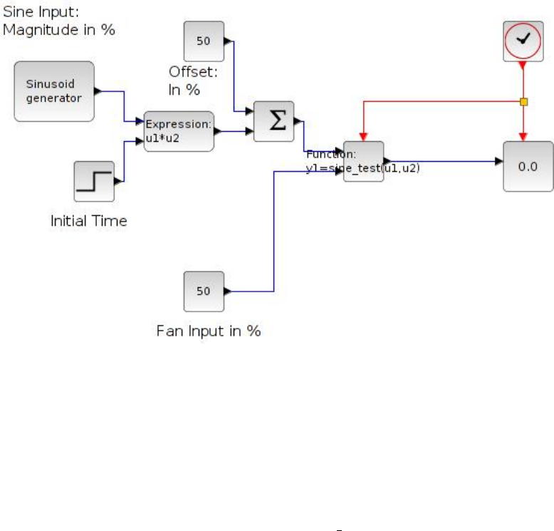
Figure 6.1: Xcos for local Sine Test
is given after the experiment is started can also be set. This can be done using the
Initial Time block. Open the Initial Time block’s parameters. To make the
sine input appear after 200 samples of start of the experiment, keep Step time =
200, Initial Value =0 and Final Value =1. The initial value and final value will
never change for any other value of step time.
The sine test data file will be saved in Sine Test folder. The name of the
file will be the date and time at which the experiment was conducted. A sam-
ple data file is provided in the same folder. The sample data file is named as
sine-data-local.txt and sine-data-virtual.txt. Refer to the one de-
1.0 20.0 50.0 20.0 1416642805261.0
2.0 20.0 50.0 20.0 1416642806332.0
.
13093.0 28.5 50.0 26.6 1416656557353.0
13094.0 28.5 50.0 26.6 1416656558363.0
Table 6.1: Data obtained after application of sine input of 0.007Hz
82
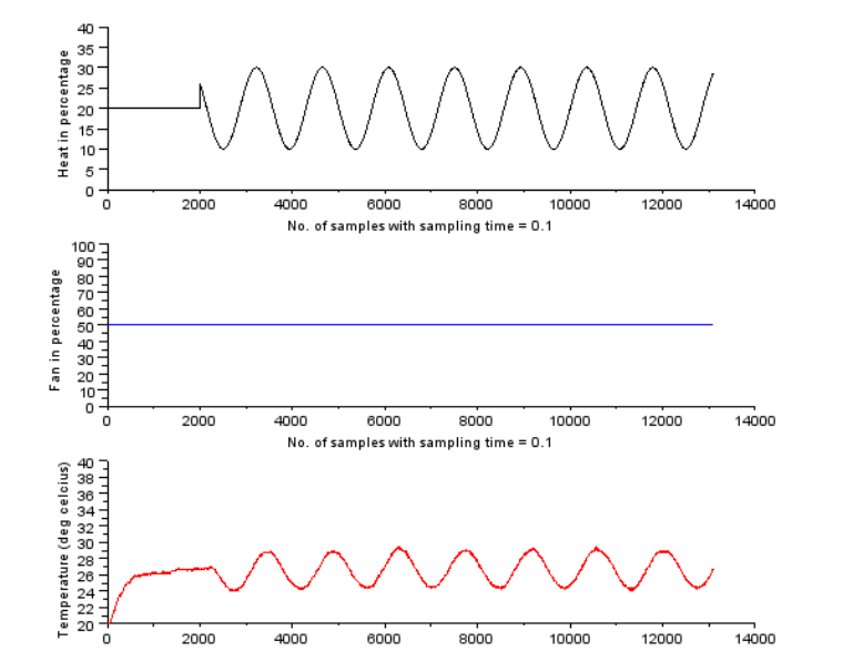
Figure 6.2: Plot for sine input 0.007Hz
83

pending on wheather you are performing a local or a virtual experiment. Referring
to the data file thus obtained as shown in table 6.1, the first column in this table
denotes samples. The second column in this table denotes heater in percentage.
It starts at 20 and then varies sinosoidally. The third column denotes the fan in
percentage. It has been held constant at 50 percent. The fourth column refers to
the value of temperature. The fifth column denotes time stamp. The virtual data
file will have four time stamp columns apart from first 3 columns. These four time
stamp columns are client departure, server arrival, server departure and client ar-
rival. These can be used for advanced control algorithms. These additional time
stamps exist in virtual mode because of the presense of network delay.
6.1 Conducting Sine Test on SBHS locally
The detailed procedure to perform a local experiment is explained in Chapter2.
A summary of the same is provided in section 2.3 It is same for this section with
following changes.
1. Step1: The working directory is Sine test
2. Step2: Same
3. Step3: Same
4. Step4: Same
5. Step5: Load sine test function by executing command
exec<space>sine test.sci
6. Step6: Load Xcos code for sine test using the command
exec<space>sine test.xcos
7. Step7: Same
6.2 Conducting Sine Test on SBHS, virtually
The detailed procedure to perform a local experiment is explained in Chapter3. A
summary of the same is provided in section 3.5. It is same for this section with
following changes.
84
0 0 100 28.80 14...4739 14...6427 14...6445 14...4786 0.10000E+01
1 20 50 28.90 14...5247 14...6938 14...6956 14...5294 0.10000E+01
.
.
999 18 50 31.00 14...2253 14...3973 14...3990 14...2299 0.99900E+03
1000 19 50 31.00 14...3268 14...4989 14...5007 14...3315 0.10000E+04
Table 6.2: Sine data obtained after performing virtual Sine Test
1. Step1: The working directory is SineTest. Open this directory.
2. Step2: Same
3. Step3: Same
4. Step4: Switch to the SineTest experiment directory and double-click on
the file sinetest.sce. This will launch scilab and also open the file
sinetest.sce in the scilab editor. Linux users will have to launch scilab
manually. They also have to change the working directory to SineTest and
then open the sinetest.sce file in the scilab editor.
5. Step5: Same
6. Step6: Execute the file sinetest.sce. Expect the sine test xcos diagram
to open automatically. If this doesnt happen, check the scilab console for
error message.
7. Step7: Execute the sinetest xcos diagram.
8. Step8: Same
The virtual experiment response is shown in figure 6.3. The corresponding
data file is shown in table 6.1. The time stamps shown are cut short for better
viewing. This data file can be found in SineTest folder for virtual experiments.
The name of this file is sine-data-virtual.txt.
6.3 Frequency Analysis of sine test data
Frequency response of a system means its steady-state response to a sinusoidal
input. For obtaining a frequency response of a system, we vary the frequency of
85
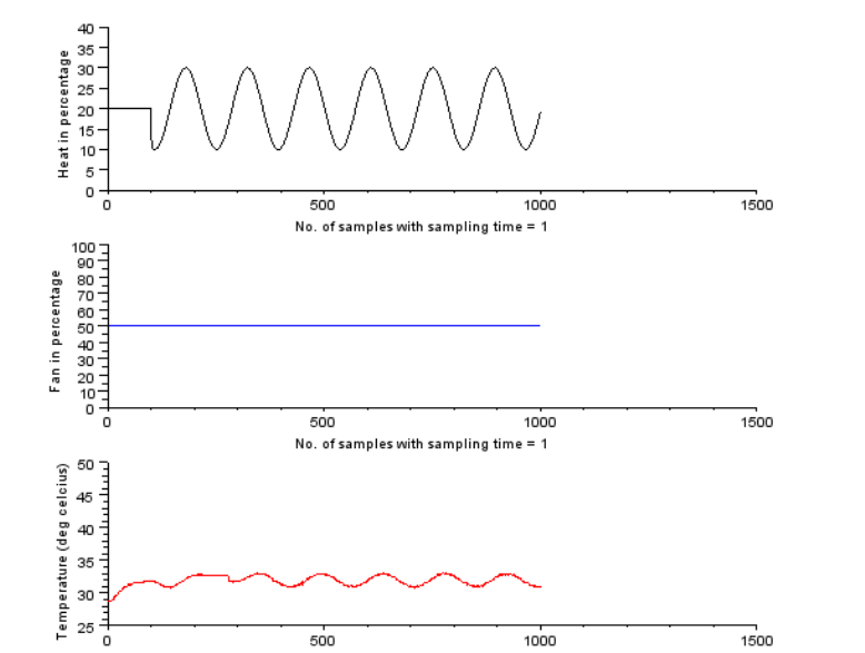
Figure 6.3: Sine test Virtual experiment response
86

the input signal over a spectrum of interest. The analysis is useful and simple
because it can be carried out with the available signal generators and measuring
devices. Let us see the theory and procedure. Please note that this procedure is
common for data obtained using both local and virtual experiments.
Consider a sinusoidal input
U(t)=Asinωt(6.1)
The Laplace transform of the above equation yields
U(s)=Aω
s2+ω2(6.2)
Consider the standard first order transfer function given below
G(s)=Y(s)
U(s)=K
s+1(6.3)
Replacing the value of U(s) from equation 6.2, we get
Y(s)=KAω
(τs+1)(s2+ω2)(6.4)
=KA
ω2τ2+1"ωτ2
τs+1−τsω
s2+ω2+ω
s2+ω2#(6.5)
Taking Laplace Inverse, we get
y(t)=KA
ω2τ2+1hωτe−t
τ−ωτcos(ωt)+sin(ωt)i(6.6)
The above equation has an exponential term e−t
τ. Hence, for large value of time,
its value will approach to zero and the equation will yield a pure sine wave. One
can also use trigonometric identities to make the equation look more simple.
y(t)="KA
√ω2τ2+1#sin(ωt)+φ(6.7)
where,
φ=−tan−1(ωτ) (6.8)
87

By observing the above equation, one can easily make out that for a sinusoidal
input the output is also sinusoidal but has some phase difference. Also, the ampli-
tude of the output signal, ˆ
A, has become a function of the input signal frequency,
ω.
ˆ
A=KA
√ω2τ2+1(6.9)
The amplitude ratio (AR) can be calculated by dividing both sides by the input
signal amplitude A.
AR =ˆ
A
A=K
√ω2τ2+1(6.10)
Dividing the above equation by the process gain K yields the normalized ampli-
tude ratio (ARn)
ARn=AR
K=1
√ω2τ2+1(6.11)
Because the process steady state gain is constant, the normalized amplitude ratio
is often used for frequency response analysis [8].
6.3.1 Procedure
Now let us calculate amplitude ratio and phase difference.
1. Download the Analysis folder from the sbhs website. It will be available
under downloads section. Download the file for SBHS Analysis Code
(local & virtual). The name of the file is scilab codes analysis.
The download will be in zip format. Extrat the downloaded zip file. You
will get a folder scilab codes analysis.
2. Open the scilab codes analysis folder and then locate and open the
folder Sine Analysis.
3. Copy the sine test data file to this folder.
4. Change the Scilab working directory to Sine Analysis
88
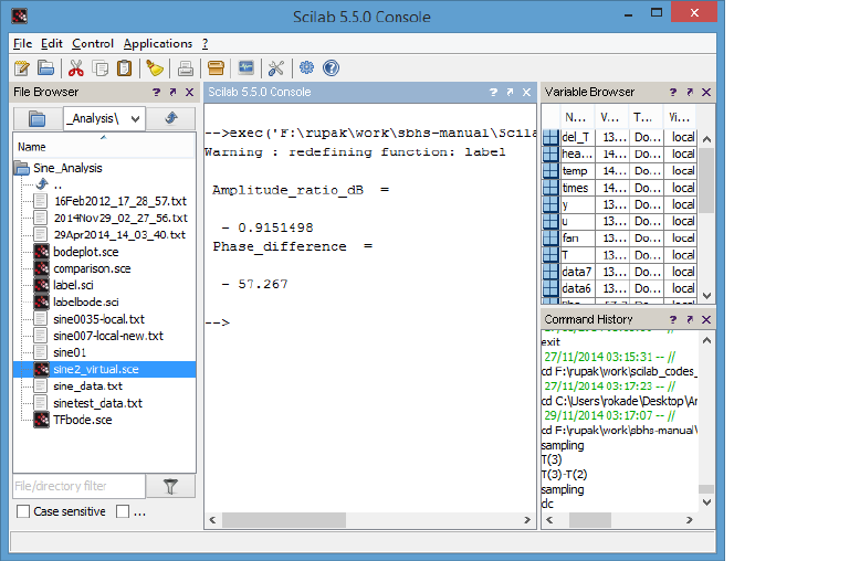
Figure 6.4: Amplitude ratio and Phase difference for local data file
5. Open the file sine-analysis.sce in scilab editor and enter the name of
the data file (with extention) in the filename field.
6. Put the value of frequency ffor the calculation of amplitude ratio and phase
difference and execute it. Here fmeans input frequency.
7. Expect the values of amplitude ratio and phase difference on the scilab con-
sole.
The results shown are for the data file sine-data-local.txt. It could be seen from
figure 6.4 that the amplitude ratio turns out to be −0.915dB and phase difference
to be −57.267°. The plot thus obtained is shown in figure 6.5
Repeat this calculation over a range of frequencies and note down the values of
amplitude ratio in dB and phase difference. Input these values for the appropriate
frequencies into the Scilab code TFbode.sce and execute it to get a Bode plot of
the plant which is illustrated in figure 6.6.
Bode plot can be obtained directly from the plant’s second order transfer func-
tion [6] with the help of Scilab code TFbode.sce, as shown in figure 6.7. A visual
89
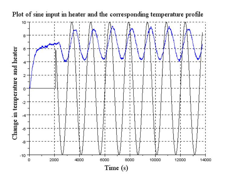
Figure 6.5: Plot of Input and Output vs time
90
Figure 6.6: Bode plot obtained from the plant
91
Figure 6.7: Bode plot obtained through plant’s transfer function
comparison of the two Bode plots can be done to validate the Bode diagram ob-
tained from the plant.
To compare the two plots, we plot it on the same graph as shown in figure 6.8
6.4 Scilab Code
Scilab Code 6.1 sine test.sci
1mode ( 0 )
2function temp =s i n e t e s t ( h e a t , f a n )
3temp =comm( h e a t , f a n ) ;
4
92
Figure 6.8: Comparison of Bode plots
93

5p l o t t i n g ( [ h e a t f a n temp ] , [ 0 0 20 0 ] , [ 1 0 0 100 40
1 0 0 0 ] )
6
7m=m+1;
8endfunction
Scilab Code 6.2 sinetest.sce
1mode ( 0 )
2global f d f h f d t f n c r fncw m e r r c o u n t y l i m i t s
s a m p l i n g t i m e m
3
4/ / **********************
5s a m p l i n g t i m e =1; / / I n s e c o n d s . F r a c t i o n s a r e a l l o w e d
6/ / **********************/ /
7e x e c ( ” s i n e t e s t . s c i ” ) ;
8
9ok =i n i t ( ) ;
10
11 i f ok ˜=[ ] / / o p e n x c o s o n l y i f c o m m u n i c a t i o n i s
t h r o u g h ( i e r e p l y h a s c o m e f r o m s e r v e r )
12 xco s ( ’ s i n e t e s t . x c os ’ ) ;
13 else
14 d i s p ( ”NO NETWORK CONNECTION! ” ) ;
15 r e t u r n
16 end
Scilab Code 6.3 sinetest.sci
1function [ s t o p ] =s i n e t e s t ( h e a t , f a n )
2
3[ s t o p , temp ] =comm ( h e a t , f a n ) ; / / N e v e r e d i t t h i s
line
4p l o t t i n g ( [ h e a t f a n temp ] , [ 0 0 25 0 ] , [ 1 0 0 100 50
1 0 0 0 ] )
5
6endfunction
94

Scilab Code 6.4 sine-analysis.sce
1mode ( 0 ) ;
2f i l e n a m e =’sine0035−l o c a l . t x t ’ ; / / E n t e r t h e d a t a f i l e
n a m e i n s i n g l e q u o t e s
3f=0.0035; / / E n t e r t h e f r e q u e n c y
4data6=fscanfMat ( f i l e n a m e ) ;
5data7=d a t a 6 ( 2 : $ , : ) ;
6e x e c ( ’ l a b e l b o d e . s c i ’ ) ;
7T=d a t a 7 ( : , 5 ) ; f a n =d a t a 7 ( : , 3 ) ; / / T i s t i m e , f a n i s
f a n s p e e d
8u=d a t a 7 ( : , 2 ) −d a t a 7 ( 1 , 2 ) ; y =d a t a 7 ( : , 4 ) −d a t a 7 ( 1 , 4 ) ;
/ / u i s c u r r e n t , y i s t e m p e r a t u r e
9
10
11 period=c e i l ( 1 /f ) ;
12 p=length ( u ) ;
13 sampling =T ( 2 ) −T ( 1 ) ; / / s a m p l i n g t i m e
14 sampling =sampling /1000;
15 index =round ( ( p e r i o d ) /sampling ) ; / / c a l c u l a t i n g t h e
d u r a t i o n o f l a s t c y c l e o f w a v e f o r m
16 times=T ( $−i n d e x : $ ) ;
17 temp =y ( $−i n d e x : $ ) ; / / o u t p u t f o r l a s t c y c l e
18 heater =u ( $−i n d e x : $ ) ; / / i n p u t f o r l a s t c y c l e
19 [ m a x h e a t e r , p o i n t e r 1 ] =max ( h e a t e r ) ; / / d e t e r m i n i n g m a x
a m p l i t u d e a n d i n d e x f o r l a s t c y c l e o f i n p u t ( i n d e x
i s r e l a t i v e t o l a s t c y c l e )
20 [ max temp , p o i n t e r 2 ] =max ( temp ) ; / / d e t e r m i n i n g m a x
a m p l i t u d e a n d i n d e x f o r l a s t c y c l e o f i n p u t ( i n d e x
i s r e l a t i v e t o l a s t c y c l e )
21 pointer1 =pointer1 +( p−i n d e x ) ; / / c o n v e r s i o n o f i n d e x
f o r i n p u t i n t e r m s o f c o m p l e t e d a t a p e r i o d
22 pointer2 =pointer2 +( p−i n d e x ) ; / / c o n v e r s i o n o f i n d e x
f o r o u t p u t i n t e r m s o f c o m p l e t e d a t a p e r i o d
23 A m p l i t u d e r a t i o d B =20*log10 (y( pointer2 ) /u( pointer1 ) )
/ / T o f i n d g a i n i n d B
24 Phase difference =360*f*( pointer1 −pointer2 )*sampling
/ / p h a s e d i f f e r e n c e i n d e g r e e s
95

25 / / Phase difference =−( ( p o i n t e r 1 −pointer2 ) /( 1 /f))*360
26
27
28 d e l T =T−T ( 1 ) ;
29 d e l T =d e l T /1000;
30 plot2d ( del T , [ u y ] ) ;
31 l a b e l ( ’ P l o t o f s i n e i n p u t i n h e a t e r and t h e
c o r r e s p o n d i n g t e m p e r a t u r e p r o f i l e ’ , 4 , ’ Time ( s ) ’ , ’
Change i n t e m p e r a t u r e and h e a t e r ’ , 4 ) ;
32 / / l e g e n d ( [ ’ H e a t e r ’ ; ’ T e m p e r a t u r e ’ ] ) ;
Scilab Code 6.5 label.sci
1/ / Updated (9 −1 2 −0 6 ) , w r i t t e n b y I n d e r p r e e t A r o r a
2/ / I n p u t a r g u m e n t s : t i t l e , x l a b e l , y l a b e l a n d t h e i r
f o n t s i z e s
3function l a b e l ( tname , t f o n t , l a b e l x , l a b e l y , x y f o n t )
4a=get ( ” c u r r e n t a x e s ” )
5xtitle ( tname , l a b e l x , l a b e l y )
6xgrid
7t=a . t i t l e ;
8t . f o n t s i z e =t f o n t ; / / T i t l e f o n t s i z e
9t . f o n t s t y l e =2 ; / / T i t l e f o n t s t y l e
10 t . t e x t =tname ;
11 u=a . x l a b e l ;
12 u . f o n t s i z e =xyfont ; / / L a b e l f o n t s i z e
13 u . f o n t s t y l e =2 ; / / L a b e l f o n t s t y l e
14 v=a . y l a b e l ;
15 v . f o n t s i z e =xyfont ; / / L a b e l f o n t s i z e
16 v . f o n t s t y l e =2 ; / / L a b e l f o n t s t y l e
17 / / a . l a b e l f o n t s i z e =3 ;
18 endfunction ;
Scilab Code 6.6 bodeplot.sce
1/ / bodeplot
2e x e c ( ’ l a b e l b o d e . s c i ’ ) ;
3x=[0.001 ,0.0035 ,0.004 ,0.005 ,0.006 ,0.007 ,...
96

40.008 ,0.009 ,0.01 ,0.02 ,0.03 ,0.04]; / / I n p u t f r e q u e n c y ( H z )
5y=[−3.87 , −5 . 6 7 , −7.53 , −7.53 , −8 . 1 7 , −8.64 ,...
6−8 . 8 7 , −8 . 9 0 , −9 . 1 1 , −1 3 . 5 5 , −1 5 . 3 9 , −16.47]; / / Amplitude
r a t i o ( d B )
7subplot ( 2 , 1 , 1 ) ;
8plot2d ( x , y , r e c t =[0.001 , −2 0 , 0 . 0 4 , 0 ] , l o g f l a g =” l n ” ) ;
9xgrid ( ) ;
10 y=[−2 5 . 2 , −2 8 . 9 8 , −3 3 . 1 1 , −4 1 . 4 , −6 0 . 4 8 , −70.56 ,...
11 −77.76 , −87.4 8 , −9 0 , −1 2 9 . 6 , −1 5 1 . 2 , −172.8]; / / Phase
d i f f e r e n c e ( d e g r e e )
12 title =’ ’
13 l a b e l ( t i t l e , 4 , ’Hz ’ , ’ Amp l i tud e r a t i o i n dB ’ , 4 ) ;
14 subplot ( 2 , 1 , 2 ) ;
15 plot2d ( x , y , r e c t =[0.001 , −180 ,0.04 , −2 0 ] , l o g f l a g =” l n ” ) ;
16 l a b e l ( t i t l e , 4 , ’ ’ , ’ P h ase d i f f e r e n c e ’ , 4 ) ;
17 subplot ( 2 , 1 , 2 ) ;
18 xgrid ( ) ;
19
20 / / s=p o l y ( 0 , ’ s ’ )
21 / / h=s y s l i n ( ’ c ’ , ( 0 . 4 7 5 /(124.827*s ˆ 2 +57.26*s+1 ) ) )
22 / / b o d e ( h , 0 . 0 0 1 , 0 . 0 4 ) ;
Scilab Code 6.7 labelbode.sci
1/ / Updated (9 −1 2 −0 6 ) , w r i t t e n b y I n d e r p r e e t A r o r a
2/ / I n p u t a r g u m e n t s : t i t l e , x l a b e l , y l a b e l a n d t h e i r
f o n t s i z e s
3
4function l a b e l ( tname , t f o n t , l a b e l x , l a b e l y , x y f o n t )
5a=get ( ” c u r r e n t a x e s ” )
6xtitle ( tname , l a b e l x , l a b e l y )
7xgrid
8t=a . t i t l e ;
9t . f o n t s i z e =t f o n t ; / / T i t l e f o n t s i z e
10 t . f o n t s t y l e =2 ; / / T i t l e f o n t s t y l e
11 t . t e x t =tname ;
12 u=a . x l a b e l ;
13 u . f o n t s i z e =xyfont ; / / L a b e l f o n t s i z e
97

14 u . f o n t s t y l e =2 ; / / L a b e l f o n t s t y l e
15 v=a . y l a b e l ;
16 v . f o n t s i z e =xyfont ; / / L a b e l f o n t s i z e
17 v . f o n t s t y l e =2 ; / / L a b e l f o n t s t y l e
18 / / a . l a b e l f o n t s i z e =3 ;
19 endfunction ;
Scilab Code 6.8 TFbode.sce
1s=p o l y ( 0 , ’ s ’ )
2d t =10; / / d e l a y t i m e
3/ / h=s y s l i n ( ’ c ’ , ( ( 0 . 5 1 0 /( 6 5 . 4 9 *s+1 ) ) ) ) / / transfer
f u n c t i o n u s i n g f i r s t o r d e r p a d e ’ a p p r o x i m a t i o n
4t f =((0.475/(36*s+1) ) *( ( −d t /2 ) *s+1/( d t /2 ) *s+1) ) ;
5bode ( h , 0 . 0 0 1 , 1 0 ) ;
Scilab Code 6.9 comparison.sce
1s=p o l y ( 0 , ’ s ’ ) ;
2f r q =[0.001 ,0.0035 ,0.004 ,0.005 ,0.006 ,0.007 ,...
30.008 ,0.009 ,0.01 ,0.02 ,0.03 ,0.04]; / / I n p u t f r e q u e n c y ( H z )
4d t =10; / / d e l a y t i m e
5
6t f =((0.475/(36*s+1) ) *( ( −d t /2 ) *s+1/( d t /2 ) *s+1) ) ; / /
t r a n s f e r f u n c t i o n u s i n g p a d e ’ a p p r o x i m a t i o n
7h=syslin ( ’ c ’ , t f ) ;
8
9[ f r q 1 , r e p ]=repfreq ( h , f r q ) ;
10 [ dB1 , p h i 1 ]=dbphi ( r e p ) ;
11 title =’ From a c t u a l p l a n t d a t a ’ ;
12 dB =[−3.87 , −5.67 , −7.53 , −7.53 , −8.17 , −8.64 ,...
13 −8 . 8 7 , −8 . 9 0 , −9 . 1 1 , −1 3 . 5 5 , −1 5 . 3 9 , −16.47]; / / Amplitude
r a t i o ( d B )
14 p h i =[−25.2 , −28.98 , −33.11 , −41.4 , −60.48 ,...
15 −70.56,−77.76,−87.48,−90 , −129.6,−151.2 , −172.8]; / / Phase
d i f f e r e n c e ( d e g r e e )
16 bode ( [ f r q ] , [ dB ; dB1 ] , [ p h i ; p h i 1 ] )
17 l e g e n d ( [ ’ P l a n t d a t a ’ ; ’ $ \f r a c {0 . 4 2 }{3 6 s +1}e ˆ{ −10 s }$ ’ ] )
98

18
19 / / t r a n s f e r f u n c t i o n u s i n g p a d e ’ a p p r o x i m a t i o n
99
Chapter 7
Controlling Single Board Heater
System using PID controller
The aim of this experiment is to apply a PID controller to the Single Board Heater
System. The target group is anyone who has basic knowledge of control engineer-
ing.
Scilab is used with Xcos as an interface for sending and receiving data. This
interface is shown in figure 7.1. Heater current and fan speed are the two inputs
to the system. The inputs are provided in percentage of maximum output. The
parameters related to PID controller (K, τi, τd) can be set in Xcos. In this experi-
ment, the fan speed is kept constant. The output temperature profile, read by the
sensor, is also plotted. The data acquired in the process is stored on the local drive
and is available to the user for further calculations.
7.1 Theory
A PID controller tries to minimize the error between measured variable and the
setpoint by calculating the error and then taking a suitable corrective action. Note
that the output of interest is called the measured variable or process variable, the
difference between the setpoint and the measured variable is called the error and
the control action taken to minimize the error is given as input to the process in the
form of the manipulated variable. A PID controller does not simply add or subtract
the error in order to calculate control action but instead uses three distinct control
features, namely, Proportional, Integral and Derivative. Thus, a PID controller has
three separate parameters.
100
Figure 7.1: Xcos interface for this experiment
7.1.1 Proportional Control Action
This parameter generates a control action based on the current value of the er-
ror. In a more simplified sense, if the error is +2, the control action is -2. The
proportional action can be generated by multiplying the error with a proportional
constant- Kp. Mathematical representation of the same is given below,
P=Kpe(t) (7.1)
where,
Pis the proportional output
Kpis the proportional gain
e(t) is the error signal
The value of Kpis very important. A large value of Kpmay lead to instability
of the system. In contrast, a smaller value of KPmay decrease the controller’s
sensitivity towards error. The problem involved in using only proportional action
is that the control action will never settle down to its target value and will always
retain a steady-state error.
101

7.1.2 Integral Control Action
This parameter generates a control action depending on the history of errors. It
means that the action is based on the sum of the recent errors. It is proportional
to both the magnitude as well as duration of the error. The summation of the error
over a period of time gives a value of the offset that should have been corrected
previously. The integral action can thus be generated by multiplying this accumu-
lated error with an integral gain Ki. Mathematical representation of the same is
given below.
I=KiZt
0
e(t)dt (7.2)
where,
Iis the integral output
Kiis the integral gain (Ki=Kp/τi, where, τiis the integral time)
The integral action tends to accelerate the control action. However, since it
looks only at the past values of the error, there is always a possibility of it causing
the present values to overshoot the setpoint values.
7.1.3 Derivative Control Action
As the name suggests, a derivative parameter generates a control action by calcu-
lating the rate of change of error. A derivative action is thus generated by multi-
plying the value of rate of change of error with a derivative gain Kd. Mathematical
representation of the same is given below.
D=Kd
d
dt e(t) (7.3)
where,
Dis the derivative output
Kdis the derivative gain (Kd=Kp/τd, where, τdis the derivative time)
The derivative action slows down the rate of change of the controller output. A
derivative controller is quite useful when the error is continuously changing with
time. One should, however, avoid using it alone. This is because there is no output
when the error is zero and when the rate of change of error is constant.
When all the above control actions are summed up and used together, the final
equation becomes
PID =Kpe(t)+KiZt
0
e(t)dt +Kd
d
dt e(t) (7.4)
102

The above equation represents an ideal form of PID controller. This means that
the integral controller can be used independently. However, it is not a good de-
cision since, the integral action begins only after the error exits for some amount
of time. The proportional controller however begins as soon as the error starts
existing. Hence, the integral controller is often used in conjunction with a pro-
portional controller. This is popularly known as PI controller and the equation for
Proportional Integral action becomes,
PI =Kpe(t)+Kp/τiZt
0
e(t)dt (7.5)
=Kp(e(t)+(1/τi)Zt
0
e(t)dt)(7.6)
Similarly, as discussed before, independent use of derivative controller is also not
desirable. Moreover, if the process contains high frequency noise then the deriva-
tive action will tend to amplify the noise. Hence, derivative controller is also
used in conjunction with Proportional or Proportional Integral controller popu-
larly known as PD or PID, respectively. Therefore the equation for Proportional
Derivative action becomes,
PD =Kpe(t)+Kpτd
d
dt e(t) (7.7)
=Kp(e(t)+τd
d
dt e(t))(7.8)
Finally, writing the equation for PID controller,
PID =K(e(t)+1
τiZt
0
e(t)dt +τd
d
dt e(t))(7.9)
7.2 Ziegler-Nichols Rule for Tuning PID Controllers
There are many rules to tune a PID controller. We shall see the two popular
methods suggested by Ziegler-Nichols.
7.2.1 First Method
Ziegler-Nichols rule determines the values of gain K, integral time τiand deriva-
tive time τdbased on the step response characteristics of a given plant. In this
103
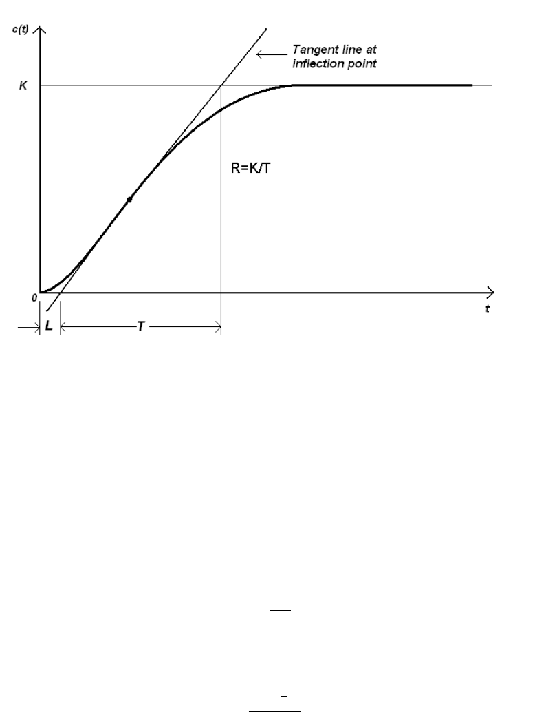
Figure 7.2: Reaction curve [5]
method, one can experimentally obtain the response of a plant to a step input, as
shown in figure 7.2. This method is applicable only when the response to the step
input exhibits S-shaped curve [7].
As shown in figure 7.2, by drawing the tangent line at the inflection point and
determining the intersection of the tangent line with the time axis and the line
c(t)=K,we get two constants, namely, delay time Land time constant T.
Ziegler and Nichols suggested to set the values of K, τi, τdaccording to the
formula shown in table 7.1. Notice that the PID controller tuned by the Ziegler-
Nichols rule gives,
Gc(s)=Kp 1+1
Tis+Tds!(7.10)
=1.2T
L 1+1
2Ls +0.5Ls!(7.11)
=0.6Ts+1
L2
s(7.12)
Thus, the PID controller has a pole at the origin and double zeros at s=−1/L.
104

Type of controller Kτiτd
P1
RL ∞0
PI 0.9
RL 3L0
PID 1.2
RL 2L0.5L
Table 7.1: Ziegler-Nichols tuning rule based on step response of plant
Type of controller Kτiτd
P0.5Ku∞0
PI 0.45Ku1
0.2Pu0
PID 0.6Ku0.5Pu0.125Pu
Table 7.2: Ziegler-Nichols tuning rule for instability tuning method
7.2.2 Second Method
The second method is also known as ‘instability method ’[6]. This is a closed loop
method in which the integral and derivative gains of the PID controller are made
zero with a unity value for proportional gain. A setpoint change is made and the
temperature profile is observed for some time. The temperature would most likely
maintain a steady-state with some offset. The gain is increased to a next distinct
value (say 2) with a change in the setpoint. The procedure is repeated until the
temperature first varies with sustained oscillations. It is necessary that the output
(temperature) should have neither under damped nor over damped oscillations.
At this particular frequency of sustained oscillations, the corresponding value of
Kpis noted and is called as the critical gain Kcr. The corresponding period of
oscillation is known as Pcr. Refer to figure 7.3.
The various P, PI and PID parameters are then calculated with the help of table
7.2. Using the Ziegler-Nichols method explained earlier, the following values
were obtained. Refer to figure 7.4.
105
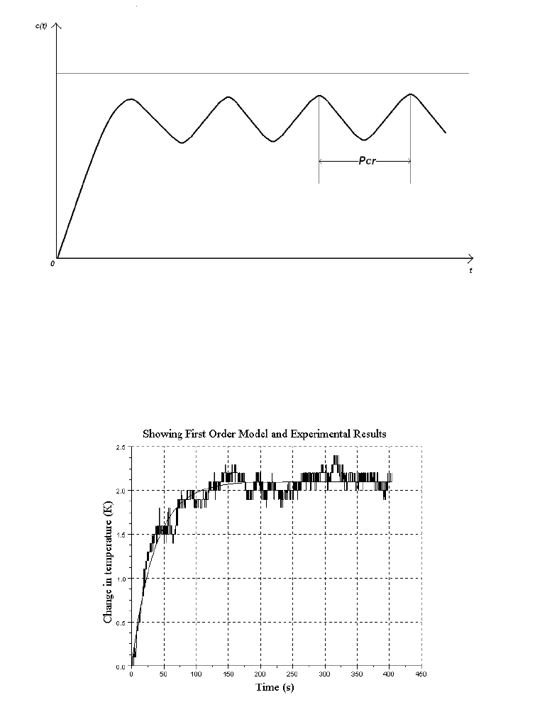
Figure 7.3: Ziegler-Nichols instability tuning method
Figure 7.4: Refer to ‘Step Test’experiment [6]
106

L=6s
T=193 s
For PI
K=6.031
τi=18
For PID
K=8
τi=12
τd=3
While performing the experiment, fine tunning of K, τi, τdmay be required.
7.3 PI Controller using Trapezoidal Approximation
Figure 7.5 shows Xcos diagram for implementing PI controller. The PI controller
in continuous time is given by,
u(t)=K(e(t)+1
τiZt
0
e(t)dt)(7.13)
On taking the Laplace transform,we obtain
u(t)=K(1+1
τis)e(t) (7.14)
By mapping controller given in equation 7.14 to the discrete time domain using
trapezoidal approximation
u(n)=K(1+Ts
2τi
z+1
z−1)e(n) (7.15)
107
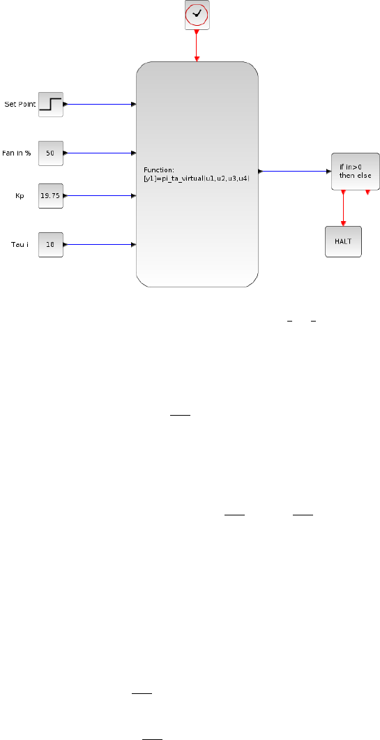
Figure 7.5: Xcos for PI controller available as pi ta virtual.xcos
On cross multiplying, we obtain
(z−1)u(n)=K((z−1) +Ts
2τi
(z+1))e(n) (7.16)
We divide by zand then by using shifting theorem, we obtain
u(n)−u(n−1) =K(e(n)−e(n−1) +Ts
2τi
e(n)+Ts
2τi
e(n−1))(7.17)
The PI controller is usually written as
u(n)=u(n−1) +s0e(n)+s1e(n−1) (7.18)
where
s0=K 1+Ts
2τi!(7.19)
s1=K −1+Ts
2τi!(7.20)
108

7.3.1 Implementing locally
The detailed procedure to perform a local experiment is explained in Chapter2.
A summary of the same is provided in section 2.3 It is same for this section with
following changes.
1. Step1: The working directory is pid controller
2. Step2: Same
3. Step3: Same
4. Step4: Same
5. Step5: Load ramp test function by executing command
exec<space>pi ta.sci
6. Step6: Load Xcos code for ramp test using the command
exec<space>pi ta.xcos
7. Step7: Same
The output of Xcos is shown in figure 7.6. Figure shows three plots. First sub
plot shows setpoint and output temperature profile. Second sub plot shows control
effort and third sub plot shows error between setpoint and plant output.
7.3.2 Implementing virtually
The detailed procedure to perform a virtual experiment is explained in Chapter3.
A summary of the same is provided in section 3.5. It is same for this section with
following changes.
1. Step1: The working directory is pid controller. Open this directory.
2. Step2: Same
3. Step3: Same
4. Step4: Switch to the PID controller experiment directory and double-click
on the file pi ta virtual.sce. This will launch scilab and also open
the file pi ta virtual.sce in the scilab editor. Linux users will have to
launch scilab manually. They also have to change the working directory to
109
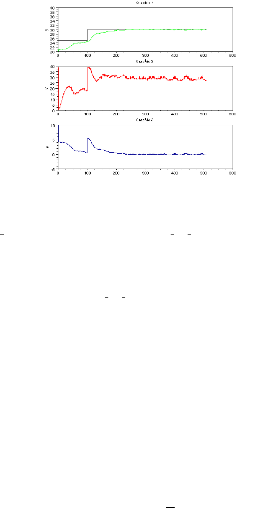
Figure 7.6: PI controller (Trapezoidal Approximation) output
pid controller and then open the pi ta virtual.sce file in the scilab
editor.
5. Step5: Same
6. Step6: Execute the file pi ta virtual.sce. Expect the PI controller xcos
diagram to open automatically. If this doesnt happen, check the scilab con-
sole for error message.
7. Step7: Execute the PI controller xcos diagram.
8. Step8: Same
7.4 Implementing PI Controller using Backward Dif-
ference Approximation
The PI controller in continuous time is given by
u(t)=K(e(t)+1
τiZt
0
e(t)dt)(7.21)
110

On taking the Laplace transform, we obtain
u(t)=K(1+1
τis)e(t) (7.22)
By mapping controller given in equation 7.22 to the discrete time domain using
Backward difference approximation:
u(n)=K(1+Ts
τi
z
z−1)e(n) (7.23)
On cross multiplying, we get
(z−1)u(n)=K((z−1) +Ts
τi
(z))e(n) (7.24)
We divide by zand then by using shifting theorem, we obtain
u(n)−u(n−1) =K(e(n)−e(n−1) +Ts
τi
e(n))(7.25)
The PI controller is usually written as
u(n)=u(n−1) +s0e(n)+s1e(n−1) (7.26)
where
s0=K 1+Ts
τi!(7.27)
s1=−K(7.28)
7.4.1 Implementing locally
The detailed procedure to perform a local experiment is explained in Chapter2.
A summary of the same is provided in section 2.3 It is same for this section with
following changes.
1. Step1: The working directory is pid controller
111
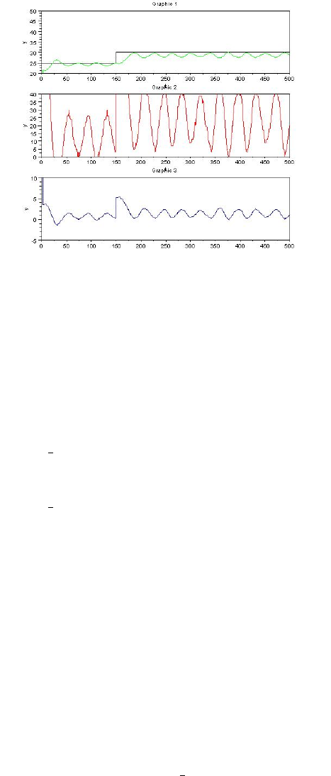
Figure 7.7: PI controller (Backward Difference Approximation) output
2. Step2: Same
3. Step3: Same
4. Step4: Same
5. Step5: Load ramp test function by executing command
exec<space>pi bda.sci
6. Step6: Load Xcos code for ramp test using the command
exec<space>pi bda.xcos
7. Step7: Same
The Xcos output is shown in figure 7.7. Figure shows three plots. First sub
plot shows setpoint and output temperature profile. Second sub plot shows control
effort and third sub plot shows error between setpoint and plant output.
7.4.2 Implementing virtually
The detailed procedure to perform a virtual experiment is explained in Chapter3.
A summary of the same is provided in section 3.5. It is same for this section with
following changes.
1. Step1: The working directory is pid controller. Open this directory.
112

2. Step2: Same
3. Step3: Same
4. Step4: Switch to the PID controller experiment directory and double-click
on the file pi bda virtual.sce. This will launch scilab and also open
the file pi bda virtual.sce in the scilab editor. Linux users will have to
launch scilab manually. They also have to change the working directory to
pid controller and then open the pi bda virtual.sce file in the scilab
editor.
5. Step5: Same
6. Step6: Execute the file pi bda virtual.sce. Expect the PI controller
xcos diagram to open automatically. If this doesnt happen, check the scilab
console for error message.
7. Step7: Execute the PI controller xcos diagram.
8. Step8: Same
7.5 Implementing PI Controller using Forward Dif-
ference Approximation
The PI controller in continuous time is given by
u(t)=K(e(t)+1
τiZt
0
e(t)dt)(7.29)
On taking the Laplace transform, we obtain
u(t)=K(1+1
τis)e(t) (7.30)
By mapping controller given in equation 7.30 to the discrete time domain using
forward difference formula, we get
u(n)=K(1+Ts
τi
1
z−1)e(n) (7.31)
113

On cross multiplying, we get
(z−1)u(n)=K((z−1) +Ts
τi)e(n) (7.32)
We divide by zand then by using shifting theorem, we get
u(n)−u(n−1) =K(e(n)−e(n−1) +Ts
τi
e(n−1))(7.33)
The PI controller is usually written as
u(n)=u(n−1) +s0e(n)+s1e(n−1) (7.34)
where
s0=K(7.35)
s1=K −1+Ts
τi!(7.36)
7.5.1 Implementing locally
The detailed procedure to perform a local experiment is explained in Chapter2.
A summary of the same is provided in section 2.3 It is same for this section with
following changes.
1. Step1: The working directory is pid controller
2. Step2: Same
3. Step3: Same
4. Step4: Same
5. Step5: Load ramp test function by executing command
exec<space>pi fda.sci
6. Step6: Load Xcos code for ramp test using the command
exec<space>pi fda.xcos
7. Step7: Same
The Xcos output is shown in figure 7.8. Figure shows three plots. First sub
plot shows setpoint and output temperature profile. Second sub plot shows control
effort and third sub plot shows error between setpoint and plant output.
114
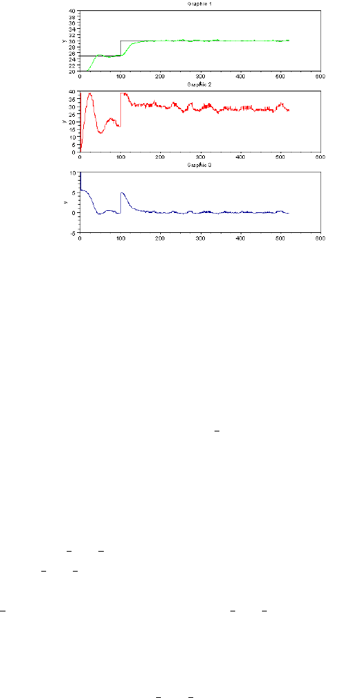
Figure 7.8: PI controller implementation (Forward Difference Approximation)
7.5.2 Implementing virtually
The detailed procedure to perform a virtual experiment is explained in Chapter3.
A summary of the same is provided in section 3.5. It is same for this section with
following changes.
1. Step1: The working directory is pid controller. Open this directory.
2. Step2: Same
3. Step3: Same
4. Step4: Switch to the PID controller experiment directory and double-click
on the file pi fda virtual.sce. This will launch scilab and also open
the file pi fda virtual.sce in the scilab editor. Linux users will have to
launch scilab manually. They also have to change the working directory to
pid controller and then open the pi fda virtual.sce file in the scilab
editor.
5. Step5: Same
6. Step6: Execute the file pi fda virtual.sce. Expect the PI controller
xcos diagram to open automatically. If this doesnt happen, check the scilab
console for error message.
115
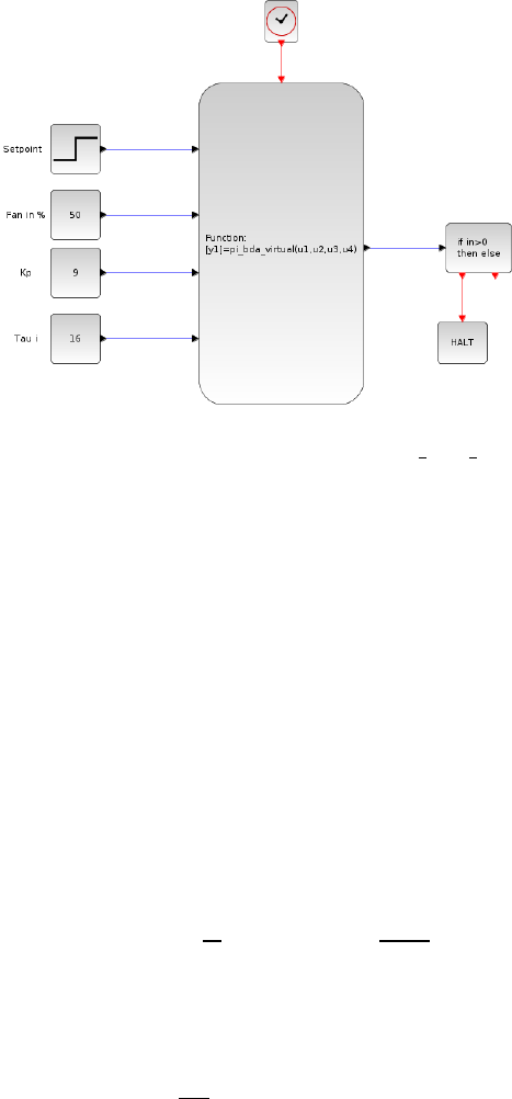
Figure 7.9: Xcos for PID controller available as pid bda virtual.xcos
7. Step7: Execute the PI controller xcos diagram.
8. Step8: Same
7.6 Implementing PID Controller using Backward
Difference Approximation
Figure 7.9 shows Xcos diagram for implementing PID controller.
The PID controller in continuous time is given by
u(t)=K(e(t)+1
τiZt
0
e(t)dt +τd
de(t)
dt )(7.37)
On taking the Laplace transform, we obtain
u(t)=K(1+1
τis+τds)e(t) (7.38)
116

By mapping controller given in equation 7.38 to the discrete time domain using
backward difference formula, we get
u(n)=K(1+Ts
τi
z
z−1+τd
Ts
z−1
z)e(n) (7.39)
On cross multiplying, we obtain
(z2−z)u(n)=K((z2−z)+Ts
τi
z2+τd
Ts
(z−1)2)e(n) (7.40)
We divide by z2and by using shifting theorem, we get
u(n)−u(n−1) =K(e(n)−e(n−1) +Ts
τi
e(n)
+τd
Ts
[e(n)−2e(n−1) +e(n−2)])(7.41)
The PID controller is usually written as
u(n)=u(n−1) +s0e(n)+s1e(n−1) +s2e(n−2) (7.42)
where
s0=K"1+Ts
τi
+τd
Ts#(7.43)
s1=K"−1−2τd
Ts#(7.44)
s2=K"τd
Ts#(7.45)
7.6.1 Implementing locally
The detailed procedure to perform a local experiment is explained in Chapter2.
A summary of the same is provided in section 2.3 It is same for this section with
following changes.
1. Step1: The working directory is pid controller
117
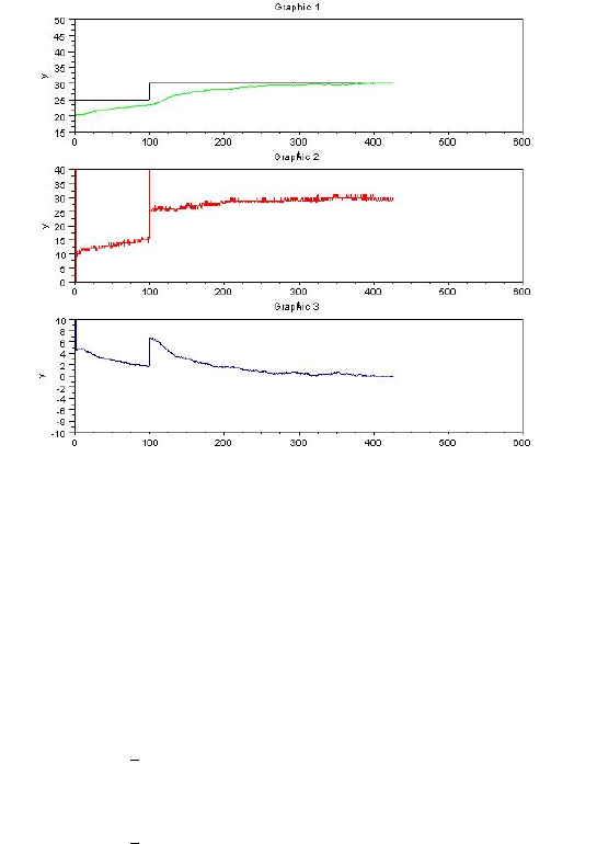
Figure 7.10: PID controller (Backward Difference Approximation) output
2. Step2: Same
3. Step3: Same
4. Step4: Same
5. Step5: Load ramp test function by executing command
exec<space>pid bda.sci
6. Step6: Load Xcos code for ramp test using the command
exec<space>pid bda.xcos
7. Step7: Same
The output of Xcos is shown in figure 7.10. Figure shows three plots. First
sub plot shows setpoint and output temperature profile. Second sub plot shows
control effort and third sub plot shows error between setpoint and plant output.
7.6.2 Implementing virtually
The detailed procedure to perform a virtual experiment is explained in Chapter3.
A summary of the same is provided in section 3.5. It is same for this section with
following changes.
118

1. Step1: The working directory is pid controller. Open this directory.
2. Step2: Same
3. Step3: Same
4. Step4: Switch to the PID controller experiment directory and double-click
on the file pid bda virtual.sce. This will launch scilab and also open
the file pid bda virtual.sce in the scilab editor. Linux users will have
to launch scilab manually. They also have to change the working directory
to pid controller and then open the pid bda virtual.sce file in the
scilab editor.
5. Step5: Same
6. Step6: Execute the file pid bda virtual.sce. Expect the PI controller
xcos diagram to open automatically. If this doesnt happen, check the scilab
console for error message.
7. Step7: Execute the PI controller xcos diagram.
8. Step8: Same
7.7 Implementing PID Controller using Trapezoidal
Approximation for Integral Mode and Backward
Difference Approximation for the Derivative Mode
The PID controller in continuous time is given by
u(t)=K(e(t)+1
τiZt
0
e(t)dt +τd
de(t)
dt )(7.46)
On taking the Laplace transform, we obtain
u(t)=K(1+1
τis+τds)e(t) (7.47)
119

By mapping controller given in equation 7.47 to the discrete time domain using
trapezoidal approximation for integral mode and backward difference approxima-
tion for the derivative mode, we get
u(n)=K(1+Ts
2τi
z+1
z−1+τd
Ts
z−1
z)e(n) (7.48)
On cross multiplying, we obtain
(z2−z)u(n)=K((z2−z)+Ts
2τi
(z2+z)τd
Ts
(z−1)2)e(n) (7.49)
We divide by z2and then by using shifting theorem, we get
u(n)−u(n−1) =K(e(n)−e(n−1) +Ts
2τi
e(n)+e(n−1)
+τd
Ts
[e(n)−2e(n−1) +e(n−2)])(7.50)
The PID controller is usually written as
u(n)=u(n−1) +s0e(n)+s1e(n−1) +s2e(n−2) (7.51)
where
s0=K"1+Ts
2τi
+τd
Ts#(7.52)
s1=K"−1+Ts
2τi−2τd
Ts#(7.53)
s2=Kτd
Ts
(7.54)
7.7.1 Implementing locally
The detailed procedure to perform a local experiment is explained in Chapter2.
A summary of the same is provided in section 2.3 It is same for this section with
following changes.
1. Step1: The working directory is pid controller
120
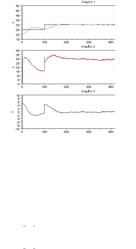
Figure 7.11: PID controller (TA - BDA) implementation
2. Step2: Same
3. Step3: Same
4. Step4: Same
5. Step5: Load ramp test function by executing command
exec<space>pid ta bda.sci
6. Step6: Load Xcos code for ramp test using the command
exec<space>pid ta bda.xcos
7. Step7: Same
The Xcos output is shown in figure 7.11. Figure shows three plots. First sub
plot shows setpoint and output temperature profile. Second sub plot shows control
effort and third sub plot shows error between setpoint and plant output.
121

7.7.2 Implementing virtually
The detailed procedure to perform a virtual experiment is explained in Chapter3.
A summary of the same is provided in section 3.5. It is same for this section with
following changes.
1. Step1: The working directory is pid controller. Open this directory.
2. Step2: Same
3. Step3: Same
4. Step4: Switch to the PID controller experiment directory and double-click
on the file pid ta bda virtual.sce. This will launch scilab and also
open the file pid ta bda virtual.sce in the scilab editor. Linux users
will have to launch scilab manually. They also have to change the working
directory to pid controller and then open the pid ta bda virtual.sce
file in the scilab editor.
5. Step5: Same
6. Step6: Execute the file pid ta bda virtual.sce. Expect the PI con-
troller xcos diagram to open automatically. If this doesnt happen, check
the scilab console for error message.
7. Step7: Execute the PI controller xcos diagram.
8. Step8: Same
Due to the introduction of derivative action, control effort shows lots of fluc-
tuations. By using filtered form of PID, we can make derivative mode imple-
mentable.
7.8 Implementing PID Controller with Filtering us-
ing Backward Difference Approximation
Figure 7.12 shows Xcos diagram for implementing PID controller with filtering.
122
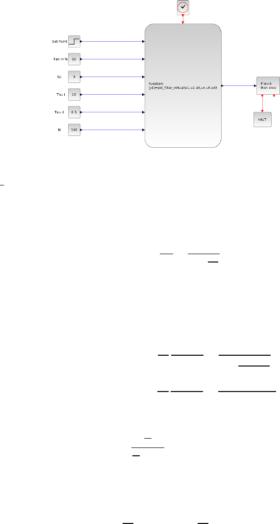
Figure 7.12: Xcos for PID controller with filtering available as
pidN virtual.xcos
PID filtered form is given by
u(t)=K(1+1
τis+τds
1+τds
N)e(t) (7.55)
where N is large number of the order of 100.
By maping controller given in equation 7.55 to the discrete time domain using
backward difference formula, we get
u(n)=K
1+Ts
τi
1
1−z−1+τd(1 −z−1)
1+τd(1−z−1)
N
e(n) (7.56)
u(n)=K 1+Ts
τi
1
1−z−1+Nr1(1 −z−1)
1+r1z−1!e(n) (7.57)
where
r1=−
τd
N
τd
N+Ts
(7.58)
On cross multiplying, we obtain
(1 −z−1)(1 +r1z−1)u(n)=K[(1 −z−1)(1 +r1z−1)
+Ts
τi
(1 +r1z−1)+τd
Ts
(1 −z−1)2]e(n) (7.59)
123

Simplifying and then by using shifting theorem, we obtain
u(n)+(r1−1)u(n−1)
−r1u(n−2) =K"1+Ts
τi−Nr1#e(n)
+K"r1(1 +Ts
τi
+2N)−1#e(n−1)
−K[r1(1 +N)]e(n−2) (7.60)
Hence
u(n)=r1u(n−2) −(r1−1)u(n−1)
+s0e(n)+s1e(n−1) +s2e(n−2) (7.61)
where
s0=K"1+Ts
τi−Nr1#(7.62)
s1=K"r1(1 +Ts
τi
+2N)−1#(7.63)
s2=−K[r1(1 +N)](7.64)
7.8.1 Implementing locally
The detailed procedure to perform a local experiment is explained in Chapter2.
A summary of the same is provided in section 2.3 It is same for this section with
following changes.
1. Step1: The working directory is pid controller
2. Step2: Same
3. Step3: Same
4. Step4: Same
5. Step5: Load ramp test function by executing command
exec<space>pid filter.sci
124
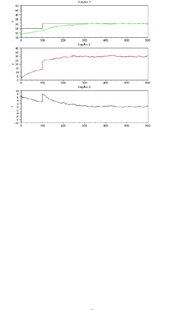
Figure 7.13: PID controller (with filtering) implementation
6. Step6: Load Xcos code for ramp test using the command
exec<space>pidN.xcos
7. Step7: Same
The Xcos output is shown in figure 7.13. Figure shows three plots. First sub
plot shows setpoint and output temperature profile. Second sub plot shows control
effort and third sub plot shows error between setpoint and plant output.
By comparing figure 7.10 and figure 7.13, it is clear that introduction of filtered
form of PID reduces fluctuations in control effort.
7.8.2 Implementing virtually
The detailed procedure to perform a virtual experiment is explained in Chapter3.
A summary of the same is provided in section 3.5. It is same for this section with
following changes.
1. Step1: The working directory is pid controller. Open this directory.
2. Step2: Same
3. Step3: Same
125

4. Step4: Switch to the PID controller experiment directory and double-click
on the file pid filter virtual.sce. This will launch scilab and also
open the file pid filter virtual.sce in the scilab editor. Linux users
will have to launch scilab manually. They also have to change the working
directory to pid controller and then open the pid filter virtual.sce
file in the scilab editor.
5. Step5: Same
6. Step6: Execute the file pid filter virtual.sce. Expect the PI con-
troller xcos diagram to open automatically. If this doesnt happen, check the
scilab console for error message.
7. Step7: Execute the PI controller xcos diagram.
8. Step8: Same
7.9 Scilab Code
7.9.1 Scilab code for serial communication
Scilab Code 7.1 ser init.sci used for serial communication
1mode ( 0 )
2global f i l e n a m e m
3/ / * * Sampling Time * * / /
4s a m p l i n g t i m e =1 ;
5/ / / / / / / * * * * /////////
6m=1;
7
8port1 =’/dev /ttyUSB0 ’ ; / / F o r l i n u x u s e r s
9port2 =’COM2’ ; / / F o r w i n d o w s u s e r s
10
11 r e s =i n i t ( [ p o r t 1 p o r t 2 ] ) ;
12 d i s p ( r e s )
126

7.9.2 Scilab code for PI controller
Scilab Code 7.2 pi ta.sci
1mode ( 0 )
2function temp =p i t a ( s e t p o i n t , fan , K, Ti )
3global h e a t d i s p f a n d i s p t e m p d i s p s e t p o i n t d i s p
s a m p l i n g t i m e m name temp h e a t i n f a n i n C0
u o l d u new e o l d e new
4
5Ts=s a m p l i n g t i m e ;
6e new =s e t p o i n t −temp ;
7
8S0=K(1+Ts /( 2 *T i ) ) ;
9S1=K*(−1+( Ts /( 2 *T i ) ) ) ;
10 u new =u o l d +( S0 *e new ) +( S1 *e o l d ) ;
11
12
13 u o l d =u new ;
14 e o l d =e new ;
15
16 h e a t =u new ;
17 temp =comm( h e a t , f a n ) ;
18
19 p l o t t i n g ( [ h e a t f a n temp s e t p o i n t ] , [ 0 0 20 0 ] , [ 1 0 0
100 40 1 0 0 0 ] )
20
21 m=m+1;
22 endfunction
Scilab Code 7.3 pi bda.sci
1/ / g l o b a l t e m p h e a t f a n s a m p l i n g t i m e m h e a t d i s p
f a n d i s p t e m p d i s p x n a m e T s
2
3mode ( 0 )
4function temp =p i b d a ( s e t p o i n t , fan , K, Ti )
127

5global h e a t d i s p f a n d i s p t e m p d i s p s e t p o i n t d i s p
s a m p l i n g t i m e m name temp h e a t i n f a n i n C0
u o l d u new e o l d e new
6
7Ts =s a m p l i n g t i m e ;
8e new =s e t p o i n t −temp ;
9
10
11 S0=K( 1 +( Ts /T i ) ) ;
12 S1=−K;
13
14
15
16 u new =u o l d +S0*e new+S1*e o l d ;
17
18
19 u o l d =u new ;
20 e o l d =e new ;
21
22 h e a t =u new ;
23 temp =comm( h e a t , f a n ) ;
24
25 p l o t t i n g ( [ h e a t f a n temp s e t p o i n t ] , [ 0 0 20 0 ] , [ 1 0 0
100 40 1 0 0 0 ] )
26
27 m=m+1;
28 endfunction
Scilab Code 7.4 pi fda.sci
1mode ( 0 )
2function temp =p i f d a ( s e t p o i n t , fan , K, Ti )
3global h e a t d i s p f a n d i s p t e m p d i s p s e t p o i n t d i s p
s a m p l i n g t i m e m name temp h e a t i n f a n i n C0
u o l d u new e o l d e new
4
5Ts=s a m p l i n g t i m e ;
6e new =s e t p o i n t −temp ;
128

7
8
9S0=K*( 1 +( ( Ts /Ti ) ) ) ;
10 S1=−K;
11 u new =u o l d +( S0 *e new ) +( S1 *e o l d ) ;
12
13 u o l d =u new ;
14 e o l d =e new ;
15
16 h e a t =u new ;
17
18 temp =comm( h e a t , f a n ) ;
19
20 p l o t t i n g ( [ h e a t f a n temp s e t p o i n t ] , [ 0 0 20 0 ] , [ 1 0 0
100 40 1 0 0 0 ] )
21
22 m=m+1;
23 endfunction
7.9.3 Scilab code for PID controller
Scilab Code 7.5 pid bda.sci
1mode ( 0 )
2
3function [ temp ] =p i d b d a ( s e t p o i n t , fan , K, Ti , Td )
4global temp h e a t i n f a n i n C0 u o l d u new e o l d e new
e old old
5
6global h e a t d i s p f a n d i s p t e m p d i s p s e t p o i n t d i s p
s a m p l i n g t i m e m name
7
8e new =s e t p o i n t −temp ;
9
10 Ts=s a m p l i n g t i m e ;
11
12 S0=K*( 1 +( Ts /T i ) +( Td /Ts ) ) ;
13 S1=K*(−1−((2*Td ) /Ts ) ) ;
129

14 S2=K*( Td /Ts ) ;
15
16 u new =u o l d +S0 *e new +S1*e o l d +S2*e o l d o l d ;
17
18 u o l d =u new ;
19 e old old =e o l d ;
20 e o l d =e new ;
21
22
23 h e a t =u new ;
24 temp =comm( h e a t , f a n ) ;
25
26 p l o t t i n g ( [ h e a t f a n temp s e t p o i n t ] , [ 0 0 20 0 ] , [ 1 0 0
100 40 1 0 0 0 ] )
27
28 m=m+1;
29 endfunction
Scilab Code 7.6 pid ta bda.sci
1
2mode ( 0 )
3
4function [ temp ] =p i d t a b d a ( s e t p o i n t , fan , K, Ti , Td )
5global temp h e a t i n f a n i n C0 u o l d u new e o l d e new
e old old
6
7global h e a t d i s p f a n d i s p t e m p d i s p s e t p o i n t d i s p
s a m p l i n g t i m e m name
8
9e new =s e t p o i n t −temp ;
10
11 Ts=s a m p l i n g t i m e ;
12
13 S0=K*( 1 +( Ts /( 2 *Ti ) ) +(Td /Ts ) ) ;
14 S1=K*(−1+( Ts /( 2 *T i ) ) −(2*Td /Ts ) ) ;
15 S2 =(K*Td /Ts ) ;
16 u new =u o l d +S0 *e new +S1*e o l d +S2*e o l d o l d ;
130

17
18 u o l d =u new ;
19 e old old =e o l d ;
20 e o l d =e new ;
21
22
23 h e a t =u new ;
24
25 temp =comm( h e a t , f a n ) ;
26
27 p l o t t i n g ( [ h e a t f a n temp s e t p o i n t ] , [ 0 0 20 0 ] , [ 1 0 0
100 40 1 0 0 0 ] )
28
29 m=m+1;
30 endfunction
Scilab Code 7.7 pid filter.sci
1mode ( 0 )
2
3function temp =p i d ( s e t p o i n t , fan , K, Ti , Td , N)
4global h e a t d i s p f a n d i s p t e m p d i s p s e t p o i n t d i s p
s a m p l i n g t i m e m name temp h e a t i n f a n i n C0
u o l d u new e o l d e new e o l d o l d r 1 u o l d o l d
5
6Ts =s a m p l i n g t i m e ;
7e new =s e t p o i n t −temp ;
8
9r 1 =−(( Td /N) /( ( Td /N) +Ts ) ) ;
10
11 S0=K*( 1 +( Ts /T i ) −(N*r 1 ) ) ;
12 S1=K*( ( r 1 *( 1 +( Ts /T i ) +(2*N) ) ) −1) ;
13 S2=−K*r 1 *(1+N) ;
14
15 u new =r 1 *u o l d o l d −( r1 −1) *u o l d +S0*e new +S1*
e o l d +S2*e o l d o l d ;
16
17 u o l d o l d =u o l d ;
131

18 u o l d =u new ;
19 e old old =e o l d ;
20 e o l d =e new ;
21
22
23 h e a t =u new ;
24
25 temp =comm( h e a t , f a n ) ;
26
27 p l o t t i n g ( [ h e a t f a n temp s e t p o i n t ] , [ 0 0 20 0 ] , [ 1 0 0
100 40 1 0 0 0 ] )
28
29 m=m+1;
30 endfunction
Scilab Code 7.8 pid bda virtual.sce
1mode ( 0 ) ;
2/ / F o r s c i l a b 5 . 1 . 1 o r l o w e r v e r s i o n u s e r s , u s e s c i c o s
c o m m a n d t o o p e n s c i c o s d i a g r a m s i n s t e a d o f x c o s
3
4global f d f h f d t f n c r fncw m e r r c o u n t y l i m i t s
s a m p l i n g t i m e m
5
6/ / **********************
7s a m p l i n g t i m e =1; / / I n s e c o n d s . F r a c t i o n s a r e a l l o w e d
8/ / **********************/ /
9
10 e x e c ( ” p i d b d a v i r t u a l . s c i ” ) ;
11
12 ok =i n i t ( ) ;
13
14 i f ok ˜=[ ] / / o p e n x c o s o n l y i f c o m m u n i c a t i o n i s
t h r o u g h ( i e r e p l y h a s c o m e f r o m s e r v e r )
15 xco s ( ’ p i d b d a v i r t u a l . x c o s ’ ) ;
16 else
17 d i s p ( ”NO NETWORK CONNECTION! ” ) ;
18 r e t u r n
132

19 end
Scilab Code 7.9 pid bda virtual.sci
1mode ( 0 ) ;
2/ / P I C o n t r o l l e r u s i n g t r a p e z o i d a l a p p r o x i m a t i o n .
3/ / H e a t e r i n p u t i s p a s s e d a s i n p u t a r g u m e n t t o
i n t r o d u c e c o n t r o l e f f o r t u ( n )
4/ / F a n i n p u t i s p a s s e d a s i n p u t a r g u m e n t w h i c h i s k e p t
a t c o n s t a n t l e v e l
5/ / R a n g e o f F a n i n p u t : 2 0 t o 2 5 2
6/ / T e m p e r a t u r e i s r e a d
7
8function [ s t o p ] =p i d b d a v i r t u a l ( s e t p o i n t , fan , K, Ti , Td
)
9
10 global temp h e a t C0 u o l d u new e o l d e new f d f h f d t
f n c r fncw m e r r c o u n t s t o p q h e a t d i s p f a n d i s p
t e m p d i s p s e t p o i n t d i s p l i m i t s m x s a m p l i n g t i m e
e old old
11
12 e new =s e t p o i n t −temp ;
13
14
15 Ts =1;
16 S0=K*( 1 +( Ts /T i ) +( Td /Ts ) ) ;
17 S1=K*(−1−((2*Td ) /Ts ) ) ;
18 S2=K*( Td /Ts ) ;
19
20 u new =u o l d +S0 *e new +S1*e o l d +S2*e o l d o l d ;
21
22 h e a t =u new ;
23
24 u o l d =u new ;
25 e old old =e o l d ;
26 e o l d =e new ;
27
133

28 [ s t o p , temp ] =comm ( h e a t , f a n ) ; / / N e v e r e d i t t h i s
line
29 p l o t t i n g ( [ h e a t f a n temp s e t p o i n t ] , [ 0 0 30 0 ] , [ 1 0 0
100 50 1 0 0 0 ] )
30
31 endfunction
134
Chapter 8
Two Degrees of Freedom (2-DOF)
Controller
In this chapter, we discuss the implementation of a 2-DOF controller using the
SBHS. We also cover the basics of 2-DOF controller theory and design.
8.1 Introduction to 2-DOF Controller
Controllers are broadly divided into two categories: feedback and feed forward
controllers. Feed forward controllers are those that take control action before a
disturbance affects the plant. But this requires an ability to sense the disturbance
accurately. Moreover, exact knowledge of the plant is also needed. As a result, a
feed forward control strategy is rarely used alone.
A feedback control strategy is shown in figure 8.1. The reference rand the
output yare continuously compared to generate error e, which is fed to the con-
troller Gc(z), to take appropriate control action. uis the controller output that is
fed to the plant. Unlike feed forward controllers, exact knowledge of the plant
G(z) and the disturbance vis not necessary in this case. Feedback controllers are
further classified as One Degree of Freedom (1-DOF) controllers and Two De-
grees of Freedom (2-DOF) controllers. Degree of freedom refers to the number of
parameters that are free to vary in a system. A higher degree of freedom controller
makes the plant less susceptible to disturbances.
135

rGc(z)
eG(z)
u
v
y
−
Figure 8.1: Feed back control strategy
The expression for output, Y(z) of the system shown in figure 8.1 is given by
Y(z)=G(z)Gc(z)
1+G(z)Gc(z)R(z)+1
1+G(z)Gc(z)V(z) (8.1)
This expression can be written in mixed notation [5] as
y(n)=G(z)Gc(z)
1+G(z)Gc(z)r(n)+1
1+G(z)Gc(z)v(n) (8.2)
Let,
T(z)=G(z)Gc(z)
1+G(z)Gc(z),S(z)=1
1+G(z)Gc(z)(8.3)
Therefore,
y(n)=T(z)r(n)+S(z)v(n) (8.4)
The controller has to track the reference input as well as eliminate the effect of
external disturbance. So ideally, we want T =1 and S =0. But, it is not possible
to achieve both the requirements simultaneously using this control strategy. This
control strategy is called One Degree of Freedom, abbreviated as 1-DOF.
ATwo Degrees of Freedom controller is as shown in figure 8.2. Here, Gb
and Gftogether constitute the controller. Gbis in the feedback path and is used to
eliminate the effect of disturbances, whereas Gfis in the feed forward path and is
used to help the output track the reference input.
The expression for control effort uin figure 8.2 is given by
u(n)=r(n)Gf−y(n)Gb(8.5)
136

Gf
rG
uy
H
v
d
Gb
−
Figure 8.2: 2DOF feed back control strategy
Let
Gb=Sc
Rc
,Gf=Tc
Rc
(8.6)
where Rc,Scand Tcare polynomials in z−1.
We get
Rc(z)u(n)=Tc(z)r(n)−Sc(z)y(n) (8.7)
Consider a plant whose model is given by
A(z)y(n)=z−kB(z)u(n)+v(n) (8.8)
Substituting equation 8.7 in equation 8.8, we get
Ay(n)=z−kB
RcTcr(n)−Scy(n)+v(n) (8.9)
Solving for y(n),
RcA+z−kBS c
Rcy(n)=z−kBTc
Rc
r(n)+v(n) (8.10)
137

This can also be written as
y(n)=z−kBTc
φcl
r(n)+Rc
φcl
v(n) (8.11)
where φcl is the closed loop characteristic polynomial given by
φcl =Rc(z)A(z)+z−kB(z)Sc(z) (8.12)
We want the following conditions to be satisfied while designing a controller.
1. The zeros of φcl should be inside the unit circle, so that the closed-loop
system becomes stable
2. The value of z−kBTc
φcl
must be close to unity, so that reference tracking is
achieved
3. The value of Rc
φcl
must be as small as possible to achieve disturbance rejec-
tion
We shall now see the pole placement controller approach to design a 2-DOF con-
troller.
8.2 2-DOF Controller Design using the Pole Place-
ment Method [5]
A 2-DOF pole placement controller is shown in figure 8.3. We will not consider
the effect of external disturbance in the design. The controller will be designed
for setpoint tracking. We want the desired output, Ym, of the system to be related
to the setpoint Rin the following manner:
Ym(z)=γz−kBr
φcl
R(z) (8.13)
φcl is the desired closed loop characteristic polynomial obtained from the desired
region analysis. Please refer to [5] for more information on desired region anal-
ysis. γis chosen such that Ymequals the setpoint at steady-state. Therefore γis
given by,
γ=φcl(1)
Br(1) (8.14)
138
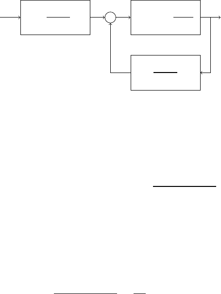
γTc(z)
Rc(z)
rG=z−kB(z)
A(z)
uy
Sc(z)
Rc(z)
−
Figure 8.3: 2-DOF pole placement controller
Simplifying the block diagram shown in figure 8.3 yields
Y=γz−kBTc
ARc+z−kBS c
R(8.15)
We have dropped the argument of zfor convenience
We want the output Yof the system to be equal to the desired output Ym. Equating
equations 8.13 and 8.15 we get
BTc
ARc+z−kBS c
=Br
φcl
(8.16)
We can expect some cancelations between the numerator and the denominator
polynomials in the LHS, thereby making degBr<degB. But the cancelations, if
any, must be between stable poles and zeros. One should avoid the cancelation of
an unstable pole with an unstable zero.
Let us split the factors of the numerator and denominator polynomials, Band A,
of the plant into good and bad factors. Therefore, we write Aand Bas
A=AgAb,B=BgBb(8.17)
We also define Rc,Scand Tcas
Rc=BgR1(8.18)
Sc=AgS1(8.19)
Tc=AgT1(8.20)
139

Hence, equation 8.16 becomes
BgBbAgT1
AgAbBgR1+z−kBgBbAgS1
=Br
φcl
(8.21)
After cancelling out the common factors, we obtain
BbT1
AbR1+z−kBbS1
=Br
φcl
(8.22)
We obtain,
BbT1=Br(8.23)
AbR1+z−kBbS1=φcl (8.24)
Equation 8.24 is known as the Aryabhatta’s identity and can be used to solve for
R1and S1. One can choose T1in many ways. If we choose T1=S1the 2-DOF
controller is reduced to a 1-DOF controller. Let us choose T1=1. Therefore
equation 8.23 becomes
Bb=Br(8.25)
The expression for γnow becomes
γ=φcl(1)
Bb(1) (8.26)
and the desired closed loop transfer function will be
Ym(z)
R(z)=γz−kBb
φcl
(8.27)
One can see that the open loop plant model imposes two limitations on the closed
loop transfer function.
1. The bad portion of the open loop model cannot be canceled out and it ap-
pears in the closed loop model.
2. The open loop plant delay cannot be removed or minimized, i.e., the closed
loop model cannot be made faster than the open loop model.
140

8.3 2-DOF Pole Placement Controller Design and
Implementation using SBHS
We obtain a first order transfer function of the plant using the step test approach.
Refer to the chapter on Step Test using SBHS for more details. The model ob-
tained is
G(s)=0.42
35.61s+1(8.28)
with a time constant of τ=35.6sand gain K=0.42
After discretization with sampling time =1 s, we obtain
G(z)=0.0116304z−1
1−0.9723086z−1(8.29)
Refer to the Scilab code myc2d.sci 1. We shall now define good and bad factors
as
Ag=1−0.9723086z−1
Ab=1
Bg=0.0116304
Bb=1
Let us now define the transient specifications. We choose Rise Time =100 s and
Overshoot ()=5%. Number of samples in one rise time (Nr), [5], is calculated as
Nr≤Rise time
Sampling time
=100
∴, ω =π
2Nr
=0.015708
1Go the folder dc inside the 2dof controller folder. Now go to the folder scilab and locate
myc2d.sci
141

and
ρ≤ω/π
=0.98513
The closed loop characteristic polynomial is given by,
φcl =1−2ρcosωz−1+ρ2z−2
=1−1.9700229z−1+0.9704870z−2
Refer to the Scilab code desired.sci to calculate Nr,ω,ρand φcl. The code is
available in the same location as myc2d.sci.
But according to equation 8.24,
AbR1+z−kBbS1=φcl
Recall that we have not considered external disturbance in the block diagram
shown in figure 8.3. However, we can still up to some extent take care of the
disturbances. This is achieved by using the Internal Model Principle. If a model
of step is present inside the loop, step disturbances can be rejected [5]. We can
apply this by forcing Rcto have this term. A step model is given by
1(z)=1
1−z−1=1
∆
Therefore,
Rc=Bg∆R1
∆has a root which lies on the unit circle. Hence it has to be treated as a bad
part and should not be canceled out. Hence, we should make sure that all of the
occurrences of R1have this term.
Therefore,
φcl =Ab∆R1+z−kBbS1(8.30)
142

Hence,
Ab∆R1+z−kBbS1=1−1.9700229z−1+0.9704870z−2(8.31)
is expression is known as the Aryabhatta Identity and is solved using rigorous
matrix calculations. The explanation of this operation is not considered here.
Refer to [5] for more details on Aryabhatta’s Identity. Refer to the Scilab code
pp im.sci, which is used to split the denominator and numerator polynomials of
the plant transfer function into good and bad factors, and solving the Aryabhatta’s
Identity given in equation 8.31. On solving equation 8.31, we get
Rc=0.0116304 −0.0229175z−1+0.0112871z−2
Sc=0.0004641 −0.0004512z−1
Tc=1−0.9723z−1
γ=0.0004641
All the above calculations are incorporated into a single Scilab code named
twodof para.sce 2.
8.3.1 Procedure to calculate 2DOF parameters using scilab
The procedure explained here is applicable to both virtual as well as local exper-
iments. The following steps must be executed properly to calculate the controller
parameters.
1. Change the directory to 2dof controller.
2. Execute the command getd dc/scilab in the scilab console.
3. Open the Scilab code twodof para.sce. Define the variable TFcont with
first order transfer function (or second order transfer function) of your SBHS.
Execute the Scilab code. With this, the 2-DOF controller parameters have
been calculated. Figure 8.6 shows the calculated 2-DOF controller parame-
ters on the Scilab console.
4. Open the Scilab code twodof.sci. Make sure that the first order control
law (or second order control law in case of second order plant transfer func-
tion) is uncommented and the second order control law (or first order control
law in case of second order transfer function) is commented.
2All the Scilab codes are given at the end of this chapter in the section 8.6
143

8.4 Implementing 2DOF controller locally
The detailed procedure to perform a local experiment is explained in Chapter2.
A summary of the same is provided in section 2.3 It is same for this section with
following changes.
1. Step1: The working directory is 2dof controller
2. Step2: Same
3. Step3: Same
4. Step4: Same
5. Step5: Load 2DOF controller function by executing command
exec<space>twodof.sci. Make sure the correct order of control law is
choosen in this file as explained in section 8.3.1
6. Step6: Load Xcos code for 2DOF controller using the command
exec<space>twodof.xcos. In the twodof.xcos Xcos file, change the
setpoint to the desired value. Make sure the period of the clock block is
the same as the sampling time used for discretisation. The Xcos diagram is
shown in figure 8.7.
7. Step7: Same
8.4.1 Implementing 2-DOF Controller on SBHS, Virtually
The detailed procedure to perform a virtual experiment is explained in Chapter3.
A summary of the same is provided in section 3.5. It is same for this section with
following changes.
1. Step1: The working directory is 2dof controller. Open this directory.
2. Step2: Same
3. Step3: Same
4. Step4: Switch to the 2dof controller experiment directory and double-click
on the file twodof.sce. This will launch scilab and also open the file
twodof.sce in the scilab editor. Linux users will have to launch scilab
manually. They also have to change the working directory to 2dof controller
and then open the twodof.sce file in the scilab editor.
144

5. Step5: Same
6. Step6: Execute the file twodof.sce. Expect the PI controller xcos diagram
to open automatically. If this doesnt happen, check the scilab console for
error message.
7. Step7: Execute the PI controller xcos diagram.
8. Step8: Same
8.5 Performing pure simulation of 2DOF controller
You can also use the Xcos file twodof simulation.xcos, shown in figure 8.4,
to simulate your controller before implementing on SBHS. This will help you val-
idate your controller. You need to execute getd dc/scilab and then execute the
file twodof para.sce. Now run twodof simulation.xcos. Figure 8.5 shows
the simulation results. Note that, execution of this Xcos file is not mandatory for
performing a virtual experiment.
The performance of the controller is shown in figure 8.8. It is seen that the
output (temperature) tracks the setpoint irrespective of the step changes in the fan
speed. We see that the overshoot turns out to be 6% and rise time turns out to be
60 seconds, which is acceptable.
8.6 Scilab Code for Local Experiment
Scilab Code 8.1 twodof para.sce
1mode ( 0 )
2s=%s ;
3z=%z ;
4global Rc Sc Tc gamm
5/ / TFcont =s y s l i n ( ’ c ’ , −280.14/( ( s −31.32) *( s +1 0 0 ) *( s
+3 1 . 3 2 ) ) ) ;
6/ / TFcont =s y s l i n ( ’ c ’ , 0 . 6 6 7 /((73.5*s+1 ) *( 1 *s+1 ) ) ) / /
s e c o n d o r d e r
7TFcont =syslin ( ’ c ’ , 0 . 6 6 8 /( 7 5 . 0 1 3 *s+1) ) / / f i r s t o r d e r
8SS c ont =tf2ss ( TFcont ) ;
145
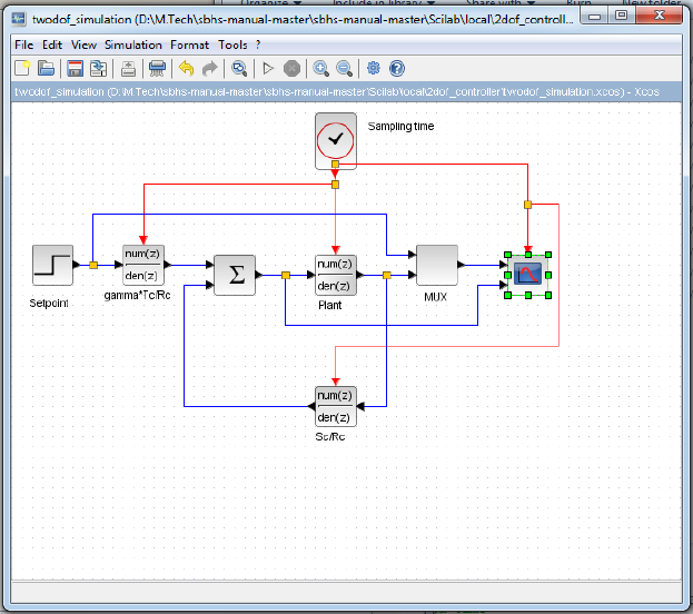
Figure 8.4: Xcos diagram for simulating 2-DOF controller
146
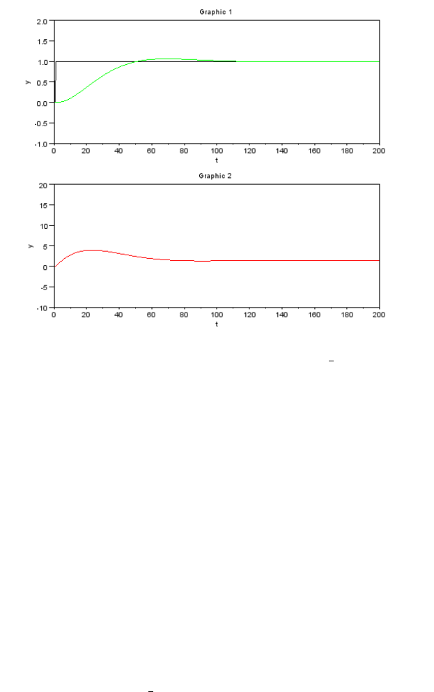
Figure 8.5: Simulation results after executing twodof simulation.xcos
9/ / T F d i s c =s s 2 t f ( S S c o n t ) ;
10 Ts =0 . 5 ;
11 [ B , A, k ] =myc2d ( SScont , Ts ) ;
12
13 / / p o l y n o m i a l s a r e r e t u r n e d
14 [ Ds , num , den ] =ss2tf ( S Sco nt ) ;
15 num =clean ( num ) ; den =clean ( den ) ;
16
17 / / T r a n s i e n t s p e c i f i c a t i o n s
18 r i s e =35; epsilon =0.05;
19 p h i =d e s i r e d ( Ts , r i s e , e p s i l o n ) ;
20
21 / / C o n t r o l l e r d e s i g n
22 Delta =[ 1 −1];
23 [ Rc , Sc , Tc , gamm] =pp im ( B , A, k , p h i ) ; / / w i t h i n t e g r a l
24
25 / / S e t t i n g u p s i m u l a t i o n p a r a m e t e r s f o r b a s i c . c o s
26 s t =0 . 0 0 0 1 ; / / d e s i r e d c h a n g e i n h , i n m .
147
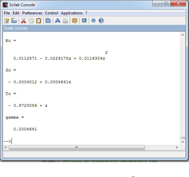
Figure 8.6: Scilab output for twodof para.sce
148
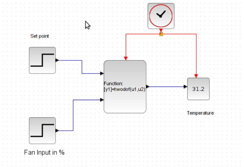
Figure 8.7: Xcos diagram for 2-DOF controller
149
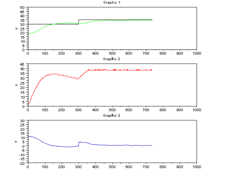
Figure 8.8: Implementation of 2-DOF controller
150

27 t i n i t =0 ; / / s i m u l a t i o n s t a r t t i m e
28 t f i n a l =0 . 5 ; / / s i m u l a t i o n e n d t i m e
29
30 / / S e t t i n g u p s i m u l a t i o n p a r a m e t e r s f o r c s s c l . c o s
31 N va r =0 ; x I n i t i a l =[ 0 0 0 ] ; N =1 ; C =0 ; D =1 ;
32
33 [ Tc1 , Rc1 ] =c o s f i l i p ( Tc , Rc ) ; / / T c /R c
34 [ Sc2 , Rc2 ] =c o s f i l i p ( Sc , Rc ) ; / / S c /R c
35
36 [ Bp ] =c o s f i l i p (B , 1 ) ;
37 [ Ap ] =c o s f i l i p (A, 1 ) ;
38
39 [ Tcp1 , Tcp2 ] =c o s f i l i p ( Tc , 1 ) ; / / T c /1
40 [ Np , Rcp ] =c o s f i l i p (N, Rc ) ; / / 1/R c
41 [ Scp1 , Scp2 ] =c o s f i l i p ( Sc , 1 ) ; / / S c /1
42 [ Cp , Dp ] =c o s f i l i p (C , D) ; / / C/D
43
44 / / Rc1 =R c ( 1 ) ; R c 2 =R c ( 2 ) ; R c 3 =R c ( 3 ) ; R c 4 =R c ( 4 ) ;
45 / / Sc1 =S c ( 1 ) ; S c 2 =S c ( 2 ) ;
46 / / Sc3 =S c ( 3 ) ;
47 / / T c 1 =T c ( 1 ) ; T c 2 =T c ( 2 ) ;
48 / / T c 3 =T c ( 3 ) ;
49 d i s p ( Rcp , ’ Rc =’ )
50 d i s p ( Scp1 , ’ Sc =’ )
51 d i s p ( Tcp1 , ’ Tc =’ )
52 d i s p ( gamm , ’gamma =’ )
53
54
55
56 / / u o l d o l d =1 ;
57 / / u o l d =1 ;
58 / / r old old =1 ;
59 / / r o l d =1 ;
60 / / y o l d o l d =1 ;
61 / / y o l d =1 ;
Scilab Code 8.2 twodof.sci
151

1mode ( 0 )
2function [ temp ] =t w odo f ( s e t p o i n t , f a n )
3global temp h e a t i n f a n i n C0 u o l d u new e o l d e new
e old old
4
5global h e a t d i s p f a n d i s p t e m p d i s p s e t p o i n t d i s p
s a m p l i n g t i m e m name
6
7global temp u o l d o l d u o l d r o l d o l d r o l d y o l d o l d
y o l d u new h e a t r n ew y new
8
9Ts=s a m p l i n g t i m e ;
10
11 r ne w =s e t p o i n t ;
12 y new =temp ;
13 e t =setpoint −temp ;
14
15 / / u n e w =( 1 /R c ( 1 ) ) *( gamm *T c ( 1 ) *r n e w +gamm *T c ( 2 ) *
r o l d +r old old *T c ( 3 ) *gamm −S c ( 1 ) *y n e w −S c ( 2 ) *
y o l d −S c ( 3 ) *y o l d o l d −R c ( 2 ) *u o l d −R c ( 3 ) *
u o l d o l d ) ; / / s e c o n d o r d e r c o n t r o l l a w
16
17 u new =( 1 /Rc ( 1 ) ) *(gamm*Tc ( 1 ) *r ne w +gamm*Tc ( 2 ) *r o l d
−Sc ( 1 ) *y new −Sc ( 2 ) *y o l d −Rc ( 2 ) *u o l d −Rc ( 3 ) *
u o l d o l d ) ; / / f i r s t o r d e r c o n t r o l l a w
18
19 u o l d o l d =u o l d ;
20 u o l d =u new ;
21 r old old=r o l d ;
22 r o l d =r n ew ;
23 y o l d o l d =y o l d ;
24 y o l d =y new ;
25
26
27 h e a t =u new ;
28 temp =comm( h e a t , f a n ) ;
29
30 p l o t t i n g ( [ h e a t f a n temp s e t p o i n t ] , [ 0 0 20 0 ] , [ 1 0 0
152

100 40 1 0 0 0 ] )
31
32 m=m+1;
33 endfunction
Scilab Code 8.3 start.sce
1g e t d . . /c o m m o n f i l e s /
2g e t d dc /scilab
3e x e c . . /c o m m o n f i l e s /l o a d e r . s c e
4
5e x e c s e r i n i t . s c e
6
7e x e c t w o d o f p a r a . s c e
8e x e c t wodo f . s c i
9
10 xco s two d of . xco s
Scilab Code 8.4 cindep.sci
1/ / Updated − − − − No change
2/ / function b =c i n d e p ( S , g a p )
3/ / u s e d i n X D +Y N =C . a l l r o w s e x c e p t t h e l a s t o f
a r e a s s u m e d t o
4/ / b e i n d e p e n d e n t . T h e a i m i s t o c h e c k i f t h e l a s t
r o w i s d e p e n d e n t o n t h e
5/ / r e s t a n d i f s o h o w . T h e c o e f f i c i e n t s o f d e p e n d e n c e
i s s e n t i n b
6function b=c i n d e p ( S , gap )
7
8i f argn ( 2 ) == 1
9gap =1 . 0 e8 ;
10 end
11 eps =2 . 2 2 0 4 e −016;
12 [ rows , c o l s ] =size ( S ) ;
13 i f rows >c o l s
14 i n d =0 ;
15 else
153

16 sigma =svd ( S ) ;
17 l e n =length ( si gm a ) ;
18 i f ( si gm a ( l e n ) /sigm a ( 1 ) <=( eps *max ( i , c o l s ) ) )
19 i n d =0 ; / / n o t i n d e p e n d e n t
20 else
21 i f or ( s igma ( 1 : l e n −1) . /sigma ( 2 : l e n )>=gap )
22 i n d =0 ; / / not dependent
23 else
24 i n d =1 ; / / independent
25 end
26 end
27 end
28 i f i n d
29 b=[];
30 else
31 b=S ( rows , : ) /S ( 1 : rows −1 , : ) ;
32 b=makezero ( b , gap ) ;
33 end
34 endfunction
Scilab Code 8.5 clcoef.sci
1/ / Updated −−−−−No change
2/ / H . K w a k e r n a a k , J u l y , 1 9 9 0
3/ / M o d i f i e d b y K a n n a n M o u d g a l y a i n N o v . 1 9 9 2
4
5function [ P , degP ] =c l c o e f (Q, degQ )
6
7[ rQ , cQ ] =p o l s i z e (Q, degQ ) ;
8
9i f and ( and (Q==0) )
10 P=zeros ( rQ , cQ ) ;
11 degP =0 ;
12 else
13 P=Q; degP =degQ ; rP =rQ ; cP =cQ ;
14 j=degP+1;
15 while j>=0
16 X=P ( : , ( j −1) *cP +1: j *cP )
154

17 i f max (sum (abs (X’ ) ) ) <( 1 e −8) *max (sum (abs ( P ) ) )
18 P=P ( : , 1 : ( j −1) *cP ) ;
19 degP =degP −1;
20 else
21 j=0 ;
22 end
23 j=j−1;
24 end
25 end
26 endfunction
Scilab Code 8.6 colsplit.sci
1/ / colsplit
2/ / T h e c o m m a n d
3/ / [ P 1 , d e g P 1 , P 2 , d e g P 2 ] =c o l s p l i t ( P , d e g P , p 1 , p 2 )
4/ / p r o d u c e s t w o p o l y n o m i a l m a t r i x P 1 a n d P 2 . P 1
c o n s i s t s o f t h e f i r s t
5/ / p 1 c o l u m n s o f P a n d P 2 c o n s i s t s o f t h e r e m a i n i n g p 2
c o l u m n s o f P .
6
7/ / H . K w a k e r n a a k , J u l y , 1 9 9 0
8
9
10 function [ P1 , degP1 , P2 , degP2 ] =c o l s p l i t ( P , degP , p1 , p2 )
11
12 i f i s e m p t y ( P )
13 P1 =[ ] ; P2 =[];
14 degP1 =0 ; degP2 =0 ;
15 r e t u r n ;
16 end
17
18 [ rP , cP ] =p o l s i z e ( P , degP ) ;
19 i f p1 <0|p1 >cP |p2 <0|p2 >cP |p1+p2 ˜=cP
20 error ( ’ c o l s p l i t : I n c o n s i s t e n t numbers o f colu mns ’ ) ;
21 end
22 rP1 =rP ; rP2 =rP ; cP1 =p1 ; cP2 =p2 ;
23 degP1=degP ; degP2 =degP ;
155

24
25 i f p1 == 0
26 P1 == [ ] ; P2 =P ;
27 elseif p2 == 0
28 P1 =P ; P2 =[];
29 else
30 P1 =zeros ( rP1 , ( degP1 +1) *cP1 ) ; P2 =zeros ( rP2 , (
degP2+1) *cP2 ) ;
31 for i=1 : degP+1
32 P1 ( : , ( i −1) *cP1+1: i *cP1 ) =P ( : , ( i −1) *cP +1 : ( i −1) *
cP+cP1 ) ;
33 P2 ( : , ( i −1) *cP2+1: i *cP2 ) =P ( : , ( i −1) *cP+cP1+1: i *
cP ) ;
34 end
35 end
36 endfunction ;
Scilab Code 8.7 cosfil ip.sci
1/ / Updated (31 −7−07)
2/ / I n p u t a r g u m e n t s a r e n u m e r a t o r a n d d e n o m i n a t o r
3/ / p o l y n o m i a l s ’ c o e f f i c i e n t s i n a s c e n d i n g
4/ / p o w e r s o f z ˆ −1
5
6/ / S c i c o s b l o c k s n e e d i n p u t p o l y n o m i a l s
7/ / w i t h p o s i t i v e p o w e r s o f z
8
9function [ nume , deno ] =c o s f i l i p ( num , den )
10
11 [ Nn , Nd ] =p ol yno ( num , ’ z ’ ) ;
12 [ Dn , Dd ] =p o l y n o ( den , ’ z ’ ) ;
13 nume =Nn*Dd ;
14 deno =Nd*Dn ;
15
16 endfunction ;
Scilab Code 8.8 indep.sci
156
1/ / Updated − − − − N o c h a n g e
2/ / function b =i n d e p ( S , g a p )
3/ / d e t e r m i n e s t h e f i r s t r o w t h a t i s d e p e n d e n t o n t h e
p r e v i o u s r o w s o f S .
4/ / T h e c o e f f i c i e n t s o f d e p e n d e n c e i s r e t u r n e d i n b
5function b=i n d e p ( S , gap )
6
7i f argn ( 2 ) == 1
8gap =1 . 0 e8 ;
9end
10 [ rows , c o l s ] =size ( S ) ;
11 i n d =1 ;
12 i=2 ;
13 eps =2 . 2 2 0 4 e −016;
14 while i n d & i <=rows
15 sigma =svd ( S ( 1 : i , : ) ) ;
16 l e n =length ( si gm a ) ;
17 i f ( s igma ( l e n ) /s ig ma ( 1 ) <( e p s *max ( i , c o l s ) ) )
18 i n d =0;
19 else
20 shsig =[ sigma ( 2 : l e n ) ; sigma ( l e n ) ] ;
21 i f o r ( ( s i gm a . /s h s i g ) >gap )
22 i n d =0 ;
23 else
24 i n d =1 ;
25 i=i+1;
26 end
27 end
28
29 end
30 i f i n d
31 b=[];
32
33 else
34 c=S ( i , : ) /S ( 1 : i −1 , : ) ;
35 c=makezero ( c , gap ) ;
36 b=[−c 1 ] ;
37 end
157

38 endfunction
Scilab Code 8.9 left prm.sci
1/ / f u n c t i o n [ B , d e g B , A , d e g A , Y , d e g Y , X , d e g X ] =. . .
2/ / l e f t p r m ( N , d e g N , D , d e g D , j o b , g a p )
3/ /
4/ / d o e s t h r e e d i f f e r e n t t h i n g s a c c o r d i n g t o i n t e g e r s
t h a t ’ j o b ’ t a k e s
5/ / j o b =1 .
6/ / t h i s i s t h e d e f a u l t . I t i s a l w a y s d o n e f o r a l l
j o b s .
7/ / −1−1
−1
8/ / G i v e n N D , r e t u r n s c o p r i m e B a n d A w h e r e N D =A
B
9/ / I t i s e n o u g h i f o n e s e n d s t h e f i r s t f o u r i n p u t
arguments
10 / / I f g a p i s r e q u i r e d t o b e s e n t , t h e n o n e c a n s e n d
e i t h e r 1 o r a n u l l
11 / / e n t r y f o r j o b
12 / / j o b =2 .
13 / / f i r s t s o l v e f o r j o b =1 a n d t h e n s o l v e X A +Y B =I
14 / / j o b =3 .
15 / / u s e d i n s o l v i n g X D +Y N =C
16 / / a f t e r f i n d i n g c o p r i m e f a c t o r i z a t i o n , d a t a a r e
returned
17 / /
18 / / c o n v e n t i o n : t h e v a r i a b l e w i t h p r e f i x d e g s t a n d f o r
degrees
19 / / o f t h e c o r r e s p o n d i n g p o l y n o m i a l m a t r i c e s
20 / /
21 / / i n p u t :
22 / / N : r i g h t f r a c t i o n n u m e r a t o r p o l y n o m i a l m a t r i x
23 / / D : r i g h t f r a c t i o n d e n o m i n a t o r p o l y n o m i a l m a t r i x
24 / / N a n d D a r e n o t n e c c e s s a r i l y c o p r i m e
25 / / g a p : v a r i a b l e u s e d t o z e r o e n t r i e s ; d e f a u l t v a l u e
i s 1 . 0 e +8
158

26 / /
27 / / output
28 / / b a n d A a r e l e f t c o p r i m e n u m . a n d d e n . p o l y n o m i a l
m a t r i c e s
29 / / X a n d Y a r e s o l u t i o n s t o A r y a b h a t t a i d e n t i t y , o n l y
f o r j o b =2
30
31 function [B , degB , A, degA , Y, degY , X, degX ] =l e f t p r m (N,
degN , D, degD , j ob , gap )
32 i f argn ( 2 ) == 4|argn ( 2 ) == 5
33 gap =1 . 0 e8 ;
34 end
35 / / p a u s e
36 i f argn ( 2 ) == 4 ,
37 j o b =1 ; end
38 [ F , degF ] =r o w j o i n (D, degD , N, degN ) ;
39 [ Frows , F b c o l s ] =p o l s i z e ( F , degF ) ; / / F b c o l s =
b l o c k c o l u m n s
40 Fcols =Fbcols *( degF+1) ; / / actual
c o l u m n s o f F
41 T1 =[ ] ; p r =[ ] ; degT1 =0; T1rows =0 ; s h f t =0 ;
42 S=F ; s e l =on es ( Frows , 1 ) ; T 1 b c o l s =1;
43 a b a r =( Fbcols +1 ) : Frows ; / / a super bar
o f B −C . Chang
44 while i s e m p t y ( T1 ) |T1rows <Frows −Fbcols
45 Srows =Frows*T 1 b c o l s ; / / m a x a c t u a l c o l u m n s o f
result
46 [ T1 , T1rows , s e l , p r ] =. . .
47 t 1 c a l c ( S , Srows , T1 , T1rows , s el , pr , Frows ,
Fbcols , ab a r , gap ) ;
48 [ T1rows , T 1 c o l s ] =size ( T1 ) ;
49 i f T1rows <Frows −Fbcols
50 T1 =[ T1 zeros ( T1rows , Frows ) ] ;
51 T1bcols =T1bcols +1 ; / / m a x . b l o c k
c o l u m n s o f r e s u l t
52 degT1 =degT1 +1 ; / / d e g r e e o f
result
53 shft =shft +Fbcols ;
159

54 S=s e s h f t ( S , F , s h f t ) ;
55 s e l =[ s e l ; s e l ( Srows −Frows+1: Srows ) ] ;
56 rowvec =( T1 bco l s −1) *Frows+( F b c o l s +1) : T 1 b c o l s
*Frows ;
57 a b a r =[ a b a r rowvec ] ; / / A super bar
o f B −C. chang
58 end
59 end
60
61 [ B , degB , A, degA ] =c o l s p l i t ( T1 , degT1 , Fbco l s , Frows −
F b c o l s ) ;
62 [ B , degB ] =c l c o e f (B , degB ) ;
63 B=−B ;
64 [A, degA ] =c l c o e f (A, degA ) ;
65 / / p a u s e
66 i f j o b == 2
67 S=S ( m t l b l o g i c a l ( s e l ) , : ) ;
/ / columns
68 [ redSrows , S c o l s ] =size ( S ) ;
69 C=[eye ( F bc ols , F b c o l s ) zeros ( F b c o l s , S c o l s −
F b c o l s ) ] ; / / a p p e n d w i t h z e r o s
70 T2 =C/S ;
71 T2 =makezero ( T2 , gap ) ;
72 T2 =m o v e s c i ( T2 , f i n d ( s e l ) , Srows ) ;
73 [X, degX , Y, degY ] =c o l s p l i t ( T2 , degT1 , Fbcols , Frows
−F b c o l s ) ;
74 [X, degX ] =c l c o e f (X, degX ) ;
75 [Y, degY ] =c l c o e f (Y, degY ) ;
76 elseif j o b == 3
77 Y=S ;
78 degY =s e l ;
79 X=degT1 ;
80 degX =Fbcols ;
81 else
82 i f j o b ˜=1
83 error ( ’ Message from l e f t p r m : no l e g a l j o b
number s p e c i f i e d ’ )
84 end
160

85 end
86 endfunction
Scilab Code 8.10 makezero.sci
1/ / Updated
2/ / function B =m a k e z e r o ( B , g a p )
3/ / w h e r e B i s a v e c t o r a n d g a p a c t s a s a t o l e r a n c e
4
5function B=ma kez ero ( B , gap )
6
7i f argn ( 2 ) == 1
8gap =1 . 0 e8 ;
9end
10 temp =B( f i n d (B) ) ; / / n o n z e r o e n t r i e s o f B
11 temp =−gsort(−abs ( temp ) ) ; / / a b s o l u t e v a l u e s s o r t e d
i n d e s c e n d i n g o r d e r
12 l e n =length ( temp ) ;
13 r a t i o =temp ( 1 : l e n −1) . /temp ( 2 : l e n ) ; / / e a c h r a t i o >1
14 m i n i n d =min (f i n d ( r a t i o >gap ) ) ;
15 i f ˜ i s e m p t y ( m i n i n d )
16 our eps =temp ( m i n i n d +1) ;
17 zeroind =f i n d (abs (B)<=o u r e p s ) ;
18 B( zeroind ) =zeros ( 1 , length ( zeroind ) ) ;
19 end
20 endfunction
Scilab Code 8.11 move sci.sci
1/ / f u n c t i o n r e s u l t =m o v e s c i ( b , n o n r e d , m a x s c i )
2/ / M o v e s m a t r i x b t o m a t r i x r e s u l t w i t h t h e
i n f o r m a t i o n o n w h e r e t o m o v e ,
3/ / d e c i d e d b y t h e i n d i c e s o f n o n r e d .
4/ / T h e m a t r i x r e s u l t w i l l h a v e a s m a n y r o w s a s b h a s
a n d m a x n u m b e r o f c o l u m n s .
5/ / b i s a u g u m e n t e d w i t h z e r o s t o h a v e n o n r e d n u m b e r o f
columns ;
161

6/ / T h e c o l u m n s o f b p u t i n t o t h o s e o f r e s u l t a s
d e c i d e d b y n o n r e d .
7
8function result =m o v e s c i ( b , no nre d , m a x s c i )
9[ brows , b c o l s ] =size ( b ) ;
10 b=[ b zeros ( brows , length ( n o n r e d ) −b c o l s ) ] ;
11 result =zeros ( brows , m a x s c i ) ;
12 r e s u l t ( : , n onred ’ ) =b ;
13 endfunction
Scilab Code 8.12 polisize.sci
1/ / Updated − − − − No change
2/ / f u n c t i o n [ r Q , c Q ] =p o l s i z e ( Q , d e g Q )
3/ / F U N C T I O N p o l s i z e T O D E T E R M I N E T H E D I M E N S I O N S
4/ / O F A P O L Y N O M I A L M A T R I X
5/ /
6/ / H . K w a k e r n a a k , A u g u s t , 1 9 9 0
7
8function [ rQ , cQ ] =p o l s i z e (Q, degQ )
9
10 [ rQ , cQ ] =size (Q) ; cQ =cQ /( degQ +1) ;
11 i f abs (round ( cQ )−cQ ) >1 e −6
12 error ( ’ p o l s i z e : Degree o f i n p u t i n c o n s i s t e n t w i t h
number o f c ol umn s ’ ) ;
13 else
14 cQ =round ( cQ ) ;
15 end
16 endfunction
Scilab Code 8.13 polyno.sci
1/ / Updated (1 −8−0 7 )
2/ / Operations :
3/ / P o l y n o m i a l d e f i n i t i o n
4/ / F l i p p i n g o f c o e f f i c i e n t s
5/ / V a r i a b l e −−−−−−− p a s s e d a s i n p u t a r g u m e n t ( e i t h e r ’
s ’ o r ’ z ’ )
162

6/ / B o t h n u m a n d d e n a r e u s e d m o s t l y u s e d i n s c i c o s
f i l e s ,
7/ / t o g e t r i d o f n e g a t i v e p o w e r s o f z
8
9/ / P o l y n o m i a l s w i t h p o w e r s o f s n e e d t o
10 / / b e f l i p p e d o n l y
11
12 function [ p ol ynu , p o l y d e ] =p o l y n o ( zc , a )
13 zc =clean ( z c ) ;
14 polynu =p o l y ( zc ( length ( zc ) : −1 : 1 ) , a , ’ c o e f f ’ ) ;
15 i f a== ’ z ’
16 p o l y d e =%z ˆ ( length ( zc ) −1 ) ;
17 else
18 p o l y d e =1 ;
19 end
20
21 / / S c i c o s ( 4 . 1 ) F i l t e r b l o c k s h o u l d n ’ t h a v e c o n s t a n t /
constant
22 i f t y p e ( p o l y n u ) ==1 & t y p e ( p o l y d e ) ==1
23 i f a== ’ z ’
24 polynu =%z ; p o l y d e =%z ;
25 else
26 polynu =%s ; p o l y d e =%s ;
27 end ;
28 end ;
29
30 endfunction
Scilab Code 8.14 rowjoin.sci
1/ / Updated − − − − − − − − No change
2/ / f u n c t i o n [ P , d e g P ] =r o w j o i n ( P 1 , d e g P 1 , P 2 , d e g P 2 )
3/ / M A T L A B F U N C T I O N r o w j o i n T O S U P E R P O S E TWO P O L Y N O M I A L
4/ / MATRICES
5
6/ / H . K w a k e r n a a k , J u l y , 1 9 9 0
7
8function [ P , degP ] =r o w j o i n ( P1 , degP1 , P2 , degP2 )
163

9
10 [ rP1 , cP1 ] =p o l s i z e ( P1 , degP1 ) ;
11 [ rP2 , cP2 ] =p o l s i z e ( P2 , degP2 ) ;
12 i f cP1 ˜=cP2
13 error ( ’ r o w j o i n : I n c o n s i s t e n t numbers o f columns ’ ) ;
14 end
15
16 rP =rP1+rP2 ; cP =cP1 ;
17 i f degP1 >=degP2
18 degP =degP1 ;
19 else
20 degP =degP2 ;
21 end
22
23 i f i s e m p t y ( P1 )
24 P=P2 ;
25 elseif i s e m p t y ( P2 )
26 P=P1 ;
27 else
28 P=zeros ( rP , ( degP +1) *cP ) ;
29 P ( 1 : rP1 , 1 : ( degP1 +1) *cP1 ) =P1 ;
30 P ( rP1 +1: rP , 1 : ( degP2 +1) *cP2 ) =P2 ;
31 end
32 endfunction
Scilab Code 8.15 seshft.sci
1/ / Updated − − − − − − − − No change
2/ / function C =s e s h f t ( A , B , N )
3/ / g i v e n A a n d B m a t r i c e s , r e t u r n s C =[<−A−>0
4/ / 0<−B−>] w i t h B
s h i f t e d e a s t b y N c o l s
5
6function C=s e s h f t (A, B,N)
7[ Arows , Ac ols ] =size (A) ;
8[ Brows , B c o l s ] =size (B ) ;
9i f N>=0
10 B=[zeros ( Brows ,N) B ] ;
164

11 Bcols =Bcols +N;
12 elseif N<0
13 A=[zeros ( Arows , abs (N) ) A ] ;
14 Acols =Acols +abs (N) ;
15 end
16 i f Acols <Bcols
17 A=[A zeros ( Arows , Bcols −A col s ) ] ;
18 elseif Acols >Bcols
19 B=[B zeros ( Brows , Acols −B c o l s ) ] ;
20 end
21 C=[A
22 B ] ;
23 endfunction
Scilab Code 8.16 t1calc.sci
1/ / Updated
2/ / f u n c t i o n [ T 1 , T 1 r o w s , s e l , p r ] =. . .
3/ / t 1 c a l c ( S , S r o w s , T 1 , T 1 r o w s , s e l , p r , F r o w s , F b c o l s , a b a r ,
g a p )
4/ / c a l c u l a t e s t h e c o e f f i c i e n t m a t r i x T 1
5/ / r e d u n d a n t r o w i n f o r m a t i o n i s k e p t i n s e l : r e d u n d a n t
r o w s a r e m a r k e d
6/ / w i t h z e r o s . T h e u n d e l e t e d r o w s a r e m a r k e d w i t h
o n e s .
7
8function [ T1 , T1rows , s e l , p r ] =t 1 c a l c ( S , Srows , T1 , T1rows
, s e l , pr , Frows , F bc ols , a ba r , gap )
9b=1 ; / / v e c t o r o f
p r i m a r y r e d . r o w s
10
11 while ( T1rows <Frows −F b c o l s ) & o r ( s e l ==1) & ˜
i s e m p t y ( b )
12 S=clean ( S ) ;
13 b=i n d e p ( S ( m t l b l o g i c a l ( s e l ) , : ) , gap ) ; / / s e n d
s e l e c t e d r o w s o f S
14 i f ˜ isempty (b)
15 b=clean ( b ) ;
165

16 b=m o v e s c i ( b , f i n d ( s e l ) , Srows ) ;
17 j=length ( b ) ;
18 while ˜ ( b ( j ) & o r ( a b a r== j ) ) / / p i c k l a r g e s t
n o n z e r o e n t r y
19 j=j−1; / / o f c o e f f .
belonging to abar
20 i f ˜ j
21 fprintf ( ’ \nMessage from t 1 c a l c ,
c a l l e d from l e f t p r m \n\n ’ )
22 error ( ’ De n omi n ato r i s n o n i n v e r t i b l e
’ )
23 end
24 end
25 i f ˜ o r ( j <p r & pmodulo ( pr , Frows ) == pmodulo ( j ,
Frows ) ) / / p r ( 2 ) , p r ( 1 )
26 T1 =[ T1 ; b ] ; / / condition
is not violated
27 T1rows =T1rows +1; / / a c c e p t t h i s
v e c t o r
28 end / / e l s e d o n ’ t
a c c e p t
29 p r =[ p r ; j ] ; / / u p d a t e
p r i m e r e d r o w i n f o
30 while j<=Srows
31 s e l ( j ) =0 ;
32 j=j+Frows ;
33 end
34 end
35 end
36 endfunction
8.7 Scilab Code for Virtual Experiment
Scilab Code 8.17 twodof para.sce
1mode ( 0 )
2global Rc Sc Tc gamm u o l d o l d u o l d r o l d o l d r o l d
166

y o l d o l d y o l d u new r n ew y new
3s=%s ;
4z=%z ;
5/ / TFcont =s y s l i n ( ’ c ’ , 0 . 5 9 3 /((47.21*s+1 ) *(1.373*s+1 ) ) )
;/ / s e c o n d o r d e r
6/ / TFcont =s y s l i n ( ’ c ’ , 0 . 5 9 4 /(49.19*s+1 ) ) / / f i r s t o r d e r
7TFcont =syslin ( ’ c ’ , 0 . 4 2 /(35.61*s+1) ) ; / / f i r s t o r d e r
8SS c ont =tf2ss ( TFcont ) ;
9Ts =1 ;
10 [ B , A, k ] =myc2d ( SScont , Ts ) ;
11
12 / / p o l y n o m i a l s a r e r e t u r n e d
13 [ Ds , num , den ] =ss2tf ( S Sco nt ) ;
14 num =clean ( num ) ; den =clean ( den ) ;
15
16 / / T r a n s i e n t s p e c i f i c a t i o n s
17 r i s e =100; epsilon =0.05;
18 p h i =d e s i r e d ( Ts , r i s e , e p s i l o n ) ;
19
20 / / C o n t r o l l e r d e s i g n
21 Delta =[ 1 −1];
22 [ Rc , Sc , Tc , gamm] =pp im ( B ,A, k , phi , D e l t a ) ; / / w i t h
i n t e g r a l
23
24 / / i n i t i a l v a l u e s
25 u o l d o l d =0 ;
26 u o l d =0 ;
27 r old old =0 ;
28 r o l d =0 ;
29 y o l d o l d =0 ;
30 y o l d =0 ;
Scilab Code 8.18 twodof.sce
1mode ( 0 )
2global f d f h f d t f n c r fncw m e r r c o u n t y l i m i t s
s a m p l i n g t i m e m h e a t temp
3
167

4/ / **********************
5s a m p l i n g t i m e =1; / / I n s e c o n d s . F r a c t i o n s a r e a l l o w e d
6/ / **********************/ /
7g e t d ( ’ dc /scilab ’);
8e x e c ( ” t w o d o f p a r a . s c e ” )
9e x e c ( ” t w odo f . s c i ” ) ;
10
11 ok =i n i t ( ) ;
12
13 i f ok ˜=[ ] / / o p e n x c o s o n l y i f c o m m u n i c a t i o n i s
t h r o u g h ( i e r e p l y h a s c o m e f r o m s e r v e r )
14 xco s ( ’ t wod of . xcos ’ ) ;
15 else
16 d i s p ( ”NO NETWORK CONNECTION! ” ) ;
17 r e t u r n
18 end
Scilab Code 8.19 twodof.sci
1function [ s t o p ] =t wo d of ( s e t p o i n t , f a n )
2global temp u o l d o l d u o l d r o l d o l d r o l d
y o l d o l d y o l d u new h e a t r new y new
3
4r ne w =s e t p o i n t ;
5y new =temp ;
6/ / u n e w =( 1 /R c ( 1 ) ) *( gamm *T c ( 1 ) *r n e w +gamm *T c ( 2 )
*r o l d +r old old *T c ( 3 ) *gamm −S c ( 1 ) *y n e w −S c
( 2 ) *y o l d −S c ( 3 ) *y o l d o l d −R c ( 2 ) *u o l d −R c
( 3 ) *u o l d o l d ) ; / / s e c o n d o r d e r c o n t r o l l a w
7
8u new =( 1 /Rc ( 1 ) ) *(gamm*Tc ( 1 ) *r ne w +gamm*Tc ( 2 ) *
r o l d −Sc ( 1 ) *y new −Sc ( 2 ) *y o l d −Rc ( 2 ) *u o l d −Rc
( 3 ) *u o l d o l d ) ; / / f i r s t o r d e r c o n t r o l l a w
9h e a t =u new ;
10 [ s t o p , temp ] =comm ( h e a t , f a n ) ; / / N e v e r e d i t t h i s
line
11 p l o t t i n g ( [ h e a t f a n temp ] , [ 0 0 25 0 ] , [ 1 0 0 100 50
1 0 0 0 ] ) ;
168

12
13 u o l d o l d =u o l d ;
14 u o l d =u new ;
15 r old old=r o l d ;
16 r o l d =r n ew ;
17 y o l d o l d =y o l d ;
18 y o l d =y new ;
19
20 endfunction
8.8 Scilab Codes Common for both Local and Vir-
tual Experiments
Scilab Code 8.20 myc2d.sci
1/ / Updated (26 −7−07)
2/ / 9 . 2
3/ / f u n c t i o n [ B , A , k ] =m y c 2 d ( G , T s )
4/ / P r o d u c e s n u m e r a t o r a n d d e n o m i n a t o r o f d i s c r e t e
transfer
5/ / f u n c t i o n i n p o w e r s o f z ˆ { − 1}
6/ / G i s c o n t i n u o u s t r a n s f e r f u n c t i o n ; t i m e d e l a y s a r e
n o t a l l o w e d
7/ / T s i s t h e s a m p l i n g t i m e , a l l i n c o n s i s t e n t t i m e
units
8/ / U s e r d e f i n e d f u n c t i o n
9/ / −−−−−−
10
11 function [ B , A, k ] =myc2d (G, Ts )
12 H=ss2tf (d s c r (G, Ts ) ) ;
13 num1 =coeff (H( ’num ’ ) ) ;
14 den1 =coeff (H( ’ den ’ ) ) ; / / −−−−−−−−−−−−−
15 A=den1 ( length ( den1 ) : −1 : 1 ) ;
16 num2 =num1 ( length ( num1 ) : −1 : 1 ) ; / / f l i p
17 nonzero =m t l b f i n d ( num1 ) ;
18 f i r s t n z =n o n z e r o ( 1 ) ;
169

19 B=num2 ( f i r s t n z : length ( num2 ) ) ; / / −−−−−−−−−−−−−
20 k=length ( den1 ) −length ( num1 ) ;
21 endfunction
Scilab Code 8.21 desired.sci
1/ / Updated (26 −7−07)
2/ / 9 . 4
3function [ p hi , d p h i ] =d e s i r e d ( Ts , r i s e , e p s i l o n )
4
5Nr =r i s e /Ts ; omega =%pi /2/Nr ; rho =e p s i l o n ˆ ( omega /
%pi ) ;
6p h i =[ 1 −2*rho*cos ( omega ) r ho ˆ 2 ] ; d p h i =length ( p h i )
−1;
7endfunction ;
Scilab Code 8.22 polmul.sci
1/ / Updated − − − − − − No change
2/ / p o l m u l
3/ / T h e c o m m a n d
4/ / [ C , d e g A ] =p o l m u l ( A , d e g A , B , d e g B )
5/ / p r o d u c e s t h e p o l y n o m i a l m a t r i x C t h a t e q u a l s t h e
p r o d u c t A *B o f t h e
6/ / p o l y n o m i a l m a t r i c e s A a n d B .
7/ /
8/ / H . K w a k e r n a a k , J u l y , 1 9 9 0
9
10
11 function [ C , degC ] =p ol mu l (A, degA , B , degB )
12 [ rA , cA ] =p o l s i z e (A, degA ) ;
13 [ rB , cB ] =p o l s i z e (B , degB ) ;
14 i f cA ˜=rB
15 error ( ’ p olm ul : I n c o n s i s t e n t d i m e n s i o n s of i n p u t
matrices ’) ;
16 end
17
18 degC =degA+degB ;
170

19 C=[];
20 for k=0 : degA+degB
21 mi =0 ;
22 i f k−degB >mi
23 mi =k−degB ;
24 end
25 ma =degA ;
26 i f k<ma
27 ma =k ;
28 end
29 Ck =zeros ( rA , cB ) ;
30 for i=mi : ma
31 Ck =Ck +A ( : , i *cA +1 : ( i +1) *cA ) *B ( : , ( k−i ) *cB
+1 : ( k−i+1) *cB ) ;
32 end
33 C=[C Ck ] ;
34 end
35 endfunction
Scilab Code 8.23 polsplit3.sci
1/ / Updated (18 −7−07)
2/ / 9.11
3/ / f u n c t i o n [ g o o d p o l y , b a d p o l y ] =p o l s p l i t 3 ( f a c , a )
4/ / S p l i t s a s c a l a r p o l y n o m i a l o f z ˆ { − 1}i n t o g o o d a n d
bad
5/ / f a c t o r s . I n p u t i s a p o l y n o m i a l i n i n c r e a s i n g d e g r e e
o f
6/ / z ˆ { − 1}. O p t i o n a l i n p u t i s a , w h e r e a <=1 .
7/ / F a c t o r s t h a t h a v e r o o t s o u t s i d e a c i r c l e o f r a d i u s
a o r
8/ / w i t h n e g a t i v e r o o t s w i l l b e c a l l e d b a d a n d t h e r e s t
9/ / g o o d . I f a i s n o t s p e c i f i e d , i t w i l l b e a s s u m e d a s
1 .
10
11 function [ g oo dp oly , b a d p o l y ] =p o l s p l i t 3 ( f a c , a )
12 i f argn ( 2 ) == 1 , a =1 ; end
13 i f a>1error ( ’ good p o l y n o m i a l a l s o i s u n s t a b l e ’ ) ; end
171

14 f a c 1 =p o l y ( f a c ( length ( f a c ) : −1 : 1 ) , ’ z ’ , ’ c o e f f ’ ) ;
15 rts =roots ( f a c 1 ) ;
16 rts =r t s ( length ( r t s ) : −1 : 1 ) ;
17
18 / / e x t r a c t g o o d a n d b a d r o o t s
19 badindex =m t l b f i n d ( ( abs ( r t s )>=a−1.0 e −5) |(r e a l ( r t s )
<−0.05) ) ;
20 badpoly =coeff (p o l y ( r t s ( b a d i n d e x ) , ’ z ’ ) ) ;
21 goodindex =m t l b f i n d ( ( abs ( r t s )<a−1.0 e −5) &( r e a l ( r t s )
>=−0.05) ) ;
22 goo d p o ly =coeff (p o l y ( r t s ( g o o d i n d e x ) , ’ z ’ ) ) ;
23
24 / / s c a l e b y e q u a t i n g t h e l a r g e s t t e r m s
25 [m, i n d e x ] =max (abs ( f a c ) ) ;
26 goodbad =c o n v o l ( g o odp ol y , b a d p o l y ) ;
27 goodbad =goodbad ( length ( goodbad ) : −1 : 1 ) ;
28 factor1 =f a c ( i n d e x ) /g ood ba d ( i n d e x ) ;
29 goo d p o ly =goo d p oly *factor1 ;
30 goo d p o ly =goo d p oly ( length ( g o o dpol y ) : −1 : 1 ) ;
31 badpoly =b a d p o l y ( length ( b a d p o l y ) : −1 : 1 ) ;
32 endfunction ;
Scilab Code 8.24 pp im.sci
1/ / Updated (27 −7−07)
2/ / 9 . 8
3/ / f u n c t i o n [ R c , S c , T c , g a m m a , p h i t ] =p p i m ( B , A , k , p h i ,
Delta )
4/ / C a l c u l a t e s 2 −D O F p o l e p l a c e m e n t c o n t r o l l e r .
5/ / −−−−−−
6function [ Rc , Sc , Tc , gamm] =pp im ( B ,A, k , ph i , D e l t a )
7
8/ / S e t t i n g u p a n d s o l v i n g A r y a b h a t t a i d e n t i t y
9[ Ag , Ab ] =p o l s p l i t 3 (A) ; dAb =length ( Ab ) −1 ;
10 [ Bg , Bb ] =p o l s p l i t 3 (B) ; dBb =length ( Bb ) −1 ;
11
12 [ zk , dzk ] =zpowk ( k ) ;
13
172

14 [N, dN ] =p olmu l ( Bb , dBb , zk , dzk ) ;
15 d D e l t a =length ( D e l t a ) −1;
16 [D, dD ] =p o l m ul ( Ab , dAb , D e l t a , d D e l t a ) ;
17 d p h i =length ( p h i ) −1;
18
19 [ S1 , dS1 , R1 , dR1 ] =x dy nc ( N, dN , D, dD , ph i , d p h i ) ;
20
21 / / D e t e r m i n a t i o n o f c o n t r o l l a w
22 Rc =c o n v o l ( Bg , c o n v o l ( R1 , D e l t a ) ) ; Sc =c o n v o l ( Ag , S1 ) ;
23 Tc =Ag ; gamm =sum ( p h i ) /sum ( Bb ) ;
24 endfunction ;
Scilab Code 8.25 xdync.sci
1/ / Updated − − − − N o c h a n g e
2/ / f u n c t i o n [ Y , d e g Y , X , d e g X , B , d e g B , A , d e g A ] =x d y n c ( N ,
d e g N , D , d e g D , C , d e g C , g a p )
3/ / g i v e n c o e f f i c i e n t m a t r i x i n T 1 , p r i m a r y r e d u n d a n t
r o w i n f o r m a t i o n s e l ,
4/ / s o l v e s X D +Y N =C
5
6/ / c a l l i n g o r d e r c h a n g e d o n 1 6 A p r i l 2 0 0 5 . O l d o r d e r :
7/ / f u n c t i o n [ B , d e g B , A , d e g A , Y , d e g Y , X , d e g X ] =x d y n c ( N ,
d e g N , D , d e g D , C , d e g C , g a p )
8
9function [Y, degY , X , degX , B , degB , A, degA ] =xdync (N, degN ,
D, degD , C , degC , gap )
10 i f argn ( 2 ) == 6
11 gap =1 . 0 e +8;
12 end
13
14 [ F , degF ] =r o w j o i n (D, degD , N, degN ) ;
15
16 [ Frows , F b c o l s ] =p o l s i z e ( F , degF ) ; / / F b c o l s =block
columns
17
18 [B , degB , A, degA , S , s e l , degT1 , F b c o l s ] =l e f t p r m (N, degN , D
, degD , 3 , gap ) ;
173

19 / / i f i s s o l n ( D , d e g D , C , d e g C , B , d e g B , A , d e g A )
20 [ Crows , C c o l s ] =size (C ) ;
21 [ Srows , S c o l s ] =size ( S ) ;
22 S=clean ( S ) ;
23 S=S ( m t l b l o g i c a l ( s e l ) , : ) ;
24 T2 =[];
25
26 f o r i=1 : Crows ,
27 Saug =s e s h f t ( S , C( i , : ) , 0 ) ;
28 b=c i n d e p ( Saug ) ;
29 b=m o v e s c i ( b , f i n d ( s e l ) , Srows ) ;
30 T2 =[T2 ; b ] ;
31 end
32
33 [X, degX , Y, degY ] =c o l s p l i t ( T2 , degT1 , Fbcols , Frows −
F b c o l s ) ;
34
35 [X, degX ] =c l c o e f (X, degX ) ;
36 [Y, degY ] =c l c o e f (Y, degY ) ;
37 Y=clean (Y) ; X =clean (X) ;
38 endfunction
Scilab Code 8.26 zpowk.sci
1/ / Updated (26 −7−07)
2/ / 9 . 6
3/ / −−−−−−
4
5function [ zk , dzk ] =zpowk ( k )
6zk =zeros ( 1 , k +1) ; zk ( 1 , k +1) =1 ;
7dzk =k ;
8endfunction
174
Chapter 9
PRBS Modeling and
Implementation of Pole Placement
Controller
The aim of this chapter is to do PRBS testing on Single Board Heater System by
the application of PRBS signal and to design a pole-placement controller. The
target group is anyone who has basic knowledge of control engineering. The first
half of this chapter is dedicated to do system identification of the SBHS system
using the response obtained for a PRBS (Pseudo Random Binary Sequence) input.
In the second half, a pole-placement controller is designed using this model and
implemented on SBHS.
9.1 PRBS Modelling
Similar to Chapter 4 and 5, we will find the transfer function model of SBHS.
But there are two major differences. First difference is that we will give a Pseudo
Random Binary Sequence to the heater input of SBHS and the second difference
is that we will find the discrete time transfer function. A Pseudo Random Binary
Sequence is nothing but a signal whose amplitude varies between two limits ran-
domly at any given time. An illustration of the same is given in figure 9.4. A
PRBS signal can be easily generated using the rand() function in Scilab. Scilab
code to generate the PRBS signal is given at the end of this chapter.
We have used Scilab with Xcos as an interface for sending and receiving data.
This interface is shown in figure 9.1. Heater current and fan speed are the two
175
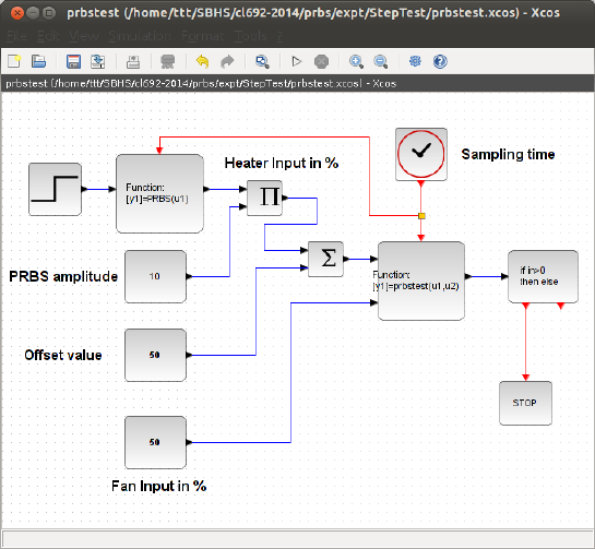
Figure 9.1: Xcos for PRBS testing experiment
inputs to the system. The heater current is varied with a PRBS signal. A provision
is made to set the parameters like PRBS amplitude and offset value. A provision
is also made to time the occurance of the PRBS input using a step block. The
value of step time in the step block has to be chosen carefully. Sufficient amount
of time should be given to allow the temperature to reach a steady-state before the
PRBS signal is applied. In this experiment we are keeping the fan speed constant
at 50%. The temperature profile thus obtained is the output.
9.1.1 Issues with Step Test and an Alternate Approach
SBHS is an example of a heater. Suppose you are working in a full scale plant.
Current control system designed to control one of the heaters of the plant is lousy
and your supervisor asks you to design a new controller from scratch. The first
step you need to do is identification of the heater transfer function. The catch
is, the plant is currently operational. You can’t shut the plant down to identify
the heater transfer function. You have to do it while the heater is operating in
the plant. You might think of giving the heater a positive step and measuring the
176
response in the controlled temperature. This will increase the temperature of the
component being heated for the period of time step is applied. However, if the
process is sensitive to temperature of the component (distillation, for example), it
will go offthe desired course and the output of the whole plant will be affected
and will be undesirable.
There is an alternate approach which is widely used in industry. The input
given to the heater for identification is not step, but a pseudo-random binary
sequence (PRBS). The concept behind PRBS is that the input is perturbed in such
a way that the time average of the input is the value at which it is being operated
currently. Thus, some positive and some negative steps can be given. This results
in some positive and some negative changes in the temperature which leads to the
time average of the performance of the plant remaining the same. Thus, PRBS
testing can be done in a working plant without affecting the plant performance
unlike step testing. A typical PRBS and corresponding plant output is shown in
figure 9.2
Figure 9.2: PRBS testing input and output [Image source: CL 686 Advanced Pro-
cess Control, Spring 2013-14 lecture slides. Prof. S. C. Patwardhan, IIT Bombay]
177

1.0 50.0 50.0 36.4 1417298828422.0
2.0 50.0 50.0 36.2 1417298828525.0
.
999.0 40.0 50.0 42.9 1417298933585.0
1000.0 40.0 50.0 42.9 1417298933694.0
Table 9.1: PRBS local experiment data
9.2 Conducting PRBS Test on SBHS locally
The detailed procedure to perform a local experiment is explained in Chapter2.
A summary of the same is provided in section 2.3 It is same for this section with
following changes.
1. Step1: The working directory is prbs/identification
2. Step2: Load the functions available in common files directory by executing
the command getd<space>..\..\common files
3. Step3: Same
4. Step4: Same
5. Step5: Load prbstest function by executing command
exec<space>prbstest.sci. Load prbs signal generation function by ex-
ecuting command exec<space>prbs.sci
6. Step6: Load Xcos code for prbs test using the command
exec<space>prbstest.xcos
7. Step7: Same
The response is as shown in figure 9.3. The data file thus obtained is as
shown in the Table 9.1. This data file is available for reference in the directory
prbs/identification with name prbs-data-local.txt
178
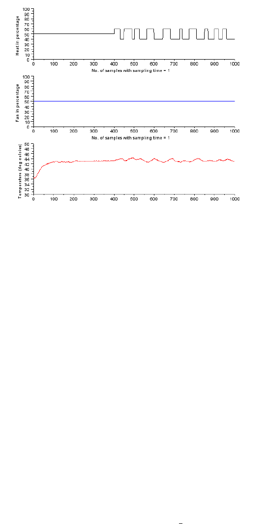
Figure 9.3: PRBS Local response
9.3 Conducting PRBS Test on SBHS, virtually
The detailed procedure to perform a virtual experiment is explained in Chapter3.
A summary of the same is provided in section 3.5. It is same for this section with
following changes.
1. Step1: The working directory is prbs/identification. Open this direc-
tory.
2. Step2: Same
3. Step3: Same
4. Step4: Switch to the working experiment directory and double-click on
the file prbstest.sce. This will launch scilab and also open the file
prbstest.sce in the scilab editor. Linux users will have to launch scilab
manually. They also have to change the working directory to prbs/identification
and then open the prbstest.sce file in the scilab editor.
5. Step5: Load the functions available in common files directory by executing
the command getd<space>..\..\common files
179
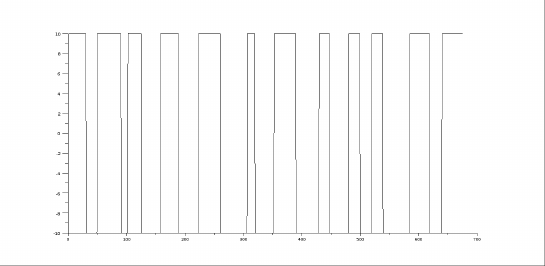
0 0 100 28.40 14...1731 14...4105 14...4123 14...1763 0.10000E+01
1 50 50 28.30 14...4706 14...7078 14...7096 14...4738 0.10000E+01
.
.
983 40 50 36.70 14...6728 14...9131 14...9148 14...6759 0.98300E+03
984 40 50 36.50 14...7712 14...0115 14...0133 14...7743 0.98400E+03
Table 9.2: PRBS data obtained after performing virtual PRBS Test
Figure 9.4: A Pseudo Random Binary Sequence
6. Step6: Execute the file prbstest.sce. Expect the prbs test xcos diagram
to open automatically. If this doesnt happen, check the scilab console for
error message.
7. Step7: Execute the prbstest xcos diagram.
8. Step8: Same
The virtual experiment response is shown in figure 9.5. The corresponding
data file is shown in table 9.2. The time stamps shown are cut short for better
viewing. This data file can be found in prbs/identification folder for virtual
experiments. The name of this file is prbs-data-virtual.txt.
180
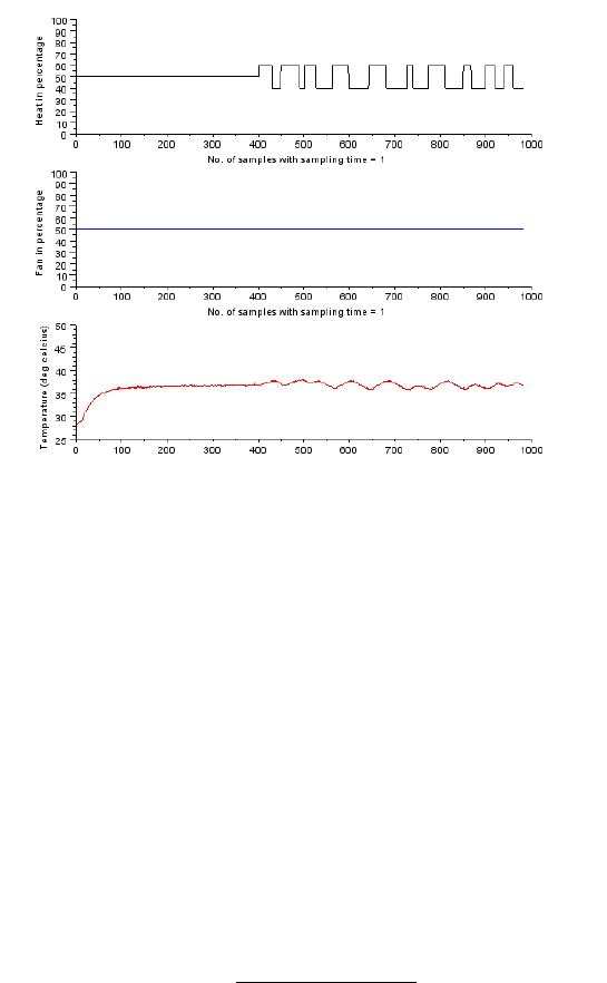
Figure 9.5: PRBS testing response for virtual experiment
9.4 Determination of Discrete Time Transfer Func-
tion models
System identification is carried out to identify the transfer function between the
input signal to the system and output from the system. Firstly, a transfer function
with unknown parameters is assumed. The system is given a known input and its
response is obtained and then the values of the unknown parameters is chosen such
that the sum of squares of the errors is minimized. Here, the error is the difference
between the actual output and the output predicted by the transfer function model
assumed. For the given SBHS system, we assume a second order transfer function:
G(z)=b1+b2z−1
1+a1z−1+a2z−2z−d(9.1)
The unknown parameters a1,a2,b1,b2and dare to be obtained through the
response of the system to the known inputs. a1,a2,b1,b2are real numbers and
dis the plant delay which is an integer. For these model parameters estimation,
we use a pseudo random binary sequence (PRBS) input. Since the optimization
over discrete variables (din this case) is a very difficult routine for computers,
we assume a value for dand then optimize over a1,a2,b1,b2. The optimization
181
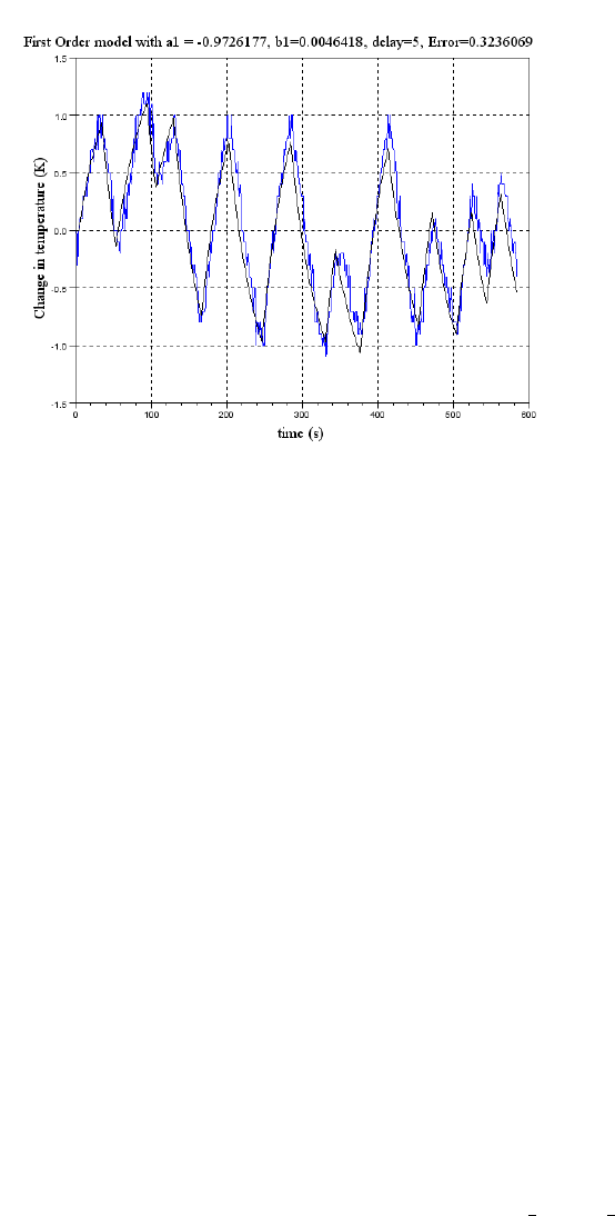
Figure 9.6: PRBS first order fit
problem, then, becomes:
(ˆ
b1,ˆ
b2,ˆa1,ˆa2)=argmin
b1,b2,a1,a2
N
X
i=0
(y(k)−ˆy(k))2(9.2)
Here, y(k) is the output obtained from the system- so it is known. ˆ
y(k) is the
estimated output using ythe model assumed, which can be written as a difference
equation:
ˆy(k)=−a1ˆy(k−1) −a2ˆy(k−2) +b1u(k−d)+b2u(k−1−d) (9.3)
9.5 Determination of First order Discrete time Trans-
fer Function
1. Download the Analysis folder from the sbhs website. It will be available
under downloads section. Download the file for SBHS Analysis Code
(local & virtual). The name of the file is scilab codes analysis.
182
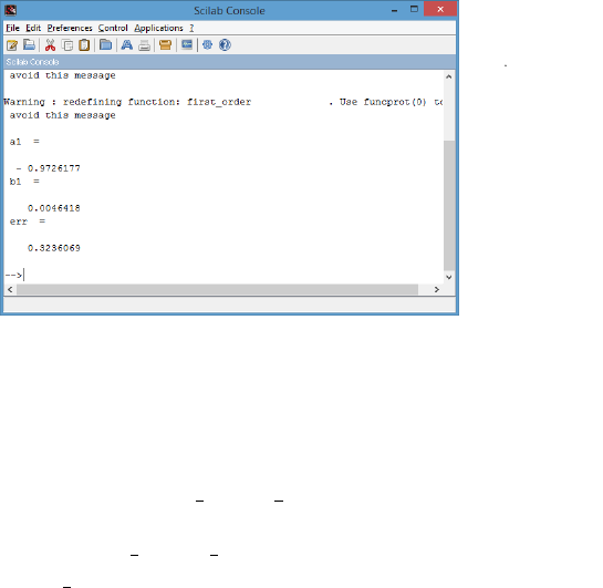
Figure 9.7: PRBS first order model
The download will be in zip format. Extrat the downloaded zip file. You
will get a folder scilab codes analysis.
2. Open the scilab codes analysis folder and then locate and open the
folder Step Analysis.
3. Inside this folder, locate and open the folder Discrete-order1
4. Copy the prbs test data file to this folder.
5. Start scilab and change the working directory to Discrete-order1
6. Open the file optimize.sce in scilab editor and enter the name of the data
file (with extention) in the filename field.
7. Save and run this code and obtain the plot as shown in figure 9.6. This plot
will also show the first order discrete time transfer function’s coefficients a1
and b1.
8. The values are also shown on scilab console as shown in figure 9.7
183

The results presented are obtained for the data file prbs-data-virtual.txt.
This data file is present under the prbs directory for virtual experiments.The plot
thus obtained is reasonably good. See the Scilab plot to get the values of a1
and b1. The figure 9.6 shows a screen shot of the same. We obtain a1=-0.97,
b1=0.004. The transfer function obtained here is at the operating point of 50
percentage of heat. If the experiment is repeated at a different operating point,
the transfer function obtained will be different. The gain will correspondingly be
more at a higher operating point. This means that the plant is faster at higher
temperature. Thus the transfer function of the plant varies with the operating
point. Let the transfer function we obtain in this experiment be denoted as G(z).
We obtain
G(z)=0.004
1−0.97z−1z−5(9.4)
9.6 Determination of Second order Discrete time Trans-
fer Function
1. Download the Analysis folder from the sbhs website. It will be available
under downloads section. Download the file for SBHS Analysis Code
(local & virtual). The name of the file is scilab codes analysis.
The download will be in zip format. Extrat the downloaded zip file. You
will get a folder scilab codes analysis.
2. Open the scilab codes analysis folder and then locate and open the
folder Step Analysis.
3. Inside this folder, locate and open the folder Discrete-order2
4. Copy the prbs test data file to this folder.
5. Start scilab and change the working directory to Discrete-order2
6. Open the file optimize.sce in scilab editor and enter the name of the data
file (with extention) in the filename field.
7. Save and run this code and obtain the plot as shown in figure 9.8. This plot
will also show the second order discrete time transfer function’s coefficients
a1, a2, b1 and b2.
184
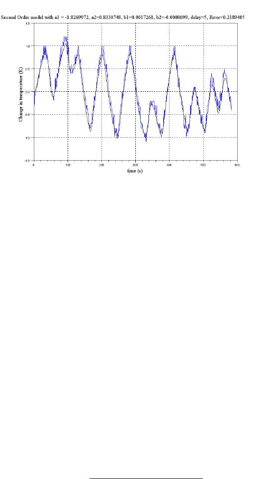
Figure 9.8: PRBS second order fit
8. The values are also shown on scilab console as shown in figure 9.9
The results presented are obtained for the data file prbs-data-virtual.txt.
This data file is present under the prbs directory for virtual experiments.The plot
thus obtained is reasonably good. See the Scilab plot to get the values of a1, a2,
b1 and b2. The figure 9.8 shows a screen shot of the same. We obtain a1=-1.82,
a2=0.833, b1=0.0017, b2=-0.00086, . The transfer function obtained here is
at the operating point of 50 percentage of heat. If the experiment is repeated at a
different operating point, the transfer function obtained will be different. The gain
will correspondingly be more at a higher operating point. This means that the
plant is faster at higher temperature. Thus the transfer function of the plant varies
with the operating point. Let the transfer function we obtain in this experiment be
denoted as G(z). We obtain
G(z)=0.0017 −0.00086z−1
1−1.826z−1+0.833z−2z−5(9.5)
185
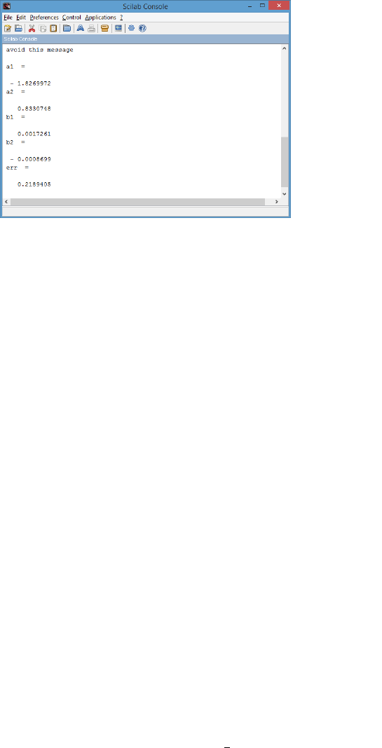
Figure 9.9: PRBS second order model
9.7 Implementing 2DOF pole-placement controller
using PRBS model, virtually
For deriving the Two degrees of freedom control law, please refer to the chapter
8.2 The controller was designed for the given transient conditions, rise time =10
sec, overshoot =0.1. The experimental result and performance of the controller
for setpoint temperature change from 38.00 to 43.00 degree C, i.e. 5 degree C
positive step change, has been shown below in Fig 9.10. The controller designed
is not derived for the model explained in earlier sections.
The parameters for the 2-DOF pole-placement controller obtained are shown
here
T c =1−1.9444137z−1+0.9447818z−2
S c =0.0337719 −0.0656666z−1+0.0319071z−2
Rc =10−9(4377900 −12034140z−1+11094713z−2−3436740.5z−3+3.469D−09z−4
−147850.06z−5+146117.57z−6)
γ=0.0337719
As can be observed from the graph of temperature vs. time (third subplot) in
Fig 9.10, the overshoot criteria was satisfied very easily. The rise time criteria is
observed to be more than 30 sec. This can be satisfied with experimentation. The
paramenters are computed by the file twodof para.sce.
186
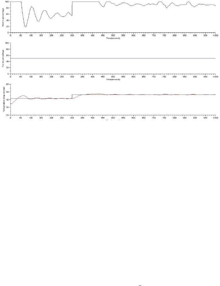
Figure 9.10: 2dof controller response
The steps to be followed to conduct PRBS test experiment virtually remains
same as explained in section 3.5. only for the following differences
•Step1: The working directory is prbs/controller. Open this directory.
•Step2: Same
•Step3: Same
•Step4: Switch to the controller experiment directory and double-click on
the file prbs.sce. This will launch scilab and also open the file prbs.sce
in the scilab editor. Linux users will have to launch scilab manually. They
also have to change the working directory to controller and then open
the prbs.sce file in the scilab editor.
•Step5: Load the functions available in common files directory by executing
the command getd<space>..\..\common files
•Step6: Execute the file prbs.sce. Expect the prbs test xcos diagram to
open automatically. If this doesnt happen, check the scilab console for error
message. The values of Rc, Sc, Tc and γare to be entered in the xcos
diagram.
•Step7: Execute the prbstest xcos diagram.
187

•Step8: Same
9.8 Implementing 2DOF pole-placement controller
using PRBS model, locally
The step by step procedure for conducting an experiment locally remains same as
explained in section 2.3 with the following changes
1. Step1: The working directory is prbs/controller
2. Step2: Load the functions available in common files directory by executing
the command getd<space>..\..\common files
3. Step3: Same
4. Step4: Same
5. Step5: Load prbstest function by executing command
exec<space>prbs pp.sci.
6. Step6: Load Xcos code for prbs test using the command
exec<space>prbs pp.xcos. The values of Rc, Sc, Tc and γare to be
entered in the xcos diagram.
7. Step7: Same
9.9 Scilab Local codes
9.9.1 Identification codes
Scilab Code 9.1 ser init.sce
1mode ( 0 )
2global f i l e n a m e m
3/ / * * Sampling Time * * / /
4s a m p l i n g t i m e =1 ;
5/ / / / / / / * * * * /////////
6m=1;
188

7
8port1 =’/dev /ttyUSB0 ’ ; / / F o r l i n u x u s e r s
9port2 =’COM2’ ; / / F o r w i n d o w s u s e r s
10
11 r e s =i n i t ( [ p o r t 1 p o r t 2 ] ) ;
12 d i s p ( r e s )
Scilab Code 9.2 costfunction.sci
1function [ f , g , i n d ] =c o s t f u n c t i o n ( x , i n d )
2global delay ;
3y prediction =s e c o n d o r d e r ( u , x ) ;
4i f s i z e ( y ) ˜=size ( y prediction ) then
5y prediction =y prediction ’;
6end
7f=(norm ( y−y p r e d i c t i o n , 2 ) ) ˆ 2 ;
8g=numdiff ( f u n c 1 , x ) ;
9endfunction
10
11 function f=f u n c 1 ( x )
12 global delay ;
13 y prediction =s e c o n d o r d e r ( u , x ) ;
14 i f s i z e ( y ) ˜=size ( y prediction ) then
15 y prediction =y prediction ’;
16 end
17 f=(norm ( y−y p r e d i c t i o n , 2 ) ) ˆ 2 ;
18 endfunction
Scilab Code 9.3 optimize.sce
1mode ( 0 ) ;
2/ / C h a n g e f i l e n a m e h e r e
3f i l e n a m e =” 30 A p r 2014 12 3 0 5 0 . t x t ” ;
4c l f
5
6
7e x e c ( ’ c o s t f u n c t i o n . s c i ’ ) ;
8e x e c ( ’ l a b e l . s c i ’ ) ;
189

9e x e c ( ’ s e c o n d o r d e r . s c i ’ ) ;
10
11
12 d a t a =fscanfMat ( f i l e n a m e ) ;
13
14 t i m e =d a t a ( : , 1 ) ;
15
16 heater =int ( d a t a ( : , 2 ) ) ;
17
18 fan =i n t ( d a t a ( : , 3) ) ;
19
20 temp =d a t a ( : , 4 ) ;
21
22 s s o p p t =h e a t e r ( 2 ) ;
23 for i=2: length ( h e a t e r )
24 i f h e a t e r ( i ) ˜=s s o p p t then
25 startTime =i ;
26 break
27 end
28 end
29
30
31 time1 =t i m e −t i m e ( 1 ) ;
32 time2 =time1 /1000;
33
34 baseheat =h e a t e r ( 5 ) ;
35 heater =h e a t e r ( s t a r t T i m e : length ( h e a t e r ) ) ;
36 heater =heater −baseheat ;
37
38 l e n =length ( h e a t e r ) ;
39
40 temp =temp ( s t a r t T i m e : length ( temp ) ) ;
41 temp =temp −temp ( 1 ) ;
42
43 t i m e =t i m e 2 ( s t a r t T i m e : length ( t i m e ) ) ;
44 t i m e =t i m e −t i m e ( 1 ) ;
45
46 t=t i m e ;
190

47 y=temp ;
48 u=heater ;
49
50 x0 =[ 0 . 2 0 . 2 0 . 5 0 . 5 ] ; / / C h a n g e i n i t i a l g u e s s h e r e
51 delay =5 ; / / C h a n g e d e l a y h e r e
52 global delay ;
53 [ f , x o p t ] =optim ( costfunction , x0) ;
54
55 a1 =x o p t ( 1 )
56 a2 =x o p t ( 2 )
57 b1 =x o p t ( 3 )
58 b2 =x o p t ( 4 )
59
60 y p r e d =s e c o n d o r d e r ( u , x op t ) ;
61
62 i f s i z e ( y ) ˜=size ( y p r e d ) th en
63 y p r e d =y p r e d ’ ;
64 end
65 e r r =norm ( y −y p r e d ) /norm ( y )
66
67 p l o t ( t , y , ”+” ) ;
68 p l o t ( t , y p r e d , ” k ” ) ;
69 / / p l o t ( t , u /1 0 , ” r ” ) ;
70
71 l a b e l ( ’ Showing Second Ord er Model and E x p e r i m e n t a l
R e s u l t s ’ , 4 , ’ Time ( s ) ’ , ’ Change i n t e m p e r a t u r e (K) ’
, 4 ) ;
Scilab Code 9.4 prbs.sci
1function u=PRBS( a c t i v e )
2i f active == 0t he n
3u=0 ;
4else
5global PRBSu PRBScount ;
6i f PRBSu == [ ] th en
7PRBSu =1 ;
8PRBScount =3 0 ;
191

9end
10 i f PRBScount == 0the n
11 PRBSu =−1*PRBSu ;
12 PRBScount =i n t (rand ( ) *4 0 ) +10;
13 else
14 PRBScount =PRBScount −1 ;
15 end
16 u=PRBSu ;
17 global PRBSu PRBScount ;
18 end
19 endfunction
Scilab Code 9.5 prbstest.sci
1mode ( 0 )
2function [ temp ] =p r b s t e s t ( h e a t , f a n )
3global h e a t d i s p f a n d i s p t e m p d i s p s e t p o i n t d i s p
s a m p l i n g t i m e m name
4
5
6temp =comm( h e a t , f a n ) ;
7
8p l o t t i n g ( [ h e a t f a n temp ] , [ 0 0 20 0 ] , [ 1 0 0 100 40
1 0 0 0 ] )
9
10 m=m+1;
11 endfunction
Scilab Code 9.6 second order.sci
1function y=s e c o n d o r d e r ( u , par ams )
2/ / D o n o t c h a n g e a n y t h i n g h e r e
3a1 =param s ( 1 ) ;
4a2 =param s ( 2 ) ;
5b1 =pa rams ( 3 ) ;
6b2 =pa rams ( 4 ) ;
7global delay ;
8/ / E n d
192

9
10 / / / Y o u s h o u l d w r i t e y o u r c o d e b e l o w t h i s l i n e
11 N=length ( u ) ;
12
13 / / D e f i n i n g y v e c t o r
14 / / f r o m t =0 u p t o t =d e l a y −1 , y =0 , s o i n s c i l a b y a t
i n d i c e s i =1 u p t o i =d e l a y i s 0
15 y ( 1 : 1 : d e l a y ) =0 ;
16 / / F i r s t n o n z e r o o u t p u t i s o n l y d u e t o i n p u t u a t t
=0 , i . e . i n s c i l a b i n p u t u a t i =1
17 y( delay+1) =b1 *u ( 1 ) ;
18 / / A f t e r t h a t y ( i ) c a n b e d e f i n e d a s f o l l o w s
19 for i=delay +2 : 1 :N
20 y ( i )=−a1 *y ( i −1)−a2 *y ( i −2)+b1 *u ( i −delay )+b2*u ( i
−1−delay ) ;
21 end
22
23 / / y=?
24
25 endfunction
Scilab Code 9.7 start.sce
1g e t d . . /. . /c o m m o n f i l e s /
2
3e x e c . . /. . /c o m m o n f i l e s /l o a d e r . s c e
4
5e x e c s e r i n i t . s c e
6e x e c p r b s . s c i
7e x e c p r b s t e s t . s c i
8
9xco s p r b s t e s t . xc o s
9.9.2 Controller codes
Scilab Code 9.8 start.sce
193

1mode ( 0 )
2global f d f h f d t f n c r fncw m e r r c o u n t y l i m i t s
s a m p l i n g t i m e m
3
4global s cn s c d t c n t c d r c n r c d gamm
5
6g e t d ” dc /scilab”
7
8/ / **********************
9s a m p l i n g t i m e =1; / / I n s e c o n d s . F r a c t i o n s a r e a l l o w e d
10 / / **********************/ /
11 e x e c (”prbstest −v i r t u a l . s c i ” ) ;
12 e x e c ( ” t w o d o f p a r a . s c e ” ) ;
13 / / e x e c ( ” s b h s c o n t r o l . s c i ” ) ;
14
15
16
17 / / [ s c n , s c d , t c n , t c d , r c n , r c d , g a m m ] =s b h s c o n t r o l ( )
18
19 ok =i n i t ( ) ;
20
21 i f ok ˜=[ ] / / o p e n x c o s o n l y i f c o m m u n i c a t i o n i s
t h r o u g h ( i e r e p l y h a s c o m e f r o m s e r v e r )
22 xco s ( ’ p r b s t e s t −v i r t u a l . x c o s ’ ) ;
23 else
24 d i s p ( ”NO NETWORK CONNECTION! ” ) ;
25 r e t u r n
26 end
Scilab Code 9.9 prbs pp.sce
1mode ( 0 )
2function [ temp ] =p r b s p p ( h e a t , fa n , s e t p o i n t )
3global h e a t d i s p f a n d i s p t e m p d i s p s e t p o i n t d i s p
s a m p l i n g t i m e m name
4
5
6temp =comm( h e a t , f a n ) ;
194

7
8p l o t t i n g ( [ h e a t f a n temp s e t p o i n t ] , [ 0 0 20 0 ] , [ 1 0 0
100 40 1 0 0 0 ] )
9
10 m=m+1;
11 endfunction
Scilab Code 9.10 ser init.sce
1mode ( 0 )
2global f i l e n a m e m
3/ / * * Sampling Time * * / /
4s a m p l i n g t i m e =1 ;
5/ / / / / / / * * * * /////////
6m=1;
7
8port1 =’/dev /ttyUSB0 ’ ; / / F o r l i n u x u s e r s
9port2 =’COM2’ ; / / F o r w i n d o w s u s e r s
10
11 r e s =i n i t ( [ p o r t 1 p o r t 2 ] ) ;
12 d i s p ( r e s )
Scilab Code 9.11 start.sce
1g e t d . . /. . /c o m m o n f i l e s /
2g e t d dc /scilab
3e x e c . . /. . /c o m m o n f i l e s /l o a d e r . s c e
4
5e x e c s e r i n i t . s c e
6e x e c p r b s p p . s c i
7
8e x e c t w o d o f p a r a . s c e
9
10 xco s p r b s p p . x co s
Scilab Code 9.12 twodof para.sce
195

1mode ( 0 )
2global Rc Sc Tc gamm
3global s cn s c d t c n t c d r c n r c d gamm
4s=%s ;
5z=%z ;
6
7
8Ts =s a m p l i n g t i m e ;
9
10 / / T r a n s f e r f u n c t i o n
11 A=[ 1 −1.87 0 . 8 7 ] ;
12 B=[0.0020 −0 . 0 0 1 5 ] ;
13 k=3 ;
14
15
16 r i s e =1 0 ;
17 epsilon =0 . 1 ;
18 Nr =r i s e /Ts ;
19
20 / / T r a n s i e n t s p e c i f i c a t i o n s
21 / / r i s e =1 0 ; e p s i l o n =0.05;
22 p h i =d e s i r e d ( Ts , r i s e , e p s i l o n ) ;
23
24 / / C o n t r o l l e r d e s i g n
25 Delta =[ 1 −1];
26 [ Rc , Sc , Tc , gamm] =pp im ( B , A, k , p h i ) ; / / w i t h i n t e g r a l
27
28 / / S e t t i n g u p s i m u l a t i o n p a r a m e t e r s f o r b a s i c . c o s
29 s t =0 . 0 0 0 1 ; / / d e s i r e d c h a n g e i n h , i n m .
30 t i n i t =0 ; / / s i m u l a t i o n s t a r t t i m e
31 t f i n a l =0 . 5 ; / / s i m u l a t i o n e n d t i m e
32
33 / / S e t t i n g u p s i m u l a t i o n p a r a m e t e r s f o r c s s c l . c o s
34 N va r =0 ; x I n i t i a l =[ 0 0 0 ] ; N =1 ; C =0 ; D =1 ;
35
36 [ Tc1 , Rc1 ] =c o s f i l i p ( Tc , Rc ) ; / / T c /R c
37 [ Sc2 , Rc2 ] =c o s f i l i p ( Sc , Rc ) ; / / S c /R c
38
196

39 [ Bp ] =c o s f i l i p (B , 1 ) ;
40 [ Ap ] =c o s f i l i p (A, 1 ) ;
41
42 [ Tcp1 , Tcp2 ] =c o s f i l i p ( Tc , 1 ) ; / / T c /1
43 [ Np , Rcp ] =c o s f i l i p (N, Rc ) ; / / 1/R c
44 [ Scp1 , Scp2 ] =c o s f i l i p ( Sc , 1 ) ; / / S c /1
45 [ Cp , Dp ] =c o s f i l i p (C , D) ; / / C/D
46
47 / / Rc1 =R c ( 1 ) ; R c 2 =R c ( 2 ) ; R c 3 =R c ( 3 ) ; R c 4 =R c ( 4 ) ;
48 / / Sc1 =S c ( 1 ) ; S c 2 =S c ( 2 ) ;
49 / / Sc3 =S c ( 3 ) ;
50 / / T c 1 =T c ( 1 ) ; T c 2 =T c ( 2 ) ;
51 / / T c 3 =T c ( 3 ) ;
52 Rcp
53 Scp1
54 Tcp1
55 gamm
56
57
58
59 scn =p o l y ( Sc ( length ( Sc ) : −1 : 1) , ’ z ’ , ’ c o e f f ’ ) ;
60 t c n =p o l y ( Tc ( length ( Tc ) : −1 : 1 ) , ’ z ’ , ’ c o e f f ’ ) ;
61 rcn =p o l y ( Rc ( length ( Rc ) : −1 : 1 ) , ’ z ’ , ’ c o e f f ’ ) ;
62
63 scd =z ˆ ( length ( Sc ) −1) ;
64 rcd =z ˆ ( length ( Rc ) −1) ;
65 t c d =z ˆ ( length ( Tc ) −1) ;
9.10 Scilab Virtual codes
9.10.1 Identification codes
Scilab Code 9.13 costfunction.sci
1function [ f , g , i n d ] =c o s t f u n c t i o n ( x , i n d )
2global delay ;
3y prediction =s e c o n d o r d e r ( u , x ) ;
197

4i f s i z e ( y ) ˜=size ( y prediction ) then
5y prediction =y prediction ’;
6end
7f=(norm ( y−y p r e d i c t i o n , 2 ) ) ˆ 2 ;
8g=numdiff ( f u n c 1 , x ) ;
9endfunction
10
11 function f=f u n c 1 ( x )
12 global delay ;
13 y prediction =s e c o n d o r d e r ( u , x ) ;
14 i f s i z e ( y ) ˜=size ( y prediction ) then
15 y prediction =y prediction ’;
16 end
17 f=(norm ( y−y p r e d i c t i o n , 2 ) ) ˆ 2 ;
18 endfunction
Scilab Code 9.14 optimize.sce
1mode ( 0 ) ;
2/ / filename =” p r b s . t x t ” ; / / C h a n g e f i l e n a m e h e r e
3/ / filename =” 2 9 A p r 2 0 1 4 1 7 0 3 5 7 . t x t ” ;
4/ / filename =” 3 0 A p r 2 0 1 4 1 2 3 0 5 0 . t x t ” ;
5f i l e n a m e =” 02 May2014 16 23 16 . t x t ” ;
6c l f
7
8e x e c ( ’ c o s t f u n c t i o n . s c i ’ ) ;
9e x e c ( ’ l a b e l . s c i ’ ) ;
10 e x e c ( ’ s e c o n d o r d e r . s c i ’ ) ;
11 / / d a t a =f s c a n f M a t ( f i l e n a m e ) ;
12 / / heater1 =i n t ( d a t a ( : , 2 ) ) ;
13 / / l e n =l e n g t h ( h e a t e r 1 ) ;
14 / / heater new =[ h e a t e r 1 ( 1 ) ; h e a t e r 1 ( 1 : l e n −1 ) ] ;
15 / / del heater =heater1 −heater new ;
16 / / i n d =f i n d ( d e l h e a t e r >1 ) ;
17 / / h e a t e r =h e a t e r 1 ( i n d ( 2 ) : l e n ) ;
18 / /
19 / / t i m e =d a t a ( i n d ( 2 ) : l e n , 5 ) ;
20 / /
198

21 / / fan =i n t ( d a t a ( i n d ( 2 ) : l e n , 3 ) ) ;
22 / / temp =d a t a ( i n d ( 2 ) : l e n , 4 ) ;
23
24
25 d a t a =fscanfMat ( f i l e n a m e ) ;
26
27 t i m e =d a t a ( : , 5 ) ;
28
29 heater =int ( d a t a ( : , 2 ) ) ;
30
31 fan =i n t ( d a t a ( : , 3) ) ;
32
33 temp =d a t a ( : , 4 ) ;
34
35 s s o p p t =h e a t e r ( 2 ) ;
36 for i=2: length ( h e a t e r )
37 i f h e a t e r ( i ) ˜=s s o p p t then
38 startTime =i ;
39 break
40 end
41 end
42
43
44 time1 =t i m e −t i m e ( 1 ) ;
45 time2 =time1 /1000;
46
47 baseheat =h e a t e r ( 5 ) ;
48 heater =h e a t e r ( s t a r t T i m e : length ( h e a t e r ) ) ;
49 heater =heater −baseheat ;
50
51 l e n =length ( h e a t e r ) ;
52
53 temp =temp ( s t a r t T i m e : length ( temp ) ) ;
54 temp =temp −temp ( 1 ) ;
55
56 t i m e =t i m e 2 ( s t a r t T i m e : length ( t i m e ) ) ;
57 t i m e =t i m e −t i m e ( 1 ) ;
58
199

59 t=t i m e ;
60 y=temp ;
61 u=heater ;
62
63 x0 =[ 0 . 2 0 . 2 0 . 5 0 . 5 ] ; / / C h a n g e i n i t i a l g u e s s h e r e
64 delay =5 ; / / C h a n g e d e l a y h e r e
65 global delay ;
66 [ f , x o p t ] =optim ( costfunction , x0) ;
67
68 a1 =x o p t ( 1 )
69 a2 =x o p t ( 2 )
70 b1 =x o p t ( 3 )
71 b2 =x o p t ( 4 )
72
73 y p r e d =s e c o n d o r d e r ( u , x op t ) ;
74
75 i f s i z e ( y ) ˜=size ( y p r e d ) th en
76 y p r e d =y p r e d ’ ;
77 end
78 e r r =norm ( y −y p r e d ) /norm ( y )
79
80 p l o t ( t , y , ”+” ) ;
81 p l o t ( t , y p r e d , ” k ” ) ;
82 / / p l o t ( t , u /1 0 , ” r ” ) ;
83
84 l a b e l ( ’ Showing Second Ord er Model and E x p e r i m e n t a l
R e s u l t s ’ , 4 , ’ Time ( s ) ’ , ’ Change i n t e m p e r a t u r e (K) ’
, 4 ) ;
Scilab Code 9.15 prbs.sci
1function u=PRBS( a c t i v e )
2i f active == 0t he n
3u=0 ;
4else
5global PRBSu PRBScount ;
6i f PRBSu == [ ] th en
7PRBSu =1 ;
200

8PRBScount =3 0 ;
9end
10 i f PRBScount == 0the n
11 PRBSu =−1*PRBSu ;
12 PRBScount =i n t (rand ( ) *4 0 ) +10;
13 else
14 PRBScount =PRBScount −1 ;
15 end
16 u=PRBSu ;
17 global PRBSu PRBScount ;
18 end
19 endfunction
Scilab Code 9.16 prbstest.sci
1function [ s t o p ] =p r b s t e s t ( h e a t , f a n )
2
3[ s t o p , temp ] =comm ( h e a t , f a n ) ; / / N e v e r e d i t t h i s
line
4p l o t t i n g ( [ h e a t f a n temp ] , [ 0 0 25 0 ] , [ 1 0 0 100 50
1 0 0 0 ] ) ;
5
6endfunction
Scilab Code 9.17 prbstest.sce
1mode ( 0 )
2global f d f h f d t f n c r fncw m e r r c o u n t y l i m i t s
s a m p l i n g t i m e m
3
4/ / **********************
5s a m p l i n g t i m e =1; / / I n s e c o n d s . F r a c t i o n s a r e a l l o w e d
6/ / **********************/ /
7e x e c ( ” p r b s t e s t . s c i ” ) ;
8e x e c ( ” p r b s . s c i ” ) ;
9
10 ok =i n i t ( ) ;
11
201

12 i f ok ˜=[ ] / / o p e n x c o s o n l y i f c o m m u n i c a t i o n i s
t h r o u g h ( i e r e p l y h a s c o m e f r o m s e r v e r )
13 xco s ( ’ p r b s t e s t . x cos ’ ) ;
14 else
15 d i s p ( ”NO NETWORK CONNECTION! ” ) ;
16 r e t u r n
17 end
Scilab Code 9.18 second order.sci
1function y=s e c o n d o r d e r ( u , par ams )
2/ / D o n o t c h a n g e a n y t h i n g h e r e
3a1 =param s ( 1 ) ;
4a2 =param s ( 2 ) ;
5b1 =pa rams ( 3 ) ;
6b2 =pa rams ( 4 ) ;
7global delay ;
8/ / E n d
9
10 / / / Y o u s h o u l d w r i t e y o u r c o d e b e l o w t h i s l i n e
11 N=length ( u ) ;
12
13 / / D e f i n i n g y v e c t o r
14 / / f r o m t =0 u p t o t =d e l a y −1 , y =0 , s o i n s c i l a b y a t
i n d i c e s i =1 u p t o i =d e l a y i s 0
15 y ( 1 : 1 : d e l a y ) =0 ;
16 / / F i r s t n o n z e r o o u t p u t i s o n l y d u e t o i n p u t u a t t
=0 , i . e . i n s c i l a b i n p u t u a t i =1
17 y( delay+1) =b1 *u ( 1 ) ;
18 / / A f t e r t h a t y ( i ) c a n b e d e f i n e d a s f o l l o w s
19 for i=delay +2 : 1 :N
20 y ( i )=−a1 *y ( i −1)−a2 *y ( i −2)+b1 *u ( i −delay )+b2*u ( i
−1−delay ) ;
21 end
22
23 / / y=?
24
25 endfunction
202

9.10.2 Controller codes
Scilab Code 9.19 prbs.sce
1mode ( 0 )
2global f d f h f d t f n c r fncw m e r r c o u n t y l i m i t s
s a m p l i n g t i m e m
3
4global s cn s c d t c n t c d r c n r c d gamm
5
6g e t d ” dc /scilab”
7
8/ / **********************
9s a m p l i n g t i m e =1; / / I n s e c o n d s . F r a c t i o n s a r e a l l o w e d
10 / / **********************/ /
11 e x e c (”prbscontrol −v i r t u a l . s c i ” ) ;
12 e x e c ( ” t w o d o f p a r a . s c e ” ) ;
13 / / e x e c ( ” s b h s c o n t r o l . s c i ” ) ;
14
15
16
17 / / [ s c n , s c d , t c n , t c d , r c n , r c d , g a m m ] =s b h s c o n t r o l ( )
18
19 ok =i n i t ( ) ;
20
21 i f ok ˜=[ ] / / o p e n x c o s o n l y i f c o m m u n i c a t i o n i s
t h r o u g h ( i e r e p l y h a s c o m e f r o m s e r v e r )
22 xco s ( ’ p r b s c o n t r o l −v i r t u a l . x c os ’ ) ;
23 else
24 d i s p ( ”NO NETWORK CONNECTION! ” ) ;
25 r e t u r n
26 end
Scilab Code 9.20 prbscontrol-virtual.sci
1function [ s t o p , temp ] =p r b s t e s t ( hea t , fan , s e t p )
203

2global s cn s c d t c n t c d r c n r c d gamm
3
4[ s t o p , temp ] =comm ( h e a t , f a n ) ; / / N e v e r e d i t t h i s
line
5p l o t t i n g ( [ h e a t f a n temp ] , [ 0 0 25 0 ] , [ 1 0 0 100 50
1 0 0 0 ] )
6
7endfunction
Scilab Code 9.21 twodof para.sce
1mode ( 0 )
2global Rc Sc Tc gamm
3global s cn s c d t c n t c d r c n r c d gamm
4s=%s ;
5z=%z ;
6/ / / / TFcont =s y s l i n ( ’ c ’ , −280.14/( ( s −31.32) *( s +1 0 0 ) *( s
+3 1 . 3 2 ) ) ) ;
7/ / TFcont =s y s l i n ( ’ c ’ , 0 . 5 9 3 /((47.21*s+1 ) *(1.373*s+1 ) ) )
/ / s e c o n d o r d e r
8/ / / / TFcont =s y s l i n ( ’ c ’ , 0 . 5 9 4 /(49.19*s+1 ) ) / / f i r s t
order
9/ / S S c o n t =t f 2 s s ( T F c o n t ) ;
10 / / / / T F d i s c =s s 2 t f ( S S c o n t ) ;
11 / / T s =1 ;
12 / / [ B , A , k ] =m y c 2 d ( S S c o n t , T s ) ;
13 / /
14 / / / / p o l y n o m i a l s a r e r e t u r n e d
15 / / [ D s , n u m , d e n ] =s s 2 t f ( S S c o n t ) ;
16 / / n u m =c l e a n ( n u m ) ; d e n =c l e a n ( d e n ) ;
17
18 Ts =s a m p l i n g t i m e ;
19
20 / / T r a n s f e r f u n c t i o n f o r P a r t −B
21 A=[ 1 −1.9529968 0 . 9 5 3 1 2 6 9 ] ;
22 B=[0.0057384 −0.0057355];
23 k=3 ;
24
204

25 / / T r a n s f e r f u n c t i o n f o r P a r t −A
26 / / B=[ 0 . 0 0 4 3 7 7 9 −0.0043266];
27 / / A=[ 1 −1 . 9 4 4 4 1 3 7 0 . 9 4 4 7 8 1 8 ] ;
28 / / k=5 ;
29
30 r i s e =1 0 ;
31 epsilon =0 . 1 ;
32 Nr =r i s e /Ts ;
33
34 / / T r a n s i e n t s p e c i f i c a t i o n s
35 / / r i s e =1 0 ; e p s i l o n =0.05;
36 p h i =d e s i r e d ( Ts , r i s e , e p s i l o n ) ;
37
38 / / C o n t r o l l e r d e s i g n
39 Delta =[ 1 −1];
40 [ Rc , Sc , Tc , gamm] =pp im ( B , A, k , p h i ) ; / / w i t h i n t e g r a l
41
42 / / S e t t i n g u p s i m u l a t i o n p a r a m e t e r s f o r b a s i c . c o s
43 s t =0 . 0 0 0 1 ; / / d e s i r e d c h a n g e i n h , i n m .
44 t i n i t =0 ; / / s i m u l a t i o n s t a r t t i m e
45 t f i n a l =0 . 5 ; / / s i m u l a t i o n e n d t i m e
46
47 / / S e t t i n g u p s i m u l a t i o n p a r a m e t e r s f o r c s s c l . c o s
48 N va r =0 ; x I n i t i a l =[ 0 0 0 ] ; N =1 ; C =0 ; D =1 ;
49
50 [ Tc1 , Rc1 ] =c o s f i l i p ( Tc , Rc ) ; / / T c /R c
51 [ Sc2 , Rc2 ] =c o s f i l i p ( Sc , Rc ) ; / / S c /R c
52
53 [ Bp ] =c o s f i l i p (B , 1 ) ;
54 [ Ap ] =c o s f i l i p (A, 1 ) ;
55
56 [ Tcp1 , Tcp2 ] =c o s f i l i p ( Tc , 1 ) ; / / T c /1
57 [ Np , Rcp ] =c o s f i l i p (N, Rc ) ; / / 1/R c
58 [ Scp1 , Scp2 ] =c o s f i l i p ( Sc , 1 ) ; / / S c /1
59 [ Cp , Dp ] =c o s f i l i p (C , D) ; / / C/D
60
61 / / Rc1 =R c ( 1 ) ; R c 2 =R c ( 2 ) ; R c 3 =R c ( 3 ) ; R c 4 =R c ( 4 ) ;
62 / / Sc1 =S c ( 1 ) ; S c 2 =S c ( 2 ) ;
205

63 / / Sc3 =S c ( 3 ) ;
64 / / T c 1 =T c ( 1 ) ; T c 2 =T c ( 2 ) ;
65 / / T c 3 =T c ( 3 ) ;
66 Rcp
67 Scp1
68 Tcp1
69 gamm
70
71
72
73 scn =p o l y ( Sc ( length ( Sc ) : −1 : 1) , ’ z ’ , ’ c o e f f ’ ) ;
74 t c n =p o l y ( Tc ( length ( Tc ) : −1 : 1 ) , ’ z ’ , ’ c o e f f ’ ) ;
75 rcn =p o l y ( Rc ( length ( Rc ) : −1 : 1 ) , ’ z ’ , ’ c o e f f ’ ) ;
76
77 scd =z ˆ ( length ( Sc ) −1) ;
78 rcd =z ˆ ( length ( Rc ) −1) ;
79 t c d =z ˆ ( length ( Tc ) −1) ;
206
Chapter 10
Implementing Internal Model
Controller for First Order System
on a Single Board Heater System
This experiment aims to implement an Internal Model Controller for first order
systems on a Single Board Heater System. The target group is anyone possessing
basic knowledge of control engineering.
Scilab is used with Xcos as an interface for sending and receiving data. This
interface is shown in figure 10.1. Fan speed and heater current are the two in-
puts to the system. For this experiment, the heater current is the control effort or
manipulated variable. The fan input is considered to be the external disturbance.
10.1 IMC Design for Single Board Heater System
Internal Model Controller contains explicit model of plant [5]. The closed loop
system can be stabilized with the use of a stable open loop transfer function and a
stable controller. The IMC is mainly used for stable plants.
Let the transfer function of the stable plant be denoted by Gp(z) and its model is
denoted by G(z). Hence
y(n)=G(z)u(n)+ξ(n) (10.1)
where:
y(n) =plant output
207
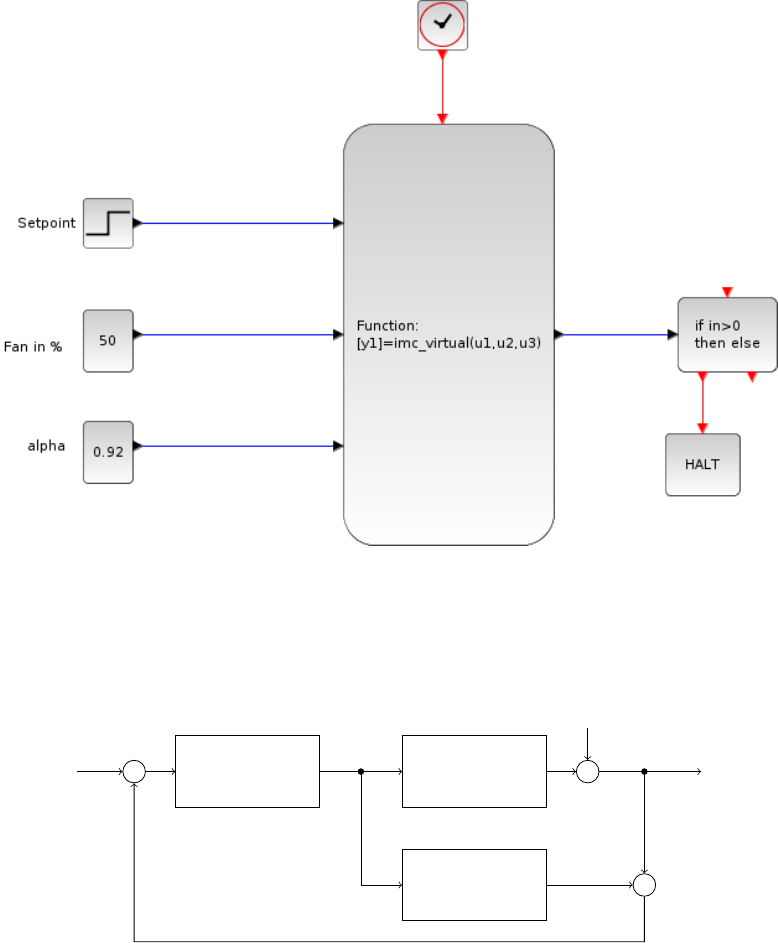
Figure 10.1: Xcos interface for this experiment
rGQ(z)
eGp(z)
u
ξ
y
G(z)¯y−
−
Figure 10.2: IMC feedback configuration
208
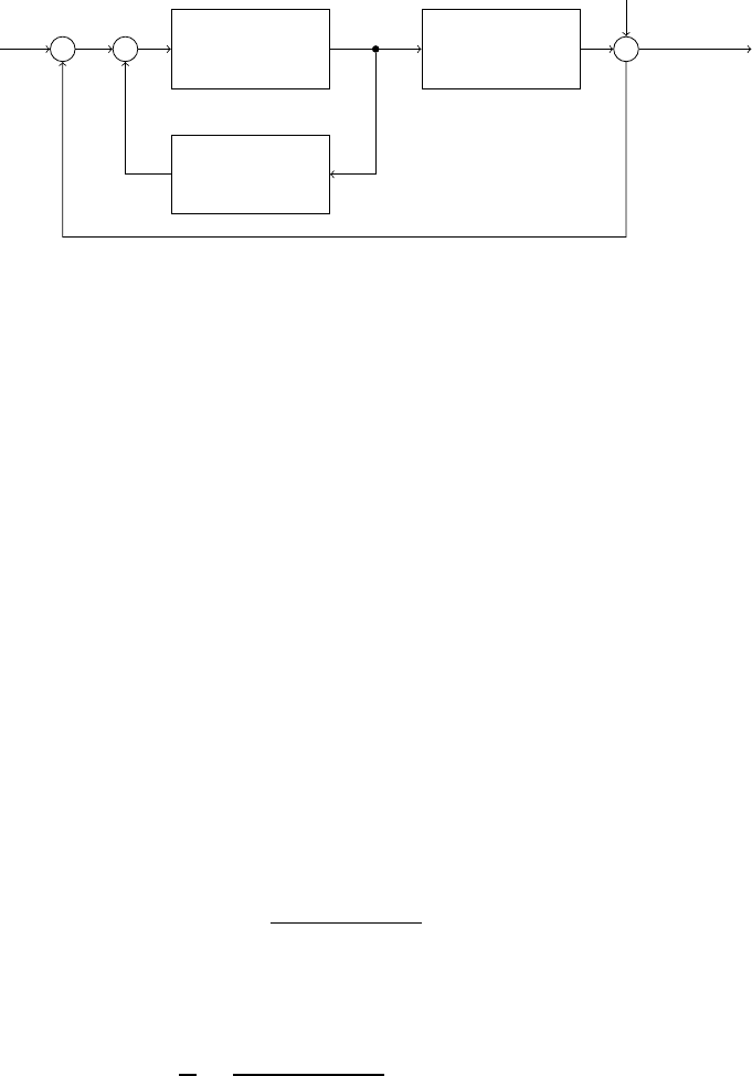
rGQ(z)
eGp(z)
u
ξ
y
G(z)
¯
ξ
Figure 10.3: Feedback configuration
u(n) =plant input
ξ(n) =noise
For noise rejection with y=0, we require GQ=G−1
pand G=Gp, i.e., for stable
GQwe require an approximate inverse of G. Also, for internal stability, transfer
function between any two points in the feedback loop must be stable [5].
10.2 Step for Designing IMC for Stable Plant
IMC design refers to obtaining a realizable GQthat is stable and approximately
inverse of G. This can be achieved by inverting the delay free plant model so that
GQis realizable. For non-minimum phase part of the plant, reciprocal polynomial
is used for stable controller. Negative real part of the plant should be replaced with
the steady state equivalent of that part to avoid oscillatory nature of control effort.
Low pass filter must be used to avoid the high frequency components because of
the model mismatch. The SBHS is modeled as-
G=Z−10.01163
1−0.9723Z−1(10.2)
Inverting delay free plant, we get
A
B=1−0.9723Z−1
0.01163 (10.3)
209

Comparing plant model with equation
G=Z−1BgB−Bnm+
A(10.4)
We get,
Bg=0.01163 (10.5)
B−=1 (10.6)
Bnm+=1 (10.7)
A=1−0.9723Z−1(10.8)
For the stable system, internal model controller is given by
GQ=A
BgB−
sBnm+
r
Gf(10.9)
GQ=1−0.9723Z−1
0.01163
1−α
1−αZ−1(10.10)
Now,
Gc=GQ
1−GGQ
(10.11)
u
e=
1−0.9723Z−1
0.01163
1−α
1−αZ−1
1−Z−10.01163
1−0.9723Z−1
1−0.9723Z−1
0.01163
1−α
1−αZ−1
(10.12)
After simplifying, we get
u
e=1−α
0.01163
1−0.9723Z−1
1−Z−1(10.13)
u
e=b1−0.9723Z−1
1−Z−1(10.14)
where,
b=1−α
0.01163 (10.15)
210
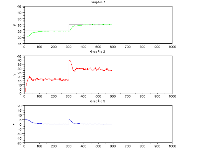
Figure 10.4: Experimental results with IMC for α=0.92
Hence,
u(n)=u(n−1) +b[e(n)−0.9723e(n−1)] (10.16)
The output of Xcos is shown in figure 10.4. Figure shows three plots. First
sub plot shows setpoint and output temperature profile. Second sub plot shows
control effort and third sub plot shows error between setpoint and plant output.
The same experiment result for α=0.85 is as shown in fig 10.5. By comparing
the two graphs, we can say that for α=0.92 the response of the controller is
sluggish. For α=0.85, the controller starts responding quickly and no overshoots
are seen in the temperature profile.
211
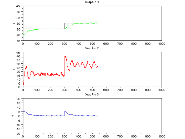
Figure 10.5: Experimental results with IMC for α=0.85
212

10.2.1 Implementing IMC locally
The detailed procedure to perform a local experiment is explained in Chapter2.
A summary of the same is provided in section 2.3 It is same for this section with
following changes.
1. Step1: The working directory is imc controller
2. Step2: Same
3. Step3: Same
4. Step4: Same
5. Step5: Load ramp test function by executing command
exec<space>imc.sci
6. Step6: Load Xcos code for ramp test using the command
exec<space>imc.xcos
7. Step7: Same
10.2.2 Implementing IMC virtually
The detailed procedure to perform a virtual experiment is explained in Chapter3.
A summary of the same is provided in section 3.5. It is same for this section with
following changes.
1. Step1: The working directory is imc controller. Open this directory.
2. Step2: Same
3. Step3: Same
4. Step4: Switch to the IMC experiment directory and double-click on the file
imc.sce. This will launch scilab and also open the file imc.sce in the
scilab editor. Linux users will have to launch scilab manually. They also
have to change the working directory to imc controller and then open
the imc.sce file in the scilab editor.
5. Step5: Same
213

6. Step6: Execute the file imc.sce. Expect the IMC controller xcos diagram
to open automatically. If this doesnt happen, check the scilab console for
error message.
7. Step7: Execute the IMC controller xcos diagram.
8. Step8: Same
10.3 Scilab Code
Scilab Code 10.1 ser init.sce
1mode ( 0 )
2global f i l e n a m e m
3/ / * * Sampling Time * * / /
4s a m p l i n g t i m e =1 ;
5/ / / / / / / * * * * /////////
6m=1;
7
8port1 =’/dev /ttyUSB0 ’ ; / / F o r l i n u x u s e r s
9port2 =’COM2’ ; / / F o r w i n d o w s u s e r s
10
11 r e s =i n i t ( [ p o r t 1 p o r t 2 ] ) ;
12 d i s p ( r e s )
Scilab Code 10.2 imc.sci
1mode ( 0 )
2function [ temp ] =imc ( s e t p o i n t , fan , a l p h a )
3global temp h e a t i n f a n i n C0 u o l d u new e o l d e new
e old old
4
5global h e a t d i s p f a n d i s p t e m p d i s p s e t p o i n t d i s p
s a m p l i n g t i m e m name
6
7e new =s e t p o i n t −temp ;
8b=((1 −alpha ) /0 . 0 1 1 6 3 ) ;
9
214

10 u new =u o l d +b*( e new −(0.9723*e o l d ) ) ;
11
12
13 u o l d =u new ;
14 e o l d =e new ;
15
16
17 h e a t =u new ;
18
19 temp =comm( h e a t , f a n ) ;
20
21 p l o t t i n g ( [ h e a t f a n temp s e t p o i n t ] , [ 0 0 20 0 ] , [ 1 0 0
100 40 1 0 0 0 ] )
22
23 m=m+1;
24 endfunction
Scilab Code 10.3 imc virtual.sce
1mode ( 0 ) ;
2/ / F o r s c i l a b 5 . 1 . 1 o r l o w e r v e r s i o n u s e r s , u s e s c i c o s
c o m m a n d t o o p e n s c i c o s d i a g r a m s i n s t e a d o f x c o s
3
4global f d f h f d t f n c r fncw m e r r c o u n t y l i m i t s
s a m p l i n g t i m e m
5
6/ / **********************
7s a m p l i n g t i m e =1; / / I n s e c o n d s . F r a c t i o n s a r e a l l o w e d
8/ / **********************/ /
9
10 e x e c ( ” i m c v i r t u a l . s c i ” ) ;
11
12 ok =i n i t ( ) ;
13
14 i f ok ˜=[ ] / / o p e n x c o s o n l y i f c o m m u n i c a t i o n i s
t h r o u g h ( i e r e p l y h a s c o m e f r o m s e r v e r )
15 xco s ( ’ imc . x c o s ’ ) ;
16 else
215

17 d i s p ( ”NO NETWORK CONNECTION! ” ) ;
18 r e t u r n
19 end
Scilab Code 10.4 imc virtual.sci
1mode ( 0 )
2
3
4function [ s t o p ] =i m c v i r t u a l ( s e t p o i n t , fan , a l p h a )
5
6global temp h e a t C0 u o l d u new e o l d e new f d f h f d t
f n c r fncw m e r r c o u n t s t o p q h e a t d i s p f a n d i s p
t e m p d i s p s e t p o i n t d i s p l i m i t s m x s a m p l i n g t i m e
e old old
7
8e new =s e t p o i n t −temp ;
9
10 b=((1 −alpha ) /0 . 0 1 1 6 3 ) ;
11 u new =u o l d +b*( e new −(0.9723*e o l d ) ) ;
12
13
14 h e a t =u new ;
15 u o l d =u new ;
16 e o l d =e new ;
17
18
19 [ s t o p , temp ] =comm ( h e a t , f a n ) ; / / N e v e r e d i t t h i s
line
20 p l o t t i n g ( [ h e a t f a n temp s e t p o i n t ] , [ 0 0 30 0 ] , [ 1 0 0
100 50 1 0 0 0 ] )
21
22 endfunction
216

Chapter 11
Design and Implementation of Self
Tuning PI and PID Controllers on
Single Board Heater System
11.1 Introduction
This chapter presents design and implementation of Self Tuning PI and PID con-
trollers on Single Board Heater System done by Mr. Vikas Gayasen.1
When a plant is wired in a close loop with a PID controller, the parameters- Kc,
τiand τddetermine the variation of the manipulated input that is given to the con-
troller. This, in turn, determines the variation of the controlled variable, when
a set point is given. Suitable values of these parameters can be found out when
plant transfer function is known. However, with large changes in the controlled
variable, there may be appreciable changes in the plant transfer function itself.
Therefore, it is needed to dynamically update the controller parameters according
to the transfer function.
11.2 Theory
11.2.1 Why a Self Tuning Controller?
The transfer function of SBHS is assumed as
1Copyright: Mr. Vikas Gayasen, student of Prof. Kannan Moudgalya, IIT Bombay for Process
Control course, 2010
217

∆T=Kp
τps+1∆H+Kf
τfs+1∆F(11.1)
∆T: Temperature change
∆F: Fan input change
∆H: Heater input change
The values of Kp,Kf,τsand τfcan be found by conducting step test exper-
iments. Using these values, the parameters (Kc,τiand τd) of the PID controller
can be defined using methods like Direct Synthesis of Ziegler Nichols Tuning.
However, when the apparatus is used in over a large range of temperature, the
values of the plant parameters (Kp,Kf,τsand τf) may change. The new values
would give new values of PID controller parameters. However, in a conventional
PID controlled system, the parameters Kc,τiand τdare defined beforehand and are
not changed when the system is working. Therefore, we might have a situation
in which the PID controller is working with unsuitable values that may not give
the desired performance.Therefore, it becomes necessary to change or update the
values of the PID parameters so that the plant gives the optimum performance.
218
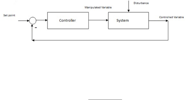
11.2.2 The Approach Followed
Variable Description:
•Manipulated Variable: Heater Input
•Disturbance Variable: Fan Input
•Controlled Variable: Temperature
Several open loop step test experiments were performed (giving step changes
in the heater input) and the values of Kpand τpwere found from the results of
each experiment by fitting the Inverse Laplace transform of the assumed transfer
function with the experimental data. These values were plotted with respect to the
corresponding average temperatures. From these plots, correlations were found
for both Kpand τpas functions of temperature. From correlations of Kpand τp,
the PID parameters were calculated as functions of temperature. Thus, in the new
PID controller, the values of Kc,τiand τdwere calculated using the temperature of
the system. For the calculation of PID settings, two approaches: Direct Synthesis
and Ziegler-Nichols Tuning were followed.
11.2.3 Direct synthesis
LoopCircuit.jpg
Figure 11.1: Closed loop circuit
We have
V(s)=Gc(s)G(s)
1+Gc(s)G(s)(11.2)
219

where
V(s) : Overall closed-loop transfer function
Gc(s) : Controller transfer function
G(s) : System transfer function.
Therefore,
Gc(s)=1
G(s)
V(s)
1−V(s)(11.3)
Let the desired closed loop transfer function be of the form
V(s)=1
(τcl s+1) (11.4)
G(s)=Kp
(τps +1) (11.5)
By using the equations for G(s) and V(s), we get
G(c)=Kc(1 +1
τs) (11.6)
where,
Kc=1
Kp
(τp/τcl) (11.7)
τi=τp(11.8)
When Kpand τpare known as a function of time, the values of Kcand τican be
found as functions of temperature as well.
220
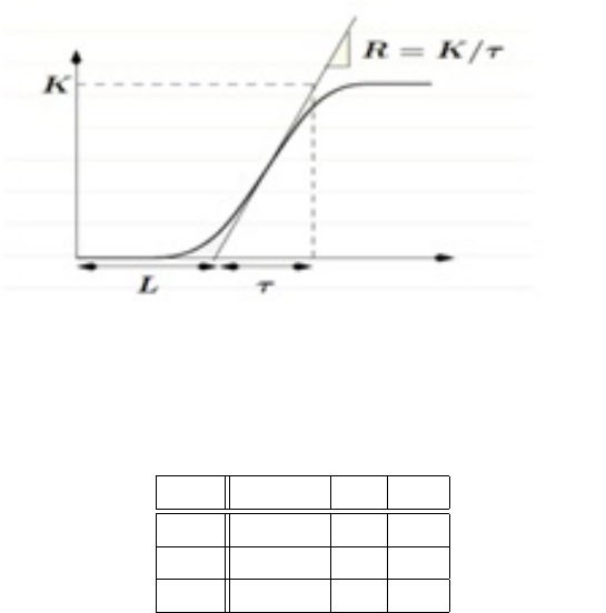
11.3 Ziegler Nichols Tuning
For Ziegler Nichols Tuning, we use the step response of the open loop experiment.
Figure 11.2: Tangent approach to Ziegler Nichols Tuning
Kcτiτd
P 1/RL
PI 0.9/RL 3L
PID 1.2/RL 2L .5L
Table 11.1: Ziegler Nichols PID Settings
Table 11.1 gives the PID settings. In this approach too, for every open step
test, K and τare found and correlated as function of average temperature and PID
settings are then found as functions of temperature.
Note: For a first order transfer function we assume
•Kp≈K
•τp≈τ
221
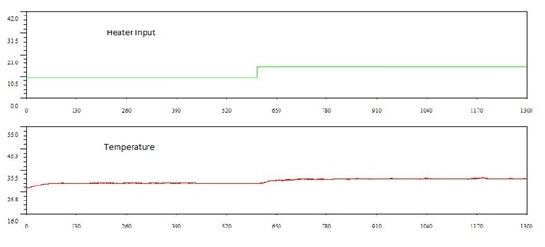
Figure 11.3: Step response for heater reading from 10 to 15
11.4 Step Test Experiments and Parmeter Estima-
tion
Several open loop step test experiments were conducted and the values of the open
loop parameters were found by curve fitting.
11.4.1 Step Test Experiment
11.4.1.1 Step change in heater reading from 10 to 15
222
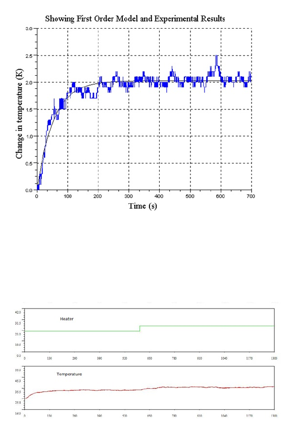
Figure 11.4: Step response for heater reading from 10 to 15 in terms of deviation
11.4.1.2 Step Change in Heater Reading from 20 to 25
Figure 11.5: Step response for Heater Reading from 20 to 25
223
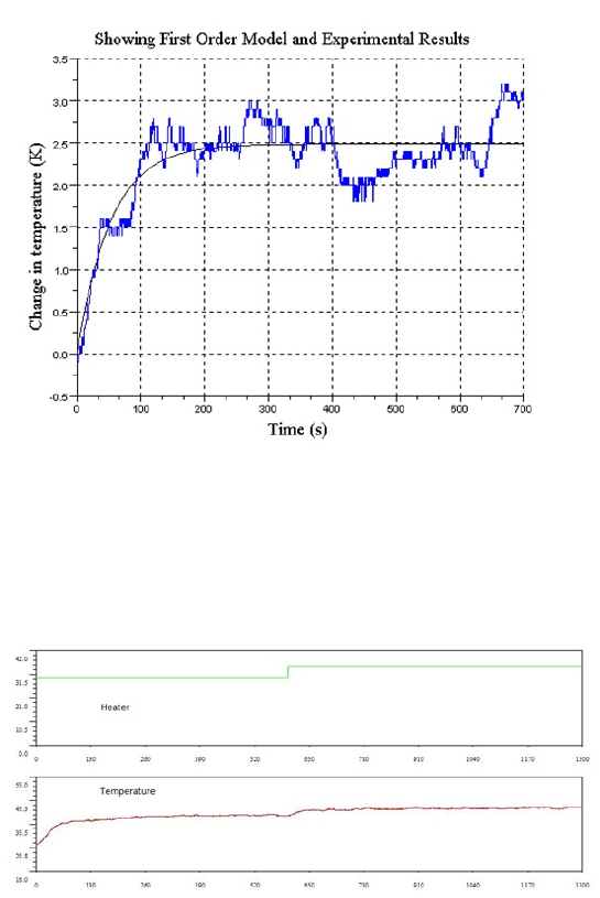
Figure 11.6: Step response for heater reading from 20 to 25 in terms of deviation
11.4.1.3 Step Change in Heater Reading from 30 to 35
Figure 11.7: Step response for heater reading from 30 to 35
224
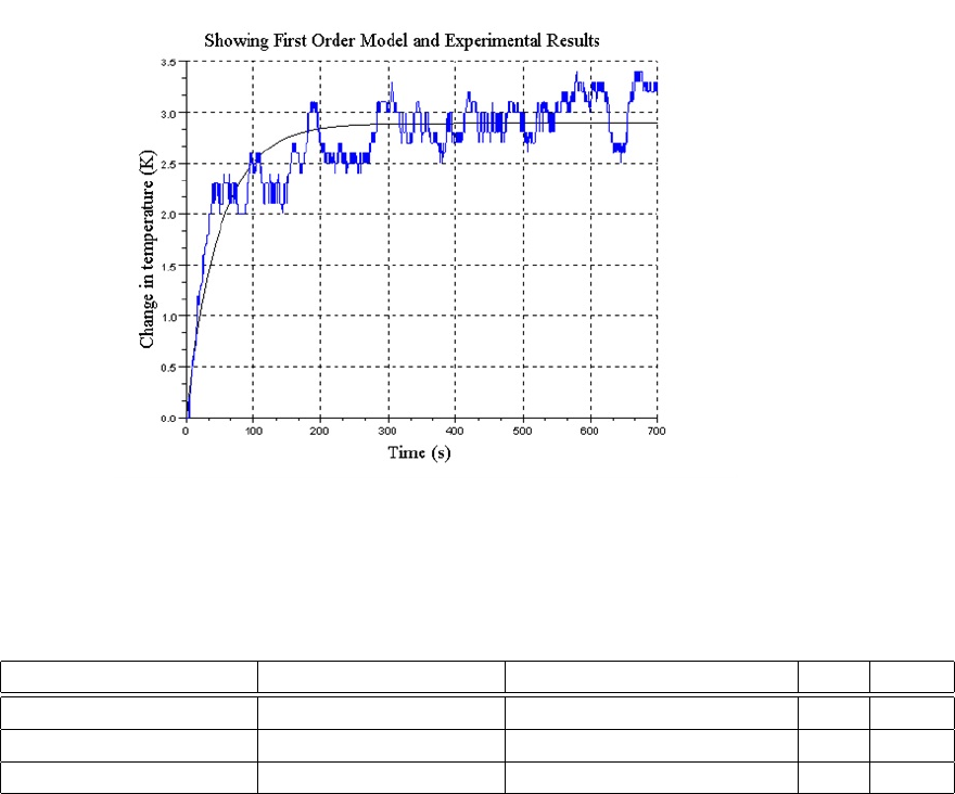
Figure 11.8: Step response for heater reading from 30 to 35 in terms of deviation
11.4.1.4 The Open Loop Parameters
Initial Heater Reading Final Heater Reading Average Temperature(0C) Kpτp
10 15 31.57 0.41 53.37
20 25 36.00 0.50 52.64
30 35 41.79 0.58 49.21
Table 11.2: Open loop parameters
It can be seen from the graphs that there is a lag of approximately 6 seconds
in each experiment.
11.4.2 Conventional Controller Design
1. PI Controller using Ziegler Nichols Tuning with the results of the first step
test experiment:
•Kc =19.75
•τi=18
225
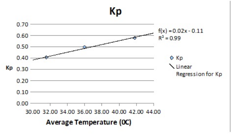
2. PID Controller using Ziegler Nichols Tuning with the results of the first step
test experiment:
•Kc =26.327
•τi=12
•τd=3
3. PI Controller Using Direct Synthesis with the results of the second step test
experiment (τcl is taken as τp/2):
•Kc =4.02
•τi=52.645
11.4.3 Self Tuning Controller Design
The graphs showing the variation of Kp and τpare shown below:
Figure 11.9: Variation of Kpwith temperature
226
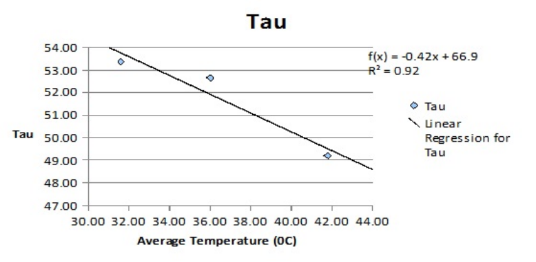
Figure 11.10: Variation of τpwith temperature
1. PI Controller using Ziegler Nichols Tuning:
L=6
R=(0.016×T-0.114)/(66.90-0.415×T) where T is the temperature
Kc =0.9(66.90-0.415T)/6(0.016T-0.114)
=(60.21 - 0.3735T)/(0.096T - 0.684)
τi=3×6=18
2. PID Controller using Ziegler Nichols Tuning:
L=6
R=(0.016 ×T-0.114)/(66.90-0.415 ×T) where T is the temperature
K=1.2(66.90-0.415T)/6(0.016T-0.114)
=(80.28 - 0.498T)/(0.096T - 0.684)
τi=2×6=12
τd=0.5×6=3
3. PI Controller using Direct Synthesis (τcl is taken as τp/2):
227
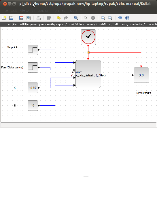
K=2/(0.016×T-0.114)
τi=(66.90-0.415×T) where T is the temperature
11.5 PID controller theory
11.5.1 PI Controller
Figure 11.11: Xcos diagram for PI controller
The PI Controller in continuous time is given by
u(t)=K"e(t)+1
τiZt
0
e(t)dt#(11.9)
On taking Laplace transform, we obtain
u(s)=K"1+1
τis#e(s) (11.10)
228

By mapping equation 11.10 to discrete time interval using Backward Difference
Approximation, we get
u(n)=K"1+Ts
τi
z
z−1#e(n) (11.11)
On cross multiplication, we obtain
(z−1) ×u(n)=K"(z−1) +Ts
τi
(z)#e(n) (11.12)
We divide by z, and using the shifting theorem, we obtain
u(n)−u(n−1) =K"e(n)−e(n−1) +Ts
τi
e(n)#(11.13)
The PI Controller is usually written as
u(n)=u(n−1) +s0e(n)+s1e(n−1) (11.14)
where,
s0=K 1+Ts
τi!
s1=−K
11.5.2 PID Controller
The PID Controller in continuous time is given by
u(t)=K"e(t)+1
τiZt
0
e(t)dt +τd
de(t)
dt #(11.15)
On taking Laplace Transform, we obtain
u(s)=K"1+1
τis+τds#e(s) (11.16)
By mapping equation 11.16 to discrete time interval by using the Trapezoidal
Approximation for integral mode and Backward Difference Approximation for
derivative mode, we get
u(n)=K"1+Ts
τi
z
z−1+τd
Ts
z−1
z#e(n) (11.17)
229
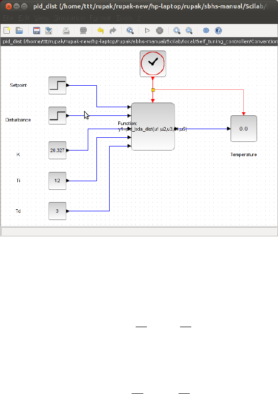
Figure 11.12: Xcos diagram for PID controller
On cross multiplication, we obtain
(z2−z)×u(n)=K"(z2−z)+Ts
τi
(z2)+τd
Ts
(z−1)2#e(n) (11.18)
We divide by z, and using the shifting theorem, we obtain
u(n)−u(n−1) =K"e(n)−e(n−1) +Ts
τi
e(n)+τd
Ts{e(n)−2e(n−1) +e(n−1)}#
(11.19)
The PID Controller is usually written as
u(n)=u(n−1) +s0e(n)+s1e(n−1) +s2e(n−2) (11.20)
230
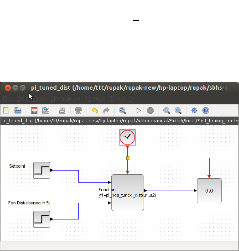
where,
s0=K 1+Ts
τi
+τd
Ts!(11.21)
s1=K"−1−2τd
Ts#(11.22)
s2=K"τd
Ts#(11.23)
11.5.3 Self Tuning Controller
Figure 11.13: Xcos diagram for self tuning controller
The parameters of the controller are determined dynamically using the tem-
perature values for every sampling time. For this, the formulae derived in section
11.4.3 are used. The formulae for the control effort are same as the conventional
PI and PID controllers. So the PI/PID settings are calculated for every sampling
231

time and the control effort is calculated thereafter using the formulae derived for
conventional controllers.
11.6 Set Point Tracking
The main aim of the controller is to track the set point and to reject disturbances.
When the set point of the controlled variable (temperature in this case) is changed,
the controller should work in such a manner that the actual temperature follows
the set point as close as possible.
In this project, several experiments were conducted with the self tuning and
conventional PI/PID Controllers. Table 11.3 shows the set point changes given
during the various experiments that were conducted with conventional and self
tuning controllers designed using several methods.
Conventional Controller Self Tuning Controller
Direct Synthesis PI 320C to 370C 320C to 370C
350C to 450C 350C to 450C
Ziegler Nichols PI 320C to 370C 320C to 370C
350C to 450C 350C to 450C
400C to 450C 350C to 450C
Ziegler Nichols PID 310C to 450C 320C to 460C
320C to 370C 320C to 370C
Table 11.3: Set point changes in experiments conducted for set point tracking
232
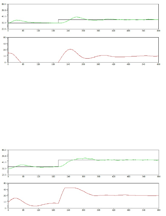
11.6.1 PI Controller Designed by Direct Synthesis
The results of the experiments carried out for the self tuning PI controller using
direct synthesis method are shown. The upper plot shows the variations of the set
point temperature (the black line) and the actual temperature (the green line) in
the SBHS. The lower plot shows the control effort.
Figure 11.14: Result for self tuning controller designed using Direct Synthesis for
set point going from 320C to 370C
Although there is a small overshoot, the controller is able to make the actual
temperature follow the set point temperature quiet closely. Looking at higher
values of set point changes, the result for set point change going from 350C to
450C is shown.
Figure 11.15: Result for self tuning controller designed using Direct Synthesis for
set point going from 350C to 450C
For a higher set point change also, the controller is able to make the tempera-
ture follow the set point closely. Notice the abrupt change in the control effort as
soon as the step change in the set point is encountered.
233
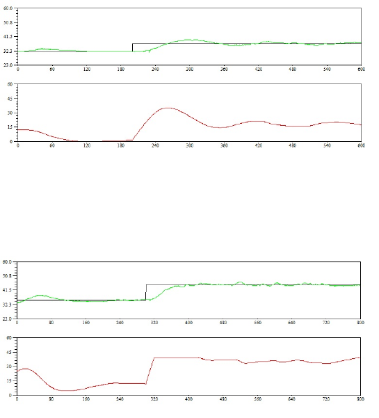
For comparison, results of experiments done with conventional PI controller de-
signed using the Direct Synthesis method are also shown.
Figure 11.16: Result for conventional controller designed using Direct Synthesis
for set point going from 320C to 370C
Figure 11.17: Result for conventional controller designed using Direct Synthesis
for Set Point going from 350C to 450C
As it can been seen from the graph, the self tuning controller stabilised the
temperature faster.
234
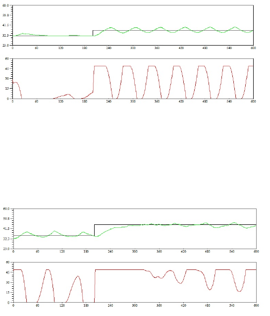
11.6.2 PI Controller using Ziegler Nichols Tuning
The results of the of the experiments carried out for the self tuning PI controller
using Ziegler Nichols tuning method are shown. The upper plot shows the varia-
tions of the set point temperature (the black line) and the actual temperature (the
green line) in the SBHS. The lower plot shows the control effort.
Figure 11.18: Result for self tuning controller designed using Ziegler Nichols
Tuning for set point going from 320C to 370C
Although there are oscillations, the temperature remains near the set point.
The result for a higher value of set point change is also shown.
Figure 11.19: Result for self tuning controller designed using Ziegler Nichols
Tuning for set point going from 350C to 450C
For this experiment, the controller is able to make the temperature follow the
set point closely. The fluctuations may be due to noises and the surrounding con-
ditions.The plot for result of an experiment with another value of set point change
is also shown.
In this experiment too, the controller is able to keep the temperature close to
the set point and it stabilises fast.
235
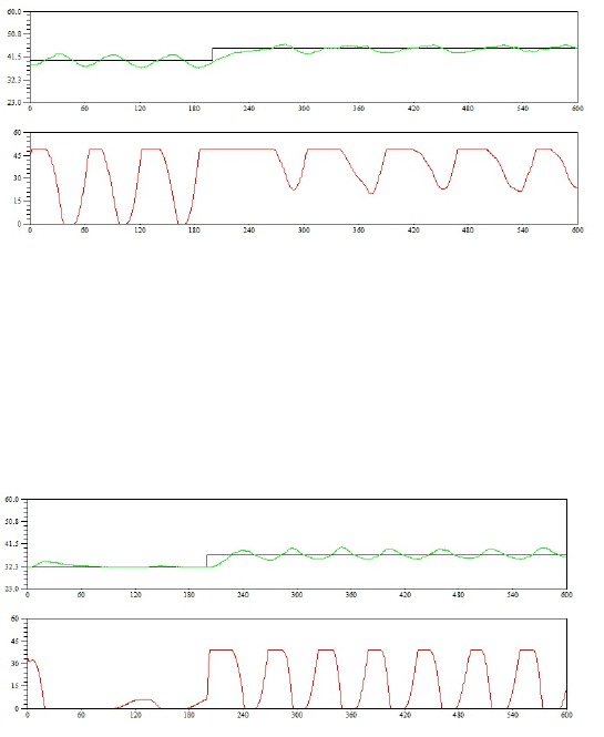
Figure 11.20: Result for self tuning controller designed using Ziegler Nichols
Tuning for set point going from 400C to 450C
For comparison, results of experiments done with conventional PI controller de-
signed using the Ziegler Nichols method are also shown.
Figure 11.21: Result for conventional controller designed using Ziegler Nichols
Tuning for set point going from 320C to 370C
236
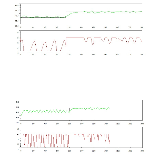
Figure 11.22: Result for conventional controller designed using Ziegler Nichols
Tuning for set point going from 350C to 450C
Figure 11.23: Result for conventional controller designed using Ziegler Nichols
Tuning for set point going from 400C to 450C
For set point change from 400C to 450C, the self tuning controller showed
small oscillations, but the conventional controller shows bigger oscillations.
237
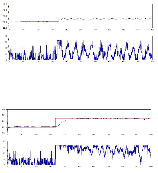
11.6.3 PID Controller using Ziegler Nichols Tuning
The results of the of the experiments carried out for the self tuning PID controller
using Ziegler Nichols tuning method are shown. The upper plot shows the varia-
tions of the set point temperature (the black line) and the actual temperature (the
purple line) in the SBHS. The lower plot shows the control effort.
Figure 11.24: Result for self tuning PID controller designed using Ziegler Nichols
Tuning for set point going from 320C to 370C
Figure 11.25: Result for self tuning PID controller designed using Ziegler Nichols
Tuning for set point going from 320C to 460C
From the graph it can be seen that for both the experiments, the self tuning PID
controller is able to keep the temperature close to the set point and the stabilisation
is also fast. For comparison, plots for experiments conducted with conventional
PID controller designed using Ziegler Nichols method are also shown.
From the graph, we can see that the conventional PID controller is not able to
make the temperature close to the set point when the set point value is 450C. The
self tuning PID controller had successfully brought the temperature to 450C.
238
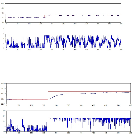
Figure 11.26: Result for conventional PID controller designed using Ziegler
Nichols Tuning for set point going from 320C to 370C
Figure 11.27: Result for conventional PID controller designed using Ziegler
Nichols Tuning for set point going from 310C to 450C
11.6.4 Conclusion
The self tuning PI controller is able to accomplish the aim of keeping the tem-
perature as close as possible to the set point. Although it may show some initial
overshoot or oscillation for some values of set point change, the time needed for
stabilisation is low. There may also some cases where the conventional controller
shows bigger oscillations than the self tuning controller.
The PI controllers, both conventional and self tuning, show oscillations for some
values of set point change. To eliminate the oscillations, when we use the PID
Controller, the self tuning design definately seems to be a better option because
for higher values of set point change, the self tuning PID controller shows a better
performance than the conventional controller as seen in section 11.6.3.
239

11.7 Disturbance Rejection
Apart from tracking the set point, the system should also be able to reject distur-
bances. There may be several factors influencing the controlled variable and not
all of them can be manipulated. Therefore, it becomes necessary for the controller
to not let the changes in the non-manipulated variables to affect the controlled
variable. This is called Disturbance Rejection.
In this system, the disturbance variable is the fan input. Therefore, the controller
has to work in such a way that changes in the fan input does not affect the temper-
ature in the SBHS.
In this project, several experiments were conducted with the self tuning and con-
ventional PI/PID Controllers. Table 11.4 shows the fan input changes given dur-
ing the various experiments that were conducted with conventional and self tuning
controllers designed using several methods.
Conventional Controller Self Tuning Controller
Direct Synthesis PI 50 to 100 50 to 100
100 to 50 100 to 50
Ziegler Nichols PI 50 to 100 50 to 100
100 to 50 100 to 50
Ziegler Nichols PID 50 to 100 50 to 100
100 to 50 100 to 50
Table 11.4: Fan input changes in experiments conducted for Disturbance Rejec-
tion
11.7.1 PI Controller Designed by Direct Synthesis
The results of the experiments carried out for the self tuning PI controller using
Direct Synthesis method are shown. The upper plot shows the variations of the
set point temperature (the black line) and the actual temperature (the green line)
in the SBHS. The second plot shows the control effort and the third shows the fan
input.
The change in the fan input introduces a small dent in the temperature. How-
ever, the controller brings the temperature back to the set point. Notice the slight
change in the controller behaviour on encountering the fan input change. The time
taken for stabilising back is also low.
240
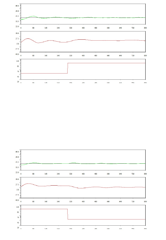
Figure 11.28: Results for fan input change from 50 to 100 for self tuning PI Con-
troller designed using Direct Synthesis
Here, results for fan input change from 100 to 50 are also shown.
Figure 11.29: Results for fan input change from 100 to 50 for self tuning PI con-
troller designed using Direct Synthesis
In this figure also, the temperature clearly increases a bit when the step change
in the fan input is encountered. However, it quickly stabilises back and continues
to be close to the set point.
From the above two results, it is clear that the self tuning controller designed
with Direct Syntheis has successfully rejected the disturbance.
For comparison, results of the disturbance change for conventional PI Con-
troller designed with direct synthesis are also shown.
241
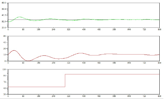
Figure 11.30: Results for the fan input change from 50 to 100 to conventional PI
controller designed using Direct Synthesis
242
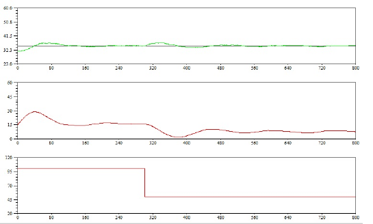
Figure 11.31: Results for the fan input change from 100 to 50 to conventional PI
controller designed using Direct Synthesis
11.7.2 PI Controller using Ziegler Nichols Tuning
The results of the experiments carried out for the self tuning PI controller using
Ziegler Nichols method are shown. The upper plot shows the variations of the set
point temperature (the black line) and the actual temperature (the green line) in
the SBHS. The second plot shows the control effort and the third shows the fan
input.
Even on encountering the fan input change, the temperature remains close to
the set point. Notice the change in the controller behaviour on encountering the
fan input change.
243
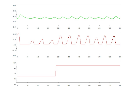
Figure 11.32: Results for Fan Input change from 50 to 100 given to Self Tuning
PI Controller designed using Ziegler Nichols method
Here, result for the fan input going from 100 to 50 is also shown.
Here, a change in the control effort can be noticed. This change has been
brought by the PI Controller to keept the temperature close to the set point.
From the above two results, it is clear that the self tuning controller designed with
direct syntheis has successfully rejected the disturbance.
244
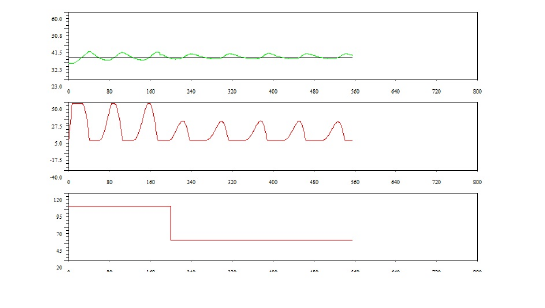
Figure 11.33: Results for fan input change from 100 to 50 given to self tuning PI
controller designed using Ziegler Nichols method
For comparison, corresponding results are also shown for conventional PI con-
trollers designed using Ziegler Nichols tuning.
245
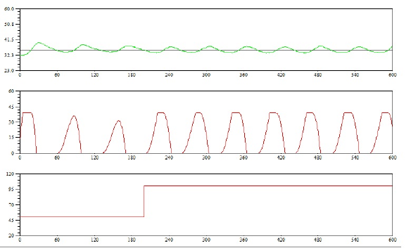
Figure 11.34: Results for the fan input change from 50 to 100 to conventional PI
controller designed using Ziegler Nichols tuning
11.7.3 PID Controller using Ziegler Nichols Tuning
The results of the experiments carried out for the self tuning PID controller using
Ziegler Nichols method are shown. The upper plot shows the variations of the set
point temperature (the black line) and the actual temperature (the purple line) in
the SBHS. The second plot shows the control effort and the third shows the fan
input.
In this system also, on encountering the fan input change, the temperature
remains close to the set point. Notice the change in the control effort profile when
the change in the fan input is given.
246
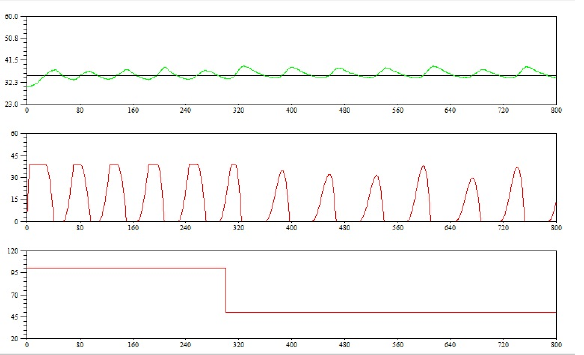
Figure 11.35: Results for the fan input change from 100 to 50 to conventional PI
controller designed using Ziegler Nichols tuning
Here, result for the fan input going from 100 to 50 is also shown.
In this figure also, the temperature clearly increses a bit when the step change
in the fan input is encountered. However, it quickly stabilises back and continues
to be close to the set point.
247
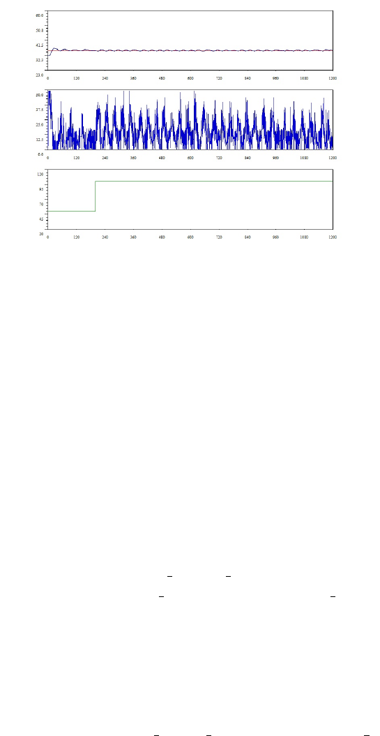
Figure 11.36: Results for Fan Input change from 50 to 100 given to Self tuning
PID Controller designed using Ziegler Nichols method
For comparison, corresponding results are also shown for conventional PID
controllers designed using Ziegler Nichols tuning.
11.7.4 Conclusion
We see that the self tuning controller manages to keep the temperature close to
the set point temperature, even when the change in fan input is encountered. This
shows that it can reject the disturbances quite nicely.
11.8 Conducting experiments locally
Under the local folder locate Self tuning controller folder. You will see
two folders ConventionalTuning Vikas and SelfTuning Vikas. These two
directories will contain four more folders, two for PI and two for PID.
The detailed procedure to perform a local experiment is explained in Chapter2.
A summary of the same is provided in section 2.3 It is same for this section with
following changes.
1. Step1: The working directory is one of the four experiments you want to
do. For example virtual/Self tuning controller/SelfTuning Vikas
/PIControllerFandisturbance
248
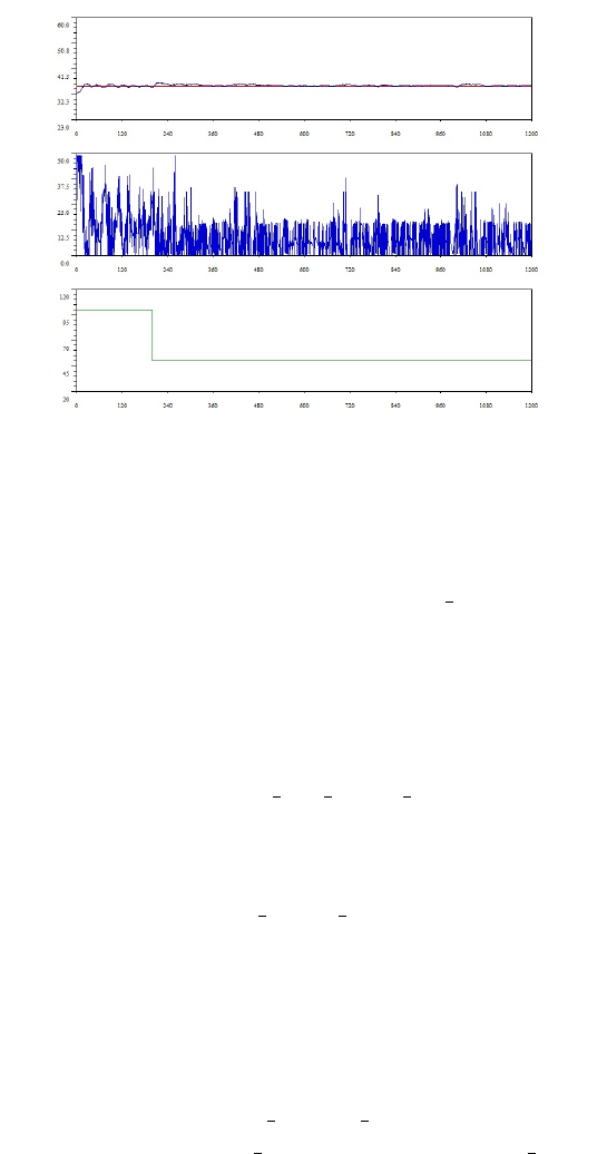
Figure 11.37: Results for fan input change from 100 to 50 given to self tuning PID
controller designed using Ziegler Nichols method
2. Step2: Load the functions available in common files directory by executing
the command getd<space>..\..\..\common files
3. Step3: Same
4. Step4: Same
5. Step5: Load required function by using exec command.
For example, exec<space>pi bda tuned dist.sce if you want to run
the PI Controller Fan disturbance experiment.
6. Step6: Load Xcos code for corresponding experiment using xcos command.
For example exec<space>pi tuned dist.xcos
7. Step7: Same
11.9 Conducting experiments virtually
Under the local folder locate Self tuning controller folder. You will see
two folders ConventionalTuning Vikas and SelfTuning Vikas. These two
directories will contain four more folders, two for PI and two for PID.
249
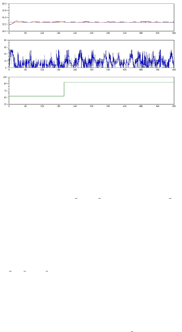
Figure 11.38: Results for the fan input change from 50 to 100 to conventional PID
controller designed using Ziegler Nichols tuning
The detailed procedure to perform a virtual experiment is explained in Chapter3.
A summary of the same is provided in section 3.5. It is same for this section with
following changes.
1. Step1: The working directory is one of the four experiments you want to
do. For example virtual/Self tuning controller/SelfTuning Vikas
/PIControllerFandisturbance
2. Step2: Same
3. Step3: Same
4. Step4: Switch to the working experiment directory and double-click on the
.sce file corresponding to the experiment you want to perform. For exam-
ple, pi bda tuned dist.sce if you want to run the PI Controller Fan
disturbance experiment. This will launch scilab and also open the file in
the scilab editor. Linux users will have to launch scilab manually. They also
have to change the working directory to corresponding experiment and then
open the .sce file in the scilab editor.
5. Step5: Load the functions available in common files directory by executing
the command getd<space>..\..\..\common files
250
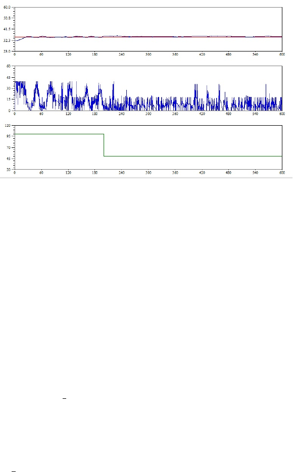
Figure 11.39: Results for the fan input change from 100 to 50 to conventional PID
controller designed using Ziegler Nichols tuning
6. Step6: Execute the .sce file. Expect the corresponding xcos diagram to
open automatically. If this doesnt happen, check the scilab console for error
message.
7. Step7: Execute the xcos diagram.
8. Step8: Same
11.10 Scilab Codes
Scilab Code 11.1 ser init.sce
1mode ( 0 )
2global f i l e n a m e
3/ / * * Sampling Time * * / /
4s a m p l i n g t i m e =1 ;
5/ / / / / / / * * * * /////////
6m=1;
7
8port1 =’/dev /ttyUSB0 ’ ; / / F o r l i n u x u s e r s
9port2 =’COM2’ ; / / F o r w i n d o w s u s e r s
251

10
11 r e s =i n i t ( [ p o r t 1 p o r t 2 ] ) ;
12 d i s p ( r e s )
11.10.1 Conventional Controller, local
11.10.1.1 Fan Disturbance in PI Controller
Scilab Code 11.2 pi bda dist.sci
1mode ( 0 )
2/ / g l o b a l t e m p h e a t f a n s a m p l i n g t i m e m h e a t d i s p
f a n d i s p t e m p d i s p x n a m e
3function temp =p i b d a d i s t ( s e t p o i n t , f an , K, Ti )
4global h e a t d i s p f a n d i s p t e m p d i s p s e t p o i n t d i s p
s a m p l i n g t i m e m name temp h e a t i n f a n i n C0 u o l d
u new e o l d e new
5
6Ts =s a m p l i n g t i m e ;
7e new =s e t p o i n t −temp ;
8
9S0=K*( 1 +( ( Ts /Ti ) ) ) ;
10 S1=−K;
11 u new =u o l d +S0 *e new +S1*e o l d ;
12
13
14 u o l d =u new ;
15 e o l d =e new ;
16
17 h e a t =u new ;
18 temp =comm( h e a t , f a n ) ;
19
20 p l o t t i n g ( [ h e a t f a n temp s e t p o i n t ] , [ 0 0 20 0 ] , [ 1 0 0
100 40 1 0 0 0 ] )
21
22 m=m+1;
23 endfunction
252

11.10.1.2 Set Point Change in PI Controller
Scilab Code 11.3 pi bda.sci
1mode ( 0 )
2function temp =p i b d a ( s e t p o i n t , fan , K, Ti )
3global h e a t d i s p f a n d i s p t e m p d i s p s e t p o i n t d i s p
s a m p l i n g t i m e m name temp h e a t i n f a n i n C0 u o l d
u new e o l d e new
4
5Ts =s a m p l i n g t i m e ;
6e new =s e t p o i n t −temp ;
7
8S0=K*( 1 +( ( Ts /Ti ) ) ) ;
9S1=−K;
10 u new =u o l d +( S0 *e new ) +( S1 *e o l d ) ;
11
12
13 u o l d =u new ;
14 e o l d =e new ;
15
16 h e a t =u new ;
17 temp =comm( h e a t , f a n ) ;
18
19 p l o t t i n g ( [ h e a t f a n temp s e t p o i n t ] , [ 0 0 20 0 ] , [ 1 0 0
100 40 1 0 0 0 ] )
20
21 m=m+1;
22 endfunction
11.10.1.3 Fan Disturbance to PID Controller
Scilab Code 11.4 pid bda dist.sci
1mode ( 0 )
2function [ temp ] =p i d b d a d i s t ( s e t p o i n t , fan , K, Ti , Td )
3global temp h e a t i n f a n i n C0 u o l d u new e o l d e new
e old old
253

4
5global h e a t d i s p f a n d i s p t e m p d i s p s e t p o i n t d i s p
s a m p l i n g t i m e m name
6
7e new =s e t p o i n t −temp ;
8
9Ts=s a m p l i n g t i m e ;
10
11 S0=K*( 1 +( Ts /T i ) +( Td /Ts ) ) ;
12 S1=K*(−1−((2*Td ) /Ts ) ) ;
13 S2=K*( Td /Ts ) ;
14
15 u new =u o l d +S0 *e new +S1*e o l d +S2*e o l d o l d ;
16
17 u o l d =u new ;
18 e old old =e o l d ;
19 e o l d =e new ;
20
21
22 h e a t =u new ;
23 temp =comm( h e a t , f a n ) ;
24
25 p l o t t i n g ( [ h e a t f a n temp s e t p o i n t ] , [ 0 0 20 0 ] , [ 1 0 0
100 40 1 0 0 0 ] )
26
27 m=m+1;
28 endfunction
11.10.1.4 Set Point Change in PID Controller
Scilab Code 11.5 pid bda.sci
1mode ( 0 )
2function [ temp ] =p i d b d a ( s e t p o i n t , fan , K, Ti , Td )
3global temp h e a t i n f a n i n C0 u o l d u new e o l d e new
e old old
4
254

5global h e a t d i s p f a n d i s p t e m p d i s p s e t p o i n t d i s p
s a m p l i n g t i m e m name
6
7e new =s e t p o i n t −temp ;
8
9Ts=s a m p l i n g t i m e ;
10
11 S0=K*( 1 +( Ts /T i ) +( Td /Ts ) ) ;
12 S1=K*(−1−((2*Td ) /Ts ) ) ;
13 S2=K*( Td /Ts ) ;
14
15 u new =u o l d +S0 *e new +S1*e o l d +S2*e o l d o l d ;
16
17 u o l d =u new ;
18 e old old =e o l d ;
19 e o l d =e new ;
20
21
22 h e a t =u new ;
23 temp =comm( h e a t , f a n ) ;
24
25 p l o t t i n g ( [ h e a t f a n temp s e t p o i n t ] , [ 0 0 20 0 ] , [ 1 0 0
100 40 1 0 0 0 ] )
26
27 m=m+1;
28 endfunction
11.10.2 Self Tuning Controller, local
11.10.2.1 Fan Discturbance to PI Controller
Scilab Code 11.6 pi bda tuned dist.sci
1mode ( 0 )
2/ / g l o b a l t e m p h e a t f a n s a m p l i n g t i m e m h e a t d i s p
f a n d i s p t e m p d i s p x n a m e
3function temp =p i b d a t u n e d d i s t ( s e t p o i n t , f a n )
4global h e a t d i s p f a n d i s p t e m p d i s p s e t p o i n t d i s p
255

s a m p l i n g t i m e m name temp h e a t i n f a n i n C0 u o l d
u new e o l d e new
5
6Ts =s a m p l i n g t i m e ;
7/ / L=6 ;
8/ / R=(0.016*t e m p −0.114) /( 6 6 . 9 0 −0 . 4 1 5 *t e m p ) ;
9/ / K=0 . 9 /( R *L ) ;
10 / / T i =3*L ;
11
12 / / t h e a b o v e i s t h e z i e g l e r n i c h o l s p a r t
13
14
15 K=2/( 0 . 0 1 6 *temp −0 . 1 1 4 ) ;
16 Ti =(66.90 −0.415*temp ) ;
17
18 / / t h e a b o v e i s t h e d i r e c t s y n t h e s i s p a r t
19
20 enew =s e t p o i n t −temp ;
21 S0=K*( 1 +( ( Ts /Ti ) ) ) ;
22 S1=−K;
23 u new =u o l d +( S0 *e new ) +( S1 *e o l d ) ;
24
25
26 u o l d =u new ;
27 e o l d =e new ;
28
29 h e a t =u new ;
30
31 temp =comm( h e a t , f a n ) ;
32
33 p l o t t i n g ( [ h e a t f a n temp s e t p o i n t ] , [ 0 0 20 0 ] , [ 1 0 0
100 40 1 0 0 0 ] )
34
35 m=m+1;
36 endfunction
256

11.10.2.2 Set Point Change to PI Controller
Scilab Code 11.7 pi bda tuned.sci
1mode ( 0 )
2function temp =p i b d a t u n e d ( s e t p o i n t , f an )
3global h e a t d i s p f a n d i s p t e m p d i s p s e t p o i n t d i s p
s a m p l i n g t i m e m name temp h e a t i n f a n i n C0 u o l d
u new e o l d e new
4
5Ts =s a m p l i n g t i m e ;
6
7/ / L=6 ;
8/ / R=(0.016*t e m p −0.114) /( 6 6 . 9 0 −0 . 4 1 5 *t e m p ) ;
9/ / K=0 . 9 /( R *L ) ;
10 / / T i =3*L ;
11
12
13 / / T h e a b o v e i s t h e Z i e g l e r n i c h o l s p a r t .
14
15 K=2/( 0 . 0 1 6 *temp −0 . 1 1 4 ) ;
16 Ti =(66.90 −0.415*temp ) ;
17 / / T h e a b o v e i s t h e d i r e c t s y n t h e s i s p a r t
18
19 e new =s e t p o i n t −temp ;
20
21 S0=K*( 1 +( ( Ts /Ti ) ) ) ;
22 S1=−K;
23 u new =u o l d +( S0 *e new ) +( S1 *e o l d ) ;
24
25 u o l d =u new ;
26 e o l d =e new ;
27
28 h e a t =u new ;
29 temp =comm( h e a t , f a n ) ;
30
31 p l o t t i n g ( [ h e a t f a n temp s e t p o i n t ] , [ 0 0 20 0 ] , [ 1 0 0
100 40 1 0 0 0 ] )
257

32
33 m=m+1;
34 endfunction
11.10.2.3 Fan Disturbance to PID Controller
Scilab Code 11.8 pid bda tuned dist.sci
1mode ( 0 )
2
3function [ temp ] =p i d b d a t u n e d d i s t ( s e t p o i n t , f a n )
4global temp h e a t i n f a n i n C0 u o l d u new e o l d e new
e old old
5
6global h e a t d i s p f a n d i s p t e m p d i s p s e t p o i n t d i s p
s a m p l i n g t i m e m name
7
8L=6 ;
9R=( 0 . 0 1 6 *temp −0 . 1 1 4 ) /(66.90 −0.415*temp ) ;
10 K=1 . 2 /( R*L )
11 Ti =2*L ;
12 Td =0.5*L ;
13
14
15 e new =s e t p o i n t −temp ;
16
17 Ts=s a m p l i n g t i m e ;
18
19 S0=K*( 1 +( Ts /T i ) +( Td /Ts ) ) ;
20 S1=K*(−1−((2*Td ) /Ts ) ) ;
21 S2=K*( Td /Ts ) ;
22
23 u new =u o l d +S0 *e new +S1*e o l d +S2*e o l d o l d ;
24
25 u o l d =u new ;
26 e old old =e o l d ;
27 e o l d =e new ;
28
258

29
30 h e a t =u new ;
31 temp =comm( h e a t , f a n ) ;
32
33 p l o t t i n g ( [ h e a t f a n temp s e t p o i n t ] , [ 0 0 20 0 ] , [ 1 0 0
100 40 1 0 0 0 ] )
34
35 m=m+1;
36 endfunction
11.10.2.4 Set Point Change to PID Controller
Scilab Code 11.9 pid bda tuned.sci
1mode ( 0 )
2function [ temp ] =p i d b d a t u n e d ( s e t p o i n t , f a n )
3global temp h e a t i n f a n i n C0 u o l d u new e o l d e new
e old old
4
5global h e a t d i s p f a n d i s p t e m p d i s p s e t p o i n t d i s p
s a m p l i n g t i m e m name
6
7L=6 ;
8R=( 0 . 0 1 6 *temp −0 . 1 1 4 ) /(66.90 −0.415*temp ) ;
9K=1 . 2 /( R*L )
10 Ti =2*L ;
11 Td =0.5*L ;
12
13
14 e new =s e t p o i n t −temp ;
15
16 Ts=s a m p l i n g t i m e ;
17
18 S0=K*( 1 +( Ts /T i ) +( Td /Ts ) ) ;
19 S1=K*(−1−((2*Td ) /Ts ) ) ;
20 S2=K*( Td /Ts ) ;
21
22 u new =u o l d +S0 *e new +S1*e o l d +S2*e o l d o l d ;
259

23
24 u o l d =u new ;
25 e old old =e o l d ;
26 e o l d =e new ;
27
28
29 h e a t =u new ;
30 temp =comm( h e a t , f a n ) ;
31
32 p l o t t i n g ( [ h e a t f a n temp s e t p o i n t ] , [ 0 0 20 0 ] , [ 1 0 0
100 40 1 0 0 0 ] )
33
34 m=m+1;
35 endfunction
11.10.3 Conventional Controller, virtual
11.10.4 Fan Disturbance in PI Controller
Scilab Code 11.10 pi bda dist.sci
1function [ s t o p ] =p i b d a d i s t ( s e t p o i n t , fan , K, Ti )
2
3global u o l d u new e o l d e new S0 S1 temp
4e new =s e t p o i n t −temp ;
5
6Ts=s a m p l i n g t i m e ;
7S0=K*( 1 +( ( Ts /Ti ) ) ) ;
8S1=−K;
9u new =u o l d +S0 *e new +S1*e o l d ;
10
11 h e a t =u new ;
12
13 u o l d =u new ;
14 e o l d =e new ;
15
16 [ s t o p , temp ] =comm ( h e a t , f a n ) ; / / N e v e r e d i t t h i s
line
260

17 p l o t t i n g ( [ h e a t f a n temp s e t p o i n t ] , [ 0 0 30 0 ] , [ 1 0 0
100 50 1 0 0 0 ] )
18
19 endfunction
11.10.4.1 Set Point Change in PI Controller
Scilab Code 11.11 pi bda.sci
1function [ s t o p ] =p i b d a ( s e t p o i n t , fan , K, Ti )
2
3
4
5global u o l d u new e o l d e new S0 S1 temp
6
7e new =s e t p o i n t −temp ;
8
9
10
11 Ts=s a m p l i n g t i m e ;
12
13 S0=K*( 1 +( ( Ts /Ti ) ) ) ;
14 S1=−K;
15 u new =u o l d +( S0 *e new ) +( S1*e o l d ) ;
16
17
18 h e a t =u new ;
19
20
21
22 u o l d =u new ;
23
24 e o l d =e new ;
25
26
27
28 [ s t o p , temp ] =comm ( h e a t , f a n ) ; / / N e v e r e d i t t h i s
line
261

29
30 p l o t t i n g ( [ h e a t f a n temp s e t p o i n t ] , [ 0 0 30 0 ] , [ 1 0 0
100 50 1 0 0 0 ] )
31
32
33
34 endfunction
11.10.4.2 Fan Disturbance to PID Controller
Scilab Code 11.12 pid bda dist.sci
1function [ s t o p ] =p i d b d a d i s t ( s e t p o i n t , fan , K, Ti , Td )
2global u o l d u new e o l d e o l d o l d e new S0 S1
temp
3
4e new =s e t p o i n t −temp ;
5Ts=s a m p l i n g t i m e ;
6
7S0=K*( 1 +( Ts /T i ) +( Td /Ts ) ) ;
8S1=K*(−1−((2*Td ) /Ts ) ) ;
9S2=K*( Td /Ts ) ;
10
11 u new =u o l d +S0 *e new +S1*e o l d +S2*e old old
;
12
13
14 h e a t =u new ;
15 u o l d =u new ;
16 e old old =e o l d ;
17 e o l d =e new ;
18
19
20 [ s t o p , temp ] =comm ( h e a t , f a n ) ; / / N e v e r e d i t t h i s
line
21
22 p l o t t i n g ( [ h e a t f a n temp s e t p o i n t ] , [ 0 0 30 0 ] , [ 1 0 0
100 50 1 0 0 0 ] )
262

23
24
25 endfunction
11.10.4.3 Set Point Change in PID Controller
Scilab Code 11.13 pid bda.sci
1function [ s t o p ] =p i d b d a ( s e t p o i n t , fan , K, Ti , Td )
2global u o l d u new e o l d e o l d o l d e new S0 S1
temp
3
4e new =s e t p o i n t −temp ;
5Ts=s a m p l i n g t i m e ;
6
7S0=K*( 1 +( Ts /T i ) +( Td /Ts ) ) ;
8S1=K*(−1−((2*Td ) /Ts ) ) ;
9S2=K*( Td /Ts ) ;
10
11 u new =u o l d +S0 *e new +S1*e o l d +S2*e old old
;
12
13
14 h e a t =u new ;
15 u o l d =u new ;
16 e old old =e o l d ;
17 e o l d =e new ;
18
19
20 [ s t o p , temp ] =comm ( h e a t , f a n ) ; / / N e v e r e d i t t h i s
line
21
22 p l o t t i n g ( [ h e a t f a n temp s e t p o i n t ] , [ 0 0 30 0 ] , [ 1 0 0
100 50 1 0 0 0 ] )
23
24
25 endfunction
263

11.10.5 Self Tuning Controller, local
11.10.5.1 Fan Discturbance to PI Controller
Scilab Code 11.14 pi bda tuned dist.sci
1function [ s t o p ] =p i b d a t u n e d d i s t ( s e t p o i n t , f a n )
2
3global u o l d u new e o l d e new S0 S1 temp
4
5K=2/( 0 . 0 1 6 *temp −0 . 1 1 4 ) ;
6Ti =(66.90 −0.415*temp ) ;
7
8e new =s e t p o i n t −temp ;
9
10 Ts=s a m p l i n g t i m e ;
11 S0=K*( 1 +( ( Ts /Ti ) ) ) ;
12 S1=−K;
13 u new =u o l d +( S0 *e new ) +( S1*e o l d ) ;
14
15 h e a t =u new ;
16
17 u o l d =u new ;
18 e o l d =e new ;
19
20 [ s t o p , temp ] =comm ( h e a t , f a n ) ; / / N e v e r e d i t t h i s
line
21 p l o t t i n g ( [ h e a t f a n temp s e t p o i n t ] , [ 0 0 30 0 ] , [ 1 0 0
100 50 1 0 0 0 ] )
22
23 endfunction
11.10.5.2 Set Point Change to PI Controller
Scilab Code 11.15 pi bda tuned.sci
1function [ s t o p ] =p i b d a t u n e d ( s e t p o i n t , f an )
2
264

3global u o l d u new e o l d e new S0 S1 temp
4
5K=2/( 0 . 0 1 6 *temp −0 . 1 1 4 ) ;
6Ti =(66.90 −0.415*temp ) ;
7
8e new =s e t p o i n t −temp ;
9
10 Ts=s a m p l i n g t i m e ;
11 S0=K*( 1 +( ( Ts /Ti ) ) ) ;
12 S1=−K;
13 u new =u o l d +( S0 *e new ) +( S1*e o l d ) ;
14
15 h e a t =u new ;
16
17 u o l d =u new ;
18 e o l d =e new ;
19
20 [ s t o p , temp ] =comm ( h e a t , f a n ) ; / / N e v e r e d i t t h i s
line
21 p l o t t i n g ( [ h e a t f a n temp s e t p o i n t ] , [ 0 0 30 0 ] , [ 1 0 0
100 50 1 0 0 0 ] )
22
23 endfunction
11.10.5.3 Fan Disturbance to PID Controller
Scilab Code 11.16 pid bda tuned dist.sci
1function [ s t o p ] =p i d b d a t u n e d d i s t ( s e t p o i n t , f a n )
2
3global u o l d u new e o l d e o l d o l d e new S0 S1
temp
4
5L=6 ;
6R=( 0 . 0 1 6 *temp −0 . 1 1 4 ) /(66.90 −0.415*temp ) ;
7K=1 . 2 /( R*L )
8Ti =2*L ;
9Td =0.5*L ;
265

10
11 e new =s e t p o i n t −temp ;
12
13 Ts=s a m p l i n g t i m e ;
14 S0=K*( 1 +( Ts /T i ) +( Td /Ts ) ) ;
15 S1=K*(−1−((2*Td ) /Ts ) ) ;
16 S2=K*( Td /Ts ) ;
17
18 u new =u o l d +S0 *e new +S1*e o l d +S2*e old old
;
19
20 h e a t =u new ;
21
22 u o l d =u new ;
23 e old old =e o l d ;
24 e o l d =e new ;
25
26 [ s t o p , temp ] =comm ( h e a t , f a n ) ; / / N e v e r e d i t t h i s
line
27 p l o t t i n g ( [ h e a t f a n temp s e t p o i n t ] , [ 0 0 30 0 ] , [ 1 0 0
100 50 1 0 0 0 ] )
28
29 endfunction
11.10.5.4 Set Point Change to PID Controller
Scilab Code 11.17 pid bda tuned.sci
1function [ s t o p ] =p i d b d a t u n e d ( s e t p o i n t , f an )
2
3global u o l d u new e o l d e o l d o l d e new S0 S1
temp
4
5L=6 ;
6R=( 0 . 0 1 6 *temp −0 . 1 1 4 ) /(66.90 −0.415*temp ) ;
7K=1 . 2 /( R*L )
8Ti =2*L ;
9/ / K c a n d t a u i c a l c u l a t e d
266

10 Td =0.5*L ;
11
12 e new =s e t p o i n t −temp ;
13
14 Ts=s a m p l i n g t i m e ;
15 S0=K*( 1 +( Ts /T i ) +( Td /Ts ) ) ;
16 S1=K*(−1−((2*Td ) /Ts ) ) ;
17 S2=K*( Td /Ts ) ;
18
19 u new =u o l d +S0 *e new +S1*e o l d +S2*e old old
;
20
21
22 h e a t =u new ;
23
24 u o l d =u new ;
25 e old old =e o l d ;
26 e o l d =e new ;
27
28 [ s t o p , temp ] =comm ( h e a t , f a n ) ; / / N e v e r e d i t t h i s
line
29 p l o t t i n g ( [ h e a t f a n temp s e t p o i n t ] , [ 0 0 30 0 ] , [ 1 0 0
100 50 1 0 0 0 ] )
30
31 endfunction
267

Chapter 12
Model Predictive Control in Single
Board Heater System using
SCILAB
This chapter presents Model Predictive Control in Single Board Heater System
done by Mr. Pratik Behera.1
12.1 MPC theory
An equivalent quadratic programming (QP) formulation for constrained DMC (as
given in LQG MPC notes by Prof Sachin Patwardhan) is given as follows
minUf
1
2Uf(k)THU f(k)+FTUf(k) (12.1)
Subject to
AU f(k)≤b(12.2)
where
(12.3)
1Copyright: Mr.Pratik Behera
268

A="Iqm
−Iqm #
b="UH
−UL#
Also, we have outputs and manipulated variables related to state variables by
x(k+1) = Φx(k)+ Γ(k)+w(k) (12.4)
y(k)=Cx(k)+v(k) (12.5)
(12.6)
φis represented by matrix A in the code, Γis represented as matrix B and C is
represented as C matrix in the code.
12.2 Implementing MPC
There are three main codes, which are being used for this experiment. mpc init.sce
is the code which opens the xcos window, wherein, we have step block for the set-
point for temperature and the fan speed. Once the values have been entered into
the xcos window and the simulation is started, the scifunc block of xcos calls the
function mpc.sci after every sampling time. The mpc.sci in turn calls mpc run.sci
every time it is called by scifunc block. The mpc run.sci code optimizes manipu-
lated variable (heater) over control horizon and returns only the first manipulated
variable (heater) value. This new heater value is then sent to the heater of the
SBHS to control the temperature at the set point.
When mpc init.sce is executed in scilab, an xcos window opens up. The xcos
window has two step input blocks. The first step input block on the left side,
is for the Temperature set point and the second step input block is for the fan
(disturbance variable). Also the sampling time can be entered via clock block
present on the xcos.
For all the experiments done for this project, sampling time of 1 second was used
(entered via clock block of xcos).
Refer to the figure below for a clear picture of the xcos.
269
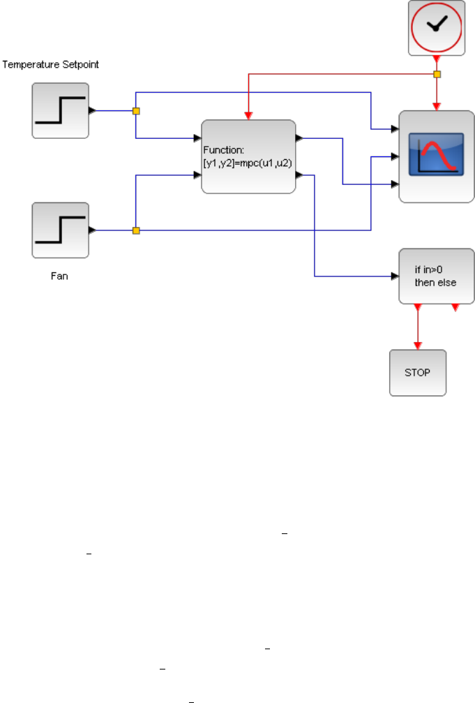
Figure 12.1: Screenshot of the xcos window with step input blocks labeled
After entering the values in the input step block, the simulation can be started.
This opens up a graph, which shows the values of Temperature-set-point, fan and
the actual temperature at each time instant during the simulation.
Other codes that were used other than mpc run.sci for conducting this ex-
periment are mpc init.sce and mpc.sci. Both these codes were originally taken
from Moodle (Process controls course for SBHS assignment). Please note that,
both these codes were slightly modified to work with our MPC.
The only changes done in the original codes are:
•addition of global variables p,q and xk old (p is the prediction horizon, q is
the control horizon, xk old represents the last value of an internal state)
•initialization of p, q and xk old
•removal of some unnecessary lines (ie, lines not relevant to MPC imple-
mentation)
270
12.3 Experiments conducted to implement MPC
Experiments were performed as shown in table above for implementation of MPC.
We carried out experiments in which both positive and negative step changes were
given to Set point and Fan (disturbance variable) and the output response was ob-
tained by application of MPC. We also have performed several experiments to
study the effect of change in the values of q (control horizon) and tuning parame-
ters - error and manipulated variable weighting factors.
The details of the experiments mentioned in this report has been tabulated
in the table given in the next page. The first column of the table represents the
experiment version (or number). For all the outputs and their figures, we have
mentioned only their experiment version (or number) to tag them. Also note that
the data files for these experiments are also named as per their experiment version
number. p and q mentioned in the table represents the prediction and control
horizon respectively.
Please note: For all the above experiments and graphs, we adhered to:
•Scilab Version: 5.2.2
•SBHS number: 12 (remotely accessed)
•Sampling time: 1 second
For graphs: Until and unless mentioned, Graphic 1 represents the Temperature
set point, Graphic 2 represents the Fan and Graphic 3 represents the Temperature.
Also, please note that there are two types of graphs. The first graph, containing
Graphic 1, Graphic 2 and Graphic 3 were directly obtained via mscope of xcos.
The graph following this in all the experiments is the temperature and heater value
graphs, which were obtained from the data (from the text file downloaded from
the server after each experiment).
271
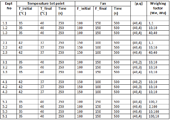
Figure 12.2: Experiments performed
All the experiments mentioned in this report has been labeled as shown in this
table. This table is just a summary of all the parameters that was used for the
corresponding experiment. Details on the inputs and a description of the output
observed for each case has been mentioned in the corresponding section of each
experiment.
12.4 Sample run to implement MPC
12.4.1 Positive Step Change to Set Point and Fan
Let us consider an experiment, wherein, a positive step change of 5◦C (from 35◦
C to 40◦C) was provided to set point at time t=250 s and a step change to fan was
provided at t =500 s, from 100 to 150.
272

Figure 12.3: Xcos output for positive Step Change to Set Point and Fan
273

Figure 12.4: Temperature and Heater plot
As can, be seen above, when, the temperature set point is raised to 40 from 30,
at t=250 s, the value of the heater increases, so that it can heat up the plant upto
the required set point. Similarly, when the fan speed is increased at t=500s, the
heater value increases yet again to maintain the same constant temperature of the
SBHS blade.
274

12.4.2 Negative Step Change to Set Point and Fan
Let us consider experiment 2.1, wherein, a negative step change of 5◦C (from
42◦C to 37◦C) was provided to set point at time t=250 s and a step change to fan
was provided at t =500 s, from 150 to 100.
Figure 12.5: Xcos output for negative Step Change to Set Point and Fan
275

Figure 12.6: Temperature and Heater plot
As can be seen from the graphs above, when the temperature set point drops
at t=250 s, the value of the heater too falls, so that the plant (SBHS blade) can
cool down to the required set point. Similarly, when the fan speed was decreased
at t=500s, the heater value decreased yet again to maintain the same constant
temperature of the SBHS blade.
276
12.5 Effect of Tuning parameters: Weighting fac-
tors, We and Wu
We also, conducted several experiments in order the study the effect of the value of
Weighting factors (both error,We and manipulated variable,Wu). We used weight-
ing factors to be 1, 10 and 40 for both positive and negative step changes to both
set point and fan (as has been summarized in Table 1). Also, experiments were
done for different values of We and Wu. The results have been shown in the
following graph.
277
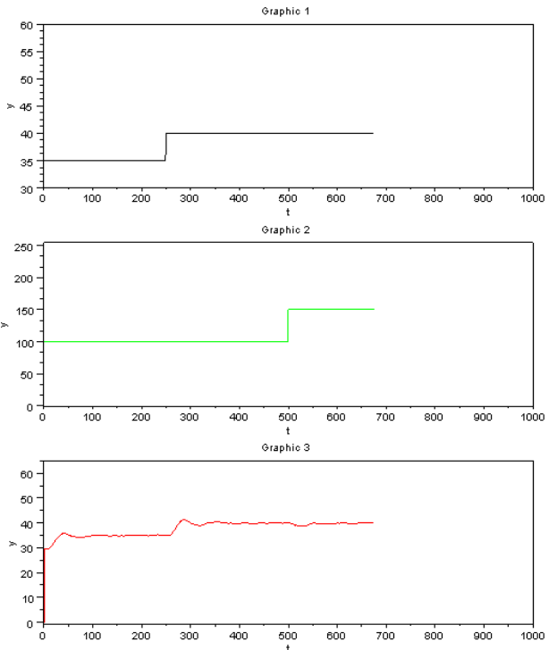
12.5.1 Positive Step Change and (We, Wu)=(1,1)
Figure 12.7: Xcos output for positive Step Change and (We, Wu)=(1,1)
Here we can clearly see the expected output. Providing a positive step to tempera-
ture set point at 250 seconds, increased heater value as per the control effort put in
by MPC. A positive step in fan at 500 seconds, decreased the temperature below
its set point and hence heater value increased to take the temperature close to its
setpoint.
278
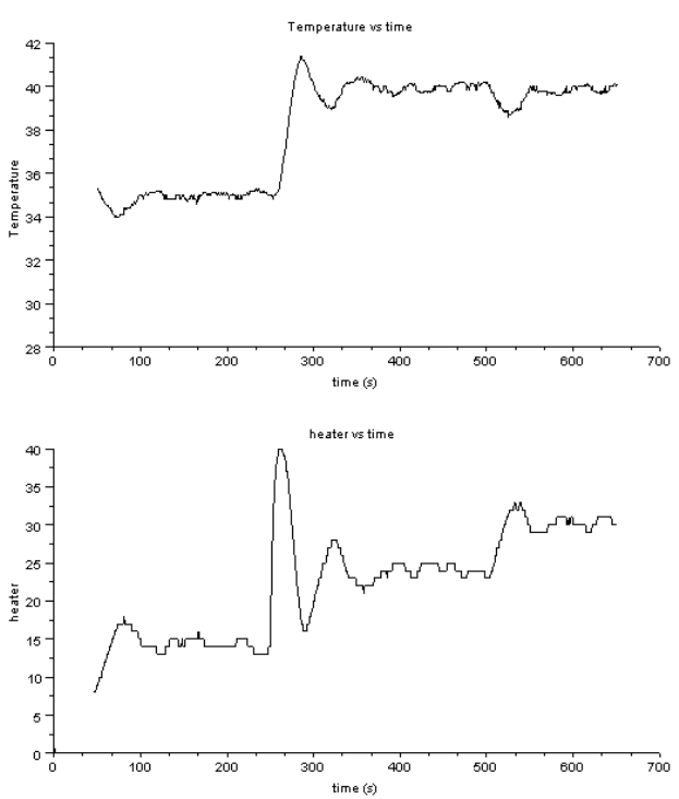
Figure 12.8: Temperature and Heater plot
As can be clearly seen, the heater graph follows the expected trend that we
talked of in the last page. Also, note that the temperature variation can be clearly
seen from this graph. This graph shows the result for the case, where we had
same weighting factors for both error and manipulated variables (We and Wu).
We will now see if changing both of these is going to have any effect on the
control behavior.
So, we now try an experiment with both We and Wu increased to 10.
279

12.5.2 Positive Step Change and (We, Wu)=(10,10)
Figure 12.9: Xcos output for positive Step Change and (We, Wu)=(10,10)
Using the same logic as has been explained in the last section, we expected to
see similar temperature and heater value profiles for the positive step change in
temperature set point and the fan. (Heater graph is shown in the next page along
with the temperature on an expanded scale). In this experiment, we increased We
and Wu both to 10 from 1 and wish to observe if this changes the response of the
plant.
280
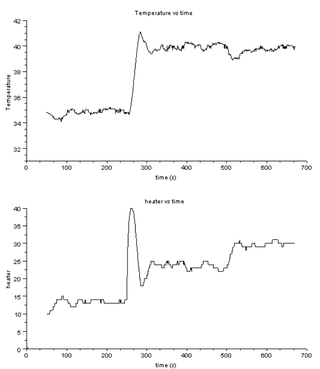
Figure 12.10: Temperature and heater plot
The results here are almost the same as that mentioned in the last section
(where We and Wu both were 1). So, we can for the time being keep in mind
that We and Wu isn’t actually much affected the output. We now will carry out
the experiment for even higher We and Wu (say 40) and see if it really does affect
the output much.
281
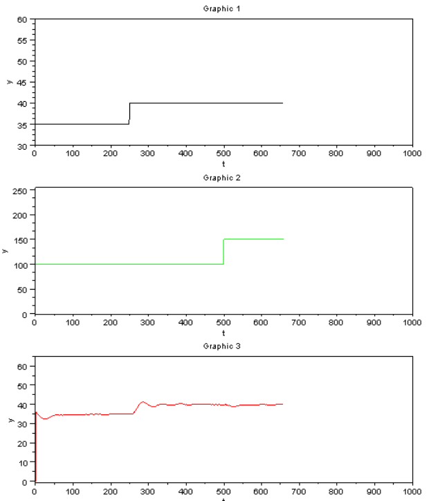
12.5.3 Positive Step Change and (We, Wu)=(40,40)
Figure 12.11: Xcos for positive Step Change and (We, Wu)=(40,40)
282
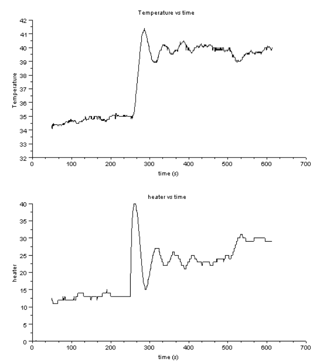
Figure 12.12: Temperature and heater plot
Even the results with We and Wu as 40 doesn’t show much difference. They are
more or less similar looking as the last two experiment’s results.
283
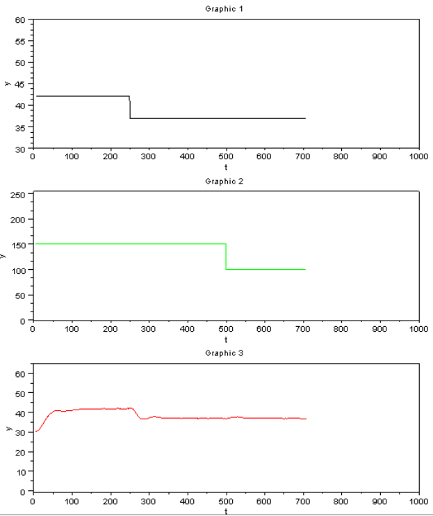
12.5.4 Negative Step Change and (We,Wu)=(1,1)
Figure 12.13: Xcos for negative Step Change and (We, Wu)=(1,1)
Here we expect somewhat similar results as was the case with positive step in
temperature set point.
284
Figure 12.14: Temperature and heater plot
We can very clearly make out that the results follow the trends as was ex-
plained for the negative step input in the section 5.2
285

12.5.5 Negative Step Change and (We, Wu)=(10,10)
Figure 12.15: Xcos for negative Step Change and (We, Wu)=(10,10)
286
Figure 12.16: Temperature and heater plot
287
12.5.6 Negative Step Change and (We, Wu)=(40,40)
Figure 12.17: Xcos for negative Step Change and (We, Wu)=(40,40)
288
Figure 12.18: Temperature and heater plot
12.6 For different We and Wu factors
We very clearly see that using the same values of We and Wu is not making much
difference in the control response. So, will now be trying different values for We
and Wu.
289
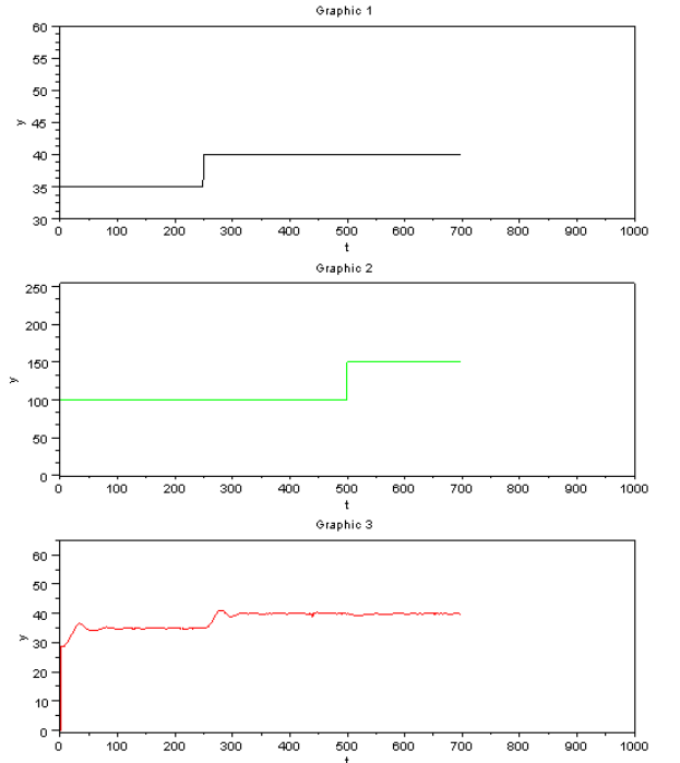
12.6.1 We =100 and Wu =2
Figure 12.19: Output for We =100 and Wu =2
Here, we have used We as 100 and Wu as 2. The response after the positive step in
temperature set point is slightly oscillatory. The temperature very well stabilzes
at the required setpoint. The settling time observed is fairly low.
290
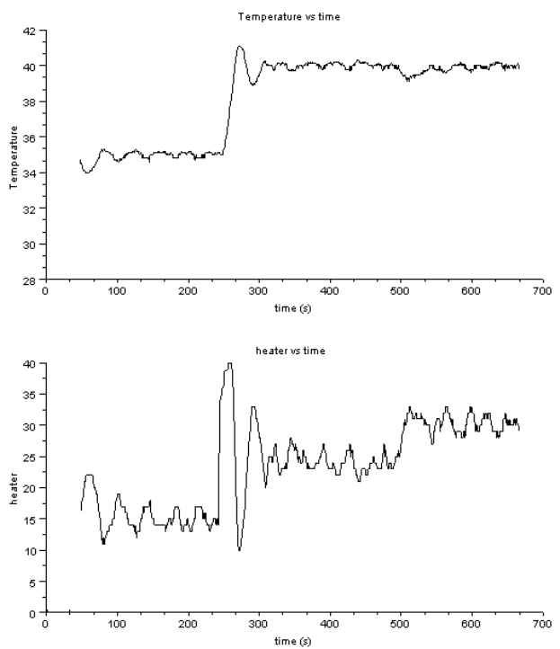
Figure 12.20: Temperature and heater plot
Now having seen the results of this experiment, we would like to check the
possible effect of reversing the values of We and Wu. So, we conduct the next
experiment, in which we have We as 2 and Wu as 100.
291
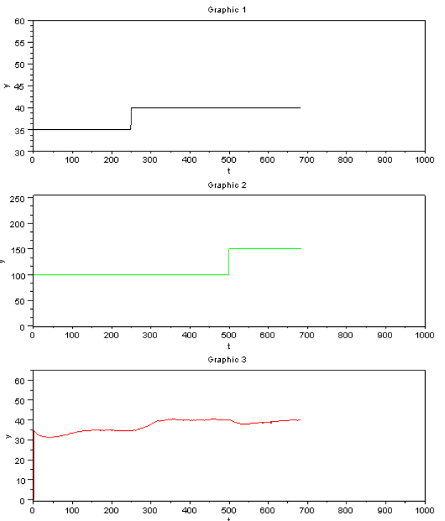
12.6.2 We =2 and Wu =100
Figure 12.21: Output for We =2 and Wu =100
With increase in Wu, we observe that the temperature stabilzes at the required ste-
point, but the settling time for reaching that setpoint increases. Also, the response
is not oscillatory. This result can be very clearly seen in the following temperature
and heater graph.
292
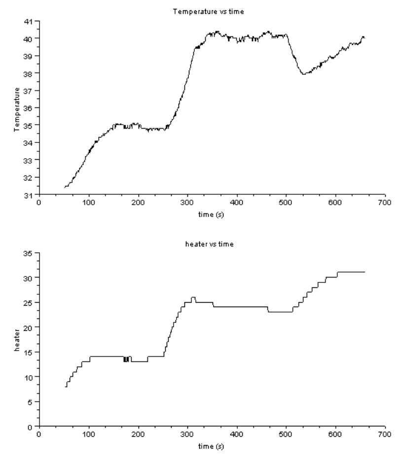
Figure 12.22: Temperature and heater plot
293
12.6.3 We =10 and Wu =100
Having seen the effect of low We and high Wu (in the last section), we would like
to see what happens if We is slightly increased keeping Wu the same. For this we
increase the value of We to 10 and keep Wu at constant 100.
Figure 12.23: Output for We =10 and Wu =100
We observe that this experiments performs better than in the last section (where
We was 2). It is slighly oscillatory and also, the settling time decreased much as
compared to last experiment.
294
Figure 12.24: Temperature and heater plot
12.6.4 We =100 and Wu =10
We now do a similar study for the case of Wu. We increase the value of Wu to 10,
keeping We constant at 100.
295
Figure 12.25: Output for We =100 and Wu =10
As is clear from the figure, we see slightly lesser oscillations compared to the
case when We was 100 and Wu was 2. Settling time more or less remained the
same.
296
Figure 12.26: Temperature and heater plot
297
12.6.5 Conclusion on Weighting factor experiments
For experiments with same values of We and Wu:
•Not much difference was seen in heater value trends and temperature value
trends for all the experiments performed above.
•Reason for this will be clear from the discussion on the trends mentioned
below (for experiments with different values of We and Wu)
For experiments with different values of We and Wu:
•Keeping We as large (around 100) and Wu as small (2) shows better per-
formance as compared to the case when the values are kept the other way
around.
•With We very small (say around 1-2), oscillations are less, and the settling
time observed was found to be more.
•With increase in We, the oscillations were observed to increase and the set-
tling time was found to reduce and hence, better control was observed.
•So, with increase in We, any error is quickly dealt with, because with in-
crease in We, we are actually increasing the significance of change of tem-
perature in deciding the control action.
•With increase in Wu, oscillations reduced and the settling time was found
to increase and hence, less preferred.
So, the best performance is obtained for the cases with high We and low Wu.
12.7 Effect of Control Horizon Paramter, q
We also tried to study the effect of change of control horizon (q) on the response
of the SBHS to step change in Setpoint and disturbance variable. Generally the
value of q (control parameter) is taken somewhere between 2 to 5. So, we per-
formed our SBHS experiment for values of q as 2, 3 and 4 (as suggested by Mr
Prashant Gupta).
Both positive and negative step change experiments for temperature set point and
298
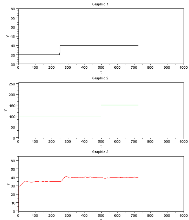
disturbance variable (fan) was performed for the sake of completeness. The re-
sults obtained thereby has been mentioned in form of graphs in this section. The
overall conclusion over these experiments has been mentioned in the conclusion
of this part.
12.7.1 For positive step change in Set point and Fan speed
Figure 12.27: Xcos putput for positive step change with q=2
299
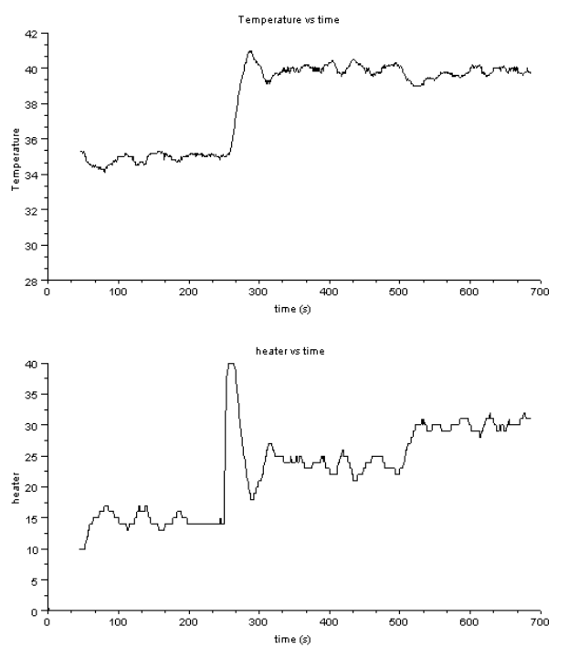
Figure 12.28: Temperature and heater plot
300
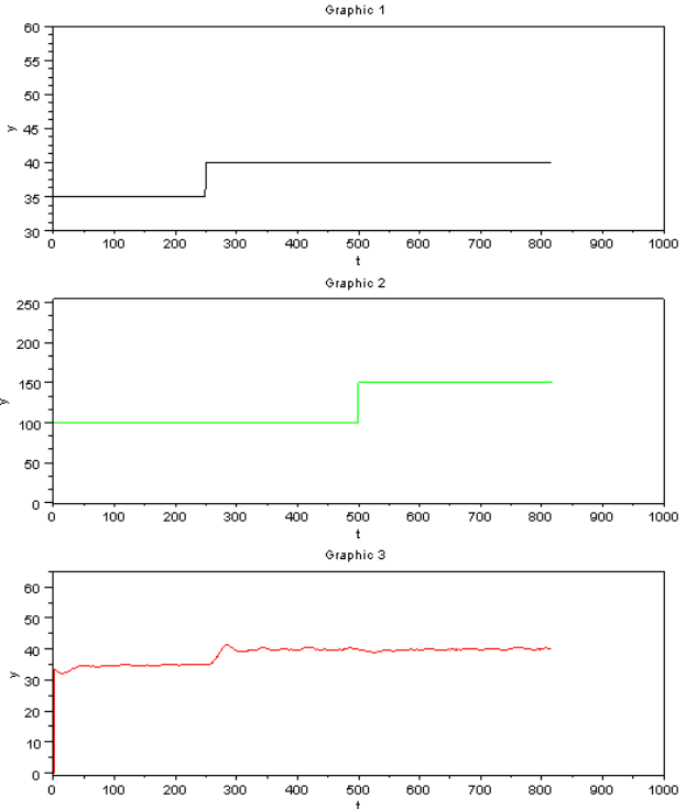
Figure 12.29: Xcos putput for positive step change with q =3
301
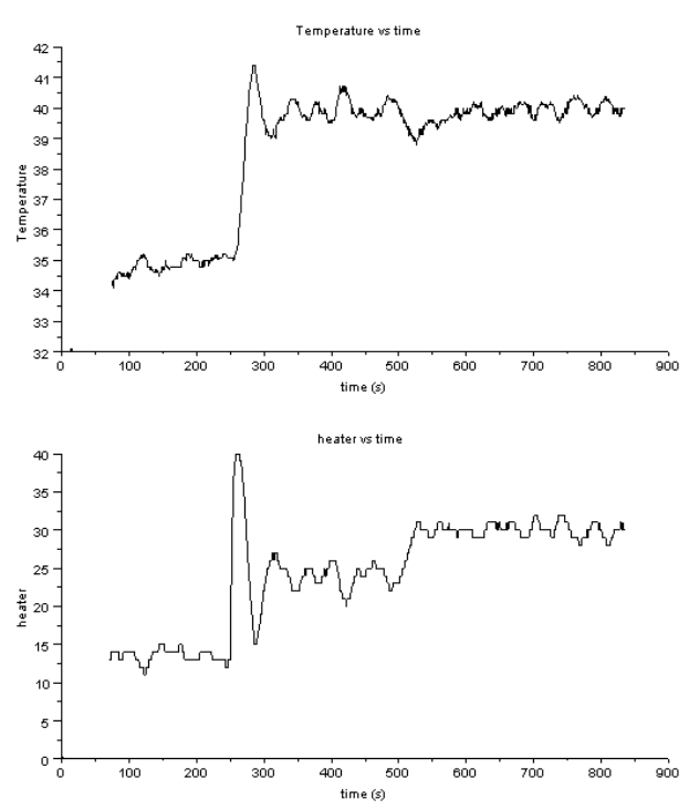
Figure 12.30: Temperature and heater plot
302
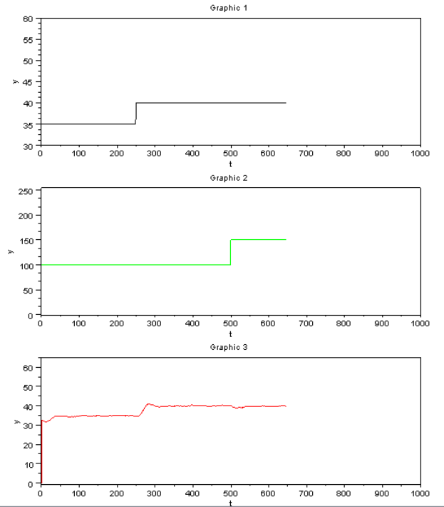
Figure 12.31: Xcos putput for positive step change with q =4
303

Figure 12.32: Temperature and heater plot
304
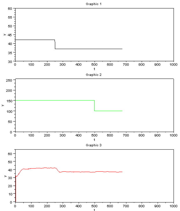
12.7.2 For negative step change in Set point and Fan speed
Figure 12.33: Xcos putput for negative step change with q =2
305
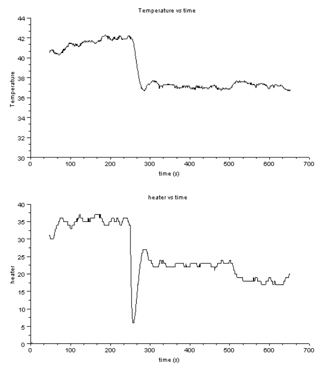
Figure 12.34: Temperature and heater plot
306
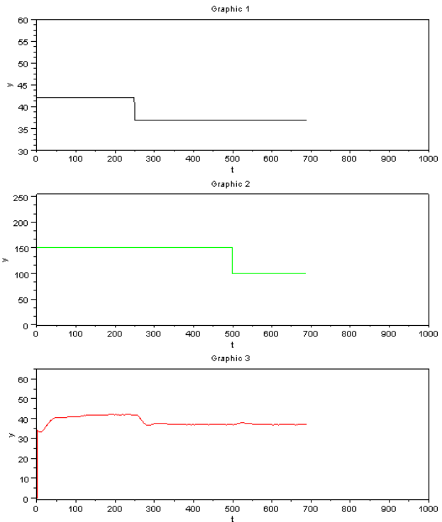
Figure 12.35: Xcos putput for negative step change with q =3
307
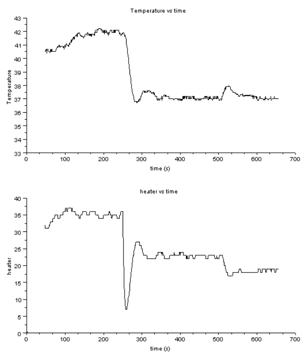
Figure 12.36: Temperature and heater plot
308
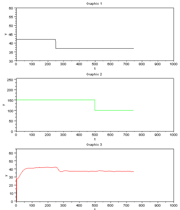
Figure 12.37: Xcos putput for negative step change with q =4
309

Figure 12.38: Temperature and heater plot
12.7.3 Conclusion on the effect of Control Horizon parameter
•The effect of change in q isn’t very distinct in the experiments performed.
•While we are calculating the optimized value of manipulated variable at a
time, the number of manipulated input moves is increasing as we are in-
creasing the q value.
•But, only the first value of the optimized manipulated variable vector is used
for control.
310

•Increase in q is only increasing the length of the manipulated variable vector
which is to be optimized.
•Since, only the first value of manipulated variable vector is used, which
itself lies in some specified range, the effect of changing q isn’t very signif-
icant for SBHS.
•Also, SBHS system is a simple system with very few variables (as compared
to real life industrial systems).
•Ideally, the value of q is to be maintained at 3 or 4.
12.8 Implementing MPC locally
The detailed procedure to perform a local experiment is explained in Chapter2.
A summary of the same is provided in section 2.3 It is same for this section with
following changes.
1. Step1: The working directory is mpc
2. Step2: Same
3. Step3: Same
4. Step4: Same
5. Step5: Load mpc function by executing command
exec<space>mpc init local.sci
6. Step6: Load Xcos code for mpc experiment using the command
xcos<space>mpc.xcos
7. Step7: Same
12.9 Implementing MPC virtually
The detailed procedure to perform a virtual experiment is explained in Chapter3.
A summary of the same is provided in section 3.5. It is same for this section with
following changes.
311
1. Step1: The working directory is mpc. Open this directory.
2. Step2: Same
3. Step3: Same
4. Step4: Switch to the MPC experiment directory and double-click on the file
mpc.sce. This will launch scilab and also open the file mpc.sce in the
scilab editor. Linux users will have to launch scilab manually. They also
have to change the working directory to mpc and then open the mpc.sce
file in the scilab editor.
5. Step5: Same
6. Step6: Execute the file mpc.sce. Expect the PI controller xcos diagram to
open automatically. If this doesnt happen, check the scilab console for error
message.
7. Step7: Execute the MPC controller xcos diagram.
8. Step8: Same
12.10 Conclusion for MPC project
The objective of this project, ie, implementing Model Predictive Control in Single
Board Heater System using Scilab was successfully achieved. Several experi-
ments were successfully performed using the developed SCILAB MPC algorithm
for both positive and negative step changes in both temperature-set-point and the
disturbance variable (fan).
In addition to the above objective, we also tried studying the effect of weight-
ing factors (tuning parameter) and control horizon parameter. We observed and
concluded that increase in values of We (error weighting factor), increases oscil-
lations and decreases settling time, while decrease in We leads to opposite effect.
Wu (manipulated variable weighting factor), on the other hand has an opposite ef-
fect. It decreases oscillations and increases settling time with increase in its value.
Hence, better control is obtained for high value of We and low value of Wu.
Thus, with this project, we were able to implement MPC successfully and also
312

were able to comment on the general preferred tuning parameters (weighting fac-
tors for error and manipulated variable).
12.11 Acknowledgement
Firstly, I (Pratik Behera)would like to thank Prof Moudgalya Kannan, for giv-
ing me this opportunity to undertake MPC project on SBHS. This project, which
involved implementing Model Predictive Control in SBHS using SCILAB, was
very interesting and provided an excellent learning opportunity. For developing
the MPC algorithm, lecture notes on Model Predictive Control by Prof. Sachin
Patwardhan too were extremely helpful. Also, I got to learn a lot from the speak-
ing tutorials of SCILAB and LaTeX, which had to be referred to for the com-
pletion of this project. Over and above this, it was very encouraging to see the
experiments working perfectly with the developed Model Predictive Control al-
gorithm. I would also like to sincerely thank Mr Prashant Gupta, without whom,
this project would not have been splendidly completed. I would like to thank him
for the time he spent explaining the concepts, clearing the doubts and suggestions
for the experiments to implement MPC.
12.12 General Information on Experiments for this
Project
All the experiments for this project was performed remotely on SBHS, using a
sampling time of 1 second. Basic codes (mpc init.sce and mpc.sci) was taken
from moodle for this course. Code for implementing MPC was written in scilab
and has been mentioned in the report.
Scilab Version used: 5.2.2
SBHS number: 12 (remotely used)
Sampling time: 1 second
For graphs: Until and unless mentioned, Graphic 1 represents the Temperature
set point, Graphic 2 represents the Fan and Graphic 3 represents the Temperature.
Initially, open loop experiment was performed, and Plant Transfer function
was obtained. For the open loop experiment, a step change in heater from 15 to
25 units at t =200 seconds was provided (sampling time 1s). The response data
313

was fitted to a first order transfer function with a time delay and the following was
observed:
Kp=0.37, time constant =45s and delay =7s.
Using the above, we obtained the plant transfer function:
Gp=0.37
1+45se−7s(12.7)
Scilab Method to calculate State Space matrices
State space matrices for a transfer function can be calculated as follows using
Scilab:
1s=p o l y ( 0 , ’ s ’ ) ;
2TFcont=syslin ( ’ c ’ , [ kp *(1 −0.5*D) /( t a u *s+1) /( 1 +0 . 5 *D) ] ) ;
3SS c ont=tf2ss ( T Fcont ) ;
SScont (in the last line above), has the value of the required State Space matrices.
(Please note: Time delays can not be directly handled in Scilab. So, for systems
with delays, we will have to use alternate approach. Pade’s approximation for
time delay being one of the approach.)
The transfer function which we dervied for our SBHS was very close to the trans-
fer function derived in an earlier attempt. So, using the values of A, B and C
which were already calculated by him previously, we obtain the following exact
values:
A=
0.9780 0 0 0 0 0 0 0
1 0 0 0 0 0 0 0
0 1 0 0 0 0 0 0
0 0 1 0 0 0 0 0
0 0 0 1 0 0 0 0
0 0 0 0 1 0 0 0
0 0 0 0 0 1 0 0
0 0 0 0 0 0 1 0
314

B=
1
0
0
0
0
0
0
0
C=h00000000.0079 i
12.13 Scilab Code
Scilab Code 12.1 mpc.sci
1function [ s t o p ] =mpc ( Tsp , f a n )
2global f d f h f d t f n c r fncw m e r r c o u n t s t o p p q
x k o l d h e a t temp h e a t o l d
3
4h e a t =mpc run ( temp , h e a t o l d , Tsp ) ;
5
6[ s t o p , temp ] =comm ( h e a t , f a n ) ; / / N e v e r e d i t t h i s
line
7p l o t t i n g ( [ h e a t f a n temp Tsp ] , [ 0 40 25 0 ] , [ 1 0 0 70
50 1 0 0 0 ] ) ;
8
9heat old =h e a t ;
10
11 r e t u r n
12 endfunction
Scilab Code 12.2 mpc init local.sce
1/ / F o r s c i l a b 5 . 1 . 1 o r l o w e r v e r s i o n u s e r s ,
2/ / u s e s c i c o s c o m m a n d t o o p e n s c i c o s d i a g r a m s i n s t e a d
o f x c o s
315

3
4global e r r c o u n t y p q x k o l d Tsp h e a t s f a n temp h e a t
5
6p=4 0 ; / / p r e d i c t i o n h o r i z o n
7q=4 ; / / c o n t r o l h o r i z o n
8x k o l d =zeros ( 8 , 1 ) ;
9Tsp=1;
10 h e a t s =1;
11 fan=1;
12 temp=1;
13
14 e x e c ( ” m p c l o c a l . s c i ” ) ;
15 e x e c ( ” mpc run . s c i ” ) ;
Scilab Code 12.3 mpc local.sci
1mode ( 0 )
2function [ temp ] =mpc ( Tsp , f a n )
3global temp h e a t i n f a n i n C0 u o l d u new e o l d e new
e old old
4
5global h e a t d i s p f a n d i s p t e m p d i s p s e t p o i n t d i s p
s a m p l i n g t i m e m name
6/ / h e a t s =1 ;
7u new =mpc ru n ( temp , h e a t s , Tsp ) ;
8
9
10 h e a t =u new ;
11
12 temp =comm( h e a t , f a n ) ;
13
14 p l o t t i n g ( [ h e a t f a n temp Tsp ] , [ 0 0 20 0 ] , [ 1 0 0 100
40 1 0 0 0 ] )
15
16 m=m+1;
17 endfunction
316

Bibliography
[1] Fossee moodle. http://www.fossee.in/moodle/. Seen on 10 May 2011.
[2] Spoken tutorials. http://spoken-tutorial.org/Study Plans Scilab. Seen on 10
May 2011.
[3] K. M. Moudgalya. Introducing National Mission on Education through ICT.
http://www.spoken-tutorial.org/NMEICT-Intro, 2010.
[4] K. M. Moudgalya and Inderpreet Arora. A Virtual Laboratory for Distance
Education. In Proceedings of 2nd Int. conf. on Technology for Education,
T4E, IIT Bombay, India, 1–3 July 2010. IEEE.
[5] Kannan M. Moudgalya. Digital Control. John Wiley and Sons, 2009.
[6] Kannan M. Moudgalya. Identification of transfer function of a single board
heater system through step response experiments. 2009.
[7] Katsuhiko Ogata. Modern Control Engineering. Prentice-Hall of India, 2005.
[8] Dale E. Seborg, Thomas F. Edgar, and Duncan A. Mellichamp. Process Dy-
namics and Control. John Wiley and Sons, 2nd edition, 2004.
[9] Virtual labs project. Single board heater system. http://www.co-
learn.in/web sbhs. Seen on 11 May 2011.
317
